Dynamics of suspended cables under turbulence loading: Reduced models of wind field and mechanical...

ARTICLE IN PRESS

Journal of Wind Engineering

and Industrial Aerodynamics 95 (2007) 183–207

0167-6105/$ -

doi:10.1016/j

�CorrespoE-mail ad

URL: htt

www.elsevier.com/locate/jweia

Dynamics of suspended cables under turbulenceloading: Reduced models of wind field and

mechanical system

Vincenzo Gattullia,�, Luca Martinellib, Federico Perottib,Fabrizio Vestronic

aDipartimento di Ingegneria delle Strutture, delle Acque e del Terreno, Universita di L’Aquila,

67040 Monteluco di Roio, L’Aquila, ItalybDipartimento di Ingegneria Strutturale, Politecnico di Milano, Piazza Leonardo da Vinci 32, Milano, 20133 Italy

cDipartimento di Ingegneria Strutturale e Geotecnica, Universita di Roma ‘‘La Sapienza’’,

Via Eudossiana 18, 00184 Roma, Italy

Received 12 October 2005; received in revised form 6 May 2006; accepted 16 May 2006

Available online 1 August 2006

Abstract

In cables, turbulent wind may cause large amplitude oscillations. The prediction of cable response

under wind action requires the use of high-dimensional numerical models either to describe the

spatial wind field or to model the expected large cable oscillations. The paper discusses the ability of

reduction techniques, for loading and cable descriptions, in reproducing accurately the dynamic

response of a suspended cable excited by an artificially generated 3D turbulent wind field. Both the

mechanical system and the spatially varying wind velocities are projected on the basis of cable

eigenfunctions, retaining in the reduced models few degrees-of-freedom associated with the low-

frequency modes. A numerical investigation performed by a refined finite element model provides

novel findings on the cable response to wind and permits to demonstrate the effectiveness of the

reduced models in the description of cable dynamics.

r 2006 Elsevier Ltd. All rights reserved.

Keywords: Cables; Wind turbulence; Aerodynamic damping; Finite element models; Reduced order models;

Nonlinear oscillations

see front matter r 2006 Elsevier Ltd. All rights reserved.

.jweia.2006.05.009

nding author. Tel.: +390862 434511; fax +39 862 434548.

dress: [email protected] (V. Gattulli).

p://www.ing.univaq.it/webdisat/.

www.elsevier.com/locate/jweia

dx.doi.org/10.1016/j.jweia.2006.05.009

mailto:[email protected]

mailto:http://www.ing.univaq.it/webdisat/a4.3d

ARTICLE IN PRESSV. Gattulli et al. / J. Wind Eng. Ind. Aerodyn. 95 (2007) 183–207184

1. Introduction

The cable is a simple but important structural element; indeed cables are frequently usedto sustain themselves, as in high-voltage transmission lines, or within tall or widestructures, as in the case of guyed towers and suspended/stayed bridges. It is characterizedby high resistance, high flexibility and a very small damping, which leads to the fact that acable is often prone to undergo large amplitude oscillations mainly due to wind loading.The dynamic response of cables has been thoroughly investigated in linear and nonlinear

regime under deterministic and stochastic excitations. Since the behavior is inherentlynonlinear and the nonlinearities of this system are very rich, a large amount of papers havebeen devoted to the study of nonlinear dynamic phenomena in the stationary oscillations([17,27,22,23]), typically in the presence of some resonance conditions, when thesephenomena become relevant ([14,1]).In these conditions it has been observed that low-dimensional models, obtained by

expanding the displacement functions in a suitable bases—like the eigenfunctions of themodes involved in the resonances—are able to capture most of the nonlinear response. Eventhough a new generation of numerical methods facilitates the general description of solutionsfor large-dimensional ODEs, efforts are still necessary to select more refined bases able tominimize the nonlinear coupling terms. Within this framework, it has been shown in a recentpaper ([11]) that even when the classical approach based on the use of eigenfunctions of thelinearized equations of motion is followed, a reduced model with a low number of modes isusually sufficient; indeed such models are able to describe accurately the response of cables,both qualitatively and quantitatively, predicting all the main bifurcated stable brancheshighlighted by means of a refined nonlinear finite element model (FEM).Less experience exists when the cable is excited by non-periodic force with varying

spatial distribution, such as the case of wind turbulence loading. In this case the degree ofapproximation of reduced models depends on two conditions: the ability of low-dimensional mechanical system in reproducing the main characteristic of the response andthe representation of the loading features through a simple description. This item is tackleddiffusely in the literature devoted to the response of linear systems excited by a stochasticprocess and is, for example, discussed in [2].In the present work the description of the dynamical response of a non-resonant

suspended cable under wind excitation is considered. The aim of the study is mainly toinvestigate the effect of adopting reduced order models, for both dynamical system andexcitation loadings, in the computation of the cable response to wind. In this light, theinfluence of the characteristics of the turbulent wind field on the cable response waspreliminarily analyzed by means of a finite element (FE) based numerical procedure ([19]);more precisely, the effects of the coupled in-plane and out-of-plane turbulence, of thedimensionality of the wind field (1D vs 3D) and of the turbulence coherence werecharacterized. Based on this investigation, the accuracy of reduced models was analyzedcomparing the results of these models to those of a refined FEM, in describing the cablenonlinear response to turbulent loading. To investigate the reduced order modeling of theexcitation, the artificially generated wind velocity fields is compared to a reduced onewhich is represented by a few components obtained projecting the complete wind onto thecable eigenfunctions basis.The paper is organized as follows. The wind model is discussed first (Section 2) and, on

the basis of a few numerical results, wind complete and reduced descriptions are compared

ARTICLE IN PRESSV. Gattulli et al. / J. Wind Eng. Ind. Aerodyn. 95 (2007) 183–207 185

(Section 2.1). In the following Section 3 the governing equations for cable dynamics underturbulent wind are presented for both analytical (Section 3.1) and FE (Section 3.2) models.The FE response analysis (Section 4) is then exploited to the aim of discussing theresponses to in-plane and out-of-plane turbulence (Section 4.1), to 1D and 3D windturbulence fields (Section 4.2) and the effects of turbulence coherence (Section 4.3).Finally, for some selected cases, the previous results are compared to those obtained bydirect integration of a low dimensional analytical model (Section 5). Concluding remarkssummarize the research findings (Section 6).

2. Wind model

When the adequacy of a reduced dynamic model is under consideration, the propertiesof perturbation forces must be carefully studied by the point of view of both frequencycontent and spatial variation. The latter aspect deserves particular care when, as in the caseof suspended cables, the structural eigenspectrum is such that a number of modes fall in thelow-frequency interval, where wind turbulence shows its most significant harmoniccomponents. Turbulent components of wind velocity are often defined, in engineeringapplications, as realizations of a zero-mean stochastic process which can be assumed asstationary in time but non-homogeneous in space when the boundary layer is considered;the process is usually described, in the frequency domain, in terms of its cross powerspectral density function (CPSD). A question arises how the properties of the loadingprocess affects the degree of approximation of a reduced wind model. For a preliminarydiscussion we shall refer to the classical theory of linearized stochastic wind loading (see[4]); as an illustrative example we shall deal with the cable out-of-plane oscillations due to asingle-component turbulent wind directed as the normal to the vertical plane containingthe cable under self-weight. In this setting, if the out-of-plane displacement componentwðx; tÞ is expanded (see Section 3.1) as a linear combination of the eigenfunctions cðxÞ ofthe linearized problem, i.e. wðx; tÞ ¼

Pnwi¼1 ciðxÞqiwðtÞ, the forcing term appearing in the ith

discretized equation of motion (generalized load component) can be written in the form

piwðtÞ ¼

ZD

ciðxÞgwðxÞw1ðx; tÞdx. (1)

In Eq. (1) D is the structural domain, w1ðx; tÞ is the transverse component of turbulentvelocity and gwðxÞ is the positive function

gwðxÞ ¼ GwcDrabðxÞW ðxÞ, (2)

i.e. the product of a trigonometric factor Gw times air density ra, section dimension b,aerodynamic coefficient cD and mean wind velocity W ; in Eq. (1) the drag force has beenlinearized according to the hypothesis that Wbw1. To characterize the dynamic loadingintensity at mode i the variance of the generalized load (1), which is a zero-mean process aswell, can be computed as its mean-square value. With standard manipulation and bydenoting with E½:� the expectation operator, we obtain

E½p2iwðtÞ� ¼

ZD

ZD

E½w1ðx1; tÞw1ðx2; tÞ�ciðx1Þgðx1Þciðx2Þgðx2Þdx1 dx2. (3)

The cross correlation function E½w1ðx1; tÞw1ðx2; tÞ� in turn can be decomposed into itsfrequency components, represented through the CPSD, Sw1

ðx1;x2; f Þ. Doing this and


interchanging the order of integration, the power spectral density function Spiwðf Þ of the

modal load is implicitly defined according to the following:

E½p2iwðtÞ� ¼

Z 10

ZD

ZD

Sw1ðx1;x2; f Þciðx1Þgðx1Þciðx2Þgðx2Þdx1 dx2 df

¼

Z 10

Spiwðf Þdf . ð4Þ

For investigating how the modal loads are affected by the wind distribution, the CPSD ofturbulent velocity can be factored as

Sw1ðx1; x2; f Þ ¼ Cw1

ðx1;x2; f ÞffiffiffiffiffiffiffiffiffiffiffiffiffiffiffiffiffiffiffiffiffiffiffiffiffiffiffiffiffiffiffiffiffiffiffiffiffiffiffiffiffiffiSw1ðx1; f Þ; Sw1

ðx2; f Þq

, (5)

where Cw1ðx1;x2; f Þ is the coherence function and Sw1

ðx1; f Þ is the power spectrum (PSD)of wind velocity for x ¼ x1. Moreover, in most of wind engineering applications thecoherence is assumed real and characterized by an exponential decay with distance andfrequency. By denoting with aðx1;x2Þ the decay coefficient, the PSD of the modal load canbe expressed, from Eqs. (4) and (5) as

Spiwðf Þ ¼

ZD

ZD

expf�aðx1;x2Þf jx1 � x2jg

�

ffiffiffiffiffiffiffiffiffiffiffiffiffiffiffiffiffiffiffiffiffiffiffiffiffiffiffiffiffiffiffiffiffiffiffiffiffiffiffiffiffiffiSw1ðx1; f Þ; Sw1

ðx2; f Þq

ciðx1Þgðx1Þciðx2Þgðx2Þdx1 dx2. ð6Þ

The evaluation of the integral (6) in the limiting conditions of full coherence ðaf ¼ 0; Cw ¼ 1Þand null coherence ðaf ¼1; Cw ¼ dðx1 � x2ÞÞ suggests interesting considerations. In the firstcase Eq. (6) gives

Spiwðf Þ ¼

ZD

ffiffiffiffiffiffiffiffiffiffiffiffiffiffiffiffiffiffiffiffiSw1ðx1; f Þ

qciðx1Þgðx1Þdx1

� �2(7)

which, for a homogeneous process ðSw1ðx1; f Þ ¼ Sw1

ðf ÞÞ, leads to a well-known result inrandom vibration theory. For the delta-correlated process, by exploiting the properties ofthe Dirac d we get, for Eq. (6), the expression

Spiwðf Þ ¼

ZD

Sw1ðx1; f Þ½ciðx1Þgðx1Þ�

2 dx1 (8)

which is again a standard result for uncorrelated loading. Expression (7) is the square ofthe weighted average of the ith eigenfunction; therefore, for high-coherence values ‘‘firstmode shaped’’ eigenfunctions, with no sign changes, are clearly dominant in the excitation.Expression (8), on the other hand, delivers the weighted mean-square of the eigenfunction;according to (8), i.e. for low-coherence loading, all modes are excited, in principle, with thesame intensity.To gain further insight into this matter, it can be also shown how this behavior can be

interpreted in terms of wind reduced models. In this light the description of the turbulencestructure can be simplified using normal modes, i.e. the so-called ‘‘wind modes’’([24,25,5,7]); following [3] the turbulence CPSD can be decomposed, within the structuraldomain D, into its eigenfunctions (modal shapes) yjðx1; f Þ and eigenvalues (modal spectral


densities) gjðf Þ, i.e.

Sw1ðx1;x2; f Þ ¼

Xj

yjðx1; f Þy�j ðx2; f Þgjðf Þ, (9)

y�j being the complex conjugates of yj. By substituting expression (9) into (6) we can write

Spiwðf Þ ¼

Xj

gjðf Þ

ZD

ciðx1Þgðx1Þyjðx1; f Þdx1

ZD

ciðx2Þgðx2Þy�j ðx2; f Þdx2

¼X

j

gjðf ÞjEijðf Þj2, ð10Þ

where

Eijðf Þ ¼

ZD

ciðxÞgðxÞyjðx; f Þdx. (11)

In [26] it is observed that, in many cases of practical interest, the structural and windeigenfunctions tend to be similar in shape; in such case the ith modal load tends to beentirely related to the corresponding wind mode. In the same paper the eigenfunctions andeigenvalues of the CPSD (5), are given, in analytical terms, as functions of the decayparameter af . It is also shown how, for high-coherence values (low af ), the first eigenvalueis dominant and tends to the value of the process PSD, i.e. Sw1

ðf Þ; for fast coherence decay(high af ) the turbulence power is spread over a large number of wind modes. Therefore, ahighly correlated wind structure is inherently suitable for a reduced model of its spatialvariation. The most efficient reduction technique should be the projection on the windmodes; however, given the similarity between wind and structural modes (see again [26,3]),it can be easily understood how projection on the first structural modes delivers a veryclose approximation of the turbulence field. In the numerical experiments here shown,wind fields with different coherence were considered, selecting as common occurrence anaverage wind coherence (AWC) in comparison to the case of a very low wind coherence(LWC). In the first case, consistently with the data reported in [26] and with the cablesetting, a constant value of a ¼ 0:3 s=m was chosen (see Eq. (5)): note that this leads tovalues of the correlation length parameter 1=ðaf Þ respectively equal to 66.7 and 6.67m atf ¼ 0:05 and 0.5Hz. In the LWC case the correlation length was fictitiously reduced of twoorders of magnitude, so that a null-coherence case was practically simulated.

2.1. Complete and reduced representation

In the numerical procedure here adopted, 3D turbulence was modeled by generatingartificial velocity time histories in all nodes of the FE mesh. Generation was based on theprobabilistic model proposed in [26]; this model is completely defined when the averagevelocity W , the terrain factor kr, the roughness length z0 and the minimum height zmin aregiven. The values here adopted are the following: W ¼ 30m=s, kr ¼ 0:22, z0 ¼ 0:3m,zmin ¼ 5m and correspond to a suburban or industrial area (type III) according to theEurocode 1 classification ([8]).

The artificial generation was performed by wave superposition, according to the classicalShinozuka method ([24,25]): for a gradual build-up of the excitation, the first part (500 s) ofthe generated turbulence histories, which are 2000 s long, was multiplied by a cosine taper.


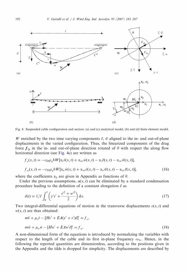
In order to investigate the effect of the accuracy in modeling the spatial variation of thewind field, starting from the generated time histories (complete wind model, CWM) areduced model (RWM) was derived, which is consistent to the cable reduced analyticalmodel. To this aim, it was assumed that the cable has the supports at the same elevationand that the wind velocity field has its mean component orthogonal to the vertical planepassing through the supports; in this setting the static equilibrium configuration of thecable, which is the reference configuration for the associated eigenproblem, belongs to arotated plane. Consequently (see Fig. 4c), the fluctuation of the wind velocity can beexpressed in terms of its in-plane and out-of-plane components v and w and then expandedin terms of the corresponding in-plane (ji ) and out-of-plane (ci) cable eigenfunctions, i.e.

vðx; tÞ ¼Xnv

i¼1

jiðxÞZivðtÞ; wðx; tÞ ¼Xnw

i¼1

ciðxÞZiwðtÞ, (12)

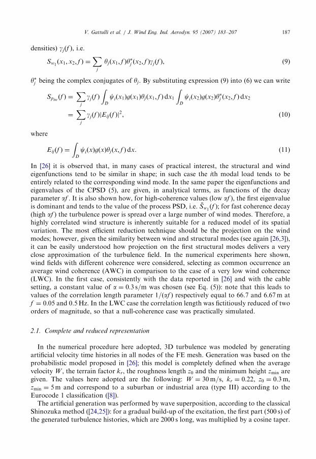
where the generalized components Ziv and Ziw of the turbulence can be easily expressed,exploiting orthogonality as shown in the Appendix. By retaining the components of thefirst in-plane and out-of-plane modes only, the reduced wind model (RWM) was obtained.In Figs. 1a,b the time histories of the horizontal wind turbulence, obtained with CWM

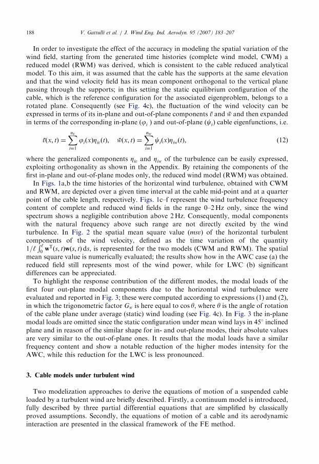
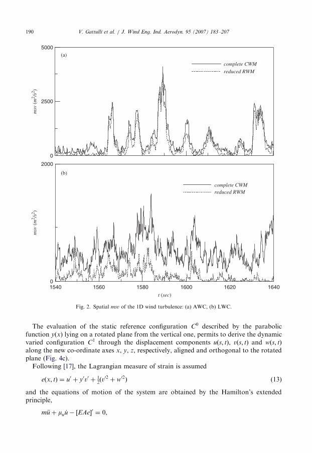
and RWM, are depicted over a given time interval at the cable mid-point and at a quarterpoint of the cable length, respectively. Figs. 1c–f represent the wind turbulence frequencycontent of complete and reduced wind fields in the range 0–2Hz only, since the windspectrum shows a negligible contribution above 2Hz. Consequently, modal componentswith the natural frequency above such range are not directly excited by the windturbulence. In Fig. 2 the spatial mean square value (msv) of the horizontal turbulentcomponents of the wind velocity, defined as the time variation of the quantity1=‘

R ‘0 w

Tðs; tÞwðs; tÞds, is represented for the two models (CWM and RWM). The spatialmean square value is numerically evaluated; the results show how in the AWC case (a) thereduced field still represents most of the wind power, while for LWC (b) significantdifferences can be appreciated.To highlight the response contribution of the different modes, the modal loads of the

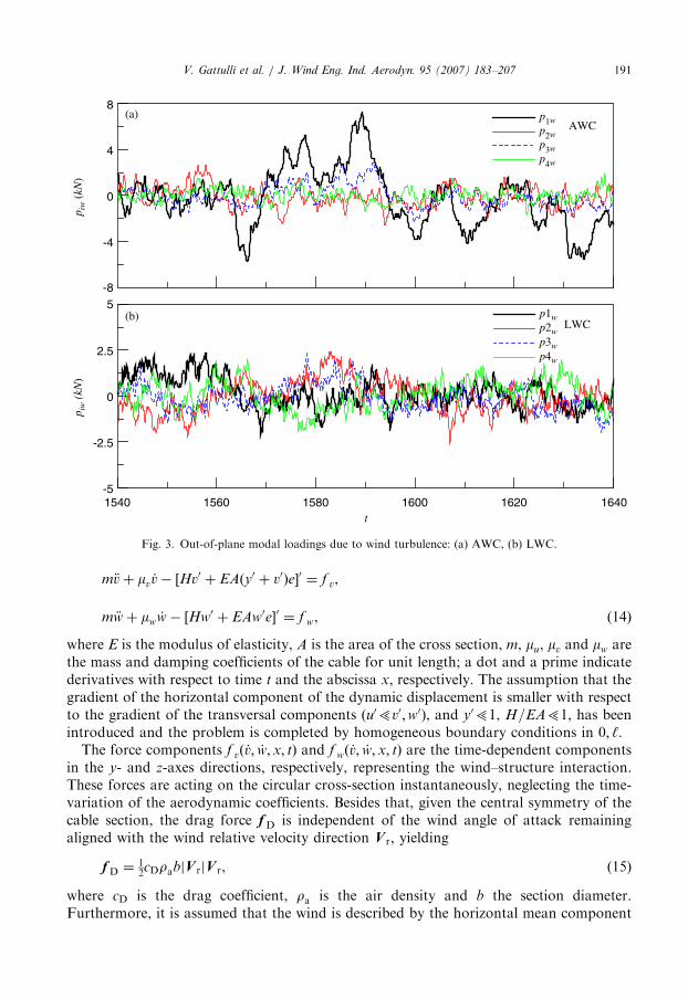
first four out-plane modal components due to the horizontal wind turbulence wereevaluated and reported in Fig. 3; these were computed according to expressions (1) and (2),in which the trigonometric factor Gw is here equal to cos y, where y is the angle of rotationof the cable plane under average (static) wind loading (see Fig. 4c). In Fig. 3 the in-planemodal loads are omitted since the static configuration under mean wind lays in 45� inclinedplane and in reason of the similar shape for in- and out-plane modes, their absolute valuesare very similar to the out-of-plane ones. It results that the modal loads have a similarfrequency content and show a notable reduction of the higher modes intensity for theAWC, while this reduction for the LWC is less pronounced.

3. Cable models under turbulent wind

Two modelization approaches to derive the equations of motion of a suspended cableloaded by a turbulent wind are briefly described. Firstly, a continuum model is introduced,fully described by three partial differential equations that are simplified by classicallyproved assumptions. Secondly, the equations of motion of a cable and its aerodynamicinteraction are presented in the classical framework of the FE method.

ARTICLE IN PRESS

1540 1560 1580 1600 1620 1640

t (sec)

-26

0

26

w1(

m/s

)

CWM (l/2)RWM (l/2)

-20

0

20

w1(

m/s

)

CWM (l/4)RWM (l/4)

0 1 2

f (Hz)

0

0.6

1.2

1.8

0 1 2

f (Hz)

0 1 2

f (Hz)

0 1 2

f (Hz)

CWM (l/2) CWM (l/4) RWM (l/2) RWM (l/4)

(a)

(b)

(c) (d) (e) (f)

Fig. 1. Horizontal wind turbulence (AWC), complete and reduced models (CWM–RWM): time histories of wind

velocity (a) at ‘=2, (b) at ‘=4, Fourier spectrum of wind turbulence (c) and (d) at ‘=2, (e) and (f) at ‘=4.

V. Gattulli et al. / J. Wind Eng. Ind. Aerodyn. 95 (2007) 183–207 189

3.1. Analytical model

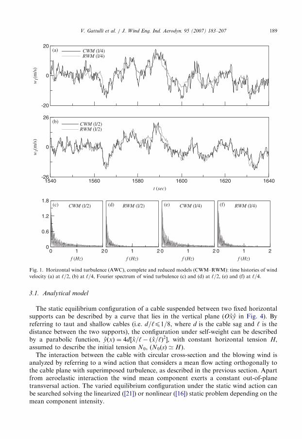
The static equilibrium configuration of a cable suspended between two fixed horizontalsupports can be described by a curve that lies in the vertical plane (Oxy in Fig. 4). Byreferring to taut and shallow cables (i.e. d=‘p1=8, where d is the cable sag and ‘ is thedistance between the two supports), the configuration under self-weight can be describedby a parabolic function, yðxÞ ¼ 4d½x=‘ � ðx=‘Þ2�, with constant horizontal tension H,assumed to describe the initial tension N0, (N0ðsÞ ’ H).

The interaction between the cable with circular cross-section and the blowing wind isanalyzed by referring to a wind action that considers a mean flow acting orthogonally tothe cable plane with superimposed turbulence, as described in the previous section. Apartfrom aeroelastic interaction the wind mean component exerts a constant out-of-planetransversal action. The varied equilibrium configuration under the static wind action canbe searched solving the linearized ([21]) or nonlinear ([16]) static problem depending on themean component intensity.

ARTICLE IN PRESS

0

2500

5000

msv

(m

2 /s2 )

complete CWM

reduced RWM

1540 1560 1580 1600 1620 1640

t (sec)

0

2000

msv

(m

2 /s2 )

complete CWMreduced RWM

(a)

(b)

Fig. 2. Spatial msv of the 1D wind turbulence: (a) AWC, (b) LWC.

V. Gattulli et al. / J. Wind Eng. Ind. Aerodyn. 95 (2007) 183–207190

The evaluation of the static reference configuration C0 described by the parabolicfunction yðxÞ lying on a rotated plane from the vertical one, permits to derive the dynamicvaried configuration C1 through the displacement components uðs; tÞ, vðs; tÞ and wðs; tÞalong the new co-ordinate axes x, y, z, respectively, aligned and orthogonal to the rotatedplane (Fig. 4c).Following [17], the Lagrangian measure of strain is assumed

eðx; tÞ ¼ u0 þ y0v0 þ 12ðv02 þ w02Þ (13)

and the equations of motion of the system are obtained by the Hamilton’s extendedprinciple,

m €uþ mu _u� ½EAe�0 ¼ 0,

ARTICLE IN PRESS

1540 1560 1580 1600 1620 1640t

-5

-2.5

0

2.5

5

p iw

(kN

)

p1wp2wp3wp4w

-8

-4

0

4

8

p iw

(kN

)

p1wp2wp3wp4w

AWC

LWC

(a)

(b)

Fig. 3. Out-of-plane modal loadings due to wind turbulence: (a) AWC, (b) LWC.


m€vþ mv _v� ½Hv0 þ EAðy0 þ v0Þe�0 ¼ f v,

m €wþ mw _w� ½Hw0 þ EAw0e�0 ¼ f w, (14)

where E is the modulus of elasticity, A is the area of the cross section, m, mu, mv and mw arethe mass and damping coefficients of the cable for unit length; a dot and a prime indicatederivatives with respect to time t and the abscissa x, respectively. The assumption that thegradient of the horizontal component of the dynamic displacement is smaller with respectto the gradient of the transversal components (u05v0;w0), and y051, H=EA51, has beenintroduced and the problem is completed by homogeneous boundary conditions in 0; ‘.

The force components f vð_v; _w; x; tÞ and f wð_v; _w;x; tÞ are the time-dependent componentsin the y- and z-axes directions, respectively, representing the wind–structure interaction.These forces are acting on the circular cross-section instantaneously, neglecting the time-variation of the aerodynamic coefficients. Besides that, given the central symmetry of thecable section, the drag force f D is independent of the wind angle of attack remainingaligned with the wind relative velocity direction V r, yielding

f D ¼12cDrabjV rjV r, (15)

where cD is the drag coefficient, ra is the air density and b the section diameter.Furthermore, it is assumed that the wind is described by the horizontal mean component

ARTICLE IN PRESS

xyz

Wl

x2 ,v2

v1

v2

-v2-v1

W1w1

w2Vrγr

.

.

..

x1 ,v1

l

d u

v

w

xz

y

C1

C 0

W

∧

∧∧

(a) (c)

(b) (d)

z, wW Fdv

Fdw

θ

y, v

∧

z, w∧ ∧

y, v∧ ∧

Fig. 4. Suspended cable configuration and section: (a) and (c) analytical model, (b) and (d) finite element model.


W enriched by the two time varying components v, w aligned to the in- and out-of-planedisplacements in the varied configuration. Thus, the linearized components of the dragforce f D in the in- and out-of-plane direction rotated of y with respect the along flowhorizontal direction (see Fig. 4c) are written as

f vðx; tÞ ¼ �cDrabW ½av _vðx; tÞ þ avw _wðx; tÞ � avvðx; tÞ � avwwðx; tÞ�,

f wðx; tÞ ¼ �cDrabW ½aw _wðx; tÞ þ awv _vðx; tÞ � awwðx; tÞ � awvvðx; tÞ�, (16)

where the coefficients aij are given in Appendix as functions of y.Under the previous assumptions, uðx; tÞ can be eliminated by a standard condensation

procedure leading to the definition of a constant elongation e as

eðtÞ ¼ 1=‘

Z ‘

0

y0v0 þv02 þ w02

2

� �dx. (17)

Two integral-differential equations of motion in the transverse displacements vðx; tÞ andwðx; tÞ are thus obtained:

m €vþ mv _v� ½Hv0 þ EAðy0 þ v0Þe�0 ¼ f v,

m €wþ mw _w� ½Hw0 þ EAw0e�0 ¼ f w. (18)

A non-dimensional form of the equations is introduced by normalizing the variables withrespect to the length of the cable and its first in-plane frequency o1v. Hence, in thefollowing the reported quantities are dimensionless, according to the positions given inthe Appendix and the tilde is dropped for simplicity. The displacements are described by


the expansions

vðx; tÞ ¼Xnv

i¼1

jiðxÞqivðtÞ; wðx; tÞ ¼Xnw

i¼1

ciðxÞqiwðtÞ, (19)

where ji and ci are the eigenfunctions of the Hamiltonian linearized equations of motion(18). The associated eigenvalues give the in-plane and out-of-plane frequencies oiv and oiw,which depend on the mechanical cable characteristics through the non-dimensional Irvineparameter, l2 ([13]). The use of the expansions (19) leads to the following expression forthe constant strain

eðtÞ ¼Xnv

j¼1

b1jqjv þXnv

i¼1;j¼1

b2ijqivqjv þXnw

i¼1

b3iq2iw. (20)

Thus, the following nonlinear ordinary differential equations describe the motion

€qiv þXnv

j¼1

zijv _qjv þXnw

j¼1

zijvw _qjw þXnv

j¼1

a0ijqjv þ a1i þXnv

j¼1

a2ijqjv

!e ¼ piv,

€qiw þXnw

j¼1

zijw _qjw þXnv

j¼1

zijwv _qjv þ o2iwqiw þ a3iqiwe ¼ piw, (21)

where the in-plane cable frequencies are obtained as o2iv ¼ ða0ii þ a1ib1iÞ, while oiw are the

out-of-plane frequencies; on the other hand, structural viscous damping has been assumedas proportional. The linear part of system (21) is composed by diagonal stiffnesscoefficients, since the off-diagonal terms ða0ij þ a1ib1jÞ vanish due to the orthogonality ofthe eigenfunctions, while aerodynamic damping coefficients, introduced by the expressions(16) are coupled due to the y-angle between the mean wind and the out-of-plane directions.Furthermore, a rich variety of coupling arises in the nonlinear part, due to quadratic andcubic nonlinear terms. The expressions of the coefficients in Eqs. (20) and (21), as well asthe definitions of the pi-functions, can be found in Appendix.

3.2. Finite element model

A three-node isoparametric FE is developed and coded following [6]; the element isdirectly formulated in the coordinates of the global dynamic model, so that notransformation is necessary to form the tangent stiffness and the generalized componentsof restoring forces.

Linear elastic behavior of the cable is assumed in the large displacement and smalldeformation range to derive the restoring forces increment during the time step Dt;following the classical ‘updated Lagrangian’ formulation, a linear estimate of the restoringforces Reðtþ DtÞ as functions of the nodal displacement increments Due of the FE is soughtin the form

Reðtþ DtÞ ¼ ReðtÞ þ ½kðeÞt

e þ kðgÞt

e �Due. (22)

In Eqs. (22), the contribution to the predicted restoring force is given in terms of elasticand geometric tangent stiffness matrices kðeÞ

t

e and kðeÞt

g , as well as by the vector of therestoring forces at time t; these are respectively defined, along with the mass matrix me, by


the following expressions:

kðeÞt

e ¼

Z L

0

EAHT;sH ;s xðtÞxTðtÞHT

;s H ;s ds; kðgÞt

e ¼

Z L

0

Nðs; tÞHT;sH ;s ds,

ReðtÞ ¼

Z L

0

Nðs; tÞHT;s H ;s xðtÞds; me ¼

Z L

0

mðsÞHTðsÞHðsÞds, (23)

where HðsÞ is the shape function matrix, H ;sðsÞ its derivative, Nðs; tÞ the axial force and xðtÞthe nodal coordinate vector. When wind loading of the element is considered, ([19]), localaxes x1 (parallel to the average wind velocity component W ) and x2 are introduced in thecross-section (Fig. 4d); accordingly, local components of wind turbulence (w1 and w2) andcable velocity (_v1 and _v2) are defined. Within the context of quasi-steady aerodynamicmodeling and for a circular section, local forces per unit length acting along x1, x2 are castinto the following form:

F ðaÞ ¼1

2

rabV2r cDðgrÞ cosðgrÞ

rabV 2rcDðgrÞ sinðgrÞ

( ), (24)

where V r, gr are the instantaneous relative velocity and angle of attack:

V r ¼ ðW þ w1 � _v1Þe1 þ ðw2 � _v2Þe2; gr ¼ arctgw2 � _v2

W 1 þ w1 � _v1

� �. (25)

To compute the generalized elemental nodal components QðaÞe of the aerodynamic localforces F ðaÞ, virtual work analysis can be applied leading to the following expression:

QðaÞe ¼

Z L

0

F ðaÞðt; sÞCeðs; uÞds, (26)

where Ceðs; uÞ ¼ aeðs; uÞHðsÞ and aeðs; uÞ is a transformation matrix depending on thedirection of the average wind velocity and on the direction of the section normal, which isin turn defined by nodal displacements u and by shape functions.Consequently, the equation of motion at time t can be written in the form

M €uþ C _uþ Rðu; _uÞ ¼ QðaÞðt; u; _uÞ þQðtÞ. (27)

In Eq. (27), M ¼P

k mekis the mass matrix, obtained by assembling elemental mass

matrices; C is the structural damping matrix; R ¼P

k Rekis the vector of the generalized

components of restoring forces, obtained by assembling elemental vector; QðaÞ ¼P

k QðaÞekis

the vector listing the generalized components of the aerodynamic forces; Q is the vector ofthe generalized components of other forces (static or dynamic) acting upon the system andu, _u are the Lagrangian nodal displacements and velocities. In the numericalimplementation of the procedure, the elastic stiffness and the mass matrices are evaluatedin closed form; two point Gauss quadrature was instead used to evaluate the integralsinvolving the variation in the axial force.The equations of motion (27) of the FE model were integrated by means of a numerical

procedure based on the Newmark method, as modified by Hilber, Hughes and Taylor forcontrolling numerical damping of high-frequency oscillations ([12]). To ensure dynamicequilibrium at the end of the time step, the modified Newton–Raphson method was


adopted; aerodynamic stiffness and damping matrices, leading to non-symmetric terms,were disregarded in building the iteration matrix.

4. FEM response analysis

The response of a cable having a section diameter of 0.0281m and subjected to anartificial turbulent wind field was studied by the FE approach. Under self-weight and anaverage wind velocity of 30m/s, the cable lays on an inclined plane and is characterized bythe following non-dimensional parameters: m ¼ EA=H ¼ 486, n ¼ d=‘ ¼ 1=45, l2 ¼ 15:36.

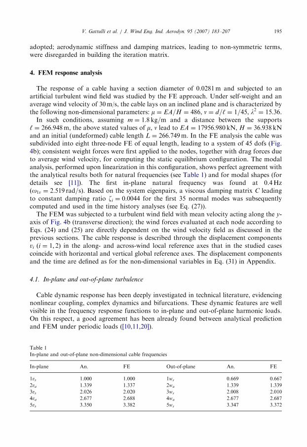
In such conditions, assuming m ¼ 1:8 kg=m and a distance between the supports‘ ¼ 266:948m, the above stated values of m, n lead to EA ¼ 17956:980 kN, H ¼ 36:938 kNand an initial (undeformed) cable length L ¼ 266:749m. In the FE analysis the cable wassubdivided into eight three-node FE of equal length, leading to a system of 45 dofs (Fig.4b); consistent weight forces were first applied to the nodes, together with drag forces dueto average wind velocity, for computing the static equilibrium configuration. The modalanalysis, performed upon linearization in this configuration, shows perfect agreement withthe analytical results both for natural frequencies (see Table 1) and for modal shapes (fordetails see [11]). The first in-plane natural frequency was found at 0.4Hzðo1v ¼ 2:519 rad=sÞ. Based on the system eigenpairs, a viscous damping matrix C leadingto constant damping ratio zi ¼ 0:0044 for the first 35 normal modes was subsequentlycomputed and used in the time history analyses (see Eq. (27)).

The FEM was subjected to a turbulent wind field with mean velocity acting along the y-axis of Fig. 4b (transverse direction); the wind forces evaluated at each node according toEqs. (24) and (25) are directly dependent on the wind velocity field as discussed in theprevious sections. The cable response is described through the displacement componentsvi ði ¼ 1; 2Þ in the along- and across-wind local reference axes that in the studied casescoincide with horizontal and vertical global reference axes. The displacement componentsand the time are defined as for the non-dimensional variables in Eq. (31) in Appendix.

4.1. In-plane and out-of-plane turbulence

Cable dynamic response has been deeply investigated in technical literature, evidencingnonlinear coupling, complex dynamics and bifurcations. These dynamic features are wellvisible in the frequency response functions to in-plane and out-of-plane harmonic loads.On this respect, a good agreement has been already found between analytical predictionand FEM under periodic loads ([10,11,20]).

Table 1

In-plane and out-of-plane non-dimensional cable frequencies

In-plane An. FE Out-of-plane An. FE

1vs 1.000 1.000 1ws 0.669 0.667

2va 1.339 1.337 2wa 1.339 1.339

3vs 2.026 2.020 3ws 2.008 2.010

4va 2.677 2.688 4wa 2.677 2.687

5vs 3.350 3.382 5ws 3.347 3.372


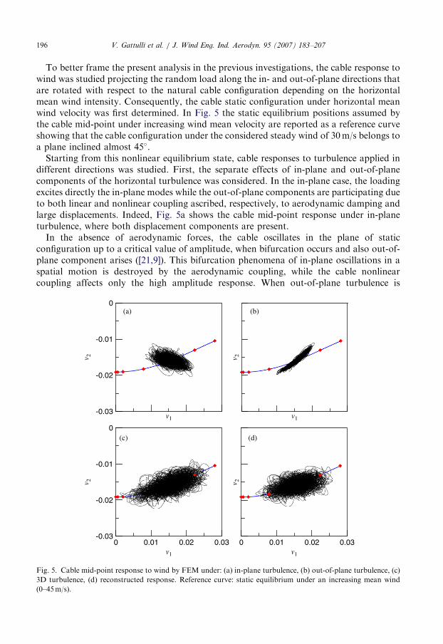
To better frame the present analysis in the previous investigations, the cable response towind was studied projecting the random load along the in- and out-of-plane directions thatare rotated with respect to the natural cable configuration depending on the horizontalmean wind intensity. Consequently, the cable static configuration under horizontal meanwind velocity was first determined. In Fig. 5 the static equilibrium positions assumed bythe cable mid-point under increasing wind mean velocity are reported as a reference curveshowing that the cable configuration under the considered steady wind of 30m/s belongs toa plane inclined almost 45�.Starting from this nonlinear equilibrium state, cable responses to turbulence applied in

different directions was studied. First, the separate effects of in-plane and out-of-planecomponents of the horizontal turbulence was considered. In the in-plane case, the loadingexcites directly the in-plane modes while the out-of-plane components are participating dueto both linear and nonlinear coupling ascribed, respectively, to aerodynamic damping andlarge displacements. Indeed, Fig. 5a shows the cable mid-point response under in-planeturbulence, where both displacement components are present.In the absence of aerodynamic forces, the cable oscillates in the plane of static

configuration up to a critical value of amplitude, when bifurcation occurs and also out-of-plane component arises ([21,9]). This bifurcation phenomena of in-plane oscillations in aspatial motion is destroyed by the aerodynamic coupling, while the cable nonlinearcoupling affects only the high amplitude response. When out-of-plane turbulence is

v1-0.03

-0.02

-0.01

0

v 2

v1

v 2

0 0.01 0.02 0.03v1

-0.03

-0.02

-0.01

0

v 2

0 0.01 0.02 0.03v1

v 2

(a) (b)

(c) (d)

Fig. 5. Cable mid-point response to wind by FEM under: (a) in-plane turbulence, (b) out-of-plane turbulence, (c)

3D turbulence, (d) reconstructed response. Reference curve: static equilibrium under an increasing mean wind

(0–45m/s).


considered, see Fig. 5b, both linear and nonlinear coupling are present at any level ofexcitation intensity, but due to the larger flexibility in the out-of-plane motion, the timehistories of the two components are quite different and out-of-plane component isprevailing; the ratio between the two amplitudes is significantly larger than two, a valueforeseen by means of the 2 dof analytical model in [21].

Then, the cable response to the simultaneous in-plane and out-of-plane turbulence hasbeen simulated and response with larger amplitudes than the ones obtained superimposingthe previous results are obtained, as it is evident comparing the Figs. 5c and d. Thisdifference can be ascribed to a slightly non-linear behavior which is compatible with thecable relatively small displacement range. Looking at a direct comparison of the two timehistories it is clearly visible that the overall aspect and amplitude of the cable motion arequite similar; examination of the Fourier spectra (not shown for brevity) points out thatthe most significant differences are in the background response, at frequencies lying belowthe cable eigenspectrum.

Further analyses have been performed to identify the main factors that are significant in thecomplex phenomena under study. Among these, the influence of the load description, such asturbulence dimensionality and coherence, and the role of cable model dimension are tackled.

4.2. 1D and 3D turbulence

The influence on cable response of the turbulence dimensionality was evaluatedconsidering both 1D and 3D turbulent wind fields. In the 1D case, the turbulence wassuperimposed to the horizontal mean wind W in the same direction; in the 3D case, threeturbulent components at each point were superimposed to the horizontal mean wind. Theparameters selected in the wind model are such that the coherence expected for theturbulence components at different points along the cable is within average ([26]) (AWC).

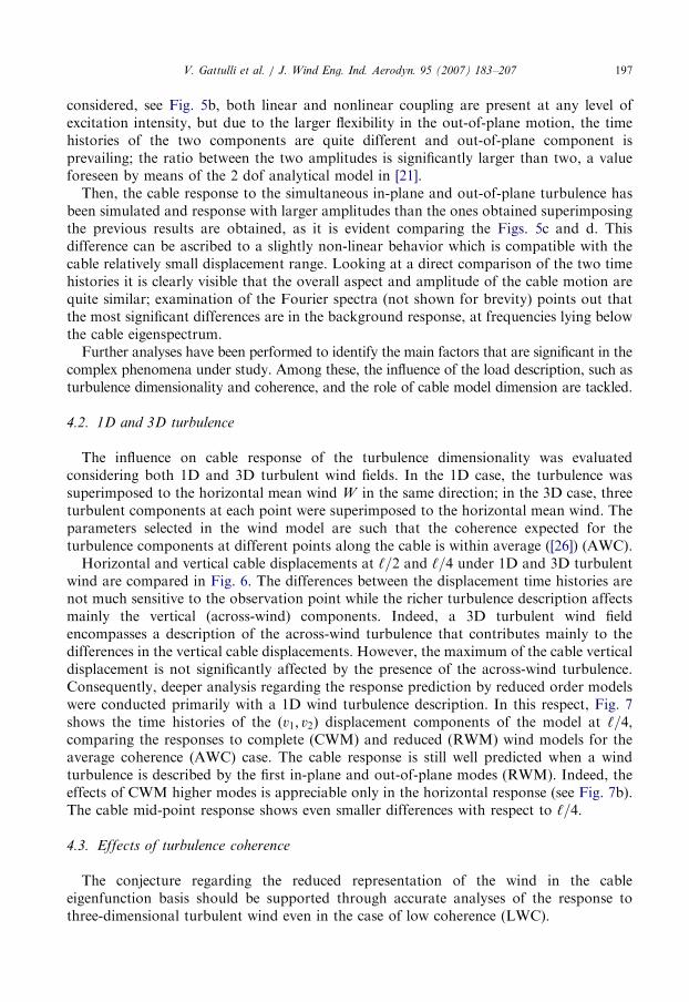
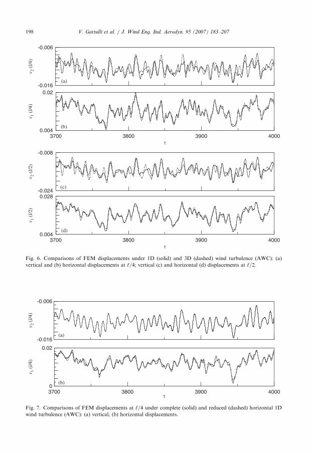
Horizontal and vertical cable displacements at ‘=2 and ‘=4 under 1D and 3D turbulentwind are compared in Fig. 6. The differences between the displacement time histories arenot much sensitive to the observation point while the richer turbulence description affectsmainly the vertical (across-wind) components. Indeed, a 3D turbulent wind fieldencompasses a description of the across-wind turbulence that contributes mainly to thedifferences in the vertical cable displacements. However, the maximum of the cable verticaldisplacement is not significantly affected by the presence of the across-wind turbulence.Consequently, deeper analysis regarding the response prediction by reduced order modelswere conducted primarily with a 1D wind turbulence description. In this respect, Fig. 7shows the time histories of the ðv1; v2Þ displacement components of the model at ‘=4,comparing the responses to complete (CWM) and reduced (RWM) wind models for theaverage coherence (AWC) case. The cable response is still well predicted when a windturbulence is described by the first in-plane and out-of-plane modes (RWM). Indeed, theeffects of CWM higher modes is appreciable only in the horizontal response (see Fig. 7b).The cable mid-point response shows even smaller differences with respect to ‘=4.

4.3. Effects of turbulence coherence

The conjecture regarding the reduced representation of the wind in the cableeigenfunction basis should be supported through accurate analyses of the response tothree-dimensional turbulent wind even in the case of low coherence (LWC).

ARTICLE IN PRESS

-0.016

-0.006

v 2 (

l/4)

3700 3800 3900 4000τ

0.004

0.02

v 1 (

l/4)

-0.024

-0.008

v 2 (

l/2)

3700 3800 3900 4000τ

0.004

0.028

v 1 (

l/2)

(a)

(c)

(b)

(d)

Fig. 6. Comparisons of FEM displacements under 1D (solid) and 3D (dashed) wind turbulence (AWC): (a)

vertical and (b) horizontal displacements at ‘=4; vertical (c) and horizontal (d) displacements at ‘=2.

-0.016

-0.006

v 2 (

l/4)

3700 3800 3900 4000τ

0

0.02

v 1 (

l/4)

(a)

(b)

Fig. 7. Comparisons of FEM displacements at ‘=4 under complete (solid) and reduced (dashed) horizontal 1D

wind turbulence (AWC): (a) vertical, (b) horizontal displacements.



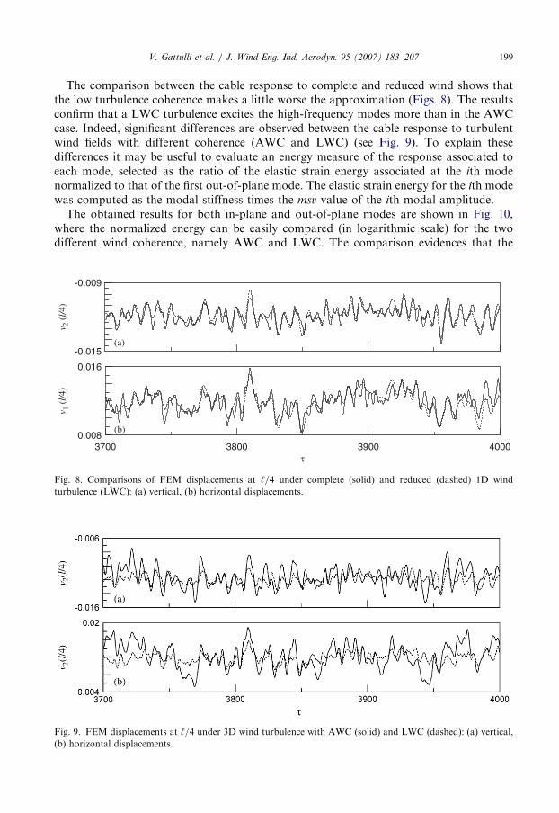
The comparison between the cable response to complete and reduced wind shows thatthe low turbulence coherence makes a little worse the approximation (Figs. 8). The resultsconfirm that a LWC turbulence excites the high-frequency modes more than in the AWCcase. Indeed, significant differences are observed between the cable response to turbulentwind fields with different coherence (AWC and LWC) (see Fig. 9). To explain thesedifferences it may be useful to evaluate an energy measure of the response associated toeach mode, selected as the ratio of the elastic strain energy associated at the ith modenormalized to that of the first out-of-plane mode. The elastic strain energy for the ith modewas computed as the modal stiffness times the msv value of the ith modal amplitude.

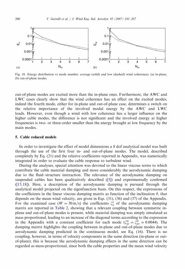
The obtained results for both in-plane and out-of-plane modes are shown in Fig. 10,where the normalized energy can be easily compared (in logarithmic scale) for the twodifferent wind coherence, namely AWC and LWC. The comparison evidences that the

-0.015

-0.009

v 2 (

l/4)

3700 3800 3900 4000τ

0.008

0.016

v 1 (

l/4)

(a)

(b)

Fig. 8. Comparisons of FEM displacements at ‘=4 under complete (solid) and reduced (dashed) 1D wind

turbulence (LWC): (a) vertical, (b) horizontal displacements.

Fig. 9. FEM displacements at ‘=4 under 3D wind turbulence with AWC (solid) and LWC (dashed): (a) vertical,

(b) horizontal displacements.

ARTICLE IN PRESS

1 2 3 4 5 6 7

Nm

0.0001

0.001

0.01

0.1

1

Ev

1 2 3 4 5 6 7

Nm

0.0001

0.001

0.01

0.1

1

Ew

(a) (b)

Fig. 10. Energy distribution vs mode number: average (solid) and low (dashed) wind coherences: (a) in-plane,

(b) out-of-plane modes.


out-of-plane modes are excited more than the in-plane ones. Furthermore, the AWC andLWC cases clearly show that the wind coherence has an effect on the excited modes;indeed the fourth mode, either for in-plane and out-of-plane case, determines a switch onthe relative importance of the involved modal energy by the AWC and LWCloads. However, even though a wind with low coherence has a larger influence on thehigher cable modes, the difference is not significant and the involved energy at higherfrequencies is two- or three-order smaller than the energy brought at low frequency by themain modes.

5. Cable reduced models

In order to investigate the effect of model dimensions a 8 dof analytical model was builtthrough the use of the first four in- and out-of-plane modes. The model, describedcompletely by Eq. (21) and the relative coefficients reported in Appendix, was numericallyintegrated in order to evaluate the cable response to turbulent wind.During the analyses, special attention was devoted to the linear viscous terms to which

contribute the cable material damping and more considerably the aerodynamic dampingdue to the fluid–structure interaction. The relevance of the aerodynamic damping onsuspended cables has been qualitatively described ([5]) and experimentally confirmed([15,18]). Here, a description of the aerodynamic damping is pursued through theanalytical model projected on the eigenfunction basis. On this respect, the expressions ofthe coefficients in the linear viscous damping matrix as function of the inclination y, thatdepends on the mean wind velocity, are given in Eqs. (31), (36) and (37) of the Appendix.For the examined case ðW ¼ 30m=sÞ the coefficients za

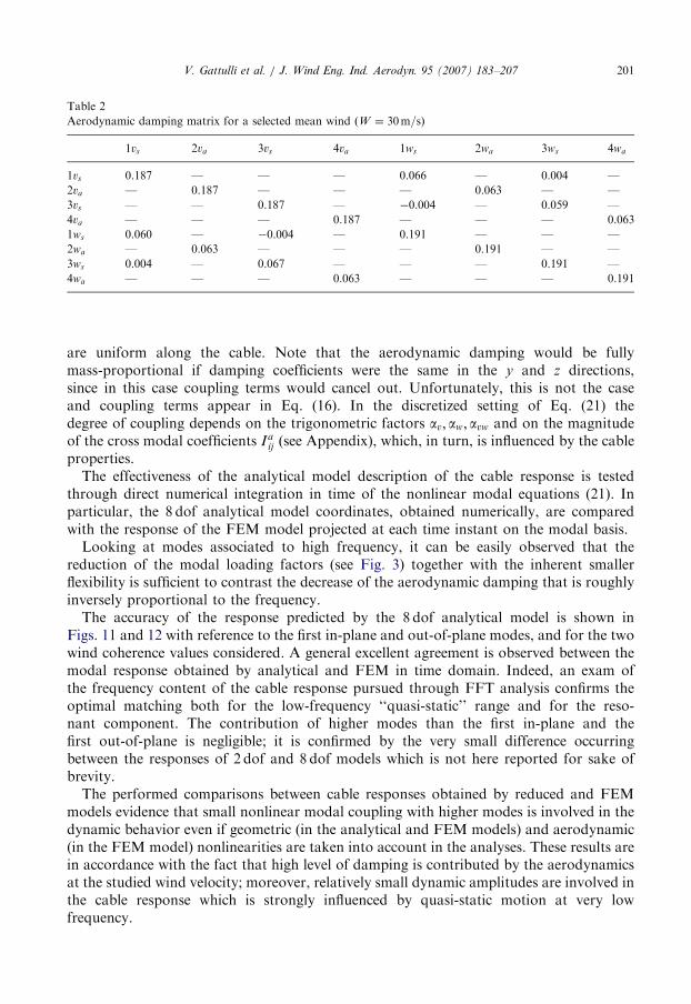
ij of the aerodynamic dampingmatrix are reported in Table 2, showing that a relevant coupling between symmetric in-plane and out-of-plane modes is present, while material damping was simply simulated asmass proportional, leading to an increase of the diagonal terms according to the expressionin the Appendix with a constant coefficient for each mode ðzm

ijv ¼ zmijw ¼ 0:0044Þ. The

damping matrix highlights the coupling between in-plane and out-of-plane modes due toaerodynamic damping predicted in the continuous model, see Eq. (16). There is nocoupling, however, in terms of velocity components in the same direction (in-plane or out-of-plane); this is because the aerodynamic damping effects in the same direction can beregarded as mass-proportional, since both the cable properties and the mean wind velocity

ARTICLE IN PRESS

Table 2

Aerodynamic damping matrix for a selected mean wind ðW ¼ 30m=sÞ

1vs 2va 3vs 4va 1ws 2wa 3ws 4wa

1vs 0.187 — — — 0.066 — 0.004 —

2va — 0.187 — — — 0.063 — —

3vs — — 0.187 — �0.004 — 0.059 —

4va — — — 0.187 — — — 0.063

1ws 0.060 — �0.004 — 0.191 — — —

2wa — 0.063 — — — 0.191 — —

3ws 0.004 — 0.067 — — — 0.191 —

4wa — — — 0.063 — — — 0.191


are uniform along the cable. Note that the aerodynamic damping would be fullymass-proportional if damping coefficients were the same in the y and z directions,since in this case coupling terms would cancel out. Unfortunately, this is not the caseand coupling terms appear in Eq. (16). In the discretized setting of Eq. (21) thedegree of coupling depends on the trigonometric factors av; aw; avw and on the magnitudeof the cross modal coefficients Ia

ij (see Appendix), which, in turn, is influenced by the cableproperties.

The effectiveness of the analytical model description of the cable response is testedthrough direct numerical integration in time of the nonlinear modal equations (21). Inparticular, the 8 dof analytical model coordinates, obtained numerically, are comparedwith the response of the FEM model projected at each time instant on the modal basis.

Looking at modes associated to high frequency, it can be easily observed that thereduction of the modal loading factors (see Fig. 3) together with the inherent smallerflexibility is sufficient to contrast the decrease of the aerodynamic damping that is roughlyinversely proportional to the frequency.

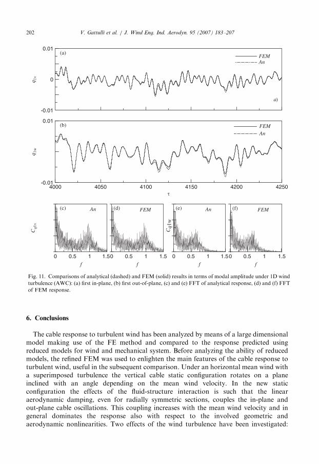
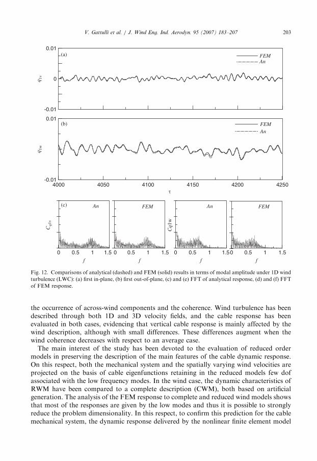
The accuracy of the response predicted by the 8 dof analytical model is shown inFigs. 11 and 12 with reference to the first in-plane and out-of-plane modes, and for the twowind coherence values considered. A general excellent agreement is observed between themodal response obtained by analytical and FEM in time domain. Indeed, an exam ofthe frequency content of the cable response pursued through FFT analysis confirms theoptimal matching both for the low-frequency ‘‘quasi-static’’ range and for the reso-nant component. The contribution of higher modes than the first in-plane and thefirst out-of-plane is negligible; it is confirmed by the very small difference occurringbetween the responses of 2 dof and 8 dof models which is not here reported for sake ofbrevity.

The performed comparisons between cable responses obtained by reduced and FEMmodels evidence that small nonlinear modal coupling with higher modes is involved in thedynamic behavior even if geometric (in the analytical and FEM models) and aerodynamic(in the FEM model) nonlinearities are taken into account in the analyses. These results arein accordance with the fact that high level of damping is contributed by the aerodynamicsat the studied wind velocity; moreover, relatively small dynamic amplitudes are involved inthe cable response which is strongly influenced by quasi-static motion at very lowfrequency.

ARTICLE IN PRESS

-0.01

0

0.01

q 1v

FEMAn

a)

4000 4050 4100 4150 4200 4250τ

-0.01

0.01

q 1w

FEMAn

0 0.5 1 1.5

f

Cq1

w

0 0.5 1 1.5

f

Cq1

v

0 0.5 1 1.5

f

An FEM

0 0.5 1 1.5

f

FEMAn

(a)

(b)

(c) (d) (e) (f)

Fig. 11. Comparisons of analytical (dashed) and FEM (solid) results in terms of modal amplitude under 1D wind

turbulence (AWC): (a) first in-plane, (b) first out-of-plane, (c) and (e) FFT of analytical response, (d) and (f) FFT

of FEM response.


6. Conclusions

The cable response to turbulent wind has been analyzed by means of a large dimensionalmodel making use of the FE method and compared to the response predicted usingreduced models for wind and mechanical system. Before analyzing the ability of reducedmodels, the refined FEM was used to enlighten the main features of the cable response toturbulent wind, useful in the subsequent comparison. Under an horizontal mean wind witha superimposed turbulence the vertical cable static configuration rotates on a planeinclined with an angle depending on the mean wind velocity. In the new staticconfiguration the effects of the fluid-structure interaction is such that the linearaerodynamic damping, even for radially symmetric sections, couples the in-plane andout-plane cable oscillations. This coupling increases with the mean wind velocity and ingeneral dominates the response also with respect to the involved geometric andaerodynamic nonlinearities. Two effects of the wind turbulence have been investigated:

ARTICLE IN PRESS

-0.01

0

0.01

q 1v

FEMAn

4000 4050 4100 4150 4200 4250τ

-0.01

0.01

q 1w

FEMAn

0 0.5 1 1.5

f

Cq1

w

0 0.5 1 1.5

f

Cq1

v

0 0.5 1 1.5

f

An FEM

0 0.5 1 1.5

f

FEMAn

(a)

(b)

(c)

Fig. 12. Comparisons of analytical (dashed) and FEM (solid) results in terms of modal amplitude under 1D wind

turbulence (LWC): (a) first in-plane, (b) first out-of-plane, (c) and (e) FFT of analytical response, (d) and (f) FFT

of FEM response.


the occurrence of across-wind components and the coherence. Wind turbulence has beendescribed through both 1D and 3D velocity fields, and the cable response has beenevaluated in both cases, evidencing that vertical cable response is mainly affected by thewind description, although with small differences. These differences augment when thewind coherence decreases with respect to an average case.

The main interest of the study has been devoted to the evaluation of reduced ordermodels in preserving the description of the main features of the cable dynamic response.On this respect, both the mechanical system and the spatially varying wind velocities areprojected on the basis of cable eigenfunctions retaining in the reduced models few dofassociated with the low frequency modes. In the wind case, the dynamic characteristics ofRWM have been compared to a complete description (CWM), both based on artificialgeneration. The analysis of the FEM response to complete and reduced wind models showsthat most of the responses are given by the low modes and thus it is possible to stronglyreduce the problem dimensionality. In this respect, to confirm this prediction for the cablemechanical system, the dynamic response delivered by the nonlinear finite element model


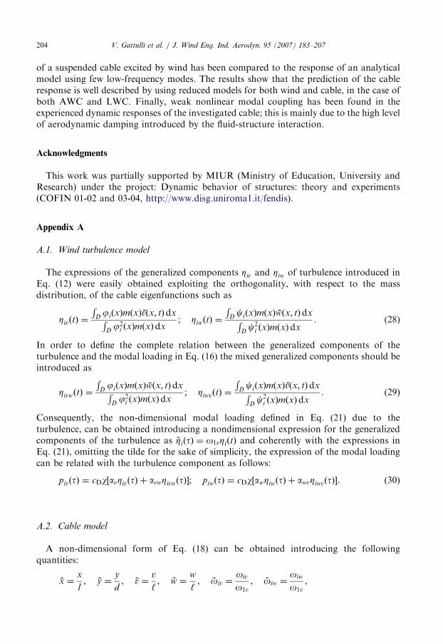
of a suspended cable excited by wind has been compared to the response of an analyticalmodel using few low-frequency modes. The results show that the prediction of the cableresponse is well described by using reduced models for both wind and cable, in the case ofboth AWC and LWC. Finally, weak nonlinear modal coupling has been found in theexperienced dynamic responses of the investigated cable; this is mainly due to the high levelof aerodynamic damping introduced by the fluid-structure interaction.

Acknowledgments

This work was partially supported by MIUR (Ministry of Education, University andResearch) under the project: Dynamic behavior of structures: theory and experiments(COFIN 01-02 and 03-04, http://www.disg.uniroma1.it/fendis).

Appendix A

A.1. Wind turbulence model

The expressions of the generalized components Ziv and Ziw of turbulence introduced inEq. (12) were easily obtained exploiting the orthogonality, with respect to the massdistribution, of the cable eigenfunctions such as

ZivðtÞ ¼

RDjiðxÞmðxÞvðx; tÞdxR

Dj2

i ðxÞmðxÞdx; ZiwðtÞ ¼

RDciðxÞmðxÞwðx; tÞdxR

Dc2

i ðxÞmðxÞdx. (28)

In order to define the complete relation between the generalized components of theturbulence and the modal loading in Eq. (16) the mixed generalized components should beintroduced as

ZivwðtÞ ¼

RDjiðxÞmðxÞwðx; tÞdxR

Dj2

i ðxÞmðxÞdx; ZiwvðtÞ ¼

RDciðxÞmðxÞvðx; tÞdxR

Dc2

i ðxÞmðxÞdx. (29)

Consequently, the non-dimensional modal loading defined in Eq. (21) due to theturbulence, can be obtained introducing a nondimensional expression for the generalizedcomponents of the turbulence as ~ZiðtÞ ¼ o1vZiðtÞ and coherently with the expressions inEq. (21), omitting the tilde for the sake of simplicity, the expression of the modal loadingcan be related with the turbulence component as follows:

pivðtÞ ¼ cDw½avZivðtÞ þ avwZivwðtÞ�; piwðtÞ ¼ cDw½awZiwðtÞ þ awvZiwvðtÞ�. (30)

A.2. Cable model

A non-dimensional form of Eq. (18) can be obtained introducing the followingquantities:

~x ¼x

l; ~y ¼

y

d; ~v ¼

v

‘; ~w ¼

w

‘; ~oiv ¼

oiv

o1v

; ~oiw ¼oiw

o1v

,

http://www.disg.uniroma1.it/fendis


t ¼ o1vt; m ¼EA

H; n ¼

d

‘; w ¼

rabW

mo1v

,

av ¼ð1þ sin2 yÞ

2; aw ¼

ð1þ cos2 yÞ2

; avw ¼ awv ¼sin y cos y

2. (31)

The modal shapes of a suspended cable are given by the following expressions:

jiðxÞ ¼ 1� tanbi

2sin bix� cos bix

� �bi; i ¼ 1; 3; . . . ðsymmetricÞ,

jiðxÞ ¼ sin ipx; i ¼ 2; 4; . . . ðantisymmetricÞ,

ckðxÞ ¼ sin kpx; k ¼ 1; 2; 3; . . . , (32)

where bi ¼ cosðbi=2Þð1=ðcos bi þ ð�1ÞhÞÞ is a normalization constant (h ¼ i for i ¼ 1; 5; . . .

and h ¼ 2i for i ¼ 3; 7; . . .) and the spatial frequencies bi are given by the roots of thecharacteristic equation

tanbi

2�

bi

2�

4

l2bi

2

� �3" #

¼ 0 (33)

which depend on Irvine parameter l2 ¼ 64mn2, with m and n given by Eqs. (32), ([13]) whilethe related dimensional natural frequencies can be obtained as

oiv ¼bi

pos; i ¼ 1; 3; . . . ðsymmetricÞ oiv ¼ ios; i ¼ 2; 4; . . . ðantisymmetricÞ,

oiw ¼ ios; i ¼ 1; 2; 3; . . . ; where os ¼p‘

ffiffiffiffiffiH

m

r. (34)

In order to define the coefficients of Eqs. (20), (21), let us introduce the following integrals:

Imi ¼

Z 1

0

f 2i ðxÞdx; Ie

ij ¼

Z 1

0

f 0iðxÞf0jðxÞdx; Ia

ij ¼

Z 1

0

f iðxÞf jðxÞdx,

Iyi ¼

Z 1

0

y0ðxÞf 0iðxÞdx; Ipi ðtÞ ¼

Z 1

0

hðx; tÞf iðxÞdx, (35)

where f i and f 0i are the placeholders of jiðxÞ, or ciðxÞ and their derivatives whereappropriate, and yðxÞ is the parabolic function lying in the y rotated plane from the verticalone while hðx; tÞ is the placeholder of gust wind velocity distributions vðx; tÞ and wðx; tÞ.Consequently, the coefficients aij and bij , the damping coefficients zij ¼ zm

ij þ zaij of the

damping matrix, including material and aerodynamic dampings, and the gust loading pi inEqs. (20) and (21) are defined as follows.


A.3. In-plane equations

zijv ¼mv

mo1v

dij þ av

Iavij

Imvi

cDw; zijvw ¼ avw

Iavwij

Imvi

cDw,

a0ij ¼Iev

ij

Imvi

1

b21; a1i ¼ mn

Iyvi

Imvi

1

b21; a2ij ¼ m

Ievij

Imvi

1

b21,

b1j ¼ nIyvj ; b2ij ¼

12

Ievij ; b3i ¼

12

Iewii ,

pivðtÞ ¼ cDwavI

pvvi ðtÞ þ avwI

pwvi ðtÞ

Imvi

. ð36Þ

A.4. Out-of-plane equations

zijw ¼mw

mo1v

dij þ aw

Iawij

Imwi

cDw; zijwv ¼ awv

Iawvij

Imwi

cDw,

o2wi ¼

Iewii

Imwi

1

b21; a3i ¼ m

Iewii

Imwi

1

b21,

b1i ¼ nIyvi ; b2ij ¼

12

Ievij ; b3i ¼

12

Iewii ,

piwðtÞ ¼ cDwawI

pwwi ðtÞ þ awvI

pvwi ðtÞ

Imwi

, ð37Þ

where dij is the Kronecher operator and the apexes of the integrals I define completely thetype of functions integrated, according to Eqs. (35), together with the use of symbols v andw as indicator of the used eigenfunctions jiðxÞ or/and ciðxÞ, respectively, while the symbolsv and w in the integral defining the time functions representing the gust loading representsthe used wind velocity distributions.

References

[1] F. Benedettini, G. Rega, R. Alaggio, Non-linear oscillations of a four-degree-of-freedom model of a

suspended cable under multiple internal resonance conditions, J. Sound Vibration 182 (1995) 775–798.

[2] L. Carassale, G. Solari, Modal transformation tools in structural dynamics and wind engineering, Wind

Struct. 3 (4) (2000) 221–241.

[3] L. Carassale, G. Solari, Wind modes for structural dynamics: a continuous approach, Prob. Eng. Mech. 17

(2002) 157–166.

[4] A.G. Davenport, The response of slender, line-like structures to a gusty wind, Proc. Instn. Civil Engrs. 23

(1962) 389–408.

[5] A.G. Davenport, How we can semplify and generalize wind loads?, J. Wind Eng. Ind. Aerodyn. 54/55 (1995)

657–669.

[6] Y.M. Desai, N. Popplewell, A. Shah, D.N. Buragohain, Geometric nonlinear analysis of cable supported

structures, Comput. Struct. 29 (6) (1988) 1001–1009.

[7] M. Di Paola, Digital simulation of wind field velocity, J. Wind Eng. Ind. Aerodyn. 74/76 (1998) 91–109.

[8] EUROCODE 1, Basis of Design and Structures—General actions—Part 1–4: Wind Actions, European

Standard prEN 1991-1-4, Final Draft, CEN, January, 2004.

[9] V. Gattulli, M. Pasca, F. Vestroni, Nonlinear oscillations of a nonresonant cable under in-plane excitation

with a longitudinal control, Nonlinear Dyn. 14 (1997) 139–156.


[10] V. Gattulli, L. Martinelli, F. Perotti, F. Vestroni, Nonlinear interactions in cables investigated using

analytical and finite element models, IV International Symposium on Cable Dynamics, Montreal, Canada,

28–30 May, 2001.

[11] V. Gattulli, L. Martinelli, F. Perotti, F. Vestroni, Nonlinear oscillations of cables under harmonic loading

using analytical and finite element models, Comput. Meth. Appl. Mech. Eng. 193 (2004) 69–85.

[12] H.M. Hilber, T.J.R. Hughes, R.L. Taylor, Improved numerical dissipation for time-integration algorithms in

structural dynamics, Earth. Eng. Struct. Dyn. 5 (1977) 283–293.

[13] H.M. Irvine, Cable Structures, The MIT Press, Cambridge, 1981.

[14] C.L. Lee, N.C. Perkins, Three-dimensional oscillations of suspended cables involving simultaneous internal

resonances, Nonlinear Dynam. 8 (1995) 45–63.

[15] A.M. Loredo-Souza, A.G. Davenport, The effects of high winds on transmission lines, J. Wind Eng. Ind.

Aerodyn. 74–76 (1998) 987–994.

[16] A. Luongo, G. Piccardo, Non-linear galloping of sagged cables in 1:2 internal resonance, J. Sound Vibration

214 (5) (1998) 915–940.

[17] A. Luongo, G. Rega, F. Vestroni, Planar nonlinear free vibrations of elastic cables, Int. J. Non-Linear Mech.

19 (1984) 39–52.

[18] J.H.G. Macdonald, Separation of contributions of aerodynamic and structural damping in vibrations of

inclined cables, J. Wind Eng. Ind. Aerodyn. 90 (2002) 19–39.

[19] L. Martinelli, F. Perotti, Numerical analysis of the non-linear dynamic behaviour of suspended cables under

turbulent wind excitation, Int. J. Struct. Stab. Dyn. 1 (2001) 207–233.

[20] L. Martinelli, V. Gattulli, F. Vestroni, Nonlinear behaviour of a suspended cable under stationary and non-

stationary loading, V European Conference on Structural Dynamics, Eurodyn’02, (2002) pp. 893–898.

[21] M. Pasca, F. Vestroni, V. Gattulli, Active longitudinal control of wind-induced oscillations of a suspended

cable, Meccanica 33 (1998) 255–266.

[22] N.C. Perkins, Modal interactions in the non-linear response of elastic cables under parametric/external

excitation, Int. J. Non-Linear Mech. 27 (1992) 233–250.

[23] G. Rega, Nonlinear vibrations of suspended cables—Part I: modelling and analysis—Part II: deterministic

phenomena, Appl. Mech. Rev. 57 (2004) 443–514.

[24] M. Shinozuka, C.M. Jan, Digital simulation of random processes and its applications, J. Sound Vibration 25

(1972) 111–128.

[25] M. Shinozuka, C.M. Jan, Analysis of multi-correlated wind excited vibrations of structures using the

covariance method, Eng. Struct. 5 (1983) 264–272.

[26] G. Solari, G. Piccardo, Probabilistic 3D turbulence modeling for gust buffeting of structures, Prob. Eng.

Mech. 16 (2001) 73–86.

[27] K. Takahashi, Y. Konishi, Non-Linear vibrations of cables in three dimensions, part I: non-linear free

vibrations; part II: out-of-plane vibrations under in-plane sinusoidally time-varying load, J. Sound Vibration

118 (1987) 69–97.

Dynamics of suspended cables under turbulence loading: Reduced models of wind field and mechanical...

Documents

Transcript of Dynamics of suspended cables under turbulence loading: Reduced models of wind field and mechanical...