Dynamics of choice during estimation of subjective value

This article appeared in a journal published by Elsevier. The attachedcopy is furnished to the author for internal non-commercial researchand education use, including for instruction at the authors institution

and sharing with colleagues.

Other uses, including reproduction and distribution, or selling orlicensing copies, or posting to personal, institutional or third party

websites are prohibited.

In most cases authors are permitted to post their version of thearticle (e.g. in Word or Tex form) to their personal website orinstitutional repository. Authors requiring further information

regarding Elsevier’s archiving and manuscript policies areencouraged to visit:

http://www.elsevier.com/copyright

http://www.elsevier.com/copyright

Author's personal copy

Behavioural Processes 87 (2011) 34–42

Contents lists available at ScienceDirect

Behavioural Processes

journa l homepage: www.e lsev ier .com/ locate /behavproc

Dynamics of choice during estimation of subjective value

Elias Roblesa,∗, Nicole A. Robertsa, Federico Sanabriab

a Division of Social & Behavioral Sciences, Arizona State University, 4701 W. Thunderbird Rd., MC3051, Glendale, AZ 85306, United Statesb Department of Psychology, 950 S. McAllister, Tempe, AZ 85287-1104, United States

a r t i c l e i n f o

Article history:Received 15 September 2010Received in revised form 17 January 2011Accepted 21 January 2011

Keywords:Delay discountingMathematical modelingPreferential choiceResponse timeSubjective value

a b s t r a c t

This study characterized preferential choice in binary trials and investigated intra-session variations inresponse time (RT). In Experiment 1, participants (N = 77) were asked to choose the preferred of twoimages of body wash; all unique combinations of 19 images were presented. The results showed: (a)marked and consistent individual preferences for specific stimuli; (b) RT decreased monotonically withincreasing exposure to each stimulus; (c) RT decreased exponentially as a function of relative preferenceranking of the 2 images in a trial; and (d) a regression model efficiently predicted trial RT as a functionof exposure and relative preference. Experiment 2 (N = 112) explored the effect of amount of exposureon RT, and relative preference as a function of the type of choice task (a previously completed vs. a newchoice task). The results showed that: (a) within a single choice task, amount of exposure and relativepreference between the stimuli predicted the systematic changes in RT observed in Exp. 1; and (b) whenthe choice task changed, the effects of previous amount of exposure, and relative stimulus preference didnot transfer to the new task.

Published by Elsevier B.V.

1. Introduction

The value of a good (i.e., an object, event, or relationship) isoften estimated by measuring patterns of choice between concur-rently available goods (Herrnstein, 1961; Mazur, 1987; Baum andRachlin, 1969; Jones and Rachlin, 2006; Rachlin et al., 1991; Bickelet al., 1999; Yi et al., 2006). A large body of evidence from con-current choice studies show that value of a reward varies withits magnitude, frequency, and delay, among others. For humans,the list of dimensions determining value is seemingly endless andincludes beauty, social proximity, social status, functionality, fair-ness, and morality, to name a few. Moreover, we often choosebetween goods whose value derives from very different dimen-sions, as when we decide between having dinner and taking a phonecall. In spite of complexity, it is possible to estimate the value ofmultifaceted and often intangible goods. For example, delay dis-counting (the loss of value of a good that is due to delay) is typicallyestimated by offering participants a series of choices between hypo-thetical immediate and delayed monetary rewards in binary (i.e.,two-option) trials (Rachlin and Green, 1972; Rachlin et al., 1991).During an assessment, the magnitude of the immediate reward andthe delay interval are systematically varied between trials in orderto find the point of indifference (or switch) in preference betweenalternatives. The magnitude of the immediate reward at the switch-

∗ Corresponding author. Tel.: +1 602 543 4515; fax: +1 602 543 6004.E-mail address: [email protected] (E. Robles).

ing point is the best estimate of the subjective current value of thedelayed rewards. Then, the obtained series of switching points areused to calculate the degree of delay discounting as either an esti-mated rate of decay in value (Killeen, 2009; McKerchar et al., 2009;Mazur, 1987) or as area under the discounting curve (AUC; Myersonet al., 2001). The method is simple, highly efficient and valid, asconsistent and systematic results are observed across species, pop-ulations, and goods, real and hypothetical (De Wit and Mitchell,2010; Madden and Johnson, 2010; Reynolds, 2006).

An alternative method to estimate the subjective value of adelayed reward involves analyzing the latencies or response times(RTs) in binary choice trials. Robles and Vargas (2007) and Chabriset al. (2008) showed that, in a series of trials where participants areasked to choose between an immediate and a delayed reward, thelongest RT in the series corresponds to the trial where the options’subjective value is most similar; i.e., the indifference point. Specif-ically, Chabris showed that RT provides a reliable way to estimatethe value of delayed rewards and delay discounting rates.

The relation between RT and value in binary trials is known asthe “distance effect” (Dashiell, 1937; Leth-Steensen and Marley,2000; Smith, 1968)—the systematic increase in RT that occurs asthe stimuli in a binary trial become more similar. The distanceeffect is intuitively appealing, as more time appears to be neces-sary to choose between two closely valued stimuli than betweenstimuli of dissimilar value. The relation between RT and subjec-tive value was first demonstrated by Dashiell (1937), who askedsubjects to choose the most liked stimulus from pairs of coloredpaper samples, and used their choices to derive individual pref-

0376-6357/$ – see front matter. Published by Elsevier B.V.doi:10.1016/j.beproc.2011.01.009


E. Robles et al. / Behavioural Processes 87 (2011) 34–42 35

erence rankings. Dashiell found that RT was an inverse functionof the difference in ranking between the two stimuli in a trial.While similar relationships had been reported before between RTand stimulus differences along physical dimensions (Baranski andPetrusic, 2003; Ehrenstein and Ehrenstein, 1999), Dashiell’s maincontribution was demonstrating that the distance effect applies tothe subjective (hedonic) value of the stimuli. The distance effect hasnow been observed in relation to various stimuli including food incapuchin monkeys (Padoa-Schioppa et al., 2006) and, in humans,social status (Chiao et al., 2004), computer screen designs (Schmidtet al., 2006), and delay discounting (Chabris et al., 2008; Robles andVargas, 2007).

Recent studies have shown that the assessment of subjectivevalue in binary choice trials is affected by contextual factors andby the subject’s previous experience with the stimuli. For exam-ple, an individual’s estimated degree of delay discounting has beenshown to depend on the magnitude of the delayed reward (Graceand McLean, 2005; Green et al., 1997), as well as the order of pre-sentation of the immediate rewards in a series (Robles et al., 2009;Scholten and Read, 2010). It is not yet clear how those factors affectestimation of delay discounting during the assessment task. Thisarticle reports an effort to better understand within-subject andintra-session factors that affect assessment of value during binarychoice tests, like those used to estimate delay discounting. Specif-ically, in two experiments we explored dynamic variations in RTwithin the experimental session with respect to: (a) preference forindividual stimuli (Experiments 1 and 2), (b) amount of exposureto individual stimuli (Experiments 1 and 2), (c) relative preferencebetween stimuli in a trial (Experiments 1 and 2), and (d) practicewith the assessment task (Experiment 2).

2. Experiment 1

2.1. Materials and methods

2.1.1. SubjectsSeventy-seven college students (18 male, 59 female), ages

18–34 (mean age = 19.3), with normal or corrected-to-normalvision, were recruited through the department’s research subjectpool. Volunteers received class credit for their participation in thestudy. All study procedures were approved in advance by the insti-tution’s review board.

2.1.2. Stimulus setsTwo sets of 19 color images were used, Set 1 and Set 2. Thirty-

two percent of the images in Sets 1 and 2 overlapped, and 68% werenon-overlapping. Subjects were randomly assigned to a bottle setfor model validation, as described below. Each image depicted abottle of body wash product commercially available to consumersin the US. The bottles were selected as samples of objects in every-day life that might have hedonic or aesthetic value. The images wereproduced by digital photography of the bottles on a consistent fea-tureless background, and presented at 400 × 200 pixels in size; witha spatial resolution of 300 × 300 dpi; and at 24 bits of color resolu-tion. Presentation of the stimuli and recording of responses werecomputerized. The program code was written in Microsoft VisualBasic 6.0. Data collection was done with a dedicated desktop com-puter running Windows XP at 2.4 GHz. The images were presentedon a 19-in. computer monitor at 1024 × 768 pixels.

2.1.3. ProcedureThere were 3 experimental phases in this study; all subjects

received the same treatments in the same order. Each phase con-sisted of a series of 171 discrete trials separated by a 2-s intertrialinterval (ITI); the experimental phases were separated by a 2-minbreak during which the subjects were asked to remain in their seats.

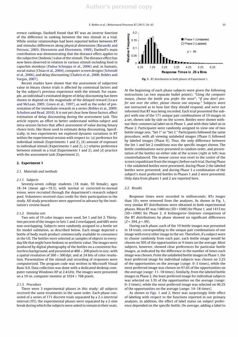
Fig. 1. RT distribution in both phases of Experiment 1.

At the beginning of each phase subjects were given the followinginstructions (as two separate bullet points): “Using the computermouse, choose the bottle you prefer the most”; “if you don’t pre-fer one over the other, please choose one anyway.” Subjects werenot instructed as to how fast they should respond, and were notinformed that RT was being recorded. Each trial presented the sub-ject with one of the 171 unique pair combinations of 19 images ina set, shown side by side on the screen. Bottles were shown with-out their commercial label on in Phase 1, and with their label on inPhase 2. Participants were randomly assigned to view one of twobottle image sets, “Set 1” or “Set 2.” Participants followed the sameprocedure, with all viewing unlabeled images (Phase I) followedby labeled images (Phase II). Thus, the only difference betweenthe Set 1 and Set 2 conditions was the specific images shown. Thebottle combinations were presented in random order, and presen-tation of the bottles on either side of the screen (right or left) wascounterbalanced. The mouse cursor was reset to the center of thescreen (equidistant from the images) before each trial. During Phase1 the unlabeled bottles were presented; during Phase 2 the labeledbottles were presented; and during Phase 3 a combination of thesubject’s most preferred bottles in Phases 1 and 2 were presented.Only data from phases 1 and 2 are reported here.

2.2. Results

Response times were recorded in milliseconds; RTs longerthan 10 s were removed from the analyses. As shown in Fig. 1,very similar RT distributions were obtained in both experimentalphases. Mean RT was 1480 ms (SD = 1040) for Phase 1, and 1415 ms(SD = 1090) for Phase 2. A Kolmogorov–Smirnov comparison ofthe RT distributions by phase showed no significant differences(Z = .394, p = .99).

During each phase, each of the 19 bottle images was presentedin 18 trials, corresponding to the unique pair combinations of oneimage with every other image in the set. Therefore, if a subject wereto choose randomly from each pair, each bottle image would bechosen on 50% of the opportunities or 9 times on the average. Mostsubjects, however, showed clear preferences for particular bottleimages, as indicated by the difference in the number of times eachimage was chosen. From the unlabeled bottle images in Phase 1, theleast preferred image for individual subjects was chosen on 3.2%of the opportunities on the average (range: 0–3 times), while themost preferred image was chosen on 97.6% of the opportunities onthe average (range: 11–18 times). Similarly, from the labeled bottleimages in Phase 2, the least preferred image for individual subjectswas selected on 3.3% of the opportunities on the average (range:0–3 times), while the most preferred image was selected on 96.2%of the opportunities on the average (range: 14–18 times).

As shown in Figs. 1 and 2, there was surprisingly little effectof labeling with respect to the functions reported in our primaryanalyses. In addition, the effect of label status on subject prefer-ence depended on the specific bottle. On average, adding a label to


36 E. Robles et al. / Behavioural Processes 87 (2011) 34–42

Fig. 2. Logged RT for chosen (top panels) and rejected (bottom panels) stimuli as a function of prior exposure (left panels) and preference ranking (right panels: preferenceincreases toward the right) in Phases 1 and 2 (filled and open circles, respectively). Continuous lines are mean predictions of Eq. (2) using parameters from Table 2. The grayareas at the bottom of the right panels are the relative frequency of trials in which the chosen (top) or rejected (bottom) stimulus was ranked x.

the bottle increased the preference ranking for 47% of the bottles,decreased the preference ranking for 37% of the bottles, and yieldedno change for 16% of the bottles. Thus, bottles were not consistentlyvalued more (or less) if they included a commercial label.

In both phases of Experiment 1 RT decreased monotonicallywith increasing prior exposure to specific stimuli (Fig. 2, leftpanels). In addition, RT decreased monotonically with decreasingpreference scores for the chosen image in the set (Fig. 2, top rightpanel). Similar relations between preference ranking for individ-ual stimuli and RT have been widely reported in the literature (e.g.,Bergum and Dooley, 1969; Jamieson and Petrusic, 1977; Petrusicand Jamieson, 1978; Tyebjee, 1979). No systematic effect of prefer-ence ranking of the rejected stimulus was observed (bottom rightpanel).

2.3. A model of choice RT based on stimulus exposure andpreference

It was initially hypothesized that RTs would vary accordingto two factors: the amount of past exposure to the stimuli onany given choice trial, and the difference in preference rankingbetween those stimuli. Each of these factors can be partitioned intotwo factors. The amount of exposure can be separately assessedfor the chosen (EC) and for the rejected (ER) stimulus. More pre-cisely, EC and ER are the number of trials, before the current trialand within the same experimental phase, in which the chosenand rejected stimulus, respectively, were shown. Because stimu-lus pairings were random, EC and ER were likely to covary; suchcovariance, however, does not imply that both stimuli contributedequally to RT.

The difference in preference ranking is made up of the rankingof the chosen (PC) and rejected (PR) stimulus. More specifically, PCand PR are the number of times the chosen and rejected stimulus,respectively, were chosen within the current experimental phase.The distance effect implies that PC and PR contribute the same to

RT, but it is possible that one ranking contributes more to RT thanthe other ranking.

It may be assumed, a priori, that RT varied between a maximum(RTmax) and a minimum (RTmin > 0 s). In absence of informative evi-dence, it may also be assumed that changes in RT between RTmax

to RTmin are exponential; i.e.:

RTt = (RTmax − RTmin) exp(−�t) + RTmin,

RTmax ≥ RTmin > 0 s; �t > 0 (1)

where RTt is the RT in trial t, and �t is the length of RTt relativeto RTmax and RTmin. If �t = 0, RTt = RTmax; as �t → ∞, RTt = RTmin. Athird parsimonious assumption is that �t linearly absorbs the effectof EC, ER, PC, and PR on RT; i.e.:

�t = ˇECECt + ˇERERt + ˇPCPC + ˇPRPR (2)

where ˇX is the regression weight of variable X (ECt, ERt, PC, and PR).EC and ER are indexed by trial t because, unlike PC and PR, they varyfrom trial to trial as exposure is accrued. This model allows for ECand ER to have the same impact on RT by setting ˇEC = ˇER. Similarly,it allows for the simple difference in preference to influence RT bysetting ˇPR = −ˇPC.

A regression analysis based on Eqs. (1) and (2) was aimed at (1)establishing whether RT was differentially sensitive to exposureto the chosen vs. rejected stimulus (EC vs. ER), and (2) whether ornot the simple difference in preference ranking (PC–PR) accountedfor the influence of preference on RT. With these goals in mind, 6special cases of Eq. (2) were considered: (1) where all regressionweights could be different (ˇEC /= ˇER; ˇPC /= ˇPR); (2) where theinfluence of stimulus exposure was independent of whether it waschosen or not (ˇEC = ˇER; ˇPC /= ˇPR); (3) where the simple differ-ence in preference influenced the RT (ˇEC /= ˇER; ˇPC = −ˇPR); (4) acombination of cases 2 and 3 (ˇEC = ˇER; ˇPC = −ˇPR); (5) where stim-ulus exposure had no effect on RT (ˇEC = ˇER = 0; ˇPC /= ˇPR); and(6) where difference in preference had no effect on RT (ˇEC /= ˇER;



Table 1Cross-validation of specific models in Experiment 1.

Model Constraint ka PVAF (Set 1 → 2)b PVAF (Set 2 → 1)

Phase 1 Phase 2 Phase 1 Phase 2

1 ˇEC /= ˇER; ˇPC /= ˇPR 6 10.43% 7.79% 10.22% 10.23%2 ˇEC = ˇER; ˇPC /= ˇPR 5 10.43% 7.93% 10.27% 11.37%3 ˇEC /= ˇER; ˇPC = −ˇPR 5 8.73% 7.36% 8.03% 9.07%4 ˇEC = ˇER; ˇPC = −ˇPR 4 8.74% 7.42% 8.04% 9.19%5 ˇEC = ˇER = 0; ˇPC /= ˇPR 4 2.90% 1.38% 6.42% 5.86%6 ˇEC /= ˇER; ˇPC = ˇPR = 0 4 9.13% 6.89% 5.52% 5.04%

a Number of free parameters.b Percent of variance in Set 2 RT accounted for by fits of model to Set 1 RT.

ˇPC = ˇPR = 0). Each of these cases, which we call specific models, con-stitutes a quantitative hypothesis of the influence of exposure andpreference on RT. These specific models are listed in Table 1.

Each specific model was evaluated by fitting it to logged RTsobtained with one set of images and assessing the percent of vari-ance accounted for in the other set of images. By logging the RTs, theexponential regression (Eq. (1)) was nearly linearized. The cross-validation was expected to select the model that better fit thevariance in RT within each set without fitting noise or stimulusidiosyncrasies (variance between sets). Goodness of fit was estab-lished using the methods of least squares, which was implementedusing the Solver add-in of Microsoft Excel 2007 for Windows.

Model evaluation results are shown in Table 1. k indicates thenumber of parameters in Eq. (2) that were allowed to vary freely.The following columns indicate the percent of variance in RT to onestimulus set accounted for by the best fit of the specific model tothe other stimulus set. Thus, for instance, the cell at the bottom-right corner of the table indicates that when RTmax, RTmin, ˇEC, andˇER were fit to Set 2, those estimates accounted for 5.04% of thevariance in RT in Set 1.

The cross-validation analysis favored model #2, which assumedthat prior exposure to either stimulus had the same impact on RT onany given trial. This model predicted RTs to an alternate stimulusset better than any other model on both experimental phases. Itaccounted for about 8–11% of the variance in RTs of the set it wasnot fit to. Interestingly, the model with most free parameters, #1,did not predict the RTs of an alternate set as well as #2 did, eventhough #2 is a special case of #1. This is likely because, when fit toRTs in each set, model #1 accommodated its parameters to fit notonly the effects of exposure and difference in preference, but alsostimuli idiosyncrasies and other sources of noise, which precludeda better fit to a new data set.

Because the cross-validation favored a single value for ˇEC andˇER, Eq. (2) was modified to

�t = ˇE(ECt + ERt) + ˇPCPC + ˇPRPR, (3)

where a single parameter, ˇE, now accounts for the impact of stimu-lus exposure on RT. Estimates of each parameter, obtained from fitsto the pooled data of stimulus Sets 1 and 2, are shown in Table 2.In both phases, the maximum RT, which was only attained withnovel stimuli of equal preference, was about 2.5 s. RTs approacheda minimum of 0.57 s with well-known stimuli of distinguishablepreference. The influence of preference on RT was more dependent

Table 2Parameter estimates for Model 2 in Experiment 1.

Parameter Phase 1 Phase 2

RTmax 2.53 s 2.48 sRTmin 0.57 s 0.57 sˇE 2.98 × 10−2 3.64 × 10−2

ˇPC 6.58 × 10−2 7.72 × 10−2

ˇPR −2.64 × 10−2 −4.15 × 10−2

on the ranking of the chosen stimulus (PC) than on the rankingof the rejected stimulus (PR). As expected, the preference for therejected stimulus had a negative impact on RT—the rejection ofmore preferred stimuli took longer than the rejection of less pre-ferred stimuli.

Fig. 2 shows the mean logged RT as a function of exposureto the chosen (EC) and rejected (ER) stimulus, and as a functionof preference for the chosen (PC) and rejected (PR) stimulus. Thecontinuous lines are the average predictions of Eq. (2) (Model 2)using the parameters from Table 2. The global trends in changesin RT are well described by the model. Moreover, the model pre-dicted a slight decrease in mean RT from Phase 1 to Phase 2 acrosslevels of exposure and preference rankings for both chosen andrejected stimuli, a decrease that is reflected in the data. Nonethe-less, two divergences between data and model predictions arenoticeable: (1) the decay in RT as a function of prior exposure tostimuli appears to be more concave than predicted by the model,resulting in underpredictions of RT to novel stimuli, and overpre-dictions of RT to stimuli that have been seen 3–7 times; (2) therejection of highly preferred stimuli (right-hand side of bottom-right panel) took substantially longer than predicted by the model,although such events were rare, as shown by the correspondingarea plot. In general, the model provided an adequate account of theaverage RT in the choice task, but there is room for improvementat extreme cases (new stimuli and rejection of highly preferredstimuli).

3. Experiment 2

Results from Experiment 1 suggested that the experience-driven reduction in RT with unlabeled stimuli (Phase 1) did nottransfer to labeled stimuli (Phase 2), as shown by the similarityin performance across phases (Fig. 2, left panels). Thus, practicewith the choice task alone (i.e., the act of choosing the preferredimage from a pair) appeared to have little effect on RT. There-fore, we suspected that the decreasing RT functions most likelyreflected the amount of exposure to individual stimuli. We wantedto determine, however, if a history of making choices on the basisof one dimension (i.e., preference) is necessary for the observedsystematic reduction in RT to occur, or if evaluating the stimuli onan unrelated dimension (e.g., a physical quality) might suffice. Inother words, experience-driven RT reduction could be dependenton simply comparing stimuli, or also could depend on the specificdimension on which stimuli are evaluated. Experiment 2 soughtto determine the extent to which previous exposure to an imageaffects future choice, and it sought to investigate if comparison oftwo images in terms of preference (rather than another evalua-tive dimension) was necessary for the within-session changes in RTobserved in Experiment 1 to occur. To assess the latter, we addedan alternate task in which participants were instructed to “choosethe brightest image.” We selected this task because it still requiressubjects to attend to and choose from each pair of images, but such



Table 3Group assignment in Experiment 2.

Image type Assigned task

Choose brightest image Choose preferred image

Old images N = 28 N = 28New images N = 28 N = 28

choices are made on the basis of a physical characteristic insteadof their hedonic value. Moreover, we assumed brightness assess-ments of the stimuli to be fairly independent from their hedonicvalue.

3.1. Method

3.1.1. SubjectsOne hundred and twelve college students (33 male/79 female),

age 18–57 (mean = 24.5), with normal or corrected-to-normalvision, were recruited through the department’s research subjectpool, in-class advertisement, and flyers posted around campus. Vol-unteers received class credit and/or a $5 gift certificate for theirparticipation in the study. All study procedures were approved inadvance by the institution’s review board.

3.1.2. Stimulus setA set of 17 unlabeled body wash bottle images similar to those

described above was used.

3.1.3. ProcedureParticipants were randomly assigned to one of four experimen-

tal groups that differed on (a) the assigned task in Phase 1: “choosethe brightest” vs. “choose the preferred” image from each pair; and(b) the amount of exposure to individual images accrued by Phase2: combinations of not previously seen (“new”) images vs. novelcombinations of previously seen (“old”) images. Table 3 shows thecomposition of the 4 experimental groups. Each group underwent2 experimental phases, each one preceded by 5 practice trials thatwere indistinguishable from the experimental trials. The 5 imagesused in the practice trials were not shown in either of the experi-mental phases. The experimental phases were separated by a 2-minbreak during which the subjects were asked to remain in theirseats. For all experimental groups, Phase 1 consisted of a series of36 discrete trials in which pairs of previously unseen images werepresented, separated by a 2-s ITI. During Phase 1, two groups wereinstructed to choose the most preferred image in each pair (similarto Exp. 1), while the other two groups were instructed to choosethe brightest image in the pair. During Phase 2, all groups weregiven 30 trials and asked to choose the most preferred image fromthe pair; however, two groups viewed novel combinations of thesame (“old”) images they had experienced during Phase 1, while theremaining two groups viewed entirely new images. Again, subjectswere not instructed as to how fast they should respond, and werenot informed that RT was being recorded. Each trial presented thesubject with one unique pair of images shown side by side on thescreen. For each subject, the image combinations were presentedin random order, and the images were shown in counterbalancedorder on the right or left side of the screen. The mouse cursor wasreset to the center of the screen (equidistant from the images)before each trial.

3.2. Results

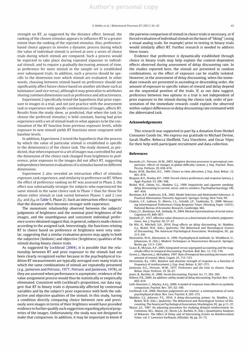
In a procedure where subjects choose the brightest image frompairs of exhaustive image combinations, the number of times animage is chosen provides a good estimate of an image’s relative

R2 = 0.71

0

2

4

6

8

10

12

100806040200

Mean % Pixel Brightness

Bri

gh

tness E

sti

mate

Ran

k

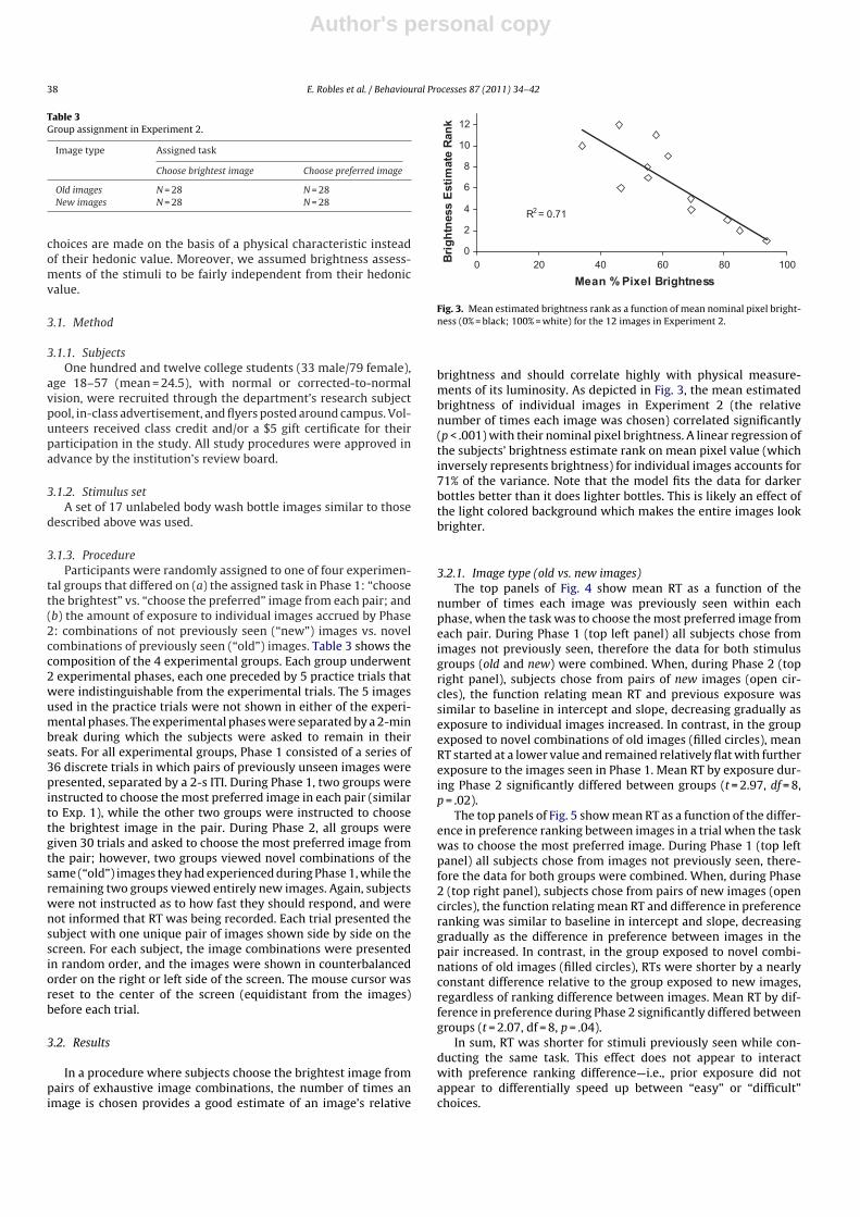
Fig. 3. Mean estimated brightness rank as a function of mean nominal pixel bright-ness (0% = black; 100% = white) for the 12 images in Experiment 2.

brightness and should correlate highly with physical measure-ments of its luminosity. As depicted in Fig. 3, the mean estimatedbrightness of individual images in Experiment 2 (the relativenumber of times each image was chosen) correlated significantly(p < .001) with their nominal pixel brightness. A linear regression ofthe subjects’ brightness estimate rank on mean pixel value (whichinversely represents brightness) for individual images accounts for71% of the variance. Note that the model fits the data for darkerbottles better than it does lighter bottles. This is likely an effect ofthe light colored background which makes the entire images lookbrighter.

3.2.1. Image type (old vs. new images)The top panels of Fig. 4 show mean RT as a function of the

number of times each image was previously seen within eachphase, when the task was to choose the most preferred image fromeach pair. During Phase 1 (top left panel) all subjects chose fromimages not previously seen, therefore the data for both stimulusgroups (old and new) were combined. When, during Phase 2 (topright panel), subjects chose from pairs of new images (open cir-cles), the function relating mean RT and previous exposure wassimilar to baseline in intercept and slope, decreasing gradually asexposure to individual images increased. In contrast, in the groupexposed to novel combinations of old images (filled circles), meanRT started at a lower value and remained relatively flat with furtherexposure to the images seen in Phase 1. Mean RT by exposure dur-ing Phase 2 significantly differed between groups (t = 2.97, df = 8,p = .02).

The top panels of Fig. 5 show mean RT as a function of the differ-ence in preference ranking between images in a trial when the taskwas to choose the most preferred image. During Phase 1 (top leftpanel) all subjects chose from images not previously seen, there-fore the data for both groups were combined. When, during Phase2 (top right panel), subjects chose from pairs of new images (opencircles), the function relating mean RT and difference in preferenceranking was similar to baseline in intercept and slope, decreasinggradually as the difference in preference between images in thepair increased. In contrast, in the group exposed to novel combi-nations of old images (filled circles), RTs were shorter by a nearlyconstant difference relative to the group exposed to new images,regardless of ranking difference between images. Mean RT by dif-ference in preference during Phase 2 significantly differed betweengroups (t = 2.07, df = 8, p = .04).

In sum, RT was shorter for stimuli previously seen while con-ducting the same task. This effect does not appear to interactwith preference ranking difference—i.e., prior exposure did notappear to differentially speed up between “easy” or “difficult”choices.



Fig. 4. Logged RT as a function of prior exposure to individual stimuli in Phases 1and 2 (left and right sides of graph, respectively). Filled circles signify stimuli seenin Phase 1 (Old); open circles signify stimuli not previously seen (New). Assignedtasks are identified as “Brightest” and “Preferred”. Continuous lines are predictionsof Eq. (2) using parameters of Table 4.

3.2.2. Assigned task (brightest vs. preferred images)The bottom panels of Fig. 4 show mean RT as a function of the

number of times each image was previously seen within the sameexperimental phase. During baseline (bottom left panel), all sub-jects chose the brightest image from pairs of new images, thereforethe data for both stimulus groups (old and new) were combined.During Phase 2 (bottom right panel), both groups of subjects wereasked to choose the most preferred image, but one group chosefrom new images while the other chose from images seen in Phase1. For both groups, the function relating mean RT and previousexposure was similar to baseline, decreasing gradually as exposureincreased. Mean RT by exposure during Phase 2 did not significantlydiffer between groups (t = .35, df = 8, p = .37). In sum, previous stim-ulus exposure did not appear to affect choice RT when a new taskwas introduced.

The bottom panels of Fig. 5 show mean RT as a function of dif-ference in ranking between each pair of images. During baseline(bottom left panel), all subjects chose the brightest image frompairs of new images, therefore the data for both groups were com-bined. During Phase 2 (bottom right panel), both groups of subjectswere asked to choose the most preferred image, but one groupchose from new images while the other chose from images seenin Phase 1. For both groups, the function relating mean RT and dif-ference in preference was similar to baseline, decreasing graduallyas the difference in stimulus ranking increased. Previous stimulusexposure did not appear to affect choice RT as a function of rela-tive preference when participants had not evaluated the stimuli in

Fig. 5. Logged RT as a function of relative choice ranking of individual stimuli in atrial within each phase, in Phases 1 and 2 (left and right sides of graph, respectively).Filled circles signify stimuli seen in Phase 1 (Old); open circles signify stimuli notpreviously seen (New). Assigned tasks are identified as “Brightest” and “Preferred”.Continuous lines are predictions of Eq. (2) using parameters of Table 4. The gray areaat the bottom of each panel is the relative frequency of trials in which the absolutedifference in stimulus ranking was x.

terms of preference. Mean RT by exposure during Phase 2 did notsignificantly differ between groups (t = .06, df = 8, p = .48). In sum,having had previous exposure to images did not affect RT when theprevious exposure involved a different task (i.e., “choose the bright-est image”). These results are in sharp contrast with the effect thatprior stimulus exposure in the same task had on RT.

3.2.3. Changes in parameters of the RT choice modelTo determine the source of variance in RT between experimen-

tal groups, we first estimated the parameters of Eq. (3) separatelyfor each of 6 experimental conditions, which were constitutedby 2 assigned tasks in Phase 1 (preference vs. brightness), and 4groups in Phase 2 (see Table 3). This specific model was calledunconstrained. The unconstrained model has 30 free parameters,5 (RTmax, RTmin, ˇE, ˇPC, ˇPR) for each of 6 experimental conditions.We then constrained the model by setting all parameters constantacross selected conditions. The purpose of these constraints was totest 4 “null” hypotheses regarding performance in Phase 2; thesehypotheses are listed in Table 4, along with the correspondingmodel constraints. Thus, for instance, to test whether performancein Phase 2 with stimuli experienced in Phase 1 was sensitive (ornot) to the choice task implemented in Phase 1, we set the param-eters of Eq. (3) to be the same for the Old Brightest group and theOld Preferred group in Phase 2.

More constrained models implied fewer free parameters butalso less variance accounted for. The merit of each specific modelwas established by balancing parsimony (fewer free parameters)against accuracy (more variance accounted for), based on theAkaike Information Criterion (AIC; Burnham & Anderson, 2002).



Table 4Hypotheses tested in Phase 2 of Experiment 2.

Hypothesis Model constraint �AICa

Performance with old stimulus was not sensitive to Phase 1 task Old Brightest = Old Preferred 42.54Performance with new stimulus was not sensitive to Phase 1 task New Brightest = New Preferred −3.45Performance with old and new stimulus was the same if Phase 1 task was Brightest Old Brightest = New Brightest −6.03Performance with old and new stimulus was the same if Phase 1 task was Preferred Old Preferred = New Preferred 92.16

Note: Model constraint column indicates the set of parameters that were forced to be equal.a �AIC ≤ 4 indicates support for hypothesis.

AIC was computed as

AIC = 2k + n ln(RSS), (4)

where k was the number of free parameters (30 for the uncon-strained model, 25 for each constrained model), n the number ofobservations (i.e., trials fitted by the model), and RSS the residualsum of squared deviations of optimized model predictions rela-tive to data. To test each hypothesis, we compared the AIC of theunconstrained model against the AIC of the constrained model cor-responding to the hypothesis. The unconstrained model had tobe at least 4 AIC units below the constrained model to supportrejecting the corresponding hypothesis in Table 4. This criterionis a standard suggested by Burnham and Anderson (2002), whichfavors the selection of the simpler, constrained model over themore complex, unconstrained one (a model that is 4 units loweris 7.4 times more likely). �AIC was computed for each comparison,where �AIC = AICconstrained − AICunconstrained. A �AIC > 4 supportedthe unconstrained model and rejected the corresponding hypoth-esis in Table 4.

�AIC in Table 4 supported two hypotheses: performance withnew stimuli in Phase 2 was not sensitive to Phase 1 task, and perfor-mance with old and new stimuli was the same in Phase 2 if the taskin Phase 1 was choosing the brightest. These results suggest thatchange in stimuli, in task, or in both had similar effects on choice RT.We thus tested a fifth model, one in which Eq. (3) parameters wereequal among the New Preferred, Old Brightest, and New Brightestgroups, and different from the Old Preferred group. For this model,the number of free parameters k = 20, and the �AIC was −6.94,even lower than for any model considered in Table 1. The low �AICsupported the new model, which we identify as highly constrained.

Estimates of the highly constrained model parameters areshown in Table 5. Two patterns are noticeable in these numbers.First, Old-Preferred parameters have extreme values: the shortestRTmax, the longest RTmin, the smallest ˇE and the most extremeˇPC and ˇPR. These estimates suggest that there was less variability(RTmax − RTmin) in RTs to previously seen stimuli in an already expe-rienced preference task. It also suggests that such small variancein RT was mostly driven by the difference in preference ranking,not by the amount of exposure to stimuli. The second noticeablepattern is a replication of a finding from Experiment 1: regardlessof experimental condition ˇPC was larger than the absolute valueof ˇPR, suggesting that RT depends more on how many times thechosen rather than the rejected stimulus was chosen in previoustrials.

Predicted mean logged RTs based on Table 2 estimates, alongwith the observed mean log RTs, are shown in Figs. 4 and 5. Thedecline in RT as a function of stimulus exposure during Phase 1(left panels of Fig. 4) was very similar regardless of whether par-ticipants were choosing on the basis of preference or on the basisof brightness. At the beginning of Phase 2 (right panels of Fig. 4),RT recovered to levels similar to those at the beginning of Phase 1,except when the same stimuli were shown and the same task wasassigned as in Phase 1. The model faithfully tracked these trends inRT.

Fig. 5 shows the predicted and obtained mean log RT as a func-tion of difference in choice ranking (PC–PR). As this differenceincreased, RTs became shorter in both experimental phases, regard-less of whether choice was based on preference or brightness, if itinvolved previously seen or novel stimuli, or if it was a previouslytrained or a novel choice task. The “savings” in RT due to prior expe-rience with stimuli and task are also visible here (top vs. bottomright panels of Fig. 5).

4. Discussion

This research investigated the dynamic variations in RT thatoccur between binary choice trials during the estimation ofpreference-based value. We found evidence that such value esti-mations are possible even when the choice is between goodsnot normally associated with strong preferences—like drugs andmoney—or do not have clear survival value. Participants in thisstudy, for example, reported strong and consistent preferencesbetween images of plastic bottles.

The measurement of preference in binary trials, however,appears to involve processes beyond the act of choosing one stim-ulus over another, as systematic changes in RT occur that cannotbe fully accounted for by the amount of practice with the valueassessment task. Results from Experiment 1 clearly show that RTdecreases with more prior exposure to individual stimuli, and thatit increases as relative preference for the stimuli in a given trialdecreases. In support of this, we propose a regression model thatefficiently predicted trial RT as a function of stimulus exposure andrelative preference.

This study extended our understanding of the distance effect(the variations in RT associated with relative preference for thetwo stimuli) in two directions. First, parameter estimates from theregression model suggest that preference ranking of the chosenand rejected items do not simply have opposite effects of similar

Table 5Estimates of highly constrained model parameters in Experiment 2.

Parameter Phase 1 Phase 2

Brightest Preferred Old Preferred New or Brightest

RTmax 3.45 s 3.19 s 2.53 s 2.80 sRTmin 0.43 s 0.40 s 1.07 s 0.40 sˇE 5.47 × 10−2 6.53 × 10−2 4.69 × 10−2 5.45 × 10−2

ˇPC 17.59 × 10−2 11.44 × 10−2 56.63 × 10−2 16.21 × 10−2

ˇPR −8.59 × 10−2 −7.20 × 10−2 −30.61 × 10−2 −9.81 × 10−2



strength on RT, as suggested by the distance effect. Instead, theranking of the chosen stimulus appears to influence RT to a greaterextent than the ranking of the rejected stimulus. Also, preference-based choice appears to involve a dynamic process during whichthe value of individual stimuli is arrived at over a series of choicetrials during which stimuli are compared. Such a process wouldbe expected to take place during repeated exposure to individ-ual stimuli, and to require a gradually decreasing amount of time,as preference for more stimuli in the sample set is establishedover subsequent trials. In addition, such a process should be spe-cific to the dimension over which stimuli are evaluated. In otherwords, choosing between stimuli based on preference should notsignificantly affect future choice based on another attribute such asluminance (and vice versa), although it may generalize to attributessharing common dimensions such as preference and attractiveness.

Experiment 2 specifically tested the hypothesis that prior expo-sure to images in a trial, and not just practice with the assessmenttask or experience with specific combinations of images, affects RT.Results from the study show, as predicted, that when the task (tochoose the preferred stimulus) is held constant, having had priorexperience with a set of stimuli leads to what appears to be the con-tinuation of the RT function from previous exposure levels, whileexposure to new stimuli yields RT functions more congruent withbaseline levels.

In addition, Experiment 2 tested the hypothesis that the processby which the value of particular stimuli is established is specificto the dimension(s) of the choice task. The study showed, as pre-dicted, that when exposure to a set of images was controlled for andthe dimension of the choice task changed from brightness to pref-erence, prior exposure to the images did not affect RT, suggestingindependence between evaluations of a stimulus based on differentdimensions.

Experiment 2 also revealed an interaction effect of stimulusexposure, task experience, and similarity in preference on RT. Whenthe effect of preference ranking on RT was assessed in Phase 2, theeffect was substantially stronger for subjects who experienced thesame stimuli in the same choice task in Phase 1 than for those forwhom either stimuli or task varied between Phases 1 and 2 (seeˇPC and ˇPR in Table 5, Phase 2). Such an interaction effect suggeststhat the distance effect becomes stronger with experience.

The monotonic relationship observed between the subjects’judgments of brightness and the nominal pixel brightness of theimages, and the unambiguous and consistent individual prefer-ence scores obtained suggest that, in general, subjects made choicesaccording to the assigned task. Interestingly, the functions relatingRT to choice based on preference or brightness were very simi-lar, suggesting that a similar evaluation process may apply to boththe subjective (hedonic) and objective (brightness) qualities of thestimuli during binary choice trials.

As suggested by Lockhead (2004), it is possible that the rela-tionship between RT and prior exposure to the stimuli had notbeen clearly recognized earlier because in the psychophysical tra-dition RT measurements are typically averaged over many trials inwhich the same combinations of stimuli are repeatedly presented(e.g., Jamieson and Petrusic, 1977; Petrusic and Jamieson, 1978), orthey are assessed when performance is asymptotic; evidence of thevalue assignment process would thus be statistically or empiricallyeliminated. Consistent with Lockhead’s proposition, our data sug-gest that RT in binary trials is dynamically affected by contextualvariables and by the subject’s prior experience with both the sub-jective and objective qualities of the stimuli. In this study, havinga condition directly comparing choice between new and previ-ously seen images in terms of their brightness would have providedevidence to further qualify such suggestion regarding physical prop-erties of the images. Unfortunately, the study was not designed tomake that comparison. In addition, it may be important to know if

the pairwise comparison of stimuli in choice trials is necessary, or ifforced evaluation of individual stimuli on the basis of “liking” (usinga visual analog scale, for example) prior to testing in binary trialswould similarly affect RT. Further research is needed to addressthese issues.

Evidence that preference is dynamically established throughchoice in binary trials may help explain the context-dependenteffects observed during assessment of delay discounting rate. Inthe studies reported here, the stimuli are presented in randomcombinations, so the effect of exposure can be readily isolated.However, in the assessment of delay discounting, when the imme-diate rewards are presented in ascending or descending order, theamount of exposure to specific values of reward and delay dependon the sequential position of the trials. If, as our data suggest,preference between two options in a trial is not independent ofprior exposure to the stimuli during the choice task, order of pre-sentation of the immediate rewards could explain the observedwithin-subject differences in delay discounting rate estimated withthe abbreviated task.

Acknowledgements

This research was supported in part by a donation from HenkelConsumer Goods Inc. We express our gratitude to Michael Devine,Sarah Shaffer, Rebecca Sheffield, Tara Vincelette, and Oscar Yépizfor their help with participant recruitment and data collection.

References

Baranski, J.V., Petrusic, W.M., 2003. Adaptive decision processes in perceptual com-parisons: effects of changes in global difficulty context. J. Exp. Psychol. Hum.Percep. Perform. 29, 658–674.

Baum, W.M., Rachlin, H.C., 1969. Choice as time allocation. J. Exp. Anal. Behav. 12,861–874.

Bergum, B.O., Dooley, R.P., 1969. Forced-choice preferences and response latency. J.Appl. Psychol. 53, 396–398.

Bickel, W.K., Odum, A.L., Madden, G.J., 1999. Impulsivity and cigarette smoking:delay discounting in current, never, and ex-smokers. Psychopharmacology 146,447–454.

Burnham, K.P., Anderson, D.R., 2002. Model Selection and Multimodel Inference: APractical Information-Theoretic Approach. Springer-Verlag, New York, NY.

Chabris, C.F., Laibson, D., Morris, C.L., Schuldt, J.P., Taubinsky, D., 2008. Measur-ing Intertemporal Preferences Using Response Times (Working Paper 14353).National Bureau of Economic Research, Cambridge, MA.

Chiao, J.Y., Bordeaux, A.R., Ambady, N., 2004. Mental representations of social status.Cognition 93, B49–B57.

Dashiell, J.F., 1937. Affective value-distances as a determinant of esthetic judgment-times. Am. J. Psychol. 50, 57–67.

De Wit, H., Mitchell, S.H., 2010. Drug effects on delay discounting. In: Madden,G.J., Bickel, W.K. (Eds.), Ipulsivity: The Behavioral and Neurological Scienceof Discounting. The American Psychological Association, Washington, DC, pp.213–241.

Ehrenstein, W.H., Ehrenstein, A., 1999. Psychophysical methods. In: Windhorst, U.,Johansson, H. (Eds.), Modern Techniques in Neuroscience Research. Springer,Berlin, pp. 1211–1241.

Grace, R., McLean, A.P., 2005. Integrated versus segregated accounting and the mag-nitude effect in temporal discounting. Psychon. Bull. Rev. 12, 732–739.

Green, L., Myerson, J., McFadden, 1997. Rate of temporal discounting decreases withamount of reward. Mem. Cognit. 25, 715–723.

Herrnstein, R.J., 1961. Relative and absolute strength of response as a function offrequency of reinforcement. J. Exp. Anal. Behav. 4, 267–272.

Jamieson, D.G., Petrusic, W.M., 1977. Preference and the time to choose. Organ.Behav. Hum. Perform. 19, 56–67.

Jones, B., Rachlin, H., 2006. Social discounting. Psychol. Sci. 17, 283–285.Killeen, P.R., 2009. An additive-utility model of delay discounting. Psychol. Rev. 116,

602–619.Leth-Steensen, C., Marley, A.A.J., 2000. A model of response time effects in symbolic

comparison. Psychol. Rev. 107, 62–100.Lockhead, G.R., 2004. Absolute judgements are relative: a reinterpretation of some

psychophysical ideas. Rev. Gen. Psychol. 8, 265–272.Madden, G.J., Johnson, P.S., 2010. A delay-discounting primer. In: Madden, G.J.,

Bickel, W.K. (Eds.), Ipulsivity: The Behavioral and Neurological Science of Dis-counting. The American Psychological Association, Washington, DC, pp. p.11–37.

Mazur, J.E., 1987. An adjusting procedure for studying delayed reinforcement. In:Commons, M.L., Mazur, J.E., Nevin, J.A., Rachlin, H. (Eds.), Quantitative Analysesof Behavior. The Effect of Delay and of Intervening Events on ReinforcementValue. vol. 5. Lawrence Earlbaum, Hillsdale, NJ, pp. 55–73.



McKerchar, T.L., Green, L., Myerson, J., Pickford, T.S., Hill, J.C., Stout, S.C., 2009. Acomparison of four models of delay discounting in humans. Behav. Process. 81,256–259.

Myerson, J., Green, L., Warusawitharana, M., 2001. Area under the curve as a measureof discounting. J. Exp. Anal. Behav. 76, 235–243.

Padoa-Schioppa, C., Jandolo, L., Visalberghi, E., 2006. Multi-stage mental process foreconomic choice in capuchins. Cognition 99, B1–B13.

Petrusic, W.M., Jamieson, D.G., 1978. Relation between probability of preferentialchoice and time to choose changes with practice. J. Exp. Psychol. Hum. Percep.Perform. 4, 471–482.

Rachlin, H., Green, L., 1972. Commitment, choice and self-control. J. Exp. Anal. Behav.17, 15–22.

Rachlin, H., Rainieri, A., Cross, D., 1991. Subjective probability and delay. J. Exp. Anal.Behav. 55, 233–244.

Reynolds, B., 2006. A review of delay-discounting research with humans: relationsto drug use and gambling. Behav. Pharmacol. 17, 651–667.

Robles, E., Vargas, P.A., 2007. Parameters of delay discounting assessment tasks:order of presentation. Behav. Process. 75, 237–241.

Robles, E., Vargas, P.A., Bejarano, R., 2009. Within-subject differences in degree ofdelay discounting as a function of order of presentation of hypothetical cashrewards. Behav. Process. 81, 260–263.

Schmidt, K.E., Liu, Y., 2006. The effects of aesthetic attributes on response time andaesthetic judgement in a multiattribute binary choice task. In: Proceedings ofthe Human Factors and Ergonomics Society , pp. 1701–1705.

Scholten, M., Read, D., 2010. The psychology of intertemporal tradeoffs. Psychol. Rev.117, 925–944.

Smith, E.E., 1968. Choice reaction time: an analysis of the major theoretical positions.Psychol. Bull. 69, 77–110.

Tyebjee, T.T., 1979. A new measure for scaling brand preference. J. Market. Res. 16,96–101.

Yi, R., Gatchalian, K.M., Bickel, W.K., 2006. Discounting of past outcomes. Exp. Clin.Psychopharmacol. 14 (3), 311–317.

Dynamics of choice during estimation of subjective value

Documents

Transcript of Dynamics of choice during estimation of subjective value