rsif.royalsocietypublishing.org

ResearchCite this article: Bates AJ, Doorly DJ, Cetto R,Calmet H, Gambaruto AM, Tolley NS, HouzeauxG, Schroter RC. 2015 Dynamics of airflow in ashort inhalation. J. R. Soc. Interface 12:20140880.http://dx.doi.org/10.1098/rsif.2014.0880

Received: 7 August 2014Accepted: 29 October 2014

Subject Areas:bioengineering, biomedical engineering,biomechanics

Keywords:inspiratory flow, respiratory tract, airways,CFD, internal flow, transitional flow

Author for correspondence:A. J. Batese-mail: a.bates11@imperial.ac.uk

Electronic supplementary material is availableat http://dx.doi.org/10.1098/rsif.2014.0880 orvia http://rsif.royalsocietypublishing.org.

Dynamics of airflow in a short inhalationA. J. Bates1, D. J. Doorly1, R. Cetto1,3, H. Calmet4, A. M. Gambaruto4,N. S. Tolley3, G. Houzeaux4 and R. C. Schroter2

1Department of Aeronautics, and 2Department of Bioengineering, Imperial College London,London SW7 2AZ, UK3Department of Otolaryngology, St Mary’s Hospital, Imperial College Healthcare Trust, London W2 1NY, UK4Computer Applications in Science and Engineering, Barcelona Supercomputing Center (BSC-CNS),Barcelona 08034, Spain

AJB, 0000-0002-8855-3448; DJD, 0000-0002-5372-4702; RC, 0000-0002-7681-7442;GH, 0000-0002-2592-1426

During a rapid inhalation, such as a sniff, the flow in the airways accelerates anddecays quickly. The consequences for flow development and convective trans-port of an inhaled gas were investigated in a subject geometry extending fromthe nose to the bronchi. The progress of flow transition and the advance of aninhaled non-absorbed gas were determined using highly resolved simulationsof a sniff 0.5 s long, 1 l s21 peak flow, 364 ml inhaled volume. In the nose, thedistribution of airflow evolved through three phases: (i) an initial transient ofabout 50 ms, roughly the filling time for a nasal volume, (ii) quasi-equilibriumover the majority of the inhalation, and (iii) a terminating phase. Flow transitioncommenced in the supraglottic region within 20 ms, resulting in large-amplitude fluctuations persisting throughout the inhalation; in the nose,fluctuations that arose nearer peak flow were of much reduced intensity anddiminished in the flow decay phase. Measures of gas concentration showednon-uniform build-up and wash-out of the inhaled gas in the nose. At thecarina, the form of the temporal concentration profile reflected both sheardispersion and airway filling defects owing to recirculation regions.

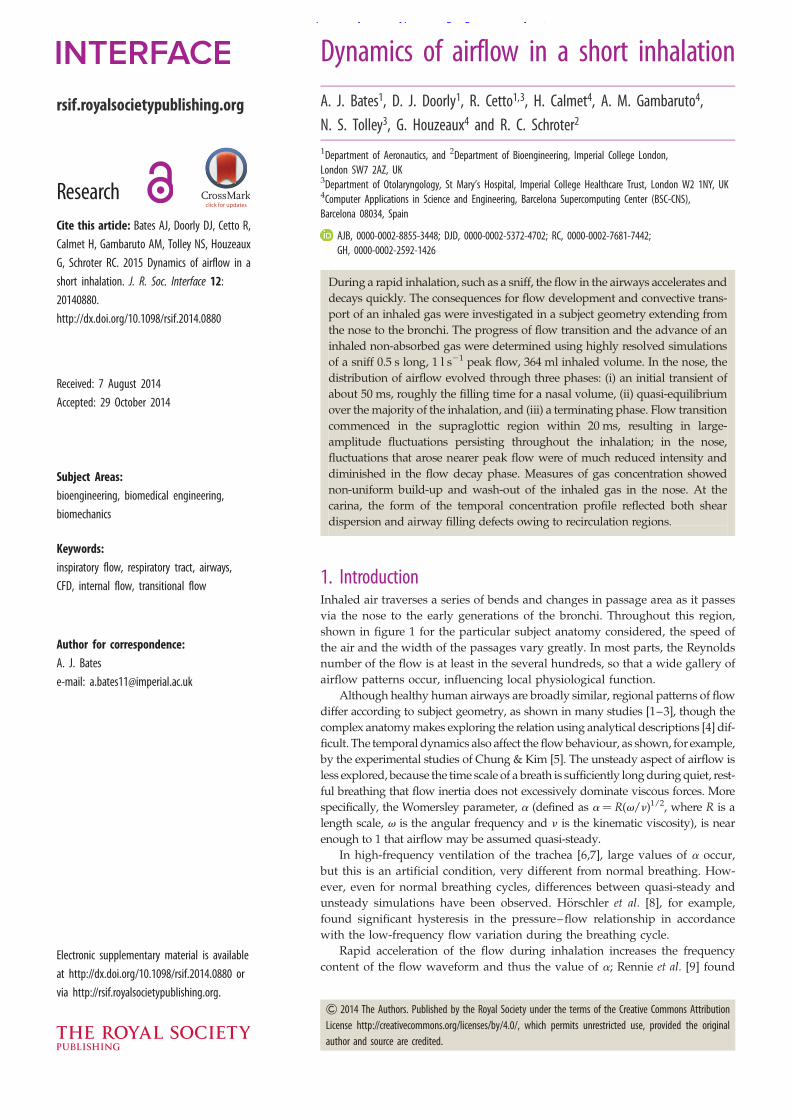
1. IntroductionInhaled air traverses a series of bends and changes in passage area as it passesvia the nose to the early generations of the bronchi. Throughout this region,shown in figure 1 for the particular subject anatomy considered, the speed ofthe air and the width of the passages vary greatly. In most parts, the Reynoldsnumber of the flow is at least in the several hundreds, so that a wide gallery ofairflow patterns occur, influencing local physiological function.

Although healthy human airways are broadly similar, regional patterns of flowdiffer according to subject geometry, as shown in many studies [1–3], though thecomplex anatomy makes exploring the relation using analytical descriptions [4] dif-ficult. The temporal dynamics also affect the flow behaviour, as shown, for example,by the experimental studies of Chung & Kim [5]. The unsteady aspect of airflow isless explored, because the time scale of a breath is sufficiently long during quiet, rest-ful breathing that flow inertia does not excessively dominate viscous forces. Morespecifically, the Womersley parameter, a (defined as a ¼ R(v/n)1/2, where R is alength scale, v is the angular frequency and n is the kinematic viscosity), is nearenough to 1 that airflow may be assumed quasi-steady.

In high-frequency ventilation of the trachea [6,7], large values of a occur,but this is an artificial condition, very different from normal breathing. How-ever, even for normal breathing cycles, differences between quasi-steady andunsteady simulations have been observed. Horschler et al. [8], for example,found significant hysteresis in the pressure–flow relationship in accordancewith the low-frequency flow variation during the breathing cycle.

Rapid acceleration of the flow during inhalation increases the frequencycontent of the flow waveform and thus the value of a; Rennie et al. [9] found

& 2014 The Authors. Published by the Royal Society under the terms of the Creative Commons AttributionLicense http://creativecommons.org/licenses/by/4.0/, which permits unrestricted use, provided the originalauthor and source are credited.

on January 21, 2015http://rsif.royalsocietypublishing.org/Downloaded from

the time taken for flow to build up to a level equivalent tothat in restful breathing was 130 ms on average in normalinspiration. This reduced to 90 ms in sniffing, and was asshort as 20 ms in a rapid inhalation.

Air flow in a rapid inhalation is of physiological interestto understand sniffing for olfaction or during manoeuvrescommonly recommended when taking aerosol medication.It also reveals the time scales over which flow responds.

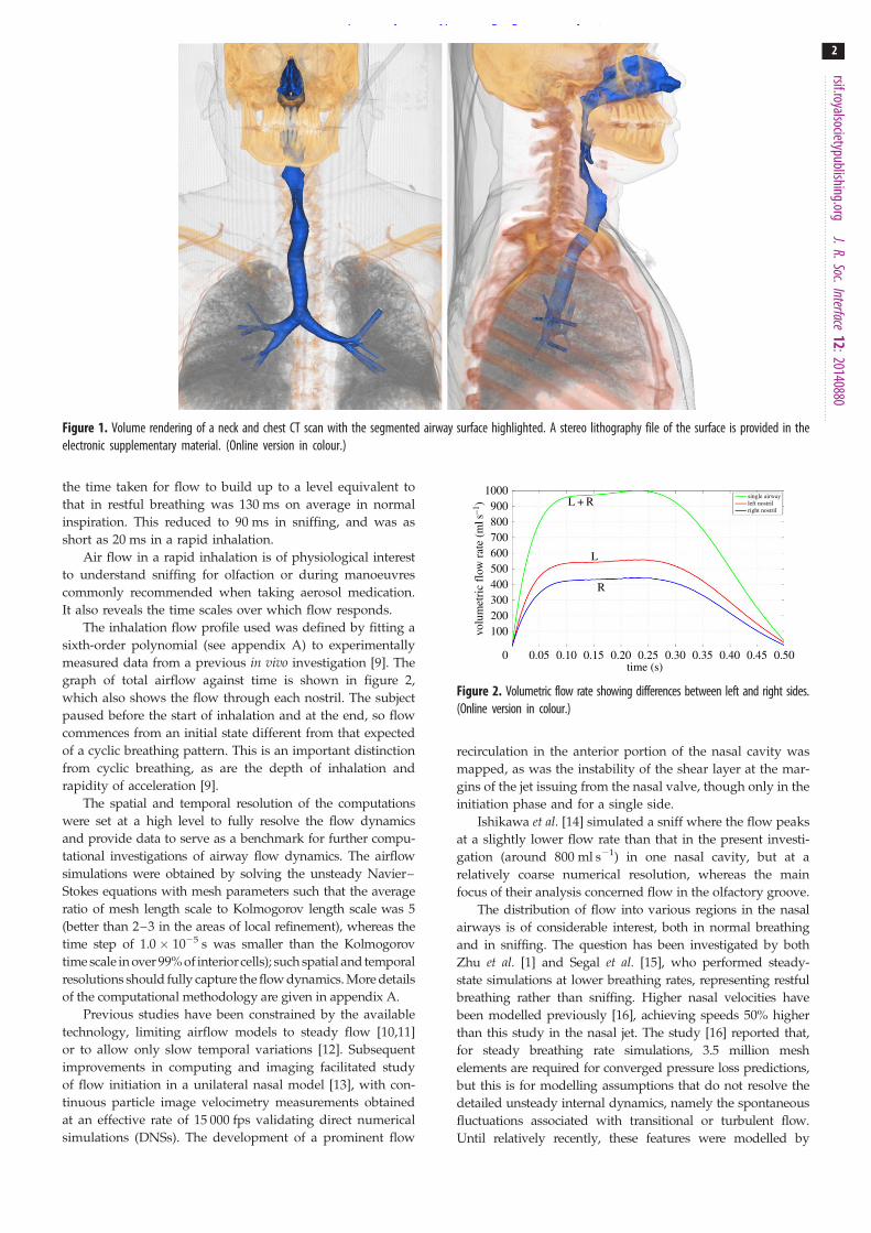
The inhalation flow profile used was defined by fitting asixth-order polynomial (see appendix A) to experimentallymeasured data from a previous in vivo investigation [9]. Thegraph of total airflow against time is shown in figure 2,which also shows the flow through each nostril. The subjectpaused before the start of inhalation and at the end, so flowcommences from an initial state different from that expectedof a cyclic breathing pattern. This is an important distinctionfrom cyclic breathing, as are the depth of inhalation andrapidity of acceleration [9].

The spatial and temporal resolution of the computationswere set at a high level to fully resolve the flow dynamicsand provide data to serve as a benchmark for further compu-tational investigations of airway flow dynamics. The airflowsimulations were obtained by solving the unsteady Navier–Stokes equations with mesh parameters such that the averageratio of mesh length scale to Kolmogorov length scale was 5(better than 2–3 in the areas of local refinement), whereas thetime step of 1.0 ! 1025 s was smaller than the Kolmogorovtime scale in over 99% of interiorcells); such spatial and temporalresolutions should fully capture the flow dynamics. More detailsof the computational methodology are given in appendix A.

Previous studies have been constrained by the availabletechnology, limiting airflow models to steady flow [10,11]or to allow only slow temporal variations [12]. Subsequentimprovements in computing and imaging facilitated studyof flow initiation in a unilateral nasal model [13], with con-tinuous particle image velocimetry measurements obtainedat an effective rate of 15 000 fps validating direct numericalsimulations (DNSs). The development of a prominent flow

recirculation in the anterior portion of the nasal cavity wasmapped, as was the instability of the shear layer at the mar-gins of the jet issuing from the nasal valve, though only in theinitiation phase and for a single side.

Ishikawa et al. [14] simulated a sniff where the flow peaksat a slightly lower flow rate than that in the present investi-gation (around 800 ml s21) in one nasal cavity, but at arelatively coarse numerical resolution, whereas the mainfocus of their analysis concerned flow in the olfactory groove.

The distribution of flow into various regions in the nasalairways is of considerable interest, both in normal breathingand in sniffing. The question has been investigated by bothZhu et al. [1] and Segal et al. [15], who performed steady-state simulations at lower breathing rates, representing restfulbreathing rather than sniffing. Higher nasal velocities havebeen modelled previously [16], achieving speeds 50% higherthan this study in the nasal jet. The study [16] reported that,for steady breathing rate simulations, 3.5 million meshelements are required for converged pressure loss predictions,but this is for modelling assumptions that do not resolve thedetailed unsteady internal dynamics, namely the spontaneousfluctuations associated with transitional or turbulent flow.Until relatively recently, these features were modelled by

Figure 1. Volume rendering of a neck and chest CT scan with the segmented airway surface highlighted. A stereo lithography file of the surface is provided in theelectronic supplementary material. (Online version in colour.)

1000900800700600500400300200100

0 0.05 0.10 0.15 0.20 0.25 0.30 0.35 0.40 0.45 0.50

single airwayleft nostrilright nostril

volu

met

ric

flow

rate

(mls

–1)

L

R

L + R

time (s)

Figure 2. Volumetric flow rate showing differences between left and right sides.(Online version in colour.)

rsif.royalsocietypublishing.orgJ.R.Soc.Interface

12:201408802

on January 21, 2015http://rsif.royalsocietypublishing.org/Downloaded from

Reynolds averaged Navier–Stokes approaches. For example,Ghahramani et al. [17] investigated turbulent intensities andtheir effect on particle deposition in an extensive airway modelranging from the nostrils to above the carina at flow ratescomparable to the peak flow rates used in this study. Furtherstudies [18,19] of particle deposition reported four millioncells as necessary for mesh independent results. However,small-scale fluctuations would not be sufficiently resolvedat this refinement level, nor are the effects of accelerating anddecelerating flows covered in steady simulations.

Zhao et al. [20] compared models of sniffing using lami-nar simulations and k 2 v and Spalart–Allmaras turbulencemodels and found little difference in particulate absorptionbetween the models.

The dynamics of spontaneous flow instability were inves-tigated by Lin et al. [2], who reported simulations of a realisticoral geometry. Large-scale flow features were resolved,whereas a comparison between an under-resolved DNSand a large eddy simulation turbulence model was foundto have a relative L1 norm (sum of absolute differences in avolume as a percentage of the total) of turbulent kineticenergy (TKE) of 13.6%. This highlights the need forsimulations at higher resolutions to serve as reference studies.

Zhang & Kleinstreuer [21] and Pollard et al. [22] investi-gated the flow in a highly idealized oral airway model. Theformer study detailed the TKE at flow rates of 10 and30 l min21. High values of TKE were found in the regionbelow the epiglottis. Various computational models ofturbulence were compared with experimental results, withhigh-resolution simulations concluded as desirable.

2. Material and methods2.1. AnatomyThe airway geometry was derived from a neck and chest com-puted tomography (CT) image set of a 48-year-old man in thesupine position. Note that anatomical left and right are usedthroughout: figures labelled subject right are shown on the leftand vice versa. The images were enhanced with contrast andwere collected retrospectively from a hospital database. Thescan was requested for clinical reasons and reported to benormal. Consent from the patient for subsequent use of thedata was obtained. Further details of the subject, data acquisitionand translation to a virtual geometry are given in appendix A.

2.2. Geometry definition for simulationThe face was placed inside a hemisphere of radius 0.5 m and flowimposed uniformly on the curved outer surface of the hemisphere,allowing a natural inflow to develop. (The consequences of pre-scribed inflow at the nostril have been described previously[23,24].) The flat plane of the hemisphere was located approximately0.05 m behind the chin and treated as a rigid wall; limiting theexterior airspace has negligible effect as little inhaled air originatesbehind the head [23]. To provide a well-defined outlet, the finalbronchial branches were extruded into constant cross-sectionpipes for several diameters.

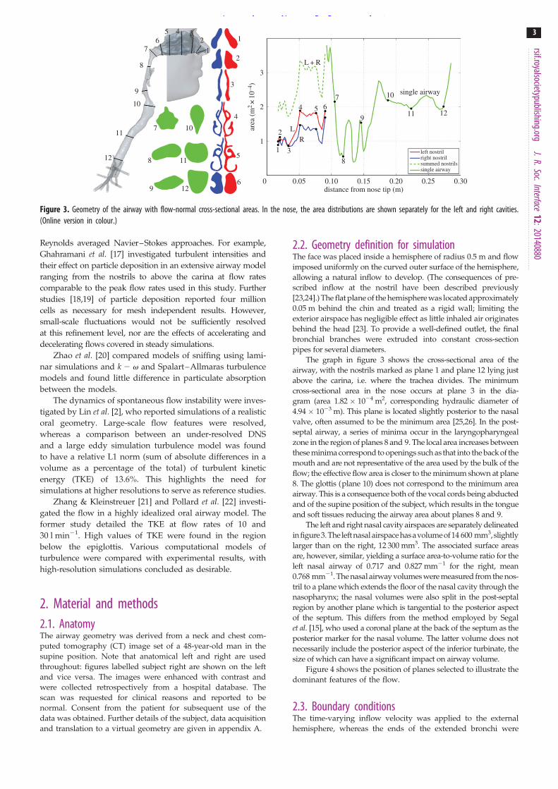
The graph in figure 3 shows the cross-sectional area of theairway, with the nostrils marked as plane 1 and plane 12 lying justabove the carina, i.e. where the trachea divides. The minimumcross-sectional area in the nose occurs at plane 3 in the dia-gram (area 1.82 ! 1024 m2, corresponding hydraulic diameter of4.94! 1023 m). This plane is located slightly posterior to the nasalvalve, often assumed to be the minimum area [25,26]. In the post-septal airway, a series of minima occur in the laryngopharyngealzone in the region of planes 8 and 9. The local area increases betweenthese minima correspond to openings such as that into the back of themouth and are not representative of the area used by the bulk of theflow; the effective flow area is closer to the minimum shown at plane8. The glottis (plane 10) does not correspond to the minimum areaairway. This is a consequence both of the vocal cords being abductedand of the supine position of the subject, which results in the tongueand soft tissues reducing the airway area about planes 8 and 9.

The left and right nasal cavity airspaces are separately delineatedin figure3.The left nasal airspace hasavolumeof 14 600 mm3,slightlylarger than on the right, 12 300 mm3. The associated surface areasare, however, similar, yielding a surface area-to-volume ratio for theleft nasal airway of 0.717 and 0.827 mm21 for the right, mean0.768 mm21. The nasal airway volumes were measured from the nos-tril to a plane which extends the floor of the nasal cavity through thenasopharynx; the nasal volumes were also split in the post-septalregion by another plane which is tangential to the posterior aspectof the septum. This differs from the method employed by Segalet al. [15], who used a coronal plane at the back of the septum as theposterior marker for the nasal volume. The latter volume does notnecessarily include the posterior aspect of the inferior turbinate, thesize of which can have a significant impact on airway volume.

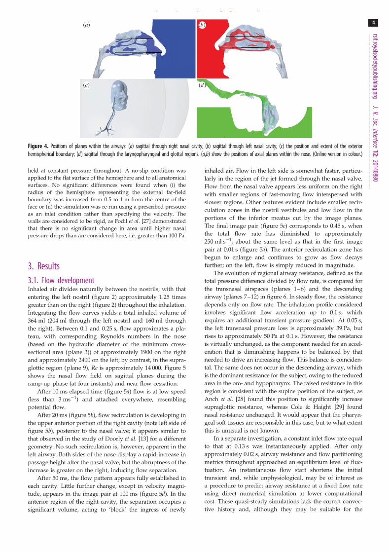
Figure 4 shows the position of planes selected to illustrate thedominant features of the flow.

2.3. Boundary conditionsThe time-varying inflow velocity was applied to the externalhemisphere, whereas the ends of the extended bronchi were

left nostrilright nostrilsummed nostrilssingle airway

area

(m2

×10

–4)

single airway

distance from nose tip (m)0.05 0.10 0.15 0.20 0.25 0.30

1

2

3

4

5

6

8

2

31

8

4 5 67

3

2

1

0

LR

9 11 12

10

L + R

9

10

11

12

7 10

8 11

9 12

76

5 4 32

1

Figure 3. Geometry of the airway with flow-normal cross-sectional areas. In the nose, the area distributions are shown separately for the left and right cavities.(Online version in colour.)

rsif.royalsocietypublishing.orgJ.R.Soc.Interface

12:201408803

on January 21, 2015http://rsif.royalsocietypublishing.org/Downloaded from

held at constant pressure throughout. A no-slip condition wasapplied to the flat surface of the hemisphere and to all anatomicalsurfaces. No significant differences were found when (i) theradius of the hemisphere representing the external far-fieldboundary was increased from 0.5 to 1 m from the centre of theface or (ii) the simulation was re-run using a prescribed pressureas an inlet condition rather than specifying the velocity. Thewalls are considered to be rigid, as Fodil et al. [27] demonstratedthat there is no significant change in area until higher nasalpressure drops than are considered here, i.e. greater than 100 Pa.

3. Results3.1. Flow developmentInhaled air divides naturally between the nostrils, with thatentering the left nostril (figure 2) approximately 1.25 timesgreater than on the right (figure 2) throughout the inhalation.Integrating the flow curves yields a total inhaled volume of364 ml (204 ml through the left nostril and 160 ml throughthe right). Between 0.1 and 0.25 s, flow approximates a pla-teau, with corresponding Reynolds numbers in the nose(based on the hydraulic diameter of the minimum cross-sectional area (plane 3)) of approximately 1900 on the rightand approximately 2400 on the left; by contrast, in the supra-glottic region (plane 9), Re is approximately 14 000. Figure 5shows the nasal flow field on sagittal planes during theramp-up phase (at four instants) and near flow cessation.

After 10 ms elapsed time (figure 5a) flow is at low speed(less than 3 ms21) and attached everywhere, resemblingpotential flow.

After 20 ms (figure 5b), flow recirculation is developing inthe upper anterior portion of the right cavity (note left side offigure 5b), posterior to the nasal valve; it appears similar tothat observed in the study of Doorly et al. [13] for a differentgeometry. No such recirculation is, however, apparent in theleft airway. Both sides of the nose display a rapid increase inpassage height after the nasal valve, but the abruptness of theincrease is greater on the right, inducing flow separation.

After 50 ms, the flow pattern appears fully established ineach cavity. Little further change, except in velocity magni-tude, appears in the image pair at 100 ms (figure 5d). In theanterior region of the right cavity, the separation occupies asignificant volume, acting to ‘block’ the ingress of newly

inhaled air. Flow in the left side is somewhat faster, particu-larly in the region of the jet formed through the nasal valve.Flow from the nasal valve appears less uniform on the rightwith smaller regions of fast-moving flow interspersed withslower regions. Other features evident include smaller recir-culation zones in the nostril vestibules and low flow in theportions of the inferior meatus cut by the image planes.The final image pair (figure 5e) corresponds to 0.45 s, whenthe total flow rate has diminished to approximately250 ml s21, about the same level as that in the first imagepair at 0.01 s (figure 5a). The anterior recirculation zone hasbegun to enlarge and continues to grow as flow decaysfurther; on the left, flow is simply reduced in magnitude.

The evolution of regional airway resistance, defined as thetotal pressure difference divided by flow rate, is compared forthe transnasal airspaces (planes 1–6) and the descendingairway (planes 7–12) in figure 6. In steady flow, the resistancedepends only on flow rate. The inhalation profile consideredinvolves significant flow acceleration up to 0.1 s, whichrequires an additional transient pressure gradient. At 0.05 s,the left transnasal pressure loss is approximately 39 Pa, butrises to approximately 50 Pa at 0.1 s. However, the resistanceis virtually unchanged, as the component needed for an accel-eration that is diminishing happens to be balanced by thatneeded to drive an increasing flow. This balance is coinciden-tal. The same does not occur in the descending airway, whichis the dominant resistance for the subject, owing to the reducedarea in the oro- and hypopharynx. The raised resistance in thisregion is consistent with the supine position of the subject, asAnch et al. [28] found this position to significantly increasesupraglottic resistance, whereas Cole & Haight [29] foundnasal resistance unchanged. It would appear that the pharyn-geal soft tissues are responsible in this case, but to what extentthis is unusual is not known.

In a separate investigation, a constant inlet flow rate equalto that at 0.13 s was instantaneously applied. After onlyapproximately 0.02 s, airway resistance and flow partitioningmetrics throughout approached an equilibrium level of fluc-tuation. An instantaneous flow start shortens the initialtransient and, while unphysiological, may be of interest asa procedure to predict airway resistance at a fixed flow rateusing direct numerical simulation at lower computationalcost. These quasi-steady simulations lack the correct convec-tive history and, although they may be suitable for the

(a) (b)

(c) (d )

Figure 4. Positions of planes within the airways: (a) sagittal through right nasal cavity; (b) sagittal through left nasal cavity; (c) the position and extent of the exteriorhemispherical boundary; (d ) sagittal through the laryngopharyngeal and glottal regions. (a,b) show the positions of axial planes within the nose. (Online version in colour.)

rsif.royalsocietypublishing.orgJ.R.Soc.Interface

12:201408804

on January 21, 2015http://rsif.royalsocietypublishing.org/Downloaded from

coarse measures above, may not be appropriate for measuressuch as scalar uptake or particle transport.

Returning to the sniff, spontaneous fluctuations associ-ated with turbulence develop earlier in the glottic regionthan in the nose, in line with the near order of magnitudegreater Reynolds number. This is evident in figure 7, wheresamples of velocity magnitude are compared for a point onplane 10 within the glottal region with those from a point

on the sagittal plane in the right nostril, halfway betweenplanes 2 and 3. In the nose, flow speed increases calmlyuntil 0.07 s (corresponding flow rate approx. 900 ml s21)then oscillations of relatively small amplitude appear; thesediminish as flow decays and are absent after 0.35 s (flowrate approx. 750 ml s21).

right nasal cavity(a)

(b)

(c)

(d )

(e)

left nasal cavity

0.01 s

0.02 s

0.05 s

0.10 s

0.45 s

0 2 4 6velocity: magnitude (m s–1)

8 10

Figure 5. (a – e) Velocity contours and planar streamlines on two planes in the right and left nasal cavities at succeeding instants.

0.5

0.4

0.3

0.2

0.1

0

–0.10 0.05 0.10 0.15 0.20 0.25 0.30 0.35 0.40 0.45 0.50

left 1–6right 1–6planes 7–12

right

left

planes 7–12

resi

stan

ce (P

asm

l–1)

time (s)

Figure 6. Comparison of transnasal and descending airway resistances.(Online version in colour.)

25

20

15

10

5

0

nose

glottis

point in glottispoint in nose

0.05 0.10 0.15 0.20 0.25time (s)

velo

city

mag

nitu

de (m

s–1)

0.30 0.35 0.40 0.45 0.50

Figure 7. Flow velocity signals at two points: lower curve—point in the rightnasal cavity towards the top of the intersection of the right sagittal plane (figure4) and plane 3 (figure 3); upper curve—point in the glottis at the intersectionof the sagittal plane (figure 4) and plane 10 (figure 3). (Online versionin colour.)

rsif.royalsocietypublishing.orgJ.R.Soc.Interface

12:201408805

on January 21, 2015http://rsif.royalsocietypublishing.org/Downloaded from

Flow in the laryngeal region becomes unsteady after 0.02 s,by which time the local mean airspeed reaches around 6 ms21.There the oscillations persist, merely reducing somewhattowards flow cessation.

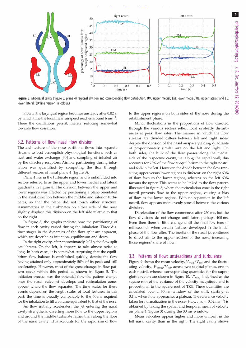
3.2. Patterns of flow: nasal flow divisionThe architecture of the nose partitions flows into separatestreams to best accomplish physiological functions such asheat and water exchange [30] and sampling of inhaled airby the olfactory receptors. Airflow partitioning during inha-lation was quantified by computing the flux throughdifferent sectors of nasal plane 4 (figure 3).

Plane 4 lies in the turbinate region and is subdivided intosectors referred to as the upper and lower medial and lateralquadrants in figure 8. The division between the upper andlower regions was affected by positioning a plane orientatedin the axial direction between the middle and inferior turbi-nates, so that the plane did not touch either structure.Asymmetries in the turbinates on either side of the noseslightly displace this division on the left side relative to thaton the right.

In figure 8, the graphs indicate how the partitioning offlow in each cavity varied during the inhalation. Three dis-tinct stages in the dynamics of the flow split are apparent,which we describe as initiation, equilibrium and decay.

In the right cavity, after approximately 0.03 s, the flow splitequilibrates. On the left, it appears to take almost twice aslong. In both cases, it is somewhat surprising that the equili-brium flow balance is established quickly, despite the flowhaving attained only approximately 50% of its peak and stillaccelerating. However, most of the gross changes in flow pat-tern occur within this period as shown in figure 5. Theinitiation process sees the potential flow-like pattern changeonce the nasal valve jet develops and recirculation zonesappear where the flow separates. The time scales for theseevents depend on the length scales of local features; in thispart, the time is broadly comparable to the 50 ms requiredfor the inhalation to fill a volume equivalent to that of the nose.

As flow initially accelerates, the jet entering the nasalcavity strengthens, diverting more flow to the upper regionsand around the middle turbinate rather than along the floorof the nasal cavity. This accounts for the rapid rise of flow

to the upper regions on both sides of the nose during theestablishment phase.

Minor fluctuations in the proportions of flow directedthrough the various sectors reflect local unsteady disturb-ances at peak flow rates. The manner in which the flowstreams are divided differs between left and right sides,despite the division of the nasal airspace yielding quadrantsof proportionately similar size on the left and right. Onboth sides, the bulk of the flow passes along the medialside of the respective cavity, i.e. along the septal wall; thisaccounts for 73% of the flow at equilibrium in the right nostriland 66% in the left. However, the divide between the flow tran-siting upper versus lower regions is different: on the right 60%of flow favours the lower regions, whereas on the left 60%favours the upper. This seems to be linked to the flow patternillustrated in figure 5, where the recirculation zone in the rightnostril prevents flow to the upper regions, causing a biasof flow to the lower regions. With no separation in the leftnostril, flow appears more evenly spread between the variousdivisions.

Deceleration of the flow commences after 250 ms, but theflow divisions do not change until later, perhaps 400 ms.Even then there is little change until the final few tens ofmilliseconds when certain features developed in the initialphase of the flow alter. The inertia of the nasal jet continuesto direct air to the upper reaches of the nose, increasingthose regions’ share of flow.

3.3. Patterns of flow: unsteadiness and turbulenceFigure 9 shows the mean velocity, Vmag/Vref, and the fluctu-ating velocity, V0mag/Vref, across two sagittal planes, one ineach nostril, whereas corresponding quantities for the supra-glottic region are shown in figure 10. V0mag is defined as thesquare root of the variance of the velocity magnitude and isproportional to the square root of TKE. These quantities arecalculated over a 30 ms window of the sniff, starting at0.1 s, when flow approaches a plateau. The reference velocitytaken for normalization in the nose (Vref,nostrils ¼ 3.52 ms21) isobtained by taking the spatial and temporal mean of velocityon plane 4 (figure 3) during the 30 ms window.

Mean velocities appear higher and more uniform in theleft nasal cavity than in the right. The right cavity shows

50

45

40

35

30

25

20

15

10

5pe

rcen

tage

of n

ostr

il’s

mas

s fl

owth

roug

h de

sign

ated

regi

ontime (s)

0 0.1 0.2 0.3 0.4 0.5time (s)

0 0.1 0.2 0.3 0.4 0.5

LM

UM

UM

LM

UL

LL

ULLL

right nostril left nostril

UL ULUM

LL

LM

LL

Figure 8. Mid-nasal cavity (figure 3, plane 4) regional division and corresponding flow distribution. UM, upper medial; LM, lower medial; UL, upper lateral; and LL,lower lateral. (Online version in colour.)

rsif.royalsocietypublishing.orgJ.R.Soc.Interface

12:201408806

on January 21, 2015http://rsif.royalsocietypublishing.org/Downloaded from

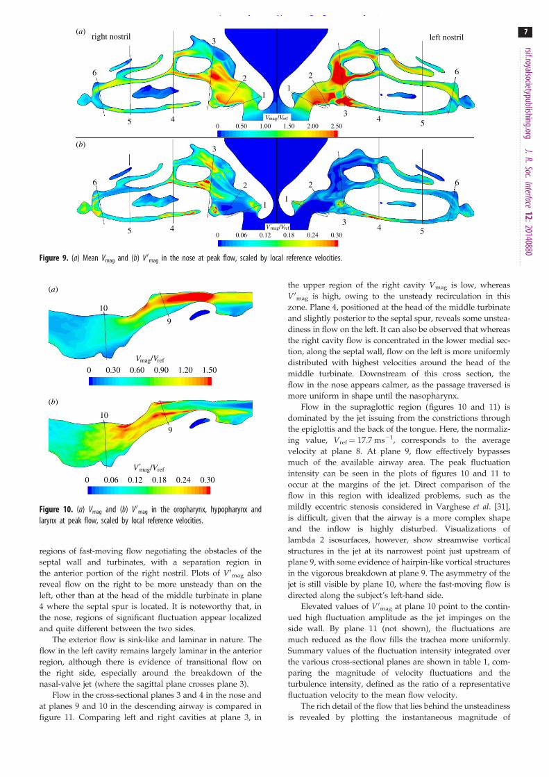
regions of fast-moving flow negotiating the obstacles of theseptal wall and turbinates, with a separation region inthe anterior portion of the right nostril. Plots of V0mag alsoreveal flow on the right to be more unsteady than on theleft, other than at the head of the middle turbinate in plane4 where the septal spur is located. It is noteworthy that, inthe nose, regions of significant fluctuation appear localizedand quite different between the two sides.

The exterior flow is sink-like and laminar in nature. Theflow in the left cavity remains largely laminar in the anteriorregion, although there is evidence of transitional flow onthe right side, especially around the breakdown of thenasal-valve jet (where the sagittal plane crosses plane 3).

Flow in the cross-sectional planes 3 and 4 in the nose andat planes 9 and 10 in the descending airway is compared infigure 11. Comparing left and right cavities at plane 3, in

the upper region of the right cavity Vmag is low, whereasV0mag is high, owing to the unsteady recirculation in thiszone. Plane 4, positioned at the head of the middle turbinateand slightly posterior to the septal spur, reveals some unstea-diness in flow on the left. It can also be observed that whereasthe right cavity flow is concentrated in the lower medial sec-tion, along the septal wall, flow on the left is more uniformlydistributed with highest velocities around the head of themiddle turbinate. Downstream of this cross section, theflow in the nose appears calmer, as the passage traversed ismore uniform in shape until the nasopharynx.

Flow in the supraglottic region (figures 10 and 11) isdominated by the jet issuing from the constrictions throughthe epiglottis and the back of the tongue. Here, the normaliz-ing value, Vref ¼ 17.7 ms21, corresponds to the averagevelocity at plane 8. At plane 9, flow effectively bypassesmuch of the available airway area. The peak fluctuationintensity can be seen in the plots of figures 10 and 11 tooccur at the margins of the jet. Direct comparison of theflow in this region with idealized problems, such as themildly eccentric stenosis considered in Varghese et al. [31],is difficult, given that the airway is a more complex shapeand the inflow is highly disturbed. Visualizations oflambda 2 isosurfaces, however, show streamwise vorticalstructures in the jet at its narrowest point just upstream ofplane 9, with some evidence of hairpin-like vortical structuresin the vigorous breakdown at plane 9. The asymmetry of thejet is still visible by plane 10, where the fast-moving flow isdirected along the subject’s left-hand side.

Elevated values of V0mag at plane 10 point to the contin-ued high fluctuation amplitude as the jet impinges on theside wall. By plane 11 (not shown), the fluctuations aremuch reduced as the flow fills the trachea more uniformly.Summary values of the fluctuation intensity integrated overthe various cross-sectional planes are shown in table 1, com-paring the magnitude of velocity fluctuations and theturbulence intensity, defined as the ratio of a representativefluctuation velocity to the mean flow velocity.

The rich detail of the flow that lies behind the unsteadinessis revealed by plotting the instantaneous magnitude of

right nostril(a)

(b)

left nostril

6

6

5 4

5 4

3

2

1

0 0.50 1.00 1.50 2.00 2.50

0 0.06 0.12 0.18 0.24 0.30

3

2

1

1

2

1

2

34 5

6

34 5

6

Vmag/Vref

V 'mag/Vref

Figure 9. (a) Mean Vmag and (b) V0mag in the nose at peak flow, scaled by local reference velocities.

10

9

10

9

0 0.30 0.60Vmag/Vref

V 'mag/Vref

0.90 1.20 1.50

0 0.06 0.12 0.18 0.24 0.30

(b)

(a)

Figure 10. (a) Vmag and (b) V0mag in the oropharynx, hypopharynx andlarynx at peak flow, scaled by local reference velocities.

rsif.royalsocietypublishing.orgJ.R.Soc.Interface

12:201408807

on January 21, 2015http://rsif.royalsocietypublishing.org/Downloaded from

vorticity (defined as the curl of the velocity field) in the noseand in the supraglottic region (figure 12). The arrow in theright nasal cavity (figure 12a) points to break-up of the shearlayer at the margin of the anterior recirculation. The pair ofarrows in the supraglottic region (figure 12b) highlights succes-sive shear layer instabilities, demonstrating the complex inflowcondition for the downstream jet.

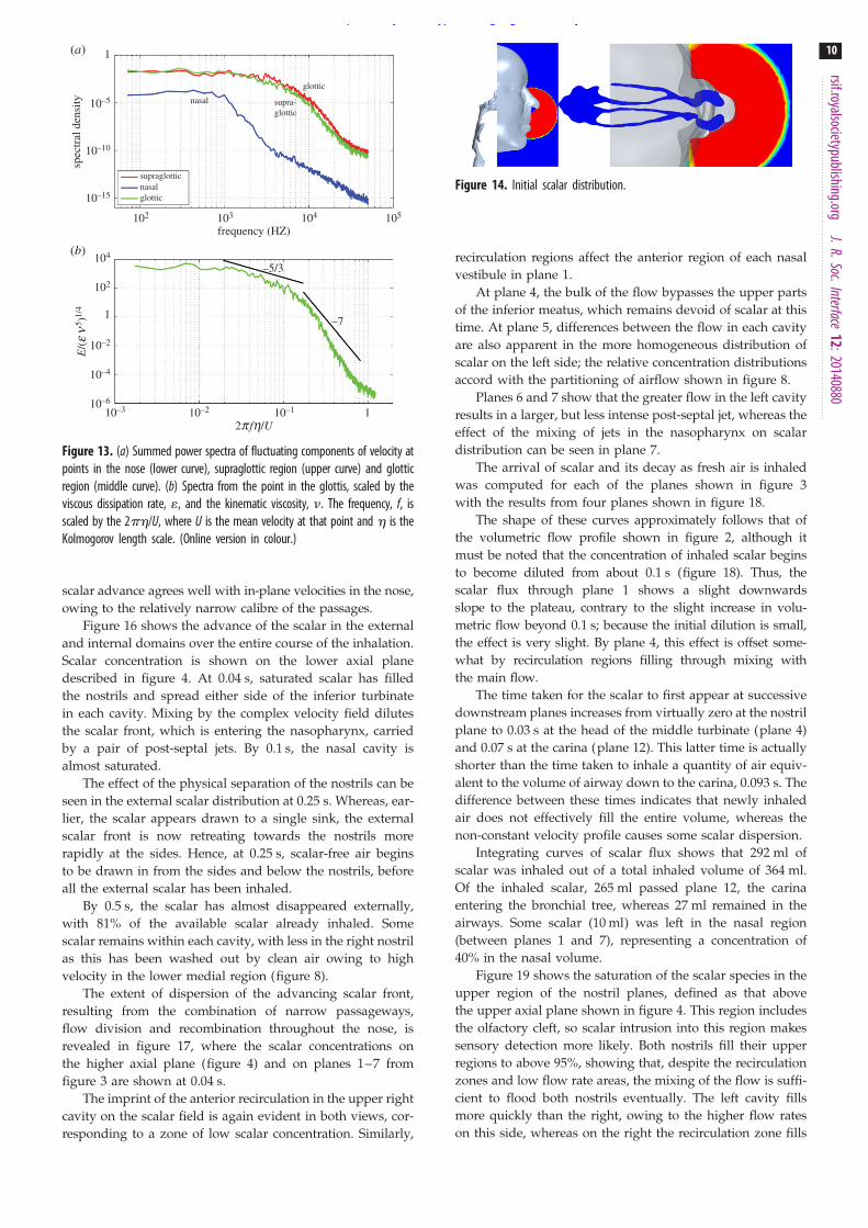
Figure 12 points to the breakdown of separated shearlayers as the primary cause of fluctuations in airway flow.The fluctuation energy is far larger in the airway through

the supraglottic and glottic zones than in the nose, but is ofa different character. This is shown by plotting the temporalenergy spectra of the velocity fluctuations in the nose andsupraglottic region in figure 13, at the points indicated bycrosses in figure 12. Given the limited duration of the tem-poral window, the spectra are processed in the mannerreferred to in Varghese et al. [31], but using just two Hannwindows. Figure 13 shows the (unnormalized) fluctuationenergy in the supraglottic region to be more than twoorders of magnitude greater than in the nose; moreover, thevelocity spectrum at the point in the nose lacks the broad-band energy content of that in the downstream regions.Normalizing the spectrum indicates the emergence of a lim-ited inertial subrange, consistent with Rel of around 20 [32],computed at the point.

3.4. Transport by the flow of inhaled scalarThe fate of inhaled species depends on several parameters,but principally their size and mass. Larger particles do notfollow path lines of the flow owing to factors such as size,shape, inertia and gravitational effects. These effects diminishwith particle size, though additional displacements owing toBrownian motion become significant at very small scales.Pure convective transport by the flow is more approximatelyrealized for nanoparticles, which are small enough to neglectinertial effects, but sufficiently larger than molecular speciesto limit diffusion. To investigate the relation between thedynamics of airflow and convective transport during rapidinhalation, a scalar species with low diffusivity (Schmidtnumber ¼ 900) was introduced and tracked. The advantageof this choice of species parameters (negligible absorption,

R

(a)

(b)

L R L

R LR L

0 0.50 1.00 1.50 2.00 2.50

0 0.30 0.60 0.90 1.20 1.50

3 4

3 4

9

9

10

10

Vmag/Vref

Vmag/Vref

0.180.120.060 0.24 0.30V 'mag/Vref

Figure 11. Through-flow (a) Vmag and (b) V0mag velocities in anterior and mid nasal cavity (figure 3, planes 3 and 4) and supraglottic and glottic regions (figure 3,planes 9 and 10).

Table 1. Mean values of velocity and turbulence quantities on planesdefined in figure 3 in the period 0.1 – 0.13 s.

plane Vmag (ms21) V 0mag (ms21) Tu (%)

1 (L – R) 5.6 – 5.5 0.11 – 0.13 4 – 3

2 (L – R) 6.4 – 5.9 0.06 – 0.10 1 – 1

3 (L – R) 7.2 – 5.8 0.13 – 0.39 1 – 7

4 (L – R) 3.5 – 3.4 0.30 – 0.31 9 – 9

5 (L – R) 3.5 – 3.5 0.22 – 0.17 5 – 5

6 (L – R) 3.6 – 3.2 0.20 – 0.50 5 – 5

7 4.9 0.36 6

8 17.7 0.47 2

9 10.8 3.37 22

10 8.8 3.39 24

11 5.3 0.88 11

12 5.2 0.64 8

rsif.royalsocietypublishing.orgJ.R.Soc.Interface

12:201408808

on January 21, 2015http://rsif.royalsocietypublishing.org/Downloaded from

minimal diffusion) is that it identifies characteristic minimumtimes for species to be transported to the varying parts byconvection alone, free of the complex confounding effectswhen absorption and diffusion are simultaneously varied.Further work will consider the effects of different parameterssuch as diffusion, surface absorption characteristics and thenature of the inhaled species. At all non-outlet boundaries,the scalar concentration gradient was held at zero, to pre-vent absorption by the surface, whereas the outlets affordedno barrier to escape. Tracking this idealized scalar revealshow the air flow field directs inhaled species to enter andto fill the various regions of the airway in the absence ofspecies-dependent absorption and diffusion characteristics.

Before the inhalation, the scalar was confined to anapproximately hemispherical volume of 364 ml (the totalvolume inhaled) positioned against the face, with thewidest point (diameter) level with the nostrils (figure 14).

Figure 15 shows the initial progress of the scalar intoeach nasal cavity, where shading is used to mark the 50%concentration threshold at various instants up to 0.1 s.

Figure 15 shows how the local recirculation regions thatdevelop hinder the scalar advance. This recirculation zoneis similar to that found experimentally by Schreck et al. [33],Kelly et al. [34] and Doorly et al. [35] and inhibits scalar

ingress into the upper regions of the nose (where olfactoryreceptors are located most densely) throughout the earlypart of the sniff. As noted by Kelly et al. in comparing theirwork with earlier studies by Schreck et al., the size and occur-rence of recirculation zones are geometry dependent; here,there is no comparable recirculation in the left cavity.

Between 0.01 and 0.02 s, the scalar front has progressedbeyond the vestibule and at 0.03 s has reached the head ofthe middle turbinate. In addition, at 0.03 s, the scalar has pro-gressed further into the left cavity, where velocities are higherthan in the right.

On both sides, the scalar progression is greater abovethan below the inferior turbinate. By 0.04 s, almost the entireleft cavity is flooded with scalar, whereas, on the right, thewhite, unfilled region marks the recirculating air in the upperanterior cavity.

After 0.05 s, the scalar field has reached the back of theturbinates and is entering the nasopharynx region. Althoughnot evident in the sagittal plane shown, the scalar takes asimilar amount of time to reach the olfactory cleft located inthe upper region of the nasal cavities.

After 0.1 s, both cavities appear well filled with the notableexception of the recirculation regions and dead-end passages,which are bypassed by the bulk flow. Overall, the pattern of

10

9

vorticity: magnitude (s–1)

vorticity: magnitude (s–1)

0

(a)

(b)

2000 4000 6000 8000 10 000

0 4000 8000 12 000 16 000 20 000

Figure 12. Contours of vorticity magnitude on sagittal planes in the right nasal cavity (a) and oropharyx, hypopharynx and larynx (b). The arrows illustrate shearlayer instabilities. The black crosses illustrate the points at which the spectra in figure 13 are calculated.

rsif.royalsocietypublishing.orgJ.R.Soc.Interface

12:201408809

on January 21, 2015http://rsif.royalsocietypublishing.org/Downloaded from

scalar advance agrees well with in-plane velocities in the nose,owing to the relatively narrow calibre of the passages.

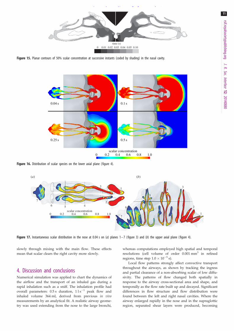
Figure 16 shows the advance of the scalar in the externaland internal domains over the entire course of the inhalation.Scalar concentration is shown on the lower axial planedescribed in figure 4. At 0.04 s, saturated scalar has filledthe nostrils and spread either side of the inferior turbinatein each cavity. Mixing by the complex velocity field dilutesthe scalar front, which is entering the nasopharynx, carriedby a pair of post-septal jets. By 0.1 s, the nasal cavity isalmost saturated.

The effect of the physical separation of the nostrils can beseen in the external scalar distribution at 0.25 s. Whereas, ear-lier, the scalar appears drawn to a single sink, the externalscalar front is now retreating towards the nostrils morerapidly at the sides. Hence, at 0.25 s, scalar-free air beginsto be drawn in from the sides and below the nostrils, beforeall the external scalar has been inhaled.

By 0.5 s, the scalar has almost disappeared externally,with 81% of the available scalar already inhaled. Somescalar remains within each cavity, with less in the right nostrilas this has been washed out by clean air owing to highvelocity in the lower medial region (figure 8).

The extent of dispersion of the advancing scalar front,resulting from the combination of narrow passageways,flow division and recombination throughout the nose, isrevealed in figure 17, where the scalar concentrations onthe higher axial plane (figure 4) and on planes 1–7 fromfigure 3 are shown at 0.04 s.

The imprint of the anterior recirculation in the upper rightcavity on the scalar field is again evident in both views, cor-responding to a zone of low scalar concentration. Similarly,

recirculation regions affect the anterior region of each nasalvestibule in plane 1.

At plane 4, the bulk of the flow bypasses the upper partsof the inferior meatus, which remains devoid of scalar at thistime. At plane 5, differences between the flow in each cavityare also apparent in the more homogeneous distribution ofscalar on the left side; the relative concentration distributionsaccord with the partitioning of airflow shown in figure 8.

Planes 6 and 7 show that the greater flow in the left cavityresults in a larger, but less intense post-septal jet, whereas theeffect of the mixing of jets in the nasopharynx on scalardistribution can be seen in plane 7.

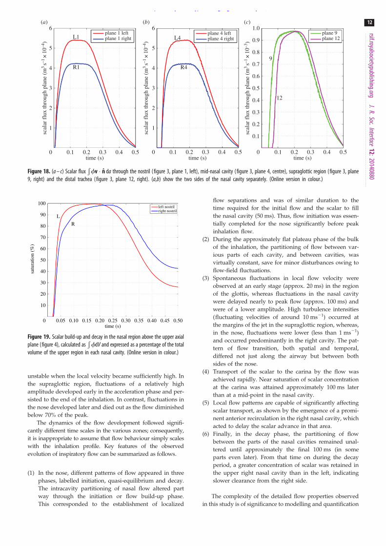
The arrival of scalar and its decay as fresh air is inhaledwas computed for each of the planes shown in figure 3with the results from four planes shown in figure 18.

The shape of these curves approximately follows that ofthe volumetric flow profile shown in figure 2, although itmust be noted that the concentration of inhaled scalar beginsto become diluted from about 0.1 s (figure 18). Thus, thescalar flux through plane 1 shows a slight downwardsslope to the plateau, contrary to the slight increase in volu-metric flow beyond 0.1 s; because the initial dilution is small,the effect is very slight. By plane 4, this effect is offset some-what by recirculation regions filling through mixing withthe main flow.

The time taken for the scalar to first appear at successivedownstream planes increases from virtually zero at the nostrilplane to 0.03 s at the head of the middle turbinate (plane 4)and 0.07 s at the carina (plane 12). This latter time is actuallyshorter than the time taken to inhale a quantity of air equiv-alent to the volume of airway down to the carina, 0.093 s. Thedifference between these times indicates that newly inhaledair does not effectively fill the entire volume, whereas thenon-constant velocity profile causes some scalar dispersion.

Integrating curves of scalar flux shows that 292 ml ofscalar was inhaled out of a total inhaled volume of 364 ml.Of the inhaled scalar, 265 ml passed plane 12, the carinaentering the bronchial tree, whereas 27 ml remained in theairways. Some scalar (10 ml) was left in the nasal region(between planes 1 and 7), representing a concentration of40% in the nasal volume.

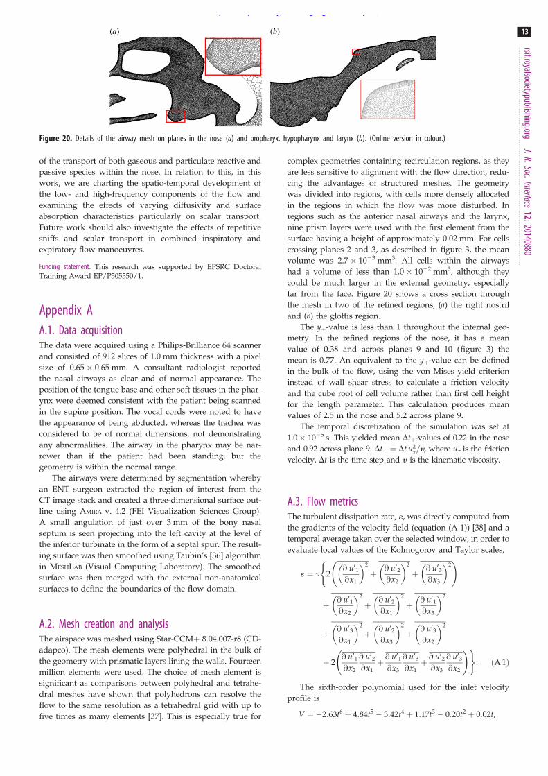
Figure 19 shows the saturation of the scalar species in theupper region of the nostril planes, defined as that abovethe upper axial plane shown in figure 4. This region includesthe olfactory cleft, so scalar intrusion into this region makessensory detection more likely. Both nostrils fill their upperregions to above 95%, showing that, despite the recirculationzones and low flow rate areas, the mixing of the flow is suffi-cient to flood both nostrils eventually. The left cavity fillsmore quickly than the right, owing to the higher flow rateson this side, whereas on the right the recirculation zone fills

Figure 14. Initial scalar distribution.

1

10–5

10–10

10–15

104

–5/3

–7

102

10–2

10–4

10–610–3

102

spec

tral

den

sity

E/(en

5 )1/

4

2p fh/U

103 104 105

10–2 10–1 1

1

supraglottic

supra-glottic

nasal

nasal

glottic

glottic

frequency (HZ)

(b)

(a)

Figure 13. (a) Summed power spectra of fluctuating components of velocity atpoints in the nose (lower curve), supraglottic region (upper curve) and glotticregion (middle curve). (b) Spectra from the point in the glottis, scaled by theviscous dissipation rate, 1, and the kinematic viscosity, n. The frequency, f, isscaled by the 2ph/U, where U is the mean velocity at that point and h is theKolmogorov length scale. (Online version in colour.)

rsif.royalsocietypublishing.orgJ.R.Soc.Interface

12:2014088010

on January 21, 2015http://rsif.royalsocietypublishing.org/Downloaded from

slowly through mixing with the main flow. These effectsmean that scalar clears the right cavity more slowly.

4. Discussion and conclusionsNumerical simulation was applied to chart the dynamics ofthe airflow and the transport of an inhaled gas during arapid inhalation such as a sniff. The inhalation profile hadoverall parameters: 0.5 s duration, 1 l s21 peak flow andinhaled volume 364 ml, derived from previous in vivomeasurements by an analytical fit. A realistic airway geome-try was used extending from the nose to the large bronchi,

whereas computations employed high spatial and temporalresolutions (cell volume of order 0.001 mm3 in refinedregions, time step 1.0 ! 1025 s).

Local flow patterns strongly affect convective transportthroughout the airways, as shown by tracking the ingressand partial clearance of a non-absorbing scalar of low diffu-sivity. The patterns of flow changed both spatially inresponse to the airway cross-sectional area and shape, andtemporally as the flow rate built up and decayed. Significantdifferences in flow structure and flow distribution werefound between the left and right nasal cavities. Where theairway enlarged rapidly in the nose and in the supraglotticregion, separated shear layers were produced, becoming

time (s)0 0.01 0.02 0.03 0.04 0.05 0.10

Figure 15. Planar contours of 50% scalar concentration at successive instants (coded by shading) in the nasal cavity.

0 0.2 0.4 0.6 0.8 1.0scalar concentration

0.04 s

0.25 s 0.5 s

0.1 s

Figure 16. Distribution of scalar species on the lower axial plane (figure 4).

scalar concentration

(a) (b)

31

1

2

34

5

6

7

24

0 0.2 0.4 0.6 0.8 1.0

56

7

Figure 17. Instantaneous scalar distribution in the nose at 0.04 s on (a) planes 1 – 7 (figure 3) and (b) the upper axial plane (figure 4).

rsif.royalsocietypublishing.orgJ.R.Soc.Interface

12:2014088011

on January 21, 2015http://rsif.royalsocietypublishing.org/Downloaded from

unstable when the local velocity became sufficiently high. Inthe supraglottic region, fluctuations of a relatively highamplitude developed early in the acceleration phase and per-sisted to the end of the inhalation. In contrast, fluctuations inthe nose developed later and died out as the flow diminishedbelow 70% of the peak.

The dynamics of the flow development followed signifi-cantly different time scales in the various zones; consequently,it is inappropriate to assume that flow behaviour simply scaleswith the inhalation profile. Key features of the observedevolution of inspiratory flow can be summarized as follows.

(1) In the nose, different patterns of flow appeared in threephases, labelled initiation, quasi-equilibrium and decay.The intracavity partitioning of nasal flow altered partway through the initiation or flow build-up phase.This corresponded to the establishment of localized

flow separations and was of similar duration to thetime required for the initial flow and the scalar to fillthe nasal cavity (50 ms). Thus, flow initiation was essen-tially completed for the nose significantly before peakinhalation flow.

(2) During the approximately flat plateau phase of the bulkof the inhalation, the partitioning of flow between var-ious parts of each cavity, and between cavities, wasvirtually constant, save for minor disturbances owing toflow-field fluctuations.

(3) Spontaneous fluctuations in local flow velocity wereobserved at an early stage (approx. 20 ms) in the regionof the glottis, whereas fluctuations in the nasal cavitywere delayed nearly to peak flow (approx. 100 ms) andwere of a lower amplitude. High turbulence intensities(fluctuating velocities of around 10 ms21) occurred atthe margins of the jet in the supraglottic region, whereas,in the nose, fluctuations were lower (less than 1 ms21)and occurred predominantly in the right cavity. The pat-tern of flow transition, both spatial and temporal,differed not just along the airway but between bothsides of the nose.

(4) Transport of the scalar to the carina by the flow wasachieved rapidly. Near saturation of scalar concentrationat the carina was attained approximately 100 ms laterthan at a mid-point in the nasal cavity.

(5) Local flow patterns are capable of significantly affectingscalar transport, as shown by the emergence of a promi-nent anterior recirculation in the right nasal cavity, whichacted to delay the scalar advance in that area.

(6) Finally, in the decay phase, the partitioning of flowbetween the parts of the nasal cavities remained unal-tered until approximately the final 100 ms (in someparts even later). From that time on during the decayperiod, a greater concentration of scalar was retained inthe upper right nasal cavity than in the left, indicatingslower clearance from the right side.

The complexity of the detailed flow properties observedin this study is of significance to modelling and quantification

6(a) (b) (c)

5

4

3

2

1

0

6 1.0

0.9

0.8

0.7

0.6

0.5

0.4

0.3

0.2

0.1

0

5

4

3

2

1

0

plane 1 leftplane 1 right

plane 4 leftplane 4 right

plane 9plane 12

scal

ar fl

ux th

roug

h pl

ane

(m3

s–1×

10–4

)

scal

ar fl

ux th

roug

h pl

ane

(m3

s–1×

10–4

)

scal

ar fl

ux th

roug

h pl

ane

(m3

s–1×

10–3

)

time (s) time (s) time (s)0.1 0.2 0.3 0.4 0.5 0.1 0.2 0.3 0.4 0.5 0.1 0.2 0.3 0.4 0.5

L4

9

12

L1

R1 R4

Figure 18. (a – c) Scalar fluxÐfv " n da through the nostril ( figure 3, plane 1, left), mid-nasal cavity (figure 3, plane 4, centre), supraglottic region (figure 3, plane

9, right) and the distal trachea (figure 3, plane 12, right). (a,b) show the two sides of the nasal cavity separately. (Online version in colour.)

100

90

80

70

60

50

40

30

20

10

0

L

R

left nostrilright nostril

time (s)0.05 0.10 0.15 0.20 0.25 0.30 0.35 0.40 0.45 0.50

satu

ratio

n (%

)

Figure 19. Scalar build-up and decay in the nasal region above the upper axialplane (figure 4), calculated as

ÐfdV and expressed as a percentage of the total

volume of the upper region in each nasal cavity. (Online version in colour.)

rsif.royalsocietypublishing.orgJ.R.Soc.Interface

12:2014088012

on January 21, 2015http://rsif.royalsocietypublishing.org/Downloaded from

of the transport of both gaseous and particulate reactive andpassive species within the nose. In relation to this, in thiswork, we are charting the spatio-temporal development ofthe low- and high-frequency components of the flow andexamining the effects of varying diffusivity and surfaceabsorption characteristics particularly on scalar transport.Future work should also investigate the effects of repetitivesniffs and scalar transport in combined inspiratory andexpiratory flow manoeuvres.

Funding statement. This research was supported by EPSRC DoctoralTraining Award EP/P505550/1.

Appendix AA.1. Data acquisitionThe data were acquired using a Philips-Brilliance 64 scannerand consisted of 912 slices of 1.0 mm thickness with a pixelsize of 0.65 ! 0.65 mm. A consultant radiologist reportedthe nasal airways as clear and of normal appearance. Theposition of the tongue base and other soft tissues in the phar-ynx were deemed consistent with the patient being scannedin the supine position. The vocal cords were noted to havethe appearance of being abducted, whereas the trachea wasconsidered to be of normal dimensions, not demonstratingany abnormalities. The airway in the pharynx may be nar-rower than if the patient had been standing, but thegeometry is within the normal range.

The airways were determined by segmentation wherebyan ENT surgeon extracted the region of interest from theCT image stack and created a three-dimensional surface out-line using AMIRA v. 4.2 (FEI Visualization Sciences Group).A small angulation of just over 3 mm of the bony nasalseptum is seen projecting into the left cavity at the level ofthe inferior turbinate in the form of a septal spur. The result-ing surface was then smoothed using Taubin’s [36] algorithmin MESHLAB (Visual Computing Laboratory). The smoothedsurface was then merged with the external non-anatomicalsurfaces to define the boundaries of the flow domain.

A.2. Mesh creation and analysisThe airspace was meshed using Star-CCMþ 8.04.007-r8 (CD-adapco). The mesh elements were polyhedral in the bulk ofthe geometry with prismatic layers lining the walls. Fourteenmillion elements were used. The choice of mesh element issignificant as comparisons between polyhedral and tetrahe-dral meshes have shown that polyhedrons can resolve theflow to the same resolution as a tetrahedral grid with up tofive times as many elements [37]. This is especially true for

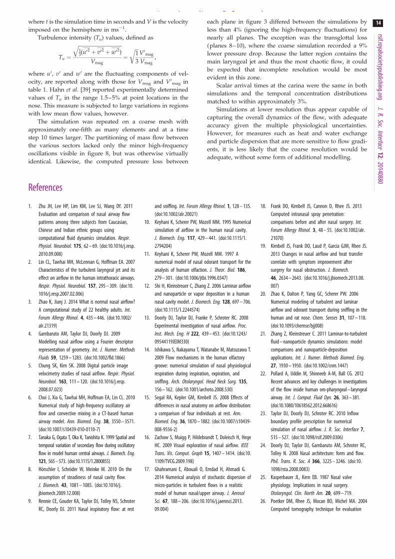
complex geometries containing recirculation regions, as theyare less sensitive to alignment with the flow direction, redu-cing the advantages of structured meshes. The geometrywas divided into regions, with cells more densely allocatedin the regions in which the flow was more disturbed. Inregions such as the anterior nasal airways and the larynx,nine prism layers were used with the first element from thesurface having a height of approximately 0.02 mm. For cellscrossing planes 2 and 3, as described in figure 3, the meanvolume was 2.7 ! 1023 mm3. All cells within the airwayshad a volume of less than 1.0 ! 1022 mm3, although theycould be much larger in the external geometry, especiallyfar from the face. Figure 20 shows a cross section throughthe mesh in two of the refined regions, (a) the right nostriland (b) the glottis region.

The yþ-value is less than 1 throughout the internal geo-metry. In the refined regions of the nose, it has a meanvalue of 0.38 and across planes 9 and 10 (figure 3) themean is 0.77. An equivalent to the yþ-value can be definedin the bulk of the flow, using the von Mises yield criterioninstead of wall shear stress to calculate a friction velocityand the cube root of cell volume rather than first cell heightfor the length parameter. This calculation produces meanvalues of 2.5 in the nose and 5.2 across plane 9.

The temporal discretization of the simulation was set at1.0! 1025 s. This yielded mean Dtþ-values of 0.22 in the noseand 0.92 across plane 9. Dtþ ¼ Dt u2

t=y, where ut is the frictionvelocity, Dt is the time step and y is the kinematic viscosity.

A.3. Flow metricsThe turbulent dissipation rate, 1, was directly computed fromthe gradients of the velocity field (equation (A 1)) [38] and atemporal average taken over the selected window, in order toevaluate local values of the Kolmogorov and Taylor scales,

1 ¼ n

(

2@ u01@x1

" #2

þ @ u02@x2

" #2

þ @ u03@x3

" #2 !

þ @ u01@x2

" #2

þ @ u02@x1

" #2

þ @ u01@x3

" #2

þ @ u03@x1

" #2

þ @ u02@x3

" #2

þ @ u03@x2

" #2

þ 2@ u01@x2

@ u02@x1þ @ u01@x3

@ u03@x1þ @ u02@x3

@ u03@x2

!)

: ðA 1Þ

The sixth-order polynomial used for the inlet velocityprofile is

V ¼ '2:63t6 þ 4:84t5 ' 3:42t4 þ 1:17t3 ' 0:20t2 þ 0:02t,

(b)(a)

Figure 20. Details of the airway mesh on planes in the nose (a) and oropharyx, hypopharynx and larynx (b). (Online version in colour.)

rsif.royalsocietypublishing.orgJ.R.Soc.Interface

12:2014088013

on January 21, 2015http://rsif.royalsocietypublishing.org/Downloaded from

where t is the simulation time in seconds and V is the velocityimposed on the hemisphere in ms21.

Turbulence intensity (Tu) values, defined as

Tu ¼

ffiffiffiffiffiffiffiffiffiffiffiffiffiffiffiffiffiffiffiffiffiffiffiffiffiffiffiffiffiffiffiffiffiffiffi13(u0

2 þ v02 þ w02)q

Vmag¼

ffiffiffi13

rV0mag

Vmag,

where u0, v0 and w0 are the fluctuating components of vel-ocity, are reported along with those for Vmag and V0mag intable 1. Hahn et al. [39] reported experimentally determinedvalues of Tu in the range 1.5–5% at point locations in thenose. This measure is subjected to large variations in regionswith low mean flow values, however.

The simulation was repeated on a coarse mesh withapproximately one-fifth as many elements and at a timestep 10 times larger. The partitioning of mass flow betweenthe various sectors lacked only the minor high-frequencyoscillations visible in figure 8, but was otherwise virtuallyidentical. Likewise, the computed pressure loss between

each plane in figure 3 differed between the simulations byless than 4% (ignoring the high-frequency fluctuations) fornearly all planes. The exception was the transglottal loss(planes 8–10), where the coarse simulation recorded a 9%lower pressure drop. Because the latter region contains themain laryngeal jet and thus the most chaotic flow, it couldbe expected that incomplete resolution would be mostevident in this zone.

Scalar arrival times at the carina were the same in bothsimulations and the temporal concentration distributionsmatched to within approximately 3%.

Simulations at lower resolution thus appear capable ofcapturing the overall dynamics of the flow, with adequateaccuracy given the multiple physiological uncertainties.However, for measures such as heat and water exchangeand particle dispersion that are more sensitive to flow gradi-ents, it is less likely that the coarse resolution would beadequate, without some form of additional modelling.

References

1. Zhu JH, Lee HP, Lim KM, Lee SJ, Wang DY. 2011Evaluation and comparison of nasal airway flowpatterns among three subjects from Caucasian,Chinese and Indian ethnic groups usingcomputational fluid dynamics simulation. Respir.Physiol. Neurobiol. 175, 62 – 69. (doi:10.1016/j.resp.2010.09.008)

2. Lin CL, Tawhai MH, McLennan G, Hoffman EA. 2007Characteristics of the turbulent laryngeal jet and itseffect on airflow in the human intrathoracic airways.Respir. Physiol. Neurobiol. 157, 295 – 309. (doi:10.1016/j.resp.2007.02.006)

3. Zhao K, Jianj J. 2014 What is normal nasal airflow?A computational study of 22 healthy adults. Int.Forum Allergy Rhinol. 4, 435 – 446. (doi:10.1002/alr.21319)

4. Gambaruto AM, Taylor DJ, Doorly DJ. 2009Modelling nasal airflow using a Fourier descriptorrepresentation of geometry. Int. J. Numer. MethodsFluids 59, 1259 – 1283. (doi:10.1002/fld.1866)

5. Chung SK, Kim SK. 2008 Digital particle imagevelocimetry studies of nasal airflow. Respir. Physiol.Neurobiol. 163, 111 – 120. (doi:10.1016/j.resp.2008.07.023)

6. Choi J, Xia G, Tawhai MH, Hoffman EA, Lin CL. 2010Numerical study of high-frequency oscillatory airflow and convective mixing in a CT-based humanairway model. Ann. Biomed. Eng. 38, 3550 – 3571.(doi:10.1007/s10439-010-0110-7)

7. Tanaka G, Ogata T, Oka K, Tanishita K. 1999 Spatial andtemporal variation of secondary flow during oscillatoryflow in model human central airways. J. Biomech. Eng.121, 565 – 573. (doi:10.1115/1.2800855)

8. Horschler I, Schroder W, Meinke M. 2010 On theassumption of steadiness of nasal cavity flow.J. Biomech. 43, 1081 – 1085. (doi:10.1016/j.jbiomech.2009.12.008)

9. Rennie CE, Gouder KA, Taylor DJ, Tolley NS, SchroterRC, Doorly DJ. 2011 Nasal inspiratory flow: at rest

and sniffing. Int. Forum Allergy Rhinol. 1, 128 – 135.(doi:10.1002/alr.20021)

10. Keyhani K, Scherer PW, Mozell MM. 1995 Numericalsimulation of airflow in the human nasal cavity.J. Biomech. Eng. 117, 429 – 441. (doi:10.1115/1.2794204)

11. Keyhani K, Scherer PW, Mozell MM. 1997 Anumerical model of nasal odorant transport for theanalysis of human olfaction. J. Theor. Biol. 186,279 – 301. (doi:10.1006/jtbi.1996.0347)

12. Shi H, Kleinstreuer C, Zhang Z. 2006 Laminar airflowand nanoparticle or vapor deposition in a humannasal cavity model. J. Biomech. Eng. 128, 697 – 706.(doi:10.1115/1.2244574)

13. Doorly DJ, Taylor DJ, Franke P, Schroter RC. 2008Experimental investigation of nasal airflow. Proc.Inst. Mech. Eng. H 222, 439 – 453. (doi:10.1243/09544119JEIM330)

14. Ishikawa S, Nakayama T, Watanabe M, Matsuzawa T.2009 Flow mechanisms in the human olfactorygroove: numerical simulation of nasal physiologicalrespiration during inspiration, expiration, andsniffing. Arch. Otolaryngol. Head Neck Surg. 135,156 – 162. (doi:10.1001/archoto.2008.530)

15. Segal RA, Kepler GM, Kimbell JS. 2008 Effects ofdifferences in nasal anatomy on airflow distribution:a comparison of four individuals at rest. Ann.Biomed. Eng. 36, 1870 – 1882. (doi:10.1007/s10439-008-9556-2)

16. Zachow S, Muigg P, Hildebrandt T, Doleisch H, HegeHC. 2009 Visual exploration of nasal airflow. IEEETrans. Vis. Comput. Graph 15, 1407 – 1414. (doi:10.1109/TVCG.2009.198)

17. Ghahramani E, Abouali O, Emdad H, Ahmadi G.2014 Numerical analysis of stochastic dispersion ofmicro-particles in turbulent flows in a realisticmodel of human nasal/upper airway. J. AerosolSci. 67, 188 – 206. (doi:10.1016/j.jaerosci.2013.09.004)

18. Frank DO, Kimbell JS, Cannon D, Rhee JS. 2013Computed intranasal spray penetration:comparisons before and after nasal surgery. Int.Forum Allergy Rhinol. 3, 48 – 55. (doi:10.1002/alr.21070)

19. Kimbell JS, Frank DO, Laud P, Garcia GJM, Rhee JS.2013 Changes in nasal airflow and heat transfercorrelate with symptom improvement aftersurgery for nasal obstruction. J. Biomech.46, 2634 – 2643. (doi:10.1016/j.jbiomech.2013.08.007)

20. Zhao K, Dalton P, Yang GC, Scherer PW. 2006Numerical modeling of turbulent and laminarairflow and odorant transport during sniffing in thehuman and rat nose. Chem. Senses 31, 107 – 118.(doi:10.1093/chemse/bjj008)

21. Zhang Z, Kleinstreuer C. 2011 Laminar-to-turbulentfluid – nanoparticle dynamics simulations: modelcomparisons and nanoparticle-depositionapplications. Int. J. Numer. Methods Biomed. Eng.27, 1930 – 1950. (doi:10.1002/cnm.1447)

22. Pollard A, Uddin M, Shinneeb A-M, Ball CG. 2012Recent advances and key challenges in investigationsof the flow inside human oro-pharyngeal – laryngealairway. Int. J. Comput. Fluid Dyn. 26, 363 – 381.(doi:10.1080/10618562.2012.668616)

23. Taylor DJ, Doorly DJ, Schroter RC. 2010 Inflowboundary profile prescription for numericalsimulation of nasal airflow. J. R. Soc. Interface 7,515 – 527. (doi:10.1098/rsif.2009.0306)

24. Doorly DJ, Taylor DJ, Gambaruto AM, Schroter RC,Tolley N. 2008 Nasal architecture: form and flow.Phil. Trans. R. Soc. A 366, 3225 – 3246. (doi:10.1098/rsta.2008.0083)

25. Kasperbauer JL, Kern EB. 1987 Nasal valvephysiology. Implications in nasal surgery.Otolaryngol. Clin. North Am. 20, 699 – 719.

26. Poetker DM, Rhee JS, Mocan BO, Michel MA. 2004Computed tomography technique for evaluation

rsif.royalsocietypublishing.orgJ.R.Soc.Interface

12:2014088014

on January 21, 2015http://rsif.royalsocietypublishing.org/Downloaded from

of the nasal valve. Arch. Facial Plast. Surg. 6,240 – 243. (doi:10.1001/archfaci.6.4.240)

27. Fodil R et al. 2005 Inspiratory flow in the nose: amodel coupling flow and vasoerectile tissuedistensibility. J. Appl. Physiol. 98, 288 – 295. (doi:10.1152/japplphysiol.00625.2004)

28. Anch AM, Remmers JE, Bunce H. 1982 Supra-glotticairway resistance in normal subjects andpatients with occlusive sleep apnea. J. Appl. Physiol.53, 1158 – 1163. (doi:10.1063/1.329867)

29. Cole P, Haight JS. 1985 Posture and the nasal cycle. Ann.Otol. Rhinol. Laryngol. 95, 233 – 237.

30. Elad D, Wolf M, Keck T. 2008 Air-conditioningin the human nasal cavity. Respir. Physiol. Neurobiol.163, 121 – 127. (doi:10.1016/j.resp.2008.05.002)

31. Varghese SS, Frankel SH, Fischer PF. 2007 Directnumerical simulation of stenotic flows. Part

1. Steady flow. J. Fluid Mech. 582, 253 – 280.(doi:10.1017/S0022112007005848)

32. Saddoughi SG, Veeravalli SV. 1994 Local isotropy inturbulent boundary layers at high Reynolds number.J. Fluid Mech. 268, 333 – 372. (doi:10.1017/S0022112094001370)

33. Schreck S, Sullivan KJ, Ho CM, Chang HK. 1993Correlations between flow resistance and geometryin a model of the human nose. J. Appl. Physiol. 75,1767 – 1767.

34. Kelly JT, Prasad AK, Wexler AS. 2000 Detailed flowpatterns in the nasal cavity. J. Appl. Physiol. 89,323 – 337.

35. Doorly DJ, Taylor DJ, Schroter RC. 2008 Mechanics ofairflow in the human nasal airways. Respir. Physiol.Neurobiol. 163, 100 – 110. (doi:10.1016/j.resp.2008.07.027)

36. Taubin G. 1995 Curve and surface smoothingwithout shrinkage. In Proc. 5th Int. Conf. onComputer Vision, Cambridge, MA, 20 – 23 June1995, pp. 852 – 857. Washington, DC: IEEEComputer Society Press.

37. Peric M. 2004 Flow simulation using controlvolumes of arbitrary polyhedral shape. ERCOFTACBull. 62, 25 – 29.

38. Delafosse A, Collignon ML, Crine M, Toye D. 2011Estimation of the turbulent kinetic energy dissipationrate from 2D-PIV measurements in a vessel stirred byan axial Mixel TTP impeller. Chem. Eng. Sci. 66,1728 – 1737. (doi:10.1016/j.ces.2011.01.011)

39. Hahn I, Scherer PW, Mozell MM. 1993 Velocityprofiles measured for airflow through a large-scalemodel of the human nasal cavity. J. Appl. Physiol.75, 2273 – 2273.

rsif.royalsocietypublishing.orgJ.R.Soc.Interface

12:2014088015

on January 21, 2015http://rsif.royalsocietypublishing.org/Downloaded from