Dynamic model of hormonal systems coupled by negative feedback

Ž .Biophysical Chemistry 73 1998 85]107

Dynamic model of hormonal systems coupled by negativefeedback

Casey H. Londergan, Enrique Peacock-LopezU´Department of Chemistry, Williams College, Williamstown, MA 01267, USA

Received 9 October 1997; received in revised form 20 February 1998; accepted 20 February 1998

Abstract

Most hormone concentrations in the body are regulated by negative feedback mechanisms in which the productionand release of hormones are regulated according to the concentration of related species. Also, it has been observedthat several hormones are released in a variety of pulsatile patterns. In most cases, the mechanism driving thesecomplex patterns is not well understood. Our model of two cells coupled through negative feedback to their externalproducts demonstrates periodic, aperiodic and chaotic oscillations. The coupling between the cells seems to beresponsible for these dynamic behaviors. The variety of dynamic behaviors observed in the model demonstrates thata simple physiological feedback loop mimicking the coupling between circulatory hormones and production centerscould be the source of complex hormone release patterns observed in vivo. Q 1998 Elsevier Science B.V. All rightsreserved.

Keywords: Hormonal systems; Negative feedback coupling; Attractor coexistence; Quasaiperiodicity; Chaos

1. Introduction

Hormones are the chemical messengers in thebody that play crucial roles in regulating manyessential biochemical and physiological processes.The production and release of hormones andchemical messengers in the body are strictly regu-

U Corresponding author. Tel.: q1 413 5972434; fax: q1 4135974116.

lated by feedback mechanisms. These mecha-nisms generally involve an element of negativefeedback. The simplest negative feedback systeminvolves a species’ concentration directly influ-encing its own production. A more complicated

w xand widely documented 1]10 form of negativefeedback is a species concentration influencingthe hormone that stimulates the species’ produc-tion.

As in the case of a number of biological sys-w xtems 11 , oscillations in hormone concentration

0301-4622r98r$19.00 Q 1998 Elsevier Science B.V. All rights reserved.Ž .P I I S 0 3 0 1 - 4 6 2 2 9 8 0 0 1 4 0 - 9

( )C.H. Londergan, E. Peacock-Lopez r Biophysical Chemistry 73 1998 85]107´86

w xare more the rule than the exception 12 . It hasw xbeen postulated 13 and determined theoretically

that periodic hormone release is actually the mostefficient method of intercellular communicationw x14 . The underlying mechanisms leading to theseperiodic behaviors remain unknown, even in manyexperimentally documented systems.

The actual existence of deterministic pheno-mena, such as limit cycles and chaos in physiolog-ical systems, is a matter of debate; observation ofoscillatory and possibly hyperchaos in physiologi-cal systems has revealed what could be pervasive

w xin mammalian physiology 15 . Some physiologicalsystems in which more complex dynamic behav-iors have been observed are the heart, the brain,and the endocrine system. For many physiologicalsystems a great deal needs to be understoodabout not just the mechanisms, but also the rela-tive soundness of mathematical descriptions ofdifferent rhythmic physiological systems. Insightsinto states that are found naturally can be veryhelpful for both biology and medicine. Whether asystem as simple as a two-cell feedback loop iscapable of sustaining oscillations and other com-plicated release patterns is an issue that thispaper addresses.

Since many hormonal systems operate in apulsatile manner, the first prerequisite of anymodel is that it demonstrates the diverse oscilla-tions observed in hormone systems. Also, manyoscillating models are externally driven at a pre-determined frequency. An external forcing rhythmof this type is not present in many physiologicalsystems that exhibit oscillatory behavior. Formu-lating a model which, like physiological systems,will oscillate without an external forcing elementis important in the modelling of oscillating physi-ological systems.

The significance of the coexistence of two at-tractors in models given the same biological ma-chinery can not be underestimated. In an organ-ism, hysteresis can be equated with the coexis-tence of a healthy temporal pattern and an un-healthy pattern in exactly the same organism orsystem under the same conditions. Given whatcan be considered a small perturbation, a produc-tive or healthy temporal pattern can become un-productive or unhealthy. Examples of hysteresis

or near-hysteresis between healthy and unhealthyphysiological attractors have been documented incardiac rhythms and brain waves. In cardiacrhythms, a heart attack represents a transitionfrom a pulsatile state to an aperiodic high fre-quency state. Also, in brain waves during anepileptic seizure, a chaotic state suddenly be-

w xcomes tightly periodic 15 . As mentioned above,it is believed that hormonal release patterns aremost efficient if they are periodic; therefore it isnot inconceivable that a healthy state’s hysteresiswith a non-periodic or less efficient state couldlead to hormone-related disorders.

Hysteresis in models like our two-cell modelbelow is present when two attractors coexist inphase space for the same parameter values. Theattractor which a trajectory is drawn to dependsentirely on the initial conditions. Models thatexhibit hysteresis can be useful in predicting thedegree and type of perturbation needed to force aphysiological system from a ‘healthy’ attractorinto another ‘unhealthy’ attractor.

In this paper, we propose a model to studymutual regulation between two production cen-ters. The two centers are coupled through amechanism of mutual feedback. The type of phys-iological system which the model emulates is acirculatory feedback loop, in which two centers ofdifferent hormones or chemical messengers arelinked to each other by the concentration of theother center’s product. In the body, the mediumthrough which external concentrations movebetween cells and organs is the circulatory sys-tem. It is a matter of conjecture whether a systemas simple as a circulatory feedback loop can beprimarily responsible for the range of periodicbehaviors observed in hormone concentrations in

w xthe body 8 . The two-cell model can be related toseveral types of feedback loops with a simplecommon distinction: all feedback loops which canbe compared to the model must contain twoexternal concentrations whose production and re-lease are linked through negative feedback mech-anisms. In Section 2, we introduce our two-cellmodel followed by numerical analysis in Section3, and discussion of the implication of our resultsin Section 4.

( )C.H. Londergan, E. Peacock-Lopez r Biophysical Chemistry 73 1998 85]107´ 87

2. Model of mutual regulation

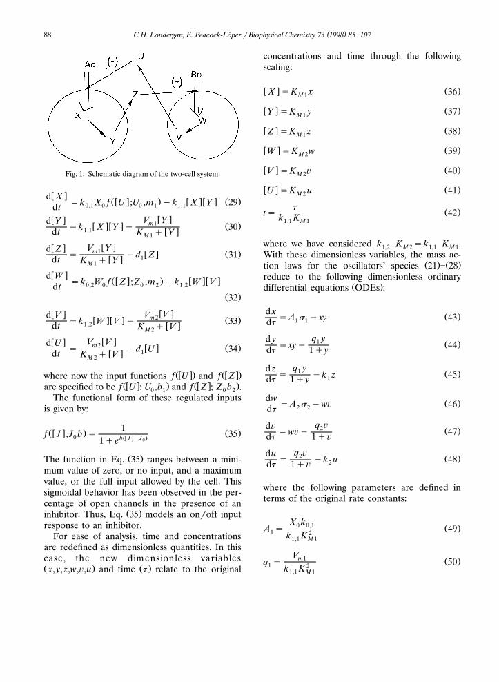
The model considered in our work is a simplesystem of two coupled cells, which is depicted inFig. 1. The cells are coupled to each other by afeedback mechanism in which the input of eachcell is dependent on the concentration of theoutput of the other cell. Internally, each cell is aHiggins oscillator. The Higgins oscillator has beenshown to exhibit a period-two limit cycle over awide range of parameter values when its input is

w xcoupled to its own product 16 . The reactionsteps of the Higgins oscillators proceed as follows.In each cell, the input of the first internal species,

Žw x.X or W, is regulated by the input function f UŽw x.or f Z ,

Žw x.f UŽ .X ª X 1external internal

Žw x.f ZŽ .W ª W 2external internal

Ž .Next, X W is enzymatically transformed into aŽ .second internal species, Y V ,

kq1,1 Ž .XqE ª XE 31 1

kq1,1 Ž .XE ª XqE 41 1

k1,2 Ž .XE ª YqE 51 1

kq1,2 Ž .WqE ª WE 63 3

ky2,1 Ž .WE ª WqE 73 3

k2,2 Ž .WE ª VqE . 83 3

Ž .The enzyme catalyzing the formation of Y V isactivated by the presence of its product,

kqa1 Ž .YqE ª E 91 1

kya1 Ž .E ª YqE 101 1

kqa2 Ž .VqE ª E 113 3

kya2 Ž .E ª VqE 123 3

In the second enzymatic reaction, the secondinternal species, Y, is transformed into the final

Ž .product, Z U , and released from the cell,

kq1,3 Ž .YqE ª YE 132 2

ky1,3 Ž .YE ª YqE 142 2

k1,4 Ž .YE ª ZqE 152 2

kq2,3 Ž .VqE ª VE 164 4

ky2,3 Ž .VE ª VqE 174 4

k2,4 Ž .VE ª UqE 184 4

The concentration of both external products Zand U decays at a given rate,

kd1 Ž .Z ª f 19

kd2 Ž .U ª f 20

Assuming steady states for all of the enzymes andenzyme complexes, this reaction scheme can besimplified to the following reactions:

Ž .k f U0,1 Ž .X ª X 210

k1,1 Ž .XqY ª 2Y 22

E Ž .Y ª Z 23

d1 Ž .Z ª f 24

Ž .k f Z0,2 Ž .W ª W 250

k1,2 Ž .WqV ª 2V 26

E Ž .V ª U 27

d2 Ž .U ª f 28

The mass action laws for each of the species inthe simplified reaction scheme are the following:


Fig. 1. Schematic diagram of the two-cell system.

w xd X Žw x . w x w x Ž .sk X f U ;U ,m yk X Y 290,1 0 0 1 1,1d tw xw x V Yd Y m1w x w x Ž .sk X Y y 301,1 w xd t K q YM 1

w xw x V Yd Z m1 w x Ž .s yd Z 311w xd t K q YM 1

w xd W Žw x . w x w xsk W f Z ;Z ,m yk W V0,2 0 0 2 1,2d tŽ .32

w xw x V Vd V m2w x w x Ž .sk W V y 331,2 w xd t K q VM 2

w xw x V Vd U m2 w x Ž .s yd U 341w xd t K q VM 2

Žw x. Žw x.where now the input functions f U and f ZŽw x . Žw x .are specified to be f U ; U ,b and f Z ; Z b .0 1 0 2

The functional form of these regulated inputsis given by:

1Žw x . Ž .f J , J b s 350 bŽw J xyJ .01qe

Ž .The function in Eq. 35 ranges between a mini-mum value of zero, or no input, and a maximumvalue, or the full input allowed by the cell. Thissigmoidal behavior has been observed in the per-centage of open channels in the presence of an

Ž .inhibitor. Thus, Eq. 35 models an onroff inputresponse to an inhibitor.

For ease of analysis, time and concentrationsare redefined as dimensionless quantities. In thiscase, the new dimensionless variablesŽ . Ž .x, y, z,w,¨ ,u and time t relate to the original

concentrations and time through the followingscaling:

w x Ž .X sK x 36M 1

w x Ž .Y sK y 37M 1

w x Ž .Z sK z 38M 1

w x Ž .W sK w 39M 2

w x Ž .V sK ¨ 40M 2

w x Ž .U sK u 41M 2

t Ž .ts 42k K1,1 M 1

where we have considered k K sk K .1,2 M 2 1,1 M 1With these dimensionless variables, the mass ac-

Ž . Ž .tion laws for the oscillators’ species 21 ] 28reduce to the following dimensionless ordinary

Ž .differential equations ODEs :

d x Ž .sA s yxy 431 1dt

q yd y 1 Ž .sxyy 44dt 1qy

q yd z 1 Ž .s yk z 451dt 1qy

dw Ž .sA s yw¨ 462 2dt

q ¨d¨ 2 Ž .sw¨ y 47dt 1q¨

q ¨du 2 Ž .s yk u 482dt 1q¨

where the following parameters are defined interms of the original rate constants:

X k0 0,1 Ž .A s 491 2k K1,1 M 1

Vm1 Ž .q s 501 2k K1,1 M 1


d1 Ž .k s 511 k K1,1 M 1

W k0 0,2 Ž .A s 522 2k K1,2 M 2

Vm2 Ž .q s 532 2k K1,2 M 2

d2 Ž .k s 542 k K1,2 M 2

The input functions are redefined as follows

1 Ž .s s 551 bŽuyu .01qe1 Ž .s s 562 cŽ zyz .01qe

with the following parameters:

Ž .bsK m 572 M 1

U0 Ž .u s 580 K2 M

Ž .csK m 591 M 2

Z0 Ž .z s 600 K1 M

Ž . Ž .The coupling functions 55 and 56 make theoscillators’ inputs dependent on each other’s out-

Ž .puts around a threshold concentration u or z .0 0The sensitivity parameter b or c defines howabrupt a change takes place in the input in theregion near the threshold concentration.

Coupled oscillator models have been used tomodel many different kinds of systems and rangefrom just two coupled oscillators to larger collec-

w xtions of reactive centers 11 . Our model is dif-ferent in that it allows for analysis of a systemcoupled by external concentrations and not by the

w xtypical diffusion coupling 17,18 . Also, our modelcan be related to a system of oscillators coupledat a short distance from each other and linkedonly by external chemical species. For this reason,it can be used in analyzing endocrinological sys-tems as well as any other systems that are cou-pled at a distance and share only a commonexternal medium.

Table 1Parameters and physical analogs

Coupling parameters

A , A Maximum input allowed by1 2input channels

Number of input channelsEfficiency of input

b,c Sensitivity to threshold concentrationEfficiency of openrclosed mechanism

u , z Upper threshold concentration0 0

Non-coupling parametersq ,q Internal reaction rate1 2

k ,k Decay rate of products1 2

In the model, we have five pairs of parameters.These parameters can be related to differentphysical aspects of the negative feedback mecha-nism, and together the parameters contribute towhat is a reasonably comprehensive model. Theparameters can be related to the physical proper-ties listed in Table 1. These properties can begeneralized to fit a large variety of feedback loopswith a range of mechanisms involved in couplingthe input of an oscillator to an external concen-tration, including different types of regulated in-put channels in cell membranes and neuron-mediated mechanisms of feedback coupling. Ourmodel is flexible in ways that reflect most of thephysical properties of negative feedback. The sim-plest circulatory feedback loop is a center tocenter system, in which two self-contained biolog-ical centers produce an external product in re-sponse to the other center’s external product. Avery simple example of a system like this is thecommunication of two bacteria or cells throughtwo different chemical concentrations. An exam-ple of this type of communication is the commu-nication of phosphorescent bacteria with the cellsin an undeveloped squid’s light-producing organw x19 . In relation to this case, the model’s centerswould represent individual cells.

A larger-scale system of the model’s type is thecommunication of two organ-based hormone orchemical production centers in which the model’soscillators are comparable to these production


centers. An even more global potential applica-tion of the model is a step up from single produc-tion centers to relating the model’s oscillators toentire hormonal axes, or the whole multi-organ,multi-chemical processes involved in producing agiven hormone or chemical messenger. Combina-tions of the cell, organ, and hormonal axis rela-tions are not inconceivable systems which wecould analyze using the model if we were able tomake the appropriate adjustments in parametervalues.

A system which lends itself to analysis with ourmodel is the endocrinological communication sys-tem between the hypothalamus and the pituitarygland. The hypothalamus is a region of the brainwhich is located quite close to the pituitary gland.The pituitary gland is a hormone-releasing glandand plays a major role in almost every bodilyprocess from growth to metabolism to sexual de-velopment. The main communication betweendifferent regions of the hypothalamus and pitu-itary gland is not through direct neuronal connec-tions but through the release of hormones intothe hypophyseal portal vessels. These vesselstransport chemicals straight to the pituitary gland.Pituitary-produced species released into thebloodstream eventually feed back to the hypotha-

w xlamus 7 .Although the communication through external

concentration in the case of the hypo-thalamusrpituitary complex takes place on whatis in practical terms a short, closed track the keychemical links are still made via the circulatorysystem. Modelling a system involving the produc-tion and mutual regulation through circulation oftwo linked hypothalamic and pituitary hormonesis a main objective of our two-cell model.

3. Numerical results

Since the system of six differential Eqs.Ž . Ž .43 ] 48 , cannot be solved analytically, themodel’s behavior was studied through numericalintegration. Numerical integrations were per-formed to two different ends: construction of

w xtrajectories and bifurcation analyses 20,21 .Characterization of attractors whose maxima wereobserved on bifurcation diagrams involved study-

ing trajectories in phase space via two- andthree-dimensional projections of attractors. In ourstudy, we have used the INSITE software packagew x22 . Initial numerical integrations were per-

w xformed using PLOD version 6 23 . In both cases,we used the Gear algorithm, with integrationtolerances of 10y12 for PLOD and 10y14 forINSITE.

In previous work, we have demonstrated thatsingle Higgins oscillators would sustain simpleperiod-one oscillations over a rage of parameter

w xvalues 16 . Thus the numerical integrations wereinitialized using parameter values from our previ-ous work; the initial parameter values appear inTable 2. With these initial parameters as a refer-ence, one member of each pair of parameters wasadjusted at first to investigate which parameterswould potentially have the greatest effect on thenature of the dynamical behavior of the system.

With all of the parameter pairs set equal to thereference values, a period-one state was observed.This behavior was expected based on the previousstudy of a single oscillator. Next, the parametersof one of the cells were varied from the referencevalues, and three pairs of coupling parameterswere determined to have the greatest effect onthe system’s dynamic behavior. In very simplebifurcation analyses, we observed that the q andk parameter pairs only had the effect of slightlyaltering the period and amplitude of the period-one state observed at the reference values. Insimilar simple analyses in which a couplingparameter was varied, we observed that the cou-pling parameters had the effect of radicallychanging the dynamical behavior.

On the basis of the preliminary observations ofthe relative importance of the coupling parame-ters, a systematic approach was devised to explore

Table 2Reference parameter values from Peacock-Lopez and Patel´w x16

Parameter Value

A , A 61 2b,c 3u , z 100 0q ,q 81 2k ,k 11 2


the range of dynamical behavior in regions ofparameter space close to the reference parametervalues. The two non-coupling pairs of parameterswere set slightly different so that the model wouldreflect a system of two distinct cells with distinctproducts. The parameter values which we setconstant throughout the analysis are listed inTables 3 and 4. The oscillator with the greater kvalue was assigned the smaller q value for thereason that a final species with a slower produc-tion rate and smaller rate constant q would morelikely have a faster rate of decay and larger decayconstant k.

The approach to exploring the parameter spacearound the reference values consisted of varyingone of each of the three coupling parameter pairsover different sets of fixed values of the othercoupling parameters. All varied parameters corre-sponded to input of the w]¨ ]u oscillator. Thecombinations of the non-varied parameter pairswere based on a qualitative greater- or less-thanscheme; each parameter was varied over four setsof parameter values.

3.1. Parameter dependence

3.1.1. Variation of A2The A parameters correspond to the degree of

input and multiply the coupling functions. Varia-tion in these parameters in the immediate vicinityof the reference values led to the observation ofseveral different routes to chaos.

At the first set of parameter values, the exter-nal product’s dynamics of the two oscillators weremarkedly different as we can see from Fig. 2a,b.Namely, the output z from the x]y]z oscillatorremained at almost constant amplitude, while theoutput u from the other oscillator went through a

Table 3Constant values of non-coupling parameters

Parameter Set value

q 101k 11q 82k 1.22

Table 4Parameter values for all figures

q s10, k s1, q s8, k s1.21 1 2 2

Figure A A b c u z1 2 0 0

2 6 Varied 5 1 10 53 6 Varied 5 1 5 104 6 Varied 1 5 5 105 7 5 5 Varied 5 106 7 5 5 1 5 Varied7 7 5 1 5 5 Varied8 7 5 5 1 5 4.39 7 5 1 5 5 12

10 7 5 1 5 5 Varied11 6 Varied 5 1 10 5

period-doubling cascade to chaos. In this case,the period-one state of the x]y]z oscillator drivesthe second oscillator through a wide range ofmore complex behaviors. At the second set ofparameter values, the bifurcation diagrams showcoincident windows of periodicity and chaos. AlsoFig. 3a,b depicts a route to chaos which is slightlydifferent from the typical period-doubling route.

Since the oscillators’ inputs dependent on theexternal products, reducing one of the As to zerohalts the production of z or u and uncouples thecells. The behavior of the outputs as A ap-2proaches zero is complex as this uncoupling se-quence is initiated; this can be seen in Fig. 4. It isa pattern of alternating behaviors which appeartowards A s0. Increasingly thin windows of pe-2riodicity and chaos alternate as the cells are un-coupled. This pattern near A f0 was observed2in both cells’ outputs over all parameter valueswhen varying A with small differences in the2relative widths of the periodic and chaotic win-dows. Its appearance in both oscillators indicatesthat it is the only uncoupling pattern for themodel and that once one cell becomes near-un-coupled, its output pattern dominates the dy-namics of the system.

Varying A parameters above values of approx.12 did not significantly change the behavior of thesystem. Large A values would be of questionablephysical significance because they would impingeon the assumption in the model of an excess ofstarting material for the oscillators.


Ž . Ž .Fig. 2. Poincare section defined by the local maxima of a z and b u varying A , with u s10 and z s5. Other parameters´ 2 0 0given in Table 4.


Ž . Ž .Fig. 3. Poincare section defined by the local maxima of a z and b u varying A , with bs5, cs1, u s5 and z s10. Other´ 2 0 0parameters given in Table 4.


Fig. 4. Poincare section defined by the local maxima of z varying A , with bs1, cs5, u s5 and z s10. Other parameters given´ 2 0 0in Table 4.

3.1.2. Variation of cVarying values of c exhibited a range of behav-

iors, but not with the variability of behaviorobserved in varying A . For example, no bifurca-2tions were observed above cs5. From this it wasconcluded that cs5 defines a steep enough inputfunction that any value of c above five would beirrelevant to our analysis. Below cs1 some bifur-cations were observed, but the physical signifi-cance of b or c values less than one is question-able because of the lack of a definiteopenedrclosed threshold. The variety of behaviorwith these constraints is best seen in Fig. 5a,b. Itis interesting to note that in the case of Fig. 5a,b,period-doubling route to chaos is only observedfor the x]y]z cell when c varies from unity to six.

3.1.3. Variation of z0Although complex behaviors were observed

varying A and c, the greatest variety of behav-2iors was observed while varying the thresholdparameter z . Varying a threshold parameter was0

found to be the best way of looking at a widerange of dynamical behaviors over a relativelysmall region of parameter space.

When z was varied towards zero, which makes0the input of the second oscillator sensitive totraces of the first’s product, a very complex se-quence of bifurcations was observed. This obser-vation could lead to a conclusion that the behav-ior of a negative feedback loop to trace amountsis different from a feedback loop which is sensi-tive only to concentrations near a threshold. Anexample of the type of bifurcation diagramobserved varying z is presented in Fig. 6a,c. A0window of chaos is observed in both oscillators’outputs between z s8 and z s10. Above z s0 0 018 changes in dynamic behavior cease. In a moredetailed bifurcation diagram, Fig. 6b, we can seethe more fine structure of the bifurcation diagramcorresponding to a homoclinic orbit.

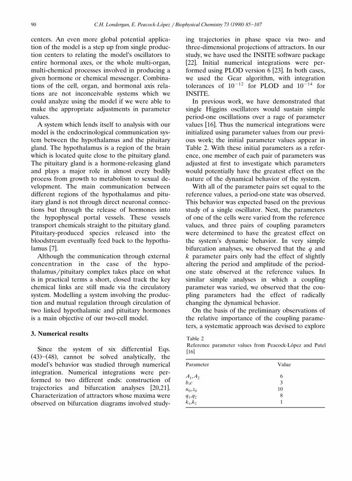
Another illustration of the variety of complexdynamics is observed while varying z as shown0by Fig. 7a,b. The homoclinic orbit appears below


Ž . Ž .Fig. 5. Poincare section defined by the local maxima of a z and b u varying c. Other parameters given in Table 4.´


Ž . Ž .Fig. 6. Poincare section defined by the local maxima of a z and b u varying z , with A s7, A s5, bs5, cs1. Other´ 0 1 2parameters given in Table 4.


Ž .Fig. 6. Continued

z s8, and an attractor with many maxima is0observed at all values above z s11. The latter0attractor was shown to be the manifestation of aquasiperiodic trajectories. Also, series of period-doubling and other bifurcations which have yet tobe fully characterized were observed between z0s9 and z s11.0

As outlined before, a large number of differentw xtypes of dynamical behavior 20 were observed in

bifurcation analyses varying coupling parameters.Finally, the most conspicuous behaviors werecharacterized using projections of trajectories inphase space at specific parameter values.

3.2. Complex dynamics

3.2.1. Homoclinic orbitThe pattern observed in Fig. 6a,c below z s80

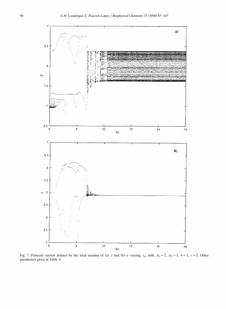
was characterized using a projection of trajecto-ries in the x]y]z space. One attractor, at z s4.30is shown in Fig. 8a,c. In Fig. 8c, the location ofthe saddle point of the attractor is evident. By

Ž .looking more closely at the saddle point Fig. 8d ,it became evident that the attractor represents ahomoclinic orbit.

w xThe Rossler-type slow manifold 24 or the¨w xBarkley scheme 25 are usually evoked to de-

scribe homoclinic orbits. The Rossler-type scheme¨is characterized by a very fast reinjection to thesaddle-focus. Once within the slow manifold, theorbit spirals out. The Barkley scheme is charac-terized by a reinjection into the neighborhood ofthe saddle-focus. After reinjection, the orbit ap-proaches the saddle-focus via damped oscilla-tions. Also, the Barkley scheme allows long quies-cent periods between damped oscillations andreinjection. The homoclinic orbits observed in ourmodel seem to follow the Barkley scheme.

The appearance of the homoclinic orbit is sig-nificant to many conclusions that can be madeabout the model. The model can easily supportcomplex dynamical behavior like the homoclinicorbit. The period of pulses in the time seriesassociated with the homoclinic orbit is long com-


Ž . Ž .Fig. 7. Poincare section defined by the local maxima of a z and b u varying z , with A s7, A s5, bs1, cs5. Other´ 0 1 2parameters given in Table 4.


Ž . Ž . Ž . Ž .Fig. 8. Time series for a z and b u. c Three dimensional x]y]z phase space and d amplification. Parameters as in Fig. 7 withz s4.300



pared to the typical periods of simpler periodicstates. This fact could help to explain the exceed-ingly long periods seen in pulsatile release ofsome hormones. Finding that this type of behav-ior is inherent to our simple model makes it

conceivable that it could appear in a more mech-anistically complex but similar physiological sys-tem. Note that similar time series and homoclinicorbit attractors have been observed experimen-

w xtally in an electrochemical system 26 and theo-


retically in a model of the peroxidase]oxidasew xreaction 27,28 .

3.2.2. QuasiperiodicityIn Fig. 7a, the behavior, which exhibits almost

no changes as z is increased above 11, appeared0

on the bifurcation diagram and in the time seriesŽ .Fig. 9a , to be chaotic. However, when the phase

Ž . Žspace projection z]u]x , was constructed Fig..9b . The attractor appeared to be toroidal.

Ž . Ž . Ž .Fig. 9. a Time series for z. b Three-dimensional z]u]x phase space. c Next maximum map. Parameters as in Fig. 8 withz s12.00.0



Toroidal attractors are characteristic of quasiperi-odicity. To confirm the toroidal nature of thebehavior, a next maximum map of the maxima of

Ž .z was constructed Fig. 9c , and the circulartoroidal cross-section observed confirmed the ex-istence of quasiperiodicity.

Observation of quasiperiodicity in models isnot a new phenomenon, but the appearance ofquasiperiodicity in this model which does notpossess an external forcing periodic term is inter-esting. Quasiperiodicity is most often observedwhen an external periodic driving term is presentin a model and underlies any other periodic be-havior that may occur. In our model, quasiperi-odicity can be explained by realizing that whilethe output pattern for the x]y]z oscillator iscomplex, the output pattern of the w]¨ ]u oscilla-tor is periodic. The periodic release of the w]¨ ]uoscillator is driving the quasiperiodic orbit.

Quasiperiodicity is another complex behaviorwhich our model supports within itself. Observa-tion of quasiperiodicity was further evidence that

the simple model and similar physiological sys-tems could be capable of sustaining complex dy-namical behaviors.

3.2.3. Attractor coexistenceFor several bifurcation analyses which

proceeded forward and backward, we observedqualitatively different attractors for the sameparameter values. An example of this birhythmic-ity was observed in the range of parameters of thehomoclinic orbit. In Fig. 10a, which is comparablewith Fig. 7a, we observed an attractor exhibiting amore typical period-doubling route to chaos coex-isting with a homoclinic orbit. In Fig. 10b, weconstructed both attractors for A s6.08; the two2attractors lie just alongside each other in phasespace. In Fig. 10c we show the region near thesaddle point.

Another example of hysteresis is observed inFig. 11a when it is compared to the non-back-tracked diagram in Fig. 2b. In this case, two


Ž . Ž .Fig. 10. a Backtracked Poincare section defined by the local maxima of z varying z . b Three-dimensional x]y]z phase space´ 0Ž .and c amplification. Parameters as in Fig. 7.

different attractors are observed to coexist. Inparticular, the coexistence of a period-one statewith a steady state is observed from A s4 to25.8; this period-one state coexists with a chaoticattractor from A s5.8 to 6.3 and with a period-32

state for A f6.4. Also notice how the x]y]z cell2drives the w]¨ ]u cell to a 1:5 cycle as is depictedin Fig. 11b for A s1.5. For the internal variable2w, we can see how the concentration increases

Ž .every time the input flux is open Fig. 11c . Thus



while z shows a periodic behavior, w can showmultiples of the z-period.

4. Conclusions

Namely, the coupling parameters were found tobe essential in determining the dynamics of themodel. In contrast, the non-coupling parametersŽthose specific to the chemical and mechanistic

.make-up of each cell were found to be relativelyunimportant. This means that the specific internalmechanism of the oscillators may not be as im-portant in determining the overall system’s behav-ior as we may tend to believe. This is an impor-tant observation, since it means that the appli-cability of the model to physiological systems canbe almost independent of the internal mecha-nisms of chemical messenger production. Withoutmajor changes, the model could conceivably beused to model any system within the range ofsystems outlined in Section 1.

The ability of the simple two-cell model togenerate a range of different dynamical behaviors

over ranges of the coupling parameters suggeststhe potential applicability of the coupling func-tion used in our study. There are many otherdocumented endocrine systems involving a circu-latory feedback element that the model could beused to analyze. These specific systems are allunderstood well enough that the model could beformulated to accurately represent them, butthere is room for more mechanistic understand-ing in each case.

The classical example of a circulatory feedbackloop is the mutual influence of the oscillatingconcentrations of dopamine and prolactin. Awell-documented cycle of pre-ovulatory surges inthese concentrations exists in female mammalsw x9 . Successfully modelling this loop would provethe usefulness of the model and provide insightinto the inherent stability or instability of thedocumented system of two co-dependent concen-trations that can fail as a result of a problem witheither hormone.

Another system involving two well-knownchemical species is the interaction between the

Ž .pituitary gland and hypothalamus and the thy-


Ž . Ž .Fig. 11. a Backtracked Poincare section defined by the local maxima of u varying A . b,c Time series for z, u and w with´ 2A s1.5. Parameters as in Fig. 2.2



roid. Thyroid stimulating hormone, or TSH,controls the production of thyroxine by thethyroid; thyroxine is the agent that the hypothala-musrpituitary complex uses to determine its out-

w xput of TSH 7 . Study of this system using es-tablished physical features to determine themodel’s parameters could help to elucidate themechanism behind the pulsatile release of thetwo species involved and to aid understanding ofthyroidrhormonal ailments.

The central role of pituitary-secreted growthhormone, HGH, in determining liver metabolism

w xhas been established but not elucidated 29 . Theliver’s rate of metabolism and its rhythm in pro-ducing certain hormones are both controlled byHGH levels. Some sort of unknown feedback tothe hypothalamusrpituitary complex is active, butthe mechanism behind the periodicity observedhas not been uncovered. Elucidation of this sys-tem’s workings via a model could help in under-standing the entire functioning of the liver, auniversally important organ.

The rhythm of liver metabolism also has beendocumented to be interconnected with the re-lease of gonadal hormones of both sexes. In thiscase the rhythms have been documented to becharacteristically male or female and intercon-

Ž .nected with but not necessarily determined bygonadal hormone release. Thus, modelling thehypothalamusrpituitary]liver axis as one oscilla-

Žtor using a hormone characteristic of that sys-.tem, like HGH it would be possible to investigate

at some depth the connection between that axisand the release of gonadal hormones. This couldpotentially aid understanding of gonadal hor-mone-related disorders in a much more globalsense than is already possible.

Given the variety of dynamic behaviorsobserved in this model based on changes in onlythe coupling parameters, it is not inconceivablethat such a coupling could indeed be responsiblefor many of the release patterns observed in vivo.For example, the observation of hysteresisstrengthens the possibility that the model may be


able to shed light on physiological systems thatseem to express hysteresis-like behavior in vivo.Being able to understand the extent of hysteresisin a model with the apparent applicability of thetwo-cell model is a large step in being able tounderstand similar physical systems that abruptlychange behavior and reasons behind thesechanges in behavior. The observation of hystere-sis in this model is an additional feature that,together with the wide range of dynamic behav-iors observed, makes a case that this model couldprovide a fair representation of the importantfeatures of real physiological systems.

To prove that the model’s behavior is mainlyinternal-mechanism independent, changes mustbe made to the internal scheme of the oscillatorsto verify that the model’s behavior will not change.A substitute internal mechanism for the Higginsoscillator mechanism used above could be the

w xtemplator developed by Peacock-Lopez et al. 30 .´Once the model’s internal mechanism-indepen-dence is studied, more physiologically relevantparameters than the reference values quoted inTable 2 must be used and the behavior of thesystem characterized. The specific systems de-scribed in Section 1 are reasonably documentedfrom which parameter values for use in the modelcould be gleaned. On the basis of the observa-tions made in this work, the two-cell model isreadily applicable to analysis of physiological sys-tems without need for the invasive and still unde-veloped analytical techniques available at thistime.

Acknowledgements

The authors gratefully acknowledge the sup-Ž .port from NSF CHE93-12160 and the Bronfinan

Science Center at Williams College.

References

w x Ž .1 P.J. Bolt, J. Reprod. Fertil. 24 1971 435]438.w x Ž .2 L.A. Schotkin, J. Theor. Biol. 43 1974 1]14.w x Ž .3 L.A. Schotkin, J. Theor. Biol. 43 1974 15]28.

w x4 T.W. Melnyk, I.W. Richardson, A.A. Simpson, W.R.Ž .Smith, Bull. Math. Biol., 38 1976 .

w x Ž .5 W.J. Bremner, C.A. Paulsen, Horm. Metab. Res. 9 19771]16.

w x Ž .6 W.R. Smith, Bull. Math. Biol. 42 1980 57]78.w x7 H. Curtisand, N.S. Barnes, Biology, 5th ed., Worth Pub-

lishers, New York, 1989.w x8 Y.-X. Li, Pulsatile Hormonal Signaling: A Theoretical

Approach, PhD Dissertation, Universite Libre de Brux-´elles, 1992.

w x9 M.H. Johnson, B.J. Everitt, Essential Reproduction, 4thed., Blackwell Scientific, Oxford, 1995.

w x Ž .10 J.A. Stamford, J.B. Justice, Anal. Chem. 68 1996359A]363A.

w x11 S.H. Strogatz, I. Stewart, Scientific American, Dec., 1993,pp. 102]109.

w x Ž .12 W.F. Crowley Jr., J.H. Hofler Ed. , The Episodic Secre-tion of Hormones, Churchill Livingstone, New York,1987.

w x Ž .13 A. Goldbeter, News Physiol. Sci. 3 1988 103]105.w x Ž .14 Y.-X. Li, A. Goldbeter, Biophys. J. 61 1992 161]171.w x Ž .15 R. Pool, Science 243 1989 604]607.w x16 E. Peacock-Lopez, S. Patel, J. Chem. Phys., 1998, to be´

submitted.w x17 J. Halloy, Y.-X. Li, J.L. Martiel, B. Wurstier, A. Gold-

Ž .beter, Phys. Lett. A 151 1990 33]36.w x Ž .18 M. Marek, I. Schreiber, in: R.J. Field, L. Gyorgyi Eds. ,¨

Chaos in Chemistry and Biochemistry, World Scientific,Singapore, 1993.

w x19 R. Losick, D. Kaiser, Scientific American, Feb., 1997, 68.w x20 S.H. Strogatz, Nonlinear Dynamics and Chaos,

Addison-Wesley, Reading, MA, 1994.w x21 R.E. Mirollo, S.H. Strogatz, SIAM J. Appl. Math. 50

Ž .1990 1645]1662.w x22 T.S. Parker, INSITE, Ver. 4.1, 1990.w x23 D.K. Kahaner, D.D. Barnett, Plotted Solutions of Dif-

ferential Equations, Ver. 6.00, NIST, Washington, DC,1989.

w x Ž .24 O.E. Rossler, Z. Naturforsch. Teil A 31 1976 259.¨w x Ž .25 D. Barkley, J. Chem. Phys. 89 1988 5547.w x Ž .26 F.N. Albahadilly, M. Schnell, J. Chem. Phys. 88 1988

4312]4319.w x Ž .27 M.J.B. Hauser, L.F. Olsen, J. Am. Chem. Soc. 92 1996

2857]2863.w x28 T.V. Bronnikova, W.M. Schaffer, L.F. Olsen, J. Chem.

Ž .Phys. 105 1996 10847]10861.w x29 J.A. Gustafsson, A. Mode, G. Norstedt, P. Shett, Ann.

Ž .Rev. Physiol. 45 1983 51]60.w x30 E. Peacock-Lopez, D.B. Radov, C.S. Flesner, Biophys.¨

Ž .Chem. 65 1997 171]178.

Dynamic model of hormonal systems coupled by negative feedback

Documents

Transcript of Dynamic model of hormonal systems coupled by negative feedback