DX212855.pdf - King's Research Portal
381
This electronic thesis or dissertation has been downloaded from the King’s Research Portal at https://kclpure.kcl.ac.uk/portal/ Take down policy If you believe that this document breaches copyright please contact [email protected] providing details, and we will remove access to the work immediately and investigate your claim. END USER LICENCE AGREEMENT Unless another licence is stated on the immediately following page this work is licensed under a Creative Commons Attribution-NonCommercial-NoDerivatives 4.0 International licence. https://creativecommons.org/licenses/by-nc-nd/4.0/ You are free to copy, distribute and transmit the work Under the following conditions: Attribution: You must attribute the work in the manner specified by the author (but not in any way that suggests that they endorse you or your use of the work). Non Commercial: You may not use this work for commercial purposes. No Derivative Works - You may not alter, transform, or build upon this work. Any of these conditions can be waived if you receive permission from the author. Your fair dealings and other rights are in no way affected by the above. The copyright of this thesis rests with the author and no quotation from it or information derived from it may be published without proper acknowledgement. An instrument for the measurement of body/support interface stresses : with particular application to below-knee prostheses. Williams, Robin Bede Download date: 02. Jun. 2022
-
Upload
khangminh22 -
Category
Documents
-
view
1 -
download
0
Transcript of DX212855.pdf - King's Research Portal

This electronic thesis or dissertation has been
downloaded from the King’s Research Portal at
https://kclpure.kcl.ac.uk/portal/
Take down policy
If you believe that this document breaches copyright please contact [email protected] providing
details, and we will remove access to the work immediately and investigate your claim.
END USER LICENCE AGREEMENT
Unless another licence is stated on the immediately following page this work is licensed
under a Creative Commons Attribution-NonCommercial-NoDerivatives 4.0 International
licence. https://creativecommons.org/licenses/by-nc-nd/4.0/
You are free to copy, distribute and transmit the work
Under the following conditions:
Attribution: You must attribute the work in the manner specified by the author (but not in anyway that suggests that they endorse you or your use of the work).
Non Commercial: You may not use this work for commercial purposes.
No Derivative Works - You may not alter, transform, or build upon this work.
Any of these conditions can be waived if you receive permission from the author. Your fair dealings and
other rights are in no way affected by the above.
The copyright of this thesis rests with the author and no quotation from it or information derived from it
may be published without proper acknowledgement.
An instrument for the measurement of body/support interface stresses : with particularapplication to below-knee prostheses.
Williams, Robin Bede
Download date: 02. Jun. 2022

An Instrument for the Measurement of
Body/Support Interface Stresses:
with particular application to below-knee prostheses
by
Robin Bede Williams
A thesis submitted for the degree of
Doctor of Philosophy
Based on research carried out in the
Department of Medical Engineering & Physics
Kings College Hospital School of Medicine & Dentistry
University of London
October 1993
1 wtut


ABSTRACT
The socket of the prosthesis forms a critical interface between the amputee and
their replacement (prosthetic) limb. Current socket design principles emphasise the
importance of redistributing the normal stresses (pressures), present at the interface,
to areas of the residual limb which can tolerant them. However, shear stresses,
which are thought to have equal potential for causing tissue damage have been
ignored. Little is known about the duration, magnitude and distribution of concurrent
shear and normal stresses imposed on the limb during normal activities. This is
primarily due to the lack of instruments to characterise them.
To address this a unique three axis transducer and data acquisition system have
been developed during this research. It is the first of its type to be demonstrated
as suitable for continuous simultaneous measurement of normal and shear stresses
occuring at any site on the residual limb/prosthetic socket interface. The transducer
(16mm diameter x 4.9 mm thick) detects stresses applied normal to, and shear
stresses applied in the plane of, the limb/socket interface. It is designed to be
recessed into, or inserted through, the socket wall. The accuracy of the shear and
normal axes are 6% indicated stress or 225KPa (whichever is the greater) and1.75% or 5.5KPa respectively. The frequency response (-3dB Bandwidth) of thetransducer is better than 0.lmHz-l000Hz.
Transducer interface circuitry, microcomputer controlled data acquisition hardware
and associated software have been designed and are described. The system is able
to digitise, to l2birs, and store 32 channels of data (10 transducers and 2 footswitchsignals) at a rate of 500Hz, for about 30 seconds per trial. Data can be archived
to disc file on a PC. Overall system noise and uncertainty is better than 0.25%FSO.
Preliminary clinical trials provide data not previously seen. It indicates that shear
stresses (2-2OKPa) are smaller than normal stresses (10-4OKPa), and interwalk
variations in stress magnitude and phasing are minimal. The significant spectral
components of the stress waveforms were all found to be below 15Hz. Waveform
timing indicates that a stress wave travels across the limb in a proximomedial
direction. Slippage of the limb in the socket was also observed.
The understanding gained from acquired stress data is beinWcan be used to: increase
knowledge on tissue response to combined shear and normal stresses; improve
prosthetic design principles; and improve models of the mechanical behaviour of
limb/socket structures for computer aided socket design.
3


DEDICATION
In memory of my
Mother and Father


ACKNOWLED CEMENTS
I sincerely thank my wife Nicola, not only for the hours spent deciphering my
illegible script whilst typing it, but principally for her enduring encouragement,
strength and unreserved dedication to myself, without which this thesis would not
be. I am grateful beyond words.
I am indebted to my colleague and good friend Mr. David Porter for his invaluable
ideas, constructive advice, enthusiasm and good humour.
I wish to thank my supervisor Professor V.C.Roberts, Head of Department, for
enabling me to undertake this work and for his guidance and support.
There are many friends and colleagues, past and present, from the Department
which I thank for their helpful suggestions and discussions over the years. Several
of them deserve particular thanks: Messrs Riad Hosein and Ming Zhang for their
co-operation and ruthless critique of my work; Dr. Eduardo Costa for his often
timely counsel; Mr. Andrew Healey for allowing me to bend his ear on many
occasions and commission his sagacious perception; Dr. Sidney Leeman for his
example, advice and confidence in me; Mr. Andrew Healey, Dr. Sidney Leeman
and Mr. Nicolas Thomas for their stimulating discussions and physics-on-a-napkin
over coffee; Ms. Beverley Conway for her friendship and support over many years;
Messrs. Kevin Jennings, Philip Millward, and Paul Richardson for the meticulous
production of the mechanical components for the transducers and calibration jigs -
often at short notice; and Dr. Inigo Deane, Ms. Lindis Richards, Mrs. Eve Langford
for their constant assistance.
I would like to thank Mr. Jim Regan, chief prosthetist, for his advice and skills
proffered. Also, I am indebted to the patients who willingly donated their time
and patience during the clinical trials
Finally, I thank (posthumously) Mr. Stanley Parsonage for his enthusiasm and
volunteering his skills during the early development of the transducer.
7


TABLE OF CONTENTS
Title 1Abstract 3Dedication 5Acknowledgements 7Table of Contents 9List of Illustrations 15Table of Tables 19
Chapter 1Introduction
1.1 Introduction 231.1.1 Historical Perspective 251.1.2 Current Trends 261.1.3 Summary 29
1.2 Anatomy of the Lower Leg 291.2.1 Bone and Muscle 291.2.2 Skin 32
1.3 Amputation Procedures 351.3.1 Discussion 41
1.4 Prosthesis Fitting 41
1.4.1 Design Considerations for Below-Knee Sockets 42
1.4.2 The P.T.B. Below-Knee Prosthesis 46
1.4.3 Conventional P.T.B. Socket Manufacture 481.4.4 C.A.S.D/C.A.M. in P.T.B. Socket Design
50
1.4.4.1 Shape Manipulation CASD
521.4.4.2 Tissue Compliant CASD
53
1.4.4.3 Computer-aided socket manufacture 55
1.4.4.4 Discussion 551.5 Prosthetic Assessment
57
1.5.1 Gait Analysis 571.5.1.1 Temporal and Spatial Parameters 581.5.1.2 Kinematic Parameters 591.5.1.3 Kinetic Parameters 601.5.1.4 Metabolic Parameters 611.5.1.5 Summary 62
9

1.6 Discussion
63
Chapter 2Soft Tissue Mechanics & Interface Stress Measurements
2.1 Soft Tissue Mechanics
65
2.1.1 Skin
66
2.1.1.1 Experimental Considerations
66
2.1.1.2 Structural Components of Skin
68
2.1.1.3 Properties of Whole Skin
68
2.1.2 Fascia, Tendon and Ligament
74
2.1.3 Muscle
76
2.2 Stress Effects on Tissue
77
2.2.1 Friction Effects
77
2.2.2 Normal Stress Effects
78
2.2.3 Shear Stress Effects
80
2.2.4 Socket Design Influence on Stress
81
2.2.5 Tissue Adaption
83
2.2.6 Discussion
84
2.3 Previous Interface Stress Measurements - Methods
85
2.3.1 Sensors between Limb and Socket
85
2.3.2 Sensors Recessed in Socket Walls
90
2.3.3 Instrumented, Isolated Sections of Socket Wall
92
2.3.4 Special Sockets
93
2.3.5 Sensors Measuring Shear Stress
93
2.3.6 Concurrent Studies
96
2.3.7 Discussion
97
2.4 Previous Interface Stress Measurements - Findings
101
2.5 Temperatures in Prosthetic Sockets
106
2.6 Transducer Design Criteria
107
Chapter 3Triaxial Stress Transducer - Prototype Design
3.1 Shear-Section Design
115
3.1.1 Principle of Operation
116
3.1.2 Force to Displacement Conversion
118
3.1.2.1 ubber as a Spring
119
10

3.1.2.1.1 Rubber in Simple Shear
122
3.1.2.1.2 Rubber in Compression
123
3.1.2.2 Time Domain Behaviour of Rubber
123
3.1.2.3 Frequency Domain Behaviour of Rubber
127
3.1.2.4 Useful Types of Rubber
130
3.1.3 Displacement to Voltage Conversion
133
3.1.3.1 Magnet Types
133
3.1.3.2 Magnetoresistor Properties
133
3.1.3.3 Disc Materials
139
3.1.3.4 Other Materials
139
3.2 Normal Section Design
141
3.2.1 Principle of Operation
141
3.2.2 Strain-gauge Properties
142
3.2.3 Excitation Limits
145
3.2.4 Diaphragm Considerations
145
3.2.5 Indentor Mechanism
149
3.3 Prototype Device Assembly
150
3.3.1 Shear-section Assembly
150
3.3.2 Normal-section Assembly
151
3.3.3 Three Axis Device Assembly
151
3.4 Mounting Considerations
152
Chapter 4Triaxial Stress Transducer - Development to Requisite Form
4.1 Shear-Stress Section Development
157
4.1.1 First Prototype Assessment - Design A
158
4.1.1.1 Test Regimes and Equipment
158
4.1.1.2 Static Stress Response
161
4.1.1.2.1 LinearityandRange
162
4.1.1.2.2 Creep and Hysteresis
164
4.1.1.3 Temperature Sensitivity
167
4.1.1.3.1 Magnetoresistor Contribution
168
4.1.1.3.2 Silicone Expansion
169
4.1.1.3.3 Magnet Contribution
172
4.1.1.4 Discussion
172
4.1.2 Component Reselection
174
4.1.2.1 Magnetoresistor Replacement
174
11

4.1.2.2 Magnet Replacement
175
4.1.2.3 Silicone Replacement
176
4.1.2.4 Dimensional Changes
178
4.1.3 Second Prototype Assessment - Design B
179
4.1.3.1 Test Equipment Modification
179
4.1.3.2 Temperature Sensitivity
182
4.1.3.2.1 Magnetoresistor Contribution
182
4.1.3.2.2 Silicone Expansion
183
4.1.3.2.3 Magnet Contribution
185
4.1.3.2.4 Component Sunmiary
186
4.1.3.2.5 Device Temperature Sensitivity
186
4.1.3.3 Static Stress Response
188
4.1.3.3.1 Linearity and Range
189
4.1.3.3.2 Force Resolution
190
4.1.3.3.3 Repeatability
190
4.1.3.3.4 Creep and Hysteresis
190
4.1.3.3.5 Alignment Errors in Testing
193
4.1.3.4 Discussion
195
4.1.4 Further Component Reselection
196
4.1.4.1 Silicone Replacement by Natural Rubber
196
4.1.4.1.1 Natural Rubber Formulation
197
4.1.4.1.2 Bonding Considerations
197
4.1.4.2 Low-Friction Polymer Central Disc
200
4.2 Normal-Stress Section Development
201
4.2.1 Test Equipment and Methods
202
4.2.2 Temperature Sensitivity
202
4.2.3 Static Stress Response
204
4.2.3.1 Non-axial Loading of Diaphragm
206
4.2.4 Discussion
208
4.3 Requisite Triaxial Transducer Design - Design C
208
4.3.1 Device Construction
208
4.3.2 Dynamic Stress Response
215
4.3.2.1 Test Equipment
216
4.3.2.2 Dynamic Measurement Considerations
217
4.3.2.3 Range, Hysteresis, Linearity and Accuracy
224
4.3.2.4 Shear Stress Vectors and Crosstalk Errors
236
4.3.2.5 Creep and Frequency Response
238
4.3.3 Temperature Sensitivity
243
4.3.3.1 Test Equipment and Methods
243
12

4.3.3.2 Sensitivity Data
244
4.4 Summary
247
Chapter 5Data Acquisition : Hardware
5.1 Transducer Interface Circuit
251
5.1.1 Transducer Excitation
252
5.1.1.1 Magneto-resistor Electrical Properties
252
5.1.1.2 Strain-gauge Electrical Properties
255
5.1.1.3 Excitation Circuit
256
5.1.2 Signal Conditioning
258
5.1.2.1 Amplification
258
5.1.2.2 Interference and Filtering
264
5.2 Signal Conversion and Data Storage
270
5.2.1 Analogue to Digital Conversion
271
5.2.2 Conversion Control and Data Storage
273
5.2.3 Power Supplies
274
5.3 Registration of Foot Contact Events
275
5.4 Interface to Kinematic Measurements
277
5.5 System Integration
278
5.6 Safety
281
5.7 Discussion
282
Chapter 6Data Acquisition: Software
6.1 System Hardware and Programming Environment
286
6.2 Software Overview
287
6.3 Levell - File Viewing
290
6.3.1 View Data Files
293
6.4 Level2 - Data Collection Unit Initialisation
293
6.4.1 Dos Functions
297
6.4.2 Monitor Functions
298
6.4.3 Programme Transfer and Execution
298
6.5 Level3 - Data Collection
299
6.5.1 Support Functions
302
6.5.2 Transfer Data Files
304
13

6.5.3 Collect New Data
307
6.5.4 View Data Files
311
6.6 Error Trapping
312
6.7 Discussion
315
Chapter 7Clinical Evaluation
7.1 Introduction
317
7.2 Evaluation Study 1 - Limb/Socket Stresses in Amputees
318
7.3 Evaluation Study 2 - Plantar Stresses in Normals
328
7.4 Performance and Mounting Notes
333
Chapter 8Discussion and Future Work
8.1 Overview of the Imperatives
337
8.2 Transducer Development
339
8.3 Data Acquisition System Development
343
8.4 Clinical Findings
344
8.5 Outhne for Future Developments
346
AppendixData File Format & Memory Map
A. 1 Data-File Format
351
A.2 DCU Memory Map
353
Publications 355
References 357
14

LIST OF ILLUSTRATIONS
Chapter 1
1.1 Section view of the leg from midway along the tibia. 301.2 Cross-sectional view of skin 331.3 Skin incisions for below-knee amputations 37
1.4 Stages of the Long Posterior Flap amputation 38
1.5 Stages of the Equal (skewed sagittal) Flap amputation
39
1.6 Pressure tolerant/sensitive areas of the residual limb
43
1.7 Forces acting on the limb and PTB socket during gait
45
1.8 Basic components of the PTB below-knee prosthesis
46
1.9 Temporal and spatial parameters of the gait cycle
58
Chapter 2
2.1 Stress-Strain curve for skin under uni-axial tension 70
2.2 Hysteresis in skin under uni-axial tension
71
2.3 Load cycle preconditioning for skin (uni-axial tension)
72
2.4 Stress strain curve for collagen 76
2.5 Normal stress sensors inserted between limb and socket
87
2.6 Stress sensors inserted through the socket wall
91
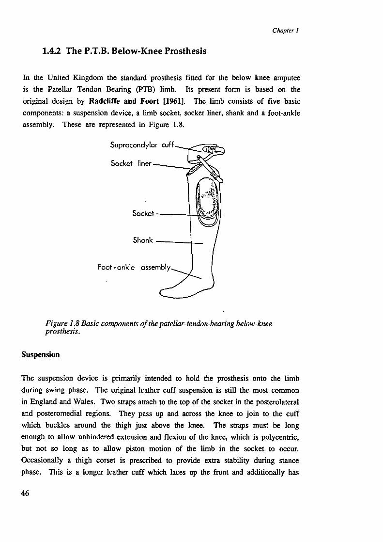
2.7 Stress measurements by isolating socket sections
93
2.8 Non-prosthetic body/support interface stress sensors
95
2.9 Triaxial stress sensor developed in concurrent research
96
2.10 Limb-in-socket temperature variation with exercise 107
Chapter 3
3.1 Principle of shear transduction mechanism 116
3.3 Schematic of biaxial shear transducer 117
3.2 Assembly of biaxial shear transducer 118
3.4 Structural formulae of some elastomers 119
3.5 Crosslinking and entanglements in long chain molecules 120
3.6 Shear stress v strain in Natural rubber (Treloar)
121
3.7 Schematic of rubber in simple shear 123
15

3.8 Viscoelastic response to constant stress/strain
124
3.9 Compliance v time for ideal rubber
125
3.10 Mechanical models for viscoelastic behaviour
126
3.11 Shear modulus v frequency for ideal rubber
129
3.12 Uncertainty of stress estimation with phase lag
129
3.13 Current path in magnetoresistor under a magnetic field
134
3.14 Resistance v induction for magnetoresistor
135
3.15 Resistance v temperature for magnetoresistor
136
3.16 Response of FP1 1OD 155 to magnet displacement
138
3.17 Dimensions of disc's - Design A shear section
140
3.18 Assembly of magnetoresistor PCB
141
3.19 Generalised diaphragm under distributed normal force
146
3.20 Operation of indentor mechanism
149
3.21 Transducer assembly jig
150
3.22 Schematic of Transducer mounted in socket wall
153
3.23 Dimensions of blanks for making transducer recessess
154
3.24 Method of making transducer blanks
155
3.25 View of fmished recess and instrumented socket
156
Chapter 4
4.1 Transducer calibration jig
160
4.2 Stress response of Design A shear sections
163
4.3 Stress response with orientation Design A shear section
164
4.4 Stress response and relaxation, Design A silicones
166
4.5 Temperature response of Design A shear sections
168
4.6 Temperature response of FP1 1OD 155 magneto-resistor
169
4.7 Output v magnet (SmCo) I MR (FP1 1OD 155) separation
171
4.8 Temperature response of SmCo magnet (experimental)
173
4.9 Relative field exposure with magnet/MR size
176
4.10 Unidirectional response, MR(FP1 1 1L100) / magnet(NdBFe)
177
4.11 Shear stress response v thickness, RTV157(GE) silicone
178
4.12 Ridge/channel dimensions, Design A v Design B
179
4.13 Circuit for interfacing test equipment to AID, Design B
181
4.14 Temperature response of FP1 1 1L100 magneto-resistor
183
4.15 Output v magnet (NdBFe) / MR (FP1 1 1L100) separation
184
4.16 Temperature response of NdBFe magnet (experimental)
185
4.17 Experimental setup, temperature response, Design B
187
4.18 Temperature response of Design B shear sections
187
16

4.19 Experimental setup, static stress response, Design B
188
4.20 Stress response with orientation Design B shear section
189
4.21 Hysteresis behaviour in Design B shear sections
191
4.22 Hysteresis behaviour in silicone disc under shear
194
4.23 Alignment errors in shear section calibration jig
195
4.24 Gauge patterns and diaphragm outlines, normal sections
201
4.25 Temperature response of prototype normal sections
203
4.26 Force sensitivity of normal stress prototypes
205
4.27 Effect of load spreading layers and indentor size
207
4.29 Dimensions of Design C PCB's
209
4.28 Dimensions of Design C shear section disc's
210
4.30 Dimensions of Design C normal section
212
4.31 Photograph of Design C before assembly
214
4.32 Dynamic test equipment setup
216
4.33 Rheological model of the dynamic test set up
218
4.34 Model for determination of calibration jig damping
221
4.35 Magnification and phase response - metal spring
224
4.36 Stress sensitivity of Design C shear section
226
4.37 Linearity of Design C shear section stress response
228
4.38 Conversion errors using 1st order polynomial - shear
229
4.39 Conversion errors using 5th order polynomial - shear
231
4.40 Stress sensitivity of Design C normal section
232
4.41 Linearity/conversion errors, 1st order poiy - normal
234
4.42 Conversion errors using 5th order polynomial - normal
235
4.43 Error in derivation of shear stress vector angle
237
4.44 Magnification and phase response of Design C
241
4.45 Impulse response of Design C shear and normal sections
242
4.46 Temperature sensitivity of Design C - shear and normal
245
Chapter 5
5.1 Block diagram of system hardware interconnections
251
5.2 Schematic of Wheatstone bridge circuit
253
5.3 Transducer excitation circuit
257
5.4 Transducer signal amplifier circuit
260
5.5 Environmental noise measurement circuit
266
5.6 Transducer signal filter circuit
269
5.7 Frequency response of amplifier and filter circuit
270
5.8 Footswitch signal conditioning circuit
276
17

5.9 Footswitch signal interface to Vicon
279
5.10 Photograph of data collection system
281
Chapter 6
6.1 Block diagram of system units interconnection
287
6.2 System software diagram
289
6.3 User screens from Levell menu
291
6.4 Programme sequences for Level 1 menu options
292
6.6 User screens from Level2 menu
294
6.5 Programme sequence to synchronise the PC and DCU
296
6.7 Programme sequence for Level2 menu support options
297
6.8 Programme sequence to download code to the DCU
299
6.9 Programme sequence for commands received on DCU
300
6.10 User screen for Level3 menu
301
6.11 Programme sequence for Level3 menu options on the PC
303
6.12 User screen listing data files on DCU
305
6.13 Programme sequence to transfer a data file from DCU
306
6.14 User screen for defining trial parameters
308
6.15 Programme sequence for defining trial parameters
309
6.16 Programme sequence for data conversion
310
6.17 Programme sequence on unexpected input
313
6.18 Principle operation of error recovery
314
Chapter 7
7.1 Stresses at Popliteal with Multiflex/Quantum foot
321
7.2 Stresses at Lat Paratibial with Multiflex/Quantum foot
322
7.3 Frequency components of stump/socket interface stresses
327
7.4 Schematic of the transducer mounting in a shoe insole
329
7.5 Shear stresses under 1st Metatarsal - Normal subject
331
7.6 Frequency components of foot/shoe interface stresses
332
7.7 Alternative external mounting method for transducer
335
18

TABLE OF TABLES
Chapter 1
1.1 Aeliology of amputations Eng., Wales, N.Ire. in 1986
27
Chapter 2
2.1 Summary of previous interface stress findings
102
2.2 Proposed performance specification for triaxial sensor
111
Chapter 3
3.1 Predicted modal stress v strain relationship in rubber
121
3.2 Physical properties of some common rubbers
130
3.3 Field and temperature sensitivity with MR doping grades
137
3.4 Properties of suitable magnetoresistors - Siemens LTD
138
3.5 Diaphragm thickness & deflection at yield point stress
148
Chapter 4
4.1 Sensitivity of Design A shear sections
162
4.2 Hysteresis in Design A shear sections
165
4.3 Creep rate of silicones used in Design A
167
4.4 Thermal expansion of Design A silicones, pure v aerated
170
4.5 Design A temperature coefficient, component summary
174
4.6 Design A v Design B temp coeff, component summary
186
4.7 Hysteresis in silicone blank v Design B shear section
192
4.8 Creep rate in Design B shear section
193
4.9 Formulation for Natural rubber spring
197
4.10 Temperature coefficients of prototype normal sections
204
4.11 Force sensitivity and drift, prototype normal sections
204
19

4.12 Masses of the calibration jig components
221
4.13 Creep rate in Design C shear section
239
4.14 Gain/offset and drift, Design C shear section
246
4.15 Performance data fmal triaxial transducer design
249
Chapter 5
5.1 Environmental noise signal magnitudes
265
5.2 Specifications of Analogue to Digital convertor
272
5.3 State table of binary footswitch signal
275
5.4 State table of trinary footswitch signal
277
Appendix A
A. 1 Data file format description
352
A.2 Memory map of the DCU address space
353
20

21

22

Chapter 1Introduction
1.1 Introduction
Throughout our daily lives our bodies or some parts of them are in contact with
a supporting structure. Whether it is the back of a sleeping man on a bed or the
toe of a pirouetting ballerina on the stage, the soft tissues beneath the skeleton
experience forces due to the ever present gravity. Sustaining the forces is something
we are normally not conscious of until pain reminds us to relieve these tissues of
stress. Ignoring pain signals, or not receiving them, or being unable to effect relief
of the tissues from these forces will lead eventually to tissue damage. Many people
daily find themselves in just this position. In order to mitigate their predicament
much must be learnt about the nature of these stresses and their effect on the soft
tissues of the body. Measurements of forces at the body surface are very problematical,
and nowhere more so than when the tissue is enclosed as in a shoe or a prosthesis.
In these situations a knowledge of the dynamics of the forces occurring at the
body/support interface is a major component in designing efficient and safe load
transfer from skeleton to the support surface. This is especially important in the
case of prosthetic design.
In normal gait, body support forces are directed through the skeleton to specialised
plantar tissues and then on to the support surface (floor). In the amputee those
support forces are to be transmitted through soft tissues which are not biologically
designed to sustain them. When tissues are subjected to stresses greater than they
are capable of tolerating, they will experience an occlusion of their blood supply
and possible direct mechanical damage. Without sufficient nutrient supply and
waste product removal the tissue cells may become dysfunctional and die [Husain1953; Levy 1962]. Mechanical damage may present as cell separation in the
epidermal layer of the skin and possible blister formation [Hunter et al 1974;Stoughton 19571. Rupture of the blister will leave an open wound susceptible to
infection and ulceration. Treatment of these conditions may require (further)
hospitalisation, loss of mobility or, in severe cases, re-amputation at a higher level
[Levit 1981]. Alternatively some tissue adaption may occur, in a similar mechanism
23

Chapter 1
to callous formation. Brand [1975] showed that the magnitude and duration of
stress loadings was an important factor in whether plantar tissues (in rats) formed
callous structures or suffered major structural failure and death.
The design of the interface between the residual limb and the prosthetic socket is
a crucial factor in the amputees mobility, independence, 'quality of life', even
livelihood. It must provide comfort, proprioceptive feedback, stable support and
sustainable weight bearing during stance and gait. Load must be relieved from
those parts of the limb which are easily damaged and transferred to those parts
which can tolerate it. The shape of the socket is therefore not simply a geometric
copy of the limb shape but will be unique to the topography of the load tolerant
tissues of each individual. Interface stress measurements are essential for a clear
understanding of the inter-relationship between the stresses (pressure and shear) and
socket comfort, prosthetic and surgical variables and gait parameters. When this
understanding is translated into effective socket design, the amputee may be able
to return quickly to their normal environment with a minimum of disadvantage in
having a prosthetic limb. To this end, there have been several investigations into
the quantification of normal stresses in sockets, but only one early report on shear
stressesin Above-Knee (AK) sockets and, coincident with the work of this thesis,
one recent investigation into shear stresses in Below-Knee (BK) sockets.
It is the objective of the study documented in this thesis to:
a) present an overview of the current knowledge on tissue mechanics,
amputation procedures and limb fitting practice.
b) develop an instrument capable of measuring normal and shear stresses
in lower limb prosthetic sockets - specifically in BK sockets. Although, a
secondary intention is to design the instrument so that it would be capable
of making the same measurements at other body/support interfaces (Eg under
feet, in shoes). The instrument should be capable of providing data to:
enable a greater understanding of the interface stress fields and their effect
on soft tissue; act as a catalyst for improvements in socket (and interface
material) design; verify theoretical models of the stress/strain characteristics
of soft tissue; improve CAD models for predictive stress simulations of
socket shapes; and investigate the processes and limitations of tissue adaption
to stress.
c) to assess the device performance and it's clinical appropriateness.
24

Introduction
The format of this thesis is as follows. The remainder of this chapter presents a
background to limb anatomy and limb amputation surgery to familiarise the reader
with shape and construction of the residual limb. The prosthetic fitting options
and assessment processes are also detailed. Chapter 2 contains a review of current
knowledge on the mechanical properties of the soft tissues of the lower limb. This
is followed by a discussion of the factors and stress modes instrumental in tissue
breakdown and their implication for socket design. A review of the previous
methods and instruments for measuring stresses in lower limb prostheses is given,
along with an overview of some interface transducer design criteria. A proposed
specification for a transducer device, which overcomes most of the limitations of
previous instruments and measures shear and normal stresses, is presented. Chapters3 and 4 detail the design philosophy, materials evaluation, development, and
performance calibration of a unique three axis stress transducer suitable for measuring
prosthetic socket/residual limb interface stresses. Chapters 5 and 6 describe the
transducer interface electronics, data collection hardware and control software,
developed for the complete interface stress measurement system. Chapter 7 presents
the clinical assessment of the efficacy of the transducer performance, its mounting
methods and the operation of the system as a whole. Also presented is some
example clinical data. Chapter 8 is a discussion of the work undertaken here
with proposals for further development.
1.1.1 Historical Perspective
From early history lower limb amputation surgery has been performed to extend
the useful life of the unfortunate individual [Isherwood 1980]. In the first century,
a Roman, Celsus (5OAD), wrote that amputation 'involves a very great risk for
patients who often die under the operation ... but it does not matter whether the
remedy is safe enough, since it is the only one' [cited in Butler 1986]. Artificial
limbs have been developed and prescribed for almost as long with the aim of
restoring or mitigating the lost function of the missing limb [Ficarra 1943].
Descriptions of prosthetic replacements from as early as J800BC have been recorded
[cited in Sanders 1985a], and an artificial leg dating from 300BC has been found
in Italy [cited in Vitali et al 1986].
The Greeks and later the Romans developed some sophistication in amputation
surgery, however the Dark Ages in Europe seemed to halt progress, and perhaps
reverse some. With the spread of leprosy and the advent of gunpowder in the
25

Chapter 1
Middle Ages the number of amputees began to increase dramatically [Rang and
Thompson 1981]. Early prostheses to serve these new multitudes were mainly
simple wooden constructions. Between the 15th and the 18th Centuries surgical
techniques and prosthetic design slowly evolved. Much of the progress during this
time in history stemmed from battlefield surgery. Many names from these centuries
are associated with key developments, but perhaps the most notable is the great
French army surgeon Ambrose Pare (1510-1590). In his book ('Apologie and
Treatise') he described improvements to surgical procedures, including level selection
with respect to prosthetics needs, as well as describing several prosthetic designs.
By the late 18th Century ankle and foot joints had been developed and skin flap
operations to promote wound closure were in practice. The use of anaesthetics
from 1840 allowed the surgeon more operating time and with this came improvements
in surgical techniques. The Crimean War (1854-1856) and the American Civil War
(1861-1865) gave great impetus to further improvements in surgical procedures and
prosthetic design [McCord 1963]. However, the vast numbers of amputees from
the First and Second World Wars, and the discovery of penicillin and suiphonamides,
produced the greatest spur for surgical and prosthetic advances.
Today, the estimated rate of new amputees in the UK is approximately 10,000 per
annum [Dormandy and Thomas 1988], although only about half of these are
referred for artificial limb fitting. The number of referrals in the UK has risen
from 3500 per annum in 1961 to 5461 per annum in 1986 [Ham et al 1989].
Similar increases have been seen in: the USA, from 33000 amputations in 1965
[Ham and Cotton 1991] to 118,000 in 1983 [Rutkow and Marlboro 1986];
Sweden, from 170 per million population in 1962 to 410 per million in 1977
[Renstrom 1981]; and Finland, 154 per million in 1972 to 325 per million in 1984
[Pohjolainen and Alaranta 1988].
1.1.2 Current Trends
Although previous to this century the majority of amputations came from the theatre
of war trauma, recent European history records new major causes of the need for
amputation. Coddington [1988] describes the breakdown of the latest statistics
[DHSS 1986] collected from England, Wales and Northern Ireland. The aetiology
of all the amputations is given in Table 1.1.
26

Introduction
In 1986 there were 65,000 amputees known to the DHSS of which 5780 were
newly registered that year. Of those, 97% were leg amputations, and the majority
of which were over 60 years (75.5%) and male (2:1).
Mate Female . Total .
Vascular 2434 1262 3696 63.9
• Daetes . I:. 765 391 1156 20.0
Trauma . 422 105 527 9.1
Malignancy 122 98 220 3.8
Infectoi 72 37 109 1 9
Defarmky...... 46 26 72 13
3861 1919 5780 100.0
Table 1.1 A etiology of new amputations in England, Wales and NJrelandin 1986 (from Coddington 1988).
From Table 1.1, the major cause of amputation is vascular disease (63.9%) followedby diabetes (20.0%). This trend is similar in Scotland (65%) [Knight and Urquhart1989] and Denmark (61%) [Ebskov 1988]. Although, the causes may have a
different order of precedence in other parts of the world. This reflects their standard
of living, life expectancy, disease patterns and social conditions. For example, in
India 82% of amputations are due to trauma [Narang and Jape 1982], where the
average age of the amputee is 25 years.
It is widely accepted that where amputation is considered, conservation of the knee
joint, whenever possible, significantly increases the amputee's rehabilitation potential
[Burgess and Matson 1981]. Also, at centres where appropriate lower limb
rehabilitation services are closely linked to the surgical unit the ratio of Below
Knee (BK) to Above Knee (AK) amputations should be a minimum of 2:5.
Dormandy and Thomas [1988] showed in their review of 16 studies publishedover 30 years that the ratio is usually very much below the recommended figure
and there has been no significant increase in this ratio over the last 20 years.
Indeed the most recent data for England, Wales and Northern Ireland show that
27

Chapter 1
the average ratio is 41:49 [Ham et al 1989]. There are however, a number of
extenuating circumstances which belie these figures. Because of the high incidence
of vascular amputations, centres with less experience in these amputations may opt
for an AK level believing it will increase the chances of successful primary healing.
It is also believed that because some statistics indicate that the need for re-amputation
(of previous BK operations) is about 16% and that the delayed/secondary healing
is about 15%, then AK amputations will avoid potential long-stay patients and result
in a quicker return to the community. There is undoubtedly a large number of
vascular patients for whom AK amputations are the only recourse, or in whom
there are other complicating factors such as diabetes - an increasing prospect as
the average life expectancy increases. Nonetheless, there are established techniques
for predicting the likely successful amputation level [Holstein and Hansen 1988;
Spence and McCollum 1985a; Fairs et at 1987]. With training and experience
of these more of the potentially successful BK amputations may be realised [Malone
et at 1979]. In some centres where the techniques are also coupled with a committed
team approach the predominance of AK over BK has been reversed as well as the
mean number of in-patient days reduced [Rush et at 1981; Ham et al 1987].
On discharge from rehabilitation the current long-term prospect for the amputee is
poor. Of the vascular amputees 25-30% have less than a 2 year life expectancy
while 50-75% have less than a 5 year life expectancy. However, this data probably
reflects the inability to halt the primary disease rather than a major shortcoming
in the rehabilitation process or change in the patient's environmental circumstance.
Despite major advances in the rehabilitation process the mobility statistics for
amputees are dismal. From the vascular amputee studies reviewed by Dormandy
and Thomas [1988] an average of 54% of the BK amputees were fully mobile
when discharged, and only 23% of AK amputees. 'Fully mobile' was defmed as
walking freely or with the assistance of one stick. It is generally thought that
mobility and independence decrease with time after discharge from rehabilitation
training. It is also well accepted that many amputees stop using their prosthesis
or only use it when attending the limb fitting centre. A 1986 survey has reported
that 33% of amputees interviewed complained of a poorly fitting or uncomfortable
prosthesis [McColl 1986]. For the year 1984 each amputee made, on average, 3.2
visits to the limb fitting centre. In that year the total cost of all prostheses supplied
was £32in. In the UK, in 1986, the average time from amputation to delivery of
28

Introduction
a definitive conventional Patellar Tendon Bearing (PTB) prosthesis was reported as
69 working days. This delay represents a significant proportion of some amputees
remaining life.
1.1.3 Summary
In summary there are a great many lower limb amputations every year, with
progressively more emphasis being placed on below knee levels of transection.
Because of age and disease factors the majority of patients have a short life
expectancy. However, many of these will have the prospect of full mobility and
therefore greater independence. Currently there is a significant problem in realising
a well fitting, comfortable prosthesis at an early stage of the rehabilitation process.
This has a direct impact on achieving the full independence potential of new
amputees. However, with functionally well designed, comfortable prostheses many
more of the current and new amputees will be encouraged to attain their optimal
mobility and therefore independence. This will in turn promote savings in facilities
and services, of time and money that may be devoted to further improvements and
more detailed individual consultations.
1.2 Anatomy of the Lower Leg
This section of the chapter describes the principal anatomy of the lower leg. It
reviews the skeletal, muscular, vascular and nervous systems/groups found at the
level of a typical below-knee transection. The material contained here references
Guyton [1981], Gray [1989] and Tortora and Angnostakos [1990] throughout.
1.2.1 Bone and Muscle
At the core of the leg are the skeletal structures - the fibula and tibia [Figure 1.1].
Their principal functions are: to provide structural support for the body; to provide
points of attachment for the muscles; to act as levers in the process of locomotion;
and for the production/storage of blood cells, minerals and energy. The bones are
not completely solid but contain both macrospaces and microspaces. At the level
of a typical trans-tibial amputation, the bones have a soft central area surrounded
29

Extensordigitorum
longus
Antettor tibia!artery
Peroneuslon.gu.s
Deep peroneal
Superficialpevoneal nerve
F,bula
So!eut
Gastrocnem:us,lateral head
Cutaneous vein
Peronea! Co
cating nerv
Tibia
Popliteus,owest part
Plexor digitorwnongus
Posteriortibtat arterynd tibia! nerve
Great saphenousvein
Peronea! artery
?astrocne,ntus,nedial head
So/cut
'tar's
Small saphenous vein Sural nerve
Chapter 1
by more compact rigid tissue. Covering this are two fibrous layers which make
up the periosteum. The inner of these layers contains elastic fibres and bone
growth cells. It also acts as the site of a attachment for ligaments and tendons.
The outer layer is primarily composed of connective tissue, blood and lymphatic
vessels.
Figure 1.1 Section view of the leg 10cm distal of the knee joint. Eachof the muscles are contained within an envelope of deep fascia. A layerofsuperflciaifascia and adipose tissue enclose all the muscles and formattachments between them and the skin (from Gray1989).
There are three groups of muscles in the lower leg, each of which is compartmentalized
by deep fascia. AU the muscles in the respective group are activated by a single
nerve. The anterior group consist of muscles which dorsiflex the foot (tibialis
anterior, extensor hallucis longus, extensor digitorum ion gus) and are innervated
by the deep peroneal nerve. The lateral group plantarfiex and evert the foot
(peroneus ion gus and brevis). These are activated by the superficial peroneal nerve.
The posterior group is subdivided into deep and superficial subgroups. All are
activated by the tibial nerve. The superficial muscles (gastrocnemius, soleus,
plantaris) plantarfiex and invert the foot. Three of the deep muscles (flexor hallucis
longus, tibialis posterior and digitorum Ion gus) plantarflex the foot and toes. The
30

Introduction
other deep muscle (popliteus) flexes the foot and rotates the leg. Enclosed in the
groups or outside them run the nerves, arteries, veins and lymphatic ducts which
service the leg and foot.
Each of the muscles is surrounded by sheets of fibrous connective tissue called
fascia.
Superficial fascia is a layer found immediately below the dermis of the skin. It
is generally inseparable from the dermis by blunt dissection. In the lower leg it
is usually 5mm thick [Lee and Ng 1965] but will vary with age and the individual.
Here it also moves freely over the underlying deep fascia except where they both
lie over bony prominences (Eg tibia! crest). It is composed of a mixture of loose
(Areolar) connective and fatty (Adipose) tissues. The connective tissue consists of
a loose matrix of elastic, collagenous and reticular fibres interspersed with nonstructural
cells in a semifluid ground substance. This provides strength elasticity and support
Adipose tissue is much thicker and consists of lipid filled cells which act as a
thermal insulator and energy store. Both layers also protect the limb from mechanical
impacts.
Deep fascia is a dense connective tissue which lines the limb wall, holds the
muscles together and separates them into functional groups. Its other functions are
to allow free movement of the muscles over one another, and connect them to
other structures. The density of the tissue is related to the local stresses it is
expected to sustain. It extends into muscle groups surrounding individual muscles
(epimysiwn), bundles of muscle fibres (perimysium) and individual muscle fibres
(endomysiuin). All these parts are continuous, contributing collagenous fibres which
attach the muscles to bone or other muscles.
As the Iascia becomes denser and extends beyond the muscle fibres it becomes a
tendon - a cord of dense connective tissue which attaches muscle to the periosteum
of a bone. Thus the deep fascia may: connect the superficial fascia to bone (Eg
tibia crest, tibia! and femoral condyles, patella and fibular head); extend to tendonous
tissue (Eg from semitendinosus and semimembranosus, gracilis, sartorius and biceps
femoris); or attach muscles to bone (Eg posterior tibialis to the posterior tibia).
In addition to fascia, but buried within it, are structures (bursae) designed to reduce
friction between moving parts. These are fluid filled sacs made from connective
31

Chapter 1
tissue and lined with synovial membrane. In the lower limb there are three groups:
anterior bursae (supra-, pre- and infra-patellar); medial bursae; and lateral bursae.
For example the infra-patellar bursa lies between the patella ligament and the upper
part of the tibial tuberosity, where it reduces friction between the tibia and the
ligament during knee flexion.
Dense connective tissue also forms ligaments which form strong attachments between
bones across joints. These consist mainly of collagenous fibres arranged in bundles
and interspersed by fibroblasts.
1.2.2 Skin
Skin is one of the largest organs of the body in terms of area. It performs six
major functions. Regulation of body temperature, which is achieved by production
of sweat (sudoriferous glands) and by modulations in skin blood flow. It forms
a physical, bacterial, waterproof and light (UV) barrier. Temperature, pressure, pain
and touch receptors detect external stimuli which are passed to the central nervous
system (CNS). Perspiration allows excretion of water, salts, and other organic
compounds. Vitamin D is synthesized in the skin layers from the action of UV
on a precursor hormone. Some cells also form part of the immune response chain.
There are also two major classes of skin which have important differences in their
detailed structure and functional properties. These are thick hairless skin found on
the surface of the palms and soles, and thin hairy skin found in the majority of
other surfaces of the body. Thick skin has a complex pattern of ridges with added
strength and specific frictional properties to aid locomotion and resist manipulation.
It also has numerous sweat glands for cooling during sustained activity and many
sensory cells where spatial discrimination is unimpeded by hair fofficies. Thin
hairy skin performs the general cutaneous functions over the rest of the body
surface.
The skin covering the leg (and elsewhere) is composed of two principle regions,
the epidermis (superficial) and the dermis (deep). The following is a description
of the structured layers within both these regions. Figure 1.2 shows a cross-section
of a specimen of skin.
32

Stratum Comeum
Stratum Granulosum
Stratum Spinosum
Stratum Basale
C/)
Ea)
-Dciw
(I)
Ea)0
Sweat Gland
Stratum Comeum
Stratum Lucidum
Stratum Granulosum
Stratum Spinosum
Stratum Basale
C,)
Ea)V
,' i(
Introduction
Ci)
Ea)0
:.- -. - . — - - S...:---
•
4 •f. ;e.,4. -1'4-
ai::z.
Figure 12 Cross-sectional view of the skin from thin hairy (top) andthick hairless (bottom) regions of the body. The epidermis and thedermis regions contain sub layers which are present to more or lessdegrees dependant on the area of the body observed. Below these skinsections lie the superficial and deep fascia (from Gray 1989).
33

Chapter 1
The epidermis is composed of stratified squameous epithelium of four basic cell
types; keratinocyte, melanocyte and two non-pigmented granular dendrocytes
(Langerhan's and Granstein cells). It is normally 0.07-0.12mm thick, however on
the palms and soles it is thicker - up to 1.4mm on the sole, and 0.8mm on the
palms [Fawcett 1986].
The epidermis is divided into four or five sublayers: stratum basale, stratum spinosum,
stratum granulosum, stratum licidum and stratum corneum. In the palms and soles
where friction is greatest, all five layers are present. Over the rest of the body
the stratum lucidum is not present. All layers are composed mainly of keratinocytes.
Their principal function is to produce the protein keratin which aids in waterproofing
and physical protection of the underlying tissues. At the deepest layer (stratum
basale) a single layer of cuboidal/columnar epithelial cells divide and multiply.
They push toward the surface layer (stratum corneum) degenerating on the way.
This migration takes about 31 days. The stratum spinosum is about 8-10 rows
deep. The migrating cells become polyhedral and tightly interlinked in a spine-like
way with inter-digitated cell membranes. The stratum granulosum consists of 3-5
rows of flattened cells which contain dark granules of the first stage of keratin
formation. Stratum lucidum consists of 3-5 rows of clear flat dead cells. These
contain a clear substance which is the second stage of keratin formation. The
stratum corneum layer is 25-30 rows of tightly bound flat dead cells filled with
keratin. Migration through this layer takes about 14 days, ending in the cell being
shed.
The dermis is composed of connective tissue containing elastic (02-0.6%) andcollagenous (2 7-39%) fibres, water (60-72%) and a high viscosity ground substanceof glycosaminglycans (GAG's) (0.03-035%). It is normally about 1-2mm thick,
although it may be up to 3mm on the palms or soles [Fawcett 1986]. There is
a tendency for it to be thicker on the dorsal aspect of the body and the lateral
aspects of the extremities. The superficial fifth of the dermis (papillary layer)
Consists of loose connective tissue containing sparse fine elastic and collagen fibres
embedded in a gel of ground substance. Finger-like loops (rete ridges) of dermis
project into the epidermal layer carrying capillaries, nerves and touch receptors.
Each elastic fibre (1 .0-02i.un) Consists of amorphous elastin protein surrounded by
microfibrils (lOnm diameter) [Sandberg et al 1981]. Amino acids in the long
elastin molecules form random widely spaced crosslinks with other elastin molecules.
34

Introduction
With these molecules linked in a loose three dimensional network, elastin has a
structure similar to that of natural rubber. This is linearly elastic up to c400%
strain.
The remaining four fifths of the dermis (reticular layer) consists of dense irregularly
oriented connective tissue containing coarse elastic fibres and bundles of collagen
fibres. The collagen bundles form into sheets in an interlaced irregular matrix.
Spaces in the matrix are occupied by adipose tissue, hair follicles, nerves and
sebaceous oil glands. Each collagen fibre (O.5-20j.tm diameter) is composed of
many collagen fibrils (30-6Onm) lying parallel to one another. They are coated
with a chemical sheath which allows them some movement relative to each other
and reduces their stiffness. Each fibril is formed of a right-handed helix of
microfibrils (3-5nm) formed as a left-handed helix of 3 to 5 collagen molecules
(—J.4nm). Each of these molecules is a right-handed helix of three polypeptide
chains arranged in individual left-handed helix's. Adjacent molecules link together
at sites along their length, each being overlapped with it's neighbour - presenting
a banded appearance under a light microscope. Collagenous fibres are very strong
but allow some flexibility due to their partially contracted spatial arrangement, and
small amount of viscoelastic stretch (2-4%). The elastin fibres loop about the
collagen bundles and probably bond with them [Gibson et al 1965]. The combination
of elastic and collagenous fibres in a matrix provide the skin with extensibility,
elasticity and strength. The aggregate directionality of the fibres in the matrix
determine the skin's local anisotropy.
1.3 Amputation Procedures
The following section is a summary of the current principles and procedures for
below knee amputation surgery.
Amputation has as its primary intention: the arrest of disease; the stabilising of a
traumatic condition; or the remedy of the result of a disease or congenital deformity.
Secondly, it aims to fashion a residual limb which is amenable to the fitting of
an effective prosthesis which may restore functional mobility.
35

Chapter 1
Where a patient presents for amputation it is important for their optimum rehabilitation
that all members of the surgical, care and rehabilitation 'team' consult on the best
surgical procedure for that individual, and for the patient to be counselled. There
are many contra-indications which may place a patient in a category which is
unsuitable for below knee amputation. These include: previous cerebrovascular
accident with residual spasticity; severe knee flexion contracture; senility; diminished
functional capacity; ablation of the opposite limb; long term immobility; and poor
vascular status [Waddell 1981].
When a below knee amputation is confirmed there are currently two major choices
of surgical technique practiced. The long posterior flap (LPF) [Kendrick 1956;
Burgess 1968] and the equal flap (EF) [Robb et al 1965; Termanson 1977;
Robinson 1982] methods. These are general techniques which have their variations.
The LPF method is most often used as the posterior tissues are generally better
vascularised by collateral arteries than the anterior tissues. Where there is insufficient
viable posterior tissue, through trauma or ulceration, the EF method is used.
Robinson [1988] and McCollum et al [1985] suggest that skewed sagittal flaps
version of the EF method may usefully divide the limb into an anteromedial flap
supplied by the saphenous artery and a posterolateral flap supplied by the sural
artery. This also produces a tapered stump with an hemispherical end which permits
early socket casting. Figure 1.3 shows the line of incision for both techniques.
Figures 1.4 and 1.5 describe the surgical sequence for the long posterior flap and
the skew(equal)-flap methods respectively.
For the LPF method the anterior skin incision is made to the level of the deep
fascia, 8-12 cm distal of the tibial tuberosity. The level of the transection is somewhat
dependant on the viability of the tissues and the blood supply. An optimal length
of 12-18cm with a minimum of 8cm is suggested [Burgess 1985; Vitali et al
1986]. Quesada and Skinner [1992] suggest that any extra length of the limb
retained at surgery theoretically reduces the average normal stress experienced by
the limb in a socket. Too long a limb will cause prosthetic and perhaps vascular
problems as the muscle flap (gastrocnemius) used to pad the distal end of the tibia,
becomes tendonous over its distal third. Short limbs will be unstable in a prosthesis,
and the small leverage will make knee flexion difficult. It may be possible however
to post-operatively lengthen short stumps to a useful size [Keier et a) 1988]. Some
36

14 Circumference
(a) (b)
Introduction
Figure 13 Skin incisions for the long posteriorfiap (a) and the (equal)skew-flap (b) below knee amputations.
surgeons divide the lower leg into thirds and amputate at the level of the proximal
third. This ensures that all patients are left with a limb in proportion to their
height.
The incision is carried transversely across the leg both medially and laterally one-half
the way around the circumference of the limb. The flap is created by extending
the incision distally by about 14cm on both medial and lateral sides, and completed
by joining both sides posteriorly. The posterior skin flap should be sufficiently
long to allow closure without tension, and will be cut to size later.
The anterior tibia! compartment is sectioned. Ligation and sectioning of the common
peroneal nerve, anterior tibia! artery and vein is carried out, before exposing the
fibula. Nerves are brought under moderate tension before sectioning so that they
retract into the tissues, in order to avoid neuromas developing.
With the EF method the skin incision is begun 10-14cm distal from the tibia!
plateau, 2cm lateral of the tibia! crest, and 2cm distal from the proposed tibia!
transection. This is the junction of the anteromedial and posterolateral skin flaps.
37

(e)
Suture skin under mild tension
Chapter 1
Ccwr,non pe.onea re.veate bat
-
\ J'\ /-.
/
(a)
Skin incision.
Section of anterior tibial muscle groups.
Ligate and section arteries and nerves.
(b)
Place leg in traction.
Section tibia and fibula.
Bevel anterior edge.
Wash out bone chippings.
(C)
Section lateral muscle group.
Ligate vessels and nerves.
Fashion postenor muscle tounge.
(d)
Insert drain.
Suture muscle tounge to muscle or bone.
Ligate, retract and section sural nerve
Figure 1.4 Stages of the Long Posterior Flap method of lower limbamputation (from Burgess 1985).
38

Introduction
(a)
Skin incision.
Section of anterior tibial muscle groups.
Ligate and section arteries and nerves.
(b)
Place leg in traction.
Section tibia and fibula.
Bevel anterior edge.
Wash out bone chippings.
(d)
Insert drain.
Suture muscle tounge to muscle or bone.
Ligate, retract and section sural nerve
(C)
Section lateral muscle group.
Ligate vessels and nerves.
Fashion posterior muscle tounge.
(
(e)
Suture skin under mild tension
Figure 1.5 Stages of the Equal (skewed sagittal) Flap method of lowerlimb amputation (from Robinson 1988).
39

Chapier 1
The limb is marked from the anterolateral point to the diametrical posteromedial
point in a semicircular arc. The radius of the arc is one-quarter of the circumference
of the limb. This line denotes the extent of the skin flap. The long and short
saphenous veins in the fascia layer are ligated and sectioned followed by sectioning
of the saphenous and sural nerves. The anterior tibial and peroneal muscles are
sectioned until the anterior tibial artery and nerve are uncovered and ligated.
The fibula is sectioned 2-4cm proximal of the proposed tibial transection. It is
considered advantageous to retain the fibula to create a triangular shaped residual
limb, which is more resistant to rotation in the prosthetic socket. With its ligumentae
and surrounding muscle bulk there may be some resilience in the limb during
rotation. The periosteum around the tibia is divided and elevated on the anterior
aspect. Care must be taken to avoid disturbance of the precarious anterior blood
supply. Tibial division is followed by the cutting of a bevel on the anterior surface
of the distal end, which is rounded by file. This is essential because in total
contact sockets high stresses will develop over the distal anterior tibia. Care is
taken to remove all sawdust and filings with a saline rinse. For the LPF method,
the distal part of the limb is removed by disection of muscle from the posterior
surfaces of the tibia and fibula. The deep flexor muscles are sectioned 3cm below
the level of the tibial section, and the underlying peroneal and tibial vessels ligated
and sectioned. Angel [1979] and Burgess [1985] recommend bevelling the remaining
gastrocnemius-soleus muscle flap from just distal to the deep flexor muscles to the
level of the fascia at the distal end of the flap. However, others [Waddell 1981,Little 1985, McCollum 1989] advocate the complete removal of the soleus muscle,
as it derives its blood supply from the anterior arteries which may be weak.
In the EF method downward traction is applied to the distal section of the limb,
and the tibialis posterior muscle sectioned to the level of the neurovascular bundle.
These vessels are ligated and sectioned. A length of the gastrocnemius-soleus
muscle equal to the vertical thickness of the stump is extricated from the distal
limb section and sectioned at the appropriate length. This muscle tongue is shaped
by a bevelled section on the anterior, lateral and medial aspects, to fit the limb
cross-section once folded. It is important to reduce the muscle bulk before folding
the flap, as this will otherwise result in a 'bulbous' stump which is difficult to fit
to a prosthetic socket and will cause instability during gait. After appropriate
fashioning the gastrocnemius muscle flap is pulled forward under slight tension and
cut to the appropriate shape. It is then sutured to the periosteum of the tibia
40

Introduction
(myodesis) and the aponeuroses of the anterior tibialis muscle (myoplasty). This
closes the medullary cavity of the tibia and provides a muscle padded load transfer
surface from the skeleton to the prosthesis. It also retains opposed muscle contraction
to aid knee flexion and venous return. The sural nerve is sectioned and retracted.
A drain is placed deep into the myofascial flap, to remove fluid build up during
healing. This is later removed. Superficial fascia from the posterior surface of
the flap is opposed to the anterior superficial fascia. These are sutured and
steri-stripped to close the skin of the limb.
The resultant healed stump will shrink in size, from reduced odema and muscle
wastage, over the 6-12 months post operative. In some cases it may continue for
up to 2 years. These changes can be accommodated for, within PTB sockets, by
stocking or liner changes or recasting.
1.3.1 Discussion
The two principle intentions of modern amputation surgery are to arrest the disease
or stabiise the traumatised tissue and to form a residual limb which is optimal for
a prosthesis. The general considerations of the surgeon in achieving these are: the
prevention of neuralgias, by attention to nerve length; salvaging a residual limb
length of 8-12 cm sufficient for good prosthesis control; retaining the fibula for a
limb shape which resists axial torsion; to provide sufficient muscle padding over
the distal end of the tibia; to ensure adequate muscle fixation for resistance to
muscle action during muscle retention exercises; and to fashion an hemispherical
distal end to the residual limb for an even loading pattern in the socket.
1.4 Prosthesis Fitting
Ham and Cotton [1991] divide the post operative period of amputation rehabilitation
into an early and a late phase. In the early phase while the limb is healing under
soft dressings or plaster cast [Mensch and Ellis 1987] it is placed horizontal with
the knee in full extension. Over the first two days post amputation both limbs
are given regular physiotherapy to strengthen muscles and avoid flexion contractures.
From the third day when the medical condition stabiises the patient moves on to
a gymnasium and group interaction. Throughout the whole rehabilitation period
the patient also works with occupational therapy to improve their general condition
41

Chapter 1
and practice activities for daily living. To improve their chances of successful
rehabilitation, patients are mobilized to bipedal gait as soon as possible [Wiess
1969; Burgess et aE 1971]. Early walking aids are utilised to introduce the patient
to standing and walking and to help assess their ability, motivation and physical
capability. These may be pneumatic [Redhead 1983; Rausch and Khalili 1985],
contact vacuum sockets [Henriksen et al 1978] or other local variants [Hutton
and Rothnie 1977; Ruder et al 1977, Callen 1981, Wu et al 1981; Acton et al
1984].
In the late phase the exercise programme is extended and the patient encouraged
to monitor their own progress. Those that are suitable for prosthetic fitting have
their stump volume monitored and are sent for measurement at the earliest feasible
time. This can be by simple tape measurements or more complex instruments
[Renstrom 1986; Rockborn and Jernerberger 1986]. After the patient has received
their prosthesis an intensive daily programme of gait training is undertaken [Steinberg
et al 1985]. These will include training over a variety of surfaces, stairs and
slopes. The patient's family are also involved. When the patient is optimally
independent they are moved back to the communiiy, ensuring that any additional
facilities required there are organised. Follow-up visits, work liaison and outpatient
physiotherapy should be implemented on a regular basis.
1.4.1 Design Considerations for Below-Knee Sockets
The socket forms the interface between the amputee and their prosthesis and as
such, if its design is not optimal then the prosthesis will not be acceptable nor
will it function properly. As stated earlier the soft tissues of the lower leg are
not specifically designed for the sustained transmission of body support forces. So
achieving this transference in a controlled manner is at the core of socket design.
The function of the socket in a prosthesis is threefold. Firstly, it must provide
for the safe, healthy and comfortable transmission of limb forces to the prosthesis.
Secondly, it must maintain the stability of the prosthesis on the limb. Thirdly, it
must enable the amputee to exert sufficient control over the prosthesis.
Now, the forces which act on the residual limb are both static and dynamic in
nature and have a normal and shear component. They are distributed over areas
of the limb rather than at specific points. Also, tissue thickness and characteristics
42

Introduction
can vary considerably from point to point on the limb and from patient to patient.
So an understanding of the dynamic pressure and shear distributions and the
biomechanical properties of the limb tissues are equally important for effective
socket design to begin. It has been shown that some areas of the residual limb
are tolerant of pressures while others are pressure sensitive [Radcliffe and Foort
1%!]. Figure 1.6 shows these areas as mapped onto the limb.
Antenor
Posterior
Anterior
Posterior
4Pressure tolerant areas
Pressure sensitive areas
Figure 1.6 Areas of the residual limb which are pressure tolerant (a) andpressure sensitive (b) (from Rae and Cockrell 1971).
Until recently [Sanders et al 1989, 1990, 1992; Williams et al 1989, 1992] there
have been no studies performed to investigate the shear stresses which are exerted
on the limb during support or gait. This is principally due to the lack of suitable
transducing instruments. With the advent of further studies in this area and that
of torsion stresses a more comprehensive understanding of the stress fields applied
to the residual limb will be gained.
The socket, therefore, must be designed to redistribute load to areas which are
relatively pressure tolerant and away from areas which are sensitive to pressure.
In the prosthetic manufacturing process this is achieved by adding or removing
material from a positive model of the limb, from which the socket will be cast.
Although these areas may be generalized, their exact extent and sensitivity must
be identified for each individual.
43

Chapter 1
Secondly adequate stiffness and contact must be present at those areas of the socket
where nett force vectors will be applied during the gait cycle. These vectors will
occur in both the anteroposterior and mediolateral planes. Examples of these nett
force vectors in a PTB socket are given in Figure 1.7. Without this the stability
of the prosthesis will be compromised and may make it unusable.
Care must also be taken, in the design phase, to allow relatively unrestricted
movement of the knee joint.
Thirdly, the other major field of prosthetic component design is that of the method
of suspension or attachment to the amputee. During stance phase the limb is forced
into the socket, however, during swing phase, gravity and centrifugal forces will
attempt to separate the limb from the socket. Adequate suspension should exert
firm holding forces to combat 'pistoning' without causing discomfort or difficulties
for cosmesis. The fit should be such that the limb does not move within the
socket, so as to provide stable control over the prosthesis direction.
However, the interaction of changes in prosthetic variables (E.g. alignment [Appoldt
et at 1968], socket liner material [Sonck et a) 1970; Silver-Thorn and Childress
1992a], prosthetic feet [Leavitt et a) 1972; Barth et a) 1992]) can also have a
significant effect on the magnitude and timing of the stress fields in the socket.
44

Introduction
L
1
(a) (b)
(c)
(d)
Figure 1.7 Force diagrams showing the nett forces acting on the limband on the PTB socket during gait. Anteroposterior plane: heel strike(a) stance phase (b) and toe-off (C), mediolateral plane (d) (fromHughes and Taylor 1989).
45
Supracondylc
Socket liner
Sockel
Shank
Foot -ankle OSS(
ft
Chapter 1
1.4.2 The P.T.B. Below-Knee Prosthesis
In the United Kingdom the standard prosthesis fitted for the below knee amputee
is the Patellar Tendon Bearing (PTB) limb. Its present form is based on the
original design by Radcliffe and Foort [1961]. The limb consists of five basic
components: a suspension device, a limb socket, socket liner, shank and a foot-ankle
assembly. These are represented in Figure 1.8.
Figure 1.8 Basic components of the patellar-tendon-bearing below-kneeprosthesis.
Suspension
The suspension device is primarily intended to hold the prosthesis onto the limb
during swing phase. The original leather cuff suspension is still the most common
in England and Wales. Two straps attach to the top of the socket in the posterolateral
and posteromedial regions. They pass up and across the knee to join to the cuff
which buckles around the thigh just above the knee. The straps must be long
enough to allow unhindered extension and flexion of the knee, which is polycentric,
but not so long as to allow piston motion of the limb in the socket to occur.
Occasionally a thigh corset is prescribed to provide extra stability during stance
phase. This is a longer leather cuff which laces up the front and additionally has
46

Introduction
elastic check straps to the socket. The cuff suspension can provide good proximal/distal
control but has poor mediolateral support. This aspect may cause instability of the
knee during gait when mediolateral moments are generated.
Alternatively the socket itself may be designed to provide suspension. This may
be a French variation of the PTB, termed PTS (Prothèse Tibiale Supra-condylienne)
where the whole of the patella and the medial and lateral condyles are enclosed.
Or it may be the German variation KBM (Kondylen Bettung Münster) which extends
over the medial and lateral condyles of the femur. Or they may be variations of
these [Murdoch 1968; Lyquist 1970]. These supra-patella or supra-condylar sockets
are issued as the standard prosthesis in Scotland and the USA. They are fomied
with high medial and lateral walls which fit over and conform closely to the bulge
of the femoral condyles. This grip is sufficient to hold the prosthesis on during
swing phase. If the socket material is made sufficiently pliable then the limb may
be inserted by pulling the walls outward by hand. If the material is more rigid
then the conformity must be relaxed during manufacture and inserts used to lock
the limb into the socket.
Socket and Liner
In recent years sockets were made from rigid fibreglass materials and lined with
a soft elastic closed cell polymer foam. This was moulded to conform closely to
an adjusted model of the patients stump. The liner was cut to ensure that there
was total surface contact over the limb. The aim of this was to maximise the
support area, aid in reducing oedema and provide a pumping action over the gait
cycle which aids venous return. It was also thought that the total contact would
improve the sensory feedback of the limb, thus aiding control and stability. There
have been modifications to the original form of the PTB socket. The supra-condylar
aspect of the socket modification provides added mediolateral stability, while the
supra-patella modification aids in combating hyperextension of the knee and provides
an anteroposterior reaction force. In the United Kingdom PTB 's are generally made
of a polyester laminate or polypropylene which are lighter, less rigid than the glass
reinforced plastics but quicker and cheaper to produce.
47

Chapter 1
1.4.3 Conventional P.T.B. Socket Manufacture
The manufacture of a PTB socket progresses through the following stages: taking
a cast of the patient's residual limb; creation of a plaster positive from the cast;
alteration or rectification of the positive; and fabrication of the socket from the
modified positive. Each of these stages is detailed below.
Before the casting procedure the prosthetist makes various physical measurements
of the stump shape. He also makes subjective assessment of such factors as tissue
compressibility, pressure tolerance, skin mobility, and range of skin motion. These
are for patient records and for use during the rectification phase. A record may
typically take the form described by Persson and Liedberg [1983] or Wall [1988].
The limb is fitted with a nylon stocking which is adjusted to be a snug fit without
distorting the limb shape.
Anatomical features such as the patella, tibia, patellar tendon and fibula head are
marked on the sock with indelible ink. These markings are transferred to the
positive during later stages and used by the prosthetist during rectification. During
wrapping of the limb the knee is usually slightly flexed. Plaster of Paris bandages
are then wrapped around the limb and sock. Care is taken not to compress the
limb generally. As the plaster begins to set the prosthetist begins to shape the
cast by hand. This procedure imparts to the cast a form coarsely suitable for load
bearing. The regions either side of the patellar tendon are indented to form an
anterior load-bearing shelf. The central area of the popliteal is indented opposite
and slightly distal of the patellar tendon indentations. This encourages the limb
to sit forward on the patella shelf and also provides a posterior load-bearing shelf.
The depth and size of these indentations are subjectively determined by the prosthetist,
based on the compliance of the patient's stump. When the cast is fully set it is
removed from the stump and the stocking removed from inside the cast.
Prior to the making of the positive model, the inside of the cast is coated with a
thin film of Vaseline or other parting agent. The cast is placed in a container
which holds it upright (a box of sand has been used). A mandrill (25mm wooden
rod or iron pipe) is positioned within the cast. This establishes an axis for the
positive model and a convenient mounting handle. This axis is also a reference
for rectification and for the initial alignment of the socket on the limb. It is
recommended practice to set the mandrill with a sagittal and ventral inclination to
48 0

Introduction
the vertical. This tends to cause flexion and adduction about the knee during
stance. The degree of the inclination is subject to the preference of each prosthetist.
A solid positive is made by pouring plaster into the cast. Alternatively a hollow
positive may be made by adding successive layers of plaster to the inside of the
cast (up to 22mm thick). The mandrill is bonded in and the cast filled with waste
paper. A cap of plaster is added to seal the positive and fix the mandrill. When
the plaster has set the cast is cut away.
The anatomical features marked on the stocking will have been transferred to the
cast and then to the positive. Using these and the earlier measurements the
prosthetist makes a judgement on how to modify/rectify the shape of the positive.
By adding or removing plaster he alters which regions of the stump will have an
increased load-bearing role and which regions are relieved of load. Also flexion
and adduction angles may be altered. The positive is sanded smooth to produce
a smooth socket.
Socket manufacture, in England and Wales, involves the fitting of a liner (typically
7mm Pelite) to the positive before the hard socket is formed. The liner allows
for close firm support over the entire skin surface. It provides some minimal load
spreading in stress tolerant areas as well as relief in stress intolerant areas. It also
absorbs some shock during gait. The socket is formed from a polypropylene sheet
or pre-formed proto-socket (bucket-like shape) which is heated until soft then pulled
down over the pelite covering the positive. The sheet or proto-socket is clamped
at its periphery and a vacuum applied between it and the positive, to encourage
an intimate fit. The process is carried out by hand or by a semi-automatic machine.
When the polypropylene has cooled the positive is broken out. The socket is
trimmed and smoothed. In Scotland and the USA, rather than using polypropylene,
Dacron felt, nylon stockinettes and glass reinforced plastic layers are sandwiched
between PVA sheets and resin bonded together. A vacuum is also used to encourage
an intimate surface conformance with the positive.
It has become increasingly popular in the USA and Northern Europe for transparent
plastic check sockets to be fabricated from the positive, before the final prosthesis
socket. Pritham [1988] argues that its use potentially leads to a better fit for the
following reasons:
49

Chapter 1
(a) its disposable temporary nature encourages the prosthetist to objectively
refine the fit.
(b) as an isolated component the attentions of both prosthetist and patient
will be focused on fit and not distracted by attempts at locomotion.
(c) both parties can see aspects of the confined limb.
(d) discussion is encouraged as the patient can illustrate his points.
(e) inexpensive iterative design methods promote innovation and change.
Their use in the UK is, however, not widespread.
Before issuing the amputee with his new prosthesis an assessment of the
appropriateness, fit and function of the socket and limb is made. It is critical that
all of these be met before the amputee begins training to regain limb function.
The prosthetist then sets the limb alignment. By inspection of the residual limb
and of the amputee's gait, and by discussion with the amputee he can determine
the quality of the fit of the socket, If it is not satisfactory the prosthetist is able
to make small adjustments to the socket fit by adding or removing material to the
liner, If, however, this is not successful the entire manufacture process must be
repeated since the limb shape information is lost when the cast and the rectified
positive are destroyed.
1.4.4 C.A.S.D./C.A.M. in P.T.B. Socket Design
There are a number of disadvantages in the present method of manufacturing and
fitting of below knee sockets. These hinder the early supply of temporary prostheses
and make copies, for research, or replacement of existing sockets difficult.
Although the manufacture and design of below knee sockets is based on biomechanical
foundations, there is a central craft element in the procedure. This craft element
sets the quality of a fit and the absolute shape of the socket. Both of these are
dependent on the skill of an individual prosthetist or team, and both of which are
not consistent. The production process is also slow and labour intensive. Since
exact shape and rectification information is lost when the wrap cast and positive
model are destroyed, incremental changes in socket shape are impossible on all but
the coarsest level. These difficulties may be exaggerated if more than one prosthetist
is involved in a manufacturing chain. Thus there is a lack of accurate quantitative
information which would allow objective modifications to be made to the fit of a
50

Introduction
prosthesis or even to repeat a successful design. Without reproducibility it may
be extremely difficult (as well as frustrating and painful for the patient) to ascertain
the reasons why a fit is unsuccessful. Research and development are hampered
by the inability to study the effects of changes in any one component when the
others cannot be held constant. Even though a skilled prosthetist may be quite
capable of producing a 'good' fitting socket on different occasions for the same
limb, it may lake several days to achieve this. Also, the craft-based skills needed
take a significant time to acquire and require much costly practical experience. In
fact, there is currently a shortage of trained personnel and a growing number of
amputees.
These disadvantages of a craft-based system have been cited by many [Eg Kiasson1985; Reynolds 1988] as being incentives for the introduction of CASD/CAM
techniques. The inherent benefits of which are shorter design times: quicker
manufacture; precise control and recording of dimensions; higher quality and lower
cost in sufficient numbers. These lead directly to patient benefits and support
greater developments in fitting principles. With faster production the prosthetist
can also devote more time to the assessment and fitting phases. The recorded
shape data allows sockets of a successful fit to be replicated easily and quantified
modifications to be made to the ill-fitting socket. In this way the improvement
of fit becomes truly iterative. With shorter manufacture cycles, the effects of
changes in residual limb shape may be easily accommodated. Also during training
the prosthetist will be able to discern more clearly the links between design variables,
assessment and quality of fit [Fernie et at 1984].
There are essentially three processes in computer aided socket design and manufacture
(CASD/CAM): the acquisition of a limited set of significant measurements of the
residual limb; the transformation of these into a well fitting socket shape; and the
physical realisation of this socket shape. The achievement of the integration of all
these processes will revolutionise the implementation and quality of prosthetic supply
[Klasson 1985; Lord and Davies 1988]. Some progress has been made in this
direction by many centres [Saunders and Fernie 1984; Dewar and Reynolds 1986;
Krouskop et at 1987; Engsberg et al 1992].
CASD methods broadly fall into two categories. Those which consider only shape
information and those which also take into account the deformation of limb, liner
and socket when under stress.
51

Chapter 1
1.4.4.1 Shape Manipulation CASD
In the first category the external geometry of a limb is captured as a number of
discrete radial measurements at various axial distances up the residual limb. These
may be obtained by: manual measurements of the limb [Saunders et al 1985];
mechanical measurement of the conventional plaster wrap [Reynolds 1988]; or
optical scanning methods employing silhouette projection [Smith et al 1986], laser
line projection [Fernie et al 1985], or moire contour projection [Tsuchiya and
Morimoto 1986]; or ultrasound CT [Faulkner et al 1986].
With some of these methods there are measurement errors inherent in the way they
are performed. During casting the limb is slightly compressed, thereby distorting
the external geometry. In current CT and MRI machines the measurements of limb
geometry are taken with the patient supine. There, the relation of the soft tissues
to bone are distorted. Similarly with ultrasound methods probe or fluid bath
pressures cause some distortion of the tissue with respect to the skeleton. Laser
and silhouette projections may produce accurate external geometry but there remains
the difficulty of registering it with internal geometry data.
Saunders et at [1985], Dean and Saunders [1985], and Torres-Moreno et al
[1989, 1991, 1992] selected a reference socket primitive from a computerised
database and scaled it to the approximate shape of the limb. The dimensions of
the primitive were described as a wire frame in terms of cylindrical polar co-ordinates.
Scale factors were derived from the limb shape measurements. Its proximal end
was scaled according to measurements made at the knee. The length was tapered
to fit circumferential and anteroposterior measurements taken at one inch intervals
down the limb. The prosthetist operated on these scaled primitives using interactive
computer graphics software, adding or removing areas from the resultant wire frame
shape by way of rectification.
This technique was improved by Fernie et al [1985] who described a laser line
projector and optical sensor system for accurate and rapid capture of the patient's
limb shape. Engsberg et at [1992] incorporated a optical/laser shape digitiser into
a CASD system where the acquired shape was manipulated graphically by a
prosthetist, in the same manner as above.
52

Introduction
An attempt to automate the rectification process was begun by Nakajima et al[1982]. The shape of the patient's limb was digitised by mechanical measurement
of a conventional positive limb cast and the resultant contours modelled by a
mathematical function. From a knowledge base of measurements of successful
socket designs, made by conventional methods, the functions were automatically
modified to effect the socket rectification.
The impetus for the development of these CASD methods was to quantify and
record the prosthetists process of socket design and to store the form of the definitive
socket. From these records iterative improvements in an individual's socket can
be performed and copies of a patient's socket can readily be produced. Also, a
data base of many patients will lend quantitative insight into the rectification process,
which can be used for teaching new prosthetists or the development of new
techniques. Essentially, the shape manipulation techniques are still craft based but
with the improvement of realising numerical data on the design and reducing the
time to socket fabrication.
1.4.4.2 Tissue Compliant CASD
The above shape manipulation techniques tend to produce the same socket shape
for a given limb shape, within operator variability and parameter selection. The
other category of CASD/CAM system attempts to account for the way the limb
tissues will deform under external stresses. As comfort depends upon the area and
magnitude of the load transference from skeleton to socket, then without knowledge
of the internal structure of the limb and its tissue characteristics the comfort of
any given design must be partly circumstantial. The shape of a comfortable socket
is critically determined by the distribution of bone in the limb. Pressure on thin
tissues over bone must be minimised, while at the same time ensuring close contact
to avoid excessive movement of the socket relative to the skin of the limb. Fleshy
and tendonous regions of the limb are, by comparison, more tolerant of pressure.
Now, external limb shape by itself yields only a minimal amount of information
about the skeletal shape and tissue type of the limb. Thus, for comprehensive data
from which to derive repeatable comfortable sockets separate internal structure
information is required.
53

Chapter 1
The internal geometry of the limb is generally determined by: radiographic methods,
either Computer-aided Tomography (CT) [Childress and Steege 1987] or Magnetic
Resonance Imaging (MRI); or ultrasonic methods [Krouskop et al 1987ab, 1989].
The mechanical properties of the limb tissues may be determined by indentation
methods [Childress and Steege 1987; Reynolds 1988; Lui et at 1992], or ultrasonics
[Krouskop et at 1987ab, 1989].
In tissue compliant CASD, an analytical model of the soft tissue of the limb is
built from measurements of its internal and external boundaries and its Young's
Modulus. Computer simulations of the model (usually implemented with Finite
Element (FE) techniques) under various applied loads is then used to predict the
shape of a comfortable socket. Two simulation methods are used. Either, the
shape of a proposed rectified socket is impressed upon the measured limb shape
and typical stance forces and moments are applied to the whole limb/socket complex.
Computer simulations then calculate the nett stresses on the external surface of the
limb [Reynolds 1988]. Or, desirable surface stress patterns are applied to the limb
model and the resultant surface displacements are calculated [Steege et al 1992]
If the limb model is realistic and the constraints imposed on it are valid, then the
effect of socket rectifications can be assessed without recourse to manufacturing
test sockets. Rectifications to the socket shape are applied manually, by a skilled
prosthetist, or automatically, from a computer knowledge base, and the simulation
run. This phase is repeated, iteratively. When a suitable load pattern is arrived
at, the socket shape is archived and sent to a computer controlled facility for
manufacture.
To assess whether current analytical limb models are realistic, the socket shapes
used in present simulations are manufactured and instrumented. The predicted
interface stresses on the models are then compared with those actually measured
at the limb/socket interface of the manufactured socket. The model is then modified
until the two sets of stresses approximate each other.
However, many of the computer simulations have been constructed to study and
predict stresses which occur during standing with weight-bearing only [Reynolds
1988; Krouskop et al 1988, 1989; Steege 1987a,b; Silver-Thorn and Chitdress
1992a]. To the author's knowledge no studies have been conducted into simulating
dynamic loading.
54

Introduction
Also, in the modelling and simulation processes various assumptions and
simplifications are made to minimise the model complexity and therefore reduce
computation time. Some of these are: soft tissue is homogeneous and locally
isotropic: the mechanism of deformation is compressive and independent of strain
magnitude with a linear stress/strain relationship: the interface is uniformly frictionless
or uniformly non-slip: Poissons ratio is approximately 0.45: and the skeleton and
socket are considered rigid. Clearly some of these are gross approximations to
reality. Moreover, modelling of the tissue deformations only considers normal stress
(pressure) loadings and does not take into account shear loading or indeed of the
shear and tension characteristics of soft tissue. As significant shearing action is
imposed on the limb during ambulation, its lack of inclusion in the model is
probably a serious shortcoming. A major reason for the lack of shear models is
the sparsity of data on the shear stress fields and friction coefficient at the limb/socket
interface.
1.4.4.3 Computer-aided socket manufacture
Rectified socket designs once archived are used as the basis of computer-aided
socket manufacture. This is effected by several methods: machining a residual limb
positive [Lawrence et a) 1985] ready for drape forming of the socket [Davies etat 1985]; by directly carving a socket from a solid [Rovick et a) 1992]; or by
building a socket in a material additive process such as photo-curing liquid plastic
[Rovick et a) 1992], plastic layer deposition [Rovick 1992], or laser sintered powders
[Rogers et al 1992].
1.4.4.4 Discussion
The impetus for development of CASD/CAM techniques was primarily to quantify
and record the rectification operation and to speed up the design-to-production phase.
Additional intentions were to: enable iterative socket design; allow some
standardisation of the rectification process; archive successful designs; facilitate the
controlled study of the effect of changes in prosthetic variables on socket comfort,
fit and function; and aid in the teaching of prosthetists skills.
55

Chapter 1
Initially, techniques concentrated on assisting skilled prosthetists in their craft by
providing them with computerised shape manipulation tools to use. These techniques
were extended to make libraries of standard patterns available for rapid initial
rectifications but retained a large manual design input. Currently, attempts are
being made to automate the rectification process, through the use of computed
mathematical models of the limb and socket mechanical behaviour, where the
prosthetist has a more supervisory role. All these techniques are currently under
development at various prosthetic centres around the world.
Several developers [Wilkinson and Dewar 1990; Torres-Moreno et at 1991;
Engsberg 1992] and comparative studies [Kohier et at 1989; Topper and Fernie
1990; Houston et at 1992] have reported that patients fitted with CASD/CAM
sockets (using computerised shape manipulation methods) expressed at least equal
preference between them and traditional hand crafted sockets. The prosthetists
involved felt that the CASD/CAM systems used could be improved and that currently
they were not as efficient as manual methods. Criticisms were directed at: more
expedient limb shape input and socket production output; and enhance the shape
manipulation and visual presentation software. Nevertheless, there was general
agreement that CASD/CAM was on the brink of being commercially feasible.
Houston et at [1992], further, suggested that "research can now be concentrated
in the areas of: . ..increasing knowledge of and developing devices for quantitative
assessment of socket/prosthesis fit.. ; developing methods and devices for quantitative
assessment of the mechanical ... residual limb tissue properties of patients, and
increasing the understanding of the effects of prosthetic socket stresses on these
properties; ... applying computer-aided engineering methods, such as fmite element
analysis and stress distribution optimization, to achieve prosthesis designs matched
to the characteristics and requirements of individual patients."
These CASD/CAM systems which employ mathematical models to predict limb and
socket mechanical behaviour, under gait and stance stress, typically use finite element
methods. These are only experimental systems and are still undergoing development.
Researchers [Krouskop et at 1987; Childress and Stege 1987; Reynolds 1988;
Silver-Thorn and Childress 1992b; Reynolds and Lord 1992] report that current
models produce significant errors between predicted and actual limb/socket interface
stresses and that "the extent to which the model quantifiably mimics the real situation
remains to be proven". These models (and current prosthetic practice) are based
on the compressive response of limb tissues and ignore its shear stress characteristics.
56

Introduction
Although, it is recognised that shear plays an important role in the determination
of interface pressures. However, there is a paucity of data on the nature of interface
shear stresses occurring in sockets, so hindering advances in prosthetic design and
model improvements by enabling comparison of predicted data with actual data.
This paucity of data is due to lack of suitable instruments to simultaneously quantify
the normal and shear stresses occurring at the interface. The development of the
transducer described in this thesis will now allow these issues to be addressed.
With the solution of the limb/socket model inaccuracies there will come the possibility
of automatic socket rectification bringing time, cost, and quality of life benefits.
1.5 Prosthetic Assessment
Once a socket has been manufactured for a patient and attached to a prosthesis
for their use, there remains the problem of assessing the quality of the fit, function,
and comfort.
Final optimisation of socket fit and comfort is generally achieved by informed trial
and error adjustments/rectifications to the socket or liner shape based on the verbal
and visual communication between patient and prosthetist. This process may be
enhanced by the use of transparent check sockets for visual inspection, or
thermographic imaging of the limb [Pye and Bowker 1976].
The functions of the lower limb are obviously support and locomotion, and successful
rehabilitation of the amputee depends on the restoration of these. In order to
monitor the progress of the amputee during prosthetic training [see 1.4] an assessment
of their gait is made. In most centres, function is assessed by a visual inspection
of the patients stance and gait, and informed adjustments to the prosthesis made.
In most cases the skill of the prosthetist at this process appears to be adequate
and patients leave with a functioning limb. However, if the assessment is inaccurate
it will inevitably lead to discomfort and poor gait and therefore non-optimal
rehabilitation.
1.5i Gait Analysis
There are many rapidly varying parameters occurring during the gait cycle some
of which may be asymmetrical. The skilled prosthetist will be able to distinguish
57

Periods
Chapter 1
gross and moderate anomalies in the patients gait, however, small and rapid deviations
will be much more difficult to detect. Saleh and Murdock [1985] showed that
visual assessment alone was an unreliable clinical skill, when they compared visual
observation with quantitative measurements.
To gain an objective method(s) of assessment, medical engineering has investigated
ways of analysing gait. These ways can be broadly split into the quantification
and understanding of the following parameters: temporal or spatial; kinematic; kinetic,
and metabolic cost [Porter and Roberts 1989ab]. A brief overview of each of
these parameters and the techniques employed to quantify them is given.
1.5.1.1 Temporal and Spatial Parameters
These are simple measures of gait: stride time, stride length, swing time, velocity
and cadence. These are pictorially described as in Figure 1.9, although there are
variations on this definition which have been noted by Sienko-Thomas and Supan[1990].
Phases Stance Phase Swing Phase I
,-
% Cycle I I I I I0% 12% 50% 62% 100%
Figure 1.9 Temporal and spatial parameters of gait as used byprosthetists (from Sienko-Thomas and Supan 1990).
Distance and symmetry recordings between successive footsteps have been made
using inked or absorbent paper, inked footpads, foil walkways and mats of electrical
switches [Kirkby et a) 1985; Laughman et a) 1984]. Tempocal 1easurements
58

Introduction
have been taken with stopwatches, electronically scanned foot/insole switches or
conductive walkways [Dewar and Judge 1980]. Tachometers have been used to
record velocity and cadence variations of the patients centre of gravity, during
normal gait along a walkway [Tibarewala and Ganguli 1982]. The findings of
these investigations typically were; single support phase was 37% of the gait cycle
for the prosthetic limb and 43% for the normal limb; velocity, cadence and stride
length were significantly lower than for normals; and the gait of a unilateral amputee
was usually asymmetrical. However, with training cadence can be improved and
a more normal gait pattern achieved, both of which have been assessed by temporal
and spatial measuring techniques [Laughman et al 1984].
1.5.1.2 Kinematic Parameters
Kinematics is the science of describing locomotion in terms of linear and angular
displacements, velocities and accelerations of the body segments. Measurements
are obtained by accelerometry, goniometry or photographic and cinematographic
techniques.
Accelerometers have been used to directly measure acceleration of body segments,
from which velocity and displacement are derived [Robinson et al 1977].
Alternatively, angular displacements have been recorded directly from goniometers
attached about limb joints and angular velocity and acceleration are obtained by
differentiation. Sophisticated three axis goniometers have been developed which
may compensate for polycentric joints [Frigo and Tesio 1986].
Photographic techniques employ periodically illuminated markers placed on significant
anatomical landmarks. When the patient wears dark clothing and the camera is
set for time exposure, the resulting photographs have equi-period dotted trajectories.
Graphical methods can be used to derive displacement, velocity and acceleration
of limb segments [Cappozzo et al 1982]. Cinematographic techniques follow the
same principles but have a greater detail because of the frame rate [Seliktar and
Mizrahi 1986]. In order to reduce the intensive manual data conversion associated
with these latter two methods, semi-automated video based equipment has been
developed for marker trajectory extraction [Lanshammer 1982].
59

Chapter 1
The following is a brief outline of some of the findings obtained using these
techniques.
Acceleration patterns have been suggested as a measure of the smoothness of gait.
In normals an harmonic analysis of gait cycle acceleration curves shows that even
harmonics are obviously dominant over odd harmonics. However, for amputees
this dominance is not so distinct. Also, amputee spectra exhibits higher active
harmonics.
Body segment motion analysis shows that amputees produce less movement of their
knee during swing phase. There may also be vaulting as the knee is held in
extension during stance phase. Where this is significant there is deficient shock
absorption causing unusual heel strike transients.
General observations were that hip movements, knee angles and upper body motion
were exaggerated in the amputee. These findings were supported by goniometry
studies. The effect of changes in prosthetic variables could also be observed.
Experienced subjective setting of optimal alignment tended to coincide with maximised
gait symmetry. Also adjustments to alignment in the prosthetic foot have the largest
effect on symmetry than any other parameter. While variations in alignment tended
to affect hip angle symmetries more than other symmetries.
1.5.1.3 Kinetic Parameters
In general the kinematic parameters are the result of muscle action, gravity and
inertia etc. Kinetics is the study of forces and moments which act internally and
externally on the body to cause movement. Internal forces and moments are not
directly measurable and need to be derived from a knowledge of the external forces
and a biomechanical model. External forces on the limb can be measured through
the use of pedobarographs (normal forces) [Symington et al 1979], force plates
(normal and shear plane forces) [Laughman et al 1984] and instrumented pylons
(normal, shear, moments and torsion forces) [Jones and Paul 1978].
Characterisation of the ground reaction forces has been used to identify causes in
gait abnormality. It was found that the anteroposterior force axis was particularly
sensitive to deficiencies in gait. Deviations on braking are thought to be due to
60

Introduction
amputee confidence and alignment variables. Variation in normal forces at push
off are thought to mainly reflect alignment conditions. While, perturbations in
vertical force curves are assumed to be more representative of the stability of the
foot mechanism.
Measurements of ground reaction forces in amputees have shown smaller vertical
and anteroposterior shear forces than normals, indicating smaller accelerations on
the prosthetic side. Asymmetry of ground reaction forces have been observed for
both adults and children. Speed of walking has a significant effect of both normal
and shear forces.
Simple linked rigid bar models of limbs have been used to solve the force balance
equations of gait and show moments about prosthetic limbs are significantly lower
than normal limbs.
Accelerometers have been used to measure kinematic variables as it is directly
related to applied force [Gilbert Ct al 19841. Analysis of forces over the gait
cycle show that prosthetic limb forces have a similar trend to normal limbs but
with smaller magnitude and lower frequency components. It is thought this is due
to the smaller mass of the prosthesis compared with that of a normal limb. This
idea was supported by adding weights to the prosthesis and observing significant
changes in its energy of motion, while that of the rest of the body was not
significantly affected.
1.5.1.4 Metabolic Parameters
Under these procedures the energy expenditure during gait is evaluated. The methods
used to measure expenditure are indirect and use: oxygen consumption [Waters et
al 1976]; heart and respiratory rate [Pagliarulo et al 1979]: or electromyographical
indicators [Cuiham et a) 1986].
It has been found that there is a relationship between assumed natural gait and
minimising energy costs. The normal gait pattcrn tends to keep the vertical
displacements of the body's centre of gravity and changes in its inertia to a
61

Chapter 1
minimum. With a prosthetic limb, control over the motion of limb segments is
degraded from normal. Because of the lack of efficiency in locomotion the amputee
expends greater energy than does the non amputee.
The curve of energy expended per mass per distance [cal/kg/rn] of a subject plotted
against speed of walking [rn/si will have a minimum value. This value has been
suggested as the 'natural' or optimum speed of locomotion for that individual.
Comparison of energy expenditure studies to date has been difficult as protocols
and data presentation have not been standardised. However, an early review by
Fisher and Gullickson [1978] summarise the findings of studies where the amputee
walks at their own natural pace. The average amputee (BK) walks 36% slower
than normals, using 2% more energy with time or 41% more energy per metre.
1.5.1.5 Summary
Porter and Roberts [1989b] categorise the aims of performing gait analysis into
three:
(i) the optimisation of the prosthesis
(ii) the monitoring of an amputee's rehabilitation progress
(iii) a greater understanding of the mechanisms of gait
A study of the ground reaction forces and joint moments have been reported as
useful in optimising prosthetic variables. Energy consumption is probably more an
indicator of the level of mobility. Kinetics and kinematics can be useful tools in
assessing new prosthetic components. While gait symmetry, cadence and energy
consumption can be employed by the rehabilitation officer to monitor a patients
progress and highlight areas of deficiency.
62

Introduction
1.6 Discussion
The number of new amputees in the UK is increasing at approximately 10000 per
annum. About half of these are referred for artificial limb fitting. The primary
causes of their need for amputation surgery are vascular disease (64%) and diabetes
(20%). The majority are over 60 years of age (755%) and the life expectancy
of 50-75% of them is only 5 years. It is essential that optimum mobility and
independence be achieved as soon as possible after amputation.
The informed skill of the surgeon is central in fashioning stable well shaped residual
limb suitable for a standard prostheses. They must ensure a good limb length
with sufficient muscle bulk fixed over its distal end in a neat hemisphere. Adequate
blood, lymph and nerve supplies need to be secured to effect the long term health
of the remaining tissues.
Following amputation, intensive physio- and occupational therapy is given to help
the amputee rehabilitate to their previous way of life. Gait training with a definitive
prosthesis is undertaken to achieve optimum mobility for the amputee before their
discharge. In order to improve their chances of successful rehabilitation, prosthetic
fitting and gait training must occur as soon as possible after surgery.
The below-knee prosthesis used in the UK consists of a socket and suspension, a
shank or pylon and a foot-ankle assembly. The socket forms the interface between
the amputee and their prosthesis. Its function is threefold: to provide safe and
comfortable transmission of ambulatory and stance forces from the limb to the
prosthesis; to afford stability of the prosthesis on the limb; and it must enable the
amputee to exert sufficient control over the prosthesis. It is known that some areas
of the residual limb are tolerant of pressures while others are pressure sensitive.
The socket must be designed to accommodate these areas.
Both normal and shear forces act on the limb during ambulation and they are static
and dynamic in nature. These forces may be modified by prosthetic variables such
as component alignment and type of foot-anide assembly. Current socket design
principles are referenced to the normal force tolerance of the limb tissues and are
ignorant of the shear force component at the limb/socket interface. However, socket
comfort, fit and function are dependent on appropriately distributing or minimising
both forces at the interface. There is presently a lack of knowledge about the
63

Chapter 1
duration, magnitude and distribution of shear stresses imposed on the limb during
ambulation. Perhaps more importantly, little is known of effect of the interaction
of shear and normal forces on limb tissues. This situation is due primarily to an
absence of instruments to measure both forces simultaneously. The transducer
described in this thesis fills this technology gap and will be able to provide such
knowledge.
Socket design methodology is currently craft orientated, relying on the skill of a
trained prosthetist(s) to fashion a comfortable, functional socket from a plaster cast
of the patients limb. This process is long and labour intensive and without sufficient
recorded data for accurate iterative design improvements or socket replication.
Because of the lack of reproducibility, socket design research is severely hampered.
Computer aided socket design (CASD) and computer aided manufacture (CAM)
are being introduced to prosthetic practice which will bring time and cost improvements
and enable precise socket reproduction and true design iterations. These processes
are still craft based with the prosthetist manipulating computer graphical limb shapes
as opposed to solid plaster limb shapes. Again, in order for the prosthetist to be
able to design comfortable, functional sockets they must know what stress magnitudes
constitute the limits of comfort and how socket shape relates to it.
Attempts are being made to minimise the craft element in socket design and to
automate the process. Computerised mathematical models of the limb and socket
mechanical behaviour have been employed to predict the stresses generated in the
limb tissues when gait cycle stresses are applied to a prospective socket shape.
With accurate models and effective simulation techniques socket, and even total
prosthesis design, can be rapid, predictably comfortable and functional at low cost.
Also, they would provide objective methods of assessing new prosthetic
components/materials without resorting to socket fabrication. However, the present
models are immature and are based only on the response of the limb and socket
to normal stress. Improvements to them will come as they are expanded to include
shear stress response characteristics. Also, when instruments are available to compare
predicted data with actual limb/socket interface stresses. The development of the
triaxial stress transducer (and system) described here will address this need for real
data and aid in determining the shear stress response of limb tissues.
64

Chapter 2
Soft Tissue Mechanics
& Interface Stress Measurements
Section 2.1 presents a brief outline of the mechanical behaviour of soft tissues of
the residual limb. This is followed [2.2-2.3] by an overview of the methods and
results of other researchers who have attempted to defme the effect of stress on
tissue and to measure the stresses in lower-limb prosthetics. Section 2.4 reviews
the literature on the range of temperatures to be found at the limb/socket interface
- that which stress transducers will experience. Finally 2.5 discusses the major
considerations of the transducer design process.
2.1 Soft Tissue Mechanics
The whole human body is subjected to external and internal stresses and strains,
which establish themselves as actions and reactions on tissues. It is becoming
increasingly possible to characterise the way in which these tissues tolerate, defonn
or degrade under the imposed loads, whether in a healthy or diseased state.
The characteristics of any organ are related to both the mechanical properties of
its constituent tissues and its relation to neighbouring organs. Similarly the properties
of its tissues are dependant on their chemical composition and their infrastructure.
It is possible to analyse the individual properties of the constituent elastin, collagen,
ground substance, muscle and other cells and interstitial fluids of tissue. When
this is coupled with a knowledge of their structural relationship, it may be possible
to deduce theoretical mechanical or mathematical models of the tissue's behaviour.
This knowledge can form the basis of improvements in diagnosis, surgical technique,
therapy, treatment monitoring and tissue prostheses.
In the pursuit of the formulation of these models and a qualitative appreciation of
the form and function of tissue much has been learnt. However, Kenedi et al
[1975] express the opinion that very little of the, then, current work was applicable
in a clinical sense, particularly regarding ... "the bulk of the biomechanical animal
work, which forms such a substantial portion of the literature and yet is virtually
65

Chapter 2
inapplicable to the human case". However, in the authors' opinion, although a
comprehensive tissue model has not yet emerged, much value has been gained in
a qualitative sense from the work which has been done.
An in-depth analysis of all the fmdings would be beyond the scope of this thesis.
Several excellent texts and reviews of the field can be found elsewhere [Stevens
and Jones 1972; Kendi et a! 1975; Fung 1972, 1981; Barbenel and Payne 1981;
Skalak and Chien 1987]. However, an overview is necessary to illustrate the
nature of the materials which will be instrumental in supporting body forces
transmitted to the skin/support interface.
The principal layers of the soft tissue found in the lower limb were described in
{1.2]. The following sections, dealing with the skin, fascia and muscle, outline
the main findings of investigations into their, or their components, mechanical
properties.
2.1.1 Skin
2.1.1.1 Experimental Considerations
The majority of investigations on skin have been carried out in-vitro and the greater
part of these have been studies of its uniaxial stress-strain relationship. Ideally,
tests would be multiaxial and conducted in-vivo, however, this is difficult to achieve,
especially while maintaining uniform strain fields. In-vivo measurements also have
difficulties in that boundary conditions cannot easily be controlled, and skin thickness
and resting tension may not be accurately assessible. Conditions in-vitro are much
easier to control. The disadvantage of this regime is that the effects of the
physiological conditions of blood, blood pressure, nervous and hormonal controls,
metabolism and lymphatic drainage cannot be evaluated. Also, under tension
experiments in-vitro Kenedi et at [1965ab1 noted the expulsion of liquid from the
specimen resulted in a change in volume. Care must be taken, however, as the
common practice of storing specimens in saline, results in its swelling and an
alteration of its mechanical properties [Lanir and Fung 1974].
It is accepted that it is difficult to compare in-vivo and in-vitro responses even
of the same tissue specimen. Kendi et at [1965a] found that in-vitro tissue may
be stiffer than the same tissue in-vivo. However, Cook et a! [1977] found evidence
66

Soft Tissue Mechanics & Interface Stress Measurements
of the opposite relationship. While Vogel and Denkel [1982] and Vogel [1982]
showed that the stress-strain relationship may be similar if the same gripping methods
were used for both in-vivo and in-vitro studies.
Comparable parametric studies may be conducted in-vitro provided certain
experimental controls are observed.
The method of gripping specimens and the mode of measuring strain can introduce
errors. Grips may cause local stress concentrations and non-uniformities in strain.
This non-uniformity in strain is a particular problem with in-vivo studies which
use adhesive tabs. To minimise this during in-vitro studies 'I' or dumbbell shaped
specimens are often used. Also, if strain measurements are taken from grip
displacement then any slippage of the grips will introduce errors. Measurements
of strain are best taken directly from the tissue surface at a site sufficiently remote
from the grips.
Without a uniform strain field it is extremely difficult to form accurate constitutive
equations for a model of skin behaviour. Uniaxial tension tests in-vivo have
non-uniform strain fields but have been used to provide information on skin
anisotropy. Improved field uniformity can be obtained by the use of biaxial tests.
Torsion, circular cup tension and skinfold compression tests in-vivo have highly
non-linear strain fields but lend parametric data for healthy and diseased tissues
studies.
Temperature and humidity very significantly affect the stiffness of epidermal specimens
under test [Papir et al 1975].
Also the stiffness of skin is very low at low strain levels and the in-vitro specimen
should be tested floating on a physiological solution so that it does not deform
under its own weight. This testing condition also mimics the in-vivo state where
skin is hydrated only from the dermal side [Lanir and Fung 1974].
For comparison of results between workers, tissue specimens must be shape and
treatment matched and taken from subjects of similar age, health and environment.
Skin properties will also vary with site and orientation on the body.
67

Chapter 2
2.1.1.2 Structural Components of Skin
The major structural components of skin are collagen, elastin and ground substance.
Collagen is the major mechanical element of the skin. The alternate-handedness
of its helically wound infrastructure is very resistant to axial elongation. It has
great tensile strength (Youngs Modulus JGPa) and has a reversible stretch ratio
of only 2-4% [Fung 1981]. In general it behaves more crystalline than rubber-like.
Elastin on the other hand is quite rubber-like in its behaviour and is considerably
less stiff than collagen (Youngs 600kPa) [Fung 1981]. It can be reversibly
stretched to more than 100% [Lee and Kopping 1971] and fails at 130% [Berget
1961; Carton et at 1962]. Because of its elasticity it is able to store energy on
stretching and release it on contraction.
Ground substance is an hydrophilic gel which has a complex viscosity. It is
suggested that it plays a role in the viscoelastic behaviour of the skin at very low
tension strain levels (0.6%) as it exudes from between the fibres as they align
[Potts and Brewer 1983].
2.1.1.3 Properties of Whole Skin
Skin in-vivo is naturally in a state of tension. This may range from 0-20N/m
depending on the body site, specimen direction and body posture [Dick 1951]
This tension is not isotropic over the whole body but is directional and varies with
site. Lanir [1987] notes that these directional effects have been known since 1834
[Dupuytren 1834] and studied in detail by Langer [1861] and more recently by
Cox [1944]. The tension direction has been mapped as the elongation of circular
puncture wounds, forming lines on the body known as Langer lines. These are
closely related to the crease and wrinkle lines on the skin. It has also been shown
histologically and by electron microscopy that the lines correspond with the
predisposition and slight tension of collagen and elastin fibres [Ridge and Wright
1966; Flint 1976]. However, it is thought that the pretension is most likely due
to the elastin fibres under strain [Finlay 1969; Pierard and Lapiere 1987]. The
68

Soft Tissue Mechanics & Interface Stress Measurements
skin has lower extensibility and a higher initial stiffness along these lines when in
the in-vivo [Gibson et al 1969] or in-vitro states [Barbenel et al 1973; Daly
1982].
Testing of the skin mechanics in-vivo is complicated by its binding to deeper layers
of tissue. Cook et al [1977] found that adhesion of the dermis to fascia affected
the results of his suction tests by 10-20%. However, little work has been directed
at assessing this effect generally. The binding of the dermis to deeper layers varies
from site to site and possibly with age and disease.
The skin does not behave as a homogeneous material from a bio-engineering
viewpoint, but is regarded as a series of networks in a gel, the variable pattern of
which gives it its mechanical characteristics [Gibson 1965; Gibson et al 1965].
Five networks in the dermis are identified: collagen fibres; elastin fibres; capillaries;
lymphatics; and nerve fibrils. The skin is further made non-uniform by the presence
of hairs, sweat glands and ducts at non-regular intervals. The networks are also
regarded as mobile in the gel of ground substance. However, on the clinical level
it may be considered statistically homogeneous, although, this may not be a valid
assumption for modelling studies such as CASD. Skin is viscoelastic and hysteretic
with a non-linear stress-strain response.
Fung [1972] describes the viscoelasticity of skin as pseudo-elastic because under
periodic steady state load cycling a steady state stress-strain relationship is evident.
This relation is described by a hysteresis loop - the loading and unloading curves
of which may be treated separately and described by the theory of elasticity.
Figure 2.1 describes a typical load deformation curve from an in-vitro skin specimen
subjected to uniaxial tension. The curve can be considered to have three phases.
Phase 1 is where the stiffness of the skin is very low (small stresses cause large
strains) and lateral contraction is gradual. In Phase 2, or the 'elbow' of the curve,
the stiffness increases rapidly and lateral contraction accelerates. Phase 3 is quickly
reached where the stiffness becomes large and constant such that very little extension
occurs even for large loads. During this phase the rate of lateral contraction slows
down to a minimal level.
69

Chapter 2
0.8 0 . 6 0 . 4 0 .2 0 0.2 0.4 0.6 0.8Lateral contraction Extension
Strain
Figure 2.1 Load deformation curve for skin specimen in-vitro underuniaxial tension. Increasing tension extends the skin axially but contractsit laterally (from Kenedi et at 1975).
Figure 2.1 shows the skin to be nonlinear. Lanir and Fung [1974], among others,
have shown it to also be anisotropic but displaying some form of orthotropy or
transverse isotropy depending on its site - Figure 2.2.
The cause of these phenomena have been described in terms of the behaviour of
the components of the skin and their interaction.
The Phase I region of the stress-strain relation is dominated by the characteristics
of elastin [Dick 1951; Daly 1969; Lanir and Fung 1974]. In this phase the
collagen fibres are re-orientating to align with the axis of tension and do not yet
bear any load. The elastin fibres are under tension and storing energy as they
deform elastically. This description is supported by electron microscope studies
[Finlay 1969; Brown 1973] and uniaxial tests which show the specimen to contract
laterally. Also, hysteresis in this region is virtually absent. As the elastin fibres
attach to the collagen fibres and/or loop around them, it is thought that the elastin
network assists in restoring the original morphology of the collagen network after
stresses are removed.
70

Soft Tissue Mechanics & Interface Stress Measurements
During Phase H some collagen fibres begin to bear load and the stiffness of the
skin geometrically increases [Markenscoff and Yannas 1979]. Hysteresis is observed
in this phase, which has been attributed to motion of the collagen fibres in the
ground substance [Minns et at 1973], although this is not certain.
Phase Ill response is due principally to the stretching of aligned collagen fibres.
The stiffness of the skin being similar to that of isolated collagen fibres. The
tensile strength of skin ranges from 2J to 16 MPa, however, it varies with site,
age, sex, and fibre direction. Apart from penetration induced failure of skin structure,
partial damage may occur under long-term moderate tensions, not high enough to
cause arrest of blood supply, such as found during pregnancy (gravidarum striae).
Itransverse .xtens.on rOt 10 1.000 Ii
EC)
e0
X (iength of body)
V (width of body)
H'I
FyFy(>y)91'Ii'4'if'I'I//'I
__-'
F
.x]
1.0 1.1 12 1.3 1.4
L6 IT 1.8 19
Strain
Figure 22 Hysteretic behaviour of skin under uniaxial tension loadcycling and some orthotropy or transverse isotropy (from Lanir 1987).
Figure 2.2 describes the hysteretic behaviour of skin under a uniaxial tension load
cycle [Gibson and Kenedi 1970]. It is known that during stress cycling the
stress-strain curve of successive cycles shifts to positions of higher strain for a
given stress. This shift decreases quickly so that after a few cycles a stable curve
is established. Figure 2.3 describes this phenomena - which is called preconditioning.
711

U0
0
Chapter 2
- Strain
Figure 2.3 Characteristic shift in the stress-strain curve with load cycleof skin under uniaxial tension (from Kenedi et a! 1975).
Figure 2.2 also indicates that skin is viscoelastic. This viscoelastic response is
nonlinear and dependent on strain level. At low strain levels (Phase I) hysteresis,
creep and stress relaxation are very small and skin behaves more or less elastically.
At moderate to high strain levels (Phase II, Ill) a load cycle exhibits large hysteresis.
The energy lost in this process may be dissipated as heat or microstructure alterations.
Skin also exhibits stress relaxation and creep processes.
In general the skin's response to compressive loading is nonlinear and viscoelastic,
although the magnitudes vary with age, sex, site, obesity and hydration. The
components of the skin which predominate during compression are the elastin fibre
network and the ground substance. Vossoughi and Vaishnav [1979] claim that
the relative compressibility of skin (bulk modulus/shear modulus) in-vitro, which is
of the order of 1000, confirms that skin is incompressible. In-vivo studies however,
tend to be unclear as yet [Lanir 1987]. This is an important parameter to establish
as the constitutive equations for incompressible materials are significantly simpler
that for the general case. Thus models of skin behaviour may be easier to use.
72

Soft Tissue Mechanics & Interface Stress Measurements
Moore [1970] in his review on the vibration studies of the skin indicates that at
low frequencies (<5KHz) the compression response is dominated by shear waves,
while at higher frequencies compression waves are important. The impedance
characteristics therefore vary with frequency and also with humidity, body site,
probe dimensions, and static pre-loads [Franke 1950; Hussein et al 1978].
The epidermis is only about one tenth of the thickness of the dermis and is thought
not to play a significant part in the skin's resistance to tension [Lanir 1987]. Its
mechanical properties are known to be significantly influenced by temperature and
humidity [Wildnauer et at 1971; Middleton 1973; Papir et at 1975]. There maybe up to a 1000-fold decrease in stiffness and a shift from linear to nonlinear
response when the humidity increases from 25% to 100%. A similar change occurs
with increasing temperature. Its breaking strain increases by 2-fold over the same
ranges although it has been observed that its tear strength is less than that of the
dermis. The stratum corneum is viscoelastic becoming more lossy [see 3.1.2.3]
with increasing humidity and temperature.
A review of various investigations found that skin becomes less compliant with
age [Lindner 19721. Also the skin's resilience and rate of recovery after load
decrease with age. As collagen ages the degree of cross links increase making
the fibres less extensible, and the total amount of collagen in skin appears to
decrease with age [Shuster et at 1975]. The elastin content of the skin increases
with age, but the elastin itself becomes calcified and irregular such that the nett
amount of functional elastin decreases [Dick 1951]. It is also thought that the
ability of the ground substance to bind water decreases with age, thus altering its
viscosity [Lindner 1972]. Skin anisotropy and nonlinearity remain constant with
age [Lanir 1987].
73

Chapter 2
Friction and surface adhesion coupled with normal (compressive) stresses are the
major factors in determining the amount of shear stress able to be sustained at the
skin surface. Unfortunately there is not the amount of data available about this
property as there is with tensile and compressive properties. Naylor [1955ab]
demonstrated that approximate linear relations exist in-vivo between frictional force
and normal loading (Amonton's law). He also determined that for some materials
(J)olythene, silver) the co-efficient of static friction is equal to the co-efficient of
dynamic friction. However, Comaish and Bottoms [1971] describe higher static
than dynamic friction with textile materials in contact with skin. They found that
over a limited normal load range skin obeys Amonton's law, but deviations did
occur with some materials approximating more toward F = tW", n < 1. This was
thought to be because skin deformation under normal loads was not plastic but
viscoelastic, thus contact area was not proportional to load. The co-efficient.s of
dynamic friction for any given material were also found to vary with the presence
of agents on the skin surface (Eg. sweat, water, talc, or oil). More recently Cua
et al [1990] studied the frictional properties of skin in relation to age, sex and
anatomical site. They did not find a significant variation in friction co-efficient
with age or sex but a nearly three-fold variation with body region (abdomen =
0.12, forehead = 0.34).
2.1.2 Fascia, Tendon and Ligament
The mechanical properties of human connective tissue have been studied both in-vivo
and in-vitro. Recall from Chapter 1 that fascia can be divided into two forms,
superficial and deep fascia.
Superficial fascia acts as a lining to the body, attaching the skin to muscle or bone
and to deep fascia. It also acts as a fat storage layer and may have up to several
centimetres of adipose tissue - in obese subjects. At most sites it is able to move
freely with respect to deep fascia or muscle. Although, at some sites it is closely
bound to bone or deep connective tissue. An in-vitro study on isolated porcine
superficial fascia yielded a bulk modulus and shear modulus of 7OkPa and 4kPa
respectively. Most studies have not isolated the superficial fascia from skin. Under
compression in-vitro fluid was expressed from the tissue. This was presumed to
be connected with ground substance. Its affect on the mechanical properties is
still unclear. It has been found that oedema in the surface tissues affects its
74

Soft Tissue Mechanics & Interface Stress Measurements
stiffness at quasi-static indentation rates although at frequencies above 100Hz thedynamic response is similar to that of normal tissue [Mridha and Odman 1985].Various researchers have attempted to measure subcutaneous fluid pressure using
needles, implanted capsules and wick catheters. There are however, disagreements
over the findings. Guyton [1963] has proposed that interstitial fluid pressures are
normally negative, -05 to -lkPa and that induced positive fluid pressures meet with
spontaneous flow. Positive pressures are said to induce the adipose cells to adopt
a spherical shape, rather than cuboid, and thus opening intercellular spaces.
Deep fascia is principally composed of collagen and a few elastin fibres. It
envelopes muscle groups and compartments, and may fuse with the periosteum and
tendon. It forms in layered sheets and may be highly directional. Again comparatively
fewer attempts have been made to characterize the mechanical properties of deep
fascia compared with those of skin. In-vitro tension experiments, on fascia lata
from the thigh, show a stress-extension relation which has three phases [Butler etal 1984]. The initial and final phases are linear - the final being much stiffer.
The middle transitional phase is nonlinear. The change in modulus from first to
third phase is much smaller than that seen in skin ( 50% increase). During the
first phase it appears that the collagen fibres are aligning and the fibres begin to
straighten. By the third phase the full load is borne on the fibres as the fibrils
and molecules extend. The modulus in this region is about 400MPa, which issimilar to that of tendon. Garfin et al [1981] found that fascia appeared to
contribute to the maintenance of muscle compartment pressure in dogs. After the
fascia was removed the pressure fell by 50% and muscle force decreased by 10-16%.
The physiological role of tendon is to transmit muscle forces to bones, while
ligaments provide stability to joints and limit their range of movement. The primary
component of these structures is collagen, with small amounts of elastin and ground
substance. The ultimate tensile strength of collagen is in the region of 45 to125MPa with a maximum strain of 0.08 to 035 [Viidik 1987]. There appears to
be good correlation between the size of a tendon and the size of the force which
its corresponding muscles can produce. The normal isometric muscle tension is
about a quarter of the ultimate tensile strength of the tendon.
The parallel arrangement of collagen fibres in tendons is the basis of their strength,
compared with the lower strength of fascia or skin. Also, because of this all the
75

ax
C
Chapter 2
fibres load bear simultaneously and evenly, where as fascia and skin with a less
pronounced fibre direction are subject to more uneven stress distributions. The
stress-strain relationship for parallel fibred collagenous tissue is given in Figure 2.4.
0
Figure 2.4. The stress-strain curveforparallelfibred collagenous tissue.It shows one loading cycle and stress loading to failure. The centreregion of the curve is linear (marked). The dashed curve is anunloading line from the linear region. (from Viidik 1987).
This figure describes a linear region flanked by nonlinear regions at the start and
end. Extension occurs as described for fascia. Most of our normal physiological
activity only effects strains in the initial region, while strenuous activity strains
may move into the linear region. A toned muscle may induce a pre-stress tension
in the tendon moving the in-vivo resting state into the initial nonlinear region.
Tendon and ligament stress-strain response is viscoelastic and hysteretic with the
preconditioning effect described earlier in the chapter. They also exhibit a moderate
strain rate dependence. With age the collagen molecules form more crosslinks and
consequently the tendon has increased stiffness and strength.
2.1.3 Muscle
Despite there being a significant amount of literature devoted to muscle mechanics
under their normal stimulation mode, there is very little information on its bulk
properties as far as prosthetics is concerned.
76

Soft Tissue Mechanics & Inierface Stress Measurements
Due to the compartmentalisation of muscle by deep fascia there is some limited
relative mobility of muscle compartments and groups. From a prosthetics point of
view the implication is that muscle will remain in place over bone when subjected
to external stresses. Shock et al [1982] conducted compression studies on porcine
muscle in-vivo. They measured the bulk and shear modulii to be 78kPa and 82kPa
respectively. Measurements of the pressures inside muscle compartments by Mubarek
et al [1976], Hargens et al [1977], and Baumann et al [1979] showed
intra-compartment pressure variations to be small, and that pressures increased
significantly during muscle contraction.
2.2 Stress Effects on Tissue
In a lower-limb prosthesis body support forces are transmitted through soft tissue
which is not adapted to bearing them. Central to the design of effective sockets
is an understanding of what modes, magnitudes, areas and durations of stress may
be injurious to soft tissue. Modes of mechanical stresses which may cause tissue
damage include friction, normal, shearing and torsion stresses. These are imposed
by forces applied perpendicular (normal), obliquely (shear and normal) or planar
(shear) to the skin surface.
2.2.1 Friction Effects
The mechanism of blister formation is unclear although there are two identifiable
phases in their formation [Naylor 1955ab]. The first is where epithelial cells suffer
necrosis and intra-epidermal splits form. Secondly the splits fill with fluid, probably
from the dermis, and distend before rupturing. It appears that their formation is
not related to local heating or enzyme action, however it is related to the number
of surface rubbings, co-efficient of friction and applied normal load - there being
an inverse relationship between the frictional force and the number of rubs required
to form a blister. The implication of this being that repeated mechanical distortion
of epidermal cells causes their failure and death. However, for a full contact
prosthetic socket with no slip, friction may not be a significant contributor to tissue
damage.
77

Chapter 2
2.2.2 Normal Stress Effects
The effects of pressure (normal stress) on the viability of tissues - in rats and
guinea pigs - was studied by Husain [1953] who found that:
(a) localised pressures were more damaging than large area distributed pressures.
(b) the duration of applied pressure was more critical than its magnitude
although there appeared to be a pressure x time threshold for tissue damage.
(c) localised pressure led to tissue injury by: increasing capillary permeability
during compression and upon release causing interstitial oedema, lymphatic
and venous blockages; decreasing blood flow (causing ischaemia) resulting in
inadequate nutrition and oxygenation; and trapping blood borne bacteria at
local sites increasing local damage.
(d) reactive hyperaemia, oedema and even capillary and venous haemorrhage
followed pressure release. This may lead to the release of blood borne bacteria
to the interstitium and lead to ischaemia of downstream tissues.
(e) pathological changes are induced in tissues under pressure (ie. structural
degradation, necrosis and absorption of muscle). Muscle tissues appeared to
be affected to a much larger degree than skin and subcutaneous tissues.
(f) pressure x time thresholds were significantly reduced by vascular
insufficiency, neurological deficiency or scorbutic conditions.
(g) decubitus ulcers were preceded by deep muscle damage and were more
common near bony protuberances.
These findings have particular relevance to the amputee, indicating that emphasis
in socket design should be placed on load spreading and instructing patients on
the pressure x time threshold for tissue damage. Particular care should be shown
to the fit and function of sockets for the vascular or diabetic amputee as they are
more susceptible to tissue damage from pressure induced ischaemia.
78

Soft Tissue Mechanics & interface Stress Measurements
Kosiak et al [1958] were of the opinion that decubitus ulcers are due to tissue
ischaemia caused by external mechanical pressures which exceed the tissue capillary
pressure. They conducted a study of the magnitude and distribution of pressures
under the sitting area of normals seated on a number of plain or padded surfaces.
They found that pressures under the ischial tuberosities were greatest. These, along
with pressures at ten other sites, were commonly greater than arterial diastolic
pressure and were far in excess of mean resting capillary pressure.
They made no conclusions as to the magnitude and duration of pressure required
to produce ischaemic necrosis. Nor did they attempt to ascertain at what pressures
the tissues ceased to be perfused. They did, however, demonstrate that even during
normal activity tissue viability may be compromised easily. This illustrates the
potential problems which face the amputee when tissues which are not normally
expected to bear such stresses are exposed to prolonged pressures. However, some
attempts to set thresholds, beyond which tissue breakdown occurs [Daniel et al1981], have not been supported by all clinical evidence [Merbit et al 19851. This
highlights that there may be many other factors than purely stress magnitude and
time, which influence tissue susceptibility.
A recent review [Crenshaw and Vistnes 1989] of pressure sore research sustained
much of Husain's findings, but suggested that ischaemia is only one of the factors
responsible for necrosis in tissues under external pressures. Histological studies
show that early damage occurs internally (sub-dermally) [Whitkowski and Parish1982]. Adipose cells necrose before other cell types, while capillaries and venules
dilate separating their endothelial cells and haemorrhaging. The displacement of
ground substance away from blood vessels during loading could play a role in
vessel haemorrhage on load release. Additionally, traumatised tissue has decreased
fibrinolytic activity, resulting in deposits in interstitial spaces and capillaries - causing
vessel occlusion, lymphatic and venous congestion, fluid cysts and localised bacteria.
This was particularly evident in tissues exposed to shear stresses [Bader et al
1986].
There appears to be a correlation with some medical conditions and increased
sensitivity to stresses (E.g. low serum albumin and lymphocyte counts, anticoagulant
medication, smoking related diseases). Some medical conditions significantly impair
the tissues ability to re-perfuse with oxygen following the removal of external
stresses [Bader 1990] . Observations made of the changes in transcutaneous oxygen
79

Chapter 2
tension (gaseous) of areas of tissue subjected to repeated moderate normal stresses
showed that oxygen levels decreased and carbon dioxide levels increased. For
normals these resultant levels rapidly reversed on relief of the pressure and exhibited
diminishing sensitivity on subsequent cycles. However, some spinal injury and
multiple sclerosis patients showed incomplete recovery during moderate periods of
relief and demonstrated a considerable build-up of CO 2 during loaded periods.
Response and inability to adapt was suggested as being due to an impaired
physiological control mechanism. Subjects demonstrating this response are at
particular risk and require adequate pressure relief mechanisms. It was also suggested
that it may be possible to establish the intervals of pressure relief necessary to
avoid tissue compromise.
2.2.3 Shear Stress Effects
Although many studies have been performed into the effects of stress on tissue the
vast majority have concentrated on the effects of normal stress only. Some of the
authors of those works [Reichel 1958; Roaf 1976] have speculated that the role
of shear stresses in causing soft tissue damage is of equal importance as that of
normal stresses. Support for this proposition was brought by Cockrell [1971] and
Meier et a! [1973], who reasoned from their studies, that shear is a major unmeasured
factor in the cause of tissue damage and comfort in prosthetic sockets.
CockreH [19711 studied the variation in average normal stress, at four sites of the
limb/socket interface, with three different liner materials. It was observed that,
although there were only small differences in normal stress between the materials,
there was a very significant, subjective, patient preference for a gel liner. This
was ascribed to the unmeasured shear stress component being a significant variable
on the perceived liner comfort. Meier et a! [1973] observed that some patients'
limbs exhibited areas of tissue damage where the measured normal stress was low.
However, a dye loaded limb sock [see 2.3] showed that these were areas of high
stress (normal and/or shear) implying that shear stress was the causative factor in
the tissue damage.
The extent and degree of influence of shear forces on deep tissues is dependent
on the strength and thickness of the stratum comeum and the strength in the
dermal-epidermal and dermal-fascia junctions. Mild shear produces tension in the
80

Soft Tissue Mechanics & Interface Stress Measurements
dermal collagen network stretching or pinching small vessels, causing ischaemia
and associated hyperaemia. This may not cause permanent damage, however, greater
forces for longer durations may cause rupture of the collagen fibres and small
vessels resulting in hemorrhage and ischaemia - possibly leading to necrosis and
ulceration. Bader et al [1986] identified shear stress as the main stress mode
instrumental in the reduced fibrinolytic activity found in damaged tissue. Despite
this, little experimental work has been undertaken to investigate shear stress fields
at the limb/socket interface.
One of the earliest studies on the in-vivo effects of combined shear and compressive
(normal) stresses on soft tissue function was that carried out by Bennett et al
[1979]. They performed a comparison of shear and normal stresses as causative
factors in vessel occlusion. It was observed that shear played a very significant
role, such that 'the value of pressure (normal stress) necessary to produce occlusion
could be nearly halved when accompanied by sufficient shear'. Bennett et al did
not specify any preparation of the skin surface before their trials. The maintenance
of shear stresses at the skin surface is dependent on the co-efficient of skin friction
and the applied normal stress. Large co-efficients (0.5-1.0) are associated with
high friction properties where large shear stresses may be sustained with low
co-incident normal stresses. Under these conditions shear alone (ostensibly) may
cause significant vessel occlusion and tissue damage.
The single shear axis device developed by Appotdt et al [1970] and the dual axis
(normal and shear) device developed by Bennett et al [1979] are the only instruments,
known to the author, which were designed to measure shear stresses applied to the
skin. Furthermore, Bennett et al [1979] were the only workers to measure and
investigate the interaction of shear and normal stresses on tissue viability. Until
the further development of multiaxis devices and their wide use the relative
significance of the two stress modes will remain speculative.
2.2.4 Socket Design Influence on Stress
Levy [1956] presented dermatological evidence that the focus of a significant
proportion of cysts in skin failure was in the proximity of the edge of load bearing
areas. Amputees often complain of pain at the socket brim or strap where the
stiff prosthesis abuts the soft tissue. Murphy [1971] argued that this was because
81

Chapter 2
stress concentrations are induced where there are transitions in stiffness, thus, socket
design should incorporate stiffness gradients. The appliance could be made stiff
at the central loaded areas and have tapered stiffness toward the brim.
Bennett [1971, 1972ab] performed a simplified analysis of transferring compressive
and shear loads to soft tissue with particular emphasis on the prosthetic problem.
This provided a simplified theoretical basis of Murphy and Levy's work, and showed
that: large stresses exist proximal to the brim of a prosthetic socket; the stress
levels could be controlled by controlling the local stiffness of the structure; and
membranes could be used to spread shear stress uniformly. Pressure induced in
tissues (theoretically) is dependent on the area of the indentor and not so dependent
on radius of indentor curvature. They indicate that the tissue reaction is roughly
divided into half normal stress and half shear stress about the indentor edge. The
ratio (shearing/normal) increases with tissue thickness and indentor curvature. This
theoretical analysis was qualitatively verified by experimental work [Bennett 1973].
Bennett applied these theoretical findings to socket design principles. He modelled
the (AK) limb/socket interaction using rigid plates indenting simulated flesh. These
experiments confirmed that increasing brim radius reduces the local compressive
stress but distributes it., raising the mean compressive stress in the tissues inside
the socket brim. It also shifts the focus of shear stresses from just outside the
brim to just inside it. Thus, there is a compromise between reduced brim stress
and increased internal stress. An optimum brim radius of 12mm was suggested.
The effectiveness of liner materials in reducing tissue stresses, and therefore damage,
was investigated by Sonck et al [1979], Cockrell [1971], and Rae and Cockrell
[1971]. These studies showed that soft liners, especially gel types, consistently
reduced peak normal stresses at many regions of the limb/socket interface. Also,
that patient subjective evaluation showed preference to these soft liners. However,
Silver-Thorn et al [1992] present data which indicates that liners may decrease
peak normal stresses in some areas of the limb/socket interface, but may also
increase stresses in other areas. Bennett [1974] formulated a simplified theory of
the effect of gel liners on stress distributions in the limb. Experimental models
of the interface showed that gel liners act to spread compressive and shear forces
more uniformly over all the interface tissues. This had the effect of raising the
stress levels in the deep tissues as well, but this was thought to be acceptably low.
82

Soft Tissue Mechanics & Interface Stress Measurements
Current design practice emphasizes the need to distribute loads on the limb over
a wide area, in order to reduce peak stresses. Regions of thin tissue over bony
prominences are relieved of load as these are more susceptible to damage. Muscular
and tendonous areas tend to receive the majority of the load. Although, tendon
is favoured as it is more resilient to stress than muscle, due to a highly parallel
collagen structure. Its sparse innervation also keeps pain sensation to a minimum.
2.2.5 Tissue Adaption
Tissue adaptation to applied stress occurs commonly in the process of normal
activities. Corns (clavus') and calluses of the palms and feet in response to friction
and pressure are examples of tissue adaptation. Brand [1975] conducted an animal
study on the response of tissue to mechanical loading. The foot pads of rats were
subjected to repetitive applications of normal ambulatory stress levels (2Opsi =
l38kPa). On applying 10 000 repititions/day 7 days a week for 10 days, the tissue
exhibited ulceration, epithelial destruction and necrosis. This rate is equivalent to
a daily 7 mile walk at a fast pace over hard ground. The same stress applied
8000 times/day for 5 days a week for 28 days, resulted in epithelial hypertrophy
and a resistance to further loading damage. Thus, fewer loading cycles and
occasional rest leads to adaption, highlighting the need for recuperative periods,
both in the immediate term and in the longer term. There is also an inverse
relation between magnitude of the applied stress and the number of regular applications
before damage occurs [Naylor 1955abJ. This may imply that the recuperation
periods should be longer for larger transient stresses.
Although, mechanical stresses imposed on healthy tissues may lead to damage
situations, it has been demonstrated, on animal models, that regular controlled
stresses applied to healing wounds can improve their resultant mechanical properties.
When wounds are clipped closed under small amounts of tension, the collagen
fibres are regenerated in a biaxial network. Open wounds grow wavy parallel
collagen which have inferior mechanical properties [Doillon et al 19881. Passive
motion of healing wounds and physical activity can improve the mechanical properties
and healing rates of the new tissue [Vallas et al 1981, VanRoyen et at 1988].
Thus with a sufficient understanding of the mechanisms of tissue growth it may
be possible to design mechanical stimulation or surgical regimes to modify the
stress tolerance of limb tissues.
83

Chapter 2
With the instrument described in this thesis measurements of the magnitude and
duration of the normal and shear stresses at the limb/socket interface can be obtained.
This data can then be used to conclude whether breakdown or adaption will occur
or to what extent tissue 'modification' regimes may be useful.
2.2.6 Discussion
The mechanical stress induced breakdown of soft tissue is a complex degenerative
process involving more than just hypoxia and necrosis - due to vessel occlusion.
A whole set of chemical and physical dysfunctions can result directly from stress
actions on organs, cells and intra-cellular structures. These dysfunctions may be
precipitated by a number of concurrent medical and nutritional conditions. Both
normal and shear stresses are instrumental in causing damage, each affecting the
tissue in a different manner. There appears to be a stress magnitude x time
threshold beyond which dysfunction is evident.
There are two generalised responses in soft tissue to applied stresses: breakdown
or adaption. Breakdown is a degenerative process where the ability of the tissue
to tolerate further applied stress is reduced and aggravation of the existing damage
occurs. Adaption is modification of tissue structures so that they become more
tolerant to the applied stress.
Significant and continuing experimental work, in-vivo and in-vitro, is being carried
out into the effects of normal stresses on tissue health. Already some of the
findings in stress related tissue damage have had influence on facets of socket
design. However, comparatively little quantitative assessment has been made of
the effect of shear stresses on soft tissue. In particular, the magnitude and duration
of the shear stress present at the limb/socket interface has not been known in
sufficient detail for correlation with observed tissue damage. Indeed, little is known
of the combined effect of concurrent normal and shear stresses and its impact on
the apparent magnitude x time threshold. The principle reason for this is the lack
of suitable instruments with which to measure the concurrent normal and shear
stresses at the interface.
84

Soft Tissue Mechanics & Interface Stress Measurements
2.3 Previous Interface Stress Measurements - Methods
From earlier this century a variety of methods have been employed to qualify or
quantify the residual limb/prosthetic socket interface stresses. These have included
dye loaded stump socks, fluid or pneumatic membranous cells, variable capacitance
stress sensors, strain gauged diaphragms/beams, and optical methods. The devices
employed have been designed to be either inserted between the limb and socket
of a standard prosthesis, recessed into the wall of an adapted socket, or mounted
on the supports of isolated sections of adapted prostheses or integral to special
sockets. The following briefly reviews the previous methods employed to measure
interface stresses.
Similar devices and other methods have been used to investigate stresses at other
body/support interfaces. Most notably: with reference to stresses under the normal
and pathological foot [Lord 1981; Alexander et al 1990]; and for evaluating seating
and bedsore problem [Ferguson-Pelt et al 1976]. Significantly, all but two of
these devices [Appotdt et at 1970; Tappin et al 1980] have been designed to
investigate only the normal stress at the body/support interface.
2.3.1 Sensors between Limb and Socket
Of the various techniques, the printing method using the dye loaded socks [Meier
et at 1973] is the only quasi-static technique. It records the stress distribution and
provides a measure of the peak stress experienced at each point at any time during
the period of the trial. The disposable sock is impregnated with microcapsules of
dye. The capsules are designed to rupture under applied load. Thus the intensity
of the, removed, stocking colour is related to the magnitude of stress and the
number of pistoning repetitions of the limb into the socket. Unfortunately this
technique is unable to distinguish between normal and shear stresses and is also
sensitive to loading rate and temperature. Although, they do provide a permanent
visual map of the stress distribution inside the socket it is, however, difficult to
quantify the stress magnitudes.
In order to obtain repeatable, accurate (quantifiable) and continuous monitoring of
limb-socket interface stresses the majority of early design effort focussed on discrete
85

Chapter 2
transducers. Some of these took the form of flexible fluid filled [Naeff and Van
Pijkeren 1980; Van Pijkeren et al 1980] or pneumatic [Krouskop et al 1987ab;
Barbenel and Sockalingham 1990] cells with remote pressure transducers.
Van Pijkeren et al and Naeff and Van Pijkeren developed their own pneumatic
device. Figure 2.5 contains a schematic of the cell. A turned rod with two
diameters (1mm and 0.2mm), was interposed between two 0.25 x 30mm diameter
PVC sheets before they were heat-sealed. The rod diameters formed the fluid
channel to an external pressure transducer and a vent capillary for fifing the fluid
chamber, respectively. A 7mm disc was cut from one of the PVC sheets to form
the fluid chamber, and a 0.1 x 30mm diameter PVC sheet heat sealed as its top
surface. This top sheet formed a low stiffness lid to the chamber (0.25 x 7mm
diameter). A lead tube (1.2mm OD) to the external pressure transducer (LX1600,
National Semiconductor Corp) was joined to the cell by a 1mm diameter dowel
tube. A flange was included in the PVC moulding to effect a strain relief at the
tube inlet. The lead and chamber were filled with low viscosity silicone oil. Each
device was fixed in place on the limb with double-sided adhesive tape. The lead
tube extended from the chamber along the interface region to the socket brim and
on to the pressure transducer. Resonant behaviour was assessed by dropping a
ball onto the sensor to apply an impulse pressure. The system time constant was
dominated by the fluid cell and its lead tube and was estimated as 2OmSec, giving
an overall bandwidth of 8Hz. This range was not sufficient to record all the
significant frequency components occurring during gait.
The system of Van Pijkeren et a) [1980] was improved by Barbene) and
Sockalingham [1990] by: employing temperature compensated, low cost, high
accuracy solid state pressure transducers with direct electric outputs; and using
commercially available large area sensor cells (Talley Group LID, UK). Each cell
was made from 0.25mm PVC sheets heat sealed to form a 28mm diameter chamber.
The lead tube was lm long (2mm ID, 3mmOD) and 'considerably stiffer than the
sensor cell'. Both the lead and cell were filled with vegetable cooking oil. The
pressure transducer was a piezoresistive gauged silicon diaphragm (SCXO5DN, Sensor
Technics, UK). The transducer linearity was approximately ±0.23mnHg (0.O3kPa),
while hysteresis was less than 0.O6kPa. Long term drift was less than 2%FSO.
Sensor calibration was by hydrostatic means and verified by pressure measurements
between the skin (forearm) and a sphygomanometer cuff.
86

7mm dia
0.2mm dia
Vent tube
Active area
Device lead
4mm
Saeens
CapacitorPlates
Dielectric
(b)
Device lead
area
(C)
Soft Tissue Mechanics & Interface Stress Measurements
30mm dlalmmdla
(from Van Pijkeren at al 1980)
thickness • 0.6mm
__iTrh1_6mm
Heat sealedPVC sheet
Ftuidliii ChamberLLLJ a
(from Ferguson-Pelletal 1976)
Device leacte
NtStrain gauges Active area
6mm
surface
(fromRaeai,dCockteIl97l)
Kulite LO-125 I
Figure 2.5 Examples of the types of normal stress sensors designed to beinserted between the residual limb and the socket. A fluid filled orpneumatic membrane cell (a); capacitive mode sensor (b); and straingauge diaphragm type (c).
A linear array of electro-pneumatic membrane cells was developed by Krouskop
et al [1987ab] to measure interface pressures at fixed intervals along the limb.
Each cell was 1.6cm diameter by 0.01cm [1987b1 or 0.5cm [1987a] thick, made
from urethane film, and had opposing metallic contacts fixed on inner walls. An
external pressure source inflated or deflated each cell until the electrical contacts
broke or made conduction, indicating that the source pressure equals the pressure
at the interface. Four to six arrays were fixed to the socket with double-sided
tape at 2.5cm intervals. Pressurisation and contact leads were conducted across the
87

Chapter 2
interface to exit at the socket brim where they were attached to an (undescribed)
'electronic readout'. The pressure detection of this device was only quasi-continuous
as it was dependent on the rate of the inflation cycles.
The shear stress and temperature response of these devices was not evaluated, nor
was the effect of lead tube compressibility on accuracy. Also, it was noted that
the vertical elevation of the sensor above the transducer produced an hydrostatic
pressure and a change in transducer output.
The other sensor types used by previous investigators and mounted between the
limb and the socket, used a mechano-electric transduction principle. Stress sensitive
variable capacitance transducers were developed and/or used by Monster [1972],
Meter et at [1973] and Ferguson-Pelt et at [1976].
Monster developed a three plate differential capacitor (0.00lin brass shim) with
two layers of compressible dielectric (#4416 Scotch mount tape, 3M Co, USA).
The centre plate was the active terminal and the outer plates the reference or ground
terminals of the capacitor. The sensor capacitor formed part of an oscillator circuit.
With applied stress the dielectric compresses, increasing the capacitance and thus
the oscillator frequency. A comparison between that frequency and another fixed
frequency, produced an error signal. That signal was filtered and used as the
system output. Bootstrapping techniques were used to reduce cable capacitance
and noise. The unstressed capacitance of the transducer was approximately 233pF/m2.
The same transducer was used by Meier et at [1973] to measure interface pressures
in below-knee sockets. Transducer attachments were to the limb or socket with
double-sided adhesive tape. The sensor had an active surface of 2cm diameter,
and a thickness of 2mm. Accuracy of the device is given as ±20%. Some hysteresis
was demonstrated but never quantified. The device's shear stress and temperature
sensitivity was not reported. The response curves given in the paper are the same
as those given by Monster.
A similar three plate capacitor arrangement [see Figure 2.5] was described by
Ferguson-Pelt et at [1976]. The compressible dielectric used was a thin layer of
polyester adhesive giving an unstressed capacitance of about 200pF and a full-scale
change of 5pF (at 500mmHg-66/cPa). Calibration curves, obtained by deadweight
loading over a foam load spreading layer, showed the device had better than 1%
88

Soft Tissue Mechanics & Interface Stress Measurements
linearity up to 60kg loading. The device was, then, still under development and
detailed performance curves were not presented. No further publications on it have
appeared since.
Several researchers have used commercial normal stress transducers employing a
strain-gauged silicon diaphragm (LP125, LQ125 : Kulite Semiconductor Products
Inc. USA). These devices are disc shaped sealed chambers with a diaphragm
sensing surface gauged to respond to circumferential and radial strains. Figure 2.5
describes the transducer outline.
Sonck et al [1970] and Rae and Cockrell [1971] developed a system for investigating
the effect of liners on the interface stresses in BK sockets. The system was based
on digital processing of signals from pressure sensors, goniometers and foot switches.
Two commercial pressure sensors were assessed for suitability (M-7F-lOO : Scientific
Advances Inc. USA and LPS-125-500 Kulite Semiconductor Products mc, USA)
before a joint design effort with Kulite resulted in a revised version of their earlier
device (LQS-125-500). Figure 2.5 has a diagram of the dimensions of this sensor.
Its natural frequency was given as 350kHz. The device was calibrated in a pressure
vessel by the manufacturer, and all sources of error were less than 1% full scale
(S00psia). Again, no shear stress or temperature sensitivity was given and errors
due to non-hydrostatic loading in the socket were not assessed. The sensors were
attached directly to the limb by tape over their leads.
Their revised transducer was used later by Pearson et al [1973, 1974] and Burgess
and Moore [19771. Pearson et al [1973] investigated the effect of alignment
changes on the interface pressures in BK PTB prostheses. The transducers were
taped directly to the limb at the patellar tendon, medial/lateral tibial condyle, and
distal anterior tibia. No mention was made of any calibration procedures. A year
later they extended their studies [Pearson et al 1974] and developed an analytical
model for predicting stresses in PTB suction sockets. The model was verified by
performing actual pressure measurements. The positive pressures were measured
with the same transducers (LQS-125-500 Kulite), while negative pressures - in the
distal socket cavity - were measured with another commercial pressure transducer
(TKM-1 Borfors AG) mounted externally. Again, there was no mention of any
calibration procedures. The positive pressure devices were taped to the limb with
89

Chapter 2
the leads exiting from the brim. While the negative pressures in the socket cavity
were conducted by a flexible tube passed through a modified socket suction valve
to the external device.
Burgess and Moore [1977] investigated the factors allowing some amputees to
ambulate normally without auxiliary suspension mechanisms (i.e. only physiological
suspension). Six pressure sensors (LQS-125-500 Kulite mc) were taped
(Micropore-3M Corp. USA) to the limb in a line centrally to the gastrocnemius
muscle. Five were at 2cm intervals across the centre of peak muscle movement.
The sixth was at the most distal end of the limb. EMG activity, foot switch
signals and motion of the limb end into the socket were also monitored. Lead
wires exited from the socket brim and were connected to an interface unit worn
at the subjects waist. Again no calibration processes were given. A nylon stocking
was worn on the residual limb.
2.3.2 Sensors Recessed in Socket Walls
Many workers have attempted to measure limb/socket interface stresses by inserting
devices through holes cut in the socket wall Appoldt et al [1967, 1968a, 1969,
1970; Redhead 1979; Steege et al 1987]. Their devices were mounted after the
subject had donned the socket, and were inserted to a known depth until the
interface is just reached. In the earliest study using this technique, Appoldt andBennett [1967] and Appoldt et al [1968a, 1969] mounted interface pressure
transducers in the socket wall so that their active faces terminated flush to the
inside surface and abutted the limb. Each subject (AK amputee) wore their total
contact socket without stockings or liners.
The transducer used by Appoldt and Bennett [1967] was a commercial strain
gauged diaphragm device (Micro-systems mc, USA). This was a 10mm dia cylinder
40mm long with a four gauge (semiconductor) diaphragm at one end and open to
the atmosphere at the other. In their follow up study [Appoldt et al 1968a] this
device was complimented by one of their own design which had improved damping
response and pressure gradient sensitivity. The second transducer employed a piston
in contact with the limb, the lower end of which was attached to a transverse
beam upon which four strain gauges (foil) were bonded. Applied stresses foree
the piston to bend the beam and cause an increase in gauge resistance. Figure
90

Soft Tissue Mechanics & Interface Stress Measurements
2.6 describes this design. The natural frequency of both devices was 1kHz.
Calibration of both sensors was by gas pressure behind a rubber diaphragm, which
was checked by dead weight loads. Combined hysteresis, repeatability and
non-linearity error sources were given as 3% of indicated load or ±O.5psi whichever
is the larger. No shear or temperature sensitivity was assessed.
Socket
Umb
(from Appoldt et all 968)
Limb
Pelite
Socket
(fromSteegel987)
Sensing Bar
Deflection Beam
(from Appoldtetall97O)
Piston
Deflection Beam
Sfraln Gauge
(a)
Epoxy Collar
Transducer
Locknut
(b)
aauge Leads
11.1 mm
(C)27.1mm "1
Figure 2.6 Interface stress sensors placed external to the socket with theiractive surface protruding through holes cut in the socket wall. Pistonattacied to internal strain gauged beam (a); external strain gaugeddiaphragm (b); single axis tangential (shear) stress sensor employing apair of strain gauged dej7ection beams (c).
The same piston type sensor was used by Appoldt et at [1969] to study the effect
of transducer protrusion on measured pressures.
91

Chapter 2
Etched silicone diaphragm transducers were used by Redhead [1979] and Steege
et al [1987]. Redhead [1979] used transducers (ZPT5OA-Ferranti UK), fixed in
holders in the socket walls, to measure pressures in total contact self suspending
AK sockets. The subject was suspended and the socket applied to the limb with
various axial forces.
The etched diaphragm pressure transducers (XTM-190, Kulite, USA) used by Steegeet al [1987] were inserted through holes in the socket wall, to abut the intact Pelite
liner. Figure 2.6 shows the transducer arrangement. The measurement of interface
stresses obtained during stance were used to verify fmite element models of the
limb/socket structure. Calibration was by hydrostatic means with dead weight
loading for confirmation. The effect of a layer of Pelite between the dead weight
and transducer was to underestimate loads by as much as 30%.
2.3.3 Instrumented, Isolated Sections of Socket Wall
In a study to determine the patient tolerance levels for bearing normal stresses on
the distal end of the limb in a PTB sockets, Katz et al [1979] isolated the distal
sixth of their sockets. Structural braces were fitted between the prosthesis shank
and the remainder of the socket, to maintain rigidity and alignment. Guide rods
were attached to the upper socket such that the cut section may be re-inserted and
be able to slide axially. A loadcell placed under the section measured the axial
stresses applied to the section by the limb. Loadcell calibration was by dead
weights in the axial direction. No shear or temperature sensitivity was assessed.
Figure 2.7 describes this arrangement. The height of the end section was adjustable
to effect increases in end-bearing loads.
The patella tendon depression of the socket wall has been isolated by Mizrahi et
al [1985] in order to measure the sagival stresses imposed on it. A section (5 x
25cm) was cut from the socket and mounted on an external frame. The lower
section of the frame was attached to the socket and the prosthesis shank, in such
a way as to present the cut section back into its original position. A strain-gauged
plate behind the section registered axial and radial stresses applied to the section.
Figure 2.7 describes this arrangement.
92
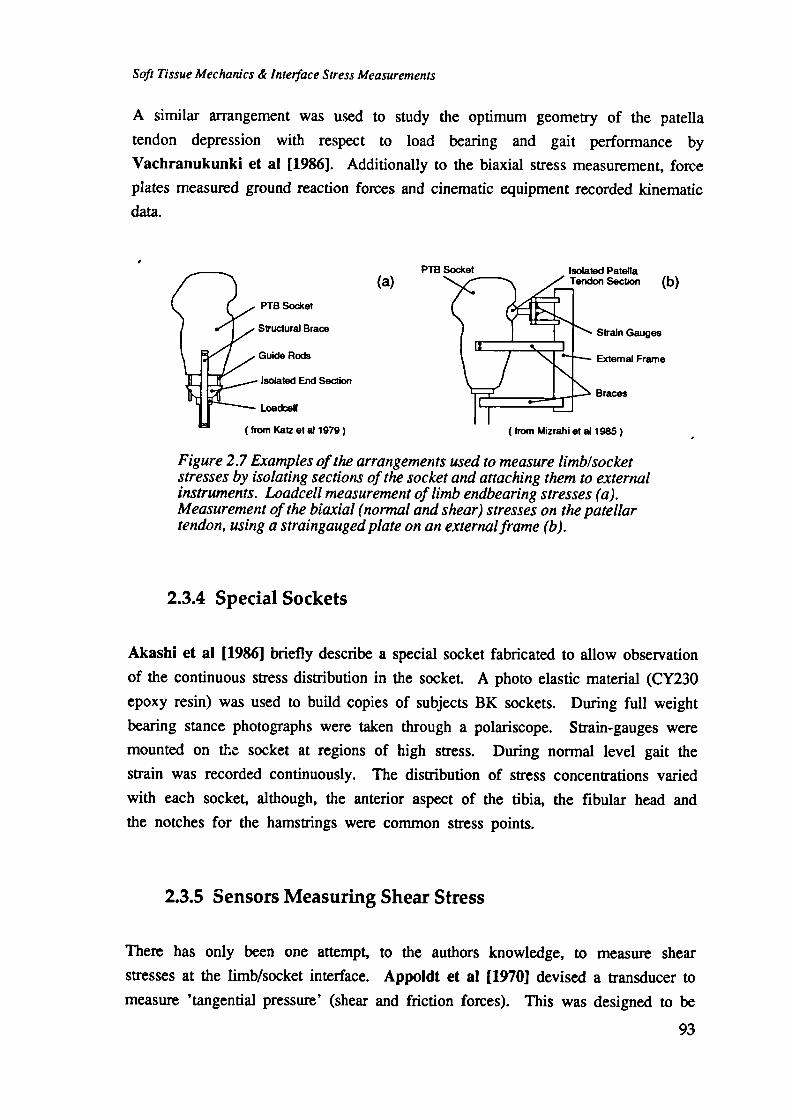
Soft Tissue Mechanics & Interface Stress Measurements
A similar arrangement was used to study the optimum geometry of the patella
tendon depression with respect to load bearing and gait performance by
Vachranukunki et a? [1986]. Additionally to the biaxial stress measurement, force
plates measured ground reaction forces and cinematic equipment recorded kinematic
data.
PTB Socket
Structural Brace
Guide Rods
Isolated End Section
Loadcel
(from Katzetal 1979)
PTB Socket Isolated Patelta
Strain Gauges
(a) onSecton (b)
External Frame
Braces
(from Mizrahietallg85)
Figure 2.7 Examples of the arrangements used to measure limb/socketstresses by isolating sections of the socket and attaching them to externalinstruments. Loadcell measurement of limb endbearing stresses (a).Measurement of the biaxial (normal and shear) stresses on the patellartendon, using a straingauged plate on an external frame (b).
2.3.4 Special Sockets
Akashi et a) [19861 briefly describe a special socket fabricated to allow observation
of the continuous stress distribution in the socket. A photo elastic material (CY230
epoxy resin) was used to build copies of subjects BK sockets. During full weight
bearing stance photographs were taken through a polariscope. Strain-gauges were
mounted on the socket at regions of high stress. During normal level gait the
strain was recorded continuously. The distribution of stress concentrations varied
with each socket, although, the anterior aspect of the tibia, the fibular head and
the notches for the hamstrings were common stress points.
2.3.5 Sensors Measuring Shear Stress
There has only been one attempt, to the authors knowledge, to measure shear
stresses at the limb/socket interface. Appoldt et a? [1970] devised a transducer to
measure 'tangential pressure' (shear and friction forces). This was designed to be
93

Chapter 2
interchangeable with the transducers used in their earlier work, of measuring normal
stresses. Figure 2.6 describes the construction of the transducer. The sensing face
is circular with a narrow slit cut across the circumference. A bar 1.6mm wide is
held centrally in the slit by two thin steel deflection beams (4.76 x 0.41mm). Foui
strain gauges on the beams measure the deflection due to applied tangential forces.
The transducer was rotated 90% on successive trials in order to measure both
horizontal and vertical 'tangential pressures'. Calibration of the device was by
applied static loads in the normal and shear planes. The maximum error from
linearity, hysteresis and crosstalk moments from normal stresses was less than 0.2psi
(1 .4 kPa). However, a limit of 0.4psi (2.8kPa) was established as the minimum
reliable measured stress. Two middle aged AK amputees had copies of their normal
sockets (suction type) fitted with 10 to 15 transducer test sites.
Other attempts to measure shear stress fields at the body/support interface are those
reported by Bennett et al [1979], Tappin et al [1980], and Pollard et al [1983].
To study the effectiveness of combined shear and normal stresses in occluding skin
blood flow - at the thenar eminence - Bennett et aJ [1979] developed a four sensor
device (2 normal, 1 shear, 1 blood flow). Both the shear and normal stress sensors
were the strain-gauged cantilever beam type [see Figure 2.8] and monitor adjacent
areas of tissue. A small pad on the end of each cantilever beam, sits flush with
the surface of the body of the device - a 77mm diameter aluminium cylinder.
Strain-gauges mounted on the lower section of the cantilever beams converts the
beam strains into electrical signals. The maximum displacement of the sensing
surface of the shear-stress beam was 0.025mm. Calibration was by dead weight
loading. Shear stress interaction on the normal stress beam was less than 6%.
Normal stress interaction on the shear stress beam was negligible. No further error
sources or accuracy values were given.
A small single axis shear stress sensor was developed, for plantar stress studies,
by Tappin et al [1980] and Pollard et al [1983]. Although, later Pollard added
a commercial strain-gauged normal stress sensor (un-named : Kulite Inc. USA) to
the top of the shear stress device, in order to record simultaneous normal and shear
stresses. These devices were specifically designed as low profile sensors suitable
for inserting in shoes or placing under bare feet. Figure 2.8 shows a plan view
and exploded assembly sketch of the shear stress transducer. This device is formed
from two stainless steel discs bonded together by an elastic medium (silicone rubber).
94

15.96mmStainless SteelDiscs
Magnet
Lead PCB
I 2.7mm
Sicone Rubber (b)
ova
3.175m,j
2mm diaMagnet
(Irom Tsn et 1960)
Soft Tissue Mechanics & Interface Stress Measurements
e........
Svain Gauges
(from Bennett et ai 1979)
'hear Stress Sensor
(a)
Figure 2.8 Shear stress sensor mechanisms employed in non-prostheticbody/support interface stress studies. Cantilever beam biaxial (normaland shear) stress sensor used on the thenar eminence (a). Single axisdevice sensing shear by measuring the amount of stretch in a siliconerubber layer (b). A magnet - magnetoresistor pair detect thedisplacement between discs bonded either side of the rubber layer. Thisdevice was employed to measure stresses at the plantar interface.
A ridge across the diagonal of one disc locates into a groove cut across the diagonal
of the other disc. The effect of these are to restrict relative displacement of the
discs to being along the axis of the ridge. The silicone rubber elasticity acts
against the shear force applied between the discs, causing them to displace relative
to one another. A magnet is fixed into one disc and a differential magneto-resistor
fixed opposite it on the other disc. The relative displacement of the discs, and
therefore applied shear force, is detected by a change in the magneto-resistor
resistance as the magnet is moved across it. Calibration was by dead weight
loading. The device response to load was stated as linear, up to 40N. Frequency
response was assessed by observation of the impulse response and found to be of
the order of 500Hz.
95

Chapter 2
2.3.6 Concurrent Studies
With the exception of the work of Mizrahi et a) [1985] and Vachranukunki et
a) [1986] all previous studies of interface stresses have employed uniaxial transduction
devices. Also only Appoldt et a) [1970] have attempted to measure shear stresses
at the limb socket interface. The author was attempting to address the lack of
simultaneous multiaxis data by the development of a triaxial transducer to measure
both normal and planar shear stresses. However, the author has since discovered
that during the course of this development, concurrent work by Sanders et a)
[1989, 1990, 1992] was being undertaken. Their device is described in Figure 2.9.
A strain-gauged diaphragm for detection of normal stresses is fixed on the end of
a cantilever beam, which detects biaxial shear stresses. A disc of liner material
is affixed to the end of the diaphragm and the transducer inserted through a hole
cut in the socket wall until it is flush with the inner socket face. The diaphragm
6.4mm diameter by 0.17mm thick. The cantilever beam was 1.6mm square.
Calibration was by static loading. Nonlinearity and crosstalk for the shear axes
were less than 1% and for the normal axes less than 2%. The largest errors were
from cable motion during gait - 5%. However, due to the length of the device,
measurements at the medial aspect of the prosthetic socket are highly improbable.
Socket SWain Gauges j Mount Electrical Connector
Liner A I I KiN fl /
Normal Stress Sensor
Shear Stress Sensor
I\\Shield LJ2LJ
(from Sanders and Daly 1989) Deflection Beam Locking Nuts
Figure 2.9 Triaxial stress transducer developed by Sanders and Daly(1989] concurrently with the authors. A strain gauged beam detects twoorthogonal axes of shear stress. Normal stress is measured by astraingauged diaphragm mounted on the end of the beam. Thetransducer is inserted through a prepared hole in the socket wall.
96

Soft Tissue Mechanics & Interface Stress Measurements
2.3.7 Discussion
The following discusses the suitability of incorporating the mechanisms, previously
used to transduce interface stresses, into the three axis stress sensor being developed
here.
Although the pneumatic cells developed/used by NaefT and Van Pijkeren [1980],
Krouskop et a) [1987] and Barbenel and Sockalingham [1990] are robust and
thin, they have potential error sources which have not thoroughly been investigated:
their sensitivity to temperature and shear stress have not been evaluated; the curvature
of the interface may cause a zero-load pressure offset; compression of the lead
tube may produce artifacts, especially as the lead volume is comparable or greater
the chamber volume; chamber collapse under local stress concentrations will affect
device linearity; vertical elevation of the (fluid filled) sensor above the external
transducer will produce hydrostatic pressure errors; the frequency response of these
devices may be lower than the bandwidth of the measurand; and the electro-pneumatic
type device used by Krouskop et a) [1987] is only quasi-continuous as it is
dependent on the rate of the inflation cycles.
In the context of the three axis transducer required here it would be practical and
cost effective to use a common transduction mode for all axes (i.e. all
mechano-pneumatic or all mechano-electric). Currently, no mechano-pneumatic
transducers exist for the measurement of shear stresses, whereas devices using a
mechano-electric principle do exist. For this reason and the above known problems
mechano-pneumatic transduction sensors were less preferred than mechano-electric
ones.
The stress sensitive variable capacitors developed/used by Monster [1972], Meier
et a) [1973] and Ferguson-PeH et a) [1976] are compact thin devices that have
been proven to be effective. They can be designed to have a linear stress response
by employing a dielectric with linear compression characteristics and using a three
plate configuration. These devices exhibit a compromise between mechanical stiffness
and stress sensitivity. Their temperature coefficient is dominated by that of the
dielectric, which can be made extremely small, and they are inherently low noise
devices - as the series-equivalent resistance is negligible. However, because the
output impedance of the device is usually high, shielding is required on cabling
97

Chapter 2
connecting it to the signal electronics. This may make the cabling of a three axis
device complex. Also, consideration must be taken to restrict the device motion
to compression as it may be shear sensitive.
Variable resistance strain sensors (strain gauges) are widely used and their technology
is well understood. They have an inherently high natural resonance (10-100kHz),
which is normally dominated by the resonance of the structure on which they are
mounted. They are accurate, repeatable sensors with low shear, temperature and
humidity sensitivity and good long term stability. Their low electrical impedance
also imbues them with low noise sensitivity. Their small size has made them
popular in prosthetics applications [Appoldt et a) 1967, 1968a, 1969, 1970; Sonck
et at 1970; Rae and Cockrell 1971; Pearson et a) 1973, 1974; Burgess and
Moore 1977; Redhead 1979; Katz 1979; Mizrahi et a) 1985; Vachranukunki et
al 1986; Steege et at 19871. Their manufacture is specialised so they are generally
purchased in a kit form which allows them to be mounted with 'in-house' skills.
However, very careful design and precise manufacture needs to be employed for
the elastic straining element on which the gauges are mounted. These devices are
widely implemented as strain-gauged diaphragms which are designed to measure
hydrostatic pressures and will not specifically measure the contact pressure of solid
media accurately. Although, the non-hydrostatic pressure measurement errors may
be overcome by suitably arranged indentor mechanisms. Additionally, the device
aspect ratio must be low to avoid indentation of the limb tissues at the interface,
unless they are recessed into the lining or socket wall.
Although magneto-resistor sensors detect changes in the magnetic field applied to
them, simple mechanical arrangements can translate mechanical stress to field strength,
thus indirectly transducing stress to resistance. Devices based on these sensors
have the similar advantages and disadvantages as strain gauge devices.
Another device type commonly used to measure stresses at other body/support
interfaces is the compression sensitive variable resistor, also known as Force Sensing
Resistors (FSR). This has conductive particles imbedded in a compressible substrate
material, such that its resistivity is inversely related to the applied compressive
strain. The stress-strain relation for the material is usually non-linear and may
exhibit time-dependencies. An evaluation of the accuracy and properties of two
leading FSR systems (Interlink Electronics Inc. USA and Teckscan mc, USA) was
98

Soft Tissue Mechanics & Interface Stress Measurements
published by Cardi et a) 11991] and Ferguson-Pet) and Cardi 11992]. Both
systems were shown to exhibit significant hysteresis (19%, 20% respectively) and
creep rates (7%/log(sec), 11 %/log(sec) respectively).
Piezo-electric effect devices have been used to measure normal stresses at the
foot/shoe interface [Hennig et at 1982; Nevill 19911. The effect occurs in many
materials, although, the most commonly used are PZT (Lead Zirconate Titanate)
ceramics and PVdF (Polyvinylidene Fluoride) films. Their piezo-electric properties
are evoked by complex manufacturing processes. They are known to be sensitive
to normal and shear stresses, bending moments and temperature. Although, with
careful attention to design and calibration shear, bending and temperature sensitivities
can be minimised or compensated for. Piezo-electric devices generate very small
electric charges and require special cabling and precision amplifiers to accurately
measure these charges without distorting them. The low frequency limit of a recent
device was given as 0.01Hz [NevilI 1991] which is inadequate for the monitoring
of suspension stresses in sockets. Although shear stress can be transduced with
piezo-electric devices, their sensitivity in this mode is very low.
In chosing the transduction methodology for each axis of the stress sensor it was
prudent, for efficiency and cost, to employ transduction methods which were related
in terms of: conversion mode; support circuitry requirements; and design skills.
Also, adapting known transduction technology was preferable to engaging in basic
transduction science research. Based on the above review and discussion,
mechano-electric transduction principles were used for both the normal and shear
stress measurement sections of the tn-axial device.
In the majority of mechano-electric transduction instruments there is a mechanism
to convert, in a well behaved manner, the applied force into a mechanical displacement
or strain. It is then the strain or displacement which is measured. However, the
stiffness of the material which is strained or displaced should bear a reasonable
similarity to the surrounding materials at the body support interface. Otherwise
the measuring device may cause a significant perturbation to the stress field it is
trying to measure.
A strain gauged diaphragm was preferred for the normal stress measurement section
of the transducer. This technique, as discussed above, has been well used in
prosthetics and is an accurate, low error method that is relatively cheap to make.
99

Chapter 2
The electronics required to excite and buffer the gauges are common and inexpensive.
However, to avoid errors due to non-hydrostatic or non-concentric loading an indentor
mechanism was used.
Shear stress transduction mechanisms were not previously well explored, so several
implementations were considered. Cantilever or simply supported beams could be
made as integral members of the section body. Applied shear forces act to strain
or displace the beams laterally, and the very small strains which occur may be
measured accurately, with strain-gauge technology. However, in order to keep the
thickness of the transducer to a minimum, transverse beams and very small
strain-gauges are needed. The complexity of design and the manual dexterity
required to mount those gauges is considerable. Also, the actual displacements
which occur are also generally small, unless long beams are employed - which
would compromise the device size. In comparison, thin displacement-sensors are
available which are less difficult to handle. They generally incorporate working
ranges of 1-2mm. To utilise the range fully, larger movements are required than
are typically achieved with strained beams, so less stiff spring materials must be
used. Suitable materials to achieve this are found amongst the elastomers. Thus
it was decided to pursue the method used by Tappin et at [1980]. This implementation
would not compromise the size of the three-axis device as a whole. It is a method
of transduction that is cheap, accurate, and compact but relatively easy to construct.
It is also resistant to vibration and shock and can be made reasonably insensitive
to electrical interference. Further, the equipment and skills necessary to assemble
this device could commonly be found in the type of organisation or institution that
might use it. Additionally it had been used previously and proved effective under
simple calibration and clinical trials.
Clearly a three axes device based on these principles and technologies will not
have a suitable size or aspect ratio to be inserted between the limb and socket.
It must therefore be designed to be recessed into or inserted through the socket
wall.
100

Soft Tissue Mechanics & Interface Stress Measurements
2.4 Previous Interface Stress Measurements - Findings
It has been observed that well fitting comfortable sockets when coupled with gait
training can result in gait patterns that are very similar to normals [Sonck et at
1970]. However, there is still no consensus as to what range and patterns of
normal and shear stresses constitute comfort. Krouskop et at [1987ab] report that
amputees felt discomfort at normal stresses of lSOmmHg (2OkPa), while other
researchers [Meier et al 1973; Leavitt et at 1972; Sonck et at 1970] report
amputees able to tolerate normal stresses in excess of 400kPa. The variation in
the magnitude of sustainable stresses between amputees is due to a number of
factors, such as: stressed area; stress duration; body weight; thickness of limb tissue;
and pain threshold - all of which may be individual to the amputee. So, although
the majority of investigators describe their findings in terms of absolute units of
mechanical stress (E.g. psi, mmHg, KPa), some relate their findings to subject
parameters (E.g. percentage of their body weight or peak standing stress).
Comfort limits have been suggested for different sites on the limb. Katz et at
[1979] suggest that during normal level gait the maximum tolerable load, borne on
the limb end, is 11-55% of the total standing stress on the whole limb. Vachranukunki
et at [1986] found that subjects could tolerate up to 60% of their total body weight,
in vertical stress, on their patella tendon without pain. Investigators have even
attempted to define minimum stress levels as the functional limit of a prosthesis.
Krouskop et at [1987ab] found that when the peak normal stress (radial), in AK
amputees, fell below 12.5/cPa then significant slippage occurs.
A summary of the peak and average stresses measured at any site on the limb, by
the investigators reviewed in [2.31, is given in Table 2.1. This describes: the
number of subjects studied; the socket type; if a liner was used; the number of
sites monitored; the site where maximum stresses mainly occurred; the peak - and
(average) - normal and shear stress values observed; and if the study was on static
or dynamic stresses. Clearly, the majority of data describes the normal stresses
found at the limb/socket interface, while little is known of the shear stresses.
101

C
'.0 I- •
. )
0
C)CU,.-
UL)
C,, •
I-
I
v-o—e1
- 'I,
ln —
8'-C'
ooQc
:':zzzzzzz
U.1Jolol
C—NC'NSrOO
C'., C" C'.' C" C" C' C'. C' C'. C" O' C\ 0" 0'.'- - - - - - - - - - - - - - - -
0
L
--
Q . 'C
-
0.'.
'
'J
- '
- I_
-
E-
•
I- '
-' . I- -
CjLC'" a-
"'C"-. . 'e C'
: "
a- -
' C)
- I-
C C'a- •
I- - C_* .
C'a..' "a-
r'•.'CC
-
. '0'.'.0'.,
C I. I

Soft Tissue Mechanics & Interface Stress Measwenienzs
The peak normal stresses at the limb/socket interface, found by previous studies,
vary quite significantly - from 88OkPa [Leavitt et at 19721 to 20k_Pa [Krouskop
et al 1987ab]. The margins of the load-bearing sites and the unloaded sites of the
socket bear much lower stresses. These have been found to be: < 10% of peak
shear stress [Appoldt et at 1970]; < 15-30% of peak normal stress in AK sockets
[Appoldt et a) 1968a; Krouskop et at 1987ab]; and < 12% of peak normal stress
in BK sockets [Rae and Cockrell 1971]. In suction sockets these values may be
higher in order to create an effective pressure seal for prosthesis suspension.
Appoldt et a) [1970] and Sanders et al [1989, 1990, 1992]' are, to date, the only
other investigators to quantify shear stresses at the interface. They all indicate that
shear stresses are much lower in magnitude than normal stresses, 25-55kPa. The
coefficient of friction which sustains the shear stresses varies with site, lubrication
and subject. Sanders et at [1992] report a range of 0.01-055 while Appoldt et
at [1970] found a range of 025-0.4 with an average value of 0.3.
The general concensus of findings shows that stresses vary with: area of the limb
studied; whether dynamic or static stresses are being measured; how much muscle
activity occurs; whether liners are used; and prosthetic alignment. Thus, before
data can be compared, between workers, there must clearly be a common protocol.
By design the load transfer from limb to socket is distributed over those areas of
the limb which are thought to be load tolerant. Specific emphasis is directed at
placing a significant portion of the load through the patella tendon shelf of the
PTB socket, hence its name. However, Rae and Cockrell [1971] and Meier et
at [1973] observed that the patella tendon shelf is not always the area bearing the
largest weight. The anterodistal site (kickpoint) can often experience larger pressures
[Sonck et al 1970], highlighting the need for a well muscle padded end tibia -
constructed during surgery. Indeed, there may be other problem areas in some
patients sockets which, in error, are generating the largest stresses.
Mizrahi et at [1985] observed that approximately 33% of ground reaction forces
are directed through the patella tendon shelf. This was supported by Vachranukunki
et at [1986] who observed that about 30% body weight was supported normally
and 5% body weight supported in shear at the patella tendon shelf. They also
1 N.B. the work of Sanders et at [1989, 1990, 1992] is added here as a postscript, at the timeof compiling this thesis, for comparison of data.
103

Chapter 2
observed that subjects could tolerate up to 60% body weight in normal stress at
the site, and that gait performance and stability increased with increased load.
Stresses in sockets are not always positive in magnitude. Large negative (suction)
pressures can exist in the distal cavity of sockets. Indeed, suction sockets employ
this as a means of socket suspension during swing phase. Pearson et at [1974]
measured the persistence time of the negative pressure in the distal socket cavity
to be of the order of 16 sec during level gait. The repetitive load cycling during
gait had a pumping effect that increased peak pressure to -300mmHg (-4OkPa).
individual variations in the observed stresses, at the limb/socket interface, during
standing occur with day to day differences in socket donning or while establishing
and maintaining balance. These are, however, relatively minor compared to changes
due to muscle contraction and the inertial and leverage effects of gait [Pearson et
at 1973, Redhead 1979]. The stresses generated during gait are known to be
higher in magnitude than those found in normal standing. Appoldt et at [1969]
suggested that standing pressures are approximately 45% of peak gait pressures.
Although, Pearson et at [1973] suggests that this ratio varies with site.
The stress fields at the limb/socket interface are periodic with the gait cycle. A
peak in the field moves across and up the limb as the prosthesis is loaded at
heelstrike [Rae and Cockrell 1971]. Leavitt et at [1972] and Sanders et at
[1990] found that step to step variations in pressure are small. But, Appoldt et
at [1968a] found significant differences in the stress patterns when taken weeks
and months apart. This they attributed to socket donning procedures; fatigue;
temporary changes in stump size; and instrumentation drift.
Muscle contraction alone can alter the interface normal stress by approximately
lOkPa [Redhead 1979]. Pearson et al [1974] observed that the negative pressure
in the distal socket cavity could be increased by 16.75kPa by the tensing of limb
muscles. As the patient alters their gait pace and balance, the changes in muscle
contractions will alter the measured interface pressures. Burgess and Moore [1977]
showed that some amputees re-learn new muscle activity sequences for their gait
cycles. Some were even able to generate sufficient stresses by muscle activity to
provide socket suspension during swing phase.
Alignment of the prosthetic limb components was also found to affect observed
interface stress patterns. Appotdt et at [1968a] were of the opinion that alignment
104

Soft Tissue Mechanics & Interface Stress Measurements
variations of 5 ' which were considered large, in AK prostheses produced a measurable
stress difference but appeared not to affect the observed gait of the subject. Extreme
changes in posterior alignment, observed by Pearson et al [1973], resulted in
elevated normal stresses at the patella tendon and lateral condyles, when the subject
accelerates. But stress magnitudes during steady level gait did not seem to be
effected. The phasing or time relationship of the stress waveforms over the gait
cycle were altered, resulting in a large delay during steady gait and deceleration
steps. Extreme lateral alignment offsets also produced large magnitude variations
at some sites and resulted in waveform delays over the gait cycle.
Sonck et al [1970] demonstrated that soft liners can significantly reduce peak
pressures at the limb/socket interface during gait. Gel liners were found to be
specifically effective in this respect. They suggested that the gel liners achieve
this by uniformly distributing the load locally. A simplified mechanical theory to
support this suggestion, and substantiating laboratory experiments, were later effected
by Bennett [1974]. The suggestion is still currently accepted. However, no
experimental data is yet available on how liners may distribute shear stresses.
Of the investigators who have recorded interface stresses in BK prosthetic sockets
[Table 2.1] only Meier et al [1973] did not present representative normal stress
waveforms. The others report regular cyclic waveforms that are clearly biphasic
during the stance phase of the gait cycle. The waveform has an initial peak at
20-35% into the stance and a second peak at 60-85%. Sanders et al [1992]
suggests that the maximal stresses within the step usually occur at the first peak,
except at anteroproximal or patella tendon sites. This observation appears to be
bourne out by the example waveforms of other workers. Appoldt et al [1968a]
showed that shear stresses in the longitudinal and circumferential axes of the socket
occur concurrently with normal stresses. Also, that they too have regular patterns.
Sanders et al [1989, 1990, 1992] are the only researchers to present shear stress
data from BK sockets. They describe waveforms similar to the normal stresses
but with less pronounced biphasism. The peaks of these waveforms occurred
synchronously with those of the normal stress waves.
The frequency content of a typical normal stress waveform was calculated by Rae
and Cockrell [1971]. It was found that the relative amplitude of the spectrum
105

Chapter 2
fell below 10% at approximately 20Hz. Although, the method of calculation used
and the sample window taken from the stress curve meant that higher harmonics
appeared in the result. The true spectrum bandwidth was probably closer to 10Hz.
2.5 Temperatures in Prosthetic Sockets
To the author's knowledge no studies of the temperatures to be found in prosthetic
sockets, during ambulation, have been published. However, Ferguson-PeIL [1980]writes that Adamson [1978] states the temperature at body/support surfaces usually
varies little throughout the measurement period, within the range 32-37 t. Also,
that the difference between ambient and body temperature is significant (0-15 0C)
and requires the transducer to be stable over this range (say 17-37r)
Ferguson-Pell et al [1985] measured temperature and humidity changes between
patients' buttocks and seating cushions. It was observed that the maximum change
in temperature after two hours was 3.75C, and the maximum change in relative
humidity was 39%.
To confirm this data in relation to changes in limb/socket interface temperature
during ambulation an experiment was carried out with an active unilateral BK
amputee. A thermistor type temperature sensor (1mm diameter), was placed against
the subject's skin and the sensor lead taped to his limb inside the pelite liner in
his standard PTB prosthesis. The subject walked continuously for 400m without
resting. The temperature was recorded at the beginning of the trial and after every
lOm. Figure 2.10 describes the increase in temperature with distance walked. From
an initial value of 332 r the temperature rose to 35.4 r in an asymptotic fashion.
Extrapolation of the curve estimates the maximum rise to be of the order of 2.5 r.No change in temperature over any given gait cycle was observed.
106

Soft Tissue Mechanics & Interface Stress Measurements
37
36
035
34
0.E0 33I-
32
10 100 200 300 400
Distance Walked (mJ
Figure 2.10 Measured temperature variation at the residuallimb/prosthetic socket (BK) interface as afunction of distance walked.
2.6 Transducer Design Criteria
The initial steps in the triaxial stress transducer design process were to observe the
previously determined, or expected, nature of the measurands and then to set the
performance/geometry specification of the device. The interface stress transduction
system as a whole will be at its most useful if it is able to accurately transform
stresses into a quantifiable property which is in turn recorded in a reviewable
format.
From the discussion in [2.4] the magnitude, direction and frequency content of the
stress field may be estimated. It is known that normal (radial) stresses, mediolateral
(circumferential) and proximodistal (longitudinal) shear stresses occur at the
limb-socket interface. Previous measurements of radial stresses vary greatly in the
observed maximum magnitude, from 19.8kpa [Krouskop et at 1987] to 827kPa
(24lkPa average) [Sonk et at 1970]. Circumferential and longitudinal shear stresses
are also active, simultaneously, in a regular pattern during the gait cycle Appoldt
et at [1968a]. Appoldt et at [1970] were able to demonstrate that the shearing
stresses at the limb/socket interface are much smaller (2-8kPa) than the coincident
radial stresses. The stress sensitivity and range of the transduction mechanism, of
the sensor described here, must reflect these findings. It is recognised that where
stresses are derived from strains, there is an inherent compromise between range
and sensitivity. There is a limit to the practical range of deflections over which
107

Chapter 2
the stress-strain relationship in transduction materials is linear. Sensitivity requirements
favour soft deflection beams, however stiff beams will allow a greater range of
forces to be transduced. An additional consideration to be made in regard to
transducer stiffness, is that if it presents a significantly different stiffness than the
surrounding material of the interface region the transducer will distort the stress
field it is attempting to measure.
Because three mutually orthogonal stress vectors are to be transduced it is important
that there be three parts of the transducer device each sensitive to only one stress
vector and insensitive to the other two. Each part should also be insensitive to
other stimuli, such as temperature, humidity and chemical attack. The transformation
characteristic should ideally be linear and exhibit minimal hysteresis.
The spectral content of recorded stress signals has been derived by Rae and
Cockrell [1971]. The relative spectral amplitude was found to be significant (>10%)
only in the range 0-20Hz. Antonsson and Mann [1985] recorded the gait spectra
of 12 normal subjects using forceplates. They observed that 'no amplitudes greater
than 5% of the fundamental [frequency] existed above 10Hz, none greater than 2%
above 20Hz, and all amplitudes greater than 1% were contained below 50Hz'. Also,
99% of the power in the spectrum was below 15Hz. In order for the transducer
to respond to the rate of change of stress at the interface it must have a natural
(resonant) frequency very much greater than the expected maximum stress frequency
(50Hz). Ideally it should also be critically damped, for accuracy in following
changes in stress.
Related to the frequency response, a constant group delay response, of the system
as a whole, over the bandwidth of the measurand is desirable. In gait related
stresses, step transients occur which have a wide spectrum content, each component
of which must experience the same processing delay in order to maintain fidelity.
The accuracy of the conversion constant, or polynomial, associated with the transducer
will generally incorporate errors due to nonlinearity, hysteresis, axes crosstalk and
signal processing. Previous workers transducers have quoted accuracies of between
1% and 20%.
Calibration of the transduction device should be carried out in a mode under which
it will be employed at the interface. It is unlikely that truly hydrostatic conditions
108

Soft Tissue Mechanics & Inteiface Stress Measurements
prevail at the limb/socket interface. The agency of stress transferral is dependent
on: the proximity of bony prominences; the age and condition of the skin; the state
of muscle and fascia tissues; and the frictional properties of the interface region.
Therefore calibration techniques must mimic the way stresses are transmitted through
semi-elastic mobile material like skin. They should also provide an estimate of
the variation in transducer response to extremes of tissue compliance and to the
proximity of bony prominences. Alternatively the device could be designed to
avoid the requirement for limb tissue conformability.
Calibration data should hold for a reasonable period of time, in relation to the ease
of recalibration. The useful life time (number of gait cycles) of the transducer
must be relative to the capital cost and the ease of installation.
As friction is necessary for the formation of shear stresses, to minimise incongruity
in the stress field due to the presence of the transducer, the sensing surface of the
device must have a similar friction coefficient to that found locally at the interface.
Appoldt et al [1969] showed that when the stress transducer protruded from the
socket wall into the flesh of the limb, it indicated larger pressures (15O%-400%)
than did a flush mounted transducer. This effect tends to be greater in areas of
bony prominences or tensed muscle. It is thought that this is due to a membrane
effect. As the membrane becomes stiffer its ability to conform to protrusions
diminishes, causing a hammocking effect and thus concentrating local loading on
the protrusion. Errors due to transducer protrusion also tend to be greater when
the actual local pressure is high. This phenomena is probably due to the non-linear
stress-strain relationship of skin. At high stresses it will increase in stiffness, and
the hammocking effect will take place. Protrusion will also have an effect of the
local shear stress fields - probably significantly - although these have not been
quantified.
An evaluation of the accuracy of five small flat (2 2-6.4mm x 1mm) strain-gauge
diaphragm transducers was carried out by Patterson and Fisher [1979]. In-vitro
tests, under rubber and cloth surfaces, and in-vivo tests, under a blood pressure
cuff at four sites of the lower leg, were carried out. From the in-vitro experiments
the pressure measurement errors were least when the devices were compressed by
the rubber balloon (condom). The largest errors were found in the devices with
the smallest diameter (15% - rubber, 70% - cloth). Adding a dome of rubber to
109

Chapter 2
the sensing surface of the smallest diameter device was seen to reduce the measurement
error, although it was still significant. During in-vivo tests errors were largest
when the devices were placed over bony prominences (tibial crest) and least when
placed over soft tissue (gastrocnemius). Again the small diameter transducers gave
the largest errors. However, all the transducers performed poorly where the soft
tissue thickness was minimal. Placing a small rubber dome on the sensing surface
produced offset errors and large overestimates of applied pressure.
Ferguson-Pen [1980] attempted to analytically derive dimension recommendations
for normal stress sensors placed between the body and its support surface. The
analysis was concerned that the sensor itself did not perturb the stress field it was
measuring and that it would indicate the peak pressures imposed on it, with a
minimum of area averaging. This analysis was dependent on the mechanical
properties of the interface materials. Skin was assumed to be homogeneous, isotropic,
elastic, linear and time independent - clearly gross assumptions. Estimates of the
support surface properties were made and a 5% error in the measurement of peak
pressure was taken as acceptable. It was suggested that the thickness to diameter
ratio of 1:30 was appropriate. Where large interface stresses were to be measured
this ratio could be reduced to 1:10. Because there may be significant pressure
gradients over the interface (OikPa/mm [Kosiak et al 1958]) the suggested sensor
diameter should ideally be small (1.4mm). Although, the specified diameter here
of 14mm and thickness of 0.5mm was considered as acceptable for most low pressure
measurements (0 - 40kPa). Other considerations discussed were that: the radius
of the transducer should be small relative to the radius of curvature of the interface;
the hysteresis inherent in the device should be minimised; the frequency and
magnitude response of the device should be greater than the expected stresses; the
sensor stress response should be independent of temperature and humidity; and
safety codes, electrical and mechanical, must be strictly adhered to in order to avoid
possible hazards.
Summary
Small diameter, low aspect-ratio transducers would cause less disturbance and more
accurately reflect the peak pressures to be found at the body/support interface
[Ferguson-PelI 1980]. Patterson and Fisher [1979] also demonstrated that small
diameter, high aspect-ratio transducers were most likely to produce greater errors
than larger diameter, low aspect-ratio devices. Also, significant errors occurred
110

Soft Tissue Mechanics & Interface Stress Measurements
when any device was placed over bony prominences. These findings are confirmed
by Appoldt et al [1969]. As it is unlikely that a three axis transducer could be
made into a small diameter, low aspect-ratio package, the above difficulties could
initially be avoided by designing the transducer to be recessed into the socket wall.
The active face of the device being made flush with the inside surface.
By creating a predefined actuator for the normal stress section of the transducer,
the problem of skin surface conformance was avoided. Also, to ensure friction
and stiffness uniformity across the interface region, a layer of the interface material
was bonded to the active face of the transducer.
Table 2.2 lists the major performance specifications to be aimed at during the
design process.
Parameter Shear stress seetion Normal stres' sectwn
Mea,w-ement RanRe 0-250 KPa 0-500 KPa
Withstand Overload 500 KPa 1000 KPa
Acewacy The greater of: ± 5% indicated load or 2.5 KPa
Temperature Rane 20-40 'C
Frequency Range 05 mHz - 500 Hz
Lfètime (gait cyde) 20000
Dimens1rns : 15 mm diameter x 5 mm
Mass <lOg
Table 22 Proposed peiformance speccation for the triaxial stresstransducer.
Without much shear stress data from other investigators it was difficult to create
a definite specification for the shear transducer. The values given in Table 2.2
represent conservative estimates for the expected shear stresses at any body/support
interface. Those stresses found at the foot/shoe interface were most likely to be
the greatest experienced by the body in its daily activities. Thus the measurement
range for the shear stress transducer was an estimate arrived at from a consideration
of the work of Pollard et al [1983]. From the results of studies on normal stresses
111

Chapter 2
found at other body/support interfaces, the value given in Table 2.2 for the
measurement range was a compromise between range and resolution. Although
Sonk et al [1970] observed stresses outside this range, those were extreme values
and it was felt less important to measure accurately their magnitude than it was
to record their presence. Thus, to allow for their presence to be recorded the
overload range was set to be greater than their magnitude. Also, it was felt that
resolution at the lower ranges was important. The overload value was the maximum
load up-to-which the transducer can be subjected without permanent damage or
requiring recalibration. The measurement range was the expected range within
which almost all of the stresses found at the body/support interface will fall. They
included errors due to nonlinearities, hysteresis, creep and temperature sensitivities.
The accuracy figures given were targets to aim for. It was felt that data accurate
to better than 10% was adequate for early research work. However, it was thought
that 5% was achievable with the facilities available to the author.
The temperature range defines the temperatures over which the transducer calibration
was to be constant. The expected range of temperatures at the limb/socket interface
was approximately 32-37 V. While the temperature variation during a clinical trial
was not expected to exceed 2.5 V [see 2.4].
Frequency considerations were based around the frequency spectrum of gait cycle
stresses and the period of typical clinical measurement sessions. Antonsson and
Mann [1985] found that there were no significant frequency components in gait
above 50Hz. Thus, as the frequency response of the transducer should be much
greater than that, a factor of ten was used to set the upper limit. The lower limit
was arrived at from a composite argument. Firstly, for accurate quantitative stress
measurements the transform characteristics of the sensor was to be stable during
the measurement period (approximately 20-30 minutes). Secondly, if the device
suffered from plastic (irreversible) deformation under stress, then to maximise the
period between calibrations, this deformation must be very slow. Thirdly, there
was strictly no such thing as 0Hz, although practically speaking stress measurement
devices are available with extremely stable characteristics. Thus, the lower frequency
limit was set to the longest expected clinical trial period, and was viewed as the
maximum acceptable value to aim for.
112

Soft Tissue Mechanics & Interface Stress Measurements
Values placed on the device's size and weight were only given as reasonable
estimates based on minimising the weight of a transducer array and a compromise
between construction complexity and radii of curvature in sockets.
The lifetime of the device reflects the period between calibrations (if complex) or
major reconstruction. It is given in gait cycles and represents a period of over
100 clinical trials.
113

Chapter 2
114

Chapter 3Triaxial Stress Transducer
- Prototype Design
Chapter 2 reviewed of the methodologies used by previous researchers and discussed
other options for stress transduction mechanisms which could be employed in a
transducer for this application. These are summarised in the discussion of [2.3.7].
Based on these reviews two mechanisms for the transduction of a) shear stresses
and b) normal stresses were selected. This chapter details: the principle mode of
operation of each of these mechanisms; and details the design considerations and
initial development stages of transducer to meet the performance specifications
proposed in [2.6].
Each axis of the transducer is essentially self contained and thus the overall device
can be thought of as the combination of three separate sections. For this chapter
the transducer will be referred to as two subassemblies; a biaxial shear-stress section
and a uniaxial normal-stress section. An overview of the principle of operation of
each section is presented in different divisions of the chapter [3.1 for shear section
& 3.2 for normal section]. The chronological sequence of the many implementation
and appraisal phases of the transducer development is summarised into three designstages:
a) the section design, operating principles, and the initial component
selection for a prototype device;
b) the performance appraisal of the prototype and component reselection;
c) and final device perfonnance tests.
The first stage is described here in Chapter 3 while the latter two are presented
in Chapter 4.
3.1 Shear-Section Design
The following presents the general design of the section of the transducer which
converts shear stresses into electrical signals. It describes the principle of operation
115

Di
Chapter 3
of this section and reports the process of selection of components for a prototype
device. Details of the assembly equipment and procedures for the prototype are
also given.
3.1.1 Principle of Operation
The sensing element is a semiconductor resistor (magneto-resistor) whose resistance
varies with the strength of any magnetic field applied perpendicular to its face.
The element is formed as two identical active regions connected in seiies with a
centre-tapped output termination. It is a three terminal device whose output is
proportional to the difference in magnetic field between the two active regions on
the element, If a small magnet is suspended in close proximity and centrally above
the element then its output will be half its input. Figure 3.1 is a schematic of
this arrangement to illustrate this concept. Any lateral displacement of the magnet
will alter the ratio of magnetic field experienced by the two active regions, and
hence the element's output will change in proportion to the movement. Moving
the magnet in one direction will have the effect of increasing the output, whilst
movement in the opposite direction will decrease the output. Thus the direction
and distance of any displacement of the magnet can be observed.
Figure 3.1 Principle of shear stress transduction using magneto-resistiveelement and magnet. Lateral displacement of the magnet changes theresistance of one active area of the element with respect to the other.This alters the ratio of the output to input.
The magnet is fixed into the centre of a rigid disc and the magneto-resistor (MR)
fixed into the centre of another. The two discs are arranged parallel to one another
with a fixed separation. They are then coupled together by an elastic medium that
acts to maintain the discs central to each other. When a sliding/shearing force is
applied to the discs it acts against the elastic medium and displaces one of the
116

Element Dtsc
Rb
Magnet DIsc
Element DIsc
Tn axial Stress Transducer - Prototype Design
discs a distance proportional to the applied force. This displacement is sensed by
the magnet/element combination by causing the output of the MR to change in
magnitude proportional to the displacement of the magnet and in sign relating to
the direction of the applied stress.
Each magnet/element pair is uniaxial. That is, the element output will only change
when the magnet is displaced transversely (movement away from one active region
toward the other). To enable the overall transducer to discern the direction and
magnitude (vector) of the stress component parallel to the shear plane, it is necessary
to have at least two of these shear transducing elements at a fixed orientation to
each other. The most effective way of achieving this is to fix the two elements
orthogonally, and to restrict the relative motion of the magnet to be transverse to
each element. This was accomplished by fabricating, a central ridge on the magnet
disc and a corresponding groove in the element disc. When these are located the
discs are mechanically constrained to slide over each other along one axis only.
The second element is identical but the ridge and groove are orthogonal to the
first. The magnet for the second axis is the opposite pole of the magnet for the
first axis. An exploded assembly of the biaxial shear section is shown in Figure
3.2. and a schematic of it fully assembled is shown in Figure 3.3.
In using the sliding disk method of shear-stress transduction there are two fundamental
mechanisms operating. The first is the conversion of the applied shear stresses
into a displacement, via the elastic or spring material. The second is the transduction
of displacement into an electrical signal. During the initial survey and design phase
these were treated separately. Each being assayed and selected according to the
predominant attribute they were required to have.
Figure 33 Schematic offully assembled biaxial force transducer.
117

Outer Disc
(element)
Chapter 3
Ouer Disc
(e4ement)
Rubber
Middle Disc
(magn)
Rubber
Figure 3.2 Schematic of the exploded assembly of the two shear sections.
3.1.2 Force to Displacement Conversion
The primary requirement of the first mechanism in the shear section is to provide
a reproducible restoring force that opposes the applied shearing stresses. It must
be truly elastic, that is, it must have a fully recoverable strain on release of the
applied force. It should also usefully have a linear stress-strain relation. Or simply
put what is required is a material that obeys Hooke's Law at large deformations.
The useful measurement range of suitable commercial displacement-sensor elements
118

Tn axial Stress Transducer - Prototype Design
was 1-2mm. The maximum expected clinical force range was approximately ±50N,
indicating a target stiffness of the elastic material of 25-50N/mm. To meet that
requirement in a compact size, elastomers was considered for their suitability.
The following subsections discuss the effective limitations of using an elastomer as
a Hookean spring under static and dynamic stresses. This is followed by the
selection of the most appropriate type for this application.
3.1.2.1 Rubber as a Spring
In leading up to the decision to utilize elastomers as the springing material, an
investigation into their theoretical physical properties was carried out. The following
section summarises the findings of these investigations.
The term 'Rubber' is commonly used to describe any material that can sustain
large elastic deformations (strains), typically of the order of 500 to 1 000%. These
materials include synthetics such as Teflon, Butyl rubber and Silicones, and naturals
such as natural-rubber (polyisoprene), wool, silk and muscle. Figure 3.4 illustrates
the structural formulae of the monomer units of some rubbers. Rubbers are members
of the class of high polymers which are constituted of very long chain molecules
that are both chemical interlinked and physically tangled at sparse irregular intervals.
Figure 3.5 illustrates the concept of sparse cross-linking and tangled chains.
91.- CH. - C = CH - CH. - Polyisoprene (Naturai Rubber)
— NH — CH — CO — NH — CH — CO -
Protien (Wool, Silk)
RCH. CH.
— CH, — - CH. - c - Polyisobutylene (Butyl Rubber)
CH, CH.
4. 94.
- I - 0 - i - 0 - Polymethylsiloxane (Silicone Rubber)
CH. CH.
Figure 3.4 Schematic of the structural formulae of some typical elastomermaterials (after Treloar (1958]).
The foundations of the theory relating the molecular structure of rubbers to their
elastic properties were postulated by Meyer, von Susich and Volko as reported in
Treloar [1958]. They considered that the thermal or kinetic vibrations of each
119

Chapter 3
eIlIIIU..Ul LU PP.
Figure 3J Schematic of the cross-linking and tangling between molecularchains of an amorphous polymer.
molecular chain tended to repel its neighbour and draw the ends of the chains
together. This retraction occurs until an equilibrium is reached where the chains
have a random statistically determinate arrangement and there is no nett force.
These ideas were developed to formulate a statistical kinetic theory based on the
configurational entropy of the chains. The assumptions of this theory were that
the rubber was amorphous, isotropic and incompressible and the distribution of
chain lengths between cross links is statistically related. All of which hold well
for most rubbers. The kinetic theory accounted satisfactorily for the observed
mechanical behaviour at equilibrium under relatively large elastic deformations. It
also implies that the stress and strain relations can be simply derived from the
equation for the elastic stored energy per unit volume. This energy is a function
of the strain and one physical parameter or elastic modulus that is soley determined
by the degree of cross-linking in the material Treloar [1958].
W = (3.0)
Where W is the work of deformation or the elastically stored force energy per unit
volume of the rubber. Here, (A, A,,, A) are the principle extension ratios along
three orthogonal axes, and G is the elastic modulus.
This theory enabled the prediction of elastic behaviour of any rubber under all
modes of strain [E.g. tension, compression, shear]. Table 3.1 shows the form of
the stress strain relations for each mode, as calculated by the statistical theory. In
its simplest form it assumes that the separation distances between each end of a
chain is as a Gaussian distribution. This assumption holds as long as the rubber
is less than moderately stretched.
120

Tria.xial Stress Transducer - Prototype Design
• Approx Seres$trainRelationship
Simple Elongationt = G - 1)
2D Extension/Compression= G (2 - 1)
Simple Shear
Pure Sheartx=G(2_)
________________________ t=G(1—)
Table 3.1. Theoretical stress-strain relation for rubber's subjected tomoderate deformations. Determined from the statistical kinetic theoryassuming a Gaussian network.
The most significant point to note from Table 3.1 is that the Gaussian form of the
theory predicts that in rubber, strain is proportional to the stress only in the simple
shear mode. This is not the case for the other modes of deformation. Treloar
[19581 in a review of his early work showed that the experimental data conforms
quite closely to the theoretical values up to about 100% strain. This is also
described by Lindley [1978]. Figure 3.6 is an example of Treloar's data for
natural-rubber under shear.
' 20
IS
12
a
0 I 2 1 4 S
Shear Strain
Figure 3.6 The relation of shear stress to shear strain for a sample ofNatural rubber. The theoretical line is calculated from the statisticaltheory assuming a Gaussian network (after Treloar (19581).
121

Chapier 3
It is noted here as an adjunct that the assumption of a Gaussian distribution of
chain lengths is only valid for moderate deformations. Other non-Gaussian statistics
and internal-energy theones conform much closer to experimental data even at very
large deformations. However, it may be sufficient in this case to use the simpler
model to interpret any observed behaviour in the proposed transducer.
In summary, under equilibrium conditions rubber subjected to moderate simple shear
deformations may behave like a Hookean spring. Furthermore this behaviour may
be predicted and understood in a broad sense at the molecular level.
3.1.2.1.1 Rubber in Simple Shear
In general a cylinder of rubber that is subjected to a shearing force will experience
both bending and shearing. Love [1943] and Southwell [1953] described how that
if the total deformation is small compared with its diameter the conditions are
similar to that of a loaded cantilever beam. The theory of superposition of the
displacements, due to both mechanisms, will then hold provided certain end conditions
are met. Figure 3.7 shows the situation that most closely approximates that found
in the shear stress transducer developed here. Where: t is the thickness of the
rubber layer (which has an area, A); x is the total deflection caused by the applied
force, F.
The total deflection is found by [Rivlin and Saunders 1949]:
1+ I (3.1)X = Xb+XS=f{t2
36K2)
Where Xb and X are the deflections due to bending and shearing respectively, G
is the shear modulus of the material and K is the radius of gyration about the
neutral axis of bending.
For a cylinder K = r/2 where r is the radius of the circular section. Therefore for
cylinders where the radius is very much greater than the thickness t2/9r2 c 1 and
the conditions in the rubber approximate to:
FtX = (3.2)
122

Tn axial Stress Transducer - Prototype Design
This means the displacement of the discs is approximately linear with applied
shear force, and (3.2) represents a Hookean relationship. This is the desired property
of the restoring force in the shear stress transducer.
-x--
_____ F
Figure 3.7 Sclzematic showing two rigid plates bonded by a rubber layerof thickness t and subjected to a shearing force, F. The resultantdisplacement is the distance x.
3.1.2.1.2 Rubber in Compression
An important property of some rubbers in this application is their very high bulk
modulus. This means that it will exhibit only very small volume changes under
compression load. Therefore, the rubber will attempt to displace or bulge. For
rubber discs with a high diameter to thickness ratios there is very little unbound
surface to do this. Thus the shape is virtually incompressible, and any normal
stresses applied to the top of the shear section will be transmitted unchanged to
the normal section. Also, magnet/magneto-resistor separation will remain relatively
constant under normal stresses [see 3.1.3].
3.1.2.2 Time Domain Behaviour of Rubber
The previous discussion considered only the equilibrium behaviour of Rubber, that
is, its response after a period of minutes under stress. In this particular application
it will be necessary to be able to accurately measure stresses that may vary at
rates up to about 50Hz. Therefore the behaviour of rubber in the short time scale
must be investigated.
123

Chapter 3
In practise when a rubber is subjected to a given stress the observed deformation
shows three phases [Ward 1971]. There is an immediate elastic phase (el), then
a time dependent continued deformation (e2) where the rate of strain decreases.
This is followed by a stage (e3) where the strain rate becomes insignificant and
the strain settles at some equilibrium value. These stages are illustrated in Figure
3.8. In the case of an applied constant strain, stresses are set up in the material
instantaneously. These then decay away at a rate which decreases until they reach
some equilibrium value.
Applied SVess
Apd Sn
Resultant Strain_J/ a2
Resultant
a)
b)
Figure 3.8 Schematic of the response of a viscoelastic solid to a)constant stress and b) constant strain. Each response has three arbitraryphases; during el there is an immediate elastic deformation; during e2the deformation is time dependent; during e3 the rate of deformation isinsignificant and equilibrium is achieved.
Toboisky and Andrews [1945] investigated the form of these phenomena and
showed that the rate of decrease of either strain or stress conforms to an approximate
exponential function of time. These cases are known as 'creep' and 'stress relaxation'
respectively and for rubbers the overall process is reversible.
It is clear from this observed behaviour that there is a time dependent compliance
in rubbers under load. Mullins [1947] in his study of the resilience of rubbers
(i.e. its capacity to store and return energy under rapid deformations ) showed that
their response is more intimately related to the molecular structure than the gross
structure of the material. In general, when stressed, rubbers may behave like glassy
solids, viscous liquids or ideal elastomers dependent on the time scale of loading.
The three phases of the creep-type deformation , as outlined above, can to some
extent be related to the dominance of the following molecular mechanisms [Billmeyer
1971]. During very short periods following the applied stress the rubber tends to
act as a glassy solid, exhibiting Hookean elasticity. Here the main mechanism of
124

410
U
Tn axial Stress Transducer - Prototype Design
material deformation is bond stretching and bond rotation. This results in very
low compliance and deformations of only a few percent. After longer periods the
sections of the molecules between crosslinks and entanglements are able to uncoil.
The effective compliance of the material in this phase is much higher. Deformations
of several hundred percent are sustainable. For intermediate times the material is
in transition between the other two phases and both mechanisms are operating. The
compliance here is time dependent and akin to viscous flow. Although in all
phases the deformation is reversible. A simplistic representation of the compliance
variation with load time can be seen in Figure 3.9. The division between the glass
and rubber states may be arbitrarily characterized by a transition time, T, which
relates to the time required for the molecules to change their configurations.
Figure 3.9 Schematic of the change in compliance of an idealised rubberas a function of time under load. T may be defined as the characteristictime constant of the material ( after Ward (19711).
If it is assumed that any incremental stresses applied to the rubber make an
independent contribution to the strain then it can be said to be linearly viscoelastic.
It is possible,then, to represent its behaviour by means of idealised spring-and-dashpot
mechanical models. In its simplest form stress-relaxation may be expressed by the
equations of state of a Maxwell element or model, which represents a liquid that
has elasticity. Similarly creep deformation can be modelled by a Voigt model and
represents a viscous solid. Both of these models are described in Figure 3.10.
It can be shown that the equation governing the stress strain relations in the Maxwell
model has the form [Ward 1971]:
125

(3.6)
(3.7)
Chapter 3
V//i/h/A
y////////J
a) b)
Figure 3.10 Schematic of the mechanical models used to represent theviscoelastic behaviour of rubbers, a) the Maxwell and b) Kelvin or Voigtelements (after Ward (19711 ).
e = l.a(3.4)
m m
Where the stress a = a1 = a2 and the strain e = e1 + e2. E,,, is the modulus of the
spring and Cm is the viscosity of the dashpot. This is of value in modelling stress
relaxation, where under constant applied strain, E =0, the solution to (3.4) describes
an exponential decay of stress with time:
Emt —ta = a0exp Cm = a0 exp— (3.5)
Here a0 is the initial stress at t=0 and the characteristic time constant of the decay,
t = Cm/Em is called the relaxation time. However under conditions of constant
stress, a = 0, (3.4) resolves to
ae=--
describing constant flow. This is not true for creep behaviour in rubbers.
The Voigt alternative model is governed by the equation:
a = Ee+CE
Here e = e3 = e4 and a = a3 + a4. E is the elastic modulus and C the viscosity.
The solution of (3.7) under conditions of constant stress, a = a0 , is found to be:
a0 ( -Ete = l-exp--- (3.8)
I-_V )
—t=
126

Tn axial Stress Transducer - Prototype Design
Where t' = C/E is the characteristic time constant referred to as the retardation or
orientation time. Equation (3.8) describes, to a first approximation, the observed
creep behaviour of rubber. However its representation of stress relaxation behaviour
is inaccurate. Under these conditions è =0 and the solution to (3.7) is:
a=E,e
(3.9)
which describes constant stress.
Kuhn [1954] proposed that the behaviour of real materials can be modelled using
a distribution of time constants. This may be thought of as a network of Maxwell
or Voigt elements each with their own unique time constant. Under this theory
it is still possible to represent the material's behaviour, to a first approximation,
by using a single element which has a time constant that is the mean value of the
distribution.
So it can be seen that to a first approximation a Voigt model can be used as an
analogy for creep behaviour while the Maxwell model describes stress relaxation.
3.1.2.3 Frequency Domain Behaviour of Rubber
For a more complete assessment of the suitability of the use of rubber as a spring
it will be useful to expand briefly on the time domain concepts of the previous
section. Here, the viscoelastic phenomena will be considered as a function of the
frequency of applied stresses. It can be easily seen from the creep curve of Figure
3.8 that there is a time delay between maximum applied stress and the maximum
strain. If the rubber sample is subjected to a sinusoidally varying stress then, under
equilibrium conditions, the strain will vary sinusoidally but with a phase lag. So
the stress and strain forms can be written as:
e = e0expicot
a = a0 expi(ot—) (3.10).
Then a modulus of shear G can be defined where
127

Chapter 3
0 - 0,- - —(cosö–zsin6) (3.11)e e0
= G1–iG2
=G
The shear modulus can be described as having a real in-phase component, G 1 , and
an imaginary out-of-phase component, G2. These are related to the elastic and
lossy or resistive components of the deformation, respectively. The amplitude of
the resultant displacement is then determined by the modulus of G or:
JGJ = \iG?+ G (3.12)
While the phase angle between the loss modulus and the elastic modulus is given
by
8 = tan 1G2
(3.13)
It is also possible to define a loss factor tan 8= G2/G 1 which is a measure of the
fraction of energy lost. For most rubbers this loss fraction is small, of the order
of 0.01. As before, it is possible to represent, to a first approximation, the dynamic
behaviour of rubber with a Maxwell or Voigt model. For example, using the Voigt
model to approximate creep processes it has been shown that [Ward 1971]:
G1 = E' 2 (3.14)
(UtG2 = E 12 (3.15)
cvwhere t = -
E,,
Figure 3.11 represents these parameters as a function of frequency, for a typical
rubber.
These relationships imply that during the viscoelastic phase where the resultant
strain lags the applied stress, there will be uncertainty in deriving the causative
stress from a simple observation of the strain. Furthermore this uncertainty wifi
vary with rate of applied stress as the phase lag is a function of frequency. This
concept can be best illustrated graphically as in Figure 3.12. The hysteresis loops
describe a maximum uncertainty when the phase lag is it/4 and it becomes a
minimum where there is zero lag.
128

a
C
0
-ø0
C
Cl)
.00
C
Cl)
.00
Tn axial Stress Transducer - Prototype Design
Log W
Figure 3.11 Schematic of the shear modulus variation (G * = G + G 2) asa function ofstressfrequencyfor a typical rubber. G is the elasticcomponent and G 2 the lossy component of the modulus. Tan d is ameasure of the proportion of energy lost during a loading/unloading cycle(after Ward [1971]).
Applied Stress Applied Siress Applied Stress
a) b) C)
Figure 3.12 Uncertainty of deriving the causative stress from the observedstrain, where the strain lags the stress by a) 0, b) 7t/8, c) 7t/4 undersinusoidal load cycles.
Theoretically it may be possible to derive the causative stress from an observed
strain history, provided that the form of dynamic modulus is known for all frequencies.
However, the complexity of the signal processing required and the complete
characterisation of the material make this impractical. The form of the loss modulus
predicts that: below the transition frequency of the material there will exist a
frequency at which ther will be no viscous hysteresis; whereas the hysteresis in
real rubbers will not diminish to zero at any frequency. It is suspected that this
is due to finite energy losses during the changing of molecular orientations and
the breaking (and reforming) of short links and chain defects. In general this form
of hysteresis is quite small compared to the maximum viscous hysteresis and is
more closely proportional to the amplitude of the deformation.
129

Chapter 3
In summary at frequencies where a rubber exhibits elastic or glassy behaviour it
will have a single modulus of elasticity (compliance). Under cyclic stresses there
will be small hysteresis losses related to the stress magnitude. Additionally in the
elastic region (low frequencies) creep processes will cause a variation in observed
strain with frequency of applied stress. However in the viscoelastic region the
modulus is frequency dependent and the observed strain will lag behind the applied
stress to a significant degree. This lag which increases with frequency will be the
cause of increasing uncertainty in deriving the magnitude of applied stress from
observation of the strain in the material. Therefore in this application it is practical
to use rubber as dynamic spring material provided a suitable type is chosen which
exhibits a transition frequency above those of clinical interest.
3.1.2.4 Useful Types of Rubber
The above sections discussed the suitability and restrictions of the use of rubber
(elastomer) as a spring in the shear-section of the required transducer. The following
is a resume of types and properties of rubber in general use in industry. It has
been difficult to find a direct comparison of the properties of all rubber types as
each is sought for different applications. So, instead, a qualitative comparison is
presented in Table 3.2 as derived from suppliers literature.
Resilience.. Set Sirenrh Hardness ( 8S) Cos!
Mtrile 5 8 4 40-90 7
Natural 9 7 6 40-90 8
Silicone 7 6 3 40-80 4
Neoprene 7 5 5 40-90 7
Flurocarbon 5 5 4 65-80 1
Polyurethane 6 5 9 - 5
Butyl 2 4 4 45-85 9
Bulk volume cost.
Table 3.2 Qualitative comparison of some properties of commonlyavailable rubbers. The highest value indicates the property is at its mostadvantageous.
130

Triaxia! Stress Transducer - Prototype Design
It should be noted that the properties above can be varied by differences in processing
and compounding. However the values given are an indication of the best that
can be achieved for that rubber type.
The resilience of a rubber is a measure of its speed of recovery after deformation.
This is particularly important for response to rapid changes in stress during the
gait cycle. Set, is related to the degree of recovery from a deformation. As each
of these rubbers is a non-ideal elastomer there will be some residual deformation
that may take a significant time to diminish. It is very important in this application
that all deformations are fully recovered to achieve accurate long-term stress
measurements. The strength value given here is for the level tensile strength
achievable, but gives an indication of the relative shear strength of each material.
It should be noted that all of these rubber types will be able to sustain clinical
loads. Hardness is a measure of the deformabiity of the material. In this application
a moderate deformation is required for a fair range of displacements. But this
must be limited to a range of deformation experienced by tissues under load. Cost
values are based on cost per volume in bulk. In practice it is generally easier to
obtain ready to use samples of some types over others - as is the case with silicone
compared with Butyl. The bulk modulus of these rubbers is very much greater
than its Young's modulus, thus they will not change their volume much under large
loads and therefore are virtually incompressible. This feature is significant as it
means that forces normal to the transducer will be transmitted unmodified by the
shear transducer and there will be very little cross-axis interference (change in the
shear axis output due to normal forces).
Natural-rubber (NR) is an organic compound derived from the sap of a tree (Hevea
Brasiliensis). The raw form is vulcanised by mixing and heating with sulphur.
During heating the sulphur aids in forming cross links between the long chain
molecules. It is common to add in a range of chemicals, at the mixing stage,
which alter the final properties of the rubber. These may be aids in the vulcanisation
process, or used to alter the rubber stiffness or improve weathering properties.
Rubbers containing only processing and protection chemicals are known as gum
rubbers. However the majority of NR's used in heavy engineering contain various
amounts and types of fillers. These are used to specifically increase hysteresis and
creep and may improve tear and abrasion properties as well. The relaxation rates
of all NR's are lower than those of other rubber types with gum rubbers exhibiting
typical rates of 1.5% per decade. For shear deformations in NR, creep and relaxation
131

Chapter 3
rates are approximately equal. The hysteresis for gum rubbers is small compared
to filled rubbers. However above 200% deformation the hysteresis increases by
orders of magnitude. In practice shear strains are normally limited to less than
100%, although they are substantially linear up to 200%.
A difficulty in using NR in the shear section is that of bonding. This is achieved
either by a hot process or a cold process. The most common method is the hot
one where the bond with the substrate is formed during the vulcanisation process.
This is carried out at temperatures in excess of 120 'C and large pressures. Under
these conditions post bonding assembly of the semiconductors in the section will
be necessary to avoid their damage st high temperatures. This however would be
a very difficult task. The cold bond method uses proprietary cements to bond
sheets of NR to metal. This requires careful chemical preparation of both surfaces.
There will be a surface boundary layer formed by this method that can be 80-l5OWn
thick - (this may represent up to 20% of the total thickness of the proposed shear
section rubber thickness).
Silicone rubber is a non-organic compound that has similar mechanical properties
to those of NR - as far as this application is concerned. It is generally manufactured
in a paste form which contains a stabiiser. When the paste is exposed to atmospheric
moisture the stabiiser reacts with the silicone molecules to form the cross links.
In contrast to NR the silicones form a bond with its substrate during the cold
curing process. They are also commonly available with a range of properties,
where as NR sheet must be formulated and made to order by specialist agencies.
In the prototype design of the shear section it was decided to use silicone in the
first instance. This was also partly encouraged by the fact that Tappin et at
[1980] used this in their device. Several manufacturers of silicone were approached
for sample silicones suited to this application. Three of these samples were taken
for testing, they were:
RTV738 (Dow Corning UK LTD);
RTV157 (General Electric UK LTD);
1039N (Ambersil LTD).
132

Tn axial Stress Transducer - Prototype Design
A final factor to be aware of, from a safety point of view, is the possible toxic
or irritant nature of the rubber or its adhesives. Both silicone and natural-rubber
are known to be non-toxic and non-irritant.
3.1.3 Displacement to Voltage Conversion
The primary requirement of the second mechanism operating in the shear stress
section is to provide sensitive conversion of uniaxial displacement to a low noise
electrical signal, over the full range of movement. It must also be insensitive to
displacement in the other two axes. In order to achieve a large change in relative
resistance of the magneto-resistor element with displacement, a combination of
sensitive element and a high field strength magnet is desirable. The following
sections describe the selection of the magneto-resistor and magnet materials.
3.1.3.1 Magnet Types
During the initial development phase a survey of the commercially available magnet
types revealed that a resin bonded Samarium Cobalt rod magnet would best satisfy
our requirement. These are very high energy, low cost magnets suitable for being
made in small dimensions. They are also widely used to operate similar semiconductor
devices (e.g. Hall effect switches). These were conveniently available in two
millimetre long rods of two millimetres diameter. In this form the magnet was
pressed into the hole in the centre disc (which is an interference fit) and cemented
in place with a cyanoacrylate adhesive (see Figure 3.2).
3.1.3.2 Magnetoresistor Properties
The magneto-resistor elements were required to have high sensitivity to magnetic
field changes as the magnet displacements were expected to be small. Especially
as the dynamic range of expected shear forces spanned over two decades (05N-50N)
where resolution of the smaller forces must be achievable. One of its primary
advantages over other transducer mechanisms is that of low electrical impedance.
133

Chapter 3
This has the advantage that in general noise signals may not have sufficient power
to generate significant interference currents, and hence voltages, in low impedance
circuits. Therefore the signal to noise ratio is greatly assisted.
Magneto-resistors (MR) are semiconductors of InSb/NiSb material whose resistance
is influenced by magnetic fields in accordance with the Gauss effect. Charge
carriers flowing in the material experience a lateral force when in a transverse
magnetic field. The angle of deflection of the charge carriers is known as the
Hall angle ô. This is dependent on the electron mobility j.t and the magnetic
induction 3. The relation is:
tanö = (3.16)
InSb has a large electron mobility and produces a large defection angle. Unlike
Hall generators it has low resistance NiSb needles grown transversely into it. These
allow an even distribution of charge carriers throughout its cross section. The
increase in the path length travelled by the carriers under a magnetic field effectively
leads to increased resistance of the MR. Figure 3.13 illustrates this increased path
length. The increase in resistance is independent of the polarity of the magnetic
field.
1•11";"
Figure 3.13 The path of currentflow under magnetic field influence in asection of InSb semiconductor. Imbed.ded NiSb needles act as lowresistance conductors across the section.
The relation of resistance to magnetic induction, [3, can be written to a first order
approximation as:
R = R0 (1+KJ.L2 [32) (3.17)
Where jt is the electron mobility, K is a material dependent constant and R0 is
the base resistance at zero magnetic induction. The resistance increases in a
quadratic manner up to about O.3T after which it is asymptotic to a straight line.
This base resistance is dependent on the following factors:
134

Tn axial Stress Transducer - Prototype Design
the conductivity of the material, which is determined by the doping level of
the NiSb needles [type D = 200 flcn(', L = 500 c2cm' and N (undoped)
= 800cicm' ];
the path width and thickness;
the total length of the path in the field (the tolerance of this value is dependent
on the homogeneity of the material and the reproducibility of the dimensions
of the path).
The relative change in resistance with magnetic induction for the three doping
grades are illustrated in Figure 3.14. Also the resistance change is only effected
by the component of the magnetic induction that is orthogonal to the element.
U)
C
10
0 05 10 15
Magnetic Indudion, B
Figure 3.14 The relative increase in resistance of InSbINiSbsemiconductor with magnetic induction, . Curves for three doping gradesare shown; D ( 200 ckm'), L ( 550 flcm'), N ( 800 L)cm').
There is a temperature coefficient of resistance associated with each doping grade.
It is generally non-linear with temperature itself and also dependent on the magnetic
induction. Figure 3.15 describes the effect of this temperature coefficient by plotting
the resistance at a given temperature as a percentage of the resistance at 25 'C for
each doping grade and for a range of inductions. Although the response is generally
non-linear it is seen that for small changes in temperature (20-40 t') it is approximately
linear.
135

110
ISO
I:.1
100
a
50
0'0
Chapter 3
' 200
ISO -------------..-- ------------
120 -7------------ -
N.lb
120
--ç
I E 1------------40 -
--,•__i......D-.Iatso 0.5r-. LMpflI
30 '--•'-—-•-— 50III __I_J20 40 40 50 100 120 -40-200204040 $0100I0 -40-2002040 SO $0100120
Temperature [CJ Temperature [C] Temperature (C)
(a) (b) (c)
Figure 3.15 Resistance of magnetoresistors as afunction of temperatureand magnetic induction, relative to their value at 25 'C, for doping gradesa)D,b)L, c)N.
For differential type MR's where the output of the device is found as the Ratio
of one resistance to another, temperature changes common to both resistances will
produce the same relative change in each, and the output will be constant. The
assumptions here are that; the resistors have identical temperature coefficients for
a given temperature and induction; they experience the same temperature; and that
the induction difference between them is small. This last point is problematical
as the induction difference is the principle action. Therefore a device under shear
stress will have a temperature coefficient difference between its arms which will
lead directly to an apparent strain error under temperature changes. If the resistance
change in a material is large for a small change in induction the effect of the
coefficient difference can be minimised. There is, however, a compromise to be
made as those doping grades with high induction sensitivities also have high
temperature coefficient variations. Table 3.3 illustrates: typical variations in Ratio
for changes in induction, at a fixed temperature; and the variation in Ratio with
changes in temperature at a fixed induction.
136

Tn axial Stress Transducer - Prototype Design
0 L :.N
a) . M %1 71 47 38
i) I] 23 16 14
Table 3.3 A comparison of the expected change in Ratio for the threedoping grades of differential magnetoresistor for a) a change ininductance of O.5T at 25°C and b) a change in temperature of 25 °Cwith induction constant at O.5T.
As the displacements in the device under shear will be small and therefore also
the induction changes, the doping grade D was used in the prototype as this will
produce the largest output signals.
There are parameters of the assembled device that are difficult to measure, that
mean an accurate analytical prediction of the device performance is impractical.
These are namely; magnet-magnetoresistor separation; the homogeneity of the induction
field; the lateral placement of the magnet; and the resistor tolerance and symmetry.
Therefore the performance will need to be assessed experimentally.
In addition to the semiconductor performance trade-offs there are physical size
considerations to be made. In order to reduce the overall device thickness each
subassembly must have minimal thickness. The elements were to be recessed into
a thin disc that already has a channel milled into it, so their thickness was critical.
Similarly if the element occupies a relatively large surface area there will be more
material removed from the disc which will affect the disc's rigidity. Elements are
available in two forms; (a) encapsulated where it is moulded in a plastic block
with an external lead frame; (b) unencapsulated where the active semiconductor is
laid on rigid substrate, usually magnetically biased. The leads from the element
are very fine (0.08mm diameter) resin insulated copper. The volume of the
encapsulated form can be up to ten times that of the basic semiconductor element.
In view of the size restrictions the unencapsulated form was preferred despite the
greater handling complexities.
A survey of the semiconductor manufactures for suitable magneto-resistors resulted
in the selection of the model FP1 1OD 155 by Siemens [see Table 3.4]
137

5
4
3
2
__ -2
-4 -
-5
3.0
Chapter 3
&e Centre Rethiance Temprnatre Thermal L)bnensionymnietry Change Coffldent Condwtanc
Typt 1%)' Ø.3T fl OT .3T ..)T :
FJ-'11O1J155 2x155 <5 >28 >12 -1.8 -2.7 -2.9 10 1.2x3 .2xO .4
FPJJILIQ() 2x100 <5 >1.7 >7 -0.16 -038 -0J4 10 2.7x3.2x0.4
Table 3.4 Table of the properties of the Magneto-resistors availablefromSiemens LTD.
Although the ridge and groove constructs on the discs are designed to stop the
magnet moving longitudinally along the element any play in the assembly may
change the position of the field over the element's active areas. It is therefore
important to ascertain if the elements are truly uniaxial. Also to ensure similarity
of resting output between devices where there is a variation in the placement of
the element during assembly. Figure 3.16 shows a map of the output from a
typical element (with a 1 volt excitation) when the magnet is moved over its face
at a separation of 0.1mm this map verifies that the elements are sufficiently uniaxial.
Figure 3.16 Map of the output response of a typical magneto-resistorelement (Siemens FPJ1ODJ55) when a small rod magnet (MagnetDevelopments Ltd., dia.2x2 mm resin bonded Samariwn Cobalt) is movedparallel to its surface at a normal separation of 0.1 mm.
138

Tn axial Stress Transducer - Prototype Design
3.1.3.3 Disc Materials
The primary requirements of the disc materials were low weight, sufficient rigidity
to resist point deformations, ease of fabrication and bonding compatibility. Materials
considered were plastics, metals - namely steels and aluminium - and ceramics.
Although the latter could provide a thinner, lighter and more rigid disc than the
others, it is significantly more expensive and complicated to manufacture. The
facilities for which are not commonly available. Some steels are ferromagnetic
and although it was thought that this would have a minimal effect on the magnetic
flux paths they were heavier than aluminium. Plastics can have good rigidity and
bonding affinities but only at higher cost and less availability than metals. Aluminium
in comparison is light, rigid, cheap and easily machinable. Silicone rubber will
easily bond to it - provided it is degreased and the oxide layer removed. It was
decided to use aluminium discs for the prototype shear transducer, the dimensions
of which are shown in Figure 3.17.
3.1.3.4 Other Materials
In order to provide a degree of strain relief for both the device leads and
magneto-resistor element leads the element is bonded to a printed circuit board and
the leads soldered to tracks. The board is a thin flexible three layer laminate of
double sided copper coated Kapton each of respective thickness 35, 50, 35j.un. A
land for the element placement and three tracks for lead attachments were photo
printed and etched onto the board. An exploded schematic of the board and how
the components are placed onto it is given in Figure 3.18. The land for the
element acts as a placement target to aid in the consistent positioning of the MR
in the centre of the disc. Due to the very small component sizes involved all
assembly work had to be carried out under an 8.75X binocular microscope. When
assembled, the leads, element and circuit board were located in the arch shaped
slot milled into the magneto-resistor disc, and cemented in place with a cyanoacrylate
adhesive. With this arrangement the accuracy of lateral placement of the element
with respect to the centre of the disc is ± 025mm.
The signal leads for the whole device are P.V.C. coated 7/0.13mm copper wires
laminated into a ten way ribbon cable.
139

1.0
3.0
Chapter 3
04.5
ftdI dmensions Wi mm
Figure 3.17. A diagram showing the dimensions of the discs used in theshear section of Design A, The top disc holds the FPJJODI55magneto-resistor element and the bottom disc holds the Samarium Cobaltrod magnet.
140

Tn axial Stress Transducer - Prototype Design
MagnetoresistorDevice S.gnai Leads
xbPdnd
cuit Board
Figure 3.18. An exploded schematic of the signal lead andmagneto-resistor element assembly, bonkd to a thin flexible printedcircuit board (35/50/35j.un: Cu/Kapton/Cu).
3.2 Normal Section Design
The following presents the general design of the section of the transducer which
converts normal stresses into electrical signals. It describes the principle of operation
of this section and reports the process of selection of components for a prototype.
Also presented are details of the assembly procedures and equipment for the
prototype.
3.2.1 Principle of Operation
The approach adopted for the design of the section for sensing applied normal-stress
was to use a combination of known technology and an unusual method of actuation.
Following from the discussion in Chapter 3, it was decided to use a resistive
strain-gauged diaphragm as the sensing mechanism.
The diaphragm is formed by machining a deep circular recess into the bottom
surface of a metal disc. The thicker material at the disc circumference acts as the
support for the thin central area or diaphragm. A strain gauge, is bonded to the
face of the diaphragm at the bottom of the recess. Any forces applied normal to
the opposite face of the diaphragm will cause it to distort and strain, consequently
straining the gauge elements. This strain causes a change in resistance which can
be measured and bears a direct relationship to the forces that are applied.
141

Chapter 3
In using a strain-gauged diaphragm to measure applied normal forces; there is an
inherent compromise between sensitivity (and ultimately resolution) and dynamic
range. The amplitude of the output signal from this type of transducer is mainly
a function of the type of gauge used, the excitation voltage, and the amount of
bending (or deflection) of the diaphragm. The following subsections discuss these
points.
3.2.2 Strain-gauge Properties
Resistive strain gauge theory was studied as far back as Lord Kelvin in the 1800's
and Dr St.Lindeck in 1908. Since then the application of strain gauges to the
measurement of stresses in many commonly used engineering materials has been
well established. There are numerous texts that treat the subject fully [Perry 1955;Potma 1967] and it is not the intention to provide a rigourous discussion of the
theory here. Instead, a brief summary and a report of the design considerations
for an accurate and stable stress transducer is given.
Strain gauges can, in principle, only be used for the measurement of deformation
or 'strain.' However it is possible to derive from these strains, information about
the stresses occurring in the material caused by external forces or pressures exerted
on it if the stress-strain relationship of the material is known.
When a strain gauge element (fine wire or semiconductor) is strained it changes
its dimensions and resistivity, If the strain magnitude is restricted to be within
the elastic limits of the material, the resistance of the element will change repeatably.
The relation for this change in resistance is given as [Peura 1978]
R =
(3.18)
Where p is the resistivity [m'}, L Em] is the length of the element and A [m2]
is the cross-sectional area. When the element is strained the change in resistance
can be found by differentiating (3.18) to give
pL LaA Lap
- A A2 +(3.19)
By substituting Poisson's ratio, ji, which relates the change in diameter to the
change in length by the relation [Sears 1978]
142

aD - aLD
(3.20)
Tn axial Stress Transducer - Prototype Design
And by re-expressing (3.19) as the ratio of the original parameters we have
AR AL Ap1 = (l + 2i.i)y + - (3.21)
Where the first term on the right hand side is the dimensional effect on the change
in resistance, and the second tenn is the piezoresistive effect. In wire or foil
gauges the dimensional effect is dominant while in semiconductor gauges the
piezoresistive effect is dominant. A quantity often used to compare the sensitivity
of strain-gauge materials is the gauge factor G,
G = - (1+2j.t) + (3.22)
The choice of gauge type has a large bearing on the amount of change in its
resistance for a given amount of strain (this is known as its gauge factor). Those
types in common use are the metallic foil, semiconductor and deposited metal
gauges. Foil gauges are the most common and are formed by rolling metal alloys
into thin layers and bonding or moulding them onto various backing materials. A
pattern, dependent on the application, is then etched into the foil. This backed
foil is then bonded to the test structure with organic cements.
Semiconductor gauges (or piezoresistive gauges) are formed by depositing doped
silicon in the appropriate patterns onto a suitable insulating substrate. The substrate
is then bonded to the test structure in the same way as foil gauges.
Deposited metallic gauges are thin films of pure metals or alloys deposited directly
onto pre-insulated structures. The various patterns are laid by using masks, or
etching the films once deposited. Their chief disadvantage is the requirement for
special facilities to effect the deposition (whereas the others can be installed in-house)
and their slightly poorer performance than foils [Measurements Group Ltd 1981].
The gauge factor of metallic gauges is comparable to foil types with a gauge factor
of approximately 2.5. Semiconductor materials have a gauge factor 50-70 times
that of metal gauges, but their temperature coefficient of resistance is 35-350 times
greater than metals [Cobbold 1974]. Also the deviation from linearity of metal
gauges is significantly lower than semiconductor gauges. In order to reduce data
processing overheads on data from semiconductor gauge systems the signal-path
processing elements would need to be significantly more complex. It must also
143

Chapter 3
be noted that the same semiconductor technology which created this type of gauge
has also produced smaller, more accurate amplifiers with very high common mode
(noise) rejection ratios, that compensate foil gauges for their low gauge factors.
As temperature stability was an important criterion then a combination of gauges
was used. These could be arranged in a half or full Wheatstone bridge circuit
that would provide some inherent cancellation of thermally induced apparent strain
(assuming all the gauges have identical characteristics and sense identical
temperatures).
It was also important to provide some environmental protection for gauges as air
borne moisture and low-level contaminates could effect their long term stability.
Moisture may attack the gauge cement and ultimately change the ability of the
gauge to follow the structure's strain. Therefore it was necessary to thoroughly
clean each gauge and coat it with a protective layer. The protective layer must
also be flexible enough to allow the gauge to stretch unhindered as the diaphragm
deflects. In this case a thin layer of polycrystalline wax or non-acetic acid based
silicone rubber was applied. It should be noted here that some silicone rubbers
give off acetic acid when they are curing. These types should be avoided as the
acid is corrosive to the backing material of the strain gauge.
On discussion with twenty six strain gauge manufacturers/distributors and after
inspection of their data sheets it became obvious that the majority of their product
lines have very similar specifications. As none had significant advantage over
another the choice of gauge was influenced mainly by availability, cost and supplier
support (as initially the gauges were to be bonded to the diaphragms by the supplier).
The following sample gauges were taken to compare sensitivity, temperature stability
for full and half bridge configuration.
a) Technimeasure QFDPF-9-350; full bridge foil gauge.
b) Tokyo Sokki Kenkyujo Co LiD FT-2-350-4B; full bridge foil gauge.
c) Technimeasure FCA-3 ; half bridge foil gauge with external temperature
compensation resistors.
The samples were mounted on diaphragms and subjected to a number of performance
tests. The results of these are reported in Chapter 5.
144

Tn axial Stress Transducer - Prototype Design
3.2.3 Excitation Limits
The greater the excitation voltage applied to the straingauge, the greater the signal
to noise ratio, for any given signal processing system, and hence the greater the
dynamic range of the electrical signal. There is however, a functional limit to the
amplitude of the excitation voltage. This will depend on the gauge configuration,
size, thermal conductivity of the gauge backing material, and the thermal conductivity
of the diaphragm material. Each gauge has a given resistance that dissipates
electrical energy as heat. When the heat is generated faster than it can be dissipated
then the device's performance will deteriorate and it will ultimately fail. Obviously
to minimise support circuitiy it would be preferable to use the same excitation
voltage as for the shear stress transducer.
3.2.4 Diaphragm Considerations
Strain gauges sense strain or deflection in a diaphragm such that, the greater the
deflection the greater will be the change in resistance of the gauge. Now, for any
given applied force, the amount of deflection of the diaphragm is inversely related
to its thickness. Also the greater the diameter of the diaphragm the greater will
be the deflection. So the gauge output will be greater for large diameters and thin
cross sections than that for small diameters and thick cross sections. Hence the
stress resolution will also be greater - as the noise in any signal processing system
is generally constant. But, the maximum force the diaphragm can safely experience
before permanent deformation occurs, is inversely related to the diaphragm thickness.
The stress at which this deformation begins is termed the yield strength of the
material. Thus within the diameter and height constraints of the device, a diaphragm
thickness was to be chosen so as to ensure the best compromise between stress
resolution and stress range. Also the height of the diaphragm supporting walls
was to be sufficient to allow maximum deflection of the diaphragm without impacting
the gauge on the bottom of the shear-stress section.
The diaphragm described above can be thought of as a flat plate clamped at its
circumference. When subjected to forces perpendicular to its face it will undergo
flexure in all planes perpendicular to the face. In the following discussion of
bending in the plate it is assumed that; the load is symmetrical; the thickness of
the plate is small compared to its diameter; strain in the middle plane of the
145
Chapter 3
diaphragm is negligible (I.e. the maximum deflection is less than approximately
one quarter of the thickness); principal stresses perpendicular to the face are not
significant; also that straight lines in the plate originally vertical become straight
lines inclined to the vertical after strain.
Let the radius of the plate be 'r' and its thickness be 't'. If it is subjected to an
evenly distributed load, of total magnitude P. over a small central area of radius,
r0, the plate can be treated as two separate regions. Where the radius is less than
r0 and when it is between r0 and r. Figure 3.19 describes this arrangement.
P
Figure 3.19. Schematic representation of a flat circular plate of radius,r, clamped at its circumference. The deflection distance, d, is due to auniformly distributed force, of total load P. over a small central area ofradius, r0.
A simplified model of the stress in the plate is derived from the Bemouffi-Euler
theory of bending in beams. It postulates that if rJr is small, then the maximum
stress in the plate occurs at its centre and is given by [Morley 1947]:
- _3(m 2 _1) I rSR (max) = S(max) P• (m + 1)1 ln—+— I (3.23)
- 2itmt2( r0 4r2)
where SR and ST are radial and circumferential stresses respectively, and 1/rn is
Poisson's Ratio for the plate material. Also the axial deflection of any radius, x,
of the plate from its unloaded position is given by:
______ 21' x 1)2(ln: 1 r02fld
= _3(m2_1)[2++
,.——Jj(3.24)
4itm 2t3E
146

Triaxial Stress Transducer - Prototype Design
where E is the modulus of Elasticity (Youngs modulus) for the plate material, and
x is the radius from the centre.
By inspection of (3.23) and (3.24) it is clear that, for a given thickness of plate,
as the radius of the loaded area (r0) increases the internal stress per unit load
decreases. Thus for greater stress sensitivity from a device the applied load should
be concentrated through a small area.
Also it is clear that for a given total load, the deflection (and hence device output)
and internal stresses will be greater for thin plates.
In general there is a compromise to be made in chosing the value of parameters
in the diaphragm design. This being between achieving good sensitivity to stress
and maximum working range - where internal stresses are limited to less than Yield
Point stresses. From (3.23) S max must not exceed the value of the Yield Point
stress for the material. Of the factors of S max, the thickness (t) and the two
radii (r, r0) are variable, while the total load P and Poisson's ratio (1/rn) are fixed
by design.
The diaphragm material was silver steel (low carbon) in order to match the thermal
coefficient of expansion of the strain gauge. That fixed Youngs modulus, Poisson's
ratio and the Yield Point stress for the material as 2.069 x 1(T/ Nmm 2, 0.29 and
770Nmm 2 respectively. The diaphragm radius (r) was bounded in the upper limit
by; the radius of the shear section, minus the guide-pin hole diameter, minus a
suitable hole clearance. The lower limit of radius was fixed by; the radius of the
strain gauge (4.75mm), plus the width of the device's electrical lead (127mm).
thus the radius had to fall within 6.02 ^ r ^ 6 .45mm. In terms of greatest stress
sensitivity and internal stresses, the worst case radius was r = 6.45mm.
Of the remaining two parameters (t, r) it is obvious that there is a sensitivity
advantage in minimising diaphragm thickness in priority to minimising loaded area.
This can readily be seen from (3.23) and (3.24) where internal stresses are proportional
to ii? while deflection is proportional to 1/?.
Reducing the loaded area also has a practical significance as is discussed in 3.2.5.
It is difficult to maintain a uniform pressure over the entire diaphragm unless the
forcing body exhibits load spreading and intimate surface conformity. But by
147
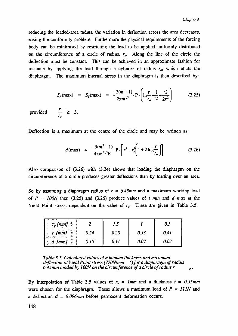
Chapter 3
reducing the loaded-area radius, the variation in deflection across the area decreases,
easing the conformity problem. Furthermore the physical requirements of the forcing
body can be minimised by restricting the load to be applied uniformly distributed
on the circumference of a circle of radius, r0. Along the line of the circle the
deflection must be constant. This can be achieved in an approximate fashion for
instance by applying the load through a cylinder of radius r0, which abuts the
diaphragm. The maximum internal stress in the diaphragm is then described by:
—3(m+1) p.I1 L 1 rSR (max) = S(max) =
2vnt2 • r0 22r2J (3.25)
rprovided - ^ 3.
To
Deflection is a maximum at the centre of the circle and may be written as:
_3(m2_1).p.[r2_r2(1+2logLJ] (3.26)d(max)
4vn 2t3E
Also comparison of (3.26) with (3.24) shows that loading the diaphragm on the
circumference of a circle produces greater deflections than by loading over an area.
So by assuming a diaphragm radius of r = 6.45mm and a maximum working load
of P = lOON then (3.25) and (3.26) produce values of t mm and d max at the
Yield Point stress, dependent on the value of r0. These are given in Table 3.5.
2 1.5 1 0.5
t (nun) 024 028 033 041
:'.4.jmrnJ. 0.15 0.11 0.07 0.03
Table 3.5 Calculated values of minimum thickness and maximumdeflection at Yield Point stress (770N/mm 2)for a diaphragm of radius6.45mm loaded by lOON on the circumference of a circle of radius r
By interpolation of Table 3.5 values of r0 = 1mm and a thickness t = 035mm
were chosen for the diaphragm. These allows a maximum load of P = 1JJN and
a deflection d = 0.096mm before permanent deformation occurs.
148

Tn axial Stress Transducer - Prototype Design
3.2.5 Indentor Mechanism
A major factor affecting the accuracy of the diaphragm-type stress transducer is
that of ensuring the repeatability of the profile of force distribution over the
diaphragm. In the two extremes a single point force applied near the supporting
wall will deflect the diaphragm very little whereas the same point force applied in
the centre of the diaphragm will produce maximum deflection. Sanders et al
[19901 chose to place the normal-stress transducer on top of their three-axes device
during clinical trials. In this situation the ability of the device to measure accurately
the true stresses occurring at the body interface would depend on the possibility
of tissue conforming to the surface of the diaphragm. In certain conditions, notably
near or under bony prominences the major forces may be applied non-centrally.
Even if a load spreading layer of material were interposed between the tissue and
the device, there would be great demands on the properties and thickness of this
material.
In order to ensure repeatability in the position and profile of any forces applied
to the diaphragm used here, a fixed indentor is used. This is a flat plate with a
cylindrical boss machined onto it. The plate is held central under the diaphragm,
but free to move normal to it, by four guide pins inserted into the annular support
wall of the diaphragm. This is most effective when the normal-stress transducer
is attached to the bottom of the three-axis device. The indentor is also designed
to provide overload protection. Its diameter is great enough that when the transducer
is loaded by large normal stresses the indentor base plate impinges on the diaphragm
support walls and therefore limits the maximum deflection of the diaphragm. Figure
3.20 shows a sectioned diagram of the pin-indentor arrangement and its operation.
Shear Secon
Strain-gauge
Indenter
li_I / jj 4-Figure 320. Sectioned view of the Normal-stress transducer showing theindentor mechanism.
149

nirailsing iioas
p Disc (Sliding)
cking Screw
rnsducer Leach
insducer
Thickness Shim
Bottom Disc (Fixed)
Chapter 3
3.3 Prototype Device Assembly
The combined prototype triaxial stress transducer is constructed from the two
sub-assemblies; the biaxial shear-section and the normal-section. These sections are
prepared and assembled separately before being bonded together.
In view of the size of the device as a whole compared with the forces it must
sustain it is essential that component bonding be sound. To achieve a strong bond
the careful preparation of the individual components and selection of the appropriate
cement is vital. The sequence of assembly of each section is outlined below, along
with any details of special preparations required at each stage.
During the assembly process achieving good alignment of the discs concentric to
one another is essential. Any eccentricity in the shear section will appear as a
displacement of the magnet and hence 'unbalance' of the MR output under no load.
To facilitate alignment an assembly jig was made up that consisted of two plates
and four rods. As the thickness of the silicone is also important shims were placed
between the jig plates to regulate this. Figure 3.21 is a schematic of a device
placed in the assembly jig while the cements dry.
Figure 321. A diagram of the transducer captured in the assembly jigwhile the cement dries. Rods hold the device discs concentric and shimsset the thickness.
3.3.1 Shear-section Assembly
The assembly procedure for the shear section began with the fabrication of the
flexible PCB that was to hold each MR and device lead attachment. One was
required for each axis. The flexible laminate was purchased externally, but the
150

Tn axial Stress Transducer - Prototype Design
photo etching and cutting out of the PCB were done in-house. The MR's were
glued (cyanoacrylate) in place and their leads trimmed and soldered. After the
section discs were inspected and deburred a lead and MR subassembly were cemented
in each of the outer discs. The magnet was pressed into the centre disc and
cemented in place (cyanoacrylate). All three discs were then cleaned prior to
section assembly.
An outer disc was placed in the assembly jig and a layer of silicone applied. A
thickness shim was placed on the outer side of the jig. The middle disc was
inserted in the jig concentrically to the first and clamped down on the silicone to
the height of the shim. Care was taken to ensure that the ridge and groove of
the discs were engaged. When the silicone was cured the jig was unclamped and
the same procedure followed for the remaining outer disc. A second thicker shim
was used for that operation.
3.3.2 Normal-section Assembly
The assembly of the normal stress transducer section began with the manufacture
of the diaphragm. After these were inspected and trimmed they were sent to the
gauge supplier for mounting of the gauges.
Small rectangles of flexible PCB were cut and cleaned. On the diaphragm return,
excess gauge cement was removed and the PCBs fitted. Gauge and device leads
were soldered onto the PCB and the device lead insulation trimmed level with the
annular wall. The indentor guide pins were fitted into their mounting holes and
cemented in place.
3.3.3 Three Axis Device Assembly
The final assembly stage was where the normal-section was attached to the bottom
face of the shear-section. In order to maintain some concentricity the assembly
jig, of Figure 3.21, was used. The joint was to be capable of withstanding the
maximum shear-stress applied to the device, so the adhesive used was an high-strength
epoxy. Both faces of the join were lightly abraded and thoroughly degreased. The
shear section was first inserted in the jig so that the bottom face was up. A thin
151

Chapter 3
layer of epoxy was applied to the upper face of the normal-section's annular support
wall. When the layer had gone tacky, the normal-section was inserted upside down
in the jig. The two sections were pushed into contact by sliding the top plate of
the jig down over the jig rods. Pressure was applied to force the jig plates together
and the locking screw tightened. When the epoxy had hardened the devices were
removed from the jig and the excess epoxy and silicone rubber removed. Each
device was uniquely labelled to identify it with its own calibration data - as the
component and assembly variables make each device different.
3.4 Mounting Considerations
A transducer must be placed at each measurement site of interest in a socket. This
must be done in such a way as to maintain the integrity of the socket and provide
a rigid fixing base for the transducer. To achieve this a device is recessed into
the socket wall, sandwiching the indentor plate underneath it. The pin and hole
combination allow the whole device to move in a direction normal to the socket
but prevent translational or rotational motion. All forces are applied to the upper
surface of the shear-stress subassembly. The normal components of these forces
are transmitted through the shear-stress section driving the whole device onto the
indentor plate. The coplanar force components react against the guide pins and
move the discs of the shear-stress section.
In order for the shear sections to move unhindered there must be a clearance void
surrounding the two sections. Care must be taken to keep the void width to a
minimum. During clinical trials skin or stocking may be folded into it, impeding
transducer movement. Figure 3.22 shows the mounting arrangement in the socket.
In this schematic the transducer is shown with a disc of liner material bonded to
the top shear section. The primary purpose of this is to attempt to match the
frictional and stiffness properties of the transducer location to those of the surrounding
material.
It is essential that the recess in the socket wall, into which the transducer locates,
be a precision fit. Also, that the device top surface be coplanar to the inside face
of the socket wall. To achieve this, a transducer shaped epoxy blank of the correct
dimensions is lightly bonded to the liner fitted over the residual limb positive prior
152

Tn axial Stress Transducer - Prototype Design
Figure 3.22 Simpled schematic representation of the mountingarrangement of the three-axis device in the socket wall.
to drape forming. During the forming process the softened polypropylene moulds
itself around the blank. After the socket positive is withdrawn the blanks are
removed and the recess trimmed for the correct fit.
The blanks themselves are made in a moulding process. The positive for the mould
is machined from a single aluminium block. It has essentially the same shape as
the assembled transducer, complete with leads and pins. The dimensions for it are
shown in Figure 3.23. Its diameter must be that of the transducer, plus one
millimetre for clearance when the shear section is displaced under applied stress.
The stubs for lead exits are extended from their true exit depth to the top surface
of the device (surface nearest the limb interface) so that the polypropylene does
not form over the blank leads, preventing their removal. Its height includes the
thickness of the indentor plate. Holes are drilled into the positive, and steel pins
are fitted. These pins are oversized to provide a clearance fit for the transducer
pins in the socket wall. Their length is also exaggerated to provide depth clearance.
The mould is made from low viscosity, low temperature coefficient silicone rubber,
(Silcoset 105 - Ambersil UK Ltd). The silicone is poured into a small bowl - in
this case the cap off a spray can. It is placed in a low-vacuum chamber for fifteen
minutes to remove any air from liquid. The positive is mounted on a flat disc
and placed inverted into the silicone. Figure 3.24 describes this arrangement. The
bowl is then left i;i the vacuum chamber overnight while the silicone cures. The
silicone is then removed from the bowl.
A low viscosity, low temperature coefficient two part epoxy, (Epotek 301 - Intertronics
Ltd, UK), was used for the blanks. This was dimensionally stable at the temperatures
153

0.8 __J11L_
il.2 Da x 2.5
14.4 at 9Odeg
Chapter 3
1 A
Figure 3.23 Dimensions of positive master used in making mould forepoxy blanks which form transducer recess in the socket wall.
experienced during drape forming. Epotek was mixed and poured into the mould.
Only enough epoxy was poured to just fill the mould. A bent paper clip was
used to encourage air bubbles out of the pin holes. The mould was placed in the
vacuum chamber for thirty minutes to remove trapped air. A sheet of Mylar was
placed on the mould and weighted. Epoxy does not bond to the Mylar and the
weight ensures a smooth flat surface. Figure 3.24 describes this arrangement. To
speed the cure of the epoxy the mould was placed in a laboratory oven at 80 t
for twelve hours. The blank is popped out of the mould and trimmed.
The intended measurement sites in the socket are marked on the liner, and blanks
are lightly bonded in place at the correct orientation. After the drape forming
process when the socket positive and liner are removed the blank stays in the
socket wall. These are then levered out or broken. The remaining recess is then
trimmed, and device-lead access holes cut through the socket wall. Discs, the
diameter of the recess are cut from the liner at the marked sites. These have one
millimetre trimmed off their radius for clearance. They are bonded to the top of
each device. The liner is placed in the socket, and each device lead is split and
passed through the holes in the socket wall. A view of a prepared recess and an
instrumented socket is presented in Figure 3.25.
154

Tn axial Stress Transducer - Prototype Design
Positive
a)
he
hank
Mould
b)
Figure 324 Schematic describing the making of the mould a) and themaking of the epoiy blanks from the resulting mould b).
155

.
Chapter 3
(a)
4$ -EL- -- -.
(b)Figure 3.25 View of the recess in the socket wall after the removal ofthe epoxy blank a). Picture of an instrumented socket, showing thedevice lead exits through the socket wall b).
156

Chapter 4
Triaxial Stress Transducer
- Development to Requisite Form
It is the objective of this chapter to plot the progress of the design of the transducer
and to record the best performance demonstrated with the fmal design - within the
limits of the experiments performed. Notes are made of the critical areas of
assembly and explanations are given of the testing phenomena observed. It is not
the intention to discuss the manufacturability or likely production yield of this
design. Variability in performance between devices was generally broad as these
were hand assembled products. It is expected that the variation in experimental
results presented here may well be reduced with a more automated manufacture
process.
The prototype shear and normal stress transducer sections described in Chapter 3
were subjected to a number of tests. The effectiveness and adequacy of the critical
components of each section were analysed and reported here. After modification
and reselection of components, the sections were then reassembled and retested.
On achieving a successful combination of components a triaxial device was assembled
and tested. In the last part of the chapter, details of calibration tests are presented
and the transducer perfonnance compared to that of the requisite transducer specified
in 2.6.
4.1 Shear-Stress Section Development
In this part of the chapter the development of the shear stress transduction mechanism
is detailed. Overall there were many changes made to the section design at differing
intervals. However for simplicity these changes are all collected into three design
stages. The first prototype will be considered as Design A, the second as Design
B, while the final form of the shear section is presented as Design C.
For each design stage a discussion is given of:
the considerations made for the selection of components
the performance test methods and equipment
the results reported from the tests
157

Chapter 4
the limitations of, or necessary changes to be made to, the current design.
At each stage the design was assessed for stress and temperature sensitivity as a
whole section as well as at component level.
4.1.1 First Prototype Assessment - Design A
In order to obtain a 'feel' for the significance and interplay of each component's
performance in the section, four identical sections (aluminium-silicone-aluminium)
were constructed using the silicone, Ambersil 1039N, which was most highly
recommended by the suppliers. Tests were run on these sections. In parallel,
samples of each of the other silicones [3.1.2.4] were bonded between two
transducer-sized blank aluminium discs and their stress-strain and creep properties
assessed. The results of these investigations are reported in the following subsections,
and a summary made in [4.1.1.4]
4.1.1.1 Test Regimes and Equipment
The test types, methods and equipments used in the initial appraisal of the prototype
sections are reported here.
Each section was tested for sensitivity, linearity with applied load, and insensitivity
to temperature changes. The properties of most importance were seen as
resolution of small forces
repeatability of any measurement
linearity of output with applied stress
sufficient dynamic range for clinical stresses
output independent of frequency and temperature
The device temperature tests were undertaken primarily to determine the stability
of the device's output over the range of temperature changes normally expected in
the clinical situation. Secondly it was necessary to ascertain if there may be any
changes to the device's modulus of rigidity. Both of these would produce an
apparent-strain error signal which would compromise the device accuracy and may
invalidate its calibration curve.
158

Tn axial Stress Transducer - Development to Requisite Form
Various testing equipments were used in carrying Out these initial tests, some of
which existed in the Department while others had to be constructed. The force
tests were initially performed on an Instron - 1195 Materials Testing Machine.
This instrument attempts to deform a test sample by tension or compression between
a moving crosshead and a rigid base. The degree of deformation is measured by
an extensometer attached to the test sample, and the amount of force required to
achieve the deformation is measured by a loadcell mounted on the crosshead or
base. The rate of deformation, the maximum force applied and the maximum
displacement can be separately controlled. With these functions it is possible to
apply cyclic loads at specific rates and to given force limits. A strip chart in the
instrument records the applied deformation and resultant forces developed in the
test sample.
In order to apply shearing forces to the transducer a special calibration jig had to
be designed. Figure 4.1 shows an exploded schematic of the construction of the
jig. It consisted of two holding blocks (A, B) mounted between side walls. One
block (A) was fixed to the Instron base loadcell and the other (B) to the crosshead.
Block B was confined to move vertically and parallel to the other (A) by two
linear bearings (C) fixed on to the side walls. Each of the blocks had a cylindrical
hole machined out of its centre. Into each of these holes fitted one half of a
cylinder (D). Each half cylinder had a recess cut into one end for holding the
transducer. The transducer (E) was sandwiched between the cylinder halves which
was then inserted into the holding blocks and fixed by screws. The cylinder could
be rotated to allow stresses to be applied to the transducer from any angle in the
shear plane. A photograph of the assembled jig is also given in Figure 4.1.
In the initial tests the output from the shear section was obtained by using a digital
multimeter (Solartron 7045 - Schlumberger (UK) LTD) to measure the resistance
of each 'arm' of the MR element. These readings each took about ten seconds
to complete. Because of this the Instron was paused during its stroke and the
displacement held while readings were taken. Thus linearity tests occurred as a
multistage ramp. Unfortunately this method allowed stress-relaxation to add errors
to each reading, but for a first approximation this scheme was acceptable.
To assess their temperature sensitivity the sections were placed in a small
thermostatically controlled electric oven (O.25m3). Hygroscopic gels in the oven
assured a dry heat. The device leads and a temperature meter probe were introduced
159

:1
Chapter 4
(a)
(b)
Figure 4.1 a) Exploded schematic of the construction of the calibrationjig for applying shear forces to the transducer; b) photograph of theassembled jig.
160

Tn axial Stress Transducer - Development to Requisite Form
into the oven via a baffled vent hole in the roof. The temperature meter (MEP 123
- Medical Engineering and Physics, Dulwich Hospital, London) used for this
measurement, had an accuracy of ±0.1 °C over the range -200 V to 400 °C.
During these tests the section's signal output was expressed in terms of the resistance
ratio of the two arms of the magneto-resistor. This was calculated in the same
manner as a resistive divider ratio. That is, given a device which had R1 ohms
in one arm and R2 ohms in the other, then:
= (R1+R2)(4.1)
the percentage change in the resistance ratio 9 with force or temperature is then calculated as:
(R —R)= •100 (4.2)
This assumes a linear change in resistance ratio with applied stimulus. All the
devices have an initial zero-stress ratio of approximately 9 = 0.5 , so comparisons
of sensitivity are possible.
From the work of Pollard [1984] it was considered that the maximum expected
shear force on the plantar surface would be less than SON (over 2cm2). Over this
force range the value of i3t % was the full scale sensitivity (FSS) of the device,
from which unit sensitivity was calculated [E9LJN].
4.1.1.2 Static Stress Response
Two regimes of loading the devices were used. A multistage ramp
increasing/decreasing displacements until a given load was reached (0, 2. ..50N),
pausing at intervals for measurements. This test was designed to observe the
linearity of the devices. Secondly, cycling between fixed loads pausing at force
extremes for measurements (0, 30, 0, 30W), allowed changes in the stiffness of the
rubber to be observed as a change in the slope of a stress strain plot. Similarly
any viscoelastic changes due to heat build up from losses in the material or creep
would translate the curve parallel to its initial curve.
161

Chapter 4
The four assembled sections [4.1.1] and the silicone blanks (aluminium - silicone
- aluminium) were subjected to force cycles at orientations of (1,45° and 90° to
the applied force vector. The silicone blanks were also orientated to preclude
nonuniform bonding from elevating stress values. Measurements of the output ratio,
R, and the deformation were taken at force intervals during loading and unloading.
For the period of the measurement the applied stress was held constant.
4.1.1.2.1 Linearity and Range
Force versus resistance ratio curves typical of Design A are shown in Figure 4.2.
They describe the change in resistance ratio for force applied in a multistage ramp
to SON while the sections were at an orientation of 45°. Also shown is the response
to five force cycles - measurements were only taken at ON and SON - and the
response to a 100% overstress. From this it was seen that both axes exhibited a
linear change in 9 with applied stress; the force versus resistance ratio curve was
repeatable; and the silicone was linearly elastic in its behaviour. Figure 4.2 also
shows that the section design was typically able to withstand at least 100% overstress.
Table 4.1 lists the FSS of the sections under load at the three orientations.
Orienranon FSS [9LJ
2 .3 :4:
5.04 53 4.8 4.7
45. 3.49 3.68 3.42 32
0.06 0.69 03 05
Table 4.1 Full scale sensitivity to load offour shear sections of DesignA. Sections were orientated at 0 45 and 90
Figure 4.3 shows the FSS of two mutually perpendicular shear sections to tangential
loads applied at different orientations. Sinewaves are superimposed on each plot
for comparison. The phase offset seen between the two axes was due to transducer
alignment errors in the calibration jig. The data indicates that the direction of load
vectors can be derived with reasonable accuracy under this design.
162

0
cc
8C
U)Cl)0)cc
(a)
Tn axial Stress Transducer - Development to Requisite Form
- 0 10 20 30 40 50Force [N]
0.40 --------- ---.--.-----cc
0.475 -------.--.- .-.-.-------. (b)
0.450 10 20 30 40 50Force [N]
0.52
0.51 •----...--.--. .-.---.-----. ----.--------
0.5 ..... •-----.--.-. -.--.---. -------------------------------4
o 0.4w
(c)0.47 ---.--- •-.-.----.. --.--.--.-. ._.. ------------
0.46 -.-----.- •___a_.__ ... -
:1:: iii
0.430 20 40 60 60 101Force [N]
Figure 4.2 Force versus Resistance Ratio curves of th X & Y axes of atypical shear section of Design A. Linearity of response to 50N (a).Repeatability over 5 cycles to 50N (b). Response to a 100% overstress(c). All loads were applied at a 45 orientation.
163

• 6
4
04-
cc000-aC/,
U)Q) -2ccC00)C -4
0
-6-20 0 20 40 60 80 100
Chapter 4
Orientation [Degrees]
Figure 43 Typical Response of a shear section of Design A to forcevectors applied at various orientations in the s/warplane.
4.1.1.2.2 Creep and Hysteresis
It was noted from Figure 4.2 that there was significant hysteresis in the force
versus resistance ratio curve. There were two major implications of this: heat build
up under prolonged stress cycling may affect the viscoelastic property of the rubber,
and an amount of uncertainty is introduced in assigning a resistance ratio to a
given force. It was expected, however, that the former was less likely to be
significant due to the small number of cycles occurring during clinical trials. This
was supported in the laboratory as the transducer response was repeatable after
several hundreds of cycles. Thus, the magnitude of the hysteresis was thought to
be the more important problem.
It was also noted for the multistage cycle that the values of 9 at zero load were
not coincident. This was attributed to more periods of measurement and hence
more stress relaxation occuring during loading than unloading. A period of unloading
equal to the loading period was required to release completely the energy stored
in the rubber.
164

Tn axial Stress Transducer - Development to Requisite Form
The average magnitudes of hysteresis loops of the four sections are reported in
Table 4.2. Each section was subjected to five cycles, to SON, at orientations of0°, 45° and 90°. The values measured were seen to be significantly large, for some
sections, in relation to the FSS of the section.
Orleiztation 0 HysteresLc fNJ
1 .2.. .:...340
0° 11.4(.89) 13.4(55) 16.6(.89) 14(.71)450 14.2(1.1) 15.4(.89) 20.8(.84) 16.8(.84)
90° 12.1(55) 13.8(.45) 15.6(1.14) 15(.71)
Table 4.2 Average magnitude (standard deviation) of hysteresis in fourshear sections of Design A. Each was subjected to five cycles to SONapplied at orientations of 0 0,450 and 90
To determine if the hysteresis seen was particular to the silicone used, a comparison
of the mechanical properties of the three silicone samples - Ambersil 1039N(A),Dow Corning RTV738(DC) and General Electric RTV157(GE) - were made.
Silicone test pieces (0.8mm thick) were sandwiched between two aluminium discs
of the same diameter as the transducer. Each silicone was mixed in air and allowed
to cure for their recommended times. Shear forces were applied to the blanks
(aluminium - silicone - aluminium) using the transducer calibration jig coupled to
the Instron. Each was subjected to a constant rate of strain (05 mm/mm) until a
force of SON was reached, at which point the strain was held. During the test
the reaction force generated in the samples was recorded on the Instron chart
recorder. Figure 4.4 shows the resultant force-time curves as traced from the chart.
From linear approximations of the initial parts of each curve, it was possible to
derive average shear modulii for each silicone.
It is obvious that GE and DC silicones were less rigid than silicone A, and would
therefore stretch further for any given applied force. In a transducer this would
give rise to greater device sensitivity and a smaller range for a given thickness of
the rubber layer. Both A and GE exhibit quite linear force response with applied
strain, while DC was significantly non-linear. The latter part of the curves indicates
that stress relaxation is occurring in the silicone. A and GE show similar relaxation
165

Chapter 4
50
40
- 30z
e0Ii-
10
60 120 180 240 300 360
Time [Sec]
Figure 4.4 Reaction force occurring in three silicone rubber sampleswhen subjected to constant strain rate (05 mm/mm). After reaching 50Nthe strain was held constant.
but DC shows dramatically more. The use of DC in a measuring device would
therefore result in a loss of accuracy for forces applied at low frequency. The
greater the rate of relaxation the higher the low frequency limit of accuracy. The
greater the amount of relaxation, the greater the magnitude of conversion inaccuracies.
It was felt that during clinical use where constant stresses are applied to the
transducer, it would be more likely to experience creep than relaxation. Thus, in
order to quantify creep reactions in each blank (aluminium - silicone - aluminium),
they were subjected to a 30N step load for 60sec. The resultant displacements
were measured with the Instron extensometer and logged on the chart recorder.
Table 4.3 presents the observed creep rate in the blanks. The values are expressed
in terms of the percentage increase in displacement, over the instantaneous
displacement (iSec), with the logarithm of time (seconds).
In summary it was clear from Figure 4.4 that GE could replace A as the rubber
in the shear section. With a layer of half the thickness the same displacement
would arise for a given force but allowing a corresponding decrease in the magnet
166

Tn axial Stress Transducer - Development to Requisite Form
Creep IRate
_______________________ f%szrainflog(Sec)J
General Electric - RTVJ57 3.6 (.4)
Ambersil -1039N 4.6(2)
Dow Corning - RTV138 23 (3)
Table 4.3 Average creep rate (standard deviation) in disc's of silicone(16 dia x 0.8 mm) when subjected to a 30N step shear stress.
element separation (for flush mounting magnets), so increasing the device sensitivity.
Also, it was obvious that the GE silicone had similar stress relaxation resistance
to that of A. So for improved performance the GE silicone was chosen to replace
A for the next development stage.
4.1.1.3 Temperature Sensitivity
The temperature sensitivity of the shear section was assessed by measuring the
resistance values of each axis when the unloaded section was heated from 20°C to
50°C. The four sections in turn and a temperature probe were suspended inside
the oven [4.1.1.1]. The temperature was incremented in steps. At each temperature
the sections were allowed to stabilize for thirty minutes before a measurement was
taken. Figure 4.5 shows the resultant change in resistance ratio with temperature
for each of the sections. There are three notable features in the data plots. Firstly,
the temperature coefficients are constant (linear slope). Secondly, the coefficients
are of opposite sign for sections with an initial resistance ratio greater than the
balance value of 0.5R. Thirdly, the coefficients corresponding to an initial 9t value
greater than 0.5, are greater than those of initial 9 value less than 0.5.
The opposite signs of the coefficients were due to the magnetic field experienced
by the MR being reduced with increasing temperature, so causing 9 to return
toward 0.5 - zero field value. A reduced magnetic field at the MR could have
been caused by the magnet field strength decreasing or the magnet-element separation
increasing. Thus, a possible theory for the differing magnitudes of the coefficients,
above and below 9=0J, was that the symmetry of the MR resistances have a
negative temperature coefficient which adds algebraically to the above phenomenon.
167
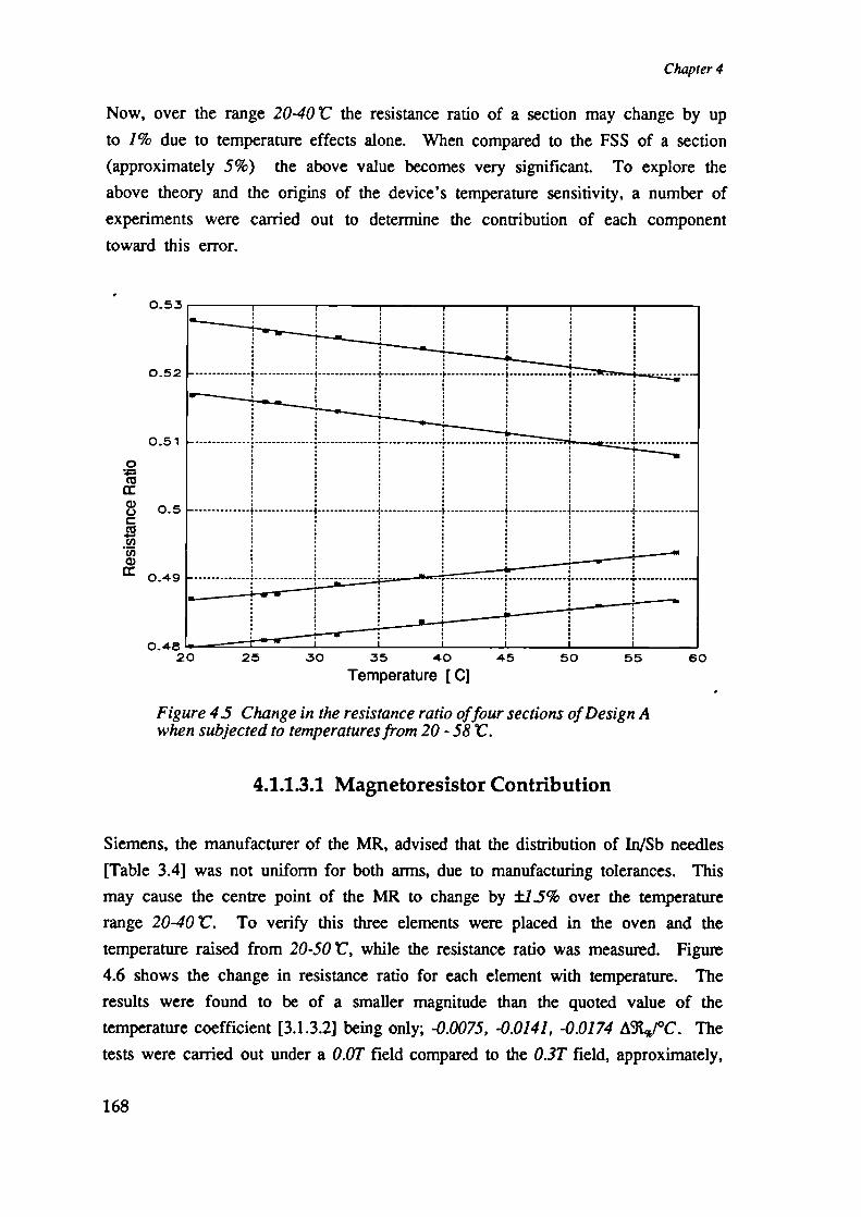
Chapter 4
Now, over the range 20-40 t the resistance ratio of a section may change by up
to 1% due to temperature effects alone. When compared to the FSS of a section
(approximately 5%) the above value becomes very significant. To explore the
above theory and the origins of the device's temperature sensitivity, a number of
experiments were carried out to determine the contribution of each component
toward this error.
0.53
052
0.510-S
a) 0.5-aC',Cna)
0.49
0.4520 25 30 35 40 45 50 55 60
Temperature [C]
Figure 45 Change in the resistance ratio offour sections of Design Awhen subjected to temperatures from 20 -58 t.
4.1.1.3.1 Magnetoresistor Contribution
Siemens, the manufacturer of the MR, advised that the distribution of In/Sb needles
[Table 3.4] was not uniform for both arms, due to manufacturing tolerances. This
may cause the centre point of the MR to change by ±1.5% over the temperature
range 20-40 t. To verify this three elements were placed in the oven and the
temperature raised from 20-50 V, while the resistance ratio was measured. Figure
4.6 shows the change in resistance ratio for each element with temperature. The
results were found to be of a smaller magnitude than the quoted value of the
temperature coefficient [3.1.3.2] being only; -0.0075, -0.0141, -0.01 74 A9tZJ°C. The
tests were carried out under a 0.OT field compared to the 0.3T field, approximately,
168

0.48
cc0) 0.478UC
0.476
20 25 30 35 40 45Temperature [C]
0.4715
0.486
0.464
0.482
0.474
0.472
Tn axial Stress Transducer - Development to Requisite Form
found in the assembled section. Under the latter conditions the temperature
coefficients and resistances would be larger, possibly resulting in a larger change
in the centre point with temperature (refer to Figure 3.15). Additionally, the
distribution of In/Sb needles is statistically random under production techniques so
the elements tested here may only have moderate differences in needle distribution.
All in all, the negative coefficient, supports the earlier theory of the unequal
magnitude of the coefficients either side of R=O5.
Figure 4.6 Experimental measurements of the change in resistanceratio of FPJ1ODJ5S magneto-resistors with temperature.
4.1.1.3.2 Silicone Expansion
The change in resistance ratio due to temperature effects on the rubber layer was
assessed by two related experiments. The axial expansion of the silicone layer
was measured with increasing temperature. Secondly, the change in resistance ratio
with magnet-element separation was determined.
Samples of the three silicones were mixed in air, as they would be when mixed
for the transducer, and bonded between blank aluminium discs. The overall thickness
169

Chapter 4
of each assembly was measured with a micrometer at 23 'C (room temperature) and
then at 79 'C. The expansion of the aluminium was assumed negligible compared
with the silicone. This assumption is thought valid due to the low linear coefficient
of expansion for aluminium (23 x 10.6 cm/cm! 'C), compared to that of the silicones
(10 cm/cm! 'C). The rubber was also assumed to expand linearly with temperature.
The results of the experiment are presented in Table 4.4.
SWcwe . .. :Aeràtd Puie'
..':.Lfc/cnil VI (crncm1 VI
Amj ersl(JO39PJJA) 3.4x10 *
Dow orniig r'RTV7$S) 4.5 x 10 3.1 x 10 -
(DC
General Ekctric (RTVI57) 5 1 x 10 ' 2 7 x 10
_______ _______
* Value not specified by the manufacturer
Table 4.4 Linear thermal expansion of silicones A, DC and GE.Comparison of measured values for aerated silicones, with puresilicones.
The change in resistance of an MR element with magnet-element separation is
dependent on three principle factors: the uniformity of In/Sb needle distribution in
the active areas of the MR element; the magnitude, direction and homogeneity of
the magnetic field; and the MR-magnet separation distance. To assess the combined
effect of all these parameters, an MR element mounted on a PCB was fixed to
the bed of a automated X/Y plotting table, while a magnet was held perpendicular
to it at a separation of 0.1mm. The resistance ratio of the arms cf the element
was measured while the magnet was scanned across it in 0.15mm steps. These
measurements were repeated while incrementing the separation in 0.1mm steps to
reach a maximum separation of 1.5mm. A summary of these measurements is
presented in Figure 4.7. The nominal silicone thickness in a shear section is 0.5mm.
From Table 4.4 the likely expansion of silicone A, over the temperature range
20-40 'C, was 3.4j.un (0.5mm to 0.5034mm). A change in the magnet-element
separation of this magnitude may alter the MR output, in the worst case, by
0.019A9t - [Figure 4.7.]
170

(a)
C.4-C'
a
(b)
Tn axial Stress Transducer - Development to Requisite Form
The expansion of the silicone layer resulting in an increase in magnet-element
separation and subsequent decrease in the field at the MR is an additional mechanism
causing 9 -40.5 with an increase in temperature.
.. 4
3
2
0
C)CoCda.Cl)
U,a)
-2
-3-4 -3 -2 -1 0 1 2 3
Lateral Displacement [mm]
Figure 4.7 Resistance ratio variation as afunction of magnet -magnetoresistor separation,for an FPJJOD155 differential magnetoresistor(Siemens (UK) LTD) and a 3x2mm diameter SmCo magnet (MagnetDevelopments LTD). Values were measured on a 0.15mm (lateral) x0.1mm (vertical) grid. Data is shown in profile (a) and also as a 3Dmesh (b).
171

Chapter 4
4.1.1.3.3 Magnet Contribution
The last component assessment was the change in the magnet's field strength with
temperature. The suppliers of the magnet (Magnet Developments LTD, UK.) advised
that the temperature coefficient was approximately 0.1%! C for the range 0-100 r.
An attempt was made to verify this, but due to the lack of availability of a
magnetometer with a probe size less than or equal to the magnet diameter, and
which has a temperature stabiised output, the magnet temperature coefficient was
estimated indirectly. An element was fixed to a solid base and a flat bottomed
polystyrene dish supported immediately above it on spacers. The magnet was held
against the bottom of the dish above the centre of the element. Water at 50 t
was introduced to the dish and allowed to cool, while the element resistance was
measured at regular intervals. The change in the field strength of the magnet was
measured by the change in resistance of the MR element. Figure 4.8 is a graph
of the results. However, it was thought that the MR would experience some heating
as well and therefore the change in its output would be due to both coefficients.
Also the magnet-element separation was unavoidably greater than that used in the
section. The change in the field strength detected by the MR at the separation
used in this experiment would be less than those typically found in a transducer.
Thus the derived temperature coefficient was thought to be an underestimate.
It was clear that the field strength of the magnet diminished with temperature
(-0 .0088 ER%/°C), further supporting the earlier theory where the sign of the
temperature coefficients either side of ¶R=03 are opposite.
4.1.1.4 Discussion
The following is a summary of the test results for Design A and their implications.
There are three observations that recommended this design. Firstly, from Figure
4.2 it is seen that the sections output response to applied stress is approximately
linear. Thus the calibration and data processing of clinical measurements is simplified.
Secondly, it also indicates that measurements are repeatable, with some minimal
errors. Thirdly, Figure 4.2 shows that the design could withstand a 100% overstress
without its function being impaired.
172

476.4
476.2
Tn axial Stress Transducer - Development to Requisite Form
478-3xlO
477.8
477.6
477.4
477.20
cc 477
476.8
4766cc
20 25 30 35 40 45 50
Temperature [C]
47615
Figure 4.8 Experimental measurement of temperature inducedchanges in the field strength of a Samarium Cobalt magnet -evaluated by its effect on a magneto-resistive element.
Conversely the following observations describe negative aspects of the design.
Firstly, the full-scale sensitivity (FSS) is typically only 5% of the output value at
zero stress. On its own this was not a deficiency - especially when compared
with the magnitude of the output change from a strain-gauge device. However,
when considered in conjunction with the temperature induced change in output, it
was quite significant. Figure 4.5 shows that an extreme temperature change in the
device, of 20 V, may typically produce a change in 9 of up to 1%, equivalent to
a 20% error in full-scale measured stress. From the discussions in Chapter 2, even
during strenuous exercise the likely increase in temperature in a prostheses will be
an order of magnitude smaller than the test range. Thus, if the device temperature
at the time of the clinical trial was known and the change during the trial was
small, it would be possible to recover the true applied stress with a small uncertainty.
However, to do this would require a measurement of temperatures during the trial
and knowledge the devices stress response at each of these. Thus making the
calibration and data processing procedures very complex. Alternatively the device
temperature could be controlled electronically both at a compromise to the size and
cost of the device and system.
173
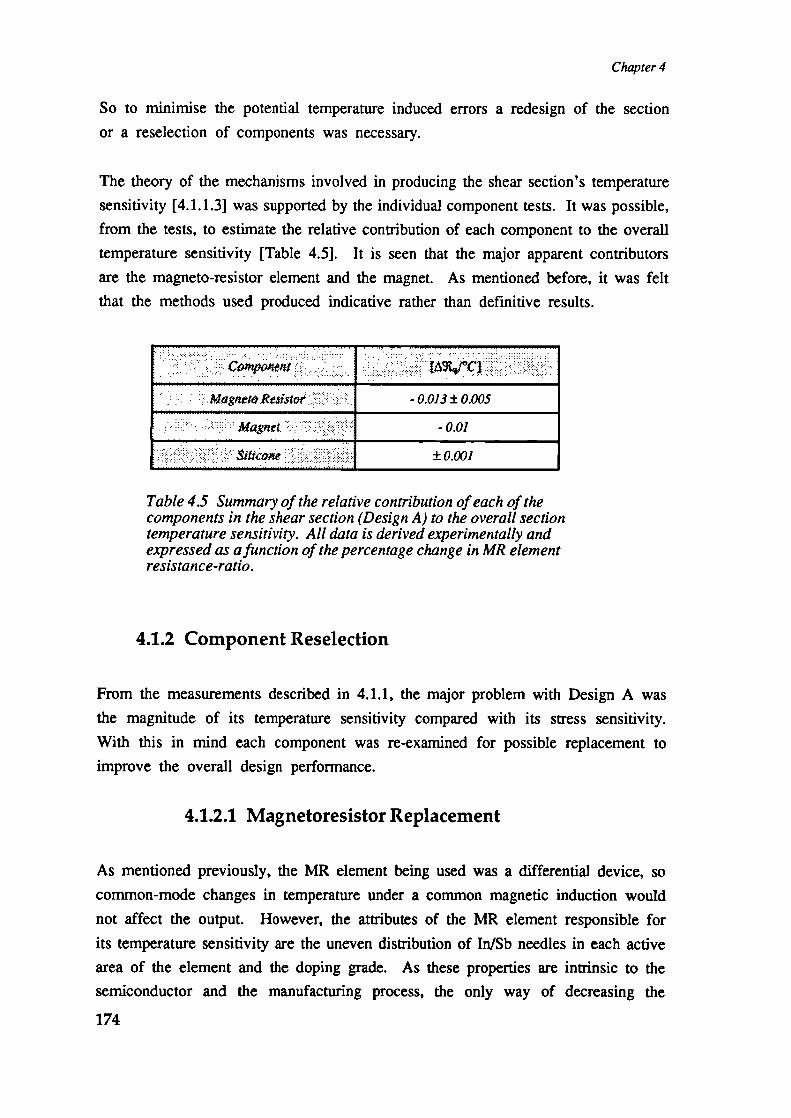
Chapter 4
So to minimise the potential temperature induced errors a redesign of the section
or a reselection of components was necessary.
The theory of the mechanisms involved in producing the shear section's temperature
sensitivity [4.1.1.3] was supported by the individual component tests. It was possible,
from the tests, to estimate the relative contribution of each component to the overall
temperature sensitivity [Table 4.5]. It is seen that the major apparent contributors
are the magneto-resistor element and the magnet. As mentioned before, it was felt
that the methods used produced indicative rather than definitive results.
Compo'øu
: .:M;Ifor - 0.013 ± 0.005
Magnet -001
± 0001
Table 4.5 Summary of the relative contribution of each of thecomponents in the shear section (Design A) to the overall sectiontemperature sensitivity. All data is derived experimentally andexpressed as afunction of the percentage change in MR elementresistance-ratio.
4.1.2 Component Reselection
From the measurements described in 4.1.1, the major problem with Design A was
the magnitude of its temperature sensitivity compared with its stress sensitivity.
With this in mind each component was re-examined for possible replacement to
improve the overall design performance.
4.1.2.1 Magnetoresistor Replacement
As mentioned previously, the MR element being used was a differential device, so
common-mode changes in temperature under a common magnetic induction would
not affect the output. However, the attributes of the MR element responsible for
its temperature sensitivity are the uneven distribution of In/Sb needles in each active
area of the element and the doping grade. As these properties are intrinsic to the
semiconductor and the manufacturing process, the only way of decreasing the
174

Tn axial Stress Transducer - Development to Requisite Form
temperature induced apparent stress from these sources was to change the MR
element to a type with a smaller overall temperature coefficient and a lower variation
in its temperature coefficient with induction. Both of these, however, lead to an
element with reduced field sensitivity to magnetic induction. So, replacement would
need to be coupled with other methods for increasing the device sensitivity to
applied stress.
A market survey revealed the most suitable alternative MR to be another Siemens
MR (FP1 1 1L100). This MR element has a significantly smaller temperature
coefficient (-0.38%! °C) compared with the FP1 1OD 155 (-2.7%I °C); while the relative
resistance change, under the field strength in use in the prototype section
(approximately 031), only decreases from 3 to 1.85. Thus in using a FP1 1 1L100
the stress sensitivity of the device was increased relative to its temperature sensitivity.
4.1.2.2 Magnet Replacement
The device's stress sensitivity was further enhanced via two approaches. The first
was to increase the magnetic field strength experienced by the MR. This could
be achieved by employing a stronger magnet and/or moving the magnet closer to
the MR. A field concentrator was already built into the substrate of both Siemens
magneto-resistors. Also, the magnet diameter could be optimised to be approximately
equal to the separation of the MR's active regions.
Previously when designing the prototype, the strongest magnet material readily
available, to the author's knowledge, was Samarium Cobalt (SmCo), and the smallest
parts obtainable were 2mm diameter rods. A further search of magnetic material
suppliers revealed a source of a relatively new material, Neodimium Boron Iron
(NdBFe). It could be obtained in the form of a powder-sintered block which could
only be ground to rectangular dimensions. The relative field saturation of the
sintered NdBFe is 2-5 times that of Polymer bonded SmCo, while the quoted
temperature coefficient of the NdBFe material was -0.15 %/ r compared to -0.10
%/ V for SmCo. Thus there was a relative advantage in using NdBFe magnets.
Stock samples of the new material with dimensions 3x2x2mm were obtained. This
longer length allowed the magnet face to be placed closer to the MR element by
extending the height of the ridges of the central disc. The new MR element was
175

Chapter 4
wider and longer than the previous one. In this case the relative increase in the
dimensions of the element to those of the magnet enhances the device sensitivity
to changes in magnet-element displacement. The original FP11OD155 element was
only 1.2mm wide, whereas the FP111L100 element was 2.7mm wide, compared to
the magnet which was 2mm across. When the magnet is large relative to the
element, the field differential between either half of the element is small. Whereas
for an element slightly larger than the magnet, there would be a greater difference
in field distribution for either half. So for a given displacement of the magnet
the latter will produce a greater change in the element resistance ratio. Figure 4.9
illustrates this. In the limit, if the magnet is much smaller than the element the
resistance of either half will change very little while the other remains constant.
Magnet
Figure 4.9 Relative exposure to magnetic field for two different widthsof magneto-resistor element.
4.1.2.3 Silicone Replacement
The results of the constant strain tests [Figure 4.4 and Table 4.3] indicated that
the General Electric RTV157 (GE) silicone exhibits a lower modulus of rigidity
and has similar relaxation resistance than Ambersil 1039N (A). Thus by replacing
A with GE the shear section thickness could be reduced and still result in the
same range of displacements. In order to determine the appropriate thickness of
the GE silicone, in a section with the new magnet and MR, two experiments were
performed. Firstly, the maximum useful lateral displacement of the magnet across
the MR was investigated. Secondly, the thickness of GE required to map the
expected maximum clinical force (±50N) onto that displacement range was determined.
Figure 4.10 is a plot of the change in resistance ratio of a typical FP1 1 1L100 MR
element when a 3x2x2mm NdBFe magnet was moved over its surface at a vertical
176

I I
0.35-6
(a)
0
0.55'I
C
U)U)a)cr 0.45
0.4
-4 -2 0 2 4 6
Lateral Distance [mm]
(b)
Tn axial Stress Transducer - Development to Requisite Form
separation of 0.1mm. Figure 4.11 shows the resulting extension when four section-sized
specimens of GE silicone, each of different thickness, was subjected to a SON
stress. Bearing in mind that these are typical results, a useful displacement range
of ±1mm was chosen and a conservative layer thickness of 0.5mm was set for the
next design stage (Design B).
0.7
0.65
0.6
Figure 4.10 Field sensitivity of FPJJJLIOO differential magneto-resistor(Siemens (UK) LTD) to 3x2x2mm NdBFe magnet (Magnet DevelopmentsLTD) stepped over its suiface on a 02mm lateral x 0.1mm longitudinalgrid at 0.1mm separation. Data is plotted in profile (a) and as a 3Dmesh (b).
177

Chapter 4
1.4
1.2
1
E o.sEC0- 0.6C
w0.4
0.2
0 I I I I
0 10 20 30 40 50
Force [N]
Figure 4.11 Force-displacement relationship for four disc's of RTVJ57silicone (GE LTD) under 50N shear force. The dimensions of the disc'swere 16mm dia x 0.15,03 ,0.5, 0.8mm.
4.1.2.4 Dimensional Changes
During the assembly of the transducers several problems became apparent. Maintaining
correct silicone thickness and hence disc separation was difficult, and ensuring an
accurate alignment so that the ridge and channel mated was not always possible.
By allowing the ridge to push home to the base of the channel, the alignment and
silicone thickness problems were removed.
The ridge height on the middle disc was increased from 0.5mm to 1.0mm. This
allowed the ridge to be pushed home into the channel, which was 0.5mm deep,
and maintain an accurate disc separation (silicone thickness) of 0.5mm. This is
illustrated in Figure 4.12.
Modifications were also made to the MR PCB shape and the PCB slot in the outer
discs of the section to accommodate the reselected components [refer to 3.1.3.3,
3.1.3.4].
178

Tn axial Stress Transducer - Development to Requisite Form
Magnet
(a) Magneto-resisl (b)emont
Figure 4.12 Schematic of the difference in geometry of the ridge andchannel structure between Design A (a) and Design B (b).
4.1.3 Second Prototype Assessment - Design B
Design B is the second prototype shear section, derived from the first prototype
(Design A), and modified according to the component changes discussed in [4.1.2].
The following part of this chapter, to [4.1.4], reports the performance assessment
of Design B.
4.1.3.1 Test Equipment Modification
During the testing of Design B, in the Instron Materials Testing Machine, a locking
bar in the calibration jig was accidently left in place during a force-strain test.
The bar effectively stopped the sliding block of the jig from moving. The resulting
plot on the Instron chart-recorder showed an unexpectedly significant hysteresis
ioop. To persue the origin of this a steel spring was placed directly under the
sliding block and was compressed. A greater than expected hysteresis loop was
again exhibited. Closer investigation showed that the cause of this exaggerated
hysteresis to be an inherent lead or lag in the Instron chart drive controls. When
an extensometer was in use the chart lagged the applied strain. Conversely when
chart motion was made proportional to the cross-head displacement, the chart led
the applied strain.
Thus for accurate calibration data the Instron force and strain signals needed to be
monitored at a point prior to the machine's chart-recorder. This necessitated
obtaining another recording system. Also from the experience gained in collecting
the data described in 4.1.1, it became obvious that a more automated method of
179

Chapter 4
data collection was required. Consequently, a signal conditioning unit was built
to interface the shear section outputs to an analogue to digital (A/D) convertor.
The A/D unit used was a DT2814 (Data Translation mc), hosted in an IBM
compatible personal computer (PC). It has an accuracy to 12 bits over a 0-JOV
input range. Software execution rates limited sample frequencies to 50Hz. A
circuit diagram of the signal conditioning unit is shown in Figure 4.13.
From a study of the Instron maintenance manuals, appropriate points were found
in the extensometer and Ioadcell circuitry where the strain and force signals could
be monitored. Coaxial leads conducted these signals to the signal conditioning unit
where they were buffered and amplified. A similar scheme was followed to derive
a signal from the MEP123 temperature meter and buffer it. A driver circuit for
the shear-stress section passed a constant current through both MR elements in
series. Differential amplifiers were used to amplify the voltage developed between
each elements' centre terminal and its lowest voltage terminal. The gain of the
amplifiers was determined experimentally and then fixed. It was chosen so that
the amplified output from any section under full load (SON) would map onto the
full input range of the A/D convertor. Due to assembly variability each section
has a different zero-stress output. The signal gain, therefore had to set low enough
to take account of this offset and allow sufficient margin for most devices to map
into the A/D input range. Conversely the gain must be large enough to provide
adequate signal resolution. The other instrument signals were similarly buffered
and digitised.
The A/D convertor was controlled by a short BASIC programme, specially written
to capture the signals from all sources (shear section, loadcell, extensometer and
temperature meter) in sequence, at a specified rate. The resultant data was stored
on disk under a specified file name. This data was later analysed in an "off-line"
mode using a commercial mathematical software programme (MATLAB - Mathworks
Inc.)
During initial tests, in an attempt to get a feel for the dynamic response of the
assembled device, the calibration jig [Figure 4.1] was uncoupled from the Instron
crosshead and forces of approximately SON were applied by hand at various
frequencies. The loadcell output and the transducer output were recorded on an
X-Y plotter. For frequencies of approximately 0.1 - 1Hz the hysteresis ioop [Figure
4.2] did not change appreciably. However, for frequencies greater than about 1Hz
180

Triaxial Stress Transducer - Develo pment to Reaul site Form
I-D C\O voz>-oa
Figure 4.13 Circuit diagram of the signal conditioning Unit used forinterfacing to the transducer (Design B), loadcell, extensometer andtemperature meter to the PC controlled AID.
181

Chapter 4
(i.e. clinical frequencies) the ioop became much larger, with the transducer output
decreasing much faster than the recorded force. The lag in recording the force
indicated that there was inherent mechanical or electrical damping in the Instron
above 1Hz. Therefore in order to simulate forces at clinical frequencies alternative
load testing equipment was required. (NB: The inherent damping in the Instron
is due to its designed use as a static or low frequency stress testing platform).
4.1.3.2 Temperature Sensitivity
Component reselection [4.1.2.] was mainly concerned with reducing the overall
temperature sensitivity, while increasing the stress sensitivity of the shear section.
The following is a report of the assessment of the temperature sensitivity of Design
B. Initially the temperature sensitivity of the individual components was assessed,
followed by the temperature response of the device as a whole.
4.1.3.2.1 Magnetoresistor Contribution
Quoted temperature coefficients, as advised by the manufacturer (Siemens (UK)
LTD), referred only to the change in resistance of any arm of the magneto-resistor
element and so were of little use in determining offset (centre point) drift in the
MR. The manufacturer was unable to provide data on the centre point drift for
the FP111L100, although it was expected to be less than the FP11OD155 (±1.5%
over 20-40 V). An experiment was performed to determine an approximate value
for it's temperature coefficient and drift, to compare to those derived for the
FP1 1OD 155. Four unmounted magneto-resistor elements were heated and cooled
over the temperature range from 24-50 t, while the resistance of the elements were
recorded. The calculated resistance ratios of the elements are shown in Figure
4.14. A first order polynomial fit (least squares sense) to each of the curves
resulted in slope coefficients of -0.0064, -0.0068 and -0.0086 E$tj°C respectively
(top to bottom in Figure 4.14).
182

0.5070
0.506
0.505
0.504a:
30 35 40 45 50 55Temperature [C]
0.50125
0.51
0.509
0.508
0.503
0.502
Tn axial Stress Transducer - Development to Requisite Form
Figure 4.14 Variation in resistance ratio with temperature of threeFP111LJOO (Siemens (UK) LTD) dtfferential magneto-resistors.
4.1.3.2.2 Silicone Expansion
The effect of expansion of the silicone layer on the MR resistance ratio was assessed
next. The quoted coefficient of thermal expansion of the pure silicone, given in
the manufacturers literature, was 27 x iO cm/cm/ V. However during the construction
process the silicone becomes aerated and it was anticipated that the thermal expansion
would be greater than the quoted value. In order to assess any possible change
in the resistance ratio due to the expansion of the silicone (and hence change in
the magnet-element separation) the same two part test used in [4.1.1.3.2] was
followed.
From Table 4.4 the measured thermal expansion coefficient for aerated GE silicone
was 5.1 x 1O cm/cm! V. Using this value and assuming a worst case temperature
change of 20 V, it was inferred that the silicone thickness, and hence magnet-element
separation may increase by 5.lWn (Oim,n to 0.5051mm).
183

-4 -2 0 2 4 6
Lateral Displacement [mm]
20
0.10
a:
CO
U)
U)0)a: -10
-30-6
-20
40
30
(a)
(b)
Chapter 4
The second part of the test was conducted as before by fixing an MR element to
the bed of an automated X/Y plotter table and positioning a magnet centrally over
it. The MR resistance ratio was measured as the magnet was scanned across the
element at various magnet-element vertical separations. The results are shown in
Figure 4.15.
0
Figure 4.15 Resistance ratio variation as afunction of magnet -magneroresistor separation,for an FPJJJLJOO dWerential magnetoresistor(Siemens (UK) LTD) and a 3x2x2inm NdBFe magnet (MagnetDevelopments LTD). Values were measured on a 0.2mm (lateral) x0.1mm (vertical) grid. Data is shown in profile (a) and also as a 3Dmesh (b).
184

0.488
0487
0
0.486C)
U)• 0.485a)cc
0.484
0.48320
0.489
25 30 35 40 45 50
Tn axial Stress Transducer - Development to Requisite Form
From Figure 4.15 the rate of change of resistance ratio with separation was greater
when the magnet was displaced by approximately 2mm. In an assembled section
the magnet-element separation is typically 0.1mm. Thus in the worst case, a change
in vertical separation of 5.4un (0.1 to 0.1 05mm) over 20°C would cause a decrease
in resistance ratio of approximately 0.2%.
Temperature [CI
Figure 4.16 Experimental measurement of the temperature inducedchanges in the field strength of a NdBFe magnet, evaluated by thefield effect on a magnetoresistor.
4.1.3.2.3 Magnet Contribution
In order to determine whether there was any significant change in the field strength
of the magnet with temperature over the temperature range being considered. The
magnet manufacturer quoted it's temperature coefficient as -0.15%/ V. In order to
assess how this would effect the resistance ratio, a similar test was carried out as
for the SmCo magnet [4.1.1.3.3]. Figure 4.16 displays the resultant data. Over
a 20 V temperature span there was a decrease of -0.59th typically. Again the test
was not thought to be very accurate as the MR measuring the field experienced
some heating and the MR-magnet separation was greater than in the shear section.
185

Chapter 4
4.1.3.2.4 Component Summary
A summary of the response of the components in Design B to temperature stress
is given in Table 4.6. These values are compared to those of Design A.
• nent •: H. Design :: : •. Design 8 1::
Mae(esisr -0.013 ± O.(X)5 - 0.008 ± 0.001
Magnet . - 0.01 - 0.024•
± o.00i ± 0.01
Table 4.6. Swnmary of the relative contributions of eachcomponent in the section, to the overall temperature coefficient ofthe shear stress section. Design B compared to Design A.
The salient features are; a reduction in MR element sensitivity; an apparent increase
in magnet sensitivity; and an order of magnitude increase in the effect due to
silicone expansion. Although the latter two compromise the shear stress section
performance they must be viewed in the context of the sections stress response
(presented later). Similarly the reduced field sensitivity of the MR must be offset
against its lower temperature coefficient.
4.1.3.2.5 Device Temperature Sensitivity
To determine the temperature sensitivity of the biaxial shear stress section as a
whole, a number of devices were assembled and their coefficients measured in both
the loaded and unloaded state. Each section was mounted in the calibration jig at
an orientation of 45'. The jig was then positioned in the oven beneath the vent
hole. A platform with an extended mounting post was attached to the sliding block
of the jig through the vent hole. Masses were placed on the platform (external)
to load the section whilst in the oven. A schematic of the equipment arrangement
is shown in Figure 4.17.
Loads of 10, 20 and 30N were placed on the platform at increments of temperature
over the range 26-51 V. After the loads were applied, a pause of five seconds
was allowed before the temperature and output were recorded. Unloaded tests were
186

30 35 40 45 50 55
Temperature [C]
0.55
0.3525
0.65
0.6
0-I
cc0.5
0
C/)
0.45cc
0.4
Tn axial Stress Transducer - Development to Requisite Form
FORCE Signal conditioning AmpSlidingbtock I
ND ConverterI 46
Transducer I oven Temperature MeterCaNbrallon Jig
Figure 4.17 Schematic of the experimental setup used to assess thetemperature sensitivity of shear stress sections of Design B. The sectionmay be loaded by placing masses on the platform.
carried out with the sections fixed in turn in horizontal and vertical orientations
on a shelf in the oven. The different orientations were intended to show up any
drift in the zero-load output due to viscoelastic changes in the silicone. Figure
4.18 shows results representative of the batch of biaxial shear stress sections tested.
Figure 4.18 Typical variations of R with temperature for shear stresssections of Design B. Over the temperature range the sections wereloaded with 10,20 and 30N masses, and placed horizontally andvertically when unloaded (H,V).
187

Chapter 4
There are three observations of significance to be made from Figure 4.18. The
first, that the gradients of each line are typically less than 0.4 9 over 20°C. This
demonstrates a temperature sensitivity significantly less than that of Design A - as
was set out to be achieved. Secondly, the traces for the various loads remained
reasonably parallel with temperature. The implication of this is that there was very
little change in the viscoelastic properties of the silicone over the temperature range.
The third observation was the relatively constant separation between the traces for
each axis, implying a linear force-resistance ratio response for the section.
The results of these temperature tests imply that sections of Design B need only
be calibrated at one temperature and possibly only under a few loads, both of
which are desirable in the requisite transducer design.
________________ Signal Conditioning Amp
5r----1
- Transducer \\ (
_______
HoldIngJlg \ re
____________ - Extensorneler
INSTRON" \ 2.-)
"Loadoell
Figure 4.19 Schematic of test equipment setup used to assess thestatic stress characteristics of the shear stress sections of DesignB.
4.1.3.3 Static Stress Response
The following, to [4.1.3.4], describes the methods used and results obtained in
characterising the response of the Design B shear stress section to applied static
forces.
Three biaxial sections were tested to determine their stress sensitivity and ability
to resolve force vector direction. The test apparatus consisted of the Instron
Materials Testing Machine, calibration jig, signal conditioning circuit and the PC
with analogue to digital convertor. Figure 4.19 is a schematic of the experimental
set up used.
188

0.64
0.62
0.6
0.58
.2 0.56cc 0.54
O52
0.48
0.46
Tn axial Stress Transducer - Development to Requisite Form
4.1.3.3.1 Linearity and Range
The assembled sections were subjected to a cyclic force from ON to SON. Each
was fixed in turn into the calibration jig at several orientations to the applied force.
They were then subjected to SON force cycles at a constant rate of strain (2mm/mm)
while the force output from the load cell, and the changing resistance ratio of each
axes was sampled at 20Hz. The transducer was then rotated and fixed at a different
orientation and the test repeated. Figure 4.20 shows a summary of the change in
resistance ratio with applied force vector for a typical shear-stress section. As
the direction of the applied force moves nearer to the orthogonal axis, the amount
of displacement, and hence change in resistance ratio becomes smaller. It was
clear that the curves were highly nonlinear at even moderate forces. Indicating
that extreme stresses were being experienced in the silicone. This was also indicated
by the presence of large hysteresis loops (±5-±13N). The implications were that
the linear range was less than satisfactory, the uncertainty of measurements were
large, and the calibration/signal processing requirements would be complex.
0.440 10 20 30 40 50 60
Force [NJ
Figure 420 Typicalforce-resistance ratio response of a shear stresssection of Design B. Loads cycles to SON were applied at 15' intervalsbetween 0-90g.
189
Chapter 4
4.1.3.3.2 Force Resolution
The short horizontal region at the beginning of each trace in Figure 4.20 gave an
idea of the amount of force required to begin displacement - overcome static friction.
The value represents the minimum detectable force of the section. As the operation
of the Instron was to effect a change in displacement and to record the force
generated in the shear section, this is an indirect method of assessing the minimum
detectable force. A more direct method was used.
During the creep measurement tests [4.1.3.3.4] the calibration jig was uncoupled
from the Instron and a small platform attached to the sliding block. Masses were
then placed on the platform until a change in output was observed. The minimum
sensitivities of the sections of Design B were between 1-5N. The probable cause
of the resolution limit was frictional inertia - static friction. This is discussed later
in [4.1.4.2]
4.1.3.3.3 Repeatability
To assess the repeatability of the section's response the devices were subjected to
many load cycles between the set limits of 0-SON. Initially, the Instron crosshead
speed was set to 5mm/mm (i.e. a load cycling frequency of 0.083Hz). After the
first three cycles the trajectory of each force versus resistance ratio cycle was
indistinguishable from the previous. Each cycle was repeatable to within 1%.
4.1.3.3.4 Creep and Hysteresis
It was obvious from Figure 4.20 that the hysteresis present in the section was far
in excess of desired levels. The load cycling test was repeated, first changing the
crosshead speed to 10mm/mm (0.17Hz), then reducing the upper load limit to 25N.
Figure 4.21 shows these results plotted as resistance ratio against force for an
orientation of 0° (along the sensing axis).
Doubling the crosshead speed, and hence frequency, from 0.083Hz to 0.1 7Hz had
no apparent effect on the size of the hysteresis loop. Halving the applied load
190

60
Triaxia! Stress Transducer - Development to Requisite Form
0.72
0.7
0.68
0.660
0.64cca, 0.62
U)0.6
cc
0.58
0.56
0.540 10 20 30 40 50
Force [NJ
Figure 4.21 Typical Force - Resistance Ratio response with load cyclefrequency of shear sections of Design B. Each was subjected to fiveload cycles of; SON at 0.083Hz; SON at 0.17Hz; and 25N at 0.083Hz.
from SON to 25N also had little effect on the relative size of the hysteresis ioop.
The question arose as to whether the large hysteresis was due to the bulk properties
of the silicone or to the manner in which it is assembled in the device. To answer
this the stress-strain relationship of disc's of GE silicone were compared to that of
the assembled shear-stress sections.
Three devices and three silicone blanks (aluminium - silicone - aluminium) were
subjected to five SON stress cycles at 0 450, and 90° orientations. Their mid
cycle hysteresis values were measured. Table 4.7 gives the mean and standard
deviation of these values.
It was clear that the hysteresis ioop for the pure silicone blank (aluminium - silicone
- aluminium) was less than that of the assembled section at any orientation. This
implied that there were additional hysteretic factors in the section design, which
appeared to be random between axes and between sections.
191

Chapter 4
Orientation As$embjedSectkrn Blank
11 2 ••.::
2
00. 10.6(35) 12.4(35) 10.4(35) 6.4(35) 7(0) 62(3)
4i 13.8(.84) 16.4(35) 15.8(.45) - - -
:. 9O .•.::. 11.6(35) 1O.6(.55) 11.8(.45) - - -
Table 4.7 Mean (standard deviation) hysteresis values [N] of threesections, of Design B, and three blanks, of GE silicone. Each sectionwas subjected to five cycles of SON stress at 0 .083Hz and orientations of0 45 °and 90 Blanks were subjected to five cycles of SON stress at0 .083Hz at one orientation.
On disassembly of the sections one of the contributing factors to the excess hysteresis
was found to be due to thin films of silicone (less than 0.1mm thick) between the
ridge and the channel. Obviously they had been trapped during the assembly
process. It is known that when rubbers are strained to high extensions (300-400%)
exhibit hysteresis several orders of magnitude greater than those found at normal
extensions (20-200%). This is due to physical changes in the material [Ward
1971]. Certainly the thin layers found would easily experience excessive extensions
at even moderate stress levels.
It was also evident that the hysteresis present in the silicone itself was approximately
±33N ( 7% FSL) which was greater than the desired accuracy of the requisite
transducer.
It was observed from Figure 4.21 that for the first three cycles the hysteresis curve
moved along a path above the original curve. When it reached the upper limit
for the second time it appeared to continue on a cyclic path that was reasonably
consistent. This behaviour is typical of 'creep' in the silicone. The hysteresis
ioop would continue to move up, but to a decreasing extent on each cycle -
characteristic of the exponential decay in the rate of creep.
The creep in the design (Design B) was evaluated by applying a 30N step load
to sections mounted in the calibration jig. The resistance ratio in the section was
sampled for 6OSec at 5Hz, and the creep rate calculated as before [4.1.1.2.2] by
192

Tn axial Stress Transducer - Development to Requisite Form
plotting beyond the initial value, against the logarithm of time. The resultant
curve was approximated by a first order polynomial and the slope taken as the
rate value. Table 4.8 lists the values for the three sections.
I
2 1
Creep Rate f%I1og($e)1
5.6(.4)
5.O(.2) I 4.9(.8)
Table 4.8 Average creep rate (standard deviation) in sections of Design Bwhen subjected to a 30N step load.
The values in Table 4.8 indicate that errors would grow to be significant (-15%)
over the course of a clinical trial - 1000 Sec.
4.1.3.3.5 Alignment Errors in Testing
When straining the silicone blanks (aluminium - silicone - aluminium) regions of
force versus displacement plots were observed where the displacement remained
constant for a period after the cycle passed through a maximum or minimum [Figure
4.22]. That is, the test assembly (silicone blank in the calibration jig) had a large
initial resistance to the change in displacement, symptomatic of the sliding mechanism
of the jig seizing momentarily (frictional inertia). Both silicone blank test pieces
and assembled sections were observed to exhibit this region during load cycles.
Although the regions appeared to be larger for sections, and especially for orientations
other than 00 and 90 Therefore the cause could not be the ridge and channel
mechanism. When a steel spring, of similar rigidity to a silicone blank, was
compressed between the sliding block and the jig base, the region was not evident.
This implies the cause lay in the way the forces were applied to produce shear.
In previous shear stress tests the test specimen was fixed in the calibration jig so
that it was in view of the Instron operator. This meant that there was a distance
of approximately 15mm between the line of applied stress and the centre of the
specimen. Figure 4.23a illustrates the early method of positioning the blank/section
in the calibration jig, where d is the moment-distance from the line of applied
stress. Any moments about the plane of the sliding block could cause friction in
the bearings, which may in turn cause some frictional inertia or stiction when
193

Chapter 4
changing the direction of motion. After retesting the silicone blank it was evident
that the size of the region was indeed related to the moment, d. The calibration
jig was thus modified to reduce d to a minimums as illustrated in Figure 4.23b.
The silicone blank was subsequently found to exhibit 1.5-2N less hysteresis than
measured previously.
As a consequence of the misalignment in early tests, the force versus resistance
ratio and creep curves of previous shear-stress transducer designs may have been
exaggerated. However, it could reasonably be assumed that all sections suffered
the same problem as none of the results were noted to be exceptional. Thus early
results still serve to give a relative comparison between section designs.
Ei::Jiii ___ ____
Force [N]
Figure 422 Force versus Displacement curve for a silicone blank(RTVJ57 - GE (UK) LTD). Note that at the extremes of the cyclethere are short constant displacement regions. These areindicative of stictionicoulomb-friction.
194

Fix
Tn axial Stress Transducer - Development to Requisite Form
plied
Force
SlidingBlock
HoldingCylinders -
(a)
Transducer—.. F AppliedForce
SlidingBlock
HoldingCylinders
Axed Block
(b)
Figure 423 Schematic of the position of a test body (siliconeblank or shear section) in the calibration jig, relative to the lineof applied shear force. The moment arm is d (a). The modifiedcalibration jig, where the moment arm is eliminated (b).
4.1.3.4 Discussion
In summary, comparing Design B with that of Design A: the stress sensitivity
was 5-6 times greater and the temperature sensitivity was 2-3 times lower. The
nett effect being that the temperature induced apparent stress was much less
significant. It was also observed that both designs yielded repeatable and approximately
linear force versus resistance ratio curves and were able to distinguish stress vectors.
Despite the above qualities there were major shortcomings of the Design B. Two
of these were: the inherent hysteresis of the silicone; and the inclusion of trapped
silicone layers between the ridge and groove during the assembly procedures. The
prevention of these layers would have been difficult to achieve. Even pre-assembly
of the discs before injecting the silicone would not guarantee success. For, to
avoid air inclusions and ensure penetration, a low viscosity rubber would have been
required which would have only exacerbated the migration of silicone into any
gaps. Regardless of any solution being found to that problem it was evident that
the silicone itself had unacceptable hysteresis.
195

Chapter 4
It is worth noting here that although Tappin et al[1980] and Pollard et al[1983]
had used silicone rubbers in their shear transducer they had only been able to
perform static and simple dynamic calibrations on them. Under those conditions
it may not have been possible for them to have appreciated the hysteresis present
in the stress cycle of the silicone.
The highly non-linear shape of the section's force versus resistance ratio curve was
most probably due to the extreme strain experienced in the thin layers of silicone
trapped between the ridge and groove. This idea was supported by the linear shape
of the stress-displacement curve for pure silicone blanks (aluminium - silicone -
aluminium).
A further property of the silicone that made it unsuitable for use in the requisite
transducer was the amount of creep demonstrated. Under low frequency stresses
errors of up to 10% (FSL) would occur after only 100 sec loading, so compromising
accuracy. The silicones tested, therefore, were not the preferred spring material
because of inherent properties and the form they were applied in. It was necessary
after these results to look closely at the alternative elastomers.
4.1.4 Further Component Reselection
4.1.4.1 Silicone Replacement by Natural Rubber
A natural-rubber (polyisoprene) was chosen to replace the silicone-rubber
(polysiloxane) as the restoring mechanism in the shear-section in an attempt to
improve performance. As discussed earlier [3.1.2.4] the potential problems with
using natural-rubber in the application were: fmding an adequate cold bonding
technique; possible rigid boundary layer on the bonding surface; and deriving a
formulation with acceptable physical properties. In seeking a better understanding
of these potential problems and of the general suitability of various natural-rubber
compounds, the advice of the National Rubber and Plastics Research Association
was sought. It was their opinion that the UK authority on natural-rubber was the
Malaysian Rubber Producers Research Association (MRPRA).
196

Tn axial Stress Transducer - Developni.ent to Requisite Form
4.1.4.1.1 Natural Rubber Formulation
In achieving an acceptable formulation there were compromises to be made. The
essential properties required were: low hysteresis; low creep and relaxation; moderate
rigidity; and high resilience. In order to obtain good resolution in shear stress
measurements the rigidity of the rubber must be such that 50N stresses displace
the magnet across the full face of the MR element. However, more rigid rubbers
have lower creep and relaxation properties. Thus the gross trade off is between
transducer thickness and minimising creep, stress relaxation, and hysteresis.
A similar layer thickness was used for the natural rubber layer (03mm) as was
used for the silicone layer. From Figure 4.15 a 200% strain would allow the
magnet to displace over its full useful range. The shear-modulus in this case would
need to be O.25N/mm2. However, a low shear-modulus was less critical than
minimising the creep and hysteresis. MRPRA were approached for advice on an
optimum natural rubber formulation. Their proposed formulation is given in Table
4.9. Two sample sheets were donated by them, however, the tested hardness of
this rubber implied that it would be twice as rigid as required (estimated at
0.48N/mm2).
Cmponeats Rat(a by parts
SMR CV 100
Zinc oxide 5
Stearic acid 2
Sulphur 2.5
CBS 0.6
Santoflex 13 1
Table 4.9 Formulation of NaturaiRubber compound used as restoringforce in shear-stress transducer.
4.1.4.1.2 Bonding Considerations
Beside being able to obtain a natural rubber compound with particular optimum
physical properties the other major obstacle to be overcome was identifying an
197

Chapter 4
adequate bonding technique. As discussed in [3.1.2.4] the preferred adhesion method
of hot bonding rubber to metal was rejected because of the probable damage to
the MR element and magnet, or the technical difficulty in, alternatively, trying to
accurately place these components into the section after the bonding process.
However, MRPRA advised that effective cold-bonding techniques were known.
Lindley [1974] conducted a study of the then commercially available adhesives and
their recommended preparation methods. The three most effective adhesives were
Araldite AY1O5/HY9S3F (Ciba-Geigy), Chemlock 304 (Hughson Chemical Co)
and Eastman 910 (Emerson & Cummings). The first two are epoxies, both of
which required pre-treatment of the rubber with concentrated acids - sulphuric or
hydrochloric. The latter is a cyanoacrylate adhesive for which there are no required
pre-treatments except degreasing the surfaces to be bonded with acetone. On
approaching the company quoted by Lindiley as suppliers of Eastman 910 (Emerson
& Cummings) the author was told that it was not part of their product range. It
was subsequently not possible to locate this product. Within Lindley's study, two
other cyanoacrylate adhesives tested produced weak bonds which could be pulled
apart by hand. For this reason it was decided to concentrate on the use of epoxies.
MRPRA were also of the opinion that the surface boundary layer was a function
of the length of exposure time to the pre-treatment process. For the stress levels
expected in the transducer, adequate bonds could be obtained for shorter pre-treatment
periods. Furthermore natural rubber compounds could be formulated with hysteresis
levels better than silicone at strains of up to 300%. Therefore any reduced effective
thickness of the layer would still bring an improvement over Design B.
Epoxy adhesives
From a survey of fifty-six suppliers and manufacturers of epoxies only two expressed
confidence in being able to bond natural rubber to aluminium. Samples of their
recommended adhesives were obtained. They were AY1O5/HY953F (Ciba Geigy)
and 556301 High strength and 554850 Quick set epoxies (RS Components Ltd).
Unfortunately Chemlock 304, used by Lindley, was not available at the time due
to importation delays. The rubber pre-treatments for these adhesives is acid based,
which is aggressive to all the other materials used in the transducer. Thus, careful
neutralisation of the acid is essential after pre-treatment of the rubber.
198

Tn axial Stress Transducer - Development to Requisite Form
At this stage of the transducer development the centre disc material was replaced
by an Acetal copolymer due to friction difficulties [4.1.4.2]. Three blanks
(acetal-rubber-acetal) made using the 556301 epoxy were tested to characterize the
rubber properties. Following this, ten complete shear-stress sections were built
using acetal as the centre disc. These were then tested to characterize the section
performance under force and temperature stresses. However, over half of them
failed during a week of testing. All suffered structural failure of the acetal centre
disc. On inspection the acetal appeared to have been chemically eroded. The
cause of the erosion was found to be due to traces of acid that was used in the
pre-treatment of the rubber. These traces had been absorbed into the rubber and
consequently seeped out. There were many such failures with sections made using
this bonding method - despite the extreme care taken to try to neutralize the acids
without significantly affecting the treated condition of the rubber. It was felt that
the assembly process had become very difficult and specialised with no simple
method of quality assurance. Long term affects of any contaminates would also
invalidate the device calibration curves, thus an alternative bonding method was
sought.
Cyanoacrylate adhesives
MRPRA advised that Loctite (UK) Ltd had recently developed a cyanoaciylate
adhesive that did not require pre-treatment of the rubber. Also, whereas previously
cyanoacrylates were very ineffective in bonding to self-lubricating thermoplastics,
a primer had also been formulated to overcome this limitation. Upon meeting with
a Loctite chemist, samples of the adhesive 406 and primer 757 were obtained and
demonstrated to form an effective shear stress bond between rubber and acetal.
Further, another Loctite product 405 was demonstrated to form an effective bond
between natural rubber and aluminium.
From tests using rubber blanks (aluminium - natural rubber - aluminium) and these
adhesives the bond strengths were found to be acceptable for the expected clinical
stress range. Also, the assembly process was considerably simplified. Complete
shear-stress sections, subsequently constructed, showed superior hysteresis and creep
properties and linear repeatable force-resistance ratio and force-displacement curves.
So with these components - Natural Rubber, acetal discs and Loctite adhesives -
199

Chapter 4
incorporated into Design B the shear-stress section design was finalised. A complete
description of the section components and assembly along with a report of detailed
performance characteristics is given in [4.3].
4.1.4.2 Low-Friction Polymer Central Disc
When a natural rubber layer was assembled in a shear-stress section, where all
three sections were aluminium, it was observed that the force-displacement curves
of the section showed flat regions at their minima and maxima, similar to those
seen for the silicones [4.1.3.3.2]. As before, there was a large initial resistance to
a change in the direction of the applied displacement. This phenomena was not
observed when a natural rubber sheet was cemented between two blank aluminium
discs and was stressed in the same manner, so implying that the cause was internal
to the section assembly. The action was that of momentary seizing of the assembly,
indicating some form of frictional inertia, possibly friction between the ridge and
channel. After silicone oil was allowed to seep between the ridge and channel,
there was a significant reduction in the size of the stationary displacement region.
On disassembly and close inspection under a microscope it was observed that
friction between the aluminium on aluminium sliding surfaces was the cause.
To overcome the friction problem outlined above, a survey was carried out for a
substitute centre disc material that had "self-lubricating" properties and adequate
bonding possibilities to rubber. Self-lubricating materials are difficult to bond to
because of the very surface properties they are sought for. Many are found in the
family of thermoplastics. They are easily machined but are not very strong materials.
The molecules in their structure do not form many crosslinks to neighbouring
molecules so they are not very resistant to chemical, particularly acid, attack. A
survey of suitable thermoplastic materials resulted in the selection of an Acetal
copolymer - mainly because of familiarity with its use in the authors Department.
Rods of acetal were obtained and three test blanks (acetal-rubber-acetai) made.
Sheets of rubber were bonded to these and the strength of these bonds tested in
shear. The breaking stress levels were well above expected clinical stress levels
(in excess of 5MPa).
200

Triaxial Stress Transducer - Development to Requisite Form
4.2 Normal-Stress Section Development
This part of the chapter [4.2] describes the design development of the normal-stress
sensing section. It details the performances of three strain gauges under applied
loads and concurrent temperature stresses and the appropriateness of the diaphragm
dimensions.
The author acknowledges that much of the work on the design and performance
assessment of the normal-stress transduction section was carried out with the help
of a colleague Mr. D. Porter. For completeness it is reported here.
For each of the foil strain gauges referred to in [3.2.2], a specific disc shape
(referred to as a diaphragm) was made. The diaphragm thickness was the same
for each but a unique pattern of slots were cut from the support wall at a variety
of angles to accommodate the different lead configurations of each strain gauge.
Figure 4.24 describes the disc outlines and gauge patterns for each of the three
gauges. The diaphragms were machined "in-house" and sent to the gauge manufacturer
for mounting of the gauges. This was to ensure optimum gauge performance on
the specified diaphragm.
FCA-3 FT-2-350-4B OFDPF-9-350
(a) (d) (c)
Figure 4.24 Schematic of the gauge pattern and diaphragmoutline of the prototype normal-stress transducer sections (a) SG1,(b) SG2, (c) SG3.
The first gauge, which will be referred to as SG1, was a simple two element
non-temperature compensated device. Two external resistors were connected to the
gauge leads to complete a Wheatstone bridge configuration. The second and third
gauges, SG2 and SG3, were four strain element types, with their elements arranged
as a bridge.
201

Chapter 4
4.2.1 Test Equipment and Methods
Each of the sections was loaded and concurrently subjected to a range of temperatures.
The experimental set-up shown in Figure 4.17 was used, with the exception that
the sections were placed under the sliding block of the jig. In that way loads on
the platform compressed the section between the sliding block and the stand. In
order to provide the same load profile for each diaphragm a two millimetre diameter
steel ball bearing was cemented to the centre of each diaphragm with epoxy. The
sliding block then rested on top of the ball bearing. Each gauge was connected
to a one volt bridge supply and amplifier - SGA85O - donated by Technimeasure
Ltd. The amplifier gain was fixed at an experimentally derived value for all
sections to allow comparisons to be made. The output of the amplifier was input
to an A/D convertor housed in a PC. Temperature measurements were made, as
before, via the MEP123 temperature meter, and interfaced to the A/D.
4.2.2 Temperature Sensitivity
The platform was loaded in sequence with 0, 0.5, 1, 2 and 3kg masses as the
temperature were increased from 20-50 t in 3 'C steps. At each temperature step
the section was allowed ten minutes to come to thermal equilibrium. The masses
were then placed on the platform in turn for five seconds while measurements
were made of the temperature and the gauge output. Figure 4.25 plots the typical
gauge output as a function of temperature and applied load for SG1, SG2 and SG3
respectively.
The measured temperature coefficient of each gauge is given in Table 4.10. These
are calculated using a linear approximation for the output change with temperature
over the range 20-50 V.
202

• 30
20
10
-:' 0
-104-.
%-200
-30
-4020 25 30 35 40 45 50 55Temperature [C]
(a)
(b)
25
20
15
d 10
4
00
Tn axial Stress Transducer - Development to Requisite Form
:__ i=PH
20 25 30 35 40 45 50 55Temperature [C]
:1 11:1 II ii: TITI1TI3C
- 2C -
IC
20 25 30 35 40 45 50 55Temperature [C]
Figure 425 Relative section output as afunction of temperatureand load for the prototype normal-stress transducer ; (a) SGJ, (b)SG2, (c) SG3. The excitation voltage was lVdc.
(c)
203

Chapter 4
Sal
S02 SW
• Temperature Coffldent -13702 -0.1898 -02230
(0.0168) I (0.0240) I (0.0345)
Table 4.10 Relative temperature coefficients of the prototypenormal-stress sections. The mean (standard deviation) of threecycles over the range 20-50 t is given.
SG2 and SG3 were comparable and clearly had significantly lower temperature
coefficients than SG1.
4.2.3 Static Stress Response
Force sensitivity (gain) data taken from Figure 4.25 was rearranged in Figure 4.26
to show the section output linearity with force and temperature. Gain data is
plotted for temperatures in the 20-40 t range at 3°C intervals. The slope of the
curves gives the gain and their change in slope provides the gain drift (change in
force sensitivity with temperature) values given in Table 4.11. From this data SG3
has greater force sensitivity than SG2 or SG1 at 20 °C, and exhibits less drift in
force sensitivity with temperature than SG2 or SG1.
.501 ••• I:5(
..J.j;sa3.....
• Gflfl (auJN/
0.857(0.017) I 0.663 (0.034) I 1.816(0.042)
Drjft (a.uJ/WVj -1.6x10 5 I -L5x10 3 I 1.4x10³
Table 4.11. Mean (Standard deviation) of relative force sensitivity anddrift values over the temperature range 20-40 Vfor the prototypenormal-stress sections.
204

4-
0
(a)
4-
0
(b)
S
4
, 3
24-
0
(c)
Tn axial Stress Transducer - Development to Requisite Form
0 5 10 15 20 25 30
Force [N]
0 5 10 15 20 25 30Force [N]
_...10I I
0 5 10 15 20 25 30
Force [N]
Figure 426 Relative force sensitivity as a function of temperatureand load of the prototype normal-stress section ; (a) SGJ, (b)SG2, (c) SG3. The excitation voltage was lVdc.
205

Chapter 4
4.2.3.1 Non-axial Loading of Diaphragm
The calculations to determine the optimum diaphragm thickness [4.2.4] involved a
compromise between diaphragm radius, and whether loads were uniformly distributed
or centralised through a point. The theory of bending in beams predicts that the
deformation (and therefore transducer output) will vary greatly with the size of the
loaded area and its centre of application. To demonstrate this theory, load spreading
layers and varying diameter spherical indentors were used to apply stresses to the
SG3 section. Figure 4.27 plots the gauge outputs (one volt excitation) over five
force cycles to 55N at 0.1Hz. Each plot has a small diagram indicating the load
applications mechanism.
In clinical applications other researchers have mounted the normal stress section of
their transducer next to the limb interlace [Sanders and Daly 1989]. Clearly, form
Figure 4.27, the dependence of the device response on the area and centre of force
application is very strong. This indicates that measurement errors will occur when
a strain gauge diaphragm is used directly at the interface surface, and these may
be significant near bony prominences.
Now, the use of small layers of liner material interposed between the transducer
and the skin interface may perform some load spreading function easing the
conformability problem at the interface, as experienced by the limb. So, over the
fleshy parts of the residual limb, interlace loads may be quite uniformly applied
across the face of the transducer, thus non-axial loading errors may be minimised.
It also tends to maintain a consistent friction coefficient across the interface. The
transducer described in this thesis was intended to be used at interface sites which
may not be fleshy. Therefore, in order to minimise errors it was important to
provide a mechanism for focusing the applied load in a consistent manner independent
of its centre of application.
206

Force [NJ
0 10 20 .10 40 50 SO
Force [N]
CS
0
(5
0.
0
CS
9-
0
0 10 20 30 40 50 50
Force [NJ
0 ID 20 .1) 40 30 SO
Force [N]
• 2
C1
9.
0
(5
9.
0
CS'
0.
0
Tn axial Stress Transducer - Development to Requisite Form
Force [N] Force [NJ
Figure 4.27 Relative output signals for SG3 strain-gauged diaphragmwhen 55N load applied to diaphragm via load spreading layers andvarious diameter indentors. Each was subjected to five cycles at 0.1 Hz.The excitation voltage was lVdc.
207

Chapter 4
4.2.4 Discussion
It was clear that full bridge gauges SG3 and SG2 had superior temperature stability
to the half-bridge SG1. Also, SG3 had greater force sensitivity and a more
constant force-output curve with temperature.
The temperature and force sensitivities of SG3 were found to be adequate for the
application considered here. Furthermore the driving and buffering circuits required
for foil strain gauges are no more complex or costly than those for a comparable
semiconductor gauge [3.2.2]. So on a cost and performance basis it was decided
that SG3 (QFDPF-9-350 Technimeasure LTD) would be used in the normal-stress
section of the triaxial-stress transducer.
4.3 Requisite Triaxial Transducer Design - Design C
In [4.1] and [4.2] details were reported of the various stages in the development
of the shear and normal stress transduction sections. This part of the chapter
[4.3-4.4] describes the construction and performance of a design that was accepted
as the final iteration of the development process and formed the requisite triaxial
transducer.
4.3.1 Device Construction
The following [4.3.1] gives details of the components used in the final three axis
transducer design (Design C), along with assembly procedures and details.
Shear stress transduction section
The basic components of the shear stress transducer section consisted of three discs.
These were cut from aluminium alloy bar stock (outer discs) and acetal rod (centre
disc). Each was subsequently inspected and deburred. Their dimensions are given
in Figure 4.28.
The PCB's, which hold the MR element and shear section leads, were fabricated
from double-sided copper laminate (EPS121RA - Fortin Inc or AKS121 - ISM
208

MR land
I-0
U)
U)
20
a)CC)
A 175
(b)
Tn axial Stress Transducer - Development to Requisite Form
Ltd). Squares of the laminate (20 x 20mm) were scrubbed to remove any oxide
layer and grease, then washed with distiled water. They were coated with two
layers of photo resist (Positiv20+ - Electrovalue LTD) and dried. A photo mask
for creating the PCB pattern has the dimensions given in Figure 4.29. After
exposure and developing they were etched and cut from the sheet. A low power
microscope (x8) was necessary to achieve the precision required during cutting
(approximately 0.1mm).
R49R63
i15J
a)C)
C)
C
1
C,)
Figure 4.29 Dimensions (mm) ofphotomasks for the PCB's used inDesign C. Magnetoresistor PCB from the shear stress section (a), andstrain-gauge lead termination PCB from the normal stress section (b).
Each PCB was again degreased with low impurity Acetone and the MR element
(FP111L100 - Siemens (UK) LTD) cemented onto the land on the PCB with
cyanoacrylate adhesive (405 - Loctite UK LTD). Very accurate placement was
essential to minimise output offset errors after assembly.
The MR element leads needed to have their insulating lacquer scraped off before
being soldered to the tracks on the PCB. Because of the size of the element a
miniature soldering iron was used and the procedure performed under the microscope.
The temperature of the iron was carefully controlled and all actions were precise
and quick to avoid melting the joint where the lead was attached to the element.
209

.115.96
E
Chapter 4
(b)
Figure 4.28 Dimensions (mm) of the disc's used in the shear section ofDesign C. Outer disc (aluminium alloy) with groove for housing the MRPCB (a) and the centre disc (acetal copolymer) with a central hole forcontaining the magnet (b).
210

Tn axial Stress Transducer - Development to Requisite Form
A standard 1 .2 7mm pitch 10-way ribbon cable (RS Components LTD) was used as
the section lead. In the assembled device all the leads were formed, because entry
to each of the two shear sections are mutually orthogonal. To facilitate this the
cores of the leads specific to each section, were cut to predetermined lengths before
being tinned. Also, to minimise the thickness of each section the top and bottom
surfaces of the section lead insulation were cut flat. These would eventually fit
into the slots milled into each outer disc and be flush with the surface of that
disc. The pretrimmed leads were soldered to the PCB tracks so that their joints
abutted the MR device lead joints. In order to provide maximum strain relief for
the device leads, as much section lead insulation as possible was cemented inside
each disc. The PCBs were fitted into their slots in the outer discs and cemented
into place (405 - Loctite (UK) LTD). An interference fit between the PCB and
slot was obtained for accurate alignment of the MR element with the magnet.
Four rectangles (18 x 7mm) of natural rubber sheet (OJmm thick) [see 4.1.4.1 for
formula] were abraded and cleaned with acetone. These were cemented to the two
semicircular upper surfaces of each of the outer discs with a cyanoacrylate adhesive
(405 - Loctite (UK) LTD). To minimise sliding friction the channel in each outer
section was coated with a thin layer of PTFE (RS Components LTD) from an
aerosol.
The bar magnet (2x2x2 NdBFe - Magnet Developments LTD) was inserted and
cemented (406 + 757 - Loctite (UK) LTD) into the hole drilled in the centre of
the acetal disc. Any excess length of the magnet was filed off so that the face
of the magnet was flush with the surface of the acetal disc. This was necessary
as any protuberances may impinge on the MR element during assembly or snag
on the edge of the MR element slot when the disc slides under applied force.
Normal stress transduction section
The assembly procedure for the normal-stress section was carried out in parallel
with the assembly of the shear-stress section. It began with the manufacture of
the diaphragm from silver steel rod. The dimensions of the diaphragm and the
indentor are given in Figure 4.30. It was important that the inside surface of the
diaphragm was smooth, otherwise the strain-gauge may be damaged by being bonded
to an uneven surface.
211
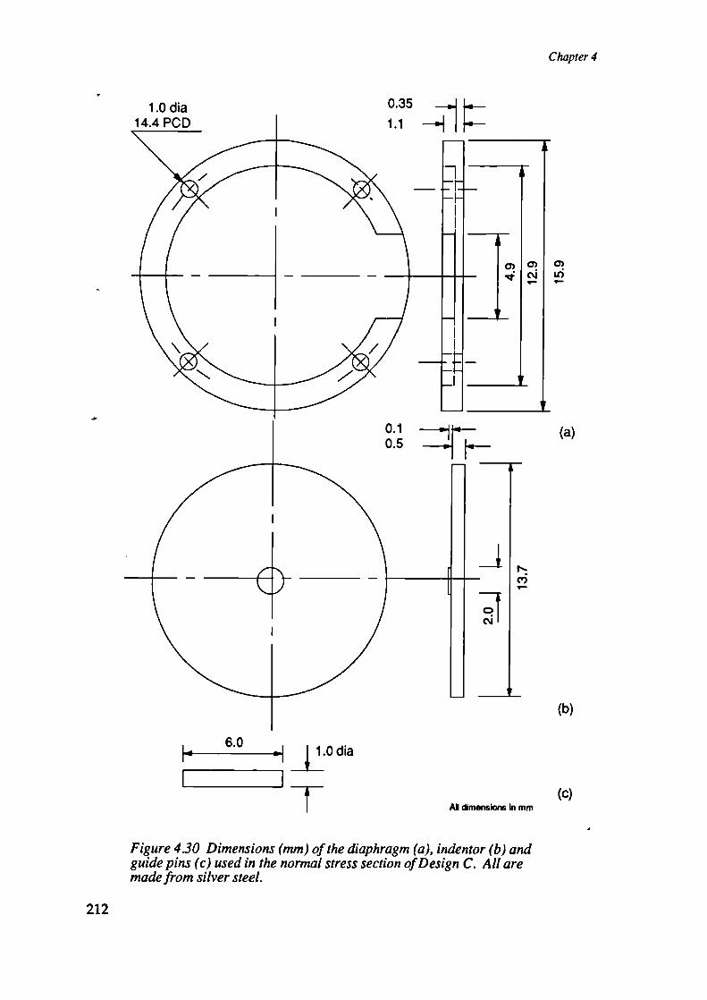
(a)
(b)
1 N.
If
0,c'i
C?U,1
Chapter 4
1.0 dia 0.35 -'1 k-
6.01.Odia
Al mensions in mm
Figure 430 Dimensions (mm) of the diaphragm (a), indentor (b) andguide pins (c) used in the normal stress section of Design C. All aremade from silver steel.
(C)
212

Tria,ia! Stress Transducer - Develop.sent to Requisite Form
The strain gauge (QFDPF-9-350 Technimeasure LTD) was cemented (P2 -
Technimeasure LTD) centrally on the diaphragm with tinned copper-wire leads
soldered to the gauge terminals. Excess gauge cement was carefully removed and
the diaphragm degreased.
Miniature PCB's were made in the same fashion as those for the shear section.
Their use was to terminate the gauge leads and section leads as well as provide
some strain relief. The dimensions for the PCB's are given in Figure 4.29. There
was an upper and a lower (nearest the section lead entrance) PCB.
Both the gauge leads and the section leads required preparation before soldering.
Under a microscope, a scalpel blade was used to scrape any oxide layer from the
gauge leads. These were then cut to length and soldered to the copper pads on
the PCB's. Each core of the section lead (remaining four cores of 10-way ribbon
above) was cut to a predefined length and its end stripped and tinned before
soldering them to the PCB's. As before this operation was conducted using a
miniature soldering iron and under a microscope. Again, to minimise the thickness
of the section the upper and lower surface of the section lead's insulation was
trimmed flat. Care was taken not to expose any of the conductors during the
trimming operation.
Because of height restrictions under the diaphragm, any excess solder was trimmed
away. A visual check was necessaiy to confirm that all conductive parts were
below the level of the diaphragm support wall. This was done bearing in mind
that the diaphragm will flex under load, so moving the gauge closer to the top of
the shear section. The section leads are formed around the inner circumference of
the diaphragm support wall and cemented in place with a small amount of contact
adhesive, cyanoacrylate. It was important that the leads butt against the diaphragm
support wall where they will cause minimum interference with the bending movement
of the diaphragm under load. Also care was taken to ensure that no adhesive
covers the top (or exposed) face of the gauge, as this would tear the gauge as the
diaphragm flexes. A second trim made certain the section leads are flush with the
support wall and the wall was free from adhesive.
When the normal section is assembled on to the bottom of shear section the joint
was air tight. So, any air trapped in the diaphragm cavity would expand and
contract with changes in ambient temperature. That would put pressure on the
213

Chapter 4
diaphragm and cause it to flex, thus generating an error signal. To avoid this
problem a small vent hole was drilled through the diaphragm close to the support
wall. However, the gauge was then exposed to the environment and may be
degraded by airborne contaminates. For protection a thin layer of silicone rubber
(non-acetic acid based) was applied over the gauge.
The indentor guide pins were assembled next. Each hole drilled in the wall of
the diaphragm and its associated pin was cleaned of debris and degreased with
acetone. An interference fit was obtained between the guide pins and the holes
in the diaphragm support wall. A small amount of high strength epoxy adhesive
(RS Components LTD) was droppered down each hole and the pins inserted. It
was sometimes necessary to force the pins with a small hammer so that they located
with their upper end flush with the top of the support wall.
A photograph of the disc's at this stage of the construction is given in Figure 4.31.
II
Figure 4.31 Photograph of the four transducer discs before finalassembly.
The final stage of the assembly was to attach the normal section to the bottom
face of the shear section. Concentricity was maintained by the assembly jig. The
214

Tn axial Stress Transducer - Development to Requisite Form
Device assembly
A jig was constructed [Figure 3.21] for the assembly process to align the discs
while the cement cured. All disc surfaces were cleaned with acetone. An outer
disc (aluminium alloy) of the shear section was inserted into the base of the
assembly jig and the adhesive (405 - Loctite (UK) LTD) applied to the top surface
of its rubber layer. The centre disc (acetal copolymer) was primed (757 - Loctite
(UK) LTD) and pressed on to the outer disc in the assembly jig. Care was taken
to align the ridge and channel immediately as bonding only took seconds. The
same procedures were followed for cementing the other outer shear section disc.
join must be capable of withstanding the maximum shear-stress applied to the
device, so the adhesive used was an high-strength epoxy (RS Components LTD).
Both surfaces to be joined were lightly abraded and thoroughly degreased with
acetone. A layer of epoxy was applied around the circumference of the diaphragm.
The two sections were mated and the assembly jig clamped. When the epoxy had
hardened the devices were removed from the jig and excess cement removed from
around the transducer.
Prior to calibration the resistances of each of the shear axes MR elements were
measured. A small padding resistor (1% metal oxide - RS Components LTD)
was added to the appropriate lead to ensure the zero-load resistance of both halves
of the axis were equal, so that the output of the shear signal amplifiers would
indicate zero volts at zero force. Thus a forward displacement would produce a
positive voltage, and a reverse displacement a negative voltage. Each device was
uniquely labelled to identify it with its calibration data [4.3.2.3], as component and
assembly variables make each device different.
4.3.2 Dynamic Stress Response
In order that the measured stress signals accurately reflect the actual stresses occurring
at the limb/socket interface it is essential that the transducer be able to closely
track the changes in stress magnitude. It is important, therefore, that the magnitude
response of the transducer is constant over the expected range of frequencies in
the stress field. This part of the chapter [4.3.2] details the equipment, test methods
and performance of the transducer design under applied load cycles. In contrast
215

Chapter 4
to previous static or quasi-static stress response testing of Design A and B it was
possible to carry out both dynamic and static assessments on the final design. Ten
transducers were constructed and subjected to loads of varying magnitudes, frequencies
and orientations. From these tests, conclusions have been made about the design's
linearity, range, hysteresis, creep, stress vector resolution and frequency response.
4.3.2.1 Test Equipment
In order to apply dynamic loads to the devices under test over a range of frequencies,
an industrial vibrator and power amplifier were purchased (SS300, G100A - Gearingand Watson LTD) [Figure 4.32]. The calibration jig for the shear transducer
sections was clamped to a rigid platform designed to place the transducer level
with the axis of the vibrator. A signal generator (HP3314A - Hewlett Packard
(UK) LTD) provided the frequency source for the power amplifier. The vibrator
and power amplifier were set in a constant-force mode so that cycles to given
force magnitudes, at the signal frequency, could be applied to the jig. A universal
joint was used to connect the vibrator to the calibration jig and address any
misalignment between the two.
To apply dynamic forces to the normal stress section of the transducer a small
aluminium ahoy plate was drilled to accommodate the diaphragm guide pins. The
indentor plate was positioned under the section as the section pins were inserted
in the plate guide holes. The plate and normal section were then placed between
the sliding block of the calibration jig and a vertical plate on the platform base.
Forces applied to the sliding block were then transmitted to the section, driving it
onto the indentor.
The forces applied to the calibration jig were measured at the point where the
universal joint attached to the sliding block by interposing a bidirectional piezoelectric
load cell (9301A, 5007 - Kistler (UK) LTD). The accuracy of the cell including
nonlinearities, was better than 0.03%.
Displacements of the sliding block, under the applied forces, were measured by an
LVDT (0D3, SM1 - Schiumberger (UK) LTD). The core of the LVDT was
attached to the sliding block and the body of the LVDT inserted into a hole in
the vertical plate of the platform. The accuracy of the LVDT, including nonlinearities,
was better than 0.5%.
216

Tn axial Stress Transducer - Development to Requisite Form
The transducer under test was powered and its signals buffered by a transducer
interface unit (MEPO8SB) built specifically for the data collection unit [Chapter 6].
The excitation applied to each device was lVdc.
Signals from the load cell, LVDT, and transducer were digitised (DT2824PGH -Data Translation mc), to 12 bits, and stored on a personal computer (LBM-PCAT)using the data capture software suite (Global Lab - Data Translation mc). The
accuracy of the AID, including nonhinearities, was better than 0.2%.
Figure 4.32 describes the setup schematically, and presents a photograph of the
equipment.
4.3.2.2 Dynamic Measurement Considerations
When measuring dynamic stresses or dynamically testing devices it is essential to
consider how the measuring or testing equipment may be affecting the desired
measurand.
To be able to precisely measure dynamic stresses it is essential that the frequency
response of the transducer is constant over the bandwidth of the measurand (50Hz).
If this not the case then the transducer will not be able to accurately track changes
in stress levels. Explicit measurements of the transducer frequency response can
be made if the bandwidth of the transducer dynamic calibration facility is greater
than that of the transducer. Otherwise, it can be implied that the transducer response
is sufficiently constant, over the measurand bandwidth, by demonstrating that it's
resonant frequency is very much greater than the measurand bandwidth. In either
case it is also necessary to assess the actual nature of the dynamic response of
the transducer in the measurand bandwidth. To do this, the calibration facility is
used to evaluate the transducer response at an arbitrary frequency in the bandwidth.
However, the bandwidth of the calibration facility with a transducer-like body in
situ must be greater than this arbitrary frequency. Therefore the frequency response
of the calibration facility was determined.
The calibration facility (jig) with transducer in situ [see Figure 4.32] form a single
mode mechanical system under forced vibration. The rheological system model for
this arrangement may be drawn, using Voigt elements, as in Figure 4.33.
217

Loadcell Amplifier
II
a
Vibrator
Loadcell 0
L.V.D T Amplifier
HTransducer Amplitiei
111111111111111111111111
II
L.V.D.T.Holding Jig
Zi. Upper Block
DlcmI°-''.
III I OI I
00000000QOOi F 'I
ND Converter
I I
ODD0000UDee DDDØ@(
Signai Generator
'0' '0' -&
Vibrator Amølifier
4'
S
Chapter 4
(a)
' 14(b)
Figure 432 Schematic (a) and photograph (b) of the inter-connection ofthe components of the transducer dynamic calibration equipment.
218

Tn axial Stress Transducer - Development to Requisite Form
r
xC2
m2 IA®
TW2>
F=Ø1W1-J
Figure 433 Rheological model of the shear transducer dynamiccalibration jig with transducer in situ.
Where: M1 and M2 are the masses of the transducer and holding block respectively;
c, and c2 are the viscous damping coefficients of the transducer and the calibration
jig respectively; h1 is the hysteresis of the transducer and k, is its elastic stiffness;
x is the displacement caused by the measured force F; F1 and F2 are the friction
(coulomb or dry) forces in the transducer (shear section only) and the calibration
jig bearings respectively; w1 and w2 are the weights of the transducer and holding
block acting normal to their bearing surfaces; while 4, 4)2 are the coefficients of
dry friction for the transducer ridge/channel (shear section only) and the jig bearings
respectively. Two terms are used to describe the damping effects in the transducer.
The hysteresis term, h1, is used to discriminate between the energy losses which
occur under cyclic loads that are independent of frequency, and those losses whose
magnitude is frequency dependent are represented by c,. In this case where the
calibration jig bearings are lubricated with a low viscosity oil, the coulomb friction
force in the bearings (F2) can be assumed negligible. Also, the viscous damping
coefficient for the jig (c2), which is due to viscous friction in the lubricating oil
and air friction during motion, will be small
The vibration of the system under steady state sinusoidal forces will be governed
by the following force-balance equation [Nagrath 1986]:
(4) 1 w1 -i- h 1 [x])sgn [t ] + (M1 +M2)i+(c1 +c2)±+k 1x = Fsincot (4.3)
where, the function 'sgn' stands for 'algebraic sign of' (i.e. +ve or - ye) the given
variable. The first term on the left hand side contains non-linear functions. The
219

Chapter 4
first part of this term, (d1w1), representing coulomb friction in the transducer (shear
section only), is constant but is manifest in two stages. From the transducer at
rest there occurs an initial static (inertial) friction force which changes to a lower
(dynamic) friction force once the body is in motion. This characteristic is generally
small in the transducer due to the PTFE film applied to the ridge/groove construct
and the self lubricating property of the Acetal centre disk. The second part of the
term, (h1[x]), represents hysteresis in the rubber layer (shear stress section) or the
diaphragm (normal stress section) of the transducer and is a function of displacement.
Hysteresis in rubbers is generally found to be a few percent of the applied stress
magnitude [Ward 1971], while in silver steel hysteresis is only a few tenths of a
percent.
The calibration data for the transducer should relate its output signals to forces
applied to it. In the calibration jig, described in Figure 4.32 and 4.33, the actual
force being applied to the transducer, at (2), is not being measured directly. Only
the force at (1) is. Although, from (4.3), if c2 c c1 and M2 cM1 then the energy
lost in moving the calibration jig would be small in comparison to the energy
expended in moving the transducer. Thus, the frequency response measured will
reflect closely that of the transducer.
Now, both c, and c2 are small and may be comparable. The masses of the sliding
block, holding cylinder (M2) and transducer (M,) are given in Table 4.12 (N.B.
half the holding cylinder is attached to the transducer and is in motion during
calibration). It is clear from Table 4.12 that in this case M2 is about 50 times
greater than M1 . This is due to its original intended use as a testing jig attached
to the static test system (Instron Materials Tester). It is also clear that it is a
non-trivial problem to reduce the mass of the gripping and supporting structure of
the sliding block to be significantly less than the mass of the transducer. Therefore,
the dynamic calibration jig cannot be used to explicitly measure the frequency
response of the transducer. Unfortunately due to time and resource constraints it
was impractical to tackle the considerable problem of designing a dynamic calibration
jig to do this. However, another testing method was available which did imply
that the frequency response of the transducer is constant over the measurand
bandwidth, as required [4.2.3.5]. It, therefore remains, only to identify the bandwidth
of the calibration jig, with a transducer-like body in situ. This is in order to select
an arbitrary frequency in the measurand bandwidth at which to observe the typical
dynamic response of the transducer.
220
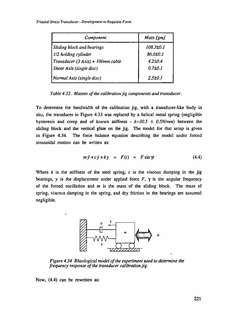
F
Tn axial Stress Transducer - Developmeni to Requisite Form
Compoht
Sliding block and bearings
1/2 holding cylinder
Transducer (3 Axis) + 1 00mm cable
Shear Axis (single disc)
Normal Axis (single disc)
Mass [vnf
1 083±0.1
86.6±0.1
4.2±0.4
0 .7±0.1
25±0.1
Table 4.12. Masses of the calibration jig components and transducer.
To determine the bandwidth of the calibration jig, with a transducer-like body in
situ, the transducer in Figure 4.33 was replaced by a helical metal spring (negligible
hysteresis and creep and of known stiffness - k=305 ± 0.SN/mm) between the
sliding block and the vertical plate on the jig. The model for that setup is given
in Figure 4.34. The force balance equation describing the model under forced
sinusoidal motion can be written as:
in9+c+ky = F(t) = Fsinyt (4.4)
Where k is the stiffness of the steel spring, c is the viscous damping in the jig
bearings, y is the displacement under applied force F, y is the angular frequency
of the forced oscillation and m is the mass of the sliding block. The mass of
spring, viscous damping in the spring, and dry friction in the bearings are assumed
negligible.
Figure 434 Rheological model of the experiment used to determine thefrequency response of the transducer calibration jig.
Now, (4.4) can be rewritten as:
221

(4.7)
(4.8)
Chapter 4
j+2A.$'+co2y = sinyr
(4.5)
C 2where 2A. = - , a) = - and a) is known as the natural frequency of the system.m in
Obtaining the general solution to (4.5) involves solving its homogeneous and
particular equations. There are three cases for solution of the homogeneous equationdepending on the algebraic sign of A.2 - a)2. For an underdamped system A.2 -
< 0,for an critically damped system A.2 - = 0, for an overdamped systemA.2 - > 0. An impulse-like impact test on the calibration jig resulted in a
decaying oscillatory motion, indicating that it is underdamped [Kreyszig 1979].
The general solution of (4.5), therefore, may be written as [Zill 1989]:
F 1y = Ae_sin(ja)2_A.2t+4))+_. sin(V-I-O)
in N/(w2_y2)2+4x2.y2
- —2A.ywhere tan 0 and A and 4) are arbitrary constants-
to satisfy any initial conditions.
The first term on the right hand side of (4.6) describes the transient response of
the system and the second term the steady state response. After sufficient time
under a steady harmonic excitation force the first term decays to zero, leaving:
F 1= rn(a)2_)2+4A.2?V
or as is more commonly seen in engineering texts:
F Iy = kf(l_w2)2+(gw)2
A.whereC=— , w=—
C)) Ci)
The amplitude of the displacement (y) relative to the excitation force (F), for agiven mass (in) and spring stiffness (k), is thus a function of both the damping(c) and the excitation frequency (y). When damping is present (c<>O), the amplitudeof (4.7) is bounded as t -9 , and reaches a maximum when
m
(4.6)

Tn axial Stress Transducer - Development to Requisite Form
Y = w2 _2 2(4.9)
or w = SI1_2 2(4.10)
Clearly, for small damping c —* 0 (2 — 0), the frequency of maximum oscillation
approaches the natural frequency of the system. By substituting (4.9) into (4.7),
the maximum value of the oscifiation is given by
F 1YImax = rn2J(O2_X2
F 1
= k2(xJjr(4.11)
Written in terms of the resultant displacement relative to the maximum of the
excitation function,
— 1
'I'Olmax — 2()\Jij(4.12)
or = ________ (4.13)2J1 —
where Y0 = F/k is the static displacement under a static force (F). Clearly, for
small damping c —*0 (2A. —* 0), the magnification approaches infinity.
The system described by Figure 4.34 was excited by sinusoidally varying forces to
20N at various frequencies between 0.1Hz and 200Hz. After ten cycles at each
frequency, when a steady state had been achieved, five cycles of section output,
displacement and applied force were recorded. A plot of the resultant peak dynamic
displacement to the static displacement with frequency is given in Figure 4.35.
This type of plot is also called a magnification plot as it is a dimensionless ratio
of dynamic to static displacements. The phase difference between the applied
sinusoidal force and resultant displacement is also given. The curve exhibits the
form of a lightly damped system, as the magnification ratio is large (yIY0=22), and
the resonant frequency (61-62Hz) is close to that of the natural frequency of the
system, 0 = = (61.8-62.8) Hz.
223

102I I
1 0
Chapter 4
Now, the measured stiffness of the shear section is typically 80±5N/mrn, and the
stiffness of the normal section is typically 280±80N/mm. Thus the resonant frequency
of the calibration jig with a transducer in situ is approximately 100Hz (shear stress
section) or 190Hz (normal stress section). This is sufficient to accurately observe
the dynamic response of the transducer over the whole bandwidth of the measurand
(50Hz). As will be shown later [4.2.3.5], the resonance of the transducer is
significantly higher than the measurand bandwidth so its frequency response is
constant over the whole bandwidth. Therefore, an arbitrary frequency of 1.0Hz
was selected at which to observe the dynamic performance of the transducer, and
this was taken as a fair assessment of its performance over the whole bandwidth.
C0-4
0CC)
25
20
15
10
5
0T IlItT I I I IIIIIT T 1 I IIIT-.-._..____ I I I
101 10° 101 102 10
2 - - 1T - - -
- 0 - - 1--'- - P.I44C/)
-6 - - __-_L_ _ I Ia. 10-1 10 101
Frequency [Hz]
Figure 4.35 Magnification (a) and Phase lag (b) curves for a spring (k= 30.5 N/mm) in the calibration jig under forced steady state oscillationto 20N. The driven mass was 0 .1991Kg.
4.3.2.3 Range, Hysteresis, Linearity and Accuracy
This part of the chapter describes the stress performance of the final transducer
design. The form of the force versus output curve is discussed, noting any features,
their causes and implications. The effect of nonlinearities, such as creep, hysteresis,
saturation and friction, on linear range and accuracy are reported. As are the
224

Tn axial Stress Transducer - Development to Requisite Form
methods used to convert recorded transducer output data back into the causative
applied force. Again the shear and normal-stress sections of the transducer design
are reported separately.
Shear-stress Section
The first part of the shear-stress section calibration was aimed at establishing the
linear range and accuracy typical of the design. Ten transducers were assembled
and the shear section of each was subjected to five load cycles of ±5, ±10, ±20,
±.50N, at 1Hz. The load cycles was applied with the transducer at orientations of
0° and 90 °. Figure 4.36 shows two examples of one shear axis output response
to applied force. From records of the section displacement with applied force the
measured stiffness of the shear section was typically 80±5 N/mm. During testing
four transducers was exposed to more than 100000 loading cycles, without degradation
of their calibrated performance.
From Figure 4.36 it can be seen that the section output may be linear with applied
force. However, hysteresis is present which tends to broaden at the extremes of
the loading cycle. Also the calibration loop exhibits short horizontal regions at its
extremes. This indicates momentary seizing of the ridge and channel construct
when motion of the two ceases at the extremes (+ or -SON) of a load cycle. As
the region is not uniform for all sections there is obviously some variation in the
dimensions/fit of the ridge and channel within the batch of transducers. This could
reasonably be due to trimming variations during assembly. The broadening of the
calibration loop at the extremes of the load cycle is a combination of localised
friction and energy losses occurring in the rubber.
The effect of friction on the force to output transfer function of the section is
analogous to that of backlash in gears. There will be a loss in transfer magnitude
and a phase lag between input and output wave forms. Both of which are dependent
on the ratio of the applied force to the friction force, such that, if the ratio is
large the loss in magnitude and the phase lag will be negligible [Nagrath 1986].
These effects are also true, in general, of hysteresis in rubber, where both magnitude
distortion and a phase lag occur.
Saturation effects are also evident. These are caused by the magnet being displaced
substantially off one half of the MR element. Therefore, although each device has
225

Chapter 4
100
80
60
40
20E- 00
-20
-40
-60
-80
-100-60 -40 -20 0 20 40 60Force [N]
(a)
120
100
80
60
40E- 20C-.s0
-20
-40
-60
-80-60 -40 -20 0 20 40Force [N]
(b)
Figure 436 Example Force versus Output curves for shear sections ofDesign C. Five consecutive cycles to ±50 N at 0.1 Hz are described.The excitation voltage was JV.
60
226

Tn axial Stress Transducer - Development to Requisite Form
a working range of approximately ±50N, the linear range is sometimes smaller.
To define a linear range, a first order polynomial was fitted by matrix methods,
under a least-squares criterion, through the central ±30N of the calibration loop of
each transducer. This was achieved through the use of the mathematics software
package Matlab (Mathworks mc). A second curve of higher order is fit to follow
closely the centre of the calibration loop, and the difference between the two is
then taken as a measure of the linearity error. The appropriate order of the second
curve is found by minimising the residuals between it and the calibration loop,
while keeping the order small. A fifth order polynomial was found to be sufficient.
An example of a first and fifth order curve fitted to an hysteresis loop is given
in Figure 4.37. The figure also depicts how the absolute linearity error varied
over the load cycle for the best three sections tested. A linear range for a device
may be derived directly from the linearity error plots. For example, the 5% linearity
range of +33 to -42N is marked on Figure 4.37b.
The slope of the first order polynomial curve may be used as the conversion
constant for the processing of clinical data. The error incurred in the use of the
conversion constant was defined as the difference between any point on the calibration
loop and the first order fit. This value thus includes both nonlinearity and hysteresis
error sources. The user may choose to use the linearity information to define the
uncertainty of any measurement he makes (E.g. 5% linearity = 5% accuracy).
However the accuracy of the device may be better specified as follows.
It was observed that the width of the calibration loop decreased as the peak
amplitude of the load cycle decreased - confirming that hysteresis is amplitude
dependent. An example of this dependence is shown in Figure 4.38a-d. As
conversion error is directly related to hysteresis, the accuracy of a conversion regime
is dependent on the local amplitude of the applied force. To define an accuracy
value for the first order polynomial conversion method, the maximum conversion
error from the ±5, ±10, ±20, ±50N load cycles was plotted against the cycle
amplitude. Figure 4.38e is a plot of these maximum conversion errors for the best
three sections tested. On this figure an arbitrary piecewise limit (line) is drawn.
This bounds the maximum conversion errors by a percentage of the cycle amplitude
and a fixed small force value. With these limits identified, any converted clinical
data may then be described as accurate to a given percentage (9%) of its converted
value or a fixed force (0.5N), whichever is the greatest.
227

Chapter 4
80
60
40
20
5' 0E
-20
-60
-80
-100
-120-60
20
18
o 16C/)LI
14
212
'100)C 8-J0,
0Cl)
2
0-60
-40 -20 0 20 40 60
Force [N]
(a)
-40 -20 0 20 40 60
Force [N]
(b)Figure 437 Example of aflrst order (linear) curve and a fifth order(central) curve fit to a force versus output calibration curve for a shearsection of Design C (a). Absolute linearity error of the best threesections tested under a full scale (±50N) load cycle (b).
228
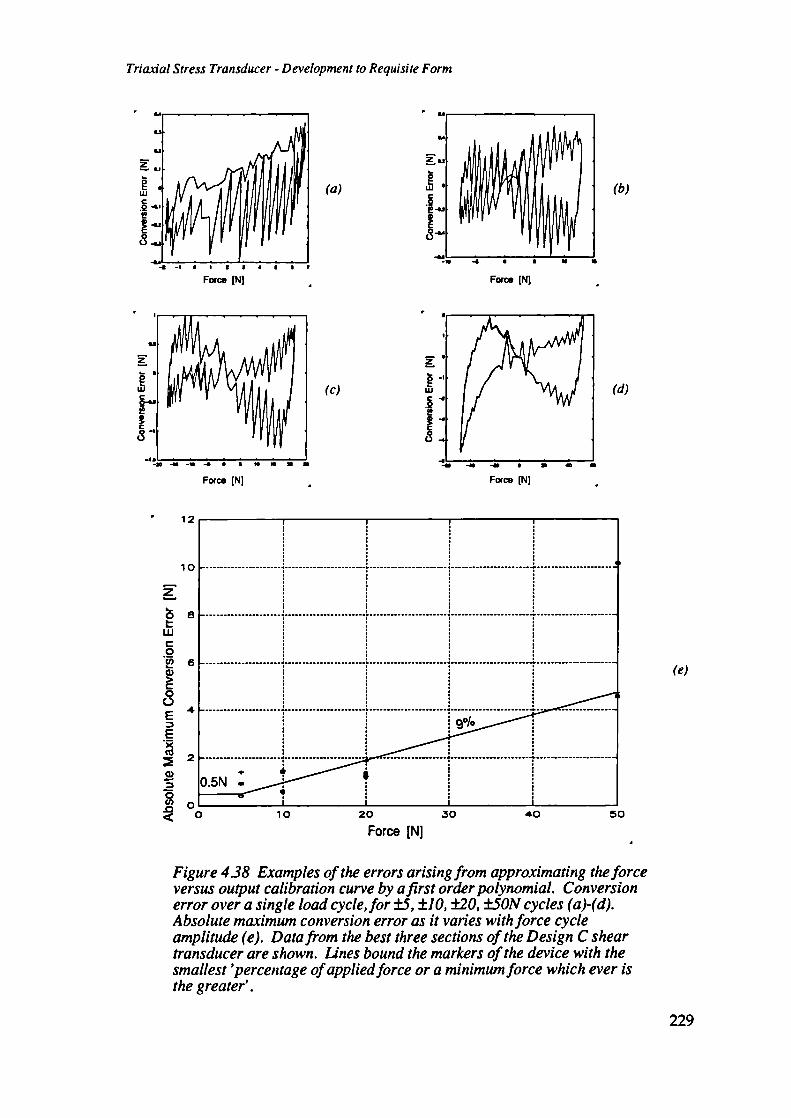
2
.S2
- -I I I I S 4 S S
Force IN]
Force (NJ
Force [NJ
(a)
Force (NJ
(c)
z
2w
I
(b)
(d)
Tn axial Stress Transducer - Development to Requisite Form
12
10
z
08
wC0
>C
(3
E
a)
(e)
0 10 20 30 40 50
Force [NJ
Figure 438 Examples of the errors arising from approximating the forceversus output calibration curve by afirst order polynomial. Conversionerror over a single load cycle,for ±5, ±10, ±20, ±5ON cycles (a)-(d).Absolute maximum conversion error as it varies with force cycleamplitude (e). Data from the best three sections of the Design C sheartransducer are shown. Lines bound the markers of the device with thesmallest 'percentage of applied force or a minimum force which ever isthe greater'.
229

Chapter 4
In some transducers, extreme friction in the sliding mechanism dominated the internal
hysteresis of the rubber. In these cases the loop width tended to be constant with
cycle amplitude, defining the accuracy as a fixed magnitude only.
Now, the coefficients of the fifth order polynomial, as used above, can be implemented
as a 'conversion equation'. To find the polynomial coefficients a fifth order
polynomial was fitted by matrix methods, under a least-squares criterion, through
the calibration loop of each transducer. This was achieved through the use of the
mathematics software package Matlab (Mathworks mc). These coefficients would
generally be unique to each device. Once determined they would be recorded in
the documentation accompanying every device. The conversion error was then the
difference between the polynomial fit and the calibration curve. Figure 4.39 plots
the maximum conversion error of this method as a function of force cycle amplitude
- for comparison with Figure 4.38e. Using a fifth order polynomial conversion
equation , any converted clinical data may then be described as accurate to a given
percentage (6%) of its converted value or a fixed force (0.45)'!), whichever is the
greatest.
Normal-stress Section
The calibration of the normal stress section followed the same regime as for the
shear stress section. Each of the ten sections was subjected to five loading cycles,
of 10, 20, 50, 100 and 200N loads at a cycle frequency of 1Hz. Two example
force versus output (calibration) curves are shown in Figure 4.40. From records
of the section displacement with applied force the measured stiffness of the normal
section was typically 28C0N/mm. During testing four transducers was exposed
to more than 100000 loading cycles, without degradation of their calibrated
performance.
In the figure, one curve [Figure 4.40a] exhibits two distinct slopes and the other
[Figure 4.40b] exhibits three. In the former case the initial slope corresponds to
unhindered flexion of the diaphragm. While the shallow slope corresponds to the
outer rim of the indentor plate impinging on the diaphragm support wall, inhibiting
further flexure. In the latter case slopes at the beginning and end of the curve
have the same causes as above. The middle portion of the curve show the diaphragm
has greater stiffness or is hindered in its flexure. The cause of the hindrance was
traced to the device leads which follow the inside rim of the diaphragm support
230

Tn axial Stress Transducer - Development to Requisite Form
4
3.5
1.01I-wC0
2a,>
l.5EElx
o.:
10 20 30 40 50Force (N]
Figure 439 Examples of the errors arising from approximating the forceversus output calibration curve by afifth order polynomial. Absolutemaximum error as it varies with force cycle amplitude. Data from thebest three sections of the Design C shear transducer are shown. Linesbound the markers of the device with the smallest 'percentage of appliedforce or a minimum force which ever is the greater'.
wall. These were thick enough to be forced into contact with top of the shear
section when the diaphragm is flexed. This in turn provides a reactionary support
force on the diaphragm, decreasing its diameter and increasing its stiffness. This
problem may be circumvented by using smaller diameter section leads.
The working range of the normal stress section may be defined as the magnitude
of applied force at which the indentor plate impinges on the diaphragm support
wall. At that point (the knee) the calibration curve changes slope. Initially the
slope is relatively constant and a single data conversion constant can be defmed.
Now, the working range may be extended by defining a second (and third) conversion
constant which is only applicable to the slope of the curve above the knee. However,
the sensitivity of the device is diminished beyond the knee, and data conversion
becomes more complex. The ranges of the normal stress sections under test varied
considerably, with half of them having a range of less than 70N. The sources of
this variation were due to differences in diaphragm thickness and indentor boss
height between the sections in the batch.
231

Chapter 4
2000
1500
1000
4-
5000
0
-5000
1000
800
600
400
200
0
-200
-4000 50 100 150
Force [NJ
(b)Figure 4.40 Example calibration curves for Normal transducer sectionsof Design C. Each was subjected to five cycles to 200N at 0.1Hz. Theexcitation voltage was lVdc.
50 100 150 200Force [NI
(a)
200
232

Tn axial Stress Transducer - Development to Requisite Form
There was hysteresis over the load cycle, but it was seen to be significantly less
than that of the shear stress section. This was expected as hysteresis in silver
steel is much smaller than that for rubber.
A conversion constant for transforming the recorded clinical data to its causative
applied force, was defined. A first order polynomial was fitted by matrix methods,
under a least-squares criterion, through the calibration loop of each transducer. This
was achieved through the use of the mathematics software package Matlab (Mathworks
mc). The coefficient of this polynomial was used as the conversion constant.
Linearity error and linear range may be calculated by fitting a high order polynomial
to the centre of the calibration loop and finding the difference between it and the
first order polynomial fit. Figure 4.41 plots the linearity error over a full scale
load cycle (lOON) for the best three sections tested. A linear range for a device
may be derived directly from the linearity error plots. For example, the 5% linearity
range of 67N is marked on Figure 4.41a.
It was observed that the width of the calibration ioop decreased as the peak
amplitude of the load cycle decreased - confirming that hysteresis is amplitude
dependent. As conversion error is directly related to hysteresis, the accuracy of a
conversion regime is dependent on the local amplitude of the applied force. To
define an accuracy value for the first order polynomial conversion method, the
maximum conversion error from ±10, ±20, ±50, ±JOON load cycles was plotted
against the cycle amplitude. Figure 4.4 lb is a plot of these maximum conversion
errors for the best three sections tested. On this figure an arbitrary piecewise limit
(line) is drawn. This bounds the maximum conversion errors by a percentage of
the cycle amplitude and a fixed small force value. With these limits identified,
any converted clinical data may then be described as accurate to a given percentage
(5%) of its converted value or a fixed force (1.9W), whichever is the greatest.
233

Chapter 4
20
18
16
14
o 12C/)U-
10
0i_ 8I-w
a,. 4-J
2
00 20 40 60 80 100 120
Force [N]
(a)
25
20
z10
W 15
0U)I-a)>o 100EExc
0U).0 0< 0 20 40 60 80 100
Force [N]
(b)
Figure 4.41 Absolute linearity errors over a full scale load cycle (lOON)(a). Absolute maximum error as it varies with force cycle amplitude,arising from a first order approximation to the Force versus output curve(b). Data is from the best three normal stress sections of the Design C.Lines bound the markers of the device with the smallest 'percentage ofapplied force or a minimum force which ever is the greater'.
234

Tn axial Stress Transducer - Development to Requisite Form
3
2.5
2
1.5
1
0.5
01 I I I I
0 20 40 60 80 100
Force [N]
Figure 4.42 Absolute maximum error as it varies with force cycleamplitude. Errors are those arising from the use of a fifth orderpolynomial approximation to the force-output curve. Data is from thebest three normal stress sections of Design C. Lines bound the markersof the device with the smallest 'percentage of applied force or aminimwn force which ever is the greater'.
Now, the coefficients of the fifth order polynomial can be implemented as a
'conversion equation'. When a higher order polynomial approximation to the force
versus output calibration curve is used, linearity errors are replaced by a smaller
trend error. This generally reduces the conversion errors to that of the hysteresis
induced uncertainty. Figure 4.42 plots the absolute conversion error for a fifth
order approximation to the calibration curve. On this figure, as above, an arbitrary
piecewise limit (line) is drawn. This bounds the maximum conversion errors by
a percentage of the cycle amplitude (1.75%) and a fixed small force value (1.1W).
The relatively high minimum force seen on the limit line is due to relatively coarse
increments (approximately iN steps) in applied force, during load cycling, creating
a jerky calibration curve. The applied force cycle was not smooth because very
small changes in displacement were required and there was a coarseness in the
movement of the bearings in the vibrator [Figure 4.32a].
z
01.wC0U,
>C0C-)
EEx
a)-S
0U,.0
235

Chapter 4
4.3.2.4 Shear Stress Vectors and Crosstalk Errors
The assessment of linearity and hysteresis described in 4.3.2.3 was performed with
each shear axis aligned to the direction of the applied force. As the two shear
axes are arranged orthogonally the magnitude and direction of applied force can
be resolved. The accuracy of this ability to distinguish the direction of applied
loads relies on each axis being insensitive to the components of the load which
are orthogonal to it. An induced change in the output of a given axis due to
loads applied along either of the other axes is called crosstalk. An assessment of
this action is described at the end of this section - [4.3.2.4].
To assess the accuracy of the direction resolution each device was subjected to
±20N loading cycles, at 1Hz, at 150 orientations from 0° through to 360 °. The
maximum and minimum output of each axis pair was recorded for the cycles at
each orientation. The change in output with angle should ideally form a sine-cosine
pair. Examples of the variation in output with orientation for the best three sections
can be seen in Figure 4.43a. By calculating the inverse tangent of these pairs it
'as possible to determine the apparent or indicated angle of the applied force
vector. When this was compared to the true angle the angular error was found.
Figure 4.43b shows the angular errors for the above three sections as a function
of the true vector angle. From this plot it can be seen that in the best case it
was possible to resolve force vector angles to better than 60 with Design C.
There are two main causes of the error in the design. Firstly, as the vector angle
approaches the orthogonal of an axis there will be an increasing frictional force
occurring at the ridge and channel construct. This will hinder displacement and
reduce the output magnitude for that axis. The resultant error in the apparent angle
will be an over or under estimate of the true angle dependant on relative friction
of the two axes. Secondly, as each MR element may not be truly uniaxial, any
lateral play in the ridge and channel will disturb the output magnitude unpredictably.
Mechanical crosstalk between the transducer axes is where a given axis output
changes when a force is applied in a direction orthogonal to it (ie. along one of
the other two axes). This change in output falsely indicates that there is a component
of the applied force acting along the direction of the given axis. This source of
error in the transducer was assessed by observing the output variations of all three
axes while a full scale loading cycle was applied parallel to each axis in turn.
236

1L)
9
8
7
C)) 6
I.-o 51w
2
Tn axial Stress Transducer - Development to Requisite Form
100
50
0
-505' 0E4-
. 504-.
0
0
-500
X- Axis
TH4 TFH50 100 150 200 250 300 350 400
50 100 150 200 250 300 350 400
Orientation [Deg]
(a)
0 50 100 150 200 250 300 350 400
Orientation [Deg]
(b)
Figure 4.43 Output variation with orientation of the applied force vector(±2ONpp loading cycle at 1Hz) (a). Error between measured orientationand applied force orientation (b). Data is from the best three shearstress sections of Design C.
237

Chapter 4
The maximum variation in the output of each axis under orthogonal loading was
taken as the maximum crosstalk error. The average crosstalk error on the shear
axes due to full scale loading on the normal axis is 1.1% FSL (SD = 1.4). The
mechanism of interference in the shear stress sections is the slight compression of
the rubber layer, under normal loads, altering the magnet-magnetoresistor separation.
This interference can be reduced by increasing the area : thickness ratio of the
rubber layer or increase the magnet-magnetoresistor separation to a less sensitive
region. Both of these schemes would decrease the stress sensitivity of the transducer.
The interference in the normal stress section is due to the combination of force
moments, from shear stresses, normal stresses and excess space in guide pin holes
of the normal section. These create a small variation in normal force as the
transducer rocks on the boss of the indentor plate. This interference can be reduced
by lengthening the guide pins and improving their fit in their holes, which will
provide greater opposing force moments and increased mechanical rigidity.
4.3.2.5 Creep and Frequency Response
The frequency response of both the shear and normal sections of the transducer
will be bounded at both low frequencies due to creep phenomena and high frequencies
due to inertial reactions. Creep in the normal stress section was indetectable, so
there is no practical low frequency limit for normal stresses. Creep was observed
in the shear stress section but was found to be completely reversible - so calibration
data remains valid. The frequency response of the shear section will be predominated
by the elastic response of the rubber - [3.1.2.3]. Thus at very low frequencies (<
0.01Hz) the output is likely to exhibit a non-linear response to stress due to creep
processes in the rubber. At intermediate frequencies (0.1-1000Hz) the output is
approximately linear with stress. While, at very high frequencies (> 10000Hz) the
rubber becomes glassy and the output is negligible.
Four shear stress sections of the ten assembled transducers were subjected to 20N
step shear forces and their outputs sampled at 100Hz. The data was plotted against
the logarithm of time and a first order polynomial was fitted to the curve. The
coefficient of the polynomial defines the creep rate in units of %/log(sec). The
value provides an indication of the error involved in using the conversion constant
at very low frequencies. Table 4.13 contains the creep constants of the four sections
tested.
238

Tn axial Stress Transducer - Development to Requisite Form
Device Creep
%IIog(sec)
1 3.87
2 2.45
3 2.26
4 232
Table 4.13. Measured creep rate offour shear sections of Design C. A20N shear force was applied and left for 150 seconds.
Assuming that the stride time of amputees may generally vary from 1-5 seconds,
the dynamic stresses, at the limb/socket interface, related to walking will generally
be of this period or shorter. A clinical study may last for approximately 20 minutes,
roughly two decades of time longer than a stride. Thus, from Table 4.13, longterm
limb/socket stresses due to fitting, retention or stance forces will contribute less
than 10% errors by the end of a study. For accuracy it is therefore advisable to
keep studies short. If an error in shear stress measurement of 10% FSL is defined
as the acceptable limit, the low frequency limit of the shear stress section is 0.1mHz.
From [4.3.2.2] the resonance of the dynamic calibration facility, when a spring of
similar stiffness to the transducer is being loaded, was identified as approximately
100 Hz. Therefore the frequency response of the transducer could only be determined
quantitatively, with this equipment, if its resonant frequency was below this. To
explore this, four triaxial devices were each mounted in the calibration jig [Figure
4.32] and subjected to sinusoidally varying forces. Load cycles to ±2ONpp at
frequencies ranging from 0.01Hz to 200Hz were applied to the shear stress sections
and load cycles to 2ONpk at frequencies ranging from 0 .01Hz to 500Hz were applied
to the normal stress sections. After ten cycles at each frequency, when a steady
state had been achieved, five cycles of section output, displacement and applied
force were recorded. Plots of the resultant peak dynamic displacements to the
static displacements with frequency (magnification plot) is given in Figure 4.44.
The phase differences between the applied force and resultant displacement is also
given. The curves exhibit the form of lightly damped systems. The magnification
ratio is moderate for the shear stress section (yIY0=53), and the resonant frequency
(100-120Hz), while the magnification ratio is low for the normal stress section
(y/Y0=1.8), and the resonant frequency (100-200Hz). Although, the test frequencies
239

Chapter 4
for the normal stress section were coarsely separated around its resonance, so the
magnification ratio may in reality be higher. In both cases the resonant frequency
is close to that of the natural frequency of the calibration jig with spring of
comparable stiffness in situ (100Hz shear : 190Hz normal).
It was evident from the curves that the resonance of both the shear and normal
stress sections was above that which the test facility could accurately measure. The
curves suggest that the dynamics of both sections may reasonably be modelled by
the Voigt model shown in Figure 4.33. Also the sections have slightly more
viscous damping than is present in the jig bearings, but are nonetheless underdamped
structures. Therefore their true frequency response has a similar form to that seen
in Figure 4.44.
Now their resonant frequency can be determined by observing their impulse response.
If an impulse force is applied to each section then from (4.6) the device will be
excited into a decaying oscillation. The second term on the right hand side of
(4.6) becomes negligible and the first, or transient term, dominates. The envelope
of the decay is related to the damping in the section as described by e. The
frequency of the oscillation is the resonant frequency described by sinJ(w2 - 2) ..44From Figure 4.44 both sections are underdamped therefore their resonant frequency
will be close to their natural frequency, which is:
80(±5)[Nmm'] 1700(±170)Hz (Shear) (4.14)= = O.7(±O.l)[g]
J 280(±80)[Nmm'] 1300(±250)Hz (Normal)
= 4.2(±O.4) [g]
To apply the impulse force a typical device was clamped to a large table top in
such a way as to allow the section under test to vibrate freely. The shear stress
section was struck a momentary (glancing) impact parallel to its axis by a metal
bar. The normal stress section was excited by a metal ball bearing being dropped
onto the transducer forcing it onto the indentor beneath it. In both cases output
was recorded by a Digitising Storage Oscilloscope (DSO). The resultant transient
outputs are presented in Figure 4.45.
240

Tn axial Stress Transducer - Development to Requisite Form
6
Co 44-
0C 2C)
010-2
0
U)Cc -2
G -4U)
.0a. 10-2
10-1 100 101 102 10
10-1 100 101 102 10
Frequency [Hz]
(a)
2
C 1.504-0
C0.5
010-2
2
0U)Cc -2
.0 -8a. 10-2 10-1 100 101 102 i0
Frequency 1Hz]
(b)
Figure 4.44 Example magnification and phase lag plots for the shearstress section (a), and normal stress section (b) of Design C, understeady state forced sinusoidal oscillation to 20N.
10-1 10 101 102 10
241
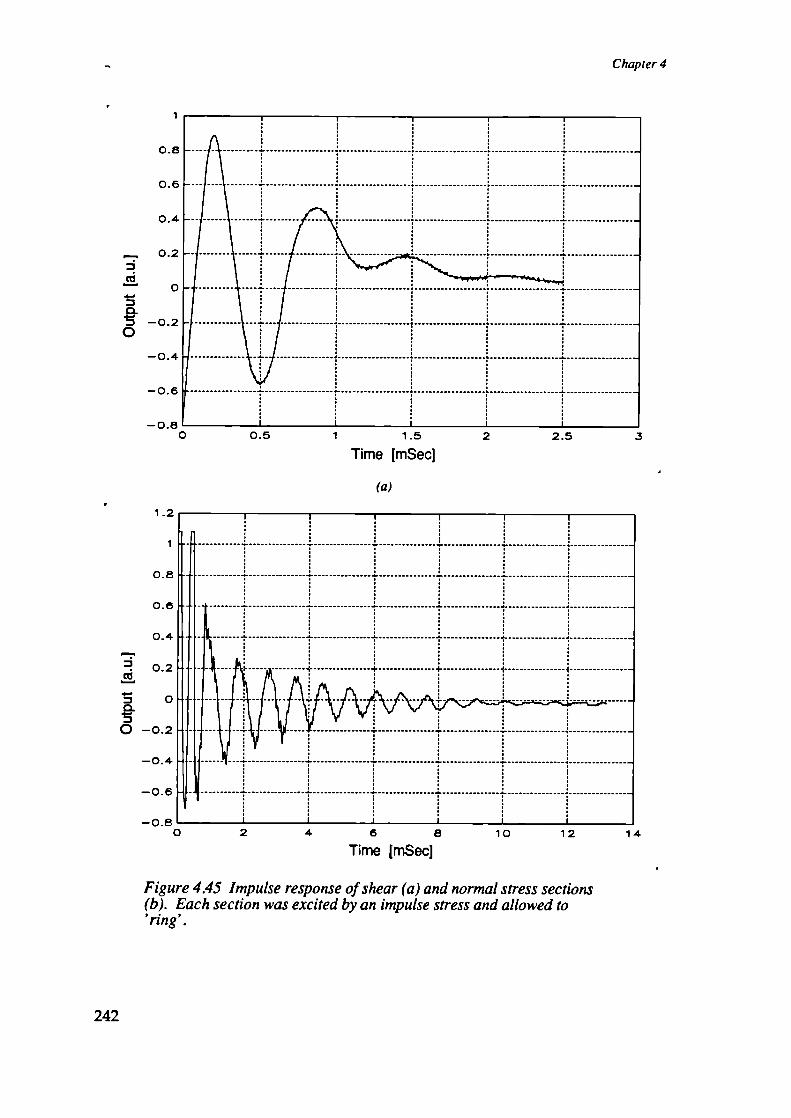
0.8
0.6
0.4
- 0.2
- 0
-0.2
-0.4
-0.6
-0.80
Chapter 4
0.5 1 1.5 2 2.5 3Time ImSec]
(a)
1.2
0.8
0.6
0.4
0.2
0
0 -0.2
-0.4
-0.6
-0.80 2 4 6 8 10 12 14
Time [mSec]
Figure 4.45 Impulse response of shear (a) and normal stress sections(b). Each section was excited by an impulse stress and allowed to'ring'.
242

Tn axial Stress Transducer - Development to Requisite Form
It is seen from the curves that the resonant frequency of the shear stress and normal
stress sections are approximately 1500Hz and 1200Hz, respectively. Both these
measured values are close to the predicted frequencies. Clearly the frequency
response of both shear and normal stress sections of the device could reasonably
be affirmed as constant up to and significantly beyond the measurand bandwidth
of 0-50Hz, as required.
4.3.3 Temperature Sensitivity
Having determined the designs' response to force magnitude, orientation to applied
force and frequency, it was necessary to establish the extent to which the response
was compromised by its temperature sensitivity. That is, where temperature induced
changes in the output signal of the device may be falsely interpreted as stress
signals.
4.3.3.1 Test Equipment and Methods
To assess the temperature sensitivity, three transducers chosen at random from the
set of ten, were mounted, in turn, in the calibration jig and placed in the laboratory
oven. The normal stress section tests were carried out with the device placed
under the sliding block of the calibration jig - [4.3.2.1]. An external platform was
attached to the sliding block of the jig via a connecting rod which projected out
of a vent hole in the oven roof [Figure 4.17]. The temperature was raised from
27 to 50C. At approximately five degree intervals various loads were placed on
the platform in succession and recordings of the temperature and section output
were recorded. Signals from the section were buffered by the MEPO86B unit
[Chapter 6] and temperature measurements were made using the meter MEP 123
platinum resistance thermometer. Signals were input to an A/D convertor
(DT2824-PGH - Data Translation mc) hosted in a personal computer (IBM PC/AT).
Control of the A/D was via applications software Global lab (Data Translation
mc).
243

Chapter 4
4.3.3.2 Sensitivity Data
From the recorded temperature and section output data, the change in output with
temperature for the loaded sections was plotted. Figure 4.46 presents example plots
of data from a shear stress and a normal stress section.
It was clear from Figure 4.46 that there were two temperature induced phenomena
occurring. Firstly, there was a noticeable temperature coefficient of output (offset
drift = slope ) and secondly, there was an accompanying change in load sensitivity
(gain drift = non parallel load lines). Therefore, the assessment of the potential
temperature induced errors is quite complex so two assumptions are made to simplify
the error estimates. Firstly, the change in offset and the change in gain are treated
as independent parameters, and secondly as being linear. With reference to Figure
3.15 the above assumptions were seen to be valid for the MR, over the temperature
range 20-40 r.
Now, the output v force calibration curve for a normal stress axis is derived at
room temperature and can be described by the equation
= m(x—A) [N] (4.15)
Where y [V] is the output, x [N] is the applied force, in [N/V] is the gain constant
and A [1"] is the offset in output at zero-load. At any other temperature + ET
the new output v force calibration curve can then be written as
YIT1Q +T = n(x—B) [N] (4.16)
Where n ^ m and B ^ A due to the gain and offset drift.
Clearly, when converting recorded output data into apparent applied force, the
difference between the performance curve and the calibration curve will lead to an
over or underestimate of the force. The error can be derived as
244

Tn axial Stress Transducer - Development to Requisite Form
45
40
35
30
5' 25E
20
0 15
10
5
025 30 35 40 45 50 55
Temperature [C]
1000
900
800
7005'
600
500
400
30025 30 35 40 45
Temperature [C]
Figure 4.46 Example of the output variation with temperature of a shearstress (a) and normal stress (b) section of Design C, when loaded (0, 10,20, 30N) and subjected to temperatures of27-50 °C.
Error = = = n(x—B)—m(x—A) (4.17)
50
245

Chapter 4
Now, if the offset drift is s [VIC] and the gain drift is g [N/V/C]
then B = A+sAT
and n = m+gAT (4.18)
So (4.17) can be written as
e = (m+gAT)(x—(A+MT))—m(x—A)
= (g(x—A)—ms)AT—gthT 2(4.19)
Using (4.19), values were derived for the gain and offset at 20C and the maximum
error over the range 20-40C, for each of the sections tested. These are given in
Table 4.14.
Gain Offset Offset Drift Gain Drift Error
Section jN/mV) [inVjE. 11 fnVICJ fN4tV/t'J 1. .fNJ (%FSSJ
1 1 5821 63.07 .1349 53 158 3.16
.74 156 .1194 .51 1.78 3.56
S .4131 34.72 -.0014 1.78 433 8.66
4 H . .6355 -21.02 .1417 1.89 1.91 3.82
568 323 .0224 1.47 232 4.64
6: 1.0037 -6.02 2856 2.79 5.99 11.98
Table 4.14 Values of the Gain, Zero-stress Offset, Offset temperaturedrift, Gain temperature dr(ft, and maximum data conversion error,for sixsections of Design C.
Clearly the majority of devices of Design C may have temperature induced errors
of less than 5% over their working temperature range. Thus implying that during
any one clinical measurement session errors due to temperature related drifts in
device performance may be considered minimal, if not negligible. The apparent
outhers in the data set of Table 4.14 may possibly disappear if a more exact and
consistent assembly procedure could be established. This is because: offset is
246

Tn axial Stress Transducer - Development to Requisite Form
dependent on spatial alignment; gain is dependent on friction, stiffness, and magnet-MR
separation; and both offset drift and gain drift are dependent on magnet-MR
separation.
4.4 Summary
This chapter has described the progress of development of the three axis stress
transducer from prototype to a requisite form. In this part a summary is given of
the best performance demonstrated by a batch of ten transducers of the final design
form. This will give an indication of the achievable performance of the design.
Comparisons are made with the initial specification given in Chapter 2.
The assembled device measured 15.96mm diameter by 4.9mm thick with the indentor
plate adding a further 1.1mm total thickness. Each shear axis had a stiffness of
80±5N/mm and the normal axis a stiffness of 280±80N/mm.
The force versus output calibration curve for all axes exhibited hysteresis. That
of the normal axis was small, less than 2% indicated load, while for the shear
axes was less than 6.5% indicated load. It was demonstrated that the hysteresis
was amplitude dependent.
Some nonlinearities occurred on all axes. A saturation effect was seen on the
shear axis, due the displacement of the magnet approaching the outer edges of the
magneto-resistor. Thus when a single conversion constant is used to transform
recorded voltage to force, a linear range for the section must be defined. For
example, the 5% linearity range is typically only ±30N. However, it has been
demonstrated that it is possible to construct the shear stress section so that it has
a total linearity error, over the full scale range (SON), of less than 6%FSO. The
nonlinearity in the normal axis was due to the device leads, bonded to the underside
of the diaphragm, interfering with its flexure. It was demonstrated that it is possible
to construct the normal stress section so that it has a total linearity error, over the
full scale range (lOON), of less than 2.S%FSO.
Friction was a source of error in the shear stress section. Although most of the
devices built exhibited some friction effects, it was demonstrated that sections could
be made which were free of significant friction.
247

Chapter 4
The above errors (hysteresis, nonlinearity and friction) for both shear and normal
stress sections can be combined into a parameter which defines the accuracy to
which the conversion method models the calibration curve. When the calibration
curve was approximated by a first order polynomial, a single constant was used to
convert recorded voltage data into apparent force data. The accuracy of this
conversion method was expressed as percentage of indicated force or some minimal
force whichever was the greater. It has been demonstrated that it is possible to
construct the shear stress section so that it has a first order conversion polynomial
with total accuracy , over the full scale range (50W), of 9% indicated force or
0.5N whichever is the greater. For the normal stress section the demonstrated best
accuracy was 5% indicated force or 1.9N whichever is the greater. When the
calibration curve is approximated by a higher order polynomial, nonlinearity errors
are replaced with a trend error. Also the useful range of the device is extended
as the polynomial fits into the previously nonlinear regions of the calibration curve.
When a fifth order polynomial was fitted to the shear and normal stress calibration
curves, the demonstrated best accuracy of data conversion was then found to be
6% indicated force or 0.45N and 1.75% indicated force or 1.JN, respectively.
The force sensitivity of the axes was taken from the first order polynomial fit and
was approximately 0.6NImV and 0.05N/j.iV for shear and normal stress axes
respectively. The excitation voltage in each case was JV d.c. Both section designs
are able to withstand 100% overload. During testing four transducers was exposed
to more than 100000 loading cycles, without degradation of their calibrated
performance.
The frequency response of each section was deduced implicitly. Both were constant
well beyond the expected clinical stress signal bandwidth of 50Hz. Resonant
frequencies were approximately 1500Hz and 1200Hz for the shear and normal stress
sections respectively. From the shape of the magnification plots of Figure 4.44 it
can be seen that the section response is constant up to approximately half of the
resonant frequency. Creep was only significant in the shear axes. The measured
rate was 2.7(0.77SD) %/log(Sec). Over a typical 20 minute clinical measurement
period, the constant pre-load forces will cause an apparent force increase of less
than 10%FSL. All instances of creep were seen to be reversible. If an error in
shear stress measurement of 10%FSL is defined as acceptable performance, the low
frequency limit of the shear stress section is 0.1mHz, while that of the normal
stress section is negligibly small.
248

Triaxial Stress Transducer - Development to Requisite Form
Temperature induced apparent stress errors were observed in both axes mechanisms.
These were manifest as offset drift and sensitivity drift. They were assessed over
the temperature range 20-40 t. The values of offset and sensitivity at 20°C were
used as a baseline for calibration data. Errors due to both drifts combined were
demonstrated to be less than 0.19 %FSL2) °C and 0.1 %FSL20/ °C for the shear and
normal stress sections respectively.
Table 4.15 presents some of the above data for comparison with Table 2.2 - the
proposed performance specification.
Parameter ..... . : SheW stress section Normal stress section
Measurement Range . 0-250 KPa 0- 500 KPa
Overload .. .. ... . 2500 KPa 1000 KPa
Accuracy (first order,. ±9% indicated load or ±5% indicated load or
convers km polynomial) 23 KPa 93 KPa
flJh Order conversion ± 6% indicated load or ± 1.75% indicated load
polynoniial .. .....E: .J.. 225 KPa orSi KPa
Temperature Range 1:. 20-40 t
Frequency Range ... 0.1 mHz - 750 Hz 0- 600 Hz
Liferfrne (gait cycles) > 100000
Dimensions . .. . . 15.96 mm diameter x 4.9 mm
Mass . . 4.6±0.4g
Figure 4.15 Performance data ofthefinal design of the tn axial stresstransducer.
Generally, it was felt that the specifications set out for the transducer had been
met to a significant degree. And furthermore, to the extent of the author's knowledge
has filled a gap in the general triaxial stress transducer market not occupied by
any other device.
249

Chapter 4
250

Chapter 5
Data Acquisition : Hardware
The previous chapter described the development path of the triaxial stress transducer
from prototype to fmal form. In this chapter the design of the circuits and systems
used to acquire and store transducer signals are detailed.
Figure 5.1 is a block diagram of the hardware units of the acquisition system. The
transducers connect to a Transducer Interface Unit (TIU). Their signals are buffered
and filtered and then passed to the Data Collection Unit (DCU) where they are
digitised. Buffered digital data is transferred to a Personal Computer (PC) for
archival and processing. Simultaneously, external event signals are also cligitised
and archived., for synchronising multi-system data sets.
Section 5.1 describes the circuitry and protocols for exciting the transducers and
conditioning their outputs. Section 5.2 reports on the nature and interconnection
of the equipment used to digitise and store the signals. Section 5.3 describes the
interface circuitry for synchronisation to a video based kinematics measurement
system. Section 5.4 describes the physical interconnection of each part of the
system. Lastly, 5.5 discusses the safety considerations of the system.
Kinematics
InterfaceTransducer
Excitation&
I User InterfaceI Signal ______ Digitizer
1& Storage
Transducer Conditioning
Figure 5.1 Block diagram of the hardware interconnection of theData-Collection system
5.1 Transducer Interface Circuit
The following section describes the functional blocks and circuitry, in the TIU,
used to interface to the transducers.
251

ChapterS
Each transducer was excited with a reference voltage which was then modulated
by the applied stress to produce the electrical stress signals. Section 5.1.1 discusses
the modes and implementation of circuits to do this. Section 5.1.2 describes the
conditioning and buffering which is applied to the stress signals before they are
input to the DCU. Also discussed is the expected noise in the clinical environment
5.1.1 Transducer Excitation
In order to devise the most effective method of exciting the transducer it is necessary
to understand the electrical characteristics of the transduction elements. What follows
is a discussion of the principle electrical properties of the magneto resistor (MR)
(FP111L100 - Siemens UK LTD) and the foil strain gauge (SG) (QFDPF-9-350
- Technimeasure LTD).
5.1.1.1 Magneto-resistor Electrical Properties
The excitation circuitry will experience the MR as a two-port, three terminal device
whose driving-point impedance is variable. Under the influence of a changing
magnetic flux density, perpendicular to its face, the resistance component of the
impedance will vary according to the approximate relationship.
R = R0(l+K.t2 32) (3.17)
Where R is the resistance when influenced by magnetic induction 1, R0 is the
resistance under zero induction, .t is the electron mobility of the material and K
is a material dependant constant.
Heidenreich [1985] states that the MR's frequency response extends into the
Gigahertz region, which implies that the reactive component of the impedance is
small. Relative to the range of frequencies expected to be met in this application
these reactive components are negligible. As discussed in Chapter 3 the MR appears
as two magneto-resistors in series. The base resistance, R0, (ie when not in the
presence of a magnetic field) of each of these is lOOf2 ± 20%. The difference
in value of each resistor, compared with the other, is expressed in the centre
symmetry parameter, M. Which is defmed as the percentage difference of the
single resistors (R,, R2) divided by the smaller of two resistances;
252

For:
Shear strain element
RI, R2-activeR3, R4-lixed
Normal strain element
R1,R2,R3.R4-active
0
Data Acquisition : Hardware
M = R1—R2 .100% forR1>R2 (5.1)
R2
For this particular MR type the symmetry is typically 2%. The relative resistance
change, with the magnetic field used in this application, is approximately 1.5. Thus
in the assembled shear section with no shear-stress applied the driving-point impedance
is approximately 300f ± 20%. When the section is loaded the impedance may
vary up to 50%.
To improve noise rejection from the excitation supply, the MR of each axis was
incorporated as one half of a Wheatstone bridge. The other arm of the bridge is
formed from two fixed series resistors across the same supply. Figure 5.2 shows
the arrangement. Output signal is taken between the centre point of each arm.
Figure 5.2 Schematic of a Wheatstone bridge circuit with two activearms.
Another advantage in this arrangement is that any imbalance in the MR can be
zeroed out by padding resistors. Then, the direction of the stress induced displacements
can be distinguished by the sign of the output voltage. With this arrangement the
change in output voltage is related to the excitation voltage, the initial resistance
and the change in resistance by;
AREtV0 = 21 VE (5.2)
Obviously the output magnitude may be increased by employing a large excitation
voltage. However consideration must be given to the power dissipation in the
device. From Chapter 4 it is seen that the MR element is adversely sensitive to
temperature changes. Now, electrical power input to the element is converted to
253

Chapter 5
heat, a proportion of which is conducted away by the surrounding material. If the
thermal conductivity of this material is insufficient then the element will itself heat
up, causing the output voltage to change erroneously. Therefore to determine the
excitation voltage or current it is necessary to determine the thermal conductivity
of the mounted MR. The quoted value for the MR lying on a metal surface is
15mW/K. The actual value for the MR enclosed in the section will be lower. In
this case it is surrounded by rubber and plastics which have lower thermal
conductances than metal.
To experimentally determine it, the following simple test was undertaken. Firstly
the assembled section was placed in an oven, heated to its maximum operating
temperature, T = 120°C and allowed to equilibrate for 30 minutes. The resistance
of each MR was measured. Secondly the section was cooled to ambient temperature,
Ta = 23°C, and allowed to equilibrate for 30 minutes. Each MR was then driven
with a current that was increased until the resistance of the MR reached that of
the first measurement. At that point the MR is operating at its maximum operating
temperature, and the electrical power input is causing an increase in temperature
of T,,, - Ta. The thermal conductance is then given by:
Gth =
[WK] (5.3)Ta
In this case the electrical power input was measured as the product of the input
current and voltage, 68mA and 13.OV. So rearranging (5.3) we have;
V.'Gth =
(5.4)TxTa
= 9.1 mWK
Now from the relation for electrical power;
V2P =
(5.5)
(5.4) can be rearranged to give:
V = (5.6)
254

Data Acquisition Hardware
Where V,, is the excitation voltage that will raise the MR to its maximum
permissible temperature. This form can be used to determine the excitation voltage
at which a given temperature rise will occur. By restricting to be 1 °C above
ambient and using the ambient value of resistance for RT = 32O, The maximum
excitation voltage allowed is V = 1.7V.
Before the excitation voltage could be fmalised it was necessary to consider the
excitation limits of the SG.
5.1.1.2 Strain-gauge Electrical Properties
It is common to excite full bridge strain-gauges by a constant voltage source. So,
there was a possibility of using the same excitation circuit for both MR and SG.
Before defining a circuit the electrical properties of the SG were investigated.
The excitation circuitry will experience the strain-gauge as a two port, four terminal
device whose driving-point impedance is relatively constant. As the gauge is
subjected to tensile stress the ratio of change in its impedance to its initial value
is given according to the relationship
Ap1 = (l+2.t)y + - (4.21)
Where R is the initial resistance, L is the initial length, t is Poissons ratio for the
gauge material and p is its resistivity. The frequency response of the free gauge
extends into the high Kilohertz. When the gauge is bonded, it is dependent on
the stress-strain relationship of the substrate. For this application the reactive
components of the gauge impedance are insignificant.
Under no-load conditions the driving-point resistance of the gauge used here is
350fl ± 03%. When the gauge is bonded and subjected to maximum tensile stress
the resistance change is typically 2% of this base value. The SO has a full bridge
configuration with four active elements. So the change in output voltage is related
to the excitation voltage, initial resistance and change in resistance as
255

ChapterS
AR0AV0 = -- • VE(5.7)
Again the magnitude of output signal is directly proportional to the excitation
voltage. The limiting value of VE is detennined from the allowable power dissipation
in the gauge. The QPFDPF-9-350 gauge is specifically designed for bonding to
low-carbon steels. Manufacturing data supplied with each gauge summarises the
power calculations and recommends a maximum excitation voltage of JV.
5.1.1.3 Excitation Circuit
From the previous discussion on allowable power dissipation it was decided that
the same excitation circuit would be used for both the MR and SO. The voltage
would be set at 1 Volt. Although small excitation voltages generally lead to poor
signal to noise ratios, both the MR and SO are relatively low impedance devices.
This tends to make them less sensitive to the relatively low power electromagnetic
interference found in the typical clinical environment. However the stability of the
excitation voltage is quite important As will be discussed later the digitiser used
has a 12 bit resolution and therefore is capable of resolving to 0.024% of its input
range. At the time of design the most cost effective high stability voltage reference
available was the AD588 (Analog Devices LTD) with a regulation of 0.1%. The
following describes the various elements of the excitation circuitry.
The circuit diagram shown in Figure 5.3 describes the transducer excitation circuit.
Components C1-C4, Ri, R2 provide a local power supply reservoir of ±12V. U)
is the precision voltage reference (AD588) with two internal buffer amplifiers A3,
A4. The output of this reference is ±5.000 V (±5mV) so in order to create a JV
±lmV to apply to the transducers, R3-R6 divide the output to ±0.5V (±50tV).
These voltages are buffered by A3 and A4. Qi and Q2 act as output current
buffers for Ui as the load current with ten transducers connected (i5OmA maximum),
exceeds the output current specification of the AD588. Ru and R12 provide Qi
and Q2 with output short-circuit protection. An analogue ground connection (AGND)
to Ui (pin 9) references the transducer excitation voltage to float at approximately
ground potential. This affords the excitation voltage an extra degree of noise
immunity from disturbances in the power supply.
256
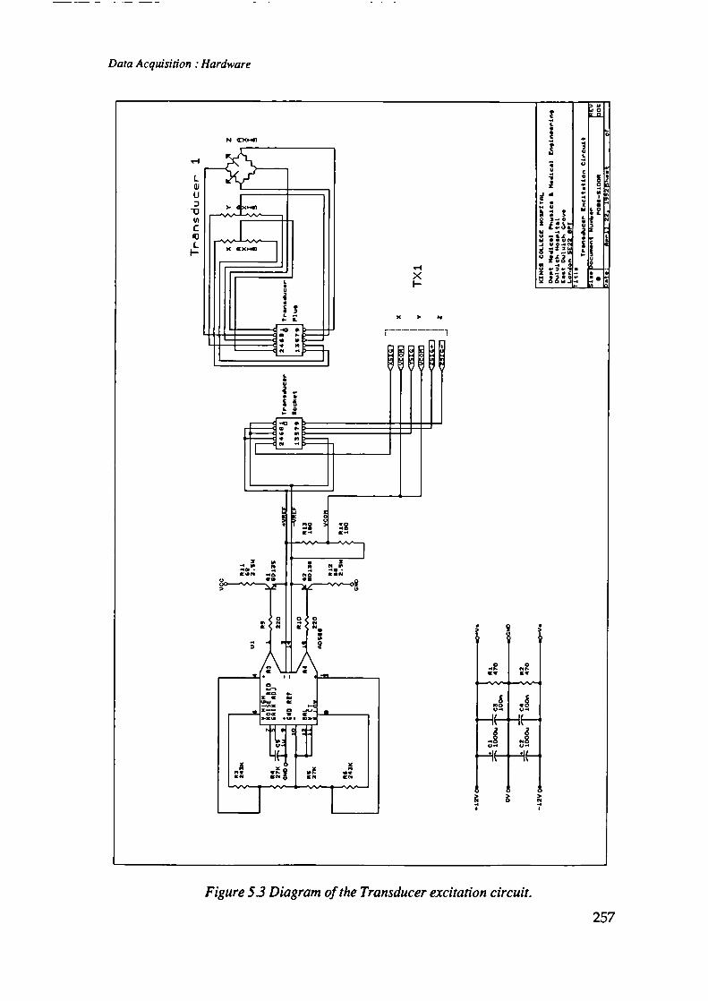
'-I
LwUJ
In
C'ULI-
Data Acquisition Hardware
N
Figure 53 Diagram of the Transducer excitation circuit.
257

Chapters
R13 and R14 act as the second arm of the Wheatstone bridge for the MR's of the
two shear sections. These resistors have approximately the same impedance as the
MR so that the source impedance of both signal and reference are equal. This
helps to minimise noise from bias currents of succeeding amplifier stages [Seippel1983]. To further minimise interference from noise on power supply rails Ui hasdecoupling capacitors C6, C7 in close proximity. Also, every connection to thepositive supply or AGND are star-point connections so that no component is directly
connected to another's demand or return currents. [Morrison 19771.
5.1.2 Signal Conditioning
The main function of this stage is to amplify and filter the signals from each axis
of a transducer. The transducers themselves may be situated some one or two
metres from the excitation circuit and signal buffers. Over this distance the lead
wires become susceptible to electromagnetic interference. Thus, although the
transducer elements of each axis have relatively low input impedance, any large
noise signals, particularly from mains frequency sources may induce some voltages
on the lead wires. Also the signals themselves are small and not much larger than
the noise around them . With the use of appropriate amplifiers and filter circuits
it was possible to separate the transducer signals from the environmental noise.
The following subsections describe the reasoning and design steps for these circuits.
5.1.2.1 Amplification
It was the purpose of the amplifier circuits to magnify the transducer signals to
be significantly above the background noise and to span the full range of the A/D
input. By using differential signal amplifiers, careful track layout, impedance
matching and earthing techniques most common-mode noise can be removed [Brokaw1988]. Cable shielding and interleaved-ground-wire techniques would aid in reducing
external interference signals. However, they can also add considerable size and
weight to the transducer leads.
In the signal conditioning circuit, differential amplifiers are used. These have a
sufficiently high input impedance and low bias currents, such that they don't
significantly alter the current flowing in either the transducer elements, reference
or excitation circuits. More importantly their high common mode rejection ratio
258

Data Acquisition Hardware
removes any significant noise commonly coupled onto the signal leads. Also the
input circuits may be isolated from the output circuits allowing the use of floating
excitation voltages, which has inherent noise minimisation advantages [Morrison
1977].
The amplifier used in this application was required to have the following properties;
differential input impedance of better than SOOkfi (for minimal loading effects on
the transducer signal); CMRR and PSRR greater than 72dB (causes less than JLSR
of noise on the A/D output - 12 bit); a bandwidth greater than 5KHz (two orders
of magnitude greater than the signal bandwidth); a noise figure of less than 2.4mV
[referred to the output] (JLSB of the A/D output); and an output voltage swing of
±5 Vpp into the input impedance of the A/D converter.
The programmable gain instrumentation amplifier AD625 (Analog Devices LTD,
USA) was chosen. It has excellent d.c. and low frequency gain stability, low
nonlinearity, offset and gain errors and a high common-mode rejection ratio (CMRR).
With most integrated circuits there is a price-performance trade off to be made
where cost rises exponentially with a linearly higher specification. It was felt that
the system performance requirements could be met with this device at moderate
cost.
Figure 5.4 is a circuit diagram of the signal amplifiers used for each transducer in
the system. The circuits for signals from the X and Y axes are identical while
those for the Z axis differ only in the gain factor applied. It is sufficient here to
describe only the function of one of these circuits (X axis) as the others follow
the same regime.
A reference voltage (Figure 5.3) is fed to the inverting terminal of U5, and the
transducer signal to the non-inverting terminal. The reference voltage ensures that
at zero applied force the amplifier output is approximately OV. A positive applied
force will thus result in a positive voltage, while a negative voltage implies a
negative force vector.
Input protection for U5 is provided by R30, R31. In choosing their value there
were four considerations. They form a resistive divider with the amplifier input
impedance and therefore will introduce a gain error. The amplifier input offset
currents will flow through them creating an offset voltage. Any difference in their
259

Chapter 5
Figure 5.4 Diagram of the ampler circuits for each Transducer signal.
260

Data Acquisition Hardware
value will increase the voltage offset and noise signal. They will be an additional
noise source (Johnson Noise) with a magnitude proportional to the square root of
their value. All these considerations recommend their value be minimised. However
to limit overload current their value should be maximised. The values chosen were
those recommended by the amplifier manufacturer, lkf^.
Gain error can be calculated from [Analog Devices 1991]:____
R3 _ R3Error = 1—
+ R3 = , + R.- ifZ R3(5.8)
where R, = R + + R - + RTTI, €T + RRefee
and Z, = I ZD,jyereflhaj
for the amplifier. Substituting in the values:
(l+1+0.3+0.3)x103 -Error = - 0.0005%
500x 106
This is obviously negligible, if the source impedances are unbalanced the
common-mode (ECM) and noise (EN) voltages are unequally divided and a differential
signal is developed. This error signal cannot be separated from the desired signal.
In the worst case where one input has zero impedance and ECM + EN = 1OV, say,
then the error voltage developed at the amplifier input is:
( R . +R 4. '\Error = (EcM+ENftzRRJ (5.9)
1300 "= 1o . ( 1Ø9i300 J 13V
For a full scale input signal (±lOOmV - shear, 2.5mV - normal) this becomes
Error 0.013 %FSO (Shear)
0.52 %FSO (Normal)
Thus as long as closely matching (< 5%) input impedances are used these errors
can be ignored.
The gain of the amplifier is set by R32-R35. These must be close tolerance
components for accurate setting of the signal scale-factor. Also they must have
261

ChapterS
low temperature coefficients and high long term stability. In order to determine
the gain required for each signal it is necessary to know the range and offset of
the input signal and the range and offset the output must be mapped onto.
The transducer output signal will generally be a complex function of the stress
applied to it. An exact determination of this relationship is impossible without
precise knowledge of; MR resistance as a function of field strength; the field
strength perpendicular to the MR at each point on the magnet face; the magnet
and MR dimensions; the magnet - MR element separation; and the signal offset
due to the non-central assembly of the magnet above the element. Of these the
first five are dependent on manufacturing and assembly tolerances for which no
individual part data are available. The latter property was measured and corrected
by inserting a padding resistor in one lead of the MR. Without this the offset of
any axis would be amplified, compromising the dynamic range and system resolution.
Kuny and Heidenreich [1985] demonstrated that the magnetoresistor output is
linear with magnet displacement over the range ±3/4 width of the magnet.
The slope and extent of the linear region of each assembled device was determined
experimentally. Full scale loads were applied to both the shear and normal sections
of each transducer. The resultant output signals were measured and the gain factor,
required to map this signal into the A/D input range, was calculated. Average
values for a batch of transducer were used to derive an optimum gain value for
the X and Y axes of 50 similar experiments with the Z axis indicated that a gain
of 2000 was optimum. Those gain values mapped the linear range of each axis
into the input range of the A/D.
An analysis of the inherent error sources in this circuit design is essential for
confidence in its accuracy.
The differential amplifier is a two stage device consisting of a variable gain input
stage and a fixed gain output stage. At high gains the input errors dominate while
at low gains the output errors dominate. Now, offset voltages occur in both stages.
The total offset may be referred to the input (RTI) or the output stage (RTO) and
are calculated by:
262

Data Acquisidon Hardware
V00E(RT1) = VJ+Gi
E(RTO) = V, x Gain + V00, (5.10)
Additionally the amplifier offset currents flowing through the input impedances
increase the offset voltages such that
E(RTI) = (5.11)
By substituting gain factor (50-shear, 2000-normal), source impedance (R = 1300)
and amplifier data, the worst case offset error is:
E(RTI) = 345 = 0.3 %FSO (Shear)
= 250 j.tV = 10 %FSO (Normal)
Clearly the worst case error for the normal stress signal is significant. However
these offsets may be nulled at the amplifier during calibration procedures. In this
case the shear signal offset error was ignored and the normal signal offset error
nulled for each amplifier if required.
A more significant error source - since it cannot be nulled - is the temperature
induced drift in offset voltage. The calculation of these errors is similar to (5.11).
Over the range 20-40 V the drift figures for the worst case were estimated to be
4OeC-
+__Oos + M x R3(5.12)AE (RTI )I 20 , -
= 3.03 l.LV0C = 0.003 %FSO 0C (Shear)
= 2.08l.tV0C = 0.08 %FSO 0C (Normal)
These values indicate that the offset drift error may effectively be ignored.
A final source of amplifier error is noise originating in each component. Major
sources are shot, thermal (Johnson) and 1/f (flicker). All three occur in the amplifiers
and are often combined into a voltage and current noise figure. Johnson noise,
however, predominates over other noise sources in resistors. Each is specified in
terms of a spectral density, and some are frequency and gain dependent. Thermal
noise in the input resistances is given by the relation
263

Chapter 5
E = J4KTR [Vfi'rms] (5.13)
Where K is Boltzmann's constant, T is the absolute temperature (Kelvin). The
amplifier current noise flows in the input impedance adding to the voltage noise.
The quoted voltage noise for the amplifier acts as a voltage source in series with
the stress signal. If it is assumed that these noise sources are random and
uncorrelated then the total noise voltage can be estimated by
EN(RTI) = x [Vrms] (5.14)
where BW is the bandwidth over which the amplifier operates [Garrett 1981].
Substituting values from the data sheet the worst case noise voltage is
EN(RTI) = 6.91.tVnns 45.9.tVpp = 0.05 %FSO (Shear)
= l.4.tVnns 9p.Vpp = 0.36 %FSO (Normal)
In summary, the amplifier circuit design described here maps the typical output of
a shear and normal transducer (lOOmV FSO, 2.5mV FSO) onto a ±5V input range
of the A/D converter. Provided the offset nulls are trimmed if required, then offset
drift errors are < 0.1 %FSO/ 'C and noise is < 0.4%FSO.
5.1.2.2 Interference and Filtering
This section discusses the expected form of the signal and noise. Then describes
circuitry designed to maximise the signal to noise ratio and adjust the signal
band-width for input to the A/D.
In general, Biomedical signals are wide spectra signals for which amplitude and
phase information are important parameters. Any filters or amplifiers which are
involved in conditioning the transducer signals before it is digitised, must faithfully
reproduce the signal while attenuating noise. Achieving this aim is often beset
with compromise as both signal and noise may be of similar magnitude and
frequency. Before the filter and amplifier parameters can be set the likely form
of signal and noise must be estimated.
264

Data Acquisition : Hardware
In this application the expected signals would contain transients that approximate
to step functions. From previous work the bandwidth is less than 50Hz Antonsson
and Mann [1985]. And from the transducer design tests the magnitude will be
lOOmV and 2.5mV full scale from the X (Y) and Z axes respectively before
amplification.
The likely form of the noise was determined by experiment. It was assumed that
signals from the transducer or amplifier would be conveyed to the A/D over a
trailing cable. The available gait laboratory space would require a ten metre cable.
This cable in its unshielded form would act as a noise aerial. The circuit of Figure
5.5 was used to determine the magnitude and band-width of the noise signal. The
cable was either terminated with 18OLT1 into O.SV or driven with a constant voltage;
to simulate both the transducer and buffered signal cable respectively. During the
test all possible electrical noise sources were turned on, to simulate worst case
conditions.
Both amplifiers used in this circuit were chosen for their inherent low noise and
wide bandwidth. The magnitude and bandwidth of the measured a.c. Noise is
given in Table 5.1
Ba,tdwith (liz)
:300. IPassive
300 j.LV
2mV
3OmV
11•1WI
200 p.V
2mV
2OmV
Table 5.1 Noise signal magnitudes (pkpk) over the given bandwidths fora lOm length of unscreened wire with a passive (18O) or activetermination.
The majority of the noise was removed by the differential amplifier. With a 300Hz
filter imposed on the remaining signal the noise magnitude will amount to less
than one bit error in a ±5V signal digitised to 12 bits.
Now, under the Nyquist criterion it is important to remove any signal components
with a frequency greater than half the sample frequency of the AID. Otherwise
those components would be under sampled and appear in the digital signal as lower
265

ChapterS
Figure 5J Schematic of the circuit used for determination of the likelyenvironmental noise pickup from long signal leads.
266

Data Acquisition Hardware
frequencies. A process known as aliasing. The sampling rate of the A/D is
1000Hz. To limit the signal bandwidth an analogue filter was applied to the
amplified signal.
The four most commonly used filter types are Cauer (Elliptic), Chebyshev, Butterworth
and Bessel (Thompson). Only a synopsis of each of their relevant characteristics
is given here. For a more detailed description the reader is referred to more general
texts, such as Williams [1981].
The first two types are used primarily where very narrow frequency selectivity is
important, at the expense of amplitude and phase integrity. Their gain factor is
not constant over the pass band, exhibiting a periodic ripple. Also the signal delay
through the filter is not constant over the passband but decreases with frequency.
And in general they tend to have underdamped step responses. Both the passband
ripple and the unequal delay may be minimised. However, that would involve a
performance compromise or extra circuitry. In the present application narrow
frequency selectivity is not critical. As Table 5.1 indicates, the likely noise is
above 300Hz, approximately a decade above the signals of interest. Because of
these considerations attention was focussed on the latter two types of filter, Butterworth
and Bessel.
Butterworth and Bessel filters have considerably less frequency selectivity than Cauer
or Chebyshev types. But their time domain behaviour is more damped. The
equations which specify Butterworth functions dictate that the filter gain is maximally
constant over the passband. However, its phase response is non-linear resulting in
a slightly underdamped step response. Bessel filters on the other hand have
maximally linear phase response but non-constant gain in the passband. Thus their
transient or step response may be optimised for critical damping at the expense of
frequency selectivity and constant gain in the passband.
In summary, the signal bandwidth is expected to be less than 50Hz; the likely
environmental noise is only significant beyond 300Hz; and Nyquist requires anti-alias
bandwidth of less than 500Hz; the signal may contain step-like transients; and in
the worst case the signal to noise ratio is only 4:1.
267
Chapter 5
With the above considerations a fourth order Bessel filter with a cut frequency of
250Hz was found to be optimum. This provides constant delay over the passband,
with less than 1% deviation in amplitude from d.c. to 50Hz. Noise attenuation is
greater than 60dB above 2.5KHz [Zverev 1967].
The circuit shown in Figure 5.6 is a standard Biquad implementation of the fourth
order Bessel filter. This form is most often used in low Q applications and is
insensitive to passive component tolerance and ageing. The passband gain of the
filter was set at unity and the corner frequency set at 250Hz. Equations for
derivation of the component values were determined by comparison of the generalised
second order biquadratic equation and the transfer function of the circuit. Those
equations were then solved from tabulated values of the Bessel polynomial roots
[Williams 1981] and the arbitrary assignment of values for the capacitors. Metal
film resistors (0.1% tolerance) and polystyrene capacitors (1% tolerance) were used
for accuracy and long term stability. U8 is a dual low noise operational amplifier,
AD648 (Analog Devices LTD). The overall frequency response of the amplifier
and filter combined is shown in Figure 5.7.
The actual noise signal at the output of the combined transducer-amplifier-filter-cable
system was evaluated in the laboratory. A transducer, at rest, was connected to
the amplifier unit (TIU) and the signal spectra and amplitude was observed at the
input to the digitiser (DCU). The maximum magnitude of the noise signal was
lOmV (024%FSO) for the shear section and lOrnV (O.25%FSO) for the normal
section. The bandwidth of the noise signal was 200Hz. These figures indicated
that with careful differential amplifier, grounding and filtering techniques
environmental noise would not interfere significantly with stress signals.
268
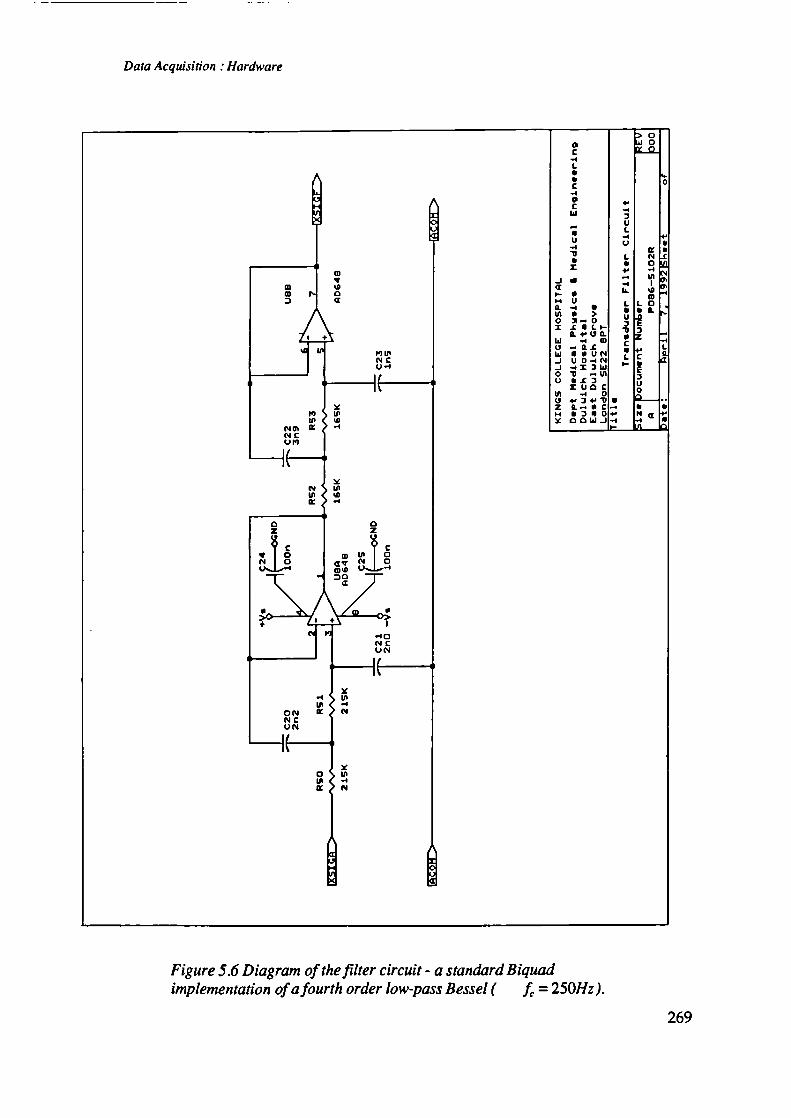
Data Acquisition Hardware
w
a
"InNCU-.ix
IP( .O1 -NCU",ix
1-I
0 0z z
J2 LNOI D U..L--4T ••4O TI a
-IDNCUNfix
oc.i /NNCUNJx
O\ISlIIl( -I
Figure 5.6 Diagram ofthefilter circuit - a standard Biquadimplementation of a fourth order low-pass Bessel ( J = 250Hz).
269

80
60
40
- 20
0
-20
-4010-2 10-1 100 101 102 1O
Frequency [Hz]
Figure 5.7 Frequency response of transducer amplifier andfllterforboth the shear stress signal path and the normal stress signal path.
1 0
Chapter 5
5.2 Signal Conversion and Data Storage
This section discusses the hardware requirement and its implementation, for the
analogue to digital conversion and subsequent archiving of transducer signals.
Section 5.2.1 outlines the specification for the A/D converter. This unit was
purchased as a subsystem component from a commercial vendor. Section 5.2.2
details the specification and selection of a microcontroller unit used to manage the
A/D and some high-speed data memory required to service the A/D output rate.
Also, it describes the personal computer system which integrates the control of each
unit and archives all the data for subsequent processing. Section 5.2.3 describes
the necessary power supply requirements for the system.
270
Data Acquisition Hardware
5.2.1 Analogue to Digital Conversion
The A/D converter subsystem was specified in terms of the : number of signal
channels; mode of signal input; input voltage range; number of bits; sample rate;
input impedance; compatibility with existing systems; software support and ease of
use.
Initially it was expected that at least five anatomical sites would be monitored
simultaneously during clinical trials. Because of the expense and time involved in
maldng an instrumented socket to fit each patient, it was more rational to insert
as many transducers as practical. On inspection of the socket area in relation to
the transducer size, an estimated ten devices could be fitted before the rigidity of
the socket was compromised. Additionally, to transducer signals, two channels
would be required for event signalling (e.g. foot switches). Thus the maximum
number of active channels would be thirty two.
As the signal amplifiers may be some distance from the A/D, differential inputs
were used to maximise noise rejection. Although the event signal was only
two-valued and therefore suitable for single ended inputs, most A/D's are unable
to accommodate both differential and single ended inputs on the same unit. So
this channel was differential also.
The A/D input range must equal the output range of the signal amplifiers which
was ±5V. While its input impedance must be significantly greater than the preceding
stage (filter) to avoid loading effects, causing signal degradation. In this case it
must be a minimum 10kg). The number of bits or the size of the digital result
required was defined by the resolution limit desired of the input signal. In the
case of the normal-stress transducer lOON ±0.5N is mapped into 0-5V of signal.
Therefore at least 200 discrete levels must be discriminated. So an 8 bit or greater
A/D converter is required.
The sample rate required was dependent on the bandwidth of the transducer signal.
It was assumed that the maximum likely frequency in the signal would be 50Hz.
Under the Nyquist criterion the minimum sample rate would need to be 1 00Hz.
However this would only provide two sample points per cycle. To allow a more
accurate reconstruction of the waveform; ten or more points per cycle would be
desirable. Thus a sample rate of 500Hz per channel was required.
271

Chapter 5
The design of an A/D unit is a complex exercise which has been surmounted by
many designers already. So initially a commercial unit which fitted the specification
was sought. Ideally the unit should reside in a standard computing platform where
the data could be archived and processed. In this case the PC was the desired
platform However a survey of the market failed to find a PC unit with thirty-two
differential channels. The only available format was a VME based unit (Plessey
Microsystems LTD). The relevant specifications for the unit are given in Table
5.2.
Model
Sample Rate
Input Ranges [VI
Number of Channels
Gain
Number of Bits
Output Format
PME 98-06
1 KHz per channel
±5, ±10,0-5,0-10
64SE,32DW
1, 10, 100 Software programmable
1 -1000 Presettable (resistor)
12
Binary, Offset binary, 2's complement
Table 5.2 Specifications of the AID convertor used.
As the unit was a slave of the VME bus, it required a host controller and software
to enable it to function. This could not be provided by the PC directly. A central
processing unit (CPU) was sought from the same company for compatibility.
It is noted here that the AID described above would have very readily fulfilled all
of the project requirements. Unfortunately the unit used was an early version and
was subsequently found to contain many operational faults. Four of the five modes
of operation did not function at all. The fifth mode was only made to work in
a very unconventional manner. Unfortunately it was a very processor intensive
method, resulting in significantly reduced throughput rates. To the authors surprise
the product support from the supplier was woefully inadequate. Despite admitting
that there were many design faults with the PM 98-06 they were not prepared to
upgrade it or offer any advice short of purchasing the latest version. As a result
significant effort was expended in achieving an acceptable sample rate of 500Hz
per channel using this faulty equipment.
272

Data Acquisition Hardware
5.2.2 Conversion Control and Data Storage
As the A/D unit was a slave on the VME bus, a CPU was required to perform
the necessary control functions. It would have to initialise the channel sampling
sequence and gains; initiate conversions at a specified rate; buffer the AID output
data; and communicate with the user.
Initially a PC was considered for this purpose. However there were a number of
difficulties to be overcome. Firstly, providing an interface from the PC bus to the
VME bus was a complex problem. There were no commercially available units
appropriate for this task, and the design effort required would be considerable.
Secondly at the desired sample rate, data transfer from the A/D would demand the
uninterrupted attention of the CPU. A difficult requirement to achieve with a
standard PC. Thirdly at maximum sample rate the data memory would be filled
at 32 Kbyteslsec. As both programme and data occupy the same memory, data
size must be traded against programme complexity. At the time PC memory was
restricted to less than 640 Kbytes. Now, although storing data directly to disk would
have provided more data space, disk access is too slow for the data rates needed.
However, a purchased VME bus based CPU was shown to provide enough memory
for both large programme and data space. Further, an application specific operating
system allowed the core processor sufficient uninterrupted time to maintain data
transfer rates. Also, being VME based the interface to the A/D was trivial.
Moreover a serial port provided a link to the user via a standard terminal. The
CPU chosen was PME 68-12 (Plessey Microsystems LTD). It contained a Motorola
MC68000 processor, 1 Mbyte DRAM, 16 Kbyte fast SRAM, 19200 Baud serial
port, and EPROM based resource table for input/output control.
However, with this CPU there were no archiving facilities provided. Nor were
there any data processing software readily available. In comparison there was a
wealth of software and standard disc storage on the PC. So to make use of this,
the PC was used as the terminal to the PME 68-12. This was a relatively common
mode for the PC to operate in. Thus the system comprised of two physical boxes.
One an IBM compatible PC with a minimum of configuration of: 80286 processor,
512 Kbytes of RAM; 1.2 Mbyte FDD or 10 Mbyte HDD; serial port (capable of
19200 Baud); CGA monitor. The other, a VME bus rack containing; PME 68-12
CPU; PME 98-06 A/D; Power supply; transducer signal termination unit; VME
backplane (3 slot) and bus termination. All of the latter was designated MEPO86A
273

Chapter 5
as this was the in-house project reference code. It will however be referred to as
the Data Collection Unit (DCU) throughout this thesis. The last unit in the DCU
was a PCB which terminated the signal cable from the transducer interface
circuits-discussed in 5.1. The transducer signal termination unit contained differential
input single pole RC filters (f = 250Hz) for each signal channel, a ground reference
point, and it re-routed the channels to the appropriate A/D connector pin. The
filter provided some noise suppression from interference picked up along the cable.
An RS232 serial cable was used to link the PC to the PME 68-12 of the DCU.
With this arrangement the user enters the trial parameters, patient comments, and
data file names to the PC via menu based software. This information is preprocessed
on the PC. Commands and control parameters are sent to the DCU over the serial
link. There they are translated into A/D control instructions and the relevant data
structures are set up. When data has been collected and resides in the memory
of the PME 68-12, it is transferred back to the PC over the same serial link. Then
they are archived to disc file for subsequent processing.
To improve data transfer time the serial ports of both PC and DCU were set to
19200 Baud. Extensive software was written to effect: the user interface menus;
preprocess trial parameters; handle the communication links; drive the A/D unit;
provide data butter structures; transfer data and create data files on disc. The
details of this are presented in Chapter 6.
5.2.3 Power Supplies
The PC for the User interface and data storage contains its own supply, deriving
power from the mains. Both the DCU and TIU are powered from the same supply.
Mains voltage is passed through an isolating transformer and fed to a switched-mode
regulator housed in the DCU. This is a standard commercial design SPG312
(Schroff UK LTD), capable of SV @ hA, ±J2V c) 2.25A. The three voltages
and OV are fed directly to the VME backplane. The PME 68-12 and PME 98-06
take their power from this backplane on the standard designated VME connector
pins.
274

Data Acquisition Hardware
There were two options for supplying power to the TIU, by battery or cable from
DCU. The estimated maximum power consumption of the unit was ±12V ) O.7A.
It was possible to supply this by either method. However, in order to reduce the
weight carried by the patient a cable supply was preferred. So a small multicore
power lead was run from the DCU alongside the transducer signal cable.
5.3 Registration of Foot Contact Events
In order to correlate the measured stresses with the various temporal phases of the
gait cycle, heel strike and toe off events for each foot were recorded. These were
detected by contact switches attached to the plantar surface of each footwear.
Signals from the switches are conveyed to the TIU by ribbon cable. There they
are modified and passed on to the DCU.
The foot-switches used were types FSW12 for the Toe, and FSW7 for the Heel
(Medical Research LTD, UK). Two were used for each foot, one under the toe
area and the other under the heel. The circuit of Figure 5.8 detected each switch
closure and produced two binary signals, one trinary signal and a visual indication
of the switch states.
On each switch closure the relevant LED (D1-D4) lights to indicate contact with
the ground has been made. Heel and toe switch closures are OR'd together through
diodes D5-D6 (D7-D8), so the signal at the collector of Q3(Q4) will be binary in
nature. In normal gait the signal states will have the interpretation given in Table
5.3.
Output state
Foot action
Low
Swing phase
Low —High
Heel strike
High
Stance phase
High —* Low
Toe off
Table 5.3 State table of binary footswitch signal for normal gait.
275

ChapterS
Figure 5.8 Footswitch conditioning circuit. Provides LED indication ofswitch states; Left and Right foot contact signals (binary); combined leftand right contact signals (trinary).
276

Data Acquisition Hardware
The binary signals from each foot are combined to form a trinary signal. U3
inverts the right foot signal. This is then summed with the left foot signal at U2.
Table 5.4 describes the output states of U2 for combinations of left and right foot
action with normal a gait pattern.
Output State Foot action
Zero
Zero -4 Positive
Positive
Positive —* Zero
Zero -4 Negative
Negative
Negative -4 Zero
Double support phase (or None)
Left Toe-off
Right support phase
Left Heel-strike
Right Toe-off
Left support phase
Right Heel-strike
Table 5.4 State table oftrinaryfootswitch signal for normal gait.
This trinary signal is passed to the DCU where it is digitised with the stress signals.
5.4 Interface to Kinematic Measurements
From analysis of the stress-time recordings much can be learned about the magnitude,
direction and timing of stresses occurring during gait. Further information can be
gained by relating these stresses to joint angles, body position and limb motion -
especially during abnormal gait.
The University Department at which this research was undertaken has the use of
a VICON Kinematics Measurement system (Oxford Metrics LTD). This is a video
based technique which records the spatial trajectories of reflective markers on a
subject, during a gait cycle. It is also capable of simultaneously recording force
plate, EMG and other event data.
By providing a signal, which contains identifiable events, to both the stress
measurement and kinematics measurement systems, then both data sets will contain
sufficient timing markers for correlation. There will, of course, be some correlation
uncertainty, as both systems are sampling data asynchronously to each other. The
277

ChapterS
worst case lag in detecting an event will be one sample period of the fastest
sampling system. Similarly the worst case error in synchronisity will be the same
period.
Two signals were passed between the two systems. Either of these could be used
for synchronising both data sets. The first and simplest was the footswitch signal
sent from the DCU to VICON. This is recorded by both systems simultaneously.
The second was a signal from VICON which reflects its Run/Halt status. In the
DCU this signal is digitised with the stress signals and serves two purposes. It
identifies which gait cycles were recorded on VICON and is used as an optional
trigger for initiating data conversion in the DCU. If the software selects the
Run/Halt signal as the trigger, the DCU continuously digitises the signal looking
for a low to high transition. When detected, stress data conversion begins.
The previous section described circuitry to capture and output footswitch events.
A combined left and right foot signal was digitised by the DCU in synchronism
with the stress signals. Two separate signals, from left and right feet, are passed
via the DCU to the VICON system. Figure 5.9 describes an interface circuit built
for this. Both signals were transferred to the VICON event channels through
opto-isolators then converted to ITL levels.
A similar circuit to that above was used to transfer the VICON Run/Halt signal
to the DCU.
5.5 System Integration
The whole stress measurement system consists of three separate enclosures with
connecting cables.
Up to ten triaxial stress transducers plug into the transducer interface unit. Each
has a cable length of 1-2m. Sufficient to span from the socket to the TIU without
impeding the free movement of the subject. The TIU itself is carried by the subject
in a backpack. The specially made pack is sewn from a polyester cover and
includes padded straps. Openings are provided on the sides for transducer and
signal cable access. Shoulder and waist straps were provided. A fully populated
(ten transducer) unit and pack have dimensions of approximately 250 x 300 x 50mm
278
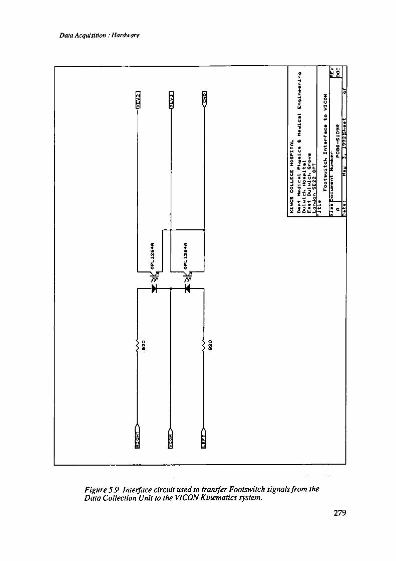
Data Acquisition : Hardware
Figure 5.9 Interface circuit used to transfer Footswitch signals from theData Collection Unit to the VICON Kinematics system.
279

Chapters
arid weighs 1.3Kg. Although it was thought that its size may be a difficulty for
smaller elderly subjects. If this was the case then a smaller unit with fewer
transducers could be built, or the researcher could follow closely behind the subject
holding the pack. In all cases care must be taken not to distract the subject from
their usual gait pattern.
Signals from the TIU are conveyed to the DCU by a ten meter length of ribbon
cable. The cable length was chosen to equal the length of the kinematics laboratory.
This would allow between ten and thirty steps. The limit to the cable length
(walkway length) is a function of; the drive capability of the transducer buffers;
noise susceptibility; and memory size at a given sample rate and stride time. With
the cable used here the output drive and noise pickup on the cable was found to
be satisfactory [5.1.2.2] and the number of steps adequate for planned studies. The
drag force of the cable on the subject was measured as < 8N on linoleum flooring.
This was thought not to have a significant effect on the gait of an active amputee.
The DCU enclosure is positioned near to the PC. It is a mains powered stand
alone unit. The signal cable from the TIU connects to the rear of the unit. After
passing through the cable termination PCB the signals are separated and output to
the A/D. Four, 26 way jumpers link the termination PCB to the A/D via their
front panels. A serial communications cable spans one or two meters from the
PME 68-12 front panel to the serial port on the rear of the PC. Two five meter
signal cables run between the DCU and VICON. Footswitch signals, left and right,
are sent to the VICON, while the VICON Run/Halt status is sent to the DCU.
The first two signals can be used as additional information to the Kinematic data
sets, or provide common synchronising events to correlate stress and kinematic data.
The latter signal is digitised with the stress signals and may provide; a record of
which gait cycles were captured on VICON; a correlating signal; or a trigger signal
to initiate sampling on the DCU.
The PC consists of the monitor, processor box and keyboard. When the system
is used in conjunction with the VICON system, the PC is usually positioned near
to the VICON controls. The User can then operate each independently if required.
Figure 5.10 shows the three enclosures with cables and pack.
280

•01
-
I- -r __._
t. 4$
,-cT ;$fY
Data Acquisition Hardware
-
OLiPItL I
Figure 5.10 Photograph of the units and cables which comprise thestress measurement system. From right to left; transducer and footswitch;Transducer Interface Unit; transducer signal cable; Data Collection Unit;serial link; PC for control and archiving.
5.6 Safety
During the design and construction of the equipments described in this thesis care
was taken to ensure that all the electrical safety recommendations of BS5724 were
followed.
To reduce the potential shock hazard, voltages in the TIU were restricted to be
below 24V d.c. Voltages in the transducers were supplied from a 1V quasi-floating
source. It is not a true floating source as it is restricted to be within the ±12V
supply of the unit. Additionally the TIU power supply is derived directly from
the DCU which is fed via an isolating transformer. All voltages and currents in
the patient circuit are isolated from mains and earth potentials. The DCU conforms
to Class lB of BS5724 and the TIU to Class 2. The chassis and accessible panels
of the DCU are bonded to mains earth.
281

Chapter 5
In order to maintain isolation the serial link from the DCU to the PC was
opto-isolated. An RS232 to RS422 to RS232 conversion was made using two
Model 262 (Teledata INC, USA ) opto-isolating modems. Isolation from the VICON
potentials was also necessary. Again opto-isolation was used in the signal paths
between the VICON and the PC.
5.7 Discussion
The data acquisition system is made from a number of interconnecting hardware
units. The transducers connect to a Transducer Interface Unit (TLU) which supplies
an excitation voltage and buffers and filters their signals. These are then passed
to the Data Collection Unit (DCU) where they are digitised. Buffered digital data
is transferred to a Personal Computer (PC) for archival and processing.
Simultaneously, external event signals are also digitised and archived, for synchronising
multi-system data sets.
The transduction elements of the triaxial stress sensor are: a magnetoresistor and
moving magnet system in the shear stress section; and a strain gauged diaphragm
and pre-shaped indentor in the normal stress section. The principle electrical
properties of the magneto resistor (MR) (FP111L100 - Siemens UK LTD) are that
it is a low impedance (30O2) three terminal device whose impedance varies (±25%)
with the magnitude of magnetic flux density perpendicular to its active face. It is
configured as one half of a Wheatstone bridge and excited by JV d.c. The strain
gauge is a four terminal metallic foil gauge configured as a full Wheatstone bridge.
Its impedance is low (350Z) and varies only fractionally under stress (±2%).
Excitation is from the same source as for the magnetoresistor, and is set at lVd.c.
The low impedance of both elements minimises their susceptibility to electromagnetic
interference, and the low excitation voltage minimises thermally induced errors due
to resistance heating. A high stability voltage reference maintains the excitation
voltage regulation to better than 0.1%.
Amplifier and filter circuits separated the transducer signals from any environmental
noise coupled on to the transducer leads. Differential amplifiers were used to take
advantage of their high common mode rejection (CMRR) to remove any significant
noise commonly coupled onto the signal leads. The high input impedance minimised
input bias current drain from the transducer signal currents. Also, the input circuits
282

Data Acquisition Hardware
were isolated from the output circuits allowing the use of floating excitation voltages,
which had inherent noise minimisation advantages. System gains were set at 50
and 2000 for the shear and normal sections respectively. Input protection resistances
on the amplifier contributed negligibly to gain errors and CMRR degradation. Input
offset errors were 0.3%FSO and 10%FSO (worst case) for the shear and normal
sections respectively, although these may be nulled at the assembly stage. Temperature
induced offset drift was not significant. Inherent noise from electrical components
was also not significant.
The expected stress signals could contain transients that approximate to step functions,
thus the type of the filter employed was Bessel. From a consideration of the
expected bandwidth of the stress signals and the environmental noise, determined
by experiment, the bandwidth of the filter was set at 250Hz, and a 4th order
implementation used.
The stress signal digitiser in the DCU was purchased as a subsystem unit to
capitalise on cost, time and design effort savings. However, because of the number
of differential channels to be digitised (32), the digitisation rate (500Hz) and the
required memory size (-1Mbyte), a PC format unit was not available. A commercial
unit was found, with a suitable performance specification, on VME format. A
subsystem controller was also purchased for directing the digitiser, buffering its
data output and transferring the data to the PC at a manageable rate. The digitiser
input range was set to ±5V to just exceed the maximum output range of the signal
amplifiers. A resolution of 8bits was sufficient for this application, although, a
l2bit unit was obtained for the same cost. The controller processor (MC68000)
was run at a clock speed of 10MHz to enable it to store digitised data at
32Kbytes/Sec. Software to effect control was run from SRAM for speed of execution.
Data transfer rate, from the DCU to the PC, was set at l9200Baud to minimise
transfer time. The PC used was an IBM-AT-compatible (80286) running at 8MHz.
Its data archive was a 10Mbyte HDD or 1Mbyte FDD. User control of the whole
acquisition system was via software being executed on the PC.
In order to correlate the measured stresses with the various temporal phases of the
gait cycle, h'el strike and toe off events for each foot were recorded. These were
detected by contact switches attached to the plantar surface of each footwear.
Signals from the switches are conveyed to the TIU by ribbon cable. There they
were modified and passed on to the DCU. There they were digitised with the
283

Chapter 5
stress signals and also passed on to an external kinematics measurement system.
A second signal, which contains identifiable events from the kinematics measurement
system, was input to the DCU and also digitised with the stress data. Thus both
DCU and kinematics data sets contained sufficient timing markers for correlation.
The DCU power was derived from an transformer isolated mains supply and the
11U was in turn powered from it by a low voltage supply (12%') to ensure patient
safety from electrical shock. Data transfer to the PC was effected over an
opto-isolated RS232 link to isolate the patient from currents derived from the PC.
The signals to and from the DCU and the kinematics system were also opto-isolated
to effect patient safety.
284

Chapter 6Data Acquisition: Software
The previous chapter described the development and function of the required data
acquisition hardware for this system. In this chapter details of the software developed
to control the hardware and to manage the acquired data are presented.
Section 6.1 describes the minimum hardware required to run the software and the
development environment under which it was created. Section 6.2 provides an
overview of the system control strategy. It outlines the software structure, hardware
interaction and the user interface. Sections 6.3 to 6.6 are detailed descriptions of
the operation of the many programme modules which make up the system software.
Flowcharts of these modules are presented in each section.
Listings of the code written for each of the modules discussed are not presented
here as they total some six thousand lines. They are however recorded in a
Departmental report (P086-SOVFMAN) which is available on request from Kings
College (Dulwich) Hospital'.
It should be noted here that two sections of the programme code were written to
control the Data Collection Unit (DCU) in an unorthodox manner. These code
sections were written in Motorola 68000 Assembler and acted to control the A/D
and the serial port on the CPU board. Although these sections comprise less than
5% of the total software they absorbed almost 70% of the code writing time.
It was necessary to write the serial port control code to achieve the higher data
throughput rates. The DCU code was 'hand-crafted' to work around the multiple
errors in the technical manual supplied with the A/D and CPU boards. An extensive
amount of effort was expended in writing code to coerce the A/D board into
digitising any signal. As supplied, the board did not operate in any mode
recommended by the supplier. More surprisingly, the supplier would not officially
support the product despite acknowledging its faults. However a confidential copy
of the circuit diagrams was obtained. By studying the interconnection of the control
1 Department Medical Engineering and Physics, Kings College (Duiwich) Hospital, East DuiwichGrove, London SE22 8FF, UK.
285

Chapter 6
logic a method was devised for initiating and terminating conversions under software
control. Eventually, successful, although less than optimum, operation of the DCU
was achieved with the software reported here.
Despite these unique sections of code the programmes are quite portable to other
Motorola 68000 based computers. Modular programming techniques were followed
throughout with a clear distinction between machine specific and machine independent
code modules. Therefore portability is assured by replacing only the machine
dependent code modules.
6.1 System Hardware and Programming Environment
This section describes the minimum hardware required on which to run the data
acquisition and processing software. It also describes the programming languages
and environments used to develop the software.
In order to acquire new data there are two hardware units required. These are an
IBM-PCAT (PC) or compatible and an MEPO86A data collection unit (DCU). The
PC must have; an 80286 CPU running MS-DOS v 3.0 or later; 512 Kilobytes of
RAM; CGA colour monitor (minimum); RS232 serial port capable of 19200 Baud
on COM1; and standard 102 key keyboard.
The MEPO86A unit is described in detail in Chapter 5. In outline it consists of
a PME68-12 processor board (CPU) and PME98-06 analogue-to-digital convertor
(AID) board on a VME (RevC) bus (Radstone Technology PLC). The PME68-12
board must have a Motorola 68000 CPU and a PLUM monitor (v 3.3) - as supplied
by Radstone - and 1 Megabyte of RAM. Additionally, an MEPO86B transducer
interface unit (TIU) may be used to buffer the transducer signals into the A/D.
AU the data processing was carried out using an interactive mathematics programming
environment and language called MATLAB386 (Mathworks INC). This software
was run on an IBM compatible COMPAQ DESKPRO 386/20. Because of the
unique characteristics of each transducer under calibration, the interactive environment
was efficient at exploring these characteristics and producing semi-automatic signal
processing functions. To run MATLAB386 the COMPAQ must have a mathematics
coprocessor - 80387. Various processing routines were written in MATLAB386
language to: perform data file conversions; display and plot performance curves;
286

Data Acquisition Software
calculate linearity, hysteresis, frequency, creep and temperature parameters; and to
perform curve fitting operations. These routines are recorded in the departmental
report mentioned above.
The development of the data acquisition software was carried out on the PC.
Programmes to run on the PC were written in the 'C' language under the
MICROSOFT QUICK C v 2.05 compiler. Also some 80286 assembly routines
were written under MICROSOFT QUICK ASSEMBLER v 2.05. Programmes
running on the DCU were written in 'C' and 68000 Assembler under the MANX
AZTEC C68K Cross-compiler/Assembler. Machine independent code was debugged
between two IBM-PC compatibles while the machine-specific code was downloaded
to the DCU and debugged under the PLUM monitor control.
6.2 Software Overview
This section presents an overview of the system control strategy. It outlines the
structure of the software, the hardware interaction and the user interface. Figure
6.1 is a diagram of the interconnection of system units.
Transfer
Transducer Personal Computer
Transducers Interlace Unit Data Collection Unit
Figure 6.1 Schematic of the interconnection of the system units.
The PC is the host controller of the whole system. Software running on it provides
the user interface and controls the functions of the DCU. Signals from the PC
are sent via the serial port to the DCU to initiate data collection; transfer data and
perform file maintenance. The DCU in turn captures signals from the TIIJ carried
by the subject. These signals are digitised and stored temporarily in the DCU
before transfer to the PC for archiving. The number of transducer signals and the
rate of conversion are dictated by the user via the PC.
287

Chapier 6
The reasons for using two independent units in the data acquisition system were
covered in detail in Chapter 5. These were essentially the lack of a commercially
available PC-based digitiser with sufficient: number of differential channels; conversion
rate; and memory capacity. Although these conditions were met by VME based
units, there was no available software for high-level user control. Thus there was
a need to develop a considerable amount of programming skills for both low-level
machine-dependent and high-level machine-independent software.
There are two main programme suites for the system, one running on the PC and
one running on the DCU. These run asynchronously to one another and communicate
by passing command codes and data over the serial link.
The purpose behind the design of the software for controlling these units, was to
provide an easy to follow step-by-step interface for the user who might be unfamiliar
with the details of PC operations. It should require the minimum knowledge of
IBM PC-DOS command line syntax, and provide an infallible route to quickly
obtain data once the various inter-unit cables have been installed. Also it must
be general enough to provide the user with a tool for collecting transducer calibration
data as well as clinical data.
For these reasons a menu-based approach was adopted. From the first screen the
user sees he is offered a menu of all the valid operations for that Level in the
programme. As the options from the menu are chosen further levels are entered
and new menus of valid operations are offered. And so on throughout the data
collection and archiving process. Each menu option is self explanatory and are
easily selected by use of the cursor keys on the keyboard. Reminders and warning
messages are flashed up for certain critical operations prompting the user to confirm
the course of action before executing it. Thus the user is relieved of having to
remember sequences of command options and is buffered from accidental loss of
data.
On the PC the programme is divided into three levels On the DCU the programme
has only two levels, these correspond with levels two and three of the PC programme.
Figure 6.2 shows diagrammatically the system control strategy and the links of
interaction between the programmes running on each machine. Initially the user
executes the PC programme.
288

C)0
0
I
Data Acquisition Software
zeAe1 CIA97
E2 ;; &
'HIHI
Il 1
a
I
Ie
L_i LJj7J
I________
LJ LJ U . LJ LJ LJI . Io
- iIeIie-1 9A97 C19A91
Figure 6.2 System diagram of control flow and interaction of thesoftware running separately on the PC and the DCU. To ease confusionsome flow lines have been replaced by annotated boxes on the diagram.All boxes with the same character are connected together and the arrowsdenote the direction offlow.
II
289

Chapter 6
At this level (Level!) the user can view existing data files, or begin a new data
collection session. At further levels the DCU is required to be connected to the
PC.
At Level2 the user has options of initialising the DCU prior to data collection,
communicating directly with DCU's monitor programme (used only for emergency
data recovery) or executing any PC-DOS function (again used mainly in conjunction
with emergency data recovery). To re-iterate what was discussed in Chapter 5,
the DCU has a monitor programme (PLUM) stored in EPROM that is executed
when it is powered up. This is a low-level control programme that cannot perform
the complex functions required for data collection. After initialisation the DCU
waits for commands input via the serial port. In order for the DCU to function
the PC programme must download the DCU's operating programme and run it.
At Level3 the user has the options of Collecting new data, Transferring the data
to the PC, Viewing a data file, Clearing the DCU memory, or executing a PC-DOS
function. These options send specific command codes to the DCU programme
which are received, checked and executed. Before collecting new data the user
must specify the number of transducer signals to digitise, the digitisation rate, and
any comments to be stored with the datafile. When the user is finished they can
return to Level2 and exit the session.
6.3 Levell - File Viewing
Levell of the software is entered on execution of the PC programme where upon
the PC is initialised. The PC screen is set to its default mode and all screen
handling is done in text mode rather than graphics mode. During all menu driven
sections of this programme the screen cursor is turned off. The Control-C (etC)
facility is enabled to allow the user to abort the programme at any time. The
COM1 port is initialised to; 9600 Baud, No parity, 8 bits, 1 stop bit. The 'First'
menu is then displayed on the screen. This offers options to QUIT, VIEW A DATA
FILE, RUN MEPO86. A photograph of the PC screen showing the Level! menu
is given in Figure 6.3. Figure 6.4 shows diagrams of the programme sequences
for this Level. If the QUIT option is selected the programme is terminated after
returning the screen and serial port to their original configurations. If the RUN
MEPO86 option is selected then control passes to Level2.
290

Data Acquisition Software
(a)
(b)
Figure 63 User screens for Levell menu a) and a displayed data fileb).
291

Chapter 6
Figure 6.4 Flow chart of the programme sequence for the Levell menu,VIEWA DATA FILE, QUIT, andRUNMEPO86 options.
292

Data Acquisition Software
6.3.1 View Data Files
Selecting VIEW A DATA FILE will display a previously saved data-file that is
stored on the PC. It must be a Transducer data file and it must be in the current
directory. Figure 6.3 is a photograph of the user screen with a displayed data file.
Figure 6.4 is the flow chart for this operation. The expected file structure is
defined in Appendix A. A message will prompt the user for a file name. Wildcards
can be used to obtain a list of all files in the current directory. The list will be
displayed and the appropriate file may be selected.
The file's existence is checked. Then it is opened and read to confirm that it is
a transducer data file. If either of these checks fail, the file is closed, an error
message written to the screen and the function is terminated. If both checks pass
then the data file is opened in binary read-only mode. This mode allows both
binary data and ASCII text to be read but protects against accidental overwriting
of the data. A header in the file contains all the notes and experimental parameters
(number of transducers, sample rate etc.) in ASCII text. These are read from the
file and displayed in a panel at the top of the screen. Data is then displayed in
a lower panel in columns according to the transducer and axis it refers to. The
cursor keys and the Page Up, Page Down keys can be used to scroll through the
data. If the ESC key is pressed the file is closed, the screen cleared and the
function returns to the Level! menu.
6.4 Level2 - Data Collection Unit Initialisation
At this point the user is requested to check all hardware connections are in place
and to switch on the DCU.
On switch-on the DCU is under control of the EPROM based monitor (PLUM) on
its CPU card. At this stage, the PC programme communicates with the monitor.
To synchronise the PC with the DCU the user is instructed to reset the DCU via
its front panel RESET switch. The programme waits up to ten seconds to recognize
the reset prompt sent from the DCU before continuing. The sequence of operations
for the synchronisation of the two machines is given in Figure 6.5.
293

Chapter 6
Characters arriving at the COM 1 port cause an intemipt of the PC which calls
an assembly routine to store the data in a buffer. This routine is installed before
communicating with the DCU. By default the DCU serial port baudrate is 9600.
When the two units are synchronised this is changed to 19200 for faster data
transfer rates. The LeveI2 menu (Menu 0) offers the options of QUIT, LOAD
AND RUN DCU programmes, interact with the MONITOR, or TEMPORARY EXIT
TO DOS. At this point the PLUM monitor still controls the DCU. Selection of
MONITOR will invoke a terminal emulator programme that will allow the user to
interact with PLUM in emergencies. QUIT will cause the COM1 service routine
to be de-installed and the entire programme to terminate. LOAD AND RUN DCU
will initiate sending and executing the suite of programmes that will control the
DCU. Figures 6.6 shows the user screen for the Level2 menu.
(a)
Figure 6.6a User screen for the Level2 menu.
294

Data Acquisition Software
(1')
(c)
Figure 6.6b,c User screens for b) TEMPORARY EXIT TO DOS and c)MONITOR.
295

C-)
C0
--\\7/
00C0
a0
F
C=
2
0
aC
8 I
E
C
8aC
Chapter 6
-a 2 2
0.
(I,aS a
> I-F
C)
\>TE
C.
P
a
C-
0
Figure 6.5 Flow chart of the programme sequence required tosynchronise the DCU to the PC.
296

Data Acquisition Software
TEMPORARY EXIT to DOS
MON ITOR
Restore screen Detaufts Napture File'
Demstail COM1 service routine
Display return Instructions
Spawn secondary command shell
Demstall COMI service routine
EUtiôAiib1Recover screen parameters
C_RETURN__)
E1
Does Ylirl DeleteFile
S.t Baud to 9600
Set screen te Defauft
Deinstall COM1 service routine
Display return Instruction
Spawn Terminal Emulator
Remstail COM1 service routine
Restore screen parameters
Set Baud to 19200
E1
RETURN
Figure 6.7 Flow chart of the programme sequence to execute a) aTEMPORARY EXIT TO DOS and b) the MONITOR option.
6.4.1 Dos Functions
In a TEMPOARY EXiT TO DOS a secondary command shell is generated to allow
the user to execute other PC-DOS applications while the control programme stays
resident in memory. A diagram of the programme sequence for this operation is
given in Figure 6.7. By the user typing "EXIT" the shell is removed and the
execution of the programme will continue from its last executed instruction. Inside
the shell the user may execute any programme that may fit into the remaining
memory. The COM1 service routines are removed before the shell is built to
297

Chapter 6
avoid its corruption or causing a fatal error. On exit from the shell the service
routine is re-installed and the screen handling parameters returned to those last in
use by the control programme.
6.4.2 Monitor Functions
To interact with PLUM a terminal emulation programme is invoked under a secondary
command shell. The use of this emulator may be necessary to recover data files
from the DCU memory in the event of a fatal error. Figure 6.7 shows the
programme sequence for this operation. A number of files were written to complement
the terminal emulator, specifically for interacting with DCU. As described above
the programme status is saved and the COM1 service routine de-installed before
the shell is invoked. On return from the emulator, the programme status is restored
and the COM1 service routine re-installed before execution of the programme is
resumed.
6.4.3 Programme Transfer and Execution
Before the DCU can be used to collect data the necessary control programme must
be sent to it from the PC and executed. The DCU does not have any non-volatile
storage to save this programme so it must be down-loaded for every session. Figure
6.8 describes the sequence of events to effect this operation.
At this point the PC programme is communicating with the DCU's PLUM monitor.
It sends monitor-specific commands to the DCU which are echoed back. These
echoes are used to check that no errors have occurred.
The programme which runs on the DCU has been compiled and encoded into
Motorola "S" record format and stored on the PC's disc. To send this and have
it installed in the DCU, the PLUM command "LOAD" is sent. After the command
is echoed the encoded programme is sent. To execute it the PLUM "EXECUTE"
command is sent. On the DCU the control programme is loaded into 3 Kbytes
of fast SRAM for maximum speed of execution. Appendix A contains a description
of the DCU memory map. The first action the DCU programme takes is to
initialise its working environment (stack pointers and memory map etc.). It then
298

Data Acquisition : Software
LOAD & RUN DCU[onPC
Openfile
HSend 'LOAD command DCU
Send DCU programme I
Send 'EXECUTE' command DCU
<(on?N say error msg
Display confirmation messageI
Figure 6.8 Flow chart of the programme sequence to transferprogramme code to the DCU and execute it.
initialises the A/D, the data file tables and memory pointers. When these have
been successfully carried out it sends a startup message to the PC. Any error in
this operation returns the user back to the Level! menu.
6.5 Level3 - Data Collection
When the DCU programme has initialised its hardware it sends a message to the
PC to indicate that it is successfully in control of the DCU. On receipt of this
message, the PC programme is synchronised with the DCU programme. Commands
are issued to the DCU from the PC in much the same way as with the PLUM
monitor. These commands are echoed back to the PC to acknowledge their receipt.
LOAD & RUN DCU[0nDCU]
299

Chapter 6
The DCU waits for a command input from the PC, checks the validity of the code
and tests for errors. When an error occurs an error number is set which defines
the module in the programme where the error occurred. The handling of these
error conditions is described in 6.6.
Before displaying the LeveI3 menu (Menu 1) information about the memory available
in the DCU is requested. The memory parameters sent are:
number of Kbytes total memory
number of Kbytes used
number of files stored
number of Kbytes free
Figure 6.9 is a flowchart of the units interaction for these operations.
Menu 1 offers the options of RETURN TO PREVIOUS MENU, VIEW a DATA
FILE from PC, COLLECT NEW DATA on DCU, TRANSFER DATA FILE from
DCU, CLEAR MEMORY on DCU or TEMPORARY EXIT TO DOS. Figure 6.10
shows the format of this menu on the PC screen before the memory on the DCU
is cleared.
Figure 6.10 User screen for Level3 menu. A confirmation of memoryclearance is requested.
300

Data Acquisition Software
U,
w
0w
0zw(0
.6 1I &! I—. —I
'Ui
IE U-
400
40
40 I40 z
LU
LU
C0
>
>C.)
c.
5'
C)0
toE >C o_C Z Z Z
.2. 0
0
zo
owI.—j
Z L4
\ - —J)I— < i:
z<
>h
I!!
i zI wI !I
0
zLU
0—i'—ii:
C/cr
__\
>>-4Ii___
>>D.g
D 40 40 __________________0 .C
- . __________ >
>>o __________ w2
- - - - CC.2.
LU
5
Figure 6.9 Flow chart of the programme sequence to request and
execute commands on the DCU.
301

Chapter 6
6.5.1 Support Functions
These functions are small relatively simple routines which act in support of the
main functions of LeveI3. They are the RETURN TO PREVIOUS MENU, CLEAR
MEMORY on DCU and TEMPORARY EXIT TO DOS options from the menu.
When data collection is finished the user returns to Level2 where control of the
DCU is handed back to the PLUM monitor programme. At this point data still
exists uncorrupted in the DCU memory and emergency access to this data can be
made through a terminal emulator package, if required. Further, if the option LOAD
AND RUN MEPO86 PROG is subsequently selected from Menu 0 this data will
be overwritten by new data. Thus, before sending the RETURN TO PREVIOUS
MENU command from the PC to the DCU the user is prompted to confirm the
action. Figure 6.11 describes the sequence of this operation.
Once all data files on the DCU have been transferred to the PC, the user may
clear the DCU memory ready for new data collection. Selection of the CLEAR
MEMORY option from the Level3 menu, begins a global delete of all data files
on the DCU. Before sending this command the user is prompted to confirm the
action. On the DCU a table is kept that holds pointers to where each of the data
files are stored in its memory. On receipt of the CLEAR MEMORY command,
the memory itself is not cleared directly, but the table entries and memory pointers
are reset to default values. Subsequent data collections will re-allocate the pointers
and overwrite the current data. Figure 6.11 shows the sequence of events for this
operation.
The selection of the TEMPORARY EXIT TO DOS option is executed in the same
way as described in 6.4.1. Its main uses in the module are; to check that duplicate
filenames are not given when files are transferred to the PC; and to make disc
space available for data files - which may be up to 1000 Kbytes in size.
302

w-JLI
UiU-Cl)
I-
0
Ui
Ui-JC.)
>-
0
Ui
(b)
0
zUi
g
z (a)
C.)0
C.)0.
g
[ji[jl
II II IaIIIII-
E!ffi
I II L
:;
E
i
Data Acquisition Software
Figure 6.11 Flow chart of the programme sequence to, return to Level2(Menu 0) a), CLEAR MEMORY on DCU b), and TRANSFER A DATAFILE to PC c).
303

Chapter 6
6.5.2 Transfer Data Files
Data captured on the DCU must be transferred to the PC for archiving and processing.
Many data files from individual clinical trials may be temporarily stored on the
DCU. Before requesting the transfer of any of these data files from the DCU, it
must be indentified from the others currently in memory. On selection of the
TRANSFER DATA FILE option from the LeveI3 menu, the number of files stored
parameter [see 6.5] is evaluated. If there are no files stored then the option is
terminated. If there are files present then a list of these files is requested from
the DCU.
The list sent by the DCU contains the file number, name, creation time and size
of each file in its memory. To form the list the DCU scans through its file table
in sequence. Each file's sequence number (file number) and size are copied from
the table then the file name and creation time are retrieved from the file header
in memory. This continues until an unused table entry is met. These parameters
are then encoded and sent to the PC. Figure 6.11 describes the sequence of events
for this operation.
The file list is displayed on the PC screen and the user may scroll through the
list using the cursor keys. Figure 6.12 shows the screen format of this list. By
pressing ESC the TRANSFER DATA FILE option is aborted. Pressing TAB selects
all files, in numerical sequence. Pressing ENTER allows the user to type the file
number of the file he wishes to transfer. The sequence of events for the transfer
operation of the selected file(s) is described in Figure 6.13.
Before transfer takes place the disc space in the current directory of the PC is
compared to the current file size. If there is not enough free space then the process
is terminated. (N.B. the Menu! option TEMPORARY EXIT TO DOS can then be
used to make disc space available). The user is then prompted for a filename
under which the transferred file will be archived to disc. If this filename is already
in use then the user is offered the choice of overwriting named file or aborting
the transfer process.
The named disc file is opened and an identifier written into it. This identifier is
recognized under the VIEW DATA FILE option and infers that the present file is
indeed a DCU data file.
304

Data Acquisition : Software
Figure 6.12 User screen listing files stored on the DCU, ready fortransfer to the PC.
A transfer command is then sent to the DCU along with the file number of the
first of the selected files. The header of this numbered DCU file is transferred
first and written to disc, followed by the file's data section. On the DCU the
header of a transferred file is stored as an ASCII sthng and the file's data is stored
as binary characters. Now, control of the communication link between the PC and
DCU, over which the files are sent, is effected by the sending of certain binary
characters. Thus, to avoid characters in the file's data section looking like control
characters all data is coded before it is sent and decoded on arrival at the PC.
On the PC, disc access is much slower than memory access. Also, each write to
the disc must be precursored by a head positioning manoeuvre. Therefore when
writing small amounts of data, relatively large time overheads are incurred. Thus,
the incoming decoded data from the DCU is saved to a large temporary buffer
(32Kbytes). When this buffer is full it is written to the disc file, and new incoming
data is allowed to fill the buffer again. When the end of transmission is met the
buffer is emptied to the disc file and the disc file closed. During any file transfer
the PC may request a pause in the transmission while it writes the file to disc.
The DCU then waits for a 'resume' command.
305

Chapter 6
TRANSFER FILE[on PCI
[or, DCU] TRANSFER FILE\/
Figure 6.13 Flow chart of the programme sequence to TRANSFER ADATA FILE from the DCU to the PC.
306

Data Acquisition Software
If a single file was selected from the list then the TRANSFER DATA FILE option
is terminated. If all files were selected then the file number and size of the next
file in the sequence is evaluated. The disc space necessary to archive it is assessed,
and if space permits, a transfer command and the file number is sent to the DCU.
That file is then sent and archived. And so on until all files are transferred.
6.5.3 Collect New Data
There are two phases to initiating collection of new data. The first is the input
of values for the experiment parameters. The second is the transfer of these
parameters and the provision of a trigger to begin sampling. At first a software
module is called which controls the input of parameter values.
A panel showing the parameters and their default values is displayed on the screen.
The user may cycle through the parameter fields by use of the up and down cursor
keys. Figure 6.14 shows the screen format of this panel while Figure 6.15 describes
the sequence of operations in this routine. To edit a field the user positions the
cursor in the field and presses the space bar. The programme then saves the region
of the screen that is about to be edited. This region is replaced once editing is
ended and the amended text is written into the field. The fields are classed
according to the type of parameter to be input and the way in which the parameter
is implemented. Notes and name fields are input without checking. The digit
fields are checked against limits that are predefined. If the input exceeds these
limits the nearest limit is used instead of the input. The Sample Period and Timeout
Period are implementation dependent and are restricted to values selected from a
menu. When all editing is finished the user presses INS to collect new data using
the new parameter values. The user can abort the data collection process by
pressing ESC (N.B. all edited fields are saved).
The second phase is a routine which controls the collection of new data using the
current parameters. Figure 6.16 describes the sequence of operations in this routine.
To initiate the collection of new data the PC sends a command code. On receipt
of the command the DCU checks that there is sufficient free space in its memory
for at least one sample plus the file header. If there is not, an error is flagged,
the process aborted, and control returns to the LeveI3 menu. Otherwise the new
307
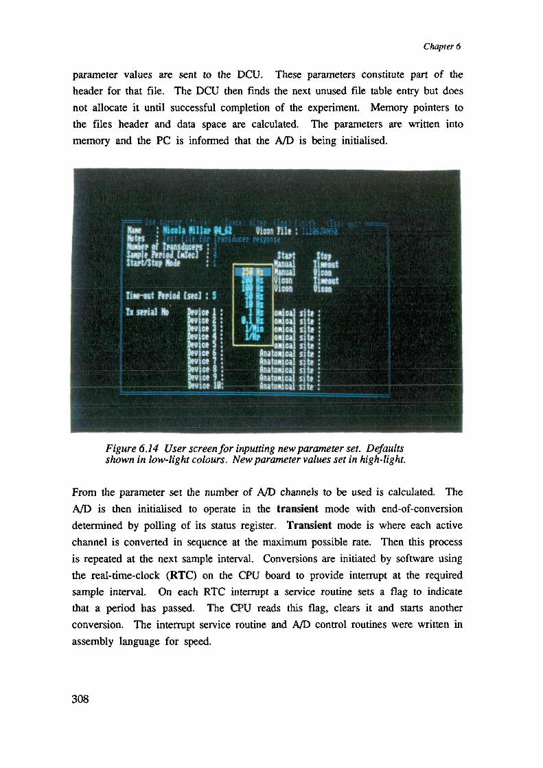
Chapter 6
parameter values are sent to the DCU. These parameters constitute part of the
header for that file. The DCU then finds the next unused file table entry but does
not allocate it until successful completion of the experiment. Memory pointers to
the files header and data space are calculated. The parameters are written into
memory and the PC is informed that the A/D is being initialised.
Figure 6.14 User screen for inputting new parameter set. Defaultsshown in low-light colours. New parameter values set in high-light.
From the parameter set the number of AID channels to be used is calculated. The
A/D is then initialised to operate in the transient mode with end-of-conversion
determined by polling of its status register. Transient mode is where each active
channel is converted in sequence at the maximum possible rate. Then this process
is repeated at the next sample interval. Conversions are initiated by software using
the real-time-clock (RTC) on the CPU board to provide interrupt at the required
sample interval. On each RTC interrupt a service routine sets a flag to indicate
that a period has passed. The CPU reads this flag, clears it and starts another
conversion. The interrupt service routine and A/D control routines were written in
assembly language for speed.
308

Next Parameter
V
Field?
Save Whole Screen
Display Menu
Select from Menu
Restore Screen
Display new Value
Data Acquisition : Software
[on PC]COLLECT NEW DATA
Display Parameter Panel
Display Default Parameter Values
SaMoa Keyboard
RETURND Cursor?
N V N
N N V
INS? ESC? Space?
V ______
Save Screen Locally
I InputText I
V Between VField? Limits?
Replace with Limit
Restore Screen
I ReplaceFieldText I
\,
Figure 6.15 Programme sequence for inputting new parameter set.
After initialising the A/D the time-out period is set and the start/stop (trigger)
mode determined. The DCU then waits for a trigger. The start trigger can be
issued by an external system (VICON kinematics measurement system) or by the
PC, on a key press. The trigger mode is specified as one of the experiment
parameters.
309

Chapter 6
Collect New Data
[on PC] [on DCU]
Collect New Data <emory?>- Error Message
____ V _________________ CI_TURN o)Request New Experiment
Next File Number
Set Memory Pointers IMemor
ntNRETURN D)
& Se Fie Header I
y? ______________________________
V
I Send ParametersInitialise ND
_________ I
Set Number of Channels IWalt for AID lnialsation I I Set Scan Sequence I
Set Conversion Mode
Waitfor'Ready' I Install RTC Inlerupt Service Routine
Set Conversion & Timeout PeriodSave Screen Image
SetTrlgger Mode IDisplay Tngger Prompt j N
Walt For Key Press IDetermine Tagger Mode
31
Send Stan Command ] 'Sfop' on VICON Set Sbp, on VICON 1
Restore Screen Image I Trigger from VICON Trigger from PC I
Waltfor Data Collection
I __________________________________CoPed Data under Interupt from RTC
Wait for Termination Process
_________ I Determine Termination Status
( ETURND1) _______________________________Update Memory Usage Parameters I
Update File Pointers & Parameters I
Allocate File Table Number
C RETURNDJ
Figure 6.16 Programme sequence for controlling the data conversionprocess.
310

Data Acquisition Software
The VICON kinematics measurement system records the body position, limb motion
and joint angles of the patient being studied [see 5.4]. In order that the kinematic
data set can be correlated with the interface stress data set, the footswitch signals
from the patient are recorded by both systems. Additionally, the collection of data
on both systems may be started by a signal from the VICON - called the RUN/HALT
signal. If the trigger mode requires a manual start the user is prompted to press
the PC's enter key for the start trigger. A VICON start calls an assembly routine
to monitor the VICON RUN/HALT signal, input to channel 1 of the A/D, and
returns a flag when the channel value rises above 400 Hex (half the signal range).
On receiving a start trigger, the DCU sends a confirmation to the PC, whereupon
the user is informed that data collection is in progress. An assembly routine is
called to control the A/D and RTC for the experiment duration. On successful
completion it returns a termination status which indicates the reason for the end
of sampling. The DCU then informs the PC what the cause of termination was
- either VICON stop; timeout; or out of memory. On correct termination the file
table entry is allocated and the file table parameters updated. Each file table entry
contains 5 parameters:
file number
header pointer
data pointer
end pointer
file size
The memory usage parameters and the experiment duration are also updated.
6.5.4 View Data Files
When this option is selected the user is offered the same route to viewing previously
archived data file as described in 6.3.1
311

Chapter 6
6.6 Error Trapping
The detection of unexpected or erroneous input and subsequent orderly recovery
without data loss, is a major requirement in any software package. In this instance
where two machines are attempting to maintain synchronisity while gathering and
transferring unique data it is paramount. Not only might an error cause a loss of
data that may have taken days of organisation to collect, but there would be great
inconvenience to the patient under study.
Therefore, in any routine in both PC and DCU programmes when input is expected,
the incoming data is checked against both its expected form (where this is possible)
and also against the system error code. If the input is not what is expected then
on the DCU the global error parameter 'ermo' is set to a given value, dependent
on which part of the programme the error was detected in. The ERROR function
is then called and passed the given error number.
Figure 6.17 shows the sequence of operations carried out when unexpected input
is received by the PC and the DCU respectively. The DCU programme is only
running a single tier deep thus on an error it returns to await another command
sent from the PC. On the PC the programme may be several tiers deep and an
error may require a return up more than one tier. The ERROR function handles
the recovery from the error condition to a controlled state. It returns a status code
to the calling routine which in turn aborts returning the status code to its calling
routine. This status code determines the action taken by the parent routine depending
on the seriousness of the error. Figure 6.17 also describes the arbitration of the
code significance by the PC programme. The difference in error number passing
on the DCU to that on the PC is so that if the stack checking routine on the
DCU detects an error the stack can be reset and the error recovered from in a
predictable way.
The principle operations of ERROR on the PC and DCU can be seen in the flow
chart of Figure 6.18. In the PC programme the error number passed to the ERROR
function is checked if the number is < 99 then the error occurred on the PC. If
so, the input buffer is flushed. Only certain error conilitions on the PC need to
notify the DCU of their occurrence. A flag is set if this is necessary and the PC
sends a system error code to the DCU. The PC then disolays a message for the
user, sets a status code and sends a continue code to the DCU before returning to
312

-Jw>Lii-J
zw
I-
Data Acquisition : Software
ri
zD
I
Figure 6.17 Programme sequence when unexpected input is received oneither unit.
313

NN
Flush Comms Butter
N
Set Status Code
NNotify DC U
Send Error Code
[on PC]x
Input Error Number
Disptay Message
Send Resume Code
Set Status Code
[on DCUJ
VError -99?
WaittorResumeCode I
Flush Comms Buffer
Send Error Code
Send Error Number
Wait for Resume Code
RETURN
Chapter 6
its calling function. If the number is 99 then the error occurred in the DCU. The
PC waits for an error number to be sent to it. If this number is 200 then a stack
overflow occurred on the DCU so the status code returned by ERROR is -1. If
the number sent is < 200 the appropriate message is displayed, the status code set
and the continue code sent back to the DCU.
On the DCU the error number passed to the ERROR function is checked. If it
is 99 the error occurred on the PC and the DCU waits for the continue code before
returning to its calling routine. If the error number is < 99 the error occurred on
the DCU during an input. The input buffer is flushed, the system error code is
sent to the PC followed by the error number 100. It then waits for the continue
code before returning to the calling routine.
Display Message
Send Resume Code
.4RETURN STATUS
Figure 6.18 Principle operation of the error handling routine.
314

Data Acquisition : Software
6.7 Discussion
The software described in this chapter was developed to control the data acquisition
hardware and to manage the acquired data. The operation of the many programme
modules which make up the system software are detailed. Listings of the code
written for each of the modules discussed are recorded elsewhere [6.1]. Each of
the modules was coded and tested individually. The entire system software was
also tested and executed without errors. It has been used successfully to acquire
transducer calibration data and subject trial data.
315

Chapter 6
316

Chapter 7Clinical Evaluation
7.1 Introduction
Subsequent to calibration and performance assessment of the transducers, it was
felt necessary to verify their appropriateness and to identify possible application
problems, via two short clinical evaluations. In particular this would provide
patient/subject feedback and design information on the efficacy of the mounting
methodologies used.
This chapter describes the two evaluations which were carried out at Kings College
Hospital (Duiwich)'.
The first was a short rudimentary investigation to set the ground work for a long
term study being carried out by other researchers at the Hospital. A method of
instrumenting a below knee supracondylar patella-tendon bearing (PTB) socket with
several transducers was developed and measurements were made of the interface
stress patterns over several gait cycles. The mounting technique was appraised and
the stress patterns were correlated to gait events using footswitches. These findings
were compared to those of other researchers in the field. Two different foot/anide
assemblies were attached to the prosthesis and measurements taken. A comparison
of the gait cycle interface stress patterns related to each foot/anlde assembly was
also made.
The second evaluation was not related to the measurement of interface stresses in
lower limb prostheses but demonstrated the effective use of the devices to measure
shear stresses at other body/support interfaces. In this case a device was mounted
in a shoe insole. This was part of the preliminary work to assess the suitability
of the transducer to quantify interface stress patterns under diabetic feet, during
gait. In the evaluation study the plantar stresses of normals were recorded to
1 Kings College Hospital (Duiwich), East Duiwich Grove, London SE22 8PT. UK317

Chapter 7
establish baseline data for the Diabetic study. The investigation was instigated by
a colleague (Hosein and Lord[1991]), with the author involved as a technical
adviser.
For both evaluations attention was focussed on: transducer robustness; identifying
problems in the mounting regime; and observing typical stress magnitudes, timings
and spectra. No conclusions were sought as to the clinical significance of the
observed patterns as the data sets were too few.
7.2 Evaluation Study 1 - Limb/Socket Stresses in Amputees
This study was performed to assess: the robustness of the transducer, to identify
possible problems with their mounting and system inter-connections; and observe
the magnitude and bandwidth of clinical stresses. One patient was studied. The
patient was a 62 year old male, weighing 70kg, and had had a left below knee
amputation sixteen months earlier. He was an active retired person who walks
2-8km/day and wears his prosthesis for 8-l2hrs/day. The limb he was supplied
with was a supracondylar PTB socket with a Multiflex foot/ankle assembly
(Chas.A.Blatchford & Sons LTD).
The proposed sites for measurement of shear and normal stresses at the limb/socket
interface were based on considerations of the general pressure-sensitive and
pressure-tolerant areas of the limb [Rae and Cockrell 1971]. The areas chosen
are those known to be pressure-tolerant and will carry the greatest stresses. With
the aid of the patients prosthetist five sites were chosen for the transducers. These
were: -
the medial and lateral femoral condyles
the popliteal
and the medial and lateral paratibials.
These sites are similar to those used by Rae and Cockrell [1971], Pearson et al
[1973] and Burgess and Moore [1977].
The procedure outlined below was followed for fabricating a test socket and mounting
the transducers. A fresh casting was taken of the patients residual limb and a
plaster positive made. At this stage of the prosthetic fitting process the wrap cast
was normally destroyed to recover the positive. This was a potential problem for
318

Clinical Evaluation
a study proposing to look at the effect of rectification variables on the interface
stress patterns. However, with care in some cases it is possible to recover the
wrap cast and make copies of the positive.
The standard rectifications were effected by the prosthetist as per the patient's
records on file. A pelite liner was prepared and fitted to the rectified positive.
Five transducer blanks were fixed to the Pelite with double-sided tape at the chosen
measurement sites. The orientation of the blanks were set to give: a positive X
axis indication for a proximal to distal stress vector along the longitudinal axis of
the socket shank; a positive Y axis indication for stress vectors tangential to the
socket circumference in an anti-clockwise sense (as viewed from above); and Z
axis indications for radially applied stress (i.e. orthogonal to the plane of the
interface). These orientations were aligned by eye and therefore the X and Y axes
carried an angular uncertainty. It was estimated at the time that this uncertainty
was likely to be less than 11 . The placement of the blanks in order to achieve
good location with anatomical sites, was effected by the prosthetist visually comparing
the positive and the residual limb. Again this was an inexact process with estimated
errors of ±2-3mm.
After the drape forming process, the blanks were removed and the recesses trimmed.
This later procedure was difficult to perform, especially for locations deep inside
the socket, where visual inspection is limited and manual dexterity is required.
Circular sections were cut from the Pelite liner at each transducer site. These were
trimmed to a smaller diameter so that when mounted on the transducer there was
a small clearance between the disc and the surrounding liner (approximately 1mm).
This aided in isolating the stresses applied to the site. Access holes for the
transducer leads were cut through the socket wall and each transducer was mounted.
A brief inspection was made to ensure that there was sufficient freedom of movement
for the normal section guide pins and the shear section disc displacement. The
liner was then inserted and the pelite disc sections bonded to the top of each
device.
The patients standard foot/ankle assembly (Multiulex) was fitted to the shank of
the prosthesis. A thin cotton stocking was worn over the residual limb which was
the patients normal practise. After the patient had donned the socket, final alignment
and length adjustments were made by the prosthetist. Two footswitch pads were
placed under each foot, one at the dorsal edge of the heel and the other just
319

Chapter 7
forward of the ball of the foot. These switches were OR'd together [see 5.3] so
that a high to low signal transition occurs when the heelstrikes and a low to high
signal transition occurs at toe-off. The transducer and footswitch leads were secured
in place by cloth tape (Micropor - 3M mc), ensuring that there was sufficient slack
for full limb movement during gait.
A fifteen metre length of carpeted corridor was commandeered as a walkway and
the patient was allowed to walk a few lengths to accustom himself with this
particular prosthesis. When he felt comfortable he was asked to walk the fifteen
metres at his normal walking pace. Interface stress and footswitch data were
collected at 50Hz over the twenty second period it took to complete one length of
the walkway. The signal cable was 'played' out behind the patient to minimise
drag and the possibility of entanglements. The walk was repeated five times and
five sets of data were collected.
Without removing the patient's limb from the socket the Multifex foot/ankle assembly
was exchanged for the Quantum (Vessa LTD) foot/ankle assembly. The necessaiy
length and alignment adjustments were made by the prosthetist. Again the patient
was allowed some time to become familiar with the prosthesis before the above
series of walks were repeated.
As no clinical relevance was being assigned to this data Figure 7.1 and Figure 7.2
show example data sets from sites which show a marked change in stress pattern
with a change ankle/foot assembly. The data corresponds to the popliteal and
lateral paratibial sites respectively. The first part of each figure shows the stress
vector components and footswitch information recorded with the Multiflex foot/anide
assembly fitted. While the second part shows data recorded when the Quantum
foot/anide assembly was fitted.
The third data set of the series of five walks recorded is used as the example data
of the figures. The first three steps of each walk were disregarded as this was
the acceleration phase of the walk. Only steps four to nine of the walk are shown
in the figures.
Without seeking to explain in detail or place too much clinical relevance on this
data, a few general observations can be made. Both sites were regarded as areas
intended for weight bearing. The normal stress at the popliteal site exhibited a
320

Clinical Evaluation
100
80
60
- 40a-
U) 20Cl)a)
U)0
—20
—400
120
100
80
- 600
u 40Cl)a)
U)20
0
1 2 3
Time [Sec]
(a)
4 5 6 7Normal --- Longitudinal
Circumferential
_20t0 1 2 3 4 5 6 7
Normal --- LongitunalTime [Sec] - Circumferential
(b)
Figure 7.1 Interface stresses between residual limb and socket at thepopliteal site. The patient was fitted with a below knee supracondylarPTB socket and Multifiex (a) and Quantum (b)footlankle assemblies.
321

200
100
0
Cl)U) 50a)4-C/)
0
Chapter 7
100
0
U)C/) 50C)-I
(I)
0
—500
200
150
150
1 2 3
Time [Sec]
(a)
—500 1 2 3
Time [Sec]
4 5 6 7Normal --- LongitucnaI
Circumferential
4 5 6 7Normal --- Longitidinal
Circumferential
(b)
Figure 72 Interface stresses between residual limb and socket at thelateral paratibial site. The patient was fitted with a below kneesupracondylar PTB socket and MuitWex (a) and Quantum (b)foot/ankleassemblies.
322

Clinical Evaluation
distinct double peak characteristic, as observed by Sanders and Daly [1989] andSanders et a) [1990, 1992]. The first peak occurring shortly after heelstrike on
the prosthetic side (left). The second maximum was just prior to toe-off. Both
resemble typical ground reaction forces at the plantar surface of the foot, as observed
by other workers. The first peak is caused by the reaction forces during rapid
deceleration of the body as the foot strikes the floor. This is followed by a trough
during transfer of weight to the forefoot and the second peak is caused by an
increasing reaction generated by the upward acceleration of the body during push-off.
It was noted however, that normal stresses began to increase while the prosthetic
limb was only part way through the swing phase. The cause of this was not clear.
Though, the coincident increase in the longitudinal stress implies that the limb is
being accelerated into the socket where the muscle bulk may bulge against the
socket wall. Or, perhaps this is due to moments about the distal end of the limb
forcing rotation of the prosthesis onto the posterior aspect of the limb.
It was also observed that a significant level of longitudinal shear stress occurred
as the limb pistoned into the socket during the stance phase and out again during
swing phase. To a lesser extent, a double peak of longitudinal shear stress was
evident during stance. The first peak was due to reaction forces during deceleration,
followed by falling off as the body rolls onto the forefoot. The second peak,
which is coincident with the maximum normal stress, is probably due to the patient
pushing down onto prosthesis to gain some spring from the artificial foot before
toe-off. It may also be due to muscle flexion as the patient gains a stable purchase
on the prosthesis before lifting it into the swing phase. Appoldt et al [1970]
recorded only single peak shear stress waveforms from AK amputee sockets during
gait. The maximum stress was seen to occur near toe-off. Circumferential shear
was seen to be much smaller than longitudinal shear, as observed by Sanders and
Daly [1989] and Sanders et al [1990, 1992]. Appoldt et al [1970], however,
observed that the shear stresses on both axes may be comparable, in the AK
amputee socket. The circumferential forces could possibly be reflecting the torsion
imposed on the limb due to the lack of rotational freedom in the prosthetic ankle
mechanism. Appoldt et a) [1970] comment that toe-in rotations are commonly
observed in force plate and instrumented pylon studies of prosthetic gait.
There are slight variations in the stress waveforms between steps, although, the
peak stresses remain similar. These variations presumably reflect the patients attempts
to achieve stable gait by changes in step to step loading of the prosthesis.
323

Chapter 7
Both normal stress and longitudinal shear stress exhibit a small reverse transient at
heelstrike, the cause of which is not certain. It may however, be due to a sudden
limb movement (slip) into the socket, as described by Appoldt et al [1968b] and
as observed in the stress patterns recorded by Sanders et al [1992]. During the
swing phase the limb may have moved proximally in the socket Small distal and
radial stresses at the initial moments of heel-strike may have been supported by
interface friction. Then with the rapid rise in stress magnitude during deceleration
the friction forces were overcome and the limb slipped distally into the socket,
momentarily releasing the stresses in the process. As the limb meets with stronger
opposing forces in the socket the stresses increase again.
Comparison of the limb/socket interface stresses at the popliteal site, revealed an
increased maximum normal stress and a decreased peak in longitudinal shear, using
the Quantum foot, as opposed to the Multiflex. Changes in circumferential shear
were relatively indetectable. The double peak in the normal stress pattern was
diminished significantly. Suggesting that the heel strike deceleration was cushioned
by the foot, and perhaps spread over a greater part of the stance phase. A double
peak was still present in the longitudinal stress pattern although it was less pronounced.
Generally, the amount of longitudinal shear during stance was lower, though the
transient at heelstrike was still present.
At the lateral paratibial site normal stresses were predominant over the shear stresses.
During stance phase there was a peak in normal stress shortly after heelstrike,
which reduced to a plateau in midstance before falling off quickly at toe-off. There
appeared to be little difference in the normal stress patterns corresponding to the
two prosthetic terminal devices. Longitudinal shear stress was approximately half
that observed at the popliteal site. A double peak pattern during stance phase was
apparent for both foot assemblies. However the peaks were reduced with the
Quantum foot. There was a significant amount of circumferential shear, its pattern
indicated there were counter clockwise stresses (as viewed from above) at heelstrike
and clockwise stresses leading toward toe-off. Again these are possibly reactions
due to limited ankle rotation after the heel had been planted.
The stress patterns observed at the medial paratibial site showed similar trends to
those seen at the lateral site. While stresses at the medial and lateral femoral
condyles were smaller in magnitude than those at the paratibials.
324

Clinical Evaluation
The frequency content of the signals was obtained by taking the Fourier transform
of each data set. Plots of these show that there was no significant frequency
components above 15Hz. A plot of the frequency components of the data sets of
Figure 7.1 and Figure 7.2 are given in Figure 7.3.
Subjectively the mounting design was considered satisfactory from the patients point
of view. Clinically there were no marks on the skin to indicate significant localised
pressure deviations. Nor were there any indentations to indicate that soft tissues
had moved into the annulus between the transducer and the housing.
325

18
16
14.
- 12
- 10
e
>. 5
4.w
2
00 2 4 6 8 10 12 14 16Frequency [Hz]
Chapter 7
.450
400
350
300
- 250
200
150>'100
w50
00 2 4. 6 8 10 12 14 16
Frequency [Hz]
2000
1 800
1 800
1 400
c 1200
1 000
800
600
.400
200
00 2 4. 6 8 10 12 14. 16Frequency [Hz]
Figure 73a Frequency components of the limb/socket inteiface stresseswhen the socket is fitted with a Multifiex or Quantum foot/ankle assembly.Measurements were taken at the mid popliteal site. The longitudinal(Proximodistal), circumferential (anti-clockwise) and normal (radial) stresscurves are shown, top to bottom respectively.
326

Clinical Evaluation
00
70
eo
50
40
30
20Cw 10
00
c 150
100
50
250
200
2 4 8 8 10 12 14 16Frequency (Hz]
2 4 6 8 10 12 14. 18Frequency [Hz]
- 3000
2500MuhiflexQuantum
• 2000
1 500C0
1 0000CW so
00 2 4 0 0 10 4. 10
Frequency [HzI
Figure 73b Frequency components of the limb/socket inteiface stresseswhen the socket is fitted with a Multifiex or Quantum foot/ankle assembly.Measurements were taken at the lateral paratibial site. The longitudinal(Proximodistal), circumferential (anti-clockwise) and normal (radial) stresscurves are shown, top to bottom respectively.
327
Chapter 7
7.3 Evaluation Study 2 - Plantar Stresses in Normals
In parallel with the intended application of these transducers to study stresses in
lower limb prostheses, investigations were begun into measuring plantar stresses at
the foot-shoe interface. Generally, the mechanical stresses which occur during
asymptomatic gait in normals, are not such as to cause serious tissue damage.
However, in cases of impractical footwear or foot pathology, these stresses may
cause serious lesions. The result of which is either reduced tolerance to further
stresses in plantar tissues or an altered plantar load distribution. Clinical studies
have established a clear relationship between areas of high normal stress and ulcer
formation, particularly in the region of the plantar metatarsal heads. In order to
better understand the relative contribution of shear and normal stresses toward tissue
damage, the transducers developed here were used to quantify plantar loads duringnormal gait.
The majority of the work carried out in this pilot study was performed by colleagues
of the author and is more fully reported in Lord et at [1992].
The method used to mount the transducer in the shoe was as follows. A transducer
was set into an inlay/insole which was suitable for inserting in a standard orthopaedic
(extra-depth) shoe. As an inlay is normally provided with these type of shoes the
foot would still experience a normal freedom of movement when the instrumented
inlay replaced the insole. The inlay was made from a combination of materials.
An open cell foam sheet (Cleron : Footman & Co LTD) was chosen to absorb
the extra depth in the shoe - six millimetres - and covered the majority of the
plantar surface. A band of more rigid material was inserted across the insole in
a strip under the metatarsal heads. In that region the top surface of the insole
was required to remain flush with the top surface of the transducer during applied
normal stresses. A high-density low compressibility material was used for the band
(Plastazote : BXL Plastics LTD).
The posterior extent of the band was at the metatarsal 'break' where the shoe sole
flexes during heel-lift. The transducer was fitted in a mounting which was clamped
into the Plastazote band. Figure 7.4 is a simplified schematic of this arrangement.
328

Clinical Evaluation
Transducer
Leeds
Figure 7.4 Schematic of the transducer mounting in the shoe inlay. Aaluminium alloy two part annulus clamps the transducer to the Plastazoteband of the inlay.
The mount was a two part annular housing of aluminium ahoy. The bottom of
the annulus held the transducer while the top collar clamped it to the inlay. Slots
were cut in both top and bottom parts to accommodate device lead exits. The
transducer had the normal section removed, leaving a two axis shear device. This
was glued into the base plate of the mounting with a contact adhesive.
The regions of high normal stress were located with the aid of a pressure measuring
insole (F-Scan Gait Analysis System : Tekscan mc). This was a thin flexible
insole of 960 load cells each of approximately five square millimetres. An insole
was trimmed to the shoe size and stress measurements taken during normal gait.
Analysis of the records enabled the location of the peak pressure under the first
metatarsal head to be found. The corresponding site on the transducer inlay was
marked, and a mounting hole was cut.
A hole was drilled through the inlay at the site and an oversized rebate cut around
the hole, top and bottom. These were to accommodate the transducer mounting
collar. Slots are cut through the Plastazote for the device lead holes. The housing
base and transducer were then inserted in the hole. The top collar of the housing
was screwed down onto the base, clamping the Plastazote.
Four asymptomatic subjects of similar shoe size, three male and one female, were
selected for the evaluation. All could fit a size 71/2 (UK) stock orthopaedic shoe
(LSB Orthopaedic LTD). It was found that the location of their peak normal
stress under the first metatarsal head was coincident to within ±5mm. Therefore
a single common location for the shear transducer, and thus inlay, was used for
them all.
329

Chapter 7
Five shear recordings were made with each subject wearing the shoe without socks.
The subjects feet were allowed to air-dry and equilibrate to room temperature before
donning the shoes. A footswitch (FSW7: MIE Medical Research LTD) was
attached to the posterior of the heel of the instrumented shoe - right foot. Each
subject was asked to walk along an eleven metre wooden walkway - right foot
first. The signals were digitised at 50Hz per channel after they had been amplified
and filtered (25Hz corner frequency). A sample of the recordings are presented in
Figure 7.5. These are the third set of the five for two of the subjects.
It was immediately obvious that shear patterns vary significantly between subjects.
Possibly due to differing frictional coefficients or tissue elasticity. Anterior stress
(positive values in Figure 7.5) occurred shortly after heel strike, but varied greatly
in magnitude between subjects. A large posterior stress was seen to occur after
heel lift, probably just prior to toe-off. These features relate to the deceleration
and acceleration of the body, respectively. Stress patterns in the mediolateral
direction appeared to follow the same trend as the anteroposterior pattern. Although,
the magnitudes were generally smaller. There were exceptions with some subjects
where lateral shear was greater than posterior shear at the end of the stance phase
[see Figure 7.5b]. Stresses along this axis are generated to help the subject balance
and provide a centralising thrust at toe off.
The frequency content of the signals was obtained by taking the Fourier transform
of each data set. Plots of these showed that there were no significant frequency
components above 15 Hz. Plots of the frequency components for the data sets of
Figure 7.5 are given in Figure 7.6.
Again, the mounting design was considered satisfactoiy from the subjects point of
view. Clinically there were no marks on the skin to indicate significant localised
pressure deviations. Nor were there any indentations to indicate that soft tissues
had moved into the annulus between the transducer and the housing.
330

- 0
0
ci —10U)0)4-C,)
—20
—30
—400 2 4
Time [Sec]
(a)
6 8 10 12AnteropostenorMedioialeral
Clinical Evaluation
30
20
10
12
10
0
—10
—20
a- -
U)—40
—50
—60
—700 2 4 6 8 10
AnteroposteriorTime [Sec] Medio4w&
(b)
Figure 7.5 Anteroposterior and mediolateral shear stresses under thefirst metatarsal head of two asymptomatic subjects wearing orthopaedicshoes without socks. The transducer is recessed into an inlay made fromCleron and Plastazote. Right heel switch data is overlaid for reference.
331

Chapter 7
1600
1400
1200
1000
' 800(I,
C)c 600>'
400w
200
0 • - 'V - - - ---- i- -.---
0 2 4 6 8 10 12 14 16
Frequency [Hz] Eli Anleroposterior
2000
1800
1 600
1400
1200
.?:' 1000cM
800
0)I-.
0)
400
200
00 2
Frequency IHzJ
10__ Sl9rIOr
1 6
Figure 7.6 Frequency components of the foot-shoe interface stresses(Figure 7.5) at the first metatarsal head of two asymptomatic subjects.Both feet were in standard orrhopaedic shoes without socks.
332

Clinical Evaluation
7.4 Performance and Mounting Notes
During the clinical evaluations above, a number of performance factors and mounting
considerations were highlighted. These are discussed here in relation to the design
specification for the transducer and system, and mounting requirements.
The relative magnitudes of the stresses measured in both studies were found to fall
well within the full-scale-output limit set as part of the design specification. Normal
stresses did not exceed 200kPa, while shear stresses never exceeded 75kJ'a on either
axis. These fmdings are very similar to those of Sanders et at [1992] where peak
magnitudes were up to 2O5kPa for normal stresses and 54kPa for shear stresses.
Indicating, perhaps, there was a case for increasing the sensitivity of all the axes,
especially for studies of plantar interface stresses. These evaluation studies, however,
were not exhaustive and therefore the fmdings can only be taken as indicators.
The frequency content of the recorded signals indicated that there was not significant
activity in the spectrum beyond 15Hz. This was taken as confirmation that the
choice for system bandwidth of 250Hz was probably excessive.
The patient felt comfortable with the position and weight of the system units and
the associated cabling. The security of the transducer leads, signal cable and their
connectors between the distributed components of the data acquisition hardware was
found to be acceptable.
From a mounting perspective, it was found that the requirement to have the Pelite
liner installed in a socket before the subject 'dons' the prosthesis, was very limiting.
The pre-insertion of the liner in the socket was necessary to avoid accidental
dislocation the pelite discs from the top surface of the devices when the limb is
inserted. Unfortunately this is a major drawback. The subject in this evaluation
was able to achieve this only with difficulty.
Generally amputees normally fit the liner to their limb before inserting it into
their sockets. Many of them will find it impossible to insert their limb if the liner
is already in place. This limits the range of patients one can study.
A further problem found with the mounting method was the difficulty in accurately
trimming and preparing the transducer recess in the socket. Access is limited for
333

Chapter 7
tools and for visual inspection. Especially when preparing precision guide holes
for the normal section pins. An error in this respect may render that site unusable
for that socket.
Thus an alternative method of putting the transducers in place was determined
which would overcome this limitation. It would allow each transducer to be fitted
from the outside of the socket and still maintain the device face coplanar to the
interface. An investigation in to its practical difficulties are only now being
investigated, although technically it is quite feasible.
The simplest method of transducer insertion from the outside would be to drill a
hole through the socket wall, from the outside, once it had been fabricated. This
method, however, embodies a source of potential misalignment errors. The residual
limb is a three dimensional curved surface. Although the inside of the socket shell
is encouraged to conform to the shape of the positive model of the limb, by vacuum
forming, the outside surface may not necessarily remain parallel to the inside. It
is important to ensure that the top of the transducer is coplanar to the residual
limb/socket interface. Mounting the drill perpendicular to the outside surface of
the socket, and cutting a transducer mount hole, will not necessarily achieve
coplanarity.
The alternative method, similarly to that described in 3.4, employs an epoxy blank
mounted on the limb positive. This forms a recess in the socket wall during the
vacuum forming process. The blank is transducer sized but is ring shaped with a
central hole moulded through it, and no guide pins. After the limb positive is
removed from the socket a small hand drill is used to cut a hole from inside the
socket to the outside, using the central hole of the blank as a guide. Figure 7.7a
is a schematic of this procedure. The newly cut hole is then perpendicular to the
plane of the interface. Then, using this new hole in the socket wall as a guide,
a radial cutting tool or boring drill can be used to cut a transducer mounting hole
from either the outside or inside of the socket [Figure 7.7b]. An external mounting
assembly incorporating the normal stress section indentor and holes for its guide
pins can contain the transducer in such a manner that it can be inserted through
the socket wall. The mounting hole may be threaded or external screws may be
used to provide a securing mechanism for the transducer assembly [Figure 7.7c].
334

Transducer
Assembly
Screws
(c)()
(b)
Clinical Evaluation
Figure 7.7 Schematic of a method of mounting a transducer from theoutside of the socket and maintaining coplanarity with the limb interface.An epoxy blank with central hole, creates a recess in the socket wall. Asmall drill cuts a guide from the inside (a). A boring tool with a centrerod cuts a perpendicular mounting hole, using the drill hole as a guide(b). The transducer assembly is secured by external screws (c).
In general the results reported in 7.2-7.3 are too few to allow any statistically
significant conclusions to be drawn. However, they do constitute some interesting
and previously unobserved stress patterns, encouraging further detailed study. The
performance specification of the transducer was observed to be broad enough to
encompass the magnitude and frequency range of measured normal and shear stress
waveforms at the limb/socket interface.
335

Chapter 7
336

Chapter 8
Discussion and Future Work
This chapter discusses the work presented in this thesis. It is split into five sections.
Section 8.1 contains a brief reiteration of the case for the requirement of the system
developed here. Section 8.2 describes the overall conclusions from the transducer
development, its performance and the mounting technique used. A discussion of
the performance of the data collection system is presented in section 8.3. The
fmdings from the clinical evaluation are summarised in section 8.4, and section 8.5
details suggested further work in continuation of this research.
8.1 Overview of the Imperatives
The estimated rate of new amputees, in the UK, is about 10000 each year [Dormandy
and Thomas 1988] and about half of these are referred for artificial limb fitting.
The majority are over 60 years (75%) [DHSS 1986] and the life expectancy for
the majority (50-75%) of them is only 5 years [Dormandy and Thomas 1988]It is therefore essential that optimum mobility and independence be achieved as
soon as possible after amputation. The current prosthetic design and provision is
a craft based practise carried out by skilled prosthetists. In 1986 the average time
from amputation to delivery of a definitive conventional below knee prosthesis was
69 working days (4.5 months) [McCoH 1986]. At the same time approximately
33% of amputees complained of poorly fitting or uncomfortable prostheses. In
1984 it took an average of 3.2 visits to the prosthetist to rectify the amputee's
prosthesis problems.
A standard prosthesis is issued to each new amputee, regardless of their age or
ability. The socket of the prosthesis forms the interface between the amputee and
the artificial limb. It is this component which is modified to uniquely accommodate
the individual amputee's limb shape. Its function is threefold: to provide safe and
comfortable transmission of ambulatory and stance forces from the residual limb
to the prosthesis; to afford stability of the prosthesis on the limb; and it must
enable the amputee to exert sufficient control over the prosthesis. The forces which
act on the limb are static and dynamic in nature and encompass both normal and
shearing stresses. It is known that some areas of the limb are relatively tolerant
337

Chapter 8
of normal stresses while others are particularly stress sensitive. The socket geometry
must be designed to direct load through stress tolerant areas and to relieve the
stress intolerant areas.
Current socket design principles are referenced to the normal stress tolerant areas
of the limb, but are ignorant of the shear stress sensitivity of the limb tissues.
There is presently a lack of knowledge about the duration, magnitude, distribution
and tissues' tolerance of shear stresses imposed on the limb during normal activities.
This is primarily due to a lack of instrumentation with which to measure both
normal and shear stresses at the residual limb/prosthetic socket interface. The
transducer and data collection system described in this thesis overcomes this technical
deficiency and facilitates the advancement of knowledge in this area.
Concurrently, attempts are being made to transform the current manual craft of
socket design into a supervised automatic process. The proposed process relies on
accurate knowledge-based mathematical models of the mechanical behaviour of the
amputee's limb and the socket. Intensive calculations (finite element analysis) with
the models try to predict a socket shape and stiffness which is optimum for each
limb. Initial studies indicate that this process is feasible, provided that accurate
models can be formulated. Again, there is a lack of knowledge about the shear
stress response of limb tissues in sockets. Without which it is extremely difficult
to refine the models needed. The interface stress measurement system described
in this thesis can be employed to address this problem.
In addition, there are a number of other body/support interfaces which require the
same knowledge but which lack the instrumentation with which to obtain it (i.e
foot/shoe, bedsores, -wheelchair seating). The system documented here may, also,
be applied to the measurement of stresses at these interfaces.
Soft tissue responds to applied stress in either of two general modes; tissue breakdown
or tissue adaptation. Breakdown is a degenerative and destructive process where
the tissues become intolerant of stresses, while adaption is a disruptive and modifying
process where tissues become more stress tolerant. Whether a particular individual's
limb tissue will undergo breakdown or adaption under a given stress regime depends
on a number of factors, most of which are not quantitatively defined as yet.
338

Discussion and Future Work
The mechanical stress induced breakdown of tissue is a complex process dependent
on the resilience of the organs, vessels, cells and intra-cellular structures. It may
also be precipitated/modified by concurrent medical and nutritional conditions. Tissue
damage appears to be proportional to a normal stress-magnitude x duration function,
and inversely proportional to the length-of-recovery-period between normal stresses.
There is no relational hypothesis for shear stresses as yet, due to the paucity of
data. Although, shear stresses are thought to be equally as destructive as normal
stresses. Also, there is evidence that the combination of the two stress modes is
particularly injurious.
The effect of moderate stresses applied at regular intervals can alter the normal
structure of soft tissue, as is evidenced by the formation of callus'. The new
adapted structure maintains or improves the tissues ability to sustain applied stress.
It has also been demonstrated in animal studies, that wound healing rates and the
strength of the resultant tissue are improved by moderate passive motion of the
wound or physical activity during healing. Thus with a sufficient understanding
of tissue healing and growth mechanisms it may be possible to design mechanical
stimulation or surgical regimes to modify the stress tolerance of limb tissues. So
with a combination of socket design and soft tissue modification, more tolerant
limbs and comfortable prostheses may be engineered.
In order to begin to define safe limits for stress magnitude, duration and length of
relief periods, it is necessary to study the damaging effects of simultaneous normal
and shear stresses on the soft tissues of the limb. To the author's knowledge a
study of this nature has not been attempted on the lower limb and no device has
been proposed for the stress measurements. The transducer and data acquisition
system described in this thesis can be utilised for such a study and to provide
direct measurement of the stresses in individual prosthetic socket designs for
comparison with any proposed limits.
8.2 Transducer Development
The transducer developed here is original in that it is the first device in the world
which is demonstrably suitable for accurate measurements of simultaneous normal
and shear stresses at any site on the residual limb/prosthetic socket interface of BK
PTB prostheses. Additionally, it is also uniquely able to be applied to stress
339

Chapter 8
measurements at other body/support interfaces where they have not previously been
possible. The specifications for this device were determined from a consideration
of previous researchers interface stress measurements coupled with informed estimates
of some unquantified parameters. The fmal form of the device was demonstrated
to meet these requirements to a significant degree. The transducer is capable of
detecting forces applied normal to its active surface and is able to resolve shear
forces applied in the plane of its active surface into two orthogonal components.
The device is constructed as three individual axes, bonded together.
The shear stress sensitive axes are uppermost in the device, closest to the residual
limb/prosthetic socket interface. They are fabricated from three rigid discs and two
interposed layers of rubber bonded together in a cylinder. Ridge and groove
constructs are employed to restrict movement of the outer discs along defined axes
with respect to the centre disc. Their motion is orthogonal with respect to each
other. Shear forces applied to the outer discs are opposed by internal stresses in
the rubber layers and the discs displace with respect to the centre disc. The linear
stress strain relation of the rubber layer in pure shear results in a linear shear force
versus displacement function. The displacement, and hence applied force, is detected
by a magnetoresistor-magnet pair. By fixing a small rod magnet to the centre disc
and the magnetoresistor to each outer disc, relative motion of the magnet with
respect to the magnetoresistor can be measured.
The normal stress sensitive axis is furthest from the residual limb/prosthetic socket
interface, being bonded to the underside of the shear stress sensitive section. It
consists of a rigid disc with a wide cylinder cut from its centre, leaving a bottle
cap (diaphragm) type construct. The top of the cap is strain-gauged on its under
surface. Indentations of the diaphragm are detected by resistance changes in the
strain-gauge. Forces applied normal to the active face (uppermost surface) of the
shear stress section are transmitted to the bottom of the section, and drives the
diaphragm of the normal stress section on to a separate indentor plate. This plate
has a boss machined on its centre which impinges on the centre of the diaphragm.
The natural spring in the diaphragm construct opposes the applied normal force
and it deflects a distance proportional to the force. The unique implementation of
the indentor mechanism obviates the potential errors, faced by all previous researchers
designs, caused when non uniform normal stresses are applied to the active face
of the transducer.
340

Discussion and Future Work
Several design iterations were necessary before the requisite transducer performance
was achieved. The greatest difficulties were encountered in the selection of the
materials for each of the mechanical components of the device.
The most problematic material was the rubber spring layer of shear stress section.
This was required to be: linearly elastic over large deformations (-100-200%) in
shear modes; incompressible under normal stress; dimensionally stable with
temperature; resilient without hysteresis, creep or stress relaxation; and must be
easy to bond to plastics and metals. These requirements were eventually, satisfactorily
met by a special formulation of a natural rubber compound. Natural rubber is an
inert, robust material which retains its properties with age. It is also easy to handle
in sheet form. Transducer construction is thus greatly simplified by the use of
preformed solid components.
In order to minimise friction in the ridge and groove constructs the centre disc
was fabricated from a low friction material (Acetal). However, Acetal is also an
extremely inert material and proved difficult to bond to. Additionally, traditional
processes for bonding rubber, using epoxies, involved a chemically aggressive
pre-treatment which is corrosive to Acetal. Failures in transducer integrity due to
corrosion problems were experienced with early designs. But, these were overcome
by employing cyanoacrylate adhesives and an etching primer, originally designed
for PTFE. Transducer construction was thus simplified by the use of non-aggressive
easy to apply brush-on adhesives.
Another difficulty was that the relative temperature sensitivity of the device with
respect to its stress sensitivity was initially very large. An analysis of the relative
contribution of each component to the overall temperature sensitivity resulted in
the reselection of some components to others with lower temperature coefficients.
This was coupled with other component reselections designed to improve the overall
stress sensitivity. The resultant combination of components yielded a device with
an acceptable temperature induced error figure. Over the range of temperatures
assumed to be found in the clinical trial (20-40 t'), temperature induced errors were
less than 0.19%FSOIC and 0.1%FSOIC, for the shear and normal stress sections
respectively. As the temperature of the interface was not expected to vary much
(within the range 32-37C) throughout the trial, the temperature sensitivity of the
device was not significant. It is interesting to note that no other researcher in this
field has presented any temperature sensitivity data for their devices.
341

Chapter 8
The last major problem was the variability in the offset, linearity and range of
devices in an assembled batch. The origins of which lay firmly in the assembly
process tolerances and fabrication tolerances of some components. Especially as
the transducer assembly was carried out by hand. The alignment of the shear
stress sensor pair was critical in establishing a balanced offset and symmetrical
range in either direction. Machining tolerances were similarly critical in realising
low friction slides with minimal backlash and consistent diaphragm deflection
distances. However, in order to prove the design it was only necessary to demonstrate
that at least one assembled device consistently meets the proposed performance
cnteria.
During device calibration, practical difficulties were encountered in mechanically
exciting the transducer over its full bandwidth. So, the bandwidth of each section
was determined by impulse force methods, and calibration was carried out a frequency
well within its passband. Calibration (force versus output voltage) curves were
obtained from plots of device output variation during forced sinusoidal mechanical
oscillation.
It was demonstrated that it is possible to construct a transducer, of the design
described in this thesis, which has a linear response of better than 6%FSO for each
shear stress axis and better than 2.5%FSO for the normal stress axis. However,
hysteresis, nonlinearity and friction errors were present on all axes. When a first
order (linear) conversion polynomial was employed to approximate the calibration
curve, the accuracy of the conversion was: 9% of indicated force or O.5N (whichever
was the greater) for the shear stress axis; and 5% indicated force or 1.9N for the
normal stress axis. When a fifth order conversion polynomial was employed the
demonstrated accuracy of the conversion was: 6% indicated force or O.45N for the
shear stress axis; and 1.75% or 1.1N for the normal stress axis. The frequency
response of the shear stress axis was O.lmHz-l500Hz and for the normal stress
axis was DC-l200Hz. Both the stress and frequency performance were comparable
or better than all other devices used in this field.
The assembled device measured 15.96mm diameter by 4.9mm thick. These dimensions
precluded its use by insertion between the limb and socket. It has been demonstrated
that by creating a recess in the socket wall the transducer could be positioned so
that it was flush with socket's inside surface. Furthennore, to maintain uniform
frictional and mechanical stiffness fields across the interface a small disc of socket
342

Discussion and Future Work
liner material was bonded to the top (active) surface of the transducer. Those
procedures ensured that measurement errors due to device protuberance and interface
discontinuities, experienced by other researchers, were minimised.
The formation of accurately dimensioned recesses at specific sites in the socket
wall was accomplished by the innovative use of cast epoxy transducer dummies
attached to the limb model positive prior to vacuum forming the socket. That
approach fulfilled three important functions: registering the correct device orientation;
ensuring the device was flush with the socket's inside surface; and guaranteed the
active surface of the transducer was parallel with the inside surface of the socket.
The latter function has not been addressed by other workers.
8.3 Data Acquisition System Development
A complete measurement system for quantifying stresses at the interface has been
designed and built. Exacting requirements exist for the transducer excitation and
signal amplifying circuits to ensure the accuracy and resolution of low amplitude
transducer output signals. To minimise space, weight and costs, a common excitation
circuit was implemented for both normal stress (strain-gauge) and shear stress
(magnetoresistor) transduction elements. The stability of the circuit was of the
order of 0.1%. To minimise ohmic heating of the transduction elements and
therefore temperature induced errors, the excitation voltage was low (lv).
Consequently, output signals were small and required precision amplification. The
accuracy of the amplifier circuitiy used was dominated by random thermal noise
in circuit components, and was calculated to be better than 0.4%FSO at worst case.
The stress signal bandwidth was expected to be less than 50Hz. It was also
expected to contain step-like transients. Preservation of these transients and
maintainence of a constant signal gain over the bandwidth, required the use of
Bessel type filters for the noise rejection circuits. Environmental noise signals in
the clinical area were found to have their greatest magnitude in the spectrum above
300Hz. Thus, the stress signal filters were set for a cut-off frequency of 250Hz.
The resultant measured electrical noise magnitude, and therefore signal uncertainty,
in the complete stress signal amplifier-filter-cable system was found to be 0.24%FSO
for the shear stress signal path and 0.25%FSO for the normal stress signal path.
343

Chapter 8
Synchronisation signals were also generated, to give reference points in signal traces
and to provide synchronisation events to external third party systems. Foot contact
events were utilised for these signals. They were detected by attaching heel and
toe switches to the plantar surface of both prosthetic and natural feet of the amputee
subject. Captured stress signals could thus be related to heel strike and toe off
events in the gait cycle. Interface circuits were built to allow synchronisation
signals to be exchanged with a third party gait kinematics analysis system (VICON).
Those allowed stress signal patterns to be related to kinematic events in the gait
cycle, a process which has only been partially implemented by two other researchers.
Stress and synchronisation signals were captured and digitised by the data acquisition
system specifically built for this research. A commercial 12-bit Analogue to Digital
(A/D) conversion subsystem and Central Processing Unit (CPU) were purchased for
the control, digitisation and buffering of the clinical signals. The system was able
to digitise and store 32 channels of data (10 transducers and 2 footswitch signals)
at a rate of 500Hz, for about 30 seconds per run. PC-bus based subsystems were
not commercially available with these specifications, therefore, a separate VME-bus
system was assembled. This was interfaced to a PC through which it could be
controlled and onto which its data could be archived. However, significant difficulties
were encountered in getting the commercial subsystem to perform in any of the
modes it was claimed to be able to. This was due to incompetence, design errors
and poor technical support by the vendor. Despite this major disadvantage, custom
software and minor hardware alterations were able to effect a working system.
Considerable software, written in C, was designed and coded to create a menu
based user interface with which to control all data acquisition and archival. Third
party software was utilised to display and process the archived data off-line.
All equipment was designed to comply with British and International Medical Safety
standards.
8.4 Clinical Findings
A limited clinical evaluation was carried out in order to: determine the suitability
of the transducer design specifications; assess the performance of the transducer,
evaluate the efficacy of the mounting methodology; and identify potential problems
from the patients perspective. From the evaluation it was concluded that the system
344

Discussion and Future Work
was effective, could readily be used as a research tool at more than one body/support
interface and that meaningful results can be obtained. It was, however, identified
that changes were needed in the transducer mounting method, in order to reduce
socket preparation time and to enable a greater number of PTB socket users to be
studied. The details of the changes are discussed in [8.5].
Despite the fact that the results were too few to admit that significant conclusions
to be drawn, they do constitute the first observations of their kind, ever. Additionally,
they provide some interesting indicators which confirm earlier related findings and
they show that the effect of some prosthetic variables is not uniform nor isotonic
at all sites across the interface. The trial confirmed that during gait, shear stresses
at the residual limb/prosthetic interface are much smaller in magnitude than normal
stresses at the same site - less than one third. The ratio of shear to normal stress
varies with site and with changes in prosthetic variables - like type of foot/anide
assembly. Longitudinal (proximodistal) shear stresses are greater than circumferential
(mediolateral) shear stresses. Normal stresses were found to have peak values in
the range 50-l7OkPa, shear stresses had a peak value range of 1O-4OkPa (longitudinal)
and 2-2OkPa (circumferential)
Some sites exhibit biphasic normal and shear stresses during the stance phase of
gait, while others are monophasic. These appeared to be influenced by prosthetic
variables. The maxima of the stress waveforms at different sites did not appear
to be coincident. They indicated that a stress wave travels over the limb in a
proximomedial direction. The waveforms were also non-symmetric over the stance
phase suggesting that the resultant shear vectors had different directions at heelstrike
and toe-off.
The stress patterns seemed to indicate that immediately following heelstrike significant
slip occurred at some sites, while it was barely distinguishable at others. Some
sites loaded during stance phase were also partially loaded during swing phase,
although, this did not appear to be the norm. It was likely that at those sites,
relearned muscle activity sequences were engaged in aiding socket suspension during
the swing phase. It also appeared that it was at these sites that slip was greatest.
The variation in stress waveforms between steps in a given trial appeared to be
minimal. There was also little change in the base stress levels over a trial, indicating
345

Chapter 8
low transducer drift and minimal changes in socket fit over the duration of the
trial. The bandwidth of the significant frequency components of both normal and
shear stresses was found to be less than 15Hz.
Subjective assessment by the patient considered the position and weight of the
system components to be acceptable and the layout of leads and cables was not
restrictive. It was felt, however, that the requirement to don the prosthesis when
the liner was already in situ in the socket was restrictive and difficult to perform.
A short clinical trial was implemented where the transducer was employed to
measure the shear stresses at the foot/shoe interface. This demonstrated the versatility
of the device and system. Again, this data was the first example of its kind to
be acquired. The results clearly demonstrated significant variation in stress patterns
between individuals but little difference between successive steps of any one individual
in a given trial. The principle direction of shear stress at various phases of the
gait cycle differ from individual to individual. The bandwidth of significant spectral
components was approximately 15Hz.
8.5 Outline for Future Developments
The work described in this thesis has provided a solution to a long standing problem,
however, as with most research it is just the beginning of future work and it is
only one solution which itself may benefit from further refinements. This section
outlines suggestions for improvements in the transducer and data acquisition equipment,
and presents proposals for the application of this measurement system.
The major limitation of the system as a clinical research tool was in its requirement
for the liner to be installed in the socket before the patient dons his prosthesis.
This was necessary in order to avoid dislocating the cylinders of liner material
bonded to the top of the transducers recessed into the socket wall. As this
requirement was contrary to normal practice and was difficult to effect, it limited
the number of patients who could take part in studies. It was also found that
accurately trimming and preparing the transducer recess was a very difficult task
requiring great dexterity where visual inspection was limited. An alternative mounting
method has been proposed (details are given in [7.4]) whereby the transducer is
inserted through the socket wall from the outside. A recess is still to be formed
346

Discussion and Future Work
in the socket, during its fabrication, but its function is to act as a guide for cutting
a transducer insertion hole. Additionally, it ensures that: the active face of the
transducer is aligned parallel with the interface; the transducer is inserted until flush
with the inside socket wall; and facilitates accurate placement of the transducer
with respect to an anatomical site. Trimming of the transducer mounting holes is
thus made redundant and precision external mounts can be utilised.
Currently, the alignment of the transducer axes with some reference axis on the
limb, or socket, is performed by eye. The accuracy of this could be improved by
designing a mechanical scribing jig, which attached to the limb model mandrill,
for cutting alignment marks.
Greater precision in the manufacture of the disc, diaphragm and indentor components
will promote an improvement in device performance consistency across a batch.
Equally effective in this area would be the implementation of a more precise or
automated assembly process.
The digitiser and data buffer subsystems of the data acquisition system were
developed around the VME-bus architecture, while the data archival and processing
used a PC-bus architecture. The rationale for this was the lack of suitable commercial
PC-bus digitisers with the required specification. A working acquisition system has
been demonstrated here which fulfilled all the project requirements. However, the
mode of its internal operation was unconventional due to technical errors on the
commercial VME-bus subsystems purchased. Also, the necessity for a precision
high speed data link between the VME units and the PC, the extra set of system
units, and separate software to run on each, added complexity to the system. During
the course of this research, technology in digitising and data buffering for PC-bus
subsystems has advanced considerably. It is now possible to replace the VME-bus
units with smaller faster subsystems which can be installed directly into a PC.
Additionally, a significant amount of third party software is available to control
these subsystems and process the acquired data. Thus, a reduction in complexity,
trial time, cost and maintenance could be achieved by developing the current
acquisition system to employ this new technology.
A further avenue of system development which could be explored is in utilising
data telemetry concepts to conduct stress signal data from the patient to the acquisition
system. The benefit of this is to endow the patient with a greater freedom of
347

Chapter 8
movement, where the trailing cable currently used is thus removed. The compromise
for this benefit is the additional cost and the need to make the patient-carried
circuitry battery powered.
If the data trend observed here is supported by further clinical measurements then
further changes could be made to the transducer and acquisition hardware to improve
their performance or manageability. These are discussed below.
It was observed that the range of peak stresses measured at the limb/socket interface
did not exceed 200KPa (40N) in the normal direction, and 75KPa (15N) in the
tangential (shear) directions. This indicated that the transducer may be over specified
in terms of measurement range. By reducing the range the resolution and accuracy
of the device may be increased, however, as device accuracy is dominated by its
hysteresis the overall improvement may be small. The device diameter may be
reduced to allow greater resolution in stress field mapping. If this is undertaken,
the reduced surface area of rubber will incur a decrease in the linear range of the
device. However, this may be counteracted by a reducing the measurement range
or by implementing a high order voltage to stress conversion polynomial. By
increasing the gain on the data acquisition amplifiers to reduce the measurement
range, resolution would be improved and the signal to noise ratio of the system
enhanced.
A further improvement in the signal to noise ratio could be gained by reducing
the bandwidth of the signal filters. It was observed that the stress signal bandwidth
was approximately 15Hz, while the filter bandwidth had been set at 250Hz. This
latter bandwidth was determined by the use of a Bessel filter type to achieve precise
transient response over the expected stress signal bandwidth of 50Hz. The observed
bandwidth implies that the transient response may be relaxed, thus the filter bandwidth
may be significantly reduced and the filter type revised to one with a faster frequency
roll-off in the stop band.
The next phase of this research is undoubtedly the instigation of laboratory and
clinical studies with the equipment designed here. These would concentrate in four
main areas.
Firstly, there is a need to establish baseline data about the stress fields inside
prostheses and the patients ability to endure them. This would involve obtaining
348

Discussion and Future Work
an appreciation of: the pattern, duration and magnitude of stresses found during
both static and dynamic states of prosthetic use; and the stress tolerance of various
limb sites, tissue types, disease states and individuals. This would involve
instrumenting a large number of sockets of known rectification for a substantial
range of patients/conditions. Also, a study of the response of tissue types to applied
stress magnitude and duration would be required to define the conditions under
which tissue adapts or breaks down. This may be supplemented by a parallel study
into forms of surgical or chemical intervention which may alter the ability of the
tissue to adapt to or tolerate stresses.
Secondly a study needs to be undertaken to map the influence on the stress field,
of changes in prosthetic variables such as liner materials, alignment, socket flexibility
and prosthetic foot/anide assemblies. This may need to be conducted, initially,
with limb models under laboratory conditions, in order to perform controlled tests.
It would be necessary to correlate these findings with the first study, proposed
above, to assess how tolerable the variations in the stress field are for the patient.
Thirdly, in parallel, models of the limb/socket interaction can be formulated using
mathematical methods. Their ultimate use being to predict the shape and properties
of an optimum socket/prosthesis for any individual, given a minimal set of
measurements of their limb properties. These models would need to be verified
or iteratively modified by experimental measurements on mechanical models or real
limbs.
Lastly, there are many other body/support interfaces for which there has been a
lack of appropriate instrumentation for triaxial stress measurements. The system
described in this thesis can be applied to some of these areas, in particular to the
foot/shoe and buttock/seat interfaces.
There are presently two studies being undertaken at the Department of Medical
Engineering and Physics, Kings College Hospital (Duiwich), London, which are
attempting to address the third and fourth issues above using the transducers and
data acquisition system components developed in this research. Some of the
suggested modifications/developments given here have been, or are being, implemented
on these projects.
349

Chapter 8
With the information to be gained from the application of this research, described
in this thesis, in the current and future studies, improvements in the function,
comfort and fit of lower limb prostheses will be realised. Thus, a more optimum
independence and quality of life for the lower limb amputee will be promoted.
350

Appendix
Data File Format & Memory Map
This Appendix describes the format of all data files captured using the MEPO86A
Data Collection Unit (DCU). It also describes the memory map of the DCU.
A.1 Data-File Format
Data captured on the DCU is uploaded to a Personal Computer (PC) via a serial
link, for archiving and processing. The software required to run on the PC and
DCU to effect the data exchange are TFT.EXE and MEPO86.EXE, respectively.
These programmes were written by the author. A copy of the code is registered
with Kings College Hospital (Duiwich)' under the title P086-SOVFMAN. Data
files stored on the PC contain an ASCII header followed by three byte-wide two's
complement BINARY data. The header contains the experimental parameters used
to collect the data, as well as notes on the patient and transducer sites.
Information fields within the header are delimited by ','. The data field is packed
and does not contain delimiters.
The file format is given in Table Al.
1 Department of Medical Engineering & Physics, Kings College Hospital (Duiwich), EastDuiwich Road, London SE22 8PT, UK
351

Appendix
x 10
xN
samples
Fiekt :: Size Destripwn
(bytesj 2'yp _______________________________________
Jdentfier 7 Ascii MEPO86 data file identification lag
BEG 1 Binary BEGinning ofheaderfleld
Name 21 Ascii Patient identifier
VICON-name 21 Ascii Associated VICON file
Com'nent 61 Ascii General comment field
N Transducers 3 Ascii Number of transducers
Sample Period S Ascii Period between data points fmSecJ
Trigger mode 2 Ascii Start/Stop triggers
Time out 6 Ascii Period of data collection before timeout (Sec]
Serial nwnber 3 Ascii Serial number of transducer -for calibration
Site 11 Ascii Anatomical site of transducer placement
Date 9 Ascii Creation date offile
Time 9 Ascii Creation time offile
N samples 8 Ascii Number of data points for each transducer
END 1 Binary END ofHeaderfleld
VICON status 3 Binary State of VICON data collection (ON/OFFJ
Footswirch data 3 Binary Three state footswitch data
Tix 3 Binary Transducer 1 : X Axis
Tly 3 Binary YAiis
Tlz 3 Binary ZAxis
T2x 3 Binary Transducer 2 X Axis
fly 3 Binary YAxis
T2z 3 Binary Z Axis
TiOx 3 Binary Transducer 10 X Axis
TlOy 3 Binary YAxis
TlOz 3 Binary Z Axis
END 1 Binary END of data field
Table A.1 File format of the MEPO86 DCU data files archived on thePC.
352

Data File Formal & Memoiy Map
A.2 DCU Memory Map
The DCU has a Motorola 68000 CPU, thus its address space is not segmented like
the IBM PC. It is capable of directly addressing FFFFFFJ6 bytes of memory. In
this unit FFFFFJ6 bytes of RAM, 4000,6 bytes of fast SRAM and 8000016 bytes
of EPROM are installed. The input/output devices (such as A/D and serial port)
devices are also mapped into the address space. The location or address of each
of these areas is given below in Table A2.
Addrs Range Memory Type....
000000 - 400000 SRAM Programme Instruction Space
400000- JFFFFF NONE --
200000 - 2FFFFF RAM Programme Data Space
300000- DFFFFF NONE --
E00000 - E7FFFF EPROM PLUM Monitor
E80000 - FOFFFF NONE --
Fl 0000 - F1003F I/O Serial Port
F10040-F11800 I/O UNUSED
F11801 - F1182F I/O Real Time Clock
F11830 - FFEFFF I/O UNUSED
FFF000 - FFF1FF I/O Analogue to Digital Convertor
FFF200 - FFFFFF I/O UNUSED
Table Al Memory map of the MEPO86 DCU address space.
353

Appendix
354

Publications
The research described in this thesis has led to the presentation and publication of
the following papers.
Williams.R.B, Porter.D, Roberts.V.C, (1989), Assessment of stresses at the
stump/socket interface, Abstracts 6th World Congress ISPO, Kobe Japan, November,
142
Porter.D, Williams.R.B, Regan.J.F, Roberts.V.C, (1990), A triaxial force transducer
for investigating stresses at the limb socket interface, Proc. Ann. Con!. ISPO(UK),
April, Edinburgh
Williams.R.B, Porter.D, Roberts.V.C, Regan.J.F, (1992), Triaxial force transducer
for investigating stresses at the stump/socket interface, Med. & Biol. Eng. & Comput.,
30, 89-96
Lord.M, Hosein.R, Williams.R.B, (1992), Method for in-shoe shear stress measurement,
J. Biomed. Eng., 14, 181-186
355

356

References
Adamson.M, (1978), Skin temperature monitoring, PhD thesis, University of
Strathclyde, Glasgow, Scotland.
Akashi.K, Katsuki.T, Hayashi.K, Funaki.K, (1986), Stress analysis of a below knee
prosthetic socket, 5th World Congress ISPO, Copenhagen, June 25-July4, 354
Alexander.I.J, Chao.E.Y.S, Johnson.K.A, (1990), The assessment of dynamic
foot-to-ground contact forces and plantar pressure distribution: A review of the
evolution of current techniques and clinical applications, Foot & Ankle, 11 (3),
152- 167
Analog Devices, (1991), Error calculations for instrwnentation amplifiers, Application
Note, Analog Devices, Norwood M.A.
Angel.J.C, (1979), Amputation below the knee, in Operative Surgery: Orthopaedics
Part I, Rob.C, Smith.R. (Eds), Butterworths, London, 311-315
Antonsson.E.K, Mann.R.W, (1985), The frequency content of gait, J. Biomechanics,
18(1), 39-47
Appoldt.F.A, Bennett.L,(1967), A preliminary report on dynamic socket pressures,
Bull. Prosthet. Res., 10 (8), 20-55
Appoldt.F.A, Bennett.L, Contini.R, (1968a), Stump-socket pressure in lower extremity
prostheses, J. Biomechanics, 1, 247-257
Appoldt.F.A, Bennett.L, Contini.R, (1968b), The results of slip measurements in
above-knee suction sockets, Bull. Prosthet. Res., FaIl, 106-112
Appoldt.F.4, Bennett.L, Contini.R, (1969), Socket pressure as a function of pressure
transducer pr9trusion, Bull. Prosthet. Res., 10 (11), 236-249
Appoldt.F.A, Bennett.L, Contini.R, (1970), Tangential pressure measurements in
above-knee sockets, Bull. Prosthet. Res., 10 (13), 70-86
357

Bader.D.L, (1990), The recovery characteristics of soft tissues following repeated
loading, J. Rehabil. Res. & Dev., 27(2), 141-150
Bader.D.L, Barnhil.R.L, Ryan.T.J, (1986), Effect of externally applied skin surface
forces on tissue vasculature, Arch. Phy. Med. Rehab., 67(11), 807-811
Barbenel.J.C, Evans.J.H, Finlay.J.B, (1973), Stress-strain time relations for soft
connective tissues, in Perspectives in Bio-medical Engineering, Kenedi.R.M, (Ed),
MacMillan Press, London, 165-172
Barbenel.J.C, Payne.P.A, (1981), In-vivo mechanical testing of dermal properties,
Bioeng. Skin, 3, 8-38
Barbenel.J.C, Sockalingham.S, (1990), Device for measuring soft tissue interface
pressures, J. Biomed. Eng., 12, 5 19-522
Baumann.J.U, Sutherland.D.H, Hanggi.A, (1979), Intramuscular pressure during
walking: An experimental study using the wick catheter technique, Clinical Orthop.& Related Res., 145, 292-299
Bennett.L, (1971), Transferring load to flesh Part H: Analysis of compressive stress,
Bulletin Prosthet. Research,, Fall, 45-63
Bennett.L, (1972a), Transferring load to flesh Part ifi: Analysis of shear stress,
Bulletin Prosthet. Research, Spring, 38-5 1
Bennett.L, (1972b), Transferring load to flesh Part IV: Flesh reaction to contact
curvature, Bulletin Prosthet. Research, Fall, 60-67
Bennett.L, (1973), Transferring load to flesh Part V: Experimental work, BulletinProsthet. Research, Spring, 88-103
Bennett.L, (1974), Transferring load to flesh Part VU: Gel liner effects, BulletinProsthet. Research, Spring, 23-53
Bennett.L, Kavner.D, Bok.K.L, Trainer.F.A, (1979), Shear vs Pressure as causative
factors in skin blood flow occlusion, Arch. Phys. Med. Rehabil., 60, 309-3 14
358

Bergel.D.H, (1961), The static elastic properties of the arterial wall, J. Physiol.,
156, 445-457
Billmeyer.F.W, (1971), Textbook of Polymer Science, 2nd Ed, Wiley, New York
Brand.P.W., (1975), Repetitive stress on insensitive feet, U.S. Public Health Service
Hospital, Carville, Louisiana
Brokaw.A.P, (1988), An IC Ampler Users Guide to Decoupling, Grounding and
making things go right for a change, Application Note, Analog Devices, Norwood
M.A.
Brown.I.A, (1973), A scanning electron microscope study of the effects of uniaxial
tension on human skin, Brit. J. Dermatol., 89, 383-393
Burgess.E.M, (1968), The below-knee amputation, Bull. Pros. Res., 10, 9
Burgess.E.M, (1985), Below-knee amputation, in Surgical Techniques Illustrated: A
Comparative Atlas, Malt.R.A, (Ed), Saunders, Philadelphia, 563-568
Burgess.E.M, Matson.F.A, (1981), Determination of amputation levels in peripheral
vascular disease, J. Bone Joint Surg., 63-A, 1493-1497
Burgess.E.M, Moore.A.J, (1977), A study of interface pressures in the below knee
prosthesis (Physiological suspension: an interim report), Bull. Prosthet. Res., 10 (28),
58-70
Burgess.E.M, Romano.R.L, Zettle.J,H, Shrock.R.D, (1971), Amputations of the leg
for vascular insufficiency, J. Bone Joint Surg., 53A, 874-890
Butler.C.M, (1986), The vascular amputee, MS Thesis, University of London
Butler.D.A, et al, (1984), Effects of structure and strain measurement technique on
the material properties of young human tendons and fascia, J. Biomech., 17, 579-596
Callen.S, (1981), Hexcelite temporary prosthesis for lower-limb amputees,
Physiotherapy, 67, 138-139
359

Cappozzo.A, Figura.F, Gazzani.F, Leo.T, Marchetti.M, (1982), Angular displacements
in the upper body of AK amputees during level walking, Prosthet. Orthot. mt.,
6(3), 131-138
Cardi.M, Ferguson-Pell.M, Minkel.J, Bhansali.L, (1991), Development and evaluation
of an advanced pressure mapping system for prescription of seating and positioning
systems, Report of Centre for Rehabilitation Technology, Helen Hayes Hospital,
New York
Carton.R.W, Bainouskas.J, Clark.J.W, (1962), Elastic properties of single elastin
fibres, J. App!. Physiol., 17, 547-55 1
Childress.D.S, SteegeJ.W, (1987), Computer-aided analysis of below-knee socket
pressure, J. Rehabil. Res. & Dev., 25, 22-24
Cobbold.R.S.C, (1974), Transducers for Biomedical Measurements, Wiley, New York
Cockrell.J.L, (1971), Point measurement of normal pressures, in The effect of pressure
on soft tissues, A workshop report sponsored by the Committee on Prosthetic
Research and Development, National Academy of Sciences, Washington D.C.
Coddington.T, (1988), Why are legs amputated in Britain?, in Limb Salvage and
Amputation for Vascular disease, (Greenhalgh.R.M, Jamieson.C.W, Nicolaides.A.N,
Eds) Saunders, London, 33 1-337
Comaish.S, Bottoms.E, (1971), The skin and friction: Deviations from Amonton's
laws and the effects of hydration and lubrication, Brit. J. Dermatol., 84, 37-43
Cook.T, Alexander.H, Cohen.M, (1977), Experimental method for determining the
2-dimensional mechanical properties of living human skin, Med. Biol. Eng. Comput.,
15, 381-390
Cox.H.T, (1944), The cleavage lines of the skin, Br. J. Surg., 29, 234-240
Cua.A.B, Wilhelm.K.P, Maibach.H.I, (1990), Frictional properties of human skin:
relation to age, sex and anatomical region, stratum corneum hydration and
transepidermal water loss, Brit. J. Dermato., 123, 473-479
360

Culham.E.G, Peat.M, Newell.E, (1986), Below knee amputation : a comparison of
the effect of the SACH foot and SINGLE AXIS foot on electromyographic patterns
during locomotion, Prosthet. Orthot. mt., 10(1), 15-22
Daly.C.H, (1969), The role of elastin in the mechanical behaviour of human skin,
Proc. 8th mt. Conf. Med. Biol. Engg., Chicago, 17-18
Daly.C.H, (1982), Biomechanical properties of dermis, I. Investig. Dermat., 79,
Supplement, 17s-20s
Daniel.R.K, Priest.D.L, Wheatley.D.C, (1981), Etiologic factors in pressure sores:
An experimental model, Arch. Phys. Med. Rehabil., 62(10), 492-498
Davies.R.M, Lawrence.R.B, Routledge.P.E, Knox.W, (1985), The RAPIDFORM
process for automated thermoplastic socket production, Prosthet. Orthot. mt., 9,
27-30
Dean.D, Saunders.C.G, (1985), A software package for design and manufacture of
prosthetic sockets for trans-tibial amputees. IEEE Trans. Biomed. Eng., BME-32(4),257-262
Dewar.M, Reynolds.D, (1986), Development of the UCL Computer Aided Socket
Design system, Annual Report, UCL Bioengineering Centre, University of London.
Dewar.M.E. Judge.G, (1980), Temporal asymmetry as a gait quality indicator, Med.
& Biol. Eng. & Comp., 18, 689-693
DHSS, (1986), Amputation Statistics for England, Wales and N. Ireland 1976-1986,
Statistics and Research Division, DHSS
Dick.J.C, (1951), Tension and resistance to stretching of human skin and other
membranes, I. Physiol., 112, 102-113
Doillon.D.J, Dunn.M.G, Silvert.J.H, (1988), Relationships between mechanical
properties and collagen structure of closed and open wounds, I. Biomech. Eng.,
110, 352-356
361

ormandy.J.A, Thomas.P.R.S, (1988), What is the natural history of a critically
ischaemic patient with and without a leg?, in Limb Salvage and Amputation for
Vascular Disease, (Greenhalgh.R.M, Jamieson.C.W, Nicolaides.A.N, Eds), Saunders,
London, 11-26
Dupuytren.G, (1834), Traité Theorique et Pratique des Blessures par Armes de
Guerre, Maison, Paris, 1, 66
Ebskov.B, (1988), Trends in lower extremity amputation (Denmark 1979-1983), in
Amputation Surgery and Lower Limb Prosthetics, Murdoch.G (Ed), Blackwell
Scientific, Oxford, 3-8
Engsberg.J.R, Clynch.G.S, Lee.A.G, Allan.J.S, Harder.J.A, (1992), A CAD CAM
method for custom below-knee sockets, Prosthet. Orthot. mt., 16, 183-188
Fairs.S.L.E, Ham.R.O, Conway.B.A, Roberts.V.C, (1987), Limb perfusion in the
lower limb amputee - a comparative study using a laser-doppler flowmeter and a
transcutaneous oxygen electrode, Prosthet. Orthot. mt., 11, 80-84
Faulkner.V, Walsh.N, Gall.N, (1986), Ultrasound as an aid to prosthetic socket
design, J. Rehab. Res. & Dev., 24, 7
Fawcett.D.W, (1986), A textbook of histology, 11th Ed, Saunders, Philideiphia,
543-578
Ferguson-Pe1LM.W, (1980), Design criteria for the measurement of pressure at
body/support interfaces, Eng. in Medicine,9(4), 209-2 14
Ferguson-Pell.M.W, Bell.F, Evans.J.H, (1976), Interface pressure sensors: existing
devices their suitability and limitations, in Bedsore Biomechanics, Kenedi.R.M,
Cowden.J.M, Scales.J.T (Eds), MacMillan Press, London
Ferguson-Pell.M.W, Cardi.M, (1992), Pressure Mapping Systems, Team Rehab.
Report, 3(7), 28-32
Ferguson-Pell.M.W, Reddy.N.P, StewaitS.F.C, Palmieri.V, Cochran.G.V.B, (1985),
Measurement of physical parameters at the patient-support interface, in Biomechanical
Measurement in Orthopaedic Practice, Whittle.M, Harris.D (Eds), Oxford, 133-144
362

Fernie.G.R, Griggs.G, Bartlett.S, Lunau.K, (1985), Shape sensing for computer aided
below-knee prosthetic socket design, Prosthetics & Orthotics, 9
Fernie.G.R, Halsall.A.P, Ruder.K, (1984), Shape sensing as an educational aid for
student prosthetists, Prosthet. Orthot. mt., 8, 87-90
Ficarra.B.I, (1943), Amputations and prostheses through the centuries, Medical
Record, 156, 154-156
Finlay.B, (1969), Scanning electron microscopy of the human dermis under uni-axial
strain, Biomed. Eng., 4, 322-327
Fisher.S.V. Gullickson.G.Jr, (1978), Energy cost of ambulation in health and disability:
a literature review, Arch. Phys. Med. Rehab., 59(3), 124-133
Flint.M.A, (1976), Langer's lines: A commentary, Surg. Annu., 8, 24-46
Franke.E.K, (1950), Mechanical Impedance of the surface of the human body, J.
Applied Physiol., 3, 582-590
Frigo.C, Tesio.L, (1986), Speed-dependent variations of the lower limb joint angles
during walking, Am. J. Phys. Med., 65(2), 5 1-62
Fung.Y.C, (Ed), (1972), Biomechanics. Its Foundations and Objectives, Prentice-Hall,
Englewood Cliffs, New Jersey
Fung.Y.C, (Ed), (1981), Biomechanics: Mechanical Properties of Living Tissues,
Springer- Vertag, New York
Fung.Y.C, (1987), Mechanics of soft tissues, in Handbook of Bio-engineering,
Skalak.R, Chien.S, (Eds), McGraw-Hill, New York
Garfin.S.R, et al, (1981), Role of fascia in the maintenance of muscle tension and
pressure, J. AppI. Physiol., 51, 3 17-320
Garrett.P.H, (1981), Analogue I/O Design, Reston Pub C°, Reston V.A.
363

Gibson.T, (1965), Biomechanics in plastic surgery, in Proc. Symp. Biomechanics
and Related Bio-engineering Topics, Kenedi.R.M, (Ed), Pergamon Press, London,
129-134
Gibson.T, Kenedi.R.M, (1970), The structural components of the dermis and their
mechanical characteristics, in Dermis, Montagna.W, Bentley.J.P, Dobson.R.L, (Eds),
Appleton-Century-Crofts, New York, 19-38
Gibson.T, Kenedi.R.M, Craik.J.E, (1965), The mobile micro-architecture of dermal
collagen: bio-engineering study, Brit. J. Surg., 52, 764-770
Gibson.T, Stark.H, Evans.J.H, (1969), Directional variation in extensibility of human
skin in-vivo, J. Biomech., 2, 201-204
Gilbert.J.A, Maxwell.G.M, McElhaney.J.H, Clippinger.F.W, (1984), A system to
measure the forces and moments at the knee and hip during level walking , J.
Orthop. Res., 2(3), 28 1-288
Gray.H, (1989), Gray's anatomy, 37th Ed, Williams.P.C, Warwick.R, Dyson.M,
Bannister.L.H (Ed's), Churchill-Livingstone, Edinburgh
Greenshaw.R.P, Vistnes.L.M, (1989), A decade of pressure sore research: 1977-1987,
J. Rehab. Res. & Devel.,26, 63-74
Guyton.A.C, (1963), A concept of negative interstitial pressure based on pressures
in implanted perforated capsules, Circulation Research, 12, 399-414
Guyton.A.C, (1981), Textbook of Medical Physiology, 6th Ed, Saunders, London
Ham.R, Cotton.L, (1991), Limb Amputation From aetiology to rehabilitation,
Therapy in Practice Series:23, Chapman & Hall, London
Ham.R.O, Luff.R, Roberts.V.C, (1989), A five year review of referrals for prosthetic
treatment in England, Wales and Northern Ireland 1981-1985, Health Trends, 21,
3-6
Ham.R.O, Regan.J.M, Roberts.V.C, (1987), Evaluation of introducing the team
approach to the care of the amputee: the Duiwich study, Frosthet. Orthot. mt., 11,25-30
364

Hargens.A.R, et al, (1977), Interstitial fluid pressure in muscle and compartment
syndromes in man, Microvascular Research, 14, 1-10
Heidenreich.W, Kuny.W, (1985), Magnetic-field-sensitive semiconductor position
sensors, Elecktronik Industrie, 6, 7-10
Hennig.E.M, Cavanagh.P.R, Albert.H.T, Macmillan.N.H, (1982), A piezo-electric
method of measuring the vertical contact stress beneath the human foot, J. Biomed.
Eng., 4, 213-222
Henriksen.O, Marsch.G, Persson.B, (1978), The Tulip prosthesis, Acta Orthop. Scand.,
47, 107
Holstein.P, Hansen.H.J.B, (1988), How do we determine the level of major
amputation?, in Limb Salvage and Amputation for Vascular Disease, (Greenhalgh.R.V,
Jamieson.C.W, Nicolaides.A.N, Eds), Saunders, London, 85-92
Hosein.R, Lord.M, (1991), Shear force measurement on the plantar surface of the
foot., Proc. 31st Ann. BES Scientific Meeting, Univ. Birmingham U.K., 18-19 Sept.
Houston.V.L, Burgess.E.M, Childress.D.M, Lehneis.H.R, Mason.C.P, Garbarini.M.A,
LeBlanc.K.P, Boone.D.A, Chan.R.B, Harlan.J.H, Brncick.M.D, (1992), Automated
fabrication of mobility aids (AFMA): Below-knee CASDICAM testing and evaluation
program results, J. Rehabil. Res. & Dev., 29(4), 78-124
HunterJ.A.A, McVittie.E, Comaish.J.S, (1974), Light and electron microscope studies
of physical injuly to the skin: II Friction, Br. J. Dermatology, 90, 491-499
Husain.T, (1953), An experimental study of some pressure effects on tissues, with
reference to the bed-sore problem, J. Path. Bact., 66, 347-358
Hussein.H.MG, Thompson.D.E, Pemtt. R.Q, (1978), Impedance of human soft tissue
under various static pre-loads, 31st ACEMB, Atlanta Georgia, 21-25 Oct. 260
Hutton.I.M, Rothnie.N.G, (1977), The early mobilisation in the elderly amputee, Br.
J. Surg., 64, 267-270
Isherwood.P.A, (1980), The controlled pressure distribution system for prosthetic
casting, PhD Thesis, University of London
365

Jones.D, Paul.J.P, (1978), Analysis of variability in pylon transducer signals, Prosthet.
Orthot. mt., 2, 161-166
Katz.K, et al, (1979), End-bearing characteristics of Patella-Tendon-Bearing prostheses
- A preliminary report, Bull. Prosthet. Res., 10 (32), 55-68
Keier.A.N, Rozhokov.A.V, Shatilov.O.Y, (1988), The management of short stumps,
in Amputation Surgery and Lower Limb Prosthetics, Murdoch.G (Ed), Blackwell
Scientific, Oxford, 327-334
Kendrick.R.R, (1956), Below-knee amputation for arteriosclerotic gangrene,
Briti.Surg., 44, 13
Kenedi.R.M, Gibson.T, Daly.C.H, (1965a), Bio-engineering studies of the human
skin; II, in Proc. Symp. Biomechanics and Related Bio-engineering Topics,
Kenedi.R.M. (Ed), Pergaman Press, Oxford, 147-158
Kenedi.R.M, Gibson.T, Daly.C.H, (1965b), The determination, significance and
application of the biomechanical characteristics of human skin, Digest 6th mt. Conf.
Medical Electronics and Biological Engineering, Tokyo
Kenedi.R.M, Gibson.T, Evans.J.H, Barbenel.J.C, (1975), Tissue Mechanics, Phys.
Med. Biol., 20(5),699-717
Kirkby.R.L, Stewart-Gray.J.F, Creaser.G.A, (1985), Usefulness of foot sequence
analysis in lower limb amputees, Phys. Ther., 65(1), 3 1-34
Klasson.B, (1985), Computer aided design, computer aided manufacture and other
computer aids in prosthetics and orthotics, Prosthet. Orthot. mt., 9, 3-11
Knight.P, Urquhart.J, (1989), Outcomes of Artificial Lower Limb Fitting in Scotland,
I.S.D. Publications, Scottish Health Service
Kohler.P, Lindh.L, Netz.P, (1989), Comparison of CAD-DAM and hand made sockets
for PTB prostheses, Prosthet. Orthot. mt., 13, 19-24
Kosiak.M, Kubicek.W.G, Olson.M, Danz.J.N, Kottke.F.J, (1958), Evaluation of
pressure as a factor in the production of ischial ulcers, Arch. Phys. Med. & Rehab.,
Oct. 623-629
366

Kreyszig.E, (1979), Advanced Engineering Mathematics, 4th Ed, Wiley, New York
Krouskop.T.A, Brown.J, Goode.B, Winningham.D, (1987b), Interface pressures in
above-knee sockets, Arch. Phys. Med. Rehabi!., 68, 713-714
Krouskop.T.A, Malinauskas.M, Williams.J, Barry.P.A, Muilenburg.A.L,
Winningham.D.J, (1989), A computerised method for the design of above-knee
prosthetic sockets, J. Prosthet. Orthot., 1(3), 131-138
Krouskop.T.A, Muilenburg.A.L, Doughtery.D.R, Winningham.D.J, (1 987a),
Computer-aided design of prosthetic socket for above-knee amputee, J. Rehabil.
Res. & Dev., 24, 3 1-38
Kuhn.W, Kunzle.O, Preissmann.A, (1954), Relaxation time spectrum, Elasticity and
Viscosity of Rubber I, Rubber Chemistry and Technology, 27, 36-73
Kuny.W, Heidenreich.W, (1985), Magnetic-field-sensitive semiconductor position
sensors, Elecktronik Industrie, 5, 5-6
Langer.K, (1861), Zur Anatomie und Physiologic der Haut: I Uber die Spaltbarkeit
der Cutis, Sitzungber Akad. Wiss. Wein., 44, 19-46
Lanir.Y, (1987), Skin mechanics, in Handbook of Bio-engineering, Skalak.R, Chien.
S, (Eds), McGraw-Hill, New York
Lanir.Y, Fung.Y.C, (1974), Two-dimensional mechanical properties of rabbit skin:
II - Experimental results, J. Biomech., 7, 171-182
Lanshammer.H, (1982), Variation of mechanical energy levels for normals and
prosthetic gait, Prosthet. Orthot. mt., 6(2), 97-102
Laughman.R.K, Asken.L.J, Bleimeyer.R.R, Chao.E.Y, (1984), Objective clinical
evaluation of function: Gait analysis., Phys. Ther., 64(12), 1839-1845
Lawrence.R.B, Knox.W, Crawford.H.V, (1985), Prosthetic shape replication using a
computer controlled carving technique, Prosthet. Orthot. mt., 9, 23-26
367

eavitt.L.A, Zuniga.E.N, Calvert.J.C, Canzoneri.J, Perterson.C.R, (1972), Gait analysis
and tissue-socket interface pressures in above-knee amputees, Southern Med. J.,
65(10), 1197-1207
Lee.G.C, Kopping.J.G, (1972), Lung elasticity, in Biornechanics: its Foundations
and Objectives, Fung.Y.0 (Ed), Prentice-Hall, Englewood Cliffs, New Jersey, 317-336
Lee.M.M.C, Ng.C.K, (1965), Post-mortem studies of skinfold caliper measurement
and actual thickness of skin and subcutaneous tissue, Human Biology, 37, 91-103
Levit.F, (1981), Skin problems in amputees, in Atlas of Limb Prosthetics. Surgical
and Prosthetic Principles (American Academy of Orthopaedic Surgeons), C.V.Mosby
Co, St. Louis, 443-447
Levy.S.W, (1956), The skin problems of lower-extremity amputee, Artific. Limbs,
3(1), 20-35
Levy.S.W, (1962), Skin problems of the leg amputee, Arch. Dermatology, 85, 65-81
Lindley.P.B, (1974), Cold bonding vulcanised rubber to metal, Natural Rubber
Technology, 5(3), 52-57
Lindley.P.B., (1978), Engineering Design with Natural Rubber, 4th Ed, NR Tech
Bulletin Malaysian Rubber Producers Research Association, Brickendonbury, Herts,
26-28
Lindner.J, (1972), Skin ageing: A review, in Connective tissue and Ageing, mt.
Cong. Series No 264, Excerpta Medica Amsterdam
Little.J.M, (1985), Below knee amputation, in Surgical Techniques Illustrated: A
Comparitive Atlas, MalLR.A, (Ed), Saunders, Philadelphia, 553-556
Liu.G.H.W, MakA.F.T, Lee.S.Y, (1992), Indentation properties of the soft tissues
around below-knee stumps, Proc. VII World Cong. ISPO, June-July, Chicago, 150
Lord.M, (1981), Foot pressure measurement: A review of methodology, J. Biomed.
Engng., 3, 91-99
368

Lord.M, Davies.R.M, (1988), Shape management: Systems concepts and the impact
of information technology, in Amputation Surgery and Lower-Limb Prosthetics,
Murdoch.G. (Ed), Blackwell Scientific, Oxford, 345-349
Lord.M, Hosein.R, Wihiams.R.B, (1992), Method for in-shoe shear stress measurement,
J. Biomed. Eng., 14, 181-186
Love.A.E.H, (1943), The Mathematical Theory of Elasticity, 2nd Ed, Cambridge
University Press, London
Lyquist.E, (1970), Recent variants of the PTB prosthesis (VI'S, KBM, and air
cushion sockets ), in Prosthetic and Orthotic Practice, Murdoch.G. (Ed), Edward
Arnold, London, 79-88
Malone.J.M, Moore.W.S, Goldstone.J, Malone.S.J, (1979), Therapeutic and economic
impact of a modem amputation program, Am. Surg., 189(6), 798-802
Markenscoff.X, Yannas.I.V, (1979), On the stress-strain relation for skin, J. Biomech.,
12, 127-129
McColl.I, (1986), Review of Artificial Limb and Appliance Centre Services, DHSS,
London
McCollum.C.N, (1985), Posterior flap below-knee amputation, in Vascular Surgical
Techniques: An Atlas, Greenhalgh.R.M (Ed), Saunders, London, 340-346
McCollum.P.T, Spence.V.A, Walker.W.F, Murdoch.G, (1985), A rationale for skew
flaps in below-knee amputation surgery, Prosthet. Orthot. mt., 9, 95-99
McCord.C.P, (1963), Cork legs and iron hands: the early history of artificial limbs,
mndust.Med.Surg, 32, 102-112
Measurements Group Ltd., (1981), Modern Strain Gauge Transducers - Their design
and construction, Epsilonics, 1(1), 5-7
Meier.R.H, Meeks.E.D, Herman.R.M, (1973), Stump-socket fit of below-knee
prostheses: comparison of three methods of measurement, Arch. Phys. Med. Rehab.,
54 (12), 553-558
369

Mensch.B, Ellis.P.M, (1987), Pre-operative and post-operative care and the
responsibility of the physical therapist, in Physical Therapy Management of LowerExtremity Amputations, Heinmann Physiotherapy, London, 45-200
Merbit.C.T, et a!, (1985), Wheelchair pushups : Measuring pressure relief frequency,
Arch. Phys. Med. Rehabil., 66(7), 433-438
Middleton.J.D, (1973), The influence of temperature and humidity on stratum comeum
and its relation to skin chapping, J. Soc. Cosmet. Chem., 24, 239-243
Minns.R.J, Soden.P.D, Jackson.D.S, (1973), The role of the fibrous components and
ground substance in the mechanical properties of biological tissues: A preliminary
investigation, J. Biomech., 6, 153-165
Mizrahi.M, et al, (1985), Biomechanical evaluation of an adjustable
patella-tendon-bearing prosthesis, Scand. J. Rehabil. Med., 12 supplement, 117-123
Monster.A.W, (1972), Sensory augmentation in weight-bearing training, in The effectof pressure on soft tissues, A workshop report sponsored by Committee on Prosthetics
Research and Development, National Academy of Sciences, Washington, D.C.
Moore.T.J, (1970), A survey of the mechanical characteristics of skin and tissue in
response to vibratory stimulation, IEEE Trans. Man-Mach. Sys., MMS-11 (1), 79-84
Morley.A, (1947), Strength of Materials, 9th Ed, Longmans Green and C°, London
Morrison.R, (1977), Grounding and Shielding Techniques in Instrwnentation, 2ndEd, Wiley, New York.
Mridha.M, Odman.S, (1985), Characterization of subcutaneous oedema by mechanical
impedance measurements, J. Invest. Dermatol., 85, 575-578
Mubarek.S.J, et a! ,(1976), The wick catheter technique for measurement of
intramuscular pressure, J. Bone Joint Surg., 58-A, 1016-1020
Murdoch.G, (1968), The 'Dundee' socket for the below-knee amputee, Prostheticsmt., 3(4-5), 15-21
370

Murphy.E.F, (1971), Transferring load to flesh Part I: Concepts, Bulletin Prosthet.
Research, Fall, 38-44
Naeff.M, Van Pijkeren.T, (1980), Dynamic pressure measurements at the interface
between residual limb and socket - the relationship between pressure distribution
comfort and brim shape, Bull. Prosthet. Res., 10-33 (Vol 17 No 1), 35-50
Nagrath.I.J, Gopal.M, (1986), Control Systems Engineering, 2nd Ed, Wiley, Singapore
Nakajima.H, Surauki.M, Inatomi.Y, (1982), Application of CAD/CAM technology
for socket design of artificial legs, Proc. Conf. on CAD/CAM technology in Mech.
Eng, MIT, 134
Narang.I.C, Jape.V.C, (1982), Retrospective study of 14400 civilian disabled (new)
treated over 25 years at an Artificial Limb Centre, Prosthet. Orthot. mt., 6, 10-16
Naylor.P.F.D, (1955a), The skin surface and friction, Brit. J. Cennatol., 67, 239-248
Naylor.P.F.D, (1955b), Experimental friction blisters, Brit. J. Dermatol., 67, 327-342
Nevill.A, (1991), A foot pressure measurement system utilising PVdF and copolymer
piezo-electric transducers, PhD Thesis, University of Kent at Canterbury
Pagliarulo.M.A, Waters.R.L, Hislop.H.J, (1979), Energy cost of walking of below-knee
amputees having no vascular disease, Phys. Ther. , 59(5), 538-542
Papir.Y.S, Hsu.K.H, Wildnauer.R.H, (1975), The mechanical properties of stratum
corneum: I, The effect of water and ambient temperature on the tensile properties
of newborn rat stratum corneum, Biochim. Biophys. Acta, 399, 170-180
Patterson.R.P, Fisher.S.V, (1979), The accuracy of electrical transducers for the
measurement of pressure applied to the skin, IEEE Trans. Biomed. Eng., BME-26(8),
450-456
Pearson.J.R, Grevsten.S, Almby.B, Marsh.L, (1974), Pressure variation in the
below-knee patella tendon bearing suction socket prosthesis, I. Biomechanics, 7,
487-496
371

arson.J.R, Holmgren.G, March.L, Oberg.K, (1973), Pressures in critical regions
of the below-knee patella-tendon-bearing prosthesis, Bull. Prosth. Res., 10 (19),
52-76
Perry.C.C, Lissner.H.R, (1955), The Strain Gauge Primer, McGraw-Hill, New York
Persson.B.M, Liedberg.E, (1983), A clinical standard of stump measurement and
classification in lower limb amputees, Prosthet. Orthot. mt., 7, 17-24
Peura.R.A, Webster.J.G, (1978), Medical Instrwnentation - Application and Design,
Webster.J.G(Ed), Houghton Mifflin Co, Boston
Pierard.G.E, Lapiere.C.M, (1987), Micro-anatomy of the dermis in relation to relaxed
skin tension lines and Langer's lines, Amer. J. Dermatopathology, 9, 2 19-224
Pohjolainen.T, Alaranta.H, (1988), Lower limb amputation in Southern Finland
1984-1985, Prosthet. Orthot. Irn, 12, 9-18
Pollard.J.P, (1984), The mechanics of diabetic forefoot ulceration, MS Thesis,
Cambridge, UK
Pollard.J.P, Le Quesne.L.P, Tappin.J.W, (1983), Forces under the foot, J. Biomed.
Eng., 5, 37-40
Porter.D, Roberts.V.C, (1989a), A review of gait assessment in the lower limb
amputee. Part 1: Temporal and kinematic analysis, Clinical Rehab., 3, 65-74
Porter.D, Roberts.V.C, (l989b), A review of gait assessment in the lower limb
amputee. Part 2: Kinetic and metabolic analysis, Clinical Re/jab., 3, 157-168
Potma.T, (1967), Strain gauges - Theory and Application, Phillips paperbacks, Iffife
Books, London
Potts.R.O, Brewer.M.M, (1983), The low-strain viscoelastic properties of skin, Bioeng.
Skin, 4, 105-114
Pritham.C.H, (1988), Prosthetic fitting: General Concepts, in Amputation Surgery
and Lower Limb Prostheses, Murdoch.G. (Ed), Blackwell Scientific, Oxford, 29-33
372

Pye.G, Bowker.P, (1976), Skin temperature as an indicator of stress in soft tissue,
Eng. Med., 5, 58-60
Quesada.P.M, Skinner.H.B, (1992), Finite element analysis of the effects of prothesis
model alterations on stump/socket interface stresses, Proc. VII World Cong. ISPO,
June-July, Chicago, 275
Radcliffe.C.W, Foort.J, (1961), The Patellar-Tendon-Bearing below-knee prosthesis,
Biomechanics Laboratory, University of California, Berkely
Rae.J.W, Cockrell.J.L, (1971), Interface pressure and stress distribution in prosthetic
fitting, Bull. Prosthet. Res., 10 (15), 64-111
Rang.M, Thompson.G.H, (1981), History of amputation and prostheses, in Amputation
Surgery and Rehabilitation - The Toronto Experience, J.P.Kostuik Ed, Churchill
Livingstone, New York, 1-12
Rausch.R.W, Khalili.A.A, (1985), Air splint pre-prosthetic rehabilitation of lower
extremity amputated limbs, Phys. Ther., 65, 912-914
Redhead.R.G, (1979), Total surface bearing self suspending above-knee sockets,
Prosthet. Orthot. bit., 3, 126-136
Redhead.R.G, (1983), The early rehabilitation of lower limb amputees using a
pneumatic walking aid, Prosthet. Orthotlnt., 1, 84-88
Reichel.S.M, (1958), Shearing force as a factor in decubitus ulcers in paraplegics,
J. Amer. Med. Ass., 166, 762-763
Renstrom.P, (1981), A follow-up study of 200 below-knee amputations amputated
between 1973-1977, in The Below-Knee Amputee, MD Thesis, University of
Gothenburg, Sweden, 7-25
Renstrom.P, (1986), Circulation, muscle and volume changes in below-knee amputee
stumps, Proc. V ISPO World Cong., Copenhagen June 29-July 4, 234
Reynolds.D, (1988), Shape design and interface load analysis for below knee
prosthetic sockets, PhD Thesis, University of London
373

Reynolds.D.P, Lord.M, (1992), Interface load analysis for computer-aided design of
below-knee prosthetic sockets, Med. Biol. Eng. Comput., 30, 419-426
Ridge.M.D, Wright.V, (1966), The directional effect of skin - A bio-engineering
study of skin with particular reference to Langer's lines, J. Invest. Derinatol., 46,341-346
Rivlin.R.S, Saunders.D.W, (1949), Cylindrical Shear Mountings, Trans. fRI. 24,296-306
Roaf.R, (1976), Causation and prevention of bedsores, in Bedsore Biomechanics,
Kenedi.R.M, Cowden.J.M, Scales.J.T (Eds), University Park Press, Baltimore
Robb.H.J, Jacobson.L.F, Hordon.P, (1985), Midcalf amputation in the ischaemic
extremity: the lateral and medial flap, Arch. Surg., 91, 506-511
Robinson.J.L, Smidt.G.L, Arora.J.S, (1977), Accelerographic, temporal and distance
gait factors in below-knee amputees, Phys. Ther., 57(8), 898-904
Robinson.K.P, (1982), Skew flap myoplastic below-knee amputation: a preliminary
report, Br. J. Surg., 69, 554-557
Robinson.K.P, (1988), Skew-flap below-knee amputation, in Limb Salvage anc
Amputation for Vascular Disease, (Greenhalgh.R.M, Jamieson.C.W, Nicolaides.A.N,
Eds), Saunders, Philidelphia, 373-382
Robinson.K.P, (1989), Skew-flap below-knee amputation, in Surgical Techniques .an atlas, Greenhalgh.R.M (Ed), Saunders, London, 348-353
Rockborn.P, Jernerberger.A, (1986), Measurement of stump volume changes by
impedance, Proc. V ISPO World Cong., Copenhagen June 29-July 4, 232
Rogers.W.E, Crawford.R.H, Faulkner.V.F, Beaman.J.J, (1992), Fabrication of an
integrated prosthetic socket using solid freeform fabrication, Proc. VII World Cong.
ISPO, June-July, Chicago, 23
Rovick.J.S, (1992), An additive fabrication technique for the computer-aided
manufacturing of sockets, Proc. VII World Cong. ISPO, June-July, Chicago, 24
374

Rovick.J.S, Chan.R.B, Van Vorhis.R.L, Childress.D.S, (1992), Computerised
manufacturing in prosthetics: various possibilities using industrial equipment, Proc.
VII World Cong. ISPO, June-July, Chicago, 22
Ruder.K, Fernie.G.R, Kostuik.J.P, (1977), Techniques of lower limb prosthetic
manufacture using Lightcast H, Prosthet. Orthot. mt., 1, 84-88
Rush.D.S, Huston.C.C, Bivins.B.A, Hyde.G.L, (1981), Operative and late mortality
rates of above-knee to below-knee amputations, Am. Surg., 47(1), 36-39
Rutkow.LM, Marlboro.P.H, (1986), Orthopaedic operations in the United States 1979
through 1983, J. Bone and Joint Surg., 68-A, 716-719
Saleh.M, Murdock.G, (1985), In defence of gait analysis; Observation and measurement
in gait assessment, I. Bone Joint Surg. (Br), 67(2), 237-24 1
Sandberg.L.B, Soskel.N.T, Leslie.J.G, (1981), Elastin structure, biosynthesis and
relation to disease states, N. Engl. J. Med., 304, 566-577
Sanders.G.T, (1985), History, in Lower Limb Amputations: a Guide to Rehabilitation,
F.A.Davis Co., Philadelphia, 13-33
Sanders.J.E, Daly.C.H, (1989), Normal and shear interface stresses in lower-limb
prosthetics, IEEE Conf. Engg. in Med. & Biol., Seattle WA, November, 1443-1444
Sanders.J.E, Boone.C.P, Daly.C.H, (1990), The residual limb/prosthetic socket
interface: Normal stress and shear stress, Proc. 13th Ann. Conf. RESNA, Washington
.D.C., RESNA Press, 234-235
Sanders.J.E, Daly.C.H, Burgess.E.M, (1992), Interface shear stress during ambulation
with a below-knee prosthetic limb, J. Rehab. Res. & Dev., 29(4), 1-8
Saunders.C.G, Fernie.G.R, (1984), Automated prosthetic fitting, in Special Sessions,
2nd mt. Conf. on Rehab. Eng., Ottawa Canada, June 17-22, RESNA, Bethesda MD,
239-242
Saunders.C.G, Foort.J, Bannon.M, Lean.D, Panych.L, (1985), Computer aided design
of prosthetic sockets for below-knee amputees. Prosthet. Orthot. mt., 9, 17-22
375

Sears.F.W, Zemansky.M.W, Young.H.D, (1978), University Physics, 5th Ed,
Addison-Wesley, Sydney
Seippel.R, (1983), Operational Amplers, Reston Publications Co, Reston Virginia.
Seliktar.R, Mizralii.J, (1986), Some gait characteristics of below knee amputees and
their reflection on the ground reaction, Eng. Med., 15(1), 27-34
Shock.R.B, Brunski.J.B, Cochran.G.V.B, (1982), In-vivo experiments on pressure
sore biomechanics: Stresses and strains in indented tissues, 1982 Advances in
Bioengineering, Thibault.L (Ed), 88-91
Shuster.S, Black.M.M, McVitie.E, (1975), The influence of age and sex on skin
thickness and skin collagen density, Brit. J. Dermatol., 93, 639-643
Sienko-Thomas.S, Supan.T.J, (1990), A comparison of current biomechanical terms,
J. Prost/zet. Orthot., 2(2), 107-114
Silver-Thom.M.B, Childress .D.S, (1 992a), Sensitivity of below-knee residual
limb/prosthetic socket interface pressures to variations in socket design, Proc. VII
World Cong. ISPO., June-July, Chicago, 148
Silver-Thorn.M.B, Childress.D.S, (1992b), Use of generic geometric finite element
model of the below-knee and prosthetic socket to predict interface pressures, Proc.
VII World Congress ISPO, June-July, Chicago, 272
Silver-Thorn.M.B, Steege.J.W, Childress.D.S, (1992), measurements of below-knee
residual limb/prosthetic socket interface pressures, Proc. VII World Cong. ISPO,
June-July, Chicago, 280
Skalak.R, Chien.S, (Eds), (1987), Handbook of Bioengineering, McGraw-Hill, New
York
Smith.D.M, Crew.A, Hankin.A, Silhouette shape sensor, Annual Report, UCL
Bioengineering Centre, Uni of London, 1986
Sonck.W.A, Cockrell.J.L, Koepke.G.H, (1970), Effect of liner materials on interface
pressures in below-knee prostheses, Arch. Phys. Med. Rehabil., 51(11), 666-669
376

Southwell R.V, (1953), An introduction to the Theory of Elasticity, 2nd Ed, Oxford
University Press, London, 101-133
Spence.V.A, McCollum.P.T, (1985), Evaluation of the ischaemic limb by
transcutaneous oxymetry, in Diagnostic Techniques and Assessment Procedures in
Vascular Surgery, Greenhalgh.R (Ed), Grune & Stratton, London, 33 1-341
Steege.J.W, Schnur.D.S, Childress.D.S, (1987a), Finite element analysis as a method
of pressure prediction at the below-knee socket interface, Proc. 10th Ann. Conf.
RESNA, San Jose, California, 814-816
Steege.J.W, Schnur.D.S, Childress.D.S, (1987b), Prediction of pressure at the
below-knee socket interface by finite element analysis, ASME Symposiwn on
Biomechanics of Normal and Prosthetic Gait, Boston, BED 4, 39-43
Steege.J.W, Silver-Thorn.M.B, Childress.D.S, (1992), Design of prosthetic sockets
using finite element analysis, Proc. Vii World Cong. ISPO., June-July, Chicago,
273
Steinberg.F.U, Sunwoo.I, Roettger.R.F, (1985), Prosthetic rehabilitation of geriatric
amputee patients: a follow-up study, Arch. Phys. Med. Rehabil., 66, 742-745
Stevens.J.C, Jones.N.B, (1972), A review of apparatus for investigating the mechanical
properties of soft animal tissue in-vitro, Eng. Med., 6, 112-119
Stoughton.R.B, (1957), Mechanisms of blister formation, AMA. Arch. Dermatology,
76, 584-590
Symington.D.C, Lowe.P.J, Olney.S.J, (1979), The pedynograph: a clinical tool for
force measurements and gait analysis in lower extremity amputees, Arch. Phys.
Med. Rehabil., 60(2), 56-6 1
Tappin.J.W, Pollard.J, Beckett.E.A, (1980), Method of measuring 'shearing' forces
on the sole of the foot, Clin. Phys. Physiol. Meas., 1(1), 83-85
Termansen.N.B, (1977), Below-knee amputation for ischaemic gangrene. Prospective
randomised comparison of a transverse and saggital operative technique, Acta Orthop.
Scand., 48, 311-316
377

Tibarewala.D.N, Ganguli.S, (1982), Pattern recognition in tachographic gait records
of normal and lower extremity handicapped human subjects, J. Biomed. Eng., 4(3),
233-240
Topper.A.K, Fernie.G.R, (1990), An evaluation of computer aided design of
below-knee prosthetic sockets, Prosthet. Orthot. mt., 14, 136-142
Torres-Moreno.R, Foort.J, Morrison.J.B, Saunders.C.G, (1989), A reference shape
library for computer-aided socket design in above-knee prostheses. Prosthet. Orthot.
mt., 13, 130-139
Torres-Moreno.R, Saunders.C.G, Foort.J, Morrison.J.B, (1991), Computer-aided design
and manufacture of an above-knee amputee socket. J. Biomed. Eng., 13, 3-9
Torres-Moreno.R, Morrison.J.B, Cooper.D, Saunders.C.G, (1992), A computer-aided
socket design procedure for above-knee prostheses. J. Rehabil. Res. & Des., 29(3),
35-44
Tortora.G.J., Angnostakos.N.P, (1990), Principles of Anatomy and Physiology, 6th
Ed, Harper Collins, New York
Treloar L.R.G., (1958), The Physics of Rubber Elasticity, 2nd Ed, Oxford UnivPress, London, 85-98
Tsuchiya.K, Morimoto.S, (1986), Measurement of stump shape using Moire
topographyand picture processing technology, Proc. 5th World Cong. ISPO,
Copenhagen, June-July, 310
Vachranukunki.T, Seliktar.R, Besser.M, Demopoulos.J.T, (1986), Optimization of
residual limb-socket load bearing of below knee prostheses, 5th World Cong. ISPO,
Copenhagen, June 29-July 4, 355
Vailas.A.C, et al, (1981), Physical activity and its influence on the repair process
of medial collateral ligaments, Connective Tissue Research, 9, 25-31
Van Pijkeren.T, Naeff.M, Kwee.H.H, (1980), A new method for the measurement
of normal pressure between amputation residual limb and socket, Bull. Prosthet.Res., 17(1), 31-34
378

Van Royen.B.J, et a!, (1988), A comparison of the effects of immobilisation and
continuous passive motion on surgical wound healing in mature rabbits, Plas. Reconst.
Surg., 78, 360-366
Viidik.A, (1987), Properties of tendons and ligaments, in Handbook of Bioengineering,
Skalak.R, Chien.S (Eds), McGraw-Hill, New York
Vitali.M, Robinson.K.P, Andrews.B.G, Harris.E.E, Redhead.R.G, (1986), Amputations
and prostheses, Baihiere Tindall, London
Vogel.H.G, (1982), Mechanical properties of rat skin as compared by in-vivo and
in-vitro measurement, Bioeng. Skin, 3, 198-209
Vogel.H.G, Denkel.K, (1982), Methodological studies on biomechanics of rat skin
comparing in-vivo and in-vitro results, Bioeng. Skin, 4, 7 1-79
Vossoughi.J, Vaishnav.R.N, (1979), A comment, J. Biomech., 12, 481
Waddell.J.P, (1981), Below-knee amputation, in Amputation Surgery anJ
Rehabilitation: The Toronto experience, Kostwick.J.P, (Ed), Churchill-Livingstone,
New York, 63-80
Wahl.M, (1988), Lower limb amputation stump descriptions, in Amputation Surgery
and Lower Limb Prosthetics, Murdoch.G (Ed), Blackwell Scientific, Oxford, 403-4 17
Ward.I.M, (1971), Mechanical Properties of Solid Polymers, Wiley-Interscience,
London, 77-109
Waters.R.L, Pery.J, Antonehli.D, Hislop.H, (1976), Energy cost of walking of
amputees: the influence of level amputation, J. Bone Joint Surg. , 58(1), 42-46
Weiss.M, (1969), Physiological amputation, immediate prosthetic and early ambulation,
Prosthetics mt., 3(8), 38-44
Whitkowski.J.E, Parish.L.C, (1982), Histopathology of the decubitus ulcer, J. Am.
Acad. Dermatol., 6(6), 1014-1021
379

Wildnauer.R.H, Bothwell.J.W, Douglass.A.B, (1971), Stratum Corneum biochemical
properties: I, Influence of relative humidity on normal and extracted human stratum
corneum, Jinvest. Dermatol.,56, 72-78
Wilkinson.J.C, Dewar.M.E, (1990), The UCL system for computer-aided socket
design: Clinical results, ISPO workshop report on CAD/CAM in Prosthetics and
Orthotics, Davies.R.M, Donovan.R.G, Spiers.R.W (Eds), ISPO, 25-27
Williams.A.B, (1981), Electronic Filter Design Handbook, McGraw-Hill, New York.
Williams.R.B, Porter.D, Roberts.V.C, (1989), Assessment of stresses at the
stump/socket interface, Abstracts 6th World Congress ISPO, Kobe Japan, November,142
Williams.R.B, Porter.D, Roberts.V.C, Regan.J.F, (1992), Triaxial force transducer
for investigating stresses at the stump/socket interface, Med. & Biol. Eng. & Comput.,
30, 89-96
Wu.Y, Binack.M.D, Krick.H.J, Pitman.T.D, Stratigos.J.S, (1981), Scotchcast PVC
interim prosthesis for below-knee amputees, Bull. Prosthet. Res., Fall, 10(36), 40-45
Zil.D.G, (1989), A first course in differential equations with applications, PWS-Kent,Boston
Zverev.A.I, (1967), Handbook of Filter Synthesis, Wiley, New York.
380