Driver Alertness Monitoring usingSteering, Lane Keeping and Eye Tracking Data

under Real Driving Conditions

Von der Fakultät Informatik, Elektrotechnik und Informati onstechnikder Universität Stuttgart

zur Erlangung der Würde eines Doktor-Ingenieurs (Dr.-Ing.)genehmigte Abhandlung

vorgelegt vonFabian Friedrichs

aus Ludwigsburg

Hauptberichter: Prof. Dr.-Ing. Bin YangMitberichter: Prof. Dr.-Ing. Klaus DietmayerTag der Einreichung: 14. Dezember 2018Tag der mündlichen Prüfung: 26. Juni 2019

Institut für Signalverarbeitung und Systemtheorieder Universität Stuttgart

2020

– iii –

Contents

Abstract ix

Zusammenfassung xi

Acknowledgement xiii

List of Tables xv

List of Figures xx

Symbols and Abbreviations xxi

1. Introduction 11.1. Chapter Overview. . . . . . . . . . . . . . . . . . . . . . . . . . . . . . . . 11.2. Motivation. . . . . . . . . . . . . . . . . . . . . . . . . . . . . . . . . . . . 2

1.2.1. History of Safety. . . . . . . . . . . . . . . . . . . . . . . . . . . . 21.2.2. Safety Systems. . . . . . . . . . . . . . . . . . . . . . . . . . . . . 31.2.3. Drowsiness related Accidents. . . . . . . . . . . . . . . . . . . . . 41.2.4. Perspective of Mobility and Safety Systems. . . . . . . . . . . . . . 6

1.3. Driver State Warning Systems and their Human Machine Interface (HMI) . . 71.4. Countermeasures against Sleepiness behind the Wheel. . . . . . . . . . . . 91.5. Approaches to Detect Drowsiness in the Vehicle. . . . . . . . . . . . . . . . 121.6. Drowsiness Detection Systems on the Market. . . . . . . . . . . . . . . . . 131.7. State-of-the Art and Literature Review. . . . . . . . . . . . . . . . . . . . . 161.8. Goals of this Thesis. . . . . . . . . . . . . . . . . . . . . . . . . . . . . . . 171.9. New Contributions of this Thesis. . . . . . . . . . . . . . . . . . . . . . . . 181.10. Challenges of in-vehicle Fatigue Detection. . . . . . . . . . . . . . . . . . . 20

2. Sensors and Data Acquisition 212.1. Driving Experiments . . . . . . . . . . . . . . . . . . . . . . . . . . . . . . 212.2. Database. . . . . . . . . . . . . . . . . . . . . . . . . . . . . . . . . . . . . 23

2.2.1. Touchscreen and Questionnaire. . . . . . . . . . . . . . . . . . . . 242.3. Sensors . . . . . . . . . . . . . . . . . . . . . . . . . . . . . . . . . . . . . 25

2.3.1. Vehicle Speed from Wheel Rotation Rate Sensor. . . . . . . . . . . 252.3.2. Inertial Sensors. . . . . . . . . . . . . . . . . . . . . . . . . . . . . 262.3.3. Steering Wheel Angle Sensor (STW). . . . . . . . . . . . . . . . . 262.3.4. Advanced Lane Departure Warning (ALDW) Assistance Systems . . 282.3.5. Global Positioning System (GPS) Sensor. . . . . . . . . . . . . . . 292.3.6. Rain and Light Sensor. . . . . . . . . . . . . . . . . . . . . . . . . 29

2.4. Co-passenger Observations during Night Experiments. . . . . . . . . . . . . 29

– iv –

3. Evaluation of Driver State References 313.1. Terminology and Physiology of Fatigue. . . . . . . . . . . . . . . . . . . . 313.2. Phases of Fatigue. . . . . . . . . . . . . . . . . . . . . . . . . . . . . . . . 333.3. Drowsiness Reference. . . . . . . . . . . . . . . . . . . . . . . . . . . . . . 33

3.3.1. Subjective Self-ratings and Expert-ratings. . . . . . . . . . . . . . . 343.3.2. Karolinska Sleepiness Scale (KSS). . . . . . . . . . . . . . . . . . 343.3.3. Desired Warning Level (DWL). . . . . . . . . . . . . . . . . . . . . 363.3.4. Warning Acceptance and Warning Assessment. . . . . . . . . . . . 373.3.5. Definition of Classesawake, acceptableanddrowsy . . . . . . . . . 373.3.6. Interpolation of KSS Entries. . . . . . . . . . . . . . . . . . . . . . 383.3.7. Temporal Smoothing Delay of Features and KSS. . . . . . . . . . . 40

3.4. Electrophysiological Measures. . . . . . . . . . . . . . . . . . . . . . . . . 423.4.1. Evaluation of EEG and EOG as Drowsiness References. . . . . . . 433.4.2. Assessment of Electrophysiological-based FatigueReferences. . . . 48

3.5. Heart Rate Tracking from Driver Camera. . . . . . . . . . . . . . . . . . . 503.5.1. Independent Component Analysis (ICA). . . . . . . . . . . . . . . . 50

3.6. Eye Blinking based Fatigue Reference and Features. . . . . . . . . . . . . . 513.6.1. Evaluation of Eye-Tracking Camera Systems. . . . . . . . . . . . . 513.6.2. Literature on Camera-based Driver Monitoring. . . . . . . . . . . . 523.6.3. Driving Simulator Experiment. . . . . . . . . . . . . . . . . . . . . 533.6.4. Database with Eye-tracking Data. . . . . . . . . . . . . . . . . . . . 533.6.5. Eye-tracking Hard-/Software. . . . . . . . . . . . . . . . . . . . . . 533.6.6. Processing of Eye Signals. . . . . . . . . . . . . . . . . . . . . . . 543.6.7. Eye Feature Extraction. . . . . . . . . . . . . . . . . . . . . . . . . 563.6.8. Eye Feature Evaluation. . . . . . . . . . . . . . . . . . . . . . . . . 593.6.9. Classification of Eye Features. . . . . . . . . . . . . . . . . . . . . 603.6.10. Classification Results for Eye Features. . . . . . . . . . . . . . . . . 603.6.11. Discussion of Camera-Based Results. . . . . . . . . . . . . . . . . 61

3.7. Comparison of Eye-Tracker and EOG. . . . . . . . . . . . . . . . . . . . . 623.8. Discussion and Conclusions on Fatigue References. . . . . . . . . . . . . . 64

4. Extraction of Driver State Features 674.1. Pre-Processing. . . . . . . . . . . . . . . . . . . . . . . . . . . . . . . . . 69

4.1.1. Digital Polynomial Smoothing- and DifferentiationFilter . . . . . . . 694.1.2. Exponentially Weighted Moving Average and Variance. . . . . . . . 724.1.3. System-Active Signals. . . . . . . . . . . . . . . . . . . . . . . . . 744.1.4. Driver Switch and Pause Detection. . . . . . . . . . . . . . . . . . . 764.1.5. Lane Change Detection. . . . . . . . . . . . . . . . . . . . . . . . . 764.1.6. Subjectively Perceived Lateral Acceleration. . . . . . . . . . . . . . 774.1.7. Driving Style Model . . . . . . . . . . . . . . . . . . . . . . . . . . 77

4.2. Overview of Features. . . . . . . . . . . . . . . . . . . . . . . . . . . . . . 784.2.1. Feature Matrix. . . . . . . . . . . . . . . . . . . . . . . . . . . . . 794.2.2. Feature Classes. . . . . . . . . . . . . . . . . . . . . . . . . . . . . 794.2.3. List of Features. . . . . . . . . . . . . . . . . . . . . . . . . . . . . 79

4.3. Lane-Data based Features. . . . . . . . . . . . . . . . . . . . . . . . . . . . 814.3.1. Lateral Lane Position Features. . . . . . . . . . . . . . . . . . . . . 814.3.2. Lane Deviation (LANEDEV, LNIQR). . . . . . . . . . . . . . . . . 834.3.3. Over-Run Area (ORA). . . . . . . . . . . . . . . . . . . . . . . . . 83

– v –

4.3.4. Unintended Lane Approximation (LANEAPPROX). . . . . . . . . . 834.3.5. Unintended Lane Exceeding (LANEX, LNERRSQ). . . . . . . . . . 844.3.6. Zig-Zag Driving (ZIGZAGS) . . . . . . . . . . . . . . . . . . . . . 854.3.7. Time-to-Lane-Crossing (TLC). . . . . . . . . . . . . . . . . . . . . 85

4.4. Steering Wheel Angle based Features. . . . . . . . . . . . . . . . . . . . . 874.4.1. Variance Criterion (VARCRIT) . . . . . . . . . . . . . . . . . . . . 884.4.2. Local Driver Inactivity Event (DEADBAND). . . . . . . . . . . . . 894.4.3. Steering Events (STWEVENT). . . . . . . . . . . . . . . . . . . . 904.4.4. Steering Event Detection using Fuzzy Logic. . . . . . . . . . . . . . 924.4.5. Steering Wheel Angle Area (Amp_D2_Theta). . . . . . . . . . . . . 954.4.6. Steering Wheel Angle and Velocity Phase (ELLIPSE). . . . . . . . 954.4.7. Steering Inactivity (NRMHOLD) . . . . . . . . . . . . . . . . . . . 974.4.8. Small Steering Adjustments (MICROCORRECTIONS). . . . . . . 974.4.9. Fast Corrections (FASTCORRECT). . . . . . . . . . . . . . . . . . 974.4.10. Degree of Driver-Vehicle Interaction (DEGOINT). . . . . . . . . . 994.4.11. Reaction Time (REACTIM). . . . . . . . . . . . . . . . . . . . . . 1004.4.12. Steering Reaction Time to TLC Minimum (TLCREACTIM). . . . . 1004.4.13. High vs. Low Steering Velocities and Angles (WHAL, VHAL-Index) 1014.4.14. Yaw-Rate Jerk (YAWJERK). . . . . . . . . . . . . . . . . . . . . . 1014.4.15. Spectral Steering Wheel Angle Analysis (STWZCR). . . . . . . . . 1034.4.16. Driver Model Parameters. . . . . . . . . . . . . . . . . . . . . . . . 103

4.5. Parameter Optimization. . . . . . . . . . . . . . . . . . . . . . . . . . . . . 1044.5.1. Optimization of Parameters. . . . . . . . . . . . . . . . . . . . . . 1044.5.2. Computational Complexity Reduction. . . . . . . . . . . . . . . . . 1054.5.3. Application . . . . . . . . . . . . . . . . . . . . . . . . . . . . . . . 106

4.6. Conclusion . . . . . . . . . . . . . . . . . . . . . . . . . . . . . . . . . . . 107

5. External Factors and Driver Influences 1095.1. Methodology to Quantify and Incorporate Non-Sleepiness-related Influences110

5.1.1. Evaluation of Geo-position mapped Events and Signals . . . . . . . . 1105.2. Influences from External Factors on the Driving Behavior . . . . . . . . . . . 110

5.2.1. Influence of Distraction and Vehicle Operation. . . . . . . . . . . . 1115.2.2. Influences by Rain, Snow, Fog, Light Conditions and Tunnels . . . . 1125.2.3. Vehicle Speed Influence. . . . . . . . . . . . . . . . . . . . . . . . 1125.2.4. Influence by Construction Sites and Narrow Lanes. . . . . . . . . . 1145.2.5. Influence of Curvature. . . . . . . . . . . . . . . . . . . . . . . . . 1155.2.6. Road Condition Influences. . . . . . . . . . . . . . . . . . . . . . . 115

5.3. Influences from Drowsiness Supporting Situations. . . . . . . . . . . . . . . 1195.3.1. Driving Duration (Time-on-Task). . . . . . . . . . . . . . . . . . . 1195.3.2. Monotony and Vehicle Speed. . . . . . . . . . . . . . . . . . . . . 1195.3.3. Traffic Density . . . . . . . . . . . . . . . . . . . . . . . . . . . . . 1205.3.4. Circadian Rhythm and Light. . . . . . . . . . . . . . . . . . . . . . 120

5.4. Influences from Inter-individual Driving Styles. . . . . . . . . . . . . . . . 1235.4.1. Normalization by Baselining. . . . . . . . . . . . . . . . . . . . . . 1245.4.2. Driver-specific Features. . . . . . . . . . . . . . . . . . . . . . . . 1255.4.3. Driver Group Clustering and Classification. . . . . . . . . . . . . . 125

5.5. Conclusion . . . . . . . . . . . . . . . . . . . . . . . . . . . . . . . . . . . 126

– vi –

6. Approximation of Lane-based Features from Inertial Sensors 1276.1. Literature review . . . . . . . . . . . . . . . . . . . . . . . . . . . . . . . . 1286.2. Sensor Signals and Synchronization. . . . . . . . . . . . . . . . . . . . . . 1286.3. Single-Track Vehicle Model. . . . . . . . . . . . . . . . . . . . . . . . . . 1286.4. State Space Model. . . . . . . . . . . . . . . . . . . . . . . . . . . . . . . 1316.5. Kalman Filter . . . . . . . . . . . . . . . . . . . . . . . . . . . . . . . . . . 133

6.5.1. Optimal State Estimation using the Kalman filter. . . . . . . . . . . 1336.5.2. The Extended Kalman Filter. . . . . . . . . . . . . . . . . . . . . . 1346.5.3. Estimation of the Lateral Distance. . . . . . . . . . . . . . . . . . . 135

6.6. GPS Data in UTM Coordinates. . . . . . . . . . . . . . . . . . . . . . . . . 1356.7. Inertial Feature Extraction. . . . . . . . . . . . . . . . . . . . . . . . . . . 136

6.7.1. Inertial Features. . . . . . . . . . . . . . . . . . . . . . . . . . . . 1366.7.2. System Active Signal. . . . . . . . . . . . . . . . . . . . . . . . . . 137

6.8. Results. . . . . . . . . . . . . . . . . . . . . . . . . . . . . . . . . . . . . . 1376.8.1. Comparison of Lane Data and Inertial Data. . . . . . . . . . . . . . 1376.8.2. Feature Evaluation. . . . . . . . . . . . . . . . . . . . . . . . . . . 138

6.9. Conclusions. . . . . . . . . . . . . . . . . . . . . . . . . . . . . . . . . . . 138

7. Assessment of Features 1397.1. Feature Assessment by Metrics. . . . . . . . . . . . . . . . . . . . . . . . . 139

7.1.1. Correlation Coefficients. . . . . . . . . . . . . . . . . . . . . . . . 1397.1.2. Fisher Linear Discriminant Metric. . . . . . . . . . . . . . . . . . . 1417.1.3. Results . . . . . . . . . . . . . . . . . . . . . . . . . . . . . . . . . 141

7.2. Visual Feature Assessment. . . . . . . . . . . . . . . . . . . . . . . . . . . 1437.2.1. Scatter Plots . . . . . . . . . . . . . . . . . . . . . . . . . . . . . . 1437.2.2. Boxplots and Error Bars. . . . . . . . . . . . . . . . . . . . . . . . 1437.2.3. Class Histograms. . . . . . . . . . . . . . . . . . . . . . . . . . . . 1457.2.4. Histogram of Correlation Coefficients. . . . . . . . . . . . . . . . . 145

7.3. Assessment of Correlation between Features. . . . . . . . . . . . . . . . . . 1467.3.1. Scatter Plot Matrix. . . . . . . . . . . . . . . . . . . . . . . . . . . 1467.3.2. Correlation Matrix . . . . . . . . . . . . . . . . . . . . . . . . . . . 146

7.4. Linear and Multiple Regression Analysis. . . . . . . . . . . . . . . . . . . . 1477.4.1. Multiple Regression Analysis. . . . . . . . . . . . . . . . . . . . . 148

7.5. Receiver-Operating-Characteristics Analysis and Area Under Curve. . . . . 1507.6. Conclusion . . . . . . . . . . . . . . . . . . . . . . . . . . . . . . . . . . . 151

8. Classification of Features 1538.1. Fusion of Features. . . . . . . . . . . . . . . . . . . . . . . . . . . . . . . . 1538.2. Pattern Recognition System Design. . . . . . . . . . . . . . . . . . . . . . 154

8.2.1. Classifier Comparison and Selection. . . . . . . . . . . . . . . . . . 1558.2.2. Classifier Training. . . . . . . . . . . . . . . . . . . . . . . . . . . 1578.2.3. Unbalanced A-priori Class Distribution. . . . . . . . . . . . . . . . 1578.2.4. Metrics for Assessment of Classification Results. . . . . . . . . . . 1588.2.5. The Fβ Score . . . . . . . . . . . . . . . . . . . . . . . . . . . . . . 160

8.3. Warning Strategy Assessment. . . . . . . . . . . . . . . . . . . . . . . . . 1608.3.1. Conversion of Classification Results into Warning. . . . . . . . . . 1608.3.2. Warning Assessment with Temporal Tolerance. . . . . . . . . . . . 1618.3.3. False Alarms by Driving Duration. . . . . . . . . . . . . . . . . . . 162

– vii –

8.4. Feature Dimension Reduction. . . . . . . . . . . . . . . . . . . . . . . . . 1628.5. Classification Results. . . . . . . . . . . . . . . . . . . . . . . . . . . . . . 164

8.5.1. Neural Network Classification Results. . . . . . . . . . . . . . . . . 1658.6. Deep Learning . . . . . . . . . . . . . . . . . . . . . . . . . . . . . . . . . 167

8.6.1. Application of Deep Learning to CAN-Signals. . . . . . . . . . . . 1688.6.2. Application of Deep Learning to Driver Camera. . . . . . . . . . . . 1708.6.3. Conclusion on Deep Learning for Fatigue Detection. . . . . . . . . 171

9. Conclusion 1739.1. Summary . . . . . . . . . . . . . . . . . . . . . . . . . . . . . . . . . . . . 1739.2. Future Work and Outlook. . . . . . . . . . . . . . . . . . . . . . . . . . . . 174

A. Appendix: 177A.1. Proving ground Papenburg and Idiada. . . . . . . . . . . . . . . . . . . . . 177A.2. Datasets. . . . . . . . . . . . . . . . . . . . . . . . . . . . . . . . . . . . . 177A.3. CAN Signals . . . . . . . . . . . . . . . . . . . . . . . . . . . . . . . . . . 179

A.3.1. Synchronization of CAN-Bus Signals. . . . . . . . . . . . . . . . . 179A.4. Accelerometer Mounting Transform to Center of Gravity. . . . . . . . . . . 181A.5. Steering Wheel Angle Sensor Principles and Unwrapping. . . . . . . . . . . 183A.6. Measurement Equipment. . . . . . . . . . . . . . . . . . . . . . . . . . . . 185A.7. Data Conversion. . . . . . . . . . . . . . . . . . . . . . . . . . . . . . . . . 185

A.7.1. SQL Database and Entity Relationship-Diagram. . . . . . . . . . . 187A.7.2. Plausibility Check . . . . . . . . . . . . . . . . . . . . . . . . . . . 187A.7.3. Data Validation. . . . . . . . . . . . . . . . . . . . . . . . . . . . . 188

A.8. Efficient Online-Histogram and Percentile Approximation . . . . . . . . . . 189A.9. List of all Features . . . . . . . . . . . . . . . . . . . . . . . . . . . . . . . 189A.10.UTM Zones . . . . . . . . . . . . . . . . . . . . . . . . . . . . . . . . . . . 192A.11.Histogram of Correlation Coefficients for Single Drives . . . . . . . . . . . . 192A.12.Feature Analysis and Evaluation GUI. . . . . . . . . . . . . . . . . . . . . 193A.13.Real-time System. . . . . . . . . . . . . . . . . . . . . . . . . . . . . . . . 193

A.13.1. Fixed-Point Arithmetic. . . . . . . . . . . . . . . . . . . . . . . . . 194A.13.2. Fixed-point Low-pass Filter. . . . . . . . . . . . . . . . . . . . . . 195A.13.3. Offline and Online Real-Time Attention Assist Vehicle Track Viewer 195

References 197

– ix –

Abstract

Since humans operate trains, vehicles, aircrafts and industrial machinery,fatiguehas alwaysbeen one of the major causes of accidents. Experts assert that sleepiness is among the majorcauses of severe road accidents. In-vehicle fatigue detection has been a research topic sincethe early 80’s. Most approaches are based on driving simulator studies, but do not properlywork under real driving conditions.

The Mercedes-BenzATTENTION ASSIST is the first highly sophisticated series equipmentdriver assistance system on the market that detects early signs of fatigue. Seven years ofresearch and development with an unparalleled demand of resources were necessary for itsseries introduction in 2009 for passenger cars and 2012 for busses. The system analyzesthe driving behavior and issues a warning to sleepy drivers.Essentially, this system extractsa singlemeasure(so-calledfeature), the steering event rateby detecting a characteristicpattern in the steering wheel angle signal. This pattern is principally described by a steeringpause followed by a sudden correction. Various challenges had to be tackled for the series-production readiness, such as handling individual drivingstyles and external influences fromthe road, traffic and weather. Fuzzy logic, driving style detection, road condition detection,change of driver detection, fixed-point parameter optimization and sensor surveillance weresome of the side results from this thesis that were essentialfor the system’s maturity.

Simply issuing warnings to sleepy drivers is faintly "experiencable" nor transparent. Thus,the next version 2.0 of the system was the introduction of themore vividATTENTION LEVEL,which is a permanently available bargraph monitoring the current driving performance. Thealgorithm is another result of this thesis and was introduced 2013 in the new S-Class.

Fatigue is very difficult to grasp since a ground truth reference does not exist. Thus, thepresented findings about camera-based driver monitoring are included as fatigue referencefor algorithm training. Concurrently, the presented results build the basis for eye-monitoringcameras of the future generation of such systems. The drivermonitoring camera will alsoplay a key role in "automated driving" since it is necessary to know if the driver looks to theroad while the vehicle is driving and if he is alert enough to take back control over the vehiclein complex situations. All these improvements represent major steps towards the paradigmof crash free driving.

In order to develop and improve theATTENTION ASSIST, the central goal of the presentwork was the development of pattern detection and classification algorithms to detect fa-tigue from driving sensors. One major approach to achieve a sufficiently high detection ratewhile maintaining the false alarm rate at a minimum was the incorporation of further patternswith sleepiness-associative ability. Features reported in literature were assessed as well asimproved extraction techniques. Various new features wereproposed for their applicabilityunder real-road conditions. The mentioned steering pattern detection is the most importantfeature and was further optimized.

Essential series sensor signals, available in most today’svehicles were considered, such assteering wheel angle, lateral and longitudinal acceleration, yaw rate, wheel rotation rate, ac-celeration pedal, wheel suspension level, and vehicle operation. Another focus was on the

– x –

lateral control using camera-based lane data. Under real driving conditions, the effects ofsleepiness on the driving performance are very small and severely obscured by external in-fluences such as road condition, curvature, cross-wind, vehicle speed, traffic, steering param-eters etc. Furthermore, drivers also have very different individual driving styles. Short-termdistraction from vehicle operation also has a big impact on the driving behavior. Proposalsare given on how to incorporate such factors. Since lane features require an optional trackingcamera, a proposal is made on how to estimate some lane deviation features from only inertialsensory by means of an extended Kalman filter. Every feature is related to a number of param-eters and implementation details. A highly accelerated method for parameter optimization ofthe large amount of data is presented and applied to the most promising features.

The alpha-spindle rate from the Electroencephalogram (EEG) and Electrooculogram (EOG)were assessed for their performance under real driving conditions. In contrast to the ma-jority of results in literature, EEG was not observed to contribute any useful informationto the fatigue reference (except for two drives with microsleeps). Generally, the subjectiveself-assessments according to the Karolinska Sleepiness Scale and a three level warning ac-ceptance question were consequently used. Various correlation measures and statistical testwere used to assess the correlation of features with the reference.

This thesis is based on a database with over 27,000 drives that accumulate to over 1.5 mio kmof real-road drives. In addition, various supervised real-road driving studies were conductedthat involve advanced fatigue levels.

The fusion of features is performed by different classifierslike Artificial Neural Networks(ANN) and Support Vector Machines (SVM).

Fair classification results are achieved withANN andSVM using cross-validation. A selec-tion of the most potential and independent features is givenbased on automatic SFFS featureselection. Classical machine learning methods are used in order to yield maximal systemtransparency and since the algorithms are targeted to run inpresent control units. The po-tential of using end-to-end deep learning algorithms is discussed. Whereas its applicationto CAN-signals is problematic, there is a high potential fordriver-camera based approaches.Finally, features were implemented in a real-time demonstrator using an ownCAN-interfaceframework.

While various findings are already rolled out inATTENTION ASSIST 1.0, 2.0 andATTEN-TION LEVEL, it was shown that further improvements are possible by incorporating a selec-tion of steering- and lane-based features and sophisticated classifiers. The problem can onlybe solved on a system level considering all topics discussedin this thesis. After decades ofresearch, it must be recognized that the limitations of indirect methods have been reached.Especially in view of emerging automated driving, direct methods like eye-tracking must beconsidered and have shown the greatest potential.

– xi –

Zusammenfassung

Seit der Bedienung von Fahrzeugen, Zügen, Flugzeugen und industriellen Maschinen durchMenschen stelltMüdigkeiteine der Hauptursachen für Unfälle dar. Experten versichern, dassMüdigkeit eine der Hauptursachen für schwere Verkehrsunfälle ist. Seit den 80er Jahren istMüdigkeit am Steuer ein Forschungsthema. Die meisten Ansätze basieren auf Fahrsimula-torstudien, die unter realen Fahrbedingungen jedoch nichtfunktionieren.

Der Mercedes-BenzATTENTION ASSIST ist das erste und fortschrittlichste Seriensystemauf dem Markt, das frühe Anzeichen von Müdigkeit zuverlässig erkennt. Sieben JahreForschung und Entwicklung sowie ein beispielloser Bedarf an Ressourcen waren für dieSerieneinführung 2009 im PKW und 2012 im Reisebus notwendig. Das System analysiertdas Fahrverhalten und warnt müde Fahrer. Im Wesentlichen extrahiert das System ein Maß(sog. Merkmal) für die Häufigkeit von Lenkereignissen indem charakteristische Muster imLenkwinkelsignal detektiert werden. Die Muster können vereinfacht durch eine Lenkpausegefolgt von einer plötzlichen Lenkkorrektur beschrieben werden. Für die Serienreife musstenvielerlei Hürden überwunden werden, wie beispielsweise der Umgang mit fahrerindividu-ellen Fahrstilen, Umwelteinflüssen von der Straße, Verkehrund Wetter. Fuzzy-Logik, Fahr-stilerkennung, Straßenzustandserkennung, Fahrerwechsel, Festkomma - Parameteroptimier-ung und Sensorüberwachung waren einige der Ergebnisse aus dieser Dissertation, die für denReifegrad des Systems essenziell waren.

Die schlichte Ausgabe eine Warnung ist weder sehr erlebbar noch transparent. Daher wurdein der Folgeversion 2.0 des Systems das dynamischereATTENTION LEVEL eingeführt, daseine permanent verfügbare Balkenanzeige anzeigt, die der aktuell ermittelten Fahrtüchtigkeitentspricht. Der Algorithmus ist ein weiteres Ergebnis dieser Arbeit und wurde 2013 in derneuen W222 S-Klasse eingeführt.

Müdigkeit ist sehr schwer zu greifen, da als Referenz keine "absolute Wahrheit" existiert. Ausdiesem Grund wurden die hier vorgestellten Ergebnisse der auf Fahrerkameradaten basieren-den Fahrerzustandsbeobachtung als Müdigkeitsreferenz zum Training der Algorithmen mit-verwendet. Gleichzeitig bilden die Ergebnisse die Basis für die Fahrerkamera in der zukünfti-gen Generation des Systems. Die Fahrerkamera wird auch einewichtige Rolle beim "hochau-tomatisierten Fahren" spielen, da es notwendig ist zu wissen ob der Fahrer während der Fahrtauf die Straße schaut und ob er in komplexen Situationen aufmerksam genug ist, um die Kon-trolle zu übernehmen. Alle diese Verbesserungen repräsentieren einen wesentlichen Schrittin Richtung der Vision vomunfallfreien Fahren.

Um denATTENTION ASSISTzu entwickeln und zu verbessern bestand das zentrale Ziel derhier vorgestellten Arbeit in der Entwicklung von Mustererkennungs- und Klassifikationsal-gorithmen die Müdigkeit anhand von Fahrzeugsensoren erkennen. Ein wesentlicher Ansatzum eine genügend hohe Erkennungsrate zu erreichen und dabeidie Falschalarmraten min-imal zu halten war der Einbezug von weiteren Mustern mit müdigkeitsbezogenen Eigen-schaften. Merkmale aus der Literatur wurden untersucht ebenso wie verbesserte Extraktions-methoden. Zahlreiche neue Merkmale wurden für den Einsatz unter realen Fahrbedingungenvorgeschlagen. Das oben genannte Lenkmuster ist das wichtigste Merkmal und wurde weiteroptimiert.

– xii –

Die wichtigsten Signale der Seriensensorik, die heute in den meisten Fahrzeugen verfüg-bar sind wurden verwendet, wie zum Beispiel Lenkwinkelsensor, Quer- und Längsbeschleu-nigung, Gierrate, Raddrehzahl, Gaspedalweg, Fahrwerkfederwege und Fahrzeugbedienung.Ein weiterer Fokus bestand in der Querregelung unter Verwendung von kamerabasiertenSpurdaten. Unter realen Fahrbedingungen sind die Einflüssevon Müdigkeit auf das Fahrver-mögen sehr klein und stark durch externe Einflüsse überlagert, wie beispielsweise Straßen-zustand, Kurvigkeit, Seitenwind, Geschwindigkeit, Verkehr, Lenkungsparameter usw. Wei-terhin unterscheiden sich Fahrer durch sehr individuelle Fahrstile. Kurzzeitige Ablenkungdurch Fahrzeugbedienhandlungen haben ebenso einen starken Einfluss auf das Fahrverhalten.Es werden Vorschläge gemacht um diese Faktoren mit zu berücksichtigen. Da Spurmerk-male eine Kamera benötigen die nur als Sonderausstattung erhältlich ist, wird ein Vorschlaggemacht wie einige der Spurmerkmale mittels Inertialsensorik und einem erweiterten KalmanFilter geschätzt werden können. Jedes Merkmal ist mit einerVielzahl von Parametern undImplementierungsdetails verknüpft. Eine beschleunigte Methode zur Parameteroptimierungzur Bewältigung der riesigen Datenmenge wird vorgestellt und für die vielversprechendstenMerkmale angewendet.

Die Alpha-Spindelrate aus dem Elektroenzephalogramm (EEG) und Elektrookulogramm(EOG) wurden hinsichtlich ihrer Eignung als Referenz unterrealen Fahrbedingungen be-wertet. Ausgenommen von wenigen Ausnahmen, konnte im Gegensatz zu den Ergebnissenin der Literatur nicht beobachtet werden, dass EEG einen wertvollen Beitrag als Müdigkeit-sreferenz liefert. Die subjektive Selbsteinschätzung nach der Karolinska Müdigkeitsskalaund einer dreistufigen Warnungsakzeptanzfrage wurde daherdurchgängig als Referenz ver-wendet. Verschiedene Korrelationsmaße und statistische Test wurden herangezogen um dieKorrelation von Merkmalen mit der Referenz zu bewerten.

Diese Dissertation basiert auf einer Datenbank mit über 27.000 Fahrten deren Fahrleistungüber 1.5 mio km reale Fahrdaten umfasst. Zusätzlich wurden überwachte Fahrversuche mitfortgeschrittenen Müdigkeitsstadien durchgeführt.

Brauchbare Klassifikationsergebnisse werden mit künstlichen neuronalen Netzwerken (ANN)und Support Vektor Machines (SVM) und Kreuzvalidierung erreicht. Eine Auswahl der un-abhängigsten Merkmale mit dem höchsten Potential wird vorgestellt, basierend auf automati-scher Merkmalselektion mittels SFFS. Es werden Mathoden aus dem klassischen maschinell-en Lernen verwendet, um maximale Transparenz über das System zu erhalten und weil dieAlgorithmen in aktuellen Steuergeräten eingesetzt werden. Abschließend wurden diese Merk-male in einem Echtzeitsystem mit einem eigenenCAN-Interface implementiert. Der Einsatzvon end-to-end deep learning wird dirkutiert. Während die Anwendung auf CAN-Signaleproblematisch ist, gibt es ein hohes Potential bei Fahrerkamera-basierten Ansätzen.

Während viele der Erkenntnisse bereits inATTENTION ASSIST 1.0, 2.0 undATTENTION

LEVEL eingeflossen sind, wurde gezeigt, dass weitere Verbesserung durch Einbezug einerAuswahl von Lenkwinkel- und Spurbasierten Merkmalen und Klassifikatoren erzielt werdenkann. Das Problem kann nur auf der Systemebene gelöst werdenindem alle in dieser Diss-ertation angesprochenen Themen berücksichtigt werden. Nach Jahrzehnten der Forschungmuss akzeptiert werden, dass die Grenzen der indirekten Methoden erreicht sind. Insbeson-dere in Betracht auf automatisiertes Fahren sind direkte Methoden wie Lidschlagerkennungnotwendig und zeigen das höchste Potential.

– xiii –

Acknowledgement

This work was partially conducted at theUniversity of Stuttgartat the Institute of SignalProcessing and System Theoryunder the supervision of Professor Dr.-Ing. Bin Yang. Firstand foremost, I would like to express my gratitude for his scientific supervision in assistanceand guidance, his advices, feedback, inspiration and especially his outstanding support inreviewing papers and preparing conferences. I also would like to thank Professor Dr.-Ing.Klaus Dietmayer from theUniversity of Ulmfor taking over the assessment of this thesis.

This project was also conducted at theDaimler AGR&D facility in Sindelfingen, where I gotaccess to vehicles, resources and an unparalleled amount ofdata. I’m grateful for the expe-rience, trust and involvement in the algorithm developmentfor the series introduction of theATTENTION ASSIST. In the Active Safety department, I gratefully acknowledgethe supportof Dr. Jörg Breuer, Dr. Uwe Petersen and Dr. Werner Bernzen for their confidence in me tostart this project. Similarly, my thanks go to Dr. Michael Wagner, Elisabeth Hentschel, Dr.Frauke Driewer, Dr. Doris Schmidt, and the entire project team for the extensive scientificexchange and the pleasant atmosphere. Again, I would like tothank Dr. Breuer to create atrainee position during the 2010 crisis that also allowed mecontinued access to project re-sources. My special thanks go to Reinhold Schneckenburger for the exchange about externalinfluences and the algorithm core functionality. Furthermore, I would like to thank WiebkeMüller, Istvan Bognar, Jens Meyn, Erik Rechtlich and Björn Westphal for organizing the testdrives and the support on vehicle software updates, measurement equipment, CAN interface,data conversions, and evaluations of the measurements.

My thanks also go to all my former students who worked with me and under my supervision.I greatly value their tremendous effort, especially Christiane Gärtner, Alexander Fürsich andÖzgür Akin who now became colleagues. The working atmosphere made the countless nightexperiments less straining and I am grateful for the ten excursion drives to Papenburg, Idi-ada (Spain) and Arjeplog (Sweden). These are the situationsin which reliable and pleasantcolleagues are priceless. I thank the countless test subjects for their participation in the ex-tremely exhausting simulator and night experiments.

Especially, I thank my successors Peter Hermanndstädter, Parisa Ebrahim and co-doctoratestudents Michael Miksch, Michael Simon, Andreas Sonnleitner, and Eike Schmidt for thecountless discussions, the cooperation and the scientific exchange on EEG. I thank Dr. Klaus-Peter Kuhn, Dr. Wolfgang Stolzmann and Andreas Pröttel fromresearch.

I would like to thank my parents for letting me use their emptyflat as office during monthsof vacations and over-hours. Most of all, I thank my son Milo for the indescribable joy,happiness and energy he gives me. At the same time I would liketo express my deep regretfor the trouble I’ve caused everyone around me with this journey.

– xv –

List of Tables

3.1. Karolinska Sleepiness Scale (KSS). . . . . . . . . . . . . . . . . . . . . . . 353.2. Distribution of the Desired Warning Level (DWL). . . . . . . . . . . . . . . 373.3. Confusion matrix for KSS and warning acceptance DWL-2. . . . . . . . . . 393.4. Confusion matrix for KSS and warning acceptance DWL-1. . . . . . . . . . 393.5. Definition of fatigue classes using KSS. . . . . . . . . . . . . . . . . . . . . 393.6. Setup of experiment 2010/03 to validate EEG and EOG as fatigue references. 433.7. Used signals from the Driver State Sensor (DSS). . . . . . . . . . . . . . . 543.8. EYE features derived from DSS 3.0 eye-tracker eye-lid signals . . . . . . . . 563.9. Pearson and Spearman correlation coefficients of 11 EYEfeatures vs. KSS . 593.10. Confusion Matrix for ANN. . . . . . . . . . . . . . . . . . . . . . . . . . . 61

4.3. Selection of features. . . . . . . . . . . . . . . . . . . . . . . . . . . . . . 804.2. Elements of the feature matrix. . . . . . . . . . . . . . . . . . . . . . . . . 814.4. Fuzzy Logic detection thresholds. . . . . . . . . . . . . . . . . . . . . . . . 944.5. Signal qualities . . . . . . . . . . . . . . . . . . . . . . . . . . . . . . . . . 102

6.1. Signals needed for lane-based feature types. . . . . . . . . . . . . . . . . . 1296.2. Selection of lane-based features. . . . . . . . . . . . . . . . . . . . . . . . 1366.3. Correlation coefficients between lane-data and odometric features . . . . . . 1376.4. Correlation coefficients between lane data and inertial features vs. KSS . . . 138

7.1. Correlation coefficients and FD measure for selected features. . . . . . . . . 142

8.1. Confusion matrix or contingency table. . . . . . . . . . . . . . . . . . . . . 1598.2. Warning assessment of classification results. . . . . . . . . . . . . . . . . . 1628.3. Correlation coefficients of frequently selected features . . . . . . . . . . . . 1648.4. Test error for three fatigue classes and 10-fold cross-validation . . . . . . . . 1658.5. Confusion matrix for Bayes and GMM with three modes. . . . . . . . . . . 1658.6. Confusion matrix for ANN classification results in percent . . . . . . . . . . 1658.7. Comparison between traditional Machine Learning (ML)and Deep Learning

(DL) . . . . . . . . . . . . . . . . . . . . . . . . . . . . . . . . . . . . . . . 167

A.1. The simplified list of major CAN sensor signals. . . . . . . . . . . . . . . . 180A.2. List of measured and used lane departure input signals (Bosch) . . . . . . . . 181A.3. CAN message fields. . . . . . . . . . . . . . . . . . . . . . . . . . . . . . . 182A.4. CAN signal definition. . . . . . . . . . . . . . . . . . . . . . . . . . . . . . 182A.5. List of all potential features. . . . . . . . . . . . . . . . . . . . . . . . . . . 191

– xvii –

List of Figures

1.1. Persons killed and injured in accidents in Germany. . . . . . . . . . . . . . 31.2. Injured persons and fatalities set into relation with registered vehicles . . . . 31.3. The driver is accountable for most traffic accidents. . . . . . . . . . . . . . 51.4. Accidents with only one vehicle involved. . . . . . . . . . . . . . . . . . . 61.5. Decreasing reaction time after increasing driving duration . . . . . . . . . . . 61.6. Proposal for two HMI concepts with bargraph. . . . . . . . . . . . . . . . . 81.7. A more self explaining HMI concept for a high resolutioncolor display . . . 81.8. Mindmap of countermeasures to reduce fatigue-relatedaccidents. . . . . . . 91.9. US, French and South African motorway signs against drowsy driving . . . . 101.10. Rumple strips and art against drowsy driving. . . . . . . . . . . . . . . . . . 101.11. Mindmap of in-vehicle approaches to reduce fatigue-related accidents. . . . 121.12. Driver within a control system. . . . . . . . . . . . . . . . . . . . . . . . . 131.13. Volvo Driver Alert showing a bargraph of sleepiness level . . . . . . . . . . . 141.14.ATTENTION ASSISTas Daimler milestone in vehicle safety. . . . . . . . . . 151.15.ATTENTION ASSISTwarning in the E- and S-Class. . . . . . . . . . . . . . 151.16. Attention Level and warning concept in the W222 S-Class . . . . . . . . . . 151.17. The signals used in this thesis. . . . . . . . . . . . . . . . . . . . . . . . . . 16

2.1. GPS map of drives. . . . . . . . . . . . . . . . . . . . . . . . . . . . . . . 212.2. Comparison of drives in the driving simulator vs. real traffic . . . . . . . . . 232.3. MATLAB KSS input GUI . . . . . . . . . . . . . . . . . . . . . . . . . . . 242.4. Statistic over the drivers’ answers to the touchscreenquestionnaire. . . . . . 252.5. Steering robot to validate steering wheel angle sensor. . . . . . . . . . . . . 272.6. "Blind Spots" in which dust covers a slot of the sensor disc . . . . . . . . . . 272.7. "Blind Spots" in the time-domain. . . . . . . . . . . . . . . . . . . . . . . . 282.8. Hysteresis (backlash) in the steering wheel angle sensor . . . . . . . . . . . . 28

3.1. Phases and effects of drowsiness while driving. . . . . . . . . . . . . . . . . 333.2. KSS over time-of-day and driving duration. . . . . . . . . . . . . . . . . . . 363.3. KSS over age. . . . . . . . . . . . . . . . . . . . . . . . . . . . . . . . . . 363.4. Warning acceptance question and KSS. . . . . . . . . . . . . . . . . . . . . 383.5. Interpolation of KSS entries. . . . . . . . . . . . . . . . . . . . . . . . . . 403.6. EEG cap used in vehicles. . . . . . . . . . . . . . . . . . . . . . . . . . . . 423.7. EEG cap application. . . . . . . . . . . . . . . . . . . . . . . . . . . . . . 433.8. EEG measurement. . . . . . . . . . . . . . . . . . . . . . . . . . . . . . . 443.9. Placement of the EEG electrodes and table with abbreviation characters . . . 443.10. EOG artifact removal in EEG signals before and after using ICA . . . . . . . 453.11. Raw EEG signals in the time domain at KSS 9 with highlighted alpha spindles463.12. Alpha spindle detection in the frequency domain usingan adaptive 1/ f curve 463.13. Major EEG features. . . . . . . . . . . . . . . . . . . . . . . . . . . . . . . 473.14. KSS, EEG and PERCLOS comparison. . . . . . . . . . . . . . . . . . . . . 47

– xviii –

3.15. KSS, EEG and lane based features ZIGZAGS and LANEAPPROXADAPT . 483.16. EEG alpha spindle rate with annotations about external influences . . . . . . 493.17. Correlation histograms between KSS and EEG 300 seconds . . . . . . . . . . 493.18. ICA and FFT applied on the driver-camera RGB channels to extract the ECG 513.19. Blinking and look to dashboard detection. . . . . . . . . . . . . . . . . . . 553.20. Extraction of blinking parameters. . . . . . . . . . . . . . . . . . . . . . . 573.21. Definition of PERCLOS as proportion of time when the eyeis over 80% closed573.22. Drive with PERCLOS and EEG and a more frequently entered KSS . . . . . 583.23. Histogram ofρs coefficients between EC and KSS for all drives. . . . . . . 593.24. Boxplot of features AECS, APCV and HEADNOD. . . . . . . . . . . . . . 603.25. Bad data quality. . . . . . . . . . . . . . . . . . . . . . . . . . . . . . . . . 623.26. Estimation of eye lid opening using eye ball movement by EOG . . . . . . . 623.27. Comparison of eye lid closure from camera based eye-tracking and EOG. . . 633.28. Scatter plot shows monotonous relationship between EOG and camera signals633.29. Long microsleep blinkings at KSS 9 from camera and EOG. . . . . . . . . . 643.30. Correlation histograms of KSS and PERCLOS calculatedfrom EOG . . . . . 64

4.1. Different methods to differentiate signals. . . . . . . . . . . . . . . . . . . . 714.2. Impulse response of smoothing and differentiation DISPO filter. . . . . . . . 724.3. Exponentially weighted moving average (EWMA) and variance (EWVAR) . 734.4. Exponentially weighted moving average (EWMA) to calculate event rates. . 734.5. Pause and driver switch detection to reset the features. . . . . . . . . . . . . 764.6. Detection of lane changes and reconstruction of lateral lane distance. . . . . 774.7. Subjectively perceived lateral acceleration. . . . . . . . . . . . . . . . . . . 784.8. GG-diagram of driving style from longitudinal and lateral acceleration. . . . 794.9. Road markings and lane lateral offset to illustrate lane deviation . . . . . . . 824.10. Over Run Area (ORA) as measure for lane deviation. . . . . . . . . . . . . . 834.11. Unintended lane approaches with intensitydl and durationdt . . . . . . . . . 844.12. Lane exceedances for intensitydl and durationdt . . . . . . . . . . . . . . . 844.13. Zig-Zag driving . . . . . . . . . . . . . . . . . . . . . . . . . . . . . . . . . 854.14. Time-to-Lane-Crossing minima models. . . . . . . . . . . . . . . . . . . . 854.15.TLC1MIN as TLC minima using the more robust model 1. . . . . . . . . . . 884.16. FeatureVARCRIT: short over long term variance. . . . . . . . . . . . . . . 894.17. Estimation ofSTV50, STV25 andSTV75 . . . . . . . . . . . . . . . . . . . 904.18. Histogram over maximum steering velocities. . . . . . . . . . . . . . . . . 914.19. Criteria to detect steering events. . . . . . . . . . . . . . . . . . . . . . . . 924.20. Different threshold functions.. . . . . . . . . . . . . . . . . . . . . . . . . . 934.21. Linear Fuzzy Logic threshold function. . . . . . . . . . . . . . . . . . . . . 934.22. Sigmoid polynomial Fuzzy Logic threshold function. . . . . . . . . . . . . 944.23. Signal differences from precision loss in fixed-pointscaling arithmetics . . . 954.24. FeatureAmpD2Theta . . . . . . . . . . . . . . . . . . . . . . . . . . . . . 964.25. FeatureELLIPSE . . . . . . . . . . . . . . . . . . . . . . . . . . . . . . . . 964.26. Comparison of mean splitting, moving ML PDF fitting andpercentiles. . . . 984.27. Degree of interaction between driver and vehicle. . . . . . . . . . . . . . . 1004.28. FeatureREACTIM: steering reaction of driver to lateral displacements. . . . 1014.29. Yaw rate vs. steering wheel angle. . . . . . . . . . . . . . . . . . . . . . . . 1024.30. Yaw jerk vs. steering wheel rate. . . . . . . . . . . . . . . . . . . . . . . . 1024.31. Spectrogram (Short-term Fourier transform) of steering velocity . . . . . . . 103

– xix –

4.32. General block diagram of parameter optimization.. . . . . . . . . . . . . . . 1044.33. Run level chart that shows featureLANEAPPROX . . . . . . . . . . . . . . . 105

5.1. External influences on the driving behavior. . . . . . . . . . . . . . . . . . 1095.2. Clustering of different events and assignment to geo-positions . . . . . . . . 1115.3. Rain, snow and luminosity sensing. . . . . . . . . . . . . . . . . . . . . . . 1125.4. Steering velocitiesSTV50 for different vehicle speeds. . . . . . . . . . . . 1135.5. Lane deviationLANEDEV for different vehicle speeds. . . . . . . . . . . . . 1145.6. Vehicle speed dependency of the steering event rateSTWEVENT . . . . . . . 1145.7. Curvature dependency of the lane deviationLANEDEV . . . . . . . . . . . . 1155.8. Curvature dependency of the maximum steering velocity. . . . . . . . . . . 1165.9. Road surface condition measurePAVEMENT over driven distance. . . . . . . 1175.10. Road bump mapping to geo-location. . . . . . . . . . . . . . . . . . . . . . 1185.11. Delay between steering jerks and road bumps. . . . . . . . . . . . . . . . . 1195.12. Distribution of KSS over daytime and driving durationfor all valid drives . . 1205.13. Sleepiness tendency by daytime. . . . . . . . . . . . . . . . . . . . . . . . 1215.14. Time of occurrence of crashes for commercial drivers by different ages. . . . 1215.15.CIRCADIANweighting factor of daytime.. . . . . . . . . . . . . . . . . . . 1225.16.LIGHT sensor to measure illumination as alternative forCIRCADIAN . . . . 1225.17. STVmax PDF over drives in DataSetALDWvalid . . . . . . . . . . . . . . . 1235.18. 2D histogram of the maximum steering velocities for two drivers . . . . . . . 1245.19. Confusion matrix for GMM. . . . . . . . . . . . . . . . . . . . . . . . . . . 1255.20. Example of a Cunfusion Matrix. . . . . . . . . . . . . . . . . . . . . . . . 126

6.1. Single-track model simplification. . . . . . . . . . . . . . . . . . . . . . . . 1296.2. Illustration of the single-track model. . . . . . . . . . . . . . . . . . . . . . 1306.3. Line segment motion model. . . . . . . . . . . . . . . . . . . . . . . . . . 1326.4. Lateral position from lane-based and odometric sensors . . . . . . . . . . . . 137

7.1. Scatter plot to illustrate correlation. . . . . . . . . . . . . . . . . . . . . . . 1407.2. Illustration of the Fisher metric. . . . . . . . . . . . . . . . . . . . . . . . . 1437.3. Scatterplot for selected features. . . . . . . . . . . . . . . . . . . . . . . . . 1447.4. Illustration of errorbar and boxplot for featureNMRSTVHOLD . . . . . . . . . 1447.5. Boxplot of selected features. . . . . . . . . . . . . . . . . . . . . . . . . . . 1457.6. The class histogram ofSTV50 split up byawake, questionableanddrowsy . 1467.7. Spearman histogram of featuresLANEX, ORA andNMRHOLD grouped by drives1477.8. Scatter plot matrices for selected features. . . . . . . . . . . . . . . . . . . 1487.9. Correlation matrix of selected features. . . . . . . . . . . . . . . . . . . . . 1497.10. Reference and the resulting signal from the multiple regression. . . . . . . . 1507.11. Scatter plot of the multiple regression result. . . . . . . . . . . . . . . . . . 1507.12. Receiver-Operating-Characteristics for featureGGGLWF . . . . . . . . . . . . 1517.13. ROC curve for Time-on-TaskTOT andCIRCADIAN . . . . . . . . . . . . . 152

8.1. Block diagram of classifier training, evaluation and application . . . . . . . . 1548.2. Overview over classification algorithms. . . . . . . . . . . . . . . . . . . . 1558.3. False-alarms accumulated by driving duration. . . . . . . . . . . . . . . . . 1638.4. Scatter plot of ANN results trained by the interpolatedKSS . . . . . . . . . . 1668.5. Comparison of ROC curves of different feature groups. . . . . . . . . . . . 167

– xx –

9.1. Visual Abstract: Overview of the entire system. . . . . . . . . . . . . . . . 173

A.1. Proving ground Papenburg and Idiada. . . . . . . . . . . . . . . . . . . . . 177A.2. Recovering sampling rate after CAN-bus transmission. . . . . . . . . . . . . 181A.3. Dimensions measured by gyroscope and accelerometers. . . . . . . . . . . . 182A.4. Tyco 3D-Hall sensors array. . . . . . . . . . . . . . . . . . . . . . . . . . . 184A.5. Tyco steering wheel angle sensor ambiguities. . . . . . . . . . . . . . . . . 185A.6. Different Tyco steering wheel angle quantization. . . . . . . . . . . . . . . 186A.7. Intermediate values between modulo overflow. . . . . . . . . . . . . . . . . 186A.8. Wrapped and unwrapped Tyco steering wheel angle signal. . . . . . . . . . 186A.9. Blind spots in the yaw rate sensor. . . . . . . . . . . . . . . . . . . . . . . 187A.10.UTM Zones . . . . . . . . . . . . . . . . . . . . . . . . . . . . . . . . . . . 192A.11.Artificial reference and feature to illustrate Spearman histogram . . . . . . . 192A.12.Scatter plot over all drives and Spearman histogram grouped by drives. . . . 193A.13.Evaluation GUI to analyze correlation of features. . . . . . . . . . . . . . . 194A.14.Scaling performance vs. accuracy. . . . . . . . . . . . . . . . . . . . . . . 195A.15.Fixed-point scaling of input signals. . . . . . . . . . . . . . . . . . . . . . . 196A.16.Offline- and real-time onlineATTENTION ASSISTvehicle track viewer. . . . 196

– xxi –

Symbols and Abbreviations

Notation

x Scalarx Vectorτ ParameterA MatrixI Identity matrixx EstimateC Set of numbersR, N, Z Set of real, natural, integer numbers

Mathematic Operations

x∗ Complex conjugated≡ "Is defined by" (also congruency, equivalent, identity)∼ "Is distributed as"|x| Magnitude|X| Determinant of matrixX||x|| Euclidean normx Arithmetic meansatul (x) Saturation ofx to the minimuml and maximumu, i.e. max(l, min(x, u))⌈x⌉ Ceiling operation (round up)⌊x⌋ Floor operation (truncatex after radix point)∨,∧ Logical OR, AND boolean conjunction (bitwise)X−1 Inverse of matrixXXT Transpose of matrixXX+ Pseudo-inverse of matrixX

Symbols and Special Functions

Fi Featurei in feature matrixFMi Measurei withMi ∈ F, KSSO(·) Landau-symbol or Big-O Notation for computational complexity estimationP(·) Probability of an eventN(µ, Q) Normal distribution with meanµ and covariance matrixQ

– xxii –

B(n,π) Binomial distribution withn trials and success probabilityπ ∈ [0,1]in each trial

U(a, b) Uniform distribution froma to b

arg mina

(C(x)) Elementa of x ∈ C for whichC is minimum

arg maxa

(C(x))Elementa of x ∈ C for whichC is maximum

mod(a, b) Modulo-operator that returns the remainder of the divisiona/b (i.e. ⌊ab⌋)sign(·) Sign-operator: sign(x) = x

|x|

E(·) Expected or mean value of a random variable or signal

Var(·) Variance of a random variable or signal

Std(·) Standard deviation of a random variable or signal

Cov(x, y) Covariance of the vectorsx andy

Σ(X) Covariance matrix of row vectors in matrixX

MSE(x, y) Mean squared error between two vectorsx andy

IQR(·) Interquartile range of a signal

FD(x, y) Fisher distance between two measuresx andy

MDA (·) Multiple dimension analysis Fischer metric between measures

MA (·) Moving Average

EWVAR N(·) Exponentially weighted moving variance filter applied to signalfor window sizeN

EWMA N(·) Exponentially weighted moving average filter applied to signalfor window sizeN

EwmaNN(·) Exponentially weighted moving average filter applied to the lastNnon-zero events

FIRb(·) non-recursive finite impulse response filter application to a signal with coef-ficientsb

IIRa,b(·) recursive infinite impulse response filter application to a signal with coeffi-cientsb, and recursive coefficientsa

NaN Not any Number (NaN)

Vehicle Parameters

dwhl Wheel circumference[m]

l Wheel base[m]

S R Steering ratio[−]SG Self-steering gradient[−]vch Characteristic lower velocity[m/s]

– xxiii –

Vehicle Dynamics and Sensors

ψ, ψ, ψ Yaw angle[], yaw rate[/s] and yaw acceleration[/s2]

CG Center of gravity of the vehicle

ICR Instant center of rotation

xveh, yveh Longitudinal and lateral coordinate origin of vehicle[m]

nFL/ FR/ RL/ RR Wheel rotation rate sensor (Front/Rear, Left/Right) [1/s]

vveh Vehicle longitudinal speed from wheel rotation rate sensors n [m/s]

ax,whl Longitudinal acceleration from wheel rotation rate sensors n [m/s2]

ax,SC Longitudinal acceleration from accelerometer in sensor cluster[m/s2]

ay,SC Lateral acceleration from accelerometer in sensor cluster[m/s2]

ay,stw Lateral acceleration from the single-track model (cf. Sec.6.3) [m/s2]

ay,stw,sub j Subjective perceived lateral acceleration fromay,stw andvveh [m/s2]

δA Ackerman steering angleδA = δS ·S R[]

δS Steering wheel angle[]

δS Steering wheel angle velocity (differentiated byDISPOfilter) [/s]

yL Lateral lane position[m]

R Curve radius (1/κ) [m]

κ Curvature (1/R) [1/m]

Jz Vehicles inertia torque[kg m2]

β Sideslip angle[]

Kalman Filter and Extended Kalman Filter ( EKF)

A State transition matrix (n× n)

B Control input transition matrix (n× o)

P Covariance of the state vector estimate

H Measurement transition matrix (m× n)

Q Process noise covariance

R Measurement noise covariance

x(k) State vector at instantk

m(k) Measurement vector at instantk

z(k) Initial states at instantk

w(k) Model/process noise with covariance matrixW

v(k) Measurement noise with covariance matrixV

J(f) Jacobi matrix of functionf

δnk Dirac delta distribution (or "impulse")

1 if n = k

0 otherwise

– xxiv –

General

Ts, Fs Cycle time 1Fs

[s] and cycle frequency1Ts[Hz]

Fs, f Sampling rate of features (0.5 Hz)[Hz]λµ Forgetting factor of exponentially weighted moving average EWMA [−]λσ2 Forgetting factor of exponentially weighted moving varianceEWVAR [−]Nµ Window size of exponentially weighted moving averageEWMA [−]Nσ2 Window size of exponentially weighted moving varianceEWVAR [−]ρS, ρP Spearman and Pearson correlation coefficient[−]βi Regression coefficients in regression analysis[−]ε Residual error[−]

Eye-tracking and EYE Features

el,r Eye closure left/right [%]x, y, z 3D head position [m]ϕ,ψ,γ 3D head rotation [m]cl,r Confidence of eye signals left/right [%]ch Confidence of 3D head signals [%]τ GPS time [s]λ GPS longitude []θ GPS latitude []vGPS GPS vehicle speed [m/s]

– xxv –

AbbreviationsABS . . . . . . . . . Anti-lock Braking SystemACC . . . . . . . . . Adaptive Cruise ControlADAS . . . . . . . . Advanced Driver Assistance SystemADC . . . . . . . . . Analog Digital ConverterAD . . . . . . . . . . Aftermarket DeviceALDW . . . . . . . Advanced Lane Departure WarningALSTM-FCN . Attention Long Short Term Memory Fully Convolutional NetworkALU . . . . . . . . . Arithmetic Logic UnitANN . . . . . . . . . Artificial Neural NetworkASIC . . . . . . . . . Application-Specific Integrated CircuitCAN . . . . . . . . . Controller Area NetworkCCP . . . . . . . . . CAN Calibration ProtocolCNN . . . . . . . . . Convolutional Neural NetworkCOMAND . . . . Mercedes-Benz Head-UnitCPU . . . . . . . . . Central Processing UnitDBC . . . . . . . . . Database CAN (encoding definition file)DFT . . . . . . . . . Discrete Fourier TransformDGPS. . . . . . . . Differential Global Positioning SystemDISPO . . . . . . . Digital Smoothing PolynomialDL . . . . . . . . . . . Deep LearningDNN . . . . . . . . . Deep Neural NetworkDSP. . . . . . . . . . Digital Signal ProcessorDWL . . . . . . . . . Desired KSS Warning LevelECG . . . . . . . . . ElectrocardiogramECU . . . . . . . . . Electronic Control UnitEEG . . . . . . . . . ElectroencephalogramEEPROM. . . . . Electrically Erasable Programmable Read-Only MemoryEKF . . . . . . . . . Extended Kalman FilterEMG . . . . . . . . . ElectromyogramEM . . . . . . . . . . Expectation Maximization algorithmEOG . . . . . . . . . ElectrooculogramESC. . . . . . . . . . Electronic Stability Control (also ESP)ESP. . . . . . . . . . Electronic Stability Program (also ESC)EWIQR . . . . . . Exponentially Weighted Interquartile RangeEWMA . . . . . . . Exponentially Weighted Moving AverageEWVAR . . . . . . Exponentially Weighted Moving VarianceFFT . . . . . . . . . . Fast Fourier TransformGPS. . . . . . . . . . Global Positioning SystemGPU . . . . . . . . . Graphics Processing UnitGRS80. . . . . . . Geodic Reference System 1980GUI . . . . . . . . . . Graphical User Interface

– xxvi –

HMI . . . . . . . . . Human Machine InterfaceICA . . . . . . . . . . Independent Component AnalysisIQR . . . . . . . . . . Interquartile RangeKNFE . . . . . . . . Kundennahe Fahrerprobung

(Customer-near driving experiments)KSS . . . . . . . . . . Karolinska Sleepiness ScaleLIDAR . . . . . . . Light Detection and RatingLIN . . . . . . . . . . Local Interconnect NetworkLSB . . . . . . . . . . Least Significant BitLSTM . . . . . . . . Long Short Term Memory Neural NetworkLTE+ . . . . . . . . Long Term Evolution (4th mobile phone generation)MEMS . . . . . . . Micro-Electro-Mechanical SystemMLE . . . . . . . . . Maximum Likelyhood EstimationML . . . . . . . . . . Machine LearningMSE . . . . . . . . . Mean Squared ErrorNHTSA . . . . . . National Highway Traffic Safety AdministrationOTA . . . . . . . . . Over-the-AirPCA . . . . . . . . . Principal Component AnalysisPLCD . . . . . . . . Permanentmagnetic Linear Contactless DisplacementPPG. . . . . . . . . . PhotoplethysmographyRAM . . . . . . . . . Random Access MemoryRMS . . . . . . . . . Root Mean SquareRNN . . . . . . . . . Rrecurrent Neural NetworkRPM . . . . . . . . . Rotations Per MinuteSNR . . . . . . . . . Signal-to-Noise RatioSOC . . . . . . . . . Systen-on-a-ChipSPI . . . . . . . . . . Serial Peripheral InterfaceSQL . . . . . . . . . Structured Query LanguageSTW . . . . . . . . . Steering Wheel AngleSVM . . . . . . . . . Support Vector MachineTLC . . . . . . . . . Time To Lane CrossingTTC . . . . . . . . . Time To CollisionUSB . . . . . . . . . Universal Serial BusWGS84 . . . . . . World Geodic System 1984XCP . . . . . . . . . Universal (X) Measurement and Calibration ProtocolZC . . . . . . . . . . . Zero CrossingLDA . . . . . . . . . Linear Discriminant AnalysisUTM . . . . . . . . . Universal Transverse Mercator

– 1 –

Chapter 1.

Introduction

1.1. Chapter Overview

Chapter 1: Introduction The current chapter will introduce the topic of assistance sys-tems that detect sleepiness from the driving style. It will provide an overview of thestate-of-the-art in literature and competitor systems while pointing out the new as-pects of the present work. Countermeasures and warning strategies against sleepinessbehind the steering wheel will be presented and further ideas will be proposed.

Chapter 2: Sensors and Data Acquisition In this chapter, in-vehicle and supplementarysensors used for the driving data acquisition, their principles and derived signals willbe presented. Another major part of this chapter is the measurement equipment, dataconversion and validation process, theSQLdatabase and everything related to it. Thisbasic process is very extensive but indispensable and not trivial.

Chapter 3: Evaluation of Driver State References This chapter will explain the defini-tions ofsleepiness, drowsiness, fatigue, vigilance, and their distinction againstdistrac-tion (Ch.3.1). Common approaches to directly and indirectly measure sleepiness willbe presented and compared. Physiological measures from brain activity and eyelidclosure are thoroughly investigated in order to obtain a reliable reference. Developinga system to detect sleepiness is impossible without a good reference, thus merging thedifferent measures into a single reference was investigated.

Chapter 4: Extraction of Features for Driver State Detection The features in literatureare described and own ideas based on steering angle, lane data and other sensors areproposed. Moreover, preprocessing of sensor signals and signal processing methodscommonly used for many features are presented. The basic principles behind the fea-tures are explained as well as the various signals they are based on. Another importanttopic of this thesis is the systematic optimization of the countless parameters involvedin the different features. Processing the large amount of data requires smart strategiesto optimize the features within manageable time. Approaches to efficiently cope withthese problems will be presented here exemplarily for the most promising features.

Chapter 5: External Factors and Driver Influences This chapter will structure all influ-ences that have an impact on the driving behavior into three groups:external, situationbasedanddriver-related influences. External influences such as vehicle speed, roadcondition, curves or cross-wind have impacts on the drivingbehavior that is generallystronger than sleepiness. Situation based factors like daytime, monotony, and trafficdensity area priori probabilities that make general statements rather than consideringindividual persons. Furthermore, every driver has an individual driving style that needs

– 2 –

to be adapted. Analyzing, understanding and considering these influences during thefeature extraction will be subject of this chapter.

Chapter 6: Approximation of Lane-based Features from Inertial Sensors This chapterwill describe how some of the features obtained from the lane-tracking camera sensorunit can be approximated using inertial sensors. The advantage is that inertial sensorsare standard equipment in contrast to the lane-tracking camera and inertial sensors donot suffer from poor vision conditions. The relevant theoryof vehicle dynamics andKalman filters will be presented here.

Chapter 7: Result of Assessment of FeaturesThis chapter will introduce various differ-ent methods to assess the correlation of single or multiple features with the sleepinessreference. Metrics as well as graphical illustrations are presented and compared. Sincemany measures are based on similar patterns and sensors, a grouping of features is pro-posed.

Chapter 8: Classification of Features The subject of this chapter will outline the fusionof features by means of classification. The information fusion either on a signal level,feature level, or on a decision level will be discussed. The benefits of transformingthe feature space to lower dimensions using principle component analysis or Fishertransform will be explained. Classification of distractionusing the same features andmethods will be another side-topic of this chapter. It is based on an extensive experi-ment with 45 real-road drives and defined distraction tasks.

Chapter 9: Conclusion This chapter will present the classification results. A real-timeframework and demonstration system will be introduced in order to assess the perfor-mance online in the vehicle. A conclusion will be given, as well as potential for futurework and open issues.

Chapter A: Appendix This chapter contains documentation and mathematical backgroundof important theory this thesis is based on.

1.2. Motivation

1.2.1. History of Safety

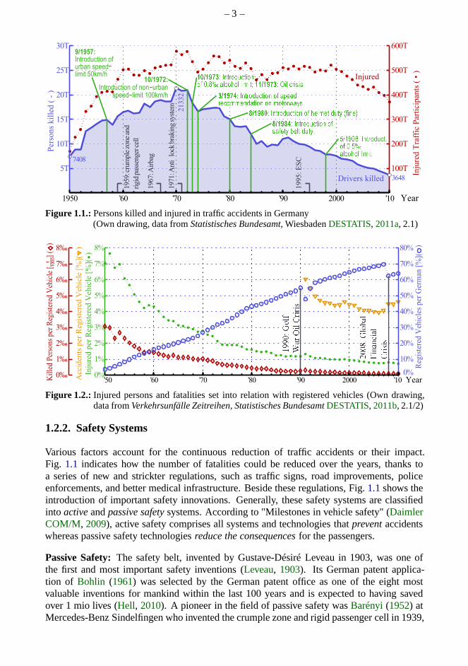
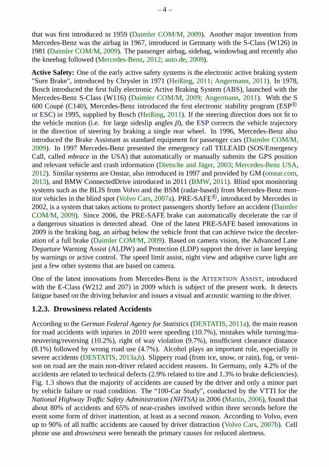
Since Karl Benz’s patent application of the Motorwagon over125 years ago1 the number ofvehicles has been steadily increasing. While the number of vehicles in Germany had grown to3.7 Mio in 1939 (DESTATIS, 2011a), it dropped below 200.000 vehicles as a consequence ofWorld War II. Fig.1.1shows the number of injured persons and persons killed within 30 daysafter a traffic accident. After the fatalities reached theirmaximum of 21.332 persons killedin 1970, both, the total number of injured and killed personsdecreased. Fig.1.2 shows thenumber of vehicles per person on the road in Germany. It can beseen that today, about 70%of all 82 Mio Germans have a car. The figure also sets the total number of crashes, injuredpersons and fatalities in relation to the registered vehicles. The proportion of accidents percar is steadily diminishing, whereas accident prevention becomes more and more difficultevery year. Even with this positive development, we have to consider that still ten personsdie and about 1000 get injured every day in Germany alone. Thenumber of crashes withoutinjury is even increasing.

1Patent 37435 of the Benz Patent-Motorwagon by Karl Benz, applied on January 29, 1886 (Benz & Co, 1886)

– 3 –

7408

1950 ’60 ’70 ’80 ’90 2000 ’10

5T

10T

15T

20T

25T

30TP

erso

ns

kil

led (

- )

100T

200T

300T

400T

500T

600T

3648

Inju

red T

raff

ic P

arti

cipan

ts (

• )

Injured

Drivers killed

1995:

ES

C

1971: A

nti

lock

bra

kin

g s

yst

em 21332

1967: A

irbag

1959: c

rum

ple

zone

and

rigid

pas

senger

cel

l

9/1957:

Introduction ofurban speedlimit 50km/h

10/1972:

Introduction of nonurbanspeedlimit 100km/h

8/1984

safety belt duty5/1998: Introduct.

Year

Figure 1.1.:Persons killed and injured in traffic accidents in Germany(Own drawing, data fromStatistisches Bundesamt, WiesbadenDESTATIS, 2011a, 2.1)

0‰

1‰

2‰

3‰

4‰

5‰

6‰

7‰

8‰

1

1000

’50 ’60 ’70 ’80 ’90 2000 ’100%

1%

2%

3%

4%

5%

6%

7%

8%

10%

20%

30%

40%

50%

60%

70%

80%

Year

Reg

iste

red

Veh

icle

s p

er G

erm

an [

%](

)

0%

Kil

led

Per

sons

per

Reg

iste

red

Veh

icle

[

] (

)

War

Oil

Cri

ris

Acc

iden

ts p

er R

egis

tere

d V

ehic

le [

%](

)

Inju

red

per

Reg

iste

red

Veh

icle

[%

](

)

Figure 1.2.: Injured persons and fatalities set into relation with registered vehicles (Own drawing,data fromVerkehrsunfälle Zeitreihen, Statistisches BundesamtDESTATIS, 2011b, 2.1/2)

1.2.2. Safety Systems

Various factors account for the continuous reduction of traffic accidents or their impact.Fig. 1.1 indicates how the number of fatalities could be reduced overthe years, thanks toa series of new and strickter regulations, such as traffic signs, road improvements, policeenforcements, and better medical infrastructure. Beside these regulations, Fig.1.1shows theintroduction of important safety innovations. Generally,these safety systems are classifiedinto activeandpassive safetysystems. According to "Milestones in vehicle safety" (DaimlerCOM/M, 2009), active safety comprises all systems and technologies that preventaccidentswhereas passive safety technologiesreduce the consequencesfor the passengers.

Passive Safety:The safety belt, invented by Gustave-Désiré Leveau in 1903,was one ofthe first and most important safety inventions (Leveau, 1903). Its German patent applica-tion of Bohlin (1961) was selected by the German patent office as one of the eight mostvaluable inventions for mankind within the last 100 years and is expected to having savedover 1 mio lives (Hell, 2010). A pioneer in the field of passive safety wasBarényi(1952) atMercedes-Benz Sindelfingen who invented the crumple zone and rigid passenger cell in 1939,

– 4 –

that was first introduced in 1959 (Daimler COM/M, 2009). Another major invention fromMercedes-Benz was the airbag in 1967, introduced in Germanywith the S-Class (W126) in1981 (Daimler COM/M, 2009). The passenger airbag, sidebag, windowbag and recently alsothe kneebag followed (Mercedes-Benz, 2012; auto.de, 2009).

Active Safety: One of the early active safety systems is the electronic active braking system"Sure Brake", introduced by Chrysler in 1971 (Heißing, 2011; Angermann, 2011). In 1978,Bosch introduced the first fully electronic Active Braking System (ABS), launched with theMercedes-Benz S-Class (W116) (Daimler COM/M, 2009; Angermann, 2011). With the S600 Coupé (C140), Mercedes-Benz introduced the first electronic stability program (ESPR©

or ESC) in 1995, supplied by Bosch (Heißing, 2011). If the steering direction does not fit tothe vehicle motion (i.e. for large sideslip anglesβ), theESPcorrects the vehicle trajectoryin the direction of steering by braking a single rear wheel. In 1996, Mercedes-Benz alsointroduced the Brake Assistant as standard equipment for passenger cars (Daimler COM/M,2009). In 1997 Mercedes-Benz presented the emergency call TELEAID (SOS/EmergencyCall, calledmbracein the USA) that automatically or manually submits the GPS positionand relevant vehicle and crash information (Dietsche and Jäger, 2003; Mercedes-Benz USA,2012). Similar systems are Onstar, also introduced in 1997 and provided by GM (onstar.com,2013), and BMW ConnectedDrive introduced in 2011 (BMW, 2011). Blind spot monitoringsystems such as the BLIS from Volvo and the BSM (radar-based)from Mercedes-Benz mon-itor vehicles in the blind spot (Volvo Cars, 2007a). PRE-SAFER©, introduced by Mercedes in2002, is a system that takes actions to protect passengers shortly before an accident (DaimlerCOM/M, 2009). Since 2006, the PRE-SAFE brake can automatically decelerate the car ifa dangerous situation is detected ahead. One of the latest PRE-SAFE based innovations in2009 is the braking bag, an airbag below the vehicle front that can achieve twice the deceler-ation of a full brake (Daimler COM/M, 2009). Based on camera vision, the Advanced LaneDeparture Warning Assist (ALDW) and Protection (LDP) support the driver in lane keepingby warnings or active control. The speed limit assist, nightview and adaptive curve light arejust a few other systems that are based on camera.

One of the latest innovations from Mercedes-Benz is theATTENTION ASSIST, introducedwith the E-Class (W212 and 207) in 2009 which is subject of thepresent work. It detectsfatigue based on the driving behavior and issues a visual andacoustic warning to the driver.

1.2.3. Drowsiness related Accidents

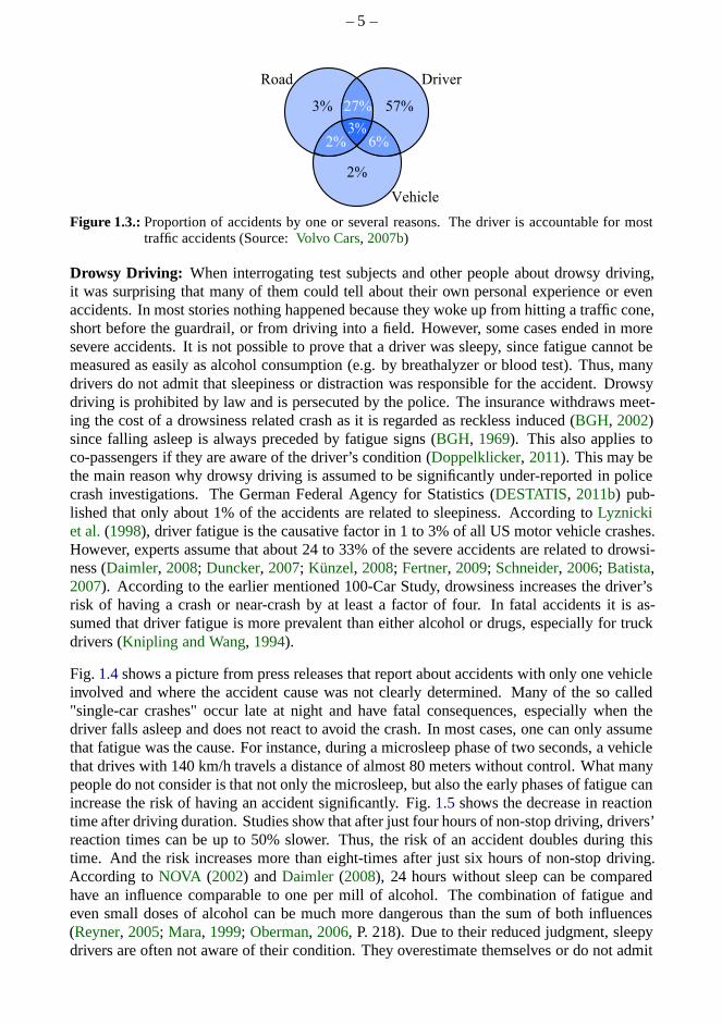
According to theGerman Federal Agency for Statistics(DESTATIS, 2011a), the main reasonfor road accidents with injuries in 2010 were speeding (10.7%), mistakes while turning/ma-neuvering/reversing (10.2%), right of way violation (9.7%), insufficient clearance distance(8.1%) followed by wrong road use (4.7%). Alcohol plays an important role, especially insevere accidents (DESTATIS, 2013a,b). Slippery road (from ice, snow, or rain), fog, or veni-son on road are the main non-driver related accident reasons. In Germany, only 4.2% of theaccidents are related to technical defects (2.9% related totire and 1.3% to brake deficiencies).Fig. 1.3 shows that the majority of accidents are caused by the driverand only a minor partby vehicle failure or road condition. The “100-Car Study", conducted by the VTTI for theNational Highway Traffic Safety Administration (NHTSA) in 2006 (Martin, 2006), found thatabout 80% of accidents and 65% of near-crashes involved within three seconds before theevent some form of driver inattention, at least as a second reason. According to Volvo, evenup to 90% of all traffic accidents are caused by driver distraction (Volvo Cars, 2007b). Cellphone use anddrowsinesswere beneath the primary causes for reduced alertness.

– 5 –

Vehicle

DriverRoad

2%

3% 27% 57%

6%2%3%

Figure 1.3.:Proportion of accidents by one or several reasons. The driver is accountable for mosttraffic accidents (Source:Volvo Cars, 2007b)

Drowsy Driving: When interrogating test subjects and other people about drowsy driving,it was surprising that many of them could tell about their ownpersonal experience or evenaccidents. In most stories nothing happened because they woke up from hitting a traffic cone,short before the guardrail, or from driving into a field. However, some cases ended in moresevere accidents. It is not possible to prove that a driver was sleepy, since fatigue cannot bemeasured as easily as alcohol consumption (e.g. by breathalyzer or blood test). Thus, manydrivers do not admit that sleepiness or distraction was responsible for the accident. Drowsydriving is prohibited by law and is persecuted by the police.The insurance withdraws meet-ing the cost of a drowsiness related crash as it is regarded asreckless induced (BGH, 2002)since falling asleep is always preceded by fatigue signs (BGH, 1969). This also applies toco-passengers if they are aware of the driver’s condition (Doppelklicker, 2011). This may bethe main reason why drowsy driving is assumed to be significantly under-reported in policecrash investigations. The German Federal Agency for Statistics (DESTATIS, 2011b) pub-lished that only about 1% of the accidents are related to sleepiness. According toLyznickiet al.(1998), driver fatigue is the causative factor in 1 to 3% of all US motor vehicle crashes.However, experts assume that about 24 to 33% of the severe accidents are related to drowsi-ness (Daimler, 2008; Duncker, 2007; Künzel, 2008; Fertner, 2009; Schneider, 2006; Batista,2007). According to the earlier mentioned 100-Car Study, drowsiness increases the driver’srisk of having a crash or near-crash by at least a factor of four. In fatal accidents it is as-sumed that driver fatigue is more prevalent than either alcohol or drugs, especially for truckdrivers (Knipling and Wang, 1994).

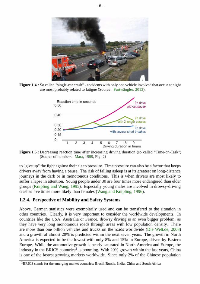
Fig. 1.4shows a picture from press releases that report about accidents with only one vehicleinvolved and where the accident cause was not clearly determined. Many of the so called"single-car crashes" occur late at night and have fatal consequences, especially when thedriver falls asleep and does not react to avoid the crash. In most cases, one can only assumethat fatigue was the cause. For instance, during a microsleep phase of two seconds, a vehiclethat drives with 140 km/h travels a distance of almost 80 meters without control. What manypeople do not consider is that not only the microsleep, but also the early phases of fatigue canincrease the risk of having an accident significantly. Fig.1.5 shows the decrease in reactiontime after driving duration. Studies show that after just four hours of non-stop driving, drivers’reaction times can be up to 50% slower. Thus, the risk of an accident doubles during thistime. And the risk increases more than eight-times after just six hours of non-stop driving.According toNOVA (2002) andDaimler (2008), 24 hours without sleep can be comparedhave an influence comparable to one per mill of alcohol. The combination of fatigue andeven small doses of alcohol can be much more dangerous than the sum of both influences(Reyner, 2005; Mara, 1999; Oberman, 2006, P. 218). Due to their reduced judgment, sleepydrivers are often not aware of their condition. They overestimate themselves or do not admit

– 6 –

Figure 1.4.:So called "single-car crash" - accidents with only one vehicle involved that occur at nightare most probably related to fatigue (Source:Furtwängler, 2013).

0.50

0.40

0.30

0.20

0.15

01 32 4 65 7 98

Reaction time in seconds

Driving duration in hours

9h drivewithout pause

9h drivewith 2 longer pauses

9h drivewith several short breakes

Figure 1.5.:Decreasing reaction time after increasing driving duration (so called "Time-on-Task")(Source of numbers:Mara, 1999, Fig. 2)

to "give up" the fight against their sleep pressure. Time pressure can also be a factor that keepsdrivers away from having a pause. The risk of falling asleep is at its greatest on long-distancejourneys in the dark or in monotonous conditions. This is when drivers are most likely tosuffer a lapse in attention. Young people under 30 are four times more endangered than eldergroups (Knipling and Wang, 1995). Especially young males are involved in drowsy-drivingcrashes five times more likely than females (Wang and Knipling, 1996).

1.2.4. Perspective of Mobility and Safety Systems

Above, German statistics were exemplarily used and can be transfered to the situation inother countries. Clearly, it is very important to consider the worldwide developments. Incountries like the USA, Australia or France, drowsy drivingis an even bigger problem, asthey have very long monotonous roads through areas with low population density. Thereare more than one billion vehicles and trucks on the roads worldwide (Die Welt.de, 2008)and a growth of almost 20% is predicted within the next seven years. The growth in NorthAmerica is expected to be the lowest with only 8% and 15% in Europe, driven by EasternEurope. While the automotive growth is nearly saturated in North America and Europe, theindustry in the BRICS countries2 is booming. With 20% growth within the last years, Chinais one of the fastest growing markets worldwide. Since only 2% of the Chinese population

2BRICS stands for the emerging market countries:Brasil,Russia,India,China andSouth Africa

– 7 –

have a car, it is expected that the growth will continue (Bleich, 2009, P. 57). In addition,the nowadays very dense road infrastructure and the relatedindustry will not disappear allof a sudden. At the same time, the protection standards in theBRICS are not very evolved.With 142 485 deaths in 2011, India has the most road fatalities in the world (Governmentof India, 2011) followed by China with 68 000 in 2009 (NPC China, 2010) due to the highpopulation. It is getting more and more difficult to further reduce the number of severeaccidents while keeping the traffic efficient. Autonomous driving is certainly a major steptowards the paradigm of efficient and "crash free driving" (Daimler COM/M, 2009). Bergerand Rumpe(2008) conclude from the Darpa Urban Challenge that autonomous driving isgenerally possible, but many open questions are still to be solved. According to Wagoner(GM CEO) (Wagoner, 2008) autopilots could become reality in 2020 or within the next years,so Ralf Herrtwich, head ofADAS at Mercedes-Benz (Heuer, 2013). An autopilot has to knoweven more that the driver is not sleeping when it needs to handover the vehicle control to thedriver in situations that cannot be handled automatically.And until the question is not solvedof who is responsible if the autopilot causes an accident, the driver will remain in charge ofthe steering wheel.

Briefly worded, we can expect that the concept of personal mobility will remain the samefor many years, which makes it crucial to introduce new advanced driver assistance systems(ADAS) for the reduction of the prohibitive high number of accidents. Thus, research in thefield of driver monitoring has the highest potential with regards to crash reduction.

1.3. Driver State Warning Systems and their Human MachineInterface (HMI)

Until today, safety systems were focusing on either intervention after a driver made a mistakeor on reducing the impact of a crash. In the precedent vehicles, there were virtually nosystems focusing on the driver. The aim of Advanced Driver Monitoring Systems (ADAS)is to detect the onset of sleepiness by analyzing the drivingstyle or physiological indicatorsof the driver. People who are skeptical about the concept of adriver monitoring systemoften argue that they do not need to be told when they are tired. They think that they arealways aware of their condition by themselves. But the danger of reduced vigilance is oftenunderestimated. 41% of the drivers interrogated in a recentstudy by theAAA Foundation forTraffic Safetyadmit to having fallen asleep behind the wheel at some point (TRUEcar, 2010).But just because nothing happened in the past doesn’t mean that it will turn out well everytime in the future. Since drivers obviously underestimate the risk and do not act adequately,it makes sense to develop systems that support the driver.

Depending on the accuracy with which the driver’s vigilancelevel can be estimated, it needsto be discussed what to do with this driver state informationin the first place. For the ac-ceptance of the system, it is essential not to infantilize the driver. Today, most drivers wouldprobably not accept a system that takes over control and automatically drives to the roadshoulder, brakes and locks the vehicle if sleepiness was detected. (This might be more ap-propriate if a cardiac flatline was detected). So the most expedient feedback strategy is toissue an acoustic and visual warning to the driver suggesting to have a pause. Issuing falsewarnings too often risks that the driver might later neglecta correct warning. As well, it isimportant not to store any data about a driver’s state that could be used against him after anaccident. A system that is switched off by the driver for suchreasons is useless. As long as

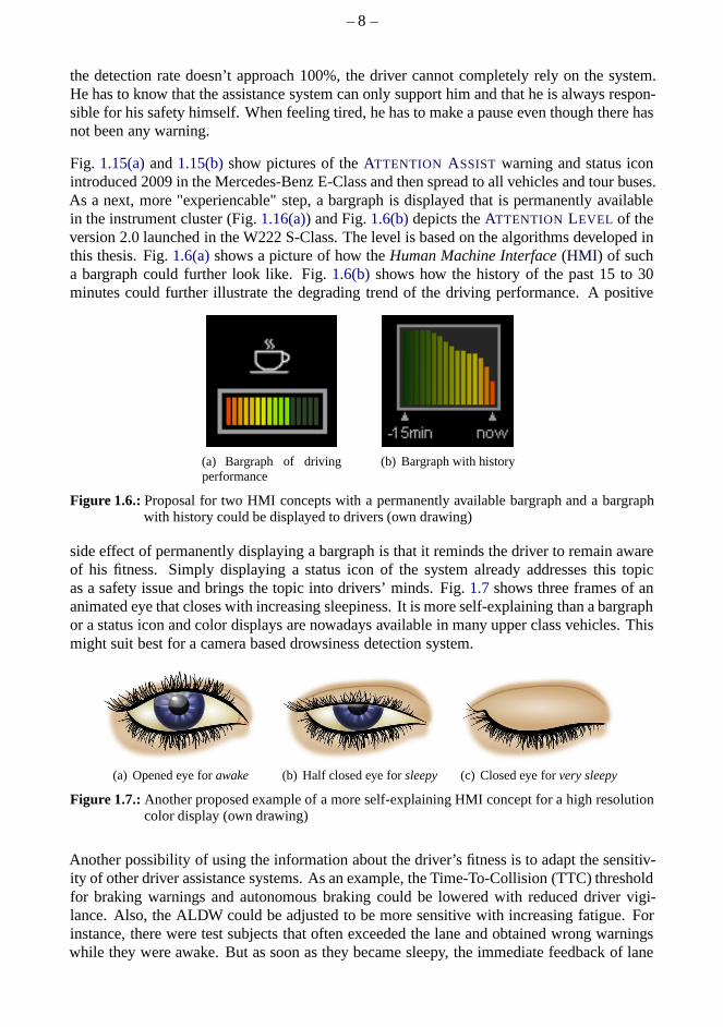
– 8 –

the detection rate doesn’t approach 100%, the driver cannotcompletely rely on the system.He has to know that the assistance system can only support himand that he is always respon-sible for his safety himself. When feeling tired, he has to make a pause even though there hasnot been any warning.

Fig. 1.15(a)and1.15(b)show pictures of theATTENTION ASSIST warning and status iconintroduced 2009 in the Mercedes-Benz E-Class and then spread to all vehicles and tour buses.As a next, more "experiencable" step, a bargraph is displayed that is permanently availablein the instrument cluster (Fig.1.16(a)) and Fig.1.6(b)depicts theATTENTION LEVEL of theversion 2.0 launched in the W222 S-Class. The level is based on the algorithms developed inthis thesis. Fig.1.6(a)shows a picture of how theHuman Machine Interface(HMI) of sucha bargraph could further look like. Fig.1.6(b) shows how the history of the past 15 to 30minutes could further illustrate the degrading trend of thedriving performance. A positive

(a) Bargraph of drivingperformance

(b) Bargraph with history

Figure 1.6.:Proposal for two HMI concepts with a permanently available bargraph and a bargraphwith history could be displayed to drivers (own drawing)

side effect of permanently displaying a bargraph is that it reminds the driver to remain awareof his fitness. Simply displaying a status icon of the system already addresses this topicas a safety issue and brings the topic into drivers’ minds. Fig. 1.7 shows three frames of ananimated eye that closes with increasing sleepiness. It is more self-explaining than a bargraphor a status icon and color displays are nowadays available inmany upper class vehicles. Thismight suit best for a camera based drowsiness detection system.

(a) Opened eye forawake (b) Half closed eye forsleepy (c) Closed eye forvery sleepy

Figure 1.7.:Another proposed example of a more self-explaining HMI concept for a high resolutioncolor display (own drawing)

Another possibility of using the information about the driver’s fitness is to adapt the sensitiv-ity of other driver assistance systems. As an example, the Time-To-Collision (TTC) thresholdfor braking warnings and autonomous braking could be lowered with reduced driver vigi-lance. Also, the ALDW could be adjusted to be more sensitive with increasing fatigue. Forinstance, there were test subjects that often exceeded the lane and obtained wrong warningswhile they were awake. But as soon as they became sleepy, the immediate feedback of lane

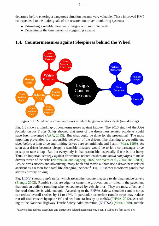
– 9 –

departure before entering a dangerous situation became very valuable. These improved HMIconcepts lead to the major goals of the research on driver monitoring systems:

• Estimating a reliable measure of fatigue with multiple levels• Determining the time instant of suggesting a pause

1.4. Countermeasures against Sleepiness behind the Wheel

Counter-

measures

Lane

Departure

Warning

Cabin

Ambient

Noise

Cabin

Ambient

Fragrance

Cabin

Ambient

Light

Massage

Seats

Lane

Parkings /

Rest Areas

General

Rumple

Strips

Figure 1.8.:Mindmap of countermeasures to reduce fatigue-related accidents (own drawing)

Fig. 1.8 shows a mindmap of countermeasures against fatigue. The 2010 study of theAAAFoundation for Traffic Safetyshowed that most of the drowsiness related accidents couldhave been prevented (AAA , 2013). But what could be done for the prevention? The mostimportant prevention is a responsible behavior of the drivers, like planning to get sufficientsleep before a long drive and limiting drives between midnight and 6 a.m. (Mara, 1999). Assoon as a driver becomes sleepy, a sensible measure would be to let a co-passenger driveor stop to take a nap. But not everybody is that reasonable, especially if one is in a hurry.Thus, an important strategy against drowsiness related crashes aremedia campaignsto makedrivers aware of the risks (Nordbakke and Sagberg, 2007; van Wees et al., 2004; Hell, 2001).Beside press articles and advertising, many book and movie authors use a drowsiness relatedaccident as a reason for a fatal life-changing incident3. Fig.1.9shows motorway panels thataddress drowsy driving.

Fig.1.10(a)showsrumple strips, which are another countermeasure to alert inattentive drivers(Elango, 2002). Rumble strips are edge- or centerline grooves, cut or rolled in the pavementthat emit an audible rumbling when encountered by vehicle tires. They are most effective ifthe road shoulder is wide enough. According to theFHWA Safety, shoulder rumble stripscan reduce overall crashes by 14 to 17%. In particular, centerline rumble strips may reducerun-off-road crashes by up to 41% and head-on crashes by up to68% (FHWA, 2012). Accord-ing to the National Highway Traffic Safety Administration (NHTSA) (Mara, 1999), rumble

3Movies that address sleepiness and distraction-related accidents: Mr. Bean, I Robot, 50 first dates, etc.

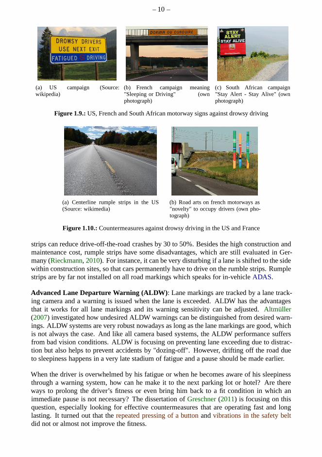
– 10 –

(a) US campaign (Source:wikipedia)

(b) French campaign meaning"Sleeping or Driving" (ownphotograph)

(c) South African campaign"Stay Alert - Stay Alive" (ownphotograph)

Figure 1.9.:US, French and South African motorway signs against drowsy driving

(a) Centerline rumple strips in the US(Source: wikimedia)

(b) Road arts on french motorways as"novelty" to occupy drivers (own pho-tograph)

Figure 1.10.:Countermeasures against drowsy driving in the US and France

strips can reduce drive-off-the-road crashes by 30 to 50%. Besides the high construction andmaintenance cost, rumple strips have some disadvantages, which are still evaluated in Ger-many (Rieckmann, 2010). For instance, it can be very disturbing if a lane is shiftedto the sidewithin construction sites, so that cars permanently have todrive on the rumble strips. Rumplestrips are by far not installed on all road markings which speaks for in-vehicleADAS.

Advanced Lane Departure Warning (ALDW) : Lane markings are tracked by a lane track-ing camera and a warning is issued when the lane is exceeded. ALDW has the advantagesthat it works for all lane markings and its warning sensitivity can be adjusted.Altmüller(2007) investigated how undesired ALDW warnings can be distinguished from desired warn-ings. ALDW systems are very robust nowadays as long as the lane markings are good, whichis not always the case. And like all camera based systems, theALDW performance suffersfrom bad vision conditions. ALDW is focusing on preventing lane exceeding due to distrac-tion but also helps to prevent accidents by "dozing-off". However, drifting off the road dueto sleepiness happens in a very late stadium of fatigue and a pause should be made earlier.

When the driver is overwhelmed by his fatigue or when he becomes aware of his sleepinessthrough a warning system, how can he make it to the next parking lot or hotel? Are thereways to prolong the driver’s fitness or even bring him back to afit condition in which animmediate pause is not necessary? The dissertation ofGreschner(2011) is focusing on thisquestion, especially looking for effective countermeasures that are operating fast and longlasting. It turned out that therepeated pressing of a buttonandvibrations in the safety beltdid not or almost not improve the fitness.

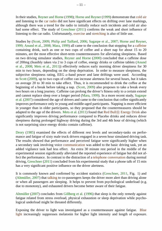
– 11 –

In their studies,Reyner and Horne(1998); Horne and Reyner(1999) demonstrate thatcold airand listening to thecar radiodid not have significant effects on drifting over lane markings,although there was a trend for the radio to initially reduce such incidents and cold air alsohad some effect. The study ofGreschner(2011) confirms the weak and short influence oflistening to the car radio. Unfortunately,exerciseandstretchingis also of little use.

Studies by (Scott, 2009; Philip and Taillard, 2006; Sagaspe et al., 2007; Horne and Reyner,1999; Anund et al., 2008; Mara, 1999) all came to the conclusion that stopping for acaffeinecontaining drink, such as one or two cups of coffee and a shortnap for about 15 to 20minutes, are the most effective short-term countermeasures for alleviating sleepiness. Basedon two driving simulator studies,Reyner and Horne(2000) concluded that a caffeine doseof 200mg (feasibly taken via 2 to 3 cups of coffee, energy drinks or caffeine tablets (Anundet al., 2008; Mets et al., 2011)) effectively reduces early morning driver sleepiness for30min to two hours, depending on the sleep deprivation. In order to measure sleepiness, thesubjective sleepiness rating, EEGα-band power and lane driftings were used. Accordingto Scott(2009), up to two cups of coffee can increase alertness for severalhours, but it takeson average 20 to 30 min to take effect. Thus, it is recommendedto drink the coffee at thebeginning of a break before taking a nap. (Scott, 2009) also proposes to take a break everytwo hours on a long journey. Caffeine can prolong the driver’s fitness only to a certain extendand cannot replace sleep over a longer period (Mara, 1999). In a more recent study,Sagaspeet al.(2007) considered the age of drivers and came to the conclusion that coffee significantlyimproves performance only in young and middle-aged participants. Napping is more efficientin younger than in older participants, so they proposed thatthe countermeasures should beadapted to the age of the drivers.Mets et al.(2011) found thatRed BullR© Energy Drinkalsosignificantly improves driving performance compared to Placebo drinks and reduces driversleepiness during prolonged highway driving during the 3rdand 4th hour of driving (whichis not surprising since energy drinks contain caffeine).

Drory (1985) examined the effects of different rest levels and secondary-tasks on perfor-mance and fatigue of sixty male truck drivers engaged in a seven hour simulated driving task.The results showed that performance and perceived fatigue were significantly higher whena secondary task involving voicecommunicationwas added to the basic driving task, yet anadded vigilance task had less effect. An extra 30 minute restperiod in the middle of theexperimental session significantly alleviated the reported experience of fatigue but did not af-fect the performance. In contrast to the distraction of atelephone conversationduring normaldriving, Greschner(2011) concluded from his experimental study that a phone talk of 15 minhas a very significant positive influence on the driver alertness.

It is commonly known and confirmed by accident statistics (Greschner, 2011, Fig. 1) and(Altmüller, 2007) thattalking to co-passengers keeps the driver more alert than driving aloneor when all passengers are sleeping. It helps to prevent frompsychological underload (e.g.due to monotony), and exhausted drivers become better awareof their fatigue.

Altmüller (2007) concludes fromGillberg et al.(1996) that sleep is the only remedy againstfatigue related from stress overload, physical exhaustionor sleep deprivation while psycho-logical underload might be threated differently.

Exposing the driver to light was investigated as a countermeasure against fatigue.Bluelight increasingly suppresses melatonin for higher light intensity and length of exposure.

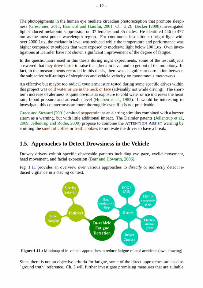
– 12 –

The photopigments in the human eye mediate circadian photoreception that promote sleepi-ness (Greschner, 2011; Brainard and Hanifin, 2001, Ch. 3.2). Becker(2008) investigatedlight-induced melatonin suppression on 37 females and 35 males. He identified 446 to 477nm as the most potent wavelength region. For continuous insolation to bright light withover 2000 Lux, the melatonin level was reduced while the temperature and performance washigher compared to subjects that were exposed to moderate light below 100 Lux. Own inves-tigations at Daimler have not shown significant improvementof the degree of fatigue.

In the questionnaire used in this thesis during night experiments, some of the test subjectsanswered that theydrive fasterto raise the adrenalin level and to get out of the monotony. Infact, in the measurements recorded in this thesis, there wasa significant correlation betweenthe subjective self-ratings of sleepiness and vehicle velocity on monotonous motorways.

An effective but maybe too radical countermeasure tested during some specific drives withinthis project wascold water or ice in the neck or face(advisably not while driving). The short-term increase of alertness is quite obvious as exposure to cold water or ice increases the heartrate, blood pressure and adrenalin level (Houben et al., 1982). It would be interesting toinvestigate this countermeasure more thoroughly even if itis not practicable.

Grace and Steward(2001) emittedpeppermintas an alerting stimulus combined with a buzzeralarm as a warning, but with little additional impact. The Daimler patents (Jellentrup et al.,2009; Jellentrup and Rothe, 2009) propose to combine theATTENTION ASSISTwarning byemitting thesmell of coffeeor fresh cookiesto motivate the driver to have a break.

1.5. Approaches to Detect Drowsiness in the Vehicle

Drowsy drivers exhibit specific observable patterns including eye gaze, eyelid movement,head movement, and facial expression (Barr and Howarth, 2006).

Fig. 1.11 provides an overview over various approaches todirectly or indirectly detect re-duced vigilance in a driving context.

In-vehicle

Fatigue

Detection

Steering

Behavior

Direct

Driver

Camera

Electro-oculo-gram

Electro-encephalo-

gram

ECG / EMG

Hand Conductivity

/ Grip

IndirectLane

Keeping

Figure 1.11.:Mindmap of in-vehicle approaches to reduce fatigue-related accidents (own drawing)

Since there is not an objective criteria for fatigue, some ofthe direct approaches are used as"ground truth" reference. Ch.3 will further investigate promising measures that are suitable

– 13 –

as fatigue reference in combination with subjective self-ratings. Fatigue can be rated by amajority voting of experts or self-rated by the driver.

Direct approaches measure vigilance immediately from the driver.For instance, the brain,muscle or heart activity can be measured by Electroenzephalography (EEG), Electromyo-gram (EMG) or Electrocardiogram (ECG). Wiring the driver with electrodes is not practica-ble for series applications, so that there are approaches toestimate theECGby radar in thevehicle cabin (Mahler, 2005). The eye lid movement is another indicator for fatigue and canbe observed by electrodes around the eyes in the Electrooculogram (EOG) or by attachingspindles directly to the eye lids (Hargutt and Krüger, 2000). A less intrusive way is to capturethe eye lid movements by an eye-tracking camera. In the past,the acceptance of a camerapointing directly at the driver was too low for a series application. More recently, internalstudies show that the acceptance for such eye-tracking "sensors" has increased. Measuringthe hand grip force or the humidity directly on the steering wheel is a weak indicator for thedriver fitness and cannot be used as standalone features.

In comparison,indirect methods evaluate secondary effects such as impaired driving accu-racy. The idea behind indirect approaches is to consider thedriver-vehicle-roadscenario(Fig. 1.12) as a control system in which the driver has to constantly adjust the lateral andlongitudinal position. Reduced vigilance results in a decrease of control accuracy which canbe represented by different driver model parameter. The driver has to constantly react toexternal influences induced by the road or traffic. The vehicle translates the actions witha certain phase delay into movements. The error that the driver makes within this control

Driver

Vehicle

Environment

Figure 1.12.:Driver within a control system

loop is partially correlated with his short-term attention, his fitness and fatigue level, butunfortunately also to other influences such as varying driving styles, road condition, trafficinfluences and many others. Thus, the long term lane keeping performance, steering behavioror reaction time to external events can be used as indirect indicators for reduced vigilance.These approaches will be investigated in Ch.4. The external influences will be discussed inCh.5.

Due to their non-intrusiveness and lower costs, indirect methods are more suitable for seriesapplications. Therefore, it is more attractive for car manufacturers to focus on indirect meth-ods using in-vehicle sensors that are already available forthe Electronic Stability Control(ESC) and other standard equipment systems.

1.6. Drowsiness Detection Systems on the Market

The first prevention driver assistance systems on the marketfocusing on fatigued driverswere the VolvoDriver Alert Control (Volvo Cars, 2007b; Ritter, 2007) introduced in 2007,as special equipment, and the Mercedes-BenzATTENTION ASSIST in 2009 as series equip-ment (Daimler, 2008; Daimler COM/M, 2009). TheATTENTION ASSIST is running onESCplatforms from Bosch, Delphi and TRW that have all differentarchitectures. In 2010, Bosch

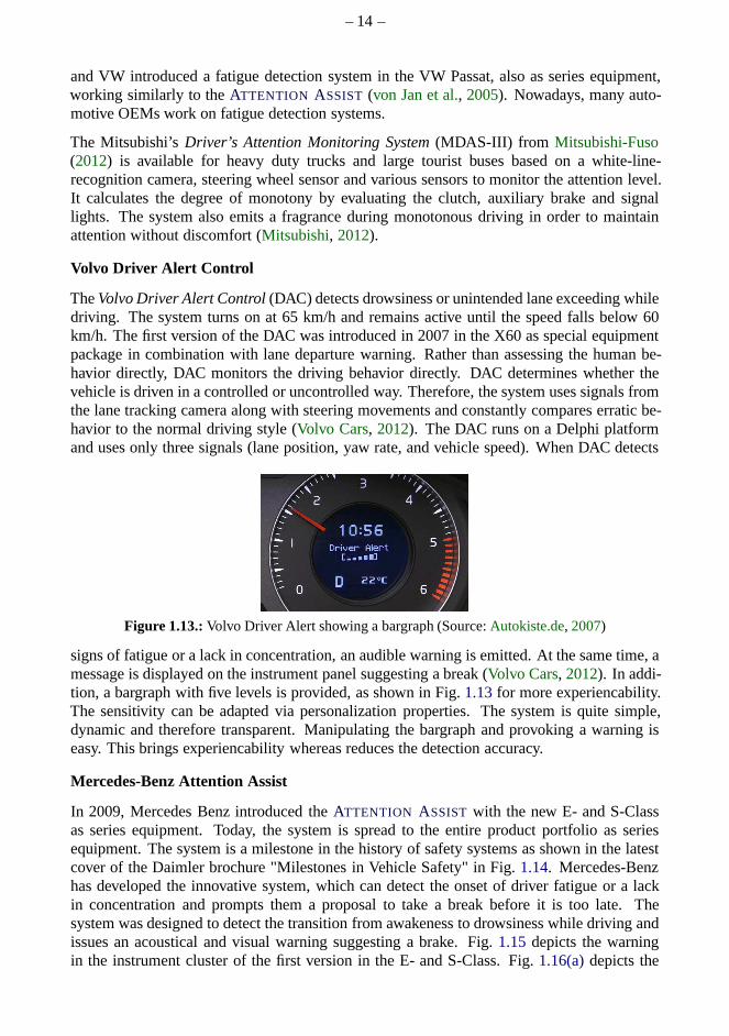
– 14 –

and VW introduced a fatigue detection system in the VW Passat, also as series equipment,working similarly to theATTENTION ASSIST (von Jan et al., 2005). Nowadays, many auto-motive OEMs work on fatigue detection systems.

The Mitsubishi’sDriver’s Attention Monitoring System(MDAS-III) from Mitsubishi-Fuso(2012) is available for heavy duty trucks and large tourist buses based on a white-line-recognition camera, steering wheel sensor and various sensors to monitor the attention level.It calculates the degree of monotony by evaluating the clutch, auxiliary brake and signallights. The system also emits a fragrance during monotonousdriving in order to maintainattention without discomfort (Mitsubishi, 2012).

Volvo Driver Alert Control

TheVolvo Driver Alert Control(DAC) detects drowsiness or unintended lane exceeding whiledriving. The system turns on at 65 km/h and remains active until the speed falls below 60km/h. The first version of the DAC was introduced in 2007 in theX60 as special equipmentpackage in combination with lane departure warning. Ratherthan assessing the human be-havior directly, DAC monitors the driving behavior directly. DAC determines whether thevehicle is driven in a controlled or uncontrolled way. Therefore, the system uses signals fromthe lane tracking camera along with steering movements and constantly compares erratic be-havior to the normal driving style (Volvo Cars, 2012). The DAC runs on a Delphi platformand uses only three signals (lane position, yaw rate, and vehicle speed). When DAC detects

Figure 1.13.:Volvo Driver Alert showing a bargraph (Source:Autokiste.de, 2007)

signs of fatigue or a lack in concentration, an audible warning is emitted. At the same time, amessage is displayed on the instrument panel suggesting a break (Volvo Cars, 2012). In addi-tion, a bargraph with five levels is provided, as shown in Fig.1.13for more experiencability.The sensitivity can be adapted via personalization properties. The system is quite simple,dynamic and therefore transparent. Manipulating the bargraph and provoking a warning iseasy. This brings experiencability whereas reduces the detection accuracy.

Mercedes-Benz Attention Assist

In 2009, Mercedes Benz introduced theATTENTION ASSIST with the new E- and S-Classas series equipment. Today, the system is spread to the entire product portfolio as seriesequipment. The system is a milestone in the history of safetysystems as shown in the latestcover of the Daimler brochure "Milestones in Vehicle Safety" in Fig. 1.14. Mercedes-Benzhas developed the innovative system, which can detect the onset of driver fatigue or a lackin concentration and prompts them a proposal to take a break before it is too late. Thesystem was designed to detect the transition from awakenessto drowsiness while driving andissues an acoustical and visual warning suggesting a brake.Fig. 1.15 depicts the warningin the instrument cluster of the first version in the E- and S-Class. Fig.1.16(a)depicts the

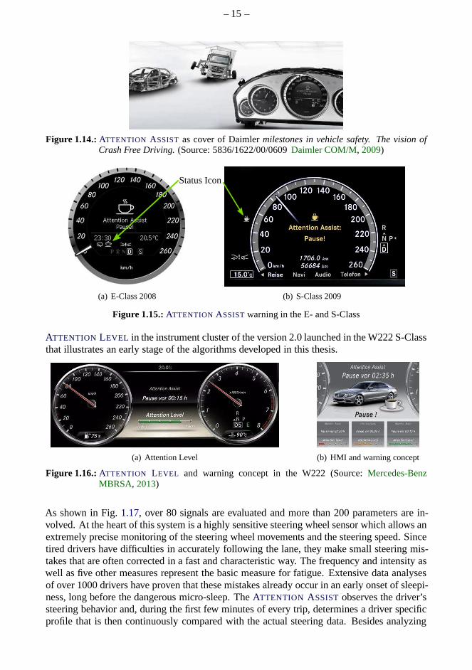
– 15 –

Figure 1.14.:ATTENTION ASSIST as cover of Daimlermilestones in vehicle safety. The vision ofCrash Free Driving.(Source: 5836/1622/00/0609Daimler COM/M, 2009)

(a) E-Class 2008

Status Icon

(b) S-Class 2009

Figure 1.15.:ATTENTION ASSISTwarning in the E- and S-Class

ATTENTION LEVEL in the instrument cluster of the version 2.0 launched in the W222 S-Classthat illustrates an early stage of the algorithms developedin this thesis.

(a) Attention Level (b) HMI and warning concept

Figure 1.16.:ATTENTION LEVEL and warning concept in the W222 (Source:Mercedes-BenzMBRSA, 2013)

As shown in Fig.1.17, over 80 signals are evaluated and more than 200 parameters are in-volved. At the heart of this system is a highly sensitive steering wheel sensor which allows anextremely precise monitoring of the steering wheel movements and the steering speed. Sincetired drivers have difficulties in accurately following thelane, they make small steering mis-takes that are often corrected in a fast and characteristic way. The frequency and intensity aswell as five other measures represent the basic measure for fatigue. Extensive data analysesof over 1000 drivers have proven that these mistakes alreadyoccur in an early onset of sleepi-ness, long before the dangerous micro-sleep. TheATTENTION ASSISTobserves the driver’ssteering behavior and, during the first few minutes of every trip, determines a driver specificprofile that is then continuously compared with the actual steering data. Besides analyzing

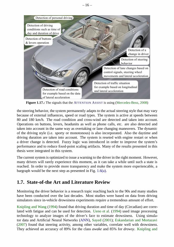
– 16 –

Detection of driving

conditions such as time of

day and duration of drive

Detection of personal driving

Detection of steering

behavior

Detection of a

change in driver

Detection of lane changes based on

control signals, steering wheel

movements and lateral acceleration

Detection of traffic situation

for example based on longitudinal

and lateral accelerationDetection of road conditions

for example based on the data

of lateral acceleration

Detection of buttons

& levers operation

Figure 1.17.:The signals that theATTENTION ASSISTis using (Mercedes-Benz, 2008)

the steering behavior, the system permanently adapts to theactual steering style that may varybecause of external influences, speed or road types. The system is active at speeds between80 and 180 km/h. The road condition and cross-wind are detected and taken into account.Operations on buttons, levers, headunits as well as phone calls, etc. are also detected andtaken into account in the same way as overtaking or lane changing maneuvers. The dynamicof the driving style (i.e. sporty or monotonous) is also incorporated. Also the daytime anddriving duration are taken into account. The system is reseted with engine restart or whena driver change is detected. Fuzzy logic was introduced in order to improve the system’sperformance and to reduce fixed-point scaling artifacts. Many of the results presented in thisthesis were integrated in this system.

The current system is optimized to issue a warning to the driver in the right moment. However,many drivers will rarely experience this moment, as it can take a while until such a state isreached. In order to provide more transparency and make the system more experiencable, abargraph would be the next step as presented in Fig.1.6(a).

1.7. State-of-the Art and Literature Review

Monitoring the driver behavior is a research topic reachingback to the 90s and many studieshave been conducted over the last decades. Most studies werebased on data from drivingsimulators since in-vehicle drowsiness experiments require a tremendous amount of effort.

Knipling and Wang(1994) found that driving duration and time of day (Circadian) arecorre-lated with fatigue and can be used for detection.Ueno et al.(1994) used image processingtechnology to analyze images of the driver’s face to estimate drowsiness. Using simula-tor data and Artificial Neural Networks (ANN), Sayed(2001); Eskandarian and Mortazavi(2007) found that steering activity, among other variables, correlate well with drowsiness.They achieved an accuracy of 89% for the classawakeand 85% fordrowsy. Knipling and

– 17 –

Wang(1994); Fairbanks et al.(1995); Wierwille (1996a); Wierwille et al.(1996); Wierwille(1996b) proposed a set of features based on driving simulator data.Their potential featuresare included and further improved in this project. In his dissertation,Altmüller (2007) ana-lyzed the deadband rate in the steering velocity, based on 44simulator drives. The deadbandis a phase in which the driver is not steering due to a lack of awareness. These features areincluded in this thesis and analyzed using real road data.Batavia(1999) used real world datato optimize a driver aware lane departure system.

Schmitz(2004) proposed improvements to suppress warnings for intended lane departuresbased on simulator results that are verified in two field studies. Kozak and Pohl(2006) didthe same, however based on 32 truck simulator drives.

Berglund(2007); Kanstrup(2006); Mattsson(2007) used multiple regression on in-vehiclesteering and lane data variables to accurately (87%) classify drowsiness, based on 22 trucksimulator drives. WhereasLöfgren (2007) was focusing on lane data,Wigh (2007) wasevaluating lane-based features such as time-to-lane crossing at Daimler.

Forsman and Vilaa(2012) performed a driving simulator study with twelve participants and87 different driving metrics focusing on the detection of moderate drowsiness levels. She con-firms that steering wheel variability provides a cost-effective and easy-to-install alternativefor in-vehicle drowsy driver detection at moderate fatiguelevels.

1.8. Goals of this Thesis

The general goal of this thesis is to improve online fatigue level estimation algorithms forthe application in drowsiness detection systems such as theMercedes-BenzATTENTION AS-SIST. For this reason, it is mandatory to use sensor data that are suitable for in-vehicle useand preferably based on available standard equipment sensors. The detection accuracy ofthe system should be as high as possible while keeping the false alarm rate at a minimum.The algorithms should be robust and reliable under any road condition and for any type ofdriver.

The main focus of this thesis is on the study, implementationand evaluation of the fatiguerelated features in literature. Moreover, own ideas and approaches will be proposed. Thisalso involves the data acquisition and handling of over one million kilometers of real roadtest data and night experiments.

In order to reach the goals, an adequate reference for sleepiness has to be found and usedto represent the ground truth for optimization. For the effectiveness of the system, the aimis to provide a warning that is plausible with regards to thesubjectiveself-assessment of thedriver on the one hand, and that prevents accidents by providing objectivefeedback to thedriver about his impaired driving performance at the other hand. Rather than the detection ofshort term distraction, the focus of this thesis is on middleand long term lack of concentrationor alertness. At the same time, the onset of fatigue should bedetectedearly enough so thatthere remains enough time for the driver to reach the next parking area. The later the systemdetects arising fatigue, the more severe is the risk of having an accident. Thus, if the earlyonset of fatigue was not detected, it is important to at leastdetect the later phases of sleepiness,especially when micro-sleep occurs.

– 18 –

Whereas the current system only displays a warning with an acoustic warning signal, thenext generation is intended to output an online bargraph that constantly monitors the driver.Providing a permanently available bargraph of the actual driver state demands the estimationof a continuous-valued measure of the driver’s vigilance level. This drowsiness level is alsovaluable for adapting the sensitivity of other driver assistance systems such as lane departureand collision warning systems.

In addition, there are other demands of series production tofulfill. The number of variants andthe effort for the application of the system to individual vehicle types must be manageable.Furthermore, it is important to keep the system simple to conquer its complexity and reducethe risk of software errors. Algorithms that are targeted torun on the ESC controller unitmust run in real-time and in fixed-point with a very limited demand of resources.

1.9. New Contributions of this Thesis

The contributions of this thesis to the field of driver state monitoring are as follows:

Signals and DataUnparalleled amount of real-world driving data:Compared to any other previous work, thisthesis is based on an unparalleled amount of real world driving data. Most studies in litera-ture, as for instance (Altmüller, 2007; Knipling and Wang, 1994; Batavia, 1999; Kozak andPohl, 2006; Schmitz, 2004; Ueno et al., 1994; Wigh, 2007) are evaluated on a comparativelysmaller amount of simulator drives or sometimes on-road measurements under restricted labconditions. As discussed in Sec.2.1, it makes a huge difference if test drives are recorded ina simulator or on real roads.Fusion of sensor signals:This thesis deals with the problem of handling mixed, asynchronousCAN data in which signals are sometimes unavailable. The lane position is often unavailabledue to bad lane markings or vision issues. The lane position and vehicle level signals are notavailable in all vehicles. Fail-safe considerations and fall-back strategies of faulty or missingsignals are made. Online sensor fault monitoring algorithms for sensor blindspots and hys-teresis are proposed that run in fixed-point with very low resource consumption. Methodsfor the plausibility check of signals by the use of redundancy, expert knowledge and physicalvehicle models are implemented.

Fatigue ReferencesAssessment of EEG, Camera and Self-estimation:The subjective self-estimation, camera-based eye-tracking andEEG brain activity are critically evaluated for their validityin realdriving environments. External measures like eye-tracking andEEG suffer from negativeinfluences during regular road drives. Hence, the Karolinska Sleepiness Scale (KSS) is pri-marily used since the driver must accept the warnings and when thoroughly recorded, it ismore reliable than any other recorded measure. But since thesubjective understanding of theKSS scale differs amongst drivers, adesired warning levelwas introduced. In addition, awarning acceptance questionwas interrogated for cross-validation of theKSS.

FeaturesNew and improved features:In addition to promising fatigue measures (so calledfeatures)found in literature, new features are proposed. Their suitability for working under real driv-ing conditions is evaluated thoroughly on an amount of real world measurements of over 1.5million kilometers. For instance, a feature similar toDegree-of-Interactionis proposed but

– 19 –

without the need of the steering wheel torque. In comparisonto (Mattsson, 2007), an alterna-tive method for detecting zig-zag events is given.Incorporation of a-priori measures:A-priori measures (such as daytime, "time-on-task",light condition) have been considered separately during the training of the classifiers. Thismakes the assessment of features more sensitive to the actual driver state rather than usingthe probability of being sleepy in the actual driving situation alone.Application of new signal processing methods:In order to improve the performance of thefeatures and their extraction efficiency, new signal processing methods are proposed for thisapplication (e.g.EWMA , EWVAR , EWIQR, DISPO,...) (cf. Ch.4).Also, a convenient and resource-efficient online-estimation of steering velocity percentiles isproposed using an array ofEWMA filters.Feature extraction using Fuzzy logic:This was introduced to detect steering corrections morereliably and to reduce fixed-float differences.Adaptive window size of filters:Drowsiness increases rather slowly, so the correlation be-tween features and drowsiness is better for smoothing with large window sizes. A majorproblem in previous work was the large window sizes of 10-30 minutes that make the systemnonreactive to quick fatigue level changes. Compared toSayed(2001), for instance, an adap-tive window size is used to be more dynamic in drowsiness supporting situations.Accelerated optimization of feature parameters:Convex parameter optimization of singlefeatures and global parameter optimization algorithms areapplied. For feature extraction,computation cost reduction of over factor 100 is achieved byscaling all pre-processed sig-nals to the tightest data type, loading the 60 GB into the RAM and applying efficient matrixoperations.

Lane DataFeatures from advanced lane-departure camera:In addition to sensor data from steering an-gle, acceleration and yaw-rate, a portion of the investigated features is based on data fromtheAdvanced Lane Departure Warning (ALDW)system. ThisadvancedLDW provides addi-tional signals, is calibrated more accurately and has higher availability compared to individu-ally built-in aftermarket sensors from previous studies.Estimation of lane-based features by inertial sensors and extended Kalman filter (EKF): Forthe extraction of some features based on lane-tracking camera, it is proposed to only use in-ertial motion sensors in combination with anEKF. The performance between original lanefeatures and the estimated coupled motion pendants are compared.

External FactorsCompensation of external factors:Moreover, external factors like road condition, cross-wind,traffic density and vehicle operations are examined. A noveladaptive notch-filter is used tosuppress vibration noise from unbalanced wheel mass. A new sensitive detection of roadbumps is presented using the temporal delay between front and rear wheels. As in no otherprevious publications, vehicle level signals from the air suspension or Active Body Control(ABC) sensor are evaluated to estimate measures for the roadcondition. A comparison to theother methods is given.Compensation of individual driving styles:Adaption to the large variety of individual drivingstyles is crucial and handled bybaselining. Different methods are compared.Compensation of vehicle parameters:There is a large number of vehicle properties like steer-ing ratio, steering resistance and torque, vehicle mass etc. on which the detection depends.Cross-wind detection, for instance, is very sensitive to vehicle parameters. Such vehicledependencies are incorporated in this thesis.

– 20 –

ClassificationFusion of features by classificationThe fusion of the features is discussed on the physical, fea-ture, and decision level. With other words, modeling expertknowledge on feature extractionlevel, feature selection and classification are compared. The performance of a combination offeatures is assessed by classifiers and dimension reductiontechniques. Classification meth-ods for modeling expert knowledge are examined by using Hidden Markov Models (HMM).Real-time online demonstrator and novel CAN-interface:Approved algorithms are imple-mented with very limited pixed-point resources in real-time in theESCof all today’s Mercedes-Benz cars. More sophisticated features were implemented inan own Matlab MEX C++ CAN-Interface with a visualizationGUI for in-vehicle online assessment.

1.10. Challenges of in-vehicle Fatigue Detection

Clearly, a major challenge about drowsiness detection is the amount of data needed for thedevelopment and everything that is related to the data recording and handling. Since thedriver’s state generally decreases slowly over many minutes or even hours, very long mea-surements are needed. At the same time, fatigue related patterns occur within seconds andrequire a sufficiently high sampling frequency. Thus, not only the 2 TB of data, but also thelong duration of the measurements makes them difficult to record, handle, and analyze. Also,the driving behavior must not be influenced by the touchscreen KSS entries or immediatefeedback of driving performance. Furthermore, it makes a big difference when the driver haslane departure warnings or lane keeping available and switched on.

Also, a big issue was driving until the onset of sleepiness, but making sure that the risk ofhaving an accident is not higher than for normal traffic. So, every drive with involved fatiguerequired at least a co-driver and sometimes a second set of pedals. These preventions madeit possible that not one single critical situation occurredduring the entire project.

Another difficulty was the large number of signals that have to be processed. Whereas manysignal processing fields are focusing one a few channels, thefeatures in this thesis are basedon over 200 signals that all need to be validated. They all have different characteristics andeach signal originates from different vehicle types with different sensors and controller unitmanufacturers with different software. The computer devices for measurement in the vehicleare very complex, sensitive to faults, and often suffer frommiss-configuration. The drivingsimulator, the various prototype vehicles, the measurement equipment, the 10.000 hours ofdriving, the man power for data acquisition, and the research over one decade costed millionsof Euros.

Finally, the most difficult challenge was to uncover the information about the driver’s condi-tion. The driver hat to be observed within countless hours and in various situations to discoverand cluster promising patterns and to come up with ideas how to automatically detect them.Every driver drives differently and even one driver can change his behavior depending onhis/her condition, his/her mood, or the situation. So the observed patterns are covered bymany factors that severely overlay the weak fatigue patterns.

Even after all these considerations, the classification results did not reach the results obtainedin a driving simulator. It is still not clear, if online fatigue detection will ever work with veryhigh accuracy under all circumstances.

– 21 –

Chapter 2.

Sensors and Data Acquisition

2.1. Driving Experiments

A prerequisite for obtaining results on fatigue detection is a sufficiently large amount ofrecorded data with high quality. But even a large amount of data is useless without a reliablereference and good transparency of what happened during thedrives. It is very importantto know under which conditions the drives have been recorded, for instance, to know thespeed profile, road type, weather and driver type. Fig.2.1 shows a map of valid drives inEurope. Different experiment scenarios have been designedto record data that representregular driving. These experiment types are described in the following section.

Figure 2.1.:Map of drives: begin / end of drives are indicated with a green/ red dot. Green linesindicateawakedriving sections, orange lines indicateacceptableand red linesdrowsydrives (see Ch.3.3).

Night experiments: Drives with provoked fatigue levels were typically performed on mo-notonous motorway sections with very low traffic and limitedspeed from about 120 to 140km/h. This was the most important scenario since most of these drives involved a certainextend of fatigue. In addition to the subjective KSS self-rating, the driver’s vigilance level

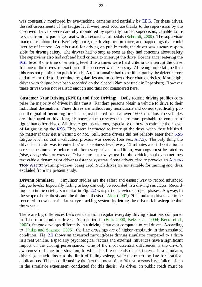
– 22 –

was constantly monitored by eye-tracking cameras and partially by EEG. For these drives,the self-assessments of the fatigue level were most accurate thanks to the supervision by theco-driver. Drivers were carefully monitored by specially trained supervisors, capable to in-tervene from the passenger seat with a second set of pedals (Schmidt, 2009). The supervisormade notes about the driver’s vigilance, the driving performance, and happenings that couldlater be of interest. As it is usual for driving on public roads, the driver was always respon-sible for driving safety. The drivers had to stop as soon as they had concerns about safety.The supervisor also had soft and hard criteria to interrupt the drive. For instance, entering theKSSlevel 9 one time or entering level 8 two times were hard criteria to interrupt the drive.In none of the drives, interaction of the co-driver was necessary. Allowing more fatigue thanthis was not possible on public roads. A questionnaire had tobe filled out by the driver beforeand after the ride to determine irregularities and to collect driver characteristics. More nightdrives with fatigue have been recorded on the closed 12km test track in Papenburg. However,these drives were not realistic enough and thus not considered here.

Customer Near Driving (KNFE) and Free Driving: Daily routine driving profiles com-prise the majority of drives in this thesis. Random persons obtain a vehicle to drive to theirindividual destination. These drives are without any restrictions and do not specifically pur-sue the goal of becoming tired. It is just desired to drive over 1600 km, thus, the vehiclesare often used to drive long distances on motorways that are more probable to contain fa-tigue than other drives. All drivers get instructions, especially on how to estimate their levelof fatigue using theKSS. They were instructed to interrupt the drive when they felt tired,no matter if they get a warning or not. Still, some drivers didnot reliably enter theirKSSfatigue level, so that a validation process was needed (see Sec.A.7.3). The only thing thedriver had to do was to enter his/her sleepiness level every 15 minutes and fill out a touchscreen questionnaire before and after every drive. In addition, warnings must be rated asfalse, acceptable, or correct. Drivers are not always used to the vehicle, so they sometimestest vehicle dynamics or driver assistance systems. Some drivers tried to provoke anATTEN-TION ASSISTwarning without being tired. Such drives are not suitable for training and, thus,excluded from the present study.

Driving Simulator: Simulator studies are the safest and easiest way to record advancedfatigue levels. Especially falling asleep can only be recorded in a driving simulator. Record-ing data in the driving simulator in Fig.2.2was part of previous project phases. Anyway, inthe scope of this thesis and the diploma thesis ofAkin (2007), 30 simulator drives had to berecorded to evaluate the latest eye-tracking system by letting the drivers fall asleep behindthe wheel.

There are big differences between data from regular everyday driving situations comparedto data from simulator drives. As reported in (Belz, 2000; Belz et al., 2004; Berka et al.,2005), fatigue develops differently in a driving simulator compared to real drives. Accordingto (Philip and Sagaspe, 2005), the line crossings are of higher amplitude in the simulatedcondition. Fig.2.2 shows an advanced moving-base driving simulator compared to a drivein a real vehicle. Especially psychological factors and external influences have a significantimpact on the driving performance. One of the most essentialdifferences is the driver’sawareness of being in a situation, in which his life depends on his fitness. In a simulator,drivers go much closer to the limit of falling asleep, which is much too late for practicalapplications. This is confirmed by the fact that most of the 30test persons have fallen asleepin the simulator experiment conducted for this thesis. As drives on public roads must be

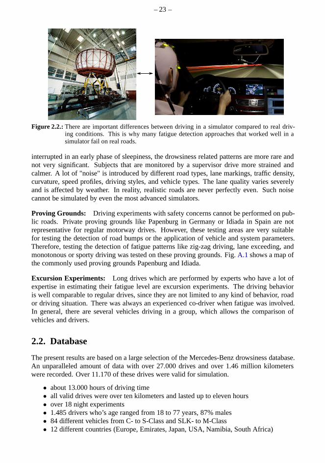
– 23 –

Figure 2.2.:There are important differences between driving in a simulator compared to real driv-ing conditions. This is why many fatigue detection approaches that worked well in asimulator fail on real roads.

interrupted in an early phase of sleepiness, the drowsinessrelated patterns are more rare andnot very significant. Subjects that are monitored by a supervisor drive more strained andcalmer. A lot of "noise" is introduced by different road types, lane markings, traffic density,curvature, speed profiles, driving styles, and vehicle types. The lane quality varies severelyand is affected by weather. In reality, realistic roads are never perfectly even. Such noisecannot be simulated by even the most advanced simulators.

Proving Grounds: Driving experiments with safety concerns cannot be performed on pub-lic roads. Private proving grounds like Papenburg in Germany or Idiada in Spain are notrepresentative for regular motorway drives. However, these testing areas are very suitablefor testing the detection of road bumps or the application ofvehicle and system parameters.Therefore, testing the detection of fatigue patterns like zig-zag driving, lane exceeding, andmonotonous or sporty driving was tested on these proving grounds. Fig.A.1 shows a map ofthe commonly used proving grounds Papenburg and Idiada.

Excursion Experiments: Long drives which are performed by experts who have a lot ofexpertise in estimating their fatigue level are excursion experiments. The driving behavioris well comparable to regular drives, since they are not limited to any kind of behavior, roador driving situation. There was always an experienced co-driver when fatigue was involved.In general, there are several vehicles driving in a group, which allows the comparison ofvehicles and drivers.

2.2. Database

The present results are based on a large selection of the Mercedes-Benz drowsiness database.An unparalleled amount of data with over 27.000 drives and over 1.46 million kilometerswere recorded. Over 11.170 of these drives were valid for simulation.

• about 13.000 hours of driving time• all valid drives were over ten kilometers and lasted up to eleven hours• over 18 night experiments• 1.485 drivers who’s age ranged from 18 to 77 years, 87% males• 84 different vehicles from C- to S-Class and SLK- to M-Class• 12 different countries (Europe, Emirates, Japan, USA, Namibia, South Africa)

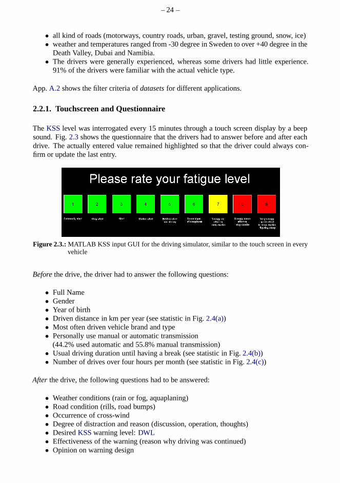
– 24 –

• all kind of roads (motorways, country roads, urban, gravel,testing ground, snow, ice)• weather and temperatures ranged from -30 degree in Sweden toover +40 degree in the

Death Valley, Dubai and Namibia.• The drivers were generally experienced, whereas some drivers had little experience.

91% of the drivers were familiar with the actual vehicle type.

App. A.2 shows the filter criteria ofdatasetsfor different applications.

2.2.1. Touchscreen and Questionnaire

TheKSSlevel was interrogated every 15 minutes through a touch screen display by a beepsound. Fig.2.3shows the questionnaire that the drivers had to answer before and after eachdrive. The actually entered value remained highlighted so that the driver could always con-firm or update the last entry.

Figure 2.3.:MATLAB KSS input GUI for the driving simulator, similar to the touch screen in everyvehicle

Beforethe drive, the driver had to answer the following questions:

• Full Name• Gender• Year of birth• Driven distance in km per year (see statistic in Fig.2.4(a))• Most often driven vehicle brand and type• Personally use manual or automatic transmission

(44.2% used automatic and 55.8% manual transmission)• Usual driving duration until having a break (see statistic in Fig.2.4(b))• Number of drives over four hours per month (see statistic in Fig. 2.4(c))

After the drive, the following questions had to be answered:

• Weather conditions (rain or fog, aquaplaning)• Road condition (rills, road bumps)• Occurrence of cross-wind• Degree of distraction and reason (discussion, operation, thoughts)• DesiredKSSwarning level:DWL• Effectiveness of the warning (reason why driving was continued)• Opinion on warning design

– 25 –

51

111

297

513

317

183

Nu

mb

er o

f d

riv

es [

dri

ver

s]

<5

Tk

m

<1

0 T

km

<1

5 T

km

<2

5 T

km

<5

0 T

km

>5

0 T

km

200

400

600

0

(a) Drivers’ annual driven distance

34

271

516

320

110

99

1h

2h

3h

4h

5h

6+h

(b) Driving duration after whichdrivers have a break

d

1

1

1

n

9 102

552

33

69

(c) Frequency of drives over 4 h

Figure 2.4.:Statistic over the driver’s answers to the touchscreen questionnaire. Even if the recordeddrivers drive many kilometers per year, they only have a few long drives over 4 h per year.Most drivers usually have a pause every 2 - 4 h whereas 19 % of the drivers drive 5 h andmore without a break.

2.3. Sensors

Every sensor was attached over ADC,LIN- or SPI-bus to anElectronic Controller Unit(ECU) that translates the physical signals toCAN messages. Some of the sensor modulessend multiple signals. The majority of the CAN signals in Tab. A.1 in App. A.3 are vehicleoperation signals, such as turn indicators or steering wheel buttons that originate from everydifferent discrete button or lever states.ALDW provides 29 signals as described in Tab.A.2.Signals from the ALDW lane keeping camera are investigated while longitudinal radar infor-mation is not used. Some reasons are that the driver’s lateral vehicle control is permanentlynecessary while the longitudinal control depends on external driving situations and the lim-iter or (adaptive) cruise control might be active. The most important sensors are described inthe following.

2.3.1. Vehicle Speed from Wheel Rotation Rate Sensor

The vehicle speed is measured by wheel rotation rate sensors("wheelticks") that use a hallsensor and a magnet wheel with magnetically encoded pulses to detect partial rotations andthe rotation direction. Depending on the vehicle drive train type, thewheel rotations perminute WhlRPMat time instantn are calculated according to Eq. (2.1). If one of the usedsensors is implausible, only the plausible sensor is taken.This, however, results in a speeddeviation within curves.

WhlRPM[n] =

(

WhlRPMFL[n] + WhlRPMFR[n])

/2 for rear wheel drive(

WhlRPMRL[n] + WhlRPMRR[n])

/2 for front wheel drive(2.1)

The vehicle speed vveh [km/h] at time intervaln is then obtained using thedynamic wheelcircumference dwhl in [m] according to Eq. (2.2). The wheel circumference grows with in-creasing speed, so thedynamicwheel circumference was chosen according to the speed rangeof interest. Too small or worn out tires cause a small deviation that cannot be detected so far.This parameter is an input of the algorithm stored as table intheESCand is selected basedon the vehicle variant code (SCN). The values originate fromthe tire suppliers.

vveh[n] = WhlRPM[n] · dwhl ·3.6km

h ·sm

60mins

(2.2)

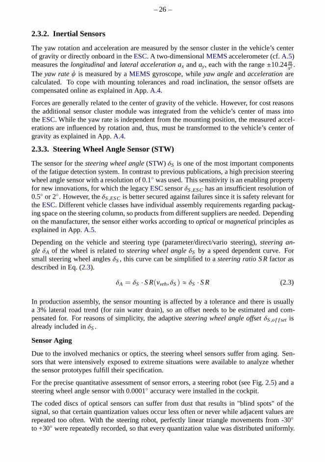
– 26 –

2.3.2. Inertial Sensors

The yaw rotation and acceleration are measured by the sensorcluster in the vehicle’s centerof gravity or directly onboard in theESC. A two-dimensionalMEMS accelerometer (cf.A.5)measures thelongitudinal andlateral acceleration ax anday, each with the range±10.24m

s2 .Theyaw rateψ is measured by aMEMS gyroscope, whileyaw angleandaccelerationarecalculated. To cope with mounting tolerances and road inclination, the sensor offsets arecompensated online as explained in App.A.4.

Forces are generally related to the center of gravity of the vehicle. However, for cost reasonsthe additional sensor cluster module was integrated from the vehicle’s center of mass intotheESC. While the yaw rate is independent from the mounting position, the measured accel-erations are influenced by rotation and, thus, must be transformed to the vehicle’s center ofgravity as explained in App.A.4.

2.3.3. Steering Wheel Angle Sensor (STW)

The sensor for thesteering wheel angle(STW) δS is one of the most important componentsof the fatigue detection system. In contrast to previous publications, a high precision steeringwheel angle sensor with a resolution of 0.1 was used. This sensitivity is an enabling propertyfor new innovations, for which the legacyESCsensorδS,ESChas an insufficient resolution of0.5 or 2. However, theδS,ESC is better secured against failures since it is safety relevant fortheESC. Different vehicle classes have individual assembly requirements regarding packag-ing space on the steering column, so products from differentsuppliers are needed. Dependingon the manufacturer, the sensor either works according tooptical or magneticalprinciples asexplained in App.A.5.

Depending on the vehicle and steering type (parameter/direct/vario steering),steering an-gle δA of the wheel is related tosteering wheel angleδS by a speed dependent curve. Forsmall steering wheel anglesδS, this curve can be simplified to asteering ratio S Rfactor asdescribed in Eq. (2.3).

δA = δS ·S R(vveh, δS) ≈ δS ·S R (2.3)

In production assembly, the sensor mounting is affected by atolerance and there is usuallya 3% lateral road trend (for rain water drain), so an offset needs to be estimated and com-pensated for. For reasons of simplicity, the adaptivesteering wheel angle offsetδS,o f f set isalready included inδS.

Sensor Aging

Due to the involved mechanics or optics, the steering wheel sensors suffer from aging. Sen-sors that were intensively exposed to extreme situations were available to analyze whetherthe sensor prototypes fulfill their specification.

For the precise quantitative assessment of sensor errors, asteering robot (see Fig.2.5) and asteering wheel angle sensor with 0.0001 accuracy were installed in the cockpit.

The coded discs of optical sensors can suffer from dust that results in "blind spots" of thesignal, so that certain quantization values occur less often or never while adjacent values arerepeated too often. With the steering robot, perfectly linear triangle movements from -30

to +30 were repeatedly recorded, so that every quantization valuewas distributed uniformly.

– 27 –

Figure 2.5.:Steering robot SR60 from Anthony Best Dynamics (Source:Anthony Best Dynamics,2012) to validate steering wheel angle sensor

Fig. 2.6 shows adiscrete histogramof the steering wheel angle and the reference signal.Fig. 2.7 shows the recorded trapezodial and a zoom of the signal in thetime-domain wherethe gaps and increased occurences can be seen.

Steering wheel angle (raw) [°]810808806804802800

0

50

100

150

200

250

300

His

togra

m o

ccure

nce

s [

]

Figure 2.6.: "Blind Spots" in which dust covers a slot of the sensor disc

As Fig. 2.8 shows, aging of the gearing can further result in ahysteresisof several samplesand non-linearity. To detect such a "backlash" across the relevant sensor range, the largelinear triangles were superposed with sines, each with an amplitude of 2. The backlashcould be detected as a plateau at inflection points by comparing of the reference and worn-out sensor signals. Non-linearities could also be detectedthis way.

Simulations with artificial blind spots have shown that the Digital Polynomial Smoothing andDifferentiation Filter (DISPO) (cf. 4.1.1) can cope with up to two blind spots equivalent to0.2 without significantly affecting the detection rate. Largerblind spots do not allow to de-tect some fast steering corrections and have a severe impacton the detection rate. An efficientonline algorithm was implemented that detects sensor defects from large gaps by exploitingthe fact that adjacent quantization values are equally probable. During the beginning of a

– 28 –

Figure 2.7.: "Blind Spots" in the time-domain

Figure 2.8.:Hysteresis (backlash) in the steering wheel angle sensor

drive, a range of ten adjacent sensor points around the±10 region of interest is randomly se-lected. AnEWMA filter for every point determines if the occurrence of one or more points issignificantly lower after a minimum number of occurrences. If such blind spots are detectedby theESCalgorithm after a number of drives, an error code is stored with the instruction toreplace the sensor during the next service visit.

Online detection of a backlash is much more difficult since itis not known how long thesteering wheel is really stopped at inflection points. Only absence of a hysteresis could bedetected, but is not discussed here.

2.3.4. Advanced Lane Departure Warning (ALDW) Assistance Systems

The driver assistance systemsAdvanced Lane Departure Warning(ALDW) and Lane De-parture Protection(LDP) help to prevent lane exceeding by distraction or late phases offatigue and micro-sleeps. The systems detect lane markingsbased on the images of a multi-ple purpose camera which is available as special equipment.The quality of the lane detectiondepends on the quality of the lane markings as well as the light conditions and environmentalinfluences like rain or fog (also cf. (Kozak and Pohl, 2006)). Data of a calibrated ALDW

– 29 –

have been used which provided over 35 signals with high accuracy. Tab.A.2 in App. A.3lists the CAN signals for the system.

2.3.5. Global Positioning System (GPS) Sensor

Global Positioning System (GPS) data are obtained over the regular built-in seriesGPSsensorthrough the head unit as well as over an additional USBGPSdevice (Weiss, 2011). The head-unit additionally providesGPSsignals matched with vehicle speed and map data. The signalsare listed in Tab.A.1.

2.3.6. Rain and Light Sensor

The rain and light sensor uses an optical photo sensor matrixto detect rain and light throughthe reflections on the windshield. The reflection coefficientof the front window is measuredby a matrix of photo resistors and IR-emitters. Rain is detected as a change of this coefficientwhile the absolute illumination level is measured at the same time by photo resistors.

2.4. Co-passenger Observations during Night Experiments,Excursions and Free drives

When looking at recorded driving data, it easily becomes clear that the transparency of whathappened during the drive is very low, especially if no videowas recorded. Aware drivingas co-passenger or by one-self provides much more transparency of the actual driving andsleepiness context.Online observation of different drivers and driving situations iscrucialfor identifying fatigue related patterns. Roughly spoken,the intensity of driving patterns, asfor instance steering correction, can be experienced live.Some qualitatively noticeable andprominent examples will be discussed here.

Thus, after every night or excursion drive of three to ten hours, plenty of notes were recordedover specific observations, the performance of fatigue measures, and sometimes new ideasfor features emerged. Thereby, the focus was particularly on patterns that can realisticallyand robustly work in practice and in real-time.

For instance, the beginning of a curve after a straight road section was notably often paralleledwith steering corrections, quite independently of the driver’s state. The consequence is thatsteering events are subsequently suppressed that result from curve entries.

Moreover, it was observed that the driving performance correlated quite well with a certainpattern for one or a group of drivers whereas other patterns correlated with other drivers.Especially one driver (ID 473) reliably started to approachor exceed the lanes with increasingfatigue levels. TheALDW system, made him aware of his exceedances and was very valuablefor this driver. This observation underlined the approach to combine driver clustering andfatigue detection.

It was reported that especially in the free or unsupervised driving, some drivers were not verymotivated to drive properly in specific situations. Such a sloppy driving style is generallycharacterized by loose lane keeping on empty roads, lane exceedances or lane changes with-out the use of the turn indicator. For instance, in France, where the maximum speed is limitedto 130 km/h and where the roads are often very empty, the driver tend to drive in a similar"sloppy" way as with fatigue. The differentiation between unmotivated and fatigue-related

– 30 –

driving style is often very difficult. However, it is plausible to objectively be monitored ofsuch impaired driving performance.

Furthermore, some drivers realized that they have the tendency to drive more to the right,when another car is overtaking. At the other hand, they tend to drive more to the left whendriving on the middle or lefter lanes if cars on the right laneare present. This effect isincreasing with higher speeds. This was the motivation to compensate driver and situationdependent lateral lane offsets for lane features.

Changes in the driving situation, e.g. during constructionsites, tunnels, weather changes, canwake up a driver out of a monotonous fatigue. However, long tunnels can be very monotonousagain after some time. It is very clear to see that the drivingand especially steering behaviorbecomes much more hectic within construction sites. For this reason, situation changes weresuppressed in the algorithm until driving parameters adapted to the new situation.

Depending on the motivation and experience of the drivers inestimating theirKSSfatiguelevel, some expert drivers were precisely aware of their actual KSSlevel, with even higherresolution than the scale allows. In this attentive focus, it was observed that the sleepinesslevel varies much faster than the 15 min long interrogation interval that only summarizesthe average level. For this purpose the supervising co-pilot noted additional informationabout the driver’s fatigue level and sometimes revisedKSSentries. This also supported themotivation to investigate other fatigue references.

Also, the different reasons for fatigue, whether it is caused by monotony or exhaustion be-came very experiencable. It was observed that the restrictions "no music", "no talking", "nocold air" have a huge impact on the time until drivers were getting sleepy. Fatigue is veryrare on regular roads but traffic accidents are also very rarewhen we consider that the averagedriver has an accident every≈ 400.000 km (Martin, 2006). Driving condition safetyof the E-and S-Class are very good, for instance due to low noise, precise steering and comfortableseats. Studies from Mercedes-Benz show that these factors significantly support the driverto remain alert for an extended time. For instance, most of the twelve hours drives fromStuttgart to Barcelona in the S-Class allowed subjects to work afterwards or even continuedriving. Small, sporty cars are louder and require more steering corrections which is muchmore exhausting. For this purpose, it was necessary to applyparameters for every vehicleindependently with a sufficiently high number of drives. These observations indicate that adriver will be longer "fit" under real circumstances than under the monotonous night experi-ments. These findings build a basis for the implementation ofnew and iteratively improvedfeatures. The repeated driving experiments were also crucial for the assessment of changedfeatures.

– 31 –

Chapter 3.

Evaluation of Driver State ReferencesDuring the development of fatigue detection algorithms, the key importance of a good fatiguereference became clear. The performance of the fatigue detection can only be as good as thereference according to which it is optimized. The major problem is to find a "true" reference,also referred to asground truth. However, there is no such objective ground truth for fatigueas there is for alphabetic character recognition, for instance. The behavior of the detectionsystem follows the properties of the reference. For instance, a reference that has a low tem-poral resolution, will not allow the development of a systemthat is more dynamic than thereference. For this reason, it is very important that the reference meets the requirements ofthe system behavior. At the same time, the amount of effort tomeasure the reference has tobe manageable. There are various approaches to measure fatigue in a driving environment.The most promising, non-intrusive and practicable ones will be evaluated in this chapter.

3.1. Terminology and Physiology of Fatigue

Fatigue (from lat. Defatigatio) is a discomfort evolving from preceding exertion, disease,suppressed need for sleep or sleep deprivation. In general,it is an imbalance between exertionand rest, due to physical or mental overstrain, induced by lifestyle. Fatigue is marked out aslack of energy, mental or physical exhaustion. Fatigue in a driving context can have differentreasons and has various facets and phases. According toAltmüller (2007, page 6), fatiguecan have the following reasons:

• Stress overload: too much mental demand that can not be handled provokes drowsiness• Physical exhaustion: hard physical or mental work can lead to a strong desire to rest• Sleep deprivation: bad or extended lack of sleep can cause a high pressure to sleep• Psychological underload or monotonous situations can provoke sleepiness. A lack of

motivation can also play a role.

For adolescent persons, fatigue is normal to a certain degree. It is caused by growth, lack ofsleep and social or scholar burdens.Oron-Gilad et al.(2007) state that fatigue is influencedby two factors: the driver’s initial state before starting the drive and the characteristics of thedrive. Both factors have a cumulative property. "Active" fatigue is caused by lack of sleep,and does not necessarily prevent "passive" fatigue (inherent boredom) caused by monotonousdriving situations. The sources of active fatigue are homeostatic factors that relate to theneurobiological need to sleep. The longer the wakefulness cycle, the more difficult it is toresist the pressure to sleep (Dinges et al., 1987). Homeostatic factors govern circadian factorsto regulate the timing of sleepiness and wakefulness (Mara, 1999). Countermeasures are notvery effective if drowsiness is caused by exhaustion. In contrast, fatigue caused by monotonycan be overcome by different activating countermeasures.

– 32 –

First of all, we need to define the terminology in regards to fatigue. A definition of the notioncan be found in (Brown, 1994; Blanco and Bocanegra, 2009):

Exhaustion Lack of energy and concentration after prolonged executionof working tasks.When a driver is extremely exhausted and deprived of sleep, even caffeine or shortpauses do not help any more.

Fatigue The difficulty to remain awake (Philip and Sagaspe, 2005). It is influenced by thecircadian rhythm and homeostatic variables (Schmidt, 2009, 1.1). The alertness canbe medically and psychologically divided in several stages. These range from uncon-scious coma to highest excitation (e.g. shock). Fatigue, asperceivable physiologicalnecessity for sleep stands in inverse relationship to alertness and vigilance. Fatigueis a rather slowly changing inner degree of exhaustion and rather a temporal smoothaverage of vigilance variations.

Sleepiness Physical sleep pressure that a person perceives. In (Philip and Sagaspe, 2005),it is defined as the difficulty to remain awake. It is influencedby circadian and homeo-static variables (Schmidt, 2009). Sleepiness is describing the late phase offatigue, i.e.the fight against sleep which is often accompanied bymicrosleep.

Vigilance (lat. vigilantia: wakefulness, sharpness). In physiology and psychology, wake-fulness denotes a state of permanent alertness. Wakefulness is a partial aspect of con-sciousness. Vigilance describes the neuro-physiologicallevel of excitation that modu-lates the willingness of a person to take action.Vigilance variationsare referred to astemporal variations in performance. A shock can, for instance, change the vigilancestate immediately to wide-awake while the basic fatigue level remains.

Hyper- and Hypovigilance Hypervigilanceis a medical term for augmented wakeful-ness and the opposite of Hypovigilance, which stands for increased sleepiness.

Attention The ability of a person to consciously or instinctively orientate (e.g. taking con-trolled action) as a reaction to different sensory or mentalinputs. Attention can beshort, mid or long-term and is strongly moderated by simultaneous secondary taskssuch as distraction by mental thoughts or side-tasks.

Microsleep Short gaps of unawareness from 0.5 to 2 seconds while the eyesare gener-ally closed. A certain kind of microsleep happens with the eye wide open ("looked-but-failed-to-see" phenomenon (Herslund and Jorgensen, 2003)). When driving on astraight motorway while not having control of the car or taking any action for twoseconds, in most cases nothing happens. However, it is oftentoo late to take action intime when driving in a curve or when approaching a preceding vehicle, a constructionsite or when a reaction to an unforeseen obstacle is needed.

Highway Hypnosis Sleep-inducing ("narcotic") impact of a monotonous driving situation.Prolonged driving in monotonous situations can favor fatigue.

Knowing that one is approaching the target destination has amotivating, arousing effect. Itwas often observed that this is the case especially for sleepiness induced by monotony.

Fatigue during the night drives recorded in this thesis is mostly induced by exhaustion froma regular work day as well as by monotony since drivers were not allowed to talk or listen tothe radio. Otherwise, the experiment would have taken much longer.

There are many aspects related to the physiology of fatigue.In this thesis, the cause or reasonfor fatigue is of little interest in contrast to the driving performance which is directly related

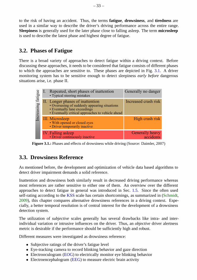
– 33 –

to the risk of having an accident. Thus, the termsfatigue, drowsiness, and tirednessareused in a similar way to describe the driver’s driving performance across the entire range.Sleepinessis generally used for the later phase close to falling asleep. The termmicrosleepis used to describe the latest phase and highest degree of fatigue.

3.2. Phases of Fatigue

There is a broad variety of approaches to detect fatigue within a driving context. Beforediscussing these approaches, it needs to be considered thatfatigue consists of different phasesto which the approaches are sensitive to. These phases are depicted in Fig.3.1. A drivermonitoring system has to be sensitive enough to detect sleepinessearly beforedangeroussituations arise, i.e. phase II.

Repeated, short phases of inattentionI.

Longer phases of inattentionII.

Generally no danger

MicrosleepIII.

Increased crash risk

High crash riskIncr

easi

ng

fat

igu

e

Falling asleepIV. Generally heavy accidents

• Typical steering mistakes

• Overseeing of suddenly appearing situations• Eventually lane exceedings• Eventually critical approaches to vehicle ahead

• With opened or closed eyes• Driver temporarily inactive

• Driver continuously inactive

Figure 3.1.:Phases and effects of drowsiness while driving (Source: Daimler, 2007)

3.3. Drowsiness Reference

As mentioned before, the development and optimization of vehicle data based algorithms todetect driver impairment demands a solid reference.

Inattention and drowsiness both similarly result in decreased driving performance whereasmost references are rather sensitive to either one of them. An overview over the differentapproaches to detect fatigue in general was introduced in Sec. 1.5. Since the often usedself-rating according to theKSSscale has certain shortcomings, as summarized in (Schmidt,2009), this chapter compares alternative drowsiness references in a driving context. Espe-cially, a better temporal resolution is of central interestfor the development of a drowsinessdetection system.

The utilization ofsubjectivescales generally has several drawbacks like intra- and inter-individual variation or intrusive influences on the driver.Thus, anobjectivedriver alertnessmetric is desirable if the performance should be sufficiently high and robust.

Different measures were investigated as drowsiness reference:

• Subjective ratings of the driver’s fatigue level• Eye-tracking camera to record blinking behavior and gaze direction• Electrooculogram (EOG) to electrically monitor eye blinking behavior• Electroencephalogram (EEG) to measure electric brain activity

– 34 –

In this thesis,EEG, EOG and eye-tracker equipment were only available in certain nightexperiments as these methods are very impractical and it wasnot feasible to wire drivers onevery drive.

As recording units become more and more mature, camera-based approaches are potentialcandidates for serial online driver monitoring, includingdistraction recognition. PERCLOS,introduced by (Hargutt, 2001), is one of the most common measures for drowsiness in litera-ture. In this chapter, an advanced measure of driver impairment is proposed that incorporateseye opening frequency, driver adaptive baselining, head movements, distraction and overtak-ing suppression.

3.3.1. Subjective Self-ratings and Expert-ratings

Subjective ratings of the driver’s fatigue level accordingto theKSSscale can be conductedin multiple ways:

Online by the driver:aware drivers are "experts" on how they feel and which mistakes theymake. However, their judgment may be subjective and impaired by reduced awarenesse.g. by sleepiness.

Online expert rating by the co-driver:the passenger can remain awake and attentively ob-serve a sleepy driver. The co-driver perspective allows to directly monitor the driver’sbehavior, facial expression and gestures while keeping an eye on the driving perfor-mance and situations.

Offline expert majority voting:a group of experts may retrospectively assess the driver’s fa-tigue level e.g. by watching video recordings of the driver and the road. Behavioralpatterns as eyelid and body movements, yawing, and head nodding (cf. Gallay andSchleicher(2002)) can also be seen in the video, yet not as good as actually being inthe car. The video additionally allows to rewind questionable situations. The advan-tage of the majority voting is that multiple persons can repeatedly estimate multipledrivers which reduces subjective variations. Results from(Wierwille and Ellsworth,1994) indicate that this is the most reliable and consistent method to estimate fatigue.

The disadvantage of subjective scales is that everyone perceives and understands fatigue andthe scales in different ways which makes the self-ratings very difficult to compare. Alsothe opinion on the level from which a driver considers his fatigue as dangerous varies, i.e.some drivers are more courageous than others. In any case, itis very difficult to comparethe fatigue level of different persons as everyone shows different behaviors and physiologicalpatterns.

Unfortunately, expert ratings are much too laborious for the amount of data in this project.For practical reasons, it was decided to use the self-ratings of the drivers since these can evenbe made with only one person in the vehicle. In night studies,the co-passenger additionallynoted the driver’s fatigue patterns as well as situations inwhich the driver’s self-rating didnot match his/her opinion.

3.3.2. Karolinska Sleepiness Scale (KSS)

Besides theStanford Sleepiness Scale (SSS)and theTiredness Symptoms Scale (TSS)(seeAkin, 2007), the most commonly used subjective self-estimation reference is theKarolin-ska Sleepiness Scale(KSS). This interval scale(Bleymüller and Gehlert, 2012) is shown inTab.3.1. TheKSS was proposed in 1979 byÅkerstedt and Gillberg(1980) and his group.

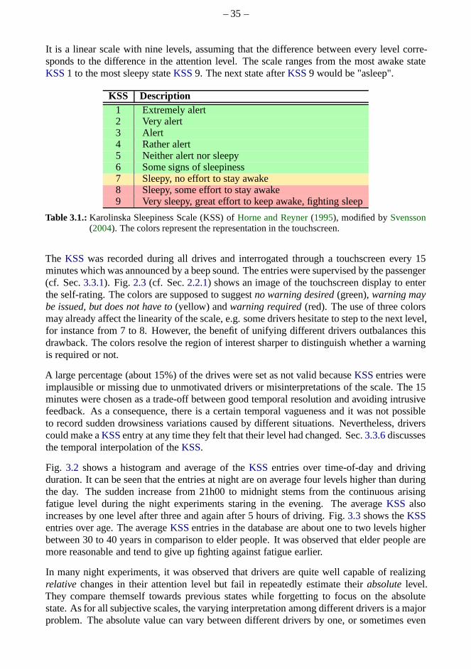
– 35 –

It is a linear scale with nine levels, assuming that the difference between every level corre-sponds to the difference in the attention level. The scale ranges from the most awake stateKSS1 to the most sleepy stateKSS9. The next state afterKSS9 would be "asleep".

KSS Description1 Extremely alert2 Very alert3 Alert4 Rather alert5 Neither alert nor sleepy6 Some signs of sleepiness7 Sleepy, no effort to stay awake8 Sleepy, some effort to stay awake9 Very sleepy, great effort to keep awake, fighting sleep

Table 3.1.:Karolinska Sleepiness Scale (KSS) ofHorne and Reyner(1995), modified bySvensson(2004). The colors represent the representation in the touchscreen.

The KSS was recorded during all drives and interrogated through a touchscreen every 15minutes which was announced by a beep sound. The entries weresupervised by the passenger(cf. Sec.3.3.1). Fig. 2.3 (cf. Sec.2.2.1) shows an image of the touchscreen display to enterthe self-rating. The colors are supposed to suggestno warning desired(green),warning maybe issued, but does not have to(yellow) andwarning required(red). The use of three colorsmay already affect the linearity of the scale, e.g. some drivers hesitate to step to the next level,for instance from 7 to 8. However, the benefit of unifying different drivers outbalances thisdrawback. The colors resolve the region of interest sharperto distinguish whether a warningis required or not.

A large percentage (about 15%) of the drives were set as not valid becauseKSSentries wereimplausible or missing due to unmotivated drivers or misinterpretations of the scale. The 15minutes were chosen as a trade-off between good temporal resolution and avoiding intrusivefeedback. As a consequence, there is a certain temporal vagueness and it was not possibleto record sudden drowsiness variations caused by differentsituations. Nevertheless, driverscould make aKSSentry at any time they felt that their level had changed. Sec.3.3.6discussesthe temporal interpolation of theKSS.

Fig. 3.2 shows a histogram and average of theKSS entries over time-of-day and drivingduration. It can be seen that the entries at night are on average four levels higher than duringthe day. The sudden increase from 21h00 to midnight stems from the continuous arisingfatigue level during the night experiments staring in the evening. The averageKSS alsoincreases by one level after three and again after 5 hours of driving. Fig. 3.3shows theKSSentries over age. The averageKSSentries in the database are about one to two levels higherbetween 30 to 40 years in comparison to elder people. It was observed that elder people aremore reasonable and tend to give up fighting against fatigue earlier.

In many night experiments, it was observed that drivers are quite well capable of realizingrelative changes in their attention level but fail in repeatedly estimate theirabsolutelevel.They compare themself towards previous states while forgetting to focus on the absolutestate. As for all subjective scales, the varying interpretation among different drivers is a majorproblem. The absolute value can vary between different drivers by one, or sometimes even

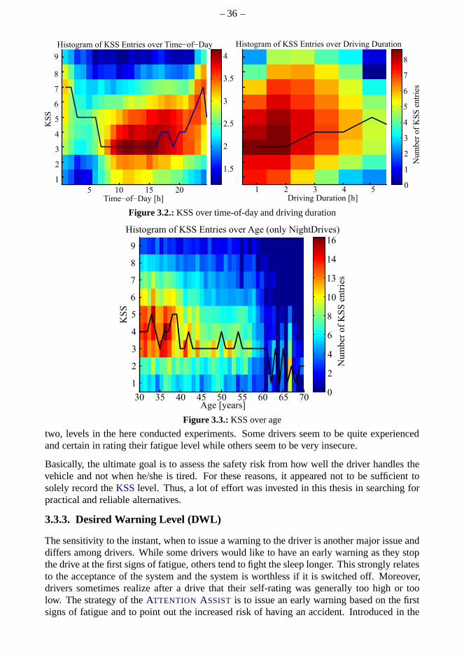
– 36 –

Figure 3.2.:KSS over time-of-day and driving duration

Figure 3.3.:KSS over age

two, levels in the here conducted experiments. Some driversseem to be quite experiencedand certain in rating their fatigue level while others seem to be very insecure.

Basically, the ultimate goal is to assess the safety risk from how well the driver handles thevehicle and not when he/she is tired. For these reasons, it appeared not to be sufficient tosolely record theKSSlevel. Thus, a lot of effort was invested in this thesis in searching forpractical and reliable alternatives.

3.3.3. Desired Warning Level (DWL)

The sensitivity to the instant, when to issue a warning to thedriver is another major issue anddiffers among drivers. While some drivers would like to havean early warning as they stopthe drive at the first signs of fatigue, others tend to fight thesleep longer. This strongly relatesto the acceptance of the system and the system is worthless ifit is switched off. Moreover,drivers sometimes realize after a drive that their self-rating was generally too high or toolow. The strategy of theATTENTION ASSIST is to issue an early warning based on the firstsigns of fatigue and to point out the increased risk of havingan accident. Introduced in the

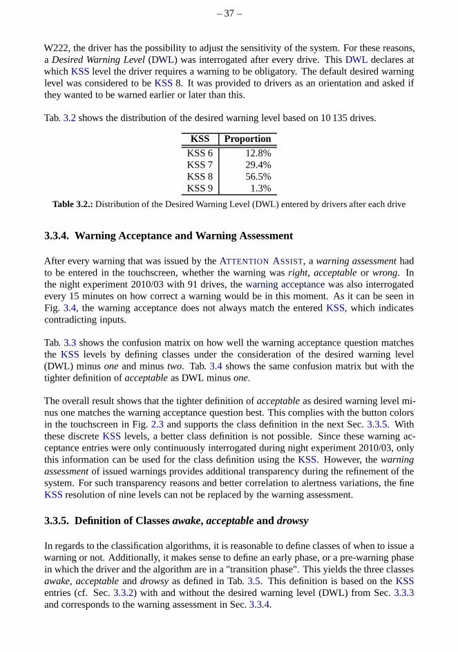
– 37 –

W222, the driver has the possibility to adjust the sensitivity of the system. For these reasons,a Desired Warning Level(DWL) was interrogated after every drive. ThisDWL declares atwhich KSSlevel the driver requires a warning to be obligatory. The default desired warninglevel was considered to beKSS8. It was provided to drivers as an orientation and asked ifthey wanted to be warned earlier or later than this.

Tab.3.2shows the distribution of the desired warning level based on10 135 drives.

KSS ProportionKSS 6 12.8%KSS 7 29.4%KSS 8 56.5%KSS 9 1.3%

Table 3.2.:Distribution of the Desired Warning Level (DWL) entered by drivers after each drive

3.3.4. Warning Acceptance and Warning Assessment

After every warning that was issued by theATTENTION ASSIST, awarning assessmenthadto be entered in the touchscreen, whether the warning wasright, acceptableor wrong. Inthe night experiment 2010/03 with 91 drives, thewarning acceptancewas also interrogatedevery 15 minutes on how correct a warning would be in this moment. As it can be seen inFig. 3.4, the warning acceptance does not always match the enteredKSS, which indicatescontradicting inputs.

Tab.3.3 shows the confusion matrix on how well the warning acceptance question matchesthe KSS levels by defining classes under the consideration of the desired warning level(DWL) minus oneand minustwo. Tab.3.4 shows the same confusion matrix but with thetighter definition ofacceptableas DWL minusone.

The overall result shows that the tighter definition ofacceptableas desired warning level mi-nus one matches the warning acceptance question best. This complies with the button colorsin the touchscreen in Fig.2.3 and supports the class definition in the next Sec.3.3.5. Withthese discreteKSS levels, a better class definition is not possible. Since these warning ac-ceptance entries were only continuously interrogated during night experiment 2010/03, onlythis information can be used for the class definition using the KSS. However, thewarningassessmentof issued warnings provides additional transparency during the refinement of thesystem. For such transparency reasons and better correlation to alertness variations, the fineKSSresolution of nine levels can not be replaced by the warning assessment.

3.3.5. Definition of Classesawake, acceptable and drowsy

In regards to the classification algorithms, it is reasonable to define classes of when to issue awarning or not. Additionally, it makes sense to define an early phase, or a pre-warning phasein which the driver and the algorithm are in a "transition phase". This yields the three classesawake, acceptableanddrowsyas defined in Tab.3.5. This definition is based on theKSSentries (cf. Sec.3.3.2) with and without the desired warning level (DWL) from Sec.3.3.3and corresponds to the warning assessment in Sec.3.3.4.

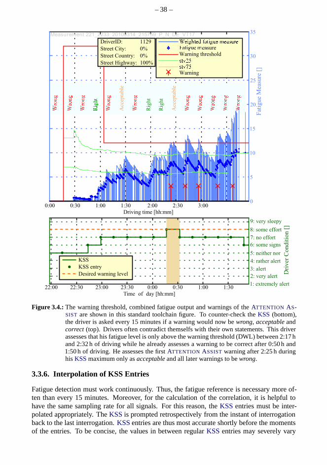
– 38 –

Fat

igue

Mea

sure

[]

ss

Warning thresholdF sureW ! " sg

#$%&'

#$%&'

#$%&'

R( ')*

#$%&'

Acc

epta

ble

#$%&'

Rig

ht

Rig

ht

Acc

epta

ble

#$%&'

#$%&'

#$%&'

#$%&'

#$%&'

Time+of+day [hh:mm]

0:00 0:30 1:00 1:3023:3023:0022:3022:00

Driving time [hh:mm]

2:00 2:30 3:000

1:301:000:300:00

9: very sleepy

Dri

ver

Condit

ion [

]

8: some effort

7: no effort

6: some signs

5: neither nor

4: rather alert

3: alert

2: very alert

1: extremely alert

10

15

DriverID:

Street City:

Street Country:

Street Highway:

1129

0%

0%

100%

KSS

KSS entry

Desired warning level

Measurement 221_2233_20100314_215759_P_N_DE_VT17

5

25

30

20

35

Warning

Figure 3.4.:The warning threshold, combined fatigue output and warnings of theATTENTION AS-SIST are shown in this standard toolchain figure. To counter-check the KSS (bottom),the driver is asked every 15 minutes if a warning would now bewrong, acceptableandcorrect (top). Drivers often contradict themselfs with their own statements. This driverassesses that his fatigue level is only above the warning threshold (DWL) between 2:17 hand 2:32 h of driving while he already assesses a warning to becorrect after 0:50 h and1:50 h of driving. He assesses the firstATTENTION ASSISTwarning after 2:25 h duringhisKSSmaximum only asacceptableand all later warnings to bewrong.

3.3.6. Interpolation of KSS Entries

Fatigue detection must work continuously. Thus, the fatigue reference is necessary more of-ten than every 15 minutes. Moreover, for the calculation of the correlation, it is helpful tohave the same sampling rate for all signals. For this reason,the KSSentries must be inter-polated appropriately. TheKSSis prompted retrospectively from the instant of interrogationback to the last interrogation.KSSentries are thus most accurate shortly before the momentsof the entries. To be concise, the values in between regularKSSentries may severely vary

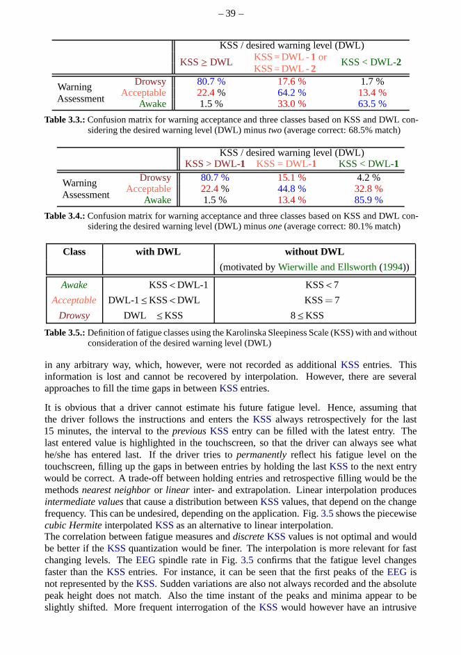
– 39 –

KSS / desired warning level (DWL)

KSS≥ DWL KSS = DWL -1 orKSS = DWL -2

KSS < DWL-2

WarningAssessment

Drowsy 80.7 % 17.6 % 1.7 %Acceptable 22.4% 64.2 % 13.4 %

Awake 1.5 % 33.0 % 63.5 %

Table 3.3.:Confusion matrix for warning acceptance and three classes based on KSS and DWL con-sidering the desired warning level (DWL) minustwo (average correct: 68.5% match)

KSS / desired warning level (DWL)KSS > DWL-1 KSS = DWL-1 KSS < DWL-1

WarningAssessment

Drowsy 80.7 % 15.1 % 4.2 %Acceptable 22.4% 44.8 % 32.8 %

Awake 1.5 % 13.4 % 85.9 %

Table 3.4.:Confusion matrix for warning acceptance and three classes based on KSS and DWL con-sidering the desired warning level (DWL) minusone(average correct: 80.1% match)

Class with DWL without DWL

(motivated byWierwille and Ellsworth(1994))

Awake KSS<DWL-1 KSS< 7

Acceptable DWL-1≤KSS<DWL KSS= 7

Drowsy DWL ≤KSS 8≤KSS

Table 3.5.:Definition of fatigue classes using the Karolinska Sleepiness Scale (KSS) with and withoutconsideration of the desired warning level (DWL)

in any arbitrary way, which, however, were not recorded as additional KSS entries. Thisinformation is lost and cannot be recovered by interpolation. However, there are severalapproaches to fill the time gaps in betweenKSSentries.

It is obvious that a driver cannot estimate his future fatigue level. Hence, assuming thatthe driver follows the instructions and enters theKSS always retrospectively for the last15 minutes, the interval to thepreviousKSS entry can be filled with the latest entry. Thelast entered value is highlighted in the touchscreen, so that the driver can always see whathe/she has entered last. If the driver tries topermanentlyreflect his fatigue level on thetouchscreen, filling up the gaps in between entries by holding the lastKSSto the next entrywould be correct. A trade-off between holding entries and retrospective filling would be themethodsnearest neighboror linear inter- and extrapolation. Linear interpolation producesintermediate valuesthat cause a distribution betweenKSSvalues, that depend on the changefrequency. This can be undesired, depending on the application. Fig.3.5shows the piecewisecubic HermiteinterpolatedKSSas an alternative to linear interpolation.The correlation between fatigue measures anddiscreteKSSvalues is not optimal and wouldbe better if theKSSquantization would be finer. The interpolation is more relevant for fastchanging levels. TheEEG spindle rate in Fig.3.5 confirms that the fatigue level changesfaster than theKSS entries. For instance, it can be seen that the first peaks of the EEG isnot represented by theKSS. Sudden variations are also not always recorded and the absolutepeak height does not match. Also the time instant of the peaksand minima appear to beslightly shifted. More frequent interrogation of theKSS would however have an intrusive

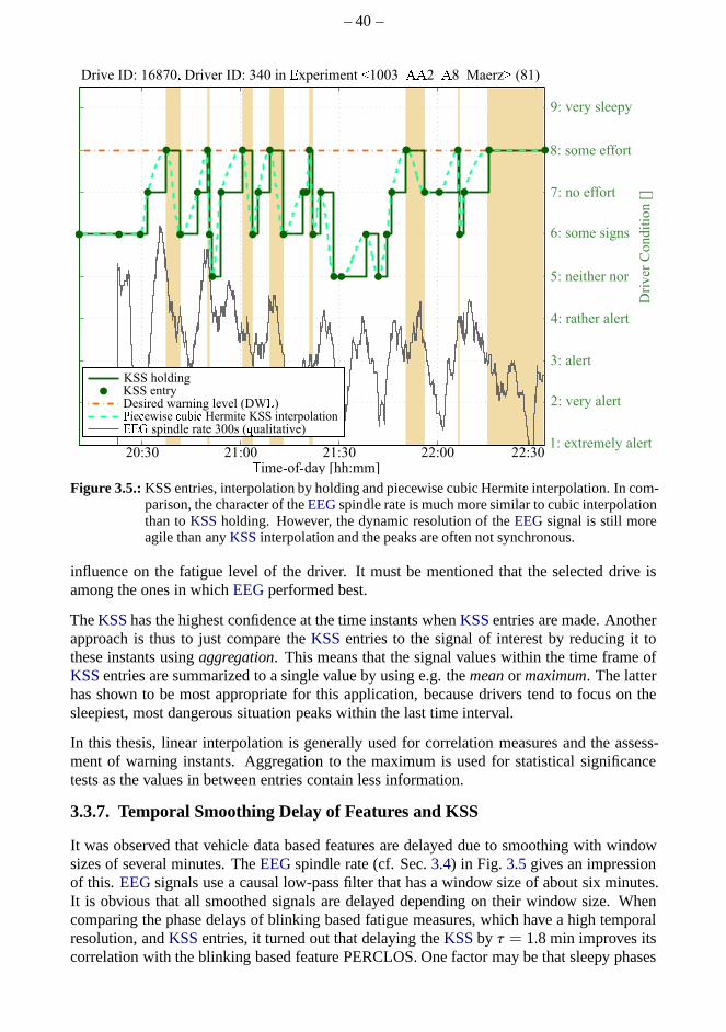
– 40 –

Drive ID: 16870, Driver ID: 340 in Experiment <1003_AA2_A8_Maerz> (81)

9: very sleepy

8: some effort

7: no effort

6: some signs

5: neither nor

4: rather alert

Dri

ver

Condit

ion

[]

3: alert

2: very alert

1: extremely alert

Time-of-day [hh:mm]20:30 21:00 21:30 22:00 22:30

KSS holdingKSS entryDesired warning level (DWL)Piecewise cubic Hermite KSS interpolation..G spindle rate 300s (qualitative)

Figure 3.5.:KSS entries, interpolation by holding and piecewise cubic Hermite interpolation. In com-parison, the character of theEEGspindle rate is much more similar to cubic interpolationthan toKSS holding. However, the dynamic resolution of theEEGsignal is still moreagile than anyKSSinterpolation and the peaks are often not synchronous.

influence on the fatigue level of the driver. It must be mentioned that the selected drive isamong the ones in whichEEGperformed best.

TheKSShas the highest confidence at the time instants whenKSSentries are made. Anotherapproach is thus to just compare theKSS entries to the signal of interest by reducing it tothese instants usingaggregation. This means that the signal values within the time frame ofKSSentries are summarized to a single value by using e.g. themeanor maximum. The latterhas shown to be most appropriate for this application, because drivers tend to focus on thesleepiest, most dangerous situation peaks within the last time interval.

In this thesis, linear interpolation is generally used for correlation measures and the assess-ment of warning instants. Aggregation to the maximum is usedfor statistical significancetests as the values in between entries contain less information.

3.3.7. Temporal Smoothing Delay of Features and KSS

It was observed that vehicle data based features are delayeddue to smoothing with windowsizes of several minutes. TheEEGspindle rate (cf. Sec.3.4) in Fig. 3.5gives an impressionof this. EEGsignals use a causal low-pass filter that has a window size of about six minutes.It is obvious that all smoothed signals are delayed depending on their window size. Whencomparing the phase delays of blinking based fatigue measures, which have a high temporalresolution, andKSSentries, it turned out that delaying theKSSby τ = 1.8 min improves itscorrelation with the blinking based feature PERCLOS. One factor may be that sleepy phases

– 41 –

can occur before the driver becomes aware of them or is willing to admit his sleepiness. Inany way, the goal remains to develop features which are reactive to the underlying groundtruth. Smoothing with low phase delay is used to obtain good correlation results.

Advantages and Disadvantages of Self-assessment

Schmidt(2009) summarized that research on the self-assessment of vigilance came to contra-dicting results. Multiple studies showed that self-ratings are not accurate enough to functionas reliable and valid indicators of driving performance andreaction time. For instance,Belzet al. (2004) evaluated driver performance in an extended-duration real-world environmentof commercial motor vehicles. Without exception, the correlation analyses betweenKSSandminimum time-to-collision (TTC) and minimum/mean headway yielded that neither of themare valid indicators of driver fatigue.Philip and Sagaspe(2005) reported as well that the self-assessment of the subsequent performance in a reaction timetask under prolonged daytimedriving conditions was rather poor.

The findings ofBaranski(2007) from a cognitive work study with 64 adults suggest thatpeople can accurately assess their own cognitive performance after being deprived of onenight of sleep. In a real car driving simulator study with 38 sleep-restricted young adults,Horne and Baulk(2004) found that subjective sleepiness,EEGactivity, and lane drifting werehighly correlated.Schmidt(2009) argues that drivers are well aware of their deterioratingvigilance, but that early warning signs are often ignored ormisinterpreted.

Besides the above mentioned intra- and inter-individual variation, self-ratings are always in-trusive, i.e. have an awaking impact. According toSchmidt(2009), theKSSpoling has anaftereffect of about one minute in theEEGalpha spindle rate and about two minutes in the eyelid closure and can be neglected. Drivers have difficulties in rating their fitness, especially af-ter more than three hours of continuous monotonous daytime driving with advanced degreesof fatigue. Schmidt has also shown that subjects that feel more awake after long drives, arenot more powerful, but rather drive even worse, react slowerand have moreα-spindles.

Hargutt et al.(2005) investigate the intrusion influence of driver state and driving perfor-mance feedback systems. Really drowsy drivers gain small fitness improvements for about5 to 15 minutes after an interrogation, so the influence is nottoo strong. Own experimentsfrom (Schmidt, 2009, 2010) and qualitative observations in night experiments generally con-firmed this finding.

On the other hand, advantages of interrogating the drivers about their sleepiness levels is verysimple and thus relatively robust. If conscientiously used, the probability of intra-individualdeviation is mostly limited to one or twoKSSlevels. Hence, self-ratings are still quite reliableand consistent compared to other automated methods. Despite the inter-individual variations,the drivers mostly know about their drowsiness and have to accept warnings of a drowsinessdetection system.

Own observations have shown that at night, especially between midnight and 6 a.m. it ismore difficult to estimate one’s self-rating. The highway hypnosis and lack of situations thatrequire action makes it difficult to estimate how tired one is. For instance, many drivershave difficulties to estimate their velocity when they have to brake behind a heading truck.Generally, drivers have more difficulties in rating their fatigue levels aboveKSS 7 and areoften not aware that they already had small microsleep events.

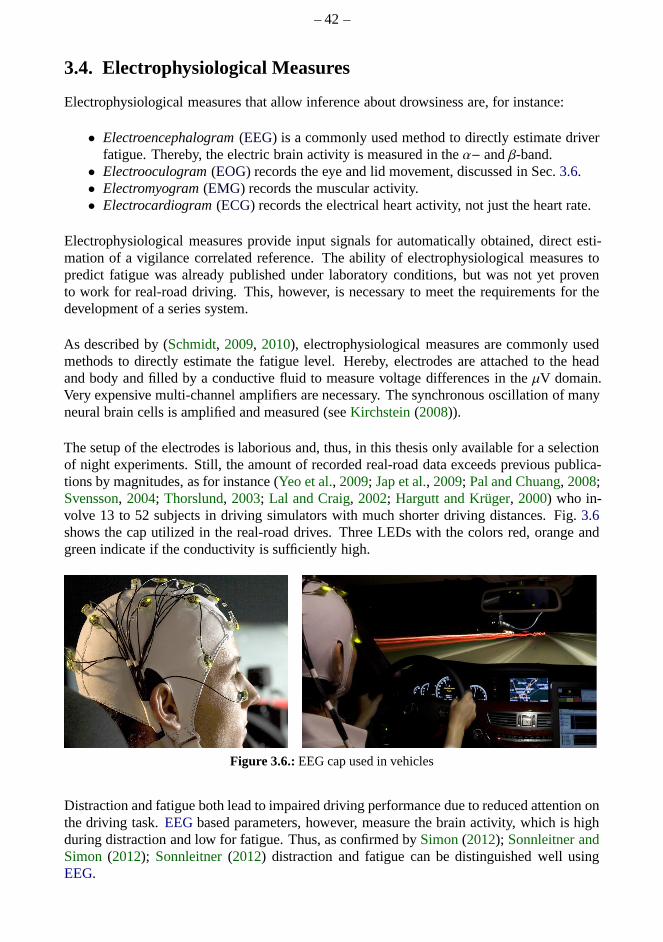
– 42 –

3.4. Electrophysiological Measures

Electrophysiological measures that allow inference aboutdrowsiness are, for instance:

• Electroencephalogram(EEG) is a commonly used method to directly estimate driverfatigue. Thereby, the electric brain activity is measured in theα− andβ-band.

• Electrooculogram(EOG) records the eye and lid movement, discussed in Sec.3.6.• Electromyogram(EMG) records the muscular activity.• Electrocardiogram(ECG) records the electrical heart activity, not just the heart rate.

Electrophysiological measures provide input signals for automatically obtained, direct esti-mation of a vigilance correlated reference. The ability of electrophysiological measures topredict fatigue was already published under laboratory conditions, but was not yet provento work for real-road driving. This, however, is necessary to meet the requirements for thedevelopment of a series system.

As described by (Schmidt, 2009, 2010), electrophysiological measures are commonly usedmethods to directly estimate the fatigue level. Hereby, electrodes are attached to the headand body and filled by a conductive fluid to measure voltage differences in theµV domain.Very expensive multi-channel amplifiers are necessary. Thesynchronous oscillation of manyneural brain cells is amplified and measured (seeKirchstein(2008)).

The setup of the electrodes is laborious and, thus, in this thesis only available for a selectionof night experiments. Still, the amount of recorded real-road data exceeds previous publica-tions by magnitudes, as for instance (Yeo et al., 2009; Jap et al., 2009; Pal and Chuang, 2008;Svensson, 2004; Thorslund, 2003; Lal and Craig, 2002; Hargutt and Krüger, 2000) who in-volve 13 to 52 subjects in driving simulators with much shorter driving distances. Fig.3.6shows the cap utilized in the real-road drives. Three LEDs with the colors red, orange andgreen indicate if the conductivity is sufficiently high.

Figure 3.6.:EEG cap used in vehicles

Distraction and fatigue both lead to impaired driving performance due to reduced attention onthe driving task.EEGbased parameters, however, measure the brain activity, which is highduring distraction and low for fatigue. Thus, as confirmed bySimon(2012); Sonnleitner andSimon (2012); Sonnleitner(2012) distraction and fatigue can be distinguished well usingEEG.

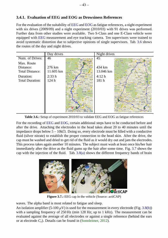
– 43 –

3.4.1. Evaluation of EEG and EOG as Drowsiness References

For the evaluation of the suitability ofEEGandEOGas fatigue references, a night experimentwith six drives (2009/09) and a night experiment (2010/03) with 91 drives was performed.Further data from other studies were available. Two S-Classand one E-Class vehicle wereequipped withEEGmeasurement and eye tracking camera. Ten supervisors were trained toavoid systematic distortion due to subjective opinions of single supervisors. Tab.3.6 showsthe routes of the day and night drives.

Day drives Night drivesNum. of Drives: 46 45Max. RouteDistance: 276 km 434 kmTotal Distance: 11.605 km 13.046 kmDuration: 2:33 h 4:12 hTotal Duration: 124 h 181 h

Table 3.6.:Setup of experiment 2010/03 to validate EEG and EOG as fatigue references

For the recording ofEEGandEOG, certain additional steps have to be conducted before andafter the drive. Attaching the electrodes to the head takes about 20 to 40 minutes until theimpedance drops below 5− 10kΩ. Doing so, every electrode must be filled with a conductivefluid (silver nitrate) to establish the proper connection tothe head skin. After the drive, thecap must be washed and dried to get rid of the fluid as it would dry out and jam the electrodes.This process takes again another 10 minutes. The subject must wash at least once his/her hairimmediately after the drive as the fluid gums up the hair aftersome time. Fig.3.7shows thecap with the injection of the fluid. Tab.3.8(a)shows the different frequency bands of brain

Figure 3.7.:EEG cap in the vehicle (Source: actiCAP)

waves. The alpha band is most related to fatigue and sleep.An isolation amplifier (5-100µV) is used for the measurement in every electrode (Fig.3.8(b))with a sampling frequency of 250 Hz (min 128 Hz; up to 1 kHz). The measurement can beevaluated against the average of all electrodes or against asingle reference (behind the earsor at electrodeCz). Details can be found in (Sonnleitner, 2012).

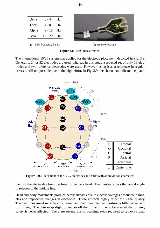
– 44 –

Delta 0 - 4 Hz

Theta 4 - 8 Hz

Alpha 8 - 13 Hz

Beta 13 - 20 Hz

(a) EEG frequency bands (b) Active electrode

Figure 3.8.:EEG measurement

The international 10/20 system was applied for the electrode placement, depicted in Fig.3.9.Generally, 24 or 32 electrodes are used, whereas in this study a reduced set of only 16 elec-trodes and two reference electrodes were used. However, using it as a reference in regulardrives is still not possible due to the high effort. In Fig.3.9, the characters indicate the place-

naison(front)

inion(rear head)

Ref

Fp2

13

Gnd

14

10

12

2

1

9

11

O2O1

hEOG

16

Right

Ear

Left

Ear

even numbersodd numbers

hEOG

vEOG

vEOG

Cz

Fz

6C4

8P4

15Pz

7P3

5C3

4F4

3F3

20%

10%

20%

20%

20%

10%

F FrontalO OccipitalC CentralP ParietalT Temporal

z Center line

Figure 3.9.:Placement of the EEG electrodes and table with abbreviationcharacters

ment of the electrodes from the front to the back head. The number shows the lateral anglein relation to the middle line.

Head and body movements produce heavy artifacts due to electric voltages produced in mus-cles and impedance changes in electrodes. These artifacts highly affect the signal quality.The head movement must be constrained and the inflexible headposture is little convenientfor driving. The chin strap slightly pinches off the throat.It has to be assured that drivingsafety is never affected. There are several post-processing steps required to remove signal

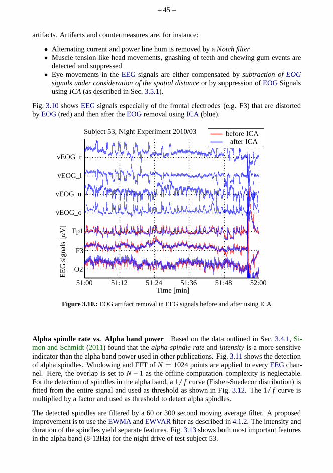
– 45 –

artifacts. Artifacts and countermeasures are, for instance:

• Alternating current and power line hum is removed by aNotch filter• Muscle tension like head movements, gnashing of teeth and chewing gum events are

detected and suppressed• Eye movements in theEEG signals are either compensated bysubtraction ofEOG

signals under consideration of the spatial distanceor by suppression ofEOGSignalsusingICA (as described in Sec.3.5.1).

Fig. 3.10showsEEGsignals especially of the frontal electrodes (e.g. F3) thatare distortedby EOG(red) and then after theEOGremoval usingICA (blue).

Time [min]51:00 52:0051:4851:3651:2451:12

EE

Gsi

gnal

s[µV

]

vEOG_o

Fp1

F3

O2

vEOG_u

vEOG_l

vEOG_r

Subject 53, Night Experiment 2010/03 before ICAafter ICA

Figure 3.10.:EOG artifact removal in EEG signals before and after using ICA

Alpha spindle rate vs. Alpha band power Based on the data outlined in Sec.3.4.1, Si-mon and Schmidt(2011) found that thealpha spindle rateand intensityis a more sensitiveindicator than the alpha band power used in other publications. Fig.3.11shows the detectionof alpha spindles. Windowing and FFT ofN = 1024 points are applied to everyEEGchan-nel. Here, the overlap is set toN − 1 as the offline computation complexity is neglectable.For the detection of spindles in the alpha band, a 1/ f curve (Fisher-Snedecor distribution) isfitted from the entire signal and used as threshold as shown inFig. 3.12. The 1/ f curve ismultiplied by a factor and used as threshold to detect alpha spindles.

The detected spindles are filtered by a 60 or 300 second movingaverage filter. A proposedimprovement is to use theEWMA andEWVAR filter as described in4.1.2. The intensity andduration of the spindles yield separate features. Fig.3.13shows both most important featuresin the alpha band (8-13Hz) for the night drive of test subject53.

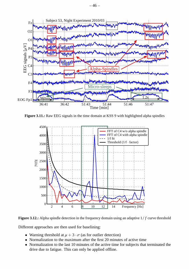
– 46 –

Subject 53, Night Experiment 2010/03

36:41 51:4751:4651:4451:4336:42

1.2s960ms

Fz

O2

O1

P4

P3

C4

C3

F4

F3

EOG Fp1

Time [min]

EE

Gsi

gnal

s[µV

]

Micro-sleeps

Alpha-Spindles

Figure 3.11.:Raw EEG signals in the time domain at KSS 9 with highlighted alpha spindles

2 4 6 8 10 12 14 Frequency [Hz]0

500

1000

1500

2000

2500

3000

3500

4000

4500

|Y(f

)|

FFT of C4 w/o alpha spindleFFT of C4 with alpha spindle1/f fitThreshold (1/f· factor)

Figure 3.12.:Alpha spindle detection in the frequency domain using an adaptive 1/ f curve threshold

Different approaches are then used for baselining:

• Warning threshold atµ+ 3 ·σ (as for outlier detection)• Normalization to the maximum after the first 20 minutes of active time• Normalization to the last 10 minutes of the active time for subjects that terminated the

drive due to fatigue. This can only be applied offline.

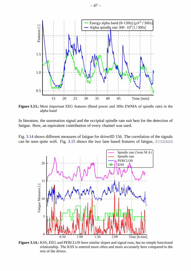
– 47 –

15 20 25 30 35 40 45

Energy alpha band (8-13Hz) [µV2/300s]Alpha spindle rate 300· 105[1/300s]

Time [min]

Fea

ture

s[-

]

0.5

1.0

1.5

Figure 3.13.:Most important EEG features (Band power and 300s EWMA of spindle rate) in thealpha band

In literature, the summation signal and the occipital spindle rate suit best for the detection offatigue. Here, an equivalent contribution of every channelwas used.

Fig. 3.14shows different measures of fatigue for driverID 156. The correlation of the signalscan be seen quite well. Fig.3.15 shows the two lane based features of fatigue,ZIGZAGS

Figure 3.14.:KSS, EEG and PERCLOS have similar slopes and signal runs, butno simple functionalrelationship. The KSS is entered more often and more accurately here compared to therest of the drives.

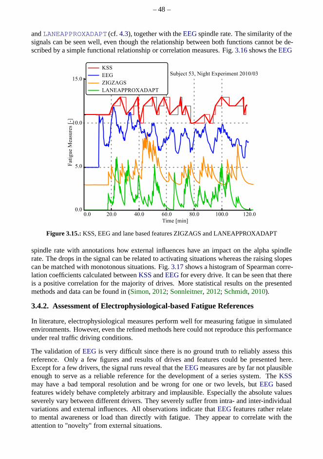
– 48 –

andLANEAPPROXADAPT (cf. 4.3), together with theEEGspindle rate. The similarity of thesignals can be seen well, even though the relationship between both functions cannot be de-scribed by a simple functional relationship or correlationmeasures. Fig.3.16shows theEEG

Figure 3.15.:KSS, EEG and lane based features ZIGZAGS and LANEAPPROXADAPT

spindle rate with annotations how external influences have an impact on the alpha spindlerate. The drops in the signal can be related to activating situations whereas the raising slopescan be matched with monotonous situations. Fig.3.17shows a histogram of Spearman corre-lation coefficients calculated betweenKSSandEEGfor every drive. It can be seen that thereis a positive correlation for the majority of drives. More statistical results on the presentedmethods and data can be found in (Simon, 2012; Sonnleitner, 2012; Schmidt, 2010).

3.4.2. Assessment of Electrophysiological-based FatigueReferences

In literature, electrophysiological measures perform well for measuring fatigue in simulatedenvironments. However, even the refined methods here could not reproduce this performanceunder real traffic driving conditions.

The validation ofEEGis very difficult since there is no ground truth to reliably assess thisreference. Only a few figures and results of drives and features could be presented here.Except for a few drivers, the signal runs reveal that theEEGmeasures are by far not plausibleenough to serve as a reliable reference for the development of a series system. TheKSSmay have a bad temporal resolution and be wrong for one or two levels, butEEG basedfeatures widely behave completely arbitrary and implausible. Especially the absolute valuesseverely vary between different drivers. They severely suffer from intra- and inter-individualvariations and external influences. All observations indicate thatEEGfeatures rather relateto mental awareness or load than directly with fatigue. Theyappear to correlate with theattention to "novelty" from external situations.

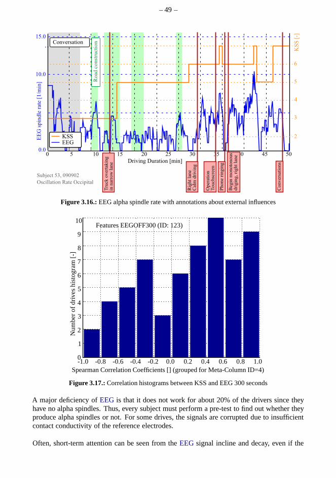
– 49 –

Figure 3.16.:EEG alpha spindle rate with annotations about external influences

0

1

2

3

4

5

6

7

8

9

10

-1.0 -0.8 -0.6 -0.4 -0.2 0.2 0.4 0.6 0.8 1.0Spearman Correlation Coefficients [] (grouped for Meta-Column ID=4)

0.0

Features EEGOFF300 (ID: 123)

Nu

mb

ero

fdriv

esh

isto

gra

m[-

]

Figure 3.17.:Correlation histograms between KSS and EEG 300 seconds

A major deficiency ofEEGis that it does not work for about 20% of the drivers since theyhave no alpha spindles. Thus, every subject must perform a pre-test to find out whether theyproduce alpha spindles or not. For some drives, the signals are corrupted due to insufficientcontact conductivity of the reference electrodes.

Often, short-term attention can be seen from theEEGsignal incline and decay, even if the

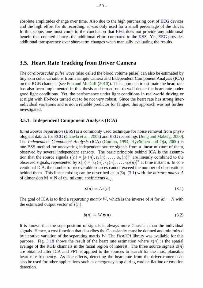
– 50 –

absolute amplitudes change over time. Also due to the high purchasing cost ofEEGdevicesand the high effort for its recording, it was only used for a small percentage of the drives.In this scope, one must come to the conclusion thatEEG does not provide any additionalbenefit that counterbalances the additional effort compared to theKSS. Yet, EEGprovidesadditional transparency over short-term changes when manually evaluating the results.

3.5. Heart Rate Tracking from Driver Camera

Thecardiovascular pulse wave(also called the blood volume pulse) can also be estimated bytiny skin color variations from a simple camera and Independent Component Analysis (ICA)on the RGB channels (seePoh and McDuff(2010)). This approach to estimate the heart ratehas also been implemented in this thesis and turned out to well detect the heart rate undergood light conditions. Yet, the performance under light conditions in real-world driving orat night with IR-Pods turned out to be not very robust. Since the heart rate has strong inter-individual variations and is not a reliable predictor for fatigue, this approach was not furtherinvestigated.

3.5.1. Independent Component Analysis (ICA)

Blind Source Separation(BSS)is a commonly used technique for noise removal from physi-ological data as forECG(Chawla et al., 2008) andEEGrecordings (Jung and Makeig, 2000).The Independent Component Analysis(ICA) (Comon, 1994; Hyvärinen and Oja, 2000) isoneBSSmethod for uncovering independent source signals from a linear mixture of them,observed by several independent sensors. The basic principle behind ICA is the assump-tion that the source signalss(n) = [s1(n), s2(n), . . . , sN(n)]T are linearly combined to theobserved signals, represented byx(n) = [x1(n), x2(n), . . . , xM(n)]T at time instantn. In con-ventional ICA, the number of recoverable sources cannot exceed the number of observationsbehind them. This linear mixing can be described as in Eq. (3.1) with themixture matrix Aof dimension M× N of the mixture coefficientsai, j .

x(n) = As(n) (3.1)

The goal of ICA is to find aseparating matrix W, which is the inverse ofA for M = N withthe estimated output vector ofs(n):

s(n) = Wx(n) (3.2)

It is known that the superposition of signals is always more Gaussian than the individualsignals. Hence, a cost function that describes the Gaussianity must be defined and minimizedby iterative variation of the separating matrixW. TheFastICAlibrary was available for thispurpose. Fig.3.18 shows the result of the heart rate estimation wherex(n) is the spatialaverage of the RGB channels in the facial region of interest.The three source signalss(n)are obtained after ICA and FFT is applied to the sources to search for the most plausibleheart rate frequency. As side effects, detecting the heart rate from the driver-camera canalso be used for other applications such as emergency stop during cardiac flatline or emotiondetection.

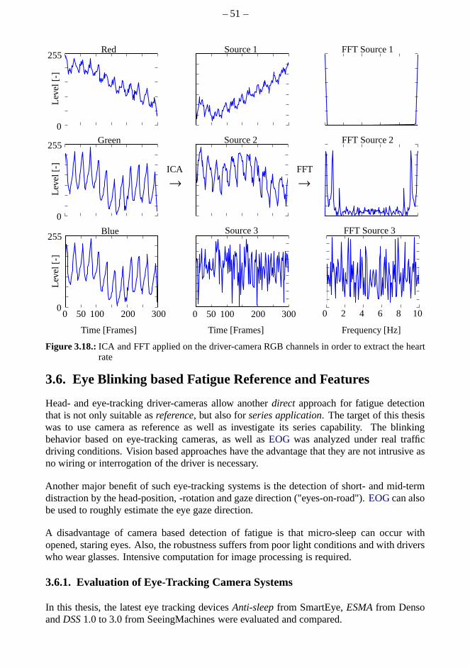
– 51 –

0 50 100 200 300

Time [Frames]

0

255L

evel

[-]

Source 1

Source 2

0 50 100 200 300

Time [Frames]

Source 3

FFT Source 1

FFT Source 2

FFT Source 3

Frequency [Hz]

Red

Green

Blue

0

255

Lev

el[-

]

0

255

Lev

el[-

]

ICA FFT

0 2 4 6 8 10

→ →

Figure 3.18.:ICA and FFT applied on the driver-camera RGB channels in order to extract the heartrate

3.6. Eye Blinking based Fatigue Reference and Features

Head- and eye-tracking driver-cameras allow anotherdirect approach for fatigue detectionthat is not only suitable asreference, but also forseries application. The target of this thesiswas to use camera as reference as well as investigate its series capability. The blinkingbehavior based on eye-tracking cameras, as well asEOG was analyzed under real trafficdriving conditions. Vision based approaches have the advantage that they are not intrusive asno wiring or interrogation of the driver is necessary.

Another major benefit of such eye-tracking systems is the detection of short- and mid-termdistraction by the head-position, -rotation and gaze direction ("eyes-on-road").EOGcan alsobe used to roughly estimate the eye gaze direction.

A disadvantage of camera based detection of fatigue is that micro-sleep can occur withopened, staring eyes. Also, the robustness suffers from poor light conditions and with driverswho wear glasses. Intensive computation for image processing is required.

3.6.1. Evaluation of Eye-Tracking Camera Systems

In this thesis, the latest eye tracking devicesAnti-sleepfrom SmartEye,ESMAfrom DensoandDSS1.0 to 3.0 from SeeingMachines were evaluated and compared.

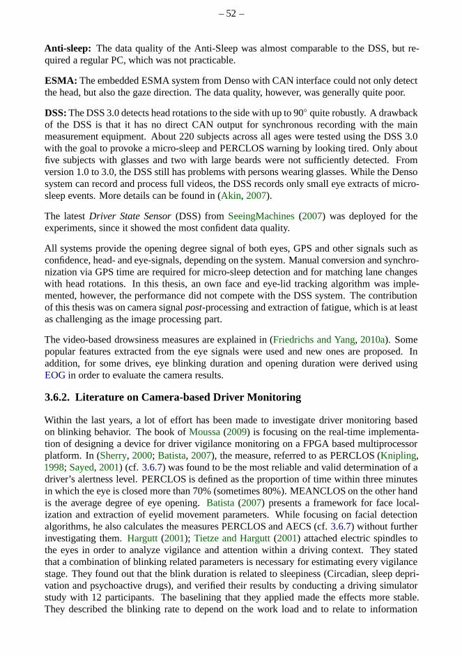
– 52 –

Anti-sleep: The data quality of the Anti-Sleep was almost comparable to the DSS, but re-quired a regular PC, which was not practicable.

ESMA: The embedded ESMA system from Denso with CAN interface couldnot only detectthe head, but also the gaze direction. The data quality, however, was generally quite poor.

DSS:The DSS 3.0 detects head rotations to the side with up to 90 quite robustly. A drawbackof the DSS is that it has no direct CAN output for synchronous recording with the mainmeasurement equipment. About 220 subjects across all ages were tested using the DSS 3.0with the goal to provoke a micro-sleep and PERCLOS warning bylooking tired. Only aboutfive subjects with glasses and two with large beards were not sufficiently detected. Fromversion 1.0 to 3.0, the DSS still has problems with persons wearing glasses. While the Densosystem can record and process full videos, the DSS records only small eye extracts of micro-sleep events. More details can be found in (Akin, 2007).

The latestDriver State Sensor(DSS) fromSeeingMachines(2007) was deployed for theexperiments, since it showed the most confident data quality.

All systems provide the opening degree signal of both eyes, GPS and other signals such asconfidence, head- and eye-signals, depending on the system.Manual conversion and synchro-nization via GPS time are required for micro-sleep detection and for matching lane changeswith head rotations. In this thesis, an own face and eye-lid tracking algorithm was imple-mented, however, the performance did not compete with the DSS system. The contributionof this thesis was on camera signalpost-processing and extraction of fatigue, which is at leastas challenging as the image processing part.

The video-based drowsiness measures are explained in (Friedrichs and Yang, 2010a). Somepopular features extracted from the eye signals were used and new ones are proposed. Inaddition, for some drives, eye blinking duration and opening duration were derived usingEOGin order to evaluate the camera results.

3.6.2. Literature on Camera-based Driver Monitoring

Within the last years, a lot of effort has been made to investigate driver monitoring basedon blinking behavior. The book ofMoussa(2009) is focusing on the real-time implementa-tion of designing a device for driver vigilance monitoring on a FPGA based multiprocessorplatform. In (Sherry, 2000; Batista, 2007), the measure, referred to as PERCLOS (Knipling,1998; Sayed, 2001) (cf. 3.6.7) was found to be the most reliable and valid determination ofadriver’s alertness level. PERCLOS is defined as the proportion of time within three minutesin which the eye is closed more than 70% (sometimes 80%). MEANCLOS on the other handis the average degree of eye opening.Batista(2007) presents a framework for face local-ization and extraction of eyelid movement parameters. While focusing on facial detectionalgorithms, he also calculates the measures PERCLOS and AECS (cf. 3.6.7) without furtherinvestigating them.Hargutt (2001); Tietze and Hargutt(2001) attached electric spindles tothe eyes in order to analyze vigilance and attention within adriving context. They statedthat a combination of blinking related parameters is necessary for estimating every vigilancestage. They found out that the blink duration is related to sleepiness (Circadian, sleep depri-vation and psychoactive drugs), and verified their results by conducting a driving simulatorstudy with 12 participants. The baselining that they applied made the effects more stable.They described the blinking rate to depend on the work load and to relate to information

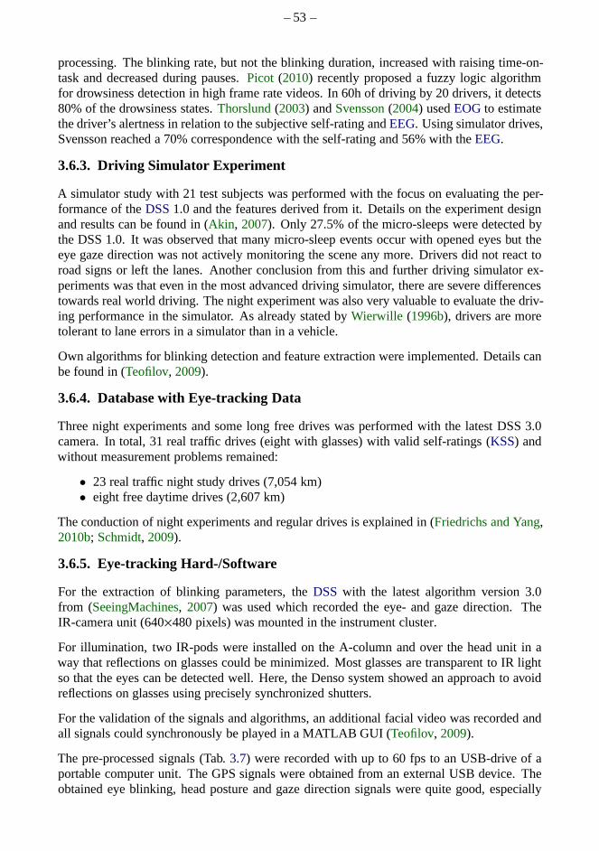
– 53 –

processing. The blinking rate, but not the blinking duration, increased with raising time-on-task and decreased during pauses.Picot (2010) recently proposed a fuzzy logic algorithmfor drowsiness detection in high frame rate videos. In 60h ofdriving by 20 drivers, it detects80% of the drowsiness states.Thorslund(2003) andSvensson(2004) usedEOGto estimatethe driver’s alertness in relation to the subjective self-rating andEEG. Using simulator drives,Svensson reached a 70% correspondence with the self-ratingand 56% with theEEG.

3.6.3. Driving Simulator Experiment

A simulator study with 21 test subjects was performed with the focus on evaluating the per-formance of theDSS1.0 and the features derived from it. Details on the experiment designand results can be found in (Akin, 2007). Only 27.5% of the micro-sleeps were detected bythe DSS 1.0. It was observed that many micro-sleep events occur with opened eyes but theeye gaze direction was not actively monitoring the scene anymore. Drivers did not react toroad signs or left the lanes. Another conclusion from this and further driving simulator ex-periments was that even in the most advanced driving simulator, there are severe differencestowards real world driving. The night experiment was also very valuable to evaluate the driv-ing performance in the simulator. As already stated byWierwille (1996b), drivers are moretolerant to lane errors in a simulator than in a vehicle.

Own algorithms for blinking detection and feature extraction were implemented. Details canbe found in (Teofilov, 2009).

3.6.4. Database with Eye-tracking Data

Three night experiments and some long free drives was performed with the latest DSS 3.0camera. In total, 31 real traffic drives (eight with glasses)with valid self-ratings (KSS) andwithout measurement problems remained:

• 23 real traffic night study drives (7,054 km)• eight free daytime drives (2,607 km)

The conduction of night experiments and regular drives is explained in (Friedrichs and Yang,2010b; Schmidt, 2009).

3.6.5. Eye-tracking Hard-/Software

For the extraction of blinking parameters, theDSS with the latest algorithm version 3.0from (SeeingMachines, 2007) was used which recorded the eye- and gaze direction. TheIR-camera unit (640×480 pixels) was mounted in the instrument cluster.

For illumination, two IR-pods were installed on the A-column and over the head unit in away that reflections on glasses could be minimized. Most glasses are transparent to IR lightso that the eyes can be detected well. Here, the Denso system showed an approach to avoidreflections on glasses using precisely synchronized shutters.

For the validation of the signals and algorithms, an additional facial video was recorded andall signals could synchronously be played in a MATLAB GUI (Teofilov, 2009).

The pre-processed signals (Tab.3.7) were recorded with up to 60 fps to an USB-drive of aportable computer unit. The GPS signals were obtained from an external USB device. Theobtained eye blinking, head posture and gaze direction signals were quite good, especially

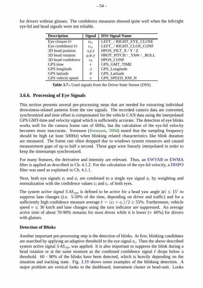
– 54 –

for drivers without glasses. The confidence measures showedquite well when the left/righteye-lid and head signals were not reliable.

Description Signal DSS Signal NameEye closure l/r el,r LEFT_ / RIGHT_EYE_CLOSEEye confidence l/r cl,r LEFT_ / RIGHT_CLOS_CONF3D head position x,y,z HPOS_FILT_X / Y / Z3D head rotation ϕ,ψ,γ HROT_PITCH / _YAW / _ROLL3D head confidence ch HPOS_CONFGPS time τ GPS_GMT_TIMEGPS longitude λ GPS_LongitudeGPS latitude θ GPS_LatitudeGPS vehicle speed v GPS_SPEED_KM_H

Table 3.7.:Used signals from the Driver State Sensor (DSS)

3.6.6. Processing of Eye Signals

This section presents several pre-processing steps that are needed for extracting individualdrowsiness-related patterns from the raw signals. The recorded camera data are converted,synchronized and time offset is compensated for the vehicleCAN data using the interpolatedGPS GMT-time and velocity signal which is sufficiently accurate. The detection of eye blinksworks well for the camera frame rate of 60Hz, but the calculation of the eye-lid velocitybecomes more inaccurate. Svensson (Svensson, 2004) stated that the sampling frequencyshould be high (at least 500Hz) when blinking related characteristics like blink durationare measured. The frame rate often dropped due to windows system resources and causedmeasurement gaps of up to half a second. These gaps were linearly interpolated in order tokeep the timestamps synchronized.

For many features, the derivative and intensity are relevant. Thus, anEWVAR or EWMAfilter is applied as described in Ch.4.1.2. For the calculation of the eye-lid velocity, aDISPOfilter was used as explained in Ch.4.1.1.

Next, both eye signalsel ander are combined to a single eye signalec by weighting andnormalization with the confidence valuescl andcr of both eyes.

The system active signal S ASeye is defined to be active for a head yaw angle|ψ| ≤ 15 tosuppress lane changes (i.e. 5-20% of the time, depending on driver and traffic) and for asufficiently high confidence measure averagec = (cl + cr)/2 ≥ 55%. Furthermore, vehiclespeedv ≤ 30 km/h and lane changes using the turn indicator are suppressed. An averageactive time of about 70-90% remains for most drives while it is lower (≈ 60%) for driverswith glasses.

Detection of Blinks

Another important pre-processing step is the detection of blinks. At first, blinking candidatesare searched by applying an adaptive threshold to the eye signalec. Then the above describedsystem active signalS ASeye was applied. It is also important to suppress the blink during ahead rotation or at the same moment as the combined confidencesignal c drops below athreshold. 60 - 90% of the blinks have been detected, which isheavily depending on thesituation and tracking state. Fig.3.19 shows some examples of the blinking detection. Amajor problem are vertical looks to the dashboard, instrument cluster or head-unit. Looks

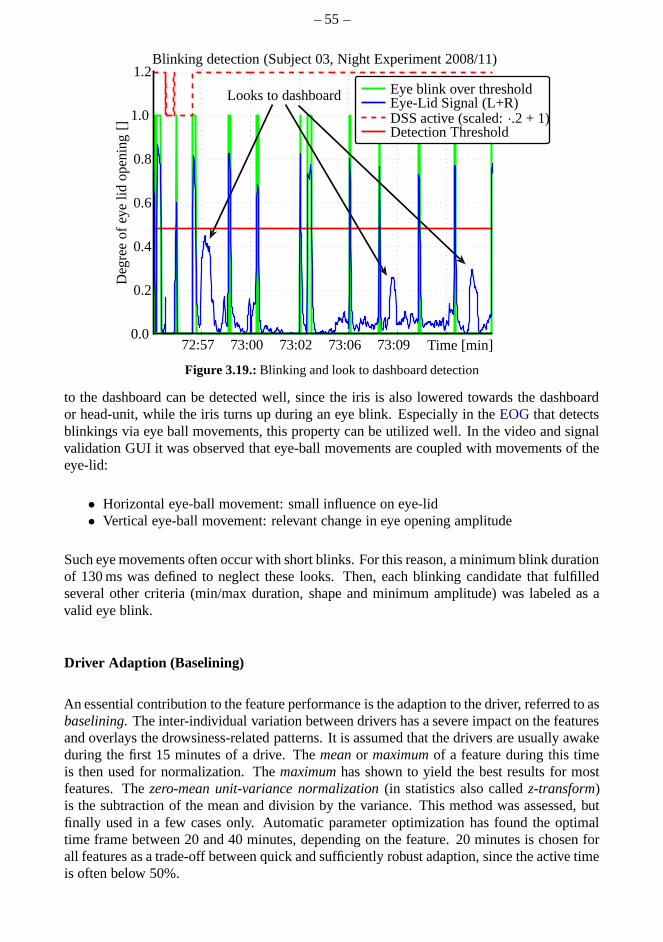
– 55 –

0.0

0.2

0.4

0.6

0.8

1.0

1.2

Time [min]

Eye blink over thresholdEye-Lid Signal (L+R)DSS active (scaled:·.2 + 1)Detection Threshold

Blinking detection (Subject 03, Night Experiment 2008/11)

Deg

ree

ofey

elid

open

ing

[]

72:57 73:00 73:02 73:06 73:09

Looks to dashboard

Figure 3.19.:Blinking and look to dashboard detection

to the dashboard can be detected well, since the iris is also lowered towards the dashboardor head-unit, while the iris turns up during an eye blink. Especially in theEOGthat detectsblinkings via eye ball movements, this property can be utilized well. In the video and signalvalidation GUI it was observed that eye-ball movements are coupled with movements of theeye-lid:

• Horizontal eye-ball movement: small influence on eye-lid• Vertical eye-ball movement: relevant change in eye openingamplitude

Such eye movements often occur with short blinks. For this reason, a minimum blink durationof 130 ms was defined to neglect these looks. Then, each blinking candidate that fulfilledseveral other criteria (min/max duration, shape and minimum amplitude) was labeled as avalid eye blink.

Driver Adaption (Baselining)

An essential contribution to the feature performance is theadaption to the driver, referred to asbaselining. The inter-individual variation between drivers has a severe impact on the featuresand overlays the drowsiness-related patterns. It is assumed that the drivers are usually awakeduring the first 15 minutes of a drive. Themeanor maximumof a feature during this timeis then used for normalization. Themaximumhas shown to yield the best results for mostfeatures. Thezero-mean unit-variance normalization(in statistics also calledz-transform)is the subtraction of the mean and division by the variance. This method was assessed, butfinally used in a few cases only. Automatic parameter optimization has found the optimaltime frame between 20 and 40 minutes, depending on the feature. 20 minutes is chosen forall features as a trade-off between quick and sufficiently robust adaption, since the active timeis often below 50%.

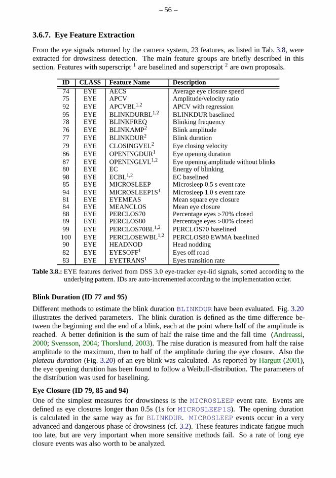
– 56 –

3.6.7. Eye Feature Extraction

From the eye signals returned by the camera system, 23 features, as listed in Tab.3.8, wereextracted for drowsiness detection. The main feature groups are briefly described in thissection. Features with superscript1 are baselined and superscript2 are own proposals.

ID CLASS Feature Name Description74 EYE AECS Average eye closure speed75 EYE APCV Amplitude/velocity ratio92 EYE APCVBL1,2 APCV with regression95 EYE BLINKDURBL 1,2 BLINKDUR baselined78 EYE BLINKFREQ Blinking frequency76 EYE BLINKAMP 2 Blink amplitude77 EYE BLINKDUR2 Blink duration79 EYE CLOSINGVEL2 Eye closing velocity86 EYE OPENINGDUR1 Eye opening duration87 EYE OPENINGLVL1,2 Eye opening amplitude without blinks80 EYE EC Energy of blinking98 EYE ECBL1,2 EC baselined85 EYE MICROSLEEP Microsleep 0.5 s event rate94 EYE MICROSLEEP1S1 Microsleep 1.0 s event rate81 EYE EYEMEAS Mean square eye closure84 EYE MEANCLOS Mean eye closure88 EYE PERCLOS70 Percentage eyes>70% closed89 EYE PERCLOS80 Percentage eyes>80% closed99 EYE PERCLOS70BL1,2 PERCLOS70 baselined100 EYE PERCLOSEWBL1,2 PERCLOS80 EWMA baselined90 EYE HEADNOD Head nodding82 EYE EYESOFF1 Eyes off road83 EYE EYETRANS1 Eyes transition rate

Table 3.8.:EYE features derived from DSS 3.0 eye-tracker eye-lid signals, sorted according to theunderlying pattern. IDs are auto-incremented according tothe implementation order.

Blink Duration (ID 77 and 95)

Different methods to estimate the blink durationBLINKDUR have been evaluated. Fig.3.20illustrates the derived parameters. The blink duration is defined as the time difference be-tween the beginning and the end of a blink, each at the point where half of the amplitude isreached. A better definition is the sum of half the raise time and the fall time (Andreassi,2000; Svensson, 2004; Thorslund, 2003). The raise duration is measured from half the raiseamplitude to the maximum, then to half of the amplitude during the eye closure. Also theplateau duration(Fig. 3.20) of an eye blink was calculated. As reported byHargutt(2001),the eye opening duration has been found to follow a Weibull-distribution. The parameters ofthe distribution was used for baselining.

Eye Closure (ID 79, 85 and 94)One of the simplest measures for drowsiness is theMICROSLEEP event rate. Events aredefined as eye closures longer than 0.5s (1s forMICROSLEEP1S). The opening durationis calculated in the same way as forBLINKDUR. MICROSLEEP events occur in a veryadvanced and dangerous phase of drowsiness (cf.3.2). These features indicate fatigue muchtoo late, but are very important when more sensitive methodsfail. So a rate of long eyeclosure events was also worth to be analyzed.

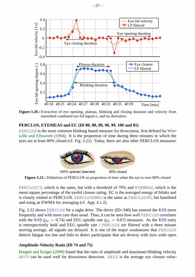
– 57 –

-0.4

-0.2

0

0.2

0.4

40:18 40:21 40:24 40:27 40:30 40:33 40:35 40:39

0.2

0.4

0.6

0.8

Eye opening duration

Eye closing duration

Time [min]Eye

-lid

op

enin

gd

egre

e[-

]E

ye-l

idve

loci

ty[1

/s]

Eye closureLP filtered

Plateau duration

Blinking duration

Eye-lid velocityLP filtered

Figure 3.20.:Extraction of eye opening, plateau, blinking and closing duration and velocity fromsmoothed combined eye-lid signalec and its derivative.

PERCLOS, EYEMEAS and EC (ID 80, 88, 89, 98, 99, 100 and 81)PERCLOS is the most common blinking based measure for drowsiness, first defined byWier-wille and Ellsworth(1994). It is the proportion of time during three minutes in which theeyes are at least 80% closed (cf. Fig.3.21). Today, there are also other PERCLOS measures:

Figure 3.21.:Definition of PERCLOS as proportion of time when the eye is over 80% closed

PERCLOS70, which is the same, but with a threshold of 70% andEYEMEAS, which is themean square percentage of the eyelid closure rating. EC is the averaged energy of blinks andis closely related to PERCLOS.PERCLOSEWBL is the same asPERCLOS80, but baselinedand using an EWMA for averaging (cf. App.4.1.2).

Fig. 3.22showsPERCLOS for a night drive. The driver (ID=340) has entered theKSSmorefrequently and with more care than usual. Thus, it can be seenhow wellPERCLOS correlateswith the KSS(ρp = 0.74) andEEGspindle rate (ρp = 0.67) measures. As theKSSentryis retrospectively hold andEEG spindle rate /PERCLOS are filtered with a three minutemoving average, all signals are delayed. It is one of the major weaknesses thatPERCLOSdetects fatigue too late and fails to detect participants that are drowsy with eyes wide open.

Amplitude-Velocity Ratio (ID 74 and 75)

Hargutt and Krüger(2000) found that the ratio of amplitude and maximum blinking velocityAPCV can be used well for drowsiness detection.AECS is the average eye closure veloc-

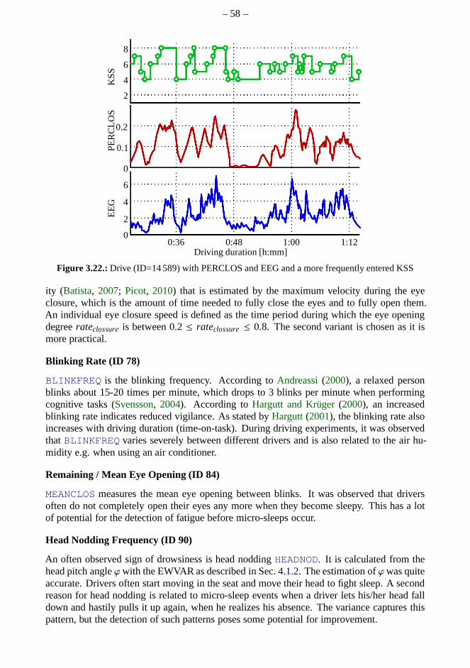
– 58 –

Driving duration [h:mm]1:121:000:480:36

EE

GP

ER

CL

OS

KS

S

0

2

4

6

0

0.1

0.2

2

4

6

8

Figure 3.22.:Drive (ID=14 589) with PERCLOS and EEG and a more frequently entered KSS

ity (Batista, 2007; Picot, 2010) that is estimated by the maximum velocity during the eyeclosure, which is the amount of time needed to fully close theeyes and to fully open them.An individual eye closure speed is defined as the time period during which the eye openingdegreerateclossure is between 0.2≤ rateclossure≤ 0.8. The second variant is chosen as it ismore practical.

Blinking Rate (ID 78)

BLINKFREQ is the blinking frequency. According toAndreassi(2000), a relaxed personblinks about 15-20 times per minute, which drops to 3 blinks per minute when performingcognitive tasks (Svensson, 2004). According toHargutt and Krüger(2000), an increasedblinking rate indicates reduced vigilance. As stated byHargutt(2001), the blinking rate alsoincreases with driving duration (time-on-task). During driving experiments, it was observedthatBLINKFREQ varies severely between different drivers and is also related to the air hu-midity e.g. when using an air conditioner.

Remaining / Mean Eye Opening (ID 84)

MEANCLOS measures the mean eye opening between blinks. It was observed that driversoften do not completely open their eyes any more when they become sleepy. This has a lotof potential for the detection of fatigue before micro-sleeps occur.

Head Nodding Frequency (ID 90)

An often observed sign of drowsiness is head noddingHEADNOD. It is calculated from thehead pitch angleϕwith the EWVAR as described in Sec.4.1.2. The estimation ofϕwas quiteaccurate. Drivers often start moving in the seat and move their head to fight sleep. A secondreason for head nodding is related to micro-sleep events when a driver lets his/her head falldown and hastily pulls it up again, when he realizes his absence. The variance captures thispattern, but the detection of such patterns poses some potential for improvement.

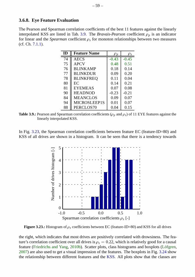
– 59 –

3.6.8. Eye Feature Evaluation

The Pearson and Spearman correlation coefficients of the best 11 features against the linearlyinterpolated KSS are listed in Tab.3.9. TheBravais-Pearsoncoefficientρp is an indicatorfor linear and theSpearmancoefficientρs for monoton relationships between two measures(cf. Ch.7.1.1).

ID Feature Name ρp ρs

74 AECS -0.43 -0.4575 APCV 0.48 0.5176 BLINKAMP 0.18 0.1477 BLINKDUR 0.09 0.2078 BLINKFREQ 0.11 0.0480 EC 0.14 0.2181 EYEMEAS 0.07 0.0890 HEADNOD -0.23 -0.2184 MEANCLOS 0.09 0.0794 MICROSLEEP1S 0.01 0.0788 PERCLOS70 0.04 0.15

Table 3.9.:Pearson and Spearman correlation coefficients (ρp andρs) of 11 EYE features against thelinearly interpolated KSS.

In Fig. 3.23, the Spearman correlation coefficients between feature EC (feature-ID=80) andKSS of all drives are shown in a histogram. It can be seen that there is a tendency towards

Spearman correlation coefficientsρs [-]0.50.0-0.5-1.0

Num

ber

ofdr

ives

hist

ogra

m[-

]

0

1

2

3

4

5

1.0

Figure 3.23.:Histogram ofρs coefficients between EC (feature-ID=80) and KSS for all drives

the right, which indicates that most drives are positively correlated with drowsiness. The fea-ture’s correlation coefficient over all drives isρs = 0.22, which is relatively good for a causalfeature (Friedrichs and Yang, 2010b). Scatter plots, class histograms and boxplots (Löfgren,2007) are also used to get a visual impression of the features. Theboxplots in Fig.3.24showthe relationship between different features and theKSS. All plots show that the classes are

– 60 –

severely overlapping, which leads to a lot of difficulties for drowsiness classification. Thereare no drives withKSSbelow 3, so these were not included in the plot.

Fea

ture

s[-

]

76543210

3 4 5 6 7 8 9

·10−3

6543 7 8 96543 7 8 96

8

10

12

14

16

5

10

·10−2AECS APCV HEADNOD

KSSKSSKSS

Figure 3.24.:Boxplot of features AECS, APCV and HEADNOD

3.6.9. Classification of Eye Features

The purpose of drowsiness classification is to combine thesedifferent features to a singlecontinuous-valued drowsiness measure or the discrete classesawake, acceptableanddrowsy(cf. class definition in Sec.3.3.5).

All features were downsampled to a sampling frequency of 0.5Hz, as it is assumed that theblinking behavior change is much slower than that. Anartificial neural network(ANN) wasused for classification (Duda et al., 2001).

Theoretically, the more features are incorporated, the more information can be exploited.However, when the number of features gets too high, the need for more training data cannotbe fulfilled any more (curse of dimensionality). For this reason, dimension reduction tech-niques are applied.Principal Component Analysis(PCA) andFisher transform(LDA) aremethods to transform a given feature space to a lower dimensional one. However, these-quential floating forward selection(SFFS) algorithm, introduced in (Pudil et al., 1994a), wasapplied to select the most promising features for a classifier. The advantage of SFFS overfeature transform techniques is its high transparency, as the selected features remain withoutany change. For practical applications that means that onlythe most relevant features need tobe computed. In our study, PCA and LDA have shown poor resultsin comparison to SFFS.Hence only results achieved by SFFS are reported. Tab.3.9 shows the most often selectedfeatures.

3.6.10. Classification Results for Eye Features

A feed-forwardANN with 25 neurons in one hidden layer was trained with the backpropaga-tion algorithm. The confusion matrix of theANN classification is given in Tab.3.10. Moreclassification results for Bayes,k-NN, GMM and LDA can be found in (Friedrichs and Yang,2010a). The results are based on the best eleven features that havebeen selected bySFFSin combination with the Bayes classifier. The classificationresults have been obtained byleave-one-out cross-validation with a training to test setratio of 80% to 20%. It is importantto divide the data by entire drives so that the drives in the test set are completely unknownto the classifier. The results are averaged over several permutations of the training/test set toobtain a more stable result.

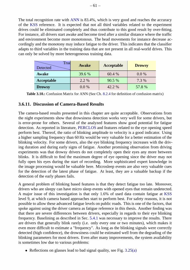
– 61 –

The total recognition rate withANN is 83.4%, which is very good and reaches the accuracyof the KSS reference. It is expected that not all third variables related to the experimentdrives could be eliminated completely and thus contribute to this good result by over-fitting.For instance, all drivers start awake and become tired aftera similar distance where the trafficand environment become more monotonous. The head movementsfor instance decrease ac-cordingly and the monotony may induce fatigue to the driver.This indicates that the classifieradapts to third variables in the training data that are not present in all real-world drives. Thiscan only be solved by more heterogeneous training data.

❳❳❳❳❳❳❳❳❳❳❳

DetectedTrue

Awake Acceptable Drowsy

Awake 39.6 % 60.4 % 0.0 %

Acceptable 2.2 % 90.5 % 7.3 %

Drowsy 0.0 % 42.2 % 57.8 %

Table 3.10.:Confusion Matrix for ANN (See Ch.8.2.4for definition of confusion matrix)

3.6.11. Discussion of Camera-Based Results

The camera-based results presented in this chapter are quite acceptable. Observations fromthe night experiments show that drowsiness detection worksvery well for some drivers, butis error-prone for others. Several of the analyzed featuresshow good potential for fatiguedetection. As reported in literature,PERCLOSand features related to the eye opening speedperform best. Thereof, the ratio of blinking amplitude to velocity is a good indicator. Usinga higher sampling frequency than 60 Hz would be very valuablefor a better estimation of theblinking velocity. For some drivers, also the eye blinking frequency increases with the driv-ing duration and during early signs of fatigue. Another promising observation from drivingexperiments was that drowsy drivers do not completely open their eyes any more betweenblinks. It is difficult to find the maximum degree of eye opening since the driver may notfully open his eyes during the start of recording. More sophisticated expert knowledge inthe image processing would be valuable here. Microsleep events are also very valuable cuesfor the detection of the latest phase of fatigue. At least, they are a valuable backup if thedetection of the early phases fails.

A general problem of blinking based features is that they detect fatigue too late. Moreover,drivers who are sleepy can have micro sleep events with opened eyes that remain undetected.A major issue of this investigation is that only 1.6% of used data contain fatigue atKSSlevel 9, at which camera based approaches start to perform best. For safety reasons, it is notpossible to allow these advanced fatigue levels on public roads. This is one of the factors, thatspoke against using the driver camera as fatigue reference in this thesis. Another finding wasthat there are severe differences between drivers, especially in regards to their eye blinkingfrequency. Baselining as described in Sec.5.4.1was necessary to improve the results. Thereare drivers that generally blink rarely (i.e. only every oneor two minutes), which makes iteven more difficult to estimate a "frequency". As long as the blinking signals were correctlydetected (high confidence), the drowsiness could be estimated well from the degrading of theblinking parameters for most drivers. Even after many improvements, the system availabilityis sometimes low due to various problems:

• Reflections on glasses lead to bad signal quality, see Fig.3.25(a)

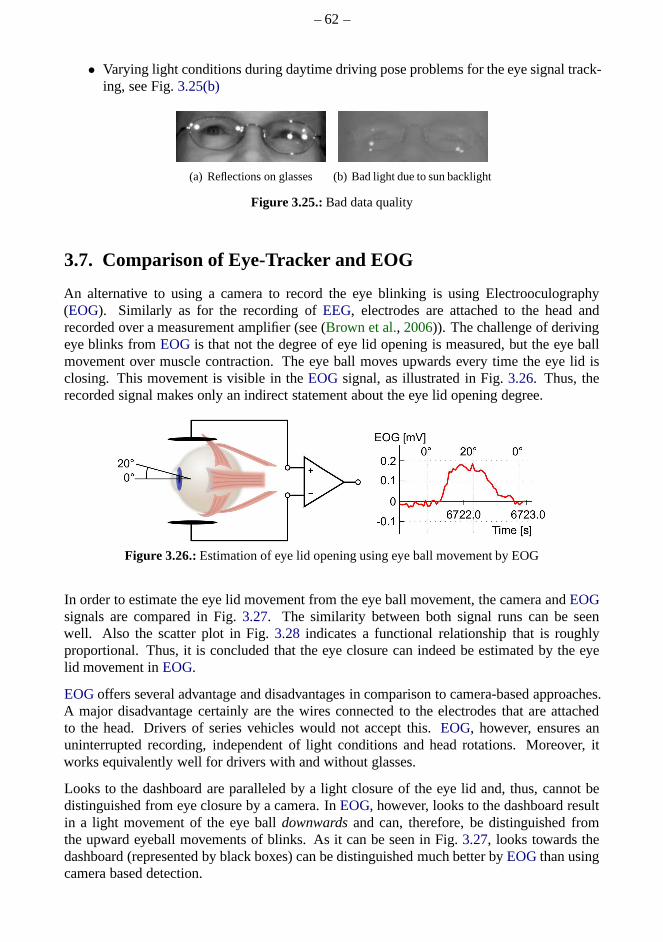
– 62 –

• Varying light conditions during daytime driving pose problems for the eye signal track-ing, see Fig.3.25(b)

(a) Reflections on glasses (b) Bad light due to sun backlight

Figure 3.25.:Bad data quality

3.7. Comparison of Eye-Tracker and EOG

An alternative to using a camera to record the eye blinking isusing Electrooculography(EOG). Similarly as for the recording ofEEG, electrodes are attached to the head andrecorded over a measurement amplifier (see (Brown et al., 2006)). The challenge of derivingeye blinks fromEOGis that not the degree of eye lid opening is measured, but the eye ballmovement over muscle contraction. The eye ball moves upwards every time the eye lid isclosing. This movement is visible in theEOG signal, as illustrated in Fig.3.26. Thus, therecorded signal makes only an indirect statement about the eye lid opening degree.

6722.00

0.2

Time [s]

EOG [mV]

0.1

-0.16723.0

Figure 3.26.:Estimation of eye lid opening using eye ball movement by EOG

In order to estimate the eye lid movement from the eye ball movement, the camera andEOGsignals are compared in Fig.3.27. The similarity between both signal runs can be seenwell. Also the scatter plot in Fig.3.28 indicates a functional relationship that is roughlyproportional. Thus, it is concluded that the eye closure canindeed be estimated by the eyelid movement inEOG.

EOGoffers several advantage and disadvantages in comparison to camera-based approaches.A major disadvantage certainly are the wires connected to the electrodes that are attachedto the head. Drivers of series vehicles would not accept this. EOG, however, ensures anuninterrupted recording, independent of light conditionsand head rotations. Moreover, itworks equivalently well for drivers with and without glasses.

Looks to the dashboard are paralleled by a light closure of the eye lid and, thus, cannot bedistinguished from eye closure by a camera. InEOG, however, looks to the dashboard resultin a light movement of the eye balldownwardsand can, therefore, be distinguished fromthe upward eyeball movements of blinks. As it can be seen in Fig. 3.27, looks towards thedashboard (represented by black boxes) can be distinguished much better byEOGthan usingcamera based detection.

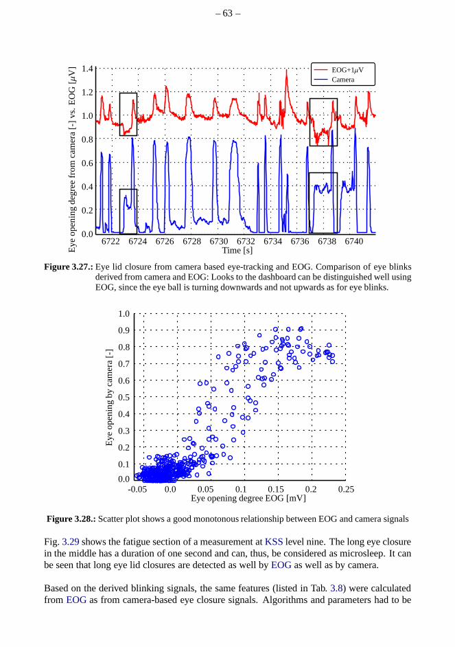
– 63 –

Time [s]6722

Eye

op

enin

gd

egre

efr

om

cam

era

[-]v

s.E

OG

[µV

]

0.0

1.4

1.2

1.0

0.8

0.6

0.4

0.2

674067386736673467326730672867266724

EOG+1µVCamera

Figure 3.27.:Eye lid closure from camera based eye-tracking and EOG. Comparison of eye blinksderived from camera and EOG: Looks to the dashboard can be distinguished well usingEOG, since the eye ball is turning downwards and not upwards as for eye blinks.

Eye opening degree EOG [mV]-0.05

Eye

op

enin

gb

yca

mer

a[-

]

0.0

1.0

0.9

0.7

0.8

0.6

0.4

0.2

0.250.20.150.10.050.0

0.1

0.5

0.3

Figure 3.28.:Scatter plot shows a good monotonous relationship between EOG and camera signals

Fig. 3.29shows the fatigue section of a measurement atKSSlevel nine. The long eye closurein the middle has a duration of one second and can, thus, be considered as microsleep. It canbe seen that long eye lid closures are detected as well byEOGas well as by camera.

Based on the derived blinking signals, the same features (listed in Tab.3.8) were calculatedfrom EOGas from camera-based eye closure signals. Algorithms and parameters had to be

– 64 –

Time [s]5526

Eye

op

enin

gd

egre

efr

om

cam

era

[-]v

s.E

OG

[µV

]

0.0

1.2

1.0

0.8

0.6

0.4

0.2

553655345533553255315530552955285527 5535

EOG+1µVCamera

Figure 3.29.:Long microsleep blinkings at KSS 9 from camera and EOG

slightly adapted. Fig.3.30shows a histogram of Spearman correlation coefficients betweenPERCLOS and theKSS. Even if there is a tendency to the right, the drives with negative

0

1

2

3

4

5

6

7

8

9

10

-1.0 -0.8 -0.6 -0.4 -0.2 0.2 0.4 0.6 0.8 1.0Spearman Correlation Coefficients [] (grouped for Meta-Column ID=4)

0.0

Features EEGOFF300 (ID: 135)

Num

ber

ofdr

ives

hist

ogra

m[-

]

Figure 3.30.:Correlation histograms of KSS and PERCLOS calculated from EOG

coefficients indicate a result inferior to the camera pendant.

3.8. Discussion and Conclusions on Fatigue References

As mentioned before, there is no "ground truth" as fatigue reference which is one of themajor challenges in online fatigue detection. The performance of the online algorithms canbe at best as good as the fatigue reference, so the goal of thissection was to evaluate different

– 65 –

approaches. The principal motivation is to investigate camera andEEG/ EOGbased measuresto overcome the main deficiencies of the subjectiveKSS self-rating, like its low temporalresolution and subjectiveness.

Nodine (2008) further investigated the reasons for the weak performances of universal fa-tigue detection methods and blames it on the large individual differences between drivers.She found that the steering range and variability have the strongest relationship with driverdrowsiness, better thanEEGor eye closure. She further claims that in-vehicle algorithms canoutperform the reference, which however cannot be validated.

As discussed in this chapter,EEGhas performed well for a few drivers, but was not suitable asa fatigue reference. This section has shown that the eye blinking signal can also be estimatedfrom the EOG Signal. WhileEOG and camera-based features show potential for fatiguedetection, it turned out at this point that they could not make the desired contribution for thefollowing reasons:

• RecordingEEG and blinking signals is laborious, which makes it unsuitable for thelarge number of free drives.

• The measurement equipment was not consistently available for most drives• The camera device was not available for most drives and vehicles• EEGand camera based features suffer from artifacts• There is no confidence if the detection is reliable or not

EOGmade a great contribution for the development of eye-tracking based algorithms.

The original goal to mergeKSS, EEG and eye-tracking to a single reference (comparableto SLEEPER1/2/3 in (Wierwille and Ellsworth, 1994; Wierwille, 1996b) or (Hargutt, 2001))failed because it was impossible to sufficiently validate the single and combined references.Knowing about the deficiencies of theKSSscale, theKSSand self-rated warning acceptanceturned out to remain the best reference available and, thus,are used for several reasons:

• Warnings from the assistance system must be transparent andaccepted by thedrivers’opinion, which is most related to theKSSself-rating

• After verification, theKSSis much more robust compared to physiological measures• TheKSSis available for all drives• The technicalKSSrecording is very reliable and relatively accurate, whereasEEGand

eye-tracking does not work for everybody.

For these reasons, theKSSis used as the central criteria whileEEG, EOG, eye-tracking, anddistraction are only considered in certain aspects. Even ifEEG and camera-based resultscannot be used to augment or replace theKSSas a reference, they are still used to assess thevehicle data based features. Furthermore, camera-based features are high potential candidatesfor online in-vehicle fatigue detection.

The lack of a ground truth reference still poses one of the mission-critical hurdles in thisresearch field.

– 67 –

Chapter 4.

Extraction of Driver State Features

This chapter presents the theoretical background about general signal processing methodolo-gies to extract measures from sleepiness related driving patterns, so called "features". Themain part of this chapter explains the pattern extraction ofpotential features from CAN-signals including their pre - and post-processing. The mostessential signals originate fromthe lane keeping camera-tracker, the steering wheel angle sensor, inertial motion sensors,wheel rotation sensors, light sensors and GPS (as describedin Sec.2.3).

In conventionalmachine learning, feature extraction is a laborious manual process based onmodels and hypotheses. The most important features are thenidentified, selected and com-bined by classification. Indeep learning, Artificial Neural Networks (ANN) with larger andmore sophisticated structures can automatically learn features from raw data. This comeshowever at the cost of a vast demand of resources: a much larger amount of data and big datacluster andGPU computing are required (such as Hadoop/Spark technologies). Thus, nei-ther the large amount of field data nor the computing resources were available off-board andon-board. For autonomous driving, the cost margin and thus the computation resources aremuch higher and purpose-designedASICs and Systems-on-a-Chip (SOC) with a high degreeof parallelization similar toGPUs can be designed. In contrast, driver monitoring systemsare targeted to require no additional cost and must run on classical vehicleECUs on top ofthe base software. For product liability reasons of safety systems in the automotive sector, amajor design goal ofESPsoftware are full transparency, model understanding and predictivebehavior that is validated. Only few of the vehicle variantsare available as prototypes priorto production, so adaption of parameters (so called "parameter application") to new vehiclesmust be possible without the need of recording training data. Classifiers can only learn pat-terns that are available in the training data and are generally not suitable for extrapolation.States and hyperparameters ofANNs do not provide the physical representation of parame-ters and decisions are not very transparent. Especially theextrapolation to operation pointsoutside the range of training data (e.g. for different countries, driving cultures, road proper-ties etc.) is a strength of models used in classical feature extraction.ANNs shall only be usedif there is no alternative and if the results justify it. For these reasons, the major focus herewas to investigate model based feature extraction in conjunction with machine learning.

Feature extraction is virtually the core of machine learning since it targets the separation ofdifferent independent patterns from the irrelevant clutter. The more precisely the featuresare extracted, the better the performance of classifiers combining these measures to a singlecontinuous-valued drowsiness measure or the discrete classesawake, acceptableanddrowsy(See Ch.3.3.5). Drowsiness can result in different patterns for different drivers or situations.Classification can exploit the combined discriminatory properties of features if they are notredundant. A model based on expert knowledge that preciselyunderstands the coherences is

– 68 –

generally superior to naive automated classification algorithms. This expert knowledge canbe incorporated during the feature extraction.

In literature and according to own observations, there is a large number of patterns withdrowsiness associative ability. Ideally, every feature isbased on one pattern that can be, forinstance, a quick steering correction, a lane exceeding, zick-zack lurching in the lane or adelayed reaction to a road unevenness.

Here, CAN-signals have a maximal sampling frequency of 50 Hz(100 Hz for FlexRay),which is necessary to properly detect fatigue related patterns like steering corrections. Incomparison, drowsiness is a slowly deteriorating process and changes only within minutes.For instance, a shock induced by an adrenalin rush can wake upa driver within a second, butis not essential for detecting the onset of sleepiness. Hence, it is necessary to extract patternswith at least 50 Hz, whereas for performance reasons, it is not beneficial to aggregate thederived features with a sampling rate higher than 0.5Hz.

Distraction leads to similar patterns as sleepiness and, thus, cannot always be distinguished.But the driver has more control and awareness over his distraction than over his drowsiness.On the other hand, the degree of distraction can change much faster than sleepiness. Sinceno reference for distraction was recorded, drivers are requested to avoid distraction in orderto not affect the fatigue features.

Further, it is proposed to distinguish betweencausalanda-priori features. Causal featuresresult from specific patterns that are caused by the driverbecausehe is drowsy. A-priorifeatures (e.g.DAYTIME) simply indicate that it isprobablefor the driver to become drowsy.Causal features are the most selective and thus most important ones. However, a-priori fea-tures are also important as they can make a significant contribution to the system performance.For instance, the (causal) features based on road exits are very probable to result from sleepi-ness when they occur in a monotonous driving situation (a-priori). A-priori features arediscussed in Ch.5.3as they are considered in the context of external influences.

Another grouping of features can be made by classifying theminto event-basedand con-tinuous. The latter can be calculated permanently, such as the lane deviation (LANEDEV),whereas zig-zag events, steering corrections or road exitsoccur relatively seldom. The fewerthe number of events, the worse the temporal resolution of the signal is. A few events withinone hour do not allow to make a qualified statement about the driver state. Hence, the goal isto focus on patterns that occur frequently and also catch small events by tuning parameterstowards high sensitivity.

Another grouping of features is proposed:basefeatures andfunctionalsof base features. Inthe following section, the base features are described. In general, for event-based features,the presence of a single pattern does not directly indicate driver drowsyness. The rate andintensity of these events are relevant. For this reason, further processing steps are applied tothe base features such as:

• Moving average, median or exponentially weighted moving average (EWMA)• Standard deviation, interquartile-range or exponentially weighted moving variance

(cf. 4.1.2)

– 69 –

4.1. Pre-Processing

A number of pre-processing steps were necessary before extracting the drowsiness-relatedfeatures from the raw signals. The proposed methods have several advantages with regardsto performance and computation time when compared to the common implementation inliterature such as the mean or variance over a moving window.

Since the measurement of the steering wheel angle originates from four different vehiclecategories with different properties, they needs to be calibrated. Further, a discrete derivativeis necessary for many signals such as thesteering velocity, the longitudinal vehicle speedandaccelerationfrom the wheel rotation rate sensors and thelateral accelerationfrom thesensor and from the single track model. This section describes these pre-processing steps.

4.1.1. Digital Polynomial Smoothing- and DifferentiationFilter

Many features require synchronized numerical smoothing and differentiation of some inputsignals. The calculation of the steering velocityδS, lateral or longitudinal velocityyL, vveh oraccelerationax,whl from the wheel rotation rateWhlRPMx, are a few examples. The differ-ence between two consecutive samples of a discrete-time signal x[n] is given by

x[n] =x[n] − x[n− 1]

Ts, (4.1)

with the sampling interval Ts in seconds can be described as a simple 1st order FIR filterwith the coefficientsb0 = 1, b1 = −1 and one division byTs. However, this differencecalculation commonly used in literature (Pander et al., 2008; Bittner and Hana, 2000; Desaiand Haque, 2006) increases high frequency components (noise) and, thus, requires low-passfiltering which again has the drawbacks of flattening peaks and shifting the phase.

A more appropriate method for digital smoothing and differentiation is to locally fit a poly-nomial, referred to asDigital Smoothing Polynomial Filter(DISPO). According to (Schafer,2011), Savitzky and Golay’s paper (Savitzky and Golay, 1964) introducingDISPOwas ratedin 2000 as one of the top 5 papers ever published in the journalAnalytical Chemistry. Itsmajor advantage is that the signal distribution, width and maximum height of impulses aremaintained. The derivative is easily obtained by an analytical differentiation of the approxi-mated polynomial.Savitzky and Golay(1964) have shown that a sliding polynomial-fit andevaluation of the polynomial at a single point is equivalentto discrete convolution with a fixedimpulse response (i.e. a regular non-recursive FIR-filter), since the coefficients are constantfor a given filter orderP and window SizeN. The polynomial smoothing and differentiationfilter coefficients can be calculated by a least-squares fitting.

For a given input sequencex[n], N = 2F + 1 adjacent pointsx[−F], . . . , x[0], . . . , x[+F]are considered to fit an (over-determined) polynomial

p(n) =P∑

k=0

ak nk (4.2)

of orderP with 0 ≤ P ≤ 2F at the point of interestn = 0. An approximated solution for thecoefficientsa = [a0, a1, . . . , aP]T can be found by minimizing the sum of squared errors

– 70 –

ǫF(a) =F∑

n=−F

(

p(n) − x[n])2

=F∑

n=−F

P∑

k=0

ak nk − x[n]

2

. (4.3)

By introducing the notations

M =

1 −F · · · (−F)P

.... . .

...1 F − 1 · · · (F − 1)P

1 F · · · FP

︸ ︷︷ ︸

Vandermonde matrixM∈R(2F+1)×(P+1)

, a =

a0...

aP

︸︷︷︸

a∈R(P+1)

, x =

x[−F]...

x[+F]

︸ ︷︷ ︸

x∈R2F+1

, (4.4)

the cost function from Eq. (4.3) can be written as

ǫF(a) = ||M a − x ||2. (4.5)

The least squares solutiona∗ is obtained if the derivative of the error by all polynomial coef-ficientsa is minimized:

∂ǫF(a)∂(a)

!= 0, yields a∗ = (MTM )−1MT

︸ ︷︷ ︸

M+

x (4.6)

whereM+ is theMoore-Penrose Pseudoinverseof M .

The smoothed output value is obtained by evaluating the polynomial at the central pointn = 0, which isy[0] = p(0) =. The next outputy[1] is again obtained by shifting theanalysis interval to the next sample to the right. As shown in(Savitzky and Golay, 1964;Schafer, 2011), this is equivalent to a convolution with a fixed set of weighting coefficientsh(n). Since only the coefficienta0 is needed,hT is the 0th row ofM+(0, :) from Eq. (4.6).SinceM+ is independent of the input samples it can be pre-computed for a given 2F + 1impulse response length and polynomial orderP. The smoothing is stronger, the more over-determined the polynomial (i.e. the closerP to N) is. This applies for lower polynomial orderP and is large window sizesN.

The first derivative ofp(n) from Eq. (4.2) can be calculated analytically by

dp(n)

dn=

P−1∑

k=0

(k+ 1) ak+1 nk . (4.7)

With the differentiation matrixD

D =

0 1 0 0

0 0... 0

0 0 0 1/P0 0 0 0

(4.8)

we obtain the differentiated sequencey[n] by applying the differentiation matrix as derivedin Orfanidis(1995, Ch. 8.3.5)

– 71 –

y[n] = MDM +︸ ︷︷ ︸

H

x (4.9)

y[n] = hTd x =

N−1∑

i=0

hd[i]x[n− i] (4.10)

with N = 2F + 1 andhTd = H(1, :) as the 1st row ofH.

The phase delay of the FIR smoothing and differentiation filter isτ = (F + 1) ·Ts and higherthan for recursive filters, which is not problematic for thisapplication. The signal needs tobe synchronized with signals that are not filtered and for thecorrect amplitude the samplingfrequencyFs must be multiplied. Fig.4.1shows for instance the steering wheel angle and its

0

2

4

6

818.8 818.9 819 819.1 819.2 819.3 819.4 819.5 819.6−20

−10

0

10

20

30

40 fc=3.18 Hz

fc=1.62 Hz

fc=/.81 Hz

fc=/.4/ Hz

Butterworth LP n=1

ST

W a

ngle

[°]

Ste

erin

g w

hee

l vel

oci

ty [

°/s]

Time [s]

S(n-1)-(n)

d /dT DISPO filter

S

SS

Steering wheel angle S

Figure 4.1.:Different methods to differentiate signals.

derivative obtained by the common and proposed method. Using a low-passButterworthIIR-filter with weak filtering i.e. a high cut-off frequencyfc (black dash-dotted line), preservesthe peak height at the cost of a high noise. Stronger filtering, i.e. low cut-off frequencysmoothes the signal but flattens the peak of the derivative. Since in the present application,the maximum steering velocity shall be determined with highrobustness, theDISPOFIRfilter properly preserves the impulse height while smoothing the signal (red solid line).

Application to CAN Signals

The steering wheel velocity in Fig.4.1 is smoothed and derived by aDISPOfilter of orderN = 13 and polynomial orderP = 5. These parameters are the best trade-off betweenpreserving the peak height and avoiding toggling around zero for zero-crossing detection.Both yield a fix phase delay ofN+1

2 = 7 samples. The related smoothing and differentiationcoefficientsh andhd are illustrated in Fig.4.2.

The longitudinal accelerationax,whl is obtained by aDISPOdifferentiation filter with the samecoefficients as in Fig.4.2on vehicle speed from the wheel rotation sensors in Ch. (2.2)

ax,whl[n] = Fs

N−1∑

i=0

hd[i] vveh[n− i] . (4.11)

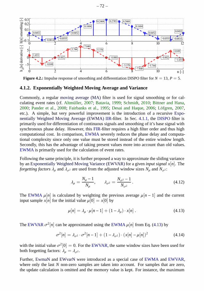
– 72 –

Figure 4.2.: Impulse response of smoothing and differentiation DISPO filter for N = 13,P = 5.

4.1.2. Exponentially Weighted Moving Average and Variance

Commonly, a regularmoving average (MA)filter is used for signal smoothing or for cal-culating event rates (cf.Altmüller, 2007; Batavia, 1999; Schmidt, 2010; Bittner and Hana,2000; Pander et al., 2008; Fairbanks et al., 1995; Desai and Haque, 2006; Löfgren, 2007,etc.). A simple, but very powerful improvement is the introduction of a recursiveExpo-nentially Weighted Moving Average (EWMA)IIR-filter. In Sec.4.1.1, the DISPOfilter isprimarily used for differentiation of continuous signals and smoothing of it’s base signal withsynchronous phase delay. However, thisFIR-filter requires a high filter order and thus highcomputational cost. In comparison,EWMA severely reduces the phase delay and computa-tional complexity since only one value must be stored instead of the entire window length.Secondly, this has the advantage of taking present values more into account than old values.EWMA is primarily used for the calculation of event rates.

Following the same principle, it is further proposed a way toapproximate the sliding varianceby anExponentially Weighted Moving Variance (EWVAR)for a giveninput signal x[n]. Theforgetting factorsλµ andλσ2 are used from the adjusted window sizesNµ andNσ2:

λµ =Nµ − 1

Nµ

, λσ2 =Nσ2 − 1

Nσ2. (4.12)

The EWMA µ[n] is calculated by weighting the previous averageµ[n− 1] and the currentinput samplex[n] for the initial valueµ[0] = x[0] by

µ[n] = λµ · µ[n− 1] + (1− λµ) · x[n] . (4.13)

TheEWVAR σ2[n] can be approximated using theEWMA µ[n] from Eq. (4.13) by

σ2[n] = λσ2 ·σ2[n− 1] + (1− λσ2) · (x[n] − µ[n])2 (4.14)

with the initial valueσ2[0] = 0. For theEWVAR, the same window sizes have been used forboth forgetting factors:λµ = λσ2.

Further,EwmaNandEWvarN were introduced as a special case ofEWMA andEWVAR,where only the lastN non-zero samples are taken into account. For samples that are zero,the update calculation is omitted and the memory value is kept. For instance, the maximum

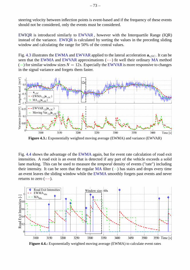
– 73 –

steering velocity between inflection points is event-basedand if the frequency of these eventsshould not be considered, only the events must be considered.

EWIQR is introduced similarly toEWVAR , however with the Interquartile Range (IQR)instead of the variance.EWIQR is calculated by sorting the values in the preceding slidingwindow and calculating the range for 50% of the central values.

Fig.4.3illustrates theEWMA andEWVAR applied to the lateral accelerationax,SC. It can beseen that theEWMA andEWVAR approximations (−−) fit well their ordinaryMA method(·−) for similar window sizesN = 12s. Especially theEWVAR is more responsive to changesin the signal variance and forgets them faster.

Figure 4.3.:Exponentially weighted moving average (EWMA) and variance(EWVAR)

Fig. 4.4shows the advantage of theEWMA again, but for event rate calculation of road exitintensities. A road exit is an event that is detected if any part of the vehicle exceeds a solidlane marking. This can be used to measure thetemporaldensity of events ("rate") includingtheir intensity. It can be seen that the regularMA filter (·−) has stairs and drops every timean event leaves the sliding window while theEWMA smoothly forgets past events and neverreturns to zero (−−).

Figure 4.4.:Exponentially weighted moving average (EWMA) to calculateevent rates

– 74 –

Computational Complexity: On a fixed-point processor, divisions and multiplications andespecially memory for unit delays (each 32Bit) are very limited and expensive. In regardsto computational complexity, Eq. (4.13) can be transformed to the more efficient Eq. (4.15)by replacing one multiplication by one subtraction. Compared to the moving average withone division,N − 1 additions andN − 1 unit delay elements, theEWMA now requires twoadditions and a multiplication:

µ[n] = x[n] + λµ·(µ[n− 1] − x[n]) . (4.15)

For EWVAR this works equivalently :

σ2[n] = (x[n] − µ[n])2 + λσ2·(

σ2[n− 1] − (x[n] − µ[n])2)

. (4.16)

Fixed-point Error: The weakness of this implementation in fixed-point arithmetics is that

the error of the feedback is accumulated. For this reason,λ+ 1N

!≡ 1 must be fulfilled asprecisely as possible. For Eq. (4.12), this is achieved by first pre-calculating the division andthenthe subtraction

λ =N − 1

N−→ λ = 1− 1

N(4.17)

since the subtraction in fixed-point is error free. Second, a32Bit quantization (instead of16Bit) is at least required for maintaining acceptable drift error of fixed-point towards floating-point after several hours. These countermeasures reduce the mean deviation of the fixed-pointerror by factor 16. Details about the results are presented in (Pape, 2008).

Adaptive Window Size: The adaption to strong signal changes and initialization oftheEWMA and EWVAR can take very long for a large window sizeNµ. Thus, further improve-ments are introduced:

• Initial values: The initial valuesµ[0] andσ2[0] are initialized to the average of theawake phase of each feature instead to 0 orx[n].

• Initialization: Growing window size is an important improvement. For instance, start-ing with Nµ = 5 increaseNµ by one for every sample or event up to the final windowsize.

• Situation adaption: The window size is reduced when the driving condition severelychanges and a faster adaption is needed, e.g. for a changed vehicle speed in construc-tion sites, i.e.Nµ(x, vveh).

4.1.3. System-Active Signals

For steering angle and lane based features, there are often driving situations (e.g. overtaking,curves, road condition etc.) that have a bad influence to the signals and features. As well,there are moments in which the signal quality is insufficientdue to bad lane markings or badweather. During the pre-processing, a BooleanSystem Active Signalfor lane-based featuresS ASLANE and a similar signal for steering and CAN based featuresS ASCAN are calculated.They indicate when distortions requires to neglect a certain situation.

S ASLANE is TRUE if all following conditions are fulfilled:

– 75 –

1. Vehicle speedis within the range:Pv,lower,LANE ≤ vveh≤ Pv,upper withPv,lower,LANE = 70km/hPv,upper,LANE = 200km/h

2. No lane changetakes place: the detection is described in Sec.4.1.5whereasPlaneChgPreS uppT= 4sbefore andPlaneChgPostS uppT= 6safter the lane change are alsosuppressed.

3. Lane data quality is sufficient:LaneDataQual≥ PlaneDataQualwithPlaneDataQual= 80%

4. Noconstruction site: thelane width is used for detection:LaneWidth> PminLaneWidth

with PminLaneWidth= 3.05m

5. No fastvelocity changes: for instance, from 130 to 80 km/h in construction sites alsocause artifacts in driving patterns and, thus, are suppressed forPvelChgPostS uppT= 3s:EWMA 3s(|vveh,LP|) > 1.5 km

h·Tswith vveh,LP filtered by a Butterworth low-pass filter of

2nd order and a cut-off frequency of 0.5Hz.

6. Noovertakings: lane signals cannot be used during overtaking maneuvers. Achangein the lane numberLaneNumaccompanied by an acceleration pedal change of∆AccelPdlPosn≥ 10% is used for detection.

7. No short active sections: in order to avoid toggling, active sections with durationsPshortS ectionsTh≤ 3 sare suppressed as well.

S ASCAN is TRUE if the following conditions are fulfilled:

1. Novehicle operationfrom buttons and levers:turn indicator operation result in inactivity forPtWghtLnCh= 10s,steering wheel buttons or clutch operation forPtWghtOper= 5sandoperation of the heat-unit (COMAND) forPtWghtDistr = 10s are suppressed.

2. No Curves: lateral perceived acceleration|EWMA s2(ay,stw)| > 0.8ms2 is suppressed

forPcurveS uppT= 0.4susingay,stw from the single-track model (Sec.6.3).

3. NoRoad bumps: longitudinal accelerationax,whl ≤ 4ms2 is suppressed for

PRoadBumpS uppT= 0.5s usingax,whl from wheel rotation sensors (cf. Sec.4.1.1).

4. Vehicle speedmust be within the range:Pv,lower,CAN ≤ vveh≤ Pv,upper,CAN withPv,lower,CAN = 80km/h andPv,upper,CAN = 180km/h.

5. Steering wheel anglemust be within|δS| < PstwLevelwith PstwLevel≤ 40.

6. Nodriving style suppression: wDynamicDrivingS tylefrom Sec.4.1.7is suppressed.

7. No Kick-down : AccelPdlPosn≥ 98%∨ AccelPdlPosnRaw ≥ 98% are suppressedfor PtKickDownS hort= 0.1s if the pedal is pressed for shorter than 2sandPtKickDownLong= 20s otherwise.

8. Nosafety assistance system is active: Traction Control, Stability Control, Anti-lockBraking System or Hydraulic Brake Assist indicate very sportive driving: AS Rctrl ∨ES Pctrl ∨ABSctrl ∨HBActrl. Events are suppressed for 0.1s for an intervention shorterthan 2sand up to 20sotherwise.

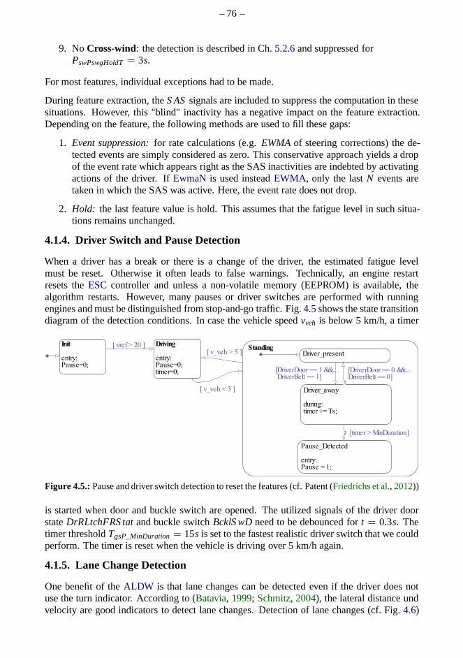
– 76 –

9. NoCross-wind: the detection is described in Ch.5.2.6and suppressed forPswPswgHoldT= 3s.

For most features, individual exceptions had to be made.

During feature extraction, theS ASsignals are included to suppress the computation in thesesituations. However, this "blind" inactivity has a negative impact on the feature extraction.Depending on the feature, the following methods are used to fill these gaps:

1. Event suppression:for rate calculations (e.g.EWMAof steering corrections) the de-tected events are simply considered as zero. This conservative approach yields a dropof the event rate which appears right as the SAS inactivitiesare indebted by activatingactions of the driver. IfEwmaNis used insteadEWMA, only the lastN events aretaken in which the SAS was active. Here, the event rate does not drop.

2. Hold: the last feature value is hold. This assumes that the fatiguelevel in such situa-tions remains unchanged.

4.1.4. Driver Switch and Pause Detection

When a driver has a break or there is a change of the driver, theestimated fatigue levelmust be reset. Otherwise it often leads to false warnings. Technically, an engine restartresets theESC controller and unless a non-volatile memory (EEPROM) is available, thealgorithm restarts. However, many pauses or driver switches are performed with runningengines and must be distinguished from stop-and-go traffic.Fig.4.5shows the state transitiondiagram of the detection conditions. In case the vehicle speedvveh is below 5 km/h, a timer

Figure 4.5.:Pause and driver switch detection to reset the features (cf.Patent (Friedrichs et al., 2012))

is started when door and buckle switch are opened. The utilized signals of the driver doorstateDrRLtchFRS tatand buckle switchBcklS wDneed to be debounced fort = 0.3s. Thetimer thresholdTgsP_MinDuration = 15s is set to the fastest realistic driver switch that we couldperform. The timer is reset when the vehicle is driving over 5km/h again.

4.1.5. Lane Change Detection

One benefit of theALDW is that lane changes can be detected even if the driver does notuse the turn indicator. According to (Batavia, 1999; Schmitz, 2004), the lateral distance undvelocity are good indicators to detect lane changes. Detection of lane changes (cf. Fig.4.6)

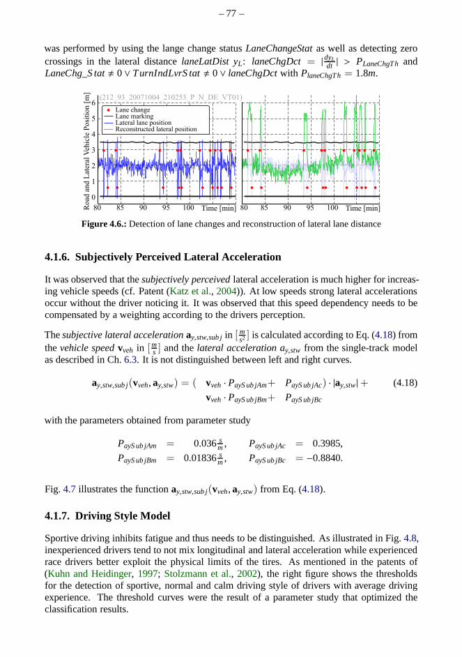
– 77 –

was performed by using the lange change statusLaneChangeStatas well as detecting zerocrossings in the lateral distancelaneLatDist yL: laneChgDct = |dyL

dt | > PLaneChgThandLaneChg_S tat, 0∨ TurnIndLvrS tat, 0∨ laneChgDctwith PlaneChgTh= 1.8m.

Figure 4.6.:Detection of lane changes and reconstruction of lateral lane distance

4.1.6. Subjectively Perceived Lateral Acceleration

It was observed that thesubjectively perceivedlateral acceleration is much higher for increas-ing vehicle speeds (cf. Patent (Katz et al., 2004)). At low speeds strong lateral accelerationsoccur without the driver noticing it. It was observed that this speed dependency needs to becompensated by a weighting according to the drivers perception.

Thesubjective lateral accelerationay,stw,sub j in [ms2 ] is calculated according to Eq. (4.18) from

thevehicle speedvveh in [ms ] and thelateral acceleration ay,stw from the single-track model

as described in Ch.6.3. It is not distinguished between left and right curves.

ay,stw,sub j(vveh, ay,stw) = ( vveh · PayS ub jAm+ PayS ub jAc) · |ay,stw|+ (4.18)

vveh · PayS ub jBm+ PayS ub jBc

with the parameters obtained from parameter study

PayS ub jAm = 0.036sm, PayS ub jAc = 0.3985,

PayS ub jBm = 0.01836sm, PayS ub jBc = −0.8840.

Fig. 4.7 illustrates the functionay,stw,sub j(vveh, ay,stw) from Eq. (4.18).

4.1.7. Driving Style Model

Sportive driving inhibits fatigue and thus needs to be distinguished. As illustrated in Fig.4.8,inexperienced drivers tend to not mix longitudinal and lateral acceleration while experiencedrace drivers better exploit the physical limits of the tires. As mentioned in the patents of(Kuhn and Heidinger, 1997; Stolzmann et al., 2002), the right figure shows the thresholdsfor the detection of sportive, normal and calm driving styleof drivers with average drivingexperience. The threshold curves were the result of a parameter study that optimized theclassification results.

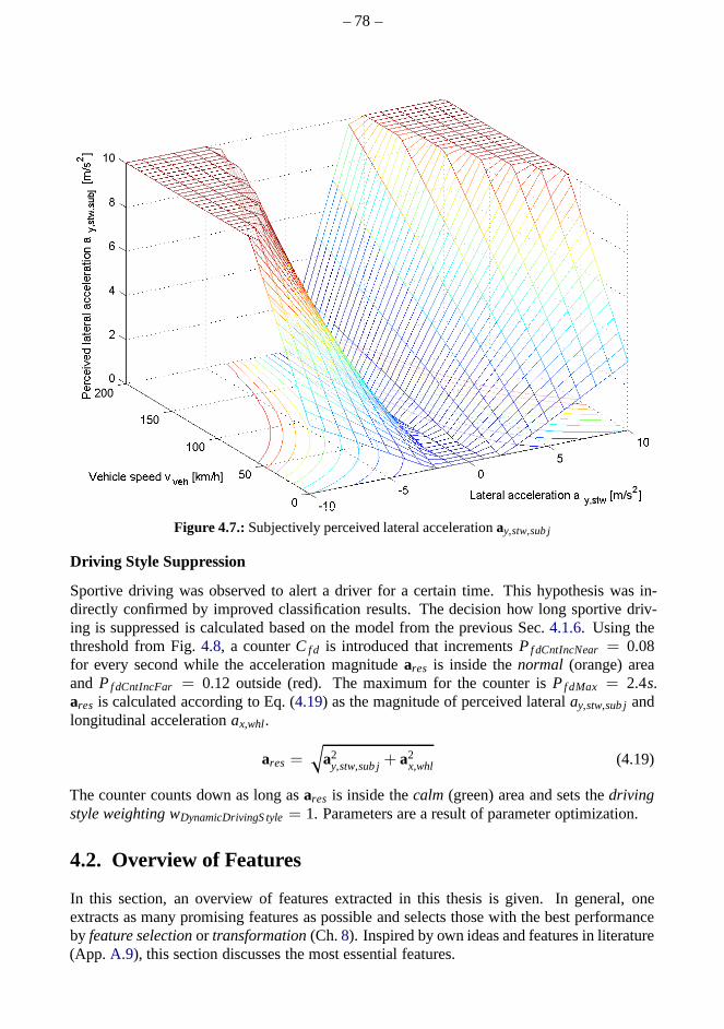
– 78 –

Figure 4.7.:Subjectively perceived lateral accelerationay,stw,sub j

Driving Style Suppression

Sportive driving was observed to alert a driver for a certaintime. This hypothesis was in-directly confirmed by improved classification results. The decision how long sportive driv-ing is suppressed is calculated based on the model from the previous Sec.4.1.6. Using thethreshold from Fig.4.8, a counterC f d is introduced that incrementsPf dCntIncNear = 0.08for every second while the acceleration magnitudeares is inside thenormal (orange) areaand Pf dCntIncFar = 0.12 outside (red). The maximum for the counter isPf dMax = 2.4s.ares is calculated according to Eq. (4.19) as the magnitude of perceived lateralay,stw,sub j andlongitudinal accelerationax,whl.

ares =√

a2y,stw,sub j+ a2

x,whl (4.19)

The counter counts down as long asares is inside thecalm (green) area and sets thedrivingstyle weighting wDynamicDrivingS tyle= 1. Parameters are a result of parameter optimization.

4.2. Overview of Features

In this section, an overview of features extracted in this thesis is given. In general, oneextracts as many promising features as possible and selectsthose with the best performanceby feature selectionor transformation(Ch.8). Inspired by own ideas and features in literature(App. A.9), this section discusses the most essential features.

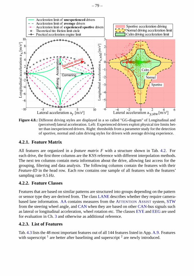
– 79 –

Figure 4.8.:Different driving styles are displayed in a so called "GG-diagram" of Longitudinal and(perceived) lateral acceleration. Left: Experienced drivers exploit physical tire limits bet-ter than inexperienced drivers. Right: thresholds from a parameter study for the detectionof sportive, normal and calm driving styles for drivers withaverage driving experience.

4.2.1. Feature Matrix

All features are organized in afeature matrix Fwith a structure shown in Tab.4.2. Foreach drive, the first three columns are the KSS reference withdifferent interpolation methods.The next ten columns contain meta information about the drive, allowing fast access for thegrouping, filtering and data analysis. The following columns contain the features with theirFeature-ID in the head row. Each row contains one sample of all features with the features’sampling rate 0.5Hz.

4.2.2. Feature Classes

Features that are based on similar patterns are structured into groups depending on the patternor sensor type they are derived from. The classLANE describes whether they require camera-based lane information.AA contains measures from theATTENTION ASSISTsystem,STWfrom the steering wheel angle, andCAN when they are based on otherCAN-bus signals suchas lateral or longitudinal acceleration, wheel rotation etc. The classesEYE andEEGare usedfor evaluation in Ch.3 and otherwise as additional reference.

4.2.3. List of Features

Tab.4.3lists the 48 most important features out of all 144 features listed in App.A.9. Featureswith superscript1 are better after baselining and superscript2 are newly introduced.

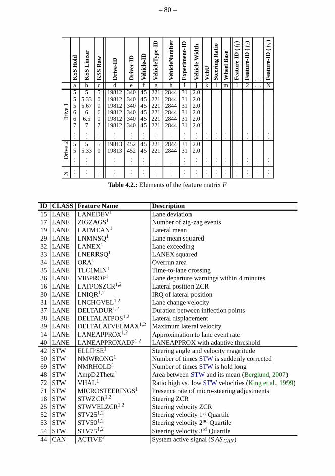
– 80 –

KS

SH

old

KS

SLi

near

KS

SR

aw

Driv

e-ID

Driv

er-I

D

Vehi

cle-

ID

Vehi

cleT

ype-

ID

Vehi

cleN

umbe

r

Exp

erim

ent-

ID

Vehi

cle

Wid

th

Vch

U

Ste

erin

gR

atio

Whe

elB

ase

Fea

ture

-ID

(f1)

Fea

ture

-ID

(f2)

. . . Fea

ture

-ID

(fN

)

a b c d e f g h i j k l m 1 2 . . . N5 5 5 19812 340 45 221 2844 31 2.05 5.33 0 19812 340 45 221 2844 31 2.0

Driv

e1 5 5.67 0 19812 340 45 221 2844 31 2.0

6 6 6 19812 340 45 221 2844 31 2.06 6.5 0 19812 340 45 221 2844 31 2.07 7 7 19812 340 45 221 2844 31 2.0...

.

.

....

.

.

....

.

.

....

.

.

....

.

.

....

.

.

....

.

.

....

.

.

....

Driv

e2 5 5 5 19813 452 45 221 2844 31 2.0

5 5.33 0 19813 452 45 221 2844 31 2.0...

.

.

....

.

.

....

.

.

....

.

.

....

.

.

....

.

.

....

.

.

....

.

.

....

N

.

.

....

.

.

....

.

.

....

.

.

....

.

.

....

.

.

....

.

.

....

.

.

....

.

.

.

Table 4.2.:Elements of the feature matrixF

ID CLASS Feature Name Description15 LANE LANEDEV1 Lane deviation17 LANE ZIGZAGS1 Number of zig-zag events19 LANE LATMEAN 1 Lateral mean29 LANE LNMNSQ1 Lane mean squared32 LANE LANEX1 Lane exceeding33 LANE LNERRSQ1 LANEX squared34 LANE ORA1 Overrun area35 LANE TLC1MIN1 Time-to-lane crossing36 LANE VIBPROP1 Lane departure warnings within 4 minutes16 LANE LATPOSZCR1,2 Lateral position ZCR30 LANE LNIQR1,2 IRQ of lateral position31 LANE LNCHGVEL1,2 Lane change velocity37 LANE DELTADUR1,2 Duration between inflection points38 LANE DELTALATPOS1,2 Lateral displacement39 LANE DELTALATVELMAX 1,2 Maximum lateral velocity14 LANE LANEAPPROX1,2 Approximation to lane event rate40 LANE LANEAPPROXADP1,2 LANEAPPROX with adaptive threshold42 STW ELLIPSE1 Steering angle and velocity magnitude50 STW NMWRONG1 Number of timesSTWis suddenly corrected69 STW NMRHOLD1 Number of timesSTWis hold long48 STW AmpD2Theta1 Area betweenSTWand its mean (Berglund, 2007)72 STW VHAL 1 Ratio high vs. lowSTWvelocities (King et al., 1999)71 STW MICROSTEERINGS1 Presence rate of micro-steering adjustments18 STW STWZCR1,2 Steering ZCR25 STW STWVELZCR1,2 Steering velocity ZCR52 STW STV251,2 Steering velocity 1st Quartile53 STW STV501,2 Steering velocity 2nd Quartile54 STW STV751,2 Steering velocity 3rd Quartile44 CAN ACTIVE2 System active signal (S ASCAN)

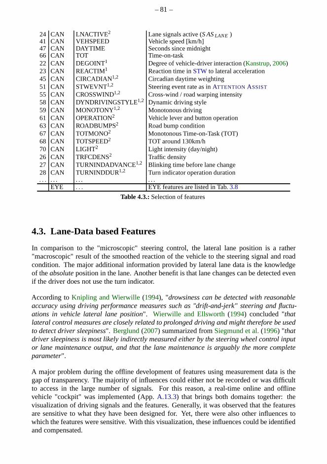
– 81 –

24 CAN LNACTIVE2 Lane signals active (S ASLANE )41 CAN VEHSPEED Vehicle speed [km/h]47 CAN DAYTIME Seconds since midnight66 CAN TOT Time-on-task22 CAN DEGOINT1 Degree of vehicle-driver interaction (Kanstrup, 2006)23 CAN REACTIM1 Reaction time inSTWto lateral acceleration45 CAN CIRCADIAN1,2 Circadian daytime weighting51 CAN STWEVNT1,2 Steering event rate as inATTENTION ASSIST

55 CAN CROSSWIND1,2 Cross-wind / road warping intensity58 CAN DYNDRIVINGSTYLE1,2 Dynamic driving style59 CAN MONOTONY1,2 Monotonous driving61 CAN OPERATION2 Vehicle lever and button operation63 CAN ROADBUMPS2 Road bump condition67 CAN TOTMONO2 Monotonous Time-on-Task (TOT)68 CAN TOTSPEED2 TOT around 130km/h70 CAN LIGHT2 Light intensity (day/night)26 CAN TRFCDENS2 Traffic density27 CAN TURNINDADVANCE1,2 Blinking time before lane change28 CAN TURNINDDUR1,2 Turn indicator operation duration. . . . . . . . . . . .

EYE . . . EYE features are listed in Tab.3.8

Table 4.3.:Selection of features

4.3. Lane-Data based Features

In comparison to the "microscopic" steering control, the lateral lane position is a rather"macroscopic" result of the smoothed reaction of the vehicle to the steering signal and roadcondition. The major additional information provided by lateral lane data is the knowledgeof theabsoluteposition in the lane. Another benefit is that lane changes canbe detected evenif the driver does not use the turn indicator.

According toKnipling and Wierwille(1994), "drowsiness can be detected with reasonableaccuracy using driving performance measures such as "drift-and-jerk" steering and fluctu-ations in vehicle lateral lane position". Wierwille and Ellsworth(1994) concluded "thatlateral control measures are closely related to prolonged driving and might therefore be usedto detect driver sleepiness". Berglund(2007) summarized fromSiegmund et al.(1996) "thatdriver sleepiness is most likely indirectly measured either by the steering wheel control inputor lane maintenance output, and that the lane maintenance isarguably the more completeparameter".

A major problem during the offline development of features using measurement data is thegap of transparency. The majority of influences could eithernot be recorded or was difficultto access in the large number of signals. For this reason, a real-time online and offlinevehicle "cockpit" was implemented (App.A.13.3) that brings both domains together: thevisualization of driving signals and the features. Generally, it was observed that the featuresare sensitive to what they have been designed for. Yet, therewere also other influences towhich the features were sensitive. With this visualization, these influences could be identifiedand compensated.

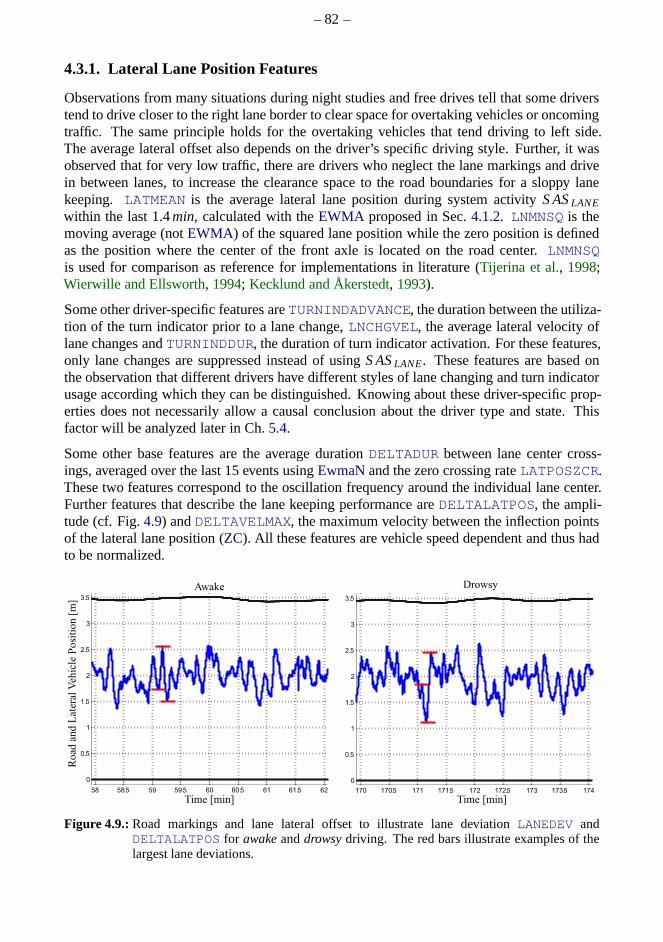
– 82 –

4.3.1. Lateral Lane Position Features

Observations from many situations during night studies andfree drives tell that some driverstend to drive closer to the right lane border to clear space for overtaking vehicles or oncomingtraffic. The same principle holds for the overtaking vehicles that tend driving to left side.The average lateral offset also depends on the driver’s specific driving style. Further, it wasobserved that for very low traffic, there are drivers who neglect the lane markings and drivein between lanes, to increase the clearance space to the roadboundaries for a sloppy lanekeeping. LATMEAN is the average lateral lane position during system activityS ASLANE

within the last 1.4min, calculated with theEWMA proposed in Sec.4.1.2. LNMNSQ is themoving average (notEWMA) of the squared lane position while the zero position is definedas the position where the center of the front axle is located on the road center.LNMNSQis used for comparison as reference for implementations in literature (Tijerina et al., 1998;Wierwille and Ellsworth, 1994; Kecklund and Åkerstedt, 1993).

Some other driver-specific features areTURNINDADVANCE, the duration between the utiliza-tion of the turn indicator prior to a lane change,LNCHGVEL, the average lateral velocity oflane changes andTURNINDDUR, the duration of turn indicator activation. For these features,only lane changes are suppressed instead of usingS ASLANE. These features are based onthe observation that different drivers have different styles of lane changing and turn indicatorusage according which they can be distinguished. Knowing about these driver-specific prop-erties does not necessarily allow a causal conclusion aboutthe driver type and state. Thisfactor will be analyzed later in Ch.5.4.

Some other base features are the average durationDELTADUR between lane center cross-ings, averaged over the last 15 events usingEwmaNand the zero crossing rateLATPOSZCR.These two features correspond to the oscillation frequencyaround the individual lane center.Further features that describe the lane keeping performance areDELTALATPOS, the ampli-tude (cf. Fig.4.9) andDELTAVELMAX, the maximum velocity between the inflection pointsof the lateral lane position (ZC). All these features are vehicle speed dependent and thus hadto be normalized.

Figure 4.9.:Road markings and lane lateral offset to illustrate lane deviation LANEDEV andDELTALATPOS for awakeanddrowsydriving. The red bars illustrate examples of thelargest lane deviations.

– 83 –

4.3.2. Lane Deviation (LANEDEV, LNIQR)

There is a large number of features associated with the vehicle’s deviation in the lane, as it isassumed that the driver-specific lane keeping becomes more sloppy with increasing fatigue(Kircher et al., 2002; Pilutti and Ulsoy, 1999; Bittner and Hana, 2000) and (seeAltmüller,2007, Ch. 4.2.3). During the test drives, it was observed that some awake drivers can alsohave a bad lane keeping depending on their mood.

The most essential features are implemented.LANEDEVmeasures the lane keeping deviationusing anEWVAR window of size 2min, while theS ASLANE is active. The often mentionedSDLPfeature (Tietze and Hargutt, 2001; Hargutt, 2001; Kircher et al., 2002; Thiffault andBergeron, 2003; Altmüller, 2007; Liu et al., 2009; Mets et al., 2011) is basically the same and,thus, not implemented. The lateral mean was observed to be driver-dependent and, thus, issubtracted before the variance is calculated. Simple variants ofLANEDEV are used asgroundtruth for distraction in many studies with driving simulator data(Greschner, 2011). In fact,it is a simple measure for driving performance, but it cannotbe completely transfered fromsimulator to real world driving. Fig.4.9 depicts an example of how the variance increaseswith increasing fatigue.LANEDEVSQ andLANEDEV4 are obtained by taking the powerof two and four respectively, as proposed byWierwille and Ellsworth(1994); Kircher et al.(2002), to stronger weight large deviations from the driver’s average.LANEDEVBL is simplythe baselined version ofLANEDEV, i.e. it is normalized by itsmaxvalue between the 1st

and 20st minute. LNIQR is the interquartile range (IQR) of the lateral position within thelast two minutes. In comparison to the variance, the IQR doesnot take outliers into accountand thus focuses more on the degradation of the small lane deviations. Again, the driver-dependent lateral offset had to be compensated. However, parameter optimization has shownthat exponential weighting of the lateral position performed best. This allows the conclusionthat large lane deviation events are more significant signs for fatigue than small deviations.

4.3.3. Over-Run Area (ORA)

The Over Run AreaORA is another deviation measure that senses the average overriddensurface and is an alternative toLANEDEV. Details can be found in the thesis of (Olabe, 2008)and in literature (Löfgren, 2007; Wigh, 2007). Fig.4.10illustrates the ORA measure. For the

Figure 4.10.:Over Run Area (ORA) as measure for lane deviation

calculation, the lateral offset is subtracted and the absolute value is averaged over anEwmaNwindow of 3min, while S ASLANE is active.

4.3.4. Unintended Lane Approximation (LANEAPPROX, VEZ etc.)

LANEAPPROX is a feature that describes the number of times any part of thevehicle isentering a proximity-zone of the lane bounds.LANEAPPROXADAPT is basically the same,however using an adaptive, driver dependent zone.

– 84 –

Kozak and Pohl(2006) andWigh (2007, 2.1) defined in their thesesVEZ as a zone whichfocuses on a lane approaching pattern, illustrated in Fig.4.11and comparable toTLC1MIN.The latter uses a driver adaptive zone size, which can be interpreted as an ‘almost’ lanedeparture. The advantage is that these departures occur much more often than real lanedepartures and, thus, allow a higher temporal resolution. Unintended lane departures aresuppressed if the driver steers towards the lane or acc-/decelerates (Schmitz, 2004). Differentweightings for curves and lane types have shown to be practical. It was observed that somedrivers almost never exit the lane boundaries, whereas others have over 50 lane exits per hour.Thus, it is proposed to adapt theALDW warning sensibility to the driver state.

dtdl

V2Z

Figure 4.11.:Unintended lane approaches with intensitydl and durationdt

4.3.5. Unintended Lane Exceeding (LANEX, LNERRSQ)

The heuristic of distinguishing intended and unintended lane exceedances is discussed in(Schmidt, 2009) and also in the lane change detection (Sec.4.1.5).

For some drivers, lane departure warningsLANEX andVIBPROP have been observed to bevery helpful features during the onset of drowsiness.LANEX, LNERRSQ andVIBPROP arebased on the intensity and frequency of lane departures and road exits (Wierwille, 1996b;Mattsson, 2007). Lane departures are defined as exceeding of a dashed road marking, whileroad exits describe the exceeding of solid road markings.LNERRSQ is the mean squareddifference between the outer vehicle dimensions that exceed the lane marking. In contrast toVIBPROP, LANEX takes the intensity into account as shown in Fig.4.12. The warnings areaveraged by anEWMA filter with window sizePVibpropEwmaWinS ize= 4min.

Figure 4.12.:Lane exceedances for intensitydl and durationdt

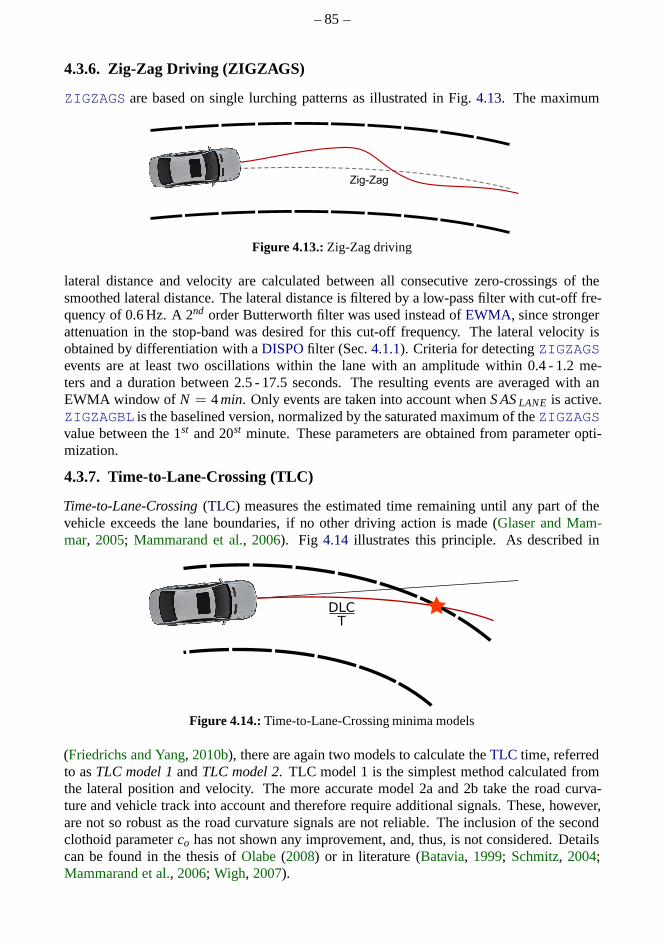
– 85 –

4.3.6. Zig-Zag Driving (ZIGZAGS)

ZIGZAGS are based on single lurching patterns as illustrated in Fig.4.13. The maximum

Zig-Zag

Figure 4.13.:Zig-Zag driving

lateral distance and velocity are calculated between all consecutive zero-crossings of thesmoothed lateral distance. The lateral distance is filteredby a low-pass filter with cut-off fre-quency of 0.6 Hz. A 2nd order Butterworth filter was used instead ofEWMA, since strongerattenuation in the stop-band was desired for this cut-off frequency. The lateral velocity isobtained by differentiation with aDISPOfilter (Sec.4.1.1). Criteria for detectingZIGZAGSevents are at least two oscillations within the lane with an amplitude within 0.4 - 1.2 me-ters and a duration between 2.5 - 17.5 seconds. The resultingevents are averaged with anEWMA window of N = 4min. Only events are taken into account whenS ASLANE is active.ZIGZAGBL is the baselined version, normalized by the saturated maximum of theZIGZAGSvalue between the 1st and 20st minute. These parameters are obtained from parameter opti-mization.

4.3.7. Time-to-Lane-Crossing (TLC)

Time-to-Lane-Crossing(TLC) measures the estimated time remaining until any part of thevehicle exceeds the lane boundaries, if no other driving action is made (Glaser and Mam-mar, 2005; Mammarand et al., 2006). Fig 4.14 illustrates this principle. As described in

Figure 4.14.:Time-to-Lane-Crossing minima models

(Friedrichs and Yang, 2010b), there are again two models to calculate theTLC time, referredto asTLC model 1andTLC model 2. TLC model 1 is the simplest method calculated fromthe lateral position and velocity. The more accurate model 2a and 2b take the road curva-ture and vehicle track into account and therefore require additional signals. These, however,are not so robust as the road curvature signals are not reliable. The inclusion of the secondclothoid parameterco has not shown any improvement, and, thus, is not considered.Detailscan be found in the thesis ofOlabe(2008) or in literature (Batavia, 1999; Schmitz, 2004;Mammarand et al., 2006; Wigh, 2007).

– 86 –

TLC Model 1

The TLC duration can simply be calculated from the lateral distance to the left or right laneedgeyl,r and lateral velocityyL by

TLC1 =yl,r

yL. (4.20)

TLC Model 2

TLC Model 2 is the more detailed model that, however, requires more signals and, thus,is less robust. There are several variants to implement thismodel. However the definitiondescribed in the theses ofOlabe(2008) andWigh (2007) is used.

This definition is based on two models: thevehicle path modeland theroad model. The vehi-cle path model describes the future path of the vehicle if themotion parameters as the currentyaw-angle would not change. The road model describes the road curvature ahead, based onthe road characteristics obtained by the lane tracking camera. The intersection point of bothtrajectories describes the distance at which the vehicle will cross the lane boundaries.

Vehicle Path Model: There are two models described in (Wigh, 2007), whereof the sec-ond, more detailed model is used here. Taking the yaw angle∆ψ between road and vehicle(LaneYawAnglfrom Tab.A.2) and the curvature of vehicle pathκc = 1

R into account, yieldsEq. (4.21) for the vehicle path model, wherey0 is the lateral distance,θ the angle against thelane marking andd is the distance in driving direction:

yveh(d) = y0 + θ · d+12· κc · d2 (4.21)

The radiusR is obtained from Eq. (6.3) of the single track model described in Ch.6.3.

Eq. (4.21) describes the center line of the future vehicle trajectory. Taking the vehicle widthwv into account, the left and right vehicle edges are obtained by:

yveh,l(d) = +wv

2+ y0 + θ · d+

12· κc · d2 (4.22)

yveh,r (d) = −wv

2+ y0 + θ · d+

12· κc · d2 .

Road Model: Road sections can be modeled by clothoids. Using the mathematical sim-plifications from Wigh (2007), the driven distances and clothoid parametersc0 and c1

(LaneClothoidParafrom Tab.A.2), the center line of the road can be formulated in x- andy-coordinates by:

x(d) = x0 + d (4.23)

y(d) = y0 +12· c0 · d2 +

16· c1 · d3

x0 andy0 are the starting positions of the vehicle and can be set to zero.

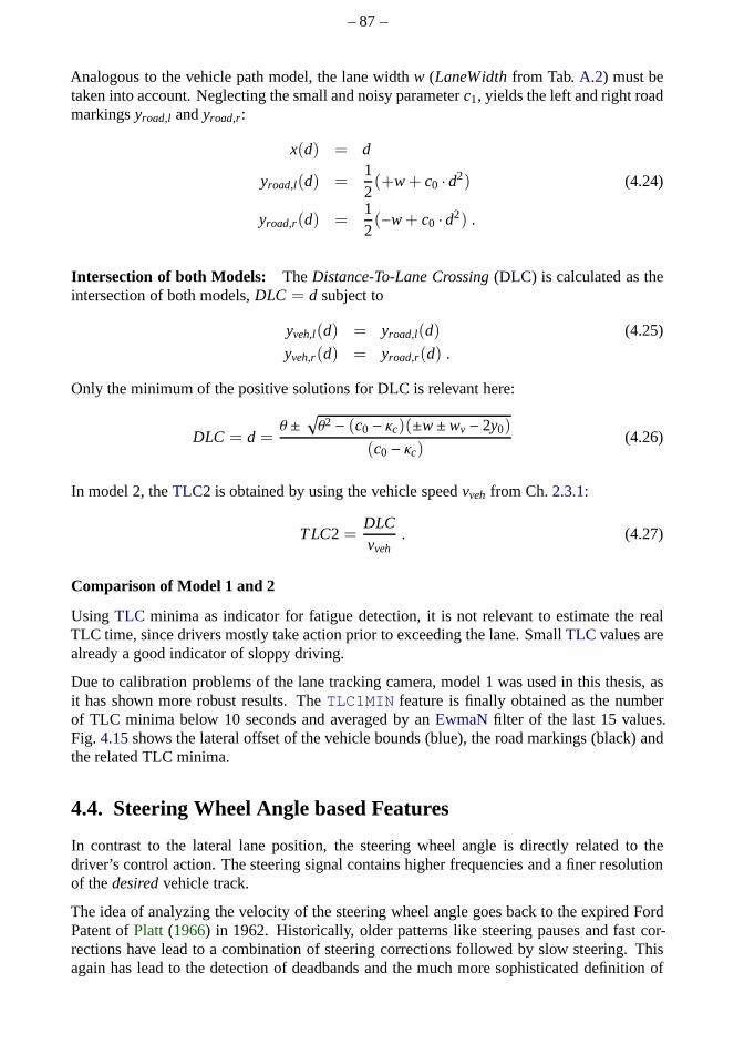
– 87 –

Analogous to the vehicle path model, the lane widthw (LaneWidthfrom Tab.A.2) must betaken into account. Neglecting the small and noisy parameter c1, yields the left and right roadmarkingsyroad,l andyroad,r :

x(d) = d

yroad,l(d) =12(+w+ c0 · d2) (4.24)

yroad,r(d) =12(−w+ c0 · d2) .

Intersection of both Models: TheDistance-To-Lane Crossing(DLC) is calculated as theintersection of both models,DLC = d subject to

yveh,l(d) = yroad,l(d) (4.25)

yveh,r (d) = yroad,r(d) .

Only the minimum of the positive solutions for DLC is relevant here:

DLC = d =θ ±

√

θ2 − (c0 − κc)(±w±wv − 2y0)

(c0 − κc)(4.26)

In model 2, theTLC2 is obtained by using the vehicle speedvveh from Ch.2.3.1:

TLC2 =DLCvveh

. (4.27)

Comparison of Model 1 and 2

Using TLC minima as indicator for fatigue detection, it is not relevant to estimate the realTLC time, since drivers mostly take action prior to exceeding the lane. SmallTLC values arealready a good indicator of sloppy driving.

Due to calibration problems of the lane tracking camera, model 1 was used in this thesis, asit has shown more robust results. TheTLC1MIN feature is finally obtained as the numberof TLC minima below 10 seconds and averaged by anEwmaNfilter of the last 15 values.Fig. 4.15shows the lateral offset of the vehicle bounds (blue), the road markings (black) andthe related TLC minima.

4.4. Steering Wheel Angle based Features

In contrast to the lateral lane position, the steering wheelangle is directly related to thedriver’s control action. The steering signal contains higher frequencies and a finer resolutionof thedesiredvehicle track.

The idea of analyzing the velocity of the steering wheel angle goes back to the expired FordPatent ofPlatt (1966) in 1962. Historically, older patterns like steering pauses and fast cor-rections have lead to a combination of steering correctionsfollowed by slow steering. Thisagain has lead to the detection of deadbands and the much moresophisticated definition of

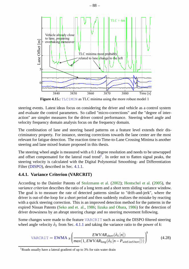
– 88 –

Figure 4.15.:TLC1MIN as TLC minima using the more robust model 1

steering events. Latest ideas focus on considering the driver and vehicle as a control systemand evaluate the control parameters. So called "micro-corrections" and the "degree of inter-action" are simpler measures for the driver control performance. Steering wheel angle andvelocity frequency domain analysis focus on the frequency domain.

The combination of lane and steering based patterns on a feature level extends their dis-criminatory property. For instance, steering correctionstowards the lane center are the mostrelevant for fatigue detection. The reaction time to Time-to-Lane Crossing Minima is anothersteering and lane mixed feature proposed in this thesis.

The steering wheel angle is measured with a 0.1 degree resolution and needs to be unwrappedand offset compensated for the lateral road trend1. In order not to flatten signal peaks, thesteering velocity is calculated with the Digital Polynomial Smoothing- and DifferentiationFilter (DISPO), described in Sec.4.1.1.

4.4.1. Variance Criterion (VARCRIT)

According to the Daimler Patents ofStolzmann et al.(2002); Hentschel et al.(2005), thevariance criteriondescribes the ratio of a long term and a short term sliding variance window.The goal is to measure the rate of detected patterns similar to "drift-and-jerk", where thedriver is out-of-the-loop for a short period and then suddenly realizes the mistake by reactingwith a quick steering correction. This is an improved detection method for the patterns in theexpired Nissan Patents (Seko and et. al., 1986; Iizuka and Obara, 1986) for the detection ofdriver drowsiness by an abrupt steering change and no steering movement following.

Some changes were made to the featureVARCRIT such as using the DISPO filtered steeringwheel angle velocityδS from Sec.4.1.1and taking the variance ratio to the power ofk:

VARCRIT = EWMA N

EWVARshort(δS[n])

max(1,EWVARlong(δS[n− PwinS izeS hort]))

k

(4.28)

1Roads usually have a lateral gradient of up to 3% for rain water drain

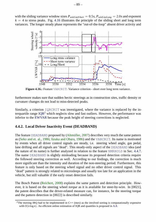
– 89 –

with the sliding variance window sizesPwinS izeS hort= 0.5s, PwinS izeLong= 2.0sand exponentk = 4 to stress peaks. Fig.4.16 illustrates the principle of the sliding short and long termvariances. The longer steady phase represents the "out-of-the-loop" absent driver activity and

Ste

erin

g w

hee

l

v4578:;=?°@BC

DHIJK?°@BC

MNOQ SUXY [\X]\O^U

`ime [s]

MNOQaefNXSShort term var]\O^U

3558355635543552355035480

5

10

15hi

hj

hk

hl

0

Figure 4.16.:FeatureVARCRIT: Variance criterion - short over long term variance.

furthermore makes sure that sudden hectic steerings as in construction sites, traffic density orcurvature changes do not lead to miss-detected peaks.

Similarly, a criterionIQRCRIT was investigated, where the variance is replaced by the in-terquartile rangeIQR2 which neglects slow and fast outliers. However, the performance wasinferior to theEWVAR because the peak height of steering corrections is neglected.

4.4.2. Local Driver Inactivity Event (DEADBAND)

The featureDEADBAND proposed by (Altmüller, 2007) describes very much the same patternas (Seko and et. al., 1986; Iizuka and Obara, 1986) and theVARCRIT. Its name is motivatedby events when all driver control signals are steady, i.e. steering wheel angle, gas pedal,lane drifting and all signals are "dead". This steady-only aspect of theDEADBAND idea (andthe nature of its name) is further analyzed in relation to thefeatureNMRHOLD in Sec.4.4.7.The nameDEADBAND is slightly misleading because its proposed detection criteria requirethe followed steering correction as well. According to our findings, the correction is muchmore significant than the intensity and duration of the non-steering period. Furthermore, thisfeature is only based on the steering wheel signal and no other driver control signal. This"dead" pattern is strongly related to microsleeps and usually too late for an application in thevehicle, but still valuable if the early onset detection fails.

The Bosch Patent (Reichert, 2008) explains the same pattern and detection principle. How-ever, it is based on the steering wheeltorqueas it is available for steer-by-wire. In [0021],the patent describes that the driver-related measure can, for instance, be the steering torqueand the pattern detection in [0022] is described similarly.

2The moving IRQ had to be implemented in C++ (mex) as the involved sorting is computationally expensivewith O(n logn). An efficient online estimation of IQR and quantiles is proposed inA.8.

– 90 –

Since the detection of the steering eventsSTWEVNTwas extensively investigated and focuseson the same pattern asDEADBAND, STWEVNT was used. Own findings show that some ofthe here presented additional criteria show more robustness for real-road drives.

4.4.3. Steering Events (STWEVENT)

As described in the Patent ofGalley et al.(2006), the method to extract the featureSTWEVNTfocuses on a steering inactivity phase and a subsequent steering action. Therefore, the steer-ing wheel velocity should not exceed a certain threshold fora minimum time and then exceeda second threshold. The thresholds are adaptive to driver and driving situations. Detectedevents are weighted by their intensity and by a factor that increases in monotonous situationsand a factor that is speed dependent with its maximum at 80 km/h. The events are averagedusing anEWMA filter. As explained in Sec.4.1.3, various situations are detected to suppresssteering corrections due to short-term distraction. External influences by cross-wind, roadwarping, road bumps and curves are suppressed as well as overtaking and sportive driving.

Driver-Adaptive Thresholds

STVmax (δS,max) is the maximum steering velocity between inflection points(i.e. zero cross-ings) of the steering wheel velocityδS while S ASCAN is active. Parameter study yielded thatsteering wheel angleδS of steering events has to exceed 0.898 to neglect noise and tomakesure that the steering amplitude is relevant and observableby the driver. This is illustratedin Fig. 4.17 in which the inactive (−) and activeδS,max (−) are averaged usingEwmaN, asdescribed in Eq.4.29 that is only updated on events and hold otherwise. TheEwmaNisinitialized bySTV50[0..4] = 10.5/s with a window size ofNinit = 5 that is increased byone up toN = 110 for every steering. Fig.4.17further illustrates the estimation ofSTV25

Figure 4.17.:Estimation ofSTV50 as the mean ofδS,max andSTV25 andSTV75 as the means ofthe corrections slower and faster thanSTV50.

andSTV75 by Mean Splittingaccording to the calculation in Eq.4.31 and Eq.4.31 withSTV75[0..5] = 7/s andSTV75[0..5] = 13/s. STV25 is the mean of the slow steeringcorrections andSTV75 the mean for all fast steering corrections.

STV50 = EwmaNN(δS,max) . (4.29)

The computation is only evaluated during steering wheel angle reversals.

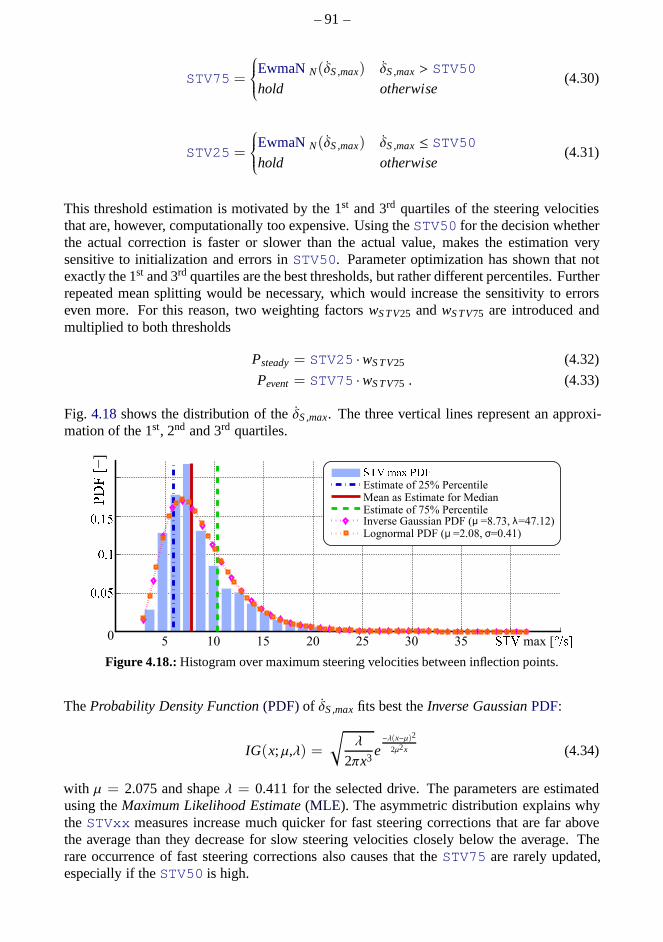
– 91 –

STV75 =

EwmaNN(δS,max) δS,max> STV50

hold otherwise(4.30)

STV25 =

EwmaNN(δS,max) δS,max≤ STV50hold otherwise

(4.31)

This threshold estimation is motivated by the 1st and 3rd quartiles of the steering velocitiesthat are, however, computationally too expensive. Using theSTV50 for the decision whetherthe actual correction is faster or slower than the actual value, makes the estimation verysensitive to initialization and errors inSTV50. Parameter optimization has shown that notexactly the 1st and 3rd quartiles are the best thresholds, but rather different percentiles. Furtherrepeated mean splitting would be necessary, which would increase the sensitivity to errorseven more. For this reason, two weighting factorswS TV25 andwS TV75 are introduced andmultiplied to both thresholds

Psteady= STV25 ·wS TV25 (4.32)

Pevent= STV75 ·wS TV75 . (4.33)

Fig. 4.18shows the distribution of theδS,max. The three vertical lines represent an approxi-mation of the 1st, 2nd and 3rd quartiles.

mop max [rtuw

xyz −

]

300 5 10 15 20 25 35

µ λ

||~

|

|~

Estimate of 25% PercentileMean as Estimate for MedianEstimate of 75% PercentileInverse Gaussian PDF ( =8.73, =47.12)Lognormal PDF ( =2.08, =0.41)µ σ

Figure 4.18.:Histogram over maximum steering velocities between inflection points.

TheProbability Density Function(PDF)of δS,max fits best theInverse GaussianPDF:

IG(x; µ,λ) =

√

λ

2πx3e−λ(x−µ)2

2µ2x (4.34)

with µ = 2.075 and shapeλ = 0.411 for the selected drive. The parameters are estimatedusing theMaximum Likelihood Estimate(MLE). The asymmetric distribution explains whytheSTVxx measures increase much quicker for fast steering corrections that are far abovethe average than they decrease for slow steering velocitiesclosely below the average. Therare occurrence of fast steering corrections also causes that theSTV75 are rarely updated,especially if theSTV50 is high.

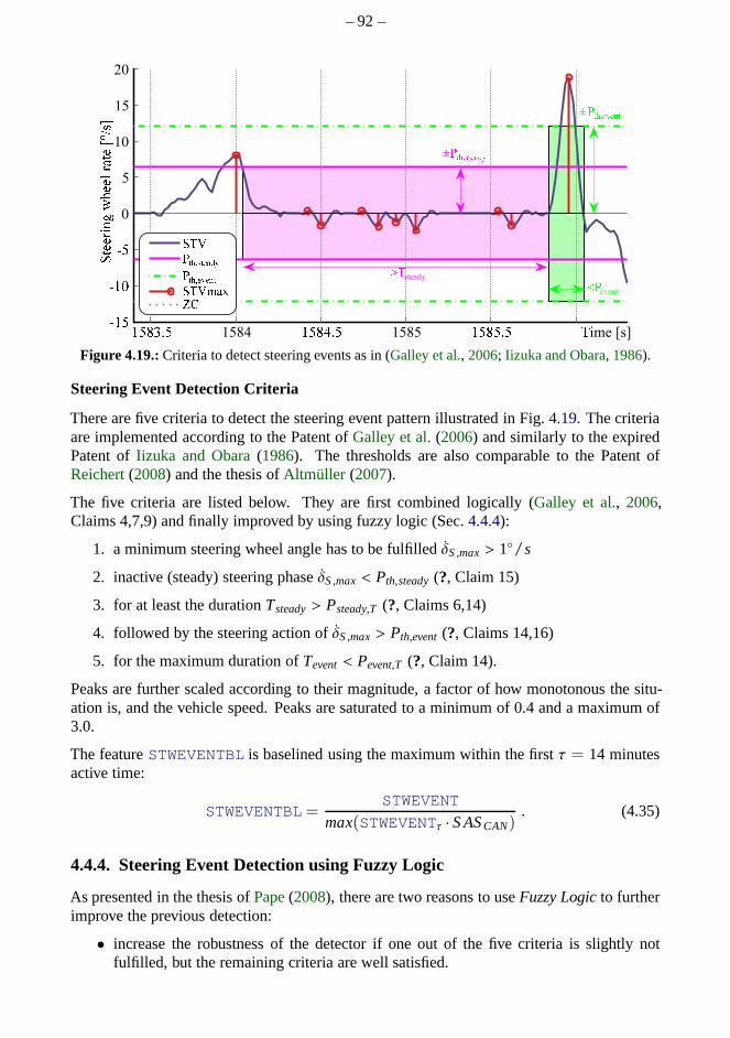
– 92 –

±

±

ime [s] 15851584

¡¢

¡¢

£steady

¤event

0

5

10

15

20

¥

¥¦

¥

§¨©©ª«¬­®¯©©±ª²¨©³´µ¶·

Figure 4.19.:Criteria to detect steering events as in (Galley et al., 2006; Iizuka and Obara, 1986).

Steering Event Detection Criteria

There are five criteria to detect the steering event pattern illustrated in Fig.4.19. The criteriaare implemented according to the Patent ofGalley et al.(2006) and similarly to the expiredPatent ofIizuka and Obara(1986). The thresholds are also comparable to the Patent ofReichert(2008) and the thesis ofAltmüller (2007).

The five criteria are listed below. They are first combined logically (Galley et al., 2006,Claims 4,7,9) and finally improved by using fuzzy logic (Sec.4.4.4):

1. a minimum steering wheel angle has to be fulfilledδS,max> 1/s

2. inactive (steady) steering phaseδS,max< Pth,steady(?, Claim 15)

3. for at least the durationTsteady> Psteady,T (?, Claims 6,14)

4. followed by the steering action ofδS,max> Pth,event(?, Claims 14,16)

5. for the maximum duration ofTevent< Pevent,T (?, Claim 14).

Peaks are further scaled according to their magnitude, a factor of how monotonous the situ-ation is, and the vehicle speed. Peaks are saturated to a minimum of 0.4 and a maximum of3.0.

The featureSTWEVENTBL is baselined using the maximum within the firstτ = 14 minutesactive time:

STWEVENTBL=STWEVENT

max(STWEVENTτ · S ASCAN). (4.35)

4.4.4. Steering Event Detection using Fuzzy Logic

As presented in the thesis ofPape(2008), there are two reasons to useFuzzy Logicto furtherimprove the previous detection:

• increase the robustness of the detector if one out of the five criteria is slightly notfulfilled, but the remaining criteria are well satisfied.

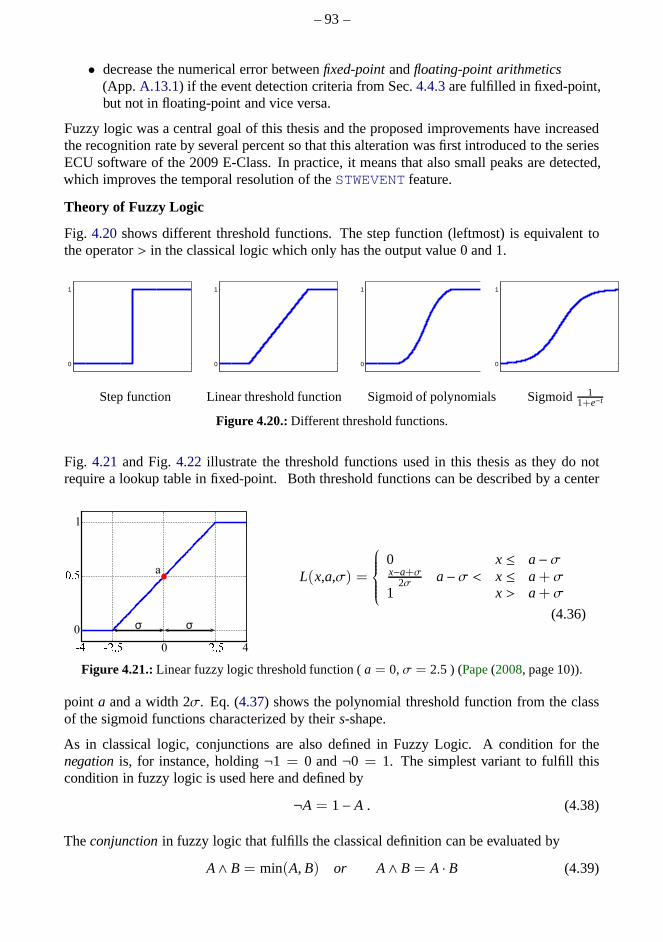
– 93 –

• decrease the numerical error betweenfixed-pointandfloating-point arithmetics(App. A.13.1) if the event detection criteria from Sec.4.4.3are fulfilled in fixed-point,but not in floating-point and vice versa.

Fuzzy logic was a central goal of this thesis and the proposedimprovements have increasedthe recognition rate by several percent so that this alteration was first introduced to the seriesECU software of the 2009 E-Class. In practice, it means that also small peaks are detected,which improves the temporal resolution of theSTWEVENT feature.

Theory of Fuzzy Logic

Fig. 4.20shows different threshold functions. The step function (leftmost) is equivalent tothe operator> in the classical logic which only has the output value 0 and 1.

0

1

0

1

0

1

0

1

Step function Linear threshold function Sigmoid of polynomials Sigmoid 11+e−t

Figure 4.20.:Different threshold functions.

Fig. 4.21 and Fig.4.22 illustrate the threshold functions used in this thesis as they do notrequire a lookup table in fixed-point. Both threshold functions can be described by a center

1

¸¹º

0

a

0»¼ »½¹º ½¹º 4

L(x,a,σ) =

0 x ≤ a−σx−a+σ

2σ a−σ < x ≤ a+ σ

1 x > a+ σ

(4.36)

Figure 4.21.:Linear fuzzy logic threshold function (a = 0,σ = 2.5 ) (Pape(2008, page 10)).

point a and a width 2σ. Eq. (4.37) shows the polynomial threshold function from the classof the sigmoid functions characterized by theirs-shape.

As in classical logic, conjunctions are also defined in FuzzyLogic. A condition for thenegationis, for instance, holding¬1 = 0 and¬0 = 1. The simplest variant to fulfill thiscondition in fuzzy logic is used here and defined by

¬A = 1− A . (4.38)

Theconjunctionin fuzzy logic that fulfills the classical definition can be evaluated by

A∧ B = min(A, B) or A∧ B = A · B (4.39)

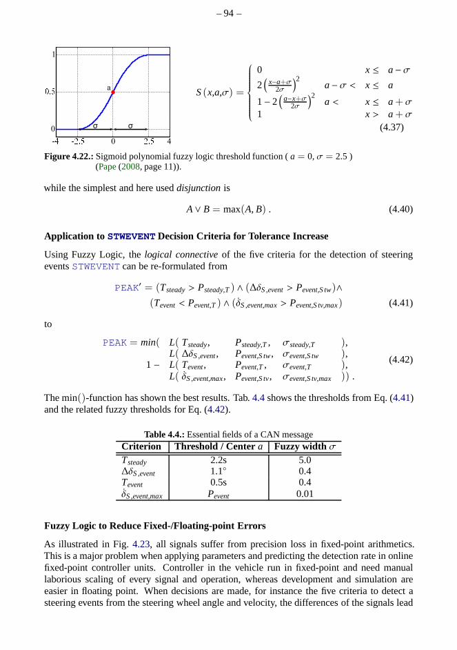
– 94 –

1

¾¿À

0

a

0Á ÁÿÀ ÿÀ 4

S(x,a,σ) =

0 x ≤ a−σ2(

x−a+σ2σ

)2a−σ < x ≤ a

1− 2(

a−x+σ2σ

)2a < x ≤ a+σ

1 x > a+σ

(4.37)

Figure 4.22.:Sigmoid polynomial fuzzy logic threshold function (a = 0,σ = 2.5 )(Pape(2008, page 11)).

while the simplest and here useddisjunctionis

A∨ B = max(A, B) . (4.40)

Application to STWEVENTDecision Criteria for Tolerance Increase

Using Fuzzy Logic, thelogical connectiveof the five criteria for the detection of steeringeventsSTWEVENT can be re-formulated from

PEAK′ = (Tsteady> Psteady,T ) ∧ (∆δS,event> Pevent,S tw)∧(Tevent< Pevent,T ) ∧ (δS,event,max> Pevent,S tv,max) (4.41)

to

PEAK = min( L( Tsteady, Psteady,T , σsteady,T ),L( ∆δS,event, Pevent,S tw, σevent,S tw ),

1 − L( Tevent, Pevent,T , σevent,T ),L( δS,event,max, Pevent,S tv, σevent,S tv,max )) .

(4.42)

The min()-function has shown the best results. Tab.4.4shows the thresholds from Eq. (4.41)and the related fuzzy thresholds for Eq. (4.42).

Table 4.4.:Essential fields of a CAN messageCriterion Threshold / Centera Fuzzy width σTsteady 2.2s 5.0∆δS,event 1.1 0.4Tevent 0.5s 0.4δS,event,max Pevent 0.01

Fuzzy Logic to Reduce Fixed-/Floating-point Errors

As illustrated in Fig.4.23, all signals suffer from precision loss in fixed-point arithmetics.This is a major problem when applying parameters and predicting the detection rate in onlinefixed-point controller units. Controller in the vehicle runin fixed-point and need manuallaborious scaling of every signal and operation, whereas development and simulation areeasier in floating point. When decisions are made, for instance the five criteria to detect asteering events from the steering wheel angle and velocity,the differences of the signals lead

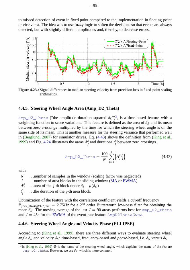
– 95 –

to missed detection of event in fixed point compared to the implementation in floating-pointor vice versa. The idea was to use fuzzy logic to soften the decisions so that events are alwaysdetected, but with slightly different amplitudes and, thereby, to decrease errors.

ÄÅÆ Çime [h]2ÄÅÈÈÅÆ0

Med

ian s

tÉÉÊËÌÍÎÉÏÐÑËÒ y

[

ÓÔÕÖ

8

×ÅÆ

9

ØÅÆ

10

ÄÈÅÆ

11

ÙÚÛÜÝÞßàá−Point

ÙÚÛÜ Floating−Point

Figure 4.23.:Signal differences in median steering velocity from precision loss in fixed-point scalingarithmetics.

4.4.5. Steering Wheel Angle Area (Amp_D2_Theta)

Amp_D2_Theta ("the amplitude duration squaredδS")3, is a time-based feature with aweighting function to score variations. This feature is defined as the area ofδS and its meanbetweenzero crossingsmultiplied by the time for which the steering wheel angle is on thesame side of its mean. This is another measure for the steering variance that performed wellin (Berglund, 2007) for simulator drives. Eq. (4.43) shows the definition from (King et al.,1999) and Fig.4.24illustrates the areasAδj and durationstδj between zero crossings.

Amp_D2_Theta=100N

J∑

j=1

(

Aδj tδj

)

(4.43)

with

N . . .number of samples in the window (scaling factor was neglected)J . . .number of area blocks in the sliding window (MA or EWMA)Aδj . . .area of thej-th block underδS − µ(δS)

tδj . . .the duration of thej-th area block.

Optimization of the feature with the correlation coefficient yields a cut-off frequencyPfCut_stwAngleO f f set= 2.75Hz for a 2nd order Butterworth low-pass filter for obtaining themeanδS. The moving average of the lastJ = 90 areas performs best forAmp_D2_ThetaandJ = 45s for theEWMA of the event-rate featureAmpD2ThetaEwma.

4.4.6. Steering Wheel Angle and Velocity Phase (ELLIPSE)

According to (King et al., 1999), there are three different ways to evaluate steering wheelangleδS and velocityδS: time-based, frequency-based andphase-based, i.e.δS versusδS.

3In (King et al., 1999) Θ is the name of the steering wheel angle, which explains the name of the featureAmp_D2_Theta. However, we useδS, which is more common.

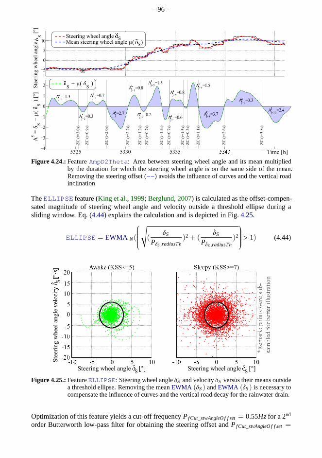
– 96 –

−4

−3

−2

−1

0

1

2

Aj−3

â =1.3

Aj−2

â =0.3

Aj−1

â =0.7

Aj

â=2.7

Aj+1

â =0.8

A

ã

= ä

S−

µ(

ä S)

[°]

−5

0

5

10

Time [h]

Ste

erin

g w

hee

l an

gle

[°

]å

S

æçèé533553305325

êS

− µ( êS

)Z

C (

t=3

.0s)

ZC

(t=

0.9

s)

ZC

(t=

2.0

s)

ZC

(t=

2.2

s)

ZC

(t=

1.2

s)

ZC

(t=

0.7

s)

ZC

(t=

1.5

s)

ZC

(t=

0.7

s)

ZC

(t=

1.5

s)

ZC

(t=

0.3

s)

ZC

(t=

1.1

s)

ZC

(t=

2.6

s)

ZC

(t=

3.8

s)

Steering wheel angle Mean steering wheel angle

ëSµ( ì )S

j+3Aí =1.5

Aj+5

í =0.8

j+9Aí =3.3

Aj+2

í =0.2A

j+îí =0.6

Aj+8

í =3.7A

j+10

í =2.ï

Aj+7

í =1.5

Figure 4.24.:FeatureAmpD2Theta: Area between steering wheel angle and its mean multipliedby the duration for which the steering wheel angle is on the same side of the mean.Removing the steering offset (−−) avoids the influence of curves and the vertical roadinclination.

TheELLIPSE feature (King et al., 1999; Berglund, 2007) is calculated as the offset-compen-sated magnitude of steering wheel angle and velocity outside a threshold ellipse during asliding window. Eq. (4.44) explains the calculation and is depicted in Fig.4.25.

ELLIPSE = EWMA N(

√

(δS

PδS,radiusTh)2 + (

δS

PδS,radiusTh)2

> 1) (4.44)

ðS

Steering wheel angle [°]

ñòóôõö÷øùúûüýþÿóöóþ*

þõôùsóúöóýýóöû ss u

stra

tion

- - 0 5 10

ðS

Steering wheel angle °

- - 0 5 10-

0

Aw

-

-

-

5

10

15

20

SS

teer

ing

wh

eel

ang

le

! S"# $=7)

.

Figure 4.25.:FeatureELLIPSE: Steering wheel angleδS and velocityδS versus their means outsidea threshold ellipse. Removing the meanEWMA (δS) andEWMA (δS) is necessary tocompensate the influence of curves and the vertical road decay for the rainwater drain.

Optimization of this feature yields a cut-off frequencyPfCut_stwAngleO f f set= 0.55Hz for a 2nd

order Butterworth low-pass filter for obtaining the steering offset andPfCut_stvAngleO f f set=

– 97 –

0.125Hz for δS. TheEWMA window size isN = 60s. The steering ratio, angle and velocityare different for every vehicle, thus the optimal weightingfactors PδS,radiusTh = 3 andPδS,radiusTh= 6/sare different than in literature (King et al., 1999).

4.4.7. Steering Inactivity (NRMHOLD)

NMRHOLDwas defined by (Wierwille and Ellsworth, 1994) as the number of times for whichthe steering wheel angleδS is hold for longer than the threshold valuePNMRHOLDT = 400ms.According to (Berglund, 2007), the maximum threshold for|δS| was set toPmaxLrw = 0.5.An EWMA filter with PEwmaWinS ize= 5min is applied after suppression of system inactivityS ASCAN. Curves are removed similarly as forELLIPSE. Further, a second variant of the fea-ture, based on the SG-differentiator filtered steering velocity, is implementedNRMSTVHOLDwith the thresholdPmaxLrv= 6/s for |δS|.

4.4.8. Small Steering Adjustments (MICROCORRECTIONS)

The idea ofMICROCORRECTIONS (discussed inFagerberg, 2004) is that an alert driver per-manently makes small steering corrections to compensate environmental factors such as roadbumps and crosswinds. With increasing drowsiness, driversbecome more sloppy and thesemicro-corrections diminish (Petit and Chaput, 1990; Hartley, 1995). According toKircheret al.(2002), the after-market device "Steering Attention Monitor" (SAM) monitors the pres-ence of micro-steerings.

Extending this concept, the presence of many small micro-corrections leads to low valuesof this feature, whereas rare and larger corrections yield high feature values. The featureextraction is updated for every steering wheel angle direction change interval by:

MICROCORRECTIONS=

EWMA (0) PS TW,Th,Min ≤ ∆δS,event≤ PS TW,Th,Max

EWMA (1) S ASCAN = 1

"hold" S ASCAN = 0

. (4.45)

For every interval, the magnitude between inflection pointsis calculated as∆δS,event. Any-time the steering amplitude∆δS,eventis betweenPS TW,Th,Min = 0.8 andPS TW,Th,Max = 2.5,a microsteering is detected and 0 is fed into theEWMA window with lengthN = 0.7min.Otherwise, if the system is active but no microsteering is detected, the feature increases byadding a 1 to theEWMA window. For an inactive system, the calculation is hold.

4.4.9. Fast Corrections (FASTCORRECT)

FASTCORRECT is a feature that is proposed here. It is focusing on a patternthat was oftenobserved in night drives. The pattern is basically the same as inSTWEVENT, however, focus-ing more on single events and the steering correction phase,especially taking into accountits rate intensity. A single strong event can indicate an advanced fatigue level.

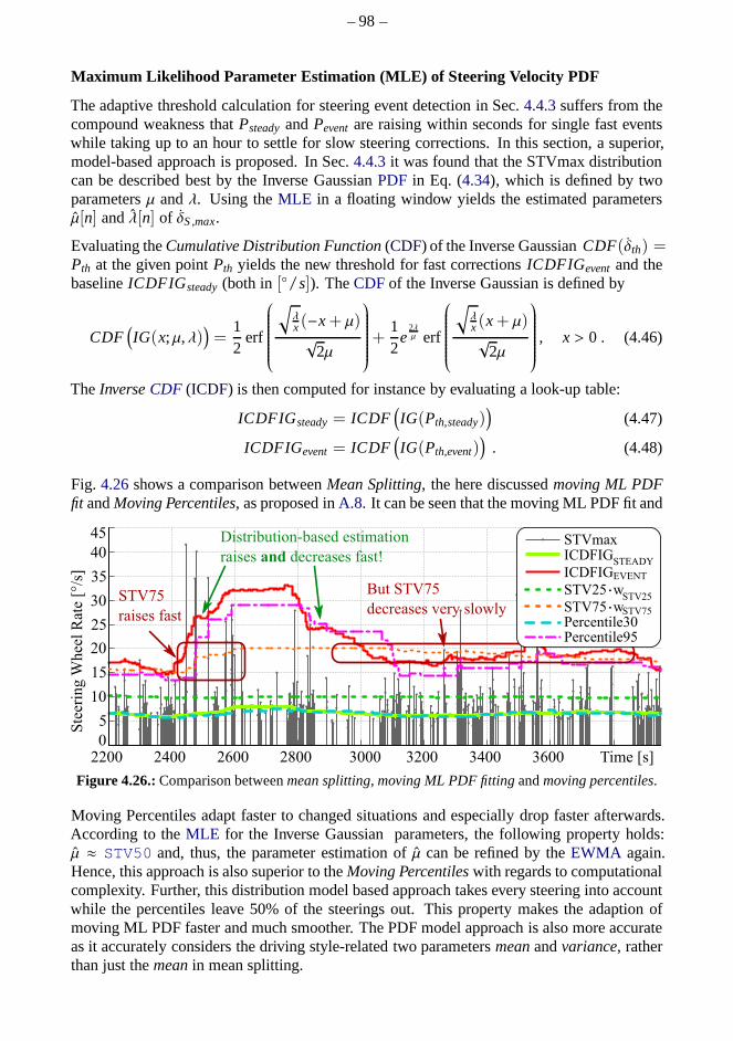
– 98 –

Maximum Likelihood Parameter Estimation (MLE) of Steering Velocity PDF

The adaptive threshold calculation for steering event detection in Sec.4.4.3suffers from thecompound weakness thatPsteadyandPevent are raising within seconds for single fast eventswhile taking up to an hour to settle for slow steering corrections. In this section, a superior,model-based approach is proposed. In Sec.4.4.3it was found that the STVmax distributioncan be described best by the Inverse GaussianPDF in Eq. (4.34), which is defined by twoparametersµ andλ. Using theMLE in a floating window yields the estimated parametersµ[n] andλ[n] of δS,max.

Evaluating theCumulative Distribution Function(CDF) of the Inverse GaussianCDF(δth) =Pth at the given pointPth yields the new threshold for fast correctionsICDFIGeventand thebaselineICDFIGsteady(both in [/s]). TheCDFof the Inverse Gaussian is defined by

CDF(

IG(x; µ,λ))

=12

erf

√

λx(−x+ µ)√

2µ

+12

e2λµ erf

√

λx(x+ µ)√

2µ

, x > 0 . (4.46)

TheInverseCDF (ICDF) is then computed for instance by evaluating a look-up table:

ICDFIGsteady= ICDF(

IG(Pth,steady))

(4.47)

ICDFIGevent= ICDF(

IG(Pth,event))

. (4.48)

Fig. 4.26shows a comparison betweenMean Splitting, the here discussedmoving ML PDFfit andMoving Percentiles, as proposed inA.8. It can be seen that the moving ML PDF fit and

Figure 4.26.:Comparison betweenmean splitting, moving ML PDF fittingandmoving percentiles.

Moving Percentiles adapt faster to changed situations and especially drop faster afterwards.According to theMLE for the Inverse Gaussian parameters, the following property holds:µ ≈ STV50 and, thus, the parameter estimation ofµ can be refined by theEWMA again.Hence, this approach is also superior to theMoving Percentileswith regards to computationalcomplexity. Further, this distribution model based approach takes every steering into accountwhile the percentiles leave 50% of the steerings out. This property makes the adaption ofmoving ML PDF faster and much smoother. The PDF model approach is also more accurateas it accurately considers the driving style-related two parametersmeanandvariance, ratherthan just themeanin mean splitting.

– 99 –

Feature Calculation using Fitted Sliding Window PDF as Adaptive Thresholds

For peak detection, we use the moving thresholdsICDFIGsteadyand ICDFIGeventobtainedby a sliding window of durationN = 2.4min. The parameter for the steering correctionthresholdICDFIGevent is set toPth,event = 0.98 to detect outliers of fast steering correc-tions that are above 98% of all regular steering reversals. The parameter of the baselineICDFIGsteady is found asPth,event = 0.30 to represent the calm steering in the actual driv-ing situation. The detected steering corrections are set inrelation to the steering baselineICDFIGsteadyin order to adapt to the current driving situation

FASTCORRECT=

EWMAN

(

(δS,max·S ASCAN

sat204 (ICDFIGsteady)

)Pw,exp

)

δS,max> ICDFIGevent

hold S ASCAN = 0. (4.49)

The event rate including the peak intensity is averaged by a small EWMA window size ofN = 3min. Weighting the peak by the exponentPw,exp =

12 allows to non-linearly adjust the

influence of the peak intensity in comparison to its frequency.

4.4.10. Degree of Driver-Vehicle Interaction (DEGOINT)

DEGOINT is originally defined as the degree of interaction between driver and vehicle ac-cording to the 2005 Patent by Eriksson and Björkman and is explained in (Kanstrup, 2006).The idea behind this feature is that the vehicle motion trajectory can be considered as a sys-tem with low-pass characteristics which reacts to steeringcontrol by the driver and to lateraldisplacements by the road surface. Steering oscillations with high frequency cannot be seenin the vehicle trajectory. From steer-by-wire, it is known that the feedback from the road hasto be provided to the driver via an actuator to enable a responsive steering control. High in-teraction means quick and precise control that indicates high driver vigilance and vice versa.DEGOINT is a simpler method to measure control parameters of a drivermodel discussed inSec.4.4.16. The original definition of (Kanstrup, 2006) is shown in Eq. (4.50)

DEGOINT′ =1

|∫

fa dt−∫

fb dt|) (4.50)

with fa as the surface under the steering wheel torque andfb under the lateral accelerationintegrated over time. It has to be remarked that both areas have different units and are notmotivated by an accurate physical model.

Since there was no steeringtorquesensor available in the series vehicles, a similar methodis proposed to obtainDEGOINT based on the steering wheelangle instead. Therefore, themeasuredlateral acceleration ay is compared to thelateral accelerationay calculated fromthesteering wheel angleδL using the single track model in Eq. (6.8) in Ch.6.3. This way, thesteering and vehicle trajectory interaction can be measured in a physically accurate model.The advantage of using the steering wheel torque, however, is that even when the steeringwheel angle is not changing, it can be measured how strong thedriver holds the steeringwheel against the feedback from the road.

ay anday are smoothed by a 2nd order Butterworth low-pass filter with corner frequencies 1and 2 Hz to compensate different sensor properties, resulting inay,LP anday,LP. For synchro-nization,ay,LP has to be delayed byτ = 280ms. And in order to compensate the lateral roadinclination offset, the difference of

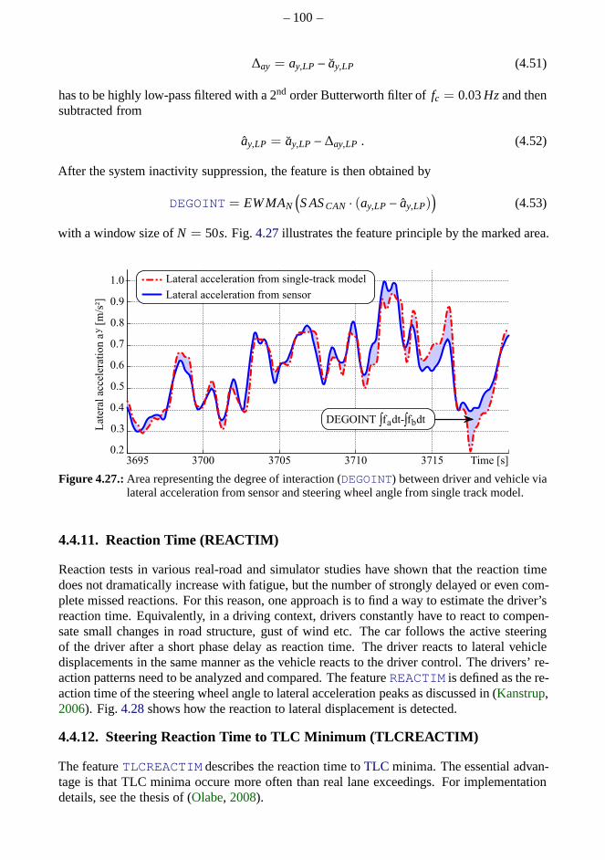
– 100–

∆ay = ay,LP − ay,LP (4.51)

has to be highly low-pass filtered with a 2nd order Butterworth filter offc = 0.03Hzand thensubtracted from

ay,LP = ay,LP −∆ay,LP . (4.52)

After the system inactivity suppression, the feature is then obtained by

DEGOINT = EWMAN

(

S ASCAN · (ay,LP − ay,LP))

(4.53)

with a window size ofN = 50s. Fig.4.27illustrates the feature principle by the marked area.

Figure 4.27.:Area representing the degree of interaction (DEGOINT) between driver and vehicle vialateral acceleration from sensor and steering wheel angle from single track model.

4.4.11. Reaction Time (REACTIM)

Reaction tests in various real-road and simulator studies have shown that the reaction timedoes not dramatically increase with fatigue, but the numberof strongly delayed or even com-plete missed reactions. For this reason, one approach is to find a way to estimate the driver’sreaction time. Equivalently, in a driving context, driversconstantly have to react to compen-sate small changes in road structure, gust of wind etc. The car follows the active steeringof the driver after a short phase delay as reaction time. The driver reacts to lateral vehicledisplacements in the same manner as the vehicle reacts to thedriver control. The drivers’ re-action patterns need to be analyzed and compared. The featureREACTIM is defined as the re-action time of the steering wheel angle to lateral acceleration peaks as discussed in (Kanstrup,2006). Fig.4.28shows how the reaction to lateral displacement is detected.

4.4.12. Steering Reaction Time to TLC Minimum (TLCREACTIM)

The featureTLCREACTIM describes the reaction time toTLC minima. The essential advan-tage is that TLC minima occure more often than real lane exceedings. For implementationdetails, see the thesis of (Olabe, 2008).

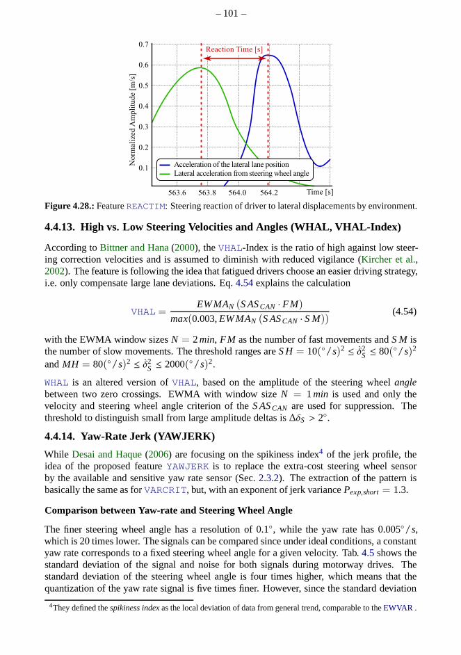
– 101–

Figure 4.28.:FeatureREACTIM: Steering reaction of driver to lateral displacements by environment.

4.4.13. High vs. Low Steering Velocities and Angles (WHAL, VHAL-Index)

According toBittner and Hana(2000), theVHAL-Index is the ratio of high against low steer-ing correction velocities and is assumed to diminish with reduced vigilance (Kircher et al.,2002). The feature is following the idea that fatigued drivers choose an easier driving strategy,i.e. only compensate large lane deviations. Eq.4.54explains the calculation

VHAL =EWMAN (S ASCAN · FM)

max(0.003,EWMAN (S ASCAN · S M))(4.54)

with the EWMA window sizesN = 2min, FM as the number of fast movements andS M isthe number of slow movements. The threshold ranges areS H= 10(/s)2 ≤ δ2

S ≤ 80(/s)2

andMH = 80(/s)2 ≤ δ2S ≤ 2000(/s)2.

WHAL is an altered version ofVHAL, based on the amplitude of the steering wheelanglebetween two zero crossings. EWMA with window sizeN = 1min is used and only thevelocity and steering wheel angle criterion of theS ASCAN are used for suppression. Thethreshold to distinguish small from large amplitude deltasis ∆δS > 2.

4.4.14. Yaw-Rate Jerk (YAWJERK)

While Desai and Haque(2006) are focusing on the spikiness index4 of the jerk profile, theidea of the proposed featureYAWJERK is to replace the extra-cost steering wheel sensorby the available and sensitive yaw rate sensor (Sec.2.3.2). The extraction of the pattern isbasically the same as forVARCRIT, but, with an exponent of jerk variancePexp,short = 1.3.

Comparison between Yaw-rate and Steering Wheel Angle

The finer steering wheel angle has a resolution of 0.1, while the yaw rate has 0.005/s,which is 20 times lower. The signals can be compared since under ideal conditions, a constantyaw rate corresponds to a fixed steering wheel angle for a given velocity. Tab.4.5shows thestandard deviation of the signal and noise for both signals during motorway drives. Thestandard deviation of the steering wheel angle is four timeshigher, which means that thequantization of the yaw rate signal is five times finer. However, since the standard deviation

4They defined thespikiness indexas the local deviation of data from general trend, comparable to theEWVAR .

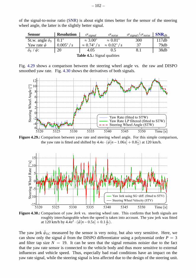
– 102–

of the signal-to-noise ratio (SNR) is about eight times better for the sensor of the steeringwheel angle, the latter is the slightly better signal.

Sensor Resolution σsignal σnoise σsignal/σnoise SNRdb

St.w. angleδS 0.1 ≈ 3.00 ≈ 0.01 300 117dbYaw rateψ 0.005/s ≈ 0.74/s ≈ 0.02/s 37 79dbδS / ψ: 20 4.05 0.5 8.1 38db

Table 4.5.:Signal qualities

Fig. 4.29 shows a comparison between the steering wheel angle vs. the raw and DISPOsmoothed yaw rate. Fig.4.30shows the derivatives of both signals.

Figure 4.29.:Comparison between yaw rate and steering wheel angle. For this simple comparison,the yaw rate is fitted and shifted by 4.4s · (ψ[n− 1.06s] + 0.8

s) at 120 km/h.

Figure 4.30.:Comparison of yawJerk vs. steering wheel rate. This confirms that both signals areroughly interchangeable when the speed is taken into account. The yaw jerk was fittedat 120 km/h by 4.4s2 · (ψ[n− 0.5s] + 0.11

s2 ).

The yaw jerkψSC measured by the sensor is very noisy, but also very sensitive. Here, wecan show only the signalψ from the DISPO differentiator using a polynomial orderP = 3and filter tap sizeN = 19. It can be seen that the signal remains noisier due to the factthat the yaw rate sensor is connected to the vehicle body and thus more sensitive to externalinfluences and vehicle speed. Thus, especially bad road conditions have an impact on theyaw rate signal, while the steering signal is less affected due to the design of the steering unit.

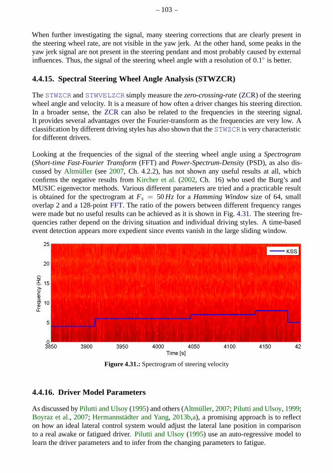
– 103–

When further investigating the signal, many steering corrections that are clearly present inthe steering wheel rate, are not visible in the yaw jerk. At the other hand, some peaks in theyaw jerk signal are not present in the steering pendant and most probably caused by externalinfluences. Thus, the signal of the steering wheel angle witha resolution of 0.1 is better.

4.4.15. Spectral Steering Wheel Angle Analysis (STWZCR)

TheSTWZCR andSTWVELZCR simply measure thezero-crossing-rate(ZCR) of the steeringwheel angle and velocity. It is a measure of how often a driverchanges his steering direction.In a broader sense, theZCR can also be related to the frequencies in the steering signal.It provides several advantages over the Fourier-transformas the frequencies are very low. Aclassification by different driving styles has also shown that theSTWZCR is very characteristicfor different drivers.

Looking at the frequencies of the signal of the steering wheel angle using aSpectrogram(Short-time Fast-Fourier Transform(FFT) andPower-Spectrum-Density(PSD), as also dis-cussed byAltmüller (see2007, Ch. 4.2.2), has not shown any useful results at all, whichconfirms the negative results fromKircher et al.(2002, Ch. 16) who used the Burg’s andMUSIC eigenvector methods. Various different parameters are tried and a practicable resultis obtained for the spectrogram atFs = 50Hz for a Hamming Windowsize of 64, smalloverlap 2 and a 128-pointFFT. The ratio of the powers between different frequency rangeswere made but no useful results can be achieved as it is shown in Fig.4.31. The steering fre-quencies rather depend on the driving situation and individual driving styles. A time-basedevent detection appears more expedient since events vanishin the large sliding window.

Figure 4.31.:Spectrogram of steering velocity

4.4.16. Driver Model Parameters

As discussed byPilutti and Ulsoy(1995) and others (Altmüller, 2007; Pilutti and Ulsoy, 1999;Boyraz et al., 2007; Hermannstädter and Yang, 2013b,a), a promising approach is to reflecton how an ideal lateral control system would adjust the lateral lane position in comparisonto a real awake or fatigued driver.Pilutti and Ulsoy(1995) use an auto-regressive model tolearn the driver parameters and to infer from the changing parameters to fatigue.

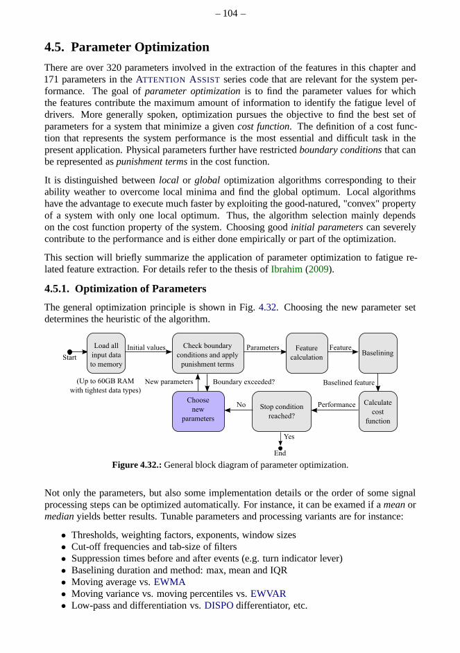
– 104–

4.5. Parameter Optimization

There are over 320 parameters involved in the extraction of the features in this chapter and171 parameters in theATTENTION ASSIST series code that are relevant for the system per-formance. The goal ofparameter optimizationis to find the parameter values for whichthe features contribute the maximum amount of information to identify the fatigue level ofdrivers. More generally spoken, optimization pursues the objective to find the best set ofparameters for a system that minimize a givencost function. The definition of a cost func-tion that represents the system performance is the most essential and difficult task in thepresent application. Physical parameters further have restrictedboundary conditionsthat canbe represented aspunishment termsin the cost function.

It is distinguished betweenlocal or global optimization algorithms corresponding to theirability weather to overcome local minima and find the global optimum. Local algorithmshave the advantage to execute much faster by exploiting the good-natured, "convex" propertyof a system with only one local optimum. Thus, the algorithm selection mainly dependson the cost function property of the system. Choosing goodinitial parameterscan severelycontribute to the performance and is either done empirically or part of the optimization.

This section will briefly summarize the application of parameter optimization to fatigue re-lated feature extraction. For details refer to the thesis ofIbrahim(2009).

4.5.1. Optimization of Parameters

The general optimization principle is shown in Fig.4.32. Choosing the new parameter setdetermines the heuristic of the algorithm.

Figure 4.32.:General block diagram of parameter optimization.

Not only the parameters, but also some implementation details or the order of some signalprocessing steps can be optimized automatically. For instance, it can be examed if ameanormedianyields better results. Tunable parameters and processing variants are for instance:

• Thresholds, weighting factors, exponents, window sizes• Cut-off frequencies and tab-size of filters• Suppression times before and after events (e.g. turn indicator lever)• Baselining duration and method: max, mean and IQR• Moving average vs.EWMA• Moving variance vs. moving percentiles vs.EWVAR• Low-pass and differentiation vs.DISPOdifferentiator, etc.

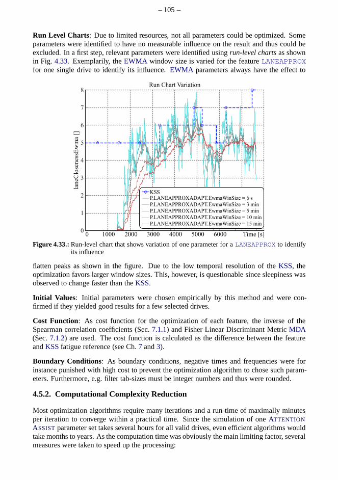
– 105–

Run Level Charts: Due to limited resources, not all parameters could be optimized. Someparameters were identified to have no measurable influence onthe result and thus could beexcluded. In a first step, relevant parameters were identified usingrun-level chartsas shownin Fig. 4.33. Exemplarily, theEWMA window size is varied for the featureLANEAPPROXfor one single drive to identify its influence.EWMA parameters always have the effect to

laneC

lose

nes

sEw

ma

[]

0

1

2

3

4

5

6

7

8

Time [s]0 600050004000300020001000

Run Chart Variation

P.LANEAPPROXADAPT.EwmaWinSize = 3 min

P.LANEAPPROXADAPT.EwmaWinSize = 5 min

P.LANEAPPROXADAPT.EwmaWinSize = 10 min

P.LANEAPPROXADAPT.EwmaWinSize = 15 min

KSSP.LANEAPPROXADAPT.EwmaWinSize = 6 s

Figure 4.33.:Run-level chart that shows variation of one parameter for aLANEAPPROX to identifyits influence

flatten peaks as shown in the figure. Due to the low temporal resolution of theKSS, theoptimization favors larger window sizes. This, however, isquestionable since sleepiness wasobserved to change faster than theKSS.

Initial Values : Initial parameters were chosen empirically by this methodand were con-firmed if they yielded good results for a few selected drives.

Cost Function: As cost function for the optimization of each feature, the inverse of theSpearman correlation coefficients (Sec.7.1.1) and Fisher Linear Discriminant MetricMDA(Sec.7.1.2) are used. The cost function is calculated as the differencebetween the featureandKSSfatigue reference (see Ch.7 and3).

Boundary Conditions: As boundary conditions, negative times and frequencies were forinstance punished with high cost to prevent the optimization algorithm to chose such param-eters. Furthermore, e.g. filter tab-sizes must be integer numbers and thus were rounded.

4.5.2. Computational Complexity Reduction

Most optimization algorithms require many iterations and arun-time of maximally minutesper iteration to converge within a practical time. Since thesimulation of oneATTENTION

ASSISTparameter set takes several hours for all valid drives, evenefficient algorithms wouldtake months to years. As the computation time was obviously the main limiting factor, severalmeasures were taken to speed up the processing:

– 106–

RAM instead of HDD: A major bottleneck is to load entire drives (including unnecessarysignals) sequentially from the hard drive during every iteration. Read access from RAM isabout 70 times faster5. Thus, only the needed signals for one feature are load and concate-nated in RAM at once. 45GB to 80GB were necessary, depending on the features, variedparameters and dataset (ALDWvalidND or ALDWvalid).

Precision-lossy data type compression:As CAN-signals use 1 to 16 bit integers, using64 bit double floating-point data types is another waste of resources. Thus, all signals arecompressed to the tightest data type with a maximum precision loss of 1%.

Pre-computation and cachingResource consumption is often a trade-off between memoryand computation. The open-loop pre-processing operationsof CAN-signals could be com-puted in advance as they solely depend on the sensor signals.Depending on the varied param-eter, further derived signals could be cached if parametersdid not change or were calculatedbefore: e.g. the system active signals, external factors and especially cross-wind detection.The reset of every drive (for baselining) could be triggeredby a drive-ID change.

Causalization: Online algorithms perform all real-time processing steps sequentially. Model-based algorithms favor "causalized" software architectures (Simulink/TargetLink). Modernarithmetic logic units(ALU) (such as CPU, GPU and DSP) can process basic function muchfaster on vectors or matrices. However, this is only possible offline and if processing stepsdo not depend on the closed loop output of a previous time step.

Model-based porting to matrix operations: The completeATTENTION ASSISTalgorithmwas ported bit-true from Simulink/TargetLink to MATLABc© where processor-optimized(MMX) matrix operation could be performed using LAPACK and BLAS. Recursive algo-rithms likeEWMA, EwmaN, EWVAR , EWIQRetc. were implemented in MEX C++.

The total performance gain is on average factor 300-500 times faster in comparison to theSimulink model. This speed up allowed to simulate a smaller selection of drives in seconds.Optimization with up to six parameters became manageable this way.

Only the most promising features and parameters could have been optimized:LANEDEV,VHAL, TLC1MIN, ZIGZAGSBL, LANEAPPROXADAPT, YAWJERK andSTEVENT. Theyall depend on theATTENTION ASSISTpre-processing.

4.5.3. Application

The features described in this chapter were optimized in several stages:

Parameter Study: TheATTENTION ASSIST series algorithm was optimized independentlyfrom the features, with the cost function based on the detection and false alarm rate of fa-tigue warnings. The detection rate is quantized due to the discrete number of warnings, thus,automatic parameter optimization is not possible here. Forobtaining the 171 parameters, thesystem understanding was part of the iteration loop, knowledge that optimization algorithmsusually do not have. Iteratively, only five to ten parametersof one module were chosen in apredefined grid and combination, similar togrid- andhierarchical searchwhile other parame-ters were kept at the best known point. Still, the simulationdistributed to several workstationseach with up to 16 cores required up to six weeks. The results were then analyzed and theunderstanding of parameters and effects lead to a refined selection of parameters.

5e.g. for DDR-3 1066 MHz, SATA 7.200 RPM, XEON server

– 107–

Empirical Parameter Selection: Initial values were chosen empirically from physicallyplausible values based on graphical assessment for a small selection of drives (cf. Ch.7.2).

Automatic Local Optimization : While the previously described method ensured that thealgorithms perform as desired for every parameter set due tothe understanding of the system,it is at the other hand very laborious and does not necessarily find the global optimum. Withthe fast implementation in Sec.4.5.2, up to six parameters were varied. With this observation,theNelder-Mead simplex algorithmas described inLagarias and Reeds(1996) was appliedand in fact further improved the feature performance.

Optimizing a combination of features: In a second step, the best features were combinedby multiple regression resulting in a single fatigue measure. For this measure, the Spearmancoefficients were again used as cost function.

Global Optimization : In the scope of the theses ofIbrahim(2009) andOlabe(2008), globaloptimization algorithms were implemented. The toolbox wascovering the optimization al-gorithms: grid search, simplex, particle swarm, genetic and evolutionary algorithms, particleswarm and simulated annealing. Due to the computational complexity, only three featurescould be investigated. For convex problems, they did not show additional benefit.

4.6. ConclusionFeatures from literature, improvements thereof and new features were discussed. Many morefeatures (cf. App.A.9) have been studied, but did not show much potential. There are stillmore potential patterns that can be investigated. Different approaches to optimize the in-volved parameters and to overcome the computational complexity were presented. The pa-rameters described together with the features are the result of one of the optimization steps.

One problem was that the optimization sometimes converged towards implausible values orvery large window sized of over one hour. The later is most probably related to the fact thatfatigue and especially theKSS entries are changing very slowly. Some parameters had tobe set manually as the results of the optimization were implausible such as zero suppressiontimes. This can be explained by the observation, that there were not enough occurrences ofsuch events in the data to make a difference.

It would be better to optimize the combination of features, for instance, by using the classifi-cation error as cost function. However, this is not yet possible due to the computation time.Most of all, the major problem was that the optimization can only be as good as the costfunction in respect to the reference.

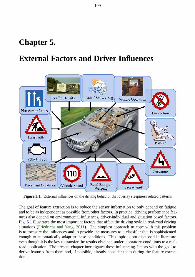
– 109–

Chapter 5.

External Factors and Driver Influences

Figure 5.1.:External influences on the driving behavior that overlay sleepiness related patterns

The goal of feature extraction is to reduce the sensor information to only depend on fatigueand to be as independent as possible from other factors. In practice, driving performance fea-tures also depend on environmental influences, driver-individual and situation based factors.Fig. 5.1 illustrates the most important factors that affect the driving style in real-road drivingsituations (Friedrichs and Yang, 2011). The simplest approach to cope with this problemis to measure the influences and to provide the measures to a classifier that is sophisticatedenough to automatically adapt to these conditions. This topic is not discussed in literatureeven though it is the key to transfer the results obtained under laboratory conditions to a real-road application. The present chapter investigates these influencing factors with the goal toderive features from them and, if possible, already consider them during the feature extrac-tion.

– 110–

5.1. Methodology to Quantify and IncorporateNon-Sleepiness-related Influences

In this thesis, new methods are presented to detect road bumps, traffic density and cross-wind. Specific test drives have been conducted at night to vary only one isolated factor, whilekeeping the others constant to identify the influence of a single factor. When, for instance,the factor vehicle speed was varied, it was assured that the other factors remained constant,for instance, the driver condition, traffic density, overtaking maneuvers, road curvature, roadbumps, vehicle parameters, cross-wind as well as precipitation and light conditions. Thedetection methods have also been implemented in real-time to evaluate the performance whiledriving in different situations. In the offline analysis, the correlation between the variedfactors and features, extracted for this road section, was evaluated. The driver’s daily mood(e.g. economic or aggressive) is another factor, which is difficult to classify and discussed inSec.5.4. The way that drivers hold the steering wheel (e.g. with one or two hands) also has asignificant influence on the steering behavior. However, additional sensors would be requiredfor its detection and, therefore, this factor is not considered here. The results emphasize theimportance of considering driving influences in driver monitoring.

The goal of this work is to find a measure for most of the thirteen factors from Fig.5.1. Thesimplest factor is the vehicle velocity, which is already represented by its speedometer signal.However, measuring the curvature or road condition is not assimple. When we consider thesethirteen dimensions, it is obvious that it’s impossible to record drives for every combinationof these factors. Thereby, we assume that superposition applies, i.e. factors overlay and thecombination can be approximated as linear. Fortunately, the probability of multiple factorsoccuring at the same time is increasingly low. For instance,it is not very probable that adriver is driving on a construction-site that is curvy, during rain with cross-wind and roadbumps at the same time etc. In this example, theSAScriteria for the system activity will setthe system to inactive anyway.

After finding these measures, the next step is to analyze the relationship of these factorswith the fatigue-related features. Usually and if possible, it is easier to compensate the rawinput signals rather than every feature individually. Curvature can, for instance, be removedfrom the steering signal by a high-pass filter. The best but most difficult way, however, is toconsider these influences during the extraction of every feature.

5.1.1. Evaluation of Geo-position mapped Events and Signals

Analysis of road bumps and the road surface would be a straightforward task, if there wasa good reference to assess the quality of these signals. One approach to have a reference ismapping road bumps to real world position where they occur.

Fig. 5.2 shows a method of how events of one or several drives can be mapped to theirgeo-coordinates on a map. This way, clusters of steering corrections and road bumps wereidentified, that often occurred at the same place.

5.2. Influences from External Factors on the Driving Behavior

This section will explain the most relevant external factors. Details of the detection areprovided and illustrations are given for important examples only.

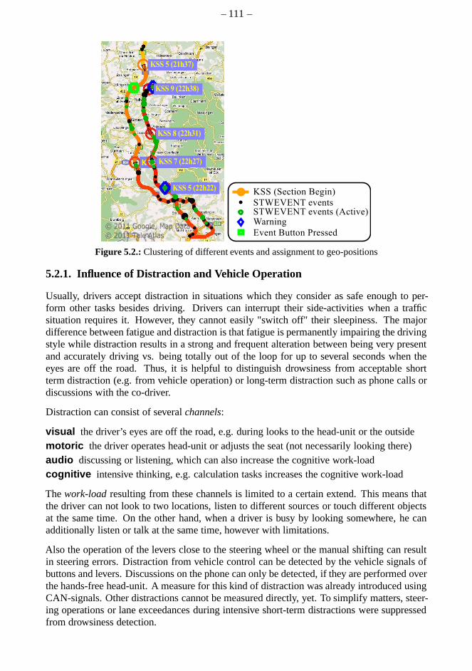
– 111–

Figure 5.2.:Clustering of different events and assignment to geo-positions

5.2.1. Influence of Distraction and Vehicle Operation

Usually, drivers accept distraction in situations which they consider as safe enough to per-form other tasks besides driving. Drivers can interrupt their side-activities when a trafficsituation requires it. However, they cannot easily "switchoff" their sleepiness. The majordifference between fatigue and distraction is that fatigueis permanently impairing the drivingstyle while distraction results in a strong and frequent alteration between being very presentand accurately driving vs. being totally out of the loop for up to several seconds when theeyes are off the road. Thus, it is helpful to distinguish drowsiness from acceptable shortterm distraction (e.g. from vehicle operation) or long-term distraction such as phone calls ordiscussions with the co-driver.

Distraction can consist of severalchannels:

visual the driver’s eyes are off the road, e.g. during looks to the head-unit or the outsidemotoric the driver operates head-unit or adjusts the seat (not necessarily looking there)audio discussing or listening, which can also increase the cognitive work-loadcognitive intensive thinking, e.g. calculation tasks increases the cognitive work-load

Thework-load resulting from these channels is limited to a certain extend. This means thatthe driver can not look to two locations, listen to differentsources or touch different objectsat the same time. On the other hand, when a driver is busy by looking somewhere, he canadditionally listen or talk at the same time, however with limitations.

Also the operation of the levers close to the steering wheel or the manual shifting can resultin steering errors. Distraction from vehicle control can bedetected by the vehicle signals ofbuttons and levers. Discussions on the phone can only be detected, if they are performed overthe hands-free head-unit. A measure for this kind of distraction was already introduced usingCAN-signals. Other distractions cannot be measured directly, yet. To simplify matters, steer-ing operations or lane exceedances during intensive short-term distractions were suppressedfrom drowsiness detection.

– 112–

Several levers, such as the limiter or high beam levers have multiple permanent states, butonly the instant of operating is of interest for these. Therefore, only the raising and fallingslopes of the signal have been considered.

5.2.2. Influences by Rain, Snow, Fog, Light Conditions and Tunnels

It was observed that the driving behavior changes severely during heavy rain or snow fall.Usually, the steering becomes more hectic and the driver hasto concentrate more. Thisinfluence is refreshing at the beginning, but can become evenmore exhausting after a while.Rainfall and foggy weather usually require the driver to slow down. As illustrated in Fig.5.3,rain can be detected well by the rain sensor and the lever position of the windshield wiper.

Figure 5.3.:Lever position of the windshield wiper, light sensor on the route for rain, snow andluminosity detection

It was observed that reduced vision due to dark light conditions also affects the steering andlane keeping performance for several persons even when theyare awake.

These drivers need to concentrate more than during the day, which can be quite exhaustingafter a while. The light level can again be measured well by the light sensor and light switch(or automatic) as shown in Fig.5.3. Illuminated tunnels or other road sections provide acertain degree ofnoveltyto the driver and usually improve the level of attention for ashortperiod. Tunnels can be detected well by looking for fast changes in the light sensor signal.To simplifiy matters, sections with intensive rain, fog or snow are suppressed here and treatedas system inactivity.

5.2.3. Vehicle Speed Influence

The vehicle velocity has a big influence on the steering velocities and the necessary reactiontimes to vehicle displacements. The time remaining to react, when heading towards thelane markings at high speeds, is of course shorter than for lower speeds. Thus, the vehiclespeed must be considered during the extraction of features.VELOCITY is simply the vehiclespeed.

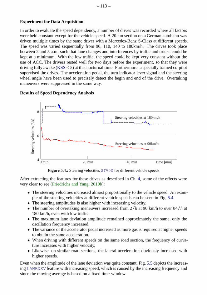
– 113–

Experiment for Data Acquisition

In order to evaluate the speed dependency, a number of driveswas recorded where all factorswere held constant except for the vehicle speed. A 20 km section on a German autobahn wasdriven multiple times by the same driver with a Mercedes-Benz S-Class at different speeds.The speed was varied sequentially from 90, 110, 140 to 180km/h. The drives took placebetween 2 and 5 a.m. such that lane changes and interferencesby traffic and trucks could bekept at a minimum. With the low traffic, the speed could be keptvery constant without theuse of ACC. The drivers rested well for two days before the experiment, so that they weredriving fully awake (KSS≤ 5) at this nocturnal time. Furthermore, a specially trainedco-pilotsupervised the drives. The acceleration pedal, the turn indicator lever signal and the steeringwheel angle have been used to precisely detect the begin and end of the drive. Overtakingmaneuvers were suppressed in the same way.

Results of Speed Dependency Analysis

4

6

8

Steering velocities at 90km/h

Steering velocities at 180km/h

0 min 20 min 40 min Time [min]

Ste

erin

gve

loci

ties

[ /s]

Figure 5.4.:Steering velocitiesSTV50 for different vehicle speeds

After extracting the features for these drives as describedin Ch.4, some of the effects werevery clear to see (Friedrichs and Yang, 2010b):

• The steering velocities increased almost proportionally to the vehicle speed. An exam-ple of the steering velocities at different vehicle speeds can be seen in Fig.5.4.

• The steering amplitudes is also higher with increasing velocity.• The number of overtaking meneuvers increased from 2/h at 90 km/h to over 84/h at

180 km/h, even with low traffic.• The maximum lane deviation amplitude remained approximately the same, only the

oscillation frequency increased.• The variance of the accelerator pedal increased as more gas is required at higher speeds

to obtain the same acceleration.• When driving with different speeds on the same road section,the frequency of curva-

ture increases with higher velocity.• Likewise, on similar road sections, the lateral acceleration obviously increased with

higher speeds.

Even when the amplitude of the lane deviation was quite constant, Fig.5.5depicts the increas-ingLANEDEV feature with increasing speed, which is caused by the increasing frequency andsince the moving average is based on a fixed time-window.

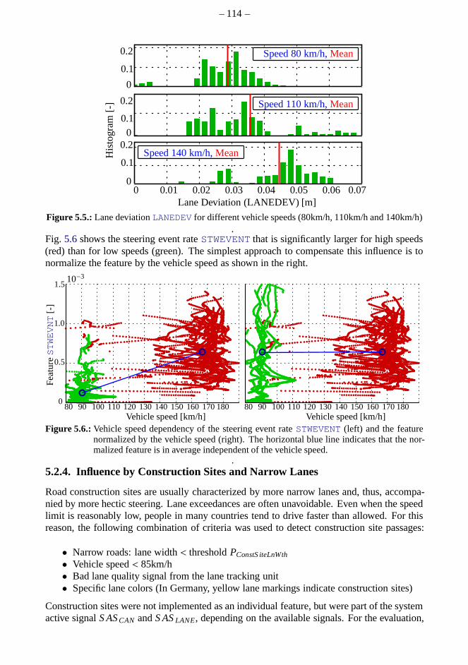
– 114–

0

0.1

0.2

00.1

0.2

0.1

Lane Deviation (LANEDEV) [m]

His

togr

am[-

]

0.2

00 0.01 0.02 0.03 0.04 0.05 0.06 0.07

Speed 110 km/h,Mean

Speed 80 km/h,Mean

Speed 140 km/h,Mean

Figure 5.5.:Lane deviationLANEDEV for different vehicle speeds (80km/h, 110km/h and 140km/h).

Fig. 5.6shows the steering event rateSTWEVENT that is significantly larger for high speeds(red) than for low speeds (green). The simplest approach to compensate this influence is tonormalize the feature by the vehicle speed as shown in the right.

Fea

tureSTWEVNT

[-]

10−3

Vehicle speed [km/h] Vehicle speed [km/h]80 180160 170140 150120 13011090 100

0

0.5

1.0

1.5

80 180160 170140 150120 13011090 100

Figure 5.6.:Vehicle speed dependency of the steering event rateSTWEVENT (left) and the featurenormalized by the vehicle speed (right). The horizontal blue line indicates that the nor-malized feature is in average independent of the vehicle speed.

.5.2.4. Influence by Construction Sites and Narrow Lanes

Road construction sites are usually characterized by more narrow lanes and, thus, accompa-nied by more hectic steering. Lane exceedances are often unavoidable. Even when the speedlimit is reasonably low, people in many countries tend to drive faster than allowed. For thisreason, the following combination of criteria was used to detect construction site passages:

• Narrow roads: lane width< thresholdPConstS iteLnWth

• Vehicle speed< 85km/h• Bad lane quality signal from the lane tracking unit• Specific lane colors (In Germany, yellow lane markings indicate construction sites)

Construction sites were not implemented as an individual feature, but were part of the systemactive signalS ASCAN andS ASLANE, depending on the available signals. For the evaluation,

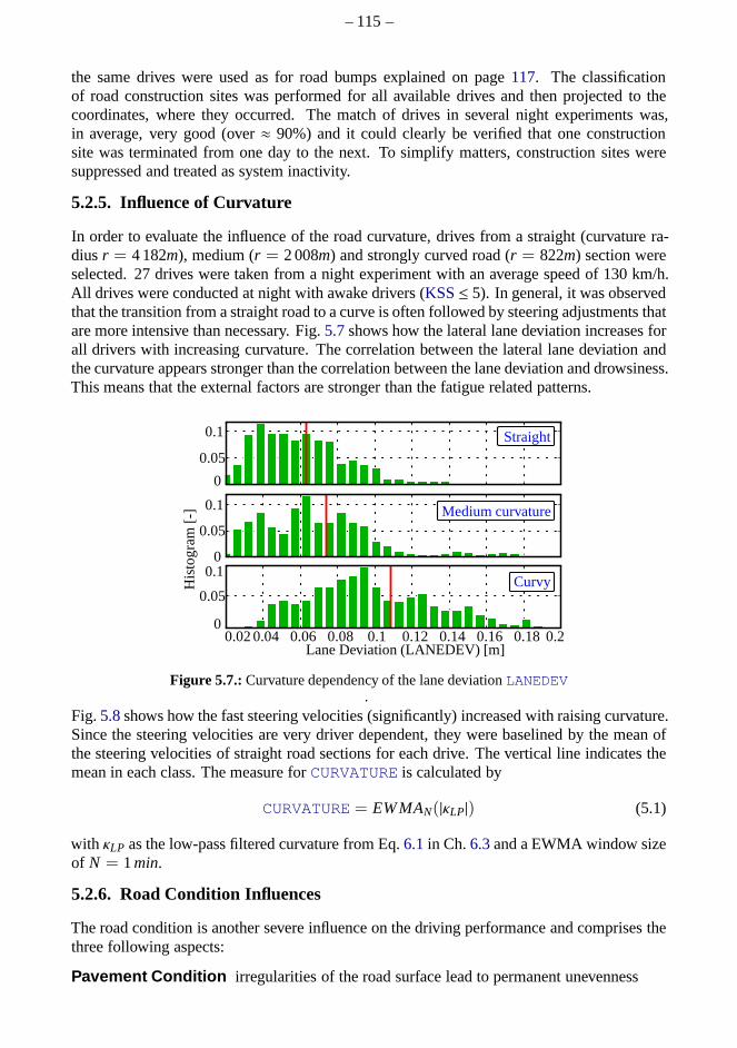
– 115–

the same drives were used as for road bumps explained on page117. The classificationof road construction sites was performed for all available drives and then projected to thecoordinates, where they occurred. The match of drives in several night experiments was,in average, very good (over≈ 90%) and it could clearly be verified that one constructionsite was terminated from one day to the next. To simplify matters, construction sites weresuppressed and treated as system inactivity.

5.2.5. Influence of Curvature

In order to evaluate the influence of the road curvature, drives from a straight (curvature ra-diusr = 4 182m), medium (r = 2 008m) and strongly curved road (r = 822m) section wereselected. 27 drives were taken from a night experiment with an average speed of 130 km/h.All drives were conducted at night with awake drivers (KSS≤ 5). In general, it was observedthat the transition from a straight road to a curve is often followed by steering adjustments thatare more intensive than necessary. Fig.5.7shows how the lateral lane deviation increases forall drivers with increasing curvature. The correlation between the lateral lane deviation andthe curvature appears stronger than the correlation between the lane deviation and drowsiness.This means that the external factors are stronger than the fatigue related patterns.

0

0.05

0.1

0

0.05

0.1

0.02 0.04 0.06 0.08 0.1 0.12 0.14 0.16 0.18 0.2

0.05

Lane Deviation (LANEDEV) [m]

His

tog

ram

[-]

0.1

Medium curvature

Straight

Curvy

0

Figure 5.7.:Curvature dependency of the lane deviationLANEDEV.

Fig.5.8shows how the fast steering velocities (significantly) increased with raising curvature.Since the steering velocities are very driver dependent, they were baselined by the mean ofthe steering velocities of straight road sections for each drive. The vertical line indicates themean in each class. The measure forCURVATURE is calculated by

CURVATURE = EWMAN(|κLP|) (5.1)

with κLP as the low-pass filtered curvature from Eq.6.1in Ch.6.3and a EWMA window sizeof N = 1min.

5.2.6. Road Condition Influences

The road condition is another severe influence on the drivingperformance and comprises thethree following aspects:

Pavement Condition irregularities of the road surface lead to permanent unevenness

– 116–

Figure 5.8.:Curvature dependency of the maximum steering velocity between inflection points. Es-pecially the fast steering corrections increase.

.Road Bumps short and stronger road bumps that usually affect both wheels

Road warping and Cross-Wind occur when the road changes its lateral inclination caus-ing the vehicle to roll around the longitudinal axis.Cross-windhas the same effect asroad warping. For the available sensors, it cannot be distinguished, whether the lateraldisplacement is caused by an uneven road surface or a wind gust.

Road Pavement Condition

Usually, the vehicle slides calmer on a new pavement than on an old, very damaged roadsurface. These irregularities are normally not immediately realized by the driver, but stillresult in small lateral displacements of the vehicle which the driver has to correct after awhile. Estimating a measure for the road condition can be done by detecting a simultaneousvibration in different sensors. As the sensors are mechanically connected road unevennessand shocks can be observed by the following sensors:

• Wheel rotation sensor• Longitudinal and lateral acceleration sensor• Yaw rate sensor• Vehicle level signals from every wheel1

A combination of all sensors would make the detection even more accurate, but is not neces-sary. The principle proposed here for the wheel rotation sensor can also be applied to othersensors, however with different parameters:

PAVEMENT = EWVARN(WhlRPMFL,HP) · EWVARN(WhlRPMFR,HP) (5.2)

WhlRPMFL,HP andWhlRPMFR,HP are the high-pass filtered wheel rotation rate sensor sig-nals with the cut-off frequencyfc = 0.5Hz evaluated in anEWVAR window of lengthN = 1min. The variance of all sensors can then be combined by multiplication to favora simultaneous vibration. After theEWVAR calculation, the signals do not necessarily needto be synchronous. This makes it less sensible to other variations such as the engine rotation.

1Vehicle level signals were available, if the vehicle was equipped with air suspension or active body control.

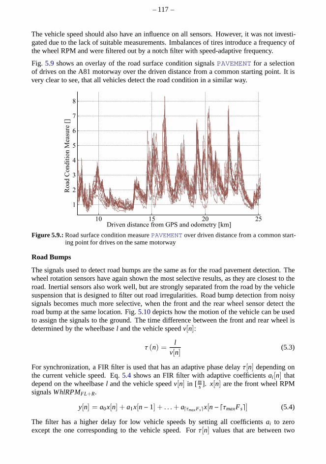
– 117–

The vehicle speed should also have an influence on all sensors. However, it was not investi-gated due to the lack of suitable measurements. Imbalances of tires introduce a frequency ofthe wheel RPM and were filtered out by a notch filter with speed-adaptive frequency.

Fig. 5.9 shows an overlay of the road surface condition signalsPAVEMENT for a selectionof drives on the A81 motorway over the driven distance from a common starting point. It isvery clear to see, that all vehicles detect the road condition in a similar way.

Figure 5.9.:Road surface condition measurePAVEMENT over driven distance from a common start-ing point for drives on the same motorway

Road Bumps

The signals used to detect road bumps are the same as for the road pavement detection. Thewheel rotation sensors have again shown the most selective results, as they are closest to theroad. Inertial sensors also work well, but are strongly separated from the road by the vehiclesuspension that is designed to filter out road irregularities. Road bump detection from noisysignals becomes much more selective, when the front and the rear wheel sensor detect theroad bump at the same location. Fig.5.10depicts how the motion of the vehicle can be usedto assign the signals to the ground. The time difference between the front and rear wheel isdetermined by the wheelbasel and the vehicle speedv[n]:

τ (n) =l

v[n](5.3)

For synchronization, a FIR filter is used that has an adaptivephase delayτ[n] depending onthe current vehicle speed. Eq.5.4 shows an FIR filter with adaptive coefficientsai [n] thatdepend on the wheelbasel and the vehicle speedv[n] in [ m

s ]. x[n] are the front wheel RPMsignalsWhlRPMFL+R.

y[n] = a0x[n] + a1x[n− 1] + . . .+ a⌈τmaxFs⌉x[n− ⌈τmaxFs⌉] (5.4)

The filter has a higher delay for low vehicle speeds by settingall coefficientsai to zeroexcept the one corresponding to the vehicle speed. Forτ[n] values that are between two

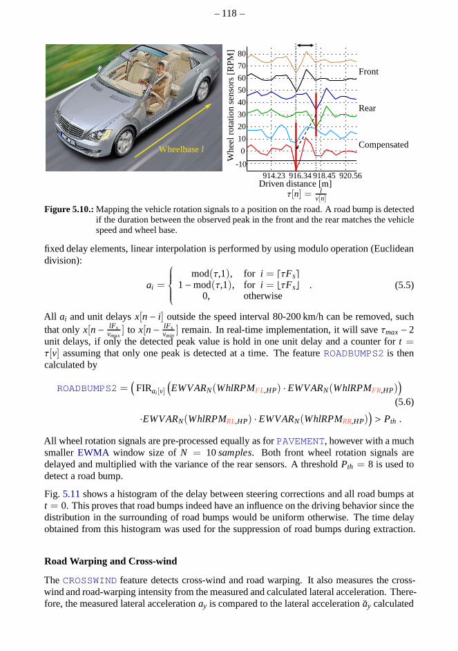
– 118–

Wheelbasel

Wh

eelr

ota

tion

sen

sors

[RP

M]

Front

Rear

Compensated

Driven distance [m]τ[n] = l

v[n]

-10

10

0

20

40

30

50

70

60

80

914.23 916.34 918.45 920.56

Figure 5.10.:Mapping the vehicle rotation signals to a position on the road. A road bump is detectedif the duration between the observed peak in the front and therear matches the vehiclespeed and wheel base.

fixed delay elements, linear interpolation is performed by using modulo operation (Euclideandivision):

ai =

mod(τ,1), for i = ⌈τFs⌉1−mod(τ,1), for i = ⌊τFs⌋

0, otherwise. (5.5)

All ai and unit delaysx[n− i] outside the speed interval 80-200 km/h can be removed, suchthat onlyx[n− lFs

vmax] to x[n− lFs

vmin] remain. In real-time implementation, it will saveτmax− 2

unit delays, if only the detected peak value is hold in one unit delay and a counter fort =τ[v] assuming that only one peak is detected at a time. The featureROADBUMPS2 is thencalculated by

ROADBUMPS2 =(

FIRai [v]

(

EWVARN(WhlRPMFL,HP) · EWVARN(WhlRPMFR,HP))

(5.6)

·EWVARN(WhlRPMRL,HP) · EWVARN(WhlRPMRR,HP))

> Pth .

All wheel rotation signals are pre-processed equally as forPAVEMENT, however with a muchsmallerEWMA window size ofN = 10samples. Both front wheel rotation signals aredelayed and multiplied with the variance of the rear sensors. A thresholdPth = 8 is used todetect a road bump.

Fig. 5.11shows a histogram of the delay between steering correctionsand all road bumps att = 0. This proves that road bumps indeed have an influence on the driving behavior since thedistribution in the surrounding of road bumps would be uniform otherwise. The time delayobtained from this histogram was used for the suppression ofroad bumps during extraction.

Road Warping and Cross-wind

TheCROSSWIND feature detects cross-wind and road warping. It also measures the cross-wind and road-warping intensity from the measured and calculated lateral acceleration. There-fore, the measured lateral accelerationay is compared to the lateral accelerationay calculated

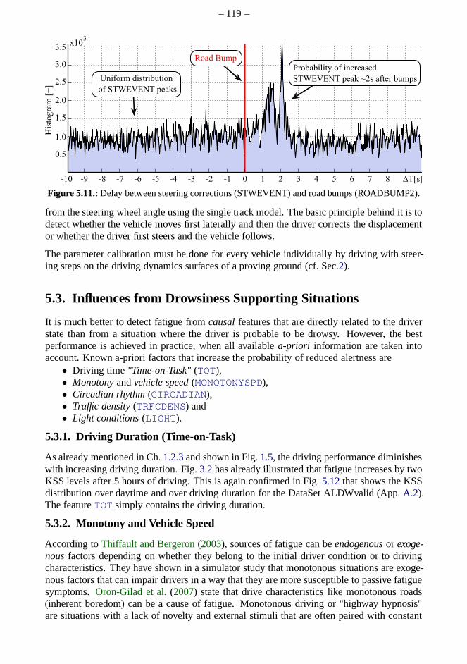
– 119–

Figure 5.11.:Delay between steering corrections (STWEVENT) and road bumps (ROADBUMP2).

from the steering wheel angle using the single track model. The basic principle behind it is todetect whether the vehicle moves first laterally and then thedriver corrects the displacementor whether the driver first steers and the vehicle follows.

The parameter calibration must be done for every vehicle individually by driving with steer-ing steps on the driving dynamics surfaces of a proving ground (cf. Sec.2).

5.3. Influences from Drowsiness Supporting Situations

It is much better to detect fatigue fromcausalfeatures that are directly related to the driverstate than from a situation where the driver is probable to bedrowsy. However, the bestperformance is achieved in practice, when all availablea-priori information are taken intoaccount. Known a-priori factors that increase the probability of reduced alertness are

• Driving time "Time-on-Task"(TOT),• Monotonyandvehicle speed(MONOTONYSPD),• Circadian rhythm(CIRCADIAN),• Traffic density(TRFCDENS) and• Light conditions(LIGHT).

5.3.1. Driving Duration (Time-on-Task)

As already mentioned in Ch.1.2.3and shown in Fig.1.5, the driving performance diminisheswith increasing driving duration. Fig.3.2has already illustrated that fatigue increases by twoKSS levels after 5 hours of driving. This is again confirmed inFig. 5.12that shows the KSSdistribution over daytime and over driving duration for theDataSet ALDWvalid (App.A.2).The featureTOT simply contains the driving duration.

5.3.2. Monotony and Vehicle Speed

According toThiffault and Bergeron(2003), sources of fatigue can beendogenousor exoge-nousfactors depending on whether they belong to the initial driver condition or to drivingcharacteristics. They have shown in a simulator study that monotonous situations are exoge-nous factors that can impair drivers in a way that they are more susceptible to passive fatiguesymptoms.Oron-Gilad et al.(2007) state that drive characteristics like monotonous roads(inherent boredom) can be a cause of fatigue. Monotonous driving or "highway hypnosis"are situations with a lack of novelty and external stimuli that are often paired with constant

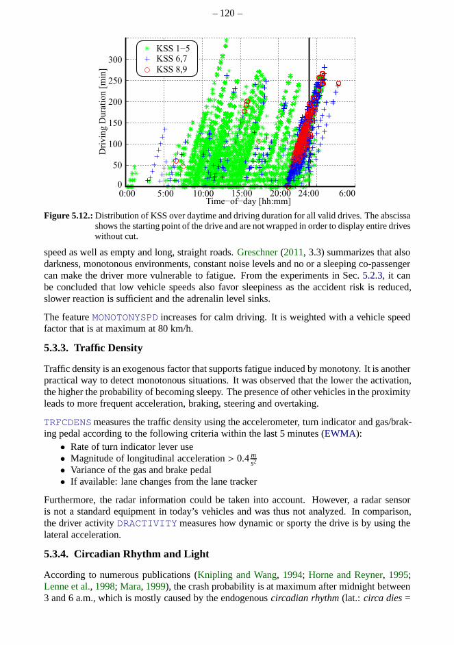
– 120–

Figure 5.12.:Distribution of KSS over daytime and driving duration for all valid drives. The abscissashows the starting point of the drive and are not wrapped in order to display entire driveswithout cut.

speed as well as empty and long, straight roads.Greschner(2011, 3.3) summarizes that alsodarkness, monotonous environments, constant noise levelsand no or a sleeping co-passengercan make the driver more vulnerable to fatigue. From the experiments in Sec.5.2.3, it canbe concluded that low vehicle speeds also favor sleepiness as the accident risk is reduced,slower reaction is sufficient and the adrenalin level sinks.

The featureMONOTONYSPD increases for calm driving. It is weighted with a vehicle speedfactor that is at maximum at 80 km/h.

5.3.3. Traffic Density

Traffic density is an exogenous factor that supports fatigueinduced by monotony. It is anotherpractical way to detect monotonous situations. It was observed that the lower the activation,the higher the probability of becoming sleepy. The presenceof other vehicles in the proximityleads to more frequent acceleration, braking, steering andovertaking.

TRFCDENSmeasures the traffic density using the accelerometer, turn indicator and gas/brak-ing pedal according to the following criteria within the last 5 minutes (EWMA):

• Rate of turn indicator lever use• Magnitude of longitudinal acceleration> 0.4m

s2

• Variance of the gas and brake pedal• If available: lane changes from the lane tracker

Furthermore, the radar information could be taken into account. However, a radar sensoris not a standard equipment in today’s vehicles and was thus not analyzed. In comparison,the driver activityDRACTIVITY measures how dynamic or sporty the drive is by using thelateral acceleration.

5.3.4. Circadian Rhythm and Light

According to numerous publications (Knipling and Wang, 1994; Horne and Reyner, 1995;Lenne et al., 1998; Mara, 1999), the crash probability is at maximum after midnight between3 and 6 a.m., which is mostly caused by the endogenouscircadian rhythm(lat.: circa dies=

– 121–

about one day). The circadian rhythm also produces an alertness dip in the early afternoonaround 2 and 4:00 pm, during which people are sleepier (Monk, 1991). This is supported bythe crash statistic in Fig.5.13and5.14.

Figure 5.13.:Sleepiness tendency by daytime (Source:Zulley, 1995)

Daylight is the pacemaker of the internal biological clock synchronized to day and night (Zul-ley, 2006) through the production of the hormonemelatonin. Light exposure to the retina inthe eyes regulates the suppression of melatonin (Burgess et al., 2002; Greschner, 2011). Af-ter several days, the sleep-wake cycle is intrinsic and inevitable rather than voluntary (Mara,1999).

Fig. 5.14shows that young drivers, especially males (cf. Ch.1.2.3), are particularly endan-gered at night, while the crash probability shifts to the afternoon with increasing age. Thus,age and gender could further be considered to improve the fatigue detection as soon as suchdriver details are available in vehicles.

Figure 5.14.:Time of occurrence of crash for commercial drivers with different ages, published bytheNHTSA for the years 1990 to 1992. (Source:Mara, 1999, Fig. 3)

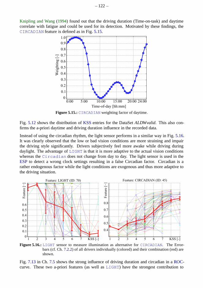
– 122–

Knipling and Wang(1994) found out that the driving duration (Time-on-task) and daytimecorrelate with fatigue and could be used for its detection. Motivated by these findings, theCIRCADIAN feature is defined as in Fig.5.15.

Figure 5.15.:CIRCADIAN weighting factor of daytime.

Fig. 5.12shows the distribution ofKSSentries for the DataSetALDWvalid. This also con-firms the a-priori daytime and driving duration influence in the recorded data.

Instead of using the circadian rhythm, the light sensor performs in a similar way in Fig.5.16.It was clearly observed that the low or bad vision conditionsare more straining and impairthe driving style significantly. Drivers subjectively feelmore awake while driving duringdaylight. The advantage ofLIGHT is that it is more adaptive to the actual vision conditionswhereas theCircadian does not change from day to day. The light sensor is used in theESPto detect a wrong clock settings resulting in a false Circadian factor. Circadian is arather endogenous factor while the light conditions are exogenous and thus more adaptive tothe driving situation.

Figure 5.16.:LIGHT sensor to measure illumination as alternative forCIRCADIAN. The Error-bars (cf. Ch.7.2.2) of all drivers individually (colored) and their combination (red) areshown.

Fig. 7.13in Ch. 7.5 shows the strong influence of driving duration and circadianin a ROC-curve. These two a-priori features (as well asLIGHT) have the strongest contribution to

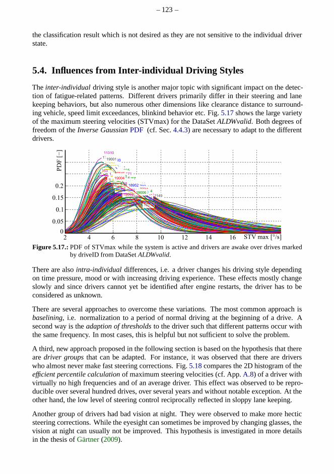
– 123–

the classification result which is not desired as they are notsensitive to the individual driverstate.

5.4. Influences from Inter-individual Driving Styles

The inter-individual driving style is another major topic with significant impacton the detec-tion of fatigue-related patterns. Different drivers primarily differ in their steering and lanekeeping behaviors, but also numerous other dimensions likeclearance distance to surround-ing vehicle, speed limit exceedances, blinkind behavior etc. Fig.5.17shows the large varietyof the maximum steering velocities (STVmax) for the DataSetALDWvalid. Both degrees offreedom of theInverse GaussianPDF (cf. Sec.4.4.3) are necessary to adapt to the differentdrivers.

Figure 5.17.:PDF of STVmax while the system is active and drivers are awakeover drives markedby driveID from DataSetALDWvalid.

There are alsointra-individual differences, i.e. a driver changes his driving style dependingon time pressure, mood or with increasing driving experience. These effects mostly changeslowly and since drivers cannot yet be identified after engine restarts, the driver has to beconsidered as unknown.

There are several approaches to overcome these variations.The most common approach isbaselining, i.e. normalization to a period of normal driving at the beginning of a drive. Asecond way is theadaption of thresholdsto the driver such that different patterns occur withthe same frequency. In most cases, this is helpful but not sufficient to solve the problem.

A third, new approach proposed in the following section is based on the hypothesis that therearedriver groupsthat can be adapted. For instance, it was observed that thereare driverswho almost never make fast steering corrections. Fig.5.18compares the 2D histogram of theefficient percentile calculationof maximum steering velocities (cf. App.A.8) of a driver withvirtually no high frequencies and of an average driver. Thiseffect was observed to be repro-ducible over several hundred drives, over several years andwithout notable exception. At theother hand, the low level of steering control reciprocally reflected in sloppy lane keeping.

Another group of drivers had bad vision at night. They were observed to make more hecticsteering corrections. While the eyesight can sometimes be improved by changing glasses, thevision at night can usually not be improved. This hypothesisis investigated in more detailsin the thesis ofGärtner(2009).

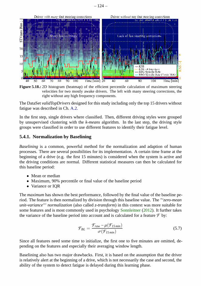
– 124–

Figure 5.18.:2D histogram (heatmap) of the efficient percentile calculation of maximum steeringvelocities for two mostly awake drivers. The left with many steering corrections, theright without any high frequency components.

The DataSetvalidTopDriversdesigned for this study including only the top 15 drivers withoutfatigue was described in Ch.A.2.

In the first step, single drivers where classified. Then, different driving styles were groupedby unsupervised clustering with thek-meansalgorithm. In the last step, the driving stylegroups were classified in order to use different features to identify their fatigue level.

5.4.1. Normalization by Baselining

Baselining is a common, powerful method for the normalization and adaption of humanprocesses. There are several possibilities for its implementation. A certain time frame at thebeginning of a drive (e.g. the first 15 minutes) is consideredwhen the system is active andthe driving conditions are normal. Different statistical measures can then be calculated forthis baseline period:

• Mean or median• Maximum, 90% percentile or final value of the baseline period• Variance or IQR

Themaximumhas shown the best performance, followed by the final value ofthe baseline pe-riod. The feature is then normalized by division through this baseline value. The"‘zero-meanunit-variance"’ normalization(also calledz-transform) in this context was more suitable forsome features and is most commonly used in psychologySonnleitner(2012). It further takesthe variance of the baseline period into account and is calculated for a featureF by:

FBL =Fraw − µ(F15min)

σ(F15min)(5.7)

Since all features need some time to initialize, the first oneto five minutes are omitted, de-pending on the features and especially their averaging window length.

Baselining also has two major drawbacks. First, it is based on the assumption that the driveris relatively alert at the beginning of a drive, which is not necessarily the case and second, theability of the system to detect fatigue is delayed during this learning phase.

– 125–

Every feature in Tab.4.2that is marked by2 is baselined. Parameter-optimization has shownthe best results when using themaximum. The optimization tends to favor window size ofup to 40 minutes because theKSSreference also changes so slowly. Thus, not more than 20minutes active time were used to preserve high feature dynamics and because the baselineperiod otherwise takes much too long for low system active levelsS ASx.

5.4.2. Driver-specific Features

While some of the features in Ch.4 are suitable for driver group classification, also additionalfeatures were used that were not suitable for fatigue detection. The following features wereinvestigated for the classification of driver groups:

• Ratio of lane changes with and without turn indicator use (TURNINDMISS: ratioaveraged by theEwmaNof the last 10 lane changes)

• Lateral lane change velocityyL (LNCHGVEL: EwmaNof the last 10 lane changes)• Duration between turn indicator use and lane change (TURNINDADVANCE: duration

differences between lever operation and lane change if below 10 seconds, averaged bytheEwmaNof the last 10 lane changes)

• Duration of turn indicator use (TURNINDDUR: EwmaNof the last 10 lane changes)• Lateral lane deviation and mean (LANEDEV: as described in Ch.4.3.2, LATMEAN is

the average lateral driver offset as described in Ch.4.3.1)• Maximum steering velocities (regular feature from Ch.4 and Fig.5.18)• Maximum longitudinal and lateral acceleration at specific speeds and curvatures (ACC75

regular features from Ch.4)• Rate of ALDW warnings (regular features from Ch.4)

5.4.3. Driver Group Clustering and Classification

Fig. 5.19 shows the classification of twelve drivers by their driving style. Details can befound in the thesis of (Gärtner, 2009).

0.86 0 0.02 0 0 0.03 0 0.09 0 0 0 0

0.2 0.72 0 0.02 0.01 0 0 0.05 0 0 0 0

0 0 0.62 0 0.24 0.04 0.03 0 0 0.02 0 0.05

0.14 0.01 0.1 0.38 0.01 0.1 0.2 0.04 0.01 0 0.02 0

0.08 0.06 0.37 0.03 0.11 0.28 0.01 0 0 0 0.01 0.05

0.05 0.3 0 0 0.23 0 0.1 0 0 0.3 0 0.02

0.01 0 0.06 0.62 0 0.16 0.05 0 0 0.1 0 0

0.14 0.03 0.05 0.01 0.01 0.02 0 0.74 0 0 0 0

0 0 0 0 0.01 0.02 0.02 0 0.75 0.01 0.08 0.13

0 0 0.02 0.01 0 0.08 0.1 0.05 0.03 0.53 0.08 0.11

0 0 0 0 0 0 0 0 0.05 0 0.95 0

0 0 0 0 0 0 0 0.24 0.27 0.18 0 0.32

5 20 59 133 152 165 340 484 607 609 611 783

5

20

59

133

152

165

340

484

607

609

611

783

Tru

e C

lass

(D

river

-ID

)

Detected Class (Driver-ID)

Figure 5.19.:Confusion matrix for drivers usingGMM classifier (Courtesy of:Gärtner, 2009)

Drivers that were often mixed up during classification (as for instance driver-ID 133 and 340)could be combined to one group. Fig.5.20 shows the classification result for the featuresSTV25, STV50, STV75, LATMEAN, LANEDEV, LNIQR andACC75 and a reduced numberof driving style groups:

– 126–

• A: Very calm steering, sloppy lane keeping (Driver-IDs 5, 20, 484)• B: Calm steering and lane keeping, sportive acceleration (ID 609, 783)• C: Calm steering, lane keeping and acceleration (ID 59, 133,152, 165, 340, 607)• D: Hectic steering, precise lane keeping (ID 611)

Figure 5.20.:Confusion matrix usingBayesclassifier and four driving style groups (Courtesy of:Gärtner, 2009)

The results show that classification of at least two main groups of driving style is quite fea-sible. As the example in Fig.5.18shows, the fatigue level of hectic drivers can be detectedbetter by their steering behavior, while the other group with a calm steering style has a moresloppy lane keeping. Thus, for the different groups, it is more appropriate to use differentfeatures for the classification of their fatigue level. In theory, the more appropriate method-ology would be to train the classifier in a single step. However, this did not work due to thelarger amount of involved features that require more training data than there were availablehere (see Ch.8.4).

5.5. Conclusion

In this chapter, it was shown that there are at least the thirteen external factors from Fig.5.1that have a strong impact on the driving behavior. The factors are in many situations moredominant than the sleepiness patterns. Further, the a-priori factors daytime, driving duration,monotony, novelty and light have the largest effect. Most ofthem can easily be measured,however are not directly sensitive to the driver state. Driver monitoring does not work underreal-road conditions without taking external factors intoaccount.

For the most important factors, specific drives were recorded and evaluated, i.e. vehicle speedand curvature. For the factors road condition, light, rain and driving style, appropriate driveswere filtered from the database. In order to consequently findall relevant parameters for theirprecise compensation, a matrix of hundreds of specific drives would be necessary for varyingonly one external factor at a time while keeping all other factors constant.

For most external factors, methods were proposed to incorporate them. Ideally, for impor-tant features, the normalization was already part of the theextraction. The system activesignals suppress events resulting from external factors. Specific features were designedfor the purpose of explicitly identifying external factorssuch asPAVEMENT, CURVATURE,ROADBUMPS2, CROSSWIND and the a-priori factorsTOT, CIRCADIAN, MONOTONYSPD,TRFCDENS andLIGHT. For the fusion of features on the classifier level, these feature wereprovided for classification and feature selection in Ch.8.

Baselining was presented as the predominant method to compensate individual driving stylesduring the extraction of features. A driving style classification has shown that different groupsof drivers can be identified for a two-stage classification.

– 127–

Chapter 6.

Approximation of Lane-based Features fromInertial Sensors

The major drawback of the utilization of lane data based features from Sec.4.3 is that theALDW camera is only available as special equipment and, thus, limited to the vehicles thathave it installed. Furthermore, the lane data signals are often affected by missing road mark-ings, bad sight etc. In comparison, inertial sensors are standard equipment and available forall vehicles.

Some lane-based features such asLANEDEV or ZIGZAGS do not require theabsolutedis-tance to the lane markings, but only depend on the lateral deviation within the lane. Theidea of this chapter is to use odometric vehicle data only (yaw rate, steering wheel angleand vehicle speed) to approximate the classical lane-basedfeatures without the need of alane-tracking camera.

The basic assumption behind this approach is that the curvature of the road can be estimatedfrom the odometric data. As described in (Clayton, 2006), there is a minimum curvatureradius for every speed limit. For instance, the minimum curvature radius at 120km/h is 750meters. Thus, when speed limits are obeyed and if the vehiclewould ideally follow the lanecenter, the road curvature never exceeds this low frequencylimit. The vehicle trajectory isthus a combination of the road curvature and the lane keepingbetween lane markings. Thus,the deviation within the lane contains much higher frequencies than the road curvature andcan be extracted by a high-pass filter. To estimate the vehicle trajectory, an extended Kalmanfilter and a vehicle motion model are applied to the availablesensors.

Since fatigue changes slowly, its detection may be delayed by up to several minutes, sosignals can be analyzed retrospectively. A second hypothesis is that the lateral mean of thelane keeping does not vary too much for one drive, so that the absolute lateral position can beassumed to be constant. In this case, also the time-to-lane-crossing and lane approximationfeatures likeTLC1MIN or LANEAPPROXADAPT can be approximated.

In addition to yaw rate and vehicle speed, the vehicle’s GPS position is also included in anextended Kalman filter model in order to create a reference toevaluate the system perfor-mance.

Using odometricCAN data such as yaw rate, steering wheel angle, and wheel rotation highlyimproves the knowledge about the absolute position of the vehicle. Many other aspects in re-gards to drowsiness detection profit from this improved vehicle position. Short lane-trackinggaps can be filled and road-condition analysis benefits from this improved spatial resolution.The correlation between features based on lane data and odometric data as well as their rela-tionship with sleepiness will be compared.

– 128–

6.1. Literature review

There are many approaches for vehicle tracking with inertial vehicle data. Hasberg andHensel(2009) uses splines and a Kalman filter for online estimation of train tracks.Buehren(2008) investigates the tracking of vehicle target lists by radar. Weiss(2011) uses a Kalmanfilter to match radar, lidar and map data for highly accurate ego-vehicle position estimation.Miksch (2010) andGuan(2008) use a vehicle motion model to estimate the ego-motion formotion compensation of camera data.

Forsman and Vilaa(2012) uses a transfer function of steering wheel angle motivatedbycardiovascular regulation analysis in (Saul and Berger, 1991) to approximate the lateral laneposition. They test their approach with a simulator study with twenty-nine subjects. Usinga transfer function on the steering wheel angle is less accurate in comparison to additionallyusing inertial sensors and vehicle tracking with a Kalman filter. Lundquist and Schön(2010)uses the single-track model and a Kalman filter for road geometry and curvature estimation ofthe ego-vehicle. However, no literature was found that analyzes the estimation of lane-basedfeatures from inertial vehicle data.

6.2. Sensor Signals and Synchronization

The yaw rate sensor has a high resolution of 0.005/s and a sampling frequency ofFs =1/T ≈ 50 Hz. The GPS signals are available with a sampling rate ofFs ≈ 1 Hz and notalways valid. Every second, when new GPS data is available, aKalman iteration is calledto update the position according to the GPS data. This way, the Kalman filter takes over theweighting between inertial data and GPS data.

Tab. 6.1 shows a matrix of the required lane signals for the differentlane feature groupsand the system active signalS ASLANE to suppress special events. From this table, it can bederived, which features require the distance to the lane andwhich only focus on lurchingwithin the lane and thus are suitable best for inertial features. For odometry-based features,the lane signal qualityLaneDataQualis not needed since the signals are always valid. Aswell, lane changes (LaneChg_Stat) can be detected from theLaneLtrlDist. The odometry-based features are the ones (markedgreen) that have no other dependency than yaw rate orLaneLtrlDist, with the limitation that not the absolute offset is available.

6.3. Single-Track Vehicle Model

In order to estimate the ego-motion of a vehicle from inertial sensor data, different mathemati-cal models are available.Zomotor and Klinkner(1987) consider inertia torques of the vehicleand tire models for the description of slip effects. Other approaches require additional sen-sors like vehicle mass sensors to determine the mass distribution in a vehicle (Weiss, 2011).Carlson and Gerdes(2002) propose a method for the determination and application of tiremodels, that, however, require vehicle specific parametersfor the vehicle’s inertia torquewhich again depends on the actual mass (occupied seats and baggage) distribution.

These specific sensors and parameters are not available here. For these reasons, several as-sumptions are made for simplification in practice (Mitschke and Wallentowitz, 2004, Ch.C.18). Under these assumptions, thesingle-track model(or Bicycle Model) can be used with

– 129–

❳❳❳❳❳❳❳❳❳❳

FeaturesSignals

Lan

eDat

aQu

al

Lan

eCh

g_

Sta

t

rela

tive

Lan

eLtr

lDis

t

abso

lute

Lan

eLtr

lDis

t

Lan

eWid

th

Lan

eYaw

An

gl

Lan

eHrz

tCrv

Lan

eClo

tho

idP

ara

Lan

eNu

m

Nu

mL

ane

Lane change (S ASLANE) × × (×)Overtakings (e.g.S ASLANE) × ×Lane deviation(e.g.LANEDEV, ORA) × (×) ×Lateral offset (e.g.LATMEAN) × (×) ×ZigZags(e.g.ZIGZAGS) × (×) ×Lane oscillation(e.g.LATPOSZCR) × (×) ×Yaw events(e.g.YAWJERK) ×Lane approx. (e.g.LANEAPPROX) × (×) × ×TLC (e.g.TLC1MIN) (×) (×) × × × (×) (×) (×)

Table 6.1.:Signals needed for lane-based feature types, where (×) indicates that these features are notabsolutely necessary. Lane changes can also be detected by the blinking lever.

good approximation. It is the simplest mathematical model for the stationary and instationarylateral dynamic of a four-wheel vehicle (Riekert and Schunck, 1940, P. 210-224). Fig.6.1illustrates the model after a simplification by combining the two wheels of each axle.

ψ vveh

β

yveh

xveh

CGCG Model

δH

vveh≈ const

ay

β

Figure 6.1.:Left: Single-track modelsimplification by combining the two wheels of one axis.Right:steering wheel angleδH and vehicle speedvveh are the model input and lateral accelera-tion ay andsideslip angleβ the outputs.β is described in the following.

The vehicle dynamics model is mostly linear with good approximation on dry roads andfor lateral accelerations under 4m/s2 . The appearing angles are then small and can beapproximated by sin(α) ≈ α . According to (Schindler, 2007, Ch. 4) and (Schramm andHiller, 2014, Ch. 10), further assumptions are made: the vehicle is assumed to be a rigidmass withinertia torque Jz and itscenter of gravity(CG) on the ground. Only the front axleis steerable and the vehicle speedvveh is considered to be stationary, so that only two degreesof freedom remain: yaw rotationψ and thesideslip angleβ (also calledbodyslip angle). βis illustrated in Fig.6.2. It describes the angle between the longitudinal vehicle axis towards

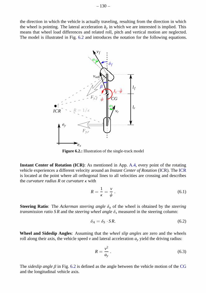
– 130–

the direction in which the vehicle is actually traveling, resulting from the direction in whichthe wheel is pointing. The lateral accelerationay in which we are interested is implied. Thismeans that wheel load differences and related roll, pitch and vertical motion are neglected.The model is illustrated in Fig.6.2 and introduces the notation for the following equations.

ψ

vveh

CG

l f

lr

Jz · ψ

vr

vf

Fy, f

Fy,r

δ f

α f

β

ey

ex

R= 1/καh

ICR

Figure 6.2.: Illustration of the single-track model

Instant Center of Rotation (ICR) : As mentioned in App.A.4, every point of the rotatingvehicle experiences a different velocity around anInstant Center of Rotation(ICR). TheICRis located at the point where all orthogonal lines to all velocities are crossing and describesthecurvature radius Ror curvatureκ with

R=1κ=

v

ψ. (6.1)

Steering Ratio: The Ackerman steering angleδa of the wheel is obtained by thesteeringtransmission ratio S Rand thesteering wheel angleδs measured in the steering column:

δA = δS ·S R. (6.2)

Wheel and Sideslip Angles: Assuming that thewheel slip anglesare zero and the wheelsroll along their axis, the vehicle speedv and lateral accelerationay yield the driving radius:

R=v2

ay. (6.3)

Thesideslip angleβ in Fig. 6.2 is defined as the angle between the vehicle motion of theCGand the longitudinal vehicle axis.

– 131–

Self Steering Gradient: Theself-steering gradient SGis defined in DIN 70000 as the differ-ence between the steering angle gradient and the Ackerman angle over the lateral accelerationay:

SG=1

S RdδS

day− dδA

day(6.4)

With the vehiclecharacteristic lower velocity vch and thewheel base l, it is obtained by:

SG= ± l

v2ch

(6.5)

wherevch andl are vehicle specific properties that are available for the vehicles.

Characteristic Velocity: It is the vehicle speed, at which under-steering vehicles (SG> 0)have the maximum of their yaw intensification

vch =

√

lSG

. (6.6)

By Schramm and Hiller(2014), it is also described by "vch is the velocity for which the vehiclereacts most sensitively to steering inputs. Typical valuesare between 65 and 100 km/h".

An SG > 0 means that the vehicle is under-steering (front wheel slips), SG = 0 meansneutral andSG < 0 means, that the vehicle is over-steering (rear wheel slips). For safetyreasons, today’s vehicles are designed to under-steer, which is easier to handle. This meansthat the vehicle tends to turn to the curve outside instead ofobserving additional rotation bythe tail "drifting" out of the curve. All vehicles in this thesis are under-steering.

Yaw intensification: Theyaw intensificationis the ratio of stationary yaw rate and steeringwheel angle for stationary steering wheel angles

δH = S R·(

lR+ SG· ay

)

(6.7)

Lateral Acceleration: The lateral acceleration obtained by the steering wheel angle de-scribes the vehicle trajectory more precisely than the accelerometer value which is affectedby the road inclination towards the road side (y-direction). For this reason, thesingle-trackmodelis used. Thelateral accelerationay is obtained by thevelocity v, thesteering ratio S R,thesteering angleδa and theself-steering gradient SG:

ay =v2 · δa

l + SG· v2(6.8)

6.4. State Space Model

For the mapping of inertial sensor signals to real-world coordinates, a motion model is re-quired that describes the trajectory in every calculation step. A description of the motion canbe approximated either by theline segment modelor thearc segment model(Guan, 2008,Ch. 3.2.2-3). He stated that in conjunction with the Kalman filter, the linear-segment model

– 132–

∆sx∆sy

∆x

∆y

sy[k]

ey

ex

sx[k+ 1] ICR

sy[k+ 1]

R[k]

l[k+ 1]l[k]

ϕ[k]

ψ[k]

∆ψ

sx[k]

κ[k]

Figure 6.3.:Line segment motion model

performs far better than the arc-segment model. Fig.6.3 illustrates the line segment model.

The vehicle motion is modeled in analogy toBuehren(2008); Miksch (2010) and Weiss(2011). Thestate vectorx[k] ∈ R

n describes the position and motion state at time instantkby:

x[k] =

sx[k]sy[k]ψ[k]ψ[k]v[k]a[k]

x-position [m]y-position [m]yaw angle []yaw rate [/s]longitudinal velocity [m/s]longitudinal acceleration [m/s2]

(6.9)

For linear systems, the system model with thestate transition matrixA (n× n) describes thestate change ofx between two consecutive instants. Here, the system ist non-linear and thestate transition matrixA is replaced by astate transition functionf(x) (cf. Eq. (6.17)):

x[k+ 1] = f(x[k]). (6.10)

The second part of the system model is the measurement equation that maps the system stateto themeasurement vectorz[k] ∈ R

m using themeasurement matrixH =(

0 I)

(m× n):

z[k+ 1] = H x[k+ 1] , z[k] =

ψ[k]v[k]a[k]

(6.11)

– 133–

According Fig.6.3, the non-linear movement of the vehicle is given by

(

sx[k+ 1]sy[k+ 1]

)

=

(

sx[k]sy[k]

)

+ v+[k]Ts

cos(

ψ+)

sin(

ψ+)

. (6.12)

with v+ = v[k] + a[k]Ts2 , ψ+ = ψ+ ψ

Ts2 and thecycle time Ts.

6.5. Kalman Filter

The Kalman filter is an optimal state estimation algorithm for linear systems to estimatethe system state vectorx[k]. For optimality, it requires that the measurement and processnoise have zero mean, white, uncorrelated and normally distributed additive noise (Welchand Bishop, 2006). After initialization, the iterative algorithm consistsof apredictionand aninnovation(or correction) step for each iterationk. The prediction step derives from the pre-vious iterationk− 1 updated state variables and uncertainties under the consideration of themotion model. The current measurement is included under consideration of its uncertaintiesform the innovation step. The Kalman Gain is a feedback that weights the influence of themodel or measurement based on their covariances.

6.5.1. Optimal State Estimation using the Kalman filter

The state transition and measurement equation in Eq. (6.10) and Eq. (6.11) are expanded bythemodel noisew[k] and themeasurement noisev[k] (with processandmeasurement noisecovariance matricesQ andR):

x[k+ 1] = Ax[k] + Bu[k] + w[k], (6.13)

z[k+ 1] = Hx[k+ 1] + v[k+ 1] (6.14)

The influence ofl input parametersu can be included by the(n× l) input matrixB, which isnot relevant here.w[k] andv[k] were found to be additive normally distributed white noisewith zero mean:

E[w[n]wT [k]] = Wδnk

E[v[n]vT [k]] = V δnk

p(w) ∝ N(0,Q), p(v) ∝ N(0,R)

E[w[k]] = E[v[k]] = 0.

Model noise, measurement noise and initial states are uncorrelated:

E[w[k]vT [k]] = E[w[k]xT [0]] = E[v[k]xT [0]] = 0.

Details for the Kalman filter and the validity of its requirements for the yaw rate, vehiclespeed and acceleration sensors can be read in (Welch and Bishop, 2006; Buehren, 2008;Weiss, 2011). Thepredictionandcorrectionsteps of the linear Kalman filter state estimationare illustrated in the following:

– 134–

Time Update (‘Predict’)

(1) Project the state aheadx−k = Ax−k−1 + Buk−1

(2) Project the errorcovariance ahead

P−k = APk−1AT + Q

Measurement Update (‘Correct’)

(1) Compute Kalman Gain FactorK k = P−k HT(HP−k HT + R)−1

(2) Update estimatewith measurementzk

xk = x−k + Kk(zk −Hx−k)

(3) Update the error covariancePk = (I −KkH)P−k

Initial estimate forxk−1 andPk−1

6.5.2. The Extended Kalman Filter

TheExtended Kalman filter (EKF)is necessary, if the state transition is non-linear, as in ourcase. Now the system is described by the non-linear, differentiable functionsf andh:

x[k+ 1] = f(

x[k], u[k], w[k]

)

(6.15)

z[k+ 1] = h(

x[k+ 1], v[k+ 1]

)

(6.16)

In our case, the measurement equation stays as in (6.14). The Extended Kalman filter stateestimation is again computed in two steps:predictionandcorrection, but now with the lin-earized function.

Time Update (‘Predict’)

(1) Project the state aheadx−k = f(x−k−1, uk−1, 0)

(2) Project the errorcovariance ahead

P−k = AkPk−1ATk + WkQk−1WT

k

Measurement Update (‘Correct’)

(1) Compute Kalman Gain Factor

Kk = P−k HTk

(

HkP−k HTk + VkRkVT

k

)−1

(2) Update estimatewith measurementzk

xk = x−k + K k

(

zk − h(xk,0)

)

(3) Update the error covariancePk = (I −K kHk)P−k

Initial estimate forxk−1 andPk−1

As the yaw rate in Eq. (6.12) changes very slowly within the cycle timeTs = 20ms, we usethe first orderTaylor series approximation, sin(α) ≈ α andcos(α) ≈ 1 for α ≪ π/2, we canlinearize the trigeonometric functions to the dimensions in Eq.6.9as follows:

f(x, q) =

sx[k] + ·v+[k]Ts cos(

ψ+)

sy[k] + ·v+[k]Ts sin(

ψ+)

ψ[k] + ψTsψ[k]

v[k] + a[k]Tsa[k]

. (6.17)

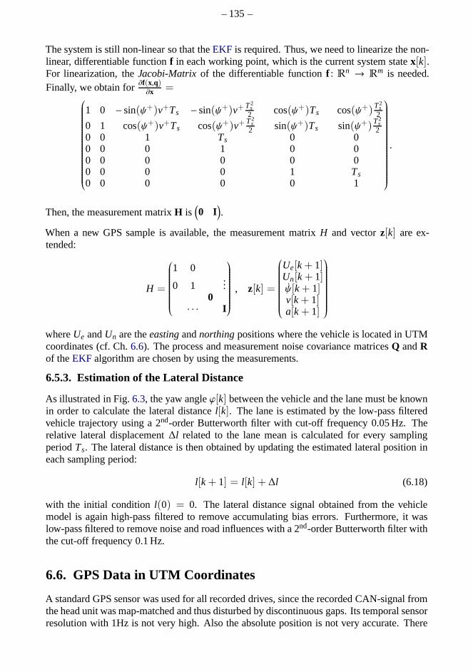
– 135–

The system is still non-linear so that theEKF is required. Thus, we need to linearize the non-linear, differentiable functionf in each working point, which is the current system statex[k].For linearization, theJacobi-Matrix of the differentiable functionf : R

n → Rm is needed.

Finally, we obtain for∂f(x,q)∂x =

1 0 − sin(ψ+)v+Ts − sin(ψ+)v+ T2s

2 cos(ψ+)Ts cos(ψ+)T2s

2

0 1 cos(ψ+)v+Ts cos(ψ+)v+ T2s

2 sin(ψ+)Ts sin(ψ+)T2s

20 0 1 Ts 0 00 0 0 1 0 00 0 0 0 0 00 0 0 0 1 Ts0 0 0 0 0 1

.

Then, the measurement matrixH is(

0 I)

.

When a new GPS sample is available, the measurement matrixH and vectorz[k] are ex-tended:

H =

1 0

0 1...

0· · · I

, z[k] =

Ue[k+ 1]Un[k+ 1]ψ[k+ 1]v[k+ 1]a[k+ 1]

whereUe andUn are theeastingandnorthingpositions where the vehicle is located in UTMcoordinates (cf. Ch.6.6). The process and measurement noise covariance matricesQ andRof theEKF algorithm are chosen by using the measurements.

6.5.3. Estimation of the Lateral Distance

As illustrated in Fig.6.3, the yaw angleϕ[k] between the vehicle and the lane must be knownin order to calculate the lateral distancel[k]. The lane is estimated by the low-pass filteredvehicle trajectory using a 2nd-order Butterworth filter with cut-off frequency 0.05 Hz. Therelative lateral displacement∆l related to the lane mean is calculated for every samplingperiodTs. The lateral distance is then obtained by updating the estimated lateral position ineach sampling period:

l[k+ 1] = l[k] + ∆l (6.18)

with the initial conditionl(0) = 0. The lateral distance signal obtained from the vehiclemodel is again high-pass filtered to remove accumulating bias errors. Furthermore, it waslow-pass filtered to remove noise and road influences with a 2nd-order Butterworth filter withthe cut-off frequency 0.1 Hz.

6.6. GPS Data in UTM Coordinates

A standard GPS sensor was used for all recorded drives, sincethe recorded CAN-signal fromthe head unit was map-matched and thus disturbed by discontinuous gaps. Its temporal sensorresolution with 1Hz is not very high. Also the absolute position is not very accurate. There

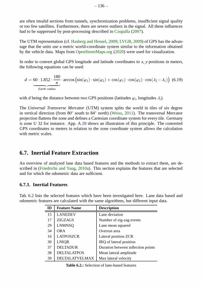
– 136–

are often invalid sections from tunnels, synchronization problems, insufficient signal qualityor too few satellites. Furthermore, there are severe outliers in the signal. All these influenceshad to be suppressed by post-processing described inCzupalla(2007).

The UTM representation (cf.Hasberg and Hensel, 2009; LVGB, 2009) of GPS has the advan-tage that the units use a metric world-coordinate system similar to the information obtainedby the vehicle data. Maps fromOpenStreetMaps.org(2020) were used for visualization.

In order to convert global GPS longitude and latitude coordinates tox, y positions in meters,the following equations can be used:

d = 60 · 1.852· 180π

︸ ︷︷ ︸

Earth radius

· arccos(

sin(ϕ1) · sin(ϕ2) + cos(ϕ1) · cos(ϕ2) · cos(λ2 − λ1))

(6.19)

with d being the distance between two GPS positions (latitudesϕi, longitudesλi).

The Universal Transverse Mercator(UTM) system splits the world in tiles of six degreein vertical direction (from 80 south to 84 north) (Weiss, 2011). The transversal Mercatorprojection flattens the zone and defines a Cartesian coordinate system for every tile. Germanyis zone U 32 for instance. App.A.10 shows an illustration of this principle. The convertedGPS coordinates to meters in relation to the zone coordinatesystem allows the calculationwith metric scales.

6.7. Inertial Feature Extraction

An overview of analyzed lane data based features and the methods to extract them, are de-scribed in (Friedrichs and Yang, 2010a). This section explains the features that are selectedand for which the odometric data are sufficient.

6.7.1. Inertial Features

Tab.6.2 lists the selected features which have been investigated here. Lane data based andodometric features are calculated with the same algorithms, but different input data.

ID Feature Name Description

15 LANEDEV Lane deviation17 ZIGZAGS Number of zig-zag events29 LNMNSQ Lane mean squared34 ORA Overrun area16 LATPOSZCR Lateral position ZCR30 LNIQR IRQ of lateral position37 DELTADUR Duration between inflection points38 DELTALATPOS Mean lateral amplitude39 DELTALATVELMAX Max lateral velocity

Table 6.2.:Selection of lane-based features

– 137–

6.7.2. System Active Signal

As the lane changes are not detected by the camera anymore, the turn indicator lever signalwas used to suppress lane changes. Three seconds before and ten seconds after lever opera-tion have been suppressed. Yaw ratesψ > 3/s have been neglected as well. Furthermore,the system was defined to be active only at velocities over 80 km/h.

6.8. Results

This section describes the comparison between lane data andinertial-data based signals. Thecorrelation of lane-based and odometric features is shown,as well as the correlation betweenodometric features and theKSSdrowsiness reference using the Spearman correlation coeffi-cient.

6.8.1. Comparison of Lane Data and Inertial Data

Fig. 6.4 shows the lateral deviation ("distance") signal obtained after removing the offset.However, the mean deviation between the two signals is 38cm,which indicates that there are

Figure 6.4.:Lateral position from lane-based (blue, solid) and odometric sensors (red, dotted)

certain different influences in the signal. The Pearson and Spearman correlation coefficientsbetween the features derived from the yaw rate and the original lane-based features are shownin Tab.6.3.

ID Feature Name ρp ρs

15 LANEDEV 0.241 0.36717 ZIGZAGS 0.512 0.63429 LNMNSQ 0.051 0.39434 ORA 0.338 0.41416 LATPOSZCR 0.908 0.35030 LNIQR 0.286 0.50537 DELTADUR 0.768 0.54038 DELTALATPOS 0.239 0.46739 DELTALATVELMAX 0.634 0.633

Table 6.3.:Correlation coefficients between lane-data and odometric features

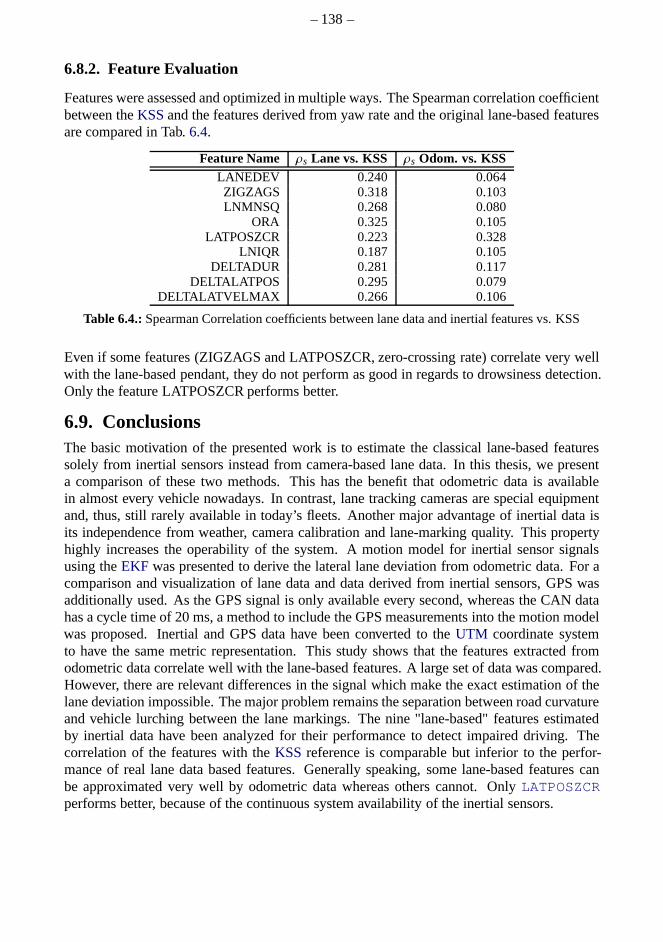
– 138–

6.8.2. Feature Evaluation

Features were assessed and optimized in multiple ways. The Spearman correlation coefficientbetween theKSSand the features derived from yaw rate and the original lane-based featuresare compared in Tab.6.4.

Feature Name ρs Lane vs. KSS ρs Odom. vs. KSSLANEDEV 0.240 0.064ZIGZAGS 0.318 0.103LNMNSQ 0.268 0.080

ORA 0.325 0.105LATPOSZCR 0.223 0.328

LNIQR 0.187 0.105DELTADUR 0.281 0.117

DELTALATPOS 0.295 0.079DELTALATVELMAX 0.266 0.106

Table 6.4.:Spearman Correlation coefficients between lane data and inertial features vs. KSS

Even if some features (ZIGZAGS and LATPOSZCR, zero-crossing rate) correlate very wellwith the lane-based pendant, they do not perform as good in regards to drowsiness detection.Only the feature LATPOSZCR performs better.

6.9. ConclusionsThe basic motivation of the presented work is to estimate theclassical lane-based featuressolely from inertial sensors instead from camera-based lane data. In this thesis, we presenta comparison of these two methods. This has the benefit that odometric data is availablein almost every vehicle nowadays. In contrast, lane tracking cameras are special equipmentand, thus, still rarely available in today’s fleets. Anothermajor advantage of inertial data isits independence from weather, camera calibration and lane-marking quality. This propertyhighly increases the operability of the system. A motion model for inertial sensor signalsusing theEKF was presented to derive the lateral lane deviation from odometric data. For acomparison and visualization of lane data and data derived from inertial sensors, GPS wasadditionally used. As the GPS signal is only available everysecond, whereas the CAN datahas a cycle time of 20 ms, a method to include the GPS measurements into the motion modelwas proposed. Inertial and GPS data have been converted to the UTM coordinate systemto have the same metric representation. This study shows that the features extracted fromodometric data correlate well with the lane-based features. A large set of data was compared.However, there are relevant differences in the signal whichmake the exact estimation of thelane deviation impossible. The major problem remains the separation between road curvatureand vehicle lurching between the lane markings. The nine "lane-based" features estimatedby inertial data have been analyzed for their performance todetect impaired driving. Thecorrelation of the features with theKSS reference is comparable but inferior to the perfor-mance of real lane data based features. Generally speaking,some lane-based features canbe approximated very well by odometric data whereas others cannot. OnlyLATPOSZCRperforms better, because of the continuous system availability of the inertial sensors.

– 139–

Chapter 7.

Assessment of Features

After the features have been extracted (Ch.4) under the consideration of external and driverinfluences (Ch.5) and with a new alternative approach to estimate lane features from inertialsensors (Ch.6), they are assessed in this chapter. The features are assessed and optimizedin multiple ways. The focus is to assess the performance of single features but also theircombinations according to different references in Ch.3.

In the first step, quantitative metrics for the correlation analysis and their results are presented.The metrics were used in Ch.4.5 as cost function for parameter optimization. Visual evalu-ations like boxplots, class histograms, correlation coefficient histograms or scatter plots leadto a higher transparency of features to identify their characteristics. The metrics from the firstpart of the chapter are the basis for these visual methods. The correlations and visualizationssuffer from the discrete interval scale of theKSS. Thus, theKSSvalues were interpolatedand smoothed as described in Ch.3.3.6. Linear and multiple regression is used to assess thecorrelations by fitting linear functions by least mean squares. Statistical tests like t-test, F-testor MANOVA are powerful methods to identify whether differences are significant. Finally,a visual user-interface (GUI) combines all the methods at once and allows filtering of thedata and reference. The results motivate several improvements in the feature extraction. Sub-jective, rather qualitative and empirical observations from night drives are also summarized.A proposal for potential features is given that comprises the various assessment aspects andknowledge of the nature and potential of features. Featuresthat are highly correlated andbased on the same patterns are reduced to the best of them.

7.1. Feature Assessment by Metrics

The goal of this section is to evaluate different measures that describe the relation betweentwo signals best. There are various potential metrics such as correlation coefficients or theFisher metric to assess the correlation and variance between features and reference. The co-variance, correlation and scatter matrices describe the relation between features. The Spear-man correlation coefficient, for instance, has also been used for parameter optimization.

7.1.1. Correlation Coefficients

The correlation describes the linear (or monoton) relationship between two measuresX ∈ FandY ∈ F , KSS, EEG, EYE. The metric is desired to be high when high and low samplevalues of the one measureX occur at the same time as for the other measureY. This can beillustrated by the scatter plot (cf. Sec.7.2.1) of the two measuredX andY in Fig. 7.1.

– 140–

MeasureXMeasureXMeasureX

Mea

sure

Y Positive No correlation Negative

Figure 7.1.:Scatter plot to illustrate correlation: positive, no and negative correlation.

This relationship can be quantitatively captured by thecorrelation coefficientsafterBravais-Pearsonρp for linear andSpearmanρs for monoton relationship. The range of values of bothcoefficients lies in−1 ≤ ρp ≤ 1. In caseρ > 0, the measures are positively correlated andvice versa. Thep-value of correlation indicates the probability with whichthe same resultcould be achieved randomly. With other words, it indicates the reliability of the result and isrelevant only for fewer test samples.

Pearson Correlation Coefficient

The empiric(Bravais-)Pearson Correlation Coefficient(Fahrmeir et al., 2003) measures thelinear relationship between two measuresX = [x1, ..,xN]T andY = [y1, ..,yN]T (with · asthe average):

ρp(X, Y) =

N∑

i=1(xi − x)(yi − y)

√

N∑

i=1(xi − x)2

N∑

i=1(yi − y)2

=Cov(X, Y)

√

Var(X) · Var(Y). (7.1)

Spearman Correlation Coefficient

The Spearman correlation coefficientρs describes how well the relationship between twomeasures can be described by amonotonicfunction. It is calculated in the same way as thePearson coefficient, only that arank function rg(·) converts the valuesX andY to a sortedrank order. For instance, the highest value is mapped to 1, the second highest value becomes2 and so on. If samples occur multiple times, they will be assigned to mean rank values. Thecalculation is defined (seeFahrmeir et al., 2003) by:

ρs(X, Y) =

N∑

i=1(rg(xi) − rg(X))(rg(yi) − rg(Y))

√

N∑

i=1(rg(xi) − rg(X))2

n∑

i=1(rg(yi) − rg(Y)2

=Cov(rg(X), rg(Y))

√

Var(rg(X)) · Var(rg(Y)),

(7.2)with the rank meansrg(X) (andrg(Y)) given by

rg(X) =1N

N∑

i=1

rg(xi) =N + 1

2. (7.3)

Even though theKSS scale is defined to be linear from a psychological perspective, it isknown that the scale is not interpreted and used linearly. This is one reason why the Spearmancorrelation coefficient has shown to be more meaningful in this application.

– 141–

7.1.2. Fisher Linear Discriminant Metric

TheFisher Linear Discriminant Metricis motivated by the fitness function of the FisherLDA(Welling, 2005) and closely related to regression analysis. It sets the scatter between classesin relation to the scatters within each class.

Multi-dimensional case: TheMultiple Discriminant Analysis(MDA) is defined as explainedin (Yang, 2018; Uhlich, 2006; Duda et al., 2001) by the quotient of the matrix determinants:

MDA (X) =|SB||SW|

(7.4)

whereSB is the scatter matrixbetweenthec classes

SB =c∑

i=1

ni(mi − m)(mi − m)T (7.5)

whereni is the number of patterns in classi. m is the average over all classes andmi are theaverages of each classi. SW is the scatterwithin classes:

SW =c∑

i=1

Si with Si =∑

x∈X i

(x− mi)(x− mi)T , (7.6)

the scatter matrixSi of the patternsXi in classi. The advantage ofMDA is that multiplefeatures can be assessed by one scalar measure. This measureis invariant to a linear transfor-mation, i.e. no normalization is required in advance.

Fig. 7.2 illustrates the strengths and weaknesses of theMDA by four examples with three bi-variate Gaussian distributed clusters and serves as validation of the implementation. Anotherweakness of the measure is that when one cluster is rotated, the center of all classes and, thus,the metric is not changed much, even when the two classes overlap more.

In the two-dimensional case and especially for more than twoclasses, the correlation coef-ficients are more meaningful since they describe the ordinallinearity. Further, it has to benoted that theKSScannot be used for theMDA, since it is only defined for classes.

7.1.3. Results

Tab.7.1 lists all metrics from this section, the correlation coefficients, the one-dimensionalMDA metric for 9 classes and theAUC (Ch. 7.5). The ending ’BL’ indicates that a featureis baselined. Only the best out of all redundant features areused for the comparison with theKSS. External influences are only relevant after the fusion of features. It can be seen thatmost a-priori features perform best, but on the same level asthe majorATTENTION ASSIST

featureGGGLWF. Further, the TLC-based and lane approximation features show the bestresults underneath the causal features.

ID Feature Name ρp ρs MDA (9 classes) AUC45 CIRCADIAN 0.4911 0.4880 84.824554 0.8005768 TOTSPEED 0.3825 0.4088 12.859585 0.52957

122 GGGLWF 0.3644 0.3541 11.141940 0.7444966 TOT 0.2579 0.2656 10.385206 0.67326

156 DISTRACTION 0.2266 0.2590 22.924826160 NMRSTVHOLD 0.2501 0.2415 10.857038

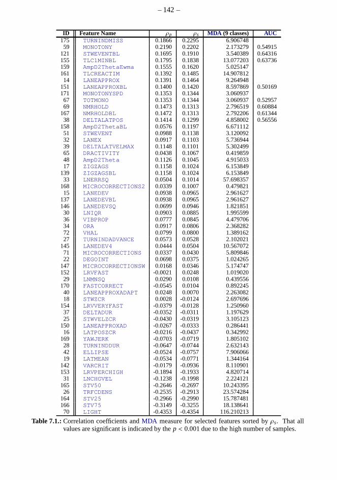
– 142–

ID Feature Name ρp ρs MDA (9 classes) AUC175 TURNINDMISS 0.1866 0.2295 6.90674859 MONOTONY 0.2190 0.2202 2.173279 0.54915

121 STWEVENTBL 0.1695 0.1910 3.540389 0.64316155 TLC1MINBL 0.1795 0.1838 13.077203 0.63736159 AmpD2ThetaEwma 0.1555 0.1620 5.025147161 TLCREACTIM 0.1392 0.1485 14.90781214 LANEAPPROX 0.1391 0.1464 9.264948

151 LANEAPPROXBL 0.1400 0.1420 8.597869 0.50169171 MONOTONYSPD 0.1353 0.1344 3.06093767 TOTMONO 0.1353 0.1344 3.060937 0.5295769 NMRHOLD 0.1473 0.1313 2.796519 0.60884

167 NMRHOLDBL 0.1472 0.1313 2.792206 0.6134438 DELTALATPOS 0.1414 0.1299 4.858002 0.56556

158 AmpD2ThetaBL 0.0576 0.1197 6.67111251 STWEVENT 0.0988 0.1138 3.12009232 LANEX 0.0917 0.1103 5.73694439 DELTALATVELMAX 0.1148 0.1101 5.30249965 DRACTIVITY 0.0438 0.1067 0.41985948 AmpD2Theta 0.1126 0.1045 4.91503317 ZIGZAGS 0.1158 0.1024 6.153849

139 ZIGZAGSBL 0.1158 0.1024 6.15384933 LNERRSQ 0.0504 0.1014 57.698357

168 MICROCORRECTIONS2 0.0339 0.1007 0.47982115 LANEDEV 0.0938 0.0965 2.961627

137 LANEDEVBL 0.0938 0.0965 2.961627146 LANEDEVSQ 0.0699 0.0946 1.82185130 LNIQR 0.0903 0.0885 1.99559936 VIBPROP 0.0777 0.0845 4.47970634 ORA 0.0917 0.0806 2.36828272 VHAL 0.0799 0.0800 1.38916227 TURNINDADVANCE 0.0573 0.0528 2.102021

145 LANEDEV4 0.0444 0.0504 10.56707271 MICROCORRECTIONS 0.0337 0.0430 5.80984622 DEGOINT 0.0698 0.0375 1.024265

147 MICROCORRECTIONSW 0.0168 0.0346 5.174747152 LRVFAST -0.0021 0.0248 1.01902029 LNMNSQ 0.0290 0.0108 0.439556

170 FASTCORRECT -0.0545 0.0104 0.89224540 LANEAPPROXADAPT 0.0248 0.0070 2.26308218 STWZCR 0.0028 -0.0124 2.697696

154 LRVVERYFAST -0.0379 -0.0128 1.25096037 DELTADUR -0.0352 -0.0311 1.19762925 STWVELZCR -0.0430 -0.0319 3.105123

150 LANEAPPROXAD -0.0267 -0.0333 0.28644116 LATPOSZCR -0.0216 -0.0437 0.342992

169 YAWJERK -0.0703 -0.0719 1.80510228 TURNINDDUR -0.0647 -0.0744 2.63214342 ELLIPSE -0.0524 -0.0757 7.90606619 LATMEAN -0.0534 -0.0771 1.344164

142 VARCRIT -0.0179 -0.0936 8.110901153 LRVPERCHIGH -0.1894 -0.1933 4.82071431 LNCHGVEL -0.1238 -0.1998 2.224121

165 STV50 -0.2646 -0.2697 10.24339526 TRFCDENS -0.2535 -0.2913 23.574284

164 STV25 -0.2966 -0.2990 15.787481166 STV75 -0.3149 -0.3255 18.13864170 LIGHT -0.4353 -0.4354 116.210213

Table 7.1.:Correlation coefficients andMDA measure for selected features sorted byρs. That allvalues are significant is indicated by thep < 0.001 due to the high number of samples.

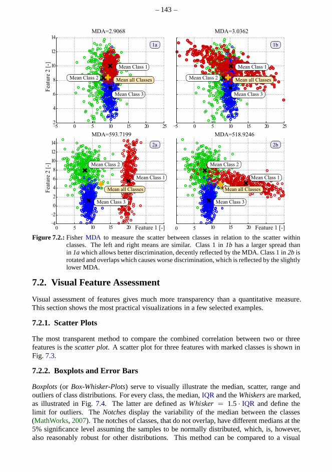
– 143–

Figure 7.2.:FisherMDA to measure the scatter between classes in relation to the scatter withinclasses. The left and right means are similar. Class 1 in1b has a larger spread thanin 1awhich allows better discrimination, decently reflected by the MDA. Class 1 in2b isrotated and overlaps which causes worse discrimination, which is reflected by the slightlylower MDA.

7.2. Visual Feature Assessment

Visual assessment of features gives much more transparencythan a quantitative measure.This section shows the most practical visualizations in a few selected examples.

7.2.1. Scatter Plots

The most transparent method to compare the combined correlation between two or threefeatures is thescatter plot. A scatter plot for three features with marked classes is shown inFig. 7.3.

7.2.2. Boxplots and Error Bars

Boxplots(or Box-Whisker-Plots) serve to visually illustrate the median, scatter, range andoutliers of class distributions. For every class, the median, IQR and theWhiskersare marked,as illustrated in Fig.7.4. The latter are defined asWhisker = 1.5 · IQR and define thelimit for outliers. TheNotchesdisplay the variability of the median between the classes(MathWorks, 2007). The notches of classes, that do not overlap, have different medians at the5% significance level assuming the samples to be normally distributed, which, is, however,also reasonably robust for other distributions. This method can be compared to a visual

– 144–

Figure 7.3.:Scatterplot for selected featuresCIRCADIAN, TLC1MINBL andSTWEVENTBL for thethree classesawake(•), acceptable(•) anddrowsy(•).

hypothesis test analogous to the t-test for means. Thus, in this example, it can be seen that thefeatureNMRSTVHOLD increases with increasingKSS with significant differences betweenclasses.

Figure 7.4.: Illustration of Boxplot for feature NMRSTVHOLD.

The Boxplots in Fig.7.5show the relationship between different other features andtheKSS.All plots show that the median of the classes significantly differ, but are still overlappingwhich pose difficulties for the drowsiness classification. There are very few drives withKSSbelow 2, so these levels should be neglected.

Error bars show the confidence level of data or the deviation along a curve (MathWorks,2007). In our case, the variance is used as displayed in Fig.7.4. In this example, the dif-ference between mean/median and variance/IQR can be seen due to the influence of outliersthat can be essential for some features.

– 145–

KSS level [-]6543 7 8 9

·10−3

TOTSPEED (ID: 68)ELLIPSE (ID 42)

21KSS level [-]

6543 7 8 921

Fea

ture

s[-

]

35

0

5

10

15

20

25

30

LATPOSZCR (ID: 16)TRFCDENS (ID: 26)·10−3

0

0.2

0.4

0.6

0.8

1.0

1.2

0

1

2

3

4

5

Fea

ture

s[-

]7

0123456

89

10

Figure 7.5.:Boxplot of selected features

7.2.3. Class Histograms

Class histograms were also used to get a visual impression ofthe features. The STV50 classhistogram can be found in Fig.7.6 as an example. It can be seen that the steering velocitiesdecrease with increasing vigilance.

7.2.4. Histogram of Correlation Coefficients

Another method of correlation analysis proposed bySimon(2012) is to cluster the featuresby drives (or drivers) and calculate the Spearman (or Pearson) correlation coefficients be-tween features andKSS reference. A histogram of the coefficients then indicates, for howmany drives this feature correlates well with fatigue. If one portion of the drives correlatesnegatively and the other portion positively, it is a contradicting statement and does not speakfor an useful feature. It has to be considered that a long drive contributes as much as a shortdrive. However, in App.A.11 the limits of this metric are discussed. Even if all correlationcoefficients are one, the overall correlation can be very bad. With other words, this metricwould work sufficiently, if the online-adaption of every drive by baselining was optimal.

Fig. 7.7 shows other examples of the causal featuresLANEX, ORA andNMRHOLD. It canbe seen that there is a tendency towards the right, that indicates, that most drives are posi-tively correlated with drowsiness. Further, it can be seen,that the last feature, with the bestoverall Spearman coefficient, performs worst from the histogram’s perspective. We can con-clude, from these three examples, thatLANEX profits most from driver (drive) adaption, i.e.baselining.

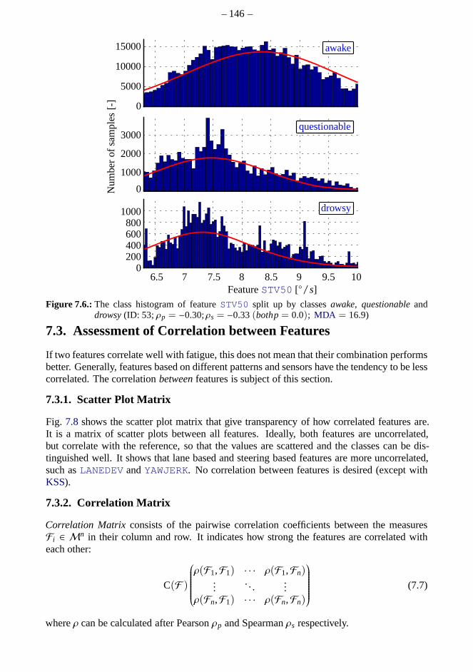
– 146–

FeatureSTV50 [/s]8.587.57 9 9.5 106.5

Num

ber

ofsa

mpl

es[-

]

awake

questionable

drowsy

0200400600800

1000

0

3000

2000

1000

0

5000

10000

15000

Figure 7.6.:The class histogram of featureSTV50 split up by classesawake, questionableanddrowsy(ID: 53; ρp = −0.30;ρs = −0.33(bothp= 0.0); MDA = 16.9)

7.3. Assessment of Correlation between Features

If two features correlate well with fatigue, this does not mean that their combination performsbetter. Generally, features based on different patterns and sensors have the tendency to be lesscorrelated. The correlationbetweenfeatures is subject of this section.

7.3.1. Scatter Plot Matrix

Fig. 7.8 shows the scatter plot matrix that give transparency of how correlated features are.It is a matrix of scatter plots between all features. Ideally, both features are uncorrelated,but correlate with the reference, so that the values are scattered and the classes can be dis-tinguished well. It shows that lane based and steering basedfeatures are more uncorrelated,such asLANEDEV andYAWJERK. No correlation between features is desired (except withKSS).

7.3.2. Correlation Matrix

Correlation Matrix consists of the pairwise correlation coefficients between the measuresFi ∈ Mn in their column and row. It indicates how strong the featuresare correlated witheach other:

C(F )

ρ(F1,F1) · · · ρ(F1,Fn)...

. . ....

ρ(Fn,F1) · · · ρ(Fn,Fn)

(7.7)

whereρ can be calculated after Pearsonρp and Spearmanρs respectively.

– 147–

Figure 7.7.:Histogram ofρs coefficient of KSS and featuresLANEX, ORA andNMRHOLD grouped bydrives

Fig. 7.9 shows an example of the matrix. Baselined features are oftencorrelated. The roadcondition features and allLANEDEV derivates are correlated, but also withORA, LANEIQRandTLC1MIN. CIRCADIAN are negatively correlated withLIGHT.

7.4. Linear and Multiple Regression Analysis

Regression Analysisis a method of statistical analysis that pursues the goal to quantitativelydetermine the relationship between a dependent variable (regressand) and one or several in-dependent variables (regressor(s)). In our case, theKSSreference is the regressand and theregressor(s) is (are) the feature(s). Regression analysisfor driver state detection was alreadyused byKnipling and Wang(1994); Wierwille and Ellsworth(1994); Wierwille (1996b);Belz(2000) and (Mattsson, 2007; Berglund, 2007, Both Sec. 2.5) for identifying the most po-tential features. When features are normalized, the coefficients indicate, which contributiona feature makes for the final result and which features are redundant. Linear andMultipleRegressionare closely related toLDA and classification. Hence, the other application of thismethod is prediction or classification, discussed in Ch.8.

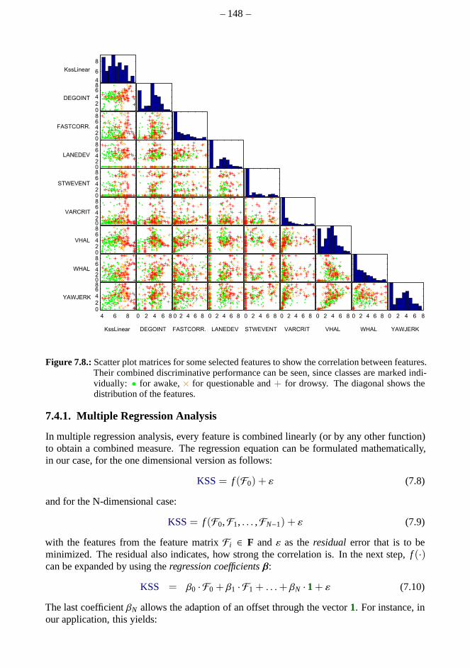
– 148–

0 2 4 6 80 2 4 6 80 2 4 6 80 2 4 6 80 2 4 6 80 2 4 6 80 2 4 6 80 2 4 6 84 6 8

0

2

4

68024

6

8

0

2

4

6

8

02

4

6

8

0

2

4

6

8

0

2

4

6

8

0

2

4

6

8

0

2

4

684

6

8

KssLinear

DEGOINT

FASTCORR.

LANEDEV

STWEVENT

VARCRIT

VHAL

WHAL

YAWJERK

KssLinear DEGOINT FASTCORR. LANEDEV STWEVENT VARCRIT VHAL WHAL YAWJERK

Figure 7.8.:Scatter plot matrices for some selected features to show thecorrelation between features.Their combined discriminative performance can be seen, since classes are marked indi-vidually: • for awake,× for questionable and+ for drowsy. The diagonal shows thedistribution of the features.

7.4.1. Multiple Regression Analysis

In multiple regression analysis, every feature is combinedlinearly (or by any other function)to obtain a combined measure. The regression equation can beformulated mathematically,in our case, for the one dimensional version as follows:

KSS= f (F0) + ε (7.8)

and for the N-dimensional case:

KSS= f (F0,F1, . . . ,FN−1) + ε (7.9)

with the features from the feature matrixFi ∈ F and ε as theresidual error that is to beminimized. The residual also indicates, how strong the correlation is. In the next step,f (·)can be expanded by using theregression coefficientsβ:

KSS = β0 · F0 + β1 · F1 + . . .+ βN · 1+ ε (7.10)

The last coefficientβN allows the adaption of an offset through the vector1. For instance, inour application, this yields:

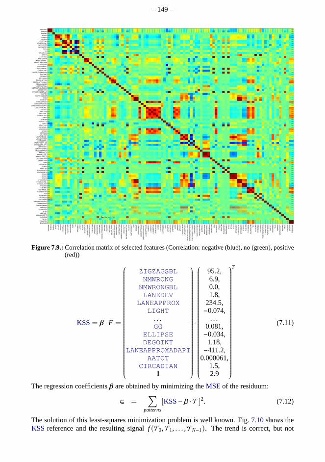
– 149–

Figure 7.9.:Correlation matrix of selected features (Correlation: negative (blue), no (green), positive(red))

KSS= β · F =

ZIGZAGSBLNMWRONGNMWRONGBLLANEDEV

LANEAPPROXLIGHT

. . .GG

ELLIPSEDEGOINT

LANEAPPROXADAPTAATOT

CIRCADIAN1

·

95.2,6.9,0.0,1.8,

234.5,−0.074,

. . .0.081,−0.034,

1.18,−411.2,

0.000061,1.5,2.9

T

(7.11)

The regression coefficientsβ are obtained by minimizing theMSEof the residuum:

⊂= =∑

patterns

[KSS− β · F ]2. (7.12)

The solution of this least-squares minimization problem iswell known. Fig.7.10shows theKSS reference and the resulting signalf (F0,F1, . . . ,FN−1). The trend is correct, but not

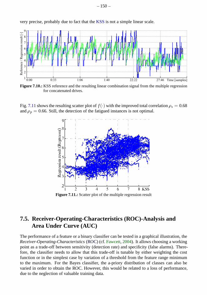
– 150–

very precise, probably due to fact that theKSSis not a simple linear scale.

Figure 7.10.:KSS reference and the resulting linear combination signal from the multiple regressionfor concatenated drives.

Fig.7.11shows the resulting scatter plot off (·) with the improved total correlationρs = 0.68andρp = 0.66. Still, the detection of the fatigued instances is not optimal.

Figure 7.11.:Scatter plot of the multiple regression result

7.5. Receiver-Operating-Characteristics (ROC)-Analysis andArea Under Curve (AUC)

The performance of a feature or a binary classifier can be tested in a graphical illustration, theReceiver-Operating-Characteristics(ROC) (cf. Fawcett, 2004). It allows choosing a workingpoint as a trade-off between sensitivity (detection rate) and specificity (false alarms). There-fore, the classifier needs to allow that this trade-off is tunable by either weighting the costfunction or in the simplest case by variation of a threshold from the feature range minimumto the maximum. For the Bayes classifier, the a-priory distribution of classes can also bevaried in order to obtain the ROC. However, this would be related to a loss of performance,due to the neglection of valuable training data.

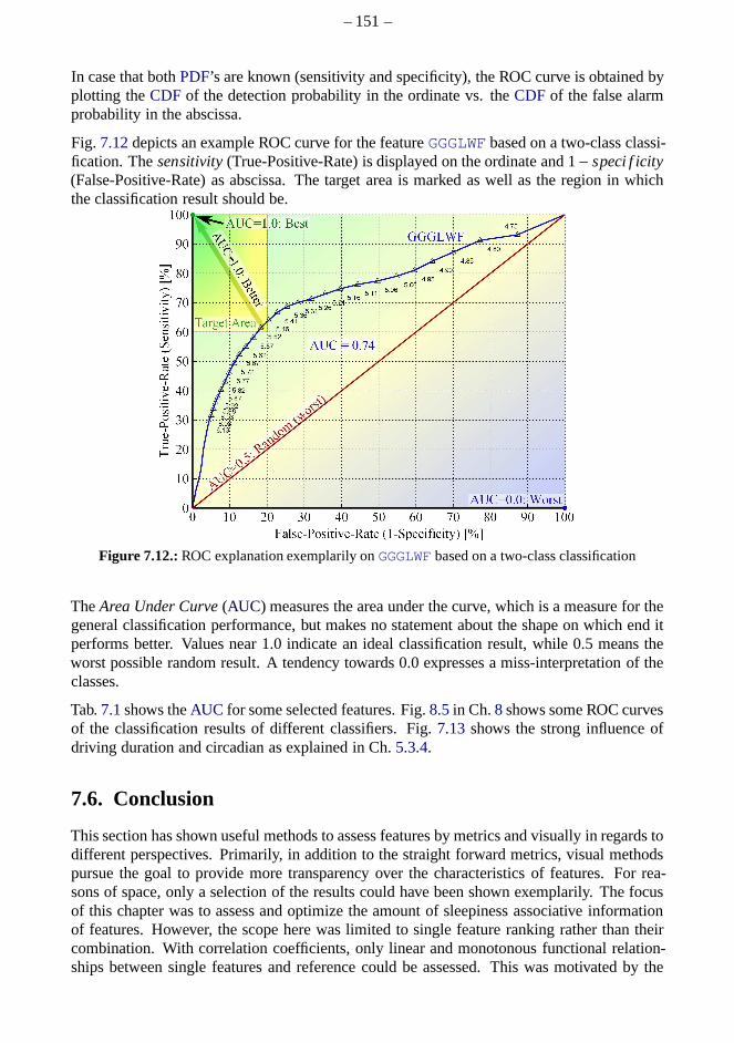
– 151–

In case that bothPDF’s are known (sensitivity and specificity), the ROC curve is obtained byplotting theCDF of the detection probability in the ordinate vs. theCDF of the false alarmprobability in the abscissa.

Fig. 7.12depicts an example ROC curve for the featureGGGLWF based on a two-class classi-fication. Thesensitivity(True-Positive-Rate) is displayed on the ordinate and 1− speci f icity(False-Positive-Rate) as abscissa. The target area is marked as well as the region in whichthe classification result should be.

Figure 7.12.:ROC explanation exemplarily onGGGLWF based on a two-class classification

TheArea Under Curve(AUC) measures the area under the curve, which is a measure for thegeneral classification performance, but makes no statementabout the shape on which end itperforms better. Values near 1.0 indicate an ideal classification result, while 0.5 means theworst possible random result. A tendency towards 0.0 expresses a miss-interpretation of theclasses.

Tab.7.1shows theAUC for some selected features. Fig.8.5in Ch.8 shows some ROC curvesof the classification results of different classifiers. Fig.7.13 shows the strong influence ofdriving duration and circadian as explained in Ch.5.3.4.

7.6. Conclusion

This section has shown useful methods to assess features by metrics and visually in regards todifferent perspectives. Primarily, in addition to the straight forward metrics, visual methodspursue the goal to provide more transparency over the characteristics of features. For rea-sons of space, only a selection of the results could have beenshown exemplarily. The focusof this chapter was to assess and optimize the amount of sleepiness associative informationof features. However, the scope here was limited to single feature ranking rather than theircombination. With correlation coefficients, only linear and monotonous functional relation-ships between single features and reference could be assessed. This was motivated by the

– 152–

Figure 7.13.:ROC curve for Time-on-TaskTOT andCIRCADIAN

fact that sleepiness is an ordinal scale rather than a multi-modal phenomenon. In contrastto Pearson correlation coefficients, the Spearman coefficients are more suitable to describethe single feature correlation for the development of a bargraph. To determine and optimizethe discriminative property of classes, the other measuresare also valuable for transparency.While the correlation is of central interest, also the redundancy in between features was in-vestigated. The nonlinear combination of this informationby Classificationis subject to thenext chapter.

The presented methods show that there are good features in every group. It is obvious that thea-priori features perform best, as they detect the time instant in driving studies, when subjectsbecome tired. Sleepiness occurs much more often during night experiments compared to realfield drives. Thus, this systematic factor is considered separately and taken into account forthe final classifier based on a dataset that has an a-priori distribution that is representativefor the real field scenario (DataSetFreeDrives). The system performance profits most fromthese features, even when they are not causal, i.e. sensitive to the driver.

The most potential pattern appears to be the steering corrections, especially followed by asteering pause. This pattern is highly analyzed and is further improved in various ways inthis thesis.

The lane features based on lane approximation and exceedingperformed best among the lanefeatures. For a few drivers, the ALDW warning worked really well and prevented them fromdrifting out of the lanes. Zig-zag events and its odometry based variant also appear to havehigh potential, especially in regards to robustness when the vision conditions are impaired.Features that are based on the same pattern as lane deviationfor instance are highly correlatedand only one of them could be used.

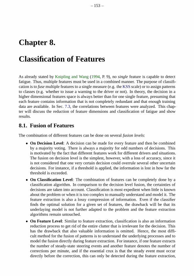
– 153–

Chapter 8.

Classification of Features

As already stated byKnipling and Wang(1994, P. 9), nosingle feature is capable to detectfatigue. Thus, multiple features must be used in a combined manner. The purpose of classifi-cation is tofusemultiple features to a single measure (e.g. theKSSscale) or to assign patternsto classes (e.g. whether to issue a warning to the driver or not). In theory, the decision in ahigher dimensional features space is always better than forone single feature, presuming thateach feature contains information that is not completely redundant and that enough trainingdata are available. In Sec.7.3, the correlations between features were analyzed. This chap-ter will discuss the reduction of feature dimensions and classification of fatigue and showresults.

8.1. Fusion of Features

The combination of different features can be done on severalfusion levels:

• On Decision Level: A decision can be made for every feature and then be combinedby a majority voting. There is always a majority for odd numbers of decisions. Thisis motivated by the fact that different features work for different drivers and situations.The fusion on decision level is the simplest, however, with aloss of accuracy, since itis not considered that one very certain decision could overrule several other uncertaindecisions. For instance, if a threshold is applied, the information is lost in how far thethreshold is exceeded.

• On Classification Level: The combination of features can be completely done by aclassification algorithm. In comparison to the decision level fusion, the certainties ofdecisions are taken into account. Classification is most expedient when little is knownabout the problem or when it is too complex to manually understand and model it. Thefeature extraction is also a lossy compression of information. Even if the classifierfinds the optimal solution for a given set of features, the drawback will be that itsunderlaying model is not further adapted to the problem and the feature extractionalgorithms remain untouched.

• On Feature Level: Similar to feature extraction, classification is also an informationreduction process to get rid of the entire clutter that is irrelevant for the decision. Thishas the drawback that also valuable information is omitted.Hence, the most diffi-cult method for the fusion of patterns is to understand the underlying processes and tomodel the fusion directly during feature extraction. For instance, if one feature extractsthe number of steady-state steering events and another feature denotes the number ofcorrections per minute, and if the essential crux is that thesteady event must occurdirectly before the correction, this can only be detected during the feature extraction,

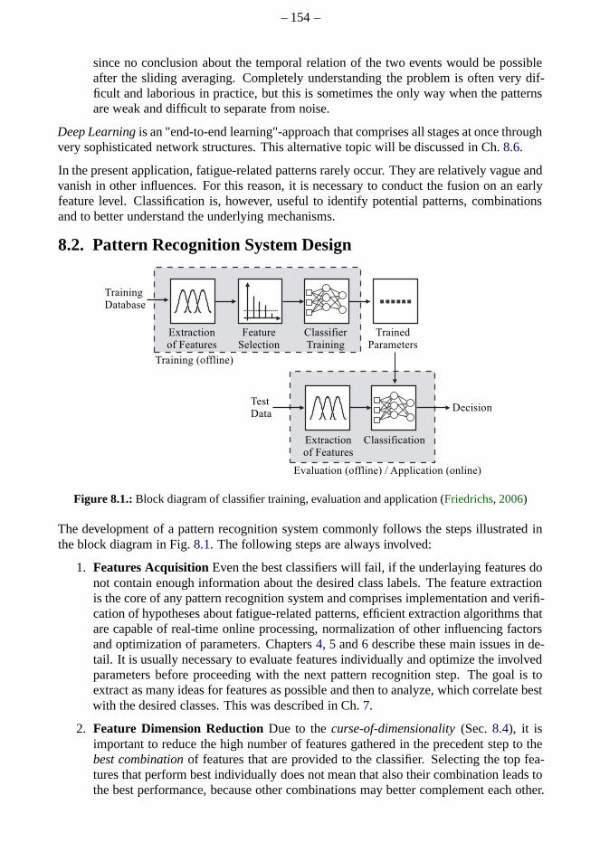
– 154–

since no conclusion about the temporal relation of the two events would be possibleafter the sliding averaging. Completely understanding theproblem is often very dif-ficult and laborious in practice, but this is sometimes the only way when the patternsare weak and difficult to separate from noise.

Deep Learningis an "end-to-end learning"-approach that comprises all stages at once throughvery sophisticated network structures. This alternative topic will be discussed in Ch.8.6.

In the present application, fatigue-related patterns rarely occur. They are relatively vague andvanish in other influences. For this reason, it is necessary to conduct the fusion on an earlyfeature level. Classification is, however, useful to identify potential patterns, combinationsand to better understand the underlying mechanisms.

8.2. Pattern Recognition System Design

Figure 8.1.:Block diagram of classifier training, evaluation and application (Friedrichs, 2006)

The development of a pattern recognition system commonly follows the steps illustrated inthe block diagram in Fig.8.1. The following steps are always involved:

1. Features AcquisitionEven the best classifiers will fail, if the underlaying features donot contain enough information about the desired class labels. The feature extractionis the core of any pattern recognition system and comprises implementation and verifi-cation of hypotheses about fatigue-related patterns, efficient extraction algorithms thatare capable of real-time online processing, normalizationof other influencing factorsand optimization of parameters. Chapters4, 5 and6 describe these main issues in de-tail. It is usually necessary to evaluate features individually and optimize the involvedparameters before proceeding with the next pattern recognition step. The goal is toextract as many ideas for features as possible and then to analyze, which correlate bestwith the desired classes. This was described in Ch.7.

2. Feature Dimension ReductionDue to thecurse-of-dimensionality(Sec.8.4), it isimportant to reduce the high number of features gathered in the precedent step to thebest combinationof features that are provided to the classifier. Selecting the top fea-tures that perform best individually does not mean that alsotheir combination leads tothe best performance, because other combinations may better complement each other.

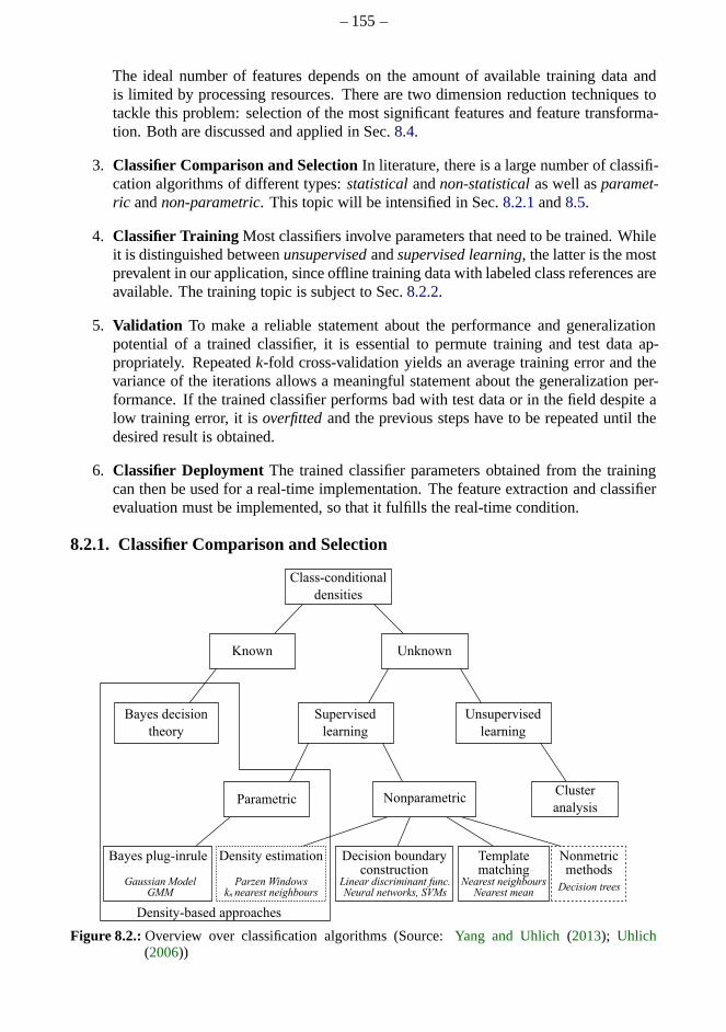
– 155–

The ideal number of features depends on the amount of available training data andis limited by processing resources. There are two dimensionreduction techniques totackle this problem: selection of the most significant features and feature transforma-tion. Both are discussed and applied in Sec.8.4.

3. Classifier Comparison and SelectionIn literature, there is a large number of classifi-cation algorithms of different types:statisticalandnon-statisticalas well asparamet-ric andnon-parametric. This topic will be intensified in Sec.8.2.1and8.5.

4. Classifier Training Most classifiers involve parameters that need to be trained.Whileit is distinguished betweenunsupervisedandsupervised learning, the latter is the mostprevalent in our application, since offline training data with labeled class references areavailable. The training topic is subject to Sec.8.2.2.

5. Validation To make a reliable statement about the performance and generalizationpotential of a trained classifier, it is essential to permutetraining and test data ap-propriately. Repeatedk-fold cross-validation yields an average training error and thevariance of the iterations allows a meaningful statement about the generalization per-formance. If the trained classifier performs bad with test data or in the field despite alow training error, it isoverfittedand the previous steps have to be repeated until thedesired result is obtained.

6. Classifier DeploymentThe trained classifier parameters obtained from the trainingcan then be used for a real-time implementation. The featureextraction and classifierevaluation must be implemented, so that it fulfills the real-time condition.

8.2.1. Classifier Comparison and Selection

Figure 8.2.:Overview over classification algorithms (Source:Yang and Uhlich(2013); Uhlich(2006))

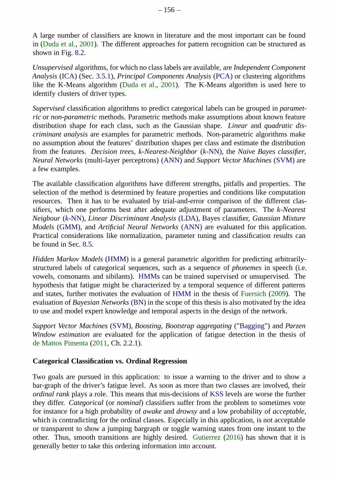
– 156–

A large number of classifiers are known in literature and the most important can be foundin (Duda et al., 2001). The different approaches for pattern recognition can be structured asshown in Fig.8.2.

Unsupervisedalgorithms, for which no class labels are available, areIndependent ComponentAnalysis(ICA) (Sec.3.5.1), Principal Components Analysis(PCA) or clustering algorithmslike the K-Means algorithm (Duda et al., 2001). The K-Means algorithm is used here toidentify clusters of driver types.

Supervisedclassification algorithms to predict categorical labels can be grouped inparamet-ric or non-parametricmethods. Parametric methods make assumptions about known featuredistribution shape for each class, such as the Gaussian shape. Linear and quadratic dis-criminant analysisare examples for parametric methods. Non-parametric algorithms makeno assumption about the features’ distribution shapes per class and estimate the distributionfrom the features.Decision trees, k-Nearest-Neighbor(k-NN), the Naive Bayes classifier,Neural Networks(multi-layer perceptrons) (ANN) andSupport Vector Machines(SVM) area few examples.

The available classification algorithms have different strengths, pitfalls and properties. Theselection of the method is determined by feature propertiesand conditions like computationresources. Then it has to be evaluated by trial-and-error comparison of the different clas-sifiers, which one performs best after adequate adjustment of parameters. Thek-NearestNeigbour(k-NN), Linear Discriminant Analysis(LDA), Bayesclassifier,Gaussian MixtureModels (GMM), andArtificial Neural Networks(ANN) are evaluated for this application.Practical considerations like normalization, parameter tuning and classification results canbe found in Sec.8.5.

Hidden Markov Models(HMM) is a general parametric algorithm for predicting arbitrarily-structured labels of categorical sequences, such as a sequence ofphonemesin speech (i.e.vowels, consonants and sibilants).HMMs can be trained supervised or unsupervised. Thehypothesis that fatigue might be characterized by a temporal sequence of different patternsand states, further motivates the evaluation ofHMM in the thesis ofFuersich(2009). Theevaluation ofBayesian Networks(BN) in the scope of this thesis is also motivated by the ideato use and model expert knowledge and temporal aspects in thedesign of the network.

Support Vector Machines(SVM), Boosting, Bootstrap aggregating("Bagging") andParzenWindow estimationare evaluated for the application of fatigue detection in the thesis ofde Mattos Pimenta(2011, Ch. 2.2.1).

Categorical Classification vs. Ordinal Regression

Two goals are pursued in this application: to issue a warningto the driver and to show abar-graph of the driver’s fatigue level. As soon as more thantwo classes are involved, theirordinal rankplays a role. This means that mis-decisions ofKSSlevels are worse the furtherthey differ. Categorical(or nominal) classifiers suffer from the problem to sometimes votefor instance for a high probability ofawakeanddrowsyand a low probability ofacceptable,which is contradicting for the ordinal classes. Especiallyin this application, is not acceptableor transparent to show a jumping bargraph or toggle warning states from one instant to theother. Thus, smooth transitions are highly desired.Gutierrez(2016) has shown that it isgenerally better to take this ordering information into account.

– 157–

Most of the previously mentioned classifiers perform categorical decisions by default. For acategoricalANN classifier, the last layer has one neuron for each class. TheKSSrepresentsa discrete quantization of a continuous-valued quantity. As described in Ch.3.3.6, theKSSentries can be considered as sample points and missing values in between were interpolated.This represents anordinal regressionproblem that can be performed by a single neuron inthe last layer of anANN, that retains the ordinality and punishes large deviations(cf. (Costa,2005; Gutierrez, 2016)). The single neuron represents a linear combination of allweightedinputs (and the bias that is present in every layer). Finallythe sub-intervals are mapped tothree classes or the bar-graph levels. In the present application, this speaks for classifiers thattake rank information into account.

8.2.2. Classifier Training

After selection of the potential classifiers their unknown parameters must be trained by val-idated features. The heuristic of the classification algorithm consists of estimating good oroptimal parameters that minimize the training error. The training of most classifiers is com-putationally intensive while the classification in online-application is generally much faster.One distinguishes between three kinds of training:

• Supervised learningmeans that the data used for training contain reference labelsthat define the class membership of a set of feature values. Inour application, the classmembership of features is defined by theATTENTION LEVEL, that is represented bytheKSSinterval scale or the reduced classesawake, acceptableor drowsy.

• Unsupervised learningmeans that no labels are available for the training and thefeatures have to be clustered into natural groups accordingto some similarity measures.In this thesis, unsupervised learning was only used to identify driver classes in Sec.5.4by a clustering analysis (Duda et al., 2001).

• Reinforcement learning means that training parameters are updated online in thevehicle based on feedback about the correctness of decisions. This is difficult in thisapplication since there is no reliable way to confirm if a decision was correct anda much higher demand of resources is needed. An conceivable option would be toadjust the sensitivity of hyperparameters of a classifier on-board as false warning ifdrivers continue to drive after they received a warning. Drivers that make a brakeafter a long drive without warning and without refueling/recharging could indicate amissing warning. Often, only few different drivers share the same car and, since it wasshown in Sec.5.4 that a small group of drivers can be identified well by their drivingstyle, the reinforced training parameters could be loaded when a driver was identifiedafter some time of driving.

In the training, a trade-off between training error reduction and remaininggeneralizationcapabilities must be found.Over-fittingof the data leads to low training errors, whereas thegeneralization capability suffers.

8.2.3. Unbalanced A-priori Class Distribution

A-priori information also covers the proportion of time thedriver is drowsy and the timedrivers are awake. When a classifier is trained, the distribution of the classes is considered.Knowledge of the a-priori ratio is, thus, advantageous. Dueto the extensive night studies, theproportion of drives that contain fatigue is much higher in this database than it is expected

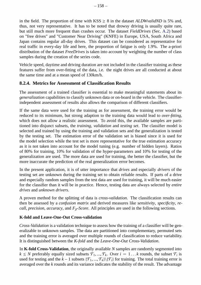
– 158–

in the field. The proportion of time with KSS≥ 8 in the datasetALDWvalidNDis 5% and,thus, not very representative. It has to be noted that drowsydriving is usually quite rare,but still much more frequent than crashes occur. The datasetFieldDrives (Sec.A.2) basedon "free drives" and "Customer Near Driving" (KNFE) in Europe, USA, South Africa andJapan contains regular all-day drives. This dataset can be considered as representative forreal traffic in every-day life and here, the proportion of fatigue is only 1.9%. The a-prioridistribution of the datasetFreeDrivesis taken into account by weighting the number of classsamples during the creation of the series code.

Vehicle speed, daytime and driving duration are not included in the classifier training as thesefeatures suffer from over-fitting of the data, i.e. the nightdrives are all conducted at aboutthe same time and at a mean speed of 130km/h.

8.2.4. Metrics for Assessment of Classification Results

The assessment of a trained classifier is essential to make meaningful statements about itsgeneralizationcapabilities to classify unknown data or on-board in the vehicle. The classifier-independent assessment of results also allows the comparison of different classifiers.

If the same data were used for the training as for assessment,the training error would bereduced to its minimum, but strong adaption to the training data would lead toover-fitting,which does not allow a realistic assessment. To avoid this, the available samples are parti-tioned into disjunct subsets, thetraining, validation and testing set. The classifier model isselected and trained by using the training and validation sets and the generalization is testedby the testing set. The estimation error of the validation set is biased since it is used forthe model selection while the test set is more representative for the true estimation accuracyas it is not taken into account for the model tuning (e.g. number of hidden layers). Ratiosof 80% for training, 10% for validation of the hyper-parameters and 10% for testing of thegeneralization are used. The more data are used for training, the better the classifier, but themore inaccurate the prediction of the real generalization error becomes.

In the present application, it is of utter importance thatdrivesand especiallydrivers of thetesting set are unknown during the training set to obtain reliable results. If parts of a driveand especially random samples from the test data are used fortraining, it will be much easierfor the classifier than it will be in practice. Hence, testingdata are always selected byentiredrivesandunknown drivers.

A proven method for the splitting of data iscross-validation. The classification results canthen be assessed by aconfusion matrixand derived measures likesensitivity, specificity, re-call, precision, accuracy, andFβ-Score. All principles are used in the following sections.

K-fold and Leave-One-Out Cross-validation

Cross-Validationis a validation technique to assess how the training of a classifier will be gen-eralizable to unknown samples. The data are partitioned into complementary, permuted setsand the training error is averaged over multiple rounds of classification to reduce variability.It is distinguished between theK-fold and theLeave-One-Out Cross-Validation.

In K-fold Cross-Validation , the originally availableN samples are randomly segmented intok ≤ N preferably equally sized subsetsT1, ...,Tk. Over i = 1 . . . k rounds, the subsetTi isused for testing and thek− 1 subsetsT1, ...,Tk\Ti for training. The total training error isaveraged over thek rounds and its variance indicates the stability of the result. The advantage

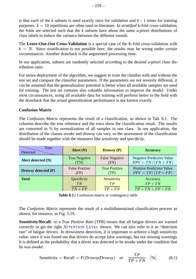
– 159–

is that each of thek subsets is used exactly once for validation andk− 1 times for trainingpurposes.k = 10 repetitions are often used in literature. Instratifiedk-fold cross-validation,the folds are selected such that thek subsets have about the same a-priori distributions ofclass labels to reduce the variance between the different rounds.

TheLeave-One-Out Cross-Validationis a special case of the K-fold cross-validation withk = N. Since stratification is not possible here, the results may be wrong under certaincircumstances. Another drawback is the augmented processing time.

In our application, subsets are randomly selected according to the desired a-priori class dis-tribution ratio.

For series-deployment of the algorithm, we suggest to trainthe clasifier with and without thetest set and compare the classifier parameters. If the parameters are not severely different, itcan be assumed that the generalization potential is better when all available samples are usedfor training. The test set contains also valuable information to improve the model. Undermost circumstances, using all available data for training will perform better in the field withthe drawback that the actual generalization performance isnot known exactly.

Confusion Matrix

The Confusion Matrixrepresents the result of a classification, as shown in Tab.8.1. Thecolumns describe the true reference and the rows show the classification result. The resultsare converted in % by normalization of all samples in one class. In our application, thedistribution of the classesawakeanddrowsycan vary, so the assessment of the classificationshould be made together with the measures likesensitivityandspecificity.

❳❳❳❳❳❳❳❳❳❳

DetectedTrue

Alert (N) Drowsy (P) Accuracy

Alert detected (N) True Negative(TN)

False Negative(FN)

Negative Predictive ValueNPV= T N/(FN + T N)

Drowsy detected (P) False Positive(FP)

True Positive(TP)

Positive Predictive ValuePPV= T P/(T P+ FP)

Total Specificity Sensitivity AccuracyT N

T N+ FPT P

T P+ FNT P+ T N

T P+ T N+ FP+ FN

Table 8.1.:Confusion matrix or contingency table

The Confusion Matrixrepresents the result of a multidimensional classificationprocess asshown, for instance, in Fig.5.19.

Sensitivity/Recall: or aTrue Positive Rate(TPR) means that all fatigue drivers are warnedcorrectly or get the rightATTENTION LEVEL shown. We can also refer to it as "detectionrate" of fatigue drivers. In drowsiness detection, it is important to achieve a high sensitivityvalue, since it was found out that drivers do accept false warnings, but not missing warnings.It is defined as the probability that a driver was detected to beawakeunder the condition thathe wasawake:

Sensitivity= Recall= P(Drowsy|Drowsy) orTP

TP+ FN[%]. (8.1)

– 160–

Specificity: or aTrue Negative Rate(TNR) of 100% means that not one awake driver got awrong warning or, with other words, this is the false alarm rate.

Specificity= P(Awake|Awake) orTN

TN+ FP[%] (8.2)

TheFalse Positive Rate(FPR) or false alarm rate is defined as:

1−Specificity= P(Drowsy|Awake) orFP

TN+ FP[%] (8.3)

Precision: is also referred to aspositive predictive value(PPV). On the other hand, precisionor positive predictive value is defined as the proportion of true positives against all positiveresults (both true positives and false positives)

Precision=TP

TP+ FP[%] (8.4)

Accuracy: (ACC) is the proportion of true results (both true positivesand true negatives) inthe entire population. An accuracy of 100% means that all classified values are exactly thesame as the reference classes.

Accuracy=TP+ TN

TP+ TN+ FP+ FN[%] (8.5)

8.2.5. The Fβ Score

Fβ-score is a measure for the overall performance of a classifier with a single indicator anddefined by

Fβ = (1+ β2)(precision· recall)/(β2 · precision+ recall), (8.6)

whereβ is a parameter to differently punish precision vs. recall. The F1-score is a specialcase:

F1 = 2(precision· recall)/(precision+ recall) . (8.7)

β is adapted according to the desired design goals as illustrated in Fig.8.5 andβ = 1.2 isused in this context. It is used as a combined measure.

8.3. Warning Strategy Assessment

8.3.1. Conversion of Classification Results into Warning

The characteristic of a warning strategy and concept in theATTENTION ASSIST is to issuea warning at the onset of fatigue. The driver can acknowledgethe warning by pressing theOK steering wheel button. If the drive is continued, the warning will repeatedly be issuedagain after 15 minutes of driving in a state classified asdrowsyin order to remind him havinga pause. If the warning is not confirmed, it will be assumed that the driver has not seen thewarning and will be issued again after 5 minutes. The warningcan only be triggered by acorrective event that the driver notices.

Now, for the offline evaluation, we assume that the driver always confirms the warning. Toconvert the classification result into a warning, the first sample for which the classdrowsyisclassified is set as the first warning. Then, the next warning is issued after at least 15 min, assoon as drowsy is classified again.

– 161–

8.3.2. Warning Assessment with Temporal Tolerance

Warnings can be assessed for an entire drive or by segmentingdrives into time slots of 15minutes. In the scope of theATTENTION ASSIST series introduction, the system warningswere assessed according to the definition below. A temporal tolerance was introduced for theassessment of warnings as drivers accept warnings during the phase of their fatigue onset.

An entire drive can be evaluated in relation to thedesired warning level(cf. Ch.3.3.3) bythe following tolerance criteria:

TN No warning necessary No warning was issued and the maximumKSS< DWLFN Missing warning No warning received, but maximumKSS≥ DWLTP Correctly warned Warning received andKSS≥ DWL-1 during first warning

or within 5 min afterwards. (The first correct warning isessential as the driver is supposed to stop the drive then).

TPE Warned too early Warning received within 5-15 min beforeKSS≥ DWL-1TPL Warned too late Warning received over 15 min after necessaryKSS≥ DWLFP False alarm (otherwise) Warning received whileKSS< DWL-1 and at

least 15 min beforeKSS≥ DWL-1

These modified classification results can be combined as described below. The number ofwarnings in relation to drowsy intervals or first warnings:

TPR=TP+TPE

TP + TPE + TPL + FN(8.8)

Everyone, who did not get a warning in time vs. everyone, who needed a warning:

Missing Warning Rate=FN+TPL

TP + TPE + TPL + FN(8.9)

Everyone who got a warning much too early or if no warning was necessary in relation toeveryone who was awake

False Alarm Rate=FP

FP + TN. (8.10)

The correct decisions in total vs. all outcomes is then:

Correct Total=TP + TPE + TN

TP + TPE + TPL + FP + FN + TN(8.11)

15 min time slots: This principle can now be evaluated for all 15 minute time slots. In thisconcept, we will categorize a warning again as wrong, if it isissued in a period, in whichthe driver is awake for at least 15 minutes before and after, even if fatigue has been involvedduring the beginning of the drive. Tab.8.2 shows this criteria for a selection of features. Atfirst, only one feature is used for classification as this is the main evaluation method usedto develop theATTENTION ASSIST. The improvedATTENTION ASSIST feature performsbetter for this criteria, however, it was not allowed to be published.

– 162–

1st warning 15 min intervalFeature TPR PPV FPR ACC Fβ TPR PPV FPR ACC Fβ

STWZCR 95% 28% 83% 36% 48% 45% 43% 16% 76% 44%LRVFAST 70% 37% 56% 52% 51% 22% 42% 7% 81% 28%STWVELZCR 77% 31% 63% 47% 48% 30% 40% 10% 79% 34%LRVVERYFAST 79% 33% 70% 44% 51% 26% 39% 9% 80% 30%LNCHGVEL 96% 26% 88% 33% 46% 42% 41% 17% 75% 42%MICROCORRECTIONSW 81% 33% 59% 51% 50% 29% 42% 9% 80% 34%STWEVENT 67% 45% 38% 64% 56% 25% 49% 6% 83% 31%TURNINDDUR 96% 27% 85% 34% 46% 41% 42% 14% 77% 41%DEGOINT 93% 29% 83% 38% 49% 35% 40% 13% 78% 37%DYNDRIVINGSTYLE 97% 25% 88% 32% 45% 47% 42% 18% 74% 45%REACTIM 91% 28% 85% 35% 47% 34% 38% 13% 77% 36%LRVPERCHIGH 94% 27% 85% 35% 47% 42% 40% 16% 75% 41%LATPOSZCR 79% 34% 62% 50% 52% 21% 40% 7% 81% 26%DELTALATVELMAX 89% 33% 78% 42% 52% 32% 42% 10% 79% 35%ZIGZAGS 86% 36% 70% 47% 55% 30% 44% 9% 80% 35%ELLIPSE 94% 27% 85% 34% 46% 46% 43% 17% 75% 45%DELTADUR 97% 25% 88% 32% 45% 47% 42% 18% 74% 45%VIBPROP 68% 35% 58% 50% 49% 23% 43% 7% 81% 29%LNERRSQ 99% 29% 87% 36% 50% 47% 44% 16% 76% 46%TURNINDADVANCE 97% 25% 89% 31% 45% 47% 43% 18% 75% 45%LNMNSQ 96% 27% 87% 34% 47% 41% 42% 15% 77% 41%LANEX 99% 29% 87% 36% 50% 47% 44% 16% 76% 46%LATMEAN 92% 30% 82% 39% 50% 41% 46% 13% 78% 43%LANEAPPROX 79% 32% 70% 44% 50% 29% 43% 9% 80% 34%LANEAPPROXAD 83% 39% 62% 52% 57% 25% 46% 7% 81% 31%LANEAPPROXADAPT 83% 34% 65% 49% 52% 26% 41% 8% 80% 30%DELTALATPOS 81% 34% 70% 46% 52% 31% 46% 8% 81% 36%LANEDEVSQ 66% 36% 58% 50% 49% 19% 44% 5% 82% 25%NMRHOLD 73% 37% 50% 57% 52% 29% 51% 6% 82% 35%LANEDEV 85% 32% 76% 42% 51% 35% 45% 10% 79% 39%ORA 96% 28% 87% 34% 48% 45% 44% 16% 76% 45%LNIQR 93% 31% 80% 40% 51% 36% 44% 11% 79% 39%

Table 8.2.:Warning assessment of single feature classification results (without a-priori features), forwhichFβ is maximal forβ = 1.2. All features are baselined bymaxof the first active 1 to20 min.

8.3.3. False Alarms by Driving Duration

Up to this point, we have not considered that the warning acceptance is much higher at night,in monotonous situations and after several hours of driving. Our studies show that driversaccept false warnings, but not missing warnings. However, amajor concern is that driversget "spammed" by too many false alarms. Our study shows also that drivers accept wrongwarnings after longer driving duration more than warnings at the beginning of a drive. Forthis reason, Fig.8.3 shows the false alarm rate by driving duration. Within 2h of driving,there are still under 1.4% false alarms.

8.4. Feature Dimension Reduction

Theoretically, the more uncorrelated the features are to fatigue, the better the classification.But if the number of features gets too high, the need of more training data cannot be fulfilledany more due to theCurse-of-Dimensionalityproblem. For instance, if 102 samples areenough to accurately describe the distribution of an one-dimensional random number, 1020

observations will be needed to obtain the same accuracy level in 10-dimensional space.

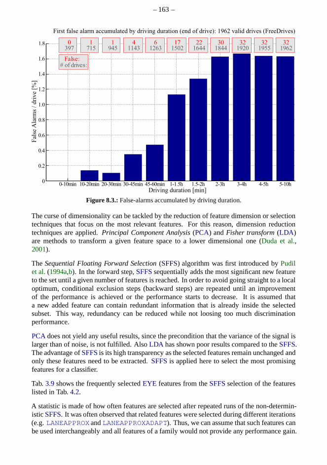
– 163–

Figure 8.3.:False-alarms accumulated by driving duration.

The curse of dimensionality can be tackled by the reduction of feature dimension or selectiontechniques that focus on the most relevant features. For this reason, dimension reductiontechniques are applied.Principal Component Analysis(PCA) andFisher transform(LDA)are methods to transform a given feature space to a lower dimensional one (Duda et al.,2001).

TheSequential Floating Forward Selection(SFFS) algorithm was first introduced byPudilet al.(1994a,b). In the forward step,SFFSsequentially adds the most significant new featureto the set until a given number of features is reached. In order to avoid going straight to a localoptimum, conditional exclusion steps (backward steps) arerepeated until an improvementof the performance is achieved or the performance starts to decrease. It is assumed thata new added feature can contain redundant information that is already inside the selectedsubset. This way, redundancy can be reduced while not loosing too much discriminationperformance.

PCAdoes not yield any useful results, since the precondition that the variance of the signal islarger than of noise, is not fulfilled. AlsoLDA has shown poor results compared to theSFFS.The advantage ofSFFSis its high transparency as the selected features remain unchanged andonly these features need to be extracted.SFFSis applied here to select the most promisingfeatures for a classifier.

Tab.3.9shows the frequently selectedEYE features from theSFFSselection of the featureslisted in Tab.4.2.

A statistic is made of how often features are selected after repeated runs of the non-determin-istic SFFS. It was often observed that related features were selected during different iterations(e.g.LANEAPPROX andLANEAPPROXADAPT). Thus, we can assume that such features canbe used interchangeably and all features of a family would not provide any performance gain.

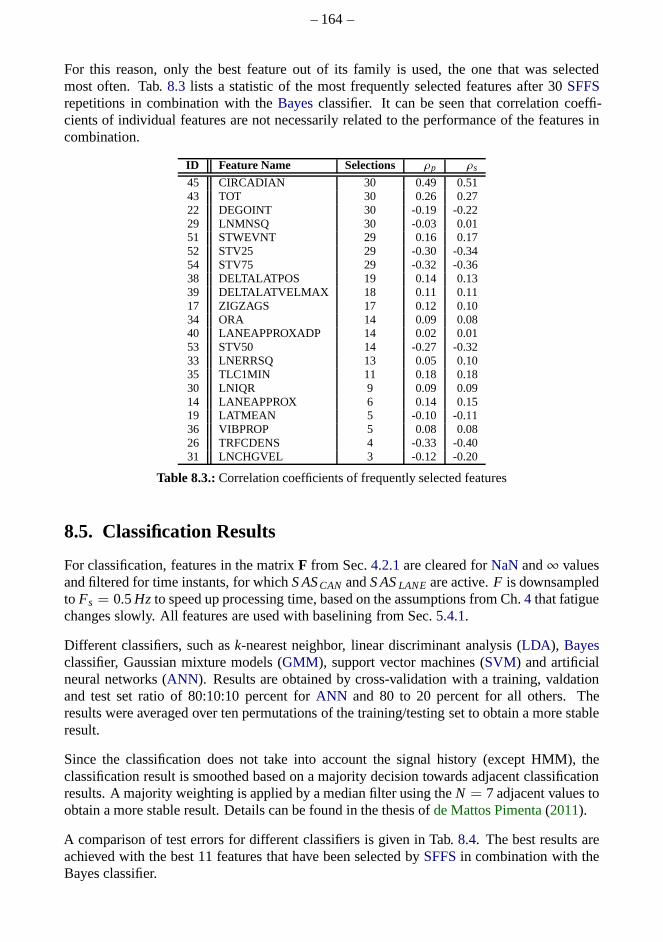
– 164–

For this reason, only the best feature out of its family is used, the one that was selectedmost often. Tab.8.3 lists a statistic of the most frequently selected features after 30 SFFSrepetitions in combination with theBayesclassifier. It can be seen that correlation coeffi-cients of individual features are not necessarily related to the performance of the features incombination.

ID Feature Name Selections ρp ρs

45 CIRCADIAN 30 0.49 0.5143 TOT 30 0.26 0.2722 DEGOINT 30 -0.19 -0.2229 LNMNSQ 30 -0.03 0.0151 STWEVNT 29 0.16 0.1752 STV25 29 -0.30 -0.3454 STV75 29 -0.32 -0.3638 DELTALATPOS 19 0.14 0.1339 DELTALATVELMAX 18 0.11 0.1117 ZIGZAGS 17 0.12 0.1034 ORA 14 0.09 0.0840 LANEAPPROXADP 14 0.02 0.0153 STV50 14 -0.27 -0.3233 LNERRSQ 13 0.05 0.1035 TLC1MIN 11 0.18 0.1830 LNIQR 9 0.09 0.0914 LANEAPPROX 6 0.14 0.1519 LATMEAN 5 -0.10 -0.1136 VIBPROP 5 0.08 0.0826 TRFCDENS 4 -0.33 -0.4031 LNCHGVEL 3 -0.12 -0.20

Table 8.3.:Correlation coefficients of frequently selected features

8.5. Classification Results

For classification, features in the matrixF from Sec.4.2.1are cleared forNaNand∞ valuesand filtered for time instants, for whichS ASCAN andS ASLANE are active.F is downsampledto Fs = 0.5Hz to speed up processing time, based on the assumptions from Ch. 4 that fatiguechanges slowly. All features are used with baselining from Sec.5.4.1.

Different classifiers, such ask-nearest neighbor, linear discriminant analysis (LDA), Bayesclassifier, Gaussian mixture models (GMM), support vector machines (SVM) and artificialneural networks (ANN). Results are obtained by cross-validation with a training, valdationand test set ratio of 80:10:10 percent forANN and 80 to 20 percent for all others. Theresults were averaged over ten permutations of the training/testing set to obtain a more stableresult.

Since the classification does not take into account the signal history (except HMM), theclassification result is smoothed based on a majority decision towards adjacent classificationresults. A majority weighting is applied by a median filter using theN = 7 adjacent values toobtain a more stable result. Details can be found in the thesis ofde Mattos Pimenta(2011).

A comparison of test errors for different classifiers is given in Tab.8.4. The best results areachieved with the best 11 features that have been selected bySFFSin combination with theBayes classifier.

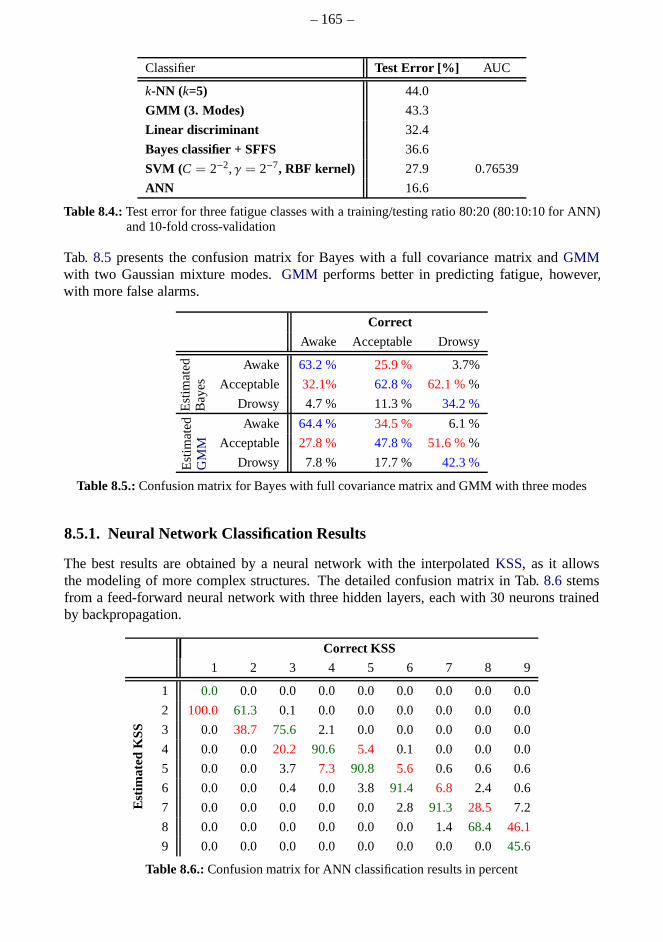
– 165–

Classifier Test Error [%] AUC

k-NN (k=5) 44.0

GMM (3. Modes) 43.3

Linear discriminant 32.4

Bayes classifier + SFFS 36.6

SVM (C = 2−2,γ = 2−7, RBF kernel) 27.9 0.76539

ANN 16.6

Table 8.4.:Test error for three fatigue classes with a training/testing ratio 80:20 (80:10:10 for ANN)and 10-fold cross-validation

Tab. 8.5 presents the confusion matrix for Bayes with a full covariance matrix andGMMwith two Gaussian mixture modes.GMM performs better in predicting fatigue, however,with more false alarms.

Correct

Awake Acceptable Drowsy

Est

imat

edB

ayes

Awake 63.2 % 25.9 % 3.7%

Acceptable 32.1% 62.8 % 62.1 %%

Drowsy 4.7 % 11.3 % 34.2 %

Est

imat

edG

MM

Awake 64.4 % 34.5 % 6.1 %

Acceptable 27.8 % 47.8 % 51.6 %%

Drowsy 7.8 % 17.7 % 42.3 %

Table 8.5.:Confusion matrix for Bayes with full covariance matrix and GMM with three modes

8.5.1. Neural Network Classification Results

The best results are obtained by a neural network with the interpolatedKSS, as it allowsthe modeling of more complex structures. The detailed confusion matrix in Tab.8.6 stemsfrom a feed-forward neural network with three hidden layers, each with 30 neurons trainedby backpropagation.

Correct KSS

1 2 3 4 5 6 7 8 9

Est

imat

edK

SS

1 0.0 0.0 0.0 0.0 0.0 0.0 0.0 0.0 0.0

2 100.0 61.3 0.1 0.0 0.0 0.0 0.0 0.0 0.0

3 0.0 38.7 75.6 2.1 0.0 0.0 0.0 0.0 0.0

4 0.0 0.0 20.2 90.6 5.4 0.1 0.0 0.0 0.0

5 0.0 0.0 3.7 7.3 90.8 5.6 0.6 0.6 0.6

6 0.0 0.0 0.4 0.0 3.8 91.4 6.8 2.4 0.6

7 0.0 0.0 0.0 0.0 0.0 2.8 91.3 28.5 7.2

8 0.0 0.0 0.0 0.0 0.0 0.0 1.4 68.4 46.1

9 0.0 0.0 0.0 0.0 0.0 0.0 0.0 0.045.6

Table 8.6.:Confusion matrix for ANN classification results in percent

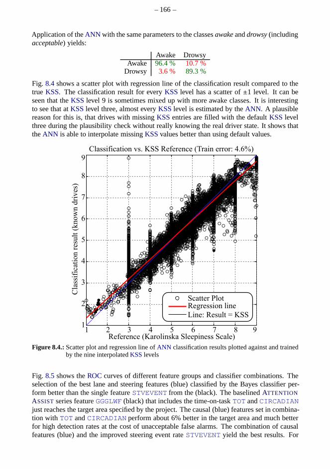
– 166–

Application of theANN with the same parameters to the classesawakeanddrowsy(includingacceptable) yields:

Awake DrowsyAwake 96.4 % 10.7 %

Drowsy 3.6 % 89.3 %

Fig. 8.4 shows a scatter plot with regression line of the classification result compared to thetrue KSS. The classification result for everyKSS level has a scatter of±1 level. It can beseen that theKSSlevel 9 is sometimes mixed up with more awake classes. It is interestingto see that atKSSlevel three, almost everyKSSlevel is estimated by theANN. A plausiblereason for this is, that drives with missingKSSentries are filled with the defaultKSSlevelthree during the plausibility check without really knowingthe real driver state. It shows thattheANN is able to interpolate missingKSSvalues better than using default values.

1 2 3 4 5 6 7 8 91

2

3

4

5

6

7

8

9

Reference (Karolinska Sleepiness Scale)

Classification vs. KSS Reference (Train error: 4.6%)

Cla

ssif

icat

ion

res

ult

(k

no

wn

dri

ves

)

Scatter PlotRegression line

Line: Result = KSS

Figure 8.4.:Scatter plot and regression line ofANN classification results plotted against and trainedby the nine interpolatedKSSlevels

Fig. 8.5 shows theROCcurves of different feature groups and classifier combinations. Theselection of the best lane and steering features (blue) classified by the Bayes classifier per-form better than the single featureSTVEVENT from the (black). The baselinedATTENTION

ASSISTseries featureGGGLWF (black) that includes the time-on-taskTOT andCIRCADIANjust reaches the target area specified by the project. The causal (blue) features set in combina-tion with TOT andCIRCADIAN perform about 6% better in the target area and much betterfor high detection rates at the cost of unacceptable false alarms. The combination of causalfeatures (blue) and the improved steering event rateSTVEVENT yield the best results. For

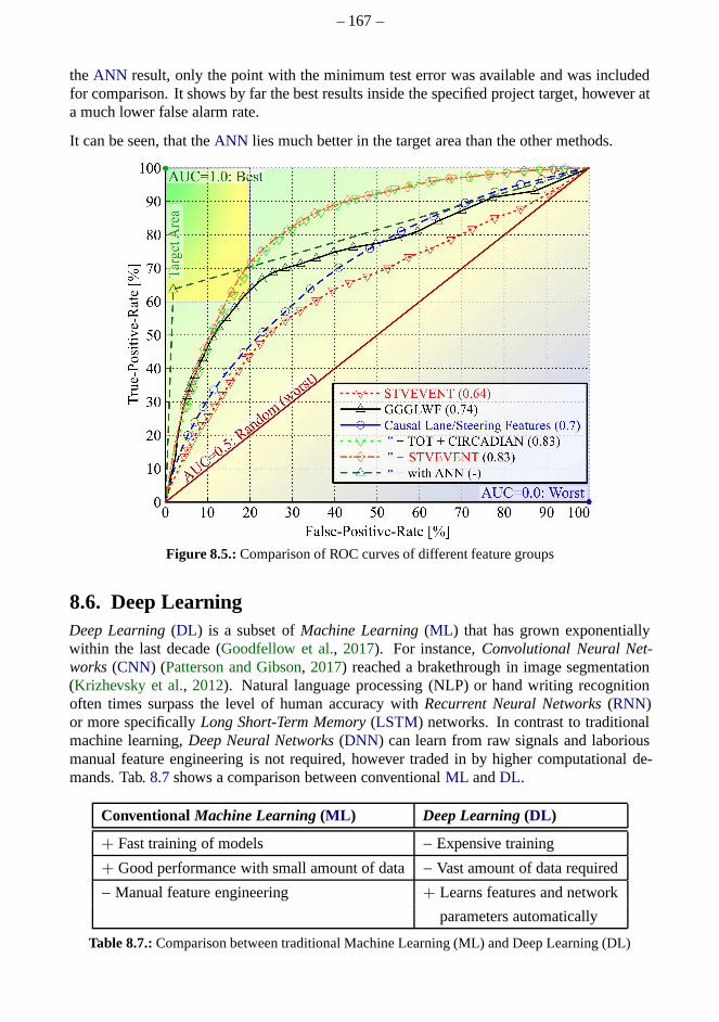
– 167–

theANN result, only the point with the minimum test error was available and was includedfor comparison. It shows by far the best results inside the specified project target, however ata much lower false alarm rate.

It can be seen, that theANN lies much better in the target area than the other methods.

Figure 8.5.:Comparison of ROC curves of different feature groups

8.6. Deep LearningDeep Learning(DL) is a subset ofMachine Learning(ML) that has grown exponentiallywithin the last decade (Goodfellow et al., 2017). For instance,Convolutional Neural Net-works(CNN) (Patterson and Gibson, 2017) reached a brakethrough in image segmentation(Krizhevsky et al., 2012). Natural language processing (NLP) or hand writing recognitionoften times surpass the level of human accuracy withRecurrent Neural Networks(RNN)or more specificallyLong Short-Term Memory(LSTM) networks. In contrast to traditionalmachine learning,Deep Neural Networks(DNN) can learn from raw signals and laboriousmanual feature engineering is not required, however tradedin by higher computational de-mands. Tab.8.7shows a comparison between conventionalML andDL.

Conventional Machine Learning (ML ) Deep Learning (DL)

+ Fast training of models − Expensive training

+ Good performance with small amount of data− Vast amount of data required

− Manual feature engineering + Learns features and network

parameters automatically

Table 8.7.:Comparison between traditional Machine Learning (ML) and Deep Learning (DL)

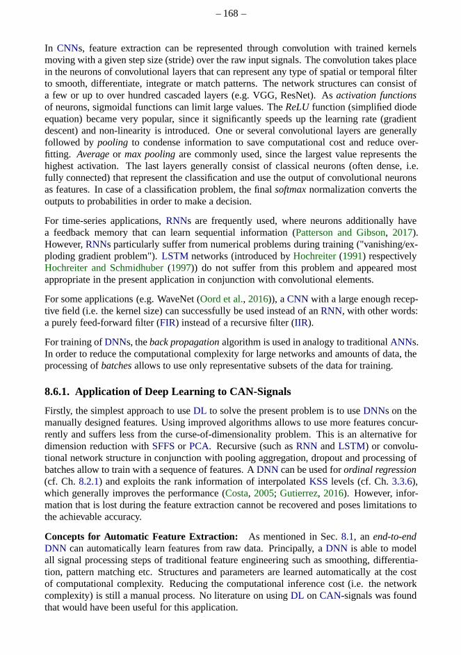
– 168–

In CNNs, feature extraction can be represented through convolution with trained kernelsmoving with a given step size (stride) over the raw input signals. The convolution takes placein the neurons of convolutional layers that can represent any type of spatial or temporal filterto smooth, differentiate, integrate or match patterns. Thenetwork structures can consist ofa few or up to over hundred cascaded layers (e.g. VGG, ResNet). As activation functionsof neurons, sigmoidal functions can limit large values. TheReLUfunction (simplified diodeequation) became very popular, since it significantly speeds up the learning rate (gradientdescent) and non-linearity is introduced. One or several convolutional layers are generallyfollowed by pooling to condense information to save computational cost and reduce over-fitting. Averageor max poolingare commonly used, since the largest value represents thehighest activation. The last layers generally consist of classical neurons (often dense, i.e.fully connected) that represent the classification and use the output of convolutional neuronsas features. In case of a classification problem, the finalsoftmaxnormalization converts theoutputs to probabilities in order to make a decision.

For time-series applications,RNNs are frequently used, where neurons additionally havea feedback memory that can learn sequential information (Patterson and Gibson, 2017).However,RNNs particularly suffer from numerical problems during training ("vanishing/ex-ploding gradient problem").LSTM networks (introduced byHochreiter(1991) respectivelyHochreiter and Schmidhuber(1997)) do not suffer from this problem and appeared mostappropriate in the present application in conjunction withconvolutional elements.

For some applications (e.g. WaveNet (Oord et al., 2016)), aCNN with a large enough recep-tive field (i.e. the kernel size) can successfully be used instead of anRNN, with other words:a purely feed-forward filter (FIR) instead of a recursive filter (IIR).

For training ofDNNs, theback propagationalgorithm is used in analogy to traditionalANNs.In order to reduce the computational complexity for large networks and amounts of data, theprocessing ofbatchesallows to use only representative subsets of the data for training.

8.6.1. Application of Deep Learning to CAN-Signals

Firstly, the simplest approach to useDL to solve the present problem is to useDNNs on themanually designed features. Using improved algorithms allows to use more features concur-rently and suffers less from the curse-of-dimensionality problem. This is an alternative fordimension reduction withSFFSor PCA. Recursive (such asRNN andLSTM) or convolu-tional network structure in conjunction with pooling aggregation, dropout and processing ofbatches allow to train with a sequence of features. ADNN can be used forordinal regression(cf. Ch. 8.2.1) and exploits the rank information of interpolatedKSS levels (cf. Ch.3.3.6),which generally improves the performance (Costa, 2005; Gutierrez, 2016). However, infor-mation that is lost during the feature extraction cannot be recovered and poses limitations tothe achievable accuracy.

Concepts for Automatic Feature Extraction: As mentioned in Sec.8.1, an end-to-endDNN can automatically learn features from raw data. Principally, a DNN is able to modelall signal processing steps of traditional feature engineering such as smoothing, differentia-tion, pattern matching etc. Structures and parameters are learned automatically at the costof computational complexity. Reducing the computational inference cost (i.e. the networkcomplexity) is still a manual process. No literature on using DL on CAN-signals was foundthat would have been useful for this application.

– 169–

CNNs have shown their strength in detecting patterns in 2D images, but lately also in 1D time-series applications (e.g.ConvLSTM, ALSTM-FCN, cf. (Cui, 2016; Gehring, 2017; Karimet al., 2018; Janos, 2018)). LSTMs have shown their strength in long time-span sequenceapplications, especially for high sampling rates where temporalCNNs would require to storea huge amount of the input data.

In the previous chapters, we found that the causal information about fatigue is expected to bein events and sliding windows in the steering and lane signals mostly. For instance, in orderto detect steering patterns that usually take up to five seconds, a temporal convolution canbe performed on the steering velocity. For the inference of aCNN, this requires to store 250samples of the input sequence. However, the event itself does not yet correlate with fatigueand theirfrequencyover a time-span over at least 20 min is required. The same temporalconvolution would be able to find lane-based patterns such aszig-zag events, lane deviationor approximations. For lane data, the time-spans are even higher and last up to one hour (180ksamples per signal). The detection of single events is possible with aCNN, but especially forthe inference, the memory demand for a large perceptive fieldto retain event rate informationcannot be met. For such long time-spans,LSTM structures are much more promising.

Recent publications (Shi, 2015; Cui, 2016; Wang et al., 2016; Karim et al., 2018) show, thata combination of convolutional and recurrent/LSTM networks can outperform solitary struc-tures. Thus, the most promising approach would be a combination of CNN layers, followedby LSTM layers for the stage of feature extraction.

As input, the steering wheel angle velocity, absolute lateral lane position and width, verticaland lateral acceleration, accelerator pedal position and wheel rotation speed are suggestedto be used. To remove useless noise, it is proposed to use theDISPOfilter for smoothingand differentiation, suggested in Ch.4.1.1. Inputs shall be standardized to zero-mean andunit-variance.

Patterns that are induced by external events, such as lane-camera inactivity, lane changes,overtaking, cross-wind, road warping, curves, construction sites etc. are not related to fatigue.These useless patterns that stem from such situations can bemuted by removing sampleswhen thesystem-active-signalis passive (cf. Ch.4.1.3).

Dense layers take over the classification of these features and the last neuron of theDNNshall be an ordinal regression neuron. As target reference,the interpolated nine levelKSSen-tries are most suitable for the regression. The predicted classes finally have to be mapped tothe bar-graph levels or the warning strategy. Finally, tuning the network structure and hyper-parameters is one of the most challenging tasks.AutoMLapproaches gained high popularityand can performNeural Architecture Search (NAS) (Hutter et al., 2019) where the structureof the network and involved parameters can be searched according to predefined strategiesand restrictions, however at the cost of additional complexity.

Challenges: As already argued in Ch.4, due to on-board inference cost and intransparency,DNNs are not the first choice for deployment on automotiveECUs. For off-board training,processing of big data andGPUin liaison with cluster/cloud computing would be necessaryand were not available for this thesis.

A-priori factors such asdaytime, time-on-task, vehicle speed, curvature monotonyand lightshall also be included. These signals need no pre-processing to directly correlate with fa-tigue. As a consequence of the very unbalanced class distribution, classifiers strongly tend todetect night experiment situations in which fatigue is muchmore prevalent than in real road

– 170–

drives. These driving situations are not causal indicatorsfor fatigue. Based on the a-prioridistribution of free drives, random oversampling the minority (sleepy) or undersampling themajority (awake) is a common approach (e.g.Synthetic minority Over-sampling TEchnique(SMOTE) usingk-NN). This would either loose information or blow up the amount of train-ing data by magnitudes. At the other hand, continuous-valued external factors such as speed,traffic density, curvature and road condition have a strong influence on features as shown inCh.5.2. Features need to be independent of these factors. It appears challenging to design aDNN that is able to distinguish between normalization and taking the a-priori distribution offree drives into account. When removing samples to mute events, the timing and event rateinformation is lost and cannot be learned by the classifier any more. The reaction time toexternal events, such as the steering correction after roadbumps is also no longer containedin the inputs. Adaption to new vehicles types and different countries is a major issue andonly works if all dozens relevant vehicle variants were available prior to production to recordtraining data, e.g. for transfer learning.

Another challenge is certainly the adaption to the driver inanalogy to baselining. In orderto adapt to individual driving styles, the result of the feature extraction layers from the be-ginning of the drive would have to be stored, aggregated by max pooling (in analogy to maxbaselining) and later fed into the decision stage of the network.

Due to the large spectrum of external factors and driver types that overlay the weak fatiguepatterns, a lot more data and situations would be required totrain aDNN. This could onlybe achieved by the oncoming over-the-air (OTA) infrastructure where sensor signals are per-manently preprocessed on-board and transferred to the back-end. For supervised learning, aground truth reference is mandatory. Using real field data may fill the lack of data and solvethe unknown a-priori distribution problems, however will raise an even bigger problem: cus-tomers will not estimate their fatigue level every few minutes nor will they wearEEG/EOGelectrodes. Transfer of driver-camera video data for offline labeling would require a drivercamera and is not possible over 4G (LTE+) or even 5G since the produced traffic would beway too expensive. Centrally storing driver videos would also be very critical for data protec-tion and crash liability reasons. If a camera would be available, it would make more sense toinvestigate eye-tracking based approaches.

Reinforced learning would require to interpret the reaction to warnings as reference, as de-scribed inreinforcement learningin Ch.8.2.2. However, this is even much less reliable thantheKSSand lacks temporal resolution and fatigue levels. An optionwould be to incentivizecustomers to rate their warnings and thereby "entertain" them with an experiencable car thatis self-learning.

8.6.2. Application of Deep Learning to Driver Camera

Especially eye-tracking camera-based driver state classification can potentially profit fromDL. Parkhi et al.(2015); Mukherjee and Robertson(2015) andHan et al.(2018) have con-firmed, that classification with multiple stages work best for eye-blinking detection. At first,the face is detected in consecutive driver-video images by aCNN. After initialization, thesearch region-of-interest (ROI) can be reduced by tracking. As face model reference, exist-ing databases can be used or manually labeled for this stage.Face models of known driverscan be stored to accelerate initialization.

– 171–

In the second stage, the eyes, pupils and eye-blinks can be detected in the again narroweddown, but higher-resolutionalROI. TheEOGsignals from Ch.3.4 can be used as referencefor eye-blinks in this stage.

In the last fatigue classification stage, anRNN or LSTM can be used for deriving the sleepi-ness level from the eye-blinks. As shown in Ch.3.6.11, a video frame rate of at least 100 fpsis required to reliably detect eye-opening and -closure speed. As reference, theKSSenteredby the driver can again be used. Video recordings even allow amajority voting of experts,which is actually considered to be the most accurate method (cf. Ch.3.3.1). By training thesestages independently, the eye-blink signal is free from influences in the video image thatcould lead to over-fitting to the training data. For instance, a full end-to-end approach thatworks on the raw data could exploit that fatigue is more prevalent during night experiments,i.e. low light conditions. Fatigue also occurs most often during low traffic, which results infewer shoulder checks, i.e. horizontal head rotations. However, these relationships are onlyvalid for the training data with artificial night experiments and no causal indicators for fatigueduring real road drives. It is desired to be independent of such situation based a-priori fac-tors, since the amount of fatigue during night and day or traffic density is unknown. Trainingan end-to-endCNN for facial expressions (e.g. yawning or head-nodding) is anadditionaloption.

8.6.3. Conclusion on Deep Learning for Fatigue Detection

Even ifDL is superior in many applications, the fatigue patterns are quite weak and obscuredby other factors in theCAN data. In summary, straightforward deployment of aDNN will beinferior to theML approach in which expert knowledge is explicitly modeled during featureengineering.

In comparison,DL approaches based on driver-camera are expected to be most feasible andpromising. The gained features are causal and can be mostly independent from the a-prioridistribution or external influences. The missing ground truth problem also remains here.However, for this thesis, the amount of representative state-of-the-art camera-data with highframe-rate and withKSS reference were not available. The focus was explicitly on usingCAN-signals, since there was no camera on the market that was ready for production.

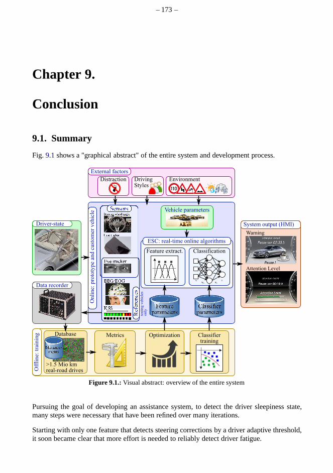
– 173–

Chapter 9.

Conclusion

9.1. Summary

Fig. 9.1shows a "graphical abstract" of the entire system and development process.

Figure 9.1.:Visual abstract: overview of the entire system

Pursuing the goal of developing an assistance system, to detect the driver sleepiness state,many steps were necessary that have been refined over many iterations.

Starting with only one feature that detects steering corrections by a driver adaptive threshold,it soon became clear that more effort is needed to reliably detect driver fatigue.

– 174–

A major restriction during the optimization of the system was the lack of a reliable "ground-truth" reference. For this reason,EEG, EOG and camera-based features were evaluated.Although the results in literature are often reported to be very good, the use of real-roaddrives did not show satisfying results. Direct camera-based blinking features have shown themost promising results. However, a camera system was not yetavailable at that time thatwas robust enough to cope with realistic driving conditions. Further, a large amount of datawere only recorded by using theKSSreference. For this reason, theKSSwas found to be themost practical reference. Numerous features were analyzedregarding their correlation withthe KSSdrowsiness reference. Many of them correlated relatively well, especially a-priorifeatures, such as time of day, time-on-task, monotony and traffic density. However, a-priorifeatures need to be treated carefully as they are not sensitive to the real driver condition.

For the series introduction of theATTENTION ASSIST 2.0 with theATTENTION LEVEL, abar graph was implemented based on several features with continuous output. An extensivenight study with a real-time implementation of theATTENTION LEVEL was conducted toverify its acceptance. Plausible levels were shown most of the time, but it was observed thata system active / passive detection was introduced which indicates to the driver, whether thesystem is passive and unable to detect theATTENTION LEVEL.

The lane based features have shown results comparable to thesteering based features. Animportant requirement of our application, however, is to use sensors from series equipmentinstead of using a special equipment lane-tracking camera,that is not available for the ma-jority of vehicles in the field. For this reason, the idea was to estimate the same lane-basedfeatures from inertial sensors and vehicle tracking. Not with the same, but still good accuracy,some lane-based patterns could be used in this way.

In the last iteration, another major impact on features was addressed, the influence of unde-sired factors like external influences and inter-individual driving styles. Especially under realworld conditions, the suppression of external influences and adaption to the driver is veryimportant. It was observed that there are different types ofdrivers, those who accuratelykeep the lane by lots of steering corrections and those who donot hastily correct the lateralposition and have a rather loose lane keeping. Specific measurements have been recorded toquantify and compensate for their effects as good as possible.

Based on the extracted features and a feature selection step, different classifiers have beencompared. In general, lane based features were often selected in combination with steeringbased features, as they provided complementary information. Neural networks, LDA and theBayes classifier, in combination with SFFS feature selection, performed best for the difficultfeatures. Especially neural networks have shown to enhancethe system performance. Buteven with a large set of new and improved steering and lane based features, the classificationperformance was not as good as the results reported in literature, using a smaller amount ofdata from a simulator or using drives under testing conditions.

9.2. Future Work and OutlookAn optimally operating fatigue detection system can only bedeveloped by jointly taking allthe factors mentioned in this thesis into account. Investigation on the following approachescould further improve the results:

• Installation of a steering wheeltorquesensor in order to measure reaction times, asdescribed in Ch.4.4.12

– 175–

• MergingEEG, eye-signals (e.g PERCLOS (Batista, 2007)) and a distraction measurein addition to theKSSfor a better temporal resolution of the reference

• Further analyze multi-level classification to use driving style specific features• Further investigate Hidden Markov-Models and Bayes networks to model temporal

aspects and expert knowledge• Derive driver-model control system parameters, as described in Ch.4.4.16• Using unsupervised learning to incorporate the driver reaction, whether he is following

the proposed warning or not, to update classification sensitivity• Applying more extensive parameter optimization, not only of single features but with

the classification performance of selected features as costfunction• Investigate Deep Learning methods and its ability to learn features automatically from

source signals. Convolutional and recurrent/LSTM neural network structures appearedto be most appropriate.

• Using existing over-the-air and cloud infrastructure for reinforcement off-board learn-ing and adaption to known drivers, environments and vehicleproperties.

Driving in a driving simulator and under supervised conditions has a big influence on thedriver’s behavior. It was observed that many awake drivers will also drive sloppy, if themotorway is empty or if they are distracted by talking or other actions. The driving behaviorin these situations is the same as for drowsiness and, thus, cannot be distinguished. For thisreason, a good strategy would be to provide feedback to the driver about his/her objectivedriving performance over theATTENTION LEVEL bargraph. In the actual system, only onefeature is used instead of theANN result in Ch.8.5.1. Usually, drivers tend to drive moreaware, if they get a feedback on their driving performance.

The temporal unavailability of the lane-tracking has already been considered during the fea-ture extraction. The block diagram in Ch.?? shows how to cope with the case that lane dataare temporarily unavailable due to bad vision, mis-calibration, missing lane markings or incase the ALDW is not installed or damaged. If theLaneDataQualindicate unavailability, thetraining parameters and classification input features should be switched.

In the big picture, after decades of research, one has to accept that the driving parameterscontain only a limited information about the driver state and by magnitudes lower than otherexternal influences. Indirect fatigue monitoring through driving parameters will still be rele-vant for at least two decades as manual driving will still play a role until 2040 even in level 5driverless vehicles and vehicles in lower segments.

In any case,camera-basedeye blinking detection was shown in this thesis to be most suit-able as a reference and for on-board implementation in series application. Especially underthe viewpoint of a future autonomous driving, a driver camera allows not only direct driverstate estimation by eye-tracking, but also a broad variety of other applications such as driverdistraction detection ("‘eyes-on-road"’), driver identification, driver vitality (heart rate), ges-ture, emotion and facial expression detection. This directmethod also works for automateddriving and is less affected by external influences and driving styles. For partial automateddriving it must be assured that drivers remain alert to hand the operation over to the driverin situations the car can’t handle. The driver camera has further benefits such as drivers canalso be identified to continuously learn their driving style. The latest over-the-air and cloudcomputing infrastructure are enablers with the highest potential for improved performance.ADAS warning thresholds can be lowered if the driver’s eyes do notpoint towards a brakingvehicle.

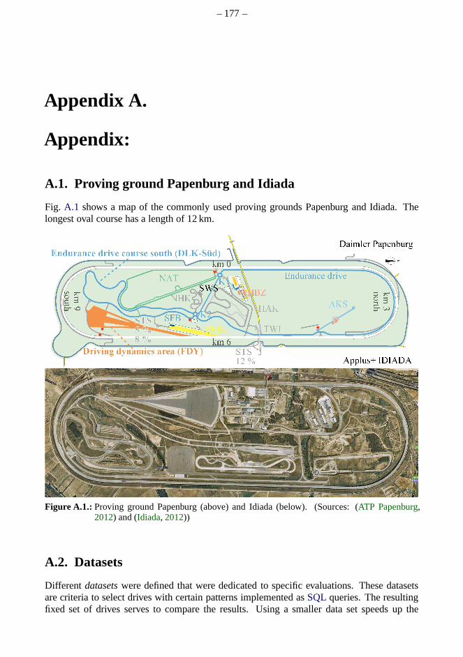
– 177–

Appendix A.

Appendix:

A.1. Proving ground Papenburg and Idiada

Fig. A.1 shows a map of the commonly used proving grounds Papenburg and Idiada. Thelongest oval course has a length of 12 km.

N

Figure A.1.: Proving ground Papenburg (above) and Idiada (below). (Sources: (ATP Papenburg,2012) and (Idiada, 2012))

A.2. Datasets

Different datasetswere defined that were dedicated to specific evaluations. These datasetsare criteria to select drives with certain patterns implemented asSQL queries. The resultingfixed set of drives serves to compare the results. Using a smaller data set speeds up the

– 178–

simulations. The results can then be refined and validated ona larger or full dataset. Themost important datasets used in this thesis are described inthe following section.

For faster processing, the datasetALDWvalidNDwas a smaller set of drives that containeda large portion of fatigue. It excluded all free and KNFE drives in which fatigue was rareand the driving situations varied too much. After filtering the full database, 82 269km of realdrives with 781 hours remained:

• 323 drives (141 night drives; 124 free drives; the rest were excursions)• 10 vehicles (Six E- and four S-Class)• 103 drivers (26% by women)

The criteria for drives in this data set were:

• Drives werevalid according to the validation criteria in Sec.A.7.3• KSSself-rating was valid and plausible• At least oneKSSentry was made• The driven distance was at least 30 km• Lane-tracking data had to be valid and without measurement errors• No driver switch (otherwise the drive would have to be cut up every time)• Only E- and S-class vehicles (excluding vehicleID=69 due toits miscalibrated camera)• Availability of plausible and valid ALDW data for over 50% ofthe time

ALDWvalid was defined equally to ALDWvalidND, just that additional drives from allexperiments with ALDW were included (32 of 91 experiments).Especially Customer NearDriving (KNFE) and free drives were added. The quality of these drives is lower, especiallywith regards to the KSS self-estimation. From 25 vehicles, 1.642 drives with over 2.722hours of driving, and 265.469 km remained. Here, the percentage of women was only 14.3%.The lane data quality and active time of drives in Sweden and Italy were sometimes very baddue to bad road conditions.

FieldDrives was a good representation of customer drives in the field and therefore cov-ered only free drives and customer near driving (KNFE). The 2.133 drives from 425 driverscovered 299.170 km of driven distance during 3.174 hours, but only 12.5% women.

validTopDrivers For the classification of drivers and clustering of driving styles in Ch.5.4,the DataSetvalidTopDrivershad to be defined. The filter criteria were the same as forALD-Wvalid, except with the additional filter criteria:

• Only the top 15 drivers with the highest number of drives wereselected:driverID ∈20, 152, 609, 607, 133, 59, 5, 340, 753, 165, 483, 485, 484, 19,482.

• Only drives with max(KS S) ≤ 7 were selected.• Only excursion experiments and free drives, no night studies

233 drives with 542 hours and 57.835 km of driven distance remained and 27% of them weremade by women.

– 179–

A.3. CAN Signals

Tab.A.1 lists the names and abbreviations of the essential CAN signals used in this thesis.The signals are grouped by the sensors they originate from, i.e. the steering wheel angle sen-sor (STW), accelerometer (ACCEL), Yaw rate sensor (YAW), accelerator pedal (ACCPDL),switches and buttons (SW), levers (LEVER), rain and light sensor (LIGHT), clock (CLK),wheel rotation rate sensors (WHLRPM), control system ECU active (CTRLECU), globalpositioning system (GPS) and lane tracking camera (ALDW).

Tab.A.2 lists the available signals for the system fromRobert Bosch GmbH.

A.3.1. Synchronization of CAN-Bus Signals

In this thesis, a novel interface for communication with thevehicle CAN-bus was imple-mented for real-time visualization, measurement and data conversion. The Controller AreaNetwork (CAN)-bus is an asynchronous, serial message-based bus protocol designed for au-tomotive application.

Every CAN message ID originates from one dedicated device, to which multiple bus mem-bers can listen. Message IDs must be unique on a single CAN bus. The message ID is usedas a priority to achieve a bus load of up to 80%. The lower the ID, the more important themessage. The 11-Bit ID Base frame format in CAN 2.0A allows upto 2048 different messageIDs while the Extended frame format in CAN 2.0B allows 229 IDs. Carrier Sense MultipleAccess / Collision Resolution (CSMA/CR) is used for arbitration to avoid collisions. Everybus member is listening bitwise and submitting its ID. If multiple units try to submit at thesame time, the dominant bit of the member with the lowest ID isoverwriting the recessivebits of the other units which, then, stop submitting. For this reason and with the present highbus load, the transmission time instant cannot be assured.

A CAN frame is composed as described in Tab.A.3. In addition, the measurement hardwarestores the message counter and the timestamp of the message reception.

Messages can be transmitted with different rates, depending on the sampling frequency ofthe contained signals. Mostly, high-speed CAN with bitrates of up to 1 Mbit/s are used atnetwork lengths below 40 meters. There are also low-speed CAN with a maximum bitrate of125 kbit/s.

Every CAN signal is defined according to the structural properties listed in Tab.A.4. Thepayload of a CAN-signal cannot be interpreted without this decoding information. Thesedefinitions of all signals of a CAN bus is stored in a DBC-file (along with signal descrip-tions). Depending on this definition, every payload of one CAN message is composed of oneor several signals. Signals with more than 32 Bit have to be distributed on multiple CANmessages. The interpretation of the data bits is only possible with this definition (DBC file),as it defines every signal.

Tab.A.4 shows the header and payload definition bits of a CAN-messageas defined in DBC-files.

Signal Synchronization

Another challenge is the synchronization of different CAN-signals and sensors that workwith different asynchronous sampling times. The CAN-bus isnot deterministic. Hence, amessage can arrive delayed and lead to gaps and jitter in the signals. Fig.A.2 illustrates

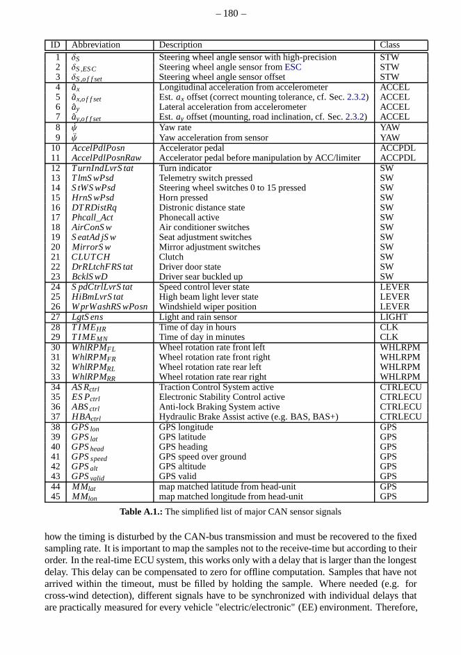
– 180–

ID Abbreviation Description Class1 δS Steering wheel angle sensor with high-precision STW2 δS,ESC Steering wheel angle sensor fromESC STW3 δS,o f f set Steering wheel angle sensor offset STW4 ax Longitudinal acceleration from accelerometer ACCEL5 ax,o f f set Est.ax offset (correct mounting tolerance, cf. Sec.2.3.2) ACCEL6 ay Lateral acceleration from accelerometer ACCEL7 ay,o f f set Est.ay offset (mounting, road inclination, cf. Sec.2.3.2) ACCEL8 ψ Yaw rate YAW9 ψ Yaw acceleration from sensor YAW

10 AccelPdlPosn Accelerator pedal ACCPDL11 AccelPdlPosnRaw Accelerator pedal before manipulation by ACC/limiter ACCPDL12 TurnIndLvrS tat Turn indicator SW13 TlmS wPsd Telemetry switch pressed SW14 S tWS wPsd Steering wheel switches 0 to 15 pressed SW15 HrnS wPsd Horn pressed SW16 DTRDistRq Distronic distance state SW17 Phcall_Act Phonecall active SW18 AirConS w Air conditioner switches SW19 S eatAd jS w Seat adjustment switches SW20 MirrorS w Mirror adjustment switches SW21 CLUTCH Clutch SW22 DrRLtchFRS tat Driver door state SW23 BcklS wD Driver sear buckled up SW24 S pdCtrlLvrS tat Speed control lever state LEVER25 HiBmLvrS tat High beam light lever state LEVER26 W prWashRS wPosn Windshield wiper position LEVER27 LgtS ens Light and rain sensor LIGHT28 T IMEHR Time of day in hours CLK29 T IMEMN Time of day in minutes CLK30 WhlRPMFL Wheel rotation rate front left WHLRPM31 WhlRPMFR Wheel rotation rate front right WHLRPM32 WhlRPMRL Wheel rotation rate rear left WHLRPM33 WhlRPMRR Wheel rotation rate rear right WHLRPM34 AS Rctrl Traction Control System active CTRLECU35 ES Pctrl Electronic Stability Control active CTRLECU36 ABSctrl Anti-lock Braking System active CTRLECU37 HBActrl Hydraulic Brake Assist active (e.g. BAS, BAS+) CTRLECU38 GPSlon GPS longitude GPS39 GPSlat GPS latitude GPS40 GPShead GPS heading GPS41 GPSspeed GPS speed over ground GPS42 GPSalt GPS altitude GPS43 GPSvalid GPS valid GPS44 MMlat map matched latitude from head-unit GPS45 MMlon map matched longitude from head-unit GPS

Table A.1.: The simplified list of major CAN sensor signals

how the timing is disturbed by the CAN-bus transmission and must be recovered to the fixedsampling rate. It is important to map the samples not to the receive-time but according to theirorder. In the real-time ECU system, this works only with a delay that is larger than the longestdelay. This delay can be compensated to zero for offline computation. Samples that have notarrived within the timeout, must be filled by holding the sample. Where needed (e.g. forcross-wind detection), different signals have to be synchronized with individual delays thatare practically measured for every vehicle "electric/electronic" (EE) environment. Therefore,

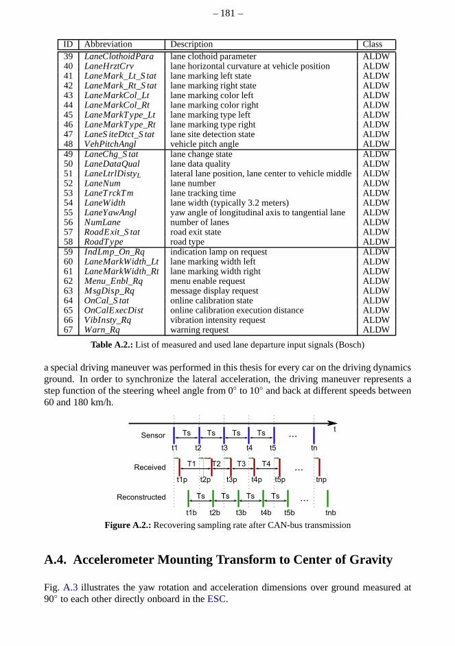
– 181–

ID Abbreviation Description Class39 LaneClothoidPara lane clothoid parameter ALDW40 LaneHrztCrv lane horizontal curvature at vehicle position ALDW41 LaneMark_Lt_S tat lane marking left state ALDW42 LaneMark_Rt_S tat lane marking right state ALDW43 LaneMarkCol_Lt lane marking color left ALDW44 LaneMarkCol_Rt lane marking color right ALDW45 LaneMarkType_Lt lane marking type left ALDW46 LaneMarkType_Rt lane marking type right ALDW47 LaneS iteDtct_S tat lane site detection state ALDW48 VehPitchAngl vehicle pitch angle ALDW49 LaneChg_S tat lane change state ALDW50 LaneDataQual lane data quality ALDW51 LaneLtrlDistyL lateral lane position, lane center to vehicle middleALDW52 LaneNum lane number ALDW53 LaneTrckTm lane tracking time ALDW54 LaneWidth lane width (typically 3.2 meters) ALDW55 LaneYawAngl yaw angle of longitudinal axis to tangential lane ALDW56 NumLane number of lanes ALDW57 RoadExit_S tat road exit state ALDW58 RoadType road type ALDW59 IndLmp_On_Rq indication lamp on request ALDW60 LaneMarkWidth_Lt lane marking width left ALDW61 LaneMarkWidth_Rt lane marking width right ALDW62 Menu_Enbl_Rq menu enable request ALDW63 MsgDisp_Rq message display request ALDW64 OnCal_S tat online calibration state ALDW65 OnCalExecDist online calibration execution distance ALDW66 VibInsty_Rq vibration intensity request ALDW67 Warn_Rq warning request ALDW

Table A.2.: List of measured and used lane departure input signals (Bosch)

a special driving maneuver was performed in this thesis for every car on the driving dynamicsground. In order to synchronize the lateral acceleration, the driving maneuver represents astep function of the steering wheel angle from 0 to 10 and back at different speeds between60 and 180 km/h.

...

t1 t2 t3

...

t4 t5 tn

tSensor

Received

Ts Ts Ts Ts

Ts Ts Ts Ts

t1p t2p t3p t4p t5p tnp

t2b t3b t4b t5b tnbt1b

Reconstructed ...

T1 T2 T3 T4

Figure A.2.: Recovering sampling rate after CAN-bus transmission

A.4. Accelerometer Mounting Transform to Center of Gravity

Fig. A.3 illustrates the yaw rotation and acceleration dimensions over ground measured at90 to each other directly onboard in theESC.

– 182–

Field Length [Bits] DescriptionIdentifier field 11 ID that describes the message

(0...2047)Identifier extension bit 1 Bit that indicates whether the message

type is extendedExtended identifier field 18 The longer ID for more than 2048 mes-

sagesData Length Code (DLC) 4 Lenght of the payloadData 0...64 PayloadCRC checksum 15 Cyclic Redundancy Checksum

Table A.3.: Essential fields of a CAN message

Property Descriptionstart-bit Index of the startbit (0...63)signal length Length of signal in bitsoffset Offset of the signalquantization Size of smallest (least significant) bit (LSB)sign Signed or unsignedbyte-order Wheter first startbit is LSB or MSBsignal type motorolaor intel byte order

Table A.4.: CAN signal definition (DBC)

ay

ax

ay

ax

xm

ym

CG

Sensorsψ

ψ

∆ax∆ay

ac

Figure A.3.: Dimensions measured by gyroscope and accelerometers transformed to the vehicle’scenter of gravity CG. Correction transform of accelerometer values to vehicle center ofgravityCG.

As mentioned in Ch.2.3.2and (Schindler, 2007, Ch. 3.2.2), the yaw rateψ sensor position isinvariant to the mounting position whereas the vehicle speed v is different in every position ofthe vehicle if rotation is involved. Thus, also the measuredaccelerationax anday are differentand need to be transformed to the vehicle’s center of gravityCG. With other words, if a steadyobject rotates around it’sCGwith ψ , 0/sor experiences a torque withψ , 0/s2, no forcecan be measured in theCG point. At any other point, CG, acentrifugal acceleration ac canbe measured forψ , 0/s. In addition, as illustrated in Fig.A.3, if the object experiencesa torque (ψ , 0/s2), a force component inx or y direction can be observed at every point, CG.

With the known sensor mounting positionxm andym and the rotation radiusR, the centrifugalaccelerationac = v2/R= ψ2R is obtained according to Eqn. (A.1). Its decomposition inx−andy−components is then given by Eqn. (A.2) and (A.3).

– 183–

ac = ψ2 ·√

x2m+ y2

m (A.1)

ac,x = ψ2 ·√

x2m+ y2

m · cos(arctanym

xm) (A.2)

ac,y = ψ2 ·√

x2m+ y2

m · sin(arctanym

xm) (A.3)

For an applied torque withψ , 0/s2, the undesiredx− andy−components of the measuredacceleration are calculated by Eqn. (A.4) and (A.5).

∆ax =1

T2s

cos(ψ

2+ arctan

ym

xm) · 2 ·

√

x2m+ y2

m cosψ

2(A.4)

∆ay =1

T2s

sin(ψ

2+ arctan

ym

xm) · 2 ·

√

x2m+ y2

m cosψ

2(A.5)

With Eqn. (A.2) to (A.5), the compensated signals of interestax anday in the vehicle’sCGfrom the measuredax anday is then given by Eqn. (A.6) and (A.7).

ax = ax −∆ax − ac,x (A.6)

ay = ay −∆ay − ac,y (A.7)

According to (Schindler, 2007, Eqn. 3.5), this can be simplified to

ax = ax − ymψ− xmψ2 (A.8)

ay = ay + yxψ − ymψ2 (A.9)

To cope with mounting tolerances and road inclination, the sensor offsetsax,o f f setanday,o f f set

with the range±2.56ms2 are estimated online by assuming that the vehicle is on average driving

straight ahead without road inclination and elevation. These four CAN signals are transferredas unsigned values and the offsets are subtracted accordingto Eq. (A.10) and (A.11).

ax = ax − ax,o f f set− 2.56m

s2− 10.24

m

s2(A.10)

ay = ay − ay,o f f set− 2.56m

s2−

10.24ms2 for Robert Bosch ESC

12.5568ms2 for Continental ESC

(A.11)

A.5. Steering Wheel Angle Sensor Principles and Unwrapping

Optical sensors have two code-slotted discs that are scanned by photo interrupters. One discis for the absolute angle and an auxiliary disc is connected over a gearing to turn faster and ob-tain the high resolution. The sensor from Kostal provide non-contact, absolute measurementranging from -420 to +420 (cf. (Kostal, 2012)).

Magnetical principles always rely on hall sensors. As described in the Patent (Delphi, 2006),Delphi introduced an auxiliary plate connected by a gear bearing to achieve the 0.1 preci-sion. Beyond thePermanentmagnetic Linear Contactless Displacement(PLCD) technology,

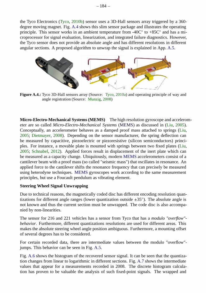
– 184–

the Tyco Electronics (Tyco, 2010b) sensor uses a 3D-Hall sensors array triggered by a 360-degree moving magnet. Fig.A.4 shows this slim sensor package and illustrates the operatingprinciple. This sensor works in an ambient temperature from-40C to +85C and has a mi-croprocessor for signal evaluation, linearization, and integrated failure diagnostics. However,the Tyco sensor does not provide an absolute angle and has different resolutions in differentangular sections. A proposed algorithm to unwrap the signalis explained in App.A.5.

Figure A.4.: Tyco 3D-Hall sensors array (Source:Tyco, 2010a) and operating principle of way andangle registration (Source:Munzig, 2008)

Micro-Electro-Mechanical Systems (MEMS) The high resolution gyroscope and accelerom-eter are so calledMicro-Electro-Mechanical Systems(MEMS) as discussed in (Liu, 2005).Conceptually, an accelerometer behaves as a damped proof mass attached to springs (Liu,2005; Dietmayer, 2008). Depending on the sensor manufacturer, the spring deflection canbe measured by capacitive, piezoelectric or piezoresistive (silicon semiconductors) princi-ples. For instance, a movable plate is mounted with springs between two fixed plates (Liu,2005; Schnabel, 2012). Applied forces result in displacement of the inert plate which canbe measured as a capacity change. Ubiquitously, modernMEMS accelerometers consist of acantilever beam with a proof mass (so called "seismic mass")that oscillates in resonance. Anapplied force to the cantilever shifts the resonance frequency that can precisely be measuredusing heterodyne techniques.MEMS gyroscopes work according to the same measurementprinciples, but use a Foucault pendulum as vibrating element.

Steering Wheel Signal Unwrapping

Due to technical reasons, the magnetically coded disc has different encoding resolution quan-tizations for different angle ranges (lower quantization outside±35). The absolute angle isnot known and thus the current section must be unwrapped. Thecode disc is also accompa-nied by non-linearities.

The sensor for 216 and 221 vehicles has a sensor from Tyco thathas amodulo "overflow"-behavior. Furthermore, different quantizations resolutions are used for different areas. Thismakes the absolute steering wheel angle position ambiguous. Furthermore, a mounting offsetof several degrees has to be considered.

For certain recorded data, there are intermediate values between the modulo "overflow"-jumps. This behavior can be seen in Fig.A.5.

Fig. A.6 shows the histogram of the recovered sensor signal. It can beseen that the quantiza-tion changes from linear to logarithmic in different sections. Fig.A.7 shows the intermediatevalues that appear for a measurements recorded in 2008. The discrete histogram calcula-tion has proven to be valuable the analysis of such fixed-point signals. The wrapped and

– 185–

56.46 56.47 56.48 56.49 56.5 56.51 56.52 56.53−200

−150

−100

−50

0

50

100

150

200

250

300

Time [min]

Ste

erin

g W

heel

Ang

le [°

]

ESP steering wheel angle (2.0° quantization)Tyco steering wheel angle (0.1° quantization)

Figure A.5.: Tyco steering wheel angle sensor ambiguities

unwrapped signals are shown in Fig.A.8. Fig. A.9 shows that also the yaw rate sensor hasblind spots.

A.6. Measurement Equipment

Over 1.000 selected CAN signals were recorded for every drive. All data communicationsin the vehicle work overCAN, LIN, FLEXRAY or Automotive Ethernetbuses. Two automo-tive computers are used in every vehicle, one with linux for real-time measurement and onewith Miscrosoft Windows for configuration and operation. CANape from VECTOR (Vector,2012) is running on the windows operation computer. The measurement computer featuresthree high- and one low-speedCAN. TheCAN Calibration Protocol(CCP) is supported toreadECU internal signals over ameasurement technique adapter(MTA). Custom devicedrivers were written to measure touchscreen inputs and a supplementary USB GPS device.Measurements are stored on an internal hard drive and have tobe copied by a Samba shareto an external USB drive.

A.7. Data Conversion

The data conversion is the most complex process step in the entire tool chain. Reasons forthat are discussed in Sec.A.7.2. The quality of the database is one of the most important basisof this thesis and also for series-production readiness. Thus, over half a year of development,over 16.000 lines of MATLAB code and one internship were inevitable to create a solid basisfor credible results. There are several tasks for the conversion:

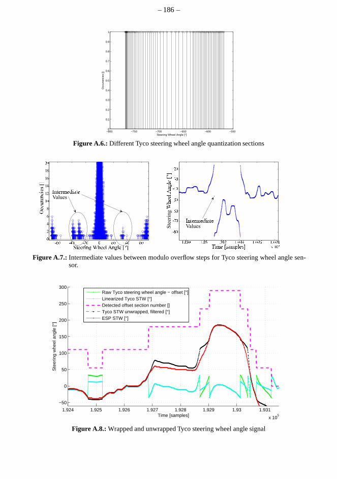
– 186–

−800 −750 −700 −650 −600 −5500

0.1

0.2

0.3

0.4

0.5

0.6

0.7

0.8

0.9

1

Steering Wheel Angle [°]

Occ

uran

cies

[]

Figure A.6.: Different Tyco steering wheel angle quantization sections

0

2

4

6

8

10

12

14

16

18

20

I%&'()'+,.&'Values

O//1234/56789

:&''(,%; W<''= >%;=' ?@BC0D0C00EF0ED0EC0

GHJKLMKNPQJKValues

TPMK [RQMUXKRY

Ste

erin

g Z

\]]^_`a^]bcd

efghiefghjefghkefghlefghefgiix egm

nig

nog

njg

npg

nkg

nqg

nlg

Figure A.7.: Intermediate values between modulo overflow steps for Tyco steering wheel angle sen-sor.

1.924 1.925 1.926 1.927 1.928 1.929 1.93 1.931

x 105

−50

0

50

100

150

200

250

300

Time [samples]

Ste

erin

g w

heel

ang

le [°

]

Raw Tyco steering wheel angle − offset [°]Linearized Tyco STW [°]Detected offset section number []Tyco STW unwrapped, filtered [°]ESP STW [°]

Figure A.8.: Wrapped and unwrapped Tyco steering wheel angle signal

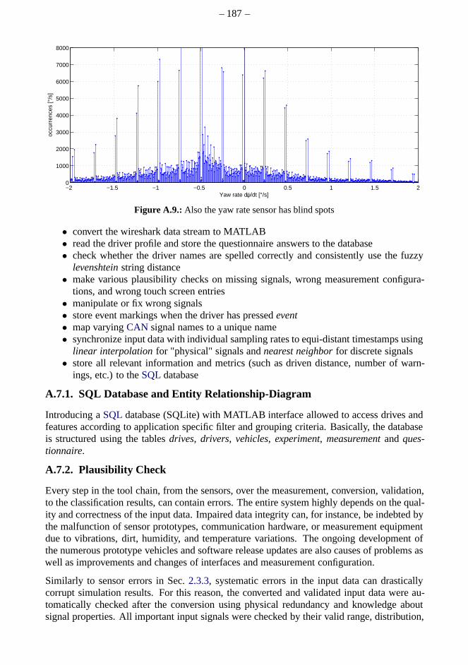
– 187–

−2 −1.5 −1 −0.5 0 0.5 1 1.5 20

1000

2000

3000

4000

5000

6000

7000

8000

Yaw rate dψ/dt [°/s]

occu

rren

ces

[°/s

]

Figure A.9.: Also the yaw rate sensor has blind spots

• convert the wireshark data stream to MATLAB• read the driver profile and store the questionnaire answers to the database• check whether the driver names are spelled correctly and consistently use the fuzzy

levenshteinstring distance• make various plausibility checks on missing signals, wrongmeasurement configura-

tions, and wrong touch screen entries• manipulate or fix wrong signals• store event markings when the driver has pressedevent• map varyingCAN signal names to a unique name• synchronize input data with individual sampling rates to equi-distant timestamps using

linear interpolationfor "physical" signals andnearest neighborfor discrete signals• store all relevant information and metrics (such as driven distance, number of warn-

ings, etc.) to theSQLdatabase

A.7.1. SQL Database and Entity Relationship-Diagram

Introducing aSQL database (SQLite) with MATLAB interface allowed to access drives andfeatures according to application specific filter and grouping criteria. Basically, the databaseis structured using the tablesdrives, drivers, vehicles, experiment, measurementandques-tionnaire.

A.7.2. Plausibility Check

Every step in the tool chain, from the sensors, over the measurement, conversion, validation,to the classification results, can contain errors. The entire system highly depends on the qual-ity and correctness of the input data. Impaired data integrity can, for instance, be indebted bythe malfunction of sensor prototypes, communication hardware, or measurement equipmentdue to vibrations, dirt, humidity, and temperature variations. The ongoing development ofthe numerous prototype vehicles and software release updates are also causes of problems aswell as improvements and changes of interfaces and measurement configuration.

Similarly to sensor errors in Sec.2.3.3, systematic errors in the input data can drasticallycorrupt simulation results. For this reason, the convertedand validated input data were au-tomatically checked after the conversion using physical redundancy and knowledge aboutsignal properties. All important input signals were checked by their valid range, distribution,

– 188–

magnitude etc. Only samples at a vehicle speed over 10 km/h and steering wheel angles below±10 were taken into account. In order to verify the correctness of the sign and magnitudeof the most important signals, a physical model was used to match the signals within a confi-dence tolerance. In our case, it was sufficient to use thesingle track model(see Sec.6.3) tocompare yaw-rateψ, wheel rotationWhlRPMFL/FR/RL/RR, accelerationsax/y, and steeringwheel anglesδa. Themean squared error (MSE)andcross-correlationfunction were usedas metrics. The conversion process must be reliable enough to meet quality requirementsof the series production. Further on, error memory records,such asESCerrors or sensorerrors were considered. Vehicle parameters and discrete encoded bit-signals were tested bythe validity of values. Pressing a button too long has been detected and suppressed.

Verification of input data does not yet cover mistakes in the simulation or evaluation environ-ment. For instance, a mistake in the evaluation can completely falsify the results. This couldonly be resolved by systematic software reviews and plausibility checks of results and calcu-lations. The simulation result plots and evaluation metrics of each drive also helped to unveilimplausibilities. The visual plots have the advantage thatthey reveal much more errors thanautomatic testing for a limited number of predefined errors.A lot of test drives for develop-ment purposes could be removed as the driving behavior was abnormal. The combination ofall methods has shown to be very effective. This way, all input data could have been verified,corrected, or set tonot valid.

A.7.3. Data Validation

The data conversion process is followed by a manual validation procedure. Data that containmistakes could not be used for classification training, so a set of hard and soft criteria weredefined:

• KSSentries and other user inputs must be valid and plausible• A desired warning level of less thanKSS6 is an indicator of careless entries• The highest reachedKSSis consistent with the number of desired warnings• The number of desired warnings is implausible• The received number of warnings does not match the obtained number of warnings• Automatic check for signal errors, measurement gaps, or byte-shifts successful• Check of the signal runs and other abnormalities successful• Drives shorter than 30 km for experiments and 10 km for free drives were set to invalid• Drives inside the plant, on testing tracks, and test drives are generally invalid

In most cases, the decision was very clear as the hard criteria applied. In the few difficultcases, several experts had to agree to avoid systematic influences. During the validation pro-cess, all new drives of one driver were grouped by this driverto quickly point out unreliabledrivers. An automatic rating was given for each driver on howreliably he entered hisKSSlevel and questionnaire to easier sort out drivers that wereunreliable. Moreover, an indicatorfor inconsistency is, when the driver indicates a differentdesired warning level for each drive.For instance, some drivers rated their fatigue level toKSS6 even when they already had laneexceedances. Other drivers, in comparison, rated them asKSS9 without any signs of fatigue.These drives have been neglected. If not a singleKSSentry was made, a separate field in thedatabasenoKSSwas set for a drive and the drive was set to "not valid". Depending on theerror, different consequences had to be drawn:

• Drives withoutKSSentry can not be used for simulation• Drives without driver profile can be simulated anyway

– 189–

• The algorithm must be tolerant to minor measurement gaps or mistakes• Drives with severe errors cannot be used for simulation

For the verification step, a separate MATLAB GUI was implemented that automatically de-tects specific implausibilities and highlights them red.

A.8. Efficient Online-Histogram and Percentile Approximationusing EWMAs

Histogram or online quartile calculation is extremely expensive in regards to computationalcomplexity as the entire window length must be sored and values be sorted. The sortingresult can be stored and every new sample sorted into this list, which still requires a lot ofmemory, especially for large window sizesN. For this reason, we propose an approximationusingl EWMA filters wherel is the number of required delay elements which only dependson the desired quartile, independent of the window sizeN. l bins are defined for thexmin =min(x[n]) and xmax = max(x[n]) ∀n. For k(i,n) = i(xmax− xmin)/l ≤ x[n] < i(xmax−xmin)/l ∀i = 1 . . . l, the EWMA for this bin is updated:

µi [n] = µi [n− 1] + λµ(

δ(k(i,n)) − µ[n− 1])

. (A.12)

Thei/l ·100% percentile is then the value ofµi [n]. Values in between can also be interpolatedto save memory.

A.9. List of all Features

Tab.A.5 list all 144 features implemented in this thesis.

Num. ID CLASS Feature Name Description1 43 AA AATOT Time-on-task2 44 AA ACTIVE System Active3 45 AA CIRCADIAN Circadian rhythm4 55 AA CROSSWIND Road warping and cross-wind intensity5 56 AA CROSSWINDSUPPRESSION Cross-wind suppression6 57 AA CUVESUPPRESSION Curve suppression7 58 AA DYNDRIVINGSTYLE Driving style suppression8 120 AA GGG AA fatigue measure including all weightings (GGG)9 122 AA GGGLWF GGG baselined (division by baseline)10 59 AA MONOTONY Monotonous driving style11 60 AA MUEDESTATUS AA drowsy (warning threshold exceeded)12 61 AA OPERATION Vehicle operation13 62 AA PEAKS Steering correction event (unweighted)14 63 AA ROADBUMPS Road bumps15 164 AA STV25 Mean of slow steering wheel rates1

16 165 AA STV50 Mean steering wheel rates1

17 166 AA STV75 Mean of fast steering wheel rates1

18 51 AA STWEVENT AA weighted fatigue measure from steering corrections(GGG)

19 121 AA STWEVENTBL GG baselined (division by baseline)20 64 AA WARNRQ AA warnings21 22 ACC DEGOINT Degree of interaction from steering wheel angle and veloc-

ity22 171 ACC MONOTONYSPD A-priori factor increasing for monotonoous situations and

at speeds around 130 km/h1

23 23 ACC REACTIM Reaction time of steering corrections to lateral displace-ments

24 169 ACC YAWJERK Yaw rate jerks used to identify drift-and-jerk patterns1

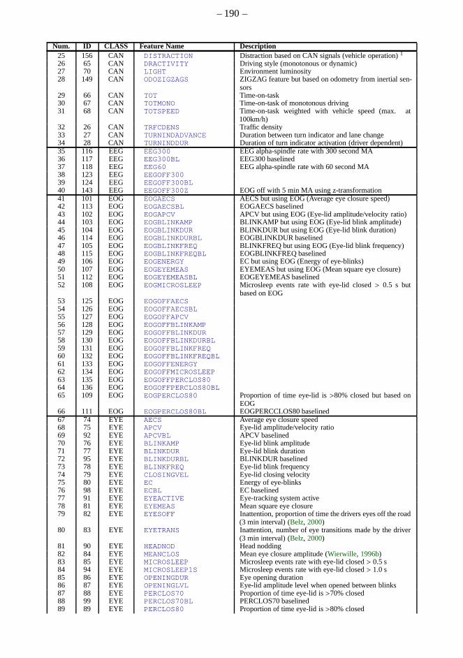
– 190–

Num. ID CLASS Feature Name Description25 156 CAN DISTRACTION Distraction based on CAN signals (vehicle operation)1

26 65 CAN DRACTIVITY Driving style (monotonous or dynamic)27 70 CAN LIGHT Environment luminosity28 149 CAN ODOZIGZAGS ZIGZAG feature but based on odometry from inertial sen-

sors29 66 CAN TOT Time-on-task30 67 CAN TOTMONO Time-on-task of monotonous driving31 68 CAN TOTSPEED Time-on-task weighted with vehicle speed (max. at

100km/h)32 26 CAN TRFCDENS Traffic density33 27 CAN TURNINDADVANCE Duration between turn indicator and lane change34 28 CAN TURNINDDUR Duration of turn indicator activation (driver dependent)35 116 EEG EEG300 EEG alpha-spindle rate with 300 second MA36 117 EEG EEG300BL EEG300 baselined37 118 EEG EEG60 EEG alpha-spindle rate with 60 second MA38 123 EEG EEGOFF30039 124 EEG EEGOFF300BL40 143 EEG EEGOFF300Z EOG off with 5 min MA using z-transformation41 101 EOG EOGAECS AECS but using EOG (Average eye closure speed)42 113 EOG EOGAECSBL EOGAECS baselined43 102 EOG EOGAPCV APCV but using EOG (Eye-lid amplitude/velocity ratio)44 103 EOG EOGBLINKAMP BLINKAMP but using EOG (Eye-lid blink amplitude)45 104 EOG EOGBLINKDUR BLINKDUR but using EOG (Eye-lid blink duration)46 114 EOG EOGBLINKDURBL EOGBLINKDUR baselined47 105 EOG EOGBLINKFREQ BLINKFREQ but using EOG (Eye-lid blink frequency)48 115 EOG EOGBLINKFREQBL EOGBLINKFREQ baselined49 106 EOG EOGENERGY EC but using EOG (Energy of eye-blinks)50 107 EOG EOGEYEMEAS EYEMEAS but using EOG (Mean square eye closure)51 112 EOG EOGEYEMEASBL EOGEYEMEAS baselined52 108 EOG EOGMICROSLEEP Microsleep events rate with eye-lid closed> 0.5 s but

based on EOG53 125 EOG EOGOFFAECS54 126 EOG EOGOFFAECSBL55 127 EOG EOGOFFAPCV56 128 EOG EOGOFFBLINKAMP57 129 EOG EOGOFFBLINKDUR58 130 EOG EOGOFFBLINKDURBL59 131 EOG EOGOFFBLINKFREQ60 132 EOG EOGOFFBLINKFREQBL61 133 EOG EOGOFFENERGY62 134 EOG EOGOFFMICROSLEEP63 135 EOG EOGOFFPERCLOS8064 136 EOG EOGOFFPERCLOS80BL65 109 EOG EOGPERCLOS80 Proportion of time eye-lid is>80% closed but based on

EOG66 111 EOG EOGPERCLOS80BL EOGPERCCLOS80 baselined67 74 EYE AECS Average eye closure speed68 75 EYE APCV Eye-lid amplitude/velocity ratio69 92 EYE APCVBL APCV baselined70 76 EYE BLINKAMP Eye-lid blink amplitude71 77 EYE BLINKDUR Eye-lid blink duration72 95 EYE BLINKDURBL BLINKDUR baselined73 78 EYE BLINKFREQ Eye-lid blink frequency74 79 EYE CLOSINGVEL Eye-lid closing velocity75 80 EYE EC Energy of eye-blinks76 98 EYE ECBL EC baselined77 91 EYE EYEACTIVE Eye-tracking system active78 81 EYE EYEMEAS Mean square eye closure79 82 EYE EYESOFF Inattention, proportion of time the drivers eyes off the road

(3 min interval) (Belz, 2000)80 83 EYE EYETRANS Inattention, number of eye transitions made by the driver

(3 min interval) (Belz, 2000)81 90 EYE HEADNOD Head nodding82 84 EYE MEANCLOS Mean eye closure amplitude (Wierwille, 1996b)83 85 EYE MICROSLEEP Microsleep events rate with eye-lid closed> 0.5 s84 94 EYE MICROSLEEP1S Microsleep events rate with eye-lid closed> 1.0 s85 86 EYE OPENINGDUR Eye opening duration86 87 EYE OPENINGLVL Eye-lid amplitude level when opened between blinks87 88 EYE PERCLOS70 Proportion of time eye-lid is>70% closed88 99 EYE PERCLOS70BL PERCLOS70 baselined89 89 EYE PERCLOS80 Proportion of time eye-lid is>80% closed

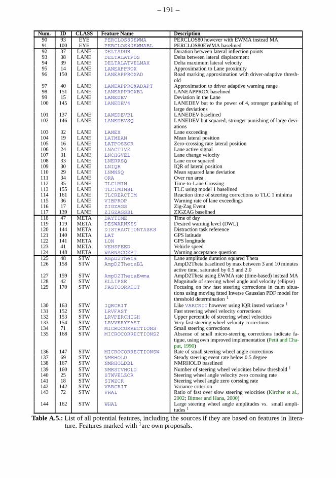
– 191–

Num. ID CLASS Feature Name Description90 93 EYE PERCLOS80EWMA PERCLOS80 however with EWMA instead MA91 100 EYE PERCLOS80EWMABL PERCLOS80EWMA baselined92 37 LANE DELTADUR Duration between lateral inflection points93 38 LANE DELTALATPOS Delta between lateral displacement94 39 LANE DELTALATVELMAX Delta maximum lateral velocity95 14 LANE LANEAPPROX Approximation to Lane proximity96 150 LANE LANEAPPROXAD Road marking approximation with driver-adaptive thresh-

old97 40 LANE LANEAPPROXADAPT Approximation to driver adaptive warning range98 151 LANE LANEAPPROXBL LANEAPPROX baselined99 15 LANE LANEDEV Deviation in the Lane100 145 LANE LANEDEV4 LANEDEV but to the power of 4, stronger punishing of

large deviations101 137 LANE LANEDEVBL LANEDEV baselined102 146 LANE LANEDEVSQ LANEDEV but squared, stronger punishing of large devi-

ations103 32 LANE LANEX Lane exceeding104 19 LANE LATMEAN Mean lateral position105 16 LANE LATPOSZCR Zero-crossing rate lateral position106 24 LANE LNACTIVE Lane active signal107 31 LANE LNCHGVEL Lane change velocity108 33 LANE LNERRSQ Lane error squared109 30 LANE LNIQR IQR of lateral position110 29 LANE LNMNSQ Mean squared lane deviation111 34 LANE ORA Over run area112 35 LANE TLC1MIN Time-to-Lane Crossing113 155 LANE TLC1MINBL TLC using model 1 baselined114 161 LANE TLCREACTIM Reaction time of steering corrections to TLC 1 minima115 36 LANE VIBPROP Warning rate of lane exceedings116 17 LANE ZIGZAGS Zig-Zag Event117 139 LANE ZIGZAGSBL ZIGZAG baselined118 47 META DAYTIME Time of day119 119 META DESWARNKSS Desired warning level (DWL)120 144 META DISTRACTIONTASKS Distraction task reference121 140 META LAT GPS latitude122 141 META LON GPS longitude123 41 META VEHSPEED Vehicle speed124 148 META WARNACCEPT Warning acceptance question125 48 STW AmpD2Theta Lane amplitude duration squared Theta126 158 STW AmpD2ThetaBL AmpD2Theta baselined by max between 3 and 10 minutes

active time, saturated by 0.5 and 2.0127 159 STW AmpD2ThetaEwma AmpD2Theta using EWMA rate (time-based) instead MA128 42 STW ELLIPSE Magnitude of steering wheel angle and velocity (ellipse)129 170 STW FASTCORRECT Focusing on few fast steering corrections in calm situa-

tions using moving fitted Inverse Gaussian PDF model forthreshold determination1

130 163 STW IQRCRIT Like VARCRIT however using IQR insted variance1

131 152 STW LRVFAST Fast streering wheel velocity corrections132 153 STW LRVPERCHIGH Upper percentile of streering wheel velocities133 154 STW LRVVERYFAST Very fast steering wheel velocity corrections134 71 STW MICROCORRECTIONS Small steering corrections135 168 STW MICROCORRECTIONS2 Absense of small micro-steering corrections indicate fa-

tigue, using own improved implementation (Petit and Cha-put, 1990)

136 147 STW MICROCORRECTIONSW Rate of small steering wheel angle corrections137 69 STW NMRHOLD Steady steering event rate below 0.5 degree138 167 STW NMRHOLDBL NMRHOLD baselined139 160 STW NMRSTVHOLD Number of steering wheel velocities below threshold1

140 25 STW STWVELZCR Steering wheel angle velocity zero corssing rate141 18 STW STWZCR Steering wheel angle zero corssing rate142 142 STW VARCRIT Variance criterion143 72 STW VHAL Ratio of fast over slow steering velocities (Kircher et al.,

2002; Bittner and Hana, 2000)144 162 STW WHAL Large steering wheel angle amplitudes vs. small ampli-

tudes1

Table A.5.: List of all potential features, including the sources if they are based on features in litera-ture. Features marked with1are own proposals.

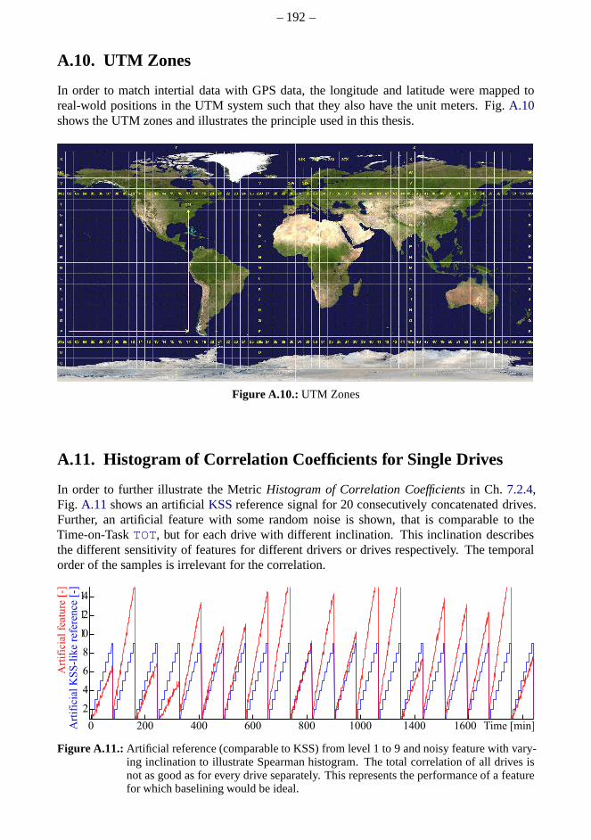
– 192–

A.10. UTM Zones

In order to match intertial data with GPS data, the longitudeand latitude were mapped toreal-wold positions in the UTM system such that they also have the unit meters. Fig.A.10shows the UTM zones and illustrates the principle used in this thesis.

Figure A.10.: UTM Zones

A.11. Histogram of Correlation Coefficients for Single Drives

In order to further illustrate the MetricHistogram of Correlation Coefficientsin Ch. 7.2.4,Fig. A.11 shows an artificialKSSreference signal for 20 consecutively concatenated drives.Further, an artificial feature with some random noise is shown, that is comparable to theTime-on-TaskTOT, but for each drive with different inclination. This inclination describesthe different sensitivity of features for different drivers or drives respectively. The temporalorder of the samples is irrelevant for the correlation.

Figure A.11.: Artificial reference (comparable to KSS) from level 1 to 9 andnoisy feature with vary-ing inclination to illustrate Spearman histogram. The total correlation of all drives isnot as good as for every drive separately. This represents the performance of a featurefor which baselining would be ideal.

– 193–

Fig. A.12 shows at the left a scatter plot and correlation coefficient calculated for all drivesat once. The Spearman correlation coefficient of all drives at once is onlyρS = 0.811 whilealmost all coefficients in the Spearman histogram, grouped by drives, areρ′S ≈ 1.

Figure A.12.: Scatter plot over all drives and Spearman histogram of coefficients grouped by drives

As a conclusion, we can see that this method of correlation analysis method serves to evaluatea feature independently from the drive or driver-specific baseline or sensitivity. With otherwords, the same result would be achieved, if the online-baselining would be ideal. We haveto consider that this can unfortunately not be achieved in practice.

Another aspect is, that theKSS should be most accurate at the moment when it is entered.For this reason, alternatively only the instants of theKSSentries are used for evaluation andthe feature was used at this time instant or aggregated from its adjacent values.

A.12. Feature Analysis and Evaluation GUI

Fig. A.13 shows an evaluation GUI to analyze single features. All displayed informationis contained in the feature matrixF . This makes it possible to select different features andfilters for references, vehicles, experiments, drivers anddrives. Scatter plots, error bar plots,and correlation measures are updated according to the selection. This allows a combinationof qualitative and quantitative assessment of features. This figure provides a good impression,that the featurePERCLOS80 performs very well for this driver. The signal plot shows thatthe feature matches better the holdKSS(green) than the linear interpolated signal due to thedelay of the smoothing.

A.13. Real-time System

The majority of the transparency about driving situations cannot be captured by the mea-surements. For this reason, it is very valuable to test the implemented features online inthe vehicle to relate signals and events to situations and tune parameters. TheATTENTION

ASSISTalgorithm was developed and tested in Fixed-point TargetLink directly running on aprogrammable developerESP. This is much to laborious and limited in resources to imple-ment sophisticated algorithms. In comparison to the Micro-Autobox MAB II from DSPACEor Vector CANoe CAPL, an alternative, own implementation inMATLAB, Mex C++ andC# was chosen for several reasons. A Vector CAN Card and CAN cases were available, but

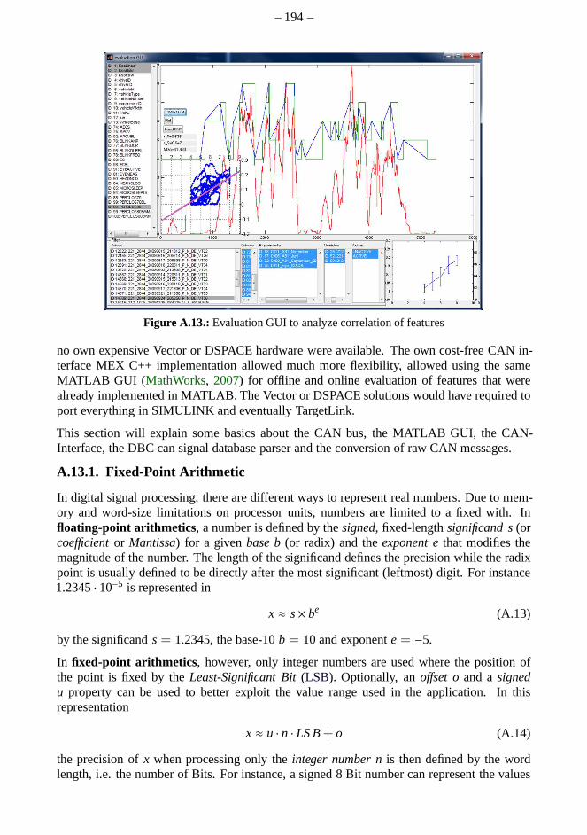
– 194–

Figure A.13.: Evaluation GUI to analyze correlation of features

no own expensive Vector or DSPACE hardware were available. The own cost-free CAN in-terface MEX C++ implementation allowed much more flexibility, allowed using the sameMATLAB GUI ( MathWorks, 2007) for offline and online evaluation of features that werealready implemented in MATLAB. The Vector or DSPACE solutions would have required toport everything in SIMULINK and eventually TargetLink.

This section will explain some basics about the CAN bus, the MATLAB GUI, the CAN-Interface, the DBC can signal database parser and the conversion of raw CAN messages.

A.13.1. Fixed-Point Arithmetic

In digital signal processing, there are different ways to represent real numbers. Due to mem-ory and word-size limitations on processor units, numbers are limited to a fixed with. Infloating-point arithmetics, a number is defined by thesigned, fixed-lengthsignificand s(orcoefficientor Mantissa) for a givenbase b(or radix) and theexponent ethat modifies themagnitude of the number. The length of the significand definesthe precision while the radixpoint is usually defined to be directly after the most significant (leftmost) digit. For instance1.2345· 10−5 is represented in

x ≈ s× be (A.13)

by the significands= 1.2345, the base-10b = 10 and exponente= −5.

In fixed-point arithmetics, however, only integer numbers are used where the position ofthe point is fixed by theLeast-Significant Bit(LSB). Optionally, anoffset oand asignedu property can be used to better exploit the value range used inthe application. In thisrepresentation

x ≈ u · n · LS B+ o (A.14)

the precision ofx when processing only theinteger number nis then defined by the wordlength, i.e. the number of Bits. For instance, a signed 8 Bit number can represent the values

– 195–

-128 to 127 where one Bit for the sign. If it is scaled by aLSB=2−4 and an offseto = 10.0,the precision (or resolution) is 0.0625 and the fixed-point representation allows to cover therange[2 . . . 17.9375] (−128· LS B+ o to 127· LS B− o).

The computation in fixed-point is many times faster since theposition of the radix pointdoes not need to be considered. As is can be seen in Fig.A.14 using an offset increasesprecision but slows down the computation time. Also, an arbitrary LSB is more precise butless performant than using a dual basedLSB. Divisions or multiplications with a dual factor2k with k ∈N can be computed very fast by logical shift of the binary number to the right orto the left.

offset=0LSB=2x

offset=0LSB=arbitrary

offset=arbitraryLSB=2x

offset=arbitraryLSB =arbitrary

More precision

Faster

Figure A.14.: Scaling performance vs. accuracy

Representation of a floating point number in fixed-point always leads to a loss of precisionand thus an error on a 16 bit architecture. A multiplication of two 16 bit numbers requires a32 Bit intermediate result, even if the final result is rescaled to 16 bit again. Such operationscan be performed with two 16 bit numbers that require howevermore resources and arethus not expedient. Depending on the signal processing operations, systematic errors leadto accumulated errors in integrators for instance. An erroris thus more severe the earlier itoccurs in the signal processing chain.

For this reason, especially the filters of the input signals had to be scaled manually and asgood as possible. This is exemplarily shown in Ch.A.15. The ATTENTION ASSIST istrunning on the controller unis of the ESP.

A.13.2. Fixed-point Low-pass Filter

Especially the Butterworth filter of 2nd order of the lateral accelerationay has been identifiedas a major cause for fixed- / floating-point errors that are accumulated in the feature extraction.App.A.13.1explains this problem in more detail. For this reson, the filter has to be optimallyscaled as shown in Fig.A.15.

A.13.3. Offline and Online Real-Time Attention Assist Vehicle Track Viewer

Fig. A.16 shows the GUI of the offline- and real-time onlineAttention Assist PlusSystem(AAP). It allows online visualization of vehicles signals and features as well as offline play-back of measurements.

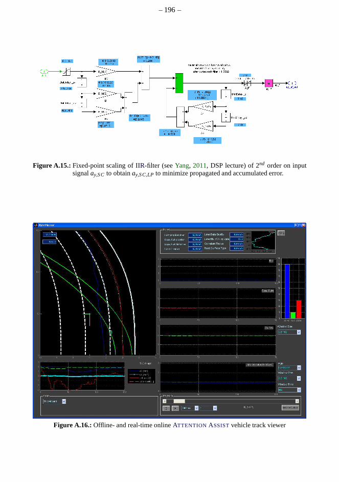
– 196–

Figure A.15.: Fixed-point scaling ofIIR-filter (seeYang, 2011, DSP lecture) of 2nd order on inputsignalay,SC to obtainay,SC,LP to minimize propagated and accumulated error.

Figure A.16.: Offline- and real-time onlineATTENTION ASSISTvehicle track viewer

– 197–

Bibliography

AAA, 2013: Foundation for Traffic Safety AAA 2013 How to Avoid Drowsy Driving,https://exchange.aaa.com/safety/driving-advice/drowsy-driving/(last visited: May 11, 2020).

Akerstedt, 1980: T. Åkerstedt and M. Gillberg 1980 Subjective and objective sleepiness in theactive individual, International Journal of Neuroscience, Volume: 52: pp. 29–37.

Akin, 2007: Özgür Akin 2007 Müdigkeitserkennung mit dem Driver State Sensor (DSS) in Kraft-fahrzeugen,Master’s thesis, Fachhochschule Giessen-Friedberg.

Altmueller, 2007: Tobias Altmüller 2007Driver Monitoring and Drowsiness Detection by SteeringSignal Analysis,PhD thesis Universitaet der Bundeswehr München.

Andreassi, 2000: J. Andreassi 2000 Psychophysiology: Human behavior and physiological re-sponse,Londin: Lawrence Erlbaum Associates.

Angermann, 2011: Roman Matthias Angermann 2011 Die Entwicklung der Aktiven Sicherheitvon ihren Anfängen bis zum Jahr 2000 - Unter besonderer Berücksichtigung der Daimler-Benz AG,Number 978-3-8348-1543-9 Vieweg & Teubnerhttps://www.buchhandel.de/buch/Die-Entwicklung-der-Aktiven-Sicherheit-v-9783834815439(last visited: May 11, 2020).

Anund et al., 2008: Anna Anund, Göran Kecklund, Björn Peters and Torbjörn Åker stedt2008Driver sleepiness and individual differences in preferences for countermeasures,Journal of SleepResearch 17, Issue 1:16–22.

auto.de, 2009: auto.de2009 IAA 2009 Rundgang: Mercedes-Benz SLS AMG Flügeltürerhttp://www.auto.de/magazin/IAA-2009-Rundgang-Mercedes-Benz-SLS-AMG-Fluegeltuerer(last visited: May 11, 2020).

Autokiste.de, 2007: Autokiste.de 2007Volvo Driver Alert: Zeit für eine Pausehttp://www.autokiste.de/psg/index/show.htm?id=6679&bild=5(last visited: May 11, 2020).

Brown et al., 2006: Malcolm Brown, Michael Marmor Vaegan, Eberhard Zrenner, M itchellBrigell and Michael Bach 2006 ISCEV Standard for Clinical Electro-oculography (EOG) ISCEVStandard for Clinical Electro-oculography (EOG),Doc Ophthalmol, Volume: 113: pp. 205–212.

Baranski, 2007: Joseph V. Baranski2007Fatigue, sleep loss and confidence in judgment,Journalof Experimental Psychology, Volume: 13(4): pp. 182–196.

Barényi, 1951: Béla Barényi 1952, Patent number: (DBP 854 15)Motor vehicles especially for thetransportation of people.https://www.mercedes-benz.com/de/mercedes-benz/classic/bela-barenyi-der-lebensretter/(last visited: May 11, 2020).

Barr and Howarth, 2006: Lawrence Barr and Heidi Howarth 2006 A Review And Evaluation ofEmerging Driver Fatigue Detection Measures and Technologies.

Batavia, 1999: Parag Batavia1999Driver-Adaptive Lane Departure Warning Systems,PhD thesisThe Robotics Institute Carnegie Mellon University Pittsburgh, Pennsylvania, 15213.

– 198–

Batista, 2007: Jorge Batista 2007 A Drowsiness and Point of Attention Monitoring System forDriver Vigilance, Proceedings of the IEEE Intelligent Transportation Systems Conference, Vol-ume: 4(4): pp. 702–708.

Becker, 2008: Ruth Becker 2008 Interindividuelle Auswirkungen von Schlafentzug,PhD thesisFachbereich Erziehungswissenschaft und Psychologie der freien Universität Berlin.

Belz et al., 2004: S. M. Belz, G.S. Robinson and J.G. Casali2004 Temporal Separation andSelf-rating of Alertness as Indicators of Driver Fatigue inCommercial Motor Vehicle Operators,Human Factors, Volume: 46 (1): pp. 154–69.

Belz, 2000: Steven Mark Belz 2000 An On-road Investigation of Self-rating of Alertness andTemporal Separation as Indicators of Driver Fatigue in Commercial Motor Vehicle Operators,PhDthesis Doctor of Philosophy in Industrial and Systems Engineering.

Benz & Co, 1886: Benz & Co 1886, Patent number: (DE 37435)Fahrzeug mit Gasmotorantrieb.http://upload.wikimedia.org/wikipedia/commons/3/37/Patentschrift_37435_Benz_Patent-Motorwagen.pdf(last visited: May 11, 2020).

Berger and Rumpe, 2008: Christian Berger and Bernhard Rumpe 2008 Autonomes Fahren -Erkenntnisse aus der Darpa Challenge,it, Volume: 4: pp. 258–264.

Berglund, 2007: Jens Berglund2007 In-Vehicle Prediction of Truck Driver Sleepiness - SteeringRelated Variables,Master’s thesis, Lulea University of Technology.

Berka et al., 2005: Chris Berka, Daniel J. Levendowski and Philip Westbrook2005 Implemen-tation of a Closed-Loop Real-Time EEG-Based Drowsiness Detection System: Effects of FeedbackAlarms on Performance in a Driving Simulator,Proceedings of the International Conference onHuman Computer Interaction, July 2005, Las Vegas, Nevada.

Bittner and Hana, 2000: Roman Bittner and Karel Hana 2000 Detecting of Fatigue States of aCar Driver.

Blanco and Bocanegra, 2009: Myra Blanco and Joseph L. Bocanegra2009 Assessment of aDrowsy Driver Warning System for Heavy-Vehicle Drivers,Technical report National HighwayTraffic Administration.

Bleich, 2009: Nils Bleich 2009 Deutsche Automobilzulieferer in China: Chancen und Risiken derErschließung des Chinesischen Automobilmarktes,Diplomica Verlag Hamburg.

Bleymüller and Gehlert, 2012: Josef Bleymüller and Günther Gehlert 2012 Statistik fürWirtschaftswissenschaftler,Volume: 16 Franz Vahlen München.

BMW, 2011: Media Information BMW 2011 The future of intelligent networking: The BMWVision ConnectedDrive.

Bohlin, 1959: Nils Ivar Bohlin 1961, Patent number: (DE 1101987a)Sicherheitsgurt fuerFahrzeuge insbesondere Kraftfahrzeuge.https://www.dpma.de/english/our_office/publications/milestones/60jahredreipunktegurt/index.html(last visited: May 11, 2020).

Boyraz et al., 2007: Pinar Boyraz, Memis Acar and David Kerr 2007 Signal Modelling andHidden Markov Models for Driving Manoeuvre Recognition andDriver Fault Diagnosis in anurban road scenario,Proceedings of the 2007 IEEE Intelligent Vehicles Symposium, Pages: 13–15.

Brainard and Hanifin, 2001: G. C. Brainard and J. P. Hanifin 2001Action spectrum for melatoninregulation in humans: evidence for a novel circadian photoreceptor, The Journal of Neuroscience:the official journal of the Society for Neuroscience, Volume: 21: pp. 6405–6412.

– 199–

Brown, 1994: Ivan D. Brown 1994 Driver Fatigue, Human Factors: The Journal of the HumanFactors and Ergonomics Society, Volume: 36(2): pp. 298–314(17).

Buehren, 2008: Markus Buehren 2008 Simulation und Verarbeitung von Radartiellisten im Auto-mobil, PhD thesis Chair of System Theory and Signal Processing.

BGH, 1969: Bundesgerichtshof1969 Court decision from 18.11.1969: Perceptibility of fatiguesigns by the driver ("Zur Wahrnehmbarkeit der Ermüdungszeichen durch einen Kraftfahrer"),AZ4 StR 66/69.

BGH, 2002: Bundesgerichtshof2002Court decision from 04.12.2002, Stendal,AZ.: 23 O 67/02.

Burgess et al., 2002: Helen Burgess, Katie Sharkey and Charmane Eastman2002 Bright light,dark and Melatonin can promote circadian adaptation in night shift workers, Sleep MedicineReviews 6(5):407–420.

Carlson and Gerdes, 2002: Christopher R. Carlson and Christian Gerdes 2002 Identifyingtire pressure variation by nonlinear estimation of longitudinal stiffness and effective radius,InProceedings of AVEC 2002 6th International Symposium of Advanced Vehicle Control,.

Chawla et al., 2008: M. P. Chawla, H. K. Verma and V. Kumar 2008Artifacts and noise removalin electrocardiograms using independent component analysis, International Journal on Cardiology,Volume: 129(2): pp. 278–281.

Clayton, 2006: Clayton 2006Klothoidehttp://ww3.cad.de/foren/ubb/uploads/Clayton/Klothoide-Formeln.pdf(last visited: May 11, 2020).

Comon, 1994: P. Comon1994Independent component analysis, a new concept?,Signal ProcessingVolume: 36(3):287–314.

Costa, 2005: Joaquim Costa and Jaime Cardoso2005 Classification of Ordinal Data UsingNeural Networks, Machine Learning: 16th European Conference on Machine Learning (ECML),Porto, Portugal, Proceedings 10:690–697.

Cui, 2016: Zhicheng Cui, Wenlin Chen and Yixin Chen 2016 Multi-Scale ConvolutionalNeural Networks for Time Series Classification, CoRR, DBLP Computer Science Vol-ume: abs/1603.06995.

Czupalla, 2007: Stephan Czupalla 2007 Messfahrtenauswertung zur Erkennung von positions-und tageszeitabhängigen Ereignishäufungen für die Optimierung eines Fahrerzustandsbeobachters,Master’s thesis, Berufsakademie Horb.

Daimler, 2008: Daimler HighTech Report 2/2008 - Feature Attention Assisthttp://www.worldcat.org/title/daimler-hightech-report/oclc/769131108(last visited: May 11, 2020).

Daimler COM/M, 2009: Daimler COM/M Meilensteine der Fahrzeugsicherheit. Die Vision vomunfallfreien Fahren.https://docplayer.org/5414305-Meilensteine-der-fahrzeugsicherheit-die-vision-vom-unfallfreien-fahren.html(last visited: May 11, 2020).

de Mattos Pimenta, 2011: Pedro A. de Mattos Pimenta2011 Driver Drowsiness ClassificationBased on Lane and Steering Behavior,Master’s thesis, University of Stuttgart, Chair of SystemTheory and Signal Processing.

Delphi, 2006: Delphi 2006, Patent number: (US 7,021,161)Gear Bearing for a Steering WheelPosition Sensor.

Desai and Haque, 2006: A.V. Desai and M.A. Haque 2006 Vigilance monitoring for operatorsafety: A simulation study on highway driving,Journal of Safety Research 37:139–147.

– 200–

DESTATIS, 2011a: Statistisches Bundesamt DESTATIS2011aUnfallentwicklung auf deutschenStrassen 2010.

DESTATIS, 2011b: Statistisches Bundesamt DESTATIS2011b Verkehrsunfälle Zahlenreihen2010.

DESTATIS, 2013b: Statistisches Bundesamt DESTATIS2013aUnfallentwicklung auf deutschenStrassen 2012,Begleitmaterial zur Pressekonferenz am 10. Juli 2013 in Berlin.

DESTATIS, 2013b: Statistisches Bundesamt DESTATIS2013b Verkehrsunfälle - Unfälle unterdem Einfluss von Alkohol oder anderen berauschenden Mittelnim Strassenverkehr.

Die Welt.de, 2008: Die Welt.de 2010 fahren weltweit eine Milliarde Autoshttp://www.welt.de/welt_print/article1561636/2010-fahren-weltweit-eine-Milliarde-Autos.html(last visited: May 11, 2020)a.

Dietmayer, 2008: Klaus C.J. Dietmayer 2008 Lecture Script for the Lecture Messtechnik II,Uni-versity of Ulm.

Dietsche and Jäger, 2003: Karl-Heinz Dietsche and Thomas Jäger2003 KraftfahrtechnischesTaschenbuch,Volume 25 ofISBN 3-528-23876-3,Friedrich Vieweg & Sohn Verlag, Wiesbaden.

Dinges et al., 1987: David F. Dinges, M. T. Orne, W. G. Whitehouse and E. C. OrneTemporalPlacement of a Nap for Alertness: Contributions of Circadian Phase and Prior Wakefulness,Sleep,Volume: August 10(4): pp. 313–29http://www.ncbi.nlm.nih.gov/pubmed/3659730(last visited: May 11, 2020)

Doppelklicker, 2011: Doppelklicker 2011Kfz-Versicherung: Beifahrer erhalten keinen Schadener-satz, wenn Müdigkeit des Fahrers bekannt war.

Drory, 1985: Amos Drory 1985 Effects of Rest and Secondary Task on Simulated Truck-DrivingTask Performance,Human Factors, Volume: 27(7): pp. 201–207.

Duda et al., 2001: Richard O. Duda, Peter E. Hart and David G. Stork 2001 Pattern Classifica-tion, Wiley-Interscience.

Duncker, 2007: Gernot I. W. Duncker 2007 Jeder vierte Autofahrer sitzt übermüdet am Steuer,Technical report Deutsche Ophthalmologische Gesellschaft e.V.

Anthony Best Dynamics, 2012: Anthony Best Dynamics2012 Steering robots SP6020 Outlinespecification,2012.

Elango, 2002: Vetri Venthan Elango 2002Safety Evaluation of Centerline Rumble Strips,Master’sthesis, University of Massachusetts.

Eskandarian and Mortazavi, 2007: Azim Eskandarian and Ali Mortazavi 2007 Evaluation ofa Smart Algorithm for Commercial Vehicle Driver DrowsinessDetection, In Proceedings of theIEEE Intelligent Vehicles Symposium, Istanbul, Turkey.

Fagerberg, 2004: Kalle Fagerberg 2004 Vehicle-Based Detection of Inattentive Driving for Inte-gratin in an Adaptive Lane Departure Warning System - Drowsiness Detection,Master’s thesis,KTH Vetenskap Och Konst.

Fahrmeir et al. 2003: Ludwig Fahrmeir, Rita Künstler, Iris Pigeot and Gerhard Tu tz 2003Statistik. Der Weg zur Datenanalyse,Springer.

Fairbanks et al. 1995: Rollin J. Fairbanks, Sarah E. Fahey and Walter W. Wierwille 1995Research on Vehicle-Based Driver Status/Performance Monitoring: Seventh Semi-Annual ResearchReport,Technical report National Highway Traffic Safety Administration.

– 201–

Fawcett, 2004: Tom Fawcett 2004 ROC Graphs: Notes and Practical Considerations for Re-searchers,Pattern Recognition Letters, Volume: 27(8): pp. 882–891.

Fertner, 2009: Maria-Luise Fertner 2009Sekundenschlaf & Ablenkung,Technical report ÖAMTC- Der Österreichische Automobil-, Motorrad- und Touring Club.

FHWA, 2012: Federal Highway Administration FHWA 2012 Roadway Departure Safety - Pave-ment Safety - Rumble Strips and Stripes - Effectivenesshttp://safety.fhwa.dot.gov/roadway_dept/pavement/rumble_strips/effectiveness/(last visited: May 11, 2020).

Forsman and Vilaa, 2012: Pia M. Forsman and Bryan J. Vilaa 2012 Efficient driver drowsinessdetection at moderate levels of drowsiness,Accident Analysis and Prevention, Volume: May:pp. 10.

Friedrichs, 2006: Fabian Friedrichs 2006 Schätzung von prosodischen Features zur Emotionsde-tektion,Master’s thesis, University of Stuttgart, Chair of System Theory and Signal Processing.

Friedrichs et al. 2012: Fabian Friedrichs, Werner Bernzen, Frauke Driewer and WiebkeMüller 2012, Patent number: (DE 201,110,012,967)Method for identifying or issuance of traveltime of driver, involves determining travel time of driver,where travel time is continuously identi-fied and optionally displayed during ignition of barrel of vehicle.http://www.google.com/patents/DE102011012967A1?cl=en(last visited: May 11, 2020).

Friedrichs and Yang, 2010a: Fabian Friedrichs and Bin Yang 2010 Camera-based DrowsinessReference for Driver State Classification under Real Driving Conditions,IEEE Intelligent VehiclesSymposium.

Friedrichs and Yang, 2010b: Fabian Friedrichs and Bin Yang 2010 Drowsiness Monitoring bySteering and Lane Data based Features under Real Driving Conditions, EUSIPCO.

Friedrichs and Yang, 2011: Fabian Friedrichs and Bin Yang 2011 Consideration of Influenceson Driver State Classification from External Factors,Driver Distraction and Inattention (DDI)Conference.

Fuersich, 2009: Alexander Fuersich 2009 Driver State Classification using Expert Knowledge inHiddden Markov Models and Bayes Networks,Master’s thesis, University of Stuttgart, Chair ofSystem Theory and Signal Processing.

Furtwängler, 2013: Sara Furtwängler 2013 Bewährungsstrafe nach tödlichem Unfall auf A81,Heilbronner Stimmehttps://www.saechsische.de/bewaehrungsstrafe-nach-toedlichem-unfall-3842144.html(last visited: May 11, 2020).

Gallay and Schleicher, 2002: N. Gallay and R. Schleicher2002 Fatigue indicators from Elec-troencephalogram - A Reasearch Report.

Galley et al., 2005: Lars Galley, Elisabeth Hentschel, Klaus-Peter Kuhn and Wolfgang Stolz-mann 2006, Patent number: (WO 2006131254 A1)Method and Control Device Recognising,Specific to a Driver, Inattentiveness of a Driver of a Vehicle.

Gärtner, 2009: Christiane Gärtner 2009 Driving Style Classification for DriverMonitoring,Mas-ter’s thesis, University of Stuttgart, Chair of System Theory and Signal Processing.

Gärtner, 2017: Jonas Gehring, Michael Auli, David Grangier, Denis Yarats and Yann N.Dauphin 2017 Convolutional Sequence to Sequence Learning,PLMR, Proceedings of the 34thInternational Conference on Machine Learning, Volume: 70(06–11)(7): pp. 1243–1252.

– 202–

Gutierrez, 2016: P.A. Gutiérrez and M. Pérez-Ortiz and J. Sánchez-Monederoand F.Fernandez-Navarro and C. Hervás-Martínez2016 Ordinal regression methods: survey and ex-perimental study,IEEE Transactions on Knowledge and Data Engineering, Volume: 28(1): pp. 127–146.

Gillberg et al., 1996: Mats Gillberg, Göran Kecklund, John Axxelsson and Torbjörn Åkerstedt1996 The Effects of a Short Daytime Nap After Restricted Night Sleep, Sleep, Volume: 19(7):pp. 570–575.

Glaser and Mammar, 2005: Sebastien Glaser and Saïd Mammar2005 Experimental Time toLine Crossing Validation, IEEE Conference on Intelligent Transportation Systems, Volume: 8:pp. 791–796.

Goodfellow et al., 2017: Ian Goodfellow, Yoshua Bengio and Aaron Courville2017Deep Learn-ing (Adaptive Computation and Machine Learning),The MIT Press, Massachusettshttps://www.deeplearningbook.org/(last visited: May 11, 2020).

Government of India, 2011: Government of India 2011Road Accidents in India 2011http://www.indiaenvironmentportal.org.in/files/file/road%20accidents%20in%20India%202017.pdf(last visited: May 11, 2020).

Grace, 2001: Richard Grace and Sonya Steward2001 Drowsy Driver Monitor and WarningSystem,First International Driving Symposium on Human Factors in Driver Assessment, Trainingand Vehicle Design page 5.

Greschner, 2011: Uwe Markus Greschner 2011 Experimentelle Untersuchung von Maßnahmengegen Schläfrigkeit beim Führen von Kraftfahrzeugen,PhD thesis Von der Fakultät Konstruktions-,Produktions- und Fahrzeugtechnik der Universität Stuttgart.

Guan, 2008: Tianyi Guan 2008Modellierung der Fahrzeugdynamik zur Einschätzung der Perspek-tivenänderung einer Kamera anhand von CAN Bus Daten,Master’s thesis, Universität Stuttgart.

Han et al., 2017: Young-Joo Han, Wooseong Kim and Joon-Sang Park2017 Eye-trackingon smartphones using regression-based prediction,Hindawi, Mobile Information Systems,Pages: 990–992.

Han et al., 2018: Young-Joo Han, Wooseong Kim and Joon-Sang Park2018 Efficient Eye-Blinking Detection on Smartphones: A Hybrid Approach Basedon Deep Learning, Hindawi,Mobile Information Systems, Volume: 2018: pp. 1–8.

Hargutt, 2001: Volker Hargutt 2001Das Liedschlussverhalten als Indikator für Aufmerksamkeits-und Müdigkeitsprozesse bei Arbeitshandlungen,PhD thesis University of Würzburg.

Hargutt and Krüger, 2000: Volker Hargutt and H.-P. Krüger 2000 Eyelid movements and theirpredictive value for fatigue stages.,International Conference of Traffic and Transport Psychology(ICTTP).

Hargutt et al., 2005: Volker Hargutt, H. Tietze and Hans-Peter Krüger 2005 Auto an Fahrer:"Sie sind müde!" - Wirkung verschiedener Strategien zur Rückmeldung des Fahrerzustands,VDI-Gesellschaft Fahrzeug- und Verkehrstechnik (Hrsg.), Fahrer im 21. Jahrhundert. Der Mensch alsFahrer und seine Interaktion mit dem Fahrzeug (Tagung Braunschweig), Pages: 95–101.

Hartley, 1995: Laurence Hartley 1995 Fatigue & Driving: driver Impairment, driver fatigue anddriving simulation,Taylor&Francis.

Hasberg and Hensel, 2009: Carsten Hasberg and Stefan Hensel2009Online-Estimation of RoadMap Elements using Spline Curves,12th International Conference on Information Fusion.

– 203–

Heißing, 2011: Bernd Heißing 2011Chassis Handbook,Springerhttp://books.google.de/books?id=NSlSJtEy-NIC&q=antilock%20braking%20system(last visited: May 11, 2020).

Hell, 2001: W. Hell 2001Verkannte Unfallursache.,Kolloquium des DVR 2001.

Hell, 2010: Wolfram Hell Fahrzeuginsassen richtig sichern,ADAC e.V. and Ludwig-Maximilians-Universität München, Institut für Rechtsmedizin, Medizinisch-Biomechanische Unfallanalyse.

Hentschel et al., 2005: Elisabeth Hentschel, Dietmar Neumerkel, Lars Galley and Klaus-PeterKuhn 2005, Patent number: (DE 103 55 221 A1)Verfahren und Computerprogramm zum Erkennenvon Unaufmerksamkeiten des Fahrers eines Fahrzeugs.

Hermannstädter and Yang, 2013a: Peter Hermannstädter and Bin Yang2013 Driver Distrac-tion Assessment Using Driver Modeling,Proceedings of the IEEE International Conference onSystems, Man, and Cybernetics, Volume: October: pp. 13–16 Manchester, UK.

Hermannstädter and Yang, 2013b: Peter Hermannstädter and Bin Yang2013Erkennung verän-derten Fahrerverhaltens mit einem Fahrermodell mit Vorausschau und Motorikkomponente,VDI-Bericht 4. Berliner Fachtagung Fahrermodellierung. Berlin, Germany, 13./14. Juni.

Herslund and Jorgensen, 2003: M.-B. Herslund and N. O. Jorgensen2003Looked-but-failed-to-see-errors in traffic,Accident Analysis & Prevention. Volume: 35(6): pp. 885–891.

Heuer, 2013: Steffan Heuer2013Autonomous driving - The triumph of the assistance systems.

Hochreiter, 1991: Josef Hochreiter 1991 Untersuchungen zu dynamischen neuronalen Netzen,Master’s thesis, Institut für Informatik, Technische Universität München.

Hochreiter and Schmidhuber, 1997: Sepp Hochreiter and Jürgen Schmidhuber1997 LongShort-term Memory,Neural Computation, Volume: 9(8): pp. 1735-80.

Horne and Reyner, 1995: J. A. Horne and L. A. Reyner 1995 Sleep related vehicle accidents,BMJ, Volume: 310: pp. 565–567.

Horne and Baulk, 2004: James A. Horne and Stuart D. Baulk 2004 Awareness of sleepinesswhen driving, Psychophysiology, Volume: 41(1): pp. 161–165.

Horne and Reyner, 1999: Jim Horne and Louise Reyner1999 Vehicle accidents related to sleep:a review, Occup Environ Med, Volume: 56: pp. 289–294.

Houben et al., 1982: H. Houben, T. Thien, G. Wijnands and A. Van t Laar 1982 Effects ofcold exposure on blood pressure, heart rate and forearm blood flow in normotensives during se-lective and non-selective beta-adrenoceptor blockade,British Journal of Clinical Pharmacology,Volume: 14(6): pp. 867–870.

Hutter et al., 2019: Frank Hutter, Lars Kotthoff and Joaquin Vanschoren 2019 AutomatedMachine Learning - Methods, Systems, Challenges,Springer Series on Challenges in Machine-Learning (Open).

Hyvärinen and Oja, 2000: Aapo Hyvärinen and Erkki Oja 2000 Independent Component Analy-sis: Algorithms and Applications,Neural Networks, Volume: 13(4-5): pp. 411–430.

Ibrahim, 2009: Mohamed Abolfadl Ibrahim 2009Global Parameter Optimization of Driver StateMonitoring System,Master’s thesis, University of Stuttgart, ISS.

Idiada, 2012: Idiada Vehicle proving ground test track, Spain,http://www.idiada.es(last visited: May 11, 2020).

– 204–

Iizuka and Obara, 1986: Haruhiko Iizuka and Hideo Obara 1986, Patent number: (4,594,583)Method and system for detection of driver drowsiness by an abrupt steering change following nosteering movement.

Janos, 2018: Nathan Janos and Jeff Roach1D Convolutional Neural Networks for Time SeriesModeling,2018https://pydata.org/la2018/schedule/presentation/14/(last visited: May 11, 2020).

Jap2009: Budi Thomas Jap, Sara Lal, Peter Fischer and Evangelos Bekiaris 2009 Using EEGspectral components to assess algorithms for detecting fatigue, Expert Systems with Applications,Volume: 36: pp. 2352–2359.

Jellentrup et al., 2009: Nina Jellentrup, Klaus-Peter Kuhn, Katja Nagel and Siegfried Rothe2009, Patent number: (DE 102008035217 A1)Vorrichtung in einem Kraftfahrzeug zur Er-möglichung eines leistungsfördernden Kurzschlafes.http://www.patent-de.com/20090402/DE102008035217A1.html(last visited: May 11, 2020).

Jellentrup and Rothe, 2009: Nina Jellentrup and Siegfried Rothe 2009, Patent number: (DE102009009468 A1)Vorrichtung zur Erzeugung eines Warn- oder Wecksignals füreinen Fahrer.http://www.patent-de.com/20091029/DE102009009468A1.html(last visited: May 11, 2020).

Jung and Makeig, 2000: T. P. Jung and S. Makeig2000 Removing electroencephalographicartifacts by blind source separation,Psychophysiology, Volume: 37(2): pp. 163–178.

Kanstrup, 2006: Lena Kanstrup 2006 Method for detection of sleepiness - Measurement of inter-action between driver and vehicle,Master’s thesis, University of Linköping.

Karim et al., 2018: F. Karim and S. Majumdar and H. Darabi and S. Chen 2018 LSTM FullyConvolutional Networks for Time Series Classification,IEEE Access, Volume: 6: pp. 1662–1669.

Katz et al., 2004: Egon Katz, Klaus-Peter Kuhn, Jürgen Schrader and Wolfram Schröder 2004,Patent number: (DE 1192061 B1)Verfahren zur fahrdynamischen Adaption der Körperabstützungeiner Sitzenden in einem Fahrzeugsitz und Fahrzeugsitz hierzu.

Kecklund and Åkerstedt, 1993: Göran Kecklund and Torbj örn Åkerstedt 1993 SleepinessIn Long Distance Druck Driving: an Ambulatory EEG Study of Night Driving, Ergonomics,Volume: 36.9: pp. 1007–1017.

King et al., 1999: David J. King, David K. Mumford, and Gunter P. Siegmund 1999 An Algo-rithm for Detecting Heavy-Truck Driver Fatigue from Steering Wheel Motion,National HighwayTraffic Safety Administration (NHTSA).

Kircher et al., 2002: Albert Kircher, Marcus Uddmann and Jesper Sandin 2002Vehicle Controland Drowsiness,Swedisch National Road Transport Research Institute.

Kirschstein, 2008: Timo Kirchstein 2008 How is the EEG generated?,Neurophysiologie-Labor,Volume: 30: pp. 29–37.

Knipling, 1998: Ron Knipling 1998PERCLOS: A Valid Psychophysiological Measure of AlertnessAs Assessed by Psychomotor Vigilance,Technical report Federal Highway Administration.

Knipling and Wang, 1994: Ronald R. Knipling and Jing-Shiam Wang 1994 Crashes and Fa-talities Related to Driver Drowsiness/Fatigue,Technical report National Highway Traffic SafetyAdministration.

– 205–

Knipling1995: Ronald R. Knipling and Jing Shiam Wang 1995 Revised Estimates of the U.S.Drowsy Driver Crash Problem Size Based on General EstimatesSystem Case Reviews,39thAnnual Proc., Association for the Adv. of Automotive Medicine, Chicago October.

Knipling and Wierwille, 1994: Ronald R. Knipling and Walter W. Wierwille 1994Vehicle-BasedDrowsy Driver Detection: Current Status and Future Prospects.

Kostal, 2012: Leopold Kostal 2012Steering Column Modules,https://www.kostal-automobil-elektrik.com/en-gb/produkte/mechatronik-module/lenksaeulenmodule(last visited: May 11, 2020)last accessed: 27 November, 2012.

Kozak and Pohl, 2006: Ksenia Kozak and Jochen Pohl2006 Evaluation of Lane DepartureWarnings for Drowsy Drivers,In Proceedings of the Human Factors And Ergonomics Society 50thAnnual Meeting,Page: 5.

Krizhevsky et al., 2012: Alex Krizhevsky, Ilya Sutskever and Geoffrey E Hinton 2012ImageNetClassification with Deep Convolutional Neural Networks,Pages: 1097–1105http://papers.nips.cc/paper/4824-imagenet-classification-with-deep-convolutional-neural-networks.pdf(last visited: May 11, 2020).

Kuhn and Heidinger, 1997: Klaus-Peter Kuhn and A. Heidinger 1997On-line driver type classi-fication, International journal of vehicle design, Volume: 18(6): pp. 616–625.

Künzel, 2008: Daniela Künzel 2008Die Rolle von Ablenkung und Müdigkeit bei Verkehrsunfällen:Nationale und internationale Statistiken,Kuratorium für Verkehrssicherheit 2008.

Lagarias and Reeds, 1996: Jeffrey C. Lagarias and James A. Reeds1996 Convergence Prop-erties of the Nelder-Mead Simplex Method in Low Dimensions,SIAM Journal of Optimization,Volume: 9: pp. 112–147.

Lal and Craig, 2002: Sarkoj K. L. Lal and Ashley Craig 2002Driver fatigue: Electroencephalog-raphy and psychological assessment,Psychophysiology, Volume: 39: pp. 313–321.

Lenne et al., 1998: Michael G. Lenne, Thomas J. Triggs and Jennifer R. Redman1998 Interac-tive Effects of Sleep Deprivation, Time of Day and Driving Experience on a Driving Task,Sleep,Volume: 21(1): pp. 38–44.

Leveau, 1903: Gustave-Désiré Leveau1903, Patent number: (FR 331926)Bretelles protectricespour voitures automobiles et autres.

Liu, 2005: Chang Liu 2005Foundations of MEMS,Illinois ECE Series.

Liu et al., 2009: Charles C. Liu, Simon G. Hosking and Michael G. Lenne2009 Predictingdriver drowsiness using vehicle measures: Recent insightsand future challenges, Journal ofSafety Research, Volume: 40: pp. 239–245.

Löfgren, 2007: Pär Löfgren 2007 Identification of Driver Unawareness based on User Interaction,Master’s thesis, Institutionen för Systemteknik, Department of Electrical Engineering.

Lundquist and Schön, 2010: Christian Lundquist and Thomas B. Schön2010Joint Ego-Motionand Road Geometry Estimation,Information Fusion, Pages: 253–263.

LVGB, 2009: LVGB 2009UTM - Abbildung und UTM - Koordinaten,Landesamt für Vermessungund Geoinformation Bayern.

Lyznicki et al., 1998: J. M. Lyznicki, T. C. Doege, R. M. Davis and M. A Williams 1998 Sleepi-ness, driving and motor vehicle crashes,JAMA: Journal of the American Medical Association,Volume: 279 (23): pp. 1908–1913.

Mahler, 2005: Michael Norbert Mahler 2005 Radar-basierte Sensorkonzepte für den Kfz-Innenraum,Cuvillier Verlag Göttingen.

– 206–

Mammarand et al., 2006: Saïd Mammarand, Sébastien Glaser and Mariana Netto2006 Timeto Line Crossing for Lane Departure Avoidance: A Theoretical Study and an Experimental Setting,IEEE Transactions on Intelligent Transportation Systems,Volume: 7 No. 2, June: pp. 226–241.

Mara, 1999: Joy Mara 1999 Drowsy Driving and Automobile Crashes,National Highway TrafficSafety Administration (NHTSC).

Martin, 2006: Elly Martin 2006Breakthrough Research on Real-World Driver Behavior Released,National Highway Traffic Safety Administration

MathWorks, 2007: MathWorks 2007 MATLAB Documentation Center - Version 7.5.0.342(R2007b),The MathWorks Inc. Natick, Massachusetts.

Mattsson, 2007: Kristina Mattsson 2007 In-vehicle prediction of truck driver sleepiness: laneposition variables,Master’s thesis, Lulea University of Technology.

Mercedes-Benz MBRSA, 2013: Mercedes-Benz MBRSA2013 S-Class Sedan Attention AssistManual.

Mercedes-Benz, 2012: Mercedes-Benz2012Techcenter Kneebag,http://m.mercedes-benz.de/techcenter/kneebag/detail.html(last visited: May 11, 2020).

Mercedes-Benz, 2008: E. Philips Mercedes-Benz2008 Mercedes-Benz To Introduce AttentionAssist Into Series Production In Spring 2009.

Mercedes-Benz USA, 2012: Mercedes-Benz USA2012mbracehttp://www.mbusa.com/mercedes/mbrace(last visited: May 11, 2020).

Mets et al., 2011: Monique A. J. Mets, Sander Ketzer and Camilla Blom2011Positive effects ofRed Bull(R) Energy Drink on driving performance during prolonged driving, Psychopharmacol-ogy, Volume: 214: pp. 737–745.

Miksch, 2010: Michael Miksch 2010 Motion Compensation for Obstacle Detection based on Ho-mography and Odometric Data with Virtual Camera Perspectives, Proceedings of the IEEE Con-ference on Intelligent Vehicles Volume: 4: pp. 1152–1158.

Mitschke and Wallentowitz, 2004: Manfred Mitschke and Henning Wallentowitz 2004Dynamikder Kraftfahrzeuge,Springer DE.

Mitsubishi, 2002: Mitsubishi 2012Driver’s Attention Monitoring System MDAShttp://www.jsae.or.jp/autotech/data_e/13-5e.html(last visited: May 11, 2020).

Mitsubishi-Fuso, 2012: Mitsubishi-Fuso 2012 Mitsubishi’s Driver’s Attention monitoring system(MDAS-III)https://www.mitsubishi-fuso.com/oa/en/press/121211/121211.html(last visited: May 11, 2020).

Monk, 1991: Timothy H. Monk 1991 Circadian aspects of subjective sleepiness: A behavioralmessenger,Sleep, sleepiness and performance, Pages: 39–63.

Moussa, 2009: Wafik Moussa 2009Designing a Driver Vigilance Monitoring Device: ApplicationDriven Development of an FPGA Based Multiprocessor System,LAP Lambert Academic Publish-ing.

Mukherjee and Robertson, 2015: Sankha Subhra Mukherjee and Neil Robertson2015 DeepHead Pose: Gaze-Direction Estimation in Multimodal Video,IEEE Transactions on Multimedia,Volume: 17(11): pp. 2094–2107

– 207–

Munzig, 2008: Thorsten Munzig 2008 Positionserfassung mit PLCD-Sensoren - BerührungsloseWeg- und Winkelemessung im Antriebsstrang und Chassishttp://www.elektronikpraxis.vogel.de/hardwareentwicklung/articles/140953/(last visited: May 11, 2020)last accessed: 27 November, 2012.

Nodine, 2008: Emily Nodine 2008 The Detection of Drowsy Drivers Through Driver PerformanceIndicators,PhD thesis TUFTS.

Nordbakke and Sagberg, 2007: S. Nordbakke and F. Sagberg2007 Sleepy at the wheel: Knowl-edge, symptoms and behaviour among car drivers,Transportation Research Part F: Traffic Psy-chology and Behaviour, Volume: 10, Issue 1: pp. 1–10.

NOVA, 2002: Australian Academy of Science NOVA2002Driver fatigue - an accident waiting tohappen.

NPC China, 2010: National People’s Congress NPC China2010 Six years, the National TrafficPolice sacrifice 435 thousand vehicles mortality decreasedto 3.6http://npc.people.com.cn/GB/11474924.html(last visited: May 11, 2020).

Oberman, 2006: Lawrence Taylor and Steven Oberman2006 Drunk driving defens,AspenPublishers.

Olabe, 2008: Irati Markuerkiaga Olabe 2008 Driver-Fatigue Detection Based on Lane Data,Master’s thesis, University of Stuttgart, Chair of System Theory and Signal Processing.

onstar.com, 2013: onstar.com2013mbracehttps://www.onstar.com(last visited: May 11, 2020).

Oord et al., 2016: Aäron van den Oord, Sander Dieleman and Heiga Zen2016 WaveNet: AGenerative Model for Raw Audio.

OpenStreetMaps.org, 2020: OpenStreetMapsThe Free Wiki World Maphttps://www.openstreetmap.org(last visited: May 11, 2020).

Orfanidis, 1995: J. Orfanidis 1995 Introduction to Signal Processing,Prentice-Hall.

Oron-Gilad et al., 2007: Tal Oron-Gilad, Adi Ronen and David Shinar 2007Alertness maintain-ing tasks (AMTs) while driving,Accident Analysis and Prevention, Volume: 3: pp. 851–860.

Pal and Chuang, 2008: Nikhil R. Pal and Chien-Yao Chuang 2008 EEG-Based Subject- andSession-independent Drowsiness Detection: An Unsupervised Approach, EURASIP Journal onAdvances in Signal Processing, 519480:11.

Pander et al., 2008: Tomasz Pander, Tomasz Przybyla and Robert Czabanski2008An Applica-tion of Detection Function for the Eye Blinking Detection,HSI.

Pape, 2008: Michael Pape2008 Erkennung von Lenkereignissen anhand Fusion softer und adap-tiver Schwellwertfunktionen und Fuzzy-Logik,Master’s thesis, Berufsakademie Stuttgart Horb.

ATP Papenburg, 2012: ATP Papenburghttp://www.atp-papenburg.de(last visited: May 11, 2020).

Park et al., 2018: Seonwook Park, Adrian Spurr and Otmar Hilliges 2018 Deep Pictorial GazeEstimation.

– 208–

Parkhi et al., 2015: Omkar M. Parkhi, Andrea Vedaldi and Andrew Zisserman 2015Deep FaceRecognition,Pages: 41.1–41.12https://dx.doi.org/10.5244/C.29.41(last visited: May 11, 2020).

Patterson and Gibson, 2017: Josh Patterson and Adam Gibson2017 Deep Learning: A Practi-tioner’s Approach,O’Reilly, Beijing, ISBN 978-1-4919-1425-0.

Petit and Chaput, 1990: Claire Petit and D. Chaput 1990 Research to prevent the driver fromfalling asleep behind the wheel,Proceedings: Association for the Advancement of AutomotiveMedicine Annual Conference, Volume: 34: pp. 505–522.

Philip and Sagaspe, 2005: Pierre Philip and Patricia Sagaspe2005 Fatigue, Sleepiness andPerformance in Simulated Versus Real Driving Conditions,SLEEP, Volume: 28, No. 12: pp. 1511–1516.

Philip and Taillard, 2006: Pierre Philip and J. Taillard 2006 The effects of coffee and nappingon nighttime highway driving: a randomized trial,Annals of Internal Medicine, Volume: 144pp. (785-91):11.

Picot, 2010: Antoine Picot 2010 Drowsiness detection based on visual signs: blinking analysisbased on high frame rate video,International Instrumentation and Measurement TechnologyConference, Volume: 1:hal–00449307.

Pilutti and Ulsoy, 1999: Tom Pilutti and A. Galip Ulsoy 1999 Identification of Driver State forLane-Keeping Tasks,IEEE Transactions on Systems, Man and Cybernetics - Part A. Systems andHumans 29(5):486.

Pilutti and Ulsoy, 1995: Tom Pilutti and Galip Ulsoy 1995 On-Line Identification of Driver Statefor Lane-Keeping Tasks,Proceedings of the American Control Conference Seattle, WashingtonJune 1995.

Platt, 1962: Fletcher N. Platt 1966, Patent number: (3227998)Automobile Driver Attention Indica-tor.

Poh and McDuff, 2010: Ming-Zher Poh and Daniel J. McDuff 2010 Non-contact, automatedcardiac pulse measurements using video imaging and blind source separation,OPTICS EXPRESS,Volume: 18, No. 10.

Pudil et al., 1994: P. Pudil, F. J. Ferrii, J. Novovicova and J. Kittler 1994a Floating SearchMethods for Feature Selection with Nonmonotonic CriterionFunctions, In Proceedings of theTwelveth International Conference on Pattern Recognition, IAPR. Conference B: Computer Vision& Image Processing, Volume: 2: pp. 279–283.

Pudil et al., 1994: P. Pudil, J. Novovicová and J. Kittler 1994b Floating Search Methods forFeature Selection,Pattern Recognition Letters 15(11):1119–1125http://dx.doi.org/10.1016/0167-8655(94)90127-9(last visited: May 11, 2020).

Reichert, 2008: Andreas Reichert 2008, Patent number: (DE 10 2007 001 362 A1)Verfahren undVorrichtung zur Fahrerermüdungserkennung mittels Drehmomentsensorik.

Reyner and Horne, 2000: Louise Reyner and James Horne2000Early morning driver sleepinessEffectiveness of 200 mg caffeine,Psychophysiology, Volume: 37: pp. 251–256.

Reyner and Horne, 1998: Louise A. Reyner and J. A. Horne1998 Evaluation "in-car" counter-measures to sleepiness: cold air and radio,Sleep, Volume: 21(1): pp. 46–50.

– 209–

Reyner, 2005: P. R. Barrett, J. A. Horne and Louise A. Reyner 2005 Early evening low al-cohol intake also worsens sleepiness-related driving impairment, Human psychopharmacology,Volume: 20(4): pp. 287–90.

Rieckmann, 2010: Tanja Rieckmann 2010Unfallschwerpunkt Autobahn: Rütteln für mehr Sicher-heithttp://www.spiegel.de/auto/aktuell/0,1518,722490,00.html(last visited: May 11, 2020).

Riekert and Schunck, 1940: P. Riekert and T. E. Schunck 1940 Zur Fahrmechanik des gum-mibereiften Kraftfahrzeugs,Ingenieur-Archiv.

Ritter, 2007: Hanno S. Ritter 2007Volvo Driver Alert: Zeit für eine Pausehttp://www.autokiste.de/psg/archiv/a.htm?id=6679(last visited: May 11, 2020).

Sagaspe et al., 2007: Patricia Sagaspe, Jacques Taillard and Guillaume Chaumet2007 Agingand Nocturnal Driving: Better with Coffee or a Nap? A Randomized Study, Sleep, Volume: 30(1808-1813): pp. 12.

Saul and Berger, 1991: J. Saul and R. Berger 1991 Transfer function analysis of the circula-tion: unique insights into cardiovascular regulation,American Journal of Physiology-Heart andCirculatory Physiology, Volume: 261(4):H1231–H1245.

Savitzky and Golay, 1964: Abraham Savitzky and Marcel J. E. Golay 1964 Smoothing andDifferentiation of Data by Simplified LS Procedure,Anal. Chemistry, Volume: 36: pp. 1627.

Sayed, 2001: R. Sayed and A. Eskandarian2001 Unobtrusive drowsiness detection by neuralnetwork learning of driver steering,Proceeding Institution of Mechanical Engineers, Volume: 215D: pp. 969–975.

Schafer, 2011: Ronald W. Schafer2011What is a Savitzky-Golay Filter?,IEEE Signal ProcessingMagazine, Volume: July: pp. 111–117.

Schindler, 2007: Erich Schindler 2007 Fahrdynamik - Grundlagen des Lenkverhaltens und ihreAnwendung für Fahrzeugreglersysteme,TAE Expert Verlaghttps://books.google.de/books?id=N4I8btNjDI4C(last visited: May 11, 2020).

Schmidt, 2009: Eike Schmidt 2009 Drivers Misjudgement Of Vigilance State During ProlongedMonotonous Daytime Driving,Accident Analysis & Prevention, Volume: 41(5): pp. 1087–1093.

Schmidt, 2010: Eike Schmidt 2010 Die objektive Erfassung von Muedigkeit waehrend monotonerTagfahrten und deren verbale Selbsteinschaetzung durch den Fahrer, PhD thesis Mathematisch-Naturwissenschaftliche Fakultät, Heinrich-Heine-Universität Düsseldorf.

Schmitz, 2004: Carsten Helmut Schmitz 2004 Adaptiver Spurverlassenswarner mitFahrerabsichts- und fahrerzustandsabhängiger Warnstrategie,PhD thesis University Karlsruhe.

Schnabel, 2012: Patrick Schnabel 2012 Elektronik Fibel Kompendium: MEMS - Micro-Electro-Mechanical Systems,http://www.elektronik-kompendium.de/sites/bau/1503041.htm(last visited: May 11, 2020).

Schneider2006: Kristina Schneider 2006SPECTARIS: Müdigkeit ist Hauptursache für Verkehrsun-fälle .

Schramm and Hiller, 2014: Dieter Schramm and Manfred Hiller 2014 Vehicle Dynamics,Springer.

– 210–

Scott, 2009: Joanna Scott2009 Coffee and Safer Driving,Technical report International CoffeeOrganization.

SeeingMachines, 2007: SeeingMachines2007 Driver State Sensor - User Manual 2.0,SeeingMachines.

Seko and et. al., 1986: Yokohama Yasutoshi Seko and Takayuki Huruhiko Iizuka et. al. 1986,Patent number: (4,611,199)Alarm System and Method for Sensing a Stand-by State in a DriverDrowsiness Detection System.

Sherry, 2000: Patrick Sherry 2000 Fatigue Countermeasures in the Railroad Industry: Past andCurrent Developments,PhD thesis Intermodal Transportation Institute, University of Denver.

Shi, 2015: Xingjian Shi, Zhourong, Chen, Hao Wang, Dit-Yan Yeung, Wai-Kin Wong andWang-chun Woo2015 Convolutional LSTM Network: A Machine Learning Approach for Precip-itation Nowcasting,CoRR, DBLP Computer Science, Volume: abs/1506.04214.

Siegmund, 1996: G. P. Siegmund, D. J. King and D. K. Mumford 1996 Correlation of Heavy-Truck Driver Fatique with Vehicle-Based Control Measures,SAE Report 952594 ISSN 0148-7191.

Simon, 2012: Michael Simon 2012 EEG measures as indicators of driver fatigue,PhD thesisUniversity of Ulm.

Simon and Schmidt, 2011: Michael Simon and Eike A. Schmidt 2011 EEG alpha spindle mea-sures as indicators of driver fatigue under real traffic conditions, Clinical Neurophysiology, Vol-ume: 112(6): pp. 1168–1178.

Sonnleitner, 2012: Andreas Sonnleitner2012 Die physiologische Erfassung des Fahrerzustandes:Der Einfluss von Unaufmerksamkeit des Fahrers auf EEG Parameter und Verhaltensdaten,PhDthesis Heinrich-Heine Universität Düsseldorf.

Sonnleitner and Simon, 2012: Andreas Sonnleitner and Michael Simon2012 Alpha spindles asneurophysiological correlates indicating attentional shift in a simulated driving task,InternationalJournal of Psychophysiology, Volume: 83: pp. 110–118.

Stolzmann et al., 2002: Wolfgang Stolzmann, Dietmar Neumerkel, Patrick Rammelt,Dirk Re-ichardt, and Axel Vogler 2002 Fahrermodelle - Ein Schlüssel für Unfallfreies Fahren?,Kuen-stliche Intelligenz, Volume: 03: pp. 34–36.

Svensson, 2004: Ulrika Svensson2004 Blinking Behaviour based drowsiness detection - methoddevelopment and validation,Master’s thesis, Linköping University.

Tyco, 2010a: Tyco MISCs TE 2010Multi Coil Resolverhttps://www.te.com/usa-en/product-CAT-ATS0024.html(last visited: May 11, 2020).

Tyco, 2010b: Tyco MISCs TE 2010Steering Position Sensor for Driver Attention Assistancehttp://www.te.com/aboutus/news/prodinnov.aspx?id=1841(last visited: May 11, 2020)

Teofilov, 2009: Angel Teofilov 2009Kamerabasierte Müdigkeits- und Ablenkungserkennung,Tech-nical report University of Stuttgart.

Thiffault and Bergeron, 2003: Pierre Thiffault and Jacques Bergeron2003Monotony of road en-vironment and driver fatigue: A simulator study,Accident Analysis and Prevention, Volume: 35(3):pp. 381–391.

Thorslund, 2003: Birgitta Thorslund 2003 Electrooculogram Analysis and Development of aSystem for Defining Stages of Drowsiness,Master’s thesis, Linköping University.

– 211–

Tietze and Hargutt, 2001: Heiko Tietze and Volker Hargutt 2001Zweidimensionale Analyse zurBeurteilung des Verlaufs von Ermüdung,Technical report Interdisziplinäres Zentrum für Verkehr-swissenschaften an der Universität Würzburg.

Tijerina et al., 1998: Louis Tijerina, Walter W. Wierwille, Michael J. Goodman, S . Johnston,D. Stoltzfus and M. Gleckler 1998 A Preliminary Assessment of Algorithms for Drowsy andInattentive Driver Detection on the Road,Technical report U.S. Department of Transportation,National Highway Safety Administration.

TRUEcar, 2010: TRUEcar 2010 Spotlight on Safety: Drowsy Driving Just as Risky as DrunkDrivinghttp://blog.truecar.com/2010/12/22/spotlight-on-safety-drowsy-driving-just-as-risky-as-drunk-driving(last visited: May 11, 2020).

Ueno et al., 1994: Hiroshi Ueno, Masayuki Kaneda and Masataki Tsukino1994Development ofdrowsiness detection system,Vehicle Navigation and Information Systems Conference, Proceed-ings.

Uhlich, 2006: Stefan Uhlich 2006 Emotion recognition of speech signals,Master’s thesis, Univer-sity of Stuttgart, Chair of System Theory and Signal Processing.

van Wees et al., 2004: Kiliaan van Wees, Karel Brookhuis and D. De Waard2004Recommenda-tions to Authorities and the Industry,2004 Awake EU Project.

Vector, 2012: Vector 2012CANape 11.0 Measuring, Calibrating, Diagnosing and Flashing ECUs,http://www.vector.com/vi_canape_de.html(last visited: May 11, 2020).

Volvo Cars, 2007a: Volvo Cars 2007Blind Spot Information System BLIShttp://www.volvocars.com/de/sales-services/service/specialsales/Pages/techniklexikon-b.aspx(last visited: May 11, 2020).

Volvo Cars, 2007b: Volvo Cars 2007 Volvo Cars introduces new systems for alerting tired anddistracted drivershttps://www.media.volvocars.com/at/de-at/media/photos/204608/blind-spot-information-blis-mit-lenkassistent(last visited: May 11, 2020).

Volvo Cars, 2012: Volvo Cars 2012Driver Alerthttps://www.volvocars.com/de/support/manuals/s60/2019/fahrerunterstutzung/driver-alert-control/driver-alert-control(last visited: May 11, 2020).

von Jan et al., 2010: T. von Jan, T. Karnahl, K. Seifert, J. Hilgenstock and R. Zobel 2005Don’t sleep and drive - VW’s fatigue detection technology,National Highway Traffic SafetyAdministration (NHTSA) ESV 19http://www-nrd.nhtsa.dot.gov/pdf/esv/esv19/Other/Print%2007.pdf(last visited: May 11, 2020).

Wagoner, 2008: Rick Wagoner 2008 CES 2008: Wagoner expected to announce driverless carswithin a decade,CNN Money/Autoshttp://www.autoblog.com/2008/01/07/ces-2008-wagoner-expected-to-announce-driverless-cars-within-a/(last visited: May 11, 2020).

Wang and Knipling, 1996: J. S. Wang and R. R. Knipling 1996 The role of driver inattention incrashes: New statistics from the 1995 Crashworthiness DataSystem, 40th An. Proc. Assoc. forthe Adv. of Automotive Med. Volume: IA: pp. 377–392.

– 212–

Wang et al., 2016: Xingyou Wang, Weijie Jiang and Zhiyong Luo 2016 Combination of Con-volutional and Recurrent Neural Network for Sentiment Analysis of Short Texts,Proceedings ofCOLING 2016, the 26th International Conference on Computational Linguistics: Technical Papers,Osaka, Japan, Volume: 16: pp. 2428–2437.

Weiss, 2011: Thorsten-Tobias Weiss2011Hochgenaue Positionierung und Kartographie mit Laser-scannern für Fahrerassistenzsysteme,PhD thesis University of Ulm.

Welch and Bishop, 2006: Greg Welch and Gary Bishop 2006 An Introduction to the KalmanFilter, University of North Carolina at Chapel Hill, Department of Computer Science.

Welling, 2005: Max Welling 2005Fisher Linear Discriminant Analysis,Technical report Universityof Toronto, Department of Computer Science.

Wierwille, 1996a: Walter W. Wierwille 1996Research of vehicle-based driver Status/Performancemonitoring - Part I,Technical report.

Wierwille, 1996b: Walter W. Wierwille 1996Research of vehicle-based driver Status/Performancemonitoring - Part III, Technical report.

Wierwille and Ellsworth 1994: Walter W. Wierwille and Lynne A. Ellsworth 1994Research onVehicle-Based Driver Status/Performance Monitoring; Development, Validation and Refinement ofAlgorithms For Detection of Driver Drowsiness,Technical report U.S. Department of Transporta-tion National Highway Traffic Safety Administratlon.

Wierwille et al. 1996: Walter W. Wierwille, Rollin J. Fairbanks, I. Mark G. Lewin a ndL. Mark G. Lewin 1996 Research of vehicle-based driver Status/Performance monitoring - PartII, Technical report.

Wigh, 2007: Frederik Wigh 2007 Detection of Driver Unawareness Based on Long- and Short-Therm Analysis of Driver Lane Keeping,Master’s thesis, Linköpings Universitet.

Yang, 2011: Bin Yang 2011 Digital Signal Processing,University of Stuttgart, Chair of SystemTheory and Signal Processing.

Yang, 2013: Bin Yang and Stefan Uhlich 2013 Pattern Recognition and Detection,University ofStuttgart, Chair of System Theory and Signal Processing.

Yang, 2018: Bin Yang 2018 Lectur Detection and Pattern Recognition,University of Stuttgart,Institute of Signal Processing and System Theory.

Yeo, 2009: Mervyn V. M. Yeo, Xiaoping Li, Kaiquan Shen and Einar P. V. Wi lder-Smith 2009Can SVM be used for automatic EEG detection of drowsiness during car driving?, Safety Science,Volume: 47: pp. 115–124.

Zomotor, 1987: Adam Zomotor and Walter Klinkner 1987 Fahrwerktechnik: Fahrverhalten,Vogel Buchverlag, Würzburg.

Zulley, 1995: Jürgen Zulley 1995 Chronobiologie, Bedeutung der biologischen Rhythmen,Weißbuch Schlafmedizin, Pages: 41–43.

Zulley, 2006: Jürgen Zulley 2006 Der Schlaf: Notwendig oder Zeitverschwendung,University ofRegensburg.

– 213–

Index

z-transform,55

AAA Foundation for Traffic Safety,7, 9Active Body Control (ABC),19Active Braking System (ABS),4Active Safety,3Advanced Driver Assistance Systems (ADAS),

7Advanced Lane Departure Warning (ALDW),

8, 10, 19, 25, 28, 152, 175Advanced Lane Departure Warning Assist (ALDW),

4Airbag,4Area Under Curve (AUC),141, 142, 151Artificial Neural Networks (ANN),60, 67, 164,

166, 167, 175Attention Assist,ix–xiii , 4, 8, 12–17, 22, 36–

38, 79, 80, 104–106, 141, 160, 161,166, 174, 193, 195, 196

Attention Level,ix–xii , 8, 15, 157, 159, 174,175

Baselining,19, 55Blind Source Separation (BSS),50Body Slip Angle,130

CAN Calibration Protocol (CCP),185Center of Gravity (CG),182Controller Area Network (CAN),179Convolutional Neural Networks (CNN),167Cross-correlation,188Crumple Zone,3Cumulative Distribution Function (CDF),98,

151Customer Near Driving (KNFE),22

DataSet ALDWvalid,178DataSet ALDWvalidND,178DataSet FieldDrives,178Deep Neural Networks (DNN),167Desired Warning Level (DWL),37, 161Digital Polynomial Smoothing and Differenti-

ation Filter (DISPO),54, 69Driver State Sensor (DSS),52

Electrocardiogram (ECG),42

Electroencephalogram (EEG),x, 11, 33, 34,39–43, 45, 48–50, 53, 57, 62, 65,139, 174, 175

Electroencephalography (EEG),22Electromyogram (EMG),42Electronic Controller Unit (ECU),18, 25Electronic Stability Control (ESC),4, 13, 18,

20Electrooculogram (EOG),x, 33, 34, 42, 43, 45,

51–53, 55, 62, 63, 65, 174Exponentially Weighted Moving Average (EWMA),

72Exponentially Weighted Moving Variance (EW-

VAR), 72Extended Kalman filter (EKF),134

Fast-Fourier Transform (FFT),103Fisher transform (LDA),163Fuzzy Logic,92

Gaussian Mixture Models (GMM),164, 165Ground Truth,12, 31, 41, 48, 83

Head Unit,53Hidden Markov Models (HMM),20Human Machine Interface (HMI),8

Independent Component Analysis (ICA),45,50

Instant Center of Rotation (ICR),130Instrument Cluster (IC),53Interquartile Range (IQR),xxii , 73, 89, 143,

144Inverse Gaussian Distribution,91, 98, 123

Karolinska Sleepiness Scale (KSS),xxi, 33–41, 48, 50, 53, 57, 59–61, 63–65,105, 125, 137–141, 144–150, 156,157, 161, 165, 166, 168–171, 174,175, 192, 193

Lane Departure Protection (LDP),4, 28Least-Significant Bit (LSB),194Linear Discriminant Analysis (LDA),141, 147,

163, 164Long Short-Term Memory Recurrent Neural

Networks (LSTM),167

– 214–

Look-up Table,98

Maximum Likelihood Estimate (MLE),91Mean Splitting,90Mean Squared Error (MSE),xxii , 149, 188Micro-Electro-MechanicalSystem (MEMS),26,

184Multiple Discriminant Analysis (MDA),xxii ,

141–143, 146

National Highway Traffic Safety Administra-tion (NHTSA),4, 9

Neural Architecture Search (NAS),169

Passive Safety,3Patent-Motorwagon,2Permanentmagnetic Linear Contactless Displace-

ment (PLCD),183Principal Component Analysis (PCA),163, 168Probability Density Function (PDF),91, 98,

123Probability Distribution Function (PDF),151

Receiver Operating Characteristics (ROC),150,166

Recurrent Neural Networks (RNN),167Regression coefficients,148Reinforced learning,170Rigid passenger cell,3Rumple Strips,9

Sensor cluster (SC),26Sequential Floating Forward Selection (SFFS),

163, 164, 168Sideslip angle,4Signal-to-Noise Ratio (SNR),102Spectrogram,103Spikiness Index,101Stanford Sleepiness Scale (SSS),34Steer-by-wire,89Steering ratio (SR),130Steering Wheel Angle Sensor (STW),26Structured Query Language (SQL),1Support Vector Machines (SVM),164

Time-on-Task,6Time-To-Collision (TTC),8Time-to-Lane-Crossing (TLC),85Tiredness Symptoms Scale (TSS),34

Vigilance,1, 7, 8, 11–13, 18, 21

Weibull-distribution,56

Zero-crossing-rate (ZCR),103Zero-mean and unit-variance,169Zero-mean unit-variance normalization,55