Draft Underground Injection Control (UIC) Program Class VI ...
170
Geologic Sequestration of Carbon Dioxide Draft Underground Injection Control (UIC) Program Class VI Well Site Characterization Guidance for Owners and Operators March 2011
-
Upload
khangminh22 -
Category
Documents
-
view
0 -
download
0
Transcript of Draft Underground Injection Control (UIC) Program Class VI ...
Geologic Sequestration of Carbon Dioxide
Draft Underground Injection Control (UIC) Program Class VI Well Site Characterization Guidance for Owners and Operators
March 2011

Office of Water (4606M) EPA 816-D-10-006 March 2011 http://water.epa.gov/drink/

Draft UIC Program Class VI i March 2011 Well Site Characterization Guidance
Disclaimer The Class VI injection well classification was established by the Federal Requirements under the Underground Injection Control (UIC) Program for Carbon Dioxide Geologic Sequestration Wells (The GS Rule) (75 FR 77230, December 10, 2010). No previous EPA guidance exists for this class of injection wells. The Safe Drinking Water Act (SDWA) provisions and EPA regulations cited in this document contain legally-binding requirements. In several chapters this guidance document makes recommendations and offers alternatives that go beyond the minimum requirements indicated by the rule. This is done to provide information and recommendations that may be helpful for UIC Class VI program implementation efforts. Such recommendations are prefaced by the words “may” or “should” and are to be considered advisory. They are not required elements of the GS Rule. Therefore, this document does not substitute for those provisions or regulations, nor is it a regulation itself; so it does not impose legally-binding requirements on EPA, states, or the regulated community. The recommendations herein may not be applicable to each and every situation. EPA and state decision makers retain the discretion to adopt approaches on a case-by-case basis that differ from this guidance where appropriate. Any decisions regarding a particular facility will be made based on the applicable statutes and regulations. Mention of trade names or commercial products does not constitute endorsement or recommendation for use. EPA is taking an adaptive rulemaking approach to regulating Class VI injection wells. The Agency will continue to evaluate ongoing research and demonstration projects and gather other relevant information as needed to refine the rule. Consequently, this guidance may change in the future without public notice. While EPA has made every effort to ensure the accuracy of the discussion in this document, the obligations of the regulated community are determined by statutes, regulations or other legally binding requirements. In the event of a conflict between the discussion in this document and any statute or regulation, this document would not be controlling. Note that this document only addresses issues covered by EPA’s authorities under the SDWA. Other EPA authorities, such as Clean Air Act (CAA) requirements to report carbon dioxide injection activities under the Greenhouse Gas Mandatory Reporting Rule (GHG MRR), are not within the scope of this document.
Draft UIC Program Class VI ii March 2011 Well Site Characterization Guidance
Executive Summary The United States Environmental Protection Agency (EPA) rule that defines required activities for geologic sequestration of carbon dioxide—Federal Requirements Under the Underground Injection Control (UIC) Program for Carbon Dioxide Geologic Sequestration Wells—is now codified in the US Code of Federal Regulations [40 CFR §146.81 et seq.]. This rule is also known as the Geologic Sequestration (GS) Rule. The GS Rule establishes a new class of injection well (Class VI) and sets minimum federal technical criteria for the operation of Class VI injection wells while ensuring protection of underground sources of drinking water (USDWs). This document is part of a series of technical guidance documents to support owners or operators of Class VI wells and the UIC Program permitting authorities. Careful site characterization is critical to operating safe and effective GS projects. The proper siting of a Class VI injection well is the foundation for successful GS operations around the United States. The GS Rule requires owners or operators of Class VI wells to perform, among other activities, a detailed assessment of the geologic, hydrogeologic, geochemical, and geomechanical properties of the proposed GS site to ensure that wells are sited in suitable locations. Key aspects of an appropriate GS site include geologic formations that provide adequate storage capacity (to store the injected carbon dioxide) and a dependable confining zone (to contain the injected carbon dioxide). Class VI well owners or operators also must identify additional confining zones, if required by the UIC Program Director, to further demonstrate protection of USDWs. As part of the site characterization required in a Class VI permit application, owners or operators of Class VI wells must submit maps and geologic cross-sections describing subsurface geologic formations as well as the general vertical and lateral limits of all USDWs at the proposed GS site. Site characterization identifies potential risks and eliminates unacceptable sites (e.g., sites with potential seismic risk or sites that contain transmissive faults or fractures). Data and information collected during site characterization are used in the development of injection well construction and operating plans; provide inputs for the computational model that estimates the extent of the injected carbon dioxide plume and related pressure front; and establish baseline information to which geochemical, geophysical, and hydrogeologic site monitoring data collected over the life of the injection project can be compared. This Draft UIC Program Class VI Well Site Characterization Guidance describes those data and information that are typically used to characterize the geology of a site, including methods for measuring or estimating important geologic parameters. The introductory section of the guidance provides an overview of the GS Rule, specifically with regard to geologic siting requirements. The second section addresses the collection of background geologic and hydrogeologic information on the region and proposed project site. The third section is subdivided into ten subsections that address various aspects of the site-specific geologic characterization process:
• Sections 3.1-3.4 focuses on the detailed geologic characterization of the injection zone and confining zones associated with the proposed project site.

Draft UIC Program Class VI iii March 2011 Well Site Characterization Guidance
• Section 3.5 describes how to perform and submit sufficient geochemical sampling and analysis to establish geochemical baseline water quality.
• Section 3.6 describes geomechanical methods for characterizing the site and predicting geomechanical effects of carbon dioxide injection.
• Section 3.7 describes the application of geophysical methods for characterizing sites for carbon dioxide storage.
• Sections 3.8-3.9 discuss concepts of storage capacity and identify parameters, quantification methods, and approaches for estimating carbon dioxide storage capacity.
• Section 3.10 describes methods for demonstrating the ability of the injection and confining zones to contain the injected carbon dioxide.
In each section, the guidance explains how to perform activities that will enable an owner or operator to comply with geologic siting requirements of the GS Rule when applying for a Class VI injection well operating permit. Case studies are also provided to illustrate applications and concepts such as screening and site selection criteria, integrating site characterization with carbon dioxide injection and monitoring, and testing methods for demonstrating confining zone integrity.
Draft UIC Program Class VI iv March 2011 Well Site Characterization Guidance
Table of Contents Disclaimer ........................................................................................................................................ i Executive Summary ........................................................................................................................ ii Table of Contents ........................................................................................................................... iv List of Tables ................................................................................................................................. vi List of Figures ............................................................................................................................... vii Acronyms and Abbreviations ........................................................................................................ ix Definitions...................................................................................................................................... xi Unit Conversions ......................................................................................................................... xvi
1. Introduction ............................................................................................................................. 1 1.1. Overview of the GS Rule Geologic Siting Requirements ................................................. 3
2. Characterization of Regional and Site Geology ...................................................................... 5 2.1. Characterizing Regional Geology ..................................................................................... 6 2.2. Characterizing General Site Geology ................................................................................ 9 2.3. Sources of Data ............................................................................................................... 11
3. Detailed Characterization of Injection Zone Geology and Confining Zone Geology ........... 13 3.1. Stratigraphy of the Injection Zone and Confining Zone ................................................. 13
3.1.1. Facies Analysis of Clastic and Carbonate Systems ................................................ 14 3.1.2. Types of Information to Submit ............................................................................. 15
3.2. Structure of the Injection Zone & Confining Zone ......................................................... 26 3.2.1. Structural Maps ...................................................................................................... 26 3.2.2. Structural Cross Sections ........................................................................................ 27 3.2.3. Geophysical Surveys .............................................................................................. 28 3.2.4. Dipmeter Logs ........................................................................................................ 28
3.3. Petrology and Mineralogy of the Injection Zone and Confining Zone ........................... 29 3.3.1. Mineralogic and Petrologic Analysis ..................................................................... 30 3.3.2. Bulk Chemical Analysis ......................................................................................... 34 3.3.3. Mineralogic/Petrologic/Geochemical Information Analysis .................................. 35
3.4. Porosity, Permeability, and Injectivity of the Injection Zone and Confining Zone ........ 36 3.4.1. Porosity ................................................................................................................... 36 3.4.2. Permeability ............................................................................................................ 39 3.4.3. Injectivity ................................................................................................................ 45
3.5. Geochemical Characterization ........................................................................................ 49 3.5.1. Field Sampling ....................................................................................................... 49 3.5.2. Geochemical Parameters to Measure ..................................................................... 50 3.5.3. Data Presentation and Interpretation ...................................................................... 50
3.6. Geomechanical Characterization ..................................................................................... 54
Draft UIC Program Class VI v March 2011 Well Site Characterization Guidance
3.6.1. Overview of Geomechanical Methods ................................................................... 54 3.6.2. Types of Data ......................................................................................................... 54 3.6.3. Data Use and Interpretation .................................................................................... 62 3.6.4. Case Studies and Applications ............................................................................... 64 3.6.5. Special Considerations – Processes Affecting Geomechanical Properties of the
Injection Zone and Confining Zone ....................................................................... 66 3.7. Geophysical Characterization .......................................................................................... 67
3.7.1. Overview of Geophysical Techniques ................................................................... 67 3.7.2. Seismic Methods .................................................................................................... 70 3.7.3. Gravity Methods ..................................................................................................... 76 3.7.4. Electrical/Electromagnetic Geophysical Methods ................................................. 78 3.7.5. Magnetic Geophysical Methods ............................................................................. 82
3.8. Demonstration of Storage Capacity ................................................................................ 84 3.8.1. Resources and Reserves ......................................................................................... 85 3.8.2. Parameters and Data Interpretation ........................................................................ 86
3.9. Methods for Estimating Carbon Dioxide Storage Capacity .......................................... 107 3.9.1. Static Models ........................................................................................................ 108 3.9.2. Dynamic Models .................................................................................................. 113
3.10. Demonstration of Confining Zone Integrity .................................................................. 114 3.10.1. Data Needs ........................................................................................................... 114 3.10.2. Use of Data to Evaluate Confining Zone Integrity ............................................... 115 3.10.3. Special Considerations for Characterizing Lower Confining Zones .................... 124 3.10.4. Summary and Conclusions ................................................................................... 125
4. Conclusion ........................................................................................................................... 127
5. References ........................................................................................................................... 128

Draft UIC Program Class VI vi March 2011 Well Site Characterization Guidance
List of Tables Table 3-1: Interpreting Borehole Condition from Caliper Readings ............................................ 22
Table 3-2: Typical Permeability for Various Lithologies ............................................................. 40
Table 3-3: Parameters and Data Needed to Define the Stress Tensor and the Geomechanical Model. ............................................................................................................................... 55
Table 3-4: Applicability of Geophysical Techniques to Geological Features of Interest ............. 69
Table 3-5: Stages in a Geologic Sequestration Project where Geophysical Techniques May Be Applicable ......................................................................................................................... 70
Table 3-6: Parameters and Methods for Quantifying Storage Capacity ....................................... 87

Draft UIC Program Class VI vii March 2011 Well Site Characterization Guidance
List of Figures Figure 1-1: Flow Chart Showing Relationships among Site Characterization, Modeling, and
Monitoring for a GS Project. .............................................................................................. 2
Figure 2-1: Detail from a Regional Stratigraphic Column, including major rock groups, hydrogeological systems, and potential sequestration units. .............................................. 8
Figure 2-2: Map of Regional Structural Lineaments Identified Through Analyses of LANDSAT Imagery and Overlain on an Isopach Map of the Davidson Salt Unit.. .............................. 9
Figure 2-3: Potentiometric Map for the St. Marks and Wakulla River Basins in Florida. ........... 10
Figure 3-1: Examples of True Vertical Thickness and True Stratigraphic Thickness. ................. 16
Figure 3-2: Interpreted Cross-Section in the Book Cliffs Region of Western Colorado .............. 18
Figure 3-3: Characteristic Log Shapes for Different Types of Sand Bodies set in Shale ............. 21
Figure 3-4: Characteristic Log Signatures for a Carbonate and Evaporite Sequence ................... 23
Figure 3-5: Structural Map of the Tensleep Sandstone, a potential storage formation in the Wind River Basin, Wyoming. ..................................................................................................... 27
Figure 3-6: Structural Cross Section of the Soan Syncline, Kohat-Potwar Geologic Province, Upper Indus Basin, Pakistan.. ........................................................................................... 28
Figure 3-7: Dip Model of a Tilted Plunging Anticline as it would appear on an arrow plot of dipmeter. ........................................................................................................................... 29
Figure 3-8: Sandstone Cemented with Calcium Carbonate. ......................................................... 33
Figure 3-9: Limestone With Fossil Fragments ............................................................................. 33
Figure 3-10: Grains of Sand in a Shale Matrix ............................................................................. 34
Figure 3-11: Piper Plot Showing Ground Water Chemistries from Different Depths in the Ketzin Area ................................................................................................................................... 51
Figure 3-12: Stiff Diagram Showing Examples of Four Water Samples. .................................... 52
Figure 3-13: Schematic Illustration of an Extended Leak-off Test and Associated Terms. ......... 57
Figure 3-14: Schematic Cross Section through Borehole. ............................................................ 58
Figure 3-15: Image Logs of a Well with Wellbore Breakouts. ..................................................... 59
Figure 3-16: Example Plot of Data Used for Estimating Frictional Limits (Petrel Sub-Basin, Australia) ........................................................................................................................... 60
Figure 3-17: Example of a Regional Stress Map based on the orientation of wellbore breakouts in Paleozoic rocks the Western Canada Sedimentary Basin near Calgary ........................... 61
Figure 3-18: Example Failure Plots Indicating Scenarios where Fault Reactivation is Possible. 62
Figure 3-19: Example Fault Slip Tendency Image. ...................................................................... 63
Figure 3-20: Example Mohr Diagram. .......................................................................................... 64
Draft UIC Program Class VI viii March 2011 Well Site Characterization Guidance
Figure 3-21: The Top Half of a Seismic Image over a Salt Dome. .............................................. 74
Figure 3-22: A Gravity Map of an Area an Ore Deposit and Mine From Yarger and Jarjur, 1972 ........................................................................................................................................... 76
Figure 3-23: A subsurface cross-section of electromagnetic resistivity data. .............................. 78
Figure 3-24: Permanently Installed ERT Array at the CO2SINK Pilot Site at Ketzin.. ............... 81
Figure 3-25: An aerial gravity map ............................................................................................... 83
Figure 3-26: Variation in Size and Resolution of Various Storage Capacities. ............................ 85
Figure 3-27: Example Pressure Recording by a Formation Tester. .............................................. 88
Figure 3-28: Example Pressure Response across Multiple Formations. ....................................... 89
Figure 3-29: Vertical Interference or Pulse Test. .......................................................................... 92
Figure 3-30: Capillary Pressure Curves for Materials of Different Permeability. ........................ 94
Figure 3-31: A Diagram Demonstrating Wetting Angle. ............................................................. 95
Figure 3-32: Capillary Pressure (Drainage and Imbibitions) as a Function of Wetting Phase Saturation. ......................................................................................................................... 97
Figure 3-33: Density of Carbon Dioxide as a Function of Depth. .............................................. 101
Figure 3-34: Density Relative Permeability Curves for Brine/Carbon Dioxide System. ........... 103
Figure 3-35: A Schematic of the Skin Effect. ............................................................................. 106
Figure 3-36: Profile of Carbon Dioxide Displacement Behavior During Injection. ................... 108
Figure 3-37: An Isometric View of a Fault Plane. ...................................................................... 118
Figure 3-38: An Example Allan Chart. ....................................................................................... 119
Figure 3-39: Simplified Shale Smearing Along a Fault . ............................................................ 121
Figure 3-40: A Calibration Diagram Correlating Sealing Behavior to SGR at a Site in the Northern North Sea. ........................................................................................................ 122
Figure 3-41: Sealing Capacity from Seismic Pore Pressure Images. .......................................... 124
Figure 3-42: A Subsurface View of the Carbon Dioxide Plume at the Sleipner Injection Site, North Sea, Norway .......................................................................................................... 126
Draft UIC Program Class VI ix March 2011 Well Site Characterization Guidance
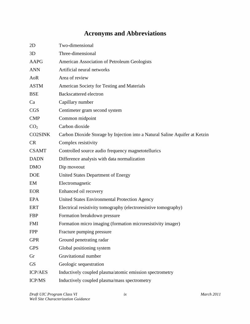
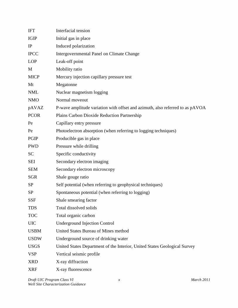
Acronyms and Abbreviations
2D Two-dimensional
3D Three-dimensional
AAPG American Association of Petroleum Geologists
ANN Artificial neural networks
AoR Area of review
ASTM American Society for Testing and Materials
BSE Backscattered electron
Ca Capillary number
CGS Centimeter gram second system CMP Common midpoint
CO2 Carbon dioxide
CO2SINK Carbon Dioxide Storage by Injection into a Natural Saline Aquifer at Ketzin
CR Complex resistivity
CSAMT Controlled source audio frequency magnetotellurics
DADN Difference analysis with data normalization
DMO Dip moveout
DOE United States Department of Energy
EM Electromagnetic
EOR Enhanced oil recovery
EPA United States Environmental Protection Agency
ERT Electrical resistivity tomography (electroresistive tomography)
FBP Formation breakdown pressure
FMI Formation micro imaging (formation microresistivity imager)
FPP Fracture pumping pressure
GPR Ground penetrating radar
GPS Global positioning system
Gr Gravitational number
GS Geologic sequestration
ICP/AES Inductively coupled plasma/atomic emission spectrometry
ICP/MS Inductively coupled plasma/mass spectrometry
Draft UIC Program Class VI x March 2011 Well Site Characterization Guidance
IFT Interfacial tension
IGIP Initial gas in place
IP Induced polarization
IPCC Intergovernmental Panel on Climate Change
LOP Leak-off point
M Mobility ratio
MICP Mercury injection capillary pressure test
Mt Megatonne
NML Nuclear magnetism logging
NMO Normal moveout
pAVAZ P-wave amplitude variation with offset and azimuth, also referred to as pAVOA
PCOR Plains Carbon Dioxide Reduction Partnership
Pe Capillary entry pressure
Pe Photoelectron absorption (when referring to logging techniques)
PGIP Producible gas in place
PWD Pressure while drilling
SC Specific conductivity
SEI Secondary electron imaging
SEM Secondary electron microscopy
SGR Shale gouge ratio
SP Self potential (when referring to geophysical techniques)
SP Spontaneous potential (when referring to logging)
SSF Shale smearing factor
TDS Total dissolved solids
TOC Total organic carbon
UIC Underground Injection Control
USBM United States Bureau of Mines method
USDW Underground source of drinking water
USGS United States Department of the Interior, United States Geological Survey
VSP Vertical seismic profile
XRD X-ray diffraction
XRF X-ray fluorescence

Draft UIC Program Class VI xi March 2011 Well Site Characterization Guidance
Definitions Area of review (AoR): The region surrounding the geologic sequestration project where USDWs may be endangered by the injection activity. The area of review is delineated using computational modeling that accounts for the physical and chemical properties of all phases of the injected carbon dioxide stream and displaced fluids, and is based on available site characterization, monitoring, and operational data as set forth in §146.84.
Brine: Water having high total dissolved solids (TDS) content.
Buoyancy: Upward force on one phase (e.g., a fluid) produced by the surrounding fluid (e.g., a liquid or a gas) in which it is fully or partially immersed, caused by differences in pressure or density.
Carbon dioxide plume: The extent underground, in three dimensions, of an injected carbon dioxide stream.
Carbon dioxide stream: Carbon dioxide that has been captured from an emission source (e.g., a power plant), plus incidental associated substances derived from the source materials and the capture process, and any substances added to the stream to enable or improve the injection process. This does not apply to any carbon dioxide stream that meets the definition of a hazardous waste under 40 CFR Part 261.
Class VI wells: Wells that are not experimental in nature that are used for geologic sequestration of carbon dioxide beneath the lowermost formation containing a USDW; or, wells used for geologic sequestration of carbon dioxide that have been granted a waiver of the injection depth requirements pursuant to requirements at §146.95; or, wells used for geologic sequestration of carbon dioxide that have received an expansion to the areal extent of an existing Class II enhanced oil recovery or enhanced gas recovery aquifer exemption pursuant to §146.4 and 144.7(d).
Computational model: A mathematical representation of the injection project and relevant features, including injection wells, site geology, and fluids present. For a GS project, site specific geologic information is used as input to a computational code, creating a computational model that provides predictions of subsurface conditions, fluid flow, and carbon dioxide plume and pressure front movement at that site. The computational model comprises all model input and predictions (i.e., output).
Confining zone: A geologic formation, group of formations, or part of a formation stratigraphically overlying the injection zone(s) that acts as barrier to fluid movement. For Class VI wells operating under an injection depth waiver, confining zone means a geologic formation, group of formations, or part of a formation stratigraphically overlying and underlying the injection zone(s).
Corrective action: The use of UIC Program Director-approved methods to assure that wells within the area of review do not serve as conduits for the movement of fluids into USDWs.

Draft UIC Program Class VI xii March 2011 Well Site Characterization Guidance
Cratonic: Pertaining to the old, stable lithosphere in the interiors of continents.
Drilling mud: A fluid used during drilling of a well to lubricate the drill bit and carry drill cuttings out of the well bore.
Dynamic models: A method or methods for estimating carbon dioxide storage capacity after initiation of carbon dioxide injection, including decline curve analysis, material balance, and reservoir simulation.
Effective permeability: The permeability of one fluid when more than one fluid phase is present.
Enhanced oil or gas recovery (EOR/EGR): Typically, the process of injecting a fluid (e.g., water, brine, or carbon dioxide) into an oil or gas bearing formation to recover residual oil or natural gas. The injected fluid thins (decreases the viscosity) and/or displaces small amounts of extractable oil and gas, which is then available for recovery. This is also known as secondary or tertiary recovery.
Equation of state: An equation that expresses the equilibrium phase relationship between pressure, volume and temperature for a particular chemical species.
Fluid: Any material or substance which flows or moves whether in a semisolid, liquid, sludge, gas or other form or state, and includes the injection of liquids, gases, and semisolids (i.e., slurries) into the subsurface.
Formation or geological formation: A layer of rock that is made up of a certain type of rock or a combination of types.
Geochemical characterization: To study formation fluids and potential chemical interactions with injectate (carbon dioxide) and solids (rock), and possible changes in injectivity or release of chemicals.
Geologic sequestration (GS): The long-term containment of a gaseous, liquid or supercritical carbon dioxide stream in subsurface geologic formations. This term does not apply to carbon dioxide capture or transport.
Geologic sequestration project: An injection well or wells used to emplace a carbon dioxide stream beneath the lowermost formation containing a USDW; or, wells used for geologic sequestration of carbon dioxide that have been granted a waiver of the injection depth requirements pursuant to requirements at §146.95; or, wells used for geologic sequestration of carbon dioxide that have received an expansion to the areal extent of an existing Class II EOR/EGR aquifer exemption pursuant to §§146.4 and 144.7(d). It includes the subsurface three-dimensional extent of the carbon dioxide plume, associated area of elevated pressure, and displaced fluids, as well as the surface area above that delineated region.

Draft UIC Program Class VI xiii March 2011 Well Site Characterization Guidance
Geomechanical characterization: To study the rock mechanical characteristics associated with carbon dioxide containment such as fault and reservoir rock stability and confining zone integrity.
Geophysical surveys: The use of geophysical techniques (e.g., seismic, electrical, gravity, or electromagnetic surveys) to characterize subsurface rock formations.
Heterogeneity: Spatial variability in the geologic structure and/or physical properties of the site.
Hysteresis: The phenomenon where the response of a system depends not only on the present stimulus, but also on the previous history of the medium.
Injection zone: A geologic formation, group of formations, or part of a formation that is of sufficient areal extent, thickness, porosity, and permeability to receive carbon dioxide through a well or wells associated with a geologic sequestration project.
Injectivity: The efficiency of displacement of an injected fluid into porous rock, both within the rock (micro-displacement efficiency) as well as from the perspective of total pore space (sweep efficiency).
In situ stresses: The three principal stresses (vertical stress, maximum horizontal stress, and minimum horizontal stress) commonly used to characterize the geomechanical model.
Intracratonic: Located in an area above old, stable lithosphere, usually in the interiors of continents far away from plate boundaries.
Intrinsic permeability: A parameter that describes properties of the subsurface that impact the rate of fluid flow. Larger intrinsic permeability values correspond to greater fluid flow rates. Intrinsic permeability has units of area (distance squared).
Irreducible water saturation: The smallest amount of remaining water in a core sample after forced displacement by another fluid.
Lithology: The description of rocks, based on color, mineral composition, and grain size.
Mineralogy, petrology, and solid-phase chemistry: The composition of the solids in an aquifer, including the minerals, rocks types and their origins, and bulk chemical composition.
Mud Log: A record of the different types of data collected when drilling a well, such as the rate of drilling, the rock types in the cuttings, and the presence of hydrocarbons.
Packer: A mechanical device that seals the outside of the tubing to the inside of the long string casing, isolating an annular space.
Parameter: A mathematical variable used in governing equations, equations of state, and constitutive relationships. Parameters describe properties of the fluids present, porous media, and

Draft UIC Program Class VI xiv March 2011 Well Site Characterization Guidance
fluid sources and sinks (e.g., injection well). Examples of model parameters include intrinsic permeability, fluid viscosity, and fluid injection rate.
Pore throat radius: The radius of the opening to a pore in a rock.
Post-injection site care (PISC): Appropriate monitoring and other actions (including corrective action) needed following cessation of injection to ensure that USDWs are not endangered, as required under §146.93.
Pressure front: The zone of elevated pressure that is created by the injection of carbon dioxide into the subsurface. For GS projects, the pressure front of a carbon dioxide plume refers to the zone where there is a pressure differential sufficient to cause the movement of injected fluids or formation fluids into a USDW.
Relative permeability: When immiscible fluids (e.g., carbon dioxide, water) are present within the pore space of a formation, the ability for flow of those fluids is reduced, due to the blocking effect of the presence of the other fluid. This reduction is represented by ‘relative permeability’, which is a factor, between 0 and 1, that is multiplied by the intrinsic permeability of a formation to compute the effective permeability for a fluid in a particular pore space.
Reserve: The estimated volume available for carbon dioxide storage in the injection zone, considering technological, economic, and regulatory constraints and limitations. Reserve estimates can be considered a subset of resources estimates.
Resource: The estimated volume available for carbon dioxide storage in the injection zone.
Site closure: The point/time, as determined by the UIC Program Director following the requirements under §146.93, at which the owner or operator of a GS site is released from post-injection site care responsibilities.
Skin factor or skin effect: Restrictions to flow in the near-wellbore region, typically associated with damage during drilling and well operations.
Static models: Methods for estimating carbon dioxide storage capacity prior to startup of injection and it includes volumetric and compressibility methods.
Storage capacity: The pore volume within the injection zone available for carbon dioxide storage.
Stratigraphy: The sequence of rock strata, or layers. This generally refers to layers of sedimentary or igneous rocks.
Supercritical fluid: A fluid above its critical temperature (31.1ºC for carbon dioxide) and critical pressure (73.8 bar for carbon dioxide). Supercritical fluids have physical properties intermediate to those of gases and liquids.
Tensile strength: The maximum force an element can take in tension before it breaks.
Draft UIC Program Class VI xv March 2011 Well Site Characterization Guidance
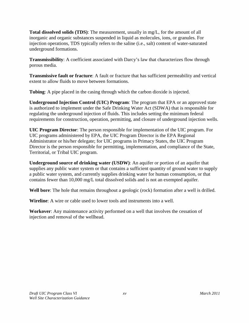
Total dissolved solids (TDS): The measurement, usually in mg/L, for the amount of all inorganic and organic substances suspended in liquid as molecules, ions, or granules. For injection operations, TDS typically refers to the saline (i.e., salt) content of water-saturated underground formations.
Transmissibility: A coefficient associated with Darcy’s law that characterizes flow through porous media.
Transmissive fault or fracture: A fault or fracture that has sufficient permeability and vertical extent to allow fluids to move between formations.
Tubing: A pipe placed in the casing through which the carbon dioxide is injected.
Underground Injection Control (UIC) Program: The program that EPA or an approved state is authorized to implement under the Safe Drinking Water Act (SDWA) that is responsible for regulating the underground injection of fluids. This includes setting the minimum federal requirements for construction, operation, permitting, and closure of underground injection wells.
UIC Program Director: The person responsible for implementation of the UIC program. For UIC programs administered by EPA, the UIC Program Director is the EPA Regional Administrator or his/her delegate; for UIC programs in Primacy States, the UIC Program Director is the person responsible for permitting, implementation, and compliance of the State, Territorial, or Tribal UIC program.
Underground source of drinking water (USDW): An aquifer or portion of an aquifer that supplies any public water system or that contains a sufficient quantity of ground water to supply a public water system, and currently supplies drinking water for human consumption, or that contains fewer than 10,000 mg/L total dissolved solids and is not an exempted aquifer.
Well bore: The hole that remains throughout a geologic (rock) formation after a well is drilled.
Wireline: A wire or cable used to lower tools and instruments into a well.
Workover: Any maintenance activity performed on a well that involves the cessation of injection and removal of the wellhead.
Draft UIC Program Class VI xvi March 2011 Well Site Characterization Guidance
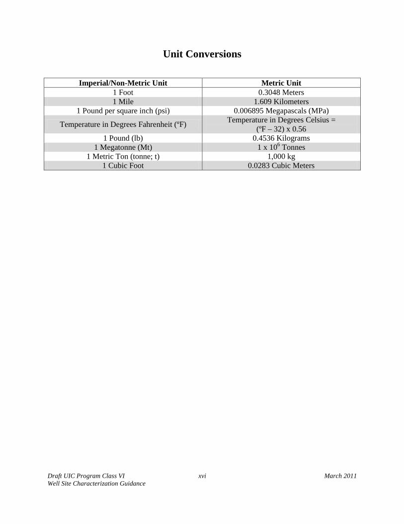
Unit Conversions
Imperial/Non-Metric Unit Metric Unit 1 Foot 0.3048 Meters 1 Mile 1.609 Kilometers
1 Pound per square inch (psi) 0.006895 Megapascals (MPa)
Temperature in Degrees Fahrenheit (ºF) Temperature in Degrees Celsius = (ºF – 32) x 0.56
1 Pound (lb) 0.4536 Kilograms 1 Megatonne (Mt) 1 x 10⁶ Tonnes
1 Metric Ton (tonne; t) 1,000 kg 1 Cubic Foot 0.0283 Cubic Meters

Draft UIC Program Class VI 1 March 2011 Well Site Characterization Guidance
1. Introduction Site characterization is a long-standing permit requirement of the Underground Injection Control (UIC) Program. Owners or operators must identify the presence of suitable geologic characteristics at a site to ensure the protection of underground sources of drinking water (USDWs) from injection activities. The Geologic Sequestration (GS) Rule similarly requires a detailed assessment to evaluate the presence and adequacy of the various geologic features necessary to receive and confine large volumes of carbon dioxide so that injection activities will not endanger USDWs. The purpose of this Guidance is to describe for potential owners and operators of GS sites how to conduct a geologic assessment that meets the geologic siting requirements of the GS Rule [§§146.82 and 146.83). The intended primary audiences of this guidance document are Class VI injection well owners and operators, their representatives that may conduct the geologic siting activities, and the UIC Program permitting authorities. This guidance document is part of a series of technical guidance documents intended to provide information and possible approaches for addressing various aspects of permitting and operating a UIC Class VI injection well. The guidance document series follows the sequence of activities that an owner or operator will perform over time at a proposed and permitted GS site. These activities will generally include:
1. Collection of relevant site characterization data;
2. Development of an area of review (AoR) and Corrective Action Plan;
3. Delineation of the AoR using computational modeling ;
4. Identification and assessment of artificial penetrations located within the AoR;
5. Development of a pre-operational formation testing plan to determine the ability of the formation to accept the injected fluid;
6. Performing corrective action on those penetrations that may serve as conduits for fluid movement;
7. Implementation of the pre-operational formation testing plan;
8. Implementation of the project monitoring program; and
9. Reevaluation of the AoR at a frequency not to exceed every five years. Activities 1 to 5 will be performed prior to receiving UIC Program Director approval for the project proposed in the Class VI permit application. Activities 6 through 9 will be performed after a permit application has been approved by the UIC Program Director. A number of draft UIC Class VI Program companion guidance documents focus on other steps in the process, such as, determination of the AoR and necessary corrective action, injection well construction, and testing and monitoring:
Draft UIC Program Class VI 2 March 2011 Well Site Characterization Guidance
• Geologic Sequestration of Carbon Dioxide: Draft Underground Injection Control (UIC) Program Class VI Well Area of Review Evaluation and Corrective Action Guidance for Owners and Operators
• Geologic Sequestration of Carbon Dioxide: Draft Underground Injection Control (UIC) Program Class VI Well Construction Guidance for Owners and Operators
• Geologic Sequestration of Carbon Dioxide: Draft Underground Injection Control (UIC) Program Class VI Well Testing and Monitoring Guidance for Owners and Operators (this guidance is under development and will be available in the future)
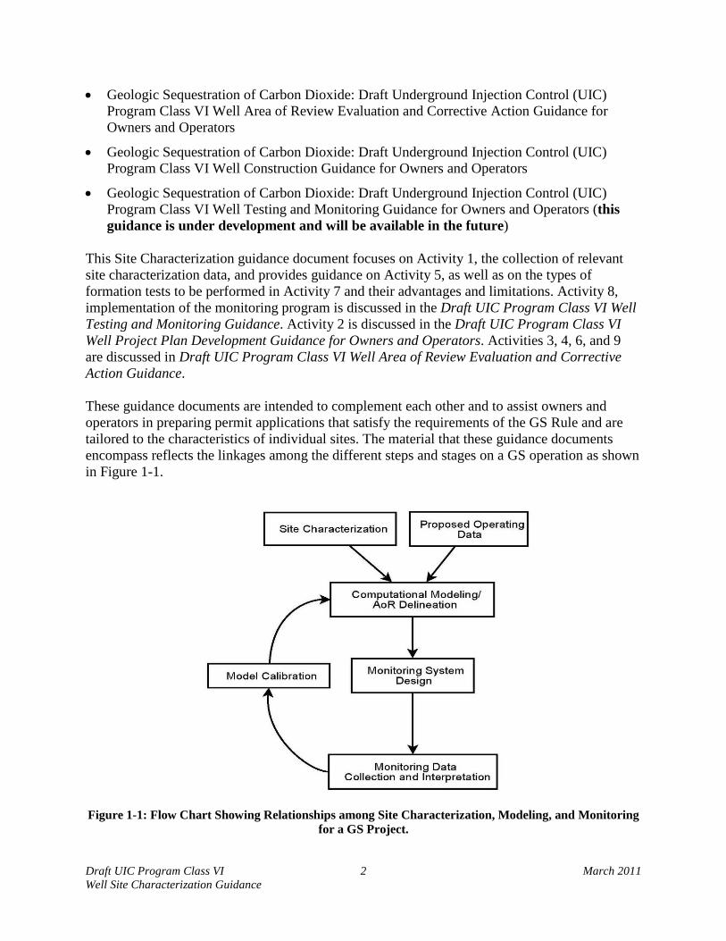
This Site Characterization guidance document focuses on Activity 1, the collection of relevant site characterization data, and provides guidance on Activity 5, as well as on the types of formation tests to be performed in Activity 7 and their advantages and limitations. Activity 8, implementation of the monitoring program is discussed in the Draft UIC Program Class VI Well Testing and Monitoring Guidance. Activity 2 is discussed in the Draft UIC Program Class VI Well Project Plan Development Guidance for Owners and Operators. Activities 3, 4, 6, and 9 are discussed in Draft UIC Program Class VI Well Area of Review Evaluation and Corrective Action Guidance. These guidance documents are intended to complement each other and to assist owners and operators in preparing permit applications that satisfy the requirements of the GS Rule and are tailored to the characteristics of individual sites. The material that these guidance documents encompass reflects the linkages among the different steps and stages on a GS operation as shown in Figure 1-1.
Figure 1-1: Flow Chart Showing Relationships among Site Characterization, Modeling, and Monitoring
for a GS Project.

Draft UIC Program Class VI 3 March 2011 Well Site Characterization Guidance
In preparing the site characterization materials necessary for submission with a Class VI permit application, specific activities will generally include the characterization of regional and general site geology, followed by detailed characterization of the injection zone and confining zones. These site-specific activities generally include the following:
• Geologic characterization (stratigraphy, structure, petrology, mineralogy, porosity,
permeability, and injectivity).
• Geochemical characterization.
• Geomechanical characterization.
• Use of geophysical methods.
• Demonstration of storage capacity.
• Demonstration of confining zone integrity.
The data obtained during the site characterization process will also be used during other stages of permit preparation and site operation. Basic geologic information, such as the lithologies, stratigraphic sequence, and thicknesses of formations in the project area feed directly into modeling efforts for delineation of the AoR. Measurements of properties such as porosity and permeability are also needed for the required AoR determination [§146.84]. The specifics of well drilling and construction, such as formulation of the drilling mud and cement, will also depend upon site characterization data such as downhole pressure. Certain aspects of site characterization (i.e. water quality and geophysical profiling) can also serve as baseline for monitoring that will take place during the operational phase of the project. These cross-linkages between guidance documents are noted in the text where appropriate. Additional guidance on using and presenting information in the permit application is provided in the plan development guidance: Draft UIC Program Class VI Well Project Plan Development Guidance.
1.1. Overview of the GS Rule Geologic Siting Requirements
The geologic siting requirements of the GS Rule [§§146.82 and 146.83] sets forth the information that must be provided by the applicant and that must be considered by the UIC Program Director in deciding whether to grant a permit for a Class VI well. The first level of material to be submitted includes information on the regional geology and hydrogeology, supported by maps, cross-sections, and other available data. The next level of information is geared towards characterization of the proposed injection site and involves submission of data on stratigraphy, structural geology, hydrogeology, and geochemistry.
Site characterization focuses on demonstrating that there is a viable injection zone and a separate, competent confining zone or zones at the proposed project site. Focus should be on the porosity, permeability, and injectivity of the injection formation and on the competence of the confining zone(s), especially with respect to faults or fractures. Data submitted for this phase includes available maps, cross-sections, geochemical data on fluids in the injection zone, and any geophysical or remote sensing information. This stage will include compiling pre-existing or

Draft UIC Program Class VI 4 March 2011 Well Site Characterization Guidance
new information collected without drilling new boreholes or wells. This document will provide guidance on the types of information to collect and submit with a Class VI injection well permit application and where such information might be obtained. It will also provide illustrative examples of some of the required information. Class VI permit application materials will also include the plans for a proposed formation testing program for the chemical and physical characteristics of both the injection zone and the confining zone(s). Once a permit for a Class VI well has been granted, the applicant will execute the formation testing program. This document will provide guidance on the types of tests to be performed, their advantages and limitations, and the types of data that will be generated. It should be noted that, in the development of Class VI permit application materials, care should be taken in the selection and use of geological, geochemical, and geophysical data. For example, geologic maps and cross-sections are generally available from reputable sources (e.g., United States Geological Survey (USGS), state geological surveys). However, when maps or cross-sections are available from more than one source, they should be checked for consistency, and discrepancies should be identified and discussed. Comparison of maps with geophysical imaging can also be helpful in interpreting regional geology. Water samples should similarly be handled with care, using chain of custody forms and certified laboratories for chemical analyses.

Draft UIC Program Class VI 5 March 2011 Well Site Characterization Guidance
2. Characterization of Regional and Site Geology The UIC Program Geologic Sequestration (GS) Rule [§146.82(a)] requires applicants for a Class VI permit to submit information on the geology and hydrogeology of the proposed storage site and overlying formations to EPA. Applicants are also required to submit geologic information on the region surrounding the proposed project site [§146.82(a)(3)(vi)]. The initial stage of site characterization will involve a desktop analysis using available information. Data collection efforts at this initial stage will help to identify potential injection intervals and confining strata and to provide preliminary estimates of site carbon dioxide storage and containment capacity. If a site is judged potentially suitable based on the initial information submitted, the project site characterization information will be subsequently refined with primary site-specific data as outlined in the proposed formation testing program specified at §146.82(a)(8) that meets the requirements at §146.87. Details on the potential methods that may be used in performing a detailed characterization of the injection zone and confining zones can be found in Section 3 of this guidance document. The first part of this section addresses the types of information that owners and operators will compile as part of their initial characterization and desktop analysis. Types of general geologic and hydrogeologic information specified by the GS Rule that may be gathered at this stage, using available information, include:
• Maps and cross-sections of the AoR [§146.82(a)(3)(i)].
• The location, orientation, and properties of known or suspected faults and fractures that may transect the confining zone(s) in the AoR [§146.82(a)(3)(ii)].
• Data on the depth, areal extent, and thickness of the injection and confining zone(s) [§146.82(a)(3)(iii)].
• Information on lithology and facies changes [§146.82(a)(3)(iii)].
• Information on the seismic history of the area, including the presence and depth of seismic sources [§146.82(a)(3)(v)].
• Geologic and topographic maps and cross-sections illustrating regional geology, hydrogeology, and the geologic structure of the local area [§146.82(a)(3)(vi)].
• Maps and stratigraphic cross-sections indicating the general vertical and lateral limits of all USDWs, water wells, and springs within the AoR, their positions relative to the injection zone(s), and the direction of water movement (where known) [§146.82(a)(5)].
• Baseline geochemical data on subsurface formations, including all USDWs in the area of review [§146.82(a)(6)].
Site characterization will occur on two scales. In the regional-scale characterization, the owner or operator will compile geologic information about the region surrounding the AoR (e.g., lithology, stratigraphy, locations and types of structures location of major aquifers). This broader perspective will enable the identification of large-scale features, such as fault zones, that might
Draft UIC Program Class VI 6 March 2011 Well Site Characterization Guidance
affect the suitability of the proposed project site. A regional evaluation can help eliminate unsuitable sites. The Intergovernmental Panel on Climate Change (IPCC) (2005) provides a general discussion of large-scale settings (e.g., mid-continent basins) and geologic formations that are considered suitable for geologic sequestration. Then, on a site-specific-scale characterization, owners and operators will also have to provide more detailed characterization information in the Class VI permit application. This will entail compiling as much site characterization information as is available on the area delineated within the AoR, including publicly or commercially available maps and literature, and any primary data that have been previously collected at the proposed site, such as sampling, drilling, subsurface investigations/tests, and remote sensing data.
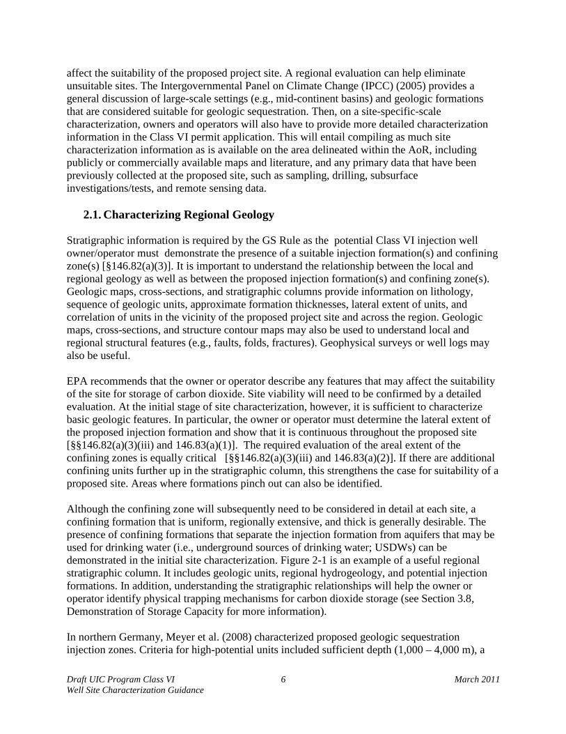
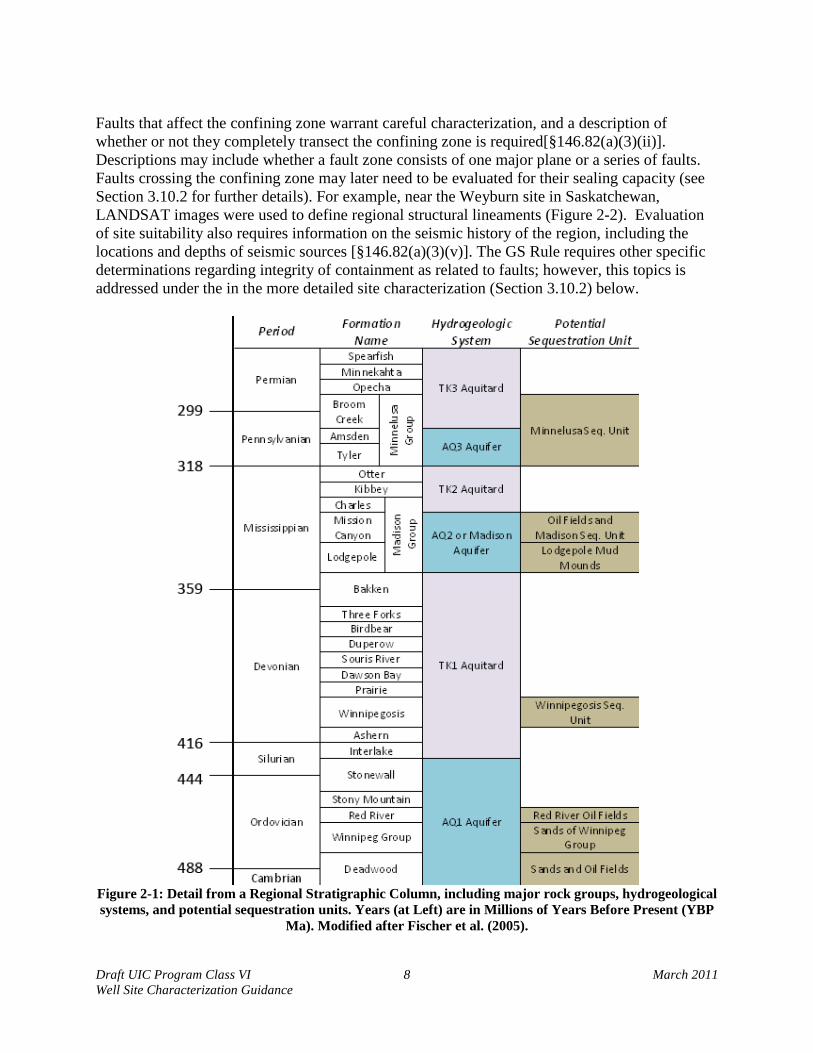
2.1. Characterizing Regional Geology Stratigraphic information is required by the GS Rule as the potential Class VI injection well owner/operator must demonstrate the presence of a suitable injection formation(s) and confining zone(s) [§146.82(a)(3)]. It is important to understand the relationship between the local and regional geology as well as between the proposed injection formation(s) and confining zone(s). Geologic maps, cross-sections, and stratigraphic columns provide information on lithology, sequence of geologic units, approximate formation thicknesses, lateral extent of units, and correlation of units in the vicinity of the proposed project site and across the region. Geologic maps, cross-sections, and structure contour maps may also be used to understand local and regional structural features (e.g., faults, folds, fractures). Geophysical surveys or well logs may also be useful. EPA recommends that the owner or operator describe any features that may affect the suitability of the site for storage of carbon dioxide. Site viability will need to be confirmed by a detailed evaluation. At the initial stage of site characterization, however, it is sufficient to characterize basic geologic features. In particular, the owner or operator must determine the lateral extent of the proposed injection formation and show that it is continuous throughout the proposed site [§§146.82(a)(3)(iii) and 146.83(a)(1)]. The required evaluation of the areal extent of the confining zones is equally critical [§§146.82(a)(3)(iii) and 146.83(a)(2)]. If there are additional confining units further up in the stratigraphic column, this strengthens the case for suitability of a proposed site. Areas where formations pinch out can also be identified. Although the confining zone will subsequently need to be considered in detail at each site, a confining formation that is uniform, regionally extensive, and thick is generally desirable. The presence of confining formations that separate the injection formation from aquifers that may be used for drinking water (i.e., underground sources of drinking water; USDWs) can be demonstrated in the initial site characterization. Figure 2-1 is an example of a useful regional stratigraphic column. It includes geologic units, regional hydrogeology, and potential injection formations. In addition, understanding the stratigraphic relationships will help the owner or operator identify physical trapping mechanisms for carbon dioxide storage (see Section 3.8, Demonstration of Storage Capacity for more information). In northern Germany, Meyer et al. (2008) characterized proposed geologic sequestration injection zones. Criteria for high-potential units included sufficient depth (1,000 – 4,000 m), a

Draft UIC Program Class VI 7 March 2011 Well Site Characterization Guidance
thickness of > 20 m, and presence of a good confining zone. This type of basic information may be obtained from desktop sources (such as consultant reports and government databases) during a screening-level site characterization. Also, with a general indication of the dimensions of the injection zone and a rough estimate of porosity, a “first cut” calculation of storage capacity may be attempted (to be refined according to methods described in Section 3.9). Meyer et al. (2008), for example, calculated an initial estimate of storage capacity using the area, thickness, effective porosity, a few values of assumed storage efficiency, and the expected density of carbon dioxide under down-hole conditions. The required information on regional and site stratigraphy is also needed to infer the depositional history and anticipate heterogeneities in subsurface lithology and permeability [§146.82(a)(3)]. Subsurface heterogeneity will affect fluid flow and, when known, can inform the placement and design of injection and monitoring wells. Ambrose et al. (2008) have discussed the importance of facies changes to geologic sequestration projects. Beach and barrier island deposits, for example, tend to be homogeneous and continuous. Depositional environments with channels give rise to formations that may have more limited, poorly connected areas for carbon dioxide storage. Although the injection formation needs to have an adequately high permeability overall, heterogeneity in the form of lenses of lower-permeability material within the injection formation can improve sequestration capacity by ensuring that the carbon dioxide is more broadly distributed throughout the injection formation. For example, at the Sleipner geologic sequestration site in Norway, layers of lower permeability material within the clean sandstone injection formation act as baffles that reduce the height of the carbon dioxide column and minimize stress on the confining zone (Hermanrud et al., 2009). Additionally, at the In Salah project in Algeria, targeted drilling has allowed injected carbon dioxide to follow high-permeability channels within the injection zone (Riddiford et al., 2004; Bishop, 2003). In the evaluation of regional structural geology, the owner or operator can evaluate folds and their role in providing a secure storage formation (in a manner similar to the role of these structures in forming oil and gas traps). The pilot project at Ketzin, Germany, for example, is sited in a lithologically heterogeneous anticline (delineated by three-dimensional (3D) seismic profiling) (Forster et al., 2006). Likewise, Meyer (2008) describes site characterization of the Schweinrich anticline in Germany. Large regional structures can also be helpful in the identification of potential storage sites; intracontinental basins, for example, have thick sequences of sedimentary formations that include saline formations. Large, saline formations, with greater than 10,000 mg/L total dissolved solids (TDS) are unlikely to be useful as future drinking water sources, and may be ideally suited for geologic sequestration. Owners and operators are required to document fractures and faults [§146.82(a)(3)(ii)]. EPA recommends that particular attention be paid to whether the fractures or faults might compromise the ability of a site to contain the carbon dioxide and pressure front or whether they contribute to an effective trap. Characteristics to record include orientation, location, degree of offset (for faults), and distance from the proposed injection zone. Tectonic history information that may be available in reports may be helpful in predicting trends of fractures and faults. Also, data on seismic history are required and will be used to indicate whether seismicity might interfere with containment [§146.82(a)(3)(v)].
Draft UIC Program Class VI 8 March 2011 Well Site Characterization Guidance
Faults that affect the confining zone warrant careful characterization, and a description of whether or not they completely transect the confining zone is required[§146.82(a)(3)(ii)]. Descriptions may include whether a fault zone consists of one major plane or a series of faults. Faults crossing the confining zone may later need to be evaluated for their sealing capacity (see Section 3.10.2 for further details). For example, near the Weyburn site in Saskatchewan, LANDSAT images were used to define regional structural lineaments (Figure 2-2). Evaluation of site suitability also requires information on the seismic history of the region, including the locations and depths of seismic sources [§146.82(a)(3)(v)]. The GS Rule requires other specific determinations regarding integrity of containment as related to faults; however, this topics is addressed under the in the more detailed site characterization (Section 3.10.2) below.
Figure 2-1: Detail from a Regional Stratigraphic Column, including major rock groups, hydrogeological systems, and potential sequestration units. Years (at Left) are in Millions of Years Before Present (YBP
Ma). Modified after Fischer et al. (2005).

Draft UIC Program Class VI 9 March 2011 Well Site Characterization Guidance
Figure 2-2: Map of Regional Structural Lineaments Identified Through Analyses of LANDSAT Imagery
and Overlain on an Isopach Map of the Davidson Salt Unit. Thin black lines are zones of lineaments, thicker red lines are lineaments correlated with the subsurface distribution of the Davidson Salt Unit.
Contour lines indicate depth to top of formation, color indicates thickness of formation. Field of view is approximately 230 km. From: Whittaker and Gilboy (2003). ©2010, Government of Saskatchewan.
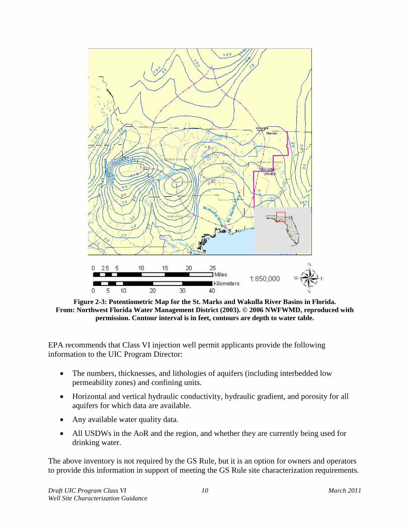
2.2. Characterizing General Site Geology Owners and operators must submit information on the regional and site hydrogeology [§146.82(a)(5)]. The stratigraphic data acquired for site-specific and regional geology (e.g., Figure 2-1) will provide a basis for characterizing the site hydrogeology by indicating local and regional aquifers and confining zones and their position in the stratigraphic column (as also shown in Figure 2-1). The required information on the lithologies, numbers of layers, and thicknesses of both the injection and confining zones is also needed for completing the required multiphase fluid modeling for AoR determinations [§§146.82(a) and 146.84]. See the Draft UIC Program Class VI Well Area of Review and Corrective Action Guidance, Section 2, for more information on multiphase fluid modeling for AoR determinations. Basic stratigraphic information is required to be supported by maps and cross-sections that also show aquifers and confining units [§146.82(a)(5)]. Such figures can demonstrate the relationship between the proposed injection formation and any USDWs. Isopach maps illustrate the thickness of the formation of interest and surrounding formations, and are a standard component of hydrogeologic investigations. Potentiometric maps (i.e., contour maps of the potentiometric surface of ground water; Figure 2-3) illustrate patterns of ground water flow.
Draft UIC Program Class VI 10 March 2011 Well Site Characterization Guidance
Figure 2-3: Potentiometric Map for the St. Marks and Wakulla River Basins in Florida.
From: Northwest Florida Water Management District (2003). © 2006 NWFWMD, reproduced with permission. Contour interval is in feet, contours are depth to water table.
EPA recommends that Class VI injection well permit applicants provide the following information to the UIC Program Director:
• The numbers, thicknesses, and lithologies of aquifers (including interbedded low permeability zones) and confining units.
• Horizontal and vertical hydraulic conductivity, hydraulic gradient, and porosity for all aquifers for which data are available.
• Any available water quality data.
• All USDWs in the AoR and the region, and whether they are currently being used for drinking water.
The above inventory is not required by the GS Rule, but it is an option for owners and operators to provide this information in support of meeting the GS Rule site characterization requirements.

Draft UIC Program Class VI 11 March 2011 Well Site Characterization Guidance
EPA recommends that the applicant submit to the UIC Program Director any available analyses of water or brine from all USDWs and other relevant formations within the AoR, including units above and below the injection zone and confining zones. Typical chemical analyses that may be available include: pH, specific conductivity (SC), total dissolved solids (TDS), salinity, dissolved oxygen, major cations, major anions, and alkalinity. Part of the definition of a USDW is that its pore fluids have < 10,000 mg/L TDS. Information on water chemistry is required by the GS Rule as it indicates which formations in the stratigraphic column qualify as USDWs and confirms that the proposed injection formation is not a USDW [§146.82(a)(6), 146.87(c) and 146.87(d)(3)]. Smith (2009), for example, used publicly available information in a characterization of three potential saline formation sequestration sites in Wyoming. All three were sufficiently deep and had good confining zones, but one of the three had variable TDS values (sometimes < 10,000 mg/L TDS) that rendered it unsuitable for GS. The geochemistry of the solids may or may not be available depending on the degree to which previous characterization work has been conducted in the area. However, bulk geochemistry or mineralogy of the solids may be estimated based on lithology. This may provide an opportunity to make a general estimate of how reactive the target formation may be to changes in fluid chemistry that would occur with injection. Gibson-Poole et al. (2008) used available information on the mineralogy of their target formation (at a potential sequestration site in the Gippsland Basin in southeast Australia) and noted that the minerals in the injection zone (potassium feldspar, quartz) would not be reactive with carbon dioxide-bearing brines.
2.3. Sources of Data Geologic information for the initial site characterization phase can be obtained from the U.S. Geological Survey (USGS), state geological surveys, local governments, and consultants’ reports. Material available from the USGS includes geologic and topographic maps (e.g., the National Geologic Map Database), stratigraphy, aerial photographs, and reports. The USGS’s Earthquake Hazards Program provides maps of faults and information on seismic activity for many regions in the United States. The associated Earthquake Hazards Program database (available on the Internet at http://geohazards.cr.usgs.gov/cfusion/qfault/index.cfm) provides detailed information on faults, including any recorded earthquakes. Maps from the USGS and state geological surveys are generally at the quadrangle scale, but maps can also be found at the county and state scale. For hydrogeologic information, reports and databases from the USGS, state geological surveys and other state and local agencies (e.g., departments of environmental protection, municipalities), as well as published academic literature, and reports from existing exploration or injection projects, may be used at this information-gathering stage. In particular, the USGS maintains a database of ground water information (http://water.usgs.gov/ogw/data.html), as well as a ground water atlas (http://pubs.usgs.gov/ha/ha730). Carbon sequestration projects that are coupled with Enhanced Oil Recovery (EOR) or planned in depleted reservoirs will have access to detailed site characterization data from the outset. Well completion cards and other well completion records may also provide additional characterization
Draft UIC Program Class VI 12 March 2011 Well Site Characterization Guidance
data. Even if areas of interest are not located in depleted or active oil and gas fields, data from nearby fields in the same basin may be available and applicable. At some locations, injection formations may be in the same stratigraphic column as oil or gas reservoirs (even when they are not themselves such reservoirs); exploration activities may have already been conducted on such formations. Data for formations with potential hydrocarbon assets may be available from state oil and gas commissions. This is certainly the case for a number of the pilot projects. At Teapot Dome in Wyoming (Friedmann and Stamp, 2005), researchers had access to existing geological, geophysical, geomechanical, and geochemical data. At the Ketzin site (Forster et al., 2006) and the Schweinrich anticline (both in Germany) (Meyer et al., 2008), information such as seismic data, cores, well logs, and wireline logs were available. In situations where such advanced data can be procured and physical samples such as cores are already available for analysis, the information in Section 3 of this document provides the owner or operator with guidance for interpreting data and for performing the required tests..
Draft UIC Program Class VI 13 March 2011 Well Site Characterization Guidance
3. Detailed Characterization of Injection Zone Geology and Confining Zone Geology
The initial site characterization stages described in Section 2 depend primarily upon the use of pre-existing maps and data to compile an understanding of the overall geology and hydrogeology of the region and site. Upon the issuance of a permit, the applicant must execute the formation testing plan described in the GS Rule at §146.82(a)(8). This will involve a more detailed characterization of the injection and confining zone(s) and will involve the collection of primary data. If the applicant does not already have monitoring wells in place, as well as available core samples, additional boreholes and/or wells will be required. Data collected during the formation testing program can be integrated with pre-existing information and used to refine the site characterization as described in Section 2. These data can also be incorporated into reservoir models to predict the behavior of carbon dioxide in the subsurface. The detailed geologic characterization of the injection zone and confining zone(s) will be based on primary data collected at the field site. The applicant will use well- and core-based methods to collect information on the injection zone and confining zone(s), as well as other overlying formations. Detailed geologic characterization is required by the GS Rule at §146.82(a)(3). The key types of information that constitute the geologic characterization are the following:
• Stratigraphy of the injection zone(s) and confining zone(s).
• Structure of the injection zone(s) and confining zone(s).
• Petrology and mineralogy of the injection zone(s) and confining zone(s).
• Porosity, permeability, and injectivity of the injection zone(s) and confining zone(s). • Geomechanical information on fractures, stress, ductility, rock strength, and in situ
fluid pressures within the confining zone(s) [§146.82(a)(3)(iv)]
•
The following sections will describe these types of information in more detail and provide guidance on collecting and interpreting data.
3.1. Stratigraphy of the Injection Zone and Confining Zone The GS Rule requires the applicant to provide information to the UIC Program Director on the areal extent, thickness, and geologic facies changes of the injection formation and confining zone [§146.82(a)(3)]. These features affect the ability of the injection formation to receive and store the injectate, as well as the ability of the confining zone(s) to contain the carbon dioxide and pressure front. Ideally, a confining zone will be regional in scale. In addition, because lateral changes in the lower layers of a confining zone can increase the chance of carbon dioxide migration, an ideal confining zone will be uniform at its base (IPCC, 2005).

Draft UIC Program Class VI 14 March 2011 Well Site Characterization Guidance
Analysis of facies changes at the injection site will help the applicant anticipate heterogeneities in porosity and permeability and associated effects on the injection and storage capabilities of the site. It can also help refine the parameterization of multiphase flow modeling for the site. See the Draft UIC Program Class VI Well Area of Review and Corrective Action Guidance, Section 2). This section will describe the concept of facies changes, with considerations for clastic and carbonate systems, as well as the types of information to be submitted to support stratigraphic evaluations.
3.1.1. Facies Analysis of Clastic and Carbonate Systems The term facies refers to the features of a rock that reflect the environmental conditions under which it was formed or deposited. Facies analysis involves determining the characteristics of rock units and their depositional environments, including mineral composition and sedimentary structures. The interplay of geologic and environmental factors such as tectonics, sea level, climate, sediment supply, transport, and deposition influences facies and determines many of the characteristics of a sedimentary system. Facies information can help predict the spatial and temporal distribution of reservoir and seal lithologies, as well as the distribution of rocks with other properties relevant to the injection and confinement of carbon dioxide (Slatt, 2006). A facies approach has been used successfully in the hydrocarbon industry to identify potential hydrocarbon sources and confining zones such as the Lance Formation in Wyoming and the Mt. Messenger Formation in New Zealand (Slatt, 2006). One unique aspect of facies surfaces is that, unlike lithologic surfaces, they are isochronic, or created at the same time. Examining isochronous surfaces can help identify additional zones or features that may impact carbon dioxide storage by providing a better understanding of how the rocks were accumulated at the time of deposition. For example, some types of geologic environments produce fine shale layers, which might not be easily identified but may have a great impact on storage capacity. Data for facies analysis of clastic systems can be obtained from cores and wireline tools such as dipmeters and formation imaging devices (Scheihing and Atkinson, 1992). More information on using wireline methods to identify facies changes and determine other geologic properties is provided below. Data from seismic surveys may also be used (see Section 3.7.2 for more information on seismic methods). Correlation of these various data sources can provide a three-dimensional representation of the subsurface stratigraphy. The characteristics of carbonate formations are controlled by diagenetic (post-deposition) processes in addition to the depositional environment. Like descriptions of clastic systems, descriptions of carbonate facies are based on observations of rock fabrics and pore space from core and cutting samples. These descriptions are correlated with wireline log responses and other information to map porosity, saturation, and permeability (Lucia, 1992). Because the characteristics of carbonates are often strongly (and sometimes completely) determined by the sediments’ interactions with formation fluids, understanding current and past hydrogeology is very important in the analysis of carbonate facies.

Draft UIC Program Class VI 15 March 2011 Well Site Characterization Guidance
3.1.2. Types of Information to Submit Several types of information may be used to support an analysis of facies changes and other stratigraphic features of the injection and confining zone(s). The following are described in greater detail in this section:
• Geological maps and stratigraphic columns • Stratigraphic cross-sections • Data from wireline methods and well logs • Core description and analysis • Geophysical data
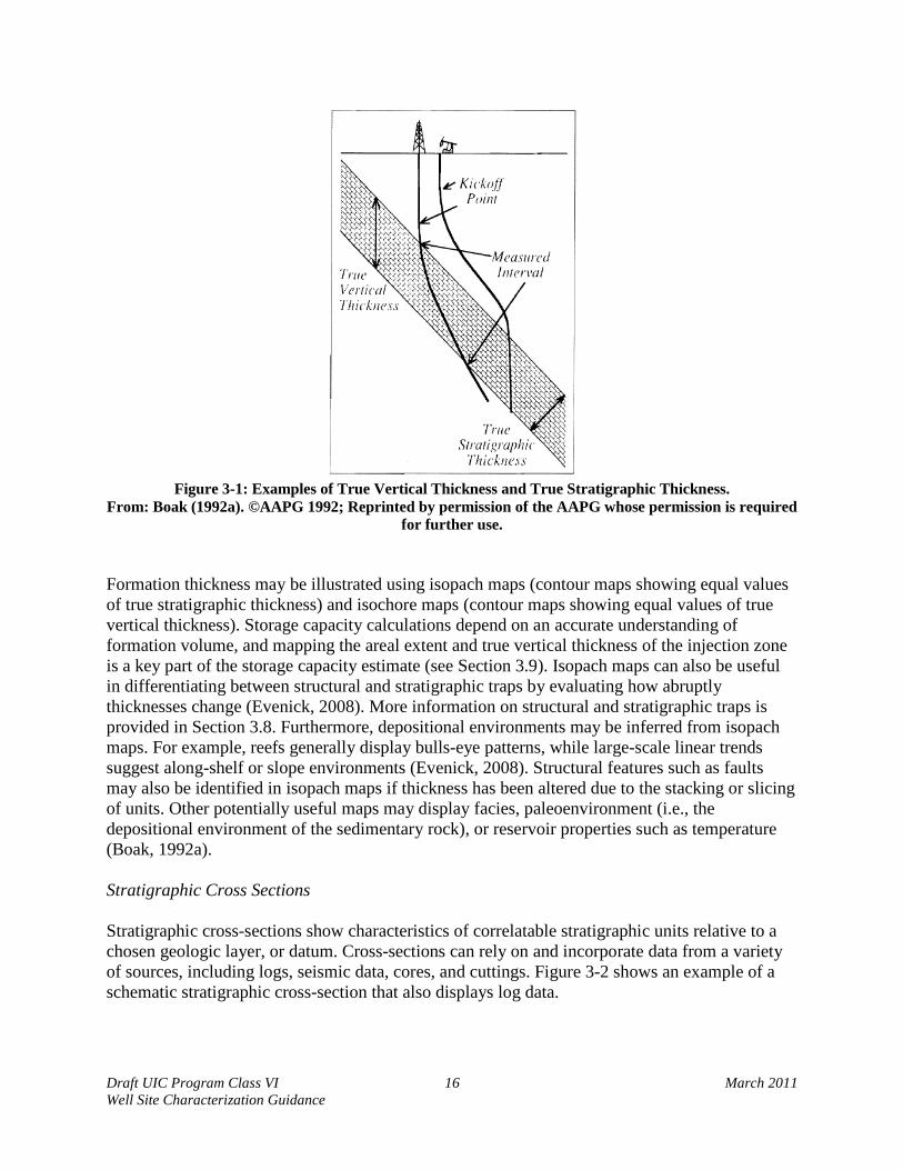
Geologic Maps and Stratigraphic Columns Geologic maps and the accompanying cross-sections and columns are a key source of stratigraphic information. Maps and cross-sections are required by the GS Rule at §146.82(3)(i). Existing geologic maps of the injection site can be supplemented with data collected during the formation testing program. A number of surfaces (as well as other geologic properties such as permeability) may be mapped and contoured to demonstrate the stratigraphic properties of the injection and confining zones. Stratigraphic columns often accompany geologic maps and illustrate the sequence of rock units in the subsurface. Diagrams illustrating depositional sequences or discussions of facies models may also be helpful. Determining the thicknesses of the injection and confining zones is required at §146.82(3)(iii) and aids in estimating storage capacity and determining the seal integrity of the confining zone. There are two primary ways of understanding the thicknesses of geologic formations: true vertical thickness and true stratigraphic thickness (Evenick, 2008). True vertical thickness is the thickness of a geologic unit in a well measured in the vertical direction, perpendicular to the surface. It is necessary to correct for any deviation in the well to determine the true vertical thickness. True stratigraphic thickness is the thickness of the unit measured in the direction perpendicular to the bedding planes of the unit. True stratigraphic thickness can be calculated from true vertical depths as described in Boak (1992a). Figure 3-1 illustrates the difference between true vertical thickness and true stratigraphic thickness with respect to two types of deviated wells.
Draft UIC Program Class VI 16 March 2011 Well Site Characterization Guidance
Figure 3-1: Examples of True Vertical Thickness and True Stratigraphic Thickness.
From: Boak (1992a). ©AAPG 1992; Reprinted by permission of the AAPG whose permission is required for further use.
Formation thickness may be illustrated using isopach maps (contour maps showing equal values of true stratigraphic thickness) and isochore maps (contour maps showing equal values of true vertical thickness). Storage capacity calculations depend on an accurate understanding of formation volume, and mapping the areal extent and true vertical thickness of the injection zone is a key part of the storage capacity estimate (see Section 3.9). Isopach maps can also be useful in differentiating between structural and stratigraphic traps by evaluating how abruptly thicknesses change (Evenick, 2008). More information on structural and stratigraphic traps is provided in Section 3.8. Furthermore, depositional environments may be inferred from isopach maps. For example, reefs generally display bulls-eye patterns, while large-scale linear trends suggest along-shelf or slope environments (Evenick, 2008). Structural features such as faults may also be identified in isopach maps if thickness has been altered due to the stacking or slicing of units. Other potentially useful maps may display facies, paleoenvironment (i.e., the depositional environment of the sedimentary rock), or reservoir properties such as temperature (Boak, 1992a). Stratigraphic Cross Sections Stratigraphic cross-sections show characteristics of correlatable stratigraphic units relative to a chosen geologic layer, or datum. Cross-sections can rely on and incorporate data from a variety of sources, including logs, seismic data, cores, and cuttings. Figure 3-2 shows an example of a schematic stratigraphic cross-section that also displays log data.
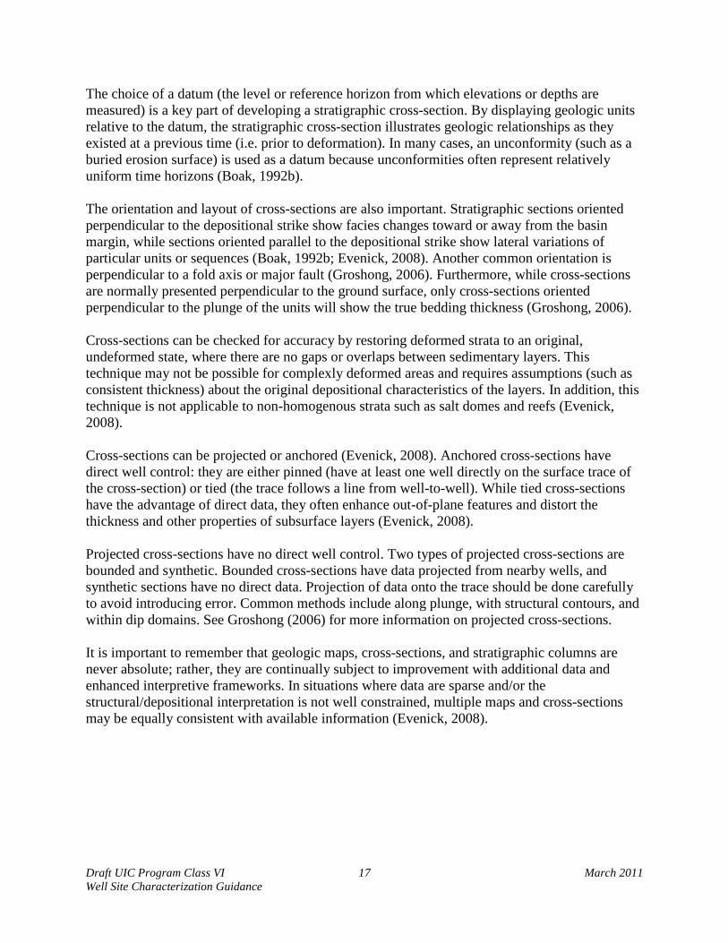
Draft UIC Program Class VI 17 March 2011 Well Site Characterization Guidance
The choice of a datum (the level or reference horizon from which elevations or depths are measured) is a key part of developing a stratigraphic cross-section. By displaying geologic units relative to the datum, the stratigraphic cross-section illustrates geologic relationships as they existed at a previous time (i.e. prior to deformation). In many cases, an unconformity (such as a buried erosion surface) is used as a datum because unconformities often represent relatively uniform time horizons (Boak, 1992b). The orientation and layout of cross-sections are also important. Stratigraphic sections oriented perpendicular to the depositional strike show facies changes toward or away from the basin margin, while sections oriented parallel to the depositional strike show lateral variations of particular units or sequences (Boak, 1992b; Evenick, 2008). Another common orientation is perpendicular to a fold axis or major fault (Groshong, 2006). Furthermore, while cross-sections are normally presented perpendicular to the ground surface, only cross-sections oriented perpendicular to the plunge of the units will show the true bedding thickness (Groshong, 2006). Cross-sections can be checked for accuracy by restoring deformed strata to an original, undeformed state, where there are no gaps or overlaps between sedimentary layers. This technique may not be possible for complexly deformed areas and requires assumptions (such as consistent thickness) about the original depositional characteristics of the layers. In addition, this technique is not applicable to non-homogenous strata such as salt domes and reefs (Evenick, 2008). Cross-sections can be projected or anchored (Evenick, 2008). Anchored cross-sections have direct well control: they are either pinned (have at least one well directly on the surface trace of the cross-section) or tied (the trace follows a line from well-to-well). While tied cross-sections have the advantage of direct data, they often enhance out-of-plane features and distort the thickness and other properties of subsurface layers (Evenick, 2008). Projected cross-sections have no direct well control. Two types of projected cross-sections are bounded and synthetic. Bounded cross-sections have data projected from nearby wells, and synthetic sections have no direct data. Projection of data onto the trace should be done carefully to avoid introducing error. Common methods include along plunge, with structural contours, and within dip domains. See Groshong (2006) for more information on projected cross-sections. It is important to remember that geologic maps, cross-sections, and stratigraphic columns are never absolute; rather, they are continually subject to improvement with additional data and enhanced interpretive frameworks. In situations where data are sparse and/or the structural/depositional interpretation is not well constrained, multiple maps and cross-sections may be equally consistent with available information (Evenick, 2008).
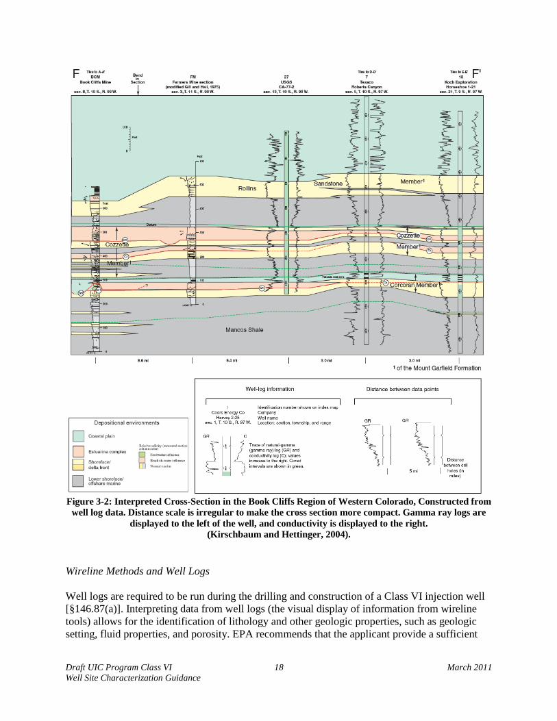
Draft UIC Program Class VI 18 March 2011 Well Site Characterization Guidance
Figure 3-2: Interpreted Cross-Section in the Book Cliffs Region of Western Colorado, Constructed from
well log data. Distance scale is irregular to make the cross section more compact. Gamma ray logs are displayed to the left of the well, and conductivity is displayed to the right.
(Kirschbaum and Hettinger, 2004). Wireline Methods and Well Logs Well logs are required to be run during the drilling and construction of a Class VI injection well [§146.87(a)]. Interpreting data from well logs (the visual display of information from wireline tools) allows for the identification of lithology and other geologic properties, such as geologic setting, fluid properties, and porosity. EPA recommends that the applicant provide a sufficient

Draft UIC Program Class VI 19 March 2011 Well Site Characterization Guidance
number of well logs to document the depths and thicknesses on any stratigraphic sections or columns. More data may be useful for certain areas if correlations are difficult or unique geologic features exist. Logs can be grouped into one of three classes; electric, radioactive, or structural (Evenick, 2008). While electric and structural logs are typically only applicable in uncased wells, radioactive logs can be equally effective in both cased and uncased wells (Evenick, 2008) It is not possible to use wireline methods in wells inclined more than 60 degrees from the vertical, because frictional forces on logging tools overcome gravitational forces and cause the logging device to become stuck (Johnson and Pile, 2006). If logging data are still desired from horizontal or heavily inclined wells, they can be collected during drilling by attaching the logging equipment to the drillstem. This technique is called measurement while drilling (MWD) (Johnson and Pile, 2006). Various commonly-used well logs can be used to determine geologic properties. Log types include gamma ray, spontaneous potential, caliper, formation density, photoelectric absorption, and neutron porosity logs. These logging methods are discussed briefly below.
• Gamma ray logs measure the natural radioactivity emitted by radioactive isotopes (e.g., potassium, thorium, and uranium) in minerals. Gamma ray logs are the most common log run for stratigraphic correlation because they are relatively unambiguous and easy to interpret (Evenick, 2008). The intensity of radioactivity is measured by a scintillation counter in API (American Petroleum Units) (Evenick, 2008). Because clays tend to have higher concentrations of potassium and thallium than other minerals, gamma ray logs can provide information on the clay and mica content (or “shaliness”) of the formation (Johnson and Pile, 2006). The log curve can also be compared to a section with 100% or 0% shale saturation in order to determine a “shale baseline” and calculate the percent of shale present in other regions of the log (Johnson and Pile, 2006). The spectral gamma ray tool, an advanced version of the gamma ray tool, allows for the identification of gamma ray counts caused by specific elements. This allows for the removal of gamma ray counts caused by uranium, which is often deposited by formation fluids, though it is also found in some sandstones and carbonates (Johnson and Pile, 2006). Gamma ray logs are virtually unaffected by changes in porosity (Johnson and Pile, 2006).
• Spontaneous potential (SP) logs show naturally occurring differences in electric potential
(usually measured in millivolts, mV) between the drilling mud and formation fluids, and between formation fluids in different units (Johnson and Pile, 2006). Because of this, SP logs can be good indicators of formation permeability (Evenick, 2008). Voltage differences occur because of membrane potential: different types of lithologies are permeable to different ions. For example, due to the negative surface charges found on phyllosilicate particles, sodium ions can diffuse across a shale layer but chlorine ions are blocked. Membrane potential creates the equivalent of a wet-cell battery between ion-permeable and ion-impermeable units.

Draft UIC Program Class VI 20 March 2011 Well Site Characterization Guidance
The SP response typically varies by lithology and can be used to correlate formations between wells, determine permeability, and estimate formation fluid resistivity (Alberty, 1992b; Hancock, 1992). Because SP logs reflect differences in electric potential, contrasts in permeability and salinity between formations are critical (see Figure 3-3). SP logs are influenced by the presence of impermeable limestones and work best when shale layers separate more permeable formations (Johnson and Pile, 2006). Hancock (1992) describes other conditions where SP logs are not applicable or difficult to interpret. SP logs are challenging to correlate because they are not good indicators of lithologic boundaries (Evenick, 2008). With the advent of other more specialized and better resolved techniques, the role of SP logs has been gradually diminished (Blackbourn, 1990).

Draft UIC Program Class VI 21 March 2011 Well Site Characterization Guidance
Figure 3-3: Characteristic Log Shapes for Different Types of Sand Bodies set in Shale. (a) funnel shape,
(b) cylinder/blocky shape, and (c) bell shape. In (b), the SP log is featureless because the borehole salinity is the same as the formation salinity. Sandy units are shown as dotted patterns, and shales are
represented by a dashed pattern. From: Hancock (1992). ©AAPG 1992; Reprinted by permission of the AAPG whose permission is required for further use.
• Caliper logs show the measured diameter of the borehole. A caliper log can be used as a crude lithologic indicator by comparing the caliper reading to the size of the drill bit, as shown in Table 3-1. Different rock and sediment types show different responses on the caliper log, depending on properties such as permeability and level of consolidation. Hancock (1992) describes the various responses that indicate specific lithologies. In general, shales, coals, and bentonites tend to cave with drilling (Evenick, 2008).
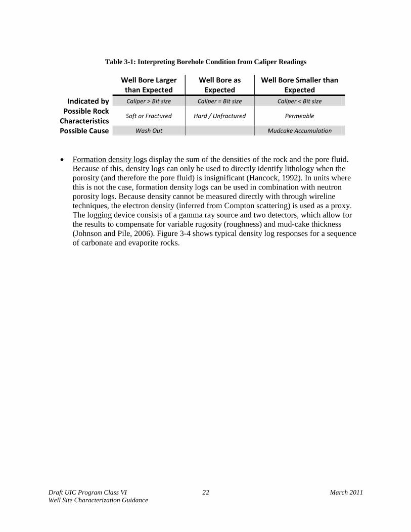
Draft UIC Program Class VI 22 March 2011 Well Site Characterization Guidance
Table 3-1: Interpreting Borehole Condition from Caliper Readings
Well Bore Larger
than Expected Well Bore as
Expected Well Bore Smaller than
Expected
Indicated by Caliper > Bit size Caliper = Bit size Caliper < Bit size
Possible Rock Characteristics
Soft or Fractured Hard / Unfractured Permeable
Possible Cause Wash Out Mudcake Accumulation
• Formation density logs display the sum of the densities of the rock and the pore fluid. Because of this, density logs can only be used to directly identify lithology when the porosity (and therefore the pore fluid) is insignificant (Hancock, 1992). In units where this is not the case, formation density logs can be used in combination with neutron porosity logs. Because density cannot be measured directly with through wireline techniques, the electron density (inferred from Compton scattering) is used as a proxy. The logging device consists of a gamma ray source and two detectors, which allow for the results to compensate for variable rugosity (roughness) and mud-cake thickness (Johnson and Pile, 2006). Figure 3-4 shows typical density log responses for a sequence of carbonate and evaporite rocks.
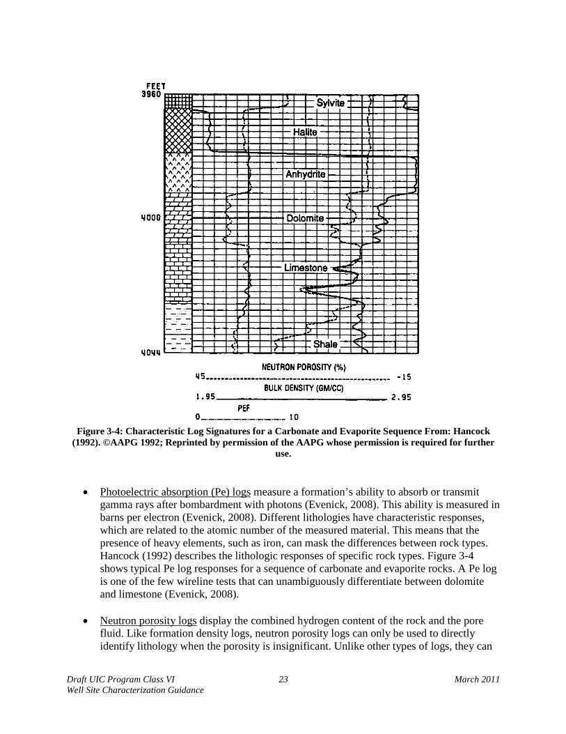
Draft UIC Program Class VI 23 March 2011 Well Site Characterization Guidance
Figure 3-4: Characteristic Log Signatures for a Carbonate and Evaporite Sequence From: Hancock
(1992). ©AAPG 1992; Reprinted by permission of the AAPG whose permission is required for further use.
• Photoelectric absorption (Pe) logs
measure a formation’s ability to absorb or transmit gamma rays after bombardment with photons (Evenick, 2008). This ability is measured in barns per electron (Evenick, 2008). Different lithologies have characteristic responses, which are related to the atomic number of the measured material. This means that the presence of heavy elements, such as iron, can mask the differences between rock types. Hancock (1992) describes the lithologic responses of specific rock types. Figure 3-4 shows typical Pe log responses for a sequence of carbonate and evaporite rocks. A Pe log is one of the few wireline tests that can unambiguously differentiate between dolomite and limestone (Evenick, 2008).
• Neutron porosity logs display the combined hydrogen content of the rock and the pore fluid. Like formation density logs, neutron porosity logs can only be used to directly identify lithology when the porosity is insignificant. Unlike other types of logs, they can
Draft UIC Program Class VI 24 March 2011 Well Site Characterization Guidance
be used in cased wells; however, a sidewall neutron porosity log is needed if the well is air filled (Johnson and Pile, 2006). A dual-detector (compensated neutron) tool may be more useful because single-detector tools have a non-linear response (Johnson and Pile, 2006). Compensated neutron tools also account for problems associated with changing rugosity. Interpretation of neutron logs can be complicated by water bound to shales, which may be confused with available pore space. Conversely, a compensated neutron log will underestimate porosity if natural gas is present, because gas has a lower hydrogen density than water (Evenick, 2008).
Figure 3-4 shows typical neutron porosity log responses for a sequence of carbonate and evaporite rocks. Using neutron and density logs together allows the interpreter to better distinguish lithologic and porosity responses. A combination of density, neutron, caliper, and gamma ray logs is the most powerful of the commonly used log suites for lithologic determination (Hancock, 1992). Superimposing logs on the same log track (as shown in Figures 3-3 and 3-4) allows for the direct comparison of responses to different wireline tools.
• Mud logs compile multiple types of information gathered while drilling from mud surfacing at the wellhead. Mud logs can include rate of penetration by the well bore, lithology, hydrocarbons present (determined by examining the mud with ultraviolet light), and other parameters. This information is often presented as a graph versus depth. Mud logs also note drilling problems and unusual events encountered while drilling. Often, mud logs also include descriptions of rock cuttings-chips of subsurface units ground up by the advancing drill bit that can be recovered as drilling mud recirculates to the surface. These samples can be washed and examined under microscopes and with other techniques to further characterize the subsurface lithologies. Because mud logs directly sample the subsurface, they provide a valuable opportunity to directly investigate the subsurface and eliminate potential interpretive error associated with indirect formation tests.
EPA recommends that wireline logs be calibrated with cores whenever possible. In the absence of continuous cores, wireline log shape in conjunction with cuttings or sidewall cores can be used, but this method involves a larger amount of uncertainty and requires more in-depth knowledge of the local geology and paleogeographic setting (Scheihing and Atkinson, 1992). Repeat sections may also be run to check reproducibility. Greater variability can be expected in radioactive logs because of the chance inherent in radioactive decay (Johnson and Pile, 2006). The best interpretive results are usually obtained when the drilling reports (including instances of kicks, stickiness, lost circulation, etc.) and mud logs are simultaneously considered (Johnson and Pile, 2006). The scale of well logs is also important; 1, 2, or 5 in per 100ft of depth are standard. While 1/100 and 2/100 logs are typically “correlation scales” used to make km-scale or longer cross-sections, or to help correlate one or two offset wells to a cross-section, 5/100 scale logs may be used when detail is needed. So-called superdetail scales, such as 10in/100ft and 25in/100ft, are also possible. Although these logs are usually not used over the entire length of wells, they can

Draft UIC Program Class VI 25 March 2011 Well Site Characterization Guidance
provide important information, such as detailed fracture identification, for key well intervals (Johnson and Pile, 2006). Core Description and Analysis Core samples of the injection and confining zones are required [§146.87(b)] and provide an essential source of information for stratigraphic correlation, environmental/depositional interpretation, and wireline log calibration. Cores can be used to calibrate well log data and to study the lithological, physical, and chemical properties of a rock at a much finer scale (i.e., a millimeter or less) than downhole logs (Major et al., 1998). Additional information can be gathered on rock type, fabric, cement, matrix, fossils, sedimentary structures, diagenetic features, weathering, tectonic structures, veins and other mineralization, porosity, permeability, and other features that may affect carbon dioxide storage (Blackbourn, 1990). Graphic logging (e.g. as described by Ethridge, 1992) is recommended for the description of continuous cores. Ideally, core logs will include descriptions or indications of: thickness, grain size, sedimentary structures, accessories (such as fossils and diagenetic features), lithologies, contacts, textural maturity, oil staining, fracturing, and porosity (Ethridge, 1992). Sidewall cores and other specialized core samples can also provide important stratigraphic information. In theory, cores offer the only opportunity to view intact, potentially vertically continuous samples of depositional sequences (Almon, 1992). However, complete core retrieval is rare and expensive (Major et al., 1998). If continuous cores are needed, special coring procedures can be taken, which include encasing the core in a fiberglass or plastic liner in order to keep it intact (Blackbourn, 1990). Scribed and oriented cores can also be taken to help reconstruct core fragments. Scribed cores are collected by gouging three lines into the side of a core during extraction, which allow sections of core to be properly aligned. For oriented cores, a camera and magnetic compass collect data every few minutes as the core is produced. This allows for the reconstruction of dip and the correct orientation of sedimentary structures within the core. A number of sampling and analytical techniques (e.g. as described by Almon, 1992) have been developed for evaluating cores. Conventional or plug analysis is one of the most common techniques for analyzing continuous cores. In this method, small samples (plugs) are used to represent intervals of the core; for example, plugs are often collected once per foot or in three to four places per meter. Plugs may be taken at the mid-point of each sampling interval (i.e. foot or meter) or at the most representative point of the interval. Formations with greater variability (e.g. with respect to lithology or pore system development) may require more frequent sampling. For heterogeneous formations with many fractures or solution features, it may be preferable to perform a whole core analysis, which examines the complete length of full-diameter core in the interval being tested (Almon, 1992). Full-diameter analysis, which examines selected lengths of the core instead of the entire core, is a variation of whole core analysis. Analytical methods for core evaluation used to examine the petrology, mineralogy, porosity, and permeability of rock formations are described in Sections 3.1.3 and 3.1.4. Since core volume is limited, the use of destructive testing methods may not be appropriate (Blackbourn, 1990).
Draft UIC Program Class VI 26 March 2011 Well Site Characterization Guidance
Well logs may also be produced from cores. This may be done if operational or other issues prevent collection of data in the well or if a greater degree of resolution is desired. Standard wellbore logs, such as gamma ray logs, may be produced from cores (more information on well logs is provided below). Other types of logs may also be created. One technique is X-radiography and tomography, which allows the processor to see inside the core without damaging the sample. This technique is especially valuable when examining massive sands (since it can detect small changes in density), or when looking for rare trace fossils (such as burrows) which may not always intersect the sides of the core. Additionally, since X-rays are able to penetrate solid objects, this technique can be used on friable samples encased in plastic or fiberglass to image cross-bedding or other features (Blackbourn, 1990). When using logging methods on cores, it is important to consider whether sections of the core are missing. The log should be edited so that these sections are marked and/or removed. If not, missing regions could be mistakenly interpreted as a zero response (Blackbourn, 1990). Geophysical Techniques Seismic techniques and other geophysical methods can provide valuable stratigraphic information related to the injection and confining zones. More information on geophysical techniques can be found in Section 7 of this guidance document and in the Draft UIC Program Class VI Well Testing and Monitoring Guidance (this guidance is currently under development).
3.2. Structure of the Injection Zone & Confining Zone The GS Rule requires that applications submit information on the geologic structure of the proposed injection site at §146.82(a)(3). This more detailed evaluation of the site’s structural geology will focus on the injection zone and confining zone(s), using primary data to build upon the structural characterization described in Sections 2.1 and 2.2. EPA recommends that the applicant provide detailed information on the folds, faults, and fractures of the injection and confining zones, including location, depth, strike, and dip, as well as information on the seismic history of the site. The types of information that can be used to characterize the structural features of the injection and confining zones include the following:
• Structural maps
• Structural cross-sections
• Geophysical surveys
• Dipmeter logs
These structural characterizing methods are described below.
3.2.1. Structural Maps Structural maps display the elevation (in the subsurface) of particular formations, layers, or other geologic features. Related maps include isopach maps (which display equal values of true
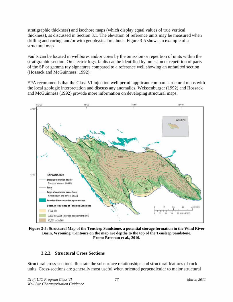
Draft UIC Program Class VI 27 March 2011 Well Site Characterization Guidance
stratigraphic thickness) and isochore maps (which display equal values of true vertical thickness), as discussed in Section 3.1. The elevation of reference units may be measured when drilling and coring, and/or with geophysical methods. Figure 3-5 shows an example of a structural map. Faults can be located in wellbores and/or cores by the omission or repetition of units within the stratigraphic section. On electric logs, faults can be identified by omission or repetition of parts of the SP or gamma ray signatures compared to a reference well showing an unfaulted section (Hossack and McGuinness, 1992). EPA recommends that the Class VI injection well permit applicant compare structural maps with the local geologic interpretation and discuss any anomalies. Weissenburger (1992) and Hossack and McGuinness (1992) provide more information on developing structural maps.
Figure 3-5: Structural Map of the Tensleep Sandstone, a potential storage formation in the Wind River
Basin, Wyoming. Contours on the map are depths to the top of the Tensleep Sandstone. From: Brennan et al., 2010.
3.2.2. Structural Cross Sections Structural cross-sections illustrate the subsurface relationships and structural features of rock units. Cross-sections are generally most useful when oriented perpendicular to major structural

Draft UIC Program Class VI 28 March 2011 Well Site Characterization Guidance
trends, though bends in the section can be used to show variable structural trends or other features (Boak, 1992b). EPA recommends that applicants include cross-sections that are oriented perpendicular to major structural trends. Additional smaller cross-sections can be included to illustrate specific features such as faults. Structural cross-sections may reference attached stratigraphic cross-sections if correlations are difficult. Figure 3-6 shows an example of a structural cross-section. Stratigraphic and structural cross-sections are developed using similar methods (see Section 3.1 for more information on stratigraphic cross-sections). For a structural cross-section, the datum is generally sea level, and units are drawn above or below that elevation according to their present positions (Boak, 1992b). Unlike stratigraphic cross-sections, structural cross-sections are generally drawn with little or no vertical exaggeration; this allows the cross-section to accurately represent the relative positions of the layers.
Figure 3-6: Structural Cross Section of the Soan Syncline, Kohat-Potwar Geologic Province, Upper
Indus Basin, Pakistan. From: Wandrey et al., 2004.
3.2.3. Geophysical Surveys Seismic techniques and other geophysical methods can provide valuable structural information related to the injection and confining zones that can assist with meeting the requirements of the GS Rule. For example, these methods can be used to identify the locations of potential faults and fractures at the proposed project site. More information on geophysical techniques can be found later in Section 3. 7 of this document as well as in the Draft UIC Program Class VI Well Testing and Monitoring Guidance.
3.2.4. Dipmeter Logs Dipmeters are designed to measure the dip and the dip direction of surfaces that intersect the well. To generate a dipmeter reading, microresistivity sensors are mounted on a caliper logging tool. A minimum of three calipers is needed, but most modern dipmeters have six or more
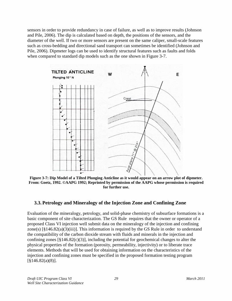
Draft UIC Program Class VI 29 March 2011 Well Site Characterization Guidance
sensors in order to provide redundancy in case of failure, as well as to improve results (Johnson and Pile, 2006). The dip is calculated based on depth, the positions of the sensors, and the diameter of the well. If two or more sensors are present on the same caliper, small-scale features such as cross-bedding and directional sand transport can sometimes be identified (Johnson and Pile, 2006). Dipmeter logs can be used to identify structural features such as faults and folds when compared to standard dip models such as the one shown in Figure 3-7.
Figure 3-7: Dip Model of a Tilted Plunging Anticline as it would appear on an arrow plot of dipmeter. From: Goetz, 1992. ©AAPG 1992; Reprinted by permission of the AAPG whose permission is required
for further use.
3.3. Petrology and Mineralogy of the Injection Zone and Confining Zone Evaluation of the mineralogy, petrology, and solid-phase chemistry of subsurface formations is a basic component of site characterization. The GS Rule requires that the owner or operator of a proposed Class VI injection well submit data on the mineralogy of the injection and confining zone(s) [§146.82(a)(3)(iii)]. This information is required by the GS Rule in order to understand the compatibility of the carbon dioxide stream with fluids and minerals in the injection and confining zones [§146.82(c)(3)], including the potential for geochemical changes to alter the physical properties of the formation (porosity, permeability, injectivity) or to liberate trace elements. Methods that will be used for obtaining information on the characteristics of the injection and confining zones must be specified in the proposed formation testing program [§146.82(a)(8)].

Draft UIC Program Class VI 30 March 2011 Well Site Characterization Guidance
3.3.1. Mineralogic and Petrologic Analysis
If previous mineralogic and petrographic analysis has not been done on both the injection zone and the confining zone(s) (e.g., through earlier characterization in well-developed basins), cuttings and core samples will be needed to perform the required analyses for site characterization purposes. This will likely be necessary in most cases in saline environments under consideration for GS project sites. Cuttings retrieved during drilling can provide basic information on lithologies encountered as drilling progresses. Features such as color, texture, and grain size can be recorded, providing a qualitative record of lithology with depth. However, cuttings are small fragments, and mud may have filtered into the pores. Detailed mineralogic examination is best done with intact cores. Various coring techniques are available, including rotary coring, wireline coring, and sidewall coring. Rotary coring yields long, continuous cores. But because rotary coring requires cessation of drilling, removal of the drillstring, and insertion of a rotary coring apparatus, it is time consuming and can be expensive. Wireline coring systems do not require removal of the drillstring, but retrieve cores of small diameter (less than 3 inches). Sidewall coring is faster and cheaper, but produces very small, short cores (1 in. wide and 1.75 in. long). Decisions about the type of coring to perform will ultimately depend upon logistics, cost, and the type of lithology to be cored. Detailed information on the various coring methods is available in Whitebay (1992) and more information is available in Section 3.1. Proper drilling methods should be practiced to maintain zonal isolation when penetrating the confining zone. Core samples will need to be taken from the injection and confining zones, however, keep in mind that the UIC Program Director will need assurance that any conduits for carbon dioxide movement out of the injection zone have been appropriately addressed before a Class VI injection well operating permit can be approved. It may also be desirable to analyze samples from the first permeable formation overlying the confining zone or from other permeable formations and confining zones further up in the stratigraphic column. It is important to remember that, these samples represent point measurements and that it may not be possible to capture all geological heterogeneities in the formations of interest. The optimal number of samples to analyze will vary by site, but representative samples should be chosen from cores and core sections that represent different lithologic characteristics (e.g., texture, grain size, color). A number of well-established methods are available for characterization of core samples for mineralogic/petrologic and chemical characteristics. The most common methods are outlined below. Analysis by Polarized Light Microscopy The use of a petrographic microscope is a fundamental tool when identifying and characterizing rock and mineral samples. Samples are prepared by mounting chips of the rock onto glass slides, cutting and grinding down to a thickness of 30 microns, and polishing. Poorly consolidated samples may need to be impregnated with epoxy prior to cutting them into chips. A petrographic microscope is a transmitted light microscope designed for the examination of rock thin sections. It includes a rotating stage and polarizers both above and below the stage; the specimen is examined both with the upper polarizer in place (“crossed polarizers”) and with it

Draft UIC Program Class VI 31 March 2011 Well Site Characterization Guidance
removed (“plane polarized light”). When the upper polarizer is inserted, the vibration directions of the two polarizers are perpendicular. This arrangement takes advantage of the optical properties of minerals; those that are not isotropic have more than one index of refraction, and light passing through is split into separate rays with different velocities. Under crossed polarizers, the difference in the velocities produces interference colors, which helps with mineral identification when taken together with cleavage, shape, and other characteristics. Petrographic microscopes have remained relatively unchanged in principle since their development in the late 1800’s. Edwards (1916) is an example of a classic book that is still available and presents the optical properties of minerals, a description of the petrographic microscope, and mineral identification using the microscope. Basic descriptions of petrographic microscopes are commonly available and on the Internet. . Careful petrographic analysis can provide information about the minerals present, the relationships among them (e.g. overgrowths), textures, grain size, weathering (e.g. rounded grains in a clastic sediment). Williams et al. (1982) provides details on the mineralogy and textures to be expected in different rock types and how they relate to rock formation.
Scanning Electron Microscopy Scanning electron microscopy (SEM) uses a beam of electrons instead of visible light, and permits much higher magnification than a petrographic microscope. The term “scanning” refers to the raster pattern used in moving the electron beam over the sample surface (similar to a television). The same thin sections prepared for light microscopy can be used in a scanning electron microscope. Also, unconsolidated samples can be prepared for analysis by mounting onto a glass slide using adhesive. The most common use of an SEM is for secondary electron imaging (SEI). In this mode, it produces a high resolution image of the sample surface, with good depth of field. This function is not appropriate for thin sections because they are polished flat. But for loose samples affixed to a slide, it can image grain morphology and other features. The oil and gas industry uses SEM in this capacity for assessment of reservoir quality (Grier and Marschall, 1992). With thin sections, an SEM can be used in backscattered electron (BSE) mode. The signal from backscattered electrons depends upon the atomic weight of the material being examined. Minerals are seen with different levels of brightness, with higher density minerals appearing brighter. This can be helpful for distinguishing minerals that appear similar under light microscopy. The same types of textural relationships would be seen as with a petrographic microscope, but very fine grains such as clay minerals and other clay-sized particles can be identified, as can mineral coatings and cements. Also, an elemental analysis of the minerals can be obtained if the SEM is equipped for energy-dispersive x-ray spectroscopy or wavelength-dispersive x-ray spectroscopy. Such analyses are point measurements, allowing analysis of specific sections of a mineral grain or of cements and grain coatings. Energy-dispersive spectra can be quickly viewed during examination as a qualitative aid in mineral identification. Quantitative analyses can also be obtained.

Draft UIC Program Class VI 32 March 2011 Well Site Characterization Guidance
Images taken in BSE mode can be used in petrographic image analysis, which can be used to calculate estimates of porosity, permeability, and capillary pressure based on two-dimensional (2D) measurements. Information on all of these parameters is important for proper site characterization and operation of a Class VI injection well. Further details are given in Section 3.1 of this guidance, above. Mineralogic and Petrologic Features Relevant to GS The most common lithology types for oil and gas reservoirs and deep saline formations are sandstone, limestone, and dolomite. The major minerals in sandstones include quartz and feldspar with calcite (often as cement) and clay fines being common as lesser components. Limestones and dolomites consist primarily of carbonate minerals (calcite, aragonite, dolomite). “Impure” limestones may have minor quartz grains, pyritic limestone contains pyrite, and argillaceous limestones contain clay components (Williams et al. 1982). Figures 3-8 and 3-9 show examples of thin sections of a sandstone and a fossiliferous limestone. The most common confining zones in stratigraphic sequences suitable for GS will include shales. These consist primarily of clay minerals, with small particles of quartz, feldspar, and mica. Individual particles can be difficult to see by optical microscopy (Figure 3-10), and aside from general confirmation of the lithology and texture, limited information will be gained. If detailed information is needed, an SEM should be used. Some of the textural features that might be observed in thin section and under SEM include cementation (secondary minerals providing cohesion to the rock), dissolution features (indicative of removal of minerals), pore size and shape, and the presence of fine clay minerals. For example, in Figure 3-9, the carbonate cement can be seen in infilling voids within the fossils and in between the fossil fragments. The degree and extent of these processes are integral to understanding porosity and permeability and for anticipating changes that may take place as a result of interactions between the injectate, native fluids, and formation solids. The composition, grain size, grain shape, and sorting seen under a microscope can all be used to infer the depositional environment. This facies analysis can help in locating changes in physical parameters. For example, if grain size is seen to decrease upwards, a corresponding decrease in permeability may be seen. Such observations are considered a routine part of the determination of reservoir quality in the oil and gas field (e.g., Grier and Marschall, 1992) and may be valuable as part of storage formation characterization. A detailed discussion of the genesis, composition, and textures of rocks is also provided in Williams et al. (1982).

Draft UIC Program Class VI 33 March 2011 Well Site Characterization Guidance
Figure 3-8: Sandstone Cemented with Calcium Carbonate, Viewed under Crossed Polarizers.
Field of view is 3.5mm. The white and gray shapes are individual grains of sand, the tan in-between the sand grains is pore space filled with calcite cement. From: Univ. of Oxford (2010). © David Waters and
the Department of Earth Sciences, University of Oxford. Reproduced with Permission.
Figure 3-9: Limestone With Fossil Fragments, Viewed under Crossed Polarizers. Field of view is 3.5mm. The angular tan and blue shapes are calcite crystals filling in pore space. From: Univ. of Oxford (2010).
© David Waters and the Department of Earth Sciences, University of Oxford. Reproduced with Permission.

Draft UIC Program Class VI 34 March 2011 Well Site Characterization Guidance
Figure 3-10: Grains of Sand in a Shale Matrix, Viewed under Crossed Polarizers. Quartz sand grains
are gray and white. Field of view is 2mm tall. From: Schieber (2006). © Juergen Schieber. Reproduced with permission.
X-ray Diffraction X-ray diffraction (XRD) may be useful for verification of mineralogy or identification of clay minerals. X-ray diffraction helps to identify minerals based on structure rather than chemistry. The most common method for geologic samples is powder XRD, in which a slurry of the ground specimen is allowed to dry on a glass slide, which is then placed in the diffractometer. The sample is exposed to a beam of x-rays, which are diffracted by the various planes within the structure of the mineral. The angle of refraction for each plane is determined by Bragg’s Law. During the analysis, a detector is moved through a range of angles relative to the sample and registers the angles at which x-rays are detected. The resulting pattern of x-ray peaks is used to identify the mineral. If multiple minerals are present, the patterns will be superimposed upon each other, and a qualitative estimate of the relative quantities of the minerals may be possible. XRD may be especially useful for identifying clay minerals, which are too fine to fully characterize by polarized light microscopy. Moore and Reynolds (1989) provide a thorough coverage of the theory and practice of x-ray diffraction, with a focus on its application to clay minerals.
3.3.2. Bulk Chemical Analysis
In addition to mineral identification, an elemental analysis of the formation solids may be desired to evaluate the potential for liberation of metals. Methods for obtaining bulk chemical analyses are briefly described in this section. X-ray fluorescence (XRF) is a well-established technique for obtaining chemical analyses of metals, rocks, glass, and ceramics. It measures the secondary electrons emitted when a sample is exposed to x-rays or gamma rays. The sample is prepared as a fused glass or pressed pellet. Quantitative measurements can be done using either an energy-dispersive or wavelength-dispersive system. Both major and trace elements can be measured. Beckhoff et al. (2006) and Jenkins (1999) provide information on the theoretical basis of XRF as well as instrumentation and applications.

Draft UIC Program Class VI 35 March 2011 Well Site Characterization Guidance
A bulk chemical analysis can also be obtained by complete digestion of samples and analysis of the extracts by inductively coupled plasma/atomic emission spectrometry (ICP/AES) or inductively coupled plasma/mass spectrometry (ICP/MS). Sample digestion can be done with EPA Method 3052 (Microwave Assisted Acid Digestion of Siliceous and Organically Based Materials). This method is appropriate for materials as durable as silicate minerals and will prepare the sample for analysis for many major and minor elements, including As, Hg, Pb, Cr, Cu, and Zn. This digestion uses heat and a combination of hydrofluoric acid and nitric acid. It also uses hydrochloric acid, if needed and hydrogen peroxide if organic matter is present. For the analysis stage, EPA Method 6020A (ICP/MS) or EPA Method 6010-C (ICP/AES) can be used. In both methods, the sample is introduced into plasma, where it is ionized. In ICP/AES, the detector is spectroscopic, identifying elements by their characteristic electromagnetic wavelengths. In ICP/MS, ions are identified by their mass-to-charge ratios. In selecting a method for bulk chemical analysis, ease of operation and detection limits might be considered. An advantage of XRF is that it does not require sample digestion using hazardous chemicals. However, ICP/AES and ICP/MS are much more sensitive. XRF can measure concentrations in the parts-per-million (ppm) range. ICP/AES can detect elements in the parts-per-billion range (ppb), and ICP/MS can reach parts-per-trillion levels. The equipment manufacturer Varian has produced a useful comparison of ICP/AES, ICP/MS, and another common method, atomic absorption spectrometry (Tyler, 1994).
3.3.3. Mineralogic/Petrologic/Geochemical Information Analysis
Characterization of the solids in both the injection zone and the confining zone(s) can be used for anticipating geochemical reactions between the carbon dioxide, brine, and minerals that may cause changes in geomechanical (i.e. porosity, permeability) and operational (injectivity) parameters. Information on the compatibility of the carbon dioxide stream with subsurface fluids and minerals is required by the GS Rule at §142.82(c)(3). Near the wellbore, the high flow rates and continued input of carbon dioxide can maintain decreased pH and lead to the dissolution of carbonate minerals, including carbonate cement in sandstones. Increased carbonate ion concentrations, however, ultimately promote precipitation of new carbonate minerals. These reactions may happen rapidly, potentially affecting porosity, permeability, and injectivity (Cailly et al., 2005). Researchers (e.g., Ross et al., 1982; Svec and Grigg, 2001) have performed laboratory studies of the effects of carbon dioxide injection on sandstones and carbonates, rock types that will be used for many if not most GS projects. Both increased and decreased permeability may occur, depending on a number of variables, including mineralogy, rock texture, and acidity of the brine. Quantitatively connecting geochemical processes to changes in porosity and permeability, however, is a complex exercise, and the effects will be site-specific (Gaus, 2010; Cailly et al. 2005). The coupled physical and geochemical processes in the injection formation can be explored through reactive transport modeling. Two programs in particular are well suited for such studies: TOUGHREACT (http://esd.lbl.gov/TOUGHREACT/) and PHREEQC
Draft UIC Program Class VI 36 March 2011 Well Site Characterization Guidance
(http://wwwbrr.cr.usgs.gov/projects/GWC_coupled/phreeqc/). These can be used to take into account both fluid transport and geochemistry to predict the loss or precipitation of minerals. Information on mineralogy collected during site characterization is needed if the owner or operator decides that such modeling will help understand the subsurface processes. It should be kept in mind that reactive transport modeling requires a large amount of information, some of which may need to be estimated, and that there will be uncertainties in the results. For confining zone interactions, it is important to assess any changes in permeability and porosity that may affect the ability of the confining zone to provide an adequate seal (Gaus, 2010). Dissolution of the silicate minerals in shale is expected to be slow, although estimates are uncertain because reaction rates are too slow to calibrate models (Gaus, 2010). In the case of the confining zone at Sleipner, modeling suggests limited effects on porosity (Chadwick et al., 2007; Gaus et al., 2005). In particular, Gaus et al. (2005) suggest that geochemical interactions will be limited to the lower few meters even over a scale of thousands of years and that porosity may decrease slightly. Again, mineralogic analysis is crucial for input into such an analysis. Mineralogic data can also be used to model longer-term dissolution and precipitation, including what might occur farther out from the injection well, which ultimately affect the degree of mineralogic trapping possible in the storage formation.
3.4. Porosity, Permeability, and Injectivity of the Injection Zone and Confining Zone
This section describes the parameters porosity, permeability, and injectivity. It provides discussion regarding factors affecting measurements and information regarding laboratory and field methods for quantifying and/or estimating values for these parameters. This information is required pursuant to §146.82(a)(3)(iii) of the GS Rule. Intrinsic permeability, relative permeability, and porosity are also required model parameters for the multiphase fluid modeling involved in AoR determinations [§146.84]. See the Draft UIC Program Class VI Well Area of Review and Corrective Action Guidance, Section 2, for more information on AoR modeling.
3.4.1. Porosity Porosity, along with permeability and injectivity, is required by the GS Rule in order to evaluate the carbon dioxide storage capacity of a formation [§146.82(a)(3)(iii)]. Two porosity measurements are common: absolute and effective. Absolute porosity is the ratio of void space in a rock to the total volume. Effective porosity is the ratio of void space that is interconnected and capable of containing fluid to the total volume of the sample (Cone and Kersey, 1992). Because it is more practical than absolute porosity, effective porosity is more often reported. Factors Affecting Measured Porosity
Porosity is controlled by many variables. In sedimentary rocks, porosity is a function of the packing, sorting, grain size, and grain shape of the individual particles as well as in-situ stress (Cone and Kersey, 1992). Pore space can occur as space between grains, as micro-scale pores along grain surfaces or other boundaries (when spaces are less than 2μm), or along fractures. It can also be controlled by dissolution features (typically in carbonates). In clastic rocks,

Draft UIC Program Class VI 37 March 2011 Well Site Characterization Guidance
intergranular pore space is generally the most significant, especially in loosely packed, medium to large grain well-sorted lithologies such as clean sandstones. Fractures are usually the most important contributors to porosity in non-sedimentary rocks although there are exceptions (e.g. vuggy basalts can have porosities up to 12% (Fetter, 1988)). Clastic rocks on average have the highest porosity of any rock type, with sandstones having up to 40% pore space (Cone and Kersey, 1992). The porosity of carbonates varies widely but is usually between 5 to 25% (Cone and Kersey, 1992). Shales, which are potential sealing formations, usually have higher porosity than sandstones upon deposition (up to 80%) but experience rapid decreases in porosity with burial compaction and additional diagenesis (Avseth et al., 2010). The mean porosity for over 100 samples of Devonian-age shale was 3.6-4.1%, with extremes of 1.2-7.6% when measured using helium gas resaturation (Davies et al., 1990). However, the study also noted difficulties in measuring shale porosity because low values may be near the resolving limit of some techniques and because small pore size (averaging 0.05μm in some shales (Soeder, 1988)) can complicate some techniques. The method of sample collection can influence the measured porosity. For lithologies with greater than 30% porosity, samples collected with sidewall cores tend to yield results a few percent too low because of compaction during coring (Almon, 1992). Damage to samples collected with percussion methods can further distort results. For low porosity units, measured porosities can be much too high because porosity is enhanced by damage that occurs during coring, while for high porosity formations, compaction and grain shattering can reduce measured porosity (Almon, 1992). Igneous and metamorphic rocks usually have low porosities. However, some tuffs and lava flows are very porous and pumice can have up to 87% absolute porosity (Fetter, 1988). Weathering can also greatly increase porosity of these lithologies; weathered ultra-mafic and plutonic rocks can have porosities up to 60% due to the breakdown of minerals such as mica (Fetter, 1988). Porosity Measurement Porosity can be measured either in the field or with laboratory methods. However, field and laboratory methods often do not yield the same results. The main reason for the difference is that field methods sample a much larger volume of the subsurface. As a result, they can incorporate formation heterogeneities due to changing lithologic characteristics and larger-scale fluid migration pathways such as vugs, fractures, and dissolution features into porosity measurements (Cone and Kersey, 1992). Correspondingly, field measurements tend to yield higher values for a particular formation than measurements collected in the laboratory. Field Methods In the field, neutron logs, density logs, and sonic logs are well-suited to help infer porosity (Aguilera, 1992). Neutron logs can be used in cased or uncased wells. A neutron-emitting probe is lowered into a well, and neutrons are captured by the hydrogen atoms in trapped pore water, gas, and hydrocarbons and are re-emitted as gamma rays. The probe logs the total amount of

Draft UIC Program Class VI 38 March 2011 Well Site Characterization Guidance
gamma radiation and estimates the pore fluid volume. One downside to this method is that water bound to clays can provide an incorrectly high measure of porosity in shales, siltstones, and other clay-rich units. As a result, a neutron log should be collected and processed with other logs such as density logs or gamma ray logs to ensure accuracy. Porosity values collected from neutron logs are also absolute porosity; space in isolated, disconnected vugs that is not available for fluid storage is captured in the measurement. Another potential problem is that the neutron log cannot determine the type of pore fluid present, which may be an important consideration when determining total storage capacity and injectivity. Density log data are collected using a sonde equipped with a source of gamma radiation and at least one gamma ray detector into a well. As it enters the formation, the radiation is scattered according to bulk density. Porosity can be calculated from density log data if the lithology of the subsurface and the saturating fluid are known:
𝒎𝒂𝒕𝒓𝒊𝒙 𝒃𝒖𝒍𝒌 𝐏𝐨𝐫𝐨𝐬𝐢𝐭𝐲 = (𝝆
𝒎𝒂𝒕𝒓𝒊𝒙 𝒇𝒍𝒖𝒊𝒅
−𝝆 )�𝝆 −𝝆 �
Equation 3-1
where ρmatrix is estimated based on the lithology (e.g. sandstone = 2.65 g/cm3, 2.71 g/cm3 for limestone, and 2.87 g/cm3 for dolomite, etc.), ρbulk is from the density log, and ρfluid is estimated based on the salinity and hydrocarbon makeup of the saturating fluid (e.g. water = 1g/cm3, etc.) (Alberty,1992a; Dewan, 1983). Sonic logs measure the speed of sound in a formation. As a sonic probe is pulled up a well, it emits a sound wave and logs the time any reflected sonic waves arrive back at the receiver. If the lithology of the layer is known, the porosity can be deduced from deviation from the theoretical sonic travel time for a layer of the same lithology with zero porosity. The Wyllie time average method or the Raymer-Hunt-Gardner methods are two common methods used with sonic logs. Sonic logs work best when the pore fluid is water or brine. Laboratory Methods Several laboratory methods are available to determine porosity. These methods provide values for effective porosity; there is no good laboratory method for determining absolute porosity. Because porosity is stress-dependant, laboratory measurements should be taken at stress conditions similar to in-situ conditions (Cone and Kersey, 1992). Furthermore, core samples represent point measurements. For reliable results, measurements are best made on a number of cores, and the applicant might consider submitting a statistical representation of measurements such as a variogram. If an unaltered, fresh sample of the formation of interest is available, the summation method can be used. Gas, oil, water, and any other fluids are extracted from the rock using a vacuum or other method. The sum of extracted fluids is assumed to equal the sum of the pore space. This method is potentially problematic because the sample is not cleaned and because core samples are often subject to damage (e.g. mud intrusion, etc.) during retrieval, which can displace pore fluids.

Draft UIC Program Class VI 39 March 2011 Well Site Characterization Guidance
With a less pristine sample, a resaturation method can be used. First, the sample is cleaned and dried, which allows for the remediation of some damage incurred during drilling. Hydrocarbons are generally removed from samples using toluene. The sample is then heated until it maintains a constant weight. One potential problem with this method is that if brines are present, precipitation of salts can reduce the porosity (Cone and Kersey, 1992). If smectite, gypsum, or clay minerals are present, samples should be dried at 63 degrees Celsius and 45% humidity to prevent removal of structural water and damage to clay minerals (Cone and Kersey, 1992). Once the sample remains at a constant weight, indicating that all fluids have been driven off, the sample is then saturated with either a liquid (usually water) or a gas. Helium is usually the gas of choice because it does not adhere to mineral surfaces and its small molecule size allows it to diffuse into micropores. If liquid resaturation is chosen, the sample is saturated with liquid and re-weighed. For rock samples with very small pore sizes, the choice of displacing and saturating fluid used during the porosity measurement may introduce variability into the final results because of the attraction between pore surfaces and displacing fluids. The amount of pore space is deduced from the density of the saturating liquid. In gas resaturation, the sample is placed in a confined volume and resaturated with gas from a referenced cell. The volume of pore space is determined from the change in the pressure in the reference cell through the ideal gas law (pV=nRT). Gas resaturation should not be used with vuggy or fractured samples. Dry methods are also available. Thin sections of rocks made from core samples can be analyzed under a polarized light microscope or scanned and analyzed with specialized software (petrographic image analysis; see Section 3.4.2) Less commonly used laboratory methods to determine porosity include x-ray computerized tomography (CT scanning) and nuclear magnetic resonance imaging.
3.4.2. Permeability Data on permeability of the injection and confining zones are required to be submitted with a Class VI injection well permit application [§146.82(a)(3)(iii)]. Permeability is the ability of a material to transmit fluids. It is measured with respect to a single fluid if more than one fluid is present; usually a single fluid is preferentially transported. The unit for permeability is the Darcy (D). A material with a permeability of 1 D will allow 1 cm3 per second of a fluid with a viscosity of 1 cP (centipoise) though a 1 cm2 cross-sectional area if a pressure gradient of 1 atm/cm is applied (Ohen and Kersey, 1992). Several physical factors can influence permeability. The median pore size (Bachu and Bennion, 2008) and connectivity of pore space within the material are two contributing factors to permeability. The grain size is also an important contributing factor; because all wetted grains have a boundary layer of fluid with a viscosity of zero, more energy is expended overcoming shearing forces between the boundary layer and through fluids when the grain size is small (Schlumberger, 2006).

Draft UIC Program Class VI 40 March 2011 Well Site Characterization Guidance
Absolute (Intrinsic) Permeability Absolute permeability, also known as intrinsic permeability, is the permeability of a material when only one fluid is present. It is dependent only on the properties of the material and not the fluid. Absolute permeability can be calculated as:
𝐀𝐛𝐬𝐨𝐥𝐮𝐭𝐞 𝐏𝐞𝐫𝐦𝐞𝐚𝐛𝐢𝐥𝐢𝐭𝐲 = 𝑸𝝁𝑳𝑨𝒇×(𝒑𝟐−𝒑𝟏)
Equation 3-2
where Q is the flow rate through the core, µ is the fluid viscosity, L is the length of the core, Af is the cross-sectional area of the core, and (p2-p1) is the pressure difference on either side of the core. Permeability values of different lithologies can vary by orders of magnitude (Table 3-2), with salts and shales typically exhibiting lower permeability values and sandstones having the highest.
Table 3-2: Typical Permeability for Various Lithologies (Davis, 1998)
Lithology Permeability (mD)
Shale (unfractured) 4.7 x 10⁻⁵ Sandstone 3.8-4,740
Coal 334 Salt 9.61 x 10⁻⁵
Because geologic materials are inherently heterogeneous, absolute permeability will vary spatially. Furthermore, permeability is an anisotropic property that varies in the x, y, and z directions and typically shows the greatest variation in the direction perpendicular to layering. For the computational modeling performed for AoR determination, a realistic representation of the permeability distribution is needed. Approaches for handling the distribution of permeability, including geostatistical approaches are discussed in the Draft UIC Program Class VI Well Area of Review and Corrective Action Guidance (Section 2). Effective Permeability Effective permeability measures the permeability of a material to one fluid when more than one fluid phase is present (such as carbon dioxide in brine or oil). In addition to pore size distribution, effective permeability is affected by the relative saturation of fluids within a material and the interfacial tension (IFT) between the fluids (Bachu and Bennion, 2008). Because IFT is influenced by in-situ conditions such as pressure and temperature, these variables can also influence effective permeability. Due to the its dependence on the IFT and the relative saturation of fluids, effective permeability in a GS project is expected to vary spatially and temporally as pressure and the distribution of brine and carbon dioxide change.

Draft UIC Program Class VI 41 March 2011 Well Site Characterization Guidance
Relative Permeability Relative permeability is the dimensionless ratio of the effective permeability to absolute permeability. It varies from 0 to 1. Relative permeability is relevant to GS because one phase or fluid can inhibit or encourage the preferential flow of another phase or fluid. Because relative permeability varies with the relative saturations of the fluids, it may be expressed as a relative permeability-saturation function for incorporation into computational modeling. See the Draft UIC Program Class VI Well Area of Review and Corrective Action Guidance, Section 2, for more information. It has been studied extensively due to its importance in hydrocarbon extraction (Schlumberger, 2006). For GS, changes in the relative permeability may result in improved or reduced injectivity into reservoir rocks and/or improved or reduced sealing capacity for confining formations. Many different mathematical methods of obtaining relative permeability are available. One of the simplest is the Pirson model, which uses the saturation of the wetting phase before and after drainage of a core sample to determine the relative permeability of the wetting phase:
𝒓(𝒊) 𝒊𝟑 (𝑺𝒊−𝑺𝒊𝒓)
𝑲 = 𝑺 � (𝟏−𝑺𝒊𝒓)�
𝟏.𝟓Equation 3-3
where Si and Sir are the saturation and residual saturation of the fluid. Relative permeability measured in the laboratory is often found to be dependent on many factors, including pore size and IFT, which in turn depends on the in-situ pressure, temperature, overburden pressure, wettability, and salinity conditions (Bachu and Bennion, 2008; Hawkins, 1992). A lower IFT encourages the transport of the non-wetting phase through the pore space, leading to an increase in the relative permeability. Hysteresis effects may also influence relative permeability (Hawkins, 1992). This may be important for fields with previous water and carbon dioxide flooding histories or if injection of carbon dioxide is not done at a constant rate. Relevant Data Permeability data for several different fluids/mixtures within the reservoir will likely be needed to fully characterize behavior of the injectate at carbon dioxide storage sites as injection progresses. These fluids/mixtures are:
• Brine, hydrocarbon, or other initial reservoir fluid • Carbon dioxide /reservoir fluid mixture • Pure carbon dioxide
Initially, the permeability depends only on the behavior of the reservoir fluid. Next, permeability becomes dependent on a mixture of two or more liquids as injectate is introduced into the reservoir. Bachu and Bennion (2008) found that the permeability of sandstone, carbonate, and shale core samples taken from a typical intracratonic sedimentary basin to carbon dioxide at irreducible water conditions was 1/5th that of brine at 100% brine conditions for lithologies with permeabilities greater than 1 mD.

Draft UIC Program Class VI 42 March 2011 Well Site Characterization Guidance
As large volumes of carbon dioxide are injected, a new zone may form near the injection well as the carbon dioxide saturation increases and the reservoir fluid is completely displaced. Once again the permeability is dependent on a single fluid, this time the injected carbon dioxide as opposed to the native reservoir fluid. This zone is called the “dry-out” zone. Salts will precipitate out of the migrating brines, potentially decreasing permeability (Burton et al., 2009). However, the presence of a dry-out zone may increase injectivity regardless because the absolute permeability of carbon dioxide in the dry-out zone exceeds the relative permeability of carbon dioxide in the two-phase region (Burton et al., 2009). Measuring Permeability Permeability can be quantified using laboratory methods or in-situ field measurement techniques. Unlike other parameters (e.g. viscosity, temperature, pressure), permeability is calculated indirectly from values derived from other measurements (e.g. capillary pressure, IFT). As a consequence, permeability can vary depending on the method used. Additional discussion is provided below. Laboratory Methods Permeability measurements in the laboratory can be conducted with water, brines, gases, or other fluids when a sample of the layer is available. Down-hole cores are an obvious choice for such a sample. However, determining permeability from down-hole cores may be difficult if damage has occurred during drilling. Permeability in core material can be reduced by as much as 50-80% due to the infiltration of mud, fine material, or other particles into the pore spaces of the core. Plug samples taken from the center of the core may be the best way to avoid such damage and generate a representative measure of permeability. Sandblasting the outside of whole-core samples may remove some built-up fines and improve results, but it cannot remediate mud that may have worked into the pores (Almon, 1992). Permeability can also be measured from sidewall cores. However, sidewall permeability measurements are often erroneously high for hard, dense formations because of grain shattering and other damage during the coring and extraction of the side wall core. Conversely, permeability measurements taken from sidewall cores for loose, friable (crumbly) formations are often erroneously low due to grain shattering introducing fines into pore spaces (Almon, 1992). Once an appropriate lithologic sample has been isolated, it can be analyzed. The most common laboratory methods involve isolating a sample of core in a non-permeable sleeve while injecting a fluid material into the core. Measurements taken using a single fluid yield information on absolute permeability. Lead sleeves are often used because traditional sleeve materials allow the diffusion of carbon dioxide across the sleeve. Also, lead sleeves transfer pressure radially throughout the core if experiments are conducted at in-situ pressure conditions. Gas (air) and brine are the most common fluids used for injection in conducting permeability tests. Gas permeability is the industry standard for hydrocarbon exploration because it is the easiest to produce. While gas and brine tests produce similar permeability results when permeability is high, gas permeability tends to be higher when the permeability is low because

Draft UIC Program Class VI 43 March 2011 Well Site Characterization Guidance
the gaseous phase does not adhere to the pore surfaces as much as an aqueous phase. Gas methods are also corrected for gas slippage effects at low pressures and inertial effects at high pressures (Ohen and Kersey, 1992). The pressure difference across the core after the flow has stabilized can be transformed into a permeability measurement using a modified version of Darcy’s Law. A non-steady state variant of this method measures the gas pressure decay across the core. Non steady-state methods usually produce more accurate results. Experiments can be conducted in a temperature controlled environment to simulate reservoir conditions when measuring effective permeability. When permeability is measured from a whole core, measurements are usually reported in two directions: one parallel to the major fracture planes and other at 90 degrees perpendicular to this direction (Almon, 1992). Measurements may also be needed along core in order to gain a representative understanding of permeability within the unit. Although effective and relative permeability can both be measured in the laboratory, relative permeability is more commonly measured and reported (Abaci et al., 1992; Ahmed, 2006). Several methods are available. One common method uses a set-up similar to absolute permeability methods except that after initial saturation and pressure equilibration, a second fluid is introduced and driven though the sample until the saturation and pressure differential across the sample returns to a constant value. A faster alternative is the unsteady-state method, in which a stream of gas is injected into a sample to displace a liquid. However, this method is only applicable if one of the fluids of interest is a gas. Additionally, mathematical calculations are more complex when using the unsteady-state method. There are several types of corrections that have been applied to core data. The Klinkenberg correction, which is important for low-permeability rocks, relates permeability for liquids to gas permeability. The pore fluid chemistry, especially salinity, may also affect permeability. Another type of adjustment is a correction for the dependence of permeability on pressure. For example, unconsolidated rocks can collapse, reducing permeability. These corrections are described by Nelson and Batzle (2006). Petrographic Image Analysis Petrographic image analysis (PIA) is an established method employed in the oil and gas industry to derive 3D petrophysical properties (porosity, capillary pressure, permeability, relative permeability) from 2D measurements of pore size and geometry. It can be used for characterization of sandstones, carbonates, and conglomerates, and it is inexpensive and rapid (Gies, 1993). To collect PIA data, standard petrographic thin sections are viewed under a petrographic microscope or scanning electron microscope in backscatter mode (BSE), and the images are stored and analyzed using image analysis software. The sample will need to have been impregnated with epoxy to fill the pore spaces prior to making the thin section. If light microscopy is to be used, adding dye to the epoxy will make pore spaces easily visible and will facilitate the image analysis. In BSE images, the pore spaces will be darker grey than the mineral

Draft UIC Program Class VI 44 March 2011 Well Site Characterization Guidance
grains. During image measurement, a number of fields of view on the thin section will be examined to obtain a representative sampling of pore spaces. The number of images needed may vary according to the rock type and magnification (Solymar and Fabricius, 1999). The images allow the quantification of the number, size, and structures of pores. Macroporosity can be determined, and with the high magnification and excellent resolution achievable with SEM, microporosity can also be determined. Pore size distribution can be measured, as well as pore circumference and area. These properties can be used to estimate capillary pressure and permeability. Capillary pressure can be expressed as a function of porosity, pore perimeter, and pore surface (Cerepi et al., 2001). Permeability can be derived using the Carman-Kozeny model (Cerepi et al., 2001; Solymar and Fabricius, 1999), which relates permeability to the porosity, the pore area, and pore perimeter. Cerepi et al. (2001) have also evaluated an alternate model for permeability (“bundle of capillary tubes”), but achieved better results using the Carman-Kozeny model. PIA has been found to produce porosity values that agree well with data from other methods (core analysis, wireline logs data, petrographic methods) (Layman, 2004). With respect to permeability, Solymar and Fabricius (1999) found that PIA tends to yield higher values than measurements of liquid permeability. This method has become well-established, and additional literature is available that further explores the basis of PIA methods and the relationship between PIA-derived parameters and those measured in the laboratory. Other Permeability Estimation Methods Based on Petrophysical Data In addition to the Carman-Kozeny model noted above, there are several equations that make use of the results of petrophysical analysis, including information that can be gained from PIA. Krumbein and Monk’s equation uses mean grain diameter and the standard deviation of grain diameter (an indication of sorting). Berg’s model links grain size, shape, and sorting to permeability. Van Baaren’s model is an empirical variation on the Carmen-Kozeny model and is similar to Berg’s (Nelson and Batzle, 2006). Some models are based on pore dimension and use capillary pressure and pore size. For example, Winland’s equation relates permeability to porosity and capillary pressure. Katz and Thompson’s equation addresses the influence of pore structure on flow properties. Details are provided by Nelson and Batzle (2006). Field Methods Permeability can be estimated in-situ using a variety of methods. Pressure changes during drawdown tests during can be analyzed quantitatively or, if multiple wells are available, variable flow test analysis can be used to determine permeability provided that the reservoir pressure, flowing bottom- hole pressure, flow rates, and the total time of the test are known (Smolen, 1992a; Matthews and Russell, 1967). The absolute permeability can also be determined from the hydraulic conductivity (Lewis et al., 2006) using the relationship:

𝑲𝝁 Equation 3-4
where K is the hydraulic conductivity, µ is the dynamic viscosity of the liquid, ρ is the density of the liquid, and g is the acceleration due to gravity. An important consideration in field measurements pertains to the effective permeability of the existing wellbores. Gasda et al. (2008) present a method to determine the permeability of the near-well bore region (which may differ due to damage during drilling, known as skin effects) using the pressure in units above and below confining formations. The method can identify permeability along the wellbore even when it is greater than reservoir permeability. Additional discussion of skin effects is provided later in this document. Permeability can be estimated from well log data. It is worthwhile to note that permeability measurements can differ by scale. Well tests are representative of a much greater area (scale) than core samples, which represent a much smaller scale (sampling point) (Ellis and Singer, 2007). As such, well testing tends to provide composite representations of localized variability. Permeability derived from well logs represents an intermediate scale, in between core logs and well tests. Estimation of permeability from well logging can be done with an estimator of porosity such as a density log. Several empirical approaches have been developed to relate porosity, resistivity, and other parameters (e.g., irreducible water saturation) to permeability, with early work starting in the 1920’s. Some empirical relationships are more suitable for certain rock types or textures; a summary and comparison of the various empirical methods is given by Balan et al. (1995). Nelson and Batzle (2006) also provide a description of methods for permeability estimation from well logs. These include multiple linear regression approaches using porosity and other variables and also involve dividing the formation into zones with different lithologies, compositions, and flow histories.
3.4.3. Injectivity Injectivity describes the ease with which a material can be introduced into a unit of subsurface area in a given amount of time at a prescribed pressure (Law and Bachu, 1996; Kovscek, 2002). Injectivity encompasses both how efficiently fluids can be displaced from pores within the rock (micro displacement efficiency) as well as the total fraction of pore space that can be displaced (sweep efficiency) to accommodate the incoming fluid. Injectivity is related to a number of lithologic and operational variables; it is not a property solely of the rock but also takes into account the method and equipment used for injection. Potentially influential variables include porosity, permeability, reservoir pressure, well orientation, pore size, amount of well in contact with the formation, injection rate, temperature, injection phase, and reservoir thickness. This is not a comprehensive list, and other factors may also be important. However, no method of determining injectivity uses all of these parameters; different measurements will be needed based on the method used.
𝐀𝐛𝐬𝐨𝐥𝐮𝐭𝐞 𝐏𝐞𝐫𝐦𝐞𝐚𝐛𝐢𝐥𝐢𝐭𝐲 =𝝆𝐠
Draft UIC Program Class VI 45 March 2011 Well Site Characterization Guidance

Draft UIC Program Class VI 46 March 2011 Well Site Characterization Guidance
Injectivity is heterogeneous in both time and space. It can be described for both the near wellbore environment and for distances farther into the reservoir formation and between wells. Because injectivity is not a property of the rock alone, it can also vary with operating conditions. Variations can be non-linear; one model study indicated that a 20% increase in injection pressure could result in a doubling of the injectivity at a specific site (Law and Bachu, 1996). Although this variability may complicate the measurement of injectivity, it also means that it may be possible to find a combination of parameters for which injectivity is high, even in thin, low porosity reservoirs (Law and Bachu, 1996). For example, because the length of screened interval in contact with the formation affects injectivity, the use of horizontal wells may substantially increase the injectivity in thin or low permeability reservoirs (Jikich et al., 2003). The variability of injectivity through time means it may need to be reevaluated throughout the operation of the Class VI injection well. For example, if carbon dioxide build-up in the reservoir leads to subsurface pressure increases, the injectivity may be affected. Additionally, the development of a dry-out zone near the well may result in the precipitation of salts that further change the injectivity. Injectivity Estimates Initial estimates of injectivity are usually made after well drilling but before commercial-scale operations begin. Characterization of the site and reservoir/sealing formations and design of the injection process may be ongoing at this time. One important consideration is that the injection pressure of any tests used to measure injectivity should not exceed the fracture pressure of the confining zone or reservoir, especially if these limits are still being determined. Near Well Estimates The basic equation for radial flow of a fluid in a homogeneous porous medium, the radial diffusivity equation, can be expressed as (Dake, 1978):
1𝑟𝜕𝜕𝑟�𝑟 𝜕𝑝
𝜕𝑟� = ∅𝜇𝑐
𝑘𝜕𝑝𝜕𝑡
Equation 3-5
where r = radial distance p = pressure ø = porosity μ = viscosity c = compressibility k = effective permeability t = time By integrating Equation 3-5, and then expressing the pressure drawdown in terms of the average reservoir pressure within the drainage volume, pa, including the mechanical skin factor, s, and expressing the drainage radius in terms of the Dietz shape factor, CA, the well inflow equation under semi steady state conditions can be expressed as (Dake, 1978):

Draft UIC Program Class VI 47 March 2011 Well Site Characterization Guidance
𝑝𝑎 𝑤𝑓𝑞𝜇2𝜋𝑘ℎ
12
4𝐴𝛾𝐶𝐴𝑟𝑤2
− 𝑝 = � ln + 𝑠� Equation 3-6 where q = injection rate pwf = bottomhole flowing well pressure pa = volumetrically average reservoir pressure h = formation thickness A = area γ = exponential of Euler’s constant equal to 1.781 CA = Dietz shape factor rw = wellbore radius s = mechanical skin factor By rearranging Equation 3-6 into Equation 3-7, injectivity can be expressed as the ratio of the injection rate to the pressure difference. For example, Bryant and Lake (2005) applied the radial diffusivity equation to carbon dioxide injection with the following expression for injectivity, J.
∆𝑝 𝑝𝑤𝑓−𝑝𝑎𝑟
𝜇�ln� 4𝐴2 �+2𝑠�
𝐽 = 𝑞 = 𝑞 = 4𝜋𝑘𝑘 𝐻
1.781𝐶𝐴𝑟𝑤
Equation 3-7
where J = injectivity
q = injection rate ∆p = pressure difference pwf = bottomhole flowing well pressure pa = volumetrically average reservoir pressure
A = area being flooded by the well rw = well radius CA = shape factor k = formation permeability kr = relative permeability H = thickness of the reservoir s = skin factor
The average reservoir pressure, pa, can be determined by extrapolation of pressure data plotted as a function of time (Dake, 1978). The Dietz shape factor, CA, is a dimensionless value associated with a geometrical configuration used to represent the areal drainage of a well (Dietz, 1965). The skin factor is discussed elsewhere in this guidance document. Injectivity, J, can thus be determined by knowing the injection rate, q, and the bottomhole flowing well pressure, pwf, and the average reservoir pressure, pa. Injectivity can also be predicted by knowing or estimating other reservoir characteristics such as permeability, viscosity, thickness, well radius, skin factor, flooded area, and Dietz shape factor.

Draft UIC Program Class VI 48 March 2011 Well Site Characterization Guidance
In another discussion, Kovscek (2002) defined injectivity, I, as the ratio of the volumetric flow rate to the pressure difference at the bottom of the well per unit thickness of formation:
𝑒 𝑤
𝐼 = 𝑞
𝐻∆𝑝= 2𝜋𝑘
𝜇 ln(𝑟 𝑟⁄ ) Equation 3-8
where the subscript e refers to the drainage radius of the well. In this case, Equation 3-8 is a rearrangement and simplified expression of Equation 3-7 without expressed modifications for the average reservoir pressure, mechanical skin factor, or drainage shape. Mavor et al. (2002) and Wong et al. (2007) provide additional methods of estimating injectivity and step-by-step procedures that can be used to help determine the technical and economic constraints on injection at a characterized site. Reservoir Estimates If multiple wells are available, information on the injectivity of the formation and the flow of an injected fluid between the wells can be gathered provided that the reservoir approximates a thin, horizontal unit which is uniform with respect to permeability and thickness and contains only one mobile phase. If these conditions are met, Equation 3-9 (Prats, 1982) can be used to calculate the flow resistance between two wells.
𝟏𝑱
= ∆𝒑𝒒
= [𝟏𝟒𝟏.𝟐(𝟐𝝅)] 𝑭𝑮𝟐𝝅𝝉
Equation 3-9
Where 𝐹𝐺 = 2 �ln 𝐿′𝑟𝑤− 0.9640�
where
J = injectivity or flow capacity between wells [L4t/m] q = injection rate [L3/t] ∆p = change in pressure [m/Lt2] τ = transmissivity [L4t/m] FG = geometric factor [dimensionless] L’ = characteristic length of a repeated well pattern [L] rw = well radius [L]
Laboratory Methods It may be possible to determine injectivity in the laboratory using three-dimensional (3D) compositional simulation (Jikich et al., 2003). This computer-based technique relies on data from other well tests, modeling, and geostatistical techniques to generate estimates of injectivity. However, no comparison studies between modeled and actual results have been identified at the time of publication of this draft guidance document.
Draft UIC Program Class VI 49 March 2011 Well Site Characterization Guidance
3.5. Geochemical Characterization
The GS Rule requires baseline geochemical information on subsurface formations [§146.82(a)(6)]. Any general geochemical information available for the region should have been obtained as part of the initial geologic characterization. See Section 2 of this guidance document, above, for more information. More specific geochemical information is required on the injection zone as part of a planned formation testing program at a proposed Class VI injection well site [§146.82(a)(8)]. Geochemical sampling and analysis is important for confirming the composition of fluids in the target formation and for considering whether the interaction of the formation fluids with the injectate and solids will cause changes in injectivity or cause the release of trace elements such as arsenic or lead. Fluid chemistry also controls the amount of carbon dioxide that can dissolve in the fluid, affecting estimates of carbon dioxide trapping mechanisms and storage capacity. Furthermore, a baseline geochemical analysis is required by the GS Rule [§146.82(a)(6)] as it will be important for comparison with future data from the required ground water quality monitoring in the formation above the confining zone. Characterization of the solids in the injection formation and the confining zones will be done as part of the mineralogic characterization and is described in Section 3.3.1 of this guidance document, above. This section will focus on options for geochemical characterization of the fluids in the subsurface.
3.5.1. Field Sampling Obtaining reliable and useful geochemical data depends upon careful sampling in appropriate locations using properly built monitoring wells. The geochemical data required by the GS rule serves the dual purposes of enabling an evaluation of storage mechanisms and carbon dioxide-mineral-brine interactions and also providing baseline data for site monitoring. Additional information pertaining to sample retrieval is included in the Draft UIC Program Class VI Testing and Monitoring Guidance. Monitoring Wells
Unless monitoring wells are already in place and can be demonstrated to be of high enough quality to prevent the movement of fluids, the owner or operator will need to install a monitoring well in the injection zone to perform the direct monitoring required at §146.90(g)(1). This may also be used to obtain the analysis of the chemical and physical characteristics of the injection zone(s) and confining zone(s) required for the proposed formation testing program [§146.82(a)(8)]. Owners or operators might consider screening such wells in the overlying permeable formation as well. This would permit economy of scale in well construction.
Sampling Apparatus
Fluid samples retrieved from depth have been exposed to elevated pressure and temperature. Bringing them to the surface without adequate control to maintain downhole conditions will result in changes in sample chemistry (e.g., separation of fluids and gases, changes in pH). Therefore, appropriate sampling equipment is needed to retrieve samples and maintain their

Draft UIC Program Class VI 50 March 2011 Well Site Characterization Guidance
integrity. The U-tube sampling system has been designed for deep well sampling, such as at GS sites; it permits repeated collection of large volumes of multiphase samples into high pressure cylinders for real time field analysis and/or laboratory analysis (Freifeld, 2009); further details can be found in the Draft UIC Program Class VI Testing and Monitoring Guidance. Commercially available multi-level sampling systems that can monitor down-hole parameters as well as retrieve samples maintained at down-hole pressure are another option.
3.5.2. Geochemical Parameters to Measure
Site characterization for fluid geochemistry is required by the GS Rule, and may include a broad suite of parameters [§§146.87(c) and 146.87(d)(3)]. Analyses may include the following:
• pH: A measure of the acidity of a solution. • Total dissolved solids (TDS): the amount of dissolved constituents in water, measured
as mg/L. By definition, an underground source of drinking water (USDW) contains less than 10,000 mg/L TDS.
• Alkalinity: An indication of the ability of a water to neutralize acids, often consisting primarily of carbonate ions.
• Specific conductivity (SC): A measure of the ability of the water to conduct an electrical current. It provides an indication of the amount of ionic constituents in the water and increases with increased TDS.
• Major anions and cations: These include Ca2+, Mg2+, K+, Na+, Cl-, Br-, SO42-, NO3
-. • Carbon dioxide: Because of anticipated injection activities, a baseline gaseous carbon
dioxide value should be measured. • Metals: Depending on the lithology and chemistry of the solids, it may be important
to analyze for trace metals (e.g., As, Hg, Cu, Zn, etc.). • Hydrocarbons: Samples from proposed injection zones that are depleted hydrocarbon
reservoirs may need to be analyzed for hydrocarbons. • TOC: Total organic carbon.
Some analyses, such as pH, SC, and gases, are generally measured in the field. Major ions, trace elements, hydrocarbons, and TDS can be quantified by laboratory methods. Samples should be analyzed using approved methods, including American Society for Testing and Materials (ASTM) methods, Standard Methods (APHA, 2005), and EPA-approved methods. The Draft UIC Program Class VI Testing and Monitoring Guidance can be consulted for more details, including a listing of specific methods that are generally used. An index of EPA methods can be found on the Internet (http://www.epa.gov/region1/info/testmethods/pdfs/testmeth.pdf).
3.5.3. Data Presentation and Interpretation As part of geochemical site characterization, owners or operators may present and compare water chemistries from different formations in tabular or graphical form. Also, the owner or operator is required to provide information that demonstrates the compatibility of the carbon dioxide stream with fluids in the injection zone as well as the minerals found in the injection zone and confining zones [§146.82(c)(3)]. This part of the evaluation may entail a general interpretation of possible reactions based on knowledge of mineral reactivities or may involve geochemical modeling. This

Draft UIC Program Class VI 51 March 2011 Well Site Characterization Guidance
section presents a brief description of graphical methods to present water chemistry data as well as a short discussion of geochemical equilibrium speciation programs and other programs that are capable of modeling reactive transport. Piper and Stiff Diagrams
In addition to submission of baseline fluid chemistry in tabular form, owners or operators may wish to present their data in graphical form. Bulk fluid composition may be described using a Piper diagram or a Stiff diagram. In both cases, a complete analysis of major cations and anions as well as bicarbonate is needed. To use a Piper (1944) diagram, cations are plotted on one trilinear plot and anions on another. Data from the two plots are then projected onto a diamond-shaped graph. This allows a visual separation of waters with different chemistries. For example, Figure 3-11 shows data for ground water from different depths in the Ketzin area in Germany, the site of a GS pilot project (Forster et al., 2006), in which water dominated by calcium and carbonate plots on the opposite side of the diamond from the sodium chloride brine.
Figure 3-11: Piper Plot Showing Ground Water Chemistries from Different Depths in the Ketzin Area. From: Forster et al. (2006). ©AAPG 1992; Reprinted by permission of the AAPG whose permission is
required for further use. A Stiff (1951) diagram (Figure 3-12) uses a vertical axis, with cations on the left side of the axis and anions on the right side. The farther a point is out on the axis, the higher the concentration. By plotting several anions and cations, the water chemistry can be represented as a polygon. Figure 3-12 shows four examples of waters with different major ion compositions. The top sample is high in (sodium + potassium) and sulfate. Because its polygon is larger, with points farther out on the axis, its TDS content would be greater than for the lower samples.

Draft UIC Program Class VI 52 March 2011 Well Site Characterization Guidance
Figure 3-12: Stiff Diagram Showing Examples of Four Water Samples. From: Hem (1985).
Both Piper and Stiff diagrams can be used to demonstrate compositional differences in water from different formations. Also, once injection has begun and water quality monitoring starts, these diagrams may be used to look for temporal differences and may indicate changes in the chemistry of the injection formation or an overlying formation. This site characterization step will provide the baseline against which future data can be compared. A number of geochemical software packages are commercially available to generate Piper and Stiff diagrams.
Geochemical Speciation and Modeling
With a complete chemical analysis of formation fluids, and measurements of pH and temperature, equilibrium geochemical speciation of the constituents in the fluids can be calculated. The U.S. Geological Survey’s geochemical speciation program, WATEQ4F (Truesdell and Jones, 1974), is kept up to date and is publicly available on the internet (http://wwwbrr.cr.usgs.gov/projects/GWC_chemtherm/software.htm). MINTEQA2 is made available by EPA (http://www.epa.gov/ceampubl/mmedia/minteq/), but this program is intended for low ionic strength waters and is not appropriate for high chloride waters. Commercial

Draft UIC Program Class VI 53 March 2011 Well Site Characterization Guidance
software is also available (e.g. Geochemist’s Workbench by Rockware). PHREEQC, the current version of the United States Geological Survey (USGS) PHREEQE program (Parkhurst et al., 1980; http://wwwbrr.cr.usgs.gov/projects/GWC_coupled/phreeqc/) can also be used for aqueous speciation. It has two options for brines; it allows for implementation of the Pitzer aqueous model or the Specific Interaction Theory (SIT) model for calculations of activity coefficients. The limitations of these models as used in PHREEQC are briefly discussed below. Using WATEQ4F, PHREEQC, or a commercial package such as the Geochemist’s workbench, aqueous speciation can be calculated for both major and minor constituents as well as ionic strength and saturation indices. The saturation indices will indicate whether minerals are thermodynamically favored to dissolve or precipitate. This approach is limited in that equilibrium is assumed; it does not take into account the rates of reactions, which are slow for silicates. Nor does it specifically model the actual reactions with minerals. Nevertheless, it provides an indication of the types of processes that may occur in the subsurface, including the dissolution of any minerals that might liberate trace metals. This site characterization step provides a baseline. Once injection has commenced, monitoring would be expected to show changes in aqueous speciation and saturation indices. If the owner or operator wishes to move beyond basic equilibrium calculations, programs are available that can model reactions of fluids with minerals and gases and can incorporate reaction kinetics (rates) and transport of fluids. The advantage of such modeling is that it allows consideration, prior to injection, of the types of reactions (e.g. loss of carbonates, precipitation of carbonates, long-term dissolution of silicates) that can change permeability, release undesirable elements, alter injectivity, and affect ultimate storage capacity. TOUGHREACT was developed at Lawrence Berkeley National Laboratory (http://esd.lbl.gov/TOUGHREACT/) and incorporates multiphase fluid and heat flow with geochemical reactions. Its capabilities are well-suited to geologic sequestration and it has been used to model geologic sequestration scenarios and anticipated mineral trapping (e.g., Xu et al., 2007; Xu et al., 2005). PHREEQC is another option for reactive transport modeling, although it was not specifically developed for deep geologic sequestration settings. In PHREEQC, the Pitzer model for high ionic strength cannot model the dissolution of silicate minerals because the database lacks parameterization for aluminum and silica aqueous species and minerals. It also does not allow for redox couples. The other option in PHREEQC for high ionic strength, the SIT model, does contain thermodynamic data for aluminum and silica as well as allowing for redox couples. It cannot, however, accommodate temperature dependence (although PHEEQC allows temperature dependence with other databases). PHREEQC cannot account for variability in pressure. This would be an issue for the solubility of supercritical carbon dioxide at depth. However, it should be possible to separately calculate the expected partial pressure of carbon dioxide at depth and use this as input for modeling. These limitations do not preclude the use of PHREEQC for geologic sequestration to gain a general understanding of subsurface processes at a GS site. Future improvements to the software and associated databases may improve the suitability of this program for GS applications.

Draft UIC Program Class VI 54 March 2011 Well Site Characterization Guidance
3.6. Geomechanical Characterization
Geomechanical characterization is an important aspect of geological carbon dioxide storage for the purpose of predicting and monitoring the effects of carbon dioxide injection on injection formation stability and confining zone integrity. The GS Rule requires geomechanical information to be submitted on fractures, stress, ductility, rock strength, and in situ fluid pressures within the confining zone [§146.82(a)(iv)]. This section describes how to perform and submit the results of geomechanical studies of fault stability and rock stresses, ductility, and strength. This includes measurement of local stress conditions, fracture pressure, and capillary pressure, as well as shear pressure of any faults and the estimated pressure for rendering a non-transmissive fault into a transmissive one. Data collected as part of the geomechanical characterization of a site will serve as baseline for future monitoring and adjustments to predictions of geomechanical effects of carbon dioxide injection.
3.6.1. Overview of Geomechanical Methods
This section focuses on descriptions of geomechanical methods for characterizing the site and predicting geomechanical effects of carbon dioxide injection. Three geomechanical characteristics of the site need to be considered when assessing potential carbon dioxide injection sites (Streit et al., 2005): (1) fault stability; (2) reservoir rock stability; and (3) confining zone integrity. Evaluation methods such as failure plots and analytical techniques can be used to estimate fault stability and reservoir rock stability (or maximum sustainable pore pressure) in the carbon dioxide injection zone. These methods (failure plots and analytical techniques) plus case studies are described below. Although not specifically discussed in this Guidance, numerical modeling approaches can also be used to provide more accurate predictions of maximum sustainable carbon dioxide injection pressure (e.g., Rutqvist et al., 2007). Some available methods for evaluating confining zone integrity are discussed later in Section 3.10 of this guidance document. It should be noted that reservoirs previously used for hydrocarbon extraction may have experienced induced stress changes and the effects therefore need to be considered as part of the geomechanical analysis. Similarly, induced stress changes in other neighboring zones should also be considered as they might potentially affect the geomechanical characteristics of the injection zone. After injection well operation commences, geomechanical monitoring techniques can be used to measure the effects of pressure and fluid changes in the storage reservoir. Additional information on monitoring after operation commences is provided in the UIC Program Class VI Well Testing and Monitoring Guidance.
3.6.2. Types of Data
Data that need to be collected for a geomechanical characterization of the site are summarized in Table 3-3 and described below.
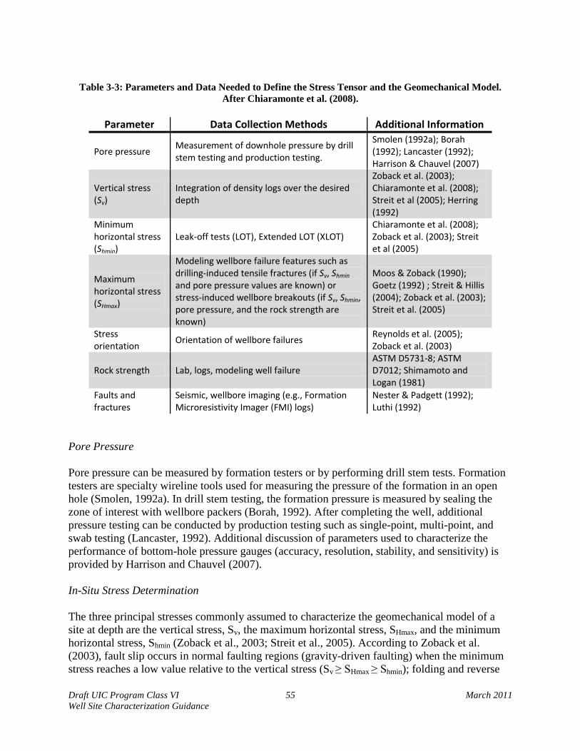
Draft UIC Program Class VI 55 March 2011 Well Site Characterization Guidance
Table 3-3: Parameters and Data Needed to Define the Stress Tensor and the Geomechanical Model.
After Chiaramonte et al. (2008).
Parameter Data Collection Methods Additional Information
Pore pressure Measurement of downhole pressure by drill stem testing and production testing.
Smolen (1992a); Borah (1992); Lancaster (1992); Harrison & Chauvel (2007)
Vertical stress (Sv)
Integration of density logs over the desired depth
Zoback et al. (2003); Chiaramonte et al. (2008); Streit et al (2005); Herring (1992)
Minimum horizontal stress (Shmin)
Leak-off tests (LOT), Extended LOT (XLOT) Chiaramonte et al. (2008); Zoback et al. (2003); Streit et al (2005)
Maximum horizontal stress (SHmax)
Modeling wellbore failure features such as drilling-induced tensile fractures (if Sv, Shmin and pore pressure values are known) or stress-induced wellbore breakouts (if Sv, Shmin, pore pressure, and the rock strength are known)
Moos & Zoback (1990); Goetz (1992) ; Streit & Hillis (2004); Zoback et al. (2003); Streit et al. (2005)
Stress orientation
Orientation of wellbore failures Reynolds et al. (2005); Zoback et al. (2003)
Rock strength Lab, logs, modeling well failure ASTM D5731-8; ASTM D7012; Shimamoto and Logan (1981)
Faults and fractures
Seismic, wellbore imaging (e.g., Formation Microresistivity Imager (FMI) logs)
Nester & Padgett (1992); Luthi (1992)
Pore Pressure
Pore pressure can be measured by formation testers or by performing drill stem tests. Formation testers are specialty wireline tools used for measuring the pressure of the formation in an open hole (Smolen, 1992a). In drill stem testing, the formation pressure is measured by sealing the zone of interest with wellbore packers (Borah, 1992). After completing the well, additional pressure testing can be conducted by production testing such as single-point, multi-point, and swab testing (Lancaster, 1992). Additional discussion of parameters used to characterize the performance of bottom-hole pressure gauges (accuracy, resolution, stability, and sensitivity) is provided by Harrison and Chauvel (2007).
In-Situ Stress Determination
The three principal stresses commonly assumed to characterize the geomechanical model of a site at depth are the vertical stress, Sv, the maximum horizontal stress, SHmax, and the minimum horizontal stress, Shmin (Zoback et al., 2003; Streit et al., 2005). According to Zoback et al. (2003), fault slip occurs in normal faulting regions (gravity-driven faulting) when the minimum stress reaches a low value relative to the vertical stress (Sv ≥ SHmax ≥ Shmin); folding and reverse
Draft UIC Program Class VI 56 March 2011 Well Site Characterization Guidance
faulting can occur in compressive stress fields when both of the horizontal stresses exceed the vertical stress and the the maximum horizontal stress is sufficiently large relative to the vertical stress (SHmax ≥ Shmin ≥ Sv); and strike-slip faulting occurs when the difference between SHmax and Shmin is sufficiently large (SHmax ≥ Sv ≥ Shmin).
The magnitude and orientation of the vertical stress, the minimum horizontal stress, and the maximum horizontal stress can be determined from drilling data and well logs. Methods for quantifying the magnitude and orientation of these principal stresses are summarized below. Vertical Stress
Vertical (orientation) stress (Sv) can be obtained from density logs (Zoback et al., 2003). The magnitude of Sv can be obtained by integrating data collected from density logs over depth. Density logs measure the bulk density of the rocks in the wellbore walls through gamma ray emissions (Chiaramonte et al., 2008; Herring 1992; Streit et al. 2005). Vertical stress at the depth of interest can be calculated by (Chiaramonte et al., 2008; Streit et al., 2005; Zoback et al., 2003)
𝑺𝒗(𝒛𝟎) = ∫ 𝝆𝐠𝒅𝒛𝒛𝟎
𝟎 Equation 3-10
where z0 is the depth of interest. In some cases (e.g., offshore wells), the analyst should account for the lower density of the water column and the transition to higher density with depth in evaluating the magnitude of vertical stress (Zoback et al., 2003). Additional editing and extrapolation of data may be necessary, for example, when borehole conditions are unfavorable and density data exhibit high levels of variability (Zoback et al., 2003).
Minimum Horizontal Stress
The magnitude of the minimum horizontal stress (Shmin) in normal and strike-slip faulting regions can be determined with considerable accuracy through direct in-situ formation stress tests (See Zoback et al., 2003). For deep wells where conventional in-situ formation stress tests are not available, information about Shmin can be collected by leak-off tests. A leak-off test is conducted by pumping into a well at a constant rate and recording the wellbore pressure as a function of cumulative volume (or time if pumped at constant rate). As described by Zoback et al. (2003), the pressure will increase linearly with volume (or time) until a distinct departure from a linear increase occurs (leak-off point or LOP). See Fig. 3-13. As pumping continues at constant rate, the maximum pressure reached is termed the formation breakdown pressure (FBP) and the pressure then falls below the FBP to a relatively constant value called the fracture pumping pressure (FPP). The FPP value should be similar to the LOP.
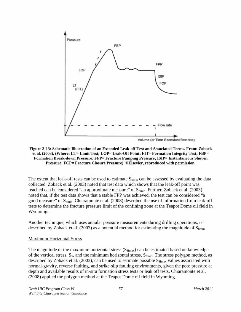
Draft UIC Program Class VI 57 March 2011 Well Site Characterization Guidance
Figure 3-13: Schematic Illustration of an Extended Leak-off Test and Associated Terms. From: Zoback
et al. (2003). (Where: LT= Limit Test; LOP= Leak-Off Point; FIT= Formation Integrity Test; FBP= Formation Break-down Pressure; FPP= Fracture Pumping Pressure; ISIP= Instantaneous Shut-in
Pressure; FCP= Fracture Closure Pressure). ©Elsevier, reproduced with permission.
The extent that leak-off tests can be used to estimate Shmin can be assessed by evaluating the data collected. Zoback et al. (2003) noted that test data which shows that the leak-off point was reached can be considered “an approximate measure” of Shmin. Further, Zoback et al. (2003) noted that, if the test data shows that a stable FPP was achieved, the test can be considered “a good measure” of Shmin. Chiaramonte et al. (2008) described the use of information from leak-off tests to determine the fracture pressure limit of the confining zone at the Teapot Dome oil field in Wyoming. Another technique, which uses annular pressure measurements during drilling operations, is described by Zoback et al. (2003) as a potential method for estimating the magnitude of Shmin.
Maximum Horizontal Stress
The magnitude of the maximum horizontal stress (SHmax) can be estimated based on knowledge of the vertical stress, Sv, and the minimum horizontal stress, Shmin. The stress polygon method, as described by Zoback et al. (2003), can be used to estimate possible SHmax values associated with normal-gravity, reverse faulting, and strike-slip faulting environments, given the pore pressure at depth and available results of in-situ formation stress tests or leak off tests. Chiaramonte et al. (2008) applied the polygon method at the Teapot Dome oil field in Wyoming.
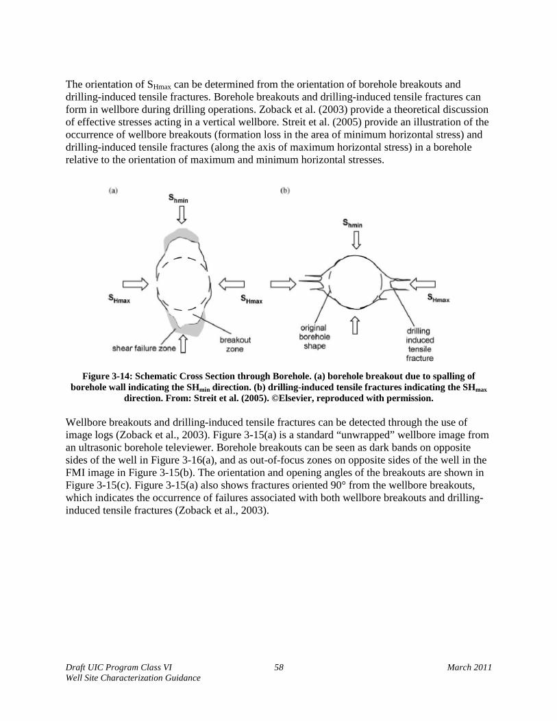
Draft UIC Program Class VI 58 March 2011 Well Site Characterization Guidance
The orientation of SHmax can be determined from the orientation of borehole breakouts and drilling-induced tensile fractures. Borehole breakouts and drilling-induced tensile fractures can form in wellbore during drilling operations. Zoback et al. (2003) provide a theoretical discussion of effective stresses acting in a vertical wellbore. Streit et al. (2005) provide an illustration of the occurrence of wellbore breakouts (formation loss in the area of minimum horizontal stress) and drilling-induced tensile fractures (along the axis of maximum horizontal stress) in a borehole relative to the orientation of maximum and minimum horizontal stresses.
Figure 3-14: Schematic Cross Section through Borehole. (a) borehole breakout due to spalling of
borehole wall indicating the SHmin direction. (b) drilling-induced tensile fractures indicating the SHmax direction. From: Streit et al. (2005). ©Elsevier, reproduced with permission.
Wellbore breakouts and drilling-induced tensile fractures can be detected through the use of image logs (Zoback et al., 2003). Figure 3-15(a) is a standard “unwrapped” wellbore image from an ultrasonic borehole televiewer. Borehole breakouts can be seen as dark bands on opposite sides of the well in Figure 3-16(a), and as out-of-focus zones on opposite sides of the well in the FMI image in Figure 3-15(b). The orientation and opening angles of the breakouts are shown in Figure 3-15(c). Figure 3-15(a) also shows fractures oriented 90° from the wellbore breakouts, which indicates the occurrence of failures associated with both wellbore breakouts and drilling-induced tensile fractures (Zoback et al., 2003).
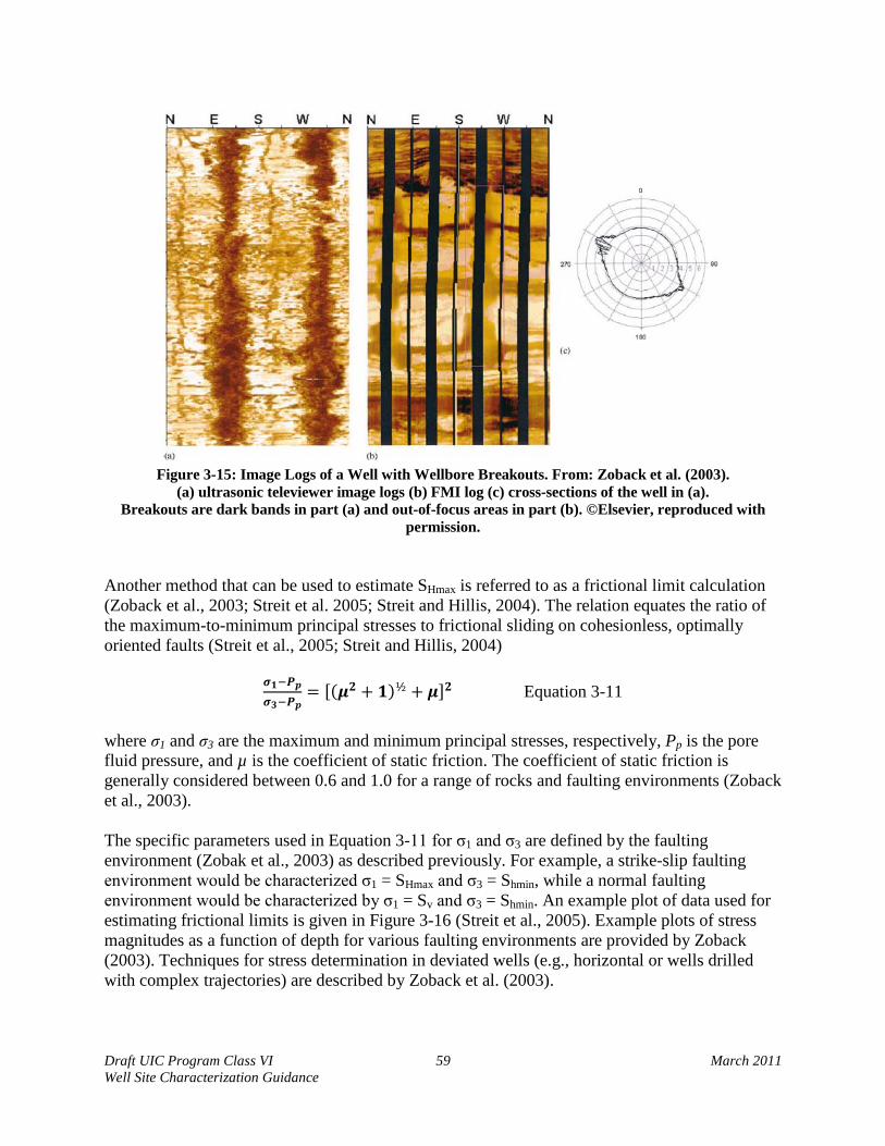
Figure 3-15: Image Logs of a Well with Wellbore Breakouts. From: Zoback et al. (2003).
(a) ultrasonic televiewer image logs (b) FMI log (c) cross-sections of the well in (a). Breakouts are dark bands in part (a) and out-of-focus areas in part (b). ©Elsevier, reproduced with
permission.
Another method that can be used to estimate SHmax is referred to as a frictional limit calculation (Zoback et al., 2003; Streit et al. 2005; Streit and Hillis, 2004). The relation equates the ratio of the maximum-to-minimum principal stresses to frictional sliding on cohesionless, optimally oriented faults (Streit et al., 2005; Streit and Hillis, 2004)
𝝈 −𝑷 = [(𝝁 +
𝝈𝟏 𝒑
𝟑−𝑷𝒑𝟐 𝟏)½ + 𝝁]𝟐 Equation 3-11
where σ1 and σ3 are the maximum and minimum principal stresses, respectively, Pp is the pore fluid pressure, and µ is the coefficient of static friction. The coefficient of static friction is generally considered between 0.6 and 1.0 for a range of rocks and faulting environments (Zoback et al., 2003).
The specific parameters used in Equation 3-11 for σ1 and σ3 are defined by the faulting environment (Zobak et al., 2003) as described previously. For example, a strike-slip faulting environment would be characterized σ1 = SHmax and σ3 = Shmin, while a normal faulting environment would be characterized by σ1 = Sv and σ3 = Shmin. An example plot of data used for estimating frictional limits is given in Figure 3-16 (Streit et al., 2005). Example plots of stress magnitudes as a function of depth for various faulting environments are provided by Zoback (2003). Techniques for stress determination in deviated wells (e.g., horizontal or wells drilled with complex trajectories) are described by Zoback et al. (2003).
Draft UIC Program Class VI 59 March 2011 Well Site Characterization Guidance

Draft UIC Program Class VI 60 March 2011 Well Site Characterization Guidance
Figure 3-16: Example Plot of Data Used for Estimating Frictional Limits (Petrel Sub-Basin, Australia). From Streit et al. (2005). Shmin estimates are derived from pressure leak-off tests, and Sv estimates were
obtained by examining density logs. R values are Pearson correlation coefficients. Vertical axis is meters. ©Elsevier, reproduced with permission.
The orientation of borehole breakouts and tensile fractures (Figure 3-15) can be determined from image logs and four-arm caliper logs. Six-arm caliper logs are also available, which may be able to provide more accurate and detailed data on borehole breakouts if four-arm caliper logs are not sufficient. Formation microresistivity imager (FMI) logs generate an electrical image of the borehole from microresistivity measurements, which penetrates about 30 in. from the wellbore. FMI data are used to identify drilling-induced features and breakouts (Schlumberger, 2002). An application using FMI logs for the analysis of tensile fractures was described by Chiaramonte et al. (2008). Caliper logs (two-, three-, four-, or six-arm) can measure the enlargement of boreholes in the presence of natural fractures (Aguilera 1992). Choosing a caliper log with a greater number of arms can increase the accuracy and level of detail in the resulting data. Breakout and tensile fracture data collected at depth from various wells can be used to develop stress maps such as those shown in Figure 3-17.

Draft UIC Program Class VI 61 March 2011 Well Site Characterization Guidance
Figure 3-17: Example of a Regional Stress Map based on the orientation of wellbore breakouts in
Paleozoic rocks the Western Canada Sedimentary Basin near Calgary. Modified after (Bell et al., 1994) ©Alberta Geological Survey. Reproduced with permission from the AGS.

Draft UIC Program Class VI 62 March 2011 Well Site Characterization Guidance
3.6.3. Data Use and Interpretation
This section discusses how data are used to assess geomechanical characteristics of the site and to predict the geomechanical effects of carbon dioxide injection on fault stability, reservoir rock stability, and confining zone integrity. Assessment of fault stability requires knowledge of fault geometries, which can be obtained from the structural interpretation of seismic data as discussed in Section 3.7.2 of this guidance document. This section includes descriptions of three methods that can be used to develop these geomechanical predictions. Failure Plots
Failure plots (Figure 3-18) can be used to identify faults within a carbon dioxide storage reservoir that are relatively stable as a function of fault angle. Failure plots are developed by plotting differential stress (i.e., the difference between the maximum and minimum principal stresses, σ1 - σ3) versus fault angle and thus identifying conditions that permit fault reactivation (failure) versus formation of new fractures (or relatively stable fault conditions) (Streit et al., 2005). Streit (1999) described the method for constructing failure plots for various rock types and fault strengths. Although the failure plot method has been applied to study sites for carbon dioxide storage, 3D methods also should be used to estimate fault slip tendency (Streit et al., 2005).
Figure 3-18: Example Failure Plots Indicating Scenarios where Fault Reactivation is Possible.
From: Streit et al. (2005). ©Elsevier, reproduced with permission.
3D Fault Slip Tendency
The parameter referred to as the slip tendency (Ts) value can be used to assess the potential for reactivating a fault associated with carbon dioxide injection by Equation 3-12 (Streit and Hillis, 2004).
𝑻𝒔 = 𝝉
𝝈𝒏−𝑷𝒇 Equation 3-12
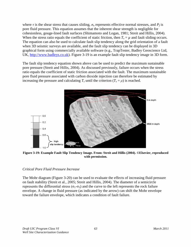
Draft UIC Program Class VI 63 March 2011 Well Site Characterization Guidance
where τ is the shear stress that causes sliding, σn represents effective normal stresses, and Pf is pore fluid pressure. This equation assumes that the inherent shear strength is negligible for cohesionless, gouge-lined fault surfaces (Shimamoto and Logan, 1981; Streit and Hillis, 2004). When the stress ratio equals the coefficient of static friction, then Ts = µ and fault sliding occurs. The equation can also be used to calculate fault slip tendency along the grid orientation of a fault when 3D seismic surveys are available, and the fault slip tendency can be displayed in 3D graphical form using commercially available software (e.g., TrapTester, Badley Geoscience Ltd, UK, http://www.badleys.co.uk). Figure 3-19 is an example fault slip tendency image in 3D form. The fault slip tendency equation shown above can be used to predict the maximum sustainable pore pressure (Streit and Hillis, 2004). As discussed previously, failure occurs when the stress ratio equals the coefficient of static friction associated with the fault. The maximum sustainable pore fluid pressure associated with carbon dioxide injection can therefore be estimated by increasing the pressure and calculating Ts until the criterion (Ts = μ) is reached.
Figure 3-19: Example Fault Slip Tendency Image. From: Streit and Hillis (2004). ©Elsevier, reproduced
with permission. Critical Pore Fluid Pressure Increase
The Mohr diagram (Figure 3-20) can be used to evaluate the effects of increasing fluid pressure on fault stability (Streit et al., 2005; Streit and Hillis, 2004). The diameter of a semicircle represents the differential stress (σ1-σ3) and the curve to the left represents the rock failure envelope. A change in fluid pressure (as indicated by the arrow) can shift the Mohr envelope toward the failure envelope, which indicates a condition of fault failure.
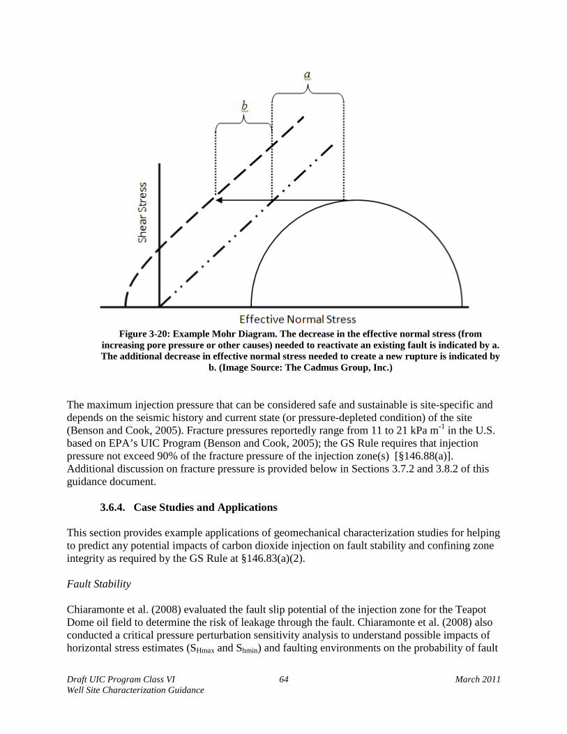
Draft UIC Program Class VI 64 March 2011 Well Site Characterization Guidance
Figure 3-20: Example Mohr Diagram. The decrease in the effective normal stress (from
increasing pore pressure or other causes) needed to reactivate an existing fault is indicated by a. The additional decrease in effective normal stress needed to create a new rupture is indicated by
b. (Image Source: The Cadmus Group, Inc.)
The maximum injection pressure that can be considered safe and sustainable is site-specific and depends on the seismic history and current state (or pressure-depleted condition) of the site (Benson and Cook, 2005). Fracture pressures reportedly range from 11 to 21 kPa m-1 in the U.S. based on EPA’s UIC Program (Benson and Cook, 2005); the GS Rule requires that injection pressure not exceed 90% of the fracture pressure of the injection zone(s) [§146.88(a)]. Additional discussion on fracture pressure is provided below in Sections 3.7.2 and 3.8.2 of this guidance document.
3.6.4. Case Studies and Applications
This section provides example applications of geomechanical characterization studies for helping to predict any potential impacts of carbon dioxide injection on fault stability and confining zone integrity as required by the GS Rule at §146.83(a)(2). Fault Stability
Chiaramonte et al. (2008) evaluated the fault slip potential of the injection zone for the Teapot Dome oil field to determine the risk of leakage through the fault. Chiaramonte et al. (2008) also conducted a critical pressure perturbation sensitivity analysis to understand possible impacts of horizontal stress estimates (SHmax and Shmin) and faulting environments on the probability of fault

Draft UIC Program Class VI 65 March 2011 Well Site Characterization Guidance
slip potential. Their study illustrates the potential for using geomechanical modeling to estimate the pore pressure required for a fault to slip during a GS project. Gibson-Poole et al. (2008) summarized a geomechanical assessment of a basin-scale carbon dioxide geological storage system in southeast Australia. Using data and information regarding the site’s rock strength, in situ stresses and fault orientation, Gibson-Poole et al. (2008) estimated the maximum sustainable pore pressure and risk of fault reactivation. Results showed large variability due to data uncertainties. Additional work (e.g., laboratory testing of tensile and compressive core strength) was therefore recommended to reduce uncertainties and thereby constrain the geomechanical model.
Rutqvist et al. (2007) demonstrated the use of two numerical modeling approaches for analyzing geomechanical fault slip (i.e., continuum stress-strain analysis and discrete fault analysis) coupled with fluid flow to estimate the maximum sustainable injection pressure during geological sequestration of carbon dioxide. The results of these two numerical approaches were compared to conventional analytical fault-slip analysis. The authors concluded that the numerical methods provided a more accurate estimation of the maximum sustainable carbon dioxide injection pressure than the conventional analytical method because the numerical models can better account for the spatial evolution of both in situ stresses and fluid pressure. Confining Zone Integrity
Haug et al. (2007) described a geomechanical characterization of a potential carbon dioxide injection site at an existing oil and gas field in Alberta, Canada, which included determination of the principal stresses (Sv, SHmax, Shmin) and discussion of laboratory testing determinations of rock strength and deformation behavior. The study also included a sensitivity analysis regarding potential success for carbon dioxide containment based on data variability. The authors concluded that laboratory triaxial tests should be conducted to confirm the accuracy of the correlations.
Smith et al. (2009) described the program components of geomechanical testing and modeling of reservoir and confining zone integrity for a carbon dioxide sequestration project at an existing oil and gas field in Alberta, Canada. This work described the overall geomechanical workflow process and provided specific examples of log-derived rock strength and elastic properties, cores used for geomechanical testing, stress versus strain data measured on cores, linear Mohr-Coulomb failure envelopes, rock strength measurements, and uniaxial pore volume compressibility tests. In situ stresses, formation pressures and mechanical properties were input into a finite-differences-based geomechanical simulator to predict conditions leading to deformation of reservoir and confining zone, induced stresses, and to assess the propensity for fault reactivation and movements.
Orlic (2009) discussed the impacts of geomechanical changes in a reservoir associated with pressure depletion and rock compression during hydrocarbon production. Computational modeling examples were used to illustrate the mechanical impact of carbon dioxide injection on confining zone integrity, fault stability, and well integrity. This study illustrates the use of
Draft UIC Program Class VI 66 March 2011 Well Site Characterization Guidance
computational modeling for predicting effects of carbon dioxide injection on containment capacity of the reservoir, taking into account previous stresses from depletion.
Rutqvist and Tsang (2002) demonstrated the use of computational modeling to study the geomechanical effects of injecting carbon dioxide into a hypothetical sandstone formation. The authors provided discussion of the rock and fluid input parameters and simulation results assuming a homogeneous confining zone without intersecting fracture zone, and the effects of a vertical fracture zone in the confining zone. The analysis provided a better understanding of possible mechanisms affecting geomechanical changes associated with carbon dioxide injection processes.
3.6.5. Special Considerations – Processes Affecting Geomechanical Properties of
the Injection Zone and Confining Zone
This section provides additional discussion regarding impacts of historical production and geochemical processes that can potentially affect the geomechanical properties of the injection zone and confining zone. Effects of Pre-Production Changes in Stress
The geomechanical features of an injection zone can be altered if the reservoir was previously used for the extraction of hydrocarbon products. Movement along faults can be produced in a hydrocarbon field by induced changes in the stress regime. This can happen when fluid pressures are substantially depleted during hydrocarbon extraction (Streit and Hillis, 2004). If pore collapse has occurred, then it might not be possible to return a pressure-depleted field to its original pore pressure without the risk of induced failure. Thus, the geomechanical characterization of a potential carbon dioxide site should address possible effects of pressure depletion, if applicable. The estimated total volume of carbon dioxide that can be stored in a pressure-depleted field could be less than otherwise estimated as well. This possible effect of pressure-depleted reservoirs on storage capacity is discussed in Section 3.9 of this guidance document. Keep in mind, however, that not all proposed carbon dioxide injection sites will have been previously used for oil and gas production, and site characterization data collection needs to be site specific.
Effects of In-situ Geochemical Processes
Coupled geomechanical-geochemical modeling may be needed to document fracture sealing by precipitation of carbonates in fractures or pores. Modeling these processes will require knowledge of the geomechanical parameters and relations as discussed above as well as geochemical processes. Discussion of these coupled reactions and implications for carbon dioxide storage is discussed by Johnson et al. (2005). Application of this methodology at a regional scale is documented by Gibson-Poole et al. (2002), and discussion of effects of geomechanical processes on long-term cap rock interactions and potential cap rock and fault leakage pathways is provided by Gaus (2010).

Draft UIC Program Class VI 67 March 2011 Well Site Characterization Guidance
3.7. Geophysical Characterization Geophysical methods gather information about subsurface features in lieu of physically sampling the region of interest. Depending upon the scale and resolution of the investigation, geophysical methods may help to provide the required information on the stratigraphy, structure, extent, thickness, porosity, and permeability of subsurface units to be submitted to the UIC Program Director with a Class VI injection well permit application [§§146.82(a)(1) through 146.82(a)(21)] There are four main types of geophysical methods: seismic, gravity, magnetic, and electrical/electromagnetic. These methods can image a large volume of the subsurface without penetrations (i.e. wells or boreholes). EPA recommends these methods as they can provide good spatial coverage of a project area and may be especially useful in regions where subsurface geology is heterogeneous and/or wells are sparse. Geophysical methods are widely used for subsurface exploration and characterization in the hydrocarbon industry, archeology, engineering, and other fields. Methods used to characterize sites for carbon dioxide storage will not differ substantially from methods used to characterize subsurface geology for other purposes. The choice of storage formation (e.g. depleted reservoir, coal seam, saline formation, etc.) will not likely strongly influence the suitability of geophysical techniques. Site-specific considerations such as depth, geologic complexity, and overlying lithologies are more likely to influence the choice of methodology. Two notable exceptions to this generalization are seismic methods, which may be hampered in depleted gas reservoirs, and gravity methods, which work especially well in most thick, brine-filled formations. The need to characterize features at depth is likely to be the most uniformly limiting factor in selecting an appropriate geophysical method for site characterization. Most carbon dioxide is likely to be stored at a depth of at least 800-1000 m, depending on site specific conditions, and resolution at depth various greatly between techniques and among different deployment techniques within the same method. Geophysical methods used primarily to image the shallow subsurface (e.g. ground penetrating radar, shallow seismic refraction, etc.) are not discussed in this section. Data collected for a baseline geophysical survey will also serve as the reference point for future monitoring as required at 146.90(g)(2) and as described in the Draft UIC Class VI Well Testing and Monitoring Guidance.
3.7.1. Overview of Geophysical Techniques Data gathered with geophysical techniques may aid in the creation of geologic maps and cross-sections that illustrate the regional geology, hydrogeology, and geologic structure. Table 3-4 summarizes the types of data produced by the various methods. Geophysical methods are also required later in the operations phase of a Class VI injection well for monitoring of the location and extent of the carbon dioxide plume [§146.90(g)(2)]. Surveys conducted for site characterization purposes may be applicable as baseline monitoring surveys, saving costs by eliminating duplicative efforts. Table 3-5 summarizes which geophysical techniques may be applied during various phases of a carbon dioxide sequestration project.

Draft UIC Program Class VI 68 March 2011 Well Site Characterization Guidance
The different geophysical methods vary in quality, cost, the surface and subsurface environments in which they can be used, and the types of data they produce. For example, unlike other geophysical methods, seismic data may allow estimates of pore pressure in the injection formation, confining zone(s), and other zones. EPA recommends that selection of methods be made based on site characteristics and the desired level of detail. Owners and operators may keep in mind that because these methods produce indirect measurements (i.e. without taking a physical sample), data processing may introduce errors. Lithology and rock properties cannot be determined solely using geophysical data. Data gathered from geophysical surveys can indicate certain lithologies but are not conclusive. Information from stratigraphic wells, columns, or other sources is required to be submitted to the UIC Program Director with a Class VI injection well permit application. These can help to confidently assign rock types and properties to formations imaged using geophysical methods. Some of the required materials (e.g., maps and cross sections, available field data such as well logs) may help in interpreting geophysical data [146.82(a)]. Regardless of the geophysical method type, aerial, surface, and borehole deployments of each method are typically available. There are common advantages and disadvantages to each.
• Aerial surveys can cover large areas at low cost, they require no site preparation, and they can be conducted over large areas, but they often produce surveys of lower resolution than those produced by surface or borehole methods.
• Surface methods offer higher resolution in most situations and still offer coverage over a
large areal extent. However, cost may be problematic, especially in areas with topographic relief, infrastructure, and/or sensitive cultural or environmental attributes.
• Borehole methods often offer the highest resolution and can also often be acquired at a
low cost. However, they do not image a large volume of the subsurface and they depend upon subsurface penetrations that cross the formations of interest.
For all survey types, increasing the density of measurements, sources, or receivers will generally increase the quality of the survey but will also increase cost.
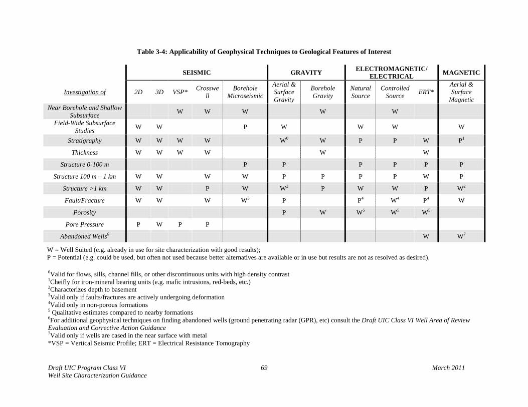
Draft UIC Program Class VI 69 March 2011 Well Site Characterization Guidance
Table 3-4: Applicability of Geophysical Techniques to Geological Features of Interest
SEISMIC GRAVITY ELECTROMAGNETIC/ ELECTRICAL MAGNETIC
Investigation of 2D 3D VSP* Crosswell
Borehole Microseismic
Aerial & Surface Gravity
Borehole Gravity
Natural Source
Controlled Source ERT*
Aerial & Surface
Magnetic Near Borehole and Shallow
Subsurface W W W W W
Field-Wide Subsurface Studies W W P W W W W
Stratigraphy W W W W W0 W P P W P1
Thickness W W W W W W
Structure 0-100 m P P P P P P
Structure 100 m – 1 km W W W W P P P P W P
Structure >1 km W W P W W2 P W W P W2
Fault/Fracture W W W W3 P P4 W4 P4 W
Porosity P W W5 W5 W5
Pore Pressure P W P P
Abandoned Wells6 W W7
W = Well Suited (e.g. already in use for site characterization with good results); P = Potential (e.g. could be used, but often not used because better alternatives are available or in use but results are not as resolved as desired). 0Valid for flows, sills, channel fills, or other discontinuous units with high density contrast 1Cheifly for iron-mineral bearing units (e.g. mafic intrusions, red-beds, etc.) 2Characterizes depth to basement 3Valid only if faults/fractures are actively undergoing deformation 4Valid only in non-porous formations 5 Qualitative estimates compared to nearby formations 6For additional geophysical techniques on finding abandoned wells (ground penetrating radar (GPR), etc) consult the Draft UIC Class VI Well Area of Review Evaluation and Corrective Action Guidance 7Valid only if wells are cased in the near surface with metal *VSP = Vertical Seismic Profile; ERT = Electrical Resistance Tomography

Draft UIC Program Class VI 70 March 2011 Well Site Characterization Guidance
Table 3-5: Stages in a Geologic Sequestration Project where Geophysical Techniques May Be Applicable
SEISMIC GRAVITY ELECTROMAGNETIC/ELECTRICAL MAGNETIC
APPLICABLE DURING 2D
3D
VSP
Cros
swel
l
Bore
hole
Mic
rose
ism
ic
Aeria
l & S
urfa
ce G
ravi
ty
Bore
hole
Gra
vity
Natu
ral S
ourc
e
Cont
rolle
d So
urce
ERT
Aeria
l & S
urfa
ce M
agne
tic
Preliminary Investigation X X X X X
Site Characterization X X X X X X X X
Injection & Monitoring X X X X X X X X
3.7.2. Seismic Methods A seismic survey uses seismic waves to produce 2D sections or 3D images of the subsurface. Both seismic reflection and seismic refraction techniques are also available. Refraction techniques, however, do not have the resolving power of reflection methods and do not work well in non-horizontal strata. The remainder of this section focuses on reflection techniques. More information on refraction techniques is available in “An Introduction to Geophysical Exploration” (Kearey et al., 2002). Seismic reflection techniques measure time delay it takes for seismic waves emitted from a source to bounce off a subsurface reflector and be detected at a geophone. This method is by far the most established, commonly deployed, varied, and advanced of the geophysical methods. More detailed information on seismic methods and processing is available from numerous sources, including introductory guides such as: A Handbook for Seismic Data Acquisition (Evans, 1997), Environmental Geology – A Handbook (Knödel et al., 2007), and An Introduction to Geophysical Education (Kearey et al., 2002). Different source/receiver deployment configurations can be used to maximize data quality depending on terrain and other factors (see Short, 1992 for more details). Newer, fully portable (cableless) data acquisition systems are also available (Criss, 2007) and may be used in regions with surface infrastructure and/or rough terrain. Seismic reflection systems are recognized as having the highest resolution of all geophysical imaging techniques in most situations (Benson and Myer, 2002). Seismic methods work best when characterizing simple, homogenous geologic settings where supplementary sources of data such as well logs, outcrop data, and other geophysical surveys are available. Increasing

Draft UIC Program Class VI 71 March 2011 Well Site Characterization Guidance
subsurface complexity may increase survey cost or decrease the resolution of survey results. Areas with accumulations of loose sediments such as thick sands or unconsolidated sandstones, conglomerates, well sorted gravels, or weathered horizons are challenging to image and may require more detailed consideration of seismic source and detector (see Short, 1992 or Knödel et al., 2007 for further information on selecting a proper seismic source). Seismic surveys are also complicated by noise contamination from roads, airports, railroads, mines, and other human activities that cause mechanical vibration. Difficulty also increases when imaging through salts, basalts, coal seams, carbonates, and non-sedimentary units (Cooper, 2009; Hyne, 2001). Non-clastic rocks (i.e. metamorphic or igneous rocks) and coal seams cannot be imaged well. If such lithologies are present in the area of interest, seismic data may need to be supplemented with additional data. For example, if salt bodies are present, gravity data can be co-analyzed with seismic data to accurately determine their size and location (Nester and Padgett, 1992). Basalts pose a problem for seismic methods because traditional seismic approaches have resulted in severe energy scattering and wave interference. Some success has been reported in imaging basalts using multicomponent systems (see below) and wave component analysis (Sullivan et al., 2008). Carbonates often have minimal changes in seismic properties even when there are changes in texture, permeability, and porosity. High quality surveys, multicomponent methods, or other additional data collection steps may be needed to obtain sufficient accuracy and resolution in difficult environments. Both surface and subsurface seismic methods can use additional wave types to improve data quality. Most seismic data acquisition systems collect only p-wave (compressional wave) data unless otherwise specified, usually in 2 vibrational directions (called components). Other seismic wave types and components may also be collected to improve survey results. Special sources, receivers, and recording capacity are usually the only changes required to modify a seismic survey for additional wave types. Geophones that measure additional seismic components (such as direction of vibration) may also be added. The main disadvantage of these methods is that they increase cost and processing time and are not as well-developed as standard approaches. Wave choice depends largely on subsurface geology. P-waves remain the best option for imaging bulk changes such as porosity. However, p-waves are distorted by gases in rock. In such cases, shear waves (s-waves), which are not distorted by subsurface gases, can be used (Thompson, 2005). This may be advantageous when characterizing some depleted gas reservoirs for carbon dioxide storage. S-waves are also appropriate for heavily faulted or fractured sites due to their greater sensitivity to continuous features such as fractures. Stoneley waves can help to identify fractures and changes in permeability (Cheng, 1992). Because s-waves provide information in the waveform as well as in the arrival time of the wave, a smaller number of geophones may be needed to gather the same amount of information, reducing cost. S-waves can also help improve seismic pore-pressure prediction. S-wave data can aid in determining which seismic velocity variations are due to variations in fluid content and which are due to variations in fluid pressure (Sayers et al., 2000). In complex areas such as shallow, grossly undercompacted sediments, zones of severe unloading with minimal effective stress, and areas near gas chimneys and clouds, s-wave data may also help improve results (Huffman, 2002; Thompson, 2005).
Draft UIC Program Class VI 72 March 2011 Well Site Characterization Guidance
S-wave seismic surveys were successfully used at the West Pearl Queen pilot in New Mexico for both site characterization and baseline monitoring data (Pawar et al., 2006). Seismic Deployments Seismic data can be collected with many different source/receiver configurations. Deployment can be done on the surface, in boreholes, or in a combination of both. 2D and 3D seismic profiling are the leading options available for surface-based seismic imaging. 2D surveys produce “slices” of the subsurface while 3D surveys produce subsurface models that can be rotated and viewed from different perspectives. 2D seismic surveys are cheaper than 3D surveys because they require less site preparation, shooting time, and post-collection data processing. The chief disadvantage of 2D imaging is that because it is collected in a line on the surface, it is difficult to determine the location of out-of-plane features. Therefore, 2D surveys are not optimal in settings where significant lateral heterogeneity is expected (e.g. areas with salt domes, intrusions, or where sedimentary layers are expected to thin or thicken). Application of 2D seismic profiling may also be problematic in faulted regions, where the choice of line orientation is more critical to capture faults. 3D surveys are preferable to 2D surveys when characterizing sites with complex or variable subsurface geology, where subsurface geology is not well constrained, where improved resolution is required, or where high well costs require greater certainty in subsurface characterization. 2D seismic surveys were used for site characterization and baseline data at the Sleipner project in the North Sea (Hellevang et al., 2005). The Weyburn project in Saskatchewan, Canada also used 2D seismic lines for site characterization and as baseline measurements (Wilson and Monea, 2004). 3D seismic surveys were used for both site characterization and as baseline data at the carbon dioxide storage pilot project at Ketzin, Germany (CO2SINK) and for site characterization at the Kallirachi oil field in Greece, which is being considered for EOR/carbon dioxide storage (Koukouzas et al., 2009). A larger number of down-hole seismic techniques are available. Vertical seismic profiles (VSPs) are the most common borehole seismic method. A VSP is conducted with one component located on the surface (usually the source) and the remaining component placed downhole. A VSP can be conducted in a vertical or deviated well to a depth of at least 3,000 m (Balch et al., 1982). The source may be directly adjacent to the borehole or, for an offset VSP, located at a fixed distance away. A VSP can resolve features 3-4.5 m in size or smaller. A VSP can also help increase the resolution and accuracy of other seismic surveys. First, a VSP can provide an accurate determination of the seismic velocity within the area of interest (seismic refraction techniques can also provide this information in simple geologic settings). This determination can help with seismic migration and pore pressure estimation. A VSP can also help confirm the depth at which upgoing reflections are generated, which can be used to link geology derived from other bore logs to seismic attributes (Kearey et al., 2002). Crosswell seismic methods deploy sources and receivers in different wells, producing a survey that images the plane between the wells. The Ketzin project used crosswell surveys and VSP surveys for site characterization and baseline monitoring data. Crosswell surveys between multiple wells can be used to produce a fence diagram. Equipment is generally deployed in

monitoring wells located with 500 m of each other (Hoversten et al., 2002), although deployment down active injection wells is also possible (Daley et al., 2007). Crosswell seismic surveys combine most of the advantages of VSP with additional lateral extent. Crosswell seismic profiling can achieve a maximum resolution of 3 m (Harris and Langan, 1997), which may provide data 10-100 times more detailed than surface seismic data (Martin et al., 2002). Crosswell seismic profiling may also be the best option available for imaging thin beds. The data can be used to fill the resolution gap between high-resolution well cores and 3D surface data (Washbourne and Bube, 1998) or to help correlate structures between well bores. However, because of the need for multiple wells, crosswell seismic profiling will not be suitable in areas that do not already have abundant subsurface penetrations. Furthermore, the distribution of wells will determine the potential planes for crosswell imaging. These orientations may not be optimal for imaging the relevant features. Crosswell imaging was used successfully for both site characterization and baseline monitoring at the Nagaoka pilot project in Japan, which injected and monitored 0.01 Mt of carbon dioxide. The borehole microseismic method relies completely on subsurface deployment and uses passive seismic energy. A string of geophones is deployed down a monitoring well and used to sense seismic events, typically on the order of -3 to -1 on the Richter scale. Microseismic events can be detected up to 1 km from the well on average (Downie et al., 2009). The period of data collection is variable and depends upon the frequency of seismic events, but typically lasts from several weeks to several months. This is disadvantageous compared to other seismic methods that collect data over a period of hours. Generally, the greater number of microseismic events, the more accurate the result. After collection, the hypocenters of the seismic events are projected onto a subsurface map to image fracture networks, faults, and other regions actively undergoing strain or deformation. The quality of the geologic model used to transform the time data and locate each hypocenter largely controls the accuracy of the result (Warpinski, 2009). Processing of Seismic Data Post-collection processing techniques provide control over the final quality of the survey and its applicability to the project site characterization. In some cases, old data may even be re-processed with newer techniques to uncover additional information. Choice of processing techniques will largely depend on site-specific factors other than the type of carbon dioxide storage reservoir being investigated. For example, certain types of processing (such as pre-stack migration) are more appropriate in regions where steep faults or other features are antipicated (such as near salt domes). Seismic processing techniques are immensely varied; the following is an overview. For more detailed information, a number of handbooks on seismic processing are available (e.g., Upadhyay, 2004). If information about faults or other discontinuities in the subsurface is desired, special processing techniques can be used to mine the data for this information. Seismic crustal anisotropy processing can be used in areas where aligned fractures, joints, or fluid inclusions recur in the subsurface at a distance smaller than the wavelength of the seismic wave. As the wave passes
Draft UIC Program Class VI 73 March 2011 Well Site Characterization Guidance

Draft UIC Program Class VI 74 March 2011 Well Site Characterization Guidance
through such a region, the wave is split into two waves with different polarization and velocities (Crampin and Lovell, 1991), in a manner similar to the effects of diffraction gratings on light waves. Studying the split waves can reveal information about the magnitude, consistency, and orientation of recurring subsurface features. Alternatively, p-wave data can be processed with a technique called p-wave amplitude variation with offset and azimuth (abbreviated pAVAZ or pAVOA) (Gray et al., 2002) to reveal information about fracture and pore orientations. However, these techniques are not fully developed and increase processing costs. These techniques may have the potential to be adapted to image cleats and other discontinuities common in coal seams or columnar joint in basaltic flows if either type of formation is used as a potential carbon dioxide reservoir. Coherence processing can be used to detect faults. This method suppresses continuous features and highlights discontinuities, such as faults, within seismic sections. Figure 3-21 compares coherence and normal processing in a faulted region. Although discontinuities in high-quality seismic data are often indicative of faults and lithologic breaks, discontinuities in low-quality seismic data may be due to a range of data collection and processing errors. As a result, coherence is very sensitive to the quality of input seismic data and is not suitable for low-quality surveys.
Figure 3-21: The Top Half of a Seismic Image over a Salt Dome. Processed with a coherence technique,
while the bottom half was processed normally. From: Brown (2001), AAPG Explorer, AAPG©2001 reprinted by permission of the AAPG whose permission is required for further use.
Other advanced processing techniques, such as difference analysis with data normalization (DADN) (Onishi et al., 2009) are also available but are not covered in this Guidance.
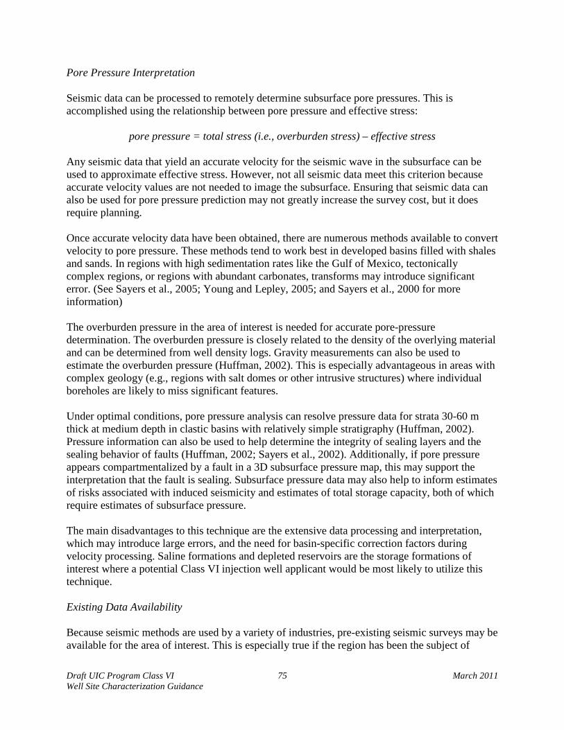
Draft UIC Program Class VI 75 March 2011 Well Site Characterization Guidance
Pore Pressure Interpretation Seismic data can be processed to remotely determine subsurface pore pressures. This is accomplished using the relationship between pore pressure and effective stress:
pore pressure = total stress (i.e., overburden stress) – effective stress
Any seismic data that yield an accurate velocity for the seismic wave in the subsurface can be used to approximate effective stress. However, not all seismic data meet this criterion because accurate velocity values are not needed to image the subsurface. Ensuring that seismic data can also be used for pore pressure prediction may not greatly increase the survey cost, but it does require planning. Once accurate velocity data have been obtained, there are numerous methods available to convert velocity to pore pressure. These methods tend to work best in developed basins filled with shales and sands. In regions with high sedimentation rates like the Gulf of Mexico, tectonically complex regions, or regions with abundant carbonates, transforms may introduce significant error. (See Sayers et al., 2005; Young and Lepley, 2005; and Sayers et al., 2000 for more information) The overburden pressure in the area of interest is needed for accurate pore-pressure determination. The overburden pressure is closely related to the density of the overlying material and can be determined from well density logs. Gravity measurements can also be used to estimate the overburden pressure (Huffman, 2002). This is especially advantageous in areas with complex geology (e.g., regions with salt domes or other intrusive structures) where individual boreholes are likely to miss significant features. Under optimal conditions, pore pressure analysis can resolve pressure data for strata 30-60 m thick at medium depth in clastic basins with relatively simple stratigraphy (Huffman, 2002). Pressure information can also be used to help determine the integrity of sealing layers and the sealing behavior of faults (Huffman, 2002; Sayers et al., 2002). Additionally, if pore pressure appears compartmentalized by a fault in a 3D subsurface pressure map, this may support the interpretation that the fault is sealing. Subsurface pressure data may also help to inform estimates of risks associated with induced seismicity and estimates of total storage capacity, both of which require estimates of subsurface pressure. The main disadvantages to this technique are the extensive data processing and interpretation, which may introduce large errors, and the need for basin-specific correction factors during velocity processing. Saline formations and depleted reservoirs are the storage formations of interest where a potential Class VI injection well applicant would be most likely to utilize this technique. Existing Data Availability Because seismic methods are used by a variety of industries, pre-existing seismic surveys may be available for the area of interest. This is especially true if the region has been the subject of
Draft UIC Program Class VI 76 March 2011 Well Site Characterization Guidance
hydrocarbon or other mineral exploration. Depleted reservoirs are much more likely than saline formations, coal seams, or other formations to have pre-existing seismic data available. Existing seismic data will most likely be 2D. Some seismic data may also be available for free from government agencies, but the quality of these data may be low. Processing methods for seismic data have improved greatly in recent years, and reprocessing vintage raw data can lead to improved resolution or identification of features not identified in the original survey (Hyne, 2001).
3.7.3. Gravity Methods Gravity-based methods image differences in density among subsurface materials. Because density is related to gravity, changes in the distribution of fluids, cementation, and porosity of subsurface materials can be measured as changes in gravity. Gravity data can be collected from land based stations, aerially, or directly from the subsurface using boreholes. Choice of deployment is usually controlled by factors such as cost, desired resolution, and site-specific geology and not limited by choice of carbon dioxide storage formation type. Gravity is measured with a gravimeter; information on how measurements are obtained can be found in Paterson and Reeves (1985). Figure 3-22 is an example of a typical surface deployment pattern.
Figure 3-22: A Gravity Map of an Area an Ore Deposit and Mine From Yarger and Jarjur, 1972. Reproduced with permission from the KGS.

Draft UIC Program Class VI 77 March 2011 Well Site Characterization Guidance
Because detection of faults and structural features using gravity data depends upon contrasts in density, gravity methods work best in basins with varied lithologies. Salt domes and igneous intrusions are the easiest types of lithologic features to image because they usually have a high density contrast with surrounding formations. Figure 3-22 illustrates the gravity anomaly associated with an ore deposit and mine. Faults may be detected with gravity data if units with contrasting density or regions with different sedimentary thicknesses are juxtaposed. Small faults or faults with large displacement occurring in discrete steps are more difficult to detect with gravity data than large planar faults. Vertical faults are especially difficult to detect using surface gravity methods (Barbosa et al., 2007). Because gravity measurements are not unique to specific lithologies, additional data from other types of geophysical surveys or other sources (e.g., boreholes, outcrops) can greatly improve the interpretation of gravity data (Jordan and Hare, 2002). One advantage of gravity data compared to seismic data is that because processing of gravity data is much more straightforward, it generally introduces much less interpretive error. Aerial and Surface Gravity Methods For aerial methods, data are typically collected along parallel lines in the area of interest. Closer spacing will generally increase resolution. For surface deployments, measurements are typically taken at discrete stations across the area of investigation. Coarse gravity surveys may suffice for detecting large-scale changes in the thickness of basin fill and other basin-wide features, while more detailed surveys will be needed to detect finer features such as the distribution and thickness of specific formations. Borehole Gravity Methods Borehole surveys can be used to determine layer thickness and aid in determination of lithologic composition. Borehole gravity methods collect information from a larger subsurface volume than other types of borehole logs. This is useful for characterizing porosity and other formation parameters in carbonate and fractured reservoirs (LaFehr, 1992; Chapin and Ander, 1999) or other situations where poor borehole conditions, problematic casings, cementing problems, and washouts are likely to affect the quality of other borehole formation-testing tools (LaFehr, 1992). Borehole gravity surveys are conducted in a manner similar to borehole seismic surveys (see Section 3.7.2). A gravimeter is lowered down the borehole and measurements are taken as the device is raised, usually at set intervals between 3 m and 15 m (Herring, 1990). Borehole surveys have been conducted in wells 2,000 m deep (Siegal et al., 2009) and inclined up to 60 degrees (Siegal et al., 2009). Resolution is usually high. Special techniques (i.e., gravity gradiometry) are needed to characterize non-horizontal strata. In regions that are laterally variable, borehole gravity data may indicate features such as salt domes and reefs even if they do not intersect the borehole (LaFehr, 1992). As a rule of thumb, borehole gravity surveys can detect anomalies as far away as one to two times the height of the

Draft UIC Program Class VI 78 March 2011 Well Site Characterization Guidance
body in question. For example, a sandy lens 50 m high could be detected 100 m from the wellbore under good conditions (Herring, 1992). When using a single well, however, it is only possible to know the radial distance from the well of a feature and not the direction. Existing Data Availability Aerial and land-based gravity surveys are commonly collected by government agencies. They are widely available and are often free. However, data available from such sources may be undersampled for many site characterization purposes or may not have been targeted at shallow to moderate depth sedimentary sequences. Gravity data may be more likely to exist than other types of geophysical data if investigations into deep saline formations have previously occurred at the site.
3.7.4. Electrical/Electromagnetic Geophysical Methods Electrical and electromagnetic (EM) methods use the conductive properties of subsurface materials to infer fluid distribution, stratigraphy, and/or structural information. Data can be collected aerially, surficially, or from the subsurface. Electrical/electromagnetic methods can use either natural electric fields or a controlled source (man-made). Deployment of survey equipment may either be temporary (for one survey) or permanent (e.g., installed during well construction). Electrical methods transmit a pulse of electrical energy into the subsurface using electrodes or other means; changes in properties such as galvanic potential that are registered when the signal arrives at a receiver are used to infer subsurface resistivity, which is then mapped and interpreted. Electromagnetic methods measure the induction effect (generation of current and electric fields) in the subsurface by another electromagnetic field or electric current (Jordan and Hare, 2002). Depending upon the method, results can be presented either as a surface map or cross-section. Figure 3-23 provides an example of the end result from an electromagnetic survey.
Figure 3-23: A subsurface cross-section of electromagnetic resistivity data. (Lucius and Bisdorf, 1997).

Draft UIC Program Class VI 79 March 2011 Well Site Characterization Guidance
Fluid saturation and composition are the two most important factors controlling the conductivity/resistivity in the subsurface and, accordingly, the response to electric and electromagnetic fields. Therefore, electrical and electromagnetic methods are most sensitive to fluid composition, distribution, and saturation and less responsive to lithologic or structural changes (Wynn, 2003). Detailed determination of subsurface lithologies or structural features is usually only possible when the flow and distribution of formation fluids are controlled by lithology and structure. For example, fractures and faults are generally considered significant for electric/electromagnetic studies in low permeability and low porosity formations, where they can act as the primary pathways for conductive fluids (Orange, 1992). Accordingly, electrical/electromagnetic data are more likely to be used to characterize saline formations and depleted reservoirs than other types of potential carbon dioxide storage formations. Interpretation of electrical data is primarily qualitative and generally attempts to explain the shape of an anomaly in terms of fluid flow direction and magnitude (Orange, 1992). Values such as flow volume and composition cannot typically be quantified. Deployment method is more strongly influenced by the desired resolution and cost concerns than the type of carbon dioxide storage formation. Most surface methods for electrical data collection yield poor results compared to subsurface methods because surface conditions are highly heterogeneous and tend to attenuate the signal (Wilt et al., 1995). Near-surface changes in saturation (e.g. from rainstorms) can also greatly affect survey results, although this is more problematic for time-lapse monitoring than site characterization. For subsurface deployments, the survey depth is typically two to three times the length of the dipole used to generate the current (Jordan and Hare, 2002). Resolution is usually 5-20% of the electrode depth (Jordan and Hare, 2002). Resolution is low for most electrical/electromagnetic methods compared to seismic methods. However, the depth and breadth of electrical/electromagnetic surveys can provide valuable information on the regional geologic framework at low cost (Orange, 1992). Highly conductive and magnetic rocks may introduce error into electric/electromagnetic methods (Jordan and Hare, 2002). Additional care should be taken if magnetite, iron-rich sands, graphite, or other conductive and/or magnetic constituents are present (at levels as low as 1%) within the area of interest. For further information, Jordan and Hare (2002) and the U.S. Army Corps of Engineers (1995) provide a detailed discussion of electric and electromagnetic methods. Natural Source Electrical/Electromagnetic Methods The self potential (SP) method is an electrical technique that detects the current (in milliVolts) generated by electrochemical reactions (i.e. oxidation/reduction reactions) in the subsurface (Orange, 1992). Measurements should not be taken within 500 m of power plants, substations, pipelines, telephone lines, or power lines (Jordan and Hare, 2002). The result is a surface map of electric potential. (See U.S. Army Corps of Engineers (1995) for further details on SP surveys.) Magnetotellurics is an electromagnetic method that measures resistivity in the subsurface based on the strength and wave impedance of naturally propagating low-frequency electromagnetic fields in the earth (Orange, 1992). Data are usually displayed as a cross-section. Magnetotelluric
Draft UIC Program Class VI 80 March 2011 Well Site Characterization Guidance
surveys can image 10 km or more into the subsurface (Orange 1992), allowing deep structures to be identified. Rock types can also be inferred when resolution is high and an existing knowledge of regional stratigraphy is available. Methods that use naturally occurring electric fields avoid the expense and logistics of choosing and operating a source. Also, natural fields are usually well understood. However, naturally occurring fields are unpredictable, and the total energy level of the field cannot be controlled (Orange, 1992). Controlled Source Electrical/Electromagnetic Methods Controlled source methods use external sources to generate electrical energy and direct it into the subsurface or to induce electromagnetic fields in the subsurface. These methods can image the subsurface up to 1-2 km deep (Orange, 1992) with low resolution. Electrical controlled-source methods use a variety of sources channeled into the subsurface using source and receiver electrodes (U.S. Army Corps of Engineers, 1995). Induced polarization (IP) and complex resistivity (CR) are subtypes of this method and are most often used in known hydrocarbon reservoirs (Orange, 1992). Electrical methods can also be used in a crosswell configuration. One such technique is electro-resistive tomography (ERT). Deployment is similar to crosswell seismic imaging with a source of electric current in one well and a receiver in another. Resistivity changes on the order of 30% can generally be detected, although under optimal conditions resistivity changes are little as 10% can be measured (Newmark et al., 2001). Figure 3-24 presents an example permanent downhole ERT array used to characterize and monitor carbon dioxide injection into a depleted reservoir.

Draft UIC Program Class VI 81 March 2011 Well Site Characterization Guidance
Figure 3-24: Permanently Installed ERT Array at the CO2SINK Pilot Site at Ketzin. The diagram uses blue boxes to represent geophones, while the red star is the source. VSP = Vertical Seismic Profile, DTS
= Distributed Thermal Sensor, VERA = Vertical Electrical Resistance Array, MSP = Moving Source Profile. From: Forster et al. (2006). ©AAPG 1992; Reprinted by permission of the AAPG whose
permission is required for further use. Surface electromagnetic controlled-source methods use coils and/or grounded wires to generate an electromagnetic field on or above the surface. This field induces currents in the subsurface, which in turn generate their own electromagnetic fields. The induced subsurface electromagnetic fields are then quantified by the disturbance they create in other fields (frequency domain methods) or as they decay (time domain methods). Resistivity can be calculated through inversion and modeling of these measurements (Orange, 1992). EM methods can be used to detect changes down to 1 km or more (Orange, 1992; Jordan and Hare, 2002). Data can be collected aerially, although the maximum depth decreases to 100-200 m when using aerial data collection. Aerial data collection usually cannot resolve anomalies smaller than 50-100 m2 (Jordan and Hare, 2002). Controlled source audio-frequency magnetotellurics (CSAMT) is similar to the magnetotellurics method mentioned above, but the electromagnetic wave is generated and introduced into the ground by a dipole or pair of dipoles, usually 10-200 m in length (Jordan and Hare, 2002). A linear array of receivers located several kilometers away collects the signal from the subsurface. Data are displayed as a cross-section. CSAMT is less affected by infrastructure-related noise than other electrical/electromagnetic depth-profiling methods.
Draft UIC Program Class VI 82 March 2011 Well Site Characterization Guidance
Using a controlled source allows the operator to control the source strength and, to some degree, the signal-to-noise ratio. However, because the field is induced, the field geometry is determined and accounted for during processing. This increases the difficulty and cost of the survey and may introduce processing errors. Also, determining the geometry of the field becomes increasingly difficult in geologically complex regions. Processing of Electrical/Electromagnetic Data Depending upon the exact deployment, electrical methods require various amounts of post-collection data processing. Advanced processing techniques are also available if high resolution in single or time-lapse studies is needed (Onishi et al., 2009). Processing methods are not affected by the type of carbon dioxide storage formation being investigated. Existing Data Availability Electrical survey data are not likely to be available for a proposed Class VI injection well site unless the region has previously been characterized for hydrocarbon or ground water resources.
3.7.5. Magnetic Geophysical Methods Magnetic methods use natural variations in the earth’s magnetic field to map features at the shallow, sedimentary, and basement levels. The magnetic field is affected by the distribution of iron-bearing minerals in subsurface formations. The distribution of iron-bearing minerals is usually controlled by the occurrence of igneous rocks, the prevalence of mineralization along faults, and the fractional separation of detrital minerals during fluvial and sedimentary processes. The type of storage formation is not likely to influence the suitability of magnetic methods for site characterization purposes, although basalts may have a slight affinity for magnetic methods since igneous rocks can have a high content of potentially magnetic minerals. Magnetic intensity surveys are usually collected aerially using a magnetometer, although ground-based surveys can be also be collected using a portable magnetometer. Figure 3-25 presents an example of the type of data an aerial survey can provide. Paterson and Reeves (1985) provide a detailed discussion of magnetic methods.
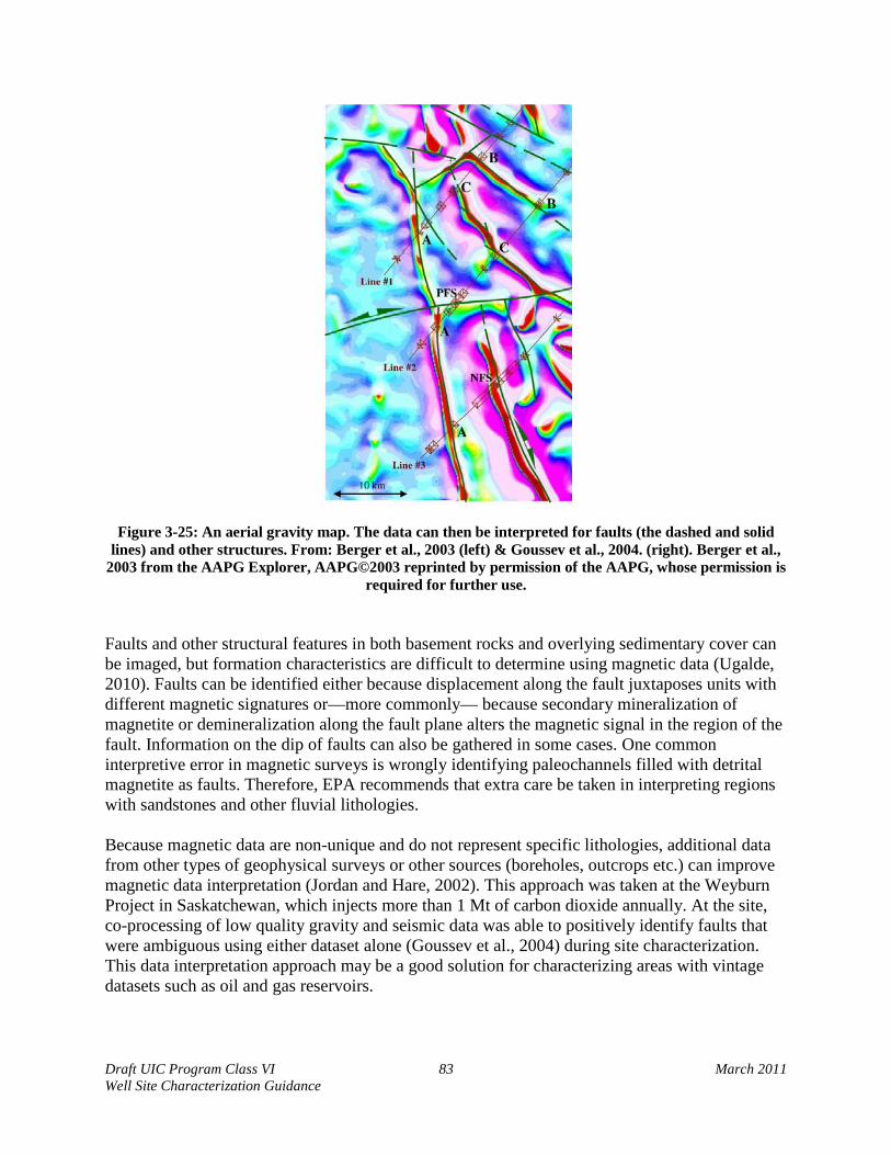
Draft UIC Program Class VI 83 March 2011 Well Site Characterization Guidance
Figure 3-25: An aerial gravity map. The data can then be interpreted for faults (the dashed and solid lines) and other structures. From: Berger et al., 2003 (left) & Goussev et al., 2004. (right). Berger et al.,
2003 from the AAPG Explorer, AAPG©2003 reprinted by permission of the AAPG, whose permission is required for further use.
Faults and other structural features in both basement rocks and overlying sedimentary cover can be imaged, but formation characteristics are difficult to determine using magnetic data (Ugalde, 2010). Faults can be identified either because displacement along the fault juxtaposes units with different magnetic signatures or—more commonly— because secondary mineralization of magnetite or demineralization along the fault plane alters the magnetic signal in the region of the fault. Information on the dip of faults can also be gathered in some cases. One common interpretive error in magnetic surveys is wrongly identifying paleochannels filled with detrital magnetite as faults. Therefore, EPA recommends that extra care be taken in interpreting regions with sandstones and other fluvial lithologies. Because magnetic data are non-unique and do not represent specific lithologies, additional data from other types of geophysical surveys or other sources (boreholes, outcrops etc.) can improve magnetic data interpretation (Jordan and Hare, 2002). This approach was taken at the Weyburn Project in Saskatchewan, which injects more than 1 Mt of carbon dioxide annually. At the site, co-processing of low quality gravity and seismic data was able to positively identify faults that were ambiguous using either dataset alone (Goussev et al., 2004) during site characterization. This data interpretation approach may be a good solution for characterizing areas with vintage datasets such as oil and gas reservoirs.

Draft UIC Program Class VI 84 March 2011 Well Site Characterization Guidance
Magnetic methods are sensitive to human infrastructure. As a result, they are not useful in populated or developed areas because buildings, pipes, and wires obscure the geologic signal. The one advantage to this sensitivity is that magnetic surveys may be used to find abandoned, cased wells. This can help in identifying abandoned wells that may need corrective action, as required in a Class VI well permit. See the Draft UIC Program Class VI Well Area of Review Evaluation and Corrective Action Guidance for further details on locating abandoned wells and performing the required corrective action activities. Processing of Magnetic Data After collection, magnetic intensity data undergo moderate processing. Processing methods are not influenced by the type of carbon dioxide reservoir under investigation. High frequency anomalies can be attributed to near-surface and shallow subsurface effects, intermediate frequency anomalies can be attributed to the composition of the sedimentary basins, and low-frequency anomalies can be ascribed to changes in the basement rocks. Most surveys collected today are of sufficient resolution to detect anomalies in all three ranges. Existing Data Availability Magnetic surveys have already been conducted over the majority of North America. However, the resolution of these surveys may not be high enough for site characterization purposes. High-resolution data are more likely to have been collected for hydrocarbon-producing basins and areas targeted for mineral exploration.
3.8. Demonstration of Storage Capacity
Demonstration of storage capacity is an important component of geological site characterization for the purpose of predicting the ability of the injection zone to receive and contain the anticipated total volume of the carbon dioxide injection stream throughout the life of the GS project. The GS Rule requires a demonstration by the proposed Class VI injection well owner or operator that the well will be sited in an area with a suitable geologic system. The geologic setting must include an injection zone or zones of sufficient areal extent, thickness, porosity, and permeability to receive the total anticipated volume of the carbon dioxide stream [§146.83(a)(1)]. This information enables the UIC Program Director to set permitted injection limits for the proposed Class VI injection well, which must be adhered to throughout the life of the injection well . This section focuses on the concept of carbon dioxide storage capacity, and it includes definitions of terms, required data, methods for estimating carbon dioxide storage capacity, and case studies. The areal extent and thickness of the storage site can be determined from several sources such as geologic maps, cross-sections, and geophysical imaging. See Sections 2 and 3.7 of this guidance document, above, for more information. The concept of injectivity and the consequences of carbon dioxide-water-rock interactions are discussed separately in Section 3.3 of this guidance document. Information on methods for determining porosity and permeability are included in Section 3.4. Concepts and guidance regarding geomechanical characterization and confining zone integrity are discussed in Sections 3.6 and 3.10, respectively. Data collected
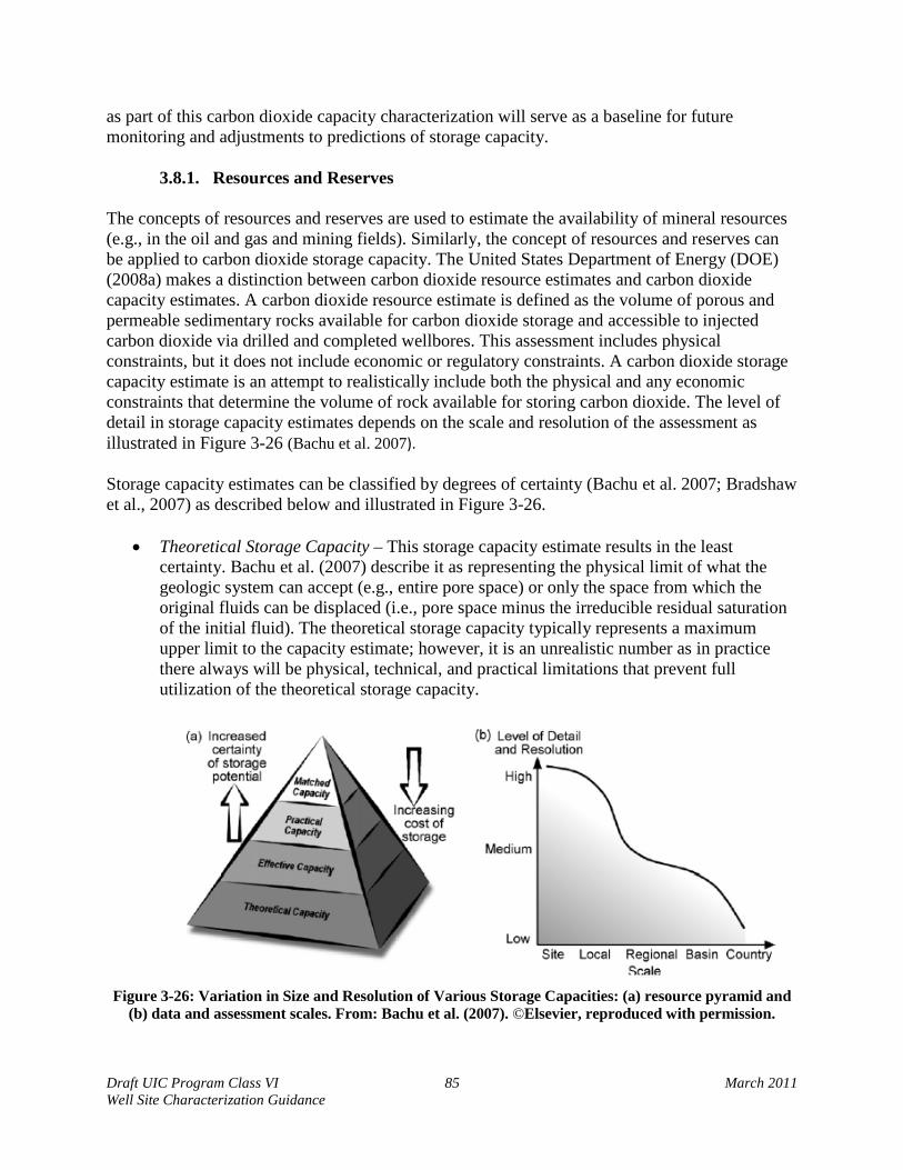
Draft UIC Program Class VI 85 March 2011 Well Site Characterization Guidance
as part of this carbon dioxide capacity characterization will serve as a baseline for future monitoring and adjustments to predictions of storage capacity.
3.8.1. Resources and Reserves The concepts of resources and reserves are used to estimate the availability of mineral resources (e.g., in the oil and gas and mining fields). Similarly, the concept of resources and reserves can be applied to carbon dioxide storage capacity. The United States Department of Energy (DOE) (2008a) makes a distinction between carbon dioxide resource estimates and carbon dioxide capacity estimates. A carbon dioxide resource estimate is defined as the volume of porous and permeable sedimentary rocks available for carbon dioxide storage and accessible to injected carbon dioxide via drilled and completed wellbores. This assessment includes physical constraints, but it does not include economic or regulatory constraints. A carbon dioxide storage capacity estimate is an attempt to realistically include both the physical and any economic constraints that determine the volume of rock available for storing carbon dioxide. The level of detail in storage capacity estimates depends on the scale and resolution of the assessment as illustrated in Figure 3-26 (Bachu et al. 2007). Storage capacity estimates can be classified by degrees of certainty (Bachu et al. 2007; Bradshaw et al., 2007) as described below and illustrated in Figure 3-26.
• Theoretical Storage Capacity – This storage capacity estimate results in the least certainty. Bachu et al. (2007) describe it as representing the physical limit of what the geologic system can accept (e.g., entire pore space) or only the space from which the original fluids can be displaced (i.e., pore space minus the irreducible residual saturation of the initial fluid). The theoretical storage capacity typically represents a maximum upper limit to the capacity estimate; however, it is an unrealistic number as in practice there always will be physical, technical, and practical limitations that prevent full utilization of the theoretical storage capacity.
Figure 3-26: Variation in Size and Resolution of Various Storage Capacities: (a) resource pyramid and
(b) data and assessment scales. From: Bachu et al. (2007). ©Elsevier, reproduced with permission.

Draft UIC Program Class VI 86 March 2011 Well Site Characterization Guidance
• Effective Storage Capacity – This estimate is also known as “realistic capacity”. Bachu et
al. (2007) note that it is obtained by applying a range of technical (geological and engineering) cut-off limits to a storage capacity assessment, which usually changes with the acquisition of new data and/or knowledge.
• Practical Storage Capacity – This estimate is also known as “viable capacity”. Bachu et al. (2007) describe it as obtained by considering both technical and practical challenges to safe carbon dioxide geological storage. This estimate is prone to changes over the life of a GS project as technology, policy, regulations and/or economics change.
• Matched Storage Capacity – This estimate yields the greatest certainty regarding carbon dioxide storage capacity. Bachu et al. (2007) describe it as a detailed matching of large stationary carbon dioxide sources with geological storage sites that are adequate in terms of capacity, injectivity and supply rate.
Additionally, the United States Geological Survey released a report on risk-based capacity estimates, which differs from the above estimates in that it uses fully probabilistic methods to incorporate geologic uncertainty in calculations of storage potential. (Brennan et al. 2010) This Guidance has been developed based on the assumption that the owner or operator has already identified an acceptable carbon dioxide storage site. It will therefore focus now on some tools that may be needed to develop estimates of storage capacity for submitting with a Class VI injection well operating permit application with the greatest certainty and highest level of detail.
3.8.2. Parameters and Data Interpretation
This section focuses on parameters used to estimate the volume (or mass) of carbon dioxide storage capacity. It includes discussion of methods for quantifying parameters, such as laboratory methods and field testing, and estimating or predictive tools (Table 3-6). Additional discussion is provided as appropriate with regard to data quality and special considerations for data from different geologic terrains (saline formations, coal seams, or oil and gas reservoirs). Parameters used to describe porosity, permeability, and injectivity (flow rate) were discussed previously in Section 3.4 of this guidance document. Some recommended data sources for determining injection zone thickness, area, and background hydraulic gradient were discussed in Section 2 of this guidance document. Several of these parameters, such as capillary pressure, temperature, compressibility, water saturation, intrinsic and relative permeability, and porosity are also for the multiphase fluid modeling required for proposed Class VI injection well AoR determinations [§§146.84]. For more information on the required AoR modeling for a proposed Class VI injection well, see the Draft UIC Program Class VI Well Area of Review and Corrective Action Guidance.
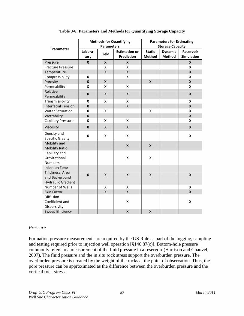
Draft UIC Program Class VI 87 March 2011 Well Site Characterization Guidance
Table 3-6: Parameters and Methods for Quantifying Storage Capacity
Parameter
Methods for Quantifying Parameters
Parameters for Estimating Storage Capacity
Labora-tory
Field Estimation or
Prediction Static
Method Dynamic Method
Reservoir Simulation
Pressure X X X X Fracture Pressure X X X Temperature X X X Compressibility X X X Porosity X X X X Permeability X X X X Relative Permeability
X X X X Transmissibility X X X X Interfacial Tension X X X Water Saturation X X X X Wettability X X Capillary Pressure X X X X Viscosity X X X X Density and Specific Gravity
X X X X Mobility and Mobility Ratio
X X
Capillary and Gravitational Numbers
X X
Injection Zone Thickness, Area and Background Hydraulic Gradient
X X X X X
Number of Wells X X X Skin Factor X X X Diffusion Coefficient and Dispersivity
X X
Sweep Efficiency X X
Pressure Formation pressure measurements are required by the GS Rule as part of the logging, sampling and testing required prior to injection well operation [§146.87(c)]. Bottom-hole pressure commonly refers to a measurement of the fluid pressure in a reservoir (Harrison and Chauvel, 2007). The fluid pressure and the in situ rock stress support the overburden pressure. The overburden pressure is created by the weight of the rocks at the point of observation. Thus, the pore pressure can be approximated as the difference between the overburden pressure and the vertical rock stress.

Draft UIC Program Class VI 88 March 2011 Well Site Characterization Guidance
Pressure transducers convert a pressure change into a mechanical displacement or deformation, which is then converted into an electrical signal (Harrison and Chauvel, 2007). In the field, pressure transducers include mechanical (nearly obsolete), capacitance (good response, low hysteresis, excellent stability and repeatability), strain gauge (ruggedness, low cost, and good dynamic behavior), and quartz gauge (exceptional accuracy, resolution, and long-term stability). Additional information regarding types of pressure transducers is available in Harrison and Chauvel (2007) and from commercial manufacturers.
The down-hole pressure of formations can be measured in open holes using wireline tools known as formation testers (Smolen, 1992b). The tool is used to make pressure measurements at various depths during a single trip into the hole. The tester is activated and hydraulically set or pressed against the formation when a depth is selected. The formation pressure can be measured under controlled flow rates and shut in conditions (Fig 3-30). The pressure measurements can be used to determine variations in formation pressures with depth (Fig 3-31). Production testing in open holes (drill stem tests) and in completed wells (e.g., multi-well tests) can be used to determine reservoir properties and to assess the degree of damage or stimulation in the near-well environment (i.e., skin effects as discussed below) (Lancaster, 1992).
Figure 3-27: Example Pressure Recording by a Formation Tester.
From: Smolen (1992b). ©AAPG 1992; Reprinted by permission of the AAPG whose permission is required for further use.

Draft UIC Program Class VI 89 March 2011 Well Site Characterization Guidance
Figure 3-28: Example Pressure Response across Multiple Formations.
From: Smolen (1992b). ©AAPG 1992; Reprinted by permission of the AAPG whose permission is required for further use.
Fracture Pressure
Field methods such as in-situ formation stress tests can provide the required calculated information about the fracture pressure of both the injection and the confining zone(s) [§146.87(d)(1)], as described in Section 3.6.2 of this guidance document, above. Maximum down-hole pressure is set by the GS Rule to avoid fracturing the injection zone; the rule also prohibits fracturing the confining zone(s) [§146.88(a)]. Van der Meer (1996) derived a relationship for maximum safe injection pressure based on 1.35 times the hydrostatic pressure to a depth of 1000 m, and 2.4 times the hydrostatic pressure for depths of 1 to 5 km. Benson and

Draft UIC Program Class VI 90 March 2011 Well Site Characterization Guidance
Cook (2005) reported typical fracture pressures in the range of 11 to 21 kPa m-1 based on practical experience from the UIC program. As an example, Shi et al. (2008) reported fracture-opening and fracture–closing pressures of 15.8 and 10.9 MPa, respectively, in coal seams that were pilot tested for carbon dioxide storage in Japan. As noted by USDOE (2008a) all geological formations will begin propagating fractures upon reaching a threshold pressure; this site-specific threshold-pressure constraint is an important consideration in estimating carbon dioxide storage capacity.
Temperature
Subsurface reservoir temperature is governed primarily by its proximity to the earth’s mantle, and the relative heat exchange capacities and the thermal conductivities of the underlying formations (Harrison and Chauvel, 2007). Temperature sensors include mechanical (obsolete), thermistors (semiconductor material and highly sensitive), and resistance temperature detectors (wide temperature range and excellent accuracy).
Prensky (1992) describes the collection of borehole temperature measurements as maximum-reading values acquired during logging runs, or as continuous-recorded temperature surveys in wells. The effective accuracy of commercial temperature logs is ±0.5ºC (Prensky, 1992). Prensky (1992) described the determination of formation temperature and temperature gradients by the two-point, or multiple-point average temperature gradient, whereby a linear relationship is assumed between the ambient surface temperature and the bottom-hole temperature. Regression techniques can be used to calculate geothermal gradients for large data sets (Speece et al., 1985).
Information regarding local and regional thermal gradients can be obtained from reports generated by academic institutions and government agencies such as Nuccio and Condon (1996). Geothermal gradients can vary within a basin, for example, the Alberta basin exhibits a trend of increasing gradients, ranging from 20°C/km in the south to 50°C/km in the north (Bachu and Haug, 2005). In most hydrocarbon producing areas, Harrison and Chauvel (2007) characterize temperature gradients usually in the range of 0.6 to 1.6°F per 100 ft of depth increase. Compressibility
Reservoir formations are subjected to constant external (rock or overburden) pressure. When the internal fluid pressure within the pore spaces is reduced (e.g., by production of hydrocarbon reserves), the bulk volume of the rock decreases while the volume of the solid rock material (e.g., sand grain or sandstone) increases. Craft and Hawkins (1959) noted that these volume changes reduce the porosity of the rock slightly, e.g., a change from 20 percent porosity to 19.9 percent. The pore volume compressibility is defined by Craft and Hawkins (1959) as the change in pore volume per unit of pore volume per unit change in pressure, with values for limestone and sandstone reservoir rocks in the range of 2×10⁻⁶ to 25×10-6 psi-1.
Rock compressibility data for a given reservoir can be obtained from laboratory measurements on core samples. In situations whereby laboratory analysis is not practical, rock compressibility values can be estimated from porosity overburden pressure as described by Craft and Hawkins (1959). Harrell and Cronquist (2007) provide a substitute correlation for estimating rock

Draft UIC Program Class VI 91 March 2011 Well Site Characterization Guidance
compressibility that depends on rock properties. Other values of rock compressibility have been reported as case studies in the literature (e.g., Law and Bachu, 1996; Ross et al., 2009).
The amount a gas deviates from ideal behavior when compressed is known in the petroleum literature as the gas deviation factor or compressibility factor, represented by the symbol z (Craft and Hawkins, 1959). Benson and Cook (2005) noted that the compressibility of the carbon dioxide injection stream can be affected by the presence of impurities. Sass et al. (2005) evaluated the impact of SOx and NOx impurities on compressed carbon dioxide. These findings are notable because changes in carbon dioxide compressibility, as a result of the presence of impurities, can affect the estimated volume of carbon dioxide for storage for a particular injection zone. Equation-of-state models have been developed to predict carbon dioxide compressibility in multi-component two-phase systems (Firoozabadi et al., 1988).
Transmissibility into Formations above the Reservoir
As part of a risk assessment, Wildenborg et al. (2005) identified several pathways for the transport of carbon dioxide from the storage reservoir into formations overlying the reservoir, each pathway providing opportunities for increasing transmissibility: along a fault plane as a result of natural or man-induced events or processes; along a well trajectory as a result of chemical processes (e.g., metallic corrosion and cement degradation) around the wellbore; or across a reservoir seal as a result of interacting chemical and mechanical processes.
Within a porous media, transmissibility can be expressed mathematically as a coefficient of Darcy’s law whereby the linear pressure dependence of flow of a component c within a phase p can be given by the following relationship (Ponting, 2007):
𝑭𝒄𝒑𝒂𝒃 = 𝑻𝒂𝒑𝑴𝒄𝒑𝒂𝒃∆Φ𝒑𝒂𝒃 Equation 3-13
where Fcpab is the flow rate of component c in phase p from cell a to its neighbor b; Tap is the transmissibility from cell a of phase p (as described below); Mcpab is the mobility of component c in phase p for the contribution of the flow between a and b, given by xcpkrp/μp, where xcp is the concentration of component c in phase p, krp is the relative permeability of phase p, and μp is the viscosity of phase p; and ∆Φpab is the potential difference of phase p between cell a and cell b, which includes pressure, gravity and capillary pressure contributions. Assuming a single component c in each phase p, Darcy’s law can be simplified as:
𝑭𝒑𝒂𝒃 = 𝑻𝒂𝒑𝑴𝒑𝒂𝒃∆Φ𝒑𝒂𝒃 Equation 3-14
where Fpab = flow rate [L3T-1]
Tap = transmissibility [L3] M = mobility [LTM-1
pab ] ∆Φ = potential [ML-1T-2
pab ]
For a given direction of flow, transmissibility Tap can be expressed as a harmonic average
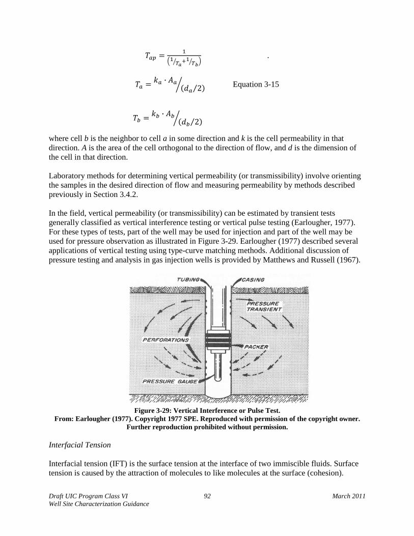
Draft UIC Program Class VI 92 March 2011 Well Site Characterization Guidance
𝑇𝑎𝑝 = 1
�1 𝑇𝑎� +1 𝑇𝑏� � .
𝑇𝑎 = 𝑘𝑎 ∙ 𝐴𝑎
(𝑑𝑎 2⁄ )� Equation 3-15
𝑇𝑏 = 𝑘𝑏 ∙ 𝐴𝑏
(𝑑𝑏 2⁄ )� .
where cell b is the neighbor to cell a in some direction and k is the cell permeability in that direction. A is the area of the cell orthogonal to the direction of flow, and d is the dimension of the cell in that direction.
Laboratory methods for determining vertical permeability (or transmissibility) involve orienting the samples in the desired direction of flow and measuring permeability by methods described previously in Section 3.4.2.
In the field, vertical permeability (or transmissibility) can be estimated by transient tests generally classified as vertical interference testing or vertical pulse testing (Earlougher, 1977). For these types of tests, part of the well may be used for injection and part of the well may be used for pressure observation as illustrated in Figure 3-29. Earlougher (1977) described several applications of vertical testing using type-curve matching methods. Additional discussion of pressure testing and analysis in gas injection wells is provided by Matthews and Russell (1967).
Figure 3-29: Vertical Interference or Pulse Test.
From: Earlougher (1977). Copyright 1977 SPE. Reproduced with permission of the copyright owner. Further reproduction prohibited without permission.
Interfacial Tension
Interfacial tension (IFT) is the surface tension at the interface of two immiscible fluids. Surface tension is caused by the attraction of molecules to like molecules at the surface (cohesion).

Draft UIC Program Class VI 93 March 2011 Well Site Characterization Guidance
Surface tension is expressed in terms of force per unit length, or energy per unit area. Surface tension can be measured by a variety of laboratory methods such as the Du Noüy Ring method, the Wilhelmy Plate method, the spinning drop method, the pendant drop method, and other techniques.
For testing in-situ conditions in the laboratory, samples of the formation brine can be pre-contacted with carbon dioxide under in-situ temperature and pressure conditions, shaken until equilibrium is reached, and then separated and charged into a high pressure and temperature cell for measurement (Bachu and Bennion, 2008; del Rio and Newman, 1997). An experimental setup for measuring interfacial tension under in-situ conditions using the axisymmetric drop shape analysis technique has been described by Nobakht et al. (2007).
IFT can be estimated mathematically by an empirical power function of pressure, whereby the values of the coefficient and exponent depend on temperature and water salinity (Bachu and Bennion, 2009):
𝑰𝑭𝑻 = 𝑨(𝑻,𝑺) × 𝑷−𝑩(𝑻,𝒔) Equation 3-16
where IFT is interfacial tension, A(T,S) is an empirical coefficient dependent on temperature and total dissolved solids, B(T,S) is an empirical exponent also dependent on temperature and total dissolved solids, and P is pressure. Bachu and Bennion (2009) provide values of A and B for a range of temperature and salinity conditions representative of in-situ carbon dioxide -brine systems. Knowledge regarding the interfacial tension between carbon dioxide and brine at in-situ conditions is needed for precise measurements of capillary pressure, which in turn impacts relative permeability (Bachu and Bennion, 2008). Water Saturation
Water saturation (Sw) describes the fraction of water in a given pore space. It depends on particle size and interparticle porosity (Lucia, 1992). Water saturation is most often determined from resistivity log measurements combined with knowledge of porosity, water resistivity, and shale volume (Alberty, 1992b). Water saturation values range from 0 (completely dry) to 1 (completely saturated). In clean sands, water saturation can be calculated based on the following equation, developed by Gus Archie in 1942:
𝑺 = 𝑭∙𝑹𝑹𝒕𝒘
𝒏 𝒘 Equation 3-17
where F is the formation resistivity factor, Rw is resistivity of formation waters, Rt is the true formation resistivity, and n is the saturation exponent. The formation resistivity factor is the ratio of the resistivity of fully saturated rock to the resistivity of the formation fluid. This value can be determined from cores or estimated based on porosity and other characteristics of the rock. The formation water resistivity can be determined from SP logs or water samples, while the true formation resistivity can be determined with dual induction or dual laterolog wireline analysis. The saturation exponent can also be determined
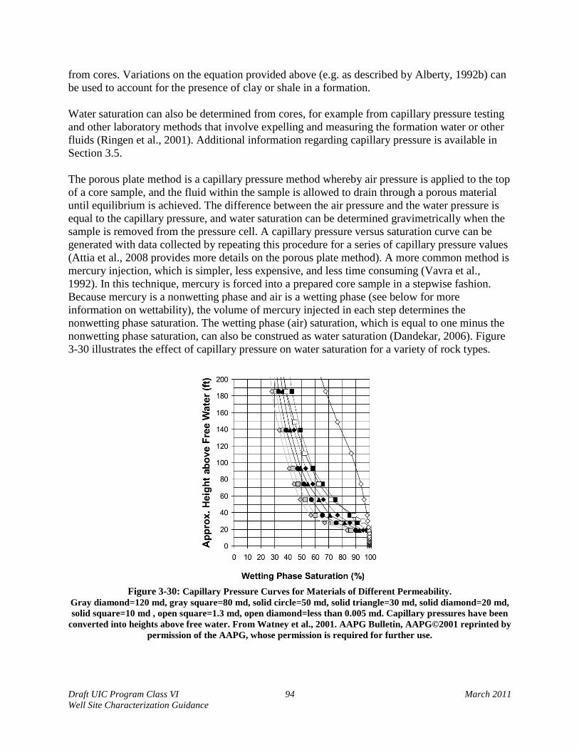
Draft UIC Program Class VI 94 March 2011 Well Site Characterization Guidance
from cores. Variations on the equation provided above (e.g. as described by Alberty, 1992b) can be used to account for the presence of clay or shale in a formation. Water saturation can also be determined from cores, for example from capillary pressure testing and other laboratory methods that involve expelling and measuring the formation water or other fluids (Ringen et al., 2001). Additional information regarding capillary pressure is available in Section 3.5.
The porous plate method is a capillary pressure method whereby air pressure is applied to the top of a core sample, and the fluid within the sample is allowed to drain through a porous material until equilibrium is achieved. The difference between the air pressure and the water pressure is equal to the capillary pressure, and water saturation can be determined gravimetrically when the sample is removed from the pressure cell. A capillary pressure versus saturation curve can be generated with data collected by repeating this procedure for a series of capillary pressure values (Attia et al., 2008 provides more details on the porous plate method). A more common method is mercury injection, which is simpler, less expensive, and less time consuming (Vavra et al., 1992). In this technique, mercury is forced into a prepared core sample in a stepwise fashion. Because mercury is a nonwetting phase and air is a wetting phase (see below for more information on wettability), the volume of mercury injected in each step determines the nonwetting phase saturation. The wetting phase (air) saturation, which is equal to one minus the nonwetting phase saturation, can also be construed as water saturation (Dandekar, 2006). Figure 3-30 illustrates the effect of capillary pressure on water saturation for a variety of rock types.
Figure 3-30: Capillary Pressure Curves for Materials of Different Permeability.
Gray diamond=120 md, gray square=80 md, solid circle=50 md, solid triangle=30 md, solid diamond=20 md, solid square=10 md , open square=1.3 md, open diamond=less than 0.005 md. Capillary pressures have been
converted into heights above free water. From Watney et al., 2001. AAPG Bulletin, AAPG©2001 reprinted by permission of the AAPG, whose permission is required for further use.
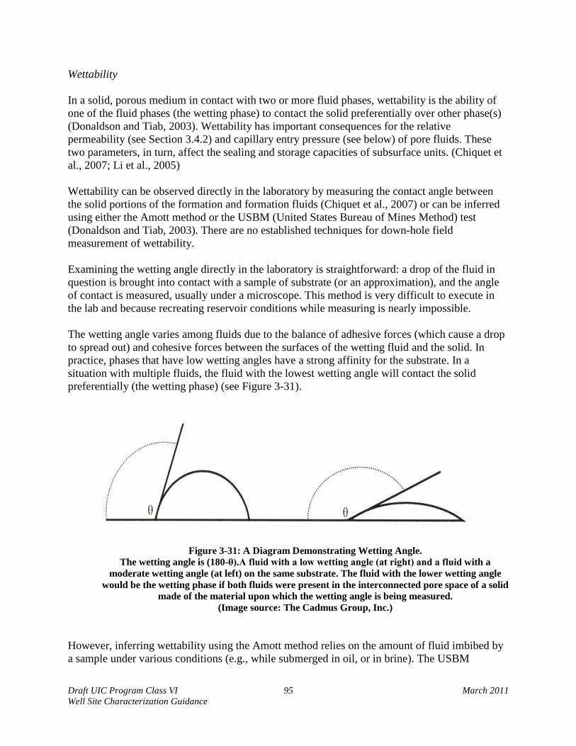
Draft UIC Program Class VI 95 March 2011 Well Site Characterization Guidance
Wettability
In a solid, porous medium in contact with two or more fluid phases, wettability is the ability of one of the fluid phases (the wetting phase) to contact the solid preferentially over other phase(s) (Donaldson and Tiab, 2003). Wettability has important consequences for the relative permeability (see Section 3.4.2) and capillary entry pressure (see below) of pore fluids. These two parameters, in turn, affect the sealing and storage capacities of subsurface units. (Chiquet et al., 2007; Li et al., 2005) Wettability can be observed directly in the laboratory by measuring the contact angle between the solid portions of the formation and formation fluids (Chiquet et al., 2007) or can be inferred using either the Amott method or the USBM (United States Bureau of Mines Method) test (Donaldson and Tiab, 2003). There are no established techniques for down-hole field measurement of wettability. Examining the wetting angle directly in the laboratory is straightforward: a drop of the fluid in question is brought into contact with a sample of substrate (or an approximation), and the angle of contact is measured, usually under a microscope. This method is very difficult to execute in the lab and because recreating reservoir conditions while measuring is nearly impossible. The wetting angle varies among fluids due to the balance of adhesive forces (which cause a drop to spread out) and cohesive forces between the surfaces of the wetting fluid and the solid. In practice, phases that have low wetting angles have a strong affinity for the substrate. In a situation with multiple fluids, the fluid with the lowest wetting angle will contact the solid preferentially (the wetting phase) (see Figure 3-31).
Figure 3-31: A Diagram Demonstrating Wetting Angle. The wetting angle is (180-θ).A fluid with a low wetting angle (at right) and a fluid with a
moderate wetting angle (at left) on the same substrate. The fluid with the lower wetting angle would be the wetting phase if both fluids were present in the interconnected pore space of a solid
made of the material upon which the wetting angle is being measured. (Image source: The Cadmus Group, Inc.)
However, inferring wettability using the Amott method relies on the amount of fluid imbibed by a sample under various conditions (e.g., while submerged in oil, or in brine). The USBM

inferential test is based on the examination of capillary pressure curves obtained by alternately displacing fluids using a centrifuge (Donaldson and Tiab, 2003). Neither of these techniques requires highly specialized equipment, and both the Amott method and the USBM test are usually conducted with oil and brine. Some modifications may be required to collect wettability measurements with carbon dioxide /brine/oil systems, as would be applicable to the site characterization of a potential Class VI injection well site. Such modifications might increase the difficulty of such measurements. Salinity, temperature, and pressure can all effect wettability (Donaldson and Tiab, 2003), and wettability measurements will be most applicable if they are taken under conditions that approximate those found within the formation of interest. For example, experiments with medium-rank coals have indicated that increases in the carbon dioxide pressure due to carbon dioxide injection can change coal microcleats from water-wet to carbon dioxide-wet, greatly increasing the efficiency of carbon dioxide transport through the coal (Plug et al., 2008). Additionally, micromodels are currently being developed that will be able to predict changes in wetting phase behavior as reservoir conditions change (Pacific Northwest National Laboratory, 2010). These may be useful if the reproduction of reservoir conditions is not possible in the laboratory.
Capillary Pressure
Capillary pressure is the minimum pressure required for an immiscible non-wetting fluid to overcome capillary and interfacial forces and enter pore space containing the wetting fluid. For carbon dioxide injection into a saline formation, the non-wetting fluid is carbon dioxide and the wetting fluid is the native brine. Capillary pressure can be calculated as follows (Vavra et al., 1992):
Draft UIC Program Class VI 96 March 2011 Well Site Characterization Guidance
𝑃𝑐 = (𝜌𝑤 − 𝜌𝑛𝑤)𝑔ℎ
Equation 3-18 𝑃𝑐 = 2𝜎 cos𝜃
𝑟𝑐
where ρw is the density of the wetting fluid, ρ nw is density of the nonwetting fluid, g is the gravitational constant, h represents the height above the free surface, σ is interfacial tension, θ is the contact angle between the fluids and the capillary tube, and rc is the radius of the capillary. The contact angle between the fluids and the capillary is typically measured as the angle between the wetting phase and the solid surface.
Capillary pressure relationships for porous media are typically reported as a function of the wetting phase saturation, and the capillary pressure curves generated by laboratory testing can be used to estimate the irreducible wetting phase saturation of the carbon dioxide/brine/rock system. Mathematical models have also been developed to predict capillary pressure relationships (e.g., van Genuchten, 1980). Figure 3-32 shows capillary pressure curves used in a simulation of carbon dioxide storage in saline formations (Ide et al., 2007).
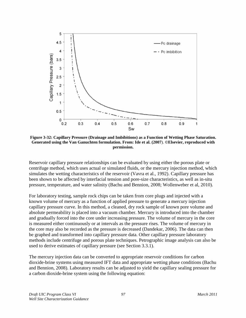
Draft UIC Program Class VI 97 March 2011 Well Site Characterization Guidance
Figure 3-32: Capillary Pressure (Drainage and Imbibitions) as a Function of Wetting Phase Saturation. Generated using the Van Ganuchten formulation. From: Ide et al. (2007). ©Elsevier, reproduced with
permission.
Reservoir capillary pressure relationships can be evaluated by using either the porous plate or centrifuge method, which uses actual or simulated fluids, or the mercury injection method, which simulates the wetting characteristics of the reservoir (Vavra et al., 1992). Capillary pressure has been shown to be affected by interfacial tension and pore-size characteristics, as well as in-situ pressure, temperature, and water salinity (Bachu and Bennion, 2008; Wollenweber et al, 2010).
For laboratory testing, sample rock chips can be taken from core plugs and injected with a known volume of mercury as a function of applied pressure to generate a mercury injection capillary pressure curve. In this method, a cleaned, dry rock sample of known pore volume and absolute permeability is placed into a vacuum chamber. Mercury is introduced into the chamber and gradually forced into the core under increasing pressure. The volume of mercury in the core is measured either continuously or at intervals as the pressure rises. The volume of mercury in the core may also be recorded as the pressure is decreased (Dandekar, 2006). The data can then be graphed and transformed into capillary pressure data. Other capillary pressure laboratory methods include centrifuge and porous plate techniques. Petrographic image analysis can also be used to derive estimates of capillary pressure (see Section 3.3.1).
The mercury injection data can be converted to appropriate reservoir conditions for carbon dioxide-brine systems using measured IFT data and appropriate wetting phase conditions (Bachu and Bennion, 2008). Laboratory results can be adjusted to yield the capillary sealing pressure for a carbon dioxide-brine system using the following equation:
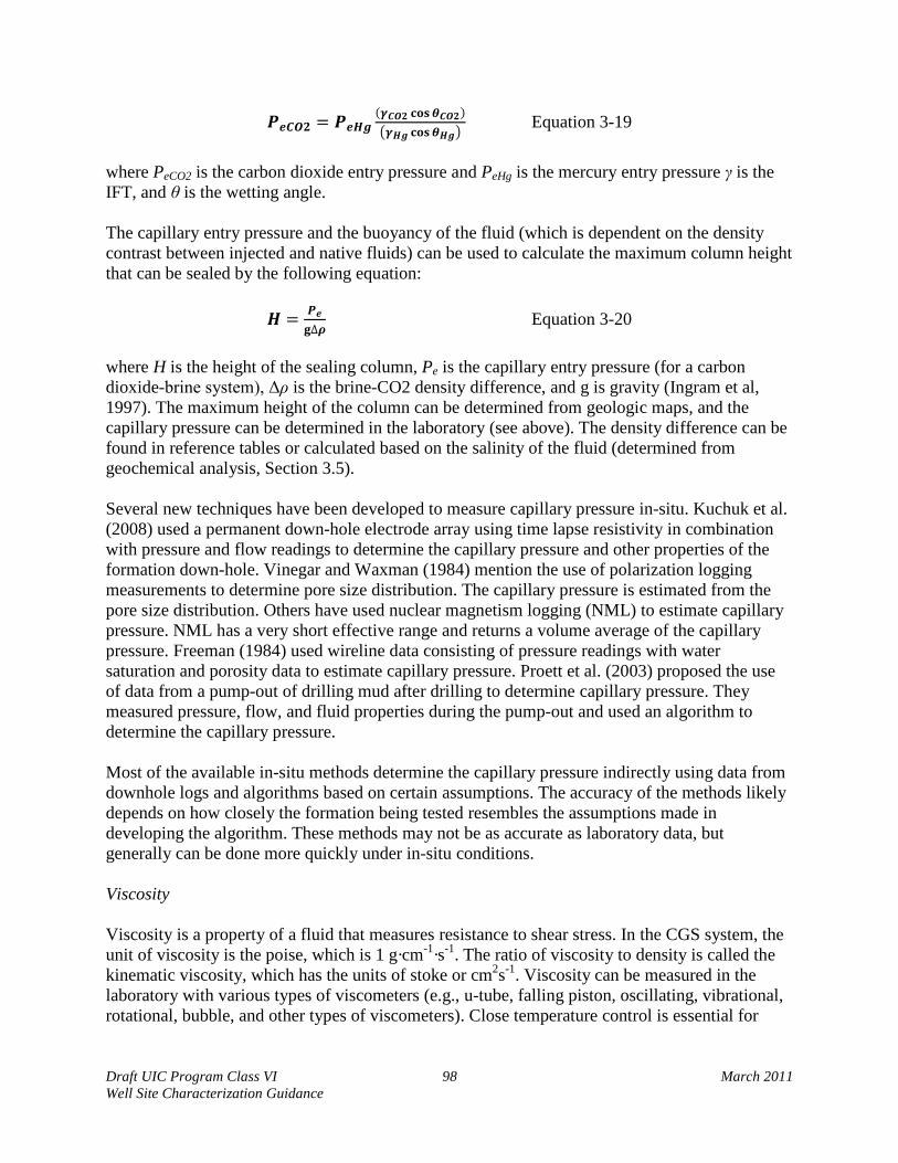
Draft UIC Program Class VI 98 March 2011 Well Site Characterization Guidance
𝑷𝒆𝑪𝑶𝟐 = 𝑷𝒆𝑯𝒈(𝜸𝑪𝑶𝟐 𝐜𝐨𝐬 𝜽𝑪𝑶𝟐)�𝜸𝑯𝒈 𝐜𝐨𝐬 𝜽𝑯𝒈�
Equation 3-19
where PeCO2 is the carbon dioxide entry pressure and PeHg is the mercury entry pressure γ is the IFT, and θ is the wetting angle.
The capillary entry pressure and the buoyancy of the fluid (which is dependent on the density contrast between injected and native fluids) can be used to calculate the maximum column height that can be sealed by the following equation:
𝑯 = 𝑷𝒆
𝐠∆𝝆 Equation 3-20
where H is the height of the sealing column, Pe is the capillary entry pressure (for a carbon dioxide-brine system), Δρ is the brine-CO2 density difference, and g is gravity (Ingram et al, 1997). The maximum height of the column can be determined from geologic maps, and the capillary pressure can be determined in the laboratory (see above). The density difference can be found in reference tables or calculated based on the salinity of the fluid (determined from geochemical analysis, Section 3.5). Several new techniques have been developed to measure capillary pressure in-situ. Kuchuk et al. (2008) used a permanent down-hole electrode array using time lapse resistivity in combination with pressure and flow readings to determine the capillary pressure and other properties of the formation down-hole. Vinegar and Waxman (1984) mention the use of polarization logging measurements to determine pore size distribution. The capillary pressure is estimated from the pore size distribution. Others have used nuclear magnetism logging (NML) to estimate capillary pressure. NML has a very short effective range and returns a volume average of the capillary pressure. Freeman (1984) used wireline data consisting of pressure readings with water saturation and porosity data to estimate capillary pressure. Proett et al. (2003) proposed the use of data from a pump-out of drilling mud after drilling to determine capillary pressure. They measured pressure, flow, and fluid properties during the pump-out and used an algorithm to determine the capillary pressure.
Most of the available in-situ methods determine the capillary pressure indirectly using data from downhole logs and algorithms based on certain assumptions. The accuracy of the methods likely depends on how closely the formation being tested resembles the assumptions made in developing the algorithm. These methods may not be as accurate as laboratory data, but generally can be done more quickly under in-situ conditions.
Viscosity
Viscosity is a property of a fluid that measures resistance to shear stress. In the CGS system, the unit of viscosity is the poise, which is 1 g·cm-1·s-1. The ratio of viscosity to density is called the kinematic viscosity, which has the units of stoke or cm2s-1. Viscosity can be measured in the laboratory with various types of viscometers (e.g., u-tube, falling piston, oscillating, vibrational, rotational, bubble, and other types of viscometers). Close temperature control is essential for

Draft UIC Program Class VI 99 March 2011 Well Site Characterization Guidance
accurate measurements. ASTM International maintains standard methods for viscosity measurements (www.astm.org).
In situ, real-time direct measurements of viscosity can be collected at reservoir conditions using a wireline formation tester such as a tool described by O’Keefe et al. (2007). The tool measures the thermophysical properties of the fluid by the vibration of a mechanical resonator submersed in the flowline fluid, and the instrument measures viscosity in the range of 0.25 to 50 cP with a reported accuracy of ±10%.
Carbon dioxide viscosity has been estimated by the Jossi-Stiel-Thodos correlation (Nobakht et al., 2007) and, more recently, carbon dioxide viscosity has been shown to be predicted as a simple algebraic function of pressure and temperature (Bahadori and Vuthaluru, 2010):
𝐥𝐧(𝝁) = 𝒂 + 𝒃
𝑷+ 𝒄
𝑷𝟐+ 𝒅
𝑷𝟑 Equation 3-21
where the parameters a, b, c, and d are calculated based on constants provided by Bahadori and Vuthaluru (2010) for given temperature conditions. For brine viscosity, Adams and Bachu (2002) compared four algorithms for estimating viscosity and noted that water or brine viscosity is strongly dependent on temperature, less dependent on salinity, and almost negligibly dependent on pressure.
Density and Specific Gravity
Density is defined as mass per unit volume, and it depends on temperature and pressure. Mathematically, density is defined as:
𝝆 = 𝒎
𝑽 Equation 3-22
where ρ is density, m represents mass, and V is volume. At standard conditions, fresh water has a density value of 1.0 g·cm-3. Bulk density refers to the mass of many particles divided by the total volume occupied, which includes grain volume and internal pore volume. The standard density value of sandstone (quartz) is 2.65 g·cm-3. The density of a gas varies with temperature and pressure, following the ideal gas equation
𝝆 = 𝑷𝑴
𝑹𝑻 Equation 3-23
where P is the absolute pressure, T is the absolute temperature, M is the molecular weight of the gas, and R is the gas constant. At standard conditions, the density of carbon dioxide is approximately 1.98 g·l-1. Density is also expressed as the dimensionless quantity specific gravity, which is the ratio of the density of a substance relative to some reference material.
In the laboratory, the density of a homogeneous substance is normally determined by weighing the mass with an appropriate scale or balance, and the volume can be measured by the displacement of a fluid or by measuring the dimensions of the object. Bulk density is the oven-dried mass of the sample divided by its field volume. The particle density is the oven-dried mass
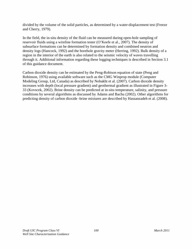
Draft UIC Program Class VI 100 March 2011 Well Site Characterization Guidance
divided by the volume of the solid particles, as determined by a water-displacement test (Freeze and Cherry, 1979).
In the field, the in-situ density of the fluid can be measured during open-hole sampling of reservoir fluids using a wireline formation tester (O’Keefe et al., 2007). The density of subsurface formations can be determined by formation density and combined neutron and density logs (Hancock, 1992) and the borehole gravity meter (Herring, 1992). Bulk density of a region in the interior of the earth is also related to the seismic velocity of waves travelling through it. Additional information regarding these logging techniques is described in Section 3.1 of this guidance document.
Carbon dioxide density can be estimated by the Peng-Robison equation of state (Peng and Robinson, 1976) using available software such as the CMG Winprop module (Computer Modeling Group, Ltd, Canada) as described by Nobakht et al. (2007). Carbon dioxide density increases with depth (local pressure gradient) and geothermal gradient as illustrated in Figure 3-33 (Kovscek, 2002). Brine density can be predicted at in-situ temperature, salinity, and pressure conditions by several algorithms as discussed by Adams and Bachu (2002). Other algorithms for predicting density of carbon dioxide -brine mixtures are described by Hassanzadeh et al. (2008).
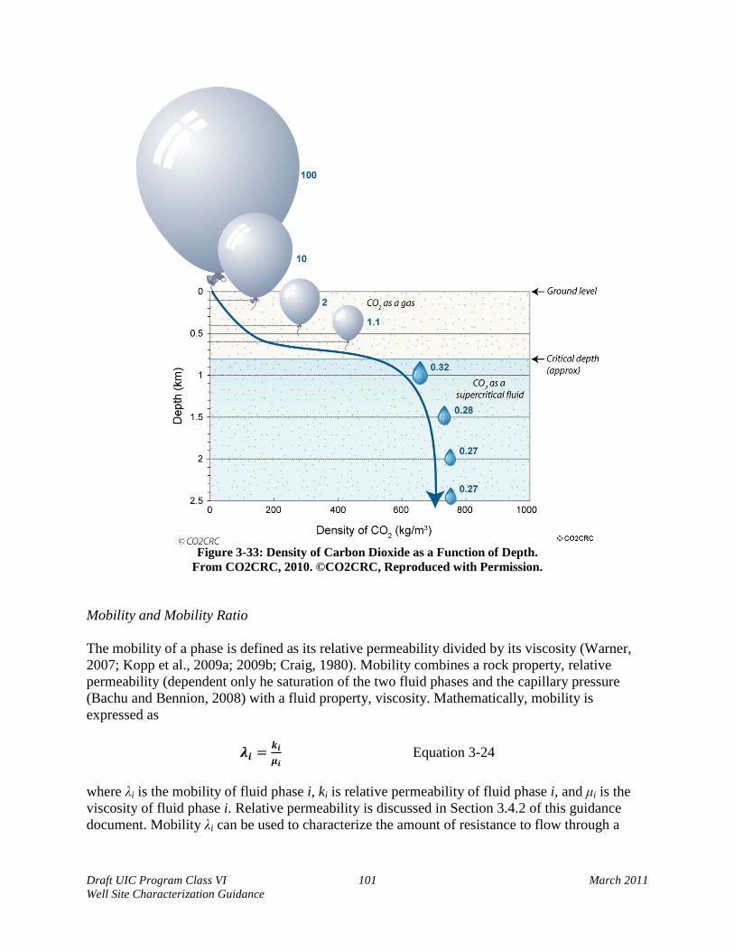
Draft UIC Program Class VI 101 March 2011 Well Site Characterization Guidance
Figure 3-33: Density of Carbon Dioxide as a Function of Depth.
From CO2CRC, 2010. ©CO2CRC, Reproduced with Permission. Mobility and Mobility Ratio
The mobility of a phase is defined as its relative permeability divided by its viscosity (Warner, 2007; Kopp et al., 2009a; 2009b; Craig, 1980). Mobility combines a rock property, relative permeability (dependent only he saturation of the two fluid phases and the capillary pressure (Bachu and Bennion, 2008) with a fluid property, viscosity. Mathematically, mobility is expressed as
𝝀𝒊 = 𝒌𝒊
𝝁𝒊 Equation 3-24
where λi is the mobility of fluid phase i, ki is relative permeability of fluid phase i, and μi is the viscosity of fluid phase i. Relative permeability is discussed in Section 3.4.2 of this guidance document. Mobility λi can be used to characterize the amount of resistance to flow through a

Draft UIC Program Class VI 102 March 2011 Well Site Characterization Guidance
reservoir rock that a fluid i exhibits at a given saturation of that fluid. Low-viscosity fluids generally have high mobility and high-viscosity fluids generally have low mobility.
The mobility ratio M generally is defined as the mobility of the displacing phase (carbon dioxide for sequestration) divided by the mobility of the displaced phase (e.g., fluid in a saline formation):
𝑴 = 𝒌𝒓𝒈 𝝁𝒈⁄
𝒌𝒓𝒘 𝝁𝒘⁄ = 𝒌𝒓𝒈𝝁𝒘𝝁𝒈𝒌𝒓𝒘
Equation 3-25
where krw is relative permeability to water, krg is relative permeability to gas (carbon dioxide), μw is the viscosity of water, and μg is the viscosity of gas (carbon dioxide).
Mobility ratios M are considered to be either “favorable” or “unfavorable”. A favorable mobility ratio is a low value (M ≤ 1), which means that the displaced fluid (water) has a higher mobility than the displacing phase (carbon dioxide). Volumetric (vertical and areal) sweep efficiency generally increases as M is reduced (Green and Willhite, 1998; Craig, 1980). An unfavorable mobility ratio (M > 1) means that the displacing fluid (carbon dioxide) has a higher mobility than the displaced fluid (water). In practical terms, a favorable mobility ratio means that the displaced water phase can move more quickly through the reservoir rock than the displacing carbon dioxide phase.
Mobility ratio M can be used to predict the capacity of a reservoir for storage of injected carbon dioxide. Viscous fingering can cause carbon dioxide to bypass much of the pore space, depending on the heterogeneity and anisotropy of rock permeability, because supercritical carbon dioxide is much less viscous than water and oil. Benson and Cook (2005) noted that only some of the resident oil or water will be displaced during carbon dioxide injection because of the comparatively high mobility of carbon dioxide, thus leading to an average saturation of carbon dioxide in the range of 30-60% during storage in the reservoir. Capillary and Gravitational Numbers
In addition to mobility, the displacement process will be driven by capillary and buoyancy forces. The Capillary number Ca is defined as the ratio of the capillary forces to the viscous forces (Kopp et al., 2009a)
𝐶𝑎 = 𝑘∆𝑃𝐶
𝜇𝐶𝑂2𝑣𝑙 Equation 3-26
where k is permeability, ∆PC is the capillary pressure drop over the system length or front length, μCO2 is viscosity of the injectant, v is the front propagation (Darcy) velocity, and l is the system length, or length of a saturation front.
As carbon dioxide migrates through a formation, some of it is retained in the pore space by capillary forces, known as residual carbon dioxide trapping. This behavior was illustrated by Bennion and Bachu (2008), who conducted relative permeability measurements (drainage and imbibition) at full reservoir conditions using supercritical pure carbon dioxide on samples of
various rock formations from Alberta, Canada. The drainage cycle was performed by injecting carbon dioxide into the brine-saturated core samples until the maximum gas saturation was obtained. The drainage cycle was followed by the imbibition cycle, which was performed by injecting brine and displacing the mobile-gas phase (carbon dioxide) from the sample until trapped-gas saturation occurred. Figure 3-34 shows an example of the brine/carbon dioxide relative permeability data generated by Bennion and Bachu (2008). Note that the trapped-gas (carbon dioxide) saturation for this example was reported by the authors as 0.297, which can be seen in Figure 3-34 at the point where carbon dioxide saturation corresponds to zero relative permeability for the carbon dioxide imbibition curve.
Draft UIC Program Class VI 103 March 2011 Well Site Characterization Guidance
Figure 3-34: Density Relative Permeability Curves for Brine/Carbon Dioxide System.
Measured in a rock sample from Alberta, Canada at reservoir conditions showing drainage and imbibitions data (From: Bennion and Bachu, 2008). ©Elsevier, reproduced with permission.
Benson and Cook (2005) noted that residual carbon dioxide saturations may be as high as 15-25% for many carbon dioxide storage formations, although this effect is formation-specific. Bennion and Bachu (2008) reported trapped-gas carbon dioxide saturations ranging from 0.102 to 0.349 for their samples collected in Alberta, Canada. Over time, this residual carbon dioxide is expected to dissolve in the formation water. The Capillary number Ca can be used to characterize the extent of carbon dioxide trapping in an injection zone. Kopp et al (2009a) examined the effect of Ca on storage capacity by using a numerical scheme to solve a system of differential equations for mass balance and constitutive equations. Kopp et al (2009a) concluded that a higher Ca is expected to be associated with a lower average carbon dioxide saturation. This expectation is based on the occurrence of stronger capillary forces associated with higher Ca values, thus leading to a smoother displacement front during the imbibitions process, and resulting in a lower, non-wetting phase (carbon dioxide) saturation in the swept area behind the brine displacement front.
Draft UIC Program Class VI 104 March 2011 Well Site Characterization Guidance
The Gravitational number Gr is defined as the ratio of the gravitational (buoyancy) forces to the viscous forces (Kopp et al, 2009a; Bryant and Lake, 2005, Chp 18)
𝐺𝑟 = (𝜌𝑤−𝜌𝐶𝑂2)𝑔𝑘𝑘𝑟
𝜇𝐶𝑂2𝑣 Equation 3-27
where ρw is the density of water (or other resident fluid), ρCO2 is the density of carbon dioxide, μCO2 is viscosity of the injectant , g is the gravity constant, v is the front propagation (Darcy) velocity, and k and kr are permeability and relative permeability, respectively.
The type of fluid in the reservoir will influence the magnitude of the buoyancy forces that drive vertical flow of carbon dioxide in an injection zone (Benson and Cook, 2005). For example, the comparatively large density difference between carbon dioxide and formation water creates strong buoyancy forces that drive carbon dioxide upwards. In oil reservoirs, the density difference and buoyancy forces are less, particularly if oil and carbon dioxide are miscible. In gas reservoirs, carbon dioxide migrates downward because carbon dioxide is denser than natural gas. Gr can therefore be used to predict the tendency of flow direction during the injection phase.
The relationships between forces (viscous, capillary, and gravitational) in a reservoir can be used to evaluate the relative influences of these forces on storage capacity during injection. For example, high storage capacity can be obtained by having strong viscous forces compared to gravitational forces, as expressed by low Gr numbers, and high capillary forces as expressed by large Ca numbers (Kopp et al., 2009a). These dimensionless numbers can be used to characterize the plume evolution during the injection phase dominated by multiphase processes. The processes that follow afterwards (e.g., dissolution, diffusion, geochemical processes) are not included in this concept, but the rates at which these storage mechanisms occur are dependent on the distribution of carbon dioxide in the reservoir.
Number of Wells Strategies that employ multiple injection wells at a site can accelerate the volume of carbon dioxide injected into storage reservoirs. According to Michael et al. (2010), comparable carbon dioxide injection rates can be achieved in a low-permeability storage reservoir as in a high-permeability reservoir by increasing the number of injection wells. Bachu et al. (2007) and Gibson-Poole et al. (2005) also discussed the benefits of increasing the number of injection wells to improve injectivity in low-permeability rocks. However, if a storage reservoir already has a number of wells that penetrate the reservoir, then there may be a risk of leakage during carbon dioxide injection. For example, Gasda et al (2004) studied clusters of wells that were previously drilled for hydrocarbon extraction in the Viking Formation. Gasda et al (2004) concluded that the number of wells that could potentially serve as leakage pathways during injection depends upon whether the injection well is located in an area with a high or low density of pre-existing wells.
Skin Factor The skin effect or skin factor represents restricted entry into the formation associated with damaged formation near the wellbore. In wellbores where skin effects are a concern, injectivity

can be enhanced by stimulating (e.g., acid treatment) or by performing a workover (e.g., added perforations) of the injection well (Gidley, 1992; Osborne, 1992).
The concept of skin effect is illustrated in Figure 3-35, which shows the pressure distribution from the wellbore (bottom-hole) flowing pressure, pwf, to the reservoir pressure, pR for ideal and actual conditions (Golan, 1992). The difference between actual and ideal conditions in the damaged near wellbore region corresponds with the pressure drop associated with the skin effect and can be written mathematically as (Golan, 1992):
∆𝒑 = 𝒑
𝒔𝒌𝒊𝒏 𝒘𝒇(𝒊𝒅𝒆𝒂𝒍)−𝒑𝒘𝒇(𝒂𝒄𝒕𝒖𝒂𝒍) Equation 3-28 Multi-point test data collected from gas wells can be used to estimate the apparent skin factor, s’ (Lancaster, 1992). Data are plotted as ∆p2/q versus the time plotting function, . The intercept of the plot is denoted as b and it is identified as the value of ∆p2/q whe
1𝑞
re is equal to zero. The apparent skin factor is determined by: ∑∆𝑞1
𝑞log∆𝑡
𝒔 = 𝟏.𝟏𝟓𝟏 � − 𝐥𝐨𝐠 � � + 𝟑.𝟐𝟑�
∑∆𝑞 log∆𝑡
′ 𝒃 𝒌
𝒕 𝒘𝟐 Equation 3-29
where s’ = apparent skin factor q = the last of n different flow rates ∆q = difference in flow rate between time steps pa = initial or current average pressure pwf = flowing bottom hole pressure ∆p2 = p 2
a – p 2wf
b = intercept from the plot m’ = straight line slot from the plot k = perm
𝑘
eabi
= 1
l
6
i
3
ty
7𝑇
cal
𝜇𝑧
culated from the straight line slope using ervoir t
𝑚′
T = res em
ℎ
perature μ = viscosity z = real gas compressibility factor h = net thickness φ = porosity ct = total compressibility rw = wellbore radius Additional information regarding plotting methods and interpretation of the radial diffusivity equation for gas well test analyses is provided by Lee (1992) and Lee (2007).
𝒎′ 𝝋𝝁𝒄 𝒓
Draft UIC Program Class VI 105 March 2011 Well Site Characterization Guidance
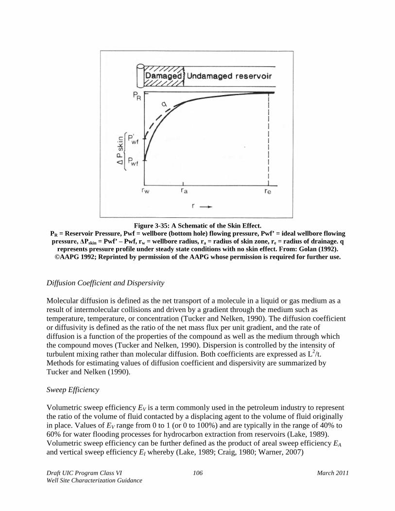
Draft UIC Program Class VI 106 March 2011 Well Site Characterization Guidance
Figure 3-35: A Schematic of the Skin Effect.
PR = Reservoir Pressure, Pwf = wellbore (bottom hole) flowing pressure, Pwf’ = ideal wellbore flowing pressure, ΔPskin = Pwf’ – Pwf, rw = wellbore radius, ra = radius of skin zone, re = radius of drainage. q
represents pressure profile under steady state conditions with no skin effect. From: Golan (1992). ©AAPG 1992; Reprinted by permission of the AAPG whose permission is required for further use.
Diffusion Coefficient and Dispersivity Molecular diffusion is defined as the net transport of a molecule in a liquid or gas medium as a result of intermolecular collisions and driven by a gradient through the medium such as temperature, temperature, or concentration (Tucker and Nelken, 1990). The diffusion coefficient or diffusivity is defined as the ratio of the net mass flux per unit gradient, and the rate of diffusion is a function of the properties of the compound as well as the medium through which the compound moves (Tucker and Nelken, 1990). Dispersion is controlled by the intensity of turbulent mixing rather than molecular diffusion. Both coefficients are expressed as L2/t. Methods for estimating values of diffusion coefficient and dispersivity are summarized by Tucker and Nelken (1990).
Sweep Efficiency
Volumetric sweep efficiency EV is a term commonly used in the petroleum industry to represent the ratio of the volume of fluid contacted by a displacing agent to the volume of fluid originally in place. Values of EV range from 0 to 1 (or 0 to 100%) and are typically in the range of 40% to 60% for water flooding processes for hydrocarbon extraction from reservoirs (Lake, 1989). Volumetric sweep efficiency can be further defined as the product of areal sweep efficiency EA and vertical sweep efficiency EI whereby (Lake, 1989; Craig, 1980; Warner, 2007)
Draft UIC Program Class VI 107 March 2011 Well Site Characterization Guidance
𝑬𝑽 = 𝑬𝑨𝑬𝑰 Equation 3-30
Areal sweep efficiency EA is generally used in the petroleum industry to represent the ratio of the area contacted by the displacing agent to the total area, and vertical sweep efficiency EI is used to characterize the ratio of the cross-sectional area contacted by the displacing agent to the total cross-sectional area (Lake, 1989; Craig, 1980; Warner 2007). Several correlations have been developed and reported in the petroleum literature for estimating sweep efficiency through porous media for various well field injection patterns and simplifying assumptions (Craig, 1980).
Injection processes in porous media are typically accompanied by fluid instabilities. Fingering is a term commonly used in the petroleum industry to describe the bypassing of a resident fluid by a displacing agent in a homogeneous, nonuniform medium. The bypassing region is known as a finger. The term “homogeneous, nonuniform medium” was used by Lake (1989), who noted that fluid instabilities are caused by both viscous forces (viscous fingers) and gravity forces (gravity fingers); however, instability analysis does not include bypassing by permeability heterogeneities. Lake (1989) also noted that viscous and gravity fingering can be prevented from occurring during displacements, but bypassing caused by permeability heterogeneities cannot be prevented (although it can be reduced). Using Darcy’s law and an expression for the mobility ratio, a condition for finger stability can be expressed as (Lake, 1989, pp 223-227)
(𝑴− 𝟏)𝒖 < 𝑘𝜆∆𝜌𝑔 𝐬𝐢𝐧𝜶 Equation 3-31
where M is the mobility ratio, λ is the mobility of the displacing fluid, u is the superficial velocity and always positive, ∆ρ is the density difference and it can be negative, and α is the dip angle and it value also can be negative. It follows from the equation above that the condition for stability in a horizontal reservoir is simply M < 1, which is universally used in the petroleum literature to describe a condition of stabile displacement (e.g., Craig, 1980; Lake, 1989; Warner, 2007).
3.9. Methods for Estimating Carbon Dioxide Storage Capacity
Global or regional-scale estimates of available carbon dioxide storage capacity have been published by a number of organizations and investigators such as the IPCC Report (Metz et al., 2005), USDOE (2008), Cawley et al. (2005), Bachu et al. (2007), and Brennan et al (2010). Bradshaw et al. (2007) attributed the wide range of estimates to the need for developing quick assessments with limited or no data. For example, when supercritical carbon dioxide is injected into a saline formation, the density and viscosity differences results in carbon dioxide tending to override the brine and accumulate at the top of the confined formation (Figure 3-36); thus, the fraction of the total pore volume that will be used for carbon dioxide storage is not likely to be known with certainty before the start of the injection (Nordbotten et al., 2005; Bachu et al., 2007; Okwen, 2010). Other factors that potentially could affect carbon dioxide storage capacity estimates include fault-sealing and wellbore integrity, injectivity, and the number of injection wells. Estimates of storage capacity, therefore, need to be accompanied with a clear statement regarding the limitations of the assessment and the intended purpose and applicability of the

estimates, thus facilitating ready comparison with other independent assessments and storage capacity estimates (Kopp et al., 2009b; Michael et al., 2009).
Draft UIC Program Class VI 108 March 2011 Well Site Characterization Guidance
Figure 3-36: Profile of Carbon Dioxide Displacement Behavior During Injection.
Qwell = volumetric injection rate, z = vertical direction, r = radial direction, t = injection time, b(r,t) = thickness of carbon dioxide plume as a function of radial distance (r) and cumulative injection time (t), B = thickness of formation. From: Nordbotten et al. (2005). Reprinted with kind permission of Springer
Science+Business Media. Methods for estimating carbon dioxide storage capacity can be divided into static and dynamic models (USDOE, 2008a). Static models are typically used for estimating carbon dioxide storage capacity prior to injection, although static models can also be used for estimating storage after injection commences. Dynamic models are typically employed after injection commences. The application of static and dynamic models for estimating carbon dioxide storage capacity is based on methods routinely used for estimating petroleum reserves, ground water resources, underground natural gas storage, and in the Underground Injection Control (UIC) program. Parameters typically used to calculate storage capacity are listed in Table 3-6. Additional discussion regarding static and dynamic modeling methods for estimating carbon dioxide storage is provided below.
3.9.1. Static Models
Static models are typically used for estimating carbon dioxide storage capacity prior to the startup of injection. Static models include the volumetric and compressibility methods for estimating carbon dioxide storage capacity (USDOE, 2008a; USDOE, 2008b). The volumetric method uses porosity, area and thickness. The compressibility method can be applied to fluids with nearly constant total compressibility over some change in pressure (increase or decrease).
Draft UIC Program Class VI 109 March 2011 Well Site Characterization Guidance
Static models rely on parameters that are directly related to the geologic description of the area for injection such as porosity, area, thickness and compressibility. Standardized methodologies for estimating carbon dioxide storage capacity in geological media (coal beds, oil and gas reservoirs, and deep saline formations) using static models have been adopted by an international organization known as the Carbon Sequestration Leadership Forum (http://www.cslforum.org). These methodologies, as described by Bachu et al. (2007), are summarized below. More recently, Brennan et al. (2010) have developed an assessment methodology that will be used by the USGS to estimate the carbon dioxide resources of the United States. The new USGS methodology is geologically based and uses probabilistic methods and statistical evaluation to identify the range of possible storage resources at a regional to sub-basinal level. Coal Beds
The carbon dioxide storage capacity of a suitable coal bed can be estimated based on analogy with estimating the total gas in place (capacity) and reservoir deliverability (White et al., 2005). For a coal bed with gas already adsorbed by the coal, the initial gas in place (IGIP) can be calculated by the relation (Bachu et al. 2007; White et al. 2005)
𝐈𝐆𝐈𝐏 = 𝑨 × 𝒉 × 𝒏𝑪 × 𝑮𝑪 × (𝟏 − 𝒇𝒂 − 𝒇𝒎) Equation 3-32
where A is the area and h is the effective thickness of the coal zone, nC is the bulk coal density (generally assumed to be 1.4 t/m3), GC is the coal gas content, and fa and fm are the ash and moisture weight content fractions of the coal, respectively. The coal gas adsorption capacity can be assumed to follow a pressure-dependent Langmuir isotherm in the form
𝑮𝑪𝑺 = 𝑽𝑳
𝑷𝑷+𝑷𝑳
Equation 3-33
where GCS is the gas content at saturation, P is the pressure, and VL and PL are Langmuir volume and pressure, respectively. These relations are based on the assumptions that coal has a high affinity for carbon dioxide, 100% saturation is achieved, and all of the coal is accessed by the injected carbon dioxide. To estimate the effective carbon dioxide storage capacity in coal beds, the analogy is drawn to the estimation of the producible gas in place (PGIP) from the initial gas in place (IGIP) with the relation
𝐏𝐆𝐈𝐏 = 𝑹𝒇 × 𝑪 × 𝐈𝐆𝐈𝐏 Equation 3-34
whereby Rf is the recovery factor and C is the completion factor (or effective contact area). It should be noted that there is limited field data for quantification of the recovery factor (Bachu et al., 2007).
Oil and Gas Reservoirs
Calculation of carbon dioxide storage capacity for depleted oil and gas reservoirs is based on the assumption that the same storage volume is available for injected carbon dioxide as was previously occupied by the extracted hydrocarbons (Bachu et al., 2007). This condition may be

Draft UIC Program Class VI 110 March 2011 Well Site Characterization Guidance
altered, for example, in the case of formation water invading a pressure-depleted reservoir. Another assumption is that carbon dioxide injection will continue until the pressure is restored to its original reservoir condition. As discussed previously, the re-pressurization of a depleted reservoir may be problematic with regard to the integrity of the reservoir and/or cap rock; thus, the maximum sustainable pore pressure may need to be lower than the original reservoir pressure.
An equation for calculating the carbon dioxide storage capacity in oil and gas reservoirs is based on the geometry of the reservoir (Bachu et al., 2007)
𝑴𝑪𝑶𝟐𝒕 = 𝝆𝑪𝑶𝟐𝒓�𝑹𝒇𝑨𝒉∅(𝟏 − 𝑺𝒘) − 𝑽𝒊𝒘 + 𝑽𝒑𝒘� Equation 3-35
where
MCO2t = theoretical mass storage capacity for carbon dioxide in a reservoir at in situ conditions [M]
ρCO2r = carbon dioxide density at reservoir conditions [ML-3] Rf = recovery factor [dimensionless] A = reservoir area [L2] h = thickness [L] ø = porosity [dimensionless] Sw = water saturation [dimensionless] Viw = volume of injected water [L3] Vpw = volume of produced water [L3]
Bachu et al. (2007) provide alternative relations that account for fluid compressibility in gas reservoirs
𝑴𝑪𝑶𝟐𝒕 = 𝝆𝑪𝑶𝟐𝒓𝑹𝒇(𝟏 − 𝑭𝑰𝑮) × 𝐎𝐆𝐈𝐏 × �(𝑷𝒔𝒁𝒓𝑻𝒓)
𝑷𝒓𝒁𝒔𝑻𝒔� Equation 3-36
and for fluid compressibility in oil reservoirs
𝑴𝑪𝑶𝟐𝒕 = 𝝆𝑪𝑶𝟐𝒓 × �𝑹𝒇𝐎𝐎𝐈𝐏𝑩𝒇
− 𝑽𝒊𝒘 + 𝑽𝒑𝒘� Equation 3-37
where OGIP and OOIP represent the original gas and oil in place at surface conditions, FIG is the fraction of injected gas, Bf is the formation volume factor that converts oil volume from standard conditions to in situ conditions, Viw and Vpw are the volumes of injected and produced gas, P, T, and Z are pressure, temperature, and gas compressibility, respectively, and the subscripts r and s represent reservoir and surface conditions.
The effective storage capacity can be influenced by the historical operation of the oil and gas reservoir (i.e., pressure depletion and formation water influx), thus reducing the total available capacity for carbon dioxide storage. The effective carbon dioxide storage capacity can also be influenced by carbon dioxide mobility, fluid density differences, reservoir heterogeneity, and
Draft UIC Program Class VI 111 March 2011 Well Site Characterization Guidance
residual water saturation. These influences can be combined to represent an efficiency factor for estimating an effective storage capacity (Bachu et al., 2007; Doughty and Pruess, 2004)
𝑴𝑪𝑶𝟐𝒆 = 𝑪𝒎𝑪𝒃𝑪𝒉𝑪𝒘𝑪𝒂𝑴𝑪𝑶𝟐𝒕 ≡ 𝑪𝒆𝑴𝑪𝑶𝟐𝒕 Equation 3-38
where MCO2e is the effective reservoir carbon dioxide storage capacity, MCO2t is the theoretical mass storage capacity of carbon dioxide in a reservoir at in situ conditions, and the coefficient Ce is a single effective capacity coefficient that incorporates the cumulative effects of the other coefficients represented by subscripts m for mobility, b for buoyancy, h for heterogeneity, w for water saturation, and a for formation strength. Currently, there is little data available for estimating values for Ce.
Deep Saline Formations
For deep saline formations, carbon dioxide storage capacity estimates can be developed for structural and stratigraphic traps, residual gas traps, solubility traps, mineral traps, and hydrodynamic traps (Bachu et al., 2007) as described below.
For structural and stratigraphic traps, the formation is initially saturated with water (instead of hydrocarbons), and the theoretical volume available for carbon dioxide storage, VCO2t, can be calculated by the relation (Bachu et al., 2007)
𝑽𝑪𝑶𝟐𝒕 = 𝑨𝒉∅(𝟏 − 𝑺𝒘𝒊𝒓𝒓) Equation 3-39
where A is the reservoir area, h is thickness, φ is porosity, and Swirr is the irreducible water saturation. Similar to oil and gas reservoirs, the effective carbon dioxide storage volume, VCO2e, can be estimated by
𝑽𝑪𝑶𝟐𝒆 = 𝑪𝒄𝑽𝑪𝑶𝟐𝒕 Equation 3-40
where Cc is a capacity coefficient that represents the effects of heterogeneity, buoyancy, and sweep efficiency, and it can be determined through numerical simulation and/or field study. Okwen et al. (2010) developed a method for estimating carbon dioxide storage efficiency applicable to structural and stratigraphic trapping that can be characterized by carbon dioxide mobility, buoyancy forces, and residual saturation.
The mass of carbon dioxide that corresponds to the effective storage volume can be estimate by multiplying VCO2e by carbon dioxide density at storage temperature and pressure conditions. Storage temperature can be estimated as discussed previously in Section 3.8.2. Storage pressure can be estimated to be greater than the initial water pressure in the reservoir and less than the maximum bottom hole injection pressure to avoid rock fracturing.
Residual gas traps form within a saline formation when injected carbon dioxide migrates through the porous media and water moves back into the pore space. For example, during injection, carbon dioxide can migrate laterally and upward due to buoyancy forces. Once injection stops, carbon dioxide can continue to migrate, water enters the pore space, and residual,
Draft UIC Program Class VI 112 March 2011 Well Site Characterization Guidance
immobile carbon dioxide is left behind the plume (Juanes et al., 2006). Qi et al. (2009) proposed an injection strategy whereby carbon dioxide and brine are injected together and thus maximize storage efficiency in formations. The theoretical carbon dioxide storage volume of the residual gas traps can then be estimated by the relation (Bachu et al., 2007)
𝑽𝑪𝑶𝟐𝒕 = ∆𝑽𝒕𝒓𝒂𝒑∅𝑺𝑪𝑶𝟐𝒕 Equation 3-41
where ∆Vtrap CO2tdioxide saturation. ∆Vtrap and SCO2t can be estimated through numerical simulations (e.g., Juanes et al., 2006). The mass of stored carbon dioxide can be estimated by multiplying the storage volume by carbon dioxide density at in situ conditions.
Solubility trapping of carbon dioxide is a relatively slow process and assumed to become significant after cessation of injection (Bachu et al, 2007). Although dissolution of free-phase carbon dioxide occurs rapidly, and water in direct contact with injected carbon rapidly becomes saturated with carbon dioxide, the available contact area between free-phase carbon dioxide and unsaturated water is small, greatly limiting solubility trapping. When migration of carbon dioxide has stopped (thus reducing the influence of dispersion), then diffusion, which is very small, becomes the only mechanism enabling unsaturated water to contact carbon dioxide unless the water itself is moving. If a hydraulic gradient within the formation replaces the carbon dioxide-saturated water with unsaturated water, or the rock permeability and thickness are conducive to the development of convection within the pore system, then carbon dioxide will continue to dissolve into the unsaturated water that passes the contact area. The theoretical mass carbon dioxide storage capacity can be estimated using a simplified relation and average values for formation thickness, porosity, and carbon dioxide content in formation fluid as (Bachu et al, 2007)
represents the carbon dioxide -invaded rock volume and S is the trapped carbon
𝑴𝑪𝑶𝟐𝒕 = 𝑨𝒉∅�𝝆𝑺𝑿𝑺𝑪𝑶𝟐 − 𝝆𝟎𝑿𝟎𝑪𝑶𝟐� Equation 3-42
where ρ is the density of the formation water, XCO2 is the mass fraction carbon dioxide content in formation water, and the subscripts 0 and S represent initial and saturated carbon dioxide content, respectively. Similar to the relations for coal beds and oil and gas reservoirs, the mass carbon dioxide storage capacity can be estimated by multiplying the theoretical value by a coefficient that includes the effects of spreading and dissolution of carbon dioxide in the whole formation However, for a site-specific application, the theoretical carbon dioxide storage capacity associated with solubility trapping should be assessed by numerical modeling (Bachu et al., 2007).
Mineral trapping of carbon dioxide depends on the chemical composition of the rock matrix and formation waters, in situ temperature and pressure conditions, the interface between the mineral grains and the formation water containing dissolved carbon dioxide, and the flow of fluids past the interface (Bachu et al., 2007). For site-specific applications, the amount and timeframe of carbon dioxide storage associated with mineral trapping should be estimated by numerical modeling and supported, where possible, with laboratory testing and field data.
Draft UIC Program Class VI 113 March 2011 Well Site Characterization Guidance
Hydrodynamic trapping of carbon dioxide is a combination of mechanisms (structural and stratigraphic trapping, dissolution, mineral precipitation, residual gas trapping) operating simultaneously, but at different rates, while an injected plume of carbon dioxide expands and migrates in a storage reservoir (Bachu et al., 2007). Carbon dioxide storage capacity associated with hydrodynamic trapping therefore needs to be evaluated at a specific point in time as the sum of the component mechanisms by numerical simulations.
3.9.2. Dynamic Models
Dynamic models are generally considered applicable for estimating carbon dioxide storage capacity after initiation of carbon dioxide injection (USDOE, 2008a). They would therefore be useful after receiving a permit to operate a Class VI injection well, as a way to monitor storage capacity over time. Dynamic models include decline curve analysis, material balance, and reservoir simulation.
Decline Curve Analysis
The decline curve analysis is a dynamic method for estimating subsurface storage volumes based on a simple exponential relation of injection rate and time (USDOE, 2008a)
𝒒𝑪𝑶𝟐 = 𝒒𝑪𝑶𝟐𝒊𝒆−𝑫𝒕 Equation 3-43
where qCO2 is the carbon dioxide injection rate and the subscript i denotes the initial injection rate, D is a decline coefficient that represent flow characteristics of the formation, and t represents time. Carbon dioxide storage capacity, GCO2, can be estimated by the relation
𝑮𝑪𝑶𝟐 = (𝒒𝑪𝑶𝟐𝒊−𝒒𝑪𝑶𝟐)
𝑫 Equation 3-44
where the decline coefficient D is determined from the exponential decline equation for a given injection rate history. This decline curve analysis is generally considered applicable to individual wells or entire fields, provided the exponential trend exists. Additional information regarding theory and application of decline curve analysis techniques is provided in Arps (1962), Campbell and Campbell (1978), and Li and Horne (2003). This relation can be used to estimate carbon dioxide storage capacity likely to be attained with continued injection. Material Balance
The material balance method for estimating carbon dioxide storage capacity is based on the relationship between cumulative carbon dioxide injection and the corresponding pore pressure as a function of time (USDOE, 2008a). The relation is analogous to the p/z plots used in gas reservoir and underground gas storage reservoirs (e.g., Harrell and Cronquist, 2007), where z is the gas compressibility factor of carbon dioxide evaluated at pressure p. A straight line is expected on a plot of p/z versus cumulative carbon dioxide gas injection. The carbon dioxide storage capacity can be estimated from this plot by extrapolating the curve and determining the value of cumulative carbon dioxide gas injection that corresponds to the maximum p/z value at capacity pressure.

Draft UIC Program Class VI 114 March 2011 Well Site Characterization Guidance
Reservoir Simulation
Reservoir simulation is considered the most advanced method for estimating carbon dioxide storage capacity, provided the input data adequately represent the injection formation and operating conditions (USDOE, 2008a). The purpose of simulation is to estimate field performance under one or more operational schemes (Batycky et al., 2007). For example, the simulation can be used to study actual field or pilot performance and thus improve estimates for carbon dioxide storage capacity. As discussed previously, reservoir simulation can be also used to develop estimates of specific carbon dioxide storage trapping mechanisms (e.g., hydrodynamic trapping). Reservoir simulation is the most resource-intensive method of estimating carbon dioxide storage. However, it requires the input of data at a scale and resolution appropriate for obtaining results at formation scale. Additional discussion regarding reservoir simulation is provided in the Draft UIC Program Class VI Well Area of Review and Corrective Action Guidance.
3.10. Demonstration of Confining Zone Integrity Demonstration of the ability of the confining zone to contain the carbon dioxide plume is a key component of site characterization and is required by the GS Rule[§146.83(a)(2)]. This section describes the data needed to make the required demonstration that the confining zone will not allow migration of carbon dioxide; either through interconnected pore spaces across the thickness of the seal or by allowing migration of carbon dioxide through the confining zone along faults or fractures. In particular, analyses may be needed to ensure that existing non-transmissive faults will not become transmissive under anticipated injection and storage pressures in order to meet the requirements [§146.83(a)(2)]. The methods described here are applicable to sites with single confining zones or multiple confining zones if characterization of such additional zones is required by the UIC Program Director [§146.83(b)].
3.10.1. Data Needs
A number of methods are available to demonstrate competence of the confining zone. The GS Rule does not specify which methods should be used for Class VI injection wells; the choices of analyses and the data needed will depend on site geology. In general, the following types of data may be useful when determining confining zone integrity:
• Lithologic and Stratigraphic Data – Includes information on the depth, thickness,
mineralogy, and heterogeneity of the confining zone. Additional information is available in Section 3.1.
• Structural Data – Includes information on faults and fractures, including fault geometry (the shape of the fault plane), depth of origin and termination, and the amount of displacement along the fault (including determinations of whether slip is consistent or variable along the fault and where such variations occur). Additional information is available in Section 3.2.
Draft UIC Program Class VI 115 March 2011 Well Site Characterization Guidance
• Data from Core Analysis – Includes information on the capillary pressure, rock strength, permeability, porosity, pore throat radius, fracture pressure, wetting angle, and IFT of pore fluid. Additional information is available in Sections 3.4 and 3.8.
• Field Formation Testing Data – Includes information on the in situ fluid pressures, the
magnitudes of principal stresses, and temperature. Additional information is available in Section 3.6.
Most of the required data needed to demonstrate confining zone integrity are also required to fulfill other Class VI injection well requirements [§§146.82(a)(1) through 146.82(a)(8)]. These data may come from direct sampling and laboratory tests, indirect methods (e.g. seismic, gravity, magnetic, or other geophysical tools), interpretive aids (e.g. maps, cross-sections, stratigraphic columns), or other sources. Data least likely to exist in other sections of the Class VI well permit application include information on the wetting angle/wettability, IFT, and detailed fault geometry.
3.10.2. Use of Data to Evaluate Confining Zone Integrity
The parameters used to assess confining zone integrity are calculated from existing data and are not primary measurements. Therefore, the reliability of the final measurement depends upon the quality of the input data, and errors will be propagated through any calculations done in support of this analysis. Also, fault properties may vary spatially along the fault, resulting in variability of sealing capacity. The owner/operator should remain aware of uncertainties in input data, communicate those uncertainties to the UIC Program Director in the Class VI injection well permit application, and be cognizant of the need for additional analyses to represent any spatial heterogeneity. Movement through the Confining Zone
Continuous confining zones lacking faults, fractures, or other obvious ruptures may still allow the transmission of carbon dioxide through interconnected pore spaces throughout the thickness of the seal. Movement across intact seals is controlled by capillary pressure, permeability, and molecular diffusion.
Capillary Pressure
Capillary pressure and related measurement techniques are discussed elsewhere in this guidance document (Section 3.8.2). As a rule of thumb, good seals will have capillary entry pressures between approximately 6 and 40 MPa (Duncan, 2009). In cases where the seal integrity is controlled by the entry pressure, the thickness of the seal is not critical as long as the layer is thicker than the capillary slug pinch off length (the length at which a continuous column of fluid entering or in contact with seal fluids disintegrates into smaller units not in contact with the source and not capable of progressing further into the seal).

Draft UIC Program Class VI 116 March 2011 Well Site Characterization Guidance
Permeability
Once the fluid pressure exceeds the capillary pressure, fluid may flow through the layer at a rate controlled by the permeability and the fluid pressure (Duncan, 2009). Laboratory and field-based methods are available to determine permeability. See Section 3.4.2 of this guidance document for further details).
A layer can make an effective seal even if the capillary entry pressure is low or if capillary entry pressure is exceeded as long as the permeability is also low. In these cases, fluid may be able to enter the sealing layer, but it will not be able to progress through the layer. A thick confining zone with low permeability may permit very slow flow, effectively impeding migration through the unit. Unlike seals that depend on capillary sealing mechanisms, if permeability is the dominating factor a thicker unit will provide a better seal. Numerical modeling could be conducted to assess the potential effectiveness of the seal.
Molecular Diffusion
A seal may also transmit carbon dioxide in the absence of faults or fractures when carbon dioxide enters the confining zone through molecular transport/simple diffusion. This type of transport happens in nearly all sedimentary rocks regardless of the permeability of the layer. Nevertheless, this potential leakage pathway is not considered a threat to confining zone integrity; any potential leakage volumes are likely to be small, and carbon dioxide entering the confining zone will most likely react with the minerals before fully migrating across the layer (Busch et al., 2008), trapping carbon dioxide by mineral sequestration. However, reactions may change the geomechanical and lithologic properties of the seal over time, potentially requiring a re-examination of such parameters. Current research suggests that in the absence of fluid-rock reactions, a 100 m thick shale at 1000 m depth (~45-50°C, 10 MPa) with 20% porosity and an infinite source of carbon dioxide will leak due to diffusive loss after 300,000 years (Busch et al., 2008).
Case Study
Wollenweber et al. (2010) simulated repeated cycles of pressure fluctuation capable of generating containment breaches of carbon dioxide through mudstone and carbonate sealing formations. Testing was conducted using petrophysical and mineralogical laboratory methods under in situ pressure and temperature conditions. Results provide information regarding potential changes in sealing properties of confining zones exposed to high carbon dioxide partial pressures. Further, this study provides a description of an approach that can be used to study the complex physic-chemical processes for site-specific carbon dioxide -water-rock systems.
Transmission of Carbon Dioxide through Faults
A confining zone may be compromised if faults or fractures allow carbon dioxide movement across the layer. Faults can provide leakage pathways either across or along the fault. These faults or fractures can either be present before injection or generated as a result of injection.

Draft UIC Program Class VI 117 March 2011 Well Site Characterization Guidance
Creation of Faults Fractures can be generated when capillary entry pressure exceeds the rock strength. At this point, the layer will fracture before carbon dioxide enters into pore spaces. These types of seals are called hydraulic seals. Very small pore throats are a common feature of hydraulic seals because the resulting capillary entry pressures in such layers is essentially infinite. The GS Rule at §146.88(a) specifies that injection cannot initiate fractures in the confining zone; injection pressures below the fracture pressure of the confining zone are required to preserve seal integrity. Characterizing the Sealing Potential of Faults Faulted formations may seal carbon dioxide (Meckel, 2007), but EPA recommends that applicants verify confining zone integrity by characterizing the sealing potential of the faulted formation. Any faults that that intersect, originate, or terminate in the confining zone should be well characterized, regardless of their size (Knipe et al., 2001; Meckel 2007). Thorough characterization of faults is important because properties can be heterogeneous across the fault plane, complicating interpretation (Freeman et al., 1998). A fault may be sealing (non-transmissive) in some regions while remaining transmissive in others. Figure 3-37 shows an example of heterogeneity across a fault plane. It is often more important to determine if the fault is sealing or non-sealing in the area or areas that have a critical impact on the integrity of the seal (e.g., above or below structural spill points) than for the entire surface of the fault.
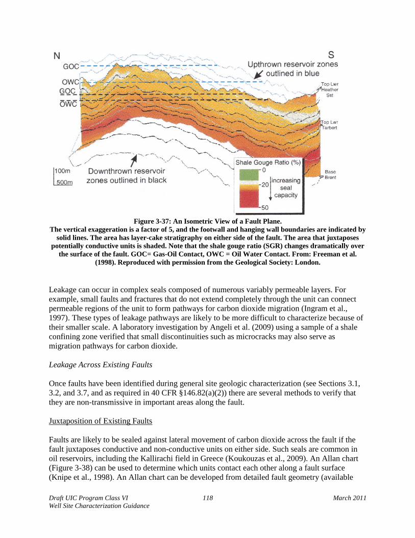
Draft UIC Program Class VI 118 March 2011 Well Site Characterization Guidance
Figure 3-37: An Isometric View of a Fault Plane.
The vertical exaggeration is a factor of 5, and the footwall and hanging wall boundaries are indicated by solid lines. The area has layer-cake stratigraphy on either side of the fault. The area that juxtaposes
potentially conductive units is shaded. Note that the shale gouge ratio (SGR) changes dramatically over the surface of the fault. GOC= Gas-Oil Contact, OWC = Oil Water Contact. From: Freeman et al.
(1998). Reproduced with permission from the Geological Society: London.
Leakage can occur in complex seals composed of numerous variably permeable layers. For example, small faults and fractures that do not extend completely through the unit can connect permeable regions of the unit to form pathways for carbon dioxide migration (Ingram et al., 1997). These types of leakage pathways are likely to be more difficult to characterize because of their smaller scale. A laboratory investigation by Angeli et al. (2009) using a sample of a shale confining zone verified that small discontinuities such as microcracks may also serve as migration pathways for carbon dioxide.
Leakage Across Existing Faults
Once faults have been identified during general site geologic characterization (see Sections 3.1, 3.2, and 3.7, and as required in 40 CFR §146.82(a)(2)) there are several methods to verify that they are non-transmissive in important areas along the fault.
Juxtaposition of Existing Faults
Faults are likely to be sealed against lateral movement of carbon dioxide across the fault if the fault juxtaposes conductive and non-conductive units on either side. Such seals are common in oil reservoirs, including the Kallirachi field in Greece (Koukouzas et al., 2009). An Allan chart (Figure 3-38) can be used to determine which units contact each other along a fault surface (Knipe et al., 1998). An Allan chart can be developed from detailed fault geometry (available
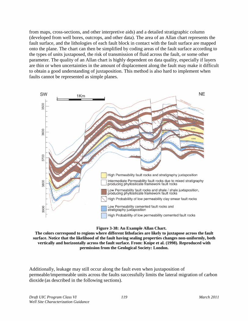
Draft UIC Program Class VI 119 March 2011 Well Site Characterization Guidance
from maps, cross-sections, and other interpretive aids) and a detailed stratigraphic column (developed from well bores, outcrops, and other data). The area of an Allan chart represents the fault surface, and the lithologies of each fault block in contact with the fault surface are mapped onto the plane. The chart can then be simplified by coding areas of the fault surface according to the types of units juxtaposed, the risk of transmission of fluid across the fault, or some other parameter. The quality of an Allan chart is highly dependent on data quality, especially if layers are thin or when uncertainties in the amount of displacement along the fault may make it difficult to obtain a good understanding of juxtaposition. This method is also hard to implement when faults cannot be represented as simple planes.
Figure 3-38: An Example Allan Chart.
The colors correspond to regions where different lithofacies are likely to juxtapose across the fault surface. Notice that the likelihood of the fault having sealing properties changes non-uniformly, both
vertically and horizontally across the fault surface. From: Knipe et al. (1998). Reproduced with permission from the Geological Society: London.
Additionally, leakage may still occur along the fault even when juxtaposition of permeable/impermeable units across the faults successfully limits the lateral migration of carbon dioxide (as described in the following sections).

Draft UIC Program Class VI 120 March 2011 Well Site Characterization Guidance
Leakage along Faults
The risk of leakage along a fault will be lower if sediments with a high capillary pressure are found along or incorporated into the fault zone. These sediments will prevent migration of carbon dioxide along the fault for the same reasons they can prevent migration upward when present as a seal. Such materials can occur along the faults as a result of catalysis, diagenetic sealing, or by entrainment during fault movement. As a rule of thumb, some research (Kovscek, 2002) suggests that faults that are capable of slip under the current stress regime are more likely to act as leakage pathways, while faults that are not likely to slip under current stress conditions are likely to seal.
Catalysis
Catalysis is the breakdown of materials along the fault due to physical abrasion during fault slip. Fine material tends to have smaller pore throats and, correspondingly, high capillary pressure. The amount of breakdown along the fault is not related to amount of displacement (Yielding et al., 1997). Catalysis can reduce the permeability of high-porosity sandstones up to four orders of magnitude with only a few centimeters of slip and lead to sealing behavior along the fault (Yielding et al., 1997). Crushing of rocks along the fault severe enough to lead to fault sealing by catalysis is more likely to occur when faults occur at depth, or in reverse or strike-slip faulting, but it can occur at depths as little as 100 m (Yielding et al., 1997). The degree of catalysis can be evaluated by examining hand samples, cores, or thin sections taken from the fault zone. After evaluation, hand samples may be subjected to capillary pressure tests or other laboratory tests (see above) to quantify the effect of catalysis on pore size.
Diagenesis
Diagenetic sealing occurs when deposition of material (e.g. calcite, silicates) along the fault plane renders a fault impermeable (Meckel, 2007). Deposition can occur because faults may act as conduits for fluids rich in dissolved materials. These materials can precipitate out along the fault plane, creating a seal. Determining the amount of diagenetic sealing requires the direct examination of core samples from the fault zone in the laboratory. In some cases, samples taken from nearby faults or outcrops may be used to infer the amount of diagenetic sealing on buried faults, provided that the faults examined originated in the same period of faulting and that examination of faults on numerous scales (e.g. thin section, hand sample, outcrop) indicate that diagenetic behavior is similar throughout the unit.
Entrainment of Materials along the Fault
Materials from the hanging- and footwalls can be incorporated along the fault (Figure 3-39). Shales and other clay- rich units are the most likely lithologies to be incorporated along the fault because of their low rock strength and high ductility. Because clay has a small pore throat radius, incorporating it along a fault raises the capillary pressure of the sediment and helps to retard the flow of fluids along the fault.

Draft UIC Program Class VI 121 March 2011 Well Site Characterization Guidance
Figure 3-39: Simplified Shale Smearing Along a Fault .
The fault crosses shale (gray) and sandstone (white) layers. As displacement occurs along the fault (a and b), portions of the shale layers are incorporated into the fault zone. As the displacement increases
(c), the amount of shale along the fault thins. Direction of fault slip indicated by arrows, fault plane idealized as a dotted line. Modeled after Koledoye et al., 2003.
The amount of shale entrained by the fault from the shale/siltstone units the fault intersects can be estimated using the shale gouge ratio (SGR) (Freeman et al., 1998). This method works best for shale/sandstone/siltstone sequences. The shale gouge ratio can be calculated as:
𝐒𝐆𝐑 = �[(𝐙𝐨𝐧𝐞 (𝐢.𝐞.,𝐥𝐚𝐲𝐞𝐫) 𝐓𝐡𝐢𝐜𝐤𝐧𝐞𝐬𝐬)×(𝐙𝐨𝐧𝐞 𝐂𝐥𝐚𝐲 𝐅𝐫𝐚𝐜𝐭𝐢𝐨𝐧)]
𝐅𝐚𝐮𝐥𝐭 𝐓𝐡𝐫𝐨𝐰� × 𝟏𝟎𝟎% Equation 3-45
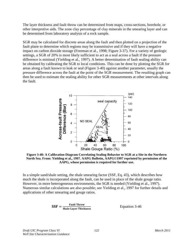
Draft UIC Program Class VI 122 March 2011 Well Site Characterization Guidance
The layer thickness and fault throw can be determined from maps, cross-sections, borehole, or other interpretive aids. The zone clay percentage of clay minerals in the smearing layer and can be determined from laboratory analysis of a rock sample.
SGR may be calculated for discrete areas along the fault and then plotted on a projection of the fault plane to determine which regions may be transmissive and if they will have a negative impact on carbon dioxide storage (Freeman et al., 1998; Figure 3-37). For a variety of geologic settings, a SGR of 20% is most likely sufficient to act as a seal across a fault if the pressure difference is minimal (Yielding et al., 1997). A better determination of fault sealing ability can be obtained by calibrating the SGR to local conditions. This can be done by plotting the SGR for areas along a fault known to leak or seal (Figure 3-40) against another parameter, usually the pressure difference across the fault at the point of the SGR measurement. The resulting graph can then be used to estimate the sealing ability for other SGR measurements at other intervals along the fault.
Figure 3-40: A Calibration Diagram Correlating Sealing Behavior to SGR at a Site in the Northern North Sea. From: Yielding et al., 1997. AAPG Bulletin, AAPG©1997 reprinted by permission of the
AAPG, whose permission is required for further use.
In a simple sand/shale setting, the shale smearing factor (SSF, Eq. 43), which describes how much the shale is incorporated along the fault, can be used in place of the shale gouge ratio. However, in more heterogeneous environments, the SGR is needed (Yielding et al., 1997). Numerous similar calculations are also possible; see Yielding et al., 1997 for further details and applications of other smearing and gouge ratios.
𝐒𝐒𝐅 = 𝐅𝐚𝐮𝐥𝐭 𝐓𝐡𝐫𝐨𝐰
𝐒𝐡𝐚𝐥𝐞 𝐋𝐚𝐲𝐞𝐫 𝐓𝐡𝐢𝐜𝐤𝐧𝐞𝐬𝐬 Equation 3-46
Draft UIC Program Class VI 123 March 2011 Well Site Characterization Guidance
Calculation of the SGR and other shale-entrainment methods requires accurate knowledge of lithology (specifically clay/phyllosilicate content) and thickness in the area of the fault. This level of information may require new boreholes, seismic surveys, other geophysical surveys, and/or a refined analysis of fault geometry and extent.
Pressure Compartmentalization
Another method of analyzing fault sealing ability is to determine if the fault compartmentalizes regions of different subsurface pressure (Huffman, 2002). If this occurs, the fault may be sealing. This method requires both subsurface mapping of all faults within the area of interest and pore pressure measurements. Pressure measurements can be taken directly from a network of wells distributed on both sides of the fault (Doughty and Karasaki, 2004). Depending on the distribution and density of wells, modeling can be used to infer pressure in regions between wells. Indirect pore pressure data may be generated by transforming seismic velocity data into pore pressure (see Section 3.7.2). Once the subsurface pore pressures have been mapped, the locations of all known faults are projected into the same subsurface visualization. Using this method, it is also possible to evaluate if sealing behavior changes along the fault (Figure 3-41). One disadvantage to be aware of when using indirect, seismic pore-pressure data is that this method of pore pressure estimation is still under development, and it can introduce considerable errors, especially in subsurface environments that have not undergone significant subsurface exploration. Gathering sufficient subsurface pressure data by wells to use the pressure compartmentalization method may be cumbersome, and although a pressure difference across a fault indicates sealing behavior, the lack of a pressure difference does not definitively indicate a transmissive fault.

Draft UIC Program Class VI 124 March 2011 Well Site Characterization Guidance
Figure 3-41: Sealing Capacity from Seismic Pore Pressure Images. Faults are interpreted in the seismic image in (A), then mapped as lines onto the pore pressure
determination (B). Color ramp from low pressure (green) to high pressure (red). While the major fault (labeled with arrow Y and Z) at right compartmentalizes pressure, indicating that it may be sealing, the
fault at left (labeled with arrow X), does not separate regions of different pressure, suggesting that it may not be sealing. The apparent non-compartmentalization of high pressure near the tip of the Z
arrow may be due to poor resolution of the pressure data. No scale given, described as “Basin-Scale”. Vertical red lines above X and Z are to be wells. From: Huffman, 2002, AAPG Memoir, AAPG©2002
reprinted by permission of the AAPG, whose permission is required for further use. 3.10.3. Special Considerations for Characterizing Lower Confining Zones
In any supplemental report to a Class VI injection well permit application requesting a waiver of the GS Rule injection depth requirements, the potential Class VI well owner or operator will need to demonstrate the integrity of both the upper and the lower confining zones[§146.95(a)(2)]. The basic methods for evaluating seal integrity remain the same whether the confining zone is above or below the injection zone. Estimates of thickness, permeability, capillary pressure and other parameters are recommended, as well as an understanding of whether the zone contains interbedded units of higher permeability. The potential Class VI injection well owner or operator will also need to demonstrate that the confining zones are free of transmissive faults and fractures [§146.95(a)(2)]. One important difference to consider between upper and lower confining zones is that the upper confining zone will likely contact free phase carbon dioxide prior to its dissolution while the lower confining zone may or may not contact free phase carbon dioxide. However, both the upper and lower confining zones will be in contact with brine and may eventually be in contact with carbon dioxide-saturated brine. While capillary entry pressure is not relevant in the case of brine contacting a confining zone already

Draft UIC Program Class VI 125 March 2011 Well Site Characterization Guidance
saturated with brine, the capillary entry pressure of free phase carbon dioxide in the lower confining zone should be determined and considered as part of the Class VI permit application supplemental report requesting an injection depth waiver.
3.10.4. Summary and Conclusions
An ideal confining zone will have a high capillary entry pressure, a low permeability, and not contain or intersect fractures or faults. The thickness of the confining zone may not be important in all cases, but in general, thicker confining zones will be more secure, especially if the confining zone has a relatively low capillary sealing pressure. If faults or fractures intersect the confining zone, at least one sealing mechanism (e.g. diagenesis, catalysis, entrainment) capable of preventing carbon dioxide migration along the fault should be identified. Identifying more than one sealing mechanism will increase confidence that the fault intersecting the confining zone is sealing.
If a confining zone is not homogenous, care should be taken to capture the range of permeabilities and capillary entry pressures in the formation. Discontinuous impermeable areas within injection formations should also be investigated. Such horizons may act as baffles, retarding migration of carbon dioxide toward the main seal. These smaller baffles may prevent a large column of carbon dioxide from building up below the main seal, helping to keep fluid pressure below the capillary entry pressure. Multiple baffles are present, for example, at the Sleipner carbon dioxide injection site, where they have been successful at retarding upward migration of injected carbon dioxide. See Figure 3-42 below for more information In addition to satisfying the Class VI permit application requirements at §146.82(a)(3), the information collected to support fault sealing and confining zone integrity analysis may also be used to support other portions of a Class VI injection well permit application. Parameters such as capillary entry pressure, IFT, and wettability, may be used to support required modeling for AoR determination [§146.84(a)], required project plan development [§146.82(a)], and required operational monitoring [§146.90]. In addition, fault seal analysis can be used to target areas where additional monitoring may be needed if faults appear close to their sealing capacity.
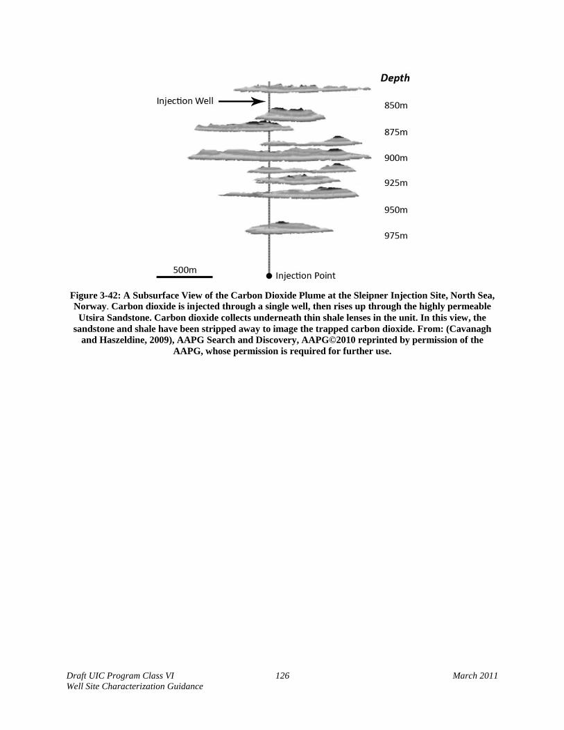
Draft UIC Program Class VI 126 March 2011 Well Site Characterization Guidance
Figure 3-42: A Subsurface View of the Carbon Dioxide Plume at the Sleipner Injection Site, North Sea, Norway. Carbon dioxide is injected through a single well, then rises up through the highly permeable
Utsira Sandstone. Carbon dioxide collects underneath thin shale lenses in the unit. In this view, the sandstone and shale have been stripped away to image the trapped carbon dioxide. From: (Cavanagh
and Haszeldine, 2009), AAPG Search and Discovery, AAPG©2010 reprinted by permission of the AAPG, whose permission is required for further use.
Draft UIC Program Class VI 127 March 2011 Well Site Characterization Guidance
4. Conclusion Site characterization entails the compilation of numerous types of information, including geological, geophysical, geomechanical, and geochemical data. This information is not only crucial for establishing the viability of a proposed sequestration site, but is also used in the required computational modeling for AoR delineation determination and to guide the development of a Testing and Monitoring Plan that meets the requirements of the GS Rule. This document was developed to provide background information and suggested approaches for gathering the information needed to complete the site characterization aspects of a Class VI injection well permit application. In the initial stages of site characterization (discussed in Section 2), a desktop analysis of existing information on the geology of the region and the project area can be done to identify the basic geologic and hydrogeologic characteristics and demonstrate the potential viability of the project site. The amount of information available at this initial stage will depend upon the history of the region with respect to subsurface characterization. Information that may be compiled at this stage (e.g., maps, cross sections, seismic history, locations of faults) is required by the GS Rule at §146.82(a). Completion of a successful Class VI Well permit application also requires detailed information about numerous subsurface properties, including the structure, petrology, mineralogy, geochemistry, and geomechanical properties of the injection zone and confining zones [§146.82(a)]. Additionally, the Rule at §146.83 provides minimum siting criteria, including requirements that the confining zone be free of transmissive fractures and able to withstand the proposed injection pressures without fracturing, and that the injection zone have sufficient capacity to receive the anticipated amount of carbon dioxide. Section 3 of this document describes the various properties for which data are needed, and describes the commonly used methods for acquiring those data. The GS Rule does not prescribe which methods should be used to obtain information; this guidance document is intended to provide the reader with an overview of various options and their advantages and disadvantages. Two of the more sophisticated analyses that are required for a proposed Class VI injection well are the determination of storage capacity and the demonstration of confining zone integrity. These analyses build upon a variety of types of data and are covered in Sections 3.8-3.9 and 3.10, respectively. Additional information relevant to site characterization can be obtained from the references cited in this document as well as from the EPA UIC program (http://water.epa.gov/type/groundwater/uic/index.cfm) and climate change program (http://www.epa.gov/climatechange/emissions/co2_geosequest.html).

Draft UIC Program Class VI 128 March 2011 Well Site Characterization Guidance
5. References Abaci, S., J.S. Edwards, and B.N. Whittaker. 1992. Relative permeability measurements for two
phase flow in unconsolidated sands. Mine Water and the Environment 11(2): 11-26. Adams, J.J. and S. Bachu. 2002. Equations of state for basin geofluids: Algorithm review and
intercomparison for brines. Geofluids 2: 257–271. Aguilera, R. 1992. Formation Evaluation of Naturally Fractured Reservoirs. In Morton-
Thompson, D. and A.M. Woods, Eds. Development Geology Reference Manual (pp. 192-193). AAPG Methods in Exploration Series, No. 10. Tulsa: Oklahoma.
Ahmed, T.H. 2006. Reservoir Engineering Handbook. 3rd edition. Gulf Professional Publishing
(Elsevier): Burlington, Massachusetts. Alberty, M. 1992a. Standard Interpretation. In Morton-Thompson, D. and A.M. Woods, Eds.
Development Geology Reference Manual (pp. 180-185). AAPG Methods in Exploration Series, No. 10. Tulsa: Oklahoma.
Alberty, M. 1992b. Basic Open Hole Tools. In Morton-Thompson, D. and A.M. Woods, Eds.
Development Geology Reference Manual (pp. 144-149). AAPG Methods in Exploration Series, No. 10. Tulsa: Oklahoma.
Almon, W.R. 1992. Overview of Routine Core Analysis. In Morton-Thompson, D. and A.M.
Woods, Eds. Development Geology Reference Manual (pp. 201-203). AAPG Methods in Exploration Series, No. 10. Tulsa: Oklahoma.
Ambrose, W.A, S. Lakshminarasimhan, M.H. Holtz, V. Núñez-López, S.D. Hovorka, and I.
Duncan. 2008. Geologic factors controlling CO2 storage capacity and permanence: Case studies based on experience with heterogeneity in oil and gas reservoirs applied to CO2 storage. Environmental Geology 54(8): 1619–1633.
Antarctic Geologic Drilling. 2010. Betty’s Blog. Available on the Internet at:
http://www.andrill.org/iceberg/blogs/betty/all.php. ASTM Standard D5731-8. 2007 (2005, 2002, 1995). Standard Test Method for Determination of
the Point Load Strength Index of Rock and Application to Rock Strength Classifications. ASTM International, West Conshohocken, PA, DOI: 10.1520/D5731-08. Available on the Internet at: http://www.astm.org.
ASTM Standard D7012-10. 2007 (2007e1, 2004). Standard Test Method for Compressive
Strength and Elastic Moduli of Intact Rock Core Specimens under Varying States of Stress and Temperatures. ASTM International, West Conshohocken, PA, DOI: 10.1520/D7012-10. Available on the Internet at: http://www.astm.org.

Draft UIC Program Class VI 129 March 2011 Well Site Characterization Guidance
Angeli, A., M. Soldal, E. Skurtveit, and E. Aker. 2009. Experimental percolation of supercritical CO2 through a caprock. Energy Procedia 1 (GHGT-9): 3351-3358.
Archie, G.E. 1942. The electrical resistivity log as an aid in determining some reservoir
characteristics. Petroleum Transactions of American Institute of Mining, Metallurgical, and Petroleum Engineers 146: 54–62.
Arps, J.J. 1962. Estimation of primary oil and gas reserves. In Frick, T.C., Ed. Petroleum
Production Handbook, Volume II Reservoir Engineering. Chapter 37. Society of Petroleum Engineers: Dallas, Texas.
Attia, A.M., D. Fratta, and Z. Bassiouni. 2008. Irreducible water saturation from capillary
pressure and electrical resistivity measurements. Oil and Gas Science and Technology 63(2): 203-217.
Avseth, P., T. Mukerji, and G. Mavko. 2010. Quantitative Seismic Interpretation: Applying Rock
Physics Tools to Reduce Interpretation Risk. Cambridge University Press: Cambridge, United Kingdom.
Bachu, S. and B. Bennion. 2008. Effects of in-situ conditions on relative permeability
characteristics of CO2 brine systems. Environmental Geology 54: 1707-1722. Bachu, S. and B. Bennion. 2009. Interfacial tension between CO2, freshwater, and brine in the
range of pressure from (2 to 27) MPa, temperature from (20 to 125) °C, and water salinity from (0 to 334 000) mgL-1. Journal of Chemical and Engineering Data 54: 765–775.
Bachu, S., D. Bonijoly, J. Bradshaw, R. Burruss, S. Holloway, N.P. Christensen, and O.M.
Mathiassen. 2007. CO2 storage capacity estimation: Methodology and gaps. International Journal of Greenhouse Gas Control 1: 430-443.
Bachu, S. and K. Haug. 2005. In situ characteristics of acid-gas injection operations in the
Alberta Basin, Western Canada: Demonstration of CO2 geological storage. In Thomas, D.C. and S.M. Benson, Eds. Carbon Dioxide Capture for Storage in Deep Geologic Formations, Volume 2. Elsevier: Oxford, United Kingdom.
Bahadori, A. and H.B. Vuthaluru. 2010. Predictive tool for an accurate estimation of carbon
dioxide transport properties. International Journal of Greenhouse Gas Control 4: 532-536. Balan, B., S. Mahaghegh, and S. Ameri. 1995. state-of-the-art in permeability determination
from well log data: Part 1 – A comparative study, model development. SPE 30978. Balch, A.H., M.W. Lee, J.J. Miller, and R.T. Ryder. 1982. The use of vertical seismic profiles in
seismic investigations of the earth. Geophysics 47: 906. Barakat, S. 2009. A seismic shift in thinking. Available on the Internet at: http:
//www.ngoilgasmena.com/article/A-seismic-shift-in-thinking/.
Draft UIC Program Class VI 130 March 2011 Well Site Characterization Guidance
Barbosa, V.C.F., P.T.L. Menezes, and J.B.C. Silva. 2007. Gravity as a tool for detecting faults: In depth enhancement of subtle Almada's basement faults, Brazil. Geophysics 73(3): B59-B68.
Batycky, R.P., M.R. Thiele, K.H. Coats, A. Grindheim, D. Ponting, J.E. Killough, T. Settari,
L.K. Thomas, J. Wallis, J.W. Watts, and C.H. Whitson. 2007. Chapter 17: Reservoir simulation. In Holstein, E.D., Ed. Reservoir Engineering and Petrophysics, Volume V(B). In Lake, L.W. and E.D. Holstein, Eds. Petroleum Engineering Handbook. Society of Petroleum Engineers: Richardson, Texas.
Beckhoff, B., B. Kanngeißer, N. Langhoff, R. Wedell, and H. Wolff, Eds. 2006. Handbook of
Practical X-Ray Fluorescence Analysis. Springer. Bell, J.S., P.R. Price, and P.J. McLellan. 1994. In-site stress in the western Canada Sedimentary
Basin. In: G.D. Mossop and I. Shetsen (eds.), Canadian Society of Petroleum Geologists and Alberta Research Council, Special Report 4. Available on the Internet at: http://www.ags.gov.ab.ca/publications/wcsb_atlas/atlas.html.
Bennion, B. and S. Bachu. 2008. The Impact of Interfacial Tension and Pore Size Distribution/
Capillary Pressure Character on CO2 Relative Permeability at Reservoir Conditions in CO2-Brine Systems. SPE Paper 99325
Benson, S. and P. Cook. 2005. Chapter 5: Underground geological storage. In IPCC Special
Report on Carbon Dioxide Capture and Storage. Cambridge University Press: New York, New York.
Benson, S.M. and L. Myer. 2002. Monitoring to ensure safe and effective geologic sequestration
of carbon dioxide. IPCC workshop on carbon dioxide capture and storage. Berger, Z., D. Fortin, and X. Wang. 2004. High-Resolution Aeromagnetic (HRAM) Surveys:
Exploration Applications from the Western Canada Sedimentary Basin - Exploration in Highly Deformed Terrrains Using Fixed-Wing Aircraft and Helicopter-Mounted Systems. Search And Discovery Article #40123. Adapted from the Geophysical Corner columns in AAPG Explorer, November and December, 2003, entitled, respectively, “HRAM Overcoming Topography” and “Whirlybird Data Have Advantage,” and prepared by the authors.
Bishop, C. 2003. Carbon dioxide storage in the In Salah gas project central Algeria. British
Petroleum: 2003. Available on the Internet at: http: //www.netl.doe.gov/publications/proceedings/03/carbon-seq/PDFs/021.pdf.
Blackbourn, G.A. 1990. Cores and Core Logging for Geologists. Whittles Publishing: Caithness,
Scotland. Boak, J.M. 1992a. Part 6: Conversion of Well Log Data to Subsurface Stratigraphic and
Structural Information. In Morton-Thompson, D. and A.M. Woods, Eds. Development
Draft UIC Program Class VI 131 March 2011 Well Site Characterization Guidance
Geology Reference Manual (pp. 289-293). AAPG Methods in Exploration Series, No. 10. Tulsa: Oklahoma.
Boak, J.M., 1992b. Part 6: Geological Cross Sections. In Morton-Thompson, D. and A.M.
Woods, Eds. Development Geology Reference Manual (pp. 300-304). AAPG Methods in Exploration Series, No. 10. Tulsa: Oklahoma.
Borah, I. 1992. Drill Stem Testing. In Morton-Thompson, D. and A.M. Woods, Eds.
Development Geology Reference Manual (pp. 131-137). AAPG Methods in Exploration Series, No. 10. Tulsa: Oklahoma.
Bradshaw, J., S. Bachu, D. Bonijoly, R. Burruss, S. Holloway, N.P. Christensen, and O.M.
Mathiassen. 2007. CO2 storage capacity estimation: issues and development of standards. International Journal of Greenhouse Gas Control 1: 62–68.
Brennan, S. T., Burruss, R.C., Merrill, M.D., Freeman, P.A., and L. F. Ruppert. 2010. A
Probabilistic Assessment Methodology for the Evaluation of Geologic Carbon Dioxide Storage. Open-File Report 2010–1127. Available on the Internet at: http://pubs.usgs.gov/of/2010/1127/ofr2010-1127.pdf.
Brown, Alistar. 2001. Is it a subtle fault, or just noise? AAPG Geophysical Corner. June 2001.
Available on the Internet at: http: //www.aapg.org/explorer/geophysical_corner/2001/06gpc.cfm.
Bryant, S. and L.W. Lake. 2005. Chapter 18: Effect of Impurities on Subsurface CO2 Storage
Processes. In Benson, S.M., C. Oldenburg, M. Hoversten, and S. Imbus. Eds. Carbon Dioxide Capture for Storage in Deep Geologic Formations - Results from the CO2 Capture Project. Vol. 2: 983-998. Elsevier: Boston, Massachusetts.
Burton, M., N. Kumar, and S.L. Bryant. 2009. CO2 injectivity into brine aquifers: Why relative
permeability matters as much as absolute permeability. GHGT-9. Energy Procedia 1: 3091-3098.
Busch, A., S. Alles, Y. Gensterblum, D. Prinz, D.N. Dewhurst, M.D. Raven, H. Stanjek, and
B.M. Kross. 2008. Carbon dioxide storage potential of shales. International Journal of Greenhouse Gas Control 2: 297-308.
Cailly, B., P. LeThiez, P. Egermann, A. Audibert, S. Vidal-Gilbert, and X. Longaygue. 2005.
Geological storage of CO2: A state-of-the-art of injection processes and technologies. Oil and Gas Science and Technology – Rev. IFP 60(3): 517-525.
Campbell, R.A. and J.M. Campbell. 1978. Mineral Property Economics, Volume 3: Petroleum
Property Evaluation, Campbell Petroleum Series, Norman, OK.
Draft UIC Program Class VI 132 March 2011 Well Site Characterization Guidance
Cavanagh, A.J., and R.S. Haszeldine. 2009. AAPG Search and Discovery Article #90103: Abstracts of the AAPG Hedberg Conference, Geological Carbon Sequestration: Prediction and Verification. Vancouver, British Columbia, Canada.
Cawley, S.J., M.R. Saunders, Y. Le Gallo, B. Carpentier, S. Holloway, G.A. Kirby, T. Bennison,
L. Wickens, R. Wikramaratna, T. Bidstrup, S.L.B. Arkley, M.A.E. Browne, and J.M. Ketzer. 2005. Chapter 5: The NGCAS Project - Assessing the potential for EOR and CO2 storage at the forties oilfield, offshore UK. In Thomas, D.C. and S.M. Benson Eds. Carbon Dioxide Capture for Storage in Deep Geologic Formations, Volume 2. Elsevier Ltd.: Oxford, United Kingdom.
Cerepi, A., L. Humbert, and R. Burlot, 2001. Petrophysical properties of porous medium from
petrographic image analysis data. Colloids and Surfaces A: Physicochemical and Engineering Aspects 187-188: 233-256.
Chadwick, A., R. Arts, C. Bernstone, F. May, S. Thibeau, and P. Zweigel. 2007. Best practice for
the Storage of CO2 in Saline Aquifers – Observations and Guidelines for the SACS and CO2STORE Projects. British Geological Survey: Nottingham, United Kingdom.
Chapin, D. and M. Ander. 1999. New Life for Borehole Gravity? AAPG Geophysical Corner,
February 1999. Available on the Internet at: http: //www.aapg.org/explorer/geophysical_corner/1999/gpc02.cfm
Cheng, C.H. 1992. Full Waveform Acoustic Logging. In Morton-Thompson, D. and A.M.
Woods, Eds. Development Geology Reference Manual (pp. 409-410). AAPG Methods in Exploration Series, No. 10. Tulsa: Oklahoma.
Chiaramonte, L., M.D. Zoback, J. Friedmann, and V. Stamp. 2008. Seal integrity and feasibility
of CO2 sequestration in the Teapot Dome EOR pilot: geomechanical site characterization. Environmental Geology 54: 1667-1675.
Chiquet, P., D. Broseta, and S. Thibeau. 2007. Wettability alteration of caprock minerals by
carbon dioxide. Geofluids 7(2): 112-122. CO2CRC. 2010. Injection and Storage of CO2. Available on the Internet at:
http://www.co2crc.com.au/aboutccs/stor_injecting.html. Cone, M.P. and D. G. Kersey. 1992. Porosity. In Morton-Thompson, D. and A.M. Woods, Eds.
Development Geology Reference Manual (pp. 204-209). AAPG Methods in Exploration Series, No. 10. Tulsa: Oklahoma.
Cooper, C., Ed. 2009. A Technical Basis for Carbon Dioxide Storage. CO2 Capture Project. CPL
Press.

Draft UIC Program Class VI 133 March 2011 Well Site Characterization Guidance
Craig, FF. 1980. The Reservoir Engineering Aspects of Waterflooding. Third Printing. Society of Petroleum Engineers: Dallas, Texas.
Craft, B.C. and M.F. Hawkins. 1959. Applied Petroleum Reservoir Engineering, Prentice-Hall,
Inc.: Englewood Cliffs, New Jersey. Crampin, S. and J.H. Lovell. 1991. A decade of shear-wave splitting in the Earth's crust: what
does it mean? What use can we make of it? And what should we do next? Geophysical Journal International 107: 387-407.
Criss, Jason. 2007. Another look at full-wave seismic imaging. First Break, 25: 109-116. Dake, L.P. 1978. Fundamentals of Reservoir Engineering. Elsevier Scientific Publishing
Company: New York, New York. Daley, Thomas M., R.D. Solbau, J.B. Ajo-Franklin, and S.M. Benson. 2007. Continuous Active-
Source Seismic Monitoring of CO2 injection in a brine aquifer. Geophysics 72(5): A57-A61.
Dandekar, A.Y. 2006. Petroleum reservoir rock and fluid properties. CRC Press: Boca Raton,
Florida. Davies, D.K., W.R. Bryant, R.K. Vessell, and P.J. Burkett. 1990. Porosities, Permeabilities, and
Microfabrics of Devonian Shales. In: Bennett, R.H., W. R. Bryant, M. H. Hulbert, W.A. Chiou, R.W. Faas, J. Kasprowicz, H. Li, T. Lomenick, N.R. O`Brien, S. Pamukcu, P. Smart, C.E. Weaver, and T. Yamamoto, Eds. Microstructure of Fine-Grained Sediments: From Mud to Shale (Frontiers in Sedimentary Geology). Springer.
Davis, S.N. 1988. Sandstones and shales. In Back, W., J.S. Rosenhein and P.R. Seaber , Eds. The
Geology of North America, Volume O–2, Hydrogeology. Geological Society of America, 323–332. Available on the Internet at: http: //www.ces.clemson.edu/hydro/murdoch/Courses/Aquifer%20Systems/documents/Heath%20and%20Back%20books/Chapter%2037.pdf.
del Rio, O.I., and A.W. Neumann. 1997. Axisymmetric drop shape analysis: computational
methods for the measurement of interfacial properties from the shape and dimensions of pendant and sessile drops. Journal of Colloid and Interface Science 196: 136–147.
Dewan, J.T. 1983. Essentials of Modern Open-Hole Log Interpretation. Pennwell Books: Tulsa,
Oklahoma. Dietz, D.N. 1965. Determination of average reservoir pressure from build-up surveys, J. Pet.
Technol., August, 955-959. Donaldson, E.C. and D. Tiab. 2003. Petrophysics: Theory and practice of measuring reservoir
rock and fluid. 2nd Edition. Gulf Professional Publishing.

Draft UIC Program Class VI 134 March 2011 Well Site Characterization Guidance
Doughty, C., B.M. Freifeld, and R.C. Trautz. 2008. Site characterization for CO2 geologic
storage and vice versa––The Frio Brine Pilot, Texas, USA as a case study. Journal of Environmental Geology 54: 1635-1656.
Doughty, C. and K. Karasaki. 2004. Modeling flow and transport in saturated fractured rock to
evaluate site chracterization needs. Journal of Hydraulic Engineering and Research 42 (extra issue): 33-44.
Doughty, C. and K. Pruess. 2004. Modeling supercritical carbon dioxide injection in
heterogeneous porous media. Vadose Zone Journal 3(3): 837-847. Downie, R.C., J.H. Le Calvez, and K. Kerrihard. 2009. Real-time microseismic monitoring of
simultaneous hydraulic fracturing treatments in adjacent horizontal wells in the Woodford shale. CSPG CSEG CWLS Convention: 484-492.
Duncan, I. 2009. CO2 Seals: Why are they relevant to EOR Projects? Presented at the 2009
Society for Petroleum Engineers International Conference on CO2 Capture, Storage, and Utilization. November 2-4; San Diego, California.
Duncan, Peter M. 1992. Basic Seismic Processing. In Morton-Thompson, D. and A.M. Woods,
Eds. Development Geology Reference Manual (pp. 364-371). AAPG Methods in Exploration Series, No. 10. Tulsa: Oklahoma.
Earlougher, Jr., R.C. 1977. Advances in Well Test Analysis. Monograph Series, SPE,
Richardson, Texas 5: 134. Edwards, M.G. 1916. Optical mineralogy and petrography: The practical methods of identifying
minerals in thin section with the microscope and the principles involved in the classification of rocks. Camp Press.
Ellis, D.V. and J.M. Singer. 2007. Well Logging for Earth Scientists, 2nd Edition. Springer.
Ethridge, F., 1992. Laboratory Methods. In Morton-Thompson, D. and A.M. Woods, Eds.
Development Geology Reference Manual (pp. 195-258). AAPG Methods in Exploration Series, No. 10. Tulsa: Oklahoma.
Evans, B.J. 1997. A handbook for seismic data acquisition in exploration. Society of Exploration
Geophysicists: January 1, 1997. Evenick, Jonathan. 2008. Introduction to Well Logs and Subsurface Maps. PennWell
Corporation: Tulsa, Oklahoma. Fetter, C.W. 1988. Applied Hydrogeology, 2nd Edition. MacMillan: New York, New York.
Draft UIC Program Class VI 135 March 2011 Well Site Characterization Guidance
Fischer, D.W., J.A. LeFever, R.D. LeFever, S.B. Anderson, L.D. Helms, S. Whittaker, J.A. Sorenson, S.A. Smith, W.D. Peck, E.N. Steadman, and J.A. Harju. 2005. Overview of Williston Basin geology as it relates to CO2 sequestration, Plains CO2 Reduction (PCOR) Partnership, Energy and Environmental Research Center (EERC). Available on the Internet at: http://www.netl.doe.gov/technologies/carbon_seq/partnerships/phase1/pdfs/OverviewWillistonBasin.pdf.
Firoozabadi, A., R. Nutakki, T.W. Wong, and K. Aziz. 1988. EOS Predictions of compressibility
and phase behavior in systems containing water, hydrocarbons, and CO2. SPE Reservoir Engineering 3(2): 673-684.
Forster, A., B. Norden, K. Zinck-Jorgensen, P. Frykman, J. Kulenkampff, E. Spangenberg, J.
Erzinger, M. Zimmer, J. Kopp, G. Borm, C. Juhlin, C.-G. Cosma, and S. Hurger. 2006. Baseline characterization of the CO2SINK geological storage site at Ketzin, Germany. Environmental Geosciences 13(3): 145-161.
Freeman, B., G. Yielding, D.T. Needham, and M.E. Badley. 1998. Fault seal prediction: The
gouge ratio method. In Coward, M.P., T.S. Daltaban, and H. Johnson, Eds. Structural Geology in Reservoir Characterization. Geological Society: London, Special Publications 127, 19-25.
Freeman, P.M. 1984. In-situ determination of capillary pressure, pore throat size and distribution,
and permeability from wireline data. Presented at SPWLA 25th Annual Logging Symposium, 1984.
Freeze, R.A. and J.A. Cherry. 1979. Groundwater. Prentice-Hall, Inc.: Englewood Cliffs, New
Jersey. Freifeld, B.M. 2009. The U-tube: A new paradigm for borehole fluid sampling. Scientific
Drilling, No. 8, September 2009. Frick, T.C. and R.W. Taylor. 1962. Petroleum Production Handbook, Volume II: Reservoir
Engineering. Society of Petroleum Engineers: Dallas, Texas. Friedmann, S.J., and V. Stamp. 2005. Teapot Dome: Site characterization of a CO-enhanced oil
recovery site in eastern Wyoming. Lawrence Livermore National Laboratory, UCRL-JRNL-217774. December 16, 2005.
Gasda, S.E., S. Bachu, and M.A. Celia. 2004. Spatial characterization of the location of
potentially leaky wells penetrating a deep saline aquifer in a mature sedimentary basin. Environmental Geology 46: 707-720.
Gasda, S.E., J.M. Norbotten, and M.A. Celia. 2008. Determining effective wellbore permeability
from a field pressure test: A numerical analysis of detection limits. Environmental Geology 54: 1207-1215.
Draft UIC Program Class VI 136 March 2011 Well Site Characterization Guidance
Gaus, I. 2010. Role and impact of CO2-rock interactions during CO2 storage in sedimentary
rocks, International Journal of Greenhouse Gas Control 4: 73-89. Gaus, I., M. Azaroual, and I. Czernichowski-Lauriol. 2005. Reactive transport modeling of the
impact of CO2 injection on the clayey cap rock at Sleipner (North Sea). Chemical Geology 217(4): 319-337.
Gibson-Poole, C.M., S.C. Lang, J.E. Streit, G.M. Kraishan and R.R. Hillis. 2002. Assessing a
basin’s potential for geological sequestration of carbon dioxide: an example from the Mesozoic of the Petrel Sub-basin, NW Australia (pp.439-463). In Keep, M. and S.J. Moss, Eds. The Sedimentary Basins of Western Australia 3, Proceedings of the Petroleum Exploration Society of Australia Symposium. Perth, Western Australia.
Gibson-Poole, C.M., R.S. Root, S.C. Lang, J.E. Streit, A.L. Hennig, C.J. Otto, and J.R.
Underschultz. 2005. Conducting comprehensive analyses of potential sites for geological CO2 storage (pp. 673-681). In Rubin, E.S., D.W. Keith, and C.F. Gilboy, Eds. Greenhouse Gas Control Technologies: Proceedings of the 7th International Conference on Greenhouse Gas Control Technologies, Volume I. Elsevier: Vancouver, British Columbia. 5–9 September 2005.
Gibson-Poole, C.M., L. Svendsen, J. Underschultz, M.N. Watson, J. Ennis-King, P.J. Van Ruth
E.J. Nelson, R.F. Daniel, and Y. Cinar. 2008. Site characterisation of a basin-scale CO2 geological storage system: Gippsland Basin, Southeast Australia. Journal of Environmental Geology 54: 1583-1606.
Gidley, J.L. 1992. Stimulation. In Morton-Thompson, D. and A.M. Woods, Eds. Development
Geology Reference Manual (pp. 469-473). AAPG Methods in Exploration Series, No. 10. Tulsa: Oklahoma.
Gies, R.M. 1993. Petrographic image analysis: An effective technology for delineating reservoir
quality. SPE Gas Technology Symposium, 28-30 June 1993, Calgary, Alberta. SPE paper 26147.
Goetz, J.F. 1992. Dipmeters. In Morton-Thompson, D. and A.M. Woods, Eds. Development
Geology Reference Manual (pp. 158-162). AAPG Methods in Exploration Series, No. 10. Tulsa: Oklahoma.
Golan, M. 1992. Fundamentals of Fluid Flow. In Morton-Thompson, D. and A.M. Woods, Eds.
Development Geology Reference Manual (pp. 508-512). AAPG Methods in Exploration Series, No. 10. Tulsa: Oklahoma.
Golden, H., W. McRae, and A. Veryaskin. 2007. Description of and results from a novel
borehole gravity gradiometer. ASEG 2007 – Perth, Western Australia.
Draft UIC Program Class VI 137 March 2011 Well Site Characterization Guidance
Gordon, I.R. 1992. Mapping with two-dimensional seismic data. In Morton-Thompson, D. and A.M. Woods, Eds. Development Geology Reference Manual (pp. 381-384). AAPG Methods in Exploration Series, No. 10. Tulsa: Oklahoma.
Goussev, S.A., L.A. Griffith, J.W. Peirse, and A. Cordsen, 2004. Enhanced HRAM anomalies
correlate faults between 2D seismic lines. Presented at the 2004 Canadian Society of Exploration Geophysicists National Convention, 11-13 May, 2004.
Gray, D., M. Lahr, G. Roberts, K. Head. 2002. Examples of the determination of fracture
parameters from P-Wave seismic data. CSEG Geophysics. Green, D.W. and G.P. Willhite. 1998. Enhanced oil recovery, Society of Petroleum Engineers:
Richardson, Texas. Grier, S.P., and D.M. Marschall. 1992. Reservoir quality, In Morton-Thompson, D. and A.M.
Woods, Eds. Development Geology Reference Manual (pp. 275-277). AAPG Methods in Exploration Series, No. 10. Tulsa: Oklahoma.
Groshong, R.H. Jr. 2006. 3-D structural geology: A practical guide to quantitative surface and
subsurface map interpretation. 2nd Edition. Springer: The Netherlands. GWR Instruments, Inc. 2010. Simplified superconducting gravimeter for portable operation.
Available on the Internet at: http://www.gwrinstruments.com/gravimeters/igrav.htm. Hancock, N.J. 1992. Quick-look lithology from logs. In Morton-Thompson, D. and A.M. Woods,
Eds. Development Geology Reference Manual (pp. 174-179). AAPG Methods in Exploration Series, No. 10. Tulsa: Oklahoma.
Hardage, B.A. 1992. Seismic data acquisition on land. In Morton-Thompson, D. and A.M.
Woods, Eds. Development Geology Reference Manual (pp. 401-403). AAPG Methods in Exploration Series, No. 10. Tulsa: Oklahoma.
Harrell, R. and C. Cronquist. 2007. Chapter 18: Estimation of primary reserves of crude oil,
natural gas, and condensate. In Holstein, E.D., Ed. Reservoir Engineering and Petrophysics, Volume V(B). In Lake, L.W. and E.D. Holstein, Eds. Petroleum Engineering Handbook. Society of Petroleum Engineers: Richardson, Texas.
Harris, J.M. and R.T. Langan. Crosswell Seismic Fills the Gap. AAPG Explorer Geophysical
Corner, January, 1997. Harrison, D. and Y. Chauvel. 2007. Chapter 7: Reservoir pressure and temperature. In Holstein,
E.D., Ed. Reservoir Engineering and Petrophysics, Volume V(B). In Lake, L.W. and E.D. Holstein, Eds. Petroleum Engineering Handbook. Society of Petroleum Engineers: Richardson, Texas.
Draft UIC Program Class VI 138 March 2011 Well Site Characterization Guidance
Hassanzadeh, H., M. Pooladi-Darvish, A.M. Elsharkawy, D.W. Keith, and Y. Leonenko. 2008. Predicting PVT data for CO2–brine mixtures for black-oil simulation of CO2 geological storage. International Journal of Greenhouse Gas Control 12: 65-77.
Haug, K., R. Nygaard, and D. Keith. 2007. Evaluation of stress and geomechanical
characteristics of a potential site for CO2 geological storage in Central Alberta, Canada. 60th Canadian Geotechnical Conference and 8th Joint CGS/IAH-CNC Groundwater Conference. Ottawa, Ontario. October 21-24, 2007.
Hawkins, J. T. 1992. Relative Permeability. In Morton-Thompson, D. and A.M. Woods, Eds.
Development Geology Reference Manual (pp. 226-228). AAPG Methods in Exploration Series, No. 10. Tulsa: Oklahoma.
Hellevang, H., S.K. Khattri, G.E. Fladmark, B. Kvamme. 2005. CO2 storage in the Utsira
Formation – ATHENA 3D reactive transport simulations. Submitted to Basin Research. Hem, J.D. 1985. Study and Interpretation of the Chemical Characteristics of Natural Water;
Third Edition. U.S. Department of the Interior; U.S. Geological Survey. Available on the Internet at: http://pubs.usgs.gov/wsp/wsp2254/pdf/wsp2254a.pdf.
Hermanrud, C., T. Andresen, O. Eiken, H. Hansen, A. Janbu, J. Lippard, H. Nordgård Bolås, T.
H. Simmenes, G.M.G. Teige, and S. Østmo. 2009. Storage of CO2 in saline aquifers – lessons learned from 10 years of injection into the Utsira Formation in the Sleipner area. GHGT-P. Energy Procedia 1: 1997-2004.
Herring, A.T. 1990. Introduction to Borehole Gravity. Available on the Internet at: http: //edcon-
prj.com/introbhg.htm. Herring, A.T. 1992. Borehole gravity. In Morton-Thompson, D. and A.M. Woods, Eds.
Development Geology Reference Manual (pp. 413-414). AAPG Methods in Exploration Series, No. 10. Tulsa: Oklahoma.
Hossack, J.R. and D.B. McGuinness. 1992. Evaluating structurally complex reservoirs. In
Morton-Thompson, D. and A.M. Woods, Eds. Development Geology Reference Manual (pp. 331-338). AAPG Methods in Exploration Series, No. 10. Tulsa: Oklahoma.
Hoversten, G.M., R. Gritto, T.M. Daley, E.L. Majer, and L.R. Myer. 2002. Crosswell seismic
and electromagnetic monitoring of CO2 sequestration. LBNL: Paper# LBNL-51281. Available on the Internet at: http: //repositories.cdlib.org/lbnl/LBNL-5128.
Hubbert, M.K. and D.G. Willis. 1957. Mechanics of hydraulic fracturing. Petroleum
Transactions AIME. 210: 153-163. Huffman, A.R. 2002. The future of pressure prediction using geophysical methods. In Huffman,
A.R. and G.L. Bowers, Eds. Pressure regimes in sedimentary basins and their prediction. AAPG Memoir, 76: 217-233.
Draft UIC Program Class VI 139 March 2011 Well Site Characterization Guidance
Hyne, N.J. 2001. Nontechnical guide to petroleum geology, exploration, drilling, and production.
Penwell: Tulsa, Oklahoma. Ide, S.T., K. Jessen, and F.M. Orr. 2007. Storage of CO2 in saline aquifers: effects of gravity,
viscous, and capillary forces on amount and timing of trapping, International Journal of Greenhouse Gas Control 1: 481-491.
Ingram, G.M., J.L. Urai, and M.A. Naylor. 1997. Sealing processes and top seal assessment. In
Moller-Pedersen, P. and A.G. Koestler, Eds. Hydrocarbon seals: Importance for exploration and production (pp. 165-174). Norwegian Petroleum Society (NPF) Special Publication 7, Elsevier.
Intergovernmental Panel on Climate Change [IPCC]. 2005. Special report on carbon dioxide
capture and storage. Metz, B., O. Davidson, H. de Coninck, M. Loos, and L. Meyer, Eds. Cambridge University Press: New York, NY.
Jenkins, R. 1999. X-Ray fluorescence spectrometry, 2nd Edition. John Wiley and Sons, Inc. Jikich, S.A., W.N. Sams, G. Bromhal, G. Pope, N. Gupta, D.H. Smith. 2003. Carbon dioxide
injectivity in brine reservoirs using horizontal wells. Presented at the Second Annual Conference on Carbon Sequestration: May 5-8, Alexandria, Virginia. Available on the Internet at: http: //www.netl.doe.gov/publications/proceedings/03/carbon-seq/PDFs/107.pdf.
Johnson, David E. and K.E. Pile. 2006. Well Logging in Non-Technical Language. 2nd Edition.
PennWell Corporation: Tulsa, Oklahoma. Johnson J.W., J.J. Nitao and J.P. Morris. 2005. Reactive transport modeling of cap rock integrity
during natural and engineered CO2 storage, Carbon Dioxide Capture for Storage in Deep Geologic Formations, Results from the CO2 Capture Project (pp. 787-814). In Benson, S.M., Ed. Volume 2: Geologic Storage of Carbon Dioxide with Monitoring and Verification. Elsevier: London, United Kingdom.
Jordan, P.W., J.L. Hare. 2002. Locating abandoned wells: A comprehensive manual of methods
and resource. Solution Mining Research Institute Report No. 2002-1-SMRI. Juanes R., E.J. Spiteri, F.M. Orr, and M.J. Blunt. 2006. Impact of relative permeability hysteresis
on geological CO2 storage, Water Resources Research 42: W12418. Kazemeini, S.H. 2009. Seismic investigations at the Ketzin CO2 Injection Site, Germany:
Applications to subsurface feature mapping and CO2 seismic response modeling. University of Uppsala: Ph.D. Thesis.
Kearey, P., M. Brooks, and I. Hill. 2002. An introduction to geophysical exploration. 3rd Edition.
Blackwell Science LTD. Cambridge University Press.
Draft UIC Program Class VI 140 March 2011 Well Site Characterization Guidance
Kirschbaum, M.A. and R. D. Hettinger. 2004. Facies Analysis and Sequence Stratigraphic
Framework of Upper Campanian Strata (Neslen and Mount Garfield Formations, Bluecastle Tongue of the Castlegate Sandstone, and Mancos Shale), Eastern Book Cliffs, Colorado and Utah. U.S. Geological Survey Digital Data Series DDS–69–G. Report available on the Internet at: http://pubs.usgs.gov/dds/dds-069/dds-069-g/REPORT/Report.pdf. Plates available on the Internet at: http://pubs.usgs.gov/dds/dds-069/dds-069-g/OPEN_FIRST/Plates.pdf.
Knipe, R.J., Q.J. Fisher, G. Jones, E. McAllister, D.T. Needham, R. Davies, M. Kay, E.
Edwards, A. Li, J.R. Porter, S.J. Harris, J. Ellis, and N. Odling. 2001. Faulting and fault seal: Progress with prediction. Rock the Foundation Convention, June 18-22, 2001. Canadian Society of Petroleum Geologists 137-1 to 137-2.
Knipe, R.J., G. Jones, Q.J. Fisher. 1998. Faulting, fault sealing, and fluid flow in hydrocarbon
reservoirs: An introduction (pp. vii-xxi). Geological Society: London, Special Publications, 147
Knödel, K., G. Lange, H.-J. Voigt. 2007. Environmental geology: Handbook of field methods
and case studies. Springer-Verlag: New York, New York. Koledoye, B.A., A. Aydin, and E. May. 2003. A new process-based methodology for analysis of
shale smear along normal faults in the Niger Delta. AAPG Bullentin 87 (3): 445-463. Kopp A., H. Class, and R. Helmig. 2009a. Investigations on CO2 storage capacity in saline
aquifers - Part 1. Dimensional analysis of flow processes and reservoir characteristics. International Journal of Greenhouse Gas Control 3: 263-276.
Kopp A., H. Class, and R. Helmig. 2009b. Investigations on CO2 storage capacity in saline
aquifers - Part 2. Estimation of storage capacity coefficients, International Journal of Greenhouse Gas Control 3: 277-287.
Koukouzas, N., F. Ziogou, and V. Gemeni. 2009. Preliminary assessment of CO2 geological
storage opportunities in Greece. International Journal of Greenhouse Gas Control 3: 502-513.
Kovscek, A.R. 2002. Screening criteria for CO2 storage in oil reservoirs, Petroleum Science and
Technology 20(7and8): 841-866. Kuchuk, F., L. Zhan, S.M. Ma, A.M. Al-Shahri, S. Aramco, T.S. Ramakrishan, B. Altundas, M.
Zeybet, R. de Loubens, and N. Chunjunov. 2008. Determination of In-situ two-phase flow properties through downhole fluid movement monitoring. Presented at SPE Annual Technical Conference and Exhibition, 21-24 September 2008. Denver, Colorado.
Draft UIC Program Class VI 141 March 2011 Well Site Characterization Guidance
LaFehr, T.R. 1992. The Gravity Method. In Morton-Thompson, D. and A.M. Woods, Eds. Development Geology Reference Manual (pp. 411-412). AAPG Methods in Exploration Series, No. 10. Tulsa: Oklahoma.
Lake, L.W. 1989. Enhanced Oil Recovery. Prentice Hall: Englewood Cliffs, New Jersey. Lancaster, D.E. 1992. Production Testing. In Morton-Thompson, D. and A.M. Woods, Eds.
Development Geology Reference Manual (pp. 474-476). AAPG Methods in Exploration Series, No. 10. Tulsa: Oklahoma.
Larner, K. and D. Hale. 1992. Seismic Migration. In Morton-Thompson, D. and A.M. Woods,
Eds. Development Geology Reference Manual (pp. 372-376). AAPG Methods in Exploration Series, No. 10. Tulsa: Oklahoma.
Law, D. H.-S. and S. Bachu. 1996. Hydrogeological and numerical analysis of CO2 disposal in
deep aquifers in the Alberta sedimentary basin, Energy Conversion and Management 37(6-8): 1167-1174.
Layman, J. 2004. Porosity Characterization Utilizing Petrographic Image Analysis: Implications
for rapid identification and ranking of reservoir flow units, Happy Spraberry Field, Garza County, Texas. AAPG International Conference, October 24-27, 2004, Cancun, Mexico.
Lee, W.J. 1992. Pressure transient testing. In Morton-Thompson, D. and A.M. Woods, Eds.
Development Geology Reference Manual (pp. 477-481). AAPG Methods in Exploration Series, No. 10. Tulsa: Oklahoma.
Lee, J. 2007. Chapter 8: Fluid flow through permeable media. In Holstein, E.D. and L.W. Lake,
Eds. Reservoir Engineering and Petrophysics, Volume V(A). Society of Petroleum Engineers: Richardson, Texas.
Lewis, M.A., C.S. Cheney, and B.E. ODochartaigh. British Geological Survey. 2006. Guide to
permeability indices. Open Report CR/06/160N. Keyworth: Nottingham, United Kingdom. Available on the Internet at: http: //nora.nerc.ac.uk/7457/1/CR06160N.pdf.
Li, S., M. Dong, Z. Li, S. Huang, H. Qing, and E. Nickel. 2005. Gas breakthrough pressure for
hydrocarbon reservoir seal rocks: Implications for the security of long-term CO2 storage in the Weyburn field. Geofluids 5: 326–334.
Li, K. and R.N. Horne. 2003. A decline curve analysis model based on fluid flow mechanisms,
Society of Petroleum Engineers, SPE 83470. Lucia, F.J. 1992. Carbonate reservoir models: Facies, diagenesis, and flow characterization. In
Morton-Thompson, D. and A.M. Woods, Eds. Development Geology Reference Manual (pp. 269-274). AAPG Methods in Exploration Series, No. 10. Tulsa: Oklahoma.
Draft UIC Program Class VI 142 March 2011 Well Site Characterization Guidance
Lucius, J.E. and R.J. Bisdorf. 1997. EM induction and DC resistivity surveys near the Norman, Oklahoma Landfill. U.S. Geological Survey Open-File Report 97-679. U.S. Department of the Interior, U.S. Geological Survey. Available on the Internet at: http://ok.water.usgs.gov/projects/norlan/maps/dcresist.html#eminduct.
Luthi, S.M. 1992. Borehole Imaging Devices. In Morton-Thompson, D. and A.M. Woods, Eds.
Development Geology Reference Manual (pp. 163-166). AAPG Methods in Exploration Series, No. 10. Tulsa: Oklahoma.
Major, C.O., C. Pirmez, D. Goldberg, and Leg 166 Scientific Party Staff. 1998. Core Log
Integration (pp. 285-295). In Harvey, P.K. and M.A. Lovell, Eds. Geological Society Special Publication No. 136. The Geological Society Publishing House: Bath, United Kingdom.
Martin, R.L., C.L. Welch, G.D. Hinterlong, J. Meyer, and R. Evans. 2002. Using crosswell
seismic tomography to provide better resolution in the Woldcamp Formation in Lea County, New Mexico. In Hunt, T.J. and P.H. Lufholm, Eds. The Permian Basin: Preserving Our Past - Securing Our Future. West Texas Geological Society Publication #02-111. Presented at the Fall Symposium 9-10 October, 2002.
Matthews, C.S. and D.G. Russell. 1967. Pressure Buildup and Flow Tests in Wells. SPE of
AIME: Dallas, Texas. Mavor, M.J., J.R. Robinson, and J. Gale. 2002. Testing for CO2 sequestration and enhanced
methane production from coal. Presented at the Society for Petroleum Engineers Gas Technology Symposium: Calgary, Alberta April 30-May 2. SPE Paper # 75683.
McFarland, John. How do seismic surveys work? April 15, 2009. Available on the Internet at:
http: //www.oilandgaslawyerblog.com/seismic-surveys/. Meckel, T.A. 2007. Considering faults in CCS: Presented at the Outreach Working Group
(OWG) for the Regional Carbon Sequestration Partnerships, Teleconference June 14, 2007. GCCC Digital Publication Series #07-04.
Metz, B., O. Davidson, H. de Coninck, M. Loos, and L. Meyer, Eds. 2005. IPCC Special Report
on Carbon Dioxide Capture and Storage. Intergovernmental Panel on Climate Change, Cambridge University Press: New York, New York.
Meyer, R., F. May, C. Müller, K. Geel, and C. Bernstone. 2008. Regional search, selection, and
geological characterization of a large anticlinal structure, as a candidate site for CO2 storage in northern Germany. Environmental Geology 54: 1607-1618.
Michael, K., M. Arnota, P. Cooka, J. Ennis-Kinga, R. Funnella, J. Kaldia, D. Kirstea, and L.
Patersona. 2009. CO2 storage in saline aquifers I – Current state of scientific knowledge. Energy Procedia 1: 3197–3204.

Draft UIC Program Class VI 143 March 2011 Well Site Characterization Guidance
Michael, K., A. Golab, V. Shulakova, J. Ennis-King, G. Allinson, S. Sharma, and T. Aiken. 2010. Geological storage of CO2 in saline aquifers – A review of the experience from existing storage operations. International Journal of Greenhouse Gas Control 4(4): 659-667
Moore, D.M. and R.C. Reynolds, Jr. 1989. X-Ray diffraction and the identification and analysis
of clay minerals. Oxford University Press. Moos, D. and M.D. Zoback. 1990. Utilization of observations of well bore failure to constrain
the orientation and magnitude of crustal stresses: Application to continental, deep sea drilling project, and ocean drilling program boreholes. Journal of Geophysical Research 95(B6): 9305-9325.
Nelson, P.H., and M.L. Batzle, 2006. Single Phase Permeability. In: Petroleum Engineering
Handbook, Vol. I: General Engineering. J.R. Fanchi (Ed.). Society of Petroleum Engineers.
Nester, D.C. and M.J. Padgett. 1992. Seismic Data Acquistion on Land. In Morton-Thompson,
D. and A.M. Woods, Eds. Development Geology Reference Manual (pp. 379-380). AAPG Methods in Exploration Series, No. 10. Tulsa: Oklahoma.
New Jersey Department of Environmental Protection. 2010. Electromagnetic Methods (EM).
Available on the Internet at: http://www.state.nj.us/dep/njgs/geophys/em.htm. Newmark, R.L., A.L. Ramirez, and W.D. Daily. 2001. Monitoring carbon dioxide sequestration
using electrical resistance tomography (ERT): Sensitivity studies. Lawrence Livermore National Laboratory. Available on the Internet at: http://www.netl.doe.gov/publications/proceedings/01/carbon_seq/7a1.pdf.
Nobakht, M., S. Moghadam, and Y. Gu. 2007. Effects of viscous and capillary forces on CO2
enhanced oil recovery under reservoir conditions. Energy and Fuels 21: 3469–3476. Nordbotten, J.M., M.A. Celia, and S. Bachu. 2005. Injection and storage of CO2 in deep saline
aquifers: Analytical solution for CO2 plume evolution during injection. Transport in Porous Media 58: 339-360.
Northwest Florida Water Management District (NWFWMD). 2003. Spring Inventory of the
Wakulla and St. Marks Rivers. Water Resources Special Report 06-03. Available on the Internet at: http://www.nwfwmd.state.fl.us/rmd/springs/wakulla_stmarks/index.htm.
Nuccio, V.F. and S.M. Condon. 1996. Burial and thermal history of the Paradox Basin, Utah and
Colorado, and petroleum potential of the Middle Pennsylvanian Paradox Formation. USGS Bulletin 2000-O. Denver, Colorado.
Draft UIC Program Class VI 144 March 2011 Well Site Characterization Guidance
Ohen, H.A. and D.G. Kersey. 1992. Permeability. In Morton-Thompson, D. and A.M. Woods, Eds. Development Geology Reference Manual (pp. 210-213). AAPG Methods in Exploration Series, No. 10. Tulsa: Oklahoma.
O'Keefe, M., S. Godefroy, R. Vasques, A. Agenes, P. Weinheber, R. Jackson, M. Ardila, W.
Wichers, S. Daungkaew, and I. De Santo. 2007. In-situ density and viscosity measured by wireline formation testers. Society of Petroleum Engineers, 110364-MS.
Okwen, R.T., M.T. Stewart, and J.A. Cunningham. 2010. Analytical solution for estimating
storage efficiency of geologic sequestration of CO2. International Journal of Greenhouse Gas Control 4: 102-107.
Onishi, K., T. Ueyama, T. Matsuoka, D. Nobuoka, H. Saito, H. Azuma, and Z. Xue. 2009.
Application of crosswell seismic tomography using difference analysis with data normalization to monitor CO2 flooding in an aquifer. International Journal of Greenhouse Gas Control 3: 311-321.
Orange, A.S. 1992. Electrical Methods. In Morton-Thompson, D. and A.M. Woods, Eds.
Development Geology Reference Manual (pp. 417-419). AAPG Methods in Exploration Series, No. 10. Tulsa: Oklahoma.
Orlic, B. 2009. Some geomechanical aspects of geological CO2 sequestration. KSCE Journal of
Civil Engineering 13(4): 225-232. Osborne, A.F. 1992. Workovers. In Morton-Thompson, D. and A.M. Woods, Eds. Development
Geology Reference Manual (pp. 496-499). AAPG Methods in Exploration Series, No. 10. Tulsa: Oklahoma.
Pacific Northwest National Laboratory (PNNL). Undated. Geologic Sequestration Research at
Pacific Northwest National Laboratory. Publication number PNNL-SA-69218. Available on the Internet at: http: //www.interpartnership.org/GS3_Brochure_v7.pdf.
Parkhurst, D.L., D.C. Thorstenson, and L.N. Plummer. 1980, PHREEQE—A computer program for geochemical calculations. U.S. Geological Survey. Water Resources Investigations Report, 80-96 (Revised and reprinted August 1990).
Paterson, N.R. and C.V. Reeves. 1985. Applications of gravity and magnetic surveys: The state-of-the-art in 1985. Geophysics 50(12): 2558-2594.
Pawar, R.J., N.R. Warpinski, J.C. Lorenz, R.D. Benson, R.B. Grigg, B.A. Stubbs, P.H. Stauffer,
J.L. Krumhansl, S.P. Cooper, and R.K. Svec. 2006. Overview of a CO2 sequestration field test in the West Pearl Queen reservoir, New Mexico. Environmental Geosciences 13(3): 163-180.
Peng D.-Y. and D.B. Robinson. 1976. A new two-constant equation of state, Industrial
Engineering and Chemistry Fundamentals 15(1): 59-64.
Draft UIC Program Class VI 145 March 2011 Well Site Characterization Guidance
Phillips, J.D. 1998. Processing and interpretation of aeromagnetic data for the Santa Cruz Basin –Patagonia Mountains area, South-Central Arizona. U.S. Geological Survey Open File Report Number 02-98. Available on the Internet at: http: //geopubs.wr.usgs.gov/open-file/of02-98/.
Piper, A.M. 1944. A graphic procedure in the geochemical interpretation of water-analyses.
Transactions of the American Geophysical Union 25: 914–923. Plug, W.J., S. Mazumder, and J. Bruining. 2008. Capillary pressure and wettability behavior of
CO2 sequestration in coal at elevated pressures. SPE Journal 13(4): 455-464. Ponting, D. 2007. Chapter 17.3: Gridding in reservoir simulation. In Holstein, E.D., Ed.
Reservoir Engineering and Petrophysics, Volume V(B). In Lake, L.W. and E.D. Holstein, Eds. Petroleum Engineering Handbook. Society of Petroleum Engineers: Richardson, Texas.
Prats, M. 1982. Thermal Recovery. Society of Petroleum Engineers of AIME: Dallas, Texas. Prensky, S. 1992. Temperature measurements in boreholes: An overview of engineering and
scientific applications. The Log Analyst, 33(3): 313-333. Available on the Internet at: http: //www.sprensky.com/publishd/temper2.html.
Proett, M.A., J. Wu, C. Torres-Verdfn, K. Shepehrnoori, and S.C. van Dolen. 2003. A new
inversion technique determine in-situ relative permeabilities and capillary pressure parameters from pumpout wireline formation test data. Society of Petrophysicists and Well Log Analysts (SPWLA) 44th Ann. Logging Symposium 22-25 June, 2003. Galveston, Texas.
Qi, R., T.C. LaForce, and M.J. Blunt. 2009. Design of carbon dioxide storage in aquifers.
International Journal of Greenhouse Gas Control 3: 195-205. Reford, M.S. 1992. Magnetics. In Morton-Thompson, D. and A.M. Woods, Eds. Development
Geology Reference Manual (pp. 390-391). AAPG Methods in Exploration Series, No. 10. Tulsa: Oklahoma.
Reynolds S.C., S.C. Mildren, R.R. Hillis, J.J. Meyer, and T. Flottmann. 2005. Maximum
horizontal stress orientations in the Cooper Basin, Australia: Implications for plate-scale tectonics and local stress sources. Geophysical Journal International 160: 331-343.
Riddiford, F., I. Wright, C. Bishop, T. Espie, and A. Tourqui. 2004. Monitoring geological
storage: The In Salah gas CO2 storage project. Presented at the Annual International Conference on Greenhouse Gas Control Technologies (GHGT-7). Vancouver, Canada.
Draft UIC Program Class VI 146 March 2011 Well Site Characterization Guidance
Ringen, J.K., C. Halvorsen, K.A. Lehne, H. Rueslaatten, and H. Holand. 2001. Reservoir water saturation measured on cores: Case histories and recommendations. Proceedings of the 6th Nordic Symposium on Petrophysics, 15-16 May 2001, Trondheim, Norway. Available on the Internet at: http://www.ipt.ntnu.no/nordic/Papers/6th_Nordic_Ringen.pdf.
Ross, H.E., P. Hagin, and M.D. Zoback. 2009. CO2 storage and enhanced coalbed methane
recovery: Reservoir characterization and fluid flow simulations of the Big George Coal, Powder River Basin, Wyoming, USA. International Journal of Greenhouse Gas Control 3: 773-786.
Ross, G.D., A.C. Todd, J.A. Tweedie, and A.G. Will. 1982. The dissolution effects of CO2-brine
systems on the permeability of UK and North Sea calcareous sandstones. Presented at the SPE/DOE Symposium on Enhanced Oil Recovery, Tulsa, Oklahoma. April 4-7, 1982. SPE/DOE Paper 10685.
Rutqvist J., J. Birkholzer, F. Cappa, and C.-F. Tsang. 2007. Estimating maximum sustainable
injection pressure during geological sequestration of CO2 using coupled fluid flow and geomechanical fault-slip analysis. Energy Conversion and Management 48: 1798-1807.
Rutqvist, J. and Tsang, C.-F. 2002. A study of caprock hydromechanical changes associated with
CO2-injection into a brine formation. Environmental Geology 42: 296-305.
Sah, S.L. 2003. Encyclopaedia of Petroleum Science and Engineering. Kalpaz Publications: Delhi, India.
Sass, B., B. Monzyk, S. Ricci, A. Gupta, B. Hindin, and N. Gupta. 2005. Chapter 17: Impact of
SOx and NOx in flue gas on CO2 separation, compression, and pipeline transmission. In Thomas, D. and S.M. Benson, Eds. Carbon Dioxide Capture for Storage in Deep Geologic Formations, Volume 2. Elsevier Ltd.: Oxford, United Kingdom.
Sayers, C.M., L. den Boer, Z. Nagy, P. Hooyman, and V. Ward. 2005. Pore pressure in the Gulf
of Mexico: Seeing ahead of the bit. World Oil December: 55-58. Sayers, C.M., G.M. Johnson, and G. Denyer. 2000. Predrill pore pressure prediction using
seismic data. Presented at the IADC/SPE Drilling Conference, New Orleans, Lousiana. IADC/SPE 59122.
Sayers, C.M., M.J. Woodward, and R.C. Bartman. 2002. Seismic pore-pressure prediction using
reflection tomography and 4-C seismic data. The Leading Edge February: 188-192. Scheihing, M.H. and C.D. Atkinson. 1992. Lithofacies and Environmental Analysis of Clastic
Depositional Systems. In Morton-Thompson, D. and A.M. Woods, Eds. Development Geology Reference Manual (pp. 210-213). AAPG Methods in Exploration Series, No. 10. Tulsa: Oklahoma.

Draft UIC Program Class VI 147 March 2011 Well Site Characterization Guidance
Schieber, Jürgen. 2006. Miscellaneous sedimentary features in shales. Available on the Internet at: http://www.shale-mudstone-research-schieber.indiana.edu/misc-sed-struc.htm.
Schlumberger. 2002. FMI – Borehole geology, geomechanics and 3D reservoir modeling.
Available on the Internet at: www.connect.slb.com. Schlumberger. 2006. Fundamentals of Formation Testing. 06-FE-014.
Shi J.-Q., S. Durucan, and M. Fujioka. 2008. A reservoir simulation study of CO2 injection and
N2 flooding at the Ishikari coalfield CO2 storage pilot project, Japan. International Journal of Greenhouse Gas Control 2: 47–57.
Shimamoto, T. and J.M. Logan. 1981. Effects of simulated fault gouge on the sliding behavior of
Tennessee Sandstone: Nonclay gouges, Journal of Geophysical Research 86(B4): 2902-2914.
Short, Dale M. 1992. Seismic Data Acquisition on Land. In Morton-Thompson, D. and A.M.
Woods, Eds. Development Geology Reference Manual (pp. 358-360). AAPG Methods in Exploration Series, No. 10. Tulsa: Oklahoma.
Seigal, H.O., C.J.M. Nind, A. Milanovic, and J. MacQueen. 2009. Results from the initial field
trials of a borehole gravity meter for mining and geotechnical applications (pp. 92-96). Presented at the 11th SAGA Biennial Technical Meeting and Exhibition. Swaziland, 16-18 September, 2009. Available on the Internet at: http://www.sagaonline.co.za/2009Conference/CD%20Handout/SAGA%202009/PDFs/Abstracts_and_Papers/seigel_paper1.pdf.
Slatt, R.M. 2006. Stratigraphic reservoir characterization for petroleum geologist, geophysicists,
and engineers; Handbook of Petroleum Exploration and Production, Volume 6. Elsevier: Amsterdam, The Netherlands.
Smith, M.S. 2009. Geochemical characterization of three potential receiving formations for
geologic carbon dioxide sequestration in southwestern Wyoming, USA. Geological Society of America Abstracts with Programs 41(7): 439.
Smith, S.A., P. McLellan, C. Hawkes, E.N. Steadman, and J.A. Harju. 2009. Geomechanical
testing and modeling of reservoir and cap rock integrity in an acid gas EOR/sequestration project, Zama, Alberta, Canada. Energy Procedia 1: 2169-2176.
Smolen, J.J. 1992a. Production Logging. In Morton-Thompson, D. and A.M. Woods, Eds.
Development Geology Reference Manual (pp. 488-491). AAPG Methods in Exploration Series, No. 10. Tulsa: Oklahoma.
Smolen, J.J. 1992b. Wireline Formation Testers. In Morton-Thompson, D. and A.M. Woods,
Eds. Development Geology Reference Manual (pp. 154-157). AAPG Methods in Exploration Series, No. 10. Tulsa: Oklahoma.

Draft UIC Program Class VI 148 March 2011 Well Site Characterization Guidance
Smythe, J., P. Docherty, D. Loren, and R. Box. 2003. How to estimate pore pressure from
seismic velocities: In West Cameron, offshore Louisiana, acoustic velocity and tomographic migration velocity analysis were used to determine formation pore pressures. World Oil, April 2003. Available on the Internet at: http://findarticles.com/p/articles/mi_m3159/is_4_224/ai_n27608549/pg_2/?tag=content;col1
Soeder, D.J. 1988. Porosity and permeability of Eastern Devonian gas shale. Society of
Petroleum Engineers Formation Evaluation, Paper #15213. Solymar, M. and I.L. Fabricius. 1999. Image analysis and estimation of porosity and
permeability of Arnager Greensand, Upper Cretaceous, Denmark. Physics and Chemistry of the Earth (A), 24(7): 587-591.
Speece, M.A., T.D. Bowen, J.L. Folcik, and H.N. Pollack. 1985. Analysis of temperatures in
sedimentary basins: the Michigan Basin. Geophysics 50(8): 1318-1334. Standard Methods for Examination of Water and Wastewater. 21st Edition. 2005. APHA
(American Public Health Association), AWWA (American Water Works Association), and Water Environment Federation (WEF).
Streit, J.E. 1999. Conditions for earthquake surface rupture along the San Andreas fault system, California. Journal of Geophysical Research 104: 17929-17939.
Streit, J.E. and R.R. Hillis. 2004. Estimating fault stability and sustainable fluid pressures for
underground storage of CO2 in porous rock. Energy 29: 1445-1456. Streit, J.E., A.F. Siggins, and B.J. Evans. 2005. Chapter 6: Predicting and monitoring
geomechanical efects of CO2 injection. In Thomas, D.C. and S.M. Benson, Eds. Carbon Dioxide Capture for Storage in Deep Geologic Formations, Volume 2. Elsevier.
Stiff, H.A. Jr. 1951. The interpretation of chemical water analysis by means of patterns. Journal
of Petroleum Technology 3: 15-17. Sullivan, E.C., B.A. Hardage, S. Roche, and B.P. McGrail. 2008. Breakthroughs in seismic
imaging of basalts for sequestration of man-made CO2. Presented at the 2008 Joint Meeting of the Geological Society of America, Soil Science Society of America, American Society of Agronomy, Crop Science Society of America, Gulf coast Association of Geological Societies with the Gulf Coast Section of SEPM. Paper No. 204-1.
Svec, R.K. and R.B. Grigg. 2001. Physical effects of WAG fluids on carbonate core plugs.
Presented at the Annual Technical Conference and Exhibition, 30 September - 3 October, 2001. New Orleans, Louisiana. SPE No. 71496.

Draft UIC Program Class VI 149 March 2011 Well Site Characterization Guidance
Thompson, Chris. 2005. Multicomponent seismic: A pragmatist's primer. Search and Discovery Article #40155.
Truesdell, A.H. and B.F. Jones. 1974. WATEQ, A computer program for calculating chemical
equilibria of natural waters. U.S. Geological Survey Journal of Research, 2: 233-274. Tucker, W.A. and L.H. Nelken. 1990. Chapter 17: Diffusion coefficients in air and water. In
Lyman, W.J., W.F. Reehl, and D.H. Rosenblatt, Eds. Handbook of Chemical Property Estimation Methods. American Chemical Society: Washington, D.C.
Tyler, G. 1994. ICP-MS, or ICP-AES and AAS? A comparison. Varian. Available on the
Internet at: http: //big5.varianinc.com.cn/products/spectr/icpms/atworks/icpms01.pdf. Ugalde, H.A. Undated; Accessed September 7, 2010. On the use of high-resolution airborne
magnetics (HRAM) to map and characterize major faults. Available on the Internet at: http://www.gemsys.ca/Students/Ugalde_H_High_Resolution.pdf.
Uielding, G., B. Freeman, and D.T. Needham. 1997. Quantitative fault seal prediction. AAPG
Bulletin 81(6): 897-917. United States Army Corps of Engineers. 1995. Geophysical Exploration for Engineering and
Environmental Investigations. Engineering Manual: 1110-1-1802. United States Department of Energy. 2008a. Methodology for development of geologic storage
estimates for carbon dioxide, prepared for Capacity and Fairways Subgroup of the Geologic Working Group of the DOE Regional Carbon Sequestration Partnership, U.S. Department of Energy, NETL Carbon Sequestration Program, August 2008. Available on the Internet at: http://www.netl.doe.gov/technologies/carbon_seq/refshelf/methodology2008.pdf
United States Department of Energy. 2008b. Carbon Sequestration Atlas of the United States and
Canada. Second Edition. Available on the Internet at: http://www.netl.doe.gov/technologies/carbon_seq/refshelf/atlas/.
United States Environmental Protection Agency (USEPA). 1988. Technical Assistance Manual:
Formation Testing, Procedures, Applications, Equipment and Specifications Related to Injection Wells, ODW, EPA 570/9-87-004. Washington DC.
USEPA. 1994. Determination of maximum injection pressure for Class I wells. Region 5 –
Underground Injection Control Section Regional Guide #7. Available on the Internet at: http: //www.epa.gov/r5water/uic/r5guid/r5_07.htm
University of Oxford Department of Earth Sciences Home Page. 2010. Available on the Internet
at: http://www.earth.ox.ac.uk/. Upadhyay, S.K. 2004. Seismic reflection processing: With special reference to anisotropy.
Springer-Verlag: New York, New York.

Draft UIC Program Class VI 150 March 2011 Well Site Characterization Guidance
Van der Meer, L.G.H. 1996. Computer modeling of underground CO2 storage. Energy
Conversion and Management 37(6–8): 1155–1160. Van Genuchten, M.Th. 1980. A closed-form equation for predicting the hydraulic conductivity
of unsaturated soils, Soil Science Society of America Journal 44: 892-898. Vasquez, M. and H.D. Beggs. 1980. Correlations for fluid physical property prediction, Journal
of Petroleum Technolog, 32(6): 968–970. Vavra, C., J.G. Kaldi, and R.M. Sneider. 1992. Capillary pressure. In Morton-Thompson, D. and
A.M. Woods, Eds. Development Geology Reference Manual (pp. 221-225). AAPG Methods in Exploration Series, No. 10. Tulsa: Oklahoma.
Vinegar, H.J. and M.H. Waxan. 1984. In-situ Method for Determining Pore Size Distribution,
Capillary Pressure, and Permeability. U.S Patent. Wandrey, C.J., B.E. Law, and H.A. Shah. 2004. Patala-Nammal Composite Total Petroleum
System, Kohat-Potwar Geologic Province, Pakistan. U.S. Geological Survey Bulletin 2208-B. U.S. Dept. of the Interior, U.S. Geological Survey, Denver, Colo. Available on the Internet at: http://pubs.usgs.gov/bul/b2208-b/b2208-b.pdf.
Warner, H.R. 2007. Chapter 11: Waterflooding. In Holstein, E.D., Ed. Reservoir Engineering
and Petrophysics, Volume V(B). In Lake, L.W. and E.D. Holstein, Eds. Petroleum Engineering Handbook. Society of Petroleum Engineers: Richardson, Texas.
Warner, D.L. and J.H. Lehr. 1977. An Introduction to the Technology of Subsurface Wastewater
Injection, EPA-600/2-77-240, U.S. Environmental Protection Agency, Ground Water Research Branch, Robert S. Kerr Environmental Research Laboratory, Ada, Oklahoma.
Warpinski, N.R., C.K. Waltman, J. Du., and Q. Ma. 2009. Anisotropy Effects in Microseismic
Monitoring. Society of Petroleum Engineers Annual Technical conference and Exhibition, New Orleans, LA, SPE#124208.
Washbourne, J. and K. Bube. 1998. 3D High-Resolution Reservoir Monitoring From Crosswell
Seismic Data. Society of Petroleum Engineers (SPE) Annual Technical Conference and Exhibition, New Orleans, LA. SPE 49176.
Watney, W.L., W.J. Guy, and A.P. Byrnes. 2001. Characterization of the Mississippian chat in
south-central Kansas. AAPG Bulletin 85(1): 85-113. Weissenburger, K.W. 1992. Subsurface Maps. In Morton-Thompson, D. and A.M. Woods, Eds.
Development Geology Reference Manual (pp. 294-299). AAPG Methods in Exploration Series, No. 10. Tulsa: Oklahoma.
Draft UIC Program Class VI 151 March 2011 Well Site Characterization Guidance
White, C.M., D.H. Smith, K.L. Jones, A.L. Goodman, S.A. Jikich, R.B. LaCount, S.B. DuBose, E. Ozdemir, B.I. Morsi, and K.T. Schroeder. 2005. Sequestration of carbon dioxide in coal with enhanced coalbed methane recovery - A review, Energy and Fuels 19(3): 559-724.
Whitebay, L. 1992. Conventional Coring. In Morton-Thompson, D. and A.M. Woods, Eds.
Development Geology Reference Manual (pp. 115-118). AAPG Methods in Exploration Series, No. 10. Tulsa: Oklahoma.
Whittaker, S. and C. Gilboy. 2003. IEA Weyburn CO2 monitoring and storage project:
geoscience framework update; In summary of investigations 2003, Volume 1. Saskatchewan Geological Survey, Saskatchewan Industry Resources, Miscellaneous Reports 2003-4.1, CD-ROM, Paper A-7.
Wildenborg, A.F.B., A.L. Leijnse, E. Kreft, M.N. Nepveu, A.N.M. Obdam, B. Orlic, E.L.
Wipfler, B. van der Grift, W. van Kesteren, I. Gaus, I. Czernichowski-Lauriol, P. Torfs and R. Wojcik. 2005. Chapter 33: Risk assessment methodology for CO2 storage: The scenario approach. In Thomas, D.C. and S.M. Benson, Eds. Carbon Dioxide Capture for Storage in Deep Geologic Formations, Volume 2. Elsevier Ltd., Oxford, United Kingdom.
Williams, H., F.J. Turner, and C.M. Gilbert. 1982. Petrography: An introduction to the study of
rocks in thin sections, 2nd Edition. W.H. Freeman and Company. Wilson, M. and M. Monea, Eds. 2004. The IEA GHG Weyburn CO2 Monitoring and Storage
Project Summary Report 2000-2004. The Petroleum Technology Research Centre: Regina, Saskatchewan.
Wilt, M.J., D.L. Alumbaugh, H.F. Morrison, A. Becker, K.H. Lee, and M. Deszcz-Pan. 1995.
Crosswell electromagnetic tomography: System design considerations and field results. Geophysics 60(3): 871-885.
Wollenweber, J., S. Alles, A. Busch, B.M. Krooss, H. Stanjek, and R. Littke. 2010. Experimental
investigation of the CO2 sealing efficiency of caprocks. International Journal of Greenhouse Gas Control 4: 231-241.
Wong, S., D. Law, X. Deng, J. Robinson, B. Kadatz, W. D. Gunter, Y. Jianping, F. Sanli, and F.
Zhiqiang. 2007. Enhanced coalbed methane and CO2 storage in anthracitic coals—Micro-pilot test at South Qinshui, Shanxi, China. International Journal of Greenhouse Gas Control I: 215-222.
Wynn, D. 2003. Geophysical monitoring of geologic sequestration in aquifers and depleted oil
and gas fields. MS Project Report, Department of Geophysics, Stanford University. Xu, T., J.A. Apps, and K. Pruess. 2005. Mineral sequestration of carbon dioxide in a sandstone-
shale system. Chemical Geology 217(3-4): 295-318.

Draft UIC Program Class VI 152 March 2011 Well Site Characterization Guidance
Xu, T., J.A. Apps, K. Pruess, and H. Yamamoto. 2007. Numerical modeling of injection and mineral trapping of CO2 with H2S and SO2 in a sandstone formation. Chemical Geology 242: 319-246.
Yarger, H.L. and S.Z. Jarjur. 1972. Gravity and Magnetic Survey of an Abandoned Lead and Zinc Mine in Linn County, Kansas. Kansas Geological Survey Bulletin 204, part 2. Available on the Internet at: http://www.kgs.ku.edu/Publications/Bulletins/204_2/index.html.
Yielding, G., B. Freeman, and D.T. Needham. 1997. Quantitative fault seal prediction. AAPG Bulletin 81(6): 897-917.
Young, R.A., and T. Lepley. 2005. Five things your pore pressure analyst won’t tell you.
Presented at the American Association of Drilling Engineers (AADE) National Technical Conference and Exhibition. Houston, Texas.
Zoback, M.D., C.A. Barton, M. Brudy, D.A. Castillo, T. Finkbeiner, B.R. Grollimund, D.B.
Moos, P. Peska, C.D. Ward, and D.J. Wipurt. 2003. Determination of stress orientation and magnitude in deep wells. International Journal of Rock Mechanics and Mining Sciences 40: 1049-1076.