DRAFT IMECE2005-82993 - UC Merced Engineering

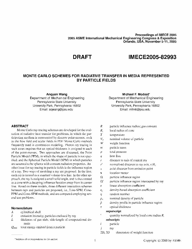
Proceedings of IMECE 20052005 ASME International Mechanical Engineering Congress & Exposition

Orlando, USA, November 5-11, 2005

DRAFT IMECE2005-82993

MONTE CARLO SCHEMES FOR RADIATIVE TRANSFER IN MEDIA REPRESENTED

BY PARTICLE FIELDS

Anquan WangDepartment of Mechanical Engineering

Pennsylvania State University

University Park, Pennsylvania 16802

Email: [email protected]

Michael F. Modest�

Department of Mechanical EngineeringPennsylvania State University

University Park, Pennsylvania 16802

Email: [email protected]

ABSTRACTMonte Carlo ray-tracing schemes are developed for the eval-

uation of radiative heat transfer for problems, in which the par-

ticipating medium is represented by discrete point-masses, such

as the �ow �eld and scalar �elds in PDF Monte Carlo methods

frequently used in combustion modeling. Photon ray tracing in

such cases requires that an optical thickness is assigned to each

of the point-masses. Two approaches are discussed, the Point

Particle Model (PPM), in which the shape of particle is not spec-

i�ed, and the Spherical Particle Model (SPM) in which particles

are assumed to be spheres with constant radiation properties. An-

other issue for ray tracing in particle �elds is the in�uence region

of a ray. Two ways of modeling a ray are proposed. In the �rst,

each ray is treated as a standard volume-less line. In the other ap-

proach, the ray is assigned a small solid angle, and is thus treated

as a cone with a decaying in�uence function away from its center

line. Based on these models, three di�erent interaction schemes

between rays and particles are proposed, i.e., Line-SPM, Cone-

PPM and Cone-SPMmethods, and are compared employing sev-

eral test problems.

NomenclatureA cylindrical shell

I emission intensity; particles enclosed by ray

L thickness of gas slab; side-length of computational do-

main

Qemi total energy emitted from a particle

�Address all correspondence to this author.

R particle in�uence radius; gas constant

Rc local radius of cone

T temperature

Vo nominal volume of particle

W weight function

m particle mass

p total pressure

q heat �ux

r distance to axis of conical ray

r0 normalized distance to ray axis, r=Rc

s axial distance from emission point

x location vector

particle in�uence region

0 particle in�uence region intercepted by ray

� linear absorption coe�cient

�� density-based absorption coe�cient

� random number

�o nominal density of particle

�� density pro�le in particle in�uence region

� optical thickness

superscript0 quantity normalized by local cone radius Rc

subscripts

i particle

j ray

2D, 3D dimension of weight function

1 Copyright c 2005 by ASME

1 Introduction

Among radiative transfer models, Monte Carlo Ray Tracing

(MCRT) has several advantages over other popular models, be-

cause it can be applied to problems of arbitrary di�culty with rel-

ative ease [1]. The MCRT method directly simulates the physi-

cal processes, i.e., emission, absorption, scattering and re�ection,

from which the Radiative Transfer Equation (RTE) is derived. In

the standard Monte Carlo method, a ray carrying a �xed amount

of energy is emitted and its progress is then traced until it is ab-

sorbed at a certain point in the participating medium or on the

wall, or until it escapes from the enclosure. As many researchers

have pointed out [2�6], this method is ine�cient when the walls

are highly re�ective and/or the medium is optically thin so that

most photon bundles exit the enclosure without any contribution.

Modest [4, 5] applied the concept of energy partitioning to alle-

viate this problem. In this method the energy carried by a ray

is no longer �xed along the path and absorbed once and for all

at one point, but rather is attenuated gradually along the path

until its depletion or until it leaves the enclosure. The locally

absorbed fraction of the ray's energy contributes to the heat ex-

change rates of sub-volumes along the ray path. This method is

also called �absorption suppression� by Walters and Buckius [6].

A large variety of problems of great complexity can be simulated

with a reasonable e�ciency using either standard or energy par-

tition methods in forward Monte Carlo simulations, when the

overall knowledge of the radiation �eld is desired. However,

such scheme can be very ine�cient if only the radiative inten-

sity hitting a small spot and/or over a small range of solid angle

is required. The idea of backward tracing, which only traces

the rays that eventually hit the targeted area or solid angle, has

been proposed by several researchers in di�erent topics to handle

this ine�ciency. The comprehensive formulation for backward

Monte Carlo simulations in radiative heat transfer can be found

in the literature (Walters and Buckius [6], Modest [7]).

The MCRT method has been applied to all aspects of ra-

diative heat transfer [8, 9]. In applications, in which no par-

ticipating medium is involved, ray tracing is relatively simple.

However, in many high-temperature applications, such as com-

bustion problems, participating media play a key role. A ma-

jor di�culty is the evaluation of the optical thickness that a ray

passes through, since the temperature and concentration �elds

are highly inhomogeneous. In their Monte Carlo modeling of

radiative heat transfer in turbulent �ames, Tesse and cowork-

ers [10, 11] assumed uniform properties of the medium along the

integral length of each coherent turbulence structure crossed by

the ray, in order to determine the optical thickness along the ray's

path. However, in other problems, in which the participating

medium is represented by the �eld of point-masses, such as the

�ow �eld and scalar �elds in PDF Monte Carlo methods [12�15]

frequently used in combustion modeling, the above continuum

model is no longer useful. No work appears to have been done

to date to implement MTRC in discrete particle �elds, which is

the aim of the present work.

2 Ray-Particle Interaction Models

To simulate the radiative transfer process by ray tracing in a

discrete particle �eld, the interaction between in�nitesimal point-

masses and in�nitesimally thin photon rays needs to be modeled.

This can be done by assigning e�ective volumes to the point-

masses, by assigning an in�uence volume to the ray's trajectory,

or a combination of both. In this section, several particle models

and ray models are developed �rst, followed by photon emission

and absorption algorithms based on these models.

2.1 Modeling Discrete Particles and Photon Rays

Point Particle Model (PPM) In this model, particles are

treated as point-masses, i.e., they carry an amount of mass with-

out a speci�c shape at a certain spatial location as shown in

Fig. 1a which is a 2D particle �eld. The only geometric informa-

tion known about the particles is their position vector. However,

particles do have a nominal volume, which may be calculated

from their thermophysical properties such as pressure and tem-

perature. For example, if the ideal gas assumption is adopted, the

nominal volume may be computed as

Vo;i =miRTi

pi; (1)

wheremi is the mass carried by particle i, Ti is its temperature, piis its total pressure and R is the gas constant. To enforce consis-

tency in the discrete particle representation of the medium, the

overall nominal volume of all particles should be the same as

the actual geometric expanse of the medium. Therefore, we may

regard the nominal volume of a particle as its real volume.

The Point Particle Model only contains the particle informa-

tion that the original discrete particle �eld contains. It does not

employ any other assumption. Therefore, it will not induce any

inconsistency that further assumptions may have. The disadvan-

tage of this model is that it is di�cult to interact a photon ray

with a volume without shape.

Spherical Particle Model In this method, each point-mass

mi has a spherical in�uence regioni, surrounding it as shown in

Fig. 1b. The mass is distributed to its in�uence region according

to a density pro�le,

��i (x) =

8>>><>>>:�o;iW3D

jx�xij

Ri

!; jx�xij < Ri

0; jx�xij � Ri

; (2)

where xi is the spatial location vector of the point-mass i, Ri is


Xi

�i

a b

rij

ray j

�

Ri

Sij

Figure 1. (a) PPM representation of a medium; (b) SPM/CDS representation of a sub-region in (a)

its in�uence radius, �o;i is the nominal density calculated by

�o;i =mi

Vo;i

=pi

RTi

; (3)

and W3D is a spherically symmetric weight function which de-

cays from the center along radial directions and satis�es the fol-

lowing condition,

Zi

W3D

jx�xij

Ri

!dx = Vo;i; (4)

so that the total mass in the in�uence region is equal to the point-

mass. In this method, particles are assigned a spherical volume

(in�uence region) with varying density, and overlapping other

particles in the domain. This is called the Spherical Particle

Method (SPM).

One may adjust the size of in�uence region and the mass

distribution of particles by employing di�erent weight functions.

Larger in�uence radii lead to more particle overlap and spatial

gradients may be smoothed out. On the other hand, Smaller in-

�uence radii result in smaller particle volumes, making it more

di�cult to interact with rays. The simplest possible weight func-

tion is

W3D

jx�xij

Ri

!= 1; (5)

i.e., the density is constant in the in�uent region and its volume

is the same as the nominal volume of the particle. The particles

can then be regarded as constant density spheres with a radius

determined by their nominal volumes,

Ri =

3Vo;i

4�

!1=3: (6)

This model will be termed the Constant Density Sphere (CDS)

model. The overall density at an arbitrary position is the sum

of density contributions from all nearby particles. Some loca-

tions may be in�uenced by more than one particle, while some

other locations may not be in the in�uence region of any particle,

i.e., there is a void in these places. Therefore, this model can-

not recover the continuous density medium as shown in Fig. 1b

and Fig. 2. Figure 1b is a small portion of the CDS represen-

tation of the 2D �eld given in Fig. 1a (if variable density were

employed, the Ri would be larger, resulting in substantial over-

lap, even in this region of few paticles). A location with lots of

void space was chosen for simplicity in Fig. 1b, and in order to

show particle locations in a plane, a 2D rather than 3D particle

�eld is depicted in Fig. 1. Figure 2 shows the density distribution

on a cross-section of a 3D CDS representation of a homogeneous

medium.

Line Ray Model In this model, a ray is simply treated as a

volume-less line and energy propagates one-dimensionally along


Density

5.54.53.52.51.5

Figure 2. Density distribution of a CDS representation for a homoge-

neous medium

the line. This is the standard model for ray tracing in continu-

ous media. Since such rays are not designed to have a speci�c

volume, they are not able to interact with point-masses. There-

fore, this model requires volumetric particle models for radiative

transfer simulations.

Cone Ray Model Physically, a photon bundle consists of

many millions of individual photons, occupying a small solid

angle. Thus, to model the volume of a ray, we assign a small

solid angle to the ray and treat it as a cone. Energy is assumed to

propagate axisymmetrically in two dimensions, with its strength

decaying in the radial direction normal to the cone axis, similar

to the weight function assigned to particle density in Eq. (2) but

in 2D. For a ray emitted at xo into a direction given by a unit

direction vector �s, the intensity at location x in the ray can be

modeled as

I(s;r) = Io(s)W2D(r=Rc(s)); (7)

where s = (x� xo) � �s is the distance from the emission location

to a point on the ray axis, r is the distance from a point on a

plane normal to the ray axis, Io(s) is the intensity at the ray cen-

ter, and Rc(s) is the local in�uence radius of the cross-section as

depicted in Fig. 3. W2D is a normalized two-dimensional center-

symmetric pro�le which satis�es

Z1

0

W2D(r0)2r0 dr0 = 1 and r0 = r=Rc: (8)

Again, many weight functions are possible, ranging fromW2D =

1 to Gaussian decay. A popular Gaussian-like weight function is

provided here [16] as

W2D(r0) =

60

7

8>>><>>>:1

3�4r02+4r03; 0 � r0 < 1

24

3(1� r0)3; 1

2� r0 < 1

0; r0 � 1

: (9)

Since in this model the ray has a speci�c volume, volume-less

particles can be intercepted by the ray, and this model can work

together with the Point Particle Model.

2.2 Emission from a ParticleWe now focus on the implementation of Monte Carlo meth-

ods for the simulation of radiative transfer in particle-based me-

dia, i.e., how photon bundles are emitted from the particle �eld,

how they are traced, and how they interacte with other particles.

A small gas volume emits energy uniformly into all direc-

tions. In Monte Carlo simulations, the total energy is divided into

a number of photon bundles (rays) which are released in random

directions. In a physical gas volume, the emitted energy comes

from every point in the volume. If the medium is represented

by discrete particles, emission takes place inside these particles.

Thus, depending on the optical thickness of the particle, and the

point and direction of emission, some of the emitted energy may

not escape from the particle due to self-absorption. If the particle

is optically thin, the self-absorption of emission is negligible and

the total emission from particle i is calculated from [1]

Qemi;i = 4��;imi�T4

i ; (10)

where ��;i is the density-based absorption coe�cient at particle

temperature Ti, � is the Stefan-Boltzmann constant, andmi is the

mass. If self-absorption is considered and the particle is assumed

to be a constant density sphere, the total emission from a sphere

is obtained from [1]

Qemi;i = 4�R2

o;i�T2

i

8>><>>:1�1

2�2o;i

h1� (1+2�o;i)e

�2�o;ii9>>=>>; ; (11)

where Ro;i =�3Vo;i=4�

�1=3is the nominal spherical radius of par-

ticle i and �o;i = �o;i��;iRo;i is the optical thickness of the spherical


volume based on the nominal radius. In the Point Particle Model,

the shape of a particle is arbitrary, but Eq. (11) is still a good ap-

proximation of total emission from such a particle. If more than

one ray is emitted from a particle, the sum of initial energy car-

ried by all rays must be equal to the total emission calculated

from Eq. (10) or Eq. (11), depending on whether self-absorption

is neglected.

2.3 Absorption Models

The basic task of simulating the absorption of a photon bun-

dle in a medium described by a point particle �eld is the evalu-

ation of the optical thickness that a ray travels through along its

way. This is achieved by modeling the interaction between the

ray and particles in its path. Based on di�erent models employed

for rays and particles, several schemes for absorption simulation

may be obtained.

Line-SPM Scheme In this scheme, the ray is treated like a

line and the Spherical Particle Model (SPM) is employed for the

particles as shown in Fig. 1b. The contribution of particle i to the

optical thickness that ray j passes through is computed as

��i j =

ZS i j

��i (x(s))��;i ds; (12)

where s is the ray coordinate as in Eq. (7), S i j is the intersection

of ray j and the in�uence region of particle i, ��;i is the density-

based absorption coe�cient of particle i at its own temperature,

and ��i is the local density of particle i as indicated in Fig. 1b.

If the Constant Density Sphere (CDS) model is employed, the

mass of particle is distributed uniformly in its in�uence region

and Eq. (12) can be simpli�ed to

��i j = 2�o;i��;i

qR2

i� r2

i j; (13)

where �o;i is the nominal density de�ned in Eq. (3), Ri is the in-

�uence radius and ri j is the distance from the center of particle i

to ray j. Since Eq. (13) has a very simple form, its implementa-

tion can be very fast.

The total optical thickness that ray j passes through is simply

the summation of the contributions from the individual particles

it interacts with,

� j =Xi2I j

��i j; (14)

where I j denotes all the particles intersected by ray j.

Cone-PPM Scheme If the ray is modeled as a cone, it is

possible to let it interact with point particles. The energy that a

conical ray reduces when it traverses over a small distance ds in

a continuous medium is,

dE =

Z Rc

0

�dsI(r)2�r dr = �ds

Z Rc

0

I(r)2�r dr; (15)

where � is the local absorption coe�cient, �(s) is the plane-

averaged absorption coe�cient over the cone cross-section at po-

sition s, and Rc(s) is the local radius of the cross-section. From

Eqs. (15), (7) and (8) the plane-averaged absorption coe�cient

can be derived as

�=

R Rc

0�Ir drR Rc

0Ir dr

=

R1

0�Ir0 dr0R1

0Ir0 dr0

=

R1

0�W2D2r

0 dr0R1

0W2D2r0 dr0

=

Z1

0

�W2D2r0 dr0

(16)

Therefore, the total optical thickness that the ray passes through

along in its path S is

� =

ZS

� ds =

ZS

Z1

0

�W2D2r0 dr0 ds

=

ZS

Z Rc

0

�W2D

�R2c

2�rdrds =

ZV

�W2D

�R2c

dV;

(17)

where V is the volume that the ray covers in its path.

In discrete particle �elds as shown in Fig. 3a, the absorption

coe�cient is represented by a set of Delta functions,

� =Xi

�iVi�(x�xi): (18)

Integrating over V yields

� =Xi2I

�iWiVi

�R2

c;i

=Xi2I

��;iWimi

�R2

c;i

; (19)

where I denotes all the particles enclosed by the cone. For point

particles, the particle weight is a point weight in the energy dis-

tribution, i.e.,

Wi =W2D(ri=Rc;i) =W2D(r0

i ); (20)

where r0iis the distance from particle i to the cone axis, normal-

ized by the local cone radius Rc;i.

Cone-SPM Scheme In the most advanced scheme, the ray

is treated as a cone, and the particle is given a speci�c shape and a

density distribution may exist in its volume, as shown in Fig. 3b.


Xi

Ri

a b

�

ray j

i�

ri

Rc,i

W2D

Xi

ray j

ir

Rc,i

W2D

Figure 3. (a) Cone-PPM scheme; (b) Cone-SPM scheme

Therefore, the weight function and absorption coe�cient cannot

be separated from the volume integral in the optical thickness

evaluation. The total optical thickness passed through by a ray is

obtained as

� =Xi2I

��;i

Z

0

i

��iW2D

�r�Rc(s)

��R2

c(s) dx; (21)

where 0

iis the intersection of the particle in�uence region and

the ray, r is the distance from a location in 0

ito the cone axis

and Rc(s) is the local cone radius at this location. Since the solid

angle of the ray is small, Rc(s) can be regarded as constant in

a single particle, i.e., the small cone segment interacting with a

particle can be treated as a small cylinder. Then, the local radius

Rc(s) � Rc;i can be separated from the integral,

� 'Xi2I

��;i

�R2

c;i

Z

0

i

��i(x)W2D

�r=Rc;i

�dx: (22)

For constant-density spherical particles this reduces to

� =Xi2I

�i

�R2

c;i

Z

0

i

W2D(r=Rc;i) dx

=Xi2I

�i

�R2

c;i

Z rmax

rmin

W2D(r=Rc;i)Ai(r) dr;

=Xi2I

�iRc;i

�

Z r0max

r0min

W2D(r0)A0

i (r0) dr0;

(23)

where r0 = r=Rc;i is the normalized distance from a point in 0

ito

the cylinder (cone) axis. r0min

is the normalized closest distance

and r0max is the farthest. All points of the same distance r0 are

part of a cylindrical shell Ai(r0) around the cone axis, and its

normalized form can be evaluated as

A0

i (r0) =

Ai(r0)

R2

c;i

=

(4r03=2r

01=2

i�1=2E(1=�); r0 � R0

i� r0

i

8r03=2r01=2

i

�2E(�)��K(�)

�; r0 > R0

i� r0

i

;

(24)

where r0i= ri=Rc;i is the normalized distance from the particle

center to the cylinder axis, R0

i= Ri=Rc;i is the normalized radius

of particle i, K and E are complete elliptic integrals of the 1st and

2nd kind [17], and

� = [R02

i� (r0� r0

i)2]

�4r0r0

i;

� = [(r0+ r0i)2�R02

i]�2r0r0

i:

(25)


If we de�ne

fi =1

�

Z r0max

r0min

W2D(r0)A0

i (r0) dr0; (26)

Eq. (23) can be rewritten as

� =Xi2I

�iRc;i fi: (27)

Rather than making costly evaluations during the simulation,

Eq. (26) can easily be tabulated as a function of the two dimen-

sionless parameters r0iand R0

i.

3 Sample CalculationsIn order to evaluate and compare the performance of the dif-

ferent schemes for Monte Carlo ray tracing in particulate media,

we consider a one-dimensional radiative heat transfer problem,

in which a non-scattering gray gas slab is bounded by two paral-

lel cold black plates which are 10 cm apart. The temperature and

density (or absorption coe�cient) may vary in the x-direction.

The resulting radiative heat �ux at the boundary can be evalu-

ated analytically as [1]

q(0) = �2�

Z �L

0

Ib(�0)E2(�

0) d�0

q(�L) = 2�

Z �L

0

Ib(�0)E2(�L ��0) d�0;

(28)

where E2 is an exponential integral and the optical thickness � is

a function of x,

�(x) =

Z x

0

�(x) dx and �L =

Z L

0

�(x) dx; (29)

and L = 10 cm is the distance between two parallel plates.

The one-dimensional medium in the problem can be simu-

lated by repeating a gas cube, each with equal side-lengths of

10 cm in the other two in�nite dimensions. A single gas cube

is then the computational domain in the Monte Carlo simulation.

The gas in the cube is represented by a number of discrete gas

particles randomly placed inside the cube. The mass of particles

may be equally-sized or have a distribution along the x-direction.

For computational e�ciency, the domain is further broken up

into cubic cells, each of which contains a number of gas parti-

cles. Some of the particles are completely inside the cell, and

the others have a part of their volume reside in the neighbor-

ing cell. If the Point Particle Model (PPM) is employed, it can

Table 1. Temperature and absorption coef�cient pro�les

Temperature pro�les, K

const T (x) = To

linear T (x) = To+ (x=L)(TL �To); TL=To = 2

sine T (x) = To+TA sin(2�x=L); TA=To = 0:5

Absorption coe�cient pro�les, cm�1

const �(x) = 0:1

linear �(x) = 0:01+0:99(x=L)

sine �(x) = 0:55+0:45sin(2�x=L)

Table 3. Particle mass distributions

uniform m(x) = mo

linear m(x) = mo+ (mL �mo)(x=L)

be assumed that all the particles are completely enclosed by the

cell, since the shape of particles is not speci�ed. However, if the

Spherical Particle Model (SPM) or the Constant Density Sphere

(CDS) model is employed, the cell contains not only the particles

with their center in it, but also parts of particles from neighbor-

ing cells. Thus, a scheme must be developed to avoid having the

ray interact with a single particle more than once, since a single

particle may belong to multiple cells.

When the Cone Ray Model is adopted for ray tracing, the

opening angle (the angle between the cone axis and the lateral

surface) needs to be chosen. Larger opening angles result in more

particles caught by the ray, requiring more CPU time per ray

but providing better accuracy. It was found that, for this one-

dimensional problem, one degree was an optimal opening angle,

which can achieve high accuracy as well as high CPU e�ciency.

Therefore, for all the simulations in this paper, the opening angle

is chosen to be one degree, whenever the Cone Ray Model is

employed.

Several combinations of temperature pro�les and absorption

coe�cient pro�les have been tested as listed in Table 1, with dif-

ferent cases numbered in Table 2. For each of the nine cases, two

di�erent particle volume distributions as given in Table 3 were

tested. In the uniform distribution, the particles are equally-sized

and their random positions in the computational domain can be

readily generated as

x = �xL; y = �yL; z = �zL; (30)

where �x, �y and �z are three independent random numbers uni-

formly distributed in [0;1). For the linear distribution of particle

mass, the random number relation for the x-coordinate of particle

positions is no longer linear. Instead, the probability distribution

P(x) associated with particle mass distribution m(x) is inversely


Table 2. Case numbering

Case (1) (2) (3) (4) (5) (6) (7) (8) (9)

T const const const linear linear linear sine sine sine

� const linear sine const linear sine const linear sine

proportional to m(x), i.e., P(x) � 1=m(x). Therefore, the follow-

ing random number relation holds,

�x =

Z x

0

P(x) dx

Z L

0

P(x) dx

=

Z x

0

1=m(x) dx

Z L

0

1=m(x) dx

=

Z x

0

[mo+ (mL �mo)(x=L)]�1 dx

Z L

0

[mo+ (mL �mo)(x=L)]�1 dx

:

(31)

After carrying out the integrations and rearranging, one obtains

x =(mL=mo)

�x �1

(mL=mo)�1L; (32)

where (mL=mo) is the mass ratio of particles at x = L to parti-

cles at x = 0. Figure 4 shows a CDS representation with a linear

particle mass distribution for a homogeneous medium.

The three absorption schemes discussed in Section 2 have

been implemented for the 1D problem and compared with the

exact solution for boundary �uxes, Eq. (28), for all nine cases.

Table 4 shows the corresponding root-mean-square (RMS) rela-

tive error of 50 simulations in each case, in which the gas cube

is represented by 10,000 equally-sized random particles each of

which emits all its energy in a single ray into a random direction.

Similarly, Table 5 gives the results for the linear particle mass

distribution. In both tables, the computational domain is divided

into 4 cells in each dimension, 64 cells in total. For all nine

cases, the same random number sequence is used in the particle

position generation as well as in the emission direction genera-

tion. As shown in the two tables, the three absorption schemes

all achieve the same level of accuracy. Comparing Table 5 to

Table 4, it is observed that the di�erence caused by varying the

particle masses is fairly small considering that the mass ratio is

as large as 1,000.

From the above comparisons, one may conclude that the

three absorption schemes are essentially equivalent in terms

of simulation accuracy. Therefore, in the following accuracy-

related discussions, we choose only one scheme, the Line-CDS

scheme, to show the results.

The errors of �uxes at the two boundaries are averaged and

plotted in Fig. 5 against the number of particles by which the

Figure 4. CDS representation with linear mass distribution for a homo-

geneous medium

Table 4. Percentage RMS errors of radiative �uxes at boundaries;

10,000 particles; 1 ray/particle; 64 cells; uniform particle mass

Case Line-CDS Cone-PPM Cone-CDS

No. x = 0 x = L x = 0 x = L x = 0 x = L

(1) 1.457 1.508 1.845 1.940 1.485 1.572

(2) 1.274 1.555 1.288 1.665 1.282 1.586

(3) 1.673 1.593 1.820 1.592 1.676 1.592

(4) 2.144 1.890 3.353 1.862 1.635 1.993

(5) 1.612 2.028 1.674 1.999 1.624 2.104

(6) 1.883 1.711 3.433 1.673 2.302 1.696

(7) 1.957 2.159 1.985 3.131 2.016 1.990

(8) 1.718 1.792 1.686 2.223 1.714 1.749

(9) 2.084 2.087 2.012 2.072 2.109 2.150


Table 5. Percentage RMS errors of radiative �uxes at boundaries;

10,000 particles; 1 ray/particle; 64 cells; mass ratio: mL=mo = 1;000

Case Line-CDS Cone-PPM Cone-CDS

No. x = 0 x = L x = 0 x = L x = 0 x = L

(1) 1.896 3.378 2.231 3.776 1.956 3.113

(2) 2.795 3.671 2.823 3.772 2.776 3.633

(3) 1.863 2.234 1.989 2.243 1.816 2.089

(4) 4.050 4.332 5.138 4.403 3.606 4.501

(5) 4.584 4.740 4.700 4.803 4.510 4.863

(6) 3.748 3.990 5.274 3.926 4.181 3.930

(7) 2.174 4.412 2.062 5.574 2.217 2.723

(8) 2.398 3.647 2.400 4.131 2.385 2.945

(9) 2.377 2.487 2.217 2.566 2.335 2.361

Number of particles, N

Err

or

(%)

102 103 104 105

100

101

Simulation resultError ~ 1/sqrt(N)

Figure 5. Averaged boundary �ux error vs. number of particles in com-

putation domain; Line-CDS scheme with one ray per particle; uniform

particle mass; Case (1)

medium in the gas cube is represented. The particles are all of

the same size and only the result of Case (1) is provided for sim-

plicity. It is seen that the error is approximately inversely pro-

portional to the square root of the number of particles. Similarly,

Fig. 6 shows the relation of error and the number of rays that

each particle emits during the Monte Carlo simulation, given the

number of particles. Once again, the accuracy follows an inverse

square root relation.

All three absorption models achieve not only the same level

Number of rays per particle, ME

rro

r(%

)2 4 6 8 10 12 14

0.5

1

1.5

2

Simulation resultError ~ 1/sqrt(M)

Figure 6. Averaged boundary �ux error vs. number of rays per particle;

Line-CDS scheme; 10,000 particles; uniform particle mass; Case (1)

Table 6. CPU time of a single Monte Carlo simulation; 1 ray/particle;

Case (1); unit: s

Particle amount 2,000 5,000 10,000 50,000 100,000

Number of cells 23 33 43 73 83

Line-CDS 0.115 0.417 1.29 48.7 183.2

Cone-PPM 0.230 0.742 1.98 56.4 215.7

Cone-CDS 0.231 0.752 2.07 58.1 214.9

of accuracy, but also similar CPU e�ciency for this 1D problem,

as shown in Table 6. The Line-CDS scheme is a little bit faster

than the other two, since a line ray interacts with fewer particles

than a cone ray, but due to the small opening angle of the Cone

Ray Model, the time di�erence is not very big.

4 Conclusions

For radiative heat transfer simulations using Monte Carlo

ray tracing in media represented by discrete particle �elds it is

important to �nd a way to model the interaction between point-

masses and photon rays. In the Point Particle Model (PPM) the

shape of particles is not presumed in order to avoid any incon-

sistency with the original particle �eld. As a result, it is lim-

ited to applications in which the ray has a shape and volume. In

the Spherical Particle Model (SPM), particles are assumed to be

spheres. As a special case, in the Constant Density Sphere (CDS)

model, the density is assumed to be constant across the entire par-

ticle volume. Although it is easy to interact spheres with a ray,


this model introduces some inconsistencies. For example, it can-

not recover continuous medium properties due to the existence

of particle overlaps and void.

In the Line Ray Model for a photon bundle, the ray is sim-

ply treated as a volume-less line and energy propagates one-

dimensionally along that line. In the Cone Ray Model, the ray

is assigned a small solid angle, and is thus treated as a cone;

energy propagates two-dimensionally. The strength of the ray

may vary across the cross-section of the cone through a given

weight function. Since the ray has a volume, it is possible to

have the ray interact with volume-less particles directly. Thus,

three schemes for the interaction between ray and particles, i.e.,

Line-CDS, Cone-PPM and Cone-CDS schemes, have been pro-

posed and examined in a one-dimensional radiative heat transfer

problem with various temperature and absorption coe�cient pro-

�les. It was shown that all three schemes achieved comparable

levels of accuracy and CPU-time e�ciency.

AcknowledgmentThis research has been sponsored by National Science Foun-

dation under Grant Number CTS-0121573.

References[1] Modest, M. F., 2003, Radiative Heat Transfer, Academic

Press, New York, 2nd ed.

[2] Heinisch, R. P., Sparrow, E. M., and Shamsundar, N., 1973,

�Radiant Emission from Ba�ed Conical Cavities�, Journal

of the Optical Society of America, 63(2), pp. 152�158.

[3] Shamsundar, N., Sparrow, E. M., and Heinisch, R. P., 1973,

�Monte Carlo Solutions � E�ect of Energy Partitioning

and Number of Rays�, International Journal of Heat and

Mass Transfer, 16, pp. 690�694.

[4] Modest, M. F. and Poon, S. C., 1977, �Determination

of Three-Dimensional Radiative Exchange Factors for the

Space Shuttle by Monte Carlo�, ASME paper no. 77-HT-

49.

[5] Modest, M. F., 1978, �Determination of Radiative Ex-

change Factors for Three Dimensional Geometries with

Nonideal Surface Properties�, Numerical Heat Transfer, 1,

pp. 403�416.

[6] Walters, D. V. and Buckius, R. O., 1992, �Monte Carlo

Methods for Radiative Heat Transfer in Scattering Media�,

In Annual Review of Heat Transfer, 5, Hemisphere, New

York, pp. 131�176.

[7] Modest, M. F., 2003, �Backward Monte Carlo Simulations

in Radiative Heat Transfer�, ASME Journal of Heat Trans-

fer, 125(1), pp. 57�62.

[8] Howell, J. R., 1998, �TheMonte Carlo Method in Radiative

Heat Transfer�, ASME Journal of Heat Transfer, 120(3),

pp. 547�560.

[9] Farmer, J. T. and Howell, J. R., 1998, �Monte Carlo strate-

gies for radiative transfer in participating media�, In Hart-

nett, J. P. and Irvine, T. F., eds., Advances in Heat Transfer,

34, Academic Press, New York.

[10] Tesse, L., Dupoirieux, F., Zamuner, B., and Taine, J., 2002,

�Radiative transfer in real gases using reciprocal and for-

ward Monte Carlo methods and a correlated-k approach�,

International Journal of Heat and Mass Transfer, 45, pp.

2797�2814.

[11] Tesse, Lionel, Dupoirieux, Francis, and Taine, Jean, 2004,

�Monte Carlo modeling of radiative transfer in a turbu-

lent sooty �ame�, International Journal of Heat and Mass

Transfer, 47, pp. 555�572.

[12] Pope, S. B., 1985, �PDF Methods for Turbulent Reactive

Flows�, Progress in Energy and Combustion Science, 11,

pp. 119�192.

[13] Dopazo, C., 1994, �Recent developments in pdf methods�,

In Turbulent Reacting Flows, Academic Press, pp. 375�

474.

[14] Li, G. and Modest, M. F., 2002, �Investigation of

Turbulence�Radiation Interactions in Reacting Flows Us-

ing a Hybrid FV/PDF Monte Carlo Method�, Journal of

Quantitative Spectroscopy and Radiative Transfer, 73(2�

5), pp. 461�472.

[15] Raman, V., Fox, R. O., and Harvey, A. D., 2004, �Hybrid

�nite-volume/transported PDF simulations of a partially

premixed methane�air �ame�, Combustion and Flame,

136, pp. 327�350.

[16] Liu, G. R. and Liu, M. B., 2003, Smoothed Particle Hydro-

dynamics � a Meshfree Particle Method, World Scienti�c

Publishing Co. Pte. Ltd., Singapore.

[17] Abramowitz, M. and Stegun, I. A., eds., 1965, Handbook of

Mathematical Functions, Dover Publications, New York.


DRAFT IMECE2005-82993 - UC Merced Engineering

Documents

Transcript of DRAFT IMECE2005-82993 - UC Merced Engineering