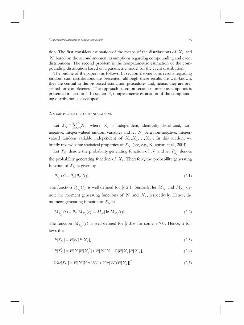
STATISTICA, anno LXIX, n. 1, 2009

NONPARAMETRIC ESTIMATION IN RANDOM SUM MODELS

H.S. Bakouch, T.A. Severini

1. INTRODUCTION

The motivation for this paper arises from the fact that the random sum models are widely used in risk theory, queueing systems, reliability theory, economics, communications, and medicine. In insurance contexts, the compound distribution of random sum variables (see, e.g., Cai and Willmot (2005), Charalambides (2005) and Panjer (2006)) arises naturally as follows. Let iX be the number of persons involved in the i th accident on a particular day in a certain city and let N be an-other random variable that represents the number of accidents occurring on that day. Then, the random variable given by

=1= ,N

N iiS X∑ 0 0= = 0,S X denotes the total number of persons involved in accidents in a day, and is called compound random variable. In queueing model, at a bus station, assume that the number of passengers on the i th bus is iX and the number of arriving buses is the random variable N ; then the number of passengers arriving buses during a period of time is the random sum

=1= N

N iiS X∑ . In communications, let us consider the random variable N as the number of data packets transmitted over a communication link in one minute such that each packet is successfully decoded with probability p , in-dependent of the decoding of any other packet. Hence, the number of successfully decoded packets in one minute span is the random sum

=1= N

N iiS X∑ , where iX is 1 if the i th packet is decoded correctly and 0 otherwise. That is, the compound random variable NS follows a binomial distribution with random and fixed pa-rameters N and p , respectively. The distribution of the random variable NS , is known as a compound distribution of the random variables iX and N , where

=1, 2,...,i N ; see, e.g., Chatfield and Thoebald (1973), Lundberg (1964), Medhi (1972), Peköz and Ross (2004), and Sahinoglu (1992). Thus, the distribution of a random sum is based on two distributions: the distribution of N , which we will call the event distribution and the distribution of the random variables

1 2, , , NX X X… , which we will call the compounding distribution.

H.S. Bakouch, T.A. Severini 74

Many authors (e.g. Pitts (1994), Buchmann and Grübel (2003, 2004), and Cai and Willmot (2005)) have been investigated the distributional properties of the random sum NS including its distribution function and the asymptotic behaviour of the tail. Pitts (1994) discussed the nonparametric estimation of the distribution function of NS based on topological concepts and assumed that the event distri-bution is known and the compounding distribution is unknown. Buchmann and Grübel (2003, 2004) considered the estimation problem of a probability set of the compounding distribution of ,iX =1, 2,..., ,i N and the compound distribution of iX and N assuming that the event distribution follows Poisson distribution. Weba (2007) investigated prediction of the compound mixed Poisson process as-suming that the event distribution is a mixed Poisson process and the compound-ing distribution is unknown. Meanwhile, we here deal with unknown event and compounding distributions. Also, our work is more general than Pitts (1994),and Buchmann and Grübel (2003, 2004), since it can be applied to any event and compounding distributions as long as they obey the assumptions that are in sec-tion 4.1. Recently, Bakouch and Ristić (2009), and Ristić et al. (2009) employed this random sum, ,NS to model integer-valued time series that are used in fore-casting and regression analysis of count data. Also, they discussed some proper-ties of NS for a known event distribution and an unknown compounding distri-bution, and then obtained estimators of the parameters of such distributions after giving a known compounding distribution. In section 4.2 of this paper, we con-sider a nonparametric estimation of the compounding distribution in the com-pound Poisson model. The approach in this case is similar to the estimation method of Buchmann and Grübel (2003, 2004) but our approach is of interest to any problem concerning the compound Poisson model. On the other hand, Buchmann and Grübel (2003, 2004) are interested only in the compound Poisson model that is commonly used in queueing theory for modeling the arrival distri-bution of the number of customers.

Let 1 , , nY Y… denote independent random variables, each with the distribution of NS . Based on the information provided by the random variables 1 , , nY Y… , we wish to estimate features of the distributions of iX and N . A common used approach to this problem is to use parametric models for the event and com-pounding distributions. This leads to a parametric model for the distribution of

1, , nY Y… . Estimating the parameters of this model leads to estimators for the pa-rameters of the distributions of iX and N . The drawback of this approach is that it requires strong assumptions about the distributions of iX and N . How-ever, since we do not observe a random sample from both distributions, these assumptions are difficult to verify empirically.

The purpose of this paper is to consider two methods of nonparametric esti-mation in random sum models; that is, we consider methods that do not require full parametric models for the compounding distribution and the event distribu-

Nonparametric estimation in random sum models 75

tion. The first considers estimation of the means of the distributions of iX and N based on the second-moment assumptions regarding compounding and event distributions. The second problem is the nonparametric estimation of the com-pounding distribution based on a parametric model for the event distribution.

The outline of the paper is as follows. In section 2 some basic results regarding random sum distributions are presented; although these results are well-known, they are central to the proposed estimation procedures and, hence, they are pre-sented for completeness. The approach based on second-moment assumptions is presented in section 3. In section 4, nonparametric estimation of the compound-ing distribution is developed.

2. SOME PROPERTIES OF RANDOM SUMS

Let =1

= NN iiS X∑ , where iX is independent, identically distributed, non-

negative, integer-valued random variables and let N be a non-negative, integer-valued random variable independent of 1 2, , , NX X X… . In this section, we briefly review some statistical properties of NS (see, e.g., Klugman et al., 2004).

Let NP denote the probability generating function of N and let XiP denote

the probability generating function of iX . Therefore, the probability generating function of NS is given by

( )= [ ( )].S N XN iP t P P t (2.1)

The function ( )SNP t is well defined for 1.t ≤ Similarly, let NM and Xi

M de-

note the moment generating functions of N and iX , respectively. Hence, the moment generating function of NS is

( )= [ ( )]= [ ln ( )].S N X N XN i iM t P M t M M t (2.2)

The function ( )SNM t is well defined for t a≤ for some > 0a . Hence, it fol-

lows that

[ ]= [ ] [ ],N iE S E N E X (2.3)

2 2[ ]= [ ] [ ] [ ( 1)] [ ] [ ],N i i jE S E N E X E N N E X E X+ − (2.4)

2[ ]= [ ] [ ] [ ]( [ ]) .N i iVar S E N Var X Var N E X+ (2.5)

H.S. Bakouch, T.A. Severini 76

3. ESTIMATION OF THE DISTRIBUTION MEANS UNDER SECOND-MOMENT ASSUMPTIONS

Let = ( ; )iE Xθ θ and let = ( ; )E Nλ λ . Suppose we observe 1, , nY Y… , inde-pendent, identically distributed random variables such that 1Y has the distribu-tion of 1=N NS X X+ + . Note that neither N nor 1, , NX X… are directly observed; the data only consists of n realizations of the random variable NS and are denoted by 1, , nY Y… .

Our goal is to estimate θ and λ , the means of the distributions of iX and N , respectively, based on 1( , , )nY Y… . Clearly, this will be impossible without further assumptions regarding the distributions of iX and N .

Define the functions : [0, )V Λ→ ∞ and : [0, )W Θ→ ∞ by

( )= ( ; ) ( )= ( ; )iV Var N and W Var Xλ λ θ θ

and assume that V and W are known. Using equations (2.3) and (2.5) we can show that 1Y has mean θλ and variance

2 ( ) ( ).V Wθ λ λ θ+

We propose to estimate ( , )θ λ using the first two moments of the distribution of

1Y . Expressing the parameters θ and λ in terms of the first two moments of the distribution of 1Y proceeds this approach. The assumption that V and W are known is meant to be a weaker version of the assumption of parametric mod-els for the distributions. This method might be used when one is willing to as-sume that ( )=V λ λ , as in the Poisson distribution, but is not willing to assume that the Poisson distribution actually holds. Thus, our approach in this section is similar to the quasi-likelihood method described, e.g., in McCullagh and Nelder (1989, chapter 9).

Since the first moment of 1Y is θλ , it is necessary that the second moment of

1Y is not a function of θλ ; hence, we require the following assumption:

Assumption 1

For ( , )θ λ Θ Λ∈ × , 2 ( ) ( )V Wθ λ λ θ+ is not a function of θλ . Let

=1

1=n

jj

Y Yn∑

and

Nonparametric estimation in random sum models 77

2 2

=1

1= ( ) .n

jj

S Y Yn

−∑

Define the estimator ( , )θ λ as the solution to

2 2= , ( ) ( )= ,Y V W Sθ λ θ λ λ θ+ (3.1)

provided that such solution exists. Determination of the asymptotic distribution of ( , )θ λ requires the following

regularity conditions:

Assumption 2

The parameter space Θ Λ× is an open subset of 2ℜ . Under assumption 2, the true parameter value ( , )θ λ is an interior point of the

parameter space.

Assumption 3

Define a function :H AΘ Λ× → by

2( , )= ( , ( ) ( )).H V Wθ λ θλ θ λ λ θ+

Then A is an open subset of 2ℜ and ( , )H θ λ is a one-to-one function with a continuously differentiable inverse.

Under assumption 3, the estimators θ and λ can be written as functions of Y and 2S . This fact, together with the asymptotic distribution of 2( , )Y S can be used to determine the asymptotic distribution of ( , )θ λ .

Assumption 4

For all ( , )θ λ Θ Λ∈ × , 41( ; , )<E Y θ λ ∞ .

Assumption 4 is used to apply the strong law of large numbers and the central limit theorem to sums of the form

=1n

jj Y∑ and 2=1

njj Y∑ .

For a non-negative definite 2 2× matrix L, let 2( , )N L0 denote a random variable with a bivariate normal distribution with mean vector 0 and covariance matrix L ; let 3( , )µ θ λ and 4 ( , )µ θ λ denote the third and fourth central mo-ments, respectively, of 1Y .

H.S. Bakouch, T.A. Severini 78

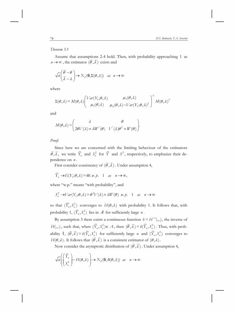
Theorem 3.1

Assume that assumptions 2-4 hold. Then, with probability approaching 1 as n →∞ , the estimator ( , )θ λ exists and

2( , ( , ))n N as nθ θ

θ λλ λ

Σ−⎛ ⎞

→ →∞⎜ ⎟−⎝ ⎠0

where 1

312

3 4 1

( , )( ; , )( , )= ( , ) ( , )

( , ) ( , ) ( ; , )TVar Y

M MVar Y

µ θ λθ λθ λ θ λ θ λ

µ θ λ µ θ λ θ λ

−

Σ⎛ ⎞⎜ ⎟

−⎝ ⎠

and

2)( , )= .

2 ( ) ( ( ) ( )' 'MV W V W

λ θθ λ

θ λ θ λ θ θλ⎛ ⎞⎜ ⎟

+ +⎝ ⎠

Proof:

Since here we are concerned with the limiting behaviour of the estimators , ,θ λ we write nY and 2

nS for Y and 2S , respectively, to emphasize their de-pendence on n .

First consider consistency of ( , )θ λ . Under assumption 4,

1( ; , )= . . 1 ,nY E Y w p as nθ λ θλ→ →∞

where “w.p.” means “with probability”, and

2 21( ; , )= ( ) ( ) . . 1nS Var Y V W w p as nθ λ θ λ λ θ→ + →∞

so that 2( , )n nY S converges to ( , )H θ λ with probability 1. It follows that, with

probability 1, 2( , )n nY S lies in A for sufficiently large n .

By assumption 3 there exists a continuous function 1= (., .)h H − , the inverse of

(., .)H , such that, when 2( , )n nY S A∈ , then 2( , )= ( , )n nh Y Sθ λ . Thus, with prob-

ability 1, 2( , )= ( , )n nh Y Sθ λ for sufficiently large n and 2( , )n nY S converges to ( , )H θ λ . It follows that ( , )θ λ is a consistent estimator of ( , )θ λ . Now consider the asymptotic distribution of ( , )θ λ . Under assumption 4,

22( , ) ( , ( , ))n

n

Yn H N B as n

Sθ λ θ λ

⎛ ⎞⎛ ⎞− → →∞⎜ ⎟⎜ ⎟⎜ ⎟⎜ ⎟⎝ ⎠⎝ ⎠

0

Nonparametric estimation in random sum models 79

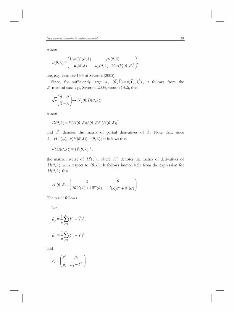
where

312

3 4 1

( , )( ; , )( , )= ;

( , ) ( , ) ( ; , )Var Y

BVar Y

µ θ λθ λθ λ

µ θ λ µ θ λ θ λ

⎛ ⎞⎜ ⎟

−⎝ ⎠

see, e.g., example 13.3 of Severini (2005). Since, for sufficiently large n , 2( , )= ( , )n nh Y Sθ λ , it follows from the

δ -method (see, e.g., Severini, 2005, section 13.2), that

2( , ( , ))n N Dθ θ

θ λλ λ

−⎛ ⎞→⎜ ⎟−⎝ ⎠

0

where

( , )= ( ( , )) ( , ) ( ( , ))TD h H B h Hθ λ θ λ θ λ θ λ′ ′

and h′ denotes the matrix of partial derivatives of h . Note that, since 1= (., .),h H − ( ( , )) = ( , )h H θ λ θ λ ; it follows that

1( ( , ))= ( , ) ,h H Hθ λ θ λ −′ ′

the matrix inverse of (., .)H ′ , where H ′ denotes the matrix of derivatives of ( , )H θ λ with respect to ( , )θ λ . It follows immediately from the expression for ( , )H θ λ that

2( , )= .2 ( ) ( ) ( ) ( )

HV W V W

θλθ λ

θ λ λ θ θ θλ⎛ ⎞

′ ⎜ ⎟′+ ′ +⎝ ⎠

The result follows. Let

33

=1

ˆ 1= ( ) ,n

jj

Y Yn

µ −∑

44

=1

ˆ 1= ( )n

jj

Y Yn

µ −∑

and

23

43 4

ˆ

ˆ ˆ= .n

SB

S

µ

µ µ

⎛ ⎞⎜ ⎟

−⎝ ⎠

H.S. Bakouch, T.A. Severini 80

Define

1ˆ = ( , ) ( , ) .Tn nM B Mθ λ θ λ−Σ

Theorem 3.2

Assume that assumptions 2-4 hold. Then

ˆ ( , ) .n as nθ λΣ Σ→ →∞

Proof:

Under assumption 4, as n →∞ ,

21 3 3 4 4ˆ ˆ,( ; ), ( , ), ( , ).S Var Y andθ λ µ µ θ λ µ µ θ λ→ → →

It follows that ( , )nB B θ λ→ as n →∞ . Since ( , )M θ λ is a continuous function of ( , )θ λ , and ( , )θ λ is a consistent estimator of ( , )θ λ , it follows that

( , ) ( , )M Mθ λ θ λ→ as n →∞ . The result follows.

4. NONPARAMETRIC ESTIMATION OF THE COMPOUNDING DISTRIBUTION

4.1 General approach

Let P denote the probability generating function of iY , let R denote the probability generating function of the event distribution, and let Q denote the probability generating function of the compounding distribution. Assume that we have a parametric model with parameter λ for the event distribution; hence, we write ( ; )R λ⋅ for R as

( ( ); )= ( ), 1.R Q t P t tλ ≤

Let

=1

1ˆ( )=n Y j

jP t t

n∑

denote the empirical probability generating function based on 1, , nY Y… . Then ˆ( )P t is a consistent estimator of ( )P t for 1t ≤ . Hence, an estimator of the

compounding distribution can be obtained by setting ˆ( ( ); )R Q t λ equal to ˆ( )P t , where λ̂ is an appropriate estimator of λ .

Nonparametric estimation in random sum models 81

In order to carry out this approach, there are several issues which must be con-sidered. First, we must ensure that λ and Q are identified in this model. Second, an estimator of λ must be constructed. Finally, we must be able to use the iden-tity

ˆ ˆ( ( ); )= ( )R Q t P tλ (4.1)

in order to obtain an estimator of the compounding distribution. First consider identification. The following assumption is sufficient for Q and

λ to be identified.

Assumption 5

1. 1 2( ; )= ( ; )R t R tλ λ if and only if 1 2=t t .

2. 1 2(0; )= (0; )R Rλ λ if and only if 1 2=λ λ .

Lemma 4.1

Assume that assumption 5 is satisfied. Then 1 1 2 2( ( ); )= ( ( ); )R Q t R Q tλ λ for 1t ≤ if and only if 1 2=Q Q and 1 2=λ λ .

Proof:

Clearly, if 1 2=Q Q and 1 2=λ λ , then 1 1 2 2( ( ); )= ( ( ); )R Q t R Q tλ λ for 1t ≤ . Hence, assume that 1 1 2 2( ( ); )= ( ( ); )R Q t R Q tλ λ for 1t ≤ . Note that

1 2(0)= (0)= 0Q Q . Hence, setting = 0t , it follows that 1 2(0; )= (0; )R Rλ λ ; by part (1) of assumption 5, it follows that 1 2=λ λ .

Fix t . By part (2) of assumption 5, 1 2( ( ); )= ( ( ); )R Q t R Q tλ λ implies that

1 2( ) = ( )Q t Q t . Since t is arbitrary, 1 2=Q Q , proving the result. Now consider estimation of λ . It follows from the identification result that an

estimator of λ can be obtained by solving

ˆ ˆ(0; )= (0)R Pλ (4.2)

for λ̂ . However, the estimator given in (4.2) will only be useful for those distri-butions for which (0)P is not close to 0 . An alternative approach is to base an estimator of a second-moment assumption, as discussed in section 3.

Finally, we must use the identity in (4.1) to obtain an estimator of the com-pounding distribution. The details of this will depend on the parametric model used for the event distribution. In the remainder of this section we consider two choices for this distribution. In section 4.2, the event distribution is taken to be a

H.S. Bakouch, T.A. Severini 82

Poisson distribution; this case was also considered by Buchmann and Grübel (2003), who developed a similar method of estimation. In section 4.3, the event distribution is taken to be a geometric distribution.

4.2 Estimation under a compound Poisson model

The compound Poisson distribution has a major importance in the class of compound distributions. This is because of using it in the probability theory and its applications in biology, risk theory, meteorology, health science, etc.

Under the assumption that N has a Poisson distribution with mean λ , it fol-lows from the discussion in section 4.1 that

( )= exp{ [ ( ) 1]}, 1.P t Q t tλ − ≤

Suppose that the parameter λ is known. Hence, we can estimate Q by Q̂ where

ˆ ˆexp{ [ ( ) 1]}= ( )Q t P tλ − (4.3)

and let

{ = }=1

1ˆ =n

k Y kjj

p In∑

so that P̂ can also be written as

=0

ˆ ˆ( )= .kk

kP t t p

∞

∑

Here { = } =1Y kjI if =jY k and 0 otherwise.

For =1, 2,j … , let = Pr( = )j iq X j . Our goal is to estimate 1 2, ,q q … based

on 0 1ˆ ˆ, ,p p … or, equivalently, based on ˆ( )P t . To do this, we make the following assumption: Assumption 6

There exists a positive integer M such that Pr( > )= 0iX M and, hence,

1 2= = = 0.M Mq q+ +

Under assumption 6, the number of unknown parameters is finite, which sim-plifies certain technical arguments. Note that M can be taken to be very large so that assumption 6 is nearly always satisfied in practice.

Nonparametric estimation in random sum models 83

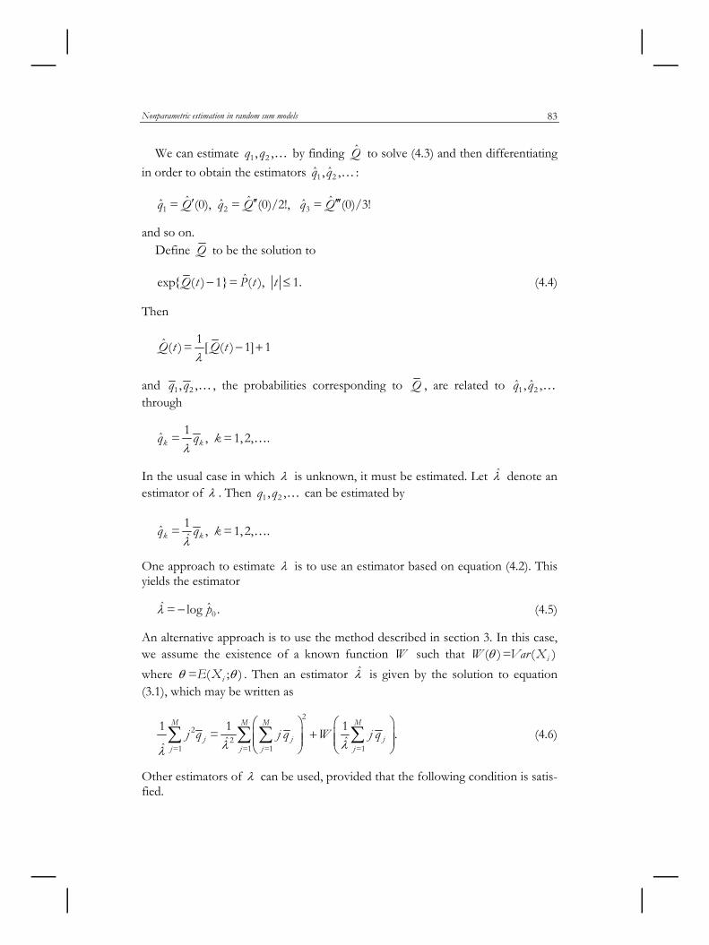
We can estimate 1 2, ,q q … by finding Q̂ to solve (4.3) and then differentiating in order to obtain the estimators 1 2ˆ ˆ, ,q q … :

1 2 3ˆ ˆ ˆˆ ˆ ˆ= (0), = (0)/2!, = (0)/3!q Q q Q q Q′ ′′ ′′′

and so on. Define Q to be the solution to

ˆexp{ ( ) 1}= ( ), 1.Q t P t t− ≤ (4.4)

Then

1ˆ ( )= [ ( ) 1] 1Q t Q tλ

− +

and 1 2, ,q q … , the probabilities corresponding to Q , are related to 1 2ˆ ˆ, ,q q … through

1ˆ = , =1, 2, .k kq q kλ

…

In the usual case in which λ is unknown, it must be estimated. Let λ̂ denote an estimator of λ . Then 1 2, ,q q … can be estimated by

ˆ1ˆ = , =1, 2, .k kq q kλ

…

One approach to estimate λ is to use an estimator based on equation (4.2). This yields the estimator

0ˆ ˆ= log .pλ − (4.5)

An alternative approach is to use the method described in section 3. In this case, we assume the existence of a known function W such that ( )= ( )iW Var Xθ where = ( ; )iE Xθ θ . Then an estimator λ̂ is given by the solution to equation (3.1), which may be written as

22

2=1 =1 =1 =1

ˆˆˆ

1 1 1= .M M M M

j j jj j j j

j q j q W j qλλλ

⎛ ⎞ ⎛ ⎞+⎜ ⎟ ⎜ ⎟⎜ ⎟ ⎜ ⎟

⎝ ⎠ ⎝ ⎠∑ ∑ ∑ ∑ (4.6)

Other estimators of λ can be used, provided that the following condition is satis-fied.

H.S. Bakouch, T.A. Severini 84

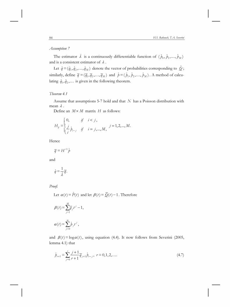
Assumption 7

The estimator λ̂ is a continuously differentiable function of 0 1ˆ ˆ ˆ( , , , )Mp p p… and is a consistent estimator of λ .

Let 1 2ˆ ˆ ˆ ˆ= ( , , , )Mq q q q… denote the vector of probabilities corresponding to Q̂ ; similarly, define 1 2= ( , , , )Mq q q q… and 1 2ˆ ˆ ˆ ˆ= ( , , , )Mp p p p… . A method of calcu-lating 1 2ˆ ˆ, ,q q … is given in the following theorem.

Theorem 4.1

Assume that assumptions 5-7 hold and that N has a Poisson distribution with mean λ .

Define an M M× matrix H as follows:

0, ,= 1, 2, ..., .ˆ , ..., ,ij

i j

if i jH j Mj p if i j M

i −

<⎧⎪ =⎨

=⎪⎩

Hence

1 ˆ=q H p−

and

ˆ1ˆ = .q qλ

Proof:

Let ˆ( )= ( )t P tα and let ( )= ( ) 1t Q tβ − . Therefore

=1( )= 1,

Mj

jj

t q tβ −∑

=0

ˆ( )= jj

jt p tα

∞

∑ ,

and ( )= log ( )t tβ α , using equation (4.4). It now follows from Severini (2005, lemma 4.1) that

1 1=0

1ˆ ˆ= , = 0,1, 2, .1

r

r j r jj

jp q p rr+ + −++∑ … (4.7)

Nonparametric estimation in random sum models 85

Expressing in terms of the matrix H and the vectors q̂ and p̂ , equation (4.7) can be written as

ˆ= .Hq p

The result for q̂ now follows from the relationship between q̂ and q . The following result shows that 1 2ˆ ˆ ˆ( , , , )Mq q q… is asymptotically normally dis-

tributed.

Theorem 4.2

Assume that assumptions 5-7 hold and that N has a Poisson distribution with mean λ . Therefore, as n →∞ ,

1 1

2 2

ˆˆ

ˆM M

q qq q

n

q q

−⎛ ⎞⎜ ⎟−⎜ ⎟⎜ ⎟⎜ ⎟

−⎝ ⎠

converges in distribution to an M dimensional multivariate normal distribution with mean vector 0 .

Proof:

It follows from equation (4.7) that 1 2( , , , )Mq q q… is a continuously differenti-able function of 0 1ˆ ˆ ˆ( , , , )Mp p p… . Under assumption 7, it follows that

1 2ˆ ˆ ˆ( , , , )Mq q q… is a continuously differentiable function of 0 1ˆ ˆ ˆ( , , , )Mp p p… . The result now follows from the δ -method (e.g., Severini, 2005, section 13.2)

together with the fact that 0 1ˆ ˆ ˆ( , , , )Mp p p… is asymptotically normally distributed (e.g., Severini, 2005, example 12.7).

The asymptotic covariance matrix of 1 2ˆ ˆ ˆ( , , , )Mq q q… , which is not specified in theorem 4.2, can be obtained using the δ -method (see, e.g., Severini, 2005, theo-rem 13.1). Since 1 2ˆ ˆ ˆ( , , , )Mq q q… is a complicated function of 0ˆ ˆ( , , )Mp p… , we do not give its expression here. The computation of such expression can be obtained via the formula in Severini (2005, theorem 13.1). Note that the estimators

1 2ˆ ˆ ˆ, , , Mq q q… are not guaranteed to be non-negative nor are they guaranteed to sum to 1 . Thus, in practice, any negative estimate should be replaced by 0 . It may also be helpful to normalize the estimates by dividing them by their sum.

H.S. Bakouch, T.A. Severini 86

4.3 Estimation under a compound geometric model

In this subsection, we consider the compound geometric distribution which plays an important role in reliability, queueing, regenerative processes, and insur-ance applications.

We now consider the case in which N has a geometric distribution with the parameter λ and probability function

( = )= (1 ) , = 0,1, 2,nP N n nλ λ− … (4.8)

where 0 < <1λ . The analysis in this case is very similar to the analysis given in section 4.2 for the compound Poisson model and, hence, we keep the treatment here in brief.

For the compound geometric model,

1( )= , 1.1 ( )

P t tQ tλ

λ−

≤−

Let λ̂ denote an estimator of λ satisfying assumption 7 and define Q̂ by

ˆˆ1 1 1/ˆ ( )= .ˆ( )

Q tP t

λλ

−+ (4.9)

A method of calculating 1 2ˆ ˆ, ,q q … is given in the following theorem.

Theorem 4.3

Assume that assumptions 5-7 hold and that the distribution of N is given by (4.8). Hence

1

=1 00ˆ

ˆˆˆ ˆ= , =1, 2, .ˆˆ

kk jk

k jj

pkpq q kj ppλ

−−⎛ ⎞

− ⎜ ⎟⎝ ⎠

∑ … (4.10)

Proof:

Rewriting (4.9) as

ˆ ˆˆ ˆ ˆ( ) ( )= ( ) 1Q t P t P tλ λ+ −

for 1t ≤ , and differentiating this expression implies

( ) ( ) ( )

=0

ˆ ˆ ˆ ˆ( ) ( )= ( ), =1, 2, .k

j k j k

j

kQ t P t P t k

jλ −⎛ ⎞

⎜ ⎟⎝ ⎠

∑ …

Nonparametric estimation in random sum models 87

Evaluating this expression at = 0t , and setting 0ˆ = 0q , lead to (4.10). The following result shows that 1 2ˆ ˆ ˆ( , , , )Mq q q… is asymptotically normally dis-

tributed. The proof is essentially the same as the proof of theorem 4.2 and, hence, is omitted.

Theorem 4.4

Assume that assumptions 5-7 hold and that the distribution of N is given by (4.8). Therefore, as n →∞ ,

1 1

2 2

ˆˆ

ˆM M

q qq q

n

q q

−⎛ ⎞⎜ ⎟−⎜ ⎟⎜ ⎟⎜ ⎟

−⎝ ⎠

converges in distribution to an M dimensional multivariate normal distribution with mean vector 0 .

The comments following theorem 4.2 can be applied here as well. Remark 4.1.

Our approach in section 4.1 works well with other event distributions (e.g. bi-nomial and negative binomial) as long as they obey the assumptions in this sec-tion. Also, the results that can be obtained to such distributions are very similar to those already given in subsections 4.2 and 4.3, so it is not necessary to include such results here. Mathematics Department, Faculty of Science, HASSAN S. BAKOUCH Tanta University, Tanta, Egypt

Department of Statistics, THOMAS A. SEVERINI Northwestern University, USA

ACKNOWLEDGMENTS

The authors thank the referees for their suggestions and comments which have signifi-cantly improved the paper. The second author gratefully acknowledges the support of the U.S. National Science Foundation.

REFERENCES

H. S. BAKOUCH, M. M. RISTIĆ (2009), Zero truncated Poisson integer-valued AR(1) model, “Metrika”, doi 10.1007/s00184-009-0252-5.

G. BUCHMANN, R. GRÜBEL (2003), Decompounding: an estimation problem for Poisson random sums, “Annals of Statistics”, 31, pp. 1054-1074.

H.S. Bakouch, T.A. Severini 88

G. BUCHMANN, R. GRÜBEL (2004), Decompounding Poisson random sums: Recursively truncated esti-mates in the discrete case, “Annals of the Institute of Statistical Mathematics”, 56, pp. 743-756.

J. CAI, G. E. WILLMOT (2005), Monotonicity and aging properties of random sums, “Statistics & Prob-ability Letters”, 73, pp. 381-392.

C. A. CHARALAMBIDES (2005), Combinatorial methods in discrete distributions, New York: Wiley. C. CHATFIELD, C. M. THEOBALD (1973), Mixtures and random sums, “The Statistician”, 22, pp.

281-287. S. A. KLUGMAN, H. H. PANJER, G. E. WILLMOT (2004), Loss models: from data to decisions, 2nd ed.,

Wiley-Interscience. O. LUNDBERG (1964), On random processes and their application to sickness and accident statistics,

2nd ed., Almqvist and Wiksell (Uppsala). P. MCCULLAGH, J. A. NELDER (1989), Generalized linear models, 2nd ed., Chapman & Hall/CRC. J. N. MEDHI (1972), Stochastic processes, 3rd ed., John Wiley: New York. H. H. PANJER (2006), Operational risk: modeling analytics, New York: Wiley. E. PEKÖZ, S. M. ROSS (2004), Compound random variables, “Probability in the Engineering and

Informational Sciences”, 18, pp. 473-484. S. M. PITTS (1994), Nonparametric estimation of compound distributions with applications in insurance,

“Annals of the Institute of Statistical Mathematics”, 46, pp. 537-555. M. M. RISTIĆ, H. S. BAKOUCH, A. S. NASTIĆ (2009), A new geometric first-order integer-valued autoregres-

sive (NGINAR(1)) process, “Journal of Statistical Planning and Inference”, 139, pp. 2218-2226.

M. SAHINOGLU (1992), Compound Poisson software reliability model, “IEEE Transactions on Software Engineering”, 18, pp. 624-630.

T. A. SEVERINI (2005), Elements of distribution theory, Cambridge University Press: Cambridge. M. WEBA (2007), Optimal prediction of compound mixed Poisson processes, “Journal of Statistical

Planning and Inference”, 137, pp. 1332-1342.

SUMMARY

Nonparametric estimation in random sum models

Let 1 2, , , NX X X… be independent, identically distributed, non-negative, integer-valued random variables and let N be a non-negative, integer-valued random variable independent of 1 2, , , NX X X… . In this paper, we consider two nonparametric estimation

problems for the random sum variable =1

= ,NN ii

S X∑ 0 0= = 0S X . The first is the es-

timation of the means of iX and N based on the second-moment assumptions on dis-tributions of iX and N . The second is the nonparametric estimation of the distribution of iX given a parametric model for the distribution of N . Some asymptotic properties of the proposed estimators are discussed.