DOSSIER DE CANDIDATURE À LAQUALIFICATION AUX FONCTIONS DE

PROFESSEUR DES UNIVERSITÉS

Section 27 : Informatique

Jamal Atif

Maître de Conférences HDR

Laboratoire de Recherche en Informatique

Université Paris Sud 11

Gif sur Yvette, le 19 mars 2014

Ce document recense les différentes pièces de mon dossier de qualification au fonctions de professeurdes universités. Il est constitué des documents suivants :

Pièces exigées

Partie 1 CV 1Partie 2 Exposé des activités 3Partie 3 Sélection de travaux de recherche 7Partie 4 Habilitation à diriger des recherches 9

4.1 – Attestation de réussite 114.2 – Rapport de soutenance 134.3 – Rapports de pré-soutenance 15

Annexes

Annexe A Liste des publications 27Annexe B Lettres de soutien à la candidature 33

B.1 – Caroline Fabre 35B.2 – Isabelle Bloch 37

Annexe C Documents administratifs 39C.1 – Déclaration de candidature 41C.2 – Copie de la carte d’identité 43

Annexe D Reproduction des travaux de recherche sélectionnés 45

Jamal Atif https://www.lri.fr/~atif/doku.php

Informations personnelles

Date de naissance : 04/08/1978Nationalité : Marocaine/FrançaiseSituation familiale : Marié, 2 enfantsAdresse : 26 Avenue du Panorama

91190, Gif Sur Yvette

Coordonnées professionnelles

Adresse : Digiteo Moulon, Bât. 660Rue Noetzlin,91190, Gif-sur-Yvette

Téléphone : 01 69 15 63 00Email : jamal.atif@u-psud.fr

Formation

2013 Habilitation à diriger des recherches, Université Paris Sud 11Titre : Quelques contributions à l’interprétation d’images, à l’apprentissage statis-tique et à la cartographie cérébrale, soutenue le 31 octobre 2013. Jury :

• Anne Vilnat, Professeur Université Paris Sud 11, présidente• Jean-Philippe Thiran, Professeur EPFL, Suisse, rapporteur• Richard Nock, Professeur UAG, Martinique, rapporteur• Amedeo Napoli, DR-CNRS, Loria-Nancy, rapporteur• Jean-Michel Jolion, professeur Insa-Lyon, examinateur• Henri Maître, Professeur émérite Télécom-ParisTech, examinateur• Michèle Sebag, DR-CNRS, Lri, examinateur• Isabelle Bloch, professeur Télécom-ParisTech, garante

. Spécialité : Informatique

2000–2004 Doctorat, Université Paris Sud 11Titre : Recalage non rigide multimodal des images radiologiques par informationmutuelle quadratique normalisée, soutenue le 29 octobre 2004. Jury :

• Alain Mérigot, Professeur Université Paris Sud 11, président• Christian Ronse, Professeur ULP-Starsbourg, rapporteur• Habib ZAIDI, Professeur UniGe, Suisse, rapporteur• Olivier HELENON, PUPH Paris-V, examinateur• Angel Osorio, DR-CNRS, directeur

. Financement : Allocation de recherche du MENRT

. Laboratoire : Laboratoire d’Informatique pour la Mécanique et les Sciences del’Ingénieur (limsi – cnrs)

. École doctorale : stits– Sciences et Technologies de l’Information, des Télécom-munications et des Systèmes

. Mention «Très Honorable» (plus haute mention décernée à l’université Paris-Sud).

2000 DEA, «Systèmes Électroniques et Traitement de l’Information», Uni-versité Paris Sud 11. Mémoire : Conception et mise en œuvre d’un système interactif de manipulationde formes 3D. Application aux images médicales. Responsable : Angel Osorio, DR-CNRS. Laboratoire : limsi – cnrs

1

Parcours professionnel

2010– Maître de Conférences à l’Université Paris Sud 11, IUT d’Orsay2008–2010 Délégation à l’Institut de Recherche pour le Développement, implantation de Guyane2006–2010 Maître de Conférences à l’Université des Antilles et de la Guyane, IUT de Kourou2005–2006 Post-doctorat à Télécom-ParisTech, Groupe Traitement et Interprétation des

Images2004–2005 Post-doctorat au limsi – cnrs, Groupe Perception Située2003–2004 Demi-ater à l’Université Paris Sud 11, Département d’Informatique

Recherche

Thèmes Interprétation d’images, apprentissage statistique, cartographie cérébralePublications 62 publications : 7 revues internationales, 2 revues nationales, 35 conférences inter-

nationales, 8 conférences nationales, 10 résumésCo-

encadrement2 thèses soutenues, 3 thèses en cours, 9 M2R

Comités 3 jurys de thèses (examinateur), 1 jury de mi-thèseDistinctions PES (2011–), 2ème prix de l’AFRIF (RFIA, 2006), 1 « Cum Laude » (2004) et 2

« Certificate of Merit » (2002, 2003) de la Société Nord-Américaine de Radiologie(RSNA)

Enseignement

2010– Enseignant titulaire à l’IUT d’Orsay (200 HTD/an en moyenne), intervenant auMaster 2 Recherche « IAC », UFR de sciences (22,5 HTD depuis 2012). Thèmes principaux : système, architecture et réseaux (IUT). Vision par ordinateur(M2R). Responsabilités de cours : système (IUT). Option « Robotique et Agents Auto-nomes » (M2R IAC)

2006–2010 Enseignant titulaire à l’IUT de Kourou (460 HTD, en délégation de 2008-2010),intervenant au Master (1 et 2R) « Remi-Vert », Université des Antilles et de laGuyane (120 HTD). Thèmes principaux : architectures des systèmes à processeurs, algorithmique &programmation (IUT). Traitement d’Images Numériques, Méthodes Numériques, Fu-sion de Données, Applications de la Télédétection (Master). Responsabilités de cours : tous

2005–2006 Vacataire à Télécom-ParisTech(40 HTD) . Thèmes principaux : Traitement et Analyse d’images. Encadrement de projets

2003–2004 Demi-ATER à l’Université Paris Sud 11, Département Informatique (96 HTD). Thèmes principaux : Programmation-Algorithmique-Complexité, Génie Logiciel(niveau Licence)

2000–2003 Vacataire à l’IUT d’Orsay (237 HTD), intervenant au DEA SETI (17 HTD). Thèmes principaux : Algorithmique et Programmation C++ (IUT). Fusion dedonnées pour le traitement des images médicales (DEA)

Responsabilités notables

Recherche . Responsable adjoint de l’équipe A&O du LRI (2013–). Membre du bureau de la CCSU 27 de l’Université Paris Sud 11 (2012–)

Enseignement . Directeur des études de 1ère année de l’IUT d’Orsay (2011-2013). Membre élu du conseil d’Institut de l’IUT d’Orsay (2011–)

2

Partie 2 – Exposé des activités

1 EnseignementExpérience Depuis septembre 2000, j’ai eu l’opportunité de mener, sans discontinuer, une activitéd’enseignement en informatique et en traitement et analyse d’images. Mon expérience de l’enseignementest marquée par la diversité. Tout d’abord une diversité de niveaux, puisque j’ai enseigné à des étudiantsen IUT d’informatique et de GEII 1, en deuxième année d’IUP MIAGE, en licence, à des étudiants deDEA et de M2R ainsi qu’à des élèves ingénieurs. Une diversité de matières, puisque j’ai enseigné laprogrammation en langages C/C++ et Java, l’algorithmique de base, l’algorithmique avancée, le génielogiciel, les réseaux locaux industriels, l’architecture des systèmes à processeurs, le système, le traitementdes images et ses applications médicales et satellitaires. Enfin ces enseignements se sont répartis entreTravaux Pratiques, Travaux Dirigés, Cours Magistraux, tutorat, encadrement de projets, etc.

Investissement Depuis mon recrutement en tant que Maître de Conférences en 2006 à l’IUT de Kourou,j’ai pris une part active dans l’organisation et la rénovation pédagogiques aussi bien au niveau Licencequ’au niveau Master. En Guyane, à l’IUT de Kourou, dès mon arrivée, j’ai pris la responsabilité del’ensemble des cours à ma charge. Dans un contexte particulièrement difficile, j’ai eu à rédiger les supportsde cours, de TD et de TP. J’ai par ailleurs été sollicité très rapidement pour animer l’option Télédétectiondu Master REMI/VERT 2. Outre assurer les cours, j’ai eu à adapter la maquette à la demande de ladirection du Master, à solliciter des intervenants de métropole et à suivre les stages des étudiants del’option Télédétection (≈ 80% de l’effectif global).

En 2010, j’ai rejoint l’IUT d’Orsay par voie de mutation. Dans ce nouveau contexte, je me suis impli-qué, dans un premier temps, dans des enseignements très variés avant de focaliser mon investissement dansles modules « système » et en animation de projets. Au niveau Master, je me suis impliqué depuis l’annéedernière dans l’option « Robotique et Agents Autonomes » du Master « IAC 3 » dont j’assure désormaisla responsabilité. Par ailleurs, je participe activement à la structuration du parcours « Apprentissage,Information et Contenu » du Master Informatique de la future université Paris-Saclay. Ce parcours re-groupe les universités Paris-Sud, Versailles Saint Quentin, Evry ainsi que l’École Polytechnique, l’EcoleCentrale Paris, l’ENSTA ParisTech, Agro-ParisTech et Télécom ParisTech.

Le tableau ci-après donne un aperçu de mes enseignements depuis mon recrutement en tant que Maîtrede Conférences en 2006.

2012– Master 2 Recherche « IAC », UFR de sciences, Université Paris Sud 11. Responsable de l’option : « Robotique et Agents Autonomes ». 22,5 HTD/an. Supports de cours : https://www.lri.fr/~atif/doku.php?id=teaching:

master2010– DUT Informatique, IUT d’Orsay, Université Paris Sud 11

. CM, TD, TP : Architecture des systèmes à processeurs, Algorithmique & Program-mation, Systèmes et Réseaux, Programmation d’Interfaces Graphiques, Système,Projets S4. 610 HTD

. Supports de cours : https://www.lri.fr/~atif/doku.php?id=teaching:iut2006–2010 Master 1 et 2 « Remi-Vert », UFR de sciences, Université des Antilles et de la

Guyane. CM, TD, TP : Traitement d’Images Numériques, Méthodes Numériques, Fusionde Données, Applications de la Télédétection. 120 HTD

2006–2008 DUT GEII, IUT de Kourou, Université des Antilles et de la Guyane. CM, TD, TP : Architectures des systèmes à processeurs, Algorithmique & Pro-grammation, Réseaux Locaux Industriels. 460 HTD

Projet d’enseignement Je suis bien sûr prêt à poursuivre mon investissement dans les thèmes citésci-avant et à continuer d’assurer des responsabilités et des charges de cours magistraux les concernant.Au niveau Licence, je souhaite poursuivre et amplifier la pédagogie de projet. Mon expérience au sein del’IUT d’Orsay m’a convaincue de l’intérêt de cette pédagogie active pour intéresser les étudiants à desconcepts qui leur paraissent souvent inatteignables. Dans cette optique je compte proposer des sujets enlien avec mes thématiques de recherche pour initier les étudiants et leur donner le gout de l’innovation.

1. Génie Électrique et Informatique Industrielle2. Ressources Enérgétiques en Milieux Inter-tropciaux-Valorisation Enérgétique, Risque et Télédétection3. Information, Apprentissage et Connaissances

3

Un sujet que je suis entrain de mettre en place est relatif à la programmation d’un robot Nao (disponibleà l’IUT d’Orsay) en exploitant les données de ses caméras. Au niveau Master, mon projet d’enseignementne peut être dissocié de mon activité de recherche. Dans le cadre de l’université Paris-Saclay, avec descollègues de l’ECP, l’ENSTA-PaisTech et Télécom-ParisTech, nous sommes entrain de mettre en placetrois modules d’analyse d’images, dont un module portant sur l’interprétation d’images directement lié àmes thématiques de recherche.

2 RechercheMon activité de recherche s’inscrit dans le champ large de l’Intelligence Artificielle (IA). Dans ce

contexte, je développe des outils théoriques pour l’interprétation des images et l’apprentissage statistique.Le domaine applicatif privilégié pour mettre en œuvre et valider ces outils théoriques est celui de lacartographie cérébrale à partir de données d’imagerie ou de signaux EEG 4.

Contributions En interprétation d’images, nous avons proposé des solutions originales aux probléma-tiques de la reconnaissances de structures à partir d’un modèle, se fondant soit sur une représentation pargraphes, soit par ontologies. Dans le cadre des représentations par graphes, les thèses de Geoffroy Fou-quier et d’Olivier Nempont ont apporté des solutions originales à cette problématique. Dans le cadredu travail de Geoffroy Fouquier, l’interprétation est vue comme un problème d’optimisation séquentielledans un graphe où la saillance joue un rôle important. Dans le travail de thèse d’Olivier Nempont, l’an-notation et l’extraction des structures cérébrales sont formalisées comme un problème de satisfaction decontraintes. Les deux approches ont été validées sur des images IRM cérébrales saines et pathologiques.Enfin, avec Céline Hudelot et Isabelle Bloch nous avons introduit un nouveau formalisme logique pourle raisonnement spatial sous-incertitude combinant de façon originale les logiques de description, l’analyseformelle de concepts et la morphologie mathématique. En apprentissage statistique, le travail de thèsede Yoann Isaac apporte une solution originale à un problème fondamental en approximation de signauxmultidimensionnels à l’aide de représentations sur-complètes. Nous avons en particulier étendu le schémadit “split Bregman” au cas multi-canal et où plusieurs termes sont non-différentiables. L’algorithme donneaujourd’hui les meilleurs résultats de l’état de l’art.

Encadrement J’ai pu depuis mon recrutement co-encadrer quatre doctorants et neuf étudiants deDEA/Master 2 Recherche. Les détails des encadrements de thèses sont donnés dans le tableau qui suit.Les thèses d’Olivier Nempont et de Geoffroy Fouquier ont été co-encadrées avec Isabelle Bloch deTélécom-ParisTech alors que j’étais en Guyane. Malgré l’éloignement géographique, j’ai pu participeractivement à leur travail comme peut en témoigner la liste de publications.

Yifan Yang Date de début : 01/09/2013 Date de fin :Taux d’encadrement : 50 %Sujet : Interprétation d’image par des approches logiques et morphologiquesCo-encadrant : Isabelle Bloch (Télécom-ParisTech)

VincentBerthier

Date de début : 01/09/2013 Date de fin :Taux d’encadrement : 80 %Sujet : Apprentissage non-supervisé pour les signaux d’interfaces cerveau-machineCo-encadrant : Michèle Sebag (LRI)

Yoann Isaac Date de début : 01/09/2011 Date de fin :Taux d’encadrement : 40 %Sujet : Apprentissage génératif pour le décodage des signaux d’interfaces cerveau-machineCo-encadrants : Michèle Sebag (LRI), Cédric Gouy-Pallier (CEA)Publications : 1 ACTI, 1 ACTN

GeoffroyFouquier

Date de début : 01/01/2007 Date de fin : 22/02/2010Taux d’encadrement : 60 %Sujet : Optimisation de séquences de segmentation combinant modèle structurel et focalisation del’attention visuelle. Application à la reconnaissance de structures cérébrales dans des images 3DCo-encadrants : Isabelle Bloch (Télécom-ParisTech)Publications : 1 ACL, 5 ACTI, 1 ACTNSituation actuelle : Ingénieur de Recherche, Exensa, Paris

OlivierNempont

Date de début : 01/03/2006 Date de fin : 01/09/2009Taux d’encadrement : 40 %Sujet : Modèles structurels flous et propagation de contraintes pour la segmentation et la reconnais-sance d’objets dans les images. Application aux structures normales et pathologiques du cerveauen IRMCo-encadrants : Isabelle Bloch, Elsa Angelini (Télécom-ParisTech)Publications : 3 ACL, 9 ACTISituation actuelle : Ingénieur de Recherche, Philips Research, Paris

4. Électro-EncéphaloGraphie

4

Projet et perspectives de recherche Trois grands thèmes seront privilégiés dans mes perspectivesde recherche :

• L’interprétation d’images, pour lequel les directions suivantes seront privilégiées :– Proposition d’un nouveau cadre algébrique pour la représentation et le raisonnement, combinantsous l’égide de la théorie des treillis, les logiques de description, l’analyse formelle de concept, lamorphologie mathématique et la logique floue.

– Exploiter ce cadre pour la proposition de services de raisonnements non-monotones, tels que l’ab-duction, la révision ou le calcul spatial sous incertitude.

– Application de ces services de raisonnements pour l’interprétation de scènes.• L’apprentissage statistique, pour lequel les directions suivantes seront privilégiées :– Caractérisation des espaces de représentations invariantes par groupes de transformations non-linéaires.

– Proposition de métriques dans ces espaces et leur exploitation dans les phases de projection et decatégorisation.

– Proposition de régularisations structurées et d’algorithmes d’optimisation dédiés pour remédier auproblème de sur-apprentissage.

et enfin la cartographie cérébrale pour étudier le fonctionnement cérébral notamment en présencede pathologies. Plus de détails sur ces perspectives peuvent être trouvées dans mon HDR jointe en annexe.

Supports de la diffusion scientifiquePublications 62 publications dont 7 revues internationales, 2 revues nationales, 35 conférences internationales

(dont IJCAI, ECAI, etc.), 8 conférences nationales, 10 résumés (liste complète en annexe A). 3 communications primées (détails dans la liste de publications en annexe A)

Logiciels . PTM3D : Poste de Traitement d’images radiologiques 3D. 1999-2005. Mode de diffusion : parcourriel (osorio@limsi.fr). http://perso.limsi.fr/osorio/conferencesfr.php?conf=PTM3D

. TIVOLI : Traitement d’Images VOLumIques. 2005–. Mode de diffusion : par courriel(bloch@enst.fr). https://trac.telecom-paristech.fr/trac/project/tivoli/wiki

. ITKenst : Outils de raisonnement spatial et par graphes basés sur la bibliothèque ITK.2005- Mode de diffusion : par email (bloch@enst.fr). https://trac.telecom-paristech.fr/trac/project/itkenst/wiki

. SpatialOntology : Ontologie de concepts spatiaux. 2006–. Mode de diffusion : par courriel(celine.hudelot@ecp.fr)

Projetsscientifiques

. ANR-CONTINT, Logiques pour l’Interprétation d’iMAges « LOGIMA », Céline Hudelot (PI),2012-2016, 436K€. Partenaires : ECP, Télécom-ParisTech, Université Paris Sud 11. Respon-sable Université Paris Sud 11. Jusqu’à août 2010 :? PO-Feder, Europe : CaRtographie dynamique des Territoires Amazoniens : des Satellites aux

AcTeurs « CARTAM-SAT », J. Atif puis F. Seyler (PI) suite à ma mutation, 2010-2013, 660K€. Partenaires : LIRMM-UMII, European Joint Research Center, IRD-Unité ESPACE, UAG

? PO-Feder, Europe : Solar Radiance Estimation and Prediction Using Remote and In-Situ Sen-sing Data « SolarEst », L. Linguet et J. Atif (CoPI), 2010-2013, 240 K€, Partenaires : IRD-UnitéESPACE, UAG

? Interreg, Europe : Système Caribéen d’Information Environnementale : du Satellite à l’Acteur« Caribsat », M. Morel (PI), 2010-2013, 2,9 M€, Partenaires : IRD, UAG, Geomatys, CIRAD,Meteo-France, etc. http://caribsat.teledetection.fr

? CNRT-Nouvelle Calédonie : CArtographie du Régolithe par Télédétection Hyperspectral Aéro-porté « CARTHA ». Marc Despinoy (PI), 2009-2011.

? CNPq-Universal, Brésil : Étalement urbain et réchauffement climatique dans la ville de JoaPessoa : adaptation des politiques urbaines et nouveaux modes de gestion intégrée basés surles images satellitaires THR , José A. Quintanilha (Ecole Polytechnique de Sao Paolo) (PI),2008-2010

? FP7, Europe : BIOSOS : from space to species : BIOdiversity multi-SOurce multi-Scale monito-ring system « BIOSOS », P Blonda (PI), 2010-2013, 3M€, Partenaires : Italie, France, Allemagne,Grèce, Pays Bas, Angleterre, Espagne, Inde

Grand public . RFO-Guyane. Emission Paroles de scientifiques, du 19 au 30 octobre 2009. Sujet : Les applica-tions de la télédétection sur le territoire guyanais.

. Article sur mes travaux en Guyane dans le journal de la cité des sciences :http://www.universcience.fr/fr/science-actualites/enquete-as/wl/1248115311492/guyane-des-images-pour-decoder-le-monde/

5

3 Charges collectivesResponsabilité d’équipe de recherche En juillet 2013, j’ai été élu comme responsable adjoint del’équipe « Apprentissage & Optimisation 5 » (A&O) du lri. L’équipe A&O compte 14 chercheurs, 25doctorants et 6 chercheurs associés. Mon rôle, en collaboration avec la responsable de l’équipe MichèleSebag, consiste d’une part à suivre les affaires administratives de l’équipe, et d’autre part à représenter etservir de relais d’information dans un paysage particulièrement mouvant suite à la création de la nouvelleUniversité de Paris-Saclay.

Responsabilités de filières De 2011 à 2013, j’ai été co-directeur des études de 1ère année de l’IUTd’Orsay. La promotion compte environ 220 étudiants par an. J’avais en charge la coordination des en-seignements avec les responsables de matières, des emplois du temps et du département, du suivi desétudiants (difficultés, réorientations, comportements), de l’organisation des bilans de mi-semestre et dela conduite des commissions de fin de semestre.

Autres fonctions d’intérêt collectif

Expertise Membre de la CCSU 27 de l’Université Paris Sud 11 (2012–), membre du bureau(2013–). Membre de comités de sélection : Université des Antilles et de la Guyane(2011), Université Paris Sud 11 (2013). Président du jury ITRF BAP E au rectorat de Guyane (2010)

Responsabilitéspédagogiques

. Membre élu du conseil d’Institut de l’IUT d’Orsay (2012–)

. Membre élu du bureau du département Informatique (2011–)

. Correspondant AVOSTTI (projet IDEFI : Accompagnement des Vocations Scien-tifiques et Techniques vers le Titre Ingénieur) du département Informatique del’IUT d’Orsay (2011–2013)

. Responsable du module complémentaire « Système » du Parcours Études Longues(2011–)

. Correspondant « Évaluation des enseignements » du département Informatiquede l’IUT d’Orsay (2010–2011)

. Chef de projet à l’IUT de Kourou. Montage du département « Réseaux et Télé-communications » : gestion des appels d’offre, recrutements, rédaction du CTTP,suivi des travaux de construction, etc. (2006–2007)

Viescientifique

. Organisation du colloque : « Raisonnement sur le Temps et l’Espace » qui s’esttenu le 24 janvier 2012 à Lyon

. Création et animation du séminaire hebdomadaire du centre IRD de Guyane :« Les jeudis de la Science pour le Développement Durable ». 2008–2010

. Relecteur régulier pour les revues internationales : Information Sciences, IEEETransactions on Fuzzy Systems, IEEE Transactions on Medical Imaging, FuzzySets and Systems, SIAM Journal on Imaging Sciences, IEEE Transactions onFuzzy Systems

. Participation active au montage de l’UMR Espace Dev associant IRD, UAG, Uni-versité de Montpellier II et l’Université de la Réunion (rédaction du projet etéchanges avec l’AERES). oct. 2008-août 2010

5. https://www.lri.fr/organigramme.php

6

Partie 3 – Sélection de travaux de recherche

Pour illustrer les résultats notables liés à ma recherche, j’ai sélectionné pour accompagner mon dos-sier quatre publications marquantes et mon manuscrit d’habilitation à diriger des recherches. Je donnequelques détails ci-après sur chacun de ces travaux et je les reproduis en annexe D.

1. Y. Isaac, Q. Barthélémy, J. Atif, C. Gouy-Pailler and M. Sebag. Multi-dimensional sparse structuredsignal approximation using split Bregman iterations. In 38th International Conference on Acoustics,Speech, and Signal Processing (ICASSP), 3826 - 3830, Vancouver, Canada, May 2013.. Dans cet article, le schéma d’optimisation de fonctionnelles convexes non-différentiables “splitBregman" est étendu au contexte de l’approximation parcimonieuse de signaux multidimensionnelsà l’aide de représentations sur-complètes. L’algorithme introduit est analysé théoriquement etnumériquement et est appliqué à la reconstruction de signaux EEG.

2. J. Atif, C. Hudelot, and I. Bloch. Explanatory reasoning for image understanding using formalconcept analysis and description logics. IEEE Transactions on Systems, Man and Cybernetics :systems, doi : 0.1109/TSMC.2013.2280440, 2013. Cet article présente notre formalisme pour le raisonnement abductif dans les logiques de descrip-tion à des fin d’interprétation d’images. Il présente en particulier comment des théories telles quela morphologie mathématique, l’analyse formelle de concepts ainsi que les logiques de descrip-tion peuvent être unifiées sous l’égide de la théorie des treillis permettant de définir de nouveauxservices de raisonnement.

3. G. Fouquier, J. Atif, and I. Bloch. Sequential model-based segmentation and recognition of imagestructures driven by visual features and spatial relations. Computer Vision and Image Understan-ding, 116(1) :146–165, January 2012.. Cet article présente le travail de thèse de Geoffroy Fouquier. Nous y montrons comment opti-miser la séquence de segmentation, dans le cadre des approches de reconnaissance progressives,en exploitant les informations de saillance et des algorithmes de retour sur trace dans les graphes.L’approche est validée sur une base d’images saines et pathologiques.

4. O. Nempont, J. Atif, and I. Bloch. A constraint propagation approach to structural model basedimage segmentation and recognition. Information Sciences 246 : 1-27 (2013). Cet article présente une partie du travail de thèse d’Olivier Nempont. Le problème de l’ex-traction et de la reconnaissance de structures d’une scène est formalisé comme un problème desatisfaction de contraintes. En exploitant le modèle structurel de l’anatomie, nous avons intro-duit une méthode de résolution globale originale, visant à extraire une solution (i.e. l’affectationd’une région de l’espace à chaque structure anatomique à reconnaître) satisfaisant les relationsdu modèle structurel. Les garanties théoriques de l’approche sont détaillées.

5. J. Atif. Quelques contributions à l’interprétation d’images, à l’apprentissage statistique et à lacartographie cérébral. Habilitation à Diriger des Recherches. Université Paris Sud 11, France.Octobre 2013. Mon manuscrit d’habilitation synthétise neuf années de recherche menées depuis la soutenancede ma thèse de doctorat en 2004. Bien que composé en partie de travaux publiés et déjà reconnus,ce document présente pour la première fois une vision unifiée de mes travaux en interprétationd’images en apprentissage statistique et en cartographie cérébrale. En particulier, les fondementsthéoriques de notre formalisme logique pour l’interprétation d’images sont exposés en détail. Lemanuscrit s’achève sur un panorama des perspectives de recherche que je compte mener dans lesannées à venir.

7

Partie 4 – Habilitation à diriger des recherches

. Titre : Quelques contributions à l’interprétation d’images, à l’apprentissage statistique et à la car-tographie cérébrale

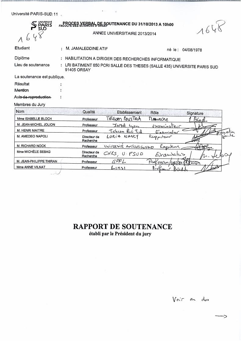
. Date de soutenance : 31 octobre 2013

. Jury :• Anne Vilnat, Professeur Université Paris Sud 11, présidente• Jean-Philippe Thiran, Professeur EPFL, Suisse, rapporteur• Richard Nock, Professeur UAG, Martinique, rapporteur• Amedeo Napoli, DR-CNRS, Loria-Nancy, rapporteur• Jean-Michel Jolion, professeur Insa-Lyon, examinateur• Henri Maître, Professeur émérite Télécom-ParisTech, examinateur• Michèle Sebag, DR-CNRS, Lri, examinateur• Isabelle Bloch, professeur Télécom-ParisTech, garante

. Spécialité : Informatique

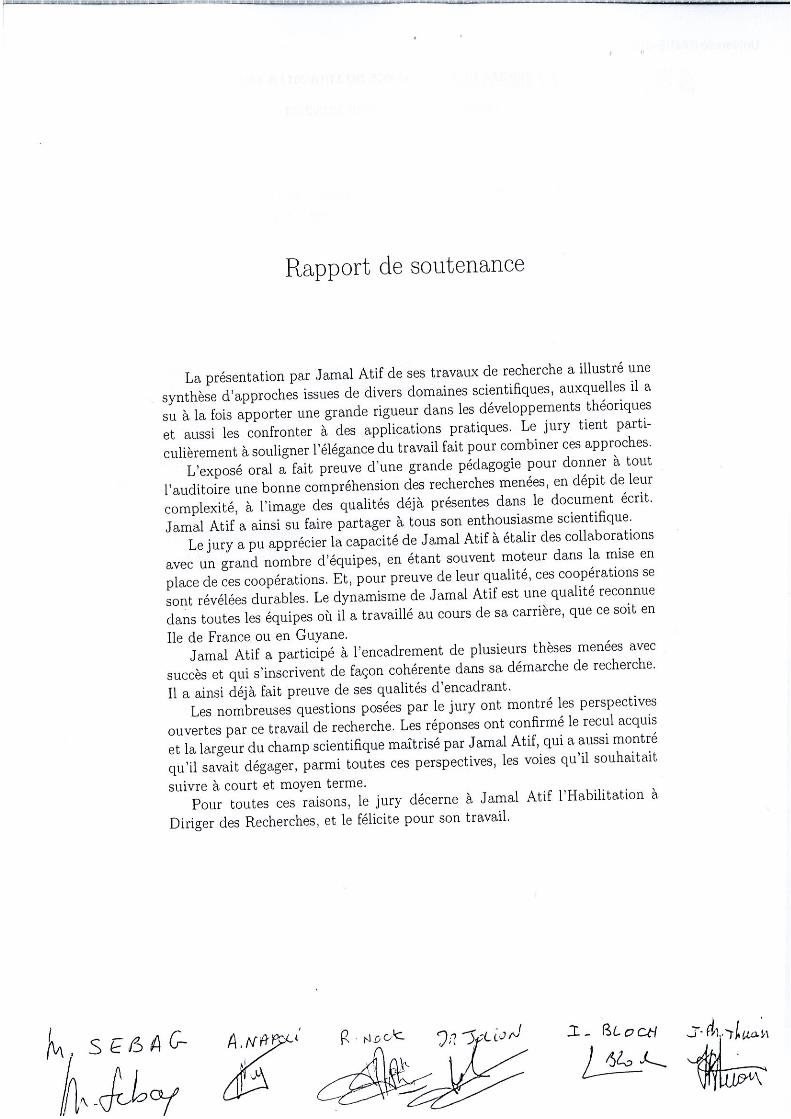
Cette partie contient :– l’attestation de réussite au diplôme,– le rapport de soutenance rédigé par le jury à l’issue de la présentation publique,– les rapports de pré-soutenance écrits par les rapporteurs.

9

Annexe A – Liste des publications

Articles dans des revues internationales avec comité de lecture (ACL)[1] O. Nempont, J. Atif, and I. Bloch. A constraint propagation approach to structural model based

image segmentation and recognition. Information Sciences, 246 :1–27, 2013. Impact factor : 2,833.[2] J. Atif, C. Hudelot, and I. Bloch. Explanatory reasoning for image understanding using formal

concept analysis and description logics. IEEE Transactions on Systems, Man and Cybernetics :systems, 2013. Impact factor : 3,08.

[3] G. Fouquier, J. Atif, and I. Bloch. Sequential model-based segmentation and recognition of imagestructures driven by visual features and spatial relations. Computer Vision and Image Understanding,116(1) :146–165, January 2012. Impact factor : 1,340.

[4] O. Nempont, J. Atif, E. Angelini, and I. Bloch. A New Fuzzy Connectivity Measure for Fuzzy Setsand Associated Fuzzy Attribute Openings. Journal of Mathematical Imaging and Vision, 34 :107–136, 2009. Impact factor : 1,391.

[5] H. Khotanlou, O. Colliot, J. Atif, and I. Bloch. 3D Brain Tumor Segmentation in MRI Using FuzzyClassification, Symmetry Analysis and Spatially Constrained Deformable Models. Fuzzy Sets andSystems, (160) :1457–1473, 2009. Impact factor : 1,759.

[6] C. Hudelot, J. Atif, and I. Bloch. Fuzzy Spatial Relation Ontology for Image Interpretation. FuzzySets and Systems, 159 :1929–1951, 2008. Impact factor : 1,759.

[7] J. Puentes, B. Batrancourt, J. Atif, E. Angelini, L. Lecornu, A. Zemirline, I. Bloch, G. Coatrieux,and C. Roux. Integrated Multimedia Electronic Patient Record and Graph-Based Image Informationfor Cerebral Tumors. Computers in Biology and Medicine, 38(4) :425–437, 2008. Impact factor :1,272.

Articles dans des revues nationales avec comité de lecture (ANCL)[8] C. Hudelot, J. Atif, and I. Bloch. FSRO : une ontologie de relations spatiales floues pour l’intepré-

tation d’images. RNTI Revue Nouvelles Technologies de l’Information (RNTI), 14 :55–86, 2008.[9] O. Nempont, J. Atif, E. D. Angelini, and I. Bloch. Propagation de contraintes pour la segmenta-

tion et la reconnaissance de structures anatomiques à partir d’un modèle structurel. Information -Interaction - Intelligence (I3), 10(1), December 2010.

Articles dans des conférences internationales avec comité de lecture (ACTI)

Conférences Rang A+ : IJCAI, IPMI,KRConférences Rang A : ECAI, ICIP, ICASSP, ICFCA, DGCIConférences Rang B : CLA, ISBI, ...[10] F. Distel, J. Atif, and I. Bloch. Concept dissimilarity with triangle inequality. In Proceedings of

the 14th International Conference on Principles of Knowledge Representation and Reasoning, (KR-2014), pages xxx–xxx, Vienna, Austria, jul 20-24 2014.

[11] S. Chevallier, Q. Barthélemy, and J. Atif. Subspace metrics for multivariate dictionaries and appli-cation to EEG. In Proceedings of the 39th International Conference on Acoustics, Speech, and SignalProcessing, (ICASSP-2014), pages xxx–xxx, Firenze, Italy„ May 4-9 2014.

[12] J. Atif, I. Bloch, F. Distel, and C. Hudelot. A fuzzy extension of explanatory relations based onmathematical morphology. In Gabriella Pasi and Javier Montero, editors, Proceedings of the 8thconference of the European Society for Fuzzy Logic and Technology (EUSFLAT-2013), pages 244–251, Milano, Italy, sep 11-13 2013.

[13] I. Bloch and J. Atif. Distance to bipolar information from morphological dilation. In Gabriella Pasiand Javier Montero, editors, Proceedings of the 8th conference of the European Society for FuzzyLogic and Technology (EUSFLAT-2013), pages 266–273, Milano, Italy, sep 11-13 2013.

27

[14] J. Atif, I. Bloch, F. Distel, and C. Hudelot. Mathematical morphology operators over concepts lat-tices. In 11th International Conference on Formal Concept Analysis, pages 28–43, Dresden, Germany,May 2013.

[15] Y. Isaac, Q. Barthélémy, J. Atif, C. Gouy-Pailler, and M. Sebag. Multi-dimensional sparse structuredsignal approximation using split bregman iterations. In 38th International Conference on Acoustics,Speech, and Signal Processing (ICASSP), pages 3826 – 3830, Vancouver, Canada, May 2013.

[16] L. Linguet and J. Atif. A particle filter approach for solar radiation estimate using satellite imageand in situ data. In 1st EARSeL Workshop on Temporal Analysis of Satellite Images, pages 208–216,Mykonos, Greece, May 2012.

[17] J. Atif, C. Hudelot, and I. Bloch. Abduction in description logics using formal concept analysis andmathematical morphology : application to image interpretation. In 8th International Conference onConcept Lattices and Their Applications (CLA 2011), pages 405–408, Nancy, France, October 2011.Acceptance rate : 57%.

[18] C. Hudelot, J. Atif, and I. Bloch. Integrating bipolar fuzzy mathematical morphology in descriptionlogics for spatial reasoning. In European Conference on Artificial Intelligence (ECAI 2010), pages497–502, Lisbon, Portugal, August 2010. Acceptance rate : 20%.

[19] J. Atif and J. Darbon. Copula-set measures over topographic maps for change detection. In IEEEInternational Conference on Image Processing (ICIP), pages 2881 – 2884, Cairo, Egypt, Nov 2009.Acceptance rate : 45%.

[20] C. Hudelot, J. Atif, and I. Bloch. A Spatial Relation Ontology Using Mathematical Morphology andDescription Logics for Spatial Reasoning. In ECAI-08 Workshop on Spatial and Temporal Reasoning,pages 21–25, Patras, Greece, jul 2008.

[21] O. Nempont, J. Atif, E. Angelini, and I. Bloch. Structure Segmentation and Recognition in ImagesGuided by Structural Constraint Propagation. In European Conference on Artificial Intelligence(ECAI 2008), pages 621–625, Patras, Greece, jul 2008. Acceptance rate : 22%.

[22] G. Fouquier, J. Atif, and I. Bloch. Sequential Spatial Reasoning in Images based on Pre-AttentionMechanisms and Fuzzy Attribute Graphs. In European Conference on Artificial Intelligence (ECAI2008), pages 611–615, Patras, Greece, jul 2008. Acceptance rate : 22%.

[23] O. Nempont, J. Atif, E. Angelini, and I. Bloch. Fuzzy Attribute Openings Based on a New FuzzyConnectivity Class. Application to Structural Recognition in Images. In International Conference onInformation Processing and Management of Uncertainty (IPMU’08), pages 652–659, Malaga, Spain,jun 2008.

[24] G. Fouquier, J. Atif, and I. Bloch. Incorporating a pre-attention mechanism in fuzzy attributegraphs for sequential image segmentation. In International Conference on Information Processingand Management of Uncertainty (IPMU’08), pages 840–847, Torremolinos (Malaga), Spain, jun 2008.

[25] O. Nempont, J. Atif, E. Angelini, and I. Bloch. A New Fuzzy Connectivity Class. Application toStructural Recognition in Images. In Discrete Geometry for Computer Imagery DGCI, volume LNCS4992, pages 446–457, Lyon, 2008. Acceptance rate : 30,26%.

[26] E. Aldea, G. Fouquier, J. Atif, and I. Bloch. Kernel Fusion for Image Classification Using FuzzyStructural Information. In 3rd International Symposium on Visual Computing ISVC07, volumeLNCS 4842, pages 307–317, Lake Tahoe, USA, nov 2007.

[27] J. Atif, C. Hudelot, G. Fouquier, I. Bloch, and E. Angelini. From Generic Knowledge to SpecificReasoning for Medical Image Interpretation using Graph-based Representations. In InternationalJoint Conference on Artificial Intelligence IJCAI’07, pages 224–229, Hyderabad, India, jan 2007.Acceptance rate : 15,7%.

[28] C. Hudelot, J. Atif, and I. Bloch. An Ontology of Spatial Relations using Fuzzy Concrete Domains.In AISB symposium on Spatial Reasoning and Communication, Newcastle, UK, apr 2007.

[29] O. Nempont, J. Atif, E. Angelini, and I. Bloch. Combining Radiometric and Spatial StructuralInformation in a New Metric for Minimal Surface Segmentation. In Information Processing inMedical Imaging (IPMI 2007), volume LNCS 4584, pages 283–295, Kerkrade, The Netherlands, jul2007. Acceptance rate : 14%.

[30] E. Aldea, J. Atif, and I. Bloch. Image Classification using Marginalized Kernels for Graphs. In 6thIAPR-TC15 Workshop on Graph-based Representations in Pattern Recognition, GbR’07, volume 1,pages 103–113, Alicante, Spain, jun 2007.

28

[31] G. Fouquier, J. Atif, and I. Bloch. Local Reasoning in Fuzzy Attributes Graphs for OptimizingSequential Segmentation. In 6th IAPR-TC15 Workshop on Graph-based Representations in PatternRecognition, GbR’07, volume 1, pages 138–147, Alicante, Spain, jun 2007.

[32] ED Angelini, J. Atif, J. Delon, E. Mandonnet, H. Duffau, and L. Capelle. Detection of glioma evo-lution on longitudinal MRI studies. In 4th IEEE International Symposium on Biomedical Imaging :From Nano to Macro, 2007. ISBI 2007, pages 49–52, Washington DC, USA, apr 2007. Acceptancerate : 48%.

[33] J. Atif, C. Hudelot, O. Nempont, N. Richard, B. Batrancourt, E. Angelini, and I. Bloch. GRAFIP :A Framework for the Representation of Healthy and Pathological Cerebral Information. In 4th IEEEInternational Symposium on Biomedical Imaging : From Nano to Macro, 2007. ISBI 2007, pages205–208, Washington DC, USA, apr 2007. Acceptance rate : 48%.

[34] H. Khotanlou, J. Atif, E. Angelini, H. Duffau, and I. Bloch. Adaptive Segmentation of Internal BrainStructures in Pathological MR Images Depending on Tumor Types. In 4th IEEE International Sym-posium on Biomedical Imaging : From Nano to Macro, 2007. ISBI 2007, pages 588–591, WashingtonDC, USA, apr 2007. Acceptance rate : 48%.

[35] J. Atif, H. Khotanlou, E. Angelini, H. Duffau, and I. Bloch. Segmentation of Internal Brain Structuresin the Presence of a Tumor. In MICCAI Workshop on Clinical Oncology, pages 61–68, Copenhagen,oct 2006.

[36] J. Puentes, B. Batrancourt, L. Lecornu, J. Atif, A. Zemirline, G. Coatrieux, E. Angelini, I. Bloch,and C. Roux. Enhancing Electronic Patient Record Functionality through Information Extractionfrom Images. In IEEE International Conference on Information and Communication Technologies :From Theory To Applications ICTTA 2006, pages 978–983, Damascus, Syria, apr 2006.

[37] C. Hudelot, J. Atif, O. Nempont, B. Batrancourt, E. Angelini, and I. Bloch. GRAFIP : a Frameworkfor the Representation of Healthy and Pathological Anatomical and Functional Cerebral Information.In Human Brain Mapping, Florence, Italy, jun 2006.

[38] B. Batrancourt, D. Hasboun, J. Atif, C. Hudelot, E. Angelini, and I. Bloch. A Clustering View of theHuman Brain Mapping Literature and an Anatomo-Functional Cerebral Model. In Human BrainMapping, Florence, Italy, jun 2006.

[39] J. Atif, O. Nempont, O. Colliot, E. Angelini, and I. Bloch. Level Set Deformable Models Constrainedby Fuzzy Spatial Relation. In Information Processing and Management of Uncertainty in Knowledge-Based Systems (IPMU’06), pages 1534–1541, Paris, France, 2006.

[40] B. Batrancourt, J. Atif, O. Nempont, E. Angelini, and I. Bloch. Integrating Information fromPathological Brain MRI into an Anatomo-Functional Model. In 24th IASTED International Multi-Conference on Biomedical Engineering, pages 236–241, Innsbruck, Austria, feb 2006.

[41] H. Khotanlou, J. Atif, O. Colliot, and I. Bloch. 3D Brain Tumor Segmentation Using Fuzzy Classifi-cation and Deformable Models. In International Workshop on Fuzzy Logic and Applications (WILF),volume LNAI 3849, pages 312–318, Crema, Italy, sep 2005.

[42] A. Tarault, J. Atif, X. Ripoche, P. Bourdot, and A. Osorio. Classification of radiological exams andorgans by belief theory. The 3rd ACS/IEEE International Conference on Computer Systems andApplications, page 20, 2005.

[43] J. Atif, X. Ripoche, and A. Osorio. Non-rigid medical image registration by maximisation of qua-dratic mutual information. In IEEE 29th Annual Northeast Bioengineering Conference, pages 32–40,Newark NJ, USA, march 2003.

[44] J. Atif, X. Ripoche, and A. Osorio. Combined quadratic mutual information to a new adaptivekernel density estimator for non rigid image registration. In SPIE Medical Imaging Conference, SanDiego, California, USA, 2004.

[45] X. Ripoche, J. Atif, and A. Osorio. Three dimensional discrete deformable model guided by mutualinformation for medical image segmentation. In SPIE Medical Imaging Conference, San Diego,California, USA, 2004.

Conférences invitées dans des congrès nationaux ou internationaux (INV)[46] I. Bloch, C. Hudelot, and J. Atif. On the Interest of Spatial Relations and Fuzzy Representations

for Ontology-Based Image Interpretation. In International Conference on Advances in Pattern Re-cognition, ICAPR’07, pages 15–25, Kolkata, India, jan 2007.

29

Articles dans des conférences nationales avec comité de lecture (ACTN)[47] Y. Isaac, Q. Barthélémy, J. Atif, C. Gouy-Pailler, and M. Sebag. Régularisations spatiales pour la

décomposition de signaux eeg sur un dictionnaire temps-fréquence. In GRETSI, Groupe d’Etudesdu Traitement du Signal et des Images, pages xxx–xx, Brest, France, September 2013.

[48] J. Atif, C. Hudelot, and I. Bloch. Abduction dans les logiques de description : apport de l’analyseformelle de concepts et de la morphologie mathématique. In Représentation et Raisonnement sur leTemps et l’Espace (RTE 2011), Chambery, France, May 2011.

[49] C. Hudelot, J. Atif, and I. Bloch. Intégration de la morphologie mathématique floue dans une logiquede description pour le raisonnement spatial. In Rencontres Francophones sur la Logique Floue et sesApplications (LFA 2008), pages 336–343, Lens, France, oct 2008.

[50] E. Aldea, G. Fouquier, J. Atif, and I. Bloch. Classification d’images par fusion d’attributs flousde graphes, relations spatiales et noyaux marginalisés. In Rencontres Francophones sur la LogiqueFloue et ses Applications (LFA 2007), pages 25–32, Nimes, France, nov 2007.

[51] J. Atif, C. Hudelot, and I. Bloch. Adaptation de connaissances génériques pour l’interprétationd’images médicales : représentations par onologies et par graphes et modélisation floue. In 7e journéesfrancophones Extraction et Gestion des Connaissances - Extraction de Connaissances et Images(EGC-ECOI’07), pages 51–61, Namur, Belgique, jan 2007.

[52] C. Hudelot, J. Atif, and I. Bloch. Ontologie de relations spatiales floues pour l’interprétation d’images.In Rencontres francophones sur la Logique Floue et ses Applications (LFA 2006), Toulouse, France,oct 2006.

[53] H. Khotanlou, J. Atif, B. Batrancourt, O. Colliot, E. Angelini, and I. Bloch. Segmentation detumeurs cérébrales et intégration dans un modèle de l’anatomie. In Reconnaissance des Formes etIntelligence Artificielle, RFIA’06, Tours, France, jan 2006. 2ème prix de l’AFRIF.

[54] J. Atif, X. Ripoche, C. Coussinet, and A. Osorio. Recalage élastique d’images médicales par maxi-misation de l’information mutuelle quadratique. In 19° Colloque sur le traitement du signal et desimages, FRA, 2003, Paris, France, 2003. GRETSI, Groupe d’Etudes du Traitement du Signal et desImages.

Communications sur résumé avec actes et comité de lecture[55] L. Linguet and J. Atif. A bayesian approach for solar resource potential assessment using satellite

images. In International Symposium on Remote Sensing of Environment, Beijing, China, April 22-262013.

[56] O. Nempont, J. Atif, A. Herment, I. Bloch, and P. Carlier. Graph-Based Segmentation of Muscles onNMR Images : Preliminary Results. In 2005 Workshop on Investigation of Human Muscle Function,Nashville, TN, USA, 2005.

[57] J. Atif, A. Osorio, B. Devaux, and F-X. Roux. Integration of short-distance radiological images, an-giography and multimodal image fusion in a stereotaxic software environment for biopsy intervention.In CARS, page 1312, 2004.

[58] A. Osorio, O. Traxer, J. Atif, X. Ripoche, M. Tligui, and B. Gattegno. Percutaneous nephrolithoto-mies improvement using a new augmented reality system integrated into operating rooms. In CARS,page 1322, 2004.

[59] V. Servois, A. Osorio, and J. Atif. A new pc based software for prostatic 3d segmentation and volumemeasurement. application to permanent prostate brachytherapy (PPB) evaluation using ct and mrimages fusion. In InfoRAD 2002, Radiological Society of North America RSNA-02, Chicago, USA,2002.

[60] A. Osorio, B. Devaux, R. Clodic, J. Atif, X. Ripoche, and F-X. Roux. A new Augmented Realitysystem for brain surgery improvements merging fluoroscopic 2D images, MR and CT 3D segmen-tations and Talairach atlas. In InfoRAD 2004, Radiological Society of North America RSNA-04,Chicago, USA, 2004.

[61] A. Osorio, O. Traxer, S. Merran, X. Ripoche, and J. Atif. Real time fusion of 2D fluoroscopic and3D segmented CT images integrated into an Augmented Reality system for percutaneous nephroli-thotomies (PCNL). In InfoRAD 2004, Radiological Society of North America RSNA-04, Chicago,USA, 2004. Cette Communication a reçu le prix (Cum Laude).

30

[62] A. Mihalcea, X. Ripoche, J. Atif, P.J. Valette, and A. Osorio. A new PC based software for semiautomatic liver segmentation. Clinical study for preoperative tumor localization. In InfoRAD 2003,Radiological Society of North America RSNA-03, Chicago, USA, 2003.

[63] A. Osorio, O. Traxer, S. Merran, X. Ripoche, and J. Atif. 3D reconstruction and instant volumemeasurement of complex renal calculi : application to percutaneous nephrolithotomy. In InfoRAD2003, Radiological Society of North America RSNA-03, Chicago, USA, 2003. Cette Communicationa reçu le prix (Certificate of merit).

[64] O. Traxer, A. Osorio, S. Merran, J. Atif, X. Ripoche, and M. Tligui. An augmented reality system forpercutaneous nephrolithotomy. In InfoRAD 2003, Radiological Society of North America RSNA-02,Chicago, USA, 2003. Cette Communication a reçu le prix (Certificate of merit).

Mémoires[65] J. Atif. Recalage non-rigide multimodal des images radiologiques par information mutuelle quadra-

tique normalisée. Mémoire de thèse, Université de Paris–Sud 11, Orsay, 29 Novembre 2004.[66] J. Atif. Quelques contributions à l’interprétation d’images, l’apprentissage statistique et la carto-

graphie cérébrale. Document d’habilitation à diriger des recherches, Université de Paris–Sud 11, 31octobre 2013.

31

Annexe B – Lettres de soutien à la candidature

Lettre de soutien et d’attestation des services d’enseignement, d’encadrement et de responsabilitéspédagogiques :

Pr. Caroline FabreChef du Département Informatique IUT d’OrsayPlateau de Moulon91400 Orsay, FranceEmail : Caroline.Fabre@u-psud.fr

Lettre de soutien et d’attestation des travaux liés aux activités de recherche :

Isabelle BlochProfesseur Télécom-ParisTech46, rue Barrault75013 Paris, FranceEmail : isabelle.bloch@telecom-paristech.fr

33

CNRS LTCIIsabelle BLOCH

Isabelle.Bloch@telecom-paristech.fr

16 decembre 2013

A qui de droit

Je connais Jamal Atif depuis son sejour post-doctoral au departement Traitement du Signal etdes Images de Telecom ParisTech / LTCI, apres sa these realisee au LIMSI. Il est un informaticientalentueux et dynamique, et c’est avec plaisir que j’appuie sa candidature pour la qualificationaux fonctions de professeur.

Sa recherche dans notre laboratoire portait sur un sujet tres di!erent de celui de sa thesepuisqu’il s’agissait de modeliser des connaissances anatomiques et de les instancier a partird’informations extraites d’images IRM du cerveau pouvant presenter des pathologies. En trespeu de temps, Jamal Atif a su s’integrer a l’equipe, exploiter les methodologies developpees dansnotre equipe pour traiter de l’anatomie normale et proposer des solutions originales pour prendreen compte les cas pathologiques, presentant des ecarts importants par rapport aux connaissancesgeneriques. Ses contributions ont porte a la fois sur la representation des connaissances, sousforme d’hyper-graphe attribue, sur des aspects de codage et de visualisation de ces graphes, etsur les interactions entre le modele generique et les informations specifiques extraites des images,y compris les aspects d’apprentissage (relations spatiales, methodes a noyaux sur des graphes).Ces travaux ont donne lieu a des publications dans les meilleurs revues et congres du domaine. Ila egalement travaille en collaboration avec des doctorants et post-doctorants de l’equipe, et sescontributions ont toujours ete marquantes dans ces travaux et ont donne lieu a des publicationscommunes.

Dans le cadre de ses recherches, Jamal Atif a egalement ete le moteur d’interactions fortesavec les services hospitaliers avec lesquels nous collaborons, ainsi qu’avec une equipe de TelecomBretagne. Ses capacites a discuter avec des neuro-anatomistes et des neuro-chirurgiens, ainsi qu’aintegrer leurs connaissances, leurs demandes et leurs contraintes dans les outils qu’il developpe,ont permis des avancees significatives dans le projet et il a su egalement les exploiter dans sesrecherches suivantes.

Pendant les quelques mois qu’il a passe au LTCI, Jamal Atif a su demarrer une recherchenouvelle, proposer des solutions originales, et il a pu acquerir de nouvelles competences, ainsique de nouveaux savoirs qui ont guide la reflexion sur ses projets de recherches futurs. Jamal Atifest ainsi tres rapidement devenu un chercheur cle dans notre petite equipe d’imagerie medicale,en renforcant en particulier les contributions en intelligence artificielle dans ce domaine, et nousavons continue a travailler ensemble sur ces themes apres son depart de l’equipe, en particulieren co-encadrant des doctorants.

Dans les enseignements qui lui ont ete confies a Telecom ParisTech (cours, encadrement deTP, de projets d’etudiants, de stagiaires), il a montre une implication exemplaire, ainsi qu’unegrande pedagogie. Les sujets qu’il propose sont toujours tres pertinents, interessants pour lesetudiants et tres formateurs. Son spectre de competences tres large lui permet d’enseigner dans

la plupart des domaines de l’informatique, de l’intelligence artificielle, du traitement des imageset de la vision par ordinateur, de la reconnaissance des formes et de l’apprentissage.

Depuis septembre 2006, Jamal Atif est maıtre de conferences, a l’UAG puis a l’universite ParisSud. Son poste d’enseignement a l’UAG, a l’IUT de Kourou, lui a demande un investissementimportant dans la preparation des cours et des travaux pratiques, ainsi que dans l’encadrementdes etudiants. En parallele, il a demarre de nouveaux axes de recherches, en particulier avecl’IRD ou il a ete en delegation. La encore il a montre un dynamisme exceptionnel pour monterde nouveaux projets et s’integrer dans une nouvelle equipe. Ces e!orts se sont concretises parl’acceptation de nouveaux projets, et de premieres publications sur une nouvelle methode dedetection de changements.

Toutes ces qualites ont vu ensuite leur confirmation dans les fonctions qu’il exerce a l’univer-site ParisSud. Son dynamisme se manifeste a la fois dans ses enseignements, dans son integrationdans l’equipe de recherche qu’il a rejointe, et dans les taches qu’il a prises en charge. Parexemple en recherche, il a su, de maniere remarquable, a la fois s’associer a des axes presentsdans l’equipe et a proposer de nouvelles pistes de recherche, dont temoignent ses publica-tions recentes. Ainsi il a contribue a de nouvelles techniques d’apprentissage de dictionnaireset a propose des representations sur-completes pour l’approximation de signaux. Citons commeautre exemple sa contribution pionniere a la modelisation du raisonnement abductif pour l’in-terpretation d’images, combinant des approches jamais associees jusque la. Il a egalement parti-cipe au montage de projets (ANR en particulier), et a pris en charge la responsabilite de grandesparties de ces projets.

En conclusion, Jamal Atif a toutes les qualites requises pour un professeur, et son dossier encontient deja toutes les composantes, qu’il s’agisse d’enseignement, d’encadrement, de recherche,de projets collaboratifs, de taches administratives ou encore de rayonnement. Il est tres appreciea la fois des chercheurs et des etudiants, il est tres actif dans ses discussions avec les etudiants,les doctorants, post-doctorants et chercheurs, son enthousiasme est contagieux et les idees qu’ilpropose sont toujours pertinentes et originales.

J’appuie donc fortement et sans aucune reserve sa candidature a la qualifation aux fonctionsde professeur.

Isabelle BLOCHProfesseur a Telecom ParisTech

Responsable de l’equipe Traitement et Interpretation des Images

2

Annexe C – Documents administratifs

39

Annexe D – Reproduction des travaux de recherche sélection-nés

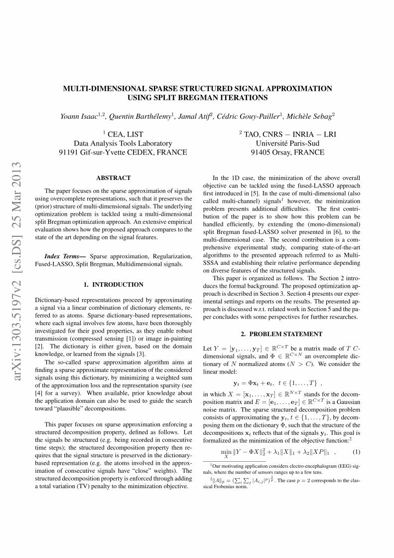
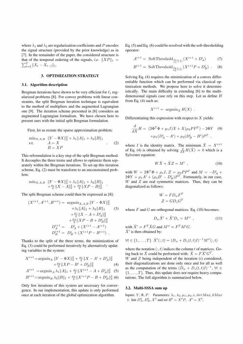
1. Y. Isaac, Q. Barthélémy, J. Atif, C. Gouy-Pailler and M. Sebag. Multi-dimensional sparse structuredsignal approximation using split Bregman iterations. In 38th International Conference on Acoustics,Speech, and Signal Processing (ICASSP), 3826 - 3830, Vancouver, Canada, May 2013.. Dans cet article, le schéma d’optimisation de fonctionnelles convexes non-différentiables “splitBregman" est étendu au contexte de l’approximation parcimonieuse de signaux multidimensionnelsà l’aide de représentations sur-complètes. L’algorithme introduit est analysé théoriquement etnumériquement et est appliqué à la reconstruction de signaux EEG.

2. J. Atif, C. Hudelot, and I. Bloch. Explanatory reasoning for image understanding using formalconcept analysis and description logics. IEEE Transactions on Systems, Man and Cybernetics :systems, doi : 0.1109/TSMC.2013.2280440, 2013. Cet article présente notre formalisme pour le raisonnement abductif dans les logiques de descrip-tion à des fin d’interprétation d’images. Il présente en particulier comment des théories telles quela morphologie mathématique, l’analyse formelle de concepts ainsi que les logiques de descrip-tion peuvent être unifiées sous l’égide de la théorie des treillis permettant de définir de nouveauxservices de raisonnement.

3. G. Fouquier, J. Atif, and I. Bloch. Sequential model-based segmentation and recognition of imagestructures driven by visual features and spatial relations. Computer Vision and Image Understan-ding, 116(1) :146–165, January 2012.. Cet article présente le travail de thèse de Geoffroy Fouquier. Nous y montrons comment opti-miser la séquence de segmentation, dans le cadre des approches de reconnaissance progressives,en exploitant les informations de saillance et des algorithmes de retour sur trace dans les graphes.L’approche est validée sur une base d’images saines et pathologiques.

4. O. Nempont, J. Atif, and I. Bloch. A constraint propagation approach to structural model basedimage segmentation and recognition. Information Sciences 246 : 1-27 (2013). Cet article présente une partie du travail de thèse d’Olivier Nempont. Le problème de l’ex-traction et de la reconnaissance de structures d’une scène est formalisé comme un problème desatisfaction de contraintes. En exploitant le modèle structurel de l’anatomie, nous avons intro-duit une méthode de résolution globale originale, visant à extraire une solution (i.e. l’affectationd’une région de l’espace à chaque structure anatomique à reconnaître) satisfaisant les relationsdu modèle structurel. Les garanties théoriques de l’approche sont détaillées.

5. J. Atif. Quelques contributions à l’interprétation d’images, à l’apprentissage statistique et à lacartographie cérébral. Habilitation à Diriger des Recherches. Université Paris Sud 11, France.Octobre 2013. Mon manuscrit d’habilitation synthétise neuf années de recherche menées depuis la soutenancede ma thèse de doctorat en 2004. Bien que composé en partie de travaux publiés et déjà reconnus,ce document présente pour la première fois une vision unifiée de mes travaux en interprétationd’images en apprentissage statistique et en cartographie cérébrale. En particulier, les fondementsthéoriques de notre formalisme logique pour l’interprétation d’images sont exposés en détail. Lemanuscrit s’achève sur un panorama des perspectives de recherche que je compte mener dans lesannées à venir.

Le manuscrit d’habilitation à diriger des recherches est fourni séparément.

45

MULTI-DIMENSIONAL SPARSE STRUCTURED SIGNAL APPROXIMATIONUSING SPLIT BREGMAN ITERATIONS

Yoann Isaac1,2, Quentin Barthelemy1, Jamal Atif2, Cedric Gouy-Pailler1, Michele Sebag2

1 CEA, LIST 2 TAO, CNRS − INRIA − LRIData Analysis Tools Laboratory Universite Paris-Sud

91191 Gif-sur-Yvette CEDEX, FRANCE 91405 Orsay, FRANCE

ABSTRACT

The paper focuses on the sparse approximation of signalsusing overcomplete representations, such that it preserves the(prior) structure of multi-dimensional signals. The underlyingoptimization problem is tackled using a multi-dimensionalsplit Bregman optimization approach. An extensive empiricalevaluation shows how the proposed approach compares to thestate of the art depending on the signal features.

Index Terms— Sparse approximation, Regularization,Fused-LASSO, Split Bregman, Multidimensional signals.

1. INTRODUCTION

Dictionary-based representations proceed by approximatinga signal via a linear combination of dictionary elements, re-ferred to as atoms. Sparse dictionary-based representations,where each signal involves few atoms, have been thoroughlyinvestigated for their good properties, as they enable robusttransmission (compressed sensing [1]) or image in-painting[2]. The dictionary is either given, based on the domainknowledge, or learned from the signals [3].

The so-called sparse approximation algorithm aims atfinding a sparse approximate representation of the consideredsignals using this dictionary, by minimizing a weighted sumof the approximation loss and the representation sparsity (see[4] for a survey). When available, prior knowledge aboutthe application domain can also be used to guide the searchtoward “plausible” decompositions.

This paper focuses on sparse approximation enforcing astructured decomposition property, defined as follows. Letthe signals be structured (e.g. being recorded in consecutivetime steps); the structured decomposition property then re-quires that the signal structure is preserved in the dictionary-based representation (e.g. the atoms involved in the approx-imation of consecutive signals have “close” weights). Thestructured decomposition property is enforced through addinga total variation (TV) penalty to the minimization objective.

In the 1D case, the minimization of the above overallobjective can be tackled using the fused-LASSO approachfirst introduced in [5]. In the case of multi-dimensional (alsocalled multi-channel) signals1 however, the minimizationproblem presents additional difficulties. The first contri-bution of the paper is to show how this problem can behandled efficiently, by extending the (mono-dimensional)split Bregman fused-LASSO solver presented in [6], to themulti-dimensional case. The second contribution is a com-prehensive experimental study, comparing state-of-the-artalgorithms to the presented approach referred to as Multi-SSSA and establishing their relative performance dependingon diverse features of the structured signals.

This paper is organized as follows. The Section 2 intro-duces the formal background. The proposed optimization ap-proach is described in Section 3. Section 4 presents our exper-imental settings and reports on the results. The presented ap-proach is discussed w.r.t. related work in Section 5 and the pa-per concludes with some perspectives for further researches.

2. PROBLEM STATEMENT

Let Y = [y1, . . . ,yT ] ∈ RC×T be a matrix made of T C-dimensional signals, and Φ ∈ RC×N an overcomplete dic-tionary of N normalized atoms (N > C). We consider thelinear model:

yt = Φxt + et, t ∈ {1, . . . , T} ,

in which X = [x1, . . . ,xT ] ∈ RN×T stands for the decom-position matrix and E = [e1, . . . , eT ] ∈ RC×T is a Gaussiannoise matrix. The sparse structured decomposition problemconsists of approximating the yt, t ∈ {1, . . . , T}, by decom-posing them on the dictionary Φ, such that the structure of thedecompositions xt reflects that of the signals yt. This goal isformalized as the minimization of the objective function:2

minX

�Y − ΦX�22 + λ1�X�1 + λ2�XP�1 , (1)

1Our motivating application considers electro-encephalogram (EEG) sig-nals, where the number of sensors ranges up to a few tens.

2�A�p = (�

i

�j |Ai,j |p)

1p . The case p = 2 corresponds to the clas-

sical Frobenius norm.

arX

iv:1

303.

5197

v2 [

cs.D

S] 2

5 M

ar 2

013

where λ1 and λ2 are regularization coefficients and P encodesthe signal structure (provided by the prior knowledge) as in[7]. In the remainder of the paper, the considered structure isthat of the temporal ordering of the signals, i.e. �XP�1 =�T

t=2 �Xt − Xt−1�1.

3. OPTIMIZATION STRATEGY

3.1. Algorithm description

Bregman iterations have shown to be very efficient for �1 reg-ularized problems [8]. For convex problems with linear con-straints, the split Bregman iteration technique is equivalentto the method of multipliers and the augmented Lagrangianone [9]. The iteration scheme presented in [6] considers anaugmented Lagrangian formalism. We have chosen here topresent ours with the initial split Bregman formulation.

First, let us restate the sparse approximation problem:

minX,A,B �Y − ΦX�22 + λ1�A�1 + λ2�B�1

s.t. A = XB = XP

. (2)

This reformulation is a key step of the split Bregman method.It decouples the three terms and allows to optimize them sep-arately within the Bregman iterations. To set-up this iterationscheme, Eq. (2) must be transform to an unconstrained prob-lem:

minX,A,B �Y − ΦX�22 + λ1�A�1 + λ2�B�1

+µ1

2 �X − A�22 + µ2

2 �XP − B�22

.

The split Bregman scheme could then be expressed as [8]:

(Xi+1, Ai+1, Bi+1) = argminX,A,B �Y − ΦX�22

+λ1�A�1 + λ2�B�1 (3)+µ1

2 �X − A + DiA�2

2

+µ2

2 �XP − B + DiB�2

2

Di+1A = Di

A + (Xi+1 − Ai+1)

Di+1B = Di

B + (Xi+1P − Bi+1) .

Thanks to the split of the three terms, the minimization ofEq. (3) could be performed iteratively by alternatively updat-ing variables in the system:

Xi+1 =argminX �Y − ΦX�22 + µ1

2 �X − Ai + DiA�2

2

+µ2

2 �XP − Bi + DiB�2

2 (4)

Ai+1 =argminA λ1�A�1 + µ1

2 �Xi+1 − A + DiA�2

2 (5)

Bi+1=argminB λ2�B�1 + µ2

2 �Xi+1P − B + DiB�2

2 (6)

Only few iterations of this system are necessary for conver-gence. In our implementation, this update is only performedonce at each iteration of the global optimization algorithm.

Eq. (5) and Eq. (6) could be resolved with the soft-thresholdingoperator:

Ai+1 = SoftThresholdλ1µ1

�.�1(Xi+1 + Di

A) (7)

Bi+1 = SoftThresholdλ2µ2

�.�1(Xi+1P + Di

B) . (8)

Solving Eq. (4) requires the minimization of a convex differ-entiable function which can be performed via classical op-timization methods. We propose here to solve it determin-istically. The main difficulty in extending [6] to the multi-dimensional signals case rely on this step. Let us define Hfrom Eq. (4) such as:

Xi+1 = argminX H(X) .

Differentiating this expression with respect to X yields:

d

dXH = (2ΦTΦ + µ1I)X + X(µ2PPT ) − 2ΦY (9)

+µ1(DiA − Ai) + µ2(D

iB − Bi)PT ,

where I is the identity matrix. The minimum X = Xi+1

of Eq. (4) is obtained by solving ddX H(X) = 0 which is a

Sylvester equation:

WX + XZ = M i , (10)

with W = 2ΦTΦ + µ1I , Z = µ2PPT and M = −DiA +

2ΦY + µ1Ai + (µ2B

i − DiB)PT . Fortunately, in our case,

W and Z are real symmetric matrices. Thus, they can bediagonalized as follows:

W = FDwFT

Z = GDzGT

where F and G are orthogonal matrices. Eq. (10) becomes:

DwX � + X �Dz = M i� , (11)

with X � = FT XG and M i� = FT M iG.X � is then obtained by:

∀t ∈ {1, . . . , T} X �(:, t) = (Dw + Dz(t, t)I)−1M i�(:, t)

where the notation (:, t) indices the column t of matrices. Go-ing back to X could be performed with: X = FX �GT .W and Z being independent of the iteration (i) considered,their diagonalizations are done only once and for all as wellas the computation of the terms (Dw + Dz(t, t)I)−1, ∀t ∈{1, . . . , T}. Thus, this update does not require heavy compu-tations. The full algorithm is summarized below.

3.2. Multi-SSSA sum up

Inputs: Y , Φ, P . Parameters: λ1, λ2, µ1, µ2, �, iterMax, kMax

1: Init D0A, D0

B , X0 and set B0 = X0P , A0 = X0,

2: W = 2ΦTΦ + µ1I and Z = µ2PP T .3: Compute Dw, Dz , F and G from W and Z.4: Precompute (t → T ), Dt

temp = (Dy + Dz(t, t)I)−1.5: i = 06: while i ≤ iterMax and �Xi−Xi−1�2

�Xi�2≥ � do

7: k = 08: Xtemp = Xi; Atemp = Ai; Btemp = Bi

9: for k → kMax do10: M � = F T (2ΦT Y − µ1(D

iA − Atemp) − µ2(D

iB −

Btemp)P T )G11: for t → T do12: Xtemp(:, t) = Dt

tempM �(:, t)13: end for14: Xtemp = FXtempGT

15: Atemp = SoftThresholdλ1µ1

�.�1(Xtemp + Di

A)

16: Btemp = SoftThresholdλ2µ2

�.�1(XtempP + Di

B)

17: end for18: Xi+1 = Xtemp; Ai+1 = Atemp; Bi+1 = Btemp

19: Di+1A = Di

A + (Xi+1 − Ai+1)20: Di+1

B = DiB + (Xi+1P − Bi+1)

21: i = i + 122: end while

4. EXPERIMENTAL EVALUATION

The following experiment aims at assessing the efficiency ofour approach in decomposing signals built with particular reg-ularities. We compare it both to algorithms coding each signalseparately, the orthogonal matching pursuit (OMP) [10] andthe LARS [11] (a LASSO solver), and to methods perform-ing the decomposition simultaneously, the simultaneous OMP(SOMP) and an proximal method solving the group-LASSOproblem (FISTA [12]).

4.1. Data generation

From a fixed random overcomplete dictionary Φ, a set of Ksignals having piecewise constant structures have been cre-ated. Each signal Y is synthesized from the dictionary Φ anda built decomposition matrix X with Y = ΦXThe TV penalization of the fused-LASSO regularizationmakes him more suitable to deal with data having abruptchanges. Thus, the decomposition matrices of signals havebeen built as linear combinations of specific activities whichhave been generated as follows:

Pind,m,d(i, j) =

0 if i �= indH(j − (m − d×T

2 ))−H(j − (m + d×T

2 )) if i = k

where P ∈ RN×T , H is the Heaviside function, ind ∈{1, . . . , N} is the index of an atom, m is the center of theactivity and d its duration. Each decomposition matrix Xcould then be written:

X =

na�

i=1

aiPindi,mi,di,

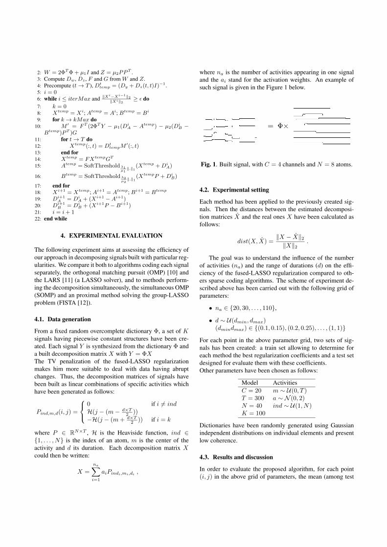
where na is the number of activities appearing in one signaland the ai stand for the activation weights. An example ofsuch signal is given in the Figure 1 below.

Fig. 1. Built signal, with C = 4 channels and N = 8 atoms.

4.2. Experimental setting

Each method has been applied to the previously created sig-nals. Then the distances between the estimated decomposi-tion matrices X and the real ones X have been calculated asfollows:

dist(X, X) =�X − X�2

�X�2.

The goal was to understand the influence of the numberof activities (na) and the range of durations (d) on the effi-ciency of the fused-LASSO regularization compared to oth-ers sparse coding algorithms. The scheme of experiment de-scribed above has been carried out with the following grid ofparameters:

• na ∈ {20, 30, . . . , 110},

• d ∼ U(dmin, dmax)(dmindmax) ∈ {(0.1, 0.15), (0.2, 0.25), . . . , (1, 1)}

For each point in the above parameter grid, two sets of sig-nals has been created: a train set allowing to determine foreach method the best regularization coefficients and a test setdesigned for evaluate them with these coefficients.Other parameters have been chosen as follows:

Model ActivitiesC = 20 m ∼ U(0, T )T = 300 a ∼ N (0, 2)N = 40 ind ∼ U(1, N)K = 100

Dictionaries have been randomly generated using Gaussianindependent distributions on individual elements and presentlow coherence.

4.3. Results and discussion

In order to evaluate the proposed algorithm, for each point(i, j) in the above grid of parameters, the mean (among test

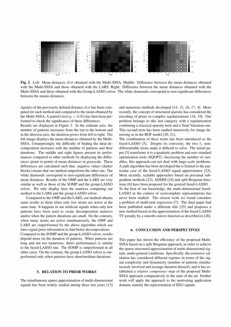
Fig. 2. Left: Mean distances dist obtained with the Multi-SSSA. Middle: Difference between the mean distances obtainedwith the Multi-SSSA and those obtained with the LARS. Right: Difference between the mean distances obtained with theMulti-SSSA and those obtained with the Group-LASSO solver. The white diamonds correspond to non-significant differencesbetween the means distances.

signals) of the previously defined distance dist has been com-puted for each method and compared to the mean obtained bythe Multi-SSSA. A paired t-test (p < 0.05) has then been per-formed to check the significance of these differences.Results are displayed in Figure 2. In the ordinate axis, thenumber of patterns increases from the top to the bottom andin the abscissa axis, the duration grows from left to right. Theleft image displays the mean distances obtained by the Multi-SSSA. Unsurprisingly, the difficulty of finding the ideal de-composition increases with the number of patterns and theirdurations. The middle and right figures present its perfor-mances compared to other methods by displaying the differ-ences (point to point) of mean distances in grayscale. Thesedifferences are calculated such that, negative values (darkerblocks) means that our method outperform the other one. Thewhite diamonds correspond to non-significant differences ofmean distances. Results of the OMP and the LARS are verysimilar as well as those of the SOMP and the group-LASSOsolver. We only display here the matrices comparing ourmethod to the LARS and the group-LASSO solver.

Compared to the OMP and the LARS, our method obtainssame results as them when only few atoms are active at thesame time. It happens in our artificial signals when only fewpatterns have been used to create decomposition matricesand/or when the pattern durations are small. On the contrary,when many atoms are active simultaneously, the OMP andLARS are outperformed by the above algorithm which useinter-signal prior information to find better decompositions.Compared to the SOMP and the group-LASSO solver, resultsdepend more on the duration of patterns. When patterns arelong and not too numerous, theirs performances is similarto the fused-LASSO one. The SOMP is outperformed in allother cases. On the contrary, the group-LASSO solver is out-performed only when patterns have short/medium durations.

5. RELATION TO PRIOR WORKS

The simultaneous sparse approximation of multi-dimensionalsignals has been widely studied during these last years [13]

and numerous methods developed [14, 15, 16, 17, 4]. Morerecently, the concept of structured sparsity has considered theencoding of priors in complex regularizations [18, 19]. Ourproblem belongs to this last category with a regularizationcombining a classical sparsity term and a Total Variation one.This second term has been studied intensively for image de-noising as in the ROF model [20, 21].The combination of these terms has been introduced as thefused-LASSO [5]. Despite its convexity, the two �1 non-differentiable terms make it difficult to solve. The initial pa-per [5] transforms it to a quadratic problem and uses standardoptimization tools (SQOPT). Increasing the number of vari-ables, this approach can not deal with large-scale problems.A path algorithm has been developed but is limited to the par-ticular case of the fused-LASSO signal approximator [22].More recently, scalable approaches based on proximal sub-gradient methods [23], ADMM [24] and split Bregman itera-tions [6] have been proposed for the general fused-LASSO.To the best of our knowledge, the multi-dimensional fused-LASSO in the context of overcomplete representations hasnever been studied. The closest work we found considersa problem of multi-task regression [7]. The final paper hadbeen published under a different title [25] and proposes anew method based on the approximation of the fused-LASSOTV penalty by a smooth convex function as described in [26].

6. CONCLUSION AND PERSPECTIVES

This paper has shown the efficiency of the proposed Multi-SSSA based on a split Bregman approach, in order to achievethe sparse structured approximation of multi-dimensional sig-nals, under general conditions. Specifically, the extensive val-idation has considered different regimes in terms of the sig-nal complexity and dynamicity (number of patterns simulta-neously involved and average duration thereof), and it has es-tablished a relative competence map of the proposed Multi-SSSA approach comparatively to the state of the art. Furtherwork will apply the approach to the motivating applicationdomain, namely the representation of EEG signals.

7. REFERENCES

[1] D.L. Donoho, “Compressed sensing,” Information Theory,IEEE Trans. on, vol. 52, no. 4, pp. 1289–1306, 2006.

[2] J. Mairal, M. Elad, and G. Sapiro, “Sparse representation forcolor image restoration,” Image Processing, IEEE Trans. on,vol. 17, no. 1, pp. 53–69, 2008.

[3] I. Tosic and P. Frossard, “Dictionary learning,” Signal Pro-cessing Magazine, IEEE, vol. 28, no. 2, pp. 27–38, 2011.

[4] A. Rakotomamonjy, “Surveying and comparing simultaneoussparse approximation (or group-Lasso) algorithms,” SignalProcessing, vol. 91, no. 7, pp. 1505–1526, 2011.

[5] R. Tibshirani, M. Saunders, S. Rosset, J. Zhu, and K. Knight,“Sparsity and smoothness via the fused Lasso,” Journal of theRoyal Statistical Society: Series B (Statistical Methodology),vol. 67, no. 1, pp. 91–108, 2005.

[6] G.B. Ye and X. Xie, “Split Bregman method for large scalefused Lasso,” Computational Statistics & Data Analysis, vol.55, no. 4, pp. 1552–1569, 2011.

[7] X. Chen, S. Kim, Q. Lin, J.G. Carbonell, and E.P. Xing,“Graph-structured multi-task regression and an efficient op-timization method for general fused Lasso,” arXiv preprintarXiv:1005.3579, 2010.

[8] T. Goldstein and S. Osher, “The split Bregman method for�1 regularized problems,” SIAM Journal on Imaging Sciences,vol. 2, no. 2, pp. 323–343, 2009.

[9] C. Wu and X.C. Tai, “Augmented Lagrangian method, dualmethods, and split Bregman iteration for ROF, vectorial TV,and high order models,” SIAM Journal on Imaging Sciences,vol. 3, no. 3, pp. 300–339, 2010.

[10] Y.C. Pati, R. Rezaiifar, and P.S. Krishnaprasad, “Orthogonalmatching pursuit: Recursive function approximation with ap-plications to wavelet decomposition,” in Signals, Systems andComputers, 1993. Conf. Record of The Twenty-Seventh Asilo-mar Conf. on. IEEE, 1993, pp. 40–44.

[11] B. Efron, T. Hastie, I. Johnstone, and R. Tibshirani, “Leastangle regression,” The Annals of statistics, vol. 32, no. 2, pp.407–499, 2004.

[12] A. Beck and M. Teboulle, “A fast iterative shrinkage-thresholding algorithm for linear inverse problems,” SIAMJournal on Imaging Sciences, vol. 2, no. 1, pp. 183–202, 2009.

[13] J. Chen and X. Huo, “Theoretical results on sparse represen-tations of multiple-measurement vectors,” Signal Processing,IEEE Trans. on, vol. 54, no. 12, pp. 4634–4643, 2006.

[14] J.A. Tropp, A.C. Gilbert, and M.J. Strauss, “Algorithms for si-multaneous sparse approximation. Part I: Greedy pursuit,” Sig-nal Processing, vol. 86, no. 3, pp. 572–588, 2006.

[15] J.A. Tropp, “Algorithms for simultaneous sparse approxima-tion. Part II: Convex relaxation,” Signal Processing, vol. 86,no. 3, pp. 589–602, 2006.

[16] R. Gribonval, H. Rauhut, K. Schnass, and P. Vandergheynst,“Atoms of all channels, unite! Average case analysis of multi-channel sparse recovery using greedy algorithms,” Journal ofFourier analysis and Applications, vol. 14, no. 5, pp. 655–687,2008.

[17] S.F. Cotter, B.D. Rao, K. Engan, and K. Kreutz-Delgado,“Sparse solutions to linear inverse problems with multiple mea-surement vectors,” Signal Processing, IEEE Trans. on, vol. 53,no. 7, pp. 2477–2488, 2005.

[18] J. Huang, T. Zhang, and D. Metaxas, “Learning with structuredsparsity,” Journal of Machine Learning Research, vol. 12, pp.3371–3412, 2011.

[19] R. Jenatton, J.Y. Audibert, and F. Bach, “Structured variableselection with sparsity-inducing norms,” Journal of MachineLearning Research, vol. 12, pp. 2777–2824, 2011.

[20] L.I. Rudin, S. Osher, and E. Fatemi, “Nonlinear total varia-tion based noise removal algorithms,” Physica D: NonlinearPhenomena, vol. 60, no. 1-4, pp. 259–268, 1992.

[21] J. Darbon and M. Sigelle, “A fast and exact algorithm for to-tal variation minimization,” in Pattern recognition and imageanalysis, 2005, vol. 3522 of Lecture Notes in Computer Sci-ence, pp. 351–359.

[22] H. Hoefling, “A path algorithm for the fused Lasso signal ap-proximator,” Journal of Computational and Graphical Statis-tics, vol. 19, no. 4, pp. 984–1006, 2010.

[23] J. Liu, L. Yuan, and J. Ye, “An efficient algorithm for a classof fused Lasso problems,” in Proc. 16th ACM SIGKDD Int.Conf. on Knowledge Discovery and Data Mining. ACM, 2010,pp. 323–332.

[24] B. Wahlberg, S. Boyd, M. Annergren, and Y. Wang, “AnADMM algorithm for a class of total variation regularized es-timation problems,” arXiv preprint arXiv:1203.1828, 2012.

[25] X. Chen, Q. Lin, S. Kim, J.G. Carbonell, and E.P. Xing,“Smoothing proximal gradient method for general structuredsparse regression,” The Annals of Applied Statistics, vol. 6, no.2, pp. 719–752, 2012.

[26] Y. Nesterov, “Smooth minimization of non-smooth functions,”Mathematical Programming, vol. 103, no. 1, pp. 127–152,2005.

IEEE TRANSACTIONS ON SYSTEMS, MAN, AND CYBERNETICS–PART A: SYSTEMS AND HUMANS VOL. X, NO. X, MONTH 2013 1

Explanatory reasoning for image understandingusing formal concept analysis and description logics

Jamal Atif, Celine Hudelot, Isabelle Bloch, Member, IEEE,

Abstract—In this paper we propose an original way of enrich-ing description logics with abduction reasoning services. Underthe aegis of set and lattice theories, we put together ingredientsfrom mathematical morphology, description logics and formalconcept analysis. We propose to compute the best explanations ofan observation through algebraic erosion over the concept latticeof a background theory which is efficiently constructed using toolsfrom formal concept analysis. We show that the defined operatorsare sound and complete and satisfy important rationality postu-lates of abductive reasoning. As a typical illustration, we considera scene understanding problem. In fact, scene understandingcan benefit from prior structural knowledge represented asan ontology and the reasoning tools of description logics. Weformulate model based scene understanding as an abductivereasoning process. A scene is viewed as an observation and theinterpretation is defined as the “best” explanation considering theterminological knowledge part of a description logic about thescene context. This explanation is obtained from morphologicaloperators applied on the corresponding concept lattice.

Index Terms—Image understanding, explanatory reasoning,mathematical morphology, formal concept analysis, descriptionlogics.

I. INTRODUCTION

AUTOMATIC image interpretation has been an activefield of research for several years. In this large field,

this paper focuses on extracting high level information fromimages or video sequences, when the detection and recognitionof structures can benefit from prior structural knowledge(such as spatial interactions). This is in particular the case invideo sequences related to a specific context (sport events forinstance), in medical imaging (using anatomical knowledge),or in aerial and satellite imaging (man-made structures suchas airports and towns for instance).

Description Logics (DL) are an important paradigm oflogic-based knowledge representation [1]. They are a decid-able family of first-order logic that spans numerous applica-tions in areas such as: semantic web, cognitive robotics, spatialreasoning, computer vision, etc., including logical-based sceneunderstanding and semantic interpretation.

Scene interpretation can benefit from prior knowledge ex-pressed as ontologies and from description logics endowedwith spatial reasoning tools as illustrated in our previouswork [2], [3]. The challenge in this work was to derivereasoning tools that are able to handle in a unified wayquantitative information supplied by the image domain andqualitative pieces of knowledge supplied by the ontology level.The interpretation task is performed in a sequential way by

J. Atif is with Universite Paris Sud, LRI - TAO, Orsay, FranceC. Hudelot is with MAS Laboratory, Ecole Centrale de Paris, FranceI. Bloch is with Telecom ParisTech - CNRS LTCI, Paris, France

maintaining the consistency between the information extractedfrom the image and the corresponding expert knowledgeencoded at the terminological level. In other words, objectrecognition and interpretation are seen as the coherence of acurrent situation (spatial configuration) encoded in the ABoxof the DL with the TBox part. However, when the expertknowledge is not crisply consistent with the observed situation,which is common in image interpretation, then this approachdoes not apply or leads to inconsistent results. Moreover, in thecontext of image interpretation, a given structural configurationcan be consistent with different prior knowledge parts (orconsistent to some degree). These facts call for adapting DLreasoning tools to such situations, and abduction seems to bean appealing framework towards this aim. In the context ofnon-monotonic reasoning paradigms in AI, abduction refersto the reasoning process of forming a hypothesis that explainsobserved phenomena. More precisely, it allows for computingthe “best explanation” of the observed phenomena, whichsuits situations where the knowledge at hand is not crisplyconsistent with the observations. Formally, given a backgroundtheory K representing the expert knowledge and a formula Crepresenting an observation on the problem domain, abductivereasoning searches for an explanation formula D such thatD is satisfiable w.r.t. K and it holds that K ⊧ (D → C)(K ∪D ⊧ C).

For readability convenience and in order to illustrate thepotential of our approach in the context of image interpretationas well as for other AI based applications, we will considertwo running examples. The first one has been introduced byC. Elsenbroich et al. in their position paper [4] to argue theneed of developing computational tools of abduction in thecontext of ontologies.

Example (SHD). In [4], C. Elsenbroich et al. consideredthe following medical ontology-based diagnosis: suppose adisease, called the Shake-Hands-Disease (SHD), that alwaysdevelops when one shakes hands with someone else whocarries the Shake-Hands-Disease-Virus (SHDV ). Supposefurther a medical ontology containing:− roles: has symptom, carries virus, etc.,− concepts: SHD, SHDV , Laziness, Pizza Appetite,

Google Lover, etc.,and a set of axioms (cf. Section III-A) specifying that:− if someone has the disease SHD then he or she suffers

from Laziness and Pizza Appetite,− a Researcher is someone that has symptoms Laziness,Pizza Appetite and Google Lover,− and finally someone who shakes hands with someone thatcarries the SHDV virus has a disease SHD.

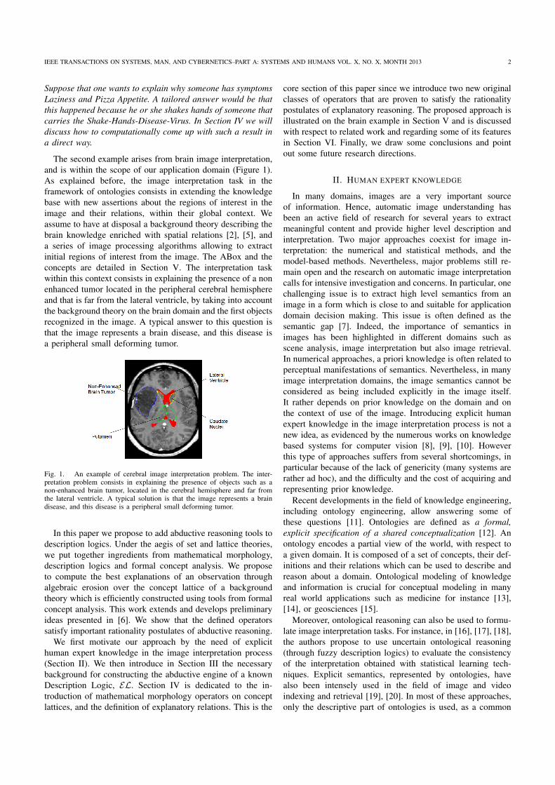
IEEE TRANSACTIONS ON SYSTEMS, MAN, AND CYBERNETICS–PART A: SYSTEMS AND HUMANS VOL. X, NO. X, MONTH 2013 2

Suppose that one wants to explain why someone has symptomsLaziness and Pizza Appetite. A tailored answer would be thatthis happened because he or she shakes hands of someone thatcarries the Shake-Hands-Disease-Virus. In Section IV we willdiscuss how to computationally come up with such a result ina direct way.

The second example arises from brain image interpretation,and is within the scope of our application domain (Figure 1).As explained before, the image interpretation task in theframework of ontologies consists in extending the knowledgebase with new assertions about the regions of interest in theimage and their relations, within their global context. Weassume to have at disposal a background theory describing thebrain knowledge enriched with spatial relations [2], [5], anda series of image processing algorithms allowing to extractinitial regions of interest from the image. The ABox and theconcepts are detailed in Section V. The interpretation taskwithin this context consists in explaining the presence of a nonenhanced tumor located in the peripheral cerebral hemisphereand that is far from the lateral ventricle, by taking into accountthe background theory on the brain domain and the first objectsrecognized in the image. A typical answer to this question isthat the image represents a brain disease, and this disease isa peripheral small deforming tumor.

Fig. 1. An example of cerebral image interpretation problem. The inter-pretation problem consists in explaining the presence of objects such as anon-enhanced brain tumor, located in the cerebral hemisphere and far fromthe lateral ventricle. A typical solution is that the image represents a braindisease, and this disease is a peripheral small deforming tumor.

In this paper we propose to add abductive reasoning tools todescription logics. Under the aegis of set and lattice theories,we put together ingredients from mathematical morphology,description logics and formal concept analysis. We proposeto compute the best explanations of an observation throughalgebraic erosion over the concept lattice of a backgroundtheory which is efficiently constructed using tools from formalconcept analysis. This work extends and develops preliminaryideas presented in [6]. We show that the defined operatorssatisfy important rationality postulates of abductive reasoning.

We first motivate our approach by the need of explicithuman expert knowledge in the image interpretation process(Section II). We then introduce in Section III the necessarybackground for constructing the abductive engine of a knownDescription Logic, EL. Section IV is dedicated to the in-troduction of mathematical morphology operators on conceptlattices, and the definition of explanatory relations. This is the

core section of this paper since we introduce two new originalclasses of operators that are proven to satisfy the rationalitypostulates of explanatory reasoning. The proposed approach isillustrated on the brain example in Section V and is discussedwith respect to related work and regarding some of its featuresin Section VI. Finally, we draw some conclusions and pointout some future research directions.

II. HUMAN EXPERT KNOWLEDGE

In many domains, images are a very important sourceof information. Hence, automatic image understanding hasbeen an active field of research for several years to extractmeaningful content and provide higher level description andinterpretation. Two major approaches coexist for image in-terpretation: the numerical and statistical methods, and themodel-based methods. Nevertheless, major problems still re-main open and the research on automatic image interpretationcalls for intensive investigation and concerns. In particular, onechallenging issue is to extract high level semantics from animage in a form which is close to and suitable for applicationdomain decision making. This issue is often defined as thesemantic gap [7]. Indeed, the importance of semantics inimages has been highlighted in different domains such asscene analysis, image interpretation but also image retrieval.In numerical approaches, a priori knowledge is often related toperceptual manifestations of semantics. Nevertheless, in manyimage interpretation domains, the image semantics cannot beconsidered as being included explicitly in the image itself.It rather depends on prior knowledge on the domain and onthe context of use of the image. Introducing explicit humanexpert knowledge in the image interpretation process is not anew idea, as evidenced by the numerous works on knowledgebased systems for computer vision [8], [9], [10]. Howeverthis type of approaches suffers from several shortcomings, inparticular because of the lack of genericity (many systems arerather ad hoc), and the difficulty and the cost of acquiring andrepresenting prior knowledge.

Recent developments in the field of knowledge engineering,including ontology engineering, allow answering some ofthese questions [11]. Ontologies are defined as a formal,explicit specification of a shared conceptualization [12]. Anontology encodes a partial view of the world, with respect toa given domain. It is composed of a set of concepts, their def-initions and their relations which can be used to describe andreason about a domain. Ontological modeling of knowledgeand information is crucial for conceptual modeling in manyreal world applications such as medicine for instance [13],[14], or geosciences [15].

Moreover, ontological reasoning can also be used to formu-late image interpretation tasks. For instance, in [16], [17], [18],the authors propose to use uncertain ontological reasoning(through fuzzy description logics) to evaluate the consistencyof the interpretation obtained with statistical learning tech-niques. Explicit semantics, represented by ontologies, havealso been intensely used in the field of image and videoindexing and retrieval [19], [20]. In most of these approaches,only the descriptive part of ontologies is used, as a common

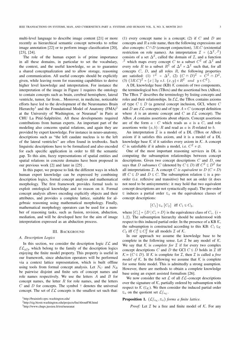
IEEE TRANSACTIONS ON SYSTEMS, MAN, AND CYBERNETICS–PART A: SYSTEMS AND HUMANS VOL. X, NO. X, MONTH 2013 3

multi-level language to describe image content [21] or morerecently as hierarchical semantic concept networks to refineimage annotation [22] or to perform image classification [20],[23], [24].

The role of the human expert is of prime importancein all these domains, in particular to set the vocabulary,the context, and the useful knowledge, so as to guaranteea shared conceptualization and to allow storage, reasoningand communication. All useful concepts should be explicitlygiven, while leaving room for reasoning capabilities to derivehigher level knowledge and interpretation. For instance theinterpretation of the image in Figure 1 requires the ontologyto contain concepts such as brain, cerebral hemisphere, lateralventricle, tumor, far from... Moreover, in medicine, noticeableefforts have led to the development of the Neuronames BrainHierarchy1 and the Foundational Model of Anatomy (FMA)2

at the University of Washington, or Neuranat3 in Paris atCHU La Pitie-Salpetriere. All these developments requiredcontributions from human experts. An important part of themodeling also concerns spatial relations, and again they areprovided by expert knowledge. For instance in neuro-anatomy,descriptions such as “the left caudate nucleus is to the leftof the lateral ventricles” are often found in textbooks. Suchlinguistic descriptions have to be formalized and also encodedfor each specific application in order to fill the semanticgap. To this aim, fuzzy representations of spatial entities andspatial relations in concrete domains have been proposed inour previous work [2] and later in [25] .

In this paper, we propose to link the different ways in whichhuman expert knowledge can be expressed by combiningdescription logics, formal concept analysis and mathematicalmorphology. The first framework provides formal tools toexploit ontological knowledge and to reason on it. Formalconcept analysis allows encoding explicitly objects and theirattributes, and provides a complete lattice, suitable for al-gebraic reasoning using mathematical morphology. Finally,mathematical morphology operators can be used for a num-ber of reasoning tasks, such as fusion, revision, abduction,mediation, and will be developed here for the aim of imageinterpretation expressed as an abduction process.

III. BACKGROUND

A. Description Logics

In this section, we consider the description logic EL andELgfp which belong to the family of the description logicsenjoying the finite model property. This property is useful inour framework, since abduction operators will be performedvia a context lattice representation, which is built offlineusing tools from formal concept analysis. Let NC and NRbe pairwise disjoint and finite sets of concept names androle names respectively. We use the letters A and B forconcept names, the letter R for role names, and the lettersC and D for concepts. The symbol ⊺ denotes the universalconcept. The set of EL concepts is the smallest set such that:

1http://braininfo.rprc.washington.edu/2http://sig.biostr.washington.edu/projects/fm/AboutFM.html3http://www.chups.jussieu.fr/ext/neuranat

(1) every concept name is a concept; (2) if C and D areconcepts and R a role name, then the following expressions arealso concepts: C ⊓D (concept conjunction), ∃R.C (existentialrestriction on role names). An interpretation I = (∆I , ⋅I)consists of a set ∆I , called the domain of I, and a function⋅I which maps every concept C to a subset CI of ∆I andevery role R to a subset RI of ∆I × ∆I such that, for allconcepts C, D, and all roles R, the following propertiesare satisfied: (1) ⊺I = ∆I , (2) (C ⊓ D)I = CI ∩ DI ,(3) (∃R.C)I = {x ∣ ∃y s.t. (x, y) ∈ RI and y ∈ CI}.

A DL knowledge base (KB) K consists of two components,the terminological box (TBox) and the assertional box (ABox).The TBox T describes the terminology by listing concepts androles and their relationships. In EL, the TBox contains axiomsof type C ⊑ D (a general concept inclusion, GCI, where Cand D are EL concepts) and of type A ≡ C (concept definitionwhere A is an atomic concept and C an EL concept). TheABox A contains assertions about objects. Concept assertionsare of the form a ∶ C which reads as a is a C, and roleassertions write (a, b) ∶ R and read as a is R-related to b.

An interpretation I is a model of a DL (TBox or ABox)axiom if it satisfies this axiom, and it is a model of a DLknowledge base K if it satisfies every axiom in K. A conceptC is satisfiable if it admits a model, i.e. CI ≠ ∅.

One of the most important reasoning services in DL iscomputing the subsumption relationships between conceptdescriptions. Given two concept descriptions C and D, onesays that D subsumes C (denoted by C ⊑D) iff CI ⊆DI forall interpretations I. A concept C is equivalent to D (C ≡D)iff C ⊑ D and D ⊑ C. The subsumption relation ⊑ is a pre-order (i.e. reflexive and transitive) but not an order (it doesnot need to be antisymmetric: it may hold that two equivalentconcept descriptions are not syntactically equal). The pre-order⊑ induces a partial order ⊑≡ on the equivalence classes ofconcept descriptions:

[C1] ⊑≡ [C2] iff C1 ⊑ C2,

where [Ci] = {D ∣ Ci ≡D} is the equivalence class of Ci, (i =1,2). The subsumption hierarchy should be understood withrespect to this induced partial order. In the presence of a KB K,the subsumption is constructed according to this KB: C1 ⊑KC2 iff CI1 ⊆ CI2 for all models I of K.

In our approach we assume the knowledge base to becomplete in the following sense. Let I be any model of K.We say that K is complete for I if for every two complexconcept descriptions C and D the GCI C ⊑ D holds in I iffK ⊧ (C ⊑ D). If K is complete for I, then I is called a freemodel of K. In the following we assume that K is completefor some finite model. This is admittedly a strong asumption.However, there are methods to obtain a complete knowledgebase using an expert assisted formalism [26].

We now consider the set L of all EL–concept descriptionsover the signature of K, partially ordered by subsumption withrespect to K (⊑K). We then consider the induced partial order⊑≡ on the quotient set L/≡K .

Proposition 1. (L/≡K ,⊑≡) forms a finite lattice.

Proof: Let I be a free and finite model of K. For any

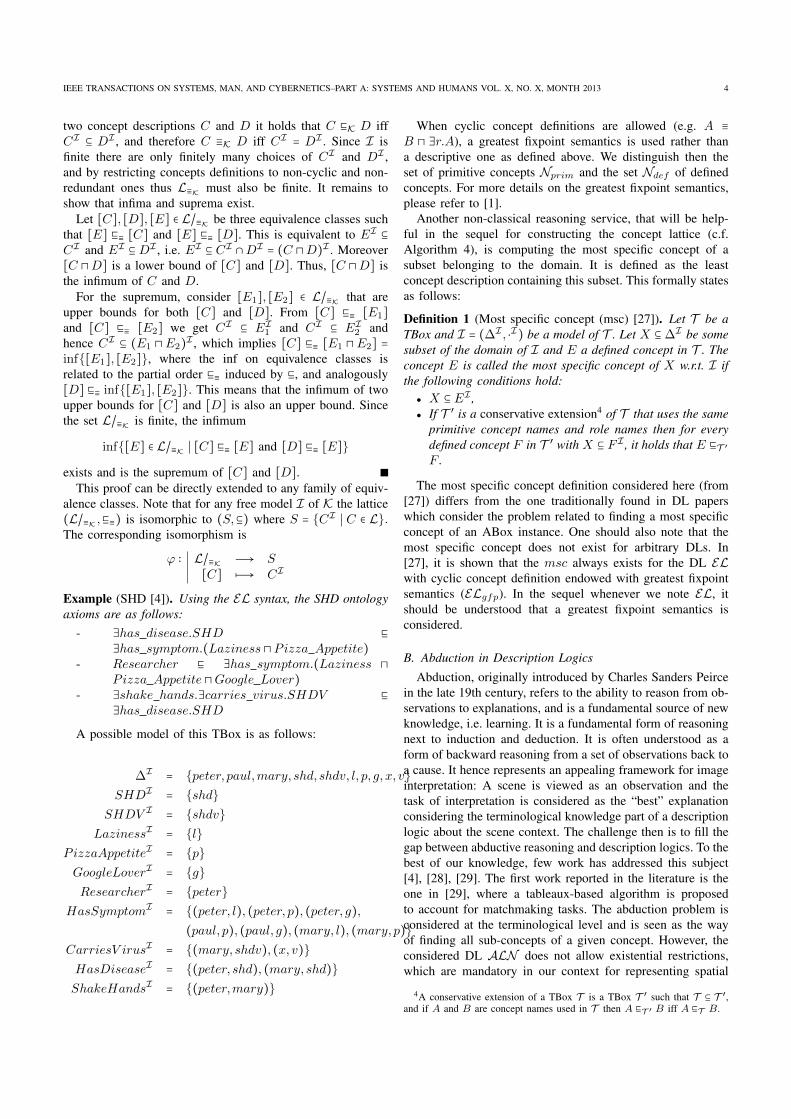
IEEE TRANSACTIONS ON SYSTEMS, MAN, AND CYBERNETICS–PART A: SYSTEMS AND HUMANS VOL. X, NO. X, MONTH 2013 4

two concept descriptions C and D it holds that C ⊑K D iffCI ⊆ DI , and therefore C ≡K D iff CI = DI . Since I isfinite there are only finitely many choices of CI and DI ,and by restricting concepts definitions to non-cyclic and non-redundant ones thus L≡K must also be finite. It remains toshow that infima and suprema exist.

Let [C], [D], [E] ∈ L/≡K be three equivalence classes suchthat [E] ⊑≡ [C] and [E] ⊑≡ [D]. This is equivalent to EI ⊆CI and EI ⊆ DI , i.e. EI ⊆ CI ∩DI = (C ⊓D)I . Moreover[C ⊓D] is a lower bound of [C] and [D]. Thus, [C ⊓D] isthe infimum of C and D.

For the supremum, consider [E1], [E2] ∈ L/≡K that areupper bounds for both [C] and [D]. From [C] ⊑≡ [E1]and [C] ⊑≡ [E2] we get CI ⊆ EI1 and CI ⊆ EI2 andhence CI ⊆ (E1 ⊓ E2)I , which implies [C] ⊑≡ [E1 ⊓ E2] =inf{[E1], [E2]}, where the inf on equivalence classes isrelated to the partial order ⊑≡ induced by ⊑, and analogously[D] ⊑≡ inf{[E1], [E2]}. This means that the infimum of twoupper bounds for [C] and [D] is also an upper bound. Sincethe set L/≡K is finite, the infimum

inf{[E] ∈ L/≡K ∣ [C] ⊑≡ [E] and [D] ⊑≡ [E]}exists and is the supremum of [C] and [D].

This proof can be directly extended to any family of equiv-alence classes. Note that for any free model I of K the lattice(L/≡K ,⊑≡) is isomorphic to (S,⊆) where S = {CI ∣ C ∈ L}.The corresponding isomorphism is

ϕ ∶ L/≡K Ð→ S[C] z→ CIExample (SHD [4]). Using the EL syntax, the SHD ontologyaxioms are as follows:

- ∃has disease.SHD ⊑∃has symptom.(Laziness ⊓ Pizza Appetite)- Researcher ⊑ ∃has symptom.(Laziness ⊓

Pizza Appetite ⊓Google Lover)- ∃shake hands.∃carries virus.SHDV ⊑∃has disease.SHDA possible model of this TBox is as follows:

∆I = {peter, paul,mary, shd, shdv, l, p, g, x, v}SHDI = {shd}

SHDV I = {shdv}LazinessI = {l}

PizzaAppetiteI = {p}GoogleLoverI = {g}ResearcherI = {peter}

HasSymptomI = {(peter, l), (peter, p), (peter, g),(paul, p), (paul, g), (mary, l), (mary, p)}CarriesV irusI = {(mary, shdv), (x, v)}HasDiseaseI = {(peter, shd), (mary, shd)}ShakeHandsI = {(peter,mary)}

When cyclic concept definitions are allowed (e.g. A ≡B ⊓ ∃r.A), a greatest fixpoint semantics is used rather thana descriptive one as defined above. We distinguish then theset of primitive concepts Nprim and the set Ndef of definedconcepts. For more details on the greatest fixpoint semantics,please refer to [1].

Another non-classical reasoning service, that will be help-ful in the sequel for constructing the concept lattice (c.f.Algorithm 4), is computing the most specific concept of asubset belonging to the domain. It is defined as the leastconcept description containing this subset. This formally statesas follows:

Definition 1 (Most specific concept (msc) [27]). Let T be aTBox and I = (∆I , ⋅I) be a model of T . Let X ⊆ ∆I be somesubset of the domain of I and E a defined concept in T . Theconcept E is called the most specific concept of X w.r.t. I ifthe following conditions hold:

● X ⊆ EI ,● If T ′ is a conservative extension4 of T that uses the same

primitive concept names and role names then for everydefined concept F in T ′ with X ⊆ F I , it holds that E ⊑T ′F .

The most specific concept definition considered here (from[27]) differs from the one traditionally found in DL paperswhich consider the problem related to finding a most specificconcept of an ABox instance. One should also note that themost specific concept does not exist for arbitrary DLs. In[27], it is shown that the msc always exists for the DL ELwith cyclic concept definition endowed with greatest fixpointsemantics (ELgfp). In the sequel whenever we note EL, itshould be understood that a greatest fixpoint semantics isconsidered.

B. Abduction in Description Logics

Abduction, originally introduced by Charles Sanders Peircein the late 19th century, refers to the ability to reason from ob-servations to explanations, and is a fundamental source of newknowledge, i.e. learning. It is a fundamental form of reasoningnext to induction and deduction. It is often understood as aform of backward reasoning from a set of observations back toa cause. It hence represents an appealing framework for imageinterpretation: A scene is viewed as an observation and thetask of interpretation is considered as the “best” explanationconsidering the terminological knowledge part of a descriptionlogic about the scene context. The challenge then is to fill thegap between abductive reasoning and description logics. To thebest of our knowledge, few work has addressed this subject[4], [28], [29]. The first work reported in the literature is theone in [29], where a tableaux-based algorithm is proposedto account for matchmaking tasks. The abduction problem isconsidered at the terminological level and is seen as the wayof finding all sub-concepts of a given concept. However, theconsidered DL ALN does not allow existential restrictions,which are mandatory in our context for representing spatial

4A conservative extension of a TBox T is a TBox T ′ such that T ⊆ T ′,and if A and B are concept names used in T then A ⊑T ′ B iff A ⊑T B.

IEEE TRANSACTIONS ON SYSTEMS, MAN, AND CYBERNETICS–PART A: SYSTEMS AND HUMANS VOL. X, NO. X, MONTH 2013 5

relations between scene objects. Later, in a position paper [4],the authors discuss, without providing hints for computationaltools, the usefulness of abductive reasoning in DL, provideseveral application scenarios and introduce rigorous definitionsand postulates of abductive reasoning in the context of ontolo-gies. Other abduction-like non-monotonic services are reportedin the literature. In [30], debugging incoherent terminologiesis considered, i.e. finding a minimally unsatisfiable subsetof TBox axioms, and in [31], and later [32], the authorsaddress the problem of finding justifications, i.e. minimal setsof axioms of an ontology that make a particular entailmentof the ontology hold. These works are pointed out in [33]where some computational complexity results in the DL ELare reported. Recently, based on the correspondence betweenDL and modal logic, the authors in [28] introduce reasoningcalculi for solving ABox abduction problems in the DL ALC.The algorithms are based on regular connection tableaux andresolution with set-of-support and are proven to be sound andcomplete. Finally, in a context similar to the one claimed inthis project, the task of multimedia interpretation as abductivereasoning over DL rules is considered in [34] and in [35].An inference service for ABox abduction restricted to rules isintroduced. A more detailed discussion of the other approachescan be found in Section VI.

Based on the TBox T and the ABox A parts of the knowl-edge base, abduction in the framework of DL can be viewedfrom different standpoints [4], [28]: concept abduction, TBoxabduction, ABox abduction, and knowledge base abduction.

In this paper, we consider the case of concept abductionw.r.t. a background theory or knowledge base. The followingdefinition formally states our purpose:

Definition 2 (Concept abduction [4]). Let Γ be an arbitraryDL, K a knowledge base and C a concept in Γ , such that Cis satisfiable w.r.t. K. A concept abduction problem, denotedas ⟨K,C⟩, consists in finding a set Expla(C) of complexconcepts γ in a possibly different DL Γ ′ (a sublogic of Γ )such that K ⊧ γ ⊑ C. An explanatory relation is a binaryrelation C ⊳ γ where the intended meaning of C ⊳ γ is “γ isa preferred explanation of C”.

Explanatory reasoning is concerned with preferred expla-nations rather than just plain explanations. So, explaining anobservation requires that some formulas must be “selected” aspreferred explanations.

Rationality postulates for abduction have been widely stud-ied in the context of propositional logic [36]. In this paper weconsider the rationality postulates introduced in [37] adaptedto the DL context:

LLEK:C ≡K D , C ⊳ γ

D ⊳ γRLEK:

γ ≡K γ′ ; C ⊳ γC ⊳ γ′

E-CM:C ⊳ γ ; γ ⊑K D(C ⊓D) ⊳ γ

E-C-Cut:(C ⊓D) ⊳ γ , ∀δ [C ⊳ δ ⇒ δ ⊑K D ]

C ⊳ γRS:

C ⊳ γ ; γ′ ⊑K γ ; γ′ /⊑K �C ⊳ γ′

ROR:C ⊳ γ ; C ⊳ δC ⊳ (γ ⊔ δ)

LOR:C ⊳ γ ; D ⊳ γ(C ⊔D) ⊳ γ

E-DR:C ⊳ γ ; D ⊳ δ(C ⊔D) ⊳ γ or (C ⊔D) ⊳ δ

E-R-Cut:(C ⊓D) ⊳ γ ; ∃δ [C ⊳ δ & δ ⊑K D]

C ⊳ γE-Reflexivity :

C ⊳ γγ ⊳ γ

E-ConK :K /⊧ ¬C(a) iff there is γ such that C ⊳ γThe intended meaning and motivation for these postulates

can be found in [37]. It is worth noting that in the contextof the relatively inexpressive DL EL not allowing for the dis-junction, ROR, LOR and E-DR postulates are not considered.

The rationality postulates can be satisfied by operators (suchas the subsumption: γ ⊑K C for instance) which we donot consider as restrictive enough. Therefore to enhance thenotion of “preferred” explanation, in addition to the rationalitypostulates detailed above we consider the following minimalityconstraints:

Definition 3 (Minimality constraint). Let us consider theconcept abduction problem ⟨K,C⟩, with Expla(C) the setof explanations and γ a preferred solution, i.e. C ⊳ γ:

● γ is ⊑-minimal if there is no explanation ζ of ⟨K,C⟩ suchthat ζ ⋤K γ and γ /⊑K �.

This should be read: γ is minimal if there is not a morespecific explanation than γ. The trivial solution � is excluded.Other minimality constraints for abduction in DL can be foundin [33] in addition to complexity analysis in the particular caseof the DL EL and EL++.

When the abduction problem is restricted to concept names,the set of all explanatory solutions is obvious. It is exactly theset of concept names that are subsumed by the observationC. This amounts to going down in the subsumption hierarchy,starting from the concept to explain. In this paper, we areinterested in complex concepts, i.e. concepts that are notdefined in the TBox and are not explicitly represented in thesubsumption hierarchy.

Example (SHD cont’d). Within the context of the SHDexample5, given the concept ∃has symptom.(Laziness ⊓Pizza Appetite), if we are restricted to GCI inthe TBox, a solution obtained by simple backwardchaining on the classification tree would be:∃shake hands.∃carries virus.SHDV . However weare looking for complex EL-concepts, and in this case ourapproach allows for abducing the following complex concept(see details in Section IV):∃shake hands.(∃carries virus.SHDV ⊓∃has disease.SHD ⊓ ∃has symptom.P izza Appetite ⊓has symptom.Laziness).

One should remark that this concept is not a named one,hence our approach goes beyond simple backward chaining

5Although the example has been originally introduced as an ABox Abudc-tion problem, we found it simple and clear enough to adapt it to the contextof concept abduction.

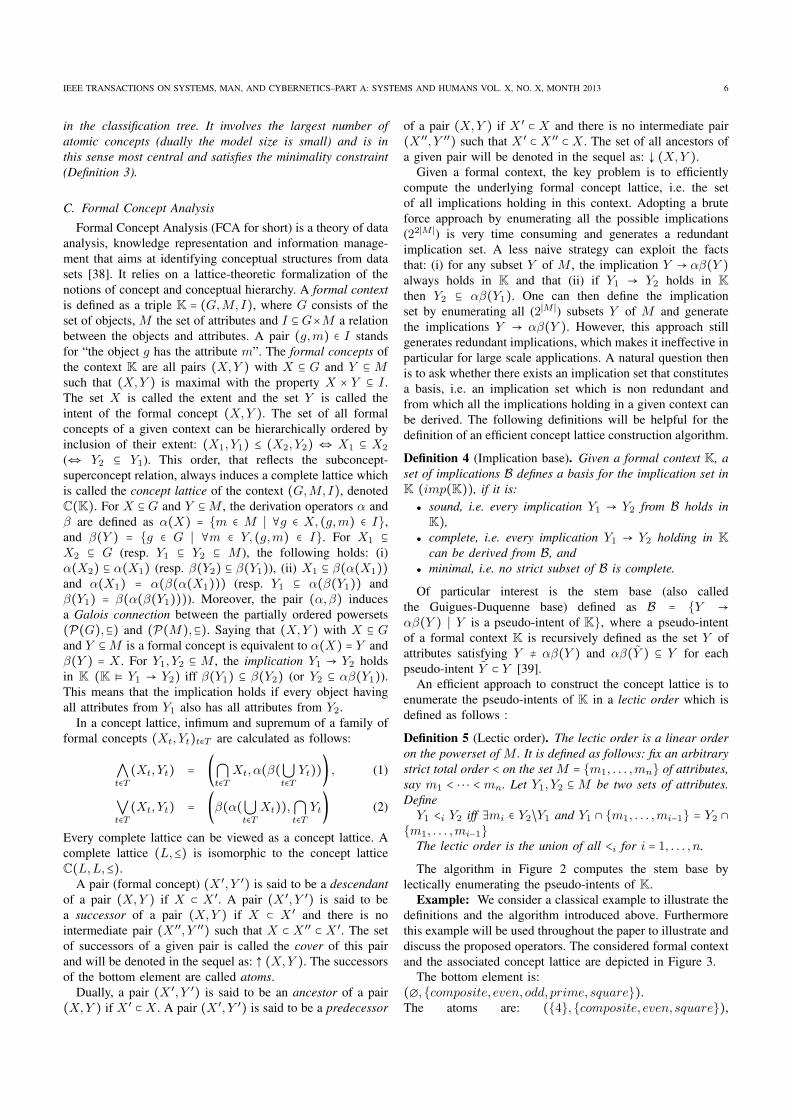
IEEE TRANSACTIONS ON SYSTEMS, MAN, AND CYBERNETICS–PART A: SYSTEMS AND HUMANS VOL. X, NO. X, MONTH 2013 6

in the classification tree. It involves the largest number ofatomic concepts (dually the model size is small) and is inthis sense most central and satisfies the minimality constraint(Definition 3).

C. Formal Concept Analysis

Formal Concept Analysis (FCA for short) is a theory of dataanalysis, knowledge representation and information manage-ment that aims at identifying conceptual structures from datasets [38]. It relies on a lattice-theoretic formalization of thenotions of concept and conceptual hierarchy. A formal contextis defined as a triple K = (G,M, I), where G consists of theset of objects, M the set of attributes and I ⊆ G×M a relationbetween the objects and attributes. A pair (g,m) ∈ I standsfor “the object g has the attribute m”. The formal concepts ofthe context K are all pairs (X,Y ) with X ⊆ G and Y ⊆ Msuch that (X,Y ) is maximal with the property X × Y ⊆ I .The set X is called the extent and the set Y is called theintent of the formal concept (X,Y ). The set of all formalconcepts of a given context can be hierarchically ordered byinclusion of their extent: (X1, Y1) ≤ (X2, Y2) ⇔ X1 ⊆ X2

(⇔ Y2 ⊆ Y1). This order, that reflects the subconcept-superconcept relation, always induces a complete lattice whichis called the concept lattice of the context (G,M, I), denotedC(K). For X ⊆ G and Y ⊆M , the derivation operators α andβ are defined as α(X) = {m ∈ M ∣ ∀g ∈ X, (g,m) ∈ I},and β(Y ) = {g ∈ G ∣ ∀m ∈ Y, (g,m) ∈ I}. For X1 ⊆X2 ⊆ G (resp. Y1 ⊆ Y2 ⊆ M ), the following holds: (i)α(X2) ⊆ α(X1) (resp. β(Y2) ⊆ β(Y1)), (ii) X1 ⊆ β(α(X1))and α(X1) = α(β(α(X1))) (resp. Y1 ⊆ α(β(Y1)) andβ(Y1) = β(α(β(Y1)))). Moreover, the pair (α,β) inducesa Galois connection between the partially ordered powersets(P(G),⊆) and (P(M),⊆). Saying that (X,Y ) with X ⊆ Gand Y ⊆M is a formal concept is equivalent to α(X) = Y andβ(Y ) = X . For Y1, Y2 ⊆ M , the implication Y1 → Y2 holdsin K (K ⊧ Y1 → Y2) iff β(Y1) ⊆ β(Y2) (or Y2 ⊆ αβ(Y1)).This means that the implication holds if every object havingall attributes from Y1 also has all attributes from Y2.

In a concept lattice, infimum and supremum of a family offormal concepts (Xt, Yt)t∈T are calculated as follows:

⋀t∈T(Xt, Yt) = (⋂

t∈T Xt, α(β(⋃t∈T Yt))) , (1)

⋁t∈T(Xt, Yt) = (β(α(⋃

t∈T Xt)),⋂t∈T Yt) (2)

Every complete lattice can be viewed as a concept lattice. Acomplete lattice (L,≤) is isomorphic to the concept latticeC(L,L,≤).

A pair (formal concept) (X ′, Y ′) is said to be a descendantof a pair (X,Y ) if X ⊂ X ′. A pair (X ′, Y ′) is said to bea successor of a pair (X,Y ) if X ⊂ X ′ and there is nointermediate pair (X ′′, Y ′′) such that X ⊂ X ′′ ⊂ X ′. The setof successors of a given pair is called the cover of this pairand will be denoted in the sequel as: ↑ (X,Y ). The successorsof the bottom element are called atoms.

Dually, a pair (X ′, Y ′) is said to be an ancestor of a pair(X,Y ) if X ′ ⊂X . A pair (X ′, Y ′) is said to be a predecessor

of a pair (X,Y ) if X ′ ⊂ X and there is no intermediate pair(X ′′, Y ′′) such that X ′ ⊂X ′′ ⊂X . The set of all ancestors ofa given pair will be denoted in the sequel as: ↓ (X,Y ).

Given a formal context, the key problem is to efficientlycompute the underlying formal concept lattice, i.e. the setof all implications holding in this context. Adopting a bruteforce approach by enumerating all the possible implications(22∣M ∣) is very time consuming and generates a redundantimplication set. A less naive strategy can exploit the factsthat: (i) for any subset Y of M , the implication Y → αβ(Y )always holds in K and that (ii) if Y1 → Y2 holds in Kthen Y2 ⊆ αβ(Y1). One can then define the implicationset by enumerating all (2∣M ∣) subsets Y of M and generatethe implications Y → αβ(Y ). However, this approach stillgenerates redundant implications, which makes it ineffective inparticular for large scale applications. A natural question thenis to ask whether there exists an implication set that constitutesa basis, i.e. an implication set which is non redundant andfrom which all the implications holding in a given context canbe derived. The following definitions will be helpful for thedefinition of an efficient concept lattice construction algorithm.

Definition 4 (Implication base). Given a formal context K, aset of implications B defines a basis for the implication set inK (imp(K)), if it is:

● sound, i.e. every implication Y1 → Y2 from B holds inK),

● complete, i.e. every implication Y1 → Y2 holding in Kcan be derived from B, and

● minimal, i.e. no strict subset of B is complete.

Of particular interest is the stem base (also calledthe Guigues-Duquenne base) defined as B = {Y →αβ(Y ) ∣ Y is a pseudo-intent of K}, where a pseudo-intentof a formal context K is recursively defined as the set Y ofattributes satisfying Y ≠ αβ(Y ) and αβ(Y ) ⊆ Y for eachpseudo-intent Y ⊂ Y [39].

An efficient approach to construct the concept lattice is toenumerate the pseudo-intents of K in a lectic order which isdefined as follows :

Definition 5 (Lectic order). The lectic order is a linear orderon the powerset of M . It is defined as follows: fix an arbitrarystrict total order < on the set M = {m1, . . . ,mn} of attributes,say m1 < ⋅ ⋅ ⋅ < mn. Let Y1, Y2 ⊆M be two sets of attributes.DefineY1 <i Y2 iff ∃mi ∈ Y2/Y1 and Y1 ∩ {m1, . . . ,mi−1} = Y2 ∩{m1, . . . ,mi−1}The lectic order is the union of all <i for i = 1, . . . , n.

The algorithm in Figure 2 computes the stem base bylectically enumerating the pseudo-intents of K.

Example: We consider a classical example to illustrate thedefinitions and the algorithm introduced above. Furthermorethis example will be used throughout the paper to illustrate anddiscuss the proposed operators. The considered formal contextand the associated concept lattice are depicted in Figure 3.

The bottom element is:(∅,{composite, even, odd, prime, square}).The atoms are: ({4},{composite, even, square}),

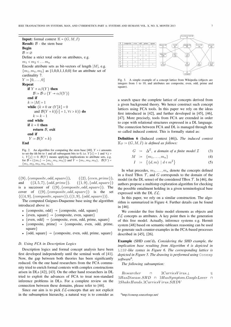
IEEE TRANSACTIONS ON SYSTEMS, MAN, AND CYBERNETICS–PART A: SYSTEMS AND HUMANS VOL. X, NO. X, MONTH 2013 7

Input: formal context K = (G,M, I)Result: B - the stem baseBeginB ∶= ∅Define a strict total order on attributes, e.g.m1 <m2 < . . .mn

Encode attribute sets as bit-vectors of length ∣M ∣, e.g.{m1,m4,m5} as [1,0,0,1,1,0,0] for an attribute set ofcardinality 7.Y ∶= [0, . . . ,0]Repeat

if Y ≠ αβ(Y ) thenB ∶= B ∪ {Y → αβ(Y )}end ifk ∶= ∣M ∣ + 1while (k ≠ 0 or (Y [k] = 0

and B(Y + k)[i] = 1,∀i > k)) dok ∶= k − 1

end whileif k = 0 then

return B, exitend ifY ∶= B(Y + k)

End

Fig. 2. An algorithm for computing the stem base [40]. Y + i amountsto set the ith bit to 1 and all subsequent bits to 0, i.e. Y [i] ∶= 1 and ∀j >i, Y [j] ∶= 0. B(Y ) means applying implications to attribute sets, e.g.for B = ({m1} → {m1,m4,m5}) and Y = {m1,m2,m3}, B(Y ) ={m1,m2,m3,m4,m5}.

({9},{composite, odd, square}), ({2},{even, prime}),and ({3,5,7},{odd, prime}). ({1,9},{odd, square})is a successor of ({9},{composite, odd, square}). Thecover of ({9},{composite, odd, square}) is the set{({4,9},{composite, square}), ({1,9},{odd, square})}.

The computed Guigues-Duquenne base using the algorithmintroduced above is:

● {composite, odd} → {composite, odd, square}● {even, square} → {composite, even, square}● {even, odd} → {composite, even, odd, prime, square}● {composite, prime} → {composite, even, odd, prime,

square}● {odd, square} → {composite, even, odd, prime, square}

D. Using FCA in Description Logics

Description logics and formal concept analysis have beenfirst developed independently until the seminal work of [41].Now, the gap between both theories has been significantlyreduced. On the one hand researchers from the FCA commu-nity tried to enrich formal contexts with complex constructionsarisen in DLs [42], [43]. On the other hand researchers in DLtried to exploit the advances of FCA to treat non-standardinference problems in DLs. For a complete review on theconnection between these domains, please refer to [44].

Since our aim is to pick EL-concepts that are not explicitin the subsumption hierarchy, a natural way is to consider as

K composite even odd prime square1 × ×2 × ×3 × ×4 × × ×5 × ×6 × ×7 × ×8 × ×9 × × ×10 × ×

Fig. 3. A simple example of a concept lattice from Wikipedia (objects areintegers from 1 to 10, and attributes are composite, even, odd, prime andsquare).

a search space the complete lattice of concepts derived froma given background theory. We hence construct such conceptlattices using FCA tools. In this paper we rely on the ideasfirst introduced in [42], and further developed in [45], [46],[47]. More precisely, tools from FCA are extended in orderto cope with relational structures expressed in a DL language.The connection between FCA and DL is managed through theso called induced context. This is formally stated as:

Definition 6 (Induced context [46]). The induced contextKT ∶= (G,M, I) is defined as follows:

G ∶= ∆I , a domain of a finite model I (3)M ∶= {m1, . . . ,mn} (4)I ∶= { (d,m) ∣ d ∈mI} (5)

In what precedes, m1, . . . ,mn denote the concepts definedin a fixed TBox T , and G corresponds to the domain of themodel (in the DL sense) of the considered TBox T . In [46], theauthors propose a multistep exploration algorithm for checkingthe possible entailment holding in a given terminological baseexpressed with the DL EL.

In this paper, we rely on a similar construction. The algo-rithm is summarized in Figure 4. Further details can be foundin [46].

We consider the free finite model elements as objects andEL concepts as attributes. A key point then is the generationof this free model. Actually, inference systems e.g. Hermitsystem [48] based on semantic-tableaux reasoning can be usedto generate such counter-examples in the FCA-based processesdescribed in [45], [26].

Example (SHD cont’d). Considering the SHD example, theimplication base resulting from Algorithm 4 is depicted inLISP-like syntax in Figure 6. The corresponding lattice isdepicted in Figure 5. The drawing is performed using Conexpsoftware6.

The following subsumption:

Researcher ⊓ ∃CarriesV irus.� ⊑∃HasDisease.SHD ⊓ ∃HasSymptom.GoogleLover ⊓∃ShakeHands.∃CarriesV irus.SHDV6http://conexp.sourceforge.net/

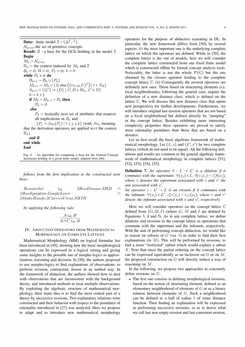
IEEE TRANSACTIONS ON SYSTEMS, MAN, AND CYBERNETICS–PART A: SYSTEMS AND HUMANS VOL. X, NO. X, MONTH 2013 8

Data: finite model I = (∆I , ⋅I)Nprim-the set of primitive conceptsResult: S - a base for the GCIs holding in the model IBeginM0 ∶= NprimK0 ∶= the context induced by M0 and IS0 ∶= ∅, Π ∶= ∅, P0 ∶= ∅, k ∶= 0while Pk ≠ ∅ do

Πk+1 ∶= Πk ∪ {Pk}Mk+1 ∶=Mk ∪ {∃r.msc ((⊓U∈Pk

U)I) ∣ r ∈ NR}Sk+1 ∶= {{C}→ {D} ∣ C,D ∈Mk, C ⊑D}k ∶= k + 1if Mk =Mk−1 = Pk then

Pk ∶= ∅elsePk ∶= lectically next set of attributes that respectsall implications in Sk and{Pj → βαk(Pj) ∣ 1 ≤ j ≤ k} (with βαk meaning

that the derivation operators are applied w.r.t the contextKk)

end ifend whileEnd

Fig. 4. An algorithm for computing a base for the General ConceptInclusions holding in a given finite model, adapted from [46].

follows from the first implication in the constructed stembase:

Researcher ⊑K ∃HasDisease.SHD ⊓∃HasSymptom.GoogleLover ⊓∃ShakeHands.∃CarriesV irus.SHDVby applying the following rule:

A ⊑K BA ⊓C ⊑K B

IV. ABDUCTION OPERATORS FROM MATHEMATICALMORPHOLOGY ON COMPLETE LATTICES

Mathematical Morphology (MM) on logical formulae hasbeen introduced in [49], showing how the basic morphologicaloperations can be expressed in a logical setting and givingsome insights to the possible use of morpho-logics to approx-imation, reasoning and decision. In [50], the authors proposedto use morpho-logics to find explanations of observations, toperform revision, contraction, fusion in an unified way. Inthe framework of abduction, the authors showed how to dealwith observations that are inconsistent with the backgroundtheory, and introduced methods to treat multiple observations.By exploiting the algebraic structure of mathematical mor-phology, their main idea is to find the most central part of atheory by successive erosions. Two explanatory relations wereconstructed and their behavior with respect to the postulates ofrationality introduced in [37] was analyzed. Here we proposeto adapt and to introduce new mathematical morphology

operators for the purpose of abductive reasoning in DL. Inparticular, the new framework differs from [50], by severalaspects: (i) the most important one is the underlying completelattice on which the operators are defined. While in [50], thecomplete lattice is the one of models, here we will considerthe complete lattice constructed from one fixed finite modelwhich is constructed offline by formal concept analysis tools.Noticeably, the latter is not the whole P(G) but the oneobtained by the closure operator leading to the completeconcept lattice C. (ii) Consequently the erosion operators aredefinitely new ones. Those based on structuring elements (i.e.local neighborhoods), following the general case, require thedefinition of a new distance class, which is defined on thelattice C. We will discuss this new distance class that opensnew perspectives for further developments. Furthermore, wewill introduce original last erosion operators that are not basedon a local neighborhood but defined directly by “jumping”in the concept lattice. Besides exhibiting more interestingcomplexity properties these operators are proved to satisfymore rationality postulates than those that are based on adistance.

Let us first recall the basic algebraic framework of mathe-matical morphology. Let (L,⪯) and (L′,⪯′) be two completelattices (which do not need to be equal). All the following defi-nitions and results are common to the general algebraic frame-work of mathematical morphology in complete lattices [51],[52], [53], [54], [55].

Definition 7. An operator δ ∶ L → L′ is a dilation if itcommutes with the supremum: ∀(xi) ∈ L, δ(∨ixi) = ∨′iδ(xi),where ∨ denotes the supremum associated with ⪯ and ∨′ theone associated with ⪯′.An operator ε ∶ L′ → L is an erosion if it commutes withthe infimum: ∀(xi) ∈ L′, ε(∧′ixi) = ∧iε(xi), where ∧ and ∧′denote the infimum associated with ⪯ and ⪯′, respectively.

Here we will consider operators on the concept lattice Cdefined from (G,M, I) (where G, M and I are defined byEquations 3, 4 and 5). As in any complete lattice, we definedilations and erosions in the concept lattice as operations thatcommute with the supremum and the infimum, respectively.With the aim of performing concept abduction, we would liketo reason on subsets of G (via β) in order to find their bestexplanations (in M ). This will be performed by erosions, tofind a more “restricted” subset which would explain a subsetX . Note that since the partial ordering on the concept latticecan be expressed equivalently as an inclusion on G or on M ,the proposed construction on G will directly induce a way ofreasoning on M .

In the following, we propose two approaches to concretelydefine erosions on C:

● The first one consists in defining morphological erosions,based on the notion of structuring element, defined as anelementary neighborhood of elements of G or as a binaryrelation between elements of G. Such a neighborhoodcan be defined as a ball of radius 1 of some distancefunction. Then finding an explanation will be expressedas performing successive erosions, so as to derive whatwe call last non empty erosion and last consistent erosion,

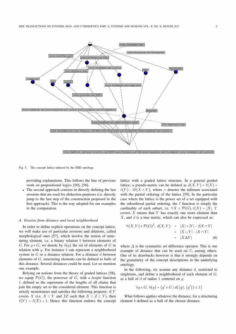
IEEE TRANSACTIONS ON SYSTEMS, MAN, AND CYBERNETICS–PART A: SYSTEMS AND HUMANS VOL. X, NO. X, MONTH 2013 9

Fig. 5. The concept lattice induced by the SHD ontology.

providing explanations. This follows the line of previouswork on propositional logics [50], [56].

● The second approach consists in directly defining the lasterosions that are used for abduction purposes (i.e. directlyjump to the last step of the construction proposed in thefirst approach). This is the way adopted for our examplesin the computation.

A. Erosion from distance and local neighborhood

In order to define explicit operations on the concept lattice,we will make use of particular erosions and dilations, calledmorphological ones [57], which involve the notion of struc-turing element, i.e. a binary relation b between elements ofG. For g ∈ G, we denote by b(g) the set of elements of G inrelation with g. For instance b can represent a neighborhoodsystem in G or a distance relation. For a distance d betweenelements of G, structuring elements can be defined as balls ofthis distance. Several distances could be used. Let us mentionone example.

Relying on notions from the theory of graded lattices [58],we equip P(G), the powerset of G, with a height function`, defined as the supremum of the lengths of all chains thatjoin the empty set to the considered element. This function isstrictly monotonous and satisfies the following property: if Ycovers X (i.e. X ⊂ Y and ∄Z such that X ⊂ Z ⊂ Y ), then`(Y ) = `(X) + 1. Hence this function endows the concept

lattice with a graded lattice structure. In a general gradedlattice, a pseudo-metric can be defined as d(X,Y ) = `(X) +`(Y ) − 2`(X ∧ Y ), where ∧ denotes the infimum associatedwith the partial ordering of the lattice [59]. In the particularcase where the lattice is the power set of a set equipped withthe subsethood partial ordering, the ` function is simply thecardinality of each subset, i.e. ∀X ∈ P(G), `(X) = ∣X ∣, Ycovers X means that Y has exactly one more element thanX , and d is a true metric, which can also be expressed as:

∀(X,Y ) ∈ P(G)2, d(X,Y ) = ∣X ∣ + ∣Y ∣ − 2∣X ∩ Y ∣= ∣X ∪ Y ∣ − ∣X ∩ Y ∣= ∣X∆Y ∣ (6)

where ∆ is the symmetric set difference operator. This is oneexample of distance that can be used on C, among others.One of its drawbacks however is that it strongly depends onthe granularity of the concept descriptions in the underlyingontology.

In the following, we assume any distance d, restricted tosingletons, and define a neighborhood of each element of G,as a ball of d of radius 1 centered on g:

∀g ∈ G, b(g) = {g′ ∈ G ∣ d({g},{g′}) ≤ 1}What follows applies whatever the distance, for a structuring

element b defined as a ball of the chosen distance.

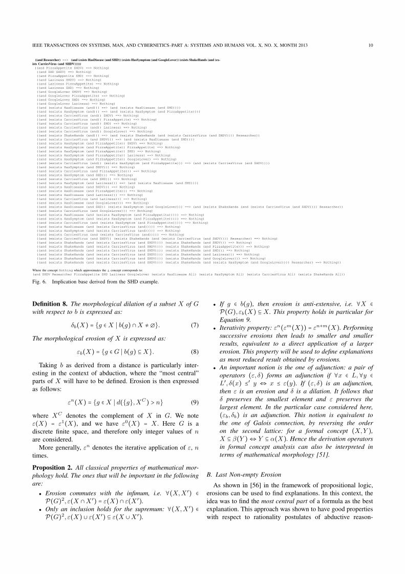
IEEE TRANSACTIONS ON SYSTEMS, MAN, AND CYBERNETICS–PART A: SYSTEMS AND HUMANS VOL. X, NO. X, MONTH 2013 10

((and Researcher) ==> (and (exists HasDisease (and SHD)) (exists HasSymptom (and GoogleLover)) (exists ShakeHands (and (ex-ists CarriesVirus (and SHDV))))))((and PizzaAppetite SHDV) ==> Nothing)((and SHD SHDV) ==> Nothing)((and PizzaAppetite SHD) ==> Nothing)((and Laziness SHDV) ==> Nothing)((and Laziness PizzaAppetite) ==> Nothing)((and Laziness SHD) ==> Nothing)((and GoogleLover SHDV) ==> Nothing)((and GoogleLover PizzaAppetite) ==> Nothing)((and GoogleLover SHD) ==> Nothing)((and GoogleLover Laziness) ==> Nothing)((and (exists HasDisease (and))) ==> (and (exists HasDisease (and SHD))))((and (exists HasSymptom (and))) ==> (and (exists HasSymptom (and PizzaAppetite))))((and (exists CarriesVirus (and)) SHDV) ==> Nothing)((and (exists CarriesVirus (and)) PizzaAppetite) ==> Nothing)((and (exists CarriesVirus (and)) SHD) ==> Nothing)((and (exists CarriesVirus (and)) Laziness) ==> Nothing)((and (exists CarriesVirus (and)) GoogleLover) ==> Nothing)((and (exists ShakeHands (and))) ==> (and (exists ShakeHands (and (exists CarriesVirus (and SHDV)))) Researcher))((and (exists CarriesVirus (and SHDV))) ==> (and (exists HasDisease (and SHD))))((and (exists HasSymptom (and PizzaAppetite)) SHDV) ==> Nothing)((and (exists HasSymptom (and PizzaAppetite)) PizzaAppetite) ==> Nothing)((and (exists HasSymptom (and PizzaAppetite)) SHD) ==> Nothing)((and (exists HasSymptom (and PizzaAppetite)) Laziness) ==> Nothing)((and (exists HasSymptom (and PizzaAppetite)) GoogleLover) ==> Nothing)((and (exists CarriesVirus (and)) (exists HasSymptom (and PizzaAppetite))) ==> (and (exists CarriesVirus (and SHDV))))((and (exists HasSymptom (and SHDV))) ==> Nothing)((and (exists CarriesVirus (and PizzaAppetite))) ==> Nothing)((and (exists HasSymptom (and SHD))) ==> Nothing)((and (exists CarriesVirus (and SHD))) ==> Nothing)((and (exists HasSymptom (and Laziness))) ==> (and (exists HasDisease (and SHD))))((and (exists HasDisease (and SHDV))) ==> Nothing)((and (exists HasDisease (and PizzaAppetite))) ==> Nothing)((and (exists HasDisease (and Laziness))) ==> Nothing)((and (exists CarriesVirus (and Laziness))) ==> Nothing)((and (exists HasDisease (and GoogleLover))) ==> Nothing)((and (exists HasDisease (and SHD)) (exists HasSymptom (and GoogleLover))) ==> (and (exists ShakeHands (and (exists CarriesVirus (and SHDV)))) Researcher))((and (exists CarriesVirus (and GoogleLover))) ==> Nothing)((and (exists HasDisease (and (exists HasSymptom (and PizzaAppetite))))) ==> Nothing)((and (exists HasSymptom (and (exists HasSymptom (and PizzaAppetite))))) ==> Nothing)((and (exists CarriesVirus (and (exists HasSymptom (and PizzaAppetite))))) ==> Nothing)((and (exists HasDisease (and (exists CarriesVirus (and))))) ==> Nothing)((and (exists HasSymptom (and (exists CarriesVirus (and))))) ==> Nothing)((and (exists CarriesVirus (and (exists CarriesVirus (and))))) ==> Nothing)((and (exists CarriesVirus (and SHDV)) (exists ShakeHands (and (exists CarriesVirus (and SHDV)))) Researcher) ==> Nothing)((and (exists ShakeHands (and (exists CarriesVirus (and SHDV)))) (exists ShakeHands (and SHDV))) ==> Nothing)((and (exists ShakeHands (and (exists CarriesVirus (and SHDV)))) (exists ShakeHands (and PizzaAppetite))) ==> Nothing)((and (exists ShakeHands (and (exists CarriesVirus (and SHDV)))) (exists ShakeHands (and SHD))) ==> Nothing)((and (exists ShakeHands (and (exists CarriesVirus (and SHDV)))) (exists ShakeHands (and Laziness))) ==> Nothing)((and (exists ShakeHands (and (exists CarriesVirus (and SHDV)))) (exists ShakeHands (and GoogleLover))) ==> Nothing)((and (exists ShakeHands (and (exists CarriesVirus (and SHDV)))) (exists ShakeHands (and (exists HasSymptom (and GoogleLover)))) Researcher) ==> Nothing))

Where the concept Nothing which approximates the � concept corresponds to:(and SHDV Researcher PizzaAppetite SHD Laziness GoogleLover (exists HasDisease All) (exists HasSymptom All) (exists CarriesVirus All) (exists ShakeHands All))

Fig. 6. Implication base derived from the SHD example.

Definition 8. The morphological dilation of a subset X of Gwith respect to b is expressed as:

δb(X) = {g ∈X ∣ b(g) ∩X ≠ ∅}. (7)

The morphological erosion of X is expressed as:

εb(X) = {g ∈ G ∣ b(g) ⊆X}. (8)

Taking b as derived from a distance is particularly inter-esting in the context of abduction, where the “most central”parts of X will have to be defined. Erosion is then expressedas follows:

εn(X) = {g ∈X ∣ d({g},XC) > n} (9)

where XC denotes the complement of X in G. We noteε(X) = ε1(X), and we have ε0(X) = X . Here G is adiscrete finite space, and therefore only integer values of nare considered.

More generally, εn denotes the iterative application of ε, ntimes.

Proposition 2. All classical properties of mathematical mor-phology hold. The ones that will be important in the followingare:

● Erosion commutes with the infimum, i.e. ∀(X,X ′) ∈P(G)2, ε(X ∩X ′) = ε(X) ∩ ε(X ′).● Only an inclusion holds for the supremum: ∀(X,X ′) ∈P(G)2, ε(X) ∪ ε(X ′) ⊆ ε(X ∪X ′).

● If g ∈ b(g), then erosion is anti-extensive, i.e. ∀X ∈P(G), εb(X) ⊆ X . This property holds in particular forEquation 9.

● Iterativity property: εn(εm(X)) = εn+m(X). Performingsuccessive erosions then leads to smaller and smallerresults, equivalent to a direct application of a largererosion. This property will be used to define explanationsas most reduced result obtained by erosions.

● An important notion is the one of adjunction: a pair ofoperators (ε, δ) forms an adjunction if ∀x ∈ L,∀y ∈L′, δ(x) ⪯′ y ⇔ x ⪯ ε(y). If (ε, δ) is an adjunction,then ε is an erosion and δ is a dilation. It follows thatδ preserves the smallest element and ε preserves thelargest element. In the particular case considered here,(εb, δb) is an adjunction. This notion is equivalent tothe one of Galois connection, by reversing the orderon the second lattice: for a formal concept (X,Y ),X ⊆ β(Y )⇔ Y ⊆ α(X). Hence the derivation operatorsin formal concept analysis can also be interpreted interms of mathematical morphology [51].

B. Last Non-empty Erosion

As shown in [56] in the framework of propositional logic,erosions can be used to find explanations. In this context, theidea was to find the most central part of a formula as the bestexplanation. This approach was shown to have good propertieswith respect to rationality postulates of abductive reason-

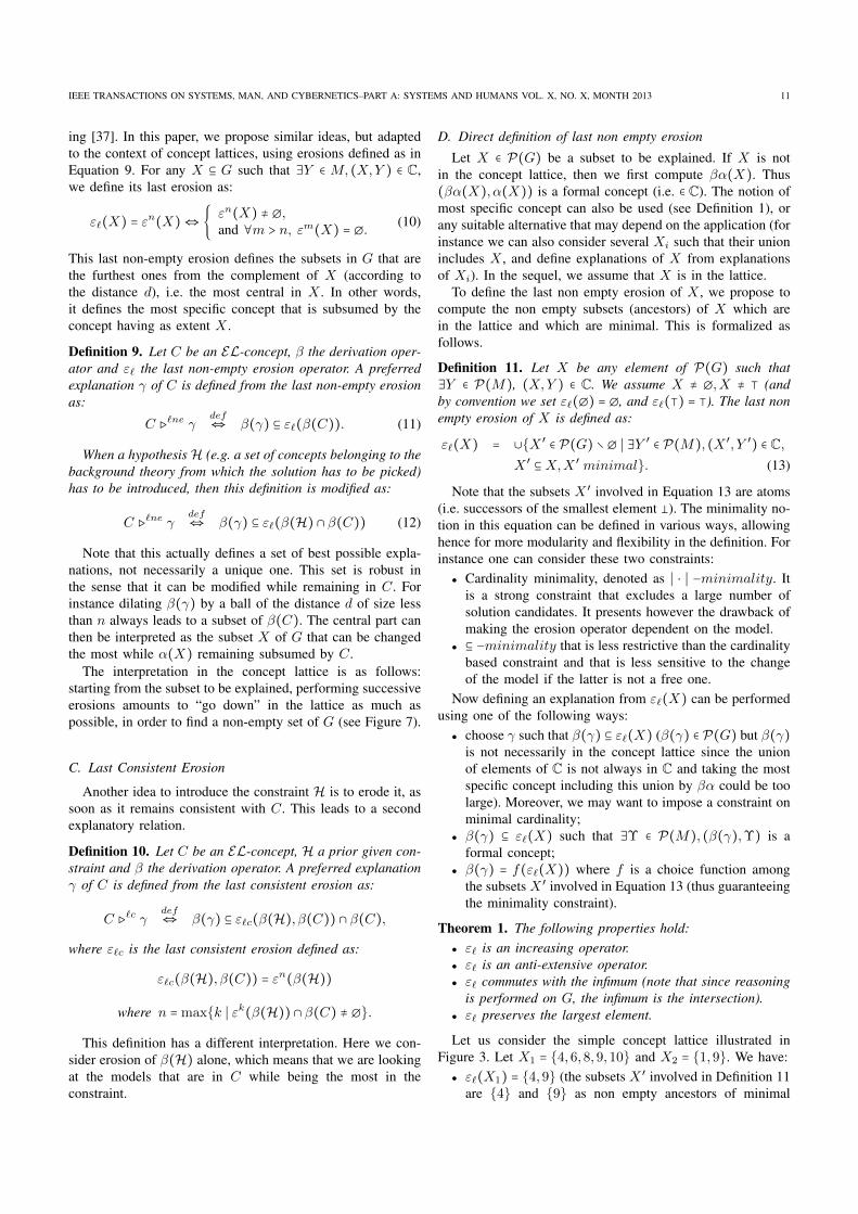
IEEE TRANSACTIONS ON SYSTEMS, MAN, AND CYBERNETICS–PART A: SYSTEMS AND HUMANS VOL. X, NO. X, MONTH 2013 11

ing [37]. In this paper, we propose similar ideas, but adaptedto the context of concept lattices, using erosions defined as inEquation 9. For any X ⊆ G such that ∃Y ∈ M, (X,Y ) ∈ C,we define its last erosion as:

ε`(X) = εn(X)⇔ { εn(X) ≠ ∅,and ∀m > n, εm(X) = ∅. (10)

This last non-empty erosion defines the subsets in G that arethe furthest ones from the complement of X (according tothe distance d), i.e. the most central in X . In other words,it defines the most specific concept that is subsumed by theconcept having as extent X .

Definition 9. Let C be an EL-concept, β the derivation oper-ator and ε` the last non-empty erosion operator. A preferredexplanation γ of C is defined from the last non-empty erosionas:

C ⊳`ne γ def⇔ β(γ) ⊆ ε`(β(C)). (11)

When a hypothesisH (e.g. a set of concepts belonging to thebackground theory from which the solution has to be picked)has to be introduced, then this definition is modified as:

C ⊳`ne γ def⇔ β(γ) ⊆ ε`(β(H) ∩ β(C)) (12)

Note that this actually defines a set of best possible expla-nations, not necessarily a unique one. This set is robust inthe sense that it can be modified while remaining in C. Forinstance dilating β(γ) by a ball of the distance d of size lessthan n always leads to a subset of β(C). The central part canthen be interpreted as the subset X of G that can be changedthe most while α(X) remaining subsumed by C.

The interpretation in the concept lattice is as follows:starting from the subset to be explained, performing successiveerosions amounts to “go down” in the lattice as much aspossible, in order to find a non-empty set of G (see Figure 7).

C. Last Consistent Erosion

Another idea to introduce the constraint H is to erode it, assoon as it remains consistent with C. This leads to a secondexplanatory relation.

Definition 10. Let C be an EL-concept, H a prior given con-straint and β the derivation operator. A preferred explanationγ of C is defined from the last consistent erosion as:

C ⊳`c γ def⇔ β(γ) ⊆ ε`c(β(H), β(C)) ∩ β(C),where ε`c is the last consistent erosion defined as:

ε`c(β(H), β(C)) = εn(β(H))where n = max{k ∣ εk(β(H)) ∩ β(C) ≠ ∅}.

This definition has a different interpretation. Here we con-sider erosion of β(H) alone, which means that we are lookingat the models that are in C while being the most in theconstraint.

D. Direct definition of last non empty erosion

Let X ∈ P(G) be a subset to be explained. If X is notin the concept lattice, then we first compute βα(X). Thus(βα(X), α(X)) is a formal concept (i.e. ∈ C). The notion ofmost specific concept can also be used (see Definition 1), orany suitable alternative that may depend on the application (forinstance we can also consider several Xi such that their unionincludes X , and define explanations of X from explanationsof Xi). In the sequel, we assume that X is in the lattice.

To define the last non empty erosion of X , we propose tocompute the non empty subsets (ancestors) of X which arein the lattice and which are minimal. This is formalized asfollows.

Definition 11. Let X be any element of P(G) such that∃Y ∈ P(M), (X,Y ) ∈ C. We assume X ≠ ∅,X ≠ ⊺ (andby convention we set ε`(∅) = ∅, and ε`(⊺) = ⊺). The last nonempty erosion of X is defined as:

ε`(X) = ∪{X ′ ∈ P(G) ∖ ∅ ∣ ∃Y ′ ∈ P(M), (X ′, Y ′) ∈ C,X ′ ⊆X,X ′ minimal}. (13)

Note that the subsets X ′ involved in Equation 13 are atoms(i.e. successors of the smallest element �). The minimality no-tion in this equation can be defined in various ways, allowinghence for more modularity and flexibility in the definition. Forinstance one can consider these two constraints:

● Cardinality minimality, denoted as ∣ ⋅ ∣ −minimality. Itis a strong constraint that excludes a large number ofsolution candidates. It presents however the drawback ofmaking the erosion operator dependent on the model.

● ⊆ −minimality that is less restrictive than the cardinalitybased constraint and that is less sensitive to the changeof the model if the latter is not a free one.

Now defining an explanation from ε`(X) can be performedusing one of the following ways:

● choose γ such that β(γ) ⊆ ε`(X) (β(γ) ∈ P(G) but β(γ)is not necessarily in the concept lattice since the unionof elements of C is not always in C and taking the mostspecific concept including this union by βα could be toolarge). Moreover, we may want to impose a constraint onminimal cardinality;

● β(γ) ⊆ ε`(X) such that ∃Υ ∈ P(M), (β(γ),Υ) is aformal concept;

● β(γ) = f(ε`(X)) where f is a choice function amongthe subsets X ′ involved in Equation 13 (thus guaranteeingthe minimality constraint).

Theorem 1. The following properties hold:● ε` is an increasing operator.● ε` is an anti-extensive operator.● ε` commutes with the infimum (note that since reasoning

is performed on G, the infimum is the intersection).● ε` preserves the largest element.

Let us consider the simple concept lattice illustrated inFigure 3. Let X1 = {4,6,8,9,10} and X2 = {1,9}. We have:

● ε`(X1) = {4,9} (the subsets X ′ involved in Definition 11are {4} and {9} as non empty ancestors of minimal

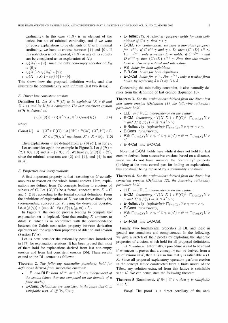
IEEE TRANSACTIONS ON SYSTEMS, MAN, AND CYBERNETICS–PART A: SYSTEMS AND HUMANS VOL. X, NO. X, MONTH 2013 12

cardinality). In this case {4,9} is an element of thelattice, but not of minimal cardinality, and if we wantto reduce explanations to be elements of C with minimalcardinality, we have to choose between {4} and {9}. Ifthis restriction is not imposed, {4,9} or any of its subsetscan be considered as an explanation of X1;

● ε`(X2) = {9}, since the only non-empty ancestor of X2

is {9};● ε`(X1) ∩ ε`(X2) = {9};● ε`(X1 ∩X2) = ε`({9}) = {9}.

This shows how the proposed definition works, and alsoillustrates the commutativity with infimum (last two items).

E. Direct last consistent erosion

Definition 12. Let X ∈ P(G) to be explained (X ≠ ∅ andX ≠ ⊺), and let H be a constraint. The last consistent erosionof H is defined as:

ε`c(β(H)) = ∪{X ′ ∩X,X ′ ∈ Cons(H)} (14)

where

Cons(H) = {X ′ ∈ P(G) ∖ ∅ ∣ ∃Y ′ ∈ P(M), (X ′, Y ′) ∈ C,X ′ ⊆ β(H),X ′ minimal,X ′ ∩X ≠ ∅}. (15)

Then explanations γ are defined from ε`c(β(H)), as for ε`.Let us consider again the example in Figure 3. Let β(H) ={2,4,6,8,10} and X = {2,3,5,7}. We have ε`c(β(H)) = {2},

since the minimal ancestors are {2} and {4}, and {4} is notin X .

F. Properties and interpretations

A first important property is that reasoning on G actuallyamounts to reason on the whole formal context. Here, expla-nations are defined from EL-concepts leading to erosions ofsubsets of G. Let (X,Y ) be a formal concept, with X ⊆ Gand Y ⊆M , according to the formal context definition. Fromthe definitions of explanations of X , we can derive directly thecorresponding concepts for Y , using the derivation operator,i.e. α(β(γ)) = {m ∈M ∣ ∀g ∈ β(γ), (g,m) ∈ I}.

In Figure 7, the erosion process leading to compute theexplanation set is depicted. Note that eroding X amounts todilate Y , which is in accordance with the correspondencebetween the Galois connection property between derivationoperators and the adjunction properties of dilation and erosion(Section IV-A).

Let us now consider the rationality postulates introducedin [37] for explanation relations. It has been proved that mostof them hold for explanations derived from last non-emptyerosion and from last consistent erosion [56]. These resultsextend to the DL context as follows:

Theorem 2. The following rationality postulates hold fordefinitions derived from successive erosions:

● LLE and RLE: Both ⊳`ne and ⊳`c are independent ofthe syntax (since they are computed on the domain of afinite model).

● E-Cons: Definitions are consistent in the sense that C issatisfiable w.r.t. K iff ∃γ,C ⊳ γ.

● E-Reflexivity: A reflexivity property holds for both defi-nitions: if C ⊳ γ, then γ ⊳ γ.

● E-CM: For conjunctions, we have a monotony propertyfor ⊳`c : if C ⊳`c γ and γ ⊑ D, then (C ⊓D) ⊳`c γ.For ⊳`ne , only a weaker form holds: if C ⊳`ne γ andD ⊳`ne γ, then (C ⊓D) ⊳`ne γ. Note that this weakerform is also very natural and interesting.

● RS holds for both definitions.● E-R-Cut holds for both definitions.● E-C-Cut holds for ⊳`c . For ⊳`ne , only a weaker form

holds, by replacing δ ⊑D by D ⊳ δ.

Concerning the minimality constraint, it also naturally de-rives from the definition of last erosion (Equation 10).

Theorem 3. For the explanations derived from the direct lastnon empty erosion (Definition 11), the following rationalitypostulates hold:

● LLE and RLE: independence on the syntax;● E-CM (monotony): ∀(X,X ′) ∈ P(G)2, ⊓U∈α(X)U ⊳γ and X ′ ⊆ β(γ)⇒X ⊓X ′ ⊳ γ;

● E-Reflexivity (reflexivity): ⊓U∈α(X)U ⊳ γ ⇒ γ ⊳ γ.● E-Cons (consistency).● RS: ⊓U∈α(X)U ⊳ γ, γ′ ⊑ γ, β(γ′) ≠ ∅ ⇒ ⊓U∈α(X)U ⊳γ′.

● E-R-Cut and E-C-Cut.

Note that E-CM holds here while it does not hold for lasterosion derived from successive erosions based on a distance,since we do not have anymore the “centrality” property(looking at the most central part for finding an explanation),this constraint being replaced by a minimality constraint.

Theorem 4. For the explanations derived from the direct lastconsistent erosion (Definition 12), the following rationalitypostulates hold:

● LLE and RLE: independence on the syntax;● E-CM (monotony): ∀(X,X ′) ∈ P(G)2, ⊓U∈α(X)U ⊳γ and X ′ ⊆ β(γ)⇒X ⊓X ′ ⊳ γ;

● E-Reflexivity (reflexivity): ⊓U∈α(X)U ⊳ γ ⇒ γ ⊳ γ.● E-Cons (consistency).● RS: ⊓U∈α(X)U ⊳ γ, γ′ ⊑ γ, β(γ′) ≠ ∅ ⇒ ⊓U∈α(X)U ⊳γ′.

● E-R-Cut and E-C-Cut.

Finally, two fundamental properties in DL and logic ingeneral are soundness and completeness. In the following,we give a sketch of their proofs by exploiting the algebraicproperties of erosion, which hold for all proposed definitions.

a) Soundness: Informally, a procedure is said to be soundif whenever it proves that a concept γ can be derived from aset of axioms in K, then it is also true that γ is satisfiable w.r.t.K. Since all proposed explanatory operators perform erosionin the concept lattice constructed from a finite model of theTBox, any solution extracted from this lattice is satisfiablew.r.t. K. We can hence state the following theorem:

Theorem 5 (Soundness). If ∃γ ∣ C ⊳ γ then γ is satisfiablew.r.t. K.

Proof: The proof is a direct corollary of the anti-

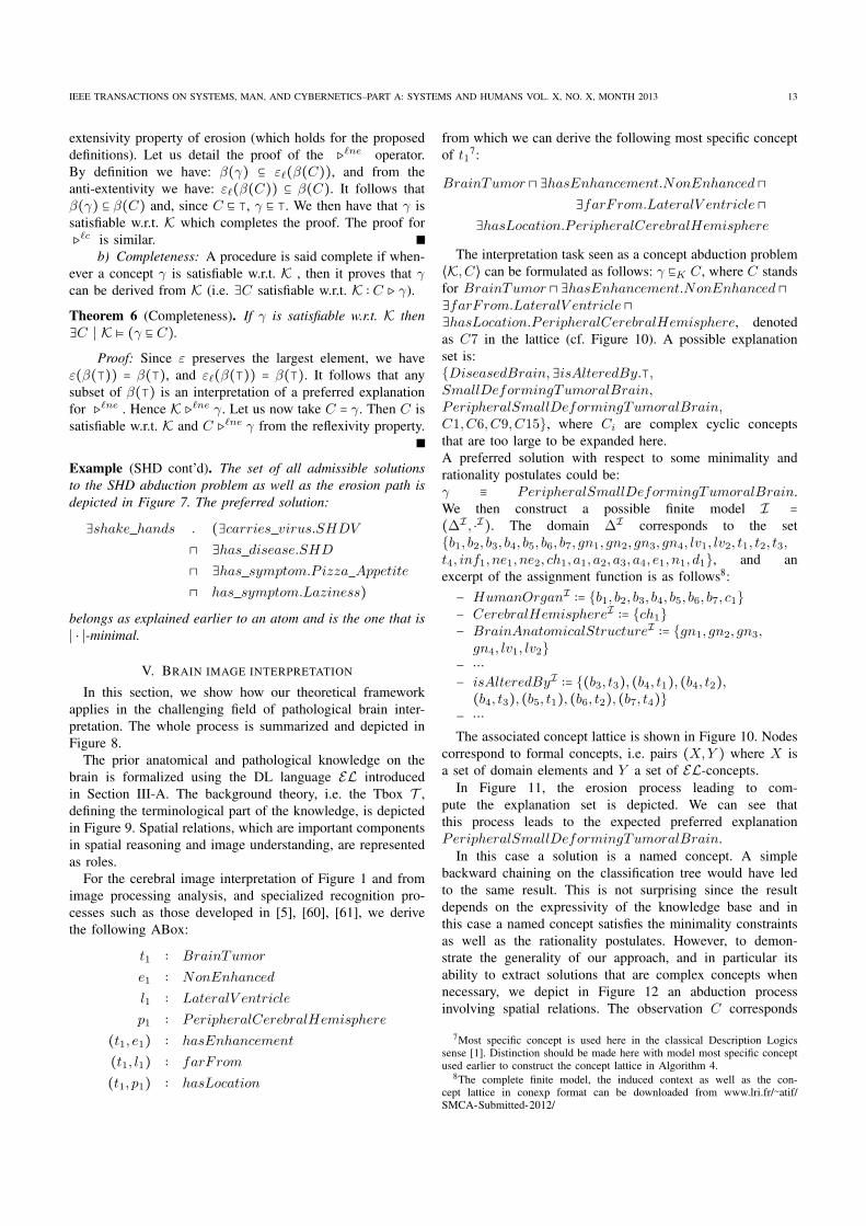
IEEE TRANSACTIONS ON SYSTEMS, MAN, AND CYBERNETICS–PART A: SYSTEMS AND HUMANS VOL. X, NO. X, MONTH 2013 13

extensivity property of erosion (which holds for the proposeddefinitions). Let us detail the proof of the ⊳`ne operator.By definition we have: β(γ) ⊆ ε`(β(C)), and from theanti-extentivity we have: ε`(β(C)) ⊆ β(C). It follows thatβ(γ) ⊆ β(C) and, since C ⊑ ⊺, γ ⊑ ⊺. We then have that γ issatisfiable w.r.t. K which completes the proof. The proof for⊳`c is similar.

b) Completeness: A procedure is said complete if when-ever a concept γ is satisfiable w.r.t. K , then it proves that γcan be derived from K (i.e. ∃C satisfiable w.r.t. K ∶ C ⊳ γ).

Theorem 6 (Completeness). If γ is satisfiable w.r.t. K then∃C ∣ K ⊧ (γ ⊑ C).

Proof: Since ε preserves the largest element, we haveε(β(⊺)) = β(⊺), and ε`(β(⊺)) = β(⊺). It follows that anysubset of β(⊺) is an interpretation of a preferred explanationfor ⊳`ne . Hence K ⊳`ne γ. Let us now take C = γ. Then C issatisfiable w.r.t. K and C ⊳`ne γ from the reflexivity property.

Example (SHD cont’d). The set of all admissible solutionsto the SHD abduction problem as well as the erosion path isdepicted in Figure 7. The preferred solution:

∃shake hands . (∃carries virus.SHDV⊓ ∃has disease.SHD⊓ ∃has symptom.P izza Appetite⊓ has symptom.Laziness)belongs as explained earlier to an atom and is the one that is∣ ⋅ ∣-minimal.

V. BRAIN IMAGE INTERPRETATION

In this section, we show how our theoretical frameworkapplies in the challenging field of pathological brain inter-pretation. The whole process is summarized and depicted inFigure 8.

The prior anatomical and pathological knowledge on thebrain is formalized using the DL language EL introducedin Section III-A. The background theory, i.e. the Tbox T ,defining the terminological part of the knowledge, is depictedin Figure 9. Spatial relations, which are important componentsin spatial reasoning and image understanding, are representedas roles.

For the cerebral image interpretation of Figure 1 and fromimage processing analysis, and specialized recognition pro-cesses such as those developed in [5], [60], [61], we derivethe following ABox:

t1 ∶ BrainTumor

e1 ∶ NonEnhanced

l1 ∶ LateralV entricle

p1 ∶ PeripheralCerebralHemisphere(t1, e1) ∶ hasEnhancement(t1, l1) ∶ farFrom(t1, p1) ∶ hasLocation

from which we can derive the following most specific conceptof t17:

BrainTumor ⊓ ∃hasEnhancement.NonEnhanced ⊓∃farFrom.LateralV entricle ⊓∃hasLocation.PeripheralCerebralHemisphereThe interpretation task seen as a concept abduction problem⟨K,C⟩ can be formulated as follows: γ ⊑K C, where C stands

for BrainTumor ⊓ ∃hasEnhancement.NonEnhanced ⊓∃farFrom.LateralV entricle ⊓∃hasLocation.PeripheralCerebralHemisphere, denotedas C7 in the lattice (cf. Figure 10). A possible explanationset is:{DiseasedBrain,∃isAlteredBy.⊺,SmallDeformingTumoralBrain,PeripheralSmallDeformingTumoralBrain,C1,C6,C9,C15}, where Ci are complex cyclic conceptsthat are too large to be expanded here.A preferred solution with respect to some minimality andrationality postulates could be:γ ≡ PeripheralSmallDeformingTumoralBrain.We then construct a possible finite model I =(∆I , ⋅I). The domain ∆I corresponds to the set{b1, b2, b3, b4, b5, b6, b7, gn1, gn2, gn3, gn4, lv1, lv2, t1, t2, t3,t4, inf1, ne1, ne2, ch1, a1, a2, a3, a4, e1, n1, d1}, and anexcerpt of the assignment function is as follows8:− HumanOrganI ∶= {b1, b2, b3, b4, b5, b6, b7, c1}− CerebralHemisphereI ∶= {ch1}− BrainAnatomicalStructureI ∶= {gn1, gn2, gn3,

gn4, lv1, lv2}− ⋯− isAlteredByI ∶= {(b3, t3), (b4, t1), (b4, t2),(b4, t3), (b5, t1), (b6, t2), (b7, t4)}− ⋯The associated concept lattice is shown in Figure 10. Nodes

correspond to formal concepts, i.e. pairs (X,Y ) where X isa set of domain elements and Y a set of EL-concepts.

In Figure 11, the erosion process leading to com-pute the explanation set is depicted. We can see thatthis process leads to the expected preferred explanationPeripheralSmallDeformingTumoralBrain.

In this case a solution is a named concept. A simplebackward chaining on the classification tree would have ledto the same result. This is not surprising since the resultdepends on the expressivity of the knowledge base and inthis case a named concept satisfies the minimality constraintsas well as the rationality postulates. However, to demon-strate the generality of our approach, and in particular itsability to extract solutions that are complex concepts whennecessary, we depict in Figure 12 an abduction processinvolving spatial relations. The observation C corresponds

7Most specific concept is used here in the classical Description Logicssense [1]. Distinction should be made here with model most specific conceptused earlier to construct the concept lattice in Algorithm 4.

8The complete finite model, the induced context as well as the con-cept lattice in conexp format can be downloaded from www.lri.fr/∼atif/SMCA-Submitted-2012/

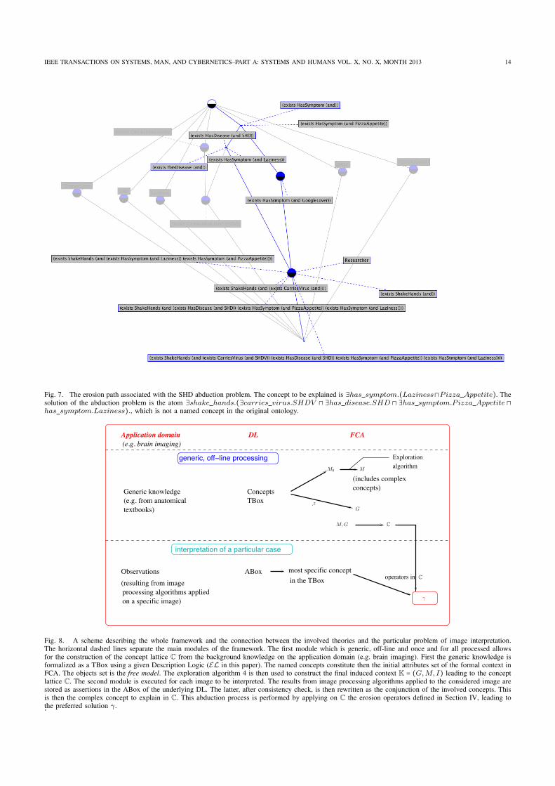
IEEE TRANSACTIONS ON SYSTEMS, MAN, AND CYBERNETICS–PART A: SYSTEMS AND HUMANS VOL. X, NO. X, MONTH 2013 14

Fig. 7. The erosion path associated with the SHD abduction problem. The concept to be explained is ∃has symptom.(Laziness⊓Pizza Appetite). Thesolution of the abduction problem is the atom ∃shake hands.(∃carries virus.SHDV ⊓ ∃has disease.SHD ⊓ ∃has symptom.P izza Appetite ⊓has symptom.Laziness)., which is not a named concept in the original ontology.

most specific concept

Generic knowledge(e.g. from anatomicaltextbooks)

ConceptsTBox

(includes complexconcepts)

Exploration algorithm

Application domain(e.g. brain imaging)

DL FCA

generic, off line processing

on a specific image)processing algorithms applied(resulting from image Observations ABox

in the TBox

interpretation of a particular case

operators in

M

M, G

G

M0

C

!

C

·I

Fig. 8. A scheme describing the whole framework and the connection between the involved theories and the particular problem of image interpretation.The horizontal dashed lines separate the main modules of the framework. The first module which is generic, off-line and once and for all processed allowsfor the construction of the concept lattice C from the background knowledge on the application domain (e.g. brain imaging). First the generic knowledge isformalized as a TBox using a given Description Logic (EL in this paper). The named concepts constitute then the initial attributes set of the formal context inFCA. The objects set is the free model. The exploration algorithm 4 is then used to construct the final induced context K = (G,M, I) leading to the conceptlattice C. The second module is executed for each image to be interpreted. The results from image processing algorithms applied to the considered image arestored as assertions in the ABox of the underlying DL. The latter, after consistency check, is then rewritten as the conjunction of the involved concepts. Thisis then the complex concept to explain in C. This abduction process is performed by applying on C the erosion operators defined in Section IV, leading tothe preferred solution γ..

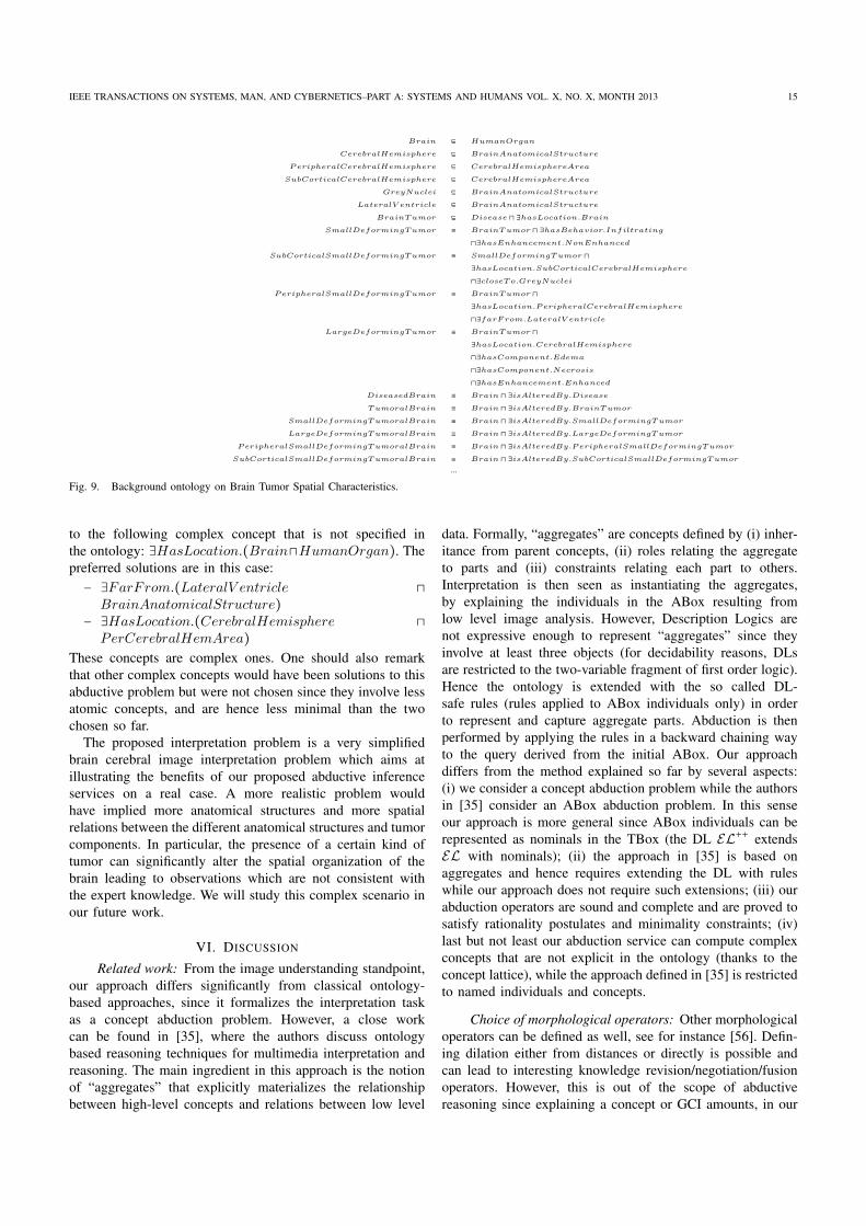
IEEE TRANSACTIONS ON SYSTEMS, MAN, AND CYBERNETICS–PART A: SYSTEMS AND HUMANS VOL. X, NO. X, MONTH 2013 15

Brain ⊑ HumanOrgan

CerebralHemisphere ⊑ BrainAnatomicalStructure

PeripheralCerebralHemisphere ⊑ CerebralHemisphereArea

SubCorticalCerebralHemisphere ⊑ CerebralHemisphereArea

GreyNuclei ⊑ BrainAnatomicalStructure

LateralV entricle ⊑ BrainAnatomicalStructure

BrainTumor ⊑ Disease ⊓ ∃hasLocation.Brain

SmallDeformingTumor ≡ BrainTumor ⊓ ∃hasBehavior.Infiltrating

⊓∃hasEnhancement.NonEnhanced

SubCorticalSmallDeformingTumor ≡ SmallDeformingTumor ⊓∃hasLocation.SubCorticalCerebralHemisphere

⊓∃closeTo.GreyNuclei

PeripheralSmallDeformingTumor ≡ BrainTumor ⊓∃hasLocation.PeripheralCerebralHemisphere

⊓∃farFrom.LateralV entricle

LargeDeformingTumor ≡ BrainTumor ⊓∃hasLocation.CerebralHemisphere

⊓∃hasComponent.Edema

⊓∃hasComponent.Necrosis

⊓∃hasEnhancement.Enhanced

DiseasedBrain ≡ Brain ⊓ ∃isAlteredBy.Disease

TumoralBrain ≡ Brain ⊓ ∃isAlteredBy.BrainTumor

SmallDeformingTumoralBrain ≡ Brain ⊓ ∃isAlteredBy.SmallDeformingTumor

LargeDeformingTumoralBrain ≡ Brain ⊓ ∃isAlteredBy.LargeDeformingTumor

PeripheralSmallDeformingTumoralBrain ≡ Brain ⊓ ∃isAlteredBy.PeripheralSmallDeformingTumor

SubCorticalSmallDeformingTumoralBrain ≡ Brain ⊓ ∃isAlteredBy.SubCorticalSmallDeformingTumor

⋯Fig. 9. Background ontology on Brain Tumor Spatial Characteristics.

to the following complex concept that is not specified inthe ontology: ∃HasLocation.(Brain⊓HumanOrgan). Thepreferred solutions are in this case:− ∃FarFrom.(LateralV entricle ⊓

BrainAnatomicalStructure)− ∃HasLocation.(CerebralHemisphere ⊓PerCerebralHemArea)

These concepts are complex ones. One should also remarkthat other complex concepts would have been solutions to thisabductive problem but were not chosen since they involve lessatomic concepts, and are hence less minimal than the twochosen so far.

The proposed interpretation problem is a very simplifiedbrain cerebral image interpretation problem which aims atillustrating the benefits of our proposed abductive inferenceservices on a real case. A more realistic problem wouldhave implied more anatomical structures and more spatialrelations between the different anatomical structures and tumorcomponents. In particular, the presence of a certain kind oftumor can significantly alter the spatial organization of thebrain leading to observations which are not consistent withthe expert knowledge. We will study this complex scenario inour future work.

VI. DISCUSSION

Related work: From the image understanding standpoint,our approach differs significantly from classical ontology-based approaches, since it formalizes the interpretation taskas a concept abduction problem. However, a close workcan be found in [35], where the authors discuss ontologybased reasoning techniques for multimedia interpretation andreasoning. The main ingredient in this approach is the notionof “aggregates” that explicitly materializes the relationshipbetween high-level concepts and relations between low level

data. Formally, “aggregates” are concepts defined by (i) inher-itance from parent concepts, (ii) roles relating the aggregateto parts and (iii) constraints relating each part to others.Interpretation is then seen as instantiating the aggregates,by explaining the individuals in the ABox resulting fromlow level image analysis. However, Description Logics arenot expressive enough to represent “aggregates” since theyinvolve at least three objects (for decidability reasons, DLsare restricted to the two-variable fragment of first order logic).Hence the ontology is extended with the so called DL-safe rules (rules applied to ABox individuals only) in orderto represent and capture aggregate parts. Abduction is thenperformed by applying the rules in a backward chaining wayto the query derived from the initial ABox. Our approachdiffers from the method explained so far by several aspects:(i) we consider a concept abduction problem while the authorsin [35] consider an ABox abduction problem. In this senseour approach is more general since ABox individuals can berepresented as nominals in the TBox (the DL EL++ extendsEL with nominals); (ii) the approach in [35] is based onaggregates and hence requires extending the DL with ruleswhile our approach does not require such extensions; (iii) ourabduction operators are sound and complete and are proved tosatisfy rationality postulates and minimality constraints; (iv)last but not least our abduction service can compute complexconcepts that are not explicit in the ontology (thanks to theconcept lattice), while the approach defined in [35] is restrictedto named individuals and concepts.

Choice of morphological operators: Other morphologicaloperators can be defined as well, see for instance [56]. Defin-ing dilation either from distances or directly is possible andcan lead to interesting knowledge revision/negotiation/fusionoperators. However, this is out of the scope of abductivereasoning since explaining a concept or GCI amounts, in our

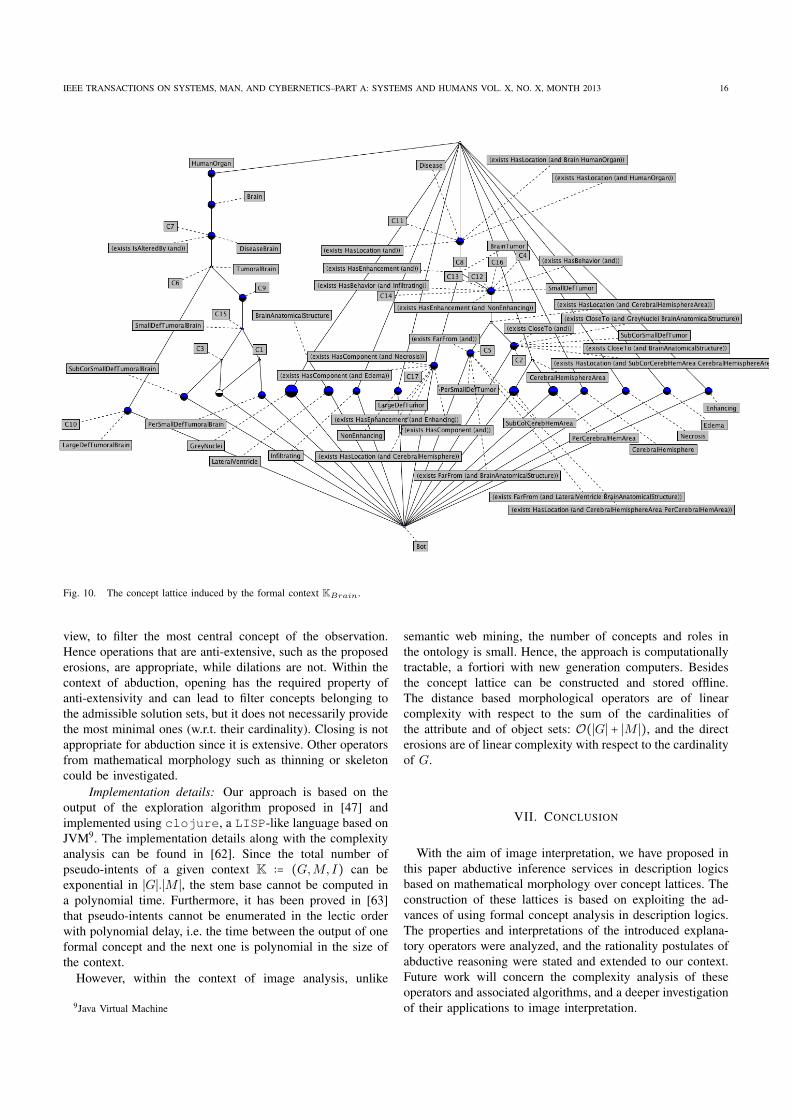
IEEE TRANSACTIONS ON SYSTEMS, MAN, AND CYBERNETICS–PART A: SYSTEMS AND HUMANS VOL. X, NO. X, MONTH 2013 16

Fig. 10. The concept lattice induced by the formal context KBrain.

view, to filter the most central concept of the observation.Hence operations that are anti-extensive, such as the proposederosions, are appropriate, while dilations are not. Within thecontext of abduction, opening has the required property ofanti-extensivity and can lead to filter concepts belonging tothe admissible solution sets, but it does not necessarily providethe most minimal ones (w.r.t. their cardinality). Closing is notappropriate for abduction since it is extensive. Other operatorsfrom mathematical morphology such as thinning or skeletoncould be investigated.

Implementation details: Our approach is based on theoutput of the exploration algorithm proposed in [47] andimplemented using clojure, a LISP-like language based onJVM9. The implementation details along with the complexityanalysis can be found in [62]. Since the total number ofpseudo-intents of a given context K ∶= (G,M, I) can beexponential in ∣G∣.∣M ∣, the stem base cannot be computed ina polynomial time. Furthermore, it has been proved in [63]that pseudo-intents cannot be enumerated in the lectic orderwith polynomial delay, i.e. the time between the output of oneformal concept and the next one is polynomial in the size ofthe context.

However, within the context of image analysis, unlike

9Java Virtual Machine

semantic web mining, the number of concepts and roles inthe ontology is small. Hence, the approach is computationallytractable, a fortiori with new generation computers. Besidesthe concept lattice can be constructed and stored offline.The distance based morphological operators are of linearcomplexity with respect to the sum of the cardinalities ofthe attribute and of object sets: O(∣G∣ + ∣M ∣), and the directerosions are of linear complexity with respect to the cardinalityof G.

VII. CONCLUSION

With the aim of image interpretation, we have proposed inthis paper abductive inference services in description logicsbased on mathematical morphology over concept lattices. Theconstruction of these lattices is based on exploiting the ad-vances of using formal concept analysis in description logics.The properties and interpretations of the introduced explana-tory operators were analyzed, and the rationality postulates ofabductive reasoning were stated and extended to our context.Future work will concern the complexity analysis of theseoperators and associated algorithms, and a deeper investigationof their applications to image interpretation.

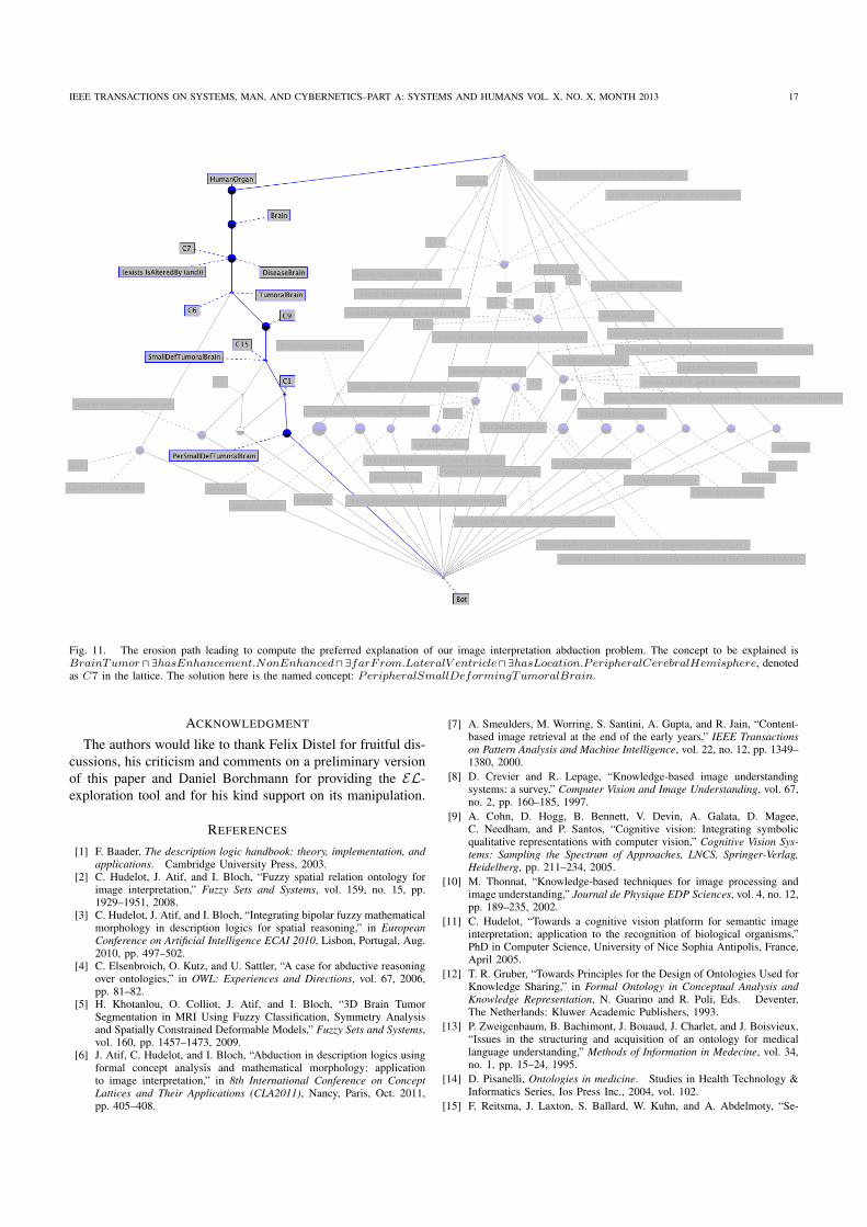
IEEE TRANSACTIONS ON SYSTEMS, MAN, AND CYBERNETICS–PART A: SYSTEMS AND HUMANS VOL. X, NO. X, MONTH 2013 17

Fig. 11. The erosion path leading to compute the preferred explanation of our image interpretation abduction problem. The concept to be explained isBrainTumor⊓∃hasEnhancement.NonEnhanced⊓∃farFrom.LateralV entricle⊓∃hasLocation.PeripheralCerebralHemisphere, denotedas C7 in the lattice. The solution here is the named concept: PeripheralSmallDeformingTumoralBrain.

ACKNOWLEDGMENT

The authors would like to thank Felix Distel for fruitful dis-cussions, his criticism and comments on a preliminary versionof this paper and Daniel Borchmann for providing the EL-exploration tool and for his kind support on its manipulation.

REFERENCES

[1] F. Baader, The description logic handbook: theory, implementation, andapplications. Cambridge University Press, 2003.

[2] C. Hudelot, J. Atif, and I. Bloch, “Fuzzy spatial relation ontology forimage interpretation,” Fuzzy Sets and Systems, vol. 159, no. 15, pp.1929–1951, 2008.

[3] C. Hudelot, J. Atif, and I. Bloch, “Integrating bipolar fuzzy mathematicalmorphology in description logics for spatial reasoning,” in EuropeanConference on Artificial Intelligence ECAI 2010, Lisbon, Portugal, Aug.2010, pp. 497–502.

[4] C. Elsenbroich, O. Kutz, and U. Sattler, “A case for abductive reasoningover ontologies,” in OWL: Experiences and Directions, vol. 67, 2006,pp. 81–82.

[5] H. Khotanlou, O. Colliot, J. Atif, and I. Bloch, “3D Brain TumorSegmentation in MRI Using Fuzzy Classification, Symmetry Analysisand Spatially Constrained Deformable Models,” Fuzzy Sets and Systems,vol. 160, pp. 1457–1473, 2009.

[6] J. Atif, C. Hudelot, and I. Bloch, “Abduction in description logics usingformal concept analysis and mathematical morphology: applicationto image interpretation,” in 8th International Conference on ConceptLattices and Their Applications (CLA2011), Nancy, Paris, Oct. 2011,pp. 405–408.

[7] A. Smeulders, M. Worring, S. Santini, A. Gupta, and R. Jain, “Content-based image retrieval at the end of the early years,” IEEE Transactionson Pattern Analysis and Machine Intelligence, vol. 22, no. 12, pp. 1349–1380, 2000.

[8] D. Crevier and R. Lepage, “Knowledge-based image understandingsystems: a survey,” Computer Vision and Image Understanding, vol. 67,no. 2, pp. 160–185, 1997.

[9] A. Cohn, D. Hogg, B. Bennett, V. Devin, A. Galata, D. Magee,C. Needham, and P. Santos, “Cognitive vision: Integrating symbolicqualitative representations with computer vision,” Cognitive Vision Sys-tems: Sampling the Spectrum of Approaches, LNCS, Springer-Verlag,Heidelberg, pp. 211–234, 2005.

[10] M. Thonnat, “Knowledge-based techniques for image processing andimage understanding,” Journal de Physique EDP Sciences, vol. 4, no. 12,pp. 189–235, 2002.

[11] C. Hudelot, “Towards a cognitive vision platform for semantic imageinterpretation; application to the recognition of biological organisms,”PhD in Computer Science, University of Nice Sophia Antipolis, France,April 2005.

[12] T. R. Gruber, “Towards Principles for the Design of Ontologies Used forKnowledge Sharing,” in Formal Ontology in Conceptual Analysis andKnowledge Representation, N. Guarino and R. Poli, Eds. Deventer,The Netherlands: Kluwer Academic Publishers, 1993.

[13] P. Zweigenbaum, B. Bachimont, J. Bouaud, J. Charlet, and J. Boisvieux,“Issues in the structuring and acquisition of an ontology for medicallanguage understanding,” Methods of Information in Medecine, vol. 34,no. 1, pp. 15–24, 1995.

[14] D. Pisanelli, Ontologies in medicine. Studies in Health Technology &Informatics Series, Ios Press Inc., 2004, vol. 102.

[15] F. Reitsma, J. Laxton, S. Ballard, W. Kuhn, and A. Abdelmoty, “Se-

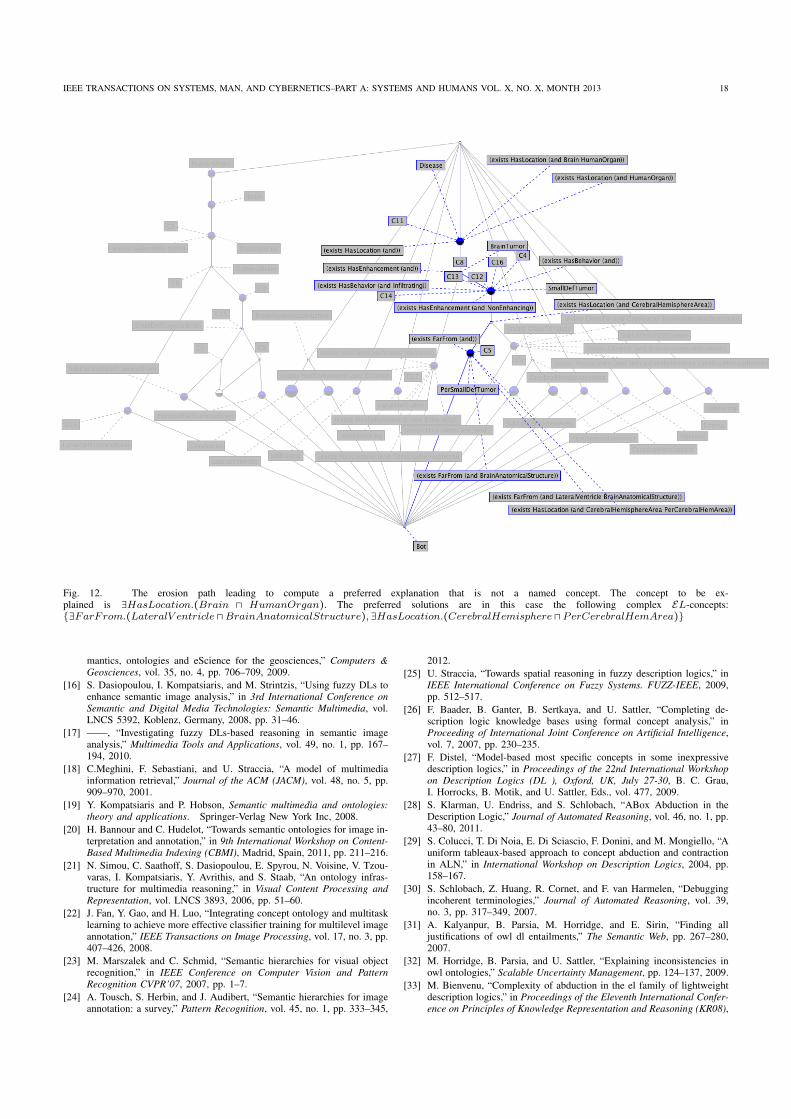
IEEE TRANSACTIONS ON SYSTEMS, MAN, AND CYBERNETICS–PART A: SYSTEMS AND HUMANS VOL. X, NO. X, MONTH 2013 18

Fig. 12. The erosion path leading to compute a preferred explanation that is not a named concept. The concept to be ex-plained is ∃HasLocation.(Brain ⊓ HumanOrgan). The preferred solutions are in this case the following complex EL-concepts:{∃FarFrom.(LateralV entricle ⊓BrainAnatomicalStructure),∃HasLocation.(CerebralHemisphere ⊓ PerCerebralHemArea)}

mantics, ontologies and eScience for the geosciences,” Computers &Geosciences, vol. 35, no. 4, pp. 706–709, 2009.

[16] S. Dasiopoulou, I. Kompatsiaris, and M. Strintzis, “Using fuzzy DLs toenhance semantic image analysis,” in 3rd International Conference onSemantic and Digital Media Technologies: Semantic Multimedia, vol.LNCS 5392, Koblenz, Germany, 2008, pp. 31–46.

[17] ——, “Investigating fuzzy DLs-based reasoning in semantic imageanalysis,” Multimedia Tools and Applications, vol. 49, no. 1, pp. 167–194, 2010.

[18] C.Meghini, F. Sebastiani, and U. Straccia, “A model of multimediainformation retrieval,” Journal of the ACM (JACM), vol. 48, no. 5, pp.909–970, 2001.

[19] Y. Kompatsiaris and P. Hobson, Semantic multimedia and ontologies:theory and applications. Springer-Verlag New York Inc, 2008.

[20] H. Bannour and C. Hudelot, “Towards semantic ontologies for image in-terpretation and annotation,” in 9th International Workshop on Content-Based Multimedia Indexing (CBMI), Madrid, Spain, 2011, pp. 211–216.

[21] N. Simou, C. Saathoff, S. Dasiopoulou, E. Spyrou, N. Voisine, V. Tzou-varas, I. Kompatsiaris, Y. Avrithis, and S. Staab, “An ontology infras-tructure for multimedia reasoning,” in Visual Content Processing andRepresentation, vol. LNCS 3893, 2006, pp. 51–60.

[22] J. Fan, Y. Gao, and H. Luo, “Integrating concept ontology and multitasklearning to achieve more effective classifier training for multilevel imageannotation,” IEEE Transactions on Image Processing, vol. 17, no. 3, pp.407–426, 2008.

[23] M. Marszalek and C. Schmid, “Semantic hierarchies for visual objectrecognition,” in IEEE Conference on Computer Vision and PatternRecognition CVPR’07, 2007, pp. 1–7.

[24] A. Tousch, S. Herbin, and J. Audibert, “Semantic hierarchies for imageannotation: a survey,” Pattern Recognition, vol. 45, no. 1, pp. 333–345,

2012.[25] U. Straccia, “Towards spatial reasoning in fuzzy description logics,” in

IEEE International Conference on Fuzzy Systems. FUZZ-IEEE, 2009,pp. 512–517.

[26] F. Baader, B. Ganter, B. Sertkaya, and U. Sattler, “Completing de-scription logic knowledge bases using formal concept analysis,” inProceeding of International Joint Conference on Artificial Intelligence,vol. 7, 2007, pp. 230–235.

[27] F. Distel, “Model-based most specific concepts in some inexpressivedescription logics,” in Proceedings of the 22nd International Workshopon Description Logics (DL ), Oxford, UK, July 27-30, B. C. Grau,I. Horrocks, B. Motik, and U. Sattler, Eds., vol. 477, 2009.

[28] S. Klarman, U. Endriss, and S. Schlobach, “ABox Abduction in theDescription Logic,” Journal of Automated Reasoning, vol. 46, no. 1, pp.43–80, 2011.

[29] S. Colucci, T. Di Noia, E. Di Sciascio, F. Donini, and M. Mongiello, “Auniform tableaux-based approach to concept abduction and contractionin ALN,” in International Workshop on Description Logics, 2004, pp.158–167.

[30] S. Schlobach, Z. Huang, R. Cornet, and F. van Harmelen, “Debuggingincoherent terminologies,” Journal of Automated Reasoning, vol. 39,no. 3, pp. 317–349, 2007.

[31] A. Kalyanpur, B. Parsia, M. Horridge, and E. Sirin, “Finding alljustifications of owl dl entailments,” The Semantic Web, pp. 267–280,2007.

[32] M. Horridge, B. Parsia, and U. Sattler, “Explaining inconsistencies inowl ontologies,” Scalable Uncertainty Management, pp. 124–137, 2009.

[33] M. Bienvenu, “Complexity of abduction in the el family of lightweightdescription logics,” in Proceedings of the Eleventh International Confer-ence on Principles of Knowledge Representation and Reasoning (KR08),

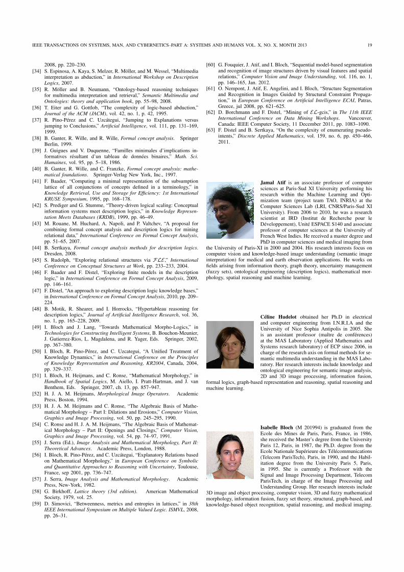
IEEE TRANSACTIONS ON SYSTEMS, MAN, AND CYBERNETICS–PART A: SYSTEMS AND HUMANS VOL. X, NO. X, MONTH 2013 19

2008, pp. 220–230.[34] S. Espinosa, A. Kaya, S. Melzer, R. Moller, and M. Wessel, “Multimedia

interpretation as abduction,” in International Workshop on DescriptionLogics, 2007.

[35] R. Moller and B. Neumann, “Ontology-based reasoning techniquesfor multimedia interpretation and retrieval,” Semantic Multimedia andOntologies: theory and application book, pp. 55–98, 2008.

[36] T. Eiter and G. Gottlob, “The complexity of logic-based abduction,”Journal of the ACM (JACM), vol. 42, no. 1, p. 42, 1995.

[37] R. Pino-Perez and C. Uzcategui, “Jumping to Explanations versusjumping to Conclusions,” Artificial Intelligence, vol. 111, pp. 131–169,1999.

[38] B. Ganter, R. Wille, and R. Wille, Formal concept analysis. SpringerBerlin, 1999.

[39] J. Guigues and V. Duquenne, “Familles minimales d’implications in-formatives resultant d’un tableau de donnees binaires,” Math. Sci.Humaines, vol. 95, pp. 5–18, 1986.

[40] B. Ganter, R. Wille, and C. Franzke, Formal concept analysis: mathe-matical foundations. Springer-Verlag New York, Inc., 1997.

[41] F. Baader, “Computing a minimal representation of the subsumptionlattice of all conjunctions of concepts defined in a terminology,” inKnowledge Retrieval, Use and Storage for Efficiency: 1st InternationalKRUSE Symposium, 1995, pp. 168–178.

[42] S. Prediger and G. Stumme, “Theory-driven logical scaling: Conceptualinformation systems meet description logics,” in Knowledge Represen-tation Meets Databases (KRDB), 1999, pp. 46–49.

[43] M. Rouane, M. Huchard, A. Napoli, and P. Valtchev, “A proposal forcombining formal concept analysis and description logics for miningrelational data,” International Conference on Formal Concept Analysis,pp. 51–65, 2007.

[44] B. Sertkaya, Formal concept analysis methods for description logics.Dresden, 2008.

[45] S. Rudolph, “Exploring relational structures via FLE ,” InternationalConference on Conceptual Structures at Work, pp. 233–233, 2004.

[46] F. Baader and F. Distel, “Exploring finite models in the descriptionlogic,” in International Conference on Formal Concept Analysis, 2009,pp. 146–161.

[47] F. Distel, “An approach to exploring description logic knowledge bases,”in International Conference on Formal Concept Analysis, 2010, pp. 209–224.

[48] B. Motik, R. Shearer, and I. Horrocks, “Hypertableau reasoning fordescription logics,” Journal of Artificial Intelligence Research, vol. 36,no. 1, pp. 165–228, 2009.

[49] I. Bloch and J. Lang, “Towards Mathematical Morpho-Logics,” inTechnologies for Constructing Intelligent Systems, B. Bouchon-Meunier,J. Gutierrez-Rios, L. Magdalena, and R. Yager, Eds. Springer, 2002,pp. 367–380.

[50] I. Bloch, R. Pino-Perez, and C. Uzcategui, “A Unified Treatment ofKnowledge Dynamics,” in International Conference on the Principlesof Knowledge Representation and Reasoning, KR2004, Canada, 2004,pp. 329–337.

[51] I. Bloch, H. Heijmans, and C. Ronse, “Mathematical Morphology,” inHandbook of Spatial Logics, M. Aiello, I. Pratt-Hartman, and J. vanBenthem, Eds. Springer, 2007, ch. 13, pp. 857–947.

[52] H. J. A. M. Heijmans, Morphological Image Operators. AcademicPress, Boston, 1994.

[53] H. J. A. M. Heijmans and C. Ronse, “The Algebraic Basis of Mathe-matical Morphology – Part I: Dilations and Erosions,” Computer Vision,Graphics and Image Processing, vol. 50, pp. 245–295, 1990.

[54] C. Ronse and H. J. A. M. Heijmans, “The Algebraic Basis of Mathemat-ical Morphology – Part II: Openings and Closings,” Computer Vision,Graphics and Image Processing, vol. 54, pp. 74–97, 1991.

[55] J. Serra (Ed.), Image Analysis and Mathematical Morphology, Part II:Theoretical Advances. Academic Press, London, 1988.

[56] I. Bloch, R. Pino-Perez, and C. Uzcategui, “Explanatory Relations basedon Mathematical Morphology,” in European Conference on Symbolicand Quantitative Approaches to Reasoning with Uncertainty, Toulouse,France, sep 2001, pp. 736–747.

[57] J. Serra, Image Analysis and Mathematical Morphology. AcademicPress, New-York, 1982.

[58] G. Birkhoff, Lattice theory (3rd edition). American MathematicalSociety, 1979, vol. 25.

[59] D. Simovici, “Betweenness, metrics and entropies in lattices,” in 38thIEEE International Symposium on Multiple Valued Logic. ISMVL, 2008,pp. 26–31.

[60] G. Fouquier, J. Atif, and I. Bloch, “Sequential model-based segmentationand recognition of image structures driven by visual features and spatialrelations,” Computer Vision and Image Understanding, vol. 116, no. 1,pp. 146–165, Jan. 2012.

[61] O. Nempont, J. Atif, E. Angelini, and I. Bloch, “Structure Segmentationand Recognition in Images Guided by Structural Constraint Propaga-tion,” in European Conference on Artificial Intelligence ECAI, Patras,Greece, jul 2008, pp. 621–625.

[62] D. Borchmann and F. Distel, “Mining of EL-gcis,” in The 11th IEEEInternational Conference on Data Mining Workshops. Vancouver,Canada: IEEE Computer Society, 11 December 2011, pp. 1083–1090.

[63] F. Distel and B. Sertkaya, “On the complexity of enumerating pseudo-intents,” Discrete Applied Mathematics, vol. 159, no. 6, pp. 450–466,2011.

Jamal Atif is an associate professor of computersciences at Paris-Sud XI University performing hisresearch within the Machine Learning and Opti-mization team (project team TAO, INRIA) at theComputer Sciences Lab (LRI, CNRS/Paris-Sud XIUniversity). From 2006 to 2010, he was a researchscientist at IRD (Institut de Recherche pour leDeveloppement), Unite ESPACE S140 and associateprofessor of computer sciences at the University ofFrench West Indies. He received a master degree andPhD in computer sciences and medical imaging from

the University of Paris-XI in 2000 and 2004. His research interests focus oncomputer vision and knowledge-based image understanding (semantic imageinterpretation) for medical and earth observation applications. He works onfields arising from information theory, graph theory, uncertainty management(fuzzy sets), ontological engineering (description logics), mathematical mor-phology, spatial reasoning and machine learning.

Celine Hudelot obtained her Ph.D in electricaland computer engineering from I.N.R.I.A and theUniversity of Nice Sophia Antipolis in 2005. Sheis an assistant professor (maıtre de conferences)at the MAS Laboratory (Applied Mathematics andSystems research laboratory) of ECP since 2006, incharge of the research axis on formal methods for se-mantic multimedia understanding in the MAS Labo-ratory. Her research interests include knowledge andontological engineering for semantic image analysis,2D and 3D image processing, information fusion,

formal logics, graph-based representation and reasoning, spatial reasoning andmachine learning.

Isabelle Bloch (M 201994) is graduated from theEcole des Mines de Paris, Paris, France, in 1986,she received the Master’s degree from the UniversityParis 12, Paris, in 1987, the Ph.D. degree from theEcole Nationale Superieure des Telecommunications(Telecom ParisTech), Paris, in 1990, and the Habil-itation degree from the University Paris 5, Paris,in 1995. She is currently a Professor with theSignal and Image Processing Department, TelecomParisTech, in charge of the Image Processing andUnderstanding Group. Her research interests include

3D image and object processing, computer vision, 3D and fuzzy mathematicalmorphology, information fusion, fuzzy set theory, structural, graph-based, andknowledge-based object recognition, spatial reasoning, and medical imaging.

Sequential model-based segmentation and recognition of image structuresdriven by visual features and spatial relations

Geoffroy Fouquier a,⇑, Jamal Atif b, Isabelle Bloch a

a Institut Telecom, Telecom ParisTech, CNRS LTCI, 46 rue Barrault, 75013 Paris, Franceb TAO INRIA, CNRS, LRI – Paris-Sud University, 91405 Orsay Cedex, France

a r t i c l e i n f o

Article history:Received 13 October 2010Accepted 14 September 2011Available online 2 October 2011

Keywords:SegmentationKnowledge-based systemSpatial relationsGraph representationsFuzzy setsMedical imagesMRI

a b s t r a c t

A sequential segmentation framework, where objects in an image are successively segmented, generallyraises some questions about the ‘‘best’’ segmentation sequence to follow and/or how to avoid error prop-agation. In this work, we propose original approaches to answer these questions in the case where theobjects to segment are represented by a model describing the spatial relations between objects. The pro-cess is guided by a criterion derived from visual attention, and more precisely from a saliency map, alongwith some spatial information to focus the attention. This criterion is used to optimize the segmentationsequence. Spatial knowledge is also used to ensure the consistency of the results and to allow backtrack-ing on the segmentation order if needed. The proposed approach was applied for the segmentation ofinternal brain structures in magnetic resonance images. The results show the relevance of the optimiza-tion criteria and the interest of the backtracking procedure to guarantee good and consistent results.

� 2011 Elsevier Inc. All rights reserved.

1. Introduction

In this paper, we deal with segmentation and recognition of ob-jects or structures in an image, based on a generic model of thescene. As a typical example, we focus on the recognition of internalbrain structures in 3D magnetic resonance images (MRI), based onan anatomical model. More specifically, we address two importantproblems occurring in sequential approaches, as detailed below.

In Refs. [1,2], the authors introduced a new paradigm combin-ing segmentation and recognition tasks. We will refer to this para-digm in the remainder of this paper as sequential segmentationand interpretation. It is defined as a knowledge-based object recog-nition approach where objects are segmented in a predefinedorder, starting from the simplest object to segment to the most dif-ficult one. The segmentation and recognition of each object arethen based on a generic model of the scene and rely on the previ-ously recognized objects. This approach uses a graph which modelsthe generic spatial information about the scene in an intuitive andexplicit way (presented in [3]). This sequential segmentationframework allows decomposing the initial problem into severalsub-problems easier to solve, using the generic knowledge aboutthe scene. This approach differs from a regular divide-and-conquerapproach since each sub-problem contributes to improve the

resolution of the next sub-problems. It also avoids relying on aninitial segmentation of the whole image.

This approach, as pointed out in Ref. [2], requires to define theorder according to which the objects have to be recognized and thechoice of the most appropriate order is one of the problems that re-main open. It also lacks a step which could evaluate the quality ofthe segmentation of a particular object and detect errors to preventtheir propagation.

In this paper, we propose original methods to answer these twoopen questions. Our contribution is twofold: first, we extend thesequential segmentation framework by introducing a pre-atten-tional mechanism, which is used, in combination with spatial rela-tions, to derive a criterion for the optimization of the segmentationorder. Secondly, we introduce criteria and a data structure whichallow us to detect the potential errors and control the orderingstrategy.

The pre-attentional mechanisms were defined in [4–6] to guidethe focus of attention in modeling the visual system such as in fea-ture integration theory. The sequential segmentation frameworkmay be viewed as a way to focus attention on a small part of thescene and thus limit the search domain and the computationalload. Among these mechanisms, we propose to use the notion ofsaliency to optimize the sequence of segmentation.

Our approach is applied to the segmentation and the recogni-tion of internal brain structures in 3D magnetic resonance images.The intrinsic variability of these structures, the lack of clearboundaries and the insufficient radiometry make this

1077-3142/$ - see front matter � 2011 Elsevier Inc. All rights reserved.doi:10.1016/j.cviu.2011.09.004

⇑ Corresponding author.E-mail addresses: geoffroy.fouquier@telecom-paristech.fr (G. Fouquier), atif@l-

ri.fr (J. Atif), isabelle.bloch@telecom-paristech.fr (I. Bloch).

Computer Vision and Image Understanding 116 (2012) 146–165

Contents lists available at SciVerse ScienceDirect

Computer Vision and Image Understanding

journal homepage: www.elsevier .com/ locate /cviu

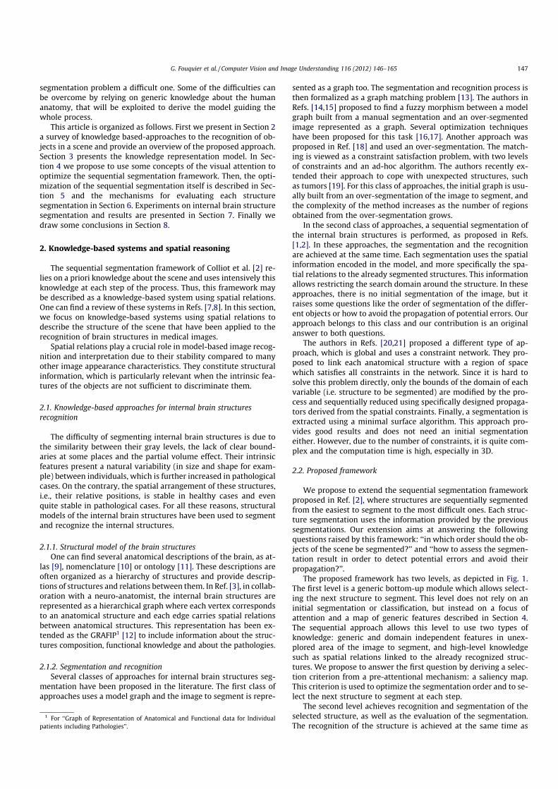
segmentation problem a difficult one. Some of the difficulties canbe overcome by relying on generic knowledge about the humananatomy, that will be exploited to derive the model guiding thewhole process.

This article is organized as follows. First we present in Section 2a survey of knowledge based-approaches to the recognition of ob-jects in a scene and provide an overview of the proposed approach.Section 3 presents the knowledge representation model. In Sec-tion 4 we propose to use some concepts of the visual attention tooptimize the sequential segmentation framework. Then, the opti-mization of the sequential segmentation itself is described in Sec-tion 5 and the mechanisms for evaluating each structuresegmentation in Section 6. Experiments on internal brain structuresegmentation and results are presented in Section 7. Finally wedraw some conclusions in Section 8.

2. Knowledge-based systems and spatial reasoning

The sequential segmentation framework of Colliot et al. [2] re-lies on a priori knowledge about the scene and uses intensively thisknowledge at each step of the process. Thus, this framework maybe described as a knowledge-based system using spatial relations.One can find a review of these systems in Refs. [7,8]. In this section,we focus on knowledge-based systems using spatial relations todescribe the structure of the scene that have been applied to therecognition of brain structures in medical images.

Spatial relations play a crucial role in model-based image recog-nition and interpretation due to their stability compared to manyother image appearance characteristics. They constitute structuralinformation, which is particularly relevant when the intrinsic fea-tures of the objects are not sufficient to discriminate them.

2.1. Knowledge-based approaches for internal brain structuresrecognition

The difficulty of segmenting internal brain structures is due tothe similarity between their gray levels, the lack of clear bound-aries at some places and the partial volume effect. Their intrinsicfeatures present a natural variability (in size and shape for exam-ple) between individuals, which is further increased in pathologicalcases. On the contrary, the spatial arrangement of these structures,i.e., their relative positions, is stable in healthy cases and evenquite stable in pathological cases. For all these reasons, structuralmodels of the internal brain structures have been used to segmentand recognize the internal structures.

2.1.1. Structural model of the brain structuresOne can find several anatomical descriptions of the brain, as at-

las [9], nomenclature [10] or ontology [11]. These descriptions areoften organized as a hierarchy of structures and provide descrip-tions of structures and relations between them. In Ref. [3], in collab-oration with a neuro-anatomist, the internal brain structures arerepresented as a hierarchical graph where each vertex correspondsto an anatomical structure and each edge carries spatial relationsbetween anatomical structures. This representation has been ex-tended as the GRAFIP1 [12] to include information about the struc-tures composition, functional knowledge and about the pathologies.

2.1.2. Segmentation and recognitionSeveral classes of approaches for internal brain structures seg-

mentation have been proposed in the literature. The first class ofapproaches uses a model graph and the image to segment is repre-

sented as a graph too. The segmentation and recognition process isthen formalized as a graph matching problem [13]. The authors inRefs. [14,15] proposed to find a fuzzy morphism between a modelgraph built from a manual segmentation and an over-segmentedimage represented as a graph. Several optimization techniqueshave been proposed for this task [16,17]. Another approach wasproposed in Ref. [18] and used an over-segmentation. The match-ing is viewed as a constraint satisfaction problem, with two levelsof constraints and an ad-hoc algorithm. The authors recently ex-tended their approach to cope with unexpected structures, suchas tumors [19]. For this class of approaches, the initial graph is usu-ally built from an over-segmentation of the image to segment, andthe complexity of the method increases as the number of regionsobtained from the over-segmentation grows.

In the second class of approaches, a sequential segmentation ofthe internal brain structures is performed, as proposed in Refs.[1,2]. In these approaches, the segmentation and the recognitionare achieved at the same time. Each segmentation uses the spatialinformation encoded in the model, and more specifically the spa-tial relations to the already segmented structures. This informationallows restricting the search domain around the structure. In theseapproaches, there is no initial segmentation of the image, but itraises some questions like the order of segmentation of the differ-ent objects or how to avoid the propagation of potential errors. Ourapproach belongs to this class and our contribution is an originalanswer to both questions.

The authors in Refs. [20,21] proposed a different type of ap-proach, which is global and uses a constraint network. They pro-posed to link each anatomical structure with a region of spacewhich satisfies all constraints in the network. Since it is hard tosolve this problem directly, only the bounds of the domain of eachvariable (i.e. structure to be segmented) are modified by the pro-cess and sequentially reduced using specifically designed propaga-tors derived from the spatial constraints. Finally, a segmentation isextracted using a minimal surface algorithm. This approach pro-vides good results and does not need an initial segmentationeither. However, due to the number of constraints, it is quite com-plex and the computation time is high, especially in 3D.

2.2. Proposed framework

We propose to extend the sequential segmentation frameworkproposed in Ref. [2], where structures are sequentially segmentedfrom the easiest to segment to the most difficult ones. Each struc-ture segmentation uses the information provided by the previoussegmentations. Our extension aims at answering the followingquestions raised by this framework: ‘‘in which order should the ob-jects of the scene be segmented?’’ and ‘‘how to assess the segmen-tation result in order to detect potential errors and avoid theirpropagation?’’.

The proposed framework has two levels, as depicted in Fig. 1.The first level is a generic bottom-up module which allows select-ing the next structure to segment. This level does not rely on aninitial segmentation or classification, but instead on a focus ofattention and a map of generic features described in Section 4.The sequential approach allows this level to use two types ofknowledge: generic and domain independent features in unex-plored area of the image to segment, and high-level knowledgesuch as spatial relations linked to the already recognized struc-tures. We propose to answer the first question by deriving a selec-tion criterion from a pre-attentional mechanism: a saliency map.This criterion is used to optimize the segmentation order and to se-lect the next structure to segment at each step.

The second level achieves recognition and segmentation of theselected structure, as well as the evaluation of the segmentation.The recognition of the structure is achieved at the same time as

1 For ‘‘Graph of Representation of Anatomical and Functional data for Individualpatients including Pathologies’’.

G. Fouquier et al. / Computer Vision and Image Understanding 116 (2012) 146–165 147

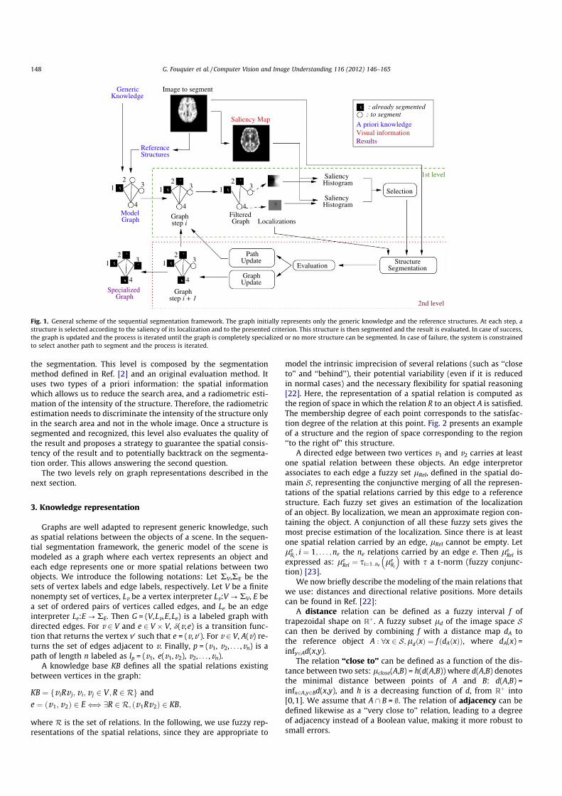
the segmentation. This level is composed by the segmentationmethod defined in Ref. [2] and an original evaluation method. Ituses two types of a priori information: the spatial informationwhich allows us to reduce the search area, and a radiometric esti-mation of the intensity of the structure. Therefore, the radiometricestimation needs to discriminate the intensity of the structure onlyin the search area and not in the whole image. Once a structure issegmented and recognized, this level also evaluates the quality ofthe result and proposes a strategy to guarantee the spatial consis-tency of the result and to potentially backtrack on the segmenta-tion order. This allows answering the second question.

The two levels rely on graph representations described in thenext section.

3. Knowledge representation

Graphs are well adapted to represent generic knowledge, suchas spatial relations between the objects of a scene. In the sequen-tial segmentation framework, the generic model of the scene ismodeled as a graph where each vertex represents an object andeach edge represents one or more spatial relations between twoobjects. We introduce the following notations: Let RV,RE be thesets of vertex labels and edge labels, respectively. Let V be a finitenonempty set of vertices, Lv be a vertex interpreter Lv:V ? RV, E bea set of ordered pairs of vertices called edges, and Le be an edgeinterpreter Le:E ? RE. Then G = (V,Lv,E,Le) is a labeled graph withdirected edges. For v 2 V and e 2 V � V, d(v,e) is a transition func-tion that returns the vertex v0 such that e = (v,v0). For v 2 V, A(v) re-turns the set of edges adjacent to v. Finally, p = (v1, v2, . . . ,vn) is apath of length n labeled as lp = (v1, e(v1,v2), v2, . . . ,vn).

A knowledge base KB defines all the spatial relations existingbetween vertices in the graph:

KB ¼ fv iRv j; v i;v j 2 V ;R 2 Rg ande ¼ ðv1; v2Þ 2 E() 9R 2 R; ðv1Rv2Þ 2 KB;

where R is the set of relations. In the following, we use fuzzy rep-resentations of the spatial relations, since they are appropriate to

model the intrinsic imprecision of several relations (such as ‘‘closeto’’ and ‘‘behind’’), their potential variability (even if it is reducedin normal cases) and the necessary flexibility for spatial reasoning[22]. Here, the representation of a spatial relation is computed asthe region of space in which the relation R to an object A is satisfied.The membership degree of each point corresponds to the satisfac-tion degree of the relation at this point. Fig. 2 presents an exampleof a structure and the region of space corresponding to the region‘‘to the right of’’ this structure.

A directed edge between two vertices v1 and v2 carries at leastone spatial relation between these objects. An edge interpretorassociates to each edge a fuzzy set lRel, defined in the spatial do-main S, representing the conjunctive merging of all the represen-tations of the spatial relations carried by this edge to a referencestructure. Each fuzzy set gives an estimation of the localizationof an object. By localization, we mean an approximate region con-taining the object. A conjunction of all these fuzzy sets gives themost precise estimation of the localization. Since there is at leastone spatial relation carried by an edge, lRel cannot be empty. Letle

Ri; i ¼ 1; . . . ;ne the ne relations carried by an edge e. Then le

Rel isexpressed as: le

Rel ¼ si¼1::ne leRi

� �with s a t-norm (fuzzy conjunc-

tion) [23].We now briefly describe the modeling of the main relations that

we use: distances and directional relative positions. More detailscan be found in Ref. [22]:

A distance relation can be defined as a fuzzy interval f oftrapezoidal shape on Rþ. A fuzzy subset ld of the image space Scan then be derived by combining f with a distance map dA tothe reference object A : 8x 2 S;ldðxÞ ¼ f ðdAðxÞÞ, where dA(x) =infy2Ad(x,y).

The relation ‘‘close to’’ can be defined as a function of the dis-tance between two sets: lclose(A,B) = h(d(A,B)) where d(A,B) denotesthe minimal distance between points of A and B: d(A,B) =infx2A,y2Bd(x,y), and h is a decreasing function of d, from Rþ into[0,1]. We assume that A \ B = ;. The relation of adjacency can bedefined likewise as a ‘‘very close to’’ relation, leading to a degreeof adjacency instead of a Boolean value, making it more robust tosmall errors.

Evaluation3

4

213

4

21

ModelGraph

SpecializedGraph

FilteredGraphstep i

Graph

step i + 1Graph

ReferenceStructures

KnowledgeGeneric

: already segmented : to segment

A priori knowledgeVisual informationResults

HistogramSaliency

HistogramSaliency

SegmentationStructure

GraphUpdate

UpdatePath

3

4

21 3

4

21 3

4

21

Saliency Map

Image to segment

Localizations

Selection

1st level

2nd level

Fig. 1. General scheme of the sequential segmentation framework. The graph initially represents only the generic knowledge and the reference structures. At each step, astructure is selected according to the saliency of its localization and to the presented criterion. This structure is then segmented and the result is evaluated. In case of success,the graph is updated and the process is iterated until the graph is completely specialized or no more structure can be segmented. In case of failure, the system is constrainedto select another path to segment and the process is iterated.

148 G. Fouquier et al. / Computer Vision and Image Understanding 116 (2012) 146–165

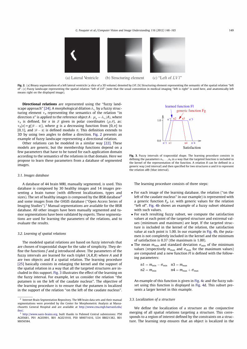
Directional relations are represented using the ‘‘fuzzy land-scape approach’’ [24]. A morphological dilation dma by a fuzzy struc-turing element ma representing the semantics of the relation ‘‘indirection a’’ is applied to the reference object A : la ¼ dma ðAÞ, wherema is defined, for x in S given in polar coordinates (q,h), as:ma(x) = g(jh � aj), where g is a decreasing function from [0,p] to[0,1], and jh � aj is defined modulo p. This definition extends to3D by using two angles to define a direction. Fig. 2 presents anexample of fuzzy landscape representing a directional relation.

Other relations can be modeled in a similar way [22]. Thesemodels are generic, but the membership functions depend on afew parameters that have to be tuned for each application domainaccording to the semantics of the relations in that domain. Here wepropose to learn these parameters from a database of segmentedimages.

3.1. Images database

A database of 44 brain MRI, manually segmented, is used. Thisdatabase is composed by 30 healthy images and 14 images pre-senting a brain tumor (with different localizations, types andsizes). The set of healthy images is composed by the IBSR database2

and some images from the OASIS database (‘‘Open Access Series ofImaging Studies’’).3 Manual segmentations are available for the IBSRdatabase. All other images have been manually segmented and tu-mor segmentations have been validated by experts. These segmenta-tions are used for learning the parameters of the relations, and toevaluate the results.

3.2. Learning of spatial relations

The modeled spatial relations are based on fuzzy intervals thatare chosen of trapezoidal shape for the sake of simplicity. They de-fine the functions f and g introduced above. The parameters of thefuzzy intervals are learned for each triplet (A,R,B) where A and Bare two objects and R a spatial relation. The learning procedure[25] basically consists in enlarging the kernel and the support ofthe spatial relation in a way that all the targeted structures are in-cluded in this support. Fig. 3 illustrates the effect of the learning onthe fuzzy interval. For example, let us consider the relation ‘‘theputamen is on the left of the caudate nucleus’’. The objective ofthe learning procedure is to ensure that the putamen is localizedin the support of the relation ‘‘on the left of the caudate nucleus’’.

The learning procedure consists of three steps:

� For each image of the learning database, the relation (‘‘on theleft of the caudate nucleus’’ in our example) is represented witha generic function Fg, i.e. with generic values for the relation‘‘left of’’. Fig. 4b shows an example of a fuzzy subset obtainedwith such values.� For each resulting fuzzy subset, we compute the satisfaction

values at each point of the targeted structure and extremal val-ues (minimum and maximum) are kept. If the targeted struc-ture is included in the kernel of the relation, the satisfactionvalue at each point is 1.00. In our example in Fig. 4b, the puta-men is not completely included in the kernel and the minimumof satisfaction is 0.37 (the maximum is 1.00).� The mean mmin and standard deviation rmin of the minimum

values (respectively mmax and rmax for the maximum values)are computed and a new function Fl is defined with the follow-ing parameters:

n1 ¼ mmin � rmin n3 ¼ mmax

n2 ¼ mmin n4 ¼ mmax þ rmax

An example of this function is given in Fig. 4c and the fuzzy sub-set using this function is displayed in Fig. 4d. This subset pre-sents a larger kernel in this example.

3.3. Localization of a structure

We define the localization of a structure as the conjunctivemerging of all spatial relations targeting a structure. This corre-sponds to a region of interest defined by the constraints on a struc-ture. The learning step ensures that an object is localized in the

1.0

0.0n1

n2 n3

n4

Satisfaction

learned function Flgeneric function Fg

n’1

n’2 n’3

n’4

Fig. 3. Fuzzy intervals of trapezoidal shape. The learning procedure consists indefining the parameters n1, . . . ,n4 in a way that the targeted function is included inthe kernel of the representation of the function. A relation R can be defined in ageneric way (red interval) and then specified for two structures a and b to representthe relation aRb (blue interval).

(a) Lateral Ventricle (b) Structuring element (c) “Left of ”

Fig. 2. (a) Binary segmentation of a left lateral ventricle (a slice of a 3D volume) denoted by LVl. (b) Structuring element representing the semantic of the spatial relation ‘‘leftof’’. (c) Fuzzy landscape representing the spatial relation ‘‘left of LVl’’ (note that the usual convention in medical imaging ‘‘left is right’’ is used here, and anatomically leftmeans right on the displayed image).

2 Internet Brain Segmentation Repository. The MR brain data sets and their manualsegmentations were provided by the Center for Morphometric Analysis at Massa-chusetts General Hospital and are available at http://www.cma.mgh.harvard.edu/ibsr/.

3 http://www.oasis-brains.org, built thanks to Pubmed Central submissions: P50AG05681, P01 AG03991, R01 AG021910, P50 MH071616, U24 RR021382, R01MH56584.

G. Fouquier et al. / Computer Vision and Image Understanding 116 (2012) 146–165 149

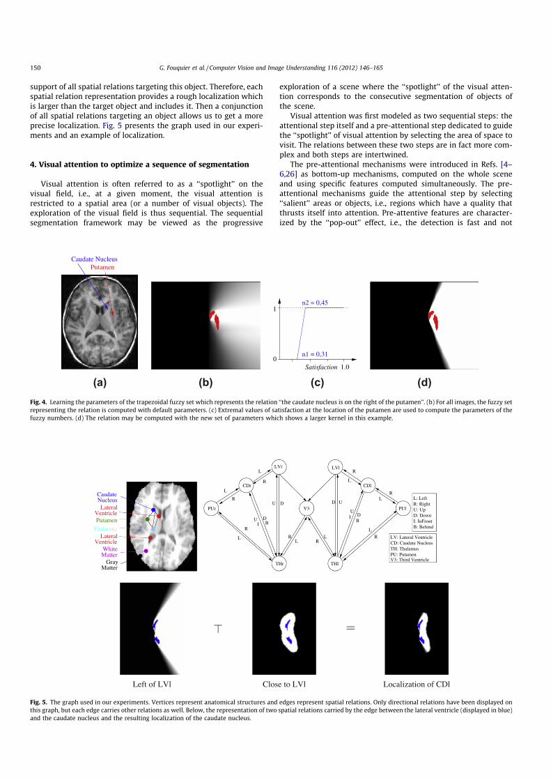
support of all spatial relations targeting this object. Therefore, eachspatial relation representation provides a rough localization whichis larger than the target object and includes it. Then a conjunctionof all spatial relations targeting an object allows us to get a moreprecise localization. Fig. 5 presents the graph used in our experi-ments and an example of localization.

4. Visual attention to optimize a sequence of segmentation

Visual attention is often referred to as a ‘‘spotlight’’ on thevisual field, i.e., at a given moment, the visual attention isrestricted to a spatial area (or a number of visual objects). Theexploration of the visual field is thus sequential. The sequentialsegmentation framework may be viewed as the progressive

exploration of a scene where the ‘‘spotlight’’ of the visual atten-tion corresponds to the consecutive segmentation of objects ofthe scene.

Visual attention was first modeled as two sequential steps: theattentional step itself and a pre-attentional step dedicated to guidethe ‘‘spotlight’’ of visual attention by selecting the area of space tovisit. The relations between these two steps are in fact more com-plex and both steps are intertwined.

The pre-attentional mechanisms were introduced in Refs. [4–6,26] as bottom-up mechanisms, computed on the whole sceneand using specific features computed simultaneously. The pre-attentional mechanisms guide the attentional step by selecting‘‘salient’’ areas or objects, i.e., regions which have a quality thatthrusts itself into attention. Pre-attentive features are character-ized by the ‘‘pop-out’’ effect, i.e., the detection is fast and not

Caudate NucleusPutamen

1

0

n2 = 0,45

1.0Satisfaction

n1 = 0,31

(a) (b) (c) (d)Fig. 4. Learning the parameters of the trapezoidal fuzzy set which represents the relation ‘‘the caudate nucleus is on the right of the putamen’’. (b) For all images, the fuzzy setrepresenting the relation is computed with default parameters. (c) Extremal values of satisfaction at the location of the putamen are used to compute the parameters of thefuzzy numbers. (d) The relation may be computed with the new set of parameters which shows a larger kernel in this example.

VentricleLateral

CaudateNucleus

VentricleLateral

WhiteMatter

MatterGray

Thalamus

Putamen

U: UpD: DownI: InFrontB: Behind

L: LeftR: Right

L

R

L

R

L

R

BD

U D

RL R

L

D U

L

R

UDB

LR

L

R

UI

I

V3: Third Ventricle

LV: Lateral VentricleCD: Caudate NucleusTH: ThalamusPU: Putamen

V3PUr

CDr

LVr

THr THl

LVl

CDl

PUl

Left of LVl Close to LVl Localization of CDl

Fig. 5. The graph used in our experiments. Vertices represent anatomical structures and edges represent spatial relations. Only directional relations have been displayed onthis graph, but each edge carries other relations as well. Below, the representation of two spatial relations carried by the edge between the lateral ventricle (displayed in blue)and the caudate nucleus and the resulting localization of the caudate nucleus.

150 G. Fouquier et al. / Computer Vision and Image Understanding 116 (2012) 146–165

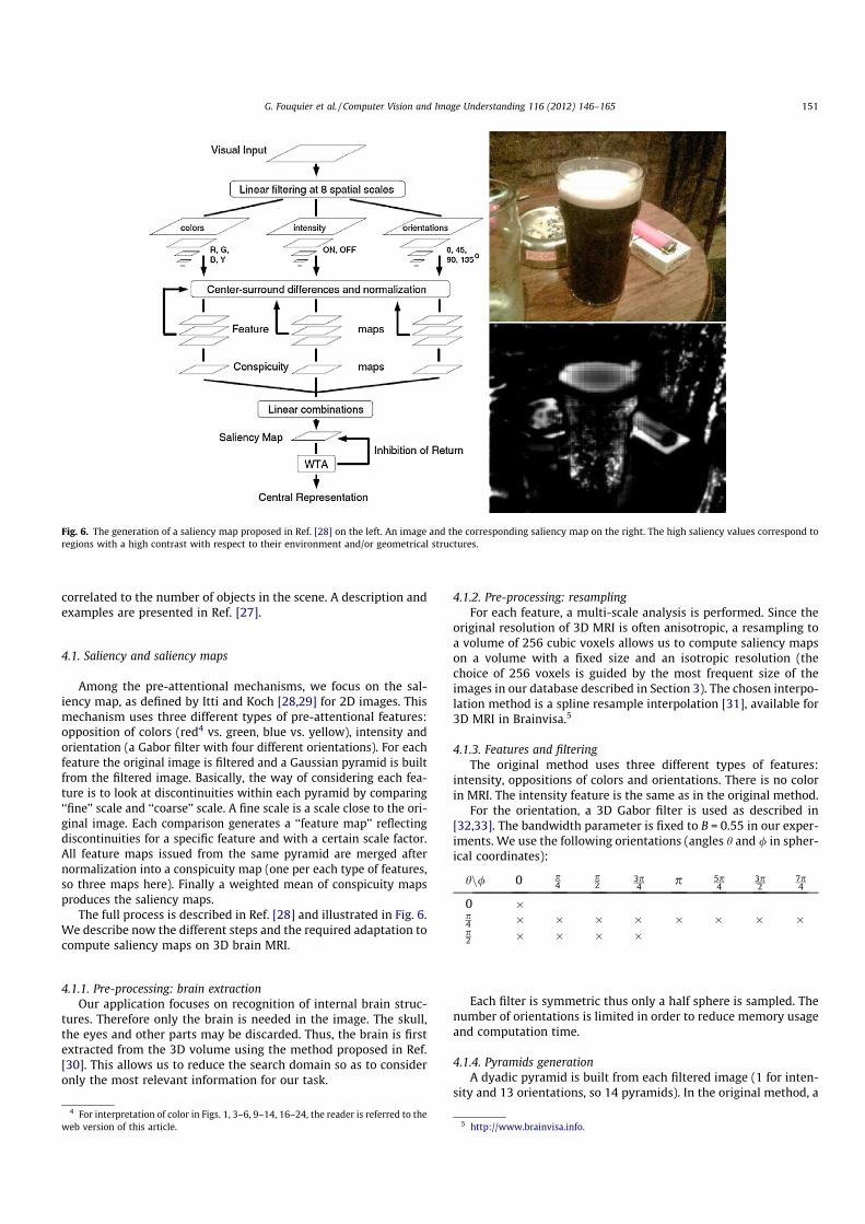
correlated to the number of objects in the scene. A description andexamples are presented in Ref. [27].

4.1. Saliency and saliency maps

Among the pre-attentional mechanisms, we focus on the sal-iency map, as defined by Itti and Koch [28,29] for 2D images. Thismechanism uses three different types of pre-attentional features:opposition of colors (red4 vs. green, blue vs. yellow), intensity andorientation (a Gabor filter with four different orientations). For eachfeature the original image is filtered and a Gaussian pyramid is builtfrom the filtered image. Basically, the way of considering each fea-ture is to look at discontinuities within each pyramid by comparing‘‘fine’’ scale and ‘‘coarse’’ scale. A fine scale is a scale close to the ori-ginal image. Each comparison generates a ‘‘feature map’’ reflectingdiscontinuities for a specific feature and with a certain scale factor.All feature maps issued from the same pyramid are merged afternormalization into a conspicuity map (one per each type of features,so three maps here). Finally a weighted mean of conspicuity mapsproduces the saliency maps.

The full process is described in Ref. [28] and illustrated in Fig. 6.We describe now the different steps and the required adaptation tocompute saliency maps on 3D brain MRI.

4.1.1. Pre-processing: brain extractionOur application focuses on recognition of internal brain struc-

tures. Therefore only the brain is needed in the image. The skull,the eyes and other parts may be discarded. Thus, the brain is firstextracted from the 3D volume using the method proposed in Ref.[30]. This allows us to reduce the search domain so as to consideronly the most relevant information for our task.

4.1.2. Pre-processing: resamplingFor each feature, a multi-scale analysis is performed. Since the

original resolution of 3D MRI is often anisotropic, a resampling toa volume of 256 cubic voxels allows us to compute saliency mapson a volume with a fixed size and an isotropic resolution (thechoice of 256 voxels is guided by the most frequent size of theimages in our database described in Section 3). The chosen interpo-lation method is a spline resample interpolation [31], available for3D MRI in Brainvisa.5

4.1.3. Features and filteringThe original method uses three different types of features:

intensity, oppositions of colors and orientations. There is no colorin MRI. The intensity feature is the same as in the original method.

For the orientation, a 3D Gabor filter is used as described in[32,33]. The bandwidth parameter is fixed to B = 0.55 in our exper-iments. We use the following orientations (angles h and / in spher-ical coordinates):

hn/ 0 p4

p2

3p4

p 5p4

3p2

7p4

0 �p4 � � � � � � � �p2 � � � �

Each filter is symmetric thus only a half sphere is sampled. Thenumber of orientations is limited in order to reduce memory usageand computation time.

4.1.4. Pyramids generationA dyadic pyramid is built from each filtered image (1 for inten-

sity and 13 orientations, so 14 pyramids). In the original method, a

Fig. 6. The generation of a saliency map proposed in Ref. [28] on the left. An image and the corresponding saliency map on the right. The high saliency values correspond toregions with a high contrast with respect to their environment and/or geometrical structures.

4 For interpretation of color in Figs. 1, 3–6, 9–14, 16–24, the reader is referred to theweb version of this article. 5 http://www.brainvisa.info.

G. Fouquier et al. / Computer Vision and Image Understanding 116 (2012) 146–165 151

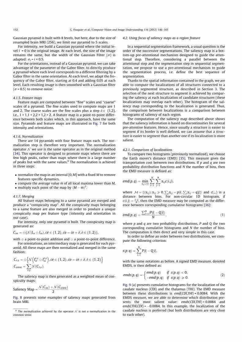
Gaussian pyramid is built with 8 levels, but here, due to the size ofresampled brain MRI (256), we limit our pyramid to 5 scales.

For intensity, we build a Gaussian pyramid where the initial le-vel i = 0 is the original image. At each level, the size of the imageremains the same, but the width of the Gaussian Filter (r) isadapted: ri = i + 0.5.

For the orientations, instead of a Gaussian pyramid, we can takeadvantage of the parameter of the Gabor filter, to directly producea pyramid where each level corresponds to a different filtering by aGabor filter in the same orientation. At each level, we adapt the fre-quency of the Gabor filter, starting at 0.4 and adding 0.05 at eachlevel. Each resulting image is then smoothed with a Gaussian filter(r = 0.5) to remove noise.

4.1.5. Feature mapsFeature maps are computed between ‘‘fine’’ scales and ‘‘coarse’’

scales of a pyramid. The fine scales used to compute maps are 1and 2. The coarse scales are the fine scales plus a step d 2 {1,2},i.e., 1 + 1,1 + 2,2 + 1,2 + 2. A feature map is a point-to-point differ-ence between both scales which, in this approach, have the samesize. Pyramids and feature maps are illustrated in Fig. 7 for bothintensity and orientations.

4.1.6. NormalizationThere are 14 pyramids with four feature maps each. The nor-

malization step is therefore very important. The normalizationoperator N we use is the same operator as in the original method[34]. This operator is designed to promote maps where there arefew high peaks, rather than maps where there is a large numberof peaks but with the same values.6 The normalization is achievedin three steps:

� normalize the map in an interval [0,M] with a fixed M to removefeatures specific dynamics,� compute the average value m of all local maxima lower than M,� multiply each point of the map by ðM � mÞ2.

4.1.7. MergingAll feature maps belonging to a same pyramid are merged and

produce a ‘‘conspicuity map’’. All the conspicuity maps belongingto a same feature are also merged in order to produce a uniqueconspicuity map per feature type (intensity and orientation inour case).

For intensity, only one pyramid is built. The conspicuity map isgenerated as:

Cint ¼ �fN ðIce � IcoÞ; ce 2 f1;2g; co ¼ ceþ d; d 2 f1;2gg;

with � a point-to-point addition and � a point-to-point difference.For orientations, an intermediary map is generated for each pyr-

amid. All these maps are then normalized and merged in the samefashion:

Ch;/ ¼ � N Ih;/ce � Ih;/co

� �; ce 2 f1;2g; co ¼ ceþ d; d 2 f1;2g

n oCorient ¼

Xh;/

NðCh;/Þ:

The saliency map is then generated as a weighted mean of con-spicuity maps:

Saliency Map ¼ NðCintÞ þ N ðCorientÞ2

Fig. 8 presents some examples of saliency maps generated frombrain MRI.

4.2. Using focus of saliency maps as a region feature

In a sequential segmentation framework, a usual question is theorder of the successive segmentations. The saliency map is a bot-tom-up pre-attentional mechanism designed to guide the atten-tional step. Therefore, considering a parallel between theattentional step and the segmentation step in sequential segmen-tation, we propose to use a pre-attentional mechanism to guidethe segmentation process, i.e. define the best sequence ofsegmentation.

Thanks to the spatial information contained in the graph, we areable to compute the localizations of all structures connected to apreviously segmented structure, as described in Section 3. Theselection of the next structure to segment is achieved by compar-ing the saliency at each localization of candidate structures (theselocalizations may overlap each other). The histogram of the sal-iency map corresponding to the localization is generated. Thus,the comparison between localizations is a comparison betweenhistograms of saliency of each region.

The computation of the saliency map described above showsthat the saliency information is based on discontinuities for severalpre-attentive features. Hence, since usually a structure is easier tosegment if its border is well defined, we can assume that a struc-ture is easier to segment than another one if its localization is moresalient.

4.2.1. Comparison of localizationsTo compare two histograms (previously normalized), we choose

the Earth mover’s distance (EMD) [35]. This measure gives thetransportation cost between two distributions. If p and q are twoprobability distribution functions and N the number of bins, thenthe EMD measure is defined as:

emdðp; qÞ ¼ minai;j2M

XN

i¼1

XN

j¼1

ai;jcði; jÞ;

where M¼ fðai;jÞ;ai;j P 0;P

jai;j ¼ p½i�;P

iai;j ¼ q½j�g and c(.,.) is adistance between bins. For non-circular 1D histogram, ifcði; jÞ ¼ ji�jj

N , then the EMD measure may be computed as the differ-ence between corresponding cumulative histograms [36]:

emdðp; qÞ ¼PN

i¼1jP½i� � Q ½i�jN

; ð1Þ

where p and q are two probability distributions, P and Q the twocorresponding cumulative histograms and N the number of bins.The computation is then direct and very simple in this case.

In order to define an order between two distributions, we com-pute the following criterion:

sðp; qÞ ¼XN

i¼1

P½i� � Q ½i�;

with the same notations as before. A signed EMD measure, denotedEMDS, is then defined as:

emdsðp; qÞ ¼emdðp; qÞ if sðp; qÞ < 0;�emdðp; qÞ if sðp; qÞP 0:

�ð2Þ

Fig. 9 (a) presents cumulative histograms for the localization of thecaudate nucleus (CDl) and the thalamus (THl). The EMD measurebetween these distributions is emd(CDl,THl) = 0.0084. With theEMDS measure, we are able to determine which distribution pre-sents the most salient value: emds(CDl,THl) = 0.0084 andemds(THl,CDl) = �0.0084. In this example, the localization of thecaudate nucleus is preferred (but both distributions are very closeto each other).

6 The normalization achieved by the operator N is not a normalization in thecommon sense.

152 G. Fouquier et al. / Computer Vision and Image Understanding 116 (2012) 146–165

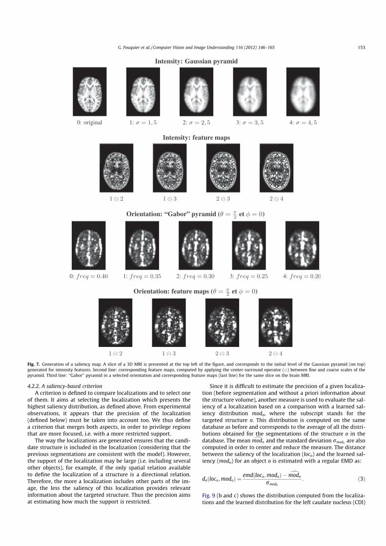
4.2.2. A saliency-based criterionA criterion is defined to compare localizations and to select one

of them. It aims at selecting the localization which presents thehighest saliency distribution, as defined above. From experimentalobservations, it appears that the precision of the localization(defined below) must be taken into account too. We thus definea criterion that merges both aspects, in order to privilege regionsthat are more focused, i.e. with a more restricted support.

The way the localizations are generated ensures that the candi-date structure is included in the localization (considering that theprevious segmentations are consistent with the model). However,the support of the localization may be large (i.e. including severalother objects), for example, if the only spatial relation availableto define the localization of a structure is a directional relation.Therefore, the more a localization includes other parts of the im-age, the less the saliency of this localization provides relevantinformation about the targeted structure. Thus the precision aimsat estimating how much the support is restricted.

Since it is difficult to estimate the precision of a given localiza-tion (before segmentation and without a priori information aboutthe structure volume), another measure is used to evaluate the sal-iency of a localization based on a comparison with a learned sal-iency distribution modo, where the subscript stands for thetargeted structure o. This distribution is computed on the samedatabase as before and corresponds to the average of all the distri-butions obtained for the segmentations of the structure o in thedatabase. The mean dmodo and the standard deviation rmodo are alsocomputed in order to center and reduce the measure. The distancebetween the saliency of the localization (loco) and the learned sal-iency (modo) for an object o is estimated with a regular EMD as:

doðloco;modoÞ ¼emdðloco;modoÞ � dmodo

rmodo

: ð3Þ

Fig. 9 (b and c) shows the distribution computed from the localiza-tions and the learned distribution for the left caudate nucleus (CDl)

Fig. 7. Generation of a saliency map. A slice of a 3D MRI is presented at the top left of the figure, and corresponds to the initial level of the Gaussian pyramid (on top)generated for intensity features. Second line: corresponding feature maps, computed by applying the center-surround operator (�) between fine and coarse scales of thepyramid. Third line: ‘‘Gabor’’ pyramid in a selected orientation and corresponding feature maps (last line) for the same slice on the brain MRI.

G. Fouquier et al. / Computer Vision and Image Understanding 116 (2012) 146–165 153

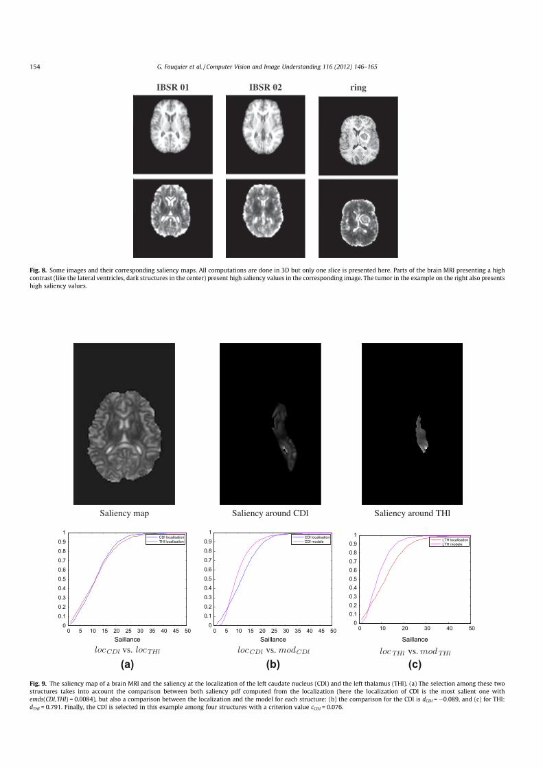
IBSR 01 IBSR 02 ring

Fig. 8. Some images and their corresponding saliency maps. All computations are done in 3D but only one slice is presented here. Parts of the brain MRI presenting a highcontrast (like the lateral ventricles, dark structures in the center) present high saliency values in the corresponding image. The tumor in the example on the right also presentshigh saliency values.

Saliency map Saliency around CDl Saliency around THl

0 5 10 15 20 25 30 35 40 45 500

0.10.20.30.40.50.60.70.80.9

1

Saillance

CDl localisationTHl localisation

0 5 10 15 20 25 30 35 40 45 500

0.10.20.30.40.50.60.70.80.9

1

Saillance

CDl localisationCDl modele

0 10 20 30 40 500

0.10.20.30.40.50.60.70.80.9

1

Saillance

LTH localisationLTH modele

(a) (b) (c)Fig. 9. The saliency map of a brain MRI and the saliency at the localization of the left caudate nucleus (CDl) and the left thalamus (THl). (a) The selection among these twostructures takes into account the comparison between both saliency pdf computed from the localization (here the localization of CDl is the most salient one withemds(CDl,THl) = 0.0084), but also a comparison between the localization and the model for each structure: (b) the comparison for the CDl is dCDl = �0.089, and (c) for THl:dTHl = 0.791. Finally, the CDl is selected in this example among four structures with a criterion value cCDl = 0.076.

154 G. Fouquier et al. / Computer Vision and Image Understanding 116 (2012) 146–165

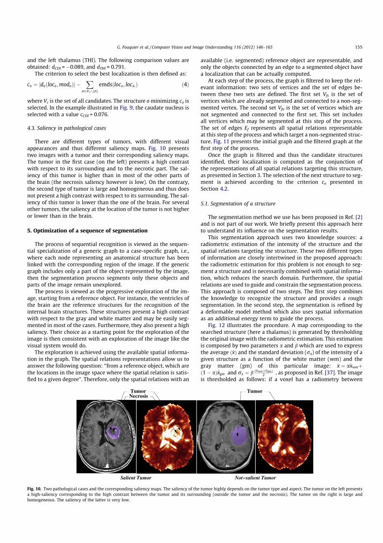
and the left thalamus (THl). The following comparison values areobtained: dCDl = �0.089, and dTHl = 0.791.

The criterion to select the best localization is then defined as:

co ¼ jdoðloco;modoÞj �X

o02Vcnfogemdsðloco; loco0 Þ ð4Þ

where Vc is the set of all candidates. The structure o minimizing co isselected. In the example illustrated in Fig. 9, the caudate nucleus isselected with a value cCDl = 0.076.

4.3. Saliency in pathological cases

There are different types of tumors, with different visualappearances and thus different saliency maps. Fig. 10 presentstwo images with a tumor and their corresponding saliency maps.The tumor in the first case (on the left) presents a high contrastwith respect to its surrounding and to the necrotic part. The sal-iency of this tumor is higher than in most of the other parts ofthe brain (the necrosis saliency however is low). On the contrary,the second type of tumor is large and homogeneous and thus doesnot present a high contrast with respect to its surrounding. The sal-iency of this tumor is lower than the one of the brain. For severalother tumors, the saliency at the location of the tumor is not higheror lower than in the brain.

5. Optimization of a sequence of segmentation

The process of sequential recognition is viewed as the sequen-tial specialization of a generic graph to a case-specific graph, i.e.,where each node representing an anatomical structure has beenlinked with the corresponding region of the image. If the genericgraph includes only a part of the object represented by the image,then the segmentation process segments only these objects andparts of the image remain unexplored.

The process is viewed as the progressive exploration of the im-age, starting from a reference object. For instance, the ventricles ofthe brain are the reference structures for the recognition of theinternal brain structures. These structures present a high contrastwith respect to the gray and white matter and may be easily seg-mented in most of the cases. Furthermore, they also present a highsaliency. Their choice as a starting point for the exploration of theimage is then consistent with an exploration of the image like thevisual system would do.

The exploration is achieved using the available spatial informa-tion in the graph. The spatial relations representations allow us toanswer the following question: ‘‘from a reference object, which arethe locations in the image space where the spatial relation is satis-fied to a given degree’’. Therefore, only the spatial relations with an

available (i.e. segmented) reference object are representable, andonly the objects connected by an edge to a segmented object havea localization that can be actually computed.

At each step of the process, the graph is filtered to keep the rel-evant information: two sets of vertices and the set of edges be-tween these two sets are defined. The first set Vfs is the set ofvertices which are already segmented and connected to a non-seg-mented vertex. The second set Vfo is the set of vertices which arenot segmented and connected to the first set. This set includesall vertices which may be segmented at this step of the process.The set of edges Ef represents all spatial relations representableat this step of the process and which target a non-segmented struc-ture. Fig. 11 presents the initial graph and the filtered graph at thefirst step of the process.

Once the graph is filtered and thus the candidate structuresidentified, their localization is computed as the conjunction ofthe representations of all spatial relations targeting this structure,as presented in Section 3. The selection of the next structure to seg-ment is achieved according to the criterion co presented inSection 4.2.

5.1. Segmentation of a structure

The segmentation method we use has been proposed in Ref. [2]and is not part of our work. We briefly present this approach hereto understand its influence on the segmentation results.

This segmentation approach uses two knowledge sources: aradiometric estimation of the intensity of the structure and thespatial relations targeting the structure. These two different typesof information are closely intertwined in the proposed approach:the radiometric estimation for this problem is not enough to seg-ment a structure and is necessarily combined with spatial informa-tion, which reduces the search domain. Furthermore, the spatialrelations are used to guide and constrain the segmentation process.This approach is composed of two steps. The first step combinesthe knowledge to recognize the structure and provides a roughsegmentation. In the second step, the segmentation is refined bya deformable model method which also uses spatial informationas an additional energy term to guide the process.

Fig. 12 illustrates the procedure. A map corresponding to thesearched structure (here a thalamus) is generated by thresholdingthe original image with the radiometric estimation. This estimationis composed by two parameters a and b which are used to expressthe average ðxÞ and the standard deviation (rx) of the intensity of agiven structure as a function of the white matter (wm) and thegray matter (gm) of this particular image: x ¼ axwmþð1� aÞxgm and rx ¼ b ðrwmþrgmÞ

2 , as proposed in Ref. [37]. The imageis thresholded as follows: if a voxel has a radiometry between

Salient Tumor Not−salient Tumor

TumorNecrosis

Tumor

Fig. 10. Two pathological cases and the corresponding saliency maps. The saliency of the tumor highly depends on the tumor type and aspect. The tumor on the left presentsa high-saliency corresponding to the high contrast between the tumor and its surrounding (outside the tumor and the necrosis). The tumor on the right is large andhomogeneous. The saliency of the latter is very low.

G. Fouquier et al. / Computer Vision and Image Understanding 116 (2012) 146–165 155

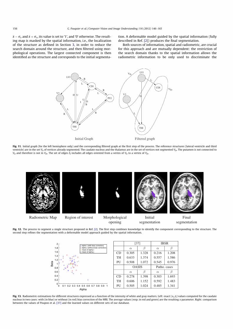
x� rx and xþ rx, its value is set to ’1’, and ’0’ otherwise. The result-ing map is masked by the spatial information, i.e., the localizationof the structure as defined in Section 3, in order to reduce thesearch domain around the structure, and then filtered using mor-phological operations. The largest connected component is thenidentified as the structure and corresponds to the initial segmenta-

tion. A deformable model guided by the spatial information (fullydescribed in Ref. [2]) produces the final segmentation.

Both sources of information, spatial and radiometric, are crucialfor this approach and are mutually dependent: the restriction ofthe search domain thanks to the spatial information allows theradiometric information to be only used to discriminate the

R

L

D U

R

L

RL

L

R

UDIB

V3

THl

LVl

CDl

PUl

Vfs

Vfo

D

L

L

LVl

V3

CDl

THl

Initial Graph Filtered graph

Fig. 11. Initial graph (for the left hemisphere only) and the corresponding filtered graph at the first step of the process. The reference structures (lateral ventricle and thirdventricle) are in the set Vfs of vertices already segmented. The caudate nucleus and the thalamus are in the set of vertices not segmented Vfo. The putamen is not connected toVfs and therefore is not in Vfo. The set of edges Ef includes all edges oriented from a vertex of Vfs to a vertex of Vfo.

Radiometric Map Region of interest Morphologicalopening

Initialsegmentation

Finalsegmentation

Fig. 12. The process to segment a single structure proposed in Ref. [2]. The first step combines knowledge to identify the component corresponding to the structure. Thesecond step refines the segmentation with a deformable model approach guided by the spatial information.

0 0.1 0.2 0.3 0.4 0.5 0.6 0.7 0.8 0.9 10

0.20.40.60.8

11.21.41.61.8

2

Alpha

Beta

alpha i (with bias correction)alpha j (without bias correction)mean of alpha i mean of alpha j

[37] IBSR

CD 0.305 1.328 0.216 1.208TH 0.633 1.374 0.557 1.586PU 0.508 1.072 0.545 0.976

OASIS Patho. cases

CD 0.278 1.398 0.303 1.693TH 0.606 1.152 0.592 1.483PU 0.505 1.024 0.485 1.341

Fig. 13. Radiometric estimations for different structures expressed as a function of the intensity of white and gray matters. Left: exact (ai,bi) values computed for the caudatenucleus in two cases: with (in blue) or without (in red) bias correction of the MRI. The average values (resp. in red and green) are the resulting a parameter. Right: comparisonbetween the values of Poupon et al. [37] and the learned values on different sets of our database.

156 G. Fouquier et al. / Computer Vision and Image Understanding 116 (2012) 146–165

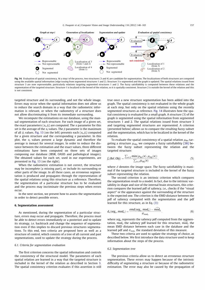
targeted structure and its surrounding, and not the whole image.Errors may occur when the spatial information does not allow usto reduce the search domain in a way that the radiometric infor-mation is relevant, or when the radiometry of a structure doesnot allow discriminating it from its immediate surrounding.

We recompute the estimations on our database, using the man-ual segmentation of each structure. For each image of a given set,the exact parameters (ai,bi) are computed. The a parameter for thisset is the average of the ai values. The b parameter is the maximumof all bi values. Fig. 13 (on the left) presents each (ai,bi) computedfor a given structure and the corresponding a parameter. In thisplot, the ai values present a large dynamic and therefore theaverage is inexact for several images. In order to reduce the dis-tance between the estimation and the exact values, three differentestimations have been computed on three sets of imagescomposing our database (IBSR, OASIS and pathological images).The obtained values for each set, used in our experiments, arepresented in Fig. 13 (on the right).

When the radiometric estimation is not correct, the structuremay be incomplete (a missing part), or include its surrounding orother parts of the image. In all these cases, an erroneous segmen-tation is produced and propagates through the representation ofthe spatial relations using this structure as a reference. Therefore,the segmentation of a particular structure has to be evaluatedand the process may incriminate the previous steps when errorsoccur.

In the next section, we present how to assess the segmentationin order to detect possible errors.

6. Segmentation assessment

As mentioned, during the segmentation of a particular struc-ture, errors may occur and propagate. Therefore, the process mustbe able to detect errors immediately or a posteriori and to updateits strategy, i.e. backtrack and change the sequence of segmenta-tion even if this implies to discard previous structures segmenta-tions. To this end, two criteria are proposed here as well as astructure of control, which consists of a tree of all current and pastsegmentations, used to update the strategy during the process.

6.1. Criteria for segmentation evaluation

The first criterion concerns the spatial information and controlsthe consistency of the structural model. The parameters of eachspatial relation are learned in a way that the targeted structure isincluded in the kernel of the relation as described in Section 3.The spatial consistency criterion evaluates if this assertion is still

true once a new structure segmentation has been added into thegraph. The spatial consistency is not evaluated in the whole graphat each step, but only on the spatial relations using the recentlysegmented structures as reference. Fig. 14 illustrates how the spa-tial consistency is evaluated for a small graph. A structure (3) of thegraph is segmented using the spatial information from segmentedstructures 1 and 2. The spatial relations issued from structure 3and targeting segmented structures are represented. A criterion(presented below) allows us to compare the resulting fuzzy subsetand the segmentation, which has to be localized in the kernel of therelation.

To evaluate the spatial consistency of a spatial relation lRel tar-geting a structure lObj, we compute a fuzzy satisfiability [38] be-tween the fuzzy subset representing the relation and thetargeted structure:

fsðRel;ObjÞ ¼P

x2S minðlRelðxÞ;lObjðxÞÞPx2SlObjðxÞ

; ð5Þ

where S denotes the image space. The fuzzy satisfiability is maxi-mal if the targeted structure is included in the kernel of the fuzzysubset representing the relation.

The second criterion is an intrinsic criterion which comparesthe segmentation result to a model. In fact, due to the intrinsic var-iability in shape and size of the internal brain structures, this crite-rion compares the learned pdf of saliency, i.e., checks if the ‘‘visualaspect’’ or the appearance against the surrounding of the structureis the expected one. The criterion is the EMD distance between thepdf of saliency computed with the segmentation and the pdflearned for this structure, as in Eq. (3):

doðsego;modoÞ ¼emdðsego;modoÞ � dmodo

rmodo

: ð6Þ

where sego represents the saliency pdf computed from the segmen-tation, modo the saliency pdf learned for this structure, dmodo themean EMD distance between each case in the database and thelearned pdf and rmodo the standard deviation of this measure.

These two criteria are used to update the strategy of choice, asdescribed below. We first introduce the data structure used to keepinformation about the steps of the process.

6.2. Segmentation tree

The previous criteria allow us to detect an erroneous structuresegmentation. These errors may happen because of the intrinsicdifficulty of segmenting a structure or because of the radiometricestimation. The error may also be caused by the propagation of

4

RepresentableNot representable

4

RepresentableNot representable

4

Segmented

Not segmented

Segmented

Not segmented

4Evaluation

Evaluation

(from 1 and 2)Localization of 3

(from 1)Localization of 4

(from 3)Localization of 1

Localization of 2(from 3)

Generation of localizations

1

2

3

Graph at step i Segmentation and update

11

22

33

1

2

3consistent

not consistent

Evaluation of spatial consistency

Fig. 14. Evaluation of spatial consistency. At a step i of the process, two structures (3 and 4) are candidate for segmentation. The localizations of both structures are computedusing the available spatial information (edge issuing from segmented structures 1 and 2). Structure 3 is segmented and the graph is updated. The spatial relations issued fromstructure 3 are now representable, particularly relations targeting segmented structures 1 and 2. The fuzzy satisfiability is computed between these relations and thesegmentation of the targeted structure. Structure 1 is localized in the kernel of the relation, so it is spatially consistent. Structure 2 is outside the kernel of the relation and thisis not consistent.

G. Fouquier et al. / Computer Vision and Image Understanding 116 (2012) 146–165 157

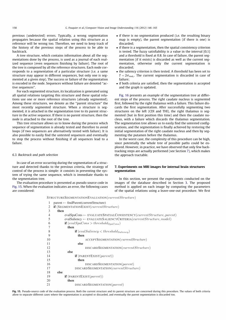
previous (undetected) errors. Typically, a wrong segmentationpropagates because the spatial relation using this structure as areference will be wrong too. Therefore, we need to keep track ofthe history of the previous steps of the process to be able tobacktrack.

A tree structure, which contains information about all the seg-mentations done by the process, is used as a journal of each real-ized sequence (even sequences finishing by failure). The root ofthe tree is composed by all the reference structures. Each node cor-responds to a segmentation of a particular structure (i.e. a samestructure may appear in different sequences, but only one is seg-mented at a given step). The success or failure of the segmentationis encoded in the node. Sequences without failure are denoted ‘‘ac-tive sequences’’.

For each segmented structure, its localization is generated usingall spatial relations targeting this structure and these spatial rela-tions use one or more reference structures (already segmented).Among these structures, we denote as the ‘‘parent structure’’ themost recently segmented structure. When a structure is seg-mented, it is attached in the segmentation tree to its parent struc-ture in the active sequence. If there is no parent structure, then thenode is attached to the root of the tree.

This tree structure allows us to know during the process whichsequence of segmentation is already tested and therefore to avoidloops (if two sequences are alternatively tested with failure). It isalso possible to easily find the untested sequences and eventuallyto stop the process without finishing if all sequences lead to afailure.

6.3. Backtrack and path selection

In case of an error occurring during the segmentation of a struc-ture and detected thanks to the previous criteria, the strategy ofcontrol of the process is simple: it consists in preventing the sys-tem of trying the same sequence, which is immediate thanks tothe segmentation tree.

The evaluation procedure is presented as pseudo source code inFig. 15. When the evaluation indicates an error, the following casesare considered:

� if there is no segmentation produced (i.e. the resulting binarymap is empty), the parent segmentation (if there is one) isdiscarded;� if there is a segmentation, then the spatial consistency criterion

is tested. The fuzzy satisfiability is a value in the interval [0,1]and a threshold is fixed at 0.8. In case of failure, the parent seg-mentation (if it exists) is discarded as well as the current seg-mentation, otherwise only the current segmentation isdiscarded;� the saliency criterion is then tested. A threshold has been set to

T ¼ 2rmodo . The current segmentation is discarded in case offailure;� if both criteria are satisfied, then the segmentation is accepted

and the graph is updated.

Fig. 16 presents an example of the segmentation tree at differ-ent steps of the process. The right caudate nucleus is segmentedfirst, followed by the right thalamus with a failure. This failure dis-cards the first segmentation. After successfully segmenting twostructures on the left (CDl and THl), the right thalamus is seg-mented (but in first position this time) and then the caudate nu-cleus, with a failure which discards the thalamus segmentation.The segmentation tree allows us to easily find the untested config-urations, and the segmentation is finally achieved by restoring theinitial segmentation of the right caudate nucleus and then by seg-menting the putamen before the thalamus.

In the worst case, the complexity of this procedure can be high,since potentially the whole tree of possible paths could be ex-plored. However, in practice, we have observed that only few back-tracking steps are actually performed (see Section 7), which makesthe approach tractable.

7. Experiments on MRI images for internal brain structuressegmentation

In this section, we present the experiments conducted on theimages of the database described in Section 3. The proposedmethod is applied on each image by computing the parametersof the spatial relations using a leave-one-out procedure. We first

Fig. 15. Pseudo-source code of the evaluation process. Both the current structure and its parent structure are concerned during this procedure. The values of both criteriaallow to separate different cases where the segmentation is accepted or discarded, and eventually the parent segmentation is discarded too.

158 G. Fouquier et al. / Computer Vision and Image Understanding 116 (2012) 146–165

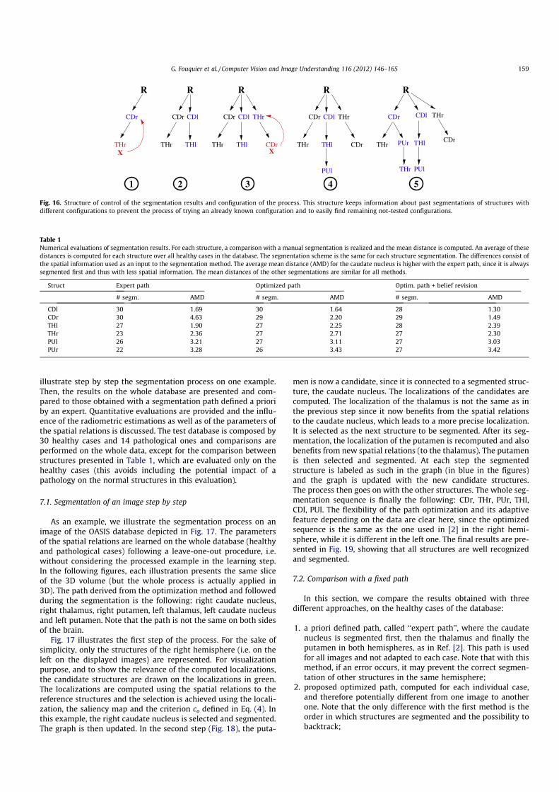
illustrate step by step the segmentation process on one example.Then, the results on the whole database are presented and com-pared to those obtained with a segmentation path defined a prioriby an expert. Quantitative evaluations are provided and the influ-ence of the radiometric estimations as well as of the parameters ofthe spatial relations is discussed. The test database is composed by30 healthy cases and 14 pathological ones and comparisons areperformed on the whole data, except for the comparison betweenstructures presented in Table 1, which are evaluated only on thehealthy cases (this avoids including the potential impact of apathology on the normal structures in this evaluation).

7.1. Segmentation of an image step by step

As an example, we illustrate the segmentation process on animage of the OASIS database depicted in Fig. 17. The parametersof the spatial relations are learned on the whole database (healthyand pathological cases) following a leave-one-out procedure, i.e.without considering the processed example in the learning step.In the following figures, each illustration presents the same sliceof the 3D volume (but the whole process is actually applied in3D). The path derived from the optimization method and followedduring the segmentation is the following: right caudate nucleus,right thalamus, right putamen, left thalamus, left caudate nucleusand left putamen. Note that the path is not the same on both sidesof the brain.

Fig. 17 illustrates the first step of the process. For the sake ofsimplicity, only the structures of the right hemisphere (i.e. on theleft on the displayed images) are represented. For visualizationpurpose, and to show the relevance of the computed localizations,the candidate structures are drawn on the localizations in green.The localizations are computed using the spatial relations to thereference structures and the selection is achieved using the locali-zation, the saliency map and the criterion co defined in Eq. (4). Inthis example, the right caudate nucleus is selected and segmented.The graph is then updated. In the second step (Fig. 18), the puta-

men is now a candidate, since it is connected to a segmented struc-ture, the caudate nucleus. The localizations of the candidates arecomputed. The localization of the thalamus is not the same as inthe previous step since it now benefits from the spatial relationsto the caudate nucleus, which leads to a more precise localization.It is selected as the next structure to be segmented. After its seg-mentation, the localization of the putamen is recomputed and alsobenefits from new spatial relations (to the thalamus). The putamenis then selected and segmented. At each step the segmentedstructure is labeled as such in the graph (in blue in the figures)and the graph is updated with the new candidate structures.The process then goes on with the other structures. The whole seg-mentation sequence is finally the following: CDr, THr, PUr, THl,CDl, PUl. The flexibility of the path optimization and its adaptivefeature depending on the data are clear here, since the optimizedsequence is the same as the one used in [2] in the right hemi-sphere, while it is different in the left one. The final results are pre-sented in Fig. 19, showing that all structures are well recognizedand segmented.

7.2. Comparison with a fixed path

In this section, we compare the results obtained with threedifferent approaches, on the healthy cases of the database:

1. a priori defined path, called ‘‘expert path’’, where the caudatenucleus is segmented first, then the thalamus and finally theputamen in both hemispheres, as in Ref. [2]. This path is usedfor all images and not adapted to each case. Note that with thismethod, if an error occurs, it may prevent the correct segmen-tation of other structures in the same hemisphere;

2. proposed optimized path, computed for each individual case,and therefore potentially different from one image to anotherone. Note that the only difference with the first method is theorder in which structures are segmented and the possibility tobacktrack;

R

X

CDr

THr

1

R

CDr

THr

CDl

THl

2

R

CDr

THr

CDl

THl

THr

CDrX

3

R

CDr

THr

CDl

THl CDr

THr

PUl

4

CDl

THl

PUl

R

THr

CDr

PUr

THr

THr

CDr

5

Fig. 16. Structure of control of the segmentation results and configuration of the process. This structure keeps information about past segmentations of structures withdifferent configurations to prevent the process of trying an already known configuration and to easily find remaining not-tested configurations.

Table 1Numerical evaluations of segmentation results. For each structure, a comparison with a manual segmentation is realized and the mean distance is computed. An average of thesedistances is computed for each structure over all healthy cases in the database. The segmentation scheme is the same for each structure segmentation. The differences consist ofthe spatial information used as an input to the segmentation method. The average mean distance (AMD) for the caudate nucleus is higher with the expert path, since it is alwayssegmented first and thus with less spatial information. The mean distances of the other segmentations are similar for all methods.

Struct Expert path Optimized path Optim. path + belief revision

# segm. AMD # segm. AMD # segm. AMD

CDl 30 1.69 30 1.64 28 1.30CDr 30 4.63 29 2.20 29 1.49THl 27 1.90 27 2.25 28 2.39THr 23 2.36 27 2.71 27 2.30PUl 26 3.21 27 3.11 27 3.03PUr 22 3.28 26 3.43 27 3.42

G. Fouquier et al. / Computer Vision and Image Understanding 116 (2012) 146–165 159

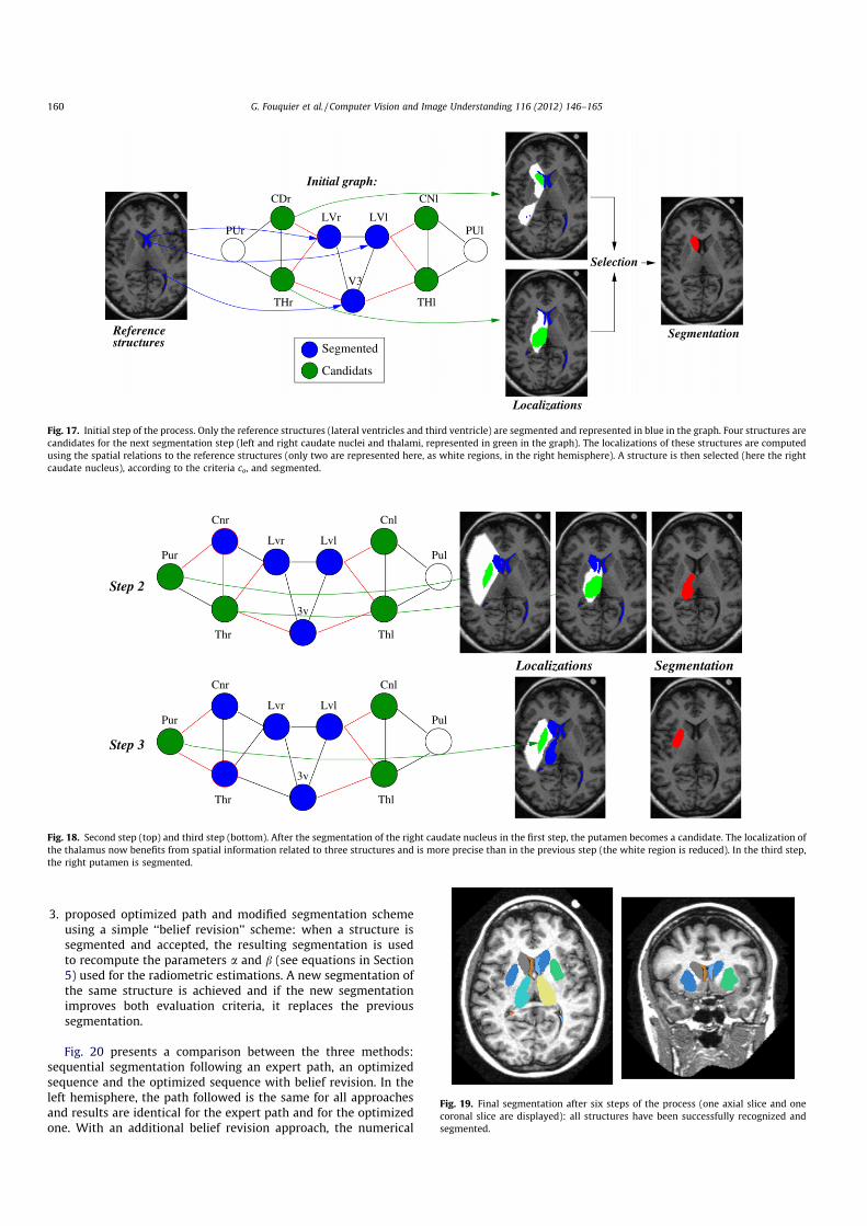
3. proposed optimized path and modified segmentation schemeusing a simple ‘‘belief revision’’ scheme: when a structure issegmented and accepted, the resulting segmentation is usedto recompute the parameters a and b (see equations in Section5) used for the radiometric estimations. A new segmentation ofthe same structure is achieved and if the new segmentationimproves both evaluation criteria, it replaces the previoussegmentation.

Fig. 20 presents a comparison between the three methods:sequential segmentation following an expert path, an optimizedsequence and the optimized sequence with belief revision. In theleft hemisphere, the path followed is the same for all approachesand results are identical for the expert path and for the optimizedone. With an additional belief revision approach, the numerical

Segmentation

Localizations

Selection

Candidats

Segmented

CDr

PUr

THr

LVr LVl

CNl

THl

PUl

V3

Initial graph:

Referencestructures

Fig. 17. Initial step of the process. Only the reference structures (lateral ventricles and third ventricle) are segmented and represented in blue in the graph. Four structures arecandidates for the next segmentation step (left and right caudate nuclei and thalami, represented in green in the graph). The localizations of these structures are computedusing the spatial relations to the reference structures (only two are represented here, as white regions, in the right hemisphere). A structure is then selected (here the rightcaudate nucleus), according to the criteria co, and segmented.

Step 2

Step 3

LvlLvr

3v

Thr

Cnl

Pul

Thl

Pur

Cnr

LvlLvr

3v

Thr

Cnl

Pul

Thl

Pur

Cnr

SegmentationLocalizations

Fig. 18. Second step (top) and third step (bottom). After the segmentation of the right caudate nucleus in the first step, the putamen becomes a candidate. The localization ofthe thalamus now benefits from spatial information related to three structures and is more precise than in the previous step (the white region is reduced). In the third step,the right putamen is segmented.

Fig. 19. Final segmentation after six steps of the process (one axial slice and onecoronal slice are displayed): all structures have been successfully recognized andsegmented.

160 G. Fouquier et al. / Computer Vision and Image Understanding 116 (2012) 146–165

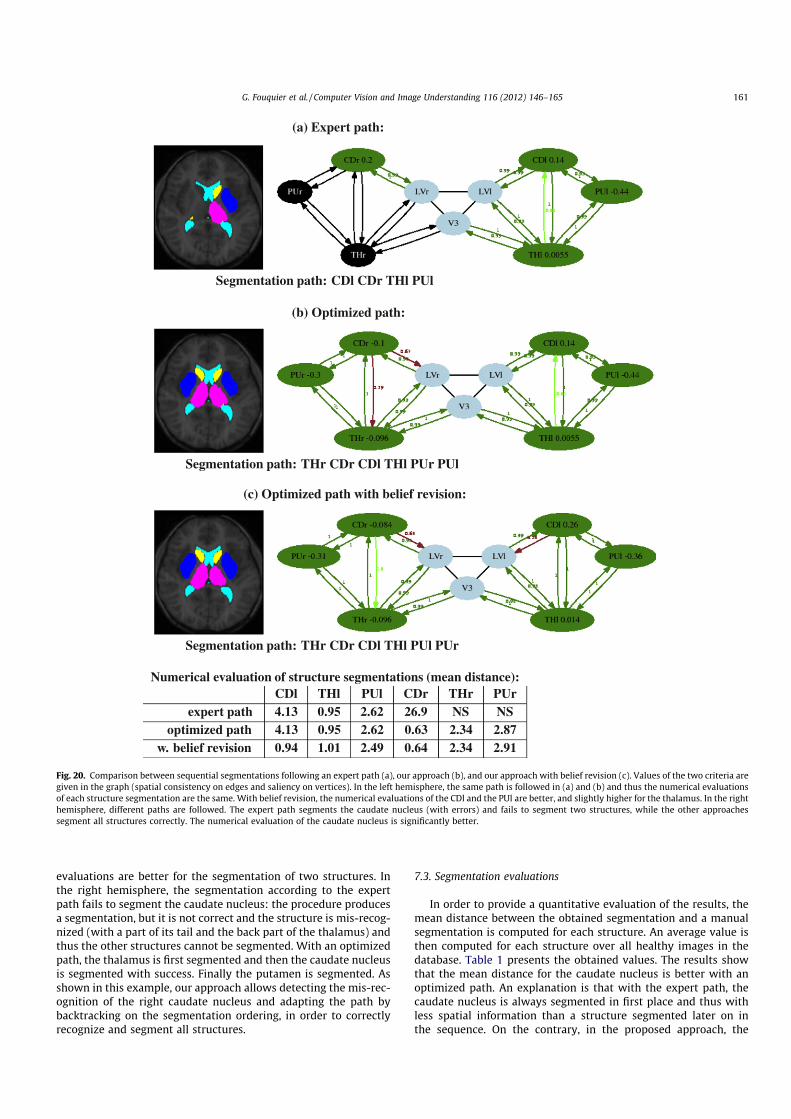
evaluations are better for the segmentation of two structures. Inthe right hemisphere, the segmentation according to the expertpath fails to segment the caudate nucleus: the procedure producesa segmentation, but it is not correct and the structure is mis-recog-nized (with a part of its tail and the back part of the thalamus) andthus the other structures cannot be segmented. With an optimizedpath, the thalamus is first segmented and then the caudate nucleusis segmented with success. Finally the putamen is segmented. Asshown in this example, our approach allows detecting the mis-rec-ognition of the right caudate nucleus and adapting the path bybacktracking on the segmentation ordering, in order to correctlyrecognize and segment all structures.

7.3. Segmentation evaluations

In order to provide a quantitative evaluation of the results, themean distance between the obtained segmentation and a manualsegmentation is computed for each structure. An average value isthen computed for each structure over all healthy images in thedatabase. Table 1 presents the obtained values. The results showthat the mean distance for the caudate nucleus is better with anoptimized path. An explanation is that with the expert path, thecaudate nucleus is always segmented in first place and thus withless spatial information than a structure segmented later on inthe sequence. On the contrary, in the proposed approach, the

(a) Expert path:

Segmentation path: CDl CDr THl PUl

(b) Optimized path:

Segmentation path: THr CDr CDl THl PUr PUl

(c) Optimized path with belief revision:

Segmentation path: THr CDr CDl THl PUl PUr

Numerical evaluation of structure segmentations (mean distance):CDl THl PUl CDr THr PUr

expert path 4.13 0.95 2.62 26.9 NS NSoptimized path 4.13 0.95 2.62 0.63 2.34 2.87

w. belief revision 0.94 1.01 2.49 0.64 2.34 2.91

Fig. 20. Comparison between sequential segmentations following an expert path (a), our approach (b), and our approach with belief revision (c). Values of the two criteria aregiven in the graph (spatial consistency on edges and saliency on vertices). In the left hemisphere, the same path is followed in (a) and (b) and thus the numerical evaluationsof each structure segmentation are the same. With belief revision, the numerical evaluations of the CDl and the PUl are better, and slightly higher for the thalamus. In the righthemisphere, different paths are followed. The expert path segments the caudate nucleus (with errors) and fails to segment two structures, while the other approachessegment all structures correctly. The numerical evaluation of the caudate nucleus is significantly better.

G. Fouquier et al. / Computer Vision and Image Understanding 116 (2012) 146–165 161

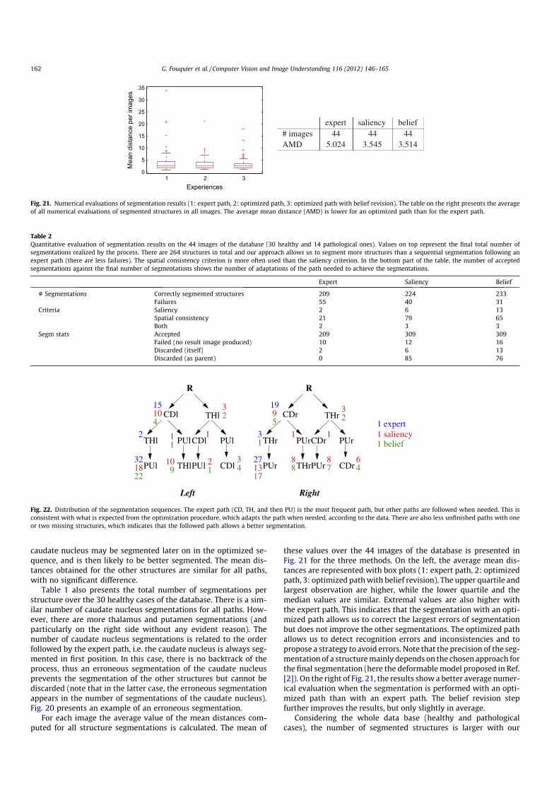
caudate nucleus may be segmented later on in the optimized se-quence, and is then likely to be better segmented. The mean dis-tances obtained for the other structures are similar for all paths,with no significant difference.

Table 1 also presents the total number of segmentations perstructure over the 30 healthy cases of the database. There is a sim-ilar number of caudate nucleus segmentations for all paths. How-ever, there are more thalamus and putamen segmentations (andparticularly on the right side without any evident reason). Thenumber of caudate nucleus segmentations is related to the orderfollowed by the expert path, i.e. the caudate nucleus is always seg-mented in first position. In this case, there is no backtrack of theprocess, thus an erroneous segmentation of the caudate nucleusprevents the segmentation of the other structures but cannot bediscarded (note that in the latter case, the erroneous segmentationappears in the number of segmentations of the caudate nucleus).Fig. 20 presents an example of an erroneous segmentation.

For each image the average value of the mean distances com-puted for all structure segmentations is calculated. The mean of

these values over the 44 images of the database is presented inFig. 21 for the three methods. On the left, the average mean dis-tances are represented with box plots (1: expert path, 2: optimizedpath, 3: optimized path with belief revision). The upper quartile andlargest observation are higher, while the lower quartile and themedian values are similar. Extremal values are also higher withthe expert path. This indicates that the segmentation with an opti-mized path allows us to correct the largest errors of segmentationbut does not improve the other segmentations. The optimized pathallows us to detect recognition errors and inconsistencies and topropose a strategy to avoid errors. Note that the precision of the seg-mentation of a structure mainly depends on the chosen approach forthe final segmentation (here the deformable model proposed in Ref.[2]). On the right of Fig. 21, the results show a better average numer-ical evaluation when the segmentation is performed with an opti-mized path than with an expert path. The belief revision stepfurther improves the results, but only slightly in average.

Considering the whole data base (healthy and pathologicalcases), the number of segmented structures is larger with our

0

5

10

15

20

25

30

35

321Experiences

Mea

n di

stan

ce p

er im

ages

expert saliency belief# images 44 44 44AMD 5.024 3.545 3.514

Fig. 21. Numerical evaluations of segmentation results (1: expert path, 2: optimized path, 3: optimized path with belief revision). The table on the right presents the averageof all numerical evaluations of segmented structures in all images. The average mean distance (AMD) is lower for an optimized path than for the expert path.

Table 2Quantitative evaluation of segmentation results on the 44 images of the database (30 healthy and 14 pathological ones). Values on top represent the final total number ofsegmentations realized by the process. There are 264 structures in total and our approach allows us to segment more structures than a sequential segmentation following anexpert path (there are less failures). The spatial consistency criterion is more often used than the saliency criterion. In the bottom part of the table, the number of acceptedsegmentations against the final number of segmentations shows the number of adaptations of the path needed to achieve the segmentations.

Expert Saliency Belief

# Segmentations Correctly segmented structures 209 224 233Failures 55 40 31

Criteria Saliency 2 6 13Spatial consistency 21 79 65Both 2 3 3

Segm stats Accepted 209 309 309Failed (no result image produced) 10 12 16Discarded (itself) 2 6 13Discarded (as parent) 0 85 76

Fig. 22. Distribution of the segmentation sequences. The expert path (CD, TH, and then PU) is the most frequent path, but other paths are followed when needed. This isconsistent with what is expected from the optimization procedure, which adapts the path when needed, according to the data. There are also less unfinished paths with oneor two missing structures, which indicates that the followed path allows a better segmentation.

162 G. Fouquier et al. / Computer Vision and Image Understanding 116 (2012) 146–165

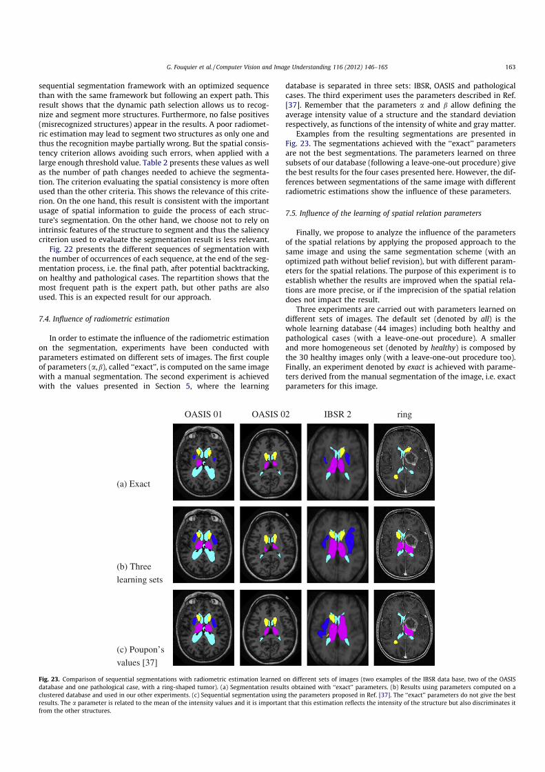
sequential segmentation framework with an optimized sequencethan with the same framework but following an expert path. Thisresult shows that the dynamic path selection allows us to recog-nize and segment more structures. Furthermore, no false positives(misrecognized structures) appear in the results. A poor radiomet-ric estimation may lead to segment two structures as only one andthus the recognition maybe partially wrong. But the spatial consis-tency criterion allows avoiding such errors, when applied with alarge enough threshold value. Table 2 presents these values as wellas the number of path changes needed to achieve the segmenta-tion. The criterion evaluating the spatial consistency is more oftenused than the other criteria. This shows the relevance of this crite-rion. On the one hand, this result is consistent with the importantusage of spatial information to guide the process of each struc-ture’s segmentation. On the other hand, we choose not to rely onintrinsic features of the structure to segment and thus the saliencycriterion used to evaluate the segmentation result is less relevant.

Fig. 22 presents the different sequences of segmentation withthe number of occurrences of each sequence, at the end of the seg-mentation process, i.e. the final path, after potential backtracking,on healthy and pathological cases. The repartition shows that themost frequent path is the expert path, but other paths are alsoused. This is an expected result for our approach.

7.4. Influence of radiometric estimation

In order to estimate the influence of the radiometric estimationon the segmentation, experiments have been conducted withparameters estimated on different sets of images. The first coupleof parameters (a,b), called ‘‘exact’’, is computed on the same imagewith a manual segmentation. The second experiment is achievedwith the values presented in Section 5, where the learning

database is separated in three sets: IBSR, OASIS and pathologicalcases. The third experiment uses the parameters described in Ref.[37]. Remember that the parameters a and b allow defining theaverage intensity value of a structure and the standard deviationrespectively, as functions of the intensity of white and gray matter.

Examples from the resulting segmentations are presented inFig. 23. The segmentations achieved with the ‘‘exact’’ parametersare not the best segmentations. The parameters learned on threesubsets of our database (following a leave-one-out procedure) givethe best results for the four cases presented here. However, the dif-ferences between segmentations of the same image with differentradiometric estimations show the influence of these parameters.

7.5. Influence of the learning of spatial relation parameters

Finally, we propose to analyze the influence of the parametersof the spatial relations by applying the proposed approach to thesame image and using the same segmentation scheme (with anoptimized path without belief revision), but with different param-eters for the spatial relations. The purpose of this experiment is toestablish whether the results are improved when the spatial rela-tions are more precise, or if the imprecision of the spatial relationdoes not impact the result.

Three experiments are carried out with parameters learned ondifferent sets of images. The default set (denoted by all) is thewhole learning database (44 images) including both healthy andpathological cases (with a leave-one-out procedure). A smallerand more homogeneous set (denoted by healthy) is composed bythe 30 healthy images only (with a leave-one-out procedure too).Finally, an experiment denoted by exact is achieved with parame-ters derived from the manual segmentation of the image, i.e. exactparameters for this image.

OASIS 01 OASIS 02 IBSR 2 ring

(a) Exact

(b) Three

learning sets

(c) Poupon’s

values [37]

Fig. 23. Comparison of sequential segmentations with radiometric estimation learned on different sets of images (two examples of the IBSR data base, two of the OASISdatabase and one pathological case, with a ring-shaped tumor). (a) Segmentation results obtained with ‘‘exact’’ parameters. (b) Results using parameters computed on aclustered database and used in our other experiments. (c) Sequential segmentation using the parameters proposed in Ref. [37]. The ‘‘exact’’ parameters do not give the bestresults. The a parameter is related to the mean of the intensity values and it is important that this estimation reflects the intensity of the structure but also discriminates itfrom the other structures.

G. Fouquier et al. / Computer Vision and Image Understanding 116 (2012) 146–165 163

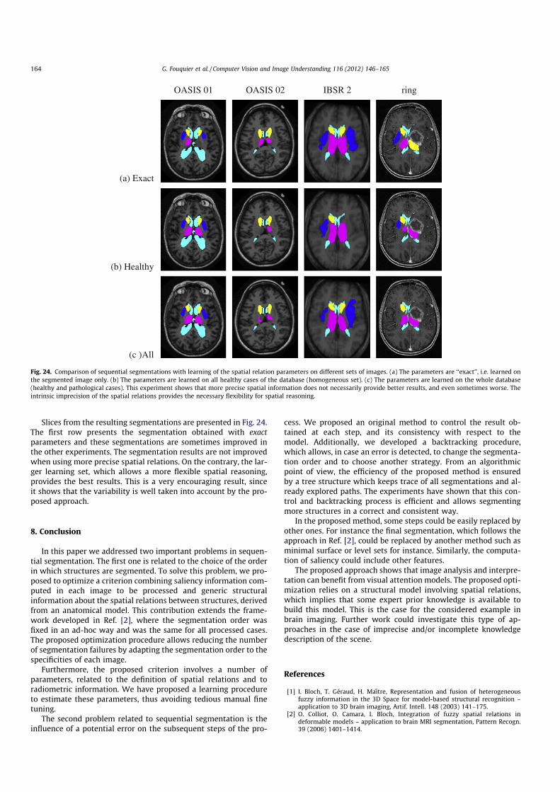
Slices from the resulting segmentations are presented in Fig. 24.The first row presents the segmentation obtained with exactparameters and these segmentations are sometimes improved inthe other experiments. The segmentation results are not improvedwhen using more precise spatial relations. On the contrary, the lar-ger learning set, which allows a more flexible spatial reasoning,provides the best results. This is a very encouraging result, sinceit shows that the variability is well taken into account by the pro-posed approach.

8. Conclusion

In this paper we addressed two important problems in sequen-tial segmentation. The first one is related to the choice of the orderin which structures are segmented. To solve this problem, we pro-posed to optimize a criterion combining saliency information com-puted in each image to be processed and generic structuralinformation about the spatial relations between structures, derivedfrom an anatomical model. This contribution extends the frame-work developed in Ref. [2], where the segmentation order wasfixed in an ad-hoc way and was the same for all processed cases.The proposed optimization procedure allows reducing the numberof segmentation failures by adapting the segmentation order to thespecificities of each image.

Furthermore, the proposed criterion involves a number ofparameters, related to the definition of spatial relations and toradiometric information. We have proposed a learning procedureto estimate these parameters, thus avoiding tedious manual finetuning.

The second problem related to sequential segmentation is theinfluence of a potential error on the subsequent steps of the pro-

cess. We proposed an original method to control the result ob-tained at each step, and its consistency with respect to themodel. Additionally, we developed a backtracking procedure,which allows, in case an error is detected, to change the segmenta-tion order and to choose another strategy. From an algorithmicpoint of view, the efficiency of the proposed method is ensuredby a tree structure which keeps trace of all segmentations and al-ready explored paths. The experiments have shown that this con-trol and backtracking process is efficient and allows segmentingmore structures in a correct and consistent way.

In the proposed method, some steps could be easily replaced byother ones. For instance the final segmentation, which follows theapproach in Ref. [2], could be replaced by another method such asminimal surface or level sets for instance. Similarly, the computa-tion of saliency could include other features.

The proposed approach shows that image analysis and interpre-tation can benefit from visual attention models. The proposed opti-mization relies on a structural model involving spatial relations,which implies that some expert prior knowledge is available tobuild this model. This is the case for the considered example inbrain imaging. Further work could investigate this type of ap-proaches in the case of imprecise and/or incomplete knowledgedescription of the scene.

References

[1] I. Bloch, T. Géraud, H. Maıtre, Representation and fusion of heterogeneousfuzzy information in the 3D Space for model-based structural recognition –application to 3D brain imaging, Artif. Intell. 148 (2003) 141–175.

[2] O. Colliot, O. Camara, I. Bloch, Integration of fuzzy spatial relations indeformable models – application to brain MRI segmentation, Pattern Recogn.39 (2006) 1401–1414.

OASIS 01 OASIS 02 IBSR 2 ring

(a) Exact

(b) Healthy

(c )All

Fig. 24. Comparison of sequential segmentations with learning of the spatial relation parameters on different sets of images. (a) The parameters are ‘‘exact’’, i.e. learned onthe segmented image only. (b) The parameters are learned on all healthy cases of the database (homogeneous set). (c) The parameters are learned on the whole database(healthy and pathological cases). This experiment shows that more precise spatial information does not necessarily provide better results, and even sometimes worse. Theintrinsic imprecision of the spatial relations provides the necessary flexibility for spatial reasoning.

164 G. Fouquier et al. / Computer Vision and Image Understanding 116 (2012) 146–165

[3] O. Colliot, Representation, évaluation et utilisation de relations spatiales pourl’interprétation d’images. Applications à la reconnaissance de structuresanatomiques en imagerie médicale, Ph.D. thesis, ENST, 2003.

[4] U. Neisser, Cognitive psychology, Appleton-Century-Crofts, 1967.[5] A. Treisman, G. Gelade, A feature-integration theory of attention, Cognitive

Psychol. 12 (1980) 97–136.[6] A. Treisman, Preattentive processing in vision, Comput. Vision Graph. Image

Process. 31 (2) (1985) 156–177. doi:http://www.dx.doi.org/10.1016/S0734-189X(85)80004-9.

[7] D. Crevier, R. Lepage, Knowledge-based image understanding systems: asurvey, Comput. Vis. Image Understand. 67 (2) (1997) 161–185, doi:10.1006/cviu.1996.0520.

[8] F. Le Ber, J. Lieber, A. Napoli, Les systèmes à base de connaissances, in: J. Akoka,I. Comyn Wattiau (Eds.), Encyclopédie de l’informatique et des systèmesd’information, Vuibert, 2006, pp. 1197–1208.

[9] J. Talairach, P. Tournoux, Co-Planar Stereotaxic Atlas of the Human Brain 3-Dimensional Proportional System: An Approach to Cerebral Imaging, Thieme,1988.

[10] D. Bowden, M. Dubach, Neuroanatomical Nomenclature and Ontology, JohnWiley and Sons, Inc., 2005. Ch. Databasing the Brain.

[11] C. Rosse, J.L. Mejino, Anatomy Ontologies for Bioinformatics: Principles andPractice, Springer, 2007, Ch. The Foundational Model of Anatomy Ontology, pp.59–117.

[12] J. Atif, C. Hudelot, O. Nempont, N. Richard, B. Batrancourt, E. Angelini, I. Bloch,GRAFIP: A Framework for the Representation of Healthy and PathologicalCerebral Information, in: IEEE International Symposium on BiomedicalImaging (ISBI), Washington DC, USA, 2007, pp. 205–208.

[13] D. Conte, P. Foggia, C. Sansone, M. Vento, Thirty years of graph matching inpattern recognition, Int. J. Pattern Rec. Art. Intell. 18 (3) (2004) 265–298.

[14] A. Perchant, Morphisme de graphes d’attributs flous pour la reconnaissancestructurelle de scènes, Ph.D. thesis, Ecole nationale supérieure destélécommunications, Paris, France, 2000.

[15] A. Perchant, I. Bloch, Fuzzy morphisms between graphs, Fuzzy Sets Syst. 128(2) (2002) 149–168.

[16] E. Bengoetxea, P. Larranaga, I. Bloch, A. Perchant, C. Boeres, Inexact graphmatching by means of estimation of distribution algorithms, Pattern Recogn.35 (2002) 2867–2880.

[17] R. Cesar, E. Bengoetxea, I. Bloch, P. Larranaga, Inexact graph matching formodel-based recognition: evaluation and comparison of optimizationalgorithms, Pattern Recogn. 38 (2005) 2099–2113.

[18] A. Deruyver, Y. Hodé, E. Leammer, J.-M. Jolion, Adaptive pyramid and semanticgraph: knowledge driven segmentation, in: Graph-Based Representations inPattern Recognition: 5th IAPR International Workshop, vol. 3434, Springer-Verlag GmbH, Poitiers, France, 2005, pp. 213–222.

[19] A. Deruyver, Y. Hodé, L. Brun, Image interpretation with a conceptual graph:labeling over-segmented images and detection of unexpected objects, Artif.Intell. 173 (14) (2009) 1245–1265. doi:http://www.dx.doi.org/10.1016/j.artint.2009.05.003..

[20] O. Nempont, Modèles structurels flous et propagation de contraintes pour lasegmentation et la reconnaissance d’objets dans les images. application auxstructures normales et pathologiques du cerveau en IRM, Ph.D. thesis, EcoleNationale Supérieure des Télécommunications (Mars 2009).

[21] O. Nempont, J. Atif, E. Angelini, I. Bloch, Structure Segmentation andRecognition in Images Guided by Structural Constraint Propagation, in:European Conference on Artificial Intelligence ECAI, Patras, Greece, 2008, pp.621–625.

[22] I. Bloch, Fuzzy spatial relationships for image processing and interpretation: areview, Image Vision Comput 23 (2) (2005) 89–110.

[23] D. Dubois, H. Prade, Fuzzy Sets and Systems: Theory and Applications,Academic Press, New-York, 1980.

[24] I. Bloch, Fuzzy relative position between objects in image processing: amorphological approach, IEEE Trans. Pattern Anal. Mach. Intell. 21 (7) (1999)657–664.

[25] J. Atif, C. Hudelot, G. Fouquier, I. Bloch, E. Angelini, From generic knowledge tospecific reasoning for medical image interpretation using graph-basedrepresentations, in: International Joint Conference on Artificial IntelligenceIJCAI’07, Hyderabad, India, 2007, pp. 224–229.

[26] A. Treisman, Search, similarity, and integration of features between and withindimensions, J. Exp. Psychol.: Hum. Percept. Perform. 17 (3) (1991) 652–676.

[27] C. Healey, Perception in visualization, available at: http://www.csc.ncsu.edu/faculty/healey/PP/index.html (2007).

[28] L. Itti, C. Koch, E. Niebur, A model of saliency-based visual attention for rapidscene analysis, IEEE Trans. Pattern Anal. Mach. Intell. 20 (11) (1998) 1254–1259.

[29] C. Koch, S. Ullman, Shifts in selective visual attention: towards the underlyingneural circuitry, Hum. Neurobiol. 4 (4) (1985) 219–227.

[30] J.-F. Mangin, O. Coulon, V. Frouin, Robust brain segmentation using histogramscale-space analysis and mathematical morphology, in: Medical ImageComputing and Computer-Assisted Interventation, 1998, p. 1230.

[31] P. Thevenaz, T. Blu, M. Unser, Interpolation revisited, IEEE Trans. Med. Imag. 19(7) (2000) 739–758.

[32] T.R. Reed, Motion analysis using the 3D Gabor transform, IEEE (1997) 506–509.[33] Y. Wang, C. Chua, Face recognition from 2D and 3D images using 3d gabor

filters, Image Vision Comput 23 (2005) 1018–1028.[34] L. Itti, C. Koch, Feature combination strategies for saliency-based visual

attention systems, J. Electr. Imag. 10 (1) (2001) 161–169.[35] Y. Rubner, C. Tomasi, L. Guibas, A metric for distributions with applications to

image databases, in: Sixth International Conference on Computer Vision,Bombay, India, 1998, pp. 59–66.

[36] C. Villani, Topics in optimal transportation, American Math. Soc., 2003.[37] F. Poupon, J.-F. Mangin, D. Hasboun, C. Poupon, I. Magnin, V. Frouin, Multi-

object deformable templates dedicated to the segmentation of brain deepstructures, in: Medical Image Computing and Computer-AssistedInterventation, vol. 1496, 2008, p. 1134.

[38] B. Bouchon-Meunier, M. Rifqi, S. Bothorel, Towards general measures ofcomparison of objects, Fuzzy Sets Syst. 84 (2) (1996) 143–153.

Geoffroy Fouquier received a PhD in image processingfrom Telecom ParisTech in 2010 and the M.Sc. degree inartificial intelligence from the Paris VI university in2006. His PhD was followed by a post-doctoral positionabout semi-automatic whole-body MRI segmentationdedicated to dosimetry studies. He is now researchengineer at eXenSa working on collaborative filteringand latent semantic analysis. His main research inter-ests include spatial reasoning, graph representations,model and knowledge-based recognition of imagestructures, pre-attentive mechanisms, medical imagesand anatomical models.

Jamal Atif is an associate professor of computer sci-ences at Paris-Sud XI University performing his researchwithin the Machine Learning and Optimization team(project team TAO, INRIA) at the Computer Sciences Lab(LRI, CNRS/Paris-Sud XI University). From 2006 to 2010,he was a research scientist at IRD (Institut de Recherchepour le Développement), Unité ESPACE S140 and asso-ciate professor of computer sciences at the University ofFrench West Indies. He received a master degree andPhD in computer sciences and medical imaging from theUniversity of Paris-XI in 2000 and 2004. His researchinterests focus on computer vision and knowledge

based image understanding (semantic image interpretation) for medical and earthobservation applications. He works on fields arising from information theory, graphtheory, uncertainty management (fuzzy sets), ontological engineering (descriptionlogics), mathematical morphology, spatial reasoning and machine learning.

Isabelle Bloch is professor at the Signal and ImageProcessing Department of Telecom ParisTech – CNRSLTCI, in charge of the Image Processing and Under-standing group. Her research interests include 3-Dimage and object processing, computer vision, 3-D,fuzzy and logics mathematical morphology, informationfusion, fuzzy set theory, structural, graph-based andknowledge-based object recognition, spatial reasoning,and medical imaging.

G. Fouquier et al. / Computer Vision and Image Understanding 116 (2012) 146–165 165

This article appeared in a journal published by Elsevier. The attachedcopy is furnished to the author for internal non-commercial researchand education use, including for instruction at the authors institution

and sharing with colleagues.

Other uses, including reproduction and distribution, or selling orlicensing copies, or posting to personal, institutional or third party

websites are prohibited.

In most cases authors are permitted to post their version of thearticle (e.g. in Word or Tex form) to their personal website orinstitutional repository. Authors requiring further information

regarding Elsevier’s archiving and manuscript policies areencouraged to visit:

http://www.elsevier.com/authorsrights

Author's personal copy

A constraint propagation approach to structural model basedimage segmentation and recognition

Olivier Nempont a,c, Jamal Atif b, Isabelle Bloch a,!a Institut Mines-Telecom, Telecom ParisTech, CNRS LTCI, 46 rue Barrault, 75013 Paris, Franceb TAO INRIA, CNRS, LRI – Paris-Sud University, 91405 Orsay Cedex, FrancecPhilips Research, 33 rue de Verdun, 92150 Suresnes, France

a r t i c l e i n f o

Article history:Received 11 January 2012Received in revised form 11 April 2013Accepted 16 May 2013Available online 28 May 2013

Keywords:Image interpretationConstraint satisfactionFuzzy setStructural model

a b s t r a c t

The interpretation of complex scenes in images requires knowledge regarding the objectsin the scene and their spatial arrangement. We propose a method for simultaneously seg-menting and recognizing objects in images, that is based on a structural representation ofthe scene and a constraint propagation method. The structural model is a graph represent-ing the objects in the scene, their appearance and their spatial relations, represented byfuzzy models. The proposed solver is a novel global method that assigns spatial regionsto the objects according to the relations in the structural model. We propose to progres-sively reduce the solution domain by excluding assignments that are inconsistent with aconstraint network derived from the structural model. The final segmentation of eachobject is then performed as a minimal surface extraction. The contributions of this paperare illustrated through the example of brain structure recognition in magnetic resonanceimages.

! 2013 Elsevier Inc. All rights reserved.

1. Introduction

The interpretation of complex scenes in images often requires (or can benefit from) a model of the scene. This model mayprovide information regarding the objects contained in the scene, as well as their spatial arrangement. The spatial layoutinformation is often crucial for differentiating among objects with similar appearances in the images, or disambiguatingcomplex cases. Examples occur in many domains, including medical imaging, in which structural knowledge can help inthe interpretation of the images. In magnetic resonance imaging (MRI), for instance, radiometry is often insufficient for rec-ognizing individual anatomical structures, and their relative spatial configuration provides an important input into the rec-ognition process [17]. Other examples occur in aerial and satellite imaging, robot vision, and video sequence interpretation,among other fields. In this paper, we address the image interpretation problem as a joint problem of image segmentation andobject recognition, based on structural information. Although the focus of the paper is methodological and theoretical,remaining as generic as possible, we illustrate the proposed method through the concrete example of 3D brain MRIinterpretation.

Graphs are often used to represent the structural information in image interpretation, where the vertices represent ob-jects or image regions (and may carry attributes such as their shapes, sizes, and colors or gray levels), and the edges carry thestructural information, such as the spatial relations among objects, or radiometric contrasts between regions. Although thistype of representation has become popular in the last 30 years [18], a number of open problems remain in its efficient imple-

0020-0255/$ - see front matter ! 2013 Elsevier Inc. All rights reserved.http://dx.doi.org/10.1016/j.ins.2013.05.030

! Corresponding author.E-mail address: isabelle.bloch@telecom-paristech.fr (I. Bloch).

Information Sciences 246 (2013) 1–27

Contents lists available at SciVerse ScienceDirect

Information Sciences

journal homepage: www.elsevier .com/locate / ins

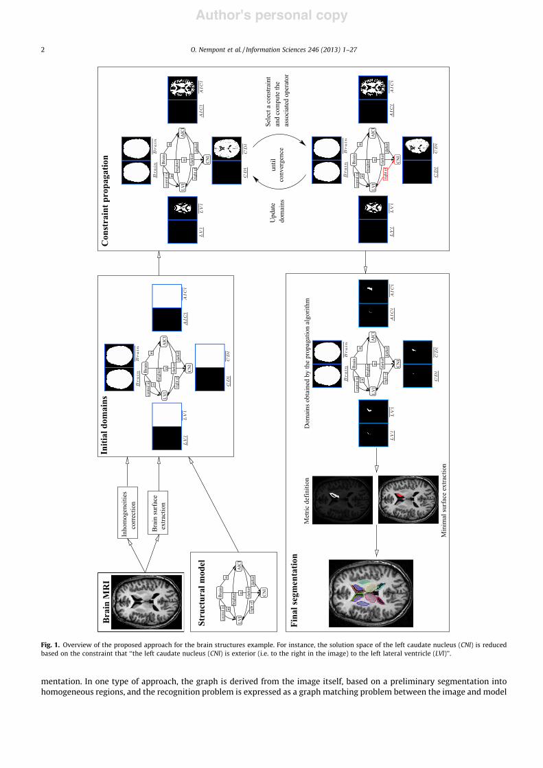
Author's personal copy

mentation. In one type of approach, the graph is derived from the image itself, based on a preliminary segmentation intohomogeneous regions, and the recognition problem is expressed as a graph matching problem between the image and model

Fig. 1. Overview of the proposed approach for the brain structures example. For instance, the solution space of the left caudate nucleus (CNl) is reducedbased on the constraint that ‘‘the left caudate nucleus (CNl) is exterior (i.e. to the right in the image) to the left lateral ventricle (LVl)’’.

2 O. Nempont et al. / Information Sciences 246 (2013) 1–27

Author's personal copy

graphs, which is an annotation problem. However this scheme often requires solving complex combinatorial problems [18].Improvements can be achieved by suppressing iteratively inconsistent annotations using a constraint propagation proce-dure, as proposed e.g. in [50,58] for simple geometrical figures or in [31,56] for the annotation of image segmentations. How-ever, the constraint propagation procedure does not guarantee a unique annotation. Moreover, all of these approachesassume a correct initial segmentation of the image. However, the segmentation problem is a known challenge in image pro-cessing, to which no universal solution exists. The segmentation is usually imperfect, and no isomorphism exists betweenthe graphs being matched. An inexact matching must then be found, for instance by allowing several image regions to beassigned to one model vertex or by relaxing the notion of morphism to that of fuzzy morphism [14,46]. For example, pre-vious studies [19,20] employ an over-segmentation of the image, which is easier to obtain. A model structure (i.e. a graphvertex) is then explicitly associated with a set of regions, and the recognition problem is expressed as a constraint satisfac-tion problem. To overcome the complexity issue, a weaker version of the model relations (encoded in the edges) is consid-ered, and the problem is solved using a modified AC-4 propagation algorithm [38]. Other recent approaches, still based on apreliminary segmentation, have revisited the grammatical approach to pattern recognition [48,57,65,66], or employed prob-abilistic models [27,61,64] or ontologies [29,44].

To deal with the difficulty of obtaining a relevant segmentation, the segmentation and recognition can also be performedsimultaneously. For instance, in the method proposed in previous studies [8,17], the structures of interest are segmented andrecognized sequentially, in a pre-calculated order [23]. The structures that are easier to segment are considered first andadopted as reference objects. The spatial relations to these structures are encoded in the structural model and are used asconstraints to guide the segmentation and recognition of other structures. Due to the sequential nature of the process,the errors are potentially propagated. Backtracking may then be needed, as proposed in [23].

To overcome the problems raised by sequential approaches while avoiding the need for an initial segmentation, we pro-pose an original method that still employs a structural model, but solves the problem in a global fashion. Our definition of asolution is the assignment of a spatial region to each model object, in a way that satisfies the constraints expressed in themodel. We propose a progressive reduction of the solution domain for all objects by excluding assignments that are incon-sistent with the structural model. Constraint networks constitute an appropriate framework for both the formalization of theproblem and the optimization. An original feature of the proposed approach is that the regions are not predetermined, butare instead constructed during the reduction process. The image segmentation and recognition algorithm therefore differsfrom an annotation procedure, and no prior segmentation of the image into meaningful or homogeneous regions is required.This feature overcomes the limitations of many previous approaches (such as [19,20]). More precisely, a constraint networkis constructed from the structural model, and a propagation algorithm is then designed to reduce the search space. Finally, anapproximate solution is extracted from the reduced search space. This procedure is illustrated in Fig. 1, using the interpre-tation of a brain MRI as an example. Once the propagation process terminates, the solution space is typically reduced sub-stantially for all of the model structures. The final segmentation and recognition results can then be obtained using anysegmentation method that is constrained by this solution space.

In Section 2, we summarize the main components of the structural model. Some preliminaries on constraint networks arereviewed in Section 3. The novel contributions of this paper are described in Sections 4 and 5, extending our preliminarywork in [42]. We describe the expression of the constraints in detail, and propose propagators that are adapted to each typeof constraint. The power and tractability of the proposed approach are illustrated using both a synthetic example and a real-world example, in which anatomical brain structures are recognized in MR images (Section 6).

2. Graphical structural model

The structural model used in this paper was developed previously in [8,17,29]. The model consists of a graph in which thevertices represent objects, and the edges encode structural relations and relations describing the radiometric contrasts. Boththe vertices and the edges have attributes. As an original feature of this model, spatial relations are represented using fuzzymodels [5], which define the semantics of the relations, and enable us to link abstract concepts to spatial representations[29]. This approach helps filling the semantic gap between symbolic information and the visual percepts that are extractedfrom the images.

We now describe this model in the context of the brain structures example (these structures are then the objects to berecognized in a medical image). Brain anatomy is commonly described in a hierarchical fashion [10,35], and can be formal-ized using ontologies. One of these ontologies is the Foundational Model of Anatomy (FMA) [51]. In addition, the spatial orga-nization of the anatomical structures is a major component of linguistic descriptions of the brain anatomy [28,60], and hastherefore been added to the existing ontology [29]. Based on these sources of knowledge, an attributed hierarchical graphdescribing the brain anatomy has been proposed in [16,30]. The relations in this model include spatial relations, such astopological, distance and direction relations, according to the hierarchy of spatial relations proposed in [32], as well as radio-metric relations. Although the radiometry of each structure in an MR image may vary depending on the acquisition, the con-trast between structures is quite robust and stable for a given acquisition protocol.

This model is particularly relevant because the overall structure of the brain is quite stable, while the shapes and sizes ofthe individual structures are prone to substantial variability. The fuzziness of the representations makes it possible to handle

O. Nempont et al. / Information Sciences 246 (2013) 1–27 3

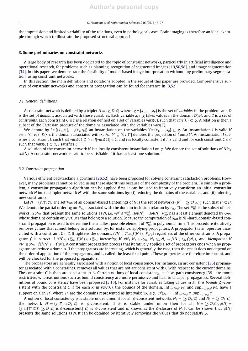
Author's personal copy

the imprecision and limited variability of the relations, even in pathological cases. Brain imaging is therefore an ideal exam-ple through which to illustrate the proposed structural approach.

3. Some preliminaries on constraint networks

A large body of research has been dedicated to the topic of constraint networks, particularly in artificial intelligence andoperational research, for problems such as planning, recognition of segmented images [19,50,58], and image segmentation[34]. In this paper, we demonstrate the feasibility of model-based image interpretation without any preliminary segmenta-tion, using constraint networks.

In this section, the main definitions and notations adopted in the sequel of this paper are provided. Comprehensive sur-veys of constraint networks and constraint propagation can be found for instance in [3,52].

3.1. General definitions

A constraint network is defined by a triplet N ! hv;D; Ci where: v = {x1, . . . ,xn} is the set of variables in the problem, and Dis the set of domains associated with those variables. Each variable xi 2 v takes values in the domain D"xi#, and C is a set ofconstraints. Each constraint C 2 C is a relation defined on a set of variables vars(C), such that vars(C) # v. A relation is then asubset of the Cartesian product of the domains associated with the variables vars(C).

We denote by I = {(x1,v1), . . . , (xk,vk)} an instantiation on the variables Y = {x1, . . . ,xk} # v. An instantiation I is valid if8xi 2 Y ; v i 2 D"xi#, the domain associated with xi. For Y0 # Y, I[Y0] denotes the projection of I onto Y0. An instantiation I sat-isfies a constraint C such that vars(C) # Y if I[vars(C)] 2 C, and I is locally consistent if I is valid and for each constraint C 2 Csuch that vars(C) # Y, I satisfies C.

A solution of the constraint network N is a locally consistent instantiation I on v. We denote the set of solutions of N bysol(N). A constraint network is said to be satisfiable if it has at least one solution.

3.2. Constraint propagation

Various efficient backtracking algorithms [26,52] have been proposed for solving constraint satisfaction problems. How-ever, many problems cannot be solved using these algorithms because of the complexity of the problem. To simplify a prob-lem, a constraint propagation algorithm can be applied first. It can be used to iteratively transform an initial constraintnetwork N into a simpler network N0 with the same solutions by: (i) reducing the domains of the variables, and (ii) inferringnew constraints.

Let N ! hv;D; Ci. The set PND of all domain-based tightenings of N is the set of networks fN0 ! hv;D0; Cig such that D0 #D.We denote the partial ordering on PND associated with the domain inclusion relation by 6N. The set Psol

ND is the subset of net-works in PND that present the same solutions as N, i.e. 8N0 2 Psol

ND; sol"N0# ! sol"N#. PsolND has a least element denoted by GND,

whose domains contain only values that belong to a solution. Because the computation of GND is NP-hard, domain-based con-straint propagation is used to determine the smallest possible element of Psol

ND in polynomial time. This procedure iterativelyremoves values that cannot belong to a solution by, for instance, applying propagators. A propagator f is an operator asso-ciated with a constraint C 2 C. It tightens the domains "8N0 2 PND; f "N0# 2 PN0D# regardless of the other constraints. A propa-gator f is correct if 8N0 2 Psol

ND; f "N0# 2 PsolN0D, increasing if 8N1;N2 2 PND; N1 6N N2 ) f "N1# 6N f "N2#, and idempotent if

8N0 2 PND; f "f "N0## ! f "N0#. A constraint propagation process that iteratively applies a set of propagators ends when no prop-agator can reduce a domain. If the propagators are increasing, which is generally the case, then the result does not depend onthe order of application of the propagators, and is called the least fixed point. These properties are therefore important, andwill be checked for the proposed propagators.

The propagators are generally associated with a notion of local consistency. For instance, an arc consistent [36] propaga-tor associated with a constraint C removes all values that are not arc consistent with C with respect to the current domains.The constraint C is then arc consistent in D. Certain notions of local consistency, such as path consistency [39], are morerestrictive, whereas notions such as bound consistency are more permissive and lead to cheaper propagators. Several defi-nitions of bound consistency have been proposed [3,15]. For instance for variables taking values in Z; D is bounds(Z)-con-sistent with the constraint C if for each xi in vars(C), the bounds of the domain, infv i2D"xi#"v i# and supv i2D"xi#"v i#, have asupport on C in DI , where DI are the domains represented as intervals: 8xi 2 v; DI"xi# ! $infv i2D"xi#v i; supv i2D"xi#v i%.

A notion of local consistency / is stable under union if for all /-consistent networks N1 ! hv;D1; Ci and N2 ! hv;D2; Ci,the network N0 ! hv;D1 [ D2; Ci is /-consistent. If / is stable under union then for all N ! hv;D; Ci;/"N# !hv;[fD0 #Djhv;D0; Ci is /-consistentg; Ci is /-consistent and is knows as the /-closure of N. It can be shown that /(N)presents the same solutions as N. It can be obtained by iteratively removing the values that do not satisfy /.

4 O. Nempont et al. / Information Sciences 246 (2013) 1–27

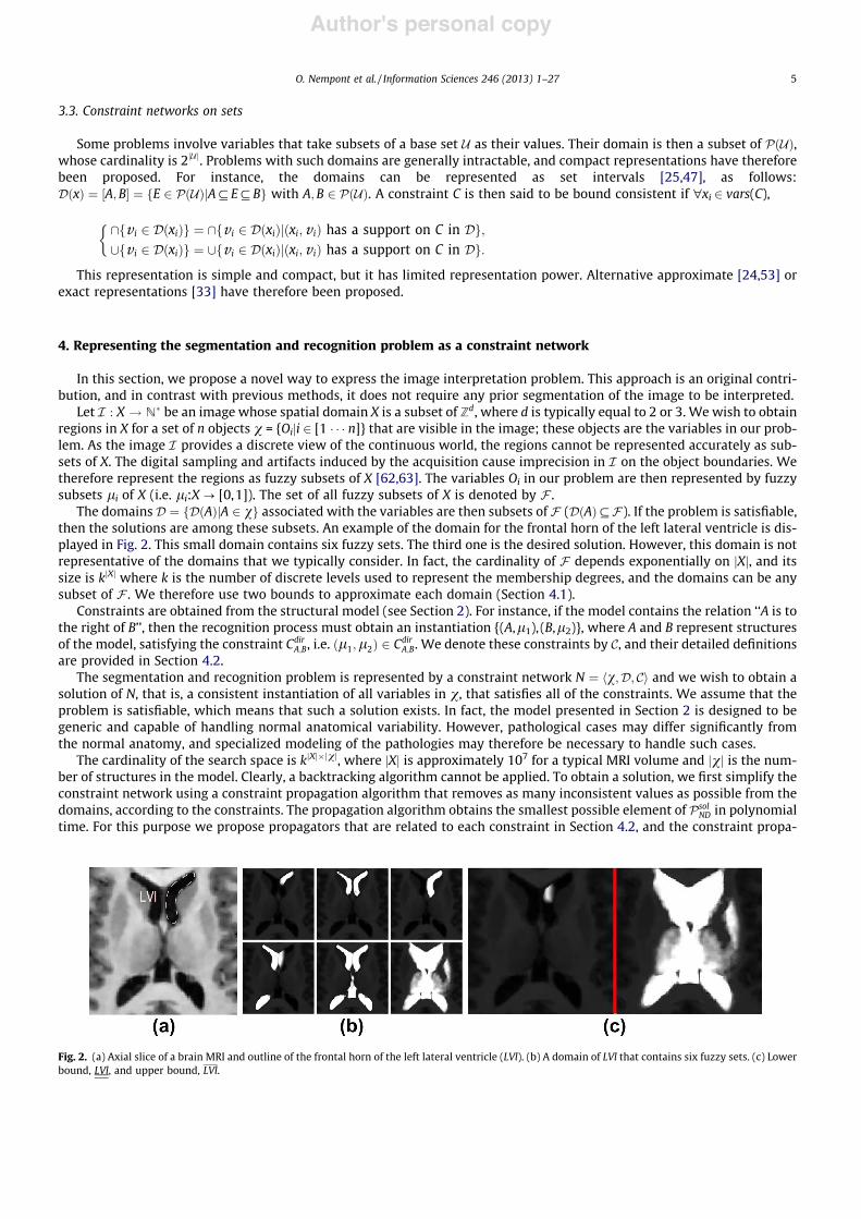
Author's personal copy

3.3. Constraint networks on sets

Some problems involve variables that take subsets of a base set U as their values. Their domain is then a subset of P"U#,whose cardinality is 2jUj. Problems with such domains are generally intractable, and compact representations have thereforebeen proposed. For instance, the domains can be represented as set intervals [25,47], as follows:D"x# ! $A;B% ! fE 2 P"U#jA# E#Bg with A;B 2 P"U#. A constraint C is then said to be bound consistent if "xi 2 vars(C),

\fv i 2 D"xi#g ! \fv i 2 D"xi#j"xi;v i# has a support on C in Dg;[fv i 2 D"xi#g ! [fv i 2 D"xi#j"xi;v i# has a support on C in Dg:

!

This representation is simple and compact, but it has limited representation power. Alternative approximate [24,53] orexact representations [33] have therefore been proposed.

4. Representing the segmentation and recognition problem as a constraint network

In this section, we propose a novel way to express the image interpretation problem. This approach is an original contri-bution, and in contrast with previous methods, it does not require any prior segmentation of the image to be interpreted.

Let I : X ! N& be an image whose spatial domain X is a subset of Zd, where d is typically equal to 2 or 3. We wish to obtainregions in X for a set of n objects v = {Oiji 2 [1 ' ' ' n]} that are visible in the image; these objects are the variables in our prob-lem. As the image I provides a discrete view of the continuous world, the regions cannot be represented accurately as sub-sets of X. The digital sampling and artifacts induced by the acquisition cause imprecision in I on the object boundaries. Wetherefore represent the regions as fuzzy subsets of X [62,63]. The variables Oi in our problem are then represented by fuzzysubsets li of X (i.e. li:X? [0,1]). The set of all fuzzy subsets of X is denoted by F .

The domainsD ! fD"A#jA 2 vg associated with the variables are then subsets of F (D"A##F ). If the problem is satisfiable,then the solutions are among these subsets. An example of the domain for the frontal horn of the left lateral ventricle is dis-played in Fig. 2. This small domain contains six fuzzy sets. The third one is the desired solution. However, this domain is notrepresentative of the domains that we typically consider. In fact, the cardinality of F depends exponentially on jXj, and itssize is kjXj where k is the number of discrete levels used to represent the membership degrees, and the domains can be anysubset of F . We therefore use two bounds to approximate each domain (Section 4.1).

Constraints are obtained from the structural model (see Section 2). For instance, if the model contains the relation ‘‘A is tothe right of B’’, then the recognition process must obtain an instantiation {(A,l1), (B,l2)}, where A and B represent structuresof the model, satisfying the constraint Cdir

A;B, i.e. "l1;l2# 2 CdirA;B. We denote these constraints by C, and their detailed definitions

are provided in Section 4.2.The segmentation and recognition problem is represented by a constraint network N ! hv;D; Ci and we wish to obtain a

solution of N, that is, a consistent instantiation of all variables in v, that satisfies all of the constraints. We assume that theproblem is satisfiable, which means that such a solution exists. In fact, the model presented in Section 2 is designed to begeneric and capable of handling normal anatomical variability. However, pathological cases may differ significantly fromthe normal anatomy, and specialized modeling of the pathologies may therefore be necessary to handle such cases.

The cardinality of the search space is kjXj(jvj, where jXj is approximately 107 for a typical MRI volume and jvj is the num-ber of structures in the model. Clearly, a backtracking algorithm cannot be applied. To obtain a solution, we first simplify theconstraint network using a constraint propagation algorithm that removes as many inconsistent values as possible from thedomains, according to the constraints. The propagation algorithm obtains the smallest possible element of Psol

ND in polynomialtime. For this purpose we propose propagators that are related to each constraint in Section 4.2, and the constraint propa-

Fig. 2. (a) Axial slice of a brain MRI and outline of the frontal horn of the left lateral ventricle (LVl). (b) A domain of LVl that contains six fuzzy sets. (c) Lowerbound, LVl, and upper bound, LVl.

O. Nempont et al. / Information Sciences 246 (2013) 1–27 5

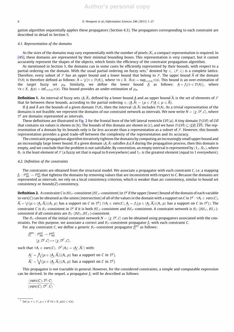
Author's personal copy

gation algorithm sequentially applies these propagators (Section 4.3). The propagators corresponding to each constraint aredescribed in detail in Section 5.

4.1. Representation of the domains

As the sizes of the domains may vary exponentially with the number of pixels jXj, a compact representation is required. In[45], these domains are represented by their minimal bounding boxes. This representation is very compact, but it cannotaccurately represent the shapes of the objects, which limits the efficiency of the constraint propagation algorithm.

As mentioned in Section 3, the domains can in some cases be efficiently represented by their bounds, with respect to apartial ordering on the domain. With the usual partial ordering on fuzzy sets,1 denoted by 6; "F ;6# is a complete lattice.Therefore, every subset of F has an upper bound and a lower bound that belong to F . The upper bound A of the domainD"A# is therefore defined as follows: A !

Wfm 2 D"A#g, where 8x 2 X; A"x# ! supm2D"A#m"x#. This bound is an over-estimation of

the target fuzzy set lA. Similarly, we define the lower bound A as follows: A !Vfm 2 D"A#g, where

8x 2 X; A"x# ! infm2D"A#m"x#. This bound provides an under-estimation of lA.

Definition 1. An interval of fuzzy sets "A;A#, defined by a lower bound A and an upper bound A, is the set of elements of Fthat lie between these bounds, according to the partial ordering 6: "A;A# ! fl 2 FjA 6 l 6 Ag.

If A and A are the bounds of a given domain D"A#, then the interval "A;A# includes D"A#. As a trivial representation of thedomains is not feasible, we represent the domains of our constraint network as intervals. We now write N ! hv;DI; Ci, whereDI are domains represented as intervals.

These definitions are illustrated in Fig. 2 for the frontal horn of the left lateral ventricle LVl (a). A tiny domain D"LVl# of LVlthat contains six values is shown in (b). The bounds of this domain are shown in (c), and we have D"LVl## "LVl; LVl#. The rep-resentation of a domain by its bounds only is far less accurate than a representation as a subset of F . However, this boundsrepresentation provides a good trade-off between the complexity of the representation and its accuracy.

The constraint propagation algorithm iteratively tightens thedomainsby computing an increasingly small upper boundandan increasingly large lower bound. If a given domain "A;A# satisfies AiA during the propagation process, then this domain isempty, andwe conclude that the problem is not satisfiable. By convention, an empty interval is represented by "1F ;0F #, where0F is the least element of F (a fuzzy set that is equal to 0 everywhere) and 1F is the greatest element (equal to 1 everywhere).

4.2. Definition of the constraints

The constraints are obtained from the structural model. We associate a propagator with each constraint C, i.e. a mappingfC : Psol

ND ! PsolND that tightens the domains by removing values that are inconsistent with respect to C. Because the domains are

represented as intervals, we rely on a local consistency criterion, which is weaker than arc consistency, similar to bound setconsistency or bounds(Z)-consistency.

Definition 2. A constraint C isBSF -consistent (BIF -consistent) inDI if the upper (lower) bound of the domain of each variablein vars(C) can be obtained as the union (intersection) of all of the values in the domainwith a support on C inDI : 8Ai 2 vars"C#,Ai !

Wfl 2 "Ai;Ai#j"Ai;l# has a support on C in DIg "8Ai 2 vars"C#;Ai !

Vfl 2 "Ai;Ai#j"Ai;l# has a support on C in DIg#. The

constraint C is BF -consistent in DI if it is both BIF -consistent and BSF -consistent. A constraint network is BF (BSF , BIF )-consistent if all constraints are BF (BSF ,BIF )-consistent.

The BF -closure of the initial constraint network N ! hv;DI; Ci can be obtained using propagators associated with the con-straints. For this purpose, we associate a correct and BF -consistent propagator fC with each constraint C.

For any constraint C, we define a generic BF -consistent propagator f genC as follows:

f genC : PsolND ! Psol

ND

hv;DI; Ci# hv;DI 0; Ci;

such that 8Ai 2 vars"C#; DI 0"Ai# ! "Ai0;Ai

0# with:

Ai0 !^

fl 2 "Ai;Ai#j"Ai;l# has a support on C in DIg;

Ai0 !_

fl 2 "Ai;Ai#j"Ai;l# has a support on C in DIg:

This propagator is not tractable in general. However, for the considered constraints, a simple and computable expressioncan be derived. In the sequel, a propagator fC will be described as follows:

hvars"C#;DI; Cihvars"C#;DI 0;Ci

;

1 Let l; m 2 F , l 6 m if "x 2 X, l(x) 6 m(x).

6 O. Nempont et al. / Information Sciences 246 (2013) 1–27

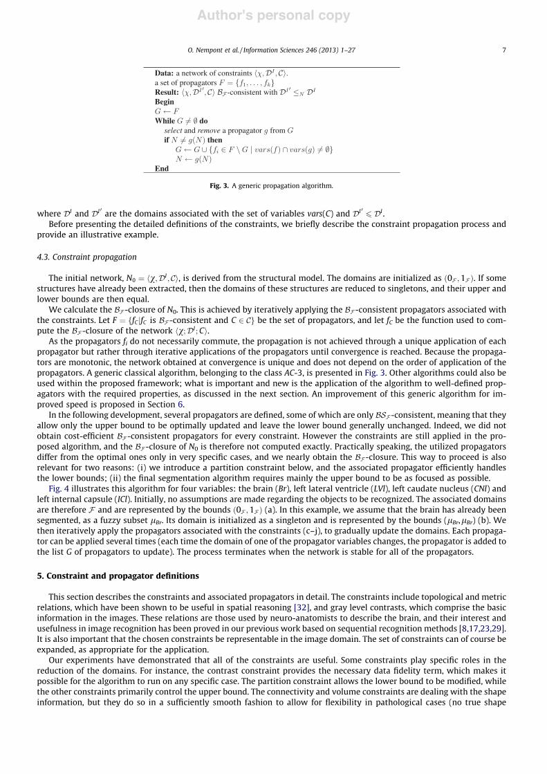
Author's personal copy

where DI and DI 0 are the domains associated with the set of variables vars(C) and DI 0 6 DI .Before presenting the detailed definitions of the constraints, we briefly describe the constraint propagation process and

provide an illustrative example.

4.3. Constraint propagation

The initial network, N0 ! hv;DI; Ci, is derived from the structural model. The domains are initialized as "0F ;1F #. If somestructures have already been extracted, then the domains of these structures are reduced to singletons, and their upper andlower bounds are then equal.

We calculate the BF -closure of N0. This is achieved by iteratively applying the BF -consistent propagators associated withthe constraints. Let F ! ffC jfC is BF -consistent and C 2 Cg be the set of propagators, and let fC be the function used to com-pute the BF -closure of the network hv;DI;Ci.

As the propagators fi do not necessarily commute, the propagation is not achieved through a unique application of eachpropagator but rather through iterative applications of the propagators until convergence is reached. Because the propaga-tors are monotonic, the network obtained at convergence is unique and does not depend on the order of application of thepropagators. A generic classical algorithm, belonging to the class AC-3, is presented in Fig. 3. Other algorithms could also beused within the proposed framework; what is important and new is the application of the algorithm to well-defined prop-agators with the required properties, as discussed in the next section. An improvement of this generic algorithm for im-proved speed is proposed in Section 6.

In the following development, several propagators are defined, some of which are only BSF -consistent, meaning that theyallow only the upper bound to be optimally updated and leave the lower bound generally unchanged. Indeed, we did notobtain cost-efficient BF -consistent propagators for every constraint. However the constraints are still applied in the pro-posed algorithm, and the BF -closure of N0 is therefore not computed exactly. Practically speaking, the utilized propagatorsdiffer from the optimal ones only in very specific cases, and we nearly obtain the BF -closure. This way to proceed is alsorelevant for two reasons: (i) we introduce a partition constraint below, and the associated propagator efficiently handlesthe lower bounds; (ii) the final segmentation algorithm requires mainly the upper bound to be as focused as possible.

Fig. 4 illustrates this algorithm for four variables: the brain (Br), left lateral ventricle (LVl), left caudate nucleus (CNl) andleft internal capsule (ICl). Initially, no assumptions are made regarding the objects to be recognized. The associated domainsare therefore F and are represented by the bounds "0F ;1F # (a). In this example, we assume that the brain has already beensegmented, as a fuzzy subset lBr. Its domain is initialized as a singleton and is represented by the bounds (lBr,lBr) (b). Wethen iteratively apply the propagators associated with the constraints (c–j), to gradually update the domains. Each propaga-tor can be applied several times (each time the domain of one of the propagator variables changes, the propagator is added tothe list G of propagators to update). The process terminates when the network is stable for all of the propagators.

5. Constraint and propagator definitions

This section describes the constraints and associated propagators in detail. The constraints include topological and metricrelations, which have been shown to be useful in spatial reasoning [32], and gray level contrasts, which comprise the basicinformation in the images. These relations are those used by neuro-anatomists to describe the brain, and their interest andusefulness in image recognition has been proved in our previous work based on sequential recognition methods [8,17,23,29].It is also important that the chosen constraints be representable in the image domain. The set of constraints can of course beexpanded, as appropriate for the application.

Our experiments have demonstrated that all of the constraints are useful. Some constraints play specific roles in thereduction of the domains. For instance, the contrast constraint provides the necessary data fidelity term, which makes itpossible for the algorithm to run on any specific case. The partition constraint allows the lower bound to be modified, whilethe other constraints primarily control the upper bound. The connectivity and volume constraints are dealing with the shapeinformation, but they do so in a sufficiently smooth fashion to allow for flexibility in pathological cases (no true shape

Fig. 3. A generic propagation algorithm.

O. Nempont et al. / Information Sciences 246 (2013) 1–27 7

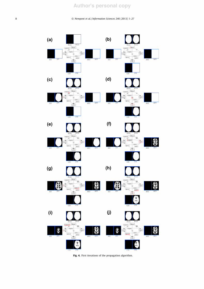
Author's personal copy

(a) (b)

(c) (d)

(e) (f)

(g) (h)

(i) (j)

Fig. 4. First iterations of the propagation algorithm.

8 O. Nempont et al. / Information Sciences 246 (2013) 1–27

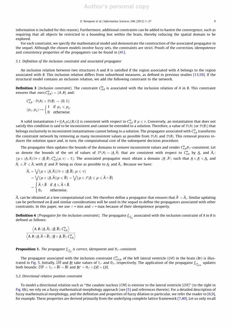
Author's personal copy

information is included for this reason). Furthermore, additional constraints can be added to hasten the convergence, such asrequiring that all objects be restricted to a bounding box within the brain, thereby reducing the spatial domain to beexplored.

For each constraint, we specify the mathematical model and demonstrate the construction of the associated propagator inthe sequel. Although the chosen models involve fuzzy sets, the constraints are strict. Proofs of the correction, idempotenceand consistency properties of the propagators can be found in [41].

5.1. Definition of the inclusion constraint and associated propagator

An inclusion relation between two structures A and B is satisfied if the region associated with A belongs to the regionassociated with B. This inclusion relation differs from subsethood measures, as defined in previous studies [13,59]. If thestructural model contains an inclusion relation, we add the following constraint to the network.

Definition 3 (Inclusion constraint). The constraint CinA;B is associated with the inclusion relation of A in B. This constraint

ensures that vars"CinA;B# ! fA;Bg and:

CinA;B : D"A# (D"B# ! f0;1g

"l1;l2##1 if l1 6 l2;

0 otherwise:

!

A valid instantiation I = {(A,l), (B,m)} is consistent with respect to CinA;B if l 6 m. Conversely, an instantiation that does not

satisfy this condition is said to be inconsistent and cannot be extended to a solution. Therefore, a value of D"A# (or D"B#) thatbelongs exclusively to inconsistent instantiations cannot belong to a solution. The propagator associated with Cin

A;B transformsthe constraint network by removing as many inconsistent values as possible from D"A# and D"B#. This removal process re-duces the solution space and, in turn, the computational cost of the subsequent decision procedure.

The propagator then updates the bounds of the domains to remove inconsistent values and render CinA;BBF -consistent. Let

us denote the bounds of the set of values of DI"A# ! "A;A# that are consistent with respect to CinA;B by Ac and Ac:

fl 2 "A;A#j9m 2 "B;B#;CinA;B"l; m# ! 1g. The associated propagator must obtain a domain "A0;A0# such that A 6 A0 6 Ac and

Ac 6 A0 6 A, with A0 and A0 being as close as possible to Ac and Ac. Because we have:

Ac !_

fl 2 "A;A#j9m 2 "B;B#;l 6 mg

!_

fl 2 "A;A#jl 6 Bg !_

fl 2 FjA 6 l 6 A ^ Bg

! A ^ B if A 6 A ^ B;0F otherwise;

(

Ac can be obtained at a low computational cost. We therefore define a propagator that ensures that A0 ! Ac . Similar updatingcan be performed on B and similar considerations will be used in the sequel to define the propagators associated with otherconstraints. In this paper, we use ^ = min and _ = max because of their idempotence property.

Definition 4 (Propagator for the inclusion constraint). The propagator fCinA;B

associated with the inclusion constraint of A in B isdefined as follows:

A;B; "A;A#; "B;B#;CinA;B

D E

A;B; "A;A ^ B#; "B _ A;B#;CinA;B

D E

Proposition 1. The propagator fCinA;B

is correct, idempotent and BF -consistent.

The propagator associated with the inclusion constraint CinLVl;Br of the left lateral ventricle (LVl) in the brain (Br) is illus-

trated in Fig. 5. Initially, LVl and Br take values of 1F and 0F , respectively. The application of the propagator fCinLVl;Br

updatesboth bounds: LVl0 ! 1F ^ Br ! Br and Br0 ! 0F _ LVl ! LVl.

5.2. Directional relative position constraint

To model a directional relation such as ‘‘the caudate nucleus (CNl) is exterior to the lateral ventricle (LVl)’’ (to the right inFig. 6b), we rely on a fuzzy mathematical morphology approach (see [5] and references therein). For a detailed description offuzzy mathematical morphology, and the definition and properties of fuzzy dilation in particular, we refer the reader to [6,9],for example. These properties are derived primarily from the underlying complete lattice framework [7,40]. Let us only recall

O. Nempont et al. / Information Sciences 246 (2013) 1–27 9

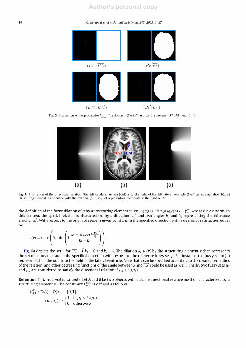
Author's personal copy

the definition of the fuzzy dilation of l by a structuring element m: "x, dm(l)(x) = supyt(l(y),m(x ) y)), where t is a t-norm. Inthis context, the spatial relation is characterized by a direction ud

"! and two angles k1 and k2 representing the tolerancearound ud

"!. With respect to the origin of space, a given point x is in the specified direction with a degree of satisfaction equalto:

m"x# ! max 0;min 1;k2 ) arccos x! ud

"!kxk

k2 ) k1

0

B@

1

CA

0

B@

1

CA:

Fig. 6a depicts the set m for ud"! !~i; k1 ! 0 and k2 ! p

2. The dilation dm(l)(x) by the structuring element m then representsthe set of points that are in the specified direction with respect to the reference fuzzy set l. For instance, the fuzzy set in (c)represents all of the points to the right of the lateral ventricle. Note that m can be specified according to the desired semanticsof the relation, and other decreasing functions of the angle between x and ud

"! could be used as well. Finally, two fuzzy sets l1

and l2 are considered to satisfy the directional relation if l2 6 dm(l1).

Definition 5 (Directional constraint). Let A and B be two objects with a stable directional relative position characterized by astructuring element m. The constraint Cdirm

A;B is defined as follows:

CdirmA;B : D"A# (D"B# ! f0;1g

"l1;l2# #1 if l2 6 dm"l1#;0 otherwise:

!

Fig. 5. Illustration of the propagator fCinLVl;Br

. The domains "LVl; LVl# and "Br;Br# become "LVl0; LVl0# and "Br0;Br0#.

CNlLVl

(a) (b) (c)Fig. 6. Illustration of the directional relation ‘‘the left caudate nucleus (CNl) is to the right of the left lateral ventricle (LVl)’’ on an axial slice (b). (a)Structuring element m associated with the relation. (c) Fuzzy set representing the points to the right of LVl.

10 O. Nempont et al. / Information Sciences 246 (2013) 1–27

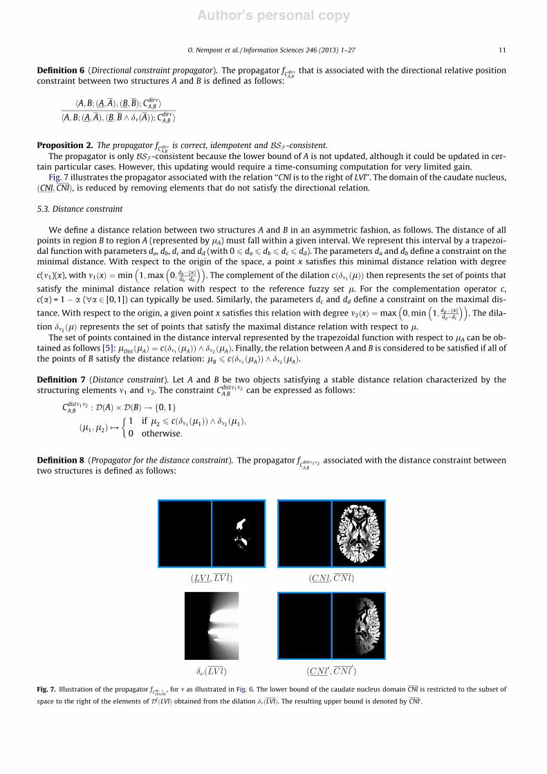
Author's personal copy

Definition 6 (Directional constraint propagator). The propagator fCdirmA;B

that is associated with the directional relative positionconstraint between two structures A and B is defined as follows:

hA;B; "A;A#; "B;B#; CdirmA;B i

hA; B; "A;A#; "B;B ^ dm"A##;CdirmA;B i

Proposition 2. The propagator fCdirmA;B

is correct, idempotent and BSF -consistent.The propagator is only BSF -consistent because the lower bound of A is not updated, although it could be updated in cer-

tain particular cases. However, this updating would require a time-consuming computation for very limited gain.Fig. 7 illustrates the propagator associated with the relation ‘‘CNl is to the right of LVl’’. The domain of the caudate nucleus,

"CNl;CNl#, is reduced by removing elements that do not satisfy the directional relation.

5.3. Distance constraint

We define a distance relation between two structures A and B in an asymmetric fashion, as follows. The distance of allpoints in region B to region A (represented by lA) must fall within a given interval. We represent this interval by a trapezoi-dal function with parameters da, db, dc and dd (with 0 6 da 6 db 6 dc 6 dd). The parameters da and db define a constraint on theminimal distance. With respect to the origin of the space, a point x satisfies this minimal distance relation with degree

c(m1)(x), with m1"x# ! min 1;max 0; db)kxkdb)da

# $# $. The complement of the dilation c"dm1 "l## then represents the set of points that

satisfy the minimal distance relation with respect to the reference fuzzy set l. For the complementation operator c,c(a) = 1 ) a ("a 2 [0,1]) can typically be used. Similarly, the parameters dc and dd define a constraint on the maximal dis-

tance. With respect to the origin, a given point x satisfies this relation with degree m2"x# ! max 0;min 1; dd)kxkdd)dc

# $# $. The dila-

tion dm2 "l# represents the set of points that satisfy the maximal distance relation with respect to l.The set of points contained in the distance interval represented by the trapezoidal function with respect to lA can be ob-

tained as follows [5]: lDist"lA# ! c"dm1 "lA## ^ dm2 "lA#. Finally, the relation between A and B is considered to be satisfied if all ofthe points of B satisfy the distance relation: lB 6 c"dm1 "lA## ^ dm2 "lA#.

Definition 7 (Distance constraint). Let A and B be two objects satisfying a stable distance relation characterized by thestructuring elements m1 and m2. The constraint Cdistm1m2

A;B can be expressed as follows:

Cdistm1m2A;B : D"A# (D"B# ! f0;1g

"l1;l2##1 if l2 6 c"dm1 "l1## ^ dm2 "l1#;0 otherwise:

!

Definition 8 (Propagator for the distance constraint). The propagator fCdistm1m2A;B

associated with the distance constraint betweentwo structures is defined as follows:

Fig. 7. Illustration of the propagator fCdir mLVl;CNl

, for m as illustrated in Fig. 6. The lower bound of the caudate nucleus domain CNl is restricted to the subset of

space to the right of the elements of DI"LVl# obtained from the dilation dm"LVl#. The resulting upper bound is denoted by CNl0 .

O. Nempont et al. / Information Sciences 246 (2013) 1–27 11

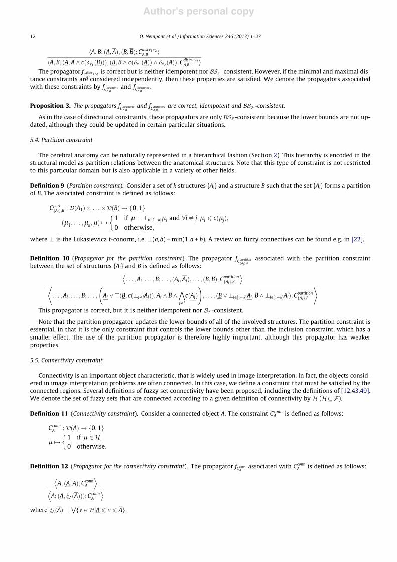
Author's personal copy

hA;B; "A;A#; "B;B#;Cdistm1m2A;B i

hA;B; "A;A ^ c"dm1 "B###; "B;B ^ c"dm1 "A## ^ dm2 "A##;Cdistm1m2A;B i

The propagator fCdistm1m2A;B

is correct but is neither idempotent nor BSF -consistent. However, if the minimal and maximal dis-tance constraints are considered independently, then these properties are satisfied. We denote the propagators associatedwith these constraints by fCdistminm

A;Band fCdistmaxm

A;B.

Proposition 3. The propagators fCdistminmA;B

and fCdistmaxmA;B

are correct, idempotent and BSF -consistent.

As in the case of directional constraints, these propagators are only BSF -consistent because the lower bounds are not up-dated, although they could be updated in certain particular situations.

5.4. Partition constraint

The cerebral anatomy can be naturally represented in a hierarchical fashion (Section 2). This hierarchy is encoded in thestructural model as partition relations between the anatomical structures. Note that this type of constraint is not restrictedto this particular domain but is also applicable in a variety of other fields.

Definition 9 (Partition constraint). Consider a set of k structures {Ai} and a structure B such that the set {Ai} forms a partitionof B. The associated constraint is defined as follows:

CpartfAig;B

: D"A1# ( . . .(D"B# ! f0;1g

"l1; . . . ;lk;l##1 if l ! ?i2$1'''k%li and 8i – j;li 6 c"lj#;0 otherwise;

!

where \ is the Lukasiewicz t-conorm, i.e. \(a,b) = min(1,a + b). A review on fuzzy connectives can be found e.g. in [22].

Definition 10 (Propagator for the partition constraint). The propagator fCpartitionfAig;B

associated with the partition constraintbetween the set of structures {Ai} and B is defined as follows:

. . . ;Ai; . . . ;B; . . . ; "Ai;Ai#; . . . ; "B;B#; CpartitionfAig;B

D E

. . . ;Ai; . . . ;B; . . . ; Ai _ >"B; c"?j–iAj##;Ai ^ B ^^

j–i

c"Aj# !

; . . . ; "B _ ?i2$1'''k%Ai;B ^ ?i2$1'''k%Ai#;CpartitionfAig;B

* +

This propagator is correct, but it is neither idempotent nor BF -consistent.

Note that the partition propagator updates the lower bounds of all of the involved structures. The partition constraint isessential, in that it is the only constraint that controls the lower bounds other than the inclusion constraint, which has asmaller effect. The use of the partition propagator is therefore highly important, although this propagator has weakerproperties.

5.5. Connectivity constraint

Connectivity is an important object characteristic, that is widely used in image interpretation. In fact, the objects consid-ered in image interpretation problems are often connected. In this case, we define a constraint that must be satisfied by theconnected regions. Several definitions of fuzzy set connectivity have been proposed, including the definitions of [12,43,49].We denote the set of fuzzy sets that are connected according to a given definition of connectivity by H (H#F ).

Definition 11 (Connectivity constraint). Consider a connected object A. The constraint CconnA is defined as follows:

CconnA : D"A# ! f0;1g

l#1 if l 2 H;

0 otherwise:

!

Definition 12 (Propagator for the connectivity constraint). The propagator fCconnA

associated with CconnA is defined as follows:

A; "A;A#;CconnA

D E

A; "A; nA"A###;CconnA

D E

where nA"A# !Wfm 2 HjA 6 m 6 Ag:

12 O. Nempont et al. / Information Sciences 246 (2013) 1–27

Author's personal copy

This propagator is computed by extracting the connected components of A based onH, i.e. the greatest elements ofH thatare smaller than A according to the usual ordering on F . If we denote the set of connected components of A by H"A#, thennA"A# can be expressed as

Wfl 2 H"A#jA 6 lg. Only the connected components including the lower bound are maintained in

the result.The most time-consuming operation in the propagator computation is extracting the connected components. The effi-

ciency of this operation depends on the definition of fuzzy set connectivity. For instance, the extraction of the connectedcomponents as defined in [49] can be achieved in quasi-linear time with respect to jXj.

Proposition 4. The propagator fCconnA

is correct, idempotent and BSF -consistent.

5.6. Volume constraint

The volume (or surface) of a fuzzy set can be defined as a fuzzy set on R* [21], as follows: fV "l#"v# ! supV"la#Pva. We rep-resent the prior information regarding the volume by an interval $fVmin ; fVmax % where fVmin : R* ! $0;1% and fVmax : R

* ! $0;1%represent the minimal and maximal volume, respectively.

Definition 13 (Volume constraint). Consider an object A whose volume falls in the interval $fVmin ; fVmax %. The constraint

Cvol$fVmin

;fVmax %A is defined as follows:

Cvol$fVmin

;fVmax %A : D"A# ! f0;1g

l#1 if f Vmin

6 fV "l# 6 fVmax ;

0 otherwise:

!

Because of the chosen representation of the domains, this constraint is useless when considered alone, as it does not leadto an efficient propagator. However, when the volume constraint is combined with a connectivity constraint, Cconn

A , we obtainthe following propagator.

Definition 14 (Propagator for Cvol$fVmin

;fVmax %A ^ Cconn

A ). The propagator fCvol$fVmin

;fVmax %

A ^CconnA

is associated with the conjunction of avolume constraint and a connectivity constraint on the object A. The propagator is defined as follows:

A; "A;A#;Cvol$fVmin

;fVmax %A ^ Cconn

A

D E

A; "A;A0#;Cvol$fVmin

;fVmax %A ^ Cconn

A

D E

where A0 !Wfl 2 HjA 6 l 6 A and f Vmin

6 fV "l#g.

Proposition 5. The propagator fCvol$fVmin

;fVmax %

A ^CconnA

is correct, idempotent and BSF -consistent.The propagator f

Cvol$fVmin

;fVmax %

LVl^Cconn

LVl

is illustrated in Fig. 8. This propagator reduces the domain of LVl by filtering the con-

nected components of LVl.

5.7. Adjacency constraint

Ameasure of adjacency between two fuzzy sets l1 and l2, denoted by ladj(l1,l2), has been proposed in [5]. We adopt thisdefinition in the sequel.

Definition 15 (Adjacency constraint). Consider two adjacent objects A and B. We define the constraint CadjA;B as follows:

Fig. 8. Illustration of the propagator fCvol$fVmin

;fVmax %

A ^CconnA

. The connected components of LVl are filtered using a minimal volume criterion.

O. Nempont et al. / Information Sciences 246 (2013) 1–27 13

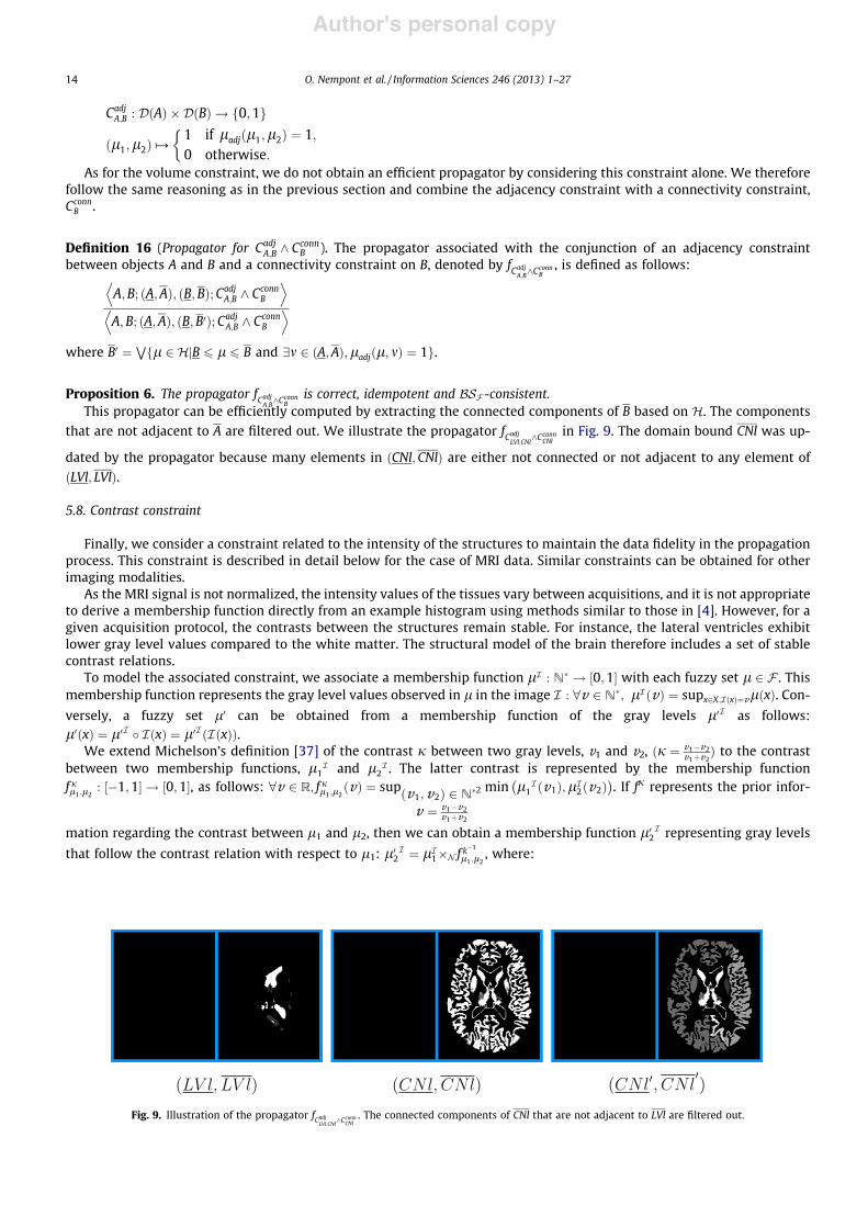
Author's personal copy

CadjA;B : D"A# (D"B# ! f0;1g

"l1;l2# #1 if ladj"l1;l2# ! 1;0 otherwise:

!

As for the volume constraint, we do not obtain an efficient propagator by considering this constraint alone. We thereforefollow the same reasoning as in the previous section and combine the adjacency constraint with a connectivity constraint,CconnB .

Definition 16 (Propagator for CadjA;B ^ Cconn

B ). The propagator associated with the conjunction of an adjacency constraintbetween objects A and B and a connectivity constraint on B, denoted by fCadj

A;B^CconnB

, is defined as follows:

A;B; "A;A#; "B;B#;CadjA;B ^ Cconn

B

D E

A; B; "A;A#; "B;B0#; CadjA;B ^ Cconn

B

D E

where B0 !Wfl 2 HjB 6 l 6 B and 9m 2 "A;A#;ladj"l; m# ! 1g.

Proposition 6. The propagator fCadjA;B^C

connB

is correct, idempotent and BSF -consistent.This propagator can be efficiently computed by extracting the connected components of B based on H. The components

that are not adjacent to A are filtered out. We illustrate the propagator fCadjLVl;CNl

^CconnCNl

in Fig. 9. The domain bound CNl was up-

dated by the propagator because many elements in "CNl;CNl# are either not connected or not adjacent to any element of"LVl; LVl#.

5.8. Contrast constraint

Finally, we consider a constraint related to the intensity of the structures to maintain the data fidelity in the propagationprocess. This constraint is described in detail below for the case of MRI data. Similar constraints can be obtained for otherimaging modalities.

As the MRI signal is not normalized, the intensity values of the tissues vary between acquisitions, and it is not appropriateto derive a membership function directly from an example histogram using methods similar to those in [4]. However, for agiven acquisition protocol, the contrasts between the structures remain stable. For instance, the lateral ventricles exhibitlower gray level values compared to the white matter. The structural model of the brain therefore includes a set of stablecontrast relations.

To model the associated constraint, we associate a membership function lI : N& ! $0;1% with each fuzzy set l 2 F . Thismembership function represents the gray level values observed in l in the image I : 8v 2 N&; lI "v# ! supx2X;I"x#!vl"x#. Con-versely, a fuzzy set l0 can be obtained from a membership function of the gray levels l0I as follows:l0"x# ! l0I + I"x# ! l0I "I"x##.

We extend Michelson’s definition [37] of the contrast j between two gray levels, v1 and v2, "j ! v1)v2v1*v2

# to the contrastbetween two membership functions, l1

I and l2I . The latter contrast is represented by the membership function

f jl1 ;l2: $)1;1% ! $0;1%, as follows: 8v 2 R; f jl1 ;l2

"v# ! sup"v1;v2# 2 N&2

v ! v1)v2v1*v2

min l1I "v1#;lI

2"v2#% &

. If fj represents the prior infor-

mation regarding the contrast between l1 and l2, then we can obtain a membership function l02I representing gray levels

that follow the contrast relation with respect to l1: l02I ! lI

1(N f k)1

l1 ;l2, where:

Fig. 9. Illustration of the propagator fCadjLVl;CNl

^CconnCNl

. The connected components of CNl that are not adjacent to LVl are filtered out.

14 O. Nempont et al. / Information Sciences 246 (2013) 1–27

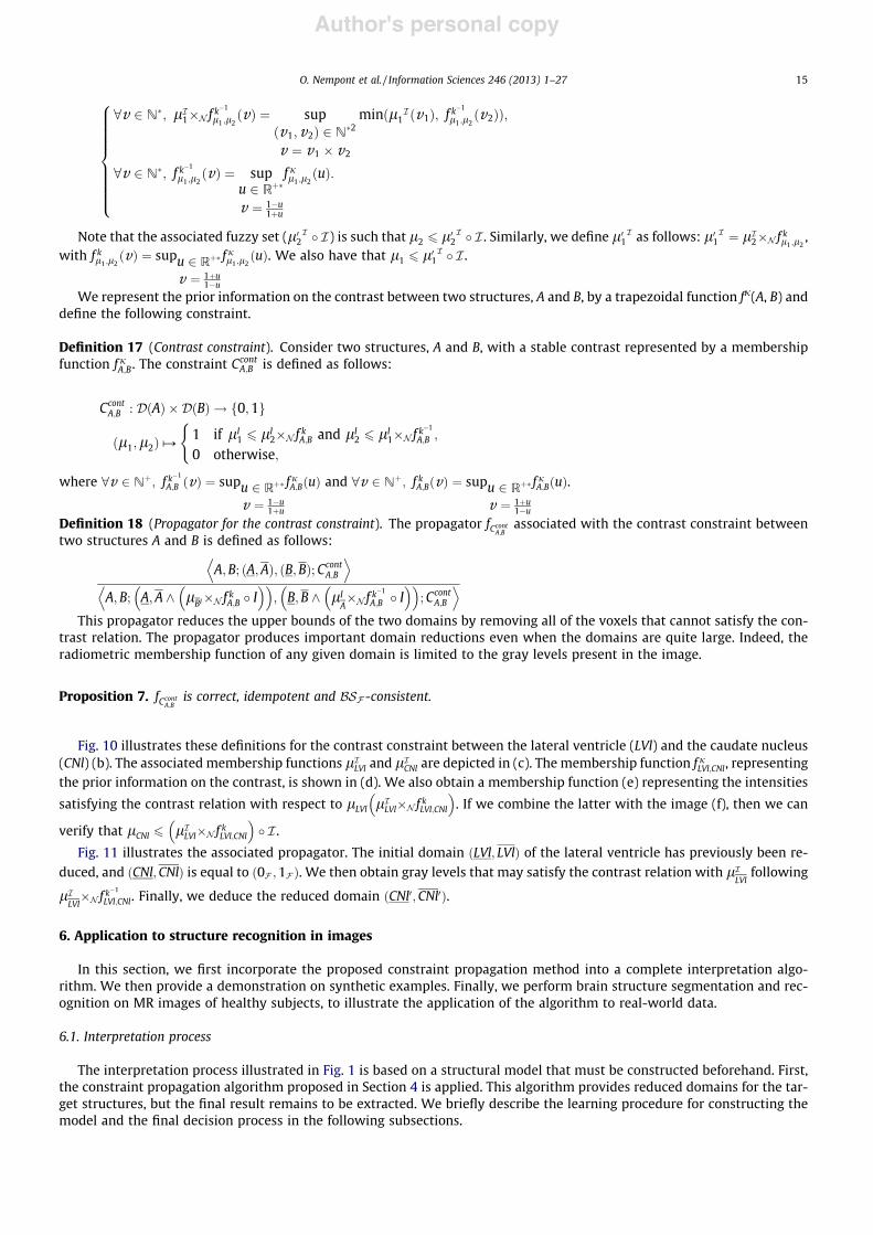
Author's personal copy

8v 2 N&; lI1(N f k

)1

l1 ;l2"v# ! sup

"v1;v2# 2 N&2

v ! v1 ( v2

min"l1I "v1#; f k

)1

l1 ;l2"v2##;

8v 2 N&; f k)1

l1 ;l2"v# ! sup

u 2 R*&

v ! 1)u1*u

f jl1 ;l2"u#:

8>>>>>>>><

>>>>>>>>:

Note that the associated fuzzy set (l02I + I) is such that l2 6 l0

2I + I . Similarly, we define l0

1I as follows: l0

1I ! lI

2(N f kl1 ;l2,

with f kl1 ;l2"v# ! supu 2 R*&

v ! 1*u1)u

f jl1 ;l2"u#. We also have that l1 6 l0

1I + I .

We represent the prior information on the contrast between two structures, A and B, by a trapezoidal function fj(A, B) anddefine the following constraint.

Definition 17 (Contrast constraint). Consider two structures, A and B, with a stable contrast represented by a membershipfunction fjA;B. The constraint Ccont

A;B is defined as follows:

CcontA;B : D"A# (D"B# ! f0;1g

"l1;l2##1 if lI

1 6 lI2(N f kA;B and lI

2 6 lI1(N f k

)1

A;B ;

0 otherwise;

(

where 8v 2 N*; f k)1

A;B "v# ! supu 2 R*&

v ! 1)u1*u

f jA;B"u# and 8v 2 N*; f kA;B"v# ! supu 2 R*&

v ! 1*u1)u

f jA;B"u#.

Definition 18 (Propagator for the contrast constraint). The propagator fCcontA;B

associated with the contrast constraint betweentwo structures A and B is defined as follows:

A;B; "A;A#; "B;B#; CcontA;B

D E

A;B; A;A ^ lBI(N f kA;B + I# $# $

; B;B ^ lIA(N f k

)1

A;B + I# $# $

;CcontA;B

D E

This propagator reduces the upper bounds of the two domains by removing all of the voxels that cannot satisfy the con-trast relation. The propagator produces important domain reductions even when the domains are quite large. Indeed, theradiometric membership function of any given domain is limited to the gray levels present in the image.

Proposition 7. fCcontA;B

is correct, idempotent and BSF -consistent.

Fig. 10 illustrates these definitions for the contrast constraint between the lateral ventricle (LVl) and the caudate nucleus(CNl) (b). The associated membership functions lI

LVl and lICNl are depicted in (c). The membership function f jLVl;CNl, representing

the prior information on the contrast, is shown in (d). We also obtain a membership function (e) representing the intensities

satisfying the contrast relation with respect to lLVl lILVl(N f kLVl;CNl

# $. If we combine the latter with the image (f), then we can

verify that lCNl 6 lILVl(N f kLVl;CNl

# $+ I .

Fig. 11 illustrates the associated propagator. The initial domain "LVl; LVl# of the lateral ventricle has previously been re-duced, and "CNl;CNl# is equal to "0F ;1F #. We then obtain gray levels that may satisfy the contrast relation with lI

LVlfollowing

lILVl(N f k

)1

LVl;CNl. Finally, we deduce the reduced domain "CNl0;CNl0#.

6. Application to structure recognition in images

In this section, we first incorporate the proposed constraint propagation method into a complete interpretation algo-rithm. We then provide a demonstration on synthetic examples. Finally, we perform brain structure segmentation and rec-ognition on MR images of healthy subjects, to illustrate the application of the algorithm to real-world data.

6.1. Interpretation process

The interpretation process illustrated in Fig. 1 is based on a structural model that must be constructed beforehand. First,the constraint propagation algorithm proposed in Section 4 is applied. This algorithm provides reduced domains for the tar-get structures, but the final result remains to be extracted. We briefly describe the learning procedure for constructing themodel and the final decision process in the following subsections.

O. Nempont et al. / Information Sciences 246 (2013) 1–27 15

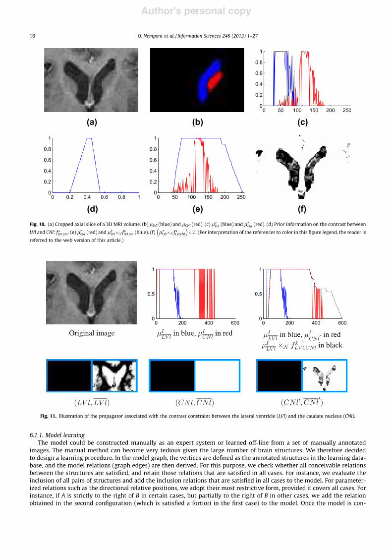
Author's personal copy

6.1.1. Model learningThe model could be constructed manually as an expert system or learned off-line from a set of manually annotated

images. The manual method can become very tedious given the large number of brain structures. We therefore decidedto design a learning procedure. In the model graph, the vertices are defined as the annotated structures in the learning data-base, and the model relations (graph edges) are then derived. For this purpose, we check whether all conceivable relationsbetween the structures are satisfied, and retain those relations that are satisfied in all cases. For instance, we evaluate theinclusion of all pairs of structures and add the inclusion relations that are satisfied in all cases to the model. For parameter-ized relations such as the directional relative positions, we adopt their most restrictive form, provided it covers all cases. Forinstance, if A is strictly to the right of B in certain cases, but partially to the right of B in other cases, we add the relationobtained in the second configuration (which is satisfied a fortiori in the first case) to the model. Once the model is con-

(a) (b) (c)

(d) (e) (f)Fig. 10. (a) Cropped axial slice of a 3D MRI volume. (b) lLVl (blue) and lCNl (red). (c) lI

LVl (blue) and lICNl (red). (d) Prior information on the contrast between

LVl and CNl: f jLVl;CNl . (e) lICNl (red) and lI

LVl(N f kLVl;CNl (blue). (f) lILVl(N f kLVl;CNl

# $+ I . (For interpretation of the references to color in this figure legend, the reader is

referred to the web version of this article.)

Fig. 11. Illustration of the propagator associated with the contrast constraint between the lateral ventricle (LVl) and the caudate nucleus (CNl).

16 O. Nempont et al. / Information Sciences 246 (2013) 1–27

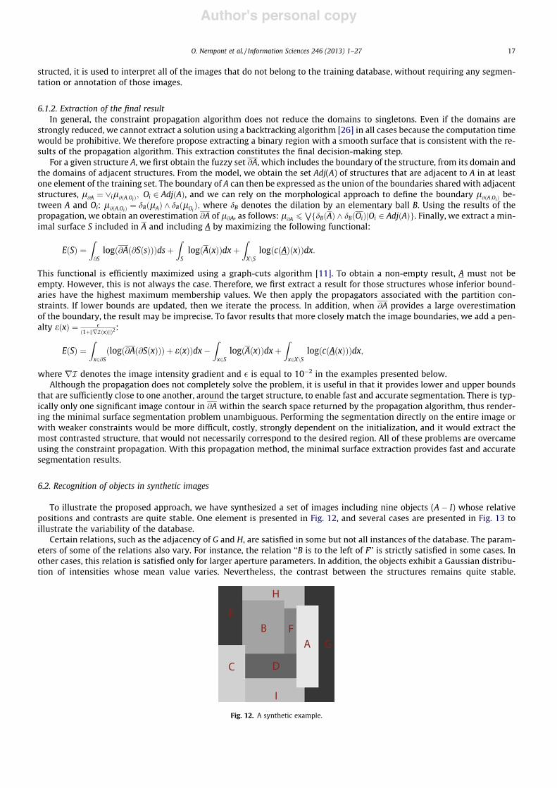
Author's personal copy

structed, it is used to interpret all of the images that do not belong to the training database, without requiring any segmen-tation or annotation of those images.

6.1.2. Extraction of the final resultIn general, the constraint propagation algorithm does not reduce the domains to singletons. Even if the domains are

strongly reduced, we cannot extract a solution using a backtracking algorithm [26] in all cases because the computation timewould be prohibitive. We therefore propose extracting a binary region with a smooth surface that is consistent with the re-sults of the propagation algorithm. This extraction constitutes the final decision-making step.

For a given structure A, we first obtain the fuzzy set @A, which includes the boundary of the structure, from its domain andthe domains of adjacent structures. From the model, we obtain the set Adj(A) of structures that are adjacent to A in at leastone element of the training set. The boundary of A can then be expressed as the union of the boundaries shared with adjacentstructures, l@A ! _il@"A;Oi#; Oi 2 Adj"A#, and we can rely on the morphological approach to define the boundary l@"A;Oi# be-tween A and Oi: l@"A;Oi# ! dB"lA# ^ dB"lOi

#; where dB denotes the dilation by an elementary ball B. Using the results of thepropagation, we obtain an overestimation @A of l@A, as follows: l@A 6 WfdB"A# ^ dB"Oi#jOi 2 Adj"A#g. Finally, we extract a min-imal surface S included in A and including A by maximizing the following functional:

E"S# !Z

@Slog"@A"@S"s###ds*

Z

Slog"A"x##dx*

Z

XnSlog"c"A#"x##dx:

This functional is efficiently maximized using a graph-cuts algorithm [11]. To obtain a non-empty result, A must not beempty. However, this is not always the case. Therefore, we first extract a result for those structures whose inferior bound-aries have the highest maximum membership values. We then apply the propagators associated with the partition con-straints. If lower bounds are updated, then we iterate the process. In addition, when @A provides a large overestimationof the boundary, the result may be imprecise. To favor results that more closely match the image boundaries, we add a pen-alty e"x# ! !

"1*krI"x#k#2:

E"S# !Z

x2@S"log"@A"@S"x### * e"x##dx)

Z

x2Slog"A"x##dx*

Z

x2XnSlog"c"A"x###dx;

where rI denotes the image intensity gradient and ! is equal to 10)2 in the examples presented below.Although the propagation does not completely solve the problem, it is useful in that it provides lower and upper bounds

that are sufficiently close to one another, around the target structure, to enable fast and accurate segmentation. There is typ-ically only one significant image contour in @A within the search space returned by the propagation algorithm, thus render-ing the minimal surface segmentation problem unambiguous. Performing the segmentation directly on the entire image orwith weaker constraints would be more difficult, costly, strongly dependent on the initialization, and it would extract themost contrasted structure, that would not necessarily correspond to the desired region. All of these problems are overcameusing the constraint propagation. With this propagation method, the minimal surface extraction provides fast and accuratesegmentation results.

6.2. Recognition of objects in synthetic images

To illustrate the proposed approach, we have synthesized a set of images including nine objects (A ) I) whose relativepositions and contrasts are quite stable. One element is presented in Fig. 12, and several cases are presented in Fig. 13 toillustrate the variability of the database.

Certain relations, such as the adjacency of G and H, are satisfied in some but not all instances of the database. The param-eters of some of the relations also vary. For instance, the relation ‘‘B is to the left of F’’ is strictly satisfied in some cases. Inother cases, this relation is satisfied only for larger aperture parameters. In addition, the objects exhibit a Gaussian distribu-tion of intensities whose mean value varies. Nevertheless, the contrast between the structures remains quite stable.

Fig. 12. A synthetic example.

O. Nempont et al. / Information Sciences 246 (2013) 1–27 17

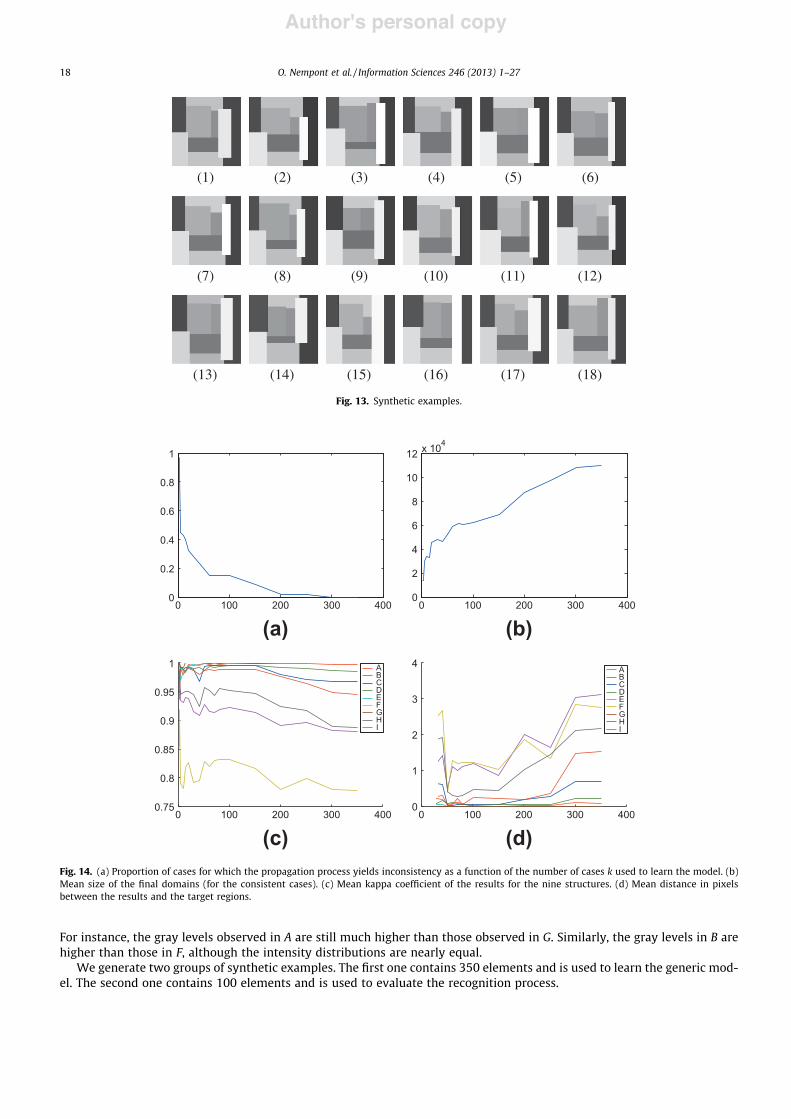
Author's personal copy

For instance, the gray levels observed in A are still much higher than those observed in G. Similarly, the gray levels in B arehigher than those in F, although the intensity distributions are nearly equal.

We generate two groups of synthetic examples. The first one contains 350 elements and is used to learn the generic mod-el. The second one contains 100 elements and is used to evaluate the recognition process.

(1) (2) (3) (4) (5) (6)

(7) (8) (9) (10) (11) (12)

(13) (14) (15) (16) (17) (18)

Fig. 13. Synthetic examples.

0 100 200 300 4000

0.2

0.4

0.6

0.8

1

0 100 200 300 4000

2

4

6

8

10

12 x 104

(b)(a)

0 100 200 300 4000.75

0.8

0.85

0.9

0.95

1

ABCDEFGHI

0 100 200 300 4000

1

2

3

4

ABCDEFGHI

(d)(c)Fig. 14. (a) Proportion of cases for which the propagation process yields inconsistency as a function of the number of cases k used to learn the model. (b)Mean size of the final domains (for the consistent cases). (c) Mean kappa coefficient of the results for the nine structures. (d) Mean distance in pixelsbetween the results and the target regions.

18 O. Nempont et al. / Information Sciences 246 (2013) 1–27

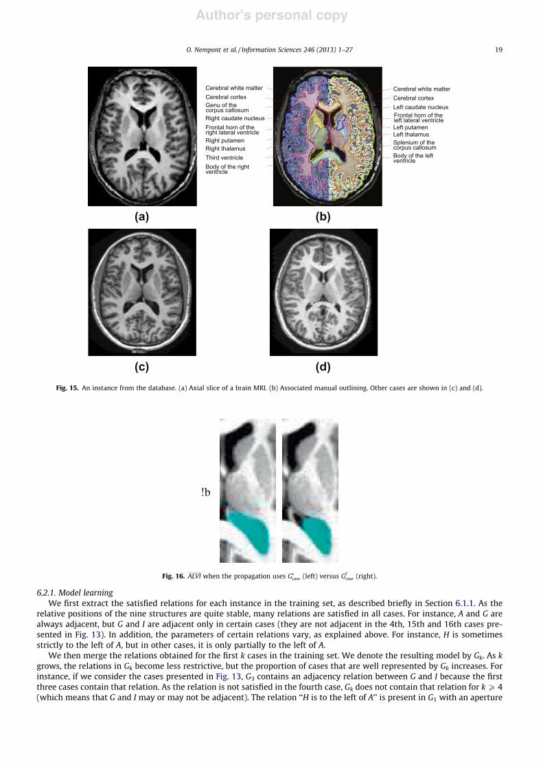
Author's personal copy

6.2.1. Model learningWe first extract the satisfied relations for each instance in the training set, as described briefly in Section 6.1.1. As the

relative positions of the nine structures are quite stable, many relations are satisfied in all cases. For instance, A and G arealways adjacent, but G and I are adjacent only in certain cases (they are not adjacent in the 4th, 15th and 16th cases pre-sented in Fig. 13). In addition, the parameters of certain relations vary, as explained above. For instance, H is sometimesstrictly to the left of A, but in other cases, it is only partially to the left of A.

We then merge the relations obtained for the first k cases in the training set. We denote the resulting model by Gk. As kgrows, the relations in Gk become less restrictive, but the proportion of cases that are well represented by Gk increases. Forinstance, if we consider the cases presented in Fig. 13, G3 contains an adjacency relation between G and I because the firstthree cases contain that relation. As the relation is not satisfied in the fourth case, Gk does not contain that relation for kP 4(which means that G and I may or may not be adjacent). The relation ‘‘H is to the left of A’’ is present in G1 with an aperture

Cerebral cortexGenu of the corpus callosumRight caudate nucleusFrontal horn of the

Right putamenRight thalamusThird ventricleBody of the right

Cerebral white matterCerebral white matterCerebral cortexLeft caudate nucleus Frontal horn of the

Splenium of thecorpus callosumBody of the left

right lateral ventricle

ventricle

left lateral ventricleLeft putamenLeft thalamus

ventricle

(a) (b)

(c) (d)Fig. 15. An instance from the database. (a) Axial slice of a brain MRI. (b) Associated manual outlining. Other cases are shown in (c) and (d).

!b

Fig. 16. ALVl when the propagation uses Gscase (left) versus Gf

case (right).

O. Nempont et al. / Information Sciences 246 (2013) 1–27 19

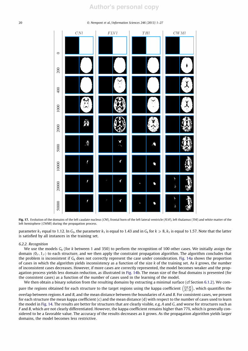
Author's personal copy

parameter k1 equal to 1.12. In G2, the parameter k1 is equal to 1.43 and in Gk for kP 8, k1 is equal to 1.57. Note that the latteris satisfied by all instances in the training set.

6.2.2. RecognitionWe use the models Gk (for k between 1 and 350) to perform the recognition of 100 other cases. We initially assign the

domain "0F ;1F # to each structure, and we then apply the constraint propagation algorithm. The algorithm concludes thatthe problem is inconsistent if Gk does not correctly represent the case under consideration. Fig. 14a shows the proportionof cases in which the algorithm yields inconsistency as a function of the size k of the training set. As k grows, the numberof inconsistent cases decreases. However, if more cases are correctly represented, the model becomes weaker and the prop-agation process yields less domain reduction, as illustrated in Fig. 14b. The mean size of the final domains is presented (forthe consistent cases) as a function of the number of cases used in the learning of the model.

We then obtain a binary solution from the resulting domains by extracting a minimal surface (cf Section 6.1.2). We com-

pare the regions obtained for each structure to the target regions using the kappa coefficient 2jA\BjjAj*jBj

# $, which quantifies the

overlap between regions A and B, and the mean distance between the boundaries of A and B. For consistent cases, we presentfor each structure the mean kappa coefficient (c) and the mean distance (d) with respect to the number of cases used to learnthe model in Fig. 14. The results are better for structures that are clearly visible, e.g. A and G, and worse for structures such asF and B, which are not clearly differentiated. However, the kappa coefficient remains higher than 77%, which is generally con-sidered to be a favorable value. The accuracy of the results decreases as k grows. As the propagation algorithm yields largerdomains, the model becomes less restrictive.

Fig. 17. Evolution of the domains of the left caudate nucleus (CNl), frontal horn of the left lateral ventricle (FLVl), left thalamus (THl) and white matter of theleft hemisphere (CWMl) during the propagation process.

20 O. Nempont et al. / Information Sciences 246 (2013) 1–27

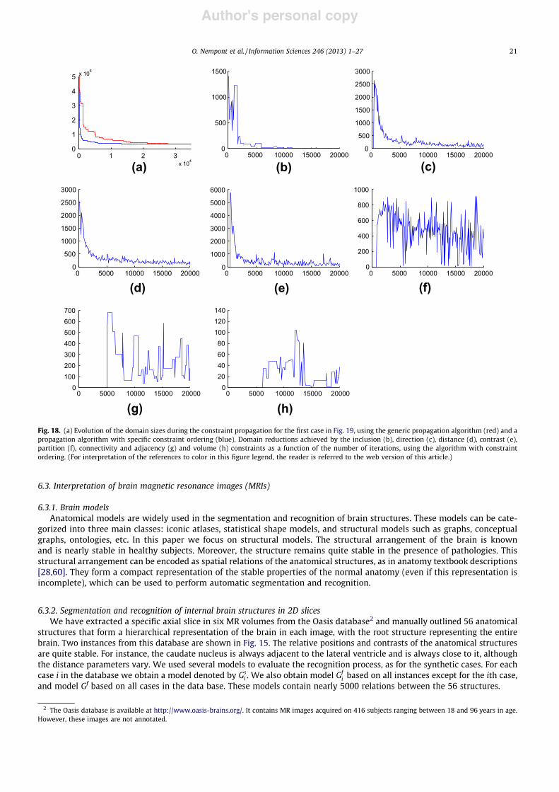
Author's personal copy

6.3. Interpretation of brain magnetic resonance images (MRIs)

6.3.1. Brain modelsAnatomical models are widely used in the segmentation and recognition of brain structures. These models can be cate-

gorized into three main classes: iconic atlases, statistical shape models, and structural models such as graphs, conceptualgraphs, ontologies, etc. In this paper we focus on structural models. The structural arrangement of the brain is knownand is nearly stable in healthy subjects. Moreover, the structure remains quite stable in the presence of pathologies. Thisstructural arrangement can be encoded as spatial relations of the anatomical structures, as in anatomy textbook descriptions[28,60]. They form a compact representation of the stable properties of the normal anatomy (even if this representation isincomplete), which can be used to perform automatic segmentation and recognition.

6.3.2. Segmentation and recognition of internal brain structures in 2D slicesWe have extracted a specific axial slice in six MR volumes from the Oasis database2 and manually outlined 56 anatomical

structures that form a hierarchical representation of the brain in each image, with the root structure representing the entirebrain. Two instances from this database are shown in Fig. 15. The relative positions and contrasts of the anatomical structuresare quite stable. For instance, the caudate nucleus is always adjacent to the lateral ventricle and is always close to it, althoughthe distance parameters vary. We used several models to evaluate the recognition process, as for the synthetic cases. For eachcase i in the database we obtain a model denoted by Gs

i . We also obtain model Gfi based on all instances except for the ith case,

and model Gf based on all cases in the data base. These models contain nearly 5000 relations between the 56 structures.

(a) (b) (c)

(d) (e)

(g) (h)

(f)

Fig. 18. (a) Evolution of the domain sizes during the constraint propagation for the first case in Fig. 19, using the generic propagation algorithm (red) and apropagation algorithm with specific constraint ordering (blue). Domain reductions achieved by the inclusion (b), direction (c), distance (d), contrast (e),partition (f), connectivity and adjacency (g) and volume (h) constraints as a function of the number of iterations, using the algorithm with constraintordering. (For interpretation of the references to color in this figure legend, the reader is referred to the web version of this article.)

2 The Oasis database is available at http://www.oasis-brains.org/. It contains MR images acquired on 416 subjects ranging between 18 and 96 years in age.However, these images are not annotated.

O. Nempont et al. / Information Sciences 246 (2013) 1–27 21

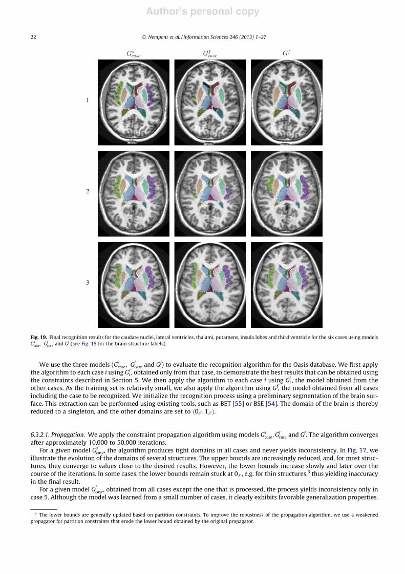
Author's personal copy

We use the three models (Gscase; Gf

case and Gf) to evaluate the recognition algorithm for the Oasis database. We first applythe algorithm to each case i using Gs

i , obtained only from that case, to demonstrate the best results that can be obtained usingthe constraints described in Section 5. We then apply the algorithm to each case i using Gf

i , the model obtained from theother cases. As the training set is relatively small, we also apply the algorithm using Gf, the model obtained from all casesincluding the case to be recognized. We initialize the recognition process using a preliminary segmentation of the brain sur-face. This extraction can be performed using existing tools, such as BET [55] or BSE [54]. The domain of the brain is therebyreduced to a singleton, and the other domains are set to "0F ;1F #.

6.3.2.1. Propagation. We apply the constraint propagation algorithm using models Gscase;G

fcase and Gf. The algorithm converges

after approximately 10,000 to 50,000 iterations.For a given model Gs

case, the algorithm produces tight domains in all cases and never yields inconsistency. In Fig. 17, weillustrate the evolution of the domains of several structures. The upper bounds are increasingly reduced, and, for most struc-tures, they converge to values close to the desired results. However, the lower bounds increase slowly and later over thecourse of the iterations. In some cases, the lower bounds remain stuck at 0F , e.g. for thin structures,3 thus yielding inaccuracyin the final result.

For a given model Gfcase, obtained from all cases except the one that is processed, the process yields inconsistency only in

case 5. Although the model was learned from a small number of cases, it clearly exhibits favorable generalization properties.

Fig. 19. Final recognition results for the caudate nuclei, lateral ventricles, thalami, putamens, insula lobes and third ventricle for the six cases using modelsGs

case; Gfcase and Gf (see Fig. 15 for the brain structure labels).

3 The lower bounds are generally updated based on partition constraints. To improve the robustness of the propagation algorithm, we use a weakenedpropagator for partition constraints that erode the lower bound obtained by the original propagator.

22 O. Nempont et al. / Information Sciences 246 (2013) 1–27

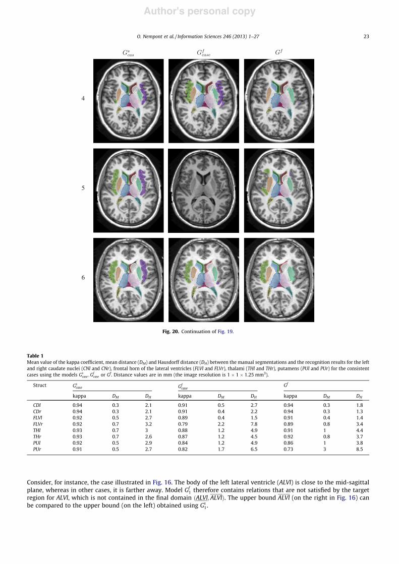
Author's personal copy

Consider, for instance, the case illustrated in Fig. 16. The body of the left lateral ventricle (ALVl) is close to the mid-sagittalplane, whereas in other cases, it is farther away. Model Gf

1 therefore contains relations that are not satisfied by the targetregion for ALVl, which is not contained in the final domain "ALVl;ALVl#. The upper bound ALVl (on the right in Fig. 16) canbe compared to the upper bound (on the left) obtained using Gs

1.

Fig. 20. Continuation of Fig. 19.

Table 1Mean value of the kappa coefficient, mean distance (DM) and Hausdorff distance (DH) between the manual segmentations and the recognition results for the leftand right caudate nuclei (CNl and CNr), frontal horn of the lateral ventricles (FLVl and FLVr), thalami (THl and THr), putamens (PUl and PUr) for the consistentcases using the models Gs

case;Gfcase or Gf. Distance values are in mm (the image resolution is 1 ( 1 ( 1.25 mm3).

Struct Gscase Gf

caseGf

kappa DM DH kappa DM DH kappa DM DH

CDl 0.94 0.3 2.1 0.91 0.5 2.7 0.94 0.3 1.8CDr 0.94 0.3 2.1 0.91 0.4 2.2 0.94 0.3 1.3FLVl 0.92 0.5 2.7 0.89 0.4 1.5 0.91 0.4 1.4FLVr 0.92 0.7 3.2 0.79 2.2 7.8 0.89 0.8 3.4THl 0.93 0.7 3 0.88 1.2 4.9 0.91 1 4.4THr 0.93 0.7 2.6 0.87 1.2 4.5 0.92 0.8 3.7PUl 0.92 0.5 2.9 0.84 1.2 4.9 0.86 1 3.8PUr 0.91 0.5 2.7 0.82 1.7 6.5 0.73 3 8.5

O. Nempont et al. / Information Sciences 246 (2013) 1–27 23

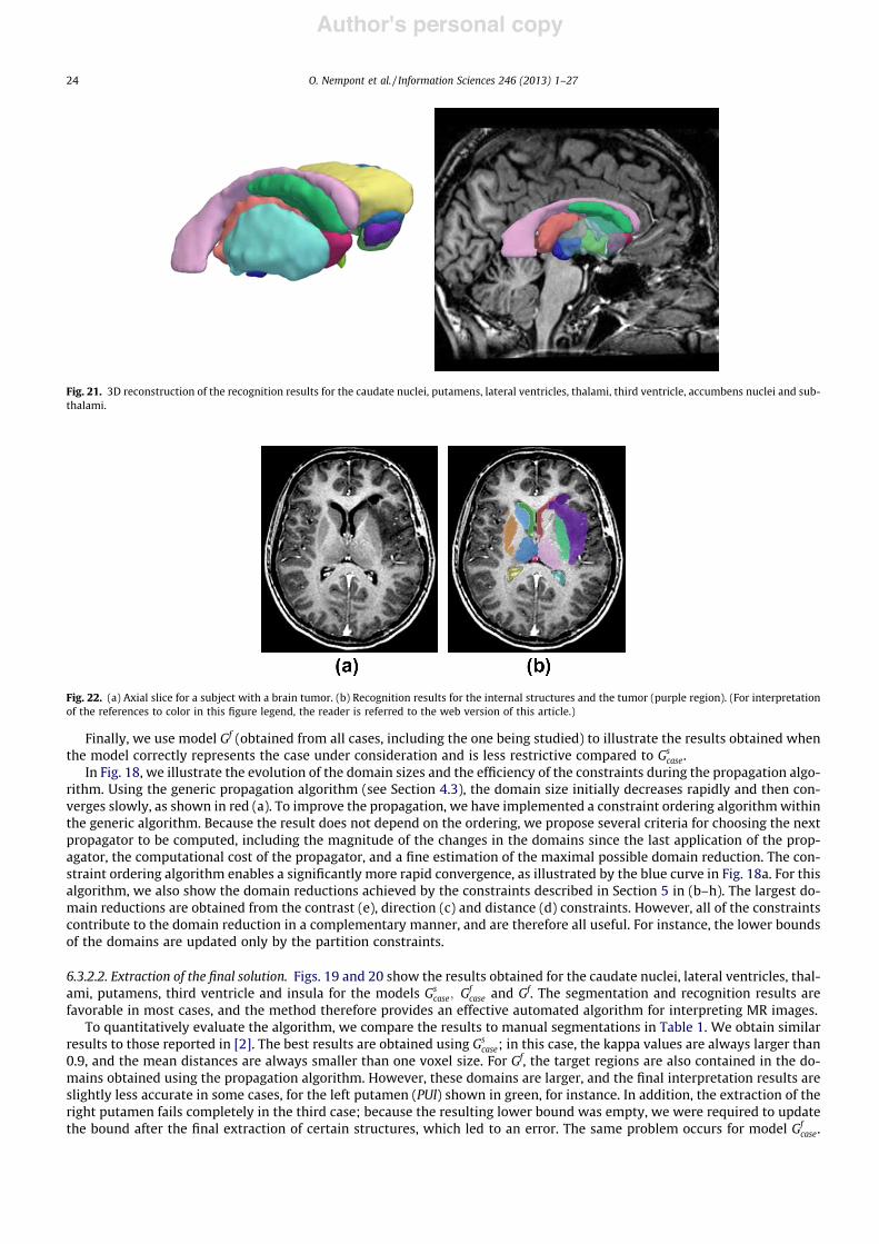
Author's personal copy

Finally, we use model Gf (obtained from all cases, including the one being studied) to illustrate the results obtained whenthe model correctly represents the case under consideration and is less restrictive compared to Gs

case.In Fig. 18, we illustrate the evolution of the domain sizes and the efficiency of the constraints during the propagation algo-

rithm. Using the generic propagation algorithm (see Section 4.3), the domain size initially decreases rapidly and then con-verges slowly, as shown in red (a). To improve the propagation, we have implemented a constraint ordering algorithmwithinthe generic algorithm. Because the result does not depend on the ordering, we propose several criteria for choosing the nextpropagator to be computed, including the magnitude of the changes in the domains since the last application of the prop-agator, the computational cost of the propagator, and a fine estimation of the maximal possible domain reduction. The con-straint ordering algorithm enables a significantly more rapid convergence, as illustrated by the blue curve in Fig. 18a. For thisalgorithm, we also show the domain reductions achieved by the constraints described in Section 5 in (b–h). The largest do-main reductions are obtained from the contrast (e), direction (c) and distance (d) constraints. However, all of the constraintscontribute to the domain reduction in a complementary manner, and are therefore all useful. For instance, the lower boundsof the domains are updated only by the partition constraints.

6.3.2.2. Extraction of the final solution. Figs. 19 and 20 show the results obtained for the caudate nuclei, lateral ventricles, thal-ami, putamens, third ventricle and insula for the models Gs

case; Gfcase and Gf. The segmentation and recognition results are

favorable in most cases, and the method therefore provides an effective automated algorithm for interpreting MR images.To quantitatively evaluate the algorithm, we compare the results to manual segmentations in Table 1. We obtain similar

results to those reported in [2]. The best results are obtained using Gscase; in this case, the kappa values are always larger than

0.9, and the mean distances are always smaller than one voxel size. For Gf, the target regions are also contained in the do-mains obtained using the propagation algorithm. However, these domains are larger, and the final interpretation results areslightly less accurate in some cases, for the left putamen (PUl) shown in green, for instance. In addition, the extraction of theright putamen fails completely in the third case; because the resulting lower bound was empty, we were required to updatethe bound after the final extraction of certain structures, which led to an error. The same problem occurs for model Gf

case.

Fig. 22. (a) Axial slice for a subject with a brain tumor. (b) Recognition results for the internal structures and the tumor (purple region). (For interpretationof the references to color in this figure legend, the reader is referred to the web version of this article.)

Fig. 21. 3D reconstruction of the recognition results for the caudate nuclei, putamens, lateral ventricles, thalami, third ventricle, accumbens nuclei and sub-thalami.

24 O. Nempont et al. / Information Sciences 246 (2013) 1–27

Author's personal copy

Moreover, the Gfcase model does not necessarily correctly represent the case under study, leading to further causes errors. For

instance, in the first case, ALVl does not fully include the target region, and the final recognition result is incorrect (seeFig. 16). However, this problem occurs rarely.

Overall, a mean error of less than one pixel or voxel was obtained, and the kappa coefficient was larger than 0.8 for Gfcase,

and even larger for the two other models. These results are very good and promising.

6.3.3. Recognition and segmentation of 3D structuresWe now illustrate the application of the algorithm to the entire MRI volume.Because the computational complexity of the propagators varies at least linearly with the number of pixels, the propa-

gation process becomes very slow in 3D. To reduce the computational cost, we perform the propagator computations oncoarser scales if necessary. Certain relations, such as the directional relative positions, exhibit a high level of granularity.The computation of these relations on a subsampled grid does not lead to substantially weaker domain reductions, andthe algorithm remains efficient at relatively low computational cost.

Moreover, the ordering of the propagators in the algorithm in Fig. 3 is simple and involves many extraneous computa-tions. We therefore proposed several criteria for choosing the next propagator (the result is independent of the order), asexplained previously. This constraint ordering algorithm improves the convergence, and reduces the computation time ofthe propagation process to a few hours for 3D images.4 Note that further significant optimizations are still feasible.

Fig. 21 shows a 3D reconstruction of the results obtained for the internal structures.

7. Conclusion

In this paper, we addressed the problem of global scene interpretation based on structural models and proposed a newinterpretation method based on a constraint propagation algorithm. The novel aspects of our work include the formulation ofthe segmentation and recognition problem as a constraint satisfaction problem, without requiring a preliminary segmenta-tion or annotation of the image. A constraint network is constructed from a generic model of the scene, representing itsstructure through spatial relations between objects and their radiometric contrasts. In addition, we defined constraintsbased on the relations in the generic model and proposed a specific propagator for each constraint for the first time. We thenused a constraint propagation algorithm to reduce the variable domains based on these constraints. Finally, we performed asegmentation of each object based on the tightened domains.

As an illustration, we have applied the proposed framework to the recognition of internal brain structures in MR images,using a model representing the standard neuro-anatomy. Promising results were obtained, with mean errors of less than onevoxel size with respect to reference segmentations. There is no inherent methodological or theoretical barrier to 3D appli-cation of the method. The only issues are the computational cost and model learning, which requires a large 3D annotateddatabase. Comparisons with other automated methods, in terms of both the accuracy and computation time, should be per-formed in future experimental studies.

Finally, we comment on the potential extension of the method to pathological cases. Pathologies such as brain tumors caninduce large deviations from the normal anatomy and must therefore be considered in the model. In addition, we could allowfor the possibility of larger membership functions defining the spatial relations, as proposed in [1]. Fig. 22 illustrates a pre-liminary result of our extended method. Despite the deformation caused by the tumor, we obtain very good recognition re-sults for the internal structures.

Acknowledgements

This work was partially supported by a grant from the National Cancer Institute (INCA) during Olivier Nempont’s PhDwork at Telecom ParisTech. We would like to thank Elsa Angelini for her collaboration and support.

References

[1] J. Atif, C. Hudelot, G. Fouquier, I. Fouquier, E. Angelini, From generic knowledge to specific reasoning for medical image interpretation using graph-based representations, in: International Joint Conference on Artificial Intelligence, IJCAI. Hyderabad, India, 2007, pp. 224–229.

[2] K.O. Babalola, B. Patenaude, P. Aljabar, J. Schnabel, D. Kennedy, W. Crum, S. Smith, T. Cootes, M. Jenkinson, D. Rueckert, An evaluation of four automaticmethods of segmenting the subcortical structures in the brain, NeuroImage 47 (4) (2009) 1435–1447.

[3] C. Bessière, Constraint Propagation, Tech. Rep., LIRMM, UMR 5506 CNRS, University of Montpellier, 2006.[4] B. Bharathi Devi, V.V.S. Sarma, Estimation of fuzzy memberships from histograms, Information Sciences 35 (1985) 43–59.[5] I. Bloch, Fuzzy spatial relationships for image processing and interpretation: a review, Image and Vision Computing 23 (2) (2005) 89–110.[6] I. Bloch, Duality vs. adjunction for fuzzy mathematical morphology and general form of fuzzy erosions and dilations, Fuzzy Sets and Systems 160 (13)

(2009) 1858–1867.[7] I. Bloch, Lattices of fuzzy sets and bipolar fuzzy sets, and mathematical morphology, Information Sciences 181 (10) (2011) 2002–2015.

4 This computation time is acceptable when the image analysis is performed in a post-processing stage on a different computer, rather than directlyfollowing the image acquisition, thus making other acquisitions possible during the computation time. If automated segmentation and recognition (and derivedquantitative measurements) are required, then a few hours is acceptable for the medical experts.

O. Nempont et al. / Information Sciences 246 (2013) 1–27 25

Author's personal copy

[8] I. Bloch, T. Géraud, H. Maıtre, Representation and fusion of heterogeneous fuzzy information in the 3d space for model-based structural recognition –application to 3d brain imaging, Artificial Intelligence 148 (1–2) (2003) 141–175.

[9] I. Bloch, H. Maıtre, Fuzzy mathematical morphologies: a comparative study, Pattern Recognition 28 (9) (1995) 1341–1387.[10] D. Bowden, R. Martin, Neuronames brain hierarchy, Neuroimage 2 (1) (1995) 63–83.[11] Y. Boykov, V. Kolmogorov, Computing geodesics and minimal surfaces via graph cuts, International Conference on Computer Vision, ICCV, vol. 1, IEEE,

Nice, France, 2003, pp. 26–33.[12] U. Braga-Neto, J. Goutsias, A theoretical tour of connectivity in image processing and analysis, Journal of Mathematical Imaging and Vision 19 (1)

(2003) 5–31.[13] H. Bustince, V. Mohedano, E. Barrenechea, M. Pagola, Definition and construction of fuzzy DI-subsethood measures, Information Sciences 176 (21)

(2006) 3190–3231.[14] R. Cesar, E. Bengoetxea, I. Bloch, P. Larranaga, Inexact graph matching for model-based recognition: Evaluation and comparison of optimization

algorithms, Pattern Recognition 38 (11) (2005) 2099–2113.[15] C. Choi, W. Harvey, J. Lee, P. Stuckey, Finite domain bounds consistency revisited, Australian Joint Conference on Artificial Intelligence, vol. LNCS 4304,

Springer, Hobart, Australia, 2006, pp. 49–58.[16] O. Colliot, Représentation, évaluation et utilisation de relations spatiales pour l’interprétation d’images, Ph.D. Thesis, Télécom ParisTech, ENST

2003E036, 2003.[17] O. Colliot, O. Camara, I. Bloch, Integration of fuzzy spatial relations in deformable models – application to brain MRI segmentation, Pattern Recognition

39 (8) (2006) 1401–1414.[18] D. Conte, P. Foggia, C. Sansone, M. Vento, Thirty years of graph matching in pattern recognition, International Journal of Pattern Recognition and

Artificial Intelligence 18 (3) (2004) 265–298.[19] A. Deruyver, Y. Hodé, Constraint satisfaction problem with bilevel constraint: application to interpretation of over-segmented images, Artificial

Intelligence 93 (1–2) (1997) 321–335.[20] A. Deruyver, Y. Hodé, Qualitative spatial relationships for image interpretation by using a conceptual graph, Image and Vision Computing 27 (7) (2009)

876–886.[21] D. Dubois, H. Prade, Fuzzy Sets and Systems: Theory and Applications, Academic Press, New York, NY, USA, 1980.[22] D. Dubois, H. Prade, A review of fuzzy set aggregation connectives, Information Sciences 36 (1-2) (1985) 85–121.[23] G. Fouquier, J. Atif, I. Bloch, Sequential model-based segmentation and recognition of image structures driven by visual features and spatial relations,

Computer Vision and Image Understanding 116 (1) (2012) 146–165.[24] G. Gange, P. Stuckey, V. Lagoon, Fast set bounds propagation using BDDs, in: European Conference on Artificial Intelligence, ECAI, vol. 178, 2008, Patras,

Greece, pp. 505–509.[25] C. Gervet, Interval propagation to reason about sets: definition and implementation of a practical language, Constraints 1 (3) (1997) 191–244.[26] S. Golomb, L. Baumert, Backtrack programming, Journal of the ACM 12 (4) (1965) 516–524.[27] J. Guo, H. Zhou, C. Zhu, Cascaded classification of high resolution remote sensing images using multiple contexts, Information Sciences 221 (2013) 85–

97.[28] D. Hasboun, Neuranat. Université Marie Curie, 2005. <http://www.chups.jussieu.fr/ext/neuranat/index.html>.[29] C. Hudelot, J. Atif, I. Bloch, Fuzzy spatial relation ontology for image interpretation, Fuzzy Sets and Systems 159 (15) (2008) 1929–1951.[30] C. Hudelot, J. Atif, O. Nempont, B. Batrancourt, E. Angelini, I. Bloch, GRAFIP: a framework for the representation of healthy and pathological anatomical

and functional cerebral information, in: Human Brain Mapping, HBM, Florence, Italy, 2006.[31] L. Kitchen, Discrete relaxation for matching relational structures, IEEE Transactions on Systems, Man, and Cybernetics 9 (12) (1978) 869–874.[32] B. Kuipers, T. Levitt, Navigation and mapping in large-scale space, AI Magazine 9 (2) (1988) 25–43.[33] V. Lagoon, P. Stuckey, Set domain propagation using ROBDDs, Principles and Practice of Constraint Programming, CP, vol. LNCS 3258, Springer, Toronto,

Canada, 2004, pp. 347–361.[34] W. Lin, E. Tsao, C. Chen, Constraint satisfaction neural networks for image segmentation, Pattern Recognition 25 (7) (1992) 679–693.[35] C. Lipscomb, Medical subject headings (MeSH), Bulletin of the Medical Library Association 88 (3) (2000) 265.[36] A. Mackworth, Consistency in networks of relations, Artificial Intelligence 8 (1) (1977) 99–118.[37] A. Michelson, Studies in Optics, Chicago University Press, Chicago, IL, USA, 1927.[38] R. Mohr, T. Henderson, Arc and path consistency revisited, Artificial Intelligence 28 (2) (1986) 225–233.[39] U. Montanari, Networks of constraints: fundamental properties and applications to picture processing, Information Sciences 7 (1974) 95–132.[40] M. Nachtegael, P. Sussner, T. Melange, E. Kerre, On the role of complete lattices in mathematical morphology: from tool to uncertainty model,

Information Sciences 181 (10) (2011) 1971–1988.[41] O. Nempont, Modèles structurels flous et propagation de contraintes pour la segmentation et la reconnaissance d’objets dans les images. Application

aux structures normales et pathologiques du cerveau en IRM, Ph.D. Thesis, Télécom ParisTech, ENST 2009E023, 2009.[42] O. Nempont, J. Atif, E. Angelini, I. Bloch, Structure segmentation and recognition in images guided by structural constraint propagation, in: European

Conference on Artificial Intelligence, ECAI, vol. 178, Patras, Greece, 2008, pp. 621–625.[43] O. Nempont, J. Atif, E. Angelini, I. Bloch, A new fuzzy connectivity measure for fuzzy sets, Journal of Mathematical Imaging and Vision 34 (2) (2009)

107–136.[44] B. Neumann, R. Möller, On scene interpretation with description logics, Image and Vision Computing 26 (1) (2008) 82–101.[45] D. Papadias, T. Sellis, Y. Theodoridis, M. Egenhofer, Topological relations in the world of minimum bounding rectangles: a study with r-trees, in:

SIGMOD International Conference on Management of Data, ACM Press, San Jose, CA, USA, 1995, pp. 92–103.[46] A. Perchant, I. Bloch, Fuzzy morphisms between graphs, Fuzzy Sets and Systems 128 (2) (2002) 149–168.[47] J. Puget, PECOS: a high level constraint programming language, in: Singapore International Conference on Intelligent Systems, SPICIS, vol. 92,

Singapore, 1992, pp. 137–142.[48] N. Ripperda, C. Brenner, Evaluation of structure recognition using labelled facade images, Pattern Recognition 84 (2) (2009) 532–541.[49] A. Rosenfeld, The fuzzy geometry of image subsets, Pattern Recognition Letters 2 (5) (1984) 311–317.[50] A. Rosenfeld, R. Hummel, S. Zucker, Scene labeling by relaxation operations, IEEE Transactions on Systems, Man and Cybernetics 6 (6) (1976) 420–433.[51] C. Rosse, J. Mejino, A reference ontology for bioinformatics: the foundational model of anatomy, Journal of Biomedical Informatics 36 (6) (2003) 478–

500.[52] F. Rossi, P. Van Beek, T. Walsh (Eds.), Handbook of Constraint Programming, Elsevier, New York, NY, USA, 2006.[53] A. Sadler, C. Gervet, Enhancing set constraint solvers with lexicographic bounds, Journal of Heuristics 14 (1) (2008) 23–67.[54] D. Shattuck, S. Sandor-Leahy, K. Schaper, D. Rottenberg, R. Leahy, Magnetic resonance image tissue classification using a partial volume model,

Neuroimage 13 (5) (2001) 856–876.[55] S. Smith, Fast robust automated brain extraction, Human Brain Mapping 17 (3) (2002) 143–155.[56] R. Srihari, Z. Zhang, Show& tell: a semi-automated image annotation system, IEEE Multimedia 7 (3) (2000) 61–71.[57] Z. Tu, X. Chen, A. Yuille, S. Zhu, Image parsing: Unifying segmentation, detection, and recognition, International Journal of Computer Vision 63 (2)

(2005) 113–140.[58] D. Waltz, Understanding line drawings of scenes with shadows, in: The Psychology of Computer Vision, McGraw-Hill, 1975, pp. 19–91.[59] C.C. Wang, A modified measure for fuzzy subsethood, Information Sciences 79 (3-4) (1994) 223–232.[60] S. Waxman, Correlative Neuroanatomy, 24th ed., McGraw-Hill, New York, NY, USA, 2000.

26 O. Nempont et al. / Information Sciences 246 (2013) 1–27

Author's personal copy

[61] M. Xu, M. Petrou, 3d scene interpretation by combining probability theory and logic: the tower of knowledge, Computer Vision and ImageUnderstanding 115 (11) (2011) 1581–1596.

[62] L.A. Zadeh, Fuzzy sets, Information and Control 8 (3) (1965) 338–353.[63] L.A. Zadeh, The concept of a linguistic variable and its application to approximate reasoning, Information Sciences 8 (3) (1975) 199–249.[64] L. Zhang, Z. Zeng, Q. Ji, Probabilistic image modeling with an extended chain graph for human activity recognition and image segmentation, IEEE

Transactions on Image Processing 20 (9) (2011) 2401–2413.[65] S. Zhou, D. Comaniciu, Shape regression machine, International Conference on Information Processing in Medical Imaging, IPMI, vol. LNCS 4584,

Springer-Verlag, Kerkrade, The Netherlands, 2007, pp. 13–25.[66] S. Zhu, D. Mumford, A stochastic grammar of images, Foundations and Trends in Computer Graphics and Vision 2 (4) (2006) 259–362.

O. Nempont et al. / Information Sciences 246 (2013) 1–27 27