Does Livestock Keeping Reduce Poverty Among Farm Households In Nigeria?

IOSR Journal of Agriculture and Veterinary Science (IOSR-JAVS)

e-ISSN: 2319-2380, p-ISSN: 2319-2372. Volume 7, Issue 7 Ver. III (July. 2014), PP 31-41 www.iosrjournals.org

www.iosrjournals.org 31 | Page

Does Livestock Keeping Reduce Poverty Among Farm

Households In Nigeria?

1Okeke-Agulu,K.I; Arene, C.J

+ and

2Noble J. Nweze

+

1Department of Agricultural Extension and Management, Federal College of Forestry Jos, Plateau State.+ 2Department of Agricultural Economics, University of Nigeria Nsukka, Enugu State, Nigeria.

Abstract: The study was conducted to analyze the impact of keeping livestock on poverty among farm

households in Nigeria as a contribution towards finding a panacea to the poverty plague in the agricultural

sector. The study used secondary data obtained from the Nigeria living Standard Survey data conducted in

2009/2010. Data were analyzed using descriptive statistics, Forster-Greer-Thorbeck poverty measures and

Propensity score matching. Results showed that 90% of the households were headed by males, 54% had

household sizes of 1-4 and 79% were within the active productive age of less than 60 years while 62% had no

formal education. About 96% were married whereas only 18.83% of the married household heads engaged in

polygamous marriage. As high as 95.6% of the respondents had less than ₦99,999 in livestock value. 1.5%

owned between ₦100,000-₦199,999 while 2.9% owned ₦200,000 and above worth in value. The incidence, gap

and severity of poverty were least among respondents with between ₦100,000 and ₦200,000 worth of livestock.

The impact of owning agricultural equipment, land and livestock increased incomes of such households by ₦3, 677.44. Hence, the impact of keeping livestock reduced poverty incidence by 33%. The study recommends a

reorganization of the existing farming systems being practiced in Nigeria. This will be aimed at encouraging the

farm households to incorporate some livestock enterprises into their farm business organizations since the

ownership of livestock significantly minimized the chances of the farmer being poor.

Keywords: Poverty, Farm households, Livestock, Propensity score matching, Average Treatment effect.

I. Introduction High poverty incidence in Nigeria in the past three decades has been a topical issue for policy makers.

National Bureau of Statistics, NBS (2005) recorded that the incidence of poverty in Nigeria increased sharply

between 1980 (28.1%) and 1985 (46.3%) and although there was a slight decrease in poverty between 1985 and

1992 (42.7%), poverty incidence increased to 65.6% in 1996. Poverty incidence in Nigeria stood at 70%; 2007

estimate according to CIA (2011). Unfortunately, these numbers are getting worse. A worrisome dimension is the fact that poverty is disproportionately concentrated among households

whose primary livelihood depends on agricultural activities. Besides the fact that there have been some level of

agricultural growth of 6.5% between 2002-2006 in Nigeria and then 40.84% of GDP in 2010(NBS, 2011), the

problem of poverty among farm households still persists (WDI, 2007).

Notwithstanding the increasing rate of poverty among farm households, the Nigeria agricultural policy

focus of food self-sufficiency is still couched mainly in terms of increasing physical output of domestically

produced commodities, neglecting the issue of income of farm households, thus making the agricultural policy,

commodity centered instead of people centered (Idachaba, 2006).

Physical assets help to increase opportunities to be more productive or to obtain credit facilities and

even to serve as safety nets.Diversity in asset choice is important in order to allow households to manage risks

in any one period. In fact any household that lacks access to physical assets and other productive resources is

unlikely to survive any negative shock and as a survival strategy will adapt risk averse production strategies (Aryeetey, 2004). Moreover, the distribution of assets will also affect the rate of returns to investments, thus

reinforcing the tendency towards income inequality (Van de Walle and Gunewardena, 2001).

This study considerslivestock as the most important productive assets of the farm household being that

most households in Nigeria possess them. More so, because it contributes 40% of the global value of

agricultural outputs and supports the livelihood of 700 million poor farmers (Spore,2011).

Poverty in this study was based on household per capita expenditure instead on income. The purpose of

doing this is because of some reasons. First respondents may find it more difficult to recall all their income as

many income sources may be informal or transient; this is less likely to be a problem with expenditure, the bulk

of which may be more frequent and regular. Secondly, respondents may have an incentive to understate or not

declare certain sources of income if they fear that the information may be used for taxation purposes. Thirdly,

respondents may have difficulty in calculating profits from household enterprises for which no formal accounts exist, and may simply not record them. Above all, the poverty indices in Nigeria are calculated based on

household expenditure per capita.

Does Livestock Keeping Reduce Poverty Among Farm Households In Nigeria?


Since possession of livestock (assets) are commonly seen as major determinants of rural households‟

poverty in developing countries (Reardon and Vosti 1995; Freeman et al., 2004; Carter and Barrett 2006; Spore,

2011). Investments into livestock enterprises have been believed to raise households out of poverty through participating in an upward spiral of capital accumulation and rising welfare levels. Despite these perceived

importance of keeping livestock in enhancing income of farm households, the mechanism through which they

affect poverty is not well known in Nigeria, neither has there been notable studies done in that direction.This

yawning knowledge gap has continued to persist, notwithstanding the deepening poverty especially among farm

households in Nigeria.

To comprehensively fight poverty and enhance the incomes of farm households in Nigeria, there is

need to focus on their livestock assets portfolios of farm households through which the income is generated.

Hence the questions are: how do livestock asset holdings differ among farm households? To what extent do

livestock assets contribute to poverty reduction? It is expected that households that have more livestock assets

are unlikely to be poor. They will have access to productive resources more than those that do not have. Also

they will be less risk averse in their production activities and can easily cope with sudden shocks and hence be less poor.

Hence, the specific objectives of this studydescribe the human capital assets of the farm households;

ascertain the size of livestock asset holdings of farm households in Nigeria;determine the poverty incidence, gap

and severity of farm households according to their livestock asset holdings; and estimate the impact of livestock

asset holdings on farm household poverty in Nigeria.

II. Theoretical Framework for livestock asset holdings and Poverty. We modeled this theoretical framework following Jalan and Ravallion (2003). Consider the impact on

poverty of an exogenous increase in, allowing for household responses in the fulfillment of other determinants of household poverty. The increase in livestock holding could arise from a decision to increase livestock holding

of the farm household. We show that once a household owns or increases his livestock and assuming that

households care about more than just acquiring or increasing their stock, that the direction of the effect on their

poverty situation is hypothetically ambiguous, and becomes an empirical question.

Let the Poverty status (h) of a household depend on its possession of livestock (w), household

characteristics (s) on regional and community characteristics (x). The latter could include the availability of

infrastructure (roads, water, electricity) and services (health, education), proximity to markets, household size,

age structure, dependency ratio, gender of head of household which could well enter non-separably with w; The

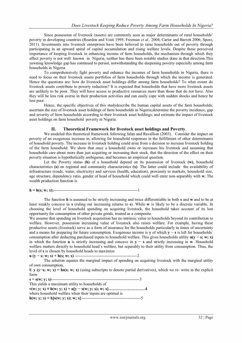
wealth production function is

h = h(s; w; x):--------------------------------------------------------------1

The function h is assumed to be strictly increasing and twice differentiable in both s and w and to be at

least weakly concave in s (ruling out increasing returns to s). While w is likely to be a discrete variable. In

choosing the level of household spending on acquiring livestock, the household takes account of its lost

opportunity for consumption of other private goods, treated as a composite.

We assume that spending on livestock acquisition has no intrinsic value to households beyond its contribution to

welfare. However, possession increasing value of livestock also raises welfare. For example, having these

productive assets (livestock) serve as a form of insurance for the households particularly in times of uncertainty

and a means for preparing for future consumption. Exogenous income is y of which y − s is left for households`

consumption after deducting purchased inputs to household welfare. This gives households utility u(y − s; w; x)

in which the function u is strictly increasing and concave in y − s and strictly increasing in w. Household

welfare matters directly to household head`s welfare, but separably to their utility from consumption. Thus, the level of s is chosen by household heads to maximize

u (y − s; w; x) + h(s; w; x) ----------------------------------------------2

The solution equates the marginal impact of spending on acquiring livestock with the marginal utility

of own consumption,

U y (y−s; w; x) = hs(s; w; x) (using subscripts to denote partial derivatives), which we re- write in the explicit

form

s = s(w; y; x)-----------------------------------------------------------------3

This yields a maximum utility to households of

v(w; y; x) ≡ h(w; y; x) + u[y − s(w; y; x); w; x]………………………4 where household welfare when their inputs are optimal is

h(w; y; x) ≡ h[s(w; y; x); w; x]--------------------------------------------5



By the envelope theorem, v (w; y; x) must be increasing in w. However, this need not hold for both components

of household utility. The effect of w on household poverty in a neighborhood of the equilibrium in which private

inputs are optimal is given by

hw = hs SW + hW ---------------------------------------------------------6 Where

𝑆𝑤 = 𝑈𝑦𝑤 −𝑕𝑠𝑤

𝑕𝑠𝑠− 𝑢𝑦𝑦………………………………………………………7

It can be seen that SW has the same sign as hSw– Uywwhich could be positive, negative or zero. Since

the direct welfare effect is positive (hw>0), it can be seen from (6) that hSW– Uyw≥ 0is sufficient for

livestock assets to improve household poverty/welfare.

Now consider the income effect on the welfare gain from livestock assets. This is given

𝐻𝑤𝑦 = 𝑆𝑦 𝑕𝑠𝑤 + 𝑆𝑤𝑕𝑠𝑠 + 𝑕𝑠𝑆𝑤𝑦 ……………………………………………………………8

Where

0 < 𝑆𝑦 =𝑢𝑦𝑦

𝑕𝑠𝑠 + 𝑢𝑦𝑦

≤ 1 …… ………… ………… ……… … 9

In the special case in which there are no interaction effects in household utility between livestock assets

and income or spending on household welfare/poverty (hsw= Uyw = 0), we find that hwy = 0;

The poverty/welfare gains from livestock assets are independent of household income. More generally,

however, the direction of the income effect could go either way. Consider the case in which household direct

utility is additively separable between consumption and livestock holding (Uyw = 0) and the livestock holding does not alter the marginal propensity to spend on household inputs to household welfare (Syw = 0).

Then hwy = S2hSW (using (7) and (9)). So in this special case, the household welfare benefit from

livestock holdings will increase (decrease) with income if the stocks are complements (substitutes) for other

household inputs.

So far we have taken livestock possession to be exogenous. In the empirical work we allowed

placement to be a function of a wide range of observable characteristics at household level. Here, we can think

(quite generally) of the placement as maximizing some weighted sum of v(wi ,xi, yi ) over all i, with weights

determined by a vector of characteristics of the household and their socioeconomic environment. This might

also include any other variable affecting the household poverty. The solutions will take the form wi =w (xi, λ)

where λ denotes one or more multipliers on the constraints, including resources available for providing other

inputs. The task of the empirical work is then to measure the welfare gains from higher w, recognizing that the observed levels of w in the cross-sectional data reflect purposive placement, assuming that the relevant x’s

are observable.

III. Methodology The Nigeria Living Standard Survey (NLSS) conducted by the National Bureau of Statistics in

2009/2010 was the source of data for this study.The NLSS data was collected on some indicators which

include demography, education, health, employment and time use, migration, housing, social capital,

agriculture, household expenditure, non-farm enterprise, credit, assets and saving, income transfer and

household income schedule.

The poverty incidence, gap and severity of farm households according to their livestock asset holdings was realized using Foster Greer Thorbecke indicators while the impact of livestock asset holdings on farm

household poverty was realized using propensity score matching.

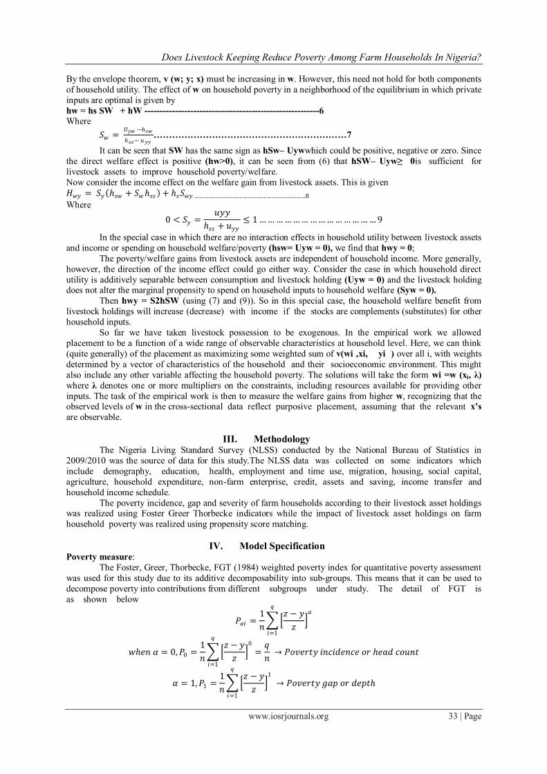
IV. Model Specification Poverty measure:

The Foster, Greer, Thorbecke, FGT (1984) weighted poverty index for quantitative poverty assessment

was used for this study due to its additive decomposability into sub-groups. This means that it can be used to

decompose poverty into contributions from different subgroups under study. The detail of FGT is

as shown below

𝑃𝛼𝑖 =1

𝑛

𝑧 − 𝑦

𝑧 𝛼

𝑞

𝑖=1

𝑤𝑕𝑒𝑛 𝛼 = 0, 𝑃0 =1

𝑛

𝑧 − 𝑦

𝑧

0𝑞

𝑖=1

=𝑞

𝑛 → 𝑃𝑜𝑣𝑒𝑟𝑡𝑦 𝑖𝑛𝑐𝑖𝑑𝑒𝑛𝑐𝑒 𝑜𝑟 𝑕𝑒𝑎𝑑 𝑐𝑜𝑢𝑛𝑡

𝛼 = 1, 𝑃1 =1

𝑛

𝑧 − 𝑦

𝑧

1𝑞

𝑖=1

→ 𝑃𝑜𝑣𝑒𝑟𝑡𝑦 𝑔𝑎𝑝 𝑜𝑟 𝑑𝑒𝑝𝑡𝑕



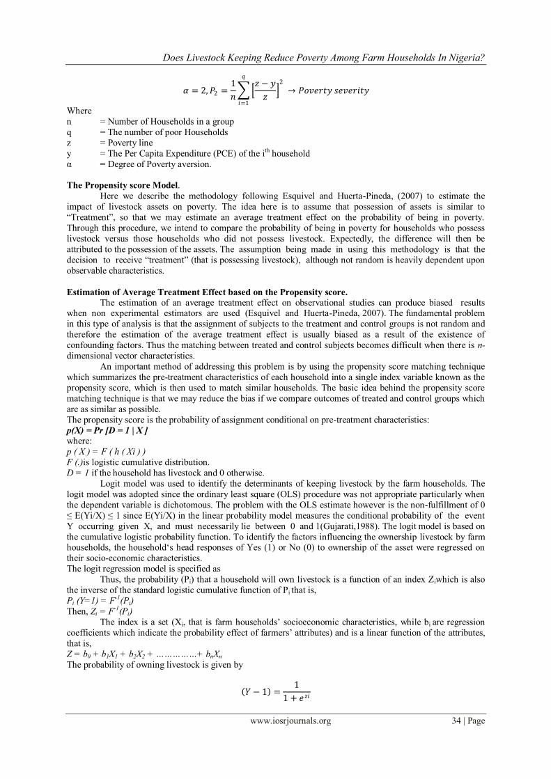
𝛼 = 2, 𝑃2 =1

𝑛

𝑧 − 𝑦

𝑧

2𝑞

𝑖=1

→ 𝑃𝑜𝑣𝑒𝑟𝑡𝑦 𝑠𝑒𝑣𝑒𝑟𝑖𝑡𝑦

Where

n = Number of Households in a group

q = The number of poor Households

z = Poverty line

y = The Per Capita Expenditure (PCE) of the ith household

α = Degree of Poverty aversion.

The Propensity score Model.

Here we describe the methodology following Esquivel and Huerta-Pineda, (2007) to estimate the

impact of livestock assets on poverty. The idea here is to assume that possession of assets is similar to

“Treatment”, so that we may estimate an average treatment effect on the probability of being in poverty.

Through this procedure, we intend to compare the probability of being in poverty for households who possess

livestock versus those households who did not possess livestock. Expectedly, the difference will then be

attributed to the possession of the assets. The assumption being made in using this methodology is that the

decision to receive “treatment” (that is possessing livestock), although not random is heavily dependent upon

observable characteristics.

Estimation of Average Treatment Effect based on the Propensity score.

The estimation of an average treatment effect on observational studies can produce biased results when non experimental estimators are used (Esquivel and Huerta-Pineda, 2007). The fundamental problem

in this type of analysis is that the assignment of subjects to the treatment and control groups is not random and

therefore the estimation of the average treatment effect is usually biased as a result of the existence of

confounding factors. Thus the matching between treated and control subjects becomes difficult when there is n-

dimensional vector characteristics.

An important method of addressing this problem is by using the propensity score matching technique

which summarizes the pre-treatment characteristics of each household into a single index variable known as the

propensity score, which is then used to match similar households. The basic idea behind the propensity score

matching technique is that we may reduce the bias if we compare outcomes of treated and control groups which

are as similar as possible.

The propensity score is the probability of assignment conditional on pre-treatment characteristics:

p(X) = Pr [D = 1 | X ]

where:

p ( X ) = F ( h ( Xi ) )

F (.)is logistic cumulative distribution.

D = 1 if the household has livestock and 0 otherwise.

Logit model was used to identify the determinants of keeping livestock by the farm households. The

logit model was adopted since the ordinary least square (OLS) procedure was not appropriate particularly when

the dependent variable is dichotomous. The problem with the OLS estimate however is the non-fulfillment of 0

≤ E(Yi/X) ≤ 1 since E(Yi/X) in the linear probability model measures the conditional probability of the event

Y occurring given X, and must necessarily lie between 0 and 1(Gujarati,1988). The logit model is based on

the cumulative logistic probability function. To identify the factors influencing the ownership livestock by farm households, the household„s head responses of Yes (1) or No (0) to ownership of the asset were regressed on

their socio-economic characteristics.

The logit regression model is specified as

Thus, the probability (Pi) that a household will own livestock is a function of an index Ziwhich is also

the inverse of the standard logistic cumulative function of Pi that is,

Pi (Y=1) = F-1(Pi)

Then, Zi = F-1(Pi)

The index is a set (Xi, that is farm households‟ socioeconomic characteristics, while bi are regression

coefficients which indicate the probability effect of farmers‟ attributes) and is a linear function of the attributes,

that is,

Z = b0 + b1X1 + b2X2 + ……………+ bnXn

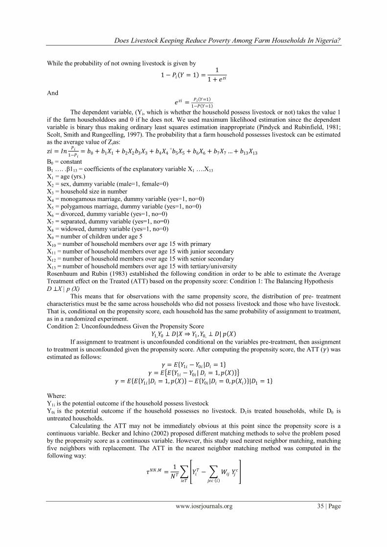
The probability of owning livestock is given by

𝑌 − 1 =1

1 + 𝑒𝑧𝑖



While the probability of not owning livestock is given by

1 − 𝑃𝑖 𝑌 = 1 =1

1 + 𝑒𝑧𝑖

And

𝑒𝑧𝑖 =𝑃𝑖 𝑌=1

1−𝑃 𝑌=1

The dependent variable, (Yi, which is whether the household possess livestock or not) takes the value 1

if the farm householddoes and 0 if he does not. We used maximum likelihood estimation since the dependent

variable is binary thus making ordinary least squares estimation inappropriate (Pindyck and Rubinfield, 1981;

Scolt, Smith and Rungeelling, 1997). The probability that a farm household possesses livestock can be estimated as the average value of Zias:

𝑧𝑖 = 𝐼𝑛𝑃𝑖

1−𝑃𝑖= 𝑏0 + 𝑏1𝑋1 + 𝑏2𝑋2𝑏3𝑋3 + 𝑏4𝑋4

+𝑏5𝑋5 + 𝑏6𝑋6 + 𝑏7𝑋7 … + 𝑏13𝑋13

Β0 = constant Β1 …. .β113 = coefficients of the explanatory variable X1 ….X13

X1 = age (yrs.)

X2 = sex, dummy variable (male=1, female=0)

X3 = household size in number

X4 = monogamous marriage, dummy variable (yes=1, no=0)

X5 = polygamous marriage, dummy variable (yes=1, no=0)

X6 = divorced, dummy variable (yes=1, no=0)

X7 = separated, dummy variable (yes=1, no=0)

X8 = widowed, dummy variable (yes=1, no=0)

X9 = number of children under age 5

X10 = number of household members over age 15 with primary

X11 = number of household members over age 15 with junior secondary X12 = number of household members over age 15 with senior secondary

X13 = number of household members over age 15 with tertiary/university

Rosenbaum and Rubin (1983) established the following condition in order to be able to estimate the Average

Treatment effect on the Treated (ATT) based on the propensity score: Condition 1: The Balancing Hypothesis

D ⊥X | p (X)

This means that for observations with the same propensity score, the distribution of pre- treatment

characteristics must be the same across households who did not possess livestock and those who have livestock.

That is, conditional on the propensity score, each household has the same probability of assignment to treatment,

as in a randomized experiment.

Condition 2: Unconfoundedness Given the Propensity Score

𝑌1,𝑌0 ⊥ 𝐷|𝑋 ⇒ 𝑌1 , 𝑌0, ⊥ 𝐷| 𝑝 𝑋

If assignment to treatment is unconfounded conditional on the variables pre-treatment, then assignment

to treatment is unconfounded given the propensity score. After computing the propensity score, the ATT (𝛾) was

estimated as follows:

𝛾 = 𝐸 𝑌1𝑖 − 𝑌0𝑖 |𝐷𝑖 = 1

𝛾 = 𝐸 𝐸 𝑌1𝑖 − 𝑌0𝑖| 𝐷𝑖 = 1, 𝑝 𝑋

𝛾 = 𝐸 𝐸 𝑌1𝑖 |𝐷𝑖 = 1, 𝑝 𝑋 − 𝐸 𝑌0𝑖|𝐷𝑖 = 0, 𝑝 𝑋𝑖 |𝐷1 = 1

Where:

Y1i is the potential outcome if the household possess livestock

Y0i is the potential outcome if the household possesses no livestock. D1is treated households, while D0 is

untreated households.

Calculating the ATT may not be immediately obvious at this point since the propensity score is a

continuous variable. Becker and Ichino (2002) proposed different matching methods to solve the problem posed by the propensity score as a continuous variable. However, this study used nearest neighbor matching, matching

five neighbors with replacement. The ATT in the nearest neighbor matching method was computed in the

following way:

𝜏𝑁𝑁 .𝑀 =1

𝑁𝑇 𝑌𝑖

𝑇 − 𝑊𝑖𝑗

𝑗𝜖𝑐 𝑖

𝑌𝑗𝑐

𝑖𝜖𝑇



=1

𝑁𝑇 𝑌𝑖

𝑇

𝑖∈𝑇

− 𝑊𝑖𝑗

𝑗 ∈𝑐 𝑖 𝑖∈𝑇

𝑌𝑗𝑐

=1

𝑁𝑇 𝑌𝑖

𝑇 −1

𝑁𝑇

𝑗∈𝑇

𝑊𝑗

𝑗∈𝑖

𝑌𝑗𝐶

Where

𝑊𝑖𝑗 =1

𝑁𝑖𝑐 𝑖𝑓𝑗 ∈ 𝑎𝑛𝑑 𝑊𝑖𝑗 = 0 𝑜𝑡𝑕𝑒𝑟𝑤𝑖𝑠𝑒

𝑊𝑗 = 𝑊𝑖𝑗𝑖

And

𝐶 𝑖 = 𝑚𝑖𝑚 𝑝𝑖 − 𝑝𝑗 𝑓𝑜𝑟 𝑡𝑕𝑒 𝑛𝑒𝑎𝑟𝑒𝑠𝑡 𝑛𝑒𝑖𝑔𝑕𝑏𝑜𝑟 𝑚𝑎𝑡𝑐𝑕𝑖𝑛𝑔 𝑚𝑒𝑡𝑕𝑜𝑑

NC is the number of control observations, and NTis the number of treated observations. YT is the outcome for the

treated and YCis the outcome for the control.

In the propensity score analysis, we treated possession of livestock as dichotomous variables. Possession of

livestock versus not having livestock. This manipulation helped to ascertain the effect of having livestock on

household poverty.

The variables included in the propensity score matching included human capital as well as other household

characteristics such as age of household head, education level, and household size, among others. These

variables have been implicated in literature to determine poverty (Grootaert, et al, 2002; Ersado, 2006; Ahmed

et al, 2009; Chaudhry, Malik and Hassan, 2009).

After matching and estimating the ATT, the ATT was then applied to households that did not have the livestock assets in order to find out the decrease/increase in poverty headcount, poverty gap, and poverty severity due to

these attributes; that is, to find out what poverty will be assuming the households who do not have livestock

assets are allowed to have access to size of income/expenditure equal to the ATT.

V. Results And Discussion Size and composition of Human capital asset indicators of the respondents

This study made use of 24,492 farm households, headed by 21,925(89.52%) males and 2,567(10.48%)

females.

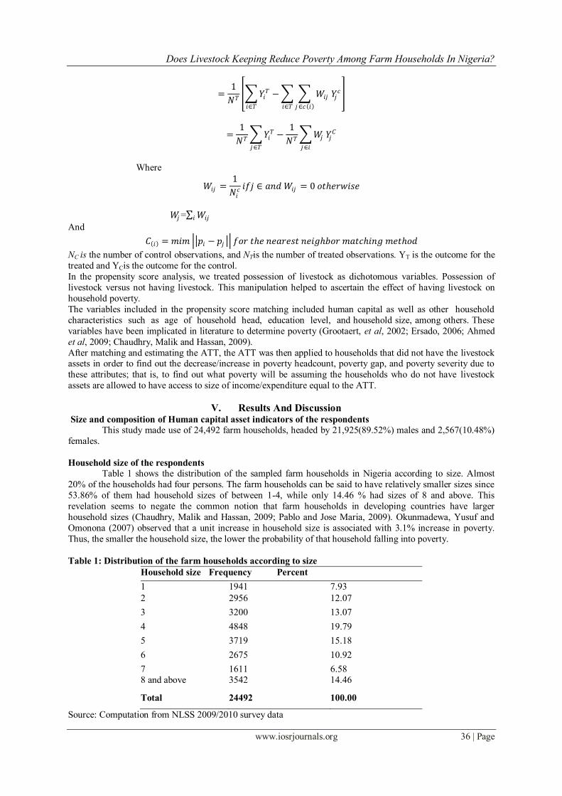
Household size of the respondents

Table 1 shows the distribution of the sampled farm households in Nigeria according to size. Almost

20% of the households had four persons. The farm households can be said to have relatively smaller sizes since

53.86% of them had household sizes of between 1-4, while only 14.46 % had sizes of 8 and above. This

revelation seems to negate the common notion that farm households in developing countries have larger

household sizes (Chaudhry, Malik and Hassan, 2009; Pablo and Jose Maria, 2009). Okunmadewa, Yusuf and

Omonona (2007) observed that a unit increase in household size is associated with 3.1% increase in poverty.

Thus, the smaller the household size, the lower the probability of that household falling into poverty.

Table 1: Distribution of the farm households according to size

Household size Frequency Percent

1 1941 7.93

2 2956 12.07

3 3200 13.07

4 4848 19.79

5 3719 15.18

6 2675 10.92

7

8 and above

1611

3542

6.58

14.46

Total 24492 100.00

Source: Computation from NLSS 2009/2010 survey data



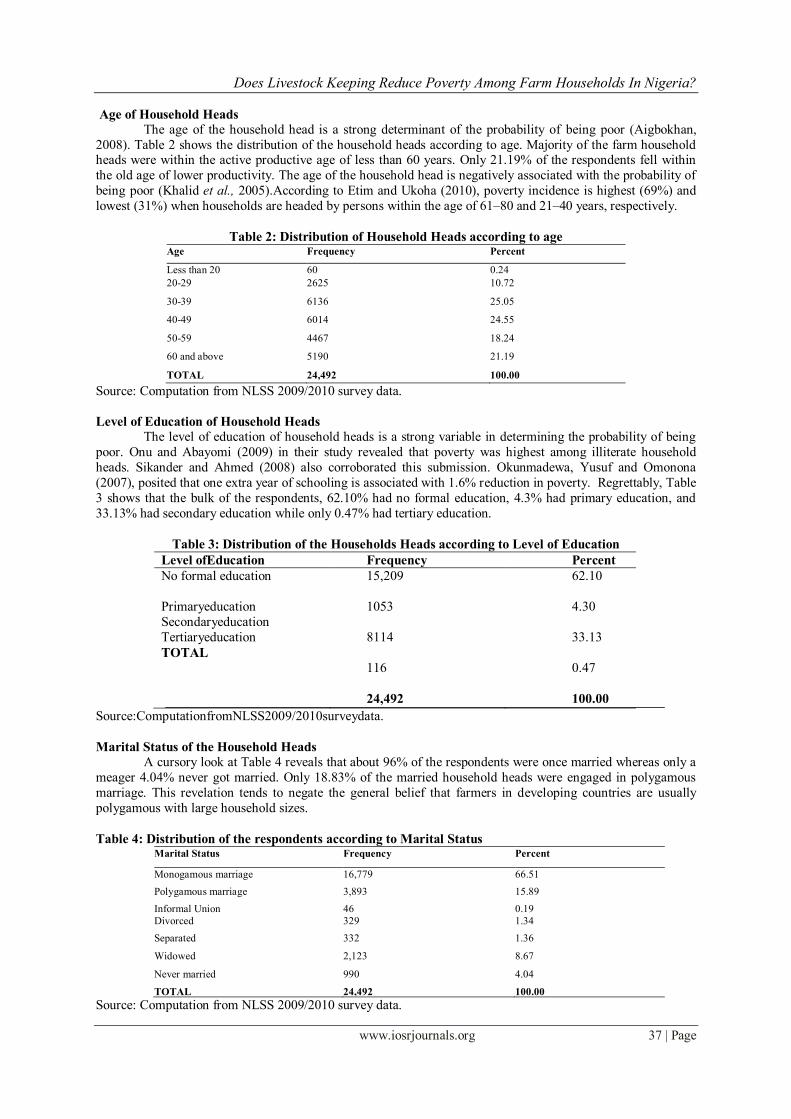
Age of Household Heads

The age of the household head is a strong determinant of the probability of being poor (Aigbokhan,

2008). Table 2 shows the distribution of the household heads according to age. Majority of the farm household heads were within the active productive age of less than 60 years. Only 21.19% of the respondents fell within

the old age of lower productivity. The age of the household head is negatively associated with the probability of

being poor (Khalid et al., 2005).According to Etim and Ukoha (2010), poverty incidence is highest (69%) and

lowest (31%) when households are headed by persons within the age of 61–80 and 21–40 years, respectively.

Table 2: Distribution of Household Heads according to age Age Frequency Percent

Less than 20 60 0.24

20-29 2625 10.72

30-39 6136 25.05

40-49 6014 24.55

50-59 4467 18.24

60 and above 5190 21.19

TOTAL 24,492 100.00

Source: Computation from NLSS 2009/2010 survey data.

Level of Education of Household Heads

The level of education of household heads is a strong variable in determining the probability of being

poor. Onu and Abayomi (2009) in their study revealed that poverty was highest among illiterate household

heads. Sikander and Ahmed (2008) also corroborated this submission. Okunmadewa, Yusuf and Omonona

(2007), posited that one extra year of schooling is associated with 1.6% reduction in poverty. Regrettably, Table

3 shows that the bulk of the respondents, 62.10% had no formal education, 4.3% had primary education, and

33.13% had secondary education while only 0.47% had tertiary education.

Table 3: Distribution of the Households Heads according to Level of Education

Level ofEducation Frequency Percent

No formal education

Primaryeducation

Secondaryeducation

Tertiaryeducation

TOTAL

15,209

1053

8114

116

24,492

62.10

4.30

33.13

0.47

100.00

Source:ComputationfromNLSS2009/2010surveydata.

Marital Status of the Household Heads

A cursory look at Table 4 reveals that about 96% of the respondents were once married whereas only a

meager 4.04% never got married. Only 18.83% of the married household heads were engaged in polygamous

marriage. This revelation tends to negate the general belief that farmers in developing countries are usually

polygamous with large household sizes.

Table 4: Distribution of the respondents according to Marital Status Marital Status Frequency Percent

Monogamous marriage 16,779 66.51

Polygamous marriage 3,893 15.89

Informal Union 46 0.19

Divorced 329 1.34

Separated 332 1.36

Widowed 2,123 8.67

Never married 990 4.04

TOTAL 24,492 100.00




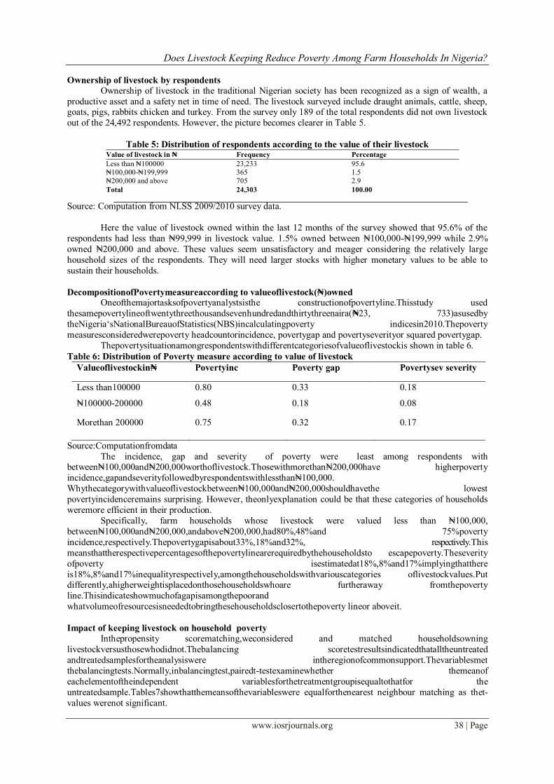
Ownership of livestock by respondents Ownership of livestock in the traditional Nigerian society has been recognized as a sign of wealth, a

productive asset and a safety net in time of need. The livestock surveyed include draught animals, cattle, sheep, goats, pigs, rabbits chicken and turkey. From the survey only 189 of the total respondents did not own livestock

out of the 24,492 respondents. However, the picture becomes clearer in Table 5.

Table 5: Distribution of respondents according to the value of their livestock Value of livestock in ₦ Frequency Percentage

Less than ₦100000

₦100,000-₦199,999

₦200,000 and above

Total

23,233

365

705

24,303

95.6

1.5

2.9

100.00


Here the value of livestock owned within the last 12 months of the survey showed that 95.6% of the

respondents had less than ₦99,999 in livestock value. 1.5% owned between ₦100,000-₦199,999 while 2.9%

owned ₦200,000 and above. These values seem unsatisfactory and meager considering the relatively large

household sizes of the respondents. They will need larger stocks with higher monetary values to be able to

sustain their households.

DecompositionofPovertymeasureaccording to valueoflivestock(₦)owned Oneofthemajortasksofpovertyanalystsisthe constructionofpovertyline.Thisstudy used

thesamepovertylineoftwentythreethousandsevenhundredandthirtythreenaira(₦23, 733)asusedby

theNigeria„sNationalBureauofStatistics(NBS)incalculatingpoverty indicesin2010.Thepoverty

measuresconsideredwerepoverty headcountorincidence, povertygap and povertyseverityor squared povertygap.

Thepovertysituationamongrespondentswithdifferentcategoriesofvalueoflivestockis shown in table 6.

Table 6: Distribution of Poverty measure according to value of livestock

Valueoflivestockin₦ Povertyinc

Incidence

Poverty gap Povertysev severity

Less than100000 0.80 0.33 0.18

₦100000-200000 0.48 0.18 0.08

Morethan 200000 0.75 0.32 0.17

Source:Computationfromdata

The incidence, gap and severity of poverty were least among respondents with between₦100,000and₦200,000worthoflivestock.Thosewithmorethan₦200,000have higherpoverty

incidence,gapandseverityfollowedbyrespondentswithlessthan₦100,000.

Whythecategorywithvalueoflivestockbetween₦100,000and₦200,000shouldhavethe lowest

povertyincidenceremains surprising. However, theonlyexplanation could be that these categories of households

weremore efficient in their production.

Specifically, farm households whose livestock were valued less than ₦100,000,

between₦100,000and₦200,000,andabove₦200,000,had80%,48%and 75%poverty

incidence,respectively.Thepovertygapisabout33%,18%and32%, respectively.This

meansthattherespectivepercentagesofthepovertylinearerequiredbythehouseholdsto escapepoverty.Theseverity

ofpoverty isestimatedat18%,8%and17%implyingthatthere

is18%,8%and17%inequalityrespectively,amongthehouseholdswithvariouscategories oflivestockvalues.Put differently,ahigherweightisplacedonthosehouseholdswhoare furtheraway fromthepoverty

line.Thisindicateshowmuchofagapisamongthepoorand

whatvolumeofresourcesisneededtobringthesehouseholdsclosertothepoverty lineor aboveit.

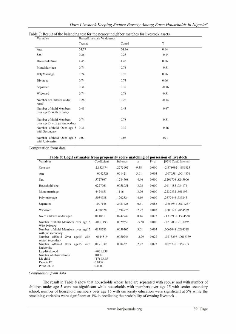
Impact of keeping livestock on household poverty

Inthepropensity scorematching,weconsidered and matched householdsowning

livestockversusthosewhodidnot.Thebalancing scoretestresultsindicatedthatalltheuntreated

andtreatedsamplesfortheanalysiswere intheregionofcommonsupport.Thevariablesmet

thebalancingtests.Normally,inbalancingtest,pairedt-testexaminewhether themeanof

eachelementoftheindependent variablesforthetreatmentgroupisequaltothatfor the

untreatedsample.Tables7showthatthemeansofthevariableswere equalforthenearest neighbour matching as thet-

values werenot significant.



Table 7: Result of the balancing test for the nearest neighbor matches for livestock assets Variables RaisedLivestock Vs doesnot

Treated Contrl T

Age 54.77 54.36 0.64

Sex 0.26 0.28 -0.14

Household Size 4.45 4.46 0.06

MonoMarriage 0.74 0.78 -0.31

PolyMarriage 0.74 0.73 0.06

Divorced 0.74 0.73 0.06

Separated 0.31 0.32 -0.36

Widowed 0.74 0.78 -0.31

Number of Children under

Age5

0.26 0.28 -0.14

Number ofhhold Members

over age15 With Primary

0.41 0.43 -0.67

Number ofhhold Members

over age15 with jnrsencondary

0.74 0.78 -0.31

Number ofhhold Over age15

with Secondary

0.31 0.32 -0.36

Number ofhhold Over age15

with University

0.07 0.08 -021

Computation from data

Table 8: Logit estimates from propensity score matching of possession of livestock Variables Coefficient Std error z P>|z| [95% Conf. Interval]

Constant -2.132474 .2273605 -9.38 0.000 -2.578092-1.686855

Age -.0042728 .001421 -3.01 0.003 -.007058 -.0014876

Sex .5727807 .1284768 4.46 0.000 .3209708 .8245906

Household size .0227961 .0058051 3.93 0.000 .0114183 .034174

Mono marriage .4424651 .1116 3.96 0.000 .2237332 .6611971

Poly marriage .5034938 .1202824 4.19 0.000 .2677446 .739243

Separated .1007145 .2481725 0.41 0.685 -.3856947 .5871237

Widowed .4728828 .1594775 2.97 0.003 .1603127 .7854529

No of children under age5 .011881 .0742742 0.16 0.873 -.1336938 .1574558

Number ofhhold Members over age15

With Primary

-.0161493 .0029359 -5.50 0.000 -.0219036 -.010395

Number ofhhold Members over age15

with jnr secondary

.0178283 .0059305 3.01 0.003 .0062048 .0294518

Number ofhhold Over age15 with

senior Secondary

-.0114819 .0050246 -2.29 0.022 -.0213298 -.0016339

Number ofhhold Over age15 with

University

.0191039 .008432 2.27 0.023 .0025776 .0356303

Log-likelihood

Number of observations

LR chi 2

Pseudo R2

Prob> chi 2

-9071.738

18112

(17) 93.65

0.0159

0.0000

Computation from data

The result in Table 8 show that households whose head are separated with spouse and with number of

children under age 5 were not significant while households with members over age 15 with senior secondary

school, number of household members over age 15 with university education were significant at 5% while the

remaining variables were significant at 1% in predicting the probability of owning livestock.



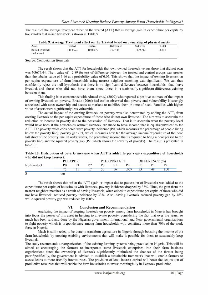
The result of the average treatment effect on the treated (ATT) that is average gain in expenditure per capita by

households that raised livestock is shown in Table 9

Table 9: Average Treatment effect on the Treated based on ownership of physical assets Asset Treated Control Difference Std error T-stat

Raised livestock

vs does not

14046.23 10368.79 3677.44 1270.713 2.894

Source: Computation from data

The result shows that the ATT for households that own owned livestock versus those that did not own

was ₦3677.44. The t value of 2.89 for test of difference between the treated and control groups was greater

than the tabular value of 1.96 at a probability value of 0.05. This shows that the impact of owning livestock on

per capita expenditure of farm households using nearest neighbor matching was significant. We can thus

confidently reject the null hypothesis that there is no significant difference between households that have

livestock and those who did not have them since there is a statistically significant differences existing

between them.

This finding is in consonance with Ahmed et al, (2009) who reported a positive estimate of the impact of owning livestock on poverty. Ersado (2006) had earlier observed that poverty and vulnerability is strongly

associated with asset ownership and access to markets to mobilize them in time of need. Families with higher

value of assets were significantly less vulnerable.

The actual impact of the owning livestock on poverty was also determined by adding the ATT, from

owning livestock to the per capita expenditure of those who do not own livestock. The aim was to ascertain the

reduction or increase in poverty due to the possession of livestock. That is to ascertain what the poverty level

would have been if the households without livestock are made to have income that is equal/equivalent to the

ATT. The poverty ratios considered were poverty incidence (P0, which measures the percentage of people living

below the poverty line), poverty gap (P1, which measures how far the average income/expenditure of the poor

fall short of the poverty line, in order words, the percentage income that is required to bring a poor person to the

poverty line) and the squared poverty gap (P2, which shows the severity of poverty). The result is presented in table 10.

Table 10: Distribution of poverty measure when ATT is added to per capita expenditure of households

who did not keep livestock

PCEXPDR PCEXPDR+ATT DIFFERENCE (%)

No livestock P0 P1 P2 P0 P1 P2 P0 P1 P2

75 31 17 50 16 .069 33 48 100

S our

The result shows that when the ATT (gain or impact due to possession of livestock) was added to the

expenditure per capita of households with livestock, poverty incidence dropped by 33%. Thus, the gain from the

nearest neighbor matches as a result of having livestock, when added to expenditure per capita of those who did

not have livestock, reduced poverty incidence by 33%. Also, having livestock reduced poverty gap by 48%

while squared poverty gap was reduced by 100%.

VI. Conclusion and Recommendation Analyzing the impact of keeping livestock on poverty among farm households in Nigeria has brought

into focus the power of this asset in helping to alleviate poverty, considering the fact that over the years, so

much has been said and done by the Nigerian government, International and Non- governmental organizations

to fight poverty which is preponderance among farm households who constitute more than 70% of the work

force in Nigeria.

Much is still needed to be done to transform agriculture in Nigeria through boosting the income of the

farm households by creating enabling environments that will make it possible for them to sustainably keep

livestock.

The study recommends a reorganization of the existing farming systems being practiced in Nigeria. This will be

aimed at encouraging the farmers to incorporate some livestock enterprises into their farm business

organizations since the ownership of livestock significantly minimized the chances of the farmer being

poor.Specifically, the government is advised to establish a sustainable framework that will enable farmers to access loans at more friendly interest rates. The provision of low- interest capital will boost the acquisition of

productive resources that will enable the farm households to invest meaningfully in livestock production.



References [1]. Aigbokhan,B.E (2008) Growth, Inequality and Poverty in Nigeria. ACGS/MPAMS Discussion Paper No.3.United Nations

Economic Commission for Africa (UNECA) Addis Ababa, Ethiopia.

[2]. Ahmed, A. U; M.Rabbani; Sulaiman, M and N.C Das (2009)TheImpact of Asset transfer On Livelihoods of theUltraPoor in

Bangladesh. Research Monograph SeriesNo. 39. BRAC CentreBangladesh

[3]. Aryeetey,E. (2004)Household asset choiceamong therural poor in Ghana.Paper presented at theworkshopUnderstanding Poverty in

Ghana Organized bytheInstituteof Statistical, Social and EconomicResearch,Universityof Ghana and Cornell University

[4]. Becker, Sascha andAndreaIchino(2002) “Estimation ofAverageTreatment Effects Based on PropensityScores”. InTheStataJournal,

Vol.2 No 4.

[5]. Carter, M. R. and C. B. Barrett(2005). TheEconomics of PovertyTraps and Persistent Poverty: An Asset-BasedApproach. Madison,

Universityof Wisconsin.

[6]. CentralIntelligenceAgency(2011) TheWorld Fact Book. http://www.cia.gov/library/publications/the-worldfactbook/geos/ni.html.

Retrieved on 19th July2011.

[7]. ChaudhryI.S., S. Malik and A. Hassan (2009) TheImpact of Socioeconomic and DemographicVariables on Poverty: A

VillageStudy.TheLahore Journalof Economics 14: 1:pp. 39-68

[8]. Ersado,Lire(2006) “Rural Vulnerabilityin Serbia”.World Bank Policy Research Working Paper 4010

[9]. Esquivel, G and A. Huerta_Pineda (2007)Remittances and Povertyin Mexico: A Propensity ScoreMatching Approach. Colegio

deMéxico, Working Paper No. 27.

[10]. Etim, N.A. and O.OUkoha (2010).Analysisof povertyprofileofrural households: evidencefrom South-South Nigeria. J. Agric.

Soc.Sci., 6: 48–52

[11]. Foster, J.J. Greer, and E.Thorbecke (1984)“A Class of Decomposable Poverty Measures”Econometrica52 (1)

[12]. Freeman, H. A., Ellis, F. and E. Allison,( 2004).Livelihoods and rural povertyreduction in Kenya. Development PolicyReview

22(2): 147-171.

[13]. Grootaert, C, Gi-taik ohand Swamy, (2002). “Social capital, household welfare and poverty in Burkina Faso”, Journal ofAfrican

Economies,11 (1).165.

[14]. Idachaba, F.(2006)GoodIntentions arenot good enough. Collected Essayson Government and NigerianAgriculture.Vol 2.

UniversityPress Ltd,Ibadan. 218p

[15]. Jalan,Jand M. Ravallion (2003)Does Piped waterreducediarrhea for children in rural India?Journal of Econometrics112, 153-173.

[16]. NBS, (2005) Draft Poverty Profilefor Nigeria 2004. National Bureau of Statistics Abuja.

[17]. NBS, (2011)News retrieved fromhttp://www.nigeriastat.gov.ngon 18th

July

[18]. Okunmadewa, F.Y, S.AYusuf and B.T. Omonona (2007) Effects of Social Capitalon rural Povertyin Nigeria.Pakistan Journal of

SocialSciences4 (3): 331-339

[19]. OnuJ.Iand Abayomi.Z(2009)AnAnalysisof Povertyamong Households in Yola Metropolis of Adamawa State, Nigeria Journal

Social Sciences,20(1): 43-48

[20]. Pablo,Band S.Jose Maria (2009)Access to landand rural povertyin developing countries:theoryandevidencefrom

Guatemala.Universidad PolitecnicadeMadrid. MPRA Paper No. 13365, Available online at http://mpra.ub.uni-muenchen.de/13365/

posted 12. February2009/ 14:29

[21]. Pindyck, R.S. and Rubinfield, D.L. (1981) Econometric Models and Economic Forecast. 2nd Edition, London, McGraw-Hill.

[22]. Reardon,T. and S. A.Vosti, (1995)Links between Rural Povertyand theEnvironment in Developing Countries: Asset Categories

andInvestment Poverty,World Development23(9).

[23]. Rosenbaum,Pand D. Rubin (1983) Thecentral role ofpropensityscorein observational studies for causal effects.Biometrica, No 70.

[24]. Scolt, L.C., Smith, L. and Rungeelling, B. (1997). Labour Force Participation inSouthern Labour Markets. American Journal of

Agricultural Economics 59 (2) 266-274 [25].

Sikander M.U. and M. Ahmed (2008)Household Determinants of Povertyin Punjab: A Logistic Regression Analysis of MICS(2003-

04)Data Set.Paper presented at the 8th

Global conferenceon Business and Economics. FlorenceItaly,October 18th

-19

th

[26]. SPORE (2011)LivestockDisease: A heavyBurden. Spore. CTA, AJWageningen. No.153

[27]. Van deWalle, Dominique and DileniGunewardena (2001),“Sources ofEthnic Inequalityin Vietnam” PolicyResearchWorkingPaper

2297.World Bank, Washington, DC.

[28]. WDI(World DevelopmentIndicators)(2007).WDIdatabase.WorldBank, Washington, D.C. WendyStone (2001)Measuring Social

Capital:Towards atheoreticallyinformed measurement frameworkfor researching social capital in familylife.Research paper No. 24

.University, St.Louis:Center forSocial Development.

http://www.cia.gov/library/publications/the-world-factbook/geos/ni.html

http://www.nigeriastat.gov.ng/

http://mpra.ub.uni-muenchen.de/13365/

Does Livestock Keeping Reduce Poverty Among Farm Households In Nigeria?

Documents

Transcript of Does Livestock Keeping Reduce Poverty Among Farm Households In Nigeria?