Does amplitude scaling of ground motion records result in biased nonlinear structural drift...

EARTHQUAKE ENGINEERING AND STRUCTURAL DYNAMICSEarthquake Engng Struct. Dyn. 2007; 36:1813–1835Published online 22 June 2007 in Wiley InterScience (www.interscience.wiley.com). DOI: 10.1002/eqe.695

Does amplitude scaling of ground motion records result in biasednonlinear structural drift responses?

Nicolas Luco1,∗,† and Paolo Bazzurro2

1United States Geological Survey, Golden, CO 80401, U.S.A.2AIR Worldwide Corporation, San Francisco, CA 94111, U.S.A.

SUMMARY

Limitations of the existing earthquake ground motion database lead to scaling of records to obtainseismograms consistent with a ground motion target for structural design and evaluation. In the engineeringseismology community, acceptable limits for ‘legitimate’ scaling vary from one (no scaling allowed) to10 or more. The concerns expressed by detractors of scaling are mostly based on the knowledge of,for example, differences in ground motion characteristics for different earthquake magnitude–distance(Mw–Rclose) scenarios, and much less on their effects on structures. At the other end of the spectrum,proponents have demonstrated that scaling is not only legitimate but also useful for assessing structuralresponse statistics for Mw–Rclose scenarios. Their studies, however, have not investigated more recentpurposes of scaling and have not always drawn conclusions for a wide spectrum of structural vibrationperiods and strengths. This article investigates whether scaling of records randomly selected from anMw–Rclose bin (or range) to a target fundamental-mode spectral acceleration (Sa) level introduces biasin the expected nonlinear structural drift response of both single-degree-of-freedom oscillators and onemulti-degree-of-freedom building. The bias is quantified relative to unscaled records from the targetMw–Rclose bin that are ‘naturally’ at the target Sa level. We consider scaling of records from the targetMw–Rclose bin and from other Mw–Rclose bins. The results demonstrate that scaling can indeed introducea bias that, for the most part, can be explained by differences between the elastic response spectra of thescaled versus unscaled records. Copyright q 2007 John Wiley & Sons, Ltd.

Received 15 September 2006; Revised 5 February 2007; Accepted 22 March 2007

KEY WORDS: ground motion record scaling and selection; nonlinear dynamic analysis; near-sourceground motions; nonlinear inelastic seismic drift response

∗Correspondence to: Nicolas Luco, P.O. Box 25046, MS 966, Denver, CO 80225, U.S.A.†E-mail: [email protected]

Contract/grant sponsor: PEER (Pacific Earthquake Engineering Research) Lifelines Program; contract/grant number:SA3592

Copyright q 2007 John Wiley & Sons, Ltd.

1814 N. LUCO AND P. BAZZURRO

1. INTRODUCTION

With the advent of performance-based earthquake engineering and the increasing availability ofsophisticated structural analysis software and faster computers, nonlinear dynamic response-historyanalysis has become more widely used for design and evaluation of structures. One of the biggestobstacles preventing more widespread use of such analysis is the selection of ‘appropriate’ groundmotion records. According to best practices (e.g. [1]), engineers seek real ground motion recordsthat closely match a spectral acceleration at a specified hazard level (e.g. 2% in 50 years), aswell as the earthquake (moment) magnitude and (closest) source-to-site distance (Mw–Rclose)

pair(s) of the event(s) controlling the seismic hazard at the building site. The spectral accelera-tion of interest in seismically active regions (such as California) is often relatively large, and thecontrolling earthquake scenarios are often large magnitude events on nearby faults. Despite therecent increase in the number of available records for large earthquakes (e.g. the 1999 Mw = 7.6Chi-Chi Earthquake, the 1999 Mw = 7.5 Kocaeli Earthquake, the 2002 Mw = 7.9 Denali Earth-quake, and the 2003 Mw = 8.0 Hokkaido Earthquake), the existing database for such spectralacceleration and Mw–Rclose conditions is still limited. Moreover, the seismic hazard at the sitemay be characterized by specific rupture-directivity conditions and site classifications (e.g. NEHRPD) that further limit record availability. Given the current preference of many engineers to usereal rather than synthetic ground motions, scaling real records to obtain seismograms consistentwith a target level is often the only remaining option. In this paper we consider the most common‘scaling’ approach, i.e. multiplying the amplitude of a record by the constant scalar factor necessaryto reach a target pseudo-spectral acceleration level at the fundamental period of the structure (anda damping ratio of 5%), denoted here simply as Sa. The effects on nonlinear structural response ofmodifying the time scale or the frequency content and phasing (e.g. [2, 3]), or of amplitude scalingto target values of ground motion intensity measures other than Sa (e.g. [4–6]), are investigatedelsewhere.

In the engineering seismology community, acceptable ground motion scaling limits vary widelyfrom one (no scaling allowed) to 10 or more. The records used for one of the Pacific Earth-quake Engineering Research (PEER) Testbeds, for example, were scaled by factors up to 11(see www.peertestbeds.net/Hbt/HumboldtBayBridgeReport.pdf). These limits are based more onnecessity and/or a ‘comfort feeling’ than on a sound technical basis. We attempt here to provide aquantitative technical basis for threshold limits beyond which scaling of records might introducebias in the median nonlinear structural drift response for a target Sa and Mw–Rclose scenario.Note that the present study will not definitively establish the thresholds beyond which the biasintroduced by scaling should be avoided or corrected, but we will quantify the extent of the biasas a function of the amount of scaling and state the reasons that seem to cause it. We will alsoaddress more specific questions, such as the following: Does the bias vary with structural periodand level of nonlinear response? Does the bias change if the source records scaled to match thetarget Sa are characterized by values of Mw and Rclose that are different from, rather than the sameas, those that control the site hazard (called inter-bin versus intra-bin scaling hereafter)? In otherwords, given the same amount of scaling, do the magnitudes and distances of the source and targetrecords affect the bias in the median nonlinear structural response? In the final discussion sectionwe will provide a demonstration of the characteristics that a record should possess in order that,when scaled to a given target, no significant bias is introduced.

Copyright q 2007 John Wiley & Sons, Ltd. Earthquake Engng Struct. Dyn. 2007; 36:1813–1835DOI: 10.1002/eqe

AMPLITUDE SCALING OF GROUND MOTION RECORDS 1815

1.1. Background

The question of whether ground motion record scaling produces biased nonlinear structural responsestatistics has been debated for at least a decade. The concerns expressed by many individualsare mostly based on unquestionable differences in ground motion characteristics (e.g. responsespectral shape and duration among different Mw–Rclose scenarios) and much less on their effectson structures. Suppositions that systematic differences in the input necessarily cause systematicdifferences in the response are often based on engineering intuition or, at best, on knowledge ofthe sensitivities of response to differences in input that is based on evaluating linear elastic (e.g.[7]) rather than nonlinear inelastic structural responses. Direct testing of the legitimacy of groundmotion scaling for nonlinear structural response assessment has been a focus of Cornell and hisco-workers at Stanford University (e.g. [8–11]). All such studies found that judicious scaling wasnot only legitimate but, under certain conditions, also useful for the purpose of efficiently assessingstructural response statistics.

It must be emphasized, however, that the referenced studies have addressed the ground motionscaling issue from a different perspective than the one used here. Their focus was on the legitimacyof scaling a pool of records from a source Mw–Rclose bin such that they match the median‘intensity’ level of records belonging either to the same bin or to a different target Mw–Rclose bin.The legitimacy was assessed in terms of bias with respect to the median structural response to anunscaled suite of records representing the target Mw–Rclose bin. In those cases, the goal was toaccurately (i.e. without bias) estimate the median response for the target Mw and Rclose scenario,e.g. for an Mw = 7 earthquake on the San Andreas Fault at Rclose = 5 km. In contrast, current bestpractice (e.g. [1]) is to estimate the nonlinear response for a target Sa at a specified hazard level(e.g. 2% in 50 years) and, jointly, the Mw–Rclose pair(s) of the event(s) that contribute most to thisseismic hazard at the site of the structure. Hence, the goal we consider in this paper is accurateestimation of the median response for a target Sa, Mw, and Rclose, e.g. for an Sa of 2.0g associatedwith an Mw = 7 earthquake on the San Andreas Fault at Rclose = 5 km. Clearly the difference liesin the specification of a target Sa level in addition to an Mw and Rclose.

1.2. Objective

To be clear, the objective is to investigate whether amplitude scaling (in practice, almost always upbut, more academically, also down) of input earthquake records, to a target Sa level associated witha particular range (or bin) of Mw and Rclose values, introduces a bias in the (estimated) mediannonlinear structural drift response. As expressed in Equation (1), the bias is computed with respectto the median (strictly speaking, geometric mean) structural response to records from the targetMw–Rclose bin that are naturally (without scaling) at the target spectral acceleration level:

Bias= median structural response to scaled records

median structural response to unscaled records naturally at target Sa(1)

As anticipated in the Introduction, we consider both intra-bin and inter-bin scaling. The pur-pose of intra-bin scaling is to obtain a record that is both at the Sa level of interest and fromthe targeted Mw–Rclose bin. This case occurs in practice when records for the hazard-controllingscenario are available but they are not at the desired target Sa level. The purpose of inter-bin



scaling, on the other hand, is to obtain a record at the Sa level of interest for an empty or sparselypopulated Mw–Rclose target bin. In order to study inter-bin scaling, however, we consider targetbins that are adequately populated in order to maintain a point of comparison. We expect theseresults to provide a useful means for extrapolating to results for inter-bin scaling cases in whichthe target Mw–Rclose bin contains few, if any, records (e.g. Mw>7.6).

The bias described above is quantified as a function of scale factor and thereby provides atechnical basis for limits on scaling. Also investigated is whether the bias depends on (i) the generalcharacteristics of the target ground motion scenario (e.g. Mw and Rclose); (ii) the characteristics ofthe records that are scaled; (iii) the vibration period(s) of the structure of interest; (iv) the strengthof the structure; and (v) the contribution of higher (than the first) vibration modes to the structuralresponse. Note that we do not attempt to quantify any bias in the dispersion of nonlinear structuralresponses that may result from scaling (again relative to unscaled records that are naturally at thetarget Sa level), although we do suspect that there is one.

2. GROUND MOTION RECORDS AND STRUCTURES CONSIDERED

2.1. Earthquake records: Bins I–VI

This study investigates both intra- and inter-bin record scaling by considering the six Mw–Rclose bins listed in Table I(a), as well as a seventh bin described in the next subsection.Besides the Mw and Rclose differences, the other characteristics of the six bins are identi-cal. More specifically, they each contain 73 records from the PEER Strong Ground MotionDatabase, from shallow crustal events, from stations that are situated on very-dense-soil-and-soft-rock to stiff-soil sites (NEHRP C to D classifications), not from instruments on dams orabove the lowest level of buildings, and filtered with high- and low-pass corner frequenciesgreater than 0.2 Hz and less than 18 Hz, respectively. The last constraint is used because, ac-cording to PEER’s specifications (http://peer.berkeley.edu/smcat/process.html), the widest usablebandwidth of such records is 1.25/18Hz= 0.07s to 1/(0.2Hz∗1.25)= 4 s, which covers the rangeof initial linear elastic fundamental vibration periods considered in this study. However, when astructure undergoes severe nonlinear response, its effective vibration period elongates, perhaps insome cases outside the suggested usable bounds. Hence, the results presented in this paper forlong-period structures (e.g. 3 or 4 s), in the severely nonlinear range, should be considered withcaution. A complete list of the records in each bin is provided in [12].

2.2. Earthquake records: Near-Source Bin

The Near-Source Bin considered is very similar to Bin I (i.e. Mw = 6.5–6.9 and Rclose = 0–16 kmversus 6.4–6.8 and 0–15 km, respectively), except that all of its 31 (rather than 73) records arefrom stations in the forward rupture-directivity region and are strike-normal components of theground motion. The forward rupture-directivity region is defined by rupture-directivity modi-fication factors [13] greater than unity. Many, but not all, of the records in this Near-SourceBin exhibit large-amplitude, low-frequency pulses. The near-source records are further describedin [14].



Table I. Panel (a): earthquake magnitude, Mw, and distance, Rclose,ranges for six of the bins of records used. As described in thetext, a seventh bin of near-source records is also considered.Panel (b): inter-bin scaling scenarios considered in this study.

Bin label Mw Rclose

(a)I 6.4 to 6.8 0 to 15 kmII 6.4 to 6.8 15 to 30 kmIII 6.4 to 6.8 30 to 50 kmIV 6.9 to 7.6 0 to 15 kmV 6.9 to 7.6 15 to 30 kmVI 6.9 to 7.6 30 to 50 km

(b)Scenario no. Source bin Target bin

1 I IV2 II IV3 V IV4 II V5 III V6 VI V7 III VI8 III I9 I Near-source

10 Near-source I

2.3. Structures and nonlinear dynamic response-history analysis software

In all, we use 48 single-degree-of-freedom (SDOF) structures of different periods and strengthsand two models of a multi-degree-of-freedom (MDOF) building. The latter are considered in orderto compare the SDOF results with those for a realistic structure, as well as to assess how thecontribution of higher modes may alter the effects of scaling.

The SDOF structures have vibration periods of T = 0.1, 0.2, 0.3, 0.5, 1, 2, 3, and 4 s. The firstsix periods are the same as those for which the U.S. Geological Survey has provided seismichazard curves [15], whereas the last period is based on the filter corners of the records. Also likethe USGS hazard maps, the damping ratio, �, is set to 5% of critical. The force–displacementhysteretic behaviour of the SDOF structures is bilinear with a strain hardening ratio of � = 2%. Foreach target Sa (at the period of the SDOF structure), six different yield forces (Fy’s) are considered.The largest Fy considered is equal to the target Sa multiplied by the mass (m) of the structure (herewe use ‘mass normalized’ structures, such that m = 1). This Fy corresponds to a strength reductionfactor of R = 1 and, therefore, elastic response for a record scaled to (or naturally at) the target Sa.The other five yield forces are fractions of this largest strength, namely (target Sa) ∗ m/R whereR = 2, 4, 6, 8, and 10. Note that R = 10 corresponds to highly inelastic response at the target Salevel. In what follows, the strength of each SDOF structure will be referred to by the correspondingvalue of R. Let us reiterate that this strength is relative to the target Sa level, such that the degreeof inelasticity in response is comparable for the different target Sa values considered. For each



SDOF structure of a given T and R, the response measure used is the peak relative (to the ground)displacement, a.k.a., the inelastic spectral displacement, SId.

The MDOF structure considered is a 9-storey (plus basement), 5-bay steel moment-resistingframe building that was designed by consulting engineers for Los Angeles conditions as part ofthe SAC Steel Project [14, 16]. We model one of the two-dimensional exterior moment-resistingframes of the building. For comparison purposes, an elastic model of the building is considered.For the ductile model, the beam ends and column ends are modelled as plastic hinges with 3%strain hardening relative to the elastic stiffness of the beam and column, respectively. In bothmodels, P–� effects are included. The elastic fundamental period of the building is T = 2.3 s,and the first-mode � is 2%. Note that unlike the SDOF structures, the strength of the MDOFstructure is fixed, i.e. not relative to Sa level. Modifying an MDOF structure’s strength in arealistic fashion is not the unique process that it is in the SDOF case, so we have not attemptedto do so. The response of each model is gauged by (i) the peak roof drift ratio, �roof (i.e. peakroof displacement normalized by the building height), and (ii) the maximum peak inter-storey driftratio over all stories, �max. Results for peak inter-storey drift ratios, �i with i = 1–9, are reportedin [12].

In investigating intra-bin scaling for each of the 48 SDOF structures (8 periods and 6 strengths),732 dynamic analyses are carried out for each of Bins I–VI, plus 312 for the Near-Source Bin,for a total of 1 580 880 SDOF dynamic analyses. Similarly, for the 10 different inter-bin scalingcombinations described later in the paper, a total of 2 263 584 SDOF dynamic analyses are per-formed. For each of the two MDOF models, 312 and 31× 73 dynamic analyses for intra- andinter-bin scaling, respectively, are carried out, for a total of 6448 MDOF dynamic analyses. Thedynamic response-history analyses of the SDOF structures are performed using our own MATLABimplementation of Newmark’s linear acceleration method (e.g. [17]). For the MDOF structures,we employ DRAIN-2DX [18].

3. PROCEDURE FOR QUANTIFYING BIAS

The following procedure is introduced in order to quantify the bias in median nonlinear responseof any given structure induced by either intra-bin or inter-bin scaling of the input record(s). Thebias is quantified as a function of scale factor (alone), combining the results of scaling to numerousdifferent target Sa levels:

(1) Select the first (e.g. the largest) target Sa to be considered from those associated with recordsin the ‘target’ bin.

(2) For this ‘target’ record (unscaled), compute the nonlinear structural response (e.g. theinelastic spectral displacement for an SDOF structure with a given strength ratio R relativeto the target Sa).

(3) Scale all of the records in the ‘source’ bin (same as the target bin for intra-bin scaling,different for inter-bin scaling) to the target Sa, keeping track of the scale factors.

(4) Compute the nonlinear structural response for each of the scaled records.(5) Plot the ratios of the nonlinear structural responses for the scaled records over that for the

unscaled record versus the scale factors.(6) Repeat Steps 1–5 for another target Sa associated with another record in the target bin, until

all have been considered.



(7) Regress (in log–log space) the resulting ratios of scaled over unscaled nonlinear structuralresponses on the corresponding scale factors.

Since the regression fit resulting from this procedure provides, as a function of scale factor, anestimate of the median of the ratio of nonlinear structural responses for scaled over unscaledrecords, and this median ratio is equal to the ratio of the medians (a property of geometric means),the regression fit also provides a quantification of the bias defined above in Equation (1).

4. RESULTS OF THE ANALYSES

4.1. SDOF structures—intra-bin scaling

The procedure outlined above is demonstrated here in a step-by-step fashion for the Near-Source Binand a moderate period (T = 1s) and strength (R = 4) SDOF structure. In subsequent subsections, asummary of the results is provided for (i) Bins I–VI and the same ‘moderate’ period and strengthstructure, and (ii) all 48 structures considered and the Near-Source Bin. Additional plots anddescriptions of intra-bin scaling results for the SDOF structures can be found in [12].

4.1.1. Moderate strength (R = 4) and period (T = 1 s) structure, Near-Source BinStep 1: As illustrated in Figure 1(a), the first target Sa value considered is 2.0g, which is the

largest Sa (at T = 1 s) amongst the records in the bin.Step 2: The SId (inelastic spectral displacement) for the unscaled ‘target record’ in Step 1 is

shown in Figure 1(c). This value, SId = 49.4 cm, is only a single (albeit unbiased) sample of SIdfor the target Sa level. Also shown in Figure 1(c), for comparison, are the SId values for the otherrecords in the bin before they are scaled in Step 3.

Step 3: Figure 1(b) shows the response spectra after scaling all of the records to the target Sa = 2g.The scale factors range from 1.0 (for the target record) to 29.1 (see Figure 1(c)), indicative of thesubstantial intra-bin variability in Sa. Note that the scale factors will not all be greater than orequal to unity for any of the other target Sa levels to be considered (see Step 6).

Step 4: The SId values for the 30 scaled records from Step 3 are shown in Figure 1(d). Notethat most of the SId values are larger than the SId from the unscaled target record. At this stage itis unclear whether this is because the SId for the target record is relatively low compared to otherunscaled records that are naturally at the target Sa level, or because the scaled records result in abiased estimate of the median SId for the target Sa level. More rigorously speaking, the record-to-record variability of SId for unscaled records with the same (or similar) values of Sa, as evident inFigure 1(c), prevents us from drawing general conclusions before, in Step 6, the other 30 targetsSa levels and records in the Near-Source Bin are considered.

Step 5: The ratios of the SId values for the scaled records (Step 4) to that for the unscaled ‘target’record (Step 2), hereafter denoted as r(SId), are plotted against the corresponding scale factors inFigure 2(a). There appears to be a trend, albeit ‘noisy,’ suggesting that the larger the scale factor,the larger the median ratio of the scaled to un-scaled SId (i.e. the bias). Because the relative strengthof the SDOF structure is kept constant (i.e., at R = 4) and the same records are scaled, we canexpect (and do see) the same trend—but not the same absolute bias levels—for the other target Savalues and records to be considered in Step 6. Note, however, that the trend (of bias versus scalefactor) will vary with the target Sa value for the constant-absolute-strength MDOF structure to be



10-1

100

10-2

10-1

100

101

Target Sa

= 2.0g

Period, T [sec]

Sa

(T

, ζ=

5%)

[ g]

Near-Source Bin

10-1

100

10-2

10-1

100

101

Period, T [sec]

Sa

(T

, ζ=

5%)

[ g]

Near-Source Bin

100

101

102

100

101

102

103

Elastic Sd

( T = 1s, ζ = 5% ) [cm]

Ine

last

icS

d (T

=1s

, ζ=

5%,R

=4

, α=

2%)

[cm

]

Near-Source Bin

Scale Factor = 29.1

Unscaled Earthquake RecordTarget

100

101

102

100

101

102

103

Elastic Sd

( T = 1s, ζ = 5% ) [cm]

Ine

last

icS

d (T

=1s

, ζ=

5%,R

=4

, α=

2%)

[cm

]Near-Source Bin

TargetScaled Earthquake Record

(a) (b)

(c) (d)

Figure 1. Pseudo-acceleration response spectra (a) before and (b) after intra-bin scaling the earthquakerecords in the Near-Source Bin to a target spectral acceleration of 2.0g (at T = 1 s), and inelastic spectraldisplacement (SId) plotted versus elastic Sd (which is proportional to pseudo-spectral acceleration, Sa)

(c) before and (d) after scaling to the equivalent target elastic Sd ∼= 50 cm.

considered in Section 4.3, as well as in Section 5.3 where a different set of records is scaled toeach target Sa.

Step 6: Repeating Steps 1–5 for the other 30 target Sa values and records in the Near-SourceBin leads to the 31× 31= 961 data points shown in Figure 2(b).

Step 7: Also shown in Figure 2(b) is a linear regression fit in logarithmic space, which providesan estimate of the expected value of ln[r(SId)] for a given value of the scale factor, and therefore



10-2

10-1

100

101

102

10-1

100

101

Scale Factor

Sca

led

/ Un

scal

edS

d(T

, ζ=

5%, R

, α=

2%)

10-2

10-1

100

101

102

10-1

100

101

Scale FactorS

cale

d/ U

nsc

aled

Sd

(T, ζ

=5%

,R, α

=2%

)

Bias = a SF b

a = 1.00b = 0.38

(a) (b)

Near-Source Bin, T = 1s, R = 4 Near-Source Bin, T = 1s, R = 4

Figure 2. For the Near-Source Bin and the SDOF structure with T = 1 s and R = 4, (a) ratios of (i) SId forrecords scaled to a target Sa of 2.0g over (ii) SId of the unscaled record naturally at the target Sa = 2.0g,plotted against the corresponding scale factors, and (b) intra-bin scaling results for all target Sa levels,along with the fitted line that gives the bias in median SId for a given scale factor. Note that the data pointsin Panel (a) are also included in Panel (b). The 95% confidence interval for the slope of the fitted line,computed via bootstrapping, is approximately 0.11–0.65, indicating that it is statistically different than 0.

the bias defined in Equation (1). The parameters of the regression fit (Figure 2(b)) indicate that(i) there is no bias when the scale factor is equal to unity (since a = 1.0), as expected but notpre-specified as a constraint in the regression, and (ii) the bias is proportional (in logarithmicspace) to the scale factor, in this case with a slope of b= 0.38. As examples, at scale factors of6.8 and 0.35 (consistent with an example to follow) the scaled records cause SId responses thatare, on average, 2.1 and 0.7 times the median SId for unscaled records that are naturally at thetarget Sa. Hereafter biases greater than or less than unity are referred to as positive or negativebiases, respectively—i.e. by the sign of their natural logarithms. A confidence interval for the slopeof the regression fit (i.e., bias versus scale factor) that substantiates its statistical significance isprovided in the caption of Figure 2. Note that because the underlying data points are correlated,by virtue of the same set of ground motion records being scaled to multiple targets from thatsame set, standard regression tests of the significance of the fitted slope (and intercept) are notstrictly applicable. Hence, we arrive at the reported confidence intervals via statistics of slopes andintercepts calculated for 1000 bootstrap [19] re-samples (with replacement, by definition of thebootstrap) of the records in the bin under consideration (e.g., the 31 Near-Source Bin records).

The positive and negative biases observed for scale factors larger and less than one, respectively,can be explained by the shapes of the response spectra for records that are scaled up versus down.In Figure 3(a), for example, the response spectra for three of the records in the Near-SourceBin are highlighted: the ‘target record’ that is naturally (i.e. without scaling) at the target Sa level(in this case 0.5g), and two records that must be scaled by factors of 6.8 and 0.35 to reach the targetSa. After scaling, it is apparent (Figure 3(b)) that the record scaled by a factor of 6.8 has larger



10-1

100

10-2

10-1

100

101

Period, T [sec]

Sa

(T

, ζ=

5%)

[g]

Near-Source Bin

SF = 0.35SF = 1.0SF = 6.8

10-1

100

10-2

10-1

100

101

Period, T [sec]S

a(

T, ζ

=5%

)[g

]

Near-Source Bin

SF = 0.35SF = 1.0SF = 6.8

(a) (b)

Figure 3. Response spectra for three of the earthquake records in the Near-Source Bin (a) before and(b) after scaling them by the scale factor, SF, to a target Sa (0.5g in this case).

spectral ordinates at periods longer than T = 1 s (the period of the structure under consideration)than does the target record. As the period elongates due to inelasticity, the SId response for thescaled record can be expected to be larger than that of the unscaled target record. This is preciselywhat is observed, on average, in Figure 2(b)—i.e. positive bias for scale factors greater than one.Conversely, the example record scaled by a factor of 0.35 has smaller spectral ordinates than thetarget record at periods to the right of T = 1 s (Figure 3(b)). It is expected, therefore, to causesmaller SId response than the unscaled target record, again consistent with Figure 2(b).

Generally speaking, records that are scaled up to a target Sa are likely scaled up becausethey exhibit a ‘valley,’ or a relatively low point in their response spectrum, at the period underconsideration. As demonstrated in Figure 3, a valley will generally result in biased-high SId responserelative to unscaled records. The opposite applies to the (mostly academic) case of records thatare scaled down to the desired target because, on average, they exhibit a ‘peak’ in their responsespectrum at the period of interest. This effect can also be described in terms of ground motionepsilon (�). Recall that the � of a record at a given period T is the value of the normalizedresidual (in natural log units) between the Sa(T ) of the record and that predicted by an attenuationrelationship for the Mw–Rclose (and soil condition, etc.) scenario. Thus, in scaling to a targetSa(T1), small negative � records will tend to be scaled up by relatively large factors, and vice versafor large positive � records. As described in [20], small/large � records tend to produce relativelylarge/small nonlinear structural responses because, like the scale factor here, � is a proxy forspectral shape. This correlation with small/large � values is consistent with the biases observedhere for large/small scale factors.

In passing, note that the bias shown in Figure 2(b) applies for both (i) a single record scaledby the given factor (or a suite of records all scaled by the given factor, if their unscaled Sa valueshappen to be the same) and (ii) a suite of records that is on average (in the median) scaled by thegiven factor, but with a different scale factor for each record in the suite. The interested reader can



10-2

10-1

100

101

102

100

T=1s, R=4

Scale Factor

Bia

s (S

cale

d/U

nsc

aled

)

M6.4-6.8, R0-15km (I)M6.4-6.8, R15-30km (II)M6.4-6.8, R30-50km (III)M6.9-7.6, R0-15km (IV)M6.9-7.6, R15-30km (V)M6.9-7.6, R30-50km (VI)Near-Source

Figure 4. Bias in median SId for a T = 1 s, R = 4 SDOF structure that is induced by intra-bin scalingwithin each of the seven bins of records.

find a formal demonstration of the equivalence of these two interpretations in [12]. The latter isuseful when, as is typical in practice, a suite of records with different unscaled Sa values is scaledto a common Sa level. Although this is the type of scaling scenario considered in [3, 9, 10], theresults are different than those presented in this paper because (as explained in the backgroundsection) there the bias was defined relative to the median nonlinear structural response for a givenMw and Rclose, rather than a given Mw, Rclose, and Sa level. Even so, when scaling a bin of recordsto its median Sa value—i.e. by a median scale factor of unity—these studies found, as we have(with additional supporting evidence to come in the next subsection) that no bias is induced.

4.1.2. Moderate strength (R = 4) and period (T = 1 s) structure, Bins I–VI. For Bins I–VI (andthe Near-Source Bin for comparison), Figure 4 illustrates the bias versus scale factor regressionfits (but not the underlying data) for the same T = 1 s and R = 4 ‘moderate’ SDOF structureconsidered above. Plots of the underlying data and resulting regression parameters (a and b) canbe found in [12]. For this SDOF structure, intra-bin scaling within the Near-Source Bin results inthe largest bias in SId response for a given scale factor, and at the other end of the spectrum, BinIII (Mw = 6.4–6.8, Rclose = 30–50km) results in the smallest bias. It is intuitive that these two binsbracket the results, because one might expect the spectral shapes in the Near-Source Bin to varythe most, and those in Bin III to vary the least, leading to greater and lesser effects, respectively,of scaling within each of the bins. These difference may not be statistically significant, however.

4.1.3. Near-Source Bin, all structures. In order to summarize the results for all 48 combinationsof period (T ) and strength (R), the slope of each bias versus scale factor regression fit, denotedb, is plotted as a function of T and R in Figure 5. (The regression parameter a, which gives thebias for a scale factor of one, is equal to unity in every case.) The value of b, and thereby the biasat a given scale factor, is relatively small for the stronger (approaching R = 1) and longer-period



02

46

810

01

23

4-0.1

0

0.1

0.2

0.3

0.4

0.5

0.6

Strength Reduction Factor, R

Near-Source Bin

"b"

in B

ias

= a

SF

b

02

46

810

01

23

4-0.1

0

0.1

0.2

0.3

0.4

0.5

0.6

S.R.F., R

Bin I to Near-Source Bin

Period, T [sec]

Period, T [sec]

b -

bin

tra =

bin

ter

00

0

00.1

0.1

0.20.2

0.2

0.2

0.20.2

0.30.3

0.3

0.30.3

0.40.4

0.4

0.40.4

0.50.5

0.5


Per

iod,

T [

sec]

1 2 3 4 5 6 7 8 9 100

0.2

0.4

0.6

0.8

1

1.2

1.4

1.6

1.8

2

0 0.1 0.2 0.3 0.4 0.5

-0.05

-0.05

-0.05 -0.05

-0.050

0 0 00.05 0.05 0.05

0.1 0.1 0.10.15 0.15 0.150.2 0.20.25


Per

iod,

T [

sec]

1 2 3 4 5 6 7 8 9 100

0.2

0.4

0.6

0.8

1

1.2

1.4

1.6

1.8

2

0 0.1 0.2 0.3 0.4 0.5

(a) (b)

Figure 5. Panel (a): slope with respect to scale factor (in logarithmic space) of thebias in median SId induced by intra-bin scaling within the Near-Source Bin for SDOFstructures of a range of T and R values. Panel (b): difference between the slope in Panel(a) and the slope for inter-bin scaling from Bin I to the Near-Source Bin. In each panel,we provide both a three-dimensional plot and a contour plot (focused on 0.1�T�2 s).

(approaching T = 4 s) SDOF structures. As expected, in the elastic cases (R = 1) there is no biasinduced for any scale factor because the response is simply equal to the target spectral displacement,which is proportional to the target Sa. Similarly, at T = 4 s (and less so at shorter periods) it canbe reasoned that the ‘equal-displacements rule’ [21] applies, such that the SId response is roughlyproportional to the target Sa, and hence that the scaled results are unbiased. (It should be keptin mind, however, that the long-period structures with large R values may oscillate at effectiveperiods that are longer than the 4 s cut-off described earlier in the paper that applies for some ofthe records considered.) Note that for the R�4 strength levels, the bias for the T = 1 s structureis larger (for a given scale factor) than that for any of the other periods considered. This may belinked to the predominant period of the pulse-like records in the Near-Source Bin, which rangesfrom approximately 1 to 5 s.



Depending on the vibration period (T ) and strength (R) of the SDOF structure, these resultsdemonstrate that intra-bin scaling records up can result in nonlinear structural responses (here SId)that are biased high, whereas the converse is true for scaling down. The magnitude of the biasfor a given scale factor is smaller for longer-period structures and for stronger (closer to elastic)structures; it also depends on the characteristics (e.g. Mw and Rclose) of the records that are scaled.These results are summarized further in the conclusions section.

4.2. SDOF structures—inter-bin scaling

The same procedure used in the preceding section is applied here to quantify the bias induced byinter-bin scaling from Bin III to Bin I and from Bin I to the Near-Source Bin. The only differencein the application of the procedure is that the earthquake records scaled (in Step 3) are no longerfrom the target bin, as they are in the case of intra-bin scaling, but are instead from a ‘source’ bin.

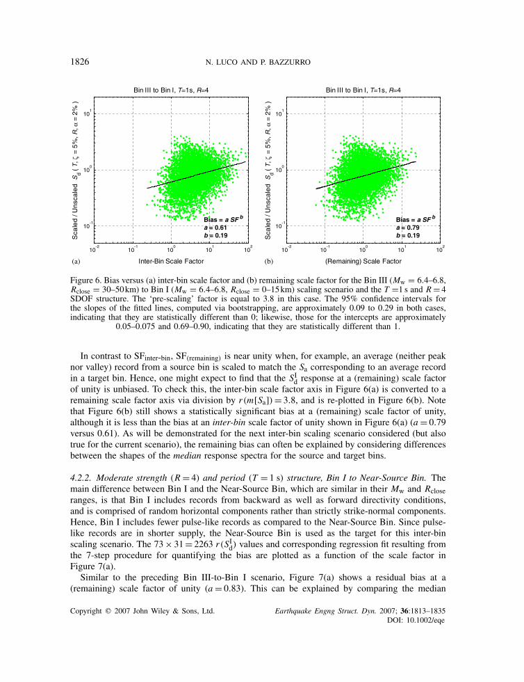
4.2.1. Moderate strength (R = 4) and period (T = 1s) structure, Bin III to Bin I. Both the ‘target’Bin I and the ‘source’ Bin III include seismograms generated by earthquakes with Mw = 6.4–6.8,but the former are recorded at closer distances (0–15 km) than the latter (30–50 km). Bin I is usedas the target here because in practice earthquake records at closer distances are in shorter supply.Plotted in Figure 6(a) are the r(SId) versus scale factor results for the 73 source records in Bin IIIscaled to the 73 target Sa (at T = 1 s) values associated with the Bin I records (i.e. 73× 73= 5329data points); also plotted in the figure is the regression fit to this data, which indicates that whenthe scale factor is equal to unity, the SId response to the scaled records is biased low (a = 0.61),and the bias increases log-linearly with scale factor (i.e. b= 0.19). The confidence intervals forthe slope (b) and intercept (a) of the regression fit, provided in the caption of Figure 6, indicatethat these observations (i.e., a �= 1 and b �=0) are statistically significant. Note that in this inter-bincase, both the target and source bins are separately resampled (with replacement) for each of the1000 bootstrap replications used to compute the confidence intervals.

The same ‘peak versus valley’ concept used to explain the intra-bin scaling results aboveapplies here to inter-bin scaling as well. The largest scale factors in Figure 6(a) (and vice versafor the smallest) result from scaling valley records from the ‘weaker’ (due to longer source-to-sitedistances) source Bin III to Sa values associated with peak records in the ‘stronger’ Bin I, therebyresulting in biased-high SId responses. In contrast to intra-bin scaling, scale factors near unity inFigure 6(a) typically result from a source-bin record with relatively large Sa for its Mw and Rclose,likely due to a peak in its response spectrum, being scaled to a target Sa level associated with atarget-bin record that is naturally at a relatively low Sa value (or valley) for its Mw and Rclose. Asin the intra-bin case, the scaled peak record is expected to produce relatively small SId responsecompared to the unscaled valley record that is naturally at the target Sa. This explains the negativebias at the inter-bin scaling factor of unity that is observed in Figure 6(a).

For comparison with intra-bin scaling results, it is instructive to split the inter-bin scaling factor,SFinter-bin, into two parts: SFinter-bin = r(m[Sa]) ∗ SF(remaining), where r(m[Sa]) is the ratio of themedian Sa value (at T = 1s, in this case) for the target bin over that for the source bin (equal to 3.8for this inter-bin scenario), and SF(remaining) is the remaining factor needed to scale the particularsource record to match the Sa value of the particular target record. Note that in all of the inter-binscaling scenarios to follow, the scale factors reported have already been divided by r(m[Sa]), i.e.they are already equal to SF(remaining). In other words, the source bin records are ‘pre-scaled’ byr(m[Sa]) before the 7-step procedure for quantifying the bias is applied.



10-2

10-1

100

101

102

10-1

100

101

Inter-Bin Scale Factor

Sca

led

/ Un

scal

edS

d(T

, ζ=

5%,R

, α=

2%)

Bin III to Bin I, T=1s, R=4

Bias = a SF b

a = 0.61b = 0.19

10-2

10-1

100

101

102

10-1

100

101

(Remaining) Scale FactorS

cale

d/ U

nsc

aled

Sd

(T, ζ

=5%

,R, α

=2%

)

Bin III to Bin I, T=1s, R=4

Bias = a SF b

a = 0.79b = 0.19

(a) (b)

Figure 6. Bias versus (a) inter-bin scale factor and (b) remaining scale factor for the Bin III (Mw = 6.4–6.8,Rclose = 30–50km) to Bin I (Mw = 6.4–6.8, Rclose = 0–15km) scaling scenario and the T =1 s and R = 4SDOF structure. The ‘pre-scaling’ factor is equal to 3.8 in this case. The 95% confidence intervals forthe slopes of the fitted lines, computed via bootstrapping, are approximately 0.09 to 0.29 in both cases,indicating that they are statistically different than 0; likewise, those for the intercepts are approximately

0.05–0.075 and 0.69–0.90, indicating that they are statistically different than 1.

In contrast to SFinter-bin, SF(remaining) is near unity when, for example, an average (neither peaknor valley) record from a source bin is scaled to match the Sa corresponding to an average recordin a target bin. Hence, one might expect to find that the SId response at a (remaining) scale factorof unity is unbiased. To check this, the inter-bin scale factor axis in Figure 6(a) is converted to aremaining scale factor axis via division by r(m[Sa]) = 3.8, and is re-plotted in Figure 6(b). Notethat Figure 6(b) still shows a statistically significant bias at a (remaining) scale factor of unity,although it is less than the bias at an inter-bin scale factor of unity shown in Figure 6(a) (a = 0.79versus 0.61). As will be demonstrated for the next inter-bin scaling scenario considered (but alsotrue for the current scenario), the remaining bias can often be explained by considering differencesbetween the shapes of the median response spectra for the source and target bins.

4.2.2. Moderate strength (R = 4) and period (T = 1 s) structure, Bin I to Near-Source Bin. Themain difference between Bin I and the Near-Source Bin, which are similar in their Mw and Rcloseranges, is that Bin I includes records from backward as well as forward directivity conditions,and is comprised of random horizontal components rather than strictly strike-normal components.Hence, Bin I includes fewer pulse-like records as compared to the Near-Source Bin. Since pulse-like records are in shorter supply, the Near-Source Bin is used as the target for this inter-binscaling scenario. The 73× 31= 2263 r(SId) values and corresponding regression fit resulting fromthe 7-step procedure for quantifying the bias are plotted as a function of the scale factor inFigure 7(a).

Similar to the preceding Bin III-to-Bin I scenario, Figure 7(a) shows a residual bias at a(remaining) scale factor of unity (a = 0.83). This can be explained by comparing the median



10-2

10-1

100

101

102

10-1

100

101

Scale Factor

Sca

led

/ Un

scal

edS

d(T

, ζ=

5%, R

, α=

2%)

Bin I to Near-Source Bin, T=1s, R=4

Bias = a SF b

a = 0.83b = 0.33

10-1

100

10-1

100

Period,T [sec]

Sa

(T

, ζ=

5%)

[g]

Bin I to Near-Source Bin

Median of Near-Source Bin (Target)Median of Bin I (Source)

(a) (b)

Figure 7. Panel (a): inter-bin scaling results for the Bin I to Near-Source Bin scenario and the T = 1 sand R = 4 SDOF structure. The scale factor in the abscissa is the remaining factor, SF(remaining). The95% confidence intervals for the slope and intercept of the fitted line, computed via bootstrapping,are approximately 0.15–0.51 and 0.66–1.05, respectively, indicating different from 0, but the inter-cept may not be statiscally distinguishable from 1. Panel (b): median response spectra for the source

Bin I records and the target Near-Source Bin records.

response spectrum for the source Bin I records (after ‘pre-scaling’ by r(m[Sa]), which in this caseis equal to one) with that for the target Near-Source Bin, as illustrated in Figure 7(b). At periodslonger than 1 s, the median response spectrum for Bin I drops off more quickly than that for theNear-Source Bin. Therefore, the SId response for the Bin I records will, on average, be smallerthan that for the records in the Near-Source Bin when no scaling is needed to match their Savalues. For small and large scale factors, the peak or valley effect still results in biased low andhigh (respectively) SId values. In fact, another observation from Figure 7(a) is that the slope of thebias versus scale factor, b= 0.33, is similar to that observed in the intra-bin scaling results forthe same target bin and structure, namely b= 0.38 in Figure 2; based on the confidence intervalsreported in the figure captions, both slopes are statistically distinguishable from b= 0. Hence, themain difference between these inter- and intra-bin results is a shift in the bias for a given scalefactor by the amount observed at a scale factor of one for the inter-bin scaling scenario (a = 0.83here), which may not be statistically different that 1, judging from the confidence interval reportedin the Figure 7 caption). This observation is fairly general and will be further commented on laterin the paper.

4.2.3. Bin I to Near-Source Bin, all structures. For all of the SDOF structures and for the BinI to Near-Source Bin scenario, a summary of the regression parameters a and b is provided inTable II(a) and (b), respectively. Similar to the intra-bin scaling trends for b described in Section4.1, the values of a for inter-bin scaling approach unity (no bias) for longer period and strongerstructures (e.g. T = 4 s and R = 1). For shorter period and weaker structures, the bias increases,which one might have anticipated based on larger and more disperse inelastic to elastic response



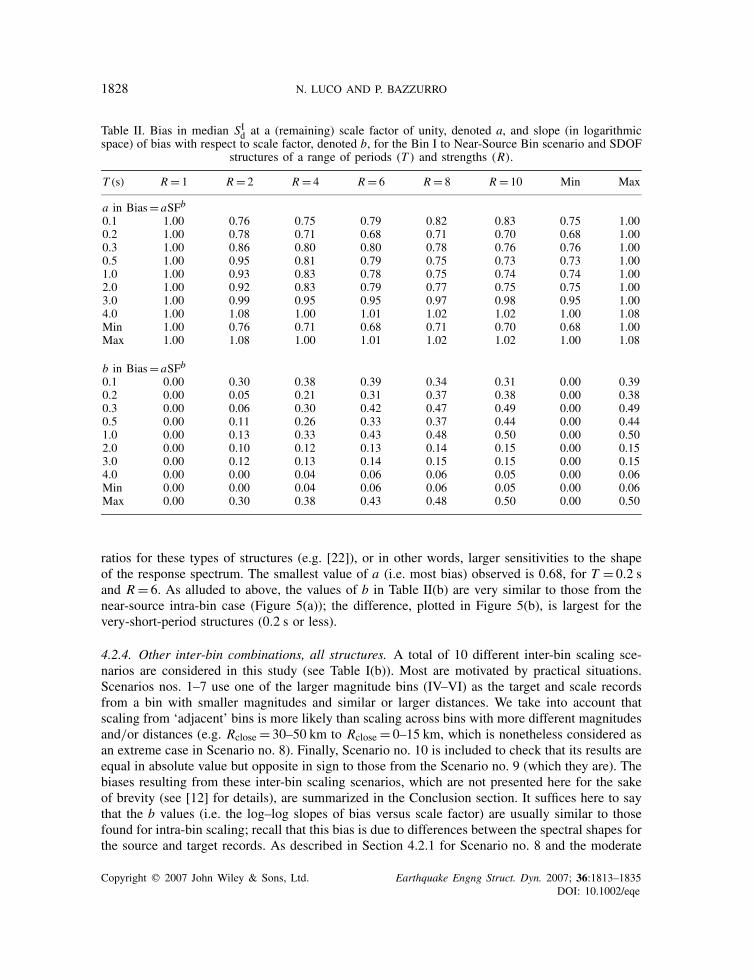
Table II. Bias in median SId at a (remaining) scale factor of unity, denoted a, and slope (in logarithmicspace) of bias with respect to scale factor, denoted b, for the Bin I to Near-Source Bin scenario and SDOF

structures of a range of periods (T ) and strengths (R).

T (s) R = 1 R = 2 R = 4 R = 6 R = 8 R = 10 Min Max

a in Bias= aSFb

0.1 1.00 0.76 0.75 0.79 0.82 0.83 0.75 1.000.2 1.00 0.78 0.71 0.68 0.71 0.70 0.68 1.000.3 1.00 0.86 0.80 0.80 0.78 0.76 0.76 1.000.5 1.00 0.95 0.81 0.79 0.75 0.73 0.73 1.001.0 1.00 0.93 0.83 0.78 0.75 0.74 0.74 1.002.0 1.00 0.92 0.83 0.79 0.77 0.75 0.75 1.003.0 1.00 0.99 0.95 0.95 0.97 0.98 0.95 1.004.0 1.00 1.08 1.00 1.01 1.02 1.02 1.00 1.08Min 1.00 0.76 0.71 0.68 0.71 0.70 0.68 1.00Max 1.00 1.08 1.00 1.01 1.02 1.02 1.00 1.08

b in Bias= aSFb

0.1 0.00 0.30 0.38 0.39 0.34 0.31 0.00 0.390.2 0.00 0.05 0.21 0.31 0.37 0.38 0.00 0.380.3 0.00 0.06 0.30 0.42 0.47 0.49 0.00 0.490.5 0.00 0.11 0.26 0.33 0.37 0.44 0.00 0.441.0 0.00 0.13 0.33 0.43 0.48 0.50 0.00 0.502.0 0.00 0.10 0.12 0.13 0.14 0.15 0.00 0.153.0 0.00 0.12 0.13 0.14 0.15 0.15 0.00 0.154.0 0.00 0.00 0.04 0.06 0.06 0.05 0.00 0.06Min 0.00 0.00 0.04 0.06 0.06 0.05 0.00 0.06Max 0.00 0.30 0.38 0.43 0.48 0.50 0.00 0.50

ratios for these types of structures (e.g. [22]), or in other words, larger sensitivities to the shapeof the response spectrum. The smallest value of a (i.e. most bias) observed is 0.68, for T = 0.2 sand R = 6. As alluded to above, the values of b in Table II(b) are very similar to those from thenear-source intra-bin case (Figure 5(a)); the difference, plotted in Figure 5(b), is largest for thevery-short-period structures (0.2 s or less).

4.2.4. Other inter-bin combinations, all structures. A total of 10 different inter-bin scaling sce-narios are considered in this study (see Table I(b)). Most are motivated by practical situations.Scenarios nos. 1–7 use one of the larger magnitude bins (IV–VI) as the target and scale recordsfrom a bin with smaller magnitudes and similar or larger distances. We take into account thatscaling from ‘adjacent’ bins is more likely than scaling across bins with more different magnitudesand/or distances (e.g. Rclose = 30–50 km to Rclose = 0–15 km, which is nonetheless considered asan extreme case in Scenario no. 8). Finally, Scenario no. 10 is included to check that its results areequal in absolute value but opposite in sign to those from the Scenario no. 9 (which they are). Thebiases resulting from these inter-bin scaling scenarios, which are not presented here for the sakeof brevity (see [12] for details), are summarized in the Conclusion section. It suffices here to saythat the b values (i.e. the log–log slopes of bias versus scale factor) are usually similar to thosefound for intra-bin scaling; recall that this bias is due to differences between the spectral shapes forthe source and target records. As described in Section 4.2.1 for Scenario no. 8 and the moderate



period and strength SDOF structure, the differences between the shapes of the median responsespectra for the source and target bins introduce an additional bias that is roughly independent ofscale factor.

4.3. MDOF structure

Due to the computational burden of dynamically analysing the 9-storey building models (elasticand ductile) for a large number of ground motion records, here we only investigate the effects of(i) intra-bin scaling within the Near-Source Bin and (ii) inter-bin scaling from Bin I to the Near-Source Bin. To some extent, these results can be extrapolated to other cases via the analogiesbetween the SDOF and MDOF results that will be drawn below and in the subsequent summarysection. The procedure for quantifying the bias is the same as that used for the SDOF structures, butthere is one noteworthy difference in its consequences. Since the strength of the MDOF structureis fixed (unlike that for an SDOF structure of a given R), the level of nonlinearity at each targetSa is different. The implications of this difference are described below.

4.3.1. Elastic and ductile models, intra-bin scaling within the Near-Source Bin. The bias versusscale factor results for the (a) �roof and (b) �max response of the ductile 9-storey building modelare shown in Figure 8. Although not shown here with an additional figure, first let it be notedthat for the elastic model of the MDOF structure, no bias in the median �roof response is induced(i.e. a = 1 and b= 0) [12]. This is because elastic �roof response is dominated by the first modeof vibration, and hence is nearly proportional to Sa (at T1 = 2.3 s). Likewise, the ductile results inFigure 8(a) show practically no bias up to a scale factor near unity, whereas a slight upward swingin the bias at scale factors greater than one (e.g. roughly 40% at a scale factor of 10) is discernedby the non-parametric locally weighted regression (LOESS) technique [23]. (Note that we have

10-1

100

101

10-1

100

101

Near-Source Bin, Ductile 9-Story

Bias = a SF b

a = 1.06b = 0.07

10-1

100

101

10-1

100

101

Near-Source Bin, Ductile 9-Story

Earthquake Record Scale FactorEarthquake Record Scale Factor

Bias = a SF b

a = 1.04b = 0.17

Sca

led

/ Uns

cale

dθ ro

ofR

espo

nse

Sca

led

/ Uns

cale

dθ m

axR

espo

nse

(a) (b)

Figure 8. Intra-bin scaling results in terms of (a) peak roof drift ratio (�roof) and (b) maximum peakinter-storey drift ratio (�max) for the ductile model of the MDOF structure and the Near-Source Bin. Linear

regression and LOESS fits are plotted with dash-dotted and solid lines, respectively.



not gone so far as to compute confidence intervals for these LOESS fits, whose width would varywith scale factor, but the same bootstrap approach used elsewhere in the paper could be appliedhere as well.) The observed variation in the bias is due to a gradual shift from linear elastic tononlinear inelastic response that takes place, on average, when the target Sa is near 0.23g. Sincethis Sa value also happens to be the median Sa of the Near-Source Bin of records, the gradualshift occurs around a scale factor of one. At scale factors greater than one, therefore, the bias canbe explained in the same way that it is for the inelastic SDOF structures (i.e. with the concept ofpeak versus valley records), since �roof is first-mode dominated (at least elastically).

In contrast to �roof, �max (or �i at higher stories—see [12]) is sensitive to higher modes ofvibration. Since the type of scaling considered in this study is to first-mode Sa, the results for�max in Figure 8(b) show a bias even at small scale factors (i.e. elastic response levels). Again thisbias can be explained with the concept of peak versus valley records, although now in terms oftheir spectral shapes at periods shorter than T1, which still display lower/higher spectral valuesfor peak/valley records (respectively). At large scale factors it is not clear whether the median�max response is biased high because of systematic spectral shape differences at shorter (reflectinghigher modes) or longer (reflecting nonlinearity) periods. The fact that the corresponding resultsfor the elastic building model (e.g. a bias of approximately 30% at a scale factor of 10, as shownin [12]) are very similar suggests the former.

4.3.2. Elastic and ductile models, inter-bin scaling from Bin I to the Near-Source Bin. The resultsfor inter-bin scaling [12] are practically the same as those described above for intra-bin scaling, andhence are not shown here with another figure. More specifically, the slopes (or curvilinear trends)of the bias versus scale factor results from the two types of scaling are comparable (e.g. b= 0.13versus 0.17 for the �max response of the ductile building model, the latter from Figure 8(b) forintra-bin scaling); recall that this was also the case for the SDOF structures. At a scale factor ofone, there is practically no difference between the biases (e.g. a = 1.0 versus 1.04 for inter- versusintra-bin scaling, respectively, the latter from Figure 8(b)), which is in contrast to the results forinelastic SDOF structures. The small difference between these biases is, however, consistent withthe difference between the median response spectra for the source Bin I and target Near-SourceBin records (refer back to Figure 7). That is, the inter-bin scaling bias (at a factor of one) is largerthan its intra-bin counterpart for the elastic building model, possibly due to the relatively highBin I spectral shape at higher-mode periods, and is the smaller for the ductile building models,possibly due to the relatively low spectral shape at longer periods associated with nonlinearity.Further investigation into this matter is a topic of future work.

5. SUMMARY OF RESULTS AND DISCUSSION

5.1. Intra-bin scaling

The SDOF results indicate that intra-bin scaling of records can introduce a systematic bias in themedian nonlinear structural response. This bias tends to increase with scale factor, with decreasingstrength (or increasing R), and with decreasing structural period. When scaled up, records produce,on average, larger responses than records that are naturally at the target Sa level. Based onthe SDOF results for all seven of the bins considered, the amount of bias can be summarized



as follows:

• Elastic or mildly inelastic structures (i.e. R�2): At most 15 and 60% (i.e. factors of 1.15 and1.60) for, respectively, scale factors of 2 and 10 (or 1/1.15 and 1/1.60 for 1/2 and 1/10),with the exception of a few short-period cases (T�0.2 s) described below.

• Long-period structures (i.e. T�3 s) with R>2: Less than 15 and 60% for scale factors of 2and 10, respectively, except for Bin VI (relatively large Mw and long Rclose), in which casethe bias is as large as 27 and 119% (respectively) when T = 3 s and R = 8 or 10.

• Short-period structures (i.e. T�0.5 s) with R>2: At least 15 and 60%, and as large as 90 and690%, for scale factors of 2 and 10, respectively. This is even true at the R = 2 strength level(with only one exception), but there are lower-bias exceptions at the R = 4 strength level andfor the Near-Source Bin.

• Moderate-period structures (i.e. T = 1 or 2 s) with R>2: Dependent on the bin of records(e.g. Mw, Rclose). When T = 1 s, the bias is less than 15 and 60% at scale factors of 2 and10 (respectively) for Bin III and V, but for the other five bins it is larger, up to 50 and 280%(respectively). When T = 2 s, the bias is less than 15 and 60% for all but Bin II, IV, and VI,in which cases it is still less than 30 and 150% (for scale factors of 2 and 10, respectively).

For the MDOF structure, both the elastic and ductile models exhibit a scaling-induced bias ofat most about 15 and 60% at scale factors of 2 and 10, respectively, for drift responses that aresensitive to higher modes of vibration (e.g. �max). Furthermore, the ductile (but not elastic) buildingmodel exhibits a bias for first-mode-dominated responses (e.g. �roof); at scale factors of 2 and 10the bias is as large as 25 and 80%, respectively, but at scale factors less than about one there isno bias because the structural response is, in most cases, essentially elastic (in addition to beingfirst-mode dominated). Of course, these summaries (of both the SDOF and MDOF results), as wellas those to follow, are specific to the structures and ground motion bins considered.

5.2. Inter-bin scaling

The variation of bias with scale factor for inter-bin scaling is similar to that for intra-bin scal-ing, except perhaps for the very short period structures (e.g. T�0.5 s). Unlike intra-bin scaling,however, inter-bin scaling sometimes introduces a bias at a (remaining, after pre-scaling) scalefactor of one, thereby shifting (by the amount of this bias) the bias for other scale factors. Basedon the SDOF results for all 10 of the inter-bin scaling cases considered, the bias at a scale factorof one shows the following trends:

• Elastic or mildly inelastic structure (i.e. R�2): Less than 15%, with the exception of a fewshort-period cases (T�0.3 s) described below.

• Long-period structures (i.e. T�3 s) with R>2: As large as 35% for very inelastic structures(R�6).

• Short-period structures (i.e. T�0.5 s) with R>2: As large as 35% for even mildly inelasticcases, and as large as 45% for severely inelastic responses.

• Moderate-period structures (i.e. T = 1 or 2 s) with R>2: As large as 35% for very inelasticstructures (R�6).

In most of the inter-bin scaling cases summarized above, the median SId response at a scale factorof one (i.e. that to the pre-scaled records) is biased low. This is because the records in the sourcebin are generally more ‘benign’ in terms of the median SId response that they generate for a given



Sa level, as compared to those in the target bin. This is a typical scenario encountered in practice,where it is often the more ‘aggressive’ target bin (larger Mw and shorter Rclose) that is of interest,but for which fewer (if any) existing records are available. Note that for MDOF structures, however,the influence of higher modes can counter this effect. For the 9-storey building models consideredin this study, for example, the inter-bin scaling results are very similar to those for intra-bin scaling.

5.3. Discussion

In this study we have claimed that the bias in the drift response of SDOF and MDOF structuresinduced by scaling records selected randomly from an Mw–Rclose bin can be explained, for themost part, by the difference in spectral shape between the source and the target records (e.g. seeFigures 3 and 7). This claim implies that if the spectral shapes of the scaled records were similarto those of the target records, then the bias would be reduced. This implication is confirmed inFigure 9, for which the same procedure used to the compute the intra-bin scaling bias for theT = 1 s and R = 4 SDOF structure and the Near-Source Bin is repeated here, with one exception.As demonstrated in Figure 9(a), for each target Sa level the response spectrum of the associatedtarget record is used to select the 10 records with the most similar spectral shape (i.e. the mostsimilar response spectrum after scaling to the target Sa level) at periods longer than T = 1 s, in themean-square error sense. The regression fit to the resulting data (now 31× 10 points) in Figure9(b) shows that the bias is now significantly reduced (slope b decreased from 0.38 in Figure 2(b)to 0.08). In fact, the confidence intervals for the slope and intercept of the regression fit (reportedin the Figure 9 caption) suggest that they are statistically indistinguishable from those that would

10-1

100

10-2

10-1

100

101

Period, T [sec]

Sa

(T

, ζ=

5%)

[ g]

Near-Source Bin

TargetMost Similar 10Remaining 20

10-2

10-1

100

101

102

10-1

100

101

Scale Factor

Sca

led

/ Un

scal

edS

d(T

, ζ=

5%,R

, α=

2%)

Near-Source Bin, T=1s, R=4

Bias = a SF b

a = 0.95b = 0.08

Bias = a SF b

a = 0.95b = 0.08

(a) (b)

Figure 9. Panel (a): same scaled response spectra shown in Figure 1(b), but with the 10 spectrathat are ‘closest’ to that of the target record (at periods larger than T = 1s) plotted with dottedlines. Panel (b): same intra-bin scaling results shown in Figure 2(b), but with the results forthe 10 closest response spectra for each target Sa level plotted with larger, darker dots, andthe regression line fitted to those data only. The 95% confidence intervals for the slopeand intercept of the fitted line, computed via bootstrapping, are approximately −0.16–0.32and 0.89–1.02, indicating that they are not statistically different than 0 and 1, respectively.



be indicative of no bias (i.e., b= 0 and a = 1, respectively). Although not shown here with anotherfigure, similar results are obtained for inter-bin scaling.

The evidence above suggests that judiciously selected records with spectral shapes similar to atarget can be scaled, even by large amounts, with a significantly reduced potential for producingbiased nonlinear inelastic responses. Interestingly, the selected records do not even need to belongto the target Mw–Rclose. Defining a target spectral shape for a spectral acceleration, Mw, and Rcloseof interest is a topic covered in [20], through the use of the ground motion parameter �. In [11],it is also demonstrated, in a slightly different manner and primarily for non-near-source groundmotions, that selecting records consistent with this target spectral shape reduces the scaling-inducedbias in median nonlinear structural response.

6. CONCLUSIONS

For a relatively wide range of SDOF structures of different periods and strengths, as well astwo models (one elastic) of an MDOF structure, we have quantified the bias in median nonlinearstructural response induced by scaling input records to a target Sa level and an associated narrowrange (or ‘bin’) of Mw and Rclose values (and rupture-directivity characteristics in one othercase considered). The nonlinear structural response measures considered are inelastic spectraldisplacement for the SDOF structures and inter-storey and roof drifts for the MDOF structure. Thebias is measured with respect to the median response to unscaled records in the target Mw–Rclosebin that are naturally at the spectral acceleration of interest. Since there are few records to compareagainst for a given Sa, Mw, and Rclose (giving rise to the need for scaling), we have introduced aprocedure for quantifying this bias as a function of scale factor by simultaneously using resultsfor a range of target Sa levels. We have considered both intra-bin and inter-bin scaling. In the caseof intra-bin scaling, the scaled records have, by definition, the same general characteristics (interms, for example, of Mw and Rclose) as the target scenario (and unscaled records). In inter-binscaling, the scaled records are from a bin with different characteristics than the target. In practicethis target bin is often devoid of records, but here we have had to consider target bins that containrecords, for comparison purposes. We assume that the inter-bin scaling results presented here canbe extrapolated to the cases encountered in practice.

The results of this study demonstrate that scaling records randomly selected from an Mw–Rclosebin can introduce a bias in median nonlinear structural response (conditional on an Mw–Rcloserange and Sa level) that increases with the degree of scaling. The amount of this bias dependson, in addition to the scaling factor, (i) the fundamental period of vibration of the structure; (ii)the overall strength of the structure; and (iii) the sensitivity of the nonlinear structural response tohigher (than the first) modes of vibration. The bias also depends on the Mw and Rclose range of therecords that are scaled. In the case of inter-bin scaling, these characteristics mainly affect the bias(if any) introduced by first ‘pre-scaling’ the records such that their median spectral accelerationmatches that of the target bin (e.g. as obtained from an attenuation relation). Any further biasinduced by additionally scaling these pre-scaled records to a target spectral acceleration leveldifferent (usually larger) than the median for the target Mw and Rclose depends primarily on thecharacteristics of the target bin, and it is comparable to the bias induced by intra-bin scaling forthe target Mw and Rclose.

The biases quantified in this study can be used to place limits on the amount scaling thatis acceptable for comparable structures, once one has decided on a tolerable amount of bias.



Alternatively, one could either ‘correct’ for a scaling-induced bias by using results like thosepresented in this paper, or select records with spectra that are, once scaled, similar to that of thetarget Sa, Mw, and Rclose. Such a selection of the records to be scaled has been demonstrated tosignificantly reduce the potential for biased responses.

ACKNOWLEDGEMENTS

The study described in this paper benefited from discussions with the following individuals: NormanAbrahamson of PG&E, Brian Chiou and Cliff Roblee of Caltrans, Maury Power of Geomatrix, and AllinCornell, Jack Baker, Gee-Liek Yeo, and Polsak Tothong of Stanford University. The PEER LifelinesProgram funded the work under an addendum to Task 1G00.

REFERENCES

1. McGuire RK, Silva WJ, Constantino CJ. Technical basis for revision of regulatory guidance on design groundmotions: hazard- and risk-consistent ground motion spectra guidelines. NUREG/CR 6728, U.S. Nuclear RegulatoryCommission, Government Printing Office, Washington, DC, 2001.

2. Carballo JE, Cornell CA. Probabilistic seismic demand analysis. Reliability of Marine Structures Program ReportNo. RMS-41, Department of Civil and Environmental Engineering, Stanford University, Stanford, CA, 2000.

3. Bazzurro P, Luco N. Parameterization of non-stationary acceleration time histories. Report on PEER-LL Program Task 1G00, Richmond, CA, 2003. Available at http://peer.berkeley.edu/lifelines/LL-CEC/reports/final reports/1G00-FR pt2.pdf

4. Haselton CB, Baker JW. Ground motion intensity measures for collapse capacity prediction: choice of optimalspectral period and effect of spectral shape. Proceedings of the 100th Anniversary Earthquake ConferenceCommemorating the 1906 San Francisco Earthquake, San Francisco, CA, 2006.

5. Watson-Lamprey J, Abrahamson NA. Selection of ground motion time series and limits on scaling. EarthquakeEngineering and Structural Dynamics 2006; 26:477–482.

6. Tothong P, Luco N. Probabilistic seismic demand analysis using advanced ground motion intensity measures.Earthquake Engineering and Structural Dynamics, accepted.

7. Bommer JJ, Acevedo AB. The use of real earthquake accelerograms as input to dynamic analysis. Journal ofEarthquake Engineering 2004; 8:43–91.

8. Sewell RT. Damage effectiveness of earthquake ground motion: characterization based on the performance ofstructures and equipment. Ph.D. Dissertation, Department of Civil Engineering, Stanford University, Stanford,CA, 1989.

9. Shome N, Cornell CA, Bazzurro P, Carballo JE. Earthquakes, records, and nonlinear MDOF responses. EarthquakeSpectra 1998; 14(3):469–500.

10. Iervolino I, Cornell CA. Record selection for nonlinear seismic analysis of structures. Earthquake Spectra 2005;21(3):685–713.

11. Baker JW. Vector-valued ground motion intensity measures for probabilistic seismic demand analysis. Ph.D.Dissertation, Department of Civil and Environmental Engineering, Stanford University, Stanford, CA, 2005.

12. Luco N, Bazzurro P. Effects of earthquake record scaling on nonlinear structural response. Reporton PEER-LL Program Task 1G00 Addendum (Sub-Task 1 of 3), Richmond, CA, 2004. Available athttp://peer.berkeley.edu/lifelines/LL-CEC/reports/final reports/1G00-FR.pdf

13. Somerville PG, Smith NF, Graves RW, Abrahamson NA. Modification of empirical strong ground motionattenuation relations to include the amplitude and duration effects of rupture directivity. Seismological ResearchLetters 1997; 68(1):199–222.

14. Luco N. Probabilistic seismic demand analysis, SMRF connection fractures, and near-source effects. Ph.D.Dissertation, Department of Civil and Environmental Engineering, Stanford University, Stanford, CA, 2002.

15. Frankel AD, Petersen MD, Mueller CS, Haller KM, Wheeler RL, Leyendecker EV, Wesson RL, Harmsen SC,Cramer CH, Perkins DM, Rukstales KS. Documentation for the 2002 update of the National Seismic HazardMaps, USGS Open-File Report 02-420, 2002.

16. Federal Emergency Management Agency. State of the art report on system performance of steel moment framessubject to ground shaking. FEMA 355C, Washington, DC, 2000.



17. Chopra AK. Dynamics of Structures: Theory and Applications to Earthquake Engineering (1st edn). Prentice-Hall:New Jersey, 1995.

18. Prakash V, Powell GH, Campbell S. DRAIN-2DX base program description and user guide, Version 1.10. ReportNo. UCB/SEMM-93/17, Department of Civil Engineering, University of California at Berkeley, Berkeley, CA,1993.

19. Efron B, Tibshirani RJ. An Introduction to the Boostrap. Chapman & Hall/CRC: Florida, 1998.20. Baker JW, Cornell CA. Spectral shape, epsilon, and record selection. Earthquake Engineering and Structural

Dynamics 2006; 35:1077–1095.21. Veletsos AS, Newmark NM. Effect of inelastic behavior on the response of simple systems to earthquake motions.

Proceedings of the 2nd World Conference on Earthquake Engineering, Tokyo, Japan, 1960; 895–912.22. Ruiz-Garcia J, Miranda E. Inelastic displacement ratios for evaluation of existing structures. Earthquake

Engineering and Structural Dynamics 2003; 32:1237–1258.23. Cleveland WS. Robust locally-weighted regression and smoothing scatterplots. Journal of the American Statistical

Association 1979; 74:829–836.


Does amplitude scaling of ground motion records result in biased nonlinear structural drift...

Documents

Transcript of Does amplitude scaling of ground motion records result in biased nonlinear structural drift...