entropy

Article

Development of Econophysics: A Biased Account andPerspective from Kolkata

Bikas K. Chakrabarti 1,2,3,* and Antika Sinha 1,4

Citation: Chakrabarti, B.K.; Sinha, A.

Development of Econophysics: A

Biased Account and Perspective from

Kolkata. Entropy 2021, 23, 254.

https://doi.org/10.3390/e23020254

Academic Editor: Ryszard Kutner

Received: 28 January 2021

Accepted: 19 February 2021

Published: 23 February 2021

Publisher’s Note: MDPI stays neutral

with regard to jurisdictional claims in

published maps and institutional affil-

iations.

Copyright: © 2021 by the authors.

Licensee MDPI, Basel, Switzerland.

This article is an open access article

distributed under the terms and

conditions of the Creative Commons

Attribution (CC BY) license (https://

creativecommons.org/licenses/by/

4.0/).

1 Saha Institute of Nuclear Physics, Kolkata 700064, India; antikasinha@gmail.com2 S. N. Bose National Center for Basic Sciences, Kolkata 700106, India3 Economic Research Unit, Indian Statistical Institute, Kolkata 700108, India4 Department of Computer Science, Asutosh College, Kolkata 700026, India* Correspondence: bikask.chakrabarti@saha.ac.in

Abstract: We present here a somewhat personalized account of the emergence of econophysics as anattractive research topic in physical, as well as social, sciences. After a rather detailed storytellingabout our endeavors from Kolkata, we give a brief description of the main research achievements ina simple and non-technical language. We also briefly present, in technical language, a piece of ourrecent research result. We conclude our paper with a brief perspective.

Keywords: traveling salesman problem; simulated annealing technique; kinetic exchange model;Gini index; Kolkata index; minority game; Kolkata Paise Restaurant problem

1. Introduction

Countless attempts and research studies, mostly in physics, to model and comprehendthe economic systems are about a century old. For the last three or four decades, majorendeavor have been made and some successes have been achieved and published, notablyunder the general title ‘Econophysics’. The term was coined at a Kolkata conference heldin 1995 by Eugene Stanley, who later in an interview said “ ... So, he (Bikas) started to havemeetings on econophysics and I think the first one was probably in 1995 (he decided tostart it in 1993–1994). Probably the first meeting in my life on this field that I went to wasthis meeting. In that sense Kolkata is — you can say — the nest from which the chicken wasborn ...” [1]. The entry on Econophysics by Berkeley Rosser in the New Palgrave Dictionaryof Economics (2nd Edition [2]) starts with the sentence “According to Bikas Chakrabarti (...),the term ‘econophysics’ was neologized in 1995 at the second Statphys-Kolkata conferencein Kolkata (formerly Calcutta), India, by the physicist H. Eugene Stanley ...” See alsoFigure 1 (and Reference [3]). It may be mentioned here that in a more generalized sense,the term ‘Sociophysics’ was introduced more than a decade earlier by Serge Galam andcoworkers [4] (also see Reference [5]).

As we will discuss in the next section, economics, like all the natural sciences (physics,chemistry, biology, geology, etc.), are, epistemologically speaking, knowledge or truthacquired through induction from observations (natural or controlled in the laboratories)using inductive logic and analyzed or comprehended using deductive logic (like math-ematics). The divisions of natural sciences between the streams, like physics, chemistry,biology, and geology, are for convenience and are man-made. ‘Truth’ established in onebranch or stream of natural science does not become ‘false’ or wrong in another; only theimportance often vary. This helps in the growth of an younger branch of science throughinterdisciplinary fusion of established knowledge from another older established branch;astrophysics, geophysics, biophysics, and biochemistry had been earlier examples. Econo-physics has been the latest one, and this special issue of Entropy attempts to capture thehistory, success and future prospect of econophysics research studies.

Entropy 2021, 23, 254. https://doi.org/10.3390/e23020254 https://www.mdpi.com/journal/entropy

Entropy 2021, 23, 254 2 of 29

1990 1995 2000 2005 2010 2015 2020Year

0

200

400

600

800

1000

1200

Freq

uenc

y

Econophysics in Google Scholar

Figure 1. Histogram plot of yearwise numbers of entries containing the term econophysics against thecorresponding year. The data are taken from Google Scholar (dated 31 December 2020). It may also benoted from Google Scholar that, while this 25-year old econophysics has today typical yearly citationfrequency of order 1.3× 103, more than 100-year old subjects, like astrophysics (Meghnad Sahapublished his thermal ionization equation for solar chromosphere in 1920), biophysics (Karl Pearsoncoined the term in his 1892 book ‘Grammar of Science’), and geophysics (Issac Newton explainedplanetary motion, origin of tides, etc., in ‘Principia Mathematica’, 1687), today (31 December 2020)have typical yearly citation frequencies of order 32.5× 103, 26.8× 103, and 38.6× 103, respectively.

In the next five sections (essentially following the structure and section-titles, sug-gested by the Editors of this special issue), we discuss in non-technical language, allow-ing them to be accessible to the uninitiated younger students and researchers (except inSection 4, where we present some new result of our research). True to the spirit suggestedby the Editors, the second section has been presented in the form of a ‘Dialogue’ using theformat of questions and answers between us, the coauthors.

2. What Attracted You to Econophysics?

As mentioned earlier, this section is formatted in the form of a dialogue (question andanswer) between the coauthors.

AS: What attracted you to Econophysics? Can you briefly recount?BKC: Meghnad Saha, founder of Saha Institute of Nuclear Physics (named so after

his death in 1956), had been a pioneering Astrophysicist (known for the Saha Ionizationformula in astrophysics), had also thought deeply about the scientific foundation of manysocial issues (see, e.g., Reference [6]). In early seventies, our undergraduate-level text bookon heat and thermodynamics had been ‘Treatise on Heat’ [7], written by Saha togetherwith Biswambhar Nath Srivastava (first published in 1931). This turns out to be the earliesttextbook where the students were encouraged, in the section on Maxwell-Boltzmanndistribution in kinetic theory of ideal gas, to compare it with the anticipated ‘gamma’distribution of income in the society (see the page from Reference [7] reproduced inReference [6]). If taken seriously, it asks the students to model the income distribution in asociety, which maximizes the entropy (assuming stochastic market transactions)!

AS: Before you go further, let me ask why should one think of applying statisticalphysics to society in the first place?

BKC: One Robinson Crusoe in an island cannot develop a running market or a func-tional society. A typical thermodynamic system, like a gas, contains Avogadro number(about 1023) of atoms (or molecules). Compared to this, the number (N ) of ‘social atoms’ oragents in any market or society is of course very small (say, about 102 for a village market toabout 109 in a global market). Still such many-body dynamical systems are statistical in na-ture and statistical physical principles should be applicable. Remember, each constituentsparticle in a gas follows some well-defined equations of motion (say, Newton’s equation for

Entropy 2021, 23, 254 3 of 29

classical gases or Schrödinger’s equation for quantum gases), yet for the collective behaviorof gases (or liquids or solids) we need to average over the ‘appropriate’ statistics for theirstochastic behavior in such ‘many-body’ systems and calculate the emerging collectiveor thermodynamic properties of the entire system. Motivation to go for the ‘appropriate’statistics to estimate the collective behavior or response of the society comes, therefore, verynaturally. In the case of human agents in a society, the corresponding equations governingindividual behavior are much more difficult and still unknown and unpredictable, yetmany collective social behavior are quite predictable; ask any traffic engineer or engineersdesigning stadium evacuation in panic situation.

AS: Which problem of economics did Saha and Srivastava try to analyze usingMaxwell-Boltzmann distribution or statistical mechanics of ideal gas?

BKC: As can be seen from the example they had put to the readers, they indicated to thestudents the problem of income and wealth inequalities (they assumed Gamma-function-like income distribution in Reference [7]; reproduced in Reference [6]). They suggestedto them that the ‘entropy maximization’ principle, along with conservation of money (orwealth), across the market (with millions of transactions between the agents, buyers, andsellers) must be at work in such ‘many-body’ social or market systems. This will result inthe consequent and inevitable inequality (equal distributions being entropically unstableagainst stochastic fluctuations, leading to steady state unequal distributions).

AS: That is quite interesting. Can you elaborate a bit more and explain a bit ofstatistical physics specifically for the classical ideal gas?

BKC: Let me try. One can present the derivation of the energy distribution among theconstituent (Newtonian) particles of a (classical) ideal gas in equilibrium at a temperatureT as follows: If n(ε) represents the number density of particles (atoms or molecules of agas) having energy ε, then one can write n(ε)dε = g(ε) f (ε, T)dε. Here, g(ε) denotes the‘density of states’ giving g(ε)dε as the number of dynamical states possible for any of thefree particles of the gas, having kinetic energy between ε and ε + dε (as counted by thedifferent momentum vectors ~p corresponding to the same kinetic energy: ε = |p|2/2m,where m denotes the mass of the particles).

Since the momentum ~p is a three-dimensional vector, g(ε)dε ∼ |p|2d|p| ∼ (√

ε)dε.This is obtained purely from mechanics. For completely stochastic (ergodic) many-bodydynamics or energy exchanges, maintaining the the energy conservation, the energy distri-bution function f (ε, T) should satisfy f (ε1) f (ε2) = f (ε1 + ε2) for any arbitrary choices ofε1 and ε2. This suggests f (ε) ∼ exp(−ε/∆), where the factor ∆ can be identified from theequation of state for the gas (positive sign in the exponential is neglected because of the ob-servation that the number decreases with increasing energy). This gives n(ε) = g(ε) f (ε) ∼(√

ε) exp(−ε/KT). Knowing this n(ε), one can estimate the average pressure P the gasexerts on the walls of the container having volume V at equilibrium temperature T andcompare with the ideal gas equation of state PV = NKT (K denoting the Boltzmann con-stant). The gas pressure can be estimated from the average rate of momentum transfer bythe atoms on the container wall, and one can compare with that obtained from the afore-mentioned equation of state and identify different quantities; in particular, one identifies∆ = KT.

AS: How does one then extend this to the markets?BKC: Yes, let us consider the trading markets, where there is no production (growth)

or decay. In addition, the total amount of money (considered equivalent to energy) andnumber of traders (or agents, considered as particles or ‘social atoms’) remain fixed orconstant throughout the trades. Since in the market money remains conserved as no onecan print money or destroy money (will end-up in jail in both cases) and the exchange ofmoney in the market is completely random, one would again expect, for any buyer-sellertransaction in the market, f (m1) f (m2) = f (m1 + m2), where f (m) denotes the equilibriumor steady state distribution of money m among the traders in the market. This then, in asimilar way, suggests f (m) ∼ exp(−m/∆′), where ∆′ is a constant. Since there cannot beany equivalent of the particle momentum vector for the agents in the market, the density

Entropy 2021, 23, 254 4 of 29

of states g(m) here is a constant (any real-number value of m corresponds to one marketstate). Hence, the number n(m) of traders or agents having money m will be given byn(m) = c exp(−m/∆′), where c is a constant. One must also have

∫ M0 n(m)dm = N, the

total number of traders in the market, and∫ M

0 mn(m)dm = M, the total amount money incirculation in the market (or country). This gives, the effective ‘temperature’ of the economy∆′ = M/N, the average available money per trader or agent in this closed-economy (as nogrowth, migration of laborers, etc., are considered). This gives exponentially decaying (orGibbs-like) distribution of money in the market (unlike the Maxwell-Boltzmann or Gammadistribution of energy in the ideal gas), where most of the people become pauper (n(m) ismaximum at m = 0).

AS: Is this exponentially decaying income or wealth distribution realistic for any economy?BKC: That discussion will take us to the recent studies by econophysicists and data

comparisons. We will defer those to the next section (Section 3). Indeed, some success of themodel (sketched above) in capturing the real data has been explored extensively by VictorYakovenko and his group from Maryland University. We, in Kolkata, explored what couldmake the distribution more like a Gamma distribution, as Saha and Srivastava indicated intheir book [6] to be an observed phenomenon. We also tried to capture the Pareto tail ofsuch a distribution. Avoiding detailed discussion here, we only refer here to three popularpapers [8–10] in this context. The model sketched above essentially follows [6,8]. In thismodel, the exchanged money or wealth in each trade (equivalent to any of the particle-particle collision in Ideal gas) is completely random, subject to conservation of money (orwealth). A trader, acquiring a lot in earlier trades may lose the entire amount of money orwealth in the next trade as the total money (wealth) will be conserved if the partner tradergets that. If one introduces a saving propensity of each trader, so that each trader saves afraction of their individual money (wealth) before the trade and exchanges randomly therespective rest amount in the trade (keeping total money or wealth again conserved) theresulting steady state distributions capture the above mentioned desirable features. Onecan easily see that, unlike in the Kinetic-exchange model described above, the possibility forany trader (with non-vanishing saving propensity) to become an absolute popper vanishes,as that will require that trader to lose in every trade. Consequently, the exponentialdistribution becomes unstable with effect to any non-vanishing saving propensity and thestable distribution will become Gamma-like for uniform saving propensity of the traders [9]and initially Gamma-like but crossing over to Pareto-like power-law decay when tradershave non-uniform saving propensities [10]. These results are non-perturbative results;any non-vanishing saving propensity will induce these features; the saving propensitymagnitudes only determine the most-probable income (wealth) or the income (wealth)crossover point for Pareto tail of the distribution.

AS: Can we come back to your journey towards econophysics? Apart from Saha-Srivastava’s book, any influence from other books, especially from economics?

BKC: After Graduation and Post-Graduation from Calcutta University, I joined, inearly 1975, the Saha Institute of Nuclear Physics as a Research Fellow in Condensed MatterStatistical Physics for my Ph.D. degree. By that time I had a huge personal collection of(mostly cheap editions, reprinted in India), general books, text books, other books andmonographs in subjects outside physics; primarily in philosophy and economics. I had at-tempted closer studies of some them including: The Problems of Philosophy, Bertrand Russell(Cambridge Univ.), Oxford Univ. Press, Oxford (1959); Mathematical Logic & the Foundationsof Mathematics: An Introductory Survey, Geoffrey Thomas Kneebone (Univ. London), D. vanNostrand Co. Ltd., London, UK, (1963); The Problems of Philosophy, Satischandra Chatterjee(Univ. Calcutta), Calcutta Univ. Press, Kolkata (1964); The Philosophy of Wittgenstein, GeorgePitcher (Princeton Univ.), Prentice-Hall Inc., New Delhi, India, (1964); An Introductionto Philosophical Analysis, John Hospers (Univ. Southern California), Prentice-Hall Inc.,New Delhi (1971); Economics, Paul A. Samuelson (MIT), Tata-McGraw Hill, New Delhi(1971); and Economic Theory & Operations Analysis, William J. Baumol (Princeton Univ.),Prentice-Hall Inc., New Delhi (1978).

Entropy 2021, 23, 254 5 of 29

I tried to go through some of the isolated chapters or sections of these books, which Icould understand, enjoyed, or liked most. Occasionally, I got excited and tried my ownanalysis, following them, on some interesting problems or discussions coming in my way.One such piece was a paper on ‘Indeterminism and Freedom’ by Bernard Berofsky ofColumbia University, published in 1975, perhaps in Philosophical Quarterly. Amongothers, it also alluded to quantum physics in defending his thesis on freedom. I wrote anote detailing my criticisms and posted that to the author. The author, from the Departmentof Philosophy, Philosophy Hall, Columbia University in the City of New York, wrote to methe following letter on 17 June 1975 (see Figure 2):

Dear Mr. Chakraborty: Thank you for letting me see your paper. I am impressed because you certainly display a grasp of philosophical issues and modes of thinking that are unusual for a person untrained in the subject. My major reservation about your paper is that you take on far teo much. You cannot, therefore, but leave many points seriously under- argued, sketchy, and, if I may say so, dogmatic sounding. With regards to your thesis about freedom at the end, I would say that it would sound more plausible if formulated about responsibility. There again, however, the thesis is seriously underargued. I take it you're saying that judgment of freedoms are not basically descriptive and cannot, therefore, enter into logical relationships with judgements about determinism or causation. But if that is so. it is difficult to see how at other places in your paper you can argue about the logical relations between freedom and determinism. By the way, I recently have completed a manuscript in which I defend a thesis contrary to the one you are defending here. Let me just add a few comments of specific sort. The claim on pages 2 and 3 that freedom is different from indeterminism is all right as you present it. But freedom may REQUIRE indeterminism. I personally tend to believel that it does not. I had a hard time following the material on page 4. Surely the second attempt (paragra- ph 3) is hopeless. Finally the irreducibility claim on page 7 is unsupported and many would disagree with you, especially about your general skepticism regarding reduction. Again let me say you certainly show a proficiency in philosophy and I am sure that you would do quite well if you choose to study it formally. Thank you for allowing me to read your manuscript. Best regards, Bernard BerofskyFigure 2. Reply (dated 17 June 1975) from Bernard Berofsky of the Philosophy Department ofColumbia University to BKC on his criticisms of Bernard’s paper on ‘Indeterminism and Freedom’.

AS: Obviously, you did not follow his suggestion, in fact, cordial invitation, to switchover to Philosophy. Why did you not?

BKC: Though I was seriously thinking of switching over to philosophy in a formalway, following Bernard’s suggestion, some quick apparent success in my physics research

Entropy 2021, 23, 254 6 of 29

publications with the newly developed Renormalization Group theory in those days kindof blinded me and left me with two minds. Somehow, I failed to take a decision andcontinued with my physics research until I practically forgot about the other choice! Inlate 1978, I submitted my Ph.D. thesis in Condensed Matter Physics to the University ofCalcutta and got the degree in 1979, and, by the end of that year, I left for post-doctoralresearch studies in the Theoretical Physics Department of the University of Oxford and theInstitute of Theoretical Physics, University of Cologne.

I came back and joined the Saha Institute of Nuclear Physics as Lecturer in 1983, and Istarted my research in statistical physics with four Ph.D. students joining me simultane-ously (including Subhrangshu Sekhar Manna, who later developed the ‘Manna Model’,belonging to the ‘Manna Universality Class’). Soon the statistical physics research in ourgroup became so engaging and happening (with sixteen Ph.D. students, so far, gettingtheir Ph.D. degrees and several of them becoming quite well known later for their pio-neering research studies and still collaborating with me), I did not get much time untilearly nineties when I decided to try some research on ‘economics-inspired physics’. I wentback to the problem Saha and Srivastava addressed in their textbook mentioned aboveand I co-organized a conference in January 1995, together with some established Indianstatistical physicists and (reluctant!) economists as participants. In the Proceedings of theConference, I published (together with an economist Sugata Marjit) my first paper [11]dealing with statistical physics of Income distribution and related problems.

By the end of the year, as a part of the StatPhys-Kolkata II (series of InternationalConferences organized by us in Kolkata every 3–4 years, latest event StatPhys-Kolkata X,held end of 2019), we had organized a special session on ‘Economics-Inspired Physics’ andEugene Stanley in his talk coined the term ’Econophysics’ and had put that in the title ofhis paper [12] published in the Proceedings of the conference in Physica A, vol 224 (1996).

Though econophysics was quite risky as a topic of Ph.D. research in the late nineties(even today; still no faculty position in econophysics in our country, or for that matter,hardly exists elsewhere in the world), two brave students (Anirban Chakraborti andArnab Chatterjee) expressed forcefully their desire to join the research on eventual topic of‘econophysics’. I was also fortunate, my colleague Sitabhra Sinha also joined us in suchinvestigations. In the last 25 years, since that conference, significant developments havetaken place in the subject, and many of them will be covered this special issue of Entropy.

AS: We will come back to those developments later. I understand, most of the paperson econophysics research studies are published in physics journals and not in economicsjournals. What is the cultural level of appreciation by the intellectuals today?

BKC: This is indeed very difficult to answer. To tell very frankly, the response sofar is not very supportive or encouraging! Although, it must be mentioned, the termeconophysics has now entered in dictionaries of economics (see, e.g., Reference [2]) andEncyclopedias of social science and philosophy (see, e.g., Reference [13]). That brings meto an interesting, rather recent, correspondence with my old philosopher ‘guide’ BernardBerofsky in January 2013, after thirty-seven years! This was quite accidental, when I cameacross in my internet search a new book published by him. I contacted him (giving a linkto my homepage) saying, “sorry, I could not follow your advice so far and had been veryshy to contact you. Now that I have become sixty, I acquired sufficient courage and ...".Bernard immediately responded (see Figure 3) praising the development of econophysicsdue to the philosophical impulses of physicists.

Entropy 2021, 23, 254 7 of 29

Figure 3. Mail from Bernard Berofsky of the Philosophy Department of Columbia University, inresponse to BKC’s surprise contact mail in 2013 (after almost thirty-seven years!), appreciatingand identifying the development of econophysics as one due to the “physicist(s) with synthesizingimpulses of a philosopher ... (using) philosophical impulses in a most creative and fecund manner”.

AS: Do you see really a philosophy behind econophysics?BKC: Yes, indeed. I wrote about it earlier also (see, e.g., References [13,14]). I am

not aware of all the documents on the mutual connection between philosophy and econo-physics. I mentioned earlier about the entry on Econophysics in the Encyclopedia ofPhilosophy and Social Sciences [13]. I came to know of a rather recent entry on SocialOntology in The Stanford Encyclopedia of Philosophy [15] which, in the context of ‘socialatomism’, writes “The idea is to model societies as large aggregates of people, much asliquids and gases are aggregates of molecules, ...”. Then, after introducing the readers totwo historical examples of Quetelet in 1848 [Adolphe Quetelet, 1848, Du système socialet des lois qui le régissent, Paris: Guillaumin] and of Spencer in 1895 [Herbert Spencer,1895, The Principles of Sociology, New York: Appleton] it says “Contemporary represen-tatives include models in sociophysics and econophysics (see Chakrabarti et al., 2007)... [which] take a society or market to be an aggregate of these interacting individuals[Bikas K. Chakrabarti, Anirban Chakraborti and Arnab Chatterjee, 2007, Econophysics andSociophysics: Trends and Perspectives, Hoboken, NJ: Wiley]”.

Let me now go back to the main to the main discussion and reiterate my basic argumentin favor of considering economics as a natural science. Our knowledge about truth can,epistemologically speaking, be either deductive or inductive. Mathematics is an usualexample of the deductive knowledge (though not all of it can be deduced from axiomaticlogic); mathematical truths do not require any laboratory test or ‘observational’ supportfrom the ‘nature’ to prove or validate them. Linguistically speaking, it is like the tautology“A bachelor does not have wife”. One does not need to check each and every bachelorto confirm truth of the statement—the first part of the sentence confirms the second part.The same is true about the statement “two plus two equals four”. Mathematical truths areanalytical truths; left-hand side equals (in every intention and content) the right-hand side.

Entropy 2021, 23, 254 8 of 29

Mathematics, therefore, is not directly a natural science [16–18], though it has been at theroot of the logical structure of many natural sciences, particularly physics. Natural sciences,however, are basically inductive in nature. They are based on natural or (controlled)laboratory observations. The statement “The sun rises every twenty four hours on the eastin the morning” is not a tautology nor an analytical truth. Though east may be defined asthe direction, and morning may be defined by the time of sunrise, that it rises every twentyfour hours is an inductive (or empirically observed) truth and, therefore, tentative (andnot like mathematical truths, which are analytical and certain). Natural sciences start withobservations and end in observations, using both inductive reasoning or logic; in-between,they often employ the tools of deductive logic, mathematics (as most condensed form ofdeductive logic).

AS: So, the tools of mathematics and logic are employed to find and establish relation-ships among these ‘natural’ observations to develop natural sciences. Where does theneconomics belong to?

BKC: That is the crucial question. Intermediate analysis using mathematics is justapplied mathematics, and can not be considered as (pure) mathematics. Any branchof natural science does that. Economics has been and will be a part of natural science,where natural observations, not much of controlled or laboratory observations, need tobe analyzed employing deductive logic and mathematics. Economics, therefore, shouldnaturally belong to natural sciences!

AS: Agreed. But why econophysics?BKC: You see, in natural sciences today, there are several branches or disciplines, likephysics, chemistry, biology, geology, etc. The differences are not natural and certainlynature did not create them: they are human creations. The demarcations among thesedisciplines are not always clear. As we mentioned earlier, there are clear differences (in thenature of logic employed) between mathematics and natural sciences. But that does notextend to the branches of natural sciences. In a white light spectrum, our color perceptioncontinuously change from violet to red (without any sharp boundary) as the wavelengthchanges in this collection of electromagnetic waves. Similar are the cases of the differentbranches of natural science. They are not strictly differentiable; are historical in originand continued by us for our own convenience (during upbringing; like perhaps religion;both are man-made). Of course, it is hard today to be an expert in the whole of evenone branch of natural science. We, therefore, try to learn and acquire expertise in onesub-branch or a sub-sub-branch of natural science. An unique feature of the sub- or sub-sub-branches of natural science is that an established ‘truth’ or a ’fundamental law’ inone branch does not become ’false’ or ’wrong’ in another; only importance varies fromdiscipline to discipline; quantum physics or gravity laws do not become invalid or wrong inchemistry or biology or mineralogy. Only gravity laws may be less important in chemistryor biology or mineralogy, and vice-versa. Models of geomagnetism in earth science cannotbe built upon a law contradicting Maxwell’s laws of electromagnetism. Developmentsin younger branches in science, therefore, profitably utilized earlier established laws orideas in older branches of natural science. Many of the early successful scientists (evensome mathematicians) happen to have been identified as physicists, and, consequently,physics has become like an ‘elder brother’ among natural sciences, and it is now equippedwith a huge armory of ideas, laws and models to comprehend the nature. Economics as arelatively newer entrant to natural science can, therefore, expect gainful advantages fromsuch econophysical attempts!

AS: I remember you once told me that the concept of modeling dynamics of physicalsystems and of economics systems are fundamentally different. Can you elaborate thepoint in this context?

BKC: I do not remember which point we had been discussing. However, there isa typical one which may be discussed. Modeling dynamics of a physical system, likea particle, using, say, the Newton’s equation of motion, gives its dynamical state at alater time t by solving the equation of motion and utilizing the information regarding its

Entropy 2021, 23, 254 9 of 29

dynamical state at an earlier time (say, at t = 0; called initial conditions). Exact solutionsmay not be possible as in the thermodynamic or many-body systems, but based on thestatistical characterization of the state of the system at an earlier time, the dynamicalformulation helps solving the statistics of the system for any future time. The economicagents or organizations, even under nominally identical economic situation, may have(continually upgradeable) anticipation about the future and the model dynamics need toaccommodate, along with their initial economic state, such anticipatory factors (whichare continually adjusted or learned through the ongoing dynamics itself!) to solve for thefuture. Such self-consistent ‘learning’ dynamics of physical systems are not typical, thoughsome recent many-body game theoretic models, with iterative learning for optimal use ofscarce resources as in the binary-choice Minority Game (see, e.g., Reference [19]), or many-choice Kolkata Paise Restaurant Problem (see, e.g., Reference [20]) naturally incorporatesuch evolving learning features in the self-correcting dynamics themselves. We will discusssome details of the later problem here. In any case, these studies are new and still verylimited in scope.

AS: To summarize, though many of you had started your econophysics research stud-ies more than twenty five years back, since Gene Stanley coined the term econophysics in1996 (in his publication [12] in the Proceedings of the second StatPhys-Kolkata Conference),and many more physicists joined after that, the subject is not established yet.

BKC: You are partly right. In fact, physicists have long been trying to formulateand comprehend various problems of economics. As mentioned before, since 1931, thestatistical physics modeling of income and wealth distributions are being tried. However,these older physics attempts had been sporadic and isolated ones; physicists, successfulin such attempts, like Jan Tinbergen (Economics Nobel Prize winner in 1969; had Ph.D. instatistical Physics under Paul Ehrenfest of Leiden University), had to migrate to economicsdepartment. Since 1996 (more correctly perhaps since 1991, when Rosario Mantegnapublished his paper [21] on Milan stock exchange data modeling), however, the situationhas changed considerably. Physicists are now investigating economics problems alongwith their students and colleagues from the same department and are publishing theireconophysical research papers in physics journals (in around 2000, Econophysics had beenassigned the Physics and Astronomy Classification Scheme (PACS) number 89.65Gh by theAmerican Institute of Physics).

I personally think, however, that an intensive and successful branch of econophysicsresearch started with Scott Kirkpatrick and coworkers in 1983 when they proposed [22]the idea and technique of ‘Simulated Annealing’ (or ‘Classical Annealing’) to get practi-cal solutions of the computationally hard multi-variable optimization problems, like the(managerial) economics problem of the Traveling Salesman Problem (TSP), using tuning(annealing) of Boltzmann-type fluctuations (simulating thermal ones) to escape from thelocal minima to reach eventually one of the (degenerate) global minima of the cost function(travel distance). This is a very successful story of the application of (statistical) physicsto solve a problem which in nature and basic intent a (financial) economics problem in-volving multi-variable optimization. It may be noted in this connection that the techniquehas since been applied to all branches of science, as well as technology, and the originalpaper [22] has received major attention of scientists and engineers (so far having receivedmore than 48,000 citations, according to Google Scholar). This idea still continues leadingto a very intriguing and active domain of research in computationally hard problems ofoptimizations, using statistical physics and physics of spin glasses. This eventually led tothe concept and technique of ‘Quantum Annealing’ (or of ‘Stochastic Quantum Comput-ing’), where simulated quantum fluctuations (instead of simulated thermal fluctuations)are profitably used to tunnel through high but narrow local barriers [23], separating theglobal minima or solutions (see, e.g., Reference [24] for a brief review on solving TSP usingquantum annealing). As I discussed earlier in my Econophysics-Kolkata Story [25], westarted in 1986 (see Section 3.1) investigations on the statistical physics of the TSP. Soonmy student Parangama Sen joined the effort [26]. (She eventually concentrated more on

Entropy 2021, 23, 254 10 of 29

Sociophysics and developed, among others, the Biswas-Chatterjee-Sen model, see, e.g.,Reference [27], for collective opinion formation together with our students SoumyajyotiBiswas and Arnab Chatterjee. In this connection, let me take the opportunity to acknowl-edge the contributions of my other students, Srutarshi Pradhan, Asim Ghosh and SudipMukherjee, Suchismita Banerjee, and, of course, you, Antika, and of my colleagues in theKolkata-econophysics group, namely Anindya Sundar Chakrabarti, Manipushpak Mitra,and Satya Ranjan Chakravarty, allowing us to make some significant contributions toeconophysics, which we are going to summarize in the next section.)

AS: So, you think that successful research studies in econophysics already started withthe Simulated Annealing paper by Kirkpatrick et al. in 1983, although econophysics re-search studies on more popular economics problems started in 1990s and, more specifically,after Stanley coined the term in 1996?

BKC: Yes, you are right. We will discuss in little more details (in the next section;Section 3.1) the impact of statistical physics in developing the Simulated (Classical orQuantum) Annealing techniques for the financial computation problems involving multi-variable optimization of the Traveling Salesman type. The inspiring success of the classicalannealing technique, initiated by the Simulated Annealing method, has led to several in-triguing developments in statistical physics and to many applications in computer science.Further potential extension in the context of solving NP-hard problems using quantum an-nealing has become one of the core research topic today in quantum many-body (statistical)physics and in quantum computation. Indeed I consider this outstanding development ofsimulated (classical or quantum) annealing techniques (starting with Kirkpatrick et al. [22];also see Reference [23]) for the Traveling Salesman type multi-variable optimization prob-lems to be a landmark achievement in the true spirit of econophysics. Of course, thepresent phase of econophysics research activities stemmed from several influential papers,analyzing financial market fluctuations, by Rosario Mantegna and Eugene Stanley andin particular following the publication of Kolkata Conference Proceedings paper [12] byStanley et al. in 1996.

3. Major Achievements and Publications of the ‘Kolkata School’

Physicist Victor Yakovenko and economist J. Barkley Rosser in their pioneering inter-disciplinary collaborative review [28] in the Reviews of Modern Physics (2009) on econo-physics of income and wealth distributions, discussed about some of the ‘influential’ and‘elegant’ papers from the ‘Kolkata School’. We will briefly summarize in this section someof our major research studies in econophysics (including those on wealth distributions).

3.1. Traveling Salesman Problem and Simulated (Classical & Quantum) Annealing

As already discussed, the Traveling Salesman Problem or TSP is, in its intent and structure,a computationally involved financial management problem (see, e.g., References [29,30]). Theproblem can be easily defined as a geometric one. Suppose in an unit square area there areN random dots, representing the cities. The salesman has to make a visit to all the cities andcome back with minimum travel cost. The travel cost to visit all these cities will dependon the total travel distance of the tour. Each component of the travel distance betweenany two cities can be taken as the Euclidean distance (or as appropriate for the spatialmetric, say Cartesian) between them. One can easily check that there are N!/2 (growingfaster than exponential in N) distinct tours or trips to visit all the N cities. Obviously, allof these trips do not have identical value (‘cost’) for the total travel length (D), and theproblem is to find the trips(s) which will correspond to the minimum travel distance D.Searching over all the possible trips soon becomes impossible as N becomes large, andthere is no perturbative way to improve on any randomly chosen travel path to reach theglobal solution. At any point or city on a tour, there are N order choices for the next moveor visit and the optimization problem of the total travel distance is truly a multi-variableone. It may be noted that the problem becomes trivial in one dimension (homes or officesplaced randomly on a straight road), where the salesman can start from one end of the

Entropy 2021, 23, 254 11 of 29

road and finish at the other end). Generally, for two dimension onwards, search time forsuch a minimum ‘cost’ (from among exp(N) number of trips or configurations), cannot bebounded by any (deterministic) polynomial in N (NP-hard problem).

From now onwards, let us concentrate our discussion on TSP in two dimension. Thescale of the total travel distance, however, can be easily guessed using a ‘mean field’ picture.If N randomly placed points (cities) fill an unit (normalized) area, then the ‘average’ or‘mean’ area per city is 1/N, giving nearest neighbor distance to be of order 1/

√N and total

travel distance D = Ω√

N. Numerical estimates suggests Ω ' 0.71 [31].The problem is truly global in nature. Choice of the next city to visit depends on

the position of even the farthest city in the country. However, one can approximatelysolve the problem (see References [32,33]) by reducing it to an effective one-dimensionalproblem where the country (unit square) is divided into hypothetical parallel strips ofwidth w and the salesman visits the cities within each strip in a ‘directed’ way and thetotal travel distance D is optimized with respects to single variable w (optimal value thengrows as

√N) and gives (see, e.g., References [32,33]) Ω ' 0.92. Another way is to put the

cities randomly with concentration ρ on the lattice sites of, say, an unit square lattice. Thelattice constraint can help then the calculation of the optimal travel distance. The optimal(normalized) travel path length then scales as D = Ω

√ρ. At ρ = 1, the lattice constraints

would immediately imply that the global search problem reduce to a local one and all thespace filling Hamiltonian walks would correspond to optimized tour with Ω = 1. In theapproximate single variable solution (minimization of D with respect to w) indicated above,the strip width w grows as 1/

√ρ as ρ decreases. For ρ→ 0, however, the lattice constraints

disappear, and the problem reduces to TSP on continuum as defined earlier (NP-hard,w→ ∞, with Ω ' 0.71 [31]). Where does the problem become NP-hard? This study wasinitiated by us (see References [26,34–37]) and they indicated (also Reference [32]) that theTSP on dilute lattices becomes NP-hard only at ρ→ 0 (though this is not settled yet andsome arguments support that it crosses over to NP-hardness at ρ = 1− or as soon as ρbecomes less than unity).

As already mentioned earlier (in Section 2), a major computational breakthrough ofTSP and other such multi-variable optimization problems came from the 1983 seminalpaper on Simulated Annealing’ [22] by Kirkpatrick et al., who proposed a novel stochas-tic technique, inspired by the metallurgical annealing process and statistical physics offrustrated systems.

Imagine a bowl on the table, and you need to ‘locate’ its bottom point. Of course, onecan calculate the local depths (from a reference height) everywhere along the inner volumeof the bowl and search for the point where the local depth is maximum. However, as everyone would easily guess, a much simpler and practical method would be to allow rolling ofa marble ball along the inner surface of the bowl and wait for locating its resting position.Here, the physics of the forces of gravity and friction allows us to ‘calculate’ the location ofthe bottom point in an analog way! Algorithm-wise, it is simple. For any possible move,if the changed ‘cost’ function has lower value, one should accept the move and reject itotherwise. Success for the search of the minimum is guaranteed. In principle, a similartrick would work for cases where the bowl becomes larger and its internal surface getsmodulated, as long as the surface contour or ‘landscape’ has valleys all tilted towards thesame bottom point location. Computationally hard problems arise when these valleysare separated by ‘barriers’, which are (macroscopically) high. The simulated annealingsuggests a way out to overcome (at least for finite height barriers) by allowing movescosting higher to have (Gibbs-like) lower probability of acceptance.

To search for the optimized cost (travel distance in TSP or energy of the ground state(s)in spin glasses) at eventually vanishing level of noise (or ‘simulated temperature’), onestarts from a high noise (temperature) ‘melt’ phase, and tune slowly the noise level. In this‘simulated’ process, the (classical) noise at any intermediate level of annealing allows forthe acceptance of the changed ‘costs’ ∆D in distance or energy D: 100% acceptance of themove if ∆D < 0 and acceptance of the move with a Gibbs-like probability ∼ exp(−∆D/T)

Entropy 2021, 23, 254 12 of 29

for moves with increased in cost (∆D > 0)). As the noise level (T) is slowly reducedduring the annealing process, the gradually decreasing probability of accepting higher costvalues, allows the system to come out of the local minima valleys and settle eventually in(one of) the ‘ground state’ (with minimum D) of the system. For slow enough decrease ofnoise T(t) with time t, one can estimate the quasi-equilibrium (thermal) average of the costfunction < D > at ant time t and derive the effective ‘specific heat’ value δ < D > /δT asa function of t. One needs to be very slow (|dT/dt| very small) when the effective specificheat increases with decreasing T, indicating the ‘glass’ transition point and anneal at fasterrates on both sides of the transition point.

As has been indicated in the earlier section, it has been a remarkably successful trick for‘practical’ computational solutions of a large class of multi-variable optimization problems,as in most multi-city travel cost optimizations and similar multi-variable optimizations(see, e.g., References [29,30,38,39]).

Though some ‘reasonable’ optimization can be achieved very quickly using appropri-ate annealing schedules, the search time for reaching the lowest cost state or configurationfor NP-hard problems, however, grows still as exp(N). The bottleneck could be iden-tified soon. Extensive study of the dynamics of frustrated random systems, like the Nspin (two state Ising) glasses, particularly of the Sherrington-Kirkpatrick variety (see, e.g.,Reference [23] also for a TSP version of the quantum annealing), showed that its (free)energy landscape (in the ‘glass’ phase), is extremely rugged, and the barriers, separatingthe local valleys, often become N order implying the search for the degenerate groundstates from 2N (or N!/2) states is NP-hard (for the N-city TSP). In the macroscopic sizelimit (N approaching infinity), therefore, such systems effectively become non-ergodic orlocalized, and the classical (thermal) fluctuations, like that in the simulated annealing, failto help the system to come out of such high barriers (at random locations or configurations,not dictated by any symmetry) as the escape probability is of order exp(−N/T) only.Naturally, the annealing time (inversely proportional to the escape probability), to get theground state of the N-spin Sherrington-Kirkpatrick model, cannot be bounded by anypolynomial in N.

The idea proposed by Ray et al. [40] was that quantum fluctuations in the Sherrington-Kirkpatrick model can perhaps lead to some escape routes to ergodicity or quantumfluctuation induced delocalization (at least in the low temperature region of the spin glassphase) by allowing tunneling through such macroscopically tall but thin (free energy orcost functions) barriers which are difficult to scale using classical fluctuations. This is basedon the observation that escape probability due to quantum tunneling, from a valley withsingle barrier of height N and width w, scales as exp(−

√Nw/Γ), where Γ represents the

quantum (or tunneling) fluctuation strength (see Figure 4). This extra handle throughthe barrier width w (absent in the classical escape probability of order exp(−N/T)) canhelp in a major way in its vanishing limit. Indeed, for a single narrow (w→ 0) barrier ofheight N, when Γ is slowly tuned to zero, the annealing time to reach the ground stateor optimized cost, will become N independent (even in the N → ∞ limit; δ-functionbarriers are transparent to quantum fluctuations, while classical or thermal annealing toescape from such a barrier is impossible)! It has led to some important clues. Of course,complications (localization) may still arise for many such barriers at random ‘locations’.In any case, with this observation and some more developments, the quantum annealingtechnique was finally launched through the subsequent publications of a series of landmarkpapers (both theoretical and experimental; see Reference [23]) and through a remarkablepractical realization of the quantum annealers by the D-wave Group [41].

Entropy 2021, 23, 254 13 of 29

C’

C

Configuration

Quantum

Tunneling

Thermal

Jump

Cost

/ E

ner

gy

Figure 4. While optimizing the cost function of a computationally hard problem (like the minimumtravel distance for the Traveling Salesman Problem (TSP)), one has to get out of a shallower localminimum, like the configuration C (travel route), to reach a deeper minimum C’. This requires jumpsor tunneling, like fluctuations, in the dynamics. Classically, one has to jump over the energy or thecost barriers separating them, while quantum mechanically one can tunnel through the same. Ifthe barrier is high enough, thermal jump becomes very difficult. However, if the barrier is narrowenough, quantum tunneling often becomes quite easy. Indeed, assuming the tall barrier to be ofheight N and width w, one can estimate (see, e.g., Reference [42]) the tunneling probability throughthe barrier to be of order exp[−(w

√N)/Γ], where Γ denotes the strength of quantum fluctuations

(instead of the the classical escape probability of order exp[−N/T], T denoting the thermal or classicalfluctuation strength).

Let us now conclude this subsection. Simulated Annealing technique, invented byKirkpatrick et al. in 1983 [22], has since been applied extensively also to solve problemsof collective decision making in economics and social sciences (see, e.g., Reference [43]for a recent review). As mentioned earlier [25], our group started investigations on sta-tistical physics of TSP in 1986. The intriguing physics of Simulated Annealing inspiredus to explore the possible further advantages of quantum tunneling (to allow escapethrough macroscopically tall but thin barriers in some NP-hard cases), where classicalannealing (using thermal fluctuations) fails. This led finally to the quantum extensionor to the invention of the quantum annealing technique, where our initial contributions(References [23,40]) are considered to be important and pioneering. See, e.g., Reference [24]for a brief review and Reference [44] for some recent discussions on the advantages of apply-ing quantum annealing method to solve TSP. Quantum annealing is a very active researchfield today in quantum statistical physics and computation (see, e.g., References [45,46] forrecent reviews).

3.2. Social Inequality Measure and Kolkata Index

Social inequality, particularly income or wealth inequality in, are ubiquitous. Thereare several indices or coefficients, used to measure them, the oldest and most popular onebeing the Gini index [47].

It is based on the Lorenz curve or function [48] L(x), giving the cumulative fractionof (total accumulated) income or wealth possessed by the fraction (x) of the population,when counted from the poorest to the richest (see Figure 5). If the income (wealth) of everyone would be identical, then L(x) would be a straight line (diagonal) passing through theorigin. This diagonal is called the equality line. The Gini coefficient (g) is given by the areabetween the Lorenz curve and the equality line (normalized by the area under the equalityline: g = 0 corresponds to equality and g = 1 corresponds to extreme inequality.

We proposed [49] the Kolkata index or k-index given by the ordinate value of theintersecting point of the Lorenz curve and the diagonal perpendicular to the equalityline (also see References [50–54]). By construction, 1− L(k) = k, saying that k fraction of

Entropy 2021, 23, 254 14 of 29

wealth is being possessed by (1− k) fraction of the richest population. As such, it gives aquantitative generalization of the approximately established (phenomenological) 80–20law of Pareto [55], saying that, in any economy, typically about 80% wealth is possessed byonly 20% of the richest population. Defining the complementary Lorenz function L(c)(x) ≡[1− L(x)], one gets k as its (nontrivial) fixed point (while Lorenz function L(x) itself hastrivial fixed points at x = 0 and 1). k-index can also be viewed as the normalized h-index [56]for social inequality; h-index is given by the fixed point value of the nonlinear citationfunction against the number of publications of individual researchers. We have studied themathematical structure of k-index in Reference [53] (see Reference [54] for a recent review)and its suitability, compared with the Gini and other inequality indices or measures, in thecontext of different social statistics, in References [49–52]. In addition, see Reference [57]for redefining a generalized Gini index and Reference [58] for a recent application incharacterizing the statistics of the spreading dynamics of COVID-19 pandemic in congestedtowns and slums of the developing world.

0 0.5 1fraction (x) of people from poorest to richest

0

0.5

1

cum

ulat

ive

fract

ion

of w

ealth

hel

d by

them

S

S ′(k,1-k)

k

(k,k)

equality lin

e

Loren

z curv

e L(x)

L (c)(x)

Figure 5. Lorenz curve (in red) or function L(x) here represents the fraction of accumulated wealthagainst the fraction x of people possessing that, when arranged from the poorest to the richest.The diagonal from the origin represents the equality line. The Gini index (g) can be measured bythe area (S) between the Lorenz curve and the equality line (shaded region), normalized by thetotal area (S + S′ = 1/2) under the equality line: g = 2S. The complementary Lorenz functionL(c)(x) ≡ 1− L(x) is shown by the green line. The Kolkata index (k) can be measured by the ordinatevalue of the intersecting point of the Lorenz curve and the diagonal perpendicular to the equalityline. By construction, L(c)(k) = 1− L(k) = k, saying that k fraction of wealth is being possessed by(1− k) fraction of richest population.

In summary, inspired by the observations of richer structure (self-similarity) of the(nonlinear) Renormalization Group equations near the fixed point (see, e.g., Reference [59]),or of the nonlinear chaos-driving maps near the fixed point (see e.g., Reference [60]) andnoting that inequality functions, such as the Lorenz function L(x) or the ComplementaryLorenz function L(c)(x), to be generally nonlinear, we studied their nontrivial fixed points.As mentioned earlier, Lorenz function L(x) has trivial fixed points (at x = 0 and 1), whilethe Complementary Lorenz function L(c)(x) ≡ 1− L(x) has a nontrivial fixed point atx = k, the Kolkata index [49]. It also offers a tangible interpretation: k-index gives thefraction k of the total wealth possessed by the rich (1− k) fraction of the population andgives a quantitative generalization of the Pareto’s 80–20 law [55]. As discussed earlier, itcan also be viewed as a normalized h-index of social inequality. Some unique featuresof Kolkata Index (k) may be noted: (a) Gini and other indices are mostly some averagequantities based on the Lorenz function L(x), which has trivial fixed points. k is a fixedpoint of the Complementary Lorenz function L(c)(x) and, if one considers the simplest formof Lorenz function L(x) = x2, then k = (

√5− 1)/2, inverse of the Golden Ratio [51]. (b) k

Entropy 2021, 23, 254 15 of 29

gives the fraction of wealth possessed by the rich 1− k fraction of the population. As such,it provides a quantitative generalization of the Pareto’s 80-20 law (see, e.g., Reference [55]).The observed values of k index for most of the cases of social inequalities [50–54] seem tofall in the range 0.80-0.86 (though have much smaller values today for world economies,presumably because of various welfare measures). (c) k-index is equivalent to a normalizedversion of the Hirsch-Index (h). While h corresponds to the fixed point of the publicationsuccess rate (measured by the integer numbers of citations) falling off nonlinearly withnumber of papers by individual academicians, k corresponds to the fixed point (fraction) of1− L(x), where L(x) gives the nonlinearly varying fraction of cumulative wealth possessedby the increasing (from poor to rich) fraction of population in any society.

3.3. Kinetic Exchange Model of Income and Wealth Distributions

We have discussed already in Section 2 some details of the Kinetic Exchange modelof income and wealth distributions. In an ideal gas, in thermal equilibrium, the numberdensity n(ε) of (Newtonian) particles (atoms or molecules) having kinetic energy ε isgiven by

n(ε) = g(ε) f (ε, T) ∼√(ε) exp(−ε/∆), (1)

where ∆ is a constant, the density of states g(ε) ∼√

ε (coming from the counting ofthree-dimensional momenta vectors which correspond to the same kinetic energy) andf (ε) ∼ exp(−ε/∆) (coming from stochastic, or entropy maximizing, scatterings betweenthe particles, conserving their total kinetic energy). As discussed already in Section 2, toget the ideal gas equation of sate PV = NKT, where P and V denote, respectively, thepressure and volume of the gas at absolute temperature T, by calculating the pressure fromthe average transfer of momentum of the particles per unit area of the container (usingEquation (1), Reference [7]), one identifies, ∆ = KT.

Following similar arguments [7,8] (also see Reference [28] ), one gets (as discussed inSection 2) for the steady state distribution of the number n(m) of agents in the market withincome or wealth m.

n(m) = g(m) f (m) = c exp(−m/∆′), (2)

where f (m) ∼ exp(−m/∆′), with g(m) a constant c (unlike in expression (1)), and ∆′ asconstants for the trading market. This is because, in a trading market, there is no production(growth) or decay, and the total amount of money (equivalent to energy in Kinetic theoryof ideal gas), as well as the number of traders (buyers and sellers), remain fixed. Stochasticmoney exchanges in the trades involving indistinguishable buyers and sellers (who changetheir roles in different trades), keeping the buyer-seller total money in any trade to remainconstant, lead to a distribution given by expression (2). This is also because there cannot beany equivalent of the particle momenta vectors for the agents in the market and hence thedensity of states g(m) here is a constant. One must also have

∫ M0 n(m)dm = N, the total

number of traders in the market, and∫ M

0 mn(m)dm = M, the total amount of money. Thesegive the effective temperature of the market ∆′ = M/N, the average money in circulationin the market (economy).

As documented in several books and reviews (see, e.g., References [7,61,62]), theincome or wealth distributions in any society have a Gamma function-like dip near zeroincome or wealth (unlike in the exponential distribution case discussed above, where thenumber density of pauper is the maximum). In addition, as is well known [62,63], the tailend of the distribution is known to be much more fat, described by the Pareto power law,and not by the thin exponentially decaying distribution.

As mentioned in the earlier section, following Saha and Srivastava’s indication in theirbook [7], we explored how the kinetic theory of trading markets indicated above could beextended to accommodate a Gamma-like distribution at the least and explore further tocapture the Pareto tail of such a distribution, as well.

We noted that many of the economics text books, in their chapters on Trades, discussthe saving propensity of the traders (habit of saving a fraction of the income or wealth

Entropy 2021, 23, 254 16 of 29

possessed by the trader and do trade with the rest). We immediately realized [9,10], ifone introduces the saving propensity of each trader, so that each trader saves a fraction oftheir individual money (wealth) before the trade and allows (random) exchanges of therest amount in the trade (keeping the total money or wealth, including the saved portions,conserved), the traders will never become paupers. Unlike in the random exchange case (asin kinetic theory of gases, where one trader may lose its entire amount of money or wealthto the other in any trade), here, to lose the entire amount of money acquired at any pointof time, the trader has to lose every time after that as the trader continues the successivetrades (and, consequently, the saved portion becomes infinitesimal). The number densityof paupers (having zero wealth) will become zero for any non-vanishing saving fractionof the traders and the exponential distribution will become unstable and the resultingsteady state distributions will capture the above mentioned desirable features. This is anon-perturbative result; any amount of saving by the traders will induce this feature.

With uniform saving, the exponential distribution collapses and the stable distributionbecomes Gamma-like [9] (also see Reference [64] for a micro-economic derivation of thekinetic exchange equations from the Cobb-Dauglas utility maximization with money savingpropensity of the traders, and Reference [65] for extended microeconomic formulation ofKinetic exchange models, having economic growths, by incorporating additional saving ofthe production in the utility maximization equation). The steady state distribution becomesinitially Gamma-like but crossing over to Pareto-like power-law decay when traders havenon-uniform saving propensities [10]. The saving propensity magnitudes determine themost-probable income (wealth) and the income (wealth) crossover point for Pareto tail ofthe distribution (see References [63,66,67] for details).

It may be mentioned in this connection that one kind of saving by the traders, con-sidered early by our group (including the students Anirban Chakrabarti and SrutarshiPradhan) can, in fact, lead to wealth condensation or extreme inequality. When two ran-domly selected traders agree to trade (in the so-called ’Yard Sale’ trade mode), such thatthe richer one among them will retain or save the extra money or wealth compared to thatof her trade partner, the dynamics will eventually lead to aggregation of the entire amountof money or wealth in the hand of one trader, and the dynamics will stop. This happensbecause once any trader becomes pauper (loses entire amount of money or wealth), noother trader (with money) will engage in trade with her. Although this Yard Sale model hasthis uninteresting wealth condensation feature, it showed some interesting slow dynamics,and Anirban published that result [68]. Later, it was shown that inclusion of tax in themodel, in the sense that a fraction of money is collected by the Government (non-playingmember of the system) in every trade and, after some period of collections, redistributesthe money among all (by investing on general social facilities, like road, hospital, etc.,constructions, used equally by all in the society). Because of this general upliftment, thepaupers come back to the trades and interesting steady state money distribution can emergeand such models of wealth distribution have become an active area of research (see, e.g.,Reference [69] for a popular review on this development).

Kinetic model of gases and the kinetic theory is the first and extremely successfulmany-body theory in physics. Economic systems, markets in particular, are intrinsicallymany-body dynamical systems. Kinetic exchange models of markets may, therefore, beexpected to provide the most successful models of market systems. In the kinetic exchangemodel, when one of the trader of a randomly chosen pair of traders is deliberately thepoorest one at that instant of time (trade), the dynamics induces a self-organization in themarket such that a ‘poverty line’ is spontaneously developed so that none of the traderremains below the emerged (self-organized) poverty threshold (see References [70,71] andreferences therein).

3.4. Statistics of the Kolkata Paise Restaurant Problems

Kolkata had, long back, very cheap fixed price ‘Paise Restaurants’ (also called ‘PaiseHotels’; Paise is, rather was, the smallest Indian coin). These ‘Paise Restaurant’ were

Entropy 2021, 23, 254 17 of 29

very popular among the daily laborers in the city. During lunch hours, these laborersused to walk down (to save the transport costs) from their place of work to one of theserestaurants. These restaurants would prepare every day a (small) number of such dishes,sold at a fixed price (Paise). If several groups of laborers would arrive any day to the samerestaurant, only one group would get their lunch, and others would miss their lunch thatday. There were no cheap communication means in those days (like mobile phones) formutual communications, for deciding the respective restaurants. Walking down to the nextrestaurant would mean failing to report back to work on time! To complicate this collectivelearning and decision-making problem, there were indeed some well-known rankings ofthese restaurants, as some of them would offer tastier items compared to the others (atthe same cost, Paise, of course), and people would prefer to choose the higher rank of therestaurant, if not crowded! This ‘mismatch’ of the choice and the consequent decision notonly creates inconvenience for the prospective customers (going without lunch), wouldalso mean ‘social wastage’ (excess unconsumed food, services, or supplies somewhere).

A similar problem arises when the public administration plans and provides hospi-tals (beds) in different localities, but the local patients prefer ‘better’ perceived hospitalselsewhere. These ‘outsider’ patients would then have to choose other suitable hospitalselsewhere. Unavailability of the hospital beds in the over-crowded hospitals may beconsidered as insufficient service provided by the administration, and, consequently theunattended potential services will be considered as social wastage.

This kind of games [72] (see References [20,73] for recent reviews), anticipating thepossible strategies of the other players and acting accordingly, is very common in society.Here, the number of choices need not be very limited (as in standard binary-choice formula-tions of most of the games, for example, in Minority Games [19,20,73]), and the number ofplayers can be truly large! In addition, these are not necessarily one shot games, rather theplayers can learn from past mistakes and improve on their selection strategies for choosingthe next move. These features make the games extremely intriguing and also versatile,with major collective or emerging social structures, not comparable to the standard finitechoice, non-iterative games among finite number of players. Such repetitive collectivesocial learning for a community sharing past knowledge for the individual intention to bein minority choice side in successive attempts are modeled by the ‘Kolkata Paise Restaurant’(KPR) problem or, in short, by the ‘Kolkata Restaurant’ problem.

KPR is a repeated game, played among a large number of players or agents having nosimultaneous communication or interaction among themselves. In KPR, the prospectiveplayers (customers/agents) choose from restaurants each day (time) in parallel decisionmode, based on the past (crowd) information and their own (evolved or learned) strategies.There is no budget constraint to restrict the choice (and hence the solutions). Each restauranthas the same price for a meal but having a different rank, agreed upon by all the customersor players.

For simplicity, we may assume that each restaurant can serve only one customer(generalization to any fixed number of daily services for each would not change thecomplexion of the problem or game). If more than one customer arrives at any restauranton any day, one of them is randomly chosen and is served, and the rest do not get meal thatday. Information regarding the prospective customer or crowd distributions for the earlierdays (up to a finite memory size) is made available to everyone. Each day, based on ownlearning and the developed (often mixed) strategies, each customer chooses a restaurantindependent of the others. Each customer wants to go to the restaurant with the highestpossible rank while avoiding a crowd so as to be able to get the meal there. Both fromindividual success and social efficiency perspective, the goal is to ‘learn collectively’ toutilize effectively the available resources.

The KPR problem seems to have a trivial solution: suppose that somebody, say adictator (who is not a player), assigns a restaurant to each person the first day and asksthem to shift to the next restaurant cyclically, on successive days. The fairest and mostefficient solution: each customer gets food on each day (if the number of plates or choices

Entropy 2021, 23, 254 18 of 29

is the same as that of the customers or players) with the same share of the rankings asothers, and that too from the first day (minimum evolution time). This, however, is NOTa true solution of the KPR problem, where each customer or agent decides on his or herown every day, based on complete information about past events. In KPR, the customerstry to evolve learning strategies to eventually to arrive at the best possible solution (closeto the dictated solution indicated above). The time for this evolution needs also to beoptimized; for example, a very efficient strategy, having convergence time which growswith the number of players (even linearly), is unsuitable for most of the social games, asour life-span is finite, and (in a democracy) the number of players or competitors cannot berestricted or bounded.

There have been many limiting formulations and studies using tricks from statisticalphysics and quantum physics (see, e.g., References [20,73–81]) and generalizations incomputer science (see, e.g., Reference [82]) and mobility (vehicle on hire) markets (see, e.g.,References [83,84] ). We will present briefly in the next section some specific results of anew study on the nature phase transition and resource utilization in KPR with number ofcustomers less (still very large) than the number of restaurants.

4. Some New Results for Statistics of the KPR Problem

Here, we consider the case where λN agents decide to choose among N availableresources (for λ < 1). Every day each restaurant prepares one dish for lunch and serveit to the visitor. If, on some day, any restaurant is visited by more than one agent, thenone of them is randomly chosen and served the prepared dish; the rest leave and have tostarve for that day. Thus, every agent is required to make her choice such that the chosenrestaurant will be visited alone by her (at most one agent arriving each restaurant) to assureher lunch that day. As λ is less than unity here, a fraction (1− λ) of restaurants will anyway go vacant any day. Additionally, a fraction (1− f (t)) of restaurants will go vacant onday (t) because of overcrowding at some restaurants due to fluctuations in choices of theprospective customers. On any day t, the average social success factor f for the agents, canbe measured as

f (t) =N

∑i=1

[δ(ni(t))/λN], (3)

with δ(n) = 1 for n = 1 and δ(n) = 0 otherwise; ni(t) denotes the number of agentsarriving at the ith (rank) restaurant on day t. [1− f (t)] gives the fraction of wastage due tofluctuation of choices and [(1− λ) + (1− f (t)] gives the fraction of restaurants not visitedby any agent on day t. The goal is to achieve f (t) = 1 preferably in finite convergence time(τ), i.e., for t ≥ τ, or at least as t→ ∞.

As usual, a dictated solution is extremely simple and efficient: A dictator asks everyoneto form a queue for visiting the restaurants in order of their respective positions in the queueand then asks them to shift their positions by one step (rank) in the next day (assumingperiodic boundary condition). Everyone gets the food and the steady state (t-independent)social utilization fraction f = 1. This is true even when the restaurants have ranks (agreedby all the agents or customers).

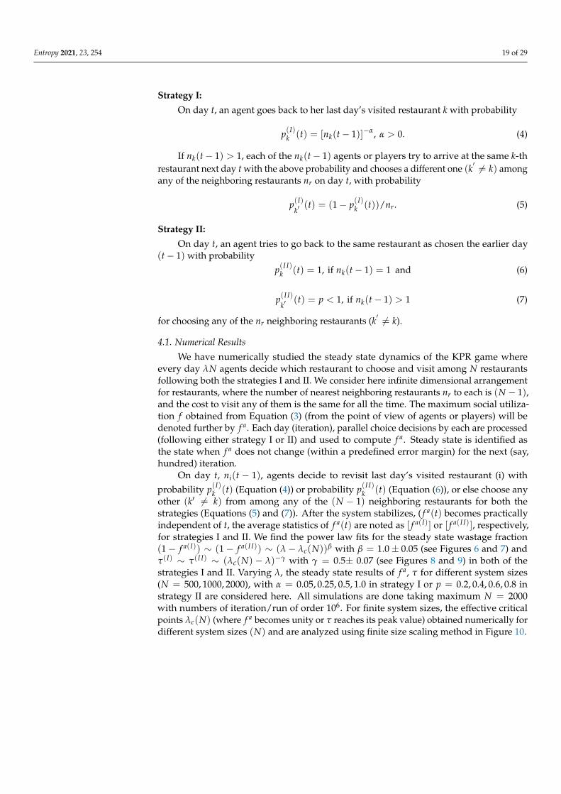
However, in democratic set-up, this dictated solution is not acceptable and the agentsor players are expected to evolve their strategy to make the best minority choice inde-pendently (without presence of any dictator), using the publicly available informationabout the past record of crowd sizes in different restaurants, such that each arrives alonethere in the respective restaurant and gets the dish. The more successful such collec-tive learning, the more is the aggregated utilization fraction f . Earlier studies (see e.g.,References [20,72,74,85–88] strategies for KPR game. Recently authors in Reference [81]have proposed two such stochastic strategies (strategy I and strategy II) where the agentscollectively learn to make their decisions utilizing the publicly available history of crowdsize of the last day’s chosen restaurant. Below, we briefly discuss them.

Entropy 2021, 23, 254 19 of 29

Strategy I:

On day t, an agent goes back to her last day’s visited restaurant k with probability

p(I)k (t) = [nk(t− 1)]−α, α > 0. (4)

If nk(t− 1) > 1, each of the nk(t− 1) agents or players try to arrive at the same k-threstaurant next day t with the above probability and chooses a different one (k

′ 6= k) amongany of the neighboring restaurants nr on day t, with probability

p(I)k′

(t) = (1− p(I)k (t))/nr. (5)

Strategy II:

On day t, an agent tries to go back to the same restaurant as chosen the earlier day(t− 1) with probability

p(I I)k (t) = 1, if nk(t− 1) = 1 and (6)

p(I I)k′

(t) = p < 1, if nk(t− 1) > 1 (7)

for choosing any of the nr neighboring restaurants (k′ 6= k).

4.1. Numerical Results

We have numerically studied the steady state dynamics of the KPR game whereevery day λN agents decide which restaurant to choose and visit among N restaurantsfollowing both the strategies I and II. We consider here infinite dimensional arrangementfor restaurants, where the number of nearest neighboring restaurants nr to each is (N − 1),and the cost to visit any of them is the same for all the time. The maximum social utiliza-tion f obtained from Equation (3) (from the point of view of agents or players) will bedenoted further by f a. Each day (iteration), parallel choice decisions by each are processed(following either strategy I or II) and used to compute f a. Steady state is identified asthe state when f a does not change (within a predefined error margin) for the next (say,hundred) iteration.

On day t, ni(t − 1), agents decide to revisit last day’s visited restaurant (i) withprobability p(I)

k (t) (Equation (4)) or probability p(I I)k (t) (Equation (6)), or else choose any

other (k′ 6= k) from among any of the (N − 1) neighboring restaurants for both thestrategies (Equations (5) and (7)). After the system stabilizes, ( f a(t) becomes practicallyindependent of t, the average statistics of f a(t) are noted as [ f a(I)] or [ f a(I I)], respectively,for strategies I and II. We find the power law fits for the steady state wastage fraction(1− f a(I)) ∼ (1− f a(I I)) ∼ (λ− λc(N))β with β = 1.0± 0.05 (see Figures 6 and 7) andτ(I) ∼ τ(I I) ∼ (λc(N) − λ)−γ with γ = 0.5± 0.07 (see Figures 8 and 9) in both of thestrategies I and II. Varying λ, the steady state results of f a, τ for different system sizes(N = 500, 1000, 2000), with α = 0.05, 0.25, 0.5, 1.0 in strategy I or p = 0.2, 0.4, 0.6, 0.8 instrategy II are considered here. All simulations are done taking maximum N = 2000with numbers of iteration/run of order 106. For finite system sizes, the effective criticalpoints λc(N) (where f a becomes unity or τ reaches its peak value) obtained numerically fordifferent system sizes (N) and are analyzed using finite size scaling method in Figure 10.

Entropy 2021, 23, 254 20 of 29

0.000 0.001 0.002 0.003 0.004 0.005 0.006 0.007 0.008c(N)

0.000

0.002

0.004

0.006

0.008

0.010

0.012

0.014

1fa(

I)

(a)

N = 1000N = 2000

0.98 1.000.00

0.01

1fa(

I)

0.0000 0.0025 0.0050 0.0075 0.0100 0.0125 0.0150 0.0175 0.0200c(N)

0.00

0.01

0.02

0.03

0.04

0.05

0.06

1fa(

I)

(b)

N = 500N = 1000N = 2000

0.90 0.950.00

0.05

1fa(

I)

0.0000 0.0025 0.0050 0.0075 0.0100 0.0125 0.0150 0.0175 0.0200c(N)

0.00

0.01

0.02

0.03

0.04

0.05

0.06

0.07

0.08

1fa(

I)

(c)

N = 500N = 1000N = 2000

0.85 0.900.00

0.05

1fa(

I)

0.000 0.005 0.010 0.015 0.020 0.025c(N)

0.00

0.02

0.04

0.06

0.08

0.10

1fa(

I)

(d)

N = 500N = 1000N = 2000

0.75 0.80 0.850.0

0.1

1fa(

I)

Figure 6. Plots of (1− f a(I)) against λ− λc(N) following strategy I at (a) α = 0.05, (b) α = 0.25, (c)α = 0.5, (d) α = 1.0. A power law holds for (1− f a(I)) ∼ (λ− λc(N))β, where β = 1.0± 0.05. Theinsets show direct relationship between (1− f a(I)) and λ (for strategy I).

0.00 0.02 0.04 0.06 0.08 0.10 0.12c(N)

0.00000

0.00001

0.00002

0.00003

0.00004

0.00005

0.00006

0.00007

[(I)

]2.

0

(a)

N = 500N = 1000N = 2000

0.90 0.95150200250

(I)

0.000 0.025 0.050 0.075 0.100 0.125 0.150 0.175c(N)

0.00000

0.00025

0.00050

0.00075

0.00100

0.00125

0.00150

0.00175

0.00200

[(I)

]2.

0

(b)

N = 500N = 1000N = 2000

0.8 1.0255075

(I)

0.00 0.02 0.04 0.06 0.08 0.10 0.12 0.14 0.16c(N)

0.000

0.001

0.002

0.003

0.004

0.005

0.006

0.007

0.008

[(I)

]2.

0

(c)

N = 500N = 1000N = 2000

0.8 0.9255075

(I)

0.00 0.02 0.04 0.06 0.08 0.10 0.12 0.14 0.16c(N)

0.000

0.005

0.010

0.015

0.020

0.025

0.030

[(I)

]2.

0

(d)

N = 500N = 1000N = 2000

0.6 0.8 1.00

100

(I)

Figure 7. Plots of steady state convergence time τ(I) from strategy I against λc(N)− λ at (a) α = 0.05,(b) α = 0.25, (c) α = 0.5, (d) α = 1.0. A power law holds for τ(I) ∼ (λc(N) − λ)−γ, whereγ = 0.5± 0.05. The insets plot direct relationship between τ(I) and λ for different system sizes (forstrategy I), also showing the variation of λ as α increases.

Entropy 2021, 23, 254 21 of 29

0.000 0.005 0.010 0.015 0.020 0.025c(N)

0.00

0.01

0.02

0.03

0.04

0.05

0.06

0.07

1fa(

II)

(a)

N = 500N = 1000N = 2000

0.90 0.950.00

0.05

1fa(

II)

0.000 0.005 0.010 0.015 0.020 0.025 0.030 0.035c(N)

0.00

0.02

0.04

0.06

0.08

0.10

1fa(

II)

(b)

N = 500N = 1000N = 2000

0.8 0.90.0

0.1

1fa(

II)

0.000 0.005 0.010 0.015 0.020 0.025 0.030c(N)

0.00

0.01

0.02

0.03

0.04

0.05

0.06

0.07

0.08

0.09

1fa(

II) (c)

N = 500N = 1000N = 2000

0.7 0.80.0

0.1

1fa(

II)

0.000 0.005 0.010 0.015 0.020 0.025 0.030c(N)

0.00

0.02

0.04

0.06

0.08

0.10

1fa(

II) (d)

N = 500N = 1000N = 2000

0.6 0.70.0

0.1

1fa(

II)

Figure 8. Plots of (1− f a(I I)) versus λ− λc(N) following strategy II at (a) p = 0.8, (b) p = 0.6, (c)p = 0.4, (d) p = 0.2. A power law holds for (1− f a(I I)) ∼ (λ− λc(N))β with β = 1.0± 0.05. Theinsets show direct relationship between variations of (1− f a(I I)) against λ (for strategy II).

0.00 0.02 0.04 0.06 0.08 0.10c(N)

0.0000

0.0002

0.0004

0.0006

0.0008

0.0010

0.0012

0.0014

0.0016

0.0018

[(II

) ]2.

0

(a)

N = 500N = 1000N = 2000

0.9 1.0

50

100

(II)

0.00 0.02 0.04 0.06 0.08 0.10c(N)

0.000

0.001

0.002

0.003

0.004

0.005

0.006

0.007

[(II

) ]2.

0

(b)

N = 500N = 1000N = 2000

0.8 0.9

255075

(II)

0.00 0.02 0.04 0.06 0.08 0.10c(N)

0.000

0.002

0.004

0.006

0.008

0.010

0.012

0.014

0.016

[(II

) ]2.

0

(c)

N = 500N = 1000N = 2000

0.7 0.8 0.90

100(II)

0.00 0.02 0.04 0.06 0.08 0.10c(N)

0.000

0.005

0.010

0.015

0.020

0.025

0.030

[(II

) ]2.

0

(d)

N = 500N = 1000N = 2000

0.6 0.80

100

(II)

Figure 9. Plots of steady state convergence time τ(I I) against λc(N)− λ following strategy II at (a)p = 0.8, (b) p = 0.6, (c) p = 0.4, (d) p = 0.2. A power law holds for τ(I I) ∼ (λc(N)− λ)−γ withγ = 0.5±0.07. The insets give direct relationship between τ(I I) and λ for different system sizes (forstrategy II), also showing the variation of λ as p decreases.

Entropy 2021, 23, 254 22 of 29

0.00 0.01 0.02 0.03 0.04 0.05N 0.5

0.70

0.75

0.80

0.85

0.90

0.95

1.00

1.05

(eff.

)c

c

c

c

c

(a)

= 1.0= 0.5= 0.25= 0.05

0.00 0.01 0.02 0.03 0.04 0.05N 0.5

0.5

0.6

0.7

0.8

0.9

1.0

(eff.

)c

c

c

c

c

(b)

p = 0.8p = 0.6p = 0.4p = 0.2

Figure 10. Extrapolation study of the effective finite size critical density of agents λc(N). The systemsize dependence is numerically fitted to 1√

Nand we estimate λc from λc ≡ λc(N → ∞). The

extrapolated values of λc are 0.99, 0.92, 0.85, 0.75 for α = 0.05, 0.25, 0.5, 1.0 (strategy I) (a), and are0.9, 0.8, 0.7, 0.6 for p = 0.8, 0.6, 0.4, 0.2 (strategy II) (b).

It may be mentioned that, in general, for the estimation of errors in the exponentsβ and γ in Figures 6–9, we tried linear fits (without any intercept) for log y versus log x,using best fits mostly for the intermediate range data points for all N values until they startdeviating (due to extreme fluctuations near λ = λc and towards their saturation valuesfor λ approaching unity [74,81]) and anticipating their universal mean field values in thisinfinite dimensional system. From the slopes of these best fit lines for different α or pvalues, we extract the universal exponent values and their standard deviations. We givethis higher error in the estimate of the unified (and universal) estimate of γ.

4.2. Summary

KPR is a multi-agent multi-choice repeated game where players try to learn fromtheir past successes or failures, utilizing publicly available information on the crowd sizesat different restaurant in the past to decide which restaurant to visit that day such thatshe would be alone there for being served the only prepared dish. Here, asymmetriccase such that λN (λ < 1) agents are considered against N restaurants, for sufficientlylarge N. End of each day (iteration), we have measured social utilization for agentsf a(t) = ∑N

i=1[δ(ni(t))/λN] where ni(t) denotes number of customers visiting ith restauranton day t.

As shown in Figure 6 (for strategy I) and Figure 8 (for strategy II), the social wastagefraction (1− f a) vanishes at the effective critical point λc(N) with the critical exponent βvalue near unity. In addition, from Figure 7 (for strategy I) and Figure 9 (for strategy II), wesee that the the convergence or relaxation time t, required for f a to stabilize, divergence nearthe same critical points λc(N) for the respective strategies, with the exponent γ value about1/2. Additionally, the finite size scaling analysis λc(N) ∼ λc + const.N−1/(dν), where λccorresponds to λc(N) for N going to infinity and d corresponds to the effective dimension,suggests the effective correlation length exponent dν value to be around 2 for both thestrategies, as expected for such mean field (infinite range systems).

In Reference [81], we have studied the dynamics of the KPR game following the sametwo strategies for the case λ = 1. For λ = 1.0, where the critical points λc (for both thestrategies) vanish, the universality class (values of the critical exponents β and γ wereobserved to be distinctly different, and this point needs further investigations. We may,however, note that, since at λ = 1, the number of both agents and restaurants are same(N), full social utilization (where f a = 1 = f r, occurring at α = 0+ for strategy I and atp = 1− for strategy II) induces an additional frustrating constraint in the collective choicedynamics involved here.

The KPR game models have been extended already and used to study real life prob-lems, like resource allocation in Internet of Things [82], vehicle for hire [83], matching inmobility markets [84], etc. We hope the KPR game models will be utilized much moreeffectively in the context of much wider practical areas of collective learning dynamicsand choices.

Entropy 2021, 23, 254 23 of 29

5. Future of Econophysics: Some Perspective

One often says that the main purpose of economic activity is to optimize the limitedfunds of labor and capital, natural and technical resources and capital resources, to satisfyour (practically) unlimited needs. “Economic science is therefore the science of efficiency,and as such, it is a quantitative science.” [89] (also see Reference [90]). We have alreadyargued [14] in Section 2 that epistemologically economics belongs to natural science (andnot mathematics). It begins with observation which are to be analyzed using logic ormathematics and eventually should end in observation, as in all natural sciences. Since1990s, most Universities of the world offer Science Graduation degrees (Bachelor of Scienceor Master of Science degrees) in economics (in addition to Bachelor of Arts or Master ofArts from Fine Arts or Humanities Departments).

Robert Solow [91] pointed out that, in the 1940s, economics had been basically adescriptive and institutional subject for a ‘gentleman scholar’. The textbooks of those dayswere ‘civilized’ and discursive. ... “Formal analysis were minimal and it made economicsthe domain of intuitive economists”. He concluded his summary of the state of economicsnear the end of the 20th century “with a paraphrase of Oscar Wilde’s description of a foxhunt - ‘the unspeakable in pursuit of the inedible’-saying that perhaps economics was anexample of ‘the over-educated in pursuit of the unknowable’.” [91]. Despite the ongoingcontroversies today in the field of economics, the “New Millennium economists are farmore comfortable with what they do after the changes in the structure and content ofeconomics over the last half century” [92]. The root cause of these changes have beenidentified by Colander [92] to be due to the rise of Complexity Science since early 1980s. Infact, concepts from physics had continually been absorbed into the main stream economicformulation of ideas and models. As Venkat Venkatasubramanian noted in his recentbook [93], “Concepts such as equilibrium, forces of supply and demand, and elasticityreveal influence of classical mechanics on economics. The analytical model of utility-basedpreferences can be traced back to Daniel Bernoulli, the great Swiss mathematical physicistfrom nineteenth century. One of the founders of neoclassical economics, Irving Fisher,was trained under the legendary Yale physicist, Jisiah Willard Gibbs, a co-founder of thediscipline of statistical mechanics. Similarly, Jan Tinbergen, who shared the first NobelPrize in Economics in 1969, was the doctoral student of the great physicist Paul Ehrenfestat Leiden University”.

Indeed, more specifically as discussed in Section 2, we would like to correlate thesechanges to occur following the successful development in econophysics of the SimulatedAnnealing technique [22] in 1983 for Traveling Salesman type multi-variable optimizationproblems, and other successive developments in econophysics of analyzing correlationsin stock prices (see, e.g., Reference [3,21]) or the kinetic exchange modelings of incomeand wealth distributions (see, e.g., References [28,63]). The statistical physics of TSP, asan example of successful developments in econophysics, had already been introduced inour 2010 econophysics textbook [32], which has been the only ‘suggested textbook’ (sinceinception in 2012) of the formal course on econophysics, offered (by Diego Garlaschelli) atthe Physics Department of the Leiden University (see the course prospectus for 2012–2013through that of 2020–2021 [94]), where one of the first Nobel-laureates in economics JanTinbergen came from.

Econophysics has come as an exceptional development in interdisciplinary sciences(see, e.g., Reference [95] for a popular exposition on this development). Historically,economics, more specifically social sciences, belonged to the Humanities departments andnot of Science. For earlier interdisciplinary developments of Astrophysics, Biophysics, orGeophysics, the scenario and ambiance had been quite different. The mother departmentshad been parts of the same science schools and even the corresponding resources, likebooks, journals, and also the faculty, had strong overlaps and could be shared. The marriagenegotiations for Econophysics have been difficult, though extremely desirable and natural;as the saying goes: “marriage between the King of natural sciences with the Queen ofsocial sciences!”

Entropy 2021, 23, 254 24 of 29

Regular interactions and collaborations between the communities of natural scientistsand social scientists are, however, rare, even today! Though, as mentioned already, interdis-ciplinary research papers on econophysics and sociophysics are regularly being publishedat a steady and healthy rate, and a number of universities (including Universities of Bern,Leiden, London, Paris, and Tufts University) are offering the interdisciplinary courses oneconophysics and sociophysics, not many clearly designated professor positions, or otherfaculty positions for that matter, are available yet (except for econophysics in Universitiesof Leiden and London). Neither are there designated institutions on these interdisciplinaryfields, nor separate departments or centers of studies for instance. Of course, there havebeen several positive and inspiring attempts and approaches from both economics andfinance side (see, e.g., References [96,97], along with a number of those [66,67,98–100] fromphysics, which have already been appreciated in the literature). Indeed, the thesis [101]in August 2018, Department of History and Philosophy of Science, University of Cam-bridge, by financial economist Christophe Schinckus (one of the co-editors of this specialissue), says that “In order to reconstruct the subfield of econophysics, I started with thegroup of the most influential authors in econophysics and tracked their papers in theliterature using the Web of Science database of Thomson-Reuters (The sample is composedof: Eugene Stanley, Rosario Mantegna, Joseph McCauley, Jean-Pierre Bouchaud, MauroGallegati, Benoît Mandelbrot, Didier Sornette, Thomas Lux, Bikas Chakrabarti and DoyneFarmer). These key authors are often presented as the fathers of econophysics simplybecause they contributed significantly to its early definition and development. Because oftheir influential and seminal works, these scholars are actually the most quoted authors ineconophysics. Having the 10 highest quoted fathers of econophysics as a sample sounds anacceptable approach to define bibliometrically the core of econophysics”. In addition, theentry on ‘Social Ontology’ in The Stanford Encyclopedia of Philosophy [15], as discussed inSection 2, confirms positive impact of such econophysics and sociophysics research studieson the overall modern philosophical outlook of social sciences.

We may note, however, a recently published highly acclaimed massive (580 page)book [96] on economics (‘landmark volume’, said E. Roy Weintraub, ‘creative, elegantand brilliant work’, said W. Brian Arthur and ‘written by master economists’, said D.Colander) by (Late) Martin Shubik (Ex-Seymour Knox Professor Emeritus of MathematicalInstitutional Economics, Yale University and Santa Fe Institute) and Eric Smith (SantaFe Institute) discussed extensively on econophysics approaches and in general on thepotential of interdisciplinary research studies inspired by the developments in naturalsciences. Getting somewhat excited, I wrote to Martin Shubik in late 2016 that their bookcan also serve as an outstanding ‘white-paper’ document in favor of a possible Proposalfor an International Center for Interdisciplinary Studies on Complexity in Social Sciences.He immediately responded and gave his impression about the difficulties involved andindicated very briefly about the minimal financial and structural requirements (both myletter to him and his response is appended below (Figures 11 and 12).

Entropy 2021, 23, 254 25 of 29

Figure 11. The first part of the email conversation between (late) Martin Shubik and BKC. Sec-ond part (email from BKC; appended to this part) is continued in Figure 12. The precise sug-gestions made in this immediate response indicate Shubik’s prior plan for such ‘interdisciplinaryinstitutes’ in economics.

Figure 12. Email conversation in the end of 2016 between (late) Martin Shubik and BKC regardinginterdisciplinary developments in economics and the possibility of setting up an International Centerfor Interdisciplinary Studies on Complexity in Social Sciences. This email from BKC was appendedto the response email (Figure 11) from Shubik. The (Yale) date and time mark in the mail-header (andthat for BKC’s in Figure 11, on arrival in Kolkata) indicate hardly any time gap between the two andthe readiness with the precise suggestions indicate Shubik’s prior thinking in similar line.

Entropy 2021, 23, 254 26 of 29

This ready and specific comments by Shubik clearly suggests that he actually hadthought about the need of such an International Center for fostering interdisciplinaryresearch which needs to be more inclusive than, for example, the Santa Fe Institute. Themodel of the Abdus Salam International Center for Theoretical Physics (ICTP), Trieste(funded by UNESCO and IAEA), was considered to provide helpful guidance for us here.It was contemplated, if an ICTP-type interdisciplinary research institute could be initiatedfor research studies on econophysics and sociophysics (see, e.g, Reference [102]). ThoughShubik (who died in 2018 at the age of 92) agreed also to be one of its founding members, wecould not make any progress yet. We may also note that Dirk Helbing and colleagues havebeen trying for an European Union funded ‘Complex Techno-Socio- Economic AnalysisCenter’ or ‘Economic and Social Observatory’ for the last decade or so (see Ref. [103]containing the White Papers arguing for their proposed project). We are also aware thatIndian Statistical Institute had taken a decision to initiate a similar Center in India (see‘Concluding Remarks’ in Reference [104]).

Hope, some such international visiting centers will come up soon and with them thespread of such interdisciplinary ideas will achieve more coherence and will lead to majorsuccess in such research studies.

Author Contributions: Data curation, A.S.; Writing—review & editing, B.K.C. and A.S. All authorshave read and agreed to the published version of the manuscript.

Funding: This research received no external funding.

Institutional Review Board Statement: Not applicable.

Informed Consent Statement: Not applicable.

Data Availability Statement: Not applicable.

Acknowledgments: We acknowledge all our colleagues (mentioned by name in Section 2) forthe collaborations. BKC is grateful to J.C. Bose National Fellowship (DST, Govt. of India) grantfor support.

Conflicts of Interest: The authors declare no conflict of interest.

References1. Gangopadhyay, K. Interview with Eugene H. Stanley. IIM Kozhikode Soc. Manag. Rev. 2013, 2, 73–78. [CrossRef]2. Rosser, J.B., Jr. Econophysics. In New Palgrave Dictionary of Economics; Durlauf, S.N., Blume, L.E., Eds.; Palgrave Macmillan:

London, UK, 2008; Volume 2, pp. 729–732.3. Mantegna, R.N.; Stanley, H.E. An Introduction to Econophysics; Cambridge University Press: Cambridge, UK, 2000.4. Galam, S.; Gefen, Y.; Shapir, Y. Sociophysics: A mean behavior model for the process of strike. J. Mathe. Sociol. Scimago 2000,

9, 1–13.5. Galam, S. Sociophysics: A Physicist’s Modeling of Psycho-Political Phenomena; Springer: New York, NY, USA, 2012.6. Chakrabarti, B.K. Econophysics as conceived by Meghnad Saha. Sci. Cult. Indian Sci. News Assoc. 2018, 84, 365–369.7. Saha, M.N.; Srivastava, B.N. A Treatise on Heat; Indian Press: Allahabad, India, 1931; p. 105.8. Dragulescu, A.; Yakovenko, V.M. Statistical mechanics of money. Eur. Phys. J. B-Condens. Matter Complex Syst. 2000, 17, 723–729.

[CrossRef]9. Chakraborti, A.; Chakrabarti, B.K. Statistical mechanics of money: How saving propensity affects its distribution. Eur. Phys. J.

B-Condens. Matter Complex Syst. 2000, 17, 167–170. [CrossRef]10. Chatterjee, A.; Chakrabarti, B.K.; Manna, S.S. Pareto law in a kinetic model of market with random saving propensity. Phys. A

Stat. Mech. Appl. 2004, 335, 155–163. [CrossRef]11. Chakrabarti, B.K.; Marjit, S. Self-organisation and complexity in simple model systems: Game of life and economics. Indian J.

Phys. IACS 1995, 69B, 681–698.12. Stanley, H.E.; Afanasyev, V.; Amaral, L.A.N.; Buldyrev, S.V.; Goldberger, A.L.; Havlin, S.; Leschhorn, H.; Maass, P.; Mantegna, R.N.;

Peng, C.-K. Anomalous fluctuations in the dynamics of complex systems: From DNA and physiology to econophysics. Phys. AStat. Mech. Appl. 1996, 224, 302–321. [CrossRef]

13. Chakrabarti, B.K. Econophysics. In Encyclopedia of Philosophy and the Social Sciences; Kaldis, B., Ed.; Sage: Thousand Oaks, CA,USA, 2013; Volume 1, pp. 229–230.

14. Chakrabarti, B.K. Can economics afford not to become natural science? Eur. Phys. J. Spec. Top. 2016, 225, 3121–3125. [CrossRef]

Entropy 2021, 23, 254 27 of 29

15. Epstein, B. Social Ontology. In The Stanford Encyclopedia of Philosophy; Stanford University: Stanford, CA, USA, 2018. Availableonline: https://plato.stanford.edu/entries/social-ontology/ (accessed on 8 January 2021).

16. Whitehead, A.N.; Russell, B. Principia Mathematica; Cambridge University Press: Cambridge, UK, 1910; Volume I.17. Whitehead, A.N.; Russell, B. Principia Mathematica; Cambridge University Press: Cambridge, UK, 1912; Volume II.18. Whitehead, A.N.; Russell, B. Principia Mathematica; Cambridge University Press: Cambridge, UK, 1913; Volume III.19. Challet, D.; Marsili, M.; Zhang, Y.-C. Minority Games: Interacting Agents in Financial Markets; Oxford University Press: Oxford, UK, 2005.20. Chakrabarti, B.K.; Chatterjee, A.; Ghosh, A.; Mukherjee, S.; Tamir, B. Econophysics of the Kolkata Restaurant Problem and Related

Games: Classical and Quantum Strategies for Multi-Agent, Multi-Choice Repetitive Games; Springer: Cham, The Netherland, 2017.21. Mantegna, R.N. Lévy walks and enhanced diffusion in Milan stock exchange. Phys. A Stat. Mech. Appl. 1991, 179, 232–242.

[CrossRef]22. Kirkpatrick, S.; Gelatt, C.D.; Vecchi, M.P. Optimization by simulated annealing. Science 1983, 220, 671–680. [CrossRef]23. Das, A.; Chakrabarti, B.K. Colloquium: Quantum annealing and analog quantum computation. Rev. Modern Phys. 2008,

80, 1061–1081. [CrossRef]24. Santoro, G.E.; Tosatti, E. Optimization using quantum mechanics: Quantum annealing through adiabatic evolution. J. Phys. A

Math. Gener. 2006, 39, R393–R431. [CrossRef]25. Chakrabarti, B.K. Econophys-Kolkata: A short story. In Econophysics of Wealth Distributions; Chatterjee, A., Yarlagadda, S.,

Chakrabarti, B.K., Eds.; Springer: Milan, Italiy, 2005; pp. 225–228.26. Sen, P.; Chakrabarti, B.K. Travelling salesman problem on dilute lattices: Visit to a fraction of cities. J. Phys. 1989, 50, 255–261.

[CrossRef]27. Sen, P.; Chakrabarti, B.K. Sociophysics: An Introduction; Oxford University Press: Oxford, UK, 2014.28. Yakovenko, V.M.; Rosser, J.B., Jr. Colloquium: Statistical mechanics of money, wealth, and income. Rev. Modern Phys. 2009, 81, 1703.

[CrossRef]29. Orman, A.J. Williams, H.P. A survey of different integer programming formulations of the travelling salesman problem. Optim. Econom.

Financ. Anal. 2006, 9, 93–108.30. Rasmussen, R. TSP in Spreadsheets–a Guided Tour. Int. Rev. Econom. Educ. 2011, 10, 94–116. [CrossRef]31. Percus, A.G.; Martin, O.C. Finite size and dimensional dependence in the Euclidean traveling salesman problem. Phys. Rev. Lett.

1996, 76, 1188–1191. [CrossRef] [PubMed]32. Sinha, S.; Chatterjee, A.; Chakraborti, A.; Chakrabarti, B.K. Econophysics: An Introduction; John Wiley & Sons: New York, NY, USA, 2010.33. Beardwood, J.; Halton, J.H.; Hammersley, J.M. The shortest path through many points. In Mathematical Proceedings of the Cambridge

Philosophical Society; Cambridge Press: Cambridge, UK, 1959; Volume 55, pp. 299–327. [CrossRef]34. Chakrabarti, B.K. Directed travelling salesman problem. J. Phys. A Math. Gen. 1986, 19, 1273–1275. [CrossRef]35. Dhar, D.; Barma, M. Chakrabarti, B.K.; Taraphder, A. The travelling salesman problem on a randomly diluted lattice. J. Phys. A

Math. Gen. 1987, 20, 5289–5298. [CrossRef]36. Ghosh, M.; Manna, S.S.; Chakrabarti, B.K. The travelling salesman problem on a dilute lattice: A simulated annealing study.

J. Phys. A Math. Gen. 1988, 21, 1483–1486. [CrossRef]37. Chakraborti, A.; Chakrabarti, B.K. The travelling salesman problem on randomly diluted lattices: Results for small-size systems.

Eur. Phys. J. B-Condens. Matter Complex Syst. 2000, 16, 677–680. [CrossRef]38. Bonomi, E.; Lutton, J.-L. The N-city travelling salesman problem: Statistical mechanics and the Metropolis algorithm. SIAM Rev.

1984, 26, 551–568. [CrossRef]39. Zhou, A.-H.; Zhu, L.-P.; Hu, B.; Deng, S.; Song, Y.; Qiu, H.; Pan, S. Traveling-salesman-problem algorithm based on simulated

annealing and gene-expression programming. Information 2019, 10, 7. [CrossRef]40. Ray, P.; Chakrabarti, B.K.; Chakrabarti, A. Sherrington-Kirkpatrick model in a transverse field: Absence of replica symmetry

breaking due to quantum fluctuations. Phys. Rev. B 1989, 39, 11828–11832. [CrossRef] [PubMed]41. Johnson, M.W.; Amin, M.H.S.; Gildert, S.; Lanting, T.; Hamze, F.; Dickson, N.; Harris, R.; Berkley, A.J.; Johansson, J.; Bunyk, P.

Quantum annealing with manufactured spins. Nature 2011, 473, 194–198. [CrossRef] [PubMed]42. Mukherjee, S.; Chakrabarti, B.K. Multivariable optimization: Quantum annealing and computation. Eur. Phys. J. Spec. Top. 2015,

224, 17–24. [CrossRef]43. Lucas, A. Ising formulations of many NP problems. Front. Phys. 2014, 2, 1–15. [CrossRef]44. Dong, Y.; Huang, Z. An Improved Noise Quantum Annealing Method for TSP. Int. J. Theor. Phys. 2020, 59, 3737–3755. [CrossRef]45. Tanaka, S.; Tamura, R.; Chakrabarti, B.K. Quantum Spin Glasses, Annealing and Computation; Cambridge University Press:

Cambridge, UK, 2017.46. Albash, T.; Lidar, D.A. Adiabatic quantum computation. Rev. Modern Phys. 2018, 90, 015002. [CrossRef]47. Gini, C. Measurement of inequality of incomes. Econ. J. 1921, 31, 124–126. [CrossRef]48. Lorenz, M.O. Methods of measuring the concentration of wealth. Publ. Am. Stat. Assoc. 1905, 9, 209–219. [CrossRef]49. Ghosh, A.; Chattopadhyay, N.; Chakrabarti, B.K. Inequality in societies, academic institutions and science journals: Gini and

k-indices. Phys. A Stat. Mech. Appl. 2014, 410, 30–34. [CrossRef]50. Ghosh, A.; Chatterjee, A.; Inoue, J.; Chakrabarti, B.K. Inequality measures in kinetic exchange models of wealth distributions.

Phys. A Stat. Mech. Appl. 2016, 451, 465–474. [CrossRef]

Entropy 2021, 23, 254 28 of 29

51. Chatterjee, A.; Ghosh, A.; Chakrabarti, B.K. Socio-economic inequality: Relationship between Gini and Kolkata indices. Phys. AStat. Mech. Appl. 2017, 466, 583–595. [CrossRef]

52. Sinha, A.; Chakrabarti, B.K. Inequality in death from social conflicts: A Gini & Kolkata indices-based study. Phys. A Stat.Mech. Appl. 2019, 527, 121185.

53. Banerjee, S.; Chakrabarti, B.K.; Mitra, M.; Mutuswami, S. On the Kolkata index as a measure of income inequality. Phys. A Stat.Mech. Appl. 2020, 545, 123178. [CrossRef]

54. Banerjee, S.; Chakrabarti, B.K.; Mitra, M.; Mutuswami, S. Social Inequality Measures: The Kolkata index in comparison withother measures. Front. Phys. 2020, 8, 562182. [CrossRef]

55. Available online: https://en.wikipedia.org/wiki/Pareto_principle (accessed on 28 January 2021).56. Hirsch, J.E. An index to quantify an individual’s scientific research output. Proc. Natl. Acad. Sci. USA 2005, 102, 16569–16572.

[CrossRef] [PubMed]57. Subramanian, S. More tricks with the Lorenz curve. Econ. Bull. 2015, 35, 580–589.58. Sahasranaman, A.; Jensen, H.J. Spread of Covid-19 in urban neighbourhoods and slums of the developing world. arXiv 2020,

arXiv:2010.06958.59. Fisher, M.E. Renormalization group theory: Its basis and formulation in statistical physics. Rev. Modern Phys. 1998, 70, 653–681.

[CrossRef]60. Feigenbaum, M.J. Universal behavior in nonlinear systems. Phys. D Nonlinear Phenom. 1983, 7, 16–39. [CrossRef]61. Chatterjee, A.; Yarlagadda, S.; Chakrabarti, B.K. Econophysics of Wealth Distributions; Springer: Milano, Italiy, 2005.62. Chatterjee, A.; Chakrabarti, B.K. Kinetic exchange models for income and wealth distributions. Eur. Phys. J. B 2007, 60, 135–149.

[CrossRef]63. Chakrabarti, B.K. Chakraborti, A.; Chakravarty, S.R.; Chatterjee, A. Econophysics of Income and Wealth Distributions; Cambridge

University Press: Cambridge, UK, 2013.64. Chakrabarti, A.S.; Chakrabarti, B.K. Microeconomics of the ideal gas like market models. Phys. A Stat. Mech. Appl. 2009, 388,

4151–4158. [CrossRef]65. Quevedo, D.S.; Quimbay, C.J. Non-conservative kinetic model of wealth exchange with saving of production. Eur. Phys. J. B 2020,

93, 186. [CrossRef]66. Pareschi, L.; Toscani, G. Interacting Multiagent Systems: Kinetic Equations and Monte Carlo Methods; Oxford University Press: Oxford,

UK, 2013.67. Ribeiro, M.B. Income Distribution Dynamics of Economic Systems: An Econophysical Approach; Cambridge University Press: Cam-

bridge, UK, 2020.68. Chakraborti, A. Distributions of money in model markets of economy. Int. J. Modern Phys. C World Sci. 2002, 13, 1315–1321.

[CrossRef]69. Boghosian, B.M. Is Inequality Inevitable? Sci. Am. 2019, 321, 70–77. [CrossRef]70. Iglesias, J.R. How simple regulations can greatly reduce inequality. arXiv 2010, arXiv:1007.0461.71. Ghosh, A.; Basu, U.; Chakraborti, A.; Chakrabarti, B.K. Threshold-induced phase transition in kinetic exchange models.

Phys. Rev. E 2011, 83, 061130. [CrossRef] [PubMed]72. Chakrabarti, A.S.; Chakrabarti, B.K.; Chatterjee, A.; Mitra, M. The Kolkata Paise Restaurant problem and resource utilization.

Phys. A Stat. Mech. Appl. 2009, 388, 2420–2426. [CrossRef]73. Chakraborti, A.; Challet, D.; Chatterjee, A.; Marsili, M.; Zhang, Y.-C.; Chakrabarti, B.K. Statistical mechanics of competitive

resource allocation using agent-based models. Phys. Rep. 2015, 552, 1–25. [CrossRef]74. Ghosh, A.; Chatterjee, A.; Mitra, M.; Chakrabarti, B.K. Statistics of the kolkata paise restaurant problem. New J. Phys. 2010, 12, 075033.

[CrossRef]75. Sharif, P.; Heydari, H. Quantum solution to a three player Kolkata restaurant problem using entangled qutrits. arXiv 2011,

arXiv:1111.1962.76. Sharif, P.; Heydari, H. An introduction to multi-player, multi-choice quantum games: Quantum minority games & kolkata

restaurant problems. In Econophysics of Systemic Risk and Network Dynamics; Abergel, F., Ed.; Springer: Milano, Italy, 2013;pp. 217–236.

77. Ghosh, D.; Chakrabarti, A.S. Emergence of distributed coordination in the Kolkata paise restaurant problem with finite informa-tion. Phys. A Stat. Mech. Appl. 2017, 483, 16–24. [CrossRef]

78. Banerjee, P.; Mitra, M.; Mukherjee, K. The economics of the Kolkata Paise Restaurant problem. Sci. Cult. Indian Sci. News Assoc.2018, 84, 26–30.

79. Sharma, K.; Anamika; Chakrabarti, A.S. Chakraborti, A.; Chakravarty, S. The Saga of KPR: Theoretical and experimentaldevelopments. Sci. Cult. Indian Sci. News Assoc. 2018, 84, 31–36.

80. Tamir, B. Econophysics and the Kolkata Paise Restaurant Problem: More is different. Sci. Cult. Indian Sci. News Assoc. 2018,84, 37–47.

81. Sinha, A.; Chakrabarti, B.K. Phase transition in the Kolkata Paise Restaurant problem. Chaos Interdiscip. J. Nonlinear Sci. 2020,30, 083116. [CrossRef] [PubMed]

Entropy 2021, 23, 254 29 of 29

82. Park, T.; Saad, W. Kolkata paise restaurant game for resource allocation in the Internet of Things. In Proceedings of the 2017 51stAsilomar Conference on Signals, Systems, and Computers, IEEE Xplore, Pacific Grove, CA, USA, 29 October–1 November 2017;pp.1774–1778.

83. Martin, L. Extending Kolkata Paise Restaurant Problem to Dynamic Matching in Mobility Markets. Jr. Manag. Sci. 2019, 4, 1–34.84. Martin, L.; Karaenke, P. The Vehicle for Hire Problem: A Generalized Kolkata Paise Restaurant Problem. In Workshop on

Information Technology and Systems; Technical University of Munich: Seoul, Korea, 2017.85. Ghosh, A. Chakrabarti, A.S.; Chakrabarti, B.K. Kolkata Paise Restaurant problem in some uniform learning strategy limits.

In Econophysics and Economics of Games, Social Choices and Quantitative Techniques; Springer: Berlin, Germany, 2010; pp. 3–9.86. Ghosh, A.; De Martino, D.; Chatterjee, A.; Marsili, M.; Chakrabarti, B.K. Phase transitions in crowd dynamics of resource

allocation. Phys. Rev. E 2012, 85, 021116. [CrossRef] [PubMed]87. Ghosh, A.; Chatterjee, A.; Chakrabarti, A.S.; Chakrabarti, B.K. Zipf’s law in city size from a resource utilization model. Phys. Rev.

E 2014, 90, 042815. [CrossRef]88. Chakrabarti, B.K. Kolkata restaurant problem as a generalised el farol bar problem. In Econophysics of Markets and Business

Networks; Springer: Milan, Italy, 2007; pp. 239–246.89. Allais, M. Economics as a Science. Cah. Vilfredo Pareto 1968, 6, 5–24. Available online: https://www.jstor.org/stable/40368894

?seq=1 (accessed on 28 January 2021).90. Frey, B.S. Economics As a Science of Human Behaviour: Towards a New Social Science Paradigm, 2nd ed.; Springer: New York, NY, USA, 1999.91. Solow, R.M. How did economics get that way and what way did it get? Daedalus 1997, 126, 39–58. [CrossRef]92. Colander, D. New millennium economics: How did it get this way, and what way is it? J. Econ. Perspect. 2000, 14, 121–132.

[CrossRef]93. Venkatasubramanian, V. How Much Inequality Is Fair? Mathematical Principles of a Moral, Optimal, and Stable Capitalist Society;

Columbia University Press: New York, NY, USA, 2017.94. Leiden University. Econophysics e-Prospectuses for 2012–2013. 2020–2021. Available online: https://studiegids.universiteitleiden.

nl/en/courses/34804/econophysics or https://studiegids.universiteitleiden.nl/courses/99643/econophysics (accessed on 28January 2021).

95. Dash, K.C. The Story of Econophysics; Cambridge Scholars Publishing: Newcastle Upon Tyne, UK, 2019.96. Shubik, M.; Smith, E. The Guidance of an Enterprise Economy; MIT Press: Cambridge, MA, USA, 2016.97. Jovanovic, F.; Schinckus, C. Econophysics and Financial Economics: An Emerging Dialogue; Oxford University Press: Oxford, UK, 2017.98. Richmond, P.; Mimkes, J.; Hutzler, S. Econophysics and Physical Economics; Oxford University Press: Oxford, UK, 2013.99. Slanina, F. Essentials of Econophysics Modelling; Oxford University Press: Oxford, UK, 2013.100. Aoyama, H.; Fujiwara, Y.; Ikeda, Y.; Iyetomi, H.; Souma, W. Macro-Econophysics: New Studies on Economic Networks and Synchro-

nization; Cambridge University Press: Delhi, India; Cambridge, UK, 2017.101. Schinckus, C. When Physics Became Undisciplined An Essay on Econophysics; University of Cambridge: Cambridge, UK, 2018.

Available online: https://www.repository.cam.ac.uk/bitstream/handle/1810/279683/Chris_Thesis_FINAL.pdf?sequence=5&isAllowed=y (accessed on 28 January 2021).

102. Chakrabarti, B.K. International Center for Social Complexity, Econophysics and Sociophysics Studies: A Proposal. In NewPerspectives and Challenges in Econophysics and Sociophysics; New Economic Windows Series; Abergel, F., Ed.; Springer: Cham,The Newtherland, 2019; pp. 259–267.

103. Helbing, D.; Balietti, S.; Bishop, S.; Lukowicz, P. Understanding, creating, and managing complex techno-socio-economic systems:Challenges and perspectives (Visioneer White Papers). Eur. Phys. J. Spec. Top. 2011, 195, 165–186. [CrossRef]

104. Ghosh, A. Econophysics Research in India in the last two Decades. IIM Kozhikode Soc. Manag. Rev. 2013, 2, 135–146. [CrossRef]