Distance Metric Learning for Complex Networks: Towards Size-Independent

Comparison of Network Structures

Sadegh Aliakbary,1, a) Sadegh Motallebi,1, b) Sina Rashidian,1, c) Jafar Habibi,1, d) and Ali

Movaghar1, e)

Department of Computer Engineering, Sharif University of Technology, Tehran,

Iran

(Dated: 4 January 2015)

Real networks show nontrivial topological properties such as community structure

and long-tail degree distribution. Moreover, many network analysis applications are

based on topological comparison of complex networks. Classification and clustering

of networks, model selection, and anomaly detection are just some applications of

network comparison. In these applications, an effective similarity metric is needed

which, given two complex networks of possibly different sizes, evaluates the amount

of similarity between the structural features of the two networks. Traditional graph

comparison approaches, such as isomorphism-based methods, are not only too time

consuming, but also inappropriate to compare networks with different sizes. In this

paper, we propose an intelligent method based on the genetic algorithms for inte-

grating, selecting, and weighting the network features in order to develop an effective

similarity measure for complex networks. The proposed similarity metric outperforms

state of the art methods with respect to different evaluation criteria.

Keywords: Complex Network, Similarity Measure, Network Comparison, Network

Classification, Distance Metric Learning

a)Electronic mail: aliakbary@ce.sharif.edu.b)Electronic mail: motallebi@ce.sharif.edu.c)Electronic mail: rashidian@ce.sharif.edu.d)Electronic mail: jhabibi@sharif.edu.e)Electronic mail: movaghar@sharif.edu.

1

A distance metric for complex networks plays an important role in many

network-analysis applications. Given two networks with possibly different sizes,

the metric should represent the distance (dissimilarity) of the features in the

two networks as a single integrated measure. Traditional graph comparison

methods such as graph isomorphism and edit distance are improper for compar-

ing the complex networks because they are computationally infeasible for large

networks, unaware of nontrivial network features, and inappropriate for the

topological comparison of networks with different sizes. Some recent network

similarity metrics have been developed based on the manual selection of the

features and creating heuristic network distance metrics. This approach is even-

tually error-prone, since it is based on trial and error. In this paper, we employ

machine learning algorithms to learn a metric based on the available network

similarity evidences. Our proposed methodology includes a novel feature selec-

tion and feature weighting method for learning a network distance metric based

on a genetic algorithm. The proposed method is comprehensively evaluated

using different artificial, real, and temporal network datasets, and outperforms

the baseline methods with respect to all considered evaluation criteria.

I. INTRODUCTION

Many network analysis applications are based on the comparison of the complex networks.

Particularly, we often need a similarity metric in order to compare networks according to

their structural properties. Given two networks of possibly different sizes, the metric is

supposed to quantify the structural similarity of the two networks. It is possible to com-

pare the networks based on individual measurements such as density, clustering coefficient,

degree distribution, and average path lengths. But many applications require a single in-

tegrated quantity as the overall similarity of the two given networks. In this paper, we

investigate the problem of developing an appropriate network similarity measure, which is

size-independent, scalable, and also compatible with available network similarity evidences.

Existing network similarity metrics define the network similarity according to a manual

selection of some local/global features1,2. In contrast to this error-prone manual approach,

2

we propose to utilize machine learning methods to infer the network similarity metric, based

on the network labels which are witnesses to network similarities.

The need for a structural similarity metric for complex networks is frequently discussed

in the literature1–10. The definition of an appropriate network distance metric is the base

of many data-analysis and data-mining tasks including classification and clustering. In

the analysis of complex networks, a size-independent similarity metric plays an impor-

tant role in the evaluation of the network generation models8,11–15, evaluation of sampling

methods16–20, generative model selection4,21,22, network classification and clustering4,10,21–24,

anomaly and discontinuity detection2,25,26, study of epidemic dynamics27–29, and biological

networks comparison1,7. In such applications, the network distance metric is supposed to

consider various network features, then compare the overall structural properties of the two

networks, and finally, return a single aggregated distance quantity. Additionally, in most of

the mentioned applications, the network distance metric should be size-independent so that

it can compare networks of different scales. For example, in the evaluation of the sampling

algorithms, which is a potential application of the network distance metric, a large network

is compared with a sampled smaller network. As a result, the intended network distance

metric is different from other similarity/dissimilarity notions including graph similarity with

known node correspondence6, classical graph similarity approaches (including graph match-

ing, graph isomorphism, graph alignment, and edit distance)30,31, and most of the existing

graph kernels32–36.

In order to develop a network similarity metric, it is possible to create a feature vector

for each network based on the existing network measurements. We can compute the sim-

ilarity of feature vectors according to naıve distance methods such as Euclidean distance.

This approach is investigated in some of the existing network distance metrics1–3. It is

also possible to manually assign specific weights for different features. The problem with

manual feature selection and manual weighting of features is the significant trial and error

effort needed in order to construct the distance function, which is actually error-prone and

inefficient. As an alternative, we consider intelligent and automated methods for creating

the distance functions. The art of using machine learning methods in developing distance

functions is called “distance metric learning”. We will show that this approach leads to

3

integrated and more accurate similarity metrics. In this paper, we propose an intelligent

network distance metric, called NetDistance. In contrast to methods that concentrate only

on local features1,2, NetDistance is based on a combination of local and global network

features. In this paper, novel methods for “feature selection” and “distance metric learning”

are devised, along with admissible “evaluation criteria”. The proposed methodology can be

applied in other network domains, perhaps with different network datasets and even other

network features. To the best of our knowledge, this is the first effort to apply machine

learning methods for feature selection and structural distance metric learning for complex

networks. The comprehensive evaluations reveal significant contributions of this research.

In the remainder of this paper, we use “network”, “complex network”, and “graph” terms

and phrases interchangeably. Since “similarity” is the counterpart of “distance” and “dissim-

ilarity”, we may also use these terms for the meaning of quantified distance measurements

for networks. Although the proposed methodology is applicable for weighted and directed

networks, we only consider simple networks (undirected and unweighted graphs) in our ex-

periments. The structure of the rest of this paper is as follows: In Section II, we review the

literature and related works. In Section III, the proposed method is illustrated. In Section

IV, we evaluate our method and compare it with baseline methods. In Section V, the time

and space complexity of the proposed distance metric is analyzed. Finally, we conclude the

paper in Section VI.

II. LITERATURE REVIEW

Among the different approaches for network comparison, the classical methods consider

the notion of “graph isomorphism”. Two graphs are called isomorphic if they have an

identical topology. Some variations of isomorphism are also proposed, including subgraph

isomorphism and maximum common subgraphs36. “Edit distance” measures the degree of

isomorphism between two graphs. Other isomorphism-inspired methods also exist which are

based on counting the number of spanning trees37, comparing graph spectrums30, or com-

puting similarity scores for nodes and edges31. Metrics that investigate graph isomorphism

are computationally expensive and totally inapplicable for large networks. This category of

similarity metrics seeks a correspondence between the nodes of networks, and they do not

4

reflect the overall structural similarities of the networks.

Another approach in network comparison is the utilization of the kernel methods. A

kernel k(x, x′) is a measure of similarity between objects x and x′, and network comparison

involves defining a kernel for graphs. An appropriate kernel function should capture the

characteristics of the graphs, and it should also be both efficiently computable and positive

definite33. Many graph kernels are proposed in the literature32–36, but they do not consider

nontrivial features such as degree distribution, community structure, and transitivity of

relationships, which are actually important for comparison of complex networks.

“Graphlet counting” is an alternative approach for comparing networks. In order to char-

acterize the local structure of graphs, it is possible to count some small subgraphs called

motifs or graphlets. Graphlets are small subgraphs and represent significant patterns of

interconnections7,38. Similarity of “graphlet counts” may be used as a measure of similarity

between graphs4,7,38–42. Graphlet counting is a computationally complex process, and its

methods are usually based on a pre-stage of network sampling4,42.

Another family of distance measures for network comparison aims at representing the

graphs by feature vectors that summarize the graph topology3,8,24,36,43. The feature vector

is referred to as the “topological descriptor” or the “signature” of the network. In this

approach, the graph is replaced by a vector-representation. The feature vectors can be

utilized for defining the graph similarity metric, since such vectors are considered beneficial

for graph comparison2,4–6.

When there exist evidences about the similarity and dissimilarity of the instances, we can

develop a distance metric by the means of artificial intelligence. “Distance Metric Learning”

is the art of applying machine learning methods in order to find a distance function based

on a given collection of similar/dissimilar instances. Yang44 has surveyed the field of dis-

tance metric learning, along with its techniques and methods. Xing et al.45 formulated the

problem as a constrained convex programming problem. Weinberger et al.46 proposed Large

Margin Nearest Neighbor (LMNN) classification method in which a Mahalanobis distance

metric is learned from labeled examples of a dataset. LMNN obtains a family of metrics by

5

computing Euclidean distances after performing a linear transformation x′ = Lx. The dis-

tance metric is expressed in terms of the squared matrix M , which is defined as M = LTL.

If the elements of L are real numbers, M is guaranteed to be positive semidefinite. Equation

1 shows the squared distance in terms of the matrix M . LMNN is admitted and applied in

many applications, and our experiments also show the effectiveness of LMNN in distance

metric learning for complex networks. However, we will show that our proposed method is

based on genetic algorithms (GA)47 since GA outperforms LMNN in this application.

DM (xi, xj) = (xi − xj)T M (xi − xj) (1)

III. PROPOSED METHOD

Our proposed method for network similarity measurement, called NetDistance, is based

on learning a distance metric by the means of available network similarity evidences. Our

proposed roadmap for learning the distance metric for networks is described in Figure 1. In

this roadmap, we first gather a set of networks in which the similar networks are known.

Then, we extract a set of topological features from each network. As a result, each network

in the dataset is represented by a feature vector. In the next step, a subset of the networks

are fed as the training data to machine learning algorithms for feature selection and distance

metric learning. Finally, the rest of the networks are used as test data in order to evaluate

the proposed network distance metric.

A. Network Similarity Evidences

Distance metric learning methods use a dataset of similar/dissimilar pairs in order to learn

a distance function that preserves the distance relation among the training data instances44.

These methods tune a distance function so that it will return smaller distances for similar

instances. In order to learn a distance metric for complex networks, some evidences are

needed about networks similarities in a set of available networks. We propose to utilize at

least three evidences about the similarity/dissimilarity of networks. The first evidence is the

expected similarity among artificial networks that are generated with the same generative

6

Gather a set of

networks with known

similarity evidences

Feature Selection

Feature Extraction

Distance Metric

Learning

Evaluate the learned

similarity metric

Training set Test set

FIG. 1: The roadmap towards learning and evaluating a distance metric for complex

networks.

model. The networks that are generated by the same model follow similar link formation

rules, and we can regard them to have similar topological structures. In this approach, a set

of artificial networks are labeled by the generative models and networks of the same model

are considered more similar to each other. For example, a scale-free network generated by

the preferential attachment process14 is probably more similar to another scale free network,

than to a network generated by the small-world13 model. This notion of similarity for

artificial networks is also utilized in the literature4,9,21,22. The second evidence of the net-

work similarity is the type of real networks. Networks in the real world appear in different

types such as communication networks, citation networks, and collaboration networks. Real

networks of the same type usually demonstrate similar structural characteristics, and they

can be regarded similar to each other. For example, the network of Twitter users is similar

to the Google+ network, but not that similar to the network of peer-to-peer networks. The

definition of similarity for real networks based on the network types is also utilized in the

literature2,5,9,10. The third evidence of network similarity exists in the structure of a network

over time. If there are no considerable changes in the behaviour of the entities in different

7

timestamps of a network, we can assume that a snapshot of the network is similar to its

near-in-the-time network snapshots48,49. This assumption is the base of anomaly detection

and discontinuity detection methods2,25,26.

In the case of artificial and real networks, we defined the network similarity criteria based

on the network classes (i.e., network models and network types). One may argue that this

definition is not valid since two networks of the same class may be structurally different.

It is worth noting that we do not assume that two same-class networks are (very) similar.

We also confirm that in some cases, two different-class networks may be more similar than

two same-class networks. But despite the differences among the same-class networks and

possible similarities among the networks of different classes, a greater average similarity

is expected among the networks of the same class. Therefore, we assume that the overall

“expected similarity” (average similarity) among networks of the same class is greater than

the expected similarity of different-class networks. This is an admissible assumption that is

used in many existing researches2,4,5,9,10,21,22.

B. Feature Extraction

Plenty of measures are defined in the literature for quantifying the structural features of

networks. In this subsection, we describe the network features considered in this research.

Most of our investigated features are well-known and frequently studied measures in the

literature. Although we have examined many network features, only some of them are finally

selected and included in the NetDistance function, based on a feature selection method

described in the next subsection.

Path lengths: In real networks, most of the nodes can reach other nodes by a small number

of steps (small-world property). Among the features related to path-lengths, we consider

average shortest path length23 and effective diameter15. Other measurements in this category

are: Radius3 and diameter3, which are not considered in our experiments, since they are

sensitive to outlier nodes.

Sparseness: Usually a small fraction of possible edges exist in real networks, and the

networks are considered sparse. Network density50 and average degree23 are measurements

8

related to sparseness of networks.

Transitivity of Relationships: Two nodes that are both neighbors of the same third

node have more chance of also being neighbors of one another51. Clustering coefficient13 and

transitivity23 are two well-known measures that quantify the tendency of nodes for creating

closed triads.

Community Structure: The nodes of many real networks can be grouped in some clusters

in such a way that the nodes in a cluster are more densely connected with each other than

with the nodes of other clusters. Modularity52 is one of the best measures to quantify com-

munity structure of a network. Networks with high modularity have dense intra-community

connections and sparse inter-community edges. Although the modularity of a network is

dependent on the employed community detection algorithm, an appropriate community de-

tection algorithm can estimate the modularity of the network.

Degree Correlation: In some real networks, the nodes prefer to attach nodes of similar

degrees. Degree correlation is a kind of homophily53 or assortative mixing12, but it is usually

referred simply as assortativity. The assortativity measure54 shows the correlation of degree

between pairs of linked nodes.

Degree Distribution: The degree distribution is an important characteristic of the com-

plex networks. If we assume that the degree distribution of a network follows the power-law

distribution (Nd ∝ d−γ), we can estimate the power-law exponent (γ) and use it as a measure-

ment about the degree distribution. But this assumption is rejected in some cases and the

power-law degree distribution is regarded an inappropriate model for many networks50,55.

We utilize the “degree distribution quantification and comparison (DDQC)” method, for

feature extraction from the degree distribution56,57. A naıve version of DDQC method has

shown successful applications in generative model selection21. DDQC extracts eight fea-

ture values (DDQC1..DDQC8) from the distribution pattern of node degrees in different

degree intervals. Since DDQC considers mean and standard deviation of the node degrees

for defining the degree intervals, it enables the effective comparison of degree distributions

for networks with different sizes.

There is no standard list for network features. Other patterns are also reported for com-

plex networks, some of which are densification15, shrinking diameter15, network resilience12,

9

TABLE I: Extracted Topological Network Features

Topological Feature Selected Measurements

Degree Distribution Eight DDQC features, Fitted power-law exponent

Path lengths Average shortest path length, Effective Diameter

Sparseness Density, Average Degree

Transitivity of Relationships Transitivity, Average Clustering

Community Structure Modularity

Degree Correlation Assortativity

vulnerability58, navigability59, and the rich-club phenomenon60. In this paper, we have only

considered simple graphs, and measurements related to directed graphs are not investigated.

Our proposed methodology is not dependent on the specified network features, and one can

utilize a different set of features, according to the desired application domain. As Table I

summarizes, we have considered 17 different global and local network features. It is worth

noting that according to our experiments, which are described in the evaluation section and

resulted in NetDistance, only nine out of 17 features are sufficient for reaching an appropri-

ate network distance metric. Actually, our utilized feature selection method excludes eight

features, and only nine features remain in the final distance metric.

C. Feature Selection and Distance Metric Learning

After extracting the relevant network features, the next step (feature selection) is to

select a subset of features that participate in the final distance metric. Then, the weight

of each selected feature in the final distance metric is specified. In our proposed method,

a genetic algorithm47 is utilized which covers both feature selection and distance metric

learning tasks. Actually, finding the most important features (feature selection) and finding

the feature weights in the distance metric are both search problems with very large search

spaces. Genetic algorithms are known for their capability to solve such search problems

efficiently47. Appendix C describes genetic algorithms in more details.

In our investigation of the network distance metric, we considered three base metric

10

types: Weighted Euclidean distance (Equation 2), weighted Manhattan distance (Equation

3), and weighted Canberra distance (Equation 4). In these equations, p and q show two

feature vectors that represent two compared networks, pi is the ith extracted feature from

network p, and wi is the corresponding weight of that feature in the distance function. Using

genetic algorithms, we searched the weight parameters for the best distance function. A

chromosome is represented by a vector of real-valued weights corresponding to each of the

considered network features. The feature weights evolve in the process of natural selection

and the best weights are produced. The fitness of a distance metric can be defined based on

its ability to classify instances. In our implementation, the distance function is employed

in k-nearest-neighbour (KNN) algorithm and the precision of the KNN classifier is utilized

as the fitness function (we will explain the KNN algorithm in detail in Section IVC). If the

weight of a feature is set to zero by the genetic algorithm, that feature is actually excluded

from the set of effective features and does not contribute in the final distance metric. Hence,

the genetic algorithm performs both the feature selection and the feature weighting (distance

metric learning) tasks.

We divide the similarity evidences into disjoint sets of training and test data. The training

data are used for learning the distance metric, and the test data are used for the evaluation

of the learned metric. We also repartitioned the instances iteratively in order to follow

the cross-validation technique and avoid overfitting. The next section shows a proof of

concept for the proposed method, based on different network datasets and various similarity

evidences. Our best finding for the distance metric, called NetDistance, is based on the

weighted Manhattan distance (Equation 3) with nine selected features.

Dweighted−euclidean(p, q) =

√√√√ n∑i=1

(wiqi − wipi)2 (2)

Dweighted−manhattan(p, q) =n∑

i=1

|wipi − wiqi| (3)

Dweighted−canberra(p, q) =n∑

i=1

wi|pi − qi||pi|+ |qi|

(4)

11

IV. EVALUATIONS

A. Dataset

We prepared three network datasets, along with similarity evidences among the networks

of each dataset, which are described in the following. These datasets are utilized for training

and testing the proposed method. The datasets are available upon request.

Artificial Networks: In this dataset, 6,000 artificial networks are generated using six gen-

erative models. The considered generative models are Barabasi-Albert model14, Erdos-

Renyi61, Forest Fire15, Kronecker model8, random power-law62, and Small-world (Watts-

Strogatz) model13. The selected generative models are some of the important and widely

used network generation methods which cover a wide range of network structures. For

each generative model, 1000 networks are generated using different parameters, i.e., no two

networks are generated using the same parameters. The number of nodes in a generated

network ranges from 1,000 to 5,000 nodes, with the average of 2,916 nodes and 12,838 edges

per network. In this dataset, the generative models are the evidences of the similarity,

i.e., those networks that are generated by the same model are considered to be structurally

similar. More details about this dataset are presented in Appendix A.

Real-world Networks: A dataset of 32 real-world networks are collected from six different

network classes: Citation Networks, Collaboration Networks, Communication Networks,

Friendship Networks, Web-graph Networks, and P2P Networks. The dataset shows a diverse

range of network sizes, from small networks (e.g., CA-GrQc with about 5,000 nodes and

14,000 edges) to extra-large networks (e.g., CitCiteSeerX with about one million nodes and

12 million edges). In this dataset, the category of the networks is a sign of their similarity.

The networks of this dataset are described in Appendix B.

Temporal Networks: We considered two networks as time series, and we extracted tem-

poral snapshots of the two networks: Cit CiteSeerX, which is a citation network extracted

from CiteSeerX digital library63 and Collab CiteSeerX which is a collaboration network (co-

authorship) obtained from the same service. For each of the two temporal networks, we

extracted 11 snapshots of the network from 1990 to 2010 biannually (1990, 1992, ... , 2010).

Although the structure of the networks evolves over time, if there are no considerable changes

12

in the behaviour of the network entities in different timestamps, we can assume that a snap-

shot of the network is similar to its near-in-the-time network snapshots48,49. As a result, it

is reasonable to assume that two snapshots of the same temporal network are more similar

if they are close in the time. For example, “Cit CiteSeerX 2010” (the citation network of

the papers published before 2010) is probably more similar to “Cit CiteSeerX 2008”, than

to “Cit CiteSeerX 1994”.

B. NetDistance Function

We followed the cross-validation technique and iteratively divided the “artificial net-

works” dataset into a training set with 1,000 networks and a test set with 5,000 networks.

In each iteration, we fed the training data to the proposed learning method. The artificial

test data (5,000 networks), along with the whole real networks dataset and the two temporal

networks datasets were kept as the test-data for the evaluations. In the rest of this paper,

when we refer to the artificial networks dataset in the evaluations, we mean the test data of

the 5,000 artificial networks. We found that the best network distance metric, called Net-

Distance, is based on the weighted Manhattan distance (Equation 3). The proposed genetic

algorithm is performed on the three weighted metrics, and the resulting weighted Manhat-

tan distance outperformed the weighted Canberra distance and weighted Euclidean distance

metrics. The selected features and corresponding weights in NetDistance are described in

Table II. The remaining network features are excluded by the genetic algorithm, since their

corresponding weight in the distance function were assigned to zero. The employed genetic

algorithm which resulted in the final NetDistance function is described in Appendix C.

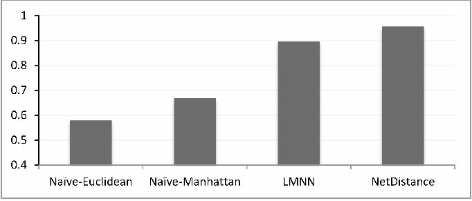
C. Effectiveness of Machine Learning for Creating the Network Distance

Metric

Existing network similarity measures utilize naıve comparison schemes and do not con-

sider the role of machine learning for specifying the weight of different network features.

In order to evaluate the effectiveness of machine learning algorithms in development of the

network distance metric, we first compare the naıve metrics with the learning-based met-

13

TABLE II: The learned weights of the selected features in NetDistance, which is a

weighted Manhattan distance function.

Selected Feature Weight of the feature

Average Clustering Coefficient 0.953

Transitivity 0.835

Assortativity 0.902

Modularity 0.803

DDQC2 0.776

DDQC3 0.439

DDQC5 0.925

DDQC7 0.890

DDQC8 0.504

rics. In this experiment, a network is represented by a feature vector containing the network

features described in Section III B, and then based on these feature vectors, four different

network distances are evaluated. Naıve-Euclidean is the Euclidean distance of the feature

vectors, Naıve-Manhattan uses the Manhattan distance as the distance function, LMNN is

based on learning a distance function using the LMNN learning method46, and NetDistance

is our proposed method which uses the described genetic algorithm for learning the feature

weights in the weighted Manhattan distance function. The details of the utilized LMNN

algorithm46 is following: The maximum iterations of the LMNN algorithm is set equal to

5000. Although it is possible to use a simplified version of LMNN method in order to learn

a diagonal M matrix, we applied the original LMNN algorithm to learn a full M matrix (see

Equation 1). LMNN may utilize auxiliary information, beyond the instance labels, as the

target neighbors of each instance. In our experiments, in the absence of prior knowledge,

LMNN method assumes that the target neighbors are computed as the k nearest neighbors

with the same class label determined by Euclidean distance46. We have utilized the public

implementation of LMNN, published by its authors, which uses k = 3 by default, but the

results were not sensitive to this setting in our experiments.

14

The four described distance functions are employed in the KNN classification algorithm46.

Measuring KNN accuracy is a common approach for evaluation of the distance metrics. KNN

is a classification method which categorizes an unlabeled example by the majority label of

its k-nearest neighbors in the training set. The accuracy of KNN is dependent on the way

that distances are computed between the examples. Hence, better distance metrics result

in better classification KNN accuracy. The resulting KNN classifiers are used for classifying

the real networks dataset and the artificial networks dataset (the 5,000 artificial networks of

the test set). The labels of these test-case networks are available and thus we can compute

the precision of the KNN classifier, which actually indicates the precision of the employed

distance metric. As Equation 5 shows, in a dataset of labeled instances, the KNN-accuracy

of a distance metric d is the probability that the predicted class of an instance is equal to its

actual class, when the distance metric d is used in the KNN classifier. Figure 2 and Figure 3

show the average precision of the KNN classifier, for K = 1..7, based on the four described

distance functions. As the figures show, in both the artificial and real networks datasets,

the learning-based distance metrics (LMNN-based metric and NetDistance) outperform the

naıve metrics (Euclidean and Manhattan). This experiment shows that the distance metric

learning methods improve the precision of the distance functions in this application. This

experiment also shows that using our proposed genetic algorithm method for learning the

feature weights, outperforms the LMNN method in this application. Existing network simi-

larity metrics do not utilize machine learning algorithms for developing the distance metric

and assign equal weights to all the features. Figure 2 and 3 confirm our hypothesis that

machine learning algorithms are effective in improving the precision of network structural

comparison.

KNN -Accuracy(d) = P (KNN -Classifyd(x) = class(x)), x ∈ dataset (5)

D. Baseline Methods

We will comprehensively compare NetDistance with three baseline methods: NetSimile2,

KronFit-based8 distance, and RGF-distance1. These metrics represent different comparison

15

FIG. 2: The average accuracy of the KNN classifier (for K = 1..7) based on different

distance metrics in artificial networks dataset.

FIG. 3: The average accuracy of the KNN classifier (for K = 1..7) based on different

distance metrics in the real networks dataset.

approaches: NetSimile considers some local network features, KronFit is based on extracting

a small graph-signature, and RGF-distance considers graphlet counts.

NetSimile is based on the Canberra distance of 35 local features (five aggregate values

for seven local features). NetSimile already outperforms FSM (frequent subgraph mining)

and EIG (eigenvalues extraction) methods2. In KronFit-based distance, the similarity of

two networks is measured via the similarity of the fitted 2 × 2 initiator matrix in KronFit

algorithm. KronFit is the algorithm for fitting the Kronecker graph generation model to large

real networks8. Leskovec et al. show that with KronFit, we can find a 2× 2 initiator matrix

(K1) that well mimics the properties of the target network, and using this matrix of four

parameters we can accurately model several aspects of global network structure. Leskovec et

al. propose to compare the structure of the networks (even of different sizes) by the means

of the differences in estimated parameters of the initiator matrix, but they do not explicitly

specify a network distance function. We employed the fitted initiator matrix as the feature

vector for the networks and realized that a Euclidean distance function based on this feature

vector outperforms Canberra and Manhattan distance metrics. We refer to the Euclidean

16

distance of the four features in the 2 × 2 fitted initiator matrix of the KronFit algorithm

by “KronFit-distance”. Finally, RGF-distance is a network distance metric proposed by

Natasa et al.1, which is based on counting the relative graphlet counts of the networks.

Natasa et al. also proposed another network similarity metric based on the graphlet counts,

called GDD-agreement7, but in our experiments RGF-distance outperforms GDD-agreement

considerably. Janssen et al.,4 also propose a method based on the graphlet counts, but

the considered features of this method are actually dependent on the network size. The

graphlet counting algorithms are also computationally complex, and thus it is not practical

to execute such algorithms for most of the networks in our real and temporal networks

datasets. This problem is also mentioned in the existing works64. Approximate graphlet

counting algorithms may improve the efficiency of the algorithm, but with the penalty of a

reduction in the accuracy64. In addition, the evaluations in the artificial networks dataset

shows that NetDistance and other baseline methods outperform RGF-distance. According

to this result, and since running RGF-distance is impractical for large networks, we exclude

the evaluation of RGF-distance for large graphs of temporal and real networks datasets.

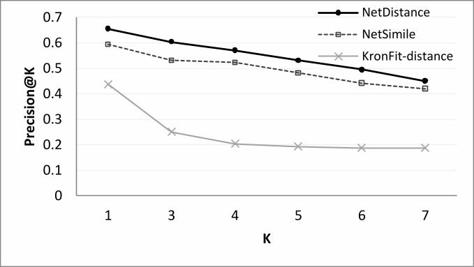
E. Experiments

In order to evaluate the precision of network distance metrics, we first employ them in

KNN algorithm, and then we assess the precision of the resulting KNN classifier. This

is the same approach described in Section IVC and Equation 5. KNN evaluation is a

common approach for testing distance metric methods when the category of records is

known in a labeled dataset . In our experiments, the instances of the artificial networks

dataset are labeled by the generative models, and the category-label is also available in

the real networks dataset. Figure 4 shows the KNN precision based on different distance

metrics for various K values in the artificial networks dataset, in which NetDistance out-

performs all the baseline methods. Figure 5 illustrates the result of the same experiment

for the real networks dataset. NetDistance surpasses the baseline methods in this evaluation.

In the next experiment, we consider the Precision-at-K (P@K) evaluation criterion. P@K

indicates the percentage of classmates in the K nearest neighbors. As Equation 6 shows,

P@K is the expected (average) number of classmates in the K nearest neighbors of an

17

0.6

0.65

0.7

0.75

0.8

0.85

0.9

0.95

1

1 3 4 5 6 7

KN

N A

ccu

racy

K

NetDistance

NetSimile

KronFit-distance

RGF-distance

FIG. 4: The accuracy of the KNN classifier for different K values in artificial networks,

based on different distance metrics.

0

0.1

0.2

0.3

0.4

0.5

0.6

0.7

0.8

1 3 4 5 6 7

KN

N A

ccu

racy

K

NetDistance

NetSimile

KronFit-distance

FIG. 5: The accuracy of the KNN classifier for different K values in real networks, based

on different distance metrics.

instance, divided by k. This measure is dependent on the distance metric d which is utilized

for computing the distances among the dataset instances. Figure 6 and Figure 7 show the

P@K for the networks of the artificial and real networks dataset respectively, according

to different distance metrics. As both the figures show, NetDistance outperforms all the

baseline methods with respect to the P@K measure.

P@K(d) =E(c)

k; c = count(m),m ∈ KNNd(x) , class(m) = class(x), x ∈ dataset (6)

In the next experiment, we study the inter-class and intra-class distances for different

distance metrics. An appropriate distance metric is supposed to return large distances for

instances with different classes (large inter-class distance) and relatively smaller distances for

classmate instances (small intra-class distance). In order to evaluate this property, we first

measure the distance between all the pairs of networks in a dataset, and then we compute the

ratio between the average inter-class distances and the average intra-class distances. Figure

18

0.4

0.5

0.6

0.7

0.8

0.9

1

1 3 4 5 6 7

Pre

cis

ion

@K

K

NetDistance

NetSimile

KronFit-distance

RGF-distance

FIG. 6: P@K for different K values in artificial networks, based on different distance

metrics.

0

0.1

0.2

0.3

0.4

0.5

0.6

0.7

1 3 4 5 6 7

Pre

cis

ion

@K

K

NetDistance

NetSimile

KronFit-distance

FIG. 7: P@K for different K values in real networks, based on different distance metrics.

8 and Figure 9 show this ratio for instances of the artificial and real networks datasets. As

the figures show, NetDistance shows the largest inter-class to intra-class distance ratio in

both the datasets.

Dunn Index65 is a more strict measure for comparing the inter/intra class distances. For

any partition setting U , in which the set of instances are clustered or classified into c groups

(U ↔ X = X1 ∪ X2 ∪ ... ∪ Xc), Dunn defined the separation index of U as described

in Equation 765. Dunn index investigates the ratio between the average distance of the

two nearest classes (Equation 8) and the average distance between the members of the

most extended class (Equation 9). The Equation 8 and Equation 9 are actually defined

in a generalized Dunn index66. Bezdek et al.66 showed that the generalized Dunn index is

more effective than the original Dunn index65 form. Figure 10 and Figure 11 illustrate the

Dunn index for different network distance metrics in the artificial and real network datasets

respectively. According to these figures, NetDistance shows the best (the largest) Dunn

19

FIG. 8: The ratio between the average inter-class distances and average intra-class

distances, in artificial networks dataset.

FIG. 9: The ratio between the average inter-class distances and average intra-class

distances, in real networks dataset.

index in comparison with other baseline methods.

DI(U) = min︸︷︷︸1≤i≤c

{min︸︷︷︸1≤j≤c

j =i

{ δ(Xi, Xj)

max︸︷︷︸1≤k≤c

{∆(Xk)}}} (7)

δ(S, T ) = δavg(S, T ) =1

|S||T |∑

x∈S,y∈T

d(x, y) (8)

∆(S) =1

|S| · (|S| − 1)

∑x,y∈S,x=y

d(x, y) (9)

The previous experiments investigate the suitability of various network similarity mea-

sures according to the network class labels. In the next experiment, we analyze the correla-

tion between the structural network distances and temporal distances for different distance

20

FIG. 10: Dunn index for different distance metrics in artificial networks dataset.

FIG. 11: Dunn index for different distance metrics in real networks dataset.

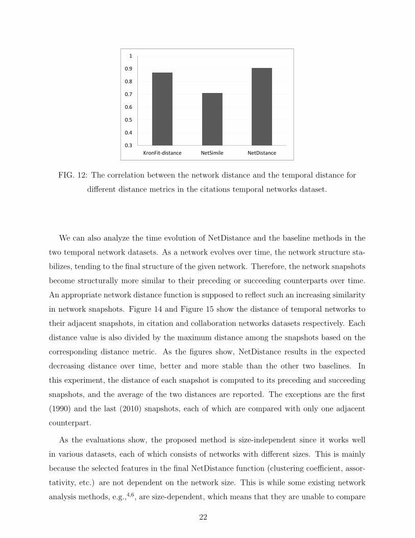
metrics in the two temporal networks datasets (Cit CiteSeerX and Collab CiteSeerX). For

an evolving network which experiences no abrupt structural changes, it is reasonable to

assume that the temporal proximity of network snapshots is an evidence of their topolog-

ical similarity48,49. In order to evaluate the distance metrics for capturing the topological

similarity of proximate temporal networks in a temporal network dataset, we extract the

distance between all the pairs of network snapshots. Then, we compute the Pearson cor-

relation between the topological distance and the temporal distance of the networks. The

temporal distance of two network snapshots is defined as their time interval gap. For in-

stance, the temporal distance between Cit CiteSeerX 2010 and Cit CiteSeerX 2008 is equal

to two (years). Figure 12 shows the correlation of different distance metrics to the temporal

distances in the Cit CiteSeerX temporal networks dataset. Figure 13 shows the same ex-

periment for the Collab CiteSeerX dataset. As the figures show, NetDistance exhibits the

greatest correlation to the temporal distances.

21

0.3

0.4

0.5

0.6

0.7

0.8

0.9

1

KronFit-distance NetSimile NetDistance

FIG. 12: The correlation between the network distance and the temporal distance for

different distance metrics in the citations temporal networks dataset.

We can also analyze the time evolution of NetDistance and the baseline methods in the

two temporal network datasets. As a network evolves over time, the network structure sta-

bilizes, tending to the final structure of the given network. Therefore, the network snapshots

become structurally more similar to their preceding or succeeding counterparts over time.

An appropriate network distance function is supposed to reflect such an increasing similarity

in network snapshots. Figure 14 and Figure 15 show the distance of temporal networks to

their adjacent snapshots, in citation and collaboration networks datasets respectively. Each

distance value is also divided by the maximum distance among the snapshots based on the

corresponding distance metric. As the figures show, NetDistance results in the expected

decreasing distance over time, better and more stable than the other two baselines. In

this experiment, the distance of each snapshot is computed to its preceding and succeeding

snapshots, and the average of the two distances are reported. The exceptions are the first

(1990) and the last (2010) snapshots, each of which are compared with only one adjacent

counterpart.

As the evaluations show, the proposed method is size-independent since it works well

in various datasets, each of which consists of networks with different sizes. This is mainly

because the selected features in the final NetDistance function (clustering coefficient, assor-

tativity, etc.) are not dependent on the network size. This is while some existing network

analysis methods, e.g.,4,6, are size-dependent, which means that they are unable to compare

22

FIG. 13: The correlation between the network distance and the temporal distance for

different distance metrics in the collaborations temporal networks dataset.

0

0.2

0.4

0.6

0.8

1

1990 1994 1998 2002 2006 2010

KronFit NETDISTANCE NetSimile

FIG. 14: The distance of a citation network to its adjacent snapshots over time, divided

by the maximum distance among the snapshots.

0

0.2

0.4

0.6

0.8

1

1990 1994 1998 2002 2006 2010

KronFit NETDISTANCE NetSimile

FIG. 15: The distance of a collaboration network to its adjacent snapshots over time,

divided by the maximum distance among the snapshots.

23

0.98 0.980.97

0.950.94

0.9

0.98 0.98 0.98

0.95

0.93

0.91

1 3 4 5 6 7

K

Comparison to Similar-Size Networks Comparison to All Networks

FIG. 16: The accuracy of the KNN classifier for different K values in artificial networks, in

two configuration. In the first case, a network is only compared with those with similar

sizes, and in the second configuration, no restriction is enforced on the size of the

compared networks. NetDistance shows a similar accuracy in the two configurations, and

thus is regarded size-independent.

networks with different sizes (size-dependent methods are not included in the baselines).

One may argue that the accuracy of NetDistance may increase if it compares networks with

similar sizes. But we have experienced such an improvement in none of the described eval-

uations. For example, Figure 16 shows that if only similar-size networks are considered in

KNN classification, the precision of NetDistance will not improve. In this experiment, we

consider two networks to be similar in size if their number of nodes differ less than a thresh-

old γ. According to the range of the network sizes in the artificial networks dataset (1000 to

5000 nodes per network), the threshold is heuristically set as γ = 500 in our experiments.

It is worth overviewing some implementation notes about the empirical experiments.

In order to calculate the network features, we used the SNAP tool67 (version 2.2), igraph

library68 (version 0.7.1), and the a fast community detection69 for estimating the network

modularity (version MSCD 0.11b4). We utilized the public implementation of the KronFit

algorithm (available in SNAP library67) and the LMNN method70 (version 2.5 as a MAT-

LAB program). We also used the SNAP tool67 as the implementation of the generative

models. The GDD-agreement and RGF-distance measures are computed by the means of

GraphCrunch2 tool71. We implemented NetSimile2, DDQC56, the proposed genetic algo-

rithm, NetDistance, and the evaluation scenarios in Java programming language.

24

TABLE III: Time and space complexity of the NetDistance feature extraction components.

Time Complexity Space Complexity

Clustering Coefficient O(E) O(V )

Transitivity O(E) O(V )

Assortativity O(E) O(E)

Modularity O(V ) O(E)

Degree Distribution (DDQC) O(E) O(d)

Total (Maximum) O(E) O(E)

V. TIME AND SPACE COMPLEXITY

In this section, we evaluate the proposed distance metric and the baselines with respect

to their time and space complexity. In order to compute the distance between two given

networks, the distance metric should first extract a feature vector from the networks (fea-

ture extraction phase), and then compute the distance between the feature vectors (distance

computation phase). All the considered distance metrics utilize a fixed-size feature vector.

Therefore, the distance computation has a constant time and space complexity (O(1)). As

a result the complexity of the metrics are equal to the complexity of their feature extraction

phase. Table III shows the complexity of extracting utilized features in NetDistance. In this

table, V shows the number of nodes, E is the number of edges, and d shows the maximum

node degree in the network. Since complex networks are usually sparse graphs, we can as-

sume that O(E) = O(V ) and d < V 8,69,72. Therefore, the overall complexity of NetDistance,

which is equal to the maximum complexity of its feature extraction components, is O(E)

for both time and space complexity. Table IV shows the number of extracted features along

with the complexity of baseline methods. As the figure shows, NetDistance and KronFit

show the least overall complexity and the smallest needed feature vector. This is whilst

NetDistance outperforms KronFit with respect to accuracy in any experienced evaluation.

The complexity of the “distance learning” is not critical in the analysis of the proposed

method since the learning phase is performed only once, and then the learned methods are

applied for each input network data. Nevertheless, it is worth noting the efficiency of the

25

TABLE IV: Time and space complexity of different methods. NetDistance and KronFit

show the least overall complexity.

Number of Features Time Complexity Space Complexity

NetDistance 9 O(E) O(E)

RGF 29 O(V d4) O(V )

KronFit 4 O(E) O(E)

NetSimile 35 O(V log V ) O(V )

learning phase in the proposed method: The distance learning is based on running a genetic

algorithm in less than 200 iterations on a population of 600 individuals, which converges

in less than an hour in a moderate workstation with a single processor and 4 gigabytes

of RAM. It is also worth noting that the learning algorithms are applied on rather small

networks with less than 5,000 nodes, and thus the feature extraction and the computations

in the learning phase are efficient.

VI. CONCLUSION

In this paper, we investigated the development of a network distance metric for compar-

ing the topologies of the complex networks. Such a distance metric plays an important role

in similarity-based network analysis applications including network classification, anomaly

detection in network time series, model selection, evaluation of generative models, and

evaluation of sampling algorithms. The proposed distance metric, rather than to check

the node/edge correspondence of similar-size networks, is capable of comparing the overall

structural properties of the networks, even for networks with different sizes. Although it

is difficult to define an accurate meaning for the topological similarity of complex net-

works, there exist various evidences (e.g., network labels) about similarity/dissimilarity of

complex networks. Instead of defining a heuristic similarity metric manually, which is a

time-consuming and error-prone approach, we utilized supervised machine learning meth-

ods to learn a distance metric based on the existing similarity evidences. The supervised

machine learning algorithm automated feature selection and feature weighting processes,

26

and it resulted in a more accurate distance metric.

In this paper, a genetic algorithm is designed for feature selection and feature weighting

(distance metric learning) in the final proposed distance metric, which is called NetDis-

tance. According to the comprehensive experiments, NetDistance outperforms the baseline

methods in all of the evaluation criteria, for the three prepared datasets. As a result,

NetDistance is regarded an appropriate distance metric for comparing the topological struc-

ture of complex networks. We have also examined an alternative machine learning method

(LMNN) for feature selection and weighting, which results in a metric that is less accurate

than NetDistance, but performs better than the naıve (not intelligent) methods. Therefore,

this paper shows the effectiveness of machine learning in development of a distance metric

for topological comparison of complex networks. The proposed methodology for learning a

network distance metric can be applied in other domains, perhaps with alternative machine

learning methods, different network features, other network datasets and alternative simi-

larity evidences.

The evaluation of the noise tolerance for the network distance metrics is a subject of fu-

ture work. We also intend to apply NetDistance in different applications including network

generation, anomaly detection, and model selection. Furthermore, we will investigate net-

work simulations to test the correlation between the dynamics of a network and its structural

properties, in processes such as decentralized search59 and the diffusion of innovation28.

VII. ACKNOWLEDGEMENTS

The authors wish to thank Hossein Rahmani, Mehdi Jalili, Mahdieh Soleymani and Ma-

soud Asadpour for their constructive comments. Some of the utilized datasets are prepared

by Javad Gharechamani, Mahmood Neshati and Hadi Hashemi and we appreciate their co-

operation. This research is supported by Iran Telecommunication Research Center (ITRC).

27

Appendix A: Artificial Networks Dataset

The utilized network generation models and the synthesized graphs of the artificial net-

works dataset are described in the following:

Barabasi-Albert model (BA)14. In this model, a new node is randomly connected

to k existing nodes with a probability that is proportional to the degree of the available

nodes. In our artificial networks dataset, k is randomly selected as an integer number from

the range 1 6 k 6 10.

Erdos-Renyi (ER). This model generates completely random graphs with a specified

density61. The density of the ER networks in our artificial networks dataset is randomly

selected from the range 0.002 6 density 6 0.005.

Forest Fire (FF). This model supports shrinking diameter and densification properties,

along with heavy-tailed in-degrees and community structure15. This model is configured by

two main parameters: Forward burning probability (p) and backward burning probability

(pb). For generating artificial networks dataset, we fixed pb = 0.32 and selected p randomly

from the range 0 6 p 6 0.3.

Kronecker graphs (KG). This model generates realistic synthetic networks by ap-

plying a matrix operation (the kronecker product) on a small initiator matrix8. The KG

networks of the artificial networks dataset are generated using a 2× 2 initiator matrix. The

four elements of the initiator matrix are randomly selected from the ranges: 0.7 6 P1,1 60.9, 0.5 6 P1,2 6 0.7, 0.4 6 P2,1 6 0.6, 0.2 6 P2,2 6 0.4.

Random power-law (RP). This model follows a variation of ER model and generates

synthetic networks with power law degree distribution62. This model is configured by the

power-law degree exponent (γ). In our parameter setting for generating artificial networks

dataset, γ is randomly selected from the range 2.5 < γ < 3.

Watts-Strogatz model (WS). The classical Watts-Strogatz small-world model syn-

thesizes networks with small path lengths and high clustering13. It starts with a regular

lattice, in which each node is connected to k neighbors, and then randomly rewires some

edges of the network with rewiring probability β. In WS networks of the artificial networks

dataset, β is fixed as β = 0.5, and k is randomly selected from the integer numbers between

2 and 10 (2 6 k 6 10).

28

Appendix B: Real Networks Dataset

In this section, the real networks dataset is briefly described.

Citation Networks . In this category, the edges in a network show the citations between

the papers or patents. The members of this class in the dataset are: Cit-HepPh73, Cit-

HepTh73, dblp cite74, and CitCiteSeerX63.

Collaboration Networks . This class shows the graph of collaborations and co-

authorships. The members of this class are: CA-AstroPh73, CA-CondMat73, CA-HepTh73,

CiteSeerX Collaboration63, com-dblp.ungraph73, dblp collab74, refined dblp2008082475, IMDB-

USA-Commedy-0976, CA-GrQc73, and CA-HepPh73.

Communication Networks . Some people who had electronically communicated with

each other will create a communication network. In this category, the dataset consists of

the following networks: Email77, Email-Enron73, Email-EuAll78, and WikiTalk73.

Friendship Networks Interactions of some social entities results in a friendship net-

work. The networks in this category are: Facebook-links79, Slashdot081173, Slashdot090273,

soc-Epinions173, Twitter-Richmond-FF76, and youtube-d-growth79.

Web-graph Networks . These networks show the graph of some web pages in which

the edges correspond the hyperlinks. The members of this category are: Web-BerkStan73,

web-Google73, web-NotreDame73, and web-Stanford73.

P2P Networks This category represents peer-to-peer networks. In this class, the fol-

lowing networks are prepared: p2p-Gnutella0473, p2p-Gnutella0573, p2p-Gnutella0673, and

p2p-Gnutella0873.

Appendix C: Genetic Algorithms

Genetic algorithm (GA) is inspired by natural evolution, and is based on crossover, mu-

tation, and natural selection operations. In this algorithm, a solution is represented by a

chromosome which is an array of genes. A population of many random chromosomes start

to evolve using crossover and mutation operations. Consequently, the best members of each

generation survive based on a fitness function which defines the suitability of a chromosome.

Genetic algorithms (GA) are frequently utilized to find solutions to optimization and search

problems47. Figure 17 shows a schematic view of the GA concepts.

29

FIG. 17: Genetic algorithm concepts and operators.

The employed genetic algorithm which resulted in the final NetDistance function is con-

figured as follows: A population of 600 random individuals evolve in the process of the

genetic algorithm. The crossover operation selects each feature weight from the corre-

sponding feature weights in one of the parent chromosomes randomly, favoring the bet-

ter (more fitted) parent with probability 0.68. The mutation is performed by assigning

a random value to a randomly selected feature weight, with the mutation rate of 0.15.

We set a maximum of 200 iterations for the genetic algorithm, but the algorithm al-

most always converged with less than 50 generations, since no considerable improvements

achieved with more iterations. The consequent execution of the algorithm resulted in no

more considerable changes in the reported weights. It is worth noting that the learned

distance metric (NetDistance) is not sensitive to utilized GA parameters. For example,

in our implementation of GA, the mutation operator is based on “Mutation Rate” and

the crossover operator is based on “Fitted Parent Preference” parameter (the genes from

the more fitted parent is preferred with this probability). Our experiments showed that

0.15 < MutationRate < 0.4 and 0.6 < FittedParentPreference < 0.75 provide stable

results. We have chosen MutationRate = 0.15 and FittedParentPreference = 0.68 based

on our experiments with trial and error. Small variations on the selected parameters results

in slight changes in the accuracy of the learned network distance metric.

30

REFERENCES

1N. Przulj, D. G. Corneil, and I. Jurisica, “Modeling interactome: scale-free or geometric?”

Bioinformatics 20, 3508–3515 (2004).

2M. Berlingerio, D. Koutra, T. Eliassi-Rad, and C. Faloutsos, “Network similarity via

multiple social theories,” in Proceedings of the 2013 IEEE/ACM International Conference

on Advances in Social Networks Analysis and Mining, ASONAM ’13 (ACM, 2013) pp.

1439–1440.

3A. Sala, L. Cao, C. Wilson, R. Zablit, H. Zheng, and B. Y. Zhao, “Measurement-calibrated

graph models for social network experiments,” in Proceedings of the 19th international

conference on World Wide Web (ACM, 2010) pp. 861–870.

4J. Janssen, M. Hurshman, and N. Kalyaniwalla, “Model selection for social networks using

graphlets,” Internet Mathematics 8, 338–363 (2012).

5A. Mehler, “Structural similarities of complex networks: A computational model by ex-

ample of wiki graphs,” Applied Artificial Intelligence 22, 619–683 (2008).

6D. Koutra, J. T. Vogelstein, and C. Faloutsos, “DELTACON: A principled massive-graph

similarity function,” in Proceedings of the 13th SIAM International Conference on Data

Mining (SDM) (2013) pp. 162–170.

7N. Przulj, “Biological network comparison using graphlet degree distribution,” Bioinfor-

matics 23, e177–e183 (2007).

8J. Leskovec, D. Chakrabarti, J. Kleinberg, C. Faloutsos, and Z. Ghahramani, “Kronecker

graphs: An approach to modeling networks,” The Journal of Machine Learning Research

11, 985–1042 (2010).

9J. P. Bagrow, E. M. Bollt, J. D. Skufca, and D. Ben-Avraham, “Portraits of complex

networks,” EPL (Europhysics Letters) 81, 68004 (2008).

10J.-P. Onnela, D. J. Fenn, S. Reid, M. A. Porter, P. J. Mucha, M. D. Fricker, and N. S.

Jones, “Taxonomies of networks from community structure,” Physical Review E 86, 036104

(2012).

11R. Albert and A.-L. Barabasi, “Statistical mechanics of complex networks,” Reviews of

modern physics 74, 47–97 (2002).

12M. E. Newman, “The structure and function of complex networks,” SIAM review 45,

167–256 (2003).

31

13D. J. Watts and S. H. Strogatz, “Collective dynamics of ’small-world’ networks,” nature

393, 440–442 (1998).

14A.-L. Barabasi and R. Albert, “Emergence of scaling in random networks,” Science 286,

509–512 (1999).

15J. Leskovec, J. Kleinberg, and C. Faloutsos, “Graphs over time: densification laws, shrink-

ing diameters and possible explanations,” in Proceedings of the eleventh ACM SIGKDD

international conference on Knowledge discovery in data mining (ACM, 2005) pp. 177–187.

16J. Leskovec and C. Faloutsos, “Sampling from large graphs,” in Proceedings of the 12th

ACM SIGKDD international conference on Knowledge discovery and data mining (ACM,

2006) pp. 631–636.

17M. P. Stumpf and C. Wiuf, “Sampling properties of random graphs: the degree distribu-

tion,” Physical Review E 72, 036118 (2005).

18M. P. Stumpf, C. Wiuf, and R. M. May, “Subnets of scale-free networks are not scale-free:

sampling properties of networks,” Proceedings of the National Academy of Sciences of the

United States of America 102, 4221–4224 (2005).

19S. H. Lee, P.-J. Kim, and H. Jeong, “Statistical properties of sampled networks,” Physical

Review E 73, 016102 (2006).

20J.-D. J. Han, D. Dupuy, N. Bertin, M. E. Cusick, and M. Vidal, “Effect of sampling on

topology predictions of protein-protein interaction networks,” Nature biotechnology 23,

839–844 (2005).

21S. Motallebi, S. Aliakbary, and J. Habibi, “Generative model selection using a scalable

and size-independent complex network classifier,” Chaos: An Interdisciplinary Journal of

Nonlinear Science 23, 043127 (2013).

22M. Middendorf, E. Ziv, and C. H. Wiggins, “Inferring network mechanisms: the drosophila

melanogaster protein interaction network,” Proceedings of the National Academy of Sci-

ences of the United States of America 102, 3192–3197 (2005).

23L. d. F. Costa, F. A. Rodrigues, G. Travieso, and P. Villas Boas, “Characterization of

complex networks: A survey of measurements,” Advances in Physics 56, 167–242 (2007).

24E. M. Airoldi, X. Bai, and K. M. Carley, “Network sampling and classification: An

investigation of network model representations,” Decision support systems 51, 506–518

(2011).

25K. Juszczyszyn, N. T. Nguyen, G. Kolaczek, A. Grzech, A. Pieczynska, and R. Katarzy-

32

niak, “Agent-based approach for distributed intrusion detection system design,” in Pro-

ceedings of the 6th international conference on Computational Science (Springer, 2006)

pp. 224–231.

26P. Papadimitriou, A. Dasdan, and H. Garcia-Molina, “Web graph similarity for anomaly

detection,” Journal of Internet Services and Applications 1, 19–30 (2010).

27R. Pastor-Satorras and A. Vespignani, “Epidemic dynamics in finite size scale-free net-

works,” Physical Review E 65, 035108 (2002).

28A. Montanari and A. Saberi, “The spread of innovations in social networks,” Proceedings

of the National Academy of Sciences of the United States of America 107, 20196–20201

(2010).

29L. Briesemeister, P. Lincoln, and P. Porras, “Epidemic profiles and defense of scale-free

networks,” in Proceedings of the 2003 ACM workshop on Rapid malcode (ACM, 2003) pp.

67–75.

30R. C. Wilson and P. Zhu, “A study of graph spectra for comparing graphs and trees,”

Pattern Recognition 41, 2833–2841 (2008).

31L. A. Zager and G. C. Verghese, “Graph similarity scoring and matching,” Applied math-

ematics letters 21, 86–94 (2008).

32S. Vishwanathan, N. N. Schraudolph, R. Kondor, and K. M. Borgwardt, “Graph kernels,”

The Journal of Machine Learning Research 99, 1201–1242 (2010).

33H. Kashima, K. Tsuda, and A. Inokuchi, “Kernels for graphs,” Kernel methods in com-

putational biology 39, 101–113 (2004).

34T. Gartner, P. Flach, and S. Wrobel, “On graph kernels: Hardness results and efficient

alternatives,” in Learning Theory and Kernel Machines (Springer, 2003) pp. 129–143.

35U. Kang, H. Tong, and J. Sun, “Fast random walk graph kernel.” in SDM (2012) pp.

828–838.

36K. M. Borgwardt, Graph kernels, Ph.D. thesis, Ludwig-Maximilians-Universitat Munchen

(2007).

37A. Kelmans, “Comparison of graphs by their number of spanning trees,” Discrete Mathe-

matics 16, 241–261 (1976).

38R. Milo, S. Shen-Orr, S. Itzkovitz, N. Kashtan, D. Chklovskii, and U. Alon, “Network

motifs: simple building blocks of complex networks,” Science 298, 824–827 (2002).

39K. Faust, “Comparing social networks: size, density, and local structure,” Metodoloski

33

zvezki 3, 185–216 (2006).

40I. Bordino, D. Donato, A. Gionis, and S. Leonardi, “Mining large networks with subgraph

counting,” in Data Mining, 2008. ICDM’08. Eighth IEEE International Conference on

(IEEE, 2008) pp. 737–742.

41R. Kondor, N. Shervashidze, and K. M. Borgwardt, “The graphlet spectrum,” in Proceed-

ings of the 26th Annual International Conference on Machine Learning (ACM, 2009) pp.

529–536.

42N. Shervashidze, T. Petri, K. Mehlhorn, K. M. Borgwardt, and S. Viswanathan, “Efficient

graphlet kernels for large graph comparison,” in International Conference on Artificial

Intelligence and Statistics (2009) pp. 488–495.

43P. Mahadevan, D. Krioukov, K. Fall, and A. Vahdat, “Systematic topology analysis

and generation using degree correlations,” ACM SIGCOMM Computer Communication

Review 36, 135–146 (2006).

44L. Yang and R. Jin, “Distance metric learning: A comprehensive survey,” Michigan State

Universiy , 1–51 (2006).

45E. P. Xing, M. I. Jordan, S. Russell, and A. Ng, “Distance metric learning with application

to clustering with side-information,” in Advances in neural information processing systems

(2002) pp. 505–512.

46K. Q. Weinberger and L. K. Saul, “Distance metric learning for large margin nearest

neighbor classification,” The Journal of Machine Learning Research 10, 207–244 (2009).

47D. E. Goldberg, Genetic Algorithms in Search, Optimization and Machine Learning, 1st

ed. (Addison-Wesley Longman Publishing Co., Inc., Boston, MA, USA, 1989).

48P. Holme and J. Saramaki, “Temporal networks,” Physics reports 519, 97–125 (2012).

49J. Tang, S. Scellato, M. Musolesi, C. Mascolo, and V. Latora, “Small-world behavior in

time-varying graphs,” Physical Review E 81, 055101 (2010).

50L. Hamill and N. Gilbert, “Social circles: A simple structure for agent-based social network

models,” Journal of Artificial Societies and Social Simulation 12, 3 (2009).

51M. Girvan and M. E. Newman, “Community structure in social and biological networks,”

Proceedings of the National Academy of Sciences 99, 7821–7826 (2002).

52M. E. Newman, “Modularity and community structure in networks,” Proceedings of the

National Academy of Sciences of the United States of America 103, 8577–8582 (2006).

53M. McPherson, L. Smith-Lovin, and J. M. Cook, “Birds of a feather: Homophily in social

34

networks,” Annual review of sociology , 415–444 (2001).

54M. E. Newman, “Assortative mixing in networks,” Physical review letters 89, 208701

(2002).

55N. Z. Gong, W. Xu, L. Huang, P. Mittal, E. Stefanov, V. Sekar, and D. Song, “Evolution

of social-attribute networks: measurements, modeling, and implications using google+,”

in Proceedings of the 2012 ACM conference on Internet measurement conference (ACM,

2012) pp. 131–144.

56S. Aliakbary, J. Habibi, and A. Movaghar, “Feature extraction from degree distribution

for comparison and analysis of complex networks,” arXiv preprint arXiv:1407.3386 (2014).

57S. Aliakbary, J. Habibi, and A. Movaghar, “Quantification and comparison of degree dis-

tributions in complex networks,” in Proceedings of The Seventh International Symposium

on Telecommunications (IST2014) (IEEE, 2014) to appear.

58V. Latora and M. Marchiori, “Vulnerability and protection of infrastructure networks,”

Physical Review E 71, 015103 (2005).

59J. M. Kleinberg, “Navigation in a small world,” Nature 406, 845–845 (2000).

60S. Zhou and R. J. Mondragon, “The rich-club phenomenon in the internet topology,”

Communications Letters, IEEE 8, 180–182 (2004).

61P. Erdos and A. Renyi, “On the central limit theorem for samples from a finite population,”

Publications of the Mathematical Institute of the Hungarian Academy 4, 49–61 (1959).

62D. Volchenkov and P. Blanchard, “An algorithm generating random graphs with power law

degree distributions,” Physica A: Statistical Mechanics and its Applications 315, 677–690

(2002).

63“Citeseerx digital library,” http://citeseerx.ist.psu.edu.

64M. Rahman, M. Bhuiyan, and M. A. Hasan, “Graft: an approximate graphlet counting al-

gorithm for large graph analysis,” in Proceedings of the 21st ACM international conference

on Information and knowledge management (ACM, 2012) pp. 1467–1471.

65J. C. Dunn, “A fuzzy relative of the isodata process and its use in detection compact

well-separated clusters,” Journal of Cybernetics 3, 32–57 (1973).

66J. C. Bezdek and N. R. Pal, “Some new indexes of cluster validity,” Systems, Man, and

Cybernetics, Part B: Cybernetics, IEEE Transactions on 28, 301–315 (1998).

67J. Leskovec and R. Sosic, “SNAP: A general purpose network analysis and graph mining

library in C++,” http://snap.stanford.edu/snap (2014).

35

68G. Csardi and T. Nepusz, “The igraph software package for complex network research,”

InterJournal, Complex Systems 1695 (2006).

69E. Le Martelot and C. Hankin, “Fast multi-scale detection of relevant communities in

large-scale networks,” The Computer Journal (2013).

70K. Q. Weinberger, “LMNN software tool for large margin nearest neighbors,”

http://www.cse.wustl.edu/~kilian/code/code.html (2014).

71O. Kuchaiev, A. Stevanovic, W. Hayes, and N. Przulj, “Graphcrunch 2: software tool for

network modeling, alignment and clustering,” BMC bioinformatics 12, 24 (2011).

72M. Fazli, M. Ghodsi, J. Habibi, P. Jalaly Khalilabadi, V. Mirrokni, and S. S.

Sadeghabad, “On the non-progressive spread of influence through social networks,” in

Proceedings of the 10th Latin American International Conference on Theoretical Informatics ,

LATIN’12 (Springer-Verlag, Berlin, Heidelberg, 2012) pp. 315–326.

73“Stanford large network dataset collection,” http://snap.stanford.edu/data/.

74“Xml repository of dblp library,” http://dblp.uni-trier.de/xml/.

75“Christian Sommer’s graph datasets,” http://www.sommer.jp/graphs/.

76“Giulio Rossetti networks dataset,” http://giuliorossetti.net/about/ongoing-works/datasets.

77“Alex Arenas’s network datasets,” http://deim.urv.cat/~aarenas/data/welcome.htm.

78“The Koblenz network collection,” http://konect.uni-koblenz.de/.

79“Network datasets at Max Planck,” http://socialnetworks.mpi-sws.org.

36

Gather a set of

networks with known

similarity evidences

Feature Selection

Feature Extraction

Distance Metric

Learning

Evaluate the learned

similarity metric

Training set Test set

0.6

0.65

0.7

0.75

0.8

0.85

0.9

0.95

1

1 3 4 5 6 7

KN

N A

ccu

racy

K

NetDistance

NetSimile

KronFit-distance

RGF-distance

0

0.1

0.2

0.3

0.4

0.5

0.6

0.7

0.8

1 3 4 5 6 7

KN

N A

ccu

racy

K

NetDistance

NetSimile

KronFit-distance

0.4

0.5

0.6

0.7

0.8

0.9

1

1 3 4 5 6 7

Pre

cis

ion

@K

K

NetDistance

NetSimile

KronFit-distance

RGF-distance

0

0.1

0.2

0.3

0.4

0.5

0.6

0.7

1 3 4 5 6 7

Pre

cis

ion

@K

K

NetDistance

NetSimile

KronFit-distance

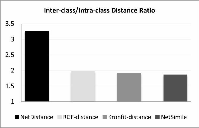
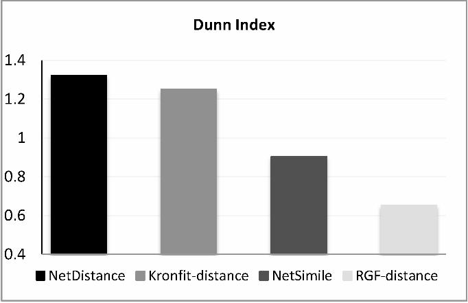
0.3

0.4

0.5

0.6

0.7

0.8

0.9

1

KronFit-distance NetSimile NetDistance

0

0.2

0.4

0.6

0.8

1

1990 1994 1998 2002 2006 2010

KronFit NETDISTANCE NetSimile

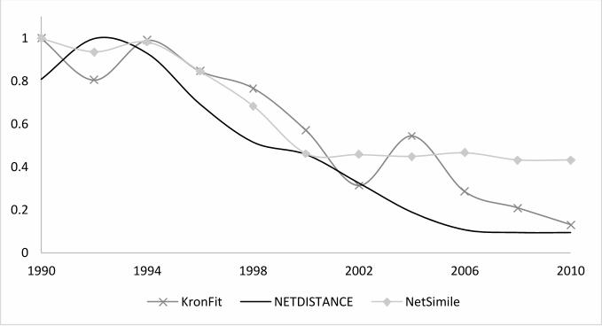
0

0.2

0.4

0.6

0.8

1

1990 1994 1998 2002 2006 2010

KronFit NETDISTANCE NetSimile

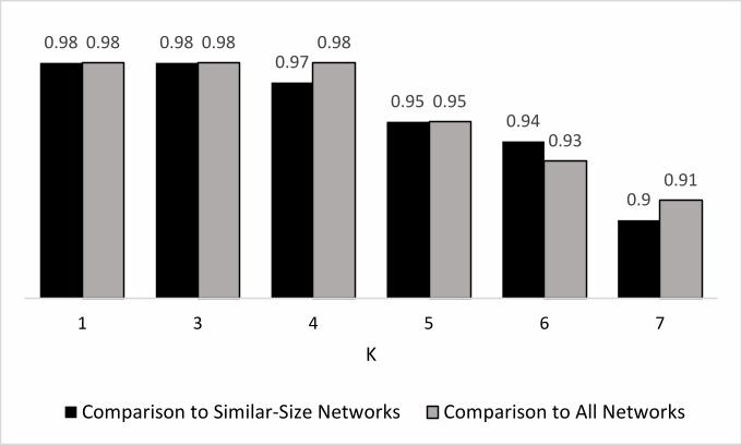
0.98 0.980.97

0.950.94

0.9

0.98 0.98 0.98

0.95

0.93

0.91

1 3 4 5 6 7

K

Comparison to Similar-Size Networks Comparison to All Networks