dissertation aqueous phase sulfate production in clouds at mt ...

DISSERTATION

AQUEOUS PHASE SULFATE PRODUCTION IN CLOUDS

AT MT. TAI IN EASTERN CHINA

Submitted by

Xinhua Shen

Department of Atmospheric Science

In partial fulfillment of the requirements

For the Degree of Doctor of Philosophy

Colorado State University

Fort Collins, Colorado

Spring 2011

Doctoral Committee:

Advisor: Jeffrey L. Collett

Sonia M. Kreidenweis

Steven A. Rutledge

Stephen J. Reynolds

ii

ABSTRACT

AQUEOUS PHASE SULFATE PRODUCTION IN CLOUDS

AT MT. TAI IN EASTERN CHINA

Clouds play an important role in the oxidation of sulfur dioxide to sulfate, since

aqueous phase sulfur dioxide oxidation is typically much faster than oxidation in the gas

phase. Important aqueous phase oxidants include hydrogen peroxide, ozone and oxygen

(catalyzed by trace metals). Because quantities of emitted sulfur dioxide in China are so

large, however, it is possible that they exceed the capacity of regional clouds for sulfate

production, leading to enhanced long-range transport of emitted SO2 and its oxidation

product, sulfate.

In order to assess the ability of regional clouds to support aqueous sulfur oxidation,

four field campaigns were conducted in 2007 and 2008 at Mt. Tai in eastern China.

Single and 2-stage Caltech Active Strand Cloudwater Collectors were used to collect bulk

and drop size-resolved cloudwater samples, respectively. Key species that determine

aqueous phase sulfur oxidation were analyzed, including cloudwater pH, S(IV), H2O2, Fe,

and Mn. Gas phase SO2, O3, and H2O2 were also measured continuously during the

campaigns. Other species in cloudwater, including inorganic ions, total organic carbon

(TOC), formaldehyde, and organic acids were also analyzed to provide a fuller view of

cloud chemistry in the region.

iii

Numerous periods of cloud interception/fog occurred during the four Mt. Tai field

campaigns; more than 500 cloudwater samples were collected in total. A wide range of

cloud pH values was observed, from 2.6 to 7.6. SO42-

, NO3-, and NH4

+ were the major

inorganic species for all four campaigns. TOC concentrations were also very high in

some samples (up to 200 ppmC), especially when clouds were impacted by emissions

from agricultural biomass burning. Back-trajectory analysis also indicated influence by

dust transport from northern China in a few spring cloud events. Differences between the

compositions of small and large cloud droplets were observed, but generally found to be

modest for major solute species and pH. Mt. Tai clouds were found to interact strongly

with PM2.5 sulfate, nitrate, and ammonium with average scavenging efficiencies of 80%,

75%, and 78%, respectively, across 7 events studied. Scavenging efficiencies for total

sulfur (PM2.5 sulfate plus gaseous sulfur dioxide), however, averaged only 43%,

indicating the majority of gaseous sulfur dioxide remained unprocessed in these cloud

events.

H2O2 was found to be the most important oxidant for aqueous sulfate production

68% of the time. High concentrations of residual H2O2 were measured in some samples,

especially during summertime, implying a substantial capacity for additional sulfur

oxidation. The importance of ozone as a S(IV) oxidant increased substantially as cloud

pH climbed above pH 5 to 5.3. Overall, ozone was found to be the most important

aqueous S(IV) oxidant in 21% of the sampling periods. Trace metal-catalyzed S(IV)

autooxidation was determined to be the fastest aqueous sulfate production pathway in the

remaining 11% of the cases. Complexation with formaldehyde was also found to be a

potentially important fate for aqueous S(IV) and should be examined in more detail in

iv

future studies. Observed chemical heterogeneity among cloud drop populations was

predicted to enhance rates of S(IV) oxidation by ozone and enhance or slow metal-

catalyzed S(IV) autooxidation rates in some periods. These effects were found to be only

of minor importance, however, as H2O2 was the dominant S(IV) oxidant most of the time.

v

ACKNOWLEDGEMENTS

I would like to first acknowledge my advisor, Professor Jeffrey L. Collett, for his

guidance and assistance throughout the course of this project. I am also very grateful to

my other committee members, Professor Sonia M. Kreidenweis, Professor Steven A.

Rutledge, and Professor Stephen J. Reynolds for their insightful comments and

recommendations for this work. I thank Professor Tao Wang (The Hong Kong

Polytechnic University) for his consistent support for this study. I am grateful to Mr.

Tingli Sun (Shandong University) for considerable logistical assistance in the field

campaigns.

I would like to thank Dr. Taehyoung Lee, Jia Guo, Xinfeng Wang, Wei Nie and Rui Gao

for their extensive contributions to the field campaigns and the subsequent sample

analysis. Further support was given by Yi Li during sample analysis. The advice and help

from various colleagues, including Katie Beem, Mandy Holden, Angela Rowe, Leigh A.

Munchak, and the rest of the Collett and Kreidenweis groups, is also greatly appreciated.

I thank my family and friends for their invaluable support and encouragement.

This work was supported by the US National Science Foundation (ATM-0711102) and

by the National Basic Research Program of China (973 Program) (2005CB422203).

vi

TABLE OF CONTENTS

ABSTRACT ........................................................................................................................... ii

ACKNOWLEDGEMENTS ..................................................................................................... v

TABLE OF CONTENTS ....................................................................................................... vi

LIST OF FIGURES................................................................................................................ ix

LIST OF ACRONYMS AND SYMBOLS............................................................................ xiv

CHAPTER 1 INTRODUCTION .............................................................................1

1.1. PROJECT MOTIVATIONS ............................................................................................. 1

1.2. AQUEOUS PHASE SULFUR REACTIONS IN CLOUDWATER ................................. 12

1.2.1. S(IV) oxidation by ozone .................................................................................... 13

1.2.2. S(IV) oxidation by hydrogen peroxide ................................................................ 15

1.2.3. S(IV) oxidation by oxygen (catalyzed by Fe(III) and Mn(II)) .............................. 16

1.2.4. Aqueous SO2 complexation with formaldehyde ................................................... 18

1.2.5. Temperature dependence of equilibrium and rate constants ................................. 19

1.2.6. pH dependent aqueous S(IV) reaction rates ......................................................... 20

1.3. CLOUD DROP SIZE-DEPENDENT AQUEOUS SULFUR REACTIONS .................... 22

1.4. MAJOR RESEARCH OBJECTIVES ............................................................................. 23

CHAPTER 2 METHODOLOGY .......................................................................... 26

2.1. SAMPLING TIME AND SITE LOCATION .................................................................. 26

2.2. SAMPLING INSTRUMENTS ....................................................................................... 28

2.2.1. Particulate Volume Monitor ................................................................................ 29

2.2.2. Cloudwater Collectors......................................................................................... 31

2.2.3. URG Annular Denuder/Filter-pack System ......................................................... 34

2.3. SAMPLING ................................................................................................................... 37

2.4. ON SITE PROCEDURES AND LABORATORY ANALYSIS ...................................... 38

2.4.1. Sample weight .................................................................................................... 38

2.4.2. Sample pH .......................................................................................................... 38

2.4.3. Major ions .......................................................................................................... 39

vii

2.4.4. S(IV) .................................................................................................................. 39

2.4.5. Metals ................................................................................................................. 40

2.4.6. HCHO ................................................................................................................ 40

2.4.7. Aqueous H2O2..................................................................................................... 41

2.4.8. Organic acids ...................................................................................................... 41

2.4.9. TOC ................................................................................................................... 42

2.5. QUALITY ASSURANCE AND CONTROL .................................................................. 42

2.5.1. Collector cleaning and blanks.............................................................................. 42

2.5.2. Determination of uncertainties and minimum detection limits (MDL) ................. 43

CHAPTER 3 RESULTS AND DISCUSSION ...................................................... 45

3.1. SUMMARY OF SAMPLING......................................................................................... 45

3.2. GASEOUS SPECIES ..................................................................................................... 48

3.2.1. Gaseous H2O2 ..................................................................................................... 48

3.2.2. O3 and SO2.......................................................................................................... 50

3.3. BULK CLOUDWATER CHEMICAL COMPOSITION ................................................. 52

3.3.1. Cloudwater pH.................................................................................................... 52

3.3.2. TOC ................................................................................................................... 53

3.3.3. Major Ions .......................................................................................................... 56

3.3.4. Aqueous hydrogen peroxide and S(IV) ................................................................ 71

3.3.5. Iron and manganese ............................................................................................ 72

3.3.6. Formaldehyde ..................................................................................................... 75

3.4. DROP SIZE-DEPENDENT CLOUDWATER CHEMICAL COMPOSITIONS .............. 77

3.4.1. Cloudwater pH.................................................................................................... 77

3.4.2. Major solutes ...................................................................................................... 78

3.4.3. Aqueous hydrogen peroxide and S(IV) ................................................................ 83

3.4.4. Iron and manganese ............................................................................................ 85

3.4.5. Formaldehyde ..................................................................................................... 86

CHAPTER 4 CLOUD-AEROSOL INTERACTIONS ......................................... 88

4.1. BACKWARD TRAJECTORY ANALYSIS ................................................................... 88

4.1.1. Backward trajectories and cloudwater composition variations ............................. 91

4.1.2. Case studies on the influence of biomass burning on cloudwater composition.... 102

4.2. AEROSOL AND GAS PROCESSING BY CLOUDS .................................................. 107

4.2.1. Before / after cloud ........................................................................................... 108

4.2.2. During cloud ..................................................................................................... 109

4.2.3. Aerosol scavenging efficiency........................................................................... 109

CHAPTER 5 AQUEOUS PHASE SULFATE PRODUCTION ......................... 121

viii

CHAPTER 6 CONCLUSIONS ........................................................................... 135

6.1. CONCLUSIONS .......................................................................................................... 135

6.2. RECOMMENDATIONS FOR FUTURE WORK ......................................................... 142

REFERENCES ................................................................................................................... 145

APPENDIX A – ALIQUOTS FOR CHEMICAL MEASUREMENTS ................................ 154

APPENDIX B – 2007 CLOUDWATER DATA TABLE ..................................................... 157

APPENDIX C – 2008 CLOUDWATER DATA TABLE ..................................................... 161

APPENDIX D – ADDITIONAL FIGURES ........................................................................ 175

ix

LIST OF FIGURES

Figure 1-1. Scheme of acid deposition formation (from http://www.epa.gov/acidrain). ............... 2

Figure 1-2. Annual anthropogenic SO2 emissions in China 1989-2009 (Data from State

Environmental Statistic Report)............................................................................... 4

Figure 1-3. The regional distribution of atmospheric SO2 concentrations in 2001. Concentrations are shown in units of mg/m

3. (Figure from 2001 State Environmental Statistic

Report). .................................................................................................................. 4

Figure 1-4. The precipitation pH value distribution in 2001. (Figure from 2001 State Environmental Statistic Report)............................................................................... 7

Figure 1-5. The regional distribution of Total Suspended Particles (TSP) concentrations in 2001.

Concentrations are shown in units of mg/m3. (Figure from 2001 State Environmental

Statistic Report). ..................................................................................................... 7

Figure 1-6. Schematic of the emission, transformation and transportation of pollutants (from

Brock et al., 2004)................................................................................................... 9

Figure 1-7. Mole fractions of S(IV) species concentrations as a function of pH (from Seinfeld and Pandis, 2006). ....................................................................................................... 12

Figure 1-8. S(IV) reaction rates by different pathways, shown as a function of pH, for the

conditions specified in the text. ............................................................................. 21

Figure 2-1. Location of the Mt. Tai sampling site and the SO2 emission intensity distribution at

30min×30min resolution (Data from http://mic.greenresource.cn/data/intex-b). ..... 28

Figure 2-2. Instruments set up in 2008 campaigns. 1-PVM, 2-CASCC, 3-sf-CASCC, 4-URG. .. 29

Figure 2-3. Schematic of the PVM (from Gerber 1991). ........................................................... 30

Figure 2-4. Side view of Caltech Active Strand Cloud Collector (CASCC) (picture from 2006

Fresno campaign, a rain cover was installed on the CASCC for the Mt. Tai project).

............................................................................................................................. 31

Figure 2-5. Front view of the Caltech Active Strand Cloud Collector (CASCC) without rain

excluding inlet. ..................................................................................................... 32

Figure 2-6. Side view of the 2-stage size-fractionating Caltech Active Strand Cloud Collector (sf-CASCC) as installed in the 2008 Mt. Tai campaigns. ............................................ 33

Figure 2-7. URG cyclone / annular denuder / filter pack setup. ................................................. 35

Figure 2-8. Interlaboratory comparisons for several samples collected in 2007 measured by

Shandong University (SDU) and Colorado State University (CSU). ...................... 44

Figure 3-1. Spring 2008 Liquid Water Content. ........................................................................ 46

x

Figure 3-2. Summer 2008 Liquid Water Content. ..................................................................... 46

Figure 3-3. The relationship between sf-CASCC cloudwater collection rate and PVM LWC. ... 47

Figure 3-4. Timelines of gaseous H2O2 mixing ratio and cloud LWC observed at the Mt. Tai

summit, 6/15-6/28/2008. ....................................................................................... 49

Figure 3-5. Measured mixing ratios of gaseous H2O2, O3 and SO2 during spring 2007 campaign.

............................................................................................................................. 50

Figure 3-6. Measured mixing ratios of gaseous H2O2, O3 and SO2 during summer 2007

campaign. ............................................................................................................. 51

Figure 3-7. Measured mixing ratios of gaseous H2O2, O3 and SO2 during spring 2008 campaign. ............................................................................................................................. 51


campaign. ............................................................................................................. 51

Figure 3-9. Frequency distributions of the pH values measured in bulk (CASCC) cloudwater

samples collected at Mt. Tai in the four sampling campaigns. ................................ 53

Figure 3-10. Frequency distributions of TOC concentrations measured in bulk (CASCC)

cloudwater samples collected at Mt. Tai in the 2008 sampling campaigns. ............. 54

Figure 3-11. Average cloud/fog TOC concentrations measured by the Collett research group in

several environments............................................................................................. 55

Figure 3-12. Photograph of several high TOC cloudwater samples collected on 6/18/2008 at Mt. Tai. ....................................................................................................................... 56

Figure 3-13. Average inorganic ion composition, by mass, of Mt. Tai cloudwater sampled during

the spring 2007 campaign...................................................................................... 57


the summer 2007 campaign. .................................................................................. 57




the summer 2008 campaign. .................................................................................. 58

Figure 3-17. Average composition, by mass, of Mt. Tai cloudwater sampled during the spring 2008 campaign. ..................................................................................................... 60

Figure 3-18. Average composition, by mass, of Mt. Tai cloudwater sampled during the summer

2008 campaign. ..................................................................................................... 60

Figure 3-19. Frequency distributions of sulfate ion concentrations measured in bulk (CASCC) cloudwater samples collected at Mt. Tai in the four sampling campaigns. .............. 61

Figure 3-20. Frequency distributions of nitrate ion concentrations measured in bulk (CASCC)

cloudwater samples collected at Mt. Tai in the four sampling campaigns. .............. 62

Figure 3-21. Average concentrations of sulfate and nitrate measured in 2008 spring and summer

in Mt. Tai cloudwater (this study) and in clouds and fogs from several other

locations (Collett et al., 2002; Raja et al., 2008; unpublished data). ........................ 63

Figure 3-22. Frequency distributions of chloride ion concentrations measured in bulk (CASCC)


xi

Figure 3-23. Frequency distributions of ammonium ion concentrations measured in bulk

(CASCC) cloudwater samples collected at Mt. Tai in the four sampling campaigns. ............................................................................................................................. 65

Figure 3-24. Frequency distributions of calcium ion concentrations measured in bulk (CASCC)


Figure 3-25. Frequency distributions of potassium ion concentrations measured in bulk (CASCC) cloudwater samples collected at Mt. Tai in the four sampling campaigns. .............. 67

Figure 3-26. Frequency distributions of sodium ion concentrations measured in bulk (CASCC)


Figure 3-27. Frequency distributions of magnesium ion concentrations measured in bulk

(CASCC) cloudwater samples collected at Mt. Tai in the four sampling campaigns.

............................................................................................................................. 69

Figure 3-28. Correlations of [H+] with the concentrations of NO3-, SO4

2-, NH4

+, and Ca

2+. ....... 70

Figure 3-29. Frequency distributions of aqueous hydrogen peroxide concentrations measured in

bulk (CASCC) cloudwater samples collected at Mt. Tai in the four sampling

campaigns. ............................................................................................................ 71

Figure 3-30. Frequency distributions of aqueous S(IV) concentrations measured in bulk


............................................................................................................................. 72

Figure 3-31. Frequency distributions of Fe concentrations measured in bulk (CASCC)


Figure 3-32. Frequency distributions of Mn concentrations measured in bulk (CASCC) cloudwater samples collected at Mt. Tai in the four sampling campaigns. .............. 75

Figure 3-33. Frequency distributions of HCHO concentrations measured in bulk (CASCC)


Figure 3-34. Comparison of pH values measured in small (4 < D < 16 µm) and large (D > 16 µm) cloud drop size fractions simultaneously collected with the sf-CASCC at Mt.

Tai during the spring and summer 2008 field campaigns. (The diagonal dashed line

is the 1:1 line). ...................................................................................................... 78

Figure 3-35. Comparisons of TOC, sulfate ion, nitrate ion and ammonium ion concentrations

measured in small (4 < D < 16 µm) and large (D > 16 µm) cloud drop size fractions

simultaneously collected with the sf-CASCC at Mt. Tai during the spring and

summer 2008 field campaigns. (The diagonal dashed line is the 1:1 line)............... 81

Figure 3-36. Comparisons of calcium ion, sodium ion and magnesium ion concentrations

measured in small (4 < D < 16 µm) and large (D > 16 µm) cloud drop size fractions

simultaneously collected with the sf-CASCC at Mt. Tai during the spring and summer 2008 field campaigns. (The diagonal dashed line is the 1:1 line)............... 83

Figure 3-37. Comparisons of aqueous H2O2 and S(IV) concentrations measured in small (4 < D <

16 µm) and large (D > 16 µm) cloud drop size fractions simultaneously collected with the sf-CASCC at Mt. Tai during the spring and summer 2008 field campaigns.

(The diagonal dashed line is the 1:1 line). .............................................................. 84

Figure 3-38. Comparisons of Fe and Mn concentrations measured in small (4 < D < 16 µm) and

large (D > 16 µm) cloud drop size fractions simultaneously collected with the sf-

xii

CASCC at Mt. Tai during the spring and summer 2008 field campaigns. (The

diagonal dashed line is the 1:1 line). ...................................................................... 86

Figure 3-39. Comparison of HCHO concentrations measured in small (4 < D < 16 µm) and large

(D > 16 µm) cloud drop size fractions simultaneously collected with the sf-CASCC

at Mt. Tai during the spring and summer 2008 field campaigns. (The diagonal

dashed line is the 1:1 line). .................................................................................... 87

Figure 4-1. Three sectors and the SO2 emission intensity distribution at 30min×30min resolution

(Data from http://mic.greenresource.cn/data/intex-b); sector 1: marine, sector 2:

polluted, sector 3: continental. ............................................................................... 90

Figure 4-2. Backward trajectories for cloud events during the spring 2007 campaign. ............... 92

Figure 4-3. Representative backward trajectories for 3 cloud events (4/18, 4/20 and 4/21) during


Figure 4-4. Backward trajectories for cloud events during the summer 2007 campaign. ............ 96

Figure 4-5. Backward trajectories for cloud events during the spring 2008 campaign. ............... 98

Figure 4-6. Backward trajectories for cloud events during the summer 2008 campaign. .......... 100

Figure 4-7. Hotspot locations during 6/11/2007-6/18/2007 (Figure from http://firefly.geog.umd.edu/firemap/)................................................................... 103

Figure 4-8. Backward trajectories of cloud-forming air parcels for event 6/19/2007. ............... 104

Figure 4-9. Hotspot locations during 6/12/2008-6/15/2008 (Figure from http://firefly.geog.umd.edu/firemap/)................................................................... 105

Figure 4-10. Backward trajectories of cloud-forming air parcels for events on 6/16/2008 and

6/18/2008. ........................................................................................................... 106

Figure 4-11. SO2(g), SO42-

, and total sulfur concentrations before cloud, during cloud and after

cloud during select 2008 campaign events. .......................................................... 115

Figure 4-12. NH3(g), NH4+, and total N(-III) concentrations before cloud, during cloud and after


Figure 4-13. HNO3(g), NO3-, and total N(V) concentrations before cloud, during cloud and after


Figure 4-14. Scavenging efficiencies for different species by event. ....................................... 120

Figure 5-1. S(IV) reaction rates determined for individual cloudwater samples according to the

approach outlined in the text. Rates of reaction are included for S(IV) oxidation by

O3, by H2O2, and by O2 (catalyzed by Fe and Mn) and for S(IV) reaction with

HCHO to form HMS. .......................................................................................... 124

Figure 5-2. Total S(IV) oxidation rate. ................................................................................... 124

Figure 5-3. Rates of S(IV) oxidation by O3, determined for the Mt. Tai cloud samples, plotted as

a function of the ambient O3 mixing ratio. ........................................................... 125

Figure 5-4. the fraction of time that each oxidation pathway was fastest for the four campaigns.

........................................................................................................................... 127

Figure 5-5. Aqueous hydrogen peroxide concentration vs. S(IV) concentration in bulk cloudwater samples collected at Mt. Tai in 2007 and 2008. ................................. 128

xiii

Figure 5-6. Comparison of predicted S(IV) oxidation rates in small (4 < D < 16 µm) and large (D

> 16 µm) cloud drop size fraction sample pairs simultaneously collected with the sf-CASCC at Mt. Tai during the spring and summer 2008 field campaigns. Results are

shown for the ozone and metal-catalyzed autooxidation pathways. (The diagonal

dashed line is the 1:1 line.) .................................................................................. 131

Figure 5-7. Sulfur oxidation enhancement factors determined using the 2008 sf-CASCC dataset. The enhancement factor is defined as the volume-weighted average oxidation rate

divided by the oxidation rate predicted from the volume-weighted average cloud

composition. See text for details. ........................................................................ 133

xiv

LIST OF ACRONYMS AND SYMBOLS

CASCC Caltech Active Strand Cloudwater Collector

CCN cloud condensation nuclei

CDTA trans-1,2-Cylohexylenedinitrilo-tetraacetic acid

DDL 3,5-diacetyl-1,4-dihydrolutidine

DI deionized

DMS dimethyl sulfide

GFAAS Graphite Furnace Atomic Absorption Spectrophotometer

HMS hydroxymethanesulfonate

HYSPLIT HYbrid Single-Particle Lagrangian Integrated Trajectory

IC ion chromatography

LWC liquid water content

MDL method detection limit

OM organic matter

PM2.5 particulate matter with an aerodynamic diameter of less than 2.5µm

POPHA p-hydroxyphenyl acetic acid

PRA pararosaniline

PVM Particulate Volume Monitor

QA quality assurance

RSD relative standard deviation

xv

S(IV) sulfur in the +4 oxidation state

S(VI) sulfur in the +6 oxidation state

sf-CASCC size-fractionating Caltech Active Strand Cloudwater Collector

SOP standard operating procedure

TOC total organic carbon

TN total nitrogen

TSP total suspended particles

URG University Research Glassware

VOCs volatile organic compounds

1

CHAPTER 1 INTRODUCTION

1.1. PROJECT MOTIVATIONS

With the world’s social and economic development, the demand for energy is increasing

dramatically, which brings a huge amount of pollutant emissions. Sulfur dioxide (SO2) is

one of the major pollutants of energy production. Atmospheric SO2 comes from both

natural and anthropogenic sources. Anthropogenic sources of SO2 mainly arise from

fossil fuel combustion. Sulfur contained within fossil fuels is released to the atmosphere

in the form of SO2 during the combustion process. Natural sources of SO2 include

volcanic eruption and atmospheric oxidation of dimethyl sulfide (DMS) emitted by

marine phytoplankton and hydrogen sulfide (H2S) emitted by volcanic eruption and

decay processes. Anthropogenic SO2 emissions are increasing quickly and have already

surpassed emissions by natural sources (Smith et al., 2001; Lu et al., 2010).

SO2 emission is of concern because SO2 and its oxidation product, sulfate, can cause

severe environmental problems. After SO2 is released into the atmosphere, it can be

oxidized to sulfate via gas phase oxidation and aqueous phase oxidation; the majority of

SO2 oxidation occurs in the aqueous phase (Lelieveld and Heintzenberg, 1992).

Atmospheric sulfate can increase atmospheric acidity and contribute to acid deposition.

2

Acidity is quantified based on the pH level. The pH level of unpolluted rain is around 5.0

to 5.6, which is slightly acidic compared to the neutral pH of 7.0 due to the dissolution of

carbon dioxide and contributions by other naturally occurring acids (Likens et al., 1979).

Acid deposition was a major environmental problem in Europe and the USA in several

decades of the last century; now it is a major environmental problem in China because of

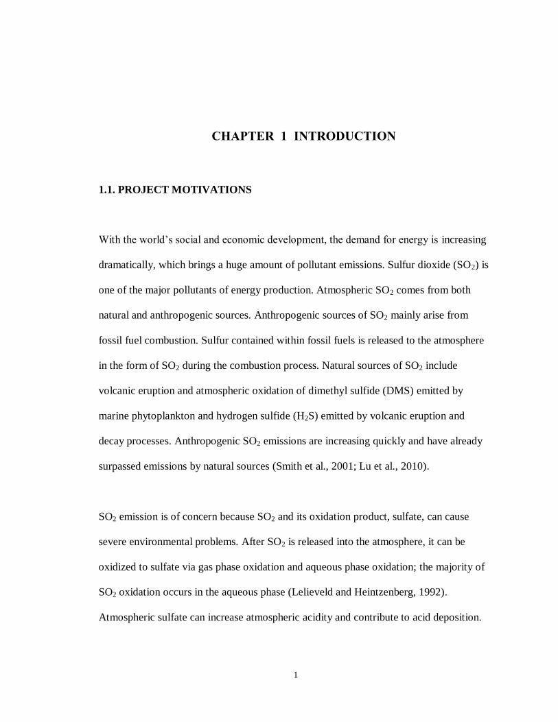
rapid growth and increasing amounts of pollution. Figure 1-1 shows the scheme of acid

deposition formation.

Figure 1-1. Scheme of acid deposition formation (from http://www.epa.gov/acidrain).

Numerous studies have been conducted world-wide on acid deposition formation and its

effects since the 1970s (Likens and Bormann, 1974; Carter, 1979; Abelson, 1983; Singer,

1984; Abelson, 1985; Abelson, 1987; Fay and Golomb, 1989; Likens et al., 1996). Acid

deposition has adverse impacts on the environment; it can increase the soil acidity and

http://www.epa.gov/acidrain

3

reduce soil fertility by leaching away nutrient cations and increasing toxic heavy metals

availability, thereby affecting the productivity of vegetation.

Acidification of water bodies will cause negative impact on aquatic ecosystem. Acid

deposition can damage building materials and can also have indirect effects on human

health (Bravo et al., 2006; Menon et al., 2007; Singh and Agrawal, 2008). Sulfate aerosol

can also perturb the Earth’s radiation budget directly through the backscattering of

sunlight and indirectly by changing cloud microphysical properties (Charlson et al., 1992;

Lelieveld and Heintzenberg, 1992; Kiehl and Briegleb, 1993; Fischer-Bruns et al., 2009).

Anthropogenic SO2 emissions in Europe and North America have decreased in the last

two decades, but they have increased in Asia due to economic growth (Manktelow et al.,

2007). Anthropogenic SO2 emissions in China have ranked highest in the word in recent

years; the total anthropogenic emitted SO2 changed dramatically during the last two

decades. From the late 1980s, total SO2 emissions in China kept increasing rapidly until

1995. After 1995 the increase in emission rate slowed down and even decreased due to a

more restrictive Chinese policy on SO2 emission. Beginning in 2002, Chinese SO2

emissions began to rapidly increase again along with economic development; emissions

increased by 53% from 2000 to 2006 (Lu et al., 2010). After 2006, SO2 emissions again

decreased as desulfurization equipment was widely adopted in China (Zhang et al.,

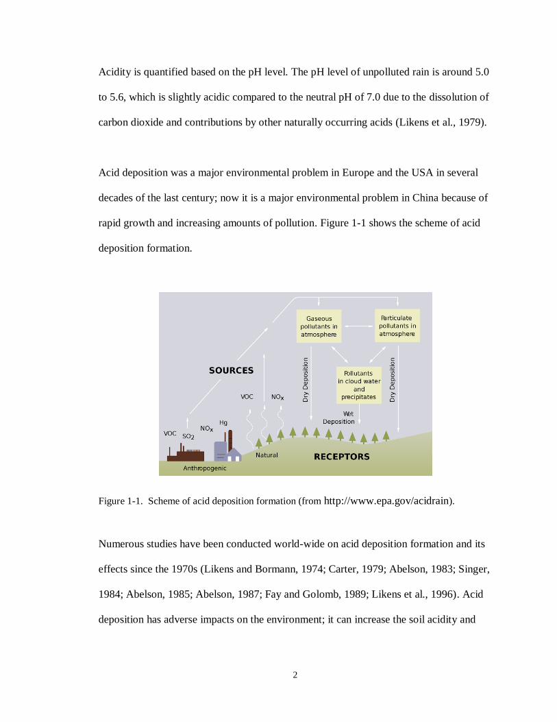
2009). Figure 1-2 shows a timeline of anthropogenic SO2 emissions in China.

4

Figure 1-2. Annual anthropogenic SO2 emissions in China 1989-2009 (Data from State

Environmental Statistic Report).

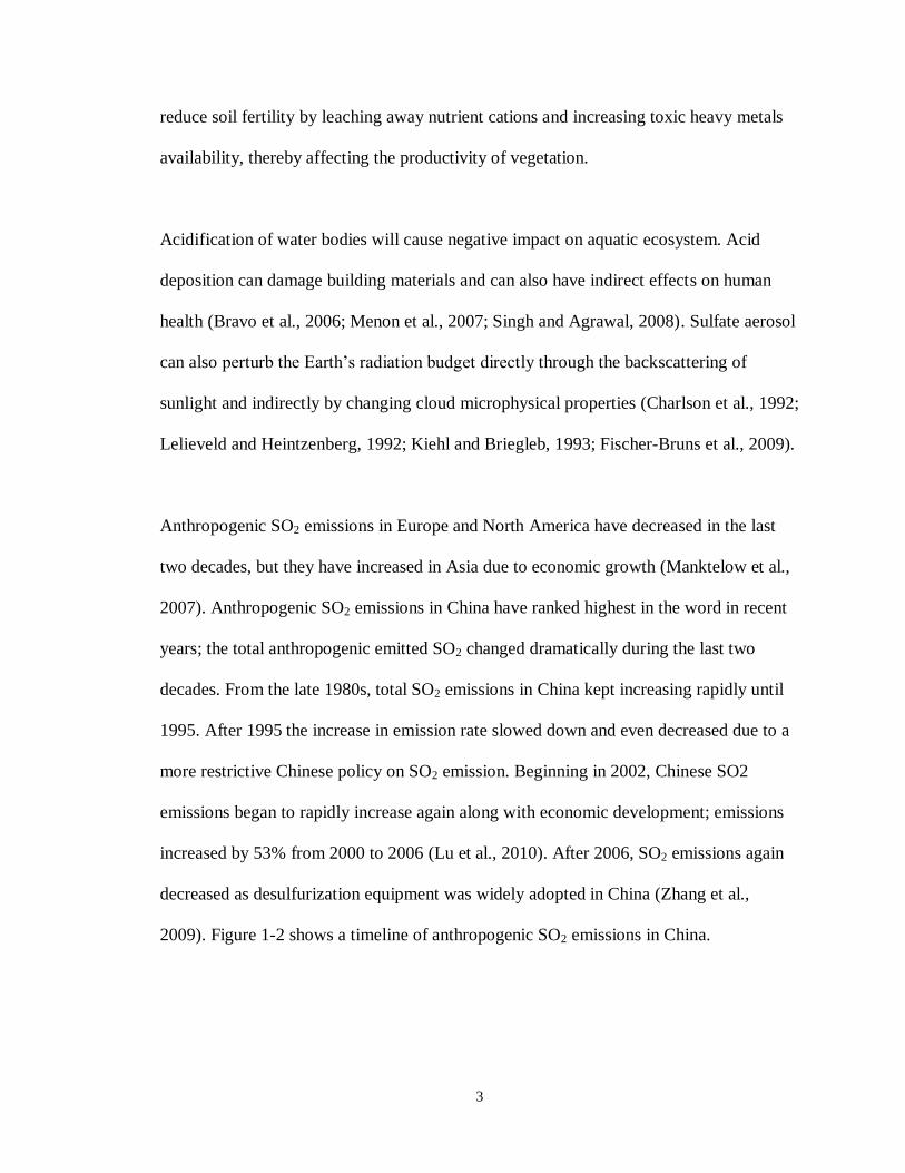
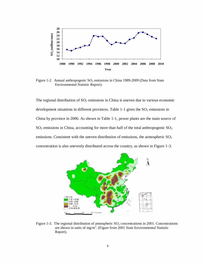
The regional distribution of SO2 emissions in China is uneven due to various economic

development situations in different provinces. Table 1-1 gives the SO2 emissions in

China by province in 2006. As shown in Table 1-1, power plants are the main source of

SO2 emissions in China, accounting for more than half of the total anthropogenic SO2

emissions. Consistent with the uneven distribution of emissions, the atmospheric SO2

concentration is also unevenly distributed across the country, as shown in Figure 1-3.

Figure 1-3. The regional distribution of atmospheric SO2 concentrations in 2001. Concentrations

are shown in units of mg/m3. (Figure from 2001 State Environmental Statistic

Report).

10121416182022242628

1988 1990 1992 1994 1996 1998 2000 2002 2004 2006 2008 2010

SO

2(m

illi

on

ton

s)

Year

5

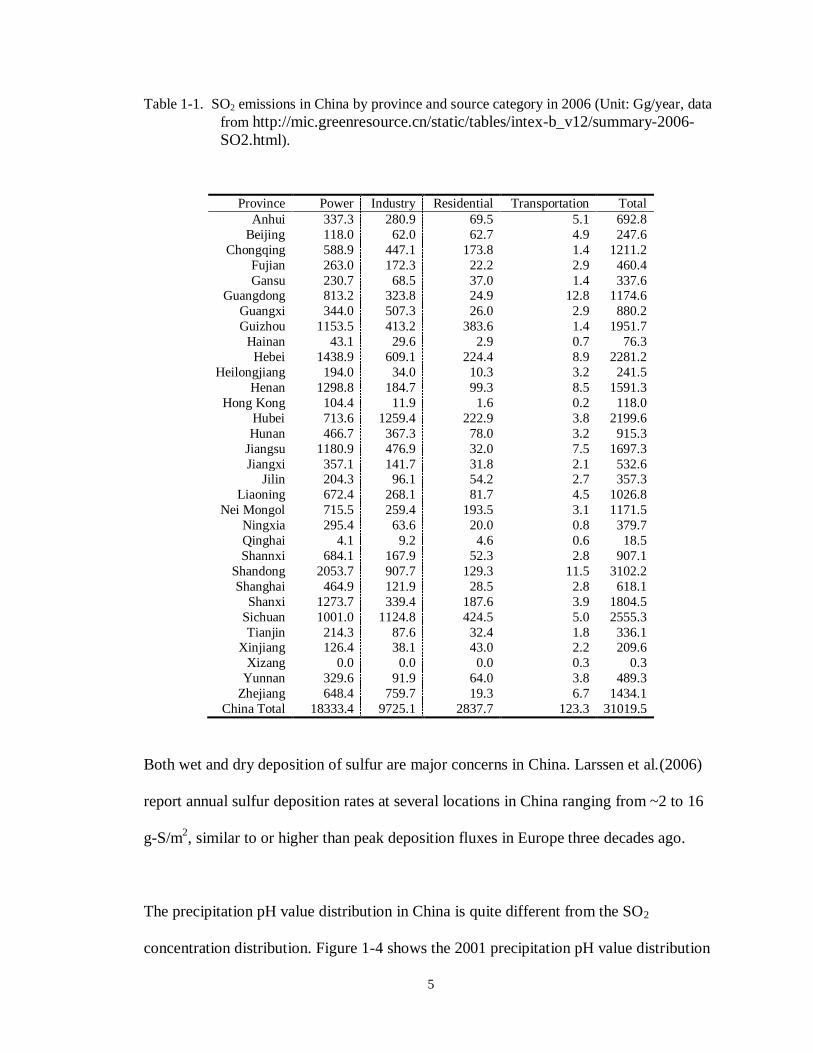
Table 1-1. SO2 emissions in China by province and source category in 2006 (Unit: Gg/year, data

from http://mic.greenresource.cn/static/tables/intex-b_v12/summary-2006-

SO2.html).

Province Power Industry Residential Transportation Total

Anhui 337.3 280.9 69.5 5.1 692.8

Beijing 118.0 62.0 62.7 4.9 247.6

Chongqing 588.9 447.1 173.8 1.4 1211.2

Fujian 263.0 172.3 22.2 2.9 460.4

Gansu 230.7 68.5 37.0 1.4 337.6 Guangdong 813.2 323.8 24.9 12.8 1174.6

Guangxi 344.0 507.3 26.0 2.9 880.2

Guizhou 1153.5 413.2 383.6 1.4 1951.7

Hainan 43.1 29.6 2.9 0.7 76.3

Hebei 1438.9 609.1 224.4 8.9 2281.2

Heilongjiang 194.0 34.0 10.3 3.2 241.5

Henan 1298.8 184.7 99.3 8.5 1591.3

Hong Kong 104.4 11.9 1.6 0.2 118.0

Hubei 713.6 1259.4 222.9 3.8 2199.6

Hunan 466.7 367.3 78.0 3.2 915.3

Jiangsu 1180.9 476.9 32.0 7.5 1697.3

Jiangxi 357.1 141.7 31.8 2.1 532.6 Jilin 204.3 96.1 54.2 2.7 357.3

Liaoning 672.4 268.1 81.7 4.5 1026.8

Nei Mongol 715.5 259.4 193.5 3.1 1171.5

Ningxia 295.4 63.6 20.0 0.8 379.7

Qinghai 4.1 9.2 4.6 0.6 18.5

Shannxi 684.1 167.9 52.3 2.8 907.1

Shandong 2053.7 907.7 129.3 11.5 3102.2

Shanghai 464.9 121.9 28.5 2.8 618.1

Shanxi 1273.7 339.4 187.6 3.9 1804.5

Sichuan 1001.0 1124.8 424.5 5.0 2555.3

Tianjin 214.3 87.6 32.4 1.8 336.1 Xinjiang 126.4 38.1 43.0 2.2 209.6

Xizang 0.0 0.0 0.0 0.3 0.3

Yunnan 329.6 91.9 64.0 3.8 489.3

Zhejiang 648.4 759.7 19.3 6.7 1434.1

China Total 18333.4 9725.1 2837.7 123.3 31019.5

Both wet and dry deposition of sulfur are major concerns in China. Larssen et al.(2006)

report annual sulfur deposition rates at several locations in China ranging from ~2 to 16

g-S/m2, similar to or higher than peak deposition fluxes in Europe three decades ago.

The precipitation pH value distribution in China is quite different from the SO2

concentration distribution. Figure 1-4 shows the 2001 precipitation pH value distribution

http://mic.greenresource.cn/static/tables/intex-b_v12/summary-2006-SO2.html

http://mic.greenresource.cn/static/tables/intex-b_v12/summary-2006-SO2.html

6

in China. Historically, acid precipitation has been most problematic in southern China.

Higher precipitation pH values in Beijing and other northern parts of China, however, do

not typically reflect an absence of substantial sulfate input; rather, sufficient acid

neutralizing capacity is generally present, from alkaline dust particles and gaseous

ammonia, to prevent significant acidification (Wai et al., 2005). As SO2 emissions

continue to increase, however, acidic precipitation is spreading more widely across

China.

Figure 1-5 shows the 2001 regional distribution of particle concentrations in China. Large

concentrations of airborne soil dust contribute to high particle concentrations in China,

especially in the north which is closer to primary dust source regions. Soil dust in the

atmosphere may alleviate the acid deposition situation in the north by neutralizing part of

the acidity contributed to precipitation by sulfuric and nitric acids. Increasing sulfur

emissions are expected to also result in more acid deposition in the northern part (Zhao

and Hou, 2010).

The neutralization ability of atmospheric dust particles is seasonally variable. Mt. Tai, the

location of the study to be described in this dissertation, is located within the warm

temperate continental monsoon climate zone; in winter, due to the cold high pressure

from Mongolia, prevailing winds blow from the north; in summer, the prevailing winds

blow from the Western Pacific to the continent driven by the subtropical high pressure

from the southeast. Generally there is more natural dust in spring than in summer, which

7

can cause seasonally variable neutralization ability. This may affect the pH value and the

sulfur chemistry in cloudwater.

Figure 1-4. The precipitation pH value distribution in 2001. (Figure from 2001 State Environmental Statistic Report).

Figure 1-5. The regional distribution of Total Suspended Particles (TSP) concentrations in 2001.

Concentrations are shown in units of mg/m3. (Figure from 2001 State Environmental

Statistic Report).

8

The sulfate that contributes to China’s acid rain and deposition problems is also of

interest internationally. Because quantities of emitted sulfur dioxide in China are so large

(total SO2 emission in 2009 was 22.1 million tons (China-MEP, 2010)) it is possible that

they exceed the capacity of regional clouds for rapid aqueous phase sulfate production,

leading to enhanced long-range transport of emitted SO2 and its oxidation product,

sulfate. Tu et al. (2004) reported that long-range transport of SO2 from East Asia to the

central North Pacific troposphere was observed on transit flights during the NASA

TRACE-P mission in March and April 2001. The SO2 emitted from East Asian sources

was generally transported to the central Pacific in 3~4 days. Studies by Brock et al.

(2004) indicated that following long-range transport of sulfur dioxide, particles were

formed over the mid-Pacific. Fiedler et al. (2009) also found that SO2 from East Asian

sources was detected over Europe after traveling across the North Pacific, North America

and the North Atlantic. High fine particle sulfate concentrations are routinely experienced

in nations immediately downwind. Kim et al. (2009), for example, document impacts on

S. Korea. Sulfate transport across the Pacific and into the U.S. is also a concern. Park et

al. (2004) estimate that concentrations of sulfate transported across the Pacific to the

United States slightly exceed the average concentration (0.12 µg/m3) suggested by the

U.S Environmental Protection Agency for estimating natural visibility conditions in the

western U.S.

9

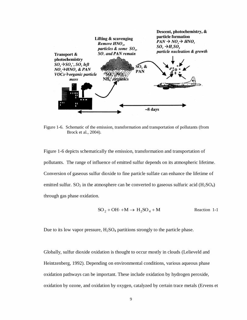
Figure 1-6. Schematic of the emission, transformation and transportation of pollutants (from Brock et al., 2004).

Figure 1-6 depicts schematically the emission, transformation and transportation of

pollutants. The range of influence of emitted sulfur depends on its atmospheric lifetime.

Conversion of gaseous sulfur dioxide to fine particle sulfate can enhance the lifetime of

emitted sulfur. SO2 in the atmosphere can be converted to gaseous sulfuric acid (H2SO4)

through gas phase oxidation.

MSOH MOHSO 422 Reaction 1-1

Due to its low vapor pressure, H2SO4 partitions strongly to the particle phase.

Globally, sulfur dioxide oxidation is thought to occur mostly in clouds (Lelieveld and

Heintzenberg, 1992). Depending on environmental conditions, various aqueous phase

oxidation pathways can be important. These include oxidation by hydrogen peroxide,

oxidation by ozone, and oxidation by oxygen, catalyzed by certain trace metals (Ervens et

10

al., 2003; Seinfeld and Pandis, 2006). At low to moderate pH (typically pH ~2-5),

oxidation is generally expected to favor the H2O2 pathway. Fast S(IV) oxidation by H2O2

can, of course, be maintained only as long as H2O2 is available. If SO2 concentrations

significantly exceed H2O2 concentrations, this pathway may be effective in converting

only a portion of the SO2 to sulfate. Aqueous H2O2 can come from gas to droplet

partitioning or be formed in situ by aqueous photochemistry (Faust et al., 1993; Anastasio

et al., 1994; Zuo and Deng, 1999). At pH values above 5, oxidation by ozone and trace

metal catalyzed autooxidation often increase in importance. At these higher pH values,

sulfate production may also be affected by competition with S(IV) complexation by

carbonyls, including formaldehyde (Munger et al., 1984; Munger et al., 1986; Olson and

Hoffmann, 1989; Rao and Collett, 1995).

In model simulations of atmospheric sulfate production, Barth et al. (2000) point out the

dominant role that aqueous phase chemistry plays, especially in the lower troposphere

and in mid-latitude regions of the northern hemisphere. They note that, globally, the

column burden of sulfate produced by aqueous phase chemistry is greatest over east Asia

and point out the important roles that cloud pH, H2O2 concentrations, and depletion of

H2O2 (by reactions in cloud) play in influencing sulfate production. Barth and Church

(1999) simulate changes in atmospheric sulfate burdens resulting from a doubling of SO2

emissions in SE China. Their simulations suggest a nonlinear response for this situation,

in part because increased SO2 emissions overwhelm available H2O2 concentrations,

making gas phase sulfate production relatively more important. Because sulfate produced

in the gas phase is less susceptible to rapid wet deposition than sulfate produced in-cloud,

11

the net effect is that a doubling of SO2 concentrations produces more than a doubling of

SE China’s contribution to the global tropospheric sulfate burden.

The sulfur lifetime is also closely related to the precipitation frequency. Sulfate produced

by oxidation in precipitating clouds can be rapidly removed by wet deposition. Less

precipitating cloud or slower in-cloud oxidation mean fewer sulfur dioxide emissions are

deposited to the surface regionally and more emissions stay in the atmosphere and are

transported farther downwind (Barth and Church, 1999).

Many studies have been conducted on acid rain in China (Jernelov, 1983; Zhao and Sun,

1986; Galloway et al., 1987; Shen et al., 1996; Wang and Wang, 1996; Larssen et al.,

2006), but not many studies have been devoted to cloud/fog chemistry. Cloud/fog

chemistry research in China started in the 1980s (Wang and Xu, 2009; Niu et al., 2010)

and most observations were conducted in areas with severe acid deposition concerns,

such as Chongqing (Peng et al., 1992; Li and Peng, 1994), Nanjing (Li et al., 2008),

Shanghai (Li et al., 1999), Mt. Lu (Ding et al., 1991), et al. Cloud chemistry research in

China has been generally limited to routine analysis of ions.

Because aqueous phase oxidation processes are so critical to sulfate production, it is

imperative to understand factors influencing cloud chemistry in China, especially the

cloudwater chemical composition and key species that determine the aqueous phase

sulfur chemistry.

12

1.2. AQUEOUS PHASE SULFUR REACTIONS IN CLOUDWATER

The total aqueous sulfur in the +4 oxidation state (S(IV)) includes hydrated SO2, the

bisulfite ion, the sulfite ion, and hydroxymethanesulfonate (HMS):

]HMS[]SO[]HSO[]OHSO[)]IV(S[ 23322

Equation 1-1

Fig. 1-7 shows the mole fractions of the three S(IV) forms of dissolved sulfur dioxide,

SO2·H2O, HSO3- and SO3

2-, as a function of pH. As the pH value increases, the speciation

of S(IV) shifts from SO2·H2O toward HSO3-and SO3

2-. The crossover points between

species correspond to the pKa of the more protonated form.

Figure 1-7. Mole fractions of S(IV) species concentrations as a function of pH (from Seinfeld and

Pandis, 2006).

13

Important aqueous phase oxidants of dissolved sulfur dioxide include hydrogen peroxide

(H2O2), ozone (O3) and oxygen (O2) (catalyzed by trace metals). The speed of aqueous

phase oxidation depends on pH, oxidant availability, and liquid water content (LWC)

(Liang and Jacobson, 1999).

1.2.1. S(IV) oxidation by ozone

In the three main aqueous phase oxidation pathways, aqueous phase S(IV) oxidation by

O3 tends to be most rapid at high pH. Tropospheric ozone predominantly forms through

photochemical and chemical reactions of nitrogen oxides (NOx) and volatile organic

compounds (VOCs). The reaction that produces ozone can be expressed as:

MOMOO 32

Reaction 1-2

NOx is one of the key species for the photochemical production of tropospheric ozone.

ONONO2 hv Reaction 1-3

223 ONOONO

Reaction 1-4

This O3-NO-NO2 cycle has no net effect on O3, but in the presence of peroxy radicals, the

cycle is perturbed and ozone production is enhanced. Peroxy radicals, formed by

photochemical oxidation of VOCs, oxidize NO to NO2 and lead to accumulation of

ozone.

14

Aqueous S(IV) oxidation by O3 is represented as

23 O S(VI)O S(IV) Reaction 1-5

The reaction rate can be expressed as follows (Hoffmann and Calvert, 1985; Hoffmann,

1986; Seinfeld and Pandis, 2006):

]O][S(IV))[kkk(dt

]S(IV)[d3221100

Equation 1-2

The characteristic time for S(IV) depletion through oxidation by O3

])O)[kkk/((1 3221100O3

Equation 1-3

0 , 1 , and 2 represent the fractions of total free S(IV) present as SO2·H2O, HSO3-

and SO32-

respectively, where at 298K, 114

0 sM102.4k , 1151 sM103.7k , and

.sM101.5k 1192

As shown in Fig. 1-7, when the pH value increases, the speciation of S(IV) shifts from

SO2·H2O toward HSO3- and SO3

2-. This draws more SO2 into the droplet (to maintain the

Henry’s Law equilibrium with the SO2 partial pressure in the gas phase) and shifts the

S(IV) to forms that are more rapidly oxidized by O3 (Hoffmann, 1986). SO2·H2O, HSO3-

and SO32-

have different reactivities, as show in equation 1-2. The rate constant of

SO2·H2O-O3 is lower than those of HSO3--O3 and SO3

2--O3. The rate constant of SO3

2--

O3 is much higher than those of the other two forms. As cloud pH increases the increase

in total S(IV) concentration and the change in speciation both contribute to a rapid rise in

the overall S(IV) oxidation rate by ozone.

15

In a chemical reaction, the species with fewer moles is the limiting reactant. The ambient

mixing ratio of O3 is generally higher than that of SO2, so normally O3 will not be

completely depleted by the aqueous oxidation process.

1.2.2. S(IV) oxidation by hydrogen peroxide

S(IV) oxidation by hydrogen peroxide is generally expected to be most important when

pH is below ~5. Atmospheric hydrogen peroxide is generated mainly through self-

reaction of the HO2 radical.

22222 OOHHOHO Reaction 1-6

The HO2 radical is mainly generated through reaction of the OH radical with CO and

other VOCs. Aqueous H2O2 comes from gas-to-droplet partitioning and can also be

produced in clouds by aqueous photochemistry (Faust et al., 1993; Anastasio et al., 1994;

Zuo and Deng, 1999). H2O2 is moderately water soluble and the oxidation of S(IV) by

H2O2 is very fast in clouds. The reaction and rate can be expressed as follows (Seinfeld

and Pandis, 2006).

OH OOHSOOH HSO 22223

Reaction 1-7

422 SOH HOOHSO

Reaction 1-8

]H[K1

]S(IV)][OH][H[k

dt

]S(IV)[d 122

Equation 1-4

16

The characteristic time for S(IV) depletion through oxidation by H2O2:

)]O][H[Hk/(])H[K1( 122OH 22

Equation 1-5

where 127 sM107.45k and 1M13 K at 298K.

As shown in Fig. 1-7, in the pH range 3-6, almost all S(IV) exists as HSO3-. Over a broad

range of pH, the H2O2 oxidation pathway exhibits essentially no pH dependence.

Although the total S(IV) in solution increases as pH rises (as discussed above), this is

offset by a decrease in the H+ concentration which slows reaction 1-8, which is the rate

limiting step.

The ambient mixing ratio of H2O2 is normally much lower than that of O3. If the mixing

ratio of H2O2 is lower than the ambient SO2 mixing ratio, the H2O2 can be consumed

completely by the aqueous S(IV) oxidation process. If the SO2 mixing ratio is lower, the

ambient SO2 can be rapidly exhausted by the reaction. In order to understand the relative

importance of both the O3 and H2O2 sulfur oxidation pathways, it is necessary to

investigate the ambient concentrations of SO2, O3 and H2O2 as well as the cloud pH.

1.2.3. S(IV) oxidation by oxygen (catalyzed by Fe(III) and Mn(II))

Uncatalyzed S(IV) oxidation by oxygen is very slow and can be neglected. Oxidation of

S(IV) to sulfate by oxygen, catalyzed by the ferric ion, Fe(III), and the manganese ion,

Mn(II), is considered a possibly important contributor to the total oxidation rate of S(IV),

especially in situations of reduced photochemical activity (producing less O3 and H2O2)

17

and higher Fe(III) and Mn(II) concentrations (Ibusuki and Takeuchi, 1987). Many studies

have investigated the kinetics for this oxidation pathway (Jacob and Hoffmann, 1983;

Ibusuki and Takeuchi, 1987; Martin and Good, 1991; Grgic et al., 1992). Fe and Mn in

the atmosphere come from both anthropogenic and natural sources. The anthropogenic

source of coal combustion (Luo et al., 2008) can have an important influence on the

regional concentrations of Fe and Mn in the atmosphere. Natural sources of Fe and Mn

are mainly from mineral dust. Chuang et al. (2005) reported that the origin of soluble iron

in the Asian atmospheric outflow is dominated by anthropogenic sources and not mineral

dust sources.

The ratio of the catalytically active iron form, Fe(III), to the concentration of the inactive

iron form, Fe(II), is important to the accurate calculation of the sulfur oxidation rate,

since only Fe(III) acts as a catalyst for S(IV) oxidation. Generally the total Fe

concentration is measured, due to the extreme difficulty in accurately speciating rapidly

cycling iron oxidation states in the field, and an assumption is made regarding the

abundance of the two oxidation states. Siefert et al. (1998) measured the Fe and Mn

oxidations states in several cloud/fog events and found that Mn(II) was the predominant

oxidation states of Mn; however, it was more difficult to identify the speciation of Fe.

Following the approach of Rao and Collett (1995), the Mn was assumed in this study to

be completely present as catalytically active Mn(II) and 25% of the Fe was assumed to be

present as catalytically active Fe(III).

18

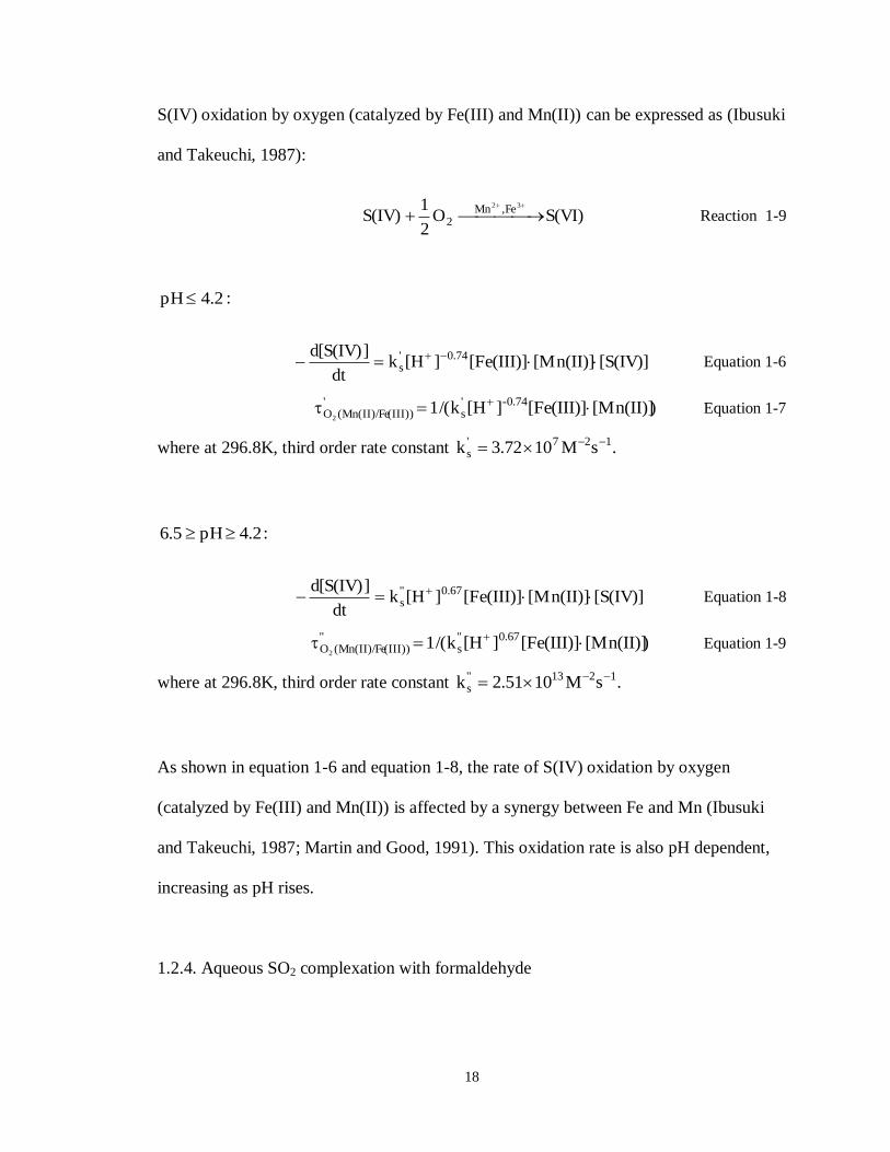
S(IV) oxidation by oxygen (catalyzed by Fe(III) and Mn(II)) can be expressed as (Ibusuki

and Takeuchi, 1987):

S(VI)O2

1 S(IV)

32 Fe,Mn2

Reaction 1-9

2.4pH :

[S(IV)][Mn(II)][Fe(III)]][Hkdt

]S(IV)[d 0.74's

Equation 1-6

)[Mn(II)][Fe(III)]][Hk/(1 -0.74's

'(III))(Mn(II)/FeO2

Equation 1-7

where at 296.8K, third order rate constant .sM103.72k 127's

2.4pH5.6 :

[S(IV)][Mn(II)][Fe(III)]][Hkdt

]S(IV)[d 67.0"s

Equation 1-8

)[Mn(II)][Fe(III)]][Hk/(1 0.67"s

"(III))(Mn(II)/FeO2

Equation 1-9

where at 296.8K, third order rate constant .sM102.51k 1213"s

As shown in equation 1-6 and equation 1-8, the rate of S(IV) oxidation by oxygen

(catalyzed by Fe(III) and Mn(II)) is affected by a synergy between Fe and Mn (Ibusuki

and Takeuchi, 1987; Martin and Good, 1991). This oxidation rate is also pH dependent,

increasing as pH rises.

1.2.4. Aqueous SO2 complexation with formaldehyde

19

Aqueous S(IV) can complex with formaldehyde in cloudwater to form

hydroxymethanesulfonate (HMS). The time constant of the complexation process is pH

dependent; as the pH decreases the time constant increases (Warneck, 1989). At low pH,

the complexation process may not reach equilibrium during a cloud event.

-323 SOOHCHHSOHCHO

Reaction 1-10

[HCHO][S(IV)]k[HCHO][S(IV)]kdt

]S(IV)[d2514

Equation 1-10

))kk([HCHO]/(1 2514HCHO

Equation 1-11

where at 298K, 1124 sM107.90k , and .sM102.48k 117

5

The formation of hydroxymethanesulfonate (HMS) via the complexation of HCHO and

S(IV) can compete with S(IV) oxidation and thereby inhibit the production of sulfate in

clouds (Munger et al., 1984; Munger et al., 1986; Rao and Collett, 1995; Reilly et al.,

2001); thus, HMS can act as a reservoir pool for S(IV) (Adewuyi et al., 1984). Although

HMS formation tends to dominate hydroxyalkylsulfonate formation, due to the greater

abundance and aqueous solubility of HCHO, similar reactions also occur with larger

carbonyls (Olson and Hoffmann, 1989).

1.2.5. Temperature dependence of equilibrium and rate constants

The temperature dependence is represented by (Seinfeld and Pandis, 2006)

)

298

11(exp298TR

HKK Equation 1-12

20

where R=8.314 Jmol-1

K-1

, K is Henry’s law coefficient and the equilibrium constant at

temperature T.

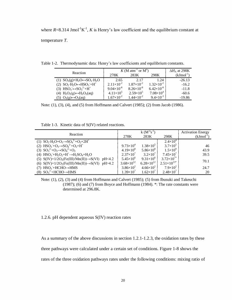
Table 1-2. Thermodynamic data: Henry’s law coefficients and equilibrium constants.

Reaction K (M atm-1 or Mn) ∆HA at 298K

278K 283K 298K (kJmol-1)

(1) SO2(g)+H2O↔SO2∙H2O 2.65 2.17 1.24 -26.13

(2) SO2∙H2O↔HSO3-+H+ 2.11×10-2 1.87×10-2 1.32×10-2 -16.2

(3) HSO3-↔SO3

2-+H+ 9.04×10-8 8.26×10-8 6.42×10-8 -11.8

(4) H2O2(g)↔H2O2(aq) 4.11×105 2.59×105 7.08×104 -60.6

(5) O3(g)↔O3(aq) 1.67×10-2 1.44×10-2 9.4×10-3 -19.86

Note: (1), (3), (4), and (5) from Hoffmann and Calvert (1985); (2) from Jacob (1986).

Table 1-3. Kinetic data of S(IV) related reactions.

Reaction k (M-ns-1) Activation Energy

278K 283K 298K (kJmol-1)

(1) SO2∙H2O+O3→SO42-+O2+2H+ 2.4×104

(2) HSO3-+O3→SO4

2-+O2+H+ 9.73×104 1.38×105 3.7×105 46 (3) SO3

2-+O3→SO42-+O2 4.19×108 5.86×108 1.5×109 43.9

(4) HSO3-+H2O2+H+→H2SO4+H2O 2.37×107 3.2×107 7.45×107 39.5

(5) S(IV)+1/2O2(Fe(III)/Mn(II))→S(VI) pH<4.2 5.45×106 9.31×106 3.72×107* 70.1

(6) S(IV)+1/2O2(Fe(III)/Mn(II))→S(VI) pH>4.2 3.68×1012 6.28×1012 2.51×1013*

(7) HSO3-+HCHO→HMS 3.86×102 4.66×102 7.9×102 24.7

(8) SO32-+HCHO→HMS 1.39×107 1.62×107 2.48×107 20

Note: (1), (2), (3) and (4) from Hoffmann and Calvert (1985); (5) from Ibusuki and Takeuchi

(1987); (6) and (7) from Boyce and Hoffmann (1984). *: The rate constants were

determined at 296.8K.

1.2.6. pH dependent aqueous S(IV) reaction rates

As a summary of the above discussions in section 1.2.1-1.2.3, the oxidation rates by these

three pathways were calculated under a certain set of conditions. Figure 1-8 shows the

rates of the three oxidation pathways rates under the following conditions: mixing ratio of

21

SO2 at 20 ppbv, O3 at 100 ppbv, H2O2 at 2 ppbv; aqueous concentration of Fe(III) at 10

µM and Mn(II) at 1 µM; T = 298K.

Figure 1-8. S(IV) reaction rates by different pathways, shown as a function of pH, for the

conditions specified in the text.

As shown in Fig. 1-8, S(IV) oxidation by hydrogen peroxide is essentially independent of

pH while S(IV) oxidation rates by ozone and by oxygen (catalyzed by Fe(III) and Mn(II))

are pH dependent. At lower pH values, S(IV) oxidation by hydrogen peroxide is much

faster than the other pathways while S(IV) oxidation by ozone tends to be much faster at

higher pH. The relative rates of the oxidation pathways, of course, can change with

changes in the available concentrations of oxidants and catalysts.

1.E-11

1.E-09

1.E-07

1.E-05

1.E-03

1.E-01

2 4 6 8

-d[S

(IV

)]/d

t (M

/s)

pH

O3

H2O2

O2/Fe(III)+Mn(II)

22

1.3. CLOUD DROP SIZE-DEPENDENT AQUEOUS SULFUR REACTIONS

Cloudwater chemical composition can vary across the drop size spectrum for a variety of

reasons, including differences in the composition of the aerosol particles on which the

droplets form (Gurciullo and Pandis, 1997). Differences in drop composition as a

function of size also occur due to size-dependent rates of condensational growth

(dilution) and soluble gas uptake (Noone et al., 1988; Ogren and Charlson, 1992).

Differences in drop composition can also give rise to differences in rates of aqueous

phase chemical reactions, leading to further differentiation in droplet compositions.

Several experimental studies have demonstrated the common occurrence of cloud drop

size-dependent composition (Noone et al., 1988; Rao and Collett, 1995; Bator and

Collett, 1997; Gurciullo and Pandis, 1997; Rao and Collett, 1998; Hoag et al., 1999;

Menon et al., 2000; Rattigan et al., 2001; Reilly et al., 2001; Ervens et al., 2003; Moore et

al., 2004a; Moore et al., 2004b; Ermakov et al., 2006). It was found that since key

parameters that determine aqueous phase sulfur reaction, like pH (Hoag et al., 1999;

Reilly et al., 2001), Fe and Mn (Rao and Collett, 1998; Hoag et al., 1999) and aqueous

HCHO (Rao and Collett, 1995), can vary with drop size, then aqueous phase SO2

oxidation rate may also be drop size-dependent. Using the bulk (average) cloudwater

composition to determine aqueous sulfate production rates may yield biased estimates.

This is especially problematic because many of the S(IV) oxidation pathways discussed

above exhibit a nonlinear dependence on various species concentrations, especially H+,

Fe(III), and Mn(II). The prediction of rates from an average cloudwater composition, in

23

such a case, is not equivalent to determining the average rate predicted from a chemically

heterogeneous droplet population. Rates predicted from drop size-resolved cloud

composition observations have been found to differ significantly from rates based on

average cloud composition for the ozone and metal-catalyzed oxidation pathways

(Gurciullo and Pandis, 1997). Because S(IV) oxidation by H2O2 is essentially

independent of pH and little drop size dependence is expected for peroxide

concentrations, this oxidation pathway has been observed to be independent of drop size

(Hoag et al., 1999; Rattigan et al., 2001) and no bias in sulfate production is expected

when neglecting chemical heterogeneity in cloud drop composition.

1.4. MAJOR RESEARCH OBJECTIVES

Because aqueous phase oxidation processes are so critical to sulfate production, it is

imperative to understand factors influencing cloud chemistry in China in order to

accurately predict effects of increasing regional SO2 emissions on sulfate production in

that part of the world and its local, regional, and intercontinental effects. While model

simulations provide valuable insight into sulfur chemistry and its sensitivity to changing

emissions, in situ observations are needed to assess actual conditions in the region. In

order to more fully investigate the cloudwater chemical composition and key species that

determine the aqueous phase sulfur chemistry and to assess the ability of regional clouds

to support aqueous sulfur oxidation, four field campaigns were conducted in 2007 and

2008 at Mt. Tai in eastern China. Observations of cloud pH, along with key S(IV)

oxidants and catalysts, are reported and used to examine the importance of various

24

aqueous phase sulfate production pathways. In summary, the specific research objectives

include:

Investigate the chemical composition of cloudwater in eastern China, providing a

comprehensive observation data set of cloudwater chemical composition for

further cloud chemistry study.

Characterize the size-dependent chemical composition of cloudwater, especially

the key species that determine sulfur chemistry in cloudwater.

Investigate aqueous sulfur oxidation rates in sampled cloudwater and examine the

capacity of the eastern China regional atmosphere to support aqueous phase sulfur

oxidation by hydrogen peroxide, ozone, and oxygen (catalyzed by Fe and Mn).

Determine the extent to which regional clouds in eastern China interact with

ambient fine particles and soluble trace gases. Determine what fractions of

regional nitrogen- and sulfur-containing air pollutants are actively processed in a

cloud event.

Investigate the seasonal variations of key factors that are critical to determining

the chemical composition of cloudwater and sulfur oxidation chemistry. SO2

concentrations can have seasonal variations due to residential heating that uses

fossil fuel combustion in winter season and due to seasonal changes in electricity

25

demand. H2O2 and O3 concentrations can change with season because of their

origins in smog photochemistry.

26

CHAPTER 2 METHODOLOGY

2.1. SAMPLING TIME AND SITE LOCATION

Four cloud sampling field campaigns were conducted in spring 2007 (March 22-April

24), summer 2007 (June 16-July 20), spring 2008 (March 28-April 25) and summer

2008(June 14-July 16). Spring and summer were selected to investigate the seasonal

variations of cloud chemistry. Seasonal changes might be expected due to changes in

photochemical activity, prevailing transport patterns, and emissions changes including

soil dust. The 2007 field campaigns were led by Shandong University and Hong Kong

Polytechnic University, with technical assistance and equipment provided by CSU. CSU

led the more extensive 2008 campaigns, with assistance from the other two institutions.

Field experiments were conducted at the summit of Mt. Tai (36.251ºN, 117.101ºE, 1534

m a.s.l.), located in eastern China (Figure 2-1). The 2007 measurements were made on

the grounds of a meteorological station operated by the China Meteorological Agency.

Restrictions on access to this site by CSU personnel in 2008 led to a relocation of

measurements a few hundred meters away to a small hotel. Both locations were near the

top of the mountain. There are several advantages to using the summit of Mt. Tai, as the

sampling site. Mt. Tai is located in central Shandong province and at the eastern edge of

the North China Plain, between the Bohai Economic Rim and Yangtze River Delta

27

Economic Zone, two of China’s three major economic circles. Shandong province has the

highest SO2 emission in China, as shown in Table 1-1; the total anthropogenic SO2

emission in 2006 was 3102.2 Gg, representing approximately 10% of total anthropogenic

SO2 emissions in China. The summit of Mt. Tai contains a number of temples and tourist

facilities, but access is only by cable car or foot. No vehicles can access the summit. The

elevation of Mt. Tai isolates the measurements from direct influence by large urban

emission sources, providing a more representative picture of regional atmospheric

composition. The summit is frequently in cloud during spring and summer and nearly

half of the days each year have fog or intercepted clouds, making Mt. Tai a reliable place

to sample fog and cloudwater under the influence of regional atmospheric pollution.

Other investigators have also found Mt. Tai a useful site for measurement of various

aerosol and gas phase pollutants (Gao et al., 2005; Wang et al., 2006; Kanaya et al., 2008;

Li et al., 2008; Wang et al., 2008; Mao et al., 2009; Ren et al., 2009; Wang et al., 2009;

Yamaji et al., 2010). These previous investigations of atmospheric composition at Mt. Tai

have focused on study of gas and particle phase constituents, but little was known about

cloud chemistry in the region prior to this study.

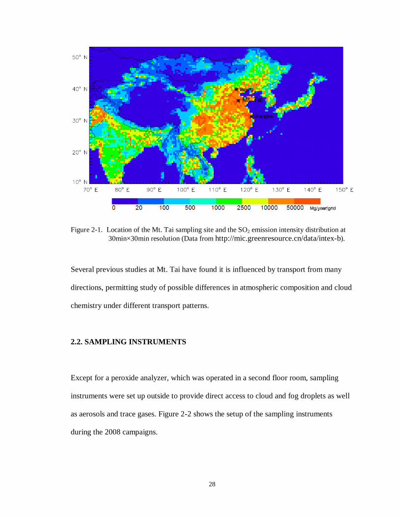
Figure 2-1 shows the location of Mt. Tai on a map of Asia with SO2 emission intensities

and political boundaries as background. It is obvious that Mt. Tai is surrounded by a high

SO2 emission intensity area. Sampling at Mt. Tai is an attempt to represent the

atmospheric condition of the eastern coastal developed areas of China.

28

Figure 2-1. Location of the Mt. Tai sampling site and the SO2 emission intensity distribution at

30min×30min resolution (Data from http://mic.greenresource.cn/data/intex-b).

Several previous studies at Mt. Tai have found it is influenced by transport from many

directions, permitting study of possible differences in atmospheric composition and cloud

chemistry under different transport patterns.

2.2. SAMPLING INSTRUMENTS

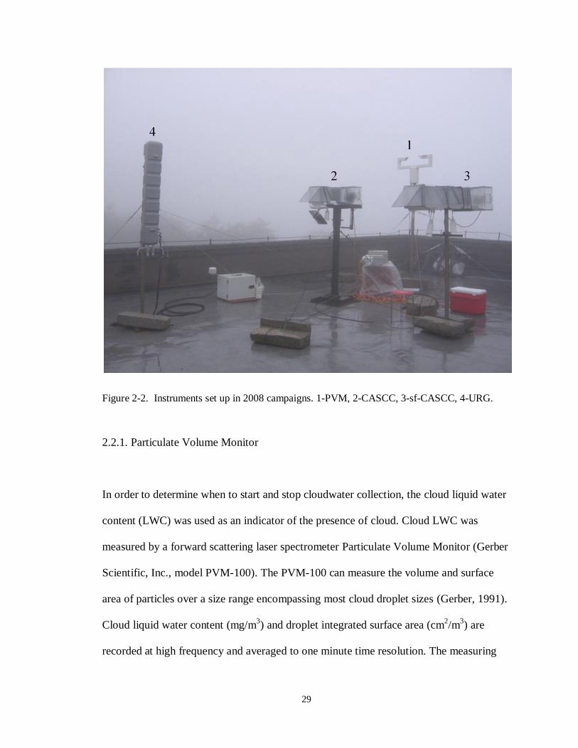
Except for a peroxide analyzer, which was operated in a second floor room, sampling

instruments were set up outside to provide direct access to cloud and fog droplets as well

as aerosols and trace gases. Figure 2-2 shows the setup of the sampling instruments

during the 2008 campaigns.

http://mic.greenresource.cn/data/intex-b

29

Figure 2-2. Instruments set up in 2008 campaigns. 1-PVM, 2-CASCC, 3-sf-CASCC, 4-URG.

2.2.1. Particulate Volume Monitor

In order to determine when to start and stop cloudwater collection, the cloud liquid water

content (LWC) was used as an indicator of the presence of cloud. Cloud LWC was

measured by a forward scattering laser spectrometer Particulate Volume Monitor (Gerber

Scientific, Inc., model PVM-100). The PVM-100 can measure the volume and surface

area of particles over a size range encompassing most cloud droplet sizes (Gerber, 1991).

Cloud liquid water content (mg/m3) and droplet integrated surface area (cm

2/m

3) are

recorded at high frequency and averaged to one minute time resolution. The measuring

30

principle of the PVM-100 is based on the linear relationship between extinction and

cloud liquid water content (Gerber, 1984; Gerber, 1991; Arends et al., 1992). The main

components of the PVM consist of a laser, collimator optics, and receiver optics. The

receiver optics include a transform lens, a light trap, a variable light transmission filter

and a large-area light detector (Gerber, 1991). Figure 2-3 shows a schematic of the PVM.

The PVM is calibrated by placing a manufacturer-supplied calibration disk in the light

path.

Figure 2-3. Schematic of the PVM (from Gerber 1991).

31

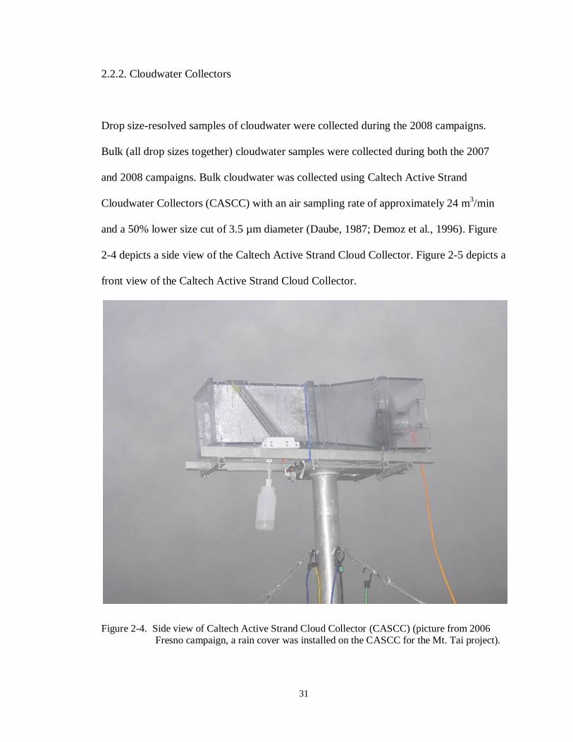
2.2.2. Cloudwater Collectors

Drop size-resolved samples of cloudwater were collected during the 2008 campaigns.

Bulk (all drop sizes together) cloudwater samples were collected during both the 2007

and 2008 campaigns. Bulk cloudwater was collected using Caltech Active Strand

Cloudwater Collectors (CASCC) with an air sampling rate of approximately 24 m3/min

and a 50% lower size cut of 3.5 µm diameter (Daube, 1987; Demoz et al., 1996). Figure

2-4 depicts a side view of the Caltech Active Strand Cloud Collector. Figure 2-5 depicts a

front view of the Caltech Active Strand Cloud Collector.

Figure 2-4. Side view of Caltech Active Strand Cloud Collector (CASCC) (picture from 2006 Fresno campaign, a rain cover was installed on the CASCC for the Mt. Tai project).

32

As shown in Figure 2-4, from left to right, air is drawn by a fan through the collector and

across 6 rows of inclined 508 µm Teflon strands. Cloud droplets are impacted upon the

Teflon strands where they coalesce and, aided by aerodynamic drag, run down the strands

(as shown in Figure 2-5) and through a Teflon collection trough and Teflon tube into a

polyethylene collection bottle. The CASCC was operated with a downward facing inlet

(see Fig. 2-2) to exclude rain collection during periods of mixed cloud and precipitation.

Figure 2-5. Front view of the Caltech Active Strand Cloud Collector (CASCC) without rain excluding inlet.

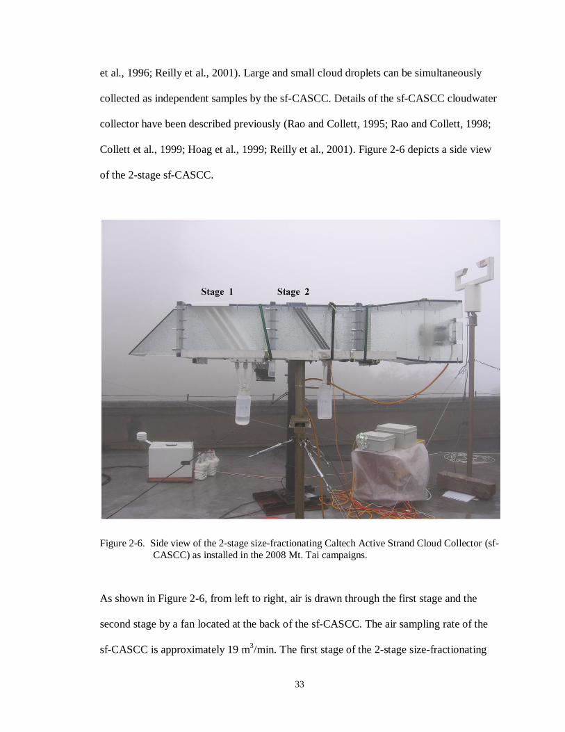
Drop size-resolved cloudwater samples were collected in the 2008 campaigns using a 2-

stage size-fractionating Caltech Active Strand Cloudwater Collector (sf-CASCC) (Demoz

33

et al., 1996; Reilly et al., 2001). Large and small cloud droplets can be simultaneously

collected as independent samples by the sf-CASCC. Details of the sf-CASCC cloudwater

collector have been described previously (Rao and Collett, 1995; Rao and Collett, 1998;

Collett et al., 1999; Hoag et al., 1999; Reilly et al., 2001). Figure 2-6 depicts a side view

of the 2-stage sf-CASCC.

Figure 2-6. Side view of the 2-stage size-fractionating Caltech Active Strand Cloud Collector (sf-

CASCC) as installed in the 2008 Mt. Tai campaigns.

As shown in Figure 2-6, from left to right, air is drawn through the first stage and the

second stage by a fan located at the back of the sf-CASCC. The air sampling rate of the

sf-CASCC is approximately 19 m3/min. The first stage of the 2-stage size-fractionating

34

Caltech Active Strand Cloud Collector consists of 12.7 mm diameter Teflon rods, and the

second stage consists of 508 µm Teflon strands identical to those of the CASCC. Larger

droplets are collected on the first stage with a 50% lower size cut of approximately 16

µm. Smaller droplets are collected on the second stage with a 50% size cut of

approximately 4 µm. As in the CASCC, collected droplets coalesce, run down the

collection surfaces into a Teflon collection trough, and are directed through Teflon

sample tubes to polyethylene sample bottles. The sf-CASCC was operated with a

downward facing inlet (see Fig. 2-6) to exclude rain collection during periods of mixed

cloud and precipitation.

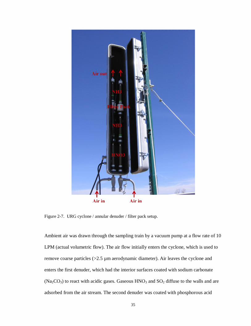
2.2.3. URG Annular Denuder/Filter-pack System

A University Research Glassware (URG) denuder/filter pack assembly (model URG-

3000C) was used in the 2008 campaigns to simultaneously collect PM2.5 and select trace

gases for chemical analysis. As shown in Figure 2-7, air was drawn in series through a

cyclone (URG-2000-30EN, 10LPM, 2.5 µm aerodynamic size cut), two coated annular

denuders (URG-2000-30×242-3CSS), a 37 mm Teflon® filter pack (URG-2000-22FB),

and a third coated denuder.

35

Figure 2-7. URG cyclone / annular denuder / filter pack setup.

Ambient air was drawn through the sampling train by a vacuum pump at a flow rate of 10

LPM (actual volumetric flow). The air flow initially enters the cyclone, which is used to

remove coarse particles (>2.5 µm aerodynamic diameter). Air leaves the cyclone and

enters the first denuder, which had the interior surfaces coated with sodium carbonate

(Na2CO3) to react with acidic gases. Gaseous HNO3 and SO2 diffuse to the walls and are

adsorbed from the air stream. The second denuder was coated with phosphorous acid

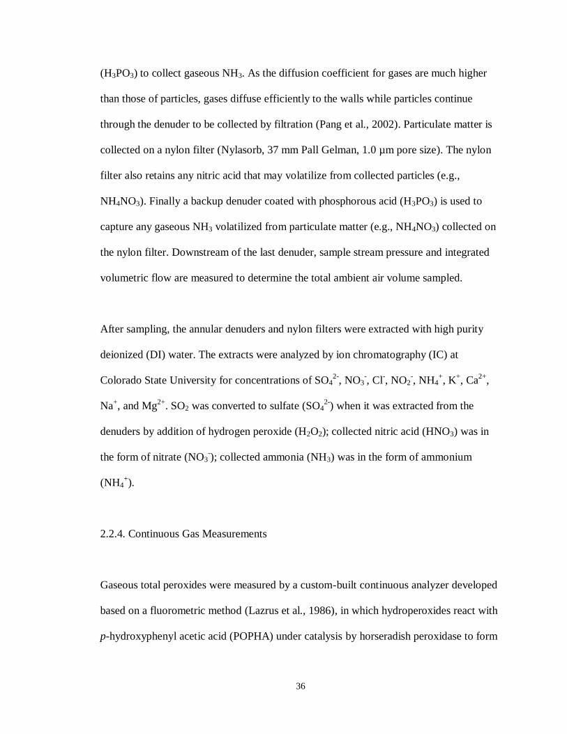
36

(H3PO3) to collect gaseous NH3. As the diffusion coefficient for gases are much higher

than those of particles, gases diffuse efficiently to the walls while particles continue

through the denuder to be collected by filtration (Pang et al., 2002). Particulate matter is

collected on a nylon filter (Nylasorb, 37 mm Pall Gelman, 1.0 µm pore size). The nylon

filter also retains any nitric acid that may volatilize from collected particles (e.g.,

NH4NO3). Finally a backup denuder coated with phosphorous acid (H3PO3) is used to

capture any gaseous NH3 volatilized from particulate matter (e.g., NH4NO3) collected on

the nylon filter. Downstream of the last denuder, sample stream pressure and integrated

volumetric flow are measured to determine the total ambient air volume sampled.

After sampling, the annular denuders and nylon filters were extracted with high purity

deionized (DI) water. The extracts were analyzed by ion chromatography (IC) at

Colorado State University for concentrations of SO42-

, NO3-, Cl

-, NO2

-, NH4

+, K

+, Ca

2+,

Na+, and Mg

2+. SO2 was converted to sulfate (SO4

2-) when it was extracted from the

denuders by addition of hydrogen peroxide (H2O2); collected nitric acid (HNO3) was in

the form of nitrate (NO3-); collected ammonia (NH3) was in the form of ammonium

(NH4+).

2.2.4. Continuous Gas Measurements

Gaseous total peroxides were measured by a custom-built continuous analyzer developed

based on a fluorometric method (Lazrus et al., 1986), in which hydroperoxides react with

p-hydroxyphenyl acetic acid (POPHA) under catalysis by horseradish peroxidase to form

37

a fluorescent POPHA dimer. The fluorescence intensity is proportional to the sampled

peroxide concentration. The instrument is calculated by injecting a series of aqueous

hydrogen peroxide standards. Details of the measurement method have been described

elsewhere (Ren et al., 2009). During the 2008 spring campaign high background levels of

H2O2 in purified water available at the site produced a high background for gas phase

peroxide measurements. S(IV) was added to the water, to consume H2O2 as it reacts to

sulfuric acid, in the summer 2008 campaign, to eliminate this problem.

Standard commercial instruments for measuring O3 and SO2 have been used in previous

field studies and have been described in detail elsewhere (Wang et al., 2001; Wang et al.,

2002; Wang et al., 2003; Wang et al., 2006). Briefly, O3 was measured using a UV

photometric O3 analyzer (Thermo Electron Corporation, Environmental Instruments,

model 49C) and SO2 was measured by a pulsed fluorescence SO2 analyzer (Thermo

Electron Corporation, Environmental Instruments, model 43C Trace Level).

2.3. SAMPLING

When the LWC was higher than 100 mg/m3 and the cloud appeared thick from all

directions, cloud collectors were turned on and run continuously until the cloud

dissipated; collecting bottles were generally changed at intervals of one or two hours.

Gas monitors were run continuously during the campaigns, although periodic zero and

span checks prevented ambient measurement during some short periods.

38

The URG denuder/filter pack system was run daily in the 2008 campaigns from 8:00 AM

to 8:00 AM local time. When cloud was present, sampling was interrupted and interstitial

air (air between the cloud drops) was sampled on a second instrument channel. This

approach permits investigation of PM2.5 and trace gas composition and concentrations

before cloud, during cloud and after cloud.

2.4. ON SITE PROCEDURES AND LABORATORY ANALYSIS

Aliquots were prepared on-site for each cloudwater sample for stabilization and later

analysis of key species including major ions (Na+, NH4

+, K

+, Mg

2+, Ca

2+, Cl

-, SO4

2-, and

NO3-), S(IV), metals (Fe and Mn), HCHO, H2O2, organic acids, and total organic carbon

(TOC). All aliquots and leftover sample portions were stored in a refrigerator on-site and

were shipped and kept refrigerated until analysis. 2007 campaign samples were analyzed

at Shandong University utilizing procedures recommended by CSU. 2008 campaign

samples were returned to the United States for analysis at CSU. Procedures for sample

measurement, including aliquot preparation and analysis, are provided below.

2.4.1. Sample weight

The sample weight was measured immediately after the cloudwater was collected.

2.4.2. Sample pH

39

The sample pH was measured using a portable pH meter (Orion model 290A, Thermo

Electron Co., Massachusetts, USA) with a microelectrode (Microelectrodes Inc. model

MI-710) calibrated with standard pH 4 and 7 buffers.

2.4.3. Major ions

Aliquots for inorganic ion analysis were prepared by pipetting 0.6 ml of cloudwater into a

polyethylene autosampler vial with Teflon lined septum. The inorganic ion analysis was

completed using two DIONEX DX-500 series cation and anion ion chromatography (IC)

systems and standard methods of analysis. A Dionex AG14A-SC guard column, an

AS14A-SC separation column, an ASRS-300 self-regenerating anion suppressor and

8mM Na2CO3 / 7mM NaHCO3 eluent were used to quantify concentrations of major

anions (Cl-, SO4

2-, and NO3

-). A Dionex CG12A-5µm guard column, a CS12A-5µm

separation column, a CSRS-300 self-regenerating cation suppressor and Methanesulfonic

Acid 20mM eluent were used to quantify concentrations of major cations (Na+, NH4

+, K

+,

Mg2+

, and Ca2+

). NIST-traceable accuracy check standards, DI water, and replicate

samples were run every 10 samples to establish calibration accuracy, verify lack of

sample carryover, and establish analytical method precision. Denuder and filter extracts

were analyzed for inorganic anions and cations following these same procedures.

2.4.4. S(IV)

40

Aliquots for S(IV) analysis were prepared by adding a preservative solution on site. The

preservative solution contains formaldehyde, trans-1,2-Cylohexylenedinitrilo-tetraacetic

acid (CDTA) and sodium hydroxide, wherein S(IV) reacts with formaldehyde to form a

stable compound hydroxymethanesulfonate (HMS). HMS can be decomposed to free

S(IV) and formaldehyde by adding sodium hydroxide solution, and then free S(IV) and

formaldehyde react with acidic pararosaniline (PRA, C19H19N3O) to form a color product

(Dasgupta et al., 1980), which can be measured by absorbance at a wavelength of 580

nm. Instrument response was calibrated through analysis of laboratory-prepared aqueous

solutions of sodium sulfite.

2.4.5. Metals

Fe and Mn were stabilized by adding nitric acid and measured by a Varian SpectrAA-

640Z Graphite Furnace Atomic Absorption Spectrophotometer (GFAAS) with a Varian

GTA-100 graphite tube atomizer and Zeeman background correction. The GFAAS was

calibrated using NIST-traceable commercial calibration solutions.

2.4.6. HCHO

Aliquots for formaldehyde analysis were prepared by adding a formaldehyde preservation

solution containing bisulfite on-site to form HMS. Thereafter HMS can be decomposed

to formaldehyde to be analyzed later in the lab through reaction with 2,4-pentanedione

and ammonium acetate to form 3,5-diacetyl-1,4-dihydrolutidine (DDL)(Dong and

41

Dasgupta, 1987) which can be detected by fluorescence. 2008 analyses completed at CSU

were measured on a Shimadzu model RF-1501 fluorescence spectrophotometer,

calibrated with laboratory-prepared HCHO standard solutions. Excitation wavelength of

412 nm, emission wavelength of 510 nm, excitation band width of 10 nm, and emission

band width of 20 nm were used for fluorescence analysis.

2.4.7. Aqueous H2O2

Aliquots for aqueous H2O2 analysis were preserved on-site by addition of a buffered

solution of p-hydroxyphenylacetic acid (POPHA) to form a fluorescent dimer under the

catalysis of horseradish peroxidase (Lazrus et al., 1985). The concentration of the dimer,

which is equal to the original sample peroxide concentration, was measured by a

fluorescence spectrophotometer. 2008 analyses completed at CSU were measured on a

Shimadzu model RF-1501 fluorescence spectrophotometer, calibrated with H2O2

standard solutions. Excitation wavelength of 320 nm, emission wavelength of 400 nm,

excitation band width of 10 nm, and emission band width of 10 nm were used for

fluorescence analysis.

2.4.8. Organic acids

Aliquots for organic acid analysis were preserved by addition of a small amount of

biocide (chloroform) and analyzed by ion chromatography. Analysis was completed on a

42

Dionex DX-500 IC using a Dionex AS11-HC separation column, a NaOH gradient

elution, anion suppressor, and conductivity detection.

2.4.9. TOC

Total organic carbon (TOC) was measured by a TOC analyzer (Shimadzu TOC-V CSH)

equipped with an automatic sample injector (ASI-V). Samples were analyzed without

filtration in order to capture both dissolved and suspended particulate organic matter in

the cloudwater. Instrument response was calibrated using laboratory-prepared aqueous

standards of potassium hydrogen phthalate.

2.5. QUALITY ASSURANCE AND CONTROL

2.5.1. Collector cleaning and blanks

Cloud collectors were cleaned thoroughly with Triton-X100 and rinsed with deionized

(DI) water prior to each field campaign. Cloud collectors were cleaned with DI water

after each cloud event and field blanks were collected and aliquotted for analysis using

the sample preparation procedures described above. After cleaning and drying for an

appropriate time, the cloud collectors were covered by clean plastic bags to avoid

contamination by dust. Samples collected during the first several minutes of each event

were discarded to avoid any influence by dust or residual DI rinse water dilution.

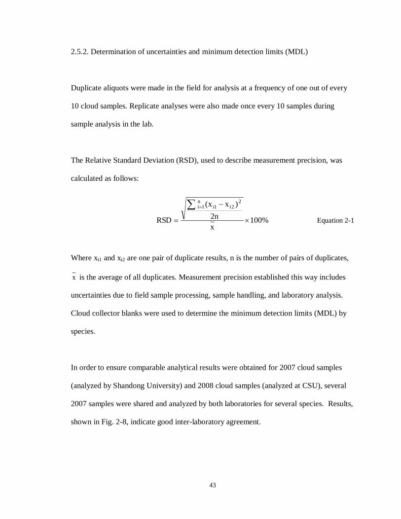
43

2.5.2. Determination of uncertainties and minimum detection limits (MDL)

Duplicate aliquots were made in the field for analysis at a frequency of one out of every

10 cloud samples. Replicate analyses were also made once every 10 samples during

sample analysis in the lab.

The Relative Standard Deviation (RSD), used to describe measurement precision, was

calculated as follows:

%100x

2n

)xx(

RSD

22i1i

n1i

Equation 2-1

Where xi1 and xi2 are one pair of duplicate results, n is the number of pairs of duplicates,

x is the average of all duplicates. Measurement precision established this way includes

uncertainties due to field sample processing, sample handling, and laboratory analysis.

Cloud collector blanks were used to determine the minimum detection limits (MDL) by

species.

In order to ensure comparable analytical results were obtained for 2007 cloud samples

(analyzed by Shandong University) and 2008 cloud samples (analyzed at CSU), several

2007 samples were shared and analyzed by both laboratories for several species. Results,

shown in Fig. 2-8, indicate good inter-laboratory agreement.

44

Figure 2-8. Interlaboratory comparisons for several samples collected in 2007 measured by

Shandong University (SDU) and Colorado State University (CSU).

0

2

4

6

8

10

0 2 4 6 8 10

CS

U

SDU

HCHO (µM)

0

1000

2000

3000

0 1000 2000 3000

CS

U

SDU

Unit: µN

AmmoniumSulfateNitrate

45

CHAPTER 3 RESULTS AND DISCUSSION

3.1. SUMMARY OF SAMPLING

Numerous periods of cloud interception/fog occurred during the four Mt. Tai field

campaigns. During the spring 2007 campaign (03/22-04/22), there were 9 cloud events; a

total of 36 bulk cloudwater samples were collected. During the summer 2007 campaign

(06/20-07/20), there were 12 cloud events; a total of 66 bulk samples were collected.

During the spring 2008 campaign (03/28-04/25), there were 4 cloud events; a total of 83

cloudwater samples (including 25 bulk samples and 58 size-fractionated samples) were

collected. During the summer 2008 campaign (06/14-07/16), there were 18 cloud events;

a total of 333 cloudwater samples (including 117 bulk samples and 216 size-fractionated

samples) were collected.

More detailed summary data for the sampled events are provided in chapter 4, by

campaign. The summaries include the number of events in each campaign, the date and

time period of each sampled event, and the average (volume-weighted) cloudwater

concentrations of several key species. The summaries also include estimated altitudes of

cloud base for each event. Complete information about individual samples is provided in

the data tables included in Appendix B and Appendix C.

46

Figure 3-1 shows the liquid water content (LWC) observations during the spring 2008

campaign. The four cloud interception episodes are readily apparent. Peak LWC values in

the events were several hundred mg/m3.

Figure 3-1. Spring 2008 Liquid Water Content.

Figure 3-2. Summer 2008 Liquid Water Content.

0

150

300

450

600

750

900

3/26 3/28 3/31 4/2 4/5 4/7 4/10 4/12 4/15 4/17 4/20 4/22 4/25

LW

C (

mg/m

3)

Date

2008 Spring Liquid Water Content

0

150

300

450

600

750

900

6/15 6/16 6/17 6/18 6/20 6/21 6/22 6/23 6/25 6/26 6/27 6/28

LW

C (

mg

/m3)

Date

2008 Summer Liquid Water Content

47

Figure 3-2 shows the LWC observations during the summer 2008 campaign. A very

active period of cloud interception is apparent between June 16 and 20. The PVM was

disabled by a lightning strike midway through the summer 2008 campaign. Estimates of

LWC for cloud interception periods after this time were obtained based on the cloudwater

collection rate of the sf-CASCC. As discussed by Demoz et al. (1996), the rate of water

collection by the CASCC family of collectors is closely related to the cloud LWC. The

relationship between sf-CASCC cloudwater collection rate and PVM LWC is examined

in Fig. 3-3. Here we see a strong correlation (R2 = 0.94). A best-fit line to this data set is

described by equation 3-1.

Figure 3-3. The relationship between sf-CASCC cloudwater collection rate and PVM LWC.

2.443.97RateCollectionLWC Equation 3-1

0

100

200

300

400

500

600

0 1 2 3 4 5 6

LW

C (

mg

/m3)

Collection Rate (ml/min)

Spring Summer

48

3.2. GASEOUS SPECIES

Key gas phase species associated with aqueous sulfate production include sulfur dioxide,

ozone, and hydrogen peroxide. Summaries of concentrations of these key species are

provided below.

3.2.1. Gaseous H2O2

Ren et al. (2009) present a detailed analysis of the H2O2 concentrations measured at Mt.

Tai in the spring and summer 2007 campaigns. H2O2 concentrations were generally lower

in spring (2007 average mixing ratio of 0.17 ppbv) than in summer (2007 average mixing

ratio of 0.55 ppbv). A similar pattern was observed in 2008, when spring H2O2 mixing

ratios averaged 1.14 ppbv (the spring 2008 gaseous H2O2 data were affected by the high

H2O2 in the analyzer system coming from the purified water bottles- the average value of

1.14 ppbv was calculated from several days that the signals were reasonable, all these

days did not have cloud. An H2O2 mixing ratio of 0.1 ppbv was used to estimate in-cloud

S(IV) oxidation rates for spring 2008). Summer 2008 H2O2 mixing ratios averaged 0.59

ppbv. Higher H2O2 concentrations are expected in summer, when more active

photochemistry occurs, promoting H2O2 formation through both gas and aqueous phase

reactions. Summertime gaseous H2O2 mixing ratios at Mt. Tai were observed to climb as

high as 4 ppbv. Because of the fast aqueous phase reaction between H2O2 and dissolved

SO2, one might expect to observe an anti-correlation between gaseous H2O2

concentrations and the presence of clouds.

49

Figure 3-4. Timelines of gaseous H2O2 mixing ratio and cloud LWC observed at the Mt. Tai

summit, 6/15-6/28/2008.

Figure 3-4 explores this relationship, plotting timelines of the gaseous H2O2 mixing ratio

and the cloud LWC measured by the PVM for the first two weeks of the summer 2008

campaign (June 15 - June 28), before the lightning strike disabled the PVM. It is

important to keep in mind that the PVM LWC only indicates the presence of clouds

intercepting the Mt. Tai summit; it does not indicate whether clouds are present nearby

that might also provide a medium for H2O2 reaction with dissolved SO2. Nevertheless,

Figure 3-4 illustrates a clear relationship between cloud interception and gas phase H2O2

mixing ratios. During the first half of the illustrated period, clouds were observed

frequently at the summit of Mt. Tai and H2O2 mixing ratios generally stayed below 0.5

ppbv. During the second half of the period, cloud interception was much less common

and H2O2 mixing ratios regularly climbed into the 2-4 ppbv range. The disappearance of

0

1

2

3

4

5

0

150

300

450

600

750

900

6/15 6/16 6/17 6/18 6/20 6/21 6/22 6/23 6/25 6/26 6/27 6/28

H2O

2C

on

cen

trati

on

(p

pb

)

LW

C (

mg/m

3)

Date

Liquid Water Content

Hydrogen Peroxide

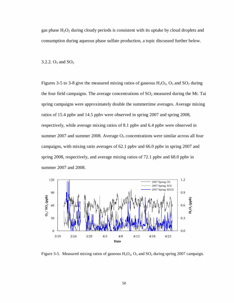
50

gas phase H2O2 during cloudy periods is consistent with its uptake by cloud droplets and

consumption during aqueous phase sulfate production, a topic discussed further below.

3.2.2. O3 and SO2

Figures 3-5 to 3-8 give the measured mixing ratios of gaseous H2O2, O3 and SO2 during

the four field campaigns. The average concentrations of SO2 measured during the Mt. Tai

spring campaigns were approximately double the summertime averages. Average mixing

ratios of 15.4 ppbv and 14.5 ppbv were observed in spring 2007 and spring 2008,

respectively, while average mixing ratios of 8.1 ppbv and 6.4 ppbv were observed in

summer 2007 and summer 2008. Average O3 concentrations were similar across all four

campaigns, with mixing ratio averages of 62.1 ppbv and 66.0 ppbv in spring 2007 and

spring 2008, respectively, and average mixing ratios of 72.1 ppbv and 68.0 ppbv in

summer 2007 and 2008.


0.0

0.3

0.6

0.9

1.2

3/19 3/24 3/29 4/3 4/8 4/13 4/18 4/23

H2O

2(p

pb

)

O3

/ S

O2

(pp

b)

Date

2007 Spring O3

2007 Spring SO2

2007 Spring H2O2

51

Figure 3-6. Measured mixing ratios of gaseous H2O2, O3 and SO2 during summer 2007 campaign.



campaign.

0

1

2

3

4

5

6/14 6/19 6/24 6/29 7/4 7/9 7/14

H2O

2(p

pb

)

O3

/ S

O2

(pp

b)

Date

2007 Summer O3

2007 Summer SO2

2007 Summer H2O2

0

0.5

1

1.5

2

3/24 3/29 4/3 4/8 4/13 4/18 4/23 4/28

H2O

2 (p

pb

)

O3 / S

O2 (

pp

b)

Date

2008 Spring O3

2008 Spring SO2

2008 Spring H2O2

0

1

2

3

4

5

6/15 6/20 6/25 6/30 7/5 7/10 7/15

H2O

2(p

pb

)

O3

/ S

O2

(pp

b)

Date

2008 Summer O3

2008 Summer SO2

2008 Summer H2O2

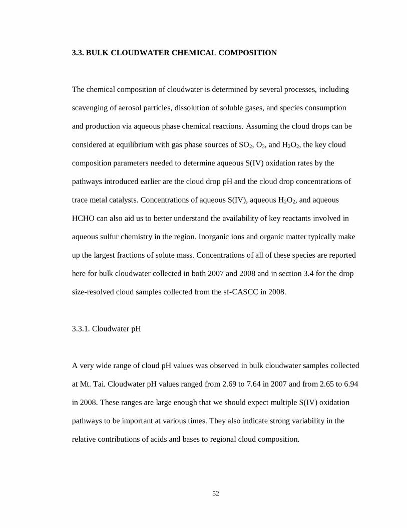
52

3.3. BULK CLOUDWATER CHEMICAL COMPOSITION

The chemical composition of cloudwater is determined by several processes, including

scavenging of aerosol particles, dissolution of soluble gases, and species consumption

and production via aqueous phase chemical reactions. Assuming the cloud drops can be

considered at equilibrium with gas phase sources of SO2, O3, and H2O2, the key cloud

composition parameters needed to determine aqueous S(IV) oxidation rates by the

pathways introduced earlier are the cloud drop pH and the cloud drop concentrations of

trace metal catalysts. Concentrations of aqueous S(IV), aqueous H2O2, and aqueous

HCHO can also aid us to better understand the availability of key reactants involved in

aqueous sulfur chemistry in the region. Inorganic ions and organic matter typically make

up the largest fractions of solute mass. Concentrations of all of these species are reported

here for bulk cloudwater collected in both 2007 and 2008 and in section 3.4 for the drop

size-resolved cloud samples collected from the sf-CASCC in 2008.

3.3.1. Cloudwater pH

A very wide range of cloud pH values was observed in bulk cloudwater samples collected

at Mt. Tai. Cloudwater pH values ranged from 2.69 to 7.64 in 2007 and from 2.65 to 6.94

in 2008. These ranges are large enough that we should expect multiple S(IV) oxidation

pathways to be important at various times. They also indicate strong variability in the

relative contributions of acids and bases to regional cloud composition.

53

Frequency distributions of observed pH values in the four sampling campaigns are shown

in Figure 3-9. The average pH values (determined as the volume weighted average H+

concentrations) in spring and summer 2007 were 3.68 and 4.10, respectively. The average

pH values in spring and summer 2008 were 4.34 and 3.77, respectively.

Figure 3-9. Frequency distributions of the pH values measured in bulk (CASCC) cloudwater

samples collected at Mt. Tai in the four sampling campaigns.

3.3.2. TOC

Total organic carbon concentrations in cloudwater are the result both of scavenging of

organic aerosol particles and uptake of soluble volatile organic compounds (VOC).

Frequency distributions of bulk cloudwater TOC concentrations observed at Mt. Tai in

the 2008 sampling campaigns are shown in Figure 3-10. TOC concentrations (volume-

0

5

10

15

20

25

30

2.5 3 3.5 4 4.5 5 5.5 6 6.5 7

Nu

mb

er o

f sa

mp

les

pH

2007 Spring Average = 3.68, 2007 Summer Average = 4.10


2007 Spring

2007 Summer

2008 Spring

2008 Summer

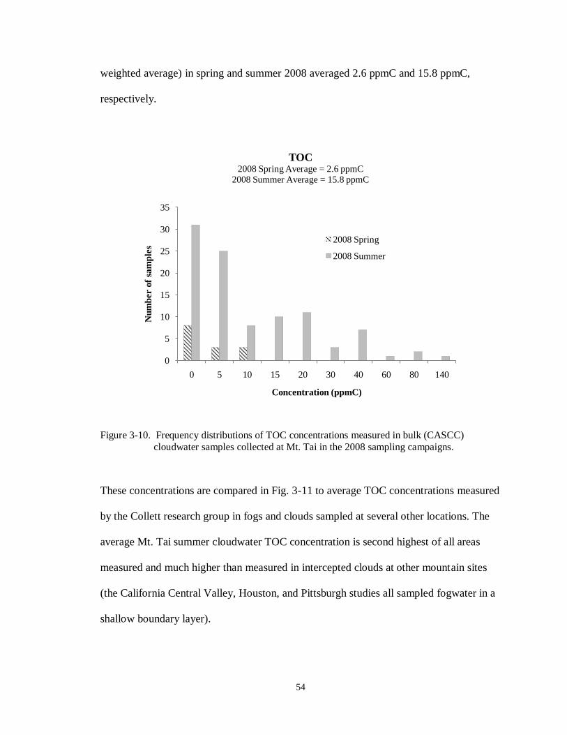
54

weighted average) in spring and summer 2008 averaged 2.6 ppmC and 15.8 ppmC,

respectively.

Figure 3-10. Frequency distributions of TOC concentrations measured in bulk (CASCC)

cloudwater samples collected at Mt. Tai in the 2008 sampling campaigns.

These concentrations are compared in Fig. 3-11 to average TOC concentrations measured

by the Collett research group in fogs and clouds sampled at several other locations. The

average Mt. Tai summer cloudwater TOC concentration is second highest of all areas

measured and much higher than measured in intercepted clouds at other mountain sites

(the California Central Valley, Houston, and Pittsburgh studies all sampled fogwater in a

shallow boundary layer).

0

5

10

15

20

25

30

35

0 5 10 15 20 30 40 60 80 140

Nu

mb

er o

f sa

mp

les

Concentration (ppmC)

TOC2008 Spring Average = 2.6 ppmC

2008 Summer Average = 15.8 ppmC

2008 Spring

2008 Summer

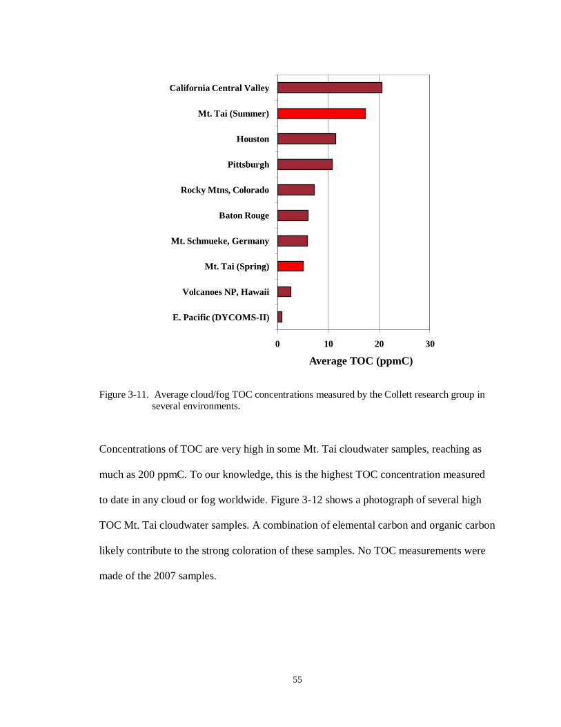
55

Figure 3-11. Average cloud/fog TOC concentrations measured by the Collett research group in several environments.

Concentrations of TOC are very high in some Mt. Tai cloudwater samples, reaching as

much as 200 ppmC. To our knowledge, this is the highest TOC concentration measured

to date in any cloud or fog worldwide. Figure 3-12 shows a photograph of several high

TOC Mt. Tai cloudwater samples. A combination of elemental carbon and organic carbon

likely contribute to the strong coloration of these samples. No TOC measurements were

made of the 2007 samples.

0 10 20 30

E. Pacific (DYCOMS-II)

Volcanoes NP, Hawaii

Mt. Tai (Spring)

Mt. Schmueke, Germany

Baton Rouge

Rocky Mtns, Colorado

Pittsburgh

Houston

Mt. Tai (Summer)

California Central Valley

Average TOC (ppmC)

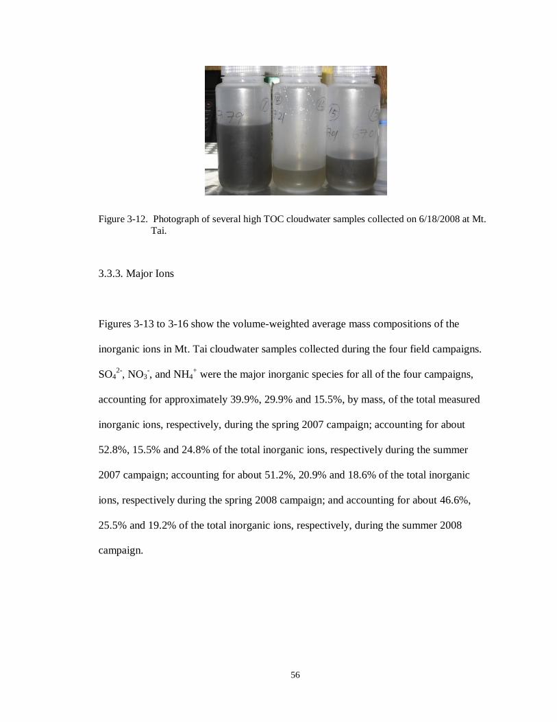
56

Figure 3-12. Photograph of several high TOC cloudwater samples collected on 6/18/2008 at Mt.

Tai.

3.3.3. Major Ions

Figures 3-13 to 3-16 show the volume-weighted average mass compositions of the

inorganic ions in Mt. Tai cloudwater samples collected during the four field campaigns.

SO42-

, NO3-, and NH4

+ were the major inorganic species for all of the four campaigns,

accounting for approximately 39.9%, 29.9% and 15.5%, by mass, of the total measured

inorganic ions, respectively, during the spring 2007 campaign; accounting for about

52.8%, 15.5% and 24.8% of the total inorganic ions, respectively during the summer

2007 campaign; accounting for about 51.2%, 20.9% and 18.6% of the total inorganic

ions, respectively during the spring 2008 campaign; and accounting for about 46.6%,

25.5% and 19.2% of the total inorganic ions, respectively, during the summer 2008

campaign.

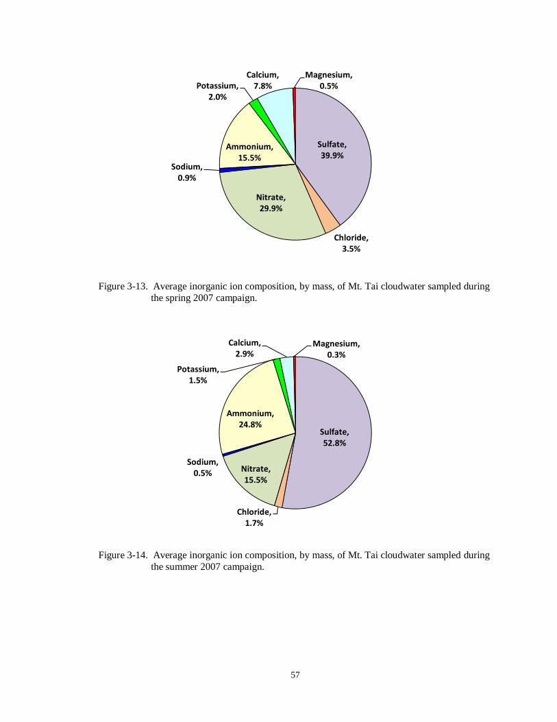
57


the spring 2007 campaign.


the summer 2007 campaign.

Sulfate, 39.9%

Chloride, 3.5%

Nitrate, 29.9%

Sodium, 0.9%

Ammonium, 15.5%

Potassium, 2.0%

Calcium, 7.8%

Magnesium, 0.5%

Sulfate, 52.8%

Chloride, 1.7%

Nitrate, 15.5%

Sodium, 0.5%

Ammonium, 24.8%

Potassium, 1.5%

Calcium, 2.9%

Magnesium, 0.3%

58




the summer 2008 campaign.

Sulfate, 51.2%

Chloride, 2.7%

Nitrate, 20.9%

Sodium, 0.7%

Ammonium, 18.6%

Potassium, 1.5%

Calcium, 3.9%

Magnesium, 0.5%

Sulfate, 46.6%

Chloride, 4.1%

Nitrate, 25.5%

Sodium, 0.3%

Ammonium, 19.2%

Potassium, 2.5%

Calcium, 1.6%

Magnesium, 0.2%

59

Figures 3-17 and 3-18 show the average mass compositions of the cloudwater samples,

including both organic matter and inorganic ions, for the spring and summer 2008

campaigns, respectively. The mass of organic matter was estimated as 1.8 times the TOC

concentration in order to account for other constituents commonly found in organic

molecules (e.g., H and O). The 1.8 multiplier was chosen based on a comparison of

various methods used to estimate OM/OC (Chan et al., 2010), the value 1.8 estimated by

Zhang et al. (2005) from m/z ratios of the AMS mass spectra for organic aerosols

measured in field experiments (Zhang et al., 2005) was adopted in this study. Given the

more polar nature and high oxygen content typical of organic matter found in clouds and

fogs, a ratio of 1.8 is considered a conservative estimate.

60

Figure 3-17. Average composition, by mass, of Mt. Tai cloudwater sampled during the spring

2008 campaign.

Figure 3-18. Average composition, by mass, of Mt. Tai cloudwater sampled during the summer

2008 campaign.

Sulfate, 43.1%

Chloride, 2.3%

Nitrate, 17.6%

Sodium, 0.6%

Ammonium, 15.6%

Potassium, 1.3%

Calcium, 3.3%

Magnesium, 0.4%

Organic Matter, 15.8%

Sulfate, 36.6%

Chloride, 3.2%

Nitrate, 20.0%

Sodium, 0.2%

Ammonium, 15.0%

Potassium, 1.9%

Calcium, 1.3%

Magnesium, 0.1%

Organic Matter, 21.6%

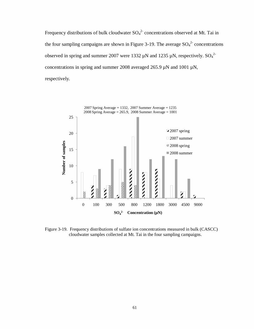
61

Frequency distributions of bulk cloudwater SO42-

concentrations observed at Mt. Tai in

the four sampling campaigns are shown in Figure 3-19. The average SO42-

concentrations

observed in spring and summer 2007 were 1332 µN and 1235 µN, respectively. SO42-

concentrations in spring and summer 2008 averaged 265.9 µN and 1001 µN,

respectively.

Figure 3-19. Frequency distributions of sulfate ion concentrations measured in bulk (CASCC)

cloudwater samples collected at Mt. Tai in the four sampling campaigns.

0

5

10

15

20

25

0 100 300 500 800 1200 1800 3000 4500 9000

Nu

mb

er o

f sa

mp

les

SO42- Concentration (µN)

2007 Spring Average = 1332, 2007 Summer Average = 12352008 Spring Average = 265.9, 2008 Summer Average = 1001

2007 spring

2007 summer

2008 spring

2008 summer

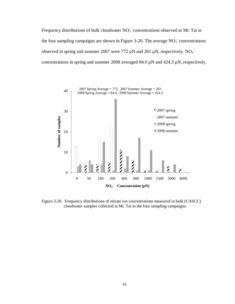
62

Frequency distributions of bulk cloudwater NO3- concentrations observed at Mt. Tai in

the four sampling campaigns are shown in Figure 3-20. The average NO3- concentrations

observed in spring and summer 2007 were 772 µN and 281 µN, respectively. NO3-

concentrations in spring and summer 2008 averaged 84.0 µN and 424.3 µN, respectively.

Figure 3-20. Frequency distributions of nitrate ion concentrations measured in bulk (CASCC)


0

10

20

30

40

0 50 100 200 400 600 1000 1500 3000 6000

Nu

mb

er o

f sa

mp

les

NO3- Concentration (µN)

2007 Spring Average = 772, 2007 Summer Average = 2812008 Spring Average = 84.0, 2008 Summer Average = 424.3

2007 spring

2007 summer

2008 spring

2008 summer

63

Fig. 3-21 compares sulfate and nitrate concentrations measured at Mt. Tai with sulfate

and nitrate concentrations measured by the Collett research group in clouds and fogs at

several other locations. The average nitrate concentrations measured at Mt. Tai are

similar to those measured in polluted clouds and fogs from several U.S. locations. Mt.

Tai cloudwater sulfate concentrations, while high, are not higher than those measured in

the 1990s at some locations in the eastern U.S.

Figure 3-21. Average concentrations of sulfate and nitrate measured in 2008 spring and summer in Mt. Tai cloudwater (this study) and in clouds and fogs from several other

locations (Collett et al., 2002; Raja et al., 2008; unpublished data).

0

1000

2000

3000

4000

Mt.

Ta

i (S

P)

Mt.

Ta

i (S

U)

SJ

V

Sa

c V

al

So. C

al.

E P

acif

ic

Oreg

on

Coa

st

Colo

ra

do

Rock

ies

Ba

ton

Rou

ge

Hou

ston

Mt.

Mit

ch

ell

Wh

itefa

ce M

t.

Pit

tsb

urg

h

Avg. C

on

c. (

µN

)

Nitrate Sulfate

64

Frequency distributions of bulk cloudwater Cl- concentrations observed at Mt. Tai in the

four sampling campaigns are shown in Figure 3-22. The average Cl- concentrations

observed in spring and summer 2007 were 156 µN and 55 µN, respectively. Cl-

concentrations in spring and summer 2008 averaged 19 µN and 119.4 µN, respectively.

Figure 3-22. Frequency distributions of chloride ion concentrations measured in bulk (CASCC)


0

10

20

30

40

0 10 30 60 100 200 400 600 900

Nu

mb

er o

f sa

mp

les

Cl- Concentration (µN)

2007 Spring Average = 156, 2007 Summer Average = 552008 Spring Average = 19, 2008 Summer Average = 119

2007 spring

2007 summer

2008 spring

2008 summer

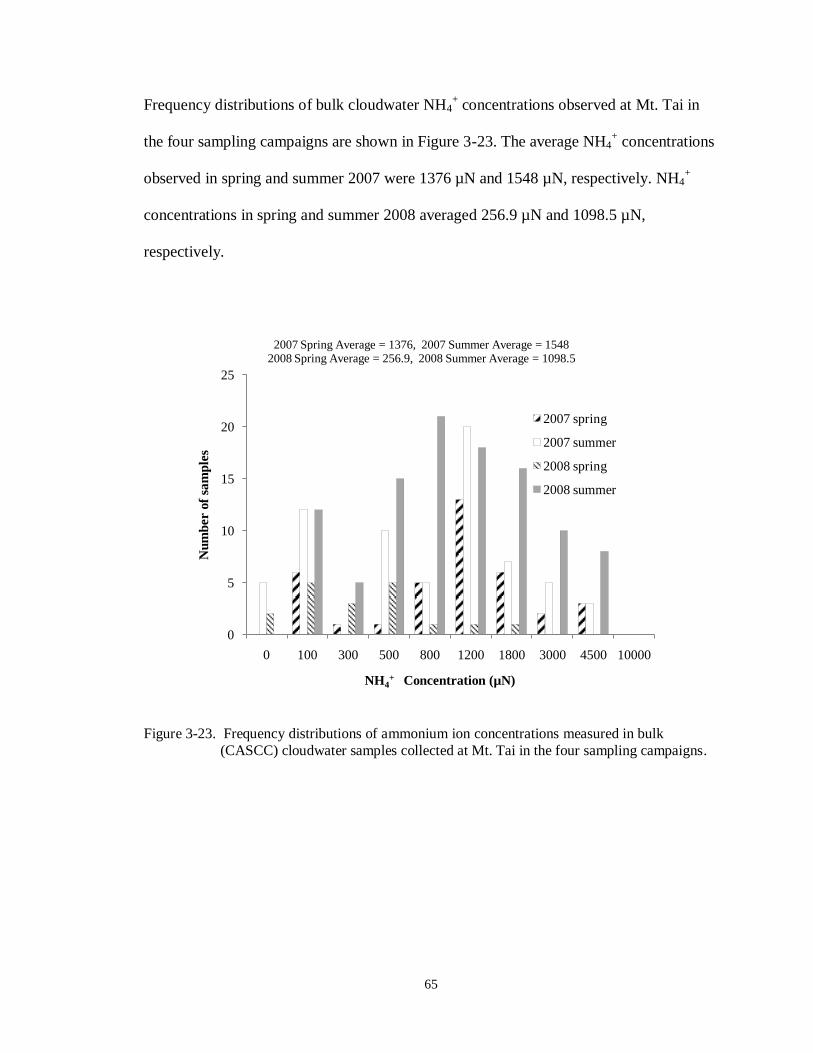
65

Frequency distributions of bulk cloudwater NH4+ concentrations observed at Mt. Tai in

the four sampling campaigns are shown in Figure 3-23. The average NH4+ concentrations

observed in spring and summer 2007 were 1376 µN and 1548 µN, respectively. NH4+

concentrations in spring and summer 2008 averaged 256.9 µN and 1098.5 µN,

respectively.

Figure 3-23. Frequency distributions of ammonium ion concentrations measured in bulk


0

5

10

15

20

25

0 100 300 500 800 1200 1800 3000 4500 10000

Nu

mb

er o

f sa

mp

les

NH4+ Concentration (µN)


2007 spring

2007 summer

2008 spring

2008 summer

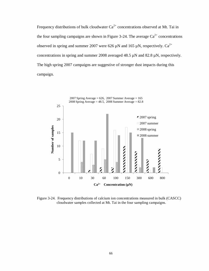
66

Frequency distributions of bulk cloudwater Ca2+


the four sampling campaigns are shown in Figure 3-24. The average Ca2+

concentrations

observed in spring and summer 2007 were 626 µN and 165 µN, respectively. Ca2+


The high spring 2007 campaigns are suggestive of stronger dust impacts during this

campaign.

Figure 3-24. Frequency distributions of calcium ion concentrations measured in bulk (CASCC)


0

5

10

15

20

25

0 10 30 60 100 150 300 600 800

Nu

mb

er o

f sa

mp

les

Ca2+ Concentration (µN)


2007 spring

2007 summer

2008 spring

2008 summer

67

Frequency distributions of bulk cloudwater K+ concentrations observed at Mt. Tai in the

four sampling campaigns are shown in Figure 3-25. The average K+ concentrations

observed in spring and summer 2007 were 83.3 µN and 42.2 µN, respectively. K+


Figure 3-25. Frequency distributions of potassium ion concentrations measured in bulk (CASCC)


0

10

20

30

0 10 25 50 75 100 150 200 250 500

Nu

mb

er o

f sa

mp

les

K+ Concentration (µN)

2007 Spring Average = 83.3, 2007 Summer Average = 42.22008 Spring Average = 9.6, 2008 Summer Average = 65.2

2007 spring

2007 summer

2008 spring

2008 summer

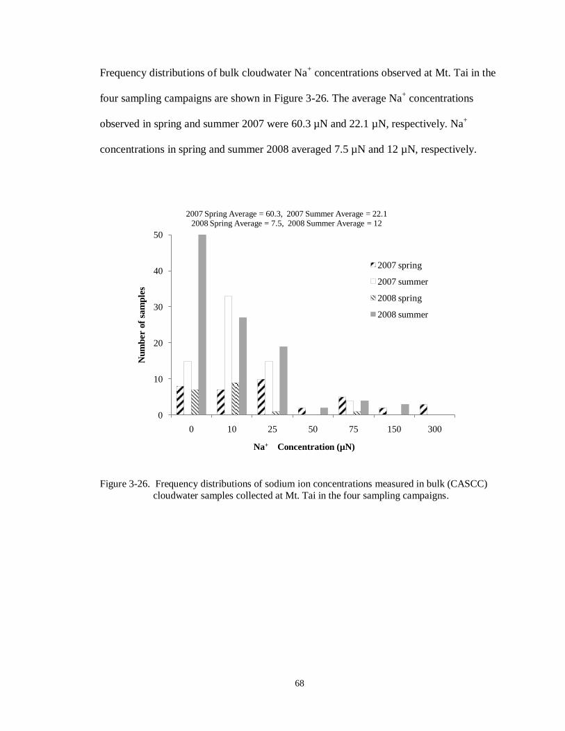
68

Frequency distributions of bulk cloudwater Na+ concentrations observed at Mt. Tai in the

four sampling campaigns are shown in Figure 3-26. The average Na+ concentrations

observed in spring and summer 2007 were 60.3 µN and 22.1 µN, respectively. Na+

concentrations in spring and summer 2008 averaged 7.5 µN and 12 µN, respectively.

Figure 3-26. Frequency distributions of sodium ion concentrations measured in bulk (CASCC)


0

10

20

30

40

50

0 10 25 50 75 150 300

Nu

mb

er o

f sa

mp

les

Na+ Concentration (µN)

2007 Spring Average = 60.3, 2007 Summer Average = 22.12008 Spring Average = 7.5, 2008 Summer Average = 12

2007 spring

2007 summer

2008 spring

2008 summer

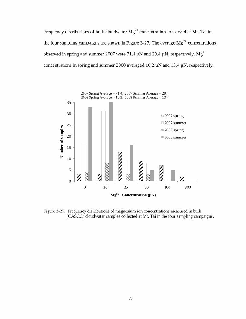
69

Frequency distributions of bulk cloudwater Mg2+


the four sampling campaigns are shown in Figure 3-27. The average Mg2+

concentrations

observed in spring and summer 2007 were 71.4 µN and 29.4 µN, respectively. Mg2+


Figure 3-27. Frequency distributions of magnesium ion concentrations measured in bulk


0

5

10

15

20

25

30

35

0 10 25 50 100 300

Nu

mb

er o

f sa

mp

les

Mg2+ Concentration (µN)


2007 spring

2007 summer

2008 spring

2008 summer

70

Figure 3-28. Correlations of [H+] with the concentrations of NO3-, SO4

2-, NH4

+, and Ca

2+.

0

500

1000

1500

2000

2500

3000

-1000 0 1000 2000 3000 4000

[H+]

(µN

)

[NO3-]+[SO4

2-]-[NH4+]-[Ca2+] (µN)

2007 spring 2007 Summer

0

50

100

150

200

250

300

350

400

450

-200 -100 0 100 200 300 400 500

[H+]

(µN

)

[NO3-]+[SO4

2-]-[NH4+]-[Ca2+] (µN)

2008 spring

0

500

1000

1500

2000

2500

-1000 0 1000 2000 3000 4000

[H+]

(µN

)

[NO3-]+[SO4

2-]-[NH4+]-[Ca2+] (µN)

16-Jun 18-Jun 19-Jun 20-Jun 21-Jun 25-Jun July

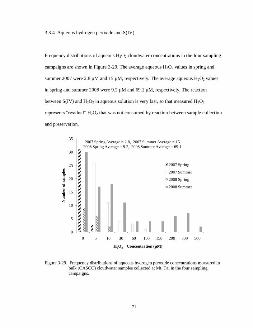
71

3.3.4. Aqueous hydrogen peroxide and S(IV)

Frequency distributions of aqueous H2O2 cloudwater concentrations in the four sampling

campaigns are shown in Figure 3-29. The average aqueous H2O2 values in spring and

summer 2007 were 2.8 µM and 15 µM, respectively. The average aqueous H2O2 values

in spring and summer 2008 were 9.2 µM and 69.1 µM, respectively. The reaction

between S(IV) and H2O2 in aqueous solution is very fast, so that measured H2O2

represents “residual” H2O2 that was not consumed by reaction between sample collection

and preservation.

Figure 3-29. Frequency distributions of aqueous hydrogen peroxide concentrations measured in

bulk (CASCC) cloudwater samples collected at Mt. Tai in the four sampling

campaigns.

0

5

10

15

20

25

30

35

0 5 10 30 60 100 150 200 300 500

Nu

mb

er o

f sa

mp

les

H2O2 Concentration (µM)

2007 Spring Average = 2.8, 2007 Summer Average = 15


2007 Spring

2007 Summer

2008 Spring

2008 Summer

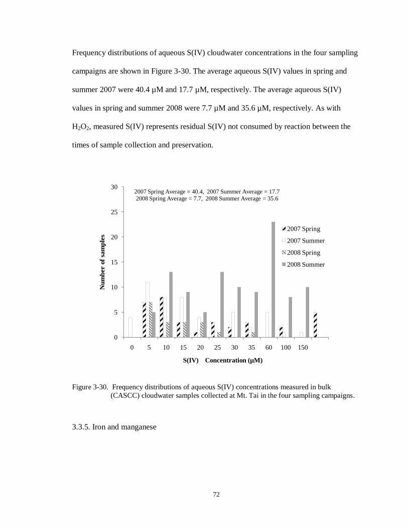
72

Frequency distributions of aqueous S(IV) cloudwater concentrations in the four sampling

campaigns are shown in Figure 3-30. The average aqueous S(IV) values in spring and

summer 2007 were 40.4 µM and 17.7 µM, respectively. The average aqueous S(IV)

values in spring and summer 2008 were 7.7 µM and 35.6 µM, respectively. As with

H2O2, measured S(IV) represents residual S(IV) not consumed by reaction between the

times of sample collection and preservation.

Figure 3-30. Frequency distributions of aqueous S(IV) concentrations measured in bulk


3.3.5. Iron and manganese

0

5

10

15

20

25

30

0 5 10 15 20 25 30 35 60 100 150

Nu

mb

er o

f sa

mp

les

S(IV) Concentration (µM)


2007 Spring

2007 Summer

2008 Spring

2008 Summer

73

As catalysts of the S(IV) autooxidation pathway, the aqueous concentrations of Fe(III)

and Mn(II) are also important to our study. Frequency distributions of bulk cloudwater Fe

concentrations observed at Mt. Tai in the four sampling campaigns are shown in Figure

3-31. The average bulk cloudwater Fe concentrations measured in spring and summer

2007 were 242.5 µg/L and 44.2 µg/L, respectively. Fe concentrations measured in spring

and summer 2008 averaged 241.8 µg/L and 415.7 µg/L, respectively. Higher Fe

concentrations observed in 2008 might reflect changes in regional emissions (industrial

activity was relocated outside Beijing in advance of the 2008 Summer Olympic Games)

or diferences in metals analysis between the SDU and CSU laboratories. For comparison,

total Fe was below 400 µg/L in Los Angeles basin cloudwater samples (Pehkonen et al.,

1992), averaged approximately 250 µg/L in clouds sampled at Great Dun Fell, U.K.

(Sedlak et al., 1997), was below 500 µg/L in clouds collected at the puy de Dome station

in France (Parazols et al., 2006) and ranged up to 886 µg/L in San Joaquin Valley,

California fogs (Rao and Collett, 1998).

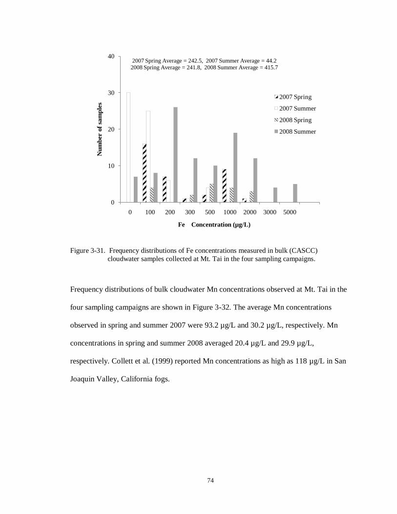
74

Figure 3-31. Frequency distributions of Fe concentrations measured in bulk (CASCC)


Frequency distributions of bulk cloudwater Mn concentrations observed at Mt. Tai in the

four sampling campaigns are shown in Figure 3-32. The average Mn concentrations

observed in spring and summer 2007 were 93.2 µg/L and 30.2 µg/L, respectively. Mn

concentrations in spring and summer 2008 averaged 20.4 µg/L and 29.9 µg/L,

respectively. Collett et al. (1999) reported Mn concentrations as high as 118 µg/L in San

Joaquin Valley, California fogs.

0

10

20

30

40

0 100 200 300 500 1000 2000 3000 5000

Nu

mb

er o

f sa

mp

les

Fe Concentration (µg/L)


2007 Spring

2007 Summer

2008 Spring

2008 Summer

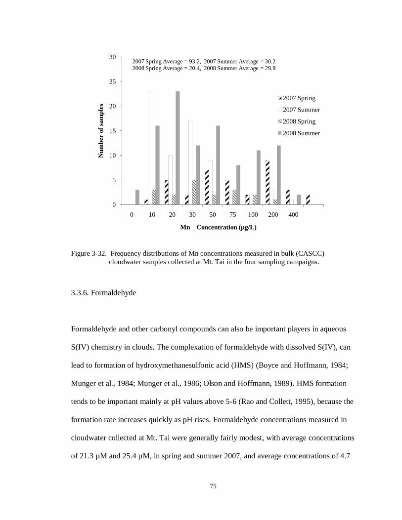
75

Figure 3-32. Frequency distributions of Mn concentrations measured in bulk (CASCC)


3.3.6. Formaldehyde

Formaldehyde and other carbonyl compounds can also be important players in aqueous

S(IV) chemistry in clouds. The complexation of formaldehyde with dissolved S(IV), can

lead to formation of hydroxymethanesulfonic acid (HMS) (Boyce and Hoffmann, 1984;

Munger et al., 1984; Munger et al., 1986; Olson and Hoffmann, 1989). HMS formation

tends to be important mainly at pH values above 5-6 (Rao and Collett, 1995), because the

formation rate increases quickly as pH rises. Formaldehyde concentrations measured in

cloudwater collected at Mt. Tai were generally fairly modest, with average concentrations

of 21.3 µM and 25.4 µM, in spring and summer 2007, and average concentrations of 4.7

0

5

10

15

20

25

30

0 10 20 30 50 75 100 200 400

Nu

mb

er o

f sa

mp

les

Mn Concentration (µg/L)


2007 Spring

2007 Summer

2008 Spring

2008 Summer

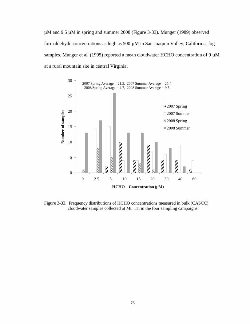
76

µM and 9.5 µM in spring and summer 2008 (Figure 3-33). Munger (1989) observed

formaldehyde concentrations as high as 500 µM in San Joaquin Valley, California, fog

samples. Munger et al. (1995) reported a mean cloudwater HCHO concentration of 9 µM

at a rural mountain site in central Virginia.

Figure 3-33. Frequency distributions of HCHO concentrations measured in bulk (CASCC)


0

5

10

15

20

25

30

0 2.5 5 10 15 20 30 40 60

Nu

mb

er o

f sa

mp

les

HCHO Concentration (µM)


2007 Spring

2007 Summer

2008 Spring

2008 Summer

77

3.4. DROP SIZE-DEPENDENT CLOUDWATER CHEMICAL COMPOSITIONS

As described in chapter 1, differences between the chemical composition of different

drops within a cloud can affect the cloud chemistry, including rates of S(IV) oxidation or

complexation. Here we present drop size-dependent concentrations of several major

cloudwater solutes and other species of key importance to rates of S(IV) reaction. These

data are taken from the two-stage size-fractionating CASCC.

3.4.1. Cloudwater pH

Figure 3-34 compares the pH values measured in small and large droplet fractions

collected with the sf-CASCC during the 2008 field campaigns. While only a small pH

difference is observed between the small and large drop fractions during many sample

periods, fairly large pH differences of 0.5 – 1.0 pH units or greater, are observed in many

other cases. The most common pattern is for large cloud drops to have a higher pH than

small cloud drops, similar to the pattern first reported by Collett et al. (1994) for cloud

and fog samples from a variety of environments. Differences in cloud composition as a

function of drop size can arise from a variety of factors including differences in the

composition of cloud condensation nuclei (CCN) that nucleate small and large cloud

drops, drop size-dependent condensational growth rates, and differences in the rate of

uptake of soluble gases between small and large droplets (Ogren and Charlson, 1992;

Bator and Collett, 1997; Moore et al., 2004a; Moore et al., 2004b). Understanding the

distribution of pH values in a population of cloud drops can be important for accurately

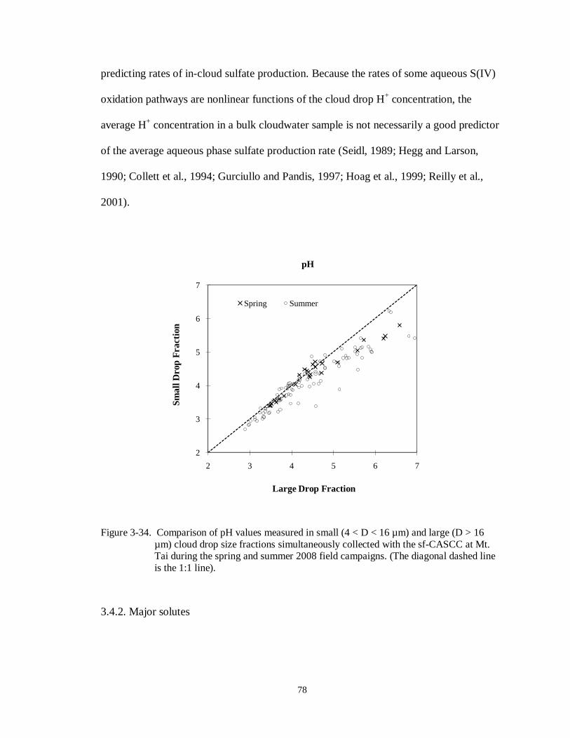
78

predicting rates of in-cloud sulfate production. Because the rates of some aqueous S(IV)

oxidation pathways are nonlinear functions of the cloud drop H+ concentration, the

average H+ concentration in a bulk cloudwater sample is not necessarily a good predictor

of the average aqueous phase sulfate production rate (Seidl, 1989; Hegg and Larson,

1990; Collett et al., 1994; Gurciullo and Pandis, 1997; Hoag et al., 1999; Reilly et al.,

2001).

Figure 3-34. Comparison of pH values measured in small (4 < D < 16 µm) and large (D > 16

µm) cloud drop size fractions simultaneously collected with the sf-CASCC at Mt. Tai during the spring and summer 2008 field campaigns. (The diagonal dashed line

is the 1:1 line).

3.4.2. Major solutes

2

3

4

5

6

7

2 3 4 5 6 7

Sm

all

Drop

Fra

cti

on

Large Drop Fraction

pH

Spring Summer

79

The four panels of Figure 3-35 compare the small and large drop concentrations of four

key Mt. Tai cloud solute species: TOC, sulfate, nitrate, and ammonium. Some enrichment

is seen of TOC in smaller drops in some sample periods. No consistent pattern of small or

large cloud drop enrichment is seen for sulfate, nitrate, or ammonium, although several

individual sample pairs do show differences between small and large drop concentrations

of these species. Bator and Collett (1997) previously reported these species to typically

be enriched in small cloud/fog drops in several locations, although their distribution

across the drop size spectrum can depend on many factors.

0

50

100

150

0 50 100 150

Sm

all

Drop

Con

cen

tra

tion

(p

pm

)

Large Drop Concentration (ppm)

TOC

Spring

Summer

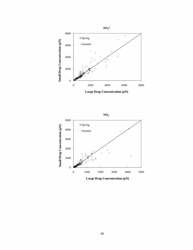
80

0

2000

4000

6000

8000

0 2000 4000 6000 8000

Sm

all

Drop

Con

cen

trati

on

(µ

N)

Large Drop Concentration (µN)

SO42-

Spring

Summer

0

1000

2000

3000

4000

5000

0 1000 2000 3000 4000 5000

Sm

all

Drop

Con

cen

tra

tion

(µ

N)


NO3-

Spring

Summer

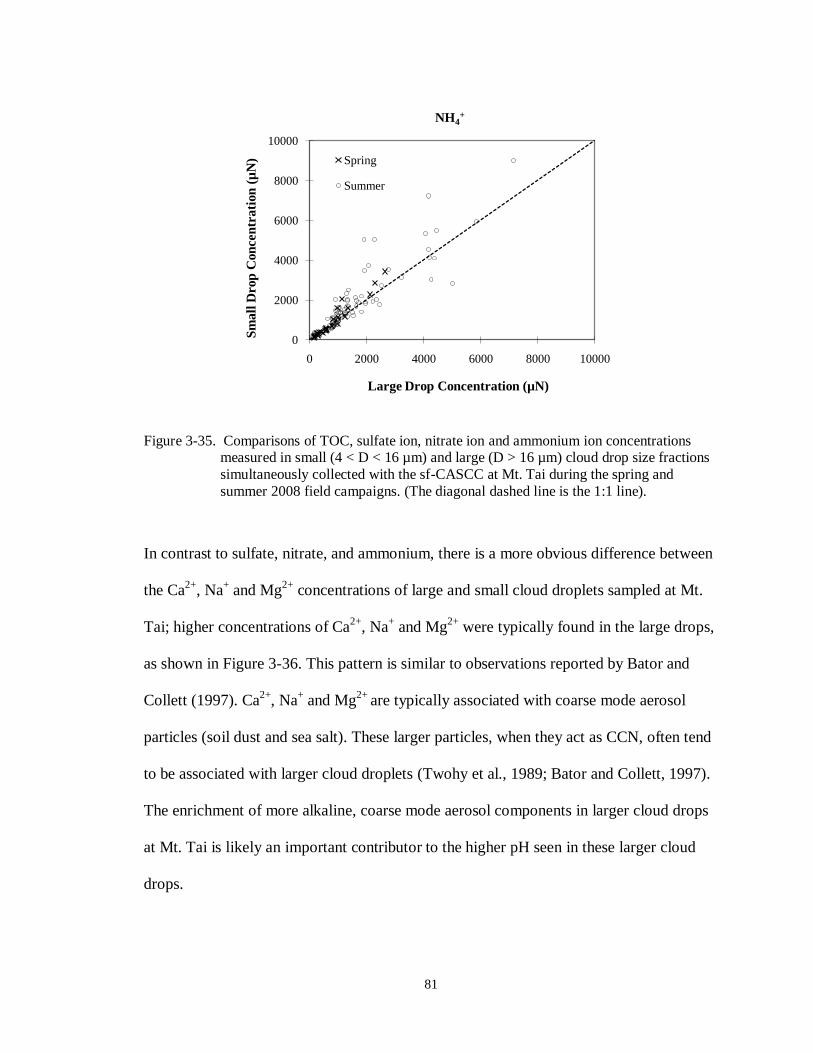
81

Figure 3-35. Comparisons of TOC, sulfate ion, nitrate ion and ammonium ion concentrations measured in small (4 < D < 16 µm) and large (D > 16 µm) cloud drop size fractions


summer 2008 field campaigns. (The diagonal dashed line is the 1:1 line).

In contrast to sulfate, nitrate, and ammonium, there is a more obvious difference between

the Ca2+

, Na+ and Mg

2+ concentrations of large and small cloud droplets sampled at Mt.

Tai; higher concentrations of Ca2+

, Na+ and Mg

2+ were typically found in the large drops,

as shown in Figure 3-36. This pattern is similar to observations reported by Bator and

Collett (1997). Ca2+

, Na+ and Mg

2+ are typically associated with coarse mode aerosol

particles (soil dust and sea salt). These larger particles, when they act as CCN, often tend

to be associated with larger cloud droplets (Twohy et al., 1989; Bator and Collett, 1997).

The enrichment of more alkaline, coarse mode aerosol components in larger cloud drops

at Mt. Tai is likely an important contributor to the higher pH seen in these larger cloud

drops.

0

2000

4000

6000

8000

10000

0 2000 4000 6000 8000 10000

Sm

all

Drop

Con

cen

trati

on

(µ

N)


NH4+

Spring

Summer

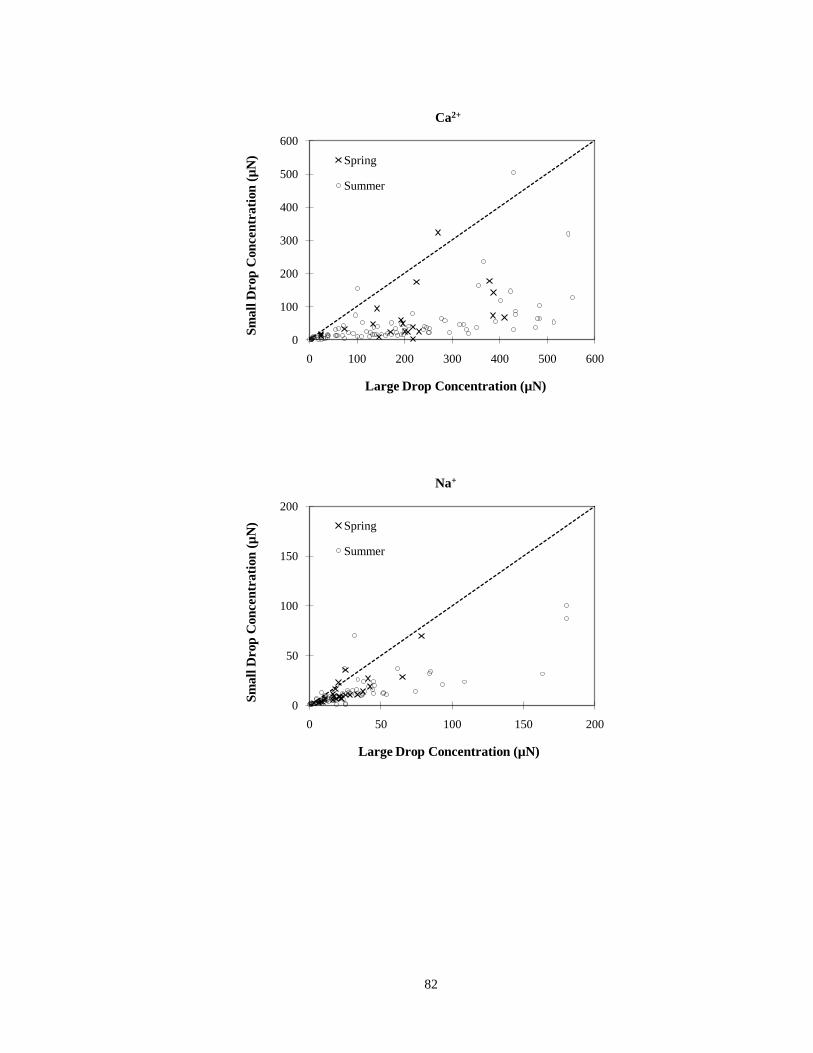
82

0

100

200

300

400

500

600

0 100 200 300 400 500 600

Sm

all

Drop

Con

cen

trati

on

(µ

N)


Ca2+

Spring

Summer

0

50

100

150

200

0 50 100 150 200

Sm

all

Drop

Con

cen

tra

tion

(µ

N)


Na+

Spring

Summer

83

Figure 3-36. Comparisons of calcium ion, sodium ion and magnesium ion concentrations measured in small (4 < D < 16 µm) and large (D > 16 µm) cloud drop size fractions


summer 2008 field campaigns. (The diagonal dashed line is the 1:1 line).

3.4.3. Aqueous hydrogen peroxide and S(IV)

Figure 3-37 compares the aqueous H2O2 and S(IV) values measured in small and large

droplet fractions collected with the sf-CASCC during the 2008 field campaigns. There is

no obvious pattern of consistent aqueous H2O2 and S(IV) enrichment in either large or

small cloud drops.

0

50

100

150

200

0 50 100 150 200

Sm

all

Drop

Con

cen

trati

on

(µ

N)


Mg2+

Spring

Summer

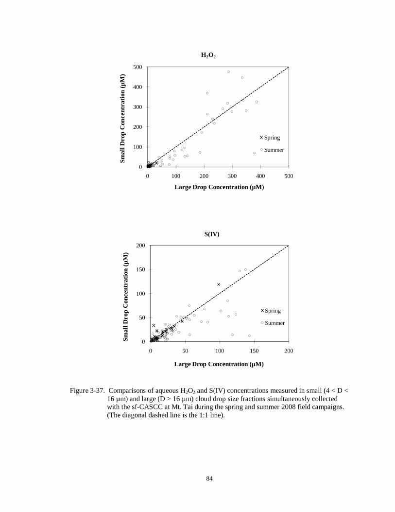
84

Figure 3-37. Comparisons of aqueous H2O2 and S(IV) concentrations measured in small (4 < D <

16 µm) and large (D > 16 µm) cloud drop size fractions simultaneously collected with the sf-CASCC at Mt. Tai during the spring and summer 2008 field campaigns.

(The diagonal dashed line is the 1:1 line).

0

100

200

300

400

500

0 100 200 300 400 500

Sm

all

Drop

Con

cen

trati

on

(µ

M)

Large Drop Concentration (µM)

H2O2

Spring

Summer

0

50

100

150

200

0 50 100 150 200

Sm

all

Drop

Con

cen

tra

tion

(µ

M)


S(IV)

Spring

Summer

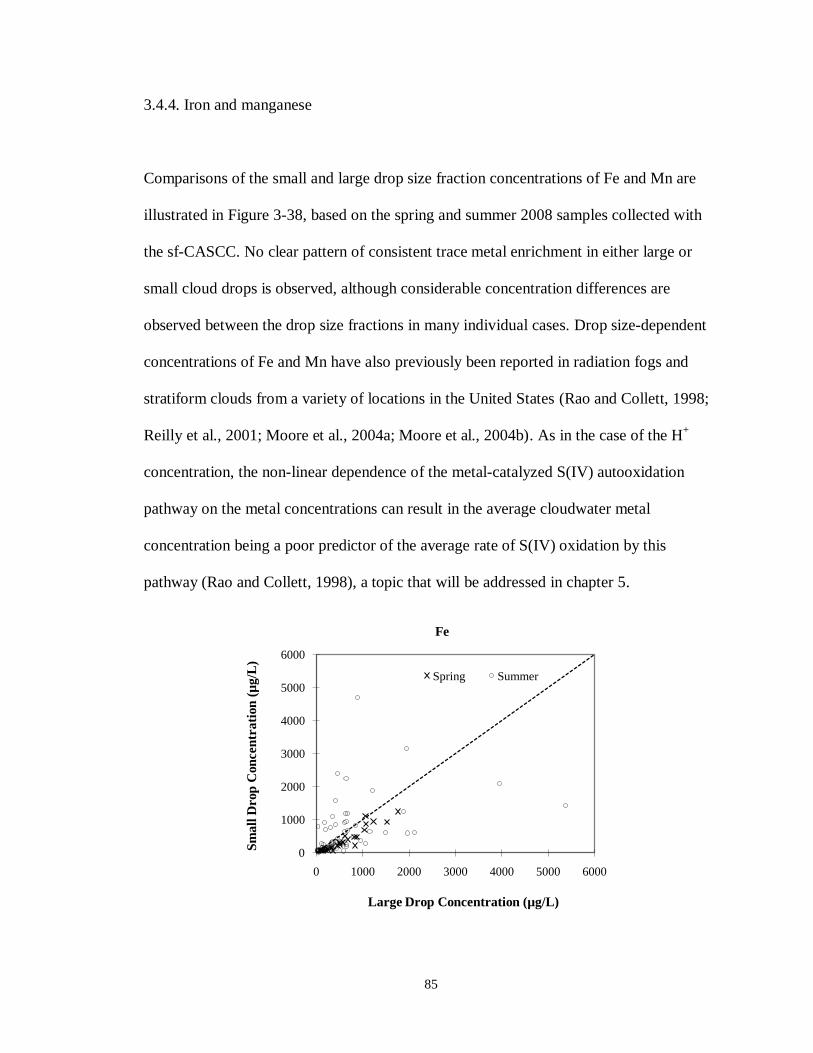
85

3.4.4. Iron and manganese

Comparisons of the small and large drop size fraction concentrations of Fe and Mn are

illustrated in Figure 3-38, based on the spring and summer 2008 samples collected with

the sf-CASCC. No clear pattern of consistent trace metal enrichment in either large or

small cloud drops is observed, although considerable concentration differences are

observed between the drop size fractions in many individual cases. Drop size-dependent

concentrations of Fe and Mn have also previously been reported in radiation fogs and

stratiform clouds from a variety of locations in the United States (Rao and Collett, 1998;

Reilly et al., 2001; Moore et al., 2004a; Moore et al., 2004b). As in the case of the H+

concentration, the non-linear dependence of the metal-catalyzed S(IV) autooxidation

pathway on the metal concentrations can result in the average cloudwater metal

concentration being a poor predictor of the average rate of S(IV) oxidation by this

pathway (Rao and Collett, 1998), a topic that will be addressed in chapter 5.

0

1000

2000

3000

4000

5000

6000

0 1000 2000 3000 4000 5000 6000

Sm

all

Drop

Con

cen

trati

on

(µ

g/L

)

Large Drop Concentration (µg/L)

Fe

Spring Summer

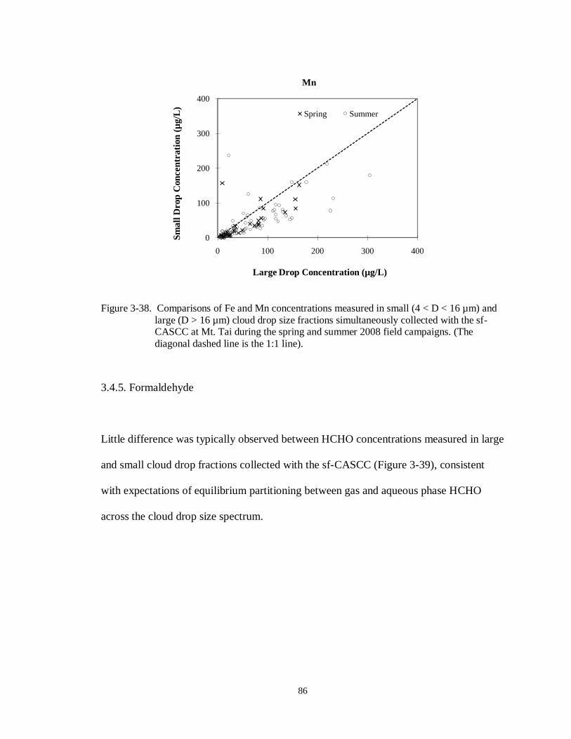
86

Figure 3-38. Comparisons of Fe and Mn concentrations measured in small (4 < D < 16 µm) and

large (D > 16 µm) cloud drop size fractions simultaneously collected with the sf-CASCC at Mt. Tai during the spring and summer 2008 field campaigns. (The

diagonal dashed line is the 1:1 line).

3.4.5. Formaldehyde

Little difference was typically observed between HCHO concentrations measured in large

and small cloud drop fractions collected with the sf-CASCC (Figure 3-39), consistent

with expectations of equilibrium partitioning between gas and aqueous phase HCHO

across the cloud drop size spectrum.

0

100

200

300

400

0 100 200 300 400

Sm

all

Drop

Con

cen

trati

on

(µ

g/L

)

Large Drop Concentration (µg/L)

Mn

Spring Summer

87

Figure 3-39. Comparison of HCHO concentrations measured in small (4 < D < 16 µm) and large

(D > 16 µm) cloud drop size fractions simultaneously collected with the sf-CASCC at Mt. Tai during the spring and summer 2008 field campaigns. (The diagonal

dashed line is the 1:1 line).

0

10

20

30

40

50

60

0 10 20 30 40 50 60

Sm

all

Drop

Con

cen

trati

on

(µ

M)


HCHO

Spring Summer

88

CHAPTER 4 CLOUD-AEROSOL INTERACTIONS

4.1. BACKWARD TRAJECTORY ANALYSIS

Backward trajectories can trace an air parcel's path before it arrives at a receptor site, the

trajectory including information concerning an air parcel’s origin, transport distance, and

the residence time in each region during its transport. Ulman and Saxena used backward

trajectories to analyze the influence of cloud-forming air mass histories on cloudwater

chemical composition at Mt. Mitchell, North Carolina (Ulman and Saxena, 1997). Menon

et al. reported the effect of cloud-forming air mass origin on the size-dependent cloud

droplet chemical composition based on backward trajectory analysis (Menon et al.,

2000). Kim et al. also used backward trajectories to investigate cloud/fog water chemical

composition differences due to air masses’ different transport trajectories (Kim et al.,

2006).

In this study, backward trajectory analysis is used to investigate the transport history of

air parcels associated with cloud interception at Mt. Tai. Then, in combination with other

factors, such as atmospheric stability, precipitation, and source emission intensity, the

relationship between the cloudwater chemical properties and the transport history of the

precursor air parcel can be examined. Because Mt. Tai is located in a region surrounded

by large urban, industrial, and agricultural activity centers, it is quite possible that

89

relationships between transport pattern and cloud composition may be complex and

difficult to elucidate.

The National Oceanic and Atmospheric Administration (NOAA) Air Resources

Laboratory’s HYSPLIT (HYbrid Single-Particle Lagrangian Integrated Trajectory) model

was used in this project to calculate backward trajectories. The HYSPLIT model is a

useful model for computing both trajectories and dispersion/deposition simulations

(Draxier and Hess, 1997; Draxier and Hess, 1998) and is widely used in numerous

research studies. As described above, in order to more efficiently investigate the

relationship between cloud chemical properties and the air parcel transport history,

trajectories were categorized into three sectors: marine, polluted, and continental sector

based on the trajectories’ geographical locations and SO2 source emission intensity

distribution, as shown in Fig. 4-1.

Sector 1 represents the 'marine' region; sector 2 represents areas that the SO2 source

emission intensities are relatively higher, and is considered as a 'polluted' region; sector 3

represents areas that the SO2 source emission intensities are somewhat lower, and is

labeled as a 'continental' region. This continental sector also contains some of the large

dust source regions. Note that the SO2 emissions map shows large SO2 emissions close to

Mt. Tai in all directions. Similar patterns are seen in regional NOx and NH3 emissions.

For these reasons, one might expect differences between the composition of clouds

associated with air parcel transport from the three sectors to be less than those observed

90

in some of the previous studies mentioned above, where a clearer separation between

source regions existed.

Figure 4-1. Three sectors and the SO2 emission intensity distribution at 30min×30min resolution

(Data from http://mic.greenresource.cn/data/intex-b); sector 1: marine, sector 2:

polluted, sector 3: continental.

72-hour back-trajectories were calculated at one hour intervals for each cloud event, with

end points at 1600 meters above mean sea-level (AMSL), representing a total of 245

individual trajectories for all the cloud events during the four field campaigns. The

National Weather Service's National Centers for Environmental Prediction (NCEP)

Global Data Assimilation System (GDAS) model output was used as the meteorological

data set input for the back-trajectory calculations. Model vertical velocity was selected as

the vertical motion calculation method.

http://mic.greenresource.cn/data/intex-b

91

4.1.1. Backward trajectories and cloudwater composition variations

In order to investigate the relationship between cloudwater chemical properties and the

transport history of the precursor air parcel, summary data for the sampled events are

provided below in tables 4-1 through 4-4, by campaign. The summaries include the

number of events in each campaign, the date and time period of each sampled event,

sectors that backward trajectories for each event passed through, a brief description of the

air parcel’s vertical motion status, and the average (volume-weighted) cloudwater

concentrations of several key species. The summaries also include estimated altitudes of

cloud base for each event obtained using the following equation (Ahrens, 2000):

)TT(125TT

H d

dewd

dbase

Equation 4-1

Where Hbase is the cloud base height (in meters), Γd is the dry adiabatic lapse rate

(~9.8°C/km), Γdew is the dew point lapse rate (~1.8°C/km), T is the surface air

temperature (in degrees Celsius), and Td is the dew point temperature (in degrees

Celsius). The cloud base height can be obtained from T and Td based on equation 4-1 for

most of the events. Because no meteorology data are available directly at the base of Mt.

Tai, meteorological observations from Jinan (60 km to the north of Mt. Tai) were used to

estimate the cloud base height, so uncertainties exist here.

Backward trajectories were represented with different colors based on the average pH

value for each event to see if significant pH differences exist for different transport

92

trajectories. Fig. 4-2 shows the backward trajectories for cloud events during the spring

2007 campaign.

Figure 4-2. Backward trajectories for cloud events during the spring 2007 campaign.

As shown in Fig. 4-2, during the spring 2007 campaign, backward trajectories for most of

the events passed through sector 2 and sector 3. There is a clear pattern that cloud events

with backward trajectories passing through continental sector 3 had a higher pH than

those with backward trajectories passing through the more polluted sector 2. Ren (2009)

reported that two strong dust storms were observed (March 31-April 2 and April 20-21)

during the spring 2007 campaign. As described in chapter 1, soil dust in the atmosphere

may alleviate the acid deposition situation in the north of China by neutralizing part of

the acidity contributed to precipitation by sulfuric and nitric acids. The increased dust

during the spring 2007 campaign, along with lower SO2 emissions in sector 3, are

93

consistent with the higher pH clouds that intercepted Mt. Tai during periods of transport

from sector 3. Fig. 4-3 gives typical backward trajectories for several cloud events (4/18,

4/20 and 4/21) that were under the influence of dust storms during the spring 2007

campaign. All those trajectories have typical long transport distance, descending vertical

motion and little influence from the local lower altitude air. A summary of the spring

2007 campaign is given in table 4-1.

94

Figure 4-3. Representative backward trajectories for 3 cloud events (4/18, 4/20 and 4/21) during


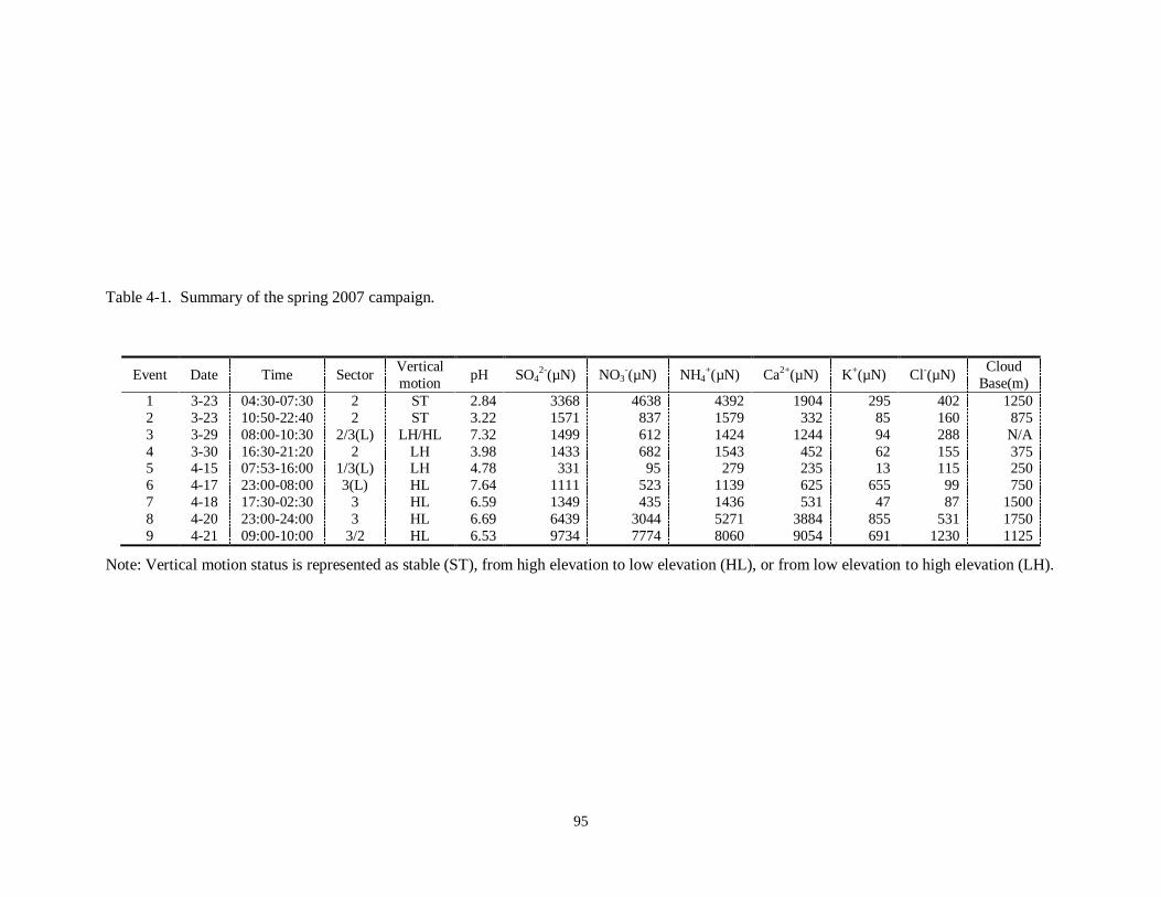
95

Table 4-1. Summary of the spring 2007 campaign.

Event Date Time Sector Vertical

motion pH SO4

2-(µN) NO3-(µN) NH4

+(µN) Ca2+(µN) K+(µN) Cl-(µN) Cloud

Base(m)

1 3-23 04:30-07:30 2 ST 2.84 3368 4638 4392 1904 295 402 1250

2 3-23 10:50-22:40 2 ST 3.22 1571 837 1579 332 85 160 875

3 3-29 08:00-10:30 2/3(L) LH/HL 7.32 1499 612 1424 1244 94 288 N/A

4 3-30 16:30-21:20 2 LH 3.98 1433 682 1543 452 62 155 375 5 4-15 07:53-16:00 1/3(L) LH 4.78 331 95 279 235 13 115 250

6 4-17 23:00-08:00 3(L) HL 7.64 1111 523 1139 625 655 99 750

7 4-18 17:30-02:30 3 HL 6.59 1349 435 1436 531 47 87 1500

8 4-20 23:00-24:00 3 HL 6.69 6439 3044 5271 3884 855 531 1750

9 4-21 09:00-10:00 3/2 HL 6.53 9734 7774 8060 9054 691 1230 1125

Note: Vertical motion status is represented as stable (ST), from high elevation to low elevation (HL), or from low elevation to high elevation (LH).

96

Figure 4-4. Backward trajectories for cloud events during the summer 2007 campaign.

Fig. 4-4 shows the back-trajectories for cloud events during the summer 2007 campaign.

Cloud events with backward trajectories passing through sector 2 generally had relatively

higher pH than those with backward trajectories passing through sectors 1 and/or 3. The

trajectories for the cloud event (7/14) with the highest ion concentrations during the

summer 2007 campaign passed through sectors 1 and 3 and the origins were from the

area close to the Beijing megalopolis, a highly polluted region. The trajectories for the

cloud event (6/20) with the lowest ion concentrations during the summer 2007 campaign

passed through sectors 1 and 2 covering Shanghai city; it was raining during this event.

From several events’ ion concentration data, it is obvious that upwind precipitation

scavenging of aerosol and trace gases has a significant impact on the cloudwater

chemical composition observed at Mt. Tai.

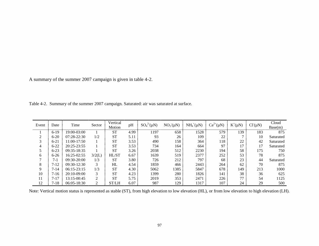
97

A summary of the summer 2007 campaign is given in table 4-2.

Table 4-2. Summary of the summer 2007 campaign. Saturated: air was saturated at surface.


Motion pH SO4



Base(m)

1 6-19 19:00-03:00 1 ST 4.99 1197 658 1528 579 139 183 875

2 6-20 07:28-22:30 1/2 ST 5.11 93 26 109 22 7 10 Saturated

3 6-21 11:00-17:50 1 ST 3.53 490 158 364 118 22 42 Saturated

4 6-22 20:25-23:55 1 ST 3.53 734 164 664 97 17 17 Saturated 5 6-23 09:35-18:35 1 ST 3.26 2038 512 2230 194 58 175 750

6 6-26 16:25-02:55 3/2(L) HL/ST 6.67 1639 519 2377 252 53 78 875

7 7-1 09:30-20:00 1/3 ST 3.80 726 212 797 68 23 44 Saturated

8 7-12 09:30-12:30 3 HL 4.54 1859 466 2443 264 62 70 875

9 7-14 06:15-23:15 1/3 ST 4.30 5062 1385 5847 678 149 213 1000

10 7-16 20:10-09:00 3 ST 4.23 1399 280 1826 141 38 36 625

11 7-17 13:15-00:45 2 ST 5.75 2019 353 2471 226 77 54 1125

12 7-18 06:05-18:30 2 ST/LH 6.07 987 129 1317 107 24 29 500


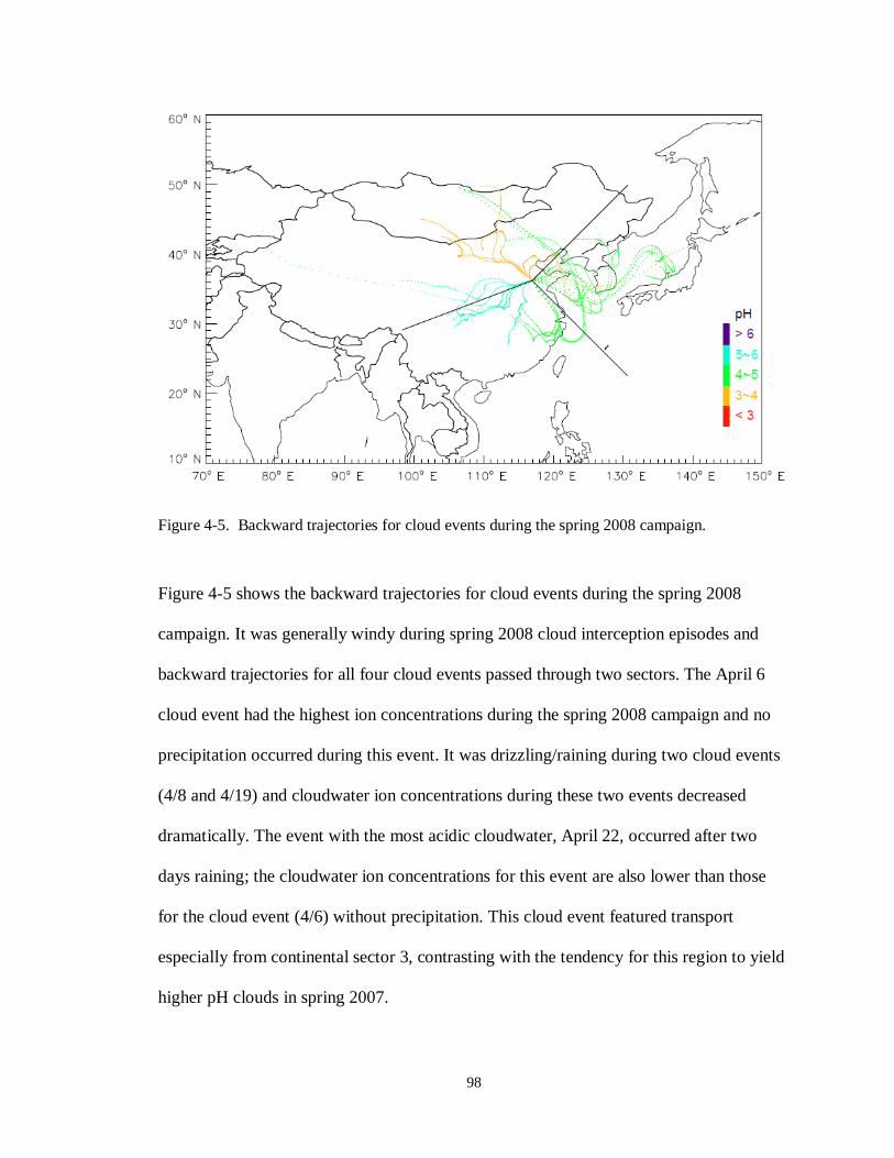
98

Figure 4-5. Backward trajectories for cloud events during the spring 2008 campaign.

Figure 4-5 shows the backward trajectories for cloud events during the spring 2008

campaign. It was generally windy during spring 2008 cloud interception episodes and

backward trajectories for all four cloud events passed through two sectors. The April 6

cloud event had the highest ion concentrations during the spring 2008 campaign and no

precipitation occurred during this event. It was drizzling/raining during two cloud events

(4/8 and 4/19) and cloudwater ion concentrations during these two events decreased

dramatically. The event with the most acidic cloudwater, April 22, occurred after two

days raining; the cloudwater ion concentrations for this event are also lower than those

for the cloud event (4/6) without precipitation. This cloud event featured transport

especially from continental sector 3, contrasting with the tendency for this region to yield

higher pH clouds in spring 2007.

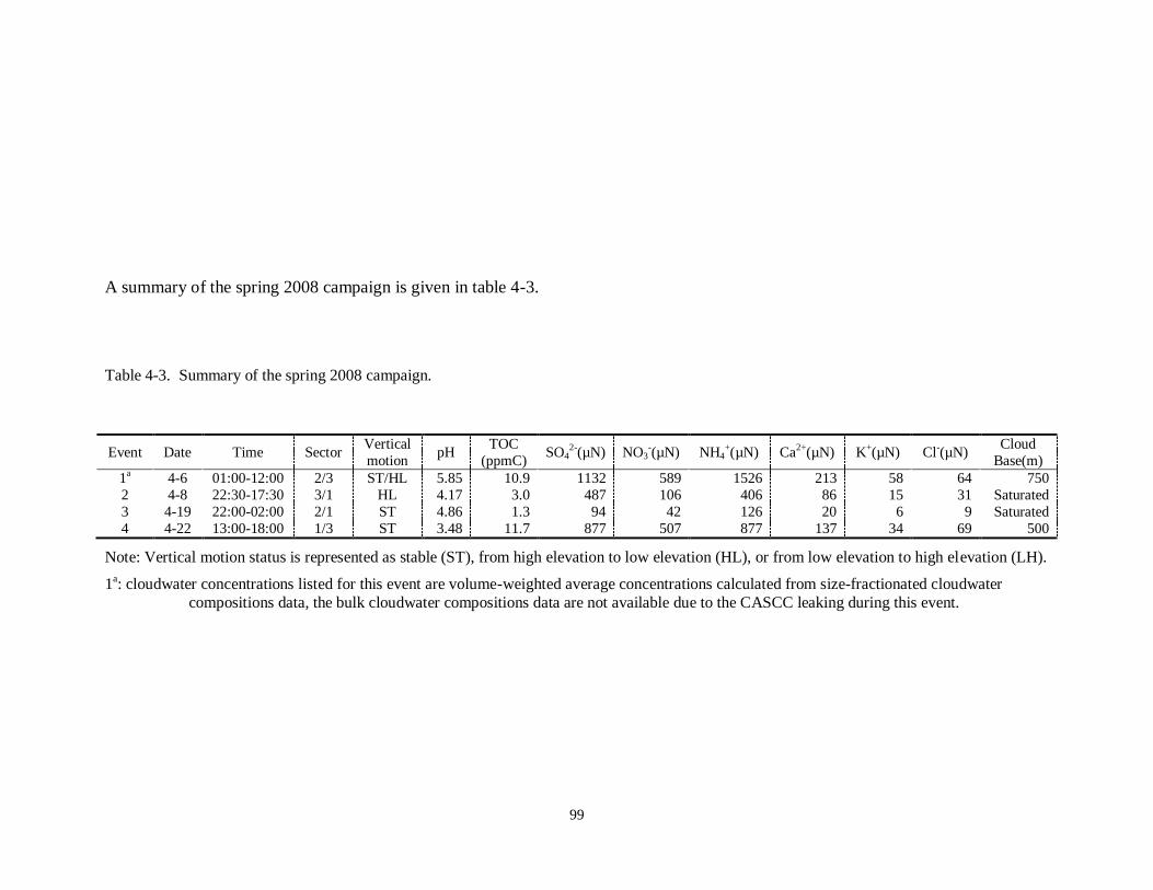
99

A summary of the spring 2008 campaign is given in table 4-3.

Table 4-3. Summary of the spring 2008 campaign.


motion pH

TOC

(ppmC) SO4



Base(m)

1a 4-6 01:00-12:00 2/3 ST/HL 5.85 10.9 1132 589 1526 213 58 64 750

2 4-8 22:30-17:30 3/1 HL 4.17 3.0 487 106 406 86 15 31 Saturated

3 4-19 22:00-02:00 2/1 ST 4.86 1.3 94 42 126 20 6 9 Saturated

4 4-22 13:00-18:00 1/3 ST 3.48 11.7 877 507 877 137 34 69 500


1a: cloudwater concentrations listed for this event are volume-weighted average concentrations calculated from size-fractionated cloudwater

compositions data, the bulk cloudwater compositions data are not available due to the CASCC leaking during this event.

100

Figure 4-6. Backward trajectories for cloud events during the summer 2008 campaign.

Fig. 4-6 shows back-trajectories for summer 2008 campaign cloud events. Two-thirds of

cloud events had low pH values (<4); some cloud events (6-21 and 7-11) had very acidic

cloudwater with pH values even lower than 3. A summary of the summer 2008 campaign

is given in table 4-4. From analysis of the backward trajectories for all the cloud events, a

preliminary conclusion can be reached that transport patterns do not have obvious impact

on the cloudwater chemical composition for these events. As discussed above, Mt. Tai is

surrounded by regions of high pollutant emission giving the potential for polluted

cloudwater regardless of the longer distance origins of air trajectories. Cloud-forming air

parcels’ origins and vertical motions and precipitation histories all can have a significant

influence on the cloudwater composition.

101

Table 4-4. Summary of the summer 2008 campaign.


motion pH

TOC

(ppmC) SO4



Base(m)

1 6-16 02:00-07:30 1 ST 3.80 22.9 3053 2217 4289 517 296 450 750

2 6-16 17:00-15:00 1 ST 3.59 6.5 719 303 513 24 31 44 Saturated

3 6-18 21:00-08:00 2/3 HL 3.15 85.6 1656 1045 1955 120 248 564 750

4 6-19 19:00-08:15 2 ST 3.62 24.0 1251 727 1663 177 164 313 875 5 6-20 16:45-19:20 2 ST 3.22 19.0 2076 552 1909 37 133 116 500

6 6-21 09:00-09:40 2 ST 2.86 45.7 3857 1269 3018 190 267 406 375

7 6-25 23:10-00:45 3 ST 6.66 20.0 4178 885 4462 467 143 127 1125

8 7-2 04:05-05:50 3 HL 3.43 17.6 3372 959 3410 367 126 155 375

9 7-3 20:00-11:40 3/2 HL/ST 5.30 14.7 1691 343 2017 152 39 47 1000

10 7-4 15:00-21:45 2 LH 4.78 6.7 992 245 1065 94 26 34 875

11 7-5 04:30-06:30 2 ST 5.50 2.1 487 56 417 21 9 11 375

12 7-5 10:00-22:15 2/3 LH/ST 4.62 1.4 219 59 223 10 5 9 Saturated

13 7-7 08:00-12:30 2 ST 3.27 15.2 2526 1325 2732 229 152 127 Saturated

14 7-7 15:30-16:30 2 ST 3.98 21.9 4281 1996 5142 418 191 122 N/A

15 7-8 14:30-05:30 2 ST 4.03 5.9 957 415 1058 83 49 42 Saturated

16 7-10 08:15-11:45 2 ST 3.87 5.3 638 262 889 16 13 37 375 17 7-11 04:15-07:40 2 ST 2.77 25.4 5042 3349 5398 414 197 257 Saturated

18 7-14 18:00-03:00 2 ST 3.85 2.3 684 221 693 38 8 31 375


102

4.1.2. Case studies on the influence of biomass burning on cloudwater composition

Aerosol particles emitted by biomass burning can contribute to high organic carbon

contents in cloudwater. They can also potentially modify cloud microphysics, for

example reducing cloud droplet size and enhancing cloud reflectance (Kaufman and

Fraser, 1997; Andreae et al., 2004). Yamaji et al. (2010) and Suthawaree et al. (2010)

observed the impact of agricultural biomass burning on air quality at Mt. Tai in June

2006 during the MTX2006 field campaign. Several cloudwater samples collected in the

summer 2007 and 2008 Mt. Tai campaigns have much higher concentrations of TOC than

average, indicating possible influence by regional biomass burning emissions. Extensive

agricultural burning is common in this region of China in late spring/early summer. The

first half of June is the wheat harvest season for North China Plain.

In order to analyze possible impacts of biomass burning on observed cloud composition,

fire locations in combination with backward trajectories were used to examine periods of

possible fire impact. An open source version of the Web Fire Mapper developed by the

Fire Information for Resource Management System (FIRMS) is used to display the

Moderate Resolution Imaging Spectroradiometer (MODIS) hotspot/fire locations

(Satellite source: Aqua & Terra) during the time period of interest. The cloudwater

potassium ion concentration can also be used as an indicator of biomass burning impacts.

One cloud event (6/19) in summer 2007 and two cloud events (6/16, 6/18) in summer

2008 that exhibit high potassium ion concentrations with no apparent impact from dust

storms are selected as case studies. Cloud cover may obscure active fire detection

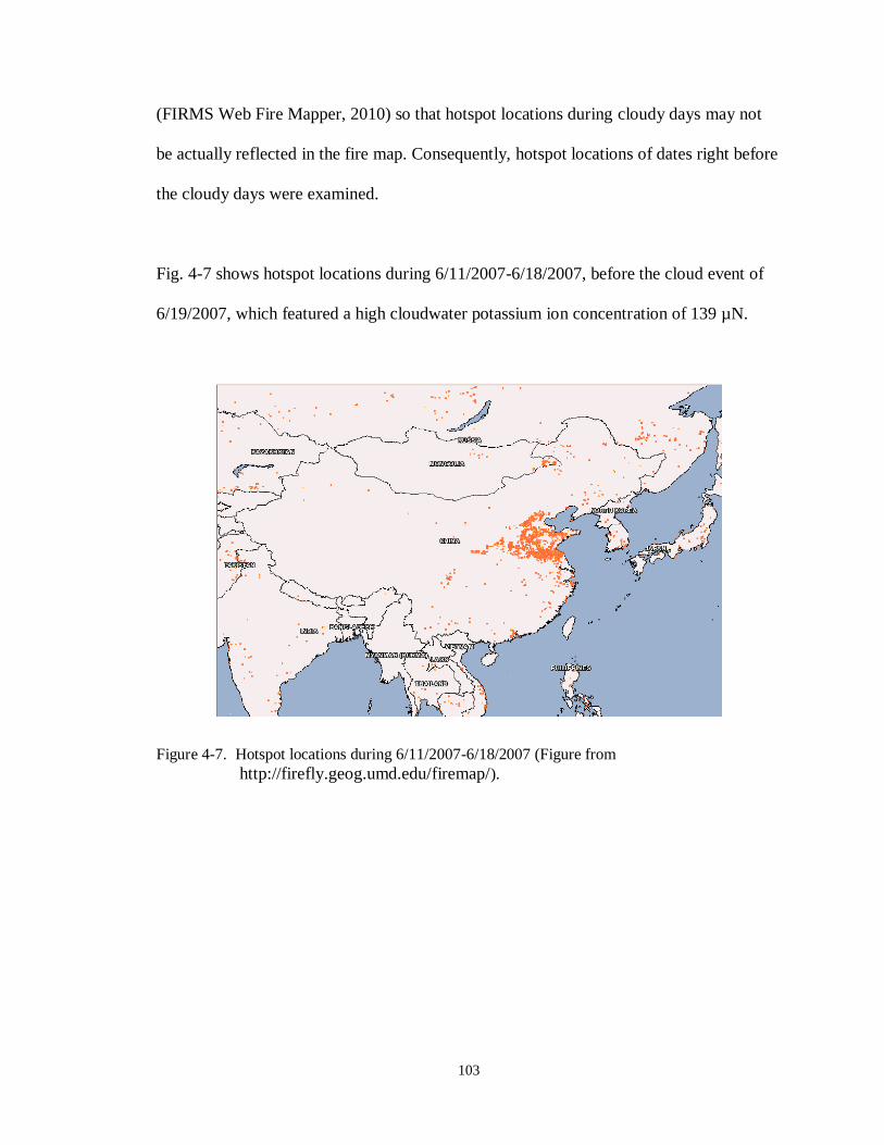
103

(FIRMS Web Fire Mapper, 2010) so that hotspot locations during cloudy days may not

be actually reflected in the fire map. Consequently, hotspot locations of dates right before

the cloudy days were examined.

Fig. 4-7 shows hotspot locations during 6/11/2007-6/18/2007, before the cloud event of

6/19/2007, which featured a high cloudwater potassium ion concentration of 139 µN.

Figure 4-7. Hotspot locations during 6/11/2007-6/18/2007 (Figure from

http://firefly.geog.umd.edu/firemap/).

http://firefly.geog.umd.edu/firemap/

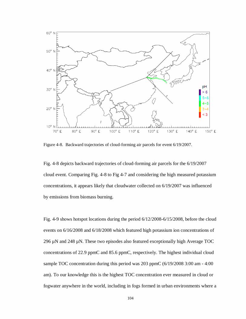
104

Figure 4-8. Backward trajectories of cloud-forming air parcels for event 6/19/2007.

Fig. 4-8 depicts backward trajectories of cloud-forming air parcels for the 6/19/2007

cloud event. Comparing Fig. 4-8 to Fig 4-7 and considering the high measured potassium

concentrations, it appears likely that cloudwater collected on 6/19/2007 was influenced

by emissions from biomass burning.

Fig. 4-9 shows hotspot locations during the period 6/12/2008-6/15/2008, before the cloud

events on 6/16/2008 and 6/18/2008 which featured high potassium ion concentrations of

296 µN and 248 µN. These two episodes also featured exceptionally high Average TOC

concentrations of 22.9 ppmC and 85.6 ppmC, respectively. The highest individual cloud

sample TOC concentration during this period was 203 ppmC (6/19/2008 3:00 am - 4:00

am). To our knowledge this is the highest TOC concentration ever measured in cloud or

fogwater anywhere in the world, including in fogs formed in urban environments where a

105

shallow boundary layer traps emissions near the surface. Fig. 4-10 gives back-trajectories

of cloud-forming air parcels for the cloud events on 6/16/2008 (sector 1) and 6/18/2008

(sectors 2 and 3).

Figure 4-9. Hotspot locations during 6/12/2008-6/15/2008 (Figure from

http://firefly.geog.umd.edu/firemap/).

http://firefly.geog.umd.edu/firemap/

106

Figure 4-10. Backward trajectories of cloud-forming air parcels for events on 6/16/2008 and 6/18/2008.

The back-trajectories and fire maps suggest likely influence of biomass burning on clouds

sampled during this period at Mt. Tai. The high potassium ion and TOC concentrations

are confirmation of these impacts. Some cloudwater samples were also atomized and

analyzed by aerosol mass spectrometer (AMS) (Yele Sun, personal communication) and

it was found that the sample with highest TOC (6/19/2008 3:00 am - 4:00 am) has a large

peak at mass fragment 60 (C2H4O2+). This fragment has been identified in the AMS

community as a marker for biomass burning emissions (Lee et al., 2010) and can be

produced by fragmentation of levoglucosan and other structurally similar molecules. The

mass ratio of C2H4O2+/OM (organic matter) could reach 0.7%, much higher than the

average ratio observed in cloudwater without substantial influence of biomass burning,

usually below 0.2%.

107

4.2. AEROSOL AND GAS PROCESSING BY CLOUDS

Clouds act as important processors of ambient aerosols and soluble trace gases

(Oberholzer et al., 1992; Collett et al., 1993; Oberholzer et al., 1993; Hoag et al., 1999;

Collett et al., 2002; Herckes et al., 2002; Herckes et al., 2002; Collett et al., 2008; Hoose

et al., 2008). Many experimental and modeling studies (Flossmann et al., 1985; Hoppel et

al., 1986; Flossmann et al., 1987; Flossmann and Pruppacher, 1988; Ahr et al., 1989;

Alheit et al., 1990; Gillani et al., 1995; Respondek et al., 1995; Henning et al., 2004;

Roelofs et al., 2006; Hoose et al., 2008; Ivanova and Leighton, 2008) have examined

cloud-aerosol interactions. During the cloud formation process, activated aerosol particles

heterogeneously nucleate water vapor and grow to cloud droplets. Additional aerosol

particles can be scavenged by other mechanisms, including interception, diffusion, and

electrophoresis. Ambient soluble trace gases are taken up by the droplets and various

aqueous phase reactions can occur in the cloudwater. Scavenged and newly formed

species can be removed through occult or wet deposition processes or be released back to

the ambient air as the cloud dissipates.

In order to examine the possible fates of atmospheric pollutants in the vicinity of clouds,

it is useful to examine the extent (efficiency) of particle and trace gas scavenging by the

clouds. Such observations are relatively rare, although some reports have been made in

the literature (Dutkiewicz and Husain, 1998; Hitzenberger et al., 2000; Hitzenberger et

al., 2001; Collett et al., 2008). Dutkiewicz and Husain (1998), for example, illustrate a

scavenging efficiency for sulfate aerosol by clouds sampled at Whiteface Mtn, NY, that

108

varies with atmospheric sulfate concentration. Observed values varied between

approximately 50% and 90%, with a tendency for decreased efficiencies at higher aerosol

sulfate loadings. The sulfate scavenging efficiencies observed at Whiteface Mtn. were

generally higher than those reported in Austria by Hitzenberger et al. (2001) for black

carbon aerosol particles. Collett et al. (2008) reported a range of scavenging efficiencies

for carbonaceous aerosol components in California radiation fogs, with a low efficiency

for elemental carbon and high scavenging efficiencies for more polar organic molecules

such as levoglucosan. Species of particular interest in the Mt. Tai study include the main

nitrogen (ammonia/ammonium and nitric acid/nitrate) and sulfur-containing (sulfur

dioxide and sulfate) pollutants.

In the spring and summer 2008 campaigns at Mt. Tai, a University Research Glassware

(URG) denuder/filter pack assembly (model URG-3000C) was used to simultaneously

collect PM2.5 and select trace gases for chemical analysis. The URG denuder/filter pack

system was run daily from 8:00 AM to 8:00 AM local time. When cloud was present,

sampling was interrupted and interstitial air (containing aerosol particles and gases not

scavenged by the cloud droplets) was sampled on a second instrument channel that pulled

air from behind the collection strands of the cloudwater collector. Regular aerosol + gas

sampling was resumed after cloud interception ceased.

4.2.1. Before / after cloud

109

The ambient sulfur and nitrogen compositions before cloud can be specified as follows.

Sulfur includes gaseous sulfur dioxide, SO2(g), and sulfate in aerosol particles, SO42-

(p).

N(-III) includes gaseous ammonia, NH3(g), and ammonium in aerosol particles, NH4+(p).

N(V) includes gaseous nitric acid, HNO3(g), and nitrate in aerosol particles NO3-(p). The

ambient sulfur and nitrogen compositions after cloud can be specified the same way as

before cloud.

4.2.2. During cloud

The ambient sulfur and nitrogen compositions during cloud can be specified as follows.

Sulfur includes interstitial (between droplet) gaseous sulfur dioxide, SO2(ig), sulfate in

interstitial aerosol particles, SO42-

(ip), SO2 in cloudwater, SO2(c), and sulfate in

cloudwater, SO42-

(c). N(-III) includes gaseous ammonia, NH3(ig), ammonium in

interstitial aerosol particles, NH4+(ip), and ammonium in cloudwater, NH4

+(c). N(V)

includes gaseous nitric acid, HNO3(ig), nitrate in interstitial aerosol particles, NO3-(ip),

and nitrate in cloudwater, NO3-(c).

4.2.3. Aerosol scavenging efficiency

All the species extracted from denuders and filters and measured in aqueous

concentration units (µN) are converted to ambient concentration units (µg/m3) based on

measured air sample volumes (m3) measured by a dry gas meter. All the species in

cloudwater measured in aqueous concentration units (µN) are converted to ambient

110

loading units (µg/m3) using the measured cloud LWC (mg/m

3). Appropriate additional

unit conversion factors are included in each case.

Aerosol scavenging efficiency was initially calculated by comparing the pre-cloud and

interstitial concentrations of a species using the following equation edited from previous

work (Collett et al., 2008):

pdbeforeclou

ip

1X

X1

Equation 4-2

Where η1 is the scavenging efficiency of species X, Xip is the ambient loading (µg/m3) of

species X existing in interstitial aerosol particles during cloud. beforecloudXp is the ambient

loading (µg/m3) of species X existing in aerosol particles before cloud. The advantage of

this approach is that it allows us to directly compare aerosol species’ concentrations. The

main limitation is that temporal changes in atmospheric composition between the pre-

cloud and interstitial samples can confound the analysis.

An alternative way to calculate species scavenging efficiency, while avoiding the

problems of temporal composition changes, is to examine species partitioning between

simultaneously measured cloudwater and interstitial air phases:

cipig

c2

XXX

X

Equation 4-3

Where η2 is the scavenging efficiency of species X, Xc is the ambient loading (µg/m3) of

species X existing in the cloudwater droplets, Xig is the ambient loading (µg/m3) of

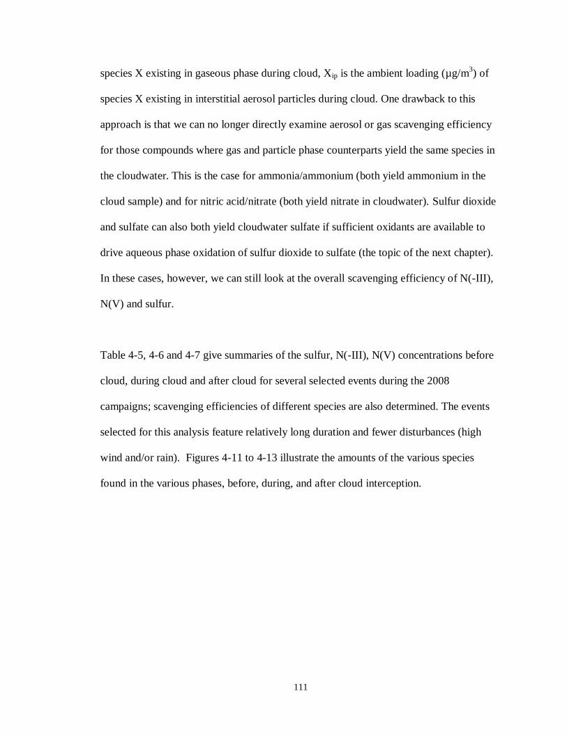
111

species X existing in gaseous phase during cloud, Xip is the ambient loading (µg/m3) of

species X existing in interstitial aerosol particles during cloud. One drawback to this

approach is that we can no longer directly examine aerosol or gas scavenging efficiency

for those compounds where gas and particle phase counterparts yield the same species in

the cloudwater. This is the case for ammonia/ammonium (both yield ammonium in the

cloud sample) and for nitric acid/nitrate (both yield nitrate in cloudwater). Sulfur dioxide

and sulfate can also both yield cloudwater sulfate if sufficient oxidants are available to

drive aqueous phase oxidation of sulfur dioxide to sulfate (the topic of the next chapter).

In these cases, however, we can still look at the overall scavenging efficiency of N(-III),

N(V) and sulfur.

Table 4-5, 4-6 and 4-7 give summaries of the sulfur, N(-III), N(V) concentrations before

cloud, during cloud and after cloud for several selected events during the 2008

campaigns; scavenging efficiencies of different species are also determined. The events

selected for this analysis feature relatively long duration and fewer disturbances (high

wind and/or rain). Figures 4-11 to 4-13 illustrate the amounts of the various species

found in the various phases, before, during, and after cloud interception.

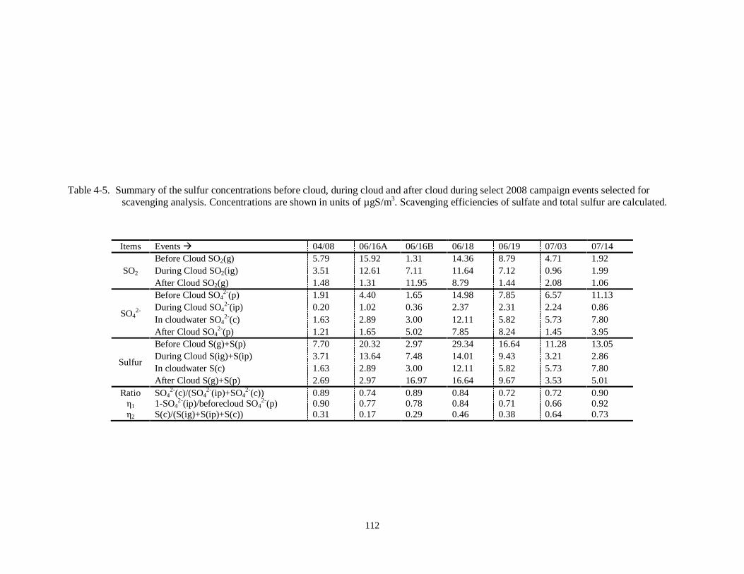
112

Table 4-5. Summary of the sulfur concentrations before cloud, during cloud and after cloud during select 2008 campaign events selected for

scavenging analysis. Concentrations are shown in units of µgS/m3. Scavenging efficiencies of sulfate and total sulfur are calculated.

Items Events 04/08 06/16A 06/16B 06/18 06/19 07/03 07/14

SO2

Before Cloud SO2(g) 5.79 15.92 1.31 14.36 8.79 4.71 1.92

During Cloud SO2(ig) 3.51 12.61 7.11 11.64 7.12 0.96 1.99

After Cloud SO2(g) 1.48 1.31 11.95 8.79 1.44 2.08 1.06

SO42-

Before Cloud SO42-(p) 1.91 4.40 1.65 14.98 7.85 6.57 11.13

During Cloud SO42-(ip) 0.20 1.02 0.36 2.37 2.31 2.24 0.86

In cloudwater SO42-(c) 1.63 2.89 3.00 12.11 5.82 5.73 7.80

After Cloud SO42-(p) 1.21 1.65 5.02 7.85 8.24 1.45 3.95

Sulfur

Before Cloud S(g)+S(p) 7.70 20.32 2.97 29.34 16.64 11.28 13.05

During Cloud S(ig)+S(ip) 3.71 13.64 7.48 14.01 9.43 3.21 2.86

In cloudwater S(c) 1.63 2.89 3.00 12.11 5.82 5.73 7.80

After Cloud S(g)+S(p) 2.69 2.97 16.97 16.64 9.67 3.53 5.01

Ratio SO42-

(c)/(SO42-

(ip)+SO42-

(c)) 0.89 0.74 0.89 0.84 0.72 0.72 0.90 η1 1-SO4

2-(ip)/beforecloud SO42-(p) 0.90 0.77 0.78 0.84 0.71 0.66 0.92

η2 S(c)/(S(ig)+S(ip)+S(c)) 0.31 0.17 0.29 0.46 0.38 0.64 0.73

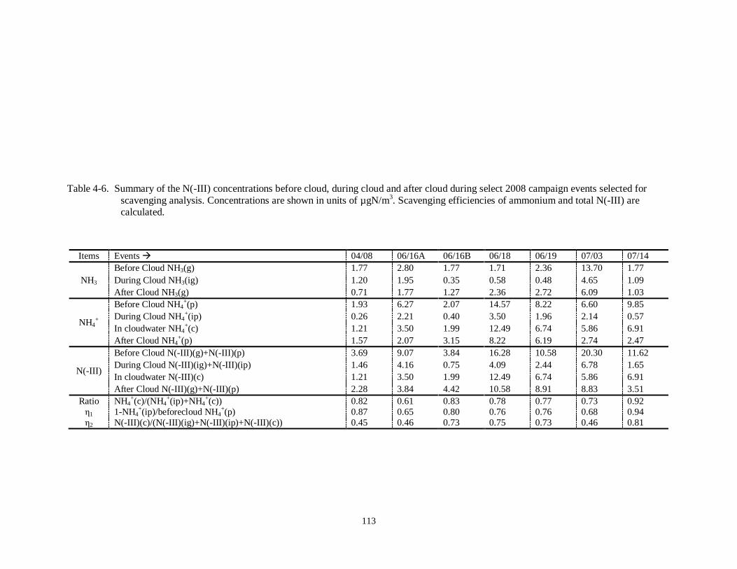
113

Table 4-6. Summary of the N(-III) concentrations before cloud, during cloud and after cloud during select 2008 campaign events selected for

scavenging analysis. Concentrations are shown in units of µgN/m3. Scavenging efficiencies of ammonium and total N(-III) are

calculated.

Items Events 04/08 06/16A 06/16B 06/18 06/19 07/03 07/14

NH3

Before Cloud NH3(g) 1.77 2.80 1.77 1.71 2.36 13.70 1.77

During Cloud NH3(ig) 1.20 1.95 0.35 0.58 0.48 4.65 1.09

After Cloud NH3(g) 0.71 1.77 1.27 2.36 2.72 6.09 1.03

NH4+

Before Cloud NH4+(p) 1.93 6.27 2.07 14.57 8.22 6.60 9.85

During Cloud NH4+(ip) 0.26 2.21 0.40 3.50 1.96 2.14 0.57

In cloudwater NH4+(c) 1.21 3.50 1.99 12.49 6.74 5.86 6.91

After Cloud NH4+(p) 1.57 2.07 3.15 8.22 6.19 2.74 2.47

N(-III)

Before Cloud N(-III)(g)+N(-III)(p) 3.69 9.07 3.84 16.28 10.58 20.30 11.62

During Cloud N(-III)(ig)+N(-III)(ip) 1.46 4.16 0.75 4.09 2.44 6.78 1.65

In cloudwater N(-III)(c) 1.21 3.50 1.99 12.49 6.74 5.86 6.91

After Cloud N(-III)(g)+N(-III)(p) 2.28 3.84 4.42 10.58 8.91 8.83 3.51

Ratio NH4+(c)/(NH4

+(ip)+NH4+(c)) 0.82 0.61 0.83 0.78 0.77 0.73 0.92

η1 1-NH4+(ip)/beforecloud NH4

+(p) 0.87 0.65 0.80 0.76 0.76 0.68 0.94

η2 N(-III)(c)/(N(-III)(ig)+N(-III)(ip)+N(-III)(c)) 0.45 0.46 0.73 0.75 0.73 0.46 0.81

114

Table 4-7. Summary of the N(V) concentrations before cloud, during cloud and after cloud during select 2008 campaign events selected for

scavenging analysis. Concentrations are shown in units of µgN/m3. Scavenging efficiencies of nitrate and total N(V) are calculated.

Items Events 04/08 06/16A 06/16B 06/18 06/19 07/03 07/14

HNO3

Before Cloud HNO3(g) 0.14 0.18 0.17 0.39 0.23 0.26 0.66

During Cloud HNO3(ig) 0.08 0.24 0.12 0.43 0.30 0.17 0.12

After Cloud HNO3(g) 0.12 0.17 0.25 0.23 0.27 0.41 0.25

NO3-

Before Cloud NO3-(p) 0.42 1.34 0.42 2.68 1.99 1.16 1.00

During Cloud NO3-(ip) 0.06 0.67 0.08 1.02 0.59 0.27 0.05

In cloudwater NO3-(c) 0.33 1.79 1.12 6.52 2.96 1.01 2.15

After Cloud NO3-(p) 0.31 0.42 0.60 1.99 0.90 0.26 0.08

N(V)

Before Cloud N(V)(g)+N(V)(p) 0.56 1.52 0.59 3.08 2.23 1.42 1.67

During Cloud N(V)(ig)+N(V)(ip) 0.13 0.90 0.19 1.45 0.89 0.43 0.17

In cloudwater N(V)(c) 0.33 1.79 1.12 6.52 2.96 1.01 2.15

After Cloud N(V)(g)+N(V)(p) 0.44 0.59 0.85 2.23 1.17 0.67 0.32

Ratio NO3-(c)/(NO3

-(ip)+NO3

-(c)) 0.86 0.73 0.94 0.86 0.83 0.79 0.98

η1 1-NO3-(ip)/beforecloud NO3

-(p) 0.87 0.50 0.81 0.62 0.70 0.77 0.95

η2 N(V)(c)/(N(V)(ig)+N(V)(ip)+N(V)(c)) 0.71 0.67 0.85 0.82 0.77 0.70 0.93

115

Figure 4-11. SO2(g), SO42-

, and total sulfur concentrations before cloud, during cloud and after

cloud during select 2008 campaign events.

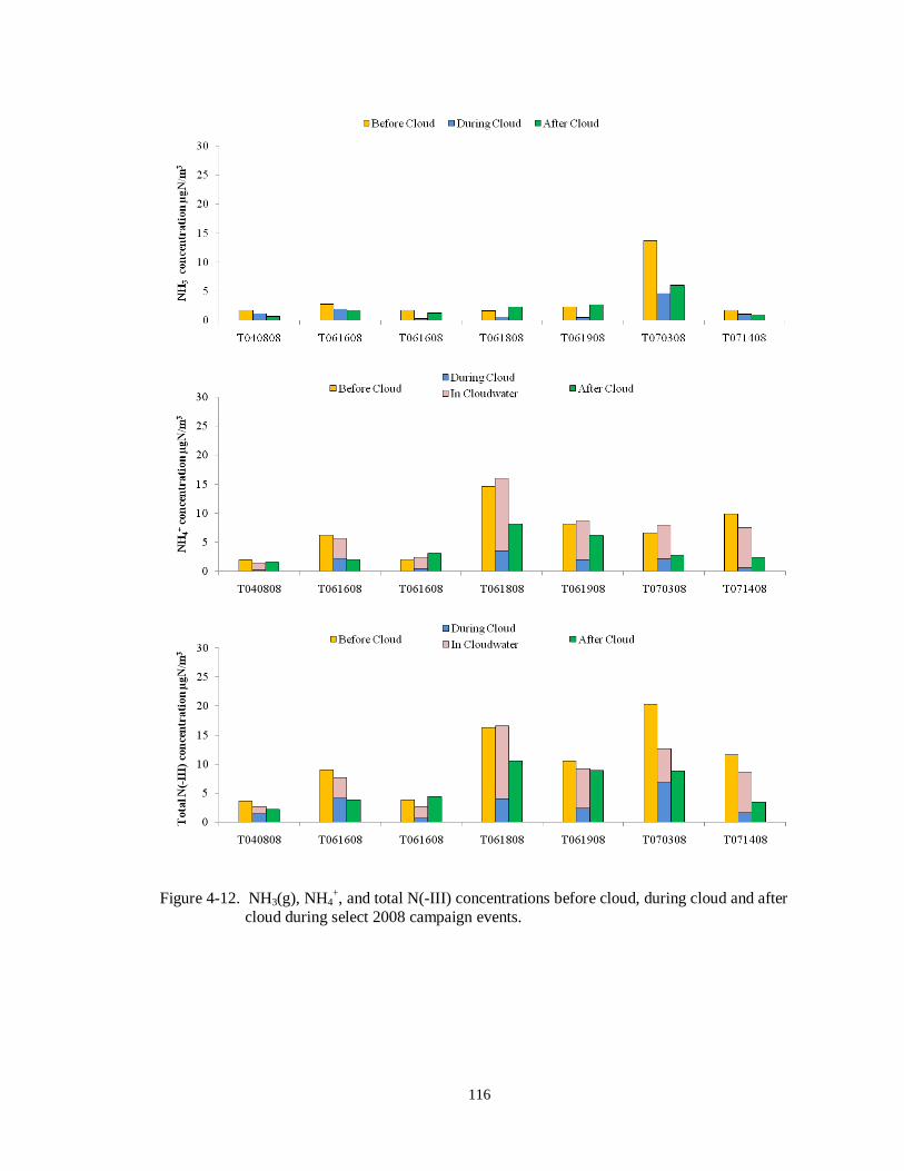
116

Figure 4-12. NH3(g), NH4+, and total N(-III) concentrations before cloud, during cloud and after


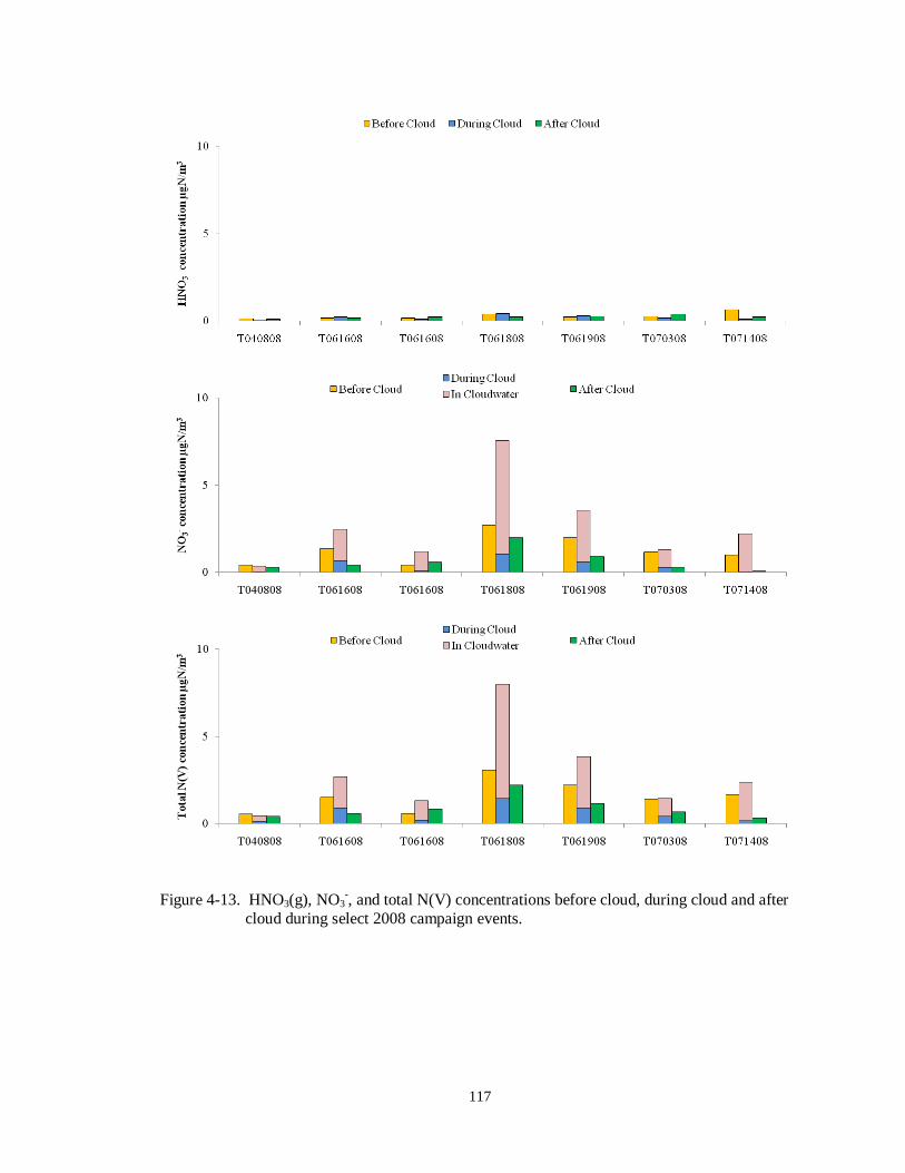
117

Figure 4-13. HNO3(g), NO3-, and total N(V) concentrations before cloud, during cloud and after


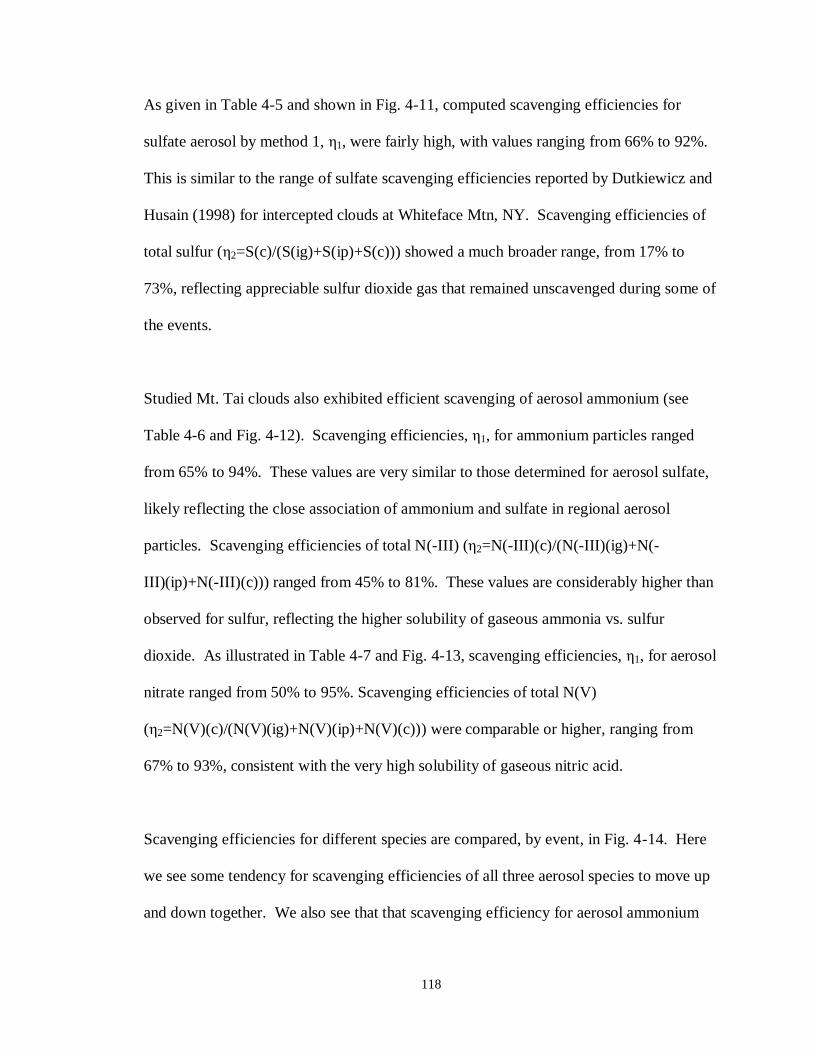
118

As given in Table 4-5 and shown in Fig. 4-11, computed scavenging efficiencies for

sulfate aerosol by method 1, η1, were fairly high, with values ranging from 66% to 92%.

This is similar to the range of sulfate scavenging efficiencies reported by Dutkiewicz and

Husain (1998) for intercepted clouds at Whiteface Mtn, NY. Scavenging efficiencies of

total sulfur (η2=S(c)/(S(ig)+S(ip)+S(c))) showed a much broader range, from 17% to

73%, reflecting appreciable sulfur dioxide gas that remained unscavenged during some of

the events.

Studied Mt. Tai clouds also exhibited efficient scavenging of aerosol ammonium (see

Table 4-6 and Fig. 4-12). Scavenging efficiencies, η1, for ammonium particles ranged

from 65% to 94%. These values are very similar to those determined for aerosol sulfate,

likely reflecting the close association of ammonium and sulfate in regional aerosol

particles. Scavenging efficiencies of total N(-III) (η2=N(-III)(c)/(N(-III)(ig)+N(-

III)(ip)+N(-III)(c))) ranged from 45% to 81%. These values are considerably higher than

observed for sulfur, reflecting the higher solubility of gaseous ammonia vs. sulfur

dioxide. As illustrated in Table 4-7 and Fig. 4-13, scavenging efficiencies, η1, for aerosol

nitrate ranged from 50% to 95%. Scavenging efficiencies of total N(V)

(η2=N(V)(c)/(N(V)(ig)+N(V)(ip)+N(V)(c))) were comparable or higher, ranging from

67% to 93%, consistent with the very high solubility of gaseous nitric acid.

Scavenging efficiencies for different species are compared, by event, in Fig. 4-14. Here

we see some tendency for scavenging efficiencies of all three aerosol species to move up

and down together. We also see that that scavenging efficiency for aerosol ammonium

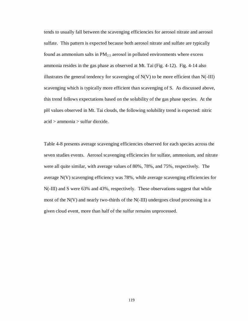
119

tends to usually fall between the scavenging efficiencies for aerosol nitrate and aerosol

sulfate. This pattern is expected because both aerosol nitrate and sulfate are typically

found as ammonium salts in PM2.5 aerosol in polluted environments where excess

ammonia resides in the gas phase as observed at Mt. Tai (Fig. 4-12). Fig. 4-14 also

illustrates the general tendency for scavenging of N(V) to be more efficient than N(-III)

scavenging which is typically more efficient than scavenging of S. As discussed above,

this trend follows expectations based on the solubility of the gas phase species. At the

pH values observed in Mt. Tai clouds, the following solubility trend is expected: nitric

acid > ammonia > sulfur dioxide.

Table 4-8 presents average scavenging efficiencies observed for each species across the

seven studies events. Aerosol scavenging efficiencies for sulfate, ammonium, and nitrate

were all quite similar, with average values of 80%, 78%, and 75%, respectively. The

average N(V) scavenging efficiency was 78%, while average scavenging efficiencies for

N(-III) and S were 63% and 43%, respectively. These observations suggest that while

most of the N(V) and nearly two-thirds of the N(-III) undergoes cloud processing in a

given cloud event, more than half of the sulfur remains unprocessed.

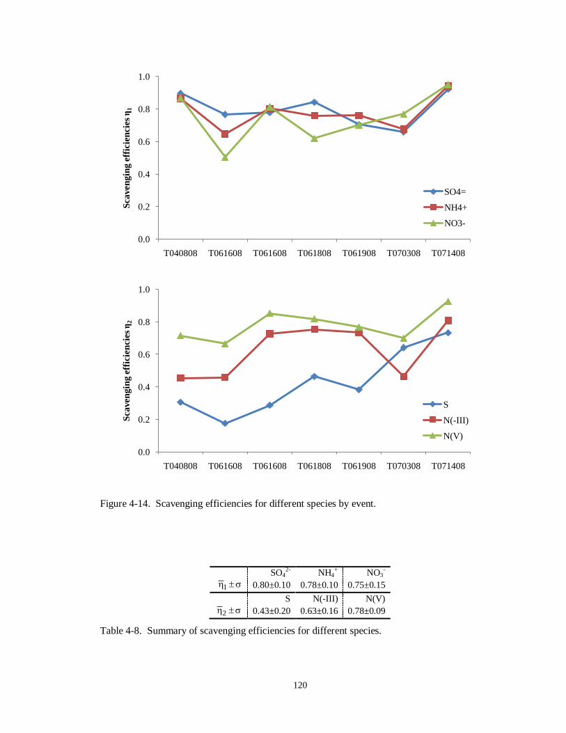
120

Figure 4-14. Scavenging efficiencies for different species by event.

SO42- NH4

+ NO3-

1 0.80±0.10 0.78±0.10 0.75±0.15

S N(-III) N(V)

2 0.43±0.20 0.63±0.16 0.78±0.09

Table 4-8. Summary of scavenging efficiencies for different species.

0.0

0.2

0.4

0.6

0.8

1.0

T040808 T061608 T061608 T061808 T061908 T070308 T071408

Scaven

gin

g e

ffic

ien

cie

s η

1

SO4=

NH4+

NO3-

0.0

0.2

0.4

0.6

0.8

1.0

T040808 T061608 T061608 T061808 T061908 T070308 T071408

Sca

ven

gin

g e

ffic

ien

cie

s η

2

S

N(-III)

N(V)

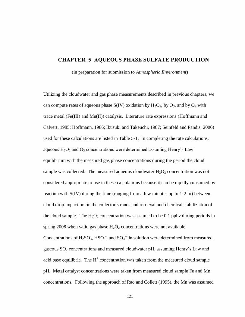
121

CHAPTER 5 AQUEOUS PHASE SULFATE PRODUCTION

(in preparation for submission to Atmospheric Environment)

Utilizing the cloudwater and gas phase measurements described in previous chapters, we

can compute rates of aqueous phase S(IV) oxidation by H2O2, by O3, and by O2 with

trace metal (Fe(III) and Mn(II)) catalysis. Literature rate expressions (Hoffmann and

Calvert, 1985; Hoffmann, 1986; Ibusuki and Takeuchi, 1987; Seinfeld and Pandis, 2006)

used for these calculations are listed in Table 5-1. In completing the rate calculations,

aqueous H2O2 and O3 concentrations were determined assuming Henry’s Law

equilibrium with the measured gas phase concentrations during the period the cloud

sample was collected. The measured aqueous cloudwater H2O2 concentration was not

considered appropriate to use in these calculations because it can be rapidly consumed by

reaction with S(IV) during the time (ranging from a few minutes up to 1-2 hr) between

cloud drop impaction on the collector strands and retrieval and chemical stabilization of

the cloud sample. The H2O2 concentration was assumed to be 0.1 ppbv during periods in

spring 2008 when valid gas phase H2O2 concentrations were not available.

Concentrations of H2SO3, HSO3-, and SO3

2- in solution were determined from measured

gaseous SO2 concentrations and measured cloudwater pH, assuming Henry’s Law and

acid base equilibria. The H+ concentration was taken from the measured cloud sample

pH. Metal catalyst concentrations were taken from measured cloud sample Fe and Mn

concentrations. Following the approach of Rao and Collett (1995), the Mn was assumed

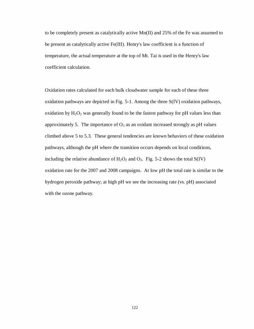
122

to be completely present as catalytically active Mn(II) and 25% of the Fe was assumed to

be present as catalytically active Fe(III). Henry's law coefficient is a function of

temperature, the actual temperature at the top of Mt. Tai is used in the Henry's law

coefficient calculation.

Oxidation rates calculated for each bulk cloudwater sample for each of these three

oxidation pathways are depicted in Fig. 5-1. Among the three S(IV) oxidation pathways,

oxidation by H2O2 was generally found to be the fastest pathway for pH values less than

approximately 5. The importance of O3 as an oxidant increased strongly as pH values

climbed above 5 to 5.3. These general tendencies are known behaviors of these oxidation

pathways, although the pH where the transition occurs depends on local conditions,

including the relative abundance of H2O2 and O3. Fig. 5-2 shows the total S(IV)

oxidation rate for the 2007 and 2008 campaigns. At low pH the total rate is similar to the

hydrogen peroxide pathway; at high pH we see the increasing rate (vs. pH) associated

with the ozone pathway.

123

Table 5-1. Rate expressions used for S(IV) oxidation and S(IV) reaction with HCHO.

Reaction Rate (M/s) Characteristic Time (s)

]O][S(IV))[(]S(IV)[

3221100 kkkdt

d ])O)[/((1 3221100O3

kkk (Hoffmann and Calvert, 1985)

]H[1

]S(IV)][OH][H[]S(IV)[ 122

K

k

dt

d )]O][H[H/(])H[1( 122OH 22

kK (Seinfeld and Pandis, 2006)

[S(IV)][Mn(II)][Fe(III)]][H]S(IV)[ 0.74'

skdt

d )[Mn(II)][Fe(III)]][H/(1 -0.74''

(III))(Mn(II)/FeO2

sk ( 2.4pH ) (Ibusuki and Takeuchi, 1987)

[S(IV)][Mn(II)][Fe(III)]][H]S(IV)[ 67.0"

skdt

d )[Mn(II)][Fe(III)]][H/(1 0.67""

(III))(Mn(II)/FeO2

sk ( 2.4pH5.6 ) (Ibusuki and Takeuchi, 1987)

[HCHO][S(IV)][HCHO][S(IV)]]S(IV)[

2514 kkdt

d ))([HCHO]/(1 2514HCHO kk (Boyce and Hoffmann, 1984)

0 , 1 , and 2 represent the fractions of total free S(IV) present as SO2·H2O, HSO3 and -2

3SO respectively. 1140 sM102.4 k , 115

1 sM103.7 k ,

1192 sM101.5 k , 127 sM107.45 k , 1M13 K , 127' 103.72 SMks , 1213" 102.51 SMks , 112

4 sM107.9 k and 1175 sM1048.2 k at 298K, ks'

and ks" were determined at 296.8K.. Equilibrium and rate constants were adjusted for ambient temperature using the thermodynamic data from Table 1-2 and 1-3.

124

Figure 5-1. S(IV) reaction rates determined for individual cloudwater samples according to the

approach outlined in the text. Rates of reaction are included for S(IV) oxidation by O3, by H2O2, and by O2 (catalyzed by Fe and Mn) and for S(IV) reaction with

HCHO to form HMS.

Figure 5-2. Total S(IV) oxidation rate.

1.E-12

1.E-10

1.E-08

1.E-06

1.E-04

1.E-02

2 3 4 5 6 7 8

-d[S

(IV

)]/d

t (M

/s)

pH

2007 O3 2008 O32007 H2O2 2008 H2O22007 O2 / Fe(III)+Mn(II) 2008 O2 / Fe(III)+Mn(II)2007 HCHO 2008 HCHO

1.E-12

1.E-10

1.E-08

1.E-06

1.E-04

1.E-02

2 3 4 5 6 7 8

-d[S

(IV

)]/d

t (M

/s)

pH

2007 Total 2008 Total

125

As depicted in Fig. 5-3, variations in the rate of S(IV) oxidation by ozone show little

overall dependence on the ozone concentration. This is because the influence of

cloudwater pH is much stronger. At higher pH, partitioning of the H2SO3-HSO3--SO3

2-

shifts toward the deprotonated S(IV) forms; this increases the SO2 oxidation rate because

more SO2 is drawn into solution and the S(IV) speciation shifts toward more reactive

forms (SO32-

>HSO3->H2SO3).

Figure 5-3. Rates of S(IV) oxidation by O3, determined for the Mt. Tai cloud samples, plotted as

a function of the ambient O3 mixing ratio.

Computed metal-catalyzed S(IV) autooxidation rates, also shown in Fig. 5-1, are highly

variable, reflecting high variability in cloudwater trace metal concentrations and the

nonlinear dependence of the Ibusuki and Takeuchi (1987) rate expression on these

concentrations. In general, the rate of this oxidation pathway is typically 2nd

or 3rd

fastest

of the three computed oxidation pathways across the full observed pH range. There are a

1.E-12

1.E-10

1.E-08

1.E-06

1.E-04

1.E-02

20 40 60 80 100

-d[S

(IV

)]/d

t (M

/s)

O3 ( ppb )

2007 2008

126

few samples, however, where the metal-catalyzed pathway appears fast enough to make

some contribution to aqueous sulfate production.

The overall oxidation rate patterns depicted in Fig. 5-2 and described above are fairly

similar for the 2007 and 2008 cloud samples, suggesting that these patterns are fairly

robust under a variety of emission, cloud formation, and transport patterns during the

period. Note that the 2008 summer campaign period concluded before the start of the

2008 Beijing Olympics when more stringent regional emissions reductions came online.

Grouping all 4 measurement periods together, we find that in 68% of the sample periods

the fastest S(IV) oxidation pathway is the hydrogen peroxide pathway. The ozone

pathway is fastest 21% of the time and the metal-catalyzed pathway is fastest 11% of the

time. Fig. 5-4 shows the fraction of time that each oxidation pathway was fastest for the

four campaigns. Given the abundant SO2 often found in the regional atmosphere, it was

somewhat surprising to see that H2O2 was the dominant oxidant so much of the time. In

addition to the gas phase H2O2 observations used for the oxidation rate calculations, we

can also examine the presence of H2O2 in the collected cloudwater. While there are many

samples where H2O2 was low (or was depleted by reaction prior to sample retrieval and

derivatization), there are also many samples, especially from the summertime, where tens

to hundreds of µM of H2O2 remain in the cloudwater and little S(IV) remained. This

residual peroxide indicates a substantial capacity during these periods for additional in-

cloud sulfate production.

127

Figure 5-4. the fraction of time that each oxidation pathway was fastest for the four campaigns.

Fig. 5-1 also depicts rates of HMS formation due to reaction of dissolved S(IV) with

HCHO. These rates were computed using the expression by Boyce and Hoffmann

(Boyce and Hoffmann, 1984). Aqueous S(IV) concentrations and speciation were

determined as outlined above for the oxidation rate concentrations. HCHO

concentrations were taken from the measured HCHO concentrations in the individual

cloud samples. Because these HCHO values may include some HMS already present in

the cloudwater (HCHO is preserved as HMS following sample collection), these rates

should be considered an upper limit to the actual HMS formation rate in Mt. Tai clouds.

While HMS formation does not appear important at low pH values, the calculations

suggest that it may provide an additional, important sink for dissolved SO2 when cloud

pH climbs much above 4. Future cloud composition studies in the region should include

measurement of HMS to determine whether its formation is as important as suggested by

the rate calculations here.

0%

20%

40%

60%

80%

100%

2007 Spring 2007 Summer 2008 Spring 2008 Summer

Bulk Samples

O2 / Fe(III)+Mn(II) H2O2 O3

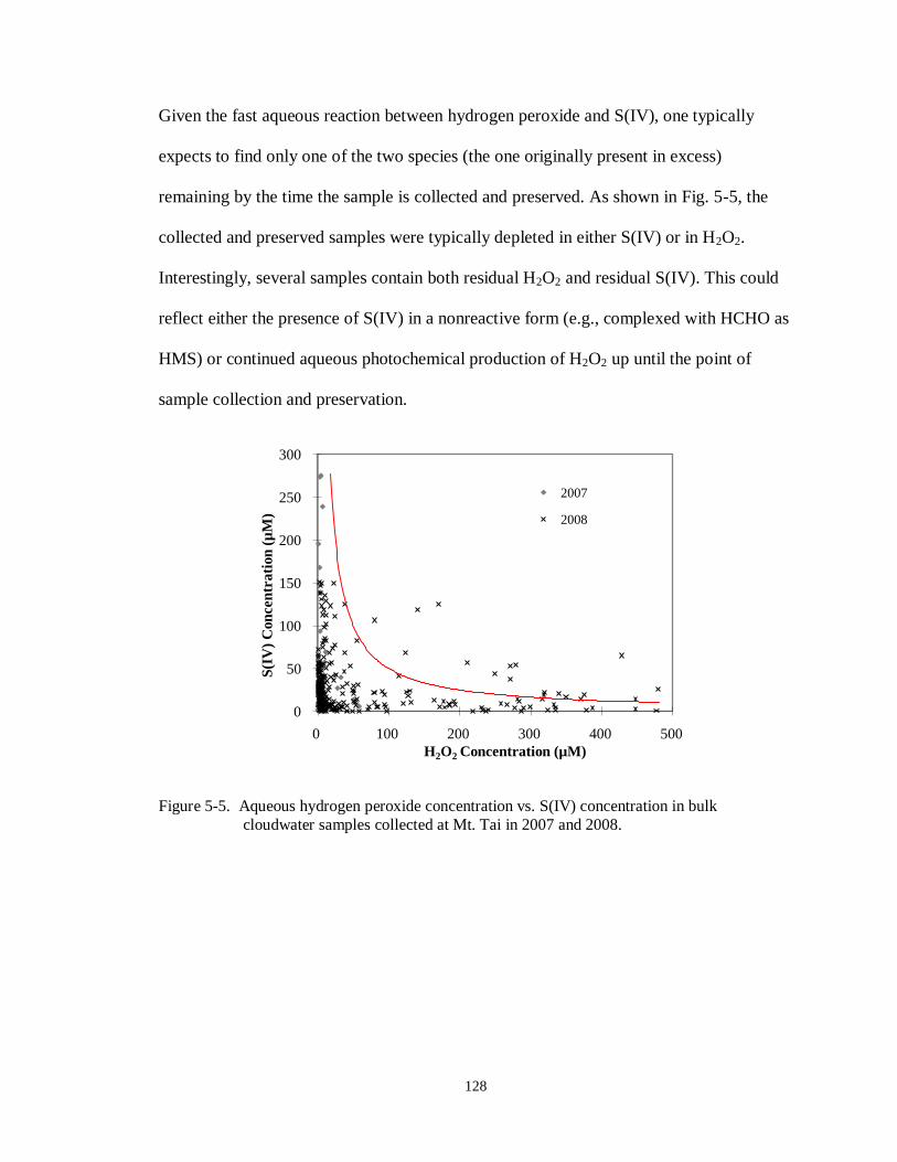
128

Given the fast aqueous reaction between hydrogen peroxide and S(IV), one typically

expects to find only one of the two species (the one originally present in excess)

remaining by the time the sample is collected and preserved. As shown in Fig. 5-5, the

collected and preserved samples were typically depleted in either S(IV) or in H2O2.

Interestingly, several samples contain both residual H2O2 and residual S(IV). This could

reflect either the presence of S(IV) in a nonreactive form (e.g., complexed with HCHO as

HMS) or continued aqueous photochemical production of H2O2 up until the point of

sample collection and preservation.

Figure 5-5. Aqueous hydrogen peroxide concentration vs. S(IV) concentration in bulk

cloudwater samples collected at Mt. Tai in 2007 and 2008.

0

50

100

150

200

250

300

0 100 200 300 400 500

S(I

V)

Con

cen

tra

tion

(µ

M)

H2O2 Concentration (µM)

2007

2008

129

Table 5-2. Data table for samples containing both residual H2O2 and residual S(IV)

pH H2O2 S(IV) HCHO Reaction rate (M/s) Most important

(µM) (µM) (µM) O3 H2O2 O2(Fe(III)/Mn(II)) HCHO reaction way

TC070308A01 5.42 169.6 124.9 14.5 7.4E-08 1.2E-07 7.3E-07 3.2E-05 HCHO

TC070308A02 5.31 55.4 82.2 13.1 3.7E-08 3.9E-08 1.5E-07 1.7E-05 HCHO

TC070308A03 5.38 79.8 106.5 4.9 4.9E-08 2.9E-08 5.6E-08 8.8E-06 HCHO

TC070308A04 5.51 122.8 68.4 4.8 8.3E-08 3.7E-08 4.6E-08 1.5E-05 HCHO

TC070308A05 5.62 279.0 54.5 6.3 1.5E-07 4.1E-08 4.2E-08 3.4E-05 HCHO

TC070308A06 5.55 271.4 37.9 4.1 1.1E-07 4.2E-08 2.8E-08 1.7E-05 HCHO

TC070308A07 5.22 479.3 26.3 4.8 2.2E-08 5.4E-08 9.5E-08 3.9E-06 HCHO TC070408A09 6.35 114.1 41.3 4.8 1.1E-06 7.1E-09 N/A1 3.4E-04 HCHO

TC070808A01 4.42 427.3 65.3 20.3 1.5E-10 1.6E-08 2.9E-09 1.2E-07 HCHO

TC070808A03 3.91 270.8 53.5 16.4 2.3E-10 1.5E-07 8.7E-10 1.1E-07 H2O2

TC070808A05 3.95 248.6 44.1 18.4 2.2E-10 9.7E-08 9.1E-10 9.6E-08 H2O2

TL070308A01 5.92 139.8 118.5 14.5 6.9E-07 9.3E-08 1.3E-06 3.2E-04 HCHO

TL070808A01 4.57 210.5 56.4 22.8 7.1E-10 3.9E-08 1.1E-08 6.3E-07 HCHO

N/A1: Fe(III) and Mn(II) data not available.

130

Table 5-2 gives a list of samples for which both S(IV) and H2O2 concentrations are

relatively high. These samples mainly came from two cloud events, 7/3/2008 and

7/8/2008. For most of these samples, calculations suggest that complexation with HCHO

to form HMS is the most important S(IV) reaction sink. This result HMS formation may

be more important in these samples than S(IV) oxidation and could help explain the

coexistence of S(IV) (which includes HMS) and H2O2 in the preserved cloudwater

samples.

A comparison between oxidation rates computed for small and large cloud drop size

fractions collected in 2008 with the sf-CASCC is shown in Figure 5-6. There is a

tendency for oxidation rates to be higher in the large drops. This comes from the strong

dependence of two of the pathways on cloud pH (faster oxidation at higher pH) and the

tendency (see Fig. 3-34) for the pH to be higher in the large cloud drop size fraction. In

the case of the metal-catalyzed pathway, there is an additional effect from any drop size-

dependence in the Fe and Mn concentrations.

131

Figure 5-6. Comparison of predicted S(IV) oxidation rates in small (4 < D < 16 µm) and large (D

> 16 µm) cloud drop size fraction sample pairs simultaneously collected with the sf-

CASCC at Mt. Tai during the spring and summer 2008 field campaigns. Results are shown for the ozone and metal-catalyzed autooxidation pathways. (The diagonal

dashed line is the 1:1 line.)

1.E-12

1.E-10

1.E-08

1.E-06

1.E-04

1.E-12 1.E-10 1.E-08 1.E-06 1.E-04

Sm

all

Drop

s -

d[S

(IV

)]/d

t (M

/s)

Large Drops -d[S(IV)]/dt (M/s)

Spring O3

Summer O3

1.E-12

1.E-10

1.E-08

1.E-06

1.E-04

1.E-12 1.E-10 1.E-08 1.E-06 1.E-04

Sm

all

D

rop

s

-d[S

(IV

)]/d

t (M

/s)

Large Drops -d[S(IV)]/dt (M/s)

Spring O2 / Fe(III)+Mn(II)

Summer O2 / Fe(III)+Mn(II)

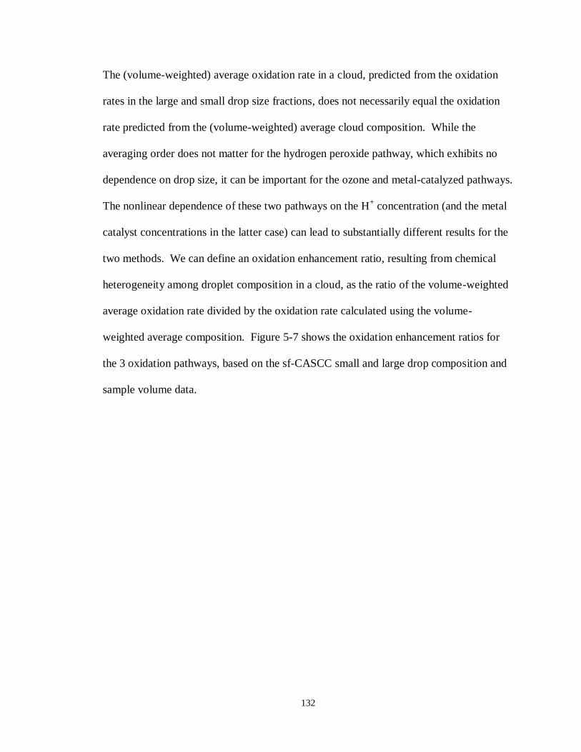
132

The (volume-weighted) average oxidation rate in a cloud, predicted from the oxidation

rates in the large and small drop size fractions, does not necessarily equal the oxidation

rate predicted from the (volume-weighted) average cloud composition. While the

averaging order does not matter for the hydrogen peroxide pathway, which exhibits no

dependence on drop size, it can be important for the ozone and metal-catalyzed pathways.

The nonlinear dependence of these two pathways on the H+ concentration (and the metal

catalyst concentrations in the latter case) can lead to substantially different results for the

two methods. We can define an oxidation enhancement ratio, resulting from chemical

heterogeneity among droplet composition in a cloud, as the ratio of the volume-weighted

average oxidation rate divided by the oxidation rate calculated using the volume-

weighted average composition. Figure 5-7 shows the oxidation enhancement ratios for

the 3 oxidation pathways, based on the sf-CASCC small and large drop composition and

sample volume data.

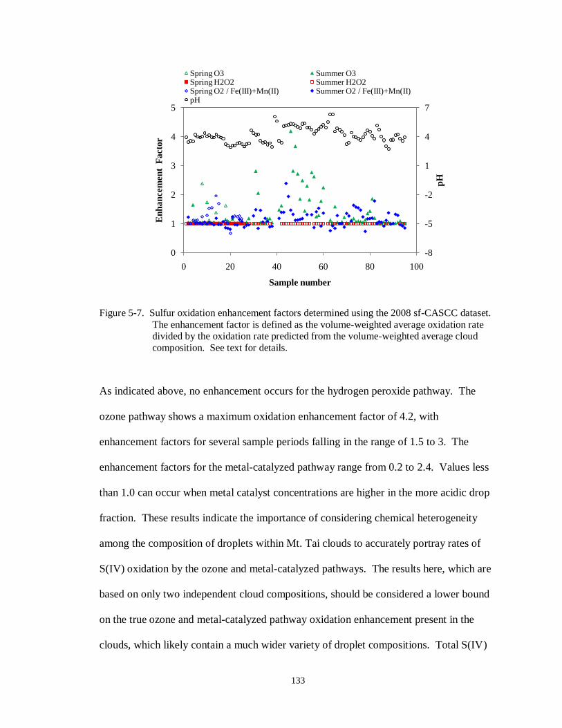
133

Figure 5-7. Sulfur oxidation enhancement factors determined using the 2008 sf-CASCC dataset.

The enhancement factor is defined as the volume-weighted average oxidation rate divided by the oxidation rate predicted from the volume-weighted average cloud

composition. See text for details.

As indicated above, no enhancement occurs for the hydrogen peroxide pathway. The

ozone pathway shows a maximum oxidation enhancement factor of 4.2, with

enhancement factors for several sample periods falling in the range of 1.5 to 3. The

enhancement factors for the metal-catalyzed pathway range from 0.2 to 2.4. Values less

than 1.0 can occur when metal catalyst concentrations are higher in the more acidic drop

fraction. These results indicate the importance of considering chemical heterogeneity

among the composition of droplets within Mt. Tai clouds to accurately portray rates of

S(IV) oxidation by the ozone and metal-catalyzed pathways. The results here, which are

based on only two independent cloud compositions, should be considered a lower bound

on the true ozone and metal-catalyzed pathway oxidation enhancement present in the

clouds, which likely contain a much wider variety of droplet compositions. Total S(IV)

-8

-5

-2

1

4

7

0

1

2

3

4

5

0 20 40 60 80 100

pH

En

han

cem

en

t F

acto

r

Sample number

Spring O3 Summer O3Spring H2O2 Summer H2O2Spring O2 / Fe(III)+Mn(II) Summer O2 / Fe(III)+Mn(II)pH

134

oxidation rates (the sums of all three oxidation pathways) in Mt. Tai clouds, however, are

less sensitive to chemical heterogeneity among cloud drop composition since hydrogen

peroxide was observed to be the dominant oxidant in most of the cloud periods measured.

135

CHAPTER 6 CONCLUSIONS

6.1. CONCLUSIONS

In consideration of the huge amount of SO2 emission in China, and the fact that aqueous

phase oxidation processes are so critical to sulfate production, it is imperative to

understand factors influencing cloud chemistry in China in order to accurately predict

effects of increasing regional SO2 emissions on sulfate production in that part of the

world and its local, regional, and intercontinental effects. While model simulations

provide valuable insight into sulfur chemistry and its sensitivity to changing emissions, in

situ observations are needed to assess actual conditions in the region. In order to more

fully investigate the cloudwater chemical composition and key species that determine the

aqueous phase sulfur chemistry and to assess the ability of regional clouds to support

aqueous sulfur oxidation, four field campaigns were conducted in 2007 and 2008 at Mt.

Tai in eastern China. Mt. Tai is located in central Shandong province, which has the

highest SO2 emission in China. The elevation of Mt. Tai isolates the measurements from

direct influence by large urban emission sources, providing a more representative picture

of regional atmospheric composition. The summit is frequently in cloud during spring

and summer and nearly half of the year days have fog, making Mt. Tai a reliable place to

sample fog and cloudwater under the influence of regional atmospheric pollution.

136

Single and 2-stage Caltech Active Strand Cloudwater Collectors were used to collect bulk

and drop size-resolved cloudwater samples, respectively. Key species that influence

aqueous phase sulfur oxidation were analyzed, including cloudwater pH, S(IV), H2O2, Fe,

and Mn. Gas phase SO2, O3, and H2O2 were also measured continuously during the

campaigns. Other species in cloudwater including inorganic ions, total organic carbon

(TOC), formaldehyde, and organic acids were also analyzed. During the 2008 campaigns,

measurements of pre-cloud, interstitial, and post-cloud aerosols and trace gases were also

made in order to examine the efficiency of cloud scavenging of key nitrogen- and sulfur-

containing species.

Many periods of cloud interception/fog occurred during the four Mt. Tai field campaigns.


bulk cloudwater samples were collected. During the summer 2007 campaign (06/20-

07/20), there were 12 cloud events; a total of 66 bulk cloudwater samples were collected.


cloudwater samples (including 25 bulk samples and 58 size-fractionated samples) were

collected. During the summer 2008 campaign (06/14-07/16), there were 18 cloud events;

a total of 333 cloudwater samples (including 117 bulk samples and 216 size-fractionating

samples) were collected.

Gaseous H2O2 concentrations were generally lower in spring (2007 average mixing ratio

of 0.17 ppbv) than in summer (2007 average mixing ratio of 0.55 ppbv). Summer 2008

H2O2 mixing ratios averaged 0.59 ppbv. The average concentrations of SO2 measured

137

during the Mt. Tai spring campaigns were approximately double the summertime

averages. Average mixing ratios of 15.4 ppbv and 14.5 ppbv were observed in spring

2007 and spring 2008, respectively, while average mixing ratios of 8.1 ppbv and 6.4 ppbv

were observed in summer 2007 and summer 2008. Average O3 concentrations were

similar across all four campaigns, with mixing ratio averages of 62.1 ppbv and 66.0 ppbv

in spring 2007 and spring 2008, respectively, and average mixing ratios of 72.1 ppbv and

68.0 ppbv in summer 2007 and 2008.

A wide range of cloud pH values was observed in bulk cloudwater samples collected at

Mt. Tai. Cloudwater pH values ranged from 2.69 to 7.64 in 2007 and from 2.65 to 6.94 in

2008. These ranges are large enough that we should expect multiple S(IV) oxidation

pathways to be important at various times. They also indicate strong variability in the

relative contributions of acids and bases to regional cloud composition. TOC

concentrations (volume-weighted average) in spring and summer 2008 averaged 2.6

ppmC and 15.8 ppmC, respectively. Concentrations of TOC are very high in some Mt.

Tai cloudwater samples, reaching as much as 200 ppmC. SO42-

, NO3-, and NH4

+ were the

major inorganic species for all of the four campaigns, accounting for approximately

39.9%, 29.9% and 15.5%, by mass, of the total measured inorganic ions, respectively,

during the spring 2007 campaign; accounting for about 52.8%, 15.5% and 24.8% of the

total inorganic ions, respectively during the summer 2007 campaign; accounting for

about 51.2%, 20.9% and 18.6% of the total inorganic ions, respectively during the spring

2008 campaign; and accounting for about 46.6%, 25.5% and 19.2% of the total inorganic

ions, respectively, during the summer 2008 campaign. The average aqueous H2O2 values

138

in spring and summer 2007 were 2.8 µM and 15 µM, respectively. The average aqueous

H2O2 values in spring and summer 2008 were 9.2 µM and 69.1 µM, respectively. The

reaction between S(IV) and H2O2 in aqueous solution is very fast, so that measured H2O2

represents “residual” H2O2 that was not consumed by reaction between sample collection

and preservation. The average aqueous S(IV) values in spring and summer 2007 were

40.4 µM and 17.7 µM, respectively. The average aqueous S(IV) values in spring and

summer 2008 were 7.7 µM and 35.6 µM, respectively. As with H2O2, measured S(IV)

represents residual S(IV) not consumed by reaction between the times of sample

collection and preservation. The average bulk cloudwater Fe concentrations measured in

spring and summer 2007 were 242.5 µg/L and 44.2 µg/L, respectively. Fe concentrations

measured in spring and summer 2008 averaged 241.8 µg/L and 415.7 µg/L, respectively.

The average Mn concentrations observed in spring and summer 2007 were 93.2 µg/L and

30.2 µg/L, respectively. Mn concentrations in spring and summer 2008 averaged 20.4

µg/L and 29.9 µg/L, respectively. The average HCHO concentrations observed in spring

and summer 2007 were 21.3 µM and 25.4 µM, respectively. HCHO concentrations in

spring and summer 2008 averaged 4.7 µM and 9.5 µM, respectively.

Comparison of the compositions large (D > 16 µm) and small (4 < D < 16 µm) cloud

drops revealed some differences. While only a small pH difference was observed during

many sample periods, fairly large pH differences, of 0.5 – 1.0 pH units or greater, were

observed in some cases. Some enrichment of TOC in smaller drops was observed in some

sample periods. No consistent pattern of small or large cloud drop enrichment was seen

for SO42-

, NO3-, NH4

+, aqueous H2O2, S(IV), HCHO, Fe and Mn. Higher concentrations

139

of Ca2+

, Na+ and Mg

2+ were typically found in the large drops. Differences in

composition among droplets can lead to differences in the rates of aqueous phase

reactions.

Analysis of cloud composition and backward trajectories revealed some patterns,

including high dust content in Mt. Tai clouds during periods of strong spring dust

transport from northern China. Several cases of strong influence of biomass burning on

Mt. Tai clouds, evidenced by high concentrations of TOC, K+, and organic smoke marker

species, were also observed during June. In some cases, however, no clear relationship

was observed between horizontal transport patterns and cloudwater chemical

composition. Mt. Tai is surrounded by regions of high pollutant emissions, giving the

potential for polluted cloudwater regardless of the longer distance origins of air

trajectories. Incorporating additional information about air parcel history (e.g., vertical

transport and precipitation history), did provide additional insight, especially when cloud

water solute content was low.

Mt. Tai clouds were found to interact strongly with PM2.5 inorganic aerosol species.

Scavenging efficiencies for sulfate aerosol were fairly high, with values ranging from

66% to 92%. Scavenging efficiencies of total sulfur showed a much broader range, from

17% to 73%, reflecting appreciable sulfur dioxide gas that remained unscavenged during

some of the events. Scavenging efficiencies for ammonium particles ranged from 65% to

94%, similar to values observed for aerosol sulfate, consistent with an expected close

association between ammonium and sulfate in regional aerosol particles. Scavenging

140

efficiencies of total N(-III) ranged from 45% to 81%. These values are considerably

higher than observed for sulfur, reflecting the higher solubility of gaseous ammonia vs.

sulfur dioxide. Scavenging efficiencies for aerosol nitrate ranged from 50% to 95%.

Scavenging efficiencies of total N(V) were comparable or higher, ranging from 67% to

93%, consistent with the very high solubility of gaseous nitric acid. The average N(V)

scavenging efficiency across studied events was 78%, while average scavenging

efficiencies for N(-III) and S were 63% and 43%, respectively. These observations

suggest that while most of the N(V) and nearly two-thirds of the N(-III) undergoes cloud

processing in a given cloud event, more than half of the sulfur remains unprocessed.

Rates of aqueous phase S(IV) oxidation by H2O2, by O3, and by O2 with trace metal

(Fe(III) and Mn(II)) catalysis were computed utilizing the cloudwater and gas phase

measurements described above. Among the three S(IV) oxidation pathways, oxidation by

H2O2 was generally found to be the fastest pathway for pH values less than

approximately 5. The importance of O3 as an oxidant increased strongly as pH values

climbed above 5 to 5.3. Variations in the rate of S(IV) oxidation by ozone show little

overall dependence on the ozone concentration and were governed more strongly by

factors influencing cloud pH. Computed metal-catalyzed S(IV) autooxidation rates were

highly variable. Overall, in 68% of the sample periods the fastest S(IV) oxidation

pathway was the hydrogen peroxide pathway. The ozone pathway was fastest 21% of the

time and the metal-catalyzed pathway was fastest 11% of the time. While many collected

cloud samples had low concentrations of H2O2, there also were many samples, especially

from the summertime, where tens to hundreds of µM of H2O2 remain in the cloudwater

141

and little S(IV) remained. This residual peroxide indicates a substantial capacity during

these periods for additional in-cloud sulfate production.

A comparison between oxidation rates computed for small and large cloud drop size

fractions revealed a general tendency for oxidation rates to be faster in the large drops for

the ozone and metal-catalyzed pathways. This comes from the strong dependence of both

pathways on cloud pH (faster oxidation at higher pH) and the tendency for the pH to be

higher in the large cloud drop size fraction. In the case of the metal-catalyzed pathway,

there is an additional effect from any drop size-dependence in the Fe and Mn

concentrations. The nonlinear dependence of these two pathways on the H+ concentration

(and the metal catalyst concentrations in the latter case) can lead to biases in oxidation

rates predicted from the (volume-weighted) average cloud composition. Chemical

heterogeneity among cloud drop composition can enhance rates of S(IV) oxidation by

ozone, vs. rates expected from average cloud composition, while it can increase or

decrease rates of metal-catalyzed S(IV) autooxidation, depending on how both H+ and

metal catalyst concentrations are distributed with drop size. No enhancement occurs for

the hydrogen peroxide pathway, which is essentially independent of the H+ concentration

over a relevant pH range. Enhancements up to 420% were observed for the ozone

oxidation pathway and up to 240% for the metal-catalyzed pathway. While these upper

limits are large, most values were smaller (suppression up to 80% was also observed for

the metal-catalyzed pathway). Furthermore, total S(IV) oxidation rates (the sums of all

three oxidation pathways) in Mt. Tai clouds, however, are less sensitive to chemical

142

heterogeneity among cloud drop composition since hydrogen peroxide was found to be

the dominant oxidant in most of the cloud periods measured.

These data provide a novel and robust dataset for future evaluations of numerical

simulations of the fate of SO2 emitted in China. The importance of H2O2 as an aqueous

phase oxidant is clear and, for the first time, observations of gas phase H2O2 and the

presence of residual H2O2 in many summertime clouds has been demonstrated. In

addition, measurements of the composition of clouds at Mt. Tai clearly reveal that

China’s air pollution has moved well beyond the point where sulfur dioxide and dust

emissions are the only concerns. Abundant cloudwater ammonium, nitrate and organic

matter clearly demonstrate the importance of other pollutant emissions, including NOx

from transportation, power generation, lightning, and other combustion sources, ammonia

from agriculture, and organic matter from many sources, including the burning of

agricultural biomass.

6.2. RECOMMENDATIONS FOR FUTURE WORK

This study represents the first extensive investigation of cloud composition and the

processing of sulfur dioxide by regional clouds in eastern China. Based on the findings

here, several avenues of possible future investigation are recommended:

Future cloud composition studies in the region should include measurement of

HMS to determine whether its formation is as important as suggested by the rate

143

calculations here. HMS measurements could also be included in aerosol

chemistry studies.

Future cloud composition studies in the region should include speciation of Fe

and Mn. Mn(II) usually is the predominant oxidation state of Mn; however, the

speciation of Fe is less certain. The relative abundance of the catalytically active

iron form, Fe(III), and the inactive iron form, Fe(II), is important for accurately

determining the metal-catalyzed S(IV) autooxidation rate. While a catalytically

active fraction of 25% was assumed for this study, measurements of the actual

Fe(III) abundance, and changes with cloud pH and/or actinic flux, would be

especially interesting to examine.

Additional work is needed to examine organic acids in cloudwater to better

understand possible effects on cloudwater acidity. Organic acids can also act as

good ligands for trace metals and may play an important role in droplet

photochemistry, including Fenton-like chemistry which may be an important

route for aqueous phase H2O2 production in these clouds.

While the samples collected in this study were assumed to be fairly representative

of cloud composition in the eastern part of China, additional measurements at

other locations could help test the validity of this assumption. Other regions, such

as Mt. Lu and Mt. Huang should be considered for future cloud composition

studies. Continued measurements at Mt. Tai would also be extremely valuable in

examining how rapidly evolving pollutant emissions in China influence cloud

chemistry.

144

The extremely high concentrations of TOC observed in some Mt. Tai cloud

samples were unexpected and are of great interest. While the 2007/08 Mt. Tai

cloud chemistry studies were not designed to examine cloud processing of

carbonaceous aerosols, such a study would be well worth pursuing in the future.

Interactions of regional clouds with carbonaceous aerosol particles can be studied

with additional aerosol sampling techniques. For example, High-Volume

Sampling of carbonaceous aerosol particles before, during and after cloud could

be used to examine carbonaceous aerosol scavenging efficiencies. Faster

measurements (e.g., the Aerosol Mass Spectrometer (AMS)) would provide an

even better (especially faster) tool to examine scavenging efficiencies for both

organic and inorganic aerosol compounds.

It has now been more than 10 years since Mary Barth and her group modeled

sulfur chemistry in the region. With the additional model input and validation

data represented by this study, and many other recent studies of atmospheric

chemistry in China, the time is ripe for another numerical simulation of regional

cloud chemistry and its effects on China’s sulfur emissions as well as other

nitrogen- and carbon-containing pollutants.

145

REFERENCES

Abelson, P. H. (1983). "Acid rain." Science 221(4606): 115.

Abelson, P. H. (1985). "Air pollution and acid rain." Science 230(4726): 617.

Abelson, P. H. (1987). "Ozone and acid rain." Science 238(4824): 141.

Adewuyi, Y. G., S. Y. Cho, et al. (1984). "Importance of formaldehyde in cloud chemistry." Atmospheric Environment 18(11): 2413-2420.

Ahr, M., A. I. Flossmann, et al. (1989). "On the effect of the chemical composition of

atmospheric aerosol particles on nucleation scavenging and the formation of a cloud interstitial aerosol." Journal of Atmospheric Chemistry 9(4): 465-478.

Ahrens, C. D. (2000). "Meteorology Today: An Introduction to Weather, Climate, and the

Environment, 6th Edition." Thomson Brooks/Cole: 172.

Alheit, R. R., A. I. Flossmann, et al. (1990). "A theoretical study of the wet removal of

atmospheric pollutants. Part IV: The uptake and redistribution of aerosol particles

through nucleation and impaction scavenging by growing cloud drops and ice particles."

Journal of the Atmospheric Sciences 47(7): 870-887.

Anastasio, C., B. C. Faust, et al. (1994). "Aqueous phase photochemical formation of hydrogen

peroxide in authentic cloud waters." Journal of Geophysical Research-Atmospheres

99(D4): 8231-8248.

Andreae, M. O., D. Rosenfeld, et al. (2004). "Smoking rain clouds over the Amazon." Science

303(5662): 1337-1342.

Arends, B. G., G. P. A. Kos, et al. (1992). "Comparison of techniques for measurements of fog

liquid water content." Tellus 44B: 604-611.

Barth, M. C. and A. T. Church (1999). "Regional and global distributions and lifetimes of sulfate

aerosols from Mexico city and southeast China." Journal of Geophysical Research-

Atmospheres 104(D23): 30231-30239.

Barth, M. C., P. J. Rasch, et al. (2000). "Sulfur chemistry in the National Center for Atmospheric

Research Community Climate Model: Description, evaluation, features, and sensitivity to

aqueous chemistry." Journal of Geophysical Research-Atmospheres 105(D1): 1387-1415.

Bator, A. and J. L. Collett (1997). "Cloud chemistry varies with drop size." Journal of

Geophysical Research-Atmospheres 102(D23): 28071-28078.

Boyce, S. D. and M. R. Hoffmann (1984). "Kinetics and mechanism of the formation of

hydroxymethanesulfonic acid at low pH." Journal of Physical Chemistry 88(20): 4740-4746.

Bravo, H., R. Soto, et al. (2006). "Effect of acid rain on building material of the El Tajin

archaeological zone in Veracruz, Mexico." Environmental Pollution 144(2): 655-660.

146

Brock, C. A., P. K. Hudson, et al. (2004). "Particle characteristics following cloud-modified

transport from Asia to North America." Journal of Geophysical Research-Atmospheres 109(D23): 17.

Carter, L. J. (1979). "Uncontrolled SO2 emissions bring acid rain." Science 204(4398): 1179-

1181.

Chan, T. W., L. Huang, et al. (2010). "Observations of OM/OC and specific attenuation coefficients (SAC) in ambient fine PM at a rural site in central Ontario, Canada."

Atmospheric Chemistry and Physics 10(5): 2393-2411.

Charlson, R. J., S. E. Schwartz, et al. (1992). "Climate forcing by anthropogenic aerosols." Science 255(5043): 423-430.

China-MEP (2010). "2009 report on the state of the environment in China."

http://jcs.mep.gov.cn/hjzl/zkgb/2009hjzkgb/201006/t20100603_190429.htm.

Chuang, P. Y., R. M. Duvall, et al. (2005). "The origin of water soluble particulate iron in the

Asian atmospheric outflow." Geophysical Research Letters 32(7): 4.

Collett, J. L., A. Bator, et al. (1994). "Acidity variations across the cloud drop size spectrum and

their influence on rates of atmospheric sulfate production." Geophysical Research Letters 21(22): 2393-2396.

Collett, J. L., A. Bator, et al. (2002). "The chemical composition of fogs and intercepted clouds in

the United States." Atmospheric Research 64(1-4): 29-40.

Collett, J. L., P. Herckes, et al. (2008). "Processing of atmospheric organic matter by California

radiation fogs." Atmospheric Research 87(3-4): 232-241.

Collett, J. L., K. J. Hoag, et al. (1999). "Spatial and temporal variations in San Joaquin Valley fog chemistry." Atmospheric Environment 33(1): 129-140.

Collett, J. L., B. Oberholzer, et al. (1993). "Contributions of cloud processes to precipitation

chemistry in mixed phase clouds." Water Air and Soil Pollution 68(1-2): 43-57.

Dasgupta, P. K., K. Decesare, et al. (1980). "Determination of atmospheric sulfur dioxide without tetrachloromercurate(II) and the mechanism of the Schiff reaction." Analytical Chemistry

52(12): 1912-1922.

Daube, B. C., Jr, Flagan, R.C. and Hoffmann, M.R. (1987). "Active cloudwater collector." United States Patent No. 4,697,462.

Demoz, B. B., J. L. Collett, et al. (1996). "On the Caltech Active Strand Cloudwater Collectors."

Atmospheric Research 41(1): 47-62.

Ding, X., X. Ji, et al. (1991). "Characters of cloud-fog water in Lu Shan Mountain (in Chinese)." Acta Meteorologica Sinica 49(2): 190-197.

Dong, S. and P. K. Dasgupta (1987). "Fast fluorometric flow injection analysis of formaldehyde

in atmospheric water." Environmental Science & Technology 21(6): 581-588.

Draxier, R. R. and G. D. Hess (1997). "Description of the HYSPLIT_4 modeling system." NOAA

Technical Memorandum ERL ARL-224.

Draxier, R. R. and G. D. Hess (1998). "An overview of the HYSPLIT_4 modeling system for trajectories, dispersion and deposition." Australian Meteorological Magazine 47(4): 295-

308.

http://jcs.mep.gov.cn/hjzl/zkgb/2009hjzkgb/201006/t20100603_190429.htm

147

Dutkiewicz, V. A. and L. Husain (1998). "Inefficient scavenging of aerosol sulfate by non-

precipitating clouds in polluted air." Atmospheric Environment 32(16): 2793-2801.

Ermakov, A. N., I. K. Larin, et al. (2006). "Size effects in the catalysis of atmospheric oxidation

of SO2 by iron ions." Kinetics and Catalysis 47(6): 825-833.

Ervens, B., P. Herckes, et al. (2003). "On the drop-size dependence of organic acid and

formaldehyde concentrations in fog." Journal of Atmospheric Chemistry 46(3): 239-269.

Faust, B. C., C. Anastasio, et al. (1993). "Aqueous-phase photochemical formation of peroxides

in authentic cloud and fog waters." Science 260(5104): 73-75.

Fay, J. A. and D. S. Golomb (1989). "Acid rain models." Science 244(4901): 127.

Fiedler, V., R. Nau, et al. (2009). "East Asian SO2 pollution plume over Europe - Part 1: Airborne

trace gas measurements and source identification by particle dispersion model

simulations." Atmospheric Chemistry and Physics 9(14): 4717-4728.

Fischer-Bruns, I., D. F. Banse, et al. (2009). "Future impact of anthropogenic sulfate aerosol on

North Atlantic climate." Climate Dynamics 32(4): 511-524.

Flossmann, A. I., W. D. Hall, et al. (1985). "A theoretical study of the wet removal of

atmospheric pollutants. Part I: The redistribution of aerosol particles captured through nucleation and impaction scavenging by growing cloud drops." Journal of the

Atmospheric Sciences 42(6): 583-606.

Flossmann, A. I. and H. R. Pruppacher (1988). "A theoretical study of the wet removal of atmospheric pollutants. Part III: The uptake, redistribution, and deposition of (NH4)2SO4

particles by a convective cloud using a two-dimensional cloud dynamics model." Journal

of the Atmospheric Sciences 45(13): 1857-1871.

Flossmann, A. I., H. R. Pruppacher, et al. (1987). "A theoretical study of the wet removal of

atmospheric pollutants. Part II: The uptake and redistribution of (NH4)2SO4 particles and

SO2 gas simultaneously scavenged by growing cloud drops." Journal of the Atmospheric

Sciences 44(20): 2912-2923.

Galloway, J. N., D. W. Zhao, et al. (1987). "Acid Rain: China, United States, and a remote area."

Science 236(4808): 1559-1562.

Gao, J., T. Wang, et al. (2005). "Observational study of ozone and carbon monoxide at the summit of mount Tai (1534m a.s.l.) in central-eastern China." Atmospheric Environment

39(26): 4779-4791.

Gerber, H. (1984). "Liquid water content of fogs and hazes from visible light scattering." Journal

of Climate and Applied Meteorology 23(8): 1247-1252.

Gerber, H. (1991). "Direct measurement of suspended particulate volume concentration and far-

infrared extinction coefficient with a laser-diffraction instrument." Applied Optics

30(33): 4824-4831.

Gillani, N. V., S. E. Schwartz, et al. (1995). "Field observations in continental stratiform clouds :

partitioning of cloud between droplets and unactivated interstitial aerosols." Journal of

Geophysical Research-Atmospheres 100(D9): 18687-18706.

Grgic, I., V. Hudnik, et al. (1992). "Aqueous S(IV) oxidation II. Synergistic effects of some metal

ions." Atmospheric Environment Part a-General Topics 26(4): 571-577.

148

Gurciullo, C. S. and S. N. Pandis (1997). "Effect of composition variations in cloud droplet

populations on aqueous-phase chemistry." Journal of Geophysical Research-Atmospheres 102(D8): 9375-9385.

Hegg, D. A. and T. V. Larson (1990). "The effects of microphysical parameterization on model

predictions of sulfate production in clouds." Tellus 42B: 272–284.

Henning, S., S. Bojinski, et al. (2004). "Aerosol partitioning in natural mixed-phase clouds." Geophysical Research Letters 31(6): 4.

Herckes, P., M. P. Hannigan, et al. (2002). "Organic compounds in radiation fogs in Davis

(California)." Atmospheric Research 64(1-4): 99-108.

Herckes, P., T. Lee, et al. (2002). "Organic matter in Central California radiation fogs."

Environmental Science & Technology 36(22): 4777-4782.

Hitzenberger, R., A. Berner, et al. (2001). "Black carbon (BC) in alpine aerosols and cloud water - concentrations and scavenging efficiencies." Atmospheric Environment 35(30): 5135-

5141.

Hitzenberger, R., A. Berner, et al. (2000). "Black carbon and other species at a high-elevation

European site (Mount Sonnblick, 3106 m, Austria): Concentrations and scavenging efficiencies." Journal of Geophysical Research-Atmospheres 105(D20): 24637-24645.

Hoag, K. J., J. L. Collett, et al. (1999). "The influence of drop size-dependent fog chemistry on

aerosol processing by San Joaquin Valley fogs." Atmospheric Environment 33(29): 4817-4832.

Hoffmann, M. R. (1986). "On the kinetics and mechanism of oxidation of aquated sulfur dioxide

by ozone." Atmospheric Environment 20(6): 1145-1154.

Hoffmann, M. R. and J. G. Calvert (1985). "Chemical transformation modules for eulerian acid

deposition models. volume II. The aqueous-phase chemistry." National Center for

Atmospheric Research, Boulder, CO.

Hoose, C., U. Lohmann, et al. (2008). "Global simulations of aerosol processing in clouds." Atmospheric Chemistry and Physics 8(23): 6939-6963.

Hoose, C., U. Lohmann, et al. (2008). "Aerosol processing in mixed-phase clouds in ECHAM5-

HAM: Model description and comparison to observations." Journal of Geophysical Research-Atmospheres 113(D7): 17.

Hoppel, W. A., G. M. Frick, et al. (1986). "Effect of nonprecipitating clouds on the aerosol size

distribution in the marine boundary layer." Geophysical Research Letters 13(2): 125-128.

Ibusuki, T. and K. Takeuchi (1987). "Sulfur dioxide oxidation by oxygen catalyzed by mixtures of manganese(II) and iron(III) in aqueous solutions at environmental reaction

conditions." Atmospheric Environment 21(7): 1555-1560.

Ivanova, I. T. and H. G. Leighton (2008). "Aerosol-cloud interactions in a mesoscale model. Part II: Sensitivity to aqueous-phase chemistry." Journal of the Atmospheric Sciences 65(2):

309-330.

Jacob, D. J. and M. R. Hoffmann (1983). "A dynamic model for the production of H+, NO3

- and

SO42-

in urban fog." Journal of Geophysical Research-Oceans and Atmospheres 88: 6611-

6621.

Jernelov, A. (1983). "Acid rain and sulphur dioxide emissions in China." Ambio 12(6): 362-362.

149

Kanaya, Y., Y. Komazaki, et al. (2008). "Mass concentrations of black carbon measured by four

instruments in the middle of Central East China in June 2006." Atmospheric Chemistry and Physics 8(24): 7637-7649.

Kaufman, Y. J. and R. S. Fraser (1997). "The effect of smoke particles on clouds and climate

forcing." Science 277(5332): 1636-1639.

Kiehl, J. T. and B. P. Briegleb (1993). "The relative roles of sulfate aerosols and greenhouse gases in climate forcing." Science 260(5106): 311-314.

Kim, M. G., B. K. Lee, et al. (2006). "Cloud/fog water chemistry at a high elevation site in South

Korea." Journal of Atmospheric Chemistry 55(1): 13-29.

Kim, Y. J., J. H. Woo, et al. (2009). "Chemical characteristics of long-range transport aerosol at

background sites in Korea." Atmospheric Environment 43(34): 5556-5566.

Larssen, T., E. Lydersen, et al. (2006). "Acid rain in China." Environmental Science & Technology 40(2): 418-425.

Lazrus, A. L., G. L. Kok, et al. (1985). "Automated fluorometric method for hydrogen peroxide

in atmospheric precipitation." Analytical Chemistry 57(4): 917-922.

Lazrus, A. L., G. L. Kok, et al. (1986). "Automated fluorometric method for hydrogen peroxide in air." Analytical Chemistry 58(3): 594-597.

Lee, T., A. P. Sullivan, et al. (2010). "Chemical Smoke Marker Emissions During Flaming and

Smoldering Phases of Laboratory Open Burning of Wildland Fuels." Aerosol Science and Technology 44(9): I-V.

Lelieveld, J. and J. Heintzenberg (1992). "Sulfate cooling effect on climate through in-cloud

oxidation of anthropogenic SO2." Science 258(5079): 117-120.

Li, D., M. Chen, et al. (1999). "Study on air pollution and composition of fog in Shanghai (in

Chinese)." Shanghai Environmental Sciences 18(3): 117-120.

Li, J., P. Pochanart, et al. (2008). "Impact of chemical production and transport on summertime

diurnal ozone behavior at a mountainous site in North China Plain." Sola 4: 121-124.

Li, Y., G. Zhang, et al. (2008). "The chemical composition of fog water in the winter of 2006 of

Nanjing (in Chinese)." China Environmental Science 28(5): 395-400.

Li, Z. and Z. Peng (1994). "Physical and chemical characteristics of the Chongqing winter fog (in Chinese)." Acta Meteorologica Sinica 52(4): 477-483.

Liang, J. and M. Z. Jacobson (1999). "A study of sulfur dioxide oxidation pathways over a range

of liquid water contents, pH values, and temperatures." Journal of Geophysical Research

104: 13,749-13,769.

Likens, G. E. and F. H. Bormann (1974). "Acid rain: a serious regional environmental problem."

Science 184(4142): 1171-1179.

Likens, G. E., C. T. Driscoll, et al. (1996). "Long-term effects of acid rain: Response and recovery of a forest ecosystem." Science 272(5259): 244-246.

Likens, G. E., R. F. Wright, et al. (1979). "Acid rain." Scientific American 241(4): 43-51.

Lu, Z., D. G. Streets, et al. (2010). "Sulfur dioxide emissions in China and sulfur trends in East Asia since 2000." Atmospheric Chemistry and Physics 10(13): 6311-6331.

Luo, C., N. Mahowald, et al. (2008). "Combustion iron distribution and deposition." Global

Biogeochemical Cycles 22(1): 17.

150

Manktelow, P. T., G. W. Mann, et al. (2007). "Regional and global trends in sulfate aerosol since

the 1980s." Geophysical Research Letters 34(14): 6.

Mao, T., Y. S. Wang, et al. (2009). "A study of the atmospheric VOCs of Mount Tai in June

2006." Atmospheric Environment 43(15): 2503-2508.

Martin, L. R. and T. W. Good (1991). "Catalyzed oxidation of sulfur dioxide in solution: the iron-

manganese synergism." Atmospheric Environment Part a-General Topics 25(10): 2395-2399.

Menon, M., S. Hermle, et al. (2007). "Effects of heavy metal soil pollution and acid rain on

growth and water use efficiency of a young model forest ecosystem." Plant and Soil 297(1-2): 171-183.

Menon, S., V. K. Saxena, et al. (2000). "Chemical heterogeneity across cloud droplet size spectra

in continental and marine air masses." Journal of Applied Meteorology 39(6): 887-903.

Moore, K. F., D. E. Sherman, et al. (2004a). "Drop size-dependent chemical composition in

clouds and fogs. Part I. Observations." Atmospheric Environment 38(10): 1389-1402.

Moore, K. F., D. E. Sherman, et al. (2004b). "Drop size-dependent chemical composition of

clouds and fogs. Part II: Relevance to interpreting the aerosol/trace gas/fog system." Atmospheric Environment 38(10): 1403-1415.

Munger, J. W., J. L. Collett, et al. (1989). "Carboxylic acids and carbonyl compounds in southern

California clouds and fogs." Tellus 41(B): 230-242.

Munger, J. W., D. J. Jacob, et al. (1995). "Formaldehyde, glyoxal, and methylglyoxal in air and

cloudwater at a rural mountain site in central Virginia." Journal of Geophysical Research-

Atmospheres 100(D5): 9325-9333.

Munger, J. W., D. J. Jacob, et al. (1984). "The occurrence of bisulfite-aldehyde addition-products

in fogwater and cloudwater." Journal of Atmospheric Chemistry 1(4): 335-350.

Munger, J. W., C. Tiller, et al. (1986). "Identification of hydroxymethanesulfonate in fog water."

Science 231(4735): 247-249.

Niu, S. J., C. S. Lu, et al. (2010). "Fog Research in China: An Overview." Advances in

Atmospheric Sciences 27(3): 639-662.

Noone, K. J., R. J. Charlson, et al. (1988). "Cloud droplets: solute concentration is size dependent." Journal of Geophysical Research-Atmospheres 93(D8): 9477-9482.

Oberholzer, B., J. L. Collett, et al. (1992). "In-cloud scavenging of gases and aerosols at a

mountain site in central Switzerland." Journal of Atmospheric Chemistry 14(1-4): 61-71.

Oberholzer, B., M. Volken, et al. (1993). "Pollutant concentrations and below-cloud scavenging of selected N(-III) species along a mountain slope." Water Air and Soil Pollution 68(1-2):

59-73.

Ogren, J. A. and R. J. Charlson (1992). "Implications for models and measurements of chemical inhomogeneities among cloud droplets." Tellus 44B: 208–225.

Olson, T. M. and M. R. Hoffmann (1989). "Hydroxyalkylsulfonate formation: its role as a S(IV)

reservoir in atmospheric water droplets." Atmospheric Environment 23(5): 985-997.

Pang, Y. B., N. L. Eatough, et al. (2002). "Evaluation of the performance of annular denuder

samplers." Aerosol Science and Technology 36(6): 790-798.

151

Parazols, M., A. Marinoni, et al. (2006). "Speciation and role of iron in cloud droplets at the puy

de Dome station." Journal of Atmospheric Chemistry 54(3): 267-281.

Park, R. J., D. J. Jacob, et al. (2004). "Natural and transboundary pollution influences on sulfate-

nitrate-ammonium aerosols in the United States: Implications for policy." Journal of

Geophysical Research-Atmospheres 109(D15): 20.

Pehkonen, S. O., Y. Erel, et al. (1992). "Simultaneous spectrophotometric measurement of Fe(II) and Fe(III) in atmospheric water." Environmental Science & Technology 26(9): 1731-

1736.

Peng, Z., G. Chen, et al. (1992). "Acid mechanism of fog and its physical condition in Chongqing (in Chinese)." Chongqing Environmental Science 14(3): 12-15.

Rao, X. and J. L. Collett (1995). "Behavior of S(IV) and formaldehyde in a chemically

heterogeneous cloud." Environmental Science & Technology 29(4): 1023-1031.

Rao, X. and J. L. Collett (1998). "The drop size-dependence of iron and manganese

concentrations in clouds and fogs: Implications for sulfate production." Journal of

Atmospheric Chemistry 30(2): 273-289.

Rattigan, O. V., J. Reilly, et al. (2001). "Sulfur dioxide oxidation in clouds at Whiteface Mountain as a function of drop size." Journal of Geophysical Research-Atmospheres

106(D15): 17347-17358.

Reilly, J. E., O. V. Rattigan, et al. (2001). "Drop size-dependent S(IV) oxidation in chemically heterogeneous radiation fogs." Atmospheric Environment 35(33): 5717-5728.

Ren, Y., A. J. Ding, et al. (2009). "Measurement of gas-phase total peroxides at the summit of

Mount Tai in China." Atmospheric Environment 43(9): 1702-1711.

Respondek, P. S., A. I. Flossmann, et al. (1995). "A theoretical study of the wet removal of

atmospheric pollutants. Part V: The uptake, redistribution, and deposition of (NH4)2SO4

by a convective cloud containing ice." Journal of the Atmospheric Sciences 52(11): 2121-

2132.

Roelofs, G. J., P. Stier, et al. (2006). "Aerosol activation and cloud processing in the global

aerosol-climate model ECHAM5-HAM." Atmospheric Chemistry and Physics 6: 2389-

2399.

Sedlak, D. L., J. Hoigne, et al. (1997). "The cloudwater chemistry of iron and copper at Great

Dun Fell, UK." Atmospheric Environment 31(16): 2515-2526.

Seidl, W. (1989). "Ionic concentrations and initial S(IV)-oxidation rates in droplets during the

condensational stage of cloud." Tellus 41B: 32–50.

Seinfeld, J. H. and S. N. Pandis (2006). "Atmospheric chemistry and physics: from air pollution

to climate change." John Wiley & Sons, Inc., New York.

Shen, Z. L., Y. X. Wu, et al. (1996). "Measurement and research on cloudwater over severe acid rain areas of China." Chinese Science Bulletin 41(20): 1726-1729.

Siefert, R. L., A. M. Johansen, et al. (1998). "Measurements of trace metal (Fe, Cu, Mn, Cr)

oxidation states in fog and stratus clouds." Journal of the Air & Waste Management Association 48(2): 128-143.

Singer, S. F. (1984). "Acid rain report." Science 226(4676): 780.

Singh, A. and M. Agrawal (2008). "Acid rain and its ecological consequences." Journal of

Environmental Biology 29(1): 15-24.

152

Smith, S. J., H. Pitcher, et al. (2001). "Global and regional anthropogenic sulfur dioxide

emissions." Global and Planetary Change 29(1-2): 99-119.

Suthawaree, J., S. Kato, et al. (2010). "Measurements of volatile organic compounds in the

middle of Central East China during Mount Tai Experiment 2006 (MTX2006):

observation of regional background and impact of biomass burning." Atmospheric

Chemistry and Physics 10(3): 1269-1285.

Tu, F. H., D. C. Thornton, et al. (2004). "Long-range transport of sulfur dioxide in the central

Pacific." Journal of Geophysical Research-Atmospheres 109(D15): 19.

Twohy, C. H., R. J. Charlson, et al. (1989). "Chemical consequences of the initial diffusional growth of cloud droplets: a clean marine case." Tellus 41B: 51-60.

Ulman, J. C. and V. K. Saxena (1997). "Impact of air mass histories on the chemical climate of

Mount Mitchell, North Carolina." Journal of Geophysical Research-Atmospheres 102(D21): 25451-25465.

Wai, K. M., P. A. Tanner, et al. (2005). "2-Year study of chemical composition of bulk deposition

in a south China coastal city: Comparison with east Asian cities." Environmental Science

& Technology 39(17): 6542-6547.

Wang, G. H., K. Kawamura, et al. (2009). "Water-soluble organic compounds in PM2.5 and size-

segregated aerosols over Mount Tai in North China Plain." Journal of Geophysical

Research-Atmospheres 114: 10.

Wang, T., T. F. Cheung, et al. (2002). "Emission characteristics of CO, NOx, SO2 and indications

of biomass burning observed at a rural site in eastern China." Journal of Geophysical

Research-Atmospheres 107(D12): 10.

Wang, T., V. T. F. Cheung, et al. (2001). "Ozone and related gaseous pollutants in the boundary

layer of eastern China: Overview of the recent measurements at a rural site." Geophysical

Research Letters 28(12): 2373-2376.

Wang, T., A. J. Ding, et al. (2006). "Strong ozone production in urban plumes from Beijing, China." Geophysical Research Letters 33(21): 5.

Wang, T., C. N. Poon, et al. (2003). "Characterizing the temporal variability and emission

patterns of pollution plumes in the Pearl River Delta of China." Atmospheric Environment 37(25): 3539-3550.

Wang, W. and P. Xu (2009). "Research progress in precipitation chemistry in China." Progress in

Chemistry 21: 266-281.

Wang, W. X. and T. Wang (1996). "On acid rain formation in China." Atmospheric Environment 30(23): 4091-4093.

Wang, Y., K. M. Wai, et al. (2008). "The impacts of anthropogenic emissions on the precipitation

chemistry at an elevated site in North-eastern China." Atmospheric Environment 42(13): 2959-2970.

Wang, Z. F., J. Li, et al. (2006). "Modeling of regional high ozone episode observed at two

mountain sites (Mt. Tai and Huang) in East China." Journal of Atmospheric Chemistry 55(3): 253-272.

Warneck, P. (1989). "Sulfur dioxide in rain clouds: gas-liquid scavenging efficiencies and wet

deposition rates in the presence of formaldehyde." Journal of Atmospheric Chemistry

8(2): 99-117.

153

Yamaji, K., J. Li, et al. (2010). "Impact of open crop residual burning on air quality over Central

Eastern China during the Mount Tai Experiment 2006 (MTX2006)." Atmospheric Chemistry and Physics 10(15): 7353-7368.

Zhang, Q., D. G. Streets, et al. (2009). "Asian emissions in 2006 for the NASA INTEX-B

mission." Atmospheric Chemistry and Physics 9(14): 5131-5153.

Zhang, Q., D. R. Worsnop, et al. (2005). "Hydrocarbon-like and oxygenated organic aerosols in Pittsburgh: insights into sources and processes of organic aerosols." Atmospheric

Chemistry and Physics 5: 3289-3311.

Zhao, D. and B. Sun (1986). "Air pollution and acid rain in China." Ambio 15(1): 2-5.

Zhao, Y. X. and Q. Hou (2010). "Characteristics of the acid rain variation in China during 1993-

2006 and associated causes." Acta Meteorologica Sinica 24(2): 239-250.

Zuo, Y. G. and Y. W. Deng (1999). "Evidence for the production of hydrogen peroxide in rainwater by lightning during thunderstorms." Geochimica Et Cosmochimica Acta 63(19-

20): 3451-3455.

154

APPENDIX A – ALIQUOTS FOR CHEMICAL MEASUREMENTS

SAMPLE PRIORITY

1. pH measurement: 2 ml sample

2. Major ion analysis by IC: 600 µl sample

3. S(IV): 1 ml sample

4. Metals: 1 ml sample

5. Formaldehyde: 1 ml sample

6. H2O2: 1 ml sample

7. Organic Acids: 1.4 ml sample

8. TOC: 25 ml sample

ALIQUOTS FOR CHEMICAL MEASUREMENTS

1. pH measurement

Place two 2 ml cryovials into holder

Pipette 1 ml sample into each vial

Rinse the electrode with DI water and shake to remove excess water

Place pH probe into the first vial, making sure it is in contact with sample

Remove the probe from first vial and shake off excess solution

Place the probe into the second vial, making sure it is in contact with sample

Write down the pH on the project log sheet when the reading first stabilizes (typically

approximately 3 seconds)

2. Major ion analysis by IC

Pipette 600 µl sample into a polyethylene autosampler vial with Teflon-lined septum. Label vial

with sample name and letters "IC."

3. S(IV)

Pipette 1.0 ml sample into a 1.5 ml glass vial with Teflon-lined cap.

Add 100 µl S(IV) preservative solution

155

Add 100 µl catalase solution

Close cap and mix completely

Label vial with sample name and "S(IV)."

4. Metals

Pipette 1.0 ml sample into a 2 ml cryovial

Add 100 µl 9.7% HNO3 solution


Label vial with sample name and "Metals."

5. Formaldehyde

Pipette 1.0 ml sample into a 1.5 ml glass vial with Teflon-lined cap

Add 100 µl formaldehyde preservative solution


Label vial with sample name and "HCHO."

6. H2O2

Pipette 1.0 ml sample into a 1.5 ml glass vial with Teflon-lined cap.

Add 200 µl conditioning reagent

Add 200 µl fluorescent reagent


Label vial with sample name and "H2O2."

7. Organic Acids

Add 50 µl chloroform into a 1.5 ml glass autosampler vial with Teflon-lined septum

Pipette 1.4 ml sample into the vial

Close cap and label vial with sample name and "Org Acids."

8. TOC

Put 25 ml sample into a 25 ml Glass autosampler with septum

Cap and label with sample name and "TOC"

METHODS OF CHECKING ACTIVITIES OF ENZYME SOLUTIONS

1. Checking activity of peroxidase

156

Pipette 1.0 ml DI water into a 1.5 ml glass vial

Add 100 µl 1.0 mM H2O2 solution




Label with date and "peroxidase check."

2. Checking activity of catalase

Pipette 1.0 ml DI water into a 1.5 ml glass vial

Add 100 µl 1.0 mM H2O2 solution

Add 100 µl catalase solution

Mix completely




Label with date and "catalase check."

NOTES

1. Follow the aliquot procedures for blank and DI samples exactly like the procedures for fog

samples

2. Make a separate DI blank for each batch of DI used at each cleaning

3. Duplicates of all aliquots should be performed for approximately 10% of the samples

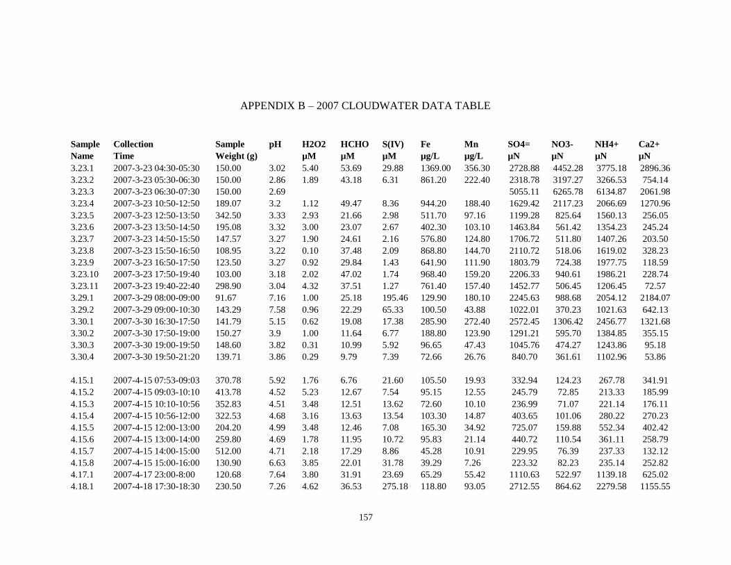
157

APPENDIX B – 2007 CLOUDWATER DATA TABLE

Sample Collection Sample pH H2O2 HCHO S(IV) Fe Mn SO4= NO3- NH4+ Ca2+

Name Time Weight (g) µM µM µM µg/L µg/L µN µN µN µN

3.23.1 2007-3-23 04:30-05:30 150.00 3.02 5.40 53.69 29.88 1369.00 356.30 2728.88 4452.28 3775.18 2896.36

3.23.2 2007-3-23 05:30-06:30 150.00 2.86 1.89 43.18 6.31 861.20 222.40 2318.78 3197.27 3266.53 754.14

3.23.3 2007-3-23 06:30-07:30 150.00 2.69

5055.11 6265.78 6134.87 2061.98

3.23.4 2007-3-23 10:50-12:50 189.07 3.2 1.12 49.47 8.36 944.20 188.40 1629.42 2117.23 2066.69 1270.96

3.23.5 2007-3-23 12:50-13:50 342.50 3.33 2.93 21.66 2.98 511.70 97.16 1199.28 825.64 1560.13 256.05

3.23.6 2007-3-23 13:50-14:50 195.08 3.32 3.00 23.07 2.67 402.30 103.10 1463.84 561.42 1354.23 245.24

3.23.7 2007-3-23 14:50-15:50 147.57 3.27 1.90 24.61 2.16 576.80 124.80 1706.72 511.80 1407.26 203.50

3.23.8 2007-3-23 15:50-16:50 108.95 3.22 0.10 37.48 2.09 868.80 144.70 2110.72 518.06 1619.02 328.23

3.23.9 2007-3-23 16:50-17:50 123.50 3.27 0.92 29.84 1.43 641.90 111.90 1803.79 724.38 1977.75 118.59

3.23.10 2007-3-23 17:50-19:40 103.00 3.18 2.02 47.02 1.74 968.40 159.20 2206.33 940.61 1986.21 228.74

3.23.11 2007-3-23 19:40-22:40 298.90 3.04 4.32 37.51 1.27 761.40 157.40 1452.77 506.45 1206.45 72.57

3.29.1 2007-3-29 08:00-09:00 91.67 7.16 1.00 25.18 195.46 129.90 180.10 2245.63 988.68 2054.12 2184.07

3.29.2 2007-3-29 09:00-10:30 143.29 7.58 0.96 22.29 65.33 100.50 43.88 1022.01 370.23 1021.63 642.13

3.30.1 2007-3-30 16:30-17:50 141.79 5.15 0.62 19.08 17.38 285.90 272.40 2572.45 1306.42 2456.77 1321.68

3.30.2 2007-3-30 17:50-19:00 150.27 3.9 1.00 11.64 6.77 188.80 123.90 1291.21 595.70 1384.85 355.15

3.30.3 2007-3-30 19:00-19:50 148.60 3.82 0.31 10.99 5.92 96.65 47.43 1045.76 474.27 1243.86 95.18

3.30.4 2007-3-30 19:50-21:20 139.71 3.86 0.29 9.79 7.39 72.66 26.76 840.70 361.61 1102.96 53.86

4.15.1 2007-4-15 07:53-09:03 370.78 5.92 1.76 6.76 21.60 105.50 19.93 332.94 124.23 267.78 341.91

4.15.2 2007-4-15 09:03-10:10 413.78 4.52 5.23 12.67 7.54 95.15 12.55 245.79 72.85 213.33 185.99

4.15.3 2007-4-15 10:10-10:56 352.83 4.51 3.48 12.51 13.62 72.60 10.10 236.99 71.07 221.14 176.11

4.15.4 2007-4-15 10:56-12:00 322.53 4.68 3.16 13.63 13.54 103.30 14.87 403.65 101.06 280.22 270.23

4.15.5 2007-4-15 12:00-13:00 204.20 4.99 3.48 12.46 7.08 165.30 34.92 725.07 159.88 552.34 402.42

4.15.6 2007-4-15 13:00-14:00 259.80 4.69 1.78 11.95 10.72 95.83 21.14 440.72 110.54 361.11 258.79

4.15.7 2007-4-15 14:00-15:00 512.00 4.71 2.18 17.29 8.86 45.28 10.91 229.95 76.39 237.33 132.12

4.15.8 2007-4-15 15:00-16:00 130.90 6.63 3.85 22.01 31.78 39.29 7.26 223.32 82.23 235.14 252.82

4.17.1 2007-4-17 23:00-8:00 120.68 7.64 3.80 31.91 23.69 65.29 55.42 1110.63 522.97 1139.18 625.02

4.18.1 2007-4-18 17:30-18:30 230.50 7.26 4.62 36.53 275.18 118.80 93.05 2712.55 864.62 2279.58 1155.55

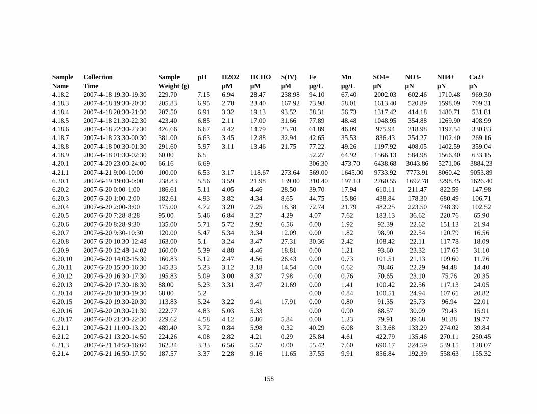
158



4.18.2 2007-4-18 19:30-19:30 229.70 7.15 6.94 28.47 238.98 94.10 67.40 2002.03 602.46 1710.48 969.30

4.18.3 2007-4-18 19:30-20:30 205.83 6.95 2.78 23.40 167.92 73.98 58.01 1613.40 520.89 1598.09 709.31

4.18.4 2007-4-18 20:30-21:30 207.50 6.91 3.32 19.13 93.52 58.31 56.73 1317.42 414.18 1480.71 531.81

4.18.5 2007-4-18 21:30-22:30 423.40 6.85 2.11 17.00 31.66 77.89 48.48 1048.95 354.88 1269.90 408.99

4.18.6 2007-4-18 22:30-23:30 426.66 6.67 4.42 14.79 25.70 61.89 46.09 975.94 318.98 1197.54 330.83

4.18.7 2007-4-18 23:30-00:30 381.00 6.63 3.45 12.88 32.94 42.65 35.53 836.43 254.27 1102.40 269.16

4.18.8 2007-4-18 00:30-01:30 291.60 5.97 3.11 13.46 21.75 77.22 49.26 1197.92 408.05 1402.59 359.04

4.18.9 2007-4-18 01:30-02:30 60.00 6.5

52.27 64.92 1566.13 584.98 1566.40 633.15

4.20.1 2007-4-20 23:00-24:00 66.16 6.69

306.30 473.70 6438.68 3043.86 5271.06 3884.23

4.21.1 2007-4-21 9:00-10:00 100.00 6.53 3.17 118.67 273.64 569.00 1645.00 9733.92 7773.91 8060.42 9053.89

6.20.1 2007-6-19 19:00-0:00 238.83 5.56 3.59 21.98 139.00 310.40 197.10 2760.55 1692.78 3298.45 1626.40

6.20.2 2007-6-20 0:00-1:00 186.61 5.11 4.05 4.46 28.50 39.70 17.94 610.11 211.47 822.59 147.98

6.20.3 2007-6-20 1:00-2:00 182.61 4.93 3.82 4.34 8.65 44.75 15.86 438.84 178.30 680.49 106.71

6.20.4 2007-6-20 2:00-3:00 175.00 4.72 3.20 7.25 18.38 72.74 21.79 482.25 223.50 748.39 102.52

6.20.5 2007-6-20 7:28-8:28 95.00 5.46 6.84 3.27 4.29 4.07 7.62 183.13 36.62 220.76 65.90

6.20.6 2007-6-20 8:28-9:30 135.00 5.71 5.72 2.92 6.56 0.00 1.92 92.39 22.62 151.13 21.94

6.20.7 2007-6-20 9:30-10:30 120.00 5.47 5.34 3.34 12.09 0.00 1.82 98.90 22.54 120.79 16.56

6.20.8 2007-6-20 10:30-12:48 163.00 5.1 3.24 3.47 27.31 30.36 2.42 108.42 22.11 117.78 18.09

6.20.9 2007-6-20 12:48-14:02 160.00 5.39 4.88 4.46 18.81 0.00 1.21 93.60 23.32 117.65 31.10

6.20.10 2007-6-20 14:02-15:30 160.83 5.12 2.47 4.56 26.43 0.00 0.73 101.51 21.13 109.60 11.76

6.20.11 2007-6-20 15:30-16:30 145.33 5.23 3.12 3.18 14.54 0.00 0.62 78.46 22.29 94.48 14.40

6.20.12 2007-6-20 16:30-17:30 195.83 5.09 3.00 8.37 7.98 0.00 0.76 70.65 23.10 75.76 20.35

6.20.13 2007-6-20 17:30-18:30 88.00 5.23 3.31 3.47 21.69 0.00 1.41 100.42 22.56 117.13 24.05

6.20.14 2007-6-20 18:30-19:30 68.00 5.2

0.00 0.84 100.51 24.94 107.61 20.82

6.20.15 2007-6-20 19:30-20:30 113.83 5.24 3.22 9.41 17.91 0.00 0.80 91.35 25.73 96.94 22.01

6.20.16 2007-6-20 20:30-21:30 222.77 4.83 5.03 5.33

0.00 0.90 68.57 30.09 79.43 15.91

6.20.17 2007-6-20 21:30-22:30 229.62 4.58 4.12 5.86 5.84 0.00 1.23 79.91 39.68 91.88 19.77

6.21.1 2007-6-21 11:00-13:20 489.40 3.72 0.84 5.98 0.32 40.29 6.08 313.68 133.29 274.02 39.84

6.21.2 2007-6-21 13:20-14:50 224.26 4.08 2.82 4.21 0.29 25.84 4.61 422.79 135.46 270.11 250.45

6.21.3 2007-6-21 14:50-16:60 162.34 3.33 6.56 5.57 0.00 55.42 7.60 690.17 224.59 539.15 128.07

6.21.4 2007-6-21 16:50-17:50 187.57 3.37 2.28 9.16 11.65 37.55 9.91 856.84 192.39 558.63 155.32

159



6.22.2 2007-6-22 20:25-21:55 255.22 3.32 5.98 16.86 32.61 330.00 25.90 1837.61 296.19 1776.69 157.86

6.22.3 2007-6-22 21:55-22:55 509.43 3.55 8.87 5.78 10.42 20.12 6.60 638.40 195.76 520.30 82.39

6.22.4 2007-6-22 22:55-23:55 440.48 3.87 8.22 7.61 3.84 0.00 1.95 205.86 50.85 185.29 79.81

6.23.1 2007-6-23 09:35-11:35 434.73 3.31 3.03 7.92 13.51 90.48 3.83 822.32 267.89 505.58 116.05

6.23.2 2007-6-23 11:35-13:35 215.69 3.04 11.46 10.24 5.82 314.30 9.38 1396.43 290.07 817.45 105.16

6.23.3 2007-6-23 13:35-16:35 242.46 3.28 1.22 20.39 31.13 499.70 30.04 3287.70 754.72 3758.22 344.46

6.23.4 2007-6-23 16:35-18:35 262.95 3.59 6.92 21.52 29.97 204.10 22.34 3421.17 873.27 4831.90 257.04

6.26.1 2007-6-26 16:25-18:55 272.02 6.86 8.18 49.39 16.99 125.30 146.40 4626.23 1644.29 6140.75 959.48

6.26.2 2007-6-26 18:55-20:55 320.72 6.86 28.01 35.63 27.12 20.23 55.44 1956.85 554.79 2789.11 290.54

6.26.3 2007-6-26 20:55-21:55 327.45 6.84 50.38 30.51 13.48 0.00 29.92 1194.29 382.06 1902.84 150.58

6.26.4 2007-6-26 21:55-22:55 309.83 6.72 58.32

5.81 0.00 26.01 969.04 339.44 1862.35 111.50

6.26.5 2007-6-26 22:55-23:55 287.61 6.5 32.70 51.49 39.68 0.00 27.53 1295.37 377.04 1821.52 152.98

6.26.6 2007-6-26 23:55-0:55 238.64 6.81 24.49 46.95 42.21 4.28 23.20 1045.83 315.34 1600.59 141.62

6.26.7 2007-6-27 00:55-01:55 236.80 6.36 9.72 56.87 57.41 0.00 28.73 1102.38 276.28 1349.13 108.59

6.26.8 2007-6-27 01:55-02:55 266.30 6.68 10.20 36.53 40.10 0.00 25.76 906.80 257.16 1426.76 105.53

7.1.1 2007-7-1 09:30-11:11 367.95 3.74 5.77 4.22 5.16 36.45 9.00 613.42 193.53 652.07 30.33

7.1.2 2007-7-1 11:11-13:41 275.63 3.72 9.17 6.64 5.16 68.32 15.11 848.75 278.37 912.20 86.92

7.1.3 2007-7-1 13:41-15:41 211.00 3.82 8.27 7.77 11.51 106.70 20.01 1246.78 331.25 1515.80 147.10

7.1.4 2007-7-1 15:41-17:41 95.00 3.71 11.48 4.99 0.00 139.60 10.89 566.22 121.78 508.00 71.97

7.1.5 2007-7-1 17:41-20:00 175.00 4.11 12.28 4.21 1.50 46.78 4.04 228.96 50.25 211.60 21.32

7.12 2007-7-12 09:30-12:30 175.00 4.54 9.70 21.29 14.60 30.03 34.54 1859.37 465.84 2443.39 263.87

7.14.1 2007-7-14 06:15-23:15 205.00 4.30

160.80 206.80 5061.76 1385.45 5847.15 678.32

7.16.1 2007-7-16 20:10-22:10 561.71 4.90 11.14 61.01 69.22 42.60 29.91 2633.17 433.59 3551.50 198.15

7.16.2 2007-7-16 22:10-23:30 503.96 3.93 6.32 17.67 35.74 48.84 15.42 1154.45 287.45 1530.13 134.08

7.16.3 2007-7-16 23:30-00:30 233.72 4.41 58.27 10.45 1.26 41.07 23.67 1088.47 220.35 1376.95 95.98

7.16.4 2007-7-17 00:30-02:00 194.07 5.96 69.60 8.79 0.11 135.00 31.41 1333.77 236.16 1469.66 129.30

7.16.5 2007-7-17 02:00-03:30 244.31 3.84 87.79 9.46 0.03 91.09 20.71 1064.37 217.96 1261.66 109.53

7.16.6 2007-7-17 03:30-06:30 513.70 3.91 71.07 10.62 0.00 60.44 19.88 1088.88 263.38 1382.18 70.61

7.17.1 2007-7-17 6:40-8:40 398.09 6.54 101.06 11.09 1.46 12.64 33.25 970.65 191.69 1390.80 208.21

7.17.2 2007-7-17 8:40-9:00 100.00 4.52

674.46 184.43 765.52 157.76

160



7.17.3 2007-7-17 13:15-15:15 358.65 5.78 16.74 68.73 2.84 34.12 126.90 3687.32 677.15 4384.59 382.83

7.17.4 2007-7-17 15:15-17:15 295.90 6.11 15.58 63.85 0.00 169.70 89.73 3388.53 618.71 4303.60 390.28

7.17.5 2007-7-17 17:15-19:15 520.21 5.97 14.28 21.95 0.55 2.10 54.00 2342.59 380.28 2739.99 267.08

7.17.6 2007-7-17 19:15-21:15 534.00 6.04 12.30 36.28

0.00 46.39 1529.68 255.18 1893.19 187.57

7.17.7 2007-7-17 21:15-23:15 528.96 5.92 7.67 51.19

0.00 29.68 1156.64 237.70 1531.09 155.62

7.17.8 2007-7-17 23:15-0:45 512.31 5.29 4.09 19.55

0.00 15.34 1133.27 164.42 1371.83 94.51

7.18.1 2007-7-18 06:05-07:05 524.00 5.56 5.07 23.54

0.00 18.32 603.51 77.27 713.97 40.63

7.18.2 2007-7-18 07:05-08:10 520.00 5.56 7.84 34.51

0.00 19.58 751.66 74.87 812.84 37.96

7.18.3 2007-7-18 08:10-09:10 520.00 6.17 6.54 49.22

0.00 27.68 799.79 77.97 957.58 55.78

7.18.4 2007-7-18 09:10-11:10 520.00 6.26 7.11 53.99

0.00 39.42 938.92 127.59 1368.70 56.65

7.18.5 2007-7-18 11:10-12:10 436.00 6.43 6.68 65.58

0.00 37.36 1187.58 155.80 1727.36 97.89

7.18.6 2007-7-18 12:10-14:10 512.31 6.44 6.76 52.53

0.00 39.40 1257.96 185.51 1724.56 166.33

7.18.7 2007-7-18 14:10-15:20 379.15 6.60 9.60 40.50

0.00 33.70 1281.66 193.56 1682.21 214.47

7.18.8 2007-7-18 15:20-16:20 385.06 6.38 6.78 17.80

0.00 29.03 1231.57 165.50 1650.55 175.99

7.18.9 2007-7-18 16:20-17:20 433.39 6.88 5.64 29.57

0.00 24.11 980.72 153.35 1470.81 146.05

7.18.10 2007-7-18 17:20-18:30 512.31 6.55 3.51 39.46

0.00 19.68 1016.14 112.35 1350.95 130.94

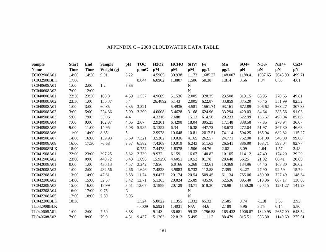
161

APPENDIX C – 2008 CLOUDWATER DATA TABLE

Sample Start End Sample pH TOC H2O2 HCHO S(IV) Fe Mn SO4= NO3- NH4+ Ca2+

Name Time Time Weight (g) ppmC µM µM µM µg/L µg/L µN µN µN µN

TC032908A01 14:00 14:20 9.01 3.22

4.5965 30.938 11.73 1685.27 148.007 1188.41 1037.65 2043.90 499.71

TC032908BLK 17:00

0.044 6.0902 1.3807 1.506 50.38 1.814 3.56 1.84 0.03 4.01

TC040608A01 1:00 2:00 1.2 5.85

N

TC040608A02 7:00 12:00

N

TC040808A01 22:30 23:30 168.8 4.59 1.537 4.9609 5.1536 2.005 328.35 23.508 313.15 66.95 270.65 49.81

TC040808A02 23:30 1:00 156.37 5.4

26.4892 5.143 2.005 622.87 33.859 375.20 76.46 351.99 82.32

TC040908A01 1:00 3:00 60.85 6.35 3.321

5.4936 4.581 1561.74 93.161 672.89 206.62 563.27 307.88

TC040908A02 3:00 5:00 224.86 5.09 3.299 4.0008 5.4628 3.168 624.96 33.294 429.03 84.64 383.56 91.03

TC040908A03 5:00 7:00 53.06 4.4

4.3216 7.688 15.13 614.56 29.233 522.99 155.57 498.04 85.66

TC040908A04 7:00 9:00 102.37 4.05 2.67 2.9201 6.4298 18.04 395.23 17.148 338.58 77.85 278.94 36.07

TC040908A05 9:00 11:00 14.95 5.08 5.985 3.1352 6.34 16.38 447.72 18.673 272.04 51.97 267.80 46.68

TC040908A06 11:00 14:00 8.65 5

2.9978 10.648 10.81 2012.51 74.114 594.25 165.04 682.82 115.27

TC040908A07 14:00 16:00 139.93 3.69 7.321 3.5202 10.036 4.165 262.57 24.771 752.90 161.09 546.80 99.00

TC040908A08 16:00 17:30 76.68 3.57 6.582 7.4208 10.919 6.243 511.63 26.541 886.90 168.71 598.04 82.77

TC040908BLK 18:00

0.752 7.4478 1.8378 1.506 44.76 2.621 3.09 -1.64 1.57 2.48

TC041908A01 22:00 23:00 397.25 5.82 2.739 9.972 6.159 16.67 140.82 10.105 114.12 47.40 174.20 29.29

TC041908A02 23:00 0:00 449.72 5.43 1.696 15.9296 4.6051 10.52 81.78 28.648 56.25 21.02 86.41 20.60

TC042008A01 0:00 1:00 436.13 4.57 2.242 7.956 6.0166 5.268 132.61 10.369 134.96 64.46 163.80 26.02

TC042008A02 1:00 2:00 432.56 4.66 1.646 7.4828 3.9883 8.732 112.88 7.395 84.27 27.90 92.59 15.79

TC042208A01 13:00 14:00 47.61 3.53 11.74 9.0477 20.174 20.54 509.45 61.134 755.06 450.90 727.49 148.34

TC042208A02 14:00 15:00 52.57 3.42 12.71 5.1263 20.824 25.89 435.96 62.536 895.40 513.36 887.17 130.05

TC042208A03 15:00 16:00 18.99 3.51 13.67 3.1888 20.129 33.71 618.36 78.98 1150.28 620.15 1231.27 141.29

TC042208A04 16:00 17:00 0.75 N

N

TC042208A05 17:00 18:00 2.69 3.95

N

TC042208BLK 18:30

1.524 5.8022 1.1355 1.332 65.32 2.585 3.74 -1.18 3.63 2.93

TL032908BLK

-0.009 6.5921 1.4031 N/A 44.6 2.189 5.96 3.75 6.14 5.80

TL040608A01 1:00 2:00 7.59 6.58

9.143 36.681 99.32 1796.58 165.432 1906.87 1340.95 2657.00 648.54

TL040608A02 7:00 8:00 79.9 4.51 9.437 5.1263 22.812 5.495 1111.2 88.479 815.51 556.30 1149.60 275.61

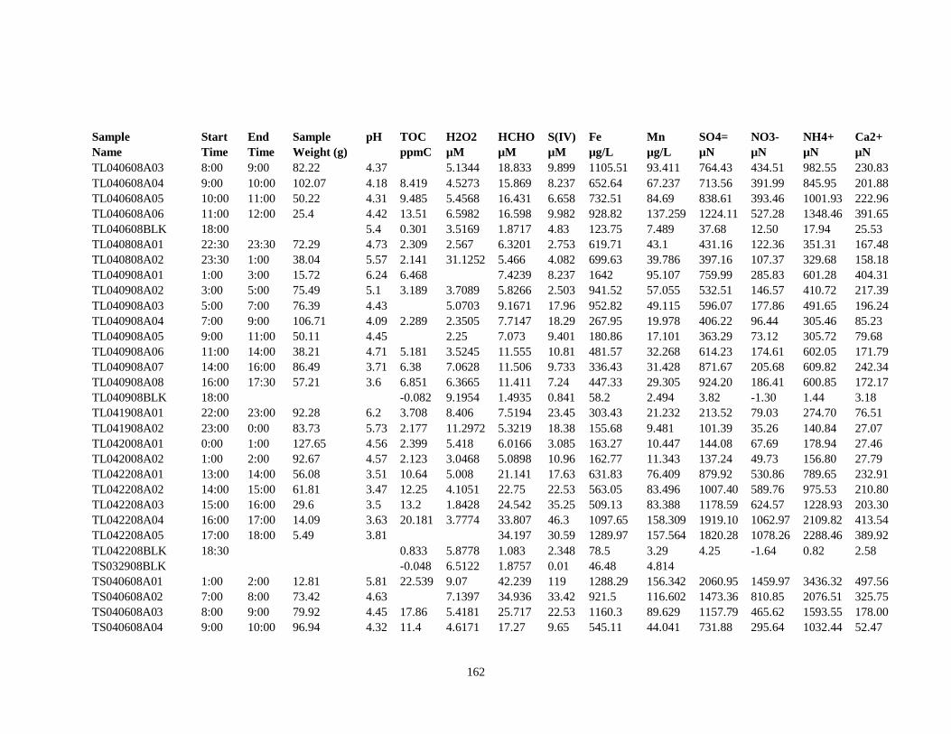
162



TL040608A03 8:00 9:00 82.22 4.37

5.1344 18.833 9.899 1105.51 93.411 764.43 434.51 982.55 230.83

TL040608A04 9:00 10:00 102.07 4.18 8.419 4.5273 15.869 8.237 652.64 67.237 713.56 391.99 845.95 201.88

TL040608A05 10:00 11:00 50.22 4.31 9.485 5.4568 16.431 6.658 732.51 84.69 838.61 393.46 1001.93 222.96

TL040608A06 11:00 12:00 25.4 4.42 13.51 6.5982 16.598 9.982 928.82 137.259 1224.11 527.28 1348.46 391.65

TL040608BLK 18:00

5.4 0.301 3.5169 1.8717 4.83 123.75 7.489 37.68 12.50 17.94 25.53

TL040808A01 22:30 23:30 72.29 4.73 2.309 2.567 6.3201 2.753 619.71 43.1 431.16 122.36 351.31 167.48

TL040808A02 23:30 1:00 38.04 5.57 2.141 31.1252 5.466 4.082 699.63 39.786 397.16 107.37 329.68 158.18

TL040908A01 1:00 3:00 15.72 6.24 6.468

7.4239 8.237 1642 95.107 759.99 285.83 601.28 404.31

TL040908A02 3:00 5:00 75.49 5.1 3.189 3.7089 5.8266 2.503 941.52 57.055 532.51 146.57 410.72 217.39

TL040908A03 5:00 7:00 76.39 4.43

5.0703 9.1671 17.96 952.82 49.115 596.07 177.86 491.65 196.24

TL040908A04 7:00 9:00 106.71 4.09 2.289 2.3505 7.7147 18.29 267.95 19.978 406.22 96.44 305.46 85.23

TL040908A05 9:00 11:00 50.11 4.45

2.25 7.073 9.401 180.86 17.101 363.29 73.12 305.72 79.68

TL040908A06 11:00 14:00 38.21 4.71 5.181 3.5245 11.555 10.81 481.57 32.268 614.23 174.61 602.05 171.79

TL040908A07 14:00 16:00 86.49 3.71 6.38 7.0628 11.506 9.733 336.43 31.428 871.67 205.68 609.82 242.34

TL040908A08 16:00 17:30 57.21 3.6 6.851 6.3665 11.411 7.24 447.33 29.305 924.20 186.41 600.85 172.17

TL040908BLK 18:00

-0.082 9.1954 1.4935 0.841 58.2 2.494 3.82 -1.30 1.44 3.18

TL041908A01 22:00 23:00 92.28 6.2 3.708 8.406 7.5194 23.45 303.43 21.232 213.52 79.03 274.70 76.51

TL041908A02 23:00 0:00 83.73 5.73 2.177 11.2972 5.3219 18.38 155.68 9.481 101.39 35.26 140.84 27.07

TL042008A01 0:00 1:00 127.65 4.56 2.399 5.418 6.0166 3.085 163.27 10.447 144.08 67.69 178.94 27.46

TL042008A02 1:00 2:00 92.67 4.57 2.123 3.0468 5.0898 10.96 162.77 11.343 137.24 49.73 156.80 27.79

TL042208A01 13:00 14:00 56.08 3.51 10.64 5.008 21.141 17.63 631.83 76.409 879.92 530.86 789.65 232.91

TL042208A02 14:00 15:00 61.81 3.47 12.25 4.1051 22.75 22.53 563.05 83.496 1007.40 589.76 975.53 210.80

TL042208A03 15:00 16:00 29.6 3.5 13.2 1.8428 24.542 35.25 509.13 83.388 1178.59 624.57 1228.93 203.30

TL042208A04 16:00 17:00 14.09 3.63 20.181 3.7774 33.807 46.3 1097.65 158.309 1919.10 1062.97 2109.82 413.54

TL042208A05 17:00 18:00 5.49 3.81

34.197 30.59 1289.97 157.564 1820.28 1078.26 2288.46 389.92

TL042208BLK 18:30

0.833 5.8778 1.083 2.348 78.5 3.29 4.25 -1.64 0.82 2.58

TS032908BLK

-0.048 6.5122 1.8757 0.01 46.48 4.814

TS040608A01 1:00 2:00 12.81 5.81 22.539 9.07 42.239 119 1288.29 156.342 2060.95 1459.97 3436.32 497.56

TS040608A02 7:00 8:00 73.42 4.63

7.1397 34.936 33.42 921.5 116.602 1473.36 810.85 2076.51 325.75

TS040608A03 8:00 9:00 79.92 4.45 17.86 5.4181 25.717 22.53 1160.3 89.629 1157.79 465.62 1593.55 178.00

TS040608A04 9:00 10:00 96.94 4.32 11.4 4.6171 17.27 9.65 545.11 44.041 731.88 295.64 1032.44 52.47

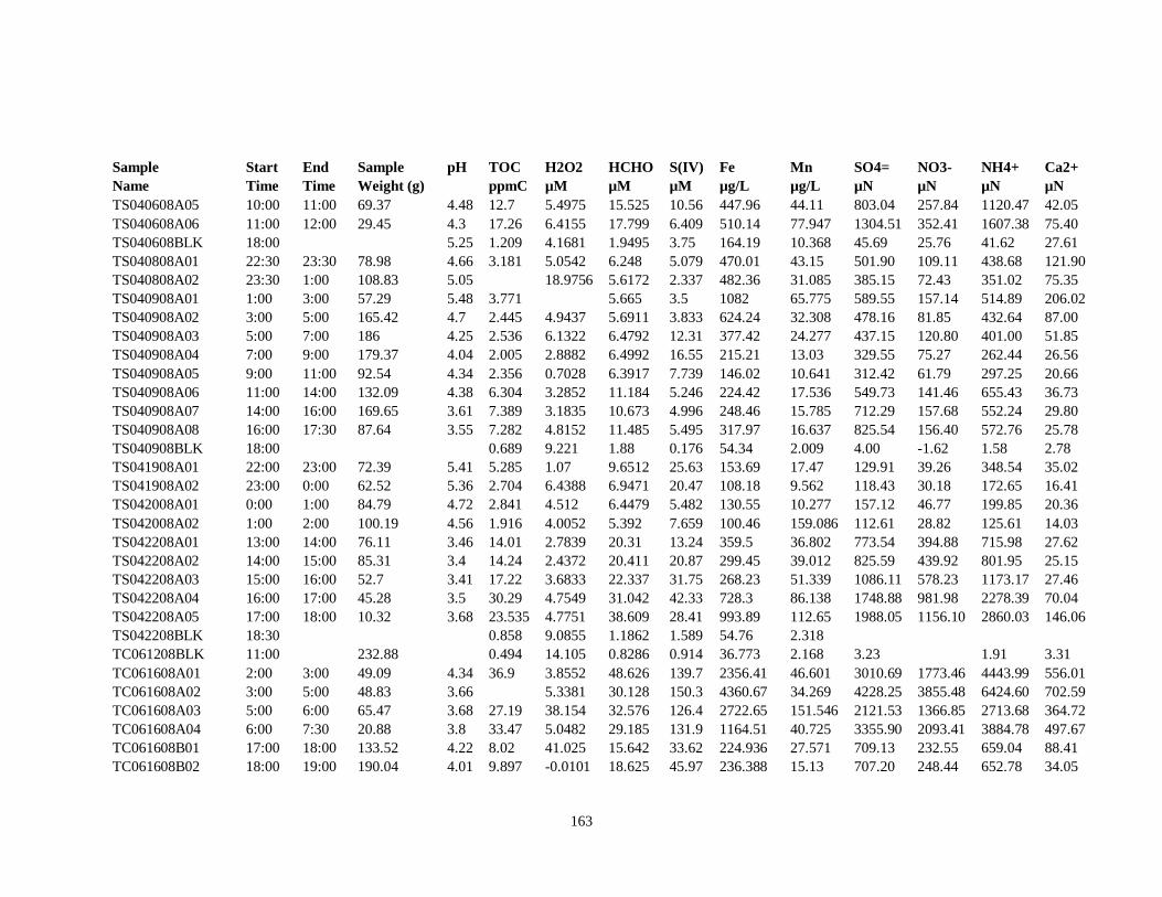
163



TS040608A05 10:00 11:00 69.37 4.48 12.7 5.4975 15.525 10.56 447.96 44.11 803.04 257.84 1120.47 42.05

TS040608A06 11:00 12:00 29.45 4.3 17.26 6.4155 17.799 6.409 510.14 77.947 1304.51 352.41 1607.38 75.40

TS040608BLK 18:00

5.25 1.209 4.1681 1.9495 3.75 164.19 10.368 45.69 25.76 41.62 27.61

TS040808A01 22:30 23:30 78.98 4.66 3.181 5.0542 6.248 5.079 470.01 43.15 501.90 109.11 438.68 121.90

TS040808A02 23:30 1:00 108.83 5.05

18.9756 5.6172 2.337 482.36 31.085 385.15 72.43 351.02 75.35

TS040908A01 1:00 3:00 57.29 5.48 3.771

5.665 3.5 1082 65.775 589.55 157.14 514.89 206.02

TS040908A02 3:00 5:00 165.42 4.7 2.445 4.9437 5.6911 3.833 624.24 32.308 478.16 81.85 432.64 87.00

TS040908A03 5:00 7:00 186 4.25 2.536 6.1322 6.4792 12.31 377.42 24.277 437.15 120.80 401.00 51.85

TS040908A04 7:00 9:00 179.37 4.04 2.005 2.8882 6.4992 16.55 215.21 13.03 329.55 75.27 262.44 26.56

TS040908A05 9:00 11:00 92.54 4.34 2.356 0.7028 6.3917 7.739 146.02 10.641 312.42 61.79 297.25 20.66

TS040908A06 11:00 14:00 132.09 4.38 6.304 3.2852 11.184 5.246 224.42 17.536 549.73 141.46 655.43 36.73

TS040908A07 14:00 16:00 169.65 3.61 7.389 3.1835 10.673 4.996 248.46 15.785 712.29 157.68 552.24 29.80

TS040908A08 16:00 17:30 87.64 3.55 7.282 4.8152 11.485 5.495 317.97 16.637 825.54 156.40 572.76 25.78

TS040908BLK 18:00

0.689 9.221 1.88 0.176 54.34 2.009 4.00 -1.62 1.58 2.78

TS041908A01 22:00 23:00 72.39 5.41 5.285 1.07 9.6512 25.63 153.69 17.47 129.91 39.26 348.54 35.02

TS041908A02 23:00 0:00 62.52 5.36 2.704 6.4388 6.9471 20.47 108.18 9.562 118.43 30.18 172.65 16.41

TS042008A01 0:00 1:00 84.79 4.72 2.841 4.512 6.4479 5.482 130.55 10.277 157.12 46.77 199.85 20.36

TS042008A02 1:00 2:00 100.19 4.56 1.916 4.0052 5.392 7.659 100.46 159.086 112.61 28.82 125.61 14.03

TS042208A01 13:00 14:00 76.11 3.46 14.01 2.7839 20.31 13.24 359.5 36.802 773.54 394.88 715.98 27.62

TS042208A02 14:00 15:00 85.31 3.4 14.24 2.4372 20.411 20.87 299.45 39.012 825.59 439.92 801.95 25.15

TS042208A03 15:00 16:00 52.7 3.41 17.22 3.6833 22.337 31.75 268.23 51.339 1086.11 578.23 1173.17 27.46

TS042208A04 16:00 17:00 45.28 3.5 30.29 4.7549 31.042 42.33 728.3 86.138 1748.88 981.98 2278.39 70.04

TS042208A05 17:00 18:00 10.32 3.68 23.535 4.7751 38.609 28.41 993.89 112.65 1988.05 1156.10 2860.03 146.06

TS042208BLK 18:30

0.858 9.0855 1.1862 1.589 54.76 2.318

TC061208BLK 11:00

232.88

0.494 14.105 0.8286 0.914 36.773 2.168 3.23

1.91 3.31

TC061608A01 2:00 3:00 49.09 4.34 36.9 3.8552 48.626 139.7 2356.41 46.601 3010.69 1773.46 4443.99 556.01

TC061608A02 3:00 5:00 48.83 3.66

5.3381 30.128 150.3 4360.67 34.269 4228.25 3855.48 6424.60 702.59

TC061608A03 5:00 6:00 65.47 3.68 27.19 38.154 32.576 126.4 2722.65 151.546 2121.53 1366.85 2713.68 364.72

TC061608A04 6:00 7:30 20.88 3.8 33.47 5.0482 29.185 131.9 1164.51 40.725 3355.90 2093.41 3884.78 497.67

TC061608B01 17:00 18:00 133.52 4.22 8.02 41.025 15.642 33.62 224.936 27.571 709.13 232.55 659.04 88.41

TC061608B02 18:00 19:00 190.04 4.01 9.897 -0.0101 18.625 45.97 236.388 15.13 707.20 248.44 652.78 34.05

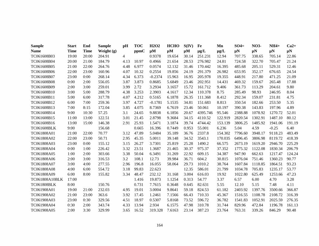
164



TC061608B03 19:00 20:00 204.91 4

0.9378 19.654 30.14 251.231 12.94 707.75 338.65 705.14 22.86

TC061608B04 20:00 21:00 184.79 4.13 10.97 0.4966 21.654 28.53 276.982 24.81 724.58 322.70 705.47 21.24

TC061608B05 21:00 22:00 264.76 4.48 6.977 0.0574 12.132 31.46 170.442 16.395 485.68 205.11 529.31 12.46

TC061608B06 22:00 23:00 160.96 4.07 10.32 0.2554 19.856 24.19 291.379 26.982 653.95 352.17 676.65 24.54

TC061608B07 23:00 0:00 268.14 4.34 6.373 -0.2374 15.963 16.95 205.978 19.355 448.91 217.80 471.25 21.09

TC061608B08 0:00 2:00 556.05 3.87 3.873 0.8685 5.6849 23.46 202.951 14.431 469.32 159.67 265.48 17.88

TC061608B09 2:00 3:00 259.01 3.99 2.72 3.2934 3.1657 15.72 161.712 9.406 361.73 113.29 204.61 9.80

TC061608B10 3:00 5:00 288.79 4.38 3.253 2.3903 4.1617 12.34 110.378 8.75 285.49 98.93 246.95 8.04

TC061608B11 5:00 6:00 317.78 4.07 4.212 0.5165 6.1878 26.35 111.368 8.412 292.34 159.07 231.81 4.75

TC061608B12 6:00 7:00 259.36 3.97 4.727 -0.1781 5.1535 34.81 151.683 8.813 350.54 182.66 253.50 5.35

TC061608B13 7:00 8:15 172.04 3.85 4.075 8.7369 6.7619 23.46 50.061 10.197 390.38 143.83 197.96 4.89

TC061608B14 9:00 10:30 57.25 3.1 24.65 9.8838 6.1856 20.67 4395.746 95.546 2388.88 1078.92 1270.72 52.01

TC061608B15 11:00 13:00 122.51 3.01 21.45 2.8798 9.3684 34.15 4110.52 122.919 2820.54 1302.91 1487.10 80.12

TC061608B16 13:00 15:00 146.38 2.91 25.93 1.5471 3.1874 39.74 4744.42 153.139 3806.25 1485.92 1941.06 191.19

TC061608BLK 9:00

156.68

0.665 16.396 0.7449 0.953 55.001 6.236 5.04 4.59 -0.25 6.40

TC061808A01 21:00 22:00 70.77 3.12 47.89 5.0484 35.189 36.76 2337.8 154.302 7796.60 3948.17 9118.23 483.49

TC061808A02 22:00 23:00 50.71 2.95 45.35 5.0011 39.148 34.52 3543.1 170.035 6496.45 3806.98 8119.72 418.39

TC061808A03 23:00 0:00 155.12 3.15 26.27 3.7301 25.819 25.28 1490.2 66.575 2673.19 1619.20 2946.70 225.29

TC061808A04 0:00 1:00 226.42 3.32 23.51 1.3687 21.465 30.37 975.37 37.352 1775.32 1122.08 1830.34 206.79

TC061808A05 1:00 2:00 303.66 3.38 50.04 6.3491 31.269 22.92 609.15 34.387 947.90 662.63 1217.47 124.24

TC061808A06 2:00 3:00 316.53 3.2 108.1 12.73 39.984 36.71 604.2 30.815 1076.04 751.46 1360.23 90.77

TC061808A07 3:00 4:00 277.55 2.96 196.8 16.055 58.064 29.73 1010.2 38.764 1607.84 1118.85 1864.51 93.23

TC061808A08 4:00 6:00 554.72 3.18 99.83 22.623

12.35 586.01 21.799 1034.78 705.83 1235.17 53.77

TC061808A09 6:00 8:00 155.82 3.34 48.47 232.12 31.168 3.004 616.03 19.92 1022.80 625.49 1253.66 47.23

TC061808A10BLK 17:00

1.416 19.873 1.1254 0.313 54.77 3.37 6.57 6.00 4.70 3.28

TC061808BLK 8:00

150.76

0.731 7.7615 0.3648 0.645 82.631 5.55 12.10 5.15 7.48 4.11

TC061908A01 19:00 21:00 232.03 4.95 19.01 3.0004 9.8641 59.18 824.53 61.182 2403.92 1397.76 3500.66 366.87

TC061908A02 21:00 23:00 363.6 3.92 17.45 1.2461 7.1566 66.43 710.33 45.367 1516.55 1108.78 2108.72 316.39

TC061908A03 23:00 0:30 329.56 4.51 18.97 0.5307 5.8168 73.52 596.72 36.782 1541.83 1052.91 2025.59 276.35

TC061908A04 0:30 2:00 343.74 4.33 13.94 2.934 6.1575 47.98 310.78 31.744 829.96 472.84 1196.78 161.13

TC061908A05 2:00 3:30 329.99 3.65 16.52 319.328 7.6163 23.14 387.23 23.764 763.31 339.26 846.29 90.48

165



TC061908A06 3:30 5:00 294.42 3.32 29.7 176.96 9.1318 12.95 517.86 27.967 969.38 461.61 1000.20 65.42

TC061908A07 5:00 7:00 483.77 3.48 44.73 11.473 13.167 6.988 532.52 29.492 1077.48 524.82 1465.31 78.95

TC061908A08 7:00 8:15 72.6 3.16 40.83 41.798 21.986 7.643 1063.38 63.796 1822.08 763.11 2098.21 134.41

TC061908A09BLK 12:00

1.385 13.277 0.9129 0.344 110.12 3.977 4.86 4.33 4.71 4.35

TC062008A01 16:45 17:45 82.47 3.25 22.57 25.923 6.1968 43.46 1705.03 40.633 1840.90 518.56 1730.96 39.60

TC062008A02 19:00 19:20 9.61 3.19

3.918 7.2684 27.63 1450.6 79.504 4143.15 877.01 3477.72 52.45

TC062108A01 9:00 9:40 78.41 2.86 47.1 10.282 11.684 34.29 1578.73 94.307 3861.70 1273.79 3022.23 194.19

TC062108BLK 12:00

0.822 11.8 0.8973 0.995 110.71 6.531 20.27 6.49 12.83 3.57

TC062308BLK 14:00

0.537 15.881 0.6897 0.431 53.84 2.201

-0.37 2.38

TC062508A01 23:10 0:00 117.48 6.61 20.51 6.7545 8.1684 25.97 953.29 76.138 4058.18 876.42 4304.55 465.08

TC062508A02 0:00 0:45 43.77 6.72 20.43 8.3722 7.0684 23.31 1238.49 73.452 4500.97 906.54 4883.78 482.14

TC062508A03BLK 9:00

0.999 9.9216 0.9874 0.846 104.25 5.104 73.52 16.75 57.14 26.13

TC070208A01 4:05 5:00 96.45 3.44 18.46 0.9218 6.5863 56.11 880.56 79.706 3257.37 972.17 3375.86 414.05

TC070208A02 5:00 5:50 22.53 3.42 19.2 4.5657 4.0648 24.73 684.5 65.492 4248.79 993.39 3857.14 305.39

TC070208BLK 12:00

149.56

0.723 16.563 0.8763 1.017 50.41 2.513 5.37 4.66 4.71 2.60

TC070308A01 20:00 22:00 90.1 5.42 70.92 169.584 15.417 125.9 1231.11 333.836 4939.02 1252.00 6101.87 499.19

TC070308A02 22:00 23:00 100.18 5.31 27.59 55.416 13.984 83.21 608.41 160.695 3048.56 604.74 3709.74 276.24

TC070308A03 23:00 0:00 169.25 5.38 17.54 79.785 5.8168 107.5 372.64 101.215 1811.97 342.50 2360.67 177.99

TC070308A04 0:00 1:00 174.53 5.51 12.34 122.84 5.6461 69.38 348.51 84.514 1899.41 309.18 1883.07 147.24

TC070308A05 1:00 2:00 182.25 5.62 9.594 279.008 7.1687 55.47 287.22 83.985 1008.15 226.94 1383.80 112.22

TC070308A06 2:00 3:00 176.04 5.55 8.776 271.424 4.9487 38.91 224.59 79.532 847.64 187.33 1145.43 89.92

TC070308A07 3:00 5:00 171.76 5.22 13.28 479.34 5.6345 27.34 439.71 165.052 1580.66 353.31 1929.76 165.22

TC070308A08 5:00 7:00 180.51 5.03 12.75 447.128 7.9463 15.26 279.72 167.804 1480.94 334.02 1672.65 124.04

TC070308A09 7:00 8:00 160.45 4.96 8.723 48.902 6.0501 25.32 273.12 90.307 1503.71 282.39 1633.40 105.20

TC070308A10 8:00 9:00 190.98 5.63 6.566 93.56 4.1674 8.702 186.07 52.418 1088.47 156.28 1206.57 77.05

TC070308A11 9:00 9:45 3.63 5.4

7.333

2315.92 436.21 2253.06 212.66

TC070308A12 10:00 11:00

5.31

2.145

889.72 189.77 1006.17 114.96

TC070308A13 11:00 11:40 7.24 5.21

334.432 6.1688 5.612 225.44 127.536 1193.21 280.33 1550.25 121.99

TC070408A01 15:00 15:45 227.5 4.71 6.226 12.312 3.1654 51.83 237.45 77.61 1038.41 286.35 1136.33 125.21

TC070408A02 15:45 16:45 190.49 4.33 7.734 37.467 5.4865 69.35 191.41 86.161 1134.86 319.07 1289.02 84.24

TC070408A03 16:45 17:45 185.83 4.79 9.379 11.685 3.1468 84.17 278.34 78.323 1391.45 413.92 1624.49 102.95

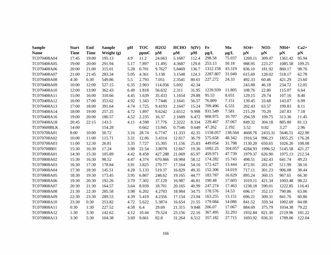
166



TC070408A04 17:45 19:00 195.13 4.9 11.2 24.663 5.1687 112.4 298.58 75.037 1269.11 309.47 1361.42 95.94

TC070408A05 19:00 20:00 291.94 5.17 7.897 11.495 4.3687 129.8 253.13 50.18 988.95 223.27 1085.58 109.25

TC070408A06 20:00 21:00 315.01 5.28 6.701 9.7627 5.8469 136.7 1312.158 43.319 836.10 181.92 860.17 98.76

TC070408A07 21:00 21:45 283.34 5.05 4.361 5.138 3.1548 124.3 2287.807 31.049 615.69 128.02 518.17 62.78

TC070408A08 4:30 6:30 549.86 5.5 2.793 7.051 2.3541 80.61 227.272 24.33 492.33 60.46 421.29 23.60

TC070408A09 10:00 12:00 527.15 6.35 2.903 114.056 5.692 42.34

243.88 46.18 234.72 12.05

TC070408A10 12:00 13:00 362.43 6.49 1.818 56.632 2.311 31.95 1239.939 11.805 108.76 22.80 115.07 6.64

TC070408A11 15:00 16:00 310.66 4.45 1.639 35.433 1.1654 29.88 95.53 8.031 129.15 29.74 107.16 8.40

TC070408A12 16:00 17:00 353.62 4.92 1.343 7.7446 2.1641 56.57 76.809 7.151 139.45 33.68 143.07 6.99

TC070408A13 17:00 18:00 391.64 4.74 1.725 9.4193 2.1647 15.24 709.496 6.531 202.43 63.57 199.83 8.11

TC070408A14 18:00 19:00 257.25 4.72 1.897 9.6242 2.6512 9.998 931.549 7.581 215.29 70.29 247.83 7.18

TC070408A16 19:00 20:00 180.57 4.52 2.235 16.37 2.1689 6.472 908.975 10.707 294.59 109.75 313.36 11.45

TC070408A18 20:45 22:15 143.5 4.11 4.598 17.776 2.3222 8.334 229.467 37.067 849.32 304.18 885.80 81.13

TC070608BLK 14:00

154.28

0.662 13.945 0.7546 0.649 47.262 2.192 3.52 0.82 3.27 2.96

TC070708A01 8:00 10:00 50.72 3.16 28.74 6.7747 11.333 42.35 1158.057 138.564 4668.76 2433.31 5646.51 422.90

TC070708A02 10:00 11:00 115.71 3.31 12.06 3.4314 12.817 36.79 575.658 48.342 1916.54 996.23 1855.25 176.28

TC070708A03 11:00 12:30 26.81 3.35 7.727 15.305 11.156 25.83 449.054 31.798 1130.20 650.65 1026.20 108.08

TC070708B01 15:30 16:30 17.24 3.98 22.54 3.8078 12.667 19.36 1092.25 104.057 4284.93 1996.52 5145.58 421.27

TC070808A01 14:30 15:30 105.89 4.42 8.458 427.288 21.069 65.97 459.971 47.739 1979.37 626.90 1975.13 212.54

TC070808A02 15:30 16:30 98.52 4.47 4.374 670.866 18.984 58.12 174.282 15.743 498.51 242.43 641.74 49.23

TC070808A03 16:30 17:30 178.84 3.91 3.825 270.77 17.164 54.16 172.427 13.444 472.91 201.47 511.99 38.16

TC070808A04 17:30 18:30 145.51 4.28 5.133 519.37 16.829 49.35 152.306 14.019 717.11 301.23 906.08 38.44

TC070808A05 18:30 19:30 173.45 3.95 6.867 248.62 19.165 44.77 183.787 16.629 895.24 360.15 967.65 66.30

TC070808A06 19:30 20:30 192.26 3.79 7.302 37.129 16.987 46.81 190.48 17.603 1019.11 421.34 1003.48 98.22

TC070808A07 20:30 21:30 164.57 3.64 8.939 18.701 20.165 40.99 247.274 17.463 1238.18 590.01 1222.85 116.41

TC070808A08 21:30 22:30 285.58 3.98 6.202 4.2783 18.984 34.75 178.576 14.53 696.17 352.13 790.86 63.06

TC070808A09 22:30 23:30 289.53 4.39 5.419 4.2356 17.154 23.94 163.255 13.151 696.21 309.31 841.76 60.86

TC070808A10 23:30 0:30 253.82 4.72 5.622 5.3874 16.654 21.55 179.084 14.086 841.52 359.34 1002.69 84.08

TC070808A11 0:30 1:30 227.52 4.58 6.4 29.69 21.315 9.848 206.07 17.067 884.69 375.79 1034.38 79.22

TC070808A12 1:30 3:30 142.62 4.12 10.44 79.524 25.156 22.16 367.495 32.293 1932.84 821.30 2119.96 181.22

TC070808A13 3:30 5:30 104.38 3.69 9.661 82.8 31.264 6.512 357.182 27.715 1693.92 836.31 1789.06 122.04

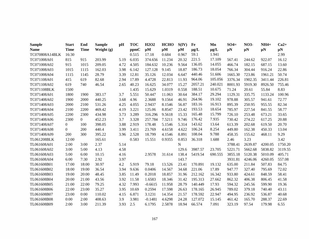
167



TC070808A14BLK 16:30

0.515 17.18 0.684 0.967 59.1 1.941

2.99

TC071008A01 815 915 203.99 5.19 6.035 374.656 11.234 20.32 221.5 17.109 567.41 244.62 922.07 16.12

TC071008A02 915 1015 209.05 4.72 4.505 184.632 10.236 9.564 136.05 14.055 466.74 182.15 687.15 13.60

TC071008A03 1015 1115 162.03 3.98 6.142 127.128 9.145 18.87 186.73 18.054 766.34 304.44 916.24 22.86

TC071008A04 1115 1145 28.79 3.39 12.81 35.126 12.034 6.647 440.46 51.606 1665.30 723.86 1961.21 50.74

TC071108A01 415 619 82.68 2.94 17.89 4.4728 22.813 11.93 964.06 105.056 3376.34 1902.35 3411.44 226.81

TC071108A02 619 740 46.54 2.65 40.23 16.625 34.077 15.27 2057.21 240.021 8001.93 5919.30 8926.50 755.46

TC071108BLK 1500

1.435 15.629 1.0319 0.558 188.51 10.675 71.24 20.61 55.84 8.83

TC071408A01 1800 1900 383.17 3.7 5.551 50.447 11.063 30.64 384.17 29.294 1129.31 335.75 1133.24 100.96

TC071408A02 1900 2000 440.25 3.68 4.96 2.3688 9.1564 46.91 264.96 19.102 978.88 305.57 941.61 72.77

TC071408A03 2000 2100 531.26 4.25 4.055 2.9437 8.1546 56.87 183.16 16.913 895.39 250.95 955.55 82.34

TC071408A04 2100 2200 469.42 4.19 3.221 125.06 8.8547 23.42 193.53 18.654 785.97 227.54 841.55 58.77

TC071408A05 2200 2300 434.98 3.73 3.289 316.296 9.5618 15.33 165.48 15.799 726.10 253.48 673.21 33.65

TC071408A06 2300 0 452.23 3.7 3.328 257.784 7.5211 9.746 176.42 7.935 730.42 274.22 617.25 20.88

TC071408A07 0 100 398.05 3.88 2.919 178.48 5.1546 5.314 143.62 13.64 613.39 202.68 619.50 20.70

TC071408A08 0 200 440.4 3.99 3.411 23.769 4.6158 4.622 106.24 8.254 449.80 162.38 450.33 13.04

TC071408A09 200 300 395.22 3.96 2.528 18.799 4.1546 8.891 108.04 9.788 458.35 155.62 468.11 9.29

TL061208BLK 12:00

165.61

0.583 15.551 0.9355 0.853 36.318 1.688 2.46 3.23

3.42

TL061608A01 2:00 3:00 2.37 5.14

N

3788.41 2639.87 4200.05 1750.20

TL061608A02 3:00 5:00 4.13 4.58

129.6 3987.57 23.705 5221.71 5662.68 5838.82 3119.55

TL061608A03 5:00 6:00 10.15 4.16

2.9578 31.614 138.4 5419.54 690.555 3855.18 5120.38 5010.09 405.71

TL061608A04 6:00 7:30 2.92 3.97

143.7

3931.81 4246.06 4260.05 557.08

TL061608B01 17:00 18:00 30.97 4.2 5.919 79.18 13.526 23.41 170.891 19.132 635.00 211.84 507.83 84.75

TL061608B02 18:00 19:00 36.54 3.94 9.636 0.0406 14.567 34.68 221.06 17.89 947.77 327.40 795.69 72.02

TL061608B03 19:00 20:00 48.45 3.85 11.49 0.2018 18.857 31.96 212.162 16.342 933.80 424.61 848.59 58.41

TL061608B04 20:00 21:00 43.56 3.92 11.58 1.6583 18.346 31.42 195.313 27.662 862.32 406.38 806.45 41.58

TL061608B05 21:00 22:00 79.25 4.32 7.993 -0.6615 11.958 28.79 140.449 17.93 594.32 245.56 599.90 19.36

TL061608B06 22:00 23:00 35.27 3.95 10.69 0.2594 17.598 26.63 178.165 26.945 789.02 379.18 740.40 43.11

TL061608B07 23:00 0:00 110.02 4.15 6.871 3.1231 14.354 21.57 178.592 22.947 494.95 236.92 536.87 40.68

TL061608B08 0:00 2:00 408.63 3.9 3.981 -0.1481 4.6298 24.28 127.072 15.145 461.42 165.70 288.37 22.69

TL061608B09 2:00 3:00 211.39 3.93 2.5 6.1795 2.5878 18.94 66.574 7.091 323.19 97.54 179.98 6.55

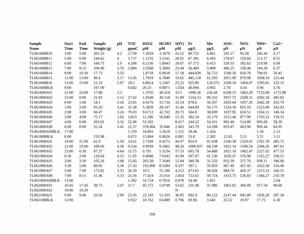
168



TL061608B10 3:00 5:00 205.23 4.2 2.758 7.1818 3.1879 23.52 80.715 6.861 245.17 95.28 185.44 4.17

TL061608B11 5:00 6:00 240.62 4 3.737 1.1235 3.1541 28.91 67.381 6.493 278.67 158.66 213.17 8.51

TL061608B12 6:00 7:00 184.75 3.9 4.268 0.2136 5.8943 29.67 67.172 6.413 329.33 182.63 219.98 6.69

TL061608B13 7:00 8:15 106.96 3.76 3.884 2.5568 5.3684 25.44 56.484 5.808 406.25 158.46 194.39 6.37

TL061608B14 9:00 10:30 17.73 3.33

1.8718 6.9618 17.18 444.828 56.723 1590.16 650.78 794.91 59.45

TL061608B15 11:00 13:00 49.4 3.17 13.45 1.7919 6.7849 19.65 485,118 61.593 2051.99 879.98 1058.24 123.44

TL061608B16 13:00 15:00 51.19 2.97 18.2 6.8014 5.1567 25.22 925.89 124.575 3108.18 1404.07 1595.01 333.15

TL061608BLK 9:00

107.09

0.642 20.25 0.9871 1.034 40.894 4.902 2.78 4.50 0.96 3.76

TL061808A01 21:00 23:00 17.88 3.3

1.3705 40.418 33.5 1990.26 236.68 6108.15 3463.29 7153.68 1172.98

TL061808A02 23:00 0:00 31.93 3.12 27.62 1.0548 30.518 31.89 1254.13 99.332 3937.72 2508.31 4392.18 483.82

TL061808A03 0:00 1:00 54.1 3.26 23.65 0.4276 33.734 32.54 878.6 56.597 2450.64 1657.29 2442.28 432.70

TL061808A04 1:00 2:00 93.26 3.41 32.38 5.3839 28.147 31.46 644.09 50.175 1324.10 855.10 1523.00 242.92

TL061808A05 2:00 3:00 94.47 3.24 79.03 9.6712 42.762 20.73 504.8 38.699 1037.95 624.51 1264.11 146.34

TL061808A06 3:00 4:00 75.17 3.02 128.9 12.286 56.849 13.35 382.24 35.179 1515.46 877.99 1703.23 139.15

TL061808A07 4:00 6:00 203.02 3.32 52.46 53.392

8.417 244.22 16.161 902.46 514.80 995.68 58.30

TL061808A08 6:00 8:00 55.34 3.45 21.57 378.464 35.846 2.663 345.79 14.598 819.47 463.96 909.44 64.95

TL061808A09BLK 17:00

1.159 18.893 1.5618 1.215 39.46 1.454

1.30 2.13

TL061808BLK 8:00

155.98

0.672 15.884 0.8626 0.981 53.8 2.582 12.83 5.51 5.51 3.11

TL061908A01 19:00 21:00 62.9 5.59 14.61 2.7169 8.4573 44.97 854.9 91.838 2168.38 1329.01 2761.59 485.75

TL061908A02 21:00 23:00 106.69 4.38 9.534 0.9039 9.1862 48.26 1009.937 68.238 1821.14 1596.54 2346.26 487.61

TL061908A03 23:00 0:30 87.37 4.64 15.75 0.791 5.3234 57.53 693.78 54.488 1831.10 1402.47 2227.02 477.53

TL061908A04 0:30 2:00 129.64 4.53 11.95 0.4946 7.9342 43.99 507.87 41.136 1026.47 576.98 1325.27 336.51

TL061908A05 2:00 3:30 105.26 3.68 15.85 283.28 7.1649 12.84 340.58 31.533 832.59 371.76 938.11 186.96

TL061908A06 3:30 5:00 89.95 3.38 27.43 192.808 8.5384 9.337 397.1 35.859 967.40 457.45 1022.56 154.46

TL061908A07 5:00 7:00 173.82 3.53 26.59 10.5 15.186 4.212 473.65 36.428 984.70 458.37 1213.15 166.51

TL061908A08 7:00 8:15 31.46 3.33 25.56 77.424 25.014 2.854 723.61 59.724 1413.75 526.83 1366.27 210.78

TL061908A09BLK 12:00

1.392 16.724 0.7816 0.878 54.48 1.821

2.64

TL062008A01 16:45 17:45 38.73 3.47 11.7 45.172 5.0748 53.62 235.48 31.986 1062.82 306.09 917.54 98.60

TL062008A02 19:00 19:20

N

TL062108A01 9:00 9:40 29.56 2.99 23.45 22.143 12.103 36.95 692.9 86.122 2147.44 945.80 1926.29 287.28

TL062108BLK 12:00

0.922 10.762 0.6489 0.796 69.96 3.442 25.52 10.97 17.75 6.30

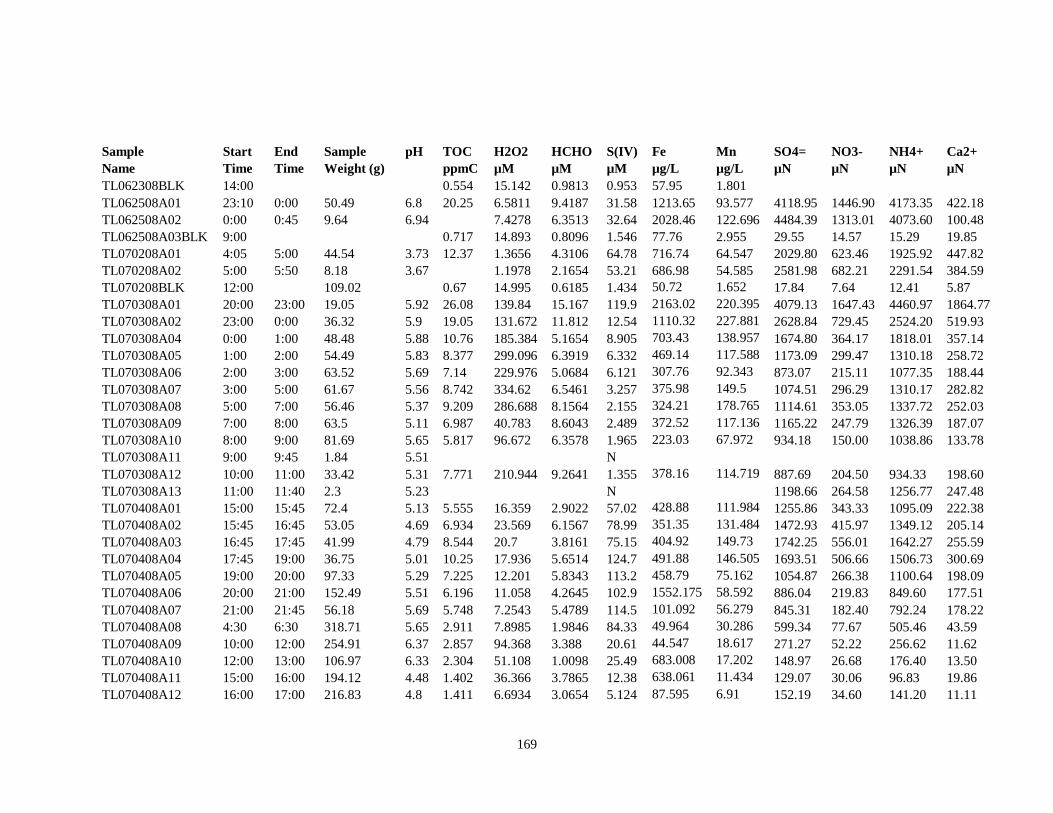
169



TL062308BLK 14:00

0.554 15.142 0.9813 0.953 57.95 1.801

TL062508A01 23:10 0:00 50.49 6.8 20.25 6.5811 9.4187 31.58 1213.65 93.577 4118.95 1446.90 4173.35 422.18

TL062508A02 0:00 0:45 9.64 6.94

7.4278 6.3513 32.64 2028.46 122.696 4484.39 1313.01 4073.60 100.48

TL062508A03BLK 9:00

0.717 14.893 0.8096 1.546 77.76 2.955 29.55 14.57 15.29 19.85

TL070208A01 4:05 5:00 44.54 3.73 12.37 1.3656 4.3106 64.78 716.74 64.547 2029.80 623.46 1925.92 447.82

TL070208A02 5:00 5:50 8.18 3.67

1.1978 2.1654 53.21 686.98 54.585 2581.98 682.21 2291.54 384.59

TL070208BLK 12:00

109.02

0.67 14.995 0.6185 1.434 50.72 1.652 17.84 7.64 12.41 5.87

TL070308A01 20:00 23:00 19.05 5.92 26.08 139.84 15.167 119.9 2163.02 220.395 4079.13 1647.43 4460.97 1864.77

TL070308A02 23:00 0:00 36.32 5.9 19.05 131.672 11.812 12.54 1110.32 227.881 2628.84 729.45 2524.20 519.93

TL070308A04 0:00 1:00 48.48 5.88 10.76 185.384 5.1654 8.905 703.43 138.957 1674.80 364.17 1818.01 357.14

TL070308A05 1:00 2:00 54.49 5.83 8.377 299.096 6.3919 6.332 469.14 117.588 1173.09 299.47 1310.18 258.72

TL070308A06 2:00 3:00 63.52 5.69 7.14 229.976 5.0684 6.121 307.76 92.343 873.07 215.11 1077.35 188.44

TL070308A07 3:00 5:00 61.67 5.56 8.742 334.62 6.5461 3.257 375.98 149.5 1074.51 296.29 1310.17 282.82

TL070308A08 5:00 7:00 56.46 5.37 9.209 286.688 8.1564 2.155 324.21 178.765 1114.61 353.05 1337.72 252.03

TL070308A09 7:00 8:00 63.5 5.11 6.987 40.783 8.6043 2.489 372.52 117.136 1165.22 247.79 1326.39 187.07

TL070308A10 8:00 9:00 81.69 5.65 5.817 96.672 6.3578 1.965 223.03 67.972 934.18 150.00 1038.86 133.78

TL070308A11 9:00 9:45 1.84 5.51

N

TL070308A12 10:00 11:00 33.42 5.31 7.771 210.944 9.2641 1.355 378.16 114.719 887.69 204.50 934.33 198.60

TL070308A13 11:00 11:40 2.3 5.23

N

1198.66 264.58 1256.77 247.48

TL070408A01 15:00 15:45 72.4 5.13 5.555 16.359 2.9022 57.02 428.88 111.984 1255.86 343.33 1095.09 222.38

TL070408A02 15:45 16:45 53.05 4.69 6.934 23.569 6.1567 78.99 351.35 131.484 1472.93 415.97 1349.12 205.14

TL070408A03 16:45 17:45 41.99 4.79 8.544 20.7 3.8161 75.15 404.92 149.73 1742.25 556.01 1642.27 255.59

TL070408A04 17:45 19:00 36.75 5.01 10.25 17.936 5.6514 124.7 491.88 146.505 1693.51 506.66 1506.73 300.69

TL070408A05 19:00 20:00 97.33 5.29 7.225 12.201 5.8343 113.2 458.79 75.162 1054.87 266.38 1100.64 198.09

TL070408A06 20:00 21:00 152.49 5.51 6.196 11.058 4.2645 102.9 1552.175 58.592 886.04 219.83 849.60 177.51

TL070408A07 21:00 21:45 56.18 5.69 5.748 7.2543 5.4789 114.5 101.092 56.279 845.31 182.40 792.24 178.22

TL070408A08 4:30 6:30 318.71 5.65 2.911 7.8985 1.9846 84.33 49.964 30.286 599.34 77.67 505.46 43.59

TL070408A09 10:00 12:00 254.91 6.37 2.857 94.368 3.388 20.61 44.547 18.617 271.27 52.22 256.62 11.62

TL070408A10 12:00 13:00 106.97 6.33 2.304 51.108 1.0098 25.49 683.008 17.202 148.97 26.68 176.40 13.50

TL070408A11 15:00 16:00 194.12 4.48 1.402 36.366 3.7865 12.38 638.061 11.434 129.07 30.06 96.83 19.86

TL070408A12 16:00 17:00 216.83 4.8 1.411 6.6934 3.0654 5.124 87.595 6.91 152.19 34.60 141.20 11.11

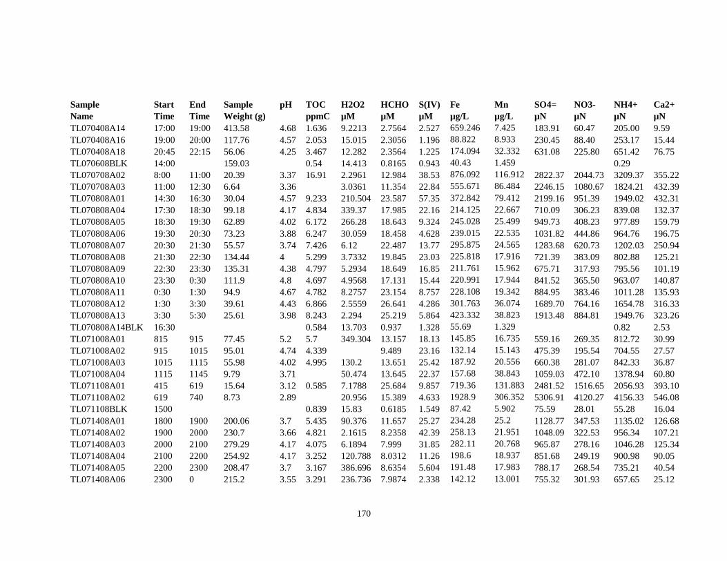
170



TL070408A14 17:00 19:00 413.58 4.68 1.636 9.2213 2.7564 2.527 659.246 7.425 183.91 60.47 205.00 9.59

TL070408A16 19:00 20:00 117.76 4.57 2.053 15.015 2.3056 1.196 88.822 8.933 230.45 88.40 253.17 15.44

TL070408A18 20:45 22:15 56.06 4.25 3.467 12.282 2.3564 1.225 174.094 32.332 631.08 225.80 651.42 76.75

TL070608BLK 14:00

159.03

0.54 14.413 0.8165 0.943 40.43 1.459

0.29

TL070708A02 8:00 11:00 20.39 3.37 16.91 2.2961 12.984 38.53 876.092 116.912 2822.37 2044.73 3209.37 355.22

TL070708A03 11:00 12:30 6.64 3.36

3.0361 11.354 22.84 555.671 86.484 2246.15 1080.67 1824.21 432.39

TL070808A01 14:30 16:30 30.04 4.57 9.233 210.504 23.587 57.35 372.842 79.412 2199.16 951.39 1949.02 432.31

TL070808A04 17:30 18:30 99.18 4.17 4.834 339.37 17.985 22.16 214.125 22.667 710.09 306.23 839.08 132.37

TL070808A05 18:30 19:30 62.89 4.02 6.172 266.28 18.643 9.324 245.028 25.499 949.73 408.23 977.89 159.79

TL070808A06 19:30 20:30 73.23 3.88 6.247 30.059 18.458 4.628 239.015 22.535 1031.82 444.86 964.76 196.75

TL070808A07 20:30 21:30 55.57 3.74 7.426 6.12 22.487 13.77 295.875 24.565 1283.68 620.73 1202.03 250.94

TL070808A08 21:30 22:30 134.44 4 5.299 3.7332 19.845 23.03 225.818 17.916 721.39 383.09 802.88 125.21

TL070808A09 22:30 23:30 135.31 4.38 4.797 5.2934 18.649 16.85 211.761 15.962 675.71 317.93 795.56 101.19

TL070808A10 23:30 0:30 111.9 4.8 4.697 4.9568 17.131 15.44 220.991 17.944 841.52 365.50 963.07 140.87

TL070808A11 0:30 1:30 94.9 4.67 4.782 8.2757 23.154 8.757 228.108 19.342 884.95 383.46 1011.28 135.93

TL070808A12 1:30 3:30 39.61 4.43 6.866 2.5559 26.641 4.286 301.763 36.074 1689.70 764.16 1654.78 316.33

TL070808A13 3:30 5:30 25.61 3.98 8.243 2.294 25.219 5.864 423.332 38.823 1913.48 884.81 1949.76 323.26

TL070808A14BLK 16:30

0.584 13.703 0.937 1.328 55.69 1.329

0.82 2.53

TL071008A01 815 915 77.45 5.2 5.7 349.304 13.157 18.13 145.85 16.735 559.16 269.35 812.72 30.99

TL071008A02 915 1015 95.01 4.74 4.339

9.489 23.16 132.14 15.143 475.39 195.54 704.55 27.57

TL071008A03 1015 1115 55.98 4.02 4.995 130.2 13.651 25.42 187.92 20.556 660.38 281.07 842.33 36.87

TL071008A04 1115 1145 9.79 3.71

50.474 13.645 22.37 157.68 38.843 1059.03 472.10 1378.94 60.80

TL071108A01 415 619 15.64 3.12 0.585 7.1788 25.684 9.857 719.36 131.883 2481.52 1516.65 2056.93 393.10

TL071108A02 619 740 8.73 2.89

20.956 15.389 4.633 1928.9 306.352 5306.91 4120.27 4156.33 546.08

TL071108BLK 1500

0.839 15.83 0.6185 1.549 87.42 5.902 75.59 28.01 55.28 16.04

TL071408A01 1800 1900 200.06 3.7 5.435 90.376 11.657 25.27 234.28 25.2 1128.77 347.53 1135.02 126.68

TL071408A02 1900 2000 230.7 3.66 4.821 2.1615 8.2358 42.39 258.13 21.951 1048.09 322.53 956.34 107.21

TL071408A03 2000 2100 279.29 4.17 4.075 6.1894 7.999 31.85 282.11 20.768 965.87 278.16 1046.28 125.34

TL071408A04 2100 2200 254.92 4.17 3.252 120.788 8.0312 11.26 198.6 18.937 851.68 249.19 900.98 90.05

TL071408A05 2200 2300 208.47 3.7 3.167 386.696 8.6354 5.604 191.48 17.983 788.17 268.54 735.21 40.54

TL071408A06 2300 0 215.2 3.55 3.291 236.736 7.9874 2.338 142.12 13.001 755.32 301.93 657.65 25.12

171



TL071408A08 0 200 430.51 3.93 2.497 78.04 3.1659 1.546 126.83 8.991 538.35 191.44 556.45 22.12

TS061208BLK 12:00

220.04

0.566 13.329 0.7741 1.387 1231.74 71.716 7.42

0.33 4.11

TS061608A01 2:00 3:00 32.66 3.88 42.74 2.6486 49.379 152.6 1178.21 113.778 3191.78 1577.06 4133.38 203.54

TS061608A02 3:00 5:00 29.85 3.38 62.25 3.8444 54.321 147.9 2131.14 241.022 4079.47 2855.73 5956.51 280.36

TS061608A03 5:00 6:00 39.12 3.47 31.15 22.871 34.025 151.3 1472.74 111.41 2215.94 1296.38 2818.10 123.20

TS061608A04 6:00 7:30 13.67 3.46

191.652 28.654 13.36 1230.15 81.027 2577.14 1208.99 3039.83 131.33

TS061608B01 17:00 18:00 68.84 4.17 7.762 50.875 15.438 12.82 180.228 13.527 715.56 199.37 608.28 26.97

TS061608B02 18:00 19:00 102.6 3.98 9.834 4.0258 16.523 31.74 177.88 11.887 745.86 246.35 645.20 17.32

TS061608B03 19:00 20:00 108 3.93 11.07 0.2524 20.784 29.13 143.591 10.378 690.52 320.33 676.19 18.00

TS061608B04 20:00 21:00 100.83 4.05 10.06 0.6036 17.976 27.65 138.564 18.534 641.86 279.37 615.53 12.48

TS061608B05 21:00 22:00 151.7 4.36 6.522 -0.1295 13.759 29.44 106.275 13.541 449.48 182.97 469.13 11.42

TS061608B06 22:00 23:00 96.98 4.07 9.294 -0.0691 20.365 32.52 154.166 19.154 488.06 274.49 600.67 16.82

TS061608B07 23:00 0:00 137.11 4.17 6.78 -0.1818 14.985 37.96 125.892 16.989 450.16 220.75 468.28 17.55

TS061608B08 0:00 2:00 209.05 4 4.037 0.8283 6.4816 26.34 90.739 10.307 323.55 120.54 265.97 6.58

TS061608B09 2:00 3:00 32.08 3.74 4.293 -0.1 5.6489 22.31 116.804 10.019 551.78 172.15 303.16 4.70

TS061608B10 3:00 5:00 46.58 4.21 4.903 0.0778 5.4183 20.77 93.002 8.388 420.31 120.04 357.83 5.15

TS061608B11 5:00 6:00 43.28 4.03 4.799 -0.2845 4.9823 35.78 86.732 7.143 359.55 137.63 283.28 5.29

TS061608B12 6:00 7:00 48 3.9 5.937 -0.3523 7.1648 24.85 91.22 7.655 403.66 173.75 314.35 5.11

TS061608B13 7:00 8:15 42.3 3.92 4.616 -0.1129 5.6477 19.72 76.111 7.106 355.93 111.35 222.09 4.32

TS061608B14 9:00 10:30 15.31 3.08

1.0867 7.4894 24.66 1607.7 46.118 2419.24 1004.52 1149.02 16.90

TS061608B15 11:00 13:00 37.28 2.95 25.96 4.3473 5.1867 23.48 2420.56 69.586 3172.06 1396.67 1634.34 30.02

TS061608B16 13:00 15:00 49.33 2.82 32.16 4.798 6.5492 18.73 4730.544 98.236 4082.66 1626.23 2132.36 35.90

TS061608BLK 9:00

156.19

0.574 17.03 0.8583 0.992 36.984 4.195

-0.44 3.19

TS061808A01 21:00 23:00 43.27 3.01 49.43 5.9463 37.641 21.96 3194.23 118.005 7686.15 3784.69 9023.35 160.67

TS061808A02 23:00 0:00 82.81 3.06 33.03 1.9588 27.594 26.44 1921.83 58.842 3608.29 1843.97 4111.15 67.57

TS061808A03 0:00 1:00 116.64 3.32 24.1 1.9181 27.483 31.25 849.4 22.505 1721.07 970.24 1784.93 34.68

TS061808A04 1:00 2:00 152.17 3.38 60.96 9.0231 40.183 23.34 468.1 18.562 850.46 578.97 1205.91 35.19

TS061808A05 2:00 3:00 143.43 3.19 126 10.81 50.618 9.102 465.22 17.62 990.69 727.93 1263.08 44.37

TS061808A06 3:00 4:00 130.74 2.94 203.7 14.819 59.152 8.771 1130.25 23.666 1556.74 1130.49 1866.58 41.51

TS061808A07 4:00 6:00 249.02 3.17 124.5 13.498

6.453 745.43 18.912 1014.65 707.99 1383.62 35.48

TS061808A08 6:00 8:00 56.22 3.18 75.62 70.135 41.763 3.147 802.68 22.65 1142.93 731.73 1462.83 36.51

172



TS061808A09BLK 17:00

1.271 12.577 1.4761 1.425 42.15 1.85 4.10 2.64 2.76 2.92

TS061808BLK 8:00

139.15

0.984 11.287 0.8468 1.379 150.42 4.879 70.05 13.80 43.79 4.64

TS061908A01 19:00 21:00 107.26 4.47 21.56 0.9636 8.1968 52.28 631.6 39.653 2313.07 1200.29 3587.49 108.50

TS061908A02 21:00 23:00 176.25 4.36 11.74 1.4802 9.1648 51.34 504.13 28.488 1493.09 942.80 2080.81 69.29

TS061908A03 23:00 0:30 181.11 4.06 20.45 0.6877 8.1684 46.85 404.17 18.798 1312.68 831.60 1950.60 41.46

TS061908A04 0:30 2:00 178.88 4.06 11.24 0.9012 8.1878 44.21 487.4 35.945 776.33 437.24 1231.37 24.76

TS061908A05 2:00 3:30 151.9 3.56 18.1 318.208 6.9487 20.97 299.89 14.764 682.75 305.27 805.26 18.21

TS061908A06 3:30 5:00 145.73 3.31 31.5 171.992 11.816 6.458 492.93 23.764 890.48 415.26 1021.65 22.43

TS061908A07 5:00 7:00 231.99 3.41 57.67 9.4718 23.618 3.477 487.77 23.512 1139.89 553.17 1577.38 23.83

TS061908A08 7:00 8:15 30.78 3.06 56.52 11.281 25.558 1.603 1323.09 62.829 2383.55 777.82 2549.72 46.40

TS061908A09BLK 12:00

1.395 12.444 0.9168 0.512 60.82 2.082 3.04 2.84 4.22 1.88

TS062008A01 16:45 17:45 30.09 3.2 24.63 5.3943 6.5687 48.94 963.31 51.445 2453.30 624.50 2013.69 76.91

TS062008A02 19:00 19:20

N

TS062108A01 9:00 9:40 32.45 2.84 60.53 7.0959 11.954 25.84 2312.22 88.349 3779.34 1315.28 3507.19 60.23

TS062108BLK 12:00

2.367 -0.1847 0.7898 1.233 238.7 8.264 157.93 26.63 139.34 5.90

TS062308BLK 14:00

0.564 15.698 0.7616 1.542 48.62 1.594

15.07 4.21

TS062508A01 23:10 0:00 15.45 5.48 28.62 4.7182 8.3169 28.41 691.99 53.003 3533.12 775.43 4556.39 151.41

TS062508A02 0:00 0:45 16.97 5.42 24.15 4.4178 7.1681 23.64 641.13 48.578 4914.07 809.45 5346.64 158.23

TS062508A03BLK 9:00

1.003 10.142 0.5416 1.207 82.25 3.92 94.13 22.63 87.23 15.89

TS070208A01 4:05 5:00 18.45 3.29 26.4 5.4678 6.3687 55.82 1035.07 130.176 5117.35 1461.25 5143.66 520.40

TS070208A02 5:00 5:50 9.89 3.22

1.7817 6.3547 49.63 983.57 73.87 4802.98 1238.09 5109.95 251.61

TS070208BLK 12:00

155.53

0.626 17.897 0.7167 1.221 48.86 1.394 6.83 4.83 2.55 3.94

TS070308A01 20:00 23:00 96.31 5 49.71 55.211 17.138 15.74 664.55 214.041 4206.03 873.70 5478.08 213.03

TS070308A02 23:00 0:00 95.04 5.02 23.98 52.904 14.735 12.33 310.28 79.503 2088.61 341.36 2723.51 57.83

TS070308A04 0:00 1:00 81.83 5.08 14.61 72.633 4.0354 6.154 226.46 65.14 1724.20 242.10 2206.56 41.36

TS070308A05 1:00 2:00 87.63 5.17 11.55 277.056 8.6943 5.485 245.66 68.382 1363.41 239.48 1654.93 37.08

TS070308A06 2:00 3:00 77.07 5.14 9.645 239.304 6.1221 3.359 180.16 58.108 970.65 171.70 1352.01 26.17

TS070308A07 3:00 5:00 69.91 4.93 16.27 447.23 10.168 3.672 362.13 160.793 2087.99 403.70 2338.35 69.29

TS070308A08 5:00 7:00 82.14 4.83 15.01 476.624 5.9783 2.317 270.18 162.002 1636.61 329.17 2011.60 40.26

TS070308A09 7:00 8:00 61.94 4.69 11.11 48.913 4.5606 1.998 229.3 96.019 1545.01 275.27 1954.89 37.22

TS070308A10 8:00 9:00 75.23 5.13 8.933 58.066 8.4186 1.957 178.4 50.441 1311.77 181.33 1612.85 27.34

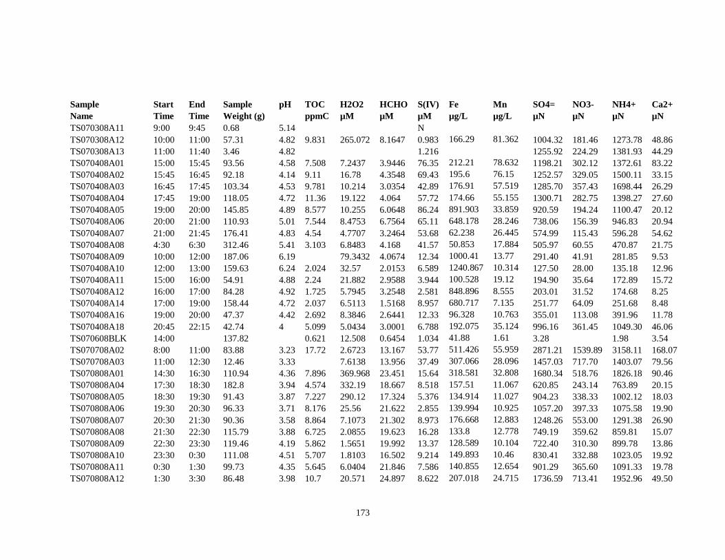
173



TS070308A11 9:00 9:45 0.68 5.14

N

TS070308A12 10:00 11:00 57.31 4.82 9.831 265.072 8.1647 0.983 166.29 81.362 1004.32 181.46 1273.78 48.86

TS070308A13 11:00 11:40 3.46 4.82

1.216

1255.92 224.29 1381.93 44.29

TS070408A01 15:00 15:45 93.56 4.58 7.508 7.2437 3.9446 76.35 212.21 78.632 1198.21 302.12 1372.61 83.22

TS070408A02 15:45 16:45 92.18 4.14 9.11 16.78 4.3548 69.43 195.6 76.15 1252.57 329.05 1500.11 33.15

TS070408A03 16:45 17:45 103.34 4.53 9.781 10.214 3.0354 42.89 176.91 57.519 1285.70 357.43 1698.44 26.29

TS070408A04 17:45 19:00 118.05 4.72 11.36 19.122 4.064 57.72 174.66 55.155 1300.71 282.75 1398.27 27.60

TS070408A05 19:00 20:00 145.85 4.89 8.577 10.255 6.0648 86.24 891.903 33.859 920.59 194.24 1100.47 20.12

TS070408A06 20:00 21:00 110.93 5.01 7.544 8.4753 6.7564 65.11 648.178 28.246 738.06 156.39 946.83 20.94

TS070408A07 21:00 21:45 176.41 4.83 4.54 4.7707 3.2464 53.68 62.238 26.445 574.99 115.43 596.28 54.62

TS070408A08 4:30 6:30 312.46 5.41 3.103 6.8483 4.168 41.57 50.853 17.884 505.97 60.55 470.87 21.75

TS070408A09 10:00 12:00 187.06 6.19

79.3432 4.0674 12.34 1000.41 13.77 291.40 41.91 281.85 9.53

TS070408A10 12:00 13:00 159.63 6.24 2.024 32.57 2.0153 6.589 1240.867 10.314 127.50 28.00 135.18 12.96

TS070408A11 15:00 16:00 54.91 4.88 2.24 21.882 2.9588 3.944 100.528 19.12 194.90 35.64 172.89 15.72

TS070408A12 16:00 17:00 84.28 4.92 1.725 5.7945 3.2548 2.581 848.896 8.555 203.01 31.52 174.68 8.25

TS070408A14 17:00 19:00 158.44 4.72 2.037 6.5113 1.5168 8.957 680.717 7.135 251.77 64.09 251.68 8.48

TS070408A16 19:00 20:00 47.37 4.42 2.692 8.3846 2.6441 12.33 96.328 10.763 355.01 113.08 391.96 11.78

TS070408A18 20:45 22:15 42.74 4 5.099 5.0434 3.0001 6.788 192.075 35.124 996.16 361.45 1049.30 46.06

TS070608BLK 14:00

137.82

0.621 12.508 0.6454 1.034 41.88 1.61 3.28

1.98 3.54

TS070708A02 8:00 11:00 83.88 3.23 17.72 2.6723 13.167 53.77 511.426 55.959 2871.21 1539.89 3158.11 168.07

TS070708A03 11:00 12:30 12.46 3.33

7.6138 13.956 37.49 307.066 28.096 1457.03 717.70 1403.07 79.56

TS070808A01 14:30 16:30 110.94 4.36 7.896 369.968 23.451 15.64 318.581 32.808 1680.34 518.76 1826.18 90.46

TS070808A04 17:30 18:30 182.8 3.94 4.574 332.19 18.667 8.518 157.51 11.067 620.85 243.14 763.89 20.15

TS070808A05 18:30 19:30 91.43 3.87 7.227 290.12 17.324 5.376 134.914 11.027 904.23 338.33 1002.12 18.03

TS070808A06 19:30 20:30 96.33 3.71 8.176 25.56 21.622 2.855 139.994 10.925 1057.20 397.33 1075.58 19.90

TS070808A07 20:30 21:30 90.36 3.58 8.864 7.1073 21.302 8.973 176.668 12.883 1248.26 553.00 1291.38 26.90

TS070808A08 21:30 22:30 115.79 3.88 6.725 2.0855 19.623 16.28 133.8 12.778 749.19 359.62 859.81 15.07

TS070808A09 22:30 23:30 119.46 4.19 5.862 1.5651 19.992 13.37 128.589 10.104 722.40 310.30 899.78 13.86

TS070808A10 23:30 0:30 111.08 4.51 5.707 1.8103 16.502 9.214 149.893 10.46 830.41 332.88 1023.05 19.92

TS070808A11 0:30 1:30 99.73 4.35 5.645 6.0404 21.846 7.586 140.855 12.654 901.29 365.60 1091.33 19.78

TS070808A12 1:30 3:30 86.48 3.98 10.7 20.571 24.897 8.622 207.018 24.715 1736.59 713.41 1952.96 49.50

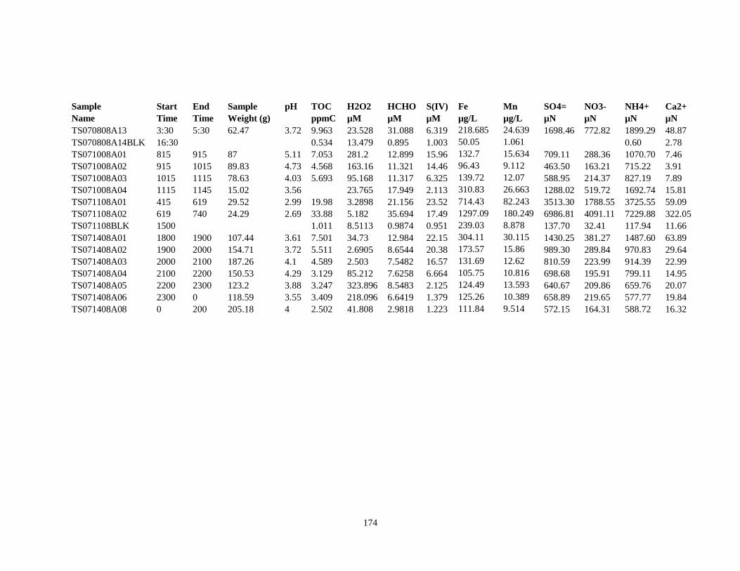
174



TS070808A13 3:30 5:30 62.47 3.72 9.963 23.528 31.088 6.319 218.685 24.639 1698.46 772.82 1899.29 48.87

TS070808A14BLK 16:30

0.534 13.479 0.895 1.003 50.05 1.061

0.60 2.78

TS071008A01 815 915 87 5.11 7.053 281.2 12.899 15.96 132.7 15.634 709.11 288.36 1070.70 7.46

TS071008A02 915 1015 89.83 4.73 4.568 163.16 11.321 14.46 96.43 9.112 463.50 163.21 715.22 3.91

TS071008A03 1015 1115 78.63 4.03 5.693 95.168 11.317 6.325 139.72 12.07 588.95 214.37 827.19 7.89

TS071008A04 1115 1145 15.02 3.56

23.765 17.949 2.113 310.83 26.663 1288.02 519.72 1692.74 15.81

TS071108A01 415 619 29.52 2.99 19.98 3.2898 21.156 23.52 714.43 82.243 3513.30 1788.55 3725.55 59.09

TS071108A02 619 740 24.29 2.69 33.88 5.182 35.694 17.49 1297.09 180.249 6986.81 4091.11 7229.88 322.05

TS071108BLK 1500

1.011 8.5113 0.9874 0.951 239.03 8.878 137.70 32.41 117.94 11.66

TS071408A01 1800 1900 107.44 3.61 7.501 34.73 12.984 22.15 304.11 30.115 1430.25 381.27 1487.60 63.89

TS071408A02 1900 2000 154.71 3.72 5.511 2.6905 8.6544 20.38 173.57 15.86 989.30 289.84 970.83 29.64

TS071408A03 2000 2100 187.26 4.1 4.589 2.503 7.5482 16.57 131.69 12.62 810.59 223.99 914.39 22.99

TS071408A04 2100 2200 150.53 4.29 3.129 85.212 7.6258 6.664 105.75 10.816 698.68 195.91 799.11 14.95

TS071408A05 2200 2300 123.2 3.88 3.247 323.896 8.5483 2.125 124.49 13.593 640.67 209.86 659.76 20.07

TS071408A06 2300 0 118.59 3.55 3.409 218.096 6.6419 1.379 125.26 10.389 658.89 219.65 577.77 19.84

TS071408A08 0 200 205.18 4 2.502 41.808 2.9818 1.223 111.84 9.514 572.15 164.31 588.72 16.32

175

APPENDIX D – ADDITIONAL FIGURES

Appendix Figure 1. Frequency distributions of TN concentrations measured in bulk (CASCC)

cloudwater samples collected at Mt. Tai in the 2008 sampling campaigns.

0

5

10

15

20

25

0 10 20 30 40 60 80 100 120

Nu

mb

er o

f sa

mp

les

Concentration (ppmN)

TN2008 Spring Average = 8.57 ppm, SD = 6.49 ppm

2008 Summer Average = 40.93 ppm, SD = 35.76 ppm

2008 Spring

2008 Summer

176

Appendix Figure 2. Comparisons of TN concentrations measured in small (4 < D < 16 µm) and

large (D > 16 µm) cloud drop size fractions simultaneously collected with the sf-CASCC at Mt. Tai during the spring and summer 2008 field campaigns. (The

diagonal dashed line is the 1:1 line.)

Appendix Figure 3. Comparisons of chloride ion concentrations measured in small (4 < D < 16 µm) and large (D > 16 µm) cloud drop size fractions simultaneously collected with

the sf-CASCC at Mt. Tai during the spring and summer 2008 field campaigns. (The


0

30

60

90

120

0 30 60 90 120

Sm

all

(p

pm

)

Large (ppm)

TN

Spring

Summer

0

200

400

600

800

1000

0 200 400 600 800 1000

Sm

all

(µ

N)

Large (µN)

Cl-

Spring

Summer

177

Appendix Figure 4. Comparisons of potassium ion concentrations measured in small (4 < D < 16

µm) and large (D > 16 µm) cloud drop size fractions simultaneously collected with the sf-CASCC at Mt. Tai during the spring and summer 2008 field campaigns. (The


0

100

200

300

400

0 100 200 300 400

Sm

all

(µ

N)

Large (µN)

K+

Spring

Summer

dissertation aqueous phase sulfate production in clouds at mt ...

Documents

Transcript of dissertation aqueous phase sulfate production in clouds at mt ...