Disparity estimation on log-polar images and vergence control

Computer Vision and Image Understanding83,97–117 (2001)doi:10.1006/cviu.2001.0924, available online at http://www.idealibrary.com on

Disparity Estimation on Log-Polar Imagesand Vergence Control

R. Manzotti, A. Gasteratos, G. Metta, and G. Sandini

Laboratory for Integrated Advanced Robotics (LIRA-Lab), Department of CommunicationsComputer and System Science, University of Genoa, Viale Causa 13, Genoa I-16145, Italy

Received September 27, 1999; accepted June 14, 2001

An important issue in the realization of an autonomous robot with stereoscopicvision is the control of vergence. Together with version, it determines uniquely theposition of the fixation point in space. Vergence control is directly related to bothdepth perception andbinocular fusion. Previous works in this field employed ei-ther a measure of correlation of stereo images or some kind of disparity-relatedestimate. In this paper, we present a new method of extracting a global dispar-ity measure for vergence control, which does not require a priori segmentationof the object of interest. Our method uses images acquired by retina-like sensorsand, therefore, the computation is performed in the log-polar plane. The techniquewe present here is: (i) global, in the sense that it is an integral measure over thewhole image, (ii) computationally inexpensive, considering that the goal was to useit in the robot control loop rather than to accurately measure some 3D world fea-tures. Moreover, the proposed technique is robust and independent of the averageillumination as well as of other features of the target such as size, shape, and di-rection of motion. It provides a precise and linear estimate of the vergence error,which is the only requirement from the control point of view. Several experimen-tal results on a real robotic setup demonstrate the effectiveness of the proposedtechnique. c© 2001 Academic Press

Key Words:active vision; log-polar; disparity; vergence.

1. INTRODUCTION

In building a robotic stereo head, an extremely important degree of freedom is representedby vergence. Given a stereoscopic vision system (Fig. 1), the vergence angle, together withversion and tilt angles, describes uniquely the fixation point in space. The problem we aredealing with here is controlling the vergence angle only with the assumption that othersubsystems maintain the object of interest close to the image center. For instance, we couldimagine a tracking module, which deals with the problem of following the target in space

97

1077-3142/01 $35.00Copyright c© 2001 by Academic Press

All rights of reproduction in any form reserved.

98 MANZOTTI ET AL.

FIG. 1. Stereoscopic vision system. The version (ϑp) and vergence (ϑv) angles are shown.

(by controlling version and tilt) or a binocular saccade-like control to quickly foveate apossibly interesting target [1].

If vergence could be controlled effectively, several advantages would arise in subsequentimage processing. These include easier fusion of stereo images in one “cyclopean image”and easier figure–ground segmentation (e.g., by means of zero disparity filters [2]). Ofcourse, if a tracked object is stable in the retinas, further image processing is facilitated.Indeed, it is not just a coincidence that most of the biological stereoscopic vision systems inthe higher branches of the evolutionary tree possess a developed and specialized vergencecontrol system [3]. If we consider biological systems, several kinds of disparity exist (hori-zontal, vertical, and rotational) in order to implement horizontal and cyclo-vergence [4]. Inthis paper only the horizontal component is considered, which is the most relevant for thecontrol of the vergence angle, in the hypothesis that the other d.o.f. are fixed. Maintaininga correct vergence angle should not be seen as a goal in itself but as a way of improvingthe performance and robustness of successive visual computation. Particularly relevant inthis respect is the intrinsic limit introduced by a correct binocular fusion in the computa-tion of binocular disparity and 3D feature extraction. Vergence angle, moreover, providesa measure of absolute distance, even if limited to a point in space, as well as a referencepoint in the environment [5]. Therefore, a general principle is that vergence control shouldbe implemented, keeping in mind its further use by the whole system [6].

In the implementation presented here we consider “only” disparity measure, which, evenif not the only source of information useful for vergence control [7], is possibly the mostdirect and relevant. Disparity estimation has been performed according to several techniques.These are based either on correlation [8–10], matching [11, 12], phase difference [13, 14],or Bayesian methods [15, 16]. Despite this big variety of disparity estimation methods,examples employing log-polar images are quite occasional [17–19]. The reason is thecomplex geometrical layout of log-polar images, which apparently is not well suited fordisparity computation. Log-polar images, however, are ideal for vergence control tasks. Theyprovide high resolution in the fovea, where the target should be located, and a wide field ofview at the same time [20]. These features, along with a computationally simple mappingtechnique used for disparity estimation, allows real-time performance to be achieved withhigh accuracy.

DISPARITY ESTIMATION ON LOG-POLAR IMAGES 99

The experimental results reported in order to show the feasibility of the approach havebeen carried out with one main goal in mind: to demonstrate that horizontal disparity aloneallows an efficient and robust vergence control, assuming that vertical, torsional, and focusdegrees of freedom (df ) are fixed. The paper is organized as follows. The essentials oflog-polar images are given in Section 2. Several techniques, which have been applied forvergence control, are discussed in Section 3. The proposed disparity estimate technique isextensively described in Section 4. In Section 5, the application of the proposed techniquefor vergence control is presented. Section 6 contains the experimental results and, finally,Section 7 contains some concluding remarks.

2. LOG-POLAR IMAGES

Studies on the primate visual pathways from the retina to the visual cortex have shownthat the geometrical layout follows an almost regular topographic arrangement [21–23].These results can be summarized as follows:

• The distribution of the photoreceptors in the retina is not uniform. They lay moredensely in the central region called fovea, while they are sparser in the periphery. Conse-quently, the resolution also decreases, moving away from the fovea toward the periphery.It has a radial symmetry, which can be approximated by a polar distribution.• The projection of the photoreceptors array to the primary visual cortex can be well

approximated by a logarithmic-polar (log-polar) distribution mapped onto a rectangular-like surface (the cortex). Here the representation of the fovea is quite expanded; i.e., moreneurons are devoted to it, and the periphery is represented using a coarser resolution.

From the mathematical point of view the log-polar mapping can be expressed as a trans-formation between the polar plane (ρ, θ ) (retinal plane), the log-polar plane (ξ, η) (corticalplane), and the Cartesian plane (x, y) (image plane),{

η = q · θξ = lna

ρ

ρ0

(1.1)

whereρ0 is the radius of the innermost circle, 1/q is the minimum angular resolution of thelog-polar layout, and (ρ, θ ) are the polar coordinates. These are related to the conventionalCartesian reference system by: {

x = ρ cosθy = ρ sinθ.

(1.2)

Figure 2 illustrates the log-polar layout as derived by Eqs. (1.1) and (1.2). In particular, thegrid on the left represents a standard Cartesian image mapped according to Eq. (1.1). Theplot on the right shows the corresponding cortical image.

3. VERGENCE CONTROL

Vergence control issues have been addressed by means of several different techniques. Itis worth noting that all of them are somehow related to the estimation of 3D features. Thesetechniques can be classified as follows:

100 MANZOTTI ET AL.

FIG. 2. The log-polar transformation. (a) The log-polar layout mapped into the Cartesian space and (b) thecorresponding cortical image.

(1) segmentation techniques [11, 12, 19, 24, 25];(2) fusion index [17, 26];(3) direct disparity estimation [9, 27].

3.1. Segmentation Techniques

This group requires some sort of heuristics to identify the object of interest (segmentation).The main problem, in this case, is their lack of flexibility. We would like to stress the factthat the segmentation of the object from its background is not an easy task itself. Many ofthe proposed systems do not use any direct control of the vergence angle, but they rathercontrol each eye separately. These approaches may, for instance, fail in the presence ofa false matching; i.e., the robot might try to follow two different targets. Moreover, inbiological systems, vergence control is a relatively low-level functionality, which does notrequire an actual segmentation or recognition of the target object. On the contrary, thesetechniques act at a higher level of abstraction, i.e., the object needs to be segmented and/orrecognized.

3.2. Fusion Index

This second group exploits the fact that if an object is correctly verged, the stereo imagesshould be very similar, at least around the fixation point. Of course, this does not holdexactly as the two images are never the same. However, under standard conditions, such as


typical fixation distance, optical parameters, and kinematics of robot heads, the differencebetween the images is rather small. In that case, the images are said to be binocularly fused.The goal of a vergence control system is to minimize this difference. The global index ofbinocular fusion is an example of such a difference estimate. It can be computed using thenormalized correlation technique [28],

C(Il , Ir ) = 1−∑

η,ξ (Ir (η, ξ )− µr ) · (Il (η, ξ )− µl )√∑η,ξ (Ir (η, ξ )− µr )2 ·∑η,ξ (Il (η, ξ )− µl )2

, (1.3)

whereIr andIl are the right and left images, respectively, andµr andµl represent their meanvalues, respectively.C(t) is almost invariant to changes of illumination. It is normalizedin the range [0, 1]. The normalized correlation measure can be employed in a standardproportional control law,

θ = −K · C, (1.4)

whereK is a constant gain andθ andC are the first derivatives of the vergence angle andthe fusion index respectively [17, 26].

However, this approach has several drawbacks:

(1) C(t) is not a linear estimation of the angular error.(2) C(t) is constant, if the eyes are still and the object is not moving (C = 0).(3) C(t) has minima whose values are variable with image characteristics in a nonlinear

and unpredictable fashion.

For these reasons, though feasible, the use ofC(t) in vergence control is limited.

3.3. Direct Disparity Estimation

The last group concerns the use of direct estimates of the binocular disparity. It is, in ourview, the most promising one, because it uses disparity directly. The latter can be easilyrelated to the vergence control error. In fact, it can be shown that binocular disparity isrelated to depth, which is in turn related to the vergence angle. Consider again the situationdepicted in Fig. 1; using only the sine law, it is easy to derive

r = bcos(ϑr ) cos(ϑl )

cos(ϑv) cos(ϑp), (1.5)

wherer is the distance of the fixation point from the baseline,b the baseline length,ϑr , ϑl theeye angles,θ = ϑl − ϑr represents the vergence angle, andϑp = (ϑl − ϑr )/2 the version(or gaze) angle. In principle, Eq. (1.5) can be used to find out the vergence angle requiredto move the fixation point from one location to another.

On the other hand, disparity is related to depthz (relative to the fixation point referenceframe) by the approximate equation,

z∼= K (θ, b)

α tan(θ )(xr − xl ), (1.6)

where K = b/sin(θ ), b is the baseline length,α is the focal length of the cameras, andxr − xl the binocular disparity [29]. Note that Eq. (1.6) is valid only in a neighborhood of

102 MANZOTTI ET AL.

the fixation point. Using Eqs. (1.5) and (1.6) together, it is thus possible to link binoculardisparity to vergence error directly. Moreover, we have actually converted the problemof estimating the vergence error in that of estimating disparity. (That is, starting fromdisparity, it is possible to compute depth by using Eq. (1.6), and from depth, which in thiscase represents the required motion, recover the vergence angle movement by employingEq. (1.5). The goal of the controller is indeed that of zeroing depth.)

Unfortunately, the direct disparity estimation approach has been undermined by somepractical difficulties. In fact, in order to reduce the computational burden, an attention regionshould be selected in advance. This means that the object has to be segmented from thebackground; this has been proved to be a hard task in itself. On the other hand, this isnot really an issue if we utilize log-polar images and we constrain ourselves to a globalestimate of the object disparity. Of course, there is nothing magic about the use of retina-likesensors. However, assuming that the object of interest is close to the center of the image, itsrelevance (e.g., number of “pixels”) becomes higher than that of more peripheral objects(its projection in the log-polar plane is effectively magnified) [30].

4. DISPARITY

In order to compute disparity it is necessary to solve a correspondence problem. That is,we have to establish which pixels on the left and right image planes map to the same pointin space. Formally, considering a standard Cartesian images case, this can be written as

d(x, y) = arg maxd{1(Il (x, y), Ir (x + d, y))}, (1.7)

where,1 is a similarity measure for each possible shiftd ∈ [−dmax, dmax]. The similaritymeasure can be either a sum of squared difference (SSD) or other criteria such as thenormalized correlation.

Assuming symmetric vergence and a simple pinhole camera model, the image and motorcoordinates systems are related by the equation,

d = 2 f · sin

(1ϑv

2

), (1.8)

where1θ is the difference between the actual and the correct vergence angle (the vergenceangle with null disparity),f the camera focal length, andd the measured disparity. It is worthnoting that Eq. (1.8) is monotonic in the required domain (typically1θ ∈ [−π/2, π/2]).Roughly speaking because the measure is well formed in Lyapunov sense ([31]) the closedloop system will be stable even if a simple PD controller is used. Furthermore, the shift ofimage pixels can be represented by a disparity operatordispcart : <3→<2, defined as

dispcart(x, y, d) ∼= (x + d, y), (1.9)

whered represents the disparity and (x, y) a point in the image plane.By applying Eq. (1.9) to an image point (x, y), we can generate the corresponding match-

ing point at disparityd. The rationale of definingdispcart will be clear when we will deal


with nonuniform mapping such as the log-polar one. Combining Eqs. (1.7) and (1.9) yields

d(x, y) = arg maxd{1(Il (x, y), Ir (dispcart(x, y, d)))}, (1.10)

In a general case, in order to apply Eq. (1.10) and recover the disparity, we need to provide

(i) the disparity functiondisp, which embeds the description of the image geometry;(ii) the similarity function1, which defines a distance measure between pixel blocks.

Considering the log-polar case, we just need to replace thedispoperator with a suitable onefor that particular topology. However, the mapping is not simple using log-polar images. Asimple horizontal shift in Cartesian coordinates is mapped to a complex curve in log-polarcoordinates. Given a (ξ, η) pair the disparity operatordisplog:<3→<2 is defined as

displog(ξ, η,d) = (ξn, ηn). (1.11)

The transformation is now given by

(ξn

ηn

)∼= 1

q · arctan[

ρ0 ·aξ · cos(η/q)ρ0 ·aξ · sin(η/q)+ d

]√

(ρ0 · aξ · sin(η/q)+ d)2+ ρ20 · a2ξ · cos2 (η/q)

. (1.12)

By applying thedispoperator we can roughly simulate a horizontal shift of (Il , Ir ) withoutactually moving the cameras. In practice this is only approximately true because of twomain reasons:

(1) Space-variant images introduce a corresponding space variant distortion. In fact, wecannot recover the missing information belonging to the periphery, where the resolution iscoarser.

(2) A real camera motion also distorts the image points along the vertical axis. However,thedispoperator, as it has been defined in Eq. (1.11), does not take this into account.

Concerning the space-variant resolution we are limited by the fact that the information losson the periphery cannot be avoided. With regard to the contribution of the vertical disparity,it is a rather small effect, and we can neglect it as a first approximation. Figure 3 shows howa regular grid in the left image would be mapped in the right one for increasing values ofdisparity (in the range zero to nine pixels). These are exactly the graphical representationsof Eqs. (1.11) and (1.12).

Furthermore, as our objective was to measure a global disparity index, Eq. (1.10) canbe further simplified by including in the aforementioned “neighborhood” of the currentpixel all the image pixels. In this case the disparity indexd is no longer dependent on theposition of a single pixel. A final comment regards the computational load associated withEq. (1.12). We can note that the equation depends only on the log-polar geometry. In factit is not dependent on the actual images. Therefore, all calculations can be performed inadvance for all possible disparities and stored into a fixed connection map (CM). A CMis basically a look-up table (LUT), which implements a mapping according to Eq. (1.12).From a more general point of view, we can see the CM as a network, where the CM valuesrepresent network nodes, and the connections the log-polar geometry itself. This suits verywell our conceptual biological bias. It is easy to imagine how these correspondence mapsmight be implemented in parallel using several layers of neurons.

104 MANZOTTI ET AL.

FIG. 3. The geometrical transformation of the cortical mesh. The disparity values increase from zero andnine pixels (from the left to the right and form the top to the bottom, respectively). In each graph the horizontalaxis represents the eccentricity, while the vertical axis the angular position. The small circle and the box show theeffects of the transformation.

4.1. Disparity Computation

As is stated above, in order to compute the disparity, we need to store the geometricaltransforms. The corresponding set of CMs can be defined as

CM SET= {CMd, d = 0 . . . N} (1.13)

CMd = {(ξn, ηn)ξ,η : ξ = 0 . . . ξmax, η = 0 . . . ηmax}, (1.14)

whereξmax ηmax is the size of the log-polar images in cortical coordinates,N the totalnumber of CMs, and

(ξn, ηn)ξ,η,d = displog

(ξ, η,

(d − N

2

N

)· ξmax/2

). (1.15)

Using this notation, an image transform can be rewritten as

Ir = displog(Il , d) (1.16)

Implicit in this notation is the fact that we are actually mapping all the pixels of the leftimageIl into those of the right oneIr . That is,

Ir (ξ, η) = Il ((ξn, ηn)ξ,η,d) (1.17)


FIG. 4. A measured disparity function obtained with an object almost in vergence. It is possible to notice themaximum of the function near the center of the curve.

It is worth noting that the set of CMs has a finite size. Consequently, in order to evaluate thearg max function overd we need to evaluate only a finite number of possible disparities. Inother words, at each time instantt the result is the discrete function (which is function ofthe disparityd),

χ (Il , Ir , d) = C(Ir , displog(Il , d)), (1.18)

whereC(Ir , Il ) is the normalized correlation function of Eq. (1.3); i.e., we employed thenormalized correlation as similarity criterion1.

Figure 4 shows a real-case plot obtained using the procedure described above. Withoutloosing the generality we can define the disparity function, for a given stereo pair (Il , Ir ),as

χ (d) = χ (Il , Ir , d). (1.19)

The global disparity index is simply

dt = arg maxx

(χ (x)). (1.20)

It is worth stating that:

(1) Given the fact that the disparity functionχ (d) is an integral correlation measure overthe whole image it is extremely robust and reliable.

(2) χ (d) represents the global image disparity because its values are the result of thecorrelation of the entire image with its corresponding image, shifted by the geometricaltransformation due tod.

106 MANZOTTI ET AL.

(3) The significant element inχ (d) is its maximum, which corresponds to the mostcommon disparity value among the image points.

(4) Most of the noise is rejected, simply because it is located out of the global maximum.

The robustness of the proposed method is a consequence of the fact that, by choosingthe disparity value corresponding to the maximum correlation, the contribution of the notrelevant part of the image is implicitly rejected. Therefore, even if the side lobes are largein comparison to the maximum of the correlation function, they do not modify the value ofχ (d).

As a matter of fact, a precise measurement of disparity requires a great resolution. Infact, even a small disparity (in the subpixel range) might correspond to a large variation inthe object distance (more than 10 cm). To prevent such a loss of accuracy it is possible toincrease the image resolution. However, this is, in general, a resource consuming approach.Consequently, we devised a few techniques to increase the estimated accuracy withoutvarying the image resolution itself. They are presented in detail in the next paragraphs.

4.1.1. Disparity nonuniform sampling.One of the main drawbacks of the previouslydescribed correlation technique is the lacking of accuracy. The fact that we have used aset of precomputed CMs restricts disparity to one of these CMs. Therefore, the accuracy islimited by the disparity difference, which corresponds to the minimum distance betweenCMs. In other words, the maximum accuracy is

d1min =

ξmax

N, (1.21)

whereN is the number of CMs, andξmax the log-polar image radius.A possible solution would be to increase the numbers of CMs (increasingN) but this

would increase the computational cost accordingly. A second solution would be to reduce theradius of the log-polar imageξmax, reducing, consequently, the field of view. An alternativeapproach exploits the space variant techniques used by using the same number of CMsdistributed in a nonlinear fashion. In this way resolution for small disparities is improvedwithout increasing the computational load. This solution does not affect the overall systemperformance, since for high-disparity values there is no need for precise disparity estimationbecause the higher the value of disparity the higher is the distance of the world point fromfixation. On the other hand, when disparity is small, high precision is required, since thecontrol should minimize even small errors.

We can therefore replace Eq. (1.13) with

CM SETvariant ={

CMvariantd , d = 0 . . . N

}(1.22)

CMvariantd = {(ξn, ηn)ξ,η: ξ = 0 . . . ξmax, η = 0 . . . ηmax}, (1.23)

whereξmax, ηmax is the log-polar image size in cortical coordinates,N is the total numberof CMs, and

(ξn, ηn)ξ,η,d = displog(ξ, η, sign(i − N/2)(abs(arctan((1− N/2)/N)))λ · ξmax/2),

(1.24)

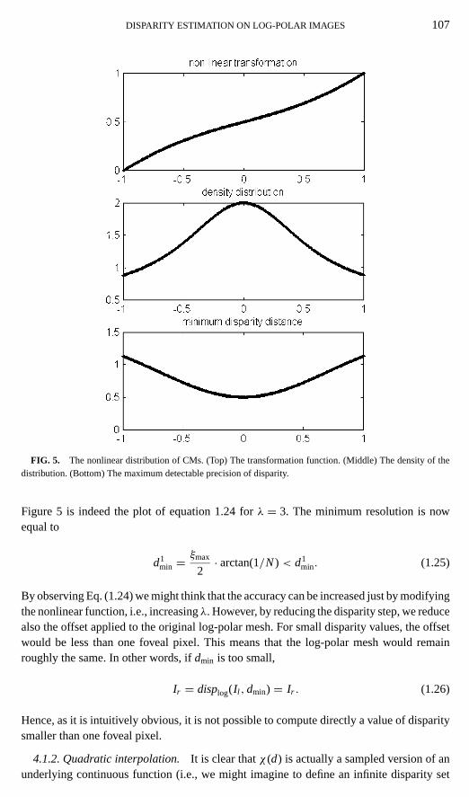
whereλ is positive number.λ acts as a steep enhancer in the nonlinear transformation andit is typically λ = 3.


FIG. 5. The nonlinear distribution of CMs. (Top) The transformation function. (Middle) The density of thedistribution. (Bottom) The maximum detectable precision of disparity.

Figure 5 is indeed the plot of equation 1.24 forλ = 3. The minimum resolution is nowequal to

d1min =

ξmax

2· arctan(1/N) < d1

min. (1.25)

By observing Eq. (1.24) we might think that the accuracy can be increased just by modifyingthe nonlinear function, i.e., increasingλ. However, by reducing the disparity step, we reducealso the offset applied to the original log-polar mesh. For small disparity values, the offsetwould be less than one foveal pixel. This means that the log-polar mesh would remainroughly the same. In other words, ifdmin is too small,

Ir = displog(Il , dmin) = Ir . (1.26)

Hence, as it is intuitively obvious, it is not possible to compute directly a value of disparitysmaller than one foveal pixel.

4.1.2. Quadratic interpolation. It is clear thatχ (d) is actually a sampled version of anunderlying continuous function (i.e., we might imagine to define an infinite disparity set

108 MANZOTTI ET AL.

FIG. 6. An example of interpolation by using the quadratic approach (Eq. (1.10)). The accuracy improved toabout 0.3 pixels.

instead of the finite one), which has the same formulation asχ (d) but it has no constraintson its argument: d∈<. It is thus possible to apply an interpolation technique on the samplesχ (d). A straightforward solution is to apply a quadratic interpolation technique as sketchedin Fig. 6. In equation form,

dn = χ (d − δ)− χ (d + δ)2 · (χ (d − δ)− χ (d)+ χ (d + δ)) , (1.27)

whered is the disparity value computed without interpolation andδ is the minimum disparityvalue (δ = dmin) or a suitable multiple.

Given the heuristic of this last technique there are no particular reasons to prefer aninterpolation technique from another. Note also that the interpolation is not performed onthe final data (the estimated disparity) but on the raw data of the disparity function. Ofcourse, this means that it is not just a mathematical smoothing but it represents a realimprovement over the noninterpolated counterpart.

5. VERGENCE CONTROL FROM DISPARITY COMPUTATION

Vergence control has been implemented by applying the following control law:

θ = −K · dt , (1.28)

whereK is a constant gain,θ is the first derivative of the vergence angle, anddt is thedisparity index (see Eq. (1.20)). The advantages of this approach can be summarized asfollows:


FIG. 7. The disparity function. These two plots were obtained by changing the vergence angle at a constantspeed (total span was 0.16 radians). For each angular position we measured the disparity (top) and the fusion indexC(t) (bottom), respectively.

(1) dt is a linear estimation of the angular error, as shown in Fig. 7.(2) dt provides the same information irrespective of the state of the system, because it

does not matter if the cameras are moving or if they are still.(3) dt is robust to noise, environmental modifications, changes in lighting conditions,

and object properties.

A few words are needed to explain the previous points. The properties ofdt are graphicallyillustrated in Figs. 7 and 10, in which it is possible to see thatdt is linear in a range ofapproximately 0.2 radians. This range is compatible with the goal of keeping the right angleof vergence, a task that is usually achieved for small values of disparity. Regarding the secondpoint it is important to stress that one of the major drawbacks of other implementationsof vergence control was the inability of detecting the correct angle without moving thecameras (e.g., [32]). In other words, for each pair of images we have a meaningful valuefor the controller without having to acquire a new pair in order to compute a gradient. Last,the robustness ofdt is partially derived from the robustness of the correlation functionC( )and partially from the property of Eqs. (1.18), (1.19), and (1.20).

6. CARTESIAN IMAGES VERSUS LOG-POLAR IMAGES

The main motives in using log-polar images derive from their computational advantages,their geometrical properties, their wide field of view, their high resolution in the fovea,and their implicit selection of a target in the central part of the image. All these properties

110 MANZOTTI ET AL.

are exploited in this implementation of disparity estimation. Of course, a “conventional”Cartesian system may present each of these properties but not all of them simultaneously.For example, it is easy to build a Cartesian system with the same resolution and field of viewas a log-polar one but at a much greater computational expense. Similarly, it is possible tobuild a system with the same number of pixel but with a limited field of view or, alternatively,a decreased resolution.

With respect to the disparity estimation and in order to make a comparison with a Cartesiansystem we assume the following: Given a log-polar image of sizeξmax× ηmax, there is noCartesian equivalent image. Two of the following three parameters should be fixed: thepixel size, the number of the pixels, and amplitude of the field of view. Therefore, threedifferent comparative approaches can be constructed and studied:

(1) a Cartesian image having the same number of pixels and the same field of view withthe log-polar one;

(2) a Cartesian image with the same number of pixels corresponding to a square areasmaller than the whole image but with the same number of pixels with the log-polar one;

(3) a Cartesian image having the same amplitude of the field of view and the sameresolution of the fovea, but with a much larger number of pixels.

Let us examine, one by one, these cases. It is assumed thatηmax= 2ξmax, as it is in the usualcase (e.g., [20, 26, 32]), and that the Cartesian equivalent image is square. Besides, it isreasonable to assume that there would be no oversampling of pixels in the fovea and, thus,the following equations must hold:

ρ0 = ηmax · r fmin

2πa = ρ0+ r fmin

ρ0, (1.27)

wherer fmin is fixed and represents the diameter of the receptive field of minimum size inthe fovea.

Same field of view, same number of pixels.Given a log-polar image of sizeξmax×ηmax, it is possible to use a Cartesian image of dimensionxmax=

√ξmax · ηmax=

√2 · ξmax.

Obviously, having to cover the same field of view, this image has to correspond to the samearea as the log-polar image: this entails a corresponding resolution (in the fovea) of

ρmax · r fmin

xmax=√

2 · r fmin · ρ0

ξmax· aξmax. (1.28)

Using Eqs. (1.27), the previous can be rewritten as

ρmax · r fmin

xmax=√

2π(1+ ξ−1

max

)ξmax. (1.29)

This means that given the constrains we have assumed there is a great reduction of resolutionin the Cartesian counterpart. The disparity suffers the same loss in resolution.

Same resolution in the center, same number of pixels.A Cartesian image of sizexmax=

√ξmax · ηmax=

√2 · ξmax is assumed. It covers only the central part of the image

and comprises the same resolution as the log-polar image in the fovea (r fmin). In this case


TABLE 1

A Case Study between Log-Polar Technique and Cartesian Counterparts

Resolution inMethods Computational load fovea Field of view Drawbacks

Log-polar ξmax · ηmax 1 1disparity = 2ξ 2

max

Same ξmax · ηmax

√2π (1+ ξ−1

max)ξmax 1 Low resolution; no implicit

amplitude = 2ξ 2max selection of target;

integral estima-tion of disparityC( )fails at small targets

Same ξmax · ηmax 1

√2

2π(1+ ξ−1

max)−ξmax Small field of view; the

resolution = 2ξ 2max target gets lost easily

Same1

2π2· ξ 2

max · 1 1 Increased computational load;

amplitude (1+ πξ−1max)

2ξmax no implicit selectionand same of target; integral estimationresolution of disparityC( ) fails at

small targets

the loss in the amplitude of the field of view is equal to (using Eq. (1.27))

xmax

ρmax · r fmin=√

2

2· ξmax

ρ0 · aξmax · r fmin=√

2

2π

(1+ ξ−1

max

)−ξmax. (1.30)

Therefore, the probability of loosing the target increases accordingly.

Same field of view, same resolution, and bigger number of pixels.A Cartesian image ofsizexmax= 2

r fminρ0 · aξmax is used, in order to achieve the samefield of view. Using Eq. (1.27),

xmax is related toξmax as

xmax=√

2

2π· ξmax ·

(1+ πξ−1

max

)ξmax. (1.31)

Besides, in each of the previous cases, there is no implicit selection of the target. This meansthat, by using a global correlation function likeC( ) (Eq. (1.3)), a target occupying a largeportion of the image is needed. If the image is log-polar, a target in the center of the imagecould correspond to a larger number of pixels, which improves significantly the estimationof disparity. A synopsis of this case study is provided in Table 1.

7. EXPERIMENTS

In order to demonstrate the feasibility of the approach we tested the algorithm on abinocular robotic setup. This consists of five degrees of freedom robot head (Fig. 8a).The head kinematics allows independent vergence (both cameras can move independentlyaround a vertical axis) and a common tilt motion. Furthermore, the neck is capable of a tiltand pan independent motion. However, in the following experiments, only twodf (i.e., the

112 MANZOTTI ET AL.

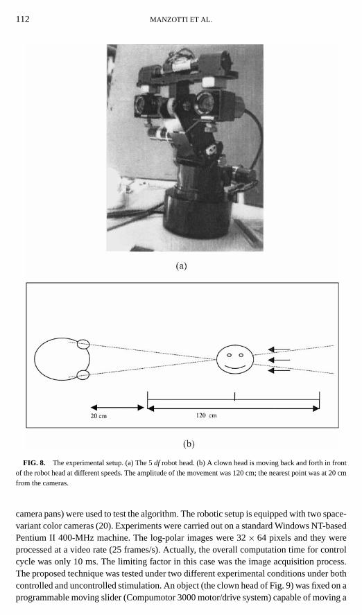
FIG. 8. The experimental setup. (a) The 5df robot head. (b) A clown head is moving back and forth in frontof the robot head at different speeds. The amplitude of the movement was 120 cm; the nearest point was at 20 cmfrom the cameras.

camera pans) were used to test the algorithm. The robotic setup is equipped with two space-variant color cameras (20). Experiments were carried out on a standard Windows NT-basedPentium II 400-MHz machine. The log-polar images were 32× 64 pixels and they wereprocessed at a video rate (25 frames/s). Actually, the overall computation time for controlcycle was only 10 ms. The limiting factor in this case was the image acquisition process.The proposed technique was tested under two different experimental conditions under bothcontrolled and uncontrolled stimulation. An object (the clown head of Fig. 9) was fixed on aprogrammable moving slider (Compumotor 3000 motor/drive system) capable of moving a


FIG. 9. An image sequence of five thumbnails (left image) of the subject, acquired during the experiment,showing the tracking while the target approaches the system: (a) in cortical plane (original on the left, zoomed-inon the right), (b) Cartesian reconstructed from the cortical ones, (c) Cartesian format with the same number ofpixels and the same field of view as the ones in (a), (d) Cartesian format with the same number of pixels and thesmaller field of view to the ones in (a), and (e) Cartesian format with bigger number of pixels and the same fieldof view as the ones in (a).

small object with speed ranging from 0 to 5 m/s. We then generated different back and forthmotion profiles. In this situation only vergence control was required (no version) to actuallytrack the moving stimulus. A sequence of log-polar images was recorded while the systemwas tracking. This is presented in Fig. 9a (cortical images). It should be noted that the actualsize of the images (32× 64) is the one on the left, while the one on the right is an enlargedimage that we have added for the reader. In Fig. 9b, the Cartesian images reconstructed fromthe cortical sequence are presented. The same sequence is presented in Figs. 9c, 9d, and 9ein Cartesian format. Each of the sequences presented in these figures (9c to 9e) correspondsto one of the three cases described in the previous section. More specifically Fig. 9c presentsCartesian images with the same number of pixels (44× 44 ) and the same field of view asthe ones in Fig. 9a. Figure 9d illustrates a Cartesian image sequence with the same number

114 MANZOTTI ET AL.

FIG. 10. Effect of the quadratic interpolation. The target, in this case, was moving along a sinusoidal trajectorywith fixed frequency. The cameras were still, i.e., the vergence control was not applied. (a) The estimated disparitywithout interpolation and (b) the improved final result, after the interpolation.

of pixels (44× 44) as the ones in Fig. 9a, but corresponding to a square area smaller than thewhole image. Finally Fig. 9e shows Cartesian images with same field of view and the sameresolution of the fovea, but with a much larger number of pixels (128× 128). ObservingFigs. 9a and 9e, it becomes obvious that the amount of clutter the system is rejecting, onlyby using space variant images. The object was able to move along either a triangular or asinusoidal trajectory. Motion amplitude was 1.20 m. The nearest point was at 20 cm in frontof the cameras (Fig. 8b). This corresponded to an angular difference (in term of vergenceangle) of 45◦.

Concerning the closed-loop case, Fig. 10 depicts the effect of the quadratic interpolation.Figure 10a is the disparity estimation without interpolation; Fig. 10b is the same traceusing the described quadratic interpolation. It is possible to notice the difference in thesmoothness of the estimate (the upper plot is step-wise). The data were obtained using thesetup described by Fig. 8. In this case the cameras were still, and the object was movingalong a sinusoidal trajectory (at a fixed frequency).

Figure 11 presents the closed loop condition where the estimated global disparity is usedto drive vergence control. In this case the control was activated and the trajectory had atriangular profile. The four plots represent the estimated disparity (Fig. 11a), the fusion indexC(t) (Fig. 11b), the motor command (speed) (Fig. 11c), and the vergence angle (Fig. 11d).An interesting effect is visible by comparing the disparity plot with the vergence angle:the biggest error (in module) corresponds to the minimum distance of the slider, whilstthe minimum estimated error corresponds to the maximum distance. Besides, when thechange in direction occurs at the minimum distance there is a relatively big overshoot in thedisparity estimate. On the other hand, when it corresponds to the maximum distance there


FIG. 11. Vergence control. The object moved along a triangular trajectory at a constant frequency. Thevergence control was activated. (a) The estimated disparity, (b) the fusion indexC(t), (c) the motor command(speed), and (d) the vergence angle.

is almost no overshoot at all. Nevertheless, by observing the absolute scale of the computederror we can see that the maximum error was only 0.05 log-polar pixels.

As far as the performance in an unconstrained environment is concerned the behavior ofthe robotic head was tested for several prolonged experimental sessions. Its performanceshave been reliable, robust, and consistent. The frequency response of the system was prac-tically flat over the tested range (10−1–2 Hz). Nevertheless, these last experiments wereconducted in a qualitative fashion and, therefore, their significance is limited. What wecan say is that the head proved to be robust to noise in the periphery of its visual field aswell as to noise derived by abrupt modification in light intensity or target object unexpectedmovement. While the robustness with respect to peripheral noise was mainly due to log-polarimages, the capability of responding quickly to object modifications both in its dynamic(speed, directions, trajectory) and in its appearance (shape, position, color, reflectance,shape, and shades) factors is due to the robustness of the processing itself.

116 MANZOTTI ET AL.

8. CONCLUSIONS

In this paper we presented a global disparity estimation method and its use in controllingthe vergence angle of a stereoscopic artificial vision system. We were able to extract ameasure of the vergence error by using space variant stereo images. This measurement wasproved to be linear, fast, and robust to environmental changes. Consequently, it has beenused to implement a closed loop vergence control that, through the use of both nonlineardistribution of CMs and space variant images, achieves accuracy much smaller than onepixel (typically around 10−1 pixels relatively to image size). Last but not least, we wereable to extract the disparity information at frame rate using a standard hardware platform.Our claim is that it is possible to efficiently estimate disparity using log-polar images,which apparently seems not well suited for such computation. Furthermore, in this paperwe showed (i) that disparity contains all useful information in order to control the vergenceangle and (ii) that there is no need to use other cues to estimate the error. Besides, we claimthat log-polar images permit an implicit selection of the central part of the overall scenethat justifies the use of a global estimator.

Experimental results substantiate the above claim. The robotic head control proved tobe robust to noise in the periphery of its visual field as well as from noise derived byabrupt modification in light intensity (as showed in Section 3) or target object unexpectedmovement (as showed in Section 5). Investigation of the integration of the proposed methodwith tracking control and saccade-like movements is underway.

ACKNOWLEDGMENTS

This work has been supported by the ESPRIT Projects NARVAL-30185 and ROBVISION-28867 and by fundsfrom the Italian MURST. Dr. Gasteratos is supported by a fellowship from the TMR project-VIRGO.

REFERENCES

1. F. Panerai, G. Metta, and G. Sandini, Visuo-inertial Stabilization in Space-variant Binocular Systems,RoboticsAutonomous Systems30(1-2), 2000, 195–214.

2. R. Manzotti, R. Tiso, E. Grosso, and G. Sandini,Primary Ocular Movements Revisited, Technical Report,7/94, LIRA-Lab, Genova, 1994.

3. M. V. Srinivasan and S. Venkatesh,From Living Eyes to Seeing Machines, Oxford University Press, London,1997.

4. J. P. Howard and B. J. Rogers,Binocular Vision and Stereopsis, Clarendon Press, Oxford, 1995.

5. D. H. Ballard and C. M. Brown, Principles of animate vision,Comput. Vision Graphics Image Process. 56(1),1992, 3–21.

6. J. Aloimonos, I. Weiss, and A. Bandyopadhyay, Active vision,Internat. J. Comput. Vision1(4), 1988, 333–356.

7. F. A. Miles and C. Busettini, Ocular compensation for self motion. Visual mechanisms,Ann. NY Acad. Sci.656, 1992, 220–232.

8. K. Pahlavan, T. Uhlin, and J.-O. Eklundh, Integrating primary ocular processes, inProceedings, ECCV92—European Conference of Computer Vision, Santa Margherita Ligure, Italy, 1992.

9. J. Taylor, T. Olson, and W. N. Martin, Accurate vergence control in complex scenes, inIEEE Computer SocietyConference on Computer Vision and Pattern Recognition, Seattle, WA, 1994.

10. T. Kanade and M. Okutomi, A stereo matching algorithm with an adaptive window: Theory and experiment,IEEE Trans. Pattern Anal. Mach. Intelligence16(9), 1994, 920–932.


11. M. R. M. Jenkin, A. D. Jepson, and J. K. Tsotsos, Techniques for disparity measurement,Comput. VisionGraphics Image Process. Image Understand.53(1), 1991, 14–30.

12. D. De Vleeschauwer, An intensity-based coarse-to-fine approach to reliably measure binocular disparity,Comput. Vision Graphics Image Process. Image Understand.57(2), 1993, 204–218.

13. C. Tieh-Yuh and A. C. Bovik, Stereo Disparity from multiscale processing of local image phase, inInterna-tional Symposium on Computer Vision, 1995.

14. S. Rougeaux,Real-time active vision for versatile interaction, Ph.D., Universite d’Evry, Courcouronnes,France, 1999.

15. L. Matthies, Stereo vision for planetary rovers: stochastic modeling to near real-time implementation,Internat.J. Comput. Vision8, 1992, 71–91.

16. C. V. Stewart, R. Y. Flatland, and K. Bubna, Geometric constraints and stereo disparity computation,Internat.J. Comput. Vision20(3), 1996, 143–168.

17. A. Bernardino and J. Santos-Victor, Vergence control for robotic heads using log-polar images, inIROS’96,Osaka, Japan, 1996.

18. A. Bernardino and J. Santos-Victor, Binocular visual tracking: Integration of perception and control,IEEETrans. Robotics Automation15(6), 1999, 1080–1094.

19. N. Oshiro, N. Maru, N. Atsushi, and M. Fumio, Binocular tracking using log polar mapping, inProceedings,IROS’96, Osaka, Japan, 1996.

20. G. Sandini, A. Alaerts, B. Dierickx, F. Ferrari, L. Hermans, A. Mannucci, B. Parmentier, P. Questa,G. Meynants, and D. Sheffer, The Project SVAVISCA: A space-variant color CMOS sensor, inAFPAEC’98,Zurich, 1998.

21. M. Daniel and D. Whitteridge, The representation of the visual field on the cerebral cortex in monkeys,J. Physiol.159, 1961, 203–221.

22. U. Schwarz and F. A. Miles, Ocular responses to translation and their dependence on viewing distance.I. Motion of the observer,J. Neurophysiol. 66, 1991, 851–864.

23. E. L. Schwartz, A Quantitative model of the functional architecture of human striate cortex with applicationto visual illusion and cortical texture analysis,Biol. Cybernetics37, 1980, 63–76.

24. M. M. Marefat, L. Wu, and C. C. Yang, Gaze stabilization in active vision. I. Vergence error extraction,PatternRecognition30(11), 1997, 1829–1842.

25. M. M. Marefat, L. Wu, and C. C. Yang, Gaze stabilization in active vision. II. Multi-rate vergence control,Pattern Recognition30(11), 1997, 1843–1853.

26. E. Grosso, R. Manzotti, R. Tiso, and G. Sandini, A space-variant approach to oculomotor control, inIEEEInternat. Symposium on Computer Vision, Coral Gables, FL, 1995.

27. I. Horswill and M. Yamamoto, A $1000 active stereo vision system, inProceedings, IEEE Symposium onVisual Languages, 1994.

28. J. Nielsen and G. Sandini, Learning mobile robot navigation: A behavior-based approach, inIEEE Interna-tional Conference on Systems, Man, and Cybernetics, San Antonio, Texas, 1994.

29. E. Grosso, G. Metta, A. Oddera, and G. Sandini, Robust visual servoing in 3D reaching tasks,IEEE Trans.Robotics Automation12(8), 1996, 732–742.

30. C. Capurro, F. Panerai, E. Grosso, and G. Sandini, A binocular active vision system using space variantsensors: Exploiting autonomous behaviors for space application, inInternational Conference on DigitalSignal Processing, Nicosia, Cyprus, 1993.

31. G. Casalino, M. Aicardi, A. Bicchi, and A. Balestrino, Closed loop steering for unicycle like vehicles: Asimple Lyapunov like approach,IEEE Robotics Automation Magazine2(1), 1995, 27–35.

32. C. Capurro, F. Panerai, and G. Sandini, Dynamic vergence using log-polar images,Internat. J. Comput. Vision24(1), 1997, 79–94.

Disparity estimation on log-polar images and vergence control

Documents

Transcript of Disparity estimation on log-polar images and vergence control