Disparities and Growth between the APEC Countries, 1990-2011

jei Disparities and Growth within APEC Countries, 1990~2011

399

Abstract

This paper examines output disparities between the Asia-Pacific Economic Cooperation countries during the period 1990~2011. The results show that inter-country levels of output per capita diverged over the study period but there was a clear break in the trend around 1998. Applying the time-varying individual common factor model, we found that all countries could be grouped into three convergence clubs. Focusing on the time path of each country’s output level relative to that of a reference economy such as The United States of America and allowing for possible structural breaks, we found that more countries converged towards the USA during the sub-period 1999~2011. The findings also suggest that the Asia-Pacific Economic Cooperation could have played some role in diminishing the output inequality between its member countries after the Asia-Pacific Economic Cooperation reached its current extent in 1998. Likewise, the paper suggests a need to further reduce the wide income gap between the Asia-Pacific Economic Cooperation countries to promote their economic integration.

JEL Classifications: O19, O47, O57, P52Keywords: Inter-Country Inequality, Regional Economic Integration, APEC Countries

Disparities and Growth within APEC Countries, 1990~2011

jei Journal of Economic Integration

Xuan-Binh Vu Griffith Asia Institute, Griffith University, Australia

* Corresponding Author: Xuan-Binh Vu; Visiting Research Fellow at Griffith Asia Institute, Griffith University, 170 Kessels Road, Nathan Queensland 4111, Australia; E-mail: [email protected].

Acknowledgements: The author is grateful to the anonymous referees, Professor Tom Nguyen and Professor Christine Smith for their helpful comments.

ⓒ 2015-Center for Economic Integration, Sejong Institution, Sejong University, All Rights Reserved. pISSN: 1225-651X eISSN: 1976-5525

Vol.30 No.3, September 2015, 399~428http://dx.doi.org/10.11130/jei.2015.30.3.399

jei Vol.30 No.3, September 2015, 399~428 Xuan-Binh Vu

http://dx.doi.org/10.11130/jei.2015.30.3.399

400

I. Introduction

The Asia-Pacific Economic Cooperation (APEC) was established in 1989 by 12 founding members: Australia, Brunei, Canada, Indonesia, Japan, Malaysia, New Zealand, the Republic of Korea, the Philippines, Singapore, Thailand, and the United States. After that, China, Hong Kong, and Chinese Taipei joined APEC in 1991, while Mexico and Papua New Guinea became members of this organisation in 1993. In 1994, Chile joined APEC, and four years later Peru, Russia, and Vietnam became its members in 1998 (source: http://www.apec.org).

As indicated in APEC’s mission statement, APEC is the premier Asia-Pacific economic forum and its primary goal is to support sustainable economic growth and prosperity in the Asia-Pacific region. Its member countries are united to build a dynamic and harmonious Asia-Pacific community by championing free and open trade and investment, promoting and accelerating regional economic integration, encouraging economic and technical cooperation, enhancing human security, and facilitating a favourable and sustainable business environment.

This question is, after more than one decade since APEC reached its current extent of 21 member countries in 1998, to what extent has APEC contributed to promoting its members’ economic integration as specified in its mission statement, particularly reducing inter-country output disparity? In particular, the following main question is taken into consideration: What have been the trends and patterns of inter-country output disparity between the APEC countries?

This question is divided into the three following sub-questions:(i) Did inter-country output levels diverge or converge? (ii) Which countries displayed the most divergence or convergence?(iii) Has APEC contributed to reduce output inequality between its member countries?

To answer the above questions, a range of complementary methods including econometric analyses are employed. The paper’s main contributions lie in the use of and interpretation of recent data and, perhaps more importantly, in the synthesis of findings from several analytical approaches into a set of consistent interpretations. Also, evidence of income convergence between the APEC countries (if any) investigated in this study will provide the basis of further understanding of their economic integration. Such


401

knowledge will be of interest to researchers and policy-makers, not only in the APEC countries but also in other co-operative organisations where income disparities are an issue of concern.

This paper is organised as follows. Section II presents a review of the literature on inter-country output/income disparities. Section III outlines the research methods to be used, while sources of data to address the research questions are described in Section IV. Sections V discusses the findings, in terms of the overall divergence/convergence pattern, the identification of clubs, or groups of countries, whose growth paths were similar, and the relative performances of individual clubs and countries. This section also discusses the role of APEC in reducing output disparity between its member countries, while Section VI concludes.

II. Literature Review

Global economic development has brought human beings remarkable achievements. In particular, during the period 1820~2008, average global GDP per capita increased almost tenfold, life expectancy nearly doubled, and literacy rates increased from below 20% to above 80% (World Bank 2009). However, these achievements of global economic development have not been spread equally among all countries, and growth came earlier to some countries than others. This section will now review inter-country output/income disparities.1

Findings from previous studies of inter-country income inequality have been mixed. Also, the trend of economic activity per capita follows different patterns depending on the measure of economic activity (income versus output) selected for analysis. Dowrick and Nguyen (1989) examined convergence of Organization for Economic Cooperation and Development (OECD) income levels during the period 1950~1985 and found that there was evidence of convergence of income per capita across OECD countries since 1950. The findings also suggested that a systematic process of catching up in levels of total factor productivity was one of the main reasons for this convergence process. Barro (1991) analysed economic growth in a cross section of 98 countries during the

1 For details, see the appendix.



402

period 1960~1985 and concluded that countries having lower real GDP per capita in 1960 tended to have a higher growth rate of real GDP per capita. Levy and Chowdhury (1994) explored income inequality between 115 countries during the period 1960~1985 and found that inter-country income inequality declined steadily by approximately 0.58 per year, showing a substantial convergence trend during the study period. Bernard and Durlauf (1995) constructed a stochastic definition of convergence based on the theory of integrated time series to test for convergence in GDP per capita across 15 OECD countries during the period 1900~1987. The results suggested that there was little evidence of convergence; however, a considerable co-integration between these countries was found.

In contrast, Levy and Chowdhury (1995) used the income-weighted entropy measure to analyse income inequality across 154 countries during the period 1960~1990. Their findings suggested that there was evidence of strong divergence during the sub-period 1960~1968, but slow convergence during the sub-period 1969~1983. For the last period 1984~1990, neither convergence nor divergence was found. Park (2000) examined inter-country income inequality across the Southeast Asian countries during the period 1967~1997. By using the Theil index, the results show that income inequality among the 10 Association of South-East Asian Nations (ASEAN) economies increased from 0.06 in 1960 to 0.18 in 1997. Similarly, there was a divergence trend in income per capita during the study period when applying the Theil index for the five core countries including Indonesia, Malaysia, the Philippines, Singapore, and Thailand. Maddison (2001) indicated that there was a wide inequality in the performance of different countries, and the most dynamic group (group 1) included Western Europe, the United States, Canada, Australia, New Zealand, and Japan. For example, during the period 1000~1820, the average per capita income of group 1 grew approximately four times as fast as the average for the rest of the world (group 2). In addition, from 1982 to 1998, the differential continuously surged when the income per capita of group 1 increased 19-fold, while it increased just 5.4-fold for group 2. The findings suggested that there have been increased income gaps over time. Two thousand years ago, the average level for group 1 and group 2 was similar. In the year 1000 the average GDP per capita for group 1 was lower, for example 405 US dollars compared with the 440 of group 2. However, by 1820, group 1 surged ahead to a level nearly twice that of group 2, and by 1998, the gap kept widening and reached nearly 7:1.

Sala-i-Martin (2002), by using a variety of measures including the Gini coefficient and the Theil index, found that inter-country income inequalities tended to decline


403

during the period 1978~1998. This was mostly because the growth of incomes in China contributed greatly to decreased inequality. However, there was a big gap in incomes between the African economies and the developed ones, and the inequality would increase if the former economies remained stagnant. Seshanna and Decornez (2003) examined the inequality in GDP per capita across 112 countries during the period 1960~2000 and found that inequality (Gini index) remained almost stable from 1960 to 1982 before increasing slightly until 2000. The findings also showed that during the study period 1960~2000, output inequality across 27 OECD countries tended to decrease, while output disparity between 85 non-OECD countries increased. Moon (2006) examined inter-country income inequality across 10 countries in East Asia (China, Hong Kong, Indonesia, Japan, Malaysia, Singapore, South Korea, Taiwan, Thailand, and the Philippines) during the period 1960~2000. Applying two conventional measures: beta-convergence and sigma-convergence, the results showed that there was no evidence of beta-convergence of GDP per capita between these countries during the study period. However, evidence of sigma-convergence suggested that the inequality trend was reversed after 1988 when a majority of developing East Asian countries tended to catch up with Japan.

Phillips and Sul (2009) employed a time series regression and a one-sided t -test of the null hypothesis of convergence against the alternatives of no convergence and partial convergence among sub-groups to examine inequality in GDP per capita across 18 Western OECD countries during the period 1870~2011. The results showed that income convergence did not exist for the whole study period; however, there was evidence of divergence during the first sub-period 1870~1929, and evidence of convergence during the last sub-period 1940~2001. When applying the same techniques for 152 PWT countries between 1970 and 2003, no evidence of convergence was found but four convergent clubs and one divergent group were formed by these countries. Apergis, Panopoulou, and Tsoumas (2010) applied the Philips-Sul’s technique (2007) for examining convergence of real output per capita across 14 European countries (Austria, Belgium, Denmark, Finland, France, Germany, Greece, Ireland, Italy, Portugal, Spain, Sweden, the Netherlands, and the United Kingdom) during the period 1980~2004. The results showed that there was no evidence of convergence of GDP per capita between these countries; however, they were grouped into two distinct convergent clubs. This was because there was substantial heterogeneity in the underlying growth factors.

Recently, Jayanthakumaran and Lee (2013) investigated inequality in income per capita across the five founding countries of the Association of South East Asian Nations



404

(ASEAN) (Malaysia, Indonesia, Thailand, the Philippines, and Singapore) during the period 1967~2005. By applying a time-series analysis for stochastic convergence with unit-root tests in the presence of two endogenously-determined structural breaks, and beta-convergence, the results indicate that the relative per capita income series of ASEAN-5 countries were consistent with stochastic convergence and beta-convergence. The same techniques were applied for five countries of the South Asian Association of Regional Cooperation (SAARC) (comprising Bangladesh, India, Nepal, Pakistan, and Sri Lanka) during the period 1973~2005; however, similar results were not found for them.

In conclusion, although many studies analysed inter-country output/income disparities, research on inter-country output disparities across the APEC countries, and tendencies of output per capita of individual countries relative to the output per capita in a reference economy such as the USA are scant. Furthermore, the role of the APEC in reducing output disparities between its member countries has not been assessed. This study seeks to fill these gaps in the literature.

III. Research Methods

This paper uses a range of methods to analyse the available data. Firstly, one of the simplest and yet often also one of the most useful methods is the familiar sigma-convergence (σ-convergence) analysis. Following Sala-i-Martin (1996), σ-convergence is said to hold if the dispersion of real GDP per capita across a set of economies falls over time. Standard measures of dispersion include the weighted coefficient of variation (CVW), the Theil coefficient, and the Gini coefficient.

Coefficient Variation [CVW ]

( )2

W

piyii PCVy

y

−∑=

(1)

where yi is the GDP per capita of country i; y is the mean of GDP per capita of countries; P is the total population of the countries; and pi is the population of country i.


405

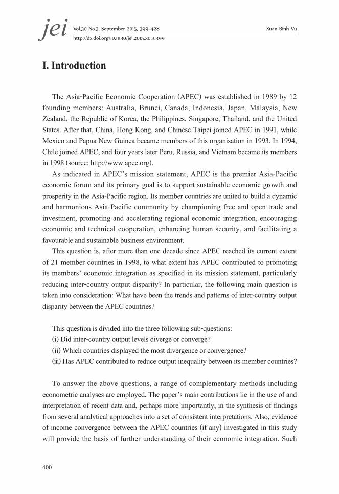
CVW was argued to diminish the degree to which smaller countries can skew the measure of inequality (Williamson 1965). And CVW varies from zero for perfect equality

to P pi

pi

− for perfect inequality where country i has all the GDP.

Theil coefficient [T]

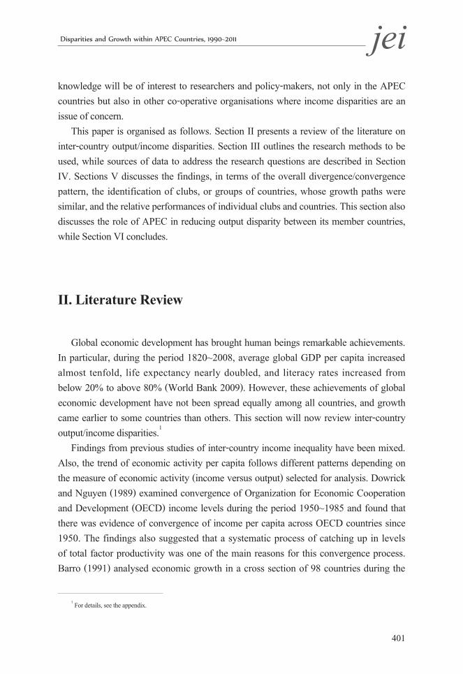
Another measure of inequality is calculated by the following equation (Theil 1967):

log ii

i i

xT xq

=

∑

(2)

where xi is the GDP share of country i and qi is the population share of country i. It is called Theil coefficient, T.

T varies from zero (for equal per capita GDP) to log (P/pi) (for a case where country i receives all the income; where P is the total population of countries; and pi is the population of country i).

Gini coefficient [G]

According to Kakwani (1980) and Shankar & Shah (2003), the weighted Gini index is computed by the following equation,

2

12

n ni j

W i ji i

p pG y y

Py

= −

∑∑

(3)

where y is the mean of per capita GDP of countries; P is the total population of countries; n is the number of countries; pi and pj are the population of countries i and j, respectively.

GW varies from zero for perfect equality to 1 i

j

pp

− for perfect inequality.

Secondly, as discussed in Section II, most of studies on inter-country income disparity applied the traditional measures of income disparity, Gini coefficient, and convergence of income growth, δ- and β-convergence tests. These traditional convergence tests assume that all countries follow the same growth path. A much more recent method of calculation is the Phillips-Sul test (2007, 2009), which is based on a time series



406

regression and includes a one-sided t -test of the null hypothesis of convergence against the alternatives of no convergence and partial convergence among sub-groups. This method is selected because of following reasons: (i) no specific assumptions regarding the stationarity of the variable of interest and/or the existence of common factors are needed although this convergence test could be interpreted as an asymptotic cointegration test without suffering from the small sample problems of unit root and cointegration testing; (ii) this method is based on a quite general form of a nonlinear time varying factor model. It takes into account that countries experience transitional dynamics, while it abstains from the hypothesis of homogeneous technological progress, an assumption extensively employed in the majority of growth studies (Apergis, Panopoulou, and Tsoumas 2010).

Let yit be the panel data of output per capita of country i at period t (i=1,…N and t=1,…T). Based on the methods of Phillips and Sul (2009), log (yit) is formulated as follows:

( )log y b tit it µ= (4)

where the idiosyncratic component, bit, measures the distance between log(yit) and the common component, μt.

Let ( )

( )log

1 1log1 =1

yit

yit

bithit N NN N biti i

= =− −∑ ∑

=

where hit measures the loading coefficient bit relative to the panel (group) average and the transition path for per capita output of country i relative to the group average. When the ultimate growth convergence within the group occurs, hit →1 for all i as t →∞, the mean square transition differential

( )21 11

NH N ht iti−= −∑

=

provides a quadratic distance measure for the panel from the common limit. Since t→∞, Ht converges to zero if all countries in the panel converge, but remains positive if those countries do not. If the panel does not converge, the countries in the panel diverge or may form convergence sub-panels (clubs).

Following Phillips and Sul (2009), the null hypothesis of growth convergence is


407

framed within a semi-parametric model that allows for heterogeneity of transition behaviour over time and across countries as specified below:

( )i itb bit i L t t

σ ξα= + (5)

where itξ is i.i.d (0, 1) across i, σ i are idiosyncratic scale parameters, and L(t) is a slowly varying function (for example, L(t) →∞) for which L(t) →∞ as t →∞, and α indicates the speed of convergence.

To test for the null hypothesis of growth convergence (bi=b and α ≥0) against the alternative hypothesis of growth divergence (bi=b for all i with α < 0) or club convergence (bi ≠b for some i with α ≥0 or α < 0), Phillips and Sul (2009) suggested the following ‘log (t)’ regression model:

1log 2 log(log( )) log( )H

t a t utHtγ− = + +utfort = T0 ,…,T (6)

In Equation (6), the initial observation in the regression is T0 = [rT] for some r>0, so that the first r% of the data is discarded.2

Under the null hypothesis of growth convergence, the point estimate of the parameter γ converges in probability to 2α which is a scaled value of the speed of convergence parameter. The corresponding t-statistic is constructed by using HAC standard errors. Under the null hypothesis, this t-statistic diverges to positive infinity when α > 0 and converges weakly to a standard normal distribution when α = 0. In contrast, under the alternative hypothesis of growth divergence or club divergence, the t-statistic diverges to negative infinity.

Thirdly, the model developed by Phillips and Sul (2007, 2009), as outlined previously, is used to identify convergence clubs among the countries. The steps suggested by Phillips and Sul for analysing the clustering patterns are as follows:

Step 1 cross-section ordering: order the countries according to the final-year GDP per capita.

Step 2 a core primary group of k*countries: Select the first k highest countries in the

2 Phillips and Sul (2007) suggested choosing the r value in the interval [0.2, 0.3].



408

panel to form the subgroup Gk for some 2 ≤k < N, run the log (t) regression and obtain the convergence test statistic tk = t (Gk). Choose the core group size k* with k* = argmaxk{tk} subject to min {tk} > -1.65.

If the convergence test fails for k = 2, the country with highest output per capita in Gk will be dropped and form new subgroups G2j = {2,….j} for 3 ≤ j ≤ N. Step 2 can be repeated with test statistics tj= t (G2j).

Step 3 sieve the data for new club members: add one country each time to the core primary group with k* members and run the log (t) test again. Include the new country in the convergence club if the associated t-statistic is greater than the chosen critical value (-1.65).

Step 4 recursion and stopping rules: form a second group from countries that the sieve condition fails in Step 3. Run the log (t)-test to see if t

γ∧ > -1.65 in this group. If this

group satisfies the convergence test, a second group is formed. Otherwise, repeat steps 1-3 to see if this second group can itself be subdivided into convergence clusters. If there is no k in Step 2 for which tk>-1.65, conclude that the remaining countries have divergent behaviour.

Fourthly, in recognition of the fact that the Phillips-Sul method does not allow for structural breaks, the log of the ratio of output per capita in each country to the output per capita in a reference economy (for instance, the USA) is analysed. This takes into account the breaks proposed by Nguyen, Smith, and Meyer-Boehm (2006).

The standard Chow test (1960) is used to test for possible structural breaks of the logarithm difference between output per capita in each country and the output per capita in a reference economy. The equation used to test for a break year is as follows:

dit= log(yit) – log(y*

t) = a + b*t + εt (7)

where yit is GDP per capita of country i; time t during the period 1990~2011; and yt

* is GDP per capita of the reference economy.

On the basis of the Chow test results, the analysis of relative income growth paths is formulated as:

*log * *itit i i i i

t

yd a DA b TRNDy

= = +

(8)

where ai is a constant intercept term; DAi is a dummy variable for the i th sub-period; bi


409

is the slope for the i th sub-period expressed by the time trend (TRNDi).

IV. Data sources

The data used in this paper including real GDP at chained PPPs (in million 2005 US dollars) and population (in million) for the 20 APEC countries are collected from the Penn World Table Version 8.0. Papua New Guinea is excluded because its relevant data is not available.

V. Findings

A. Overall divergence

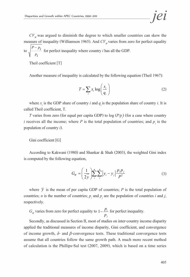
To have an overview of trends of GDP per capita of the APEC countries, we plot their logarithm of GDP per capita during the period 1990~2011 as it can be observed from Figure 1. Applying the log t convergence test developed by Phillips and Sul (2007, 2009) to data for output per capita of the APEC countries over the entire study period 1990~2011, we found that the null hypothesis of overall convergence is rejected ( γ̂ = -0.48 and γ̂t = -14.32). The finding suggests that inter-country output per capita between the APEC countries tended to diverge during the study period.

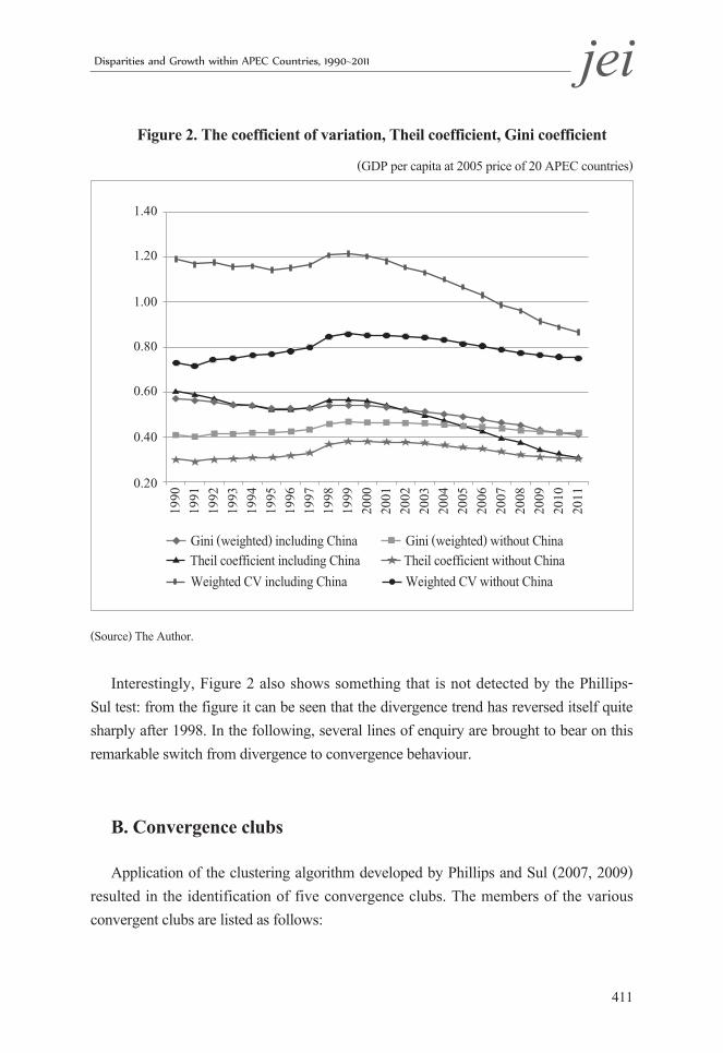
The results of conventional methods of σ-convergence (weighted CV) analysis, Theil coefficient, and Gini coefficient indicate that, if China is excluded due to its dominant population, all measures of dispersion displayed a rising trend during the sub-period 1990~1998 in spite of a downward trend after that as it can be seen from Figure 2.



410

Figure 1. Logarithm of GDP per capita in APEC countries(1990~2011)

6.8

7.3

7.8

8.3

8.8

9.3

9.8

10.3

10.8

11.3

1990

1991

1992

1993

1994

1995

1996

1997

1998

1999

2000

2001

2002

2003

2004

2005

2006

2007

2008

2009

2010

2011

AustraliaBruneiCanadaChileChina

Hong KongIndonesiaJapanKoreaMexico

MalaysiaNew ZealandPeruPhilippinesRussia

SingaporeThailandTaiwanUnited StatesVietnam

(Source) The Author.


411

Figure 2. The coefficient of variation, Theil coefficient, Gini coefficient

(GDP per capita at 2005 price of 20 APEC countries)

0.20

0.40

0.60

0.80

1.00

1.20

1.40

1990

1991

1992

1993

1994

1995

1996

1997

1998

1999

2000

2001

2002

2003

2004

2005

2006

2007

2008

2009

2010

2011

Gini (weighted) including China Gini (weighted) without ChinaTheil coefficient including China Theil coefficient without China

Weighted CV without ChinaWeighted CV including China


Interestingly, Figure 2 also shows something that is not detected by the Phillips-Sul test: from the figure it can be seen that the divergence trend has reversed itself quite sharply after 1998. In the following, several lines of enquiry are brought to bear on this remarkable switch from divergence to convergence behaviour.

B. Convergence clubs

Application of the clustering algorithm developed by Phillips and Sul (2007, 2009) resulted in the identification of five convergence clubs. The members of the various convergent clubs are listed as follows:



412

Club 1: Australia, Brunei, Chinese Taipei, Russia, South Korea, Singapore, and the United States

Club 2: Canada, China, Hong Kong, and JapanClub 3: Chile and New ZealandClub 4: Mexico, Malaysia, Peru, and ThailandClub 5: Indonesia, the Philippines, and Vietnam

To check the robustness of the overall divergence of output per capita of the APEC countries, we apply the log t convergence test (Phillips and Sul 2009) to data for the average levels of output per capita for five clubs (club 1, club 2, club 3, club 4, and club 5) during the period 1990~2011. The results show that the null hypothesis of overall convergence is rejected ( γ̂ = -0.75 and γ̂t =-31.94).

As indicated previously, Club 1 is composed of seven countries. These countries recorded relatively high levels of output per capita in 2011 and relatively high (and similar) growth rates. It could be argued that, from the viewpoint of economic performance, the four countries of club 2 (Canada, China, Hong Kong, and Japan) and the two members of club 3 (Chile and New Zealand) should be included, thus forming an augmented Club 1. In 2011, all of these countries recorded output per capita levels which were comparable to those of Club 1 members. This argument is supported by the results of employing the log t convergence test (Phillips and Sul 2009) to data for the average levels of output per capita for the augmented club 1 during the period 1990~2011, outlined in Table 1.


413

Table 1. Phillips-Sul Tests of Overall and Club Convergence(1990~2011)

Members Log-t coefficient t-statistic

APEC countries* All 20 countries -0.475 -14.316

Augmented Club 1(combined by Club 1 to 3)

Australia, Brunei, Korea, Russia, Singapore, Chinese Taipei, USA, Canada, China, Hong Kong, Japan, Chile, and New Zealand

0.043 0.624

Club 4 Mexico, Malaysia, Peru, and Thailand 0.429 4.670

Club 5 Indonesia, the Philippines, and Vietnam 2.868 9.334

(Notes) (i) The Phillips-Sul log-t test is applied to sets of data for GDP per capita. A set of economies is considered a convergent set (or club ) if the log-t coefficient is positive, or if log-t coefficient is negative but its t-statistic is > -1.65.

(ii) Asterisk (*) indicates divergent economy.

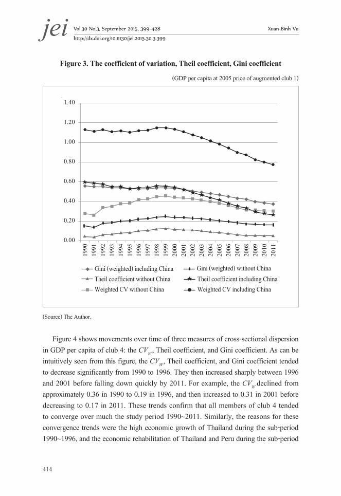
Concerning countries within augmented club 1, the coefficient of variation (CVW), Theil coefficient, and Gini coefficient as indicated in Figure 3 show that all countries of this club tended to diverge during the period 1990~1998. In contrast, they had a propensity towards convergence from 1999 to 2011. For example, the CVW (without China) increased from 0.28 in 1990 to 0.45 in 1998. It then decreased quite sharply to 0.30 in 2011. These tendencies indicate that all countries of augmented club 1 converged over much of the period 1990~2011. One of the reasons leading to the switch from divergence to convergence in 1999 was high economic growth of poorer countries including China and Russia, while the economic growth of Brunei slowed down. For example, the average economic growth rate of China was approximately 9.7% over the period 1999~2013, and the average economic growth rate of Russia was about 7.0% during the period 1999~2008.3

3 Source: http://data.worldbank.org/indicator/NY.GDP.MKTP.KD.ZG



414


(GDP per capita at 2005 price of augmented club 1)

0.00

0.20

0.40

0.60

0.80

1.00

1.20

1.40

1990

1991

1992

1993

1994

1995

1996

1997

1998

1999

2000

2001

2002

2003

2004

2005

2006

2007

2008

2009

2010

2011

Gini (weighted) including China Gini (weighted) without ChinaTheil coefficient without China Theil coefficient including ChinaWeighted CV without China Weighted CV including China


Figure 4 shows movements over time of three measures of cross-sectional dispersion in GDP per capita of club 4: the CVW , Theil coefficient, and Gini coefficient. As can be intuitively seen from this figure, the CVW , Theil coefficient, and Gini coefficient tended to decrease significantly from 1990 to 1996. They then increased sharply between 1996 and 2001 before falling down quickly by 2011. For example, the CVW declined from approximately 0.36 in 1990 to 0.19 in 1996, and then increased to 0.31 in 2001 before decreasing to 0.17 in 2011. These trends confirm that all members of club 4 tended to converge over much the study period 1990~2011. Similarly, the reasons for these convergence trends were the high economic growth of Thailand during the sub-period 1990~1996, and the economic rehabilitation of Thailand and Peru during the sub-period


415

2002~2011. For example, the average economic growth rate of Thailand was nearly 8.6% during the sub-period 1990~1996, and the economic growth rate of Peru was roughly 6.2% during the period 2002~2011.4


(GDP per capita at 2005 price of club 4)

0.00

0.05

0.10

0.15

0.20

0.25

0.30

0.35

0.40

1990

1992

1994

1996

1998

2000

2002

2004

2006

2008

2010

1991

1992

1995

1997

1999

2001

2003

2005

2007

2009

2011

Gini (weighted) Weighted CV Theil coefficient


On the graph of figure 5, the CVW , Theil coefficient, and Gini coefficient of club 5 countries fluctuated from 1990 to 1996. They then tended to decrease rapidly until 2007 before increasing slightly between 2008 and 2011. For example, the CVW fluctuated at approximately 0.28 between 1990 and 1996. It then declined to 0.06 in 2007 before increasing to roughly 0.08 by 2011. The results confirm that all countries of club 5 tended to converge over much of the study period. The high economic growth of Vietnam during the period 1990~2011 and the financial crisis of Indonesia and the Philippines during the sub-period 1997~1998 were the main reasons for the trend of all inequality




416

measures of club 5. For instance, the average economic growth rate of Vietnam was approximately 7% during the period 1990~2011; whereas in 1998 the economic growth rates of Indonesia and the Philippines were -13% and -0.6%, respectively.5


(GDP per capita at 2005 price of club 5)


0.00

0.05

0.10

0.15

0.20

0.25

0.30

0.35

1990

1992

1994

1996

1998

2000

2002

2004

2006

2008

2010

1991

1993

1995

1997

1999

2001

2003

2005

2007

2009

2011


As discussed earlier, within each club, output per capita levels tended to converge, in that they passed the log t test (as applied to the club’s members only). However, the average levels of output per capita for the various clubs tended to diverge from each other. Indeed, the results of employing the log t convergence test, developed by Phillips and Sul (2007, 2009), to data for the average levels of output per capita for the three clubs during the period 1990~2011, show that the null hypothesis of overall convergence is rejected ( γ̂ = -0.97 and γ̂t =-46.59). Similarly, the CVW, Theil coefficient, and Gini coefficient of club averages tended to decrease from 1990 to 1997. They then



417

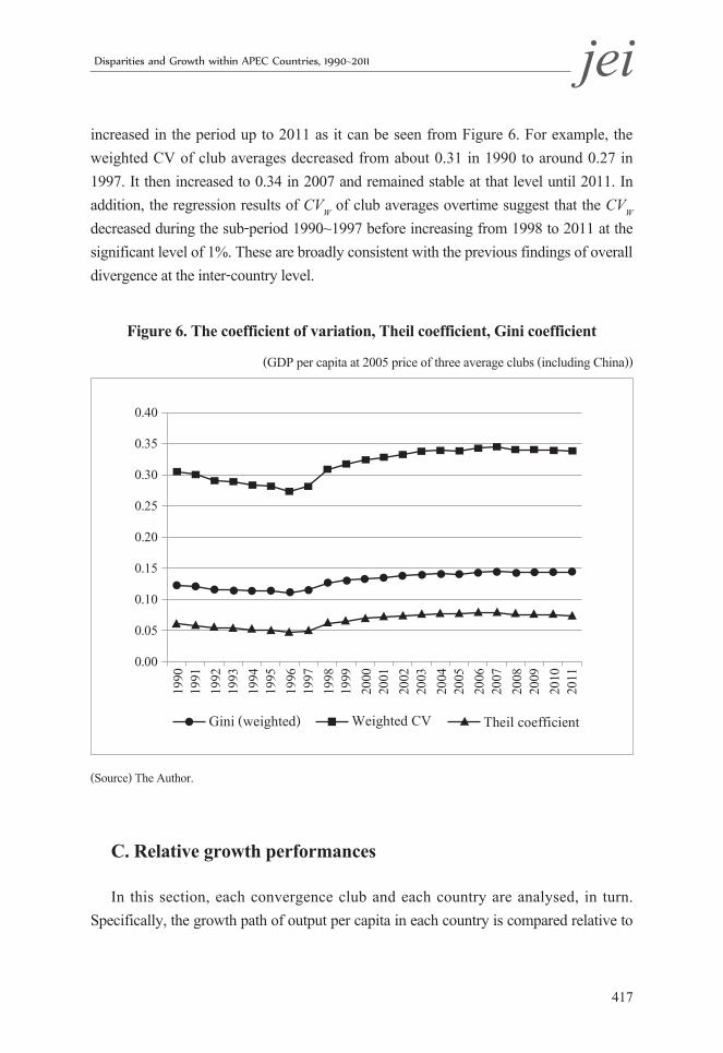
increased in the period up to 2011 as it can be seen from Figure 6. For example, the weighted CV of club averages decreased from about 0.31 in 1990 to around 0.27 in 1997. It then increased to 0.34 in 2007 and remained stable at that level until 2011. In addition, the regression results of CVW of club averages overtime suggest that the CVW

decreased during the sub-period 1990~1997 before increasing from 1998 to 2011 at the significant level of 1%. These are broadly consistent with the previous findings of overall divergence at the inter-country level.


(GDP per capita at 2005 price of three average clubs (including China))


0.00

0.05

0.10

0.15

0.20

0.25

0.30

0.35

0.40

1990

1992

1994

1996

1998

2000

2002

2004

2006

2008

2010

1991

1993

1995

1997

1999

2001

2003

2005

2007

2009

2011


C. Relative growth performances

In this section, each convergence club and each country are analysed, in turn. Specifically, the growth path of output per capita in each country is compared relative to



418

that of the USA. Ordinary Least Squares (OLS) is used to estimate the intercept, i.e., was the economy above or below the reference economy initially? and the slope, i.e., did the economy become richer or poorer relative to reference economy? In particular, the time series is calculated as follows:

( ) ( )**log log logit

it it tt

yd y yy

= = −

where yit is GDP per capita of country i, time t during the period 1990~2011; and yt* is

GDP per capita of the reference economy. The series dit are then tested for stationarity.The results of using the USA as a reference economy and KPSS tests (Kwiatowski

et al. 1992) indicate that the null hypotheses of stationarity of five countries (including Australia, China, Mexico, Russia, and Singapore) were rejected at 5% level of significance.

Although the KPSS test is used to check whether the data series are stationary, the short time period involved and the presence of structural breaks tend to limit its usefulness in this particular instance. Therefore, Equation (8), as presented in Section III, is applied for this study, and is reproduced below for convenience.

*log * *itit j j j j

t

yd a DA b TRNDy

= = +

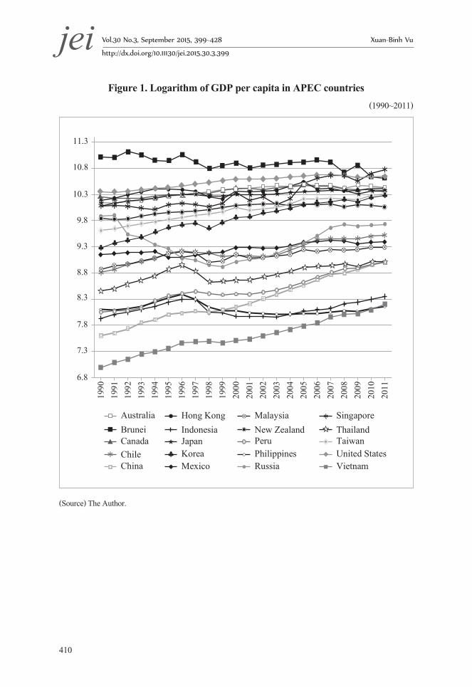
Summing up the Chow test results as shown in Table 2, this study found one structural break for nine countries (China, Chinese Taipei, Russia, South Korea, Mexico, Malaysia, Singapore, Thailand, and Vietnam); two structural breaks for seven countries (Chile, Hong Kong, Indonesia, Japan, New Zealand, Peru, and the Philippines); and three structural breaks for Australia. For Brunei and Canada, there were no structural breaks. Also, Table 2 indicates several results of time-series tests comparing the logarithm of GDP per capita of each country and that of the USA. In particular, China, the Republic of Korea, Malaysia, Thailand, and Vietnam tended to converge upward to the USA over the period 1990~2011, although there was a break in 1998. In contrast, Brunei converged downward towards the USA, while Canada diverged downward from the USA during the study period. Australia and New Zealand tended to converge towards USA during the sub-period 1990~2003, while they diverged from USA from 2004 to 2011. Of particular interest is that after 1998, China and Russia tended to catch up most quickly


419

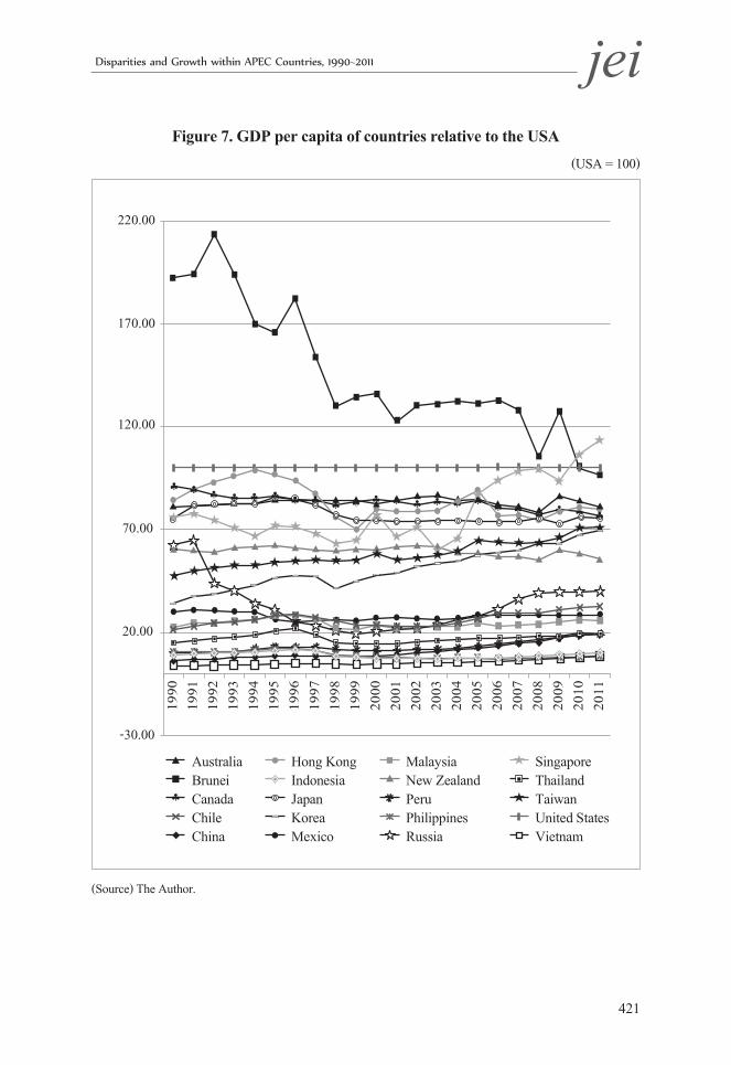
with the USA (slope 2 = 0.07) compared with other countries. If USA is presented by a horizontal line at 100%, China is shown as most clearly catching up with USA, from approximately 6.4% of the USA in 1990 to 19.4% in 2011 as it can be seen from figure 7. This was because China achieved high economic growth with huge investment over the years. For example, China’s gross capital formation accounted for 49% of GDP in 2013.6 Only Brunei started out with a higher GDP per capita than that of the USA. This was mainly because of Brunei’s oil resources.

6 Source: http://data.worldbank.org/indicator/NE.GDI.TOTL.ZS#



420

Tabl

e 2.

APE

C c

ount

ries

synt

hesis

rel

ativ

e to

the

USA

(1

990~

2011

)

Prov

ince

sSt

ruct

ural

bre

aks

Inte

rcep

tD

A2

DA

3D

A4

Slop

e1Sl

ope2

Slop

e3Sl

ope4

Aus

tralia

2000

, 200

4, 2

009

Belo

w**

*N

egat

ive*

**N

egat

ive

Posit

ive*

**0.

0042

***

0.01

69**

*-0

.018

7***

-0.0

133*

**

Brun

ein.

aA

bove

***

n.a

n.a

n.a

-0.0

313*

**n.

an.

an.

a

Cana

dan.

aBe

low

***

n.a

n.a

n.a

-0.0

061*

**n.

an.

an.

a

Chile

1997

, 200

3Be

low

***

Neg

ativ

e**

Posit

ive

n.a

0.04

94**

*-0

.035

6***

0.04

21**

*n.

a

Chin

a19

98Be

low

***

Neg

ativ

e***

n.a

n.a

0.04

94**

*0.

07**

*n.

an.

a

Hon

g K

ong

1996

, 200

0Be

low

***

Posit

ive*

*Po

sitiv

e***

n.a

0.02

92**

*-0

.100

3***

-0.0

016

n.a

Indo

nesia

1998

, 200

4Be

low

***

Neg

ativ

e***

Neg

ativ

en.

a-0

.033

4***

-0.0

328*

**0.

0491

***

n.a

Japa

n19

96, 2

000

Belo

w**

*Po

sitiv

e***

Neg

ativ

en.

a0.

0191

***

-0.0

453*

**0.

0012

n.a

Kor

ea19

98Be

low

***

Neg

ativ

e***

n.a

n.a

0.04

84**

*0.

0362

***

n.a

n.a

Mex

ico

1995

Belo

w**

*N

egat

ive*

**n.

an.

a-0

.002

00.

0077

***

n.

a

Mal

aysia

1998

Belo

w**

*N

egat

ive*

**n.

an.

a0.

0274

***

0.01

32**

*n.

an.

a

New

Zea

land

2003

, 200

9Be

low

***

Posit

ive

Posit

ive*

**n.

a0.

0017

-0.0

191*

**-0

.037

1***

n.a

Peru

1998

, 200

2Be

low

***

Neg

ativ

e***

Neg

ativ

e**

n.a

0.04

18**

*-0

.023

6***

0.06

34**

*n.

a

Phili

ppin

es19

98, 2

007

Belo

w**

*N

egat

ive*

**Po

sitiv

en.

a0.

0209

***

-0.0

283*

**0.

0356

***

n.a

Russ

ia20

00Be

low

***

Posit

ive

n.a

n.a

-0.1

405*

**0.

0717

***

n.a

n.a

Sing

apor

e20

05Be

low

***

Posit

ive*

**n.

an.

a-0

.010

4***

0.03

54**

*

n.a

Thai

land

1998

Belo

w**

*N

egat

ive*

**n.

an.

a0.

0474

***

0.02

49**

*n.

an.

a

Taip

ei20

01Be

low

***

Neg

ativ

e***

n.a

n.a

0.01

59**

*0.

0248

***

n.a

n.a

Vie

tnam

1998

Belo

w**

*N

egat

ive*

**n.

an.

a0.

0421

***

0.05

54**

*n.

an.

a

(Not

es) (

i) y

i is G

DP

per c

ap a

t 200

5 pr

ice

of c

ount

ry i,

y*

is G

DP

per c

ap a

t 200

5 pr

ice

of U

SA.

(ii)

** in

dica

tes s

igni

fican

t at 5

%, *

** in

dica

tes s

igni

fican

t at 1

%.

(iii)

n.a

= n

ot a

pplic

able

.


421

Figure 7. GDP per capita of countries relative to the USA (USA = 100)

-30.00

20.00

70.00

120.00

170.00

220.00

1990

1991

1992

1993

1994

1995

1996

1997

1998

1999

2000

2001

2002

2003

2004

2005

2006

2007

2008

2009

2010

2011

AustraliaBruneiCanadaChileChina

Hong KongIndonesiaJapanKoreaMexico

MalaysiaNew ZealandPeruPhilippinesRussia

SingaporeThailandTaiwanUnited StatesVietnam




422

D. The role of APEC in promoting its members’ economic integration

Our analytical results indicate that output inequality between the APEC countries (excluding Russia, China, and Papua New Guinea)7 tended to decrease during the 1970 to 1982 period that coincided with the world oil crisis. It then increased slightly until 1987 before declining again until 1996 with the onset of the Asian crisis. However, this output disparity decreased quite dramatically during the sub-period 1999~2011. For example, the CVW declined from approximately 0.87 in 1970 to 0.79 in 1982. After that it increased to roughly 0.83 in 1987 before declining to 0.77 in 1996. During the sub-period 1999~2011, output inequality between the APEC countries decreased again from 0.83 in 1999 to 0.78 in 2011 as it can be seen from Figure 8. We understand that there may be additional reasons resulting in a downward tendency of output inequality between the APEC countries (CVW) after 1998, when APEC was fully formed. However, it could be concluded that APEC has played some role in diminishing output inequality between the APEC economies. Indeed, APEC has brought its economies closer together and boosted trade by reducing trade barriers and smoothing out differences in regulations. For example, average tariffs fell from 17% in 1989 to 5.2% in 2012.8 As a result, total trade between the APEC countries increased seven times from 1989 to 2013, and two-thirds of their total trade occurred between the APEC economies. Also, the APEC’s Ease of Doing Business Action Plan has promoted cheaper, easier, and faster business activities between its member economies. For instance, during the period 2009~2013, the APEC countries improved the ease of doing business by 11.3%, including starting a business, getting credit, or applying for permits.

7 China is excluded due to its dominant population, while Russia and Papua New Guinea are eliminated because their data is not available for the entire period of 1970~2011. .

8 Source: http://www.apec.org/About-Us/About-APEC/Achievements-and-Benefits.aspx


423


(GDP per capita at 2005 price of 18 APEC countries9)

Weighted CV Theil coefficient Weighted Gini

0.30

0.40

0.50

0.60

0.70

0.80

0.90

1970

1972

1974

1976

1978

1980

1982

1984

1986

1988

1990

1992

1994

1996

1998

2000

2002

2004

2006

2008

2010

As discussed previously, although more countries converged towards the USA after APEC reached its current membership of 21 countries in 1998, there are still huge gap in economic development between the APEC countries. In particular, in 2011 the GDPs per capita of the Philippines, Vietnam, Indonesia, or even China accounted for only 8.3%, 8.7%, 10.1%, and 19.4% of that of the USA, respectively as it can be seen from Figure 7. The large income gap could be a block to their economic integration and may generate political tensions resulting in the separation of the economically depressed countries. Therefore, for the APEC countries to become more integrated, the wide income gap should be further addressed.

9 China is excluded due to its dominant population, while Russia and Papua New Guinea are eliminated because of their unavailable data for the whole period 1970~2011.



424

VI. Conclusion

This study analysed inter-country output disparities between the APEC countries during the period 1990~2011. The results of applying Phillips and Sul’s method (2007, 2009) indicate that GDP per capita between countries tended to diverge over the study period. Nevertheless, the results of conventional analyses based on coefficient of variation (CVW ), Gini coefficient, and Theil coefficient show that since 1999, this divergence trend has turned into a convergence tendency.

In an effort to gain further insight into these dynamics, three convergence clubs are identified using Phillips-Sul’s algorithm. Also, the growth path of each individual country is analysed in comparison with that of the United States. The results indicate that China, Russia, and Vietnam tended to catch up more quickly with USA after 1998, while Australia, Canada, and New Zealand tended to diverge from the USA. Of particular notice is that more APEC countries converged towards the USA during the sub-period 1999~2011.

The turn-around which occurred after APEC reached its current membership of 21 countries in 1998, from a divergence trend to a convergence trend, may suggest that APEC has played some role in reducing output disparity between its member countries, and more broadly promoting its members’ economic integration. However, to promote economic integration between the APEC countries, there is a need to reduce further their wide income gap.

Received 27 February 2015, Revised 8 April 2015, Accepted 22 July 2015


425

App

endi

x

App

endi

x: P

revi

ous s

tudi

es o

n in

ter-

coun

try

inco

me

disp

ariti

es

Aut

hors

Yea

rC

ount

ryD

ata

sam

ple

Tech

niqu

esFi

ndin

gs

Dow

rick

and

Ngu

yen

1989

OEC

D

coun

tries

Inco

me

per c

apita

1950

~198

5A

mod

el o

f gro

wth

pr

oces

s Ev

iden

ce o

f con

verg

ence

of i

ncom

e pe

r cap

ita a

cros

s th

e co

untri

es

since

195

0

Barro

1991

98 c

ount

ries

GD

P pe

r cap

ita19

60~1

985

Beta

-con

verg

ence

Coun

tries

hav

ing

low

er G

DP

per c

apita

in 1

960

tend

ed to

hav

e hi

gher

gr

owth

rate

of G

DP

per c

apita

(196

0~19

85)

Levy

and

Ch

owdh

ury

1994

115

coun

tries

Inco

me

per c

apita

1960

~198

5Th

eil i

ndex

The

inco

me

ineq

ualit

y de

clin

ed s

tead

ily b

y 0.

58 p

er y

ear,

show

ing

a su

bsta

ntia

l con

verg

ence

tren

d

Bern

ard

and

Dur

lauf

1995

15 O

ECD

co

untri

esG

DP

per c

apita

1900

~198

7St

ocha

stic

conv

erge

nce

A li

ttle

evid

ence

of

conv

erge

nce

but a

con

side

rabl

e co

-inte

grat

ion

betw

een

thes

e co

untri

es w

as fo

und

Levy

and

Ch

owdh

ury

1995

154

coun

tries

Inco

me

per c

apita

1960

~199

0In

com

e-w

eigh

ted

entro

py m

easu

re

Evid

ence

of s

trong

div

erge

nce

durin

g th

e su

b-pe

riod

1960

-192

8, b

ut

slow

con

verg

ence

dur

ing

the

sub-

perio

d 19

69-1

983.

For

the

perio

d 19

84-1

990,

nei

ther

con

verg

ence

nor

div

erge

nce

was

foun

d

Park

2000

Sout

heas

t A

sian

coun

tries

Inco

me

per c

apita

1967

~199

7Th

eil i

ndex

Inco

me

ineq

ualit

y am

ong

the

10 A

SEA

N e

cono

mie

s in

crea

sed

from

0.

06 in

196

0 to

0.1

8 in

199

7.

Sim

ilarly

, the

re w

as a

div

erge

nce

trend

in in

com

e pe

r cap

ita a

cros

s th

e fiv

e co

re A

SEA

N c

ount

ries.

Mad

diso

n20

01A

ll co

untri

esIn

com

e pe

r cap

ita10

00~1

998

Des

crip

tive

met

hod

A w

ide

ineq

ualit

y in

the

perfo

rman

ce o

f diff

eren

t cou

ntrie

s

Sala

-i-M

artin

2002

All

coun

tries

Inco

me

per c

apita

1978

~199

8G

ini I

ndex

and

Th

eil I

ndex

Inte

r-cou

ntry

inco

me

ineq

ualit

ies

tend

ed to

dec

line

durin

g th

e pe

riod

1978

~199

8



426

Aut

hors

Yea

rC

ount

ryD

ata

sam

ple

Tech

niqu

esFi

ndin

gs

Sesh

anna

and

D

ecor

nez

2003

112

coun

tries

GD

P pe

r cap

ita19

60~2

000

Gin

i ind

ex

The

ineq

ualit

y re

mai

ned

alm

ost s

tabl

e fr

om 1

960

to 1

982

befo

re

incr

easin

g sli

ghtly

unt

il 20

00.

Dur

ing

the

perio

d 19

60~2

000,

out

put i

nequ

ality

acr

oss

27 O

ECD

co

untri

es te

nded

to d

ecre

ase,

whi

le o

utpu

t disp

arity

bet

wee

n 85

non

-O

ECD

cou

ntrie

s inc

reas

ed.

Moo

n20

0610

cou

ntrie

s in

Eas

t Asia

Inco

me

per c

apita

1960

~200

0Be

ta-c

onve

rgen

ce a

nd

sigm

a-co

nver

genc

e

No

evid

ence

of b

eta-

conv

erge

nce

of G

DP

per c

apita

bet

wee

n th

ese

coun

tries

dur

ing

the

stud

y pe

riod.

How

ever

, evi

denc

e of

sig

ma-

conv

erge

nce

sugg

este

d th

at th

e in

equa

lity

trend

was

reve

rsed

afte

r 19

88 w

hen

a m

ajor

ity o

f dev

elop

ing

East

Asia

n co

untri

es te

nded

to

catc

h up

with

Japa

n.

Phill

ips

and

Sul

2009

18 W

este

rn

OEC

D co

untri

es

152

PWT

coun

tries

GD

P pe

r cap

ita18

70~2

011

1970

~200

3

A ti

me

serie

s

A ti

me

serie

s

Inco

me

conv

erge

nce

did

not

exis

t fo

r th

e w

hole

stu

dy p

erio

d;

how

ever

, the

re w

as e

vide

nce

of d

iver

genc

e du

ring

the

per

iod

1870

~192

9, a

nd e

vide

nce

of c

onve

rgen

ce d

urin

g th

e pe

riod

19

40~2

001.

No

evid

ence

of c

onve

rgen

ce w

as fo

und

but f

our c

onve

rgen

t clu

bs a

nd

one

dive

rgen

t gro

up w

ere

form

ed b

y th

ese

152

coun

tries

.

Ape

rgis,

Pa

nopo

ulou

an

d Ts

aum

as20

1014

Eur

opea

n co

untri

esG

DP

per c

apita

1980

~200

4Ph

ilips

-Sul

’s

tech

niqu

e

No

evid

ence

of

conv

erge

nce

of G

DP

per

capi

ta b

etw

een

thes

e co

untri

es; h

owev

er, t

hey

wer

e gr

oupe

d in

to tw

o di

stinc

t con

verg

ent

club

s.

Jaya

ntha

kum

aran

and

Le

e20

13

5 So

uth

East

Asia

n co

untri

es

5 So

uth

Asia

n co

untri

es

Inco

me

per c

apita

1967

~200

5

1973

~200

5

Stoc

hasti

c co

nver

genc

e an

d be

ta-c

onve

rgen

ce

Stoc

hasti

c co

nver

genc

e an

d be

ta-c

onve

rgen

ce

The

rela

tive

per

capi

ta in

com

e se

ries

of A

SEA

N-5

cou

ntrie

s w

ere

cons

isten

t with

stoc

hasti

c co

nver

genc

e an

d be

ta-c

onve

rgen

ce.

The

simila

r res

ults

wer

e no

t fou

nd.

(Sou

rce)

the

Aut

hor.


427

References

Apergis, Nicholas, Ekaterini Panopoulou, and Chris Tsoumas. “Old Wine in a New Bottle: Growth Convergence Dynamics in the EU.” Atlantic Economic Journal 38, no. 2 (2010): 169-181.

Barro, Robert J. “Economic Growth in a Cross Section of Countries.” The Quarterly Journal of Economics 106, no. 2 (1991): 407-443.

Bernard, Andrew B., and Steven N. Durlauf. “Convergence in International Output.” Journal of Applied Econometrics 10, no. 2 (1995): 97-108.

Chow, Gregory C. “Tests of Equality between Sets of Coefficients in Two Linear Regressions.” Econometrica 28, no. 3 (1960): 591-565.

Dowrick, Steve, and Duc-Tho Nguyen. “OECD Comparative Economic Growth 1950-85: Catch-up and Convergence.” The American Economic Review 79, no. 5 (1989): 1010-1030.

Jayanthakumaran, Kankesu, and Shao-Wei Lee. “Evidence on the Convergence of Per Capita Income: A Comparison of Founder Members of the Association of South East Asian Nations and the South Asian Association of Regional Cooperation.” Pacific Economic Review 18, no. 1 (2013): 108-121.

Kakwani, Nanak C. Inequality and Poverty - Methods of Estimation and Policy Applications. The World Bank, Oxford University Press, 1980.

Kwiatkowski, Denis, Peter C.B. Phillips, Peter Schmidt, and Yongcheol Shin. “Testing the Null Hypothesis of Stationarity against the Alternative of a Unit Root. How Sure Are We That Economic Time Series Have a Unit Root?”. Journal of Econometrics 54 (1992): 159-178.

Levy, Amnon, and Khorshed Chowdhury. “Inter-Country Income Inequality: World Levels and Decomposition between and within Developmental Clusters and Regions.” Comparative Economic Studies 36, no. 3 (1994): 33-50.

Levy, Amnon, and Khorshed Chowdhury. “A Geographical Decomposition of Inter-Country Income Inequality.” Comparative Economic Studies 37, no. 4 (1995): 1-17.

Maddison, Angus. “The World Economy: A Millennial Perspective.” 1-383: OECD, 2001.



428

Moon, Woosik. “Income Convergence across Nations and Regions in East Asia.” Journal of International and Area Studies 13, no. 2 (2006): 1-16.

Nguyen, Duc Tho, Christine Smith, and G. Meyer-Boehm. “Growth and Divergence in Output Per Capita and Labour Productivity among the States of Australia, 1984-85 to 2004-05.” 1-36: Department of Accounting, Finance, and Economics, Griffith University, 2006.

Park, Donghuyn. “Intra-Southeast Asian Income Convergence.” ASEAN Economic Bulletin 17, no. 3 (2000): 285-292.

Phillips, Peter C. B., and Donggyu Sul. “Transition Modelling and Econometric Convergence Tests.” Econometrica 75, no. 6 (2007): 1771-1855.

Phillips, Peter C. B., and Donggyu Sul. “Economic Transition and Growth.” Journal of Applied Econometrics 24, no. 7 (2009): 1153-1185.

Sala-i-Martin, Xavier X. “Regional Cohesion: Evidence and Theories of Regional Growth and Convergence.” European Economic Review 40, no. 6 (1996): 1325-1352.

Sala-i-Martin, Xavier. “The Distributing “Rise” of Global Income Inequality”. 1050 Massachusetts Avenue, Cambridge, MA 02138: National Bureau of Economic Research 2002.

Seshanna, Shubhasree, and Stéphane Decornez. “Income Polarization and Inequality across Countries: An Empirical Study.” Journal of Policy Modelling 25, no. 4 (2003): 335-358.

Shankar, Raja, and Anwar Shah. “Bridging the Economic Divide within Countries: A Scorecard on the Performance of Regional Development Policies in Reducing Regional Income Disparities.” World Development 31, no. 8 (2003): 1421-1441.

Theil, Henri. Economics and Information Theory. North-Holland Publishing Company, Amsterdam, Netherlands, 1967.

Williamson, Jeffrey G. “Regional Inequality and the Process of National Development: A Description of the Patterns.” Economic Development and Cultural Change 13, no. 4, part II (1965): 1-84.

“World Development Report 2009: Reshaping Economic Geography.” Washington, DC: The World Bank, 2009.

Disparities and Growth between the APEC Countries, 1990-2011

Documents

Transcript of Disparities and Growth between the APEC Countries, 1990-2011