1

DIRECT NUMERICAL CALCULATION OF THE KINEMATIC TORTUOSITY OF REACTIVE

MIXTURE FLOW IN THE ANODE LAYER OF SOLID OXIDE FUEL

CELLS BY THE LATTICE BOLTZMANN METHOD

Pietro Asinari (a), Michele Calì Quaglia (a), Michael R. von Spakovsky (b, *), Bhavani V. Kasula (b)

(a) Energy Engineering Department, Politecnico di Torino

Corso Duca degli Abruzzi 24, Torino, Zip Code 10129, Italy

Emails: pietro.asinari@polito.it, michele.cali@polito.it

(*) Corresponding author. Tel. (540) 231-6684, Fax. (540) 231-9100

(b) Center for Energy Systems Research, Mechanical Engineering Department

Virginia Polytechnic Institute and State University (Virginia Tech)

Blacksburg, VA 24061, U.S.A.

Emails: vonspako@vt.edu, bvkasula@vt.edu

(Revised Version 1.1)

Keywords: tortuosity; microscopic modelling; reactive flow; lattice Boltzmann method; solid oxide fuel cells

ABSTRACT

Mathematical models that predict performance can aid in the understanding and development of solid oxide fuel cells

(SOFCs). Of course, various modeling approaches exist involving different length scales. In particular, very significant

advances are now taking place using microscopic models to understand the complex composite structures of electrodes and

three-phase boundaries. Ultimately these advances should lead to predictions of cell behavior, which at present are measured

empirically and inserted into macroscopic cell models.

In order to achieve this ambitious goal, simulation tools based on these macroscopic models must be redesigned by

matching them to the complex microscopic phenomena, which take place at the pore scale level. As a matter of fact, the

macroscopic continuum approach essentially consists of applying some type of homogenization technique, which properly

averages the underlying microscopic phenomena for producing measurable quantities. Unfortunately, these quantities in the

porous electrodes of fuel cells are sometimes measurable only in principle. For this reason, this type of approach introduces

2

additional uncertainties into the macroscopic models, which can significantly affect the numerical results, particularly their

generality.

This paper is part of an ongoing effort to address the problem by following an alternative approach. The key idea is to

numerically simulate the underlying microscopic phenomena in an effort to bring the mathematical description nearer to

actual reality. In particular, some recently developed mesoscopic tools appear to be very promising since the microscopic

approach is, in this particular case, partially included in the numerical method itself. In particular, the models based on the

lattice Boltzmann method (LBM) treat the problem by reproducing the collisions among particles of the same type, among

particles belonging to different species, and finally among the species and the solid obstructions.

Recently, a model developed by the authors was proposed which, based on LBM, models the fluid flow of reactive

mixtures in randomly generated porous media by simulating the actual coupling interaction among the species. A parallel

three–dimensional numerical code was developed in order to implement this model and to simulate the actual microscopic

structures of SOFC porous electrodes.

In this paper, a thin anode (50 micron) of Ni-metal / YSZ-electrolyte cermet for a high–temperature electrolyte supported

SOFC was considered in the numerical simulations. The three–dimensional anode structure was derived by a regression

analysis based on the granulometry law applied to some microscopic pictures obtained with an electron microscope. The

numerical simulations show the spatial distribution of the mass fluxes for the reactants and the products of the

electrochemical reactions. The described technique will allow one to design new improved materials and structures in order

to statistically optimize these fluid paths.

Nomenclature

Α : geometric area

c : lattice speed

D : mutual diffusivity

e : specific internal energy

f : continuous single particle distribution function

3

F : Faraday’s constant

g : acceleration due to an external field

J : electric current density

k : kinetic forcing term

L : length

m : single particle mass

M : molecular mass

Q : collisional operator

R : universal gas constant

T : temperature

t : time

u : macroscopic velocity

v : microscopic velocity

δ : discrete step

ε : porosity

λ : relaxation frequency

ν : kinetic viscosity

ρ : density

τ : collision time

Subscripts and superscripts

A : generic species

B : generic species

e : equilibrium

m : mixture

0 : value at I/O bottom value

σ : generic species

4

INTRODUCTION

Solid oxide fuel cells (SOFCs) are receiving considerable interest since they are suited for both stationary and vehicle

applications [1,2,3]. The reduction of activation polarization, the elimination of expensive catalysts, potential integration with

cogeneration systems, and the possibility of being able to consider different composition of syngas as the fuel are interesting

technical challenges. The Department of Energy (DOE) of the United States a few years ago initiated a set of research

projects (SECA - Solid State Energy Conversion Alliance) with the purpose of increasing the power density, reducing the

manufacturing costs, and encouraging commercially cost-effective prototypes. The European Union, through the European

Hydrogen and Fuel Cell Technology Platform: Strategic Research Agenda (January 2005), has indicated that the SOFC is a

priority choice for stationary applications.

The typical solid oxide structure involves a thick electrolyte of yttria stabilized zirconia (ZrO2 + 8% Y2O3) for the

electrolyte supported (ES) cells. The function of the YSZ ceramic support is to maintain the stability of the electronically

conductive nickel-metal particles and to provide an anode thermal expansion coefficient acceptably close to those of the

electrolyte. The YSZ part of the cermet structure also partially serves as the ionic conductor. Very thin layers (50-100 µm are

typical values) are coated on both sides in order to form the cathode and the anode elements and must sustain actual operating

conditions of 900–1000 °C.

A new trend during recent years is to employ thick porous electrodes, which are made of cermet [4,5,6]. This practice

allows one to lower the operating temperature to a moderate range (700–850 °C) and consequently to reduce the material cost

and the requirements for auxiliaries. With regards to the cathode electrode, a material addressing the technical requirements

of this component is lanthanum manganite suitably doped with alkaline (calcium) and rare earth (strontium) elements in order

to improve its electronic conductivity (La0.7Sr0.3MnO3). This material allows one to reduce the cathode layer thickness to 1

mm in cathode supported (CS) cells and 0.1 mm in anode supported (AS) ones. With regards to the anode electrode, its basis

material is a skeleton of yttria stabilized zirconia (YSZ) around Ni particles. The anode layer thickness is on the order of 0.1

mm (CS) and 1.5 mm (AS).

In many international research centers, most of investigations are focused on the experimental analysis of single cells

SOFC under typical operating conditions or of small stacks fed from various fuels such as methane or hydrogen [7]. The

objective of these experiments is to understand the phenomena that are at the base of the operation and the stability of the

5

cells [8], characterizing the electrochemical behavior of a single cell’s components and identifying the optimal conditions for

its operation [9,10]. Cell or stack performance is recorded with respect to parameters such as fuel composition, the pressure

of the reactants, the operating temperature of the cell, eventual phenomena of macroscopic degradation (e.g., de-lamination or

carbon deposition [8]), cell polarization losses related to processes of microscopic degradation (e.g., evolution of the

microstructure of the anode [11,12,13,14,15], cathode [16,17], and electrolyte [18,19,20]). Sometimes these phenomena are

investigated by resorting to morphological analyses of the materials before and after the phases of operation through the use

of sophisticated techniques such as scanning electron microscopy (SEM).

Some of the microscopic phenomena investigated in the literature include those for the cathode electrode, which can be

affected by kinetic de-mixing. This effect does not seem related to the cell operating temperature but instead to the fact that

the material is affected by the electric field present. This condition of kinetic de-mixing can lead to pore formation in the

material which is primarily situated at the cathode/electrolyte interface, leading in turn to losses in electrochemical

performance. The applied current of the electric field creates an oxygen potential gradient, and it is this difference which may

be the driving force for pore formation [16]. As to the anode electrode, it can be affected by nickel agglomeration, which can

be explained as a degradation of the electrochemical three phase boundary (TPB) due to the sintering of metal particles and a

decrease in contact area at the electrolyte/anode interface as well as a decrease in the specific surface area of Ni particles

[15].

The mass transport phenomena throughout the electrode materials are key to cell performance. The thickness of the

electrodes, their porosity (in volume fraction), the pore dimensions, the tortuosity factor, and the pore connections are the

main parameters affecting the mass transport of chemical species through the electrode/electrolyte interface [21]. The mass

transport of chemical species greatly influences the concentration overpotentials on the anode and cathode sides (in

particular, the cell voltage is primarily affected by cathode layer thickness [22, 23]) and modifies the fuel reforming rate on

the anode electrode surface, causing temperature non-uniformities and mechanical failure due to thermally induced stresses

[24].

Because of the difficulties in realizing prototypes, an extensive simulation activity can be found in the open literature [25-

27]. Many models are based on the assumption that the structure of the porous medium is isotropic so that the cermet can be

described by three structural parameters (the ratio of porosity to tortuosity, the mean value and the standard deviation of the

pore radii). They are used to compute the phenomenological coefficients which are involved in the constitutive correlations

6

for the diffusion and the permeation (MTPM – mean transport pore model) [28]. In particular, the diffusion and the

permeation phenomena depend on conventional molecular effects and on kinetic effects, since some of the pore radii are

comparable to the mean free path of flowing fluids. In particular, for an anode-supported SOFC where high fuel utilization is

required, a small error in the concentration overpotential calculation, which is mainly affect by mass transport inside the

porous anode, may cause a dramatic change in its design performance [29]. Some experiments have been performed in order

to determine the structural parameters for cermet materials [30]. These experiments and additional theoretical reasons induce

one to conclude that among the structural parameters, it is the ratio of porosity to tortuosity and the mean value of pore radii

that primarily affect the reaction rate [30]. However, at the moment, the suitability of structural parameters and of the

constitutive correlations to describe macroscopic flow rates has not been completely verified for the cermet involved in

SOFCs. This is due to reasons:

• many different microscopic topologies are possible which share the same values for structural parameters such as the

macroscopic averaged properties of porosity and tortuosity;

• there are a myriad of working conditions for porous electrodes and for this reason it is very difficult to experimentally

verify the constitutive correlations which describe the diffusion and the permeation in all practical ranges.

Despite the success of macroscopic modeling in understanding the complex phenomena occurring during fuel cell

operation and in contributing to improved fuel cell designs, the actual micro structure of the porous layers that constitute a

fuel cell is usually not modeled. Its effects on cell operation and performance are taken into account by considering

homogeneous layers characterized by the macroscopic averaged parameters of porosity and tortuosity. While this eases the

modeling efforts, it carries two disadvantages. Firstly, if an in–situ measurement of such macroscopic quantities is performed,

the related uncertainties are bound to affect the model results, whereas if porosity and tortuosity are treated as fitting

parameters, there is no guarantee that the true values are used since such parameters can be used to compensate for the

inaccurate modeling of other phenomena. Secondly, it has been shown [31] that different porous layer micro structures,

characterized by the same porosity, show different hydraulic characteristics. In other words, no macroscopic parameter can

exhaustively describe what happens at microscopic levels.

In order to overcome these limitations, a novel approach to gas flow modeling in porous media, based on the lattice

Boltzmann methods (LBMs), has been utilized. LBMs are efficient numerical tools for investigating flow in highly complex

geometries, such as porous media [32-34]. Even though traditional Navier-Stokes solvers could be used to describe porous

media flow, LBMs do not require pressure-velocity decoupling or the resolution of a large system of algebraic equations

[35,36]. They solve a simplified Boltzmann equation for an ensemble-averaged distribution of moving, interacting particles

7

on a discrete lattice. The macroscopic quantities that describe the fluid flow can be calculated as moments of this distribution.

Since the motion of particles is limited to fixed paths connecting lattice nodes, the resolution process needs only information

about the nearest neighbor nodes. This feature, along with the explicit nature of the numerical scheme, makes LBMs very

suitable for parallelization.

Lattice Boltzmann models seem to be very promising for the analysis of reactive mixtures in porous layers [37,38]. For

this reason, a lot of work has been performed in recent years in order to produce reliable lattice Boltzmann models for multi-

component fluids and, in particular, for mixtures composed of miscible species [39–43]. The problem is to find a proper way,

within the framework of a simplified kinetic model, of describing the interactions among different particles. Once this

milestone is achieved, the extension of the model to reactive flows is straightforward [44,45] and essentially involves

additional source terms in the species equations which result from the reaction rate. Unfortunately, most existing lattice

Boltzmann models for mixtures are based on heuristic assumptions or prescribe too many constraints for setting the

microscopic parameters, the end result of which is an idealized macroscopic description.

The ultimate goal of the present work is that of obtaining a complete mesoscopic model of fluid flow and reaction in

three-dimensional fuel cell porous media. The advantage of this would be that only the medium microstructure would need to

be measured (for example by means of microscopic images and/or tomography scans) and then cell performance could be

predicted. In the present paper, the following concrete steps towards the achievement of this goal are discussed:

• Firstly, the reliability of the numerical simulations strongly depends on the reliability of the considered microscopic

topology used in the simulations, i.e. if the microscopic topology actually reproduces the physical distribution of the

solid phases. In this paper a three-dimensional microscopic topology was reconstructed from microscopic images using

the granulometry law. The intrinsic limits of this technique are outlined.

• Secondly, the reactive mixture model [46] previously considered [47] was substituted with an updated model recently

proposed [48,49] which is based on the Gross & Krook model, in order to deal with reactive gas mixtures characterized

by large mass ratios and a non-fixed Schmidt number like those involved in fuel cell modeling.

• Thirdly, a new semi-implicit algorithm, called SILBE scheme [49], was implemented in the three-dimensional code for

reducing the computational time, thus, enabling larger computational domains. In particular, some numerical results are

reported for the 2563 case (16.8 million cells).

8

In the next sections, the reconstruction of microscopic topologies by means of the granulometry law, the essential features

of the mathematical model and finally the numerical results will be discussed.

RECONSTRUCTION OF MICROSCOPIC TOPOLOGIES

First of all, the microscopic topology of the material for the numerical simulation must be obtained. For a wide range of

materials, this can be achieved by computer tomography using X-ray absorption contrast (XCT). Unfortunately, materials

with fine structures do not yield the necessary image quality when using XCT. In particular, non-destructive X-ray computed

micro-tomography directly produces 3D pore space at resolutions of around a micron. For SOFC application, this resolution

is not sufficient and reconstructions from reliable 2D techniques such as standard and back scanning electron microscopy

(SEM/BSEM), is the only viable alternative. New three-dimensional imaging techniques like phase contrast tomography [50]

relying on the use of synchrotron radiation overcome this problem. However, conventional microscopic images of cross-

sections are still cheaper, faster, and require less effort to obtain [51].

With these images, proper digital image processing is needed in order to recognize the different solid phases and to

distinguish them from the void fraction [51]. To do this, a number of proper threshold values are assumed in order to

distinguish among the constituent materials of the porous medium so as to produce a truly digitalized image, i.e. an image

where each point belongs to a single specified region (ion conducting, electron conducing, or pore).

After 2D component identification, a proper reconstruction strategy (or a proper stereological theory, using the

nomenclature of reference [51]) must be assumed in order to transform the 2D micrograph into a 3D structure, preserving the

main features outlined by the experimental investigation. These main features can be computed by means of statistics of

increasing complexity, limited only by the computational power available.

A model of stochastic geometry is adapted to the microstructure by fitting the model parameters. To this end, geometric

characteristics of the microstructure are determined and the parameters of the model are chosen such that characteristic

properties of the material (e.g., porosity or fiber radius distribution) are represented correctly.

There are two main techniques for dealing with this statistical regression:

• the granulometry law, which is based on the simplifying assumption that the porous medium is made of regular grain

with a fixed, known shape [52];

• multiple–point statistics, which takes into account the neighboring information for producing a more reliable

reconstruction [53].

9

Multiple-point statistics is used, based on two-dimensional (2D) thin sections as training images to generate 3D pore

space representations. Assuming that the medium is isotropic, a 3D image can be generated that preserves typical patterns of

the void space seen in the thin sections. The use of multiple-point statistics predicts the long-range connectivity of the

structures better than the granulometry law. The three principal steps in this algorithm are as follow: borrowing multiple-

point statistics from 2D training images; pattern reproduction; and final image processing for improving the local quality and

consistency of the reconstruction. Since the implementation by the authors of multiple-point statistics is currently underway,

the simpler granulometry law is used in this paper.

Let us now consider the anode-side of a conventional electrolyte-supported planar SOFC. The experimental data and the

microscopic pictures obtained by means of back scanning electron microscopy are taken from [54]. Information regarding the

three-dimensional porous structure of the Ni-metal / YSZ-electrolyte cermet is obtained using the microscopic image of the

porous anode obtained by a back scanning electronic microscope. The reference microscopic image used for computing the

granulometry laws for both Ni and YSZ is shown in Fig 1. First of all, some threshold must be considered in order to

automatically distinguish among the two solid phases and the free pores for the mixture fluid flow. This conversion from the

original analogical image (characterized by all the possible values of the gray scale) to the final digital map, which allows one

to recognize the nature of the materials involved, is effected by errors dealing with how to estimate the proper thresholds for

each material. This is one of the main sources of errors in producing reliable post-processing of microscopic images.

Once the digital map has been created, it is possible to apply the granulometry law. Essentially, one must count how many

grains, characterized by a given shape (square) and a given size, exist in the digital map. The procedure used to obtain the

total number of grains of a particular grain size of a particular species is as follows:

• the whole computational domain is checked for the largest grain size possible;

• wherever the grain size is obtained, the corresponding cells are converted to neutral cells (i.e. are no longer considered

in the following computations);

• the number of grains corresponding to that particular grain size is counted;

• this procedure is repeated until the total count for the least grain size of that species is obtained in order to completely

fill the whole surface occupied by a given species.

The results of the previous procedure are reported in Fig. 2 for Ni and in Fig. 3 for YSZ. The granulometry laws for both

materials are reasonably interpolated by exponential functions, namely,

10

00.4187 exp 0.6433

t Ni

N dN d

= ⋅ − ⋅

(1)

00.2762 exp 0.6109

t YSZ

N dN d

= ⋅ − ⋅

(2)

where 0d = 0.404 µm and is the minimum grain size considered by the statistical regression. Obviously the minimum grain

size is dictated by the resolution of the micrograph. In the present case, the whole anode thickness (80 µm) is described by

means of 198 pixels in the considered micrograph.

Once the granulometry law is applied for both the electron conducting grain distribution and the ion conducting grain

distribution, this information is used to generate the random porous structure of the portion of the anode layer where the

three-phase boundaries are located. A code was developed to create the porous structure. The procedure used to generate the

porous structure is as follows:

• the computational domain is first filled with the largest possible electron conducting grains (number of grains

calculated from the granulometry law);

• the next step is to randomly fill the remaining computational domain with the next largest electron conducting grains;

• this procedure is continued till the smallest electron conducting grains are filled up in the computational domain;

• the above three steps are carried out for the ion conducting grains to fill up the computational domain.

Some simple geometric relations must be applied in order to ensure that the 3D reconstructed microscopic topology has

the porosity experimentally measured.

The size of the reconstructed domain can obviously be different from that of the original training image used for

calculating the granulometry law. Usually the size of the reconstructed domain depends on the available computational

power. It is worth remembering that, in order to ensure grid independent results, the computational mesh must be finer than

the physical grid used for describing the porous medium. In this paper, one of the goals is to find the optimal ratio between

the size of the computational (structured) mesh and the physical grid, conventionally called refinement. For this reason, a

small reconstructed domain has been selected for considering very large computational refinements and, consequently, more

accurate estimations of the fluid flow. In particular a 13 µm cube was considered filled by a 323 physical grid. The

11

reconstructed cube sizes can be evaluated in Fig. 1 by comparing them with the full anode thickness. The final result of the

3D reconstruction procedure is reported in Fig. 4.

The next step is to locate the tree-phase boundaries (TPBs) where the electrochemical reactions take place. For locating

the TBPs, it is not enough to simply check where an electron conducting cell (ECC), an ion conducting cell (ICC), and a fluid

path cell (FPC) are in contact with each other. In fact, in order to realize an electrochemical reaction, the ECC must be in

contact with the electron sink, i.e. the metal grid collecting the electrons on the anode-side of the fuel cell. This means that at

least one connection path must exist between the collecting grid and the ECC in question. In a similar way, one must ensure

that the ICC is physically connected with the electrolyte bulk and the FPC is connected with the gas supply/discharge

network (otherwise the reactants and the products of the electrochemical reaction would not be available). The location of the

active TPBs, where the electrochemical reactions take place (by means of modified local concentrations of the species, as

outlined in the section dealing with the boundary conditions), is performed automatically by the developed numerical code.

This is done in two steps:

• First of all, the code searches for all the regions of the reconstructed porous medium where an electron conducting cell

(ECC), an ion conducting cell (ICC), and a fluid path cell (FPC) are in contact with each other by means of a non–null

surface. These regions are labeled as potential TPBs and their geometric characteristics (essentially size and actual

shape) are stored for post–processing.

• In the next step, the numerical code verifies if (at least) three elementary paths exist which connect the potential TPB

with the electrical grid, electrolyte bulk, and the gas supply/discharge network, respectively. In this case (and only in

this case), the potential TPB is marked as an actual TPB and the code takes into account the effects of the

electrochemical reactions at the gas site close to it.

In the next section, the details of the physical model used for describing the fluid flow of the reactive mixture are

discussed.

MATHEMATICAL MODEL FOR REACTIVE MIXTURE FLOW IN POROUS MEDIA

Continuous kinetic model

12

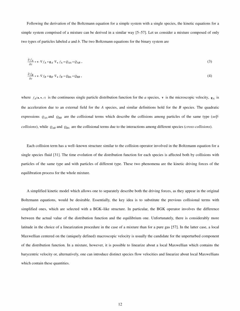
Following the derivation of the Boltzmann equation for a simple system with a single species, the kinetic equations for a

simple system comprised of a mixture can be derived in a similar way [5–57]. Let us consider a mixture composed of only

two types of particles labeled a and b. The two Boltzmann equations for the binary system are

AA A A AA AB

ff f Q Q

t∂

+ ⋅∇ + ⋅∇ = +∂ vv g , (3)

BB B B BA BB

ff f Q Q

t∂

+ ⋅∇ + ⋅∇ = +∂ vv g , (4)

where ( , , )Af tx v is the continuous single particle distribution function for the a species, v is the microscopic velocity, Ag is

the acceleration due to an external field for the A species, and similar definitions hold for the B species. The quadratic

expressions AAQ and BBQ are the collisional terms which describe the collisions among particles of the same type (self-

collisions), while ABQ and BAQ are the collisional terms due to the interactions among different species (cross-collisions).

Each collision term has a well–known structure similar to the collision operator involved in the Boltzmann equation for a

single species fluid [31]. The time evolution of the distribution function for each species is affected both by collisions with

particles of the same type and with particles of different type. These two phenomena are the kinetic driving forces of the

equilibration process for the whole mixture.

A simplified kinetic model which allows one to separately describe both the driving forces, as they appear in the original

Boltzmann equations, would be desirable. Essentially, the key idea is to substitute the previous collisional terms with

simplified ones, which are selected with a BGK–like structure. In particular, the BGK operator involves the difference

between the actual value of the distribution function and the equilibrium one. Unfortunately, there is considerably more

latitude in the choice of a linearization procedure in the case of a mixture than for a pure gas [57]. In the latter case, a local

Maxwellian centered on the (uniquely defined) macroscopic velocity is usually the candidate for the unperturbed component

of the distribution function. In a mixture, however, it is possible to linearize about a local Maxwellian which contains the

barycentric velocity or, alternatively, one can introduce distinct species flow velocities and linearize about local Maxwellians

which contain these quantities.

13

Even though it could result in slightly more complicated models, the choice of separate Maxwellians seems more general

and better suitable for dealing with different regimes consistently. The model obtained is due to Hamel [58–60]. A Lattice

Boltzmann formulation of this model was recently proposed [46] and used for describing reactive mixtures [47].

Unfortunately, the Hamel model (and all those resulting from a proper linearization of it) are not completely self-

consistent [48]. In fact, if one sums over the species equations, one does not exactly recover the momentum equations (as one

should). Since the errors are negligible for fluid flows characterized by low Reynolds numbers, this model was considered in

our preliminary simulations, because it allows one to tune the Schmidt number of the binary mixture (ratio between the

molecular diffusivity and the mixture kinematic viscosity). Unfortunately, the tuning strategy, i.e. finding the proper

combination of relaxation parameters for achieving this goal, and the correction terms for compensating the discretization

errors required some complicated algebra, which (unacceptably) increases the computational demand.

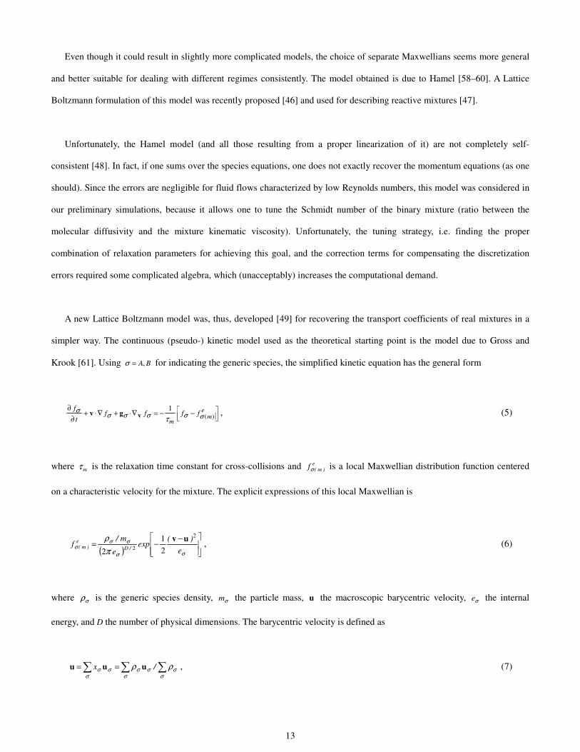
A new Lattice Boltzmann model was, thus, developed [49] for recovering the transport coefficients of real mixtures in a

simpler way. The continuous (pseudo-) kinetic model used as the theoretical starting point is the model due to Gross and

Krook [61]. Using ,A Bσ = for indicating the generic species, the simplified kinetic equation has the general form

( )1 e

mm

ff f f f

tσ

σ σ σ σ στ∂ + ⋅∇ + ⋅∇ = − − ∂ vv g , (5)

where mτ is the relaxation time constant for cross-collisions and e)m(fσ is a local Maxwellian distribution function centered

on a characteristic velocity for the mixture. The explicit expressions of this local Maxwellian is

( )

−−=σσ

σσσ π

ρe

)(exp

e

m/f /D

e)m(

2

2 21

2

uv , (6)

where σρ is the generic species density, σm the particle mass, u the macroscopic barycentric velocity, σe the internal

energy, and D the number of physical dimensions. The barycentric velocity is defined as

==σ σ

σσσσ

σσ ρρ /x uuu , (7)

14

where σx is the mass concentration (mass fraction) for the generic species. Local momentum conservation implies that the

relaxation time constant mτ for the cross-collisions must be the same for all species.

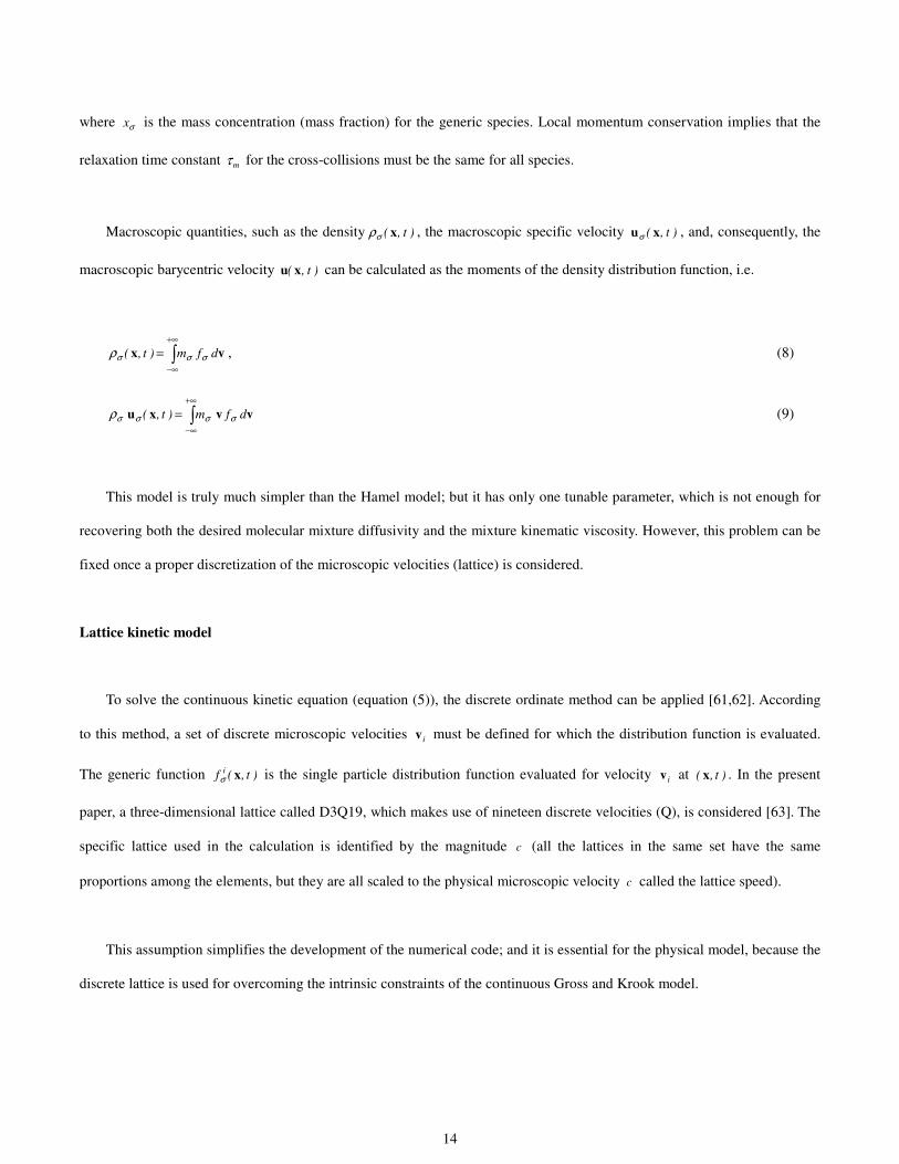
Macroscopic quantities, such as the density )t,( xσρ , the macroscopic specific velocity )t,( xuσ , and, consequently, the

macroscopic barycentric velocity )t,( xu can be calculated as the moments of the density distribution function, i.e.

+∞

∞−

= vx dfm)t,( σσσρ , (8)

+∞

∞−

= vvxu dfm)t,( σσσσρ (9)

This model is truly much simpler than the Hamel model; but it has only one tunable parameter, which is not enough for

recovering both the desired molecular mixture diffusivity and the mixture kinematic viscosity. However, this problem can be

fixed once a proper discretization of the microscopic velocities (lattice) is considered.

Lattice kinetic model

To solve the continuous kinetic equation (equation (5)), the discrete ordinate method can be applied [61,62]. According

to this method, a set of discrete microscopic velocities iv must be defined for which the distribution function is evaluated.

The generic function )t,(f i xσ is the single particle distribution function evaluated for velocity iv at )t,( x . In the present

paper, a three-dimensional lattice called D3Q19, which makes use of nineteen discrete velocities (Q), is considered [63]. The

specific lattice used in the calculation is identified by the magnitude c (all the lattices in the same set have the same

proportions among the elements, but they are all scaled to the physical microscopic velocity c called the lattice speed).

This assumption simplifies the development of the numerical code; and it is essential for the physical model, because the

discrete lattice is used for overcoming the intrinsic constraints of the continuous Gross and Krook model.

15

Thus, the kinetic equation, which is an integro-differential equation, reduces to a system of differential equations. The

term that takes into account the effect of the external force field can be neglected, because we are interested in concentration

driven flows (actually, a proper forcing term is considered in the numerical implementation for improving the accuracy of the

method). Since the reference lattice has been defined, it is possible to write the operative formula in vectorial form, namely,

( )e

m mtσ

σ σσ∂ + ⋅∇ = −

∂f

V f A f f , (10)

where V is the matrix collecting all the lattice components ( V v has dimensions Q x D, i.e. 19x3) and the scalar product

between matrices must be thought of as saturating the second index (in fact σ∇f has dimensions 19x3 and consequently

σ⋅∇V f is a column vector 19x1).

According to the Gross and Krook model on a lattice, the collisional matrix should be diagonal, namely m mλ=A I , where

1/m mλ τ= . However, in order to increase the number of tunable parameters, the collisional matrix is assumed to be

1m D m D

−=A M D M , (11)

where DM defines a proper orthonormal basis1 for the D3Q19 lattice and mD is the diagonal matrix, namely,

1 1 1 1 1 2( ) [0, , , , , , , , , ,

, , , , , , , , ]

I I I II II II II II IIm m m m m m m m m m

III III III III III III IV IV IVm m m m m m m m m

diag λ λ λ λ λ λ λ λ λ

λ λ λ λ λ λ λ λ λ

=D, (12)

collecting the generalized relaxation frequencies for self and cross collisions. As will be clear later on (see the section

concerning the numerical implementation), Imλ controls the molecular diffusivity, 1

IImλ and 2

IImλ control the mixture kinematic

and bulk viscosity respectively, while IIImλ and IV

mλ are free parameters effecting the stability of the model (usually

1III IVm mλ λ= = ).

1 Details on how to derive the ortho-normal basis are reported in [A3]. Even though this paper discusses the two dimensional case (D2Q9 lattice), the derivation technique for the three dimensional case is the same. The transformation matrix is made of (simple) numerical constants.

16

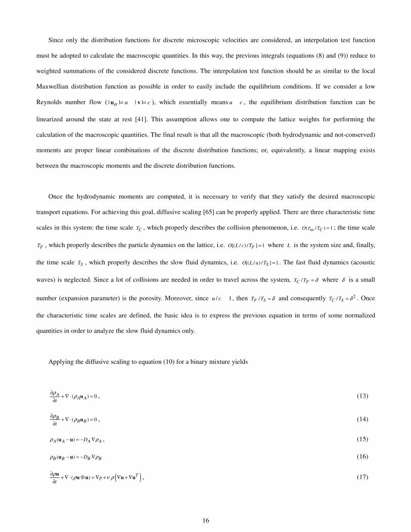
Since only the distribution functions for discrete microscopic velocities are considered, an interpolation test function

must be adopted to calculate the macroscopic quantities. In this way, the previous integrals (equations (8) and (9)) reduce to

weighted summations of the considered discrete functions. The interpolation test function should be as similar to the local

Maxwellian distribution function as possible in order to easily include the equilibrium conditions. If we consider a low

Reynolds number flow ( | | | |u cσ = =u v ), which essentially means u c , the equilibrium distribution function can be

linearized around the state at rest [41]. This assumption allows one to compute the lattice weights for performing the

calculation of the macroscopic quantities. The final result is that all the macroscopic (both hydrodynamic and not-conserved)

moments are proper linear combinations of the discrete distribution functions; or, equivalently, a linear mapping exists

between the macroscopic moments and the discrete distribution functions.

Once the hydrodynamic moments are computed, it is necessary to verify that they satisfy the desired macroscopic

transport equations. For achieving this goal, diffusive scaling [65] can be properly applied. There are three characteristic time

scales in this system: the time scale CT , which properly describes the collision phenomenon, i.e. ( / ) 1m CO Tτ = ; the time scale

FT , which properly describes the particle dynamics on the lattice, i.e. [( / ) / ] 1FO L c T = where L is the system size and, finally,

the time scale ST , which properly describes the slow fluid dynamics, i.e. [( / ) / ] 1SO L u T = . The fast fluid dynamics (acoustic

waves) is neglected. Since a lot of collisions are needed in order to travel across the system, /C FT T δ= where δ is a small

number (expansion parameter) is the porosity. Moreover, since / 1u c , then /F ST T δ= and consequently 2/C ST T δ= . Once

the characteristic time scales are defined, the basic idea is to express the previous equation in terms of some normalized

quantities in order to analyze the slow fluid dynamics only.

Applying the diffusive scaling to equation (10) for a binary mixture yields

( ) 0AA At

ρ ρ∂+ ∇ ⋅ =

∂u , (13)

( ) 0BB Bt

ρ ρ∂+ ∇ ⋅ =

∂u , (14)

( )A A A ADρ ρ− = − ∇u u , (15)

( )B B B BDρ ρ− = − ∇u u (16)

( )( ) Tpt

ρ ρ ν ρ∂ + ∇ ⋅ ⊗ = ∇ + ∇ + ∇∂

u u u u u , (17)

17

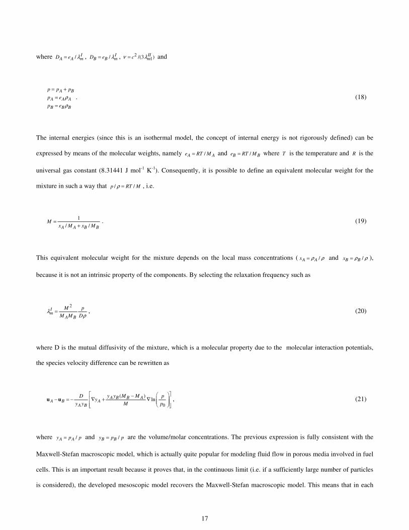
where / IA A mD e λ= , / I

B B mD e λ= , 21/(3 )II

mcν λ= and

A B

A A A

B B B

p p p

p e

p e

ρρ

= +==

. (18)

The internal energies (since this is an isothermal model, the concept of internal energy is not rigorously defined) can be

expressed by means of the molecular weights, namely /A Ae RT M= and /B Be RT M= where T is the temperature and R is the

universal gas constant (8.31441 J mol-1 K-1). Consequently, it is possible to define an equivalent molecular weight for the

mixture in such a way that / /p RT Mρ = , i.e.

1/ /A A B B

Mx M x M

=+

. (19)

This equivalent molecular weight for the mixture depends on the local mass concentrations ( /A Ax ρ ρ= and /B Bx ρ ρ= ),

because it is not an intrinsic property of the components. By selecting the relaxation frequency such as

2Im

A B

M pM M D

λρ

= , (20)

where D is the mutual diffusivity of the mixture, which is a molecular property due to the molecular interaction potentials,

the species velocity difference can be rewritten as

0

( )lnA B B A

A B AA B

y y M MD py

y y M p

−− = − ∇ + ∇

u u , (21)

where /A Ay p p= and /B By p p= are the volume/molar concentrations. The previous expression is fully consistent with the

Maxwell-Stefan macroscopic model, which is actually quite popular for modeling fluid flow in porous media involved in fuel

cells. This is an important result because it proves that, in the continuous limit (i.e. if a sufficiently large number of particles

is considered), the developed mesoscopic model recovers the Maxwell-Stefan macroscopic model. This means that in each

18

(sufficiently large) fluid pore, the mesoscopic model is consistent with the macroscopic approach and consequently the

averaged macroscopic results derived from the proposed model depend only on the topology of the porous medium, which is

the goal of our investigation. Before proceeding in this direction, it is worth highlighting that the macroscopic equations

which derive from the lattice kinetic model do not involve chemical reactions, because there is no source term in the

continuity equation. The electrochemical reactions realize a concentration driven flow by modifying the species

concentrations at the three-phase boundaries, while there are no chemical reactions in the bulk fluid. For this reason, the

electrochemical reactions were simply modeled by means of proper boundary conditions with regards to the concentration for

the fluid cells close to the three-phase boundaries.

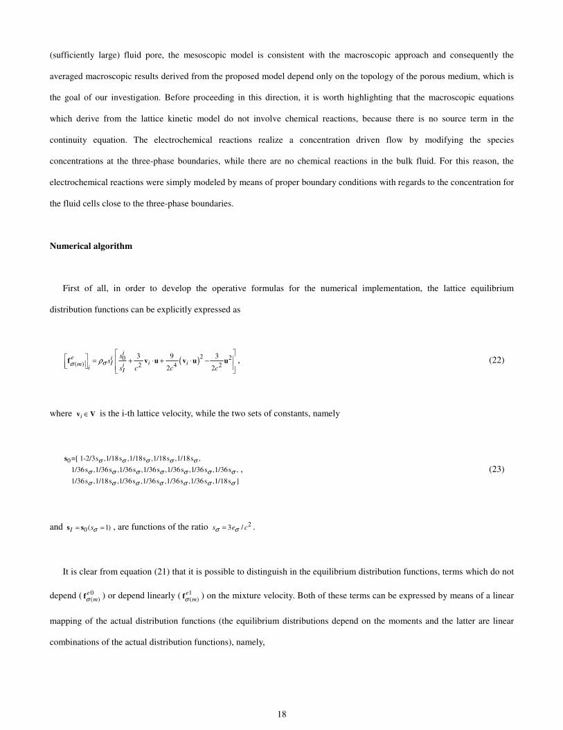
Numerical algorithm

First of all, in order to develop the operative formulas for the numerical implementation, the lattice equilibrium

distribution functions can be explicitly expressed as

( )2 20( ) 2 4 2

3 9 3

2 2

ie i

I i im ii I

ss

s c c cσσ ρ

= + ⋅ + ⋅ −

f v u v u u , (22)

where i ∈v V is the i-th lattice velocity, while the two sets of constants, namely

0 =[ 1-2/3s ,1/18s ,1/18s ,1/18s ,1/18s ,

1/36s ,1/36s ,1/36s ,1/36s ,1/36s ,1/36s ,1/36s ,

1/36s ,1/18s ,1/36s ,1/36s ,1/36s ,1/36s ,1/18s ]

σ σ σ σ σ

σ σ σ σ σ σ σ

σ σ σ σ σ σ σ

s, (23)

and 0 ( 1)I sσ= =s s , are functions of the ratio 23 /s e cσ σ= .

It is clear from equation (21) that it is possible to distinguish in the equilibrium distribution functions, terms which do not

depend ( 0( )

emσf ) or depend linearly ( 1

( )e

mσf ) on the mixture velocity. Both of these terms can be expressed by means of a linear

mapping of the actual distribution functions (the equilibrium distributions depend on the moments and the latter are linear

combinations of the actual distribution functions), namely,

19

00( )

eem σσ =f M f , (24)

11( )

eem xσ σσ

σ

= f M f . (25)

Consequently, the residual quadratic terms can be expressed as

2 0 1( ) ( ) ( ) ( )

e e e em m m mσ σ σ σ= − −f f f f . (26)

Secondly, some dimensionless coordinates can be considered (the so-called “lattice units”). Let us introduce a

dimensionless space ˆ /x x L= , time ˆ / St t T= , and collisional operator ˆm C mT=A A . In this dimensionless system, the continuous

formula given by equation (10) can be approximated by the following discrete formula on a regular spatial mesh, namely,

( )ˆˆ ˆ ˆ ˆ ˆ ˆˆ ˆ ˆ ˆ ˆ( , ) ( 1, ) ( , ) ( , ) ( , )e

m bmt t t t tσ σ σσ − − − = − +

f X f X V A f X f X k X , (27)

where ˆˆ( , )b tk X is a proper forcing term, which must be introduced in order to satisfy the continuity equations with the discrete

formula up to the second order in space and the first order in time (see [49] for details). The previous integration rule derives

directly from the implicit backward Euler formula. The implicit formulation allows one to improve the stability of the

scheme, i.e. for any values of the relaxation frequencies, the macroscopic transport coefficients cannot assume unphysical

(negative) values.

Unfortunately, the implicit formulation is computationally more demanding and, for this reason, the improved stability is

paid by longer simulations. However, in this case, it is possible to develop a semi-implicit formulation, i.e. it is possible to

compute implicitly all the terms which can be solved once and for all at the beginning of the computations (pre-processing)

and explicitly only the quadratic terms. The reason is that the quadratic terms do not affect the stability performance much.

The first step is to derive an operative formula for the barycentric distribution function, which is computed by the sum of

the species distribution functions. Substituting equations (24), (25), and (26) into equation (27) and summing over all the

species yields

20

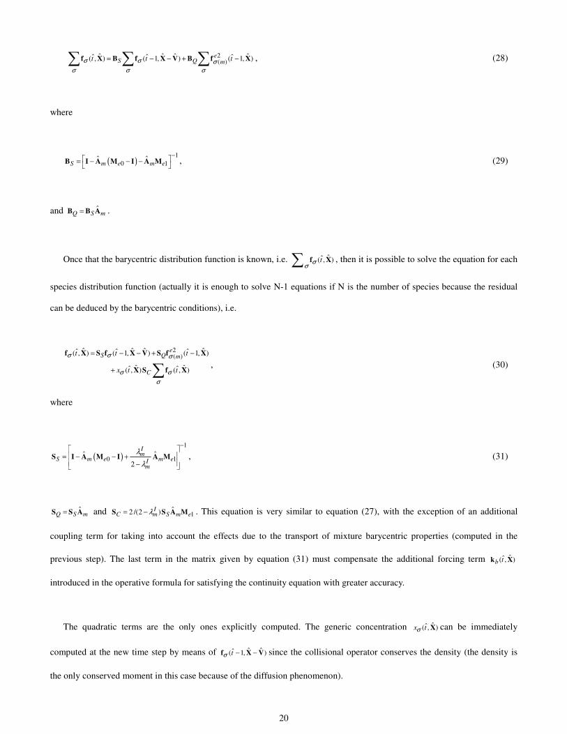
2( )

ˆ ˆ ˆ ˆˆ ˆ ˆ( , ) ( 1, ) ( 1, )eS Q mt t tσ σ σ

σ σ σ

= − − + − f X B f X V B f X , (28)

where

( )1

0 1ˆ ˆ

S m e m e−

= − − −

B I A M I A M , (29)

and ˆQ S m=B B A .

Once that the barycentric distribution function is known, i.e. ˆˆ( , )tσσ f X , then it is possible to solve the equation for each

species distribution function (actually it is enough to solve N-1 equations if N is the number of species because the residual

can be deduced by the barycentric conditions), i.e.

2( )

ˆ ˆ ˆ ˆˆ ˆ ˆ( , ) ( 1, ) ( 1, )

ˆ ˆˆ ˆ( , ) ( , )

eS Q m

C

t t t

x t t

σ σ σ

σ σσ

= − − + −

+ f X S f X V S f X

X S f X, (30)

where

( )1

0 1ˆ ˆ

2

Im

S m e m eIm

λλ

− = − − + −

S I A M I A M , (31)

ˆQ S m=S S A and 1

ˆ2 /(2 )IC m S m eλ= −S S A M . This equation is very similar to equation (27), with the exception of an additional

coupling term for taking into account the effects due to the transport of mixture barycentric properties (computed in the

previous step). The last term in the matrix given by equation (31) must compensate the additional forcing term ˆˆ( , )b tk X

introduced in the operative formula for satisfying the continuity equation with greater accuracy.

The quadratic terms are the only ones explicitly computed. The generic concentration ˆˆ( , )x tσ X can be immediately

computed at the new time step by means of ˆ ˆˆ( 1, )tσ − −f X V since the collisional operator conserves the density (the density is

the only conserved moment in this case because of the diffusion phenomenon).

21

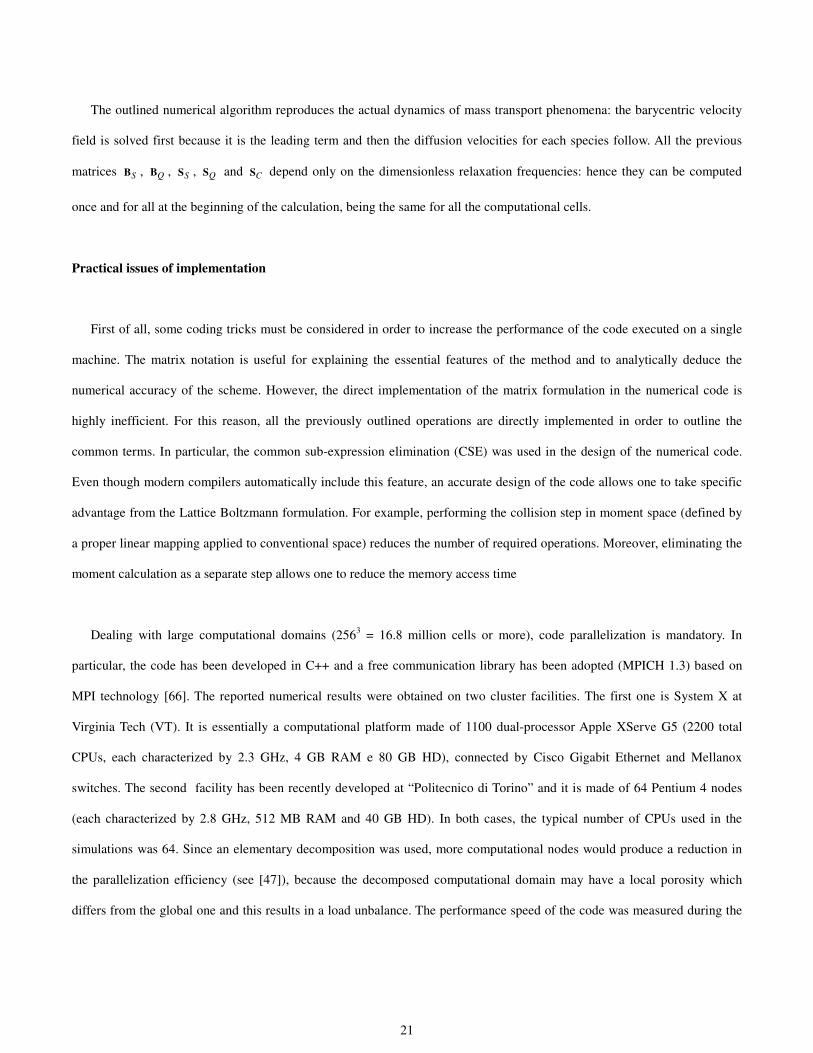
The outlined numerical algorithm reproduces the actual dynamics of mass transport phenomena: the barycentric velocity

field is solved first because it is the leading term and then the diffusion velocities for each species follow. All the previous

matrices SB , QB , SS , QS and CS depend only on the dimensionless relaxation frequencies: hence they can be computed

once and for all at the beginning of the calculation, being the same for all the computational cells.

Practical issues of implementation

First of all, some coding tricks must be considered in order to increase the performance of the code executed on a single

machine. The matrix notation is useful for explaining the essential features of the method and to analytically deduce the

numerical accuracy of the scheme. However, the direct implementation of the matrix formulation in the numerical code is

highly inefficient. For this reason, all the previously outlined operations are directly implemented in order to outline the

common terms. In particular, the common sub-expression elimination (CSE) was used in the design of the numerical code.

Even though modern compilers automatically include this feature, an accurate design of the code allows one to take specific

advantage from the Lattice Boltzmann formulation. For example, performing the collision step in moment space (defined by

a proper linear mapping applied to conventional space) reduces the number of required operations. Moreover, eliminating the

moment calculation as a separate step allows one to reduce the memory access time

Dealing with large computational domains (2563 = 16.8 million cells or more), code parallelization is mandatory. In

particular, the code has been developed in C++ and a free communication library has been adopted (MPICH 1.3) based on

MPI technology [66]. The reported numerical results were obtained on two cluster facilities. The first one is System X at

Virginia Tech (VT). It is essentially a computational platform made of 1100 dual-processor Apple XServe G5 (2200 total

CPUs, each characterized by 2.3 GHz, 4 GB RAM e 80 GB HD), connected by Cisco Gigabit Ethernet and Mellanox

switches. The second facility has been recently developed at “Politecnico di Torino” and it is made of 64 Pentium 4 nodes

(each characterized by 2.8 GHz, 512 MB RAM and 40 GB HD). In both cases, the typical number of CPUs used in the

simulations was 64. Since an elementary decomposition was used, more computational nodes would produce a reduction in

the parallelization efficiency (see [47]), because the decomposed computational domain may have a local porosity which

differs from the global one and this results in a load unbalance. The performance speed of the code was measured during the

22

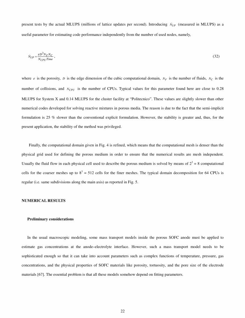
present tests by the actual MLUPS (millions of lattice updates per second). Introducing UPN (measured in MLUPS) as a

useful parameter for estimating code performance independently from the number of used nodes, namely,

3F C

UPCPU

D N NN

N Timeε

= , (32)

where ε is the porosity, D is the edge dimension of the cubic computational domain, FN is the number of fluids, CN is the

number of collisions, and CPUN is the number of CPUs. Typical values for this parameter found here are close to 0.28

MLUPS for System X and 0.14 MLUPS for the cluster facility at “Politecnico”. These values are slightly slower than other

numerical codes developed for solving reactive mixtures in porous media. The reason is due to the fact that the semi-implicit

formulation is 25 % slower than the conventional explicit formulation. However, the stability is greater and, thus, for the

present application, the stability of the method was privileged.

Finally, the computational domain given in Fig. 4 is refined, which means that the computational mesh is denser than the

physical grid used for defining the porous medium in order to ensure that the numerical results are mesh independent.

Usually the fluid flow in each physical cell used to describe the porous medium is solved by means of 23 = 8 computational

cells for the coarser meshes up to 83 = 512 cells for the finer meshes. The typical domain decomposition for 64 CPUs is

regular (i.e. same subdivisions along the main axis) as reported in Fig. 5.

NUMERICAL RESULTS

Preliminary considerations

In the usual macroscopic modeling, some mass transport models inside the porous SOFC anode must be applied to

estimate gas concentrations at the anode–electrolyte interface. However, such a mass transport model needs to be

sophisticated enough so that it can take into account parameters such as complex functions of temperature, pressure, gas

concentrations, and the physical properties of SOFC materials like porosity, tortuosity, and the pore size of the electrode

materials [67]. The essential problem is that all these models somehow depend on fitting parameters.

23

In general, mass transport of components inside porous media can be described using either the extended Fick model

(EFM) or the dusty gas model (DGM). Both FM and the DGM are mass transport equations taking into account Knudsen

diffusion, molecular diffusion, and the effect of a finite pressure gradient. Some other authors have eliminated the effect of

Knudsen diffusion, using only the Stefan–Maxwell model in their mass transport equations (SMM).

There are some evident degrees of freedom in selecting the fitting parameters concerning the porous medium

microstructure in order to recover the experimental data. Moreover, the application of the previous model requires some

additional simplifications. For example, it is quite popular to neglect the effects due to the finite pressure gradient. This

hypothesis seems reasonable since there is no net change in the number of moles in the gas phase due to the electrochemical

reactions. From the practical point of view, this means neglecting the second terms on the right hand sides of equation (21).

Unfortunately, this assumption is not acceptable. The fact that the total number of moles in the gas phase does not change

does not necessarily imply that the pressure is constant. In fact, the total mixture mass increases due to the electrochemical

reactions (lighter hydrogen particles are being substituted with heavier water particles) and, for this reason, a net out-coming

mass flux must exist under steady state conditions. This is understandable if one takes into account that a relevant mass flux

is entering by means of the (heavy) ions moving in the electrolyte. In other words, there is a relevant out-coming mixture flux

and consequently a proper total pressure gradient must exist to ensure the driving force of this flow.

The goal of the calculations reported here is to directly solve the fluid flow of reactive mixtures in porous anodes. First of

all, the transport coefficients must be tuned based on the (pure) molecular values, which come form kinetic theory. These

input data must be the same as those considered by the macroscopic approaches in order to make the comparison more

reliable.

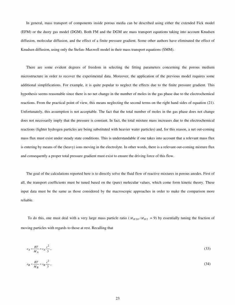
To do this, one must deal with a very large mass particle ratio ( 2 2/H O HM M = 9) by essentially tuning the fraction of

moving particles with regards to those at rest. Recalling that

2

3A AA

RT ce s

M= = , (33)

2

3B BB

RT ce s

M= = , (34)

24

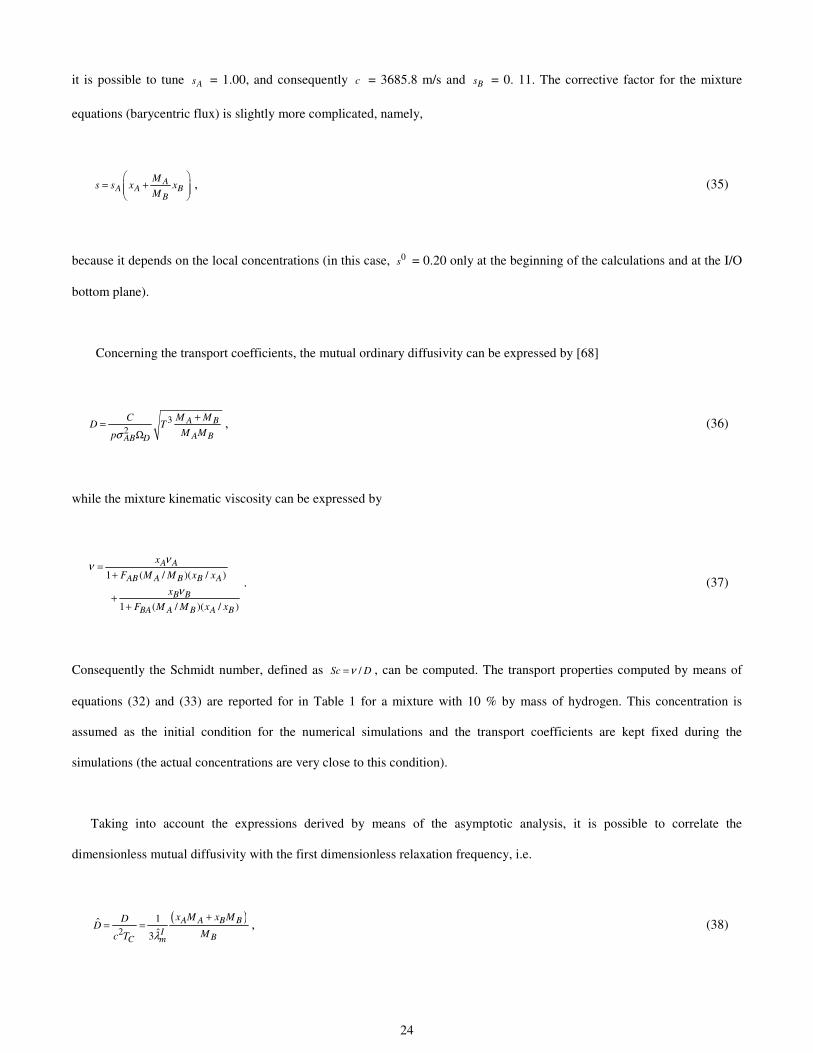
it is possible to tune As = 1.00, and consequently c = 3685.8 m/s and Bs = 0. 11. The corrective factor for the mixture

equations (barycentric flux) is slightly more complicated, namely,

AA A B

B

Ms s x x

M

= +

, (35)

because it depends on the local concentrations (in this case, 0s = 0.20 only at the beginning of the calculations and at the I/O

bottom plane).

Concerning the transport coefficients, the mutual ordinary diffusivity can be expressed by [68]

32

A B

A BAB D

M MCD T

M Mpσ+

=Ω

, (36)

while the mixture kinematic viscosity can be expressed by

1 ( / )( / )

1 ( / )( / )

A A

AB A B B A

B B

BA A B A B

xF M M x x

xF M M x x

νν

ν

=+

++

. (37)

Consequently the Schmidt number, defined as /Sc Dν= , can be computed. The transport properties computed by means of

equations (32) and (33) are reported for in Table 1 for a mixture with 10 % by mass of hydrogen. This concentration is

assumed as the initial condition for the numerical simulations and the transport coefficients are kept fixed during the

simulations (the actual concentrations are very close to this condition).

Taking into account the expressions derived by means of the asymptotic analysis, it is possible to correlate the

dimensionless mutual diffusivity with the first dimensionless relaxation frequency, i.e.

( )2

1ˆˆ3

A A B BI BC m

x M x MDD

Mc T λ

+= = , (38)

25

or equivalently

( )ˆˆ3

A A B BIm

B

x M x M

M Dλ

+= . (39)

For the mixture kinematic viscosity, a similar procedure can be considered with the difference that an additional term due to

the artificial numerical viscosity must be included (preserving the fact that this coefficient must always be positive). Thus,

12

1

ˆ1ˆ 1ˆ 23

IIm

IIC mc T

λννλ

= = +

, (40)

or equivalently

11ˆ

ˆ3 1/ 2IImλ

ν=

−. (41)

Finally, a proper set of boundary conditions must be considered. Since the computational domain is chosen to be smaller

than the physical thickness of the anode layer, periodic geometric conditions are considered. This means that one must

imagine that the computational domain is repeated in all directions in order to create the actual physical topology.

As to the electrochemical reactions, they do not take place in the bulk fluid but are instead believed to take place near the

(active) three-phase boundary of Ni, YSZ and the gas phase. It is formulated globally as

H2 (gas) + O2– (YSZ) → H2O (gas) + 2e– (Ni).

There is quite some controversy as to the actual pathway and nature of the elementary steps of the previous global reaction

(see [69-72] for a general discussion of this topic). From the theoretical point of view, it is possible to consider various

reaction pathways, focusing on the elementary-step charge-transfer reactions that are involved. Recently a tentative

thermodynamic model of the H2/H2O/Ni/YSZ three-phase boundary was established in order to investigate the influence of

operating conditions (in terms the gas concentrations of both reactants and products) on the Ni/YSZ anode kinetics [69].

Three different reaction pathways (oxygen spillover, hydrogen spillover, interstitial hydrogen transfer), based on five

26

different elementary charge-transfer reactions, are the basis of this model. All charge-transfer reactions show a strong and

highly nonlinear dependence of their kinetics on gas-phase hydrogen and water concentration. However, the behaviour is

distinctly different for the various mechanisms. According to this model [69], the full set of intermediate electrochemical

charge-transfer reactions, which are discussed in the following, are grouped into three different sets (oxygen spillover,

hydrogen spillover, interstitial hydrogen transfer):

(a) At the three-phase boundary line, oxygen ions (formally O2–) may hop from the YSZ surface to the Ni surface in an

elementary charge-transfer reaction (oxygen spillover) such as

O2−YSZ + []Ni → ONi + []YSZ + 2e−,

where the subscripts denote the surface to which the species is attached and [] indicates a free surface site. Subsequent

chemical reactions of hydrogen and oxygen species, including adsorption of molecular hydrogen and desorption of water,

take place on the Ni surface. Alternatively, spillover of hydroxyl ions (formally OH–) from the YSZ to the Ni surface is

possible, namely,

OH−YSZ + []Ni → OHNi + []YSZ + e−.

(b) A different possible pathway for the global reaction is the spillover of hydrogen from the Ni to the YSZ surface. The

hydrogen atoms may hop to either an oxygen ion site in an elementary charge-transfer reaction such as

HNi + O2−YSZ → OH−

YSZ + []Ni + e−,

or to a hydroxyl site (both reactions may be active in parallel or consecutively),

HNi + OH−YSZ → H2OYSZ + []Ni + e−.

(c) Finally, at the typically high SOFC operating temperatures, both interstitial hydrogen atoms in the bulk Ni and

interstitial protons in the bulk YSZ are known to be present in relatively high concentrations with high enough diffusivities to

27

support the global reaction. Charge transfer may, therefore, take place at the two-phase boundary of Ni and YSZ. Interstitial

hydrogen and protons are formed via surface adsorption and surface/bulk exchange from hydrogen on Ni and water on YSZ,

respectively.

For each single step elementary reaction, the forward and backward reaction rate constants may be theoretically defined.

By substituting the potential difference by the activation overpotential , i.e. act = – eq, in the equations ruling the

kinetics of the intermediate electrochemical charge-transfer reactions and expressing eq via the Nernst relation, after some

algebraic manipulation, the familiar Butler – Volmer relation [73] is recovered, namely,

−−−

= actact TR

FzTRFz

JJ ηαηα )1(expexp0 ,

where J is the current density, 0J is the exchange current density, z is the number of electrons, α is the symmetry factor

and F is Faraday’s constant (F = 96,500 C mol-1).

As clearly outlined in the previous section, the actual microscopic dynamics of the electrochemical reactions is quite a

complicated phenomenon, which from the theoretical point of view is not entirely clear in all of its details. On the other hand,

there is a large consensus in most of the applications concerning the heuristic Butler – Volmer relation. As of yet, the ion and

electron dynamics is not directly solved in the present model (the focus of our development has been elsewhere), even though

it is not difficult to imagine some possible extensions of the model in this direction, since the required additional equations

are essentially those of potential flow. Hence, it is not possible in our model to calculate at the moment the activation

overpotential act for use in the Butler – Volmer relation. However, in principle, this is not a problem for the mass transfer

model discussed in this paper, because from the point of view of the mass transfer, the electrochemical reactions are modelled

by proper boundary conditions. An eventual problem with this approach could be that due to the omitted back–coupling of

the mass transfer on the reaction dynamics.

Nonetheless, this last, more simplified approach of proper boundary conditions is adopted in the following. The practical

effects on the electrochemical reactions is to locally modify the species concentration and hence to produce concentration

28

driven flow. It is easy to correlate the total inlet / outlet fluxes (at the bottom I/O plane) with the averaged operating

conditions of the fuel cell by means of the current density J so that

2A A AJ

MF

ρ< >= +u , (42)

2B B BJ

MF

ρ< >= −u , (43)

( ) 02A BJ

M MF

ρ< >= − <u , (44)

where < ⋅ > indicates a surface averaged quantity at the I/O bottom plane (see Fig. 5). From the previous expressions, it is

easy to prove that, for a fixed current, the net out-coming mass flux is 8=(18-2)/2 times larger than the in-coming one. For

this reason, a total pressure gradient must exist as a driving force.

The actual species concentrations close to the (active) three-phase boundaries must be such as to generate the mass fluxes

given by equations (41), (42), and (43). Instead of using an iterative procedure (more computational demanding), the

following strategy is suggested. Suppose that all the reactive cells behave in the same way (i.e. have homogeneous

electrochemical reactions). The local species densities for the generic reactive cells can be expressed as

0RA A Dρ ρ δρ= − , (45)

( )0R BB B D M

A

MM

ρ ρ δρ δρ= + + , (46)

where Dδρ and Mδρ are freely tunable parameters, while 0Aρ and 0

Bρ are the fixed densities at the I/O bottom plane. The

ratio /B AM M has been introduced in order to directly affect the partial pressures (in fact the densities must be divided by the

corresponding molecular weights to obtain the partial pressure).

The numerical simulations confirm that the relation between the mass fluxes and the tunable parameters used for

specifying the density in the reaction fluid cells is linear, namely,

0A A A D Dx kρ ρ δρ< > − < >=u u , (47)

29

0B B B D Dx kρ ρ δρ< > − < >= −u u , (48)

M Mkρ δρ< >= −u , (49)

where Dk and Mk are fitting parameters which can be measured by means of the numerical simulations. Recalling equations

(41) and (42) and substituting them into the previous equations yields

0

0 2A A D A M D A

B B M BD B M

k x k MJMFk x k

ρ δρρ δρ

< > − = = < > − − −

uu

, (50)

and consequently

10

02 ( 1)

D D A M A

M BD A M

k x k MJMF k x k

δρδρ

− − = − − −

, (51)

which allows one to select the freely tunable parameters based on the local densities for the reactive cells in order to produce

mass fluxes coherent with a given current density. The simulations can be performed in three steps:

• first, some guessed values for the freely tunable parameters Dδρ and Mδρ are assumed;

• then the fitting parameters Dk and Mk (for the specific porous medium) are computed;

• finally, the actual current density (homogeneously distributed) can be simulated by means of equation (51).

In order to prove the effectiveness of the discussed technique in simulating reactive mixtures for SOFCs, the following

example is reported. The smallest grain used in the definition of the porous medium reported in Fig. 4 is 0.404 micron. A

refinement factor of 8 was used in the numerical simulations, because it ensures mesh independent results (see the following

section). This implies that the smallest computational cell is 0.005053 micron3. The total size of the computational domain is

2563 and was solved on 64 CPUs. Hence, each cube of the split domain reported in Fig. 5 is 643. The number of collisions

required to produce steady state conditions was roughly 60,000 (15 hours of wall clock time on the cluster).

The reactive boundary conditions were tuned for modeling a current density equal to J = 0.4 A cm-2, which is a typical

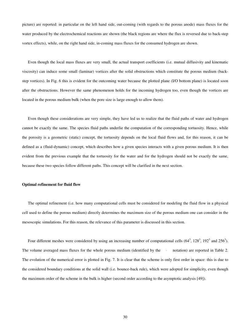
value for this technology. In Fig. 6, the contours for the mass fluxes at the main I/O bottom plane (moving orthogonal to the

30

picture) are reported: in particular on the left hand side, out-coming (with regards to the porous anode) mass fluxes for the

water produced by the electrochemical reactions are shown (the black regions are where the flux is reversed due to back-step

vortex effects), while, on the right hand side, in-coming mass fluxes for the consumed hydrogen are shown.

Even though the local mass fluxes are very small, the actual transport coefficients (i.e. mutual diffusivity and kinematic

viscosity) can induce some small (laminar) vortices after the solid obstructions which constitute the porous medium (back-

step vortices). In Fig. 6 this is evident for the outcoming water because the plotted plane (I/O bottom plane) is located soon

after the obstructions. However the same phenomenon holds for the incoming hydrogen too, even though the vortices are

located in the porous medium bulk (when the pore size is large enough to allow them).

Even though these considerations are very simple, they have led us to realize that the fluid paths of water and hydrogen

cannot be exactly the same. The species fluid paths underlie the computation of the corresponding tortuosity. Hence, while

the porosity is a geometric (static) concept, the tortuosity depends on the local fluid flows and, for this reason, it can be

defined as a (fluid-dynamic) concept, which describes how a given species interacts with a given porous medium. It is then

evident from the previous example that the tortuosity for the water and for the hydrogen should not be exactly the same,

because these two species follow different paths. This concept will be clarified in the next section.

Optimal refinement for fluid flow

The optimal refinement (i.e. how many computational cells must be considered for modeling the fluid flow in a physical

cell used to define the porous medium) directly determines the maximum size of the porous medium one can consider in the

mesoscopic simulations. For this reason, the relevance of this parameter is discussed in this section.

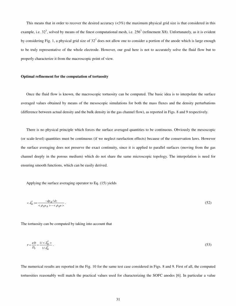
Four different meshes were considered by using an increasing number of computational cells (643, 1283, 1923 and 2563).

The volume averaged mass fluxes for the whole porous medium (identified by the ⋅ notation) are reported in Table 2.

The evolution of the numerical error is plotted in Fig. 7. It is clear that the scheme is only first order in space: this is due to

the considered boundary conditions at the solid wall (i.e. bounce-back rule), which were adopted for simplicity, even though

the maximum order of the scheme in the bulk is higher (second order according to the asymptotic analysis [49]).

31

This means that in order to recover the desired accuracy (<3%) the maximum physical grid size is that considered in this

example, i.e. 323, solved by means of the finest computational mesh, i.e. 2563 (refinement X8). Unfortunately, as it is evident

by considering Fig. 1, a physical grid size of 323 does not allow one to consider a portion of the anode which is large enough

to be truly representative of the whole electrode. However, our goal here is not to accurately solve the fluid flow but to

properly characterize it from the macroscopic point of view.

Optimal refinement for the computation of tortuosity

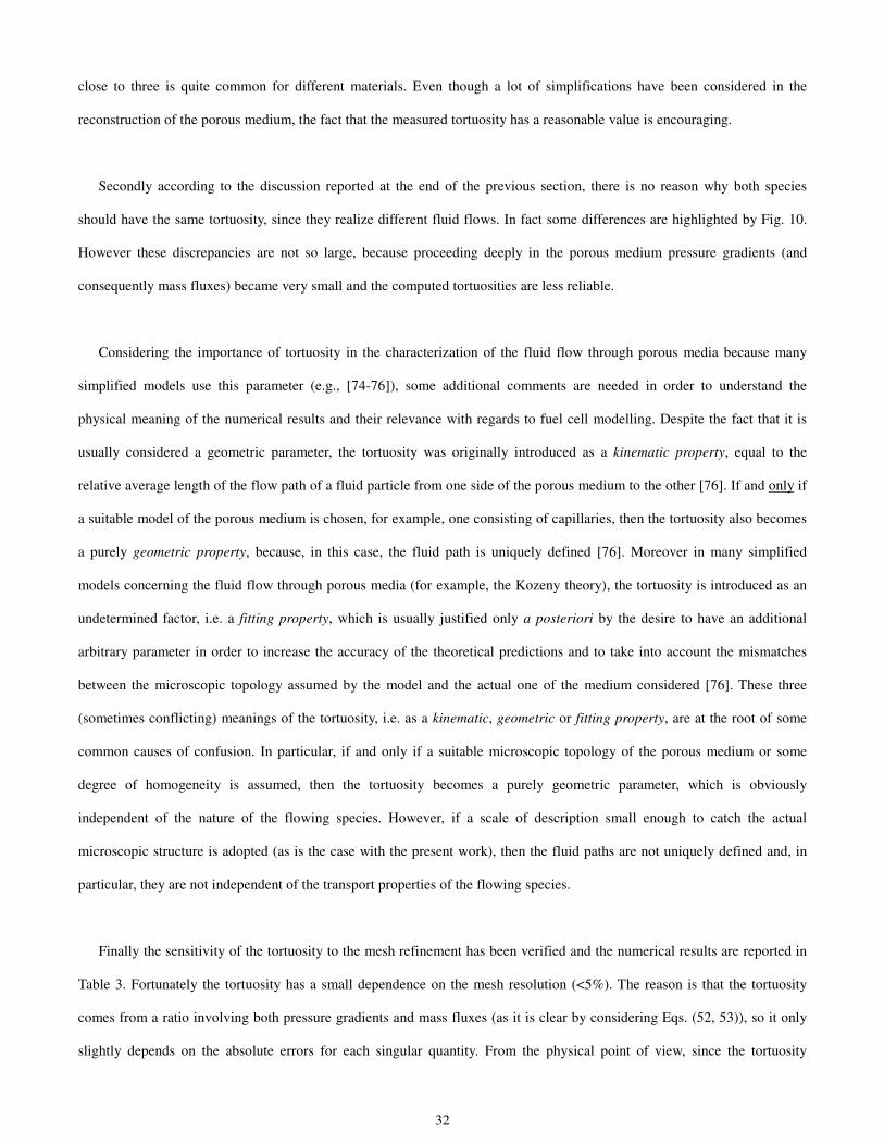
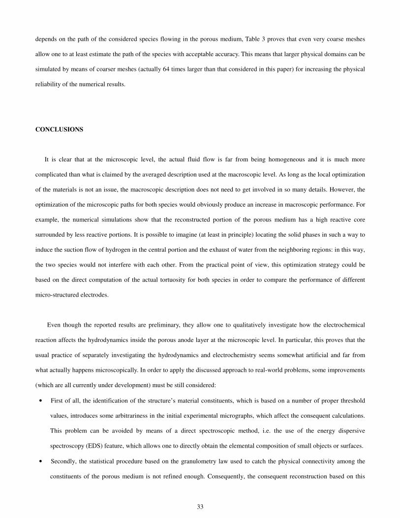
Once the fluid flow is known, the macroscopic tortuosity can be computed. The basic idea is to interpolate the surface

averaged values obtained by means of the mesoscopic simulations for both the mass fluxes and the density perturbations

(difference between actual density and the bulk density in the gas channel flow), as reported in Figs. 8 and 9 respectively.

There is no physical principle which forces the surface averaged quantities to be continuous. Obviously the mesoscopic

(or scale-level) quantities must be continuous (if we neglect rarefaction effects) because of the conservation laws. However

the surface averaging does not preserve the exact continuity, since it is applied to parallel surfaces (moving from the gas

channel deeply in the porous medium) which do not share the same microscopic topology. The interpolation is need for

ensuring smooth functions, which can be easily derived.

Applying the surface averaging operator to Eq. (15) yields

/I Am

A A A

dp dzu u

λρ ρ

−< >=

< > − < >. (52)

The tortuosity can be computed by taking into account that

1/

1/

ImIe m

DD

λετλ

< >= = . (53)

The numerical results are reported in the Fig. 10 for the same test case considered in Figs. 8 and 9. First of all, the computed

tortuosities reasonably well match the practical values used for characterizing the SOFC anodes [6]. In particular a value

32

close to three is quite common for different materials. Even though a lot of simplifications have been considered in the

reconstruction of the porous medium, the fact that the measured tortuosity has a reasonable value is encouraging.

Secondly according to the discussion reported at the end of the previous section, there is no reason why both species

should have the same tortuosity, since they realize different fluid flows. In fact some differences are highlighted by Fig. 10.

However these discrepancies are not so large, because proceeding deeply in the porous medium pressure gradients (and

consequently mass fluxes) became very small and the computed tortuosities are less reliable.

Considering the importance of tortuosity in the characterization of the fluid flow through porous media because many

simplified models use this parameter (e.g., [74-76]), some additional comments are needed in order to understand the

physical meaning of the numerical results and their relevance with regards to fuel cell modelling. Despite the fact that it is

usually considered a geometric parameter, the tortuosity was originally introduced as a kinematic property, equal to the

relative average length of the flow path of a fluid particle from one side of the porous medium to the other [76]. If and only if

a suitable model of the porous medium is chosen, for example, one consisting of capillaries, then the tortuosity also becomes

a purely geometric property, because, in this case, the fluid path is uniquely defined [76]. Moreover in many simplified

models concerning the fluid flow through porous media (for example, the Kozeny theory), the tortuosity is introduced as an

undetermined factor, i.e. a fitting property, which is usually justified only a posteriori by the desire to have an additional

arbitrary parameter in order to increase the accuracy of the theoretical predictions and to take into account the mismatches

between the microscopic topology assumed by the model and the actual one of the medium considered [76]. These three

(sometimes conflicting) meanings of the tortuosity, i.e. as a kinematic, geometric or fitting property, are at the root of some

common causes of confusion. In particular, if and only if a suitable microscopic topology of the porous medium or some

degree of homogeneity is assumed, then the tortuosity becomes a purely geometric parameter, which is obviously

independent of the nature of the flowing species. However, if a scale of description small enough to catch the actual

microscopic structure is adopted (as is the case with the present work), then the fluid paths are not uniquely defined and, in

particular, they are not independent of the transport properties of the flowing species.

Finally the sensitivity of the tortuosity to the mesh refinement has been verified and the numerical results are reported in

Table 3. Fortunately the tortuosity has a small dependence on the mesh resolution (<5%). The reason is that the tortuosity

comes from a ratio involving both pressure gradients and mass fluxes (as it is clear by considering Eqs. (52, 53)), so it only

slightly depends on the absolute errors for each singular quantity. From the physical point of view, since the tortuosity

33

depends on the path of the considered species flowing in the porous medium, Table 3 proves that even very coarse meshes

allow one to at least estimate the path of the species with acceptable accuracy. This means that larger physical domains can be

simulated by means of coarser meshes (actually 64 times larger than that considered in this paper) for increasing the physical

reliability of the numerical results.

CONCLUSIONS

It is clear that at the microscopic level, the actual fluid flow is far from being homogeneous and it is much more

complicated than what is claimed by the averaged description used at the macroscopic level. As long as the local optimization

of the materials is not an issue, the macroscopic description does not need to get involved in so many details. However, the

optimization of the microscopic paths for both species would obviously produce an increase in macroscopic performance. For

example, the numerical simulations show that the reconstructed portion of the porous medium has a high reactive core

surrounded by less reactive portions. It is possible to imagine (at least in principle) locating the solid phases in such a way to

induce the suction flow of hydrogen in the central portion and the exhaust of water from the neighboring regions: in this way,

the two species would not interfere with each other. From the practical point of view, this optimization strategy could be

based on the direct computation of the actual tortuosity for both species in order to compare the performance of different

micro-structured electrodes.

Even though the reported results are preliminary, they allow one to qualitatively investigate how the electrochemical

reaction affects the hydrodynamics inside the porous anode layer at the microscopic level. In particular, this proves that the

usual practice of separately investigating the hydrodynamics and electrochemistry seems somewhat artificial and far from

what actually happens microscopically. In order to apply the discussed approach to real-world problems, some improvements

(which are all currently under development) must be still considered:

• First of all, the identification of the structure’s material constituents, which is based on a number of proper threshold

values, introduces some arbitrariness in the initial experimental micrographs, which affect the consequent calculations.

This problem can be avoided by means of a direct spectroscopic method, i.e. the use of the energy dispersive

spectroscopy (EDS) feature, which allows one to directly obtain the elemental composition of small objects or surfaces.

• Secondly, the statistical procedure based on the granulometry law used to catch the physical connectivity among the

constituents of the porous medium is not refined enough. Consequently, the consequent reconstruction based on this

34

information is not completely reliable. The use of a two–point statistics, which directly takes into account the

connectivity among the material constituents, would be highly welcomed and is under development.

• Finally, the ion and electron dynamics must be included in the numerical model, meaning that two additional equations

for the corresponding potential flows must be solved. This would allow one to include the Butler – Volmer relation for

the active TPBs, in order to model the electrochemical reactions, which, in this way, would take into account the

activation overpotential and the local concentrations.

Acknowledgments

B. V. Kasula would like to thank Prof. Michele Calì for offering him the opportunity of spending time at the “Politecnico

di Torino”, during which time part of this work was done and Prof. Romano Borchiellini for his support. P. Asinari would like

to thank Dr. Marco Coppo for his precious help during the early coding phase. P. Asinari and Prof. M. Calì would like to

thank Prof. Romano Borchiellini for promoting the set-up of the new cluster facility at “Politecnico di Torino”, CESIT for

powering its practical development, in particular Giuliano Appino and Nicola Gentile for their useful help.

The authors would like to acknowledge ASME as original publisher of the proceedings of ESDA2006 8th Biennial

ASME Conference on “Engineering Systems Design and Analysis”, during which part of this work was presented.

REFERENCES

[1] Larminie, J., Dicks, A.L., “Fuel Cells Systems Explained”, Wiley, New York, 2000.

[2] S. Srinivasan, R. Mosdale, P. Stevens, C. Yang, “Fuel cells: Reaching the era of clean and efficient power generation

in the twenty-first century”, Annual Review of Energy and the Environment, Vol. 24, pp. 281-328, 1999.

[3] F.J. Gardner, “Thermodynamic processes in solid oxide and other fuel cells”, Proceedings of the Institution of

Mechanical Engineers, Part A: Journal of Power and Energy, Vol. 211, n. 5, pp. 367-380, 1997.

[4] Singhal S.C., “Advances in solid oxide fuel cell technology”, Solid State Ionics, Vol. 135, pp. 305-313, 2000.

[5] McEvoy A.J., “Thin SOFC electrolytes and their interfaces – A near-term research strategy”, Solid State Ionics, Vol.

132, pp.159-165, 2000.

[6] T. Ackmann, L.G.J. Haart, W. Lehnert, F. Thom, “Modeling of mass and heat transport in thick-substrate thin-

electrolyte layer SOFCs”, proceedings of the 4th European Solid Oxide Fuel Cell Forum, Lucerne/Switzerland, pp.

431-438, 2000.

35

[7] A. Weber et Al., “Materials and concepts for solid oxide fuel cells (SOFCs) in stationary and mobile applications”,

Journal of Power Sources, Vol. 127, pp.273-283, 2004.

[8] A. Weber et Al., “Oxidation of H2, CO, and methane in SOFCs with Ni/YSZ-cermet anodes”, Solid State Ionics,

Vol. 152-153, pp.543-550, 2004.

[9] U. Stimming et Al., “Operation of anode-supported thin electrolyte film solid oxide fuel cells at 800 ° C and below”,

J. of Power Souces, Vol. 71, pp.302-305, 1996.

[10] U. Stimming et Al., “Advances, aging mechanisms and lifetime in solid oxide fuel cells”, J. of Power Souces, Vol.

127, pp.284-293 , 2004.

[11] M. Mogensen et Al., “Durability and thermal cycling of Ni/YSZ cermet anodes for solid oxide fuel cells”, Journal of

Applied Electrochemistry, Vol. 30, Issue 2, pp 247-257, 2000.

[12] T. Fukuia et Al., “Performance and stability of SOFC anode fabricated from NiO/YSZ composite particles”, Journal

of the European Ceramic Society, Vol. 23, pp. 2963–2967, 2003.

[13] T. Iwata et Al., “Characterization of Ni-YSZ anode degradation for substrate-Type solid oxide fuel cells”, J.

Electrochemical society, Vol. 143, pp.1521-1525, 1996.

[14] Stover et Al., “Modelling of the agglomeration of Ni-particles in anodes of solid oxide fuel cells”, Vol. 36, pp.147-

151, 2001.

[15] A. Ioselevich et Al., “Degradation of solid oxide fuel cell anode”, J. Electrochemical society, Vol. 144, pp.3010-

3018, 1997.

[16] C.C. Appel,“Durability test of SOFC cathodes”, Journal of Applied Electrochemistry, Vol. 30, pp.411-418, 2000.

[17] U. Stimming et Al., “Catalysis of the electrochemical processes on solid oxide fuel cell cathodes”, J. of Power

Souces, Vol. 61, pp.205-211, 1998.

[18] Y. Nigara et Al., “Hydrogen permeability of YSZ single crystals at high temperatures”, Solid State Ionics, Vol. 171,

pp.61-67 , 2004.

[19] M. Mogensen et Al., “Factors controlling the oxide ion conductivity of fluorite and perovskite structured oxides”, ”,

Solid State Ionics, Vol.174, pp.279-286, 2004.

[20] F. Iguchi et Al., “Oxygen partial pressure dependence of creep on yttria-doped ceria ceramics”, Solid State Ionics

Vol. 176, pp. 641–644, 2005.

[21] G. Di Giuseppe et al., “Fuel sensitivity tests in tubular solid oxide fuel cells”, J. of Power Souces, Vol. 125, pp.183-

188 , 2004.

36

[22] Lee J.-H., Heo J.-W., Lee D.-S., Kim J., Kim G.-H., Lee H.-W., Song H.S., “Moon J.-H., The impact of anode

microstructure on the power generating characteristics of SOFC”, Solid State Ionics, Vol. 158, pp. 225-232, 2003.

[23] Chan S.H., Khor K.A., Xia Z.T., “A complete polarization model of a solid oxide fuel cell and its sensitivity to the

change of cell component thickness”, Journal of Power Sources, Vol. 93, pp. 130-140, 2001.

[24] A.VOL. Virkar, J. Chen, C.W. Tanner, J.W. Kim, “The role of electrode microstructure on activation and

concentration polarizations in solid oxide fuel cells”, Solid State Ionics, Vol. 131, pp. 189-198, 2000.

[25] Lehnert W., Meusinger J., Thom F., “Modelling of gas transport phenomena in SOFC anodes”, Journal of Power

Sources, Vol. 87, pp. 57-63, 2000.

[26] T. Nishino, H. Komori, H. Iwai, K. Suzuki, “Development of a comprehensive numerical model for analyzing a

tubular-type indirect internal reforming SOFC”, proceedings of First International Conference on Fuel Cell Science,

Engineering and Technology, Rochester NY, 2003.

[27] W.A. Rogers, R.S. Gemmen, C. Johnson, M. Prinkey, M. Shahnam, “Validation and application of a CFD-based

model for solid oxide fuel cells and stacks”, proceedings of First International Conference on Fuel Cell Science,

Engineering and Technology, Rochester NY, 2003.

[28] P.W. Li, M.K. Chyu, “Simulation of the chemical/electrochemical reactions and heat/mass transfer for a tubular

SOFC in a stack”, Journal of Power Sources, Vol. 124, n. 2, pp. 487-498, 2003.

[29] Bessette II N.F., Wepfer W.J., Winnick J., “A mathematical model of a solid oxide fuel cell”, Journal of the

Electrochemical Society, Vol. 142, pp. 3792-3800, 1995.

[30] D. Arnost, P. Schneider, “Dynamic transport of multicomponent mixtures of gases in porous solids”, Chemical

Engineering Journal, Vol. 57, pp. 91–99, 1995.

[31] P. Asinari, M. Coppo, “Influence of Porous Electrode Structure on PEM Fuel Cells Design and Performance”,

Proceedings of the 2nd International Conference on Fuel Cell Science, Engineering and Technology, ASME,

Rochester N.Y., 2004.

[32] D. H. Rothman, “Cellular automaton fluids: a model for flow in porous media”, Geophysics, Vol. 53, p. 509, 1988.

[33] J. Bernsdorf, M. Schafer, F. Durst, “Comparison of Cellular Automata and Finite Volume Techniques for simulation

of incompressible Flow in Complex Geometries”, International Journal of Numerical Methods in Fluids, Vol. 29, p.

251, 1999.

[34] J. Bernsdorf, G. Brenner, F. Durst, “Numerical analysis of the pressure drop in porous media flow with lattice

Boltzmann (BGK) automata“, Computer Physics Communications, Vol. 129, p. 246-255, 2000.

37

[35] S. Succi, R. Benzi, F. Higuera, “The lattice-Boltzmann equation: a new tool for computational fluid dynamics”,

Lattice Gas Methods: Theory, Applications and Hardware, edited by G. Doolen (Elsevier, Amsterdam), reprinted from

Physica D, Vol. 47, p. 219, 1991.

[36] S. Chen, G. D. Doolen, “Lattice Boltzmann method for fluid flow”, Annual Review of Fluid Mechanics, Vol. 30, p.

329-338, 1998.

[37] B. Manz, L.F. Gladden, P.B. Warren, “Flow and Dispersion in Porous Media: Lattice-Boltzmann and NMR Studies”,

AIChE. Journal, Vol. 45, pp. 1845, 1999.

[38] Th. Zeiser, P. Lammers, E. Klemm, Y.W. Li, J. Bernsdorf, G. Brenner, “CFD-Calculation of Flow, Dispersion and

Reaction in a Catalyst Filled Tube by Lattice Boltzmann Method”, Chemical Engineering Science, Vol. 56, pp. 1697,

2001.

[39] E.G. Flekkoy, “Lattice Bhatnagar-Gross-Krook models for miscible fluids”, Physics Review E, Vol. 47, pp. 4247,

1993.

[40] X. Shan, G. Doolen, “Multicomponent lattice-Boltzmann model with interparticle interaction “, Journal of Statistical

Physics, Vol. 81, pp. 379, 1995.

[41] V. Sofonea, R.F. Sekerka, “BGK models for diffusion in isothermal binary fluid systems “, Physica A, Vol. 299, pp.

494, 2001.

[42] Z. Guo, T.S. Zhao, “Discrete velocity and lattice Boltzmann models for binary mixtures of nonideal fluids “, Physics

Review E, Vol. 68, N. 035302, 2003.

[43] L.-S. Luo, S.S. Girimaji, “Theory of the lattice Boltzmann method: Two-fluid model for binary mixtures “, Physics

Review E, Vol. 67, N. 036302, 2003.

[44] K. Xu, “BGK-Based Scheme for Multicomponent Flow Calculations”, Journal of Computational Physics, Vol. 134,

pp. 122, 1997.

[45] K. Xu, “A Gas-Kinetic Scheme for Multimaterial Flows and Its Application in Chemical Reactions”, Journal of

Computational Physics, Vol. 163, pp. 349, 2000.

[46] P. Asinari, “Viscous coupling based lattice Boltzmann model for binary mixtures”, Physics of Fluids, 17, 067102,

2005.P. Asinari, M. Coppo, M.R. von Spakovsky, B.V. Kasula, “Numerical simulations of gaseous mixture flow in

porous electrodes for PEM fuel cells by the lattice Boltzmann method”, proceedings of the “Third International

Conference on Fuel Cell Science, Engineering and Technology”, Ypsilanti, Michigan, 2005.

[48] P. Asinari, “Asymptotic analysis of multiple-relaxation-time lattice Boltzmann schemes for mixture modeling”,

Computers and Mathematics with Applications, 2006 (in press).P. Asinari, “Semi-implicit-linearized Multiple-

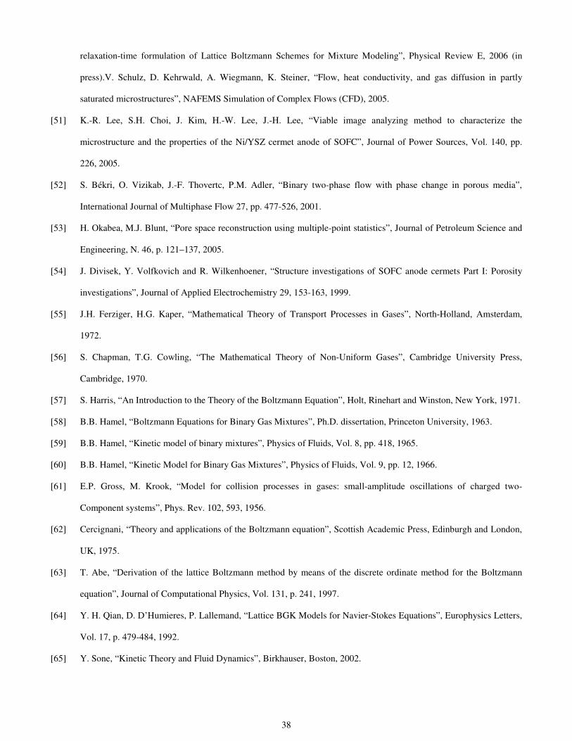
38

relaxation-time formulation of Lattice Boltzmann Schemes for Mixture Modeling”, Physical Review E, 2006 (in

press).V. Schulz, D. Kehrwald, A. Wiegmann, K. Steiner, “Flow, heat conductivity, and gas diffusion in partly

saturated microstructures”, NAFEMS Simulation of Complex Flows (CFD), 2005.

[51] K.-R. Lee, S.H. Choi, J. Kim, H.-W. Lee, J.-H. Lee, “Viable image analyzing method to characterize the

microstructure and the properties of the Ni/YSZ cermet anode of SOFC”, Journal of Power Sources, Vol. 140, pp.

226, 2005.

[52] S. Békri, O. Vizikab, J.-F. Thovertc, P.M. Adler, “Binary two-phase flow with phase change in porous media”,

International Journal of Multiphase Flow 27, pp. 477-526, 2001.

[53] H. Okabea, M.J. Blunt, “Pore space reconstruction using multiple-point statistics”, Journal of Petroleum Science and

Engineering, N. 46, p. 121–137, 2005.

[54] J. Divisek, Y. Volfkovich and R. Wilkenhoener, “Structure investigations of SOFC anode cermets Part I: Porosity

investigations”, Journal of Applied Electrochemistry 29, 153-163, 1999.

[55] J.H. Ferziger, H.G. Kaper, “Mathematical Theory of Transport Processes in Gases”, North-Holland, Amsterdam,

1972.

[56] S. Chapman, T.G. Cowling, “The Mathematical Theory of Non-Uniform Gases”, Cambridge University Press,

Cambridge, 1970.

[57] S. Harris, “An Introduction to the Theory of the Boltzmann Equation”, Holt, Rinehart and Winston, New York, 1971.

[58] B.B. Hamel, “Boltzmann Equations for Binary Gas Mixtures”, Ph.D. dissertation, Princeton University, 1963.

[59] B.B. Hamel, “Kinetic model of binary mixtures”, Physics of Fluids, Vol. 8, pp. 418, 1965.

[60] B.B. Hamel, “Kinetic Model for Binary Gas Mixtures”, Physics of Fluids, Vol. 9, pp. 12, 1966.

[61] E.P. Gross, M. Krook, “Model for collision processes in gases: small-amplitude oscillations of charged two-

Component systems”, Phys. Rev. 102, 593, 1956.

[62] Cercignani, “Theory and applications of the Boltzmann equation”, Scottish Academic Press, Edinburgh and London,

UK, 1975.

[63] T. Abe, “Derivation of the lattice Boltzmann method by means of the discrete ordinate method for the Boltzmann

equation”, Journal of Computational Physics, Vol. 131, p. 241, 1997.

[64] Y. H. Qian, D. D’Humieres, P. Lallemand, “Lattice BGK Models for Navier-Stokes Equations”, Europhysics Letters,

Vol. 17, p. 479-484, 1992.

[65] Y. Sone, “Kinetic Theory and Fluid Dynamics”, Birkhauser, Boston, 2002.

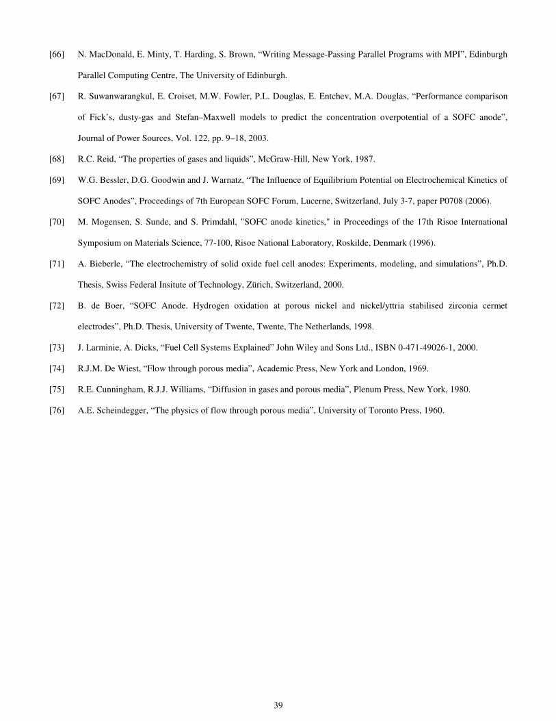
39

[66] N. MacDonald, E. Minty, T. Harding, S. Brown, “Writing Message-Passing Parallel Programs with MPI”, Edinburgh

Parallel Computing Centre, The University of Edinburgh.

[67] R. Suwanwarangkul, E. Croiset, M.W. Fowler, P.L. Douglas, E. Entchev, M.A. Douglas, “Performance comparison

of Fick’s, dusty-gas and Stefan–Maxwell models to predict the concentration overpotential of a SOFC anode”,

Journal of Power Sources, Vol. 122, pp. 9–18, 2003.

[68] R.C. Reid, “The properties of gases and liquids”, McGraw-Hill, New York, 1987.

[69] W.G. Bessler, D.G. Goodwin and J. Warnatz, “The Influence of Equilibrium Potential on Electrochemical Kinetics of

SOFC Anodes”, Proceedings of 7th European SOFC Forum, Lucerne, Switzerland, July 3-7, paper P0708 (2006).

[70] M. Mogensen, S. Sunde, and S. Primdahl, "SOFC anode kinetics," in Proceedings of the 17th Risoe International

Symposium on Materials Science, 77-100, Risoe National Laboratory, Roskilde, Denmark (1996).

[71] A. Bieberle, “The electrochemistry of solid oxide fuel cell anodes: Experiments, modeling, and simulations”, Ph.D.

Thesis, Swiss Federal Insitute of Technology, Zürich, Switzerland, 2000.

[72] B. de Boer, “SOFC Anode. Hydrogen oxidation at porous nickel and nickel/yttria stabilised zirconia cermet

electrodes”, Ph.D. Thesis, University of Twente, Twente, The Netherlands, 1998.

[73] J. Larminie, A. Dicks, “Fuel Cell Systems Explained” John Wiley and Sons Ltd., ISBN 0-471-49026-1, 2000.

[74] R.J.M. De Wiest, “Flow through porous media”, Academic Press, New York and London, 1969.

[75] R.E. Cunningham, R.J.J. Williams, “Diffusion in gases and porous media”, Plenum Press, New York, 1980.

[76] A.E. Scheindegger, “The physics of flow through porous media”, University of Toronto Press, 1960.

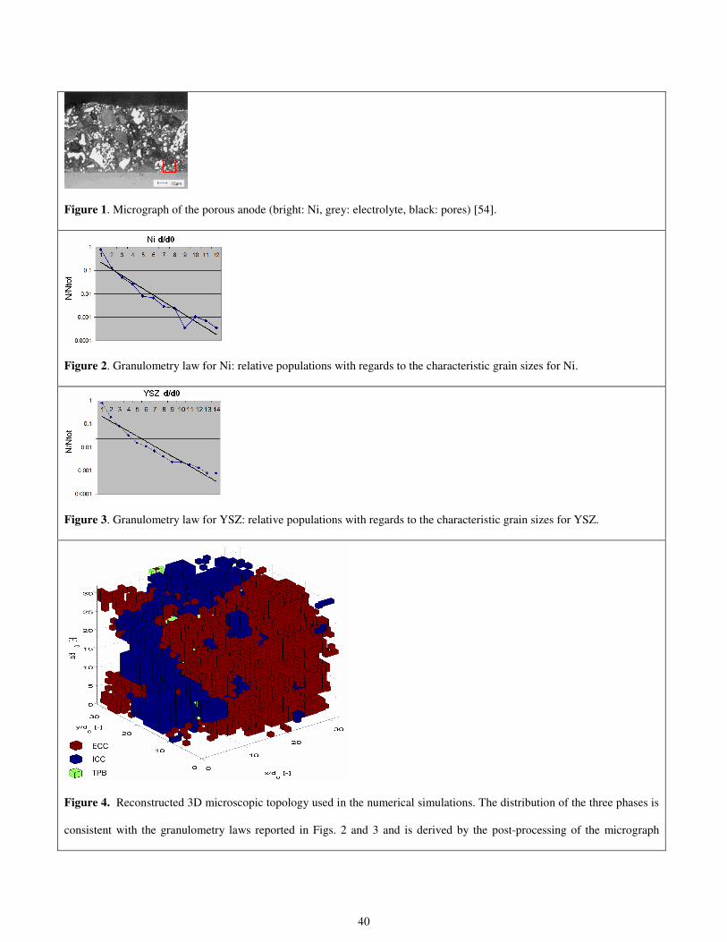
40

Figure 1. Micrograph of the porous anode (bright: Ni, grey: electrolyte, black: pores) [54].

Figure 2. Granulometry law for Ni: relative populations with regards to the characteristic grain sizes for Ni.

Figure 3. Granulometry law for YSZ: relative populations with regards to the characteristic grain sizes for YSZ.

Figure 4. Reconstructed 3D microscopic topology used in the numerical simulations. The distribution of the three phases is

consistent with the granulometry laws reported in Figs. 2 and 3 and is derived by the post-processing of the micrograph

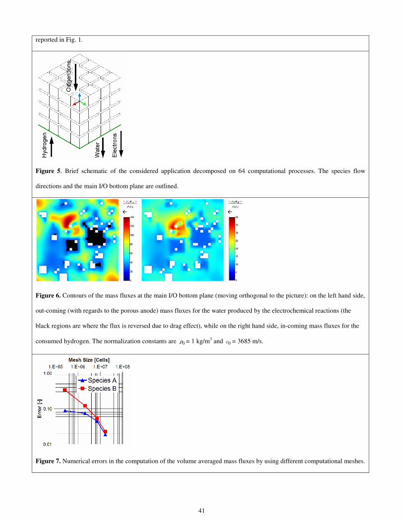
41

reported in Fig. 1.

Figure 5. Brief schematic of the considered application decomposed on 64 computational processes. The species flow

directions and the main I/O bottom plane are outlined.

Figure 6. Contours of the mass fluxes at the main I/O bottom plane (moving orthogonal to the picture): on the left hand side,

out-coming (with regards to the porous anode) mass fluxes for the water produced by the electrochemical reactions (the

black regions are where the flux is reversed due to drag effect), while on the right hand side, in-coming mass fluxes for the

consumed hydrogen. The normalization constants are 0ρ = 1 kg/m3 and 0c = 3685 m/s.

Figure 7. Numerical errors in the computation of the volume averaged mass fluxes by using different computational meshes.

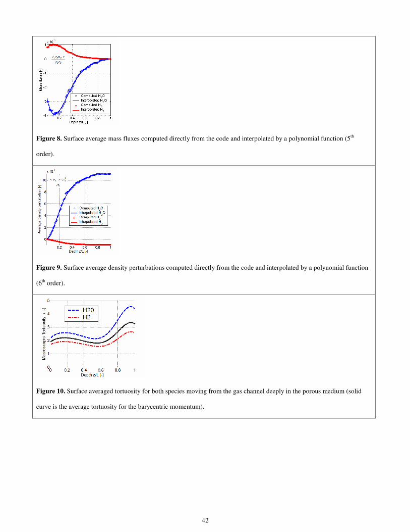
42

Figure 8. Surface average mass fluxes computed directly from the code and interpolated by a polynomial function (5th

order).

Figure 9. Surface average density perturbations computed directly from the code and interpolated by a polynomial function

(6th order).

Figure 10. Surface averaged tortuosity for both species moving from the gas channel deeply in the porous medium (solid

curve is the average tortuosity for the barycentric momentum).

43

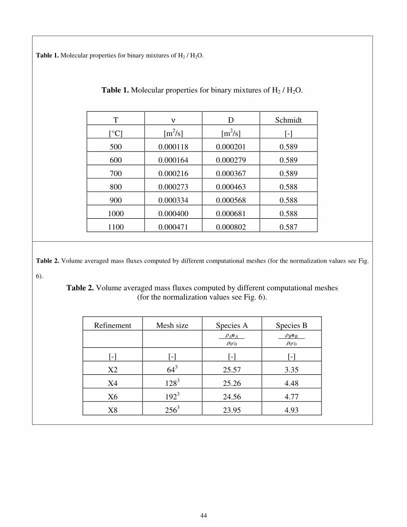
44

Table 1. Molecular properties for binary mixtures of H2 / H2O.

Table 1. Molecular properties for binary mixtures of H2 / H2O.

T ν D Schmidt

[°C] [m2/s] [m2/s] [-]

500 0.000118 0.000201 0.589

600 0.000164 0.000279 0.589

700 0.000216 0.000367 0.589

800 0.000273 0.000463 0.588

900 0.000334 0.000568 0.588

1000 0.000400 0.000681 0.588

1100 0.000471 0.000802 0.587

Table 2. Volume averaged mass fluxes computed by different computational meshes (for the normalization values see Fig.

6).

Table 2. Volume averaged mass fluxes computed by different computational meshes (for the normalization values see Fig. 6).

Refinement Mesh size Species A Species B

0 0

A Ac

ρρ

u 0 0

B Bc

ρρ

u

[-] [-] [-] [-]

X2 643 25.57 3.35

X4 1283 25.26 4.48

X6 1923 24.56 4.77

X8 2563 23.95 4.93

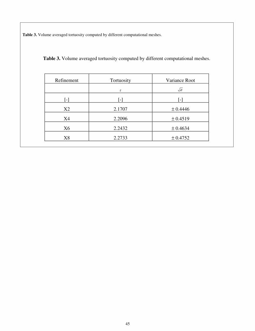
45

Table 3. Volume averaged tortuosity computed by different computational meshes.

Table 3. Volume averaged tortuosity computed by different computational meshes.

Refinement Tortuosity Variance Root

τ σ

[-] [-] [-]

X2 2.1707 ± 0.4446

X4 2.2096 ± 0.4519

X6 2.2432 ± 0.4634

X8 2.2733 ± 0.4752