Direct measurement of the system-environment coupling as a tool for understandingdecoherence and dynamical decoupling

Ido Almog1, Yoav Sagi1, Goren Gordon2, Guy Bensky2, Gershon Kurizki2, and Nir Davidson1

1Department of Physics of Complex Systems, Weizmann Institute of Science, Rehovot 76100, Israel and2Department of Chemical Physics, Weizmann Institute of Science, Rehovot 76100, Israel

Decoherence is a major obstacle to any practical implementation of quantum information pro-cessing. One of the leading strategies to reduce decoherence is dynamical decoupling — the useof an external field to average out the effect of the environment. The decoherence rate under anycontrol field can be calculated if the spectrum of the coupling to the environment is known. Wepresent a direct measurement of the bath coupling spectrum in an ensemble of optically trappedultracold atoms, by applying a spectrally narrow-band control field. The measured spectrum followsa Lorentzian shape at low frequencies, but exhibits non-monotonic features at higher frequencies dueto the oscillatory motion of the atoms in the trap. These features agree with our analytical mod-els and numerical Monte-Carlo simulations of the collisional bath. From the inferred bath-couplingspectrum, we predict the performance of well-known dynamical decoupling sequences: CPMG, UDDand CDD. We then apply these sequences in experiment and compare the results to predictions,finding good agreement in the weak-coupling limit. Thus, our work establishes experimentally thevalidity of the overlap integral formalism, and is an important step towards the implementation ofan optimal dynamical decoupling sequence for a given measured bath spectrum.

I. INTRODUCTION

In any implementation of quantum information pro-cessing by qubits [1] it is crucial to keep the qubits coher-ent for long periods of times. The qubits, however, arenever completely isolated from the environment. Thiscoupling to the environment means that after some timean entanglement between the system (the qubits) and theenvironment (all other degrees of freedom) is established.Usually the environment (bath) consists of many degreesof freedom which are not controlled. This means that onehas to trace over these degrees of freedom to obtain thestate of the system. The entanglement to the bath andthe tracing leave the system in a separable classical state.Obviously, the resulting loss of coherence (decoherence)is one of the major obstacles towards the successful im-plementation of quantum information processing.

Over the years, several strategies have been suggestedto cope with the decoherence problem. Clearly, the firstthing to do is to minimize the coupling to the environ-ment. Borrowing ideas from classical error correctiontheory, it was shown that by encoding a logical qubit inseveral physical qubits, it is possible to correct for er-rors which are introduced in the calculation process [1].Quantum error correction protocols can correct errors upto some maximal rate. The upper bound on the errorprobability of a quantum gate depends on the details ofthe error correction protocol, but the typical values rangefrom 10−4 to 10−2. The gate can also be an identity gatewhich describes the storage of information in a quantummemory. Such a memory is essential in the architectureof a quantum network in order to enable scalability [2].

Dynamical decoupling (DD) is a technique that was de-veloped to further reduce the error rate below the faulttolerant threshold [3–7]. The main idea of DD is to useexternal control fields that induce rotations of the qubitin the Bloch sphere such that the overall decoherence is

reduced. This method was first considered in the con-text of nuclear magnetic resonance [8–10]. In the field ofquantum information processing, the pursuit for fault tol-erance has pushed forward the development of a similarformalism for controlling the decoherence of noisy qubits[3, 4, 6]. The simplest example of DD is the well-knownHahn echo technique: a single population inverting pulse(π-pulse) is introduced exactly at half the final observa-tion time [11]. The echo technique is widely used andvery efficient in counteracting the effect of a quasi-staticcoupling to the environment. Once the coupling spec-trum extends to higher frequencies, the echo techniquefails and more elaborate control sequences are needed.

A strategy aimed at maximizing the decoupling hasbeen developed by Kofman and Kurizki [12–17], based ona formula that relates the decoherence rate to the over-lap of the bath coupling spectrum on the control powerspectrum. This overlap can be minimized under the con-straint of the available control field energy [15, 17]. Inorder to successfully implement this decoupling controlstrategy, detailed knowledge of the bath-coupling spec-trum is required. In this work, we explain how to measurethis spectrum, and then use it to calculate the coherenceof the system after a DD sequence has been applied. Theexperiments we present are performed in an ensemble ofultra-cold atoms held together by a potential induced bya far-off resonance laser field. This system is used notonly for demonstration purposes, but also because it canserve as a quantum memory [18–23].

Two of the most widely used physical qubits are pho-tons and neutral atoms. Photons are easy to produce,manipulate and transport. They interact weakly withtheir environment and therefore can remain coherent forlong travel distances. This last advantage is also theirdisadvantage: interactions between photons are usuallyvery small, making the implementation of an all-opticaltwo-qubit gate very difficult. Atoms, on the other hand,

arX

iv:1

103.

1104

v1 [

quan

t-ph

] 6

Mar

201

1

2

are easy to keep in one place, and can interact stronglywith other atoms and electromagnetic fields. It is there-fore sensible to use atoms as “stationary qubits” for stor-age and manipulation and use photons as “flying qubits”that carry the information between distant sites.

One of the controlled schemes of interaction betweenatoms and photons is electromagnetically induced trans-parency (EIT) [24]. In this scheme, atoms with a lambda-shape energy structure interact with two light fieldscalled “pump” and “probe”. The pump is usually muchstronger than the probe, and is used to control the inter-action strength between the probe and the atomic ensem-ble. Turning off the pump while the probe is propagatingin the atomic ensemble leads to a conversion of the pho-tonic excitation into the coherence between the two low-lying states of the atoms. This is sometimes called “stor-age of light”, although only the coherence which was car-ried by the light is actually stored in the ensemble. Thebeauty of this conversion process is that it is reversible,which makes the atomic ensemble a true memory.

In order to increase the efficiency of the storage andretrieval processes, it is desirable to work with atomicensembles with high optical depth [25, 26]. This is be-cause the coupling of the atoms to the external electro-magnetic field scales as the square root of the number ofatoms in a volume where the light intensity is approxi-mately uniform. Working at high optical depth, however,usually implies that the atomic density is high and therate of inter-particle collisions is large compared to thestorage time. The coherence properties of the atomicensemble are markedly changed due to elastic collisions[27]. From the point of view of a particular atom, otheratoms can be regarded as the bath. The collisions withother atoms define the nature of the coupling to the bath.The three important physical quantities in the descrip-tion of the collisional bath are: the collision rate, theinhomogeneous dephasing rate (i.e. the dephasing with-out collisions) and the harmonic confinement oscillationfrequency. The spectral behavior of the collisional reser-voir stems from the interplay between these quantities.

The goal of this work is to present a general method ofmeasuring the bath-coupling spectrum, and demonstrateits usefulness in calculating the result of any control field.We start by reviewing the mathematical formalism ofthe overlap integral spectrum and the power spectrumof the control sequence that acts as filter function (Sec-tion II). Using this formalism it is possible to calculatefrom the bath-coupling spectrum the coherence at someobservation time with any control sequence, as long asthe so-called ’weak coupling’ limit applies. In particular,it can be used with a null control sequence, which simplydescribes a dephasing process. For a known filter func-tion of the control field, it is possible to de-convolve theoverlap integral to obtain the bath-coupling spectrum.We present this technique for a constant-power contin-uous control field in Section III, and illustrate it by full3D Monte-Carlo simulations. We then employ the tech-nique to measure directly the collisional bath spectrum

in our cold atomic ensemble (Section IV). The measuredbath shows interesting non-monotonic behavior due tothe oscillatory motion of the atoms in the trap. Once thebath-coupling spectrum is known, it is interesting to testits implications for the outcome of other DD sequences.This is done in Section V, where we use the measuredbath and the overlap-integral formalism to calculate thecoherence under the well-known CPMG, UDD and CDDsequences. We then experimentally apply these DD se-quences and compare the results with the predictions ofthe theoretical calculations based on the measured bath.We conclude and give our outlook in Section VI.

II. THE SPECTRAL OVERLAP INTEGRALAPPROACH TO THE FIDELITY CALCULATION

In this section we review the formalism [12–17] whichis useful to calculate the ensemble coherence at a giventime. Here we give a simplified version of this approachassuming an effective two-level stochastic Hamiltonianweakly coupled to the environment.

We consider the same model as was described in Ref.[28]. Our ensemble consists of two-level systems (TLS),and due to inhomogeneities in the external environment,the transition energy of each TLS is different than thefrequency it may have in free space (we shall call thisdifference the detuning). We reduce the full many-bodyHamiltonian to an effective single particle Hamiltoniangiven by

H = h [ω0 + δ(t)] |2〉 〈2|+ hΩ(t) |2〉 〈1|+ h.c. , (1)

where ω0 is the free space transition frequency betweenthe two states, δ(t) is the detuning, and Ω(t) is a classicalexternal control field which is going to be used for theDD. The detuning is a random function of time, and weassume it is averaging to 0 over different realizations ofthe Hamiltonian. The reduced density matrix can becalculated by

ρ(t) = |φ(t)〉 〈φ(t)| , (2)

where φ(t) is the state of the system at time t with a spe-cific realization of the stochastic Hamiltonian, and theaverage is taken over many realizations. |φ(0)〉 is theinitial state of the system, and ultimately our goal is toconserve this state in the ensemble for as long as possi-ble. To characterize how well this goal is achieved it isinstructive to introduce the fidelity function:

F = 〈φ(0)| ρ(t) |φ(0)〉 , (3)

which starts at 1 and decays to 0.5 at long times.To make the model clearer, we now relate these defini-

tions to atomic ensembles [27]. In our system, ultracoldatoms are confined by an external optical potential. Al-though the atoms have many energy levels, we confine ourattention to two low-lying states with negligible sponta-

3

neous decay. The potential is not exactly the same forthe two states. The main source inhomogeneous broad-ening is that the energy difference between the two sates,which is proportional to the total energy of the atom, ischanging in space [29]. The phase space density of ourensemble is low enough to be considered classical (farfrom quantum degeneracy). The motion of the atom inthe external potential causes the transition frequency tochange in time. Since the ensemble consists of manyatoms, each with a different trajectory, measuring thecoherence of the ensemble gives the averages discussedabove in a single shot. In the experiment, the coherenceis measured in a time-domain Ramsey-like experiment,as described in Ref. [27].

We shall define two functions which are going to beuseful later for the calculation of the fidelity. First, thebath coupling spectrum characterizes the spectral con-tent of the coupling of the system to the bath and isdefined as

G(f) =

∫ ∞−∞

e−2πifτ 〈δ(t) · δ(t+ τ)〉 dτ , (4)

where 〈...〉 stands for the averaging over many realiza-tions of δ(t). G(f) is the Fourier transform of the timecorrelation function of δ(t). The second function we de-fine is a ’filter function’ which characterizes the powerspectrum of the control sequence:

Ft(f) =

∣∣∣∣∫ t

0

e−2πift · cos

(∫ t

0

Ω(τ)dτ

)dt

∣∣∣∣2 . (5)

Note that although Ft(f) is defined in the frequency do-main, it does depend on the observation time t.

A simple expression for the fidelity at time t can beobtained under the weak coupling assumption, namelythat the fidelity decay during the bath correlation time isnegligible. In this case the fidelity is given by the overlapintegral [12, 13, 15]:

F(t) =1

2(1 + e−R(t)t) , (6)

where R(t) is the decay rate given by the overlap integral

R(t) =2α

t

∫ t

0

G(f)Ft(f)df , (7)

where α is a constant between 0 and 1, depending onthe assumptions for the statistics of the initial state, inparticular, α = 1

4 for an initial state which is an equalsuperposition of the two internal states. Generally speak-ing, R(t) is not constant and therefore the decay in notexponential: a signature of the non-Markov time-domain.

A related quantity is the ensemble coherence, whichis defined to be the normalized off-diagonal element ofthe reduced density matrix [30]. In the overlap integralframework, the coherence is given by C(t) = e−R(t)t. Inthe Bloch sphere representation, the coherence is given by

the length of the Bloch vector, which is usually measuredby quantum state tomography [1, 28].

III. HOW TO MEASURE THE BATHCOUPLING SPECTRUM ?

In order for Eqs. (6-7) to be useful, one has to knowthe bath coupling spectrum G(f), preferably from ex-perimental data. This spectrum can be inferred fromEq. (7) by measuring the coherence for a given pulse se-quence with a known Ft(f). Obviously, if Ft(f) where aDirac δ function, the decay rate would be linearly propor-tional to the bath coupling spectrum. A good approxi-mation to a δ function can be obtained if the control fieldis nearly-continuous and on-resonant field. This controlfield causes Rabi oscillations with a frequency f0 whichdepends on its strength. The resulting filter function isa sinc-function centered around f0. To be more precise,the filter function is given by

Ft(f) =1

4t[sinc2(t(f − f0)) + sinc2(t(f + f0))

], (8)

where t is the pulse duration. For this pulse, assumingf0T 1, Eq. (7) yields the following decoherence rate:

R(f0) ∼=1

4G(f0) . (9)

We see, then, that by scanning the strength of the con-trol fields (thus scanning f0) and measuring the decayof coherence, it is possible to directly measure the bathcoupling spectrum.

To illustrate the method and check its sensitivity tothe weak-coupling assumption, we have run a 3D Monte-Carlo simulations of a cold atomic ensemble trapped inan optical potential. The simulation solves for the clas-sical Newtonian motion of 3500 atoms. The initial con-ditions of the atoms are drawn from a Boltzmann distri-bution, assuming a temperature of 7µK. As explainedpreviously, the fluctuations in our system originate fromelastic collisions between the atoms, and it is thereforenecessary to include them in the simulation. In order notto run into computational complexity problems, we havedeveloped a mean-field technique [31]. Once the trajec-tories of all the atoms are calculated, we calculate theenergy shift of the internal states induced by the exter-nal potential along the trajectory of each atom. In ourγ = 1.06µm-wavelength dipole trap, the differential shiftof the internal states is 6.6 · 10−5 times the overall po-tential [29]. These energy shifts are then used to solvethe Bloch equations [32] in the presence of the controlfield. We calculate the decoherence rate by computingthe length of the Bloch vector at different times and fitit to a decaying exponent.

We simulate a measurement of the bath spectral func-tion as described above by a continuous control field, intwo parameter regimes which correspond to weak and

4

strong coupling. The results of the simulations are de-picted in Figure 1. At low frequencies, the spectrum fol-lows a Lorentzian curve which is expected since the fluc-tuations originate from a scattering process with Poissonstatistics [28]. Also apparent in the spectrum is a non-monotonic feature, due to the oscillatory motion of theatoms in the trap (for more details see the next section).The only difference between the two simulations is thenumber of atoms, resulting in different correlation timesof the bath. It is interesting to note that by increasingthe number of atoms one also decreases the decoherencerate at low frequencies, a result of collisional narrowing(see Ref. [27] for more details). Thus, increasing thenumber of atoms increases both the collision rate andthe coherence time, thereby pushing the ensemble deeperinto the weak-coupling regime. Note that the relevantdecoherence rate for considering whether the system inweakly coupled is the decoherence rate obtained with thedecoupling pulse. This means that a system can be inthe strong-coupling regime at low frequencies and in theweak-coupling regime at high frequencies, whence devi-ations from the calculated spectrum are larger at lowfrequencies.

IV. MEASUREMENT OF THE BATHCOUPLING SPECTRUM

We have used the technique described in the previ-ous section to measure the bath coupling spectrum inan ensemble of colliding ultra-cold atoms. In the exper-iment, 78Rb atoms are trapped in an optical potentialcreated by a far-off-resonance laser with a wavelength of1.064µm. Initially ∼ 109 atoms are trapped and cooledin a magneto-optical trap, and further cooled by theSisyphus [33] and Raman-sideband techniques [34]. Wethen use rapid adiabatic passage with a constant RF ra-diation and a ramped-up magnetic field to transfer theatoms from the state

∣∣52S1/2, F = 1;mf = 1⟩

to the state∣∣52S1/2F = 1mF = −1⟩for ∼ 69% of the atoms, and the

rest to the state∣∣52S1/2, F = 1;mf = 0

⟩. The thermo-

dynamic parameters of the ensemble are measured byabsorption-imaging of the cloud.

The optical trap consists of two beams crossing at anangle of 28 after passing through a zoom system ca-pable of controlling their waist. We start by collectingthe atoms in a 180µm-waist beam, and then dynamicallycompress the waist down to 50µm. The polarization ofthe two crossing beams is parallel to the magnetic field,and their frequency differs by 120MHz, in order to elim-inate standing waves. In this experiment we choose towork with the two states |1〉 =

∣∣52S1/2F = 1mF = −1⟩

and |2〉 =∣∣52S1/2F = 2mF = +1

⟩. At the applied mag-

netic field of 3.23 Gauss these states are Zeeman in-sensitive to magnetic field fluctuations to the first or-der [35]. The two states are separated by an energy of2πh · 6.833GHz, but are slightly affected by the differen-tial AC Stark shift of the dipole trap [29]. As explained

0

1

2

3

4

simulated bath spectrumsimulated decoherence rate

50 100 150 200 250 300 3500

10

20

30

40

50

frequency [Hz]

dec

oher

ence

rate

[sec

−1]

a

b

FIG. 1. Numerical simulations of the bath-coupling spectruminferred from decoherence measurements as compared to thedirect calculation. We simulate the classical motional of 87Rbatoms in the trap. The blue solid line is the bath spectrum ascalculated directly from the detunings along the atomic tra-jectories using Eq. (4). The red circles are the decoherencerates of atoms subject to a continuous field (long pulse) withthe Rabi frequency plotted on the x-axis. The conditions ofthe simulations are a temperature of T = 7µK, radial andaxial oscillation frequencies of 2π · 600Hz and 2π · 160Hz, re-spectively, and number of atoms, N = 2 · 106 for graph (a)and N = 1.5 · 105 for graph (b). The deviation of low fre-quencies of the simulated decoherence measurements from thedirectly simulated spectrum is due to the breakdown of theweak-coupling assumption. The number of atoms is differ-ent in the two graphs and so is the frequency at which thebreakdown occurs. In graph (a) the non-monotonic spectralfeature (peak) is smeared due to the much larger Lorentzianwidth.

above, for a moving atom this shift is time-dependentand follows the trajectory.

Since ∆m = ±2 between the two internal states, theexternal control Ω(t) has to be effected by a two-photontransition. We employ RF radiation at 2.15MHz and mi-crowave radiation at 6.832527928GHz, which is chosensuch that both frequencies are detuned by 90kHz fromthe intermediate level

∣∣52S1/2F = 2mF = 0⟩. The max-

imum Rabi frequency we achieve is Ω = 2π · 1000Hz.To detect the state of the atoms we use a state-selectivefluorescence-detection scheme, similar to the one de-scribed in Ref. [36].

Two main difficulties arise from driving the system bya strong control field. First, at high Rabi frequencies anyinaccuracies from shot to shot in the field strength trans-

5

−500 0 5000

0.1

0.2

0.3

0.4

0.5

frequecy-fc [Hz]

PF

=2

0 5 10

x 105

−150

−100

−50

f2rabi [Hz2]

shift

[Hz]

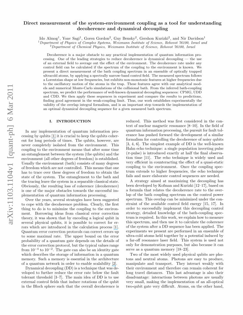
FIG. 2. Calibration of the microwave dressing effect. They-axis shows the population at F=2 as a function of thecontrol pulse frequency shifted by fc, the center frequencywithout the dressing. The data was taken with a Rabi fre-quency of Ω = 340Hz. We fit the data to the theoretical curve

A f2

(f−f0)2+f2 [1 + cos(φ+ T√

(f − f0)2 + f2)], where T is the

duration of the Rabi pulse and f is the field frequency. The fitgives f0, the dressing for the applied Rabi frequency. In thisexample, the shift is −37Hz. The inset shows the microwavedressing shift as a function of the Rabi frequency squared.

late into noise in the atomic population. For example,an average noise of 1% in the Rabi frequency transformsinto ∼ 100% noise in the atomic population, if we driveour system at Ω = 2π · 100Hz for 1sec. Strictly speaking,this noise in the control field results in a reduction of thefidelity. In order to avoid this difficulty, we randomizecompletely the initial population difference by an addi-tional pulse that rotates the atomic state by a randomuniformly distributed angle and analyze ∼ 30 data pointstaken for the same pulse power using envelope spec-troscopy. The corresponding Bloch-vector length is es-timated using the maximum likelihood estimator. Sincethe angle of the Bloch vector is now completely randomwe can assume that its z-component is C sin(Φ), whereΦ is a uniformly distributed random phase. The resultsof the maximum-likelihood algorithm that extracts theBloch vector length C coincide with the extreme valuesof the measured z-component (the population inversion).

The second difficulty is due to the energy-level shiftinduced by the control field [37]. This “field dressing” ofthe levels depends on the microwave field strength (we donot observe the shift due to the rf field) . When the bathspectrum is measured using a continuous control field,this effect causes the control to have a detuning whichdepends on its strength (and therefore on its Rabi fre-quency). We measure the shift by applying a long pulsewhich induces Rabi oscillations and detect the popula-tion at state |2〉 while scanning the frequency of the mi-crowave field. Such a measurement is shown in Figure 2.This data yields the relative-level shift for a given Rabifrequency. We then repeat this measurement for severalRabi frequencies and obtain a calibration graph, shownin the inset of Figure 2. As expected from theory, the

250 500 750 1000

0.3

0.4

0.5

frequency [Hz]250 500 750 1000

0.3

0.4

0.5

0.6

0.7

PF

=2

a b

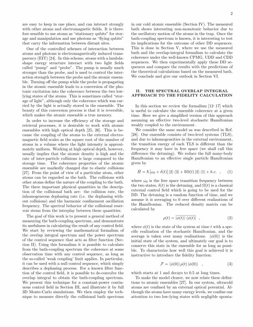
FIG. 3. Raw data of coupling spectra. The points are thepopulation at F=2 as a function of the control pulse Rabi fre-quency. The experiment was done for 160k atoms in a trapwith a radial and axial oscillation frequencies of 2π·910Hz and2π·240Hz, respectively. The field dressing results in the reduc-tion of the contrast which is dominant in high frequency. Onthe right we show that after correction for this field-dressingthe contrast does not decay at higher frequencies even after1sec. The contrast between the two graphs is different sincethe observation time is 0.4sec for the left graph and 1sec forthe right graph. The difference in the mean population stemsfrom m-changing transitions in the F = 2 hyperfine level. Thecoherence is calculated by a maximal likelihood method (seetext), and is determined by the envelope of the scattered datapoints.

dressing at small field strengths is linearly proportionalto the control-field Rabi-frequency squared [37].

In Figure 3 two examples of raw data from a bath-spectrum measurement are shown. The scattering of thedata points is a consequence of our randomization tech-nique explained above. The bath-coupling spectrum ata given frequency is related to the envelope of the scat-tered points. The data presented in Figure 3a was takenwithout changing the control field frequency (not to beconfused with its strength which controls the Rabi fre-quency).

The second difficulty described above leads to a sub-stantial reduction of the contrast at higher Rabi frequen-cies due to the detuning of the control field from reso-nance, caused by the strong field-dressing of the levels.In order to eliminate this effect, we change the frequencyof the microwave field as its power changes to compensatefor the field dressing. The result is shown in Figure 3b torestore contrast at high frequencies. In general, this cor-rection should also be applied in other DD sequences. Inthe cases we present below, however, the dressing effectis very small and unimportant.

To obtain the bath-coupling spectrum, we repeat themeasurement described above with at least three differ-ent Rabi pulse durations. From each such experiment weget the coherence at that time for all Rabi frequencies.For each Rabi frequency we fit the decay of the coherenceat different times to a decaying exponent, from which weobtain the decoherence rate. As explained above, thefitting to an exponent is justified in the weak-couplingregime. In Figure 4 we plot the experimentally measureddecoherence rate as a function of frequency. Similarly to

6

0 50 100 150 200 250 3000

1

2

3

4

5

frequency [Hz]

dec

oher

ence

rate

[sec

−1]

simulated bath spectrumsimulated decay ratemeasured decoherence rates

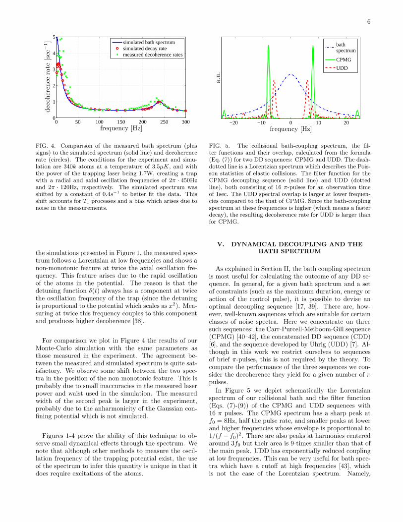
FIG. 4. Comparison of the measured bath spectrum (plussigns) to the simulated spectrum (solid line) and decoherencerate (circles). The conditions for the experiment and simu-lation are 340k atoms at a temperature of 3.5µK, and withthe power of the trapping laser being 1.7W, creating a trapwith a radial and axial oscillation frequencies of 2π · 450Hzand 2π · 120Hz, respectively. The simulated spectrum wasshifted by a constant of 0.4s−1 to better fit the data. Thisshift accounts for T1 processes and a bias which arises due tonoise in the measurements.

the simulations presented in Figure 1, the measured spec-trum follows a Lorentzian at low frequencies and shows anon-monotonic feature at twice the axial oscillation fre-quency. This feature arises due to the rapid oscillationof the atoms in the potential. The reason is that thedetuning function δ(t) always has a component at twicethe oscillation frequency of the trap (since the detuningis proportional to the potential which scales as x2). Mea-suring at twice this frequency couples to this componentand produces higher decoherence [38].

For comparison we plot in Figure 4 the results of ourMonte-Carlo simulation with the same parameters asthose measured in the experiment. The agreement be-tween the measured and simulated spectrum is quite sat-isfactory. We observe some shift between the two spec-tra in the position of the non-monotonic feature. This isprobably due to small inaccuracies in the measured laserpower and waist used in the simulation. The measuredwidth of the second peak is larger in the experiment,probably due to the anharmonicity of the Gaussian con-fining potential which is not simulated.

Figures 1-4 prove the ability of this technique to ob-serve small dynamical effects through the spectrum. Wenote that although other methods to measure the oscil-lation frequency of the trapping potential exist, the useof the spectrum to infer this quantity is unique in that itdoes require excitations of the atoms.

−20 −10 0 10 20frequency [Hz]

a.u

.

bathspectrum

CPMG

UDD

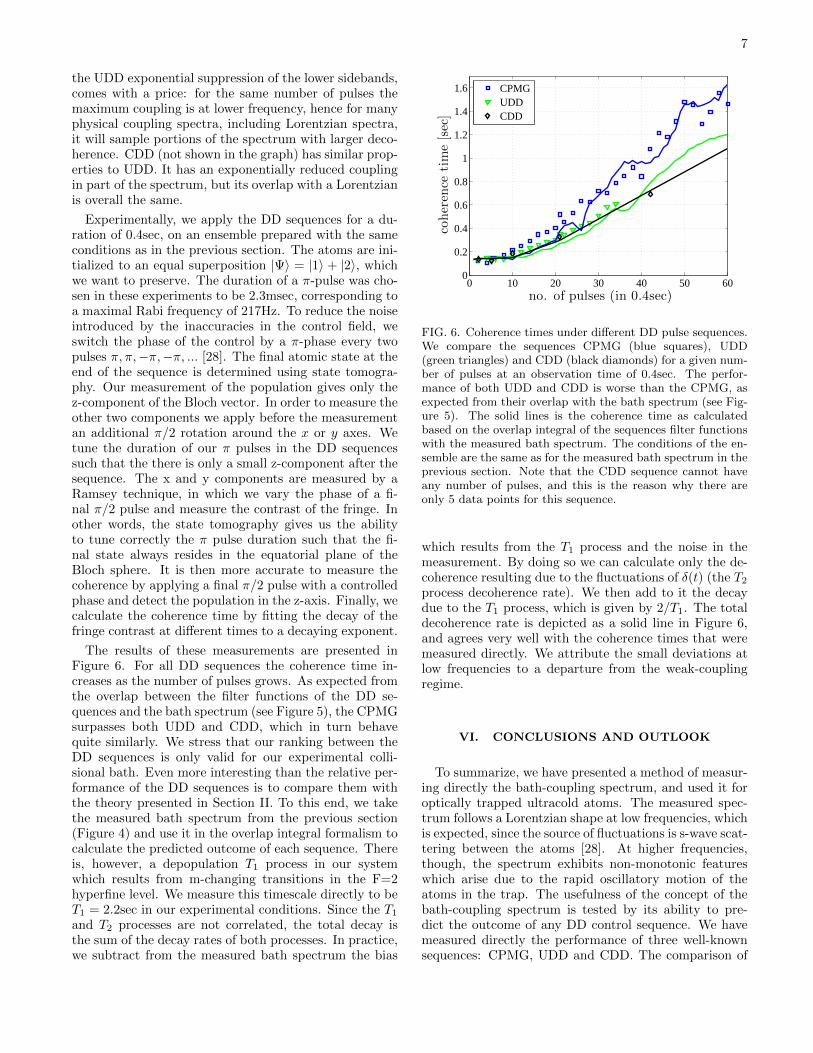
FIG. 5. The collisional bath-coupling spectrum, the fil-ter functions and their overlap, calculated from the formula(Eq. (7)) for two DD sequences: CPMG and UDD. The dash-dotted line is a Lorentzian spectrum which describes the Pois-son statistics of elastic collisions. The filter function for theCPMG decoupling sequence (solid line) and UDD (dottedline), both consisting of 16 π-pulses for an observation timeof 1sec. The UDD spectral overlap is larger at lower frequen-cies compared to the that of CPMG. Since the bath-couplingspectrum at these frequencies is higher (which means a fasterdecay), the resulting decoherence rate for UDD is larger thanfor CPMG.

V. DYNAMICAL DECOUPLING AND THEBATH SPECTRUM

As explained in Section II, the bath coupling spectrumis most useful for calculating the outcome of any DD se-quence. In general, for a given bath spectrum and a setof constraints (such as the maximum duration, energy oraction of the control pulse), it is possible to devise anoptimal decoupling sequence [17, 39]. There are, how-ever, well-known sequences which are suitable for certainclasses of noise spectra. Here we concentrate on threesuch sequences: the Carr-Purcell-Meiboom-Gill sequence(CPMG) [40–42], the concatenated DD sequence (CDD)[6], and the sequence developed by Uhrig (UDD) [7]. Al-though in this work we restrict ourselves to sequencesof brief π-pulses, this is not required by the theory. Tocompare the performance of the three sequences we con-sider the decoherence they yield for a given number of πpulses.

In Figure 5 we depict schematically the Lorentzianspectrum of our collisional bath and the filter function(Eqs. (7)-(9)) of the CPMG and UDD sequences with16 π pulses. The CPMG spectrum has a sharp peak atf0 = 8Hz, half the pulse rate, and smaller peaks at lowerand higher frequencies whose envelope is proportional to1/(f − f0)2. There are also peaks at harmonies centeredaround 3f0 but their area is 9-times smaller than that ofthe main peak. UDD has exponentially reduced couplingat low frequencies. This can be very useful for bath spec-tra which have a cutoff at high frequencies [43], whichis not the case of the Lorentzian spectrum. Namely,

7

the UDD exponential suppression of the lower sidebands,comes with a price: for the same number of pulses themaximum coupling is at lower frequency, hence for manyphysical coupling spectra, including Lorentzian spectra,it will sample portions of the spectrum with larger deco-herence. CDD (not shown in the graph) has similar prop-erties to UDD. It has an exponentially reduced couplingin part of the spectrum, but its overlap with a Lorentzianis overall the same.

Experimentally, we apply the DD sequences for a du-ration of 0.4sec, on an ensemble prepared with the sameconditions as in the previous section. The atoms are ini-tialized to an equal superposition |Ψ〉 = |1〉 + |2〉, whichwe want to preserve. The duration of a π-pulse was cho-sen in these experiments to be 2.3msec, corresponding toa maximal Rabi frequency of 217Hz. To reduce the noiseintroduced by the inaccuracies in the control field, weswitch the phase of the control by a π-phase every twopulses π, π,−π,−π, ... [28]. The final atomic state at theend of the sequence is determined using state tomogra-phy. Our measurement of the population gives only thez-component of the Bloch vector. In order to measure theother two components we apply before the measurementan additional π/2 rotation around the x or y axes. Wetune the duration of our π pulses in the DD sequencessuch that the there is only a small z-component after thesequence. The x and y components are measured by aRamsey technique, in which we vary the phase of a fi-nal π/2 pulse and measure the contrast of the fringe. Inother words, the state tomography gives us the abilityto tune correctly the π pulse duration such that the fi-nal state always resides in the equatorial plane of theBloch sphere. It is then more accurate to measure thecoherence by applying a final π/2 pulse with a controlledphase and detect the population in the z-axis. Finally, wecalculate the coherence time by fitting the decay of thefringe contrast at different times to a decaying exponent.

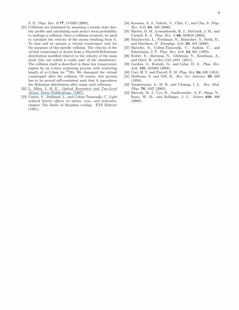
The results of these measurements are presented inFigure 6. For all DD sequences the coherence time in-creases as the number of pulses grows. As expected fromthe overlap between the filter functions of the DD se-quences and the bath spectrum (see Figure 5), the CPMGsurpasses both UDD and CDD, which in turn behavequite similarly. We stress that our ranking between theDD sequences is only valid for our experimental colli-sional bath. Even more interesting than the relative per-formance of the DD sequences is to compare them withthe theory presented in Section II. To this end, we takethe measured bath spectrum from the previous section(Figure 4) and use it in the overlap integral formalism tocalculate the predicted outcome of each sequence. Thereis, however, a depopulation T1 process in our systemwhich results from m-changing transitions in the F=2hyperfine level. We measure this timescale directly to beT1 = 2.2sec in our experimental conditions. Since the T1and T2 processes are not correlated, the total decay isthe sum of the decay rates of both processes. In practice,we subtract from the measured bath spectrum the bias

0 10 20 30 40 50 600

0.2

0.4

0.6

0.8

1

1.2

1.4

1.6

no. of pulses (in 0.4sec)

coher

ence

tim

e[s

ec]

CPMGUDDCDD

FIG. 6. Coherence times under different DD pulse sequences.We compare the sequences CPMG (blue squares), UDD(green triangles) and CDD (black diamonds) for a given num-ber of pulses at an observation time of 0.4sec. The perfor-mance of both UDD and CDD is worse than the CPMG, asexpected from their overlap with the bath spectrum (see Fig-ure 5). The solid lines is the coherence time as calculatedbased on the overlap integral of the sequences filter functionswith the measured bath spectrum. The conditions of the en-semble are the same as for the measured bath spectrum in theprevious section. Note that the CDD sequence cannot haveany number of pulses, and this is the reason why there areonly 5 data points for this sequence.

which results from the T1 process and the noise in themeasurement. By doing so we can calculate only the de-coherence resulting due to the fluctuations of δ(t) (the T2process decoherence rate). We then add to it the decaydue to the T1 process, which is given by 2/T1. The totaldecoherence rate is depicted as a solid line in Figure 6,and agrees very well with the coherence times that weremeasured directly. We attribute the small deviations atlow frequencies to a departure from the weak-couplingregime.

VI. CONCLUSIONS AND OUTLOOK

To summarize, we have presented a method of measur-ing directly the bath-coupling spectrum, and used it foroptically trapped ultracold atoms. The measured spec-trum follows a Lorentzian shape at low frequencies, whichis expected, since the source of fluctuations is s-wave scat-tering between the atoms [28]. At higher frequencies,though, the spectrum exhibits non-monotonic featureswhich arise due to the rapid oscillatory motion of theatoms in the trap. The usefulness of the concept of thebath-coupling spectrum is tested by its ability to pre-dict the outcome of any DD control sequence. We havemeasured directly the performance of three well-knownsequences: CPMG, UDD and CDD. The comparison of

8

these measurements to a calculation based on the overlapintegral with the directly measured bath spectrum provesthe validity of this framework at the weak-coupling limit.As was already shown numerically in [28], the CPMG se-quence is found to be superior to the UDD and CDDsequences, for our collisional bath spectrum.

As noted above, the weak-coupling assumption is es-sential for the overlap-integral formalism to be correct.Under certain experimental conditions and at low fre-quencies, our bath does not fulfil this assumption, andindeed we observe deviations from the corresponding the-oretical calculations. Measuring the coupling spectrumunder these conditions is a major challenge. One wayof addressing it is by using a sequence that mostly re-sides in the weak-coupling part of the spectrum, whilea small sideband probes the low frequencies of the spec-trum. The idea is to keep most of the overlap betweenthe spectrum and the filter function in the weak-couplingdomain, while still probing the strong coupling domainof the spectrum. An example of such a pulse is:

Ω(t) = 2πf0(1 + βfmf0cos(2πfmt)), (10)

where f0 is the carrier Rabi frequency, β is the modu-

lation index and fm is the AM modulation frequency.By measuring the decoherence twice: once with the side-band and once without, it is possible to extract the cou-pling spectrum at the sideband frequency, even if thisfrequency is in the strong-coupling part of the spectrum.

For a given bath spectrum and a set of constraints onthe control field, an optimal decoupling sequence can beconstructed [17, 39]. This is done by solving the Euler-Lagrange equation which minimizes the overlap of thecontrol-field filter function and the bath-coupling spec-trum. This procedure is yet to be demonstrated exper-imentally. In our system, as well as in other systems,the spectrum is non-monotonic and as such we expect anon-trivial optimal decoupling sequence. What can com-plicate this picture is noise in the control field. In thiswork we have circumvented this issue by using an enve-lope spectroscopy method. It is possible to extend theoverlap-integral formalism to include the classical noisycontrol as a second (classical) bath-like spectral function.The decay rate is then given by two overlap integralswhich can be solved to find the optimal DD sequencefor a noisy control. Since noise in the control is alwayspresent, this extension of the theory is both necessaryand practical.

We acknowledge the financial support of MIDAS, MIN-ERVA, GIF, ISF, and DIP.

[1] Nielsen, M. A. and Chuang, I. L. Quantum Computationand Quantum Information. Cambridge University Press,(2000).

[2] Duan, L. M., Lukin, M. D., Cirac, J. I., and Zoller, P.Nature 414, 413 (2001).

[3] Viola, L. and Lloyd, S. Phys. Rev. A 58, 2733 Oct (1998).[4] Viola, L., Knill, E., and Lloyd, S. Phys. Rev. Lett. 82,

2417 (1999).[5] Search, C. and Berman, P. R. Phys. Rev. Lett. 85, 2272

(2000).[6] Khodjasteh, K. and Lidar, D. A. Phys. Rev. Lett. 95,

180501 (2005).[7] Uhrig, G. S. Phys. Rev. Lett. 98, 100504 (2007).[8] Kubo, R. Fluctuation, relaxation and resonance in mag-

netic systems, 23. Scottish Universities Summer School inPhysics. Oliver and Boyd, Edinburgh and London (1961).

[9] Kubo, R. J. Phys. Soc. Jpn. 9, 935 (1954).[10] Haeberlen, U. High Resolution NMR in Solids. Advances

in Magnetic Resonance Series. Academic, (1976).[11] Hahn, E. L. Phys. Rev. 80, 580 (1950).[12] Kofman, A. G. and Kurizki, G. Phys. Rev. Lett. 87,

270405 (2001).[13] Kofman, A. G. and Kurizki, G. Phys. Rev. Lett. 93,

130406 (2004).[14] Gordon, G. and Kurizki, G. Phys. Rev. A 76, 042310

(2007).[15] Gordon, G., Erez, N., and Kurizki, G. J. Phys. B40, S75

(2007).[16] Gordon, G. and Kurizki, G. Phys. Rev. Lett. 97, 110503

(2006).[17] Clausen, J., Bensky, G., and Kurizki, G. Phys. Rev. Lett.

104, 040401 (2010).[18] Kuzmich, A., Bowen, W. P., Boozer, A. D., Boca, A.,

Chou, C. W., Duan, L. M., and Kimble, H. J. Nature423, 731 (2003).

[19] Chou, C. W., de Riedmatten, H., Felinto, D., Polyakov,S. V., van Enk, S. J., and Kimble, H. J. Nature 438, 828(2005).

[20] Yuan, Z.-S., Chen, Y.-A., Zhao, B., Chen, S., Schmied-mayer, J., and Pan, J.-W. Nature 454, 1098 (2008).

[21] Zhao, B., Chen, Y. A., Bao, X. H., Strassel, T., Chuu,C. S., Jin, X. M., Schmiedmayer, J., Yuan, Z. S., Chen,S., and Pan, J. W. Nature Phys. 5, 95 (2009).

[22] Schnorrberger, U., Thompson, J. D., Trotzky, S., Pu-gatch, R., Davidson, N., Kuhr, S., and Bloch, I. Phys.Rev. Lett. 103, 033003 (2009).

[23] Zhang, R., Garner, S. R., and Hau, L. V. Phys. Rev.Lett. 103, 233602 (2009).

[24] Lukin, M. D. Rev. Mod. Phys. 75, 457 (2003).[25] Harris, S. E. and Hau, L. V. Phys. Rev. Lett. 82, 4611

(1999).[26] Gorshkov, A. V., Andre, A., Fleischhauer, M., Sørensen,

A. S., and Lukin, M. D. Phys. Rev. Lett. 98, 123601(2007).

[27] Sagi, Y., Almog, I., and Davidson, N. Phys. Rev. Lett.105, 093001 (2010).

[28] Sagi, Y., Almog, I., and Davidson, N. Phys. Rev. Lett.105, 053201 (2010).

[29] Kuhr, S., Alt, W., Schrader, D., Dotsenko, I., Miroshny-chenko, Y., Rauschenbeutel, A., and Meschede, D. Phys.Rev. A 72, 023406 (2005).

[30] Cywinski, L., Lutchyn, R. M., Nave, C. P., and Sarma,

9

S. D. Phys. Rev. B 77, 174509 (2008).[31] Collisions are simulated by assuming a steady state den-

sity profile and calculating each atom’s local probabilityto undergo a collision. Once a collision occurred, we needto calculate the velocity of the atoms resulting from it.To that end we assume a virtual counterpart only forthe purposes of this specific collision. The velocity of thevirtual counterpart is drawn from a Maxwell-Boltzmanndistribution modified relative to the velocity of the mainatom (the one which is really part of the simulation).The collision itself is described in these low temperatureregime by an s-wave scattering process with scatteringlength of a=5.2nm for 87Rb. We disregard the virtualcounterpart after the collision. Of course, this processhas to be proved self-consistent such that it reproducesthe Boltzman distribution after many such collisions.

[32] L. Allen, J. H. E. Optical Resonance and Two-LevelAtoms. Dover Publications, (1987).

[33] Castin, Y., Dalibard, J., and Cohen-Tannoudji, C. Lightinduced kinetic effects on atoms, ions, and molecules,chapter The limits of Sisyphus cooling. ETS Editrice(1991).

[34] Kerman, A. J., Vuletic, V., Chin, C., and Chu, S. Phys.Rev. Lett. 84, 439 (2000).

[35] Harber, D. M., Lewandowski, H. J., McGuirk, J. M., andCornell, E. A. Phys. Rev. A 66, 053616 (2002).

[36] Khaykovich, L., Friedman, N., Baluschev, S., Fathi, D.,and Davidson, N. Europhys. Lett. 50, 454 (2000).

[37] Haroche, S., Cohen-Tannoudji, C., Audoin, C., andSchermann, J. P. Phys. Rev. Lett. 24, 861 (1970).

[38] Kotler, S., Akerman, N., Glickman, Y., Keselman, A.,and Ozeri, R. arXiv:1101.4885 (2011).

[39] Gordon, G., Kurizki, G., and Lidar, D. A. Phys. Rev.Lett. 101, 010403 (2008).

[40] Carr, H. Y. and Purcell, E. M. Phys. Rev. 94, 630 (1954).[41] Meiboom, S. and Gill, D. Rev. Sci. Instrum. 29, 688

(1958).[42] Vandersypen, L. M. K. and Chuang, I. L. Rev. Mod.

Phys. 76, 1037 (2005).[43] Biercuk, M. J., Uys, H., VanDevender, A. P., Shiga, N.,

Itano, W. M., and Bollinger, J. J. Nature 458, 996(2009).