
Deductive Versus Probabilistic Reasoning in Healthy Adults: An EEG Analysis of Neural Differences
Upload
khangminh22Category
view
3download
0
RUPRECHT-KARLS-UNIVERSITÄT HEIDELBERG
Dimitri Probst
A Neural Implementation of Probabilistic Inferencein Binary Probability Spaces
Masterarbeit
HD-KIP 14-31
KIRCHHOFF-INSTITUT FÜR PHYSIK


Faculty of Physics and AstronomyUniversity of Heidelberg
Master’s thesis
in Physics
submitted by
Dimitri Probst
born in Zatobolsk, Kazakhstan
March 2014


A Neural Implementation of ProbabilisticInference in Binary Probability Spaces
This master’s thesis has been carried out by Dimitri Probst at the
Kirchhoff Institute for Physics
Ruprecht-Karls-Universität Heidelberg
under the supervision of
Prof. Dr. Karlheinz Meier


A Neural Implementation of Probabilistic Inference in Binary ProbabilitySpaces
Widely regarded as a hallmark of intelligence, be it artificial or biological, the ability toperform stochastic inference has been the subject of intense research in both the fields ofmachine learning and neuroscience. In this context, graphical models – such as Bayesiannetworks – provide a useful framework for representing probability distributions andperforming inference in their respective probability spaces. Extending the theoreticalapproaches from Pecevski et al. [2011] and Petrovici et al. [2013], this thesis describes the"physical" implementation of arbitrary binary probability distributions, represented asBayesian networks, in ensembles of leaky integrate-and-fire (LIF) neurons. Based on asampling approach rather than belief propagation, the proposed implementation offerssignificant advantages in terms of sparseness, convergence and speed. In this framework,individual neurons represent the binary random variables, while conditional probabilitiesare embedded in the synaptic interactions, mediated by postsynaptic potentials (PSPs).Due to the difference between theoretically optimal PSP shapes and those achievable withLIF neurons, a novel interaction model is proposed, based on feedforward neural chains.This new approach is characterized in detail and validated through extensive softwaresimulations. While creating a bridge to experimental neuroscience, the proposed approachinherently fosters a promising application for neuromorphic hardware, which can therebyprovide the substrate for fast and power-efficient inference machines. As a necessarypreliminary for such an application, several critical parameters of the BrainScaleS wafer-scale neuromorphic platform are characterized and discussed.


Eine neuronale Realisierung probabilistischer Inferenz in binärenWahrscheinlichkeitsräumen
Weitgehend aufgefasst als ein Kennzeichen von Intelligenz, sei sie künstlich oder biolo-gisch, ist die Fähigkeit, stochastische Inferenz durchzuführen, Gegenstand umfangreicherForschung sowohl im Bereich des maschinellen Lernens als auch der Neurowissenschaft. Indiesem Zusammenhang bieten grafische Modelle – wie z.B. Bayes’sche Netze – einen hilfrei-chen Rahmen zur Darstellung von Wahrscheinlichkeitsverteilungen und Durchführung vonInferenz in den jeweiligen Wahrscheinlichkeitsräumen. Durch Erweitern der theoretischenMethoden von Pecevski et al. [2011] und Petrovici et al. [2013] beschreibt diese Arbeit die"physikalische"Realisierung beliebiger binärer Wahrscheinlichkeitsverteilungen, repräsen-tiert durch Bayes’sche Netze, in Ensembles von Leaky Integrate-and-Fire (LIF) Neuronen.Auf der Grundlage einer Samplingmethode an Stelle von Belief Propagation, bietet dievorgeschlagene Umsetzung wesentliche Vorteile hinsichtlich Effizienz, Konvergenz undGeschwindigkeit. In diesem Rahmen stellen einzelne Neuronen die binären Zufallsvariablendar, während bedingte Wahrscheinlichkeiten in synaptischen Wechselwirkungen verankertsind und durch postsynaptische Potentiale (PSPs) vermittelt werden. Auf Grund der Ab-weichung der theoretisch optimalen von den mit LIF Neuronen erreichbaren PSP-Formenwird ein neuartiges Wechselwirkungsmodell vorgeschlagen, welches auf Feedforwardkettenvon Neuronen gründet. Dieser neuartige Ansatz wird eingehend charakterisiert und mittelsumfassender Softwaresimulationen validiert. Indem es einen Übergang zur experimentellenNeurowissenschaft schafft, ermöglicht das vorgeschlagene Konzept eine vielversprechen-de Anwendung für neuromorphe Hardware, die dabei das Substrat für schnelle undleistungseffiziente Inferenzmaschinen bereitstellt. Als notwendige Vorbereitung für einederartige Anwendung werden entscheidende Parameter der BrainScaleS wafer-skaligenneuromorphen Plattform charakterisiert und diskutiert.


Contents
1 Introduction 1
2 Materials and Methods 42.1 Theoretical Prerequisites . . . . . . . . . . . . . . . . . . . . . . . . . . . . 5
2.1.1 Basics of Probability Theory and Inference . . . . . . . . . . . . . 52.1.2 Boltzmann Machines . . . . . . . . . . . . . . . . . . . . . . . . . . 82.1.3 Bayesian Networks . . . . . . . . . . . . . . . . . . . . . . . . . . . 82.1.4 Markov Chain Monte Carlo Sampling . . . . . . . . . . . . . . . . 112.1.5 Neural Sampling . . . . . . . . . . . . . . . . . . . . . . . . . . . . 132.1.6 Deterministic Neuron and Synapse Models . . . . . . . . . . . . . . 202.1.7 LIF Sampling . . . . . . . . . . . . . . . . . . . . . . . . . . . . . . 23
2.2 Neuromorphic Hardware . . . . . . . . . . . . . . . . . . . . . . . . . . . . 292.2.1 The HICANN Chip . . . . . . . . . . . . . . . . . . . . . . . . . . . 302.2.2 Demonstrator Setup . . . . . . . . . . . . . . . . . . . . . . . . . . 362.2.3 Hybrid Multiscale Facility . . . . . . . . . . . . . . . . . . . . . . . 38
2.3 Software Framework . . . . . . . . . . . . . . . . . . . . . . . . . . . . . . 392.3.1 Simulation of Neural Networks . . . . . . . . . . . . . . . . . . . . 392.3.2 Emulation of Neural Networks . . . . . . . . . . . . . . . . . . . . 41
3 Characterization of LIF Sampling from Boltzmann Distributions 433.1 Calibration of a LIF Neuron to Perform LIF Sampling . . . . . . . . . . . 44
3.1.1 Finding a Good Range of Effective Membrane Potentials . . . . . . 453.1.2 Measuring the Activation Curve . . . . . . . . . . . . . . . . . . . . 45
3.2 LIF Sampling from Boltzmann Distributions of 5 Random Variables . . . 463.3 Parameter Analysis of LIF Neurons for Boltzmann Machines of 5 Random
Variables . . . . . . . . . . . . . . . . . . . . . . . . . . . . . . . . . . . . . 483.3.1 Parameter Selection . . . . . . . . . . . . . . . . . . . . . . . . . . 503.3.2 Parameter Optimization for Sample Boltzmann Machines . . . . . 50
3.4 Conclusion . . . . . . . . . . . . . . . . . . . . . . . . . . . . . . . . . . . . 52
4 Bayesian Networks: Implementation 1 544.1 Implementation 1: Illustrative Implementation of Example Bayesian Networks 55
4.1.1 Implementation of the Visual Perception Experiment . . . . . . . . 554.1.2 Implementation of the ASIA Network . . . . . . . . . . . . . . . . 55
4.2 Parameter Analysis of LIF Neurons for Example Bayesian Networks . . . 574.2.1 Dependence of LIF Sampling on the Parameter µ . . . . . . . . . . 57
V

4.2.2 Dependence of LIF Sampling from Bayesian Networks on the Pa-rameters of the LIF Neurons . . . . . . . . . . . . . . . . . . . . . 58
4.3 Optimal Results of LIF Sampling from Bayesian Networks . . . . . . . . . 604.3.1 Results of LIF Sampling for the Visual Perception Experiment . . 614.3.2 Results of LIF Sampling from the ASIA Network . . . . . . . . . . 64
4.4 LIF Sampling Improvement via mLIF PSPs . . . . . . . . . . . . . . . . . 664.4.1 Engineering mLIF PSPs . . . . . . . . . . . . . . . . . . . . . . . . 664.4.2 Results of LIF Sampling with mLIF PSPs for the Visual Perception
Experiment . . . . . . . . . . . . . . . . . . . . . . . . . . . . . . . 704.4.3 Results of LIF Sampling with mLIF PSPs from the ASIA Network 704.4.4 Temporal Evolution of the KL Divergence . . . . . . . . . . . . . . 72
4.5 Implementation 1: LIF Sampling Performance on General Bayesian Networks 724.5.1 Generating General Bayesian Networks . . . . . . . . . . . . . . . . 744.5.2 Performance Comparison of Sampling from General Bayesian Networks 75
4.6 Conclusion . . . . . . . . . . . . . . . . . . . . . . . . . . . . . . . . . . . . 76
5 Bayesian Networks: Implementation 2 785.1 Implementation 2: Illustrative Implementation of Sample Bayesian Networks 79
5.1.1 Implementation of the Two-Node-Network . . . . . . . . . . . . . . 815.1.2 Implementation of the Visual Perception Experiment . . . . . . . . 81
5.2 Implementation 2: Performance on Sample Bayesian Networks . . . . . . . 835.2.1 Results of Sampling from the Two-Node-Network and the Visual
Perception Experiment . . . . . . . . . . . . . . . . . . . . . . . . . 835.2.2 Theoretical Explanation of the Insufficiency of LIF Sampling when
Applying Implementation 2 . . . . . . . . . . . . . . . . . . . . . . 835.3 Improvement of LIF Sampling via mLIF PSPs . . . . . . . . . . . . . . . . 85
5.3.1 Engineering mLIF PSPs . . . . . . . . . . . . . . . . . . . . . . . . 855.3.2 Results of LIF Sampling with mLIF PSPs . . . . . . . . . . . . . . 86
5.4 Investigation of the Distributions of First Passage Times of LIF Neurons . 895.4.1 Distribution of First Passage Times for α0 from the Two-Node-
Network . . . . . . . . . . . . . . . . . . . . . . . . . . . . . . . . . 905.4.2 Distribution of First Passage Times for α1 from the Two-Node-
Network . . . . . . . . . . . . . . . . . . . . . . . . . . . . . . . . . 905.5 Conclusion . . . . . . . . . . . . . . . . . . . . . . . . . . . . . . . . . . . . 95
6 Towards LIF-based Boltzmann Machines on Neuromorphic Hardware 966.1 Characterization of the Neural and Synaptic Circuits of the HICANN chip 97
6.1.1 Parameter Selection . . . . . . . . . . . . . . . . . . . . . . . . . . 976.1.2 Measuring the Time Constants . . . . . . . . . . . . . . . . . . . . 1006.1.3 Measuring the Activation Curve . . . . . . . . . . . . . . . . . . . . 103
6.2 Towards a Parametrization that Will Enable LIF Sampling on Hardware . 1056.2.1 Background Input Parameters . . . . . . . . . . . . . . . . . . . . . 1056.2.2 Time Constants . . . . . . . . . . . . . . . . . . . . . . . . . . . . . 106
6.3 Conclusion . . . . . . . . . . . . . . . . . . . . . . . . . . . . . . . . . . . . 107
VI

7 Discussion 109
8 Outlook 111
A Appendix 113A.1 Code References . . . . . . . . . . . . . . . . . . . . . . . . . . . . . . . . 113A.2 Neuron Parameters . . . . . . . . . . . . . . . . . . . . . . . . . . . . . . . 114A.3 Acronyms . . . . . . . . . . . . . . . . . . . . . . . . . . . . . . . . . . . . 119
Bibliography 125
Acknowledgments 128
VII


1 Introduction
We owe to the frailty of human mindone of the most delicate and ingeniousof mathematical theories, namely thescience of chance or probabilities.
(Pierre Simon Laplace 1776)
The human mind is able to discover causal relationships in its surrounding world basedonly on a sparse amount of information and to use this knowledge to make predictivereasoning for future events. This is the key ability which makes it possible for our speciesto understand past occurrences and to plan and manipulate prospective actions. Mostnotably, the human mind can learn complex causalities with myriads of aspects andconnections far beyond direct cause-effect relationships.Inference in human mind seems to be Bayesian in nature, rather than purely frequentist.Decisions rarely depend only on observed events; usually, observations serve to updatea prior model of the problem at hand. It therefore appears natural to describe humanreasoning using Bayesian models. Indeed, Bayesian inference lies at the heart of mostprobabilistic models of cognition [Griffiths et al., 2008]. In these approaches, the environ-mental situation, its causes and its possible effects are represented via random variables,and their underlying joint and conditional probability distributions. Two or more randomvariables can be causally related to each other. The resulting networks of random variables,so-called Bayesian networks, are an abstract diagrammatic representation of the causalstructure of the contemplated problem.The search for Bayesian inference at the level of neural network dynamics in the brainis novel compared the about 100 year-old history of neuroscience [Knill and Pouget ,2004; Griffiths and Tenenbaum, 2006; Oaksford and Chater , 2007; Doya et al., 2011].Only recently, empirical research started uncovering how the internal models of themammalian brain progressively adapt to the statistics of natural stimuli at the level ofsingle neurons [Berkes et al., 2011]. Provided with support by these empirical studies,theoretical neuroscientists use computer simulations of spiking neural networks as abottom-up approach for deciphering inference in the neocortex.In the context of probabilistic inference, the question arises of how to represent statisticaldistributions at all. One possible way is to have a closed-form representation of all therelationships between the random variables and perform inference analytically. This ideabuilds the basis of powerful and often precise so-called belief propagation algorithms,which have also been investigated in the context of spiking neural networks [Steimer et al.,2009; Petkov , 2012]. However, these algorithms often require complicated calculationsand are not guaranteed to converge towards the correct result (loopy belief propagation,
1

1 Introduction
see Bishop [2006]). In contrast to these analytical approaches, probabilistic distributionscan be represented, up to an arbitrary degree of precision, by drawing samples from them.Sampling methods, such as Markov chain Monte Carlo (MCMC), have the advantage ofbeing computationally efficient and, in particular, of being able to provide an increasinglyimproving approximation of the sought distribution at any moment during their application(anytime computing).Early during the BrainScaleS project, a stochastic framework for probabilistic inferencewith spiking neural networks, the so-called neural sampling framework, has been developed,which combines MCMC sampling with the activity of neural networks [Buesing et al.,2011; Pecevski et al., 2011]. Each binary random variable is represented by a spikingneuron and the spiking frequency of the neuron is proportional to the probability of thecorresponding variable to assume the state ”1”. Buesing et al. [2011] demonstrate that thesequences of states assumed by a network of stochastic neurons can be used to samplefrom distributions with second-order dependencies over binary variables (Boltzmanndistributions). Pecevski et al. [2011] extend this approach to arbitrary distributions, whichthey represent as Bayesian graphical models.The original neural sampling algorithm uses an abstract neuron model with a sigmoidalactivation function, non-resetting membrane potential after the emission of a spike, anadditional so-called refractory variable and rectangular postsynaptic potentials (PSPs),none of which applies to biological or standard neuron models. Petrovici et al. [2013],however, demonstrate that the abstract neuron model from Buesing et al. [2011] can bemapped to a deterministic Leaky Integrate-and-Fire (LIF) neuron embedded in a noisyenvironment.The aim of this master’s thesis is to extend the framework from Petrovici et al. [2013] bytransferring the implementation of Bayesian networks, proposed by Pecevski et al. [2011],to networks of LIF neurons. In particular, the more demanding requirements imposedby the additional complexity of Bayesian networks as compared to Boltzmann machinesrequire additional structural elements, which are discussed in detail throughout this work.Beyond investigating the compatibility of the theory proposed by Pecevski et al. [2011]and networks of LIF neurons, extensive validation runs in software are performed againstthe benchmark provided by the abstract neuron model. On the long run, however, themodeling of large Bayesian networks with the help of software simulations will becomeunsuitable because the duration of the simulation increases exponentially with the size ofthe neural network.The BrainScaleS neuromorphic hardware system [Schemmel et al., 2010], which is beingdeveloped in cooperation of the Electronic Vision(s) group at the University of Heidelbergand the group for Parallel VLSI Systems and Neural Circuits at the TU Dresden, offers asolution for these time-consuming experiments. The physical modeling of neural networkson a neuromorphic hardware substrate comes with multiple crucial advantages comparedto traditional numerical simulations. First, neuromorphic systems can be characterizedby a massive parallelism which is only present in the most efficient computing systemin the universe, the human brain. Together with the inherent time scales of the siliconsubstrate, this aspect allows to speedup experiments up to 4 orders of magnitude fasterthan biological real time, and up to 6 orders of magnitude faster than nowadays’ computer
2

simulations. Second, the emulation of the neuron’s differential equations only involves afew transistors leading to a power consumption reduction by several orders of magnitudecompared to numerical simulations [Schemmel et al., 2010]. The inherent reduction ofthe power consumption fosters excellent scalability, with the potential to emulate largecortical areas, or even an entire brain.On that account, the final part of this manuscript is dedicated to extensive tests of thecompatibility of the sampling framework from Petrovici et al. [2013] with the neural andsynaptic parameters of the BrainScaleS neuromorphic hardware system.
Outline
This manuscript is structured hierarchically, with each new topic building on the previouslydiscussed ones. For a detailed understanding of the presented arguments, reading thechapters in their given order is recommended.Chapter 2 outlines the mathematical and experimental prerequisites in detail. In particular,the theory of sampling with spiking neurons, on the one hand, and the hardware andsoftware framework which are used to implement the theory, on the other hand, arein the main focus. Chapter 3 provides simulation results of sampling from Boltzmanndistributions with LIF neurons. This chapter functions as a preparatory study for theremaining experiments described in this thesis. Chapters 4 and 5 represent the backboneof this manuscript. There, two different implementations of Bayesian networks proposedby Pecevski et al. [2011] are discussed in detail and translated to networks of LIF neurons.Additional network substructures required by the LIF implementation are designed andcharacterized, and the sampling performance of these networks is investigated againstthe benchmark provided by the theoretically ideal abstract model. Chapter 6 illustratesexperimental results aiming to characterize the neuromorphic hardware substrate describedin Chapter 2 and, in particular, to test its compatibility with the requirements of thesampling framework. In addition, software simulations are used to spot the parameterranges which entail the potential to improve the quality of future sampling experimentson the neuromorphic hardware substrate. Chapter 7 gives a summary of the resultsachieved in this thesis. Chapter 8 finally concludes the manuscript by listing suggestionsfor prospective experiments which will enhance the sampling results in both software andhardware implementations.
3

2 Materials and Methods
This chapter provides an overview, on the one hand, of the theoretical models utilizedthroughout the thesis and, on the other hand, of the tools which were used to implementthe theoretical models.Broadly speaking, this thesis focuses on the implementation of an abstract theoreticalmodel in a neuromorphic substrate. The largest part of this chapter is therefore dedicatedto a step-by-step introduction of the theoretical background (see Section 2.1). Here, westart by summarizing the most essential concepts of probability theory. Afterwards, twopowerful classes of physical implementations of probability distributions are presented:Boltzmann machines and Bayesian networks. Incidentally1, these are widely used formodeling paradigms like probabilistic inference in human reasoning (see e.g. Alais andBlake [2005] or Knill and Kersten [1991]).An analytical evaluation of probabilities is not always computationally feasible. However,under certain conditions, sampling algorithms offer an efficient alternative for representingdistributions with, in principle, an arbitrary degree of precision.Of particular interest to us is the theory of neural sampling, which creates a link betweenthe dynamics of spiking networks and the widely used Gibbs sampling algorithm. Here,we briefly recap the neural sampling approach from Buesing et al. [2011] and discussconcrete implementations of Boltzmann machines and Bayesian networks with stochasticspiking neural networks.Neural sampling ultimately serves as a basis for LIF sampling, which denotes sampling fromprobability distributions with deterministic LIF neurons in a spiking noisy environment.Here, we first describe the membrane dynamics of LIF neurons in detail and observe thatthey can be well characterized by an Ornstein-Uhlenbeck process under certain stimulusconditions. This equivalence is the prerequisite for proving that LIF neurons can be usedto sample from well-defined probability distributions.Section 2.2 surveys the BrainScaleS wafer-scale hardware system, which is the neuromor-phic hardware substrate on which the feasibility of the LIF sampling implementationwas tested in the course of this thesis. Here, we begin with the description of the analogand digital circuitry of the HICANN chip, which is the centerpiece of the hardwaresystem. Thereafter, we continue with the demonstrator setup, which entails the identicalcommunication infrastructure to the HICANN chip as the actual wafer-scale system andwhich was used to run experiments on the HICANN chip. Finally, the prospective HybridMultiscale Facility (HMF) will be briefly introduced.
1While Boltzmann machines have been inspired by Hopfield networks [Hopfield , 1982], which in turnhave been designed as abstract replicas of biological content-addressable memory [Sejnowski , 1986],Bayesian networks were first developed within the machine learning community [Pearl , 1985] and onlylater adopted to explain how animals can perform inference (see e.g. Oaksford and Chater [2007]).
4

2.1 Theoretical Prerequisites
Section 2.3 concludes this chapter by presenting the software tools which were appliedto setup neural networks and conduct software and hardware experiments throughoutthis thesis. This section is divided into two subparts. The first part describes thesimulator-independent modeling tool PyNN which will be used to run the experimentswith deterministic LIF neurons in Chapters 3, 4 and 5. The second part introduces thethe native interpreter of the BrainScaleS wafer-scale hardware system, the so-calledHardware Abstraction Layer (HAL). The Python-based PyHAL API, which wraps theHardware Abstraction Layer (HAL) interface, is used to setup the hardware experimentsin Chapter 6.
2.1 Theoretical Prerequisites
This section will introduce the theoretical methods underlying this thesis. Subsection2.1.1 offers a compact overview of the basics of probability theory. Afterwards, in2.1.2 and 2.1.3, two important representations of probability distributions are presented,namely Boltzmann machines and Bayesian networks. Subsection 2.1.4 introduces MCMCsampling in general and Gibbs sampling as a special case, which allows sampling fromprobability distributions without knowing their partition function. The MCMC frameworkis instrumental for explaining neural sampling, which is presented in Subsection 2.1.5.Thereafter, Subsection 2.1.6 discusses the dynamics of the utilized deterministic neuronand synapse models. Subsection 2.1.7 finally transfers neural sampling to leaky integrate-and-fire neurons, referred to as LIF sampling.
2.1.1 Basics of Probability Theory and Inference
The following summary of basic principles of probability theory is based on Bishop [2006]and Griffiths et al. [2008].A random variable (RV) X describes the outcome of a random event. For each RV X andmember c of a set of real numbers, one can calculate the probability p (X = c) that Xtakes the value c. The collection of all these probabilities results in the distribution of X. ARV can be discrete or continuous. Discrete RVs can assume a nonnegative probability fora countable set of values. A discrete probability distribution is described by its probabilitymass function p (X = c) for which the following rules have to be fulfilled:
0 ≤ p (X = c) ≤ 1 , (2.1)
and ∑c
p (X = c) = 1 . (2.2)
If X is a continuous RV, it has an associated probability density function f(x), whichsatisfies:
p (a < X ≤ b) =
∫ b
af(x) dx , (2.3)
5
2 Materials and Methods
and ∫ ∞−∞
f(x) dx = 1 . (2.4)
Binary RVs are in the main focus of this thesis. A binary RV X can assume the valuesc ∈ {0, 1}.Multiple RVs X1, X2, X3, ..., XK can be combined to a random vector X =(X1, X2, X3, ..., XK) with a multivariate distribution over all random variablesp (x = (x1, x2, x3, ..., xK)) with possible assignments x1, x2, x3, ..., xK of the variables.p (x) is called the joint probability distribution of the RVs X1, X2, X3, ..., XK .The probability distribution associated with only one of the variables, e.g. Xk, is called amarginal probability distribution. It is calculated by summing the joint distribution overall possible assignments of all the other variables, which is known as marginalization:
p (xk) =∑x1
...∑xk−1
∑xk+1
...∑xK
p (x) . (2.5)
If some of the RVs Xk+1, ..., XK are known to assume the particular values xk+1, ..., xK ,then the joint probability distribution p (x) can be factorized into
p (x1, ..., xK) = p (x1, ..., xk|xk+1, ..., xK) p (xk+1, ..., xK) , (2.6)
where p (x1, ..., xk|xk+1, ..., xK) is the conditional probability of x1, ..., xk given xk+1, ..., xK .Equation 2.6 ultimately results in what is known as Bayes’ rule:
p (x1, ..., xk|xk+1, ..., xK) =p (xk+1, ..., xK |x1, ..., xk) p (x1, ..., xk)
p (xk+1, ..., xK). (2.7)
The four probability distributions in Equation 2.7 are referred to as
• the prior probability distribution p (x1, ..., xk),
• the posterior probability distribution p (x1, ..., xk|xk+1, ..., xK),
• the likelihood function p (xk+1, ..., xK |x1, ..., xk),
• the evidence p (xk+1, ..., xK).
The derivation of the posterior probability from the prior probability and the likelihoodfunction of the assumed model is known as probabilistic inference.Schematic representations of probability distributions, so-called probabilistic graphicalmodels, are helpful if complex inferential computations have to be performed. In proba-bilistic graphical models, RVs are represented by nodes and probabilistic relationshipsbetween RVs are expressed by edges [Bishop, 2006]. Figure 2.1 illustrates examples ofthe two general classes of probabilistic graphical models, namely Markov random fields(or undirected graphical models) and Bayesian networks (or directed graphical models).Markov random fields are useful for expressing soft constraints between RVs, whileBayesian networks are suited to expressing causal relationships between RVs [Bishop,
6

2.1 Theoretical Prerequisites
x1 x2
x3
A: Markov random field
x x
x
1 2
3
B: Bayesian network
Figure 2.1: Examples of probabilistic graphical models of a probability distributionof 3 RVs. (A) Markov random field which describes the probabilitydistribution p (x1, x2, x3) = 1
Zφ1(x1, x3)φ2(x2, x3) with some nonnegativespecific potential functions φ1 and φ2 and the partition function Z,which ensures normalization. (B) Bayesian network which representsthe probability distribution p (x1, x2, x3) = p (x1) p (x2) p (x3|x1, x2).
2006]. Section 2.1.2 will describe one special type of Markov random fields, so-calledBoltzmann machines. Afterwards, Section 2.1.3 will introduce Bayesian networks.A typical evaluation for probabilistic inference in a graphical model which repre-sents a multivariate distribution p (x) is the computation of a conditional probabilityp (x1, ..., xk|xk+1, ..., xK) or marginals thereof. The values xk+1, ..., xK , which are fixed,could e.g. represent some sensory input or a specific goal for a decided motoric action,and x1, ..., xl have to be inferred from them.Computing a marginal p(xn) with a brute force summation over all K − 1 remaining RVsvia Equation 2.5 would require the evaluation and storage of 2K−1 distinct values in thebinary case, so that quickly rendering marginalizations in large ensembles becomes com-putationally infeasible. Broadly speaking, one can distinguish between two conceptuallydifferent approaches to this problem:
• Exact methods exploit the structure of the underlying graphical model. Message-passing algorithms are a widely used example of exact inference. Message-passingalgorithms are based on clever reorderings of sums and products of the jointprobability distribution during marginalization. Intermediate sums that arise duringthe calculation can be viewed as messages attached to the edges in the graphicalmodel. In this context, inference can be viewed in terms of a local computationand routing of messages [Arbib, 2002]. Message-passing algorithms provide an exactsolution to the inference problem if the graphical model does not contain any loops.In many other cases, they yield an approximate solution. Steimer et al. [2009] andPetkov [2012] extensively delve into exact computations of marginal and conditionalprobabilities via abstract stochastic neurons or via deterministic spiking neurons,respectively.
• Approximate methods exploit the law of large numbers, which describes that therelative frequencies of the results of a random experiment converge to the expectedprobability distribution if performing the experiment a large number of times.
7

2 Materials and Methods
Monte Carlo algorithms are characteristic for approximate methods. Monte Carloalgorithms are based on the fact that while it may not be possible to computeexpectations under p (x), it may be feasible to obtain samples from p (x), or froma closely related distribution [Arbib, 2002]. Marginals and other expectations canthen be approximated using sample-based averages. Markov chain Monte Carlo(MCMC) and Gibbs sampling as a special case of MCMC are examples for MonteCarlo algorithms (see Section 2.1.4).
2.1.2 Boltzmann Machines
Boltzmann Machines (BMs) are a special type of Markov random fields [Ackley et al.,1985]. In its original meaning, a BM describes a physical instantiation of the Boltzmanndistribution which is a network of symmetrically connected binary units that are randomlyeither "on" (1) or "off" (0) [Hinton, 2007]. For a binary random vector Z = (Z1, ..., ZK),the general shape of the Boltzmann distribution is
p(z) =1
Zexp
∑i,j
1
2Wijzizj +
∑i
bizi
(2.8)
with arbitrary real-valued parameters bi and Wij , which satisfy the conditions Wij = Wji
and Wii = 0. The parameter bi is called the bias of Zi while Wij is the weight betweenZi and Zj . The constant Z ensures normalization and is called the partition function ofp(z):
Z =∑z
exp
∑i,j
1
2Wijzizj +
∑i
bizi
. (2.9)
Each state is associated with an energy function
E(z) = −∑i,j
1
2Wijzizj −
∑i
bizi . (2.10)
From Equation 2.8 and 2.10 it follows immediately that states with lower energies aremore likely.By definition (see Equation 2.8), a Boltzmann distribution maximally allows pairwise, orsecond-order, interactions between RVs. Two RVs which are not connected to each otherdo not interact. Second-order interactions between RVs, however, are not adequate tomodel numerous computational tasks in the brain (see e.g. Figure 2.2).One example are so-called explaining away effects. For instance, the graphical modelin Figure 2.1B can be interpreted as a probability distribution in which X1 and X2
model two competing causes, or hypotheses, for the random occurrence of the eventdescribed by X3. A change in the probability of one of the hypotheses would affect theprobability of the other hypothesis, even though both of them are not causally related.These higher-order interactions between RVs can be described with Bayesian networks,which will be presented in the following section.
8

2.1 Theoretical Prerequisites
2z : 3D shapez : relative reflectance1
z : shading3 z : contour4
z = 01z = 11 2z = 02z = 1
z = 03z = 13 z = 14 z = 04
or
or other or
orA B
Figure 2.2: Demonstration of the explaining away effect in the visual perception ex-periment from Knill and Kersten [1991]. Panel A shows the phenomenon.Two visual stimuli originate from the reflectance of two geometrical ob-jects which are both composed of two identical 3D shapes. Both stimulifeature the same shading profile in the horizontal direction. The percep-tion of the reflectance of each stimulus is influenced by the perceived 3Dshape: In the case of a flat contour, the right subobject appears brighterthan the left one. This reflectance step is hardly observable for a cylindri-cal contour. A cylindrical 3D shape thus explains away the reflectancestep. Panel B demonstrates the mathematical description of this opticalillusion. The corresponding Bayesian network model consists of four RVs:z1 (reflectance step versus uniform reflectance), z2 (cylindrical versusflat 3D shape), z3 (sawtooth-shaped shading profile versus some otherprofile) and z4 (cylindrical versus flat contour). The inference of theprobability distribution p (z1, z2|z3 = 1, z4 = 0) models the perception ofthe upper stimulus of Panel A, while the lower stimulus is representedby the inference of the probability distribution p (z1, z2|z3 = 1, z4 = 1).The figure is taken from Pecevski et al. [2011].
2.1.3 Bayesian Networks
A Bayesian Network (BN) is a directed acyclic graphical model whose nodes represent theRVs Z1, ..., ZK [Bishop, 2006; Koller and Friedman, 2009]. The joint distribution definedby a Bayesian graph is given by the product of a conditional distribution for each nodeconditioned on the parent variables of that node. For a graph with K nodes, the jointprobability distribution is given by
p(z) =
K∏k=1
p(zk|pak) , (2.11)
where pak expresses the set of parents of zk. The factor p(zk|pak) is called an nth-orderfactor if it depends on n RVs or rather |pak| = n− 1.
9
2 Materials and Methods
A: visit to Asia? S: smoking?
T: tuberculosis? C: lung cancer? B: bronchitis?
X: positive X-ray? D: dyspnoea?
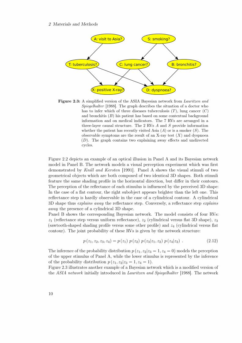
Figure 2.3: A simplified version of the ASIA Bayesian network from Lauritzen andSpiegelhalter [1988]. The graph describes the situation of a doctor whohas to infer which of three diseases tuberculosis (T ), lung cancer (C)and bronchitis (B) his patient has based on some contextual backgroundinformation and on medical indicators. The 7 RVs are arranged in athree-layer causal structure. The 2 RVs A and S provide informationwhether the patient has recently visited Asia (A) or is a smoker (S). Theobservable symptoms are the result of an X-ray test (X) and dyspnoea(D). The graph contains two explaining away effects and undirectedcycles.
Figure 2.2 depicts an example of an optical illusion in Panel A and its Bayesian networkmodel in Panel B. The network models a visual perception experiment which was firstdemonstrated by Knill and Kersten [1991]. Panel A shows the visual stimuli of twogeometrical objects which are both composed of two identical 3D shapes. Both stimulifeature the same shading profile in the horizontal direction, but differ in their contours.The perception of the reflectance of each stimulus is influenced by the perceived 3D shape:In the case of a flat contour, the right subobject appears brighter than the left one. Thisreflectance step is hardly observable in the case of a cylindrical contour. A cylindrical3D shape thus explains away the reflectance step. Conversely, a reflectance step explainsaway the presence of a cylindrical 3D shape.Panel B shows the corresponding Bayesian network. The model consists of four RVs:z1 (reflectance step versus uniform reflectance), z2 (cylindrical versus flat 3D shape), z3
(sawtooth-shaped shading profile versus some other profile) and z4 (cylindrical versus flatcontour). The joint probability of these RVs is given by the network structure:
p (z1, z2, z3, z4) = p (z1) p (z2) p (z3|z1, z2) p (z4|z2) . (2.12)
The inference of the probability distribution p (z1, z2|z3 = 1, z4 = 0) models the perceptionof the upper stimulus of Panel A, while the lower stimulus is represented by the inferenceof the probability distribution p (z1, z2|z3 = 1, z4 = 1).Figure 2.3 illustrates another example of a Bayesian network which is a modified version ofthe ASIA network initially introduced in Lauritzen and Spiegelhalter [1988]. The network
10

2.1 Theoretical Prerequisites
−3 −2 −1 0 1 2 3x
−3
−2
−1
0
1
2
3
y
0.001
0.003
0.010
0.030
0.100
0.300
acceptedrejected
A: Sampling transitions
-2.5 -2.0 -1.5 -1.0 -0.5 0.0 0.5 1.0 1.5 2.0 2.5x
-2.5
-2.0
-1.5
-1.0
-0.5
0.0
0.5
1.0
1.5
2.0
2.5
y
0
4
8
12
16
20
24
28
32
# Samples
B: Resulting sampling distribution
Figure 2.4: Demonstration of the Metropolis-Hastings algorithm (A) in two dimen-sions with a uniform proposal distribution q and a Gaussian targetdistribution p [Bishop, 2006]. Iso-probability lines of the target distribu-tion are shown in black. Samples are drawn from the proposal distributionq and accepted according to Equation 2.14. Accepted transitions areshown in blue, while rejected ones are red. In this case already 5000drawn samples can well approximate the target distribution (B).
contains seven RVs: two context aspects (A: visit to Asia, S: smoking), three diseases(T : tuberculosis, C: lung cancer, B: bronchitis) and two indicators (X: positive X-raytest, D: dyspnoea). The joint probability of the network is given by
p (A,S, T, C,B,X,D) = p (A) p (S) p (T |A) p (C|S) p (B|S) p (X|T,C) p (D|T,C,B) .(2.13)
The graph shows a more complex structure than the previous example, i.e. two explainingaway effects and undirected cycles, e.g. between the RVs S, C, D and B. A typicalexample for evidence in this network is the knowledge that the person has recently visitedAsia (A = 1) and exhibits the symptom of breathlessness (D = 1). The inference task isto calculate the likelihoods of the three diseases tuberculosis, lung cancer and bronchitisand how a positive X-ray test (X = 1) would affect these likelihoods [Lauritzen andSpiegelhalter , 1988].
2.1.4 Markov Chain Monte Carlo Sampling
Markov chain Monte Carlo (MCMC) sampling can be used to construct samples z fromprobability distributions p(z) even if the normalizing constant is unknown. MCMCmethods produce a new sample via a local search around a sample from the distributionrather than a global search over the whole state space of the RVs [Bishop, 2006].
11

2 Materials and Methods
Metropolis-Hastings algorithm: Each MCMC method uses an arbitrary proposaldistribution q
(z|z(τ)
)to generate a sample based only on the current sample z(τ), where τ
is the iteration step. At each iteration, a candidate sample z∗ is drawn from the proposaldistribution. The Metropolis-Hastings algorithm then offers a general criterion, accordingto which this candidate sample z∗ is accepted with probability
A(z∗, z(τ)
)= min
(1,
p̃(z∗)q(z(τ)|z∗)p̃(z(τ))q(z∗|z(τ))
), (2.14)
with p (z) = p̃ (z) /Zp and the normalizing constant Zp [Bishop, 2006]. If the candidatesample is accepted, then z(τ+1) = z∗, otherwise it is rejected and z(τ+1) = z(τ). The nextsample is drawn from q
(z|z(τ+1)
). Figure 2.4 shows an example of the Metropolis-Hastings
algorithm in two dimensions.
Gibbs sampling: The Gibbs sampling algorithm is a special case of the Metropolis-Hastings algorithm [Geman and Geman, 1984]. At each iteration of the algorithm, thevalue zk of one of the RVs from the random vector Z is replaced by a value which isdrawn from the proposal distribution p
(zk|z\k
). The vector z\k contains all assignments
z1, ..., zK but with zk omitted. This update scheme is repeated for all RVs of the vectorZ, either in some defined order or at random [Bishop, 2006]. With z∗\k = z\k andp (z) = p
(zk|z\k
)p(z\k)in Equation 2.14, the acceptance probability of the Gibbs
sampling algorithm is always 1 by design.For the concrete example of a probability distribution p (z1, z2, z3) of three RVs z1, z2, z3
with initial samples z(0)1 , z
(0)2 , z
(0)3 , the first sample is drawn from p(z
(1)1 |z
(0)2 , z
(0)3 ), the
following one from p(z(1)2 |z
(1)1 , z
(0)3 ) and so on.
Kullback-Leibler divergence: The approximation quality of the sampled probabilitydistribution can be evaluated by a measure of the difference of the approximated probabilitydistribution q(z) and the target probability distribution p(z), the so-called Kullback-Leibler(KL) divergence DKL(q||p). It is defined as
DKL(q||p) =∑z
q(z) log
(q(z)
p(z)
). (2.15)
The KL divergence is a distance measure DKL(q||p) ≥ 0, with equality if and only if p = q.But, unlike a distance, it is not symmetric with respect to interchange of p and q [Dayanand Abbott , 2001].
Markov chain: MCMC algorithms create a set of consecutive samples z(1), z(2), ... whichforms a Markov chain of order 1. A Markov chain of order m is defined by a sequenceof states z(1), z(2), ..., z(K) of a random vector Z such that the following conditionalindependence property holds for k ∈ {1, ...,K − 1}:
p(z(k+1)|z(k), z(k−1), ..., z(1)
)= p
(z(k+1)|z(k), z(k−1), ..., z(k−m+1)
), (2.16)
12

2.1 Theoretical Prerequisites
with k ≥ m. For the particular example of m = 1, a Markov chain can be characterizedby the probability distribution for the initial state p(z(0)) and a transition operatorT(z(k), z(k+1)
)≡ p
(z(k+1)|z(k)
)[Bishop, 2006]. The chain starts in some initial state
z(0) and moves through a trajectory of states z(τ) drawn from the conditional probabilitydistribution T
(z(τ), z(τ+1)
).
A Markov chain can have several important properties. It is called irreducible if any statez(k+1) can be reached from any other state z(k) in finitely many steps with a probabilitylarger than zero. A Markov chain is aperiodic if its state transitions cannot be trapped indeterministic cycles. Irreducibility and aperiodicity are sufficient conditions for ensuringthat the required distribution p (z) is invariant or stationary, i.e. that the probabilitydistribution p
(z(τ)|z(0)
)converges for τ → ∞ to the distribution p (z) that does not
depend on the initial state z(0) [Grimmett and Stirzaker , 2001]. A Markov chain of order1 is said to be reversible if its transition operator T satisfies the detailed balance condition:
T(z(k+1), z(k)
)p(z(k+1)
)= T
(z(k), z(k+1)
)p(z(k)
). (2.17)
Reversibility is a sufficient but not necessary condition for the invariance of the probabilitydistribution p (z) [Bishop, 2006]. It is important to note that indeed many physicalensembles, e.g. neural networks, have irreversible dynamics (see Section 2.1.5).
2.1.5 Neural Sampling
The term neural sampling in general refers to sampling from probability distributions withnetworks of spiking neurons. This section presents the theory of neural sampling fromBuesing et al. [2011] which links MCMC sampling to the dynamics of spiking neurons.In the context of Buesing et al. [2011], neural sampling is performed with a particularabstract inherently stochastic neuron model.In contrast to MCMC, spiking neurons do not incorporate reversible dynamics due torefractory mechanisms. For example, a neuron which is not refractory can always bebrought into the refractory state with enough stimulation, which is not possible for theopposite case.However, Buesing et al. [2011] prove that the Markov chain built into the dynamics of anetwork of stochastic neurons can be used to sample from probability distributions. Thisoffers the theoretical framework for the physical instantiation of Boltzmann machines andBayesian networks with spiking neurons.
Neural Sampling in Discrete and Continuous Time: In the abstract model used byBuesing et al. [2011], a neuron elicits spikes stochastically depending on the currentmembrane potential. The assignment zk of a RV Zk from a binary random vector Z isencoded in the spiking activity of a neuron νk. If the neuron νk has elicited a spike withinthe recent τ time steps (refractory period) it encodes the state zk = 1, otherwise zk = 0.The time since the last spike is measured by an additional non-binary refractory variableζk ∈ {0, 1, ..., τ} for each individual neuron νk.
13

2 Materials and Methods
Figure 2.5: Illustration of the local transition operator T k for the internal statevariable ζk of a neuron νk from Buesing et al. [2011]. The transitionprobability to the state ζk depends only on the previous state ζ ′k. Theneuron is allowed to elicit a spike for ζk ≤ 1.
In order for a network to sample correctly from a target distribution p (z1, ..., zK) over thebinary random vector Z, each of its constituent neurons νk must "know" their respectiveconditional probability p
(zk|z\k
). The so-called neural computability condition (NCC)
provides a sufficient condition for correct sampling, wherein a neuron’s "knowledge" aboutthe state of the rest of the network is encoded in its membrane potential:
uk(t) = logp(zk(t) = 1|z\k(t))p(zk(t) = 0|z\k(t))
, (2.18)
where z\k(t) are the current values zi(t) of all other variables zi with i 6= k. It is requiredthat each single neuron in the network fulfills the NCC. Equation 2.18 can also beformulated in terms of an activation function
p(zk(t) = 1|z\k(t)) = σ (uk (t)) :=1
1 + exp (−uk(t)), (2.19)
exploiting the condition p(zk = 1) = 1− p(zk = 0).The neural dynamics can be expressed via a local transition operator
T k(ζk|ζ ′k, z\k) =
σ(uk − log τ), if ζk = τ and ζ ′k ≤ 11− σ(uk − log τ), if ζk = 0 and ζ ′k ≤ 11, if ζk = ζ ′k − 1 and ζ ′k > 10, otherwise
, (2.20)
and
zk =
{1, if ζk > 00, if ζk = 0
. (2.21)
14

2.1 Theoretical Prerequisites
neuro
n 1
2
time
state (1,1) (0,0) (0,1) (1,0)
t1 t +τ1 t2 t +τ2
Figure 2.6: The spike pattern of two neurons which are sampling from a probabilitydistribution p (z1, z2). The neurons have the refractory period τ (graybox ) during which their associated RVs keep the state zk = 1. The overallnetwork state at time t is (z1, z2).
The transition probability to the state ζk only depends on the previous state ζ ′k. Theresulting sequence of states ζk(t = 0), ζk(t = 1), ζk(t = 2), ... is a Markov chain. Equation2.20 implements what is known as Glauber dynamics. Figure 2.5 illustrates the dynamicsof Equation 2.20.Buesing et al. [2011] prove that after some (ideally infinite) burn-in time, the dynam-ics of the network given by the transition operator T k produce samples from the ex-tended distribution p(ζ, z). The distribution p(z) is provided by marginalizing over ζ:p(z) =
∑ζ p(ζ, z). Thus, given that each single neuron in the network fulfills the NCC,
the network will sample from the target distribution p(z).The spiking neural network can also be used to sample from the posterior distributionp(z1, ..., zk|zk+1, ..., zK) with the observed subset of variables zk+1, ..., zK . The neuronsνk+1, ..., νK just need to be clamped to a strong positive (negative) current to representzj = 1 (zj = 0).Buesing et al. [2011] present also a continuous version of neural sampling by analyzing thediscrete sampling network in the limit dt→ 0. A continuous version allows for updatingall neurons in parallel.
Implementation of Boltzmann Machines: For the particular case of Boltzmanndistributions, the NCC (see Equation 2.18) is satisfied by neurons νk with the membranepotential
uk(t) = bk +K∑i=1
Wkizi(t) , (2.22)
with the bias bk of neuron νk and the weight Wki of the connection from neuron νi toneuron νk. Wkizi(t) is the shape of the Postsynaptic Potential (PSP) in the course of themembrane potential of the neuron νk caused by the firing of neuron νi with a square pulse.Equation 2.22 implies that all neurons have the synaptic time constant τsyn = τref = τ .For instance, if we have some bivariate probability distribution p (z1, z2) over binary RVsZ1 and Z2, the biases of the neurons ν1 and ν2 are implemented as (see Equations 2.18
15

2 Materials and Methods
and 2.22)
b1 = logp (z1 = 1, z2 = 0)
p (z1 = 0, z2 = 0)and b2 = log
p (z1 = 0, z2 = 1)
p (z1 = 0, z2 = 0), (2.23)
while the weights between ν1 and ν2 are both
W12 = W21 = logp (z1 = 0, z2 = 0) p (z1 = 1, z2 = 1)
p (z1 = 1, z2 = 0) p (z1 = 0, z2 = 1). (2.24)
Figure 2.6 illustrates a possible spike pattern of two stochastic neurons ν1 and ν2 whichare sampling from a probability distribution p(z1, z2). Both neurons have an absoluterefractory time τ after firing.BMs provide an adequate model for many real-world inference tasks like e.g. the binocularrivalry described by Alais and Blake [2005]. However, BMs maximally allow second-orderprobability distributions (see Equation 2.8), but numerous real-world phenomena requireprobabilistic models with higher-order dependencies between the RVs. Pecevski et al.[2011] introduce five methods which allow to extend the theory of neural sampling tohigher-order probability distributions. In the course of this thesis, two of these approachesare applied, which are outlined in the following.
Implementation 1 of Bayesian Networks: Implementation 1 from Pecevski et al.[2011] exploits the fact that any probability distribution p can be reduced to a Boltzmanndistribution [Ackley et al., 1985]. In particular, a higher-order probability distributionp (z1, ..., zK) over K binary RVs Z1, ..., ZK can be reduced to a Boltzmann distributionin the following way: For each nth-order factor with n > 2, 2n auxiliary binary RVsX1, ..., X2n are introduced, such that the target probability distribution p (z) can berepresented as marginal distribution
p (z) =∑x∈X
p (z,x) (2.25)
of the extended distribution p (z,x). Here, X denotes the set of all possible assignmentsof the random vector X. The auxiliary variables are chosen such that each possibleassignment of the higher-order factor is covered.Let us consider the concrete example
p (z1, z2, z3) = p (z1) p (z2) p (z3|z1, z2) . (2.26)
The probability distribution contains the third-order factor p (z3|z1, z2). The reduc-tion of p (z1, z2, z3) to a Boltzmann distribution will involve 8 additional auxiliary RVsX000, X001, ..., X111, one for each possible assignment of p (z3|z1, z2). For example, theauxiliary RV X001 assumes the value 1 only if z1 = 0, z2 = 0 and z3 = 1. For all otherassignments, the variable remains 0.In the neuron model, this can be achieved by setting the connection strengths toMexc = αbetween the neurons corresponding to the variables Z3 and X001 and to Minh = −α
16
2.1 Theoretical Prerequisites
ν ν
ν ν
1 2
3 4
000 001 010 011 100 101 110 111
MexcMinh Mexc Minh
Mexc Minh
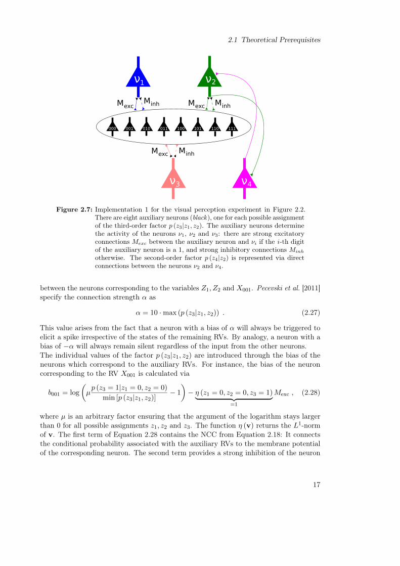
Figure 2.7: Implementation 1 for the visual perception experiment in Figure 2.2.There are eight auxiliary neurons (black), one for each possible assignmentof the third-order factor p (z3|z1, z2). The auxiliary neurons determinethe activity of the neurons ν1, ν2 and ν3: there are strong excitatoryconnections Mexc between the auxiliary neuron and νi if the i-th digitof the auxiliary neuron is a 1, and strong inhibitory connections Minh
otherwise. The second-order factor p (z4|z2) is represented via directconnections between the neurons ν2 and ν4.
between the neurons corresponding to the variables Z1, Z2 and X001. Pecevski et al. [2011]specify the connection strength α as
α = 10 ·max (p (z3|z1, z2)) . (2.27)
This value arises from the fact that a neuron with a bias of α will always be triggered toelicit a spike irrespective of the states of the remaining RVs. By analogy, a neuron with abias of −α will always remain silent regardless of the input from the other neurons.The individual values of the factor p (z3|z1, z2) are introduced through the bias of theneurons which correspond to the auxiliary RVs. For instance, the bias of the neuroncorresponding to the RV X001 is calculated via
b001 = log
(µp (z3 = 1|z1 = 0, z2 = 0)
min [p (z3|z1, z2)]− 1
)− η (z1 = 0, z2 = 0, z3 = 1)︸ ︷︷ ︸
=1
Mexc , (2.28)
where µ is an arbitrary factor ensuring that the argument of the logarithm stays largerthan 0 for all possible assignments z1, z2 and z3. The function η (v) returns the L1-normof v. The first term of Equation 2.28 contains the NCC from Equation 2.18: It connectsthe conditional probability associated with the auxiliary RVs to the membrane potentialof the corresponding neuron. The second term provides a strong inhibition of the neuron
17

2 Materials and Methods
to ensure that the neuron may only elicit a spike if the assignments of the RVs Z1, Z2
and Z3 assume the appropriate combination.If, for example, the assignments of the random vector Z are z1 = 1, z2 = 0 and z3 = 1,which is not compatible with the combination 001, then the voltage of the neuroncorresponding to the auxiliary RV X001 is forced to about −α by the input of ν1 andthe neuron remains silent. Another example is the assignment z1 = 1, z2 = 0 andz3 = 0, which is not compatible with the combination 101. In this case, the neuron whichcorresponds to the RV X101 gets not enough input and thus remains at the low membranepotential of about −α.Figure 2.7 illustrates how the visual perception experiment from Figure 2.2 is modeledvia Implementation 1. The neural network contains the four neurons ν1, ..., ν4, whichrepresent the RVs Z1, ..., Z4, and additionally 8 auxiliary neurons representing the RVsX000, X001, ..., X111, one for each possible assignment of the factor p (z3|z1, z2).According to Levin et al. [2006], the convergence of the sampling distribution towards thetarget probability distribution p (z) is very slow due to the introduction of additional RVsX. The following paragraph will present another implementation of BNs with spikingneurons in which the original RVs Z1, ..., ZK directly fulfill the NCC without the need ofadditional RVs.
Implementation 2 of Bayesian Networks: Implementation 2 from Pecevski et al. [2011]provides the ability to sample from higher-order probability distributions over the binaryrandom vector Z through a Markov blanket expansion of the NCC (see Equation 2.18).The Markov blanket Bk of a node Zk in a Bayesian network is defined as the set of allparents, children and co-parents of this node [Pearl , 1988]. By definition, it has theproperty that, once any assignment v to the RVs ZBk in the Markov blanket has beenfixed, Zk is independent from all other RVs in the graph:
p(zk|z\k) = p(zk|zBk) . (2.29)
The Markov blanket Bk "shields" the RV Zk from the rest of the nodes [Bishop, 2006].For instance, the Markov blanket of node Z1 in Figure 2.2 consists of its co-parent Z2
and its child Z3. By fixing the RVs Z2 and Z3, Z1 becomes conditionally independent ofthe RV Z4.The NCC from Equation 2.18 can then be expanded as
logp(zk(t) = 1|zBk(t))
p(zk(t) = 0|zBk(t))=
∑v∈ZBk
logp(zk = 1|zBk = v)
p(zk = 0|zBk = v)︸ ︷︷ ︸wvk
·[zBk(t) = v] , (2.30)
where v runs through all possible assignments zBk . The expression [zBk(t) = v] is 1 if thecondition inside the brackets is true, otherwise 0. Equation 2.30 implies that for satisfyingthe NCC it suffices if there are 2|Bk| auxiliary neurons, one for each possible assignmentv, that become active if and only if the RVs ZBk assume v. The current values zBk ofthe RVs ZBk are encoded in the firing activity of their associated principal neurons νk.
18

2.1 Theoretical Prerequisites
ν2
ν1
α100
ι1
excitatoryinhibitory
ν3
α101 α1
10 α111
Figure 2.8: Implementation 2 for the example in Equation 2.26. The figure is takenfrom Pecevski et al. [2011]. It shows the neural representation of theMarkov blanket of the RV z1. There are 4 auxiliary neurons, one foreach possible assignment v to the RVs z2 and z3. The correspondingprincipal neurons νi connect to the auxiliary neuron αv
1 with an excitatory(inhibitory) connection if vi = 1 (0). The auxiliary neurons connect withstrong (ideally ∞) excitatory synapses to both the principal neuronν1 and the inhibitory interneuron ι1 causing them to fire immediatelyupon stimulation. The inhibitory neuron connects back to the auxiliaryneurons with strong inhibitory weights. This ensures that all auxiliaryneurons remain silent for τref whenever one of them has spiked.
The NCC is satisfied in the neural implementation by choosing appropriate values forthe excitability of the auxiliary neurons and a specific connectivity pattern between theprincipal and the auxiliary neurons.Figure 2.8 shows the neural implementation of the Markov blanket of variable z1 for theconcrete example distribution in Equation 2.26. It consists of the variables z2 and z3.The associated principal neurons ν2 and ν3 thus connect directly to the auxiliary neuronsαv
1 . A connection from the ith principal neuron of the Markov blanket to αv1 is excitatory
(inhibitory) if the assignment v contains a 1 (0) a position i. At each moment in time onlythe auxiliary neuron αv
1 corresponding to the current state of the inputs zBk(t) = v canfire (with a probability determined by the NCC), but only if it is not laterally inhibiteddue to a recent spike from another auxiliary neuron. All auxiliary neurons αv
k connectwith strong excitatory synapses to both the principal neuron νk and the local inhibitoryinterneuron ιk, causing all efferent neurons to fire whenever they fire. The local inhibitoryinterneuron ιk connects back to the auxiliary neurons with strong inhibitory synapses.This ensures that all auxiliary neurons remain silent for a time τ = τref = τsyn whenever
19
2 Materials and Methods
one of them has spiked.The term wv
k from Equation 2.30 is implemented via the bias bvk of the auxiliary neuronthat corresponds to the assignment v, which ensures the satisfaction of the NCC:
bvk = logp(zk = 1|zBk = v)
p(zk = 0|zBk = v)− η(v)Mv
k . (2.31)
The factor η(v) denotes the L1-norm of the vector v and Mvk represents the excitatory
synaptic weight from the principal neuron νi to the auxiliary neuron αvk . In the case
v 6= zBk(t), the neuron αkv remains silent either due to insufficient input or due to thestrong inhibitory connections from the principal neurons.The excitatory synaptic weight Mv
k from the principal neuron νi to an auxiliary neuronαvk is set to
Mvk = max
(log
p(zk = 1|zBk = v)
p(zk = 0|zBk = v)+ 10, 0
). (2.32)
Similarly, the inhibitory synaptic weight Mvk from both a principal neuron νi and the
local inhibitory interneuron ιk to an auxiliary neuron αvk is set to
Mvk = min
(− log
p(zk = 1|zBk = v)
p(zk = 0|zBk = v)− 10, 0
). (2.33)
The biases of the principal neurons and the local inhibitory interneurons amount tob = −10. All efferent synaptic weights of the auxiliary neurons are set to w = 30 in orderto ensure that the postsynaptic neurons fire upon each incoming spike.
2.1.6 Deterministic Neuron and Synapse Models
This section discusses the dynamics of deterministic neuron and synapse models. Westart with the description of the membrane dynamics of the leaky integrate-and-fire (LIF)neuron and study the impact of synaptic input via current-based and conductance-basedsynapses on the course of its membrane potential. Thereafter, we discuss the membranedynamics of the adaptive exponential integrate-and-fire (AdEx) neuron model, which isimplemented on the BrainScaleS wafer-scale hardware system (see Section 2.2). The lastparagraph describes the Tsodyks-Markram (TM) mechanism of synaptic plasticity whichmodels the limitedness of synaptic neurotransmitters. The TM model is crucial for LIFsampling, which will follow in Section 2.1.7.
Leaky Integrate-and-Fire Neuron Model The membrane dynamics of the leakyintegrate-and-fire (LIF) neuron can be described by the following differential equation[Gerstner and Kistler , 2002]:
CmdV (t)
dt+ gl (V (t)− El) +
∑syn i
Ii(t) + Iext(t) = 0 . (2.34)
Cm, gl and El represent the membrane capacitance, the membrane leakage conductanceand the membrane leakage potential, respectively. The membrane time constant τm
20

2.1 Theoretical Prerequisites
is determined by gl according to τm = Cm/gl. Iext(t) subsumes all external currents,while Ii is the synaptic input current due to recurrent connections in the network ordiffusive background noise. Equation 2.34 describes the dynamics of what is called thefree membrane potential of the LIF neuron.If a certain threshold voltage Vth is exceeded, the neuron emits a spike and is reset to thereset voltage Vreset for the so-called refractory time τref .One can distinguish current-based and conductance-based synapse models. For exponential-decaying current-based synapses, Ii from Equation 2.34 is the synaptic input current
Ii(t) = wi∑
spike k
Θ (t− tk) · exp
(− t− tk
τi
). (2.35)
wi determines the height of the PSP and thus represents the synaptic weight. If wi ispositive (negative), the connection is excitatory (inhibitory). τi is the synaptic timeconstant, determining the decay speed of the synaptic current in Equation 2.35. Thesum runs over the arrival times of incoming spikes via synapse i. Θ is the Heaviside stepfunction. The synaptic current is fully determined by wi and τi. We assume from now onthat the synaptic time constant is identically τi = τsyn for each synapse of the neuron.With the choice of Ii in Equation 2.35, Equation 2.34 becomes a linear differential equationand can be solved analytically. Bytschok [2011] calculates the PSP time course VPSP(t)for a current-based LIF neuron upon an incoming spike at time tspike:
VPSP(t) =wi
gl · τm ·(
1τsyn− 1
τm
) · [exp
(−t− tspike
τm
)− exp
(−t− tspike
τsyn
)]. (2.36)
For conductance-based synapses, the current Ii from Equation 2.34 becomes
Ii(t) = gi(t) (V (t)− Erevi ) . (2.37)
The quantities gi and Erevi are the synaptic conductance and the synaptic reversal
potential, respectively. The synaptic conductance gi amounts to
gi(t) = wi∑
spike k
Θ (t− tk) · exp
(− t− tkτsyn
), (2.38)
by analogy to Equation 2.35. In difference to the current-based model, each synapsecomes with its individual reversal potential Erev
i . The amplitude of the injected currentupon arrival of a spike depends on the value of the membrane voltage itself, which makesthe system nonlinear. Equation 2.34 then yields
CmdV (t)
dt= −gl (V (t)− El)−
∑syn i
gi(t) (V (t)− Erevi )− Iext(t) , (2.39)
Due to the nonlinearity in V (t), Equation 2.39 cannot be solved analytically and aclosed-form solution of the voltage course VPSP of a PSP cannot be calculated. However,an approximative solution of Equation 2.39 can be obtained for the case that the neuronis exposed to a spiking noisy environment, which will be presented in Section 2.1.7.
21

2 Materials and Methods
Capacity of the membrane CmLeakage conductance glSynaptic conductance giLeakage potential ElReversal potential Erev
i
Slope factor ∆thEffective threshold potential VthReset potential VresetAdaptation time constant τwAdaptation coupling parameter aSpike-triggered adaptation b
Table 2.1: Parameters of the adaptive exponential integrate-and-fire neuron model
Adaptive Exponential Integrate-and-Fire Neuron Model The membrane dynamics ofthe neurons integrated on the BrainScaleS wafer-scale hardware system (see Section 2.2)follow those of the adaptive exponential integrate-and-fire (AdEx) neuron model withconductance-based synapses [Brette and Gerstner , 2005]. The model is described by twodifferential equations. The first differential equation determines the time course of themembrane potential V (t):
−CmdV (t)
dt= gl (V (t)− El)− gl ∆th exp
(V (t)− Vth
∆th
)+
∑syn i
gi(t) (V (t)− Erevi ) + w(t) . (2.40)
The second differential equation describes the temporal progress of the so-called adaptationcurrent w (t):
− τwdw(t)
dt= w(t)− a(V (t)− El) . (2.41)
Table 2.1 lists the parameters of the two differential equations.The process of spike generation is embedded in the exponential term: A spike occurseach time the membrane potential V (t) grows towards infinity. For practical reasons, theintegration of the AdEx model equations usually stops at the time at which the membranepotential crosses some threshold Θ. Exactly this time is registered as spike time. Uponeach elicited spike, the membrane potential and the adaptation current are abruptly reset,which serves as a simplification of the downswing of the action potential:
V → Vreset (2.42)w → w + b . (2.43)
The AdEx model can be reduced to the LIF model by taking the limit ∆th → 0 andsetting w = 0.
22

2.1 Theoretical Prerequisites
Tsodyks-Markram Mechanism The Tsodyks-Markram (TM) mechanism of synapticplasticity, or Short-Term Plasticity (STP), models the limitedness of neurotransmittersin a synapse [Tsodyks and Markram, 1997; Markram et al., 1998]. It takes account ofthe fact that the neurotransmitters which are released upon an action potential arenot instantaneously available for a subsequent action potential and first need to berecovered. Therefore, the actual effective synaptic strength E is equal to the absolutesynaptic strength A, which is the maximum response to a presynaptic spike, only if allneurotransmitters are on the spot and otherwise smaller. In the following, the dynamicsof the TM mechanism are presented.Each presynaptic action potential of a neuron uses some fraction of the absolute synapticstrength A, which is defined as the utilization of synaptic efficacy parameter U . Thevariable U changes for each spike. The running variable of U is referred to as u and isdetermined by the equation
un+1 = U0 + un (1− U0) exp
(− ∆t
τfacil
), (2.44)
where ∆t is the time interval between the nth and the (n+1)th spike. Without an arrivingaction potential, u decays exponentially with the time constant τfacil towards its restingvalue U0.The fraction of available synaptic strength is described by the recovered synaptic efficacyparameter R which follows the update rule
Rn+1 = Rn (1− un+1) exp
(−∆t
τrec
)+ 1− exp
(−∆t
τrec
), (2.45)
with the recovery time constant τrec. In the absence of action potentials, the R increasestowards 1. The EPSP generated by any action potential then amounts to
EPSPn = A ·Rn · un . (2.46)
Inhibitory synaptic connections are characterized by τfacil → 0 which yields un = U0.
2.1.7 LIF Sampling
This section illustrates the theoretical background of LIF sampling, the sampling fromprobability distributions with recurrent networks of deterministic leaky integrate-and-fire(LIF) neurons. First the characteristics of the membrane dynamics of a LIF neuron in theso-called High-Conductance-State (HCS) are described. In the HCS, the free membranepotential of a LIF neuron can be described by an Ornstein-Uhlenbeck (OU) process, whichis outlined thereafter. This mathematical prerequisite finally allows the neuron to closelyreproduce a logistic activation function, which connects the mean membrane potential ofthe neuron to the probability to find it in the refractory state. This analogy to the NCCfrom Equation 2.18 is the basis for performing neural sampling with LIF neurons.
23

2 Materials and Methods
The Leaky Integrate-and-Fire Neuron in a Spiking Noisy Environment Due to thenonlinearity in the membrane potential of a LIF neuron with conductance-based synapses(see Equation 2.37), Equation 2.39 cannot be solved analytically and a closed-form solutionof the voltage course VPSP of a PSP cannot be calculated. An approximative solutionof Equation 2.39, however, can be obtained for the case that the neuron is exposed to aspiking noisy environment, which will be outlined in the following.First we divide both sides of Equation 2.39 by the total conductance gtot(t) = gl+
∑i gi(t)
and define the effective membrane potential Veff and the effective time constant τeff as
Veff(t) =glEl +
∑i gi(t) · Erev
i + Iext
gtot(t)and τeff(t) =
Cm
gtot(t). (2.47)
Equation 2.39 can then be written as
τeff(t)dV (t)
dt= Veff(t)− V (t) . (2.48)
A spiking noisy environment can be generated via the stimulation by excitatory andinhibitory Poisson sources of rate νi →∞ and synaptic weights wi → 0 of the connectionsfrom the Poisson sources to the neuron. The neuron then enters the so-called high-conductance state (HCS) which can be characterized by an approximately constant totalaverage conductance gtot(t), which is larger than the leakage conductance gl, and thusa τeff smaller than τm [Destexhe et al., 2003]. Bytschok [2011] calculates the mean V (t)and the variance σ2
V (t) of the free membrane potential of a LIF neuron in the HCS:
V (t) = Veff(t) =glEl +
∑i gi(t)E
revi + Iext
gtot(t)(2.49)
andσ2V (t) =
∑i
νiS2i
(τeff
2+τsyn,i
2− 2
τeffτsyn,i
τeff + τsyn,i
)(2.50)
with
Si =wi
(Erevi − V (t)
)Cm
(1τeff− 1
τsyn,i
) . (2.51)
With τeff → 0, which implies that the membrane potential V (t) instantly follows theeffective membrane potential Veff(t), Equations 2.47 and 2.48 can be rewritten as
V (t) ≈ Veff(t) =glEl +
∑i gi(t)E
revi +
∑i ∆gi(t)E
revi + Iext
gtot(t) +∑
i ∆gi(t)(2.52)
with the fluctuations of the synaptic conductances
∆gi(t) = gi(t)− gi(t) . (2.53)
24

2.1 Theoretical Prerequisites
The mean and the variance of the conductance evoked by the stimulation via a singlePoisson source with the rate νi, connected to the neuron by a synapse with weight wiand time constant τsyn, can be calculated analytically [Bytschok , 2011]:
gi(t) = wiνiτsyn and σ2gi(t)
=w2i νiτsyn
2. (2.54)
The relative fluctuations of the synaptic conductance can be described by the coefficientof variation cV:
cV =σgi(t)
gi(t)=
√1
2νiτsyn. (2.55)
In the limit νi →∞, the fluctuations of the synaptic conductances become small, whichallows an expansion of Equation 2.52 in ∆gi. The first-order approximation amounts to[Petrovici et al., 2013]:
V (t) =glEl +
∑i gi(t)E
revi + Iext
gtot(t), (2.56)
which reveals that in the limit of high input frequencies the free membrane potential (i.e.Vth →∞) of a LIF neuron depends linearly on the synaptic input
∑i gi(t)E
revi .
The free membrane potential in the HCS as an Ornstein-Uhlenbeck process Thedescription of the free membrane potential of a LIF neuron in the HCS as an Ornstein-Uhlenbeck process is the mathematical prerequisite which allows the application of theneural sampling theory (see Section 2.1.5) with LIF neurons.An Ornstein-Uhlenbeck (OU) process [Uhlenbeck and Ornstein, 1930] is a stochasticprocess defined by the ODE
dx(t) = Θ · (µ− x(t)) + σ · dW (t) . (2.57)
Here, Θ is a positive constant and W (t) a stationary delta-correlated random processwith mean 0 and variance σ2, a so-called Wiener process. Equation 2.57 can intuitively beunderstood as the Brownian motion of the step size σdW (t) of a particle with an attractorat µ towards which it decays exponentially with the time constant Θ. Ricciardi [1977],among others, proves that the probability density function (PDF) of the OU process
f(x, t|x0) =
√Θ
πσ2 (1− e−2Θt)exp
(− Θ
σ2
[(x− x0e−Θt
)2 − µ1− e−2Θt
])(2.58)
is the unique solution of the Fokker-Planck equation
∂f(x, t)
∂t= Θ · ∂
∂x[(x− µ) f ] +
σ2
2
∂2f(x, t)
∂x2(2.59)
which satisfies the initial condition
limt→0
f(x, t|x0) = δ (x− x0) . (2.60)
25

2 Materials and Methods
Gerstner and Kistler [2002] and Petrovici et al. [2013] show that the distribution f (ξ, t)of the synaptic noise ξ := ξ(t) =
∑i gi(t)E
revi of a LIF neuron with conductance-based
synapses obeys the Fokker-Planck equation:
∂f(ξ, t)
∂t=
1
τsyn
∂
∂ξ
[(ξ −
∑i
νi∆ξiτsyn
)· f(ξ, t)
]+
∑i νi∆ξ
2i τsyn
2τsyn
∂2f(ξ, t)
∂ξ2. (2.61)
This fact implies that the temporal evolution of the synaptic noise of a LIF neuron canbe described by an OU process.Due to Equation 2.56, the free membrane potential of a LIF neuron in the HCS dependslinearly on the synaptic noise ξ(t) in the limit τeff → 0. In this situation the free membranepotential of the a LIF neuron can therefore also be approximated by an OU process.The parameters of the OU process which describes the free membrane potential can bededuced from Equations 2.49 and 2.50 with τeff → 0:
Θ =1
τsyn(2.62)
µ =glEl +
∑i νiwiE
revi τsyn + Iext
gtot(t)(2.63)
σ2 =
∑i νi (wi (Erev
i − µ))2 τsyn
gtot(t). (2.64)
In the next section, we will derive the activation function of a LIF neuron in the HCS,which connects the mean membrane potential of the neuron with the probability to findit in the refractory state. This finally allows to translate the biases and weights of thestochastic neurons from the abstract model described in Section 2.1.5 to the LIF domain.
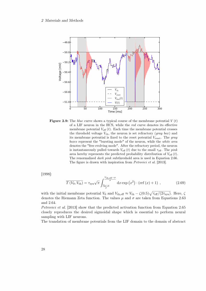
Neural Sampling via Leaky Integrate-and-Fire Neurons with Conductance-BasedSynapses Petrovici et al. [2013] show that a single LIF neuron in the HCS, whosemembrane dynamics thus can be described by an OU process, can closely reproduce theactivation function p (zk = 1) (see Equation 2.19). The activation function p (zk = 1)creates a link between the mean membrane potential of a neuron νk and the probabilityto find it in the refractory state zk = 1. In the following, the shape of the activationfunction of a LIF neuron is presented. Finally, with the help of the activation function, theparameters of the abstract neuron model from Equation 2.22 can be directly translatedto the parameters of LIF neurons.By analogy with the abstract neuron model of Section 2.1.5, the RV zk is 1 if neuron νkis refractory. The state of the LIF neuron can be divided into two "modes": A "burstingmode" in which the neuron emits spikes sequentially with an inter-spike interval (ISI) of∆t = τref and a "freely evolving mode" between these bursts, during which the membranepotential evolves freely in the subthreshold regime. Figure 2.9 shows a typical courseof the membrane potential of a LIF neuron in the HCS with its "bursting states" (grayboxes) and "freely evolving states" (white area).
26

2.1 Theoretical Prerequisites
With these two "modes", the activation function of a LIF neuron assumes the followingshape:
p (zk = 1) =
∑n Pn · n · τref∑
n Pn · (n · τref + Tn). (2.65)
Here, Pn is the probability of the occurrence of an n-spike-burst, lasting for nτref . Tnis the average time interval between the end of the previous n-spike-burst and the nextspike. Summing over the contributions of all possible burst lengths, the nominator inEquation 2.65 represents the mean bursting time of the neuron, while the denominator isthe sum of both, the mean bursting time and the mean free evolving time, equaling thetotal propagation time of the LIF neuron.As we have seen in the previous paragraph, the free membrane potential of a neuron in theHCS can be described by an OU process. Thus Pn and Tn can be calculated iterativelymaking use of the PDF of the OU process (see Equation 2.58). The pink areas in Figure2.9 depict the PDFs of the membrane potential of a LIF neuron in a HCS after it leavesthe refractory state.We will in the following denote the spike times of within an n-spike-burst by t0, ..., tn−1
and define Vi := V (ti). For an arbitrary burst length n we can then write:
Pn = p (Vn < Vth, Vn−1 ≥ Vth, ..., V1 ≥ Vth|V0 = Vth) (2.66)
=
(1−
n−1∑i=1
Pn
)∫ ∞Vth
dVn−1 p (Vn−1|Vn−1 ≥ Vth)
[∫ Vth
−∞dVn p (Vn|Vn−1)
]Tn =
∫ ∞Vth
dVn−1 p (Vn−1|Vn−1 ≥ Vth)
[∫ Vth
−∞dVn p (Vn|Vn < Vth, Vn−1)T (Vn, Vth)
],
where p(Vi|Vi−1) = f(V, τref |Vi) from Equation 2.58 and p(Vi|R(Vi)) is the renormalizationof the PDF of Vi for all values that fulfill the condition R(Vi) (dark pink areas in Figure2.9). For example, the probability of a burst of length n = 1, which is the probability thatthe neuron enters the "freely evolving mode" after a spike, yields according to Equation2.66:
P1 = p (V1 < Vth|V0 = Vth) =
∫ ∞Vth
dV0 p (V0|V0 ≥ Vth)
[∫ Vth
−∞dV1 p (V1|V0)
]. (2.67)
By analogy, the average interval between the previous "burst" of length n = 1 and thenext spike amounts to:
T1 =
∫ ∞Vth
dV0 p (V0|V0 ≥ Vth)
[∫ Vth
−∞dV1 p (V1|V1 < Vth, V0)T (V1, Vth)
]. (2.68)
T (Vi, Vth) from Equation 2.66 denotes the mean first passage time (FPT) which representsthe duration of reaching the threshold Vth for the first time when starting from Vi. If weassume a nonzero effective time constant τeff � τsyn, we can find a first-order correctionto the average FPT using an expansion in
√τeff/τsyn, according to Brunel and Sergi
27
2 Materials and Methods
0 50 100 150 200 250 300Time [ms]
51.0
50.8
50.6
50.4
50.2
50.0
49.8
Voltage[m
V]
Vth
Vreset
Vfree(t)
V(t)
Figure 2.9: The blue curve shows a typical course of the membrane potential V (t)of a LIF neuron in the HCS, while the red curve denotes its effectivemembrane potential Veff (t). Each time the membrane potential crossesthe threshold voltage Vth, the neuron is set refractory (gray box ) andits membrane potential is fixed to the reset potential Vreset. The grayboxes represent the "bursting mode" of the neuron, while the white areadenotes the "free evolving mode". After the refractory period, the neuronis instantaneously pulled towards Veff (t) due to the small τeff . The pinkarea hereby represents the predicted probability distribution of Veff (t).The renormalized dark pink subthreshold area is used in Equation 2.66.The figure is drawn with inspiration from Petrovici et al. [2013].
[1998]:
T (V0, Vth) = τsyn
√π
∫ Vth,eff−µσ
V0−µσ
dx exp(x2)· (erf (x) + 1) , (2.69)
with the initial membrane potential V0 and Vth,eff ≈ Vth − ζ(0.5)√τeff/(2τsyn). Here, ζ
denotes the Riemann Zeta function. The values µ and σ are taken from Equations 2.63and 2.64.Petrovici et al. [2013] show that the predicted activation function from Equation 2.65closely reproduces the desired sigmoidal shape which is essential to perform neuralsampling with LIF neurons.The translation of membrane potentials from the LIF domain to the domain of abstract
28

2.1 Theoretical Prerequisites
stochastic neurons from Section 2.1.5 is provided by
u =V (t)− Vk
b=0
α, (2.70)
where Vkb=0 represents the value of Vk for which the probability p(zk = 1) to find the
neuron in the refractory state is 12 . The factor α denotes the scaling factor between the
two domains and can be deduced by fitting a logistic function to p(zk = 1) in Equation2.65 and determining its slope.The linear transformation of the membrane potentials in Equation 2.70 allows to directlyspecify the parameter translation of the bias bk of neuron νk and the weight Wki fromneuron νi to νk from the abstract and the LIF domain. The average free membranepotential Vk
b of the LIF neuron νk that fulfills p (zk = 1) = σ (bk) (see Equation 2.19)amounts to
Vkb
= αbk + Vkb=0
. (2.71)
The translation of synaptic weights Wki from the domain of abstract stochastic neuron tosynaptic weights wki between LIF neurons is achieved in the following fashion. The PSPof a LIF neuron with conductance-based synapses in the HCS has the approximate shape[Bytschok , 2011]:
VPSP(t) =wki
(Erevk − Veff
)Cm ·
(1τsyn− 1
τeff
) · [exp
(−t− tspike
τeff
)− exp
(−t− tspike
τsyn
)], (2.72)
with the synaptic weight wki, the synaptic time constant τsyn and the mean effectivemembrane potential from Equation 2.49. For both the LIF domain and the abstractdomain, a presynaptic spike must have the same impact on the postsynaptic neuron. Thisis realized by matching the integrals of individual PSP:
1
α
∫ τref
0VPSP(t)dt︸ ︷︷ ︸
LIF neuron
!= Wki · τref︸ ︷︷ ︸
Stochastic neuron
. (2.73)
Evaluating the integral in Equation 2.73 results in the following weight translation betweenthe abstract and the LIF model:
Wki =wki (Erev
k − µ)
αCmτref
(1τsyn− 1
τeff
) · [τsyn
(e− τrefτsyn − 1
)− τeff
(e− τrefτeff − 1
)]. (2.74)
Therefore, the weight translation factor β from the abstract domain to the LIF domain
wki = β ·Wki (2.75)
can be expressed as
β =αCmτref
(1τsyn− 1
τeff
)(Erevk − µ
) ·[τsyn
(e− τrefτsyn − 1
)− τeff
(e− τrefτeff − 1
)]−1
. (2.76)
29

2 Materials and Methods
By definition, in the abstract neural model from Section 2.1.5, the rectangular PSPs arerenewing, which means that the contribution to the membrane potential from an afferentneuron is binary (see Equation 2.22). In the context of LIF neurons, however, staticsynapses lead to additive conductance courses and thus nonlinearly additive superpositionsof PSPs.The TM mechanism (see Section 2.1.6) offers a possible workaround for LIF neurons.Setting τfacil = 0 in Equation 2.44 leads to un+1 = U0. With the choice U0 = 1 andτrec ≈ τsyn for example, the parameter R, which describes the recovery of the synapticstrength after emission of an action potential, yields
Rn+1 = 1− exp
(− ∆t
τsyn
), (2.77)
where ∆t is the time interval between the nth and the (n + 1)th spike and τsyn thesynaptic time constant of the LIF neuron. The condition in Equation 2.77 is equivalentto approximately renewing PSPs.
2.2 Neuromorphic Hardware
With increasing knowledge about the dynamics of biological neural networks it becameclear that the operation principles of the brain are fundamentally different from those oftraditional von Neumann machines. The question therefore naturally arose to which extenttraditional computing architectures are useful instruments for implementing large-scale,biologically inspired models of cortical tissue. As an alternative to the von Neumannarchitecture, the so-called "neuromorphic" concept was proposed in the early 80s. In itswidest sense, as it is used today, the term "neuromorphic" describes a computational devicewhich mimics some aspect(s) of biological neural networks, be it in terms of architectureor dynamics. In a more narrow sense, as originally intended by its original proponents (seee.g. Mead and Mahowald [1988]; Mead [1989]), neuromorphic devices represent physicalimplementations of their biological archetype, i.e., they contain electronic componentswhich behave equivalently to neurons and synapses, albeit on a different time or voltagescale.By adopting design principles directly from biological brains, several important functionalconsequences are expected. Massively parallel by nature, a physical model of brain tissueshould exhibit a similar defect tolerance, much in contrast to traditional computers. Fur-thermore, the inherent reduction in power consumption would foster excellent scalability,with the potential to emulate large cortical areas, or even an entire brain. Throughminiaturization, VLSI technology also offers an additional advantage: due to the smallsize of the involved components, neuromorphic circuits can operate with a significantspeedup compared to the biological circuits they emulate, with obvious benefits for largeparameter sweeps or long simulation (or rather, emulation) runs [Schemmel et al., 2010].Within the FACETS project and its successor BrainScaleS, several such neuromorphicplatforms have been developed. The current wafer-scale system can emulate networkswith up to 180,000 neurons and 40 million synapses [Schemmel et al., 2010]. However, it
30
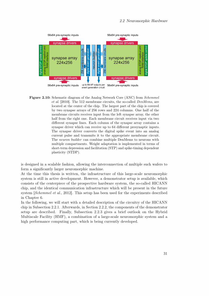
2.2 Neuromorphic Hardware
Figure 2.10: Schematic diagram of the Analog Network Core (ANC) from Schemmelet al. [2010]. The 512 membrane circuits, the so-called DenMems, arelocated at the center of the chip. The largest part of the chip is coveredby two synapse arrays of 256 rows and 224 columns. One half of themembrane circuits receives input from the left synapse array, the otherhalf from the right one. Each membrane circuit receives input via twodifferent synapse lines. Each column of the synapse array contains asynapse driver which can receive up to 64 different presynaptic inputs.The synapse driver converts the digital spike event into an analogcurrent pulse and transmits it to the appropriate membrane circuit.The neuron builder can combine multiple DenMems to neurons withmultiple compartments. Weight adaptation is implemented in terms ofshort-term depression and facilitation (STP) and spike-timing dependentplasticity (STDP).
is designed in a scalable fashion, allowing the interconnection of multiple such wafers toform a significantly larger neuromorphic machine.At the time this thesis is written, the infrastructure of this large-scale neuromorphicsystem is still in active development. However, a demonstrator setup is available, whichconsists of the centerpiece of the prospective hardware system, the so-called HICANNchip, and the identical communication infrastructure which will be present in the futuresystem [Schemmel et al., 2012]. This setup has been used for the experiments describedin Chapter 6.In the following, we will start with a detailed description of the circuitry of the HICANNchip in Subsection 2.2.1. Afterwards, in Section 2.2.2, the components of the demonstratorsetup are described. Finally, Subsection 2.2.3 gives a brief outlook on the HybridMultiscale Facility (HMF), a combination of a large-scale neuromorphic system and ahigh performance computing part, which is being currently developed.
31

2 Materials and Methods
Figure 2.11: The modular structure of a membrane circuit of the ANC. Eachmodule represents a subcircuit which models the respective variablesand/or dynamics of the AdEx neuron (see Section 2.1.6). Additionally,dedicated subcircuits allow the injection of an external current or thereadout of the membrane potential. Each generated spike is fed back intothe circuit to reset the membrane potential and increase the adaptationcurrent. The figure is taken from Schemmel et al. [2010].
2.2.1 The HICANN Chip
The HICANN chip is the centerpiece of the neuromorphic hardware system developedwithin the frame of the BrainScaleS project [Schemmel et al., 2010]. It consists of twoparts: the Analog Network Core (ANC) and the surrounding digital bus system. TheANC contains the membrane circuits with floating gate cells, which store the parametervalues of the model, and two synapse arrays, which manage the transport of analogcurrent pulses to the membrane circuits and occupy the largest part of the ANC. TheANC is surrounded by a bus system, the so-called Layer 1 (L1), which regulates thecorrect transduction of digital spikes between two neurons on the same HICANN chip aswell as between neurons located on adjacent chips.The following paragraphs offer a detailed description of the ANC, the neuron and synapseintegration and the digital circuitry on the HICANN chip. The major information istaken from Schemmel et al. [2006], Schemmel et al. [2010], Millner [2012] and the internalHICANN documentation [Schemmel et al., 2014]. These details are of central importanceto the experiments in Chapter 6.
The Analog Network Core of the HICANN chip Figure 2.10 displays a schematic ofthe ANC. The ANC contains 512 membrane circuits, the so-called DenMems, whichemulate the dynamics of the AdEx neuron model (see Section 2.1.6). The circuits aredivided into two subgroups: one group of 256 circuits receives synaptic input from theleft synapse array, the other group from the right synapse array. The 512 circuits on thechip are subdivided into 8 blocks of 64 neurons each. The neuron builder can combine upto 64 DenMems of the same block to single neurons with multiple compartments.
32

2.2 Neuromorphic Hardware
The largest part of the die is occupied by two synapse arrays, each of which consists of256 rows and 224 columns. Each column contains one synapse driver which can receiveup to 64 different inputs from the same and adjacent HICANN chips. In total, about115, 000 synapse circuits are integrated on one HICANN chip. Each membrane circuitreceives analog input via two different synapse lines for which the reversal potentials canbe set individually.The following paragraphs outline the integration of the membrane and synapse circuitsand the digital circuitry on the HICANN chip.
Neuron Integration Figure 2.11 illustrates the modular architecture of a membranecircuit of the HICANN chip [Schemmel et al., 2010]. Each DenMem consists of severalspatially divided subcircuits, each of which emulates one particular component of thedynamics of the AdEx model (see Section 2.1.6). These are:
• two synaptic input circuits,
• a leakage circuit,
• an exponential circuit, which models the rise of the membrane potential during theupswing of an action potential,
• an adaptation circuit, which models the adaptation current
• and a circuit which generates digital spike events whenever the membrane potentialcrosses some defined threshold.
The digital spike signal is sent to the digital part of the chip. Additionally, the same spikesignal is fed back into the membrane circuit to reset the membrane potential and theadaptation current. An additional subcircuit allows the injection of an external currentand the readout of the membrane potential of single neurons via two analog readoutchannels [Millner , 2012]. One of two different membrane capacitances can be selected forone block of membrane circuits [Schemmel et al., 2014].All 18 parameters of the AdEx model are stored as 24 electrical parameters in 10-bitanalog floating gate cells (see Table A.6) which are also located in the center of the ANCand which bias the membrane circuits [Srowig et al., 2007], depending on their voltage(0 to 1.8 mV) or current (0 to 2.5µA) value. The parameters which are represented bythe floating gate cells can be subdivided into individual neuron parameters and globalparameters which are shared by the membrane circuits of one block. The floating gatecells are organized in 4 arrays, each containing 129 columns with 24 rows. Of these, 128columns are used to store individual neuron parameters, while the last column storesthe values for global parameters such as the reset voltage of the block of neurons, themaximum synaptic conductance of the synapse row and the STDP parameters. The mainadvantage of the floating gate technique is the slow decay of the stored value which is inthe range of several hours [Srowig et al., 2007].However, the current design of the system entails several drawbacks which are crucialfor this thesis. One drawback of the complex circuitry are leakage currents. Each of
33

2 Materials and Methods
Figure 2.12: Simplified block diagram of a synapse array of the HICANN chip, on theleft, and a schematic of the connection between the synapse driver andthe synapse lines, on the right. Each synapse driver receives digital spikeevents, consisting of a 6 bit address, from up to 64 different presynapticsources. The first 2 bits are used to address one of the four strobe lines,while the last 4 bits determine the destination DenMem of the spike.An activated synapse line sends a square current pulse of an adjustablelength τSTDF and amplitude wi(t)× gmax(t), where wi is the individual4 bit synaptic weight and gmax the row-wise maximum conductance.The figure is taken from Schemmel et al. [2008].
the subcircuits generates unwanted leakage currents, which are of significant amplitudecompared to functionally relevant currents, such as those generated by synaptic interactionor the LIF leak current gl (V − El) itself.In summation, these effects may completely disturb the expected membrane dynamics.Due to varying leakage currents, a complete disconnection of single subcircuits, such as areduction of the AdEx model to the simpler LIF model by "turning off" the exponentialcircuit, can not be ensured for every membrane circuit on the HICANN chip. One furtherdrawback lies in the limited precision of the floating gate cell programming, which neverreaches the ideal value of 10 bits. Reprogramming the floating gate cells always leadsto small deviations in the resulting voltages and currents, thereby causing significanttrial-to-trial variability.
Synapse Integration The integration of the synapse circuits is addressed in Schemmelet al. [2008] in detail. The following passages summarize the most important aspects.The output of the membrane circuit is a digital spike event which consists of a time stampand a 6 bit address. The time stamp is used for the correct recording of the spike eventsand for Spike-Timing Dependent Plasticity (STDP) [Song et al., 2000; Friedmann, 2013],
34

2.2 Neuromorphic Hardware
while the address is used for routing the spike to the correct target neurons. The first2 bits of the address are used to choose one of four strobe lines, which initiate currentpulses of length τSTDF. The duration of these strobe pulses can be modulated by a STPmechanism (see Section 2.1.6). The last 4 bits of the address are transmitted to thesynapse array and used to address the 256 DenMem circuits of a half of the HICANNchip. Figure 2.12 depicts a block diagram of a synapse array of the HICANN chip and aschematic of the connection between the synapse driver and the synapse lines.The synaptic weights wi(t) are stored by a 4 bit SRAM cell. A 4 bit DAC translates theweight wi(t) into an output current pulse. The maximum conductance gmax, which canbe set row-wise by a programmable analog floating-gate cell, determines the scale for thesynapse DAC [Schemmel et al., 2008]. The output signal of a synapse is a square currentpulse with amplitude wi(t)× gmax(t) and duration τSTDF.The synapses are connected to the DenMem circuits via 2 lines (blue lines in Figure 2.12),respectively. The current pulses of all synaptic connections to one DenMem circuit sumup to two time-varying total input currents. The DenMem circuit translates the totalinput currents into time-varying conductance traces, emulating two different groups ofion channels, the reversal potentials of which can be programmed arbitrarily [Schemmelet al., 2008]. For instance, one ion channel can represent the excitatory input and one theinhibitory input.One drawback of the synaptic circuit induced by the nonlinearity of conductance-basedmodels is the difficulty to calibrate the synaptic drivers. The correct calibration of thesynaptic drivers requires a successful calibration of the synaptic reversal potentials ofthe membrane circuits. At the time this thesis is written, the calibration of the synapticdrivers and the reversal potentials is in active development. Synaptic weights have tobe set by hand based on the PSPs they generate on the postsynaptic membrane, whichobviously leads to limited precision and reproducibility.Furthermore, a mismatch of the parameter range of the maximum synaptic conductancegmax shrinks the usable input current pulse height [Millner , 2012]. Due to this mismatch,in the case of measurements with large biasing parameters in the floating-gate cells,the membrane potential saturates at some maximum and minimum voltage because ofsaturating synaptic weights. This mismatch will be crucial for the results in Chapter 6 ofthis thesis.
Digital Circuitry In the following, it is important to differentiate between the hardwaretime frame (HT) and the equivalent biological time (BT). The ratio between the twois defined by the acceleration factor of the hardware, which is usually assumed as 104
[Schemmel et al., 2010]. The membrane circuits generate digital spike signals whichare synchronized to an internal reference clock. The frequency of the reference clock is250 MHz and thus allows a temporal resolution of 4 ns HT (= 40µs BT). Spikes, whichare emitted closer to each other, are shifted in time. These digital signals then have to berouted to the appropriate destination. One possible destination are synaptic drivers on thesame or adjacent HICANN chips. For this, the asynchronous serial on-chip Layer 1 (L1)routing is used, which is composed of parallel Low Voltage Differential Signaling (LVDS)
35

2 Materials and Methods
Figure 2.13: The merger tree handles the routing of digital spike events on theHICANN chip. The tree structure allows to combine outputs fromthe membrane circuits and the on-chip background event generatorsin an arbitrary fashion. The lower row of the merger tree contains theso-called DNC mergers. The DNC mergers establish a communicationinterface with the DNC: Spike events can be sent from the HICANNchip to the DNC to record spike patterns, as well as from the DNC tothe HICANN chip to enable the generation of a pre-defined spike inputfor the membrane circuits. The figure is taken from Kononov [2011].
lines. Signal repeaters and switch matrices ensure that the signal reaches its target. Thedelays of the synaptic connections between two neurons are fixed by design to about0.12µs HT (= 1.2 ms BT).The other possible destination is the so-called Digital Network Chip (DNC). The DNCis a digital ASIC which allows to record the spike patterns of neurons of the HICANNchip and send them via an FPGA board to the host computer [Schemmel et al., 2010].Conversely, it allows to generate a predefined spike pattern on the host computer androute it to arbitrary membrane circuits. The DNCs together with the FPGA boardsconstitute the so-called Layer 2 (L2) routing, which is synchronous and packet-based.The so-called merger tree, which is depicted in Figure 2.13, enables an efficient routing ofdigital signals on the HICANN chip. There are 8 different mergers in the upper row ofthe merger tree, one for each block of membrane circuits. These mergers allow to mergethe digital spike events of the neurons with spike events from one of 8 Background EventGenerators (BEG) which are placed on the HICANN chip.The BEGs can generate periodic or pseudo-random Poisson-distributed spike patterns
36

2.2 Neuromorphic Hardware
Figure 2.14: The demonstrator setup, which was used to perform the hardware ex-periments in the course of this thesis [Schemmel et al., 2012]. It consistsof a System Emulator Board (SEB) which connects up to 8 HICANNchips to a DNC. Two FPGA boards provide the connection to thehost computer and the power supply. Additionally, an ADC board (notshown here) is located on the SEB which allows the simultaneous digitalreadout of the membrane potential of two neurons of one HICANN chip.The demonstrator setup establishes a communication infrastructureequivalent to that of the FACETS Wafer-Scale Hardware System, theinfrastructure of which is currently in active development. The figure istaken from Millner [2012].
with a temporal resolution of 4 ns HT [Kononov , 2011]. The pseudo-random input isgenerated via a 16-bit Linear Feedback Shift Register (LFSR). Therefore, the generatedPoisson-distributed spike pattern is completely deterministic and repeats after it hasoccupied its 216 = 65535 states, which is equivalent to about 262µs HT (= 2.62 s BT)[Schemmel et al., 2014]. Furthermore, each of the 8 BEGs on one HICANN chip occupiesthe same sequence of states. However, the starting point of this sequence can be variedby choosing an arbitrary seed between 0 and 65535.The lower row of the merger tree (see Figure 2.13) contains the so-called DNC mergers.At this point, digital signals can leave the HICANN chip towards the DNC or sent to theHICANN chip via the DNC.The following section presents the hardware setup which was used to perform the experi-ments in Chapter 6. Particular focus is placed on the achievable data rates between thedigital and the analog parts of the system.
37
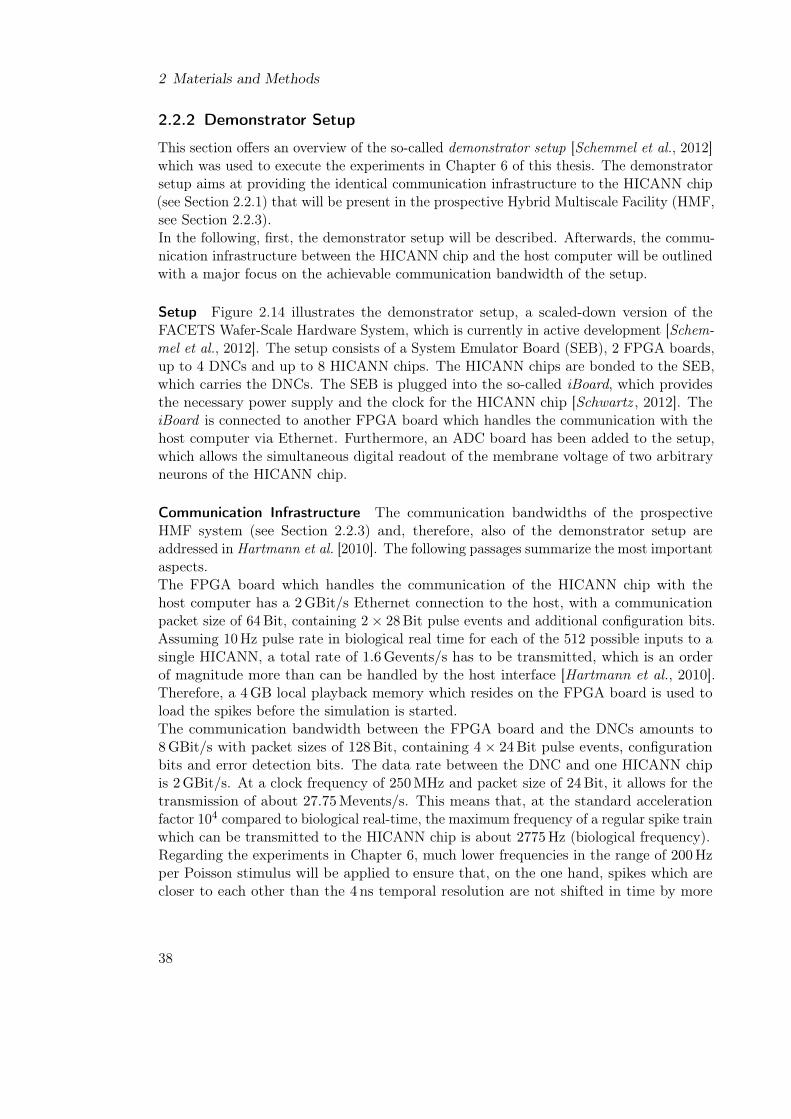
2 Materials and Methods
2.2.2 Demonstrator Setup
This section offers an overview of the so-called demonstrator setup [Schemmel et al., 2012]which was used to execute the experiments in Chapter 6 of this thesis. The demonstratorsetup aims at providing the identical communication infrastructure to the HICANN chip(see Section 2.2.1) that will be present in the prospective Hybrid Multiscale Facility (HMF,see Section 2.2.3).In the following, first, the demonstrator setup will be described. Afterwards, the commu-nication infrastructure between the HICANN chip and the host computer will be outlinedwith a major focus on the achievable communication bandwidth of the setup.
Setup Figure 2.14 illustrates the demonstrator setup, a scaled-down version of theFACETS Wafer-Scale Hardware System, which is currently in active development [Schem-mel et al., 2012]. The setup consists of a System Emulator Board (SEB), 2 FPGA boards,up to 4 DNCs and up to 8 HICANN chips. The HICANN chips are bonded to the SEB,which carries the DNCs. The SEB is plugged into the so-called iBoard, which providesthe necessary power supply and the clock for the HICANN chip [Schwartz , 2012]. TheiBoard is connected to another FPGA board which handles the communication with thehost computer via Ethernet. Furthermore, an ADC board has been added to the setup,which allows the simultaneous digital readout of the membrane voltage of two arbitraryneurons of the HICANN chip.
Communication Infrastructure The communication bandwidths of the prospectiveHMF system (see Section 2.2.3) and, therefore, also of the demonstrator setup areaddressed in Hartmann et al. [2010]. The following passages summarize the most importantaspects.The FPGA board which handles the communication of the HICANN chip with thehost computer has a 2 GBit/s Ethernet connection to the host, with a communicationpacket size of 64 Bit, containing 2× 28 Bit pulse events and additional configuration bits.Assuming 10Hz pulse rate in biological real time for each of the 512 possible inputs to asingle HICANN, a total rate of 1.6 Gevents/s has to be transmitted, which is an orderof magnitude more than can be handled by the host interface [Hartmann et al., 2010].Therefore, a 4 GB local playback memory which resides on the FPGA board is used toload the spikes before the simulation is started.The communication bandwidth between the FPGA board and the DNCs amounts to8 GBit/s with packet sizes of 128 Bit, containing 4 × 24 Bit pulse events, configurationbits and error detection bits. The data rate between the DNC and one HICANN chipis 2 GBit/s. At a clock frequency of 250 MHz and packet size of 24 Bit, it allows for thetransmission of about 27.75 Mevents/s. This means that, at the standard accelerationfactor 104 compared to biological real-time, the maximum frequency of a regular spike trainwhich can be transmitted to the HICANN chip is about 2775 Hz (biological frequency).Regarding the experiments in Chapter 6, much lower frequencies in the range of 200 Hzper Poisson stimulus will be applied to ensure that, on the one hand, spikes which arecloser to each other than the 4 ns temporal resolution are not shifted in time by more
38

2.2 Neuromorphic Hardware
Figure 2.15: The neuromorphic part of the HMF with the wafer as main component.One wafer consists of about 180,000 neurons and more than 40 millionsynapses. Additionally, the infrastructure of the wafer is depicted whichconsists of a large PCB with modules which handle the wafer-to-waferand the wafer-to-host communication. Aluminum frames stabilize thesystem and act as heat sinks. The figure is taken from [Brüderle et al.,2011].
than about 100 ns hardware execution time. On the other hand, multiple neurons can besimultaneously supplied by multiple independent Poisson sources.
2.2.3 Hybrid Multiscale Facility
The Electronic Vision(s) group at the University of Heidelberg and the group for ParallelVLSI Systems and Neural Circuits at the TU Dresden are currently developing theso-called Hybrid Multiscale Facility (HMF), which is a system that goes far beyond thesingle chip level [Schwartz , 2012]. The HMF will consist of two parts: a neuromorphicpart of 6 interconnected wafers containing up to 1.2 million membrane circuits and about260 million synapse circuits, and a modern high-performance computer cluster whichprovides the communication and control of the neuromorphic system [Schwartz , 2012].The following brief discussion will focus on the characterization of the neuromorphic partof the system, which comprises the wafers and their communication environment.
Wafer The neuromorphic part of the HMF will contain 6 wafer modules. Figure 2.15depicts one of the wafer modules and its associated communication, control and powerstructures. The silicon wafer has a diameter of 20 cm and is fabricated using the 180 nm
39

2 Materials and Methods
UMC CMOS process [Schemmel et al., 2010]. It consists of 384 HICANN chips (seeSection 2.2.1) which are organized in groups of 8 chips, the so-called reticles. Each waferis left uncut after the fabrication and during the so-called post-processing step the chipsare connected directly on the wafer. With the help of this "third spatial dimension",very large communication densities between the chips are realized. Altogether, one wafercontains about 180, 000 membrane circuits and 40 million synapse circuits.
Communication Infrastructure The wafer is connected to a Printed Circuit Board(PCB) which provides the necessary power supply for the wafer and connects it to thedigital communication part. The digital communication part has the same hierarchy andidentical bandwidths as the communication part of the demonstrator setup described inSection 2.2.2. At the lowest hierarchical level are the 48 DNCs, one DNC per reticle. 4DNCs are connected to 1 FPGA board, respectively, which amounts to 12 FPGA boardsfor the whole wafer. The FPGA boards are connected to the host computer and to eachother via a 10 GBit/s Ethernet connection. For further information, see Hartmann et al.[2010].
2.3 Software Framework
This section describes the software environments which have been used throughout thisthesis. It is divided into two subsections.Subsection 2.3.1 presents the simulator-independent metalanguage PyNN which, togetherwith the simulator NEST [Diesmann and Gewaltig , 2002] as its back-end, has been usedto run the simulations of networks of LIF neurons in Chapters 3, 4 and 5.Subsection 2.3.2 deals with the Hardware Abstraction Layer (HAL), the stack of softwaremodules which allows to run experiments on the demonstrator setup described in Section2.2. In particular, the hardware experiments in Chapter 6 have been executed via thePython-based interpreter PyHAL, which wraps the native HAL language.
2.3.1 Simulation of Neural Networks
Plenty of simulation environments have emerged in computational neuroscience in thepast 20 years [Brette et al., 2007] and nowadays serve as non-invasive alternatives forthe common in-vivo and in-vitro experiments in neuroscientific research. All of thesesoftware simulators come with their individualities: the level of detail of neuron andnetwork models, the simulation strategy, the algorithms and the native programminglanguage to name some of these. They offer the neuroscientific modeler a diverse pool oftools to set up the desired networks models.However, with the diversity of software simulators, the lack of reproducibility of neurosci-entific experiments increases [Davison et al., 2008]. The code of a model which has beenwritten for one particular simulation environment has to be, in the worst case, completelyrewritten in order to fit into another simulator, since network components and parametersare expressed differently in the different environments.
40

2.3 Software Framework
To overcome this lack of reproducibility, the simulator-independent software environmentPyNN has been established [Davison et al., 2008] and remains in active developmentwithin the BrainScaleS project. The following paragraph gives a brief introduction ofPyNN and its API. Afterwards, the simulator NEST is described, which is used as PyNNback-end throughout this thesis.
PyNN PyNN [2014] is a Python package [Python, 2014] for simulator-independentmodeling of neural networks. PyNN is designed with the main aim to "write the codeonce and run it on any supported simulator or hardware device without modification"[Davison et al., 2008].PyNN exploits the fact that many of the available non-commercial software simulatorshave, additionally to their native interpreter language, a Python interpreter which offersthe equivalent functionality to the native language. Figure 2.16 gives an overview of thesimulation and emulation back-ends which PyNN currently supports: NEST [Diesmannand Gewaltig , 2002], NEURON [Hines and Carnevale, 2003], PCSIM [Pecevski et al., 2009],Brian [Goodman and Brette, 2008], NeuroML [Gleeson et al., 2010] and the FACETS andBrainScaleS hardware systems, described in Section 2.2. However, due to the still ongoingdevelopment of suitable calibration and routing routines of the current neuromorphichardware system (see Section 2.2), a PyNN-level implementation was infeasible. Instead,the hardware experiments were executed via the native interpreter language StHAL (seeSection 2.3.2).The PyNN API can be divided into two levels of abstraction: the low-level API and thehigh-level API [PyNN , 2014]. The low-level procedural API provides a flexible accessto individual neurons and synapses via functions like create(), connect() and record().The high-level object-oriented API provides classes like Population() and Projection().These classes allow the modeling of neuron populations, layers or columns with arbitraryconnectivity algorithms, such as all-to-all connections, random or distance-dependentconnectivity.The PyNN API contains a huge library of models of neurons, synapses and synapticplasticity which have been proven to show the same dynamics on all supported simulationback-ends [Davison et al., 2008].
NEST The software simulations in the course of this thesis have been carried out usingPyNN with the simulator NEST as a back-end.The NEST software environment [Diesmann and Gewaltig , 2002] mainly focuses on thesimulation of large networks of neurons with a biologically realistic connectivity pattern,without going into the morphological details of individual neurons. Biologically realisticconnectivity patterns require an efficient representation and updating of synapses aswell as a parallelization of the network construction and its dynamics. Therefore, thecomputational efficiency is of major interest for the NEST developers [Brette et al., 2007].
41

2 Materials and Methods
Figure 2.16: Schematic of the simulator-independent modeling language PyNN fromBrüderle et al. [2011]. The software simulators NEST [Diesmannand Gewaltig , 2002], NEURON [Hines and Carnevale, 2003], PCSIM[Pecevski et al., 2009], Brian [Goodman and Brette, 2008], NeuroML[Gleeson et al., 2010] as well as the FACETS and BrainScaleS neuro-morphic hardware systems have been integrated into the PyNN concept.The dashed frame comprises the interpreter levels of the hardware ab-straction layer (HAL), which is currently in active development. TheHAL is the stack of software modules which will, in the future, providean automated translation between PyNN model descriptions and appro-priate hardware configuration and control patterns. For further details,see Brüderle et al. [2011].
2.3.2 Emulation of Neural Networks
The desired software framework for the neuromorphic hardware setup described in Section2.2 has to comprise two general aspects: it has to hide as many hardware-specific detailsas possible from the modeler on the one hand, and, on the other hand, provide anintuitive access to the hardware system similar to that of common software simulators.Therefore, a PyNN interface to the hardware system is currently in active development(see Figure 2.16).However, setting up an experiment in software distinctly differs from setting up exactly thesame experiment on the hardware system. Several additional facts have to be consideredwhen running experiments on hardware: the limited range of neurons and synapses,the maximally available bandwidths, the spatial arrangement of neurons and synapses,varying or even defect dynamics of membrane and synapse circuits due to floating gateimprecisions or production faults during the fabrication process to name just a few.Therefore, in order to be able to provide a reliable system for the end user, sophisticatedmapping and calibration routines have to implemented which are able to translate abstractdescriptions of neural networks to maps of membrane circuits on the hardware systemand parameters of single neurons, such as reversal potentials and time constants, to theirhardware representation.At the time this thesis was written, the mapping and calibration routines were in active
42
2.3 Software Framework
development. Thus, the experiments which were executed on the hardware systemthroughout this thesis had to be setup by hand using the native interpreter of thehardware system (HAL, see Figure 2.16). Setting up the experiments by hand involvesthe searching of appropriate membrane and synapse circuits on the hardware setup andthe adjusting of floating gates cells such that the circuits exhibit the expected dynamics.The following paragraph gives a brief introduction to the HAL interpreter and its majorclasses and functions. Further information can be found e.g. in Brüderle et al. [2011].
The HAL Interface The dashed frame in Figure 2.16 comprises the interpreter levelsof the so-called hardware abstraction layer (HAL). The HAL is the batch of softwaremodules which will provide an automated translation between PyNN model descriptionsand correct hardware configuration and control patterns in the prospective hardwaresystem [Brüderle et al., 2011]. In its current version, the hardware system is accessedvia calling the native classes and functions of the HAL API from its Python layer, theso-called PyHAL.At the lowest level, the HAL interfaces with the hardware assembler via various C++classes and uses the ARQ protocol [Peterson and Davie, 2003] to establish a fast andreliable communication. The HAL can be subdivided into two different interfaces: thestateless HALbe interface and the stateful StHAL interface.The major task of the HALbe interface is the specification of a coordinate system foreach single component of the hardware system described in Section 2.2. The coordinatesystem represents several addressable layers reaching from wafers, to FPGAs and DNCsconnected to the wafer, to reticles on the wafer, to HICANN chips on the reticle, andfinally to membrane circuits, floating gate cells, synapse circuits, repeaters and switchmatrices on the HICANN chip. For detailed information, see Schemmel et al. [2014].The stateful StHAL interface provides, from the end-user perspective, methods whichenable to e.g. write floating gate cells, set up the configuration of the BEGs and themerger tree, change the state of repeaters and switches on the HICANN chip, configure thesynapse drivers, inject a current into the membrane of a neuron, read out the membranepotential and the output spikes of a neuron or send spikes from the host computer viathe FPGA boards to the chip (see Schemmel et al. [2014]).The Boost.Python library [Abrahams and Grosse-Kunstleve, 2003] is used to wrap theoriginal C++ classes and functions to Python, yielding the Python control layer PyHAL[Brüderle et al., 2009]. PyHAL is the highest abstraction level of the hardware systemand provides the desired interpreter-based interface to the hardware.A module for the integration of this interface into the meta-language PyNN (see Sec-tion 2.3.1) is implemented, but not utilizable at the time this thesis is written due tothe lack of reliable mapping and calibration routines, which are in active development.In the future, the mapping of a PyNN network onto the configuration space of thewafer-scale hardware system will be divided into three automated processing steps: theplacing of neurons onto the available circuitry, the configuring of the routing infrastructureon the device, and the transformation of 18 neuron and synapse parameters into thecorresponding 24 hardware parameters [Brüderle et al., 2011].
43

3 Characterization of LIF Sampling fromBoltzmann Distributions
The characterization of LIF sampling from Boltzmann distributions is an essential startingpoint for the remainder of this thesis. We get used to the crucial parameters of LIFneurons and find out the limits of LIF sampling from Boltzmann distributions. Here, weespecially focus on the question: how reliable are the sampling results of LIF neurons fromBoltzmann distributions with large weights and biases? Since both implementations ofBayesian Networks with spiking neurons require large weights and biases (see Section 2.1.5)these results will be useful for prognosticating the expected performance of LIF samplingfrom Bayesian Networks.Section 3.1 describes the necessary calibration procedure which aims at finding thecorrespondence of the effective membrane potential of a conductance-based LIF neuronand the probability to find the neuron in the refractory state. For this, the effectivemembrane voltage of a LIF neuron in a spiking noisy environment will be varied and thetime fraction during which the neuron is refractory will be measured. The calibrationallows to set the resting potential of a LIF neuron according to the a priori known bias ofthe associated RV.Then we attend in Section 3.2 to Boltzmann Machines (BMs) of 5 RVs and test thesampling performance of LIF neurons for randomly generated Boltzmann distributionswith different maximal weights and biases. For this, the parameters of the LIF neuronsare set with respect to simplicity and compatibility with fluctuations of the neuromorphichardware which will be used in Chapter 6. The same measure of the sampling quality isperformed for stochastic spiking neurons with ideal rectangular or alpha-shaped PSPs(from Pecevski et al. [2011]) for reasons of comparison. In contrast to the ideal PSPs, LIFPSPs are highly asymmetric and decay exponentially, thus, they significantly affect thesubsequent course of the membrane potential. These facts will turn out to delimitate theLIF sampling performance.Two randomly picked BMs, one with low weights and biases and one which incorporatesvery large weights and biases, are then used in Section 3.3 to explore the samplingperformance under different parameter choices. The time constants τm, τsyn and τref arein the major focus of this investigation since they define the shape of a PSP. Although itwill be impossible to draw general conclusions for all BMs from these results, we will seethat there are indeed individual task-dependent parameters, which enable LIF neurons tosample with a satisfactory precision from Boltzmann distributions with large weights andbiases.
44

3.1 Calibration of a LIF Neuron to Perform LIF Sampling
50.6 50.4 50.2 50.0 49.8 49.6 49.4Effective membrane potential [mV]
0.0
0.2
0.4
0.6
0.8
1.0p
ON
fitted pON
measured pON
0
20000
40000
60000
80000
100000
120000
Occu
rren
ces
Figure 3.1: The figure shows the calibration procedure which has to be establishedonce per set of neuron parameters. For 21 different effective potentialsVeff (blue) the fraction of time is measured which the neuron spends inthe refractory state (ON-state). The error bars are standard deviationsfrom 5 simulations of duration 200 s. The calibration via effective po-tentials Veff , instead of resting potentials Vrest, is appropriate for theconductance-based model, since it considers the impact of the additionalsynaptic conductances provided by the background input on the mem-brane potential. The green histogram shows the distribution of the freemembrane potential of a LIF neuron with parameters from Table A.1and Vrest = −50 mV.
3.1 Calibration of a LIF Neuron to Perform LIF Sampling
A conductance-based LIF neuron has to be calibrated before it can be used for samplingfrom probability distributions. Similar to the NCC in Equation 2.18, its mean membranepotential has to be related to its probability pON to be in the refractory state.For this, two essential steps have to be fulfilled. First we need to measure the activationcurve. A range of effective membrane potentials Veff is chosen which covers the wholerange of probabilities pON from 0 to 1. This is done by estimating the mean µV and thespread σV of the free membrane potential based on the known mean synaptic input. Inthe second step, these effective membrane potentials are translated into resting potentialsVrest and corresponding leakage conductances gl. For each resting potential and leakageconductance, pON can be measured from a single neuron simulation. A logistic function isthen fitted to the measured data and we directly obtain the value of the resting potential
45

3 Characterization of LIF Sampling from Boltzmann Distributions
Vb=0, for which pON = 0.5, and the parameter α from Equation 2.70. This will allow for
translating Boltzmann biases and weights to resting potentials of neurons and weights ofthe synaptic connections.
3.1.1 Finding a Good Range of Effective Membrane Potentials
Section 2.1.7 demonstrates that under balanced random synaptic stimulation the freemembrane potential of a LIF neuron can be described by an OU process. The histogramin Figure 3.1 shows that the free membrane potential of the neuron then is Gaussiandistributed. Given the parameters of the neuron and the background input, the mean µVand the spread σV of the free membrane potential amount to (see Equations 2.49 and2.50):
µV =glEl +
∑i gi(t)E
revi
gtot(t), (3.1)
andσ2V =
∑i
νiS2i
(τeff
2+τsyn,i
2− 2
τeffτsyn,i
τeff + τsyn,i
), (3.2)
withSi =
wi (Erevi − µV )
Cm
(1τeff− 1
τsyn,i
) . (3.3)
Now we can estimate the range of effective membrane voltages which is needed to coverthe whole range of probabilities pON from 0 to 1. Under the assumption that in theHCS the membrane potential will stay close to the threshold compared to the reversalpotentials the threshold voltage is used as central point for this range. Heuristically 4σVturns out to be a good estimate for the spread of this range: it contains more than 99.9%of the possible assignments of the free membrane voltage and likewise provides for anoptimal resolution of the growth of the activation curve. We choose NV equally spacedpotentials with a maximal effective membrane potential
Veff,max = Vth + 4σV
(1 +
1
NV − 1
), (3.4)
and a minimal effective membrane potential
Veff,min = Vth − 4σV
(1 +
1
NV − 1
). (3.5)
3.1.2 Measuring the Activation Curve
Now the membrane potential of the LIF neuron has to be set to these effective membranepotentials and the fraction of time has to be measured during which the neuron staysrefractory. For this, the effective membrane potentials have to be transformed to resting
46

3.2 LIF Sampling from Boltzmann Distributions of 5 Random Variables
potentials Vrest and additional leakage conductances w. The maximal and minimaladditional conductance wmax and wmin can be calculated:
wmax =gtot(t)Veff,max − glVth −
∑i gi(t)E
revi
Erevexc − Veff,max
, (3.6)
and wmin = −wmax. For each of the equally spaced NV additional conductances w thetotal leakage conductance amounts to g̃l = gl + |w|. The parameters of the LIF neuronwhich determine the effective membrane potential are τm and Vrest, for which we get:
τm =Cm
g̃l, (3.7)
and
Vrest =
{glVth+wErev
excg̃l
, if w ≥ 0glVth−wErev
inhg̃l
, if w < 0. (3.8)
Following this procedure, we get NV different values for τm and Vrest. These values cannow be initialized for the LIF neuron in simulations. If the neuron elicits NS spikes in asimulation of duration T , then the probability to be in the ON-state z = 1 is
pON =NSτref
T. (3.9)
The blue dots in Figure 3.1 illustrate the measured probabilities pON for NV = 21 differenteffective membrane potentials for a LIF neuron with parameters from Table A.1. Theerror bars indicate the standard deviations from 5 simulations of duration 200 s.The measured data is fitted to a logistic function
σ
(V − V b=0
α
)=
1
1 + exp(−(V−V b=0
α
)) , (3.10)
and the parameters V b=0 and α can be directly extracted. Figure 3.1 shows a logisticfit to measured data. For the intermediate part of the curve, the logistic function welldescribes the data. However, at low voltages the transition to pON = 0 occurs faster. Atlarge voltages, the state pON = 1 is never reached because of non-zero time constants.
3.2 LIF Sampling from Boltzmann Distributions of 5Random Variables
From previous experiments by e.g. Petrovici et al. [2013], it is known that the LIFparameters in Table A.1 provide for a good sampling performance from BMs with lowweights and biases. We will conduct a closer investigation of BMs via the followingexperiment: Different BMs of 5 RVs are randomly generated by drawing the weightsand biases from a uniform distribution [−wmax, wmax]. The parameter wmax is varied
47

3 Characterization of LIF Sampling from Boltzmann Distributions
0 10 20 30 40 50Time [ms]
0.0
0.1
0.2
0.3
0.4
0.5
0.6
0.7
0.8
0.9
Volta
ge [a
.u.]
Rectangular PSPAlpha PSPLIF PSP
Figure 3.2: The LIF PSP shape (green) with τref = 30 ms and τsyn = 30 ms which wasused in the simulations in this section. In addition, the rectangular PSPand alpha-shaped PSP, which are the original PSPs from Pecevski et al.[2011], are plotted.
from 0.2 to 10.0 and for each generated BM a simulation of 200 s is run. The obtainedjoint probability distribution is compared to the theoretical joint distribution via the KLdivergence (see Equation 2.15). This experiment is repeated 10 times for each wmax.Figure 3.3 shows the results of the simulations. Furthermore, it shows results of the sameexperiments with stochastic neurons with ideal rectangular PSPs and alpha-shaped PSPs(see Figure 3.2). For each wmax, the LIF sampling result is does not reach the quality ofsampling with stochastic neurons: about one order of magnitude less precise than thesimulations using alpha-shaped PSPs and up to two orders of magnitude less precise thanthe results with ideal rectangular PSPs. Furthermore, the sampling quality decreasesby three orders of magnitude for large weights and biases, which is to some degree alsoobservable in the experiments with stochastic neurons: The KL divergence between thesimulated and theoretical joint probability distribution for alpha-shaped PSPs decreasesby two orders of magnitude, for rectangular PSPs by about one order of magnitude.The imprecise LIF sampling performance can be explained based on the PSP shapesin Figure 3.2. Two differences are crucial: On the one hand, in opposite to the PSPsof the stochastic neurons the LIF PSP is highly asymmetric, thus the firing probabilitydirectly after an incoming spike is by far larger than the firing probability at the end ofthe refractory period. On the other hand, the LIF PSP has an infinite duration and thusinfluences the course of the membrane potential beyond τref . This influence obviously
48
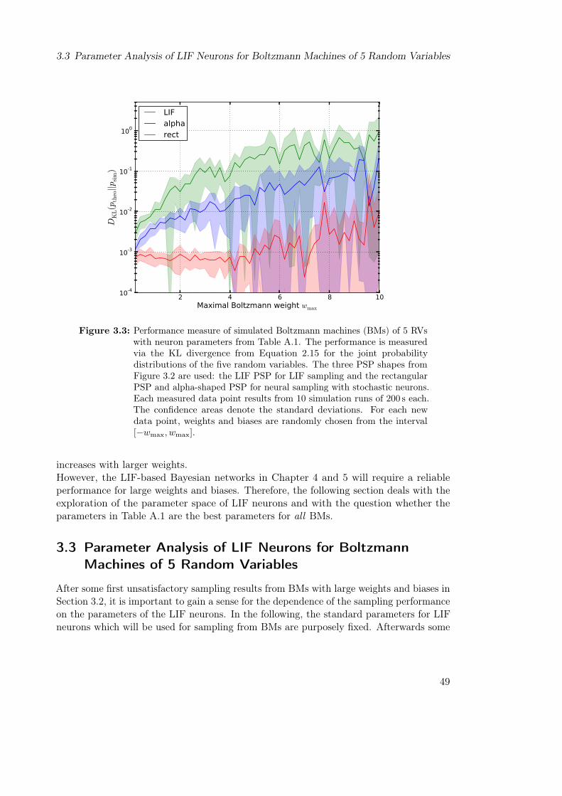
3.3 Parameter Analysis of LIF Neurons for Boltzmann Machines of 5 Random Variables
2 4 6 8 10Maximal Boltzmann weight wmax
10-4
10-3
10-2
10-1
100
DK
L(p
theo||p
sim)
LIFalpharect
Figure 3.3: Performance measure of simulated Boltzmann machines (BMs) of 5 RVswith neuron parameters from Table A.1. The performance is measuredvia the KL divergence from Equation 2.15 for the joint probabilitydistributions of the five random variables. The three PSP shapes fromFigure 3.2 are used: the LIF PSP for LIF sampling and the rectangularPSP and alpha-shaped PSP for neural sampling with stochastic neurons.Each measured data point results from 10 simulation runs of 200 s each.The confidence areas denote the standard deviations. For each newdata point, weights and biases are randomly chosen from the interval[−wmax, wmax].
increases with larger weights.However, the LIF-based Bayesian networks in Chapter 4 and 5 will require a reliableperformance for large weights and biases. Therefore, the following section deals with theexploration of the parameter space of LIF neurons and with the question whether theparameters in Table A.1 are the best parameters for all BMs.
3.3 Parameter Analysis of LIF Neurons for BoltzmannMachines of 5 Random Variables
After some first unsatisfactory sampling results from BMs with large weights and biases inSection 3.2, it is important to gain a sense for the dependence of the sampling performanceon the parameters of the LIF neurons. In the following, the standard parameters for LIFneurons which will be used for sampling from BMs are purposely fixed. Afterwards some
49
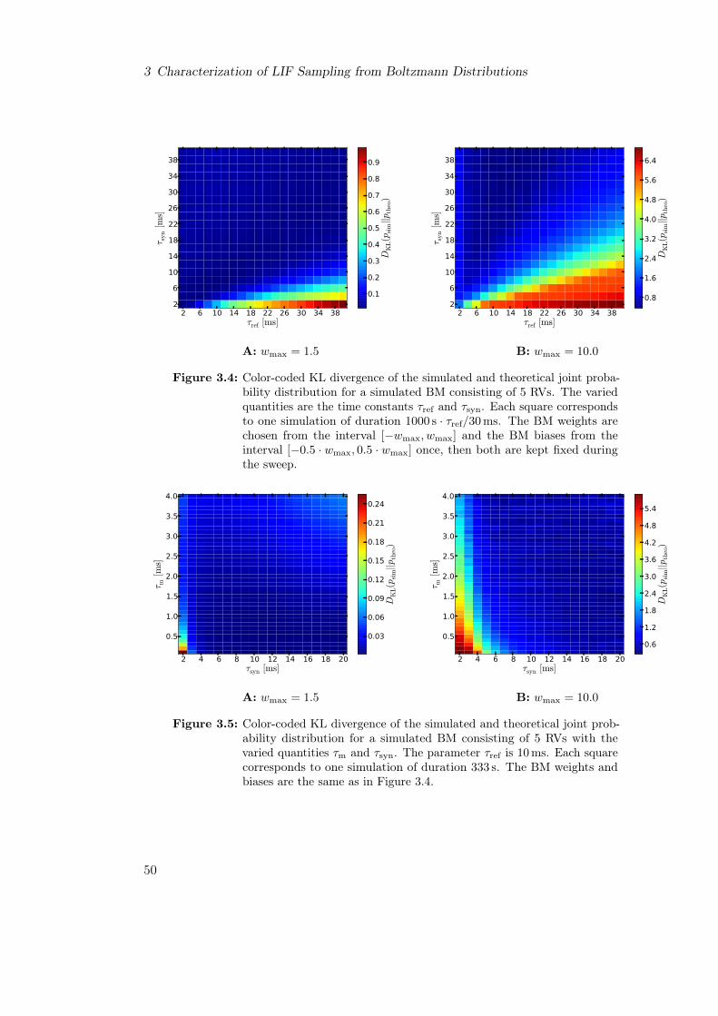
3 Characterization of LIF Sampling from Boltzmann Distributions
2 6 10 14 18 22 26 30 34 38τref [ms]
2
6
10
14
18
22
26
30
34
38τ s
yn
[ms]
0.1
0.2
0.3
0.4
0.5
0.6
0.7
0.8
0.9
DK
L(p
sim||p
theo)
A: wmax = 1.5
2 6 10 14 18 22 26 30 34 38τref [ms]
2
6
10
14
18
22
26
30
34
38
τ syn
[ms]
0.8
1.6
2.4
3.2
4.0
4.8
5.6
6.4
DK
L(p
sim||p
theo)
B: wmax = 10.0
Figure 3.4: Color-coded KL divergence of the simulated and theoretical joint proba-bility distribution for a simulated BM consisting of 5 RVs. The variedquantities are the time constants τref and τsyn. Each square correspondsto one simulation of duration 1000 s · τref/30 ms. The BM weights arechosen from the interval [−wmax, wmax] and the BM biases from theinterval [−0.5 · wmax, 0.5 · wmax] once, then both are kept fixed duringthe sweep.
2 4 6 8 10 12 14 16 18 20τsyn [ms]
0.5
1.0
1.5
2.0
2.5
3.0
3.5
4.0
τ m[m
s]
0.03
0.06
0.09
0.12
0.15
0.18
0.21
0.24
DK
L(p
sim||p
theo)
A: wmax = 1.5
2 4 6 8 10 12 14 16 18 20τsyn [ms]
0.5
1.0
1.5
2.0
2.5
3.0
3.5
4.0
τ m[m
s]
0.6
1.2
1.8
2.4
3.0
3.6
4.2
4.8
5.4
DK
L(p
sim||p
theo)
B: wmax = 10.0
Figure 3.5: Color-coded KL divergence of the simulated and theoretical joint prob-ability distribution for a simulated BM consisting of 5 RVs with thevaried quantities τm and τsyn. The parameter τref is 10 ms. Each squarecorresponds to one simulation of duration 333 s. The BM weights andbiases are the same as in Figure 3.4.
50

3.3 Parameter Analysis of LIF Neurons for Boltzmann Machines of 5 Random Variables
free parameters will be altered and the sampling performance will be measured for thenew parameter choices. In particular, it will be tested whether the sampling results canbe improved for BMs with large weights and biases by optimizing the neural parameters.
3.3.1 Parameter Selection
The parameters in Table A.1 have been selected for different reasons. First, there is thereason of simplicity. The values for Vth, Erev
exc and Erevinh are selected such that EPSPs and
IPSPs are approximately the same size. The STP parameters U0 and τrec are chosen inorder to provide for renewal PSPs (see Section 2.1.7).Second, for mathematical reasons it is important to keep the quotient τeff/τsyn small suchthat the first-order approximation of Equation 2.69 can be applied. This is achieved bya very small membrane time constant τm and a very large synaptic time constant τsyn.Finally, the parameters Cm, Vreset and the background input rates are chosen such thatthey match the constraints of the neuromorphic hardware which will be used in Chapter6.
3.3.2 Parameter Optimization for Sample Boltzmann Machines
In the following an extensive parameter analysis of LIF neurons is provided based on theLIF sampling results from two different Boltzmann distributions. The distributions arerandomly generated once, by uniformly drawing weights from the interval [−wmax, wmax]and biases from [−0.5 · wmax, 0.5 · wmax], and kept for all experiments. For the first BMthe maximum weight is wmax = 1.5, so only small weights and biases are allowed.The KL divergence of the product of theoretical marginals and the theoretical jointdistribution is DKL(pPOM||ptheo) = 0.02. This result is taken as a worst case scenariobecause it assumes independence among the RVs. The second BM has wmax = 10.0 andalso allows for large weights and biases. Its KL divergence of the product of theoreticalmarginals and the theoretical joint distribution is DKL(pPOM||ptheo) = 2.03.If not explicitly mentioned, the standard parameters of the following simulations aretaken from Table A.1. The experimental durations of the simulations are chosen forreasons of comparability. The duration of a simulation with LIF neurons with a refractorytime τref = 30 ms is fixed to 1000 s for this chapter. For other τref the duration of thesimulation obviously has to be 1000 s · τref/30 ms such that the LIF neuron has the samenumber of opportunities to change the state of its corresponding RV.Figure 3.4 shows the LIF sampling results for different choices of the refractory timeconstant τref and the synaptic time constant τsyn. In both cases, τsyn � τref is the yieldsa bad sampling quality and τsyn ≈ τref performs better. For the BM with wmax = 10,τsyn > τref yields the best results of about DKL(psim||ptheo) = 0.4 which is distinctlybetter than DKL(pPOM||ptheo) = 2.03.Figure 3.5 illustrates the LIF sampling quality under variation of the membrane timeconstant τm and the synaptic time constant τsyn with τref = 10 ms. For the BM withwmax = 1.5, the best results are achieved for τm = 0.1 ms and τsyn < τref . LIF samplingfrom the BM with wmax = 10, if τsyn > τref , a result which can also be seen in Figure 3.4.
51
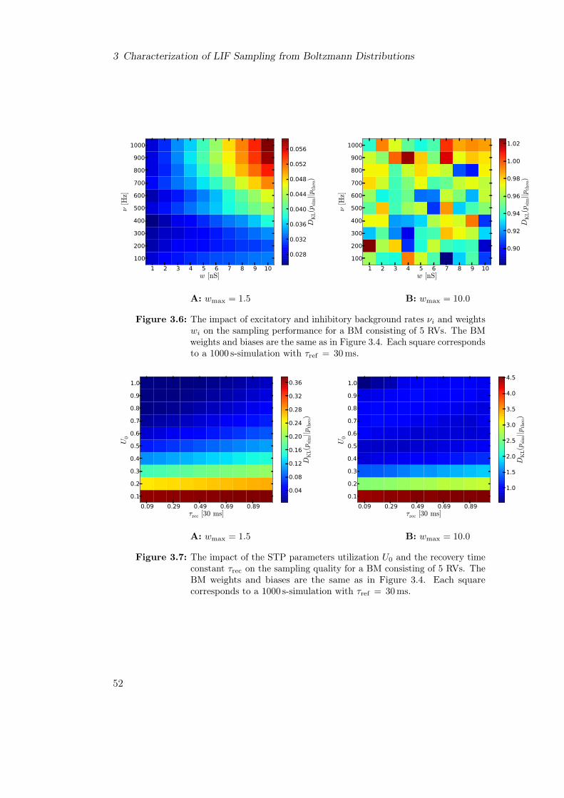
3 Characterization of LIF Sampling from Boltzmann Distributions
1 2 3 4 5 6 7 8 9 10w [nS]
100
200
300
400
500
600
700
800
900
1000
ν[H
z]
0.028
0.032
0.036
0.040
0.044
0.048
0.052
0.056
DK
L(p
sim||p
theo)
A: wmax = 1.5
1 2 3 4 5 6 7 8 9 10w [nS]
100
200
300
400
500
600
700
800
900
1000
ν[H
z]
0.90
0.92
0.94
0.96
0.98
1.00
1.02
DK
L(p
sim||p
theo)
B: wmax = 10.0
Figure 3.6: The impact of excitatory and inhibitory background rates νi and weightswi on the sampling performance for a BM consisting of 5 RVs. The BMweights and biases are the same as in Figure 3.4. Each square correspondsto a 1000 s-simulation with τref = 30 ms.
0.09 0.29 0.49 0.69 0.89τrec [30 ms]
0.1
0.2
0.3
0.4
0.5
0.6
0.7
0.8
0.9
1.0
U0
0.04
0.08
0.12
0.16
0.20
0.24
0.28
0.32
0.36
DK
L(p
sim||p
theo)
A: wmax = 1.5
0.09 0.29 0.49 0.69 0.89τrec [30 ms]
0.1
0.2
0.3
0.4
0.5
0.6
0.7
0.8
0.9
1.0
U0
1.0
1.5
2.0
2.5
3.0
3.5
4.0
4.5
DK
L(p
sim||p
theo)
B: wmax = 10.0
Figure 3.7: The impact of the STP parameters utilization U0 and the recovery timeconstant τrec on the sampling quality for a BM consisting of 5 RVs. TheBM weights and biases are the same as in Figure 3.4. Each squarecorresponds to a 1000 s-simulation with τref = 30 ms.
52

3.4 Conclusion
Figure 3.6 shows the impact of the input rate and weight of the Poisson backgroundstimulus on the LIF sampling performance. For the BM with wmax = 1.5, a tendencytowards small weights is visible, an observation which is also expected due to Equation2.55. For the BM with large weights and biases, no significant preference of a rate andweight can be observed. However, in difference to the parameter sweeps in Figures 3.4and 3.5, the overall variations of the sampling performance are very low.Figure 3.7 demonstrates the LIF sampling performance for different choices of the uti-lization of the synaptic efficacy parameter U0 and the recovery time constant τrec fromthe TM model (see Section 2.1.6). For both BMs, the best results are achieved with theutilization parameter U = 1 and the recovery time τrec = 0.09 · τsyn. These results mightexpress that for these two special BMs the resulting LIF PSPs are too large. In this case,the experimental results would probably improve by choosing a larger weight translationfactor β from Equation 2.76.Figure 3.8 shows the impact of the weight translation factor β from Equation 2.76 and thesynaptic time constant τsyn on the LIF sampling quality. Here, three different BMs areexamined: a BM with wmax = 1.0 in Panels A and B, a BM with wmax = 2.0 in PanelsC and D and another BM with wmax = 4.0 in Panels E and F. The biases are drawnuniformly from the interval [−0.1 ·wmax, 0.1 ·wmax]. The experiments are performed withtwo different refractory time constants: once with τref = 10 ms and once with τref = 30 ms.The color-plots imply that the choice τref = τsyn yields the best sampling results for allthree BMs, but only if the weight translation factor β is calculated by matching the areasunder the PSP shape as in Equation 2.76 (black curve). However, these are not the bestsampling results. There are distribution-specific parameters for which the sampling qualityis even better. These are synaptic time constants τsyn > τref together with β ≈ 0.01.
3.4 Conclusion
This chapter showed that there are no unique neuron parameters which yield optimalresults for LIF sampling from arbitrary Boltzmann distributions. This circumstance hasadvantages and disadvantages with regard to the requirements in the next chapter, wherewe move to LIF sampling from distributions represented as Bayesian Networks.On the one hand, the results from this chapter do not preclude from a satisfactory samplingquality from BMs with large weights and biases when using LIF neurons. Indeed, thereexist individual task-dependent parameters which enable LIF neurons to approximatelygenerate samples from Boltzmann distributions with large weights and biases.On the other hand, however, for each new Boltzmann distribution an extensive search forthe parameters which facilitate the optimal LIF sampling quality has to be accomplished.These parameters can not be calculated analytically and can only be optimized via anexhaustive exploration of the parameter space.
53

6 12 18 24 30 36 42 48 54 60τsyn [ms]
2.0
4.0
6.0
8.0
10.0
12.0
14.0
β[1
0−3]
0.08
0.16
0.24
0.32
0.40
0.48
0.56
0.64
0.72
DK
L(p
sim||p
theo)
A: τref = 10 ms, wmax = 1
6 12 18 24 30 36 42 48 54 60τsyn [ms]
2.0
4.0
6.0
8.0
10.0
12.0
14.0
β[1
0−3]
0.15
0.30
0.45
0.60
0.75
0.90
1.05
1.20
DK
L(p
sim||p
theo)
B: τref = 30 ms, wmax = 1
6 12 18 24 30 36 42 48 54 60τsyn [ms]
2.0
4.0
6.0
8.0
10.0
12.0
14.0
β[1
0−
3]
0.15
0.30
0.45
0.60
0.75
0.90
1.05
1.20
DK
L(p
sim||p
theo)
C: τref = 10 ms, wmax = 2
6 12 18 24 30 36 42 48 54 60τsyn [ms]
2.0
4.0
6.0
8.0
10.0
12.0
14.0
β[1
0−
3]
0.15
0.30
0.45
0.60
0.75
0.90
1.05
1.20
DK
L(p
sim||p
theo)
D: τref = 30 ms, wmax = 2
6 12 18 24 30 36 42 48 54 60τsyn [ms]
2.0
4.0
6.0
8.0
10.0
12.0
14.0
β[1
0−
3]
0.15
0.30
0.45
0.60
0.75
0.90
1.05
1.20
DK
L(p
sim||p
theo)
E: τref = 10 ms, wmax = 4
6 12 18 24 30 36 42 48 54 60τsyn [ms]
2.0
4.0
6.0
8.0
10.0
12.0
14.0
β[1
0−
3]
0.2
0.4
0.6
0.8
1.0
1.2
1.4
1.6
DK
L(p
sim||p
theo)
F: τref = 30 ms, wmax = 4
Figure 3.8: Color-coded KL divergence of the simulated and theoretical joint proba-bility distribution for BMs of 5 samplers. Each square corresponds toa 333 s simulation for τref = 10 ms (left column) or a 1000 s simulationfor τref = 30 ms (right column). In each simulation, the synaptic timeconstant τsyn and the weight translation factor β (see Equation 2.74)are varied. Before the sweep, the BM weights are chosen from the in-terval [−wmax, wmax] while the BM biases are chosen from the interval[−0.1 · wmax, 0.1 · wmax] and then are kept fixed for the simulations withboth refractory times. The black lines in the color-plots indicate thecalculated β for the given τsyn and τref.

4 Bayesian Networks: Implementation 1with LIF Neurons
The previous chapter focused on the feasibility of LIF sampling from Boltzmann distribu-tions which have large weights and biases. Simulation results showed that the samplingperformance varies greatly depending on the choice of the neuron parameters. Now wewill focus on LIF sampling from Bayesian Networks (BNs). Section 2.1.5 presented twomethods to implement BNs with LIF neurons.This chapter deals with Implementation 1, which exploits the fact, that each BN canbe reduced to a Boltzmann distribution with the help of auxiliary variables. Hereby,each nth-order factor of the probability distribution, with n > 2, is represented via 2n
additional auxiliary RVs, each of which codes for one of the possible states of the nth-orderfactor.Section 4.1 will explicitly describe the representation via LIF neurons for two example BNs:a model of the Visual Perception Experiment (VPE) and the ASIA network (see Section2.1.3). The VPE is represented by a probability distribution of 4 RVs and incorporatesan explaining away effect. The ASIA network consists of 7 RVs which are arranged in astructure of three layers. This network has two explaining away effects, multiple acyclicloops and a larger discrepancy of prior and conditional probabilities than the model ofthe VPE.Section 4.2 presents the simulation results of a rigorous parameter analysis for bothexample BNs. We will observe that it is indeed possible to find a set of parameters whichyields good LIF sampling results for both probability distributions.In Section 4.3, the optimal LIF sampling results for the two example distributions areillustrated and compared to sampling results of stochastic neurons with rectangular andalpha-shaped PSPs. Although the results for the VPE are comparable to those of thestochastic neurons, sampling from the ASIA network will yield unsatisfactory results fortypical inference tasks.With the special aim to enhance the LIF sampling results for the ASIA network, Section4.4 introduces a method which enables to create LIF PSPs close to the ideal rectangularshape. Hereby the postsynaptic effect of each sampling neuron is modified by a feedforward chain of additional neurons which are connected on the postsynaptic site of thesampling neuron. It is demonstrated for the two example BNs that these so-called mLIFPSPs yield better sampling results than the standard LIF PSPs. This section also revealsthe overall slow convergence of Implementation 1 due to the introduction of additionalRVs.Section 4.5 generalizes the sampling results for arbitrary BNs of 5 RVs. For this, BNs arerandomly generated and the extremeness of the discrepancy of the prior and conditional
55

4 Bayesian Networks: Implementation 1
probabilities is determined by a parameter α. The simulations show that mLIF PSPsoutperform the original LIF PSPs for arbitrary BNs.
4.1 Implementation 1: Illustrative Implementation ofExample Bayesian Networks
This section introduces the neural implementation of the two Bayesian networks, theVPE and the ASIA network, which will be applied in the following sections as exampleprobability distributions to test the LIF sampling performance. The phenomenology ofboth Bayesian networks is described in Section 2.1.3.
4.1.1 Implementation of the Visual Perception Experiment
The VPE is modeled by the joint probability distribution
p(z1, z2, z3, z4) = p(z1) p(z2) p(z3|z1, z2) p(z4|z2) . (4.1)
Due to the presence of the third-order factor p(z3|z1, z2), 8 auxiliary RVs have to beintroduced, which code for the 8 possible assignments of p(z3|z1, z2). Figure 4.1 illustratesthe representation of the BN with neurons. In addition to the 4 principal neurons ν1 to ν4
which code for the 4 principal RVs z1 to z4 there are 8 auxiliary neurons. The connectivitypattern of the neural network is described in Section 2.1.5. Due to Equation 2.27 and themaximal conditional probability of the third-order factor max (p(z3|z1, z2)) = 0.85, thestrength of the connections between the principal and the auxiliary neurons amounts toMexc = 8.5 and Minh = −8.5. The biases of the auxiliary neurons are set according toEquation 2.28. The biases of the principal neurons are calculated via Equation 2.23 andthe weights between the neurons ν2 and ν4 according to Equation 2.24.
4.1.2 Implementation of the ASIA Network
The ASIA network is modeled by the joint probability distribution
p(A,S, T, C,B,X,D) = p(A) p(S) p(T |A) p(C|S) p(B|S) p(X|T,C) p(D|T,C,B) . (4.2)
The probability distribution has two factors which depend on more than 2 RVs. The factorp(X|T,C) provides for 8 auxiliary RVs, the factor p(D|T,C,B) for 16 auxiliary RVs. Theentire neural network which represents this BN is illustrated in Figure 4.2. It consists of7 principal neurons and 24 auxiliary neurons. With max (p(X|T,C)) = 0.98 we have theconnection strengths Mexc = 9.8 and Minh = −9.8 between the neurons representing theRVs T,C,X and the corresponding auxiliary neurons. The connection strengths betweenthe neurons representing the RVs T,C,B,D and their corresponding auxiliary neuronsamount to Mexc = 9.0 and Minh = −9.0 due to max (p(D|T,C,B)) = 0.9. As before,the biases of the principal and auxiliary neurons are calculated via Equations 2.23 and2.28, respectively. The weights between the principal neurons are calculated according toEquation 2.24.
56

4.1 Implementation 1: Illustrative Implementation of Example Bayesian Networks
z z
z z
1 2
3 4
000 001 010 011 100 101 110 111
z =02z =12
0.15 0.850.85 0.15
p(z =1|z =0,z ) p(z =1|z =1,z )3 1 2 3 1 2
p(z =1) = 0.51
z =02z =12
0.150.85
p(z =1|z )4 2
p(z =1) = 0.52
MexcMinh Mexc Minh
Mexc Minh
Figure 4.1: Implementation 1 of the visual perception experiment from Figure 2.2.The network contains 8 auxiliary neurons (black) in order to representthe third-order factor p(z3|z1, z2).
T C
X D
000 001 010 011 100 101 110 111
A S
B
0000 0001 0010 0011 0100 0101 0110 0111
1000 1001 1010 1011 1100 1101 1110 1111
C=00.05 0.980.98 0.98
p(X=1|T,C) C=1T=0T=1
p(A=1) = 0.01
0.010.05
p(T=1|A)
A=0A=1
0.010.10
p(C=1|S)
S=0S=1
0.300.60
p(B=1|S)
S=0S=1
T=00.1 0.70.9 0.9
p(D=1|T,C,B) T=1C=0, B=0C=0, B=1
0.7 0.7C=1, B=00.9 0.9C=1, B=1
Mexc
Minh
MexcMinh
Mexc Minh
MexcMinh Mexc
Minh
Mexc Minh
Mexc
Minh
p(S=1) = 0.5
Figure 4.2: Implementation 1 of the ASIA network from Figure 2.3. The networkcontains 8 auxiliary neurons to express the third-order factor p(X|T,C)and additional 16 auxiliary neurons to represent the fourth-order factorp(D|T,C,B).
57

4 Bayesian Networks: Implementation 1
10-7 10-6 10-5 10-4 10-3 10-2 10-1
µ−1
10-1
100
DK
L(p
theo||p
sim)
VPEASIA
Figure 4.3: Measure of the sampling quality for the VPE and ASIA network withvariation of the unspecified parameter µ from Equation 2.28. The du-ration of a simulation is 100 s. For µ = 1 + 10−3 and lower µ, the KLdivergence between the simulated and theoretical joint probability distri-bution remains constant. For the remainder of this thesis, µ = 1 + 10−4
is chosen.
4.2 Parameter Analysis of LIF Neurons for ExampleBayesian Networks
A detailed parameter analysis for the two example BNs equivalent to the analysis ofSection 3.3 for Boltzmann distributions is in the focus of this section. The followingsweeps will yield the LIF neuron parameters which provide for the best sampling resultsfrom the BNs described in Section 4.1.
4.2.1 Dependence of LIF Sampling on the Parameter µ
Equation 2.28 introduces the parameter µ which determines the magnitude of the biasesof the auxiliary neurons, once they are not inhibited due to the wrong combination ofactive principal neurons. For example, the bias of the auxiliary neuron which correspondsto the RV X001 from the VPE in Figure 4.1 is determined by
b001 = log
(µp (z3 = 1|z1 = 0, z2 = 0)
min [p (z3|z1, z2)]− 1
)− η (z1 = 0, z2 = 0, z3 = 1)︸ ︷︷ ︸
=1
Mexc . (4.3)
58

4.2 Parameter Analysis of LIF Neurons for Example Bayesian Networks
2 6 10 14 18 22 26 30 34 38τref [ms]
2
6
10
14
18
22
26
30
τ syn
[ms]
0.15
0.30
0.45
0.60
0.75
0.90
1.05
DK
L(p
sim||p
theo)
A: VPE network
2 6 10 14 18 22 26 30 34 38τref [ms]
2
6
10
14
18
22
26
30
τ syn
[ms]
0.3
0.6
0.9
1.2
1.5
1.8
2.1
2.4
2.7
DK
L(p
sim||p
theo)
B: ASIA network
Figure 4.4: Sampling quality for the VPE and ASIA network with variation of thetime constants τref and τsyn. Each colored square corresponds to the KLdivergence of the simulated and theoretical joint probability distributionof all RVs in one simulation of duration 1000 s · τref/30 ms.
Whenever the principal RVs assume the state (z1 = 0, z2 = 0, z3 = 1), Equation 4.3 reducesto
b′001 = log
(µp (z3 = 1|z1 = 0, z2 = 0)
min [p (z3|z1, z2)]− 1
), (4.4)
since the neuron ν3 connects with the weight Mexc to the auxiliary neuron correspondingto X001 and thus the second term of Equation 4.3 vanishes. This allows for a free choiceof the parameter µ as long as µ is larger than 1. The closer µ approaches 1, however, themore negative become the values of the biases.Figure 4.3 illustrates the LIF sampling performance from both BNs described in Section4.1 depending on the the choice of the parameter µ. Table A.1 lists the parameters of theLIF neurons. For both networks, there is a significant change in sampling performanceif µ assumes values larger than 1 + 10−3. For µ smaller than 1 + 10−3, the samplingperformance stays almost constant. However, for very small µ the absolute values of thebiases are very large and the performance may become affected by asymmetrical effectsdue to the nonlinear impact of PSPs to the course of the membrane potential in theconductance-based LIF models, since then the voltage traces are much closer to Erev
inh thanErev
exc. For the remaining experiments µ will be fixed to 1 + 10−4.
4.2.2 Dependence of LIF Sampling from Bayesian Networks on theParameters of the LIF Neurons
Figure 4.4 shows the LIF sampling results for different choices of the refractory timeconstant τref and the synaptic time constant τsyn. Both BNs entail the similar preferencethat τsyn has to be slightly smaller than τref to achieve the best sampling results. The
59

4 Bayesian Networks: Implementation 1
2 4 6 8 10 12 14 16 18 20τsyn [ms]
0.5
1.0
1.5
2.0
2.5
3.0
3.5
4.0
τ m[m
s]
0.15
0.30
0.45
0.60
0.75
0.90
1.05
DK
L(p
sim||p
theo)
A: VPE network
2 4 6 8 10 12 14 16 18 20τsyn [ms]
0.5
1.0
1.5
2.0
2.5
3.0
3.5
4.0
τ m[m
s]
0.06
0.12
0.18
0.24
0.30
0.36
0.42
0.48
DK
L(p
sim||p
theo)
B: ASIA network
Figure 4.5: Sampling quality for the VPE and ASIA network for different timeconstants τm and τsyn. Each colored square corresponds to the KLdivergence of the simulated and theoretical joint probability distributionof all RVs in one simulation of duration 333 s. The parameter τref is10 ms.
best parameters lie for both distributions on the curve τsyn ≈ 0.5 τref . However, the bestparameters for the ASIA network have a smaller spread in the parameter space than thebest parameters for the VPE. A choice which yields good LIF sampling results from bothBNs is τsyn = 10 ms and τref = 20 ms.Figure 4.5 illustrates the LIF sampling quality under variation of the membrane timeconstant τm and the synaptic time constant τsyn with τref = 10 ms. Due to the low inputfrequency of 2 × 400 Hz, the approximation τm ≈ τeff is valid. As expected from thediscussion in Section 3.3, a very small τm and a comparably large τsyn yield good samplingresults. Like in Figure 4.4 the parameter choice τsyn ≈ 0.5 τref is preferred. An interestingobservation is that for both BNs the region around τm = 3.5 ms and τsyn = 6.5 ms alsoyield good results. This fact has not been further considered since such large τeff areunfavorable whenever e.g. a neuron with a large negative bias is perpetually activated bythe large synaptic weight from another neuron. The neuron will never reach an ON-stateclose to p = 1 due to the slow membrane dynamics. Another reason is the fact that asmall ratio τm/τsyn necessary for the validity of the approximation in Equation 2.69.Figure 4.6 demonstrates the LIF sampling performance for different choices of the STPparameters utilization U0 and the recovery time constant τrec. For both BNs the optimalparameter choices are U = 1 and τrec ≈ τsyn which is a good approximation to renewingPSPs (see Equation 2.77).Like in Chapter 3, we can conclude that each BN requires its specific parameter choicewhich achieves the best sampling performance. However, for the two investigated BNsthe parameters from Table A.2 yield good sampling results. The preference of τsyn < τref
for networks with large weights can be explained based on Figure 4.7. Due to the shorter
60

4.3 Optimal Results of LIF Sampling from Bayesian Networks
0.09 0.29 0.49 0.69 0.89τrec [30 ms]
0.1
0.2
0.3
0.4
0.5
0.6
0.7
0.8
0.9
1.0
U0
0.25
0.50
0.75
1.00
1.25
1.50
1.75
2.00
DK
L(p
sim||p
theo)
A: VPE network
0.09 0.29 0.49 0.69 0.89τrec [30 ms]
0.1
0.2
0.3
0.4
0.5
0.6
0.7
0.8
0.9
1.0
U0
0.1
0.2
0.3
0.4
0.5
0.6
0.7
0.8
DK
L(p
sim||p
theo)
B: ASIA network
Figure 4.6: Impact of the STP parameters utilization U0 and recovery time constantτrec on the sampling quality for the VPE and ASIA network. Theneuron parameters are taken from Table A.2. The duration of each singlesimulation is 666 s. Each square corresponds to one simulation.
synaptic time constant, the impact of a PSP on the subsequent course of the membranepotential is much smaller than with a large τsyn. This property comes with the fact thatthe peak height of the PSP is larger compared to the LIF PSP in Figure 3.2 and thusless similar to the ideal rectangular PSP shape. However, a larger peak height comparedto Figure 3.2 together with a PSP which has almost completely decayed at τref appearsto be a good compromise.
4.3 Optimal Results of LIF Sampling from BayesianNetworks
Section 4.2 showed that LIF PSPs with τsyn = 10 ms and τref = 20 ms allow for good resultsfor sampling from the probability distributions which model the VPE and the ASIAnetwork.This section offers a comparison of the LIF sampling results with ideal sampling resultsusing stochastic neurons with rectangular or alpha-shaped PSP shapes from the originalimplementation by Pecevski et al. [2011]. Figure 4.7 illustrates the three PSP shapeswhich all have the refractory time τref = 20 ms. In contrast to the PSPs of the stochasticneurons, the LIF PSPs are highly asymmetric and influence the course of the membranevoltage on a larger time scale than τref .
61

4 Bayesian Networks: Implementation 1
0 5 10 15 20 25 30 35Time [ms]
0.0
0.1
0.2
0.3
0.4
0.5
0.6
0.7
Volta
ge [a
.u.]
Rectangular PSPAlpha PSPLIF PSP
Figure 4.7: The three single neuron PSP shapes with τref = 20 ms which were usedin the simulations. The rectangular PSP and alpha-shaped PSP are theoriginal PSPs from Pecevski et al. [2011] and are used for neural samplingwith stochastic neurons, while the LIF PSPs are used for LIF sampling.
4.3.1 Results of LIF Sampling for the Visual Perception Experiment
Figure 4.8 shows the sampling results for the VPE averaged over 20 simulations of duration100 s. The bar charts A and B contain the sampling results of the marginals and jointsof the free distribution, C and D the results of sampling from the conditional distribu-tion p (z1, z2|z3 = 1, z4 = 1), and E and F the results of sampling from the conditionaldistribution p (z1, z2|z3 = 1, z4 = 0).The sampling from these two conditional distributions refers to the inference taskspresented in Section 2.1.3. The conditional probability distribution p (z1, z2|z3 = 1, z4 = 1)describes the scenario that a sawtooth-like shading profile and cylindrical contour havebeen observed, which implicates a high probability p (z2 = 1) that the 3D shape iscylindrical and a high probability p (z1 = 0) that the relative reflectance is uniform. Thedistribution p (z1, z2|z3 = 1, z4 = 0) instead presumes the observation of a flat contour,which results in a high probability p (z2 = 0) that the 3D shape is flat and a highprobability p (z1 = 1) there is a reflectance step. The clamping of the RVs to 1 or 0 isachieved by injecting a large positive or negative current which is equivalent to settingthe bias of the corresponding LIF neurons to 20 or −20, respectively.For all three sampling tasks the LIF sampling performance is comparable to the resultsof the stochastic neurons with alpha-shaped PSPs. The average probabilities always lieclose to the theoretical values. In contrast to the performance of stochastic neurons with
62

z1 z2 z3 z4
Random variable0.0
0.1
0.2
0.3
0.4
0.5
0.6
p(zk=
1)
LIF alpha rect theory
A: Marginals of the free distribution
0000
0001
0010
0011
0100
0101
0110
0111
1000
1001
1010
1011
1100
1101
1110
1111
State z
10-3
10-2
10-1
100
p(z
)
LIF alpha rect theory
B: Joints of the free distribution
z1 z2
Random variable0.0
0.2
0.4
0.6
0.8
1.0
p(zk=
1)
LIF alpha rect theory
C: Marginals, e = (1, 1)
00 01 10 11
State z10-3
10-2
10-1
100p(z
)LIF alpha rect theory
D: Joints, e = (1, 1)
z1 z2
Random variable0.0
0.1
0.2
0.3
0.4
0.5
0.6
0.7
0.8
0.9
p(zk=
1)
LIF alpha rect theory
E: Marginals, e = (1, 0)
00 01 10 11
State z10-3
10-2
10-1
100
p(z
)
LIF alpha rect theory
F: Joints, e = (1, 0)
Figure 4.8: Comparison of the sampling performance for simulations of Implemen-tation 1 with LIF PSPs with parameters from Table A.2, alpha-shapedPSPs, ideal rectangular PSPs and the target probabilities for the VPE.The left column shows the marginal distributions and the right columnthe corresponding joint probability distributions of the random variablesz1 and z2. The evidence e corresponds to the vector (z3, z4). The barsshow the average results of 20 simulations each of duration 100 s. Theerror bars denote the standard deviations.
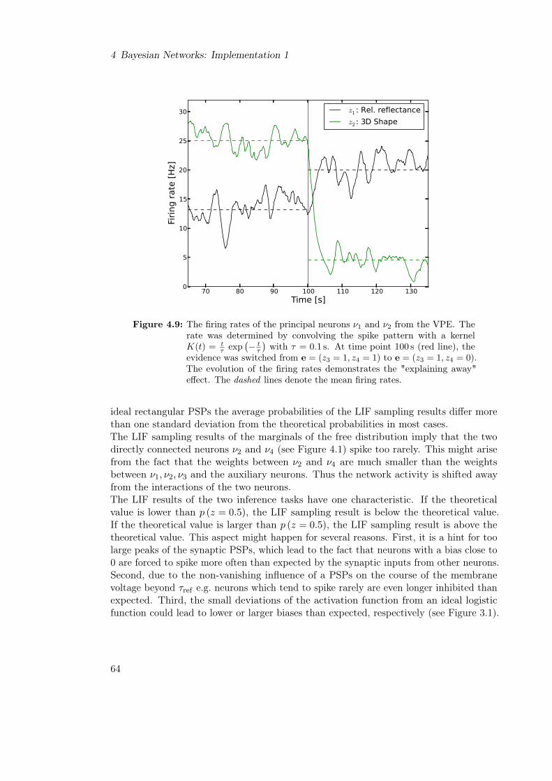
4 Bayesian Networks: Implementation 1
70 80 90 100 110 120 130Time [s]
0
5
10
15
20
25
30
Firin
g ra
te [H
z]
z1 : Rel. reflectancez2 : 3D Shape
Figure 4.9: The firing rates of the principal neurons ν1 and ν2 from the VPE. Therate was determined by convolving the spike pattern with a kernelK(t) = t
τ exp(− tτ
)with τ = 0.1 s. At time point 100 s (red line), the
evidence was switched from e = (z3 = 1, z4 = 1) to e = (z3 = 1, z4 = 0).The evolution of the firing rates demonstrates the "explaining away"effect. The dashed lines denote the mean firing rates.
ideal rectangular PSPs the average probabilities of the LIF sampling results differ morethan one standard deviation from the theoretical probabilities in most cases.The LIF sampling results of the marginals of the free distribution imply that the twodirectly connected neurons ν2 and ν4 (see Figure 4.1) spike too rarely. This might arisefrom the fact that the weights between ν2 and ν4 are much smaller than the weightsbetween ν1, ν2, ν3 and the auxiliary neurons. Thus the network activity is shifted awayfrom the interactions of the two neurons.The LIF results of the two inference tasks have one characteristic. If the theoreticalvalue is lower than p (z = 0.5), the LIF sampling result is below the theoretical value.If the theoretical value is larger than p (z = 0.5), the LIF sampling result is above thetheoretical value. This aspect might happen for several reasons. First, it is a hint for toolarge peaks of the synaptic PSPs, which lead to the fact that neurons with a bias close to0 are forced to spike more often than expected by the synaptic inputs from other neurons.Second, due to the non-vanishing influence of a PSPs on the course of the membranevoltage beyond τref e.g. neurons which tend to spike rarely are even longer inhibited thanexpected. Third, the small deviations of the activation function from an ideal logisticfunction could lead to lower or larger biases than expected, respectively (see Figure 3.1).
64

4.3 Optimal Results of LIF Sampling from Bayesian Networks
Figure 4.9 shows the evaluation of the firing rates of the neurons ν1 and ν2 for the twoinference tasks. During the first 100 s the RVs z3 and z4 are clamped to 1. In this case,the neuron ν1 has a firing rate of about 13 Hz and the neuron ν2 of about 25 Hz. Thissituation corresponds to the inference task in Figure 4.8C and D. At time point 100 s, theRV z4 is clamped to 0. Now we have the inference situation of Figure 4.8E and F. Aftera transition of about 5 s, the firing rates of the neurons ν1 and ν2 settle to new valuesand remain there in average. Now, the neuron ν1 elicits spikes with a frequency of about20 Hz and the neuron ν2 with about 4 Hz. These values correlate with the probabilitieswhich were inferred in Figure 4.8.
4.3.2 Results of LIF Sampling from the ASIA Network
The same performance comparison as in Section 4.3.1 was provided for the ASIA network.Here the probabilities of a patient having one of the three diseases tuberculosis (T ), lungcancer (C) and bronchitis (B) are inferred for two different situations. Figures 4.10Aand B display the results of sampling from the conditional probability distributionp (T,C,B|A = 1, D = 1): this distribution models the situation in which the patient hasrecently visited Asia (A = 1) and suffers from dyspnoea (D = 1). The diagnosis thatthe person has a bronchitis is much more probable than any of the the other diseases.Figures 4.10C and D present the results of sampling from the conditional probabilitydistribution p (T,C,B|A = 1, X = 1, D = 1). In this case, an additional X-ray test hasbeen accomplished with a positive result. Now the diagnosis that the person has abronchitis is not as certain any more and the probabilities to have any of the otherdiseases are almost as large as the probability to have bronchitis.In both cases, the results of LIF sampling from the conditional probability distributionsare unsatisfactory compared to the sampling results with stochastic neurons. The sampledprobabilities with LIF neurons always differ more than two standard deviations from thecorresponding theoretical values. In particular, Figure 4.10C implies that the LIF neuronsfall short of sampling correctly from the distribution p (T,C,B|A = 1, X = 1, D = 1).According to Figure 4.10D, the states (T = 0, C = 0, B = 0) and (T = 0, C = 0, B = 1)are occupied systematically more frequent than statistical fluctuations would account for atan expense of the occurrence of states (T = 0, C = 1, B = 1) and (T = 1, C = 0, B = 1).The unsatisfactory LIF sampling results can be mainly traced back to the large differencesof weights and biases induced by the extreme values of the conditionals p (X = 1|T,C)(see Figure 4.2). Furthermore, both RVs T and C interact with two groups of auxiliaryRVs, while the RV B is only influenced by one group of auxiliary RVs. This might leadto the fact that the neurons associated with T and C are e.g. longer inhibited becausethe PSP impact on the course of the membrane voltage is nonzero beyond τref and bothneurons are inhibited by large negative weights from two groups of auxiliary neurons.The standard deviations of the sampling results of the stochastic neurons also expressthe difficulty to sample from the given conditional probability distributions of the ASIAnetwork. With much longer simulation times, the results can be vastly improved. However,this can not be applied to the LIF sampling results. Here, the standard deviations arealready very small and longer simulation runs would not improve the sampling performance,
65

4 Bayesian Networks: Implementation 1
T C BRandom variable
0.0
0.2
0.4
0.6
0.8
1.0
p(zk=
1)
LIF alpha rect theory
A: Marginals, e = (A = 1, D = 1)
000
001
010
011
100
101
110
111
State z
10-4
10-3
10-2
10-1
100
p(z
)
LIF alpha rect theory
B: Joints, e = (A = 1, D = 1)
T C BRandom variable
0.0
0.1
0.2
0.3
0.4
0.5
0.6
0.7
0.8
p(zk=
1)
LIF alpha rect theory
C: Marginals, e = (A = 1, X = 1, D = 1)
000
001
010
011
100
101
110
111
State z
10-3
10-2
10-1
100
p(z
)
LIF alpha rect theory
D: Joints, e = (A = 1, X = 1, D = 1)
Figure 4.10: Comparison of the sampling performance for simulations of Implemen-tation 1 with LIF PSPs with parameters from Table A.2, alpha-shapedPSPs, ideal rectangular PSPs and the target probabilities for the ASIAnetwork. The left column shows the marginal distributions and theright column the corresponding joint probability distributions of thethree RVs of interest: T , C and B. The bars show the average resultsof 20 simulations of duration 100 s. The error bars denote the standarddeviations.
66

4.4 LIF Sampling Improvement via mLIF PSPs
which implies systematic mismatches. An eligible question at this point is whether thereis an option to modify the LIF PSP shape towards the optimal rectangular PSP shape.The next section will introduce mLIF PSP with the help of which the sampling resultswill improve considerably.
4.4 LIF Sampling Improvement via mLIF PSPs
In the course of the 4th BrainScaleS Demo3 workshop [2013], the idea originated that aLIF PSP shape which is closer to an ideal rectangular shape and which abruptly vanishesafter the refractory time τref will drastically improve the LIF sampling results. A morerectangular LIF PSP shape would mimic the ideal PSP shape of stochastic neurons andcomprise the advantage of being symmetrical. A PSP shape which vanishes after therefractory time would have the advantage that it will not influence the course of themembrane potential of the neuron beyond τref .In the following, first the generation of such a so-called mLIF1 PSP shape is described.Afterwards, the LIF sampling results with the new mLIF PSPs are compared to theresults with the standard LIF PSPs. In the end of this section a temporal analysis of theconvergence behavior with LIF PSPs and mLIF PSPs is presented.
4.4.1 Engineering mLIF PSPs
The generation of a PSP shape with LIF neurons which is close to the ideal rectangularshape requires the interplay of the dynamics of multiple neurons for at least two reasons.First, a single neural membrane with the requirement of a fast rising edge of the membranepotential will result in a highly asymmetrical shape. Thus the falling edge has to beprolonged such that the membrane stays at an almost constant potential during therefractory period. Second, a prolongation of the PSP shape will even increase the sizeof the PSP at the end of the refractory period and thus increase the impact on thesubsequent course of the membrane potential. For this reason, an additional neuron isneeded, which abruptly terminates the PSP.Figure 4.11 illustrates the general idea to design such a PSP shape with LIF neurons,which will be referred to as mLIF PSP. One principal or auxiliary sampling neuron of theoriginal Implementation 1 is replaced by a group of neurons. The first neuron remainsthe actual sampling neuron with bias and weights as introduced in Section 2.1.5. Theremaining neurons are parrot neurons which forward the action potentials of the samplingneuron. In the following I will refer to the first neuron as sampling neuron and to theremaining neurons as forwarding neurons.In addition to the existing network connectivity, each of the forwarding neurons projectsonto the same sampling neurons to which their associated sampling neuron is connected.The biases of the forwarding neurons and the weights to the forwarding neurons areselected such that a forwarding neuron is directly triggered to spike upon each incomingspike. The last of the forwarding neurons connects with the opposite sign to postsynaptic
1The letter "m" in mLIF refers to "multiple" since we are now using multiple neurons per RV.
67

4 Bayesian Networks: Implementation 1
A B mLIFPSP
ν1 ν2 ν2
ν1
ν1
ν1
ν1
ν1
1
2
3
4
5
LIFPSP
Figure 4.11: The previous experiments were simulated with a standard LIF PSPshape (A). To establish a PSP shape which is closer to the ideal rect-angular shape, the following network structure was set up (B): Insteadof using one principal neuron ν for one random variable, each randomvariable is represented by a chain of neurons of which the first neuronis the actual sampling neuron. Additionally to the network connectionsfrom Figure 4.1, there are feed forward connections along this neuralchain. Each of the chain neurons connects to the postsynaptic samplingneuron (all connections from νi1 to ν2) which itself is the samplingneuron of another feed forward chain. By choosing appropriate synapticefficacies, a sawtooth like PSP shape can be artificially establishedwhich is close to the desired rectangular shape.
sampling neuron. This allows to directly terminate the PSP on the postsynaptic site.This last forwarding neuron automatically provides for renewal PSPs even without thepresence of STP.One will ensure a sawtooth-like PSP shape which is shown in Figure 4.12A, if thedelays and the weights connecting the forwarding neurons and also those connecting theforwarding neurons and the following sampling neurons are chosen deliberately. TableA.4 lists the parameters of the extended neural network.Several issues when engineering mLIF PSP shapes need to be considered. First, the sizeof the teeth of the PSP shape has to be constructed such that it is smaller than theoverall size of the PSP. This prevents from strong variation of the firing probabilityof the postsynaptic neuron during the refractory period of the presynaptic samplingneuron. A second issue is illustrated in Figure 4.12B. The delays between the forwardingneurons have to be chosen such that once a sampling neuron ν1 is clamped to a very highmembrane potential, the postsynaptic sampling neuron ν2 will receive a constant offset.An incautious selection of the delays will result in terminating and directly arising PSPsafter each refractory period and might cause undesired threshold crossings.The same PSP shape could also be modeled in a different manner. This involves thesimultaneous activation of the forwarding neurons by the sampling neuron. Due to differentsynaptic weights and membrane time constants, the time course of the postsynaptic action
68

4.4 LIF Sampling Improvement via mLIF PSPs
95 100 105 110 115 120 125 130 135Time [ms]
51.0
50.8
50.6
50.4
50.2
50.0
Volt
age [
mV
]
A: Resulting mLIF PSP shape by apply-ing the method described in Figure 4.11.
400 450 500 550 600Time [ms]
51.5
51.0
50.5
50.0
49.5
49.0
Volta
ge [m
V]
τref = 29.4 ms
τref = 29.5 ms
τref = 29.6 ms
B: Membrane potential of a noise-free LIFneuron with a constant offset
Figure 4.12: Panel A shows the resulting mLIF PSP shape of the method describedin Figure 4.11. The neural chains which are used in this chapter consistof 6 neurons: one neuron to initiate the PSP, 4 neurons to maintainthe level of the membrane potential and one neuron to cancel the PSP.Table A.4 lists the parameters of this extended neural network. Panel Bshows the criterion which was used to find the optimal refractory timeτref for a given number of chain neurons: a sampling neuron receivesthe spiking input of a presynaptic sampling neuron and its forwardingneurons. Without Poisson background input the membrane just receivesan almost constant offset current, which is the stringing together ofconsecutive mLIF PSPs. A refractory time of τref = 29.5 ms is preferredfor 6 neurons and τsyn = 30 ms. With τref = 29.4 ms or τref = 29.6 ms,there are potential jumps after each τref which may cause undesirablethreshold crossings.
potential of each forwarding neuron would be delayed for each neuron differently whichwould result in the same PSP course on the membrane of the postsynaptic sampling neuronas shown in Figure 4.12. However, there are several crucial disadvantages compared tothe method explained before. First, this method would require an individual adjustmentof the membrane time constants for each neuron which becomes very exhausting forlarge groups of neurons and long refractory times. Second, this method would requirean arbitrary flexibility and a high precision of the membrane time constants. This willnot be compatible with the inherent variations of a neuromorphic hardware device (seeChapter 6).The next sections will compare the sampling performance of sampling with LIF PSPsand mLIF PSPs for the VPE and the ASIA network. It will become apparent that themLIF PSPs outperform the LIF PSPs by a large margin.
69

z1 z2 z3 z4
Random variable0.0
0.1
0.2
0.3
0.4
0.5
0.6
p(zk=
1)
LIF mLIF-53 mLIF-50 theory
A: Marginals of the free distribution
0000
0001
0010
0011
0100
0101
0110
0111
1000
1001
1010
1011
1100
1101
1110
1111
State z
10-3
10-2
10-1
100
p(z
)
LIF mLIF-53 mLIF-50 theory
B: Joints of the free distribution
z1 z2
Random variable0.0
0.2
0.4
0.6
0.8
1.0
p(zk=
1)
LIF mLIF-53 mLIF-50 theory
C: Marginals, e = (1, 1)
00 01 10 11
State z
10-3
10-2
10-1
100
p(z
)
LIF mLIF-53 mLIF-50 theory
D: Joints, e = (1, 1)
z1 z2
Random variable0.0
0.1
0.2
0.3
0.4
0.5
0.6
0.7
0.8
p(zk=
1)
LIF mLIF-53 mLIF-50 theory
E: Marginals, e = (1, 0)
00 01 10 11
State z
10-3
10-2
10-1
100
p(z
)
LIF mLIF-53 mLIF-50 theory
F: Joints, e = (1, 0)
Figure 4.13: Comparison of the LIF sampling performance via Implementation 1 withstandard LIF neurons with parameters from Table A.2, two versions ofImplementation 1 with the improved PSPs from Figure 4.11B and thetarget probabilities for the VPE. The versions mLIF−50 and mLIF−53
have different reset voltages -50.01mV and -53.0mV, respectively. Theleft column contains the marginal distributions and the right column thecorresponding joint probability distributions of the random variablesz1 and z2. The evidence e corresponds to the vector (z3, z4). The barsshow the average results of 20 simulations of duration 100 s for the LIFPSP, 150 s for the mLIF PSPs. The error bars denote the standarddeviations.

4.4 LIF Sampling Improvement via mLIF PSPs
4.4.2 Results of LIF Sampling with mLIF PSPs for the Visual PerceptionExperiment
Two different versions of mLIF PSPs were used to test the sampling performance andcompare it to the performance with standard LIF PSPs. A.2 lists the parameters ofthe neurons with standard LIF PSPs. The parameters for generating the mLIF PSPsare taken from Table A.4. The PSPs mLIF−50 and mLIF−53 only differ in the resetpotential of the sampling neuron. mLIF−50 refers to an optimal reset potential ofVreset = −50.01 mV which is close to the threshold potential such that the neuronis allowed to spike again directly after the refractory period. mLIF−53 refers to thereset potential Vreset = −53.0 mV which e.g. takes account for the compatibility withthe fluctuations of floating gate voltages and currents on the FACETS Wafer-ScaleHardware System, with respect to a prospective implementation of mLIF PSPs. Dueto the reset potential Vreset = −53.0 mV, the neuron needs a longer time to recover toits free membrane potential after it has passed the refractory time, which shifts neuralcorrelations and, therefore, leads to a slight imprecision of the sampling results comparedto Vreset = −50.01 mV.Figure 4.13 shows the LIF sampling results for the VPE of 20 simulation runs of 100.0 s eachfor LIF PSPs and of 150.0 s each for mLIF PSPs. This distinction is made due to differentrefractory times τref. For each of the three probability distributions p (z1, z2, z3, z4),p (z1, z2|z3 = 1, z4 = 1) and p (z1, z2|z3 = 1, z4 = 0), the sampling results with mLIF PSPsare superior. The theoretical probabilities are mostly in the range of two standarddeviations of the simulated probabilities for both, mLIF−50 and mLIF−53. Only forthe distribution p (z1, z2|z3 = 1, z4 = 1) (see Figure 4.13C and D) larger deviations areobservable, but which still the results are better than the results obtained via LIF PSPs.
4.4.3 Results of LIF Sampling with mLIF PSPs from the ASIA Network
Figure 4.13 shows the LIF sampling results for the ASIA network of 20 simulationruns of 100.0 s each for LIF PSPs and of 150.0 s each for mLIF PSPs. With bothimplementations of mLIF PSPs, the LIF sampling quality distinctly improves for bothprobability distributions p (T,C,B|A = 1, D = 1) and p (T,C,B|A = 1, X = 1, D = 1).The theoretical probabilities are always in the range of two standard deviations of thesimulated probabilities for both versions of the mLIF PSP.The most distinctive result is the sampling performance for the distributionp (T,C,B|A = 1, X = 1, D = 1) in Figure 4.13C and D. Similar to the results withstochastic neurons in Figure 4.10 the standard deviations of the results of the simulationswith mLIF PSP become very large. This might indicate two facts. On the one hand, theconvergence of Implementation 1 is known to be very slow due to the additional set ofauxiliary RVs [Levin et al., 2006]. On the other hand, the underlying Bayesian networkcontains prior and conditional probabilities which are close to 0 or 1 and thus lead tolarge variations of firing frequencies throughout the network.The following section offers an analysis of the convergence time of LIF sampling with LIFand mLIF PSPs based on the presented example BNs.
71

4 Bayesian Networks: Implementation 1
T C BRandom variable
0.0
0.2
0.4
0.6
0.8
1.0p(zk=
1)LIF mLIF-53 mLIF-50 theory
A: Marginals, e = (A = 1, D = 1)
000
001
010
011
100
101
110
111
State z
10-5
10-4
10-3
10-2
10-1
100
p(z
)
LIF mLIF-53 mLIF-50 theory
B: Joints, e = (A = 1, D = 1)
T C BRandom variable
0.0
0.1
0.2
0.3
0.4
0.5
0.6
0.7
p(zk=
1)
LIF mLIF-53 mLIF-50 theory
C: Marginals, e = (A = 1, X = 1, D = 1)
000
001
010
011
100
101
110
111
State z
10-4
10-3
10-2
10-1
100
p(z
)
LIF mLIF-53 mLIF-50 theory
D: Joints, e = (A = 1, X = 1, D = 1)
Figure 4.14: Comparison of the LIF sampling performance via Implementation 1 withstandard LIF neurons with parameters from Table A.2, two versionsof Implementation 1 with the improved PSPs from Figure 4.11B, andthe target probabilities for the ASIA network. The versions mLIF−50
and mLIF−53 have different reset voltages -50.01mV and -53.0mV,respectively. The left column contains the marginal distributions andthe right column the corresponding joint probability distributions ofthe random variables T , C and B. The bars show the average resultsof 20 simulations of duration 100 s for the LIF PSP, 150 s for the mLIFPSPs. The error bars denote the standard deviations.
72

4.5 Implementation 1: LIF Sampling Performance on General Bayesian Networks
4.4.4 Temporal Evolution of the KL Divergence
Figure 4.14 already indicated that the convergence of the sampled probability distributiontowards the stationary probability distribution is very slow for mLIF PSPs. In thefollowing, the convergence times of sampling with LIF PSPs and mLIF PSPs are compared.As before, Table A.2 lists the parameters for LIF sampling with LIF PSPs. Table A.4contains the parameters for the LIF sampling with mLIF PSPs.Figure 4.15 presents the temporal evolution of the KL divergence between the simulatedand the target joint probability distributions for the VPE, in Panels A and B, and the ASIAnetwork, in Panels C and D. Panels A and B refer to the results of sampling from the distri-butions p (z1|z3 = 1, z4 = 1) and p (z1|z3 = 1, z4 = 0) of the VPE, respectively. Panels Cand D show the results of sampling from the distributions p (T,C,B|A = 1, X = 1, D = 1)and p (T,C,B|A = 1, D = 1) of the ASIA network, respectively.For all four probability distributions, the convergence time of sampling with LIF PSPs isin the range of 10 s. With mLIF PSPs the convergence time is about 100 s for the VPEand larger than 100 s for the ASIA network. This can be partly explained by the fact thathe refractory time constant is longer for mLIF PSPs than for LIF PSPs. Another reasonis that for mLIF PSPs the firing times of the sampling neurons are more distributed alongthe duration of the PSP. Implementation 1 rather favors PSP shapes for which the firingoccurs directly after activation ("all or nothing") and which better mimic ideal infiniteweights (see Section 2.1.5). With regard to the convergence time, this feature fits betterto the asymmetric LIF PSPs because they peak at the beginning of τref .However, the slow convergence and longer simulation times due to a larger number ofneurons comes with the advantage of a more accurate sampling result which militatesfor the implementation of mLIF PSPs. The obviously better sampling performance withLIF PSP in Panel A and D of Figure 4.15 is misleading. If comparing with the actualsampling results in Figures 4.13C and 4.14C, respectively, the results of LIF samplingwith mLIF PSPs are better. This discrepancy is an artifact of the asymmetry of the KLdivergence (see Equation 2.15).
4.5 Implementation 1: LIF Sampling Performance onGeneral Bayesian Networks
So far, the sampling performance via Implementation 1 via LIF neurons has been testedon the two specific BNs presented in Section 4.1. As for sampling from BMs in Chapter3, it would be desirable to gain a more general result of LIF sampling from BNs andcompare sampling with LIF PSPs to sampling with mLIF PSPs from random BNs. Forthis, Section 4.5.1 describes a procedure to create random BNs with pairwise randomprior and conditional probabilities. Section 4.5.2 presents the results of sampling fromrandom BNs of 5 RVs with LIF neurons and compares them to the sampling results ofstochastic neurons with ideal PSPs.
73

4 Bayesian Networks: Implementation 1
0 200 400 600 800 1000Time [s]
10-5
10-4
10-3
10-2
10-1
100
⟨ D KL(p
sim(z
1,z
2|e
)||p
theo(z
1,z
2|e
))⟩
LIFmLIF-53mLIF-50rect
A: VPE, e = (z3 = 1, z4 = 1)
0 200 400 600 800 1000Time [s]
10-5
10-4
10-3
10-2
10-1
100
⟨ D KL(p
sim(z
1,z
2|e
)||p
theo(z
1,z
2|e
))⟩ LIF
mLIF-53mLIF-50rect
B: VPE, e = (z3 = 1, z4 = 0)
0 200 400 600 800 1000Time [s]
10-2
10-1
100
⟨ D KL(p
sim(T,C,B|e
)||p
theo(T,C,B|e
))⟩
LIFmLIF-53mLIF-50rect
C: ASIA, e = (A = 1, X = 1, D = 1)
0 200 400 600 800 1000Time [s]
10-2
10-1
100⟨ D KL
(psi
m(T,C,B|e
)||p
theo(T,C,B|e
))⟩ LIF
mLIF-53mLIF-50rect
D: ASIA, e = (A = 1, D = 1)
Figure 4.15: Temporal evolution of the mean KL divergence of the simulated andtarget joint probability distribution of the RVs z1 and z2 from the VPE(upper row) and of the RVs T , C and B from the ASIA network (lowerrow) for the three PSP shapes LIF, mLIF−50, mLIF−53 as well as theideal rectangular PSP shape. For each plot, the given evidence e isdifferent. Each curve denotes the average result of 10 simulations ofduration 1000 s. The shaded regions denote the standard error of themean.
74

4.5 Implementation 1: LIF Sampling Performance on General Bayesian Networks
0.2 0.4 0.6 0.8Sample x1
0.0
0.5
1.0
1.5
2.0
P.d.f. of D
irich
let d
istribution
α1 =0.6, α2 =0.6
α1 =1.0, α2 =1.0
α1 =1.4, α2 =1.4
Figure 4.16: Symmetrical two-dimensional Dirichlet distributions for different pa-rameters α1=α2=α. The prior and conditional probabilities of therandomly generated Bayesian networks are samples from these Dirichletdistributions. The parameter α allows to choose the extreme natureof the resulting BN. The smaller α is, the larger is the probability tochoose a sample close to the boundaries 0 or 1. With higher α, thediscrepancy of the prior and conditional probabilities decreases.
4.5.1 Generating General Bayesian Networks
Ide and Cozman [2002] present a method to generate random BNs of K binary RVsz1, z2, ..., zK and pairwise random prior and conditional probabilities. The algorithmstarts with the simplest possible connectivity pattern for which a BN is fully connected,which is a Markov chain (see Section 2.1.4): z1 is connected to z2, z2 is connected to z3
and so on. The term fully connected means that irrespective of the direction of the edgesin the BNs every node can be reached from every other node. The algorithm runs for Niterations and in each iteration randomly creates a pair (zi, zj) of RVs with the conditionzi < zj . For each pair one of the two following actions is performed:
• If the connection zi → zj exists, it is removed, but only if the BN remains fullyconnected. Otherwise nothing is done.
• If the connection zi → zj does not exist, then it is added, but only if zi and zj haveless than 8 connections to other nodes. Otherwise nothing is done.
This algorithm leads to a BN with a random connectivity pattern.
75

4 Bayesian Networks: Implementation 1
The BN then needs to be fully defined by assigning prior and conditional probabilitiessimilar to these of the VPE and the ASIA network in Figure 4.1 and 4.2. For this, theprior and conditional probabilities xi are randomly drawn from a Dirichlet distribution ofsecond order
D (x1, x2, α1, α2) =1
B (α)
2∏i=1
xαi−1i , (4.5)
with the multinomial Beta function
B (α) =
∏2i=1 Γ (αi)
Γ(∑2
i=1 αi
) , (4.6)
with the Gamma function Γ (α), the vector α = (α1, α2) and the condition x1 + x2 = 1.The last condition means that the probabilities xi are pairwise determined: once x1
has been drawn, x2 denotes 1− x1. Choosing the parameters α1 = α2 := α makes theDirichlet distribution symmetrical.Figure 4.16 shows the probability density function of a Dirichlet distribution as a functionof α. The case α = 1 is the one-dimensional uniform distribution. For α < 1, theprobability to draw samples close to the boundaries 0 and 1 is larger than the probabilityto draw samples from the middle of the interval. For α > 1, the probability to drawsamples around 0.5 is larger than the probability to draw samples close to the boundaries0 and 1. By choosing α, we determine the extreme nature of the resulting BN.
4.5.2 Performance Comparison of Sampling from General BayesianNetworks
The algorithm to generate random BNs described in Section 4.5.1 is applied for BNs ofK = 5 RVs and N = 50000 iterations. The parameter α is varied between 0.3 and 10. Foreach α, 10 random BNs are created. For each of these BNs, the sampling performancewith standard LIF PSPs and mLIF PSPs is measured and compared to the performanceof stochastic neurons with ideal rectangular PSPs. The duration of one simulation is 500 sfor all investigated PSPs.Figure 4.17 illustrates the average sampling results for the different PSP shapes as afunction of α. For larger α, the sampling performance increases for each of the PSPs afterthe same simulation time. This can be explained by the fact that a large α favors priorand conditional probabilities which are rather close to 0.5 than to the boundaries 0 and 1.In this case, we have a smaller discrepancy of the prior and conditional probabilities, and,thus, a smaller discrepancy of the weights and biases in the neural representation of theBNs due to Equations 2.27 and 2.28. It has been shown in Figure 3.3 that sampling fromBMs with low weights and biases yields better results after the same simulation time.Sampling with mLIF PSPs leads to results which are up to one order of magnitude moreprecise than sampling with LIF PSPs in terms of KL divergence between the simulated andthe target joint probability distribution. Among the mLIF PSPs, sampling with mLIF−50
PSPs is more precise than sampling with mLIF−53 PSPs for each α, a consequence of thedifferent choice of the reset potential (see Section 4.4.2).
76

4.6 Conclusion
100 101
α
10-3
10-2
10-1
100
101⟨ D KL
(psi
m||p
theo)⟩
LIFmLIF-53mLIF-50rect
Figure 4.17: Sampling performance of LIF neurons and stochastic neurons on generalBayesian networks as a function of the Dirichlet parameter α (seeFigure 4.16). Both mLIF PSP implementations show a better samplingperformance of up to one order of magnitude, in terms of KL divergencebetween the sampling and the target probability distribution, comparedto LIF PSPs. The shaded regions denote the standard error of themean.
4.6 Conclusion
This chapter showed that it is possible to transfer Implementation 1, or in general words,sampling from probability distributions described by BNs to the dynamics of LIF neuronsin a spiking noisy environment.A sophisticated modification of the LIF PSPs led to a vast improvement of the LIFsampling performance from general BNs. The so-called mLIF PSPs were designed by anextension of the connectivity pattern of Implementation 1 by chains of parrot-like neurons.In difference to the LIF PSPs, the new PSPs were close to the ideal rectangular PSPs andhad a finite duration. The introduced mLIF PSPs allowed for a sampling performancefrom general BNs which was up to one order of magnitude more precise than samplingwith LIF PSPs in terms of KL divergence between the simulated and the target jointprobability distribution.A disfavor of the mLIF PSPs was the slow convergence in the range of 100 s and longerwhich arises due to the introduced auxiliary RVs. However, the same slow convergence ofImplementation 1 as for mLIF PSPs was observed for the abstract neuron model withrectangular and alpha-shaped PSPs. Inherent LIF PSPs, indeed, allowed for a convergence
77

4 Bayesian Networks: Implementation 1
time in the range of 10 s. This can be explained by the asymmetry of the PSP shape and,thus, a fast settling towards some stationary distribution.With regard to a possible application of Implementation 1 on the BrainScaleS neuromorphichardware system (see Section 2.2), the mLIF PSPs were tested for an optimal and ahardware-compatible distance between the threshold and reset voltage of the samplingneurons. The sampling performance of the hardware-compatible version was close to theoptimal one and more precise than the sampling quality with standard LIF PSPs. Whatwill be more crucial for an application on hardware are for both LIF PSPs and mLIFPSPs the time constants and delays (see Chapter 6).
78

5 Bayesian Networks: Implementation 2with LIF Neurons
The simulation results in Chapter 4 demonstrated that Implementation 1 (see Section2.1.5) allows for sampling from BNs via networks of LIF neurons. It was shown for generalBNs that so-called mLIF PSPs, which aim at mimicking the ideal rectangular PSP shapeof the abstract neuron model, yield better sampling results than the original LIF PSPs.However, one disadvantage of Implementation 1 in general, which results due to theincreased number of RVs and, consequently, a higher number of computational units, wasthe slow convergence in the range of 100 s towards a stationary distribution.Pecevski et al. [2011] introduce a further method which uses auxiliary neurons to implementneural sampling from BNs. In opposite to the method described in Chapter 4, in thisso-called Implementation 2 (see Section 2.1.5) the neurons which correspond to theoriginal RVs directly satisfy the NCC (see Equation 2.18), and not only in the extendedprobability distribution p(z,x) with auxiliary RVs X. According to Pecevski et al. [2011],this circumstance allows for a much faster convergence to the stationary distribution.Implementation 2 uses a Markov blanket expansion of the NCC to provide the ability tosample from BN. For each Markov blanket Bk in the graphical model, which is the set ofall parents, co-parents and children of the node k, auxiliary neurons αv
k are introduced,which code for all possible states v of the Markov blanket. An auxiliary neuron αv
k is onlyallowed to spike, if the Markov blanket occupies its corresponding state v. In this case,the membrane potential of the auxiliary neuron αv
k satisfies the NCC. Each Zk of theactual RVs Z of the probability distribution p (z) is represented via a principal neuron νk.The firing of an auxiliary neuron αv
k triggers an immediate firing of the correspondingprincipal neuron νk which ensures that also the principal neurons satisfy the NCC.Section 5.1 introduces the concrete implementations of two BNs which were used to testthe sampling performance with LIF neurons. The first BN is a network which consists oftwo RVs whose joint probability distribution is a uniform distribution. The second BN isthe probabilistic model of the Visual Perception Experiment (see Section 2.1.3).Section 5.2 presents the sampling performance of LIF neurons for the two describedBNs when using Implementation 2. The LIF sampling results are compared with theseof stochastic neurons with rectangular or alpha-shaped PSPs. It is shown that thenon-uniformity of the LIF PSP shape facilitates a correlated spiking activity among theprincipal neurons and, thus, is responsible for the unsatisfactory sampling results ofImplementation 2.Section 5.3 entails the sampling results of LIF neurons with mLIF PSPs, which wereintroduced in Section 4.4. Neurons incorporating mLIF PSPs show a better samplingperformance compared to those with standard LIF PSPs. However, the sampling quality
79

5 Bayesian Networks: Implementation 2
z z1 2
ν
ν1
2
α α α α11
11
2 20 0
ι
ι1
2
excitatory connectioninhibitory connection
A
B
p(z =1) = 0.51
z =01z =11
0.50.5
p(z =1|z )2 1
Figure 5.1: Demonstration of Implementation 2 (see Section 2.1.5) for the so-calledTwo-Node-Network (TNN), a Bayesian network of two random variableswhose joint probability distribution follows a uniform distribution. A)Graphical model and prior probabilities. B) Its neural representation.Each of the auxiliary neurons (black) satisfies the NCC (Equation 2.18).The principal neurons (blue) and the inhibitory interneurons (gray) fireon each incoming spike.
is unsatisfactory compared to the results of Implementation 1 in Section 4.4. A vastimprovement of the sampling quality can only be achieved with distinctly longer chainsof neurons, which goes at the expense of the overall network size and, thus, the durationof simulations.Finally, Section 5.4 provides for a theoretical explanation of the dissatisfying samplingperformance with mLIF PSPs based on the distributions of first passage times. It is shownthat substantial imprecisions arise due to the non-uniformity of the firing probability,the stochasticity induced by the OU process of LIF neurons in a noisy environment incontrast to the Bernoulli process of abstract neurons, and the autocorrelation of themembrane potential.
5.1 Implementation 2: Illustrative Implementation ofSample Bayesian Networks
This section presents the two BNs which are used as example probability distributionsfor testing the sampling performance of LIF neurons with Implementation 2.
80

ν 3ν 4
ν 2
ι3ι4
α100
αα001
000
αα011
010
αα101
100
αα111
110
ι1
ι2ν 1
22
22
22
22
α101
α110
α111
α300
α301
α310
α311
α10
α11
Fig
ure
5.2:
Implem
entation
2of
theVPE.The
neural
netw
orkconsists
ofthefour
principa
lneuronsν 1,ν
2,ν
3,ν
4,theircorrespo
nding
auxilia
ryneuron
s(b
lack
)an
dinhibitory
interneurons
(gra
y).Fo
rreason
sof
clarity,
notallc
onnections
from
principa
lto
auxilia
ryneuron
san
dbe
tweentheau
xilia
ryneuron
san
dinhibitory
interneu
rons
aredraw
n.Section2.1.5contains
adetaileddescriptionof
theim
plem
entation
ofaMarkovblan
ket.

5 Bayesian Networks: Implementation 2
5.1.1 Implementation of the Two-Node-Network
The first BN is a uniform probability distribution of two RVs Z1 and Z2 of the shape
p (z1, z2) = p (z1) p (z2|z1) . (5.1)
Figure 5.1A shows the graphical model of the BN and the prior and conditional probabili-ties p (z1 = 1) and p (z2 = 1|z1), which completely describe the BN. In the following, thenetwork will be referred to as Two-Node-Network (TNN).Figure 5.1B shows the neural implementation of the BN in terms of Implementation 2.The task involves 8 neurons: the two principal neurons ν1 and ν2 represent the two nodesZ1 and Z2. The RV Z1 constitutes the Markov blanket B2 of Z2 and Z2 constitutes theMarkov blanket B1 of Z1. Therefore, each Markov blanket can have two possible states,which are coded by the auxiliary neurons α0
k and α1k, where νk is their corresponding RV.
Furthermore, each group of auxiliary neurons is connected to an inhibitory interneuronι which ensures that after one of the auxiliary neurons α0
k and α1k has emitted a spike,
both of them remain silent during the refractory period.Since the membrane potential of the auxiliary neurons satisfies the NCC, the biases of theauxiliary neurons are calculated via Equation 2.31. In the case of the TNN, both α0
1 andα0
2 have the bias 0 and α11 and α1
2 occupy the bias −10 in the stochastic neuron model.Equation 2.32 is used to calculate the excitatory weights from the principal neurons tothe auxiliary neurons. The excitatory weights of the connections ν1 → α1
2 and ν2 → α11
amount to 10. The inhibitory weights of the connections ν1 → α02, ν2 → α0
1, as well asthe weights from the inhibitory interneurons ιk to the auxiliary neurons are calculatedvia Equation 2.33. Each of these weights amount to −10 in the stochastic neuron model.The strengths of all outgoing connections of the auxiliary neurons are chosen such that aspike of an auxiliary neuron directly evokes a spike of the postsynaptic neuron. For thestochastic neurons the weight is 30 and for LIF neurons with the parameters from TableA.3 the weight amounts to 0.16µS.
5.1.2 Implementation of the Visual Perception Experiment
The second BN is the probability distribution which models the VPE described in Section2.1.3. It is described by the probability distribution
p(z1, z2, z3, z4) = p(z1) p(z2) p(z3|z1, z2) p(z4|z2) . (5.2)
Figure 5.2 shows the neural implementation of the VPE. The Markov blankets of theRVs Z1 to Z4 are: B1 = (Z2, Z3), B2 = (Z1, Z3, Z4), B3 = (Z1, Z2) and B4 = (Z2). Theneural implementation therefore involves 26 neurons: 4 principal neurons, 4 inhibitoryinterneurons, 4 auxiliary neurons of z1, 8 auxiliary neurons of z2, 4 auxiliary neuronsof z3 and 2 auxiliary neurons of z4. The concrete implementation of biases and weightsis accomplished via the Equations 2.31, 2.32 and 2.33 using the prior and conditionalsprobabilities introduced in Figure 4.1.
82
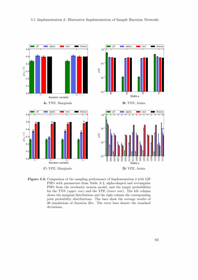
5.1 Implementation 2: Illustrative Implementation of Sample Bayesian Networks
z1 z2
Random variable0.0
0.1
0.2
0.3
0.4
0.5
0.6
p(zk=
1)
LIF alpha rect theory
A: TNN, Marginals
00 01 10 11
State z10-3
10-2
10-1
100
p(z
)
LIF alpha rect theory
B: TNN, Joints
z1 z2 z3 z4
Random variable0.0
0.1
0.2
0.3
0.4
0.5
0.6
p(zk=
1)
LIF alpha rect theory
C: VPE, Marginals
0000
0001
0010
0011
0100
0101
0110
0111
1000
1001
1010
1011
1100
1101
1110
1111
State z
10-3
10-2
10-1
100
p(z
)
LIF alpha rect theory
D: VPE, Joints
Figure 5.3: Comparison of the sampling performance of Implementation 2 with LIFPSPs with parameters from Table A.2, alpha-shaped and rectangularPSPs from the stochastic neuron model, and the target probabilitiesfor the TNN (upper row) and the VPE (lower row). The left columnshows the marginal distributions and the right column the correspondingjoint probability distributions. The bars show the average results of20 simulations of duration 20 s. The error bars denote the standarddeviations.
83

5 Bayesian Networks: Implementation 2
5.2 Implementation 2: Performance on Sample BayesianNetworks
In the following, the sampling results of a LIF-based version of Implementation 2 arepresented and compared to the sampling results of stochastic neurons with rectangularand alpha-shaped PSPs. The example probability distributions are the two distributionsTNN and VPE which were described in Section 5.1.
5.2.1 Results of Sampling from the Two-Node-Network and the VisualPerception Experiment
Table A.2 lists the parameters of the auxiliary neurons. The principal neurons andinhibitory interneurons adopt the parameter set of Table A.3. They are designed suchthat upon each incoming spike they elicit exactly one spike. The principal neurons andinhibitory interneurons do not receive background stimuli and the connections to theseneurons are static.For both probability distributions, 20 simulations of 20 s are executed and the averageresults of sampling from the joint probability distribution of the involved principal neuronsare measured. The small standard deviations of the sampling results justify the shortduration 20 s of one simulation compared to the ones obtained via Implementation 1.Figure 5.3 illustrates the sampling results: Panels A and B presents the results ofsampling from the TNN while Panels C and D show the results of sampling from theVPE. In comparison to the sampling performance of stochastic neurons with rectangularor alpha-shaped PSPs, the LIF neurons exhibit substantial inaccuracies when samplingfrom both probability distributions. The most salient characteristic of the samplingresults of LIF neurons is the U-like shape of the joint probability distributions. Thisis caused by the correlated spiking activity of auxiliary neurons, which leads to a vastoverrepresentation of the states (z1 = 0, z2 = 0) and (z1 = 1, z2 = 1) for the TNN and(z1 = 0, z2 = 0, z3 = 0, z4 = 0) and (z1 = 1, z2 = 1, z3 = 1, z4 = 1) for the VPE, indicatinga significant tendency to synchronize the dynamics.
5.2.2 Theoretical Explanation of the Insufficiency of LIF Sampling whenApplying Implementation 2
An explanation for the insufficiency of of LIF Sampling when applying Implementation 2is sketched in Figure 5.4. It shows a simplified sketch of the membrane potential traceswithout the Gaussian jitter due to the Poisson distributed background input. The startingpoint is the network state (z1 = 0, z2 = 0). The illustration begins in Panel A with aspike of the auxiliary neuron α0
1 according to the NCC at time t1. This action potentialtriggers a firing of the inhibitory interneuron ι1 which leads to an inhibitory PSP inthe membrane voltage trace of α0
1. Furthermore, the principal neuron ν1 is triggered toelicit an immediate spike at time t1 + ∆t (Panel B), which changes the network state to(z1 = 1, z2 = 0). The expression ∆t hereby denotes the combination of the interneuraldelay and the rise time of the membrane potential.
84

t1 t +τ1 time
α fires
A: α01
C: α12
t 2 time
α fires
state 0010
1101
00
B: ν1
t +Δt1 t +Δt+τ1 time
ν fires
D: ν2
t +Δt2 t +Δt+τ2time
ν fires
t +τ2
Vth
Vreset
Vb=0
Vb=-10
Vth
Vth
Vb=0
voltage
voltage
voltage
voltage
Vb=-10
Vth
Vreset
_
_
_
_01
12
1
2
Figure 5.4: A simplified sketch of the mean membrane voltage traces for the neuronsfrom the TNN, which shows the impact of the asymmetry of the LIF PSPshape on the sampling distribution of network states. After the neuronα0
1 has elicited a spike (A), it forces ν1 to spike directly (B) which itselfraises the membrane potential of neuron α1
2 to the average potentialVb=0
. The firing probability during the first milliseconds of the LIF PSPis much higher than the firing probability during the residual part. Thus,α1
2 is very likely to spike very soon after it has been activated (C). Thefiring of α1
2 directly triggers ν2 to elicit a spike (D). This leads to theoverrepresentation of the states (z1 = 0, z2 = 0) and (z1 = 1, z2 = 1) inthe sampling probability distribution decreasing the frequency of thestates (z1 = 0, z2 = 1) and (z1 = 1, z2 = 0) (see Figure 5.3).

5 Bayesian Networks: Implementation 2
The firing of the principal neuron ν1 decreases the average membrane potential of α02 to
Vb=−10 and, at once, raises the average membrane potential of α1
2 to V b=0. Due to theasymmetric PSP shape the α1
2 spikes with a very high probability at the beginning of therefractory period and a very low probability close to τref . This discrepancy, comparedto the stochasticity of the abstract neuron model, favors a soon spiking of α1
2 at time t2as shown in Panel C. The spike of α1
2 immediately triggers ν2 to spike at t2 + ∆t (PanelD), which changes the network state to (z1 = 1, z2 = 1). In average, this quick change ofstates is the reason that the states (z1 = 0, z2 = 1) and (z1 = 1, z2 = 0) are only assumedfor a short fraction of time, which results in the U-like shape of the joint probabilitydistribution in Figure 5.3B.A further error source is the too large residual of a LIF PSP on the course of themembrane potential after τref (see Figure 4.7). Since the overall network activity has tobe spontaneously initiated by the firing of one of the α0 neurons, a prolonged inhibitiondue to this effect explains the higher frequency of the states (z1 = 0, z2 = 0) as comparedto (z1 = 1, z2 = 1) in the sampling result of LIF neurons in Figure 5.3B.The large deviations of the simulated joint probability distribution of the VPE from thetheoretical distribution can be reduced to the same drawbacks. The overrepresentationof the states (z1 = 0, z2 = 0, z3 = 0, z4 = 0) and (z1 = 1, z2 = 1, z3 = 1, z4 = 1) in Figure5.3D at the reduces probability of occurrence of the remaining states follows directly fromthe asymmetry and (endless) exponential decay of the PSP shape, which were describedin Figure 5.4.
5.3 Improvement of LIF Sampling via mLIF PSPs
The unsatisfactory LIF sampling results from Section 5.2 raise the question whether itis possible to improve the sampling performance with mLIF PSPs, a method which wasalready successfully applied for Implementation 1 in Section 4.4. A PSP shape which iscloser to the ideal rectangular shape would have two advantages. Firstly, the symmetricshape would not favor the firing at a special point in time during the refractory period.Secondly, due to the instant decay of the PSP at the end of the refractory period, thesubsequent course of the membrane potential, and therefore the spiking probability, willnot be influenced beyond the refractory period.
5.3.1 Engineering mLIF PSPs
Figure 5.5 shows the two mLIF PSP shapes which were used in this section. The PSPshape in Panel A is generated with chains of 6 neurons and thus will be referred to asmLIF6 PSP. Table A.4 contains the parameters that are necessary to design the mLIF6
PSP, with the reset voltage of the sampling neurons Vreset = −50.01 mV. The mLIF6
PSP already provided for sufficiently precise sampling results with Implementation 1.Panel B shows the so-called mLIF166 PSP. It is generated via chains of 166 neurons. Theutilized parameters are listed in Table A.5.Only the principal neurons and the inhibitory interneurons are replaced by neural chains,
86

5.3 Improvement of LIF Sampling via mLIF PSPs
95 100 105 110 115 120 125 130 135Time [ms]
51.0
50.8
50.6
50.4
50.2
50.0
Volt
age [
mV
]
A: mLIF6
480 500 520 540 560 580 600 620Time [ms]
50.7
50.6
50.5
50.4
50.3
50.2
50.1
50.0
49.9
Volt
age [
mV
]
B: mLIF166
Figure 5.5: The two mLIF PSP shapes which are used to investigate the feasibilityof Implementation 2 with LIF neurons. Each of the PSP shapes isconstructed by a chain of multiple principle neurons realizing the methodfrom Figure 4.11B. In each of the voltage plots the dashed line representsthe threshold potential, the upper solid line is V
b=0(no bias) and the
lower solid line is Vb=−10
, the potential which corresponds to the bias−10. Both figures show a PSP shape induced by an incoming spike viaa connection of strength 10.
which is in contrast to Implementation 1. The principal neurons and the inhibitoryinterneurons indeed require the asymmetric shape of a standard LIF PSP, such that withthe parameters listed in Table A.4 and A.5, they are triggered to elicit a spike upon eachincoming spike from their corresponding auxiliary neurons. Therefore, the spikes of theauxiliary neurons do not need to be forwarded by parrot neurons.In contrast to mLIF6 PSPs, two consecutive mLIF166 PSP are completely uncorrelatedwhich can be deduced from Figure 5.6. The synaptic time constant τsyn hereby can beassociated with a "memory" of the LIF neuron in the HCS. For τsyn = 30 ms, whichcorresponds to an mLIF6 PSP, the autocorrelation of the membrane voltage is muchlarger than 0 at τref = 30 ms. For τsyn = 10 ms, which indeed corresponds to an mLIF166
PSP, the "memory" of the LIF unit is shorter, such that the autocorrelation functionis approximately 0 at τref = 100 ms, which is exactly like the autocorrelation of themembrane potential in the stochastic neuron model.
5.3.2 Results of LIF Sampling with mLIF PSPs
The sampling performance of LIF neurons with LIF PSPs, mLIF6 PSPs and mLIF166
PSPs is measured for the two probability distributions which are introduced in Section5.1. The total number of neurons which is needed to sample from the TNN amounts to28 neurons for mLIF6 PSPs and 668 neurons for mLIF166 PSPs. The number of neurons
87

5 Bayesian Networks: Implementation 2
150 100 50 0 50 100 150Time [ms]
0.0
0.2
0.4
0.6
0.8
1.0
Auto
corr
ela
tion o
f th
e m
em
bra
ne p
ote
nti
al [a
.u.]
mLIF6 , τsyn = 30 ms
mLIF166, τsyn = 10 ms
Figure 5.6: The relative autocorrelation function of the membrane potential of aLIF neuron with τsyn = 30 ms, which refers to mLIF6 PSPs, or τsyn =10 ms, which refers to mLIF166 PSPs, with respect to the maximalautocorrelation. For mLIF6 PSPs, autocorrelations of the membranepotential exist even after the refractory period τref = 30 ms. In contrast,the autocorrelation of the membrane potential for mLIF166 PSPs areabout 0 at τref = 100 ms.
which is indeed needed to sample from the VPE network is 66 neurons for mLIF6 PSPsand 1346 neurons for sampling with mLIF166 PSPs.Figure 5.7 presents the sampling results of 20 simulations of duration 20 s for LIF PSPs,30 s for mLIF6 PSPs and 100 s for mLIF166 PSPs. The different simulation times arechosen due to differing refractory times τref , such that in all three cases the neurons havethe same number of opportunities to change their state.Both implementations with mLIF PSPs outperform the sampling results with LIF PSPs.The results with mLIF166 PSPs, however, are much closer to the target probabilities.mLIF6 PSPs show a less precise sampling performance than stochastic neurons withalpha-shaped PSPs in Figure 5.3. Similar to the results with LIF PSPs in Figure 5.3,mLIF6 PSPs lead to a U-like shape of the sampled joint probability distribution.This observation needs to be discussed in the following, since the mLIF PSP shapes wereprimarily engineered in order to resolve the drawbacks due to the asymmetry of the LIFPSP shape and its influence on the membrane potential beyond the refractory period.The insufficient results of mLIF6 PSPs, on the one hand, and the satisfactory results formLIF166 PSPs, on the other hand, however, show that these can not be the only factorswhich influence the sampling ability when using Implementation 2. The next section
88

5.3 Improvement of LIF Sampling via mLIF PSPs
z1 z2
Random variable0.0
0.1
0.2
0.3
0.4
0.5
0.6
0.7
p(zk=
1)
LIF mLIF6 mLIF166 theory
A: TNN, Marginals
00 01 10 11
State z10-3
10-2
10-1
100
p(z
)
LIF mLIF6 mLIF166 theory
B: TNN, Joints
z1 z2 z3 z4
Random variable0.0
0.1
0.2
0.3
0.4
0.5
p(zk=
1)
LIF mLIF6 mLIF166 theory
C: VPE, Marginals
0000
0001
0010
0011
0100
0101
0110
0111
1000
1001
1010
1011
1100
1101
1110
1111
State z
10-3
10-2
10-1
100
p(z
)
LIF mLIF6 mLIF166 theory
D: VPE, Joints
Figure 5.7: Comparison of the sampling performance for simulations of Implemen-tation 2 with LIF PSPs with parameters from Table A.2, mLIF6 PSPs,mLIF166 PSPs and the target probabilities for the TNN (Panels A andB) and the VPE (Panels C and D). The left column shows the marginaldistributions and the right column the corresponding joint probabilitydistributions. The bars show the average results of 20 simulations ofduration 20 s for LIF PSPs, 30 s for mLIF6 PSPs and 100 s for mLIF166
PSPs. The error bars denote the standard deviations.
89

5 Bayesian Networks: Implementation 2
0 20 40 60 80 100FPT [ms]
0
100
200
300
400
500
600
700
800
Occu
rren
ces
stochastic, τref = 29.5 ms
LIF, τsyn = 30 ms, τref = 29.5 ms
A: FPT distribution for τref = 29.5 ms
0 20 40 60 80 100FPT [ms]
0
50
100
150
200
250
Occu
rren
ces
stochastic, τref = 99 ms
LIF, τsyn = 10 ms, τref = 99 ms
B: FPT distribution for τref = 99 ms
Figure 5.8: Comparison of the FPT distributions of stochastic neurons and LIFneurons with τref = 29.5 ms (A), which is the duration of the mLIF6
PSP shape, and τref = 99 ms (B), which is the duration of the mLIF166
PSP shape, for the auxiliary neuron α0 from the TNN. The stochasticneuron model allows for an instant spiking. Thus, the FPT distributionof the stochastic neuron model is exponential, while the FPT distributionof LIF neurons is Poisson-shaped. Both distributions of first passagetimes of LIF neurons are characteristic for an OU process (see e.g. Gotohet al. [2011]).
deals with the investigation of the distribution of first passage times for both, mLIF6 andmLIF166 PSPs, and reveals that the distribution of spike times is crucial for a satisfactorysampling performance via Implementation 2.
5.4 Investigation of the Distributions of First Passage Timesof LIF Neurons
Section 5.2 concluded based on simulation results that the LIF sampling performancewith standard LIF PSPs using Implementation 2 is unsatisfactory due to the asymmetricPSP shape and the exponential decay of the PSP shape and, thus, an influence on thecourse of the membrane potential beyond the refractory period.With the help of mLIF PSPs, we eliminated both error sources (see Section 5.3), whichdistinctly improved the sampling results. However, compared to the sampling resultsof Implementation 1 in Section 4.4, these results are still unsatisfactory. In order toinvestigate the inferior sampling quality of LIF neurons with mLIF6 PSPs, a detailedanalysis of the first passage times of the auxiliary neurons α0 and α1 of the TNN inFigure 5.1 is performed in the following.
90
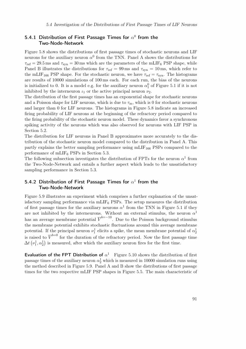
5.4 Investigation of the Distributions of First Passage Times of LIF Neurons
5.4.1 Distribution of First Passage Times for α0 from theTwo-Node-Network
Figure 5.8 shows the distributions of first passage times of stochastic neurons and LIFneurons for the auxiliary neuron α0 from the TNN. Panel A shows the distributions forτref = 29.5 ms and τsyn = 30 ms which are the parameters of the mLIF6 PSP shape, whilePanel B illustrates the distributions for τref = 99 ms and τsyn = 10 ms, which refer tothe mLIF166 PSP shape. For the stochastic neuron, we have τref = τsyn. The histogramsare results of 10000 simulations of 100 ms each. For each run, the bias of the neuronsis initialized to 0. It is a model e.g. for the auxiliary neuron α0
1 of Figure 5.1 if it is notinhibited by the interneuron ι1 or the active principal neuron ν2.The distribution of the first passage times has an exponential shape for stochastic neuronsand a Poisson shape for LIF neurons, which is due to τm, which is 0 for stochastic neuronsand larger than 0 for LIF neurons. The histograms in Figure 5.8 indicate an increasedfiring probability of LIF neurons at the beginning of the refractory period compared tothe firing probability of the stochastic neuron model. These dynamics favor a synchronousspiking activity of the neurons which was also observed for neurons with LIF PSP inSection 5.2.The distribution for LIF neurons in Panel B approximates more accurately to the dis-tribution of the stochastic neuron model compared to the distribution in Panel A. Thispartly explains the better sampling performance using mLIF166 PSPs compared to theperformance of mLIF6 PSPs in Section 5.3.The following subsection investigates the distribution of FPTs for the neuron α1 fromthe Two-Node-Network and entails a further aspect which leads to the unsatisfactorysampling performance in Section 5.3.
5.4.2 Distribution of First Passage Times for α1 from theTwo-Node-Network
Figure 5.9 illustrates an experiment which comprises a further explanation of the unsat-isfactory sampling performance via mLIF6 PSPs. The setup measures the distributionof first passage times for the auxiliary neurons α1 from the TNN in Figure 5.1 if theyare not inhibited by the interneurons. Without an external stimulus, the neuron α1
has an average membrane potential V b=−10. Due to the Poisson background stimulusthe membrane potential exhibits stochastic fluctuations around this average membranepotential. If the principal neuron ν1
1 elicits a spike, the mean membrane potential of α12
is raised to V b=0 for the duration of the refractory period. Now the first passage time∆t(ν1
1 , α12
)is measured, after which the auxiliary neuron fires for the first time.
Evaluation of the FPT Distribution of α1 Figure 5.10 shows the distribution of firstpassage times of the auxiliary neuron α1
2 which is measured in 10000 simulation runs usingthe method described in Figure 5.9. Panel A and B show the distributions of first passagetimes for the two respective mLIF PSP shapes in Figure 5.5. The main characteristic of
91

5 Bayesian Networks: Implementation 2
α2
ν1
ν1
ν1
ν1
ν1
1
2
3
4
5
spike sourcearray time: 500 ms
low bias: -10
large weight: +10
1
350 400 450 500 550 600 650Time [ms]
51.2
51.0
50.8
50.6
50.4
50.2
50.0
49.8
Vo
lta
ge
[mV
]
11Δt(ν ,α )2
1
Figure 5.9: Feasibility test of Implementation 2 with LIF neurons and PSP shapesfrom Figure 5.5: The auxiliary neuron α1
2 has a mean membrane potentialVb=−10
, which corresponds to the bias−10 in the stochastic neuron model.At the point 500ms, a spike of an external spike source triggers the firingof the chain of K principal neurons ν1
1 , ..., νK1 which provide an mLIF
PSP shape in the voltage trace of α12. The weight from the chain of
principal neurons to the auxiliary neuron corresponds to the weight 10in the stochastic neuron model. The first passage time ∆t
(ν1
1 , α12
)is
measured, which is the time after which α12 emits a spike once its mean
membrane potential has been raised to Vb=0
by the input of the principalneurons.
both distributions of LIF neurons are the large peaks within the first few millisecondscompared to distributions of stochastic neurons with rectangular or alpha-shaped PSPs.In the FPT distribution of the mLIF6 PSP in Figure 5.10A 5 peaks can be distinguishedwhich coincide with the time positions of the edges of the "teeth" of the correspondingPSP shape in Figure 5.5. The first peak is more than an order of magnitude higher thanthe largest value of the exponentially-shaped distribution of the stochastic neuron with arectangular PSP shape. This means: if the mean membrane potential of the neurons α1
1
and α12 is increased to V b=0 by an incoming spike from a principal neuron, they either
emit a spike immediately or, otherwise, tend to remain silent for the whole refractoryperiod of the principal neurons. In addition to the FPT distribution of α0
1 and α02 in
Figure 5.8, this fact is a further and even more intuitive explanation for the unsatisfactorysampling performance of LIF neurons with mLIF6 PSPs in Figure 5.7.In contrast to the distribution of the mLIF6 PSP, the FPT distribution when usingmLIF166 PSP in Panel A fits well to the distribution of rectangular PSPs for the mostpart of the interval. This explains the clearly superior sampling performance of mLIF166
PSPs in Figure 5.7. The large first peak explains the small overrepresentation of thestates (z1 = 1, z2 = 1) in Figure 5.7B: the neurons α1
1 and α12 spike consecutively slightly
92

5.4 Investigation of the Distributions of First Passage Times of LIF Neurons
0 5 10 15 20 25 30∆t(ν 1
1 ,α12
)[ms]
10-1
100
101
102
103
104
Occu
rren
ces
rect, τref = 29.5 ms
alpha, τref = 29.5 ms
mLIF6
A: Distribution of ∆t(ν1
1 , α12
)for
τref = 29.5 ms
0 20 40 60 80 100∆t(ν 1
1 ,α12
)[ms]
101
102
103
Occu
rren
ces
rect, τref = 99 ms
alpha, τref = 99 ms
mLIF166
B: Distribution of ∆t(ν1
1 , α12
)for
τref = 99 ms
50.8 50.6 50.4 50.2 50.0 49.8 49.6 49.4Free membrane potential [mV]
0.0
0.5
1.0
1.5
2.0
2.5
3.0
3.5
Occu
rren
ces
1e4
V ≥ Vth
V < Vth
C: Distribution of Vfree for a LIF neuronwith τref = 29.5 ms
50.6 50.4 50.2 50.0 49.8Free membrane potential [mV]
0.0
0.5
1.0
1.5
2.0
2.5
3.0
3.5
4.0
Occu
rren
ces
1e4
V ≥ Vth
V < Vth
D: Distribution of Vfree for a LIF neuronwith τref = 99 ms
Figure 5.10: Panels A and B show the unnormalized probability densities that afiring after the time ∆t occurs once the auxiliary neuron α1 for theTNN has been activated from voltage V
b=−10to V
b=0(see Figure 5.9).
The distributions for rectangular PSPs, alpha-shaped PSPs and mLIFPSPs are illustrated with τref = 29.5 ms (left) and τref = 99 ms (right).Panels C and D show the distributions of the free membrane potentialof the auxiliary neuron α1
1, which is elevated to the average membranepotential V
b=0by stringing together consecutive mLIF PSP. This
mimics the input of ν2 with z2 clamped to 1. The blue part of thedistributions is below the threshold voltage while the red part is above.
93

5 Bayesian Networks: Implementation 2
10 30 50 70 90 110 130 150 170 190τref [ms]
5.0
10.0
15.0
20.0
25.0
30.0
τ syn
[ms]
0.05
0.10
0.15
0.20
0.25
0.30
0.35
0.40
p(V
free≥V
th)
A: Background rate ν = 400 Hz andweight w = 2 nS
10 30 50 70 90 110 130 150 170 190τref [ms]
5.0
10.0
15.0
20.0
25.0
30.0
τ syn
[ms]
0.04
0.08
0.12
0.16
0.20
0.24
0.28
0.32
0.36
p(V
free≥V
th)
B: Background rate ν = 6400 Hz andweight w = 0.5 nS
Figure 5.11: Color-coded probability p (Vfree ≥ Vth = −50 mV) of the free membranepotential of a LIF neuron, whose mean membrane potential is V
b=0and
which receives a balanced random background input. With larger τrefand lower τsyn (e.g. mLIF166 compared to mLIF6), the fraction of Vfree
above Vth becomes smaller and, therefore, the sampling performancewill improve (see Figure 5.10). The simulations are run with differentbackground rates and weights, both of which are chosen such that thestandard deviation of the free membrane potential is equal, but theaverage free membrane potential is lower in Panel B compared to PanelA (see Equation 2.54). However, the shift of the average membranepotential to lower values is too small to expect a noticeable improvementof the sampling quality.
more frequently than the stochastic neurons with rectangular PSPs and, thus, decreasethe proportion of the states (z1 = 0, z2 = 1) and (z1 = 1, z2 = 0).
Evaluation of the Distribution of the Free Membrane Potential of α1 The large firstpeaks of the distributions of first passage times in Figure 5.10 can be explained byevaluating the distribution of the free membrane potential of a LIF neuron with averagemembrane potential V b=0 which is plotted in Figure 5.10C and D for the respective PSPshapes in Figure 5.5. For both distributions, the red bars denote the fraction of themembrane potential above the threshold voltage and the blue bars denote the fraction ofthe membrane potential below the threshold voltage.The fluctuations of the membrane voltage around some mean membrane potential inducedby the Poisson-distributed background input are equal for the mean membrane potentialsVb=−10 and for V b=0. This implies that the probability of the neurons α1
1 and α12 to fire
immediately after the increase of the mean membrane potential from Vb=−10 to V b=0
is proportional to the red area of the corresponding distribution of the free membrane
94

5.4 Investigation of the Distributions of First Passage Times of LIF Neurons
potential in Figure 5.10C and D. For τref = 29.5 ms and τsyn = 30 ms, which are thetime scales of the mLIF6 PSP, the red area in Figure 5.10C amounts to about 27.2%.This value is in approximate accordance with the relative height of the first peak of theFPT distribution of α1 in Figure 5.10A. For τref = 99 ms and τsyn = 10 ms, which refersto the mLIF166 PSP, the red fraction in Figure 5.10D is about 3.7%, which is also inapproximate accordance with the overshoot of the first large peak in Figure 5.10B.Figure 5.11A illustrates the fraction of the free membrane potential which is larger thanthe threshold voltage Vth for different choices of τsyn and τref. In order to achieve asatisfactory sampling result with Implementation 2, it is essential to choose a large τrefand low τsyn, which means that the autocorrelation of the membrane potential, whichbears the "memory" of the LIF neuron, has to vanish at best. However, a large τref andlow τsyn implies very long chains of neurons which scales exponentially for tasks with anincreasing number of RVs and, thus, becomes computationally not feasible.A question that remains is whether it is possible to decrease the height of the first peakin of the FPT distribution of α1 in Figure 5.10A by modifying the background inputparameters. The new frequency and synaptic input weights can be chosen such thatthe standard deviation of the membrane potential remains constant but the averagemembrane potential is shifted to a lower value (see Equation 2.54). A shift of the meanmembrane potential to a lower value implies a shrinkage of the red area of Figure 5.10Cand consequently a shrinkage of the height of the first peak in of the FPT distribution ofα1 in Figure 5.10A.Figure 5.11B shows the fraction of the free membrane potential which is larger than thethreshold voltage Vth for a much larger background input frequency of ν = 6400 Hz andmuch lower synaptic input weight w = 0.5 nS for the excitatory and inhibitory connections.However, this shift of the mean membrane potential turns out to be very small comparedto Figure 5.11A and will not significantly improve the sampling results.The following paragraph comprises two crucial reasons against a modification of the mLIFPSP shape with the aim to improve the sampling quality.
Reasons Against a Further Modification of the mLIF PSP Shape The results of thedistribution of first passage times with alpha-shaped PSPs in Figure 5.10 might lead tothe assumption that rounder PSP shapes, instead of the imitations of the ideal rectangularPSPs in Figure 5.5, could improve the results of LIF sampling with mLIF6 PSPs. Arounding of the PSP shape would shift the large peak in Figure 5.10A towards the end ofthe refractory period of the principal neuron.However, rendering the first "tooth" of the PSP shape in Figure 5.5 smaller would entaila raising of the remaining "teeth" in order to fulfill the consistency of the integral ofindividual PSPs of the LIF neuron model and the stochastic neuron model in Equation2.73. Such an increase would result in a PSP shape crossing the threshold potential bydesign.Furthermore, a rounding of the PSP shape would lead to large jumps of the membranepotential e.g. of the auxiliary neuron α1
1 whenever the RV z2 is clamped to 1. This resultsin undesirable threshold crossings (see Figure 4.12B) and distorts the sampling quality.
95
5 Bayesian Networks: Implementation 2
5.5 Conclusion
This chapter aimed at testing the feasibility of Implementation 2 of BNs with LIF neurons(see Section 2.1.5). Based on simulation results we can conclude that, if the samplingability depends on the distribution of spike timings, LIF sampling with both original LIFPSPs and mLIF PSPs suffers substantial precision.This imprecision could be ascribed to three inherent aspects which differ between theLIF neuron model and the abstract neuron model. First, both LIF and mLIF PSPs arenon-uniform, which results in a non-uniform firing probability. Second, the stochasticityinduced by the OU process, which describes the membrane potential of LIF neurons in anoisy environment, is different from the stochasticity induced by the Bernoulli process,which characterizes the evolution of the membrane potential of abstract neurons. Third,the membrane potential of the LIF neurons is autocorrelated, which is in contrast to theabstract neuron model. Due to this fact, additional correlations of the spiking activity ofthe sampling neurons were introduced, which deterred from the desired functionality ofthe networks.Only for large chains of neurons, yielding large refractory times and low synaptic timeconstants, adequate sampling results were achieved which are still less promising than theLIF sampling results via Implementation 1 in Chapter 4. In this case, the occurrences ofthe first threshold crossing were much more distributed in accordance with the distributionof first passage times of the stochastic neuron model.An application of Implementation 2 with mLIF166 PSPs on the BrainScaleS neuromorphichardware system (see Section 2.2) will be infeasible with the inherent fluctuations ofvoltages and currents, since mLIF166 PSPs require the implementation of chains of 166neurons which all have the same characteristics.
96

6 Towards LIF-based BoltzmannMachines on Neuromorphic Hardware
The previous chapters have demonstrated through software simulations that it is possibleto physically instantiate Boltzmann Machines and Bayesian Networks with networks ofLIF neurons. This chapter investigates the feasibility of performing LIF sampling withthe neurons integrated on the HICANN chip described in Section 2.2.1. The demonstra-tor setup, which is described in Section 2.2.2, provides the necessary communicationinfrastructure for the chip. The PyHAL API (see Section 2.3.2) is used to control thedesired neural and synaptic parameters and run the experiments.As outlined in Section 2.2, a neuromorphic hardware system entails a broad rangeof advantages such as defect tolerance, massive parallelism, acceleration compared tobiological real-time and low power consumption. However, especially when runningexperiments with which strongly depend on certain parameter settings, whose precisionis crucial for the expected outcome of the experiment, the drawbacks and limitations ofthe analog elements of the neuromorphic hardware become apparent: the imprecisionof floating gate cells, the limitation of parameter ranges, the malfunction of electricalcircuits due to production faults or the limitation of the communication bandwidth, toname some examples.The simulation results in the previous chapters showed that LIF sampling strongly dependson the accurate choice of neuron parameters. In particular, the choice of time constantsis important: The refractory period has to be much larger than the inherent delays onthe chip, the synaptic time constant must be of the order of the refractory period andthe effective membrane time constant has to be much smaller than the synaptic timeconstant (see Section 2.1.7). The crucial question in this chapter is therefore: Do therange limitations and the variations of parameters on the HICANN chip suit the needs ofLIF sampling? And if not, can suitable workarounds be found?Section 6.1 thus starts with a characterization of the circuits on the HICANN chip witha particular focus on the parameters which are essential for LIF sampling. First, thevalues of the floating gate cells are fixed to plausible values needed for LIF sampling andthose neurons are selected on the HICANN chip, whose membrane potential exhibitsapproximately the expected behavior. Thereafter, Spike-Triggered Average (STA) is usedto extract the time constants of the selected membrane circuits. It will become clear thatthe ranges of time constants are unsatisfactory to allow a concrete implementation ofLIF sampling. In particular, the saturation of the synaptic conductances and the limitedranges of the synaptic and membrane time constants will complicate the application ofLIF sampling on the current version of the HICANN chip.Section 6.2 therefore aims at providing desired parameter ranges for the LIF neurons based
97

6 Towards LIF-based Boltzmann Machines on Neuromorphic Hardware
on the results of software simulations of neurons with the deduced hardware parametersfrom Section 6.1. It will become apparent that a reasonable LIF sampling performancecan only be achieved with larger synaptic time constants together with larger frequenciesof the background stimulus or smaller membrane time constants than currently achievableon the used version of the HICANN chip.
6.1 Characterization of the Neural and Synaptic Circuits ofthe HICANN chip
This section aims at testing the feasibility of the application of LIF sampling with theneurons integrated on the HICANN chip. Subsection 6.1.1 starts with a description of theutilized set of the individual neural and synaptic parameters. Thereafter, Subsection 6.1.2continues with a rigorous measurement of the involved time constants, the proportions ofwhich are essential for a satisfactory LIF sampling performance. Subsection 6.1.3 presentsthe activation curve of a selected neuron and concludes that, with the currently availablemethods, a generic application of LIF sampling on the current version of the HICANNchip is not feasible.
6.1.1 Parameter Selection
Table A.6 contains the utilized values of the floating gate cells that were used throughoutthe experiments in this section. The table comprises global and individual neuronparameters as well as parameters of the synaptic circuits. The following paragraphs discussthe choice of the neural and synaptic parameters in the course of this section. Hereby, thehardware parameters are written in typewriter font, while their corresponding actualneural and synaptic parameters are written in normal font.
Neural Parameters 24 of the 44 parameters in Table A.6 describe the dynamics ofthe AdEx membrane circuits (see Section 2.1.6) on the HICANN chip. The neuralparameters which were manually set for the experiments in this thesis are the globalparameter V_reset and the individual neuron parameters V_t, E_l, E_synx, E_syni,I_fire, I_gladapt, I_gl, I_pl, V_syntcx and V_syntci.First of all, the exponential term in Equation 2.40 and the adaptive current w(t) (seeEquation 2.41) have to be quiesced such that the membrane dynamics of the neuronsapproximately reduce to those of standard LIF neurons in Equation 2.34. For this, theDAC-values of the currents I_fire and I_gladapt are set to 0 [Millner , 2012]. However,this does not exclude the existence of remaining leakage currents, such that, for someneurons, adaptive mechanisms are still observable.The floating gate cells of the leakage potential, E_l, and of the reversal potentials, E_synxand E_syni, are set to 512 DAC, 626 DAC and 398 DAC, respectively, so that the reversalpotentials are lying symmetrically with respect to the leakage potential. The leakage andreversal potentials are therefore expected to lie at 0.9 V, 0.7 V and 1.1 V, respectively(DAC value
1024 × 1.8 V).
98
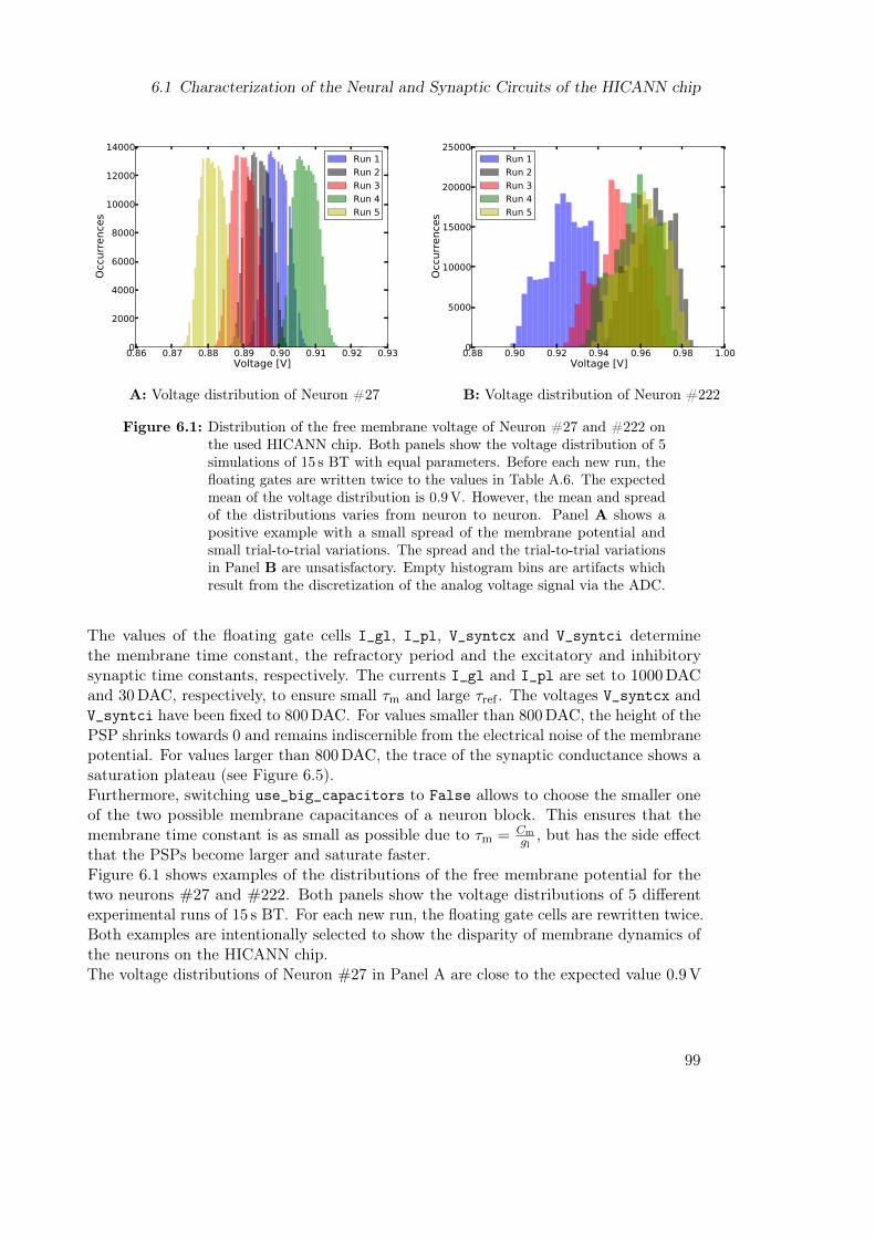
6.1 Characterization of the Neural and Synaptic Circuits of the HICANN chip
0.86 0.87 0.88 0.89 0.90 0.91 0.92 0.93Voltage [V]
0
2000
4000
6000
8000
10000
12000
14000
Occ
urr
ence
s
Run 1
Run 2
Run 3
Run 4
Run 5
A: Voltage distribution of Neuron #27
0.88 0.90 0.92 0.94 0.96 0.98 1.00Voltage [V]
0
5000
10000
15000
20000
25000
Occ
urr
ence
s
Run 1
Run 2
Run 3
Run 4
Run 5
B: Voltage distribution of Neuron #222
Figure 6.1: Distribution of the free membrane voltage of Neuron #27 and #222 onthe used HICANN chip. Both panels show the voltage distribution of 5simulations of 15 s BT with equal parameters. Before each new run, thefloating gates are written twice to the values in Table A.6. The expectedmean of the voltage distribution is 0.9 V. However, the mean and spreadof the distributions varies from neuron to neuron. Panel A shows apositive example with a small spread of the membrane potential andsmall trial-to-trial variations. The spread and the trial-to-trial variationsin Panel B are unsatisfactory. Empty histogram bins are artifacts whichresult from the discretization of the analog voltage signal via the ADC.
The values of the floating gate cells I_gl, I_pl, V_syntcx and V_syntci determinethe membrane time constant, the refractory period and the excitatory and inhibitorysynaptic time constants, respectively. The currents I_gl and I_pl are set to 1000 DACand 30 DAC, respectively, to ensure small τm and large τref . The voltages V_syntcx andV_syntci have been fixed to 800 DAC. For values smaller than 800 DAC, the height of thePSP shrinks towards 0 and remains indiscernible from the electrical noise of the membranepotential. For values larger than 800 DAC, the trace of the synaptic conductance shows asaturation plateau (see Figure 6.5).Furthermore, switching use_big_capacitors to False allows to choose the smaller oneof the two possible membrane capacitances of a neuron block. This ensures that themembrane time constant is as small as possible due to τm = Cm
gl, but has the side effect
that the PSPs become larger and saturate faster.Figure 6.1 shows examples of the distributions of the free membrane potential for thetwo neurons #27 and #222. Both panels show the voltage distributions of 5 differentexperimental runs of 15 s BT. For each new run, the floating gate cells are rewritten twice.Both examples are intentionally selected to show the disparity of membrane dynamics ofthe neurons on the HICANN chip.The voltage distributions of Neuron #27 in Panel A are close to the expected value 0.9 V
99
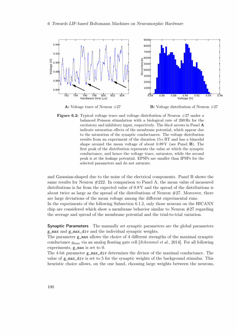
6 Towards LIF-based Boltzmann Machines on Neuromorphic Hardware
792 794 796 798 800 802 804Hardware time [µs]
0.84
0.86
0.88
0.90
0.92
0.94
Volta
ge [V
]
A: Voltage trace of Neuron #27
0.84 0.86 0.88 0.90 0.92 0.94 0.96Voltage [V]
0
1000
2000
3000
4000
5000
6000
7000
8000
9000
Occu
rren
ces
B: Voltage distribution of Neuron #27
Figure 6.2: Typical voltage trace and voltage distribution of Neuron #27 under abalanced Poisson stimulation with a biological rate of 200 Hz for theexcitatory and inhibitory input, respectively. The black arrows in Panel Aindicate saturation effects of the membrane potential, which appear dueto the saturation of the synaptic conductances. The voltage distributionresults from an experiment of the duration 15 s BT and has a bimodalshape around the mean voltage of about 0.89 V (see Panel B). Thefirst peak of the distribution represents the value at which the synapticconductance, and hence the voltage trace, saturates, while the secondpeak is at the leakage potential. EPSPs are smaller than IPSPs for theselected parameters and do not saturate.
and Gaussian-shaped due to the noise of the electrical components. Panel B shows thesame results for Neuron #222. In comparison to Panel A, the mean value of measureddistributions is far from the expected value of 0.9 V and the spread of the distributions isabout twice as large as the spread of the distributions of Neuron #27. Moreover, thereare large deviations of the mean voltage among the different experimental runs.In the experiments of the following Subsection 6.1.2, only those neurons on the HICANNchip are considered which show a membrane behavior similar to Neuron #27 regardingthe average and spread of the membrane potential and the trial-to-trial variation.
Synaptic Parameters The manually set synaptic parameters are the global parametersg_max and g_max_div and the individual synaptic weights.The parameter g_max allows the choice of 4 different strengths of the maximal synapticconductance gmax via an analog floating gate cell [Schemmel et al., 2014]. For all followingexperiments, g_max is set to 0.The 4-bit parameter g_max_div determines the divisor of the maximal conductance. Thevalue of g_max_div is set to 5 for the synaptic weights of the background stimulus. Thisheuristic choice allows, on the one hand, choosing large weights between the neurons,
100
6.1 Characterization of the Neural and Synaptic Circuits of the HICANN chip
when setting g_max_div to 0, and, on the other hand, prevents the PSPs from becomingvery small and thus indistinguishable from the electrical noise on the membrane.Figure 6.2 shows a typical voltage trace (Panel A) and voltage distribution (Panel B)of a neuron which receives synaptic input from an excitatory and inhibitory Poissonsource with a biological rate of 200 Hz, respectively. The spikes are generated on the hostcomputer and sent to the HICANN chip via the FPGA board and the DNC.Figure 6.2A reveals that the membrane voltage saturates at about 0.86 V which can betraced back to the saturation of the total synaptic conductance, a phenomenon whichhas also been documented in Millner [2012]. The voltage distribution in Figure 6.2B hasa bimodal shape around a mean voltage of 0.89 V. The first peak of the distribution at0.86 V represents the value at which the synaptic conductance, and hence the voltagetrace, saturates, while the second peak at 0.89 V is the leakage potential. EPSPs aresmaller than IPSPs for the selected parameters and, thus, do not saturate.
6.1.2 Measuring the Time Constants
The appropriate setting of the time constants of a LIF neuron is crucial for the LIFsampling performance (see e.g. Figures 3.4 and 4.4). The refractory period τref has tobe at least an order of magnitude larger than the inherent synaptic delays, in order tominimize their effect on neuron correlations. The synaptic time constant τsyn has to bein the order of the refractory period τref , such that a neuron which elicits a spike hasa noticeable impact on the postsynaptic neurons during the next refractory period. Incontrast, the effective membrane time constant τeff of the neuron has to be very smallin order to enable fast membrane dynamics. This can be achieved either by settingthe membrane time constant τm to a value close to 0 or by injecting a high-frequencyexcitatory and inhibitory background stimulus into the neuron.The following three paragraphs aim at determining the time constants of the neurons onthe HICANN chip with a special focus on the consistency with the requirements of LIFsampling. The constants τref and τsyn are measured via Spike-Triggered Average (STA)[de Boer and Kuyper , 1968], while τm is measured by injecting a finite current pulseinto the membrane and fitting an exponential function to the response of the membranepotential. For each time constant, 200 PSPs (for τsyn), 200 APs (for τref), or 200 currentpulses (for τm) are averaged. The experiments are run once with Neuron #27 usingdifferent hardware parameters, and once with different neurons which have the samehardware parameters. All measured results of the time constants are given in biologicalreal-time.
Refractory Period For the measurement of τref , the hardware parameter V_t, whichrepresents the threshold potential, is set to 410 DAC, which is far below the leakagepotential. This setting provokes a bursting of the neuron with an ISI of τref plus theupswing time until the following spike. Thus, τref is the distance between a peak (averagedspike) and the upswing to the following peak. Likewise, the parameter V_reset is set to400 DAC to remain below the threshold potential.
101

6 Towards LIF-based Boltzmann Machines on Neuromorphic Hardware
0 5 10 15 20 25 30 35 40Biological time [ms]
0.00
0.01
0.02
0.03
0.04
0.05
0.06
0.07
Auto
corr
ela
tion o
f V
mem
[a.u
.]
Ipl =0 DAC, τref =31.88 ms
Ipl =10 DAC, τref =7.50 ms
Ipl =30 DAC, τref =2.08 ms
Ipl =50 DAC, τref =1.58 ms
Ipl =100 DAC, τref =1.04 ms
A: Neuron #27
0 5 10 15 20 25 30 35 40Biological time [ms]
0.00
0.02
0.04
0.06
0.08
0.10
Auto
corr
ela
tion o
f V
mem
[a.u
.]
Neuron #19, τref =8.13 ms
Neuron #27, τref =2.08 ms
Neuron #80, τref =15.62 ms
Neuron #213, τref =4.26 ms
Neuron #252, τref =6.38 ms
B: Ipl = 30 DAC
Figure 6.3: Measurement of the refractory period τref of Neuron #27 for differentcurrents I_pl in Panel A and of different neurons for the current I_pl =30 DAC in Panel B. The panels show the autocorrelation of the membranepotential of a neuron whose threshold potential is below the leakagepotential, such that the neuron spikes with a ISI close to τref . The valueof τref corresponds to the distance between one peak (spike) and the nextupswing. Panel A implies that the refractory period can be selected fromat least two different orders of magnitude. However, τref varies greatlyfor different neurons when injecting the same currents I_pl (see PanelB).
Figure 6.3A shows the measured refractory periods τref of Neuron #27 for differentcurrents I_pl. The figure implies that τref can be selected from at least 2 different ordersof magnitude: For I_pl = 0 DAC, we get τref = 31.88 ms, while for I_pl = 100 DAC, wehave τref = 1.04 ms, which is more than one order of magnitude lower.Figure 6.3B displays the measured τref of different neurons for the current I_pl = 30 DAC.Similar to Panel A, the value of τref varies by an order of magnitude between 2 ms and16 ms for different neurons, even if the same current I_pl = 30 DAC is selected.For too low τref ≈ 1.2 ms the synaptic delays on the HICANN chip, which are fixed to1.2 ms (see Section 2.2.1), will have a disturbing effect on the resulting LIF samplingquality because they will affect neuron correlations. That is why τref � 1.2 ms is requiredand, indeed, achievable for certain neurons on the chip.
Membrane Time Constant The measurement of the membrane time constant τm isconducted by averaging the responses of the membrane potential to the same currentstimuli and fitting an exponential function to the average curve. The growth constant ofthe exponential function then corresponds to τm.Figure 6.4A shows the results of the measured τm of Neuron #27 for different currentsI_gl. The membrane time constant can be tuned on a finer scale compared to the
102
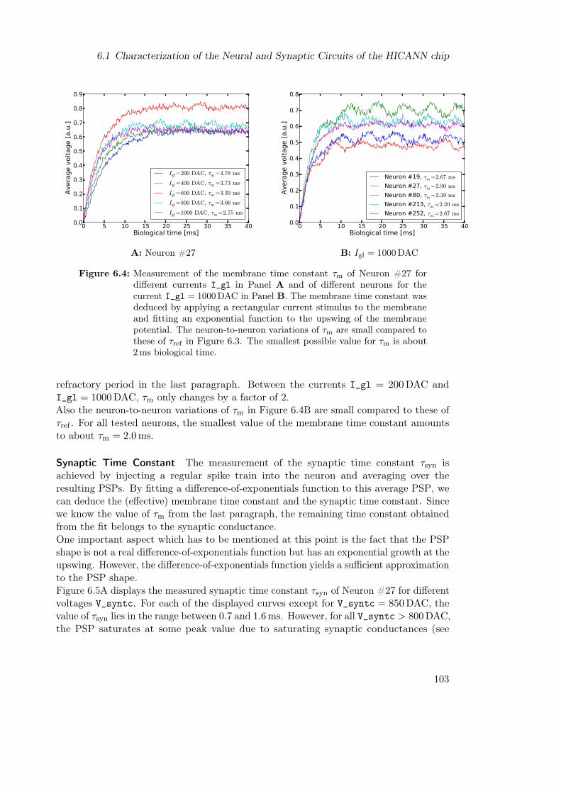
6.1 Characterization of the Neural and Synaptic Circuits of the HICANN chip
0 5 10 15 20 25 30 35 40Biological time [ms]
0.0
0.1
0.2
0.3
0.4
0.5
0.6
0.7
0.8
0.9
Avera
ge v
olt
age [
a.u
.]
Igl =200 DAC, τm =4.78 ms
Igl =400 DAC, τm =3.73 ms
Igl =600 DAC, τm =3.39 ms
Igl =800 DAC, τm =3.06 ms
Igl =1000 DAC, τm =2.75 ms
A: Neuron #27
0 5 10 15 20 25 30 35 40Biological time [ms]
0.0
0.1
0.2
0.3
0.4
0.5
0.6
0.7
0.8
Avera
ge v
olt
age [
a.u
.]
Neuron #19, τm =2.67 ms
Neuron #27, τm =2.90 ms
Neuron #80, τm =2.39 ms
Neuron #213, τm =2.20 ms
Neuron #252, τm =2.67 ms
B: Igl = 1000 DAC
Figure 6.4: Measurement of the membrane time constant τm of Neuron #27 fordifferent currents I_gl in Panel A and of different neurons for thecurrent I_gl = 1000 DAC in Panel B. The membrane time constant wasdeduced by applying a rectangular current stimulus to the membraneand fitting an exponential function to the upswing of the membranepotential. The neuron-to-neuron variations of τm are small compared tothese of τref in Figure 6.3. The smallest possible value for τm is about2 ms biological time.
refractory period in the last paragraph. Between the currents I_gl = 200 DAC andI_gl = 1000 DAC, τm only changes by a factor of 2.Also the neuron-to-neuron variations of τm in Figure 6.4B are small compared to these ofτref . For all tested neurons, the smallest value of the membrane time constant amountsto about τm = 2.0 ms.
Synaptic Time Constant The measurement of the synaptic time constant τsyn isachieved by injecting a regular spike train into the neuron and averaging over theresulting PSPs. By fitting a difference-of-exponentials function to this average PSP, wecan deduce the (effective) membrane time constant and the synaptic time constant. Sincewe know the value of τm from the last paragraph, the remaining time constant obtainedfrom the fit belongs to the synaptic conductance.One important aspect which has to be mentioned at this point is the fact that the PSPshape is not a real difference-of-exponentials function but has an exponential growth at theupswing. However, the difference-of-exponentials function yields a sufficient approximationto the PSP shape.Figure 6.5A displays the measured synaptic time constant τsyn of Neuron #27 for differentvoltages V_syntc. For each of the displayed curves except for V_syntc = 850 DAC, thevalue of τsyn lies in the range between 0.7 and 1.6 ms. However, for all V_syntc > 800 DAC,the PSP saturates at some peak value due to saturating synaptic conductances (see
103

6 Towards LIF-based Boltzmann Machines on Neuromorphic Hardware
0 10 20 30 40 50 60 70Biological time [ms]
0.000
0.005
0.010
0.015
0.020
0.025
0.030
0.035
Avera
ge v
olt
age [
a.u
.]
Vsyntc =700 DAC, τsyn =0.94 ms
Vsyntc =750 DAC, τsyn =0.78 ms
Vsyntc =800 DAC, τsyn =1.37 ms
Vsyntc =850 DAC, τsyn =3.91 ms
Vsyntc =900 DAC, τsyn =1.60 ms
Vsyntc =1000 DAC, τsyn =1.25 ms
A: Neuron #27
0 10 20 30 40 50Biological time [ms]
0.00
0.01
0.02
0.03
0.04
0.05
Avera
ge v
olt
age [
a.u
.]
Neuron #19, τsyn =1.54 ms
Neuron #27, τsyn =1.44 ms
Neuron #80, τsyn =1.93 ms
Neuron #213, τsyn =1.45 ms
Neuron #252, τsyn =1.56 ms
B: Vsyntc = 800 DAC
Figure 6.5: Measurement of the synaptic time constant τsyn of Neuron #27 for differ-ent voltages V_syntc in Panel A and of different neurons for the voltageV_syntc = 800 DAC in Panel B. For each V_syntc except 850 DAC, thevalue of τsyn lies in the range between 0.7 and 1.6 ms in Panel A. However,for each V_syntc > 800 DAC, the PSP saturates at some peak value dueto saturating synaptic conductances. The synaptic time constant at thevoltage V_syntc = 800 DAC lies around 1.5 ms for all tested neurons (seePanel B).
Subsection 6.1.1). For the remaining range of V_syntc, the PSPs can not be distinguishedfrom the electrical noise of the membrane potential.The synaptic time constant at the voltage V_syntc = 800 DAC lies around 1.5 ms forall tested neurons, which is shown in Figure 6.5B. Thus, the synaptic time constant isconsistently lower than the membrane time constant of the neurons and of the order ofthe synaptic delays. The second statement is even worse because τsyn has to be in therange of τref (see Chapters 3 and 4) to achieve optimal LIF sampling results, but, however,delays of the order of τref will affect neuron correlations.
6.1.3 Measuring the Activation Curve
In the software simulations in Chapters 3, 4 and 5, the activation curve of a LIF neuronwas measured by varying the mean membrane potential of the neuron and measuring thefraction pON of the time that the neuron spends in the refractory state (see Figure 3.1).A shift of the leakage potential towards one of the reversal potentials might introducenon-linearities, additionally to those which are in the system anyway.Therefore, the method used in this section leaves the leakage potential and the reversalpotentials constant such that the reversal potentials remain symmetrical with respect tothe leakage potential. In order to trace the activation curve, the threshold voltage V_tand the reset voltage V_reset = V_t− 10 DAC are shifted from the inhibitory towards
104

6.1 Characterization of the Neural and Synaptic Circuits of the HICANN chip
400 420 440 460 480 500 520Threshold potential Vt [DAC]
0
1000
2000
3000
4000
5000
Num
ber o
f Spi
kes
0.0
0.1
0.2
0.3
0.4
0.5
0.6
0.7
0.8
pO
N
0.75 0.80 0.85 0.90Threshold potential Vth [V]
Figure 6.6: Activation curve of Neuron #27. Each measuring point corresponds tothe average of 5 experiments of the duration 15 s biological time. Theerror bars denote the standard deviations. The Poisson backgroundhas a biological rate of 200 Hz for the excitatory and inhibitory input,respectively. In opposite to Figure 3.1, the threshold voltage V_t and thereset voltage V_reset = V_t−10 DAC are modified. This ensures that theactual reversal potentials stay symmetrically around the leakage potential.Due to τm (see Figure 6.4) and the necessary condition V_t− V_reset ≥10 DAC , the neuron maximally reaches pON = 0.7, which is insufficientfor LIF sampling.
the excitatory reversal potential. For each data point, the number NS of elicited spikesduring T = 15 s biological time is measured. With the extracted refractory period of theneurons from Figure 6.3, pON = NSτref
T can be calculated.Figure 6.6 displays the measured activation curve of Neuron #27. Each data point ofthe curve corresponds to an average over 5 experiments, in which the neuron receivedan excitatory and inhibitory background input of 200 Hz biological rate1, respectively.Between consecutive experimental runs, the floating gate cells are reprogrammed twice.The activation curve in Figure 6.6 is sigmoidal and can be well fitted to a logistic functionwith a proper linear transformation of V_t. However, several aspects are unsatisfactoryfor a reliable application of LIF sampling. First, the curve saturates at a maximum ofabout 5000 spikes which corresponds to pON ≈ 0.7. This implies that a larger pON can
1A background rate of 200Hz allows to supply several neurons with the same rate in parallel inprospective experiments with LIF-based BMs, with the given maximal bandwidth and accelerationfactor (see Section 2.2.2).
105

6 Towards LIF-based Boltzmann Machines on Neuromorphic Hardware
not be reached. This can be traced back to the large τm and the saturation of synapticconductances, which results in a large effective membrane time constant τeff ≈ τm andthus insufficiently fast membrane dynamics.A second unsatisfactory issue are the large error bars particularly around the midpointof the activation curve. These errors can be mainly ascribed to the imprecision of thefloating gate cells in the individual experimental runs. However, this inconsistency isexpected to be overcome in prospective experiments with a calibrated hardware system.The following subsection will present the results of software simulations which aim to findthe parameter values of the time constants and the background input which fit best tothe requirements of LIF sampling.
6.2 Towards a Parametrization that Will Enable LIFSampling on Hardware
The previous section has shown that a naive application of LIF sampling is not directlycompatible with the range and the fluctuations of parameters available on the currentversion of the HICANN chip. This section aims at finding the parameters ranges which fitbest to the requirements of LIF sampling, while still taking into account the parameters ofthe neurons on the HICANN chip, which were deduced in Section 6.1. For this, softwaresimulations are run in which the neurons are initialized with the optimal parameters of theneurons on the HICANN chip. Subsection 6.2.1 deals with the impact of the parametersof the background stimulus on the effective membrane time constant of the LIF neuron.Thereafter, Subsection 6.2.2 investigates the quality of LIF sampling from an exampleBoltzmann distribution of 5 RVs based on the determined time constants of the neuronson the HICANN chip.
6.2.1 Background Input Parameters
The saturation of the activation function in Figure 6.6 at pON = 0.7 implies that theeffective membrane time constant τeff is not small enough compared to τsyn and τref . Thisis due to the fact that, on the one hand, the maximum background input frequency andweight to the neuron is too small and, on the other hand, the membrane time constant τm
too large. According to Equation 2.54, both the background input frequency and weighthave an impact on the synaptic conductance and, consequently, on the total conductancegtot = Cm
τeff:
gi(t) = wiνiτsyn . (6.1)
With gtot(t) = gl +∑
i gi(t), the effective membrane time constant τeff can be directlycalculated:
τeff =Cm
gtot=
Cm
gl + τsyn (wexcνexc + winhνinh). (6.2)
Now we can fix the parameters τsyn = 1.5 ms and τm = 2.0 ms, which were both measuredin Section 6.1, and illustrate τeff as a function of the background input rates ν = νexc = νinh
and weights w = wexc = winh.
106

6.2 Towards a Parametrization that Will Enable LIF Sampling on Hardware
102 103 104 105
Background input frequency ν [Hz]
10-1
100
101
Effe
ctiv
e tim
e co
nsta
nt τ e
ff[m
s]
A: τeff versus background rate ν
100 101 102 103
Background input weight w [nS]
10-1
100
101
Effe
ctiv
e tim
e co
nsta
nt τ e
ff[m
s]
B: τeff versus background weight w
Figure 6.7: Dependence of the effective membrane time constant τeff on the rate ν(see Panel A) and the weight w (see Panel B) of the background Poissonstimulus. The excitatory and inhibitory synaptic weights in Panel Aare 2 nS. The background rate in Panel B amounts to 400 Hz for theexcitatory and inhibitory input, respectively.
Figure 6.7A shows the impact of the background input rate ν on τeff for the synaptic inputweights w = 2.0 nS. For low input frequencies, the effective membrane time constant staysconstant at τeff = τm. At frequencies higher than 1.0 kHz, τeff begins to shrink. At about100.0 kHz and more, τeff reaches values of 0.2 to 0.4 ms, which are an order of magnitudesmaller than τsyn, and, thus, suit the requirements of LIF sampling.Figure 6.7B displays the dependency of τeff on the strength of the background inputweights w for an input frequency of ν = 400.0 Hz for the excitatory and inhibitoryconnections, respectively. The plot shows that τeff decreases with larger synaptic weights.Only for very large synaptic weights close to w = 1.0µS, τeff becomes about an order ofmagnitude smaller than τsyn. However, very large weights are impractical because theneurons would quickly reach the reversal potentials and the PSPs would saturate.
6.2.2 Time Constants
In Section 6.1.2 it was shown that the best achievable values of the time constants onthe current version of the HICANN chip are τm = 2 ms and τsyn = 1.5 ms. The followingdiscussion aims at finding an optimal working point for LIF sampling for a BM of 5RVs using the determined hardware parameters. Furthermore, the experiments compriseoptimal values for the time constants, which fit best to the requirements of LIF sampling.Figure 6.8 presents the sampling performance based on the KL divergence of the simulatedand theoretical joint probability distribution (see Equation 2.15) for a simulated BM of 5RVs. Each experiment has a duration of 15 s BT, just like in the hardware measurementsin Section 6.1. If not given by the color-plots, the parameters of the LIF neuron are
107

6 Towards LIF-based Boltzmann Machines on Neuromorphic Hardware
2 4 6 8 10 12 14 16 18 20τref [ms]
2
4
6
8
10
12
14
16
18
20
τ syn
[ms]
0.1
0.2
0.3
0.4
0.5
0.6
0.7
0.8
DK
L(p
sim||p
theo)
A: DKL(psim‖ptheo) versus τref and τsyn
0.1 0.3 1.0 3.2 10.0 31.6ν [kHz]
0.10
0.22
0.46
1.00
2.15
4.64
10.00
τ m[m
s]
0.2
0.4
0.6
0.8
1.0
1.2
1.4
1.6
DK
L(p
sim||p
theo)
B: DKL(psim‖ptheo) versus ν and τm
Figure 6.8: Color-coded KL divergence of the simulated and target joint probabilitydistribution for a simulated BM consisting of 5 RVs. The duration of onesimulation is 15 s biological time. Table A.1 shows the utilized neuron andstimulus parameters, but with τm = 2 ms in Panel A and τref = 1.5 msand τsyn = 1.5 ms in Panel B. Furthermore, in contrast to Table A.1,the synaptic delays are fixed to 1.2 ms, mimicking the synaptic delays onthe HICANN chip. The black crosses show the best currently achievableresults with the neurons on the HICANN chip. The figures imply thatthe best sampling results are reached with large τref and τsyn comparedto τm, and large input frequencies.
chosen from Table A.1, but with τref = 1.5 ms, τm = 2.0 ms, τsyn = 1.5 ms and delays of1.2 ms.Figure 6.8A shows the sampling quality under the variation of the time constants τsyn
and τref . The best sampling performance is achieved with the conditions τref � 1.2 ms,such that the synaptic delay is vanishing compared to the time scales of the neuron, andτsyn ≈ τref , a result which has already been verified in Chapter 3. The black cross inFigure 6.8A shows the expected best achievable result with the current version of theHICANN chip taking into account a constant synaptic time constant τsyn ≈ 2.0 ms.Figure 6.8B displays the sampling performance for different background input rates νand membrane time constant τm. As expected according to Equations 2.48 and 2.55,respectively, the best sampling results are achieved with very large input rates ν and thusa fast membrane, which means τeff ≈ 0. Due to the bandwidth limitation (see Chapter2.2) regarding the current acceleration of 104 of the HICANN chip compared to biologicalreal-time, however, the best achievable result, when using the parameter set of the neuronson the HICANN chip, is unsatisfactory (see black cross in Figure 6.8B).
108
6.3 Conclusion
6.3 Conclusion
This chapter investigated the feasibility of naively implementing LIF sampling on the cur-rent version of the HICANN chip. It turned out that the membrane and synaptic circuitson the current version of the HICANN chip do not allow such a direct implementation ofLIF sampling for several reasons.First, and most crucially, the synaptic conductances saturate very quickly. This leads toa rapid saturation of the membrane potential and, consequently, non-additive PSPs.Second, the synaptic time constant cannot be set larger than the effective membranetime constant, a fact which is crucial for LIF sampling. Due to the short synaptic timeconstant, the effect of the individual background spikes on the course of the membranepotential of a neuron is very small, demanding for large input frequencies far beyond themaximum bandwidth of about 2775 Hz for regular spike trains at the acceleration factor104 of the HICANN chip compared to biological real-time.Third, the membrane time constant of the neurons cannot be set smaller than τm = 2.0 ms.In the software simulations of the previous chapters, τm ≈ 0.1 ms was used, which allowedfast membrane dynamics independent of the background input rates. Software simulationsshowed that, with the demonstrated constraint of the parameter range of τm on theHICANN chip, a very large background input frequency in the range of 10 kHz is requiredto achieve a fast membrane and, consequently, satisfactory LIF sampling results. Thisoption is, however, not approachable with the current hardware setup due to the bandwidthlimitation.Fourth, imprecisions arise during the measurements which prevent from setting up well-tuned LIF-based BMs. These imprecisions can be be ascribed to the inaccuracies of thefloating gate cells. Since many parameters (τref , τsyn, τm, Erev
exc, Erevinh , Vrest, Vth) need
to be tuned simultaneously, inaccuracies of one parameter affect the precision of otherparameters.All in all, the current version of the HICANN chip appears to prohibit a direct implemen-tation of LIF sampling. In the ongoing experiments, some workarounds can be envisioned,among which mLIF PSPs emerge as a promising candidate, since large τref but only smallτsyn can be achieved.
109
7 Discussion
The simulation results in this thesis have demonstrated the feasibility of using networks ofdeterministic Leaky Integrate-and-Fire (LIF) neurons to sample from probability distribu-tions schematized by Bayesian Networks (BNs). For this, two different implementations ofBNs over binary RVs, which were proposed by Pecevski et al. [2011], have been transferredto the framework of Petrovici et al. [2013].In the first implementation, the BNs were reduced to a Boltzmann Machines (BMs) withthe help of auxiliary RVs. Each factor of order larger than 2 of the probability distributionwas represented via additional auxiliary RVs, each of which coded for one of the possiblestates of this higher-order factor. The neurons corresponding to the original RVs satisfiedthe NCC in the extended probability distribution of the original and auxiliary RVs.Chapter 4 provided the results of this first implementation of BNs with LIF neurons.The chapter revealed that it is possible to sample from BNs via networks of LIF neurons.However, the sampling quality was unsatisfactory for BNs with an extreme discrepancyof the probability distribution due to the shape of the LIF PSP. In this case, auxiliaryneurons with high firing rates consistently silenced auxiliary neurons with very low,non-zero firing rates. This phenomenon arose mainly due to the exponential tail of thePSP shape. A sophisticated modification of the synaptic interaction in order to approachthe shape of ideal rectangular PSPs from Pecevski et al. [2011] led to a vast improvementof the LIF sampling performance for arbitrary BNs. For this, instead of one neuronper RV, each RV was represented by a feed-forward chain of neurons, which allowed toreshape the PSPs of the postsynaptic sampling neuron. However, similar to the resultsusing the original stochastic neuron model with rectangular PSPs, a slow convergencein the range of hundreds of seconds towards the stationary probability distribution wasobserved, which was a result of the increase of the probability space dimensionality due tothe addition of auxiliary RVs. In contrast, the convergence time with standard LIF PSPswas about an order of magnitude lower, which could be explained by the asymmetry ofthe PSP shape and, thus, a fast settling towards some stationary distribution.In the second implementation of BNs with LIF neurons, the principal neurons, whichcorrespond to the original RVs, directly satisfied the NCC. This was achieved by adifferent network structure which is induced via a Markov blanket expansion of the NCC:Auxiliary neurons were introduced as preprocessing units which code for the states ofthe Markov blanket of the corresponding principal neuron, while satisfying the NCC.In contrast to the first implementation, the information flow in the neural network wasdirected, such that concrete distributions of spike timings became crucial.Chapter 5 described the results of Implementation 2 with LIF neurons. Achieving goodsampling quality using both the standard LIF PSPs and the novel mLIF PSPs wasparticularly challenging compared to the first implementation for three different reasons.
110

First, the non-uniformity of the PSP shape led to a non-uniformity of the firing probability.Second, the stochasticity induced by the Poisson background input was different fromthe inherent stochasticity of the abstract neuron model. Third, the autocorrelationof the membrane potential provoked undesired correlations of spike times among theauxiliary neurons. Only for large refractory periods and small synaptic time constants,a modification which came in favor of all three issues, LIF sampling with mLIF PSPsprovided adequate results. However, large refractory periods and small synaptic timeconstants came at the expense of very large neural networks and, therefore, long durationsof simulations.Chapter 6 investigated the feasibility to realize BMs with LIF neurons integrated onthe HICANN chip, which is the centerpiece of the neuromorphic hardware system whichis being developed in the frame of the BrainScaleS project. The neural and synapticcircuits on the current version of HICANN chip, however, appear to not allow a directimplementation of LIF sampling for several reasons. The most crucial issue is thesaturation of synaptic conductances due to a production mismatch which leads to alimited dynamic range of the membrane potential. This saturation also does not allowsetting the synaptic time constant larger than the membrane time constant, which isrequired to achieve satisfactory sampling results. Furthermore, the limitation of availableindependent Poisson sources on the HICANN chip, together with the acceleration factor of104 compared to biological time, only allowed for maximal biological rates in the range of100 Hz for the Poisson stimulus on the chip. These frequencies, however, were insufficientto facilitate a low effective membrane time constant, and thus, the High-Conductance-State (HCS) required to perform sampling with LIF neurons.The following chapter will provide an overview of tasks which will extend the existentframework of LIF-based BNs. Furthermore, the potential for facilitating LIF samplingwith the current and the new, decelerated version of the HICANN chip, which is currentlybeing developed, is discussed.
111

8 Outlook
This thesis has successfully demonstrated the applicability of deterministic Leaky Integrate-and-Fire (LIF) neurons for sampling from probability distributions described by BayesianNetworks (BNs). A modification of the standard LIF PSPs, the so-called mLIF PSPs,led to a vast improvement of the sampling quality. The inherent parameter constraintsand fluctuations of the neurons and synapses integrated on the BrainScaleS neuromorphichardware system, however, appeared to not allow a naive application of LIF sampling.The following discussion contains suggestions for prospective experiments which willenhance the sampling results in both software and hardware implementations.
Improvement of the LIF Sampling Performance in Software Simulations First of all,the mLIF PSP shape needs to be optimized. In particular, the sampling performance hasto be measured for different sizes of the feed-forward chains, synaptic time constants andrefractory periods.Second, the LIF sampling performance with mLIF PSPs needs to be tested with respectto the size of the BN. Here, a limiting factor regarding software simulations is expected.The size of the neural networks grows exponentially with the size of the BNs, due to anincreasing number of auxiliary RVs. In addition, a larger number of RVs automaticallyleads to longer convergence times towards the target distributions. Both facts come atthe expense of the necessary simulation time.Third, the question arises, whether the feed-forward chains of neurons might be extendedto small populations of neurons in order to increase robustness. This modification will,on the one hand, make the system more complex but, on the other hand, might come infavor of Implementation 2, because the stochastic firing of the neural populations mightredistribute the FPTs of the postsynaptic sampling neuron.Fourth, regarding the simulation results of Implementation 1 when using standard LIFPSPs, a PyNN option facilitating the selection of different synaptic time constants forthe connections to the same neuron would allow to choose the shape of the PSP as afunction of the weight and, with this, would improve the LIF sampling results.Furthermore, the work which is planned for the future incorporates the learning of synapticweights using Contrastive Divergence [Hinton, 2002] or rules based on STDP [Nessleret al., 2013], which hold the potential to enhance the LIF sampling results. In addition,as proposed by Pecevski et al. [2011], WTA circuits could be used to extend the samplingframework from binary to discrete probability distributions.
Preparation of an Effective Implementation of LIF Sampling on the BrainScaleSNeuromorphic Hardware System Concerning a future implementation of LIF samplingon the HICANN chip, several issues have to be managed. With respect to the current
112
version of the HICANN chip, one could use the on-chip BEGs and BEGs from neighboringHICANN chips to provide for a high-frequent background input of the hardware neurons,and, consequently, a small effective membrane time constant. Each BEG would beinitialized with a different seed, which is randomly updated during the experiment, suchthat, adding two or more spike trains from two different BEGs might results in a uniquePoisson-distributed spike train [Schemmel , 2014]. However, the randomness of this spiketrain needs to be investigated, e.g. by comparing the resulting sampling quality to anideal Poisson-distributed background spike pattern.Recurrent networks of spiking neurons, so-called Balanced Random Networks (BRNs),which were investigated in Jordan [2013], are a promising candidate to be used forgenerating uncorrelated background noise for the functional BNs on the neuromorphichardware substrate, even if the on-chip noise resources are limited. Jordan [2013] showsthat the output activity of a BRN, whose neurons partly share the same input sources, canbe decorrelated by inhibitory feedback within the networks themselves. BRNs integratedon the neuromorphic hardware, on the one hand, will allow a high-frequent backgroundinput for the functional networks and, thus, fast membrane dynamics, and on the otherhand, will improve the sampling results compared to these with usual Poisson input[Jordan, 2013].The prospective version of the HICANN chip, which is currently being developed, willcontain several useful improvements with regard to the feasibility of the implementationof LIF sampling. First, a correct matching of the synaptic conductance will allow fornon-saturating membrane voltage traces and additive PSPs, which is a fundamentalrequirement of LIF sampling. Second, an increase of the reliably achievable refractorytimes and, by the same amount, of the synaptic constant by at least a magnitude abovethe inherent synaptic delays on the HICANN chip will come in favor of the LIF samplingresults.The planned reduction of the acceleration factor of the HICANN chip from 104 to 103
compared to biological time will automatically solve two issues available on the currenthardware system regarding the applicability of LIF sampling. On the one hand, thesynaptic delays will shrink by an order of magnitude in terms of biological time, therebybecoming less problematic. On the other hand, a reduced speed-up factor will allow forinput frequencies, which are by an order of magnitude larger than these on the currenthardware system. These high input frequencies are essential to reduce the effectivemembrane time constant, which will be in favor of the LIF sampling performance.Last but not least, a complete calibration of the membrane and synaptic circuits willsignificantly ease the implementation of any network model on the hardware substrate,including, of course, LIF sampling.
113

A Appendix
A.1 Code References
The code associated with this manuscript is located in the BrainScaleS git [email protected]:model-nmsampling.git.The folder root/code/bayesian contains the subfolders:
• neuralsampling: Implementation 1 and 2 of BMs and BNs using the abstractneuron model
• impl1LIF: Implementation 1 with LIF neurons
• impl2LIF: Implementation 2 with LIF neurons
• impl1mLIF: Implementation 1 with LIF neurons and mLIF PSPs
• impl2mLIF: Implementation 2 with LIF neurons and mLIF PSPs
• Psp: Design and investigation of PSP shapes
The folder root/code/gibbs_sampling provides an efficient implementation of Gibbssampling from Boltzmann distributions.Hardware experiments are saved in root/code/hardware_experiments:
• lif_in_hcs: LIF neuron in a spiking noisy environment provided by spikes createdon the host computer and transmitted via the FPGA
• lif_in_hcs_beg: LIF neuron in a spiking noisy environment provided by theon-chip BEGs
• bm_2: Neural implementation of a BM of 2 RVs
• bm_3: Neural implementation of a BM of 3 RVs
114

A.2 Neuron Parameters
A.2 Neuron Parameters
The following tables contain the parameters which have been used for the LIF neurons inthe course of this thesis.
Resting membrane potential Vrest V bk with bias b
Capacity of the membrane Cm 0.2 nFMembrane time constant τm 0.1msDuration of refractory period τref 30.0msDecay time of the excitatory synaptic conductance τsyn,exc 30.0msDecay time of the inhibitory synaptic conductance τsyn,inh 30.0msReversal potential for excitatory input Erev
exc 0.0mVReversal potential for inhibitory input Erev
inh -100.0mVSpike threshold Vth -50.0mVReset potential after a spike Vreset -53.0mVOffset current Ioffset 0.0 nAUtilization of synaptic efficacy U0 1.0Recovery time constant τrec 0.99 · 30.0 msFacilitation time constant τfacil 0.0msExcitatory/inhibitory Poisson input rate 400.0Hz/400.0HzExcitatory/inhibitory background weight 0.002µS/0.002µSSynaptic delays 0.1ms
Table A.1: Standard parameters of the LIF neurons with conductance-based synapsesutilized in Chapter 3.
115

A Appendix
Resting membrane potential Vrest V bk with bias b
Capacity of the membrane Cm 0.2 nFMembrane time constant τm 0.1msDuration of refractory period τref 20.0msDecay time of the excitatory synaptic conductance τsyn,exc 10.0msDecay time of the inhibitory synaptic conductance τsyn,inh 10.0msReversal potential for excitatory input Erev
exc 0.0mVReversal potential for inhibitory input Erev
inh -100.0mVSpike threshold Vth -50.0mVReset potential after a spike Vreset -53.0mVOffset current Ioffset 0.0 nAUtilization of synaptic efficacy U0 1.0Recovery time constant τrec 0.99 · 10.0 msFacilitation time constant τfacil 0.0msExcitatory/inhibitory Poisson input rate 400.0Hz/400.0HzExcitatory/inhibitory background weight 0.002µS/0.002µSSynaptic delays 0.1ms
Table A.2: Standard parameters of the LIF neurons with conductance-based synapsesutilized in Chapter 4 and 5.
Resting membrane potential Vrest -52.3mVCapacity of the membrane Cm 0.2 nFMembrane time constant τm 0.1msDuration of refractory period τref 19.8msDecay time of the excitatory synaptic conductance τsyn,exc 2.0msDecay time of the inhibitory synaptic conductance τsyn,inh 2.0msReversal potential for excitatory input Erev
exc 0.0mVReversal potential for inhibitory input Erev
inh -100.0mVSpike threshold Vth -50.0mVReset potential after a spike Vreset -52.3mVOffset current Ioffset 0.0 nASynaptic delays 0.1ms
Table A.3: Parameters of the principal LIF neurons utilized in Chapter 5.
116

A.2 Neuron Parameters
Parameters of the sampling neurons
Capacity of the membrane Cm 0.2 nFMembrane time constant τm 0.1msDuration of refractory period τref 29.5msDecay time of the excitatory synaptic conductance τsyn,exc 30.0msDecay time of the inhibitory synaptic conductance τsyn,inh 30.0msReversal potential for excitatory input Erev
exc 0.0mVReversal potential for inhibitory input Erev
inh -100.0mVSpike threshold Vth -50.0mVReset potential after a spike V mLIF-50
reset -50.01mVReset potential after a spike V mLIF-53
reset -53.00mV
Parameters of the forwarding neurons
Capacity of the membrane Cm 0.2 nFMembrane time constant τm 0.1msDuration of refractory period τref 29.3msDecay time of the excitatory synaptic conductance τsyn,exc 2.0msDecay time of the inhibitory synaptic conductance τsyn,inh 2.0msReversal potential for excitatory input Erev
exc 0.0mVReversal potential for inhibitory input Erev
inh -100.0mVSpike threshold Vth -50.0mVReset potential after a spike Vreset -52.3mVResting membrane potential Vrest -52.3mV
Parameters of the neural chain
Number of chain neurons 6Delay: sampling → sampling neuron 0.1msDelay: sampling → forwarding neuron 5.8msDelay: forwarding → sampling neuron 0.1msDelay: forwarding → forwarding neuron 5.8msDelay: forwarding → last forwarding neuron 5.9msWeight: sampling → sampling neuron wWeight: sampling → forwarding neuron 0.16µSWeight: forwarding → sampling neuron 0.180 · wWeight: last forwarding → sampling neuron −0.815 · wWeight: forwarding → forwarding neuron 0.16µS
Table A.4: Parameters of the chain of 6 neurons which is used to create mLIF PSPsin Chapters 4 and 5
117
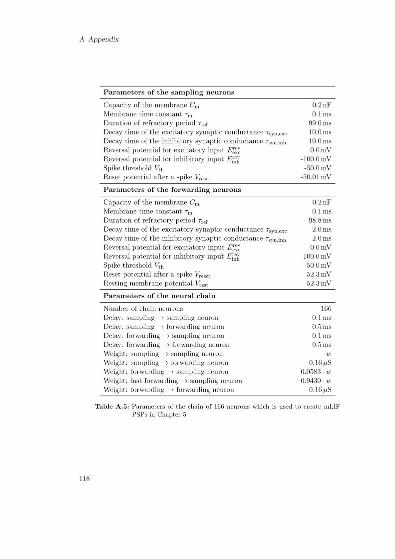
A Appendix
Parameters of the sampling neurons
Capacity of the membrane Cm 0.2 nFMembrane time constant τm 0.1msDuration of refractory period τref 99.0msDecay time of the excitatory synaptic conductance τsyn,exc 10.0msDecay time of the inhibitory synaptic conductance τsyn,inh 10.0msReversal potential for excitatory input Erev
exc 0.0mVReversal potential for inhibitory input Erev
inh -100.0mVSpike threshold Vth -50.0mVReset potential after a spike Vreset -50.01mV
Parameters of the forwarding neurons
Capacity of the membrane Cm 0.2 nFMembrane time constant τm 0.1msDuration of refractory period τref 98.8msDecay time of the excitatory synaptic conductance τsyn,exc 2.0msDecay time of the inhibitory synaptic conductance τsyn,inh 2.0msReversal potential for excitatory input Erev
exc 0.0mVReversal potential for inhibitory input Erev
inh -100.0mVSpike threshold Vth -50.0mVReset potential after a spike Vreset -52.3mVResting membrane potential Vrest -52.3mV
Parameters of the neural chain
Number of chain neurons 166Delay: sampling → sampling neuron 0.1msDelay: sampling → forwarding neuron 0.5msDelay: forwarding → sampling neuron 0.1msDelay: forwarding → forwarding neuron 0.5msWeight: sampling → sampling neuron wWeight: sampling → forwarding neuron 0.16µSWeight: forwarding → sampling neuron 0.0583 · wWeight: last forwarding → sampling neuron −0.9430 · wWeight: forwarding → forwarding neuron 0.16µS
Table A.5: Parameters of the chain of 166 neurons which is used to create mLIFPSPs in Chapter 5
118

A.2 Neuron Parameters
Floating gate parameters of the membrane circuits
Parameter Value [DAC] Parameter Value [DAC]
I_breset 1023 V_reset (global) 590I_bstim 1023 E_l 512V_bout 1023 E_syni 398V_bexp 1023 E_synx 626V_br 0 I_bexp 0V_bstdf 0 I_convi 1023V_ccas 800 I_convx 1023V_clrc 0 I_fire 0V_clra 0 I_gl 1023V_dep 0 I_gladapt 0V_fac 0 I_intbbi 1023V_dllres 200 I_intbbx 1023V_dtc 0 I_pl 30V_gmax0 1000 I_radapt 1023V_gmax1 1000 I_rexp 1023V_gmax2 1000 I_spikeamp 1023V_gmax3 1000 V_exp 1023V_m 0 V_syni 1023int_op_bias 1023 V_syntci 800V_stdf 0 V_syntcx 800V_thigh 0 V_synx 1023V_tlow 0 V_t 600
Parameters of the synapse circuits
Parameter Value Parameter Value
g_max 0 g_max_div 5Exc. synaptic weight 5 Inh. synaptic weight 5
Additional settings
Parameter Value Parameter Value
fg_speed_up_scaling NORMAL use_big_capacitors False
Table A.6: Floating gate parameters of the membrane and synapse circuits on theHICANN chip which have been used in Chapter 6. The membraneparameters on the left hand side are global, the membrane parameterson the right hand side are individual neuron parameters except for theglobal parameter Vreset.
119

A Appendix
A.3 Acronyms
ADC Analog-to-Digital-Converter
AdEx Adaptive Exponential Integrate-and-Fire
ANC Analog Network Core
AP Action Potential
API Application Programming Interface
ARQ Automatic Repeat reQuest
ASIC Application Specific Integrated Circuit
BEG Background Event Generator
BM Boltzmann Machine
BN Bayesian Network
BRN Balanced Random Network
BT Biological Time
CMOS Complementary Metal Oxide Semiconductor
DAC Digital Analog Converter
DenMem Dendrite membrane
DNC Digital Network Chip
EPSP Excitatory Postsynaptic Potential
FACETS Fast Analog Computing with Emergent Transient States
FPGA Field Programmable Gate Array
FPT First-Passage Time
HAL Hardware Abstraction Layer
HCS High-Conductance-State
HICANN High Input Count Analog Neural Network
HMF Hybrid Multiscale Facility
HT Hardware Time
IPSP Inhibitory Postsynaptic Potential
120

A.3 Acronyms
ISI Inter-Spike Interval
KL Kullback-Leibler
L1 Layer 1
L2 Layer 2
LFSR Linear Feedback Shift Register
LIF Leaky Integrate-and-Fire
LVDS Low Voltage Differential Signaling
MCMC Markov chain Monte Carlo
mLIF "Multiple" Leaky Integrate-and-Fire
NCC Neural computability condition
ODE Ordinary Differential Equation
OU Ornstein-Uhlenbeck
PCB Printed Circuit Board
PDF Probability Density Function
PSP Postsynaptic Potential
RV Random Variable
SEB System Emulator Board
SRAM Static Random-Access Memory
STA Spike-Triggered Average
STDP Spike-Timing Dependent Plasticity
STP Short-Term Plasticity
TM Tsodyks-Markram
TNN Two-Node-Network
UMC United Microelectronics Corporation
VLSI Very-Large-Scale Integration
VPE Visual Perception Experiment
WTA Winner-Take-All
121

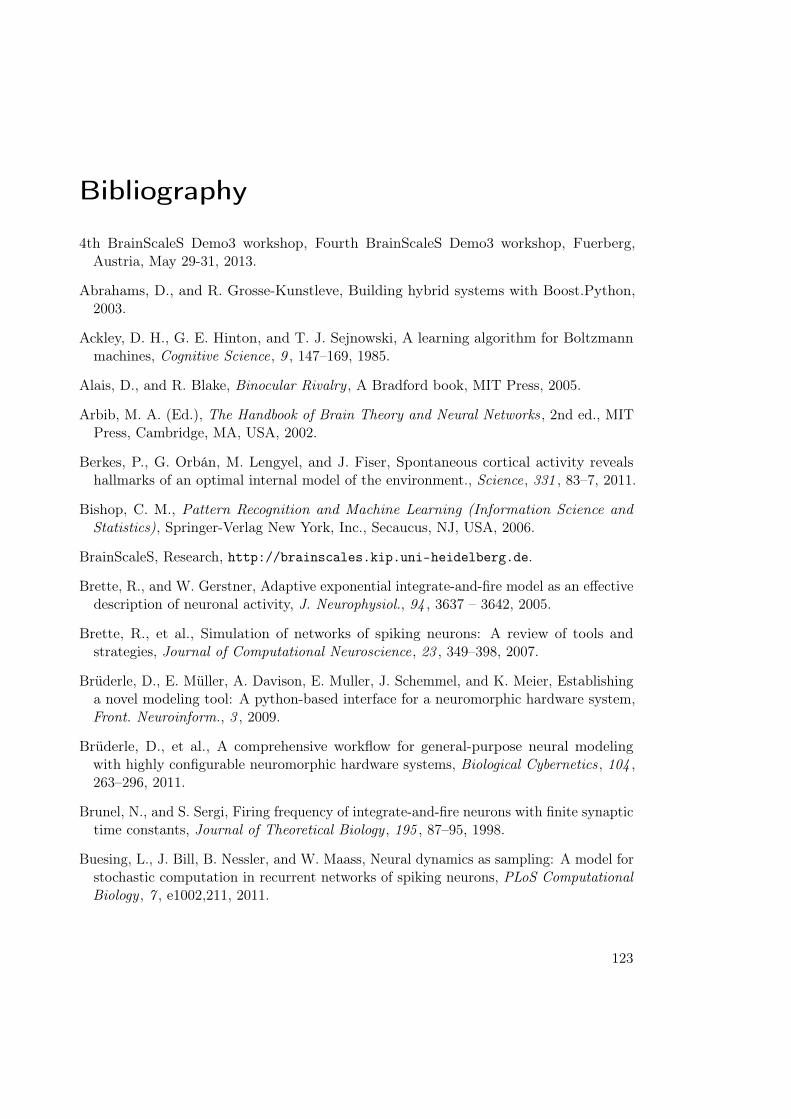
Bibliography
4th BrainScaleS Demo3 workshop, Fourth BrainScaleS Demo3 workshop, Fuerberg,Austria, May 29-31, 2013.
Abrahams, D., and R. Grosse-Kunstleve, Building hybrid systems with Boost.Python,2003.
Ackley, D. H., G. E. Hinton, and T. J. Sejnowski, A learning algorithm for Boltzmannmachines, Cognitive Science, 9 , 147–169, 1985.
Alais, D., and R. Blake, Binocular Rivalry , A Bradford book, MIT Press, 2005.
Arbib, M. A. (Ed.), The Handbook of Brain Theory and Neural Networks , 2nd ed., MITPress, Cambridge, MA, USA, 2002.
Berkes, P., G. Orbán, M. Lengyel, and J. Fiser, Spontaneous cortical activity revealshallmarks of an optimal internal model of the environment., Science, 331 , 83–7, 2011.
Bishop, C. M., Pattern Recognition and Machine Learning (Information Science andStatistics), Springer-Verlag New York, Inc., Secaucus, NJ, USA, 2006.
BrainScaleS, Research, http://brainscales.kip.uni-heidelberg.de.
Brette, R., and W. Gerstner, Adaptive exponential integrate-and-fire model as an effectivedescription of neuronal activity, J. Neurophysiol., 94 , 3637 – 3642, 2005.
Brette, R., et al., Simulation of networks of spiking neurons: A review of tools andstrategies, Journal of Computational Neuroscience, 23 , 349–398, 2007.
Brüderle, D., E. Müller, A. Davison, E. Muller, J. Schemmel, and K. Meier, Establishinga novel modeling tool: A python-based interface for a neuromorphic hardware system,Front. Neuroinform., 3 , 2009.
Brüderle, D., et al., A comprehensive workflow for general-purpose neural modelingwith highly configurable neuromorphic hardware systems, Biological Cybernetics, 104 ,263–296, 2011.
Brunel, N., and S. Sergi, Firing frequency of integrate-and-fire neurons with finite synaptictime constants, Journal of Theoretical Biology , 195 , 87–95, 1998.
Buesing, L., J. Bill, B. Nessler, and W. Maass, Neural dynamics as sampling: A model forstochastic computation in recurrent networks of spiking neurons, PLoS ComputationalBiology , 7 , e1002,211, 2011.
123
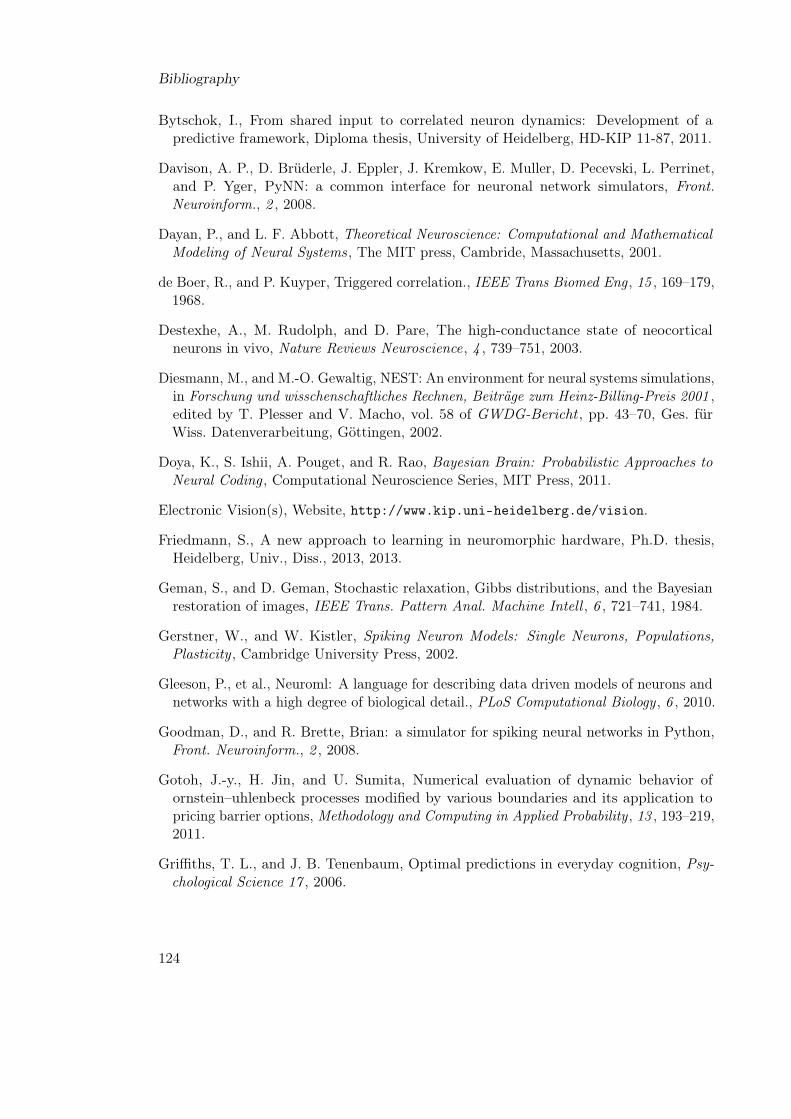
Bibliography
Bytschok, I., From shared input to correlated neuron dynamics: Development of apredictive framework, Diploma thesis, University of Heidelberg, HD-KIP 11-87, 2011.
Davison, A. P., D. Brüderle, J. Eppler, J. Kremkow, E. Muller, D. Pecevski, L. Perrinet,and P. Yger, PyNN: a common interface for neuronal network simulators, Front.Neuroinform., 2 , 2008.
Dayan, P., and L. F. Abbott, Theoretical Neuroscience: Computational and MathematicalModeling of Neural Systems, The MIT press, Cambride, Massachusetts, 2001.
de Boer, R., and P. Kuyper, Triggered correlation., IEEE Trans Biomed Eng , 15 , 169–179,1968.
Destexhe, A., M. Rudolph, and D. Pare, The high-conductance state of neocorticalneurons in vivo, Nature Reviews Neuroscience, 4 , 739–751, 2003.
Diesmann, M., and M.-O. Gewaltig, NEST: An environment for neural systems simulations,in Forschung und wisschenschaftliches Rechnen, Beiträge zum Heinz-Billing-Preis 2001 ,edited by T. Plesser and V. Macho, vol. 58 of GWDG-Bericht , pp. 43–70, Ges. fürWiss. Datenverarbeitung, Göttingen, 2002.
Doya, K., S. Ishii, A. Pouget, and R. Rao, Bayesian Brain: Probabilistic Approaches toNeural Coding , Computational Neuroscience Series, MIT Press, 2011.
Electronic Vision(s), Website, http://www.kip.uni-heidelberg.de/vision.
Friedmann, S., A new approach to learning in neuromorphic hardware, Ph.D. thesis,Heidelberg, Univ., Diss., 2013, 2013.
Geman, S., and D. Geman, Stochastic relaxation, Gibbs distributions, and the Bayesianrestoration of images, IEEE Trans. Pattern Anal. Machine Intell , 6 , 721–741, 1984.
Gerstner, W., and W. Kistler, Spiking Neuron Models: Single Neurons, Populations,Plasticity , Cambridge University Press, 2002.
Gleeson, P., et al., Neuroml: A language for describing data driven models of neurons andnetworks with a high degree of biological detail., PLoS Computational Biology , 6 , 2010.
Goodman, D., and R. Brette, Brian: a simulator for spiking neural networks in Python,Front. Neuroinform., 2 , 2008.
Gotoh, J.-y., H. Jin, and U. Sumita, Numerical evaluation of dynamic behavior ofornstein–uhlenbeck processes modified by various boundaries and its application topricing barrier options, Methodology and Computing in Applied Probability , 13 , 193–219,2011.
Griffiths, T. L., and J. B. Tenenbaum, Optimal predictions in everyday cognition, Psy-chological Science 17 , 2006.
124
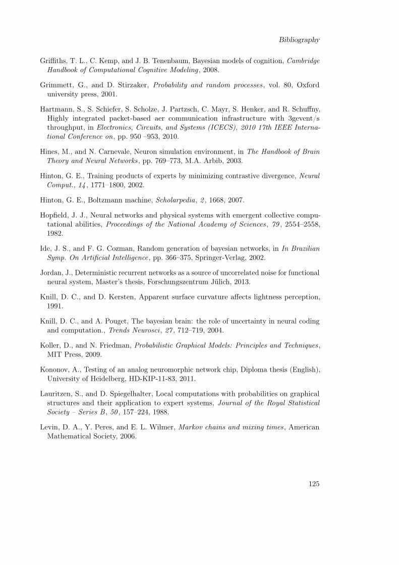
Bibliography
Griffiths, T. L., C. Kemp, and J. B. Tenenbaum, Bayesian models of cognition, CambridgeHandbook of Computational Cognitive Modeling , 2008.
Grimmett, G., and D. Stirzaker, Probability and random processes, vol. 80, Oxforduniversity press, 2001.
Hartmann, S., S. Schiefer, S. Scholze, J. Partzsch, C. Mayr, S. Henker, and R. Schuffny,Highly integrated packet-based aer communication infrastructure with 3gevent/sthroughput, in Electronics, Circuits, and Systems (ICECS), 2010 17th IEEE Interna-tional Conference on, pp. 950 –953, 2010.
Hines, M., and N. Carnevale, Neuron simulation environment, in The Handbook of BrainTheory and Neural Networks, pp. 769–773, M.A. Arbib, 2003.
Hinton, G. E., Training products of experts by minimizing contrastive divergence, NeuralComput., 14 , 1771–1800, 2002.
Hinton, G. E., Boltzmann machine, Scholarpedia, 2 , 1668, 2007.
Hopfield, J. J., Neural networks and physical systems with emergent collective compu-tational abilities, Proceedings of the National Academy of Sciences, 79 , 2554–2558,1982.
Ide, J. S., and F. G. Cozman, Random generation of bayesian networks, in In BrazilianSymp. On Artificial Intelligence, pp. 366–375, Springer-Verlag, 2002.
Jordan, J., Deterministic recurrent networks as a source of uncorrelated noise for functionalneural system, Master’s thesis, Forschungszentrum Jülich, 2013.
Knill, D. C., and D. Kersten, Apparent surface curvature affects lightness perception,1991.
Knill, D. C., and A. Pouget, The bayesian brain: the role of uncertainty in neural codingand computation., Trends Neurosci , 27 , 712–719, 2004.
Koller, D., and N. Friedman, Probabilistic Graphical Models: Principles and Techniques,MIT Press, 2009.
Kononov, A., Testing of an analog neuromorphic network chip, Diploma thesis (English),University of Heidelberg, HD-KIP-11-83, 2011.
Lauritzen, S., and D. Spiegelhalter, Local computations with probabilities on graphicalstructures and their application to expert systems, Journal of the Royal StatisticalSociety – Series B , 50 , 157–224, 1988.
Levin, D. A., Y. Peres, and E. L. Wilmer, Markov chains and mixing times, AmericanMathematical Society, 2006.
125

Bibliography
Markram, H., Y. Wang, and M. Tsodyks, Differential signaling via the same axon ofneocortical pyramidal neurons., Proceedings of the National Academy of Sciences of theUnited States of America, 95 , 5323–5328, 1998.
Mead, C. A., Analog VLSI and Neural Systems, Addison Wesley, Reading, MA, 1989.
Mead, C. A., and M. A. Mahowald, A silicon model of early visual processing, NeuralNetworks, 1 , 91–97, 1988.
Millner, S., Development of a multi-compartment neuron model emulation, 2012.
Nessler, B., M. Pfeiffer, L. Buesing, and W. Maass, Bayesian computation emergesin generic cortical microcircuits through spike-timing-dependent plasticity, PLOSComputational Biology , 9 , e1003,037, 2013.
Oaksford, M., and N. Chater, Bayesian Rationality: The Probabilistic Approach to HumanReasoning , Oxford Cognitive Science Series, OUP Oxford, 2007.
Pearl, J., Bayesian networks: A model of self-activated memory for evidential reasoning,in Proceedings of the 7th Conference of the Cognitive Science Society, University ofCalifornia, Irvine, pp. 329–334, 1985.
Pearl, J., Probabilistic reasoning in intelligent systems: networks of plausible inference,Morgan Kaufmann Publishers Inc., San Francisco, CA, USA, 1988.
Pecevski, D., L. Buesing, and W. Maass, Probabilistic inference in general graphicalmodels through sampling in stochastic networks of spiking neurons, PLoS ComputationalBiology , 7 , 2011.
Pecevski, D. A., T. Natschläger, and K. N. Schuch, Pcsim: A parallel simulation en-vironment for neural circuits fully integrated with Python, Front. Neuroinform., 3 ,2009.
Peterson, L. L., and B. S. Davie, Computer Networks: A Systems Approach, 3rd Edition,Morgan Kaufmann Publishers Inc., San Francisco, CA, USA, 2003.
Petkov, V., Toward belief propagation on neuromorphic hardware, Diploma thesis (En-glish), Ruprecht-Karls-Universität Heidelberg, HD-KIP 12-23, 2012.
Petrovici, M. A., J. Bill, I. Bytschok, J. Schemmel, and K. Meier, Stochastic inferencewith deterministic spiking neurons., CoRR, abs/1311.3211 , 2013.
PyNN, A Python package for simulator-independent specification of neuronal networkmodels – website, http://www.neuralensemble.org/PyNN, 2014.
Python, The Python Programming Language – website, http://www.python.org, 2014.
Ricciardi, L., Diffusion processes and related topics in biology , Lecture notes in biomathe-matics, Springer-Verlag, 1977.
126
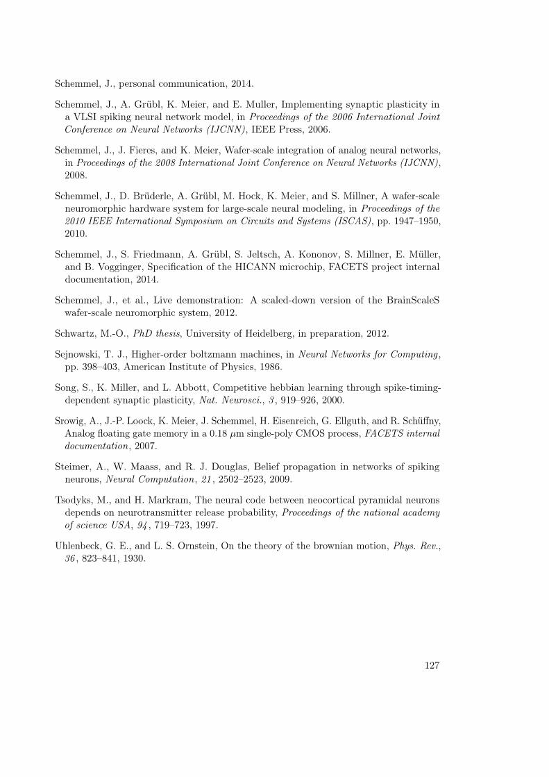
Schemmel, J., personal communication, 2014.
Schemmel, J., A. Grübl, K. Meier, and E. Muller, Implementing synaptic plasticity ina VLSI spiking neural network model, in Proceedings of the 2006 International JointConference on Neural Networks (IJCNN), IEEE Press, 2006.
Schemmel, J., J. Fieres, and K. Meier, Wafer-scale integration of analog neural networks,in Proceedings of the 2008 International Joint Conference on Neural Networks (IJCNN),2008.
Schemmel, J., D. Brüderle, A. Grübl, M. Hock, K. Meier, and S. Millner, A wafer-scaleneuromorphic hardware system for large-scale neural modeling, in Proceedings of the2010 IEEE International Symposium on Circuits and Systems (ISCAS), pp. 1947–1950,2010.
Schemmel, J., S. Friedmann, A. Grübl, S. Jeltsch, A. Kononov, S. Millner, E. Müller,and B. Vogginger, Specification of the HICANN microchip, FACETS project internaldocumentation, 2014.
Schemmel, J., et al., Live demonstration: A scaled-down version of the BrainScaleSwafer-scale neuromorphic system, 2012.
Schwartz, M.-O., PhD thesis, University of Heidelberg, in preparation, 2012.
Sejnowski, T. J., Higher-order boltzmann machines, in Neural Networks for Computing ,pp. 398–403, American Institute of Physics, 1986.
Song, S., K. Miller, and L. Abbott, Competitive hebbian learning through spike-timing-dependent synaptic plasticity, Nat. Neurosci., 3 , 919–926, 2000.
Srowig, A., J.-P. Loock, K. Meier, J. Schemmel, H. Eisenreich, G. Ellguth, and R. Schüffny,Analog floating gate memory in a 0.18 µm single-poly CMOS process, FACETS internaldocumentation, 2007.
Steimer, A., W. Maass, and R. J. Douglas, Belief propagation in networks of spikingneurons, Neural Computation, 21 , 2502–2523, 2009.
Tsodyks, M., and H. Markram, The neural code between neocortical pyramidal neuronsdepends on neurotransmitter release probability, Proceedings of the national academyof science USA, 94 , 719–723, 1997.
Uhlenbeck, G. E., and L. S. Ornstein, On the theory of the brownian motion, Phys. Rev.,36 , 823–841, 1930.
127


Acknowledgments (Danksagungen)
Allen voran Mihai und Ilja für die osum Betreuung.
Herrn Meier und Johannes für die dritte Aufnahme bei den Visions.
Allen Visionären für die freundliche Atmosphäre.
Meiner one and only Motivationskünstlerin Nina.
Mama.
Ferdi und Waldi.
Irina, Wowa, Leon, Oma und Alex.
Adriana, Degga und Lara sowie die Eingesaarländerten Andi, André, Fabe, Hans, Julian,Paul und Raphi für die (rückblickend doch so) schöne Studienzeit.
Den Gräther Kickers, the gräthest team of all time: 1 - Bieri, 1 - Nilles, 5 - Pueppi, 7 -Gill, 8 - Dany Gee, 9 - Marv, 10 - Pippo, 11 - Jens, 13 - Kosta, 14 - Lukki, 17 - Konzka, ?- Motschi.
Paulé.
Janine.
Der Fußballgruppe des IWR.
129


Statement of Originality (Erklärung):
I certify that this thesis, and the research to which it refers, are the product of my ownwork. Any ideas or quotations from the work of other people, published or otherwise, arefully acknowledged in accordance with the standard referencing practices of the discipline.
Ich versichere, daß ich diese Arbeit selbständig verfaßt und keine anderen als die angege-benen Quellen und Hilfsmittel benutzt habe.
Heidelberg, March 28, 2014.......................................
(signature)
Copyright © 2022 FDOKUMEN