Digital video processing Tekalp
275
Digital Video Processing
-
Upload
jntukakinada -
Category
Documents
-
view
0 -
download
0
Transcript of Digital video processing Tekalp

Digital Video Processing
PRENTICE HALL SIGNAL PROCESSING SERIES
Alan V Oppenheim, Series Editor
ANDREWS & HUNT Digital Image RestorationBRACEWELL Two Dimensional ImagingBRIGHAM The Fast Fourier Transform and Its ApplicationsBURDIC Underwater Acoustic System Analysis 2/ECASTLEMAN Digital Image ProcessingCROCHIERE & RABINER Multirate Digital Signal ProcessingDUDGEON & MERSEREAU Multidimensional Digital Signal ProcessingHAYKIN Advances in Spectrum Analysis and Array Processing. Vols. I, II & IIIHAYKIN, ED. Array Signal ProcessingJOHNSON & DUDGEON Array Signal ProcessingK A Y Fundamentals of Statistical Signal ProcessingKAY Modern Spectral EstimationKIN0 Acoustic Waves: Devices, Imaging, and Analog Signal ProcessingLIM Two-Dimensional Signal and Image ProcessingLIM, ED. Speech EnhancementLIM & OPPENHEIM, EDS. Advanced Topics in Signal ProcessingMARPLE Digital Spectral Analysis with ApplicationsMCCLELLAN & RADER Number Theory in Digital Signal ProcessingMENDEL Lessons in Estimation Theory for Signal Processing Communications
and Control 2/ENIKIAS Higher Order Spectra AnalysisOPPENHEIM & NAWAB Symbolic and Knowledge-Based Signal ProcessingOPPENHEIM, WILLSKY, WITH YOUNG Signals and SystemsOPPENHEIM & SCHAFER Digital Signal ProcessingOPPENHEIM & SCHAFER Discrete-Time Signal ProcessingPHILLIPS & NAGLE Digital Control Systems Analysis and Design, 3/EPICINBONO Random Signals and SystemsRABINER & GOLD Theory and Applications of Digital Signal ProcessingRABINER & SCHAFER Digital Processing of Speech SignalsRABINER & JUANG Fundamentals of Speech RecognitionROBINSON & TREITEL Geophysical Signal AnalysisSTEARNS & DAVID Signal Processing Algorithms in Fortran and CTEKALP Digital Video ProcessingTHERRIEN Discrete Random Signals and Statistical Signal ProcessingTRIBOLET Seismic Applications of Homomorphic Signal ProcessingVIADVANATHAN Multirate Systems and Filter BanksWIDROW & STEARNS Adaptive Signal Processing \
Digital Video Processing
A. Murat TekalpUniversity of Rochester
For book and bookstore inforr?IatiOn
i
I http://www.prenhall.com I
=-==Prentice Hall PTR
Upper Saddle River, NJ 07458

t
Tekalp, A. Murat.Digital video processing / A. Murat Tekalp.
P. cm. -- (Prentice-Hall signal processing series)ISBN O-13-190075-7 (alk. paper)1. Digital video. I. Title. II. Series.
TK6680.5.T45 1995621.388'33--d&O 95-16650
CIP
Editorial/production supervision: Ann SullivanCover design: Design SourceManufacturing manager: Alexis R. HeydtAcquisitions editor: Karen GettmanEditorial assistant: Barbara Alfieri
@ Printed on Recycled Paper
01995 by Prentice Hall PTRPrentice-Hall, Inc.A Simon and Schuster CompanyUpper Saddle River, NJ 07458
The publisher offers discounts on this book when ordered in bulk quantities.
For more information, contact:
Corporate Sales DepartmentPrentice Hall PTROne Lake StreetUpper Saddle River, NJ 07458
Phone: 800-382-3419Fax: 201-236-7141
email: [email protected]
All rights reserved. No part of this book may be reproduced, in any form or by any means,without permission in writing from the publisher.
Printed in the United States of America
1 0 9 8 7 6 5 4 3 2 1
ISBN: O-13-190075-7
Prentice-Hall International (UK) Limited, LondonPrentice-Hall of Australia Pty. Limited, SydneyPrentice-Hall Canada Inc., TorontoPrentice-Hall Hispanoamericana, S.A., MexicoPrentice-Hall of India Private Limited, New DelhiPrentice-Hall of Japan, Inc., TokyoSimon & Schuster Asia Pte. Ltd., SingaporeEditora Prentice-Hall do Brasil, Ltda., Rio de Janeiro
To Seviy and Kaya Tekalp, my mom and dadand to Ozge, my beloved wife

Contents
Preface . . . . . . . . . . . . . . . . . . . . . . . . . . . . . . . . . . . . . xviiAbout the Author. . . . . . . . . . . . . . . . . . . . . . . . . . . . . . xixAbout the Notation . . . . . . . . . . . . . . . . . . . . . . . . . . . . . xxi
I REPRESENTATION OF DIGITAL VIDEO
1 BASICS OF VIDEO1.1 Analog Video . . . .
1.1.1 Analog Video Signal .1.1.2 Analog Video Standards1.1.3 Analog Video Equipment
1 . 2 D i g i t a l V i d e o .1.2.1 Digital Video Signal1.2.2 Digital Video Standards .1.2.3 Why Digital Video?
1.3 Digital Video Processing . .
2 TIME-VARYING IMAGE FORMATION MODELS
.
2.1
2.2
2.3
2.42.5
Three-Dimensional Motion Models . . . . . . . . . .2.1.1 Rigid Motion in the Cartesian Coordinates . . . .2.1.2 Rigid Motion in the Homogeneous Coordinates . .2.1.3 Deformable Motion . . . . . . . . . . . . . . . . . .Geometric Image Formation . . . . . . . . . . . . . .2.2.1 Perspective Projection . . . . . . . . . . . . . . . .2.2.2 Orthographic Projection . . . . . . . . . . . . . . .Photometric Image Formation . . . . . . . . . . . . .2.3.1 Lambertian Reflectance Model . . . . . . . . . . .2.3.2 Photometric Effects of 3-D Motion . . . . . . . . .Observation Noise . . . . . . . . . . . . . . . . . . . . .Exercises . . . . . . . . . . . . . . . . . . . . . . . . . . .
1. 1
24899
1114
. 16
19. . 20. 20. 26. 27
28. 28. 30. 32. . 32. . 33. 33. . 34
vii

CONTENTS CONTENTS ix
3 SPATIO-TEMPORAL SAMPLING 36
3.1 Sampling for Analog and Digital Video . . . . . . . . . . . . . 373.1.1 Sampling Structures for Analog Video . . . . . . . . . . . . . 37
3.1.2 Sampling Structures for Digital Video . . . . . . . . . . . . . 383.2 Two-Dimensional Rectangular Sampling . . . . . . . . . . . . . 40
3.2.1 2-D Fourier Transform Relations . . . . . . . . . . . . . . . . 413.2.2 Spectrum of the Sampled Signal . . . . . . . . . . . . . . . . 42
3.3 Two-Dimensional Periodic Sampling . . . . . . . . . . . . . . . 43
3.3.1 Sampling Geometry . . . . . . . . . . . . . . . . . . . . . . . 443.3.2 2-D Fourier Transform Relations in Vector Form . . . . . . . 44
3.3.3 Spectrum of the Sampled Signal . . . . . . . . . . . . . . . . 46
3.4 Sampling on 3-D Structures . . . . . . . . . . . . . . . . . . . . 46
3.4.1 Sampling on a Lattice . . . . . . . . . . . . . . . . . . . . . . 47
3.4.2 Fourier Transform on a Lattice . . . . . . . . . . . . . . . . . 47
3.4.3 Spectrum of Signals Sampled on a Lattice 493.4.4 Other Sampling Structures . . . . . . . . . . . . . . . . . . . 51
3.5 Reconstruction from Samples. . . . . . . . . . . . . . . . . . . . 53
3.5.1 Reconstruction from Rectangular Samples . . . . . . . . . . . 53
3.5.2 Reconstruction from Samples on a Lattice . . . . . . . . . . . 55
3.6 Exercises . . . . . . . . . . . . . . . . . . . . . . . . . . . . . . . . . 56
4 SAMPLING STRUCTURE CONVERSION 57
4.1
4.24.3
Sampling Rate Change for 1-D Signals. . . . . . . . . . . . . . 58
4.1.1 Interpolation of 1-D Signals . . . . . . . . . . . . . . . . . . . 584.1.2 Decimation of 1-D Signals4.1.3 Sampling Rate Change bySampling Lattice ConversionExercises . . . . :
.................... 62a Rational Factor . . . . . . . . . 64. . . . . . . . . . . . . . . . . . . . 66. . . . . . . . . . . . . . . . . . . . 70
II TWO-DIMENSIONAL MOTION ESTIMATION
5 OPTICAL FLOW METHODS 725 .1 2 -D Motion vs . Apparent Motion . . 72
5.1.1 2-D Motion . . . . . 735 .1 .2 Cor re spondence and Op t i ca l F low 74
5.2 2-D Motion Estimation. . . . . 765.2.1 The Occlusion Problem . . . . . 785.2.2 The Aperture Problem . . . . . . 785.2.3 Two-Dimensional Motion Field Models . 79
5.3 Methods Using the Optical Flow Equation . 815.3.1 The Optical Flow Equation . . . 815.3.2 Second-Order Differential Methods . . 825.3.3 Block Motion Model . . . . 83
5.3.4 Horn and Schunck Method . . . . . . . . . . . . . . . . . . . 845.3.5 Estimation of the Gradients . . . . . . . . . . . . . . . . . .' . 855.36 Adaptive Methods . . . . . . . . . . . . . . . . . . . . . . . . 86
5.4 Examples . . . . . . . . . . . . . . . . . . . . . . . . . . . . . . . . 88
5.5 Exercises . . . . . . . . . . . . . . . . . . . . . . . . . . . . . . . . . 93
6 BLOCK-BASED METHODS 95
6.1
6.2
6.3
6.46.5
6.66.7
Block-Motion Models . . . . 956.1.1 Translational Block Motion . . 966 . 1 . 2 G e n e r a l i z e d / D e f o r m a b l e B l o c k M o t i o n . 97P h a s e - C o r r e l a t i o n M e t h o d 996.2.1 The Phase-Correlation Function 996 . 2 . 2 I m p l e m e n t a t i o n I s s u e s 100B l o c k - M a t c h i n g M e t h o d . 1016 . 3 . 1 M a t c h i n g C r i t e r i a 1026.3.2 Search Procedures . 104H i e r a r c h i c a l M o t i o n E s t i m a t i o n . 106G e n e r a l i z e d B l o c k - M o t i o n E s t i m a t i o n . 1096.5.1 Postprocessing for Improved Motion Compensation . 1096.5.2 Deformable Block Matching . . . 109Examples . . 112Exercises . . . . . 115
7 PEL-RECURSIVE METHODS 117
7.17.2
7.3
7.47.57.6
D i s p l a c e d F r a m e D i f f e r e n c eGradient -Based Optimizat ion . . .7 . 2 . 1 S t e e p e s t - D e s c e n t M e t h o d .7 . 2 . 2 N e w t o n - R a p h s o n M e t h o d . .7.2.3 Local vs. Global Minima . .Steepest-Descent-Based Algorithms.7.3.1 Netravali-Robbins Algori thm . .7.3.2 Walker-Rao Algorithm . .7.3.3 Extension to the Block Motion ModelWiener-Estimation-Based AlgorithmsExamples . . . . . . .Exercises . . . . . .
.
.
.
.
.
118119120120121121122123124125127129
8 BAYESIAN METHODS 130
8.1 Optimization Methods . . . . . . . . . . . . . . . . . . . . . . . . 130
8.1.1 Simulated Annealing . . . . . . . . . . . . . . . . . . . . . . . 1318.1.2 Iterated Conditional Modes . . . . . . . . . . . . . . . . . . . 1348.1.3 Mean Field Annealing . . . . . . . . . . . . . . . . . . . . . . 1358.1.4 Highest Confidence First . . . . . . . . . . . . . . . . . . . . . 135

X CONTENTS
8.2 Basics of MAP Motion Estimation . . . 1368.2.1 The Likelihood Model . . . . . . 1378.2.2 The Prior Model . . . . . 137
8.3 MAP Motion Estimation Algorithms 13983.1 Formulation with Discontinuity Models 1398.3.2 Estimation with Local Outlier Rejection . 1468.3.3 Estimation with Region Labeling . 147
8.4 Examples . . . . . . . . . . . 1488.5 Exercises . . . . . 150
III THREE-DIMENSIONAL MOTION ESTIMATIONAND SEGMENTATION
9 METHODS USING POINT CORRESPONDENCES 1529.1 Modeling the Projected Displacement Field . . . . . . . . . . 153
9.1.1 Orthographic Displacement Field Model . . . . . . . . . . . . 1539.1.2 Perspective Displacement Field Model . . . . . . . . . . . . . 154
9.2 Methods Based on the Orthographic Model . . . . . . . . . . 1559.2.1 Two-Step Iteration Method from Two Views . . . . . . . . . 1559.2.2 An Improved Iterative Method . . . . . . . . . . . . . . . . . 157
9.3 Methods Based on the Perspective Model . . . . . . . . . . . 1589.3.1 The Epipolar Constraint and Essential Parameters . . . . . . 1589.3.2 Estimation of the Essential Parameters . . . . . . . . . . . . 1599.3.3 Decomposition of the E-Matrix . . . . . . . . . . . . . . . . . 1619.3.4 Algorithm . . . . . . . . . . . . . . . . . . . . . . . . . . . . . 164
9.4 The Case of 3-D Planar Surfaces . . . . . . . . . . . . . . . . . 1659.4.1 The Pure Parameters . . . . . . . . . . . . . . . . . . . . . . 1659.4.2 Estimation of the Pure Parameters . . . . . . . . . . . . . . . 1669.4.3 Estimation of the Motion and Structure Parameters . . . . . 166
9.5 Examples . . . . . . . . . . . . . . . . . . . . . . . . . . . . . . . . 1689.5.1 Numerical Simulations . . . . . . . . . . . . . . . . . . . . . . 1689.5.2 Experiments with Two Frames of Miss America . . . . . . . . 173
9.6 Exercises . . . . . . . . . . . . . . . . . . . . . . . . . . . . . . . . . 175
10 OPTICAL FLOW AND DIRECT METHODS 17710.1 Modeling the Projected Velocity Field . . . . . . . . . . . . . . 177
10.1.1 Orthographic Velocity Field Model . . . . . . . . . . . . . . . 17810.1.2 Perspective Velocity Field Model . . . . . . . . . . . . . . . . 17810.1.3 Perspective Velocity vs. Displacement Models . . . . . . . . . 179
10.2 Focus of Expansion . . . . . . . . . . . . . . . . . . . . . . . . . . 18010.3 Algebraic Methods Using Optical Flow . . . . . . . . . . . . . 181
10.3.1 Uniqueness of the Solution . . . . . . . . . . . . . . . . . . . 18210.3.2 AffineFlow . . . . . . . . . . . . . . . . . . . . . . . . . . . . 182
CONTENTS xi
10.4
10.5
10.6
10.7
10.3.3 Quadratic Flow . . . . . . . . 18310.3.4 Arbitrary Flow . . . . . . . . . . . . . . 184
Optimization Methods Using Optical Flow . . . 186
Direct Methods . . . . . . . . . . . . . 187
10.5.1 Extension of Optical Flow-Based Methods . . . 18710.5.2 Tsai-Huang Method . . . . . . . 188
Examples . . . . . . . . . . . . . . . 190
10.6.1 Numerical Simulations . . . . . . . 191
10.6.2 Experiments with Two Frames of Miss America 194Exercises . . . . . . . . . . . . 196
11 MOTION SEGMENTATION 198
11.1 Direct Methods . . . . . . . . . . . . . 200
11.2
11.3
11.411.5
11.1.1 Thresholding for Change Detection . . . . . . . ....... 200
11.1.2 An Algorithm Using Mapping Parameters . . . . . . . . . . 20111.1.3 Estimation of Model Parameters . . . . . . . . . . . . . . . 203
Optical Flow Segmentation . . . . . . . . . . . . . . . . . . . . 204
11.2.1 Modified Hough Transform Method . . . . . . . . . . . . . 205
11.2.2 Segmentation for Layered Video Representation . . . . . . . 20611.2.3 Bayesian Segmentation . . . . . . . . . . . . . . . . . . . . . 207
Simultaneous Estimation and Segmentation . . . . . . . . 209
11.3.1 Motion Field Model . . . . . . . . . . . . . . . . . . . . . . 210
11.3.2 Problem Formulation . . . . . . . . . . . . . . . . . . . . . 21011.3.3 The Algorithm . . . . . . . . . . . . . . . . . . . . . . . . . 212
11.3.4 Relationship to Other Algorithms . . . . . . . . . . . . . . 213
Examples . . . . . . . . . . . . . . . . . . . . . . . . . . . . . . . 214
Exercises . . . . . . . . . . . . . . . . . . . . . . . . . . . . . . . . 217
12 STEREO AND MOTION TRACKING 219
12.1 Motion and Structure from Stereo . . . . . . . . . . . . . . . . 21912.1.1 Still-Frame Stereo Imaging . . . . . . . . . . . . . . . . . . . 220
12.1.2 3-D Feature Matching for Motion Estimation . . . . . . . . . 222
12.1.3 Stereo-Motion Fusion . . . . . . . . . . . . . . . . . . . . . . . 22412.1.4 Extension to Multiple Motion . . . . . . . . . . . . . . . . . . 227
12.2 Motion Tracking . . . . . . . . . . . . . . . . . . . . . . . . . . . . 229
12.2.1 Basic Principles . . . . . . . . . . . . . . . . . . . . . . . . . . 229
12.2.2 2-D Motion Tracking . . . . . . . . . . . . . . . . . . . . . . . 23212.2.3 3-D Rigid Motion Tracking . . . . . . . . . . . . . . . . . . . 235
12.3 Examples . . . . . . . . . . . . . . . . . . . . . . . . . . . . . . . . 239
12.4 Exercises . . . . . . . . . . . . . . . . . . . . . . . . . . . . . . . . . 241

xii CONTENTS
IV VIDEO FILTERING
13 MOTION COMPENSATED FILTERING 24513.1 Spatio-Temporal Fourier Spectrum . . . . 246
13.1.1 Global Motion with Constant Velocity 24713.1.2 Global Motion with Accelerat ion . . 249
13.2 Sub-Nyquist Spatio-Temporal Sampling . 25013.2.1 Sampling in the Temporal Direction Only . 25013.2.2 Sampling on a Spatio-Temporal Lattice 25113.2.3 Critical Velocities . . . . . 252
13.3 Filtering Along Motion Trajectories . 25413 .3 .1 Arb i t r a ry Mot ion Tra j ec to r i e s . . . 25513.3.2 Global Motion with Constant Velocity . 25613.3.3 Accelerated Motion . . . 256
13.4 Applications . . . 25813.4.1 Motion-Compensated Noise Fil tering 25813.4.2 Motion-Compensated Reconstruction Filtering 258
13.5 Exercises . . . . . . . . 260
14 NOISE FILTERING14.1
14.2
14.3
14.414.5
Intraframe Filtering. . . . . . . . . . . . . . . . . .14.1.1 LMMSE Filtering . . . . . . . . . . . . . . . .1 4 . 1 . 2 A d a p t i v e ( L o c a l ) L M M S E F i l t e r i n g14.1.3 Directional Filtering . . . . . . . . . . . . . . .14.1.4 Median and Weighted Median Filtering . . . .Motion-Adaptive Filtering . . . . . . . . . . . . .14.2.1 Direct Filtering . . . . . . . . . . . . . . . . . .14.2.2 Motion-Detection Based Filtering . . . . . . . .Motion-Compensated Filtering. . . . . . . . . . .14.3.1 Spatio-Temporal Adaptive LMMSE Filtering14.3.2 Adaptive Weighted Averaging Filter . . . . . .Examples . . . . . . . . . . . . . . . . . . . . . . . .Exercises . . . . . . . . . . . . . . . . . . . . . . . . .
15 RESTORATION15.1 Modeling. . . . . . . . . . . . . . . . . . . . . . . . .
15.1.1 Shift-Invariant Spatial Blurring . . . . . . . . .15.1.2 Shift-Varying Spatial Blurring . . . . . . . . . .
15.2 Intraframe Shift-Invariant Restoration . . . . . .15.2.1 Pseudo Inverse Filtering . . . . . . . . . . . . .15.2.2 Constrained Least Squares and Wiener Filtering
15.3 Intraframe Shift-Varying Restoration . . . . . .15.3.1 Overview of the POCS Method . . . . . . . . .15.3.2 Restoration Using POCS . . . . . . . . . . . .
262263264267269270270271272272274275277277
283283284
. 285286
. 286287
. 289290291
I CONTENTS x111
t15.4 Multiframe Restoration . . . . 2 9 2
15.4.1 Cross-Correlated Multiframe Filter . . 29415.4.2 Motion-Compensated Multiframe Filter . 295
15.5 Examples . . . . . . . . . 2 9 515.6 Exercises . . . . . . . . . . . . . . 296
16 STANDARDS CONVERSION16.1 Down-Conversion . . . . . . .
16.1.1 Down-Conversion with Anti-Alias Filtering .16.1.2 Down-Conversion without Anti-Alias Filtering
16.2 Practical Up-Conversion Methods . . . .16.2.1 Intraframe Filtering . . . . . . .16.2.2 Motion-Adaptive Filtering . . . . .
16.3 Motion-Compensated Up-Conversion. .16.3.1 Basic Principles . . . .16.3.2 Global-Motion-Compensated De-interlacing
16.4 Examples . . . . . .16.5 Exercises . . . . . . . . . .
302304305305308309314317317322323329
17 SUPERRESOLUTION17.1 Modeling . . . . . .
17.1.1 Continuous-Discrete Model .17.1.2 Discrete-Discrete Model . .17.1.3 Problem Interrelations . . . .
17.2 Interpolation-Restoration Methods17.2.1 Intraframe Methods . . . . .17.2.2 Multiframe Methods . . . .
17.3 A Frequency Domain Method . .17.4 A Unifying POCS Method . . .17.5 Examples . . . . . . . . .17.6 Exercises . . . . . . . . . .
.
.
V STILL IMAGE COMPRESSION
18 LOSSLESS COMPRESSION18.1 Basics of Image Compression . . . . .
18.1.1 Elements of an Image Compression System18.1.2 Information Theoretic Concepts . .
18.2 Symbol Coding . . . . . . . . . .18.2.1 Fixed-Length Coding . . . . . . .18.2.2 Huffman Coding . . . . . . . .18.2.3 Arithmetic Coding . . . . . .
.
.
.
. .. .. ..
331332332335336336337337338341343346
348349349
. 350
. 353353354357
xiv CONTENTS
18.3 Lossless Compression Methods . . . . . . . . 36018.3.1 Lossless Predictive Coding . . . . . . . . . 36018.3.2 Run-Length Coding of Bit-Planes. . . . . 36318.3.3 Ziv-Lempel Coding . . . . . . . . . . . . . 364
18.4 Exercises . . . . . . . . . . . . . . . . . . . . . . 366
19 DPCM AND TRANSFORM CODING19.1 Quantization . . . . . . . . . . . . . . . . . . .
19.1.1 Nonuniform Quantization . . . . . . . . .19.1.2 Uniform Quantization . . . . . . . . . . .
19.2 Differential Pulse Code Modulation. . . .19.2.1 Optimal Prediction . . . . . . . . . . . . .19.2.2 Quantization of the Prediction Error . . .19.2.3 Adaptive Quantization . . . . . . . . . . .19.2.4 Delta Modulation . . . . . . . . . . . . . .
19.3 Transform Coding . . . . . . . . . . . . . . . .19.3.1 Discrete Cosine Transform . . . . . . . . .19.3.2 Quantization/Bit Allocation . . . . . . . .19.3.3 Coding . . . . . . . . . . . . . . . . . . .19.3.4 Blocking Artifacts in Transform Coding
19.4 Exercises . . . . . . . . . . . . . . . . . . . . . .
20 STILL IMAGE COMPRESSION STANDARDS20.1 Bilevel Image Compression Standards . . .
20.1.1 One-Dimensional RLC . . . . . . . . . . .20.1.2 Two-Dimensional RLC . . . . . . . . . . .20.1.3 The JBIG Standard . . . . . . . . . . . .
20.2 The JPEG Standard . . . . . . . . . . . . . .20.2.1 Baseline Algorithm . . . . . . . . . . . . .20.2.2 JPEG Progressive . . . . . . . . . . . . .20.2.3 JPEG Lossless . . . . . . . . . . . . . . .20.2.4 JPEG Hierarchical . . . . . . . . . . . . .20.2.5 Implementations of JPEG . . . . . . . . .
20.3 Exercises . . . . . . . . . . . . . . . . . . . . . .
21 VECTOR QUANTIZATION, SUBBAND CODINGAND OTHER METHODS21.1 Vector Quantization . . . . . . . . . . . . . . . . . . .
21.1.1 Structure of a Vector Quantizer . . . . . . . . . .21.1.2 VQ Codebook Design . . . . . . . . . . . . . . .21.1.3 Practical VQ Implementations . . . . . . . . . .
21.2 Fractal Compression . . . . . . . . . . . . . . . . . . .
368368369370373374375376377378380381383385385
388389389391393394395400401401402403
404404405408408409
CONTENTS XV
21.3 Subband Coding . . . . . . . . . . . . . . . . . . . 411
21.3.1 Subband Decomposition . . . . . . . . . . . . 411
21.3.2 Coding of the Subbands . . . . . . . . . . . . 414
21.3.3 Relationship to Transform Coding . . . . . . 414
21.3.4 Relationship to Wavelet Transform Coding 415
21.4 Second-Generation Coding Methods . . . . . . 415
21.5 Exercises . . . . . . . . . . . . . . . . . . . . . . . . 416
VI VIDEO COMPRESSION
22 INTERFRAME COMPRESSION METHODS 419
22.1 Three-Dimensional Waveform Coding 4202 2 . 1 . 1 3 - D T r a n s f o r m C o d i n g . 420
22.1.2 3-D Subband Coding . . . 421
22.2 Motion-Compensated Waveform Coding 424
22.2.1 MC Transform Coding . . 424
22.2.2 MC Vector Quantization . . 425
22.2.3 MC Subband Coding . . 426
22.3 Model-Based Coding . . 426
2 2 . 3 . 1 O b j e c t - B a s e d C o d i n g 427
22.3.2 Knowledge-Based and Semantic Coding 428
22.4 Exercises . 429
23 VIDEO COMPRESSION STANDARDS 432
23.1 The H.261 Standard . . . . . . . . . . . . . . . . . . . . . . . . . 432
23.1.1 Input Image Formats . . . . . . . . . . . . . . . . . . . . . . . 433
23.1.2 Video Multiplex . . . . . . . . . . . . . . . . . . . . . . . . . 434
23.1.3 Video Compression Algorithm . . . . . . . . . . . . . . . . . 435
23.2 The MPEG-1 Standard . . . . . . . . . . . . . . . . . . . . . . . 44023.2.1 Features . . . . . . . . . . . . . . . . . . . . . . . . . . . . . . 440
23.2.2 Input Video Format . . . . . . . . . . . . . . . . . . . . . . . 44123.2.3 Data Structure and Compression Modes . . . . . . . . . . . . 441
23.2.4 Intraframe Compression Mode . . . . . . . . . . . . . . . . . 443
23.2.5 Interframe Compression Modes . . . . . . . . . . . . . . . . . 444
23.2.6 MPEG-1 Encoder and Decoder . . . . . . . . . . . . . . . . . 447
23.3 The MPEG-2 Standard . . . . . . . . . . . . . . . . . . . . . . . 448
23.3.1 MPEG-2 Macroblocks . . . . . . . . . . . . . . . . . . . . . . 44923.3.2 Coding Interlaced Video . . . . . . . . . . . . . . . . . . . . . 450
23.3.3 Scalable Extensions . . . . . . . . . . . . . . . . . . . . . . . 452
23.3.4 Other Improvements . . . . . . . . . . . . . . . . . . . . . . . 453
23.3.5 Overview of Profiles and Levels . . . . . . . . . . . . . . . . . 454
23.4 Software and Hardware Implementations . . . . . . . . . . . . 455
xvi
24 MODEL-BASED CODING24.1
24.2
24.3
G e n e r a l O b j e c t - B a s e d M e t h o d s24.1.1 2-D/3-D Rigid Objects with 3-D Motion24.1.2 2-D Flexible Objects with 2-D Motion24.1.3 Affine Transformations with Triangular MeshesKnowledge-Based and Semantic Methods24.2.1 General Principles . .2 4 . 2 . 2 M B A S I C A l g o r i t h m24.2.3 Estimation Using a Flexible Wireframe ModelExamples . .
25 DIGITAL VIDEO SYSTEMS25.1 Videoconferencing . .25.2 Interactive Video and Multimedia,2 5 . 3 D i g i t a l T e l e v i s i o n .
2 5 . 3 . 1 D i g i t a l S t u d i o S t a n d a r d s25.3.2 Hybrid Advanced TV Systems2 5 . 3 . 3 A l l - D i g i t a l T V .
25.4 Low-Bitrate Video and Videophone25.4.1 The ITU Recommendation H.26325.4.2 The IS0 MPEG-4 Requirements
APPENDICES
A MARKOV AND GIBBS RANDOM FIELDSA.1 Definitions .
A . l . l M a r k o v R a n d o m F i e l d s .A . 1 . 2 G i b b s R a n d o m F i e l d s
A . 2 E q u i v a l e n c e o f M R F a n d G R FA.3 Local Conditional Probabilities . .
B BASICS OF SEGMENTATIONB.l Thresholding . .
B.l.l Finding the Optimum Threshold(s)B.2 Clustering . .B . 3 B a y e s i a n M e t h o d s .
B.3.1 The MAP Method .B.3.2 The Adaptive MAP Method. .B . 3 . 3 V e c t o r F i e l d S e g m e n t a t i o n
C KALMAN FILTERINGC.l Linear State-Space Model .C . 2 E x t e n d e d K a l m a n F i l t e r i n g .
CONTENTS
457457458460462464465470471478
486487488489490491493497498499
502502503504505
. 506
508508509510512513515516
518. 518
520
xvii
PrefaceAt present, development of products and services offering full-motion digital
video is undergoing remarkable progress, and it is almost certain that digital videowill have a significant economic impact on the computer, telecommunications, andimaging industries in the next decade. Recent advances in digital video hardwareand the emergence of international standards for digital video compression havealready led to various desktop digital video products, which is a sign that the fieldis starting to mature. However, much more is yet to come in the form of digitalTV, multimedia communication, and entertainment platforms in the next couple ofyears. There is no doubt that digital video processing, which began as a specializedresearch area in the 7Os, has played a key role in these developments. Indeed, theadvances in digital video hardware and processing algorithms are intimately related,in that it is the limitations of the hardware that set the possible level of processingin real time, and it is the advances in the compression algorithms that have madefull-motion digital video a reality.
The goal of this book is to provide a comprehensive coverage of the principlesof digital video processing, including leading algorithms for various applications, ina tutorial style. This book is an outcome of an advanced graduate level course inDigital Video Processing, which I offered for the first time at Bilkent University,Ankara, Turkey, in Fall 1992 during my sabbatical leave. I am now offering it atthe University of Rochester. Because the subject is still an active research area, theunderlying mathematical framework for the leading algorithms, as well as the newresearch directions as the field continues to evolve, are presented together as muchas possible. The advanced results are presented in such a way that the application-oriented reader can skip them without affecting the continuity of the text.
The book is organized into six parts: i) Representation of Digital Video, includ-ing modeling of video image formation, spatio-temporal sampling, and samplinglattice conversion without using motion information; ii) Two-Dimensional (2-D)Motion Estimation; iii) Three-Dimensional (3-D) Motion Estimation and Segmen-
tation; iv) Video Filtering; v) Still Image Compression; and vi) Video Compression,each of which is divided into four or five chapters. Detailed treatment of the math-ematical principles behind representation of digital video as a form of computerdata, and processing of this data for 2-D and 3-D motion estimation, digital videostandards conversion, frame-rate conversion, de-interlacing, noise filtering, resolu-tion enhancement, and motion-based segmentation are developed. The book alsocovers the fundamentals of image and video compression, and the emerging worldstandards for various image and video communication applications, including high-definition TV, multimedia workstations, videoconferencing, videophone, and mobileimage communications. A more detailed description of the organization and thecontents of each chapter is presented in Section 1.3.
.xv111 PREFACE
As a textbook, it is well-suited to be used in a one-semester advanced graduatelevel course, where most of the chapters can be covered in one 75-minute lecture.A complete set of visual aids in the form of transparency masters is available fromthe author upon request. The instructor may skip Chapters 18-21 on still-imagecompression, if they have already been covered in another course. However, it isrecommended that other chapters are followed in a sequential order, as most ofthem are closely linked to each other. For example, Section 8.1 provides back-ground on various optimization methods which are later referred to in Chapter 11.Chapter 17 provides a unified framework to address all filtering problems discussedin Chapters 13-16. Chapter 24, “Model-Based Coding,” relies on the discussion of3-D motion estimation and segmentation techniques in Chapters 9-12. The bookcan also be used as a technical reference by research and development engineersand scientists, or for self-study after completing a standard textbook in image pro-cessing such as Two-Dimensional Signal and Image Processing by J. S. Lim. Thereader is expected to have some background in linear system analysis, digital sig-nal processing, and elementary probability theory. Prior exposure to still-frameimage-processing concepts should be helpful but is not required. Upon completion,the reader should be equipped with an in-depth understanding of the fundamentalconcepts, able to follow the growing literature describing new research results in atimely fashion, and well-prepared to tackle many open problems in the field.
My interactions with several exceptional colleagues had significant impacton the development of this book. First, my long time collaboration withDr. Ibrahim Sezan, Eastman Kodak Company, has shaped my understanding ofthe field. My collaboration with Prof. Levent Onural and Dr. Gozde Bozdagi,a Ph.D. student at the time, during my sabbatical stay at Bilkent University helpedme catch up with very-low-bitrate and object-based coding. The research of sev-eral excellent graduate students with whom I have worked Dr. Gordana Pavlovic,Dr. Mehmet Ozkan, Michael Chang, Andrew Patti, and Yucel Altunbasak has mademajor contributions to this book. I am thankful to Dr. Tanju Erdem, Eastman Ko-dak Company, for many helpful discussions on video compression standards, andto Prof. Joel Trussell for his careful review of the manuscript. Finally, readingof the entire manuscript by Dr. Gozde Bozdagi, a visiting Research Associate atRochester, and her help with the preparation of the pictures in this book are grate-fully acknowledged. I would also like to extend my thanks to Dr. Michael Kriss,Carl Schauffele, and Gary Bottger from Eastman Kodak Company, and to severalprogram directors at the National Science Foundation and the New York StateScience and Technology Foundation for their continuing support of our research;Prof. Kevin Parker from the University of Rochester and Prof. Abdullah Atalarfrom Bilkent University for giving me the opportunity to offer this course; and ChipBlouin and John Youngquist from the George Washington University ContinuingEducation Center for their encouragement to offer the short-course version.
A. Murat Tekalp “[email protected]”Rochester, NY February 1995
xix
About the Author
A. Murat Tekalp received B.S. degrees in electrical engineering and mathemat-ics from BoifaziCi University, Istanbul, Turkey, in 1980, with the highest honors,and the M.S. and Ph.D. degrees in electrical, computer, and systems engineeringfrom Rensselaer Polytechnic Institute (RPI), Troy, New York, in 1982 and 1984,respectively.
From December 1984 to August 1987, he was a research scientist and thena senior research scientist at Eastman Kodak Company, Rochester, New York.He joined the Electrical Engineering Department at the University of Rochester,Rochester, New York, as an assistant professor in September 1987, where he is cur-rently a professor. His current research interests are in the area of digital imageand video processing, including image restoration, motion and structure estimation,segmentation, object-based coding, content-based image retrieval, and magnetic res-onance imaging.
Dr. Tekalp is a Senior Member of the IEEE and a member of Sigma Xi. He wasa scholar of the Scientific and Technical Research Council of Turkey from 1978 to1980. He received the NSF Research Initiation Award in 1988, and IEEE RochesterSection Awards in 1989 and 1992. He has served as an Associate Editor for IEEETransactions on Signal Processing (1990-1992), and as the Chair of the TechnicalProgram Committee for the 1991 MDSP Workshop sponsored by the IEEE SignalProcessing Society. He was the organizer and first Chairman of the Rochester Chap-ter of the IEEE Signal Processing Society. At present he is the Vice Chair of theIEEE Signal Processing Society Technical Committee on Multidimensional SignalProcessing, and an Associate Editor for IEEE Transactions on Image Processing,and Kluwer Journal on Multidimensional Systems and Signal Processing. He is alsothe Chair of the Rochester Section of IEEE.

xxi
About the Notation
Before we start, a few words about the notation used in this book are in order.Matrices are always denoted by capital bold letters, e.g., R. Vectors, defined ascolumn vectors, are represented by small or capital bold letters, e.g., x or X. Smallletters refer to vectors in the image plane or their lexicographic ordering, whereascapitals are used to represent vectors in the 3-D space. The distinction betweenmatrices and 3-D vectors will be clear from the context. The symbols F and fare reserved to denote frequency. F (cycles/mm or cycles/set) indicates the fre-quency variable associated with continuous signals, whereas f denotes the unitlessnormalized frequency variable.
In order to unify the presentation of the theory for both progressive and inter-laced video, time-varying images are assumed to be sampled on 3-D lattices. Time-varying images of continuous variables are denoted by s,(zi, x2, t). Those sampledon a lattice can be considered as either functions of continuous variables with ac-tual units, analogous to multiplication by an impulse train, or functions of discretevariables that are unitless. They are denoted by +,(x1, zs,t) and s(nl,nz,k), re-spectively. Continuous or sampled still images will be represented by sk(xi,cs),where (xi, x2) denotes real numbers or all sites of the lattice that are associatedwith a given frame/field index !r, respectively. The subscripts “2’ and “p” may beadded to distinguish between the former and the latter as need arises. Sampled stillimages will be represented by sk(ni, 7x2). We will drop the subscript k in sk(zi, x2)and Sk (nl, n2) when possible to simplify the notation. Detailed definitions of thesefunctions are provided in Chapter 3.
We let d(zi, ~2, t;eAt) denote the spatio-temporal displacement vector field be-tween the frames/fields sP(zl, zz,t) and ~~(21, zs,t + !At), where ! is an integer,and At is the frame/field interval. The variables (zi,xs,t) are assumed to be ei-ther continuous-valued or evaluated on a 3-D lattice, which should be clear fromthe context. Similarly, we let v(xi, x2, t) denote either a continuous or sampledspatio-temporal velocity vector field, which should be apparent from the context.The displacement field between any two particular frames/fields k and k + r willbe represented by the vector dk,k+e(xi, x2). Likewise, the velocity field at a givenframe k will be denoted by the vector vk(zi,xs). Once again, the subscripts ondk,b+e(ei, x2) and vk (xi, ~2) will be dropped when possible to simplify the notation.
A quick summary of the notation is provided below, where R and Z denote thereal numbers and integer numbers, respectively.
xxii
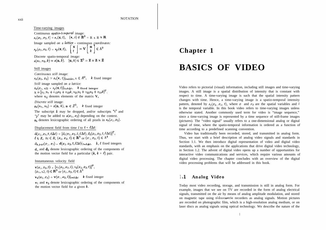
Time-varying images
Continuous spaGo-temporal image:s,(xl, x2, t) = sc(x, t), (x, t) E R3 = R x R x R
Image sampled on a la22ife - continuous coordinates:r _ISp(%&) = Sp(X,Q ~;J=V~;JElP
Discrete spatio-temporal image:s(nl,nz,k)=s(n,k), (n,k)EZ3=ZXZXZ.
Still images
Continuous still image:sk(xl, x2) = sC(x, t)ltzkAt, x E R’, k fixed integer
Still image sampled on a lattice:sk(xl, x2) = s,(x,t)lkkAt, k fixed integer
X = [vllnl + VlZn2 $ V13k, V2lnl + V22n2 + V23klTjwhere vij denotes elements of the matrix V,
Discrete still image:sk(nl, n2) = s(n, Ic), n E Z2, Ic fixed integer
The subscript le may be dropped, and/or subscripts “c’ and“p” may be added to s(c1, ~2) depending on the context.sk denotes lexicographic ordering of all pixels in S~(XI, ~2).
Displacement field from time t to t + eat:
d(zl,xz,t;!At) = [d 1 zl,cz,t;eAt),dz(zl,cz,t;eAt)lT,(1 E Z, At E R, (XI, 22, t) E R3 or (21, x2, t) E A3
drc,s+e(xl, x2) = d(xl,xz,t;eAt)lt=kat, le, 1 fixed integers
d1 and d2 denote lexicographic ordering of the components ofthe motion vector field for a particular (Ic, le + 1) pair.
Instantaneous velocity field
v(xl,xz,q = [Vl(x1,+2,t),V2(21,C2,t)lT,(XI, x2, t) E R3 or (II, x2, t) E A3
V&,X2) = v(Xl,Xz,t)lt=kAt t fixed integer
v1 and v2 denote lexicographic ordering of the components ofthe motion vector field for a given k.
NOTATION
Chapter 1
BASICS OF VIDEO
Video refers to pictorial (visual) information, including still images and time-varyingimages. A still image is a spatial distribution of intensity that is constant withrespect to time. A time-varying image is such that the spatial intensity patternchanges with time. Hence, a time-varying image is a spatio-temporal intensitypattern, denoted by sC(xl, 22, t), where x1 and c2 are the spatial variables and tis the temporal variable. In this book video refers to time-varying images unlessotherwise stated. Another commonly used term for video is “image sequence,”since a time-varying image is represented by a time sequence of still-frame images(pictures). The “video signal” usually refers to a one-dimensional analog or digitalsignal of time, where the spatio-temporal information is ordered as a function oftime according to a predefined scanning convention.
Video has traditionally been recorded, stored, and transmitted in analog form.Thus, we start with a brief description of analog video signals and standards inSection 1.1. We then introduce digital representation of video and digital videostandards, with an emphasis on the applications that drive digital video technology,in Section 1.2. The advent of digital video opens up a number of opportunities forinteractive video communications and services, which require various amounts ofdigital video processing. The chapter concludes with an overview of the digitalvideo processing problems that will be addressed in this book.
1 .l Analog Video
Today most video recording, storage, and transmission is still in analog form. Forexample, images that we see on TV are recorded in the form of analog electricalsignals, transmitted on the air by means of analog amplitude modulation, and storedon magnetic tape using videocasette recorders as analog signals. Motion picturesare recorded on photographic film, which is a high-resolution analog medium, or onlaser discs as analog signals using optical technology. We describe the nature of the
1

2 CHAPTER 1. BASICS OF VIDEO k 1.1. ANALOG VIDEO 3
analog video signal and the specifications of popular analog video standards in thefollowing. An understanding of the limitations of certain analog video formats isimportant, because video signals digitized from analog sources are usually limitedby the resolution and the artifacts of the respective analog standard.
1.1.1 Analog Video Signal
The analog video signal refers to a one-dimensional (1-D) electrical signal f(t)of time that is obtained by sampling s,(zli za,t) in the vertical ~2 and temporalcoordinates. This periodic sampling process is called scanning. The signal f(t),then, captures the time-varying image intensity ~~(21, zz,t) only along the scanlines, such as those shown in Figure 1.1. It also contains the timing informationand the blanking signals needed to align the pictures correctly.
The most commonly used scanning methods are progressive scanning and in-terlaced scanning. A progressive scan traces a complete picture, called a frame, atevery At sec. The computer industry uses progressive scanning with At = l/72 seefor high-resolution monitors. On the other hand, the TV industry uses 2:l interlacewhere the odd-numbered and even-numbered lines, called the odd field and the evenfield, respectively, are traced in turn. A 2:l interlaced scanning raster is shown inFigure 1.1, where the solid line and the dotted line represent the odd and the evenfields, respectively. The spot snaps back from point B to C, called the horizontalretrace, and from D to E, and from F to A, called the vertical retrace.
E
Figure 1.1: Scanning raster.
An analog video signal f(t) is shown in Figure 1.2. Blanking pulses (black) areinserted during the retrace intervals to blank out retrace lines on the receiving CRT.Sync pulses are added on top of the blanking pulses to synchronize the receiver’s
horizontal and vertical sweep circuits. The sync pulses ensure that the picture startsat the top left corner of the receiving CRT. The timing of the sync pulses are, ofcourse, different for progressive and interlaced video.
White
Figure 1.2: Video signal for one full line.
Some important parameters of the video signal are the vertical resolution, aspectratio, and frame/field rate. The vertical resolution is related to the number of scanlines per frame. The aspect ratio is the ratio of the width to the height of a frame.Psychovisual studies indicate that the human eye does not perceive flicker if therefresh rate of the display is more than 50 times per second. However, for TVsystems, such a high frame rate, while preserving the vertical resolution, requires alarge transmission bandwidth. Thus, TV systems utilize interlaced scanning, whichtrades vertical resolution to reduced flickering within a fixed bandwidth.
An understanding of the spectrum of the video signal is necessary to discussthe composition of the broadcast TV signal. Let’s start with the simple case of astill image, Q(z~,Q), where (z~,zz) E R’. We construct a doubly periodic arrayof images, &(z~,Q), which is shown in Figure 1.3. The array &(c~~xz) can beexpressed in terms of a 2-D Fourier series,
kl=-co kz=-co
where Sklkz are the 2-D Fourier series coefficients, and L and H denote the horizon-tal and vertical extents of a frame (including the blanking intervals), respectively.
The analog video signal f(t) is then composed of intensities along the solid lineacross the doubly periodic field (w 1c corresponds to the scan line) in Figure 1.3.h’ h
4 CHAPTER 1. BASICS OF VIDEO I 1.1. ANALOG VIDEO 5
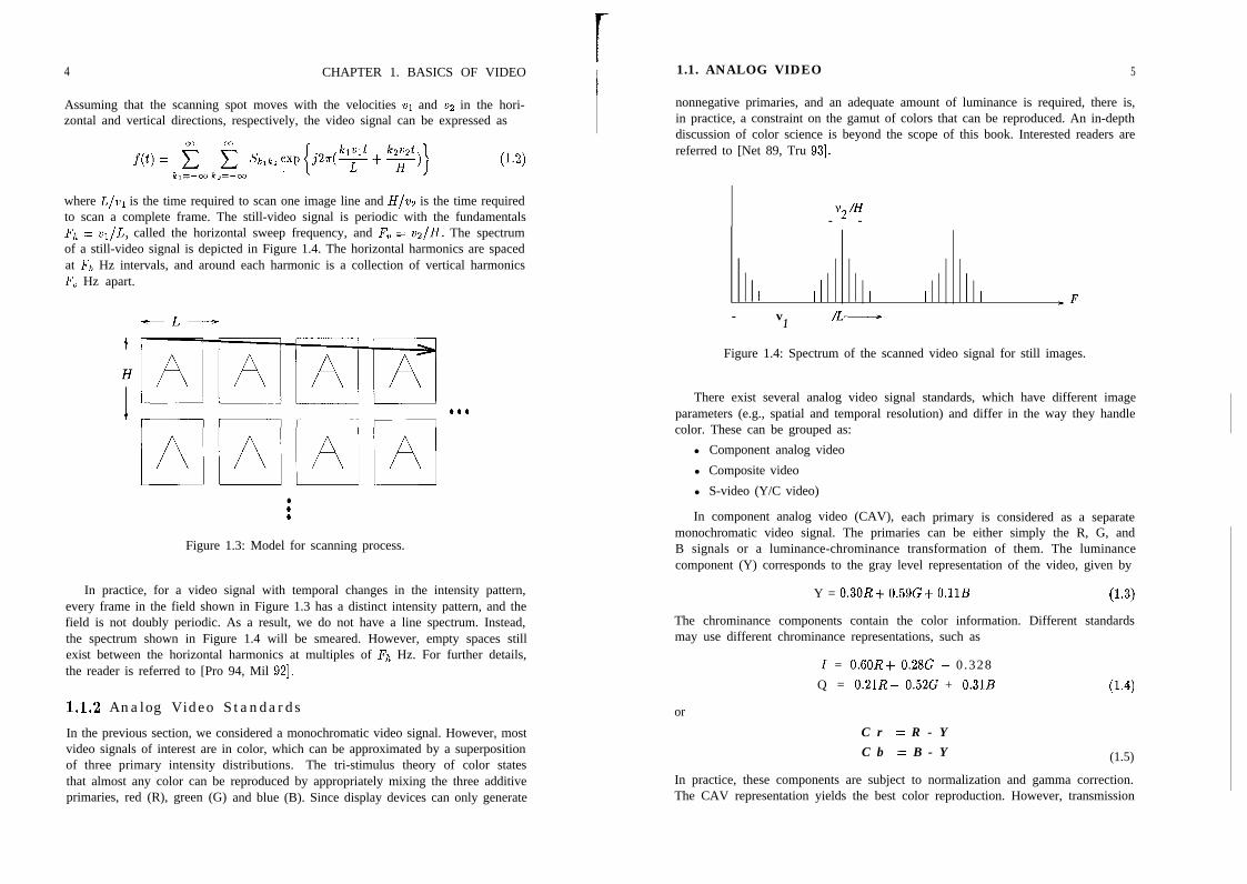
Assuming that the scanning spot moves with the velocities vi and v2 in the hori-zontal and vertical directions, respectively, the video signal can be expressed as
(1.2)
where L/VI is the time required to scan one image line and H/v2 is the time requiredto scan a complete frame. The still-video signal is periodic with the fundamentalsFh = vi/L, called the horizontal sweep frequency, and F, = vz/H. The spectrumof a still-video signal is depicted in Figure 1.4. The horizontal harmonics are spacedat Fh Hz intervals, and around each harmonic is a collection of vertical harmonicsF, Hz apart.
Figure 1.3: Model for scanning process.
In practice, for a video signal with temporal changes in the intensity pattern,every frame in the field shown in Figure 1.3 has a distinct intensity pattern, and thefield is not doubly periodic. As a result, we do not have a line spectrum. Instead,the spectrum shown in Figure 1.4 will be smeared. However, empty spaces stillexist between the horizontal harmonics at multiples of Fh Hz. For further details,the reader is referred to [Pro 94, Mil 921.
1.1.2 Analog Video Standards
In the previous section, we considered a monochromatic video signal. However, mostvideo signals of interest are in color, which can be approximated by a superpositionof three primary intensity distributions. The tri-stimulus theory of color statesthat almost any color can be reproduced by appropriately mixing the three additiveprimaries, red (R), green (G) and blue (B). Since display devices can only generate
nonnegative primaries, and an adequate amount of luminance is required, there is,in practice, a constraint on the gamut of colors that can be reproduced. An in-depthdiscussion of color science is beyond the scope of this book. Interested readers arereferred to [Net 89, Tru 931.
v2 /H- -
l II I I I ,F- v /L-1
Figure 1.4: Spectrum of the scanned video signal for still images.
There exist several analog video signal standards, which have different imageparameters (e.g., spatial and temporal resolution) and differ in the way they handlecolor. These can be grouped as:
l Component analog video
l Composite video
l S-video (Y/C video)
In component analog video (CAV), each primary is considered as a separatemonochromatic video signal. The primaries can be either simply the R, G, andB signals or a luminance-chrominance transformation of them. The luminancecomponent (Y) corresponds to the gray level representation of the video, given by
Y = 0.30R+ 0.59G+ O.llB (1.3)
The chrominance components contain the color information. Different standardsmay use different chrominance representations, such as
1 = 0.60R+ 0.28G - 0 .328Q = 0.21R- 0.52G + 0.31B (1.4)
or
C r = R - YC b = B - Y (1.5)
In practice, these components are subject to normalization and gamma correction.The CAV representation yields the best color reproduction. However, transmission

6 CHAPTER 1. BASICS OF VIDEO
of CAV requires perfect synchronization of the three components and three timesmore bandwidth.
Composite video signal formats encode the chrominance components on top ofthe luminance signal for distribution as a single signal which has the same band-width as the luminance signal. There are different composite video formats, such asNTSC (National Television Systems Committee), PAL (Phase Alternation Line),and SECAM (Systeme Electronique Color Avec Memoire), being used in differentcountries around the world.
N T S C
The NTSC composite video standard, defined in 1952, is currently in use mainly inNorth America and Japan. NTSC signal is a 2:l interlaced video signal with 262.5lines per field (525 lines per frame), 60 fields per second, and 4:3 aspect ratio. As aresult, the horizontal sweep frequency, Fh, is 525 x 30 = 15.75 kHz, which meansit takes l/15,750 set = 63.5 ps to sweep each horizontal line. Then, from (1.2), theNTSC video signal can be approximately represented as
f ( t ) E e fJ Sklkz exp {j2n(15,7501el+ 3Okz)t) (1.6)kl=-oo kz=-co
Horizontal retrace takes 10 ps, that leaves 53.5 ps for the active video signal perline. The horizontal sync pulse is placed on top of the horizontal blanking pulse, andits duration is 5 11s. These parameters were shown in Figure 1.2. Only 485 lines outof the 525 are active lines, since 20 lines per field are blanked for vertical backtrace[Mil 921. Although there are 485 active lines per frame, the vertical resolution,defined as the number of resolvable horizontal lines, is known to be
485 X 0.7 = 339.5 (340) lines/frame,
where 0.7 is known as the Kell factor, defined as
(1.7)
Kell factor =number of perceived vertical linesnumber of total active scan lines
M 0.7
Using the aspect ratio, the horizontal resolution, defined as the number of resolvablevertical lines, should be
339 x t = 452 elements/line. (1.8)
Then, the bandwidth of the luminance signal can be calculated as
4522 x 53.5 x 10-s
= 4.2 MHz.
The luminance signal is vestigial sideband modulated (VSB) with a sideband, thatextends to 1.25 MHz below the picture carrier, as depicted in Figure 1.5.
r1.1. ANALOG VIDEO 7
The chrominance signals, I and Q, should also have the same bandwidth. How-ever, subjective tests indicate that the I and Q channels can be low-pass filteredto 1.6 and 0.6 MHz, respectively, without affecting the quality of the picture dueto the inability of the human eye to perceive changes in chrominance over smallareas (high frequencies). The I channel is separated into two bands, O-O.6 MHz and0.6-1.6 MHz. The entire Q channel and the O-O.6 MHz portion of the I channelare quadrature amplitude modulated (&AM) with a color subcarrier frequency 3.58MHz above the picture carrier, and the 0.6-1.6 MHz portion of the I channel is lowerside band (SSB-L) modulated with the same color subcarrier. This color subcarrierfrequency falls in midway between 227Fh and 228Fh; thus, the chrominance spectrashift into the gaps midway between the harmonics of Fh. The audio signal is fre-quency modulated (FM) with an audio subcarrier frequency that is 4.5 MHz abovethe picture carrier. The spectral composition of the NTSC video signal, which hasa total bandwidth of 6 MHz, is depicted in Figure 1.5. The reader is referred to acommunications textbook, e.g., Lathi [Lat 891 or Proakis and Salehi [Pro 941, for adiscussion of various modulation techniques including VSB, &AM, SSB-L, and FM.
1 6 MHz
picture color audiocarrier carrier carrier
Figure 1.5: Spectrum of the NTSC video signal.
PAL and SECAM
PAL and SECAM, developed in the 196Os, are mostly used in Europe today. Theyare also 2:l interlaced, but in comparison to NTSC, they have different vertical andtemporal resolution, slightly higher bandwidth (8 MHz), and treat color informationdifferently. Both PAL and SECAM have 625 lines per frame and 50 fields per second;thus, they have higher vertical resolution in exchange for lesser temporal resolutionas compared with NTSC. One of the differences between PAL and SECAM is howthey represent color information. They both utilize Cr and Cb components for thechrominance information. However, the integration of the color components withthe luminance signal in PAL and SECAM are different. Both PAL and SECAM aresaid to have better color reproduction than NTSC.
8 CHAPTER 1. BASICS OF VIDEO
In PAL, the two chrominance signals are &AM modulated with a color subcar-rier at 4.43 MHz above the picture carrier. Then the composite signal is filteredto limit its spectrum to the allocated bandwidth. In order to avoid loss of high-frequency color information due to this bandlimiting, PAL alternates between +Crand -Cr in successive scan lines; hence, the name phase alternation line. The high-frequency luminance information can then be recovered, under the assumption thatthe chrominance components do not change significantly from line to line, by av-eraging successive demodulated scan lines with the appropriate signs [Net 891. InSECAM, based on the same assumption, the chrominance signals Cr and Cb aretransmitted alternatively on successive scan lines. They are FM modulated on thecolor subcarriers 4.25 MHz and 4.41 MHz for Cb and Cr, respectively. Since onlyone chrominance signal is transmitted per line, there is no interference between thechrominance components.
The composite signal formats usually result in errors in color rendition, knownas hue and saturation errors, because of inaccuracies in the separation of the colorsignals. Thus, S-video is a compromise between the composite video and the com-ponent analog video, where we represent the video with two component signals, aluminance and a composite chrominance signal, The chrominance signal can bebased upon the (I,&) or (Cr,Cb) representation for NTSC, PAL, or SECAM sys-tems. S-video is currently being used in consumer-quality videocasette recordersand camcorders to obtain image quality better than that of the composite video.
1.1.3 Analog Video Equipment
Analog video equipment can be classified as broadcast-quality, professional-quality,and consumer-quality. Broadcast-quality equipment has the best performance, butis the most expensive. For consumer-quality equipment, cost and ease of use arethe highest priorities.
Video images may be acquired by electronic live pickup cameras and recordedon videotape, or by motion picture cameras and recorded on motion picture film(24 frames/set), or formed by sequential ordering of a set of still-frame images suchas in computer animation. In electronic pickup cameras, the image is opticallyfocused on a two-dimensional surface of photosensitive material that is able tocollect light from all points of the image all the time. There are two major types ofelectronic cameras, which differ in the way they scan out the integrated and storedcharge image. In vacuum-tube cameras (e.g., vidicon), an electron beam scans outthe image. In solid-state imagers (e.g., CCD cameras), the image is scanned out bya solid-state array. Color cameras can be three-sensor type or single-sensor type.Three-sensor cameras suffer from synchronicity problems and high cost, while single-sensor cameras often have to compromise spatial resolution. Solid-state sensors areparticularly suited for single-sensor cameras since the resolution capabilities of CCDcameras are continuously improving. Cameras specifically designed for televisionpickup from motion picture film are called telecine cameras. These cameras usuallyemploy frame rate conversion from 24 frames/set to 60 fields/set.
1.2. DIGITAL VIDEO 9
Analog video recording is mostly based on magnetic technology, except for thelaser disc which uses optical technology. In magnetic recording, the video signalis modulated on top of an FM carrier before recording in order to deal with thenonlinearity of magnetic media. There exist a variety of devices and standards forrecording the analog video signal on magnetic tapes. The Betacam is a componentanalog video recording standard that uses l/2” tape. It is employed in broadcast-and professional-quality applications. VHS is probably the most commonly usedconsumer-quality composite video recording standard around the world. U-maticis another composite video recording standard that uses 3/4” tape, and is claimedto result in a better image quality than VHS. U-matic recorders are mostly used inprofessional-quality applications. Other consumer-quality composite video record-ing standards are the Beta and 8 mm formats. S-VHS recorders, which are basedon S-video, recently became widely available, and are relatively inexpensive forreasonably good performance.
1.2 Digital Video
We have been experiencing a digital revolution in the last couple of decades. Dig-ital data and voice communications have long been around. Recently, hi-fi digitalaudio with CD-quality sound has become readily available in almost any personalcomputer and workstation. Now, technology is ready for landing full-motion digi-tal video on the desktop [Spe 921. Apart from the more robust form of the digitalsignal, the main advantage of digital representation and transmission is that theymake it easier to provide a diverse range of services over the same network [Sut 921.Digital video on the desktop brings computers and communications together in atruly revolutionary manner. A single workstation may serve as a personal com-puter, a high-definition TV, a videophone, and a fax machine. With the addition ofa relatively inexpensive board, we can capture live video, apply digital processing,and/or print still frames at a local printer [Byt 921. This section introduces digitalvideo as a form of computer data.
1.2.1’ Digital Video Signal
Almost all digital video systems use component representation of the color signal.Most color video cameras provide RGB outputs which are individually digitized.Component representation avoids the artifacts that result from composite encoding,provided that the input RGB signal has not been composite-encoded before. Indigital video, there is no need for blanking or sync pulses, since a computer knowsexactly where a new line starts as long as it knows the number of pixels per line[Lut 881. Thus, all blanking and sync pulses are removed in the A/D conversion.
Even if the input video is a composite analog signal, e.g., from a videotape, itis usually first converted to component analog video, and the component signalsare then individually digitized. It is also possible to digitize the composite sig-

10 CHAPTER 1. BASICS OF VIDEO I1
nal directly using one A/D converter with a clock high enough to leave the colorsubcarrier components free from aliasing, and then perform digital decoding to ob-tain the desired RGB or YIQ component signals. This requires sampling at a ratethree or four times the color subcarrier frequency, which can be accomplished byspecial-purpose chip sets. Such chips do exist in some advanced TV sets for digitalprocessing of the received signal for enhanced image quality.
The horizontal and vertical resolution of digital video is related to the number ofpixels per line and the number of lines per frame. The artifacts in digital video due tolack of resolution are quite different than those in analog video. In analog video thelack of spatial resolution results in blurring of the image in the respective direction.In digital video, we have pixellation (aliasing) artifacts due to lack of sufficientspatial resolution. It manifests itself as jagged edges resulting from individual pixelsbecoming visible. The visibility of the pixellation artifacts depends on the size ofthe display and the viewing distance [Lut 881.
The arrangement of pixels and lines in a contiguous region of the memory iscalled a bitmap. There are five key parameters of a bitmap: the starting addressin memory, the number of pixels per line, the pitch value, the number of lines, andnumber of bits per pixel. The pitch value specifies the distance in memory fromthe start of one line to the next. The most common use of pitch different fromthe number of pixels per line is to set pitch to the next highest power of 2, whichmay help certain applications run faster. Also, when dealing with interlaced inputs,setting the pitch to double the number of pixels per line facilitates writing linesfrom each field alternately in memory. This will form a “composite frame” in acontiguous region of the memory after two vertical scans. Each component signal isusually represented with 8 bits per pixel to avoid “contouring artifacts.” Contouringresulm in slowly varying regions of image intensity due to insufficient bit resolution.Color mapping techniques exist to map 2 24 distinct colors to 256 colors for displayon &bit color monitors without noticeable loss of color resolution. Note that displaydevices are driven by analog inputs; therefore, D/A converters are used to generatecomponent analog video signals from the bitmap for display purposes.
The major bottleneck preventing the widespread use of digital video today hasbeen the huge storage and transmission bandwidth requirements. For example, digi-tal video requires much higher data rates and transmission bandwidths as comparedto digital audio. CD-quality digital audio is represented with 16 bits/sample, andthe required sampling rate is 44kHz. Thus, the resulting data rate is approximately700 kbits/sec (kbps). In comparison, a high-definition TV signal (e.g., the AD-HDTV proposal) requires 1440 pixels/line and 1050 lines for each luminance frame,and 720 pixels/line and 525 lines for each chrominance frame. Since we have 30frames/s and 8 bits/pixel per channel, the resulting data rate is approximately 545Mbps, which testifies that a picture is indeed worth 1000 words! Thus, the viabilityof digital video hinges upon image compression technology [Ang 911. Some digitalvideo format and compression standards will be introduced in the next subsection.
1.2. DIGITAL VIDEO 11
1.2.2 Digital Video Standards
Exchange of digital video between different applications and products requires digi-tal video format standards. Video data needs to be exchanged in compressed form,which leads to compression standards. In the computer industry, standard displayresolutions; in the TV industry, digital studio standards; and in the communicationsindustry, standard network protocols ha.ve already been established. Because theadvent of digital video is bringing these three industries ever closer, recently stan-dardization across the industries has also started. This section briefly introducessome of these standards and standardization efforts.
Table 1.1: Digital video studio standards
CCIR601 CCIR601 CIFParameter 525/60 625/50
NTSC PAL/SECAMNumber ofactive pels/lineLum (Y) 720 720 360Chroma (U,V) 360 360 180Number ofactive lines/pitLum (Y) 480 576 288Chroma (U,V) 480 576 144Interlacing /
2:l 2:l 1:lTemporal rate 60 50 30Aspect ratio 4:3 4:3 4:3
Digital video is not new in the broadcast TV studios, where editing and spe-cial effects are performed on digital video because it is easier to manipulate digitalimages. Working with digital video also avoids artifacts that would be otherwisecaused by repeated analog recording of video on tapes during various productionstages. Another application for digitization of analog video is conversion betweendifferent analog standards, such as from PAL to NTSC. CCIR (International Con-sultative Committee for Radio) Recommendation 601 defines a digital video formatfor TV studios for 525-line and 625-line TV systems. This standard is intendedto permit international exchange of production-quality programs. It is based oncomponent video with one luminance (Y) and two color difference (Cr and Cb) sig-nals. The sampling frequency is selected to be an integer multiple of the horizontalsweep frequencies in both the 525- and 625-line systems. Thus, for the luminancecomponent,
fs,lurn = 858~4525 = 864fh,s~ = 13.5MHz, (1.10)
12 CHAPTER 1. BASICS OF VIDEO
and for the chrominance,
fs,chr = .fs,iw& = 6.7’5MHz. (1.11)
The parameters of the CCIR 601 standards are tabulated in Table 1.1. Note thatthe raw data rate for the CCIR 601 formats is 165 Mbps. Because this rate is toohigh for most applications, the CCITT (International Consultative Committee forTelephone and Telegraph) Specialist Group (SGXV) has proposed a new digitalvideo format, called the Common Intermediate Format (CIF). The parameters ofthe CIF format are also shown in Table 1.1. Note that the CIF format is progressive(noninterlaced), and requires approximately 37 Mbps. In some cases, the numberof pixels in a line is reduced to 352 and 176 for the luminance and chrominancechannels, respectively, to provide an integer number of 16 x 16 blocks.
In the computer industry, standards for video display resolutions are set bythe Video Electronics Standards Association (VESA). The older personal computer(PC) standards are the VGA with 640 pixels/line x 480 lines, and TARGA with512 pixels/line x 480 lines. Many high-resolution workstations conform with theS-VGA standard, which supports two main modes, 1280 pixels/line x 1024 lines or1024 pixels/line x 768 lines. The refresh rate for these modes is 72 frames/set. Rec-ognizing that the present resolution of TV images is well behind today’s technology,several proposals have been submitted to the Federal Communications Commission(FCC) for a high-definition TV standard. Although no such standard has beenformally approved yet, all proposals involve doubling the resolution of the CCIR601 standards in both directions.
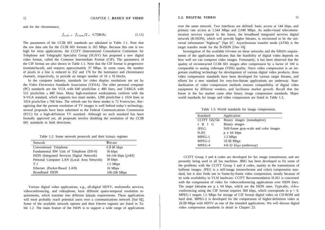
Table 1.2: Some network protocols and their bitrate regimes
Network BitrateConventional Telephone 0.3-56 kbpsFundamental BW Unit of Telephone (DS-0) 56 kbpsISDN (Integrated Services Digital Network) 64-144 kbps (~~64)Personal Computer LAN (Local Area Network) 30 kbpsT-l 1.5 MbpsEthernet (Packet-Based LAN) 10 MbpsBroadband ISDN 100-200 Mbps
Various digital video applications, e.g., all-digital HDTV, multimedia services,videoconferencing, and videophone, have different spatio-temporal resolution re-quirements, which translate into different bitrate requirements. These applicationswill most probably reach potential users over a communications network [Sut 921.Some of the available network options and their bitrate regimes are listed in Ta-ble 1.2. The main feature of the ISDN is to support a wide range of applications
1.2. DIGITAL VIDEO 13
over the same network. Two interfaces are defined: basic access at 144 kbps, andprimary rate access at 1.544 Mbps and 2.048 Mbps. As audio-visual telecommu-nication services expand in the future, the broadband integrated services digitalnetwork (B-ISDN), which will provide higher bitrates, is envisioned to be the uni-versal information “highway” [Spe 911. Asynchronous transfer mode (ATM) is thetarget transfer mode for the B-ISDN [Onv 941.
Investigation of the available bitrates on these networks and the bitrate require-ments of the applications indicates that the feasibility of digital video depends onhow well we can compress video images. Fortunately, it has been observed that thequality of reconstructed CCIR 601 images after compression by a factor of 100 iscomparable to analog videotape (VHS) quality. Since video compression is an im-portant enabling technology for development of various digital video products, threevideo compression standards have been developed for various target bitrates, andefforts for a new standard for very-low-bitrate applications are underway. Stan-dardization of video compression methods ensures compatibility of digital videoequipment by different vendors, and facilitates market growth. Recall that theboom in the fax market came after binary image compression standards. Majorworld standards for image and video compression are listed in Table 1.3.
Table 1.3: World standards for image compression.
Standard ApplicationCCITT G3/G4 Binary images (nonadaptive)J B I G Binary imagesJPEG Still-frame gray-scale and color imagesH.261 p x 64 kbpsMPEG-1 1.5 MbpsMPEG-2 lo-20 MbpsMPEG-4 4.8-32 kbps (underway)
CCITT Group 3 and 4 codes are developed for fax image transmission, and arepresently being used in all fax machines. JBIG has been developed to fix some ofthe problems with the CCITT Group 3 and 4 codes, mainly in the transmission ofhalftone images. JPEG is a still-image (monochrome and color) compression stan-dard, but it also finds use in frame-by-frame video compression, mostly because ofits wide availability in VLSI hardware. CCITT Recommendation H.261 is concernedwith the compression of video for videoconferencing applications over ISDN lines.The target bitrates are p x 64 kbps, which are the ISDN rates. Typically, video-conferencing using the CIF format requires 384 kbps, which corresponds to p = 6.MPEG-1 targets 1.5 Mbps for storage of CIF format digital video on CD-ROM andhard disk. MPEG-2 is developed for the compression of higher-definition video atlo-20 Mbps with HDTV as one of the intended applications. We will discuss digitalvideo compression standards in detail in Chapter 23.
14 CHAPTER 1. BASICS OF VIDEO
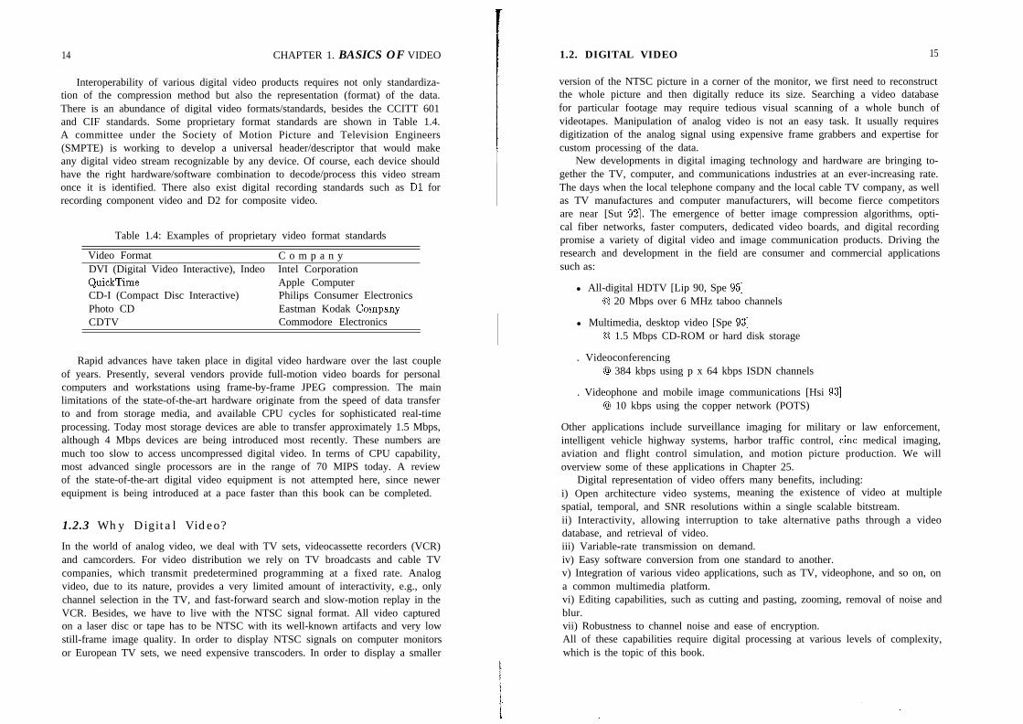
Interoperability of various digital video products requires not only standardiza-tion of the compression method but also the representation (format) of the data.There is an abundance of digital video formats/standards, besides the CCITT 601and CIF standards. Some proprietary format standards are shown in Table 1.4.A committee under the Society of Motion Picture and Television Engineers(SMPTE) is working to develop a universal header/descriptor that would makeany digital video stream recognizable by any device. Of course, each device shouldhave the right hardware/software combination to decode/process this video streamonce it is identified. There also exist digital recording standards such as Dl forrecording component video and D2 for composite video.
Table 1.4: Examples of proprietary video format standards
Video Format C o m p a n yDVI (Digital Video Interactive), Indeo Intel CorporationQuickTime Apple ComputerCD-I (Compact Disc Interactive) Philips Consumer ElectronicsPhoto CD Eastman Kodak CompanvCDTV
_ ”Commodore Electronics
Rapid advances have taken place in digital video hardware over the last coupleof years. Presently, several vendors provide full-motion video boards for personalcomputers and workstations using frame-by-frame JPEG compression. The mainlimitations of the state-of-the-art hardware originate from the speed of data transferto and from storage media, and available CPU cycles for sophisticated real-timeprocessing. Today most storage devices are able to transfer approximately 1.5 Mbps,although 4 Mbps devices are being introduced most recently. These numbers aremuch too slow to access uncompressed digital video. In terms of CPU capability,most advanced single processors are in the range of 70 MIPS today. A reviewof the state-of-the-art digital video equipment is not attempted here, since newerequipment is being introduced at a pace faster than this book can be completed.
1.2.3 Why Digital Video?
In the world of analog video, we deal with TV sets, videocassette recorders (VCR)and camcorders. For video distribution we rely on TV broadcasts and cable TVcompanies, which transmit predetermined programming at a fixed rate. Analogvideo, due to its nature, provides a very limited amount of interactivity, e.g., onlychannel selection in the TV, and fast-forward search and slow-motion replay in theVCR. Besides, we have to live with the NTSC signal format. All video capturedon a laser disc or tape has to be NTSC with its well-known artifacts and very lowstill-frame image quality. In order to display NTSC signals on computer monitorsor European TV sets, we need expensive transcoders. In order to display a smaller
1.2. DIGITAL VIDEO 15
version of the NTSC picture in a corner of the monitor, we first need to reconstructthe whole picture and then digitally reduce its size. Searching a video databasefor particular footage may require tedious visual scanning of a whole bunch ofvideotapes. Manipulation of analog video is not an easy task. It usually requiresdigitization of the analog signal using expensive frame grabbers and expertise forcustom processing of the data.
New developments in digital imaging technology and hardware are bringing to-gether the TV, computer, and communications industries at an ever-increasing rate.The days when the local telephone company and the local cable TV company, as wellas TV manufactures and computer manufacturers, will become fierce competitorsare near [Sut 921. The emergence of better image compression algorithms, opti-cal fiber networks, faster computers, dedicated video boards, and digital recordingpromise a variety of digital video and image communication products. Driving theresearch and development in the field are consumer and commercial applicationssuch as:
l All-digital HDTV [Lip 90, Spe 951@ 20 Mbps over 6 MHz taboo channels
l Multimedia, desktop video [Spe 931@ 1.5 Mbps CD-ROM or hard disk storage
. Videoconferencing@ 384 kbps using p x 64 kbps ISDN channels
. Videophone and mobile image communications [Hsi 931@ 10 kbps using the copper network (POTS)
Other applications include surveillance imaging for military or law enforcement,intelligent vehicle highway systems, harbor traffic control, tine medical imaging,aviation and flight control simulation, and motion picture production. We willoverview some of these applications in Chapter 25.
Digital representation of video offers many benefits, including:i) Open architecture video systems, meaning the existence of video at multiplespatial, temporal, and SNR resolutions within a single scalable bitstream.ii) Interactivity, allowing interruption to take alternative paths through a videodatabase, and retrieval of video.iii) Variable-rate transmission on demand.iv) Easy software conversion from one standard to another.v) Integration of various video applications, such as TV, videophone, and so on, ona common multimedia platform.vi) Editing capabilities, such as cutting and pasting, zooming, removal of noise andblur.vii) Robustness to channel noise and ease of encryption.All of these capabilities require digital processing at various levels of complexity,which is the topic of this book.
16 CHAPTER 1. BASICS OF VIDEO
1.3 Digital Video Processing
Digital video processing refers to manipulation of the digital video bitstream. Allknown applications of digital video today require digital processing for data com-pression, In addition, some applications may benefit from additional processing formotion analysis, standards conversion, enhancement, and restoration in order toobtain better-quality images or extract some specific information.
Digital processing of still images has found use in military, commercial, andconsumer applications since the early 1960s. Space missions, surveillance imaging,night vision, computed tomography, magnetic resonance imaging, and fax machinesare just some examples. What makes digital video processing different from stillimage processing is that video imagery contains a significant amount of temporalcorrelation (redundancy) between the frames. One may attempt to process videoimagery as a sequence of still images, where each frame is processed independently.However, utilization of existing temporal redundancy by means of multiframe pro-cessing techniques enables us to develop more effective algorithms, such as motion-compensated filtering and motion-compensated prediction. In addition, some tasks,such as motion estimation or the analysis of a time-varying scene, obviously cannotbe performed on the basis of a single image. It is the goal of this book to provide thereader with the mathematical basis of multiframe and motion-compensated videoprocessing. Leading algorithms for important applications are also included.
Part 1 is devoted to the representation of full-motion digital video as a formof computer data. In Chapter 2, we model the formation of time-varying imagesas perspective or orthographic projection of 3-D scenes with moving objects. Weare mostly concerned with 3-D rigid motion; however, models can be readily ex-tended to include 3-D deformable motion. Photometric effects of motion are alsodiscussed. Chapter 3 addresses spatio-temporal sampling on 3-D lattices, whichcovers several practical sampling structures including progressive, interlaced, andquincunx sampling. Conversion between sampling structures without making useof motion information is the subject of Chapter 4.
Part 2 covers nonparametric 2-D motion estimation methods. Since motioncompensation is one of the most effective ways to utilize temporal redundancy, 2-Dmotion estimation is at the heart of digital video processing. 2-D motion estima-tion, which refers to optical flow estimation or the correspondence problem, aimsto estimate motion projected onto the image plane in terms of instantaneous pixelvelocities or frame-to-frame pixel correspondences. We can classify nonparametric2-D motion estimation techniques as methods based on the optical flow equation,block-based methods, pel-recursive methods, and Bayesian methods, which are pre-sented in Chapters 5-8, respectively.
Part 3 deals with 3-D motion/structure estimation, segmentation, and tracking.3-D motion estimation methods are based on parametric modeling of the 2-D opticalflow field in terms of rigid motion and structure parameters. These parametricmodels can be used for either 3-D image analysis, such as in object-based imagecompression and passive navigation, or improved 2-D motion estimation. Methods
1.3. DIGITAL VIDEO PROCESSING 17
that use discrete point correspondences are treated in Chapter 9, whereas optical-flow-based or direct estimation methods are introduced in Chapter 10. Chapter 11discusses segmentation of the motion field in the presence of multiple motion, usingdirect methods, optical flow methods, and simultaneous motion estimation andsegmentation. Two-view motion estimation techniques, discussed in Chapters 9-11,have been found to be highly sensitive to small inaccuracies in the estimates of pointcorrespondences or optical flow. To this effect, motion and structure from stereopairs and motion tracking over long monocular or stereo sequences are addressed inChapter 12 for more robust estimation.
Filtering of digital video for such applications as standards conversion, noisereduction, and enhancement and restoration is addressed in Part 4. Video filteringdiffers from still-image filtering in that it generally employs motion information. Tothis effect, the basics of motion-compensated filtering are introduced in Chapter 13.Video images often suffer from graininess, especially when viewed in freeze-framemode. Intraframe, motion-adaptive, and motion-compensated filtering for noisesuppression are discussed in Chapter 14. Restoration of blurred video frames is thesubject of Chapter 15. Here, motion information can be used in the estimationof the spatial extent of the blurring function. Different digital video applicationshave different spatio-temporal resolution requirements. Appropriate standards con-version is required to ensure interoperability of various applications by decouplingthe spatio-temporal resolution requirements of the source from that of the display.Standards conversion problems, including frame rate conversion and de-interlacing(interlaced to progressive conversion), are covered in Chapter 16. One of the lim-itations of CCIR 601, CIF, or smaller-format video is the lack of sufficient spatialresolution. In Chapter 17, a comprehensive model for low-resolution video acqui-sition is presented as well as a novel framework for superresolution which unifiesmost video filtering problems.
Compression is fundamental for all digital video applications. Parts 5 and 6are devoted to image and video compression methods, respectively. It is the emer-gence of video compression standards, such as JPEG, H.261, and MPEG and theirVLSI implementations, that makes applications such as all-digital TV, multimedia,and videophone a reality. Chapters 18-21 cover still-image compression methods,which form the basis for the discussion of video compression in Chapters 22-24,In particular, we discuss lossless compression in Chapter 18, DPCM and transformcoding in Chapter 19, still-frame compression standards, including binary and gray-scale/color image compression standards, in Chapter 20, and vector quantizationand subband coding in Chapter 21. Chapter 22 provides a brief overview of in-terframe compression methods. International video compression standards such asH.261, MPEG-1, and MPEG-2 are explained in Chapter 23. Chapter 24 addressesvery-low-bitrate coding using object-based methods. Finally, several applicationsof digital video are introduced in Chapter 25.
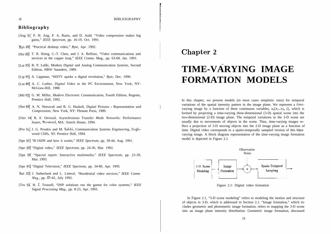
18 BIBLIOGRAPHY
Bibliography
[Ang 911 P. H. Ang, P. A. Ruetz, and D. Auld, “Video compression makes biggains,” IEEE Spectrum, pp. 16-19, Oct. 1991.
FW 921[Hsi 931
[Lat 891
[Lip 901
[Lut 881
[Mil 921
[Net 891
“Practical desktop video,” Byte, Apr. 1992.
T. R. Hsing, C.-T. Chen, and J. A. Bellisio, “Video communications andservices in the copper loop,” IEEE Comm. Mag., pp. 63-68, Jan. 1993.
B. P. Lathi, Modern Digital and Analog Communication Systems, SecondEdition, HRW Saunders, 1989.
A. Lippman, “HDTV sparks a digital revolution,” Byte, Dec. 1990.
A. C. Luther, Digital Video in the PC Environment, New York, NY:McGraw-Hill, 1988.
G. M. Miller, Modern Electronic Communication, Fourth Edition, Regents,Prentice Hall, 1992.
A. N. Netravali and B. G. Haskell, Digital Pictures - Representation andCompression, New York, NY: Plenum Press, 1989.
[Onv 941 R. 0. Onvural, Asynchronous Transfer Mode Networks: PerformanceIssues, Norwood, MA: Artech House, 1994.
[Pro 941 J. G. Proakis and M. Salehi, Communication Systems Engineering, Engle-wood Cliffs, NJ: Prentice Hall, 1994.
[Spe 911 “B-1SDN and how it works,” IEEE Spectrum, pp. 39-44, Aug. 1991.
[Spe 921 “Digital video,” IEEE Spectrum, pp. 24-30, Mar. 1992.
[Spe 931 “Special report: Interactive multimedia,” IEEE Spectrum, pp. 22-39,Mar. 1993.
[Spe 951 “Digital Television,” IEEE Spectrum, pp. 34-80, Apr. 1995.
[Sut 921 J. Sutherland and L. Litteral, “Residential video services,” IEEE Comm.Msg., pp. 37-41, July 1992.
[Tru 931 H. J. Trussell, “DSP solutions run the gamut for color systems,” IEEESignal Processing Mag., pp. 8-23, Apr. 1993.
Chapte,r 2..u
TIME-VARYING IMAGEFORMATION MODELS
In this chapter, we present models (in most cases simplistic ones) for temporalvariations of the spatial intensity pattern in the image plane. We represent a time-varying image by a function of three continuous variables, se(x1,x2, t), which isformed by projecting a time-varying three-dimensional (3-D) spatial scene into thetwo-dimensional (2-D) image plane. The temporal variations in the 3-D scene areusually due to movements of objects in the scene. Thus, time-varying images re-flect a projection of 3-D moving objects into the 2-D image plane as a function oftime. Digital video corresponds to a spatio-temporally sampled version of this time-varying image. A block diagram representation of the time-varying image formationmodel is depicted in Figure 2.1.
ObservationNoise
Figure 2.1: Digital video formation
In Figure 2.1, “3-D scene modeling” refers to modeling the motion and structureof objects in 3-D, which is addressed in Section 2.1. “Image formation,” which in-cludes geometric and photometric image formation, refers to mapping the 3-D sceneinto an image plane intensity distribution. Geometric image formation, discussed
19
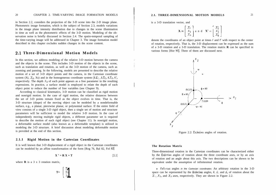
20 CHAPTER 2. TIME-VARYING IMAGE FORMATION MODELS
in Section 2.2, considers the projection of the 3-D scene into the 2-D image plane.Photometric image formation, which is the subject of Section 2.3, models variationsin the image plane intensity distribution due to changes in the scene illuminationin time as well as the photometric effects of the 3-D motion. Modeling of the ob-servation noise is briefly discussed in Section 2.4. The spatio-temporal sampling ofthe time-varying image will be addressed in Chapter 3. The image formation modeldescribed in this chapter excludes sudden changes in the scene content.
2.1 Three-Dimensional Motion Models
In this section, we address modeling of the relative 3-D motion between the cameraand the objects in the scene. This includes 3-D motion of the objects in the scene,such as translation and rotation, as well as the 3-D motion of the camera, such aszooming and panning. In the following, models are presented to describe the relativemotion of a set of 3-D object points and the camera, in the Cartesian coordinatesystem (Xi, Xz, Xs) and in the homogeneous coordinate system (/eXr ) leXz, leXs, lc),respectively. The depth Xs of each point appears as a free parameter in the resultingexpressions. In practice, a surface model is employed to relate the depth of eachobject point to reduce the number of free variables (see Chapter 9).
According to classical kinematics, 3-D motion can be classified as rigid motionand nonrigid motion. In the case of rigid motion, the relative distances betweenthe set of 3-D points remain fixed as the object evolves in time. That is, the3-D structure (shape) of the moving object can be modeled by a nondeformablesurface, e.g., a planar, piecewise planar, or polynomial surface. If the entire field ofview consists of a single 3-D rigid object, then a single set of motion and structureparameters will be sufficient to model the relative 3-D motion. In the case ofindependently moving multiple rigid objects, a different parameter set is requiredto describe the motion of each rigid object (see Chapter 11). In nonrigid motion,a deformable surface model (also known as a deformable template) is utilized inmodeling the 3-D structure. A brief discussion about modeling deformable motionis provided at the end of this section.
2.1.1 Rigid Motion in the Cartesian Coordinates
It is well known that 3-D displacement of a rigid object in the Cartesian coordinatescan be modeled by an affine transformation of the form [Rog 76, Bal 82, Fol 831
X ’ = R X + T (2.1)
where R is a 3 x 3 rotation matrix, TlT= Tz[ 1T3
2.1. THREE-DIMENSIONAL MOTION MODELS
is a 3-D translation vector, and
21
X= [::I a n d X’= [l]
denote the coordinates of an object point at times t and t’ with respect to the centerof rotation, respectively. That is, the 3-D displacement can be expressed as the sumof a 3-D rotation and a 3-D translation. The rotation matrix R can be specified invarious forms [Hor 861. Three of them are discussed next.
Figure 2.2: Eulerian angles of rotation.
The Rotation Matrix
Three-dimensional rotation in the Cartesian coordinates can be characterized eitherby the Eulerian angles of rotation about the three coordinate axes, or by an axisof rotation and an angle about this axis. The two descriptions can be shown to beequivalent under the assumption of infinitesimal rotation.
l Eulerian angles in the Cartesian coordinates: An arbitrary rotation in the 3-Dspace can be represented by the Eulerian angles, 0, $, and 4, of rotation about theX1, X2, and Xs axes, respectively. They are shown in Figure 2.2.
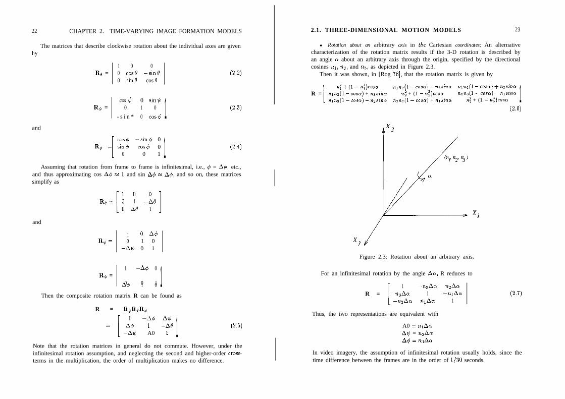
22 CHAPTER 2. TIME-VARYING IMAGE FORMATION MODELS
The matrices that describe clockwise rotation about the individual axes are givenby
R. =
Rti =
1 0 00 cos0 -sin00 sin0 cos 0
cos * 0 sin11,0 1 0
- s i n * 0 cosII, 1(24
(2.3)
and
[
cos cp -sin4 0R$ = sin4 cosq4 0 (2.4)
0 0 1 1Assuming that rotation from frame to frame is infinitesimal, i.e., 4 = A4, etc.,
and thus approximating cos A4 u 1 and sin A+ m A4, and so on, these matricessimplify as
and
Ri =
1 -A4 0Rd =
A$ 1 00 0 1 1Then the composite rotation matrix R can be found as
1 0 A40 1 0
-A$ 0 1
R = R6RoRI
1 -A4 AlClZ 4 1 -A0 1 (2.5)
-A$ A0 I
Note that the rotation matrices in general do not commute. However, under theinfinitesimal rotation assumption, and neglecting the second and higher-order cross-terms in the multiplication, the order of multiplication makes no difference.
2.1. THREE-DIMENSIONAL MOTION MODELS 23
l Rotation about an arbitrary axis in the Cartesian coordinates: An alternativecharacterization of the rotation matrix results if the 3-D rotation is described byan angle a about an arbitrary axis through the origin, specified by the directionalcosines n1, n2, and ns, as depicted in Figure 2.3.
Then it was shown, in [Rog 761, that the rotation matrix is given by
n: + (1 - nf)cosCY nlnz(l - cosa) - n3sina nlns(l - cosa) + n~sincuR = nlna(l - cm(~) + n3sina n$ + (1 - n~)cosa nznz(l - coscx) - nlsina
n~ns(l -cost) - n2sina n2n3(1 - COSCY) + nlsina nz + (1 - 7ai)co.m 1(2.6)
AX2
Figure 2.3: Rotation about an arbitrary axis.
For an infinitesimal rotation by the angle Aa, R reduces to
[
1 -nsAol nzAaR = nsAa 1 -nlAa
-nzAcu n,Aa 1
Thus, the two representations are equivalent with
A0 = nlAaA$ = nzAcrA4 = nsAa
(2.7)
In video imagery, the assumption of infinitesimal rotation usually holds, since thetime difference between the frames are in the order of l/30 seconds.
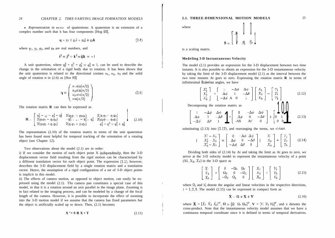
24 CHAPTER 2. TIME-VARYING IMAGE FORMATION MODELS 2.1. THREE-DIMENSIONAL MOTION MODELS
l Representation in terms of quaternions: A quaternion is an extension of acomplex number such that it has four components [Hog 921,
q = m + qli + a$ + q&
where qo, qi, qz, and 4s are real numbers, and
(2.8)
i2 = j2 = k2 = ijk = -1
A unit quaternion, where qi + q: + qz $ qi = 1, can be used to describe thechange in the orientation of a rigid body due to rotation. It has been shown thatthe unit quaternion is related to the directional cosines nr, n2, n3 and the solidangle of rotation cy in (2.6) as [Hor 861
n1 sin(a/2)
q=n2 sin(cu/2)123 sin(o/2)cos(o!/2)
(2.9)
The rotation matrix R can then be expressed as
d - 42 - 4’; -d 2(qon+qzq3) QOP:, - qlP3)
R = 2(qoql - qm) -d + a : - 422 + 432 2(q1qa + Q-043) (2.10)qqoqz + 4143) 2hq2 - qoq3) -d-G+Q;+d
1The representation (2.10) of the rotation matrix in terms of the unit quaternionhas been found most helpful for temporal tracking of the orientation of a rotatingobject (see Chapter 12).
Two observations about the model (2.1) are in order:i) If we consider the motion of each object point X independent,ly, then the 3-Ddisplacement vector field resulting from the rigid motion can be characterized bya different translation vector for each object point. The expression (2.1), however,describes the 3-D displacement field by a single rotation matrix and a translationvector. Hence, the assumption of a rigid configuration of a set of 3-D object pointsis implicit in this model.ii) The effects of camera motion, as opposed to object motion, can easily be ex-pressed using the model (2.1). The camera pan constitutes a special case of thismodel, in that it is a rotation around an axis parallel to the image plane. Zooming isin fact related to the imaging process, and can be modeled by a change of the focallength of the camera. However, it is possible to incorporate the effect of zoominginto the 3-D motion model if we assume that the camera has fixed parameters butthe object is artificially scaled up or down. Then, (2.1) becomes
X ’ = S R X + T (2.11)
where s1 0 0s= [ 0 s2 00 0 s, 1is a scaling matrix.
25
Modeling 3-D Instantaneous Velocity
The model (2.1) provides an expression for the 3-D displacement between two timeinstants. It is also possible to obtain an expression for the 3-D instantaneous velocityby taking the limit of the 3-D displacement model (2.1) as the interval between thetwo time instants At goes to zero. Expressing the rotation matrix R in terms ofinfinitesimal Eulerian angles, we have
X; = A4 1 -:,][;y+[;] (2.12)
Xh -A$ A 0
Decomposing the rotation matrix as
[
1 -A4 A$Ad 1 -A@ = A4 0-A$ AQ 1 1 [ 0 -Ad A$ 1 0 0
-A8 + 0 1 0I[ 1 (2.13)-A$ At’ 0 0 0 1
substituting (2.13) into (2.12)) and rearranging the terms, we obta.in
[ g!;;]=[ ;$ ?-@’ !fQ] [ :i]+[ ;] (2.14)
Dividing both sides of (2.14) by At and taking the limit as At goes to zero, wearrive at the 3-D velocity model to represent the instantaneous velocity of a point(Xl, X2, Xs) in the 3-D space as
Xl[:I [x2 = i, ,%” “I[ %lj+[ ;] (2.15)
x3
where sli and Vi denote the angular and linear velocities in the respective directions,i = 1,2,3. The model (2.15) can be expressed in compact form as
X=~xX+V (2.16)
where x = [Xi X2 &IT, 0 = [fir Qz Q,#, V = [VI Vz V31T, and x denotes thecross-product. Note that the instantaneous velocity model assumes that we have acontinuous temporal coordinate since it is defined in terms of temporal derivatives.
26 CHAPTER 2. TIME-VARYING IMAGE FORMATION MODELS
2.1.2 Rigid Motion in the Homogeneous Coordinates
We define the homogeneous coordinate representation of a Cartesian pointX = [X1X2X3]* as
(2.17)
Then the affine transformation (2.11) in the Cartesian coordinates can be ex-pressed as a linear transformation in the homogeneous coordinates
x’, = AXI, (2.18)
where
A= 1 all a12 a13 TI41 a22 a23 TZa31 a32 a33 T3
0 0 0 1 1and the matrix A
Translation in the Homogeneous Coordinates
Translation can be represented as a matrix multiplication in the homogeneous co-ordinates given by
where
x; = TXh (2.19)
1 0 0 Tr
T= [ 0 1 0 T2
0 0 1 T30 0 0 1 1
is the translation matrix.
Rotation in the Homogeneous Coordinates
Rotation in the homogeneous coordinates is represented by a 4 x 4 matrix multi-plication in the form
x;, = l%Xh (2.20)
2.1. THREE-DIMENSIONAL MOTION MODELS
where
27
and rij denotes the elements of the rotation matrix R in the Cartesian coordinates
Zooming in the Homogeneous Coordinates
The effect of zooming can be incorporated into the 3-D motion model as
x; = sx, (2.21)
where
2.1.3 Deformable Motion
Modeling the 3-D structure and motion of nonrigid objects is a complex task. Anal-ysis and synthesis of nonrigid motion using deformable models is an active researcharea today. In theory, according to the mechanics of deformable bodies [Som 501,the model (2.1) can be extended to include 3-D nonrigid motion as
X ’ = ( D + R ) X + T (2.22)
where D is an arbitrary deformation matrix. Note that the elements of the rotationmatrix are constrained to be related to the sines and cosines of the respective angles,whereas the deformation matrix is not constrained in any way. The problem withthis seemingly simple model arises in defining the D matrix to represent the desireddeformations.
Some examples of the proposed 3-D nonrigid motion models include those basedon free vibration or deformation modes [Pen 9la] and those based on constraintsinduced by intrinsic and extrinsic forces [Ter @a]. Pentland et ~2. [Pen 91a] param-eterize nonrigid motion in terms of the eigenvalues of a finite-element model of thedeformed object. The recovery of 3-D nonrigid motion using this model requires theknowledge of the geometry of the undeformed object. Terzopoulos el ab. [Ter SSa]have exploited two intrinsic constraints to design deformable models: surface coher-ence and symmetry seeking. The former is inherent in the elastic forces prescribedby the physics of deformable continua, and the latter is an attribute of many naturaland synthetic objects. Terzopoulos and Fleischer [Ter 88b] also proposed a phys-ically based modeling scheme using mechanical laws of continuous bodies whose

28 CHAPTER 2. TIME-VARYING IMAGE FORMATION MODELS 2.2. GEOMETRIC IMAGE FORMATION
shapes vary in time. They included physical features, such as mass and damping,in their models in order to simulate the dynamics of deformable objects in responseto applied forces. Other models include the deformable superquadrics [Ter 911 andextensions of the physically based framework [Met 931. The main applications ofthese models have been in image synthesis and animation.
A simple case of 3-D nonrigid models is that of flexibly connected rigid patches,such as a wireframe model where the deformation of the nodes (the so-called localmotion) is allowed. In this book, we will consider only 2-D deformable models thatis, the effect of various deformations in the image plane; except for the simple caseof 3-D flexible wireframe models, that are discussed in Chapter 24.
2.2 Geometric Image Formation
Imaging systems capture 2-D projections of a time-varying 3-D scene. This projec-tion can be represented by a mapping from a 4-D space to a 3-D space,
f: R4 + R3
(Xl,Xz,X3,q + (Xl,XZ,~) (2.23)
where (Xi,Xz,Xs), the 3-D world coordinates, (zi, Q), the 2-D image plane co-ordinates, and t, time, are continuous variables, Here, we consider two types ofprojection, perspective (central) and orthographic (parallel), which are described inthe following.
Figure 2.4: Perspective projection model.
2.2.1 Perspective Projection
where f denotes the distance from the center of projection to the image plane.If we move the center of projection to coincide with the origin of the world
coordinates, a simple change of variables yields the following equivalent expressions:
Perspective projection reflects image formation using an ideal pinhole camera ac-cording to the principles of geometrical optics. Thus, all the rays from the objectpass through the center of projection, which corresponds to the center of the lens.For this reason, it is also known as “central projection.” Perspective projection isillustrated in Figure 2.4 when the center of projection is between the object and theimage plane, and the image plane coincides with the (Xi, X2) plane of the worldcoordinate system.
.fXlx1 = x3
a n d 22 = fxzx3
The algebraic relations that describe the perspective transformation for the con-figuration shown in Figure 2.4 can be obtained based on similar triangles formedby drawing perpendicular lines from the object point (Xi, X2, Xs) and the imagepoint (21) x2,0) to the Xs axis, respectively. This leads to
The configuration and the similar triangles used to obtain these expressions areshown in Figure 2.5, where the image plane is parallel to the (Xl, X2) plane of theworld coordinate system. Observe that the latter expressions can also be employedas an approximate model for the configuration in Figure 2.4 when Xs >> f withthe reversal of the sign due to the orientation of the image being the same as theobject, as opposed to being a mirror image as in the actual image formation. Thegeneral form of the perspective projection, when the image plane is not parallel tothe (Xl ) X2) plane of the world coordinate system, is given in [Ver 891.
or
Xl Xl X2 x2-= - - - -f X3-f and f = X3-f
We note that the perspective projection is nonlinear in the Cartesian coordinatessince it requires division by the Xs coordinate. However, it can be expressed as alinear mapping in the homogeneous coordinates, as
fX1x1= f-X3
fX2and x2 = ,f-x3 (2.24)
29
(2.25)
(2.26)
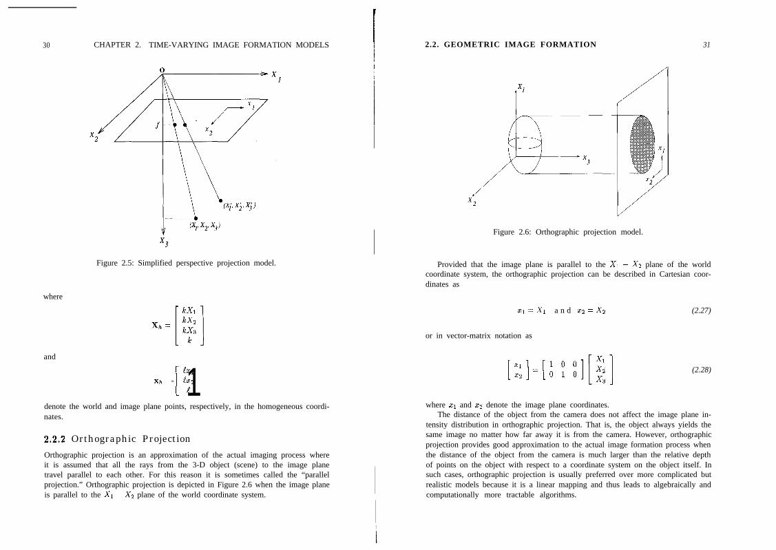
30 CHAPTER 2. TIME-VARYING IMAGE FORMATION MODELS
Figure 2.5: Simplified perspective projection model.
where
and
lx1
xh = lx2[ 1edenote the world and image plane points, respectively, in the homogeneous coordi-nates.
2.2.2 Orthographic Projection
Orthographic projection is an approximation of the actual imaging process whereit is assumed that all the rays from the 3-D object (scene) to the image planetravel parallel to each other. For this reason it is sometimes called the “parallelprojection.” Orthographic projection is depicted in Figure 2.6 when the image planeis parallel to the Xr - X2 plane of the world coordinate system.
2.2. GEOMETRIC IMAGE FORMATION 31 ~
Figure 2.6: Orthographic projection model.
Provided that the image plane is parallel to the X1 - Xs plane of the worldcoordinate system, the orthographic projection can be described in Cartesian coor-dinates as
Xl = x1 a n d x2=X2 (2.27)
or in vector-matrix notation as
[::]=[t Y :I[;;] (2.28)
where x1 and x2 denote the image plane coordinates.The distance of the object from the camera does not affect the image plane in-
tensity distribution in orthographic projection. That is, the object always yields thesame image no matter how far away it is from the camera. However, orthographicprojection provides good approximation to the actual image formation process whenthe distance of the object from the camera is much larger than the relative depthof points on the object with respect to a coordinate system on the object itself. Insuch cases, orthographic projection is usually preferred over more complicated butrealistic models because it is a linear mapping and thus leads to algebraically andcomputationally more tractable algorithms.
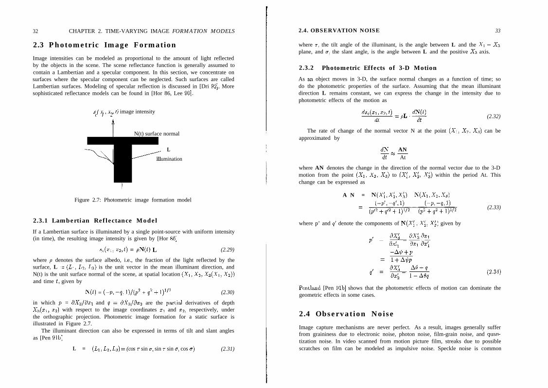
32 CHAPTER 2. TIME-VARYING IMAGE FORMATION MODELS
2.3 Photometric Image Formation
Image intensities can be modeled as proportional to the amount of light reflectedby the objects in the scene. The scene reflectance function is generally assumed tocontain a Lambertian and a specular component. In this section, we concentrate onsurfaces where the specular component can be neglected. Such surfaces are calledLambertian surfaces. Modeling of specular reflection is discussed in [Dri 921. Moresophisticated reflectance models can be found in [Hor 86, Lee 901.
s,( ai , x2, t) image intensity
f N(t) surface normal
L
illumination
Figure 2.7: Photometric image formation model
2.3.1 Lambertian Reflectance Model
If a Lambertian surface is illuminated by a single point-source with uniform intensity(in time), the resulting image intensity is given by [Hor 861
~,(a, xz,t) = pN(t) L (2.29)
where p denotes the surface albedo, i.e., the fraction of the light reflected by thesurface, L = (~51, Lz, ~5s) is the unit vector in the mean illuminant direction, andN(t) is the unit surface normal of the scene, at spatial location (Xl, Xx, X3(X1, X2))and time t, given by
N(t) = (-P, -9, l)/(p2 + q2 + 1)1’2 (2.30)
in which p = dXs/dxl and q = &&/?I 22 are the padtial derivatives of depthX3(x1, za) with respect to the image coordinates x1 and ~2, respectively, underthe orthographic projection. Photometric image formation for a static surface isillustrated in Figure 2.7.
The illuminant direction can also be expressed in terms of tilt and slant anglesas [Pen 91b]
L = (Ll, L2, L3) = (cos T sin q, sin r sin U, cos u) (2.31)
2.4. OBSERVATION NOISE 33
where 7, the tilt angle of the illuminant, is the angle between L and the X1 - Xsplane, and u, the slant angle, is the angle between L and the positive X3 axis.
2.3.2 Photometric Effects of 3-D Motion
As aa object moves in 3-D, the surface normal changes as a function of time; sodo the photometric properties of the surface. Assuming that the mean illuminantdirection L remains constant, we can express the change in the intensity due tophotometric effects of the motion as
(2.32)
The rate of change of the normal vector N at the point (Xl, X2, X3) can beapproximated by
dN AN-GMdt At
where AN denotes the change in the direction of the normal vector due to the 3-Dmotion from the point (Xl, X2, X3) to (Xl, Xi, Xi) within the period At. Thischange can be expressed as
A N = N(X;,X;,X;)-N(X~,X~,XS)
where p’ and Q’ denote the components of N(X{ ) Xi, X;) given by
ax; ax; ax1p’ = ad -Kdz;
-&+p= ~+A$JP
Q’ = ax; M+qax, -
2 l-A@
(2.33)
Pentland [Pen 91b] shows that the photometric effects of motion can dominate thegeometric effects in some cases.
2.4 Observation Noise
Image capture mechanisms are never perfect. As a result, images generally sufferfrom graininess due to electronic noise, photon noise, film-grain noise, and quan-tization noise. In video scanned from motion picture film, streaks due to possiblescratches on film can be modeled as impulsive noise. Speckle noise is common
34 CHAPTER 2. TIME-VARYING IMAGE FORMATION MODELS
in radar image sequences and biomedical tine-ultrasound sequences. The availablesignal-to-noise ratio (SNR) varies with the imaging devices and image recording me-dia. Even if the noise may not be perceived at full-speed video due to the temporalmasking effect of the eye, it often leads to poor-quality “freeze-frames.”
The observation noise in video can be modeled as additive or multiplicativenoise, signal-dependent or signal-independent noise, and white or colored noise. Forexample, photon and film-grain noise are signal-dependent, whereas CCD sensor andquantization noise are usually modeled as white, Gaussian distributed, and signal-independent. Ghosts in TV images can also be modeled as signal-dependent noise.In this book, we will assume a simple additive noise model given by
gc(xl,xz,t) = s,(z1,xz,t) + v,(x1,xa,t) (2.35)
where se(xl, x2, t) and u,(xl,x2,t) denote the ideal video and noise at time t,respectively.
The SNR is an important parameter for most digital video processing applica-tions, because noise hinders our ability to effectively process the data. For example,in 2-D and 3-D motion estimation, it is very important to distinguish the variationof the intensity pattern due to motion from that of the noise. In image resolutionenhancement, noise is the fundamental limitation on our ability to recover high-frequency information. Furthermore, in video compression, random noise increasesthe entropy hindering effective compression. The SNR of video imagery can be en-hanced by spatio-temporal filtering, also called noise filtering, which is the subjectof Chapter 14.
2 . 5
1.
2.
3.
4.
5.
6.
7.
Exercises
Suppose a rotation by 45 degrees about the X2 axis is followed by anotherrotation by 60 degrees about the X1 axis. Find the directional cosines 121, 712,ns and the solid angle (Y to represent the composite rotation.
Given a triangle defined by the points (l,l,l), (l,-1,0) and (0,1,-l). Find thevertices of the triangle after a rotation by 30 degrees about an axis passingthrough (O,l,O) which is parallel to the X1 axis.
Show that a rotation matrix is orthonormal.
Derive Equation (2.6).
Show that the two representations of the rotation matrix R given by (2.6)and (2.10) are equivalent.
Discuss the conditions under which the orthographic projection provides agood approximation to imaging through an ideal pinhole camera.
Show that the expressions for p’ and q’ in (2.34) are valid under the ortho-graphic projection.
BIBLIOGRAPHY
Bibliography
35
[Bal 821
[Dri 921
[Fol 831
[Hog 921
[Hor 861
[Lee 901
[Met 931
[Pen 9la]
[Pen 91b]
[Rag 761
[Som 501
[Ter SSa]
[Ter 88b]
[Ter 911
[Ver 891
D. H. Ballard and C. M. Brown, Computer Vision, Englewood Cliffs, NJ:Prentice-Hall, 1982.
J. N. Driessen, Motion Edimation for Digital Video, Ph.D. Thesis,Delft University of Technology, 1992.
J. D. Foley and A. Van Dam, Fundamen2als of Interactive ComputerGraphics, Reading, MA: Addison-Wesley, 1983.
S. G. Hoggar, Mathematics for Computer Graphics, CambridgeUniversity Press, 1992.
B. K. P. Horn, Robot Vision, Cambridge, MA: MIT Press, 1986.
H. C. Lee, E. J. Breneman, and C. P. Schutte, “Modeling light reflec-tion for computer color vision,” IEEE Trans. Putt. Anal. Mach. Intel.,vol. PAMI-12, pp. 402-409, Apr. 1990.
D. Metaxas and D. Terzopoulos, “Shape and nonrigid motion estimationthrough physics-based synthesis,” IEEE Trans. Patt. Anal. Mach. Intel.,vol. 15, pp. 580-591, June 1993.
A. Pentland and B. Horowitz, “Recovery of nonrigid motion and struc-ture,” IEEE Trans. Putt. Anal. Mach. Intel., vol. 13, pp. 730~742, 1991.
A. Pentland, “Photometric motion,” IEEE Trans. Putt. Anal. Mach.Mel., vol. PAMI-13, pp. 879-890, Sep. 1991.
D. F. Rogers and J. A. Adams, Mathematical Elements for ComputerGraphics, New York, NY: McGraw Hill, 1976.
A. Sommerfeld, Mechanics of Deformable Bodies, 1950.
D. Terzopoulos, A. Witkin, and M. Kass, “Constraints on deformablemodels: Recovering 3-D shape and nonrigid motion,” Artif. Intel.,
vol. 36, pp. 91-123, 1988.
D. Terzopoulos and K. Fleischer, “Deformable models,” Visual Comput.,vol. 4, pp. 306~331, 1988.
D. Terzopoulos and D. Metaxas, “Dynamic 3-D models with local andglobal deformations: Deformable superquadrics,” IEEE Trans. Putt.Anal. Mach. Intel., vol. PAMI-13, pp. 703-714, July 1991.
A. Verri and T. Poggio, “Motion field and optical flow: Qualita-tive properties,” IEEE Trans. Putt. Anal. Mach. Intel., vol. PAMI-11,pp. 490-498, May 1989.

Chapter 3
SPATIO-TEMPORALSAMPLING
In order to obtain an analog or digital video signal representation, the continuoustime-varying image s,(z~, x2, t) needs to be sampled in both the spatial and tempo-ral variables. An analog video signal representation requires sampling s,(z~) x2, t)
in the vertical and temporal dimensions. Recall that an analog video signal is a1-D continuous function, where one of the spatial dimensions is mapped onto timeby means of the scanning process. For a digital video representation, s,(xl s czi t)
is sampled in all three dimensions. The spatio-temporal sampling process is de-picted in Figure 3.1, where (nl, n2, %) denotes the discrete spatial and temporalcoordinates, respectively.
sJ”1, x,J., Spaho-Temporal
S a m p l i n g --)shlj nZ k )
Figure 3.1: Block diagram.
Commonly used 2-D and 3-D sampling structures for the representation of ana-log and digital video are shown in Section 3.1. Next, we turn our attention to thefrequency domain characterization of sampled video. In order to motivate the mainprinciples, we start with the sampling of still images. Section 3.2 covers the case ofsampling on a 2-D rectangular grid, whereas Section 3.3 treats sampling on arbitrary2-D periodic grids. In Section 3.4, we address extension of this theory to sampling of
36
3.1. SAMPLING FOR ANALOG AND DIGITAL VIDEO 37
multidimensional signals on lattices and other periodic sampling structures. How-ever, the discussion is limited to sampling of spatio-temporal signals s,(x~, ~2, t) on3-D lattices, considering the scope of the book. Finally, Section 3.5 addresses thereconstruction of continuous time-varying images from spatio-temporally sampledrepresentations. The reader is advised to review the remarks about the notationused in this book on page xxi, before proceeding with this chapter.
3.1 Sampling for Analog and Digital Video
Some of the more popular sampling structures utilized in the representation ofanalog and digital video are introduced in this section.
3.1.1 Sampling Structures for Analog Video
An analog video signal is obtained by sampling the time-varying image intensitydistribution in the vertical x2, and temporal t directions by a 2-D sampling processknown as scanning. Continuous intensity information along each horizontal lineis concatenated to form the 1-D analog video signal as a function of time. Thetwo most commonly used vertical-temporal sampling structures are the orthogonalsampling structure, shown in Figure 3.2, and the hexagonal sampling structure,depicted in Figure 3.3.
v =
Figure 3.2: Orthogonal sampling structure for progressive analog video.
In these figures, each dot indicates a continuous line of video perpendicular tothe plane of the page. The matrices V shown in these figures are called the samplingmatrices, and will be defined in Section 3.3. The orthogonal structure is used inthe representation of progressive analog video, such as that shown on workstation
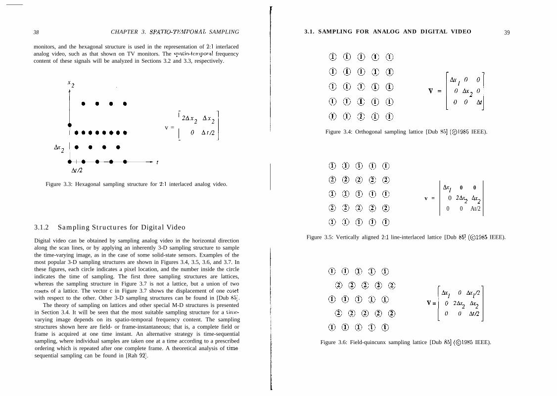
38 CHAPTER 3. SPATIO-TEMPORAL SAMPLING
monitors, and the hexagonal structure is used in the representation of 2:l interlacedanalog video, such as that shown on TV monitors. The spatio-temporal frequencycontent of these signals will be analyzed in Sections 3.2 and 3.3, respectively.
t 0 0 0 0 v =0 0 0 0
Figure 3.3: Hexagonal sampling structure for 2:l interlaced analog video.
3.1.2 Sampling Structures for Digital Video
Digital video can be obtained by sampling analog video in the horizontal directionalong the scan lines, or by applying an inherently 3-D sampling structure to samplethe time-varying image, as in the case of some solid-state sensors. Examples of themost popular 3-D sampling structures are shown in Figures 3.4, 3.5, 3.6, and 3.7. Inthese figures, each circle indicates a pixel location, and the number inside the circleindicates the time of sampling. The first three sampling structures are lattices,whereas the sampling structure in Figure 3.7 is not a lattice, but a union of twocosets of a lattice. The vector c in Figure 3.7 shows the displacement of one cosetwith respect to the other. Other 3-D sampling structures can be found in [Dub 851.
The theory of sampling on lattices and other special M-D structures is presentedin Section 3.4. It will be seen that the most suitable sampling structure for a time-varying image depends on its spatio-temporal frequency content. The samplingstructures shown here are field- or frame-instantaneous; that is, a complete field orframe is acquired at one time instant. An alternative strategy is time-sequentialsampling, where individual samples are taken one at a time according to a prescribedordering which is repeated after one complete frame. A theoretical analysis of time-sequential sampling can be found in [Rah 921.
3.1. SAMPLING FOR ANALOG AND DIGITAL VIDEO 39
Figure 3.4: Orthogonal sampling lattice [Dub 851 (01985 IEEE).
Ax1 0 0
v = 0 2Ax2 Ax2
0 0 At/2
Figure 3.5: Vertically aligned 2:l line-interlaced lattice [Dub 851 (01985 IEEE).
Figure 3.6: Field-quincunx sampling lattice [Dub 851 (01985 IEEE).
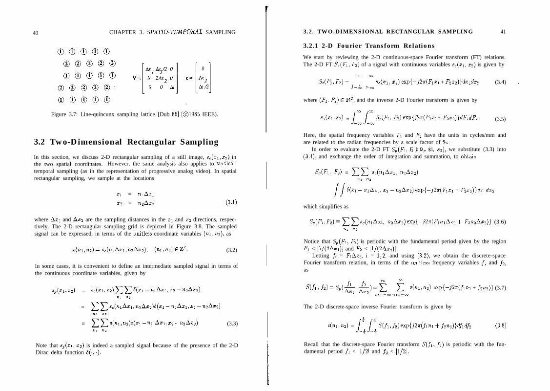
40 CHAPTER 3. SPATIO-TEMPORAL SAMPLING
r 7
0
i -
l?y12Art/2
Figure 3.7: Line-quincunx sampling lattice [Dub 851 (01985 IEEE).
3.2 Two-Dimensional Rectangular Sampling
In this section, we discuss 2-D rectangular sampling of a still image, s,(xi,xs) inthe two spatial coordinates. However, the same analysis also applies to vertical-temporal sampling (as in the representation of progressive analog video). In spatialrectangular sampling, we sample at the locations
21 = nlAx1x2 = nzAx2 (3.1)
where AZ, and Ax2 are the sampling distances in the xi and x2 directions, respec-tively. The 2-D rectangular sampling grid is depicted in Figure 3.8. The sampledsignal can be expressed, in terms of the unitless coordinate variables (nr, nz), as
s(nl,nz) = sc(n~Ax~,nzAxz), (nl,nz) E 2’. (3.2)
In some cases, it is convenient to define an intermediate sampled signal in terms ofthe continuous coordinate variables, given by
Sp(Xl,XZ) = sc(xl,x2)yy-)q x1 - nlAxl, x2 - nzAx2)721 n2
= c Cs,(nlAxl, nzAxc2)6(xl- nlAx:1, x2 - wAxa)n1 na
= cc s(nl, nz)6(xl - nl Axl, xz - nzAxz) (3.3)la1 nz
Note that sp(xi, x2) is indeed a sampled signal because of the presence of the 2-DDirac delta function S(., .).
3.2. TWO-DIMENSIONAL RECTANGULAR SAMPLING
3.2.1 2-D Fourier Transform Relations
41
We start by reviewing the 2-D continuous-space Fourier transform (FT) relations.The 2-D FT S,(Fi, Fs) of a signal with continuous variables s,(xi, x2) is given by
co ccSc(~,,Fz)=
J ’ s5,(x1, x2) exp{-j2n(Fixi + Fzxs)}dxrdx2 (3.4) /
-co --oo
where (FL, Fz) E R2, and the inverse 2-D Fourier transform is given by
00 cc%(%X2) =
ss&(FI, Fz) exp{jZ~(Flxl + Fzxz)}~FI~Fz (3.5)
-cc -‘xl
Here, the spatial frequency variables Fi and Fz have the units in cycles/mm andare related to the radian frequencies by a scale factor of 2n.
In order to evaluate the 2-D FT Sp(Fl, F ) f2 o sp xi, x2), we substitute (3.3) into((3.4), and exchange the order of integration and summation, to obt,ain
SdFl, Fz) = cc s,(nlAxl, nbxz)nl 02
J’s 6(x1 - nlAxl, 22 - nzAxz) exp{-j2n(Frxi + F~x~)}dx~d2~
which simplifies as
S,(FI,FZ) = zxs,(nlAxi, n4Axz)exp{-j2~(Fl’lnlAxl+ FznsAxz)} (3.6)nl n*
Notice that S,(Fl) Fs) is periodic with the fundamental period given by the regionFI < ]1/(2Axi)] and FZ < ]1/(2Axs)].
Letting fi = FiAxi, i = 1,2, and using (3.2), we obtain the discrete-spaceFourier transform relation, in terms of the unitless frequency variables fi and ~“2,as
s(fr 1 f2) = .S,(&, &) = 2 5 s(nl, n2) exp{-j2Qinl + fin2)) (3.7)n1=-cc nz=-cc
The 2-D discrete-space inverse Fourier transform is given by
i
J’s
4s(nl, n2) = S(fi,f2)exp{.Q~(fin1 -I- finz))GiG2
-4 -+ (3.8)
Recall that the discrete-space Fourier transform S(fi, fs) is periodic with the fun-damental period fi < ]1/2( and f2 < ]1/2].
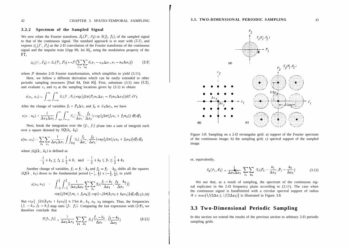
42 CHAPTER 3. SPATIO-TEMPORAL SAMPLING
3.2.2 Spectrum of the Sampled Signal
We now relate the Fourier transform, S,(Fi, Fz) or S(fi, fi), of the sampled signalto that of the continuous signal. The standard approach is to start with (3.3), andexpress S,(Fi, Fz) as the 2-D convolution of the Fourier transforms of the continuoussignal and the impulse train [Opp 89, Jai 901, using the modulation property of theFT,
where ?= denotes 2-D Fourier transformation, which simplifies to yield (3.11).Here, we follow a different derivation which can be easily extended to other
periodic sampling structures [Dud 84, Dub 851. First, substitute (3.5) into (3.2),and evaluate zi and x2 at the sampling locations given by (3.1) to obtain
After the change of variables fi = FlAxi and fi = FzAxs, we have
s(n1, n2) = -L00 cc
ssAxlAxz --oo m-00 .‘4&, #-I ewW%flnl+ fm)) dfldfz
Next, break the integration over the (fl, f2) plane into a sum of integrals eachover a square denoted by SQ(ki) kz),
where SQ(ki ) k2) is defined as
Another change of variables, fi = fi -ICI and f2 = f2 - k2, shifts all the squaresSQ(ki, ka) down to the fundamental period c-f, $) x (-5, f), to yield
exp{.Q~(flnl + fm)} exp{-j2r(klnl + km)}dfidh (3.10)
But exp{-j2z(kini + kznz)} = l‘for ki, k2, ni, n2 integers. Thus, the frequencies(fl - kl, fz - k2) map onto (fl, fi). Comparing the last expression with (3.8), wetherefore conclude that
S(fl,fi) = -&-& p s&$, G)
1 k2
3.3. TWO-DIMENSIONAL PERIODIC SAMPLING 43
0 0 l 0
(W
Figure 3.8: Sampling on a 2-D rectangular grid: a) support of the Fourier spectrumof the continuous image; b) the sampling grid; c) spectral support of the sampledimage.
or, equivalently,
sp(F~,Fz) = Ax cc S,(ll;-32-&Ax2 kl ka
(3.12)
We see that, as a result of sampling, the spectrum of the continuous sig-nal replicates in the 2-D frequency plane according to (3.11). The case whenthe continuous signal is bandlimited with a circular spectral support of radiusB < max{l/(2Azi), 1/(2A22)} is illustrated in Figure 3.8.
3.3 Two-Dimensional Periodic SamplingIn this section we extend the results of the previous section to arbitrary 2-D periodicsampling grids.

44 CHAPTER 3. SPATIO-TEMPORAl. SAMPLING
3.3.1 Sampling Geometry
An arbitrary 2-D periodic sampling geometry can be defined by two basis vectorsvr = (~1 ~21)~ and vz = (U ~zz)~, such that every sampling location can beexpressed as a linear combination of them, given by
x1 = VII~I + v12n2
x2 = v21nl + v22n2 (3.13)
In vector-matrix form, we have
where
and
x=Vn (3.14)
x = (x1 ZZ)~, n = (721 nZ)T
v = [VllV21
is the sampling matrix. The sampling locations for an arbitrary periodic grid aredepicted in Figure 3.9.
Then, analogous to (3.2) and (3.3), the sampled signal can be expressed as
s(n) = se(Vn), n E Z2 (3.15)
or as
SP (4 = se(x) C 6(x-Vn)neZ2
= C s,(Vn)S(x - Vn) = C s(n)h(x - Vn) (3.16)n n
3.3.2 2-D Fourier Transform Relations in Vector Form
Here, we restate the 2-D Fourier transform relations given in Section 3.2.1 in a morecompact vector-matrix form as follows:
J’MS,(F) = se(x) exp{-j2rFTx} dx (3.17)
-cc
J
cc
SC(X) = S,(F) exp{j2rFTx} dF (3.18)-co
3.3. TWO-DIMENSIONAL PERIODIC SAMPLING 45
64
0 0 0 0 0
0 0
“10 0 0 0 0
a 0 b 0 0
(b)
Figure 3.9: Sampling on an arbitrary 2-D periodic grid: a) support of the Fourierspectrum of the continuous image; b) the sampling grid; c) spectral support of thesampled image.
where x = (21 2~)~ and F = (Fl Fz)~. We also have
S,(F) = 2 s,(Vn) exp{-j2TFTVn}n=-c0
01
S(f) = 2 s(n) exp{-j2rfTn}n=--co
(3.19)
(3.20)
J ts(n) = S(f) exp{j2afTn} df (3.21)
-$
where f = (fr f2)T. Note that the integrations and summations in these relationsare in fact double integrations and summations.
46 CHAPTER 3. SPATIO-TEMPORAL SAMPLING 3.4. SAMPLING ON 3-D STRUCTURES
3.3.3 Spectrum of the Sampled Signal
To derive the relationship between S(f) and Se(F), we follow the same steps as inSection 3.2. Thus, we start by substituting (3.18) into (3.15) as
sOcis(n) = s,(Vn) = Se(F) exp{j2rFTVn}dF
--co
Making the change of variables f = VTF, we have
sco
s(n) =-a, ,de:V,
-&(Uf) exp{j2afTn}df
where U = VT-l and df = IdetVldF.Expressing the integration over the f plane as a sum of integrations over the
squares (-l/2,1/2) x (-l/2, l/2), we obtain
s(n) = LS,(U(f - k)) exp{j2dTn} exp{-j2nkTn}df (3.22)
where exp{-j2nkTn} = 1 for k an integer valued vector.Thus, comparing this expression with (3.21), we conclude that
S(f) = & c SNf - k))k
or, equivalently,
s,(F) = & CS,(F - Uk)k
(3.23)
(3.24)
where the periodicity matrix in the frequency domain U satisfies
UTV=I (3.25)
and I is the identity matrix. The periodicity matrix can be expressed as U = [u~Iu~],where ~1 and u2 are the basis vectors in the 2-D frequency plane.
Note that this formulation includes rectangular sampling as a special case withthe matrices V and U being diagonal. The replications in the 2-D frequency planeaccording to (3.24) are depicted in Figure 3.9.
3.4 Sampling on 3-D StructuresThe concepts related to 2-D sampling with an arbitrary periodic geometry can bereadily extended to sampling time-varying images sc(xlt) = s,(Q, zz)t) on 3-Dsampling structures. In this section, we first elaborate on 3-D lattices, and thespectrum of 3-D signals sampled on lattices. Some specific non-lattice structuresare also introduced. The theory of sampling on lattices and other structures hasbeen generalized to M dimensions elsewhere [Dub 851.
47
3.4.1 Sampling on a Lattice
We start with the definition of a 3-D lattice. Let ~1, ~2, vs be linearly independentvectors in the 3-D Euclidean space R3. A lattice A3 in R3 is the set of all linearcombinations of ~1, ~2, and vs with integer coefficients
A3 = {nlvl+ n2vz + kv3 1 nl, 122, !f E Z)
The set of vectors ~1, ~2, and vg is called a basis for h3.In vector-matrix notation, a lattice can be defined as
(3.26)
h3={V ;I 1 1 n E Z2, k E Z} (3.27)
where V is called a 3 x 3 sampling matrix defined by
v = [Vl I vz I v31 (3.28)
The basis, and thus the sampling matrix? for a given lattice is not unique. Inparticular, for every sampling matrix V, V = EV, where E is an integer matrixwith detE = *l, forms another sampling matrix for A3. However, the quantityd(A3) = IdetVl is unique and denotes the reciprocal of the sampling density.
Then, similar to (3.15) and (3.16), the sampled spatio-temporal signal can beexpressed as
or as
s(n, Ic) = sc(V 1 1z ), (n,k) = (nl,nz,k) E Z3 (3.29)
dx,t) = s,(x;t)(n~Z 6([ 1x1 -v [ ;I)3
The observant reader may already have noticed that the 2-D sampling structuresdiscussed in Sections 3.2 and 3.3 are also lattices. Hence, Sections 3.2 and 3.3constitute special cases of the theory presented in this section.
3.4.2 Fourier Transform on a Lattice
Based on (3.19), we can define the spatio-temporal Fourier transform of +(x, t)jsampled on A3, as follows:
S,(F) = C sc(x,t) exp { -j2aFT [ y I}, F = [FI p2 FtlT E R3(X,t)EA3
= (34V [ F ]j exp {-%F’V [ F ]}
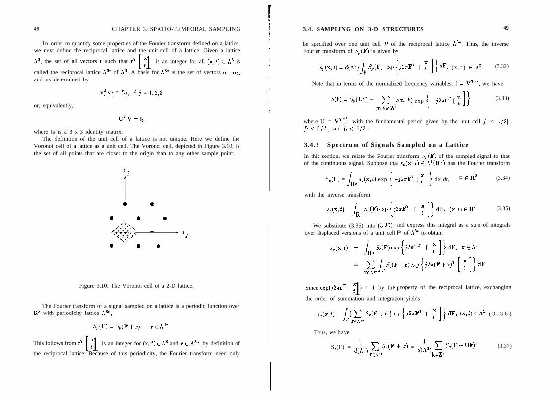
48 CHAPTER 3. SPATIO-TEMPORAL SAMPLING
In order to quantify some properties of the Fourier transform defined on a lattice,we next define the reciprocal lattice and the unit cell of a lattice. Given a lattice
A3, the set of all vectors r such that rT 1 1T is an integer for all (x,t) E A3 is
called the reciprocal lattice A3* of A3. A basis for A3* is the set of vectors ur, ~2,and us determined by
or, equivalently,
u;vj = &j, i,j = 1,2,3
UTV = I3
where Is is a 3 x 3 identity matrix.The definition of the unit cell of a lattice is not unique. Here we define the
Voronoi cell of a lattice as a unit cell. The Voronoi cell, depicted in Figure 3.10, isthe set of all points that are closer to the origin than to any other sample point.
@
0 0
‘1. m2’ >
x1
0 0
Figure 3.10: The Voronoi cell of a 2-D lattice.
The Fourier transform of a signal sampled on a lattice is a periodic function overR3 with periodicity lattice A3*,
S,(F)=S,(F+r), reA3*
This follows from rT 1 1F is an integer for (x, t) E A3 and r E A3*, by definition of
the reciprocal lattice. Because of this periodicity, the Fourier transform need only
3.4. SAMPLING ON 3-D STRUCTURES 49
be specified over one unit cell P of the reciprocal lattice A3*. Thus, the inverseFourier transform of S,(F) is given by
sp(x, t) = d(A3)sP
S,(F) exp{j2aFT [ ; ]}dF, (x ,t ) E A3 (3.32)
Note that in terms of the normalized frequency variables, f = VTF, we have
S(f) = SpWf) = cngz s(n, k) exp { -j2rfT [ E ] }3
(3.33)
where U = VT-l, with the fundamental period given by the unit cell fi < 11/21,fz < 11/21, and .ft < 11/21.
3.4.3 Spectrum of Signals Sampled on a Lattice
In this section, we relate the Fourier transform S,(F) of the sampled signal to thatof the continuous signal. Suppose that s,(x, t) E L1(R3) has the Fourier transform
Se(F) = S,, sc(x,t) exp { -j2aFT [ T ]} dx dt, F E R3 (3.34)
with the inverse transform
s&t) = J’R3Sc(F)exp{.i2iTFT [ ;]}dF; (x,t)ER3 (3.35)
We substitute (3.35) into (3.30), and express this integral as a sum of integralsover displaced versions of a unit cell P of A3* to obtain
sp(x,t) = J’ S,(F)exp{j2~FT [ F]>dF, xgA3
= g J’S,(F+r)exp{jZrr(F+r)‘[ ;]}dFrEh3* p
Since exp(j2mT [ 1; ) = 1 by the property of the reciprocal lattice, exchanging
the order of summation and integration yields
sp(x,t) = [SCp rcA3*Sc(F+r)]exp{j2rrFT [ ;]}dF, (x,t)EA3 ( 3 . 3 6 )
Thus, we have
S,(F) = -& c S,(F + r) = q& c SC(~+~~)rch3* kcZ3
(3.37)
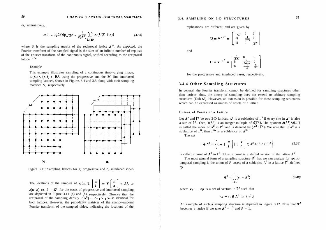
50 CHAPTER 3. SPATIO-TEMPORAL SAMPLING
or, alternatively,
S(f) = %dF)IF=Uf = q& c Sc(U(f +k))kcZ3
(3.38)
where U is the sampling matrix of the reciprocal lattice A3*. As expected, theFourier transform of the sampled signal is the sum of an infinite number of replicasof the Fourier transform of the continuous signal, shifted according to the reciprocallattice A3*.
Example
This example illustrates sampling of a continuous time-varying image,4x,4, (~4 E R3, using the progressive and the 2:l line interlacedsampling lattices, shown in Figures 3.4 and 3.5 along with their samplingmatrices V, respectively.
(a) (b)
Figure 3.11: Sampling lattices for a) progressive and b) interlaced video.
The locations of the samples of sp(x,t), [;]=V[i]Er\“,ors(n, k), (n, Ic) E Z3, for the cases of progressive and interlaced samplingare depicted in Figure 3.11 (a) and (b), respectively. Observe that thereciprocal of the sampling density d(A3) = AxlAxxAt is identical forboth lattices. However, the periodicity matrices of the spatio-temporalFourier transform of the sampled video, indicating the locations of the
3.4. SAMPLING ON 3-D STRUCTURES 51
replications, are different, and are given by
U=V-lT= [ c & !Jand
for the progressive and interlaced cases, respectively.
3.4.4 Other Sampling Structures
In general, the Fourier transform cannot be defined for sampling structures otherthan lattices; thus, the theory of sampling does not extend to arbitrary samplingstructures [Dub 851. However, an extension is possible for those sampling structureswhich can be expressed as unions of cosets of a lattice.
Unions of Cosets of a Lattice
Let A3 and I3 be two 3-D lattices. A3 is a sublattice of I3 if every site in A3 is alsoa site of 13. Then, d(h3) is an integer multiple of d(T3). The quotient d(A3)/d(13)is called the index of A3 in r3, and is denoted by (A3 : r3). We note that if A3 is asublattice of T3, then 13* is a sublattice of A3*.
The set
c+~s= {c+ [ ;] 1 [ ;] EA3andcE13) (3.39)
is called a coset of A3 in r3. Thus, a coset is a shifted version of the lattice A3.The most general form of a sampling structure Q3 that we can analyze for spatio-
temporal sampling is the union of P cosets of a sublattice A3 in a lattice r3, definedby
q3 = ij(c, + A3) (3.40)i=l
where cl, . , cp is a set of vectors in r3 such that
ci - ci 6 A3 for i # j
An example of such a sampling structure is depicted in Figure 3.12. Note that e3becomes a lattice if we take A3 = T3 and P = 1.
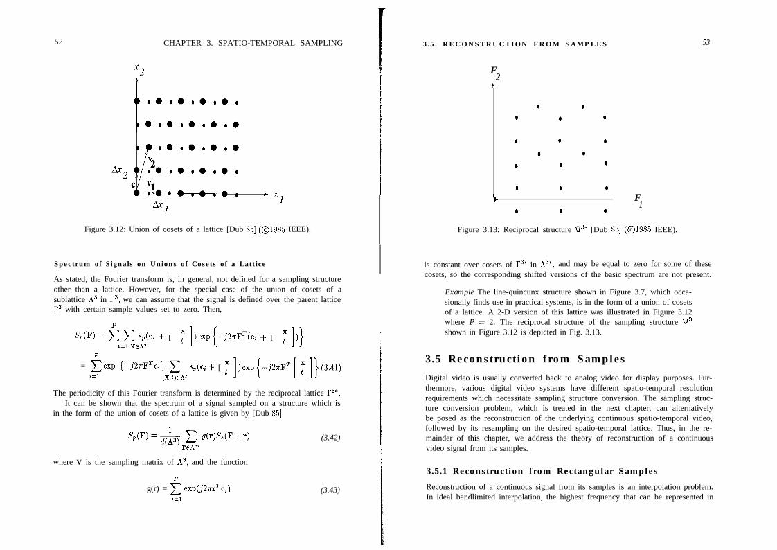
52 CHAPTER 3. SPATIO-TEMPORAL SAMPLING
>
%xl
Figure 3.12: Union of cosets of a lattice [Dub 851 (01985 IEEE).
Spectrum of Signals on Unions of Cosets of a Lattice
As stated, the Fourier transform is, in general, not defined for a sampling structureother than a lattice. However, for the special case of the union of cosets of asublattice A3 in F3, we can assume that the signal is defined over the parent latticeF3 with certain sample values set to zero. Then,
SPP’) = 5 C sp(ci + [ F ])rap{-j2rrFT(ei + [ T I)}i=l XC.43
= eexp {-j2=FTci} ci=l (X$)EA3
+(ci+ [ ;])exp{-j2sFT[ ;]}(3.41)
The periodicity of this Fourier transform is determined by the reciprocal lattice F3*.It can be shown that the spectrum of a signal sampled on a structure which is
in the form of the union of cosets of a lattice is given by [Dub 851
S,(F) = -& c drF@+r)l-Eli- (3.42)
where V is the sampling matrix of A3, and the function
g(r) = 5 exp(j2arTci)i=l
(3.43)
3.5. RECONSTRUCTION FROM SAMPLES
F2
A
La e 6
0 e 0
53
F1
Figure 3.13: Reciprocal structure Q3* [Dub 851 (01985 IEEE).
is constant over cosets of F3* in A3*, and may be equal to zero for some of thesecosets, so the corresponding shifted versions of the basic spectrum are not present.
Example The line-quincunx structure shown in Figure 3.7, which occa-sionally finds use in practical systems, is in the form of a union of cosetsof a lattice. A 2-D version of this lattice was illustrated in Figure 3.12where P = 2. The reciprocal structure of the sampling structure Q3shown in Figure 3.12 is depicted in Fig. 3.13.
3.5 Reconstruction from Samples
Digital video is usually converted back to analog video for display purposes. Fur-thermore, various digital video systems have different spatio-temporal resolutionrequirements which necessitate sampling structure conversion. The sampling struc-ture conversion problem, which is treated in the next chapter, can alternativelybe posed as the reconstruction of the underlying continuous spatio-temporal video,followed by its resampling on the desired spatio-temporal lattice. Thus, in the re-mainder of this chapter, we address the theory of reconstruction of a continuousvideo signal from its samples.
3.5.1 Reconstruction from Rectangular Samples
Reconstruction of a continuous signal from its samples is an interpolation problem.In ideal bandlimited interpolation, the highest frequency that can be represented in

54 CHAPTER 3. SPATIO-TEMPORAL SAMPLING 3.5 . RECONSTRUCTION FROM SAMPLES 55
the analog signal without aliasing, according to the Nyquist sampling theorem, isequal to one-half of the sampling frequency. Then, a continuous image, s,(zi, zz),can be reconstructed from its samples taken on a 2-D rectangular grid by ideallow-pass filtering as follows:
The support of the ideal reconstruction filter in the frequency domain is illustratedin Figure 3.14.
Figure 3.14: Reconstruction filter.
The reconstruction filter given by (3.44)is sometimes referred to as the ‘(idealbandlimited interpolation filter,” since the reconstructed image would be identicalto the original continuous image, that is
s, (Xl, x2) = %(X1, x2) (3.45)
provided that the original continuous image was bandlimited, and Ax, and Ax,were chosen according to the Nyquist criterion.
The ideal bandlimited interpolation filtering can be expressed in the spatialdomain by taking the inverse Fourier transform of both sides of (3.44)
&(X1, x2) &=J J*-1A&Ax2 S(FrAxr, FzAzz) exp{j2n(Fixi + F2~2)) dFldF’2
--1i7iq a&q
Substituting the definition of S(FiAxi, FzAxz) into this expression, and rearrang-ing the terms, we obtain
exp{j2s(Flxl + Fsa))dFldFz
= AxrAzz cc s(nl, nz)h(xi - niAxr, z2 - nzAx2)nl na
(3.46)
where h(xi, x2) denotes the impulse response of the ideal interpolation filter for thecase of rectangular sampling, given by
qx1, x2) =sin (&xi) sin (&x2)
&“I 23(3.47)
3 . 5 . 2 Reconstruction from Samples on a Lattice
Similar to the case of rectangular sampling, the reconstructed time-varying images,(x, t) can be obtained through the ideal low-pass filtering operation
S,(F) =jdetVIS(VTF) for F E P
0 otherwise.
Here, the passband of the ideal low-pass filter is determined by the unit cell P ofthe reciprocal sampling lattice.
Taking the inverse Fourier transform, we have the reconstructed time-varyingimage
where
h(x,t) = \detVI k exp { j2rFT [ T ] } dF
(3.48)
(3.49)
is the impulse response of the ideal bandlimited spatio-temporal interpolation filterfor the sampling structure used. Unlike the case of rectangular sampling, thisintegral, in general, cannot be reduced to a simple closed-form expression. Asexpected, exact reconstruction of a continuous signal from its samples on a latticeA3 is possible if the signal spectrum is confined to a unit cell P of the reciprocallattice.
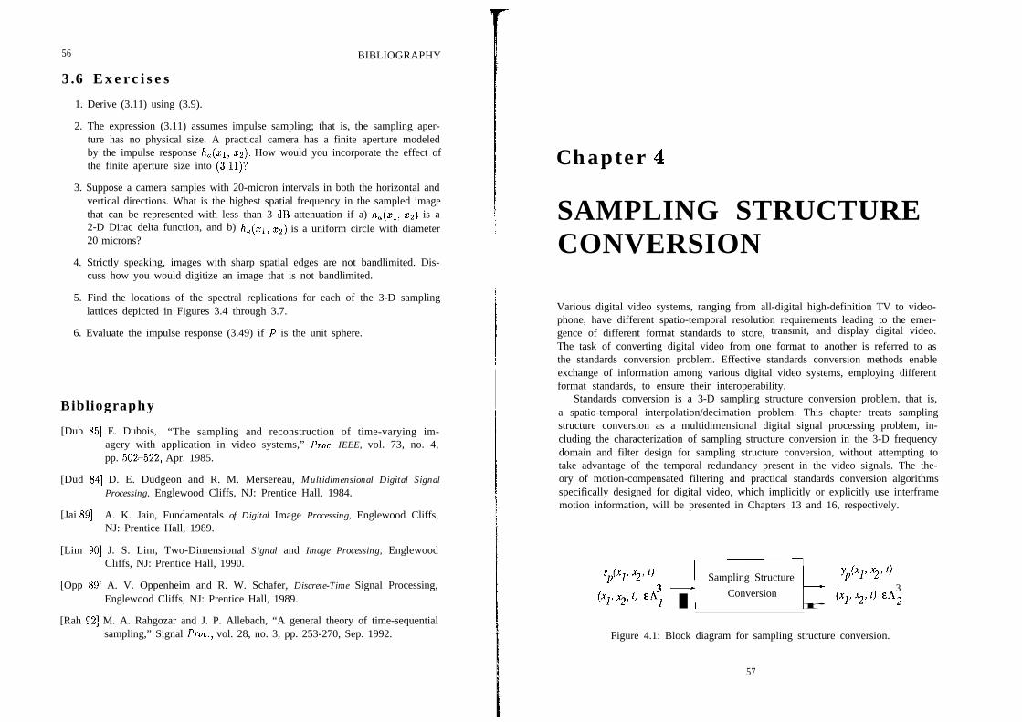
56 BIBLIOGRAPHY
3.6 Exercises
1. Derive (3.11) using (3.9).
2. The expression (3.11) assumes impulse sampling; that is, the sampling aper-ture has no physical size. A practical camera has a finite aperture modeledby the impulse response &(a~, ~2). How would you incorporate the effect ofthe finite aperture size into (3.11)?
3. Suppose a camera samples with 20-micron intervals in both the horizontal andvertical directions. What is the highest spatial frequency in the sampled imagethat can be represented with less than 3 dB attenuation if a) h,(zr, zz) is a2-D Dirac delta function, and b) h,(~1) ~2) is a uniform circle with diameter20 microns?
4. Strictly speaking, images with sharp spatial edges are not bandlimited. Dis-cuss how you would digitize an image that is not bandlimited.
5. Find the locations of the spectral replications for each of the 3-D samplinglattices depicted in Figures 3.4 through 3.7.
6. Evaluate the impulse response (3.49) if P is the unit sphere.
Bibliography
[Dub 851 E. Dubois, “The sampling and reconstruction of time-varying im-agery with application in video systems,” Proc. IEEE, vol. 73, no. 4,pp. 502-522, Apr. 1985.
[Dud 841 D. E. Dudgeon and R. M. Mersereau, Multidimensional Digital SignalProcessing, Englewood Cliffs, NJ: Prentice Hall, 1984.
[Jai 891 A. K. Jain, Fundamentals of Digital Image Processing, Englewood Cliffs,NJ: Prentice Hall, 1989.
[Lim 901 J. S. Lim, Two-Dimensional Signal and Image Processing, EnglewoodCliffs, NJ: Prentice Hall, 1990.
[Opp 891 A. V. Oppenheim and R. W. Schafer, Discrete-Time Signal Processing,Englewood Cliffs, NJ: Prentice Hall, 1989.
[Rah 921 M. A. Rahgozar and J. P. Allebach, “A general theory of time-sequentialsampling,” Signal Proc., vol. 28, no. 3, pp. 253-270, Sep. 1992.
Chapter 4
SAMPLING STRUCTURECONVERSION
Various digital video systems, ranging from all-digital high-definition TV to video-phone, have different spatio-temporal resolution requirements leading to the emer-gence of different format standards to store, transmit, and display digital video.The task of converting digital video from one format to another is referred to asthe standards conversion problem. Effective standards conversion methods enableexchange of information among various digital video systems, employing differentformat standards, to ensure their interoperability.
Standards conversion is a 3-D sampling structure conversion problem, that is,a spatio-temporal interpolation/decimation problem. This chapter treats samplingstructure conversion as a multidimensional digital signal processing problem, in-cluding the characterization of sampling structure conversion in the 3-D frequencydomain and filter design for sampling structure conversion, without attempting totake advantage of the temporal redundancy present in the video signals. The the-ory of motion-compensated filtering and practical standards conversion algorithmsspecifically designed for digital video, which implicitly or explicitly use interframemotion information, will be presented in Chapters 13 and 16, respectively.
Sp’“p 3, t) Sampling Structure Y& 2, t)
(x1, 3, t) CA; Conversion 3(X]’ “2, 0 Eh2
Figure 4.1: Block diagram for sampling structure conversion.
57
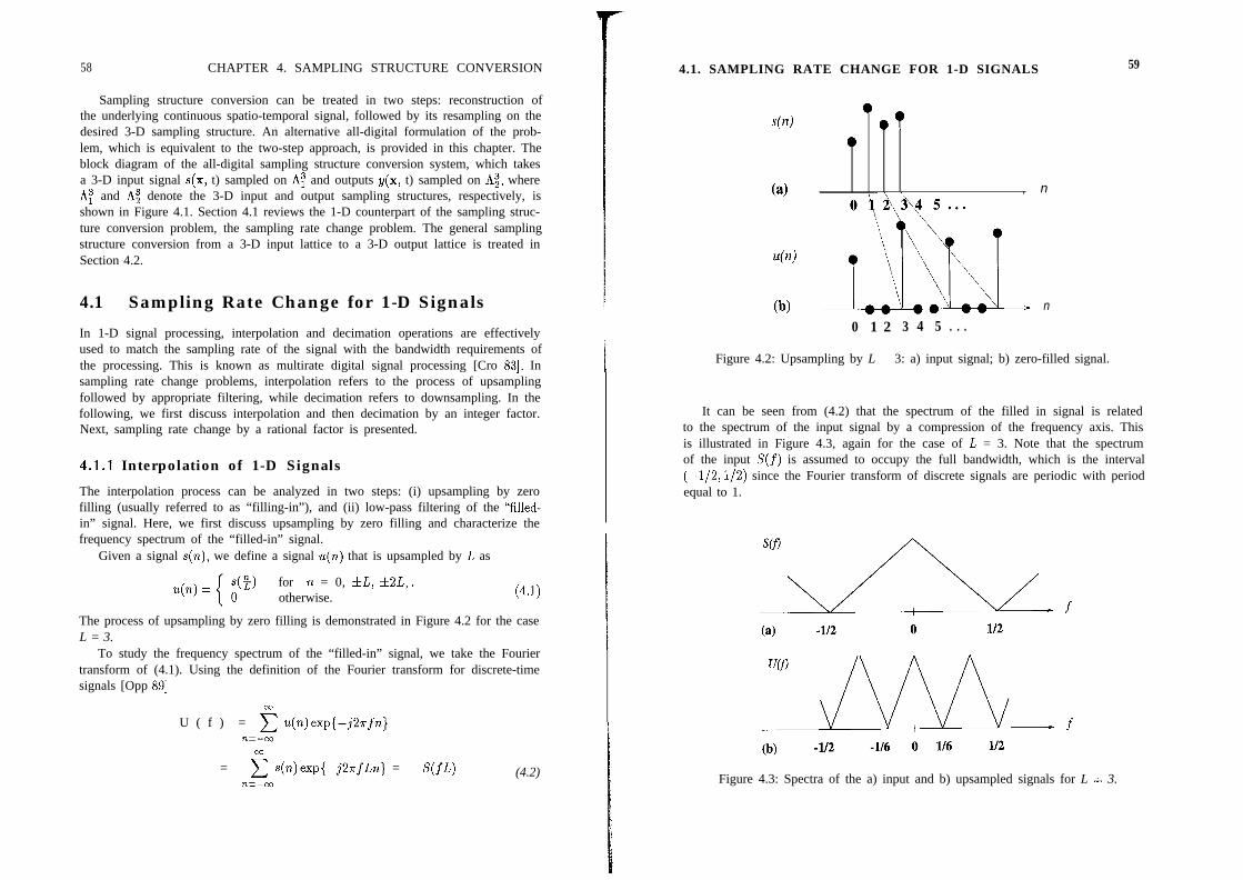
58 CHAPTER 4. SAMPLING STRUCTURE CONVERSION
Sampling structure conversion can be treated in two steps: reconstruction ofthe underlying continuous spatio-temporal signal, followed by its resampling on thedesired 3-D sampling structure. An alternative all-digital formulation of the prob-lem, which is equivalent to the two-step approach, is provided in this chapter. Theblock diagram of the all-digital sampling structure conversion system, which takesa 3-D input signal s(x, t) sampled on A: and outputs y(x, t) sampled on AZ, whereA: and AZ denote the 3-D input and output sampling structures, respectively, isshown in Figure 4.1. Section 4.1 reviews the 1-D counterpart of the sampling struc-ture conversion problem, the sampling rate change problem. The general samplingstructure conversion from a 3-D input lattice to a 3-D output lattice is treated inSection 4.2.
4.1 Sampling Rate Change for 1-D Signals
In 1-D signal processing, interpolation and decimation operations are effectivelyused to match the sampling rate of the signal with the bandwidth requirements ofthe processing. This is known as multirate digital signal processing [Cro 831. Insampling rate change problems, interpolation refers to the process of upsamplingfollowed by appropriate filtering, while decimation refers to downsampling. In thefollowing, we first discuss interpolation and then decimation by an integer factor.Next, sampling rate change by a rational factor is presented.
4.1.1 Interpolation of 1-D Signals
The interpolation process can be analyzed in two steps: (i) upsampling by zerofilling (usually referred to as “filling-in”), and (ii) low-pass filtering of the “filled-in” signal. Here, we first discuss upsampling by zero filling and characterize thefrequency spectrum of the “filled-in” signal.
Given a signal s(n), we define a signal u(n) that is upsampled by L as
for 12 = 0, &L, f2L,.otherwise.
The process of upsampling by zero filling is demonstrated in Figure 4.2 for the caseL = 3.
To study the frequency spectrum of the “filled-in” signal, we take the Fouriertransform of (4.1). Using the definition of the Fourier transform for discrete-timesignals [Opp 891
U ( f ) = 2 u(n)exp{-j2nfn)TX=---M
= 5 s(n)exp{-j2TfLn) = S(fL)7X=-IX
(4.2)
4.1. SAMPLING RATE CHANGE FOR 1-D SIGNALS
044 0.
0
(4
uW
, n
@I n
I 0 1 2 3 4 5 . . .
Figure 4.2: Upsampling by L = 3: a) input signal; b) zero-filled signal.
59
It can be seen from (4.2) that the spectrum of the filled in signal is relatedto the spectrum of the input signal by a compression of the frequency axis. Thisis illustrated in Figure 4.3, again for the case of L = 3. Note that the spectrumof the input S(f) is assumed to occupy the full bandwidth, which is the interval(-l/2,1/2) since the Fourier transform of discrete signals are periodic with periodequal to 1.
(4
Figure 4.3: Spectra of the a) input and b) upsampled signals for L = 3.

60 CHAPTER 4. SAMPLING STRUCTURE CONVERSION
Interpolation filtering aims at eliminating the replications caused by the zero-filling process. This requires low-pass filtering of the filled-in signal. In the timedomain, the filtering operation can be viewed as replacing the zero samples withnonzero values by means of a smoothing operation.
Ideal Interpolation
Ideal interpolation can be achieved by ideal low-pass filtering. The ideal low-passfilter would have a DC gain factor of L, and its cutoff frequency would be fC = 1/2~,The frequency response of the ideal interpolation filter is shown by the dotted linesin Figure 4.4.
G-4
(b) -1 0 1
Figure 4.4: Ideal interpolation filter (L = 3): Spectra a) before and b) after filtering.
The impulse response of the ideal interpolation filter is a sine function given by
(4.3)
Thus, the interpolated signal samples are given by
(4.4)
The impulse response of the ideal interpolation filter has the property that h(O) = 1,and h(n) = 0, for n = fL,&2L,. Because of these zero-crossings, y(n) = s(n)
4.1. SAMPLING RATE CHANGE FOR 1-D SIGNALS 61
at the existing sample values, while assigning nonzero values for the zero samplesin the upsampled signal.
Practical Interpolation Filters
The ideal interpolation filter is unrealizable since it is an infinite impulse response,noncausal filter; that is, its implementation requires infinite time delay. Thus, it isusually replaced by one of the following realizable approximations:
n
Figure 4.5: The zero-order hold filter for L = 3.
. Zero-order hold filterZero-order hold is the simplest interpolation filter. It corresponds to pixel repli-
cation. The impulse response and the implementation of the zero-order hold filterare shown in Figure 4.5. Note that the zero-order hold filter is a poor interpolationfilter, since its frequency response is given by a sine function, which has large side-lobes. These sidelobes cause leakage of energy from the replications in the frequencydomain, which results in high-frequency artifacts in the interpolated signal.
fn
Figure 4.6: The linear interpolation filter for L = 3.
0 Linear interpolation filterLinear interpolation is achieved by a weighted sum of the neighboring pixels. The
weights are inversely proportional to the distance of the pixel, to be interpolated,from its neighbors. The impulse response of the linear interpolation filter is shownin Figure 4.6 for L = 3. The frequency response of the linear interpolation filter

62 CHAPTER 4. SAMPLING STRUCTURE CONVERSION
is equal to the square of the sine function. Thus, it has lower sidelobes than thezero-order hold filter.
l Cubic spline interpolation filterThe cubic spline interpolation filter approximates the impulse response of the
ideal low-pass filter (4.3) by a piecewise cubic polynomial consisting of three cubits.A procedure for designing FIR cubic-spline interpolation filters is given by Keys[Key 811 (see Exercise 2). The impulse response of the cubic-spline filter, whichhas 4L + 1 taps, is demonstrated in Figure 4.7. This filter also has the samplepreserving property of the ideal low-pass filter. We note that the cubic spline filterapproximates the unrealizable ideal low-pass filter better than a truncated sine filterof the same length, because the frequency response of the truncated sine filter suffersfrom ringing effects due to the well-known Gibbs phenomenon [Opp 891.
Figure 4.7: The cubic-spline filter for L = 3.
4.1.2 Decimation of 1-D Signals
The process of decimation by a factor of M can also be modeled in two steps: first,multiplication by an impulse train to replace M - 1 samples in between every Mthsample with zeros and then, discarding the zero samples to obtain a signal at thelower rate. We describe these steps in the following,
Given the input signal s(n), define an intermediate signal w(n) by
w(n) = s(n) 2 S(n - kM) (4.5)h=-CO
Then, the signal decimated by a factor of M can be expressed as
y(n) = w(Mn) (4.6)
The process of decimation is illustrated in Figure 4.8 for M = 2. The intermedi-ate signal w(n) is introduced to faciliate the frequency domain characterization ofdecimation.
4.1. SAMPLING RATE CHANGE FOR 1-D SIGNALS 63
wfn) t
0 1 2 3 4 5 6...
Figure 4.8: Decimation by M = 2: a) input signal, b) intermediate signal, andc) downsampled signal.
To analyze the spectrum of the decimated signal, we first compute the Fouriertransform of the intermediate signal as
(4.7)
It can easily be seen that the spectrum of the intermediate signal consists of replica-tions of the input signal spectrum. There are M replicas in the interval (-l/2,1/2)as shown in Figure 4.9. Then the spectrum of the decimated signal is given by
Y(f) = g w(Mn) exp{-j2rfn) = w($)72=--M
(4.8)
which results in an expansion of the frequency axis for the spectrum of the inter-mediate signal. Note that in Figure 4.9 the bandwidth of the input signal is l/4;thus, decimation by two yields a full bandwidth signal.
If the bandwidth of the input signal is more than 1/(2M), then the replicationswill overlap and the decimated signal will suffer from aliasing. This is as expected,because the sampling rate of the decimated signal should not be allowed to fall belowthe Nyquist sampling rate. If an application mandates going below the Nyquist

64 CHAPTER 4. SAMPLING STRUCTURE CONVERSION
rate, then appropriate anti-alias filtering should be applied prior to the decimation.Ideal anti-alias filtering can be achieved by ideal low-pass filtering, as shown inFigure 4.10. For decimation by M, the cutoff frequency of the ideal anti-alias filteris 1/(2M).
1 . A...+
-1 -l/2 0 l/2 1 ”
Figure 4.9: Spectra of the a) input signal, b) intermediate signal, and c) downsam-pled signal (M = 2).
The simplest realizable anti-alias filter is a box filter. Box filtering correspondsto averaging all pixels within a local window. Although they are a poor approxi-mation of the ideal low-pass filter, box filters are usually preferred because of theirsimplicity.
4.1.3 Sampling Rate Change by a Rational Factor
The theory of decimation and interpolation (by an integer factor) extends to sam-pling rate change by a rational factor in a straightforward fashion. Sampling ratechange by a rational factor, L/M, can be achieved by first interpolating the signalup by a factor of L and then decimating the result by a factor of M. The interpola-tion filter and the anti-alias filter of decimation can be merged into a single low-passfilter with the cutoff frequency fc = min{l/(ZM), 1/(2L)}. A block diagram of asystem for sampling rate change by a factor of L/M is depicted in Figure 4.11.
4.1. SAMPLING RATE CHANGE FOR 1-D SIGNALS
WI. .
WI
. . ./
,f-1 -l/2 0 l/2 1
. . .
L/- Decimation filter
65
-f-1 -112 0 112 1
. . .,f
-1 -l/2 0 l/2 1
Figure 4.10: Anti-alias filtering for M = 2: Spectra of the a) input signal, b) inter-mediate signal, and c) downsampled signal with anti-alias filtering.
If M > L, then the sampling rate change problem is effectively a decimationproblem; otherwise, it is an interpolation problem. In any case, the constraint thatthe values of the existing samples must be preserved needs to be incorporated intothe low-pass filter design using one of the suggested interpolation filter design pro-cedures. If a linear interpolation filter is to be used, the system given in Figure 4.11can be simplified into a single filter which does not first require interpolation bya factor of L. This simplification may result in significant computational savings,especially for factors such as 9/2, where the numerator is large.
Figure 4.11: Sampling rate change by a factor of L/M.

66 CHAPTER 4. SAMPLING STRUCTURE CONVERSION
4.2 Sampling Lattice Conversion
In this section, the theory of sampling rate change is extended to conversion fromone 3-D sampling lattice to another. A system for sampling lattice conversion canbe decomposed, as shown in Figure 4.12, where the input video is first upconvertedto the lattice AT + Ai. After appropriate filtering, it is downconverted to the outputlattice Ai. In the following, we describe the components of this system in detail.
s (x > x , t)p 1 2 Upconvert &Low pass IL Downconvert ~ Yp(X1’ “7 t)
3 u filter(xllx21 t) E Al D 3
(.Q x7 t) E A2
Figure 4.12: Decomposition of the system for sampling structure conversion.
We define the sum of two lattices as
G+G={[ t:‘]+[ z] 1 (xI,~I) E A: and (xz,tz) E Ai > (4.9)
Thus, the sum of two lattices can be found by adding each point in one lattice toevery point of the other lattice. The intersection of two lattices is given by
A: n A; = {(x, t) I (x, t) E AT and (x, t) E Ai} (4.10)
The intersection A: n AZ is the largest lattice that is a sublattice of both A: andA:, while the sum A: + Ai: is the smallest lattice that contains both A: and A: assublattices.
The upconversion from A: to A: + Ai is defined as follows:
t$(X,t) = zlsp(x,t) = sp(x,t) (~4 E A:o (x,4 $ A:, (x,4 E A; + A; (4.11)
and downconversion from AT + Ai to Aj: as:
z/p@, 4 = %4x, t) = q(x, t), (x, t) E A; (4.12)
The interpolation filter (anti-alias filter in the case of downsampling) is appliedon the lattice Ay+Ai. By definition, this filter will be shift-invariant if the output isshifted by the vector p when the input is shifted by p. Thus, we need p E A: n Ai.
4.2. SAMPLING LATTICE CONVERSION 67
This condition is satisfied if A: n A,3 is a lattice, that is, VT1V2 is a matrix ofintegers. This requirement is the counterpart of L/M to be a rational number inthe 1-D sampling rate change problems.
The linear, shift-invariant filtering operation on A: + As can be expressed as
WP(X, 4 = (z,rg+*; %4z, T) hp( [ ; ] - [ “, ] 1, (x,t) 6 A? + A; (4W1
However, by the definition of the upsampling operator, u~(x, t) = sp(x,t) for(x, t) E AT and zero otherwise; thus,
(z,r)EA:L-J
After the downsampling operation,
yp(x,4 = c SJZ,T) hp((z,~)EA: [ 1“, 1, (x,4 E A; (4.15)
The frequency response of the filter is periodic with the main period determinedby the unit cell of (A: + A$*. In order to avoid aliasing, the passband of theinterpolation/anti-alias (low-pass) filter is restricted to the smaller of the Voronoicells of A;* and A$*. Sampling lattice conversion is illustrated by means of thefollowing examples.
Example: Conversion from AT to Ai [Dub 851
We consider a 2-D sampling lattice conversion from the input lattice A:to the output lattice A$, which are shown in Figure 4.13 along with theirsampling matrices, VI and Vz. The sampling densities of AT and A$ areinversely proportional to the determinants of VI and V2, given by
d(AT) = 2AxlAx2 and d(A;) = 4AxlAx2
Also shown in Figure 4.13 are the lattices A: + Ai and AT n AZ, whichare used to define the sampling conversion factor
Because we have a downconversion problem, by a factor of 2, anti-aliasfiltering must be performed on the lattice AT + Ai. The fundamen-tal period of the filter frequency response is given by the unit ccl1 of(AT + AZ)*, which is indicated by the dotted lines in Figure 4.14. Inorder to avoid aliasing, the passband of the low-pass filter must be re-stricted to the Voronoi cell of Ai* which has an hexagonal shape.

68 CHAPTER 4. SAMPLING STRUCTURE CONVERSION
Ax1x1
v = I 1AxI 0
Ax2 2Ax2
x2
10 0 00
2 2 0 0 0 0w2 0 0 0 0
0 0 000 0 0 0
Ax2 0 0 0 0xI
Axl
v =
x2
2A2
AX,1
I 0 0
1
0 00 0
“1Axl
v =
x2 0 0
47 A22
Ax2
0 0
x1AxIv =
Figure 4.13: The lattices AT, Ai, A: + Ai, and Af n Ai [Dub 851 (@1985 IEEE).
Example: De-interlacingDe-interlacing refers to conversion from an interlaced sampling grid (in-put) to a progressive grid (output), shown in Figure 4.15 (a) and (b),respectively. The sampling matrices for the input and output grids are
AQ 0 00 2Ax2 Ax20 0 At 1
and
V out =Axe, 0 0
0 Ax, 00 0 At 1
4.2. SAMPLING LATTICE CONVERSION 69
l/Ax1 - Il2AxI
0 112 Ax2I
Figure 4.14: The spectrum of s(x) with the periodicity matrix U, and the supportof the frequency response of the filter [Dub 851 (01985 IEEE).
respectively. Note that ]detVi,] = 2]detV,,t]; hence, we have a spatio-temporal interpolation problem by a factor of 2. The interpolation canbe achieved by zero-filling followed by ideal low-pass filtering. The pass-
64 (b)
Figure 4.15: Interlaced to progressive conversion: a) input; b) output lattices.

70 CHAPTER 4. SAMPLING STRUCTURE CONVERSION
band of the ideal low-pass filter should be restricted to the unit cell ofthe reciprocal lattice of the output sampling lattice, which is given by
In spatio-temporal sampling structure down-conversion without motion com-pensation, there is a tradeoff between allowed aliasing errors and loss of resolution(blurring) due to anti-alias (low-pass) filtering prior to down-conversion. Whenanti-alias filtering has been used prior to down-conversion, the resolution that islost cannot be recovered by subsequent interpolation. In Chapters 13 and 16, wepresent methods to incorporate interframe motion information to sampling struc-ture conversion problems by means of motion compensation. Motion-compensatedinterpolation makes it possible to recover full-resolution frames by up-conversion ofpreviously down converted frames if no anti-alias filtering has been applied in thedown-conversion process.
4.3 Exercises
1. Find the frequency response of the zero-order hold and the linear interpolationfilters shown in Figures 4.5 and 4.6, respectively. Compare them with that ofthe ideal (band-limited) interpolation filter.
2. In this problem, we design 1-D and 2-D cubic-spline interpolation filters.
a) We start by designing a continuous-time cubic spline reconstruction filterthat approximates the ideal low-pass filter.with the cutoff frequency fc = l/2.The impulse response h(t) (shown below) of a filter that uses four neighboringsamples at any time t can be expressed as
i
a31t13 + a21t12 + a1ltl + aa 05 ItI < 1h(t) = b3143 + bzlt(2 + hItI + bo 1 I ItI < 2 (4.16)
0 21 ItIThe design criteria are: h(t) = 0 for all integer t (i.e., original sample points),except t = 0 where h(0) = 1; and the slope of the impulse response y mustbe continuous across original sample points.
F
BIBLIOGRAPHY 71
Show that the design criteria are met if the 8 unknown coefficients ai, and bi,i=o,..., 3 satisfy the following 7 equations:
a0 = 1, a1 = 0
u3 + u2 = -1, b3 + bz + bl + bo = 0863 + 4ba + 2bl + b. = 0, 12bs + 4bz + bl = 0
3~x3 + 2az = 3b3 + 2b2 + bl
b) Let b3 be a free parameter, and express all other parameters in terms ofb3. Determine a range of values for b3 such that
7It=0 < 0 a n d y],=i > 0d2h(t)
c) A digital cubic spline filter can be obtained by sampling h(t). Show that forinterpolation by a factor of L, the impulse response of the cubic-spline filterhas 4L + 1 taps. Determine the impulse response for L = 2 and bs = -1.
d) Design a 2-D separable cubic spline interpolation filter with the same pa-rameters.
Bibliography
[Cro 831 R. E. Crochiere and L. R. Rabiner, M&irate Digital Signal Processing,Englewood Cliffs, NJ: Prentice Hall, 1983.
[Dub 851 E. Dubois, “The sampling and reconstruction of time-varying im-agery with application in video systems,” Proc. IEEE, vol. 73, no. 4,pp. 502-522, Apr. 1985.
[Key $11 R. G. Keys, “Cubic convolution interpolation for digital image pro-cessing,” IEEE Trans. Acoust. Speech and Sign. Proc., vol. ASSP-29,pp. 115331160, Dec. 1981.
[Lim 901 J. S. Lim, Two-Dimensional Signal and Image Processing, EnglewoodCliffs, NJ: Prentice Hall, 1990.
[Opp 891 A. V. Oppenheim and R. W. Schafer, Discrete-Time Signal Processing,Englewood Cliffs, NJ: Prentice Hall, 1989.
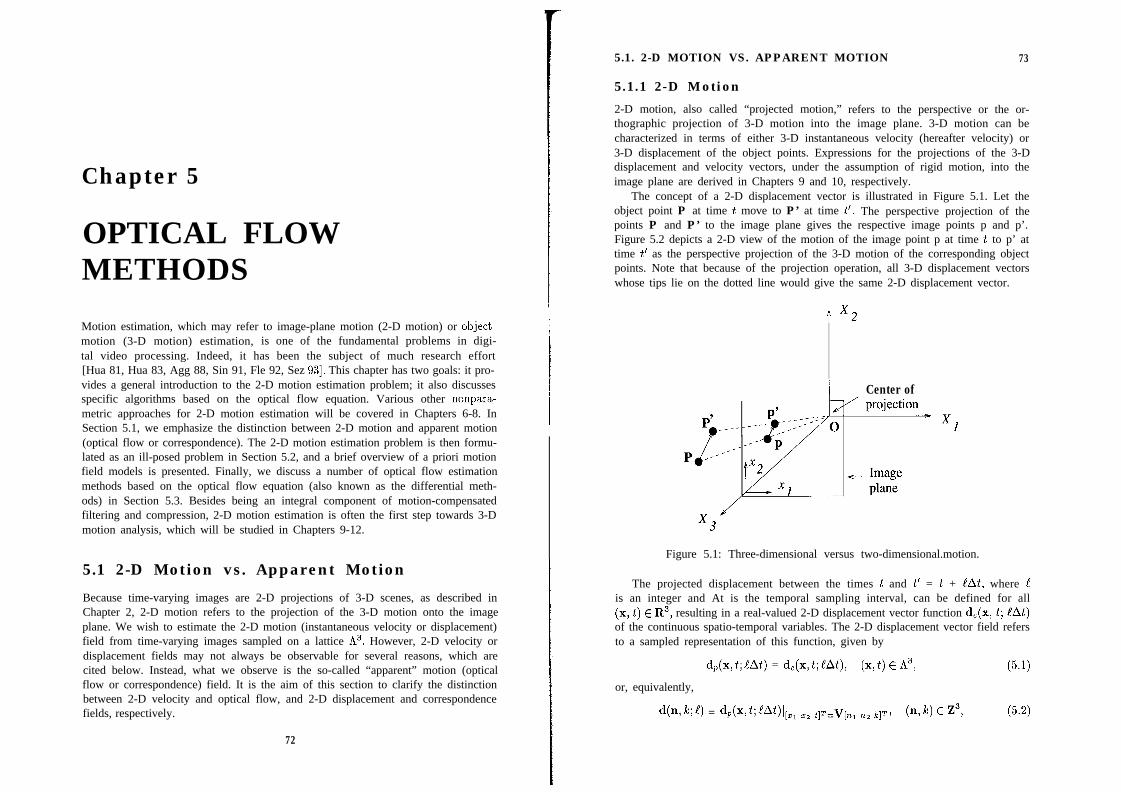
Chapter 5
OPTICAL FLOWMETHODS
Motion estimation, which may refer to image-plane motion (2-D motion) or object-motion (3-D motion) estimation, is one of the fundamental problems in digi-tal video processing. Indeed, it has been the subject of much research effort[Hua 81, Hua 83, Agg 88, Sin 91, Fle 92, Sez 931. This chapter has two goals: it pro-vides a general introduction to the 2-D motion estimation problem; it also discussesspecific algorithms based on the optical flow equation. Various other nonpara-metric approaches for 2-D motion estimation will be covered in Chapters 6-8. InSection 5.1, we emphasize the distinction between 2-D motion and apparent motion(optical flow or correspondence). The 2-D motion estimation problem is then formu-lated as an ill-posed problem in Section 5.2, and a brief overview of a priori motionfield models is presented. Finally, we discuss a number of optical flow estimationmethods based on the optical flow equation (also known as the differential meth-ods) in Section 5.3. Besides being an integral component of motion-compensatedfiltering and compression, 2-D motion estimation is often the first step towards 3-Dmotion analysis, which will be studied in Chapters 9-12.
5.1 2-D Motion vs. Apparent Motion
Because time-varying images are 2-D projections of 3-D scenes, as described inChapter 2, 2-D motion refers to the projection of the 3-D motion onto the imageplane. We wish to estimate the 2-D motion (instantaneous velocity or displacement)field from time-varying images sampled on a lattice h3. However, 2-D velocity ordisplacement fields may not always be observable for several reasons, which arecited below. Instead, what we observe is the so-called “apparent” motion (opticalflow or correspondence) field. It is the aim of this section to clarify the distinctionbetween 2-D velocity and optical flow, and 2-D displacement and correspondencefields, respectively.
72
5.1. 2-D MOTION VS. APPARENT MOTION 73
5.1.1 2-D Motion
2-D motion, also called “projected motion,” refers to the perspective or the or-thographic projection of 3-D motion into the image plane. 3-D motion can becharacterized in terms of either 3-D instantaneous velocity (hereafter velocity) or3-D displacement of the object points. Expressions for the projections of the 3-Ddisplacement and velocity vectors, under the assumption of rigid motion, into theimage plane are derived in Chapters 9 and 10, respectively.
The concept of a 2-D displacement vector is illustrated in Figure 5.1. Let theobject point P at time t move to P’ at time t’. The perspective projection of thepoints P and P’ to the image plane gives the respective image points p and p’.Figure 5.2 depicts a 2-D view of the motion of the image point p at time t to p’ attime t’ as the perspective projection of the 3-D motion of the corresponding objectpoints. Note that because of the projection operation, all 3-D displacement vectorswhose tips lie on the dotted line would give the same 2-D displacement vector.
li “2
I Center of
Figure 5.1: Three-dimensional versus two-dimensional.motion.
The projected displacement between the times t and t’ = t + eAt, where !is an integer and At is the temporal sampling interval, can be defined for all(x, t) E R3, resulting in a real-valued 2-D displacement vector function d,(x, t; !At)of the continuous spatio-temporal variables. The 2-D displacement vector field refersto a sampled representation of this function, given by
d,(x,t;eAt) = d,(x,t;eAt), (x,t) E h3, (5.1)
or, equivalently,
d(n,k4 = Ux,C~A~)lI,, 12 tlT=~[nl n2 kl~j (n,k) E Z3, (5.2)

74 CHAPTER 5. OPTICAL FLOW METHODS
0Center of Image
projection plane
Figure 5.2: The projected motion.
where V is the sampling matrix of the lattice h3. Thus, a 2-D displacement field isa collection of 2-D displacement vectors, d(x, t; iAt), where (x, t) E h3.
The projected velocity function v,(x,t) at time t, and the 2-D velocity vectorfield vp(x,t) = v(n, k), for [XI xz tlT = V[nl, n2, lelT E A” and (n, k) E Z3 can besimilarly defined in terms of the 3-D instantaneous velocity (Xi, 22, is), where thedot denotes a time derivative.
5.1.2 Correspondence and Optical Flow
The displacement of the image-plane coordinates x from time t to t’, based onthe variations of se(x) t), is called a correspondence vector. An optical flow vec-tor is defined as the temporal rate of change of the image-plane coordinates,(vi, ~2) = (dxi/dt, dxz/dt), at a particular point (x,t) E R3 as determined bythe spatio-temporal variations of the intensity pattern sc(x,t). That is, it corre-sponds to the instantaneous pixel velocity vector. (Theoretically, the optical flowand correspondence vectors are identical in the limit At = t’ -t goes to zero, shouldwe have access to the continuous video.) In practice, we define the correspondence(optical flow) field as a vector field of pixel displacements (velocities) based on theobservable variations of the 2-D image intensity pattern on a spatio-temporal latticeh3. The correspondence field and optical flow field are also known as the “apparent2-D displacement” field and “apparent 2-D velocity” field, respectively.
The correspondence (optical flow) field is, in general, different from the 2-Ddisplacement (2-D velocity) field due to [Ver 891:
. Lack of sufficient spatial image gradient: There must be sufficient gray-level(color) variation within the moving region for the actual motion to be observ-able. An example of an unobservable motion is shown in Figure 5.3, wherea circle with uniform intensity rotates about its center. This motion generatesno optical flow, and thus is unobservable.
5.1. 2-D MOTION VS. APPARENT MOTION
a rad/s
75
Figure 5.3: All projected motion does not generate optical flow.
. Changes in external illumination: An observable optical flow may not alwayscorrespond to an actual motion. For example, if the external illuminationvaries from frame to frame, as shown in Figure 5.4, then an optical flow willbe observed even though there is no motion. Therefore, changes in the externalillumination impair the estimation of the actual 2-D motion field.
Frame k k-i-1r \ //
Figure 5.4: All optical flow does not correspond to projected motion.
In some cases, the shading may vary from frame to frame even if there isno change in the external illumination. For example, if an object rotates itssurface normal changes, which results in a change in the shading. This changein shading may cause the intensity of the pixels along a motion trajectory tovary, which needs to be taken into account for 2-D motion estimation.
In conclusion the 2-D displacement and velocity fields are projections of the re-spective 3-D fields into the image plane, whereas the correspondence and optical flowfields are the velocity and displacement functions perceived from the time-varyingimage intensity pattern. Since we can only observe optical flow and correspondencefields, we assume they are the same as the 2-D motion field in the remainder of thisbook.
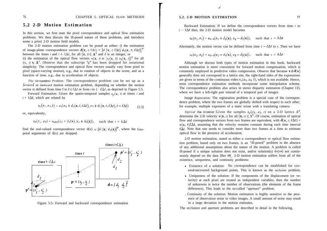
76 CHAPTER 5. OPTICAL FLOW METHODS
5.2 2-D Motion Estimation
In this section, we first state the pixel correspondence and optical flow estimationproblems. We then discuss the ill-posed nature of these problems, and introducesome a priori 2-D motion field models.
The 2-D motion estimation problem can be posed as either: i) the estimationof image-plane correspondence vectors d(x, t; !At) = [dl(x, t; 1At) dz(x, t; !At)lTbetween the times t and t + 1At, for all (x, t) E A3 and 1 is an integer, orii) the estimation of the optical flow vectors v(x, t) = [vr(x, t) uz(x, t)lT for all(x, t) E A3. Observe that the subscript “p” has been dropped for notationalsimplicity. The correspondence and optical flow vectors usually vary from pixel topixel (space-varying motion), e.g., due to rotation of objects in the scene, and as afunction of time, e.g., due to acceleration of objects.
The Correspondence Problem: The correspondence problem can be set up as aforvlard or backward motion estimation problem, depending on whether the motionvector is defined from time t to t+!At or from t to t-lAt, as depicted in Figure 5.5.
Forward Estimation: Given the spatio-temporal samples sp(x, t) at times t andt + eat, which are related by
s~(zI,xz>~) = s,(q +d~(x,t;lAt),x,+dz(x,t;lAt),t+lAt)
or, equivalently,
(5.3)
sk(xi, x2) = sk+e(zi + di(x),xz + dz(x)), such that t = kAt
find the real-valued correspondence vector d(x) = [dr(x) d2(x)lT, where the tem-poral arguments of d(x) are dropped.
time t
time t-1At
time t+lAt
,’.,
Figure 5.5: Forward and backward correspondence estimation
P
5.2. 2-D MOTION ESTIMATION 77
Backward Estimation: If we define the correspondence vectors from time t tot - eAt then, the 2-D motion model becomes
sk(xi, x2) = sk-e(xi + di(x), x2 $ I&(X)), such that t = EAt
Alternately, the motion vector can be defined from time t - !At to t. Then we have
sk(zi, x2) = sk-e(xr - dr(x), 22 - &(x)), such that t = kAt
Although we discuss both types of motion estimation in this book, backwardmotion estimation is more convenient for forward motion compensation, which iscommonly employed in predictive video compression. Observe that because x*d(x)generally does not correspond to a lattice site, the right-hand sides of the expressionsare given in terms of the continuous video s,(xr, x2, t), which is not available. Hence,most correspondence estimation methods incorporate some interpolation scheme.The correspondence problem also arises in stereo disparity estimation (Chapter 12),where we have a left-right pair instead of a temporal pair of images.
Image Registration: The registration problem is a special case of the correspon-dence problem, where the two frames are globally shifted with respect to each other,for example, multiple exposures of a static scene with a translating camera.
Optical Flow Estimation: Given the samples sp(xr, x2, t) on a 3-D lattice h3,determine the 2-D velocity v(x, t) for all (xI t) E A3. Of course, estimation of opticalflow and correspondence vectors from two frames are equivalent, with d(x, t; !At) =v(x, t)eAt, assuming that the velocity remains constant during each time interval!At. Note that one needs to consider more than two frames at a time to estimateoptical flow in the presence of acceleration.
2-D motion estimation, stated as either a correspondence or optical flow estima-tion problem, based only on two frames, is an “ill-posed” problem in the absenceof any additional assumptions about the nature of the motion. A problem is calledill-posed if a unique solution does not exist, and/or solution(s) do(es) not contin-uously depend on the data [Ber 881. 2-D motion estimation suffers from all of theexistence, uniqueness, and continuity problems:
l Existence of a solution: No correspondence can be established for cov-ered/uncovered background points. This is known as the occlusion problem.
l Uniqueness of the solution: If the components of the displacement (or ve-locity) at each pixel are treated as independent variables, then the numberof unknowns is twice the number of observations (the elements of the framedifference). This leads to the so-called “aperture” problem.
. Continuity of the solution: Motion estimation is highly sensitive to the pres-ence of observation noise in video images. A small amount of noise may resultin a large deviation in the motion estimates.
The occlusion and aperture problems are described in detail in the following.
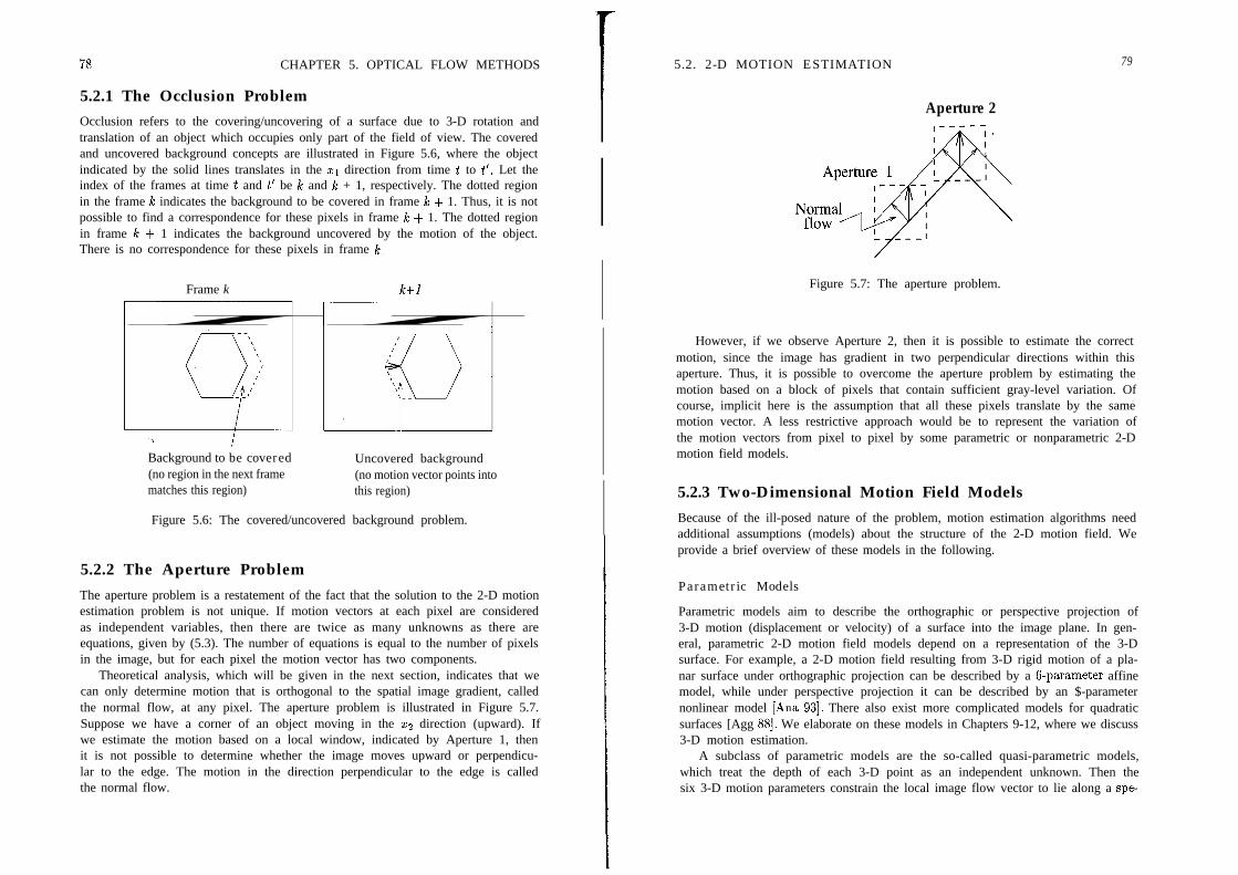
78 CHAPTER 5. OPTICAL FLOW METHODS
5.2.1 The Occlusion ProblemOcclusion refers to the covering/uncovering of a surface due to 3-D rotation andtranslation of an object which occupies only part of the field of view. The coveredand uncovered background concepts are illustrated in Figure 5.6, where the objectindicated by the solid lines translates in the 21 direction from time t to t’. Let theindex of the frames at time t and t’ be Ic and I% + 1, respectively. The dotted regionin the frame le indicates the background to be covered in frame lc + 1. Thus, it is notpossible to find a correspondence for these pixels in frame le + 1. The dotted regionin frame le + 1 indicates the background uncovered by the motion of the object.There is no correspondence for these pixels in frame I%.
Frame k k+l
Background to be covered Uncovered background(no region in the next frame (no motion vector points intomatches this region) this region)
Figure 5.6: The covered/uncovered background problem.
5.2.2 The Aperture ProblemThe aperture problem is a restatement of the fact that the solution to the 2-D motionestimation problem is not unique. If motion vectors at each pixel are consideredas independent variables, then there are twice as many unknowns as there areequations, given by (5.3). The number of equations is equal to the number of pixelsin the image, but for each pixel the motion vector has two components.
Theoretical analysis, which will be given in the next section, indicates that wecan only determine motion that is orthogonal to the spatial image gradient, calledthe normal flow, at any pixel. The aperture problem is illustrated in Figure 5.7.Suppose we have a corner of an object moving in the x2 direction (upward). Ifwe estimate the motion based on a local window, indicated by Aperture 1, thenit is not possible to determine whether the image moves upward or perpendicu-lar to the edge. The motion in the direction perpendicular to the edge is calledthe normal flow.
5.2. 2-D MOTION ESTIMATION
Aperture 2
Figure 5.7: The aperture problem.
79
However, if we observe Aperture 2, then it is possible to estimate the correctmotion, since the image has gradient in two perpendicular directions within thisaperture. Thus, it is possible to overcome the aperture problem by estimating themotion based on a block of pixels that contain sufficient gray-level variation. Ofcourse, implicit here is the assumption that all these pixels translate by the samemotion vector. A less restrictive approach would be to represent the variation ofthe motion vectors from pixel to pixel by some parametric or nonparametric 2-Dmotion field models.
5.2.3 Two-Dimensional Motion Field ModelsBecause of the ill-posed nature of the problem, motion estimation algorithms needadditional assumptions (models) about the structure of the 2-D motion field. Weprovide a brief overview of these models in the following.
Parametric Models
Parametric models aim to describe the orthographic or perspective projection of3-D motion (displacement or velocity) of a surface into the image plane. In gen-eral, parametric 2-D motion field models depend on a representation of the 3-Dsurface. For example, a 2-D motion field resulting from 3-D rigid motion of a pla-nar surface under orthographic projection can be described by a 6-parameter affinemodel, while under perspective projection it can be described by an $-parameternonlinear model [Ana 931. There also exist more complicated models for quadraticsurfaces [Agg 881. We elaborate on these models in Chapters 9-12, where we discuss3-D motion estimation.
A subclass of parametric models are the so-called quasi-parametric models,which treat the depth of each 3-D point as an independent unknown. Then thesix 3-D motion parameters constrain the local image flow vector to lie along a spe-
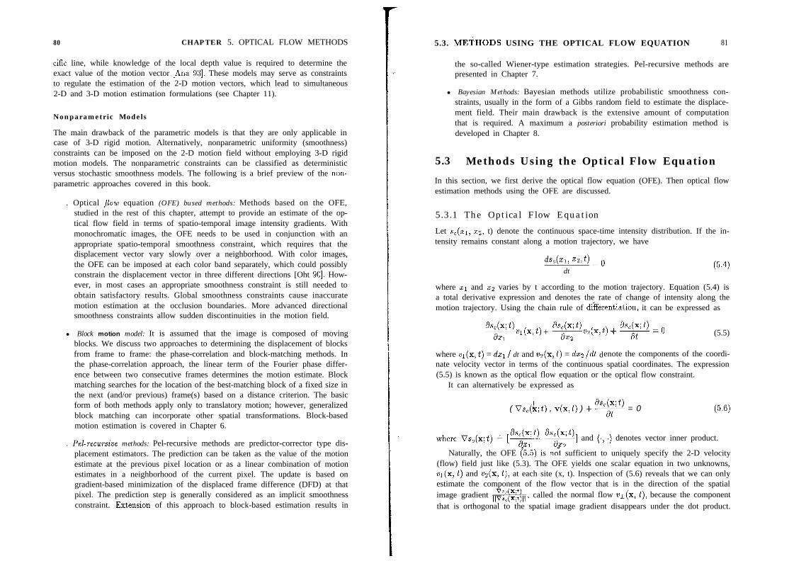
80 CHAPTER 5. OPTICAL FLOW METHODS
cific line, while knowledge of the local depth value is required to determine theexact value of the motion vector [Ana 931. These models may serve as constraintsto regulate the estimation of the 2-D motion vectors, which lead to simultaneous2-D and 3-D motion estimation formulations (see Chapter 11).
Nonparametric Models
The main drawback of the parametric models is that they are only applicable incase of 3-D rigid motion. Alternatively, nonparametric uniformity (smoothness)constraints can be imposed on the 2-D motion field without employing 3-D rigidmotion models. The nonparametric constraints can be classified as deterministicversus stochastic smoothness models. The following is a brief preview of the non-parametric approaches covered in this book.
. Optical flow equation (OFE) bused methods: Methods based on the OFE,studied in the rest of this chapter, attempt to provide an estimate of the op-tical flow field in terms of spatio-temporal image intensity gradients. Withmonochromatic images, the OFE needs to be used in conjunction with anappropriate spatio-temporal smoothness constraint, which requires that thedisplacement vector vary slowly over a neighborhood. With color images,the OFE can be imposed at each color band separately, which could possiblyconstrain the displacement vector in three different directions [Oht 901. How-ever, in most cases an appropriate smoothness constraint is still needed toobtain satisfactory results. Global smoothness constraints cause inaccuratemotion estimation at the occlusion boundaries. More advanced directionalsmoothness constraints allow sudden discontinuities in the motion field.
l Block motion model: It is assumed that the image is composed of movingblocks. We discuss two approaches to determining the displacement of blocksfrom frame to frame: the phase-correlation and block-matching methods. Inthe phase-correlation approach, the linear term of the Fourier phase differ-ence between two consecutive frames determines the motion estimate. Blockmatching searches for the location of the best-matching block of a fixed size inthe next (and/or previous) frame(s) based on a distance criterion. The basicform of both methods apply only to translatory motion; however, generalizedblock matching can incorporate other spatial transformations. Block-basedmotion estimation is covered in Chapter 6.
. Pebrecursive methods: Pel-recursive methods are predictor-corrector type dis-placement estimators. The prediction can be taken as the value of the motionestimate at the previous pixel location or as a linear combination of motionestimates in a neighborhood of the current pixel. The update is based ongradient-based minimization of the displaced frame difference (DFD) at thatpixel. The prediction step is generally considered as an implicit smoothnessconstraint. .Extension of this approach to block-based estimation results in
5.3. METHODS USING THE OPTICAL FLOW EQUATION 81
the so-called Wiener-type estimation strategies. Pel-recursive methods arepresented in Chapter 7.
l Bayesian Methods: Bayesian methods utilize probabilistic smoothness con-straints, usually in the form of a Gibbs random field to estimate the displace-ment field. Their main drawback is the extensive amount of computationthat is required. A maximum a posteriori probability estimation method isdeveloped in Chapter 8.
5.3 Methods Using the Optical Flow Equation
In this section, we first derive the optical flow equation (OFE). Then optical flowestimation methods using the OFE are discussed.
5.3.1 The Optical Flow Equation
Let s,(zr, ~2, t) denote the continuous space-time intensity distribution. If the in-tensity remains constant along a motion trajectory, we have
d&(X1, mt) = 0dt
where zr and zz varies by t according to the motion trajectory. Equation (5.4) isa total derivative expression and denotes the rate of change of intensity along themotion trajectory. Using the chain rule of dcfferentiation, it can be expressed as
h(x; t)TV1 (XI t) +
&(x; 4--$p(x,t) +
h(x; t)7=0 (5.5)
where wr(x, t) = dxl f dt and vz(x, t) = dxz Jdt denote the components of the coordi-nate velocity vector in terms of the continuous spatial coordinates. The expression(5.5) is known as the optical flow equation or the optical flow constraint.
It can alternatively be expressed as
( vs,&;t, , v(x,t) ) + +p = 0
where Vsc(x;t) & ,w @d$ and (., .) denotes vector inner product.
Naturally, the OFE (5.5) is not sufficient to uniquely specify the 2-D velocity(flow) field just like (5.3). The OFE yields one scalar equation in two unknowns,wr(x, t) and z)z(x, t), at each site (x, t). Inspection of (5.6) reveals that we can onlyestimate the component of the flow vector that is in the direction of the spatialimage gradient &$$, called the normal flow ZI~(X, t), because the componentthat is orthogonal to the spatial image gradient disappears under the dot product.
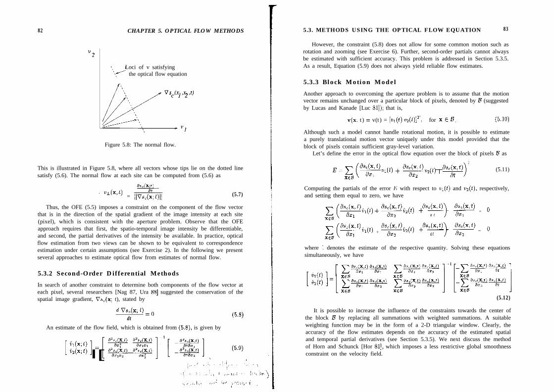
82
v2
CHAPTER 5. OPTICAL FLOW METHODS
Loci of v satisfying“‘I< the optical flow equation
Figure 5.8: The normal flow.
This is illustrated in Figure 5.8, where all vectors whose tips lie on the dotted linesatisfy (5.6). The normal flow at each site can be computed from (5.6) as
as,(w)
’ vJ-(x,t) = ,,vs,(r;t),, (5.7)
Thus, the OFE (5.5) imposes a constraint on the component of the flow vectorthat is in the direction of the spatial gradient of the image intensity at each site(pixel), which is consistent with the aperture problem. Observe that the OFEapproach requires that first, the spatio-temporal image intensity be differentiable,and second, the partial derivatives of the intensity be available. In practice, opticalflow estimation from two views can be shown to be equivalent to correspondenceestimation under certain assumptions (see Exercise 2). In the following we presentseveral approaches to estimate optical flow from estimates of normal flow.
5.3.2 Second-Order Differential Methods
In search of another constraint to determine both components of the flow vector ateach pixel, several researchers [Nag 87, Ura 881 suggested the conservation of thespatial image gradient, Vs,(x; t), stated by
d vsL+; t) = 0dt
An estimate of the flow field, which is obtained from (5.8), is given by
31(x; t)[ c,(x;t) = $g $g]-l[ -%gJ] (5.9)
51
5.3. METHODS USING THE OPTICAL FLOW EQUATION 83
However, the constraint (5.8) does not allow for some common motion such asrotation and zooming (see Exercise 6). Further, second-order partials cannot alwaysbe estimated with sufficient accuracy. This problem is addressed in Section 5.3.5.As a result, Equation (5.9) does not always yield reliable flow estimates.
5.3.3 Block Motion Model
Another approach to overcoming the aperture problem is to assume that the motionvector remains unchanged over a particular block of pixels, denoted by B (suggestedby Lucas and Kanade [Luc 811); that is,
V(X, t) = v(t) = [vi(t) u2(t)lT, for x E B,
Although such a model cannot handle rotational motion, it is possible to estimatea purely translational motion vector uniquely under this model provided that theblock of pixels contain sufficient gray-level variation.
Let’s define the error in the optical flow equation over the block of pixels B as
E = c v,,(t) + !?d&2(t) I asc($t) 12
(5.11)XEB
Computing the partials of the error E with respect to vi(t) and vg(t), respectively,and setting them equal to zero, we have
CC
h(x, f) ^
XEBrz’l(t) +
d&(X, t) * as&t) Wx,t) oFvz(t) + ~ ~ =
a t > 8x1
c(
as&t) ^
XEB-j-+4 +
a&(x, 4 n dsc(x,t) as&t) o--&vz(t) + ~ ~ =
at > ax2
where ‘Y denotes the estimate of the respective quantity. Solving these equationssimultaneously, we have
(5.12)
It is possible to increase the influence of the constraints towards the center ofthe block B by replacing all summations with weighted summations. A suitableweighting function may be in the form of a 2-D triangular window. Clearly, theaccuracy of the flow estimates depends on the accuracy of the estimated spatialand temporal partial derivatives (see Section 5.3.5). We next discuss the methodof Horn and Schunck [Hor 811, which imposes a less restrictive global smoothnessconstraint on the velocity field.

84 CHAPTER 5. OPTICAL FLOW METHODS
5.3.4 Horn and Schunck Method
Horn and Schunck seek a motion field that satisfies the OFE with the minimumpixel-to-pixel variation among the flow vectors. Let
&,f(v(x,t)) = ( vsJx;t) , v(x,t) ) + (5.13)
denote the error in the optical flow equation. Observe that the OFE is satisfiedwhen fOf (v(x, t)) is equal to zero. In the presence of occlusion and noise, we aim tominimize the square of E,f (v(x, t))m order to enforce the optical flow constraint.
The pixel-to-pixel variation of the velocity vectors can be quantified by the sumof the magnitude squares of the spatial gradients of the components of the velocityvector, given by
63v(XIt)) = IIWX,~)l12 + IIVm(x,t)l12
= &2+(&)2+(g)2+(g)2 (5.14)
where we assume that the spatial and temporal coordinates are continuous variables.It can easily be verified that the smoother the velocity field, the smaller &f(v(x, t)).
Then the Horn and Schunck method minimizes a weighted sum of the error inthe OFE and a measure of the pixel-to-pixel variation of the velocity field
$&) + Q2GYV))dX, J’(5.15)
to estimate the velocity vector at each point x, where A denotes the continuous im-age support. The parameter 02, usually selected heuristically, controls the strengthof the smoothness constraint. Larger values of LY 2 increase the influence of theconstraint.
The minimization of the functional (5.15), using the calculus of variations, re-quires solving the two equations
as as, as,(q2iqX,t) $ --C,(x,t) =8x1 ax1 8x2a2v2fi1(x,t) - ds,ds,
ax1 at$$Cl(X, t) t ( +3i2(x, t) = 02V2c2(x, t) - 2% (5.16)
simultaneously, where V2 denotes the Laplacian and Y denotes the estimate of therespective quantity. In the implementation of Horn and Schunck [Hor 811, theLaplacians of the velocity components have been approximated by FIR highpassfilters to arrive at the Gauss-Seidel iteration
as, &p(x, t) t ~~p'(x, t) + !$@+l)(x, t) = $'(x, t) - dzla2 t (&)"+ (gy
672+1)(x, t) =I
p(x, t) _ 2 ~4%~) + $PW) + %a2 + (gy + (gg2
(5.17)
5.3. METHODS USING THE OPTICAL FLOW EQUATION 85
where n is the iteration counter, the overbar denotes weighted local averaging (ex-cluding the present pixel), and all partials are evaluated at the point (x,t). Thereader is referred to [Hor 811 for the derivation of this iterative estimator. Theinitial estimates of the velocities ~(1O)(x,t) and ~~)(x,t) are usually taken as zero.The above formulation assumes a continuous spatio-temporal intensity distribution.In computer implementation, all spatial and temporal image gradients need to beestimated numerically from the observed image samples, which will be discussed inthe next subsection.
5.3.5 Estimation of the Gradients
We discuss two gradient estimation methods. The first method makes use of finitedifferences, and the second is based on polynomial fitting.
Gradient Estimation Using Finite Differences
One approach to estimating the partial derivatives from a discrete image s(ni, nz, k)is to approximate them by the respective forward or backward finite differences. Inorder to obtain more robust estimates of the partials, we can compute the averageof the forward and backward finite differences, called the average difference. Fur-thermore, we can compute a local average of the average differences to eliminatethe effects of observation noise. Horn and Schunck [Hor 811 proposed averaging fourfinite differences to obtain
dsc(%xz,t) ~
8x1$ { s(nl t 1, 122, k) - s(nl, n2, k) t s(nl + Lnz + 1, k)
-s(nl,n2+l,k)+s(n~t1,n2,~t1)-s(nl~nz~~+1)
ts(nl +1,n2tl,kt1) - s(nl,nz+Lkt 1) >
d&(X1, xz,t) M
8x2ii (s n1, n2 t 1, k) - ~(1~1, n2, k) t s(nl t Ln2 + 1, k)
-s(n~+1,n2,k)ts(nl,n2t1,~t1)-s(nl~n2~let1)
ts(nl t l,n2 t 1, k t 1) - s(nl+ Lnz,k+ 1) 1ds,(xl,xz,t) M
at ai (s nl,nz,IctI)- s(nl,nz,II-)+s(nl t l,nz,kt 1)
-s(nl + l,nz, k) t s(nl,nz t l,k t 1) - s(nl,nz t Ilk)ts(nl+l,n2tl,ktl)-s(nltl,n2+1,k)} ( 5 . 1 8 )
Various other averaging strategies exist for estimating partials using finite differ-ences [Lim 901. Spatial and temporal presmoothing of video with Gaussian kernelsusually helps gradient estimation.

86 CHAPTER 5. OPTICAL FLOW METHODS
Gradient Estimation by Local Polynomial Fitting
An alternative approach is to approximate S,(Q) x2, t) locally by a linear combina-tion of some low-order polynomials in cl, c2 and t; that is,
i=o
where &(z,, x2, t) are the basis polynomials, N is the number of basis functionsused in the polynomial approximation, and ai are the coefficients of the linearcombination. Here, we will set N equal to 9, with the following choice of the basisfunctions:
&(x1, xz,t) = 13x1, xz,t, x;, x;, x1x2, x1t, x2t (5.20)
which are suggested by Lim [Lim 901. Then, Equation (5.19) becomes,
s,(xl,xz,t) ~uo+a~e~+a2~2+ast+a~x~+a~x~+asz~z~+a~;t~t+usx~t (5.21)
The coefficients a;, i = 0,. . ,8, are estimated by using the least squares method,which minimizes the error function
N - l 2
e2 = 4n1, n2, k) - C WUXI, x2, t)lI,, ra alT_v[,, n2 klT (5.22)i=o
with respect to these coefficients. The summation over (nl, n2, Ic) is carried withina local neighborhood of the pixel for which the polynomial approximation is made.A typical case involves 50 pixels, 5 x 5 spatial windows in two consecutive frames.
Once the coefficients ai are estimated, the components of the gradient can befound by simple differentiation,
h(n) x2, t)
0x1x Ul+2U4xl +U6C2+U7tlzI=rz=t=o = Ul (5.23)
dS,(Xl, x2, t)8x2
= uz + %iQ + 421 + US&~=~~=~=O = Uz (5.24)
~~c(~l,~z,qat M U3 + U7xl+ u8x21zl=z2ml = a3 (5.25)
Similarly, the second-order and mixed partials can be easily estimated in terms ofthe coefficients a4 through us.
5.3.6 Adaptive Methods
The Horn-Schunck method imposes the optical flow and smoothness constraintsglobally over the entire image, or over a motion estimation window. This has twoundesired effects:
5.3. METHODS USING THE OPTICAL FLOW EQUATION 87
i) The smoothness constraint does not hold in the direction perpendicular to anocclusion boundary. Thus, a global smoothness constraint blurs “motion edges.”For example, if an object moves against a stationary background, there is a suddenchange in the motion field at the boundary of the object. Motion edges can bepreserved by imposing the smoothness constraint only in the directions along whichthe pixel intensities do not significantly change. This is the basic concept of theso-called directional or oriented smoothness constraint.ii) The nonadaptive method also enforces the optical flow constraint at the occlusionregions, where it should be turned off. This can be achieved by adaptively varying cyto control the relative strengths of the optical flow and smoothness constraints. Forexample, at occlusion regions, such as the dotted regions shown in Figure 5.6, theoptical flow constraint can be completely turned off, and the smoothness constraintcan be fully on.
Several researchers proposed to impose the smoothness constraint along theboundaries but not perpendicular to the occlusion boundaries. Hildreth [Hi1 841minimized the criterion function of Horn and Schunck given by (5.15) along objectcontours. Nagel and Enkelman [Nag 86, Enk 881 introduced the concept of direc-tional smoothness, which suppresses the smoothness constraint in the direction ofthe spatial image gradient. Fogel [Fog 911 used directional smoothness constraintswith adaptive weighting in a hierarchical formulation. Note that adaptive weight-ing methods require strategies to detect moving object (occlusion) boundaries. Re-cently, Snyder [Sny 911 proposed a general formulation of the smoothness constraintthat includes some of the above as special cases.
Directional-Smoothness Constraint
The directional smoothness constraint can be expressed as
E&(v(x,Q) = (VV1)TW(VVl)+(v~2)TW(v~2) (5.26)
where W is a weight matrix to penalize variations in the motion field depending onthe spatial changes in gray-level content of the video. Various alternatives for theweight matrix W exist [Nag 86, Nag 87, Enk 881. For example, W can be chosenas
(5.27)
where I is the identity matrix representing a global smoothness term to ensure anonzero weight matrix at spatially uniform regions, 6 is a scalar, and
with b2 a constant.

88 CHAPTER 5. OPTICAL FLOW METHODS
Then, the directional-smoothness method minimizes the criterion function
to find an estimate of the motion field, where A denotes the image support ando2 is the smoothness parameter. Observe that the method of Horn and Schunck(5.15) is a special case of this formulation with 6 = 1 and F = 0. A Gauss-Seideliteration to minimize (5.28) has been described in [Enk 881, where the update termin each iteration is computed by means of a linear algorithm. The performance ofthe directional-smoothness method depends on how accurately the required secondand mixed partials of image intensity can be estimated.
Hierarchical Approach
Fogel [Fog 911 used the concepts of directional smoothness and adaptive weightingin an elegant hierarchical formulation. A multiresolution representation s:(zi, xz, t)of the video was defined as
(5.29) *
where (Y is the resolution parameter, A denotes the image support, and
qx1, x2) =
A exp ( -(c2+m
B2 ( C z12 zfD2z;)} C2xf + D2x; < B20 otherwise
(5.30)
denotes a low pass filter with parameters A, B, C and D. It can readily be seenthat the spatial resolution of sF(xi, zs,t) decreases as o increases. Observe thatspatial partial derivatives of sF(~i, x2, t) can be computed by correlating s,(zi, x2, t)with the partial derivatives of h(~1, ~2) which can be computed analytically. Anonlinear optimization problem was solved at each resolution level using a Quasi-Newton method. The estimate obtained at one resolution level was used as theinitial estimate at the next higher resolution level. Interested readers are referredto [Fog 911 for implementational details.
5.4 Examples
We compare the results of three representative methods of increasing complexity:a simple Lucas-Kanade (L-K) type estimator given by (5.12) based on the blockmotion model, the Horn-Schunck (H-S) method (5.17) imposing a global smooth-ness constraint, and the directional-smoothness method of Nagel. In all cases,the spatial and temporal gradients have been approximated by both average finitedifferences and polynomial fitting as discussed in Section 5.3.5. The images arespatially presmoothed by a 5 x 5 Gaussian kernel with the variance 2.5 pixels.
5.4. EXAMPLES 89
(b)
Figure 5.9: a) First and b) second frames of the Mobile and Calendar sequence.(source: CCETT, Cesson Sevigne Cedex, France.)
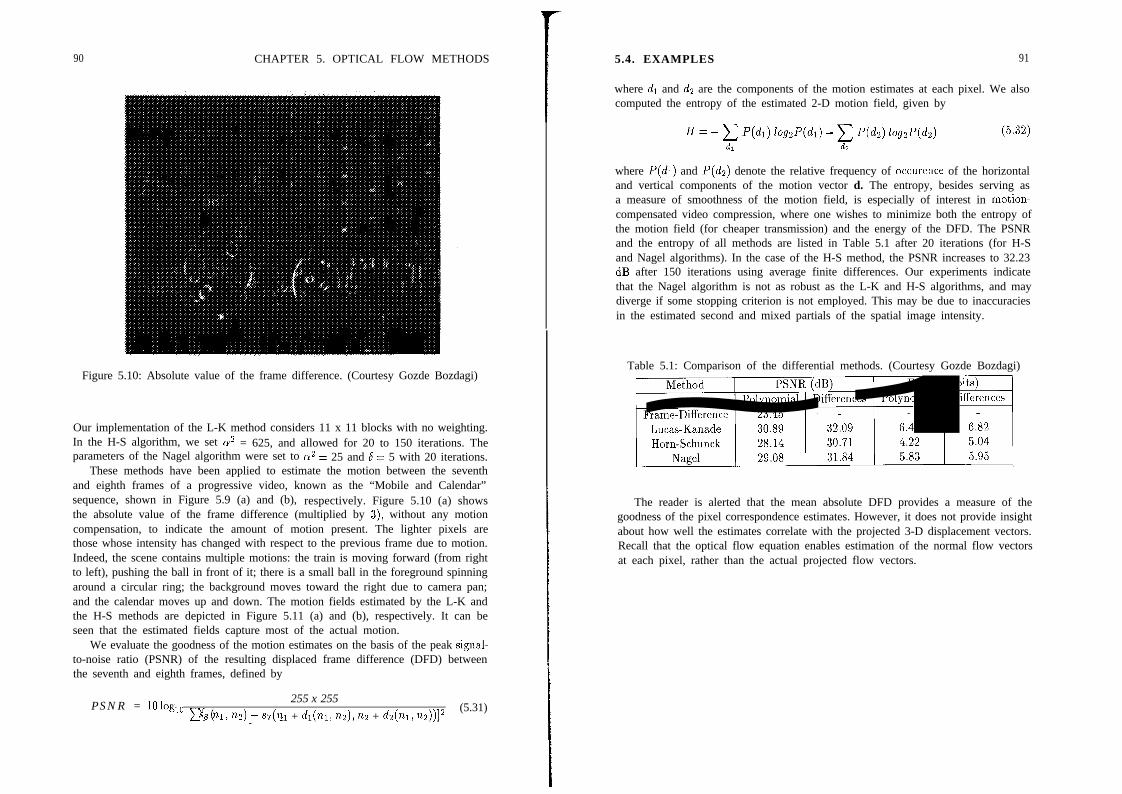
90 CHAPTER 5. OPTICAL FLOW METHODS
Figure 5.10: Absolute value of the frame difference. (Courtesy Gozde Bozdagi)
Our implementation of the L-K method considers 11 x 11 blocks with no weighting.In the H-S algorithm, we set LY ’ = 625, and allowed for 20 to 150 iterations. Theparameters of the Nagel algorithm were set to LY ’ = 25 and S = 5 with 20 iterations.
These methods have been applied to estimate the motion between the seventhand eighth frames of a progressive video, known as the “Mobile and Calendar”sequence, shown in Figure 5.9 (a) and (b), respectively. Figure 5.10 (a) showsthe absolute value of the frame difference (multiplied by 3), without any motioncompensation, to indicate the amount of motion present. The lighter pixels arethose whose intensity has changed with respect to the previous frame due to motion.Indeed, the scene contains multiple motions: the train is moving forward (from rightto left), pushing the ball in front of it; there is a small ball in the foreground spinningaround a circular ring; the background moves toward the right due to camera pan;and the calendar moves up and down. The motion fields estimated by the L-K andthe H-S methods are depicted in Figure 5.11 (a) and (b), respectively. It can beseen that the estimated fields capture most of the actual motion.
We evaluate the goodness of the motion estimates on the basis of the peak signal-to-noise ratio (PSNR) of the resulting displaced frame difference (DFD) betweenthe seventh and eighth frames, defined by
PSNR = lOlog,, c[ (255 x 255
St3 n1, m) S7(n_l + dl(W, Q), m2 + &(w, m))]”(5.31)
-_
5.4. EXAMPLES 91
where di and dz are the components of the motion estimates at each pixel. We alsocomputed the entropy of the estimated 2-D motion field, given by
H = - c P(4) hd’(dd - c P(h) logzP(da)dl &
where P(di) and P(dz) denote the relative frequency of occurence of the horizontaland vertical components of the motion vector d. The entropy, besides serving asa measure of smoothness of the motion field, is especially of interest in motion-compensated video compression, where one wishes to minimize both the entropy ofthe motion field (for cheaper transmission) and the energy of the DFD. The PSNRand the entropy of all methods are listed in Table 5.1 after 20 iterations (for H-Sand Nagel algorithms). In the case of the H-S method, the PSNR increases to 32.23dB after 150 iterations using average finite differences. Our experiments indicatethat the Nagel algorithm is not as robust as the L-K and H-S algorithms, and maydiverge if some stopping criterion is not employed. This may be due to inaccuraciesin the estimated second and mixed partials of the spatial image intensity.
Table 5.1: Comparison of the differential methods. (Courtesy Gozde Bozdagi)
Polynomial Differences Polynomial Differences
The reader is alerted that the mean absolute DFD provides a measure of thegoodness of the pixel correspondence estimates. However, it does not provide insightabout how well the estimates correlate with the projected 3-D displacement vectors.Recall that the optical flow equation enables estimation of the normal flow vectorsat each pixel, rather than the actual projected flow vectors.
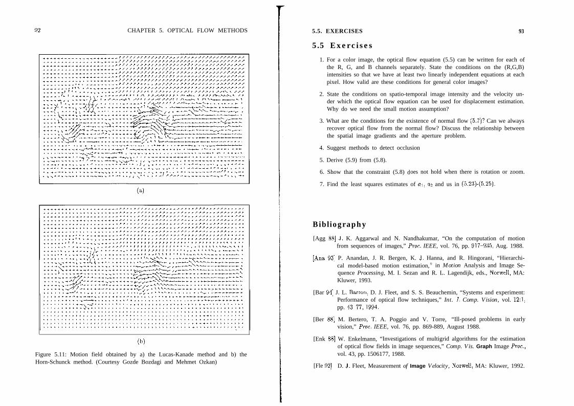
CHAPTER 5. OPTICAL FLOW METHODS
Figure 5.11: Motion field obtained by a) the Lucas-Kanade method and b) theHorn-Schunck method. (Courtesy Gozde Bozdagi and Mehmet Ozkan)
5.5. EXERCISES 93
5.5 Exercises
1. For a color image, the optical flow equation (5.5) can be written for each ofthe R, G, and B channels separately. State the conditions on the (R,G,B)intensities so that we have at least two linearly independent equations at eachpixel. How valid are these conditions for general color images?
2. State the conditions on spatio-temporal image intensity and the velocity un-der which the optical flow equation can be used for displacement estimation.Why do we need the small motion assumption?
3. What are the conditions for the existence of normal flow (5.7)? Can we alwaysrecover optical flow from the normal flow? Discuss the relationship betweenthe spatial image gradients and the aperture problem.
4. Suggest methods to detect occlusion
5. Derive (5.9) from (5.8).
6. Show that the constraint (5.8) does not hold when there is rotation or zoom.
7. Find the least squares estimates of al, u2 and us in (5.23)-(5.25).
Bibliography
[Agg 881 J. K. Aggarwal and N. Nandhakumar, “On the computation of motionfrom sequences of images,” Proc. IEEE, vol. 76, pp. 917-935, Aug. 1988.
[Ana 931 P. Anandan, J. R. Bergen, K. J. Hanna, and R. Hingorani, “Hierarchi-cal model-based motion estimation, ” in Motion Analysis and Image Se-quence Processing, M. I. Sezan and R. L. Lagendijk, eds., Norwell, MA:Kluwer, 1993.
[Bar 941 J. L. Barron, D. J. Fleet, and S. S. Beauchemin, “Systems and experiment:Performance of optical flow techniques,” Int. J. Comp. Vision, vol. 12:1,pp. 43377,1994.
[Ber 881 M. Bertero, T. A. Poggio and V. Torre, “Ill-posed problems in earlyvision,” Proc. IEEE, vol. 76, pp. 869-889, August 1988.
[Enk 881 W. Enkelmann, “Investigations of multigrid algorithms for the estimationof optical flow fields in image sequences,” Comp. Vis. Graph Image Proc.,vol. 43, pp. 1506177, 1988.
[Fle 921 D. J. Fleet, Measurement of Image Velocity, Norwell, MA: Kluwer, 1992.
94 BIBLIOGRAPHY
[Fog 911 S. V. Fogel, “Estimation of velocity vector fields from time-varying imagesequences,” CVGIP: Image Understanding, vol. 53, pp. 253-287, 1991.
[Hi1 841 E. C. Hildreth, ‘Computations underlying the measurement of visualmotion,” Artif. Intel., vol. 23, pp. 309-354, 1984.
[Hor 811 B. K. P. Horn and B. G. Schunck, “Determining optical flow,”Artif. Intell., vol. 17, pp. 185-203, 1981.
[Hua 811 T. S. Huang, ed., Image Sequence Analysis, Springer Verlag, 1981.
[Hua 831 T. S. Huang, ed., Image Sequence Processing and Dynamic Scene Analysis,Berlin, Germany: Springer-Verlag, 1983.
[Lim 901 J. S. Lim, Two-Dimensional Signal and Image Processing, EnglewoodCliffs, NJ: Prentice Hall, 1990.
[Luc 811 B. D. Lucas and T. Kanade, “An iterative image registration techniquewith an application to stereo vision,” Proc. DARPA Image UnderstandingWorkshop, pp. U-130, 1981.
[Nag 861 H. H. Nagel and W. Enkelmann, “An investigation of smoothness con-straints for the estimation of displacement vector fields from image se-quences,” IEEE Trans. Patt. Anal. Mach. Intel., vol. 8, pp. 565-593, 1986.
[Nag 871 H. H. Nagel, “On the estimation of optical flow: Relations between dif-ferent approaches and some new results,” Artificial Intelligence, vol. 33,pp. 2999324, 1987.
[Oht 901 N. Ohta, “Optical flow detection by color images,” NEC Res. and Dev.,no. 97, pp. 78-84, Apr. 1990.
[Sez 931 M. I. Sezan and R. L. Lagendijk, eds., Motion Analysis and ImageSequence Processing, Norwell, MA: Kluwer, 1993.
[Sin 911 A. Singh, Optic Flow Compatation, Los Alamitos, CA: IEEE ComputerSot. Press, 1991.
[Sny 911 M. A. Snyder, “On the mathematical foundations of smoothness con-straints for the determination of optical flow and for surface reconstruc-tion,” IEEE Trans. Patt. Anal. Mach. Intel., vol. 13, pp. 1105-1114,1991.
[Ura 881 S. Uras, F. Girosi, A. Verri, and V. Torre, “A computational approach tomotion perception,” Biol. Cybern., vol. 60, pp. 79-97, 1988.
[Ver 891 A. Verri and T. Poggio, “Motion field and optical flow: Qualita-tive properties,” IEEE Trans. Patt. Anal. Mach. Intel., vol. PAMI-11,pp. 490-498, May 1989.
Chapter 6
BLOCK-BASEDMETHODS
Block-based motion estimation and compensation are among the most popularapproaches. Block-based motion compensation has been adopted in the inter-national standards for digital video compression, such as H.261 and MPEG 1-2.Although these standards do not specify a particular motion estimation method,block-based motion estimation becomes a natural choice. Block-based motion es-timation is also widely used in several other digital video applications, includingmotion-compensated filtering for standards conversion.
We start with a brief introduction of the block-motion models in Section 6.1.A simple block-based motion estimation scheme, based on the translatory blockmodel, was already discussed in Chapter 5, in the context of estimation using theoptical flow equation. In this chapter, we present two other translatory-block-based motion estimation strategies. The first approach, discussed in Section 6.2,is a spatial frequency domain technique, called the phase-correlation method. Thesecond, presented in Section 6.3, is a spatial domain search approach, called theblock-matching method. Both methods can be implemented hierarchically, usinga multiresolution description of the video. Hierarchical block-motion estimationis addressed in Section 6.4. Finally, in Section 6.5, possible generalizations of theblock-matching framework are discussed, including 2-D deformable block motionestimation, in order to overcome some shortcomings of the translatory block-motionmodel.
6.1 Block-Motion ModelsThe block-motion model assumes that the image is composed of moving blocks. Weconsider two types of block motion: i) simple 2-D translation, and ii) various 2-Ddeformations of the blocks.
95

96 CHAPTER 6. BLOCK-BASED METHODS
6.1.1 Translational Block Motion
The simplest form of this model is that of translatory blocks, restricting the motionof each block to a pure translation. Then an N x N block B in frame lc centeredabout the pixel n = (no, n2) is modeled as a globally shifted version of a same-sizeblock in frame k + !, for an integer 1. That is,
s(nl,nz,k) = S,(XI + dl,x2 +d2,t +lAt)I
[;]=v[ ;]
for all (nr,n2) E B, where dl and dz are the components of the displacement(translation) vector for block B. Recall from the previous chapter that the right-hand side of (6.1) is given in terms of the continuous time-varying image s,(xl, x2, t),because dl and dz are real-valued. Assuming the values of dl and dz are quantizedto the nearest integer, the model (6.1) can be simplified as
s(nl,nz, k) = s(nl +dl,nz +dz,k+e) (6.2)
Observe that it is possible to obtain 1/2L pixel accuracy in the motion estimates,using either the phase-correlation or the block-matching methods, if the frames kand k + e in (6.2) are interpolated by a factor of L.
frame k
block B
a)
I ’EEI
b)
Figure 6.1: Block-motion models: a) nonoverlapping and b) overlapping blocks.
In the model (6.1), the blocks B may be nonoverlapping or overlapping as shownin Figure 6.1 (a) and (b), respectively. In the nonoverlapping case, the entire block
6.1. BLOCK-MOTION MODELS
is assigned a single motion vector. Hence, motion compensation can be achievedby copying the gray-scale or color information from the corresponding block in theframe k + 1 on a pixel-by-pixel basis. In the case of overlapping blocks, we caneither compute the average of the motion vectors within the overlapping regions,or select one of the estimated motion vectors. Motion compensation in the case ofoverlapping blocks was discussed in [Sul 931, where a multihypothesis expectationapproach was proposed.
The popularity of motion compensation and estimation based on the model oftranslational blocks originates from:
l low overhead requirements to represent the motion field, since one motionvector is needed per block., and
. ready availability of low-cost VLSI implementations.
However, motion compensation using translational blocks i) fails for zoom, rota-tional motion, and under local deformations, and ii) results in serious blockingartifacts, especially for very-low-bitrate applications, because the boundaries of ob-jects do not generally agree with block boundaries, and adjacent blocks may beassigned substantially different motion vectors.
6.1.2 Generalized/Deformable Block Motion
In order to generalize the translational block model (6.1), note that it can be char-acterized by a simple frame-to-frame pixel coordinate (spatial) transformation ofthe form
x; = XI $4x’z = 22 + dz (6.3)
where (xi,&) denotes the coordinates of a point in the frame k + 1. The spatialtransformation (6.3) can be generalized to include affine coordinate transformations,given by
x; = ~1x1 + a222 + 4x; = ~a+ a4xz + dz (6.4)
The affine transformation (6.4) can handle rotation of blocks as well as 2-D defor-mation of squares (rectangles) into parallelograms, as depicted in Figure 6.2. Otherspatial transformations include the perspective and bilinear coordinate transforma-tions. The perspective transformation is given by
x; =alxl + a222 + a3a721 +%3x2 + 1
x’z =a4xl + a522 + a6
a7xl + a822 + 1(6.5)
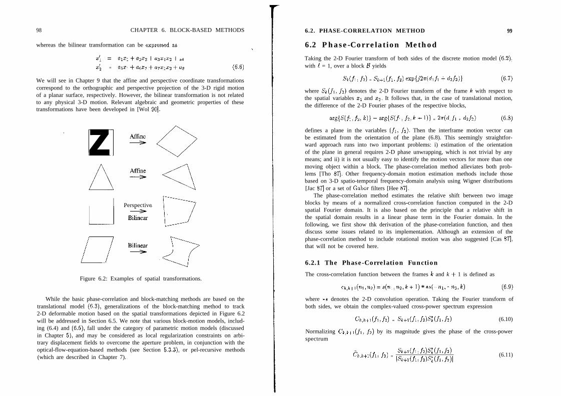
98 CHAPTER 6. BLOCK-BASED METHODS
whereas the bilinear transformation can be expressed as
x; = alxl + a222 + a32122 + a4
x; = a5xl +&x2 + a7xlx2 + ‘% (6.6)
We will see in Chapter 9 that the affine and perspective coordinate transformationscorrespond to the orthographic and perspective projection of the 3-D rigid motionof a planar surface, respectively. However, the bilinear transformation is not relatedto any physical 3-D motion. Relevant algebraic and geometric properties of thesetransformations have been developed in [Wol 901.
’Perspective
Figure 6.2: Examples of spatial transformations.
While the basic phase-correlation and block-matching methods are based on thetranslational model (6.3), generalizations of the block-matching method to track2-D deformable motion based on the spatial transformations depicted in Figure 6.2will be addressed in Section 6.5. We note that various block-motion models, includ-ing (6.4) and (6.5), fall under the category of parametric motion models (discussedin Chapter 5), and may be considered as local regularization constraints on arbi-trary displacement fields to overcome the aperture problem, in conjunction with theoptical-flow-equation-based methods (see Section 5.3.3), or pel-recursive methods(which are described in Chapter 7).
6.2. PHASE-CORRELATION METHOD
6.2 Phase-Correlation Method
99
Taking the 2-D Fourier transform of both sides of the discrete motion model (6.2),with ! = 1, over a block B yields
Sk(.fi, .f2) = Sk+l(fi, fi) expL7W~lfi + d2.f~)) (6.7)
where Sk(fi) f2) denotes the 2-D Fourier transform of the frame Ic with respect tothe spatial variables II and ~2. It follows that, in the case of translational motion,the difference of the 2-D Fourier phases of the respective blocks,
arg{S(fi,fi, k)) - arg{S(fi, f2,k + 1)) = W&f1 + WZ) (6.8)
defines a plane in the variables (fi, fz). Then the interframe motion vector canbe estimated from the orientation of the plane (6.8). This seemingly straightfor-ward approach runs into two important problems: i) estimation of the orientationof the plane in general requires 2-D phase unwrapping, which is not trivial by anymeans; and ii) it is not usually easy to identify the motion vectors for more than onemoving object within a block. The phase-correlation method alleviates both prob-lems [Tho 871. Other frequency-domain motion estimation methods include thosebased on 3-D spatio-temporal frequency-domain analysis using Wigner distributions[Jac 871 or a set of Gabor filters [Hee 871.
The phase-correlation method estimates the relative shift between two imageblocks by means of a normalized cross-correlation function computed in the 2-Dspatial Fourier domain. It is also based on the principle that a relative shift inthe spatial domain results in a linear phase term in the Fourier domain. In thefollowing, we first show thk derivation of the phase-correlation function, and thendiscuss some issues related to its implementation. Although an extension of thephase-correlation method to include rotational motion was also suggested [Cas 871,that will not be covered here.
6.2.1 The Phase-Correlation Function
The cross-correlation function between the frames I% and k + 1 is defined as
clc,h+l(nl, m) = s(nl, nz, k + 1) * *s(--nl, -2, k) (6.9)
where ** denotes the 2-D convolution operation. Taking the Fourier transform ofboth sides, we obtain the complex-valued cross-power spectrum expression
G,ktl(fl>.fz) = sk,l(fl,fz)s~(fl,f2) (6.10)
Normalizing C’k,ktl(fi) f2) by its magnitude gives the phase of the cross-powerspectrum
z;,,k,l(fl, fz) =s~tl(fl,fz)s~(fl,f2)
Is~tl(fl, fd%(fl, f2)l(6.11)
100 CHAPTER 6. BLOCK-BASED METHODS
Assuming translational motion, we substitute (6.7) into (6.11) to obtain
Ch,k+l(fi, fi) = exp{-Px(fi4 + f2d2)) (6.12)
Taking the inverse 2-D Fourier transform of this expression yields the phase-correlation function
C”lc,b+l(w , n2) = S(m - 4, nz - dz) (6.13)
We observe that the phase-correlation function consists of an impulse whose locationyields the displacement vector.
6.2.2 Implementation Issues
Implementation of the phase-correlation method in the computer requires replacingthe 2-D Fourier transforms by the 2-D DFT, resulting in the following algorithm:
1. Compute the 2-D DFT of the respective blocks from the leth and Ic + lthframes.
2. Compute the phase of the cross-power spectrum as in (6.11).
3. Compute the 2-D inverse DFT of ck,k+,(fl,f2) to obtain the phase-correlation function Fh,s+l(nl, 7~2).
4. Detect the location of the peak(s) in the phase-correlation function
Ideally, we expect to observe a single impulse in the phase-correlation functionindicating the relative displacement between the two blocks. In practice, a numberof factors contribute to the degeneration of the phase-correlation function to containone or more peaks. They are the use of the 2-D DFT instead of the 2-D Fouriertransform, the presence of more than one moving object within the block, and thepresence of observation noise.
The use of the 2-D DFT instead of the 2-D Fourier transform has a number ofconsequences:
l Boundary effects: In order to obtain a perfect impulse, the shift must be cyclic.Since things disappearing at one end of the window generally do not reappearat the other end, the impulses degenerate into peaks. Further, it is well knownthat the 2-D DFT assumes periodicity in both directions. Discontinuities fromleft to right boundaries, and from top to bottom, may introduce spuriouspeaks.
l Spectral leakage due to noninteger motion vectors: In order to observe a per-fect impulse, the components of the displacement vector must correspond toan integer multiple of the fundamental frequency. Otherwise, the impulse willdegenerate into a peak due to the well-known spectral leakage phenomenon.
6.3. BLOCK-MATCHING METHOD 101
l Range of displacement estimates: Since the 2-D DFT is periodic with theblock size (Nl, Nz), the displacement estimates need to be unwrapped as
2 - N. othlrwiseif Id,1 < Ni/2, Ni even, or ldil 5 (Ni - 1)/2, Ni odd (6.14)2 2
to accommodate negative displacements. Thus, the range of estimates is[-Ni/2+ 1, Ni/2] for Ni even. For example, to estimate displacements withina range [-31,321, the block size should be at least 64 x 64.
The block size is one of the most important parameters in any block-basedmotion estimation algorithm. Selection of the block size usually involves a tradeoffbetween two conflicting requirements. The window must be large enough in order tobe able to estimate large displacement vectors. On the other hand, it should be smallenough so that the displacement vector remains constant within the window. Thesetwo contradicting requirements can usually be addressed by hierarchical methods[Erk 931. Hierarchical methods will be treated for the case of block matching thatalso faces the same tradeoff in window size selection.
The phase-correlation method has some desirable properties:Frame-to-frame intensity changes: The phase-correlation method is relatively insen-sitive to changes in illumination, because shifts in the mean value or multiplicationby a constant do not affect the Fourier phase. Since the phase-correlation functionis normalized with the Fourier magnitude, the method is also insensitive to anyother Fourier-magnitude-only degradation.Mul2iple moving objects: It is of interest to know what happens when multiplemoving objects with different velocities are present within a single window. Exper-iments indicate that multiple peaks are observed, each indicating the movement ofa particular object [Tho 871. Detection of the significant peaks then generates a listof candidate displacement vectors for each pixel within the block. An additionalsearch is required to find which displacement vector belongs to which pixel withinthe block. This can be verified by testing the magnitude of the displaced framedifference with each of the candidate vectors.
6.3 Block-Matching Method
Block matching can be considered as the most popular method for practical motionestimation due to its lesser hardware complexity [Jai 81, Ghr 901. As a result it iswidely available in VLSI, and almost all H.261 and MPEG l-2 codecs are utilizingblock matching for motion estimation. In block matching, the best motion vectorestimate is found by a pixel-domain search procedure.
The basic idea of block matching is depicted in Figure 6.3, where the displace-ment for a pixel (121) n2) in frame k (the present frame) is determined by consideringan N1 x Nz block centered about (nl, Q), and searching frame le + 1 (the searchframe) for the location of the best-matching block of the same size. The search is
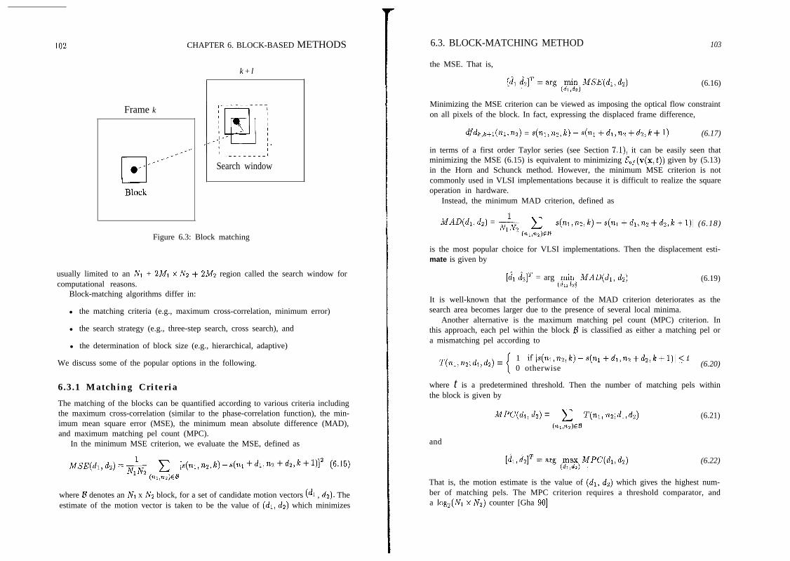
CHAPTER 6. BLOCK-BASED METHODS
k + l
Frame k
Search window
Figure 6.3: Block matching
usually limited to an Ni + 2Mi x Nz + 2A4z region called the search window forcomputational reasons.
Block-matching algorithms differ in:
l the matching criteria (e.g., maximum cross-correlation, minimum error)
l the search strategy (e.g., three-step search, cross search), and
l the determination of block size (e.g., hierarchical, adaptive)
We discuss some of the popular options in the following.
6.3.1 Matching Criteria
The matching of the blocks can be quantified according to various criteria includingthe maximum cross-correlation (similar to the phase-correlation function), the min-imum mean square error (MSE), the minimum mean absolute difference (MAD),and maximum matching pel count (MPC).
In the minimum MSE criterion, we evaluate the MSE, defined as
MSE(ch, &) = & c [S(Q, n2, k) - s(n1 + 4, nz + &I k + 1)l” (6.3(~l,nz)a
where B denotes an Ni x Nz block, for a set of candidate motion vectors (dr , dz). Theestimate of the motion vector is taken to be the value of (di, dz) which minimizes
6.3. BLOCK-MATCHING METHOD
the MSE. That is,
103
(6.16)
Minimizing the MSE criterion can be viewed as imposing the optical flow constrainton all pixels of the block. In fact, expressing the displaced frame difference,
Gb,k+l(nl,nz) = s(w,nz,k) - s(nl +h,nz +h,k+ 1) (6.17)
in terms of a first order Taylor series (see Section 7.1), it can be easily seen thatminimizing the MSE (6.15) is equivalent to minimizing f,f(v(x,t)) given by (5.13)in the Horn and Schunck method. However, the minimum MSE criterion is notcommonly used in VLSI implementations because it is difficult to realize the squareoperation in hardware.
Instead, the minimum MAD criterion, defined as
MAD(&, d2) =T& c ‘(snl,nz,k)-s(nl+dl,na+dz,k+l)l (6.18)
(nl,%)En
is the most popular choice for VLSI implementations. Then the displacement esti-mate is given by
[d^l d^ZIT = arg (Fp) IMAD &) (6.19)I> 2
It is well-known that the performance of the MAD criterion deteriorates as thesearch area becomes larger due to the presence of several local minima.
Another alternative is the maximum matching pel count (MPC) criterion. Inthis approach, each pel within the block B is classified as either a matching pel ora mismatching pel according to
T(nl,nz;h,dz) =1 ifIs(n~,n2,k)-s(n~+dl,nz+dz,k+l)lIt0 otherwise (6.20)
where t is a predetermined threshold. Then the number of matching pels withinthe block is given by
MPC(d1, d2) = C T(nl, n2; 4, d2) (6.21)(nlm)a
and
(6.22)
That is, the motion estimate is the value of (dr, ds) which gives the highest num-ber of matching pels. The MPC criterion requires a threshold comparator, anda log,(Ni x Nz) counter [Gha 901.

104 CHAPTER 6. BLOCK-BASED METHODS
6.3.2 Search Procedures
Finding the best-matching block requires optimizing the matching criterion overall possible candidate displacement vectors at each pixel (ni, nz). This can beaccomplished by the so-called “full search,” which evaluates the matching criterionfor all values of (di, dz) at each pixel, and is extremely time-consuming.
As a first measure to reduce the computational burden, we usually limit thesearch area to a
“search window” centered about each pixel for which a motion vector will be esti-mated, where Ml and M2 are predetermined integers. A search window is shown inFigure 6.3. Another commonly employed practice to lower the computational loadis to estimate motion vectors on a sparse grid of pixels, e.g., once every eight pixelsand eight lines using a 16 x 16 block, and to then interpolate the motion field toestimate the remaining motion vectors.
In most cases, however, search strategies faster than the full search are uti-lized, although they lead to suboptimal solutions. Some examples of faster searchalgorithms include the
l three-step search and,
l cross-search.
These faster search algorithms evaluate the criterion function only at a predeter-mined subset of the candidate motion vector locations. Let’s note here that the ex-pected accuracy of motion estimates varies according to the application. In motion-compensated compression, all we seek is a matching block, in terms of some metric,even if the match does not correlate well with the actual projected motion. It isfor this reason that faster search algorithms serve video compression applicationsreasonably well.
Three-Step Search
We explain the three-step search procedure with the help of Figure 6.4, where onlythe search frame is depicted with the search window parameters Ml = Mz = 7. The“0” marks the pixel in the search frame that is just behind the present pixel. In thefirst step, the criterion function is evaluated at nine points, the pixel “0” and thepixels marked as “1.” If the lowest MSE or MAD is found at the pixel “0,” then wehave “no motion.” In the second step, the criterion function is evaluated at 8 pointsthat are marked as “2” centered about the pixel chosen as the best match in thefirst stage (denoted by a circled “1”). Note that in the initial step, the search pixelsare the corners of the search window, and then at each step we halve the distanceof the search pixels from the new center to obtain finer-resolution estimates. Themotion estimate is obtained after the third step, where the search pixels are all 1pixel away from the center.
6.3. BLOCK-MATCHING METHOD 105
Figure 6.4: Three-step search.
Additional steps may be incorporated into the procedure if we wish to obtainsubpixel accuracy in the motion estimates. Note that the search frame needs to beinterpolated to evaluate the criterion function at subpixel locations. Generalizationof this procedure to other search window parameters yields the so-called “n-stepsearch” or “log-D search” procedures.
Figure 6.5: Cross-search
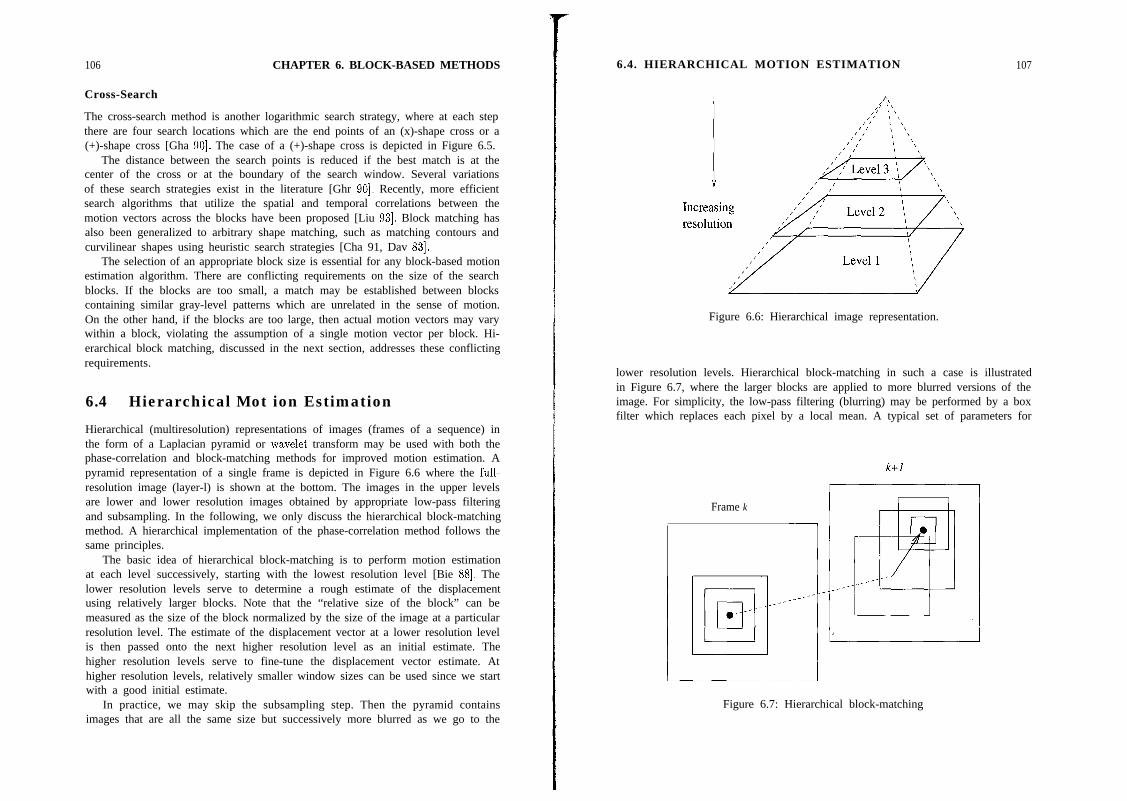
106 CHAPTER 6. BLOCK-BASED METHODS
Cross-Search
The cross-search method is another logarithmic search strategy, where at each stepthere are four search locations which are the end points of an (x)-shape cross or a(+)-shape cross [Gha 901. The case of a (+)-shape cross is depicted in Figure 6.5.
The distance between the search points is reduced if the best match is at thecenter of the cross or at the boundary of the search window. Several variationsof these search strategies exist in the literature [Ghr 901. Recently, more efficientsearch algorithms that utilize the spatial and temporal correlations between themotion vectors across the blocks have been proposed [Liu 931. Block matching hasalso been generalized to arbitrary shape matching, such as matching contours andcurvilinear shapes using heuristic search strategies [Cha 91, Dav 831.
The selection of an appropriate block size is essential for any block-based motionestimation algorithm. There are conflicting requirements on the size of the searchblocks. If the blocks are too small, a match may be established between blockscontaining similar gray-level patterns which are unrelated in the sense of motion.On the other hand, if the blocks are too large, then actual motion vectors may varywithin a block, violating the assumption of a single motion vector per block. Hi-erarchical block matching, discussed in the next section, addresses these conflictingrequirements.
6.4 Hierarchical Mot ion Estimation
Hierarchical (multiresolution) representations of images (frames of a sequence) inthe form of a Laplacian pyramid or wavelet transform may be used with both thephase-correlation and block-matching methods for improved motion estimation. Apyramid representation of a single frame is depicted in Figure 6.6 where the full-resolution image (layer-l) is shown at the bottom. The images in the upper levelsare lower and lower resolution images obtained by appropriate low-pass filteringand subsampling. In the following, we only discuss the hierarchical block-matchingmethod. A hierarchical implementation of the phase-correlation method follows thesame principles.
The basic idea of hierarchical block-matching is to perform motion estimationat each level successively, starting with the lowest resolution level [Bie 881. Thelower resolution levels serve to determine a rough estimate of the displacementusing relatively larger blocks. Note that the “relative size of the block” can bemeasured as the size of the block normalized by the size of the image at a particularresolution level. The estimate of the displacement vector at a lower resolution levelis then passed onto the next higher resolution level as an initial estimate. Thehigher resolution levels serve to fine-tune the displacement vector estimate. Athigher resolution levels, relatively smaller window sizes can be used since we startwith a good initial estimate.
In practice, we may skip the subsampling step. Then the pyramid containsimages that are all the same size but successively more blurred as we go to the
6.4. HIERARCHICAL MOTION ESTIMATION 107
Figure 6.6: Hierarchical image representation.
lower resolution levels. Hierarchical block-matching in such a case is illustratedin Figure 6.7, where the larger blocks are applied to more blurred versions of theimage. For simplicity, the low-pass filtering (blurring) may be performed by a boxfilter which replaces each pixel by a local mean. A typical set of parameters for
k+l
Frame k I I
Figure 6.7: Hierarchical block-matching

108 CHAPTER 6. BLOCK-BASED METHODS
Table 6.1: Typical set of parameters for 5-Level hierarchical block-matching.
LEVEL: 5 4 3 2 1Filter Size 10 10 5 5 3M a x i m u m D i s p l a c e m e n t f31 f15 f7 A3 flBlock Size 64 32 16 8 4
5-level hierarchical block-matching (with no subsampling) is shown in Table 6.1.Here, the filter size refers to the size of a square window used in computing thelocal mean.
Figure 6.8 illustrates hierarchical block-matching with 2 levels, where the max-imum allowed displacement M = 7 for level 2 and M = 3 for level 1. The bestestimate at the lower resolution level (level 2) is indicated by the circled “3.” Thecenter of the search area in level 1 (denoted by “0”) corresponds to the best esti-mate from the second level. The estimates in the second and first levels are [7, 1lTand [3, 1lT, respectively, resulting in an overall estimate of [lo, 21T. Hierarchicalblock-matching can also be performed with subpixel accuracy by incorporating ap-propriate interpolation.
Level 1(higher resolution)
Level 2 (lower resolution)
Figure 6.8: Example of hierarchical block-matching with 2 levels.
6.5. GENERALIZED BLOCK-MOTION ESTIMATION
6.5 Generalized Block-Motion Estimation
109
While motion estimation based on the translatory block model is simple, it dealspoorly with rotations and deformations of blocks from frame to frame, as well asdiscontinuities in the motion field. We discuss two approaches in the following forimproved motion tracking and compensation using block-based methods: a postpro-cessing approach, and a generalized block-matching approach using spatial trans-formations.
6.5.1 Postprocessing for Improved Motion Compensation
Block-based motion representation and compensation have been adopted in inter-national standards for video compression, such as H.261, MPEG-1, and MPEG-2,where a single motion vector is estimated for each 16 x 16 square block, in orderto limit the number of motion vectors that need to be transmitted. However, thislow-resolution representation of the motion field results in inaccurate compensationand visible blocking artifacts, especially at the borders of the blocks.
To this effect) Orchard [Ore 931 proposed a postprocessing method to reconstructa higher-resolution motion field based on image segmentation. In this method, asingle motion vector is estimated per block, as usual, in the first pass. Next, imageblocks are segmented into K regions such that each region is represented by a singlemotion vector. To avoid storage/transmission of additional motion vectors, the Kcandidate motion vectors are selected from a set of already estimated motion vectorsfor the neighboring blocks. Then, the motion vector that minimizes the DFD ateach pixel of the block is selected among the set of K candidate vectors. A predic-tive MAP segmentation scheme has been proposed to avoid transmitting overheadinformation about the boundaries of these segments, where the decoder/receivercan duplicate the segmentation process. As a result, this method allows for motioncompensation using a pixel-resolution motion field, while transmitting the sameamount of motion information as classical block-based methods.
6.5.2 Deformable Block Matching
In deformable (or generalized) block matching, the current frame is divided intotriangular, rectangular, or arbitrary quadrilateral patches. We then search for thebest matching triangle or quadrilateral in the search frame under a given spatialtransformation. This is illustrated in Figure 6.9. The choice of patch shape andthe spatial transformation are mutually related. For example, triangular patchesoffer sufficient degrees of freedom (we have two equations per node) with the affinetransformation, which has only six independent parameters. Perspective and bilin-ear transformations have eight free parameters. Hence, they are suitable for usewith rectangular or quadrilateral patches. Note that using affine transformationwith quadrilateral patches results in an overdetermined motion estimation problemin that affine transformation preserves parallel lines (see Figure 6.2).

110 CHAPTER 6. BLOCK-BASED METHODS
The spatial transformations (6.4), (6.5), and (6.6) clearly provide superior mo-tion tracking and rendition, especially in the presence of rotation and zooming,compared to the translational model (6.3). However, the complexity of the motionestimation increases significantly. If a search-based motion estimation strategy isadopted, we now have to perform a search in a 6- or 8-D parameter space (affine orperspective/bilinear transformation) instead of a 2-D space (the ~1 and xz compo-nents of the translation vector). Several generalized motion estimation schemes havebeen proposed, including a full-search method [Sef 931, a faster hexagonal search[Nak 941, and a global spline surface-fitting method using a fixed number of pointcorrespondences [Flu92].
The full-search method can be summarized as follows [Sef 931:
1. Segment the current frame into rectangular (triangular) blocks.
2. Perturb the coordinates of the corners of a matching quadrilateral (triangle)in the search frame starting from an initial guess.
3. For each quadrilateral (triangle), find the parameters of a prespecified spatialtransformation that maps this quadrilateral (triangle) onto the rectangular(triangular) block in the current frame using the coordinates of the four (three)matching corners.
4. Find the coordinates of each corresponding pixel within the quadrilateral (tri-angle) using the computed spatial transformation, and calculate the MSEbetween the given block and the matching patch.
5. Choose the spatial transformation that yields the smallest MSE or MAD.
In order to reduce the computational load imposed by generalized block-matching,generalized block-matching is only used for those blocks where standard block-matching is not satisfactory. The displaced frame difference resulting from standardblock matching can be used as a decision criterion. The reader is referred to [Flu921and [Nak 941 for other generalized motion estimation strategies.
The generalized block-based methods aim to track the motion of all pixels withina triangular or quadrilateral patch using pixel correspondences established at thecorners of the patch. Thus, it is essential that the current frame is segmented intotriangular or rectangular patches such that each patch contains pixels only froma single moving object. Otherwise, local motion within these patches cannot betracked using a single spatial transformation. This observation leads us to feature-and/or motion-based segmentation of the current frame into adaptive meshes (alsoknown as irregular-shaped meshes). Regular and adaptive mesh models are depictedin Figure 6.10 for comparison.
There are, in general, two segmentation strategies: i) Feature-based segmen-tation: The edges of the patches are expected to align sufficiently closely withgray-level and/or motion edges. Ideally, adaptive mesh fitting and motion track-ing should be performed simultaneously, since it is not generally possible to isolatemotion rendition errors due to adaptive mesh misfit and motion estimation. A si-multaneous optimization method was recently proposed by Wang et al. [Wan 941.
6.5. GENERALIZED BLOCK-MOTION ESTIMATION
I (search frame)
Frame k
Figure 6.9: Generalized block-matching.
ii) Hierarchical segmentation: It is proposed to start with an initial coarse mesh,and perform a synthesis of the present frame based on this mesh. Then this meshis refined by successive partitioning of the patches where the initial synthesis erroris above a threshold. A method based on the hierarchical approach was proposedby Flusser [Flu92].
Fitting and tracking of adaptive mesh models is an active research area atpresent. Alternative strategies for motion-based segmentation (although not nec-essarily into mesh structures) and parametric motion model estimation will be dis-cussed in Chapter 11.
a) b)
Figure 6.10: a) Regular and b) adaptive mesh models fitted to frame Ic.
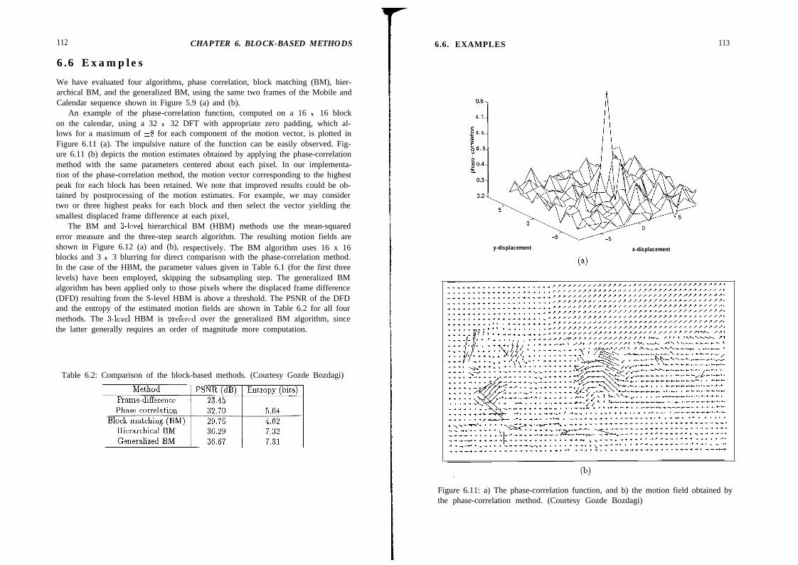
112 CHAPTER 6. BLOCK-BASED METHODS
6.6 Examples
We have evaluated four algorithms, phase correlation, block matching (BM), hier-archical BM, and the generalized BM, using the same two frames of the Mobile andCalendar sequence shown in Figure 5.9 (a) and (b).
An example of the phase-correlation function, computed on a 16 x 16 blockon the calendar, using a 32 x 32 DFT with appropriate zero padding, which al-lows for a maximum of *8 for each component of the motion vector, is plotted inFigure 6.11 (a). The impulsive nature of the function can be easily observed. Fig-ure 6.11 (b) depicts the motion estimates obtained by applying the phase-correlationmethod with the same parameters centered about each pixel. In our implementa-tion of the phase-correlation method, the motion vector corresponding to the highestpeak for each block has been retained. We note that improved results could be ob-tained by postprocessing of the motion estimates. For example, we may considertwo or three highest peaks for each block and then select the vector yielding thesmallest displaced frame difference at each pixel,
The BM and 3-level hierarchical BM (HBM) methods use the mean-squarederror measure and the three-step search algorithm. The resulting motion fields areshown in Figure 6.12 (a) and (b), respectively. The BM algorithm uses 16 x 16blocks and 3 x 3 blurring for direct comparison with the phase-correlation method.In the case of the HBM, the parameter values given in Table 6.1 (for the first threelevels) have been employed, skipping the subsampling step. The generalized BMalgorithm has been applied only to those pixels where the displaced frame difference(DFD) resulting from the S-level HBM is above a threshold. The PSNR of the DFDand the entropy of the estimated motion fields are shown in Table 6.2 for all fourmethods. The 3-level HBM is prefered over the generalized BM algorithm, sincethe latter generally requires an order of magnitude more computation.
Table 6.2: Comparison of the block-based methods. (Courtesy Gozde Bozdagi)
6.6. EXAMPLES 113
0.6.0.7.
.s;i 0.6.55 0 . 5 .
y-displacement x-displacement
Figure 6.11: a) The phase-correlation function, and b) the motion field obtained bythe phase-correlation method. (Courtesy Gozde Bozdagi)
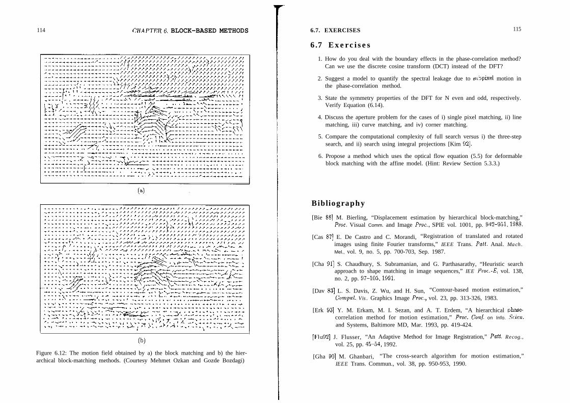
114 CHAPTER6. BLOCK-BASED METHODS
Figure 6.12: The motion field obtained by a) the block matching and b) the hier-archical block-matching methods. (Courtesy Mehmet Ozkan and Gozde Bozdagi)
6.7. EXERCISES 115
6.7 Exercises
1. How do you deal with the boundary effects in the phase-correlation method?Can we use the discrete cosine transform (DCT) instead of the DFT?
2. Suggest a model to quantify the spectral leakage due to subpixel motion inthe phase-correlation method.
3. State the symmetry properties of the DFT for N even and odd, respectively.Verify Equation (6.14).
4. Discuss the aperture problem for the cases of i) single pixel matching, ii) linematching, iii) curve matching, and iv) corner matching.
5. Compare the computational complexity of full search versus i) the three-stepsearch, and ii) search using integral projections [Kim 921.
6. Propose a method which uses the optical flow equation (5.5) for deformableblock matching with the affine model. (Hint: Review Section 5.3.3.)
Bibliography
[Bie 881 M. Bierling, “Displacement estimation by hierarchical block-matching,”Proc. Visual Comm. and Image Proc., SPIE vol. 1001, pp. 942-951,1988.
[Cas 871 E. De Castro and C. Morandi, “Registration of translated and rotatedimages using finite Fourier transforms,” IEEE Trans. Palt. Anal. Mach.Mel., vol. 9, no. 5, pp. 700-703, Sep. 1987.
[Cha 911 S. Chaudhury, S. Subramanian, and G. Parthasarathy, “Heuristic searchapproach to shape matching in image sequences,” IEE Proc.-E, vol. 138,no. 2, pp. 97-105,1991.
[Dav 831 L. S. Davis, Z. Wu, and H. Sun, “Contour-based motion estimation,”Compu2. Vis. Graphics Image Proc., vol. 23, pp. 313-326, 1983.
[Erk 931 Y. M. Erkam, M. I. Sezan, and A. T. Erdem, “A hierarchical phase-correlation method for motion estimation,” Proc. Conf. on Info. Scien.
and Systems, Baltimore MD, Mar. 1993, pp. 419-424.
[Flu921 J. Flusser, “An Adaptive Method for Image Registration,” Pa2t. Recog.,vol. 25, pp. 45-54, 1992.
[Gha 901 M. Ghanbari, “The cross-search algorithm for motion estimation,”IEEE Trans. Commun., vol. 38, pp. 950-953, 1990.
116 BIBLIOGRAPHY
[Ghr 901 H. Gharavi and M. Mills, “Block-matching motion estimation algorithms:New results,” IEEE Trans. Circ. and Syst., vol. 37, pp. 6499651, 1990.
[Hee 871 D. J. Heeger, “Model for the extraction of image flow,” b. Opt. Sot. Am. A,vol. 4, no. 8, pp. 145551471, Aug. 1987.
[Jac 871 L. Jacobson and H. Wechsler, “Derivation of optical flow using a spatio-temporal frequency approach,” Comp. Vision Graph. Image Proc., vol. 38,pp. 57-61, 1987.
[Jai 811 J. R. Jain and A. K. Jain, “Displacement measurement and its appli-cation in interframe image coding,” IEEE Trans. Commun., vol. 29,pp. 1799-1808, 1981.
[Kim 921 J.-S. Kim and R.-H. Park, “A fast feature-based block-matching algorithmusing integral projections,” IEEE J. Selected Areas in Comm., vol. 10,pp. 968-971, June 1992.
[Liu 931 B. Liu and A. Zaccarin, “New fast algorithms for the estimation of blockmotion vectors,” IEEE Trans. Circ. and Syst. Video Tech., vol. 3, no. 2,pp. 148-157, Apr. 1993.
[Nak 941 Y. Nakaya and H. Harashima, “Motion compensation based on spatialtransformations,” IEEE Trans. CAS Video Tech., vol. 4, pp. 339-356,June 1994.
[Ore 931 M. Orchard, “Predictive motion-field segmentation for image sequencecoding,” IEEE Trans. Circ. and Syst: Video Tech., vol. 3, pp. 54-70,Feb. 1993.
[Sef 931 V. Seferidis and M. Ghanbari, “General approach to block-matching mo-tion estimation,” Optical Engineering, vol. 32, pp. 1464-1474, July 1993.
[Sul 931 G. Sullivan, “Multi-hypothesis motion compensation for low bit-ratevideo coding,” Proc. IEEE Int. Conf. ASSP, Minneapolis, MN, vol. 5,pp. 437-440, 1993.
[Tho 871 G. A. Thomas and B. A. Hons, “Television motion measurement for DATVand other applications,” Tech. Rep. BBC-RD-1987-11, 1987.
[Wan 941 Y. Wang and 0. Lee, “Active mesh: A feature seeking and track-ing image sequence representation scheme,” IEEE Trans. Image Proc.,vol. 3, pp. 610-624, Sep. 1994.
[Wol90] G. Wolberg, Digital Image Warping, Los Alamitos, CA: IEEE Comp. Sot.Press, 1990.
Chapter 7
PEL-RECURSIVEMETHODSAll motion estimation methods, in one form or another, employ the optical flowconstraint accompanied by some smoothness constraint. Pel-recursive methods arepredictor-corrector-type estimators, of the form
&(x, t; At) = &(x, t; At) + u(x,t; At) (7.1)
where 2,(x, t; At) denotes the estimated motion vector at the location x and time t,da(x, t; At) denotes the predicted motion estimate, and u(x, t; At) is the updateterm. The subscripts ‘(a” and “b” denote after and before the update at the pellocation (x)t). The prediction step, at each pixel, imposes a local smoothnessconstraint on the estimates, and the update step enforces the optical flow constraint.
The estimator (7.1) is usually employed in a recursive fashion, by performing oneor more iterations at (x, t) and then proceeding to the next pixel in the direction ofthe scan; hence the name pel-recursive. Early pel-recursive approaches focused onease of hardware implementation and real-time operation, and thus employed simpleprediction and update equations [Rob 831. Generally, the best available estimateat the previous pel was taken as the predicted estimate for the next pel, followedby a single gradient-based update to minimize the square of the displaced framedifference at that pel. Later, more sophisticated prediction and update schemesthat require more computation were proposed [Wal 84, Bie 87, Dri 91, Bor 911.
We start this chapter with a detailed discussion of the relationship between theminimization of the displaced frame difference and the optical flow constraint in Sec-tion 7.1. We emphasize that the update step, which minimizes the displaced framedifference at the particular pixel location, indeed enforces the optical flow equation(constraint) at that pixel. Section 7.2 provides an overview of some gradient-basedminimization methods that are an integral part of basic pel-recursive methods.Basic pel-recursive methods are presented in Section 7.3. An extension of thesemethods, called Wiener-based estimation, is covered in Section 7.4.
117

118 CHAPTER 7. PEL-RECURSIVE METHODS
7.1 Displaced Frame DifferenceThe fundamental principle in almost all motion estimation methods, known as theoptical flow constraint, is that the image intensity remains unchanged from frameto frame along the true motion path (or changes in a known or predictable fash-ion). The optical flow constraint may be employed in the form of the optical flowequation (5.5)) as in Chapter 5, or may be imposed by minimizing the displacedframe difference (6.15), as in block-matching and pel-recursive methods. This sec-tion provides a detailed description of the relationship between the minimization ofthe displaced frame difference (DFD) and the optical flow equation (OFE).
Let the DFD between the time instances t and t’ = t + At be defined by
dfd(x, d) h s,(x + d(x, t; At), t + At) - s,(x, t)
where s,(zi, x2, t) denotes the time-varying image distribution, and
(7.2)
d(x, t; At) + d(x) = [&(x) &(x)]~
denotes the displacement vector field between the times t and t + At. We observethat i) if the components of d( )x assume noninteger values, interpolation is requiredto compute the DFD at each pixel location; and ii) if d(x) were equal to the truedisplacement vector at site x and there were no interpolation errors, the DFD attainsthe value of zero at that site under the optical flow constraint.
Next, we expand s,(x + d(x), t + At) tm o a Taylor series about (x;t), for d(x)and At small. as
Sc(Xl + h(x), xz + h(x); t + At) = s&r; t) + d&$+
+ At ‘dx; t, + fL.0.t.at (7.3)
Substituting (7.3) into (7.2), and neglecting the higher-order terms (h.o.t.),
dfd(x, d) = &(x) + %k$ d2(x) + At!%$ (7.4)
We investigate the relationship between the DFD and OFE in two cases:
1. &nit At approaches 0: Setting dfcl(x,d) = 0, dividing both sides of (7.4)by At, and taking the limit as At approaches 0, we obtain the OFE
as,(x; t)~ ?Jl(x,t) + y$l v2(x,t) + !y = 0ax1 (7.5)
where v(x, t) = [111(x, t) vz(x,t)lT denotes the velocity vector at time t. Thatis, velocity estimation using the OFE and displacement estimation by settingthe DFD equal to zero are equivalent in the limit At goes to zero.
7.2. GRADIENT-BASED OPTIMIZATION 119
2. For At finite: An estimate of the displacement vector d(x) between any twoframes that are At apart can be obtained from (7.4) in a number of ways:
(a) Search for (i( ) h’ hx w ic would set the left-hand side of (7.4), given by(7.2)) to zero over a block of pixels (block-matching strategy).
(b) Compute a(x) which would set the left-hand side of (7.4) to zero ona pixel-by-pixel basis using a gradient-based optimization scheme (pel-recursive strategy).
(c) Set At = 1 and dfd(x, 4) = 0; solve for a(x) using a set of linear equa-tions obtained from the right-hand side of (7.4) using a block of pixels.
All three approaches can be shown to be identical if i) local variation of thespatio-temporal image intensity is linear, and ii) velocity is constant withinthe time interval At; that is,
dl(x) = 61(x, t)At and I&(X) = 02(x, t)At
In practice, the DFD, djd(x, d), hardly ever becomes exactly zero for any value ofd(x), because: i) there is observation noise, ii) there is occlusion (covered/uncoveredbackground problem), iii) errors are introduced by the interpolation step in the caseof noninteger displacement vectors, and iv) scene illumination may vary from frameto frame. Therefore, we generally aim to minimize the absolute value or the squareof the dfd (7.2) or the left-hand side of the OFE (7.5) to estimate the 2-D motionfield. The pel-recursive methods presented in this chapter employ gradient-basedoptimization techniques to minimize the square of the dfd (as opposed to a searchmethod used in block matching) with an implicit smoothness constraint in theprediction step.
7.2 Gradient-Based OptimizationThe most straightforward way to minimize a function f(~i, . . , un) of several un-knowns is to calculate its partials with respect to each unknown, set them equal tozero, and solve the resulting equations
afo = 0au1
simultaneously for Ur, . . , ‘II,. This set of simultaneous equations can be expressedas a vector equation,
Vuf(u) = 0 (7.7)

120 CHAPTER 7. PEL-RECURSIVE METHODS
a E(d)
d(k)
I
mind‘ d
Figure 7.1: An illustration of the gradient descent method
where Vu is the gradient operator with respect to the unknown vector u. Becauseit is difficult to define a closed-form criterion function f(ni, ) un) for motionestimation, and/or to solve the set of equations (7.7) in closed form, we resortto iterative (numerical) methods. For example, the DFD is a function of pixelintensities which cannot be expressed in closed form.
7.2.1 Steepest-Descent Method
Steepest descent is probably the simplest numerical optimization method. It up-dates the present estimate of the location of the minimum in the direction of thenegative gradient, called the steepest-descent direction. Recall that the gradientvector points in the direction of the maximum. That is, in one dimension (func-tion of a single variable), its sign will be positive on an “uphill” slope. Thus, thedirection of steepest descent is just the opposite direction, which is illustrated inFigure 7.1.
In order to get closer to the minimum, we update our current estimate as
dk+l) = dk) - “Vuf+l)IU(k) (7.8)
where a is some positive scalar, known as the step size. The step size is criticalfor the convergence of the iterations, because if 01 is too small, we move by a verysmall amount each time, and the iterations will take too long to converge. On theother hand, if it is too large the algorithm may become unstable and oscillate aboutthe minimum. In the method of steepest descent, the step size is usually chosenheuristically.
7.2.2 Newton-Raphson Method
The optimum value for the step size (Y can be estimated using the well-knownNewton-Raphson method for root finding. Here, the derivation for the case of
7.3. STEEPEST-DESCENT-BASED ALGORITHMS 121
a function of a single variable is shown for simplicity. In one dimension, we wouldlike to find a root of f’(n), To this effect, we expand f’(u) in a Taylor series aboutthe point ~(~1 to obtain
f$(“+l)) = f’(J”‘) + (,(W - “(k))f(&))
Since we wish ~(~~~1 to be a zero of f’(u), we set
f’(J”‘) + (JW _ up))f”(Jk)) = 0
Solving (7.10) for n(‘+r), we have
(7.9)
(7.10)
.(k+l) = ,#I - L@!Yf”(d”))
This result can be generalized for the case of a function of several unknowns as
u(‘+l) = I&~) - H-lVUf(~)(UrkJ (7.12)
where H is the Hessian matrix @.f(u)Hij = &&[ 1The Newton-Raphson method finds an analytical expression for the step-size pa-rameter in terms of the second-order partials of the criterion function. When aclosed-form criterion function is not available, the Hessian matrix can be estimatedby using numerical methods [Fle 871.
7.2.3 Local vs. Global Minima
The gradient descent approach suffers from a serious drawback: the solution de-pends on the initial point. If we start in a “valley, ” it will be stuck at the bottomof that valley, even if it is a “local” minimum. Because the gradient vector is zeroor near zero, at or around a local minimum, the updates become too small for themethod to move out of a local minimum. One solution to this problem is to initializethe algorithm at several different starting points, and then pick the solution thatgives the smallest value of the criterion function.
More sophisticated optimization methods, such as simulated annealing, exist inthe literature to reach the global minimumregardless of the starting point. However,these methods usually require significantly more processing time. We will discusssimulated annealing techniques in detail in the next chapter.
7.3 Steepest-Descent-Based Algorithms
Pel-recursive motion estimation is usually preceeded by a change detection stage,where the frame difference at each pixel is tested against a threshold. Estimation
122 CHAPTER 7. PEL-RECURSIVE METHODS
is performed only at those pixels belonging to the changed region. The steepest-descent-based pel-recursive algorithms estimate the update term u(x, t; At) in (7.1),at each pel in the changed region, by minimizing a positive-definite function E ofthe frame difference dfd with respect to d. The function E needs to be positivedefinite, such as the square function, so that the minimum occurs when the dfd iszero. The dfd converges to zero locally, when &(x, t; At) converges to the actualdisplacement. Therefore, the update step corresponds to imposing the optical flowconstraint locally. In the following, we present some variations on the basic steepest-descent-based pel-recursive estimation scheme.
7.3.1 Netravali-Robbins Algorithm
The Netravali-Robbins algorithm finds an estimate of the displacement vector,which minimizes the square of the DFD at each pixel, using a gradient descentmethod. Then the criterion function to be minimized is given by
E(x; d) = [dfd(x, d)]’ (7.13)
From Section 7.2, minimization of E(x; d) with respect to d, at pixel x, by thesteepest descent method yields the iteration
2+‘(x) = %(x) - (1/2)~ Vd[dfd(x, d)ldza,]”
= @(x) - t dfd(x, a) Vddfd(x, d)ldch, (7.14)
where V is the gradient with respect to d, and t is the step size. Recall that thenegative gradient points to the direction of steepest descent.
We now discuss the evaluation of Vddfd(x, d). From (7.2), we can write
dfd(x, d) - dfd(x, a) = s,(x $ d, t $ At) - s,(x + #, t + At) (7.15)
Now, expanding the intensity s,(x + d, t + At) at an arbitrary point x + d into aTaylor series about x + #, we have
s,(x+d,t+At) = s,(x+&,t+At)+
(d - &?7,sc(x - d; t - At)IdEhZ + o(x, @) (7.16)
where o(x, &) denotes the higher-order terms in the series. Substituting the Taylorseries expansion into (7.15), we obtain the linearized DFD expression
dfd(x, d) = dfd(x, &) + V&(x - 2; t - At)(d - (ii) + o(x, ;li) (7.17)
where Vxse(x - a; t - At) k Vxse(x - d; t - At)],=;1,.Using (7.17) and ignoring the higher-order terms, we can express the gradient
of the DFD with respect to d in terms of the spatial gradient of image intensity as
V&-d(x, d)ld,;l, = Vxsc(x - (ii; t - At) (7.18)
7.3. STEEPEST-DESCENT-BASED ALGORITHMS 123
and the pel-recursive estimator becomes
#+l(x) = $(x) - E dfd(x, 2) Vxsc(x - ;li; t - At) (7.19)
In (7.19), the first and second terms are the prediction and update terms, respec-tively. Note that the evaluation of the frame difference dfd(x, &) and the spatialgradient vector may require interpolation of the intensity value for noninteger dis-placement estimates.
The aperture problem is also apparent in the pel-recursive algorithms. Theupdate term is a vector along the spatial gradient of the image intensity. Clearly,no correction is performed in the direction perpendicular to the gradient vector.
In an attempt to further simplify the structure of the estimator, Netravali andRobbins also proposed the modified estimation formula
@+l(x) = 8(x) - E sgn{dfd(x, @)}sgn{&s,(x - 2; t - At)} (7.20)
where the update term takes one of the three values, ft and zero. In this case, themotion estimates are updated only in 0, 45, 90, 135, degrees directions.
The convergence and the rate of convergence of the Netravali-Robbins algorithmdepend on the choice of the step size parameter t. For example, if E = l/16, then atleast 32 iterations are required to estimate a displacement by 2 pixels. On the otherhand, a large choice for the step size may cause an oscillatory behavior. Severalstrategies can be advanced to facilitate faster convergence of the algorithm.
7.3.2 Walker-Rao Algorithm
Walker and Rao [Wal 841 proposed an adaptive step size motivated by the follow-ing observations: i) In the neighborhood of an edge where ]Vs,(zi) xz, t)I is large,t should be small if the DFD is small, so that we do not make an unduly largeupdate. Furthermore, in the neighborhood of an edge, the accuracy of motion esti-mation is vitally important, which also necessitates a small step size. ii) In uniformimage areas where ]Vs,(~i, xz, t) I is small, we need a large step size when the DFDis large. Both of these requirements can be met by a step size of the form
1E=
2 (Ivxse(x - &t - At)]12(7.21)
. In addition, Walker and Rao have introduced the following heuristic rules:
1. If the DFD is less than a threshold, the update term is set equal to zero.
2. If the DFD exceeds the threshold, but the magnitude of the spatial imagegradient is zero, then the update term is again set equal to zero.
3. If the absolute value of the update term (for each component) is lessthan l/16, then it is set equal to &l/16.

124 CHAPTER 7. PEL-RECURSIVE METHODS
4. If the absolute value of the update term (for each component) is more than 2,then it is set equal to f2.
Caffario and Rocca have also developed a similar step-size expression [Caf 831
1E=
]]Vxsc(x - &t - At)]12 + n2(7.22)
which includes a bias term n2 to avoid division by zero in areas of constant intensitywhere the spatial gradient is almost zero. A typical value for $ = 100.
Experimental results indicate that using an adaptive step size greatly improvesthe convergence of the Netravali-Robbins algorithm. It has been found that fiveiterations were sufficient to achieve satisfactory results in most cases.
7.3.3 Extension to the Block Motion Model
It is possible to impose a stronger regularity constraint on the estimates at eachpixel x, by assuming that the displacement remains constant locally over a slidingsupport B about each pixel. We can, then, minimize the DFD over the support B,defined as
E(x, 4 = c W(XB, d)12XBEB
(7.23)
as opposed to on a pixel-by-pixel basis. Notice that the support B needs to be“causal” (in the sense of recursive computability) in order to preserve the pel-recursive nature of the algorithm. A typical causal support with N = 7 pixels isshown in Figure 7.2.
Figure 7.2: A causal support 8 for N = 7.
Following steps similar to those in the derivation of the pixel-by-pixel algorithm,steepest-descent minimization of this criterion function yields the iteration
&+1(x) = ayx) - E c dfd(xB,&(x)) Vx s,(xn - ;li(x);t -At) (7.24)XBEB
Observe that this formulation is equivalent to that of block matching, except for theshape of the support 8. Here, the solution is sought for using the steepest-descentminimization rather than a search strategy.
7.4. WIENER-ESTIMATION-BASED ALGORITHMS
7.4 Wiener-Estimation-Based Algorithms
125
The Wiener-estimation-based method is an extension of the Netravali-Robbins al-gorithm in the case of block motion, where the higher-order terms in the linearizedDFD expression (7.17) are not ignored. Instead, a linear least squares error (LLSE)or linear minimum mean square error (LMMSE) estimate of the update term
d(x) = d(x) - g(x) (7.25)
where d(x) denotes the true displacement vector, is derived based on a neighborhoodB of a pel x. In the following, we provide the derivation of the Wiener estimatorfor the case of N observations with a common displacement vector d(x).
Writing the linearized DFD (7.17), with dfd(x~, d) = 0, at all N pixels xBwithin the support B, we have N equations in the two unknowns (the componentsof ui) given by
-dfd(X~(l),ai(X)) = VT+&) - ;li(X),t - At)ui + O(XB(l),;la(X))
-&(x&2), 2(x)) = VTs,(xB(2) - 2(x), t - At)ui + o(x~(2), a(x))
: = :
-dfd(xB(N), 8(x)) = VTs,(xB(N) - @(x),t - At)ui + o(xB(N), ;ti(x))
where xg(l), ,xn(N) denote an ordering of the pixels within the support a(shown in Figure 7.2). These equations can be expressed in vector-matrix form as
z = @u(x) $ n (7.26)
where
as,(x,(l)-&,t-At) as,(x,(l)-&$-At)8x1" amzA
as,(x&)-d’,t-at) %(x,(z)-d’,t-at)a= 8x1 aza
and
n =
as,(xs(N)-d’,t-At)ax,
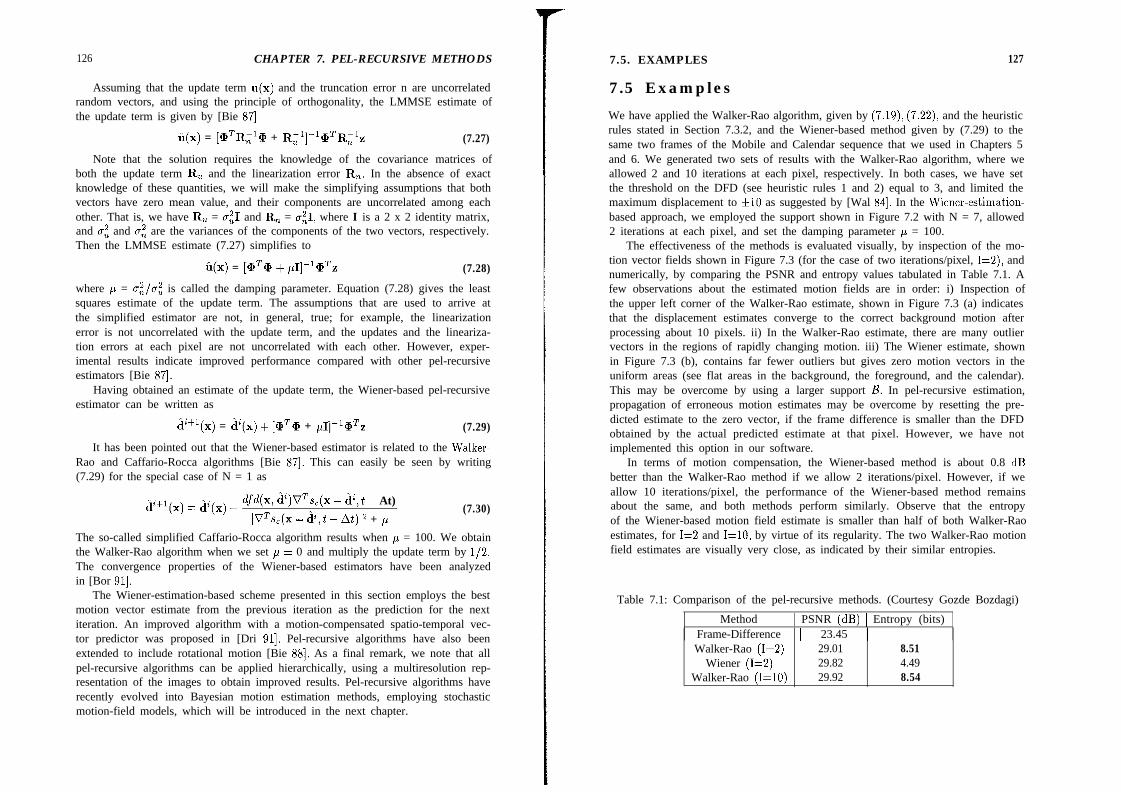
126 CHAPTER 7. PEL-RECURSIVE METHODS
Assuming that the update term u(x) and the truncation error n are uncorrelatedrandom vectors, and using the principle of orthogonality, the LMMSE estimate ofthe update term is given by [Bie 871
ii(x) = [@R,%@ + R,l]-l@TR,lz (7.27)
Note that the solution requires the knowledge of the covariance matrices ofboth the update term R, and the linearization error R,. In the absence of exactknowledge of these quantities, we will make the simplifying assumptions that bothvectors have zero mean value, and their components are uncorrelated among eachother. That is, we have R, = ~$1 and R, = u:I, where I is a 2 x 2 identity matrix,and uz and cri are the variances of the components of the two vectors, respectively.Then the LMMSE estimate (7.27) simplifies to
ii(x) = pT9 + /61]-1@z (7.28)
where p = uf/ut is called the damping parameter. Equation (7.28) gives the leastsquares estimate of the update term. The assumptions that are used to arrive atthe simplified estimator are not, in general, true; for example, the linearizationerror is not uncorrelated with the update term, and the updates and the lineariza-tion errors at each pixel are not uncorrelated with each other. However, exper-imental results indicate improved performance compared with other pel-recursiveestimators [Bie 871.
Having obtained an estimate of the update term, the Wiener-based pel-recursiveestimator can be written as
@+1(x) = 2(x) + [aTa + p1]-wz (7.29)
It has been pointed out that the Wiener-based estimator is related to the Walker-Rao and Caffario-Rocca algorithms [Bie 871. This can easily be seen by writing(7.29) for the special case of N = 1 as
2+1(x) = qx) - @-d(x, @VTsc(x - &,t - At)
IVTs,(x - &,t - At)12 + ,u(7.30)
The so-called simplified Caffario-Rocca algorithm results when p = 100. We obtainthe Walker-Rao algorithm when we set p = 0 and multiply the update term by l/2.The convergence properties of the Wiener-based estimators have been analyzedin [Bor 911.
The Wiener-estimation-based scheme presented in this section employs the bestmotion vector estimate from the previous iteration as the prediction for the nextiteration. An improved algorithm with a motion-compensated spatio-temporal vec-tor predictor was proposed in [Dri 911. Pel-recursive algorithms have also beenextended to include rotational motion [Bie 881. As a final remark, we note that allpel-recursive algorithms can be applied hierarchically, using a multiresolution rep-resentation of the images to obtain improved results. Pel-recursive algorithms haverecently evolved into Bayesian motion estimation methods, employing stochasticmotion-field models, which will be introduced in the next chapter.
7.5. EXAMPLES
7.5 Examples
127
We have applied the Walker-Rao algorithm, given by (7.19), (7.22), and the heuristicrules stated in Section 7.3.2, and the Wiener-based method given by (7.29) to thesame two frames of the Mobile and Calendar sequence that we used in Chapters 5and 6. We generated two sets of results with the Walker-Rao algorithm, where weallowed 2 and 10 iterations at each pixel, respectively. In both cases, we have setthe threshold on the DFD (see heuristic rules 1 and 2) equal to 3, and limited themaximum displacement to 410 as suggested by [Wal 841. In the Wiener-estimation-based approach, we employed the support shown in Figure 7.2 with N = 7, allowed2 iterations at each pixel, and set the damping parameter p = 100.
The effectiveness of the methods is evaluated visually, by inspection of the mo-tion vector fields shown in Figure 7.3 (for the case of two iterations/pixel, 1=2), andnumerically, by comparing the PSNR and entropy values tabulated in Table 7.1. Afew observations about the estimated motion fields are in order: i) Inspection ofthe upper left corner of the Walker-Rao estimate, shown in Figure 7.3 (a) indicatesthat the displacement estimates converge to the correct background motion afterprocessing about 10 pixels. ii) In the Walker-Rao estimate, there are many outliervectors in the regions of rapidly changing motion. iii) The Wiener estimate, shownin Figure 7.3 (b), contains far fewer outliers but gives zero motion vectors in theuniform areas (see flat areas in the background, the foreground, and the calendar).This may be overcome by using a larger support a. In pel-recursive estimation,propagation of erroneous motion estimates may be overcome by resetting the pre-dicted estimate to the zero vector, if the frame difference is smaller than the DFDobtained by the actual predicted estimate at that pixel. However, we have notimplemented this option in our software.
In terms of motion compensation, the Wiener-based method is about 0.8 dBbetter than the Walker-Rao method if we allow 2 iterations/pixel. However, if weallow 10 iterations/pixel, the performance of the Wiener-based method remainsabout the same, and both methods perform similarly. Observe that the entropyof the Wiener-based motion field estimate is smaller than half of both Walker-Raoestimates, for I=2 and I=lO, by virtue of its regularity. The two Walker-Rao motionfield estimates are visually very close, as indicated by their similar entropies.
Table 7.1: Comparison of the pel-recursive methods. (Courtesy Gozde Bozdagi)
Method [ PSNR (dB) 1 Entropy (bits)Frame-Difference 1 23.45 1Walker-Rao (1=2) 29.01 8.51
Wiener (1=2) 29.82 4.49Walker-Rao (I=lO) 29.92 8.54

128 CHAPTER 7. PEL-RECURSIVE METHODS
Figure 7.3: Motion field obtained by a) the Walker-Rao method and b) the Wiener-based method. (Courtesy Gozde Bozdagi and Mehmet Ozkan)
7.6. EXERCISES
7.6 Exercises
129
1. Derive (7.12). How would you compute the optimal step size for the Netravali-Robbins algorithm?
2. Derive an explicit expression for (7.24). Comment on the relationship betweenblock matching and the algorithm given by (7.24).
3. Comment on the validity of the assumptions made to arrive at the Wiener-based estimator (7.29).
4. Derive (7.30) from (7.29).
Bibliography
[Bie 871 J. Biemond, L. Looijenga, D. E. Boekee, and R. H. J. M. Plompen, “A pel-recursive Wiener-based displacement estimation algorithm,” Sign. Proc.,vol. 13, pp. 399-412, Dec. 1987.
[Bie 881 J. Biemond, J. N. Driessen, A. M. Geurtz, and D. E. Boekee, “A pel-recursive Wiener based algorithm for the simultaneous estimation of ro-tation and translation,” Proc. SPIE Conf. Visual Commun. Image Proc.,pp. 917-924, Cambridge MA, 1988.
[Bor 911 L. Boroczky, Pel-Recursive Motion Estimation for Image Coding,Ph.D. thesis, Delft University of Technology, 1991.
[Caf 831 C. Cafforio and F. Rocca, “The differential method for image motionestimation,” in Image Sequence Processing and Dynamic Scene Analysis,T. S. Huang, ed., pp. 104-124, Berlin, Germany: Springer-Verlag, 1983.
[Dri 911 J. N. Driessen, L. Boroczky, and J. Biemond, “Pel-recursive motion fieldestimation from image sequences,” J. Vis. Comm. Image Rep., vol. 2,no. 3, pp. 259-280, 1991.
[Fle 871 R. Fletcher, Practical Methods of Optimization, Vol. 1, 2nd ed., Chichester,UK: John Wiley and Sons, 1987.
[Rob 831 J. D. Robbins and A. N. Netravali, “Recursive motion compensation:A review ,” in Image Sequence Processing and Dynamic Scene Analysis,T. S. Huang, ed., pp. 76-103, Berlin, Germany: Springer-Verlag, 1983.
[Wal 841 D. R. Walker and K. R. Rao, “Improved pel-recursive motion compensa-tion,” IEEE Trans. Commun., vol. COM-32, pp. 1128-1134, Oct. 1984.

8.1. OPTIMIZATION METHODS 131
This minimization is exceedingly difficult due to large dimensionality of the un-known vector and the presence of local minima. With nonconvex criterion func-tions, gradient descent methods, discussed in Chapter 7, generally cannot reach theglobal minimum, because they get trapped in the nearest local minimum.
In this section, we present two simulated (stochastic) annealing algorithms, theMetropolis algorithm [Met 531 and the Gibbs sampler [Gem 841, which are capableof finding the global minimum; and three deterministic algorithms, the iterativeconditional modes (ICM) algorithm [Bes 741, the mean field annealing algorithm[Bil 91a], and the highest confidence first (HCF) algorithm [Cho 901, to,obtain fasterconvergence. For a detailed survey of popular annealing procedures the reader isreferred to [Kir 83, Laa 871.
Chapter 8
BAYESIAN METHODS8.1.1 Simulated Annealing
In this chapter, 2-D motion estimation is formulated and solved as a Bayesian esti-mation problem. In the previous chapters, where we presented deterministic formu-lations of the problem, we minimized either the error in the optical flow equationor a function of the displaced frame difference (DFD). Here, the deviation of theDFD from zero is modeled by a random process that is exponentially distributed.Furthermore, a stochastic smoothness constraint is introduced by modeling the 2-D motion vector field in terms of a Gibbs distribution. The reader is referred toAppendix A for a brief review of the definitions and properties of Markov andGibbs random fields. The clique potentials of the underlying Gibbsian distributionare selected to assign a higher a priori probability to slowly varying motion fields.In order to formulate directional smoothness constraints, more structured Gibbsrandom fields (GRF) with line processes are also introduced.
Since Bayesian estimation requires global optimization of a cost function,we study a number of optimization methods, including simulated annealing (SA),iterated conditional modes (ICM), mean field annealing (MFA), and highest con-fidence first (HCF) in Section 8.1. Section 8.2 provides the basic formulation ofthe maximum a posteriori probability (MAP) es imation problem. Extensions oft’the basic formulation to deal with motion discontinuities and occlusion areas arediscussed in Section 8.3. It will be seen that block/pel matching and Horn-Schunckalgorithms form special cases of the MAP estimator under certain assumptions.
8.1 Optimization Methods
Many motion estimation/segmentation problems require the minimization of a non-convex criterion function E(u), where u is some N-dimensional unknown vector.Then, the motion estimation/segmentation problem can be posed so as to find
ti = arg {minu E(u)}
130
(8.1)
Simulated annealing (SA) refers to a class of stochastic relaxation algorithms knownas Monte Carlo methods. They are essentially prescriptions for a partially randomsearch of the solution space. At each step of the algorithm, the previous solution issubjected to a random perturbation. Unlike deterministic gradient-based iterativealgorithms which always move in the direction of decreasing criterion function,simulated annealing permits, on a random basis, changes that increase the criterionfunction. This is because an uphill move is sometimes necessary in order to preventthe solution from settling in a local minimum.
The probability of accepting uphill moves is controlled by a temperature param-eter. The simulated annealing process starts by first “melting” the system at a highenough temperature that almost all random moves are accepted. Then the tem-perature is lowered slowly according to a “cooling” regime. At each temperature,the simulation must proceed long enough for the system to reach a “steady-state.”The sequence of temperatures and the number of perturbations at each temperatureconstitute the “annealing schedule.” The convergence of the procedure is stronglyrelated to the annealing schedule. In their pioneering work, Geman and Geman[Gem 841 proposed the following temperature schedule:
TX-ln(i.l)’ i=l,...
where r is a constant and i is the iteration cycle. This schedule is overly conservativebut guarantees reaching the global minimum. Schedules that lower the temperatureat a faster rate have also been shown to work (without a proof of convergence).
The process of generating random perturbations is referred to as sampling thesolution space. In the following, we present two algorithms that differ in the waythey sample the solution space.
The Metropolis Algorithm
In Metropolis sampling, at each step of the algorithm a new candidate solution isgenerated at random. If this new solution decreases the criterion function, it is

132 CHAPTER 8. BAYESIAN METHODS
always accepted; otherwise, it is accepted according to an exponential probabilitydistribution. The probability P of accepting the new solution is then given by
exp(-AE/T) if AE > 0ifAE<O
where AE is the change in the criterion function due to the perturbation, and T isthe temperature parameter. If T is relatively large, the probability of accepting apositive energy change is higher than when T is small for a given AE. We providea summary of the Metropolis algorithm in the following [Met 531:
1. Seti=OandT=T,,,. Choose an initial u(O) at random2. Generate a new candidate solution u(i+l) at random.3. Compute AE = E(uci+l)) - E(u(~)).4. Compute P from
P= 11
exp(-AE/T) if AE > 0ifAE<O
5. If P = 1, accept the perturbation; otherwise, draw a random number that isuniformly distributed between 0 and 1. If the number drawn is less than P, acceptthe perturbation. .
6. Set i = i + 1. If i < G,,, where I,,, is predetermined, go to 2.7. Set i = 0, and u(O) = u(~~G=), Reduce T according to a temperature schedule.
If T > Tmin, go to 2; otherwise, terminate.
Because the candidate solutions are generated by random perturbations, thealgorithm typically requires a large number of iterations for convergence. Thus, thecomputational load of simulated annealing is significant, especially when the set ofallowable values r (defined in Appendix A for u discrete) contains a large numberof values or u is a continuous variable. Also, the computational load increases withthe number of components in the unknown vector.
The Gibbs Sampler
Let’s assume that u is a random vector composed of lexicographic ordering of theelements of a scalar GRF U(X). In Gibbs sampling, the perturbations are generatedaccording to local conditional probability density functions (pdf) derived from thegiven Gibbsian distribution, according to (A.5) in Appendix A, rather than makingtotally random perturbations and then deciding whether or not to accept them.The Gibbs sampler method is summarized in the following.
1. Set T = T,,,. Choose an initial u at random.2. Visit each site x to perturb the value of u at that site as follows:a) At site x, first compute the conditional probability of U(X) to take each of,the
allowed values from the set r, given the present values of its neighbors using (A.5)in Appendix A. This step is illustrated for a scalar U(X) by an example below.
8.1. OPTIMIZATION METHODS 133
Example: Computation of local conditional probabilities
Let l? = (0, 1,2,3}. Given a 3 x 3 binary GRF, we wish to computethe conditional probability of the element marked with “x” in Figure 8.1being equal to “0,” “1,” ‘Y,” or “3” given the values of its neighbors. Ifwe define
P(Y) = P(n(xi) = y, u(xj),xj E Nx,), for all y E I‘
to denote the joint probabilities of possible configurations, then, using(A.4), we have
P(U(Xi) = 0 P(O)’ u(xj), x.i E jvxJ = P(0) + P(1) + P(2) + P(3)
P(,(x,) = 1 P(l)’ u(xjLxj E NxJ = P(0) + P(1) + P(2) + P(3)
PC4P(4Xi) = 2 I UC%), x.i E NXJ = p(o) + pcl) + p(2) + p(3)
and
P(3)p(4xi) = 3 I 4XjLXj E JJX,) = qo) + p(l) + p(2) + p(3)
The evaluation of P(y) for all y E r, using the 4-pixel neighborhoodsystem shown in Figure A.1 and the 2-pixel clique potential specifiedby (8.11), is left as an exercise. You may assume that the a prioriprobabilities of a “0” and a “1” are equal.
2 0 2
1 x 0
1 0 3
Figure 8.1: Illustration of local probability computation.
b) Once the probabilities for all elements of the set F are computed, draw thenew value of U(X) from this distribution. To clarify the meaning of “draw,” againan example is provided.
134 CHAPTER& BAYESIANMETHODS
Example: Suppose that I = (0, 1,2,3}, and it was found that
P(u(x,) = 0 1 U(Xj), xj E Nx.) = 0.2P(u(xa) = 1 1 U(Xj), xj ENX,) = 0.1P(U(Xi) = 2 1 U(Xj), xj E Nx,) = 0.4P(U(Xi) = 3 1 U(Xj), xj E Nx,) = 0.3
Then a random number R, uniformly distributed between 0 and 1, isgenerated, and the value of u(x~) is decided as follows: if 0 5 R 5 0.2then u(x~) = 0 if 0.2 < R 5 0.3 then u(x~) = 1 if 0.3 < R 5 0.7 thenu(x~) = 2 if 0.7 < R 5 1 then u(x~) = 3.
3. Repeat step 2 a sufficient number of times at a given temperature, then lowerthe temperature, and go to 2. Note that the conditional probabilities depend onthe temperature parameter.
Perturbations through Gibbs sampling lead to very interesting properties thathave been shown by Geman and Geman [Gem 841:(i) For any initial estimate, Gibbs sampling will yield a distribution that is asymp-totically Gibbsian, with the same properties as the Gibbs distribution used to gen-erate it. This result can be used to simulate a Gibbs random field.(ii) For the particular temperature schedule (8.2), the global optimum will bereached. However, in practice, convergence with this schedule may be too slow.
8.1.2 Iterated Conditional Modes
Iterated conditional modes (ICM), also known as the greedy algorithm, is a deter-ministic procedure which aims to reduce the computational load of the stochasticannealing methods. It can be posed as special cases of both the Metropolis andGibbs sampler algorithms.
ICM can best be conceptualized as the “instant freezing” case of the Metropolisalgorithm, that is, when the temperature T is set equal to zero for all iterations.Then the probability of accepting perturbations that increase the value of the costfunction is always 0 (refer to step 4 of the Metropolis algorithm). Alternatively,it has been shown that ICM converges to the solution that maximizes the localconditional probabilities given by (A.5) ta each site. Hence, it can be implementedas in Gibbs sampling, but by choosing the value at each site that gives the maximumlocal conditional probability rather than drawing a value based on the conditionalprobability distribution.
ICM convergences much faster than the stochastic SA algorithms. However,because ICM only allows those perturbations yielding negative AE, it is likely toget trapped in a local minimum, much like gradient-descent algorithms. Thus, it iscritical to initialize ICM with a reasonably good initial estimate. The use of ICM ’has been reported for image restoration [Bes 741 and image segmentation [Pap 921.
8.1. OPTIMIZATION METHODS 135
8.1.3 Mean Field Annealing
Mean field annealing is based on the “mean field approximation” (MFA) idea instatistical mechanics. MFA allows replacing each random variable (random fieldevaluated at a particular site) by the mean of its marginal probability distribution ata given temperature. Then mean field annealing is concerned about the estimationof these means at each site. Because the estimation of each mean is dependent onthe means of the neighboring sites, this estimation is performed using an annealingschedule. The algorithm for annealing the mean field is similar to SA except thatstochastic relaxation at each temperature is replaced by a deterministic relaxatr n to.fiminimize the so-called mean field error, usually using a gradient-descent algorithm.
Historically, the mean field algorithms were limited to Ising-type models de-scribed by a criterion function involving a binary vector. However, it has recentlybeen extended to a wider class of problems, including those with continuous vari-ables [Bil Sib]. Experiments suggest that the MFA is valid for MRFs with localinteractions over small regions. Thus, computations of the means and the mean fielderror are often based on Gibbsian distributions. It has been claimed that mean fieldannealing converges to an acceptable solution approximately 50 times faster thanSA. The implementation of MFA is not unique. Covering all seemingly differentimplementations of the mean field annealing [Or1 85, Bil 92, Abd 92, Zha 931 isbeyond the scope of this book.
8.1.4 Highest Confidence First
The highest confidence first (HCF) algorithm proposed by Chou and Brown [Cho 901is a deterministic, noniterative algorithm. It is guaranteed to reach a local minimumof the potential function after a finite number of steps.
In the case of a discrete-valued GRF, the minimization is performed on a site-by-site basis according to the following rules: 1) Sites with reliable data can belabeled without using the prior probability model. 2) Sites where the data is unre-liable should rely on neighborhood interaction for label assignment. 3) Sites withunreliable data should not affect sites with reliable data through neighborhood in-teraction. Guided by these principles, a scheme that determines a particular orderfor assigning labels and systematically increases neighborhood interaction is de-signed. Initially, all sites are labeled “uncommitted.” Once a label is assigned toan uncommitted site, the site is committed and cannot return to the uncommit-ted state. However, the label of a committed site can be changed through anotherassignment. A “stability” measure is calculated for each site based on the localconditional a posteriori probability of the labels at that site, to determine the orderin which the sites are to be visited. The procedure terminates when the criterionfunction can no longer be decreased by reassignment of the labels.
Among the deterministic methods, HCF is simpler and more robust than MFA,and more accurate than the ICM. Extensions of HCF for the case of continuousvariables also exist.

136 CHAPTER 8. BAYESIAN METHODS
8.2 Basics of MAP Motion Estimation
In this section, 2-D motion estimation is formulated as a maximum a posterioriprobability (MAP) estimation problem. The MAP formulation requires two pdfmodels: the conditional pdf of the observed image intensity given the motion field,called the likelihood model or the observation model, and the a priori pdf of themotion vectors, called the motion field model. The basic formulation assumes aGaussian observation model to impose consistency with the observations, and aGibbsian motion field model to impose a probabilistic global smoothness constraint.
In order to use a compact notation, we let the vector sk denote a lexicographicordering of the ideal pixel intensities sk(x) in the kth picture (frame or field), suchthat (x, t) E A3 for t = kAt. If d(x) = (dl(x),dz(x)) denotes the displacementvector from frame/field k - 1 to k at the site x = (~1, ~2)~ then we let dl and dzdenote a lexicographic ordering of dl(x) and &(x), respectively. Hence, ignoringcovered/uncovered background regions and intensity variations due to changes inthe illumination and shading, we have
Q(X) = a-1(x - d(x)) - SLI(XI - h(x), xz - b(x)) (8.3)
which is a restatement of the optical flow constraint.In general, we can only observe video that is corrupted by additive noise, given
byg?c(x) = Sk(X) + N(X) (8.4)
and need to estimate 2-D motion from the noisy observations. Then the basic MAPproblem can be stated as: given two frames gk and gb-l, find
(4, d2) = arg ma+&,& p(dl, &la, gh-1) (8.5)
where p(dl, dzlgk, gk-1) denotes the a posterior-i pdf of the motion field given thetwo frames. Using the Bayes theorem,
p(dl d21gk gk-l) = P(gkldl,dz,gk-1)P(dl,d2lgk-l)> ,
~(&I&-1)(8.6)
where p(gk(dl, dz, gk-1) is the cqnditional probability, or the “consistency (likeli-hood) measure,” that measures how well the motion fields dl and dz explain theobservations gk through (8.3) given gk-1; and p(dl,dzlgk-1) is the a priori pdfof the motion field that reflects our prior knowledge about the actual motion field.Since the denominator is not a function of dl and dz, it is a constant for thepurposes of motion estimation. Then the MAP estimate (8.5) can be expressed as
or as
(41, &) = a% maXd,,d, pk-lldl, dz, gk)ddl, &la)
Next, we develop models for the conditional and the prior pdfs.
8.2. BASICS OF MAP MOTION ESTIMATION 137
8.2.1 The Likelihood Model
Based on the models (8.3) and (8.4), the change in the intensity of a pixel alongthe true motion trajectory is due to observation noise. Assuming that the observa-tion noise is white, Gaussian with zero mean and variance u2, the conditional pdfp(gkldl, dz,gk-1) can be modeled as
p(gkldl, dz,gk-1) = (2ru2)-* exp - C h(x) - .c-lb - 44)122u2 (84
XEA
where d(h) denotes the determinant of A which gives the reciprocal of the samplingdensity. The conditional pdf (8.8) gives the likelihood of observing the intensitygk given the true motion field, dl and d2, and the intensity vector of the previousframe gk-1.
8.2.2 The Prior Model
The motion field is assumed to be a realization of a continuous-valued GRF, wherethe clique potential functions are chosen to impose a local smoothness constrainton pixel-to-pixel variations of the motion vectors. Thus, the joint a priori pdf ofthe motion vector field can be expressed as
p(dl, d&-l) = &exp Wd(dl, &k-l))
where Qd is the partition function, and
Ud(4, dzlgrc-1) = Ad c V,“(dl, d&k-l)CECd
Here Cd denotes the set of all cliques for the displacement field, Vi(.) representsthe clique potential function for c E Cd, and Xd is a positive constant. The cliquepotentials will be chosen to assign smaller probability to configurations where themotion vector varies significantly from pixel to pixel. This is demonstrated by twoexamples in the following.
Example: The case of a continuous-valued GRF
This example demonstrates that a spatial smoothness constraint canbe formulated as an a priori pdf in the form of a Gibbs distribution.Let us employ a four-point neighborhood system, depicted in Figure A.1,with two-pixel cliques (see Appendix A). For continuous-valued GRF,a suitable potential function for the two-pixel cliques may be
V:‘(d(xi), d(q)) = IId - d(q)l12 (8.10)
where xi and xj denote the elements of any two-pixel clique ~2, and II.11is the Euclidian distance. In Equation 8.9, Vi'(d(xi),d(xj)) needs to
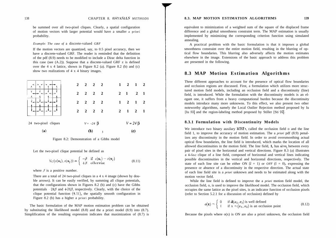
138 CHAPTER 8. BAYESIAN METHODS
be summed over all two-pixel cliques. Clearly, a spatial configurationof motion vectors with larger potential would have a smaller a prioriprobability.
Example: The case of a discrete-valued GRF
If the motion vectors are quantized, say, to 0.5 pixel accuracy, then wehave a discrete-valued GRF. The reader is reminded that the definitionof the pdf (8.9) needs to be modified to include a Dirac delta function inthis case (see (A.2)). Suppose that a discrete-valued GRF z is definedover the 4 x 4 lattice, shown in Figure 8.2 (a). Figure 8.2 (b) and (c)show two realizations of 4 x 4 binary images.
I I I
2 2 2 2
2 2 2 2
2 2 2 2
2 2 2 2
1 2 1 2
2 1 2 1
1 2 1 2
2 1 2 1
24 two-pixel cliques V= -24 p V=24p
(4 (b) .i (cl
Figure 8.2: Demonstration of a Gibbs model
Let the two-pixel clique potential be defined as
(8.11)
where /3 is a positive number.
There are a total of 24 two-pixel cliques in a 4 x 4 image (shown by dou-ble arrows). It can be easily verified, by summing all clique potentials,that the configurations shown in Figures 8.2 (b) and (c) have the Gibbspotentials -24p and +24,/3, respectively. Clearly, with the choice of theclique potential function (8.11), the spatially smooth configuration inFigure 8.2 (b) has a higher a priori probability.
The basic formulation of the MAP motion estimation problem can be obtainedby substituting the likelihood model (8.8) and the a priori model (8.9) into (8.7).Simplification of the resulting expression indicates that maximization of (8.7) is
8.3. MAP MOTION ESTIMATION ALGORITHMS 139
equivalent to minimization of a weighted sum of the square of the displaced framedifference and a global smoothness constraint term. The MAP estimation is usuallyimplemented by minimizing the corresponding criterion function using simulatedannealing.
A practical problem with the basic formulation is that it imposes a globalsmoothness constraint over the entire motion field, resulting in the blurring of op-tical flow boundaries. This blurring also adversely affects the motion estimateselsewhere in the image. Extensions of the basic approach to address this problemare presented in the following.
8.3 MAP Motion Estimation Algorithms
Three different approaches to account for the presence of optical flow boundariesand occlusion regions are discussed. First, a formulation which utilizes more struc-tured motion field models, including an occlusion field and a discontinuity (line)field, is introduced. While the formulation with the discontinuity models is an el-egant one, it suffers from a heavy computational burden because the discontinuitymodels introduce many more unknowns. To this effect, we also present two othernoteworthy algorithms, namely the Local Outlier Rejection method proposed by Iu[Iu 931 and the region-labeling method proposed by Stiller [Sti 931.
8.3.1 Formulation with Discontinuity Models
We introduce two binary auxilary MRFs, called the occlusion field o and the linefield 1, to improve the accuracy of motion estimation. The a priori pdf (8.9) penal-izes any discontinuity in the motion field. In order to avoid oversmoothing actualoptical flow boundaries, the line field is introduced, which marks the location of allallowed discontinuities in the motion field. The line field, 1, has sites- between everypair of pixel sites in the horizontal and vertical directions. Figure 8.3 (a) illustratesa 4-line clique of a line field, composed of horizontal and vertical lines indicatingpossible discontinuities in the vertical and horizontal directions, respectively. Thestate of each line site can be either ON (1 = 1) or OFF (I = 0), expressing thepresence or absence of a discontinuity in the respective direction. The actual stateof each line field site is a priori unknown and needs to be estimated along with themotion vector field.
While the line field is defined to improve the a priori motion field model, theocclusion field, o, is used to improve the likelihood model. The occlusion field, whichoccupies the same lattice as the pixel sites, is an indicator function of occlusion pixels(refer to Section 5.2.1 for a discussion of occlusion) defined by
if d(q) ~2) is well definedif x = (~1, ~2) is an occlusion point (8.12)
Because the pixels where o(x) is ON are also a priori unknown, the occlusion field
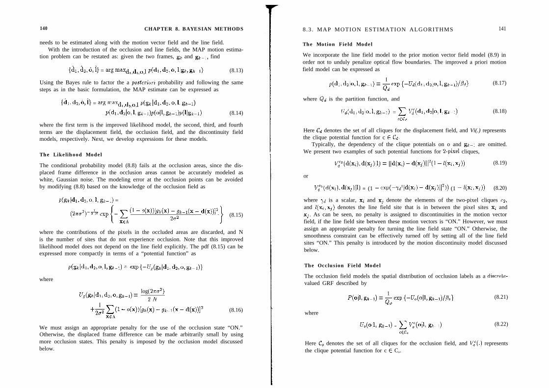
140 CHAPTER 8. BAYESIAN METHODS
needs to be estimated along with the motion vector field and the line field.With the introduction of the occlusion and line fields, the MAP motion estima-
tion problem can be restated as: given the two frames, gk and gb-1, find
{&, b, 6, i) = a% maxdl,d2,0,J P(dl, dz, 0, llglc, &z-l) (8.13)
Using the Bayes rule to factor the a posteriori probability and following the samesteps as in the basic formulation, the MAP estimate can be expressed as
{h, dz,k i} = w maxd,,&o,J & 14, dz, o,l, m-1)
ddl, dzlo,l, gk-&oll, gk-&olgk-1) (8.14)
where the first term is the improved likelihood model, the second, third, and fourthterms are the displacement field, the occlusion field, and the discontinuity fieldmodels, respectively. Next, we develop expressions for these models.
The Likelihood Model
The conditional probability model (8.8) fails at the occlusion areas, since the dis-placed frame difference in the occlusion areas cannot be accurately modeled aswhite, Gaussian noise. The modeling error at the occlusion points can be avoidedby modifying (8.8) based on the knowledge of the occlusion field as
p(gkldl, ho, 1, gk-1) =
(2Ta2)-& exp _ c (1 - o(x))[sk(x) -%1(x - d(x))122u2
(8.15)XEA
where the contributions of the pixels in the occluded areas are discarded, and Nis the number of sites that do not experience occlusion. Note that this improvedlikelihood model does not depend on the line field explicitly. The pdf (8.15) can beexpressed more compactly in terms of a “potential function” as
dg#l,ho,l,g~-l) =exp(-Ug(gl,ldl,dz,o,g~-l))where
U,Mdl,dr,o,gk-1) = log( 27rc72)2 N
+& x(1 - +))b&4 - a-1(x - +))I2XEA
(8.16)
We must assign an appropriate penalty for the use of the occlusion state “ON.”Otherwise, the displaced frame difference can be made arbitrarily small by usingmore occlusion states. This penalty is imposed by the occlusion model discussedbelow.
8 .3 . MAP MOTION ESTIMATION ALGORITHMS
The Motion Field Model
141
We incorporate the line field model to the prior motion vector field model (8.9) inorder not to unduly penalize optical flow boundaries. The improved a priori motionfield model can be expressed as
ddl,dzlo,l,gk-1) = &ew {-Ud(dlldzlo,l,grc-l)lPd)
where &d is the partition function, and
Ud(dl,dzlo,l,gk-1) = c V;(dl,dalo,1,gt-1)CECd
(8.17)
(8.18)
Here Cd denotes the set of all cliques for the displacement field, and Vi(.) representsthe clique potential function for c E Cd.
Typically, the dependency of the clique potentials on o and gk-1 are omitted.We present two examples of such potential functions for 2-pixel cliques,
V;‘(d(xi),d(xj)ll) = IId - d(xj)l12(1 - +i,xj)) (8.19)
or
Vi’(d(x;),d(xj)Il) = (1 - exp(-ydlld(xi) - d(xj)l12)) (1 - b(xi,xj)) (8.20)
where Y,j is a scalar, xi and xj denote the elements of the two-pixel cliques es,and l(xi,xj) denotes the line field site that is in between the pixel sites xi andxj. As can be seen, no penalty is assigned to discontinuities in the motion vectorfield, if the line field site between these motion vectors is “ON.” However, we mustassign an appropriate penalty for turning the line field state “ON.” Otherwise, thesmoothness constraint can be effectively turned off by setting all of the line fieldsites “ON.” This penalty is introduced by the motion discontinuity model discussedbelow.
The Occlusion Field Model
The occlusion field models the spatial distribution of occlusion labels as a discrete-valued GRF described by
P(4, gk-1) = $ ev {-~o(oll, gh-dlPoI (8.21)0
where
Uo(oll, !a-1) = c v:/,c(4, !a-1) (8.22)CECO
Here C, denotes the set of all cliques for the occlusion field, and Vt(.) representsthe clique potential function for c E C,.
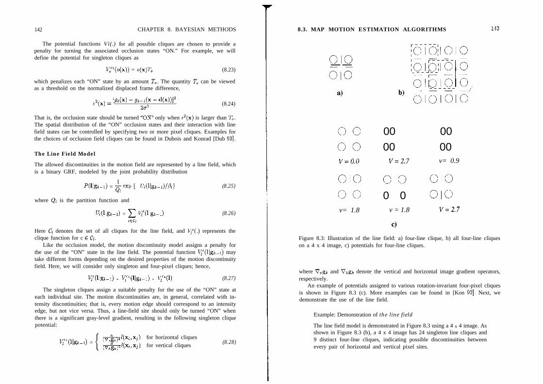
142 CHAPTER 8. BAYESIAN METHODS
The potential functions Vi(.) for all possible cliques are chosen to provide apenalty for turning the associated occlusion states “ON.” For example, we willdefine the potential for singleton cliques as
iq’(o(x)) = o(x)To (8.23)
which penalizes each “ON” state by an amount To. The quantity To can be viewedas a threshold on the normalized displaced frame difference,
tz(x) = h(4 - a-l@ - +))I22$
(8.24)
That is, the occlusion state should be turned "ON" only when c2(x) is larger than To.The spatial distribution of the “ON” occlusion states and their interaction with linefield states can be controlled by specifying two or more pixel cliques. Examples forthe choices of occlusion field cliques can be found in Dubois and Konrad [Dub 931.
The Line Field Model
The allowed discontinuities in the motion field are represented by a line field, whichis a binary GRF, modeled by the joint probability distribution
P(h-1) = $exp {-uf(llgk-d//Al (8.25)
where &I is the partition function and
Wb-1) = c y(llgk-1) (8.26)CCC1
Here Cl denotes the set of all cliques for the line field, and v,“(.) represents theclique function for c E Cf.
Like the occlusion model, the motion discontinuity model assigns a penalty forthe use of the “ON” state in the line field. The potential function 1/,‘(llgk-l) maytake different forms depending on the desired properties of the motion discontinuityfield. Here, we will consider only singleton and four-pixel cliques; hence,
I/q&-l) = y(llgk-1) + v,yl) (8.27)
The singleton cliques assign a suitable penalty for the use of the “ON” state ateach individual site. The motion discontinuities are, in general, correlated with in-tensity discontinuities; that is, every motion edge should correspond to an intensityedge, but not vice versa. Thus, a line-field site should only be turned “ON” whenthere is a significant gray-level gradient, resulting in the following singleton cliquepotential:
I/le'(llgk-l) =&;Tal(xi, xj) for horizontal cliques*[(xi, xj) for vertical cliques (8.28)
8.3. MAP MOTION ESTIMATION ALGORITHMS
010
010
4
00
00v= 0.0
010
00
v= 1.8
00 0000 00
V=2.7 v= 0.9
010 0100 0 010
v = 1.8 V=2.7
dFigure 8.3: Illustration of the line field: a) four-line clique, b) all four-line cliqueson a 4 x 4 image, c) potentials for four-line cliques.
where V,gt and Vhgk denote the vertical and horizontal image gradient operators,respectively.
An example of potentials assigned to various rotation-invariant four-pixel cliquesis shown in Figure 8.3 (c). More examples can be found in [Kon 921. Next, wedemonstrate the use of the line field.
Example: Demonstration of the line field
The line field model is demonstrated in Figure 8.3 using a 4 x 4 image. Asshown in Figure 8.3 (b), a 4 x 4 image has 24 singleton line cliques and9 distinct four-line cliques, indicating possible discontinuities betweenevery pair of horizontal and vertical pixel sites.
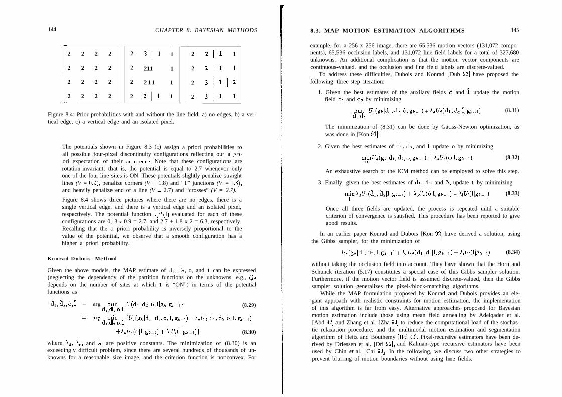
144
2 2 2 2
2 2 2 2
2 2 2 2
2 2 2 2
CHAPTER 8. BAYESIAN METHODS
2 211 1
2 211 1
2 211 1
2 211 1
2 211 1
2 211 1
2 21112
2 211 1
Figure 8.4: Prior probabilities with and without the line field: a) no edges, b) a ver-tical edge, c) a vertical edge and an isolated pixel.
The potentials shown in Figure 8.3 (c) assign a priori probabilities toall possible four-pixel discontinuity configurations reflecting our a pri-ori expectation of their occurence. Note that these configurations arerotation-invariant; that is, the potential is equal to 2.7 whenever onlyone of the four line sites is ON. These potentials slightly penalize straightlines (V = 0.9), penalize corners (V = 1.8) and “T” junctions (V = 1.8),and heavily penalize end of a line (V = 2.7) and “crosses” (V = 2.7).
Figure 8.4 shows three pictures where there are no edges, there is asingle vertical edge, and there is a vertical edge and an isolated pixel,respectively. The potential function V,‘“(l) evaluated for each of theseconfigurations are 0, 3 x 0.9 = 2.7, and 2.7 + 1.8 x 2 = 6.3, respectively.Recalling that the a priori probability is inversely proportional to thevalue of the potential, we observe that a smooth configuration has ahigher a priori probability.
Konrad-Dubois Method
Given the above models, the MAP estimate of dl, dz, o, and 1 can be expressed(neglecting the dependency of the partition functions on the unknowns, e.g., Qddepends on the number of sites at which 1 is “ON”) in terms of the potentialfunctions as
;11,&,6,i = arg mind,,d,,o,l
U(dl, dz, o,llgk, gk-1) (8.29)
1 w d $no 1 Vdg~ldl, dz,o, 1, a-1) + Mddl, &lo, 1, g-1)I, 2, 3
+uJo(oll,gk-1) + Wl(1lgk-l)} (8.30)
where Xd, X,, and XI are positive constants. The minimization of (8.30) is anexceedingly difficult problem, since there are several hundreds of thousands of un-knowns for a reasonable size image, and the criterion function is nonconvex. For
8.3. MAP MOTION ESTIMATION ALGORITHMS 145
example, for a 256 x 256 image, there are 65,536 motion vectors (131,072 compo-nents), 65,536 occlusion labels, and 131,072 line field labels for a total of 327,680unknowns. An additional complication is that the motion vector components arecontinuous-valued, and the occlusion and line field labels are discrete-valued.
To address these difficulties, Dubois and Konrad [Dub 931 have proposed thefollowing three-step iteration:
1. Given the best estimates of the auxilary fields i, and I, update the motionfield dl and dz by minimizing
mind,,d,
u,(gkldl, dz, 6 a-1) + UJddl, hIi, a-1) (8.31)
The minimization of (8.31) can be done by Gauss-Newton optimization, aswas done in [Kon 911.
2. Given the best estimates of ai, dz, and i, update o by minimizing
m~U~(g,lal~$2,0,gk-l) + hUo(olLgk-l) (8.32)
An exhaustive search or the ICM method can be employed to solve this step.
3. Finally, given the best estimates of Ai, az, and 6, update 1 by minimizing
mFbUd(hl, &ll,gk-1) + X,Uo(~ll,gk-~) + h&(llgk-1) (8.33)
Once all three fields are updated, the process is repeated until a suitablecriterion of convergence is satisfied. This procedure has been reported to givegood results.
In an earlier paper Konrad and Dubois [Kon 921 have derived a solution, usingthe Gibbs sampler, for the minimization of
~,(g~ldl, dz,l,grc-1) + kdJ~(4,&14glc-d + WOlg~-~) (8.34)
without taking the occlusion field into account. They have shown that the Horn andSchunck iteration (5.17) constitutes a special case of this Gibbs sampler solution.Furthermore, if the motion vector field is assumed discrete-valued, then the Gibbssampler solution generalizes the pixel-/block-matching algorithms.
While the MAP formulation proposed by Konrad and Dubois provides an ele-gant approach with realistic constraints for motion estimation, the implementationof this algorithm is far from easy. Alternative approaches proposed for Bayesianmotion estimation include those using mean field annealing by Adelqader et al.[Abd 921 and Zhang et al. [Zha 931 to reduce the computational load of the stochas-tic relaxation procedure, and the multimodal motion estimation and segmentationalgorithm of Heitz and Bouthemy [Hei 901. Pixel-recursive estimators have been de-rived by Driessen et al. [Dri 921, and Kalman-type recursive estimators have beenused by Chin et al. [Chi 931. In the following, we discuss two other strategies toprevent blurring of motion boundaries without using line fields.

146 CHAPTER 8. BAYESIAN METHODS
8.3.2 Estimation with Local Outlier Rejection
The local outlier rejection approach proposed by Iu [Iu 931 is an extension of thebasic MAP formulation, given by (8.7), w ic aims at preserving the optical flowh’ hboundaries without using computationally expensive line field models. At site x,the basic MAP method clearly favors the estimate d(x) that is closest to all othermotion estimates within the neighborhood of site x. The local outlier rejectionmethod is based on the observation that if the pixels within the neighborhood ofsite x exhibit two different motions, the estimate d(x) is then “pushed” towardsthe average of the two, resulting in blurring. To eliminate this undesirable effect,it is proposed that all the values of the clique potential function, one for each site,are ranked, and the outlier values are rejected. The outlier rejection procedure isrelatively simple to incorporate into the local Gibbs potential calculation step.
To describe the approach in more detail, we revisit the basic MAP equations(8.7)-(8.9). While the likelihood model (8.8) remains unchanged, we rewrite thepotential function of the prior distribution (8.9) as
Ud(dl> dzk-1) = Ai c $ c IId - d(xj)l12 (8.35)X, vnr,,
where the summation xi is over the whole image and the summation xj runs over allthe neighbors of the site xi, and Nh is the number of neighbors of the site xi. Theterm IId(d(xj)]]” is the clique potential for the two-pixel clique containing sitesxi and xj. Observe that (8.35) is different than (8.9) because: i) the summationis not over all cliques, but over all pixels to simplify the outlier rejection process(it can be easily shown that in (8.35) every clique is counted twice); and ii) thepotential function includes the mean clique potential, rather than the sum of allclique potentials, for each site (indeed, this corresponds to scaling of Xd).
To incorporate outlier rejection, the potential function (8.35) is further modifiedas
U(dl, d&k-l) = Xa c $ c hjlld(xa) - d(xj)l12 (8.36)X, XJ E.nr,,
6. = 1 if IId - d(q)l12 I TOR3 0 otherwise
is the indicator function of the rejected cliques, TOE is a threshold, and
Nh = cbj
(8.37)
(8.38)
The expression (8.36) can be used in two ways: i) given a fixed threshold TOR,in which case the number of cliques hrh varies from pixel to pixel, or ii) given afixed number of cliques, in which case the threshold TOR varies from pixel to pixel.
8.3. MAP MOTION ESTIMATION ALGORITHMS 147
The selection of the right threshold or number of cliques is a compromise betweentwo conflicting requirements. A low threshold preserves the optical flow boundariesbetter, while a high threshold imposes a more effective smoothness constraint. Foran &pixel neighborhood system, Iu suggests setting hrh = 3. For most neighborhoodsystems, the ranking of clique potentials and the outlier rejection procedure onlyaccount for a small computational overhead.
8.3.3 Estimation with Region Labeling
Yet another extension of the basic MAP approach (8.7) to eliminate blurring ofoptical flow boundaries can be formulated based on region labeling [Sti 931. Inthis approach, each motion vector is assigned a label Z(X) such that the label field zdesignates regions where the motion vectors are expected to remain constant or varyslowly. Region labeling differs from the line-field approach in that here the labelsbelong to the motion vectors themselves as opposed to indicating the presence ofdiscontinuities between them. Clearly, the label field is unknown, and has to beestimated along with the motion field.
The region-labeling formulation can be expressed as
p(dl,dz,z (gk,gb-1) ccp(gk I dl,dz,z,gk-&(dl,dz ( Z)P(Z) (8.39)
where p(gk I dl,da,z,gk-1) is again the likelihood model and p(dl, d2 ( z)p(z) =p(dl, d2, z) is the joint prior pdf of the motion and label fields. While the likelihoodmodel follows straightforwardly from (8.8), we will examine the prior pdf modelin more detail. The prior pdf of the motion field conditioned on the label fieldp(di, d2 I z) is modeled by a Gibbs distribution,
p(dl, cl:! I z) = $exp {--U(dl, d2 I z)> (8.40)
where
U(dl, dz I z) = c c Ild(xi) - d(xj)l126(z(xi) - +j)) (8.41)x, X,E&,
in which xi ranges over all pixel sites, and xj over all neighbors of xi. The function6(z) is the Kronecker delta function, that is, 1 when z = 0 and 0 otherwise. Itensures that the local smoothness constraint is imposed only when both pixels inthe clique have the same label, thus avoiding the smoothness constraint acrossregion boundaries. The other part of this prior pdf, p(z), enforces a connectedconfiguration of regions (labels) over the image. A suitable prior pdf model is adiscrete-valued Gibbs distribution with the potential function given by (8.11).
The MAP estimate of the triplet dl, d2, and z can be obtained by minimizingthe potential function corresponding to the a posteriori pdf (8.39). An ICM opti-mization method has been used by Stiller [Sti 931. While this approach provides asimpler formulation than that of Konrad-Dubois, the performance is dependent on

148 CHAPTER 8. BAYESIAN METHODS
the appropriate region assignments. Since the region labels are used only as a tokento limit the motion smoothness constraint, there exists a certain degree of latitudeand arbitrariness in the assignment of labels.
8.4 Examples
We have implemented four Bayesian motion estimation algorithms; namely, thebasic method, the method of Konrad-Dubois (K-D), the outlier-rejection method ofIu, and the segmentation method of Stiller, on the same two frames of the Mobileand Calendar sequence that were used in the previous three chapters. The basicalgorithm using a smoothness constraint evaluates (8.7) given the pdf models (8.8)and (8.9) with the potential function (8.10). In our implementation, the DFD in theexponent of (8.8) has been smoothed over the 8-neighborhood of each pixel using themotion estimate at that pixel. The initial iteration does not impose the smoothnessconstraint; that is, it resembles block matching. The optimization is performedby the ICM method with a temperature schedule of the form T = lOOO(1 - i/l))where i = 0,. and 1 stand for the iteration index and the maximum number ofiterations, respectively. The algorithm usually converges after I = 5 iterations.
For the K-D, Iu, and Stiller algorithms, the initial motion field is set equal tothe result of the basic algorithm. Our implementation of the K-D algorithm didnot include an occlusion field. Hence, it is a two-step iteration, given by (8.31)and (8.33). The horizontal and vertical line fields are initialized by simple edgedetection on the initial motion estimates. The method of Iu is a variation of the basicalgorithm, where an outlier-rejection stage is built into the smoothness constraint.At each site, the distance between the present motion vector and those within theS-neighborhood of that site are rank-ordered. The smallest third (iVh = 3) are usedin imposing the smoothness constraint. Stiller’s algorithm employs a segmentationfield, which is initialized by a K-means segmentation of the initial motion estimateswith K = 9. In the ICM iterations, we have used an exponential temperatureschedule of the form T = 1000(0.8)i, i = 0,.
,The motion fields obtained by the K-D and the Iu estimators are shown in
Figure 8.5 (a) and (b), respectively. Observe that Iu’s motion field is slightly moreregular. A numerical comparison of the motion fields is presented in Table 8.1.
Table 8.1: Comparison of the Bayesian methods. (Courtesy Gozde Bozdagi)
8.4. EXAMPLES
Figure 8.5: Motion field obtained by a) the Konrad-Dubois method and b) Iu’smethod. (Courtesy Gozde Bozdagi and Michael Chang)
150 BIBLIOGRAPHY
8.5 Exercises
1. How do you define the joint pdf of a discrete-valued GRF?
,I 2. The initial motion field for the MAP estimator is usually computed by a de-
: / terministic estimator such as the Horn-Schunck estimator or block matching.Suggest methods to initialize the line field and the occlusion field.
3. The MAP estimator (8.30) has been found to be highly sensitive to the valuesof the parameters Xd, X,, and XI, which are free parameters. How would youselect them?
4. Discuss the relationship between the MAP estimator and the Horn-Schunckalgorithm. (Hint: see [Kon 921.)
5. Compare modeling motion discontinuities by line fields versus region labeling.
Bibliography
[Abd 921 I. Abdelqader, S. Rajala, W. Snyder, and G. Bilbro, “Energy minimizationapproach to motion estimation,” Signal Processing, vol. 28, pp. 291-309,Sep. 1992.
[Bes 741 J. Besag, “Spatial interaction and the statistical analysis of lattice sys-tems,” J. Royal Stat. Sot. B, vol. 36, no. 2, pp. 1922236, 1974.
[Bil 9la] G. L. Bilbro and W. E. Snyder, “Optimization of functions with manyminima,” IEEE Trans. Syst., Man and Cyber., vol. 21, pp. 8406849,Jul/Aug. 1991.
[Bil 91b] G. L. Bilbro, W. E. Snyder, and R. C. Mann, “Mean field approximationminimizes relative entropy,” J. Opt. Sot. Am. A, vol. 8, pp. 290-294,Feb. 1991.
[Bil 921 G. L. Bilbro, W. E. Snyder, S. J. G arnier, and J. W. Gault, “Mean field an-nealing: A formalism for constructing GNC-like algorithms,” IEEE Trans.Neural Networks, vol. 3, pp. 131-138, Jan. 1992.
[Chi 931 T. M. Chin, M. R. Luettgen, W. C. Karl, and A. S. Willsky, “An es-timation theoretic prespective on image processing and the calculationof optical flow,” m Motion Analysis and Image Sequence Processing,M. I. Sezan and R. L. Lagendijk, eds., Norwell, MA: Kluwer, 1993.
[Cho 901 P. B. Chou and C. M. Brown, “The theory and practice of Bayesian imagelabeling,” Int. I. Comp. Vis., vol. 4, pp. 185-210, 1990.
[Dep 921 R. Depommier and E. Dubois, “Motion estimation with detection ofocclusion areas,” Proc. ICASSP, pp. 111.2699272, Mar. 1992.
BIBLIOGRAPHY 153
[Dri 921 J. N. Driessen, Motion Estimation for Digital Video, Ph.D. Thesis,Delft University of Technology, 1992.
[Dub 931 E. Dubois and J. Konrad, “Estimation of 2-D motion fields fromimage sequences with application to motion-compensated processing,”in Motion Analysis and Image Sequence Processing, M. I. Sezan and
[Gem 841
[Hei 901
[Kir 831
[Kon 911
[Kon 921
[Laa 871
[Met 531
[Or1 851
Pap 921
[Iu 931
[Sti 931
[Zha 931
R. L. Lagendijk, eds., Norwell, MA: Kluwer, 1993.
S. Geman and D. Geman, “Stochastic relaxation, Gibbs distribution, andBayesian restoration of images, ” IEEE Trans. Patt. Anal. Mach. Intel.,vol. 6, pp. 721-741, Nov. 1984.
F. Heitz and P. Bouthemy, “Motion estimation and segmentation usinga global Bayesian approach,” Proc. Int. Conf. ASSP, Albuquerque, NM,pp. 230552308, April 1990.
S. Kirkpatrick, C. D. G. Jr., and M. P. Vecchi, “Optimization by simulatedannealing,” Science, vol. 220, pp. 671-679, May 1983.
J. Konrad and E. Dubois, “Comparison of stochastic and deterministicsolution methods in Bayesian estimation of 2D motion,” Image and Vis.Comput., vol. 9, pp. 215-228, Aug. 1991.
J. Konrad and E. Dubois, “Bayesian estimation of motion vector fields,”lEEE Trans. Patt. Anal. Mach. Intel., vol. 14, pp. 910-927, Sep. 1992.
I’. J. M. Van Laarhoven and E. H. Aarts, Simulated Annealing: Theoryand Applications, Dordrecht, Holland: Reidel, 1987.
N. Metropolis, A. Rosenbluth, M. Rosenbluth, H. Teller, and E. Teller,“Equation of state calculations by fast computing machines,” J. Chem.Phys., vol. 21, pp. 1087-1092, June 1953.
H. Orland, “Mean-field theory for optimization problems,” J. PhysiqueLett., vol. 46, 17, pp. 763-770, 1985.
T. N. Pappas, “An Adaptive Clustering Algorithm for Image Segmen-tation,” IEEE Trans. Signal Proc., vol. SP-40, pp. 901-914, April 1992.
S.-L. Iu, “Robust estimation of motion vector fields with disconti-nuity and occlusion using local outliers rejection,” SPIE, vol. 2094,pp. 588-599, 1993.
C. Stiller and B. H. Hurtgen, “Combined displacement estimation andsegmentation in image sequences,” Proc. SPIE/EUROPTO Video Comm.and PACS for Medical Applications, Berlin, Germany, vol. SPIE 1977,pp. 276-287, 1993.
J. Zhang and J. Hanauer, “The mean field theory for image mo-tion estimation,” Proc. IEEE Int. Conf. ASSP, vol. 5, pp. 197-200,Minneapolis, MN, 1993.

Chapter 9
METHODS USING POINTCORRESPONDENCES3-D motion estimation refers to estimating the actual motion of objects in a scenefrom their 2-D projections (images). Clearly, the structure (depth information) ofthe objects in the scene affect the projected image. Since the structure of the sceneis generally unknown, 3-D motion and structure estimation need to be addressedsimultaneously. Applications of 3-D motion and structure estimation include roboticvision, passive navigation, surveillance imaging, intelligent vehicle highway systems,and harbor traffic control, as well as object-based video compression. In some ofthese applications a camera moves with respect to a fixed environment, and inothers the camera is stationary, but the objects in the environment move. In eithercase, we wish to determine the 3-D structure and the relative motion parametersfrom a time sequence of images.
Needless to say, 3-D motion and structure estimation from 2-D images is anill-posed problem, which may not have a unique solution without some simplifyingassumptions, such as rigid motion and a parametric surface. It is well-known that3-D rigid motion can be modeled by three translation and three rotation parameters(see Chapter 2). The object surface may be approximated by a piecewise planar orquadratic model, or represented by a collection of independent 3-D points. Then,3-D motion estimation refers to the estimation of the six rigid motion parameters,and structure estimation refers to the estimation of the parameters of the surfacemodel, or the depth of each individual point from at least two 2-D projections.
The 3-D motion and structure estimation methods can be classified into twogroups: those which require a set of feature point correspondences to be deter-mined a priori, and those which do not [Agg 881. This chapter is about the formerclass. Furthermore, it is assumed in this chapter that the field of view contains asingle moving object. The segmentation problem in the presence of multiple mov-ing objects will be dealt with in Chapter 11. Section 9.1 introduces parametricmodels for the projected displacement field that are based on the orthographic andperspective projection, respectively. 3-D motion and structure estimation using the
152
9.1. MODELING THE PROJECTED DISPLACEMENT FIELD 153
orthographic displacement field model is covered in Section 9.2, whereas Section 9.3deals with estimation using the perspective displacement field model.
9.1 Modeling the Projected Displacement Field
We start by deriving parametric models for the 2-D projected displacement fieldbased on the orthographic and perspective projections of the 3-D rigid motionmodel, respectively.
Suppose a point X = [Xl, X2) XslT on a rigid object at time t moves to X’ =[X{,Xi,XAIT at time t’ subject to a rotation described by the matrix R and atranslation by the vector T. Then, from Chapter 2, we have
[s]=R[;;]+T=[i;; ;;; :,,][?]+[;] ( 9 . 1 )
Recall that in the case of small rotation, the composite rotation matrix can beexpressed, in terms of the Eulerian angles, as
R= AC/I 1 -A8 (94-A$ A0 1 1
where A@, A$, and Ad denote small clockwise angular displacements about theXi, X2, and Xs axes, respectively.
[
1 -A4 All,
9.1.1 Orthographic Displacement Field Model
The orthographic displacement field refers to the orthographic projection of the3-D displacement vectors into the image plane, which is obtained by substitutingXi and Xi from (9.1) into
x; = x; and z; = Xi
that define the orthographic projection as discussed in Chapter 2. Since we haveXi = zi and X2 = 2s under the orthographic projection, the resulting model isgiven by
x1 = TllXl + mzz + (7-13X3 + Tl)
x2 = 7-2121 + c!zx2 + (7-23X3 + Tz) (9.4)
The model (9.4) is an affine mapping of the pixel (xi, ~2) at frame t to the pixel(xi, xi) at frame t’ defined in terms of the six parameters ~1, ~12, (~13x3 + Ti),~21, ~22, and (rssXs+Ts). Thus, it constitutes a parametric 2-D motion field model(see Section 5.2).

154 CHAPTER9. METHODSUSINGPOINTCORRESPONDENCES
It should be noted that the actual distance of the object points from the imageplane is not observable in orthographic projection, since it is a parallel projection.Thus, if we express the actual depth of a point as Xs = Xs + Xs, where Xs is thedepth of a reference point on the object, and Xs is the relative depth of all otherobject points with respect to the reference point, we can only expect to estimateXs associated with each image point. Further observe that in (9.4), Xs multipliesr13 and rzs. Obviously, if we scale ~1s and ~23, a new value of X3 can be found foreach pixel that would also satisfy (9.4). Hence, these variables cannot be uniquelydetermined for an arbitrary surface from two views, as stated in [Hua 89a].
Orthographic projection is a reasonable approximation to the actual imagingprocess described by the perspective projection, when the depth of object pointsdoes not vary significantly. Other approximations, such as weak perspective, para-perspective, and orthoperspective projections, also exist in the literature [Dem 921.
9.1.2 Perspective Displacement Field Model
The perspective displacement field can be derived by substituting Xi, Xi, and XAfrom (9.1) into the perspective projection model given by (from Chapter 2)
X; I f;Y; and x; = fx:
XA xi
to obtain
21 = fmxl + rlzX2 + r13X3 +TlT3lxl + f32X2 + T33x3 + T3
Ix2 = f
r21x1 + 7+22X2 + r23X3 + T2%x1 + ?-32x2 + r33x3 + T3
(9.5)
(9.6)
Letting f = 1, dividing both the numerator and the denominator by Xs, andexpressing the object-space variables in terms of image plane coordinates using theperspective transform expression, we obtain
x1 =mxi + r1222 + r13 + 2
p31xi + r32x2 + r33 + 2
,x2 =
T21xi + r2222 + r23 + 2
r31xl + r3222 + r33 + E(9.7)
The expressions (9.7) constitute a nonlinear model of the perspective projectedmotion field in terms of the image-plane coordinates because of the division by xiand x2. Notice that this model is valid for arbitrary shaped moving surfaces in 3-D,since the depth of each point Xs remains as a free parameter. Observe, however,that X3 always appears in proportion to T3 in (9.7). That is, the depth informationis observable only when Ts # 0. Furthermore, it can only be determined up to
9.2. METHODS BASED ON THE ORTHOGRAPHIC MODEL 155
a scale factor. For example, an object at twice the distance from the image planeand moving twice as fast yields the same image under the perspective projection.
We develop 3-D motion and structure estimation algorithms based on the affinemodel (9.4) and the nonlinear model (9.7) in the next two sections. Because of theaforementioned limitations of these projections, we can estimate depth only up toan additive constant at best, using the orthographic displacement field, and onlyup to a multiplicative scale factor under the perspective displacement field modt/l.
9.2 Methods Based on the Orthographic Model
It is well known that, from two orthographic views, we can estimate the depthof a feature point up to a scale factor cr and an additive constant X3. The scaleambiguity arises because scaling Xi3 by cr, and ris and rzs by l/o results in thesame orthographic projection as can be seen from Equation (9.4). That is, if Xi3denotes the true depth value, we expect to estimate
Xi3 = 23 + cxifi3, for i = l,...,N (9.8)
from two views. It is not possible to estimate Xs under any scheme, because thisinformation is lost in the projection. However, the scale ambiguity may be overcomeif more than two views are utilized. In his classical book Ullman [Ull 791 proved thatfour point correspondences over three frames, i.e. four points each traced from ti totz and then to ts, are sufficient to yield a unique solution to motion and structureup to a reflection. Later, Huang and Lee [Hua 89a] proposed a linear algorithm toobtain the solution in this case. Furthermore, they showed that with three pointcorrespondences over three frames, there are 16 different solutions for motion andfour for the structure plus their reflections.
In this section, we concentrate on the two-view problem, and first discuss asimple two-step iteration which was proposed by Aizawa et al. [Aiz 891 as partof the MBASIC algorithm for 3-D model-based compression of video. Two-stepiteration is a simple and effective iterative algorithm for 3-D motion and depthestimation when the initial depth estimates are relatively accurate. However, ithas been found to be particularly sensitive to random errors in the initial depthestimates. Thus, after introducing the two-step iteration algorithm, we proposean improved algorithm which yields significantly better results with only a smallincrease in the computational load.
9.2.1 Two-Step Iteration Method from Two Views
The two-step iteration method, proposed by Aizawa et al. [Aiz 891, is based on thefollowing model of the projected motion field:
,Xl = x1 - A422 + AtiX3 + TI
Ix2 = Adx, + x2 - ABX3 + T2 (9.9)
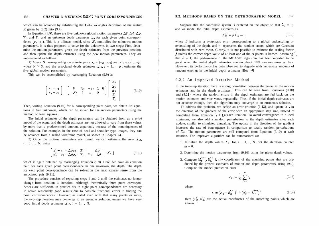
156 CHAPTER 9. METHODS USING POINT CORRESPONDENCES
which can be obtained by substituting the Eulerian angles definition of the matrixR given by (9.2) into (9.4).
In Equation (9.9), there are five unknown global motion parameters AQ, A$, A4,Ti, and T2, and an unknown depth parameter Xs for each given point correspon-dence (zi, ~2). This is a bilinear model, since Xs multiplies the unknown motionparameters. It is thus proposed to solve for the unknowns in two steps: First, deter-mine the motion parameters given the depth estimates from the previous iteration,and then update the depth estimates using the new motion parameters. They areimplemented as follows:
1) Given N corresponding coordinate pairs xi = (xii, zia) and x’i = (&, &)where N > 3, and the associated depth estimates Xis, i = 1,. .) N, estimate thefive global motion parameters.
This can be accomplished by rearranging Equation (9.9) as
r AQ
1 7-z
(9.10)
Then, writing Equation (9.10) for N corresponding point pairs, we obtain 2N equa-tions in five unknowns, which can be solved for the motion parameters using themethod of least squares.
The initial estimates of the depth parameters can be obtained from an a priorimodel of the scene, and the depth estimates are not allowed to vary from these valuesby more than a predetermined amount, apparently because of the nonuniqueness ofthe solution. For example, in the case of head-and-shoulder type images, they canbe obtained from a scaled wireframe model, as shown in Chapter 24.
2) Once the motion parameters are found, we can estimate the new Xis,i=l ,...l N, using
x; - XI + A~x, - Tix’z - x2 - A~x, - T2 ] = [ !fo ] [ x3 1 (9.11)
which is again obtained by rearranging Equation (9.9). Here, we have an equationpair, for each given point correspondence in one unknown, the depth. The depthfor each point correspondence can be solved in the least squares sense from theassociated pair (9.11).
The procedure consists of repeating steps 1 and 2 until the estimates no longerchange from iteration to iteration. Although theoretically three point correspon-dences are sufficient, in practice six to eight point correspondences are necessaryto obtain reasonably good results due to possible fractional errors in finding thepoint correspondences. However, as stated even with that many points or more,the two-step iteration may converge to an erronous solution, unless we have verygood initial depth estimates Xis, i = 1,. , N.
9.2. METHODS BASED ON THE ORTHOGRAPHIC MODEL 157
Suppose that the coordinate system is centered on the object so that Xs = 0,and we model the initial depth estimates as
xty = pxis + 1zi (9.12)
where p indicates a systematic error corresponding to a global underscaling oroverscaling of the depth, and ni represents the random errors, which are Gaussiandistributed with zero mean. Clearly, it is not possible to estimate the scaling factor/3 unless the correct depth value of at least one of the N points is known. Assuming \that 0 = 1, the performance of the MBASIC algorithm has been reported to begood when the initial depth estimates contain about 10% random error or less.However, its performance has been observed to degrade with increasing amounts ofrandom error 1zi in the initial depth estimates [Boz 941.
9.2.2 An Improved Iterative Method
In the two-step iteration there is strong correlation between the errors in the motionestimates and in the depth estimates. This can be seen from Equations (9.10)and (9.11), where the random errors in the depth estimates are fed back on themotion estimates and vice versa, repeatedly. Thus, if the initial depth estimates arenot accurate enough, then the algorithm may converge to an erroneous solution.
To address this problem, we define an error criterion (9.13), and update Xis inthe direction of the gradient of the error with an appropriate step size, instead ofcomputing from Equation (9.11), ta each iteration. To avoid convergence to a localminimum, we also add a random perturbation to the depth estimates after eachupdate, similar to simulated annealing. The update in the direction of the gradientincreases the rate of convergence in comparison to totally random perturbationsof Xis. The motion parameters are still computed from Equation (9.10) at eachiteration. The improved algorithm can be summarized as:
1. Initialize the depth values Xi3 for i = 1,. , N. Set the iteration counterm = 0.
2. Determine the motion parameters from (9.10) using the given depth values.
3. Compute (Z::“‘, $,“‘), the coordinates of the matching points that are pre-dicted by the present estimates of motion and depth parameters, using (9.9).Compute the model prediction error
(9.13)
where
ei = (XI1 - $;‘,2 + (&?‘a2 - i(y))2 (9.14)
Here (x:i,xi2) are the actual coordinates of the matching points which areknown.
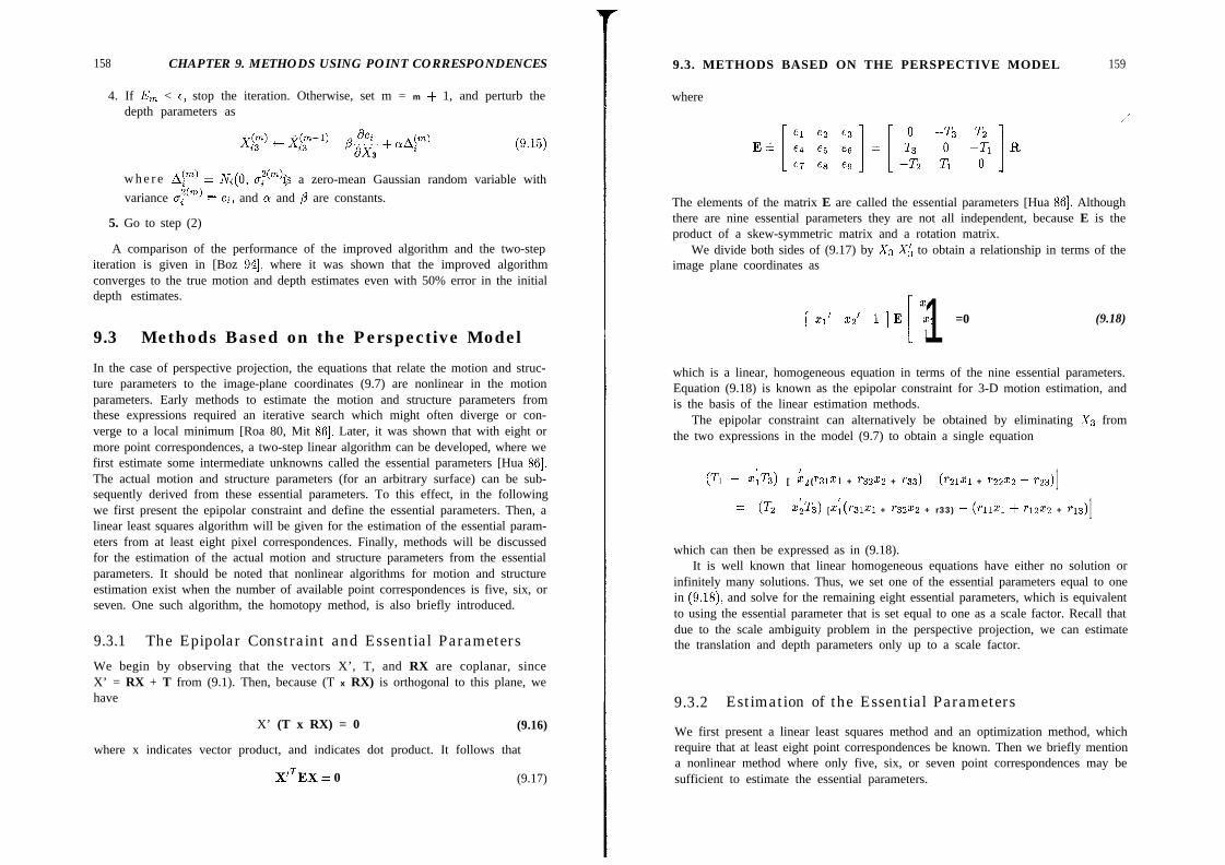
158 CHAPTER 9. METHODS USING POINT CORRESPONDENCES
4. If E, < E, stop the iteration. Otherwise, set m = m + 1, and perturb thedepth parameters as
+ $r-‘) - “2 + aAim)3
w h e r e Aa-) = Ni(O, gf’“‘)is a zero-mean Gaussian random variable withZ(m) -variance ui - ei, and Q and /? are constants.
5. Go to step (2)
A comparison of the performance of the improved algorithm and the two-stepiteration is given in [Boz 941, where it was shown that the improved algorithmconverges to the true motion and depth estimates even with 50% error in the initialdepth estimates.
9.3 Methods Based on the Perspective Model
In the case of perspective projection, the equations that relate the motion and struc-ture parameters to the image-plane coordinates (9.7) are nonlinear in the motionparameters. Early methods to estimate the motion and structure parameters fromthese expressions required an iterative search which might often diverge or con-verge to a local minimum [Roa 80, Mit 861. Later, it was shown that with eight ormore point correspondences, a two-step linear algorithm can be developed, where wefirst estimate some intermediate unknowns called the essential parameters [Hua 861.The actual motion and structure parameters (for an arbitrary surface) can be sub-sequently derived from these essential parameters. To this effect, in the followingwe first present the epipolar constraint and define the essential parameters. Then, alinear least squares algorithm will be given for the estimation of the essential param-eters from at least eight pixel correspondences. Finally, methods will be discussedfor the estimation of the actual motion and structure parameters from the essentialparameters. It should be noted that nonlinear algorithms for motion and structureestimation exist when the number of available point correspondences is five, six, orseven. One such algorithm, the homotopy method, is also briefly introduced.
9.3.1 The Epipolar Constraint and Essential Parameters
We begin by observing that the vectors X’, T, and RX are coplanar, sinceX’ = RX + T from (9.1). Then, because (T x RX) is orthogonal to this plane, wehave
X’ (T x RX) = 0 (9.16)
where x indicates vector product, and indicates dot product. It follows that
XtTEX = 0 (9.17)
9.3. METHODS BASED ON THE PERSPECTIVE MODEL 159
where
The elements of the matrix E are called the essential parameters [Hua 861. Althoughthere are nine essential parameters they are not all independent, because E is theproduct of a skew-symmetric matrix and a rotation matrix.
We divide both sides of (9.17) by Xs X4 to obtain a relationship in terms of theimage plane coordinates as
Xl1 Xl’ x2’ l]E x2 =0[ 11 (9.18)
which is a linear, homogeneous equation in terms of the nine essential parameters.Equation (9.18) is known as the epipolar constraint for 3-D motion estimation, andis the basis of the linear estimation methods.
The epipolar constraint can alternatively be obtained by eliminating Xs fromthe two expressions in the model (9.7) to obtain a single equation
(Tl - xiT3) [ ’ (22 r31x1 + r3222 + ~33) - (~ZIXI + 52x2 + 7-23) 1ZZ (Tz - xiT3, [x1’ ( r31x1 + r32xz + r33) - (TllXl + TlZX2 + r13) 1which can then be expressed as in (9.18).
It is well known that linear homogeneous equations have either no solution orinfinitely many solutions. Thus, we set one of the essential parameters equal to onein (9.18), and solve for the remaining eight essential parameters, which is equivalentto using the essential parameter that is set equal to one as a scale factor. Recall thatdue to the scale ambiguity problem in the perspective projection, we can estimatethe translation and depth parameters only up to a scale factor.
9.3.2 Estimation of the Essential Parameters
We first present a linear least squares method and an optimization method, whichrequire that at least eight point correspondences be known. Then we briefly mentiona nonlinear method where only five, six, or seven point correspondences may besufficient to estimate the essential parameters.

160 CHAPTER 9. METHODS USING POINT CORRESPONDENCES
Linear Least Squares Method
Setting es = 1 arbitrarily, we can rearrange (9.18) as
[ Xl’Xl 21’22 Xl’ XZ’Xl x2’xz x2’ x1 x2 1
ele2
e3
e4
e5
e6
e7
e8
ZY- 1
which is a linear equation in the remaining eight essential parameters. Given N > 8point correspondences, we can set up a system of N 2 8 linear equations in 8unknowns. Conditions for the coefficient matrix to have full rank were investigatedby Longuet-Higgins [Lon 811. Briefly stated, the coefficient matrix has full rankif T # 0 and the shape of the 3-D surface satisfies certain conditions, called thesurface constraint [Zhu 891. The solution, then, gives the essential matrix E up toa scale factor. We note here that any of the essential parameters could have beenchosen as the scale factor. In practice, it is advisable to select the ei, i = 1,. ,9,which would yield the coefficient matrix with the smallest condition number as thescale factor.
Optimization Method
Because it is not obvious, in general, which essential parameter should be chosenas a scale factor, an alternative is to use the norm of the solution as a scale factor.Then the estimation of the essential parameters can be posed as a constrainedminimization problem [Wen 93a], such that
e = argm@ ]I Ge I], subject to ]I e ]I = 1 (9.19)
where ]I ]I denotes vector or matrix norm,
Xll’Xl2 x11’ Xl2’Xll m!‘~lZ x12’ x11 dl2 1
f (9.20)
xNl’xN2 XNl’ xN2’xNl xN2’xN2 xN2’ XNl xN2 1 1is the observation matrix (derived from (9.18)), N > 8, ande = [ei ez es e4 e5 es er es eslT denotes the 9 x 1 essential parameter vector.It is well-known that the solution of this problem is the unit eigenvector of GTGassociated with its smallest eigenvalue.
9.3. METHODS BASED ON THE PERSPECTIVE MODEL 161
The Homotopy Method
When fewer than eight point correspondences are known, or the rank of the co-efficient matrix is less than 8, the system of linear equations is underdetermined.However, the fact that the matrix E can be decomposed into a skew-symmetric’matrix postmultiplied by a rotation matrix (see Equation 9.21) can be formulatedin the form of additional polynomial equations. In particular, the decomposabilityimplies that one of the eigenvalues of E is zero, and the other two are equal. Capital-izing on this observation, Huang and Netravali [Hua 901 introduced the homotopymethod to address the cases where five, six, or seven point correspondences areavailable. For example, with five point correspondences, they form five linear equa-tions and three cubic equations, which are then solved by the homotopy method.It has been shown that there are at most ten solutions in this case. The interestedreader is referred to [Hua 901.
9.3.3 Decomposition of the E-Matrix
Theoretically, from (9.17), the matrix E can be expressed as
E = [el I e2 I es] = [k+ x r1 ) ki! X r2 I k? x rs 1 (9.21)
where the vectors ri, i = 1,. ,3 denote the columns of the rotation matrix R, kdenotes the length of the translation vector T, and T is the unit vector along T.In the following, we discuss methods to recover R and !I! given E computed fromnoise-free and noisy point correspondence data, respectively.
Noise-Free Point Correspondences
It can easily be observed from (9.21) that each column of E is orthogonal to T.Then the unit vector along T can be obtained within a sign by taking the crossproduct of two of the three columns as
ei x ej+=*l,eixejlI i+j
(9.22)
Furthermore, it can be shown that [Hua 861
k2 = f(el el + e2 . e2 + e3 e3) (9.23)
Obviously, finding k from (9.23) cannot overcome the scale ambiguity problem, sincees contains an arbitrary parameter. However, it is needed to determine the correctrotation parameters.
In order to determine the correct sign of the translation vector, we utilize
X;+ x [xi x; llT = X3+ x R[xl x2 llT
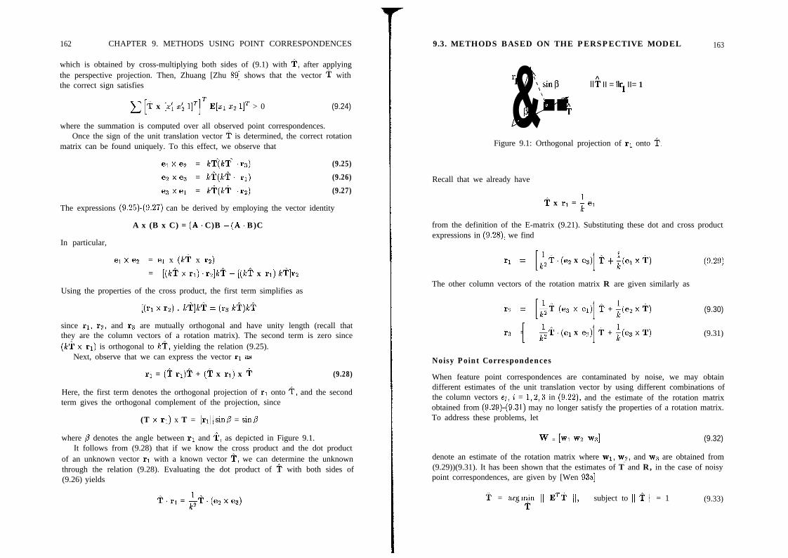
162 CHAPTER 9. METHODS USING POINT CORRESPONDENCES
which is obtained by cross-multiplying both sides of (9.1) with +I after applyingthe perspective projection. Then, Zhuang [Zhu 891 shows that the vector + withthe correct sign satisfies
c p x [xi x’z 11’1’ E[q x2 llT > 0 (9.24)
where the summation is computed over all observed point correspondences.Once the sign of the unit translation vector LI? is determined, the correct rotation
matrix can be found uniquely. To this effect, we observe that^ A
el x e2 = kT(kT ‘1.3) (9.25)
e2 x e3 = leq!ct. rl) (9.26)
e3 x el = !tTqKt .r2) (9.27)
The expressions (9.25)-(9.27) can be derived by employing the vector identity
A x (B x C) = (A. C)B - (A. B)C
In particular,
el x e2 = el x (ki? x r2)= [(k!i X q) .q]k+ - [(k+ x rl) k+]r,
Using the properties of the cross product, the first term simplifies as
[(q X r2) . k!f]k!F = (r3 k!k)k+
since rl, 12, and r3 are mutually orthogonal and have unity length (recall thatthey are the column vectors of a rotation matrix). The second term is zero since(le’? x q) is orthogonal to le?, yielding the relation (9.25).
Next, observe that we can express the vector q as
q = (+ q)+ + (+ x rl) x + (9.28)
Here, the first term denotes the orthogonal projection of rl onto T) and the secondterm gives the orthogonal complement of the projection, since
(T x q) x T = ]]rl]]sinP = sin/3
where /I denotes the angle between rI and f, as depicted in Figure 9.1.It follows from (9.28) that if we know the cross product and the dot product
of an unknown vector q with a known vector ?‘, we can determine the unknownthrough the relation (9.28). Evaluating the dot product of ? with both sides of(9.26) yields
i?. q = &+. (e2 X es)
9.3. METHODS BASED ON THE PERSPECTIVE MODEL 163
‘l ‘1 sin p\\
II+ II = llrl II= 1
\
p ’ t\
Figure 9.1: Orthogonal projection of rl onto !I?.
Recall that we already have
i? x q = 1 el
from the definition of the E-matrix (9.21). Substituting these dot and cross productexpressions in (9.28), we find
q =[$!t. (e2 x es)1 i? + i(el X +)
The other column vectors of the rotation matrix R are given similarly as
r2 =[fiY (es X el) 1 + + i(e2 X +)
r3 =[
iiT. (el x e2)1 Yi + i(e3 X !k)
(9.30)
(9.31)
Noisy Point Correspondences
When feature point correspondences are contaminated by noise, we may obtaindifferent estimates of the unit translation vector by using different combinations ofthe column vectors ei, i = 1,2,3 in (9.22), and the estimate of the rotation matrixobtained from (9.29)-(9.31) may no longer satisfy the properties of a rotation matrix.To address these problems, let
w = [w w2 w31 (9.32)
denote an estimate of the rotation matrix where ~1, wz, and ws are obtained from(9.29))(9.31). It has been shown that the estimates of T and R, in the case of noisypoint correspondences, are given by [Wen 93a]
+ = argmc I] ET? 11, subject to I] $ (1 = 1 (9.33)
164 CHAPTER 9. METHODS USING POINT CORRESPONDENCES
and
k = argm$ ]I R - W I(, subject to R is a rotation matrix (9.34)
respectively.The solution + of (9.33) is the unit eigenvector of EET associated with its
smallest eigenvalue. Note that the correct sign of + must satisfy (9.24). Let thesolution of (9.34) be expressed in terms of the quaternion representation (2.10).Then, q = [QO 41 4s qslT is the unit eigenvector of the 4 x 4 matrix
B $B:.Bii=l
where
Bi = 1such that Ii, i = 1,2,3 denote the columns of a 3 x 3 identity matrix, and
The reader is referred to [Wen 93a] for a derivation of this result.
9.3 .4 Algori thm
The method can then be summarized as:1) Given eight or more point correspondences, estimate E up to a scale factor
using either the least squares or the optimization method.2) Compute T (up to a scale factor) using (9.33).3) Find W from (9.29)-(9.31) and R from (9.34).Given the rotation matrix R, the axis of rotation in terms of its directional
cosines (nl,nz,ns) and the incremental angle of rotation Acr about this axis canthen be determined, if desired, from
trace(R) = 1+ 2 cos Ao (9.35)
and
R-RT = 2sinAcu (9.36)
9.4. THE CASE OF 3-D PLANAR SURFACES 165
4) Once the motion parameters are estimated, solve for the depth parameter Xsin the least squares sense (up to a scale factor) from
[;$;I=[qr31x1 + r32xz + r33) - (TllXl + r12xz + n3)
G(r3121 + r32x2 + ~33) - (~1x1 + r22x2 + ~3) 1hf3) (9.37)
We note that the translation vector T and the depth parameters can only be de-termined up to a scale factor due to the scale ambiguity inherent in the perspectiveprojection.
Alternative algorithms for the estimation of the 3-D motion and structure pa-rameters from feature correspondences exist in the literature. The two-step linearalgorithm presented in this section is favored because it provides an algebraic so-lution which is simple to compute. However, it is known to be sensitive to noisein the pixel correspondences [Wen 89, Phi 91, Wen 921. This sensitivity may beattributed to the fact that the epipolar constraint constrains only one of the twocomponents of the image plane position of a 3-D point [Wen 931. It is well knownthat the matrix E possesses nice properties, such as that two of its eigenvalues mustbe equal and the third has to be zero [Hua 89b], which the linear method is unableto use. To this effect, Weng et al. [Wen 931 proposed maximum likelihood andminimum variance estimation algorithms which use properties of the matrix E asconstraints in the estimation of the essential parameters to improve the accuracy ofthe solution in the presence of noise.
9.4 The Case of 3-D Planar Surfaces
Planar surfaces are an important special case because most real-world surfaces canbe approximated as planar at least on a local basis. This fact leads to representationof arbitrary surfaces by 3-D mesh models composed of planar patches, such as thewireframe model widely used in computer graphics. The main reason for treatingplanar surfaces as a special case is that they do not satisfy the surface assumptionrequired in the general case provided above. Fortunately, it is possible to derivesimple linear algorithms for the case of planar surfaces, as described in this section.
9.4.1 The Pure Parameters
We start by deriving a simplified model for the case of planar surfaces. Let the 3-Dpoints that we observe all lie on a plane described by
UXi+bXz+CX3=l (9.38)
where [ a b c IT denotes the normal vector of this plane. Then, the 3-D displacementmodel (9.1) can be rewritten as
[ z]=R[ ;;]+T[ubc][ ;;]
166 CHAPTER 9. METHODS USING POINT CORRESPONDENCES
01
where
A=R+T[abc]
Next, we map the 3-D displacements onto the 2-D image plane using the perspec-tive transformation, and normalize as = 1 due to the well-known scale ambiguity,to obtain the image plane mapping from t to t’ given by
x'1 =a121 + a222 + a3
~721 + a8x2 + 1
x’z =a421 + a522 + a6
a721 + a80 + 1(9.40)
The constants al,. . . , us are generally known as the pure parameters [Tsa 811. Nextwe present a linear algorithm for the estimation of the pure parameters.
9.4.2 Estimation of the Pure Parameters
By cross-multiplying each equation, we can rearrange (9.40) for each given pointcorrespondence, as follows:
[ x1 0 x2 0 0 1 x1 0 x2 0 0 1 -21x1’ -21x2’ -22x1’ -xzxz’ 1a1a2
a3
a4
a5
a6
a7
R3
= (9.41)
Therefore, given at least four point correspondences, we can set up eight or morelinear equations to solve for the eight pure parameters. It has been shown that therank of the coefficient matrix is 8 if and only if no three of the four observed pointsare collinear in three dimensions [Hua 861.
9.4.3 Estimation of the Motion and Structure Parameters
Once the matrix A has been determined, the motion parameters R and T, andthe structure parameters, i.e., the normal vector of the plane, can be estimated by
9.4. THE CASE OF 3-D PLANAR SURFACES 167
means of a singular value decomposition (SVD) of the matrix A as described in[Tsa 821. We start by expressing the matrix A as
(9.42)
where U = [ui ) us ) us] and V = [vi 1 vs 1 ogonal matricesand Xi 2 X2 2 As 2 0 are the singular values of A. There are three possibilitiesdepending on the singular values:
Case 1) The singular values are distinct with X1 > X2 > Xs, which indicates thatthe motion can be decomposed into a rotation about an axis through the originfollowed by a translation in a direction other than the direction of the normalvector of the plane. Then two solutions for the motion parameters exist, which canbe expressed as a 0 P
R = U [ 10 10 V7-sp 0 sa
(x3T = k -Pul+ (- - m)u3x2 >
[ a b c IT = t(6vl + v3)
where
s = det(U) det(V)
and I% is an arbitrary scale factor (positive or negative). The sign ambiguity maybe resolved by requiring l/Xs > 0 for all points.
Case 2) If the multiplicity of the singular values is two, e.g., Ai = X2 # A3, thena unique solution for the motion parameters exist, which is given by
1[a b clT = -vgk
s = det(U) det(V)
168 CHAPTER 9. METHODS USING POINT CORRESPONDENCES
and le is an arbitrary scale factor, In this case, the motion can be described by arotation about an axis through the origin followed by a translation along the normalvector of the plane.
Case 3) If the multiplicity of the singular values is three, i.e., X1 = X2 = As, thenthe motion is a pure rotation around an axis through the origin, and R is uniquelydetermined by
R = ($)A
However, it is not possible to determine T and [ a 6 c IT.As an alternative method, Tsai and Huang [Tsa 811 obtained a sixth-order poly-
nomial equation to solve for one of the unknowns, and then solved for the remainingunknowns. However, the SVD method provides a closed-form solution.
9.5 ExamplesThis section provides an experimental evaluation of the performances of some lead-ing 3-D motion and structure estimation algorithms in order to provide the readerwith a better understanding of their relative strengths and weaknesses. Results arepresented for numerical simulations as well as with two frames of the sequence “MissAmerica. ” In each case, we have evaluated methods based on both the orthographicprojection (two-step iteration and the improved method) and the perspective pro-jection (E-matrix and A-matrix methods).
9.5.1 Numerical Simulations
Simulations have been performed to address the following questions: 1) Under whatconditions can we successfully use the methods based on orthographic projection?2) Which method, among the four that we compare, performs the best? 3) Howsensitive are these methods to errors in the point correspondences? To this effect, wehave generated two 3-D data sets, each containing 30 points. The first set consistsof 3-D points that are randomly selected within a 100 cm x 100 cm x 0.6 cmrectangular prism whose center is 51.7 cm away from the center of projection; thatis, we assume Xi and Xz are uniformly distributed in the interval [-50,50] cm, andXs is uniformly distributed within [51.4,52] cm. The second set consists of pointssuch that Xi and X2 are uniformly distributed in the interval [-25,251 cm, and Xsis uniformly distributed within [70,100] cm. The image-plane points are computedvia the perspective projection, Q = fXi/Xs, i = 1,2, with f = 50 mm. In orderto find the matching points in the next frame, the 3-D data set is rotated andtranslated by the “true” motion parameters, and the corresponding image-planepoints are recomputed. Clearly, the orthographic projection model provides a goodapproximation for the first data set, where the range of Xs (AXs = 0.6 cm) is smallcompared to the average value of Xs (2s = 51.7 cm), since zi = fX,/51.7, i = 1,2,
9.5. EXAMPLES 169
Table 9.1: Comparison of the motion parameters. All angles are in radians, andthe translations are in pixels. (Courtesy Gozde Bozdagi)
10% Error 30% Error 50% ErrorTrue
A8 = 0.007Two-Step Improved Two-Step Improved Two-Step Improved
0.00689 0.00690 0.00626 0.00641 0.00543 0.00591A$ = 0.010 0.00981 0.00983 0.00898 0.00905 0.00774 0.00803A$ = 0.025 0.02506 0.02500 0.02515 0.02500 0.02517 0.02501Tl = 0.100 0.09691 0.09718 0.08181 0.08929 0.06172 0.07156T2 = 0.180 0.18216 0.18212 0.19240 0.19209 0.20660 0.17011
more-or-less describes all image-plane points. On the contrary, for the second setA& = 30 cm is not small in comparison to Xs = 85 cm; hence, the orthographicprojection would not be a good approximation.
We have tested the performance of the methods based on the orthographic pro-jection, the two-step iteration, and the improved algorithm on the first data set.The true motion parameters that are used in the simulations are listed in Table 9.1.Recall that both the two-step and the improved iterative algorithms require an ini-tial estimate of the depth values for each point pair. In order to test the sensitivityof these algorithms to random errors in the initial depth estimates, *lo%, f30%,or *50% error has been added to each depth parameter Xi,. The sign of the error(+ or -) was chosen randomly for each point. The parameter values 01 = 0.95 and/J = 0.3 have been used to obtain the reported results. In the case of the improvedalgorithm, we iterate until E,,, given by (9.13) 1is ess than an acceptable level. Inorder to minimize the effect of random choices, the results are repeated three timesusing different seed values. The average results are reported.
Table 9.1 provides a comparison of the motion parameter estimates obtained bythe two-step algorithm and the improved algorithm at the conclusion of the itera-tions. In order to compare the results of depth estimation, we define the followingerror measure:
I
Error =d
where N is the number of matching points, and Xis and Xi3 are the “true” andestimated depth parameters, respectively. Figures 9.2 (a) and (b) show the errormeasure plotted versus the iteration number for the cases of 30% and 50% initialerror, respectively. Note that the scale of the vertical axis is not the same in bothplots. Although the results are depicted for 500 iterations, convergence has resultedin about 100 iterations in almost all cases.
It can be seen from Table 9.1 that the error in the initial depth estimates directly
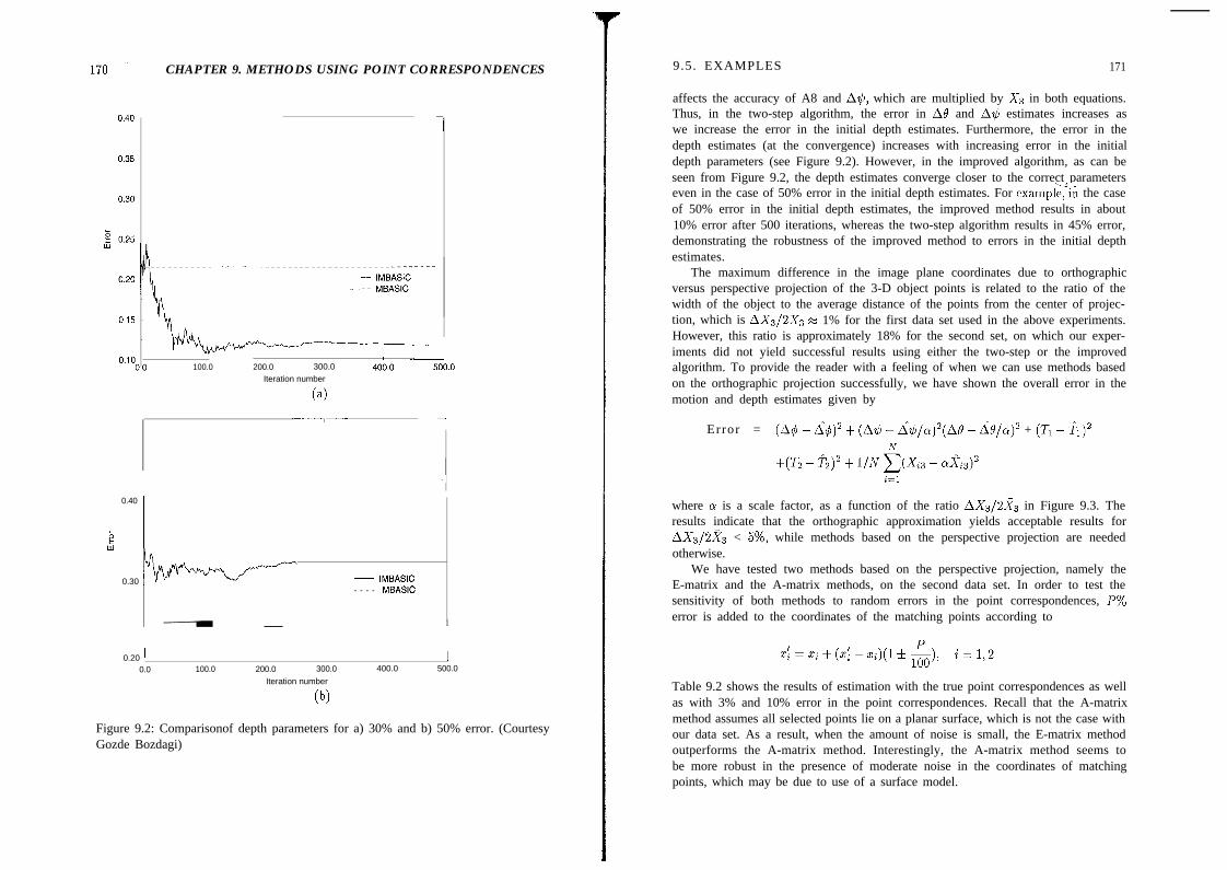
CHAPTER 9. METHODS USING POINT CORRESPONDENCES
..---~i~ .~100.0 200.0 300.0
Iteration number
(4
1
-
-I
0.40
b:
0.30 ! _ IMBASIC- - - - MBASIC
1
0.20 10.0 100.0 200.0 300.0
Iteration number
(b)
I400.0 500.0
Figure 9.2: Comparisonof depth parameters for a) 30% and b) 50% error. (CourtesyGozde Bozdagi)
9.5. EXAMPLES 171
affects the accuracy of A8 and A$, which are multiplied by Xs in both equations.Thus, in the two-step algorithm, the error in A0 and A$ estimates increases aswe increase the error in the initial depth estimates. Furthermore, the error in thedepth estimates (at the convergence) increases with increasing error in the initialdepth parameters (see Figure 9.2). However, in the improved algorithm, as can beseen from Figure 9.2, the depth estimates converge closer to the correct parameterseven in the case of 50% error in the initial depth estimates. For exampl$n the caseof 50% error in the initial depth estimates, the improved method results in about10% error after 500 iterations, whereas the two-step algorithm results in 45% error,demonstrating the robustness of the improved method to errors in the initial depthestimates.
The maximum difference in the image plane coordinates due to orthographicversus perspective projection of the 3-D object points is related to the ratio of thewidth of the object to the average distance of the points from the center of projec-tion, which is AXsf2Xs M 1% for the first data set used in the above experiments.However, this ratio is approximately 18% for the second set, on which our exper-iments did not yield successful results using either the two-step or the improvedalgorithm. To provide the reader with a feeling of when we can use methods basedon the orthographic projection successfully, we have shown the overall error in themotion and depth estimates given by
Error = (A4 - &)’ + (A$ - A$/a)2(A6’ - A8/# + (Ti - ?1)2
S(T2 - Q2 + 1,N .&Xi, - *X-i,)”i=l
where Q is a scale factor, as a function of the ratio AXs/2Xs in Figure 9.3. Theresults indicate that the orthographic approximation yields acceptable results forAXs/2Xs < 5%) while methods based on the perspective projection are neededotherwise.
We have tested two methods based on the perspective projection, namely theE-matrix and the A-matrix methods, on the second data set. In order to test thesensitivity of both methods to random errors in the point correspondences, P%error is added to the coordinates of the matching points according to
Table 9.2 shows the results of estimation with the true point correspondences as wellas with 3% and 10% error in the point correspondences. Recall that the A-matrixmethod assumes all selected points lie on a planar surface, which is not the case withour data set. As a result, when the amount of noise is small, the E-matrix methodoutperforms the A-matrix method. Interestingly, the A-matrix method seems tobe more robust in the presence of moderate noise in the coordinates of matchingpoints, which may be due to use of a surface model.

172 CHAPTER 9. METHODS USING POINT CORRESPONDENCES 9.5. EXAMPLES 173
Table 9.2: Comparison of the motion parameters. All angles are in radians, andthe translations are in pixels. (Courtesy Yucel Altunbasak)
E-Matrix A-MatrixTrue No Error 3% Error 10% Error No Error 3% Error 10% Error
A6’ =0.007 0.00716 0.00703 0.00938 0.00635 0.00587 0.00470A4 = 0.010 0.00991 0.00920 0.00823 0.01467 0.01450 0.01409Ad = 0.025 0.02500 0.02440 0.02600 0.02521 0.02513 0.02501
T2/Tl = 1.80 1.80014 1.89782 2.15015 1.05759 1.12336 1.28980T3fTl = 0.48 0.47971 0.50731 -0.98211 0.25627 0.29159 0.37145Depth error 0.00298 0.02284 0.15549 0.09689 0.09744 0.09974Match error 1.73 E-6 2.20 E-4 6.57 E-4 1.15 E-3 1.20 E-3 1.61 E-3
The “depth error” refers to the root mean square (RMS) error in the Xs coordi-nates of the 30 points selected. We have also calculated the “matching error” which
0.50
0.40
r45 0.30
5P
EP&,& 0.20
b5
0.10
r
0.00 i0.00 0.05 0.10 0.15
error(deltazL?average z)
Figure 9.3: The performance of methods based on the orthographic projection(Courtesy Gozde Bozdagi)
is the RMS difference between the coordinates of the matching points calculatedwith the true parameter values and those predicted by the estimated 3-D motionand structure parameters. The matching error with no motion compensation hasbeen found as 1.97 E - 3. /
9.5.2 Experiments with Two Frames of Miss America
We next tested all four methods on two frames of the “Miss America” sequence,which are shown in Figure 9.4 (a) and (b), respectively. We note that the ratio ofthe maximum depth on a front view of a typical face to the average distance of theface from the camera falls within the range for which the orthographic projectionis a reasonable approximation. Marked in Figure 9.4 (a) are the coordinates of 20points (~1, ~2) which are selected as features. The corresponding feature points(xi, z$) are likewise marked in Figure 9.4 (b). The coordinates of the matchingpoints have been found by hierarchical block matching to the nearest integer. Thistruncation corresponds to adding approximately 15% noise to the matching pointcoordinates.
Table 9.3: Comparison of methods on two frames of the Miss America sequence.
Since we have no means of knowing the actual 3-D motion parameters betweenthe two frames or the actual depth of the selected feature points, we have calculatedthe RMS difference between the coordinates of the matching points determined byhierarchical block matching and those predicted by estimated 3-D motion and thestructure parameters in order to evaluate the performance of the four methods.
Inspection of the RMSE values in Table 9.3 indicates that the improved iterativealgorithm based on the orthographic projection performed best on the head-and-shoulder-type sequence. The reader is reminded that this sequence can be wellapproximated by the orthographic projection. The A-matrix method has beenfound to be the second best. We note that in the case of the A-matrix method,the image-plane points were compensated by the “a-parameters” without actuallydecomposing the A-matrix to determine the rotation and translation parameters.In the case of the E-matrix method, the E-matrix needs to be decomposed to findthe motion parameters in order to be able compensate the image-plane points. Wehave observed that in the presence of errors in the coordinates of the matchingpoints, the decomposition step tends to increase the coordinate RMSE.
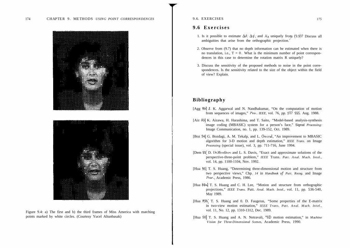
174 CHAPTER 9. METHODS USING POINT CORRESPONDENCES
Figure 9.4: a) The first and b) the third frames of Miss America with matchingpoints marked by white circles. (Courtesy Yucel Altunbasak)
9.6. EXERCISES
9.6 Exercises
175
1. Is it possible to estimate A6’, A$, and Xs uniquely fro,m (9.9)? Discuss allambiguities that arise from the orthographic projection.
2. Observe from (9.7) that no depth information can be estimated when there isno translation, i.e., T = 0. What is the minimum number of point correspon-dences in this case to determine the rotation matrix R uniquely?
3. Discuss the sensitivity of the proposed methods to noise in the point corre-spondences. Is the sensitivity related to the size of the object within the fieldof view? Explain.
Bibliography
[Agg 881 J. K. Aggarwal and N. Nandhakumar, “On the computation of motionfrom sequences of images,” Proc. IEEE, vol. 76, pp. 917-935, Aug. 1988.
[Aiz 891 K. Aizawa, H. Harashima, and T. Saito, “Model-based analysis-synthesisimage coding (MBASIC) system for a person’s face,” Signal Processing:Image Communication, no. 1, pp. 139-152, Oct. 1989.
[Boz 941 G. Bozdagi, A. M. Tekalp, and L. Onural, “An improvement to MBASICalgorithm for 3-D motion and depth estimation,” IEEE Trans. on ImageProcessing (special issue), vol. 3, pp. 711-716, June 1994.
[Dem 921 D. DeMenthon and L. S. Davis, “Exact and approximate solutions of theperspective-three-point problem,” IEEE Trans. Patt. Anal. Mach. Intel.,vol. 14, pp. 1100-1104, Nov. 1992.
[Hua 861 T. S. Huang, “Determining three-dimensional motion and structure fromtwo perspective views,” Chp. 14 in Handbook of Putt. Recog. and ImageProc., Academic Press, 1986.
[Hua 89a] T. S. Huang and C. H. Lee, “Motion and structure from orthographicprojections,” IEEE Trans. Putt. Anal. Mach. Intel., vol. 11, pp. 536-540,May 1989.
[Hua 89b] T. S. Huang and 0. D. Faugeras, “Some properties of the E-matrixin two-view motion estimation,” IEEE Trans. Patt. Anal. Mach. Intel.,vol. 11, No. 12, pp. 1310-1312, Dec. 1989.
[Hua 901 T. S. Huang and A. N. Netravali, “3D motion estimation,” in MachineVision for Three-Dimensional Scenes, Academic Press, 1990.
176 BIBLIOGRAPHY
[Hua 941 T. S. Huang and A. N. Netravali, “Motion and structure from featurecorrespondences: A review,” Proc. IEEE, vol. 82, pp. 2522269, Feb. 1994.
[Lon 811 H. C. Longuet-Higgins, “A computer program for reconstructing a scenefrom two projections,” Nature, vol. 392, pp. 133-135, 1981.
[Mit 861 A. Mitiche and J. K. Aggarwal, “A computational analysis of time-varying images,” in Handbook of Pattern Recognition and Image Processing,T. Y. Young and K. S. Fu, eds., New York, NY: Academic Press, 1986.
[Phi 911 J. Philip, “Estimation of three-dimensional motion of rigid objects fromnoisy observations,” IEEE Trans. Putt. Anal. Mach. Intel., vol. 13, no. 1,
1 pp. 61-66, Jan. 1991.
[Roa 801 J. W. Roach and J. K. Aggarwal, “Determining the movement of objectsfrom a sequence of images,” IEEE Trans. Putt. Anal. Mach. Intel., vol. 6,pp. 554-562, 1980.
[Tsa 811 R. Y. Tsai and T. S. Huang, “Estimating three-dimensional motion pa-rameters of a rigid planar patch,” IEEE Trans. Acoust. Speech Sign. Proc.,vol. 29, no. 6, pp. 1147-1152, Dec. 1981.
[Tsa 821 R. Y. Tsai, T. S. Huang, and W. L. Zhu, “Estimating 3-D motion pa-rameters of a rigid planar patch II: Singular value decomposition,” IEEETrans. Acoust. Speech Sign. Proc., vol. 30, no. 4, pp. 525-534, 1982; andvol. ASSP-31, no. 2, p. 514, 1983.
[Ull 791 S. Ullman, The Interpretation of Visual Motion, Cambridge, MA:MIT Press, 1979.
[Wen 891 J. Weng, T. S. Huang, and N. Ahuja, “Motion and structure from twoperspective views: Algorithms, error analysis, and error estimation,” IEEETrans. Putt. Anal. Mach. Intel., vol. 11, no. 5, pp. 451-476, May 1989.
[Wen 911 J. Weng, N. Ahuja, and T. S. Huang, “Motion and structure from pointcorrespondences with error estimation: Planar surfaces,” IEEE Trans.
Sign. Proc., vol. 39, no. 12, pp. 2691-2717, Dec. 1991.
[Wen 921 J. Weng, N. Ahuja, and T. S. Huang, “Motion and structure from line cor-respondences: Closed-form solution, uniqueness, and optimization,” IEEETrans. Putt. Anal. Mach. Intel., vol. 14, no. 3, pp. 3188336, Mar. 1992.
[Wen 931 J. Weng, N. Ahuja, and T. S. Huang, “Optimal motion and struc-ture estimation,” IEEE Trans. Putt. Anal. Mach. Intel., vol. 15, no. 9,pp. 864-884, Sep. 1993.
[Wen 93a] J. Weng, T. S. Huang, and N. Ahuja, Motion and Structure from Image
Sequences, Springer-Verlag (Series in Information Sciences), 1993.
[Zhu 891 X. Zhuang, “A simplification to linear two-view motion algorithms,”Comp. Vis. Graph. Image Proc., vol. 46, pp. 1755178, 1989.
Chapter IO
OPTICAL FLOW ANDDIRECT METHODS
This chapter discusses 3-D motion and structure estimation from two orthographicor perspective views based on an estimate of the optical flow field (optical flowmethods) or on spatio-temporal image intensity gradients using the optical flowconstraint (direct methods). The main differences between the methods in thischapter and the previous one are: optical flow methods utilize a projected veloc-ity model as opposed to a projected displacement model (see Section 10.1.3 for acomparison of the two models); and optical flow methods require a dense flow fieldestimate or estimation of the image intensity gradient everywhere, rather than se-lecting a set of distinct feature points and matching them in two views. Here, weassume that the optical flow field is generated by a single object subject to 3-D rigidmotion. The case of multiple moving objects, hence motion segmentation, will bedealt with in the next chapter.
Section 10.1 introduces 2-D velocity field models under orthographic and per-spective projections. Estimation of the 3-D structure of the scene from the opticalflow field in the case of pure 3-D translational motion is discussed in Section 10.2.Motion and structure estimation from the optical flow field in the case of general3-D rigid motion using algebraic methods and optimization methods are the sub-jects of Section 10.3 and 10.4, respectively. Finally, in Section 10.5, we cover directmethods which do not require estimation of the optical flow field or any featurecorrespondence, but utilize spatio-temporal image intensity gradients directly.
10.1 Modeling the Projected Velocity Field
In this section, we present models for the 2-D (projected) velocity field startingwith the 3-D velocity expression. Recall from Chapter 2 that, for the case of small
177

178 CHAPTER 10. OPTICAL FLOW AND DIRECT METHODS
angular rotation, the 3-D velocity vector (Xi, X,, Xs) of a rigid object is given by
Xl
[:I i
x2 =X3
--L2 rf’ -q [ z]+[ ;]
which can be expressed in vector notation as a cross product
x=nxx+v (10.1)
where fl = [& fiz &,lT is the angular velocity vector and V = [VI Vz V31Trepresents the translational velocity vector. In scalar form, we have
Xl = 02x3 - R3Xz + VI
x2 = Q3X1- QlX3 + vzx3 = n1xz -&X1 + v3 (10.2)
We will present two models for the 2-D velocity field, based on the orthographicand perspective projections of the model (10.2), respectively, in the following.
10.1.1 Orthographic Velocity Field Model
The orthographic projection of the 3-D velocity field onto the image plane can becomputed from
211 = il = x,
212 = ii, = i,
which results in
Vl = vl + 02x3 - 0322
212 = vz + a321 - RlX3 (10.3)
in terms of the image plane coordinates. The orthographic model can be thoughtof as an approximation of the perspective model as the distance of the object fromthe image plane gets larger and the field of view becomes narrower.
10.1.2 Perspective Velocity Field Model
In order to obtain the perspective projection of the 3-D velocity field, we first applythe chain rule of differentiation to the perspective projection expression as
II1 = lil = f x3x1--x1x3 = f$-xlgx3”
I& = kz = f x3x2 - x2x3 = f 2 _ x2$x,z (10.4)
10.1. MODELING THE PROJECTED VELOCITY FIELD 179
Now, substituting the 3-D velocity model (10.2) in (10.4), and rewriting theresulting expressions in terms of the image plane coordinat$s, we have
(10.5)
When the projection is normalized, f = 1, the model (10.5) can be rearranged as
-vl + 2lv3Vl =x3
+ %x1%2 - fi2(l + XT) + a322
-h + 22%v2 =x3
+ fh(1+ x;, - R2XlX2 - a2321
Note that the perspective velocities in the image plane depend on the Xs coordinateof the object. The dependency of the model on X3 can be relaxed by assuming aparametric surface model, at least on a local basis (see Sections 10.3.1 and 10.3.2).
For arbitrary surfaces, the depth X3 of each scene point can be eliminated fromthe model (10.6) by solving both expressions for Xs and equating them. This resultsin a single nonlinear expression, which relates each measured flow vector to the 3-Dmotion and structure parameters, given by
-v2e1 + vle2 - x1(% + R3el) - x2(Q2 + fi3e2) - xlx2(fi2el + Rlez)
+(x2 + ~$03 + (1 + x$Rlel + (1 + xW2e2 = 21122 - 02x1 (10.7)
where ei = Vl/V3 and ez = Vg,/V3 denote the focus of expansion (see Section 10.2).Recall from the discussion of perspective projection that we can find the transla-tional velocities and the depth up to a scaling constant, which is set equal to V3above.
10.1.3 Perspective Velocity vs. Displacement Models
Because optical flow estimation from two views indeed corresponds to approxi-mate displacement estimation using spatio-temporal image intensity gradients (seeSection 7.1), it is of interest to investigate the relation between the perspectivevelocity (10.5) and displacement (9.7) models for finite At. To this effect, let
Substituting (9.7) into (10.8), we can write
xi - x1 xl+Axl Xl- - = At(l+AX3) A tAt
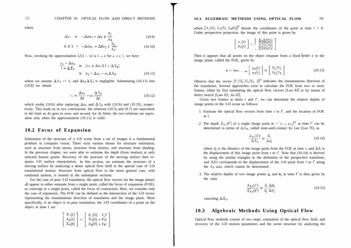
180
where
CHAPTER 10. OPTICAL FLOW AND DIRECT METHODS
Ax1 = TI-Aba+A$+-x3
(10.9)
T3A X 3 = -A$xl +A$xz+ -x3
(10.10)
Now, invoking the approximation l/(1 + x) z 1 - z for x << 1, we have
XI + Ax,ixGg+ (XI + a~)(1 - AX3)
M x1 + AQ - xlAX3 (10.11)
where we assume AXs << 1, and AxlAX is negligible. Substituting (10.11) into(10.8) we obtain
AXI AX3v1= at-xlat (10.12)
which yields (10.6) after replacing Az, and AX3 with (10.9) and (lO.lO), respec-tively. This leads us to two conclusions: the relations (10.5) and (9.7) are equivalentin the limit as At goes to zero; and second, for At finite, the two relations are equiv-alent only when the approximation (10.11) is valid.
10.2 Focus of Expansion
Estimation of the structure of a 3-D scene from a set of images is a fundamentalproblem in computer vision. There exist various means for structure estimation,such as structure from stereo, structure from motion, and structure from shading.In the previous chapter, we were able to estimate the depth (from motion) at onlyselected feature points. Recovery of the structure of the moving surface then re-quires 3-D surface interpolation. In this section, we estimate the structure of amoving surface by analyzing a dense optical flow field in the special case of 3-Dtranslational motion. Structure from optical flow in the more general case, withrotational motion, is treated in the subsequent sections.
For the case of pure 3-D translation, the optical flow vectors (in the image plane)all appear to either emanate from a single point, called the focus of expansion (FOE),or converge to a single point, called the focus of contraction. Here, we consider onlythe case of expansion. The FOE can be defined as the intersection of the 3-D vectorrepresenting the instantaneous direction of translation and the image plane. Morespecifically, if an object is in pure translation, the 3-D coordinates of a point on theobject at time t are
10.3. ALGEBRAIC METHODS USING OPTICAL FLOW 181
where [X,(0),X2(0),Xs(0)]T denote the coordinates of the point at time t = 0.Under perspective projection, the image of this point is given by
Then it appears that all points on the object emanate from a fixed boint e in theimage plane, called the FOE, given by
(10.13)
Observe that the vector [VI/& V2/Vs l] T indicates the instantaneous direction ofthe translation. Several approaches exist to calculate the FOE from two or moreframes, either by first estimating the optical flow vectors [Law 831 or by means ofdirect search [Law 83, Jai 831.
Given two frames at times t and t’, we can determine the relative depths ofimage points in the 3-D scene as follows:
1. Estimate the optical flow vectors from time t to t’, and the location of FOEat t.
2. The depth Xz,i(t’) of a single image point xi = [xl,i) x:z,ilT at time t’ can bedetermined in terms of AXs, called time-until-contact by Lee [Lee 761, as
(10.14)
where d; is the distance of the image point from the FOE at time t, and Adi isthe displacement of this image point from t to t’. Note that (10.14) is derivedby using the similar triangles in the definition of the perspective transform,and AX3 corresponds to the displacement of the 3-D point from t to t’ alongthe Xs axis, which cannot be determined.
3. The relative depths of two image points xi and xj at time t’ is then given bythe ratio
(10.15)
canceling AXs.
10.3 Algebraic Methods Using Optical Flow
Optical flow methods consist of two steps: estimation of the optical flow field, andrecovery of the 3-D motion parameters and the scene structure by analyzing the

182 CHAPTER 10. OPTICAL FLOW AND DIRECT METHODS
estimated optical flow. Methods to estimate the optical flow were discussed inChapter 5. Various approaches exist to perform the second step which differ in theassumptions they make about the structure of the optical flow field and the criteriathey employ. We can broadly classify these techniques in two groups: algebraicmethods, which seek for a closed-form solution; and optimization methods, whichcan be characterized as iterative refinement methods towards optimization of acriterion function.
This section is devoted to algebraic methods. After a brief discussion about theuniqueness of the solution, we first assume a planar surface model to eliminate Xsfrom (10.2). In this case, the orthographic and perspective projection of the 3-Dvelocity field results in an affine flow model and a quadratic flow model, respectively[Ana 931. A least squares method can then be employed to estimate the affineand quadratic flow parameters. We then present two linear algebraic methods toestimate 3-D motion and structure from arbitrary flow fields,
10.3.1 Uniqueness of the Solution
Because 3-D motion from optical flow requires the solution of a nonlinear equation(10.7), there may, in general, be multiple solutions which yield the same observedoptical flow. Observe that (10.7) has five unknowns, L$, 1;2s, as, ei and es. However,in the presence of noise-free optical flow data, it has been shown, using algebraicgeometry and homotopy continuation, that [Ho1 931:
l there are at most 10 solutions with five optical flow vectors,l optical flow at six or more points almost always determines 3-D motion
uniquely,l if the motion is purely rotational, then it is uniquely determined by two optical
ilow values, andl in the case of 3-D planar surfaces, optical flow at four points almost always
gives two solutions.With these uniqueness results in mind, we now present a number of algorithms todetermine 3-D motion and structure from optical flow.
10.3.2 Affine Flow
A planar surface undergoing rigid motion yields an affine flow field under the or-thographic projection. This can easily be seen by approximating the local surfacestructure with the equation of a plane
x3 = 20 + 21x1 + 22x2 (10.16)
Substituting (10.16) into the orthographic velocity expressions (10.3), we obtain thesix-parameter affine flow model
211 = al + a221 + a322
212 = a4 + a521 -t a622 (10 .17 ) ,
10.3. ALGEBRAIC METHODS USING OPTICAL FLOW 183
where
a1 = vl + 2002, a2 = G2, a3 = 22L?2 - Cl3
a4 = V2 - zoR1, ag = 03 - 2101, a6 = -%&21
Observe that, if we know the optical flow at three or more points, we can set upsix or more equations in six unknowns to solve for (al). , us). However, becauseof the orthographic projection, it is not possible to determine all eight motion andstructure parameters from (ai, ) as) uniquely. For example, ~0 is not observableunder the orthographic projection. ./
10.3.3 Quadratic Flow
The quadratic flow is the most fundamental flow field model, because it is an exactmodel for the case of planar surfaces under perspective projection; otherwise, it islocally valid under a first-order Taylor series expansion of the surface [Wax 871. Inthe case of a planar surface, we observe from (10.16) that
1 1 Zi-=-- -X1 - %2x3 20 zo 20
(10.18)
Substituting the expression (10.18) into the perspective velocity field model (10.5))we obtain the eight-parameter quadratic flow field
v1 = al + a221 + a322 + a,xt + as212202 = a4 + a521 + a622 + a72122 + asxz (10.19)
where
al=,f(z+f22), a2=-(fF+z), as=-(S%+&)
a4=f ($-al), a5=-(fF-f13), as=-(f%+z)
a7= (%+F), a8= (Jf$-F)
If we know the optical flow on at least four points that lie on a planar patch, wecan set up eight or more equations in eight unknowns to solve for (al,. , as). Notethat ~0, which is the distance between the surface point and the camera, alwaysappears as a scale factor. Other approaches have also been reported to solve for themodel parameters [Die 91, Ana 931.
In order to recover the 3-D motion and structure parameters using the second-order flow model, Waxman el al. [Wax 871 defined 12 kinematic deformation pa-rameters that are related to the first- and second-order partial derivatives of theoptical flow. Although closed-form solutions can be obtained, partials of the flowestimates are generally sensitive to noise.
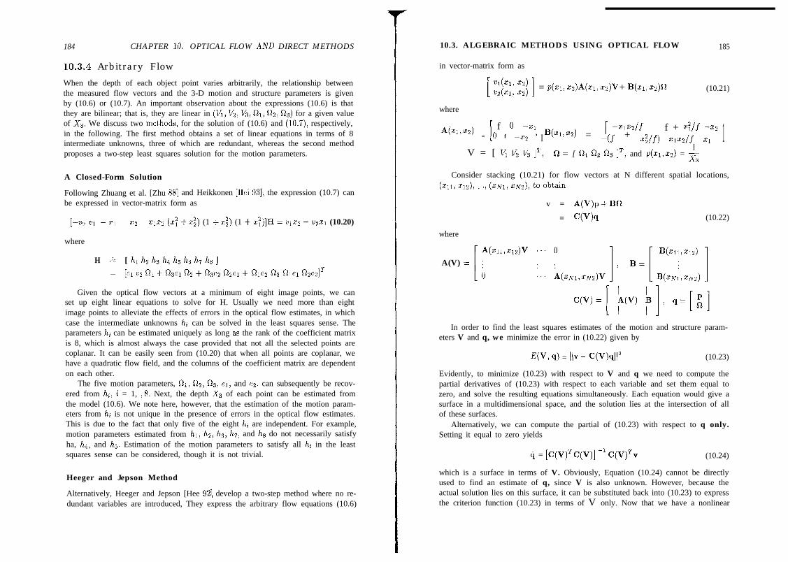
184 CHAPTER 10. OPTICAL FLOW AND DIRECT METHODS
10.3.4 Arbitrary Flow
When the depth of each object point varies arbitrarily, the relationship betweenthe measured flow vectors and the 3-D motion and structure parameters is givenby (10.6) or (10.7). An important observation about the expressions (10.6) is thatthey are bilinear; that is, they are linear in (VI] Vz, V3, al, 02, Qs) for a given valueof Xs. We discuss two met,hods, for the solution of (10.6) and (10.7), respectively,in the following. The first method obtains a set of linear equations in terms of 8intermediate unknowns, three of which are redundant, whereas the second methodproposes a two-step least squares solution for the motion parameters.
A Closed-Form Solution
Following Zhuang et al. [Zhu 881 and Heikkonen [Hei 931, the expression (10.7) canbe expressed in vector-matrix form as
1-2 VI - Xl - x2 - zlz2 (XT +x;) (1 +x;) (1 + xT)]H = v1x2 - vzxl (10.20)
where
H - [ hl hz h3 hq h5 h6 h7 hs ]Z [el e2 al + fi3el 02 $ fi3e2 fi2el + file2 fi3 fhel fi2e21T
Given the optical flow vectors at a minimum of eight image points, we canset up eight linear equations to solve for H. Usually we need more than eightimage points to alleviate the effects of errors in the optical flow estimates, in whichcase the intermediate unknowns hi can be solved in the least squares sense. Theparameters hi can be estimated uniquely as long as the rank of the coefficient matrixis 8, which is almost always the case provided that not all the selected points arecoplanar. It can be easily seen from (10.20) that when all points are coplanar, wehave a quadratic flow field, and the columns of the coefficient matrix are dependenton each other.
The five motion parameters, Ql, 02, s/s, el, and e2, can subsequently be recov-ered from hi, i = 1, ,8. Next, the depth X3 of each point can be estimated fromthe model (10.6). We note here, however, that the estimation of the motion param-eters from hi is not unique in the presence of errors in the optical flow estimates.This is due to the fact that only five of the eight hi are independent. For example,motion parameters estimated from h 1, ha, hs, h7, and hs do not necessarily satisfyha, hh, and hg. Estimation of the motion parameters to satisfy all hi in the leastsquares sense can be considered, though it is not trivial.
Heeger and Jepson Method
Alternatively, Heeger and Jepson [Hee 921 develop a two-step method where no re-dundant variables are introduced, They express the arbitrary flow equations (10.6)
10.3. ALGEBRAIC METHODS USING OPTICAL FLOW 185
in vector-matrix form as
[ :$:r :j ] = p(xl, 22)A(x1, x2)V + B(zl, XZ)~ (10.21)
where
[f 0 -21
I [-x122/f f + G/f -22
A(x1,x2) = 0 f -x2 ’ B(xl,4 = -(f + g/f) xIx2,f x1 1V = [ VI I,5 V, ITI 1(1= [ ill Rz % IT, and P(Q,XZ) = &
Consider stacking (10.21) for flow vectors at N different spatial locations,(XII, x12), . .) (XNI, XNZ), to obtain
V = A(V)p+BR
= C(% (10.22)
where
A(V) =A(m,xlz)V
[.x
CP)=[ ;:v! y. cl=[r,]In order to find the least squares estimates of the motion and structure param-
eters V and q, we minimize the error in (10.22) given by
w, Q) = llv - V)ql12 (10.23)
Evidently, to minimize (10.23) with respect to V and q we need to compute thepartial derivatives of (10.23) with respect to each variable and set them equal tozero, and solve the resulting equations simultaneously. Each equation would give asurface in a multidimensional space, and the solution lies at the intersection of allof these surfaces.
Alternatively, we can compute the partial of (10.23) with respect to q only.Setting it equal to zero yields
4 = [C(V)TC(V)] -l C(V)% (10.24)
which is a surface in terms of V. Obviously, Equation (10.24) cannot be directlyused to find an estimate of q, since V is also unknown. However, because theactual solution lies on this surface, it can be substituted back into (10.23) to expressthe criterion function (10.23) in terms of V only. Now that we have a nonlinear
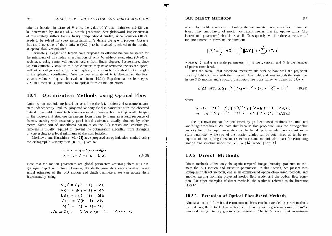
186 CHAPTER 10. OPTICAL FLOW AND DIRECT METHODS
criterion function in terms of V only, the value of V that minimizes (10.23) canbe determined by means of a search procedure. Straightforward implementationof this strategy suffers from a heavy computational burden, since Equation (10.24)needs to be solved for every perturbation of V during the sea,rch process. Observethat the dimensions of the matrix in (10.24) to be inverted is related to the numberof optical flow vectors used.
Fortunately, Heeger and Jepson have proposed an efficient method to search forthe minimum of this index as a function of only V, without evaluating (10.24) ateach step, using some well-known results from linear algebra. Furthermore, sincewe can estimate V only up to a scale factor, they have restricted the search space,without loss of generality, to the unit sphere, which can be described by two anglesin the spherical coordinates. Once the best estimate of V is determined, the leastsquares estimate of q can be evaluated from (10.24). Experimental results suggestthat, this method is quite robust to optical flow estimation errors.
10.4 Optimization Methods Using Optical Flow
Optimization methods are based on perturbing the 3-D motion and structure param-eters independently until the projected velocity field is consistent with the observedoptical flow field. These techniques are most successful for tracking small changesin the motion and structure parameters from frame to frame in a long sequence offrames, starting with reasonably good initial estimates, usually obtained by othermeans. Some sort of smoothness constraint on the 3-D motion and structure pa-rameters is usually required to prevent the optimization algorithm from divergingor converging to a local minimum of the cost function.
Morikawa and Harashima [Mor 911 have proposed an optimization method usingthe orthographic velocity field (~1, ~2) given by
211 = i1 = Vl + n,x, - f&x2
II2 = ii’2 = v2 + i-2321 - 021x3 (10.25)
Note that the motion parameters are global parameters assuming there is a sin-gle rigid object in motion. However, the depth parameters vary spatially. Giveninitial estimates of the 3-D motion and depth parameters, we can update themincrementally using
f&(k) = R1(k - 1) +A&
Q,(k) = O&k- 1) +A&
Q,(k) = R&k - 1) $A03
VI(~) = Vl(k- l)+AK
V2(k) = Vz(k- l)+AV,
&(X,,Q)(~) = X3(xl,ZZ)(k - 1) + AXa(m,xz)
10.5. DIRECT METHODS 187
where the problem reduces to finding the incremental parameters from frame toframe. The smoothness of motion constraint means that the update terms (theincremental parameters) should be small. Consequently, we introduce a measure ofthe smoothness in terms of the functional
where (Y, /3, and y are scale parameters, I].]] is the La norm, and N is the numberof points considered.
Then the overall cost functional measures the sum of how well the projectedvelocity field conforms with the observed flow field, and how smooth the variationsin the 3-D motion and structure parameters are from frame to frame, as f&ows
E(A& AT, AXa) = c [(w - %I)’ + (via - k$] -t llPl/’ (10.26)
where
61 = (VI + Ah) + (G + A%)(&3 + (AX),,) - (a3 + A%)xa
Oi2 = (Vz + Ah) + (03 + AO3)n - (a, + AR1)(Xi3 + (AX),,)
The optimization can be performed by gradient-based methods or simulatedannealing procedures. We note that because this procedure uses the orthographicvelocity field, the depth parameters can be found up to an additive constant and ascale parameter, while two of the rotation angles can be determined up to the re-ciprocal of this scaling constant. Other successful methods also exist for estimatingmotion and structure under the orthogra,phic model [Kan 861.
10.5 Direct Methods
Direct methods utilize only the spatio-temporal image intensity gradients to esti-mate the 3-D motion and structure parameters. In this section, we present twoexamples of direct methods, one as an extension of optical-flow-based methods, andanother starting from the projected motion field model and the optical flow equa-tion. For other examples of direct methods, the reader is referred to the literature[Hor 881.
10.5.1 Extension of Optical Flow-Based Methods
Almost all optical-flow-based estimation methods can be extended as direct methodsby replacing the optical flow vectors with their estimates given in terms of spatio-temporal image intensity gradients as derived in Chapter 5. Recall that an estimate

188 CHAPTER 10. OPTICAL FLOW AND DIRECT METHODS 10.5. DIRECT METHODS 189
of the flow field was given by (5.12)
Substituting this expression in a.ny optical-flow-based method for the opticalflow vectors, we can obtain an estimate of the 3-D motion and structure parametersdirectly in terms of the spatio-temporal image intensity gradients. However, thereader is alerted that (5.12) may not provide the best possible estimates for theoptical flow field. An alternative approach is presented in the following st,artingwith the projected motion and optical flow equations.
10.5.2 Tsai-Huang Method
Tsai and Huang [Tsa 811 considered the case of planar surfaces, where we can modelthe displacement of pixels from frame t to t’ by (9.40)
xi =Tl(al,...,as)= alxl+ a20 + a3a721 + a822 + 1
xi =Tz(al,...,as) =a421 + au2 + a6
a721 +asx2+1(10.28)
where the pure parameters al, ) a8 are usually represented in vector notation bya. Note that a = e, where e = (1, 0, O,O, l,O, 0, O)T corresponds to no motion, i.e.,21 = Tl(e), x2 = Tz(e).
In order to obtain a linear estimation algorithm, the mapping (10.28) will belinearized by means of a first-order Taylor series expansion about a = e, assumingsmall motion, as
TV-l;(e)=Ax,=x-a aT1(a) laze (ai - ei)i=l aai
* aT2(a)Tz(a) - Tz(e) = Ax2 = c -la=e (ai - ei)i=l aai
(10.29)
where a = (al,. , as), Ax, = xi - ~1 and Ax2 = X; - x2.Now, referring to the optical flow equation (5.5) and approximating the partials
by finite differences, we obta$ the discrete expression
Sk(Xl,X2) -sk+l(xl,x2) ZZ ask+l(xl,x2)AxlAt ax1 a t +
where At is the time interval between the frames k and k + 1 at times t and t’,respectively. After cancelling At, we obtain
/
Sk(Xl,XZ) = sk+l(xl,x%)+a~ktlhxz)Ax
ax11+ aSktl(xl,x2)
ax2Ax , (10 .31 )
Observe that (10.31) may also be interpreted as the linearization of image in-tensity function in the vicinity of (21, x2) in frame I% + 1, as
sktl(x;,xB) -skt1(x11x2)=asktl(xl, x2)
ax1Ax1 + askt1~xl'x2)Ax
ax22
since we have
sk+l(x:,x;) = Sk(Xl,X2)
Substituting the linearized expressions for Ax, and Ax2 from (10.29) into(10.31)) we can write the frame difference between the frames k and k + 1 as
FD(Xl,XZ) = Sk(Q,X2) - sktl(xl,xz)
ZZ aSktl (xl, x2)8x1
kF(ai-ei,i=l z 1+aSktlhx2)ax2 [e F(ai - ei)] (10.32)
i=l
In order to express (10.32) in vector matrix form, we define
H = [HI Hz H3 H4 H5 He H7 H8lT (10.33)
where
Tl(a) ask+1HI = - aSktl-=x1-aal ax1 ax1 1
Tl(a) dsktlHa=---- aSktlaa2 ax1
= x2-ax1Tl(a) dsktl asktlH3=--- ,aa ax1 ax1
H4 = Tda) asktl ask+1- - II x1-aa4 ax2 ax2
H5=T2(a) ask+1 .,aSktl--= ask+1aa5 ax2 ax2 9
& = T2(a) ask+1--I=-aa6 ax2 ax2
H7= Tl(a) ask+1 + TZ(a) ask+1__- _ _ ask+1 ask+1aa 8x1 aa
- = -xfax2
- - x1x2-ax1 ax2
Ha = Tda) asktl + G(a) ask+1-__ ask+1 asktlaas ax1
- - = -x1x2- - x;-aa8 ax2 ax1 ax2
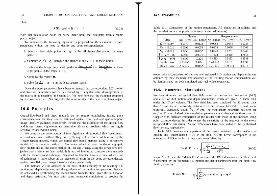
190 CHAPTER 10. OPTICAL FLOW AND DIRECT METHODS
Then
FD(z1,~2)=H.(a-e) (10.34)
Note that this relation holds for every image point that originates from a singleplanar object.
To summarize, the following algorithm is proposed for the estimation of pureparameters without the need to identify any point correspondences:
1. Select at least eight points (II, ~2) in the lath frame that are on the sameplane.
2. Compute FD(ci, zs) between the frames Ic and Ic + 1 at these points
3. Estimate the image gray level gradients ask+~~l’sz) and ask+~~“2) at theseeight points in the frame le + 1.
4. Compute the vector H.
5. Solve for Aa = a - e in the least squares sense.
Once the pure parameters have been estimated, the corresponding 3-D motionand structure parameters can be determined by a singular value decomposition ofthe matrix A as described in Section 9.4. We note here that the estimator proposedby Netravali and Salz [Net 851 yields the same results in the case of a planar object.
10.6 Examples
Optical-flow-based and direct methods do not require establishing feature pointcorrespondences, but they rely on estimated optical flow field and spatio-temporalimage intensity gradients, respectively. Recall that the estimation of the optical flowand image intensity gradients are themselves ill-posed problems which are highlysensitive to observation noise.
We compare the performances of four algorithms, three optical flow-based meth-ods and one direct method. They are: i) Zhuang’s closed-form solution and ii) theHeeger-Jepson method, which are optical-flow-based methods using a perspectivemodel; iii) the iterative method of Morikawa, which is based on the orthographicflow model; and iv) the direct method of Tsai and Huang, using the perspective pro-jection and a planar surface model. It is also of interest to compare these methodswith the feature-based techniques discussed in Chapter 9 to determine which classof techniques is more robust in the presence of errors in the point correspondences,optical flow field, and image intensity values, respectively.
The methods will be assessed on the basis of the accuracy of the resulting 3-Dmotion and depth estimates, and the goodness of the motion compensation that canbe achieved by synthesizing the second frame from the first, given the 3-D motionand depth estimates. We start with some numerical simulations to provide the
10.6. EXAMPLES 191
Table 10.1: Comparison of the motion parameters. All angles are in radians, andthe translations are in pixels. (Courtesy Yucel Altunbasak)
Zhuang Heeger-JepsonTrue No Error 3% Error No Error 3% Error 10% Error
RI = 0.007 0.0070 0.0133 0.0064 0.0094 0.0036cc222 = 0.010 0.0099 0.0058 0.0105 0.0066 0.0008523 = 0.025 0.0250 0.0232 0.0249 0.0251 0.0249
VyK = 1.80 1.7999 2.9571 1.7872 1.9439 2.7814Vs/Vl = 0.48 0.4799 10.121 0.4693 0.5822 0.8343Depth Error 1.73 E-5 0.824 1.41 E-3 0.0181 0.0539Match Error 2.17 E-7 0.0152 2.71 E-5 5.99 E-4 0.0018
reader with a comparison of the true and estimated 3-D motion and depth estimatesobtained by these methods. The accuracy of the resulting motion compensation willbe demonstrated on both simulated and real video sequences.
10.6.1 Numerical Simulations
We have simulated an optical flow field using the perspective flow model (10.5)and a set of 3-D motion and depth parameters, which are given in Table 10.1under the “True” column. The flow field has been simulated for 30 points suchthat X1 and Xs are uniformly distributed in the interval [-25,251 cm, and Xs isuniformly distributed within [70,100] cm. The focal length parameter has been setto f = 50 mm. Indeed, the simulation parameters are identical to those used inChapter 9 to facilitate comparison of the results with those of the methods usingpoint correspondences. In order to test the sensitivity of the methods to the errorsin optical flow estimation, 3% and 10% errors have been added to the synthesizedflow vectors, respectively.
Table 10.1 provides a comparison of the results obtained by the methods ofZhuang and Heeger-Jepson (H-J). In the table, “Depth Error” corresponds to thenormalized RMS error in the depth estimates given by
I
Depth Error =J
(10.35)
where N = 30, and the “Match Error” measures the RMS deviation of the flow fieldi generated by the estimated 3-D motion and depth parameters from the input flowfield v, given by
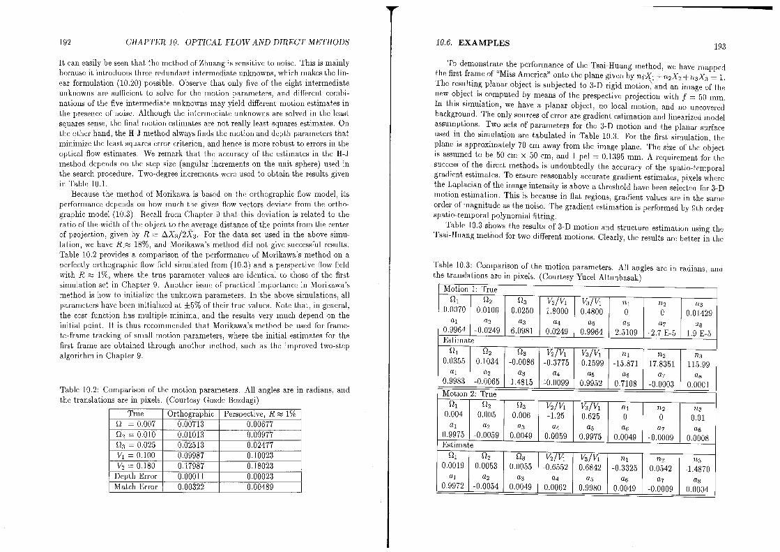

CHAPTER 10. OPTICAL FLOW AND DIRECT METRODS
case of Motion 2. To see how well we can compensate for the motion using theestimated u-parameters, we synthesized the second frame from the first for bothmotions, The resulting mean square displaced frame differences (MS-DFD) werecompared with plain frame differences (MS-FD) (i e no motion compensation). In.,the first case, the MS-DFD was 16.02 compared to MS-FD equal to 19.84. However,in the second cases the MS-DFD has dropped to 0.24 in comparison to MS-FD equalto 4.63, Inspection of the results indicates that the Tsai-Huang method performsbetter when both the frame difference and the u-parameter values are relativelysmall. In fact, this is expected since the method relies on the linearization ofboth the frame difference (the discrete optical Ilow equation) and the pixel-to-pixelmapping in terms of the u-parameters.
10.6.2 Experiments with Two F’rames of Miss America
These methods have also been tested on the same two frames of “Miss America”that were used in Chapter 9, shown in Figure 9.4 (a) and (b). The optical flow fieldbetween these two frames has been estimated by 3-level hierarchical block matching.All algorithms have been applied to those pixels, where the Laplacian of the image
intensity is above a predetermined threshold (T=50) to work with reliable optical
Figure 10.1: The map of pixels selected for 3-D motion estimation marked on thefirst frame of Miss America. (Courtesy Yucel Altunbasak)
10.6. EXAMPLES -\ 195
flow estimates, In order to exclude points which may exhibit nonrigid motion, onlypixels within the white box depicted in Figure 10.1 have been used. Althoughwe expect to have reliable optical flow and/or spatio-temporal gradient estimatesat these pixels, some of these pixels may still fall into regions of local motion oruncovered background, violating the assumption of rigid motion. However) becausewe work with at least 500 pixels, it is expected that the effect of such pixels willbe negligible. The results are compared on the basis of how well we can synthesizethe estimated optical flow field at those pixels shown in Figure 10.1 through theestimated 3-D motion and structure parameters and in some cases how well we cansynthesize the next frame from the first and estimated motion parameters,
We have initialized Morikawa’s algorithm with the 3-D motion estimates ob-tained from the improved algorithm discussed in Chapter 9. The initial depthestimates at all selected points have been computed using the optical flow and theinitial motion parameter values. After 100 iterations, the criterion function hasdropped from 1.94 to 1.04. The value of the criterion function with zero motion es-timation was computed as 6.79. Clearly, Morikawa’s method is suitable to estima,tesmall changes in the motion and depth parameters, provided a good set of initialestimates are available.
Next) the method of Heeger and Jepson (H-J) was used with the same twoframes where the search for the best V was performed with angular increments of1 degree on the unit sphere. The RMSE difference between the optical flow syn-thesized using the parameters estimated by the H-J method and the one estimatedby hierarchical block matching was found to be 0.51, which ranks among the bestresults. Finally, we have applied the direct method of Tsai-Huang on the same setof pixels in the two frames and compare the results with those of the A-matrixmethod where each optical flow vector is used to determine a point correspondence.Table 10.4 tabulates the respective velocity and intensity synthesis errors. The re-sults indicat,e that the A-matrix method is more successful in compensating for themotion.
Table 10.4: Comparison of sythesis errors. (Courtesy Yucel Altunbasak)

196 BIBLIOGRAPHY
10.7 Exercises
1. How do you compare 3-D motion estimation from point correspondences ver-sus that from optical flow? List the assumptions made in each case. Supposewe have 3-D motion with constant acceleration and precession; which methodwould you employ?
2. Which one can be estimated more accurately, token matching or spatio-temporal image intensity gradients?
3. Suppose we assume that the change in Xs (AX,) in the time interval betweenthe two views can be neglected. Can you propose a linear algorithm, similar tothe one in Section 9.3, to estimate the 3-D motion and structure parametersfrom optical flow?
4. Show that (10.31) may also be interpreted as the linearization of the imageintensity function in the vicinity of (21, ~2) in frame le + 1.
Bibliography
[Adi 851 G. Adiv, “Determining three-dimensional motion and structure from op-tical flow generated by several moving objects,” IEEE Trans. Putt. Anal.Mach. Intel., vol. 7, pp. 384-401, July 1985.
[Agg 881 J. K. Aggarwal and N. Nandhakumar, “On the computation of motionfrom sequences of images,” Proc. IEEE, vol. 76, pp. 917935, Aug. 1988.
[Ana 931 P. Anandan, .I. R. Bergen, K. J. Hanna, and R. Hingorani, “Hierarchicalmodel-based motion estimation, ” in Motion Analysis and Image SequenceProcessing, M. I. Sezan and R. L. Lagendijk, eds., Kluwer, 1993.
[Cam 921 M. Campani and A. Verri, “Motion analysis from first-order propertiesof optical flow,” CVGIP: Image Understanding, vol. 56, no. 1, pp. 90-107,Jul. 1992.
[Die 911 N. Diehl, “Object-oriented motion estimation and segmentation in imagesequences,” Signal Processing: Image Comm., vol. 3, pp. 23-56, 1991.
[Hee 921 D. J. Heeger and A. Jepson, “Subspace methods for recovering rigidmotion I: Algorithm and implementation,” Int. J. Comp. Vis., vol. 7,pp. 955117,1992.
[Hei 931 J. Heikkonen, “Recovering 3-D motion from optical flow field,” Image Pro-cessing: Theory and Applications, Vernazza, Venetsanopoulos, and Brac-cini, eds., Elsevier, 1993.
BIBLIOGRAPHY 197
[Ho1 931 R. J. Holt and A. N. Netravali, “Motion from optk flow: Multiplicity ofsolutions,” J. Vis. Comm. Image Rep., vol. 4, no. 1, pp. 14-24, 1993.
[Hor 881 B. K. P. Horn and E. J. Weldon Jr., “Direct methods for recovering mo-tion,” Int. J. Comp. Vision, vol. 2, pp. 51-76, 1988.
[Jai 831 R. Jain, “Direct computation of the focus of expansion,” IEEE Trans. Patt.Anal. Mach. Intel., vol. 5, pp. 58863, Jan. 1983.
[Jer 911 C. P. Jerian and R. Jain, “Structure from motion - A critical analysis ofmethods,” IEEE System, Man and Cyber., vol. 21, pp. 572-588, 1991.
[Kan 861 K. Kanatani, “Structure and motion from optical flow under orthographicprojection,” Comp. Vision Graph. Image Proc., vol. 35, pp. 181-199, 1986.
[Law 831 D. T. Lawton, “Processing translational motion sequences,” Comp. Vis.
Grap. Image Proc., vol. 22, pp. 1166144, 1983.
[Lee 761 D. N. Lee, “A theory of visual control of braking based on informationabout time to collision,” Perception, vol. 5, pp. 4377459, 1976.
[Mor 911 H. Morikawa and H. Harashima, “3D structure extraction coding of imagesequences,” J. Visual Comm. and Image Rep., vol. 2, no. 4, pp. 3322344,Dec. 1991.
[Net 851 A. N. Netravali and J. Salz, “Algorithms for estimation of three-dimensionalmotion,” AT&T Tech. I., vol. 64, no. 2, pp. 335-346, Feb. 1985.
[Tsa 811 R. Y. Tsai and T. S. Huang, “Estimating three-dimensional motion pa-rameters of a rigid planar patch,” IEEE Trans. Acoust. Speech Sign. Proc.,vol. 29, no. 6, pp. 1147-1152, Dec. 1981.
[Ver 891 A. Verri and T. Poggio, “Motion field and optical flow: Qualitativeproperties,” IEEE Trans. Patt. Anal. Mach. Intel., vol. PAMI-11, no. 5,pp. 490-498, May 1989.
[Wax 871 A. M. Waxman, B. Kamgar-Parsi, and M. Subbarao, “Closed-form solu-tions to image flow equations for 3-D structure and motion,” Int. I. Comp.Vision vol. 1, pp. 2399258, 1987.
[Zhu 881 X. Zhuang, T. S. Huang, N. Ahuja, and R. M. Haralick, “A simplifiedlinear optic-flow motion algorithm,” Comp. Vis. Graph. and Image Proc.,vol. 42, pp. 334~344, 1988.

199
Chapter 11
MOTIONSEGMENTATION
Most real image sequences contain multiple moving objects or multiple motions.For example, the Calendar and Train sequence depicted in Chapter 5 exhibits fivedifferent motions, shown in Figure 11.1. Optical flow fields derived from multiplemotions usually display discontinuities (motion edges). Motion segmentation refersto labeling pixels that are associated with each independently moving 3-D objectin a sequence featuring multiple motions. A closely related problem is optical flowsegmentation, which refers to grouping together those optical flow vectors that areassociated with the same 3-D motion and/or structure. These two problems areidentical when we have a dense optical flow field with an optical flow vector forevery pixel.
It should not come as a surprise that motion-based segmentation is an inte-gral part of many image sequence analysis problems, including: i) improved opticalflow estimation, ii) 3-D motion and structure estimation in the presence of multiplemoving objects, and iii) higher-level description of the temporal variations and/orthe content of video imagery. In the first case, the segmentation labels help toidentify optical flow boundaries and occlusion regions where the smoothness con-straint should be turned off. The approach presented in Section 8.3.3 constitutesan example of this strategy. Segmentation is required in the second case, because adistinct parameter set is needed to model the flow vectors associated with each in-dependently moving 3-D object. Recall that in Chapters 9 and 10, we have assumedthat all feature points or flow vectors belong to a single rigid object. Finally, in thethird case, segmentation information may be considered as a high-level (object-level)description of the frame-to-frame motion information as opposed to the low-level(pixel-level) motion information provided by the individual flow vectors.
As with any segmentation problem, proper feature selection facilitates effec-tive motion segmentation. In general, application of standard image segmentation
198
Background++
Calendar
I -+Figure 11.1: Example of optical flow generated by multiple moving objects.
methods (see Appendix B for a brief overview) directly to optical flow data maynot yield meaningful results, since an object moving in 3-D usually generates a spa-tially varying optical flow field. For example, in the case of a single rotating object,there is no flow at the center of the rotation, and the magnitude of the flow vectorsgrows as we move away from the center of rotation. Therefore, in this chapter, aparametric model-based approach has been adopted for motion-based video segmen-tation where the model parameters constitute the features. Examples of parametricmappings that can be used with direct methods include the ¶meter mapping(10.28), and affine mapping (9.4). Recall, from Chapter 9, that the mapping pa-rameters depend on: i) the 3-D motion parameters, the rotation matrix R and thetranslation vector T, and ii) the model of the object surface, such as the orienta-tion of the plane in the case of a piecewise planar model. Since each independentlymoving object and/or different surface structure will best fit a different paramet-ric mapping, parameters of a suitably selected mapping will be used as features todistinguish between different 3-D motions and surface structures.
Direct methods, which utilize spatio-temporal image gradients, are presentedin Section 11.1. These techniques may be considered as extensions of the directmethods discussed in Chapter 10 to the case of multiple motion. In Section 11.2,a two-step procedure is followed, where first the optical flow field is estimated us-ing one of the techniques covered in Chapters 5 through 8. A suitable parametricmotion model has subsequently been used for optical flow segmentation using clus-tering or maximum a posterior-i (MAP) es imation. The accuracy of segmentationt’results clearly depends on the accuracy of the estimated optical flow field. As men-tioned earlier, optical flow estimates are usually not reliable around moving objectboundaries due to occlusion and use of smoothness constraints. Thus, optical flowestimation and segmentation are mutually interrelated, and should be addressedsimultaneously for best results. We present methods for simultaneous optical flowestimation and segmentation using parametric flow models in Section 11.3.
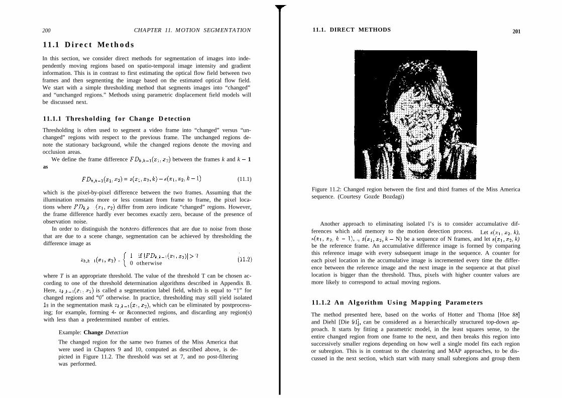
200 CHAPTER 11. MOTION SEGMENTATION 11.1. DIRECT METHODS
11.1 Direct Methods
In this section, we consider direct methods for segmentation of images into inde-pendently moving regions based on spatio-temporal image intensity and gradientinformation. This is in contrast to first estimating the optical flow field between twoframes and then segmenting the image based on the estimated optical flow field.We start with a simple thresholding method that segments images into “changed”and “unchanged regions.” Methods using parametric displacement field models willbe discussed next.
11.1.1 Thresholding for Change Detection
Thresholding is often used to segment a video frame into “changed” versus “un-changed” regions with respect to the previous frame. The unchanged regions de-note the stationary background, while the changed regions denote the moving andocclusion areas.
We define the frame difference FDk,k-i(~i~ ~2) between the frames k and k - 1as
FLI~+~(x~, x2) = 5(x1, xz, k) - 4x1, xz, k - 1) (11.1)
which is the pixel-by-pixel difference between the two frames. Assuming that theillumination remains more or less constant from frame to frame, the pixel loca-tions where FDk,k+i(xi, 2s) differ from zero indicate “changed” regions. However,the frame difference hardly ever becomes exactly zero, because of the presence ofobservation noise.
In order to distinguish the nonzero differences that are due to noise from thosethat are due to a scene change, segmentation can be achieved by thresholding thedifference image as
a+-1(x1, x2) =1 if IF&+-I(xI, x2)1 > T0 otherwise
where T is an appropriate threshold. The value of the threshold T can be chosen ac-cording to one of the threshold determination algorithms described in Appendix B.Here, zk,k-1(x1, ~2) is called a segmentation label field, which is equal to “1” forchanged regions and “0” otherwise. In practice, thresholding may still yield isolatedIs in the segmentation mask .zk,k-1(x1, Q), which can be eliminated by postprocess-ing; for example, forming 4- or &connected regions, and discarding any region(s)with less than a predetermined number of entries.
Example: Change Detection
The changed region for the same two frames of the Miss America thatwere used in Chapters 9 and 10, computed as described above, is de-picted in Figure 11.2. The threshold was set at 7, and no post-filteringwas performed.
201
Figure 11.2: Changed region between the first and third frames of the Miss Americasequence. (Courtesy Gozde Bozdagi)
Another approach to eliminating isolated l’s is to consider accumulative dif-ferences which add memory to the motion detection process.4x1, x2, k - 11, ., s(
Let s(zi, x2, k),xi, ~2, k - N) be a sequence of N frames, and let s(zi) x2, k)
be the reference frame. An accumulative difference image is formed by comparingthis reference image with every subsequent image in the sequence. A counter foreach pixel location in the accumulative image is incremented every time the differ-ence between the reference image and the next image in the sequence at that pixellocation is bigger than the threshold. Thus, pixels with higher counter values aremore likely to correspond to actual moving regions.
11.1.2 An Algorithm Using Mapping Parameters
The method presented here, based on the works of Hotter and Thoma [Hoe 881and Diehl [Die 911, can be considered as a hierarchically structured top-down ap-proach. It starts by fitting a parametric model, in the least squares sense, to theentire changed region from one frame to the next, and then breaks this region intosuccessively smaller regions depending on how well a single model fits each regionor subregion. This is in contrast to the clustering and MAP approaches, to be dis-cussed in the next section, which start with many small subregions and group them
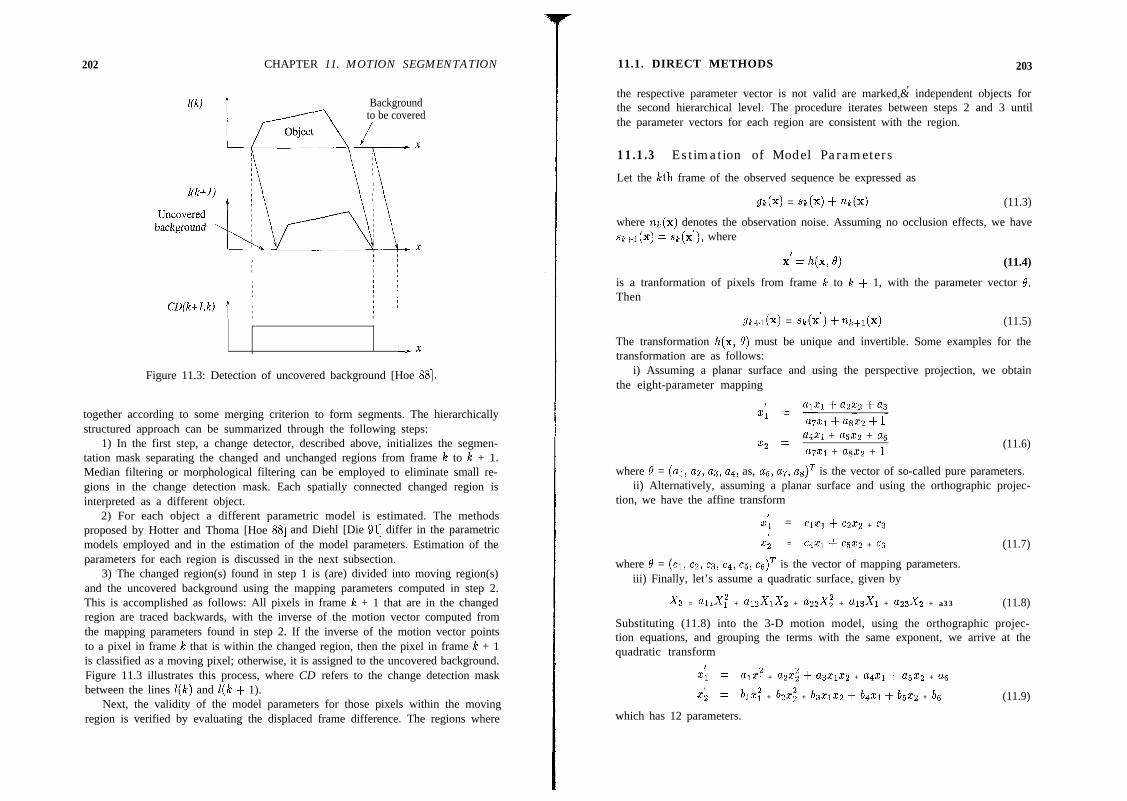
202 CHAPTER 11. MOTION SEGMENTATION
Backgroundto be covered
CD(k+l,k)
‘,X
Figure 11.3: Detection of uncovered background [Hoe 881.
together according to some merging criterion to form segments. The hierarchicallystructured approach can be summarized through the following steps:
1) In the first step, a change detector, described above, initializes the segmen-tation mask separating the changed and unchanged regions from frame Ic to Ic + 1.Median filtering or morphological filtering can be employed to eliminate small re-gions in the change detection mask. Each spatially connected changed region isinterpreted as a different object.
2) For each object a different parametric model is estimated. The methodsproposed by Hotter and Thoma [Hoe 881 and Diehl [Die 911 differ in the parametricmodels employed and in the estimation of the model parameters. Estimation of theparameters for each region is discussed in the next subsection.
3) The changed region(s) found in step 1 is (are) divided into moving region(s)and the uncovered background using the mapping parameters computed in step 2.This is accomplished as follows: All pixels in frame le + 1 that are in the changedregion are traced backwards, with the inverse of the motion vector computed fromthe mapping parameters found in step 2. If the inverse of the motion vector pointsto a pixel in frame iE that is within the changed region, then the pixel in frame Ic + 1is classified as a moving pixel; otherwise, it is assigned to the uncovered background.Figure 11.3 illustrates this process, where CD refers to the change detection maskbetween the lines 2(lc) and b(k + 1).
Next, the validity of the model parameters for those pixels within the movingregion is verified by evaluating the displaced frame difference. The regions where
11.1. DIRECT METHODS 203,
the respective parameter vector is not valid are marked,& independent objects forthe second hierarchical level. The procedure iterates between steps 2 and 3 untilthe parameter vectors for each region are consistent with the region.
11.1.3 Estimation of Model Parameters
Let the leth frame of the observed sequence be expressed as
!a@) = Sk(X) + m(x) (11.3)
where nk(x) denotes the observation noise. Assuming no occlusion effects, we havesk+l(x) = sk(x’), where
x’ = qx, 0) (11.4)
is a tranformation of pixels from frame Ic to $ + 1, with the parameter vector 6’.Then
.9rc+1(x) = Sk(X’) +%+1(x) (11.5)
The transformation h(x, 0) must be unique and invertible. Some examples for thetransformation are as follows:
i) Assuming a planar surface and using the perspective projection, we obtainthe eight-parameter mapping
ai’21 + a822 + 1
04x1 + a50 + asx2 =@xl + a8x2 + 1
(11.6)
where Q = (al) a2, as, ad, as, as, ~7, as)T is the vector of so-called pure parameters.ii) Alternatively, assuming a planar surface and using the orthographic projec-
tion, we have the affine transform/
x1 = Cl”%1 + czxz + c3I
x2 = c421 + c5xZ + c6 (11.7)
where 8 = (cl, ~2, cs, ~4, cg, ~s)~ is the vector of mapping parameters.iii) Finally, let’s assume a quadratic surface, given by
X3 = allX,2 + a&lx2 + w&i + ~13x1 + 43x2 + a33 (11.8)
Substituting (11.8) into the 3-D motion model, using the orthographic projec-tion equations, and grouping the terms with the same exponent, we arrive at thequadratic transform
Ix1 = NIX? + a2.x~ + a32122 + a421 + a5x2 + a6
,22 = 61~: + bzx; + k,xlxz + b4x1+ bm + bs (11.9)
which has 12 parameters.

204 CHAPTER Il. MOTION SEGMENTATION
Note that we may not always be able to determine the actual 3-D motion andsurface structure parameters from the mapping parameters. However, for imagecoding applications this does not pose a serious problem, since we are mainly in-terested in predicting the next frame from the current frame. Furthermore, theapproach presented here is not capable of handling occlusion effects.
The method of Hotter and Thoma uses the eight-parameter model (11.6). Theyestimated the model parameters for each region using a direct method which issimilar to the method of Tsai and Huang [Tsa 811 that was presented in Chapter 10.On the other hand, Diehl [Die 911 suggests using the quadratic transform, becauseit provides a good approximation to many real-life images. He proposed estimatingthe mapping parameters to minimize the error function
m = ;E { ( &+1(x) - Sk(X’, 4) )“}
where E {.} is the expectation operator, and gk(x’, 6) denotes the prediction offrame Ic + 1 from frame I% using the mapping h(x, 0). A gradient-based minimizationalgorithm, the modified Newton’s method, is used to find the best parameter vector4. The contents of the images gk(x) and gk+i(x) must be sufficiently similar inorder for the error function to have a unique minimum.
11.2 Optical Flow Segmentation
In this section, we treat segmentation of a given flow field using parameters ofa flow field model as features. We assume that there are 1%’ independently movingobjects, and each flow vector corresponds to the projection of a 3-D rigid motion ofa single opaque object. Then each distinct motion can be accurately described bya set of mapping parameters. Most common examples of parametric models, suchas eight-parameter mapping (10.19) and affine mapping (10.17), implicitly assumea 3-D planar surface in motion. Approximating the surface of a real object by aunion of a small number of planar patches, the optical flow generated by a realobject can be modeled by a piecewise quadratic flow field, where the parametersai,. , as in (10.19) vary in a piecewise fashion. It follows that flow vectors corre-sponding to the same surface and 3-D motion would have the same set of mappingparameters, and optical flow segmentation can be achieved by assigning the flowvectors with the same mapping parameters into the same class.
The underlying principle of parametric, model-based segmentation methods canbe summarized as follows: Suppose we have K sets of parameter vectors, where eachset defines a correspondence or a flow vector at each pixel. Flow vectors defined bythe mapping parameters are called model-based or synthesized flow vectors. Thus,we have II synthesized flow vectors at each pixel. The segmentation procedure thenassigns the label of the synthesized vector which is closest to the estimated flow vec-tor at each site. However, there is a small problem with this simple scheme: boththe number of classes, K, and the mapping parameters for each class are not known
11.2. OPTICAL FLOW SEGMENTATION 205
a priori. Assuming a particular value for K, the mapping parameters for each classcould be computed in the least squares sense provided that the estimated opticalflow vectors associated with the respective classes are known. That is, we need toknow the mapping parameters to find the segmentation labels and the segmenta-tion labels are needed to find the mapping parameters. This suggests an iterativeprocedure, similar to the I<-means clustering algorithm where both the segmenta-tion labels and the class means are unknown (see Appendix B). The modified Houghtransform approach of Adiv [Adi 851, the modified &means approach of Wang andAdelson [Wan 941, and the MAP method of Murray and Buxton [Mur 871, whichare described in the following, all follow variations of this strategy.
11.2.1 Modified Hough Transform Method
The Hough transform is a well-known clustering technique where the data samples“vote” for the most representative feature values in a quantized feature space. In astraightforward application of the Hough transform method to optical flow segmen-tation using the six-parameter affine flow model (10.17)) the six-dimensional featurespace al). , as would be quantized to certain parameter states after the minimaland maximal values for each parameter are determined. Then, each flow vectorv(x) = [w(x) Q(X)1 T votes for a set of quantized parameters which minimizes
v2(x) - d(x) + d(x) (11.10)
where Q(X) = VI(X) - ai - az~i - ~3x2 and Q(X) = v~(x) - u4 - ~5x1 - ~~6x2.
The parameter sets that receive at least a predetermined amount of votes are likelyto represent candidate motions. The number of classes I< and the correspondingparameter sets to be used in labeling individual flow vectors are hence determined.The drawback of this scheme is the significant amount of computation involved.
In order to keep the computational burden at a reasonable level, Adiv proposeda two-stage algorithm that involves a modified Hough transform procedure. In thefirst stage of his algorithm, connected sets of flow vectors are grouped together toform components which are consistent with a single parameter set. Several simplifi-cations were proposed to ease the computational load, including: i) decompositionof the parameters space into two disjoint subsets {al) ~2, us} x (~4, us, us} to per-form two 3-D Hough transforms, ii) a multiresolution Hough transform, where ateach resolution level the parameter space is quantized around the estimates obtainedat the previous level, and iii) a multipass Hough technique, where the flow vectorswhich are most consistent with the candidate parameters are grouped first. In thesecond stage, those components formed in the first stage which are consistent withthe same quadratic flow model (10.19) in the least squares sense are merged to-gether to form segments. Several merging criteria have been proposed. In the thirdand final stage, ungrouped flow vectors are assimilated into one of their neighboringsegments.
In summary, the modified Hough transform approach is based on first clusteringthe flow vectors into small groups, each of which is consistent with the flow generated
206 CHAPTER 11. MOTION SEGMENTATION
by a moving planar facet. The fusion of these small groups into segments is thenperformed based on some ad-hoc merging criteria.
11.2.2 Segmentation for Layered Video Representation
A similar optical flow segmentation method using the &means clustering techniquehas been employed in the so-called layered video representation strategy. Insteadof trying to capture the motion of multiple overlapping objects in a single motionfield, Wang and Adelson [Wan 941 proposed a layered video representation in whichthe image sequence is decomposed into layers by means of an optical-flow-basedimage segmentation, and ordered in depth along with associated maps defining theirmotions, opacities, and intensities, In the layered representation, the segmentationlabels denote the layer in which a particular pixel resides.
The segmentation method is based on the affine motion model (10.17) and clus-tering in a six-dimensional parameter space. The image is initially divided intosmall blocks. Given an optical flow Geld (e.g.) computed by using (5.12)) a setof affine parameters are estimated for each block. To determine the reliability ofthe parameter estimates, the sum of squared distances between the synthesized andestimated flow vectors is computed as
17” = c II+) - qx)II” (11.11)
where a refers to a block of pixels. Obviously, if the Row within the block complieswith an affine model, the residual will be small. On the other hand, if the blockfalls on the boundary between two distinct motions, the residual will be large.The motion parameters for blocks with acceptably small residuals are selected asthe candidate layer models. To determine the appropriate number Ii of layers,the motion parameters of the candidate layers are clustered in the six-dimensionalparameter space. The initial set of affine model parameters are set equal to themean of the I< clusters. Then the segmentation label of each pixel site is selected asthe index of the parameter set that yields the closest optical flow vector at that site.After all sites are labeled, the affine parameters of each layer are recalculated basedon the new segmentation labels. This procedure is repeated until the segmentationlabels no longer change or a fixed number of iterations is reached.
It should be noted that if the smallest difference between an observed vector andits parameter-based estimate exceeds a threshold, then the site is not labeled in theabove iterative procedure, and the observed flow vector is ignored in the parameterestimation that follows. After the iterative procedure converges to reliable affinemodels, all sites without labels are assigned one according to the motion compen-sation criterion, which assigns the label of the parameter vector that gives the bestmotion compensation at that site. This feature ensures more robust parameter esti-mation by eliminating the outlier vectors. A possible limitation of this segmentationmethod is that it lacks constraints to enforce spatial and temporal continuity of the
11.2. OPTICAL FLOW SEGMENTATION 207
segmentation labels. Thus, rather ad-hoc steps are needed to eliminate small, iso-lated regions in the segmentation label field. The Bayesian segmentation strategypromises to impose continuity constraints in an optimization framework.
11.2.3 Bayesian Segmentation
The Bayesian method searches for the maximum of the a posteriori probability ofthe segmentation labels given the optical flow data, which is a measure of how wellthe current segmentation explains the observed optical flow data and how well itconforms to our prior expectations. Murray and Buxton [Mur 871 first proposeda MAP segmentation method where the optical flow data was modeled by a piece-wise quadratic flow field, and the segmentation field modeled by a Gibbs distri-bution. The search for the labels that maximize the a posteriori probability wasperformed by simulated annealing. Here we briefly present their approach.
Problem Formulation
Let vi, vz, and z denote the lexicographic ordering of the components of the flowvector v(x) = [vi(x) v~(x)]~ and the segmentation labels Z(X) at each pixel. Thea posteriori probability density function (pdf) p(z vi, ~2) of the segmentation label1field z given the optical flow data vi and vz can be expressed, using the Bayestheorem, as
P(ZlVl,VZ) =P(Vl> VZIZMZ)
P(W) vz)(11.12)
where p(vr ) valz) is the conditional pdf of the optical flow data given the segmen-tation z, and p(z) is the a priori pdf of the segmentation. Observe that, i) z isa discrete-valued random vector with a finite sample space a, and ii) p(vi, ~2) isconstant with respect to the segmentation labels, and hence can be ignored for thepurposes of segmentation. The MAP estimate, then, maximizes the numerator of(11.12) over all possible realizations of the segmentation field z = w, w E s1.
The conditional probability p(vi, v2 Iz) is a measure of how well the piecewisequadratic flow model (10.19), where the model parameters al,. , us depend on thesegmentation label z, fits the estimated optical flow field vi and ~2. Assuming thatthe mismatch between the observed flow v(x) and the synthesized flow,
i&(x) = ~1x1 +a2x2 -a3+a7xf +asxlxz
t&(x) = a4xl+ a522 - a6 + a7xlzZ+ usxi (11.13)
is modeled by white, Gaussian noise with zero mean and variance u2, the conditionalpdf of the optical flow field given the segmentation labels can be expressed as
$1, v&5) = (2sg~)M,” exp { - 5$(xi)i2u2}i=l (11.14)
208 CHAPTER 11. MOTION SEGMENTATION
where M is the number of flow vectors available at the sites xi, and
$(Xi) = (%(Xi) - G(xi))2 + (w(3) - qxi))2 (11.15)
is the norm-squared deviation of the actual flow vectors from what is predicted bythe quadratic flow model. Assuming that the quadratic flow model is more or lessaccurate, this deviation is due to segmentation errors and the observation noise.
The prior pdf is modeled by a Gibbs distribution which effectively introduceslocal constraints on the interpretation (segmentation). It is given by
p(z) = $ C exp {-U(z)} S(z -U)wEn
where R denotes the discrete sample space of z, Q is the partition function
Q = c ew-U(w))WErl(11.17)
and U(w) is the potential function which can be expressed as a sum of local cliquepotentials V~(Z(X;), z(xj)). The prior constraints on the structure of the segmenta-tion labels can be specified in terms of local clique potential functions as discussedin Chapter 8. For example, a local smoothness constraint on the segmentation la-bels can be imposed by choosing V~(Z(X~), z(xj)) as in Equation (8.11). Temporalcontinuity of the labels can similarly be modeled [Mur 871.
Substituting (11.14) and (11.16) into the criterion (11.12) and taking the log-arithm of the resulting expression, maximization of the a posteriori probabilitydistribution can be performed by minimizing the cost function
(11.18)
The first term describes how well the predicted data fit the actual optical flowmeasurements (in fact, optical flow is estimated from the image sequence at hand),and the second term measures how much the segmentation conforms to our priorexpectations.
The Algorithm
Because the model parameters corresponding to each label are not known a priori,the MAP segmentation alternates between estimation of the model parameters andassignment of the segmentation labels to optimize the cost function (11.18) basedon a simulated annealing (SA) procedure. Given the flow field v and the number ofindependent motions I(, MAP segmentation via the Metropolis algorithm can besummarized as follows:
\ -
11.3. SIMULTANEOUS ESTIMATION AND SEGMENTATION 209
1. Start with an initial labeling z of the optical flow vectors. Calculate themapping parameters a = [ai cr$ for each region using least squaresfitting as in Section 10.3.2. Set the initial temperature for SA.
2. Scan the pixel sites according to a predefined convention. At each site xi:
(a) Perturb the label zi = randomly.(b) Decide whether to accept or reject this perturbation, as described in
Section 8.1.1, based on the change AE in the cost function (11.18),
AE = &A?(4 + c Ak(+i), z(y)) (11.19)x, EM,*
where A&, denotes a neighborhood of the site xi and Vc(z(xi), z(xj)) isgiven by Equation (8.11). The first term indicates whether or not theperturbed label is more consistent with the given flow field determinedby the residual (11.15), and the second term reflects whether or not it isin agreement with the prior segmentation field model.
3. After all pixel sites are visited once, re-estimate the mapping parameters foreach region in the least squares sense based on the new segmentation labelconfiguration.
4. Exit if a stopping criterion is satisfied. Otherwise, lower the temperatureaccording to the temperature schedule, and go to step 2.
The following observations about the MAP segmentation algorithm are in order:i) The procedure proposed by Murray-Buxton suggests performing step 3, the modelparameter update, after each and every perturbation. Because such a procedure willbe computationally more demanding, the parameter updates are performed only af-ter all sites have been visited once.ii) This algorithm can be applied to any parametric model relating to optical flow,although the original formulation has been developed on the basis of vernier veloc-ities [Mur 871 and the associated eight-parameter model.iii) The actual 3-D motion and depth parameters are not needed for segmentationpurposes. If desired, they can be recovered from the parameter vector a for eachsegmented flow region at convergence.
We conclude this section by noting that all methods discussed so far are limitedby the accuracy of the available optical flow estimates. Next, we introduce a novelframework, in which optical flow estimation and segmentation interact in a mutuallybeneficial manner.
11.3 Simultaneous Estimation and Segmentation
By now, it should be clear that the success of optical flow segmentation is closelyrelated to the accuracy of the estimated optical flow field, and vice versa. It follows
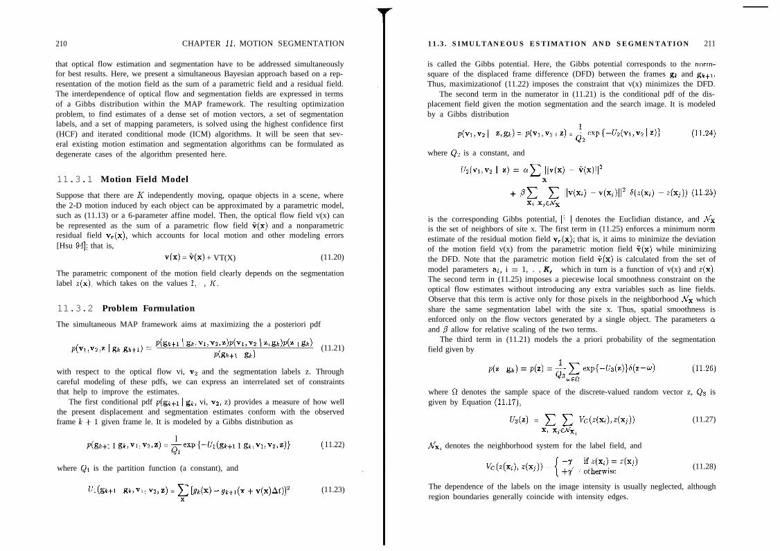
210 CHAPTER 11. MOTION SEGMENTATION
that optical flow estimation and segmentation have to be addressed simultaneouslyfor best results. Here, we present a simultaneous Bayesian approach based on a rep-resentation of the motion field as the sum of a parametric field and a residual field.The interdependence of optical flow and segmentation fields are expressed in termsof a Gibbs distribution within the MAP framework. The resulting optimizationproblem, to find estimates of a dense set of motion vectors, a set of segmentationlabels, and a set of mapping parameters, is solved using the highest confidence first(HCF) and iterated conditional mode (ICM) algorithms. It will be seen that sev-eral existing motion estimation and segmentation algorithms can be formulated asdegenerate cases of the algorithm presented here.
11.3.1 Motion Field Model
Suppose that there are K independently moving, opaque objects in a scene, wherethe 2-D motion induced by each object can be approximated by a parametric model,such as (11.13) or a 6-parameter affine model. Then, the optical flow field v(x) canbe represented as the sum of a parametric flow field c(x) and a nonparametricresidual field vr(x), which accounts for local motion and other modeling errors[Hsu 941; that is,
v(x) = C(x) + VT(X) (11.20)
The parametric component of the motion field clearly depends on the segmentationlabel Z(X)) which takes on the values 1,. , K.
11.3.2 Problem Formulation
The simultaneous MAP framework aims at maximizing the a posteriori pdf
p(vl v2 z Igk gk+l) = Pbt1 l&~%v2~zMvl,vz lz,gtMz 1%)> 1 ,
P(!wl I&)(11.21)
with respect to the optical flow vi, vs and the segmentation labels z. Throughcareful modeling of these pdfs, we can express an interrelated set of constraintsthat help to improve the estimates.
The first conditional pdf p(gk+i 1 gk, vi, vs, z) provides a measure of how wellthe present displacement and segmentation estimates conform with the observedframe I% + 1 given frame le. It is modeled by a Gibbs distribution as
dgktl I gk,vl,vz,z) = &expl-Ul(gktl I gk,vl,w,z)l (
where Qi is the partition function (a constant), and
11.22)
UlkWl 1 gk>vl, vz, z) = c [gk(x) - grc+l(x + v(x)At)]’ (11.23)X
11.3. SIMULTANEOUS ESTIMATION AND SEGMENTATION 211
is called the Gibbs potential. Here, the Gibbs potential corresponds to the norm-square of the displaced frame difference (DFD) between the frames gk and gk+r.Thus, maximizationof (11.22) imposes the constraint that v(x) minimizes the DFD.
The second term in the numerator in (11.21) is the conditional pdf of the dis-placement field given the motion segmentation and the search image. It is modeledby a Gibbs distribution
p(vl,v2 1 z,gk)=p(h,v2 I z) = ~expl--l:a(v1~~2 Iz)l
where Qs is a constant, and
Vz(v1,vz I z) = ac lIv(x) - qx)ll”
+ PC xC Ii+4 -v(xj)ii2 q+) -4~~)) p.25)x, X,E&
is the corresponding Gibbs potential, ]I I[ denotes the Euclidian distance, and A’xis the set of neighbors of site x. The first term in (11.25) enforces a minimum normestimate of the residual motion field v?(x); that is, it aims to minimize the deviationof the motion field v(x) from the parametric motion field c(x) while minimizingthe DFD. Note that the parametric motion field c(x) is calculated from the set ofmodel parameters ai, i = 1, . , K, which in turn is a function of v(x) and Z(X).The second term in (11.25) imposes a piecewise local smoothness constraint on theoptical flow estimates without introducing any extra variables such as line fields.Observe that this term is active only for those pixels in the neighborhood Nx whichshare the same segmentation label with the site x. Thus, spatial smoothness isenforced only on the flow vectors generated by a single object. The parameters cyand /3 allow for relative scaling of the two terms.
The third term in (11.21) models the a priori probability of the segmentationfield given by
P(Z I gk) = P(Z) = $ C exp{--U3(z)P(z - u)
wa
where fi denotes the sample space of the discrete-valued random vector z, Qs isgiven by Equation (11.17),
U3(z) = c c k(eG),4xj)) (11.27)xt X,EJux;
&, denotes the neighborhood system for the label field, and
V&Xi), Z(Xj)) = { +> ‘; ft;fWs; dxj) (11.28)
The dependence of the labels on the image intensity is usually neglected, althoughregion boundaries generally coincide with intensity edges.

212 CHAPTER 11. MOTION SEGMENTATION
11.3.3 The Algorithm
Maximizing the a posteriori pdf (11.21)1s equivalent to minimizing the cost function,
E = Ul(grct1 I .tia>v1,vz,z) + Wvl,vz I z) + Us(z) (11.29)
that is composed of the potential functions in Equations (11.22), (11.24),and (11.26). Direct minimization of (11.29) with respect to all unknowns is anexceedingly difficult problem, because the motion and segmentation fields consti-tute a large set of unknowns. To this effect, we perform the minimization of (11.29)through the following two-steps iterations [Cha 941:
1. Given the best available estimates of the parameters ai, i = 1,. , I<, and z,update the optical flow field ~1, v2. This step involves the minimization of amodified cost function
El = ~[slc(x) - glc+l(x+v(x)At)]2 + ax IIv(x)- V(x)II"
+;c c IlV(%) - V(Xj)lj” 6(3(x:) - Z(Xj)) (11.30)x, X,ENx
which is composed of all the terms in (11.29) that contain v(x). While the firstterm indicates how well v(x) explains our observations, the second and third termsimpose prior constraints on the motion estimates that they should conform with theparametric flow model, and that they should vary smoothly within each region. Tominimize this energy function, we employ the HCF method recently proposed byChou and Brown [Cho 901. HCF is a deterministic method designed to efficientlyhandle the optimization of multivariable problems with neighborhood interactions.
2. Update the segmentation field z, assuming that, the optical flow field v(x) isknown. This step involves the minimization of all the terms in (11.29) which containz as well as G(x), given by
Ez = a~~~v(x)-~(x~~"~~ c k(+i),+q)) (11.31)X ‘x, x,cNx,
The first term in (11.31) quantifies the consistency of c(x) and v(x). The secondterm is related to the a priori probability of the present configuration of the seg-mentation labels. We use an ICM procedure to optimize Ez [Cha 931. The mappingparameters ai are updated by least squares estimation within each region.
An initial estimate of the optical flow field can be found using the Bayesian ap-proach with a global smoothness constraint. Given this estimate, the segmentationlabels can be initialized by a procedure similar to Wang and Adelson’s [Wan 941.The determination of the free parameters a, p, and y is a design problem. Onestrategy is to choose them to provide a dynamic range correction so that each term
11.3. SIMULTANEOUS ESTIMATION AND SEGMENTATION 21 3
InitializationLevel = L
Level = Level- 1
$Segmentation
No
Figure 11.4: The block diagram of the simultaneous MAP algorithm
in the cost function (11.29) has equal emphasis. However, because the optimiza-tion is implemented in two steps, the ratio a/y also becomes of consequence. Werecommend to select 1 5 cy/y 5 5, depending on how well the motion field canbe represented by a piecewise-parametric model and whether we have a sufficientnumber of classes.
A hierarchical implementation of this algorithm is also possible by forming suc-cessive low-pass filtered versions of the images gk and gk+l. Thus, the quantities~1, ~2, and z can be estimated at different resolutions. The results of each hierarchyare used to initialize the next lower level. A block diagram of the hierarchical algo-rithm is depicted in Figure 11.4. Note that the Gibbsian model for the segmentationlabels has been extended to include neighbors in scale by Kato et al. [k-at 931.
11.3.4 Relationship to Other Algorithms
It is important to recognize that this simultaneous estimation and segmentationframework not only enables 3-D motion and structure estimation in the presenceof multiple moving objects, but also provides improved optical flow estimates. Sev-eral existing motion analysis algorithms can be formulated as special cases of thisframework. If we retain only the first and the third terms in (11.29), and assumethat all sites possess the same segmentation label, then we have Bayesian motionestimation with a global smoothness constraint. The motion estimation algorithmproposed by Iu [Iu 931 utilizes the same two terms, but replaces the S(.) functionby a local outlier rejection function (Section 8.3.2).
The motion estimation and region labeling algorithm proposed by Stiller [Sti 941(Section 8.3.3) involves all terms in (11.29), except the first term in (11.25). Fur-

214 CHAPTER 11. MOTION SEGMENTATION
thermore, the segmentation labels in Stiller’s algorithm are used merely as tokensto allow for a piecewise smoothness constraint on the flow field, and do not attemptto enforce consistency of the flow vectors with a parametric component. We alsonote that the motion estimation algorithms of Konrad and Dubois [Kon 92, Dub 931and Heitz and Bouthemy [Hei 931 w ic use line fields are fundamentally differenth’ hin that they model discontinuities in the motion field, rather than modeling regionsthat correspond to different physical motions (Section 8.3.1).
On the other hand, the motion segmentation algorithm of Murray and Buxton[Mm- 871 (Section 11.2.2) employs only the second term in (11.25) and third termin (11.29) to model the conditional and prior pdf, respectively. Wang and Adelson[Wan 941 relies on the first term in (11.25) to compute the motion segmentation(Section 11.2.3). However, they also take the DFD of the parametric motion vectorsinto consideration when the closest match between the estimated and parametricmotion vectors, represented by the second term, exceeds a threshold.
11.4 Examples
Examples are provided for optical flow segmentation using the Wang-Adelson (W-A)and Murray-Buxton (M-B) methods, as well as for simultaneous motion estimationand segmentation using the proposed MAP algorithm with the same two framesof the Mobile and Calendar sequence shown in Figure 5.9 (a) and (b). This isa challenging sequence, since there are several objects with distinct motions asdepicted in Figure 11.1.
The W-A and M-B algorithms use the optical flow estimated by the Horn-Schunck algorithm, shown in Figure 5.11 (b), as input. We have set the numberof regions to four. In order to find the representative affine motion parametersin the W-A algorithm, 8 x 8 and 16 x 16 seed blocks have been selected, andthe affine parameters estimated for each of these blocks are clustered using theK-means algorithm. It is important that the size of the blocks be large enoughto identify rotational motion. The result of the W-A segmentation is depicted inFigure 11.5 (a). We have initialized the M-B algorithm with the result of the W-Aalgorithm, and set the initial temperature equal to 1. The resulting segmentationafter 50 iterations is shown in Figure 11.5 (b). Observe that the M-B algorithmeliminates small isolated regions on the calendar, and grows the region representingthe rotating ball in the right direction by virtue of the probabilistic smoothnessconstraint that it employs.
Next, we initialized the simultaneous MAP estimation and segmentationmethod, also by the result of the W-A algorithm. We have set o! = p = 10 ando/y = 5, since the motion field can be well-represented by a piecewise paramet-ric model. The estimated optical flow and segmentation label fields are shown inFigure 11.6 (a) and (b), respectively. Note that the depicted motion field corre-sponds to the lower right portion of the segmentation field. The results show someimprovement over the M-B method.
11.4. EXAMPLES 215
Figure 11.5: The segmentation field obtained by the a) Wang-Adelson method andb) Murray-Buxton method. (Courtesy Michael Chang)

216 CHAPTER 11. MOTION SEGMENTATION
Figure 11.6: a) The optical flow field and b) segmentation field estimated by thesimultaneous MAP method after 100 iterations. (Courtesy Michael Chang)
11.5. EXERCISES 217
11.5 Exercises
1. Show that the MAP segmentation reduces to the I(-means algorithm if weassume the conditional pdf is Gaussian and no a priori information is available.
2. How would you apply the optimum threshold selection method discussed inAppendix B.l.l to change detection?
3. How would you modify (11.15) considering that (~1, uz) is the measured nor-mal flow rather than the projected flow?
4. Do you prefer to model the flow discontinuities through a segmentation fieldor through line fields? Why?
5. Verify the relationships claimed in Section 11.3.3
6. Discuss how to choose the scale factors 01, X, y, and $ in (11.30) and (11.31).
Bibliography
[Adi 851 G. Adiv, “Determining three-dimensional motion and structure from opti-cal flow generated by several moving objects,” IZEE Trans. Pattern Anal.Mach. Intell., vol. 7, pp. 384-401, 1985.
[Ber 921 J. R. Bergen, P. J. Burt, R. Hingorani, and S. Peleg, “A three-frame al-gorithm for estimating two-component image motion,” IEEE Trans. Putt.Anal. Mach. Intel., vol. 14, pp. 8866896, Sep. 1992.
[Cha 931 M. M. Chang, A. M. Tekalp, and M. I. Sezan, “Motion field segmentationusing an adaptive MAP criterion,” Proc. Int. Conf. ASSP, Minneapolis,MN, April 1993.
[Cha 941 M. M. Chang, M. I. Sezan, and A. M. Tekalp, “An algorithm for simulta-neous motion estimation and scene segmentation,” Proc. Int. Conf. ASSP,Adelaide, Australia, April 1994.
[Cho 901 P. B. Chou and C. M. Brown, “The theory and practice of Bayesian imagelabeling,” Int. J. Comp. Vision, vol. 4, pp. 1855210, 1990.
[Die 911 N. Diehl, “Object-oriented motion estimation and segmentation in imagesequences,” Signal Processing: Image Comm., vol. 3, pp. 23-56, 1991.
[Dub 931 E. Dubois and J. Konrad, “Estimation of 2-D motion fields from imagesequences with application to motion-compensated processing,” in MotionAnalysis and Image Sequence Processing, M. I. Sezan and R. L. Lagendijk,eds., Norwell, MA: Kluwer, 1993.
218 BIBLIOGRAPHY
[Hoe 881 M. Hoetter and R. Thoma, “Image segmentation based on object orientedmapping parameter estimation,” Signal Pm., vol. 15, pp. 315-334, 1988.
[Hsu 941 S. Hsu, P. Anandan, and S. Peleg, “Accurate computation of optical flowby using layered motion representations,” Proc. Id Conf. Pat2. Recog.,Jerusalem, Israel, pp. 743-746, Oct. 1994.
[Ill 931 S . -L . I u , “Robust estimation of motion vector fields with disconti-nuity and occlusion using local outliers rejection,” SPIE, vol. 2094,pp. 588-599, 1993.
[Kat 931 Z. Kato, M. Berthod, and J. Zerubia, “Parallel image classification us-ing multiscale Markov random fields,” Proc. IEEE Id. Conf. ASSP,Minneapolis, MN, pp. V137-140, April 1993.
[Mur 871 D. W. Murray and B. F. Buxton, “Scene segmentation from visual motionusing global optimization,” IEEE Trans. Pall. Anal. Mach. Intel., vol. 9,no. 2, pp. 220-228, Mar. 1987.
[Sti 931 C. Stiller, “A statistical image model for motion estimation,” Proc. Int.Conf. ASSP, Minneapolis, MN, pp. V193%196, April 1993.
[Sti 941 C. Stiller, “Object-oriented video coding employing dense motion fields,”Proc. Id. Conf. ASSP, Adelaide, Australia, April 1994.
[Tho 801 W. B. Thompson, “Combining motion and contrast for segmentation,”IEEE Trans. Pattern Anal. Mach. Idel., vol. 2, pp. 543-549, 1980.
[Wan 941 J. Y. A. Wang and E. Adelson, “Representing moving images withlayers,” IEEE Trans. on Image Proc., vol. 3, pp. 625-638, Sep. 1994.
[Wu 931 S. F. Wu and J. Kittler, “A gradient-based method for general motionestimation and segmentation,” J. Vis. Comm. Image Rep., vol. 4, no. 1,pp. 25-38, Mar. 1993.
Chapter 12
STEREO ANDMOTION TRACKING
Because 3-D motion and structure estimation from two monocular views has beenfound to be highly noise-sensitive, this chapter presents two new approaches, stereoimaging and motion tracking, that offer more robust estimates. They are discussedin Sections 12.1 and 12.2, respectively. In stereo imaging, we acquire a pair of rightand left images, at each instant. More robust motion and structure estimation fromtwo stereo pairs is possible, because structure parameters can be estimated usingstereo triangulation, hence decoupling 3-D motion and structure estimation. More-over, the mutual relationship between stereo disparity and 3-D motion parameterscan be utilized for stereo-motion fusion, thereby improving the accuracy of bothstereo disparity and 3-D motion estimation. In motion tracking, it is assumed thata long sequence of monocular or stereo video is available. In this case, more robustestimation is achieved by assuming a temporal dynamics; that is, a model describ-ing the temporal evolution of the motion. Motion between any pair of frames isexpected to obey this model. Then batch or recursive filtering techniques can beemployed to track the 3-D motion parameters in time. At present, stereo-motionfusion and motion tracking using Kalman filtering are active research topics of sig-nificant interest.
12.1 Motion and Structure from Stereo
It is well known that 3-D motion and structure estimation from monocular videois an ill-posed problem, especially when the object is relatively far away from thecamera. Several researchers have employed stereo sequences for robust 3-D motionand structure estimation [Dho 89, Hua 941. Stereo imaging also alleviates the scaleambiguity (between depth and translation) inherent in monocular imaging, sincea properly registered stereo pair contains information about the scene structure.
219
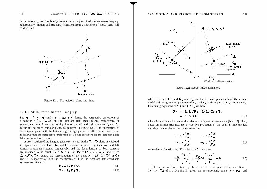
220 CHAPTER12. STEREO ANDMOTION TRACKING
In the following, we first briefly present the principles of still-frame stereo imaging.Subsequently, motion and structure estimation from a sequence of stereo pairs willbe discussed.
Epipolar plane
Figure 12.1: The epipolar plane and lines.
12.1.1 Still-Frame Stereo Imaging
Let pi = (zr~, 22~) and pn = (z~R, Z~R) denote the perspective projections ofa point P = (X1,X2, Xs) onto the left and right image planes, respectively. Ingeneral, the point P and the focal points of the left and right cameras, fL and fR,define the so-called epipolar plane, as depicted in Figure 12.1. The intersection ofthe epipolar plane with the left and right image planes is called the epipolar lines.It follows that the perspective projection of a point anywhere on the epipolar planefalls on the epipolar lines.
A cross-section of the imaging geometry, as seen in the X1 -Xs plane, is depictedin Figure 12.2. Here, Cw, CR, and CL denote the world, right camera, and leftcamera coordinate systems, respectively, and the focal lengths of both camerasare assumed to be equal, fR = f~ = f. Let PR = (X~R,X~R,X~R) and PL =(X~L,X~L,X~L) denote the representation of the point P = (Xl,Xz,X3) in CRand CL, respectively. Then the coordinates of P in the right and left coordinatesystems are given by
PR=RRP+TR (12.1)
PL=RLP+TL (12.2)
12.1. MOTION AND STRUCTURE FROM STEREO
system
map cw' xl
World coordinate system
221
Figure 12.2: Stereo image formation.
where RR and TR, and Rr, and Tr, are the extrinsic parameters of the cameramodel indicating relative positions of CR and CL with respect to Cw) respectively.Combining equations (12.1) and (12.2), we have
PL = RLR,~PR - RLR,~TR + TL+ MPR+B (12.3)
where M and B are known as the relative configuration parameters [Wen 921. Then,based on similar triangles, the perspective projection of the point P into the leftand right image planes. can be expressed as
XlLXlL = f-,
XZL
X3LX2L = f-
X3L
XlRXlR = f ->
X2R
X3Rx2R = f-
X3R
respectively. Substituting (12.4) into (12.3), we have
(12.4)
(12.5)
The structure from stereo problem refers to estimating the coordinates(X1,X2, X3) of a 3-D point P, given the corresponding points (xr~, x2~) and
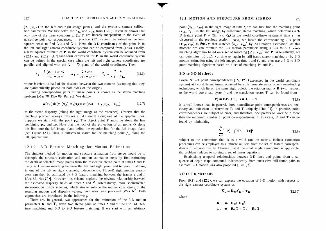
222 CHAPTER 12. STEREO AND MOTION TRACKING
(Z~R,ZZR) in the left and right image planes, and the extrinsic camera calibra-tion parameters. We first solve for X~L and X~R from (12.5). It can be shown thatonly two of the three equations in (12.5) are linearly independent in the event ofnoise-free point correspondences. In practice, (12.5) should be solved in the leastsquares sense to find X~L and X~R. Next, the 3-D coordinates of the point P inthe left and right camera coordinate systems can be computed from (12.4). Finally,a least squares estimate of P in the world coordinate system can be obtained from(12.1) and (12.2). A 1c osed-form expression for P in the world coordinate systemcan be written in the special case when the left and right camera coordinates areparallel and aligned with the Xi - Xz plane of the world coordinates. Then
x1= b (zIL+ZlR) 2 b XZL 2.fb
XlL -ZlR 'X2 =
XlL - ZlR’x3 = (12.6)
XlL - XlR
where b refers to half of the distance between the two cameras (assuming that theyare symmetrically placed on both sides of the origin).
Finding corresponding pairs of image points is known as the stereo matchingproblem [Mar 78, Dho 89, Bar 931. We define
+R)- (wl(xR),%(xR))=(xlR - ZlL,ZZR- XZL) (12.7)
as the stereo disparity (taking the right image as the reference). Observe that thematching problem always involves a 1-D search along one of the epipolar lines.Suppose we start with the point pi. The object point P must lie along the linecombining pR and fR. Note that the loci of the projection of all points Q alongthis line onto the left image plane define the epipolar line for the left image plane(see Figure 12.1). Thus, it suffices to search for the matching point pi along theleft epipolar line.
12.1.2 3-D Feature Matching for Motion Estimation
The simplest method for motion and structure estimation from stereo would be todecouple the structure estimation and motion estimation steps by first estimatingthe depth at selected image points from the respective stereo pairs at times t and t’using 2-D feature matching between the left and right pairs, and temporal matchingin one of the left or right channels, independently. Three-D rigid motion param-eters can then be estimated by 3-D feature matching between the frames t and t’[Aru 87, Hua 89c]. However, this scheme neglects the obvious relationship betweenthe estimated disparity fields at times t and t’. Alternatively, more sophisticatedstereo-motion fusion schemes, which aim to enforce the mutual consistency of theresulting motion and disparity values, have also been proposed [Wax 861. Bothapproaches are introduced in the following.
There are, in general, two approaches for the estimation of the 3-D motionparameters R and T, given two stereo pairs at times t and t’: 3-D to 3-D fea-ture matching and 3-D to 2-D feature matching. If we start with an arbitrary
12.1. MOTION AND STRUCTURE FROM STEREO 223
point (ZiR, 22~) in the right image at time t, we can first find the matching point(zip, zs~) in the left image by still-frame stereo matching, which determines a 3-D feature point P = (Xi, X2, Xs) in the world coordinate system at time t, asdiscussed in the previous section. Next, we locate the corresponding 2-D point(ziR,xkR) at time t’ that matches (X1& CzR) by 2-D motion estimation. At thismoment, we can estimate the 3-D motion parameters using a 3-D to 2-D point-matching algorithm based on a set of matching (ziR, g’ZR) and P. Alternatively, wecan determine (z&, xiL) at time t’ again by still-frame stereo matching or by 2-Dmotion estimation using the left images at time t and t’, and then use a 3-D to 3-Dpoint-matching algorithm based on a set of matching P’ and P.
3-D to 3-D Methods
Given N 3-D point correspondences (Pi, Pi) (expressed in the world coordinatesystem) at two different times, obtained by still-frame stereo or other range-findingtechniques, which lie on the same rigid object; the rotation matrix R (with respectto the world coordinate system) and the translation vector T can be found from
P;=RPi+T, i=l,...,N (12.8)
It is well known that, in general, three noncollinear point correspondences are nec-essary and sufficient to determine R and T uniquely [Hua 941. In practice, pointcorrespondences are subject to error, and therefore, one prefers to work with morethan the minimum number of point correspondences. In this case, R and T can befound by minimizing
2 ,,P: - (RPi + T)ll”i=l
(12.9)
subject to the constraints that R is a valid rotation matrix. Robust estimationprocedures can be employed to eliminate outliers from the set of feature correspon-dences to improve results. Observe that if the small angle assumption is applicable,the problem reduces to solving a set of linear equations.
Establishing temporal relationships between 3-D lines and points from a se-quence of depth maps computed independently from successive still-frame pairs toestimate 3-D motion was also proposed [Kim 871.
3-D to 2-D Methods
From (9.1) and (12.1), we can express the equation of 3-D motion with respect tothe right camera coordinate system as
XL = RRXR + TR (12.10)where
RR = RRRR$
TR = RRT + TR - RRTR

224 CHAPTER 12. STEREO AND MOTION TRACKINGI
12.1. MOTION AND STRUCTURE FROM STEREO
denote the rotation matrix and the translation vector, respectively, with respect tothe right camera coordinate system. Then, substituting (12.10) into (12.4), we havea computed correspondence in the right image given by
-/xlR = .Fg and
X’ZiR II f-2XAR
(12.11)
Given N 3-D to 2-D point correspondence measurements, (PER, p&), wherePR = (X~R~X~R,X~R) refers to a 3-D point with respect to the right cameracoordinate system at time t, and p ;1 = (xiR1 xiR) denotes the corresponding rightimage point at time t’; we can estimate k, and +R by minimizing
(12.12)
where pi, refers to the corresponding image point computed by (12.11) as a functionof kR and !I?,. The minimization of (12.12) can be posed as a nonlinear leastsquares problem in the six unknown 3-D motion parameters. Once again, a linearformulation is possible if the small angle of rotation approximation is applicable.Assuming that the extrinsic parameters of the camera system RR and TR areknown, the rotation and translation parameters R and T in the world coordinatescan be easily recovered from RR and TR based on (12.10).
The difficulty with both 3-D to 3-D and 2-D to 3-D approaches is in the process ofestablishing the matching 3-D and/or 2-D features. Stereo disparity estimation andestimation of feature correspondences in the temporal direction are, individually,both ill-posed problems, complicated by the aperture and occlusion problems; hence,the motivation to treat these problems simultaneously.
12.1.3 Stereo-Motion Fusion
Theoretically, in a time-varying stereo pair, the stereo matching need be performedonly for the initial pair of frames. For subsequent pairs, stereo correspondences canbe predicted by means of the left and right optical flow vectors. Stereo matchingwould only be required for those features that newly enter the field of view. How-ever, because both optical flow estimation and disparity estimation are individuallyill-posed problems, several studies have recently been devoted to fusion of stereodisparity and 3-D motion estimation in a mutually beneficial way. Stereo-motionfusion methods impose the constraint that the loop formed by the disparity andmotion correspondence estimates, in Figure 12.3, must be a closed loop. Richards[Ric 851 and Waxman et al. [Wax 861 derived an analytical expression for the tem-poral rate of change of the disparity to disparity ratio as a function of the 3-D motionand structure parameters. They then proposed a simultaneous stereo and motionestimation method based on this relation. Aloimonos et al. [Alo 901 proposed an al-gebraic solution which requires no point-to-point correspondence estimation for the
225
@lC d2LJMotion
‘dlR’ $R ’Motion
1 1 c IDiSP~itY / I / Timeta
I I I I
Left Right
Figure 12.3: Stereo-motion fusion.
special case of 3-D planar objects. Methods to integrate stereo matching and opti-cal flow estimation using multiresolution edge matching and dynamic programming[Liu 931 and constrained optimization [Tam 911 have also been proposed.
In the following, we first develop a maximum a posteriori probability (MAP)estimation framework (see Chapter 8) for stereo-motion fusion, based on densedisplacement and disparity field models, in the case of a single rigid object in motion.Note that stereo-motion fusion with a set of isolated feature points (instead of densefields) can be posed as a maximum-likelihood problem, which is a special case ofthis MAP framework. The MAP framework is extended to the case of multiplemoving objects in the next section.
Dense Fields: Let dR(xR) = (dry, dzR(x~)) and dL(xL) = (dl~(x~), &,(x~))denote the 2-D displacement fields computed at each pixel XR = (ZrR,ZzR) andXL = (zr~, QL) of the right and left images, respectively, and w(x~) denote thedisparity field at each pixel XR of the right image. Let dlR, dzfi, dlL, d2L, WI;and wz denote vectors formed by lexicographic ordering of the scalars dirtdSR(XR), &L(xL), ~ZL(xL), wl(xR), and wz(xR) at all pixels, respectively. Wewish to estimate dlR, d2R, dlL, d2L, WI, and wz, given IL, In, I/L, I&, the leftand right images at times t and t’, respectively, in order to maximize the joint aposteriori probability density function (pdf)
p(dm, dm, ch, dx, WI, w211;, I&, IL, IR) a
P(I~,Ik,ILldlR,dzR,dl~,d2~,Wl,W2,IR)
P(dm, &R, da &LIwl, Wz, IR)l+‘l, W21IR) (12.13)
where p(Ii, IL, ILldlR, d2R, dlL, d2L, ~1, ~2, IR) provides a measure of how well
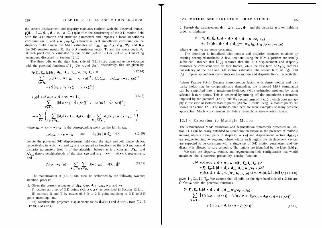
226 CHAPTER 12. STEREO AND MOTION TRACKING 12.1. MOTION AND STRUCTURE FROM STEREO 227
the present displacement and disparity estimates conform with the observed frames,p(dlR, d2R, dlL, dztlwl, wz,I~) quantifies the consistency of the 2-D motion fieldwith the 3-D motion and structure parameters and imposes a local smoothnessconstraint on it, and p(wl,wzII~) enforces a local smoothness constraint on thedisparity field. Given the MAP estimates of dm, dm, dlL, daL, wi, and wz,the 3-D rotation matrix R, the 3-D translation vector T, and the scene depth X3at each pixel can be estimated by one of the 3-D to 3-D or 3-D to 2-D matchingtechniques discussed in Section 12.1.2.
2. Perturb the displacement dlR, d2R, dlL, d2L and the disparity wi, ws fields inorder to minimize
where yi and yz are some constants.
The three pdfs on the right hand side of (12.13) are assumed to be Gibbsianwith the potential functions Ui(.), Uz(.), and Us(.), respectively, that are given by
The algorithm is initialized with motion and disparity estimates obtained byexisting decoupled methods. A few iterations using the ICM algorithm are usuallysufficient. Observe that VI(.) requires that the 2-D displacement and disparityestimates be consistent with all four frames, ,while the first term of U2(.) enforcesconsistency of the 2-D and 3-D motion estimates. The second term of Uz(.) andUs(.) impose smoothness constraints on the motion and disparity fields, respectively.Ul(I~,IIR,IzldlR,dzR,dlL,d2L,wl,w2,IR) = (12.14)
c [ (IdxR + w(xR)) - lR(XR))’ + (&(xR + dR(xR)) - IR(xR))2
XREIR
+ (G,(xz + dL(XZj) - IL(xL))2 ]
U2(dlR,dzR,dlL,dzLIw1,w2,IRj =
c ( IldR(XR) - aR(xR)112 + Ildr,(x~) - h(Xd12 )
XREIR
(12.15)
+ ac c IId&Ri) - d&?il12 + c Ildzh) - ddx~j)112XR, xwcNxR, XL1 ENX,,
where XL = xR + w(xR) is the corresponding point on the left image,
d&R) - & - xR and dL(xL) - $, - xL (12.16)
denote the projected 3-D displacement field onto the right and left image planes,respectively, in which %k and 2:. are computed as functions of the 3-D motion anddisparity parameters (step 1 of the algorithm below), o is a constant, NxR, andNx,, denote neighborhoods of the sites xRi and x~i = x& + w(xRi), respectively,and
&(WI,WZIIR)= c c IIw(xRi)-w(xRj)l12(12.17)
XR. XR~~NX,,
The maximization of (12.13) can, then, be performed by the following two-stepiteration process:
1. Given the present estimates of dlR, d2R, dlL, daL, wi, and wz:i) reconstruct a set of 3-D points (Xi, X2, Xs) as described in Section 12.1.1,ii) estimate R and T by means of 3-D to 2-D point matching or 3-D to 3-D
point matching, andiii) calculate the projected displacement fields OR and AL from (12.1),
(12.2), and (12.4).
Isolated Feature Points: Because stereo-motion fusion with dense motion and dis-parity fields may be computationally demanding, the proposed MAP formulationcan be simplified into a maximum-likelihood (ML) estimation problem by usingselected feature points. This is achieved by turning off the smoothness constraintsimposed by the potential (12.17) and the second term of (12.15), which does not ap-ply in the case of isolated feature points [Alt 951. Results using 14 feature points areshown in Section 12.3. The methods cited here are mere examples of many possibleapproaches. Much work remains for future research in stereo-motion fusion.
12.1.4 Extension to Multiple Motion
The simultaneous MAP estimation and segmentation framework presented in Sec-tion 11.3 can be easily extended to stereo-motion fusion in the presence of multiplemoving objects. Here, pairs of disparity w(xR) and displacement vectors dR(xR)are segmented into I< regions, where within each region the displacement vectorsare expected to be consistent with a single set of 3-D motion parameters, and thedisparity is allowed to vary smoothly. The regions are identified by the label field z.
We seek the disparity, motion, and segmentation field configuration that wouldmaximize the a posteriori probability density function
p(dlR,dzR,dlLtdzL,w1,wz,~IIIL,I~,IL,IR,) m
p(I~,Ik,Ir.ldl~,dz~,dl~,dz~,~l,w2,Z, IR)
P(dlR,dzR,dlz,dzLIw1,wz,z,IR) ~(w1,wzlqIR) p(z(IR) (12.18)
given IL, IR, IL, IL. We assume that all pdfs on the right-hand side of (12.18) areGibbsian with the potential functions
Ul(I~,I~,I~(dl~,d2~,dl~,d2~, wllw2,z,IR) =
c [ (lL(xR + w(xR)) - IR(XR))~ + (&(XR $ dR(XR)) - IR(xR))~XREIR
+ ($(xL + d&J) - IL(xL))~ ] (12.19)
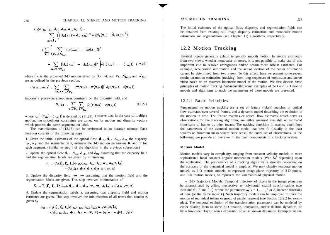
228 CHAPTER 12. STEREO AND MOTION TRACKING
Us(dm, dm, da dzh,wz, z) =
c (Ildn(XR) - aR(xR)i1’+ Ilddw) - ~dxdli2)
XAEIR
+c c IId&%) - dR(Xd2XRI xRicnr,R,+ c II&hi) - d&Lj)l12 h(+Ri) - +Rj)) (12.20)
XLiENX,, 1
where a, is the projected 3-D motion given by (12.16)) and XL, Nx,,, and Nx,,are as defined in the previous section,
u3(wl,w21Z) = c c b+Ri) -w(xRj)~~2 +(xRi) - +Rj))
XRI XRJ ENX,,
imposes a piecewise smoothness constraint on the disparity field, and
u4(z) = c c vC(+Ri), z(xRj))
XRI XR;CN~,,(12.21)
where Vc(.z(xRi), z(xRj)) is defined by (11.28). Observe that, in the case of multiplemotion, the smoothness constraints are turned on for motion and disparity vectorswhich possess the same segmentation label.
The maximization of (12.18) can be performed in an iterative manner. Eachiteration consists of the following steps:
1. Given the initial estimates of the optical flow, dlfi, d2R, dlL, dzr, the disparitywi, ~2, and the segmentation z, estimate the 3-D motion parameters R and T foreach segment. (Similar to step 1 of the algorithm in the previous subsection.)
2. Update the optical flow dlR, d2R, dlL, and d2L assuming that the disparity fieldand the segmentation labels are given by minimizing
El = Ul(I~,Ik,I~ldlR,dzR,dl~,dz~,wl,wz,Z,IR)
S&(&R, dzR, dx, dzL[wi, wz, z)
3. Update the disparity field, WI, wz assuming that the motion field and thesegmentation labels are given. This step involves minimization of
Ez. = &(I;,I;,IL(~~ dm, dx, da ~1, wz, z, IR) + u3(w1, wzlz)
4. Update the segmentation labels z, assuming that disparity field and motionestimates are given, This step involves the minimization of all terms that contain z,given by
E3 = Ul(I~,I~,ILIdlR,d2R,dlL,d2L,w1,w2,z,IR)
+Uz(dlR,dzR,dlL,d2L1wl,~z,z) + ~3(wl,wzIz) + u4(z)
12.2. MOTION TRACKING 229
The initial estimates of the optical flow, disparity, and segmentation fields canbe obtained from existing still-image disparity estimation and monocular motionestimation and segmentation (see Chapter 11) algorithms, respectively.
12.2 Motion Tracking
Physical objects generally exhibit temporally smooth motion. In motion estimationfrom two views, whether monocular or stereo, it is not possible to make use of thisimportant cue to resolve ambiguities and/or obtain more robust estimates. Forexample, acceleration information and the actual location of the center of rotationcannot be determined from two views. To this effect, here we present some recentresults on motion estimation (tracking) from long sequences of monocular and stereovideo based on an assumed kinematic model of the motion. We first discuss basicprinciples of motion tracking. Subsequently, some examples of 2-D and 3-D motionmodels and algorithms to track the parameters of these models are presented.
12.2.1 Basic Principles
Fundamental to motion tracking are a set of feature (token) matches or opticalflow estimates over several frames, and a dynamic model describing the evolution ofthe motion in time. The feature matches or optical flow estimates, which serve asobservations for the tracking algorithm, are either assumed available or estimatedfrom pairs of frames by other means. The tracking algorithm in essence determinesthe parameters of the assumed motion model that best fit (usually in the leastsquares or minimum mean square error sense) the entire set of observations. In thefollowing, we provide an overview of the main components of a tracking system.
Motion Model
Motion models vary in complexity, ranging from constant velocity models to moresophisticated local constant angular momentum models [Wen 871 depending uponthe application. The performance of a tracking algorithm is strongly dependent onthe accuracy of the dynamical model it employs. We may classify temporal motionmodels as 2-D motion models, to represent image-plane trajectory of 3-D points,and 3-D motion models, to represent the kinematics of physical motion.
l 2-D Trajectory Models: Temporal trajectory of pixels in the image plane canbe approximated by affine, perspective, or polynomial spatial transformations (seeSections 6.1.2 and 9.1)) where the parameters ai, i = 1,. . . ,6 or 8, become functionsof time (or the frame index Ic). Such trajectory models can be employed to track themotion of individual tokens or group of pixels (regions) (see Section 12.2.2 for exam-ples). The temporal evolution of the transformation parameters can be modeled byeither relating them to some 2-D rotation, translation, and/or dilation dynamics, orby a low-order Taylor series expansion of an unknown dynamics. Examples of the
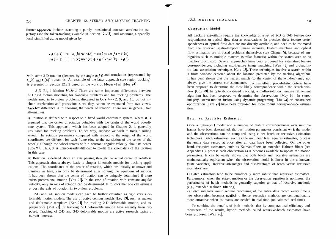
230 CHAPTER 12. STEREO AND MOTION TRACKING
former approach include assuming a purely translational constant acceleration tra-jectory (see the token-tracking example in Section 12.2.2), and assuming a spatiallylocal simplified afline model given by
z1(lc+l) = Xl@) cosa(k) - ~(k)sinc*(lc) +ti(le)
zz(le + 1) = zi(le)sincu(lc) + az(le) coso(E) + tz(k)
with some 2-D rotation (denoted by the angle o(k)) and translation (represented by
TV and h(k)) dynamics. An example of the latter approach (see region tracking)is presented in Section 12.2.2 based on the work of Meyer el al. [Mey 941.
. 3-D Rigid Motion Models: There are some important differences between3-D rigid motion modeling for two-view problems and for tracking problems. Themodels used in two-view problems, discussed in Chapt,ers 2, 9, and 10, do not in-clude acceleration and precession, since they cannot be estimated from two views.Anot,her difference is in choosing the center of rotation. There are, in general, twoalternatives:
i) Rotation is defined with respect to a fixed world coordinate system, where it isassumed that the center of rotation coincides with the origin of the world coordi-nate system. This approach, which has been adopted in Chapter 2, is generallyunsuitable for tracking problems. To see why, suppose we wish to track a rollingwheel. The rotation parameters computed with respect to the origin of the worldcoordinates are different for each frame (due to the translation of the center of thewheel), although the wheel rotates with a constant angular velocity about its center[Sha 901. Thus, it is unnecessarily difficult to model the kinematics of the rotationin this case.
ii) Rotation is defined about an axis passing through the actual center of rot,ation.This approach almost always leads to simpler kinematic models for tracking appli-cations. The coordinates of the center of rotation, which are initially unknown andtranslate in time, can only be determined after solving the equations of motion.It has been shown that the center of rotation can be uniquely determined if thereexists precessional motion [You 901. In the case of rotation with constant angularvelocity, only an axis of rotation can be determined. It follows that one can estimateat best the axis of rotation in two-view problems.
2-D and 3-D motion models can each be further classified as rigid versus de-formable motion models. The use of active contour models [Ley 931, such as snakes,and deformable templates [Ker 941 for tracking 2-D deformable motion, and su-perquadrics [Met 931 for tracking 3-D deformable motion have recently been pro-posed. Tracking of 2-D and 3-D deformable motion are active research topics ofcurrent interest.
12.2. MOTION TRACKING
Observation Model
231
All tracking algorithms require the knowledge of a set of 2-D or 3-D feature cor-respondences or optical flow data as observations. In practice, these feature corre-spondences or optical flow data are not directly available, and need to be estimatedfrom the observed spatio-temporal image intensity. Feature matching and opticalflow estimation are ill-posed problems themselves (see Chapter 5), because of am-biguities such as multiple matches (similar features) within the search area or nomatches (occlusion). Several approaches have been proposed for estimating featurecorrespondences, including multifeature image matching [Wen 931 and probabilis-tic data association techniques [Cox 931. These techniques involve a search withina finite window centered about the location predicted by the tracking algorithm.It has been shown that the nearest match (to the center of the window) may notalways give the correct correspondence. To this effect, probabilistic criteria havebeen proposed to determine the most likely correspondence within the search win-dow [Cox 931. In optical-flow-based tracking, a multiresolution iterative refinementalgorithm has been proposed to determine the observations [Mey 941. In stereoimagery, stereo-motion fusion using dynamic programing [Liu 931 or constrainedoptimization [Tam 911 have been proposed for more robust correspondence estima-tion.
Batch vs. Recursive Estimation
Once a dynamical model and a number of feature correspondences over multipleframes have been determined, the best motion parameters consistent wit#h the modeland the observations can be computed using either batch or recursive estimationtechniques. Batch estimators, such as the nonlinear least squares estimator, processthe entire data record at once after all data have been collected. On the otherhand, recursive estimators, such as Kalman filters or extended Kalman filters (seeAppendix C), process each observation as it becomes available to update the motionparameters. It can be easily shown that both batch and recursive estimators aremathematically equivalent when the observation model is linear in the unknowns(state variables). Relative advantages and disadvantages of batch versus recursiveestimators are:
1) Batch estimators tend to be numerically more robust than recursive estimators.Furthermore, when the state-transition or the observation equation is nonlinear, theperformance of batch methods is generally superior to that of recursive methods(e.g., extended Kalman filtering).2) Batch methods would require processing of the entire data record every time anew observation becomes a,vailable. Hence, recursive methods are computationallymore attractive when estimates are needed in real-time (or “almost” real-time).
To combine the benefits of both methods, that is, computational efficiency androbustness of the results, hybrid methods called recursive-batch estimators have
been proposed [Wen 931.
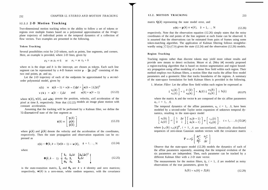
232 CHAPTER 12. STEREO AND MOTION TRACKING
12.2.2 2-D Motion Tracking
Two-dimensional motion tracking refers to the ability to follow a set of tokens orregions over multiple frames based on a polynomial approximation of the image-plane trajectory of individual points or the temporal dynamics of a collection offlow vectors. Two examples are presented in the following.
Token Tracking
Several possibilities exist for 2-D tokens, such as points, line segments, and corners.Here, an example is provided, where 2-D lines, given by
22 = m xl+ 6 or xl = m x2 + b
where m is the slope and b is the intercept, are chosen as tokens. Each such linesegment can be represented by a 4-D feature vector p = [pl p21T consisting of thetwo end points, p1 and pz.
Let the 2-D trajectory of each of the endpoints be approximated by a second-order polynomial model, given by
x(k) = x(k - 1) + v(k - 1)At + ta(k - l)(At)”
v ( k ) = a(le - l)At and a(lc) = a(le - 1) (12.22)
where x(k), v(k), and a(h) denote the position, velocity, a.nd acceleration of thepixel at time le, respectively. Note that (12.22) models an image plane motion withconstant acceleration.
Assuming that the tracking will be performed by a Kalman filter, we define the12-dimensional state of the line segment as
(12.23)
where Ij(k) and fi(!c) denote the velocity and the acceleration of the coordinates,respectively. Then the state propagation and observation equations can be ex-pressed as
z(k) = @(k, k - l)z(k - 1) + w(k), lc = 1,. .) N (12.24)
where
[
I4 14At i14(At)2Q(k,k-- 1) = O4 I4 14At 1 (12.25)
04 04 14
is the state-transition matrix, I4 and 04 are 4 x 4 identity and zero matrices;respectively, w(k) is a zero-mean, white random sequence, with the covariance
12.2. MOTION TRACKING 233
matrix Q(lc) representing the state model error, and
y(k) = p(h) + v(h), le = 1,. .) N (12.26)
respectively. Note that the observation equation (12.26) simply states that the noisycoordinates of the end points of the line segment at each frame can be observed. Itis assumed that the observations can be estimated from pairs of frames using sometoken-matching algorithm. The application of Kalman filtering follows straightfor-wardly using (C.5)-(C.9) given the state (12.24) and the observation (12.26) models.
Region Tracking
Tracking regions rather than discrete tokens may yield more robust results andprovide new means to detect occlusion. Meyer et al. [Mey 941 recently proposeda region-tracking algorithm that is based on motion segmentation and region bound-ary propagation using affine modeling of a dense flow field within each region. Theirmethod employs two Kalman filters, a motion filter that tracks the affine flow modelparameters and a geometric filter that tracks boundaries of the regions. A summaryof the state-space formulation for both Kalman filters is provided in the following.
1. Motion Filter: Let the affine flow field within each region be expressed as
[ $j ] = [ $; ] = A(lc) [ :$j ] + b(lc) (12.27)
where the matrix A and the vector b are composed of the six affine parametersai, i = 1,. .6.
The temporal dynamics of the affine parameters, ai, i = 1,. ,6, have beenmodeled by a second-order Taylor series expansion of unknown temporal dy-namics, resulting in the state-space model
where [c;i(le) cis(t%)lT, i = 1 ) ,6 are uncorrelated, identically distributedsequences of zero-mean Gaussian random vectors with the covariance matrix *
Observe that the state-space model (12.28) models the dynamics of each ofthe affine parameters separately, assuming that the temporal evolution of thesix parameters are independent. Then, each parameter can be tracked by adifferent Kalman filter with a 2-D state vector.
The measurements for the motion filters, &, i = 1, .6 are modeled as noisyobservations of the true parameters, given by
h(k) = ai + Pi(k) (12.29)

234 CHAPTER 12. STEREO AND MOTION TRACKING 12.2. MOTION TRACKING 235
where @i(k) is a sequence of zero-mean, white Gaussian random variables withthe variance ui. As mentioned before, the measurements iii, i = 1, .6 areestimated from the observed image sequence, two views at a time. Combining(12.27) with the well-known optical flow equation (5.5), a multiresolutionestimation approach has been proposed by Meyer et al. [Mey 941 using least-squares fitting and iterative refinement within each region.
2. Geometric Filter: The geometric filter is concerned with tracking each regionprocess that is identified by a motion segmentation algorithm [Bou 931. Theconvex hull (the smallest convex polygon covering the region) of a polygonalapproximation of each region is taken as the region descriptor. The regiondescriptor vector consists of 2N components, consisting of the (21, ~2) coor-dinates of the N vertices of the convex hull.
A state-space model for tracking the evolution of the region descriptor vectorover multiple frames can be written as
where
@(k,k-1) 0 ... 0
Ix [.b 0 i(k, k - 1) 1u(k) + w(k) (12.30)
Q(k, k - 1) = I2 + AtA
which can be seen by considering a first-order Taylor expansion of[n(k) m(k)lT given by
about the time k - 1, and substituting the flow field model (12.27) forh(k) k(k)1 T ,
u ( k ) = A t b ( k )
is a deterministic input vector which follows from the above derivation, andw(k) is a white-noise sequence with the covariance matrix Q(k).
The measurement f:q1iation can be expressed as
h(k) x11(k)ha(k) m(k)
Z
Em(k), XNl(k)&w(k) _ _ xm(k)
+ n(k) (12.31)
where n(k) is a sequence of zero-mean, white Gaussian random vectors. Anobservation of the region descriptor vector can be estimated by two-view op-tical flow analysis as described in [Bou 931.
All motion-tracking algorithms should contain provisions for detecting occlusionand de-occlusion, as moving objects may exit the field of view, or new objectsmay appear or reappear in the picture. An occlusion and de-occlusion detectionalgorithm based on the divergence of the motion field has been proposed in [Mey 941.The main idea of the detector is to monitor the difference in the area of the regionsfrom frame to frame, taking into account any global zooming. The descriptor isupdated after each frame using occlusion/de-occlusion information. The regiontracking algorithm presented in this section has recently been extended to includeactive contour models for representation of complex primitives with deformableB-splines [Bas 941.
12.2.3 3-D Rigid Motion Tracking
Three-dimensional motion tracking refers to the ability to predict and monitor 3-Dmotion and structure of moving objects in a scene from long sequences of monocularor stereo video. In what follows, we present examples of 3-D rigid motion trackingfrom monocular and stereo video based on the works of Broida and Chellappa[Bro 911 and Young and Chellappa [You 901.
From Monocular Video
Suppose we wish to track the 3-D motion of M feature points on a rigid object. Wedefine two coordinate systems, depicted in Figure 12.4: C,, the object coordinatesystem whose origin X, = [X,1(k) Xo2(k) X,,(k)lT, with respect to the camera andworld coordinate systems, coincides with the center of rotation (which is unknown);and C,, the structure coordinate system, whose origin is located at a known pointon the object. It is assumed that C, and C, are related by an unknown translationI -T,. Let Xi = [Xii Xi2 zislT denote the known coordinates of a feature point iwith respect to the structure coordinate system. Then the coordinates of the featurepoint with respect to the world and camera coordinate systems are given by
Xi(k) = X,(k) + R(k)& - T,), k = 0,. .) N (12.32)
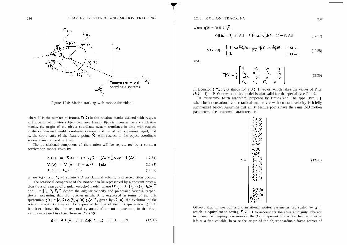
236 CHAPTER 12. STEREO AND MOTION TRACKINGI
coordinate systems
x3
Figure 12.4: Motion tracking with monocular video.
where N is the number of frames, R(le) is the rotation matrix defined with respectto the center of rotation (object reference frame), R(0) is taken as the 3 x 3 identitymatrix, the origin of the object coordinate system translates in time with respectto the camera and world coordinate systems, and the object is assumed rigid; thatis, the coordinates of the feature points xi with respect to the object coordinatesystem remains fixed in time.
The translational component of the motion will be represented by a constantacceleration model given by
X,(b) = X,(k - 1) + V,,(k - l)At + ;A@ - l)(At)” (12.33)
V,(k) = V,(lc - 1) + AO(le - 1)At (12.34)
A&) = A,(k - 1 ) (12.35)
where V,(k) and A,(k) denote 3-D translational velocity and acceleration vectors.The rotational component of the motion can be represented by a constant preces-
sion (rate of change of angular velocity) model, where n(k) = [fir(k) n,(k) as(kand P = [PI P2 P31T denote the angular velocity and precession vectors, respec-tively. Assuming that the rotation matrix R is expressed in terms of the unitquaternion q(k) = [qe(l%) or qs(le) qs(le)lT, given by (2.10), the evolution of therotation matrix in time can be expressed by that of the unit quaternion q(lc). Ithas been shown that the temporal dynamics of the unit quaternion, in this case,can be expressed in closed form as [You 901
q(le) = @[n(lc - l), P; At]q(k - l), le = 1,. . . , N (12.36)
12.2. MOTION TRACKING
where q(0) = [0 0 0 llT,
237
@[0(/c - l), P; At] = A[P; At]A[n(k - 1) - P; At] (12.37)
A[G; At] = 14 cos + &I’[G] sin ifG#O
14 ifG=O(12.38)
and
r[G] = f ! 0 -GB Gz -G1G3 0 -GI -Gz-G2 GI 0 -G3GI G2 G3 0 1 (12.39)
In Equation (12.38), G stands for a 3 x 1 vector, which takes the values of P orn(k - 1) - P. Observe that this model is also valid for the special case P = 0.
A multiframe batch algorithm, proposed by Broida and Chellappa [Bro 911,when both translational and rotational motion are with constant velocity is brieflysummarized below. Assuming that all M feature points have the same 3-D motionparameters, the unknown parameters are
- $yO)$+p)g(o)&)$0)fil(O)WO)fi3(0)
$p)s&4$fp)$p)$fy4
+yO)*c9
+e(O)
(12.40)
Observe that all position and translational motion parameters are scaled by X03,which is equivalent to setting X03 = 1 to account for the scale ambiguity inherentin monocular imaging. Furthermore, the X3 component of the first feature point isleft as a free variable, because the origin of the object-coordinate frame (center of
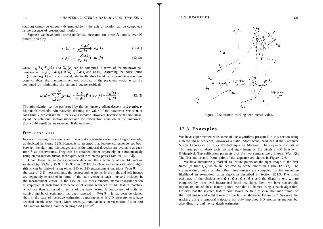
238 CHAPTER 12. STEREO AND MOTION TRACKING 12.3. EXAMPLES
rotation) cannot be uniquely determined (only the axis of rotation can be computed)in the absence of precessional motion.
Suppose we have point correspondences measured for these M points over Nframes, given by
&l(k)m(k) = xis(k) + nil(k)
&z(k)“a(k) = xi3(k) + m.(k)
(12.41)
(12.42)
where Xii(k), Xiz(k), and Xis(k) can be computed in terms of the unknown pa-rameters u using (12.32), (12.35), (12.36), and (2.10). Assuming the noise termsnil(k) and niz(k) are uncorrelated, identically distributed zero-mean Gaussian ran-dom variables, the maximum-likelihood estimate of the parameter vector u can becomputed by minimizing the summed square residuals
E(u) = F f)ii(k) - %I2 + [m(k) - #I2k=l i=l
(12.43)
The minimization can be performed by the conjugate-gradient descent or Levenberg-Marquardt methods. Alternatively, defining the value of the parameter vector u ateach time k, we can define a recursive estimator. However, because of the nonlinear-ity of the rotational motion model and the observation equation in the unknowns,this would result in an extended Kalman filter.
From Stereo Video
In stereo imaging, the camera and the world coordinate systems no longer coincide,as depicted in Figure 12.5. Hence, it is assumed that feature correspondences bothbetween the right and left images and in the temporal direction are available at eachtime k as observations. They can be obtained either separately or simultaneouslyusing stereo-motion fusion techniques with two stereo-pairs [Tam 91, Liu 931.
Given these feature correspondence data and the kinematics of the 3-D motionmodeled by (12.32), (12.35), (12.36), and (2.10), batch or recursive estimation algo-rithms can be derived using either 2-D or 3-D measurement equations [You 901. Inthe case of 2-D measurements, the corresponding points in the right and left imagesare separately expressed in terms of the state vector at each time and included inthe measurement vector. In the case of 3-D measurements, stereo triangularizationis employed at each time k to reconstruct a time sequence of 3-D feature matches,which are then expressed in terms of the state vector. A comparison of both re-cursive and batch estimators has been reported in [Wu 941. It has been concludedthat, in the case of recursive estimation, experiments with 2-D measurements havereached steady-state faster. More recently, simultaneous stereo-motion fusion and3-D motion tracking have been proposed [Alt 951.
239
Figure 12.5: Motion tracking with stereo video.
12.3 Examples
We have experimented with some of the algorithms presented in this section usinga stereo image sequence, known as a static indoor scene, produced at the ComputerVision Laboratory of Ecole Polytechnique de Montreal. The sequence consists of10 frame pairs, where each left and right image is 512 pixels x 480 lines with8 bits/pixel. The calibration parameters of the two cameras were known [Wen 921.The first and second frame pairs of the sequence are shown in Figure 12.6.
We have interactively marked 14 feature points on the right image of the firstframe (at time ti), which are depicted by white circles in Figure 12.6 (b). Thecorresponding points on the other three images are computed by the maximumlikelihood stereo-motion fusion algorithm described in Section 12.1.3. The initialestimates of the displacement dlR, d2R, dlL, d2L and the disparity ~1, w2 arecomputed by three-level hierarchical block matching. Next, we have tracked themotion of one of these feature points over the 10 frames using a batch algorithm.Observe that the selected feature point leaves the field of view after nine frames onthe right image and eight frames on the left, as shown in Figure 12.7. We note thattracking using a temporal trajectory not only improves 3-D motion estimation, butalso disparity and hence depth estimation.

240 CHAPTER 12. STEREO AND MOTION TRACKING 12.4. EXERCISES 241
(4
Figure 12.6: The first and second frame pairs of a stereo indoor scene producedat the Computer Vision Laboratory of Ecole Polytechnique de Montreal: a) leftimage at time tr, b) right image at time tr, c) left image at time tz, and d) rightimage at time tz. Fourteen feature points (marked by white circles) have beenselected interactively on the right image at time tr. Point correspondences on theother images are found by the maximum likelihood stereo-motion fusion algorithm.(Courtesy Yucel Altunbasak)
(4 (b)Figure 12.7: Temporal trajectory of a single point marked on the a) left and b) rightimages of the first frame. The white marks indicate the position of the feature pointin the successive frames. (Courtesy Yucel Altunbasak)
12.4 Exercises
1. Show that only two of the three equations in (12.5) are linearly independentif we have exact left-right correspondences.
2. Derive (12.6) given that the left and right camera coordinates are parallel andaligned with the Xr - X2 plane of the world coordinate system.
3. Derive (12.10).
4. Write the Kalman filter equations for the 2-D token-matching problem dis-cussed in Section 12.2.2 given the state-transition model (12.24) and the ob-servation model (12.26).
5. Write the equations of a recursive estimator for the 3-D motion-tracking prob-lem discussed in Section 12.2.3. Discuss the relationship between this recursiveestimator and the batch solution that was provided.

242 BIBLIOGRAPHY
Bibliography
[Alo 901 Y. Aloimonos and J.-Y. Herve, “Correspondenceless stereo and mo-tion: Planar surfaces,” IEEE Trans. Patt. Anal. Mach. Intel., vol. 12,pp. 504-510, May 1990.
[Alt 951 Y. Altunbasak, A. M. Tekalp, and G. Bozdagi, “Simultaneous stereo-motion fusion and 3-D motion tracking,” Proc. Int. Conf. Acoust. Speech
and Sign. Proc., Detroit, MI, May 1995.
[Aru 871 K. S. Arun, T. S. Huang, and S. D. Blostein, “Least squares fittingof two 3-D point sets,” IEEE Trans. Patt. Anal. Mach. Intel., vol. 9,pp. 698-700, Sep. 1987.
[Bar 931 S. T. Barnard, ‘Stereo matching,” in Markov Random Fields,R. Chellappa and A. Jain, eds., Academic Press, 1993.
[Bas 941 B. Bascle, P. Bouthemy, R. Deriche, and F. Meyer, “Tracking complexprimitives in an image sequence,” Int. Conf. Pa2t. Recog., Jerusalem,Israel, pp. 4266431, Oct. 1994.
[Bou 931 P. Bouthemy and E. Francois, “Motion segmentation and qualitativedynamic scene analysis from an image sequence,” Int. b. Comp. Vis.,vol. 10:2, pp. 157-182, 1993.
[Bro 911 T. J. Broida and R. Chellappa, “Estimating the kinematics and structureof a rigid object from a sequence of monocular images,” IEEE Trans. Patt.Anal. Mach. Intel, vol. 13, pp. 497-513, June 1991.
[Che 941 R. Chellappa, T.-H. Wu, P. Burlina, and Q. Zheng, ‘Visual motion anal-YSlS, ” in Control and Dynamic Systems, C. T. Leondes, ed., vol. 67,pp. 199-261, 1994.
[Cox 931 I. J. cox, “A review of statistical data association techniques for motioncorrespondence,” Int. J. Comp. Vis., vol. lO:l, pp. 53-66, 1993.
[Dho $91 U. R. Dhond, and J. K. Aggarwal, “Structure from stereo - A review,”IEEE Trans. Syst., Man, and Cyber., vol 19, no 6, Nov. 1989.
[Fau 931 0. Faugeras, Three-Dimensional Computer Vision, MIT Press, 1993.
[Fuj 931 K. Fujimura, N. Yokoya, and K. Yamamoto, “Motion tracking of de-formable objects by active contour models using multiscale dynamic pro-gramming,” J. Vis. Comm. and Image Rep., vol. 4, no, 4, pp. 382-391,Dec. 1993.
[Hua 89c] T. S. Huang, “Motion estimation from stereo sequences,” in MachineVision for Inspection and Measurement, H. Freeman, ed., pp. 1277135,New York, NY: Academic Press, 1989.
BIBLIOGRAPHY 243
[Hua 941 T. S. Huang and A. Netravali, “Motion and structure from feature corre-spondences: A review,” Proc. IEEE, vol. 82, pp. 252-269, Feb. 1994.
[Ker 941 C. Kervrann and F. Heitz, “Robust tracking of stochastic deformable mod-els in long image sequences,” Proc. IEEE Int. Conf. Image Proc., Austin,TX, vol. III, pp. 88-92, Nov. 1994.
[Kim 871 Y. C. Kim and J. K. Aggarwal, “Determining object motion in a se-quence of stereo images,” IEEE J. Robotics and Auto., vol. 3, pp. 599-614,Dec. 1987.
[Ley 931 F. Leymarie and M. D. Levine, “Tracking deformable objects in the planeusing an active contour model,” IEEE Trans. Patt. Anal. Mach. Intel,vol. 15, pp. 617-634, June 1993.
[Liu 931 J. Liu and R. Skerjanc, ‘Stereo and motion correspondence in a sequenceof stereo images,” Signal Proc.: Image Comm., vol. 5, pp. 305-318, 1993.
[Mar 781 D. Marr, G. Palm, and T. Poggio, “Analysis of a cooperative stereo algo-rithm,” Biol. Cybern., vol. 28, pp. 2233229, 1978.
[Mat 891 L. Matthies, R. Szeliski and T. Kanade, “Kalman-filter based algorithmsfor estimating depth from image sequences,” Int. J. Comp. Vision, vol. 3,pp. 181~208, 1989.
[Met 931 D. Metaxas and D. Terzopoulos, “Shape and nonrigid motion estimationthrough physics-based synthesis,” IEEE Trans. Patt. Anal. Mach. Intel,vol. 15, pp. 580-591, June 1993.
[Mey 941 F. G. Meyer and P. Bouthemy, “Region-based tracking using affine motionmodels in long image sequences,” CVGIP: Image Understanding, vol. 60,no. 2, pp. 119-140, Sep. 1994.
[Ric 851 W. Richards, “Structure from stereo and motion,” J. Opt. Sot. Am. A,vol. 2, pp. 343-349, Feb. 1985.
[Sha 901 H. Shariat and K. Price, “Motion estimation with more than two frames,”IEEE Trans. Patt. Anal. Mach. Intel, vol. 12, pp. 417-434, May 1990.
[Spe 911 M. Spetsakis and J. Aloimonos, “A multi-frame approach to visual motionperception,” Int. J. Comp. Vision, vol. 6, no. 3, pp. 245-255, 1991.
[Tam 911 A. Tamtaoui and C. Labit, “Constrained disparity and motion estimatorsfor 3DTV image sequence coding,” Sign. Proc.: Image Comm., vol. 4,pp. 45-54, 1991.
[Wax 861 A. M. Waxman and J. H. Duncan, “Binocular image flows: Steps to-wards stereo-motion fusion,” IEEE Trans. Patt. Anal. Mach. Intel., vol. 8,pp. 715-729, Nov. 1986.
244 BIBLIOGRAPHY
[Wen 871 J. Weng, T. S. Huang, and N. Ahuja, “3-D motion estimation, under-standing, and prediction from noisy image sequences,” IEEE Trans. Patt.Anal. Mach. Intel, vol. 9, pp. 370-389, May 1987.
[Wen 921 J. Weng, P. Cohen and M. Herniou, ‘Camera calibration with distortionmodels and accuracy evaluation, ” IEEE Trans. Patt. Anal. Mach. Intel.,vol. 14, no. 10, pp. 965-980, Oct. 1992.
[Wen 931 J. Weng, T. S. Huang, and N. Ahuja, Motion and Structure from ImageSequences, Springer-Verlag (Series in Information Sciences), 1993.
[Wu 881 J. J. Wu, R. E. Rink, T. M. Caelli, and V. G. Gourishankar, “Recoveryof the 3-D location and motion of a rigid object through camera image(An extended Kalman filter approach),” Int. J. Comp. Vision, vol. 3,pp. 3733394, 1988.
[Wu 941 T.-H. Wu and R. Chellappa, “Stereoscopic recovery of egomotion andstructure: Models, uniqueness and experimental results,” Proc. Int. Conf.Patt. Recog., Jerusalem, Israel, vol. I, pp. 645-648, Oct. 1994.
[You 901 G.-S. J. Young and R. Chellappa, “3-D motion estimation using a sequenceof noisy stereo images: Models, estimation, and uniqueness results,”IEEE Trans. Patt. Anal. Mach, Intel., vol. 12, pp. 735-759, Aug. 1990.
[Zha 921 Z. Zhang and 0. D. Faugeras, “Estimation of displacements from two3-D frames obtained from stereo,” IEEE Trans. Patt. Anal. Mach. Intel.,vol. 14, pp. 1141-1156, Dec. 1992.
[Zhe 921 Z. Zhang and 0. Faugeras, “Three-dimensional motion computation andobject segmentation in a long sequence of stereo frames,” Int. J. Comp.Vision, vol. 7, no. 3, pp. 211-241, 1992.
Chapter 13
MOTION COMPENSATEDFILTERING
This chapter is devoted to the theory of motion-compensated filtering, which formsthe basis of several popular methods for noise filtering, restoration, standards con-version, and high-resolution reconstruction, presented in the next three chapters.Motion compensation is also an essential part of interframe compression methods,which are discussed in Part 6 [Gir 931. In essence, this chapter incorporates specificmotion models into the theory of sampling and reconstruction that was presentedin Chapters 3 and 4 for video with arbitrary temporal variations. These resultsare presented in a separate chapter, because an in-depth underst,anding of mot)ion-compensated filtering is fundamental for a complete appreciation of how and whyspatio-temporal filt’ering is superior to intraframe filtering.
In Section 13.1, we derive the spatio-temporal frequency spectrum of video, as-suming that the intensity variations in the temporal direction follow simplified mo-tion models. It is shown that motion models introduce constraints on the support ofthe spa&temporal frequency spectrum of video. The implications of the resultingspatio-temporal spectral characterizations for sub-Nyquist sampling of video are in-vestigated in Section 13.2. The frequency responses of spatio-temporal filters thatoperate along motion trajectories have been derived for the special cases of globalconstant velocity and accelerated motions in Section 13.3. Section 13.4 discusses theapplication of motion-compensated filtering in noise reduction and reconstruction ofa continuous video from digital data possibly sampled at sub-Nyquist rates. Specificdetails of designing motion-compensated noise reduction and standards conversionfilters will be addressed in Chapters 14 and 16, respectively.
245

246 CHAPTER 13. MOTION COMPENSATED FILTERING
13.1 Spatio-Temporal Fourier Spectrum
The aim of this section is to derive the spatio-temporal frequency spectrum of videounder the assumption that the temporal vaaiations in the image intensity patterncan be represented by simplified motion models. The fundamental principle ofmotion compensation is that the intensity of a pixel remains unchanged along awell-defined motion trajectory. In the following, we first define a motion trajectoryand then derive the frequency spectrum of video in the case of two specific motionmodels.
Motion in the image plane refers to the 2-D displacement or velocity of theprojection of scene points, under either orthographic or perspective projection. Eachimage plane point follows a curve in the (21, ~2, t) space, which is called a “ motiontrajectory.” The motion trajectory can be formally defined as a vector functionc(t; cl, x2, to) which specifies the horizontal and vertical coordinates at time t of areference point (~1, ~2) at time ts [Dub 921. The concept of motion trajectory isillustrated in Figure 13.1, where c(t’; ~1, zz;ts) = (xi, ~‘2).
Figure 13.1: Motion trajectory.
Given the motion trajectory c(t; ~1, ~s,ts), the velocity at time t’ at a point(x;, ~‘2) along the trajectory can be defined by
v(x;,x;,t’) = g(t;zl,rz,iO)ltd (13.1)
13.1 . SPATIO-TEMPORAL FOURIER SPECTRUM 247
In the following, we model the motion trajectory with closed-form expressions in twocases: global motion with constant velocity, and global motion with acceleration.These expressions are then incorporated into the spatio-temporal frequency domainanalysis of video.
13.1.1 Global Motion with Constant Velocity
A simplified model of the projected motion is that of global motion with constantvelocity (81, ~2) in the image plane. Then the frame-to-frame intensity variationscan be modeled as
Sc(~l,~Z, t) = %(21 - wt, 22 - vd, 0)
t sg(x1 - zyt, x2 - vat) (13.2)
where the reference frame is chosen as to = 0, and sc(zi, xs) denotes the 2-Dintensity distribution within the reference frame. This model is commonly used inmany practical applications, including international video compression standardssuch as H.261 and MPEG 1-2, and many motion-compensated standards conversionmethods, because it leads to analytically tractable algorithms, as shown in thefollowing.
In order to derive the spatio-temporal spectrum of such video, we first definethe Fourier transform of an arbitrary spatio-temporal function as
&(FI, Fz, Ft) = JJJ sc(xl,xart) e -j2*(F,~c,tF,~atF,t)dxldx2df (13.3)
and the inverse Fourier transform relationship is given by
%(X1, xa>q = JJJ S,(Fl, Fz, Ft) e~2*(F’x’tFzxatFit)dF~dF2dFt (13.4)
The support of S,(Fl, Fz, Ft) generally occupies the entire (FI, Fz,Ft) space forarbitrary s,(xi, x2, t).
Next, we substitute (13.2) into (13.3) to obtain
O”Sc(Fl, Fz, Ft) = J S,J(X~ - vlt, x2 - vzt) e-~21i(F1z1tF2~2tFtt)dx~dx~dt (13.5)--co
Making the change of variables xi = xi - vit, for i = 1,2, we get
Sc(Fl,Fz,Ft) = O” O”JJ so(x1, x2) e-j2*(F1z1tF2z2) dxldxz--co -03
Me -~2*~F,wtF,v,tF~)t dt (13.6)
which can be simplified as
Se(Fl, E”z, 4) = So(4, F2) S(4v1 + F2v2 + F,) (13.7)

248 CHAPTER 13. MOTION COMPENSATED FILTERING
Figure 13.2: The spectral support of video with global, uniform velocity motion.
where Ss(Fr, Fz) is the 2-D Fourier transform of se(~r, ~2) and 6(,) is the 1-D Diracdelta function.
Defining F - [Fi Fz FilT and v A [VI IJ~ llT, the delta function in (13.7) isnonzero only when the argument FTv = 0. The delta function thus confines thesupport of S,(Fi, Fz, Ft) to a plane in R3 given by
Fm + Fzvz + Ft = 0 (13.8)
which passes through the origin, and is orthogonal to the vector v. The spectralsupport of video with global, uniform velocity motion is depicted in Figure 13.2.
This result is intuitively clear. Since the reference frame is sufficient to de-termine all future frames by the nature of the motion model, we expect that theFourier transform of the reference frame would be sufficient to represent the en-tire spatio-temporal frequency spectrum of the video. The extent of the supportof the continuous video spectrum S,(Fl, Fz, pt’t) on the plane FTv = 0 is deter-mined by the support of So(Fl, Fz). We assume that ss(~i, ~2) is bandlimited, i.e.,So(Fl, Fz) = 0 for IF11 > Br and ]F2] > Bz, then clearly, s,(zr, x2, t) is bandlimitedin the temporal variable; that is, S,(Fi, Fz, F,) = 0 for lFt( > Bt, where
Bt = &VI + B2v2 (13.9)
For simplicity of notation and the illustrations, in the following we base ourdiscussions on the projection of the support of S,(Fr, F2, Ft) into the (Fl, F,) plane,which is defined by Flvl + Ft = 0 and depicted in Figure 13.3.
13.1. SPATIO-TEMPORAL FOURIER SPECTRUM
F1 Fr = -(I/y) 5
249
Figure 13.3: Projection of the support into the (Fl, Ft) plane.
13.1.2 Global Motion with Acceleration
In the case of motion with constant acceleration, the trajectory functionc(t; ~1, x2, to) may be approximated by a second-order polynomial. Consideringglobal (space-invariant) motion, we then have
&(X1, x2,4 = &(X1 - qt - ;a& x2 - v2t - ;a2t2, 0)
= s(J(x1 - v1t - ;a1t2, 22 - v2.t - ka2t2) (13.10)
where vi, ~2, al, and a2 denote the components of instantaneous velocity andacceleration, respectively.
The spatio-temporal spectrum of video containing accelerated motion has beenshown to have infinite support in the temporal dimension. This is because thevelocity increases without a bound as time goes to infinity. Short-time spectralanalysis techniques can be used for spectral characterization of video with acceler-ated motion by applying a window to the video signal in the temporal dimension(see Exercise 1). Patti et al. [Pat 941 show that the support of the short-timespectrum (STS) of the video is concentrated along a line whose orientation changesby the instantaneous velocity vector. The interested reader is referred to [Pat 941for further details. A similar analysis is possible for the case of spatially varyingmotion fields.

250 CHAPTER 13. MOTION COMPENSATED FILTERING
13.2 Sub-Nyquist Spatio-Temporal Sampling
The goal of this section is to extend the sampling theory presented in Chapter 3 (forarbitrary spatio-temporal signals) to video with global, constant-velocity motion.We assume that most video sources can be represented by such a simplified modelat least on a block-by-block basis over a short period of time. We will see thatthe nature of the spatio-temporal frequency support of video with global, uniform(constant) velocity motion makes it possible to sample it at sub-Nyquist rates with-out introducing aliasing effects. That is, in most cases a full-resolution video canbe recovered from samples at a sub-Nyquist rate, without any aliasing artifacts, bymotion-compensated reconstruction/interpolation filtering.
13.2.1 Sampling in the Temporal Direction Only
For simplicity, we first study sampling in the temporal direction only, with thespatial variables taken as continuous variables. According to the Nyquist samplingtheorem, the temporal sampling frequency should be greater than 2&, where Btdenotes the temporal bandwidth. However, in the case of global constant-velocitymotion, the spectral replications due to temporal sampling can come arbitrarilyclose to each other without overlapping, as depicted in Figure 13.4. Observe thatthis is true even if Bt is equal to infinity.
Figure 13.4: Spectral replications due to temporal sampling only.
The above frequency-domain result indeed states that just a single referenceframe, s,(zi,xs,O), is sufficient to represent the entire video s,(zi, zs,t) withoutloss of information, when xi and x2 are continuous variables, provided that theglobal velocity vector (~1, ~2) is known. Thus, the sampling interval in the temporaldirection can be chosen to be arbitrarily large, since any desired frame can begenerated by shifting the reference frame appropriately. Of course, hidden here is
13.2. SUB-NYQUIST SPATIO-TEMPORAL SAMPLING 251
the assumption that the images are infinitely wide in the spatial coordinates, sothat there are no boundary effects.
13.2.2 Sampling on a Spatio-Temporal Lattice
Recall that if we sample s,(xr, xs,t) on a spatio-temporal lattice A with the sam-pling matrix V, the Fourier transform of the sampled video S(fi, fs, ft) is periodicwith the periodicity matrix U defining the reciprocal lattice A*. That is, we have
Wl, .f2, ft) = (& k c S,(F + Uk)
where F = (Fr, F2,Ft) and k = (ki,ks,kt). It follows from (13.7) and (13.11) thatwe can sample video with global, constant-velocity motion at sub-Nyquist rates inboth the temporal and spatial dimensions without introducing aliasing. This canbe achieved by choosing an appropriate sampling lattice such that the resultingspectral replications do not overlap for a given velocity.
Figure 13.5: a) Progressive sampling, v = 0; b) interlaced sampling, u # 0.
Let’s first treat spatio-temporal sampling where the spatial sampling frequen-cies are above the Nyquist rate, i.e., above 2Bi and 2B2, respectively. The sampledvideo spectrum in this case is depicted in Figure 13.5, where the spectral replica-tions are contained within nonoverlapping strips, shown by horizontal dotted lines,in the spatial frequency direction. Inspection of Figure 13.5 indicates that thetemporal sampling rate in this case is arbitrary. This is intuitively clear, becauseperfect reconstruction of s,(zr, x2,0) is possible from s(m, n, 0) as long as the spa-tial sampling frequencies are above the Nyquist rate. Then, the case where the
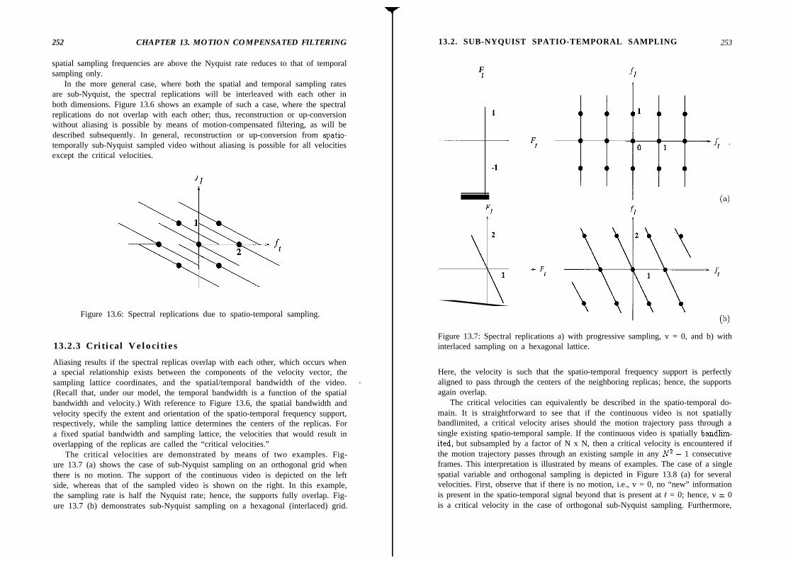
252 CHAPTER 13. MOTION COMPENSATED FILTERING
spatial sampling frequencies are above the Nyquist rate reduces to that of temporalsampling only.
In the more general case, where both the spatial and temporal sampling ratesare sub-Nyquist, the spectral replications will be interleaved with each other inboth dimensions. Figure 13.6 shows an example of such a case, where the spectralreplications do not overlap with each other; thus, reconstruction or up-conversionwithout aliasing is possible by means of motion-compensated filtering, as will bedescribed subsequently. In general, reconstruction or up-conversion from spatio-temporally sub-Nyquist sampled video without aliasing is possible for all velocitiesexcept the critical velocities.
Jl
Figure 13.6: Spectral replications due to spatio-temporal sampling.
13.2.3 Critical Velocities
Aliasing results if the spectral replicas overlap with each other, which occurs whena special relationship exists between the components of the velocity vector, thesampling lattice coordinates, and the spatial/temporal bandwidth of the video. ’(Recall that, under our model, the temporal bandwidth is a function of the spatialbandwidth and velocity.) With reference to Figure 13.6, the spatial bandwidth andvelocity specify the extent and orientation of the spatio-temporal frequency support,respectively, while the sampling lattice determines the centers of the replicas. Fora fixed spatial bandwidth and sampling lattice, the velocities that would result inoverlapping of the replicas are called the “critical velocities.”
The critical velocities are demonstrated by means of two examples. Fig-ure 13.7 (a) shows the case of sub-Nyquist sampling on an orthogonal grid whenthere is no motion. The support of the continuous video is depicted on the leftside, whereas that of the sampled video is shown on the right. In this example,the sampling rate is half the Nyquist rate; hence, the supports fully overlap. Fig-ure 13.7 (b) demonstrates sub-Nyquist sampling on a hexagonal (interlaced) grid.
13.2. SUB-NYQUIST SPATIO-TEMPORAL SAMPLING 253
F1
1
-1
FI
2
1
Figure 13.7: Spectral replications a) with progressive sampling, v = 0, and b) withinterlaced sampling on a hexagonal lattice.
Here, the velocity is such that the spatio-temporal frequency support is perfectlyaligned to pass through the centers of the neighboring replicas; hence, the supportsagain overlap.
The critical velocities can equivalently be described in the spatio-temporal do-main. It is straightforward to see that if the continuous video is not spatiallybandlimited, a critical velocity arises should the motion trajectory pass through asingle existing spatio-temporal sample. If the continuous video is spatially bandlim-ited, but subsampled by a factor of N x N, then a critical velocity is encountered ifthe motion trajectory passes through an existing sample in any N2 - 1 consecutiveframes. This interpretation is illustrated by means of examples. The case of a singlespatial variable and orthogonal sampling is depicted in Figure 13.8 (a) for severalvelocities. First, observe that if there is no motion, i.e., v = 0, no “new” informationis present in the spatio-temporal signal beyond that is present at t = 0; hence, v = 0is a critical velocity in the case of orthogonal sub-Nyquist sampling. Furthermore,
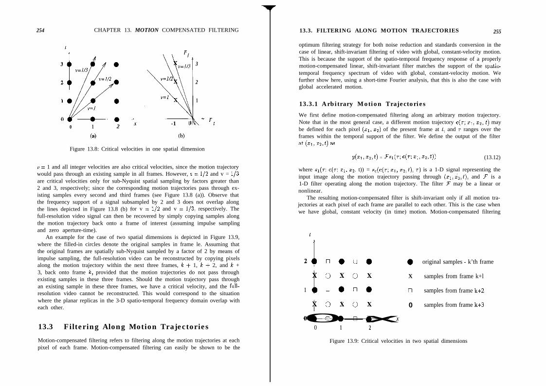
254 CHAPTER 13. MOTION COMPENSATED FILTERING 13.3. FILTERING ALONG MOTION TRAJECTORIES 255
0 1 2 a
(4
-1 (
@I
3
2
1
7 Fl
Figure 13.8: Critical velocities in one spatial dimension
0 = 1 and all integer velocities are also critical velocities, since the motion trajectorywould pass through an existing sample in all frames. However, ‘u = l/2 and v = l/3are critical velocities only for sub-Nyquist spatial sampling by factors greater than2 and 3, respectively; since the corresponding motion trajectories pass through ex-isting samples every second and third frames (see Figure 13.8 (a)). Observe thatthe frequency support of a signal subsampled by 2 and 3 does not overlap alongthe lines depicted in Figure 13.8 (b) for v = l/2 and v = l/3, respectively. Thefull-resolution video signal can then be recovered by simply copying samples alongthe motion trajectory back onto a frame of interest (assuming impulse samplingand zero aperture-time).
An example for the case of two spatial dimensions is depicted in Figure 13.9,where the filled-in circles denote the original samples in frame le. Assuming thatthe original frames are spatially sub-Nyquist sampled by a factor of 2 by means ofimpulse sampling, the full-resolution video can be reconstructed by copying pixelsalong the motion trajectory within the next three frames, I% + 1, Ic + 2, and Ic +3, back onto frame le, provided that the motion trajectories do not pass throughexisting samples in these three frames. Should the motion trajectory pass throughan existing sample in these three frames, we have a critical velocity, and the full-resolution video cannot be reconstructed. This would correspond to the situationwhere the planar replicas in the 3-D spatio-temporal frequency domain overlap witheach other.
13.3 Filtering Along Motion Trajectories
Motion-compensated filtering refers to filtering along the motion trajectories at eachpixel of each frame. Motion-compensated filtering can easily be shown to be the
optimum filtering strategy for both noise reduction and standards conversion in thecase of linear, shift-invariant filtering of video with global, constant-velocity motion.This is because the support of the spatio-temporal frequency response of a properlymotion-compensated linear, shift-invariant filter matches the support of the spatio-temporal frequency spectrum of video with global, constant-velocity motion. Wefurther show here, using a short-time Fourier analysis, that this is also the case withglobal accelerated motion.
13.3.1 Arbitrary Motion Trajectories
We first define motion-compensated filtering along an arbitrary motion trajectory.Note that in the most general case, a different motion trajectory ~(7; ~1, x2, t) maybe defined for each pixel (“cl, x2) of the present frame at t, and r ranges over theframes within the temporal support of the filter. We define the output of the filterat (XI, x2,4 as
Y(Z1, x2,t) = F’sl(T C(T Zlr xz,t)) (13.12)
where sr(r; c(~; xl, x2, t)) = s,(c(~; x1, xa,t), T) is a 1-D signal representing theinput image along the motion trajectory passing through (xr,xz,t), and F is a1-D filter operating along the motion trajectory. The filter F may be a linear ornonlinear.
The resulting motion-compensated filter is shift-invariant only if all motion tra-jectories at each pixel of each frame are parallel to each other. This is the case whenwe have global, constant velocity (in time) motion. Motion-compensated filtering
t
i
2+ 0 0 0 0 0 original samples - k’th frame
:
oxox X samples from frame k+l
1 0 0 0 0 0 samples from frame k+2
Y oxox 0 samples from frame k+3
0 1 2
Figure 13.9: Critical velocities in two spatial dimensions

256 CHAPTER 13. MOTION COMPENSATED FILTERING
in the case of global but accelerated (in time) motion, or in the case of any space-varying motion will result in a shift-varying filter. Obviously, a spatio-temporalfrequency domain analysis of motion-compensated filtering can only be performedin the linear, shift-invariant case. This is discussed next.
13.3.2 Global Motion with Constant Velocity
A linear, shift-invariant filtering operation along a constant-velocity motion trajec-tory can be expressed as
Y(Xl, x2,4
ZZ JJJ hl(T)S(Zl - VlT, z2 - V2T)S,(X1 - 21, x2 - 22) t - T)dZldZ2d7= J hl(T)S,(Xl - ?JITT, x2 - vzr, t - r)drZ-Z J h(r)e(t - T; Xl, XZ>@~ (13.13)
where hi(r) is the impulse response of the 1-D filter applied along the motiontrajectory, and vi and vs are the components of the motion vector. The impulseresponse of this spatio-temporal filter can be expressed as
qz1, x2, t) = h(@(Q - vlt, x2 - Q) (13.14)
The frequency response of the motion-compensated filter can be found by takingthe 3-D Fourier transform of (13.14)
H(Fl,Fz,Ft)
ZI JJJ hlW(x1 - vlt, x2 - v,t)e-~2~(F1x~+F2x2+ftt)dFIdF2dt
= J h(t)e- j27i(F~w+h%+ft)t&
= HI(FIVI + Fzvz + .ft) (13.15)
The shaded areas in Figure 13.10 show the support of the frequency response ofthe motion-compensated filter projected into the (Fl, F,) plane for the cases when2ri = 0, and when 211 matches the input video signal. The case when vr = 0corresponds to pure temporal filtering with no motion compensation. Inspection ofthe figure shows that proper motion compensation is achieved when ~1 matches thevelocity of the input video signal.
13.3.3 Accelerated Motion
Analogous to the case of global constant-velocity motion, it is desirable that thesupport of the motion-compensated filter matches that of the signal. Since it was
13.3. FILTERING ALONG MOTION TRAJECTORIES 257
t ft
Figure 13.10: a) No motion-compensation, ~1 = 0; b) motion-compensated filter.
shown in [Pat 941 that in the case of accelerated motion the support of the STS (thesupport of the FT of the windowed signal) varies with to, we would expect that themotion-compensated filter in this case has a time varying frequency response, i.e.,it is a linear time-varying (LTV) filter.
If we let hi(t) be a 1-D filter operating along an accelerated motion trajectory attime to, then the time-varying impulse response hto(x, t) of the motion-compensatedspatio-temporal filter can be expressed as
ht.(xl, t) = hl(t)S(xl - (VI + alt,)t - $t’)
= a1 2hI(t)6(x1 - v;t - -t )2 (13.16)
The support of this filter coincides with the motion trajectory for all t,. The time-varying frequency response of this filter can be written as
Ht,,(fi,.ft) = J's al 2hl(t)b(xl - vit - - t2
)e-%h,-j2~f’tdxl&
= J hl(t)e- j2*jl(U:t+~t2),-j2*jltdt (13.17)
It was shown in [Pat 941 that the support of this time-varying frequency responsematches that of the input video with global accelerated motion for the proper choiceof the motion trajectory parameters vr and al.
The facts that the LTV filter operating along the accelerated motion trajectoryhas STS magnitude support characteristics matching those of the signal, and that ithas zero phase in the passband, make this filter an ideal choice for the sampled videoreconstruction problem in the presence of global accelerated motion. The function
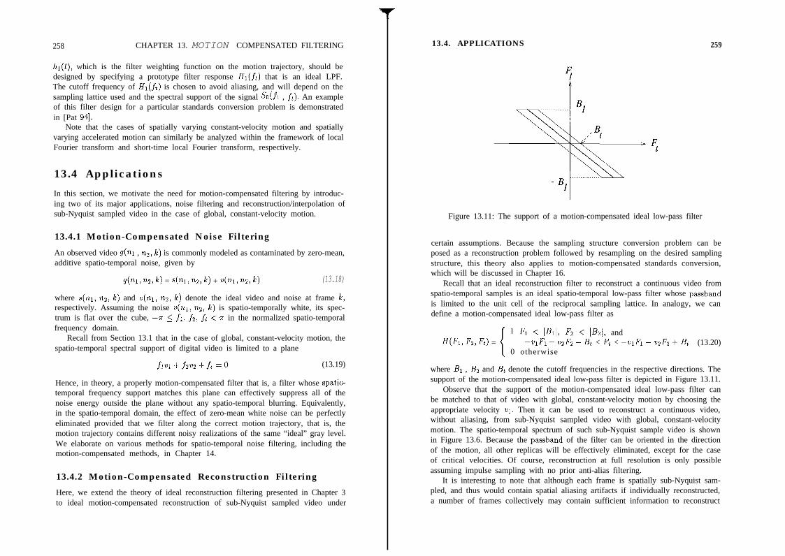
258 CHAPTER 13. MOTION COMPENSATED FILTERING
hr(t), which is the filter weighting function on the motion trajectory, should bedesigned by specifying a prototype filter response HI that is an ideal LPF.The cutoff frequency of Hr(ft) is chosen to avoid aliasing, and will depend on thesampling lattice used and the spectral support of the signal Sc(fr , ft). An exampleof this filter design for a particular standards conversion problem is demonstratedin [Pat 941.
Note that the cases of spatially varying constant-velocity motion and spatiallyvarying accelerated motion can similarly be analyzed within the framework of localFourier transform and short-time local Fourier transform, respectively.
13.4 Applications
In this section, we motivate the need for motion-compensated filtering by introduc-ing two of its major applications, noise filtering and reconstruction/interpolation ofsub-Nyquist sampled video in the case of global, constant-velocity motion.
13.4.1 Motion-Compensated Noise Filtering
An observed video g(nr , nz, le) is commonly modeled as contaminated by zero-mean,additive spatio-temporal noise, given by
g(nl, 122, k) = s(w) 712, k) + 4121) nz, k) (13.18)
where s(nl, nz, R) and v(ni, n2, Ic) denote the ideal video and noise at frame I%,respectively. Assuming the noise v(nl, n2, k) is spatio-temporally white, its spec-trum is flat over the cube, --7~ 5 fi, fz, ft < r in the normalized spatio-temporalfrequency domain.
Recall from Section 13.1 that in the case of global, constant-velocity motion, thespatio-temporal spectral support of digital video is limited to a plane
flvl+fz~2+ft=o (13.19)
Hence, in theory, a properly motion-compensated filter that is, a filter whose spatio-temporal frequency support matches this plane can effectively suppress all of thenoise energy outside the plane without any spatio-temporal blurring. Equivalently,in the spatio-temporal domain, the effect of zero-mean white noise can be perfectlyeliminated provided that we filter along the correct motion trajectory, that is, themotion trajectory contains different noisy realizations of the same “ideal” gray level.We elaborate on various methods for spatio-temporal noise filtering, including themotion-compensated methods, in Chapter 14.
13.4.2 Motion-Compensated Reconstruction Filtering
Here, we extend the theory of ideal reconstruction filtering presented in Chapter 3to ideal motion-compensated reconstruction of sub-Nyquist sampled video under
13.4. APPLICATIONS 259
Figure 13.11: The support of a motion-compensated ideal low-pass filter
certain assumptions. Because the sampling structure conversion problem can beposed as a reconstruction problem followed by resampling on the desired samplingstructure, this theory also applies to motion-compensated standards conversion,which will be discussed in Chapter 16.
Recall that an ideal reconstruction filter to reconstruct a continuous video fromspatio-temporal samples is an ideal spatio-temporal low-pass filter whose passbandis limited to the unit cell of the reciprocal sampling lattice. In analogy, we candefine a motion-compensated ideal low-pass filter as
1
1 Fl < I&I, Fz < IBzl, andH(Fl, F2, Ft) = -vlFl- VZF, - Bt < Ft < -vlF~ - v2Fz + Bt (13.20)
0 otherwise
where Br , Bz and Bt denote the cutoff frequencies in the respective directions. Thesupport of the motion-compensated ideal low-pass filter is depicted in Figure 13.11.
Observe that the support of the motion-compensated ideal low-pass filter canbe matched to that of video with global, constant-velocity motion by choosing theappropriate velocity ~1. Then it can be used to reconstruct a continuous video,without aliasing, from sub-Nyquist sampled video with global, constant-velocitymotion. The spatio-temporal spectrum of such sub-Nyquist sample video is shownin Figure 13.6. Because the passband of the filter can be oriented in the directionof the motion, all other replicas will be effectively eliminated, except for the caseof critical velocities. Of course, reconstruction at full resolution is only possibleassuming impulse sampling with no prior anti-alias filtering.
It is interesting to note that although each frame is spatially sub-Nyquist sam-pled, and thus would contain spatial aliasing artifacts if individually reconstructed,a number of frames collectively may contain sufficient information to reconstruct

260 CHAPTER 13. MOTION COMPENSATED FILTERING
Figure 13.12: (a) Progressive sampling, v # 0; b) interlaced sampling, v = 0
~~(21, ~2, t), The “new” information may be provided by. the subpixel valued motion vectors,. the sampling lattice, orl a combination of the two.
Two examples in which “new” information is present in consecutive frames areshown in Figure 13.12. Note that in the first example the new information isprovided by the interframe motion, whereas in the second the new information isprovided by the sampling lattice. In theory, perfect reconstruction is possible frommultiple frames even if they are not spatially bandlimited. Of course, this wouldrequire an infinite number of sampled frames. Various algorithms for standards con-version and high-resolution reconstruction will be discussed in Chapters 16 and 17.
13.5 Exercises
1. This problem extends the spectral analysis of motion compensation to videowith global, accelerated motion. Let the short-time spectrum (STS) of videobe defined by
S,‘,“‘(Fl, F2, Ft) =J/S
sc(x1, zz,v+ - to)
exp{-j2n(~~;zl+ Fzxz + Ftt)} dxldxzdt
where h(t) denotes the temporal analysis window. Show that the STS of avideo signal modeled by (13.10) can be expressed as
S,‘,h’(Wz,Ft) = So(F,,Fz)[H(Ft t FIVI + F2v2) exp{-j2a(Ft + F1~1 t F2w)~o)l *it Q(Fl, F2, Ft)
BIBLIOGRAPHY 261
where
Q(Fl, Fz, Ft) = Tt exp{-j2a(Fl$ $ F2$)}>
*F~ denotes 1-D convolution over the variable Ft, and ?=t denotes 1-D Fouriertransform with respect to t.
Show that this expression reduces to (13.7) when al = Q = 0, and h(t) = 1for all t.
2. Consider the case of a space-varying 2-D motion, which can be modeled locallyby a piecewise quadratic flow model. Extend the STS analysis frameworkdeveloped in Exercise 1 to this case by employing a spatio-temporal analysiswindow.
3. Can you conclude that the best motion-compensated filtering strategy is fil-tering along the motion trajectory, even in the case of an arbitrary motiontrajectory?
4. Suppose we have a video with global, constant-velocity motion, modeled by(13.2). Show that the motion-compensated ideal low-pass filter (13.20), tunedto the nominal velocity (VI) Vz), passes the video if the actual velocity (~1) ~2)satisfies
Plot the velocity passband (the range of velocities for which the filter allowsvideo to pass with no attenuation) in the velocity plane (VI, 7~).
5. Comment on the tradeoffs between the width of the passband versus thenumber of framestores required to implement a motion-compensated low-passfilter, and the ability to reject close replicas versus motion estimation errors.
Bibliography
[Dub 921 E. Dubois, “Motion-compensated filtering of time-varying images,”Multi&m. Syst. Sign. Proc., vol. 3, pp. 211-239, 1992.
[Gir 931 B. Girod, “Motion compensation: Visual aspects, accuracy, and fun-damental limits,” in Motion Analysis and Image Sequence Processing,M. I. Sezan and R. L. Lagendijk, eds., Norwell, MA: Kluwer, 1993.
[Pat 941 A. J. Patti, M. I. Sezan, and A. M. Tekalp, “Digital video standards con-version in the presence of accelerated motion,” Signal Proc.: Image Com-munication, vol. 6, pp. 213-227, June 1994.
Chapter 14
NOISE FILTERING
Image recording systems are not perfect. As a result, all images are contaminatedby noise to various levels, which may or may not be visible. Sources of noise includeelectronic noise, photon noise, film-grain noise, and quantization noise. In videoscanned from motion picture film, streaks due to possible scratches on film aregenerally modeled by impulsive noise. Speckle noise is common in radar image.sequences and biomedical tine-ultrasound sequences. The level of noise m an imageis generally specified in terms of a signal-to-noise ratio (SNR), which may be definedin a number of ways. If the SNR is below a certain level, the noise becomes visible asa pattern of graininess, resulting in a degradation of the image quality. Even if thenoise may not be perceived at full-speed video due to the temporal masking effect ofthe eye, it often leads to unacceptable “freeze-frames.” In addition to degradationof visual quality, the noise pattern may mask important image detail and increasethe entropy of the image, hindering effective compression.
The SNR of video can be enhanced by spatio-temporal filtering, which is basedon some sort of modeling of the image and noise characteristics. It should be ratherobvious that exact separation of variations in the recorded image intensity which aredue to noise from genuine image detail is impossible. To this effect, both the imageand noise will be characterized by statistical models. In general, the noise can bemodeled as additive or multiplicative, signal-dependent or signal-independent, andwhite or colored. For example, photon noise and film-grain are signal-dependent,whereas CCD sensor noise and quantization noise are usually modeled as white,Gaussian distributed, and signal-independent. Ghosts in TV images can also bemodeled as signal-dependent noise. In this chapter, we will assume a simple additivenoise model given by
g(nl,nz,le)=s(nl,nz,~)+w(nl~nz~le) (14.1)
where s(nl,nz,k) and v(ni,nz,lc) denote the ideal video and noise at frame k,respectively.
262
14.1. INTRAFRAME FILTERING 263
Noise filters can be classified as spatial (intraframe) filters and spatio-temporal(interframe) filters. Spatial filters, covered in Section 14.1, may be used to filter eachframe independently. However, in intraframe filtering, there is a tradeoff betweennoise reduction and spatial blurring of the image detail. Spatio-temporal filtersare 3-D filters with two spatial coordinates and one temporal coordinate [Sam 85,Alp 90, Arc 91, Kat 911. They utilize not only the spatial correlations, but alsothe temporal correlations between the frames. We classify spatio-temporal noisefilters as motion-adaptive and motion-compensated filters, which are treated inSections 14.2 and 14.3, respectively. Motion-adaptive filtering utilizes a motion-detection scheme, but does not require explicit estimation of the interframe motionvectors. This is distinct from motion-compensated filtering schemes, which operatealong motion trajectories, thus requiring exact knowledge of the trajectories at eachpixel.
14.1 Intraframe Filtering
Spatial filtering for image enhancement and restoration has received significant at-tention in the image processing literature over the last three decades. Image en-hancement generally refers to eliminating the noise as well as sharpening the imagedetail. In this section, we provide an overview of noise filtering techniques. Manyother still-frame image enhancement techniques, including contrast adjustment byhistogram equalization and unsharp masking, will not be treated in this book. Thereader is referred to [Lim 901 for a detailed presentation of these techniques and edgedetection methods. The discussion of intraframe image restoration methods for de-blurring of blurred images is deferred until Chapter 15. We can classify intraframenoise filters into three categories: (i) linear, shift-invariant (LSI) filters, such as theweighted averaging filters and linear minimum mean square error (LMMSE) filters,also known as Wiener filters, (ii) nonlinear filters, such as median filters and otherorder statistics filters, and (iii) adaptive filters, such as directional smoothing filtersand local (space-varying) LMMSE filters.
LSI noise filters can be designed and analyzed using frequency domain concepts,and are easier to implement. However, they present a tradeoff between noise re-duction and sharpness of the image detail. This is because any LSI noise reductionfilter is essentially a low-pass filter which eliminates high-frequency noise. Imagesusually feature a low-pass Fourier spectra, and the Fourier spectrum of the noiseis flat, assuming white noise. As illustrated in Figure 14.1, an LSI noise reductionfilter attenuates those frequencies where the noise power exceeds the signal power.As a result, the high-frequency content of the image is also attenuated, causing blur-ring. In the following, we study the optimal LSI filtering, and two approaches foradaptive filtering where the filter characteristics vary with the spatial coordinatesto preserve edges and other image detail.
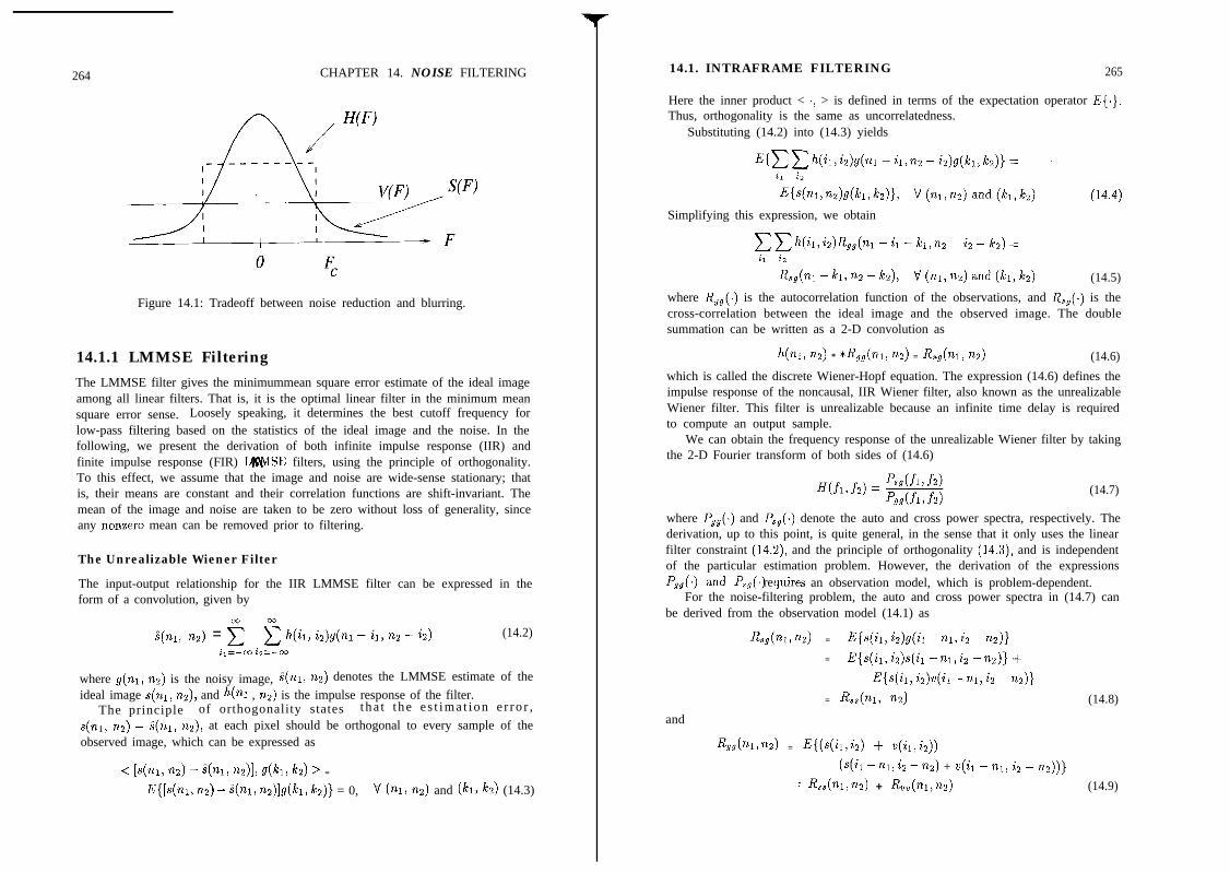
264 CHAPTER 14. NOISE FILTERING
Figure 14.1: Tradeoff between noise reduction and blurring.
14.1.1 LMMSE FilteringThe LMMSE filter gives the minimummean square error estimate of the ideal imageamong all linear filters. That is, it is the optimal linear filter in the minimum meansquare error sense. Loosely speaking, it determines the best cutoff frequency forlow-pass filtering based on the statistics of the ideal image and the noise. In thefollowing, we present the derivation of both infinite impulse response (IIR) andfinite impulse response (FIR) LWSE filters, using the principle of orthogonality.To this effect, we assume that the image and noise are wide-sense stationary; thatis, their means are constant and their correlation functions are shift-invariant. Themean of the image and noise are taken to be zero without loss of generality, sinceany nonzero mean can be removed prior to filtering.
The Unrealizable Wiener Filter
The input-output relationship for the IIR LMMSE filter can be expressed in theform of a convolution, given by
L(n1, n2) = 2 5 h(il, iz)g(n1 - il, 122 - iz) (14.2)i,=-co iz=-cn
where g(nr, nz) is the noisy image, i(ni, na) denotes the LMMSE estimate of theideal image s(ni, nz), and h(nr , n2) is the impulse response of the filter.
The principle of orthogonality states tha t t he e s t ima t ion e r ro r ,s(nr, nz) - i(nr, ns), at each pixel should be orthogonal to every sample of theobserved image, which can be expressed as
< [s(m, n2) - qw, %)I, g(h, h) > =
E{[s(nr, no) - i(ni, n2)]g(Icr, lez)} = 0, V (nr, nz) and (ICI, ICZ) (14.3)
14.1. INTRAFRAME FILTERING 265
Here the inner product < ., > is defined in terms of the expectation operator E{.}.Thus, orthogonality is the same as uncorrelatedness.
Substituting (14.2) into (14.3) yields
Simplifying this expression, we obtain
CCh(ii,iz)R,,(ni - ii - kl,n2 - i2 - le2) =il iz
&,(nl - h, n2 - b), V (nl, n2) and (h, b) (14.5)
where R,,(.) is the autocorrelation function of the observations, and R,,(.) is thecross-correlation between the ideal image and the observed image. The doublesummation can be written as a 2-D convolution as
h(nl, w,) * *Rgg(nl, m) = &,(n~, 7~2) (14.6)
which is called the discrete Wiener-Hopf equation. The expression (14.6) defines theimpulse response of the noncausal, IIR Wiener filter, also known as the unrealizableWiener filter. This filter is unrealizable because an infinite time delay is requiredto compute an output sample.
We can obtain the frequency response of the unrealizable Wiener filter by takingthe 2-D Fourier transform of both sides of (14.6)
(14.7)
where Pgg(.) and Psg(.) denote the auto and cross power spectra, respectively. Thederivation, up to this point, is quite general, in the sense that it only uses the linearfilter constraint (14.2), and the principle of orthogonality (14.3)) and is independentof the particular estimation problem. However, the derivation of the expressionspgg(.> and J’sg(.) qre uires an observation model, which is problem-dependent.
For the noise-filtering problem, the auto and cross power spectra in (14.7) canbe derived from the observation model (14.1) as
R,g(w, nz) = E{S(il, i&7(& - 121, i2 - w)>
= E{S(il, i2)S(il - 121, iz - 74) +E{s(h, i2)4& - nl, i2 - n2))
= Rss(w, n2) (14.8)
and
%v(n1,n2) = Jq(s(G,iz) + W(il,iZ))
(s(il - 121, i2 - n2) + v(il - n1, i2 - n2)))= L(nl,n2) + Rvv(nl,n2) (14.9)
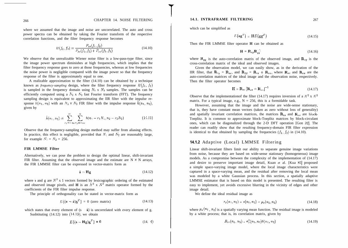
T266 CHAPTER 14. NOISE FILTERING
I14.1. INTRAFRAME FILTERING 267
where we assumed that the image and noise are uncorrelated. The auto and crosspower spectra can be obtained by taking the Fourier transform of the respectivecorrelation functions, and the filter frequency response becomes
(14.10)
We observe that the unrealizable Wiener noise filter is a low-pass-type filter, sincethe image power spectrum diminishes at high frequencies, which implies that thefilter frequency response goes to zero at those frequencies, whereas at low frequenciesthe noise power is negligible compared with the image power so that the frequencyresponse of the filter is approximately equal to one.
A realizable approximation to the filter (14.10) can be obtained by a techniqueknown as frequency-sampling design, where the filter frequency response H(fr, fz)is sampled in the frequency domain using Ni x Nz samples. The samples can beefficiently computed using a Ni x Nz fast Fourier transform (FFT). The frequencysampling design is equivalent to approximating the IIR filter with the impulse re-sponse h(nr, nz) with an Ni x Nz FIR filter with the impulse response i(ni, nz),given by
Observe that the frequency-sampling design method may suffer from aliasing effects.In practice, this effect is negligible, provided that Nr and Nz are reasonably large,for example Ni = N2 = 256.
which can be simplified as
WsgTl = =%gTl
Then the FIR LMMSE filter operator H can be obtained as
H = R,,R,-,1
(14.15)
(14.16)
where R,, is the auto-correlation matrix of the observed image, and R,, is thecross-correlation matrix of the ideal and observed images.
Given the observation model, we can easily show, as in the derivation of theIIR filter, that R,, = R,,, and R,, = R,, + R,,, where R,, and R,, are theauto-correlation matrices of the ideal image and the observation noise, respectively.Then the filter operator becomes
H = R,, [FL + RJ1 (14.17)
Observe that the implementationof the filter (14.17) requires inversion of a N2 x N2matrix. For a typical image, e.g., N = 256, this is a formidable task.
However, assuming that the image and the noise are wide-sense stationary,that is, they have constant mean vectors (taken as zero without loss of generality)and spatially invariant correlation matrices, the matrices R,, and R,, are block-Toeplitz. It is common to approximate block-Toeplitz matrices by block-circulantones, which can be diagonalized through the 2-D DFT operation [Gon 921. Thereader can readily show that the resulting frequency-domain FIR filter expressionis identical to that obtained by sampling the frequencies (fr, fz) in (14.10).
14.1.2 Adaptive (Local) LMMSE FilteringFIR LMMSE Filter
Alternatively, we can pose the problem to design the optimal linear, shift-invariantFIR filter. Assuming that the observed image and the estimate are N x N arrays,the FIR LMMSE filter can be expressed in vector-matrix form as
i=Hg (14.12)
where i and g are N2 x 1 vectors formed by lexicographic ordering of the estimatedand observed image pixels, and H is an N2 x N2 matrix operator formed by thecoefficients of the FIR filter impulse response.
Linear shift-invariant filters limit our ability to separate genuine image variationsfrom noise, because they are based on wide-sense stationary (homogeneous) imagemodels. As a compromise between the complexity of the implementation of (14.17)and desire to preserve important image detail, Kuan et al. [Kua 851 proposeda simple space-varying image model, where the local image characteristics werecaptured in a space-varying mean, and the residual after removing the local meanwas modeled by a white Gaussian process. In this section, a spatially adaptiveLMMSE estimator that is based on this model is presented. The resulting filter iseasy to implement, yet avoids excessive blurring in the vicinity of edges and otherimage detail.
The principle of orthogonality can be stated in vector-matrix form as
E{(s - s)gT} = 0 (zero matrix) (14.13)
which states that every element of (s - s) is uncorrelated with every element of g.Susbtituting (14.12) into (14.13), we obtain
We define the ideal residual image as
fs(w,nz) = s(n1,m) -ps(121,122) (14.18)
where f& (nr , Q) is a spatially varying mean function. The residual image is modeledby a white process; that is, its correlation matrix, given by
E{(s - Hg)gT} = 0 (14. 4 I Rrr(w, n2) = u:(w,nz)qnl, n2) (14.19)

268 CHAPTER 14. NOISE FILTERING
is diagonal. Note that the variance, u:(nl, ns) of the residual is allowed to changefrom pixel to pixel.
It follows t,hat the residual of the observed image, defined as
Tg(W,Q) = S(%,W) - fQ(%,4 (14.20)
where pLs(ni,nz) is the local mean of the observed image, is also zero-mean andwhite, because the noise is assumed to be zero-mean and white. Furthermore, from(14.1),
Pg(%, na) = ps(n1,nz) (14.21)
since the noise is zero-mean.Applying the filter (14.17) to the residual observation vector, rg = g - pLs which
is a zero-mean, wide-sense stationary image, we have
f, - ps = Hr,
= R,, [Rrr + L-’ k - ~gl (14.22)
The matrix R,, is diagonal because r,(ni, na) is white. Then the above vector-matrix expression simplifies to the scalar form
qn1, n2) = Pg(nl, 4 + n1, ,nz) - P”SWl m)l (14.23)
which has a predictor-corrector structure.Note that the adaptive LMMSE filter (14.23) requires the estimation of the mean
pls(ni, ns) and the variance ui(nr, 712) at each pixel. We estimate the local samplemean and sample variance over an M x M window, W, as
ps = pg = C dnl,nz) (14.24)(n1,nz)EW
and
fli = C [s(nl, n2) - pg(nl, n2)12 (14.25)(nl,Q)EW
We have
uf = max{,,Z - cri, 0) (14.26)
so that ui is always nonnegative. It is assumed that the variance of the noise u,” iseither known or can be estimated from a uniform image region.
It is interesting to note that when up is small, the second term in (14.23) isnegligible, and the adaptive LMMSE filter approaches a direct averaging filter. Onthe other hand, when cr: is large compared with u,,’ the filter is turned off. Becauselarge rrf usually indicates presence of edges, the adaptive LMMSE filter preservesedges by effectively turning the filter off across edges. Consequently, some noise isleft in the vicinity of edges which may be visually disturbing.
14.1. INTRAFRAME FILTERING
14.1.3 Directional Filtering
269
An alternative approach for edge-preserving filtering is the directional filtering ap-proach, where we filter along the edges, but not across them. The directionalfiltering approach may in fact be superior to adaptive LMMSE filtering, since noisearound the edges can effectively be eliminated by filtering along the edges, as op-posed to turning the filter off in the neighborhood of edges.
In directional filtering, possible edge orientations are generally quantized intofour, 0 deg, 45 deg, 90 deg, and 135 deg; and five FIR filter kernels, one for each ori-entation and one for nonedge regions are defined. The supports of the edge-orientedFIR filters are depicted in Figure 14.2. In general, there exist two a.pproaches fordirectional filtering: i) select the most uniform support out of the five at each pixelaccording to a criterion of uniformity or by edge-detection [Dav 751, and ii) applyan edge-adaptive filter within each kernel at each pixel, and cascade the results.They are discussed in more detail in the following
/
7
T4 Ts
Figure 14.2: Directional filtering kernels.
i) Method I: The variance of pixels within each support can be used as a selectioncriterion. If the variance of the pixels within the nonedge kernel is more than apredetermined threshold, we decide that an edge is present at that pixel. Then theedge-kernel with the lowest variance indicates the most likely edge orientation atthat pixel. Filtering can be performed by averaging the pixels in the direction ofthe smallest variance. Filtering along the edge avoids spatial blurring to a largeextent.
ii) Method II: Alternatively, we can use a spatially adaptive filter, such as thelocal LMMSE filter, within each of the five supports at each pixel. Recall that the

270 CHAPTER 14. NOISE FILTERING
local LMMSE filter is effectively off within those supports with a high variance, andapproaches direct averaging as the signal variance goes to zero. Thus, cascadingthe five filters as [Cha 851
T = TlT2T3T4T5 (14.27)
where Ti is the local LMMSE filter applied over the respective kernel, we expectthat effective filtering is performed only over those kernels with a small variance.This method avoids the support selection process by using adaptive filtering withineach support.
Directional filtering, using either method, usually offers satisfactory noise reduc-tion around edges, since at least one of the filters should be active at every pixel.In contrast, the local LMMSE filter performs very little filtering in windows withan edge, leaving a significant amount of noise around edges.
14.1.4 Median and Weighted Median Filtering
Median filtering is a nonlinear operation that is implicitly edge-adaptive. The out-put i(nl) 712) of t.he median filter is given by the median of the pixels within thesupport of the filter, that is,
qn1> w) = Med {s(G) ia)} , for (G, i2) E Ben, ,n2) (14.28)
where &nl,n2) is the filter support centered about (nl, na), and “Med” denotesthe median operation. The median filter is edge-preserving because the medianoperation easily rejects outliers, avoiding blurring across edges [Arc 861. Fast algo-rithms for one- and two-dimensional (separable) median filtering exist for real-timeimplementations [Ata 801.
In median filtering each sample in the filter support is given an equal emphasis.The weighted median filter is an extension of the median filter where each sample(il, iz) is assigned a weight wil,ia. The weighting is achieved by replicating the(il) iz)th sample wil,iZ times. Then, the output of the weighted median filter isgiven by
i(n1, m.) = Med{w,,i, os(h,h)), for (G, Gt) E &nl,nz) (14.29)
where o is the replication operator. The properties of the filter vary depending onhow the weights are assigned. The reader is referred to [Arc 911 and the referencestherein for other generalizations of median filtering, including order statistic andmultistage order statistic filters.
14.2 Motion-Adaptive FilteringIn video processing, interframe noise filtering may provide several advantages overintraframe filtering. A special class of interframe filters is temporal filters, which
14.2. MOTION-ADAPTIVE FILTERING 271
employ 1-D filtering in the temporal direction [McM 79, Den 80, Hua 81, Dub 84,Mar 85, Sez 91, Rei 91, Boy 921. In principle, temporal filters can avoid spatial andtemporal blurring. In this section, we discuss motion-adaptive noise filters wherethere is no explicit motion estimation. The filters that are presented here are appliedover a fixed spatio-temporal support at each pixel. We start with direct filteringwhere there is no adaptivity at all, or the adaptivity is implicit in the filter design.Next, we discuss filter structures, where some coefficients vary as a function of aso-called “motion-detection” signal.
14.2.1 Direct Filtering
The simplest form of direct filtering is frame averaging, where we average pixelsoccupying the same spatial coordinates in consecutive frames. Direct temporalaveraging is well-suited to stationary parts of the image, because averaging multipleobservations of essentially the same pixel in different frames eliminates noise whileresulting in no loss of spatial image resolution. It is well known that direct averagingin this case corresponds to maximum likelihood estimation under the assumptionof white, Gaussian noise, and reduces the variance of the noise by a factor of N,where N is the number of samples. It follows that in purely temporal filtering alarge number of frames may be needed for effective noise reduction, which requiresa large number of frame stores. Spatio-temporal filtering provides a compromisebetween the number of frame stores needed for effective noise reduction and theamount of spatial blurring introduced.
Although direct temporal averaging serves well for stationary image regions,it may lead to smearing and chrominance separation in the moving areas. Directtemporal averaging causes temporal blurring in the same way that direct spatial av-eraging leads to spatial blurring, that is, when there are sudden temporal variations.These degradations may be avoided if the filter makes use of interframe motion in-formation. A fundamental question is how to distinguish the temporal variationsdue to motion from those due to noise. Motion-adaptive filtering is the temporalcounterpart of edge-preserving spatial filtering in that frame-to-frame motion givesrise to temporal edges. It follows that spatio-temporal noise filters that adapt tomotion can be obtained by using structures similar to t,hose of t,he edge-preservingfilters. Examples of such filters include directional filters and order statistic filters,including median, weighted median, and multistage median filters [Arc 911.
For instance, Martinez and Lim [Mar 851 proposed a cascade of five one-dimensional finite impulse response (FIR) 1’inear minimum mean square error(LMMSE) estimators over a set of five hypothesized motion trajectories at eachpixel. These trajectories correspond to no motion, motion in the +zl direction,motion in the -21 direction, motion in the +z2 direction, and motion in the -ZZdirection. Due to the adaptive nature of the LMMSE estimator, filtering is effectiveonly along hypothesized trajectories that are close to actual ones. This approachhas been reported to be successful in cases where one of the hypothesized motiontrajectories is close to the actual one.

272 CHAPTER 14. NOISE FILTERING
14.2.2 Motion-Detection Based Filtering
In this approach, the selected filter structure has parameters which can be tunedaccording to a motion detection signal, such as the frame difference. Both FIR andIIR filter structures can be employed in motion adaptive filtering. A simple exampleof a motion-adaptive FIR filter may be given by
qn,, 122, k) = (l-y) g(nl, n2, k) + y g(nl, 122, k - I) (14.30)
and that of an IIR filter by
i(nl, nz, k) = (l-y)g(nl,nz,k) + yi(nl,nz,k--I) (14.31)
where
y - max{O,~-nlg(ni,n2,~)--9(n1,nZ~~-l)lis the motion detection signal, and (Y is a scaling constant. Observe that thesefilters tend to turn off filtering when a large motion is detected in an attempt toprevent artifacts. The FIR structure has limited noise reduction ability, especiallywhen used as a purely temporal filter with a small number of frames, because thereduction in the noise variance is proportional to the number of samples in the filtersupport. IIR filters are more effective in noise reduction, but they generally causeFourier phase distortions.
Several implementations of noise filters based on the above structures have beenproposed in the literature, which generally differ in the way they compute themotion-detection signal. Use of motion-adaptive IIR filters in practical systemshave been demonstrated by McMann e2 al. [McM 791 and Dennis [Den 801.
14.3 Motion-Compensated Filtering
The motion-compensated approach is based on the assumption that the variation ofthe pixel gray levels over any motion trajectory ~(7; 21, 22, t) is due mainly to noise.Recall from the definition of the motion trajectory in Chapter 13 that c(~; 21, xz,t)is a continuous-valued vector function returning the coordinates of a point at timeT that corresponds to the point (xl, ~2) at time t. Thus, noise in both the station-ary and moving areas of the image can effectively be reduced by low-pass filteringover the respective motion trajectory at each pixel. Motion-compensated filtersdiffer according to (i) the motion estimation method, (ii) the support of the filter,(e.g., temporal vs. spatio-temporal) and (iii) the filter structure (e.g., FIR vs. IIR,adaptive vs. nonadaptive).
The concept and estimation of a motion trajectory in spatio-temporally sampledimage sequences are illustrated in Figure 14.3. Suppose we wish to filter the kthframeofanimagesequenceusingNframesIc-M,...,le-1,Ic,lc+1,...,le+M,where N = 2M + 1. The first step is to estimate the discrete motion trajectory
14.3. MOTION-COMPENSATED FILTERING 273
k-2 k-l Frame k k+l k+2
- - - - - - - 3 Motion estimation path
, Motion trajectory at (nl, 9, k)
Figure 14.3: Estimation of the motion trajectory (N=5).
c(l; nl, n2, k), I = k-M,. .) k-l, I%, k+l, , k+M, at each pixel (nl, n2) ofthe kthframe. The function c(I; nl, n2, k) is a continuous-valued vector function returningthe (21,x2) coordinates of the point in frame 1 which corresponds to the pixel(nl, n2) of the kth frame, The discrete motion trajectory is depicted by the solidline in Figure 14.3 for the case of N = 5 frames. In estimating the trajectory, thedisplacement vectors are usually estimated in reference to the frame k as indicatedby the dotted lines. The trajectory in general passes through subpixel locations,where the intensities can be determined via spatial or spatio-temporal interpolation.The support Snl,nz,le of a motion-compensated spatio-temporal filter is defined asthe union of predetermined spatial neighborhoods (e.g., 3 x 3 regions) centered aboutthe pixel (subpixel) locations along the motion trajectory. In temporal filtering, thefilter support Sral,nz,k coincides with the motion trajectory ~(1; n1, nz, k). Clearly,the effectiveness of motion-compensated spatio-temporal filtering is strongly relatedto the accuracy of the motion estimates.
Various filtering techniques, ranging from averaging to more sophisticated adap-tive filtering, can be employed given the motion-compensated filter support. In theideal case, where the motion estimation is perfect, direct averaging of image inten-sities along a motion trajectory provides effective noise reduction [Hua 81, Mar 851.In practice, motion estimation is hardly ever perfect due to noise and sudden scenechanges, as well as changing camera views. As a result, image intensities overan estimated motion trajectory may not necessarily correspond to the same im-age structure, and direct temporal averaging may yield artifacts. In the case ofspatio-temporal filtering, there may also be spatial variations within the support;hence the need for adaptive filter structures over the motion-compensated filtersupport. Here, we consider two adaptive filter structures: the adaptive LMMSEfilter, which is aimed at reducing the amount of filtering whenever a nonuniformity
274 CHAPTER 14. NOISE FILTERING 14.3. MOTION-COMPENSATED FILTERING 275
is detected within the motion-compensated support, and the adaptive weighted av-eraging (AWA) filter, which is aimed at weighting down the effect of the outliersthat create the nonuniformity and achieving effective filtering by concentrating onthe remaining similar image intensities.
14.3.1 Spatio-Temporal Adaptive LMMSE FilteringThe motion-compensated adaptive LMMSE filter [Sam 85, Sez 911 is an extension ofthe edge-preserving spatial filter proposed by Lee [Lee 801 and Kuan et al. [Kua 851to the spatio-temporal domain, where the local spatial statistics are replaced by theirspatio-temporal counterparts. Then, the estimate of the pixel value at (ni, n2, k) isgiven by
where p,(ni, ns, Ic) and uy(ni, nz, k) denote the ensemble mean and variance of thecorresponding signal, respectively. Depending on whether we use spatio-temporal ortemporal statistics, this filter will be referred to as the LMMSE-ST or the LMMSE-T filter, respectively.
We assume that the noise can be modeled as
where u(nl, n2, le) is a wide sense stationary process with zero mean, which is in-dependent of the signal, and cy is a real number. The film grain noise is com-monly modeled with (Y = l/3 [Hua 661. Observe that the signal-independentnoise is a special case of this model with o = 0. Under this model, we have~L,(nl,nz,le)=~Lg(n1,n2,le),anda~(nl,nz,~)=ug2(nl,nz,k)-a~(nl,n2,~),wheregz(ni, n2, k) denotes the spatio-temporal variance of the noise process.
In practice, the ensemble mean pLs(ni, nz, k) and variance ui(nl, n2, k) are re-placed with the sample mean j&(ni,ns, /r) and variance Si(nl,nz,k), which arecomputed within the support Snl,nz,k as
Ps(nl,n2,k) = k c g(~1,~z;-e) (14.33)
(il,i2;qE%, ,rQ,*
and
c?fj(nl,nz,k) = + C [g(il,i2;e)-pg(nl,n2,1C)12 (14.34)
(il,iz;qESn,,n,,k
where L is the number of pixels in Sfal,na,k. Then
(14.35)
in order to avoid the possibility of a negative variance estimate.Substituting these estimates into the filter expression (14.32), we have
i(nl, 122, k) =fiZ(nl, 122, k)
6:(n1, n2, k) + 6Z(nl,n2,k) dnl, n2, k)
++(nl, n2, R)
&-,2(7x1, n2, k) + SZ(nl, m, k>&(nl, 122, k) (14.36)
The adaptive nature of the filter can be observed from (14.36). When the spatio-temporal signal variance is much smaller than the noise variance, ?:(ni, nz, le) z 0,that is, the support Snl,raa,k is uniform, the estimate approaches the spatio-temporalmean, & = is. In the extreme, when the spatio-temporal signal variance is muchlarger than the noise variance, $(nl,n2,k) > Si(nl,nz,k), due to poor motionestimation or the presence of sharp spatial edges in Snl,na,h, the estimate approachesthe noisy image value to avoid blurring.
A drawback of the adaptive LMMSE filter is that it turns the filtering down evenif there is a single outlier pixel in the filter support, thus often leaving noisy spotsin the filtered image. An alternative implementation, called “the switched LMMSEfilter (LMMSE-SW),” may maintain the advantages of both the spatio-temporaland the temporal LMMSE filtering by switching between a selected set of temporaland spatio-temporal supports at each pixel, depending on which support is the mostuniform [Ozk 931. If the variance $(nl, nz, rE) computed over Snl,nz,k is less thanthe noise variance, then the filtering is performed using this support; otherwise, thelargest support over which $(nl, n2, Ic) is less than the noise variance is selected. Inthe next section, we introduce an adaptive weighted averaging (AWA) filter whichemploys an implicit mechanism for selecting the most uniform subset within Snl,nz,kfor filtering.
14.3.2 Adaptive Weighted Averaging FilterThe adaptive weighted averaging (AWA) filter computes a weighted average of theimage values within the spatio-temporal support along the motion trajectory. Theweights are determined by optimizing a criterion functional, and they vary withthe accuracy of motion estimation as well as the spatial uniformity of the regionaround the motion trajectory. In the case of sufficiently accurate motion estimationacross the entire trajectory and spatial uniformity, image values within the spatio-temporal filter support attain equal weights, and the AWA filter performs directspatio-temporal averaging. When the value of a certain pixel within the spatio-temporal support deviates from the value of the pixel to be filtered by more than athreshold, its weight decreases, shifting the emphasis to the remaining image valueswithin the support that better matches the pixel of interest. The AWA filter istherefore particularly well suited for efficient filtering of sequences containing seg-ments with varying scene contents due, for example, to rapid zooming and changesin the view of the camera.

276 CHAPTER 14. NOISE FILTERING
The AWA filter can be defined by
where
w(il,iz;e) - IC(nl, 122, E)l+a max{c2, [g(nl,nz,le)-g(il,iz;e)l’}
(14.38)
are the weights within the support Snl,nz,k and K(ni, n2, %) is a normalizationconstant, given by
K(nl, 122, k) = ( C1
1+ a max{t2 ) [g(nl, n2, k) - g(ii, ~z;~)12~)-’ (14.39)
(ii,iz;+srL1,r‘,,l,
The quantities a (u > 0) and t are the parameters of the filter. These parametersare determined according to the following principles:
1) When the differences in the intensities of pixels within the spatio-temporalsupport are merely due to noise, it is desirable that the weighted averaging reducesto direct averaging. This can be achieved by appropriately selecting the param-eter c2, Note that, if the square of the differences are less than t2, then all theweights attain the same value K/(1 + at’) = l/L, and i(ni, nz, Ic) reduces to directaveraging. We set the value of t2 equal to two times the value of the noise variance,i.e., the expected value of the square of the difference between two image valuesthat differ due to the presence of noise only.
2) If the square of the difference between the values g(nl, nz, Ic) and g(ii, iz; 1) fora particular (iI,&,!) E Snl,nz,t is larger than t2, then the contribution of g(il, i2;1)is weighted down by w(il, is;!) < w(nl, n2, Ic) = K/(1 + UC’). The parameter a isa “penalty” parameter that determines the sensitivity of the weight to the squareddifference [g(ni, nz, lc)-g(ii, iz; l)]“. The “penalty” parameter a is usually set equalto unity.
The effect of the penalty parameter a on the performance of the AWA filtercan be best visualized considering a special case where one of the frames withinthe filter support is substantially different from the rest. In the extreme, whena = 0, all weights are equal. That is, there is no penalty for a mismatch, and theAWA filter performs direct averaging. However, for a large, the weights for the2M “matching” frames are equal, whereas the weight of the nonmatching frameapproaches zero. Generally speaking, the AWA filter takes the form of a “limited-amplitude averager,” where those pixels whose intensities differ from that of thecenter pixel by not more than &C are averaged. A similar algorithm is K nearestneighbor averaging [Dav 781, where the average of K pixels within a certain windowwhose values are closest to the value of the pixel of interest are computed.
14.4. EXAMPLES 277
14.4 Examples
We demonstrate the performance of the motion-compensated LMMSE and AWAfilters with temporal and spatio-temporal supports using five frames of an imagesequence scanned from motion picture film at a resolution of 1216 pixel x 832 lines.The central three frames of the sequence, degraded by actual film-grain noise, areshown in Figure 14.4.
The motion trajectories have been estimated as shown in Figure 14.3, by ahierarchical block-matching algorithm with five levels using log-D search, the MADcriterion, and l/4 pixel accuracy. We have estimated the variance of the noiseprocess over a uniform region in the frame to be filtered (selected interactively).In the LMMSE filter the noise variance appears directly in the filter expression,whereas in the AWA filter it is used in defining the filter parameter c’, which istypically set equal to twice the estimated noise variance. Figure 14.5 (b-f) showthe results of applying the temporal LMMSE, spatio-temporal LMMSE, switchedLMMSE, temporal AWA, and spatio-temporal AWA filters, respectively, on thenoisy face section depicted in Figure 14.5 (a). Figure 14.6 shows the same set ofresults on the hand section. Inspection of the results suggests that the spatio-temporal filters provide better noise reduction than the respective temporal filters,at the expense of introducing some blurring. The switched LMMSE filter strikesthe best balance between noise reduction and retaining image sharpness. The visualdifference between the results of the LMMSE and AWA filters was insignificant forthis particular sequence, because there were no sudden scene changes involved. Ithas been shown that the AWA filter outperforms the LMMSE filter, especially incases of low input SNR and abruptly varying scene content [Ozk 931.
14.5 Exercises
1. In the Wiener filter (14.10), how would you estimate the power spectrum ofthe original image P,,(fi, fi) and the noise P,,(fl, fz)?
2. Let s denote the lexicographic ordering of pixel intensities in an image. Showthat convolution by an FIR filter kernel h(ni, nz) can be expressed as y = Hs,where H is block-Toeplitz and block-circulant for linear and circular convolu-tion, respectively. Write the elements of H in terms of h(ni, nz).
3. Show that a block-circulant matrix can be diagonalized by a 2-D DFT.
4. Show a complete derivation of (14.23)
5. How do you compare motion-adaptive filtering and adaptive motion-compensated filtering in the presence of motion estimation errors?
6. How would you compare the motion-compensated adaptive LMMSE and AWAfilters in the presence of a sudden scene change?

278 CHAPTER 14. NOISE FILTERING
!
Figure 14.4: Three frames of a sequence digitized from motion picture film.
14.5. EXERCISES 279
Figure 14.5: Comparison of the filters at the central frame (the face section):a) the noisy’original (top-left), b) tem oral LMMSE filtering (top-right), c) spatio-ptemporal LMMSE filtering (center-left), d) switched LMMSE filtering, (center-right) e) temporal AWA filtering (bottom-left), and f) spatio-temporal AWAfiltering (bottom-right). (Courtesy Mehmet Ozkan)
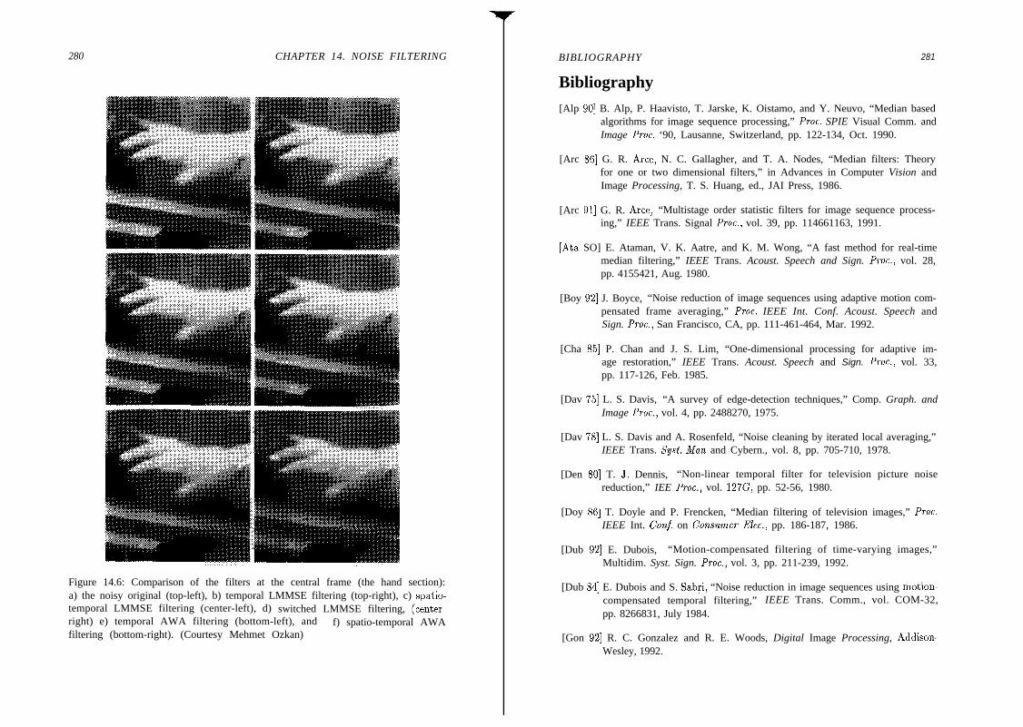
280 CHAPTER 14. NOISE FILTERING
Figure 14.6: Comparison of the filters at the central frame (the hand section):a) the noisy original (top-left), b) temporal LMMSE filtering (top-right), c) spatio-temporal LMMSE filtering (center-left), d) switched LMMSE filtering, (center-right) e) temporal AWA filtering (bottom-left), and f) spatio-temporal AWAfiltering (bottom-right). (Courtesy Mehmet Ozkan)
BIBLIOGRAPHY 281
Bibliography[Alp 901 B. Alp, P. Haavisto, T. Jarske, K. Oistamo, and Y. Neuvo, “Median based
algorithms for image sequence processing,” Proc. SPIE Visual Comm. andImage Proc. ‘90, Lausanne, Switzerland, pp. 122-134, Oct. 1990.
[Arc 861 G. R. Arce, N. C. Gallagher, and T. A. Nodes, “Median filters: Theoryfor one or two dimensional filters,” in Advances in Computer Vision andImage Processing, T. S. Huang, ed., JAI Press, 1986.
[Arc 911 G. R. Arce, “Multistage order statistic filters for image sequence process-ing,” IEEE Trans. Signal Proc., vol. 39, pp. 114661163, 1991.
[Ata SO] E. Ataman, V. K. Aatre, and K. M. Wong, “A fast method for real-timemedian filtering,” IEEE Trans. Acoust. Speech and Sign. Proc., vol. 28,pp. 4155421, Aug. 1980.
[Boy 921 J. Boyce, “Noise reduction of image sequences using adaptive motion com-pensated frame averaging,” Proc. IEEE Int. Conf. Acoust. Speech andSign. Proc., San Francisco, CA, pp. 111-461-464, Mar. 1992.
[Cha 851 P. Chan and J. S. Lim, “One-dimensional processing for adaptive im-age restoration,” IEEE Trans. Acoust. Speech and Sign. Proc., vol. 33,pp. 117-126, Feb. 1985.
[Dav 751 L. S. Davis, “A survey of edge-detection techniques,” Comp. Graph. andImage Proc., vol. 4, pp. 2488270, 1975.
[Dav 781 L. S. Davis and A. Rosenfeld, “Noise cleaning by iterated local averaging,”IEEE Trans. Sysl. Man and Cybern., vol. 8, pp. 705-710, 1978.
[Den 801 T. J. Dennis, “Non-linear temporal filter for television picture noisereduction,” IEE Proc., vol. 127G, pp. 52-56, 1980.
[Doy 861 T. Doyle and P. Frencken, “Median filtering of television images,” Proc.IEEE Int. Conf on Conslamer Elec., pp. 186-187, 1986.
[Dub 921 E. Dubois, “Motion-compensated filtering of time-varying images,”Multidim. Syst. Sign. Proc., vol. 3, pp. 211-239, 1992.
[Dub 841 E. Dubois and S. Sabri, “Noise reduction in image sequences using motion-compensated temporal filtering,” IEEE Trans. Comm., vol. COM-32,pp. 8266831, July 1984.
[Gon 921 R. C. Gonzalez and R. E. Woods, Digital Image Processing, Addison-Wesley, 1992.
282 BIBLIOGRAPHY
[Hua 661 T. S. Huang, “Some notes on film-grain noise,” in Restoration of At-mospherically Degraded Images, NSF Summer Study Rep., pp. 1055109,Woods Hole, MA, 1966.
[Hua 811 T. S. Huang and Y. P. Hsu, “Image sequence enhancement,” in Image
Sequence Analysis, T. S. Huang, ed., Berlin: Springer Verlag, 1981.
[Kat 911 A. K. Katsaggelos, R. P. Kleihorst, S. N. Efstratiadis, and R. L. Lagendijk,“Adaptive image sequence noise filtering methods,” Proc. SPIE Conf.Visual Comm. and Image Proc., Nov. 1991.
[Kua 851 D. T. Kuan, A. A. Sawchuk, T. C. Strand, and P. Chavel, “Adaptive noisesmoothing filter for images with signal-dependent noise”, IEEE Trans.Putt. Anal. Mach. Intel., vol. PAMI-7, pp. 165-177, Mar. 1985.
[Lee 801 J. S. Lee, “Digital image enhancement and noise filtering by use oflocal statistics,” IEEE Trans. Putt. Anal. Mach. Intel., vol. PAMI-2,pp. 165-168, Mar. 1980.
[Mar 851 D. Martinez and J. S. Lim, “Implicit motion compensated noise reductionof motion video scenes,” Proc. IEEE Int. Conf. Acoust. Speech, SignalProc., pp. 375-378, Tampa, FL, 1985.
[McM 791 R. H. McMann, S. Kreinik, J. K. Moore, A. Kaiser and J. Rossi, “Adigital noise reducer for encoded NTSC signals,” SMPTE Jour., vol. 87,pp. 129-133, Mar. 1979.
[Ozk 931 M. K. Ozkan, M. I. Sezan, and A. M. Tekalp, “Adaptive motion-compensated filtering of noisy image sequences,” IEEE Trans. Circuits
and Syst. for Video Tech., vol. 3, pp. 277-290, Aug. 1993.
[Rei 911 T. A. Reinen, “Noise reduction in heart movies by motion compensatedfiltering,” Proc. SPIE. VW. Comm. and Image Proc. ‘91, Boston, MA,pp. 755-763, Nov. 1991.
[Sam 851 R. Samy, “An adaptive image sequence filtering scheme based on motiondetection,” SPIE, vol. 596, pp. 135-144, 1985.
[Sez 911 M. I. Sezan, M. K. Ozkan, and S. V. Fogel, “Temporally adaptive filteringof noisy image sequences using a robust motion estimation algorithm,”Proc. IEEE Int. Cont. Acoust. Speech, Signal Processing, pp. 2429-2432,Toronto, Canada, 1991.
[Uns 901 M. Unser and M. Eden, “Weighted averaging of a set of noisy images formaximumsignal-to-noise ratio,” IEEE Trans. on Acoust., Speech and Sign.Proc., vol. ASSP-38, pp. 890-895, May 1990. i
Chapter 15
RESTORATION
Restoration refers to spatial deblurring of video degraded by optical smearing, in-cluding linear motion or out-of-focus blurs. Optical blurring arises when a singleobject point spreads over several image pixels, which may be due to relative motionbetween the object and the camera, or out-of-focus imaging. The extent of the spa-tial spread is determined by the point spread function (PSF) of the imaging system.The chapter starts with modeling of spatially invariant and spatially varying blurformation in Section 15.1. Temporal blurring is not discussed because it is oftennegligible. In the discrete spatio-temporal domain, the restoration problem can beformulated as solving a set of simultaneous linear equations, which simplifies to adeconvolution problem in the case of spatially invariant blurs. We present someselected intraframe methods for the restoration of spatially invariant and spatiallyvarying blurred images in Sections 15.2 and 15.3, respectively. Multiframe methodsfor image restoration are discussed in Section 15.4, where we make use of the tem-poral correlation and frame-to-frame motion information to better regularize therestoration process and/or identify the spatial extent of the blur PSF.
15 .1 Model ing
Images suffer from optical blurring as well as noise. Spatial blurring due to mo-tion and out-of-focus may be encountered in images acquired by fixed surveillancecameras, or cameras mounted on moving vehicles such as aircraft and robot-arms.Motion blurs are also common in still images of scenes with high activity, such asin freeze-frames of sports video. Temporal blurring in video is often negligible, andwill not be considered here. In the following, we discuss modeling of shift-invariantand shift-varying spatial blurring, respectively. A vector-matrix model for the mul-tiframe formulation, where each frame possibly suffers from a different spatial blur,is also presented.
283
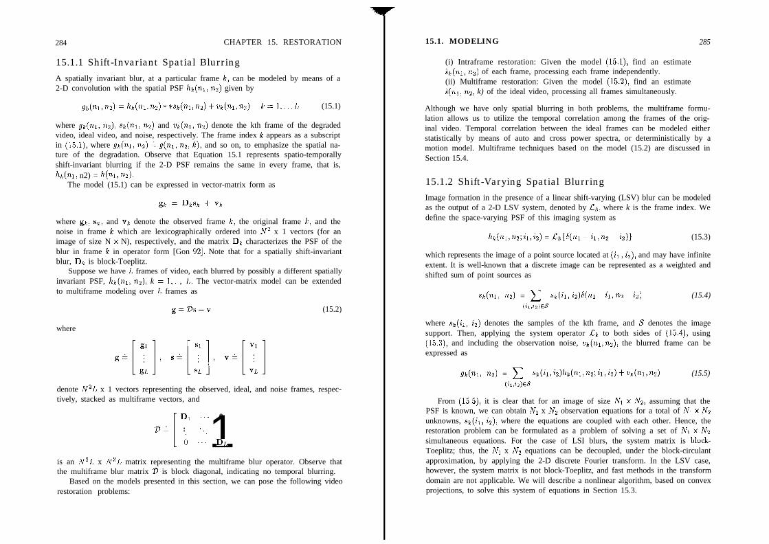
284 CHAPTER 15. RESTORATION
15.1.1 Shift-Invariant Spatial Blurring
A spatially invariant blur, at a particular frame k, can be modeled by means of a2-D convolution with the spatial PSF hk(l~i, nz) given by
gk(nl,nz) =~k(~l,~z)**~~(~l,~z)+~~(~l,~z) k= l,...L (15.1)
where gt(ni, 7~2)~ sk(ni, n2) and vk(ni, nz) denote the kth frame of the degradedvideo, ideal video, and noise, respectively. The frame index k appears as a subscriptin (15.1)) where gk(ni, nz) G g(nr, ng, k), and so on, to emphasize the spatial na-ture of the degradation. Observe that Equation 15.1 represents spatio-temporallyshift-invariant blurring if the 2-D PSF remains the same in every frame, that is,hk(nl, n2) = h(nl, 3).
The model (15.1) can be expressed in vector-matrix form as
where gt, sk, and vk denote the observed frame k, the original frame k, and thenoise in frame k which are lexicographically ordered into N2 x 1 vectors (for animage of size N x N), respectively, and the matrix Dk characterizes the PSF of theblur in frame k in operator form [Gon 921. Note that for a spatially shift-invariantblur, DI, is block-Toeplitz.
Suppose we have L frames of video, each blurred by possibly a different spatiallyinvariant PSF, hk(nl, na), k = 1,. , L. The vector-matrix model can be extendedto multiframe modeling over L frames as
g=Ds+v (15.2)
where
denote N’L x 1 vectors representing the observed, ideal, and noise frames, respec-tively, stacked as multiframe vectors, and
D1 ... 02,A : ‘., 1[ 1i ... DL
is an N’L x N’L matrix representing the multiframe blur operator. Observe thatthe multiframe blur matrix 2, is block diagonal, indicating no temporal blurring.
Based on the models presented in this section, we can pose the following videorestoration problems:
15.1. MODELING 285
(i) Intraframe restoration: Given the model (15.1)) find an estimateik(nl) n2) of each frame, processing each frame independently.(ii) Multiframe restoration: Given the model (15.2), find an estimatei(ni, 122, k) of the ideal video, processing all frames simultaneously.
Although we have only spatial blurring in both problems, the multiframe formu-lation allows us to utilize the temporal correlation among the frames of the orig-inal video. Temporal correlation between the ideal frames can be modeled eitherstatistically by means of auto and cross power spectra, or deterministically by amotion model. Multiframe techniques based on the model (15.2) are discussed inSection 15.4.
15.1.2 Shift-Varying Spatial Blurring
Image formation in the presence of a linear shift-varying (LSV) blur can be modeledas the output of a 2-D LSV system, denoted by Ck, where k is the frame index. Wedefine the space-varying PSF of this imaging system as
h(nl,nz;il,iz) = LCk{S(nl- h,n2 - i2)) (15.3)
which represents the image of a point source located at (ir ) iz), and may have infiniteextent. It is well-known that a discrete image can be represented as a weighted andshifted sum of point sources as
sk(n1, n2) = C sk(il) iz)S(nl - &, n2 - i2) (15.4)(il,iZ)ES
where sh(ii) i2) denotes the samples of the kth frame, and S denotes the imagesupport. Then, applying the system operator Lt to both sides of (15.4), using(15.3), and including the observation noise, vh(nl,nz), the blurred frame can beexpressed as
.a(nl, n2) = C sk(il,iz)hk(nl,nz;il, i2) + uk(nl,n2) (15.5)(~l,~Z)ES
From (15.5), it is clear that for an image of size Ni x Nz, assuming that thePSF is known, we can obtain Ni x Nz observation equations for a total of Ni x Nzunknowns, sk(ii, iz), where the equations are coupled with each other. Hence, therestoration problem can be formulated as a problem of solving a set of Ni x Nzsimultaneous equations. For the case of LSI blurs, the system matrix is block-Toeplitz; thus, the Ni x Nz equations can be decoupled, under the block-circulantapproximation, by applying the 2-D discrete Fourier transform. In the LSV case,however, the system matrix is not block-Toeplitz, and fast methods in the transformdomain are not applicable. We will describe a nonlinear algorithm, based on convexprojections, to solve this system of equations in Section 15.3.

286 CHAPTER 15. RESTORATION
15.2 Intraframe Shift-Invariant Restoration
Image restoration may be defined as the process of undoing image blurring (smear-ing) based on a mathematical model of its formation. Because the model (15.1)is generally not invertible, restoration algorithms employ regularization techniquesby using a priori information about the solution (the ideal image). Many methodsexist for image restoration depending on the amount and nature of the a prioriinformation used about the ideal image. The most commonly used techniques arepseudo inverse filtering, Wiener and constrained least squares filtering, the MAPmethod, the constrained iterative method, and the POCS method. In this section,we briefly discuss pseudo inverse filtering and constrained least squares filtering.Wiener filtering is introduced as a special case of the constrained least squares fil-tering. The interested reader is referred to [And 771 for the fundamentals and to[Tek 94, Sez 901 for more recent overviews of image restoration methods.
15.2.1 Pseudo Inverse Filtering
If we neglect the presence of noise in the degradation model (15.1); that is, if thevector gk lies in the column space of the matrix DI,, and the matrix Dk is invertible,an exact solution can be found by direct inversion
it = Dslge (15.6)
where sk denotes an estimate of the ideal frame le. The operation (15.6) is known asinverse filtering [And 771. However, because inverse filtering using (15.6) requires ahuge matrix inversion, it is usually implemented in the frequency domain. Takingthe 2-D (spatial) Fourier transforms of both sides of (15.1)) we have
Gd.fi,fz) = Hk(fi,fz)Sk(fi,f~)+~(fi,fz)
Then, inverse filtering can be expressed in the frequency domain as
(15.7)
(15.8)
The implementation of (15.8) in the computer requires sampling of the frequencyvariables (fi, fi), which corresponds to computing the discrete Fourier transform(DFT) of the respective signals.
The relationship between the expressions (15.6) and (15.8) can be shown bydiagonalizing the matrix operator Dk. Because the N2 x N2 matrix Dk is block-Toeplitz for spatially shift-invariant blurs, it can be diagonalized, under the block-circulant approximation [Gon 871, as
Dk = w&w-l (15.9)
where W is the N2 x N2 2-D DFT matrix which contains N2 partitions of size N x N.The imth partition of W is in the form Wi, = exp { -j$m} exp { -j$+in},
15.2. INTRAFRAME SHIFT-INVARIANT RESTORATION 287
1, n = 0, . . , N - I, and Ak is a diagonal matrix of the eigenvalues of Dk which aregiven by the 2-D DFT of hk(ni, nz) [Gon 871. Then, premultiplying both sides of(15.6) by W-l, and inserting the term WW-l between Dil and gk, we have
w-l& = w-lD,lww-lgk, o r
(15.10)
where multiplication by W-l computes the 2-D DFT, and ui and us denote thediscretized spatial frequency variables; hence, the equivalence of (15.8) and (15.10).
However, inverse filtering has some drawbacks. First, the matrix Dk may be sin-gular, which means at least one of its eigenvalues H(ui, ~2) would be zero, resultingin a division by zero in the 2-D DFT implementation (15.8). Even if the matrixDk is nonsingular, i.e., H(ui,~) # 0, for all (~1, UZ), the vector gk almost neverlies in the column space of the matrix Dk due to presence of observation noise vk;thus, an exact solution (15.6) does not exist. As a result, one must resort to a leastsquares (LS) solution that minimizes the norm of the residual gk - Dksk. The LSsolution, given by
ik = (D&)-k&l, (15.11)
exists whenever the columns of the matrix Dk are linearly independent. If thiscondition is not satisfied, we can define the minimum norm LS solution by meansof the pseudo inverse D?f (see, for example [Rus 871). In the frequency domain, thecorresponding solution is referred to as the pseudo-inverse filter, where division byzero is defined as zero.
Deconvolution by pseudo inversion is often ill-posed owing to the presence ofobservation noise [Tek 901. Th’IS of 11ows because the pseudo inverse of the blurtransfer function usually has a very large magnitude at high frequencies and nearthose frequencies where the blur transfer function has zeros. This results in excessiveamplification of the sensor noise at those frequencies. Regularized deconvolutiontechniques using information about the image generation process attempt to roll offthe transfer function of the pseudo inverse filter at these frequencies in an attemptto limit the noise amplification. However, inevitably the regularized filter deviatesfrom the exact inverse at these frequencies, which leads to other artifacts, knownas regularization artifacts. Regularization of the inversion can be achieved eithervia deterministic constrained optimization techniques or by statistical estimationtechniques. We discuss the constrained least squares and Wiener filtering in thefollowing.
15.2.2 Constrained Least Squares and Wiener Filtering
The constrained least squares (CLS) filter is one of the most commonly used regu-larized deconvolution methods for image restoration. It is formulated as minimizing
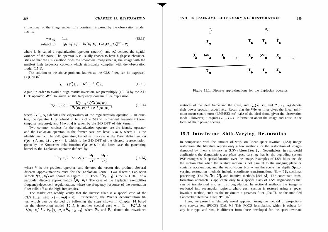
288 CHAPTER 15. RESTORATION
a functional of the image subject to a constraint imposed by the observation model,that is,
min sk LSL (15.12)
subject to Ilgk(w,nz) - h(m,nz) **sk(nm)l12 = d
where L is called a regularization operator (matrix), and u,” denotes the spatialvariance of the noise. The operator L is usually chosen to have high-pass character-istics so that the CLS method finds the smoothest image (that is, the image with thesmallest high frequency content) which statistically complies with the observationmodel (15.1).
The solution to the above problem, known as the CLS filter, can be expressedas [Gon 871
it = (D;D~ + L~L)-~D;~~ (15.13)
Again, in order to avoid a huge matrix inversion, we premultiply (15.13) by the 2-DDFT operator W-l to arrive at the frequency domain filter expression
(15.14)
where L(ur) ~2) denotes the eigenvalues of the regularization operator L. In prac-tice, the operator L is defined in terms of a 2-D shift-invariant generating kernel(impulse response), and L(ui, ~2) is given by the 2-D DFT of this kernel.
Two common choices for the regularization operator are the identity operatorand the Laplacian operator. In the former case, we have L = I, where I is theidentity matrix. The 2-D generating kernel in this case is the Dirac delta function6(x1, Q), and L(ui, ~2) = 1, which is the 2-D DFT of the discrete representationgiven by the Kronecker delta function 6(ni,ns). In the latter case, the generatingkernel is the Laplacian operator defined by
l(Bl,82)=v.v(.)4+~1 2
where V is the gradient operator, and denotes the vector dot product. Severaldiscrete approximations exist for the Laplacian kernel. Two discrete Laplaciankernels l(ni, 7~2) are shown in Figure 15.1. Then L(ui, ~2) is the 2-D DFT of aparticular discrete approximation b(nr ,7rs), The case of the Laplacian exemplifiesfrequency-dependent regularization, where the frequency response of the restorationfilter rolls off at the high frequencies.
The reader can readily verify that the inverse filter is a special case of theCLS filter with ]L(u~, Q)] = 0. Furthermore, the Wiener deconvolution fil-ter, which can be derived by following the steps shown in Chapter 14 basedon the observation model (15.1), is another special case with L = R;lR, orIL(Ul, 2L2)12 = Pvu(w, ~2)lPsA~1, Q), where R, and R, denote the covariance
15.3. INTRAFRAME SHIFT-VARYING RESTORATION 289
n2 n2
(1) q (1) 0)0
(1) C-4) (1)nl
- : -
mm C-8) Cl),- nl
‘l? (1)
.
‘l?
Figure 15.1: Discrete approximations for the Laplacian operator.
matrices of the ideal frame and the noise, and P,,(ui, ~2) and P,,(ul, ~2) denotetheir power spectra, respectively. Recall that the Wiener filter gives the linear mini-mum mean square error (LMMSE) es imate of the ideal frame given the observationt’model. However, it requires a priori information about the image and noise in theform of their power spectra.
15.3 Intraframe Shift-Varying Restoration
In comparison with the amount of work on linear space-invariant (LSI) imagerestoration, the literature reports only a few methods for the restoration of imagesdegraded by linear shift-varying (LSV) blurs [Sez 901. Nevertheless, in real-worldapplications the degradations are often space-varying; that is, the degrading systemPSF changes with spatial location over the image. Examples of LSV blurs includethe motion blur when the relative motion is not parallel to the imaging plane orcontains acceleration, and the out-of-focus blur when the scene has depth. Space-varying restoration methods include coordinate transformations [Saw 741) sectionalprocessing [Tru 78, Tru 921, and iterative methods [Sch 811. The coordinate trans-formation approach is applicable only to a special class of LSV degradations thatcan be transformed into an LSI degradation. In sectional methods the image issectioned into rectangular regions, where each section is restored using a space-invariant method, such as the maximum a posteriori filter [Tru 781 or the modifiedLandweber iterative filter [Tru 921.
Here, we present a relatively novel approach using the method of projectionsonto convex sets (POCS) [Ozk 941. This POCS formulation, which is robust forany blur type and size, is different from those developed for the space-invariant

290 CHAPTER 15. RESTORATION
image restoration problem [Tru 84, Sez 911. In [Tru 841 ‘Iiussell and Civanlar usethe variance of the residual constraint for restoration of space-invariant images.Unfortunately, this constraint cannot easily be extended for space-variant restora-tion since it involves inversion of huge matrices that would not be Toeplitz forspace-varying blurs. In [Sez 911, Sezan and Trussell develop a general framework ofprototype-image-based constraints. Although this framework is rather general, thespecific constraints proposed in [Sez 911 are designed for the space-invariant blurcase.
Figure 15.2: The method of projection onto convex sets
15.3.1 Overview of the POCS Method
In the POCS method, the unknown signal, s, is assumed to be an element of anappropriate Hilbert space ‘R. Each a priori information or constraint restricts thesolution to a closed convex set in ‘R. Thus, for m pieces of information, there arem corresponding closed convex sets Ci E 31, i = 1,2, . . . . m and s E CO t nr=“=, Ciprovided that the intersection Ce is nonempty. Given the sets Ci and their respectiveprojection operators Pi, the sequence generated by
S&l = P,P,-1.. .P1slc; k = 0 , 1 , (15.16)
or, more generally, by
sktl = T,T,.ml Tlsk ; Ic=O,l,... (15.17)
15.3. INTRAFRAME SHIFT-VARYING RESTORATION 291
where Ti h (1 - &)I + &Pi, 0 < Xi < 2, is the relaxed projection operator,converges weakly to a feasible solution in the intersection Cc of the constraint sets.The convex sets and the successive projections are illustrated in Figure 15.2.
Indeed, any solution in the intersection set is consistent with the a priori con-straints and therefore is a feasible solution. Note that Ti’s reduce to Pa’s for unityrelaxation parameters, i.e., & = 1. The initialization se can be arbitrarily chosenfrom 7-t. It should be emphasized that the POCS algorithm is in general nonlinear,because the projection operations are in general nonlinear. For more detailed dis-cussions of the fundamental concepts of the POCS, the reader is referred to [Sta 871.
15.3.2 Restoration Using POCS
The POCS method can readily be applied to the space-varying restoration prob-lem using a number of space-domain constraints that are defined on the basis ofthe observed image, and a priori information about the space-varying degradationprocess, the noise statistics, and the ideal image itself.
Assuming that the space-varying blur PSF and the statistics of the noise processare known, we define the following closed, convex constraints (one for each observedblurred image pixel):
where
is the residual associated with yk, which denotes an arbitrary member of the set.The quantity So is an a priori bound reflecting the statistical confidence with whichthe actual image is a member of the set &,,nz,k. since fcSk)(nl, n2) = vk(nl, nz),where st denotes the ideal frame, the statistics of f(‘k)(nr, nz) is identical to that of‘uk (ni, nz). Hence, the bound 60 is determined from the statistics of the noise processso that the actual frame (i.e., the ideal solution) is a member of the set within acertain statistical confidence. For example, if the noise has Gaussian distributionwith the standard deviation u,, 60 is set equal to co,, where c 2 0 is determined byan appropriate statistical confidence bound (e.g., c = 3 for 99% confidence). Thebounded residual constraint enforces the estimate to be consistent with the observedimage. In other words, at each iteration, the estimate is constrained such that atevery pixel (ni) nz), the absolute value of the residual between the observed imagevalue gk(nr, n2) and the pixel value obtained at (nr ) ns) by simulating the imagingprocess using that estimate is required to be less than a predetermined bound.
From [Tru 841, the projection zk(&,iz) - Pnl,nZ,k [zk(il, iz)] of an arbitrary
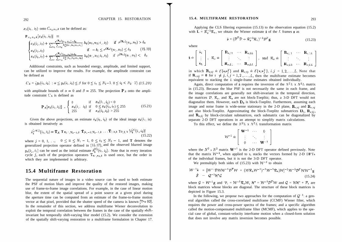
292 CHAPTER 15. RESTORATION 15.4. MULTIFRAME RESTORATION 293
xk(il, iz) onto Cnl,na,k can be defined as:
PnI,nz,k[Zk(il,i2)1 =
Additional constraints, such as bounded energy, amplitude, and limited support,can be utilized to improve the results. For example, the amplitude constraint canbe defined as
CA = {yk(il,ia) : a 5 yk(il,i2) 5 ,8 for 0 < il 5 Ni-1, 0 5 iz 5 Np-1) (15.20)
with amplitude bounds of o = 0 and /3 = 255. The projection PA onto the ampli-tude constraint CA is defined as
l
0 if xb(ir , iz) < 0PA[xk(il,h)] = xk(il, iz) if 0 5 xk(il, i2) 5 255 (15.21)
255 if xk(ir, i2) > 255
Given the above projections, an estimate ih(ir) iz) of the ideal image sk(ir, is)is obtained iteratively as
,$+l)(il, iz) = TA TN l,iV-l,k TN~-QV-I,~ ” .Tu,k1- To o IC [$(& &)I, ,’ (15.22)
where j = 0, 1, . ., 0 5 ii 5 Nr - 1, 0 5 is 5 N2 - 1, and T denotes thegeneralized projection operator defined in (15.17), and the observed blurred image
gk(il, i2) can be used as the initial estimate $c)(ir, iz). Note that in every iterationcycle j, each of the projection operators Tnl,na,k is used once, but the order inwhich they are implemented is arbitrary.
15.4 Multiframe RestorationThe sequential nature of images in a video source can be used to both estimatethe PSF of motion blurs and improve the quality of the restored images, makinguse of frame-to-frame image correlations. For example, in the case of linear motionblur, the extent of the spatial spread of a point source at a given pixel duringthe aperture time can be computed from an estimate of the frame-to-frame motionvector at that pixel, provided that the shutter speed of the camera is known [Tru 921.In the remainder of this section, we address multiframe Wiener deconvolution toexploit the temporal correlation between the frames in the case of the spatially shift-invariant but temporally shift-varying blur model (15.2). We consider the extensionof the spatially shift-varying restoration to a multiframe formulation in Chapter 17.
Applying the CLS filtering expression (15.13) to the observation equation (15.2)with L = R;i’R,, we obtain the Wiener estimate i of the L frames s as
where
i = (DTD + R;lRJIDTg (15.23)
in which R,;ij - f{sisjT} and R,;ij + t{v$}, i,j = 1,2,...,L. Note thatif R,;ij = 0 for i # j, i,j = 1,2 ,..,) L, then the multiframe estimate becomesequivalent to stacking the L single-frame estimates obtained individually.
Again, direct computation of S requires the inversion of the N’L x N’L matrixin (15.23). Because the blur PSF is not necessarily the same in each frame, andthe image correlations are generally not shift-invariant in the temporal direction,the matrices 2>, R,, and R, are not block-Toeplitz; thus, a 3-D DFT would notdiagonalize them. However, each Dk is block-Toeplitz. Furthermore, assuming eachimage and noise frame is wide-sense stationary in the 2-D plane, R,,ij and R,;ijare also block-Toeplitz. Approximating the block-Toeplitz submatrices Di, R,;ij,and R,;ij by block-circulant submatrices, each submatrix can be diagonalized byseparate 2-D DFT operations in an attempt to simplify matrix calculations.
To this effect, we define the N2L x N2L transformation matrix
where the N2 x N2 matrix W-l is the 2-D DFT operator defined previously. Notethat the matrix W-l, when applied to s, stacks the vectors formed by 2-D DFTsof the individual frames, but it is not the 3-D DFT operator.
We premultiply both sides of (15.23) with W-l to obtain
w-lj: = [W-lDWW-lDTW + (WR,W-l)-lW-lR,)W]-lW-lDTww-lg8 1 Q-‘~*cJ- (15.24)
where B = W-‘g and ‘P, = WmlR,W, ti* = WelDTW and Q = KY* + P, areblock matrices whose blocks are diagonal. The structure of these block matrices isdepicted in Figure 15.3.
In the following, we propose two approaches for the computation of Q-l: a gen-eral algorithm called the cross-correlated multiframe (CCMF) Wiener filter, whichrequires the power and cross-power spectra of the frames; and a specific algorithmcalled the motion-compensated multiframe filter (MCMF), which applies to the spe-cial case of global, constant-velocity interframe motion when a closed-form solutionthat does not involve any matrix inversion becomes possible.
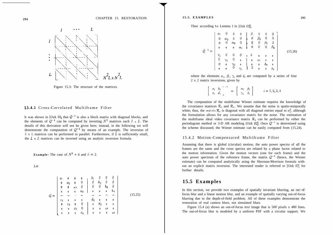
294 CHAPTER 15. RESTORATION 15.5. EXAMPLES 295
Figure 15.3: The structure of the matrices.
15.4.1 Cross-Correlated Multiframe Filter
It was shown in [Ozk 921 that Q-i is also a block matrix with diagonal blocks, andthe elements of Q-i can be computed by inverting N2 matrices each L x L. Thedetails of this derivation will not be given here; instead, in the following we willdemonstrate the computation of Q-i by means of an example. The inversion ofL x L matrices can be performed in parallel. Furthermore, if L is sufficiently small,the L x L matrices can be inverted using an analytic inversion formula.
Example: The case of N2 = 4 and L = 2.
Let
Q=
L
a1 0 0 0 1 bl 0 0 00 a2 0 0 I 0 b2 0 00 0 a3 0 1 0 0 b3 00 0 0 a4 ( 0 0 0 b4
-_ - - - - - -
Cl 0 0 0 I dl 0 0 0
0 c2 0 0 1 0 a2 0 0
0 0 c3 0 ( 0 0 a3 0
0 0 0 c4 1 0 0 0 a4
(15.25)
Then according
i-1 =
o Lemma 1 in [Ozk 921,
a1 0 0 0 I/31 0 0 o-0 a2 0 0 I 0 P2 0 0
0 0 ff3 0 I 0 0 P3 0
0 0 0 a4 I 0 0 0 P4
(15.26)71 0 0 0 I 61 0 0 0
0 72 0 0 I 0 62 0 0
0 0 73 0 I 0 0 63 0
0 0 0 “14 I 0 0 0 64
where the elements oi, pi, +yi and 6; are computed by a series of four2 x 2 matrix inversions, given by
[ :; 21-l = [ ;; ff] i= 1,2,3,4
The computation of the multiframe Wiener estimate requires the knowledge ofthe covariance matrices R, and R,. We assume that the noise is spatio-temporallywhite; thus, the matrixR, is diagonal with all diagonal entries equal to u,“) althoughthe formulation allows for any covariance matrix for the noise. The estimation ofthe multiframe ideal video covariance matrix R, can be performed by either theperiodogram method or 3-D AR modeling [Ozk 921. Once Q-i is determined usingthe scheme discussed, the Wiener estimate can be easily computed from (15.24).
15.4.2 Motion-Compensated Multiframe Filter
Assuming that there is global (circular) motion, the auto power spectra of all theframes are the same and the cross spectra are related by a phase factor related tothe motion information. Given the motion vectors (one for each frame) and theauto power spectrum of the reference frame, the matrix &-I (hence, the Wienerestimate) can be computed analytically using the Sherman-Morrison formula with-out an explicit matrix inversion. The interested reader is referred to [Ozk 921 forfurther details.
15.5 Examples
In this section, we provide two examples of spatially invariant blurring, an out-of-focus blur and a linear motion blur, and an example of spatially varying out-of-focusblurring due to the depth-of-field problem. All of these examples demonstrate therestoration of real camera blurs, not simulated blurs.
Figure 15.4 (a) shows an out-of-focus text image that is 500 pixels x 480 lines.The out-of-focus blur is modeled by a uniform PSF with a circular support. We
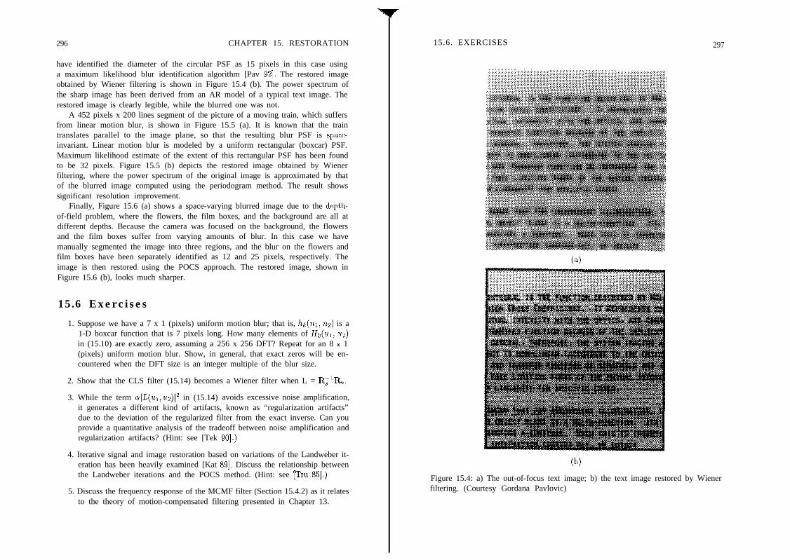
296 CHAPTER 15. RESTORATION
have identified the diameter of the circular PSF as 15 pixels in this case usinga maximum likelihood blur identification algorithm [Pav 921. The restored imageobtained by Wiener filtering is shown in Figure 15.4 (b). The power spectrum ofthe sharp image has been derived from an AR model of a typical text image. Therestored image is clearly legible, while the blurred one was not.
A 452 pixels x 200 lines segment of the picture of a moving train, which suffersfrom linear motion blur, is shown in Figure 15.5 (a). It is known that the traintranslates parallel to the image plane, so that the resulting blur PSF is space-invariant. Linear motion blur is modeled by a uniform rectangular (boxcar) PSF.Maximum likelihood estimate of the extent of this rectangular PSF has been foundto be 32 pixels. Figure 15.5 (b) depicts the restored image obtained by Wienerfiltering, where the power spectrum of the original image is approximated by thatof the blurred image computed using the periodogram method. The result showssignificant resolution improvement.
Finally, Figure 15.6 (a) shows a space-varying blurred image due to the depth-of-field problem, where the flowers, the film boxes, and the background are all atdifferent depths. Because the camera was focused on the background, the flowersand the film boxes suffer from varying amounts of blur. In this case we havemanually segmented the image into three regions, and the blur on the flowers andfilm boxes have been separately identified as 12 and 25 pixels, respectively. Theimage is then restored using the POCS approach. The restored image, shown inFigure 15.6 (b), looks much sharper.
15.6 Exercises
1. Suppose we have a 7 x 1 (pixels) uniform motion blur; that is, he(ni, nz) is a1-D boxcar function that is 7 pixels long. How many elements of Ht(ur) ~2)in (15.10) are exactly zero, assuming a 256 x 256 DFT? Repeat for an 8 x 1(pixels) uniform motion blur. Show, in general, that exact zeros will be en-countered when the DFT size is an integer multiple of the blur size.
2. Show that the CLS filter (15.14) becomes a Wiener filter when L = R;iR,.
3. While the term o]l(ui,uz)]’ in (15.14) avoids excessive noise amplification,it generates a different kind of artifacts, known as “regularization artifacts”due to the deviation of the regularized filter from the exact inverse. Can youprovide a quantitative analysis of the tradeoff between noise amplification andregularization artifacts? (Hint: see [Tek 901.)
4. Iterative signal and image restoration based on variations of the Landweber it-eration has been heavily examined [Kat 891. Discuss the relationship betweenthe Landweber iterations and the POCS method. (Hint: see [Tru 851.)
5. Discuss the frequency response of the MCMF filter (Section 15.4.2) as it relatesto the theory of motion-compensated filtering presented in Chapter 13.
15.6. EXERCISES 297
Figure 15.4: a) The out-of-focus text image; b) the text image restored by Wienerfiltering. (Courtesy Gordana Pavlovic)
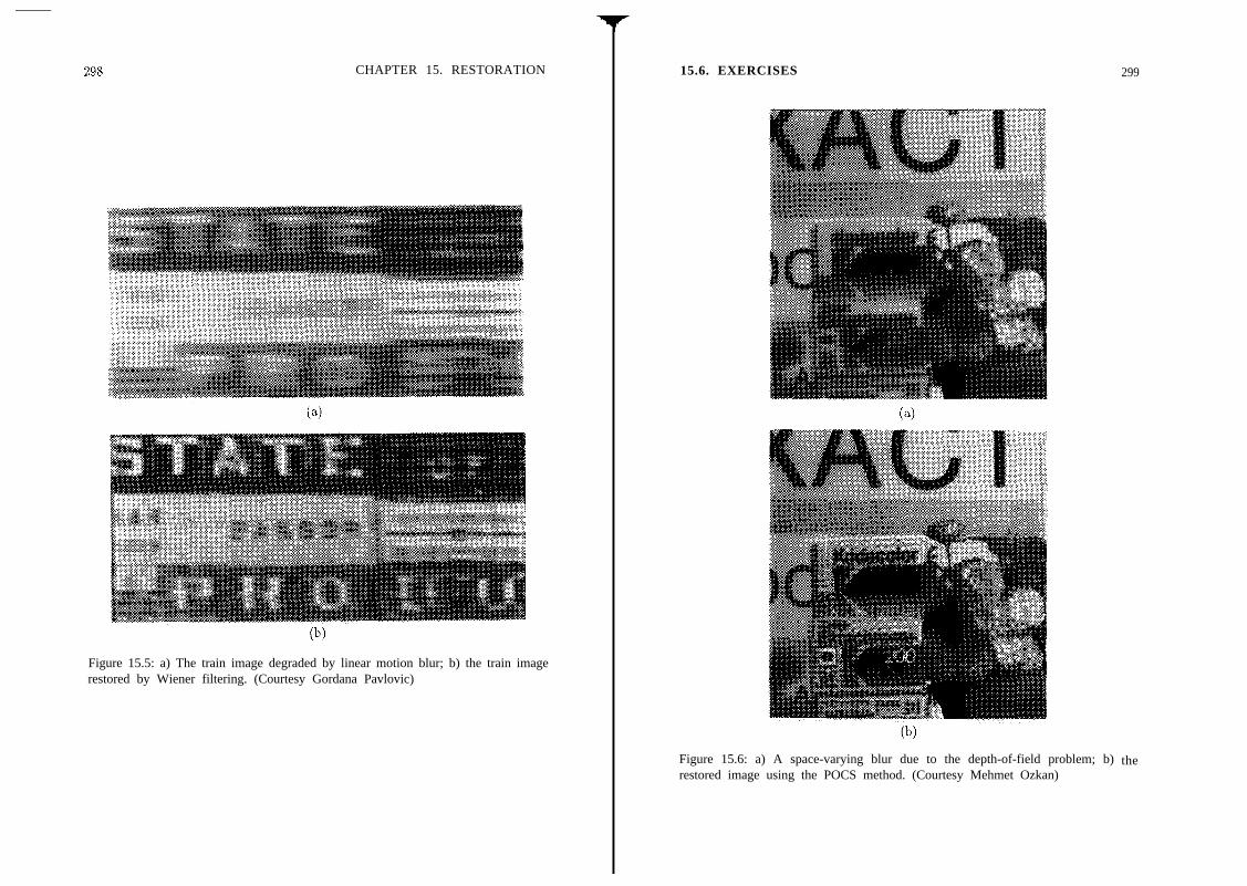
CHAPTER 15. RESTORATION
(b)Figure 15.5: a) The train image degraded by linear motion blur; b) the train imagerestored by Wiener filtering. (Courtesy Gordana Pavlovic)
15.6. EXERCISES 299
Figure 15.6: a) A space-varying blur due to the depth-of-field problem; b)restored image using the POCS method. (Courtesy Mehmet Ozkan)
the
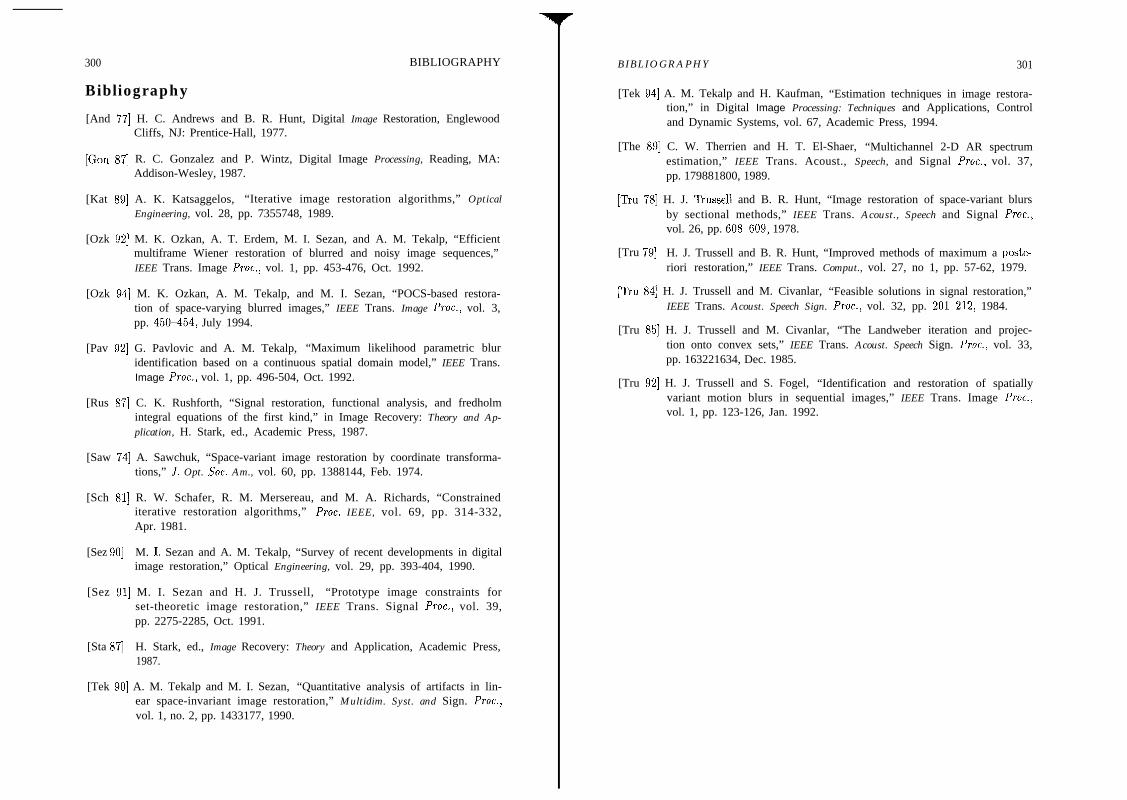
300
Bibliography
BIBLIOGRAPHY
[And 771 H. C. Andrews and B. R. Hunt, Digital Image Restoration, EnglewoodCliffs, NJ: Prentice-Hall, 1977.
[Con 871 R. C. Gonzalez and P. Wintz, Digital Image Processing, Reading, MA:Addison-Wesley, 1987.
[Kat 891 A. K. Katsaggelos, “Iterative image restoration algorithms,” OpticalEngineering, vol. 28, pp. 7355748, 1989.
[Ozk 921 M. K. Ozkan, A. T. Erdem, M. I. Sezan, and A. M. Tekalp, “Efficientmultiframe Wiener restoration of blurred and noisy image sequences,”IEEE Trans. Image Proc., vol. 1, pp. 453-476, Oct. 1992.
[Ozk 941 M. K. Ozkan, A. M. Tekalp, and M. I. Sezan, “POCS-based restora-tion of space-varying blurred images,” IEEE Trans. Image Proc., vol. 3,pp. 450-454, July 1994.
[Pav 921 G. Pavlovic and A. M. Tekalp, “Maximum likelihood parametric bluridentification based on a continuous spatial domain model,” IEEE Trans.Image Proc., vol. 1, pp. 496-504, Oct. 1992.
[Rus 871 C. K. Rushforth, “Signal restoration, functional analysis, and fredholmintegral equations of the first kind,” in Image Recovery: Theory and Ap-plication, H. Stark, ed., Academic Press, 1987.
[Saw 741 A. Sawchuk, “Space-variant image restoration by coordinate transforma-tions,” J. Opt. Sot. Am., vol. 60, pp. 1388144, Feb. 1974.
[Sch 811 R. W. Schafer, R. M. Mersereau, and M. A. Richards, “Constrainediterative restoration algorithms,” Proc. IEEE, vol. 69, pp. 314-332,Apr. 1981.
[Sez 901 M. I. Sezan and A. M. Tekalp, “Survey of recent developments in digitalimage restoration,” Optical Engineering, vol. 29, pp. 393-404, 1990.
[Sez 911 M. I. Sezan and H. J. Trussell, “Prototype image constraints forset-theoretic image restoration,” IEEE Trans. Signal Proc., vol. 39,pp. 2275-2285, Oct. 1991.
[Sta 871 H. Stark, ed., Image Recovery: Theory and Application, Academic Press,1987.
[Tek 901 A. M. Tekalp and M. I. Sezan, “Quantitative analysis of artifacts in lin-ear space-invariant image restoration,” Multidim. Syst. and Sign. Proc.,vol. 1, no. 2, pp. 1433177, 1990.
BIBLIOGRAPHY 301
[Tek 941 A. M. Tekalp and H. Kaufman, “Estimation techniques in image restora-tion,” in Digital Image Processing: Techniques and Applications, Controland Dynamic Systems, vol. 67, Academic Press, 1994.
[The 891 C. W. Therrien and H. T. El-Shaer, “Multichannel 2-D AR spectrumestimation,” IEEE Trans. Acoust., Speech, and Signal Proc., vol. 37,pp. 179881800, 1989.
[Tru 781 H. J. Russell and B. R. Hunt, “Image restoration of space-variant blursby sectional methods,” IEEE Trans. Acoust., Speech and Signal Proc.,vol. 26, pp. 608-609, 1978.
[Tru 791 H. J. Trussell and B. R. Hunt, “Improved methods of maximum a poste-riori restoration,” IEEE Trans. Comput., vol. 27, no 1, pp. 57-62, 1979.
[‘Du 841 H. J. Trussell and M. Civanlar, “Feasible solutions in signal restoration,”IEEE Trans. Acoust. Speech Sign. Proc., vol. 32, pp. 201-212, 1984.
[Tru 851 H. J. Trussell and M. Civanlar, “The Landweber iteration and projec-tion onto convex sets,” IEEE Trans. Acoust. Speech Sign. Proc., vol. 33,pp. 163221634, Dec. 1985.
[Tru 921 H. J. Trussell and S. Fogel, “Identification and restoration of spatiallyvariant motion blurs in sequential images,” IEEE Trans. Image Proc.,vol. 1, pp. 123-126, Jan. 1992.

Chapter 16
STANDARDSCONVERSION
Various digital video systems, ranging from all-digital high-definition TV to video-phone, have different spatio-temporal resolution requirements, leading to the emer-gence of different format standards to store, transmit, and display digital video sig-nals. The task of converting digital video from one standard to another is referred toas standards conversion, which includes frame/field rate down-/up-conversion andinterlacing/de-interlacing. Frame and field rate up-conversion increase the temporalsampling rate in progressive and interlaced video, respectively. De-interlacing refersto conversion from interlaced to progressive video. These problems are illustratedin Figure 16.1. Note that in field rate doubling two fields, one even and one odd,need to be inserted between existing fields.
(b)
Figure 16.1: Different up-conversion problems: a) Frame rate up-conversion; b) fieldrate up-conversion; c) de-interlacing.
302
303
Standards conversion enables the exchange of information among various dig-ital video systems employing different standards to ensure their interoperability.Some examples of commonly used video standards employed in such applicationsas motion pictures, workstations, and NTSC TV are shown in Figure 16.2. Forexample, video recorded by motion picture equipment can be used as high-qualitysource material for HDTV after proper frame rate conversion, and spatio-temporaldown-conversion helps data compression. In addition to facilitating exchange of in-formation, frame rate up-conversion generally yields higher visual quality throughbetter motion rendition and less flicker. and de-interlacing provides improved spatialresolution in the vertical direction.
24 frameshec
tNTSC HDTV PAL
525 lines, 2:l int 1440 x 1050,2:1 int .e 625 lines, 2:l int60 fieldshec 60 fieldshec 50 fieldshec
4
Figure 16.2: Typical standards conversion applications.
All standards conversion problems essentially deal with sampling structure con-version, which was introduced in Chapter 4. In Chapter 4, the sampling structureconversion problem has been discussed for arbitrary spatio-temporal signals withinthe framework of linear filtering. It is the goal of this chapter to extend this frame-work by incorporating motion models, following the analysis in Chapter 13, whichcharacterize temporal variations of the video signal. The down-conversion problemis studied in Section 16.1, where we discuss methods with or without using an anti-alias filter. A variety of up-conversion methods exist in the literature, which can
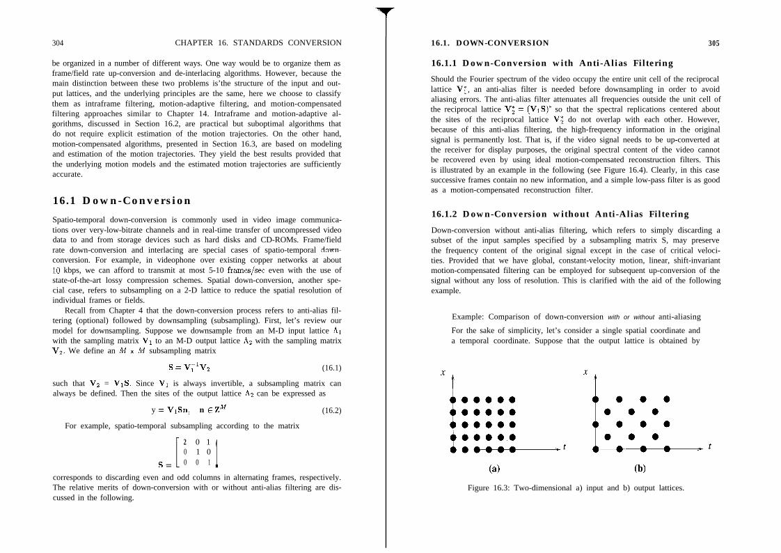
304 CHAPTER 16. STANDARDS CONVERSION
be organized in a number of different ways. One way would be to organize them asframe/field rate up-conversion and de-interlacing algorithms. However, because themain distinction between these two problems is’the structure of the input and out-put lattices, and the underlying principles are the same, here we choose to classifythem as intraframe filtering, motion-adaptive filtering, and motion-compensatedfiltering approaches similar to Chapter 14. Intraframe and motion-adaptive al-gorithms, discussed in Section 16.2, are practical but suboptimal algorithms thatdo not require explicit estimation of the motion trajectories. On the other hand,motion-compensated algorithms, presented in Section 16.3, are based on modelingand estimation of the motion trajectories. They yield the best results provided thatthe underlying motion models and the estimated motion trajectories are sufficientlyaccurate.
16.1 Down-Conversion
Spatio-temporal down-conversion is commonly used in video image communica-tions over very-low-bitrate channels and in real-time transfer of uncompressed videodata to and from storage devices such as hard disks and CD-ROMs. Frame/fieldrate down-conversion and interlacing are special cases of spatio-temporal down-conversion. For example, in videophone over existing copper networks at about10 kbps, we can afford to transmit at most 5-10 frames/set even with the use ofstate-of-the-art lossy compression schemes. Spatial down-conversion, another spe-cial case, refers to subsampling on a 2-D lattice to reduce the spatial resolution ofindividual frames or fields.
Recall from Chapter 4 that the down-conversion process refers to anti-alias fil-tering (optional) followed by downsampling (subsampling). First, let’s review ourmodel for downsampling. Suppose we downsample from an M-D input lattice hiwith the sampling matrix VI to an M-D output lattice Az with the sampling matrixVz. We define an M x hil subsampling matrix
s = v;$ (16.1)
such that Vz = VlS. Since VI is always invertible, a subsampling matrix canalways be defined. Then the sites of the output lattice Az can be expressed as
y = VI%, n E ZM (16.2)
For example, spatio-temporal subsampling according to the matrix
s= [ 2 0 10 1 00 0 1 1
corresponds to discarding even and odd columns in alternating frames, respectively.The relative merits of down-conversion with or without anti-alias filtering are dis-cussed in the following.
16.1. DOWN-CONVERSION 305
16.1.1 Down-Conversion with Anti-Alias Filtering
Should the Fourier spectrum of the video occupy the entire unit cell of the reciprocallattice VT, an anti-alias filter is needed before downsampling in order to avoidaliasing errors. The anti-alias filter attenuates all frequencies outside the unit cell ofthe reciprocal lattice Va = (VlS)* so that the spectral replications centered aboutthe sites of the reciprocal lattice Vz do not overlap with each other. However,because of this anti-alias filtering, the high-frequency information in the originalsignal is permanently lost. That is, if the video signal needs to be up-converted atthe receiver for display purposes, the original spectral content of the video cannotbe recovered even by using ideal motion-compensated reconstruction filters. Thisis illustrated by an example in the following (see Figure 16.4). Clearly, in this casesuccessive frames contain no new information, and a simple low-pass filter is as goodas a motion-compensated reconstruction filter.
16.1.2 Down-Conversion without Anti-Alias Filtering
Down-conversion without anti-alias filtering, which refers to simply discarding asubset of the input samples specified by a subsampling matrix S, may preservethe frequency content of the original signal except in the case of critical veloci-ties. Provided that we have global, constant-velocity motion, linear, shift-invariantmotion-compensated filtering can be employed for subsequent up-conversion of thesignal without any loss of resolution. This is clarified with the aid of the followingexample.
Example: Comparison of down-conversion with or without anti-aliasing
For the sake of simplicity, let’s consider a single spatial coordinate anda temporal coordinate. Suppose that the output lattice is obtained by
(4 (b)Figure 16.3: Two-dimensional a) input and b) output lattices.

306 CHAPTER 16. STANDARDS CONVERSION
(b) (clFigure 16.4: Spectra of a) input signal; b) subsampled signal with anti-alias filtering;c) subsampled signal without anti-alias filtering.
subsampling a progressive input lattice according to the subsamplingmatrix
SF 2 l[ 10 1which corresponds to discarding even and odd spatial samples in alter-nating time samples. The 2-D input and output lattices in this case aredepicted in Figure 16.3.
16.1. DOWN-CONVERSION 307
The spectrum of the input video, assuming global, constant-velocitymotion, is depicted in Figure 16.4 (a), where the solid dots indicate thesites of the reciprocal lattice VT. The dotted lines denote the supportof an ideal anti-alias filter that would be used in the case of down-conversion with anti-alias filtering. The spectra of the down-convertedsignal with and without anti-alias filtering are shown in Figures 16.4 (b)and (c), respectively. The loss of high-frequency information when ananti-alias filter has been employed can be clearly observed. Furtherobserve that the spectrum of the down-converted signal in Figure 16.4 (c)retains the high-frequency content of the original signal, provided thatthe subsampling structure does not lead to a critical velocity.
Figure 16.5: Critical velocities in the spatio-temporal domain.
It can easily be seen that for the subsampling matrix in this example, thevelocities v, = 2i + 1, i E 2 constitute critical velocities in the absenceof anti-alias filtering. For these velocities, the motion trajectory passesthrough either all existing or non-existing pixel sites at every frame,as shown in Figure 16.5. Note that with the use of proper anti-aliasfiltering, the replicas in the frequency domain can never overlap; hence,there are no critical velocities.
In conclusion, down-conversion to sub-Nyquist rates followed by up-conversionwithout loss of resolution is possible only if no anti-alias filtering has been usedin the down-conversion process, and we do not have a critical velocity. Assumingglobal, constant-velocity motion, this process leads to motion-adaptive downsam-pling, where the subsampling matrix is selected to avoid the critical velocities givenan estimate of the motion vector. Up-conversion methods are studied in the nextthree sections.

308 CHAPTER 16. STANDARDS CONVERSION
16.2 Practical Up-Conversion MethodsStandards conversion problems of common interest include frame/field rate up-conversion and de-interlacing. Examples of frame rate conversion include conversionfrom a digitized motion picture recorded with a temporal rate of 24 frames/set toNTSC format, which requires 60 fields/set. Conversion from NTSC to PAL formatrequires field (scan) rate conversion from 60 to 50 fields/s. Field rate doubling andde-interlacing are generally employed in improved-definition TV receivers to providebetter visual quality.
Frame rate up-conversion refers to the case where the input and output sequencesare both progressive. Suppose we represent a sequence of input frames as
., s(t - l), s(t) s(t + l), s(t + 2))
Then the output sequence in the case of up-conversion by an integer factor L isgiven by
s s(t)@*)> ,. > ,(t*l, s(t + l),
L-l times
where t* denotes the time instances where new frames are inserted.Field rate, or scan rate, up-conversion, where both the input and output se-
quences are interlaced, by an arbitrary factor is complicated by the fact that theordering of even and odd fields must be preserved. If we let
“‘1 s((t - 1)0), s((t - l)e), s(to), s&e), s((t + 1)0), s((t + l)&
denote a sequence of input fields, where s(&,) and s(te) are the odd and even fields,respectively, then the output sequence
“‘, s(to), S(b), s(C), s(t$), s((t + l)o), ”
corresponds to the special case of doubling the scan rate. Note in this case that aneven number of fields must be inserted between two existing fields to preserve theordering of the fields. Conversion by an arbitrary factor can generally be modeledby de-interlacing each field, then frame rate conversion to the desired temporal rate,followed by interlacing.
De-interlacing refers to up-conversion from an interlaced to a progressive sam-pling lattice at the same temporal rate. It is often necessary to view interlacedvideo on progressively scanned display devices. In addition, proper de-interlacingreduces line flicker and improves the vertical resolution of the displayed images.
Both frame/field rate up-conversion and de-interlacing are based on the sameprinciples of sampling structure conversion. Indeed, the only difference betweenframe/field rate up-conversion and de-interlacing is the structure of the input andoutput lattices. Standards up-conversion algorithms can be classified, in the orderof increasing complexity, as intrafield, motion-adaptive, and motion-compensated
16.2. PRACTICAL UP-CONVERSION METHODS 309 k
filtering techniques. Although the motion-compensated approach is optimal, pro-vided that a motion model is given and the trajectory can be accurately estimated,it is highly sensitive to errors. This fact, along with the cost of hardware imple-mentation, have led to the development of suboptimal but more robust algorithmswhich do not require explicit estimation of the motion information. We first discusssome of these algorithms in the following.
16.2.1 Intraframe Filtering
Intraframe filtering refers to algorithms that need no more than a single frame-store. Frame/field repetition algorithms for frame/field rate conversion and spatialinterpolation methods for de-interlacing are examples of intraframe filtering.
Frame/Field Rate Conversion
The most obvious and simple way to increase the frame or the field rate is to repeatthe existing information. Common examples of frame/field repetition are the “3 to2 pull-down” method used for conversion of a motion picture source to NTSC video,and doubling of the field rate, which has been adopted by several TV manufacturersin Europe for commercial lOO-Hz receivers.
In the “3 to 2 pull-down” method, each odd frame of the digitized motion pictureis repeated three times and each even frame is repeated twice, yielding a 60 Hz fieldrate. That is, the output is a sequence of fields given by
> s(t - l), s((t - I)*), s((t - l)*),s(t), s(t*), s(t + l), s((t + I)*),s((t + I)*), s(t + 2), s((t + 2)*),
In order to characterize the 3:2 pull-down method in the temporal frequency do-main, we describe it through the steps illustrated in Figure 16.6. They are: (i) insertfour zero frames in between every existing frame, (ii) apply a zero-order hold filterwhose impulse response is depicted, and (iii) downsample the resulting sequence offrames by two. The 3:2 pull-down method introduces temporal aliasing because thezero-order hold filter is a poor low-pass filter. The jerky motion rendition due tothis aliasing is hardly visible at the spatio-temporal resolution provided by currentNTSC receivers. However, with bigger displays and high-resolution video formats,there is need for more sophisticated frame/field rate conversion algorithms.
For scan rate doubling, there exist more than one way to repeat the fields. Weprovide two algorithms in the following.
Algorithm 1: In the first approach, the existing odd frame is repeated to formthe next even frame, and the existing even frame is repeated for the next odd frame.This can be expressed as
s(t%) = s(b)s(g) = s(b) (16.3)

310 CHAPTER 16. STANDARDS CONVERSION 16.2. PRACTICAL UP-CONVERSION METHODS 311
. . .45
IoooolooooIooooloooo11*1*1*1*2 2*2”2*2*33*3*33”3*4 4*4*4*4*
LPF
i
. . .
11*1*1*1*2 2*2*2*2*33*3*3*3*4 4”4*4”4”
1 1* 1” 2 2” 3
. . .
3” 3” 4 4”
Figure 16.6: Interpretation of the 3 to 2 pull-down method by linear filtering.
Algorithm-l has reasonably good performance with moving scenes, but poor resultsin stationary regions is inevitable.
Algoridhm 2: The second approach repeats an even field for the next even field,and an odd field for the next odd field, which can be expressed as
s(t:) = s(b)
s(C) = s(b) (16.4)
This strategy is optimal for stationary scenes but fails for the moving parts. Obvi-ously, neither algorithm alone is sufficient for both stationary and moving regions
c I 6 It t” t*0 e 0
Figure 16.7: Two-point line averaging.
of the scene, which motivates the need for motion-adaptive or motion-compensatedfiltering schemes.
An interesting application which requires scan rate conversion by a rationalfactor is conversion from NTSC to PAL and vice versa. The NTSC standard employs60 fields/set and 262.5 lines/field, whereas the PAL standard uses 50 fields/setand 312.5 lines/field. The conversion from NTSC to PAL may be achieved bydropping a complete frame (an even and an odd field) every five frames, and spatiallyinterpolating for the missing lines. On the other hand, PAL to NTSC conversionrequires dropping some extra lines per frame, and replicating a complete frameevery five frames.
Alternatively, one can use a line averaging filter, defined by
s(~l,Q,t:) = ; b(z1,22- 1,t,)+s(x1,zz+ l,&)]
s(a,zz,fg = ~~~(tl;rz-l,t,)+S(Z1,22+l,t”)] (16.5)
for field rate up-conversion. The solid pixels in Figure 16.7 denote the input pixels,and the open circles pointed by the arrows denote the output pixels. The line-averaging filter provides reasonable performance in the moving regions. However,in stationary image parts it introduces blurring because it is purely a spatial filter.Notice that while the repetition algorithms yield jagged edges, averaging algorithmsprovide blurred edges. A compromise between the performances of these two classesof algorithms may be reached by using interframe filtering.
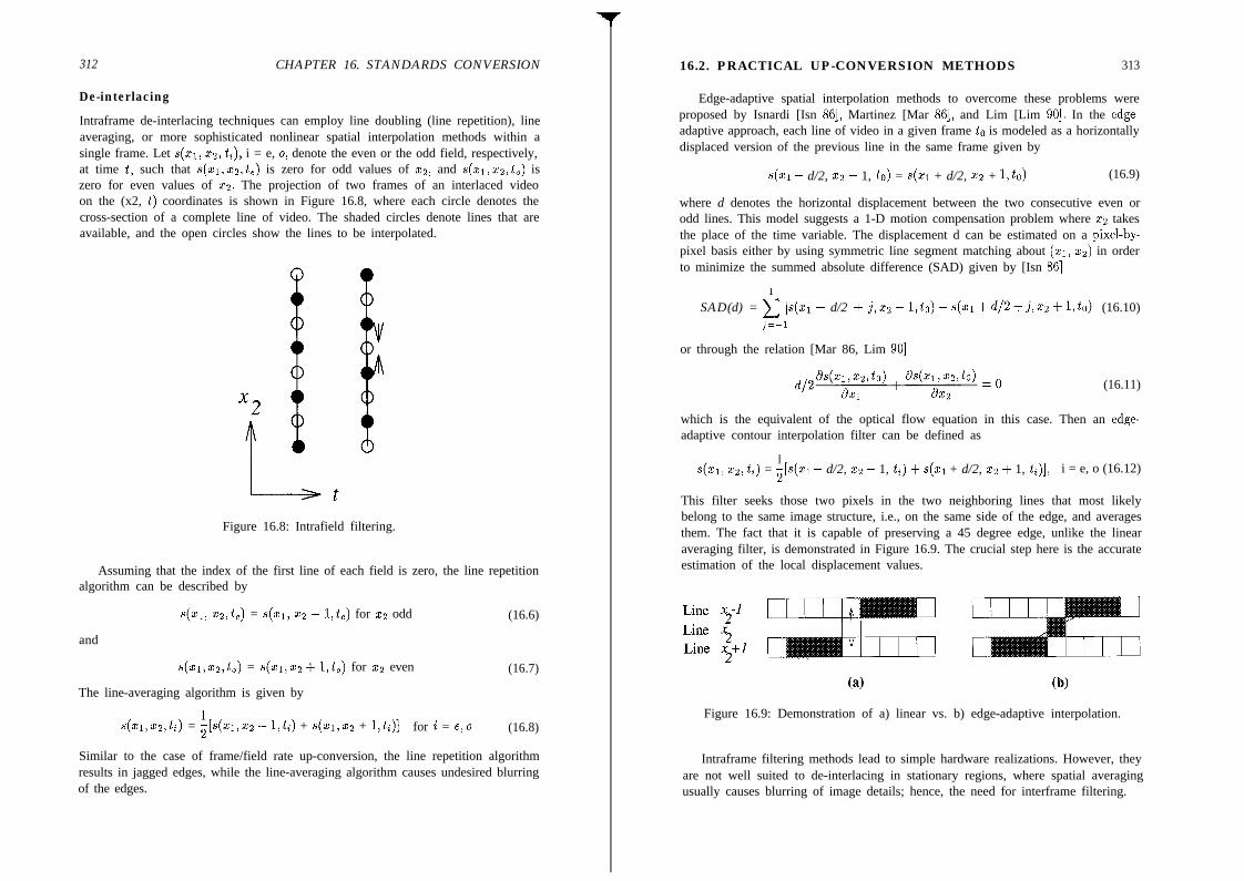
312 CHAPTER 16. STANDARDS CONVERSION
De-interlacing
Intraframe de-interlacing techniques can employ line doubling (line repetition), lineaveraging, or more sophisticated nonlinear spatial interpolation methods within asingle frame. Let ~(41) ~2, ti), i = e, o, denote the even or the odd field, respectively,at time t, such that s(zl,xz,t,) is zero for odd values of xg, and s(zl,xz,t,) iszero for even values of x2. The projection of two frames of an interlaced videoon the (x2, t) coordinates is shown in Figure 16.8, where each circle denotes thecross-section of a complete line of video. The shaded circles denote lines that areavailable, and the open circles show the lines to be interpolated.
Figure 16.8: Intrafield filtering.
Assuming that the index of the first line of each field is zero, the line repetitionalgorithm can be described by
and
s(x1, xz,t,) = s(x1, x2 - l,t,) for 22 odd (16.6)
s(xl,xz,t,) = s(xl,x2+ l,t,) for x2 even (16.7)
The line-averaging algorithm is given by
s(x1,x2,ti) = i[s(x,,x, - l,ti) + s(zl,xz + l,ti)] for i = e,o (16.8)
Similar to the case of frame/field rate up-conversion, the line repetition algorithmresults in jagged edges, while the line-averaging algorithm causes undesired blurringof the edges.
16.2. PRACTICAL UP-CONVERSION METHODS 313
Edge-adaptive spatial interpolation methods to overcome these problems wereproposed by Isnardi [Isn 861, Martinez [Mar 861, and Lim [Lim 901. In the edge-adaptive approach, each line of video in a given frame to is modeled as a horizontallydisplaced version of the previous line in the same frame given by
S(XI - d/2, xz - 1, to) = s(x1 + d/2, xz + 1,to) (16.9)
where d denotes the horizontal displacement between the two consecutive even orodd lines. This model suggests a 1-D motion compensation problem where 22 takesthe place of the time variable. The displacement d can be estimated on a pixel-by-pixel basis either by using symmetric line segment matching about (21, x2) in orderto minimize the summed absolute difference (SAD) given by [Isn 861
SAD(d) = k (~(21 - d/2 + j ,x2-l,to)-s(xl+d/2+j,x2+1,to)l (16.10)j=-1
or through the relation [Mar 86, Lim 901
(16.11)
which is the equivalent of the optical flow equation in this case. Then an edge-adaptive contour interpolation filter can be defined as
s(xll x2) ti) = i[s(xl - d/2, x2 - 1, ti) + s(x1 + d/2, x2 + 1, t;)]> i = e, o (16.12)
This filter seeks those two pixels in the two neighboring lines that most likelybelong to the same image structure, i.e., on the same side of the edge, and averagesthem. The fact that it is capable of preserving a 45 degree edge, unlike the linearaveraging filter, is demonstrated in Figure 16.9. The crucial step here is the accurateestimation of the local displacement values.
(4 (b)
Figure 16.9: Demonstration of a) linear vs. b) edge-adaptive interpolation.
Intraframe filtering methods lead to simple hardware realizations. However, theyare not well suited to de-interlacing in stationary regions, where spatial averagingusually causes blurring of image details; hence, the need for interframe filtering.
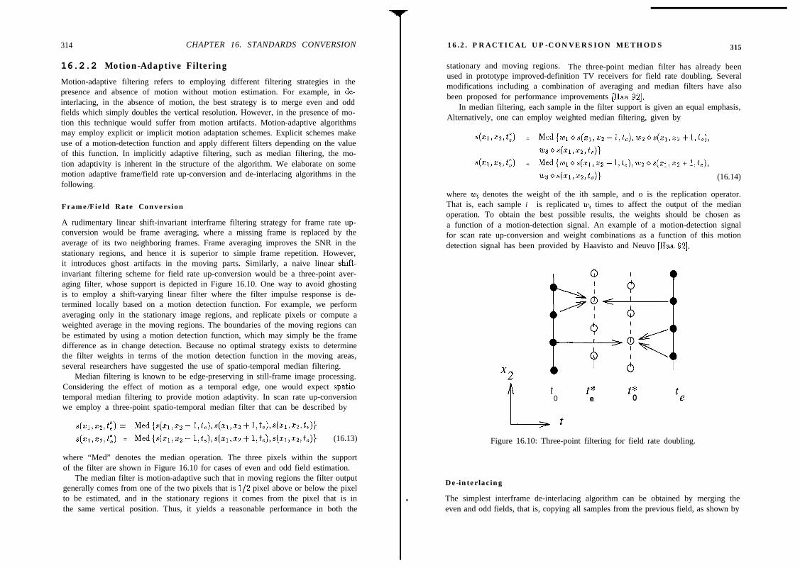
314 CHAPTER 16. STANDARDS CONVERSION 16.2. PRACTICAL UP-CONVERSION METHODS 315
16.2.2 Motion-Adaptive Filtering
Motion-adaptive filtering refers to employing different filtering strategies in thepresence and absence of motion without motion estimation. For example, in de-interlacing, in the absence of motion, the best strategy is to merge even and oddfields which simply doubles the vertical resolution. However, in the presence of mo-tion this technique would suffer from motion artifacts. Motion-adaptive algorithmsmay employ explicit or implicit motion adaptation schemes. Explicit schemes makeuse of a motion-detection function and apply different filters depending on the valueof this function. In implicitly adaptive filtering, such as median filtering, the mo-tion adaptivity is inherent in the structure of the algorithm. We elaborate on somemotion adaptive frame/field rate up-conversion and de-interlacing algorithms in thefollowing.
Frame/Field Rate Conversion
A rudimentary linear shift-invariant interframe filtering strategy for frame rate up-conversion would be frame averaging, where a missing frame is replaced by theaverage of its two neighboring frames. Frame averaging improves the SNR in thestationary regions, and hence it is superior to simple frame repetition. However,it introduces ghost artifacts in the moving parts. Similarly, a naive linear shift-invariant filtering scheme for field rate up-conversion would be a three-point aver-aging filter, whose support is depicted in Figure 16.10. One way to avoid ghostingis to employ a shift-varying linear filter where the filter impulse response is de-termined locally based on a motion detection function. For example, we performaveraging only in the stationary image regions, and replicate pixels or compute aweighted average in the moving regions. The boundaries of the moving regions canbe estimated by using a motion detection function, which may simply be the framedifference as in change detection. Because no optimal strategy exists to determinethe filter weights in terms of the motion detection function in the moving areas,several researchers have suggested the use of spatio-temporal median filtering.
Median filtering is known to be edge-preserving in still-frame image processing.Considering the effect of motion as a temporal edge, one would expect spatio-temporal median filtering to provide motion adaptivity. In scan rate up-conversionwe employ a three-point spatio-temporal median filter that can be described by
s(xl,x2,t~) = Med{s(zi,z:! - l,t,),s(zi,~z+ l,L),s(~i,~,t,)]
s(xl,x2,t~) = Med{s(x~,x~-~,t,),~(~l,~2+1,~~),~(~~,~~~~~)~ (16.13)
where “Med” denotes the median operation. The three pixels within the supportof the filter are shown in Figure 16.10 for cases of even and odd field estimation.
The median filter is motion-adaptive such that in moving regions the filter outputgenerally comes from one of the two pixels that is l/2 pixel above or below the pixelto be estimated, and in the stationary regions it comes from the pixel that is inthe same vertical position. Thus, it yields a reasonable performance in both the
stationary and moving regions. The three-point median filter has already beenused in prototype improved-definition TV receivers for field rate doubling. Severalmodifications including a combination of averaging and median filters have alsobeen proposed for performance improvements [Haa 921.
In median filtering, each sample in the filter support is given an equal emphasis,Alternatively, one can employ weighted median filtering, given by
s(xl,xz,t:) = Med{w OS(XI, xz - Lb), UJZ OS(XI,X~ + l,t,),
w3 0 s(x1, x2, te)}
s(~l,x21~;) = Med{w OS(XI, 22 - 1,&J, w OS(XI, xz + l,t,),
‘W3 0 s(21, x21 to)> (16.14)
where wi denotes the weight of the ith sample, and o is the replication operator.That is, each sample i is replicated UJ~ times to affect the output of the medianoperation. To obtain the best possible results, the weights should be chosen asa function of a motion-detection signal. An example of a motion-detection signalfor scan rate up-conversion and weight combinations as a function of this motiondetection signal has been provided by Haavisto and Neuvo [Haa 921.
A I 6 I
t t” t”0 e 0 te
Figure 16.10: Three-point filtering for field rate doubling.
De-interlacing
l The simplest interframe de-interlacing algorithm can be obtained by merging theeven and odd fields, that is, copying all samples from the previous field, as shown by
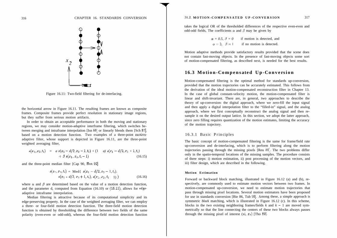
316 CHAPTER 16. STANDARDS CONVERSION
0 t
x2
t
l-1
Figure 16.11: Two-field filtering for de-interlacing.
the horizontal arrow in Figure 16.11. The resulting frames are known as compositeframes. Composite frames provide perfect resolution in stationary image regions,but they suffer from serious motion artifacts.
In order to obtain an acceptable performance in both the moving and stationaryregions, we may consider motion-adaptive interframe filtering, which switches be-tween merging and intraframe interpolation [Isn 861 or linearly blends them [Sch 871,based on a motion detection function. Two examples of a three-point motion-adaptive filter, whose support is depicted in Figure 16.11, are the three-pointweighted averaging filter,
s(x1, xz,ti) = a s(x1 - d/2,x2 - l,ti) + (1 - a) s(xl + d/2,x2 + l,ti)
+ P S(Q) e2,ti - 1) (16.15)
and the three-point median filter [Cap 90, Haa 921
s(xl,xz,ti) = Med{ s(zi -d/2,x2- l,ti),
~(21 + d/2, xz + 1, ii), 4x1, xz, ti - 1) } (16.16)
where o and p are determined based on the value of a motion detection function,and the parameter d, computed from Equation (16.10) or (16.11), allows for edge-adaptive intraframe interpolation.
Median filtering is attractive because of its computational simplicity and itsedge-preserving property. In the case of the weighted averaging filter, we can employa three- or four-field motion detection function. The three-field motion detectionfunction is obtained by thresholding the difference between two fields of the samepolarity (even-even or odd-odd), whereas the four-field motion detection function
16.3. MOTION-COMPENSATED UP-CONVERSION 317
takes the logical OR of the thresholded differences of the respective even-even andodd-odd fields, The coefficients (Y and /3 may be given by
a = 0.5, p = 0 if motion is detected, and
a=o, p=1 if no motion is detected.
Motion adaptive methods provide satisfactory results provided that the scene doesnot contain fast-moving objects. In the presence of fast-moving objects some sortof motion-compensated filtering, as described next, is needed for the best results.
16.3 Motion-Compensated Up-Conversion
Motion-compensated filtering is the optimal method for standards up-conversion,provided that the motion trajectories can be accurately estimated. This follows fromthe derivation of the ideal motion-compensated reconstruction filter in Chapter 13.In the case of global constant-velocity motion, the motion-compensated filter islinear and shift-invariant. There are, in general, two approaches to describe thetheory of up-conversion: the digital approach, where we zero-fill the input signaland then apply a digital interpolation filter to the “filled-in” signal, and the analogapproach, where we first conceptually reconstruct the analog signal and then re-sample it on the desired output lattice. In this section, we adopt the latter approach,since zero filling requires quantization of the motion estimates, limiting the accuracyof the motion trajectory.
16.3.1 Basic Principles
The basic concept of motion-compensated filtering is the same for frame/field rateup-conversion and de-interlacing, which is to perform filtering along the motiontrajectories passing through the missing pixels [Reu 891. The two problems differonly in the spatio-temporal locations of the missing samples. The procedure consistsof three steps: i) motion estimation, ii) post processing of the motion vectors, andiii) filter design, which are described in the following.
Motion Estimation
Forward or backward block matching, illustrated in Figure 16.12 (a) and (b), re-spectively, are commonly used to estimate motion vectors between two frames. Inmotion-compensated up-conversion, we need to estimate motion trajectories thatpass through missing pixel locations. Several motion estimators have been proposedfor use in standards conversion [Bie 86, Tub 931. Among these, a simple approach issymmetric block matching, which is illustrated in Figure 16.12 (c). In this scheme,blocks in the two existing neighboring frames/fields k and k - 1 are moved sym-metrically so that the line connecting the centers of these two blocks always passesthrough the missing pixel of interest (xi, x2) [Tho 891.

318 CHAPTER 16. STANDARDS CONVERSION
x 2
x + dx1 I
“z + dx2”
frame k-l /----I: 3+dx2
/x +dxI 1frame k /
“1
frame k
“1
framek-l j . /
-:.::p.::-:J
@I
“2 + dx2”
x, + dxl /2 CC)
Figure 16.12: a) Forward, b) backward, and c) symmetric block matching.
The accuracy of the motion estimates is probably the most important factor inthe effectiveness of motion-compensated interpolation. Thus, some kind of postpro-cessing is usually applied to the estimated motion vectors to improve their accuracy.
Postprocessing of Motion Estimates
The accuracy of the motion estimates can be improved by postprocessing techniques.Here we present two approaches to test the accuracy of the motion estimates: occlu-sion detection method, and displaced frame difference (DFD) method. Note thatthese methods are applied to the two nonzero frames used in symmetrical blockmatching.
The occlusion detection method is based on the assumption that a corona ofmotion vectors is usually located around moving objects. This assumption, coupledwith the observation that the correct motion vectors from frame k to frame k + 1
16.3. MOTION-COMPENSATED UP-CONVERSION 319
always map into the “changed region” CD(k, k + l), leads to the following occlusiondetection procedure, which was also used in Chapter 11. If an estimated motionvector from frame k to frame k+l maps to outside of the changed region, it indicatesa pixel in frame k that will be covered in frame k + 1. Likewise, if a motion vectorfrom frame k+l to frame k maps to outside of the changed region, it indicates a pixelin frame k + 1 that is uncovered. Of course, such motion vectors are not reliable andhave to be discarded. An alternative method to detect unreliable motion vectors isto test the DFD between the frames k and k+ 1. In this scheme, all vectors yieldinga DFD that is above a prespecified threshold are discarded.
The unreliable motion vectors can be replaced by a set of candidate motionvectors if any of the candidate vectors yields a DFD that is less than the threshold.The candidate vectors can be determined based on the analysis of the histogramof the reliable motion vectors, where the dominant peaks of the histogram indicatebackground motion or the motion of large objects in the scene [Lag 921. If noreliable replacement motion vector can be found at a pixel, it is marked as a motionestimation failure, where a motion-adaptive or an intraframe filter is employed.
Filter Design
Given the velocity estimates, the motion-compensated low-pass filter is defined by
ff(fl, ft) =i
1 for - Bi < fi < Bia n d -vl.fi - Bt < ft < -vlfi +Bt
0 otherwise
whose support is depicted in Figure 16.13. Because this filter is unrealizable, itneeds to be approximated, usually by an FIR filter, which poses a trade-off betweenfilter length and passband width. In practice, there is a limitation to the number offrame-stores that can be used in hardware implementations, which necessitates theuse of short temporal filters. This causes a wider than desired transition band in thetemporal frequency direction. Thus, the replications due to sub-Nyquist samplingshould not come closer than the transition band of the filter frequency response.
For example, in the interest of real-time implementation with a small numberof frame-stores, a simple zero-order hold filter may be employed along the motiontrajectory for interpolation filtering. Thus, we attempt to find the missing pixelvalues from the past fields using the information provided by the motion vectors.In an attempt to find a match with one of the existing sample values, Woods andHan [Woo 911 carry this search over two previous fields, as shown in Figure 16.14.For those pixels whose motion vectors do not point to an existing pixel locationin either of the past two fields, the values are taken to be the average of the twonearest existing pixels in the previous two fields. A number of other filter de-sign issues for motion-compensated sampling structure conversion are addressed in[Dub 92, Be1 93, Gir 931. Application of motion-compensated filtering to standardsconversion from NTSC to PAL or vice versa has been discussed in [Yam 941.
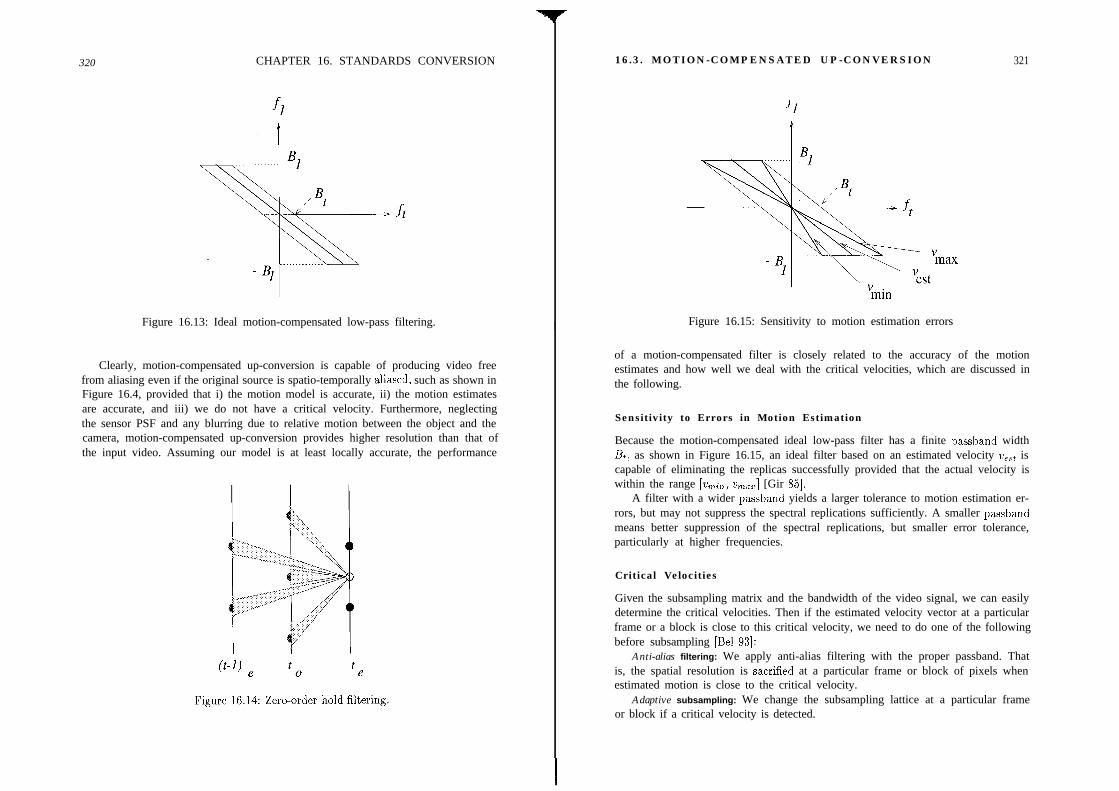
320 CHAPTER 16. STANDARDS CONVERSION 16.3. MOTION-COMPENSATED UP-CONVERSION
Figure 16.13: Ideal motion-compensated low-pass filtering. I Figure 16.15: Sensitivity to motion estimation errors
Clearly, motion-compensated up-conversion is capable of producing video freefrom aliasing even if the original source is spatio-temporally aliased, such as shown inFigure 16.4, provided that i) the motion model is accurate, ii) the motion estimatesare accurate, and iii) we do not have a critical velocity. Furthermore, neglectingthe sensor PSF and any blurring due to relative motion between the object and thecamera, motion-compensated up-conversion provides higher resolution than that ofthe input video. Assuming our model is at least locally accurate, the performance
321
of a motion-compensated filter is closely related to the accuracy of the motionestimates and how well we deal with the critical velocities, which are discussed inthe following.
Sensitivity to Errors in Motion Estimation
Because the motion-compensated ideal low-pass filter has a finite passband width&, as shown in Figure 16.15, an ideal filter based on an estimated velocity v,,~ iscapable of eliminating the replicas successfully provided that the actual velocity iswithin the range [u,in, u,,,] [Gir 851.
A filter with a wider passband yields a larger tolerance to motion estimation er-rors, but may not suppress the spectral replications sufficiently. A smaller passbandmeans better suppression of the spectral replications, but smaller error tolerance,particularly at higher frequencies.
Critical Velocities
Given the subsampling matrix and the bandwidth of the video signal, we can easilydetermine the critical velocities. Then if the estimated velocity vector at a particularframe or a block is close to this critical velocity, we need to do one of the followingbefore subsampling [Be1 931:
Anti-alias filtering: We apply anti-alias filtering with the proper passband. Thatis, the spatial resolution is sacrified at a particular frame or block of pixels whenestimated motion is close to the critical velocity.
Adaptive subsampling: We change the subsampling lattice at a particular frameor block if a critical velocity is detected.
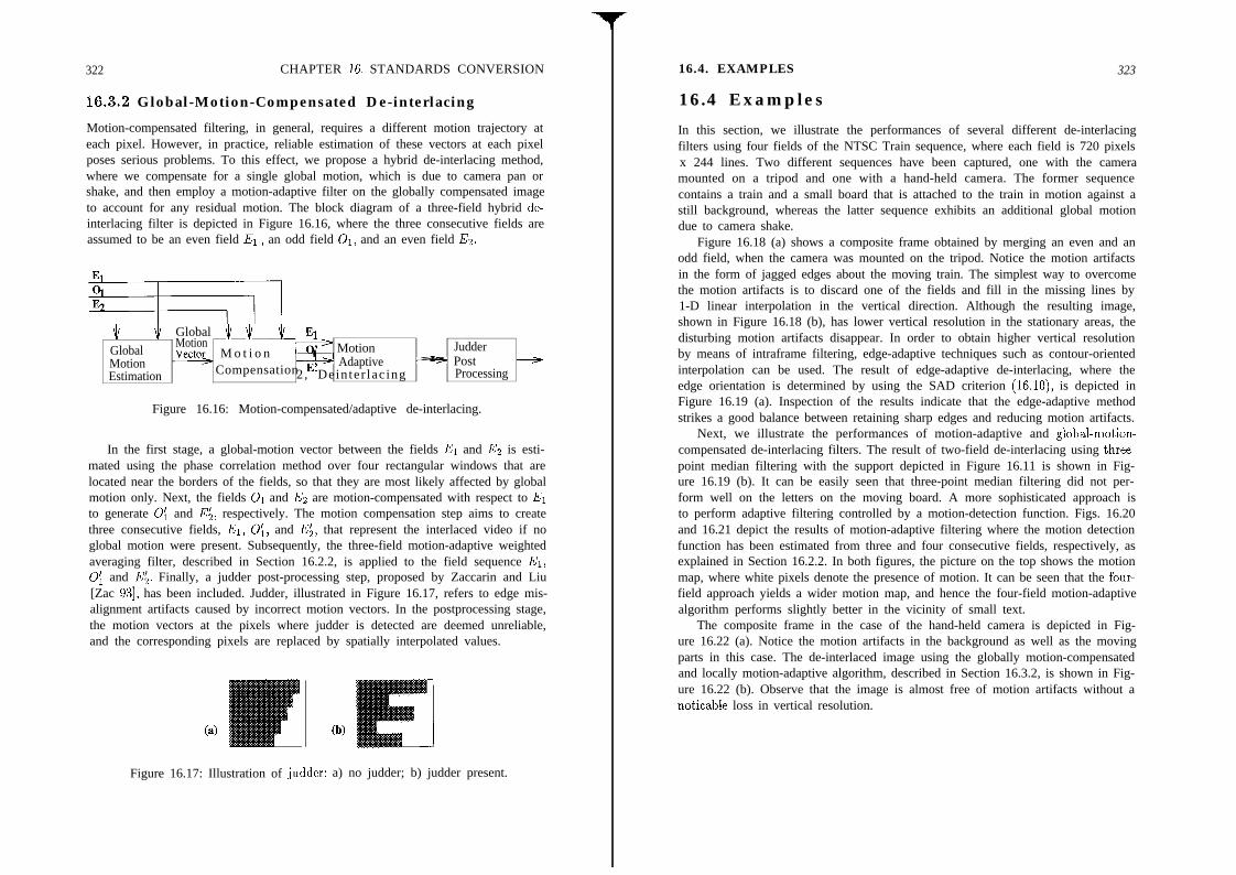
322 CHAPTER 16. STANDARDS CONVERSION
16.3.2 Global-Motion-Compensated De-interlacing
Motion-compensated filtering, in general, requires a different motion trajectory ateach pixel. However, in practice, reliable estimation of these vectors at each pixelposes serious problems. To this effect, we propose a hybrid de-interlacing method,where we compensate for a single global motion, which is due to camera pan orshake, and then employ a motion-adaptive filter on the globally compensated imageto account for any residual motion. The block diagram of a three-field hybrid de-interlacing filter is depicted in Figure 16.16, where the three consecutive fields areassumed to be an even field El ) an odd field 01, and an even field Ez.
i $ Global $ $ LMotion El
Global 0’ Motion JudderMotion
vectos M o t i o nAdaptive Post
Estimation Compensation E’2 , Dein ter lac ing Processing
Figure 16.16: Motion-compensated/adaptive de-interlacing.
In the first stage, a global-motion vector between the fields El and Ez is esti-mated using the phase correlation method over four rectangular windows that arelocated near the borders of the fields, so that they are most likely affected by globalmotion only. Next, the fields 01 and Ez are motion-compensated with respect to Elto generate 0; and Ei, respectively. The motion compensation step aims to createthree consecutive fields, El, O;, and Ea, that represent the interlaced video if noglobal motion were present. Subsequently, the three-field motion-adaptive weightedaveraging filter, described in Section 16.2.2, is applied to the field sequence El,0; and Ek. Finally, a judder post-processing step, proposed by Zaccarin and Liu[Zac 931, has been included. Judder, illustrated in Figure 16.17, refers to edge mis-alignment artifacts caused by incorrect motion vectors. In the postprocessing stage,the motion vectors at the pixels where judder is detected are deemed unreliable,and the corresponding pixels are replaced by spatially interpolated values.
(4
Figure 16.17: Illustration of judcler: a) no judder; b) judder present.
(b)
16.4. EXAMPLES 323
16.4 Examples
In this section, we illustrate the performances of several different de-interlacingfilters using four fields of the NTSC Train sequence, where each field is 720 pixelsx 244 lines. Two different sequences have been captured, one with the cameramounted on a tripod and one with a hand-held camera. The former sequencecontains a train and a small board that is attached to the train in motion against astill background, whereas the latter sequence exhibits an additional global motiondue to camera shake.
Figure 16.18 (a) shows a composite frame obtained by merging an even and anodd field, when the camera was mounted on the tripod. Notice the motion artifactsin the form of jagged edges about the moving train. The simplest way to overcomethe motion artifacts is to discard one of the fields and fill in the missing lines by1-D linear interpolation in the vertical direction. Although the resulting image,shown in Figure 16.18 (b), has lower vertical resolution in the stationary areas, thedisturbing motion artifacts disappear. In order to obtain higher vertical resolutionby means of intraframe filtering, edge-adaptive techniques such as contour-orientedinterpolation can be used. The result of edge-adaptive de-interlacing, where theedge orientation is determined by using the SAD criterion (16.10), is depicted inFigure 16.19 (a). Inspection of the results indicate that the edge-adaptive methodstrikes a good balance between retaining sharp edges and reducing motion artifacts.
Next, we illustrate the performances of motion-adaptive and global-motion-compensated de-interlacing filters. The result of two-field de-interlacing using three-point median filtering with the support depicted in Figure 16.11 is shown in Fig-ure 16.19 (b). It can be easily seen that three-point median filtering did not per-form well on the letters on the moving board. A more sophisticated approach isto perform adaptive filtering controlled by a motion-detection function. Figs. 16.20and 16.21 depict the results of motion-adaptive filtering where the motion detectionfunction has been estimated from three and four consecutive fields, respectively, asexplained in Section 16.2.2. In both figures, the picture on the top shows the motionmap, where white pixels denote the presence of motion. It can be seen that the four-field approach yields a wider motion map, and hence the four-field motion-adaptivealgorithm performs slightly better in the vicinity of small text.
The composite frame in the case of the hand-held camera is depicted in Fig-ure 16.22 (a). Notice the motion artifacts in the background as well as the movingparts in this case. The de-interlaced image using the globally motion-compensatedand locally motion-adaptive algorithm, described in Section 16.3.2, is shown in Fig-ure 16.22 (b). Observe that the image is almost free of motion artifacts without anoticable loss in vertical resolution.
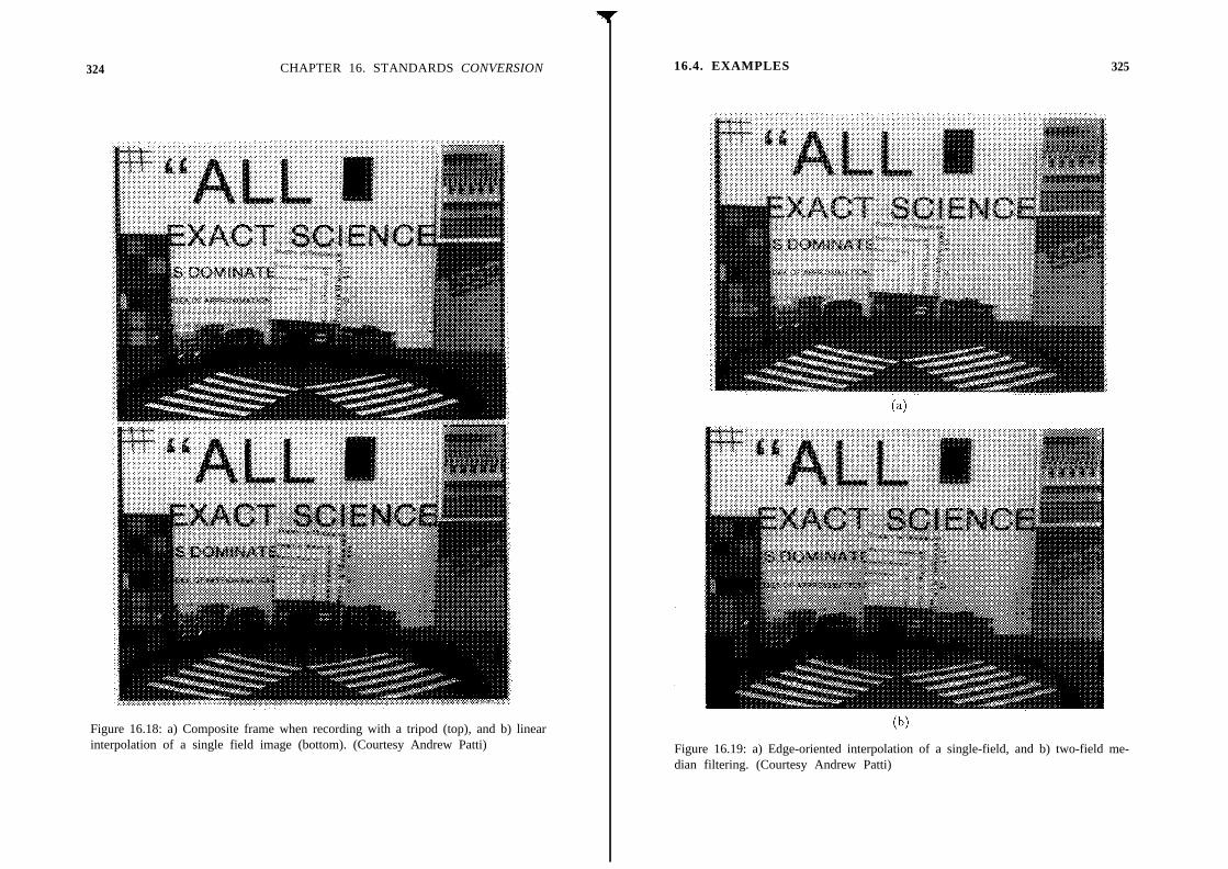
324 CHAPTER 16. STANDARDS CONVERSION
Figure 16.18: a) Composite frame when recording with a tripod (top), and b) linearinterpolation of a single field image (bottom). (Courtesy Andrew Patti)
16.4. EXAMPLES 325
Figure 16.19: a) Edge-oriented interpolation of a single-field, and b) two-field me-dian filtering. (Courtesy Andrew Patti)

326 CHAPTER 16. STANDARDS CONVERSION
Fig;ure 16.20: Motion-adaptive de-interlacing with three fields: a) the motion detec-tioln map (top), and b) the de-interlaced picture (bottom). (Courtesy Andrew Patti)
16.4. EXAMPLES 327
Figure 16.21: Motion-adaptive de-interlacing with four fields: a) the motion detion map (top), and b) the de-interlaced picture (bottom). (Courtesy Andrew Pzttti)
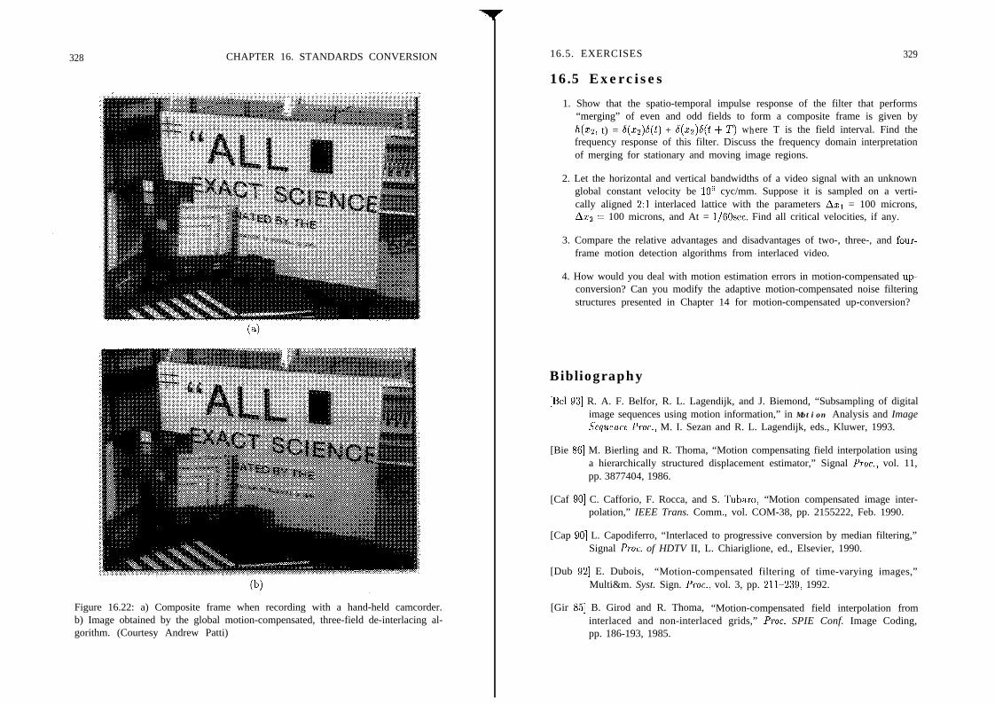
328 CHAPTER 16. STANDARDS CONVERSION
Figure 16.22: a) Composite frame when recording with a hand-held camcorder.b) Image obtained by the global motion-compensated, three-field de-interlacing al-gorithm. (Courtesy Andrew Patti)
16.5. EXERCISES 329
16.5 Exercises
1. Show that the spatio-temporal impulse response of the filter that performs“merging” of even and odd fields to form a composite frame is given byh(xz, t) = 6(x$(t) + 6(x$(t + 7’) where T is the field interval. Find thefrequency response of this filter. Discuss the frequency domain interpretationof merging for stationary and moving image regions.
2. Let the horizontal and vertical bandwidths of a video signal with an unknownglobal constant velocity be lo6 cyc/mm. Suppose it is sampled on a verti-cally aligned 2:l interlaced lattice with the parameters AXI = 100 microns,Ax2 = 100 microns, and At = 1/60sec. Find all critical velocities, if any.
3. Compare the relative advantages and disadvantages of two-, three-, and four-frame motion detection algorithms from interlaced video.
4. How would you deal with motion estimation errors in motion-compensated up-conversion? Can you modify the adaptive motion-compensated noise filteringstructures presented in Chapter 14 for motion-compensated up-conversion?
Bibliography
[Be1 931 R. A. F. Belfor, R. L. Lagendijk, and J. Biemond, “Subsampling of digitalimage sequences using motion information,” in Motion Analysis and ImageSepzlence Proc., M. I. Sezan and R. L. Lagendijk, eds., Kluwer, 1993.
[Bie 861 M. Bierling and R. Thoma, “Motion compensating field interpolation usinga hierarchically structured displacement estimator,” Signal Proc., vol. 11,pp. 3877404, 1986.
[Caf 901 C. Cafforio, F. Rocca, and S. Tubaro, “Motion compensated image inter-polation,” IEEE Trans. Comm., vol. COM-38, pp. 2155222, Feb. 1990.
[Cap 901 L. Capodiferro, “Interlaced to progressive conversion by median filtering,”Signal Proc. of HDTV II, L. Chiariglione, ed., Elsevier, 1990.
[Dub 921 E. Dubois, “Motion-compensated filtering of time-varying images,”Multi&m. Syst. Sign. Proc., vol. 3, pp. 211-239, 1992.
[Gir 851 B. Girod and R. Thoma, “Motion-compensated field interpolation frominterlaced and non-interlaced grids,” Proc. SPIE Conf. Image Coding,pp. 186-193, 1985.
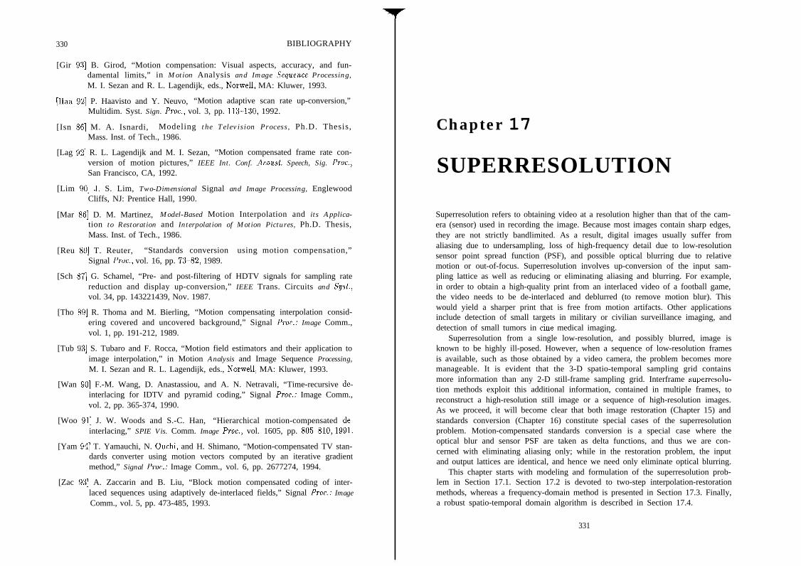
330 BIBLIOGRAPHY
[Gir 931 B. Girod, “Motion compensation: Visual aspects, accuracy, and fun-damental limits,” in Motion Analysis and Image Sequence Processing,M. I. Sezan and R. L. Lagendijk, eds., Norwell, MA: Kluwer, 1993.
[Haa 921 P. Haavisto and Y. Neuvo, “Motion adaptive scan rate up-conversion,”Multidim. Syst. Sign. Proc., vol. 3, pp. 1133130, 1992.
[Isn 861 M. A. Isnardi, Modeling the Television Process, Ph.D. Thesis,Mass. Inst. of Tech., 1986.
[Lag 921 R. L. Lagendijk and M. I. Sezan, “Motion compensated frame rate con-version of motion pictures,” IEEE Int. Conf. Acoust. Speech, Sig. Proc.,San Francisco, CA, 1992.
[Lim 901 J. S. Lim, Two-Dimensional Signal and Image Processing, EnglewoodCliffs, NJ: Prentice Hall, 1990.
[Mar 861 D. M. Martinez, Model-Based Motion Interpolation and its Applica-tion to Restoration and Interpolation of Motion Pictures, Ph.D. Thesis,Mass. Inst. of Tech., 1986.
[Reu 891 T. Reuter, “Standards conversion using motion compensation,”Signal Proc., vol. 16, pp. 73-82, 1989.
[Sch 871 G. Schamel, “Pre- and post-filtering of HDTV signals for sampling ratereduction and display up-conversion,” IEEE Trans. Circuits and Syst.,vol. 34, pp. 143221439, Nov. 1987.
[Tho 891 R. Thoma and M. Bierling, “Motion compensating interpolation consid-ering covered and uncovered background,” Signal Proc.: Image Comm.,vol. 1, pp. 191-212, 1989.
[Tub 931 S. Tubaro and F. Rocca, “Motion field estimators and their application toimage interpolation,” in Motion Analysis and Image Sequence Processing,M. I. Sezan and R. L. Lagendijk, eds., Norwell, MA: Kluwer, 1993.
[Wan 901 F.-M. Wang, D. Anastassiou, and A. N. Netravali, “Time-recursive de-interlacing for IDTV and pyramid coding,” Signal Proc.: Image Comm.,vol. 2, pp. 365-374, 1990.
[Woo 911 J. W. Woods and S.-C. Han, “Hierarchical motion-compensated de-interlacing,” SPIE Vis. Comm. Image Proc., vol. 1605, pp. 8055810,199l.
[Yam 941 T. Yamauchi, N. Ouchi, and H. Shimano, “Motion-compensated TV stan-dards converter using motion vectors computed by an iterative gradientmethod,” Signal Proc.: Image Comm., vol. 6, pp. 2677274, 1994.
[Zac 931 A. Zaccarin and B. Liu, “Block motion compensated coding of inter-laced sequences using adaptively de-interlaced fields,” Signal Proc.: ImageComm., vol. 5, pp. 473-485, 1993.
Chapter 17
SUPERRESOLUTION
Superresolution refers to obtaining video at a resolution higher than that of the cam-era (sensor) used in recording the image. Because most images contain sharp edges,they are not strictly bandlimited. As a result, digital images usually suffer fromaliasing due to undersampling, loss of high-frequency detail due to low-resolutionsensor point spread function (PSF), and possible optical blurring due to relativemotion or out-of-focus. Superresolution involves up-conversion of the input sam-pling lattice as well as reducing or eliminating aliasing and blurring. For example,in order to obtain a high-quality print from an interlaced video of a football game,the video needs to be de-interlaced and deblurred (to remove motion blur). Thiswould yield a sharper print that is free from motion artifacts. Other applicationsinclude detection of small targets in military or civilian surveillance imaging, anddetection of small tumors in tine medical imaging.
Superresolution from a single low-resolution, and possibly blurred, image isknown to be highly ill-posed. However, when a sequence of low-resolution framesis available, such as those obtained by a video camera, the problem becomes moremanageable. It is evident that the 3-D spatio-temporal sampling grid containsmore information than any 2-D still-frame sampling grid. Interframe superresolu-tion methods exploit this additional information, contained in multiple frames, toreconstruct a high-resolution still image or a sequence of high-resolution images.As we proceed, it will become clear that both image restoration (Chapter 15) andstandards conversion (Chapter 16) constitute special cases of the superresolutionproblem. Motion-compensated standards conversion is a special case where theoptical blur and sensor PSF are taken as delta functions, and thus we are con-cerned with eliminating aliasing only; while in the restoration problem, the inputand output lattices are identical, and hence we need only eliminate optical blurring.
This chapter starts with modeling and formulation of the superresolution prob-lem in Section 17.1. Section 17.2 is devoted to two-step interpolation-restorationmethods, whereas a frequency-domain method is presented in Section 17.3. Finally,a robust spatio-temporal domain algorithm is described in Section 17.4.
331

332 CHAPTER 17. SUPERRESOLUTION
17 .1 Model ing
An important limitation of electronic imaging today is that most available still-frame or video cameras can only record images at a resolution lower than desirable.This is related to certain physical limitations of the image sensors, such as finite cellarea and finite aperture time. Although higher-resolution imaging sensors are beingadvanced, these may be too expensive and/or unsuitable for mobile imaging appli-cations. In the following, we first present a model that relates the low-resolutionsampled video to the underlying continuous video. Next, the low-resolution sampledvideo is expressed in terms of a higher-definition sampled video. The superresolu-tion problem is then posed as the reconstruction of this higher-definition video froma number of observed low-resolution frames.
1’7.1.1 Continuous-Discrete Model
We present a comprehensive model of video acquisition, which includes the effects offinite sensor cell area and finite aperture time. Low-resolution images suffer from acombination of blurring due to spatial integration at the sensor surface (due to finitecell area), modeled by a shift-invariant spatial PSF h,(ci, za), and aliasing due tosub-Nyquist sampling. In addition, relative motion between the objects in a sceneand the camera during the aperture time gives rise (due to temporal integration) toshift-varying spatial blurring. The relative motion may be due to camera motion, asin camera pan or a camera mounted on a moving vehicle, or the motion of objectsin a scene, which is especially significant in high-action movies and sports videos.Recall that it is often this motion which gives rise to temporal variation of thespatial intensity distribution. Images may also suffer from out-of-focus blur, whichwill be modeled by a shift-invariant spatial PSF h,(zi, ~2) (ignoring the depth-of-field problem), and additive noise.
Figure 17.1: Block diagram of video acquisition.
A block diagram of the continuous-input, discrete-output model of a low-resolution video acquisition process is depicted in Figure 17.1. Here, the first sub-system represents the temporal integration during the aperture time TA, resulting in
17.1. MODELING 333
a blurred video (due to relative motion) given by
(17.1)
where s,(zi, ~2, t) denotes the ideal continuous video that would be formed by aninstantaneous aperture. The model (17.1) can be best interpreted by consideringa stationary camera and mapping the effect of any camera motion to a relativescene motion. The next subsystem models the combined effects of integration atthe sensor surface and any shift-invariant out-of-focus blur, resulting in a furtherblurred video given by
c7(~1,~2, t) = hc(zl,Q) * *Sm(n, 22) t) (17.2)
where h,(zi, ~2) = h,(zi, ~2) * *h,(zi, ~2) is the combined shift-invariant spatialPSF and ** denotes 2-D convolution.
The integration over time in the model (17.1) can equivalently be written asa spatial integration at a single time instant r considering our ideal video sourcemodel
%(X1, x2,t) = Sc(Cl(T Xl, x2,4, C2(? Xl, z2,4, T) (17.3)
where c(~; 21, xz,t) = (ci(~.; 21, xz,t), cz(r; xi, x2, t)) is the motion trajectory func-tion that is defined in Chapter 13. Then, under the assumption that the refer-ence time r is within the temporal span of all motion trajectories passing through(zi, xs,t - v), 0 < 17 < TA, all (zil x2) within the time interval (t - TA,~) can betraced onto the plane at time T using the source model (17.3) to perform a spatialintegration over these points. The corresponding spatial PSF is given by
i
+qw, u2, +qu2 - C2(T Xl, x2, c;+> Xl, x2, Ul)))
bn(ul> uz, 7; Xl, x2, q = if CI(T;XI,X~,~-TA) < ~1 < ci(r;xi,zz,t) (17.4)0 otherwise
where J(ui,us,t) denotes the Jacobian of the change of variables, andc;i(r,xi,x2,ui) returns the time t - TA < to < t when ui = ci(r;xi,x:z,ta).(See [Pat 941 for a complete derivation of this PSF.) The spatial support ofh,(ui, us, 7; xi, x2, t), which is a shift-variant PSF, is a path at the reference time r,that is depicted in Figure 17.2. The path, mathematically expressed by the 1-D deltafunction within the interval ci(~;xi, x2,t - TA) < ui < ci(r;xi,xs,t) in (17.4), isobtained by mapping all points (zi,xy,t - q), 0 < 17 < TA (shown by the solidvertical line) onto time T.
Therefore, combining the video acquisition model in Figure 17.1 with the sourcemodel (17.3), we can establish the relationship
g(x1, xz,t) =SJ’
sc(u1, u2, T)h(Ul, w, T’; 21, xz,+hduz (17.5)

334 CHAPTER 17. SUPERRESOL UTION
t = 7
t-TA
Figure 17.2: Representation of the effect of motion during the aperture time (tem-poral integration) by a spatial PSF (spatial integration).
between the observed intensity g(xr,xz,t) and the ideal intensities S,(UI,UZ,T)
along the path (~1, ~2) = c(r; ~1, x2, t) at time 7, where
h(u1, u2, T; Xl, x2, t) = h,(Xl, x2) * *h,(u1,uz, T; Xl, x2,4 (17.6)
denotes the effective shift-variant spatial PSF of the composite model. A blockdiagram of this composite model is shown in Figure 17.3.
The degraded video is then ideally sampled on a 3-D low-resolution lattice AI,and noise is added to form the observed discrete video
g~(nl,nz) = S(~l,x2,t)l[,l z2 t]T=Vl[nl n2 J?lT + wk(n1,n2) (17.7)
where VI is the sampling matrix of the low-resolution lattice Al. If we assumethat g(zr, xz,t) is bandlimited, but the sampling intervals in the x1, x2) and t
Figure 17.3: Block diagram of system model.
17.1. MODELING 335
directions are larger than the corresponding Nyquist intervals, aliasing may result.It is essential that no anti-alias filtering be used prior to sampling in order to achievesuperresolution, which follows from the discussion in Section 16.1.
1’7.1.2 Discrete-Discrete Model
Next, we relate a set of low-resolution observations, gk(nr, nz), to the desired high-resolution frame(s) to be reconstructed, which are defined as
sdm11m2) = @w%~)l[,, z2 t]T=Vh[nl m2 i]T
where Vh is the sampling matrix of the high-resolution sampling grid.
(17.8)
Let’s assume that the high-resolution video si(mr,mz) is sampled above theNyquist rate, so that the continuous intensity pattern is more or less constant withineach high-resolution pixel (cells depicted in Figure 17.4). Then, for any frame iwithin the temporal span of the motion trajectory passing through (ni, nz, iE), wehave, from (17.7) and (17.5),
a(w, %) M Si(W, m2)ss
h(u1, w,, T; Xl, 22, t)dUldlLZ (17.9)
w h e r e [pi 22 t]T = Vr[ni nz lelT, [ur uz rlT = Vh[mr m2 iIT, and(~1, ~2) = ~(7; xl, x2) t). Next, we define
hik(ml, m2; nl) ~2) =J ’ s
qm, u2,7; 211 xz,~)~w~ua (17.10)
to arrive at our discrete-input (high-resolution video), discrete-output (observedlow-resolution video) model, given by
gk(nl,n2) = xy:,( s, ml, mz)hik(ml, m2; 121, n2) + u(n1, n2) (17.11)ml mz
where the support of the summation over the high-resolution grid (ml, mz) at aparticular low-resolution sample (ni, n2, !x) is depicted in Figure 17.4. The size ofthe support in Figure 17.4 depends on the relative velocity of the scene with respectto the camera, the size of the support of the low-resolution sensor PSF h,(xr, x2)(depicted by the solid line, assuming no out-of-focus blur) with respect to the highresolution grid, and whether there is any out-of-focus blur. Because the relativepositions of low- and high-resolution pixels in general vary from pixel to pixel, thediscrete sensor PSF is space-varying.
The model (17.11) establishes a relationship between any high-resolution frame iand observed low-resolution pixels from all frames JC which can be connected to theframe i by means of a motion trajectory. That is, each low-resolution observed pixel(nl, n2, !c) can be expressed as a linear combination of several high-resolution pixelsfrom the frame i, provided that (nr,nx,lc) is connected to frame i by a motiontrajectory. Note that both the continuous-discrete and discrete-discrete models areinvalid in case of occlusion. We assume that occlusion regions can be detectedn priori using a proper motion estimation/segmentation algorithm.
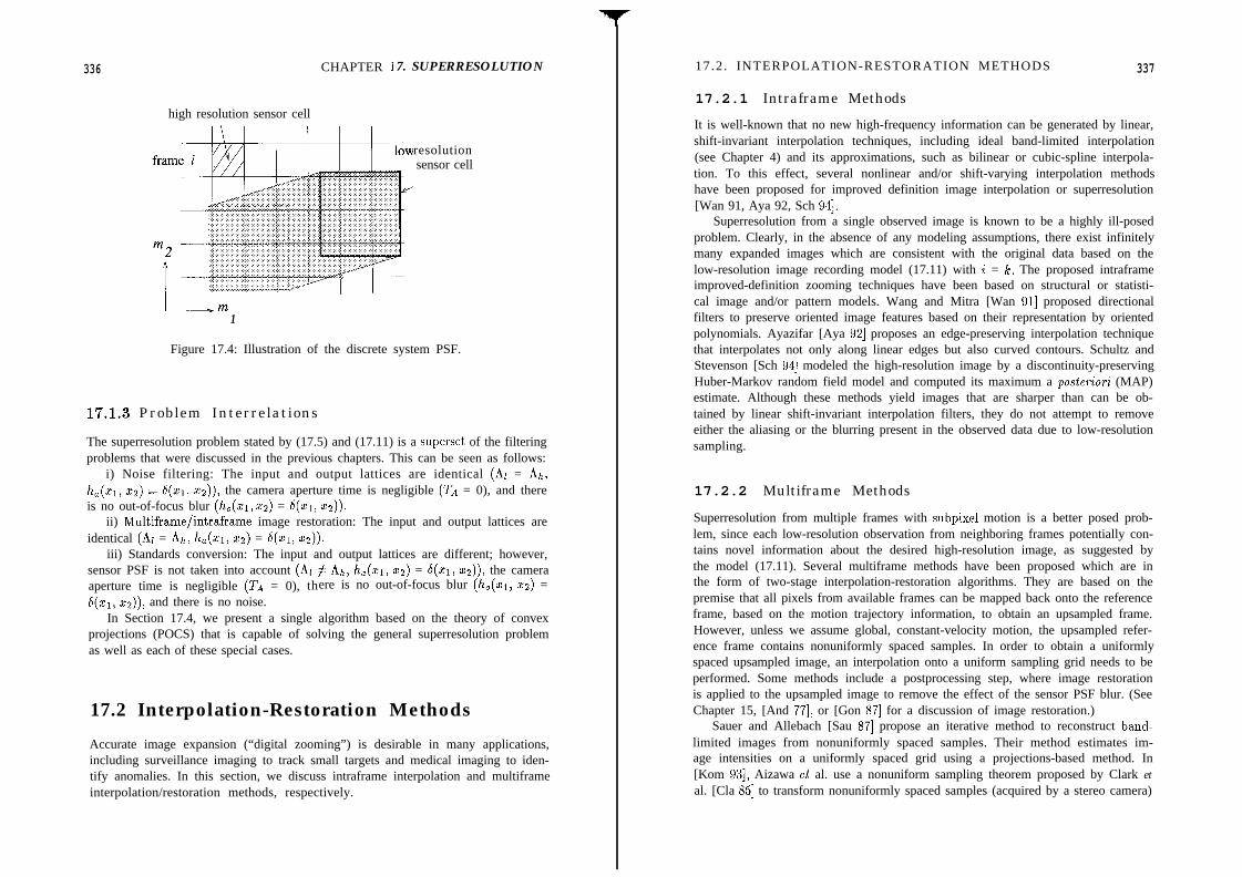
336 CHAPTER 1 7. SUPERRESOLUTION
high resolution sensor cell
resolutionsensor cell
I-m1
Figure 17.4: Illustration of the discrete system PSF.
17.1.3 Problem Interrelations
The superresolution problem stated by (17.5) and (17.11) is a superset of the filteringproblems that were discussed in the previous chapters. This can be seen as follows:
i) Noise filtering: The input and output lattices are identical (Al = Ah,h,(zr, ~2) = S(zr, ~z)), the camera aperture time is negligible (Ta = 0), and thereis no out-of-focus blur (h,(zi,zz) = S(zr, ~2)).
ii) Multiframe/intraframe image restoration: The input and output lattices areidentical (Al = Ah, h,(zr, Q) = S(zr, ~2)).
iii) Standards conversion: The input and output lattices are different; however,sensor PSF is not taken into account (Al # Ah, h,(zr, Q) = 6(x1, ~z)), the cameraaperture time is negligible (Ta = 0), there is no out-of-focus blur (h,(~r, ~2) =S(Q) Q)), and there is no noise.
In Section 17.4, we present a single algorithm based on the theory of convexprojections (POCS) that is capable of solving the general superresolution problemas well as each of these special cases.
17.2 Interpolation-Restoration Methods
Accurate image expansion (“digital zooming”) is desirable in many applications,including surveillance imaging to track small targets and medical imaging to iden-tify anomalies. In this section, we discuss intraframe interpolation and multiframeinterpolation/restoration methods, respectively.
17.2 . INTERPOLATION-RESTORATION METHODS
17.2.1 Intraframe Methods
337
It is well-known that no new high-frequency information can be generated by linear,shift-invariant interpolation techniques, including ideal band-limited interpolation(see Chapter 4) and its approximations, such as bilinear or cubic-spline interpola-tion. To this effect, several nonlinear and/or shift-varying interpolation methodshave been proposed for improved definition image interpolation or superresolution[Wan 91, Aya 92, Sch 941.
Superresolution from a single observed image is known to be a highly ill-posedproblem. Clearly, in the absence of any modeling assumptions, there exist infinitelymany expanded images which are consistent with the original data based on thelow-resolution image recording model (17.11) with i = I%. The proposed intraframeimproved-definition zooming techniques have been based on structural or statisti-cal image and/or pattern models. Wang and Mitra [Wan 911 proposed directionalfilters to preserve oriented image features based on their representation by orientedpolynomials. Ayazifar [Aya 921 proposes an edge-preserving interpolation techniquethat interpolates not only along linear edges but also curved contours. Schultz andStevenson [Sch 941 modeled the high-resolution image by a discontinuity-preservingHuber-Markov random field model and computed its maximum a posteriori (MAP)estimate. Although these methods yield images that are sharper than can be ob-tained by linear shift-invariant interpolation filters, they do not attempt to removeeither the aliasing or the blurring present in the observed data due to low-resolutionsampling.
17.2.2 Multiframe Methods
Superresolution from multiple frames with subpixel motion is a better posed prob-lem, since each low-resolution observation from neighboring frames potentially con-tains novel information about the desired high-resolution image, as suggested bythe model (17.11). Several multiframe methods have been proposed which are inthe form of two-stage interpolation-restoration algorithms. They are based on thepremise that all pixels from available frames can be mapped back onto the referenceframe, based on the motion trajectory information, to obtain an upsampled frame.However, unless we assume global, constant-velocity motion, the upsampled refer-ence frame contains nonuniformly spaced samples. In order to obtain a uniformlyspaced upsampled image, an interpolation onto a uniform sampling grid needs to beperformed. Some methods include a postprocessing step, where image restorationis applied to the upsampled image to remove the effect of the sensor PSF blur. (SeeChapter 15, [And 771, or [Gon 871 for a discussion of image restoration.)
Sauer and Allebach [Sau 871 propose an iterative method to reconstruct band-limited images from nonuniformly spaced samples. Their method estimates im-age intensities on a uniformly spaced grid using a projections-based method. In[Kom 931, Aizawa et al. use a nonuniform sampling theorem proposed by Clark etal. [Cla 851 to transform nonuniformly spaced samples (acquired by a stereo camera)

338 CHAPTER 17. SUPERRESOLUTION
onto a single uniform sampling grid. Recently, Ur and Gross [Ur 921 have proposeda nonuniform interpolation scheme based on the generalized sampling theorem ofPapoulis to obtain an improved-resolution blurred image. They acknowledge theneed for the restoration step after nonuniform interpolation. An important draw-back of these algorithms is that they do not address removal of aliasing artifacts.Furthermore, the restoration stage neglects the errors in the interpolation stage.
17.3 A Frequency Domain Method
The frequency domain method, first proposed by Tsai and Huang [Tsa 841, ex-ploits the relationship between the continuous and discrete Fourier transformsof the undersampled frames in the special case of global motion. If we letse(zi, ~2) 2 se(zr, x2,0) denote the reference frame, and assume zero aperture time(Ta = 0) and rectangular sampling with the sampling interval A in both directions,then the continuous-input, discrete-output model (17.5) simplifies as
N - l N - l
g!c(w,w) = c c [SO(XI - ak, 2 2 - Ph) * *h,(xl, x2)] 6(x1 - n,A, 22 - n2A)
nl=o nz=O
+ Vk(W, n2) (17.12)
where crh and & denote the 21 and 22 components of the displacement of the lathframe with respect to the reference frame, 6(x1, xz) denotes the 2-D Dirac deltafunction, and the low-resolution frames are assumed to be N x N. Because of thelinearity of convolution, Equation (17.12) can be equivalently expressed as
N - l N - l
Sk(%, m) = C c [so(xl, x2) * +&(x1 - ak, xz - A+)] 6(x1 - n,A, x2 - 6)
nl=o n2=0+ ~lc(~l,w4 (17.13)
Suppose we wish to reconstruct an M x M high-resolution sampled version ofthe reference frame sc(xr, Q), where M is an integer multiple of N, i.e., R = M/Nis an integer. Assuming that se(ci, xz) is bandlimited, such that
ISo(Fl,Fz) I=O, f o r II;;,F2 I> R& (17.14)
the model (17.13) undersamples se(~i,~z) by a factor R in both the ~1 and czdirections. Taking the Fourier transform of both sides of the observation model(17.13), we obtain
17.3. A FREQUENCY DOMAIN METHOD 339
where So(fl/A, fi/A) and H,(fi/A, fJA) denote the 2-D continuous Fouriertransform of the reference frame ss(zi, ~2) and the sensor PSF &(x1, Q), respec-r.ively, and Gk(fi,fz) and Vk(fl, f2) denote the 2-D discrete Fourier transform ofgk(ni,nz) and vk(ni,nz), respectively. We note that the motion blur can be in-corporated into the simplified model (17.15) (that is, the assumption TA = 0 maybe relaxed) only if we have global, constant-velocity motion, so that the frequencyresponse of the motion blur remains the same from frame to frame.
In order to recover the unaliased spectrum So(fl/A, fJA) at a given frequencypair (fl, fi), we need at least R2 equations (17.15) at that frequency pair, whichcould be obtained from L > R2 low-resolution frames. The set of equations (17.15),I% = 1, ) L, at any frequency pair (fl, f2) are decoupled from the equations thatare formed at any other frequency pair. The formulation by Tsai and Huang[Tsa 841 ignores the sensor blur and noise, hence proposes to set up L = R2 equa-tions in as many unknowns at each frequency pair to recover the alias-free spec-trum So[fi/A, fz/A). This procedure is illustrated by means of an example inthe following. Taking the sensor blur into account, we first recover the productSo(fl/A, fi/A) Hc(fl/A, fz/A) similarly. Subsequently, So(fl/A, fi/A) can beestimated by inverse filtering or any other regularized deconvolution technique.
Example: 1-D case
Consider two low-resolution observations of a 1-D signal (L = 2), whichare shifted with respect to each other by a subsample amount o, suchthat
N - l
c/l(n) = c so(x)~(x - nA) + ~(71)n=ON - l
gz(n) = c so(x - a)S(x - nA) + 712(n)
n=O
where N is the number of low-resolution samples, and the sensor PSFis assumed to be a delta function.
Assuming that gk(n), le = 1,2, are sampled at one half of the Nyquistrate (R = 2)) and taking the Fourier transform of both sides, we have
Gl(f) = $(;) + iSo
C&(f) = ~,,+W + ;so(k&jfc.t-~,o
There is only one aliasing term in each expression, because we assumedsampling at half the Nyquist rate.
The aliasing in the spectrum of the low-resolution sampled signal Gl(f)is illustrated in Figure 17.5. We can solve for the two unknowns
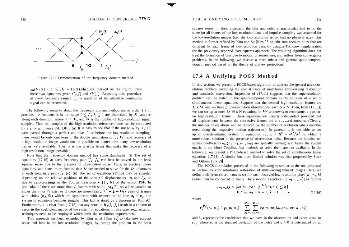
340 CHAPTER 17. SUPERRESOL UTION
Figure 17.5: Demonstration of the frequency domain method
So(.fo/A) and So((fo - 1)/A), h’ hw ic are marked on the figure, fromthese two equations given Gi(f) and Gz(f). Repeating this procedureat every frequency sample f, the spectrum of the alias-free continuoussignal can be recovered.
The following remarks about the frequency domain method are in order: (i) Inpractice, the frequencies in the range 0 5 fr) fi 5 1 are discretized by h’ samplesalong each direction, where I< > M, and M is the number of high-resolution signalsamples. Then the samples of the high-resolution reference frame can be computedby a K x K inverse 2-D DFT. (ii) It is easy to see that if the image s,(zi, zz, 0)were passed through a perfect anti-alias filter before the low-resolution sampling,there would be only one term in the double summation in (17.15), and recovery ofa high-resolution image would not be possible no matter how many low-resolutionframes were available. Thus, it is the aliasing terms that make the recovery of ahigh-resolution image possible.
Note that the frequency domain method has some drawbacks: (i) The set ofequations (17.15) at each frequency pair (fi, fz) can best be solved in the leastsquares sense due to the presence of observation noise. Thus, in practice, moreequations, and hence more frames, than L2 are needed to solve for the L2 unknownsat each frequency pair (fi, fz). (ii) The set of equations (17.15) may be singulardepending on the relative positions of the subpixel displacements, LYE and pk, ordue to zero-crossings in the Fourier transform He(fi, fz) of the sensor PSF. Inparticular, if there are more than L frames with shifts (ok,,&) on a line parallel toeither the 21 or cz axis, or if there are more than L(L2 - L - 1)/2 pairs of frameswith shifts (ak,pk) which are symmetric with respect to the line ~1 = ~2, thesystem of equations becomes singular. This fact is stated by a theorem in [Kim 901.Furthermore, it is clear from (17.15) that any zeros in H,(fi, fz) result in a column ofzeros in the coefficient matrix of the system of equations. In this case, regularizationtechniques need to be employed which limit the resolution improvement.
In this section, we present a POCS-based algorithm to address the general superres-olution problem, including the special cases of multiframe shift-varying restorationand standards conversion. Inspection of (17.11) suggests that the superresolutionproblem can be stated in the spatio-temporal domain as the solution of a set ofsimultaneous linear equations. Suppose that the desired high-resolution frames areMx n/r, and we have L low-resolution observations, each N x N. Then, from (17.11))we can set up at most Lx N x N equations in M2 unknowns to reconstruct a particu-lar high-resolution frame i. These equations are linearly independent provided thatall displacements between the successive frames are at subpixel amounts. (Clearly,the number of equations will be reduced by the number of occlusion labels encoun-tered along the respective motion trajectories.) In general, it is desirable to setup an overdetermined system of equations, i.e., L > R2 = M2/N2, to obtain amore robust solution in the presence of observation noise. Because the impulse re-sponse coefficients hik(ni) 122; ml, mz) are spatially varying, and hence the systemmatrix is not block-Toeplitz, fast methods to solve them are not available. In thefollowing, we present a POCS-based method to solve the set of simultaneous linearequations (17.11). A similar but more limited solution was also proposed by Starkand Oskoui [Sta 891.
The POCS formulation presented in the following is similar to the one proposedin Section 15.3 for intraframe restoration of shift-varying blurred images. Here, wedefine a different closed, convex set for each observed low-resolution pixel (ni) 122) Ic)(which can be connected to frame i by a motion trajectory c(i;ni, nz, Ic)) as follows
where
c nl,nz;i,k = {G(W) m2) : Ir$‘)(nl, n2)l i SO),
O<ni,nz<N-1, le=l,..., L (17.16)
This approach has been extended by Kim et. al. [Kim 901 to take into account and 60 represents the confidence that we have in the observation and is set equal tonoise and blur in the low-resolution images, by posing the problem in the least cu,, where uu is the standard deviation of the noise and c > 0 is determined by an
17.4. A UNIFYING POCS METHOD 341
squares sense. In their approach, the blur and noise characteristics had to be thesame for all frames of the low-resolution data, and impulse sampling was assumed forthe low-resolution images (i.e., the low-resolution sensor had no physical size). Thismethod is further refined by Kim and Su [Kim 931 to take into account blurs that aredifferent for each frame of low-resolution data, by using a Tikhonov regularizationfor the previously reported least squares approach. The resulting algorithm does nottreat the formation of blur due to motion or sensor size, and suffers from convergenceproblems. In the following, we discuss a more robust and general spatio-temporaldomain method based on the theory of convex projections.
17.4 A Unifying POCS Method
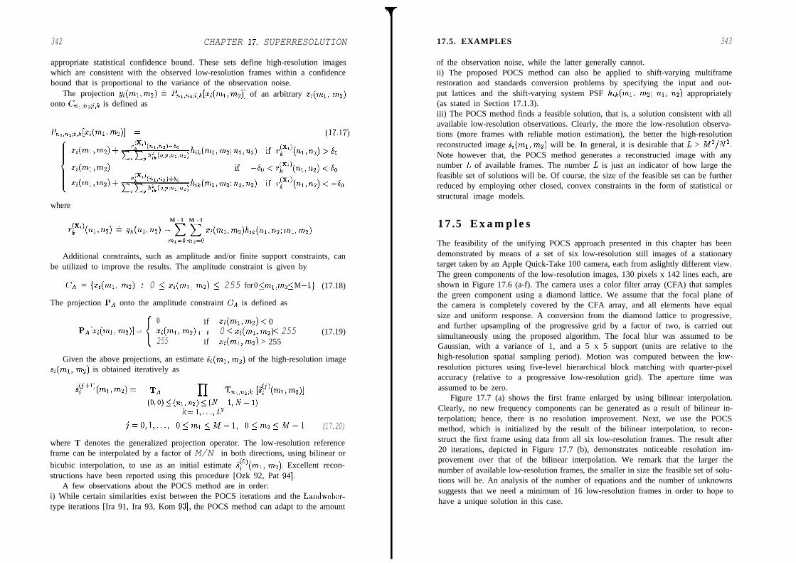
342 CHAPTER 17. SUPERRESOLUTION
appropriate statistical confidence bound. These sets define high-resolution imageswhich are consistent with the observed low-resolution frames within a confidencebound that is proportional to the variance of the observation noise.
The projection yi(mi,ms) - Pnl,na;i,k [zi(mi,ms)] of an arbitrary zi(mi, ms)onto Cnl,nz;i,k is defined as
where
M - l M - l
fp(%,nz) - grc(n1,nz) - c c zi(ml,m2)hik(nl,n2;ml,m2)
ml=om~=o
Additional constraints, such as amplitude and/or finite support constraints, canbe utilized to improve the results. The amplitude constraint is given by
CA = {zi(ml, mz) : 0 < zi(ml, m2) 5 255 for 0 5 ml, mz 5 M - 1) (17.18)
The projection PA onto the amplitude constraint CA is defined as
i
0 if zi(ml, m2) < 0PA[xi(ml, mZ)] = zi(ml, m2) i f 0 5 zi(ml,mz) 5 255 (17.19)
255 if zi(ml, mz) > 255
Given the above projections, an estimate i;(ml, rns) of the high-resolution imagesi(mi, ms) is obtained iteratively as
;(Hl)2 (ml,w)= TA(60) I (111, n2) 5 (N - 1, N - 1)
k =1,...,L2j=O,l,..., O<mi<M-1, O<ms<M-1 (17.20)
where T denotes the generalized projection operator. The low-resolution referenceframe can be interpolated by a factor of M/N in both directions, using bilinear orbicubic interpolation, to use as an initial estimate ia’)(rnl, mz). Excellent recon-structions have been reported using this procedure [Ozk 92, Pat 941.
A few observations about the POCS method are in order:i) While certain similarities exist between the POCS iterations and the Landweber-type iterations [Ira 91, Ira 93, Kom 931, the POCS method can adapt to the amount
17.5. EXAMPLES 343
of the observation noise, while the latter generally cannot.ii) The proposed POCS method can also be applied to shift-varying multiframerestoration and standards conversion problems by specifying the input and out-put lattices and the shift-varying system PSF hak(mi, ms; 121, ns) appropriately(as stated in Section 17.1.3).iii) The POCS method finds a feasible solution, that is, a solution consistent with allavailable low-resolution observations. Clearly, the more the low-resolution observa-tions (more frames with reliable motion estimation), the better the high-resolutionreconstructed image ia(mi, mz) will be. In general, it is desirable that L > M2/N2.Note however that, the POCS method generates a reconstructed image with anynumber L of available frames. The number L is just an indicator of how large thefeasible set of solutions will be. Of course, the size of the feasible set can be furtherreduced by employing other closed, convex constraints in the form of statistical orstructural image models.
17.5 Examples
The feasibility of the unifying POCS approach presented in this chapter has beendemonstrated by means of a set of six low-resolution still images of a stationarytarget taken by an Apple Quick-Take 100 camera, each from aslightly different view.The green components of the low-resolution images, 130 pixels x 142 lines each, areshown in Figure 17.6 (a-f). The camera uses a color filter array (CFA) that samplesthe green component using a diamond lattice. We assume that the focal plane ofthe camera is completely covered by the CFA array, and all elements have equalsize and uniform response. A conversion from the diamond lattice to progressive,and further upsampling of the progressive grid by a factor of two, is carried outsimultaneously using the proposed algorithm. The focal blur was assumed to beGaussian, with a variance of 1, and a 5 x 5 support (units are relative to thehigh-resolution spatial sampling period). Motion was computed between the low-resolution pictures using five-level hierarchical block matching with quarter-pixelaccuracy (relative to a progressive low-resolution grid). The aperture time wasassumed to be zero.
Figure 17.7 (a) shows the first frame enlarged by using bilinear interpolation.Clearly, no new frequency components can be generated as a result of bilinear in-terpolation; hence, there is no resolution improvement. Next, we use the POCSmethod, which is initialized by the result of the bilinear interpolation, to recon-struct the first frame using data from all six low-resolution frames. The result after20 iterations, depicted in Figure 17.7 (b), demonstrates noticeable resolution im-provement over that of the bilinear interpolation. We remark that the larger thenumber of available low-resolution frames, the smaller in size the feasible set of solu-tions will be. An analysis of the number of equations and the number of unknownssuggests that we need a minimum of 16 low-resolution frames in order to hope tohave a unique solution in this case.

344 CHAPTER 17. SUPERRESOLUTION
Figure 17.6: Six frames of a low-resolution image sequence taken by an AppleQuickTake 100 camera. (Courtesy Andrew Patti)
17.5. EXAMPLES 345
(b)Figure 17.7: The first frame a) interpolated by 2 using bilinear interpolation, andb) reconstructed by the POCS algorithm. (Courtesy Andrew Patti)
BIBLIOGRAPHY
17.6 Exercises
1. Consider global, constant-velocity motion, where the velocity is modeled asconstant during each aperture time (piecewise constant-velocity model). Letits value during ith aperture time (acquisition of the ith frame) be given byvi = [uii vzi]‘. Show that the Jacobian ,T(ui, uz, t) in (17.4) is equal to &.
2. Suppose we have four low-resolution images that are globally translating withrespect to a reference frame with velocities z’ii = v2i = 8.25,8,5,9, and 10 inunits of pixels per high-resolution sampling grid for i = 1, . ,4, respectively.Assume that each side of the low-resolution sensor cell is four times that of thehigh-resolution cell with rectangular sensor geometry shown in Figure 17.2.How would you calculate the discrete-discrete PSF &(mi,mz; ni,na) in(17.11)?
3. Derive (17.15).
4. Derive (17.17).
5. Discuss the relationship between the POCS reconstruction method discussedin Section 17.4 and the backprojection iterations presented in [Ira 931.
Bibliography
[And 771 H. C. Andrews and B. R. Hunt, Digital Image Restoration, EnglewoodCliffs, NJ: Prentice-Hall, 1977.
[Aya 921 B. Ayazifar, Pel-Adaptive Model-Based Interpolation of Spatially Subsam-pled Images, M.S. Thesis, Mass. Inst. of Tech., 1992.
[Cla 851 J. J. Clark, M. R. Palmer, and P. D. Lawrence, “A transformation methodfor the reconstruction of functions from nonuniformly spaced samples,”IEEE Trans. Acoust. Speech Sign. Proc., vol. 33, pp. 1151-1165, Oct.1985.
[Gon 871 R. C. Gonzalez and P. Wintz, Digital Image Processing, Reading, MA:Addison-Wesley, 1987.
[Ira 911 M. Irani and S. Peleg, “Improving resolution by image registration,”CVGIP: Graphical Models and Image PTOC., vol. 53, pp. 231-239,May 1991.
[Ira 931 M. Irani and S. Peleg, “Motion analysis for image enhancement: Resolu-tion, occlusion and transparency,”pp. 324-335, Dec. 1993.
J. Vis. Comm. and Image Rep., vol. 4,
BIBLIOGRAPHY 347
[Kim 901 S. P. Kim, N. K. Bose, and H. M. Valenzuela, “Recursive reconstructionof high-resolution image from noisy undersampled frames,” IEEE Trans.Acowt., Speech and Sign. Proc., vol. 38, pp. 1013-1027, June 1990.
[Kim 931 S. P. Kim and W.-Y. Su, “Recursive high-resolution reconstructionof blurred multiframe images,” IEEE Trans. Image Proc., vol. 2,pp. 534-539, Oct. 1993.
[Kom 931 T. Komatsu, T. Igarashi, K. Aizawa, and T. Saito, ‘Very high-resolutionimaging scheme with multiple different aperture cameras,” Signal Proc.:Image Comm., vol. 5, pp. 511-526, Dec. 1993.
[Ozk 941 M. K. Ozkan, A. M. Tekalp, and M. I. Sezan, “POCS-based restora-tion of space-varying blurred images,” IEEE Trans. Image Proc., vol. 3,pp. 450-454, July 1994.
[Pat 941 A. Patti, M. I. Sezan, and A. M. Tekalp, “High-resolution image recon-struction from a low-resolution image sequence in the presence of time-varying motion blur,” Proc. IEEE Int. Conf. Image Proc., Austin, TX,Nov. 1994.
[Sau 871 K. D. Sauer and J. P. Allebach, “Iterative reconstruction of bandlimitedimages from non-uniformly spaced samples,” IEEE Trans. Circ. and Syst.,
vol. 34, pp. 1497-1505, 1987.
[Sch 941 R. R. Schultz and R. L. Stevenson, “A Bayesian approach to imageexpansion for improved definition,” IEEE Trans. Image Proc., vol. 3,pp. 233-242, May 1994.
[Sta 891 H. Stark and P. Oskoui, “High-resolution image recovery from imageplane arrays using convex projections,” J. Opt. Sot. Amer. A, vol. 6,pp. 171551726, 1989.
[Tek 921 A. M. Tekalp, M. K. Ozkan, and M. I. Sezan, “High-resolution imagereconstruction from lower-resolution image sequences and space-varyingimage restoration,” IEEE Int. Conf. Acoust. Speech and Sign. Proc.,San Francisco, CA, vol. III, pp. 169-172, March 1992.
[Tsa 841 R. Y. Tsai and T. S. Huang, “Multiframe image restoration and regis-tration,” in Advances in Computer Vision and Image Processing, vol. 1,T. S. Huang, ed., pp. 317-339, Greenwich, CT: Jai Press, 1984.
[Ur 921 H. Ur and D. Gross, “Improved resolution from subpixel shifted pictures,”CVGIP: Graphical Models and Image Processing, vol. 54, pp. 181-186,March 1992.
[Wan 911 Y. Wang and S. K. Mitra, “Motion/pattern adaptive interpolation ofinterlaced video sequences,” Proc. IEEE Int. Conf. Acowt. Speech Sign.
Proc., pp. 282992832, Toronto, Canada, May 1991.

Chapter 18
LOSSLESSCOkiPRESSION
The need for effective data compression is evident in almost all applications wherestorage and transmission of digital images are involved. For example, an 8.5 x 11 indocument scanned at 300 pixels/in with 1 bit/pixel generates 8.4 Mbits data, whichwithout compression requires about 15 min transmission time over a 9600 baud line.A 35 mm film scanned at 12 micron resolution results in a digital image of size 3656pixels x 2664 lines. With 8 bits/pixel per color and three color channels, the storagerequired per picture is approximately 233 Mbits. The storage capacity of a CD isabout 5 Gbits, which without compression can hold approximately 600 pages of adocument, or 21 color images scanned from 35 mm film. Several world standardsfor image compression, such as ITU (formerly CCITT) Group 3 and 4 codes, andISO/IEC/CCITT JPEG, have recently been developed for efficient transmissionand storage of binary, gray-scale, and color images.
Compression of image data without significant degradation of the visual qualityis usually possible because images contain a high degree of i) spatial redundancy, dueto correlation between neighboring pixels, ii) spectral redundancy, due to correlationamong the color components, and iii) psychovisual redundancy, due to propertiesof the human visual system. The higher the redundancy, the higher the achievablecompression. This chapter introduces the basics of image compression, and discussessome lossless compression methods. It is not intended as a formal review of therelated concepts, but rather aims to provide the minimum information necessary tofollow the popular still-image and video compression algorithms/standards, whichwill be discussed in the subsequent chapters. Elements of an image compressionsystem as well as some information theoretic concepts are introduced in Section 18.1.Section 18.2 discusses symbol coding, and in particular entropy coding, which is anintegral part of lossless compression methods. Finally, three commonly used losslesscompression algorithms are presented in Section 18.3.
348
18.1. BASICS OF IMAGE COMPRESSION 349
18.1 Basics of Image Compression
In this section, we first present the elements of a general image compression system,then summarize some results from the information theory which provide bounds onthe achievable compression ratios and bitrates.
18.1.1 Elements of an Image Compression System
In information theory, the process of data compression by redundancy reduction isreferred to as source encoding. Images contain two types of redundancy, statistical(spatial) and pyschovisual. Statistical redundancy is present -because certain spatialpatterns are more likely than others, whereas psychovisual redundancy originatesfrom the fact that the human eye is insensitive to certain spatial frequencies. Theblock diagram of a source encoder is shown in Figure 18.1. It is composed of thefollowing blocks:
SymbolsI
Input _j Timage
I , Binary
z. Q (‘J bitstream
Figure 18.1: Block diagram of an image compression system.
i) Transformer (T) applies a one-to-one transformation to the input image data.The output of the transformer is an image representation which is more amenableto efficient compression than the raw image data. Typical transformations are linearpredictive mapping, which maps the pixel intensities onto a prediction error signalby subtracting the predictible part of the pixel intensities; unitary mappings such asthe discrete cosine transform, which pack the energy of the signal to a small numberof coefficients; and multiresolution mappings, such as subband decompositions andthe wavelet transform.ii) Quantizer (Q) generates a limited number of symbols that can be used in the rep-resention of the compressed image. Quantization is a many-to-one mapping whichis irreversible. It can be performed by scalar or vector quantizers. Scalar quantiza-tion refers to element-by-element quantization of the data, whereas quantization ofa block of data at once is known as vector quantization.iii) Coder (C) assigns a codeword, a binary bitstream, to each symbol at the outputof the quantizer. The coder may employ fixed-length or variable-length codes.Variable-length coding (VLC), 1 ka so nown as entropy coding, assigns codewords insuch a way as to minimize the average length of the binary representation of the
350 CHAPTER 18. LOSSLESS COMPRESSION
symbols. This is achieved by assigning shorter codewords to more probable symbols,which is the fundamental principle of entropy coding.
Different image compression systems implement different combinations of thesechoices. Image compression methods can be broadly classified as:i) Lossless (noiseless) compression methods, which aim to minimize the bitratewithout any distortion in the image.ii) Lossy compression methods, which aim to obtain the best possible fidelity for agiven bitrate, or to minimize the bitrate to achieve a given fidelity measure.The transformation and encoding blocks are lossless. However, quantization is lossy.Therefore, lossless methods, which only make use of the statistical redundancies, donot employ a quantizer. In most practical cases a small degradation in the imagequality must be allowed to achieve the desired bitrate. Lossy compression methodsmake use of both the statistical and psychovisual redundancies.
In the following, we first briefly review some results from the information theorywhich gives bounds on the achievable, bitrates in both lossless and lossy compres-sion. In Section 18.2, we present techniques for symbol coding (the third box inFigure 18.1). The discussion of the second box, the quantizer, is deferred until thenext chapter. Finally, some commonly used lossless image compression methods arepresented in Section 18.3.
18.1.2 Information Theoretic Concepts
A source X with an alphabet A is defined as a discrete random process (a sequenceof random variables Xi ) i = 1, .) in the form X = X1 Xz .) where each randomvariable Xi takes a value from the alphabet A. In the following, we assume thatthe alphabet contains a finite number (M) of symbols, i.e., d = {ui, ~2, , a~}.Here, we introduce two source models, a discrete memoryless source (DMS) and aMarkov-I( source.
A DMS is such that successive symbols are statistically independent. It iscompletely specified by the probabilities p(aa) = pi, i = 1,. , M such thatpi + + pi = 1. In VLC, the optimum length of the binary code for a sym-bol is equal to the information (in bits) that the symbol conveys. According toinformation theory, the information content of a symbol is related to the extentthat the symbol is unpredictable or unexpected. If a symbol with low probabilityoccurs, a larger amount of information is transferred than in the occurence of amore likely symbol. This quantitative concept of surprise is formally expressed bythe relation
I(Q) = log, (l/p(~)), for ai E A (18.1)
where I(ui) is the amount of information that the symbol ui with probability p(ua)carries, The unit of information is bit when we use logarithm with base-2. Observethat if p = 1, then I = 0 as expected, and as p + 0, I -+ 00. In practice,the probability of occurrence of each symbol is estimated from the histogram of aspecific source, or a training set of sources.
18.1. BASICS OF IMAGE COMPRESSION 351
The entropy H(X) of a DMS X with an alphabet A is defined as the averageinformation per symbol in the source, given by
H(X) = c P(U) lo&wP(~))aEd
= - c P(a) 1%2P(U)acd
(18.2)
The more skewed the probability distribution of the symbols, the smaller the entropyof the source. The entropy is maximized for a flat distribution that is, when allsymbols are equally likely. It follows that a source where some symbols are morelikely than others has a smaller entropy than a source where all symbols are equallylikely.
Example: Entropy of raw image data
Suppose an 8-bit image is taken as a realization of a DMS X. Thesymbols i are the gray levels of the pixels, and the alphabet .4 is thecollection of all gray levels between 0 and 255. Then the entropy of theimage is given by
255
H(X) = - c P(i) log2 P(i)
i=o
where p(i) denotes the relative frequency of occurrence of the gray leveli in the image. Note that the entropy of an image consisting of a singlegray level (constant image) is zero.
Most realistic sources can be better modeled by Markov-I< random processes.That is, the probability of occurence of a symbol depends on the values of I< preced-ing symbols. A Markov-K source can be specified by the conditional probabilitiesp(Xj = ~i1Xj-i~. ,Xj-K), for all j, ui E: A. The entropy of a Markov-K sourceis defined as
H(X) = CP(Xj-l,. . . ,~~-~)~(~I~~-l,...,~j-ri) (18.3)S”
where SK denotes all possible realizations of X,-i, . . . , X~-K, and
H(XIXj-1,. .,Xj-K) = Cp(uilXj-l,. .,Xj-K) logp(uiIXj-1,. .,Xj-K)aEd
In the following, we present two fundamental theorems, the Lossless Coding The-orem and the Source Coding Theorem, which are used to measure the performanceof lossless coding and lossy coding systems, respectively.
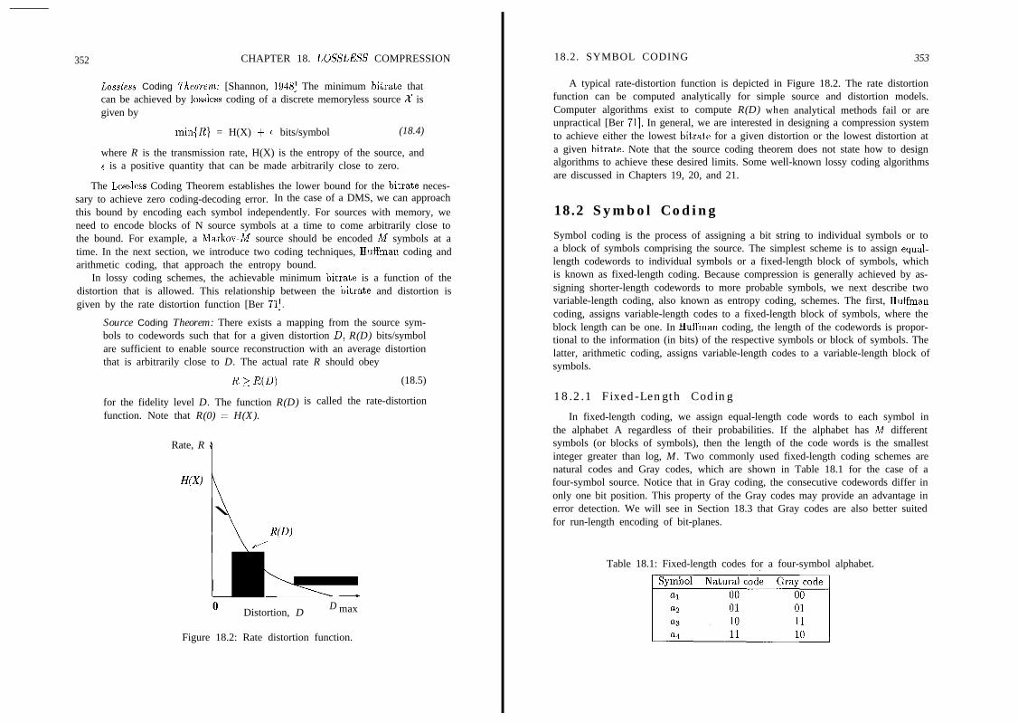
352 CHAPTER 18. LOSSLESS COMPRESSION
Lossless Coding Theorem: [Shannon, 19481 The minimum bitrate thatcan be achieved by lossless coding of a discrete memoryless source X isgiven by
min{R} = H(X) + t bits/symbol (18.4)
where R is the transmission rate, H(X) is the entropy of the source, andt is a positive quantity that can be made arbitrarily close to zero.
The Lossless Coding Theorem establishes the lower bound for the bitrate neces-sary to achieve zero coding-decoding error. In the case of a DMS, we can approachthis bound by encoding each symbol independently. For sources with memory, weneed to encode blocks of N source symbols at a time to come arbitrarily close tothe bound. For example, a Markov-M source should be encoded M symbols at atime. In the next section, we introduce two coding techniques, Huffman coding andarithmetic coding, that approach the entropy bound.
In lossy coding schemes, the achievable minimum bitrate is a function of thedistortion that is allowed. This relationship between the bitrate and distortion isgiven by the rate distortion function [Ber 711.
Source Coding Theorem: There exists a mapping from the source sym-bols to codewords such that for a given distortion D, R(D) bits/symbolare sufficient to enable source reconstruction with an average distortionthat is arbitrarily close to D. The actual rate R should obey
R 2 R(D) (18.5)
for the fidelity level D. The function R(D) is called the rate-distortionfunction. Note that R(0) = H(X).
Rate, R
HO
R(D)Distortion, D D max
Figure 18.2: Rate distortion function.
18.2. SYMBOL CODING 353
A typical rate-distortion function is depicted in Figure 18.2. The rate distortionfunction can be computed analytically for simple source and distortion models.Computer algorithms exist to compute R(D) when analytical methods fail or areunpractical [Ber 711. In general, we are interested in designing a compression systemto achieve either the lowest bitrate for a given distortion or the lowest distortion ata given bitrate. Note that the source coding theorem does not state how to designalgorithms to achieve these desired limits. Some well-known lossy coding algorithmsare discussed in Chapters 19, 20, and 21.
18.2 Symbol Coding
Symbol coding is the process of assigning a bit string to individual symbols or toa block of symbols comprising the source. The simplest scheme is to assign equal-length codewords to individual symbols or a fixed-length block of symbols, whichis known as fixed-length coding. Because compression is generally achieved by as-signing shorter-length codewords to more probable symbols, we next describe twovariable-length coding, also known as entropy coding, schemes. The first, Huffmancoding, assigns variable-length codes to a fixed-length block of symbols, where theblock length can be one. In Huffman coding, the length of the codewords is propor-tional to the information (in bits) of the respective symbols or block of symbols. Thelatter, arithmetic coding, assigns variable-length codes to a variable-length block ofsymbols.
18.2.1 Fixed-Length Coding
In fixed-length coding, we assign equal-length code words to each symbol inthe alphabet A regardless of their probabilities. If the alphabet has h/l differentsymbols (or blocks of symbols), then the length of the code words is the smallestinteger greater than log, M. Two commonly used fixed-length coding schemes arenatural codes and Gray codes, which are shown in Table 18.1 for the case of afour-symbol source. Notice that in Gray coding, the consecutive codewords differ inonly one bit position. This property of the Gray codes may provide an advantage inerror detection. We will see in Section 18.3 that Gray codes are also better suitedfor run-length encoding of bit-planes.
Table 18.1: Fixed-length codes for a four-symbol alphabet.

354 CHAPTER 18. LOSSLESS COMPRESSION 18.2. SYMBOL CODING 355
It can easily be shown that fixed-length coding is optimal only when:
1) the number of symbols is equal to a power of 2, and2) all the symbols are equiprobable.
Only then would the entropy of the source be equal to the average length of thecodewords, which is equal to the length of each codeword in the case of fixed-lengthcoding. For the example shown in Table 18.1, both the entropy of the source and theaverage codeword length is 2, assuming all symbols are equally likely. Most often,some symbols are more probable than others, where it would be more advantageousto use entropy coding. Actually, the goal of the transformation box in Figure 18.1is to obtain a set of symbols with a skew probability distribution, to minimize theentropy of the transformed source.
18.2.2 Huffman CodingHuffman coding yields the optimal integer prefix codes given a source with a finitenumber of symbols and their probabilities. In prefix codes, no codeword is a prefixof another codeword. Such codes are uniquely decodable since a given binary stringcan only be interpreted in one way. Huffman codes are optimal in the sense that noother integer-length VLC can be found to yield a smaller average bitrate. In fact,the average length of Huffman codes per codeword achieves the lower bound, theentropy of the source, when the symbol probabilities are all powers of 2.
Huffman codes can be designed by following a very simple procedure. Let Xdenote a DMS with the alphabet A and the symbol probabilities P(Q), ai E A,i=l,..., M. Obviously, if M = 2, we must have
c(ul) = 0 and C(Q) = 1 (18.6)
where c(ni) denotes the codeword for the symbol Eli, i = 1,2. If A has more thantwo symbols, the Huffman procedure requires a series of source reduction steps. Ineach step, we find and merge the two symbols with the smallest probabilities, whichresults in a new source with a reduced alphabet. The probability of the new symbolin the reduced alphabet is the sum of the probabilities of the two “merged” symbolsfrom the previous alphabet. This procedure is continued until we reach a sourcewith only two symbols, for which the codeword assignment is given by (18.6). Thenwe work backwards towards the original source, each time splitting the codewordof the “merged” symbol into two new codewords by appending it with a zero andone, respectively. The following examples demonstrate this procedure.
Example: Symbol probabilities are powers of 2
Let the alphabet A consist of four symbols, shown in Table 18.2. Theprobabilities and the information content of the symbols in the alphabetare also listed in the table. Note that all symbol probabilities are powersof 2, and consequently the symbols have integer information values.
Table 18.2: An alphabet where the symbol probabilities are powers of 2.
The Huffman coding procedure is demonstrated for this alphabet inTable 18.3. The reduced alphabet in Step 1 is obtained by mergingthe symbols as and a4 in the original alphabet which have the lowesttwo probabilities. Likewise, the reduced alphabet in Step 2 is obtainedby merging the two symbols with the lowest probabilities after Step 1.Since the reduced alphabet in Step 2 has only two symbols, we assignthe codes 0 and 1 to these symbols in arbitrary order. Next, we assigncodes to the reduced alphabet in Step 1. We recall that the symbol 2in Step 2 is obtained by merging the symbols 2 and 3 in Step 1. Thus,we assign codes to symbols 2 and 3 in Step 1 by appending the code forsymbol 2 in Step 2 by a zero and one in arbitrary order. The appendedzero and one are shown by bold fonts in Table 18.3. Finally. the codesfor the original alphabet are obtained in a similar fashion.
Table 18.3: Illustration of alphabet reduction.
Original Alphabet Reduced Alphabet Reduced AlphabetStep 1 Step 2
ofjo ; o:o fi oT50c0
0.25 10 0.25 10 0.50 10.125 110 0.25 110.125 111
This procedure can alternatively be described by the tree diagram shownin Figure 18.3.
Observe that in this case, the average codeword length is
i? = 0.5 x 1 + 0.25 x 2 + 0.125 x 3 + 0.125 x 3 = 1.75
and the entropy of the source is
H = -0.51n0.5 - 0.251n0.25 - 0.1251n0.125 - 0.1251n0.125 = 1.75
which is consistent with the result that Huffman coding achieves theentropy of the source when the symbol probabilities are powers of 2.
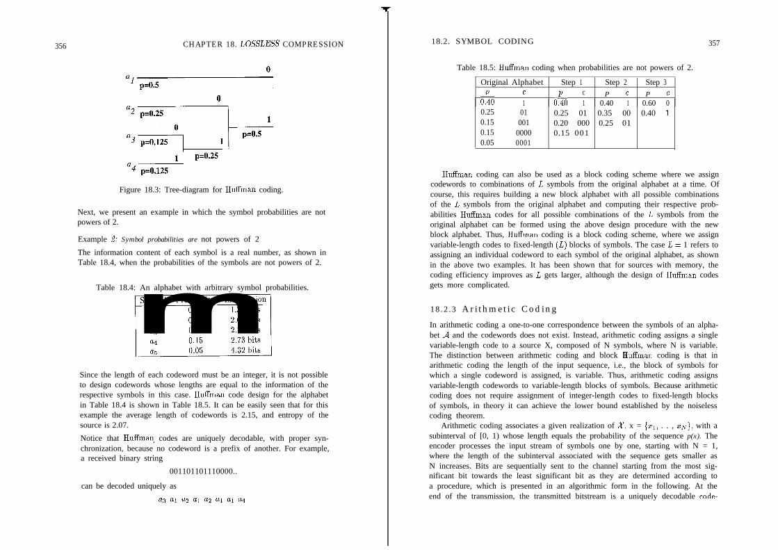
356 CHAPTER 18. LOSSLESS COMPRESSION
Figure 18.3: Tree-diagram for Huffman coding.
Next, we present an example in which the symbol probabilities are notpowers of 2.
Example 2: Symbol probabilities are not powers of 2
The information content of each symbol is a real number, as shown inTable 18.4, when the probabilities of the symbols are not powers of 2.
Table 18.4: An alphabet with arbitrary symbol probabilities.
Symbol Probability Information
Since the length of each codeword must be an integer, it is not possibleto design codewords whose lengths are equal to the information of therespective symbols in this case. Huffman code design for the alphabetin Table 18.4 is shown in Table 18.5. It can be easily seen that for thisexample the average length of codewords is 2.15, and entropy of thesource is 2.07.
Notice that Huffman, codes are uniquely decodable, with proper syn-chronization, because no codeword is a prefix of another. For example,a received binary string
001101101110000..
can be decoded uniquely as
~3 al a2 al a2 al al a4
18.2. SYMBOL CODING 357
Table 18.5: Huffman coding when probabilities are not powers of 2.
Original Alphabet Step 1 Step 2 Step 3
ozoC c P c P c1 o:o 1 0.40 1 0.60 0
0.25 01 0.25 01 0.35 00 0.40 10.15 001 0.20 000 0.25 010.15 0000 0.15 0010.05 0001
Huffman coding can also be used as a block coding scheme where we assigncodewords to combinations of L symbols from the original alphabet at a time. Ofcourse, this requires building a new block alphabet with all possible combinationsof the L symbols from the original alphabet and computing their respective prob-abilities Huffman codes for all possible combinations of the L symbols from theoriginal alphabet can be formed using the above design procedure with the newblock alphabet. Thus, Huffman coding is a block coding scheme, where we assignvariable-length codes to fixed-length (L) blocks of symbols. The case L = 1 refers toassigning an individual codeword to each symbol of the original alphabet, as shownin the above two examples. It has been shown that for sources with memory, thecoding efficiency improves as L gets larger, although the design of Huffman codesgets more complicated.
18 .2 .3 Arithmetic Coding
In arithmetic coding a one-to-one correspondence between the symbols of an alpha-bet A and the codewords does not exist. Instead, arithmetic coding assigns a singlevariable-length code to a source X, composed of N symbols, where N is variable.The distinction between arithmetic coding and block Huffman coding is that inarithmetic coding the length of the input sequence, i.e., the block of symbols forwhich a single codeword is assigned, is variable. Thus, arithmetic coding assignsvariable-length codewords to variable-length blocks of symbols. Because arithmeticcoding does not require assignment of integer-length codes to fixed-length blocksof symbols, in theory it can achieve the lower bound established by the noiselesscoding theorem.
Arithmetic coding associates a given realization of X, x = (~1, . . , ZN}) with asubinterval of [0, 1) whose length equals the probability of the sequence p(x). Theencoder processes the input stream of symbols one by one, starting with N = 1,where the length of the subinterval associated with the sequence gets smaller asN increases. Bits are sequentially sent to the channel starting from the most sig-nificant bit towards the least significant bit as they are determined according toa procedure, which is presented in an algorithmic form in the following. At theend of the transmission, the transmitted bitstream is a uniquely decodable code-

358 CHAPTER 18. LOSSLESS COMPRESSION 18.2. SYMBOL CODING 359
word representing the source, which is a binary number pointing to the subintervalassociated with this sequence.
The ProcedureConsider an alphabet A that has M symbols ai, i = 1,. . , M, with the proba-
bilities p(ai) = pi, such that pr + . +p~ = 1. The procedure starts with assigningeach individual symbol in the alphabet a subinterval, within 0 to 1, whose length isequal to its probability. It is assumed that this assignment is known to the decoder.
1. If the first input symbol zi = ai, i = 1,. .) M, then define the initialsubinterval as 11 = [Ii,ri) = [pi-i,pi-i +pi), where pe = 0. Set n = 1, L = 11,R=ri,andd=ri-11.
2. Obtain the binary expansions of L and R as
k=l
and R= -j&2-’k=l
where Ilk and Vk are 0 or 1.Compare ~1 and ‘~1. If they are not the same, send nothing to the channel at
this time, and go to step 3.If ui = VI, then send the binary symbol ~1, and compare u:, and ~2. If they are
not the same, go to step 3.If ~2 = vs, also send the binary symbol ~2, and compare us and vs, and so on,
until the next two corresponding binary symbols do not match, at which time goto step 3.
3. Increment n, and read the next symbol. If the nth input symbol 2, = ai,then subdivide the interval from the previous step as
In = [L,fn) = [b-l +pi-141,-l+ (pi-1 +pi)d).SetL=E,,R=r,,andd=r,-l,,andgotostep2.
Note that the decoder may decode one binary symbol into several source sym-bols, or it may require several binary symbols before it can decode one or moresource symbols. The arithmetic coding procedure is illustrated by means of thefollowing example.
ExampleSuppose we wish to determine an arithmetic code to represent a sequenceof symbols,
a2 al a s
from the source shown in Table 18.2. Because we have four symbolsin the alphabet, the interval from 0 to 1 is initially subdivided into 4,where the lengths of the subintervals are equal to 0.5, 0.25, 0.125 and0.125, respectively. This is depicted in Figure 18.4.
Symbol L
Decimal 0
Binary 0.0
Decimal
Binary
Decimal
Binary
al I , , a4 ,a2 a3,,--‘bS
,’0.7-s,\ 0.875 1.0
,’,’,’ 0.1 0.11 1.0,’ ‘b.~l!~,’,’,’
b0.;’
a2al a2a2Ia2a3 iQa4-
I J0.625. 0.6875 0.71875 0.75_
;‘0.1->
0.101 “-0.~011 0.10111 0.11*_
I0.5
0.1
a2alal a2ala2 a2al+yJa4I I
0.5625 0.59375 0.609375 0.625
0.1001 0.10011 0.100111 0.101
Figure 18.4: Illustration of the concept of arithmetic coding.
The first symbol defines the initial interval as 11 = [0.5,0.75), where thebinary representations of the left and right boundaries are L = 2-l = 0.1and R = 2-l + 2- ’ = 0.11, respectively. According to step 2,ui = vi = 1; thus, 1 is sent to the channel. Noting that ~2 = 0and v2 = 1, we read the second symbol, al. Step 3 indicates thatI2 = [0.5,0.625), with L = 0.10 and R = 0.101. Now that u2 = o2 = 0,we send 0 to the channel. However, us = 0 and ~3 = 1, so we read thethird symbol, as. It can be easily seen that 1s = [0.59375,0.609375),with L = 0.10011 and R = 0.100111. Note that us = v3 = 0,~4 = v4 = 1, and us = vs = 1, but us = 0 and vs = 1. At this stage, wesend 011 to the channel, and read the next symbol. A reserved symbolusually signals the end of a sequence.
Let’s now briefly look at how the decoder operates, which is illustratedin Figure 18.5. The first bit restricts the interval to [0.5,1). However,
Received Bit Interval Symbol1 k-).5,1)0 [0.5,0.75) Q,0 [0.5,0.609375) ai1 [0.5625,0.609375) -1 [0.59375,0.609375) a3
Figure 18.5: The operation of the decoder.
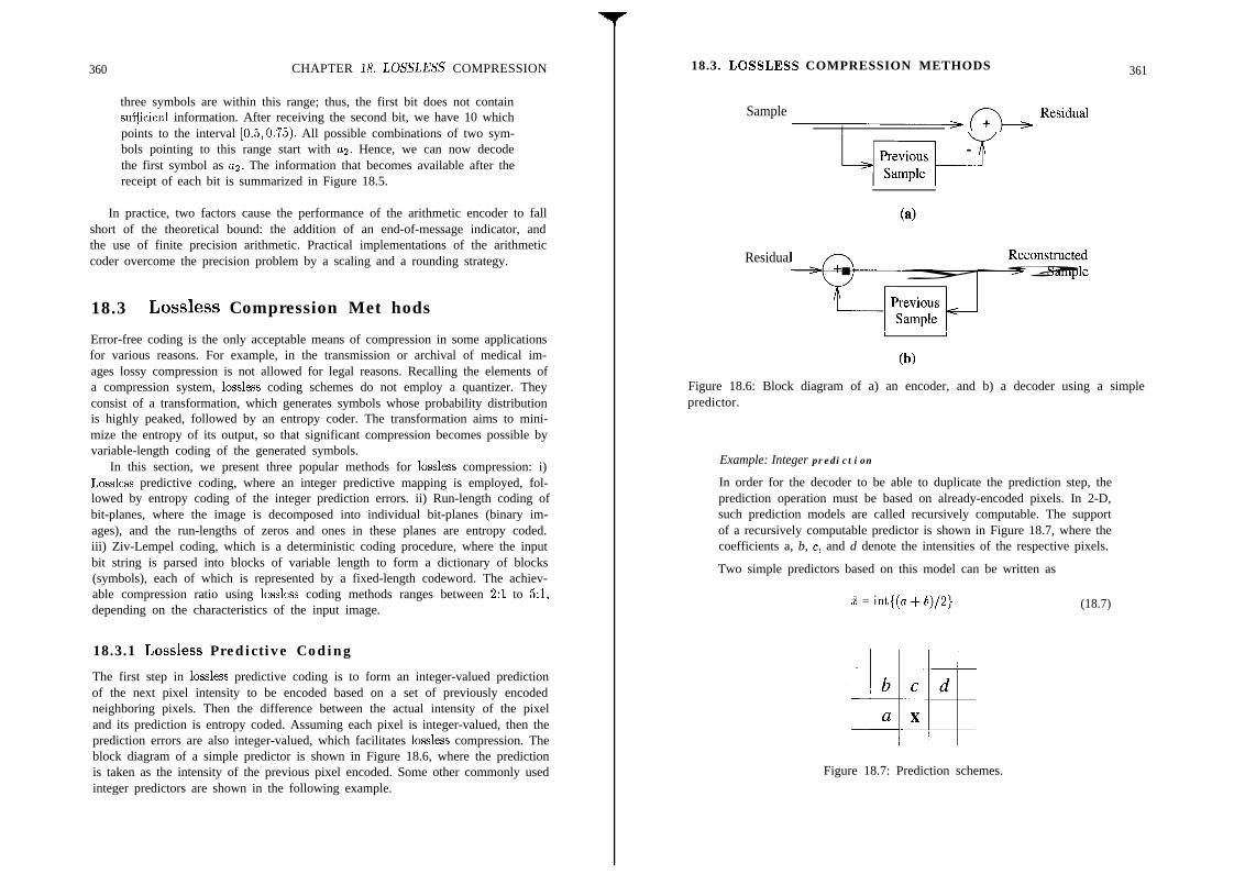
360 CHAPTER 18. LOSSLESS COMPRESSION 18.3. LOSSLESS COMPRESSION METHODS 361
three symbols are within this range; thus, the first bit does not containsu$cient information. After receiving the second bit, we have 10 whichpoints to the interval [0.5,0.75). All possible combinations of two sym-bols pointing to this range start with a2. Hence, we can now decodethe first symbol as a2. The information that becomes available after thereceipt of each bit is summarized in Figure 18.5.
In practice, two factors cause the performance of the arithmetic encoder to fallshort of the theoretical bound: the addition of an end-of-message indicator, andthe use of finite precision arithmetic. Practical implementations of the arithmeticcoder overcome the precision problem by a scaling and a rounding strategy.
18.3 Lossless Compression Met hods
Error-free coding is the only acceptable means of compression in some applicationsfor various reasons. For example, in the transmission or archival of medical im-ages lossy compression is not allowed for legal reasons. Recalling the elements ofa compression system, lossless coding schemes do not employ a quantizer. Theyconsist of a transformation, which generates symbols whose probability distributionis highly peaked, followed by an entropy coder. The transformation aims to mini-mize the entropy of its output, so that significant compression becomes possible byvariable-length coding of the generated symbols.
In this section, we present three popular methods for lossless compression: i)Lossless predictive coding, where an integer predictive mapping is employed, fol-lowed by entropy coding of the integer prediction errors. ii) Run-length coding ofbit-planes, where the image is decomposed into individual bit-planes (binary im-ages), and the run-lengths of zeros and ones in these planes are entropy coded.iii) Ziv-Lempel coding, which is a deterministic coding procedure, where the inputbit string is parsed into blocks of variable length to form a dictionary of blocks(symbols), each of which is represented by a fixed-length codeword. The achiev-able compression ratio using lossless coding methods ranges between 2:l to 5:1,depending on the characteristics of the input image.
18.3.1 Lossless Predictive Coding
The first step in lossless predictive coding is to form an integer-valued predictionof the next pixel intensity to be encoded based on a set of previously encodedneighboring pixels. Then the difference between the actual intensity of the pixeland its prediction is entropy coded. Assuming each pixel is integer-valued, then theprediction errors are also integer-valued, which facilitates lossless compression. Theblock diagram of a simple predictor is shown in Figure 18.6, where the predictionis taken as the intensity of the previous pixel encoded. Some other commonly usedinteger predictors are shown in the following example.
Sample m--+- Residua1
(a)
Residual
I 1
(b)
Figure 18.6: Block diagram of a) an encoder, and b) a decoder using a simplepredictor.
Example: Integer prediction
In order for the decoder to be able to duplicate the prediction step, theprediction operation must be based on already-encoded pixels. In 2-D,such prediction models are called recursively computable. The supportof a recursively computable predictor is shown in Figure 18.7, where thecoefficients a, b, c, and d denote the intensities of the respective pixels.
Two simple predictors based on this model can be written as
2 = int{(a + b)/2} (18.7)
Figure 18.7: Prediction schemes.
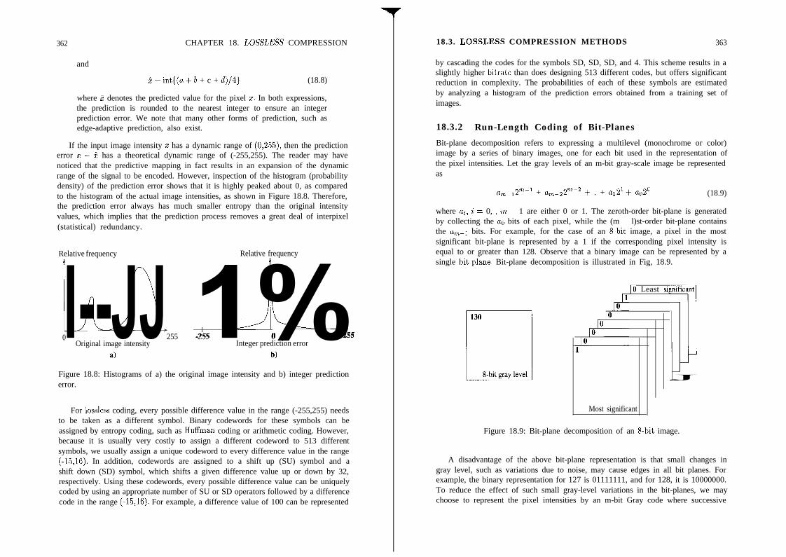
362 CHAPTER 18. LOSSLESS COMPRESSION
and
f = int{(a + b + c + d)/4} (18.8)
where P denotes the predicted value for the pixel IC. In both expressions,the prediction is rounded to the nearest integer to ensure an integerprediction error. We note that many other forms of prediction, such asedge-adaptive prediction, also exist.
If the input image intensity z has a dynamic range of (0,255), then the predictionerror z - 2 has a theoretical dynamic range of (-255,255). The reader may havenoticed that the predictive mapping in fact results in an expansion of the dynamicrange of the signal to be encoded. However, inspection of the histogram (probabilitydensity) of the prediction error shows that it is highly peaked about 0, as comparedto the histogram of the actual image intensities, as shown in Figure 18.8. Therefore,the prediction error always has much smaller entropy than the original intensityvalues, which implies that the prediction process removes a great deal of interpixel(statistical) redundancy.
Relative frequency Relative frequency4 t
0 255 -2.55 0Original image intensity Integer prediction error
a) b)
Figure 18.8: Histograms of a) the original image intensity and b) integer predictionerror.
For lossless coding, every possible difference value in the range (-255,255) needsto be taken as a different symbol. Binary codewords for these symbols can beassigned by entropy coding, such as Huffman coding or arithmetic coding. However,because it is usually very costly to assign a different codeword to 513 differentsymbols, we usually assign a unique codeword to every difference value in the range(-15,16). In addition, codewords are assigned to a shift up (SU) symbol and ashift down (SD) symbol, which shifts a given difference value up or down by 32,respectively. Using these codewords, every possible difference value can be uniquelycoded by using an appropriate number of SU or SD operators followed by a differencecode in the range (-15,16). For example, a difference value of 100 can be represented
18.3. LOSSLESS COMPRESSION METHODS 363
by cascading the codes for the symbols SD, SD, SD, and 4. This scheme results in aslightly higher bitrate than does designing 513 different codes, but offers significantreduction in complexity. The probabilities of each of these symbols are estimatedby analyzing a histogram of the prediction errors obtained from a training set ofimages.
18.3.2 Run-Length Coding of Bit-Planes
Bit-plane decomposition refers to expressing a multilevel (monochrome or color)image by a series of binary images, one for each bit used in the representation ofthe pixel intensities. Let the gray levels of an m-bit gray-scale image be representedas
um_12m-l + a,-22m-Z + . + a12l+ ao2O (18.9)
where ai, i = 0, ) m - 1 are either 0 or 1. The zeroth-order bit-plane is generatedby collecting the a0 bits of each pixel, while the (m - l)st-order bit-plane containsthe a,_l bits. For example, for the case of an 8-bit image, a pixel in the mostsignificant bit-plane is represented by a 1 if the corresponding pixel intensity isequal to or greater than 128. Observe that a binary image can be represented by asingle bit-plane. Bit-plane decomposition is illustrated in Fig, 18.9.
IO Least signific,ant
Most significant
Figure 18.9: Bit-plane decomposition of an 8-bit image.
A disadvantage of the above bit-plane representation is that small changes ingray level, such as variations due to noise, may cause edges in all bit planes. Forexample, the binary representation for 127 is 01111111, and for 128, it is 10000000.To reduce the effect of such small gray-level variations in the bit-planes, we maychoose to represent the pixel intensities by an m-bit Gray code where successive
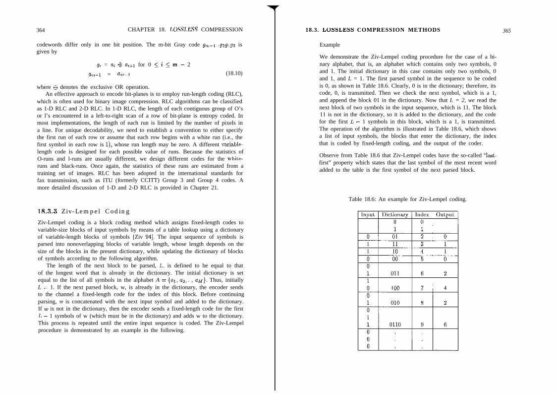
364 CHAPTER 18. LOSSLESS COMPRESSION
codewords differ only in one bit position. The m-bit Gray code gm-r .gsgrgc isgiven by
gi = ai $ ai+l for 0 5 i 5 m - 2
h-1 = h-1
where $ denotes the exclusive OR operation.
(18.10)
An effective approach to encode bit-planes is to employ run-length coding (RLC),which is often used for binary image compression. RLC algorithms can be classifiedas 1-D RLC and 2-D RLC. In 1-D RLC, the length of each contiguous group of O’sor l’s encountered in a left-to-right scan of a row of bit-plane is entropy coded. Inmost implementations, the length of each run is limited by the number of pixels ina line. For unique decodability, we need to establish a convention to either specifythe first run of each row or assume that each row begins with a white run (i.e., thefirst symbol in each row is l), whose run length may be zero. A different variable-length code is designed for each possible value of runs. Because the statistics ofO-runs and l-runs are usually different, we design different codes for the white-runs and black-runs. Once again, the statistics of these runs are estimated from atraining set of images. RLC has been adopted in the international standards forfax transmission, such as ITU (formerly CCITT) Group 3 and Group 4 codes. Amore detailed discussion of 1-D and 2-D RLC is provided in Chapter 21.
18.3.3 Ziv-Lempel Coding
Ziv-Lempel coding is a block coding method which assigns fixed-length codes tovariable-size blocks of input symbols by means of a table lookup using a dictionaryof variable-length blocks of symbols [Ziv 941. The input sequence of symbols isparsed into nonoverlapping blocks of variable length, whose length depends on thesize of the blocks in the present dictionary, while updating the dictionary of blocksof symbols according to the following algorithm.
The length of the next block to be parsed, L, is defined to be equal to thatof the longest word that is already in the dictionary. The initial dictionary is setequal to the list of all symbols in the alphabet A = {al, as,. , aM}. Thus, initiallyL = 1. If the next parsed block, w, is already in the dictionary, the encoder sendsto the channel a fixed-length code for the index of this block. Before continuingparsing, w is concatenated with the next input symbol and added to the dictionary.If w is not in the dictionary, then the encoder sends a fixed-length code for the firstL - 1 symbols of w (which must be in the dictionary) and adds w to the dictionary.This process is repeated until the entire input sequence is coded. The Ziv-Lempelprocedure is demonstrated by an example in the following.
18.3. LOSSLESS COMPRESSION METHODS 365
Example
We demonstrate the Ziv-Lempel coding procedure for the case of a bi-nary alphabet, that is, an alphabet which contains only two symbols, 0and 1. The initial dictionary in this case contains only two symbols, 0and 1, and L = 1. The first parsed symbol in the sequence to be codedis 0, as shown in Table 18.6. Clearly, 0 is in the dictionary; therefore, itscode, 0, is transmitted. Then we check the next symbol, which is a 1,and append the block 01 in the dictionary. Now that L = 2, we read thenext block of two symbols in the input sequence, which is 11. The block11 is not in the dictionary, so it is added to the dictionary, and the codefor the first L - 1 symbols in this block, which is a 1, is transmitted.The operation of the algorithm is illustrated in Table 18.6, which showsa list of input symbols, the blocks that enter the dictionary, the indexthat is coded by fixed-length coding, and the output of the coder.
Observe from Table 18.6 that Ziv-Lempel codes have the so-called “last-first” property which states that the last symbol of the most recent wordadded to the table is the first symbol of the next parsed block.
Table 18.6: An example for Ziv-Lempel coding.

366 CHAPTER 18. LOSSLESS COMPRESSION
Ziv-Lempel coding is noiseless, does not require probabilities of the source sym-bols to be known or estimated, and is optimum in the limit of unbounded dictionarysize. In practice, one places a bound on the dictionary size. Once this size limitis reached, the encoder can no longer add codewords and must simply use the ex-isting dictionary. However, methods exist to adapt the dictionary to varying inputcharacteristics.
Ziv-Lempel coding has been succesfully used for compression of binary data files,with a compression ratio of approximately 2.5:1. Indeed, it forms the basis of the“compress” utility in UNIX and the “arc” program for the PC environment.
18.4 Exercises
1. Suppose we have a discrete memoryless source with the alphabet A and thesymbol probabilities p(ai) for ai E A specified by the following table:
a) Find the entropy of this source.
b) Design a Huffman code for this source.
c) Find the average codeword length.
d) How good is this code?
2. Let X be a binary, Markov-2 source with the alphabet A = { 0, 1 }. Thesource is modeled by the conditional probabilities
P(OIO,O) = 0.7 P(llO,O) = 0.3
P(OIO,l) = 0.6 P(l(O,l) = 0.4
P(O]l, 0) = 0.4 P(l]l,O) = 0.6
P(O]l, 1) = 0.3 P(l(l,l) = 0.7
a) What is the entropy of this source?
b) Design a block Huffman code for N = 3.
c) What is the average codeword length? What would be the average codewordlength if we design a scalar Huffman code?
3. Suppose we have an R-bit gray-level image. How would you estimate theentropy of this image:
a) Assuming that it is a discrete memoryless source?
b) Assuming that it is a Markov-1 source?
Which one do you guess will be smaller? Why?
BIBLIOGRAPHY 367
4. Assume that the histogram of the differential image shown in Figure 18.8 canbe modeled by a Laplacian distribution, given by
de) = & exp -JZlel1 I
u,
with u, = 15. Write an expression for the entropy of the differential image.Estimate its value. What is the expected compression ratio (using losslessdifferential encoding)?
5. How do you compare arithmetic coding with block Huffman coding?
6. What is the primary motivation of using the Gray codes in bit-plane encoding?
Bibliography
[Ber 711 T. Berger, Rate Distortion Theory, Englewood Cliffs, NJ: Prentice-Hail,1971.
[Ger 921 A. Gersho and R. M. Gray, Vector Quantization and Signal Compression,Norwell, MA: Kluwer, 1992.
[Jai 811 A. K. Jain, “Image data compression: A review,” Proc. IEEE, vol. 69,pp. 349-389, Mar. 1981.
[Jay 841 N. S. Jayant and P. Noll, Digital Coding of Waveforms, Principles andApplications to Speech and Video, Englewood Cliffs, NJ: Prentice Hall,1984.
[Jay 921 N. S. Jayant, “Signal compression: Technology targets and research direc-tions,” IEEE Trans. Spec. Areas Comm, vol. 10, pp. 7966819, June 1992.
[Net881 A. N. Netravali and B. G. Haskell, Digital Pictures: Representation andCompression, New York, NY: Plenum Press, 1988.
[Rab 911 M. Rabbani and P. Jones, Digital Image Compression Techniques,Bellingham, WA: SPIE Press, 1991.
[Ziv 771 J. Ziv and A. Lempel, “A universal algorithm for sequential data compres-sion,” IEEE Trans. Info. Theory, vol. IT-23, pp. 337-343, 1977.
[Ziv 941 J. Ziv, “On universal data compression - An intuitive overview,”J. Vis. Comm. Image Rep., vol. 5, no. 4, pp. 317-321, Dec. 1994.

Chapter 19
DPCM ANDTRANSFORM CODING
This chapter introduces two popular lossy compression schemes, differential pulsecode modulation (DPCM) and discrete cosine transform (DCT) coding. Lossycompression methods compromise fidelity in exchange for increased compression.For example, DCT coding can easily provide a compression ratio of 25:l withoutvisually apparent degradations. The main difference between the lossy and losslesscompression schemes is that the former employs a quantizer while the latter doesnot. To this effect, we start our discussion of lossy compression schemes withthe process of quantization and quantizer design in Section 18.1. Next, DPCM iscovered in Section 18.2. In DPCM, a predictive mapping transforms pixel intensitiesto prediction errors, which are then quantized and entropy coded. In transformcoding, studied in Section 18.3, the image is first divided into blocks. Then the DCTcoefficients for each block are zig-zag scanned, quantized, and run-length/entropycoded. Both DCT coding and DPCM play important roles in the internationalstandards for still-frame and video compression. Thus, this chapter serves to providethe necessary background to understand the international compression standards.
19.1 Quantization
Quantization is the process of representing a set of continuous-valued samples with afinite number of states. If each sample is quantized independently, then the processis known as scalar quantization. A scalar quantizer Q(.) is a function that is definedin terms of a finite set of decision levels da and reconstruction levels ri, given by
Q(s)=ri, i f s~(di-I,&], i=l,..., L (19.1)
where L is the number of output states. That is, the output of the quantizer is thereconstruction level ri, if s, the value of the sample, is within the range (&-I, di].
368
19.1. QUANTIZATION 369
Vector quantization refers to representing a set of vectors, each formed by severalcontinuous-valued samples, with a finite number of vector states. In image compres-sion, scalar or vector quantization is usually applied to a transform-domain imagerepresentation. In the following, we discuss how to design a scalar quantizer, thatis, how to determine di and ri in (19.1). We will return to vector quantization inChapter 21.
Let S = Q(s) denote the quantized variable. Then e = s - 6 is the quantizationerror. The performance of a quantizer may be quantified by a distortion measure Dwhich is a function of e, and therefore di and ri. If we treat s as a random variable,then the distortion measure may be selected as the mean square quantization error,that is, D = E{(s - i)“}, where E{.} stands for the expectation operator. Given adistortion measure D and the input probability density function (pdf) p(s), thereare, in general, two different optimum scalar quantizer design criteria:
i) For a fixed number of levels L, find pi, i = 1, , L, and di, i = 0, , 15, inorder to minimize D. Quantizers with a fixed number of levels which are optimal inthe mean square error sense, D = E{(s - ri)“}, are known as Lloyd-Max quantizers[Llo 82, Max 601.
ii) For a fixed output entropy, H(s) = C, where C is a constant, find riand di (L is unknown) in order to minimize D. Quantizers that minimize a dis-tortion measure for a constant output entropy are known as entropy-constrainedquantizers [Woo 691.Recall from Chapter 18 that the rate R in the case of fixed-length coding is givenby R = LdogzL], (1.J denotes the smallest integer greater than), while R > H(i) inthe case of variable-length encoding (VLC). Thus, Lloyd-Max quantization is moresuitable for use with fixed-length coding, whereas entropy-constrained quantizationis well-suited for VLC (Huffman or arithmetic coding). A detailed discussion ofentropy-constrained quantization is beyond the scope of this book. We elaborateon the design of Lloyd-Max quantizers below.
19.1.1 Nonuniform Quantization
The determination of the Lloyd-Max quantizer requires minimization of
E{(s - Q)“> = g 1’” (s - ri)%(s)dsI 1
(19.2)
with respect to ri and di. It has been shown that the necessary conditions tominimize (19.2) are given by [Jai 90, Lim 901
p’ = .6-, sp(s)ds’ J%,p(s)ds’ lSiSL
(19.3)
ri + pi+1di=p,2
ISilL-1 (19.4)
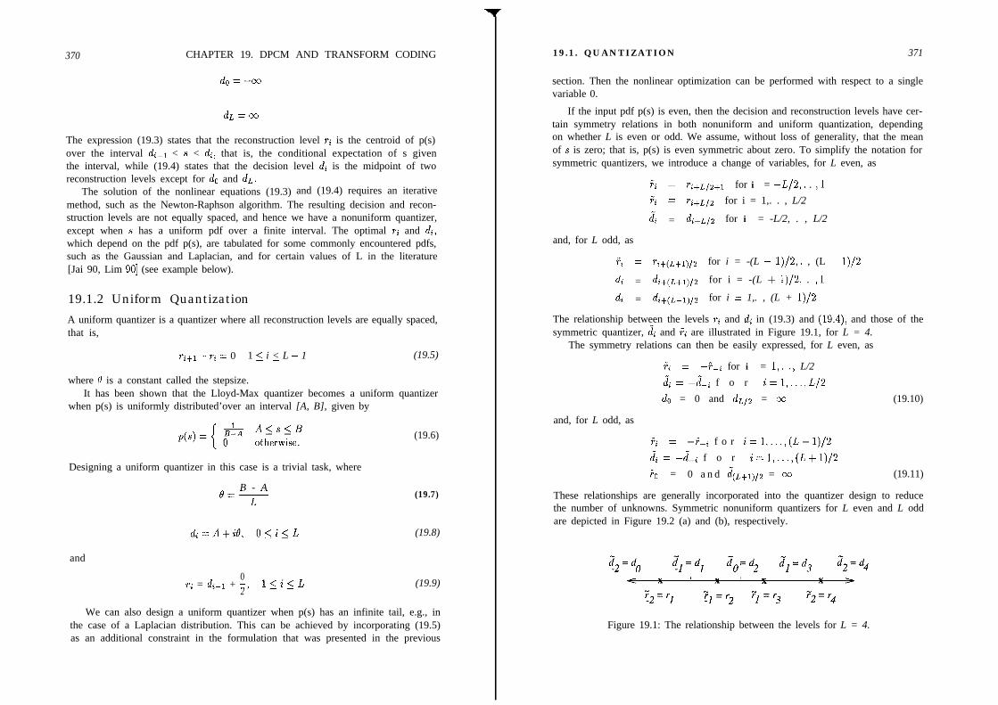
370 CHAPTER 19. DPCM AND TRANSFORM CODING
d~=-co
dL = 03
The expression (19.3) states that the reconstruction level ri is the centroid of p(s)over the interval &-i < s < di, that is, the conditional expectation of s giventhe interval, while (19.4) states that the decision level di is the midpoint of tworeconstruction levels except for do and do.
The solution of the nonlinear equations (19.3) and (19.4) requires an iterativemethod, such as the Newton-Raphson algorithm. The resulting decision and recon-struction levels are not equally spaced, and hence we have a nonuniform quantizer,except when s has a uniform pdf over a finite interval. The optimal ~a and di,which depend on the pdf p(s), are tabulated for some commonly encountered pdfs,such as the Gaussian and Laplacian, and for certain values of L in the literature[Jai 90, Lim 901 (see example below).
19.1.2 Uniform Quantization
A uniform quantizer is a quantizer where all reconstruction levels are equally spaced,that is,
ri+l - 7-i = 0 1 < i < L - 1- (19.5)
where B is a constant called the stepsize.It has been shown that the Lloyd-Max quantizer becomes a uniform quantizer
when p(s) is uniformly distributed’over an interval [A, B], given by
Designing a uniform quantizer in this case is a trivial task, where
B - AO==T
(19.6)
(19.7)
di=A$il?, Oji<L (19.8)
and
0ri = da-1 + -,
2l<i<L (19.9)
We can also design a uniform quantizer when p(s) has an infinite tail, e.g., inthe case of a Laplacian distribution. This can be achieved by incorporating (19.5)as an additional constraint in the formulation that was presented in the previous
19.1. QUANTIZATION 371
section. Then the nonlinear optimization can be performed with respect to a singlevariable 0.
If the input pdf p(s) is even, then the decision and reconstruction levels have cer-tain symmetry relations in both nonuniform and uniform quantization, dependingon whether L is even or odd. We assume, without loss of generality, that the meanof s is zero; that is, p(s) is even symmetric about zero. To simplify the notation forsymmetric quantizers, we introduce a change of variables, for L even, as
ra = ri+L/2+l for i = -L/2,. . ,1Fa zz ri+~jz for i = 1,. . , L/2
& = &L/z for i = -L/2, . , L/2
and, for L odd, as
r, 1 Pi+p+lp for i = -(L - 1)/2,. , (L - 1)/2
4 = di+(L+l)/z for i = -(L + 1)/2, . ,1
4 = di+(L-1)/z for i = 1,. , (L + 1)/2
The relationship between the levels ri and di in (19.3) and (19.4), and those of thesymmetric quantizer, & and Fi are illustrated in Figure 19.1, for L = 4.
The symmetry relations can then be easily expressed, for L even, as
yi = --f-i for i = 1,. ., L/2
& = -2-i f o r i=l,...,L/2
de = 0 and dLp = 00
and, for L odd, as
r, = -F-i f o r i=l,...,(L-1)/2
& = -2-i f o r i=l,...,(L+1)/2
r”o = 0 a n d Jcr,+i),s = co
(19.10)
(19.11)
These relationships are generally incorporated into the quantizer design to reducethe number of unknowns. Symmetric nonuniform quantizers for L even and L oddare depicted in Figure 19.2 (a) and (b), respectively.
Figure 19.1: The relationship between the levels for L = 4.
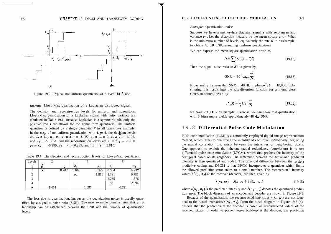
372 CHAPTEH 19. DPCM AND TRANSFORM CODING
(a) (b)
Figure 19.2: Typical nonuniform quantizers: a) L even; b) L odd
Example: Lloyd-Max quantization of a Laplacian distributed signal.
The decision and reconstruction levels for uniform and nonuniformLloyd-Max quantization of a Laplacian signal with unity variance aretabulated in Table 19.1. Because Laplacian is a symmetric pdf, only thepositive levels are shown for the nonuniform quantizers. The uniformquantizer is defined by a single parameter 8 in all cases. For example,in the case of nonuniform quantization with L = 4, the decision levelsare ds = dx-2 = --oo, dl = 2-1 = -1.102, da = & = 0, d3 = d; = 1.102,and da = dz = 00, and the reconstruction levels are ~1 = rX_2 = -1.810,r2 = r”-r = -0.395, rs = ?r = 0.395, and r4 = rXs = 1.810.
Table 19.1: The decision and reconstruction levels for Lloyd-Max quantizers.Levels 2 4 8
i & i$ !& Fi 2;1 cc 0.707 1.102 0.395 0.504 0.;222 cm 1.810 1.181 0.7853 2.285 1.5764 co 2.9948 1.414 1.087 0.731
The loss due to quantization, known as the quantization noise, is usually quan-tified by a signal-to-noise ratio (SNR). The next example demonstrates that a re-lationship can be established between the SNR and the number of quantizationlevels.
19.2. DIFFERENTIAL PULSE CODE MODULATION
Example: Quantization noise
Suppose we have a memoryless Gaussian signal s with zero mean andvariance u2. Let the distortion measure be the mean square error. Whatis the minimum number of levels, equivalently the rate R in bits/sample,to obtain 40 dB SNR, assuming uniform quantization?
We can express the mean square quantization noise as
(19.12)D = c E{ (s - S)Z}
Then the signal noise ratio in dB is given by
SNR = 10 logr,, $ (19.13)
It can easily be seen that SNR = 40 dB implies a2/D = 10,000. Sub-stituting this result into the rate-distortion function for a memorylessGaussian source, given by
373
we have R(D) % 7 bits/sample. Likewise, we can show that quantizationwith 8 bits/sample yields approximately 48 dB SNR.
19.2 Differential Pulse Code Modulation
Pulse code modulation (PCM) is a commonly employed digital image representationmethod, which refers to quantizing the intensity of each pixel individually, neglectingthe spatial correlation that exists between the intensities of neighboring pixels.One approach to exploit the inherent spatial redundancy (correlation) is to usedifferential pulse code modulation (DPCM), which first predicts the intensity of thenext pixel based on its neighbors. The difference between the actual and predictedintensity is then quantized and coded. The principal difference between the losslesspredictive coding and DPCM is that DPCM incorporates a quantizer which limitsthe allowed prediction error states to a small number. The reconstructed intensityvalues B(nr , ns) at the receiver (decoder) are then given by
qnl,w)= i(nl,nz)+qnl,nz) (19.15)
where i(nr , n2) is the predicted intensity and d(nr , 7~2) denotes the quantized predic-tion error. The block diagrams of an encoder and decoder are shown in Figure 19.3.
Because of the quantization, the reconstructed intensities B(nr, n2) are not iden-tical to the actual intensities s(nr , nz). From the block diagram in Figure 19.3 (b),observe that the prediction at the decoder is based on reconstructed values of thereceived pixels. In order to prevent error build-up at the decoder, the prediction

374 CHAPTER19. DPCMAND TRANSFORMCODING
e e> Quantizer Symbol
coder Binary
stream
Binarystream
a
H Decompressedz image
Predictor
(b)
Figure 19.3: Block diagrams of a DPCM a) encoder and b) decoder.
at both the encoder and decoder must be identical. Therefore, the predictor at theencoder also uses the reconstructed values of the previously encoded samples in theprediction instead of their actual values. To this effect, the encoder simulates thedecoder in the prediction loop, as shown in Figure 19.3 (a).
DPCM is relatively simple to implement; however, it provides only a modestcompression. The prediction and quantization steps are discussed in detail in thefollowing. Despite the apparent interaction between the prediction and quantiza-tion, e.g., the reconstructed values are used in prediction, the predictor is tradition-ally designed under the assumption of no quantization error, and the quantizer isdesigned to minimize its own error.
19.2.1 Optimal Prediction
Modeling the image by a stationary random field, a linear minimum mean squareerror (LMMSE) predictor, in the form
qn1, nz) = ClS(W - 1, n2 - 1) + czs(n1 - 1, nz) + czs(n1 - 1, nz + 1)
+c4s(n1,n2 - 1) (19.16)
can be designed to minimize the mean square prediction error
E{[s - ilT[s -i]}
19.2. DIFFERENTIAL PULSE CODE MODULATION 375
where s and r? denote lexicographic ordering of the pixels in the actual and predictedimages, respectively.
The optimal coefficient vector c = [ci c2 cs c41T in (19.16) can be found bysolving the normal equation,
(fl = (PC
where
and
. R&40) RdO, 1) W, 2) &Cl, 0)R,(O, -1) R,(O, 0) W, 1) &(I, -1)R&4 -2) &(O, -1) R&h 0) &(l, -2)
. &(-LO) R&1,1) J&(-1,2) f&(0,0)
4 = P&(1,1) &(A 0) Rs(4 -1) f&(0, l)lT
(19.18)
1 (19.19)
(19.20)
The function R,(il, iz) stands for the autocorrelation function of the image, whichis defined by an ensemble average
R,(G, iz) = E{s(nl, nz)s(nl - G, n2 - i2)) (19.21)
where E{.} is the expectation operator. In practice, it is approximated by thesample average
&(G, i2) = h C s(nl, n2)s(nl - il, n2 - i2) (19.22)(%m)
where N is the number of pixels within the support of the summation. The matrixQ is almost always invertible, provided that the summation (19.22) is computedover a large enough support. Then
c = wll$ (19.23)
Note that although these coefficients may be optimal in the LMMSE sense, theyare not necessarily optimal in the sense of minimizing the entropy of the predictionerror. Furthermore, images rarely obey the stationarity assumption. As a result,most DPCM schemes employ a fixed predictor.
19.2.2 Quantization of the Prediction Error
In standard DPCM, the difference signal is scalar quantized using K bits/sample,where K is an integer that is less than 8. Empirical studies show that the statisticsof the prediction error can be well modeled by a Laplacian distribution with vari-ance a’. Because the Laplacian distribution is heavily peaked about 0, nonuniform
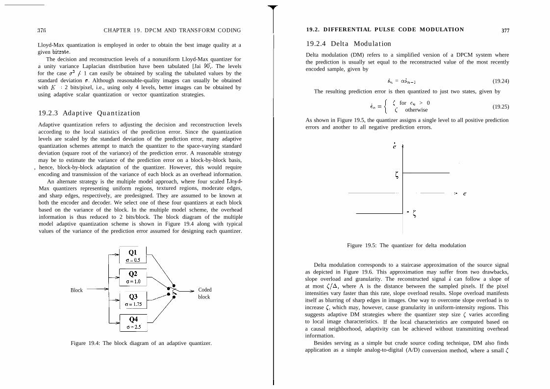
CHAPTER 19. DPCM AND TRANSFORM CODING
Lloyd-Max quantization is employed in order to obtain the best image quality at agiven bitrate.
The decision and reconstruction levels of a nonuniform Lloyd-Max quantizer fora unity variance Laplacian distribution have been tabulated [Jai 901. The levelsfor the case u2 # 1 can easily be obtained by scaling the tabulated values by thestandard deviation cr. Although reasonable-quality images can usually be obtainedwith K = 2 bits/pixel, i.e., using only 4 levels, better images can be obtained byusing adaptive scalar quantization or vector quantization strategies.
19.2.3 Adaptive Quantization
Adaptive quantization refers to adjusting the decision and reconstruction levelsaccording to the local statistics of the prediction error. Since the quantizationlevels are scaled by the standard deviation of the prediction error, many adaptivequantization schemes attempt to match the quantizer to the space-varying standarddeviation (square root of the variance) of the prediction error. A reasonable strategymay be to estimate the variance of the prediction error on a block-by-block basis,
, hence, block-by-block adaptation of the quantizer. However, this would requireencoding and transmission of the variance of each block as an overhead information.
An alternate strategy is the multiple model approach, where four scaled Lloyd-Max quantizers representing uniform regions, textured regions, moderate edges,and sharp edges, respectively, are predesigned. They are assumed to be known atboth the encoder and decoder. We select one of these four quantizers at each blockbased on the variance of the block. In the multiple model scheme, the overheadinformation is thus reduced to 2 bits/block. The block diagram of the multiplemodel adaptive quantization scheme is shown in Figure 19.4 along with typicalvalues of the variance of the prediction error assumed for designing each quantizer.
Block Codedblock
Figure 19.4: The block diagram of an adaptive quantizer.
19.2. DIFFERENTIAL PULSE CODE MODULATION 377
19.2.4 Delta ModulationDelta modulation (DM) refers to a simplified version of a DPCM system wherethe prediction is usually set equal to the reconstructed value of the most recentlyencoded sample, given by
s^, = ad,-1 (19.24)
The resulting prediction error is then quantized to just two states, given by
C for e, > 0-c otherwise (19.25)
As shown in Figure 19.5, the quantizer assigns a single level to all positive predictionerrors and another to all negative prediction errors.
Figure 19.5: The quantizer for delta modulation
Delta modulation corresponds to a staircase approximation of the source signalas depicted in Figure 19.6. This approximation may suffer from two drawbacks,slope overload and granularity. The reconstructed signal 6 can follow a slope ofat most (/A, where A is the distance between the sampled pixels. If the pixelintensities vary faster than this rate, slope overload results. Slope overload manifestsitself as blurring of sharp edges in images. One way to overcome slope overload is toincrease C, which may, however, cause granularity in uniform-intensity regions. Thissuggests adaptive DM strategies where the quantizer step size C varies accordingto local image characteristics. If the local characteristics are computed based ona causal neighborhood, adaptivity can be achieved without transmitting overheadinformation.
Besides serving as a simple but crude source coding technique, DM also findsapplication as a simple analog-to-digital (A/D) conversion method, where a small C
I
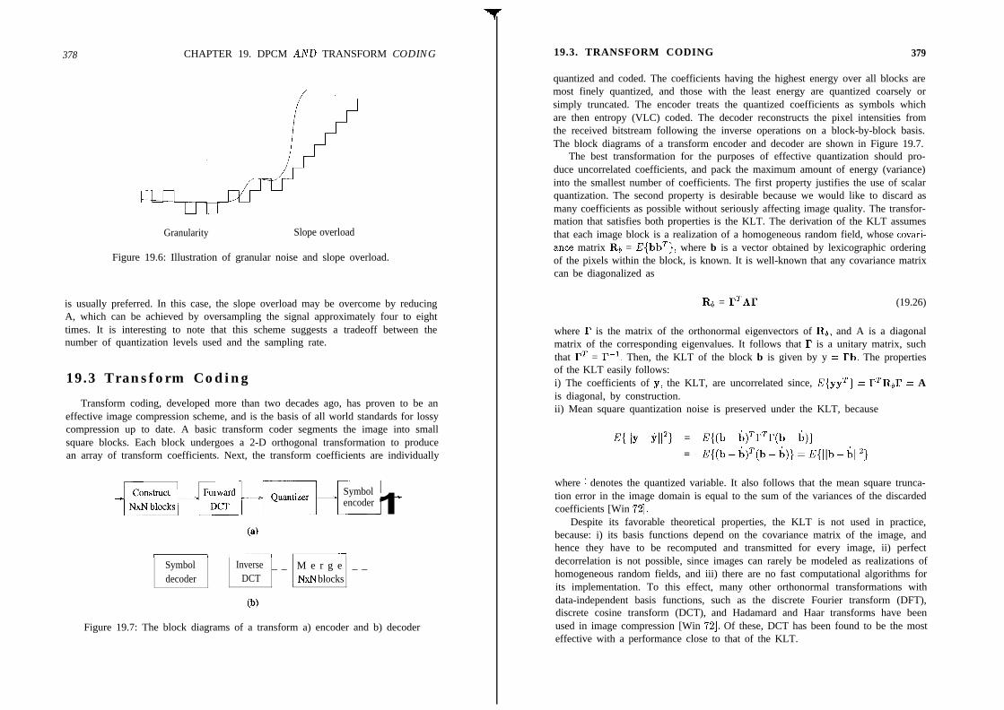
378 CHAPTER 19. DPCM AND TRANSFORM CODING
Granularity Slope overload
Figure 19.6: Illustration of granular noise and slope overload.
is usually preferred. In this case, the slope overload may be overcome by reducingA, which can be achieved by oversampling the signal approximately four to eighttimes. It is interesting to note that this scheme suggests a tradeoff between thenumber of quantization levels used and the sampling rate.
19.3 Transform Coding
Transform coding, developed more than two decades ago, has proven to be aneffective image compression scheme, and is the basis of all world standards for lossycompression up to date. A basic transform coder segments the image into smallsquare blocks. Each block undergoes a 2-D orthogonal transformation to producean array of transform coefficients. Next, the transform coefficients are individually
H-1”---
(a)H Symbol
encoder
Symboldecoder
Inverse _ _ M e r g e _ _DCT NxN blocks
(b)
Figure 19.7: The block diagrams of a transform a) encoder and b) decoder
19.3. TRANSFORM CODING 379
quantized and coded. The coefficients having the highest energy over all blocks aremost finely quantized, and those with the least energy are quantized coarsely orsimply truncated. The encoder treats the quantized coefficients as symbols whichare then entropy (VLC) coded. The decoder reconstructs the pixel intensities fromthe received bitstream following the inverse operations on a block-by-block basis.The block diagrams of a transform encoder and decoder are shown in Figure 19.7.
The best transformation for the purposes of effective quantization should pro-duce uncorrelated coefficients, and pack the maximum amount of energy (variance)into the smallest number of coefficients. The first property justifies the use of scalarquantization. The second property is desirable because we would like to discard asmany coefficients as possible without seriously affecting image quality. The transfor-mation that satisfies both properties is the KLT. The derivation of the KLT assumesthat each image block is a realization of a homogeneous random field, whose covari-ante matrix Ra = E{bbT}, where b is a vector obtained by lexicographic orderingof the pixels within the block, is known. It is well-known that any covariance matrixcan be diagonalized as
Rb = rTAr (19.26)
where I? is the matrix of the orthonormal eigenvectors of Ra, and A is a diagonalmatrix of the corresponding eigenvalues. It follows that I? is a unitary matrix, suchthat rT = I’-l. Then, the KLT of the block b is given by y = I’b. The propertiesof the KLT easily follows:i) The coefficients of yI the KLT, are uncorrelated since, E{yyT} = rTRbl? = Ais diagonal, by construction.ii) Mean square quantization noise is preserved under the KLT, because
E{lly-,I[“} = E{(b-I;)TrTr(b-b)}
= E{(b-li)T(b-li)}=E{~~b-~~~2}
where : denotes the quantized variable. It also follows that the mean square trunca-tion error in the image domain is equal to the sum of the variances of the discardedcoefficients [Win 721.
Despite its favorable theoretical properties, the KLT is not used in practice,because: i) its basis functions depend on the covariance matrix of the image, andhence they have to be recomputed and transmitted for every image, ii) perfectdecorrelation is not possible, since images can rarely be modeled as realizations ofhomogeneous random fields, and iii) there are no fast computational algorithms forits implementation. To this effect, many other orthonormal transformations withdata-independent basis functions, such as the discrete Fourier transform (DFT),discrete cosine transform (DCT), and Hadamard and Haar transforms have beenused in image compression [Win 721. Of these, DCT has been found to be the mosteffective with a performance close to that of the KLT.

380 CHAPTER 19. DPCM AND TRANSFORM CODING
19.3.1 Discrete Cosine Transform
The DCT is the most widely used transformation in transform coding. It is anorthogonal transform which has a fixed set of (image-independent) basis functions,an efficient algorithm for its computation, and good energy compaction and correla-tion reduction properties. Ahmed et al. [Ahm 741 first noticed that the KLT basisfunctions of a first-order Markov image closely resemble those of the DCT. Theybecome identical as the correlation between adjacent pixel approaches one [Cla 851.
The DCT belongs to the family of discrete trigonometric transforms, which has16 members [Mar 941. The type-2 DCT of an N x N block is defined as
S(h, k2) =d-
-.&kl)C(k2) y y s(q, na) COS( ?rjZn;; l)lel ) cog s(2n;; lb)
nl=O nz=O
whereIcr,kz,nr,nz=O,l,... N - l , a n d
for le = 0,otherwise
A significant factor in transform coding is the block size. The most popularsizes have been 8 x 8 and 16 x 16, both powers of 2 for computational reasons.It is no surprise that the DCT is closely related to the DFT. In particular, anN x N DCT of s(nr, na) can be expressed in terms of a 2N x 2N DFT of its even-symmetric extension, which leads to a fast computational algorithm. Using theseparability of the DFT and one of several fast Fourier transform (FFT) algorithms,it is possible to compute an N x N DCT by means of 0(2N2 log, N) operationsinstead of O(N4), where a(.) t d fs an s or “order of.” In addition, because of theeven-symmetric extension process, no artificial discontinuities are introduced at theblock boundaries, unlike the DFT, resulting in superior energy compaction. Thefact that the computation of the DCT requires or$p real arithmetic facilitates itshardware implementation. As a result; DCT is widely available in special-purposesingle-chip VLSI hardware, which makes it attractive for real-time use. L
The energy compaction property of 8 x 8 DCT is illustrated in the followingexample.
. Example: Energy Compaction Property of DCT
An 8 x 8 block from the seventh frame of the Mobile and Calendarsequence is shown below:
s(w,na) =
183 160 94 153 194. 163 132 165183 153 116 176 187 166 130 169179 168 171 182 179 170 131 167177 177 179 177 179 165 131 167178 178 179 176 182 164 130 171179 180 180 179 183 169 132 169179 179 180 182 183 170 129 173180 179 181 179 181 170 130 169
19.3. TRANSFORM CODING
The DCT coefficien ts,
NINT[S(lci, lc2)] =
after subtracting 128.from each element, are313 56 -27 18 78 -60 2 7 - 2 7- 3 8 - 2 7 13 44 32 - 1 - 2 4 - 1 0- 2 0 - 1 7 10 33 21 -6 -16 -9-10 -8 9 17 9 -10 -13 1-6 1 6 4 -3 -7 -5 5
2 3 0 -3 -7 -4 0 34 4 -1 -2 -9 0 2 43 1 0 -4 -2 -1 3 1
381
where NINT denotes nearest integer truncation. Observe that most ofthe high-frequency coefficients (around the lower right corner) are muchsmallerthan those around the (0,O) frequency (at the upper left corner).
19.3.2 Quantization/Bit Allocation
Bit allocation refers to.determination of which coefficients should be retained forcoding, and how coarsely each retained coefficient should be quantized in orderto minimize the overall mean square quantization noise. Bit allocation can be
, performed either globally, using zonal coding, or adaptively, using threshold coding.
Zonal Coding
J Zonal coding is based on the premise that the transform coefficients of maximumvariance carry the most picture information, in the information theoretic sense, andshould be retained. The locations of the coefficients with the K largest variancesare indicated by means of a zonal mask, which is the same for all’blocks. A typicalzonal mask, where the retained coefficients are denoted by a 1, is shown in Fig-ure 19.8 (a). To design a zonal mask, variances of each coefficient can be calculatedeither over an ensemble of representative transformed subimage arrays (blocks) orbased on a global image model, such as the Gauss-Markov model. Zonal maskscan be customized for individual images, provided that they are stored with theencoded image data.
The Bit Allocation Probley: Because’the dynamic range of each’retained coef-ficient is usually different, the number of bits alloted to represent each coefficientshould be proportional to the dynamic range of that coefficient. Various algorithmsexist fir bit allocation. A simple.bit allocation strategy is to choose the numberof bits proportional to the variance of each coefficient over the ensemble of blocks.Suppose a total of B bits are available to represent a block, and there are A4 re-tained coefficients with the variances u”, i = 1,. . . , M. Then the number of bitsallocated for each of these coefIIcients is given by
(19.27)

382 CHAPTER 19. DPCM AND TRANSFORM CODING
(a) (b)
Figure 19.8: Illustration of the a) zonal mask and b) zonal bit allocation
Note that the results are rounded to the nearest integer such that bi +. . .+ by = B.The typical number of bits per each retained coefficient is shown in Figure 19.8 (b).Once the number of bits allocated for each coefficient is determined, a differentLloyd-Max quantizer can be designed for each coefficient.
Threshold Coding
In most images, different blocks have different spectral and statistical characteris-tics, necessitating the use of adaptive bit allocation methods. To obtain the bestresults, both the location of the retained coefficients and the average number ofbits/pixel should vary from block to block. Threshold coding is an adaptive method,where only those coefficients whose magnitudes are above a threshold are retainedwithin each block. In practice, the operations of thresholding and quantization canbe combined by means of a quantization matrix as
S(h, kz).!?(k,, k2) = NINT ___1 1T(h, h) (19.28)
where $kl, k2) is a thresholded and quantized approximation of S(kl, kz), andT(k1, k2) is the respective element of the quantization matrix (QM). A coefficient(k,, k2) is retained if S(k1, kz) is nonzero. The elements of the QM are 8-bit integerswhich determine the quantization step size for each coefficient location. The choiceof the QM depends on the source noise level and viewing conditions. In general,coarser quantization, hence larger weights, is used for higher-frequency coefficients.A typical QM for luminance images is shown in the example below.
19.3. TRANSFORM CODING 383
We can either use a single QM for all blocks, or scale the elements of the QM ona block-by-block basis as a function of the spatial activity within the block, whichprovides improved scene adaptivity. In the latter case, blocks containing morespatial activity are encoded using more bits than do low-energy blocks [Che 841.
Exumple: Threshold Coding of DCT Coefficients
Suppose the quantization matrix is given by
16 11 10 16 24 40 51 6112 12 14 19 26 58 60 5514 13 16 24 40 57 69 56
T(h, kz) 14 17 22 29 51 87 80 62=18 22 37 56 68 109 103 7724 35 55 64 81 104 113 9249 64 78 87 103 121 120 10172 92 95 98 112 100 103 99
Applying the above QM to the DCT coefficientsexample, we have
I -3 -1 20 -1 -2 5 -3 1 1 2 1 1 3 1 1 -2 0 0 0 0 1 0 0 0$k,,k,) -; ; 0 1 0 0 0 0=
0 0 0 0 0 0
I 0 0 0 0 0 0 0 0 0 0 0 0 0 0 0 0 0 0 0 0 0 0 0 0
In this example, 45 out of 64 DCT coefficients are truncated to zero.Coding of the remaining coefficients is discussed next.
19.3 .3 Coding
In zonal coding, since the locations of the retained coefficients are assumed to beknown at the receiver, they can be individually coded using entropy coding tech-niques, such as Huffman coding or arithmetic coding, and transmitted. However,in threshold coding, since the relative locations of the transmitted coefficients varyfrom block to block, more sophisticated coding strategies are required to encode thepositions of these coefficients without an excessive amount of overhead information.
A common strategy is to zig-zag scan the transform coefficients, except the DC(0,O) coefficient, in an attempt to order them in decreasing magnitude. Zig-zagscanning is illustrated in Figure 19.9. The coefficients along the zig-zag scan linesare mapped into symbols in the form [~‘on, level], where level is the value of a nonzero
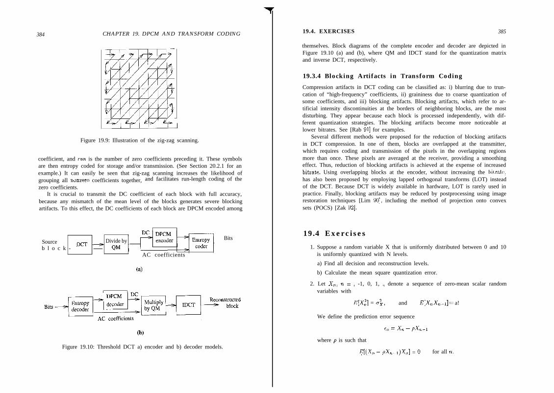
384 CHAPTER 19. DPCM AND TRANSFORM CODING
1Figure 19.9: Illustration of the zig-zag scanning.
coefficient, and rzllz is the number of zero coefficients preceding it. These symbolsare then entropy coded for storage and/or transmission. (See Section 20.2.1 for anexample.) It can easily be seen that zig-zag scanning increases the likelihood ofgrouping all nonzero coefficients together, and facilitates run-length coding of thezero coefficients.
It is crucial to transmit the DC coefficient of each block with full accuracy,because any mismatch of the mean level of the blocks generates severe blockingartifacts. To this effect, the DC coefficients of each block are DPCM encoded among
Source Divide by Bits
b l o c k - DCT QMAC coefficients
(4
04
Figure 19.10: Threshold DCT a) encoder and b) decoder models.
19.4. EXERCISES 385
themselves. Block diagrams of the complete encoder and decoder are depicted inFigure 19.10 (a) and (b), where QM and IDCT stand for the quantization matrixand inverse DCT, respectively.
19.3.4 Blocking Artifacts in Transform Coding
Compression artifacts in DCT coding can be classified as: i) blurring due to trun-cation of “high-frequency” coefficients, ii) graininess due to coarse quantization ofsome coefficients, and iii) blocking artifacts. Blocking artifacts, which refer to ar-tificial intensity discontinuities at the borders of neighboring blocks, are the mostdisturbing. They appear because each block is processed independently, with dif-ferent quantization strategies. The blocking artifacts become more noticeable atlower bitrates. See [Rab 911 for examples.
Several different methods were proposed for the reduction of blocking artifactsin DCT compression. In one of them, blocks are overlapped at the transmitter,which requires coding and transmission of the pixels in the overlapping regionsmore than once. These pixels are averaged at the receiver, providing a smoothingeffect. Thus, reduction of blocking artifacts is achieved at the expense of increasedbitrate. Using overlapping blocks at the encoder, without increasing the bitrate,has also been proposed by employing lapped orthogonal transforms (LOT) insteadof the DCT. Because DCT is widely available in hardware, LOT is rarely used inpractice. Finally, blocking artifacts may be reduced by postprocessing using imagerestoration techniques [Lim 901, including the method of projection onto convexsets (POCS) [Zak 921.
19.4 Exercises
1. Suppose a random variable X that is uniformly distributed between 0 and 10is uniformly quantized with N levels.
a) Find all decision and reconstruction levels.
b) Calculate the mean square quantization error.
2. Let X,, n = ) -1, 0, 1, ., denote a sequence of zero-mean scalar randomvariables with
E[X;] = &, and E[X,X,-I] = a!
We define the prediction error sequence
tn = x, - px,-1
where p is such that
q(xn - pxn-1)X,] = 0 for all n.
386 CHAPTER 19. DPCM AND TRANSFORM CODING
a) Find the value of p.
b) Let Di and Ds denote the distortion incurred by uniform quantization ofX, and E,, respectively, using r bits. Show that D1 is always greater than orequal to Dz.
3. Suppose we have a differential image that is Laplacian distributed with thestandard deviation 15. We wish to quantize it using 2 bits/sample.
a) Find the decision and reconstruction levels of a uniform quantizer.
b) Find the decision and reconstruction levels of the Lloyd-Max quantizer.
4. Explain why the transmitter in DPCM bases its prediction on previouslyreconstructed values rather than on the originals.
5. Compute the Karhunen-Loeve transform, DFT and DCT of the block shownbelow.
16 11 10 16 24 40 51 6112 12 14 19 26 58 60 5514 13 16 24 40 57 69 5614 17 22 29 51 87 80 6218 22 37 56 68 109 103 7724 35 55 64 81 104 113 9249 64 78 87 103 121 120 10172 92 95 98 112 100 103 99
Compare these transforms on the basis of energy compaction (decorrelation),and similarity of the basis functions.
6. Suppose we have three scalar random variables, Xi, X2, and Xs, with vari-ances 2.5,7, and 10. Propose a method to allocate a total of 20 bits to quantizeeach random variable independently to minimize the mean of the sum of thesquare quantization errors.
7. Explain the purpose of the zig-zag scanning in DCT compression. Do we needit with the zonal sampling strategy?
BIBLIOGRAPHY
Bibliography
387
[Ahm 741 N. Ahmed, T, Natarajan, and K. R. Rao, “Discrete cosine transforms,”IEEE Trans. Comp., vol. 23, pp. 90-93, 1974.
[Che 841 W.-H. Chen and W. K. Pratt, “Scene adaptive coder,” IEEE Trans.Comm., vol. 32, pp. 225232, Mar. 1984.
[Cla 851 R. J. Clark, Transform Coding of Images, Academic Press, 1985.
[Jai 811 A. K. Jain, “Image data compression: A review,” Proc. IEEE, vol. 69,pp. 3499389, Mar. 1981.
[Jai 901 A. K. Jain, Fundamentals of Digital Image Processing, Englewood Cliffs,NJ: Prentice Hall, 1989.
[Jay 921 N. Jayant, “Signal compression: Technology targets and research direc-tions,” IEEE J. Selected Areas in Comm., vol. 10, pp. 7966819, Jun. 1992.
[Lim 901 J. S. Lim, Two-Dimensional Szgnal and Image Processing, EnglewoodCliffs, NJ: Prentice Hall, 1990.
[Llo 821 S. P. Lloyd, “Least squares quantization in PCM,” IEEE Trans. Info.The., vol. 28, pp. 129-137, Mar. 1982.
[Mar 941 S. Martucci, “Symmetric convolution and the discrete sine and cosinetransforms,” IEEE Trans. Signal Proc., vol. 42, pp. 1038%1051, May 1994.
[Max 601 J. Max, “Quantizing for minimum distortion,” IfiRE Trans. Info. Theory,vol. 6, pp. 7-12, Mar. 1960.
[Mus 851 H. G. Musmann, P. Pirsch, and H. J. Grallert, “Advances in picturecoding,” Proc. IEEE, vol. 73, pp. 523-548, Apr. 1985.
[Net 801 A. N. Netravali and J. 0. Limb, “Picture coding: A review,” Proc. IEEE,vol. 68, no. 3, pp. 366-406, Mar. 1980.
[Rab 911 M. Rabbani and P. Jones, Digital Imuge Compression Techniques, Belling-ham, WA: SPIE Press, 1991.
[Rao 901 K. R. Rao and P. Yip, Discrete Cosine Transform, Academic Press, 1990.
[Win 721 P. A. Wintz, “Transform picture coding,” Proc. IEEE, vol. 60,pp. 8099820, July 1972.
[Woo 691 R. C. Wood, “On optimum quantization,” IEEE Trans. Info. Theory,vol. 15, no. 2, pp. 248-252, 1969.
[Zak 921 A. Zakhor, “Iterative procedures for reduction of blocking effects in trans-form image coding,” IEEE Trans. Circ. and Syst.: Video Tech., vol. 2,pp. 91-95, Mar. 1992.

Chapter 20
STILL IMAGECOMPRESSIONSTANDARDS
Recent developments in electronic imaging technology are creating both a capabilityand a need for digital storage and transmission of binary and continuous-tone colorimages and video. Image compression is an essential enabling technology behindthese developments, considering the raw data rates associated with digital images.However, storage and transmission of digital images in compressed formats necessi-tates internationally accepted standards to ensure compatibility and interoperabilityof various products from different manufacturers.
Recognizing this need, several international organizations, including the Interna-tional Standards Organization (ISO), the International Telecommunications Union(ITU) - formerly the International Consultative Committee for Telephone and Tele-graph (CCITT), - and the International Electrotechnical Commission (IEC), haveparticipated in programs to establish international standards for image compressionin specific application areas. To this effect, expert groups, formed under the auspicesof ISO, IEC, and ITU (CCITT), solicited proposals from companies, universities,and research laboratories. The best of those submitted have been selected on thebasis of image quality, compression performance, and practical constraints. Thischapter addresses the international standards on bilevel and continuous-tone colorstill image compression, which are summarized in Table 20.1. The bilevel imagecompression standards are discussed in Section 20.1, while the JPEG algorithm ispresented in Section 20.2.
388
20.1. BILEVEL IMAGE COMPRESSION STANDARDS 389
Table 20.1: International standards for still-image compression
Standard DescriptionITU (CCITT) Developed for bilevel image compression;Group 3 primarily designed for fax transmission of documents;Group 4 most widely used image compression standards.JBIG Joint (ITU-ISO/IEC) Bilevel Imaging Group;
developed for improved bilevel image compressionto handle progressive transmission and digital halftones.
JPEG Joint (ITU-ISO/IEC) Photographic Expert Group;developed for color still-image compression.
20.1 Bilevel Image Compression StandardsProbably the best example of the relationship between standardization and mar-ket growth is the boom in the fax market that we experienced following the ITU(CCITT) standards for binary image compression. Today, undoubtedly the mostwidely used image compression standards are the ITU (CCITT) Group 3 (G3) andGroup 4 (G4) codes for the compression of bilevel images.
ITU (CCITT) G3, also known as MR, modified READ (Relative Element AdressDesignate), is based, on nonadaptive, 1-D run-length coding in which the last II - 1lines of each group of K lines can be (optionally) 2-D run-length coded. Typicalcompression ratio has been found to be 15:l on representative test documents. ITU(CCITT) G4 refers to a simplified version of G3 standard in which only 2-D run-length coding is allowed. Both standards use the same nonadaptive 2-D codingmethod and the same Huffman tables. G4 obtains 30% better compression byremoving some error recovery from G3. ITU (CCITT) G3 and G4 standards havebeen vital in the world of fax machines and document storage applications.
It has been recognized that the ITU (CCITT) G3 and G4 codes cannot effec-tively deal with some images, especially digital halftones. JBIG is a new bilevelimage compression standard developed to improve upon the performance of the G3and G4 standards by using adaptive arithmetic coding, and adaptive templates forhalftones. In the following, we discuss the 1-D and 2-D run-length coding methodswhich form the basis of ITU (CCITT) G3, G4, and JBIG. We conclude the sectionwith a discussion of the new features in JBIG.
20.1.1 One-Dimensional RLC
In 1-D RLC, which is used in the ITU (CCITT) G3 algorithm, each line of abilevel image is described as a series of alternating white and black runs using aleft-to-right scan. The resulting run-lengths are Huffman coded by means of anappropriate combination of make-up codes and terminating codes. Run lengths
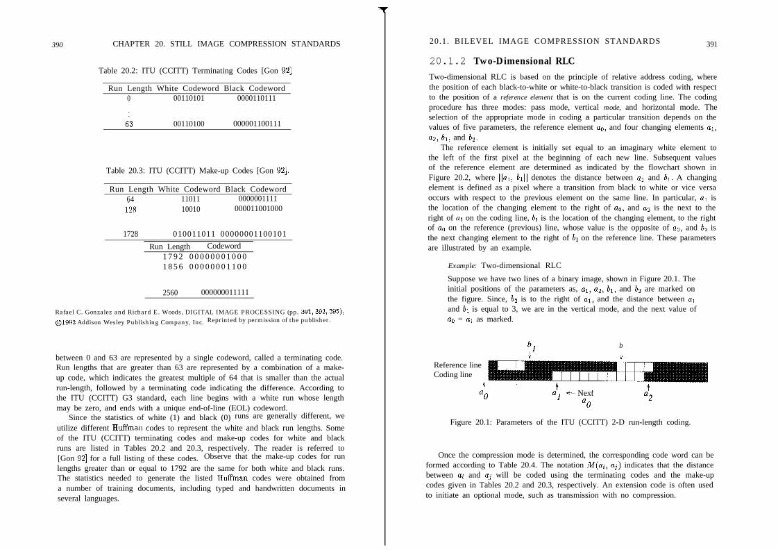
390 CHAPTER 20. STILL IMAGE COMPRESSION STANDARDS
Table 20.2: ITU (CCITT) Terminating Codes [Gon 921
Run Length White Codeword Black Codeword0 00110101 0000110111
6; 00110100 000001100111
Table 20.3: ITU (CCITT) Make-up Codes [Gon 921.
Run Length White Codeword Black Codeword64 11011 00000011111-2i 10010 000011001000
1728 010011011 00000001100101
Run Length Codeword1 7 9 2 0 0 0 0 0 0 0 1 0 0 01 8 5 6 0 0 0 0 0 0 0 1 1 0 0
2560 000000011111
Rafael C. Gonzalez and Richard E. Woods, DIGITAL IMAGE PROCESSING (pp. 391,392,395),
01992 Addison Wesley Publishing Company, Inc. Reprinted by permission of the publisher.
between 0 and 63 are represented by a single codeword, called a terminating code.Run lengths that are greater than 63 are represented by a combination of a make-up code, which indicates the greatest multiple of 64 that is smaller than the actualrun-length, followed by a terminating code indicating the difference. According tothe ITU (CCITT) G3 standard, each line begins with a white run whose lengthmay be zero, and ends with a unique end-of-line (EOL) codeword.
Since the statistics of white (1) and black (0) runs are generally different, weutilize different Huffman codes to represent the white and black run lengths. Someof the ITU (CCITT) terminating codes and make-up codes for white and blackruns are listed in Tables 20.2 and 20.3, respectively. The reader is referred to[Gon 921 for a full listing of these codes. Observe that the make-up codes for runlengths greater than or equal to 1792 are the same for both white and black runs.The statistics needed to generate the listed Huffman codes were obtained froma number of training documents, including typed and handwritten documents inseveral languages.
20.1. BILEVEL IMAGE COMPRESSION STANDARDS 391
20.1.2 Two-Dimensional RLCTwo-dimensional RLC is based on the principle of relative address coding, wherethe position of each black-to-white or white-to-black transition is coded with respectto the position of a reference element that is on the current coding line. The codingprocedure has three modes: pass mode, vertical mode, and horizontal mode. Theselection of the appropriate mode in coding a particular transition depends on thevalues of five parameters, the reference element ac, and four changing elements al,a2, bl, and b2.
The reference element is initially set equal to an imaginary white element tothe left of the first pixel at the beginning of each new line. Subsequent valuesof the reference element are determined as indicated by the flowchart shown inFigure 20.2, where ]]ar, bill denotes the distance between al and bl. A changingelement is defined as a pixel where a transition from black to white or vice versaoccurs with respect to the previous element on the same line. In particular, al isthe location of the changing element to the right of ac, and az is the next to theright of al on the coding line, bl is the location of the changing element, to the rightof a0 on the reference (previous) line, whose value is the opposite of ae, and b2 isthe next changing element to the right of bl on the reference line. These parametersare illustrated by an example.
Example: Two-dimensional RLC
Suppose we have two lines of a binary image, shown in Figure 20.1. Theinitial positions of the parameters as, al, a2, bl, and b2 are marked onthe figure. Since, b2 is to the right of al, and the distance between aland bl is equal to 3, we are in the vertical mode, and the next value ofas = al as marked.
bh
Reference lineCoding line
AI
aO al - NextaO
Figure 20.1: Parameters of the ITU (CCITT) 2-D run-length coding.
Once the compression mode is determined, the corresponding code word can beformed according to Table 20.4. The notation M(ai, aj) indicates that the distancebetween ai and aj will be coded using the terminating codes and the make-upcodes given in Tables 20.2 and 20.3, respectively. An extension code is often usedto initiate an optional mode, such as transmission with no compression.

392 CHAPTER 20. STILL IMAGE COMPRESSION STANDARDS
The algorithm can, then, be summarized as follows:i) Initialize as.ii) Determine the four changing elements, al, az, bi, and b2, according to their
definitions given above.iii) Determine the appropriate mode based on these values, using the flowchart
in Figure 20.2, and form the codeword using Table 20.4.iv) Establish the next reference element for the next coding cycle, according to
the flowchart in Figure 20.2, and go to step ii. Go to step i if an end of line is
I IStart a new line .~a o = 0 (first pixel)
I
Figure 20.2: Flowchart of the ITU (CCITT) 2-D RLC algorithm.
20.1. BILEVEL IMAGE COMPRESSION STANDARDS 393
Table 20.4: ITU (CCITT) two-dimensional run-length codes [Gon 921.
Mode CodewordPass 0001Horizontal 001SM(ao, al) + M(W) %)Vertical
al below bi 1ai one to the right of bl 011al two to the right of bi 000011al three to the right of bi 0000011ai one to the left of bi 010ai two to the left of bl 000010al three to the left of bl 0000010
Extension 0000001xxx
20.1.3 The JBIG Standard
JBIG is a new standard for lossless binary and low-precision gray-level (less than6 bits/pixel) image compression proposed and developed by a joint committee be-tween ISO/IEC and ITU (CCITT). The mission of the JBIG committee has been:(i) to develop adaptive lossless algorithms that will outperform the existing stan-dards, and (ii) to accommodate progressive transmission.
In JBIG, binary pel values are directly fed into an arithmetic encoder, which uti-lizes a “sequential template” (a set of neighboring pixels that are already encoded)to create a “context” in the generation of each binary symbol. The context affectsthe decision probabilities used in the arithmetic encoder. The best performancecan be obtained by using adaptive templates leading to adaptive arithmetic coding.Using adaptive arithmetic coding, JBIG improves upon the performance of the ITU(CCITT) G4 algorithm by another 30% for typical text images.
One of the primary reasons why JBIG has been formed is the performance im-provement needed for binary halftones. Digital halftones have statistical propertiesthat are quite different than those of the text documents. Because the Huffmantables used in ITU (CCITT) G3 and G4 have been based on a set of text docu-ments, they are unsuitable for binary halftones, and have been found to cause dataexpansion in some cases. JBIG provides about 8:l compression on typical digitalhalftones (using adaptive templates) which would have expanded with G3/G4.
In addition, JBIG defines a progressive mode in which a reduced-resolutionstarting layer image is followed by transmission of progressively higher-resolutionlayers. The templates used in the progressive mode may include pixels from previouslayers as well as previously encoded pixels from the same layer. JBIG syntax alsoallows coding of images with more than one bit/pixel using bit-plane encoding.
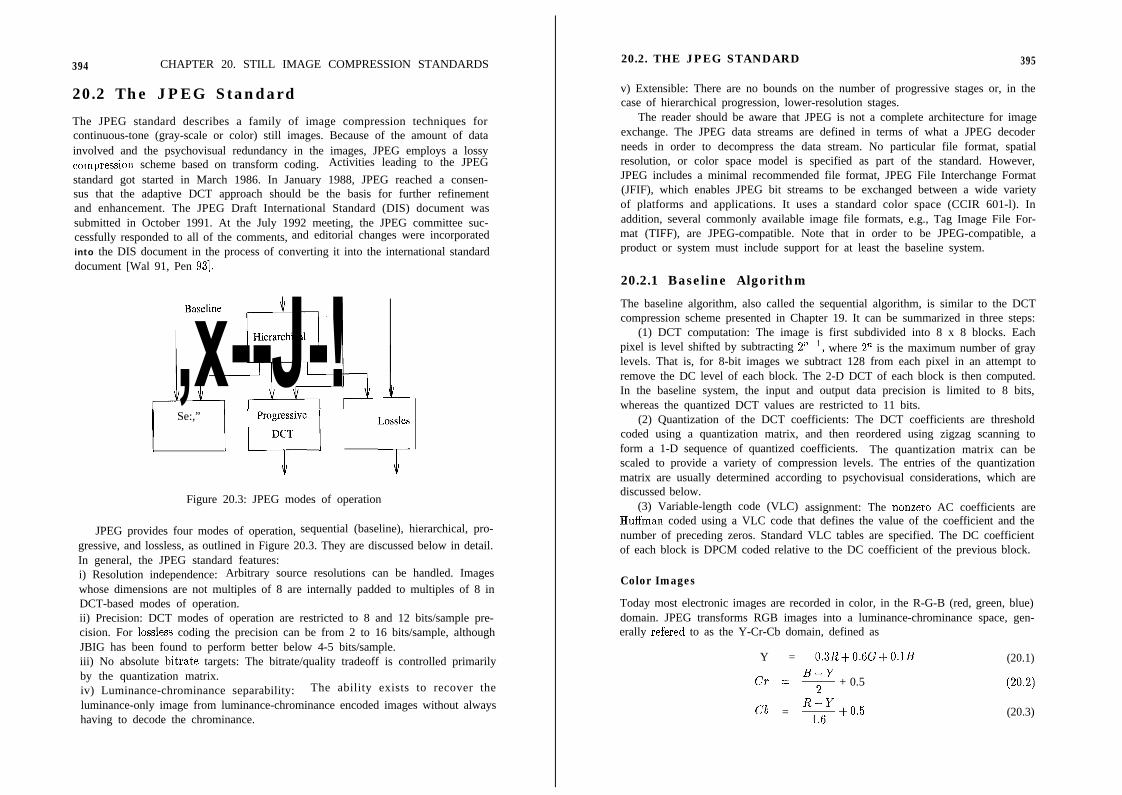
394 CHAPTER 20. STILL IMAGE COMPRESSION STANDARDS
20.2 The JPEG Standard
The JPEG standard describes a family of image compression techniques forcontinuous-tone (gray-scale or color) still images. Because of the amount of datainvolved and the psychovisual redundancy in the images, JPEG employs a lossycompression scheme based on transform coding. Activities leading to the JPEGstandard got started in March 1986. In January 1988, JPEG reached a consen-sus that the adaptive DCT approach should be the basis for further refinementand enhancement. The JPEG Draft International Standard (DIS) document wassubmitted in October 1991. At the July 1992 meeting, the JPEG committee suc-cessfully responded to all of the comments, and editorial changes were incorporatedinto the DIS document in the process of converting it into the international standarddocument [Wal 91, Pen 931.
Baseline
Hierarchical
1 Se:,” 11 Los;IPro 1
Figure 20.3: JPEG modes of operation
JPEG provides four modes of operation, sequential (baseline), hierarchical, pro-gressive, and lossless, as outlined in Figure 20.3. They are discussed below in detail.In general, the JPEG standard features:i) Resolution independence: Arbitrary source resolutions can be handled. Imageswhose dimensions are not multiples of 8 are internally padded to multiples of 8 inDCT-based modes of operation.ii) Precision: DCT modes of operation are restricted to 8 and 12 bits/sample pre-cision. For lossless coding the precision can be from 2 to 16 bits/sample, althoughJBIG has been found to perform better below 4-5 bits/sample.iii) No absolute bitrate targets: The bitrate/quality tradeoff is controlled primarilyby the quantization matrix.iv) Luminance-chrominance separability: The ability exists to recover theluminance-only image from luminance-chrominance encoded images without alwayshaving to decode the chrominance.
20.2. THE JPEG STANDARD 395
v) Extensible: There are no bounds on the number of progressive stages or, in thecase of hierarchical progression, lower-resolution stages.
The reader should be aware that JPEG is not a complete architecture for imageexchange. The JPEG data streams are defined in terms of what a JPEG decoderneeds in order to decompress the data stream. No particular file format, spatialresolution, or color space model is specified as part of the standard. However,JPEG includes a minimal recommended file format, JPEG File Interchange Format(JFIF), which enables JPEG bit streams to be exchanged between a wide varietyof platforms and applications. It uses a standard color space (CCIR 601-l). Inaddition, several commonly available image file formats, e.g., Tag Image File For-mat (TIFF), are JPEG-compatible. Note that in order to be JPEG-compatible, aproduct or system must include support for at least the baseline system.
20.2.1 Baseline Algorithm
The baseline algorithm, also called the sequential algorithm, is similar to the DCTcompression scheme presented in Chapter 19. It can be summarized in three steps:
(1) DCT computation: The image is first subdivided into 8 x 8 blocks. Eachpixel is level shifted by subtracting 2”-r, where 2” is the maximum number of graylevels. That is, for 8-bit images we subtract 128 from each pixel in an attempt toremove the DC level of each block. The 2-D DCT of each block is then computed.In the baseline system, the input and output data precision is limited to 8 bits,whereas the quantized DCT values are restricted to 11 bits.
(2) Quantization of the DCT coefficients: The DCT coefficients are thresholdcoded using a quantization matrix, and then reordered using zigzag scanning toform a 1-D sequence of quantized coefficients. The quantization matrix can bescaled to provide a variety of compression levels. The entries of the quantizationmatrix are usually determined according to psychovisual considerations, which arediscussed below.
(3) Variable-length code (VLC) assignment: The nonzero AC coefficients areHuffman coded using a VLC code that defines the value of the coefficient and thenumber of preceding zeros. Standard VLC tables are specified. The DC coefficientof each block is DPCM coded relative to the DC coefficient of the previous block.
Color Images
Today most electronic images are recorded in color, in the R-G-B (red, green, blue)domain. JPEG transforms RGB images into a luminance-chrominance space, gen-erally refered to as the Y-Cr-Cb domain, defined as
Y = 0.3R+O.BG+O.lB (20.1)
Cr = 7 + 0.5
Cb = F.o.5 (20.3)

396 CHAPTER 20. STILL IMAGE COMPRESSION STANDARDS 20.2. THE JPEG STANDARD 397
Because, the human eye is relatively insensitive to the high-frequency content of thechrominance channels Cr and Cb (see Figure 20.5), they are subsampled by 2 inboth directions. This is illustrated in Figure 20.4 where the chrominance channelscontain half as many lines and pixels per line compared to the luminance channel.
Figure 20.4: Subsampling of the chrominance channels Figure 20.5: Visual response to luminance and chrominance variations [Mu1 851.
JPEG orders the pixels of a color image as either noninterleaved (three separatescans) or interleaved (a single scan). In reference to Figure 20.4, the noninterleavedordering can be shown as
Scan 1: Yl, Y2, Y3, .) Y16Scan 2: Crl, Cr2, Cr3, Cr4Scan 3: Cbl, Cb2, Cb3, Cb4
whereas the interleaved ordering becomes
Yl, Y2, Y3, Y4, Crl, Cbl, Y5, Y6, Y7, Y8, Cr2, Cb2,
Interleaving makes it possible to decompress the image, and convert from luminance-chrominance representation to RGB for display with a minimum of intermediatebuffering. For interleaved data, the DCT blocks are ordered according to the pa-rameters specified in the frame and scan headers.
Psychovisual Aspects
In order to reduce the psychovisual redundancy in images, JPEG incorporates thecharacteristics of the human visual system into the compression process throughthe specification of quantization matrices. It is well known that the frequencyresponse of the human visual system drops off with increasing spatial frequency.Furthermore, this drop-off is faster in the two chrominance channels. The contrastsensitivity function depicted in Figure 20.5 demonstrates this effect. It impliesthat a small variation in intensity is more visible in slowly varying regions than inbusier ones, and also more visible in luminance compared to a similar variation inchrominance.
1000 ,
5 0 0
200
100
Contrast 50s e n s i t i v i t y 2.
10
5
2t
Spatial frequency (cycles/degree)
As a result, JPEG allows specification of two quantization matrices, one for theluminance and another for the two chrominance channels to allocate more bits forthe representation of coefficients which are visually more significant. Tables 20.5and 20.6 show typical quantization matrices for the luminance and chrominancechannels, respectively. The elements of these matrices are based on the visibility ofindividual 8 x 8 DCT basis functions with a viewing distance equal to six times thescreen width. The basis functions were viewed with a luminance resolution of 720pixels x 576 lines and a chrominance resolution of 360 x 576. The matrices suggestthat those DCT coefficients corresponding to basis images with low visibility canbe more coarsely quantized.
Table 20.5: Quantization Table for the Luminance Channel
16 11 10 16 24 40 51 6112 12 14 19 26 58 60 5514 13 16 24 40 57 69 5614 17 22 29 51 87 80 6218 22 37 56 68 109 103 7724 35 55 64 81 104 113 9249 64 78 87 103 121 120 10172 92 95 98 112 100 103 99

398 CHAPTER20. STILLIMAGECOMPRESSIONSTANDARDS 20.2. THE JPEG STANDARD 399
Table 20.6: Quantization Table for the Chrominance Channel
17 18 24 47 99 99 99 9918 21 26 66 99 99 99 9924 26 56 99 99 99 99 9947 66 99 99 99 99 99 9999 99 99 99 99 99 99 9999 99 99 99 99 99 99 9999 99 99 99 99 99 99 9999 99 99 99 99 99 99 99
Example: JPEG Baseline Algorithm
We demonstrate the application of the JPEG baseline algorithm on the8 x 8 luminance block presented in Section 19.3.1. Following the samesteps demonstrated on pages 380-383, the gray levels are first shiftedby -128 (assuming that the original is an 8-bit image), and then a for-ward DCT is applied. The DCT coefficients divided by the quantizationmatrix, shown in Table 20.5, have been found as
The codewords for the symbols formed from these coefficients can befound according to the Tables for JPEG Coefficient Coding Categories,JPEG Default DC Codes (Luminance/Chrominance), and JPEG De-fault AC Codes (Luminance/ Chrominance) [Gon 92, Pen 931. For ex-ample, the DC difference -9 falls within the DC difference category 4.The proper base (default) code for category 4 is 011 (a S-bit code),while the total length of a completely encoded category 4 coefficient is7 bits. The remaining 4 bits will be the least significant bits (LSBs) ofthe difference value. Each default AC Huffman codeword depends onthe number of zero-valued coefficients preceding the nonzero coefficientto be coded as well as the magnitude category of the coefficient. Theremaining bits are found in the same way as in DC difference coding.
The decoder implements the inverse operations. That is, the receivedcoefficients are first multiplied by the same quantization matrix to obtain
$h, h) =20 5 -3 1 3 -2 1 0
-3 -2 1 2 1 0 0 0-1 -1 1 1 1 0 0 0
S(kl,k2) = -A ; 0 1 0 0 0 00 0 0 0 0 0
0 0 0 0 0 0 0 00 0 0 0 0 0 0 00 0 0 0 0 0 0 0
320 55 -30 16 72 -80 51 0- 3 6 - 2 4 14 38 26 0 00- 1 4 - 1 3 16 24 40 0 00-14 0 0 29 0 0 00
0 0 0 0 0 0 000 0 0 0 0 0 000 0 0 0 0 0 000 0 0 0 0 0 00
Performing an inverse DCT, and adding 128 to each element, we findthe reconstructed block as
Following a zigzag scanning of these coefficients, the 1-D coefficient se-quence can be expressed as
[ 20, 5, -3, -1, -2, -3, 1, 1, -1, -1, 0, 0, 1, 2,s”(n1, m) =
3, -2, 1, 1, 0, 0, 0, 0, 0, 0, 1, 1, 0, 1, EOB ]where EOB denotes the end of the block (i.e., all following coefficientsare zero.)
195 140 119 148 197 171 120 170186 153 143 158 193 168 124 175174 169 172 168 187 166 128 177169 180 187 171 185 170 131 170172 182 186 168 186 175 131 161177 180 181 168 189 175 129 161181 178 181 174 191 169 128 173183 178 184 181 192 162 127 185
The DC coefficient is coded using DPCM, as depicted in Figure 19.10.That is, the difference between the DC coefficient of the present blockand that of the previously encoded block is coded. (Assume that theDC coefficient of the previous block was 29, so the difference is -9.)The AC coefficients are mapped into the following run-level pairs
(0, 5), (0, -3) (0, -11, (0, -2), (0, -3) (0, 11, (0, 11, (0, -I), (0, -11,(2, 11, (0, 2)) (0, 3), (0, -2) (0, 11, (0, 11, (6, I), (0, 11, (1, 11, EOB.
The reconstruction error varies 525 gray levels, as can be seen by com-paring the result with the original block shown on page 380.
The compression ratio, and hence the quality of the reconstructed im-age, is controlled by scaling the quantization matrix as desired. Scalingthe quantization matrix by a factor larger than 1 results in a coarserquantization, and a lower bitrate at the expense of higher reconstruc-tion error.
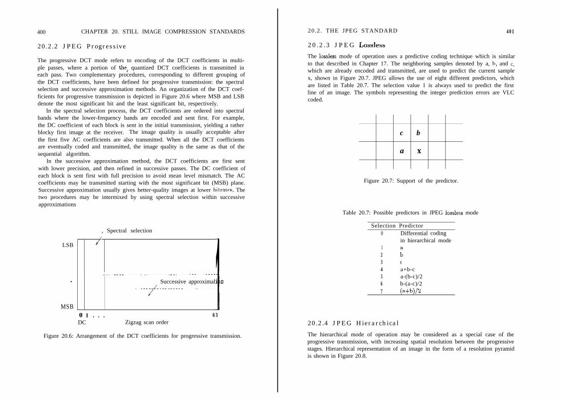
400 CHAPTER 20. STILL IMAGE COMPRESSION STANDARDS
20.2.2 JPEG Progressive
The progressive DCT mode refers to encoding of the DCT coefficients in multi-ple passes, where a portion of the: quantized DCT coefficients is transmitted ineach pass. Two complementary procedures, corresponding to different grouping ofthe DCT coefficients, have been defined for progressive transmission: the spectralselection and successive approximation methods. An organization of the DCT coef-ficients for progressive transmission is depicted in Figure 20.6 where MSB and LSBdenote the most significant bit and the least significant bit, respectively.
In the spectral selection process, the DCT coefficients are ordered into spectralbands where the lower-frequency bands are encoded and sent first. For example,the DC coefficient of each block is sent in the initial transmission, yielding a ratherblocky first image at the receiver. The image quality is usually acceptable afterthe first five AC coefficients are also transmitted. When all the DCT coefficientsare eventually coded and transmitted, the image quality is the same as that of thesequential algorithm.
In the successive approximation method, the DCT coefficients are first sentwith lower precision, and then refined in successive passes. The DC coefficient ofeach block is sent first with full precision to avoid mean level mismatch. The ACcoefficients may be transmitted starting with the most significant bit (MSB) plane.Successive approximation usually gives better-quality images at lower bitrat,es. Thetwo procedures may be intermixed by using spectral selection within successiveapproximations
, Spectral selection
LSB
.
MSB
/d
i~~.----~.....~~~~~~~.~~~-.~....---..-----Successive approximal
-----~----------------------
:i n
0 1 . . . 63DC Zigzag scan order
Figure 20.6: Arrangement of the DCT coefficients for progressive transmission.
20.2. THE JPEG STANDARD 401
20.2.3 JPEG Lossless
The lossless mode of operation uses a predictive coding technique which is similarto that described in Chapter 17. The neighboring samples denoted by a, b, and c,which are already encoded and transmitted, are used to predict the current samplex, shown in Figure 20.7. JPEG allows the use of eight different predictors, whichare listed in Table 20.7. The selection value 1 is always used to predict the firstline of an image. The symbols representing the integer prediction errors are VLCcoded.
c b
a x
Figure 20.7: Support of the predictor.
Table 20.7: Possible predictors in JPEG lossless mode
Selection Predictor0 Differential coding
in hierarchical mode12 ;3 c4 a+b-c5 a-(b-c)/26 b-(a-c)/27 (a+b)/2
20.2.4 JPEG Hierarchical
The hierarchical mode of operation may be considered as a special case of theprogressive transmission, with increasing spatial resolution between the progressivestages. Hierarchical representation of an image in the form of a resolution pyramidis shown in Figure 20.8.
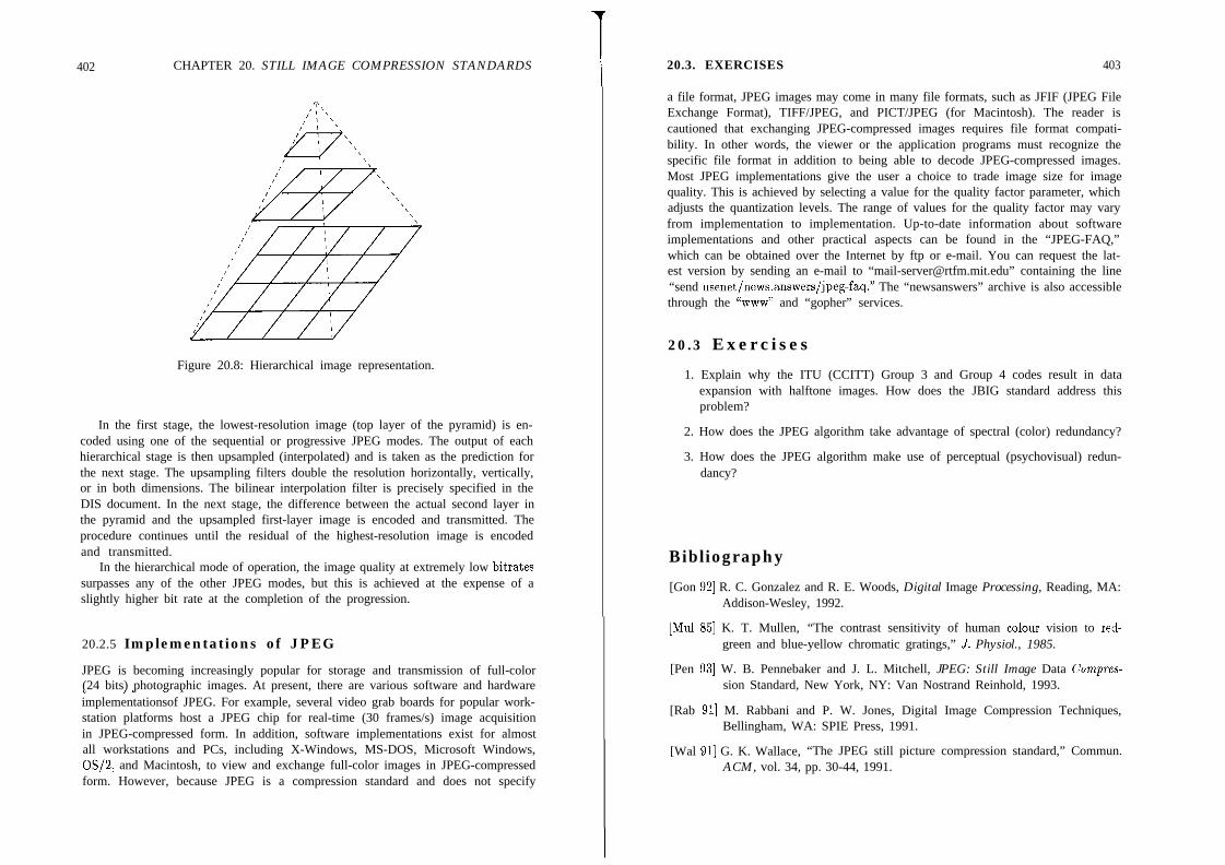
402 CHAPTER 20. STILL IMAGE COMPRESSION STANDARDSI
20.3. EXERCISES 403
Figure 20.8: Hierarchical image representation.
In the first stage, the lowest-resolution image (top layer of the pyramid) is en-coded using one of the sequential or progressive JPEG modes. The output of eachhierarchical stage is then upsampled (interpolated) and is taken as the prediction forthe next stage. The upsampling filters double the resolution horizontally, vertically,or in both dimensions. The bilinear interpolation filter is precisely specified in theDIS document. In the next stage, the difference between the actual second layer inthe pyramid and the upsampled first-layer image is encoded and transmitted. Theprocedure continues until the residual of the highest-resolution image is encodedand transmitted.
In the hierarchical mode of operation, the image quality at extremely low bitratessurpasses any of the other JPEG modes, but this is achieved at the expense of aslightly higher bit rate at the completion of the progression.
a file format, JPEG images may come in many file formats, such as JFIF (JPEG FileExchange Format), TIFF/JPEG, and PICT/JPEG (for Macintosh). The reader iscautioned that exchanging JPEG-compressed images requires file format compati-bility. In other words, the viewer or the application programs must recognize thespecific file format in addition to being able to decode JPEG-compressed images.Most JPEG implementations give the user a choice to trade image size for imagequality. This is achieved by selecting a value for the quality factor parameter, whichadjusts the quantization levels. The range of values for the quality factor may varyfrom implementation to implementation. Up-to-date information about softwareimplementations and other practical aspects can be found in the “JPEG-FAQ,”which can be obtained over the Internet by ftp or e-mail. You can request the lat-est version by sending an e-mail to “[email protected]” containing the line“send usenet/news.answers/jpeg-faq.” The “newsanswers” archive is also accessiblethrough the “www” and “gopher” services.
20.3 Exercises
1. Explain why the ITU (CCITT) Group 3 and Group 4 codes result in dataexpansion with halftone images. How does the JBIG standard address thisproblem?
2. How does the JPEG algorithm take advantage of spectral (color) redundancy?
3. How does the JPEG algorithm make use of perceptual (psychovisual) redun-dancy?
Bibliography
[Gon 921 R. C. Gonzalez and R. E. Woods, Digital Image Processing, Reading, MA:Addison-Wesley, 1992.
20.2.5 Implementations of JPEG
JPEG is becoming increasingly popular for storage and transmission of full-color(24 bits) photographic images. At present, there are various software and hardware\ ,_ --implementationsof JPEG. For example, several video grab boards for popular work-station platforms host a JPEG chip for real-time (30 frames/s) image acquisitionin JPEG-compressed form. In addition, software implementations exist for almostall workstations and PCs, including X-Windows, MS-DOS, Microsoft Windows,OS/2, and Macintosh, to view and exchange full-color images in JPEG-compressedform. However, because JPEG is a compression standard and does not specify
[Mu1 851 K. T. Mullen, “The contrast sensitivity of human colour vision to red-green and blue-yellow chromatic gratings,” b. Physiol., 1985.
[Pen 931 W. B. Pennebaker and J. L. Mitchell, JPEG: Still Image Data Compres-sion Standard, New York, NY: Van Nostrand Reinhold, 1993.
[Rab 911 M. Rabbani and P. W. Jones, Digital Image Compression Techniques,Bellingham, WA: SPIE Press, 1991.
[Wal 911 G. K. Wallace, “The JPEG still picture compression standard,” Commun.ACM, vol. 34, pp. 30-44, 1991.
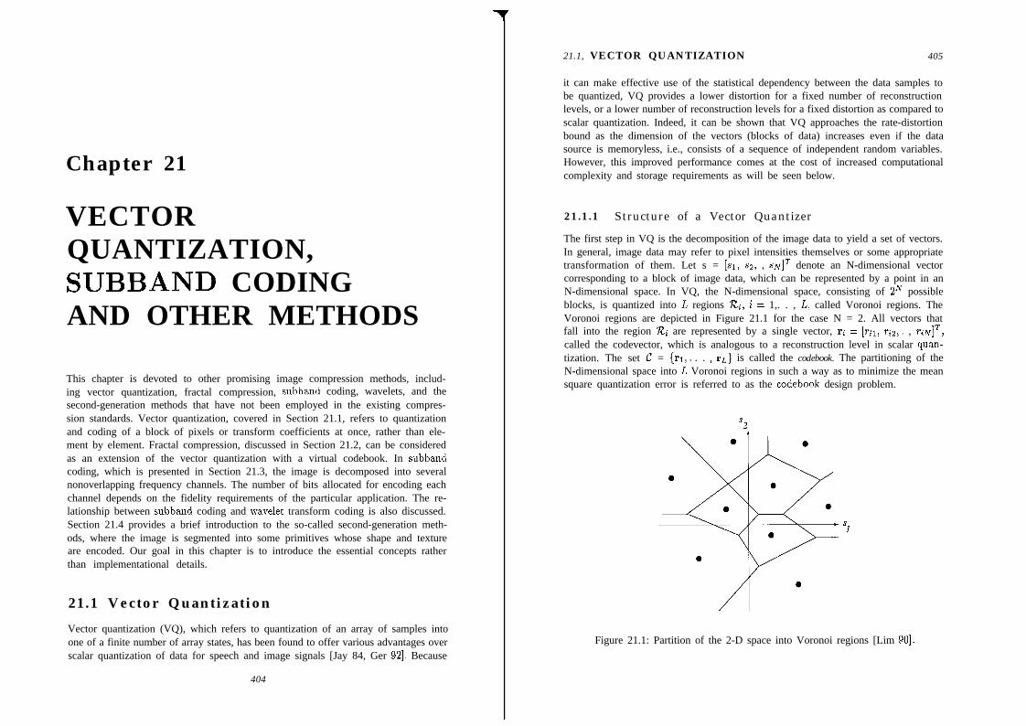
Chapter 21
VECTORQUANTIZATION,SUBBAND CODINGAND OTHER METHODS
This chapter is devoted to other promising image compression methods, includ-ing vector quantization, fractal compression, subband coding, wavelets, and thesecond-generation methods that have not been employed in the existing compres-sion standards. Vector quantization, covered in Section 21.1, refers to quantizationand coding of a block of pixels or transform coefficients at once, rather than ele-ment by element. Fractal compression, discussed in Section 21.2, can be consideredas an extension of the vector quantization with a virtual codebook. In subbandcoding, which is presented in Section 21.3, the image is decomposed into severalnonoverlapping frequency channels. The number of bits allocated for encoding eachchannel depends on the fidelity requirements of the particular application. The re-lationship between subband coding and wavelet transform coding is also discussed.Section 21.4 provides a brief introduction to the so-called second-generation meth-ods, where the image is segmented into some primitives whose shape and textureare encoded. Our goal in this chapter is to introduce the essential concepts ratherthan implementational details.
21.1 Vector Quantization
Vector quantization (VQ), which refers to quantization of an array of samples intoone of a finite number of array states, has been found to offer various advantages overscalar quantization of data for speech and image signals [Jay 84, Ger 921. Because
404
21.1, VECTOR QUANTIZATION 405
it can make effective use of the statistical dependency between the data samples tobe quantized, VQ provides a lower distortion for a fixed number of reconstructionlevels, or a lower number of reconstruction levels for a fixed distortion as compared toscalar quantization. Indeed, it can be shown that VQ approaches the rate-distortionbound as the dimension of the vectors (blocks of data) increases even if the datasource is memoryless, i.e., consists of a sequence of independent random variables.However, this improved performance comes at the cost of increased computationalcomplexity and storage requirements as will be seen below.
21.1.1 Structure of a Vector Quantizer
The first step in VQ is the decomposition of the image data to yield a set of vectors.In general, image data may refer to pixel intensities themselves or some appropriatetransformation of them. Let s = [si, sz, I SN] T denote an N-dimensional vectorcorresponding to a block of image data, which can be represented by a point in anN-dimensional space. In VQ, the N-dimensional space, consisting of 2N possibleblocks, is quantized into L regions Xi, i = 1,. . , L, called Voronoi regions. TheVoronoi regions are depicted in Figure 21.1 for the case N = 2. All vectors thatfall into the region %$ are represented by a single vector, ra = [rir, viz,. , ra~]~,called the codevector, which is analogous to a reconstruction level in scalar quan-tization. The set C = {PI,. . . ) r~.} is called the codebook. The partitioning of theN-dimensional space into L Voronoi regions in such a way as to minimize the meansquare quantization error is referred to as the codebook design problem.
Figure 21.1: Partition of the 2-D space into Voronoi regions [Lim 901.
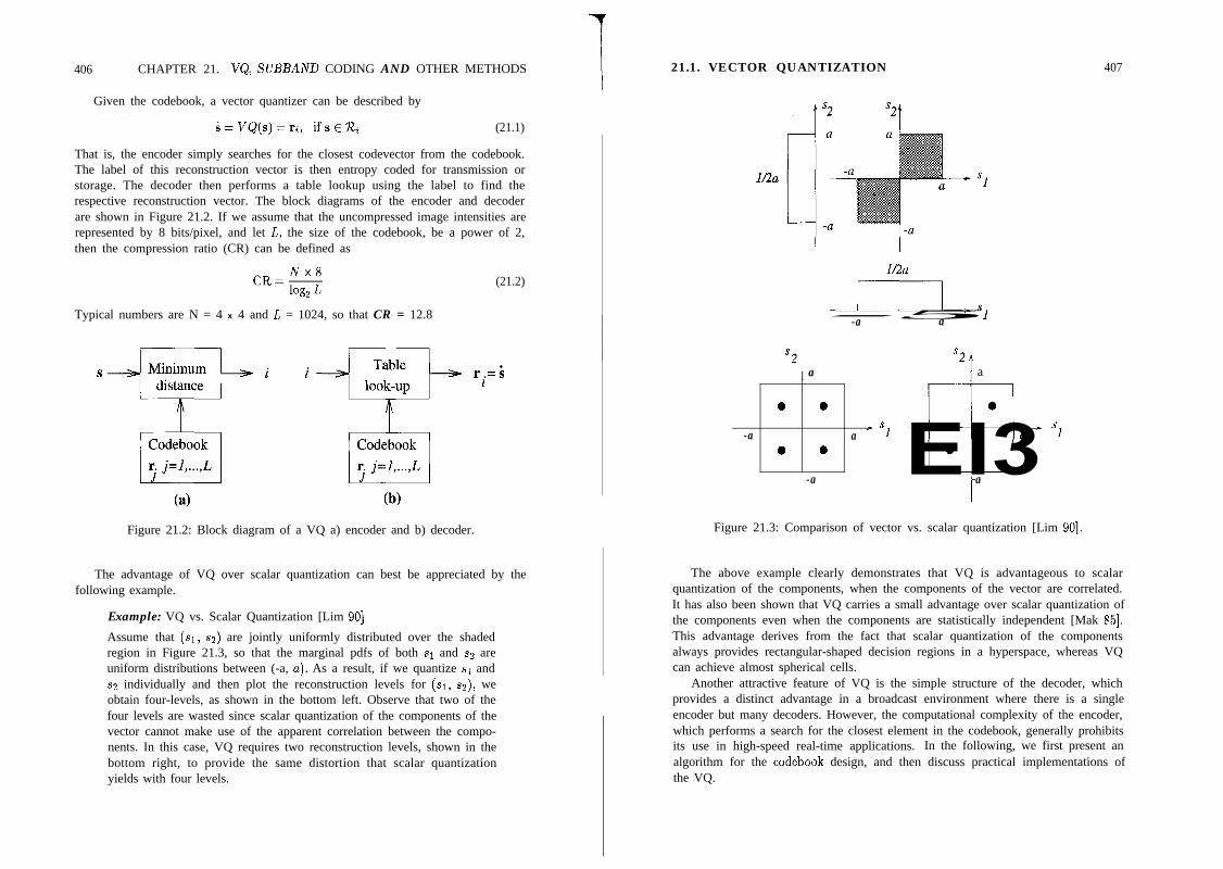
406 CHAPTER 21. VQ, SUBBAND CODING AND OTHER METHODS
Given the codebook, a vector quantizer can be described by
i=VQ(s)=ri, ifsERa (21.1)
That is, the encoder simply searches for the closest codevector from the codebook.The label of this reconstruction vector is then entropy coded for transmission orstorage. The decoder then performs a table lookup using the label to find therespective reconstruction vector. The block diagrams of the encoder and decoderare shown in Figure 21.2. If we assume that the uncompressed image intensities arerepresented by 8 bits/pixel, and let L, the size of the codebook, be a power of 2,then the compression ratio (CR) can be defined as
(21.2)
Typical numbers are N = 4 x 4 and L = 1024, so that CR = 12.8
(4 (b)
Figure 21.2: Block diagram of a VQ a) encoder and b) decoder.
The advantage of VQ over scalar quantization can best be appreciated by thefollowing example.
Example: VQ vs. Scalar Quantization [Lim 901
Assume that (si, ~2) are jointly uniformly distributed over the shadedregion in Figure 21.3, so that the marginal pdfs of both sr and sz areuniform distributions between (-a, u). As a result, if we quantize si andsz individually and then plot the reconstruction levels for (sr, ss), weobtain four-levels, as shown in the bottom left. Observe that two of thefour levels are wasted since scalar quantization of the components of thevector cannot make use of the apparent correlation between the compo-nents. In this case, VQ requires two reconstruction levels, shown in thebottom right, to provide the same distortion that scalar quantizationyields with four levels.
21.1. VECTOR QUANTIZATION
U2a
s2I a
1/2a
-a a
0 0
-a a * sI0 0
-a
s2f a 0
-a a sll
407
ta
Figure 21.3: Comparison of vector vs. scalar quantization [Lim 901.
The above example clearly demonstrates that VQ is advantageous to scalarquantization of the components, when the components of the vector are correlated.It has also been shown that VQ carries a small advantage over scalar quantization ofthe components even when the components are statistically independent [Mak 851.This advantage derives from the fact that scalar quantization of the componentsalways provides rectangular-shaped decision regions in a hyperspace, whereas VQcan achieve almost spherical cells.
Another attractive feature of VQ is the simple structure of the decoder, whichprovides a distinct advantage in a broadcast environment where there is a singleencoder but many decoders. However, the computational complexity of the encoder,which performs a search for the closest element in the codebook, generally prohibitsits use in high-speed real-time applications. In the following, we first present analgorithm for the codebook design, and then discuss practical implementations ofthe VQ.
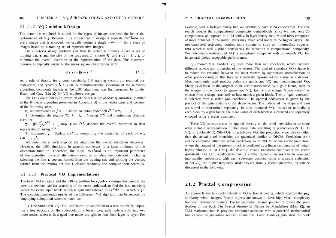
408 CHAPTER 21. VQ, SUBBAND CODING AND OTHER METHODS
21.1.2 VQ Codebook Design
The better the codebook is suited for the types of images encoded, the better theperformance of VQ. Because it is impractical to design a separate codebook forevery image that is encoded, we usually design a single codebook for a class ofimages based on a training set of representative images.
The codebook design problem can then be stated as follows. Given a set oftraining data s and the size of the codebook L, choose ‘R.i and ri, i = 1, , L tominimize the overall distortion in the representation of the data. The distortionmeasure is typically taken as the mean square quantization error
d(s,r) = 11s - rf (21.3)
As a rule of thumb, for a good codebook, 100 training vectors are required percodevector, and typically L < 5000. A multidimensional extension of the K-meansalgorithm, commonly known as the LBG algorithm, was first proposed by Linde,Buzo, and Gray [Lin 801 for VQ codebook design.
The LBG algorithm is an extension of the scalar Lloyd-Max quantization (similarto the K-means algorithm presented in Appendix B) to the vector case, and consistsof the following steps:
0) Initialization: Set j = 0. Choose an initial codebook C(j) = ri, . . , rL.1) Determine the regions ‘%&, i = 1,. , L using C(j) and a minimum distance
classifier.D(j-l)-D(j)
2, If l)(j) < E, stop. Here D(j) denotes the overall distortion in datarepresentation using C(j).
3) Increment j. Update C(j) by computing the centroids of each of Xi,i=l,...,L.
We note that at each step of the algorithm the overall distortion decreases.However, the LBG algorithm, in general, converges to a local minimum of thedistortion function. Therefore, the initial codebook is an important parameterof the algorithm. Several alternatives exist to initialize the codebook, includingselecting the first L vectors formed from the training set, and splitting the vectorsformed from the training set into L classes randomly and compute their centroids.
21.1.3 Practical VQ Implementations
The basic VQ structure and the LBG algorithm for codebook design discussed in theprevious sections call for searching of the entire codebook to find the best matchingvector for every input block, which is generally referred to as “the full-search VQ.”The computational requirements of the full-search VQ algorithm can be reduced byemploying suboptimal schemes, such as:
1) Tree-Structured VQ: Full search can be simplified to a tree search by impos-ing a tree structure on the codebook. In a binary tree, each node is split into twomore nodes, whereas in a quad tree nodes are split to four from layer to layer. For
21.2. FRACTAL COMPRESSION 409
example, with a lo-layer binary tree we eventually have 1024 codevectors. The treesearch reduces the computational complexity tremendously, since we need only 20comparisons, as opposed to 1024 with a lo-layer binary tree. Mixed trees composedof more branches in the initial layers may avoid void nodes at the higher layers. Thetree-structured codebook requires more storage to store all intermediate codevec-tars, which is well justified considering the reduction in computational complexity.We note that tree-structured VQ is suboptimal compared with full-search VQ, butin general yields acceptable performance.
2) Product VQ: Product VQ uses more than one codebook, which capturesdifferent aspects and properties of the vectors. The goal of a product VQ scheme isto reduce the variation between the input vectors by appropriate normalization orother preprocessing so that they be effectively represented by a smaller codebook.Most commonly used product codes are gain/shape VQ and mean-removed VQ,Shape is defined as the original input vector normalized by a gain factor, such asthe energy of the block. In gain-shape VQ, first a unit energy “shape vector” ischosen from a shape codebook to best match a given block. Then a “gain constant”is selected from a scalar gain codebook. The optimal codevector is given by theproduct of the gain scalar and the shape vector. The indices of the shape and gainare stored or transmitted separately. In mean-removed VQ, instead of normalizingeach block by a gain factor, the mean value of each block is subtracted and separatelyencoded using a scalar quantizer.
These VQ structures can be applied directly on the pixel intensities or to someother suitable representation of the image data, resulting in predictive-Vi&, DCT-VQ, or subband-VQ (SB-VQ). In predictive VQ, the prediction error blocks ratherthan the actual pixel intensities are quantized similar to DPCM. Prediction errorcan be computed either via scalar prediction, as in DPCM, or via vector prediction,where the content of the present block is predicted as a linear combination of neigh-boring blocks. In DCT-VQ, the d’iscrete cosine transform coefficients are vectorquantized. The DCT coefficients having similar dynamic ranges can be arrangedinto smaller subvectors, with each subvector encoded using a separate codebook.In SB-VQ, the higher-frequency subbands are usually vector quantized, as will bediscussed in the following.
21.2 Fkactal Compression
An approach that is closely related to VQ is fractal coding, which exploits the self-similarity within images. Fractal objects are known to have high visual complexitybut low information content. Fractal geometry became popular following the pub-lication of the book The Fractal Geometry of Nature by Mandelbrot [Man 821, anIBM mathematician. It provided computer scientists with a powerful mathematicaltool capable of generating realistic animations. Later, Barnsley published the book

410 CHAPTER 21. VQ, SUBBAND CODING AND OTHER METHODS
Fructals Everywhere [Bar 881 in which he discussed the application of fractals toimage compression using the theory of Iterated Function Systems (IFS). An IFSis a set of contractive transformations that map an image into smaller blocks. Of-ten, affine transformations are used, which include translation, rotation, shear, andscaling. In addition, scaling and offset of gray level or color are also allowed. Therepresentation of images by an IFS was formalized by the so-called Collage Theorem[Bar 881.
Because of practical difficulties with the initial approach, fractal-block coding(also known as a partitioned IFS), which utilizes self-similarity between pairs ofblocks under a set of affine transformations, was later proposed [Jac 92, Lu 931.Here, the transformations do not map from the whole image into the blocks, butfrom larger blocks to smaller blocks, to make use of local self-similarity. In Jacquin’snotation [Jac 921, large blocks are called domain blocks and small blocks are calledrange blocks. It is necessary that every pixel of the original image belong to (atleast) one range block. The pattern of range blocks is called the partitioning ofthe image. In fractal-block coding, an image is encoded in terms of a sequence ofchild-parent maps and a corresponding sequence of transformations chosen from atransformation codebook. In particular, the method consists of the following steps:
1. Partition the image into range blocks.
2. Form the set of domain blocks.
3. Choose a set of contractive transformations.
4. Select a distance metric between blocks.
5. Specify a search method for pairing range blocks to domain blocks.
The reconstruction process starts with a flat background. Observe that no do-main block information is transmitted. The set of affine transformations is appliediteratively. The process converges, because all transformations are contractive, usu-ally after a small number of iterations. Compression ratios in the range 25:l to 5O:lare typical with fractal compression schemes. Note that because fractal images arescaleless, compression ratio must be calculated at the resolution of the input image.
The similarity of fractal compression to VQ can be seen as follows:
. In VQ, the codebook is computed and stored independent of the image beingcoded; in an IFS, strictly speaking, there is no codebook. However, the domainblocks can be viewed to define a “virtual codebook” which is adapted to eachimage.
. In VQ, domain blocks and range blocks are the same size, and the intensitywithin the domain blocks is copied directly; in an IFS, domain blocks are largerthan range blocks, and each domain block undergoes a luminance scaling andoffset in addition to an affine transformation.
21.3. SUBBAND CODING
21.3 Subband Coding
411
The basic idea of subband coding is to split the Fourier spectrum of an image intononoverlapping bands, and then inverse transform ea.ch subband to obtain a setof bandpass images. Each bandpass image is then subsampled according to its fre-quency content, and encoded separately using a bitrate matched to the statistics andsubjective visual perception requirements of the respective subband. The decoderreconstructs the original image by adding upsampled and appropriately filtered ver-sions of the subimages. In the following, we first address the decomposition of theoriginal image into subimages, and its reconstruction from the subimages, which isgenerally refered to as the analysis-synthesis problem. Methods for the encoding ofthe individual subimages are presented next.
21.3.1 Subband Decomposition
In order to understand the principles involved in the subband decomposition ofimages, we first consider the simple case of splitting a 1-D signal s(n) into twoequal-size subbands, called the lower and upper subbands. If we let the normalizedsampling frequency set equal to f = 1, theoretically, we need an ideal low-pass filterwith the passband (0,1/4) and an ideal high-pass filter with the passband (l/4,1/2)for the binary decomposition. The lower and upper subbands are inverse Fouriertransformed, then subsampled by 2 to obtain the lower and upper subsignals. Theblock diagram of the analysis-synthesis filtering is shown in Figure 21.4.
Figure 21.4: Block diagram of subband decomposition and reconstruction filtering.
Because ideal filters are unrealizable, we have to allow for an overlap between thepassbands of the low-pass and high-pass filters in practice to avoid any frequencygaps. The frequency response of realizable binary subband filters are depicted inFigure 21.5. The fact that the frequency response of the low-pass filter H!(f)extends into the band (l/4,1/2) an vice versa causes aliasing when each subbanddsignal is decimated by 2.
Quadrature mirror filters (QMFs) which exhibit mirror symmetry about f = l/4have been introduced for alias-free analysis-synthesis filtering (assuming losslesscoding). In QMF, the filters are designed in such a way that the aliasing introduced
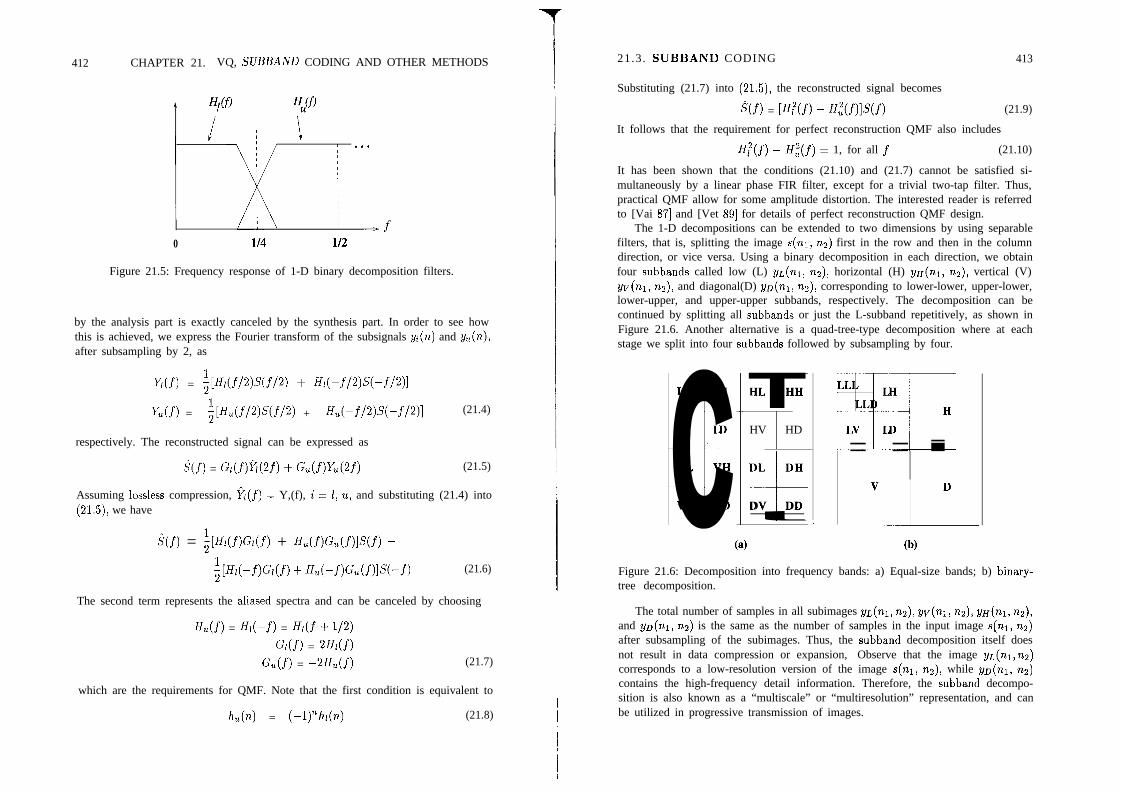
412 CHAPTER 21. VQ, SUBBAND CODING AND OTHER METHODS
0 l/4 l/2
Figure 21.5: Frequency response of 1-D binary decomposition filters.
by the analysis part is exactly canceled by the synthesis part. In order to see howthis is achieved, we express the Fourier transform of the subsignals yi(n) and yu(n),after subsampling by 2, as
Y(f) = ;Pwa)s(f/2) + ~f(-fl~)s(-fl~)l
K(f) = gw)w’L) + fL-flw-fl4l (21.4)
respectively. The reconstructed signal can be expressed as
s(f) = G(f)fi;(Xf) + G(f)@f) (21.5)
Assuming lossless compression, 3(f) = Y,(f), i = 1, u, and substituting (21.4) into(21.5), we have
g(f) = $WWf) + K(f)GCf’)lS(f) +
+Wf)Wf) + fL(-.f)G(f)lS(-f) (21.6)
The second term represents the aliased spectra and can be canceled by choosing
H,(f) = Hbf) = Hdf + l/2)GO) = 2&(f)
G,(f) = -2&(f) (21.7)
which are the requirements for QMF. Note that the first condition is equivalent to
h(n) = (-lyh(n) (21.8)
21.3. SUBBAND CODING 413
Substituting (21.7) into (21.5), the reconstructed signal becomes
s(f) = [@(f) - Ht%f)lS(f) (21.9)
It follows that the requirement for perfect reconstruction QMF also includes
H;(f) - Hz(f) = 1, for all f (21.10)
It has been shown that the conditions (21.10) and (21.7) cannot be satisfied si-multaneously by a linear phase FIR filter, except for a trivial two-tap filter. Thus,practical QMF allow for some amplitude distortion. The interested reader is referredto [Vai 871 and [Vet 891 for details of perfect reconstruction QMF design.
The 1-D decompositions can be extended to two dimensions by using separablefilters, that is, splitting the image s(ni, ns) first in the row and then in the columndirection, or vice versa. Using a binary decomposition in each direction, we obtainfour subbands called low (L) yr,(ni, ns), horizontal (H) y~(ni, 12s)) vertical (V)yv(nr, nz), and diagonal(D) y~(nr, nz), corresponding to lower-lower, upper-lower,lower-upper, and upper-upper subbands, respectively. The decomposition can becontinued by splitting all subbands or just the L-subband repetitively, as shown inFigure 21.6. Another alternative is a quad-tree-type decomposition where at eachstage we split into four subbands followed by subsampling by four.
LL LH
LV LD
VL VH
vv VD
(4
HL HH
HV HD
DL DH
DV DD
L LHL H
LV ID
(b)
Figure 21.6: Decomposition into frequency bands: a) Equal-size bands; b) binary-tree decomposition.
The total number of samples in all subimages y~(nr, nz), yv(nr, ns), y~(n1, ns),and yD(ni, ns) is the same as the number of samples in the input image s(ni, ns)after subsampling of the subimages. Thus, the subband decomposition itself doesnot result in data compression or expansion, Observe that the image y~(ni,ns)corresponds to a low-resolution version of the image s(nr, nz), while yD(nr, n2)contains the high-frequency detail information. Therefore, the subband decompo-sition is also known as a “multiscale” or “multiresolution” representation, and canbe utilized in progressive transmission of images.

414 CHAPTER 21. VQ, SUBBAND CODING AND OTHER METHODS
21.3.2 Coding of the SubbandsIn subband coding, each subimage can be encoded using a method and bitrate mostsuitable to the statistics and the visual significance of that subimage. Experimentsindicate that for typical images, more than 95% of the image energy resides inthe (L) frequency band. The other bands contain high-frequency detail (residual)information which may be more coarsely represented. There are many approachesreported in the literature for the encoding of subimages. In most subband codingschemes, the (L) subimage is encoded by transform coding, DPCM or VQ. All otherbands are either encoded by PCM or run-length coded after coarse thresholding.Some schemes apply VQ to high-frequency subimages using a separate codebook.
For quantization purposes, the statistics of the high-frequency subimages can bemodeled by a generalized Gaussian distribution of the form
p(s) = Keep{-q(a)lsle}, for Q > 0 (21.11)
where
r(3/a) It2da) = Iyl/a)[ 1
and for most images, o = 0.7. The same pdf can also be used to model the statisticsof the prediction error in DPCM or the DCT coefficients in the (L) subimage with
a = 0.6 for the prediction residual, andcy = 0.6 - 1.0 for the DCT coefficients.
For heavy-tailed distributions, entropy coding results in significant reduction inbitrate over fixed-length coding.
21.3.3 Relationship to Transform CodingOne can easily establish a connection between subband coding and transform cod-ing. In transform coding, recall that we compute the DCT of N x N image blocks.For example, if we order the DC coefficients of each block in an array, the result-ing image corresponds to a realization of the lowest-resolution subband image withsome choice of the filter parameters. Likewise, grouping intermediate frequencycoefficients together would result in intermediate subband images (see Exercise 7).In the case of using a subband decomposition filter whose number of taps is largerthan the decimation factor, the transform used in transform coding correspondsto the lapped orthogonal transform (LOT), where the transformation is applied tooverlapping blocks of pixels. Since the LOT is primarily used to avoid blockingartifacts in transform coding, it should be of no surprise that blocking artifacts arenot common in subband coding even at very low bitrates.
21.4. SECOND-GENERATION CODING METHODS 415
21.3.4 Relationship to Wavelet Transform CodingWavelet transform coding is closely related to subband coding in that it provides analternative method for filter design. In subband coding, the decomposition of theimage into subimages is usually accomplished by using perfect reconstruction QMFfilters. The wavelet transform describes this multiresolution decomposition processin terms of expansion of an image onto a set of wavelet basis functions. The waveletbasis functions, unlike the basis function for DFT and DCT, are well localized inboth space and frequency.
In 1-D wavelet analysis, there are two functions of interest: the motherwavelet 4, and the scaling function (p. The dilated and translated versions of thescaling function, dmn(z) = 2-“/2$(2-mz-n)) are associated with the design of thelow-pass filter Hi(f), and those of the mother wavelet are associated with the designof the high-pass filter H,(f). In 2-D wavelet analysis, we can define a separablescaling function,
4(x11 x2) = 4(a)4(4
and three directional wavelets,
(21.12)
Y%l, x2) = $(34$(22)
4”(Q, x2) = $(X1)4(Q)
IclD(%O) = $(Qb(Q) (21.13)
where GH(a,z2), $J”(Q,Q), and $D(21, ~2) denote horizontal, vertical, anddiagonal wavelets. These functions are then associated with a separable four-banddecomposition of the image. The wavelet transform coefficients, then, correspondto pixels of the respective subimages. In most cases, the decomposition is carriedout in multiple stages yielding a multiscale pyramidal decomposition. In this sense,the wavelet transform is also related to the well-known pyramid coding methods[Bur 831.
The wavelet-transform-based filters possess some regularity properties that notall QMF filters have, which give them improved coding performance over QMFfilters with the same number of taps. For example, Antonini e2 al. [Ant 921 reportthat they can achieve a performance close to that Woods and O’Neil [Woo 861by using only 7- and g-tap filters, whereas the latter uses 32-tap Johnston filters.However, some more recent QMF designs may yield performance similar to that ofthe wavelet filters with the same number of taps [Ade 901.
21.4 Second-Generation Coding Methods
The compression methods described so far are generally known as waveform cod-ing techniques because they operate on individual pixels or blocks of pixels basedon some statistical image models. Efforts to utilize more complicated structural

416 CHAPTER 21. VQ, SUBBAND CODING AND OTHER METHODS
image models and/or models of the human visual system in an attempt to achievehigher compression ratios lead to a new class of coding methods which are referredto as “second generation coding techniques” [Kun 851. Second-generation codingtechniques can be grouped into two classes: local-operator-based techniques, andcontour/texture-oriented techniques.
Local-operator-based techniques include pyramidal coding and anisotropic non-stationary predictive coding, which are discussed in [Kun 851, Pyramid and subbandcoding have also been classified as “second-generation,” because they are based onmodels that resemble the operation of the human visual system. For example, insubband coding, we use parallel bandpass filters, which can be chosen to resemblethe direction-sensitive cells in the human visual system.
Contour/texture-oriented techniques attempt to describe an image in termsof structural primitives such as contours and textures. They segment the imageinto textured regions surrounded by contours such that the contours correspond,as much as possible, to those of the objects in the image. Two commonly em-ployed methods are the region-growing method and the directional decompositionmethod. In these methods, the contour and texture information are encoded sep-arately [Kun 85, Kun 871. Contour/texture-based methods are capable of achiev-ing very high compression ratios in comparison to classical waveform-based meth-ods. Indeed, they form the basis of object-based very-low-bitrate video compressionschemes, which are described in Chapter 24.
21.5 Exercises
1. Suppose we employ a mean-removed VQ, with 4 x 4 blocks, where we use8 bits to encode the mean of each block, and the residual codebook size isL = 512. Calculate the compression ratio, assuming that we have encodedthe indices le using fixed-length coding.
2. Show that D(j-i) is always greater than or equal to D(j) in the LBG algorithm.
3. Suppose that, in Figure 21.3, you are allowed to first transform the vectors bya linear transformation and then use scalar quantizers. (This is the principleof transform coding.)
a) Describe a transformation that can match the performance of the VQ byusing a single scalar quantizer. Explain clearly.
b) Do you think that the difference in performance between scalar versus vec-tor quantization would be more pronounced in waveform coding or transformcoding? Explain why.
4. Elaborate on the similarities between VQ and fractal coding.
5. Verify that the requirements for perfect reconstruction are given by (21.7)and (21.10).
BIBLIOGRAPHY 417
6. Show that a perfect reconstruction filter cannot satisfy all of the followingrequirements simultaneously:i) it is symmetric,ii) it is FIR, andiii) analysis and synthesis filters are equal-length.
7. Elaborate on the relationship between the subband coding and the DCT cod-ing. In particular, consider a 64 x 64 image. Suppose we partition the imageinto 8 x 8 blocks, and compute their DCT.
a) Show that we can construct 64 subband images, each of which is 8 x 8, byan ordering of the DCT coefficients.
b) Discuss the relationship between DPCM encoding of the DC coefficients inJPEG, and DPCM encoding of the lowest subband in this case.
Bibliography
[Ade 901 E. H. Adelson and E. Simoncelli, “Non-separable extensions of quadraturemirror filters to multiple dimensions,” Proc. IEEE, vol. 78, Apr. 1990.
[Ant 921 M. Antonini, M. Barlaud, P. Mathieu, and I. Daubechies, “Image codingusing wavelet transform,” IEEE Trans. Image Proc., vol. 1, pp. 2055220,Apr. 1992.
[Bar 881 M. F. Barnsley, Fractals Everywhere, New York, NY: Academic Press,1988.
[Bur 831 P. Burt and E. Adelson, “The Laplacian pyramid as a compact imagecode,” IEEE Trans. Comm., vol. 31, pp. 482-540, 1983.
[Ger 821 A. Gersho, “On the structure of vector quantizer,” IEEE Trans. Info. The.,vol. IT-28, pp. 157-166, Mar. 1982.
[Ger 921 A. Gersho and R. Gray, Vector Quantization and Signal Compression,Norwell, MA: Kluwer, 1992.
[Gha 881 H. Gharavi and A. Tabatabai, “Subband coding of monochrome and colorimages,” IEEE Trans. Circ. and Syst., vol. 35, pp. 207-214, Feb. 1988.
[Gra 841 R. M. Gray, “Vector quantization,” IEEE ASSP Magazine, vol. 1,pp. 4429, April 1984.
[Jac 921 A. E. Jacquin, “Image coding based on a fractal theory of iterated contrac-tive image transformations,” IEEE Trans. Image Proc., vol. 1, pp. 18830,Jan. 1992.

418 BIBLIOGRAPHY
[Jay 841 N. S. Jayant and P. Noll, Digital Coding of Waveforms - Principles andApplications to Speech and Video, Englewood Cliffs, NJ: Prentice Hall,1984.
[Kun 851 M. Kunt, A. Ikonomopoulos and M. Kocher, “Second-generation imagecoding techniques,” Proc. IEEE, vol. 73, 549-574, 1985.
[Kun 871 M. Kunt, M. Benard, R. Leonardi, “Recent results in high-compressionimage coding,” IEEE Trans. Circ. Syslems, Vol. 34, pp. 1306-1336, 1987.
[Lim 901 J. S. Lim, Two-Dimensional Signal and Image Processing, EnglewoodCliffs, NJ: Prentice Hall, 1990.
[Lin 801 Y. Linde, A. Buzo, and R. M. Gray, “An algorithm for vector quantizerdesign,” IEEE Trans. Comm., vol. 28, pp. 84-89, Jan. 1980.
[Lu 931 G. Lu, “Fractal image compression,” Signal Processrng: Image Comm.,
vol. 5, pp. 327-343, 1993.
[Mak 851 J. Makhoul, S. Roucos, and H. Gish, “Vector quantization in speechcoding,” Proc. IEEE, vol. 73, pp. 1551-1588, Nov. 1985.
[Man 821 B. Mandelbrot, The Fraclal Geometry of Nature, Freeman, 1982.
[Nas 881 N. M. Nasrabadi and R. A. King, “Image coding using vector quantization:A review,” IEEE Trans. Comm, vol. 36, pp. 957-971, Aug. 1988.
[Rab 911 M. Rabbani and P. W. Jones, Digital Image Compression Techniques,Bellingham, WA: SPIE Press, 1991.
[Vai 871 P. P. Vaidyanathan, “Quadrature mirror filter banks, M-band extensions,and perfect reconstruction technique,” IEEE Acoust. Speech Sign. Proc.Magazine, vol. 4, pp. 4-20, 1987.
[Vet 841 M. Vetterli, “Multidimensional sub-band coding: Some theory and algo-rithms, Signal Processing, vol. 6, pp. 97-112, 1984.
[Vet 891 M. Vetterli and D. LeGall, “Perfect reconstruction FIR filter banks: Someproperties and factorizations,” IEEE Trans. Acoust. Speech Sign. Proc,,vol. 37, pp. 1057-1071, 1989.
[Wes 881 P. Westerink and J. W. Woods, “Subband coding of images using vectorquantization,” IEEE Trans. Comm., vol. 36, pp. 713-719, June 1988.
[Woo 861 J. W. Woods and S. D. O’Neil, “Subband coding of images,” IEEE Trans.Acoust. Speech and Sign. Proc., vol. 34, pp. 1278-1288, Oct. 1986.
Chapter 22
INTERFRAMECOMPRESSIONMETHODS
Video compression is a key enabling technology for desktop digital video. With-out compression, digital transmission of an NTSC color video, with 720 pixels x480 lines, 8 bits/pixel per color, and 30 frames/set, requires a transmission capac-ity of 248 Mbps. Likewise, an HDTV color video, with 1920 pixels x 1080 lines,8 bits/pixel per color, and 30 frames/set, needs a channel capacity of 1.5 Gbps.A super-35 format motion picture is usually digitized with 4096 pixels x 3112 linesand 10 bits/pixel per color. At a rate of 24 frames/set, one second of a colormovie requires approximately 9 Gbits (1.15 Gbytes) storage space. These datarates suggest that a CD with a storage capacity of about 5 Gbits can hold, withoutcompression, approximately 20 set of NTSC video, 3 set of HDTV video, and one-half second of a movie. A typical data transfer rate for a CD-ROM device is about1.5 Mbps (although faster devices that can transfer up to 4 Mbps are appearing inthe market). Then full-motion NTSC quality video can be played back from a CD(1.2 Mbps for video and 0.3 Mbps for stereo audio) with 2OO:l compression of thevideo signal. At 2OO:l compression, a single CD can hold 3400 set or about onehour of video. The HDTV signal needs be broadcast over a 6 MHz channel whichcan support about 20 Mbps. As a result, a compression ratio of 75:l is required forbroadcasting HDTV signals. For transmission using fiber optic networks or satellitelinks, similar compression is needed to transmit multiple channels.
An elementary approach to video compression would be to employ any of thestill-frame compression techniques discussed in Chapters 18-21 on a frame by framebasis. However, the compression that can be achieved by such an approach will belimited because each frame is treated as an independent image. Interframe compres-sion methods exploit the temporal redundancies due to similarity between neigh-
419

420 CHAPTER 22. INTERFRAME COMPRESSION METHODS
boring frames, in addition to the spatial, spectral, and pyschovisual redundanciesto provide superior compression efficiency. Note, however, that some applicationspecific requirements, such as random access capability at all frames, may dictatethe use of intraframe compression rather than interframe methods in some cases. Ingeneral, interframe compression methods take advantage of temporal redundanciesthrough i) 3-D waveform coding strategies, which are based on statistical signalmodels, ii) motion-compensated (MC) coding strategies, which use elementary mo-tion models, or iii) object/knowledge based coding strategies, which utilize more so-phisticated scene models. Three-dimensional waveform coding strategy is discussedin Section 22.1. Various motion-compensated compression schemes are presentedin Section 22.2. Note that all international video compression standards, coveredin Chapter 23, utilize the MC, transform coding strategy. Section 22.3 provides anoverview of model-based coding methods, which are studied in detail in Chapter 24.
22.1 Three-Dimensional Waveform Coding
The simplest way to extend still-frame image compression methods to interframevideo compression is to consider 3-D waveform coding schemes, which include 3-Dtransform and 3-D subband coding. These methods exploit spatio-temporal redun-dancies in a video source through statistical signal models.
22.1.1 3-D Transform Coding
Three-dimensional DCT coding is a straightforward extension of the 2-D DCT cod-ing method, where the video is divided into M x N x J blocks (M, N, and Jdenote the horizontal, vertical, and temporal dimensions of the block, respectively).The transform coefficients are then quantized subject to zonal coding or thresholdcoding, and encoded similar to 2-D transform coding of still-frame images. Sincethe DCT coefficients are closely related to the frequency content of the blocks, fortemporally stationary blocks the DCT coefficients in the temporal direction willbe close to zero, and will be truncated in a threshold coding scheme. For mostblocks, the DCT coefficients will be packed towards the low spatial and temporalfrequency zone. The 3-D DCT coding scheme has the advantage that it does notrequire a separate motion estimation step. However, it requires J frame stores bothin the transmitter and receiver. Therefore, J is typically chosen as 2 or 4, to allowfor practical hardware implementations. Observe that random access to video ispossible once for every J frames, as shown in Figure 22.1.
A related 3-D waveform coding approach is the hybrid transform/DPCM codingmethod, which has been proposed to overcome the multiple frame-store requirement[Roe 77, Nat 771. This is an extension of the 2-D hybrid DCT/DPCM coding con-cept proposed by Habibi [Hab 741 to 3-D, where a 2-D orthogonal transform isperformed on each spatial block within a given frame. A bank of parallel DPCMcoders, each tuned to the statistics of a specific DCT coefficient, is then applied to
22.1. THREE-DIMENSIONAL WAVEFORM CODING 421
Figure 22.1: Three-dimensional transform coding
the transform coefficients in the temporal direction. Thus, the differences in therespective DCT coefficients in the temporal direction are quantized and encoded,which eliminates the need for multiple frame-stores. This scheme generally requiresadaptation of the DPCM quantizers to the temporal statistics of the 2-D DCT co-efficients for results comparable to that of the 3-D DCT coding [Roe 771. Note thatneither 3-D DCT coding nor hybrid DCT/DPCM coding has been widely used inpractical applications.
22.1.2 3-D Subband Coding
3-D subband coding, an extension of 2-D subband coding, has recently receivedincreased attention [Vet 92, Bos 92, Luo 941 motivated by the following considera-tions: i) it is almost always free from blocking artifacts, which is a common problemwith 3-D DCT and MC/DCT coding methods, especially at low bitrates, ii) unlikeMC compression methods, it does not require a separate motion estimation stage,and iii) it is inherently scalable, both spatially and temporally. Scalability, whichrefers to availability of digital video at various spatial and temporal resolutionswithout having to decompress the entire bitstream, has become an important fac-tor in recent years due to the growing need for storage and transmission of digitalvideo that is cornformable with various format standards. For example, standardTV and high-definition TV differ only in spatial resolution, whereas videophonesystems offer lower spatial and temporal resolution.
In 3-D subband coding, the video is decomposed into various properly subsam-pled component video signals, ranging from a low spatial and temporal resolutioncomponent to various higher-frequency detail signal components. These variouscomponent video signals are encoded independently using algorithms adapted to

422 CHAPTER 22. INTERFRAME COMPRESSION METHODS
the statistical and pyschovisual properties of the respective spatio-temporal fre-quency bands. Compression is achieved by appropriate quantization of the variouscomponents and entropy coding of the quantized values. Higher-resolution video,in both spatial and temporal coordinates, can be recovered by combining the de-compressed low-resolution version with the decompressed detail components. Most3-D subband decomposition schemes utilize 2- or 4-frame temporal blocks at a timedue to practical implementation considerations.
r
WV > 11
LPV - 10
Lph
LPV z- 8
Figure 22.2: A typical 3-D subband decomposition.
An ll-band 3-D subband decomposition is illustrated in Figure 22.2. Typically,the temporal decomposition is based on a simple 2-tap Haar filterbank [Luo 941,which in the case of two frame blocks gives the average and the difference of thetwo frames for the low-pass (LP) and high-pass (HP) temporal components, re-spectively. This choice minimizes the number of frame-stores needed as well as thecomputational burden for the temporal decomposition. In the second stage, boththe low and high temporal subbands are decomposed into low and high horizontal
7 22.1. THREE-DIMENSIONAL WAVEFORM CODING 423
subbands, respectively. In the next stage, each of these bands are decomposed intolow and high vertical subbands, as depicted in Figure 22.2. Subsequently, the low(temporal)-low (horizontal)-low (vertical) band is further decomposed into four spa-tial subbands to yield the 11-band decomposition. Note that longer filters can beapplied for the spatial (horizontal and vertical) decompositions, since these filterscan be operated in parallel and do not affect the frame-store requirements. To thiseffect, Luo e2 al. report using wavelet filterbanks for the spatial decompositions.
The resulting component video signals can be subsampled consistent with thespatio-temporal frequency characteristics of each band, which is illustrated in Fig-ure 22.3. In this figure, the left- and right-hand side templates correspond to thelow- and high-temporal-frequency components, respectively. For example, the com-ponent 1, which is subsampled by a factor of 2 in time and by a factor of 4 ineach spatial direction, represents a spatio-temporally blurred version of a 2-frameblock. As a result, a time-sequence composed of the component 1 for all 2 frameblocks constitutes a low-resolution (both spatially and temporally) version of theoriginal video. Likewise, time sequences composed of the other components (e.g.,2-11) constitute auxilary video signals containing high-frequency detail informationneeded to reconstruct the original video from the low-resolution video. The readeris referred to [Vet 92, Bos 92, Luo 941 for various approaches offered to compressthe individual component signals.
LPt
8 10
9 11
HPt
Figure 22.3: Representation of 3-D subband video.
The basic approach of 3-D DCT and subband coding is quite different fromthat of motion-compensated (MC) coding, which is presented next. MC techniquescharacterize the temporal correlation in a video by means of motion vectors ratherthan through the respective transform coefficients.
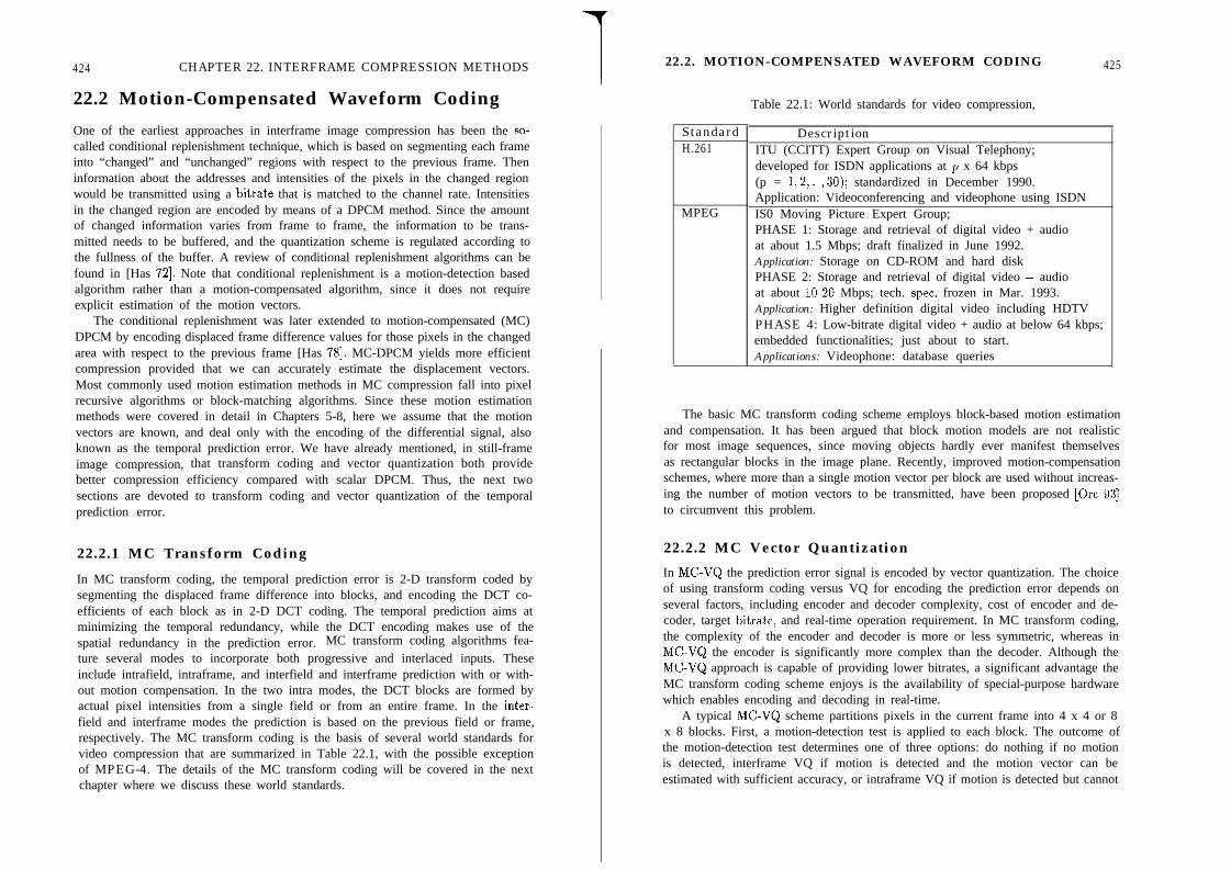
424 CHAPTER 22. INTERFRAME COMPRESSION METHODS
22.2 Motion-Compensated Waveform Coding
One of the earliest approaches in interframe image compression has been the so-called conditional replenishment technique, which is based on segmenting each frameinto “changed” and “unchanged” regions with respect to the previous frame. Theninformation about the addresses and intensities of the pixels in the changed regionwould be transmitted using a bitrate that is matched to the channel rate. Intensitiesin the changed region are encoded by means of a DPCM method. Since the amountof changed information varies from frame to frame, the information to be trans-mitted needs to be buffered, and the quantization scheme is regulated according tothe fullness of the buffer. A review of conditional replenishment algorithms can befound in [Has 721. Note that conditional replenishment is a motion-detection basedalgorithm rather than a motion-compensated algorithm, since it does not requireexplicit estimation of the motion vectors.
The conditional replenishment was later extended to motion-compensated (MC)DPCM by encoding displaced frame difference values for those pixels in the changedarea with respect to the previous frame [Has 781. MC-DPCM yields more efficientcompression provided that we can accurately estimate the displacement vectors.Most commonly used motion estimation methods in MC compression fall into pixelrecursive algorithms or block-matching algorithms. Since these motion estimationmethods were covered in detail in Chapters 5-8, here we assume that the motionvectors are known, and deal only with the encoding of the differential signal, alsoknown as the temporal prediction error. We have already mentioned, in still-frameimage compression, that transform coding and vector quantization both providebetter compression efficiency compared with scalar DPCM. Thus, the next twosections are devoted to transform coding and vector quantization of the temporalprediction error.
22.2.1 MC Transform Coding
In MC transform coding, the temporal prediction error is 2-D transform coded bysegmenting the displaced frame difference into blocks, and encoding the DCT co-efficients of each block as in 2-D DCT coding. The temporal prediction aims atminimizing the temporal redundancy, while the DCT encoding makes use of thespatial redundancy in the prediction error. MC transform coding algorithms fea-ture several modes to incorporate both progressive and interlaced inputs. Theseinclude intrafield, intraframe, and interfield and interframe prediction with or with-out motion compensation. In the two intra modes, the DCT blocks are formed byactual pixel intensities from a single field or from an entire frame. In the inter-field and interframe modes the prediction is based on the previous field or frame,respectively. The MC transform coding is the basis of several world standards forvideo compression that are summarized in Table 22.1, with the possible exceptionof MPEG-4. The details of the MC transform coding will be covered in the nextchapter where we discuss these world standards.
7 22.2. MOTION-COMPENSATED WAVEFORM CODING 425
StandardH.261
MPEG
Table 22.1: World standards for video compression,
DescriptionITU (CCITT) Expert Group on Visual Telephony;developed for ISDN applications at p x 64 kbps(p = 1,2,. ,30); standardized in December 1990.Application: Videoconferencing and videophone using ISDNIS0 Moving Picture Expert Group;PHASE 1: Storage and retrieval of digital video + audioat about 1.5 Mbps; draft finalized in June 1992.Application: Storage on CD-ROM and hard diskPHASE 2: Storage and retrieval of digital video + audioat about lo-20 Mbps; tech. spec. frozen in Mar. 1993.Application: Higher definition digital video including HDTVPHASE 4: Low-bitrate digital video + audio at below 64 kbps;embedded functionalities; just about to start.Applications: Videophone: database queries
The basic MC transform coding scheme employs block-based motion estimationand compensation. It has been argued that block motion models are not realisticfor most image sequences, since moving objects hardly ever manifest themselvesas rectangular blocks in the image plane. Recently, improved motion-compensationschemes, where more than a single motion vector per block are used without increas-ing the number of motion vectors to be transmitted, have been proposed [Ore 931to circumvent this problem.
22.2.2 MC Vector Quantization
In MC-V& the prediction error signal is encoded by vector quantization. The choiceof using transform coding versus VQ for encoding the prediction error depends onseveral factors, including encoder and decoder complexity, cost of encoder and de-coder, target bitrate, and real-time operation requirement. In MC transform coding,the complexity of the encoder and decoder is more or less symmetric, whereas inMC-V& the encoder is significantly more complex than the decoder. Although theMC-V& approach is capable of providing lower bitrates, a significant advantage theMC transform coding scheme enjoys is the availability of special-purpose hardwarewhich enables encoding and decoding in real-time.
A typical MC-V& scheme partitions pixels in the current frame into 4 x 4 or 8x 8 blocks. First, a motion-detection test is applied to each block. The outcome ofthe motion-detection test determines one of three options: do nothing if no motionis detected, interframe VQ if motion is detected and the motion vector can beestimated with sufficient accuracy, or intraframe VQ if motion is detected but cannot
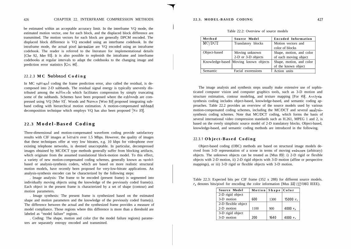
426 CHAPTER 22. INTERFRAME COMPRESSION METHODS
be estimated within an acceptable accuracy limit. In the interframe VQ mode, theestimated motion vector, one for each block, and the displaced block difference aretransmitted. The motion vectors for each block are generally DPCM encoded. Thedisplaced block difference is VQ encoded using an interframe codebook. In theintraframe mode, the actual pixel imensities are VQ encoded using an intraframecodebook. The reader is referred to the literature for implementational details[Che 92, Mer 931. It is also possible to replenish the intraframe and interframecodebooks at regular intervals to adapt the codebooks to the changing image andprediction error statistics [Go1 861.
2 2 . 2 . 3 M C Subband C o d i n g
In MC subband coding the frame prediction error, also called the residual, is de-composed into 2-D subbands. The residual signal energy is typically unevenly dis-tributed among the subbands which facilitates compression by simply truncatingsome of the subbands. Schemes have been proposed where the subbands are com-pressed using VQ [Mer 931. Woods and Naveen [Woo 891 proposed integrating sub-band coding with hierarchical motion estimation. A motion-compensated subbanddecomposition technique which employs VQ has also been proposed [Nit 931.
2 2 . 3 Model -Based Coding
Three-dimensional and motion-compensated waveform coding provide satisfactoryresults with CIF images at bitrates over 1.5 Mbps. However, the quality of imagesthat these techniques offer at very low bitrates, e.g. 10 kbps for videophone overexisting telephone networks, is deemed unacceptable. In particular, decompressedimages obtained by MC/DCT type methods generally suffer from blocking artifacts,which originate from the assumed translational block-motion model. To this effect,a variety of new motion-compensated coding schemes, generally known as model-based or analysis-synthesis coders, which are based on more realistic structuralmotion models, have recently been proposed for very-low-bitrate applications. Ananalysis-synthesis encoder can be characterized by the following steps:
. Image analysis: The frame to be encoded (present frame) is segmented intoindividually moving objects using the knowledge of the previously coded frame(s).Each object in the present frame is characterized by a set of shape (contour) andmotion parameters.
. Image synthesis: The present frame is synthesized based on the estimatedshape and motion parameters and the knowledge of the previously coded frame(s).The difference between the actual and the synthesized frame provides a measure ofmodel compliance. Those regions where this difference is more than a threshold arelabeled as “model failure” regions.
. Coding: The shape, motion and color (for the model failure regions) parame-ters are separately entropy encoded and transmitted.
22.3. MODEL-BASED CODING 4 2 7
Table 22.2: Overview of source models
Method Source Model Encoded InformationMC/DCT Translatory blocks Motion vectors and
color of blocksObject-based Moving unknown Shape, motion, and color
2-D or 3-D objects of each moving objectKnowledge-based Moving known objects Shape, motion, and color
of the known objectSemantic 1 Facial exoressions 1 Action units
The image analysis and synthesis steps usually make extensive use of sophis-ticated computer vision and computer graphics tools, such as 3-D motion andstructure estimation, contour modeling, and texture mapping [For 891. Analysis-synthesis coding includes object-based, knowledge-based, and semantic coding ap-proaches. Table 22.2 provides an overview of the source models used by variousmotion-compensated coding schemes, including the MC/DCT and several analysis-synthesis coding schemes. Note that MC/DCT coding, which forms the basis ofseveral international video compression standards such as H.261, MPEG 1 and 2, isbased on the overly simplistic source model of 2-D translatory blocks. Object-based,knowledge-based, and semantic coding methods are introduced in the following.
2 2 . 3 . 1 O b j e c t - B a s e d C o d i n g
Object-based coding (OBC) methods are based on structural image models de-rived from 3-D representation of a scene in terms of moving unknown (arbitrary)objects. The unknown objects can be treated as [Mus 891: i) 2-D rigid or flexibleobjects with 2-D motion, ii) 2-D rigid objects with 3-D motion (affine or perspectivemappings), or iii) 3-D rigid or flexible objects with 3-D motion.
Table 22.3: Expected bits per CIF frame (352 x 288) for different source models.r, denotes bits/pixel for encoding the color information [Mus 931 (01993 IEEE).
Source Model Motion Shape Color2-D rigid object3-D motion 6 0 0 1300 1 5 0 0 0 r,2-D flexible object2-D motion 1100 900 4 0 0 0 P,3-D rigid object3-D motion 2 0 0 1 6 4 0 4 0 0 0 r,
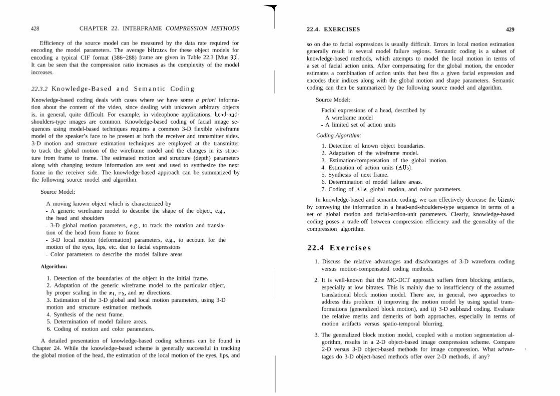
428 CHAPTER 22. INTERFRAME COMPRESSION METHODS
Efficiency of the source model can be measured by the data rate required forencoding the model parameters. The average bitrates for these object models forencoding a typical CIF format (386~288) frame are given in Table 22.3 [Mus 931.It can be seen that the compression ratio increases as the complexity of the modelincreases.
22.3.2 Knowledge-Based and Semantic Coding
Knowledge-based coding deals with cases where we have some a priori informa-tion about the content of the video, since dealing with unknown arbitrary objectsis, in general, quite difficult. For example, in videophone applications, head-and-shoulders-type images are common. Knowledge-based coding of facial image se-quences using model-based techniques requires a common 3-D flexible wireframemodel of the speaker’s face to be present at both the receiver and transmitter sides.3-D motion and structure estimation techniques are employed at the transmitterto track the global motion of the wireframe model and the changes in its struc-ture from frame to frame. The estimated motion and structure (depth) parametersalong with changing texture information are sent and used to synthesize the nextframe in the receiver side. The knowledge-based approach can be summarized bythe following source model and algorithm.
Source Model:
A moving known object which is characterized by- A generic wireframe model to describe the shape of the object, e.g.,the head and shoulders- 3-D global motion parameters, e.g., to track the rotation and transla-tion of the head from frame to frame- 3-D local motion (deformation) parameters, e.g., to account for themotion of the eyes, lips, etc. due to facial expressions- Color parameters to describe the model failure areas
Algorithm:
1. Detection of the boundaries of the object in the initial frame.2. Adaptation of the generic wireframe model to the particular object,by proper scaling in the ~1, ~2, and zs directions.3. Estimation of the 3-D global and local motion parameters, using 3-Dmotion and structure estimation methods.4. Synthesis of the next frame.5. Determination of model failure areas.6. Coding of motion and color parameters.
A detailed presentation of knowledge-based coding schemes can be found inChapter 24. While the knowledge-based scheme is generally successful in trackingthe global motion of the head, the estimation of the local motion of the eyes, lips, and
22.4. EXERCISES 429
so on due to facial expressions is usually difficult. Errors in local motion estimationgenerally result in several model failure regions. Semantic coding is a subset ofknowledge-based methods, which attempts to model the local motion in terms ofa set of facial action units. After compensating for the global motion, the encoderestimates a combination of action units that best fits a given facial expression andencodes their indices along with the global motion and shape parameters. Semanticcoding can then be summarized by the following source model and algorithm.
Source Model:
Facial expressions of a head, described by- A wireframe model- A limited set of action units
Coding Algorithm:
1. Detection of known object boundaries.2. Adaptation of the wireframe model.3. Estimation/compensation of the global motion.4. Estimation of action units (AUs).5. Synthesis of next frame.6. Determination of model failure areas.7. Coding of AUs, global motion, and color parameters.
In knowledge-based and semantic coding, we can effectively decrease the bitrateby conveying the information in a head-and-shoulders-type sequence in terms of aset of global motion and facial-action-unit parameters. Clearly, knowledge-basedcoding poses a trade-off between compression efficiency and the generality of thecompression algorithm.
22.4 Exercises
1. Discuss the relative advantages and disadvantages of 3-D waveform codingversus motion-compensated coding methods.
2. It is well-known that the MC-DCT approach suffers from blocking artifacts,especially at low bitrates. This is mainly due to insufficiency of the assumedtranslational block motion model. There are, in general, two approaches toaddress this problem: i) improving the motion model by using spatial trans-formations (generalized block motion), and ii) 3-D subband coding. Evaluatethe relative merits and demerits of both approaches, especially in terms ofmotion artifacts versus spatio-temporal blurring.
3. The generalized block motion model, coupled with a motion segmentation al-gorithm, results in a 2-D object-based image compression scheme. Compare2-D versus 3-D object-based methods for image compression. What advan- *tages do 3-D object-based methods offer over 2-D methods, if any?
430 BIBLIOGRAPHY
Bibliography[Bos 921 F. Bosveld, R. L. Lagendijk, and J. Biemond, “Compatible spatio-
temporal subband encoding of HDTV,” Signal Proc., vol. 28, pp. 271-290,Sep. 1992.
[Che 921 H.-H. Chen, Y.-S. Chen, and W.-H. Hsu, “Low-rate sequence image codingvia vector quantization,” Signal Proc., vol. 26, pp. 265-283, 1992.
[For 891 R. Forchheimer and T. Kronander, “Image coding-from waveforms toanimation,” IEEE Trans. Acoust. Speech Sign. Proc., vol. 37, no. 12,pp. 2008-2023, Dec. 1989.
[Gha 911 H. Gharavi, “Subband coding of video signals,” in Subband Image Coding,J. W. Woods, ed., Norwell, MA: Kluwer, 1991.
[Go1 861 M. Goldberg and H. Sun, “Image sequence coding using vector quantiza-tion,” IEEE Trans. Comm., vol. 34, pp. 703-710, July 1986.
[Hab 741 A. Habibi, “Hybrid coding of pictorial data,” IEEE Trans. Comm.,vol. 22, no. 5, pp. 614-624, May 1974.
[Hab 811 A. Habibi, “An adaptive strategy for hybrid image coding,” IEEE Trans.Comm., vol. 29, no. 12, pp. 1736-1740, Dec. 1981.
[Has 721 B. G. Haskell, F. W. Mounts, and J. C. Candy, “Interframe coding ofvideotelephone pictures,” Proc. IEEE, vol. 60, pp. 792-800, July 1972.
[Has 781 B. G. Haskell, “Frame replenishment coding of Television,” in ImageTransmission Techniques, W. K. Pratt, ed., Academic Press, 1978.
[Hot 901 M. Hotter, “Object oriented analysis-synthesis coding based on mov-ing two-dimensional objects,” Signal Proc: Image Comm., vol. 2, no. 4,pp. 409-428, Dee 1990.
[Luo 941 J. Luo, C. W. Chen, K. J. Parker, and T. S. Huang, “Three dimensionalsubband video analysis and synthesis with adaptive clustering in high-frequency subbands,” Proc. IEEE I&. Conf. Image Processing, Austin,TX, Nov. 1994.
[Mer 931 R. M. Mersereau, M. J. T. Smith, C. S. Kim, F. Kossentini, and K.K. Truong, “Vector quantization for video data compression,” in MotionAnalysis and Image Sequence Processing, M. I. Sezan and R. L. Lagendijk,eds., Norwell, MA: Kluwer, 1993.
[Mus 891 H. G. Musmann, M. Hotter, and J. Ostermann, “Object-oriented analysissynthesis coding of moving images,” Signal Proc: Image Comm., vol. 1,pp. 117-138, 1989.
BIBLIOGRAPHY 431
[Mus 931 H. G. Musmann, “Object-oriented analysis-synthesis coding based onsource models of moving 2D and 3D objects,” Proc. IEEE Int. Conf.Acoust. Speech and Sign. Proc., Minneapolis, MN, April 1993.
[Nat 771 T. R. Natarajan and N. Ahmed, “On interframe transform coding,” IEEETrans. Comm., vol. 25, no. 11, pp. 1323-1329, Nov. 1977.
[Nit 931 A. Nicoulin, M. Mattavelli, W. Li, A. Basso, A. C. Popat, and M. Kunt,“Image sequence coding using motion compensated subband decomposi-tion,” in Motion Analysis and Image Sequence Processing, M. I. Sezan andR. L. Lagendijk, eds., Norwell, MA: Kluwer, 1993.
[Ore 931 M. Orchard, “Predictive motion-field segmentation for image sequencecoding,” IEEE Trans. Circ. and Syst: Video Tech., vol. 3, pp. 54-70,Feb. 1993.
[Plo 821 A. Ploysongsang and K. R. Rao, “DCT/DPCM processing of NTSC com-posite video signal,” IEEE Trans. Comm., vol. 30, no. 3, pp. 541-549,Mar. 1982.
[Pur 911 A. Puri and R. Aravind, “Motion-compensated video coding with adaptiveperceptual quantization,” IEEE Trans. Circ. Sysz!. Video Tech., vol. 1,pp. 351-361, 1991.
[Roe 771 J. A. Roese, W. K. Pratt, and G. S. Robinson, “Interframe cosine trans-form image coding,” IEEE Trans. Comm., vol. 25, no. 11, pp. 1329-1339,Nov. 1977.
[Sab 841 S. Sabri and B. Prasada, “Coding of broadcast TV signals for trans-mission over satellite channels,” IEEE Trans. Comm., vol. 32, no. 12,pp. 1323-1330, Dec. 1984.
[Saw 781 K. Sawada and H. Kotera, “32 Mbit/s transmission of NTSC colorTV signals by composite DPCM coding,” IEEE Trans. Comm., vol. 26,no. 10, pp. 1432-1439, Oct. 1978.
[Vet 921 M. Vetterli and K. M. Uz, “Multiresolution coding techniques fordigital television: A review,” Multidim. Syst. Signal Proc., vol. 3,pp. 161-187, 1992.
[Woo 891 J. W. Woods and T. Naveen, “Subband encoding of video sequences,”Proc. SPIE Visual Comm. Image Proc. IV, vol. 1199, pp. 724-732, 1989.

723.1. THE H.261 STANDARD 433
Chapter 23
VIDEO COMPRESSIONSTANDARDS
Standardization of compressed digital video formats facilitates manipulation andstorage of full-motion video as a form of computer data, and its transmission overexisting and future computer networks, or over terrestrial broadcast channels. Envi-sioned areas of application for digital video compression standards include all-digitalTV, videoconferencing, videophone, video mail, multimediastations, digital movies,video games, other forms of entertainment, and education. In this chapter, we dis-cuss the international video compression standards for videoconferencing (H.261),multimedia (MPEG-l), and all-digital TV (MPEG-2) applications.
23.1 The H.261 Standard
ITU (CCITT) Recommendation H.261 is a video compression standard developedto facilitate videoconferencing and videophone services over the integrated servicesdigital network (ISDN) at p x 64 kbps, p = 1, . ,30. For example, 64 kbps (p = 1)may be appropriate for a low quality videophone service, where the video signal canbe transmitted at a rate of 48 kbps, and the remaining 16 kbps is used for the audiosignal. Videoconferencing services generally require higher image quality, whichcan be achieved with p > 6, i.e., at 384 kbps or higher. Note that the maximumavailable bitrate over an ISDN channel is 1.92 Mbps (p = 30), which is sufficeint toobtain VHS-quality (or better) images.
ITU (CCITT) Recommendation H.261 has emerged as a result of studies per-formed within the European Project COST (Cooperation in the field of Scientificand Technical research) 2llbis during the period 1983-1990. In 1985, the COSTBllbis videoconference hardware subgroup developed an initial codec operating atbit rates of n x 384 kbps, n = 1,. . . ,5, which was adopted in 1987 as ITU (CCITT)Recommendation H.120. Later, it became clear that a single standard can cover
432
all ISDN rates, p x 64 kbps, p = 1, ) 30. The specifications of such a codec werecompleted in 1989, and the corresponding Recommendation H.261 was adopted byITU (CCITT) in 1990.
In addition to forming a basis for the later video compression standards suchas MPEG-1 and MPEG-2, the H.261 standard offers two important features: i)It specifies a maximum coding delay of 150 msec. because it is mainly intendedfor bidirectional video communication. It has been determined that delays exceed-ing 150 msec. do not give the viewer the impression of direct visual feedback.ii) It is amenable to low-cost VLSI implementation, which is rather important forwidespread commercialization of videophone and teleconferencing equipment. Theimportant aspects of the H.261 standard are summarized below. Further detailscan be found in [Lio 90, Lio 91, CC1 901.
23.1.1 Input Image Formats
To permit a single recommendation for use in and between regions using 625- and525-line TV standards, the H.261 input picture format is specified as the so-calledCommon Intermediate Format (CIF). For lower-bitrate applications, a smaller for-mat, QCIF, which is one-quarter of the CIF, has been adopted. The specificationsof the CIF and QCIF formats are listed in Table 23.1, where the numbers in theparenthesis denote the modified specifications so that all four numbers are integermultiples of 8. Note that, at 30 frames/s, the raw data rate for the CIF is 37.3Mbps, and for QCIF it is 9.35 Mbps. Even with QCIF images at 10 frames/s, 48:lcompression is required for videophone services over a 64 kbps channel. CIF imagesmay be used when p > 6, that is, for videoconferencing applications. Methods forconversion to and from CIF/QCIF are not subject to recommendation.
Table 23.1: H.261 input image formats.
Number of active pels/line )Lum (Y)Chroma (U,V)Number of active lines/pitLum (Y)
CIF QCIF
360 (352) 180 (176)180 (176) 90 (88)
288 144Chroma (U,V) 144 72Interlacing 1:l 1:lTemporal rate 30, 15, 10, or 7.5 30, 15, 10 or 7.5Aspect ratio 4:3 4:3

434 CHAPTER 23. VIDEO COMPRESSION STANDARDS
23.1.2 Video Multiplex
The video multiplex defines a data structure so that a decoder can interpret thereceived bit stream without any ambiguity. The video data is arranged in a hierar-chical structure consisting of a picture layer, which is divided into several group-of-blocks (GOB) layers. Each GOB layer in turn consists of macroblocks (MB), whichare made of blocks of pixels. Each layer has a header identifying a set of parametersused by the encoder in generating the bitstream that follows.
A macroblock is the smallest unit of data for selecting a compression mode.(The choices for the modes of compression are described below.) It consists of four8 x8 (i.e., 16 pixels by 16 lines) of Y (luminance) and the spatially corresponding 8x8 U and V (chrominance) blocks. Since the chrominance channels are subsampledin both directions, there is only one U and one V block for every four luminanceblocks. The composition of a macroblock is shown in Figure 23.1.
C-4 (b)Figure 23.1: a) Positioning of luminance and chrominance pixels; b) the compositionof a macroblock.
The GOB layer is always composed of 33 macroblocks, arranged as a 3 x 11matrix, as depicted in Figure 23.2. Note that each MB has a header, which containsa MB address and the compression mode, followed by the data for the blocks.
Finally, the picture layer consists of a picture header followed by the data forGOBS. The picture header contains data such as the picture format (CIF or QCIF)
Table 23.2: The composition of the picture layer.
Format Number of GOB Number of MB Total number ofin a frame in a GOB MB in a frame
CIF 12 33 396QCIF 3 33 99
723.1. THE H.261 STANDARD 435
(4
MBA MTYPE MQUANT MVD CB
(b)
Figure 23.2: a) Arrangement of macroblocks (MBs) in a GOB; b) structure of theMB layer [CC1 901.
and the frame number. Note that each CIF image has 12 GOBS, while the QCIFhas only 3 GOBS, as shown in Table 23.2.
23.1.3 Video Compression Algorithm
The video compression scheme chosen for the H.261 standard has two main modes:the intra and inter modes. The intra mode is similar to JPEG still-image compres-sion in that it is based on block-by-block DCT coding. In the inter mode, first atemporal prediction is employed with or without motion compensation (MC). Thenthe interframe prediction error is DCT encoded. Each mode offers several options,such as changing the quantization scale parameter, using a filter with MC, and soon. The algorithm can be summarized through the following steps:
1) Estimate a motion (displacement) vector for each MB. The standarddoes not specify a motion estimation method (in fact, MC is optional),but block matching based on 16 x 16 luminance blocks is generallyused. The decoder accepts one integer-valued motion vector per MBwhose components do not exceed f 15.
2) Select a compression mode for each MB, based on a criterion involvingthe displaced block difference (dbd), which is defined by
dbd(+ k) = b(x, k) - b(x - d, k - 1) (23.1)
where b(.l .) denotes a block, x and k are pixel coordinates and timeindex, respectively, and d is the displacement vector defined for the lathframe relative to the (k - l)st frame. If d is set equal to zero, then
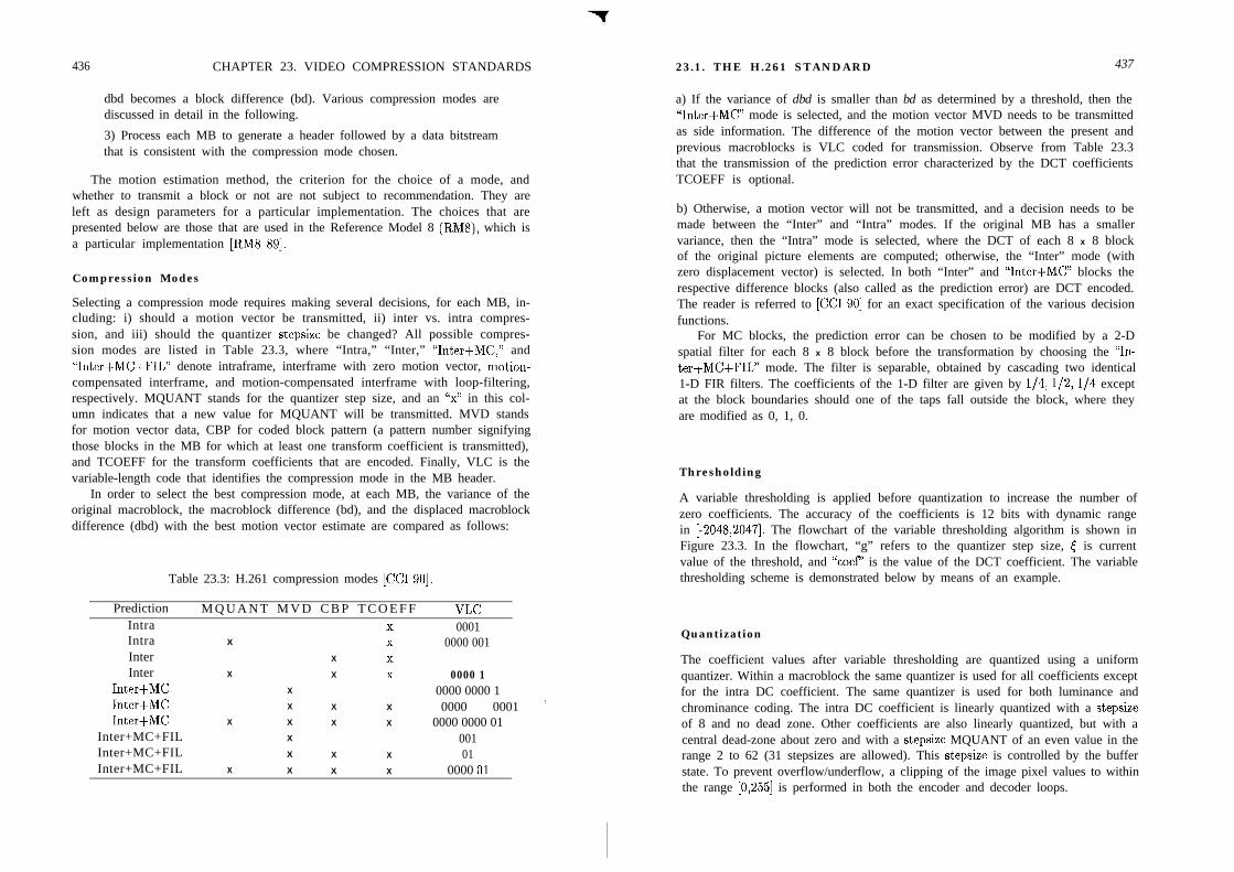
436 CHAPTER 23. VIDEO COMPRESSION STANDARDS 23.1. THE H.261 STANDARD 437
dbd becomes a block difference (bd). Various compression modes arediscussed in detail in the following.
3) Process each MB to generate a header followed by a data bitstreamthat is consistent with the compression mode chosen.
The motion estimation method, the criterion for the choice of a mode, andwhether to transmit a block or not are not subject to recommendation. They areleft as design parameters for a particular implementation. The choices that arepresented below are those that are used in the Reference Model 8 (RM8), which isa particular implementation [RM8 891.
Compression Modes
Selecting a compression mode requires making several decisions, for each MB, in-cluding: i) should a motion vector be transmitted, ii) inter vs. intra compres-sion, and iii) should the quantizer stepsize be changed? All possible compres-sion modes are listed in Table 23.3, where “Intra,” “Inter,” “Inter+MC,” and“Inter+MC+FIL” denote intraframe, interframe with zero motion vector, motion-compensated interframe, and motion-compensated interframe with loop-filtering,respectively. MQUANT stands for the quantizer step size, and an “x” in this col-umn indicates that a new value for MQUANT will be transmitted. MVD standsfor motion vector data, CBP for coded block pattern (a pattern number signifyingthose blocks in the MB for which at least one transform coefficient is transmitted),and TCOEFF for the transform coefficients that are encoded. Finally, VLC is thevariable-length code that identifies the compression mode in the MB header.
In order to select the best compression mode, at each MB, the variance of theoriginal macroblock, the macroblock difference (bd), and the displaced macroblockdifference (dbd) with the best motion vector estimate are compared as follows:
Table 23.3: H.261 compression modes [CC1 901.
Prediction M Q U A N T M V D C B P T C O E F F VLCIntraIntraInterInter
Inter+MCInter+MCInter+MC
Inter+MC+FILInter+MC+FILInter+MC+FIL
X
X
X X
X
X XX X X
X
X X
X X X
X
X
X
X
00010000 001
0000 10000 0000 10000 0001 (
0000 0000 0100101
0000 01
a) If the variance of dbd is smaller than bd as determined by a threshold, then the“Inter+MC” mode is selected, and the motion vector MVD needs to be transmittedas side information. The difference of the motion vector between the present andprevious macroblocks is VLC coded for transmission. Observe from Table 23.3that the transmission of the prediction error characterized by the DCT coefficientsTCOEFF is optional.
b) Otherwise, a motion vector will not be transmitted, and a decision needs to bemade between the “Inter” and “Intra” modes. If the original MB has a smallervariance, then the “Intra” mode is selected, where the DCT of each 8 x 8 blockof the original picture elements are computed; otherwise, the “Inter” mode (withzero displacement vector) is selected. In both “Inter” and “Inter+MC” blocks therespective difference blocks (also called as the prediction error) are DCT encoded.The reader is referred to [CC1 901 for an exact specification of the various decisionfunctions.
For MC blocks, the prediction error can be chosen to be modified by a 2-Dspatial filter for each 8 x 8 block before the transformation by choosing the “In-ter+MC+FIL” mode. The filter is separable, obtained by cascading two identical1-D FIR filters. The coefficients of the 1-D filter are given by l/4, l/2, l/4 exceptat the block boundaries should one of the taps fall outside the block, where theyare modified as 0, 1, 0.
Thresholding
A variable thresholding is applied before quantization to increase the number ofzero coefficients. The accuracy of the coefficients is 12 bits with dynamic rangein [-2048,2047]. The flowchart of the variable thresholding algorithm is shown inFigure 23.3. In the flowchart, “g” refers to the quantizer step size, [ is currentvalue of the threshold, and “coef’ is the value of the DCT coefficient. The variablethresholding scheme is demonstrated below by means of an example.
Quantization
The coefficient values after variable thresholding are quantized using a uniformquantizer. Within a macroblock the same quantizer is used for all coefficients exceptfor the intra DC coefficient. The same quantizer is used for both luminance andchrominance coding. The intra DC coefficient is linearly quantized with a stepsizeof 8 and no dead zone. Other coefficients are also linearly quantized, but with acentral dead-zone about zero and with a stepsize MQUANT of an even value in therange 2 to 62 (31 stepsizes are allowed). This stepsize is controlled by the bufferstate. To prevent overflow/underflow, a clipping of the image pixel values to withinthe range [0,255] is performed in both the encoder and decoder loops.
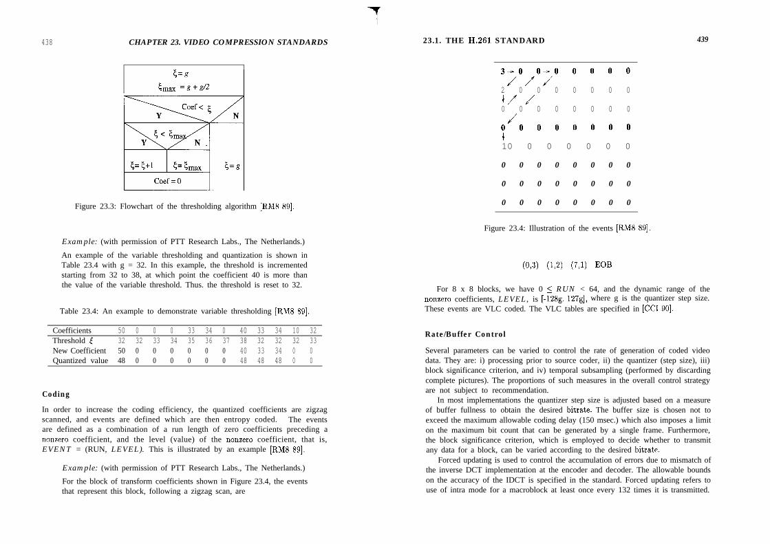
438 CHAPTER 23. VIDEO COMPRESSION STANDARDS 23.1. THE H-261 STANDARD 439
Figure 23.3: Flowchart of the thresholding algorithm [RM8 891.
Example: (with permission of PTT Research Labs., The Netherlands.)
An example of the variable thresholding and quantization is shown inTable 23.4 with g = 32. In this example, the threshold is incrementedstarting from 32 to 38, at which point the coefficient 40 is more thanthe value of the variable threshold. Thus. the threshold is reset to 32.
Table 23.4: An example to demonstrate variable thresholding [RM8 891.
Coefficients 50 0 0 0 33 34 0 40 33 34 10 32Threshold [ 32 32 33 34 35 36 37 38 32 32 32 33New Coefficient 50 0 0 0 0 0 0 40 33 34 0 0Quantized value 48 0 0 0 0 0 0 48 48 48 0 0
Coding
In order to increase the coding efficiency, the quantized coefficients are zigzagscanned, and events are defined which are then entropy coded. The eventsare defined as a combination of a run length of zero coefficients preceding anonzero coefficient, and the level (value) of the nonzero coefficient, that is,EVENT = (RUN, LEVEL). This is illustrated by an example [RM8 891.
Example: (with permission of PTT Research Labs., The Netherlands.)
For the block of transform coefficients shown in Figure 23.4, the eventsthat represent this block, following a zigzag scan, are
3io/oio O O O O2 0 0 0 0 0 0 0v J0 0 0 0 0 0 0 0J
0 0 0 0 0 0 0 0410 0 0 0 0 0 0
0 0 0 0 0 0 0 0
0 0 0 0 0 0 0 0
0 0 0 0 0 0 0 0
Figure 23.4: Illustration of the events [RM8 891.
(013) CL21 (7J) EOB
For 8 x 8 blocks, we have 0 5 RUN < 64, and the dynamic range of thenonzero coefficients, LEVEL, is [-128g, 127g], where g is the quantizer step size.These events are VLC coded. The VLC tables are specified in [CC1 901.
Rate/Buffer Control
Several parameters can be varied to control the rate of generation of coded videodata. They are: i) processing prior to source coder, ii) the quantizer (step size), iii)block significance criterion, and iv) temporal subsampling (performed by discardingcomplete pictures). The proportions of such measures in the overall control strategyare not subject to recommendation.
In most implementations the quantizer step size is adjusted based on a measureof buffer fullness to obtain the desired bitrate. The buffer size is chosen not toexceed the maximum allowable coding delay (150 msec.) which also imposes a limiton the maximum bit count that can be generated by a single frame. Furthermore,the block significance criterion, which is employed to decide whether to transmitany data for a block, can be varied according to the desired bitrate.
Forced updating is used to control the accumulation of errors due to mismatch ofthe inverse DCT implementation at the encoder and decoder. The allowable boundson the accuracy of the IDCT is specified in the standard. Forced updating refers touse of intra mode for a macroblock at least once every 132 times it is transmitted.
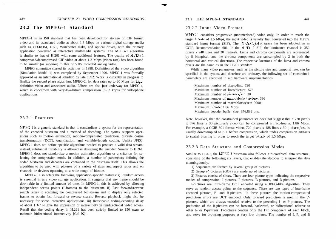
440 CHAPTER 23. VIDEO COMPRESSION STANDARDS 23.2. THE MPEG-1 STANDARD 441
23.2 The MPEG-1 Standard
MPEG-1 is an IS0 standard that has been developed for storage of CIF formatvideo and its associated audio at about 1.5 Mbps on various digital storage mediasuch as CD-ROM, DAT, Winchester disks, and optical drives, with the primaryapplication perceived as interactive multimedia systems. The MPEG-1 algorithmis similar to that of H.261 with some additional features. The quality of MPEG-1compressed/decompressed CIF video at about 1.2 Mbps (video rate) has been foundto be similar (or superior) to that of VHS recorded analog video.
MPEG committee started its activities in 1988. Definition of the video algorithm(Simulation Model 1) was completed by September 1990. MPEG-1 was formallyapproved as an international standard by late 1992. Work is currently in progress tofinalize the second phase algorithm, MPEG-2, for data rates up to 20 Mbps for high-definition video and associated audio. Efforts are also just underway for MPEG-4,which is concerned with very-low-bitrate compression (8-32 kbps) for videophoneapplications.
23.2.1 Features
MPEG-1 is a generic standard in that it standardizes a syn2az for the representationof the encoded bitstream and a method of decoding. The syntax supports oper-ations such as motion estimation, motion-compensated prediction, discrete cosinetransformation (DCT), quantization, and variable-length coding. Unlike JPEG,MPEG-1 does not define specific algorithms needed to produce a valid data stream;instead, substantial flexibility is allowed in designing the encoder. Similar to H.261,MPEG-1 does not standardize a motion estimation algorithm or a criterion for se-lecting the compression mode. In addition, a number of parameters defining thecoded bitstream and decoders are contained in the bitstream itself. This allows thealgorithm to be used with pictures of a variety of sizes and aspect ratios and onchannels or devices operating at a wide range of bitrates.
MPEG-1 also offers the following application-specific features: i) Random accessis essential in any video storage application. It suggests that any frame should bedecodable in a limited amount of time. In MPEG-1, this is achieved by allowingindependent access points (I-frames) to the bitstream. ii) Fast forward/reversesearch refers to scanning the compressed bit stream and to display only selectedframes to obtain fast forward or reverse search. Reverse playback might also benecessary for some interactive applications. iii) Reasonable coding/decoding delayof about 1 set to give the impression of interactivity in unidirectional video access.Recall that the coding delay in H.261 has been strictly limited to 150 msec tomaintain bidirectional interactivity [Gal 921.
23.2.2 Input Video Format
MPEG-1 considers progressive (noninterlaced) video only. In order to reach thetarget bitrate of 1.5 Mbps, the input video is usually first converted into the MPEGstandard input format (SIF). The (Y,Cr,Cb) 1co or space has been adopted, as inCCIR Recommendation 601. In the MPEG-1 SIF, the luminance channel is 352pixels x 240 lines and 30 frames/s. Luma and chroma components are representedby 8 bits/pixel, and the chroma components are subsampled by 2 in both thehorizontal and vertical directions. The respective locations of the luma and chromapixels are the same as in the H.261 standard.
While many video parameters, such as the picture size and temporal rate, can bespecified in the syntax, and therefore are arbitrary, the following set of constrainedparameters are specified to aid hardware implementations:
Maximum number of pixels/line: 720Maximum number of lines/picture: 576Maximum number of pictures/set: 30Maximum number of macroblocks/picture: 396Maximum number of macroblocks/sec: 9900Maximum bitrate: 1.86 MbpsMaximum decoder buffer size: 376,832 bits.
Note, however, that the constrained parameter set does not suggest that a 720 pixelsx 576 lines x 30 pictures/s video can be compressed artifact-free at 1.86 Mbps.For example, a CCIR 601 format video, 720 pixels x 488 lines x 30 pictures/set, isusually downsampled to SIF before compression, which trades compression artifactsto spatial blurring in order to reach the target bitrate of 1.5 Mbps.
23.2.3 Data Structure and Compression Modes
Similar to H.261, the MPEG-1 bitstream also follows a hierarchical data structure,consisting of the following six layers, that enables the decoder to interpret the dataunambiguously.
1) Sequences are formed by several group of pictures.2) Group of pictures (GOP) are made up of pictures.3) Pictures consist of slices. There are four picture types indicating the respective
modes of compression: I-pictures, P-pictures, B-pictures, and D-pictures.I-pictures are intra-frame DCT encoded using a JPEG-like algorithm. They
serve as random access points to the sequence. There are two types of interframeencoded pictures, P- and B-pictures. In these pictures the motion-compensatedprediction errors are DCT encoded. Only forward prediction is used in the P-pictures, which are always encoded relative to the preceding I- or P-pictures. Theprediction of the B-pictures can be forward, backward, or bidirectional relative toother I- or P-pictures. D-pictures contain only the DC component of each block,and serve for browsing purposes at very low bitrates. The number of I, P, and B
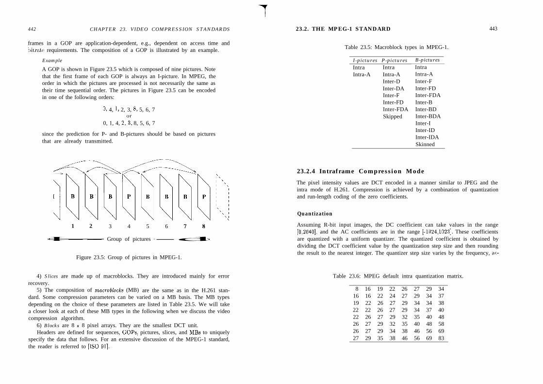
442 CHAPTER 23. VIDEO COMPRESSION STANDARDS 23.2. THE MPEG-1 STANDARD
frames in a GOP are application-dependent, e.g., dependent on access time andbitrate requirements. The composition of a GOP is illustrated by an example.
Example
A GOP is shown in Figure 23.5 which is composed of nine pictures. Notethat the first frame of each GOP is always an I-picture. In MPEG, theorder in which the pictures are processed is not necessarily the same astheir time sequential order. The pictures in Figure 23.5 can be encodedin one of the following orders:
0, 4, 1, 2, 3, 8, 5, 6, 7
0, 1, 4, 2,?, 8, 5, 6, 7
since the prediction for P- and B-pictures should be based on picturesthat are already transmitted.
1 2 3 4 5 6 7 8
Group of pictures
Figure 23.5: Group of pictures in MPEG-1.
4) Slices are made up of macroblocks. They are introduced mainly for errorrecovery.
5) The composition of macroblocbs (MB) are the same as in the H.261 stan-dard. Some compression parameters can be varied on a MB basis. The MB typesdepending on the choice of these parameters are listed in Table 23.5. We will takea closer look at each of these MB types in the following when we discuss the videocompression algorithm.
6) Blocks are 8 x 8 pixel arrays. They are the smallest DCT unit.Headers are defined for sequences, GOPs, pictures, slices, and MBs to uniquely
specify the data that follows. For an extensive discussion of the MPEG-1 standard,the reader is referred to [ISO 911.
Table 23.5: Macroblock types in MPEG-1.
I-pictures P-picturesIntra IntraIntra-A Intra-A
Inter-DInter-DAInter-FInter-FDInter-FDASkipped
B-picturesIntraIntra-AInter-FInter-FDInter-FDAInter-BInter-BDInter-BDAInter-IInter-IDInter-IDASkinned
443
23.2.4 Intraframe Compression Mode
The pixel intensity values are DCT encoded in a manner similar to JPEG and theintra mode of H.261. Compression is achieved by a combination of quantizationand run-length coding of the zero coefficients.
Quantization
Assuming R-bit input images, the DC coefficient can take values in the range[0,2040], and the AC coefficients are in the range [-1024,1023]. These coefficientsare quantized with a uniform quantizer. The quantized coefficient is obtained bydividing the DCT coefficient value by the quantization step size and then roundingthe result to the nearest integer. The quantizer step size varies by the frequency, ac-
Table 23.6: MPEG default intra quantization matrix.
8 16 19 22 26 27 29 3416 16 22 24 27 29 34 3719 22 26 27 29 34 34 3822 22 26 27 29 34 37 4022 26 27 29 32 35 40 4826 27 29 32 35 40 48 5826 27 29 34 38 46 56 6927 29 35 38 46 56 69 83
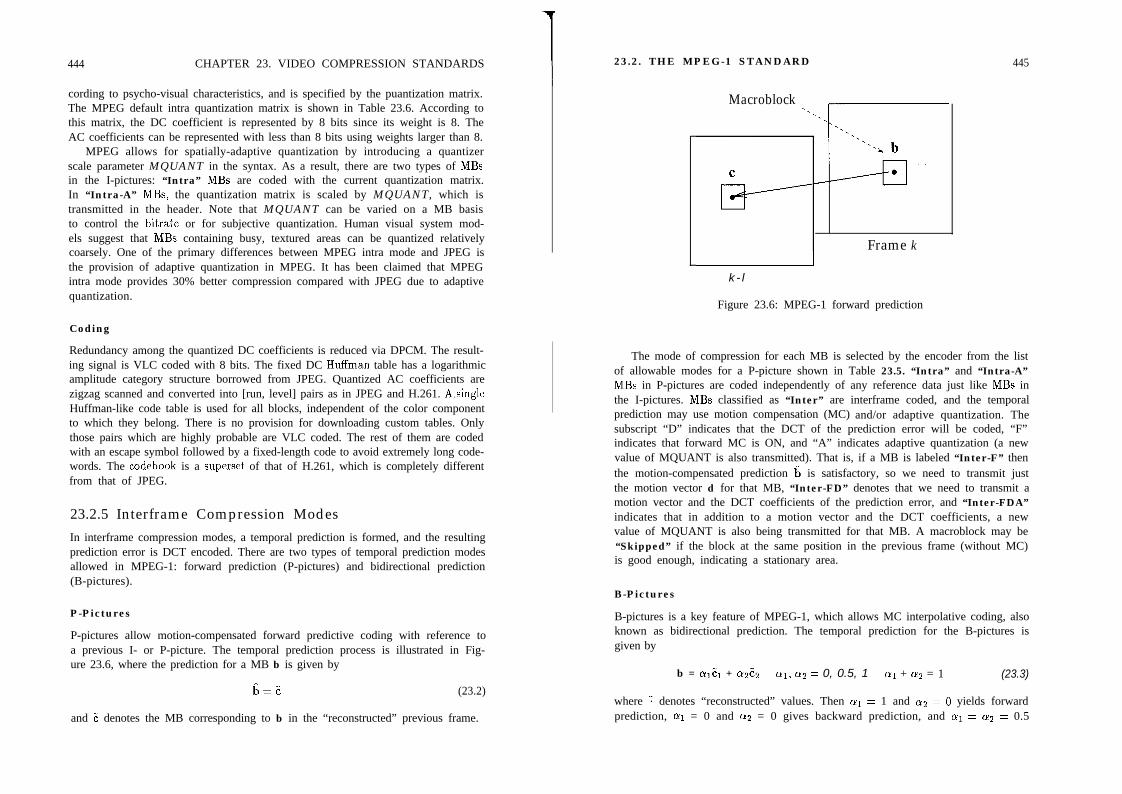
444 CHAPTER 23. VIDEO COMPRESSION STANDARDS 23.2. THE MPEG-1 STANDARD 445
cording to psycho-visual characteristics, and is specified by the puantization matrix.The MPEG default intra quantization matrix is shown in Table 23.6. According tothis matrix, the DC coefficient is represented by 8 bits since its weight is 8. TheAC coefficients can be represented with less than 8 bits using weights larger than 8.
MPEG allows for spatially-adaptive quantization by introducing a quantizerscale parameter MQUANT in the syntax. As a result, there are two types of MBsin the I-pictures: “Intra” MBs are coded with the current quantization matrix.In “Intra-A” MBs, the quantization matrix is scaled by MQUANT, which istransmitted in the header. Note that MQUANT can be varied on a MB basisto control the bitrate or for subjective quantization. Human visual system mod-els suggest that MBs containing busy, textured areas can be quantized relativelycoarsely. One of the primary differences between MPEG intra mode and JPEG isthe provision of adaptive quantization in MPEG. It has been claimed that MPEGintra mode provides 30% better compression compared with JPEG due to adaptivequantization.
Coding
Redundancy among the quantized DC coefficients is reduced via DPCM. The result-ing signal is VLC coded with 8 bits. The fixed DC Huffman table has a logarithmicamplitude category structure borrowed from JPEG. Quantized AC coefficients arezigzag scanned and converted into [run, level] pairs as in JPEG and H.261. A.singleHuffman-like code table is used for all blocks, independent of the color componentto which they belong. There is no provision for downloading custom tables. Onlythose pairs which are highly probable are VLC coded. The rest of them are codedwith an escape symbol followed by a fixed-length code to avoid extremely long code-words. The codebook is a superset of that of H.261, which is completely differentfrom that of JPEG.
23.2.5 Interframe Compression ModesIn interframe compression modes, a temporal prediction is formed, and the resultingprediction error is DCT encoded. There are two types of temporal prediction modesallowed in MPEG-1: forward prediction (P-pictures) and bidirectional prediction(B-pictures).
P-Pictures
P-pictures allow motion-compensated forward predictive coding with reference toa previous I- or P-picture. The temporal prediction process is illustrated in Fig-ure 23.6, where the prediction for a MB b is given by
&=C (23.2)
and C denotes the MB corresponding to b in the “reconstructed” previous frame.
Macroblock
Frame k
k - l
Figure 23.6: MPEG-1 forward prediction
The mode of compression for each MB is selected by the encoder from the listof allowable modes for a P-picture shown in Table 23.5. “Intra” and “Intra-A”MBs in P-pictures are coded independently of any reference data just like MBs inthe I-pictures. MBs classified as “Inter” are interframe coded, and the temporalprediction may use motion compensation (MC) and/or adaptive quantization. Thesubscript “D” indicates that the DCT of the prediction error will be coded, “F”indicates that forward MC is ON, and “A” indicates adaptive quantization (a newvalue of MQUANT is also transmitted). That is, if a MB is labeled “Inter-F” thenthe motion-compensated prediction h is satisfactory, so we need to transmit justthe motion vector d for that MB, “Inter-FD” denotes that we need to transmit amotion vector and the DCT coefficients of the prediction error, and “Inter-FDA”indicates that in addition to a motion vector and the DCT coefficients, a newvalue of MQUANT is also being transmitted for that MB. A macroblock may be“Skipped” if the block at the same position in the previous frame (without MC)is good enough, indicating a stationary area.
B-Pictures
B-pictures is a key feature of MPEG-1, which allows MC interpolative coding, alsoknown as bidirectional prediction. The temporal prediction for the B-pictures isgiven by
b = alcl + cl+:! al, a2 = 0, 0.5, 1 a1 + a2 = 1 (23.3)
where 7 denotes “reconstructed” values. Then cyi = 1 and os = 6 yields forwardprediction, oi = 0 and ~2 = 0 gives backward prediction, and cyi = a2 = 0.5
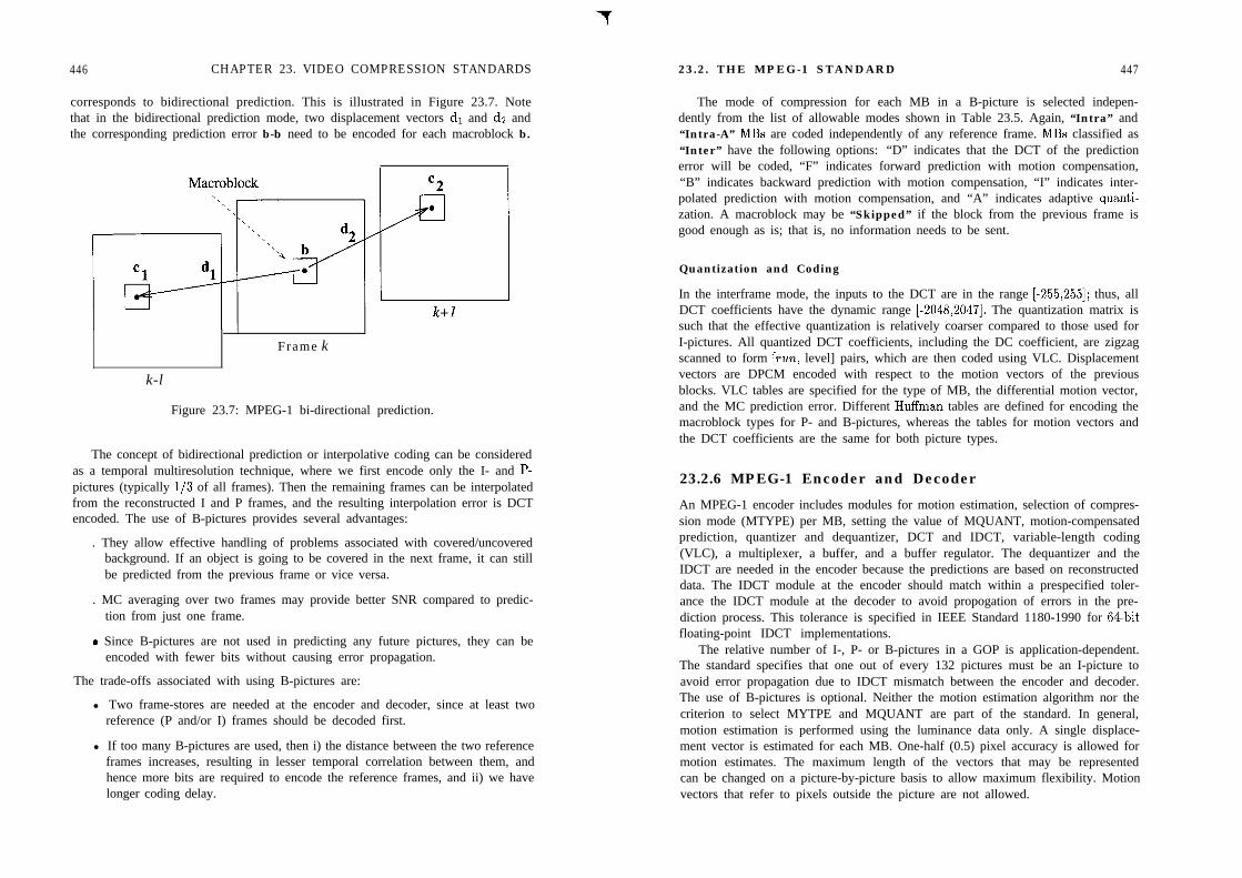
446 CHAPTER 23. VIDEO COMPRESSION STANDARDS
corresponds to bidirectional prediction. This is illustrated in Figure 23.7. Notethat in the bidirectional prediction mode, two displacement vectors dl and dz andthe corresponding prediction error b-b need to be encoded for each macroblock b.
I
Frame k
k-l
Figure 23.7: MPEG-1 bi-directional prediction.
The concept of bidirectional prediction or interpolative coding can be consideredas a temporal multiresolution technique, where we first encode only the I- and P-pictures (typically l/3 of all frames). Then the remaining frames can be interpolatedfrom the reconstructed I and P frames, and the resulting interpolation error is DCTencoded. The use of B-pictures provides several advantages:
. They allow effective handling of problems associated with covered/uncoveredbackground. If an object is going to be covered in the next frame, it can stillbe predicted from the previous frame or vice versa.
. MC averaging over two frames may provide better SNR compared to predic-tion from just one frame.
s Since B-pictures are not used in predicting any future pictures, they can beencoded with fewer bits without causing error propagation.
The trade-offs associated with using B-pictures are:
l Two frame-stores are needed at the encoder and decoder, since at least tworeference (P and/or I) frames should be decoded first.
l If too many B-pictures are used, then i) the distance between the two referenceframes increases, resulting in lesser temporal correlation between them, andhence more bits are required to encode the reference frames, and ii) we havelonger coding delay.
23.2. THE MPEG-1 STANDARD 447
The mode of compression for each MB in a B-picture is selected indepen-dently from the list of allowable modes shown in Table 23.5. Again, “Intra” and“Intra-A” MBs are coded independently of any reference frame. MBs classified as“Inter” have the following options: “D” indicates that the DCT of the predictionerror will be coded, “F” indicates forward prediction with motion compensation,“B” indicates backward prediction with motion compensation, “I” indicates inter-polated prediction with motion compensation, and “A” indicates adaptive quanti-zation. A macroblock may be “Skipped” if the block from the previous frame isgood enough as is; that is, no information needs to be sent.
Quantization and Coding
In the interframe mode, the inputs to the DCT are in the range [-255,255]; thus, allDCT coefficients have the dynamic range [-2048,2047]. The quantization matrix issuch that the effective quantization is relatively coarser compared to those used forI-pictures. All quantized DCT coefficients, including the DC coefficient, are zigzagscanned to form [run, level] pairs, which are then coded using VLC. Displacementvectors are DPCM encoded with respect to the motion vectors of the previousblocks. VLC tables are specified for the type of MB, the differential motion vector,and the MC prediction error. Different Huffman tables are defined for encoding themacroblock types for P- and B-pictures, whereas the tables for motion vectors andthe DCT coefficients are the same for both picture types.
23.2.6 MPEG-1 Encoder and Decoder
An MPEG-1 encoder includes modules for motion estimation, selection of compres-sion mode (MTYPE) per MB, setting the value of MQUANT, motion-compensatedprediction, quantizer and dequantizer, DCT and IDCT, variable-length coding(VLC), a multiplexer, a buffer, and a buffer regulator. The dequantizer and theIDCT are needed in the encoder because the predictions are based on reconstructeddata. The IDCT module at the encoder should match within a prespecified toler-ance the IDCT module at the decoder to avoid propogation of errors in the pre-diction process. This tolerance is specified in IEEE Standard 1180-1990 for 64-bitfloating-point IDCT implementations.
The relative number of I-, P- or B-pictures in a GOP is application-dependent.The standard specifies that one out of every 132 pictures must be an I-picture toavoid error propagation due to IDCT mismatch between the encoder and decoder.The use of B-pictures is optional. Neither the motion estimation algorithm nor thecriterion to select MYTPE and MQUANT are part of the standard. In general,motion estimation is performed using the luminance data only. A single displace-ment vector is estimated for each MB. One-half (0.5) pixel accuracy is allowed formotion estimates. The maximum length of the vectors that may be representedcan be changed on a picture-by-picture basis to allow maximum flexibility. Motionvectors that refer to pixels outside the picture are not allowed.

448 CHAPTER 23. VIDEO COMPRESSION STANDARDS 23.3. THE MPEG-2 STANDARD 449
In summary, a typical MPEG encoder performs the following steps:
1. Decide on the labeling of I-, P- and B-pictures in a GOP.
2. Estimate a motion vector for each MB in the P- and B-pictures,
3. Determine the compression mode MTYPE for each MB from Table 23.5.
4. Set the quantization scale, MQUANT, if adaptive quantization is selected
An MPEG-1 decoder reverses the operations of the encoder. The incoming bitstream (with a standard syntax) is demultiplexed into DCT coefficients and sideinformation such as MTYPE, motion vectors, MQUANT, and so on. The decoderemploys two frame-stores, since two reference frames are used to decode the B-pictures.
We conclude this section by summarizing the main differences between the H.261and MPEG-1 standards in Table 23.7.
Table 23.7: Comparison of H.261 and MPEG-1 Standards
CIF and QCIF images only Flexible image sizeY
MC over 1 frame1 uixel MV accuracv121 filter in the loopVariable threshold +uniform quantizationNo GOF structure
I ’
1 MC over 1 or more frames1 l/2 pixel MV accuracy
No filterQuantization ma,trix
GOF structureGOB structure
I
1 Slice structure
23.3 The MPEG-2 Standard
The quality of MPEG-1 compressed video at 1.2 Mbps has been found unacceptablefor most entertainment applications. Subjective tests indicate that CCIR 601 videocan be compressed with excellent quality at 4-6 Mbps. MPEG-2 is intended as acompatible extension of MPEG-1 to serve a wide range of applications at variousbitrates (2-20 Mbps) and resolutions. Main features of the MPEG-2 syntax are: i) itallows for interlaced inputs, higher-definition inputs, and alternative subsampling ofthe chroma channels, ii) it offers a scalable bitstream, and iii) it provides improvedquantization and coding options.
Considering the practical difficulties with the implementation of the full syntaxon a single chip, subsets of the full syntax have been specified under five “profiles,”simple profile, main profile, SNR scalable profile, spatially scalable profile, and highprofile. Furthermore, a number of “levels” have been introduced within these pro-files to impose constraints on some of the video parameters [ISO 931. It is importantto note that the MPEG-2 standard has not yet been finalized. The syntax of theMain Profile was frozen in March 1993. However, work in other profiles is stillongoing. It is likely that the all-digital HDTV compression algorithm will conformwith one of the profiles in MPEG-2.
In the following we discuss the MB structure in MPEG-2, how MPEG-2 han-dles interlaced video, the concepts related to scalability, and some extensions forencoding of higher-definition video along with a brief overview of the profiles andlevels.
23.3.1 MPEG-2 Macroblocks
A macroblock (MB) refers to four 8 x 8 luminance blocks and the spatially associ-ated chroma blocks. MPEG-2 allows for three chroma subsampling formats, 4:2:0(same as MPEG-l), 4:2:2 (chroma subsampled in the horizontal direction only), and4:4:4 (no chroma subsampling). The spatial locations of luma and chroma pixelsfor the 4:2:0 and 4:2:2 formats are depicted in Figure 23.8. Therefore, in MPEG-2a MB may contain 6 (4 luma, 1 Cr, and 1 Cb), 8 (4 luma, 2 Cr, and 2 Cb), or 12(4 luma, 4 Cr, and 4 Cb) 8 x 8 blocks.
x0x x0x (81X181Xxxxx (81xE3xx0x x0x (81xE3xxxxx (81X181X
(4 (b)
X Luminance pixels
0 Chrominance pixels
Figure 23.8: Chrominance subsampling options: a) 4:2:0 format; b) 4:2:2 format.

450 CHAPTER 23. VIDEO COMPRESSION STANDARDS 23.3. THE MPEG-2 STANDARD 451
23.3.2 Coding Interlaced Video
MPEG-2 accepts both progressive and interlaced inputs. If the input is interlaced,the output of the encoder consists of a sequence of fields that are separated bythe field period, There are two options in coding interlaced video: i) every fieldcan be encoded independently (field pictures), or ii) two fields may be encodedtogether as a composite frame (frame pictures). It is possible to switch betweenframe pictures and field pictures on a frame-to-frame basis. Frame encoding ispreferred for relatively still images; field encoding may give better results when thereis significant motion. In order to deal with interlaced inputs effectively, MPEG-2supports:
. two new picture formats: frame-picture and field-picture,
. field/frame DCT option per MB for frame pictures, and
. new MC prediction modes for interlaced video,which are described in the following.
New Picture Types for Interlaced Video
Interlaced video is composed of a sequence of even and odd fields separated by afield period. MPEG-2 defines two new picture types for interlaced video. They are:
i) Frume pictures, which are obtained by interleaving lines of even and odd fieldsto form composite frames. Frame pictures can be I-, P-, or B-type. An MB of theluminance frame picture is depicted in Figure 23.9.
8 8
Odd field
Even field
Figure 23.9: The luminance component of a MB of a frame picture.
ii) Field pictures are simply the even and odd fields treated as separate pictures.Each field picture can be I-, P- or B-type.
Picture types in MPEG2
Progressive video Interlaced video
Frame Picture Frame Picture Field PictureI, P, or B type I, P, or B type I, P, or B type
Figure 23.10: Summary of picture types in MPEG-2.
A summary of all picture types is shown in Figure 23.10. Clearly, in progressivevideo all pictures are frame pictures. A group of pictures can be composed of anarbitrary mixture of field and frame pictures. Field pictures always appear in pairs(called the top field and bottom field) which together constitute a frame. If thetop field is a P- (B-) picture, then the bottom field must also be a P- (B-) picture.If the top field is an I-picture, then the bottom field can be an I- or a P-picture.A pair of field pictures are encoded in the order in which they should appear at theoutput. An example of a GOP for an interlaced video is shown in Figure 23.11.
P I P
I B
Figure 23.11: A GOP for an interlaced video
Field/Frame DCT Option for Frame Pictures
MPEG-2 allows a field- or frame-DCT option for each MB in a frame picture. Thisallows computing DCT on a field-by-field basis for specific parts of a frame picture.For example, field-DCT may be chosen for macroblocks containing high motion,whereas frame-DCT may be appropriate for macroblocks with little or no motionbut containing high spatial activity. The internal organization of a MB for frame(on the left) and field (on the right) DCT is shown in Figure 23.12. Note that in4:2:0 sampling, only frame DCT can be used for the chroma blocks to avoid 8 x 4IDCT.

452 CHAPTER 23. VIDEO COMPRESSION STANDARDS
(a) (b)
Figure 23.12: DCT options for interlaced frame pictures: a) Frame DCT andb) field DCT.
MC Prediction Modes for Interlaced Video
There are two main types of predictions: simple field and simple frame prediction.In simple field prediction, each field is predicted independently using data from oneor more previously decoded fields. Simple frame prediction forms a prediction foran entire frame based on one or more previously decoded frames. Within a fieldpicture only field predictions can be used. However, in a frame picture either fieldor frame prediction may be employed on an MB-by-MB basis. Selection of the bestprediction mode depends on presence/absence of motion in an MB, since in thepresence of motion, frame prediction suffers from strong motion artifacts, while inthe absence of motion, field prediction does not utilize all available information.
There are also two other prediction modes: 16 x 8 MC mode and dual-primemode. 16 x 8 MC mode is only used in field pictures, where two motion vectorsare used per MB, one for the upper and the other for the lower 16 x 8 region,which belong to the top and bottom fields, respectively. In the case of bidirectionalprediction, four motion vectors will be needed. In dual-prime mode, one motionvector and a small differential vector are encoded. In the case of field pictures,two motion vectors are derived from this information and used to form predictionsfrom two reference fields, which are averaged to form the final prediction [ISO 931.Dual-prime mode is used only for P-pictures.
23.3.3 Scalable ExtensionsScalability refers to ability to decode only a certain part of the bit-stream to obtainvideo at the desired resolution. It is assumed that decoders with different complex-ities can decode and display video at different spatio-temporal resolutions from the
23.3. THE MPEG-2 STANDARD 453
same bitstream. The minimum decodable subset of the bitstream is called the baselayer. All other layers are enhancement layers, which improve the resolution of thebase layer video. MPEG-2 syntax allows for two or three layers of video. There aredifferent forms of scalability:
Spatial (pixel resolution) scalability provides the ability to decode video at dif-ferent spatial resolutions without first decoding the entire frame and decimating it.The base layer is a low spatial resolution version of the video. Enhancement layerscontain successively higher-frequency information. MPEG-2 employs a pyramidalcoding approach. The base layer video is obtained by decimating the original inputvideo. The enhancement layer is the difference of the actual input video and theinterpolated version of the base-layer video.
SNR scalability offers decodability using different quantizer step sizes for theDCT coefficients. The base-layer video is obtained by using a coarse quantizationof the DCT coefficients. It is at the same spatio-temporal resolution with the inputvideo. The enhancement layer simply refers to the difference of the base layer andthe original input video.
Temporal scalability refers to decodability at different frame rates without firstdecoding every single frame. Hybrid scalability refers to some combination of theabove. An important advantage of scalability is that it provides higher resilience totransmission errors as the base-layer video is usually transmitted with better errorcorrection capabilities.
23.3.4 Other ImprovementsMPEG-2 also features some extensions in the quantization and coding steps forimproved image quality in exchange to slightly higher bitrate. In particular, it allowsfor i) a new scanning scheme (alternate scan) in addition to the zigzag scanningof the DCT coefficients, ii) finer quantization of the DCT coefficients, iii) fineradjustment of the quantizer scale factor, and iv) a separate VLC table for the DCTcoefficients for the intra macroblocks, which are explained in the following.
Alternate Scan
In addition to the zigzag scanning, MPEG-2 allows for an optional scanning pattern,called the “alternate scan.” The alternate scan pattern, which is said to fit interlacedvideo better, is depicted in Figure 23.13.
Finer Quantization of the DCT Coefficients
In intra macroblocks, the quantization weight for the DC coefficient can be 8, 4, 2or 1. That is, 11 bits (full) resolution is allowed for the DC coefficient. Recall thatthis weight is fixed to 8 in MPEG-1. AC coefficients are quantized in the range[-2048,2047], as opposed to [-256,255] in MPEG-1. In non-intra macroblocks, allcoefficients are quantized into the range [-2048,2047]. This range was [-256,255] inMPEG-1.

454 CHAPTER 23. VIDEO COMPRESSION STAXDARDS
Figure 23.13: Alternate scan.
Finer Adjustment of MQUANT
In addition to a set of MQUANT values that are integers between 1 and 31, MPEG-2 allows for an optional set of 31 values that include real numbers ranging from 0.5to 56. These values are listed in Table 23.8.
Table 23.8: Optional set of MQUANT values.
5.06.07.08.09.010.011.012.0
14.016.018.020.022.024.026.028.0
23.3.5 Overview of Profiles and Levels
MPEG-2 full syntax covers a wide range of features and free parameters. The fiveMPEG-2 profiles define subsets of the syntax while the four levels impose constraintson the values of the free parameters for the purpose of practical hardware imple-mentations. The parameter constraints imposed by the four levels are summarizedin Table 23.9.
23.4. SOFTWARE AND HARDWARE IMPLEMENTATIONS 455
Table 23.9: Parameter constraints according to levels.
The Simple profile does not allow use of B-pictures and only support the Mainlevel. The maximum bitrate for the Simple profile is 15 Mbps. The Main profilesupports all four levels with upper bounds on the bitrates equal to 4, 15, 60, and 80Mbps for the Low, Main, High-1440 and High levels, respectively. The Main profiledoes not include any scalability. The SNR Scalable profile supports Low and Mainlevels with maximum bitrates 4 (3) and 15 (10) Mbps, respectively. The numbers inparentheses indicate the maximum bitrate for the base layer. The Spatially Scalableprofile supports only High-1440 level with a maximum bitrate of 60 (15) Mbps. TheHigh profile includes Main, High-1440 and High levels with maximum bitrates of20 (4), 80 (20), and 100 (25) Mbps, respectively.
23.4 Software and Hardware Implementations
There are several software and hardware implementations of the H.261 andMPEG algorithms. The Portable Video Research Group (PVRG) at Stan-ford University has public-domain source codes for both H.261 and MPEGstandards, called PVRG-P64 and PVRG-MPEG, respectively. They can beobtained through anonymous ftp from “havefun.stanford.edu” - IP address[36.2.0.35] - (/pub/p64/P64v1.2.tar.Z) and (/pub/mpeg/MPEGvl.2.tar.Z). Otherpublic-domain software includes the INRIA H.261 codec, which can be obtainedfrom “avahi.inria.fr” (/pub/h26l.tar.Z), and the Berkeley Plateau Research GroupMPEG encoder, which can be obtained from “toe.cs.berkeley.edu” - IP address[128.32.149.117] - (/pub/multimedia/mpeg/mpeg-2.0.tar.Z).
Single- or multichip implementations of the video compression standards areavailable from many vendors, including
l C-Cube: CL-450, single-chip MPEG-1, SIF rates. CL-950, MPEG-2,CL-4000, single-chip, can code MPEG-1, H.261, and JPEG,
l SGS-Thomson: STi-3400, single-chip MPEG-1, SIF rates. STi-3500, the firstMPEG-2 chip on the market,
l Motorola: MCD250, single-chip MPEG-1, SIF rates, and

456
l GEC Plassey: Chip sets for the H.261 algorithm.
BIBLIOGRAPHY
For more complete listings, the reader is referred to MPEG-FAQ, available from“[email protected],” and to Compression-FAQ (part 3), available by ftp from“rtfm.mit.edu” (/pub/usenet/news.answers/compression-faq/part[l-3].
Chapter 24
Bibliography
[CC1 901
[Che 931
[Chi 951
[Gal 911
[Gal 921
[ISO 911
[ISO 931
[Lio 911
[Lio 901
CCITT Recommendation H.261: “Video Codec for Audio Visual Servicesat p x 64 kbits/s,” COM XV-R 37-E, 1990.
C.-T. Chen, “Video compression: Standards and applications,” J. VisualComm. Image Rep., vol. 4, no. 2, pp. 103-111, Jun. 1993.
L. Chiariglione, “The development of an integrated audiovisual codingstandard: MPEG,” Proc. IEEE, vol. 83, no. 2, pp. 151-157, Feb. 1995.
D. J. LeGall, “MPEG: A video compression standard for multimedia ap-plications,” Commun. ACM, vol. 34, pp. 46-58, 1991.
D. J. LeGall, “The MPEG video compression algorithm,” Signal Proc.:Image Comm., vol. 4, pp. 129-140, 1992.
ISO/IEC CD 11172: “Coding of Moving Pictures and Associated Audio -For Digital Storage Media at up to 1.5 Mbits/set,” Dec. 1991.
ISO/IEC CD 13818-2: “Generic Coding of Moving Pictures and Associ-ated Audio,” Nov. 1993.
M. L. Liou, “Overview of the p x 64 kbits/sec video coding standard,”Commun. ACM, vol. 34, pp. 59-63, 1991.
M. L. Liou, “Visual telephony as an ISDN application,” IEEE Communi-cations Magazine, vol. 28, pp. 30-38, 1990.
[Oku 921 S. Okubo, “Requirements for high quality video coding standards,” SignalProc.: Image Comm., vol. 4, pp. 141-151,1992.
[Pen 931 W. B. Pennebaker and J. L. Mitchell, JPEG: Still image data compressionstandard, New York, NY: Van Nostrand Reinhold, 1993.
[RMS 891 COST211bis/SIM89/37: “Description of Reference Model 8 (RM8),”PTT Research Laboratories, The Netherlands, May 1989.
MODEL-BASED CODING
Due to growing interest in very-low-bitrate digital video (about 10 kbps), signifi-cant research effort has recently been focused on new compression methods basedon structural models, known as model-based analysis-synthesis coding. Scientistsbecame interested in model-based coding because the quality of digital video pro-vided by hybrid waveform encoders, such as the CCITT Rec. H.261 encoder, hasbeen deemed unacceptable at these very low bitrates. The general principles ofmodel-based coding, including general object-based, knowledge-based, and semanticcoding, were presented in Chapter 22. These techniques employ structural modelsranging from general purpose 2-D or 3-D object models [Mus 89, Die 93, Ost 931 toapplication-specific wireframe models [Aiz 89, Li 93, Boz 941. In the following, weelaborate on general 2-D/3-D object-based coding in Section 24.1, and knowledge-based and semantic coding in Section 24.2.
24.1 General Object-Based Methods
A major deficiency of the MC/DCT compression is that it is based on a 2-D trans-latory block-motion model. This model is not adequate for a precise description ofmost motion fields, because it does not include rotation and zooming, and bound-aries of moving objects hardly ever coincide with those of the rectangular blocks.Object-based methods aim to develop more realistic 2-D motion field models byconsidering affine, perspective, and bilinear spatial transformations and/or segmen-tation of the scene into individually moving objects. Typically, a frame is partitionedinto an “unchanged region,” an “uncovered background,” and a number of movingobjects which are either model-compliant (MC) or model-failure (MF) objects, asdepicted in Figure 24.1. Segmentation is an integral part of these schemes, becausedifferent regions require different model parameters. We can classify object-basedmodels as: i) piecewise planar or arbitrary 3-D surfaces with 3-D motion, ii) 2-Dflexible models with 2-D translational motion, and iii) spatial transformations withtriangular/rectangular patches, which are described in the following.
457

458 CHAPTER 24. MODEL-BASED CODING
Frame
Unchanged Changedregion region
Uncovered Moving regionbackground
1 Object 1 Object N
O b j e c t 2 MC MF MC MF
MC MF
Figure 24.1: Segmentation of a frame into objects.
24.1.1 2-D/3-D Rigid Objects with 3-D Motion
In this approach, a 3-D model of a moving scene is estimated, which is consistentwith a given sequence of frames. A realistic 2-D motion field model can thenbe obtained by projecting the resulting 3-D motion into the image plane. Twoapproaches are commonly used to represent 3-D surfaces: i) approximation by apiecewise planar model, also known as the case of 2-D rigid objects with 3-D motion[Hot 90, Die 931, and ii) estimation of a global surface model under a smoothnessconstraint, which leads to the so-called 3-D object with 3-D motion models [Mus 89,Ost 90, Ost 93, Mor 91, Koc 931. Here, we provide a brief overview of the formerapproach.
We have seen in Chapter 9 that the orthographic and perspective projectionsof arbitrary 3-D motion of a rigid planar patch into the image plane yield the 6-parameter affine and the H-parameter perspective models, respectively. It followsthat, using the 2-D rigid object with 3-D motion approach, the 2-D motion fieldcan be represented by a piecewise affine or a piecewise perspective field, where theboundaries of the patches and the respective model parameters can be estimatedby a simultaneous motion estimation and segmentation algorithm (see Chapter 11).Then the parameter set for each independently moving object (motion parame-ters) together with the segmentation mask denoting the boundaries of each objectin the image plane (shape parameters) constitute a complete description of theframe-to-frame pixel correspondences, which provide an MC-prediction of the nextframe. Because of motion estimation/segmentation errors and problems related touncovered background, the frame prediction error or the synthesis error (color pa-rameters) also needs to be transmitted to improve upon image quality in the modelfailure regions.
24.1. GENERAL OBJECT-BASED METHODS 459
An object-oriented analysis-synthesis encoder implements the following steps:
Analysis: Perform simultaneous motion parameter estimation and segmenta-tion, between frame le and the reconstructed frame le - 1, to find the best mo-tion and shape parameters. Two specific algorithms that have been reportedwith successful results are those of Hotter e2 al. [Hot SO] and Diehl [Die 931.They can be summarized using the flowchart shown in Figure 24.2, where theframe is initially segmented into a changed and an unchanged region. Eachcontiguous changed segment is assumed as an independent moving object, anda set of mapping parameters, such as a 6-parameter affine or an B-parameterperspective mapping, is estimated for each moving object. The present frame(frame IE) can then be synthesized from the previously reconstructed frameE - 1 using these parameters. Those objects, where the synthesis error is
Frame k
Mapping parameterestimation
i
Image synthesis
Updatesegmentation mask
t
Transmit segmentation & mappingparameters
Figure 24.2: Flowchart of the mapping-parameter-based method.
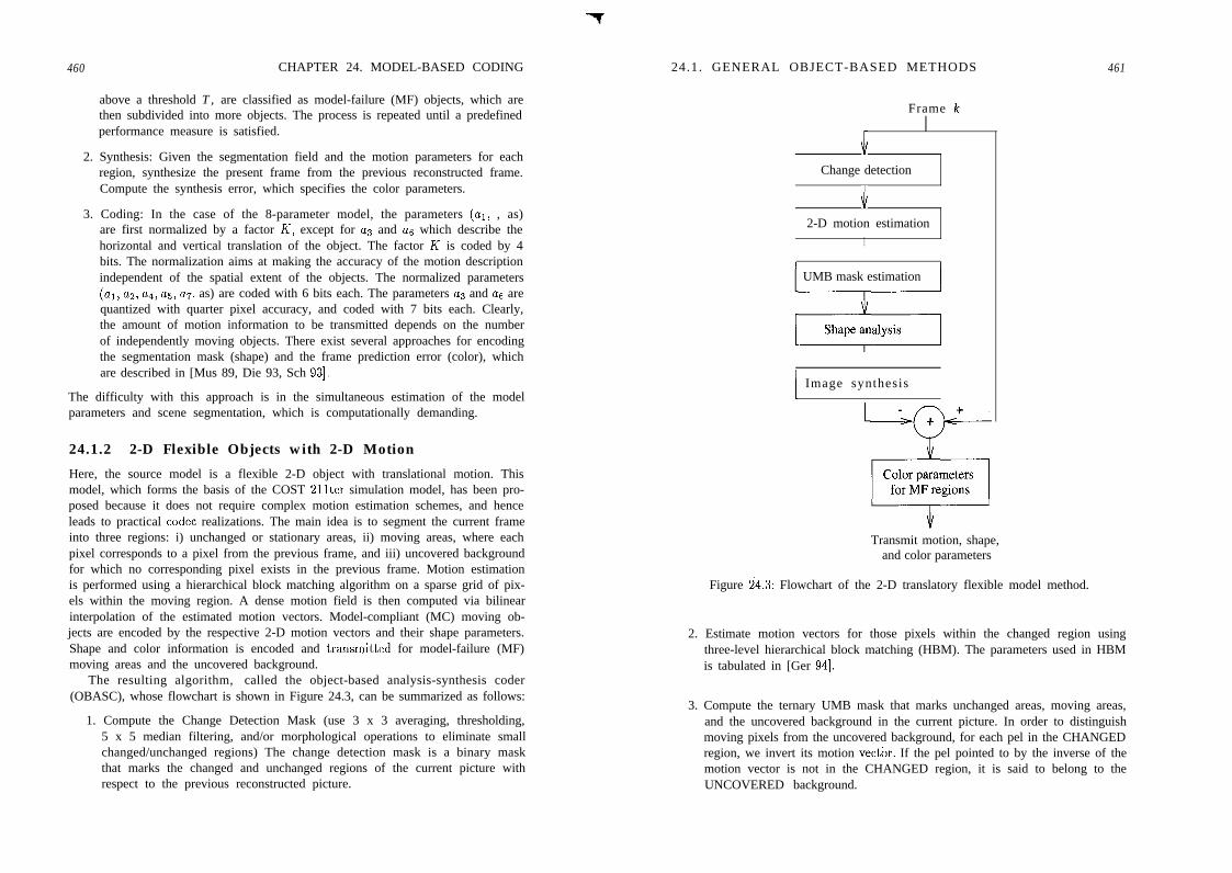
-7
460 CHAPTER 24. MODEL-BASED CODING
above a threshold T, are classified as model-failure (MF) objects, which arethen subdivided into more objects. The process is repeated until a predefinedperformance measure is satisfied.
2. Synthesis: Given the segmentation field and the motion parameters for eachregion, synthesize the present frame from the previous reconstructed frame.Compute the synthesis error, which specifies the color parameters.
3. Coding: In the case of the 8-parameter model, the parameters (al, , as)are first normalized by a factor Ii’, except for a3 and as which describe thehorizontal and vertical translation of the object. The factor I-C is coded by 4bits. The normalization aims at making the accuracy of the motion descriptionindependent of the spatial extent of the objects. The normalized parameters(al, a~, a4, as, ~7, as) are coded with 6 bits each. The parameters us and a6 arequantized with quarter pixel accuracy, and coded with 7 bits each. Clearly,the amount of motion information to be transmitted depends on the numberof independently moving objects. There exist several approaches for encodingthe segmentation mask (shape) and the frame prediction error (color), whichare described in [Mus 89, Die 93, Sch 931.
The difficulty with this approach is in the simultaneous estimation of the modelparameters and scene segmentation, which is computationally demanding.
24.1.2 2-D Flexible Objects with 2-D Motion
Here, the source model is a flexible 2-D object with translational motion. Thismodel, which forms the basis of the COST Pllter simulation model, has been pro-posed because it does not require complex motion estimation schemes, and henceleads to practical codec realizations. The main idea is to segment the current frameinto three regions: i) unchanged or stationary areas, ii) moving areas, where eachpixel corresponds to a pixel from the previous frame, and iii) uncovered backgroundfor which no corresponding pixel exists in the previous frame. Motion estimationis performed using a hierarchical block matching algorithm on a sparse grid of pix-els within the moving region. A dense motion field is then computed via bilinearinterpolation of the estimated motion vectors. Model-compliant (MC) moving ob-jects are encoded by the respective 2-D motion vectors and their shape parameters.Shape and color information is encoded and transmitt#ed for model-failure (MF)moving areas and the uncovered background.
The resulting algorithm, called the object-based analysis-synthesis coder(OBASC), whose flowchart is shown in Figure 24.3, can be summarized as follows:
1. Compute the Change Detection Mask (use 3 x 3 averaging, thresholding,5 x 5 median filtering, and/or morphological operations to eliminate smallchanged/unchanged regions) The change detection mask is a binary maskthat marks the changed and unchanged regions of the current picture withrespect to the previous reconstructed picture.
24.1. GENERAL OBJECT-BASED METHODS
Frame k
4
Change detection
42-D motion estimation
I
UMB mask estimation
1 Image synthesis1
461
Transmit motion, shape,and color parameters
Figure 24.3: Flowchart of the 2-D translatory flexible model method.
2. Estimate motion vectors for those pixels within the changed region usingthree-level hierarchical block matching (HBM). The parameters used in HBMis tabulated in [Ger 941.
3. Compute the ternary UMB mask that marks unchanged areas, moving areas,and the uncovered background in the current picture. In order to distinguishmoving pixels from the uncovered background, for each pel in the CHANGEDregion, we invert its motion vectbr. If the pel pointed to by the inverse of themotion vector is not in the CHANGED region, it is said to belong to theUNCOVERED background.
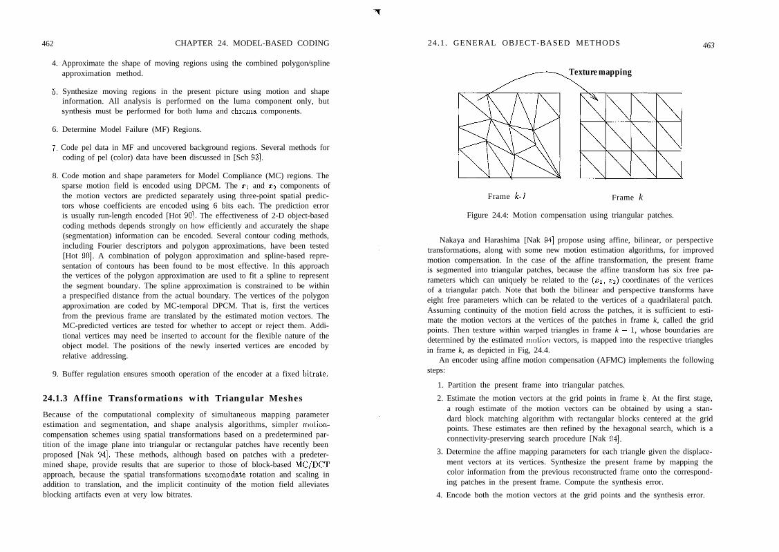
462 CHAPTER 24. MODEL-BASED CODING
4. Approximate the shape of moving regions using the combined polygon/splineapproximation method.
5. Synthesize moving regions in the present picture using motion and shapeinformation. All analysis is performed on the luma component only, butsynthesis must be performed for both luma and chroma components.
6. Determine Model Failure (MF) Regions.
7. Code pel data in MF and uncovered background regions. Several methods forcoding of pel (color) data have been discussed in [Sch 931.
8. Code motion and shape parameters for Model Compliance (MC) regions. Thesparse motion field is encoded using DPCM. The ~1 and ~2 components ofthe motion vectors are predicted separately using three-point spatial predic-tors whose coefficients are encoded using 6 bits each. The prediction erroris usually run-length encoded [Hot 901. The effectiveness of 2-D object-basedcoding methods depends strongly on how efficiently and accurately the shape(segmentation) information can be encoded. Several contour coding methods,including Fourier descriptors and polygon approximations, have been tested[Hot 901. A combination of polygon approximation and spline-based repre-sentation of contours has been found to be most effective. In this approachthe vertices of the polygon approximation are used to fit a spline to representthe segment boundary. The spline approximation is constrained to be withina prespecified distance from the actual boundary. The vertices of the polygonapproximation are coded by MC-temporal DPCM. That is, first the verticesfrom the previous frame are translated by the estimated motion vectors. TheMC-predicted vertices are tested for whether to accept or reject them. Addi-tional vertices may need be inserted to account for the flexible nature of theobject model. The positions of the newly inserted vertices are encoded byrelative addressing.
9. Buffer regulation ensures smooth operation of the encoder at a fixed bitrate. I
24.1.3 Affine Transformations with Triangular Meshes
Because of the computational complexity of simultaneous mapping parameterestimation and segmentation, and shape analysis algorithms, simpler motion-compensation schemes using spatial transformations based on a predetermined par-tition of the image plane into triangular or rectangular patches have recently beenproposed [Nak 941. These methods, although based on patches with a predeter-mined shape, provide results that are superior to those of block-based GC/DCTapproach, because the spatial transformations accomodate rotation and scaling inaddition to translation, and the implicit continuity of the motion field alleviatesblocking artifacts even at very low bitrates.
24.1. GENERAL OBJECT-BASED METHODS 463
,,----, Texture mapping
Frame k-1 Frame k
Figure 24.4: Motion compensation using triangular patches.
Nakaya and Harashima [Nak 941 propose using affine, bilinear, or perspectivetransformations, along with some new motion estimation algorithms, for improvedmotion compensation. In the case of the affine transformation, the present frameis segmented into triangular patches, because the affine transform has six free pa-rameters which can uniquely be related to the (21) ~2) coordinates of the verticesof a triangular patch. Note that both the bilinear and perspective transforms haveeight free parameters which can be related to the vertices of a quadrilateral patch.Assuming continuity of the motion field across the patches, it is sufficient to esti-mate the motion vectors at the vertices of the patches in frame k, called the gridpoints. Then texture within warped triangles in frame k - 1, whose boundaries aredetermined by the estimated mot#ion vectors, is mapped into the respective trianglesin frame k, as depicted in Fig, 24.4.
An encoder using affine motion compensation (AFMC) implements the followingsteps:
1. Partition the present frame into triangular patches.
2. Estimate the motion vectors at the grid points in frame Ic. At the first stage,a rough estimate of the motion vectors can be obtained by using a stan-dard block matching algorithm with rectangular blocks centered at the gridpoints. These estimates are then refined by the hexagonal search, which is aconnectivity-preserving search procedure [Nak 941.
3. Determine the affine mapping parameters for each triangle given the displace-ment vectors at its vertices. Synthesize the present frame by mapping thecolor information from the previous reconstructed frame onto the correspond-ing patches in the present frame. Compute the synthesis error.
4. Encode both the motion vectors at the grid points and the synthesis error.
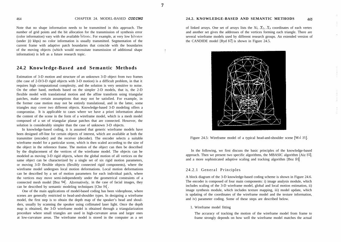
7
464 CHAPTER 24. MODEL-BASED CODING
Note that no shape information needs to be transmitted in this approach. Thenumber of grid points and the bit allocation for the transmission of synthesis error(color information) vary with the available bitrate. For example, at very low bitrates(under 10 kbps) no color information is usually transmitted. Segmentation of thecurrent frame with adaptive patch boundaries that coincide with the boundariesof the moving objects (which would necessitate transmission of additional shapeinformation) is left as a future research topic.
24.2 Knowledge-Based and Semantic Methods
Estimation of 3-D motion and structure of an unknown 3-D object from two frames(the case of 2-D/3-D rigid objects with 3-D motion) is a difficult problem, in that itrequires high computational complexity, and the solution is very sensitive to noise.On the other hand, methods based on the simpler 2-D models, that is, the 2-Dflexible model with translational motion and the affine transform using triangularpatches, make certain assumptions that may not be satisfied. For example, inthe former case motion may not be entirely translational, and in the latter, sometriangles may cover two different objects. Knowledge-based 3-D modeling offers acompromise. It is applicable to cases where we have a priori information aboutthe content of the scene in the form of a wireframe model, which is a mesh modelcomposed of a set of triangular planar patches that are connected. However, thesolution is considerably simpler than the case of unknown 3-D objects.
In knowledge-based coding, it is assumed that generic wireframe models havebeen designed off-line for certain objects of interest, which are available at both thetransmitter (encoder) and the receiver (decoder). The encoder selects a suitablewireframe model for a particular scene, which is then scaled according to the size ofthe object in the reference frame. The motion of the object can then be describedby the displacement of the vertices of the wireframe model. The objects can bemodeled as moving 3-D rigid objects, where the global motion of all vertices on thesame object can be characterized by a single set of six rigid motion parameters,or moving 3-D flexible objects (flexibly connected rigid components), where thewireframe model undergoes local motion deformations. Local motion deformationscan be described by a set of motion parameters for each individual patch, wherethe vertices may move semi-independently under the geometrical constraints of aconnected mesh model [Boz 941. Alternatively, in the case of facial images, theycan be described by semantic modeling techniques [Cho 941.
One of the main applications of model-based coding has been videophone, wherescenes are generally restricted to head-and-shoulder types. In designing a wireframemodel, the first step is to obtain the depth map of the speaker’s head and shoul-ders, usually by scanning the speaker using collimated laser light. Once the depthmap is obtained, the 3-D wireframe model is obtained through a triangularizationprocedure where small triangles are used in high-curvature areas and larger onesat low-curvature areas. The wireframe model is stored in the computer as a set
24.2. KNOWLEDGE-BASED AND SEMANTIC METHODS 465
of linked arrays. One set of arrays lists the Xi, X2, Xs coordinates of each vertexand another set gives the addresses of the vertices forming each triangle. There areseveral wireframe models used by different research groups. An extended version ofthe CANDIDE model [Ryd 871 is shown in Figure 24.5.
Figure 24.5: Wireframe model of a typical head-and-shoulder scene [We1 911.
In the following, we first discuss the basic principles of the knowledge-basedapproach. Then we present two specific algorithms, the MBASIC algorithm [Aiz 931,and a more sophisticated adaptive scaling and tracking algorithm [Boz 941.
24.2.1 General Principles
A block diagram of the 3-D knowledge-based coding scheme is shown in Figure 24.6.The encoder is composed of four main components: i) image analysis module, whichincludes scaling of the 3-D wireframe model, global and local motion estimation, ii)image synthesis module, which includes texture mapping, iii) model update, whichis updating of the coordinates of the wireframe model and the texture information,and iv) parameter coding. Some of these steps are described below.
1. Wireframe model fitting
The accuracy of tracking the motion of the wireframe model from frame toframe strongly depends on how well the wireframe model matches the actual
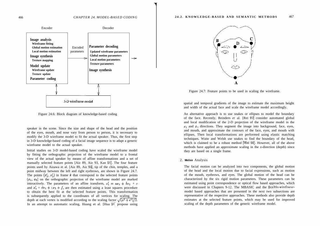
466
Encoder
Image analysisWireframe fittingGlobal motion estimationLocal motion estimation
Image synthesisTexture mapping
Model updateWireframe updateTexture update
Parameter coding
H f
CHAPTER 24. MODEL-BASED CODING
Encodedparameters
>
Decoder
Parameter decodingUpdated wireframe parametersGlobal motion parametersLocal motion parametersTexture parameters
Image synthesis
Figure 24.6: Block diagram of knowledge-based coding
2 4 . 2 . K N O W L E D G E - B A S E D A N D S E M A N T I C M E T H O D S 467
speaker in the scene. Since the size and shape of the head and the positionof the eyes, mouth, and nose vary from person to person, it is necessary tomodify the 3-D wireframe model to fit the actual speaker. Thus, the first stepin 3-D knowledge-based coding of a facial image sequence is to adapt a genericwireframe model to the actual speaker.
Initial studies on 3-D model-based coding have scaled the wireframe modelby fitting the orthographic projection of the wireframe model to a frontalview of the actual speaker by means of affine transformations and a set ofmanually selected feature points [Aiz 89, Aiz 93, Kan 911. The four featurepoints used by Aizawa et al. [Aiz 89, Aiz 931, tip of the chin, temples, and apoint midway between the left and right eyebrows, are shown in Figure 24.7.The points (z;, ~5) in frame le that correspond to the selected feature points(21, ~2) on the orthographic projection of the wireframe model are markedinteractively. The parameters of an affine transform, X: = aal + bxz + cand Z; = CEzl + ez2 + f, are then estimated using a least squares procedureto obtain the best fit at the selected feature points. This transformationis subsequently applied to the coordinates of all vertices for scaling. Thedepth at each vertex is modified according to the scaling factor dw.In an attempt to automatic scaling, Huang et al. [Hua 911 propose using
Figure 24.7: Feature points to be used in scaling the wireframe.
spatial and temporal gradients of the image to estimate the maximum heightand width of the actual face and scale the wireframe model accordingly.
An alternative approach is to use snakes or ellipses to model the boundaryof the face. Recently, Reinders et al. [Rei 921 consider automated globaland local modification of the 2-D projection of the wireframe model in the~1 and x2 directions. They segment the image into background, face, eyes,and mouth, and approximate the contours of the face, eyes, and mouth withellipses. Then local transformations are performed using elastic matchingtechniques. Waite and Welsh use snakes to find the boundary of the head,which is claimed to be a robust method [We1 901. However, all of the abovemethods have applied an approximate scaling in the z-direction (depth) sincethey are based on a single frame.
2. Motion Analysis
The facial motion can be analyzed into two components, the global motionof the head and the local motion due to facial expressions, such as motionof the mouth, eyebrows, and eyes. The global motion of the head can becharacterized by the six rigid motion parameters. These parameters can beestimated using point correspondence or optical flow based approaches, whichwere discussed in Chapters 9-12. The MBASIC and the flexible-wireframe-model based approaches that are presented in the next two subsections arerepresentative of the respective approaches. These methods also provide depthestimates at the selected feature points, which may be used for improvedscaling of the depth parameters of the generic wireframe model.
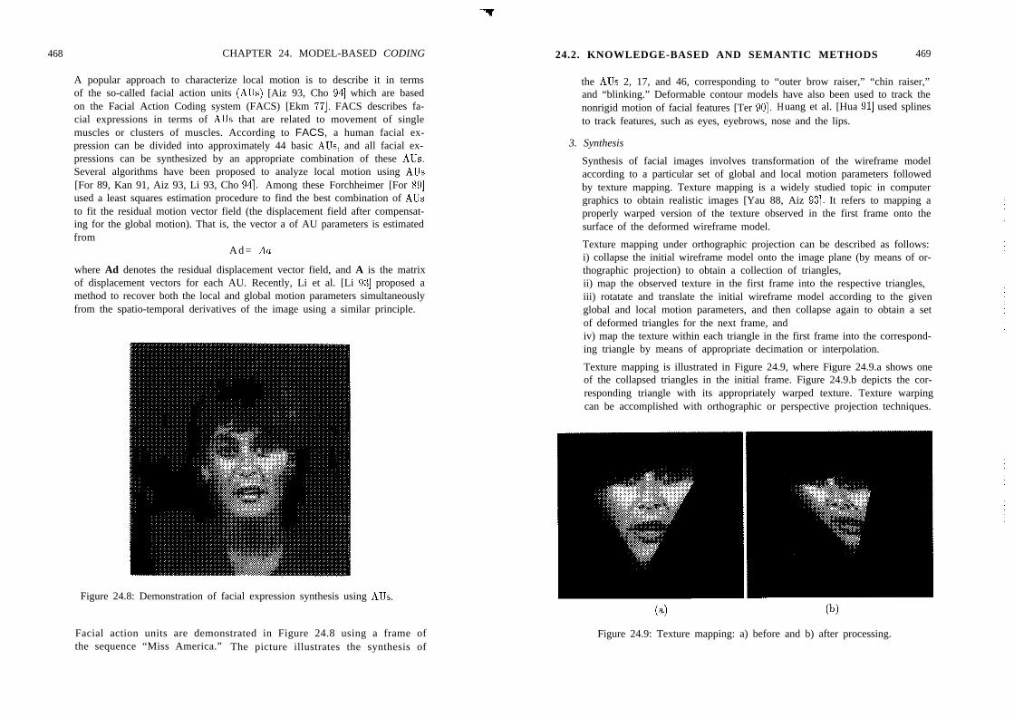
468 CHAPTER 24. MODEL-BASED CODING
A popular approach to characterize local motion is to describe it in termsof the so-called facial action units (AUs) [Aiz 93, Cho 941 which are basedon the Facial Action Coding system (FACS) [Ekm 771. FACS describes fa-cial expressions in terms of AUs that are related to movement of singlemuscles or clusters of muscles. According to FACS, a human facial ex-pression can be divided into approximately 44 basic AUs, and all facial ex-pressions can be synthesized by an appropriate combination of these AUs.Several algorithms have been proposed to analyze local motion using AUs[For 89, Kan 91, Aiz 93, Li 93, Cho 941. Among these Forchheimer [For 891used a least squares estimation procedure to find the best combination of AUsto fit the residual motion vector field (the displacement field after compensat-ing for the global motion). That is, the vector a of AU parameters is estimatedfrom
A d = Aa
where Ad denotes the residual displacement vector field, and A is the matrixof displacement vectors for each AU. Recently, Li et al. [Li 931 proposed amethod to recover both the local and global motion parameters simultaneouslyfrom the spatio-temporal derivatives of the image using a similar principle.
Figure 24.8: Demonstration of facial expression synthesis using AUs.
Facial action units are demonstrated in Figure 24.8 using a frame ofthe sequence “Miss America.” The picture illustrates the synthesis of
24.2. KNOWLEDGE-BASED AND SEMANTIC METHODS 469
the AUs 2, 17, and 46, corresponding to “outer brow raiser,” “chin raiser,”and “blinking.” Deformable contour models have also been used to track thenonrigid motion of facial features [Ter 901. Huang et al. [Hua 911 used splinesto track features, such as eyes, eyebrows, nose and the lips.
3. Synthesis
Synthesis of facial images involves transformation of the wireframe modelaccording to a particular set of global and local motion parameters followedby texture mapping. Texture mapping is a widely studied topic in computergraphics to obtain realistic images [Yau 88, Aiz 931. It refers to mapping aproperly warped version of the texture observed in the first frame onto thesurface of the deformed wireframe model.
Texture mapping under orthographic projection can be described as follows:i) collapse the initial wireframe model onto the image plane (by means of or-thographic projection) to obtain a collection of triangles,ii) map the observed texture in the first frame into the respective triangles,iii) rotatate and translate the initial wireframe model according to the givenglobal and local motion parameters, and then collapse again to obtain a setof deformed triangles for the next frame, andiv) map the texture within each triangle in the first frame into the correspond-ing triangle by means of appropriate decimation or interpolation.
Texture mapping is illustrated in Figure 24.9, where Figure 24.9.a shows oneof the collapsed triangles in the initial frame. Figure 24.9.b depicts the cor-responding triangle with its appropriately warped texture. Texture warpingcan be accomplished with orthographic or perspective projection techniques.
(4 (b)Figure 24.9: Texture mapping: a) before and b) after processing.
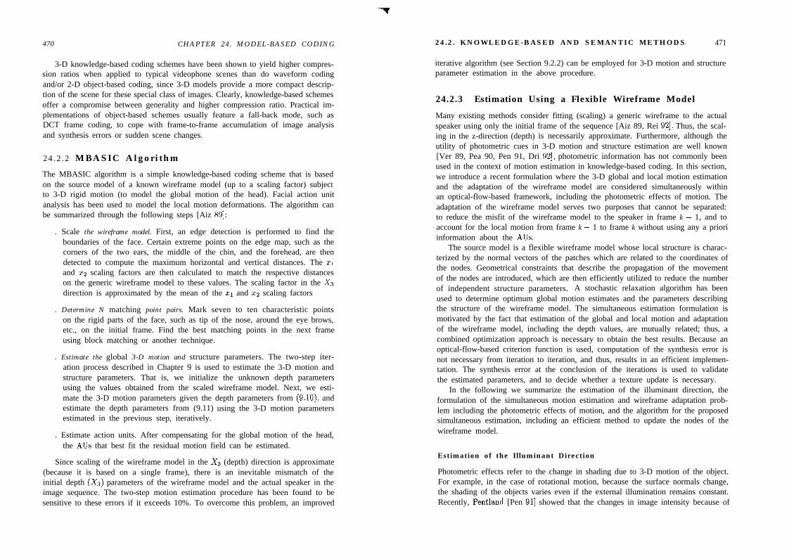
470 CHAPTER 24. MODEL-BASED CODING
3-D knowledge-based coding schemes have been shown to yield higher compres-sion ratios when applied to typical videophone scenes than do waveform codingand/or 2-D object-based coding, since 3-D models provide a more compact descrip-tion of the scene for these special class of images. Clearly, knowledge-based schemesoffer a compromise between generality and higher compression ratio. Practical im-plementations of object-based schemes usually feature a fall-back mode, such asDCT frame coding, to cope with frame-to-frame accumulation of image analysisand synthesis errors or sudden scene changes.
24 .2 .2 MBASIC Algori thm
The MBASIC algorithm is a simple knowledge-based coding scheme that is basedon the source model of a known wireframe model (up to a scaling factor) subjectto 3-D rigid motion (to model the global motion of the head). Facial action unitanalysis has been used to model the local motion deformations. The algorithm canbe summarized through the following steps [Aiz 891:
. Scale the wireframe model. First, an edge detection is performed to find theboundaries of the face. Certain extreme points on the edge map, such as thecorners of the two ears, the middle of the chin, and the forehead, are thendetected to compute the maximum horizontal and vertical distances. The ~1and 22 scaling factors are then calculated to match the respective distanceson the generic wireframe model to these values. The scaling factor in the Xadirection is approximated by the mean of the ~1 and ~2 scaling factors
. Determine N matching point pairs. Mark seven to ten characteristic pointson the rigid parts of the face, such as tip of the nose, around the eye brows,etc., on the initial frame. Find the best matching points in the next frameusing block matching or another technique.
. Estimate the global 3-D motion and structure parameters. The two-step iter-ation process described in Chapter 9 is used to estimate the 3-D motion andstructure parameters. That is, we initialize the unknown depth parametersusing the values obtained from the scaled wireframe model. Next, we esti-mate the 3-D motion parameters given the depth parameters from (9.10), andestimate the depth parameters from (9.11) using the 3-D motion parametersestimated in the previous step, iteratively.
. Estimate action units. After compensating for the global motion of the head,the AUs that best fit the residual motion field can be estimated.
Since scaling of the wireframe model in the Xs (depth) direction is approximate(because it is based on a single frame), there is an inevitable mismatch of theinitial depth (Xs) parameters of the wireframe model and the actual speaker in theimage sequence. The two-step motion estimation procedure has been found to besensitive to these errors if it exceeds 10%. To overcome this problem, an improved
24.2. KNOWLEDGE-BASED AND SEMANTIC METHODS 471
iterative algorithm (see Section 9.2.2) can be employed for 3-D motion and structureparameter estimation in the above procedure.
24.2.3 Estimation Using a Flexible Wireframe Model
Many existing methods consider fitting (scaling) a generic wireframe to the actualspeaker using only the initial frame of the sequence [Aiz 89, Rei 921. Thus, the scal-ing in the z-direction (depth) is necessarily approximate. Furthermore, although theutility of photometric cues in 3-D motion and structure estimation are well known[Ver 89, Pea 90, Pen 91, Dri 921, photometric information has not commonly beenused in the context of motion estimation in knowledge-based coding. In this section,we introduce a recent formulation where the 3-D global and local motion estimationand the adaptation of the wireframe model are considered simultaneously withinan optical-flow-based framework, including the photometric effects of motion. Theadaptation of the wireframe model serves two purposes that cannot be separated:to reduce the misfit of the wireframe model to the speaker in frame k - 1, and toaccount for the local motion from frame k - 1 to frame k without using any a prioriinformation about the AUs.
The source model is a flexible wireframe model whose local structure is charac-terized by the normal vectors of the patches which are related to the coordinates ofthe nodes. Geometrical constraints that describe the propagation of the movementof the nodes are introduced, which are then efficiently utilized to reduce the numberof independent structure parameters. A stochastic relaxation algorithm has beenused to determine optimum global motion estimates and the parameters describingthe structure of the wireframe model. The simultaneous estimation formulation ismotivated by the fact that estimation of the global and local motion and adaptationof the wireframe model, including the depth values, are mutually related; thus, acombined optimization approach is necessary to obtain the best results. Because anoptical-flow-based criterion function is used, computation of the synthesis error isnot necessary from iteration to iteration, and thus, results in an efficient implemen-tation. The synthesis error at the conclusion of the iterations is used to validatethe estimated parameters, and to decide whether a texture update is necessary.
In the following we summarize the estimation of the illuminant direction, theformulation of the simultaneous motion estimation and wireframe adaptation prob-lem including the photometric effects of motion, and the algorithm for the proposedsimultaneous estimation, including an efficient method to update the nodes of thewireframe model.
Estimation of the Illuminant Direction
Photometric effects refer to the change in shading due to 3-D motion of the object.For example, in the case of rotational motion, because the surface normals change,the shading of the objects varies even if the external illumination remains constant.Recently, Pentland [Pen 911 showed that the changes in image intensity because of
CHAPTER 24. MODEL-BASED CODING
photometric effects can dominate intensity changes due to the geometric effects ofmotion (changes in projected surface geometry due to 3-D motion). Similar discus-sions can be found in [Ver 89, Pea 90, Dri 921. Here we briefly discuss estimation ofthe illuminant direction with the aim of incorporating photometric effects into theabove optical-flow-based formulation.
Recall from Section 2.3 that the image intensity s,(xi, x2, t) can be expressed as
4x1, xz, t) = pN(t) . L (24.1)
where L = (Li, Lz, Ls) is the unit vector in the mean illuminant direction and Nis the unit surface normal of the scene at position (Xl, Xz, Xs(Xi, X2)) given by
N(t) = (-P, -4, l)/(p2 + q2 + l)l” (24.2)
CL&and p = al, and q = $$ are the partial derivatives of depth X~(Q,Q) withrespect to the image coord&ates 21 and x2, respectively.
Note that the illuminant direction L can also be expressed in terms of tilt andslant angles as
L = (L1 , L2, L3) = (cos T sin r, sin r sin q, cos fl) (24.3)
where T, the tilt angle of the illuminant, is the angle between L and the X1 - Xsplane, and a, the slant angle, is the angle between L and the positive Xs axis. Inorder to incorporate the photometric effects of motion into 3-D knowledge-basedcoding, the illuminant direction L must be known or estimated from the availableframes.
A method to estimate the tilt and slant angles of the illuminant, based onapproximating the 3-D surface by spherical patches, was proposed by Zheng et al.[Zhe 911. They estimate the tilt angle as
24.2. KNOWLEDGE-BASED AND SEMANTIC METHODS 473
(24.4)
where E{.} denotes expectation over the spatial variables (which is approximatedby 4 x 4 local averaging), and ir and &J are the xi and 22 components of the localestimate of the tilt of the illuminant, respectively, computed as
Here, SIi, i = 1, , N is the difference in image intensity along a particular direc-tion (&ii, Sxs;), and N is the number of directions (typically N = 8 for each 4 x 4window).
The slant angle d can be uniquely estimated from
gq = f3(4 (24.5)
since fs(g) (defined in [Zhe 911)is a monotonically decreasing function of u, whereE(Z) and E(1’) are the expected values of the image intensities and the squareof the image intensities, respectively, estimated from the image area where thewireframe model is fitted.
Finally, the surface albedo can be estimated from
E(I) fl(U) + E{W . h(u)P=
fi"(fl) + Mu)(24.6)
where fr(a) and fz(g) are seventh-order polynomials in cos (T as defined in [Zhe 911.
Incorporation of the Photometric Effects into the OFE
Since we represent the 3-D structure of a head-and-shoulders scene by a wireframemodel and the surface of the wireframe model is composed of planar patches, thevariation in the intensity of a pixel due to photometric effects of motion will berelated to a change in the normal vector of the patch to which this pixel belongs.
Assuming that the mean illuminant direction L = (Li, Lz, Ls) remains constant,we can represent the change in intensity due to photometric effects of motion, basedon the photometric model (2.32), as
dsc(xl,m,t) dN
dt=pL.x (24.7)
Then, substituting Equations (24.7) and (2.33) into the optical flow equation (5.5),and expressing 2-D velocities in terms of the 3-D motion parameters, we includethe photometric effects into the optical-flow-based formulation as [Boz 941
(24.8)
The term on the right-hand side of Equation (24.8) may be significant, especially ifthe change in the surface normal has components either toward or away from theilluminant direction [Pen 911.
Structure of the Wireframe Model
Next, we introduce geometrical constraints about the structure of the wireframemodel and discuss formulation of the simultaneous estimation problem. The wire-frame model is composed of triangular patches which are characterized by the

474 CHAPTER 24. MODEL-BASED CODING
(Xi, X2) Xs) coordinates of their respective vertices. Given the (Xl, Xs, Xs) co-ordinates of the vertices of a patch, we can write the equation of the plane contain-ing this patch. Let Pii’ = (Xii’, X$‘, X$‘), Pii) = (Xl:)‘, X!$, Xti)‘, and pii) z(X:23), X!$, X$) denote the vertices of the ith patch, and Pci) = (Xii), Xt), Xt’)be any point on this patch. Then,
p(i;p,ii) (pppp x pp&)) = 0
gives the equation of the plane containing P!i’, Pii’ and P3(i), where P(i)P1 )- (9
pp@1 , and p(i&(i)3 1 are the vectors from the former point to the latter, respec-
tively. We can express this equation in the form
$1 = pix;i) + 4ix(i) + C.2 2 (24.9)
where
and
Using Equation (24.9), the Xs coordinate of any point on the ith patch can beexpressed in terms of the parameters pi, qi, and ci and the Xi and Xs coordinatesof the point. Then, we can eliminate Xs from Equation (24.8) by substituting (24.9)into (24.8) with Xji) = z?‘, Xp) = z$‘, where the patch index i is determined foreach (~1) ~2) according to the orthographic projection.
It is important to note that the parameters pi, qi, and ca of each planar patch ofthe wireframe are not completely independent of each other. Each triangular patchis either surrounded by two (if it is on the boundary of the wireframe) or threeother triangles. The requirement that the neighboring patches must intersect at astraight line imposes a constraint on the structure parameters of these patches inthe form
p,z(,ij)2 + q.ay) + ci = pjc(lij) + *jzy) + cj2 (24.10)
where pj, ~j, and cj denote the parameters of the jth patch, and (~‘lij), zF’) denotethe coordinates of a point that lie at the intersection of the ith and jth patches.
24.2. KNOWLEDGE-BASED AND SEMANTIC METHODS 475
Problem Statement
The 3-D global motion parameters 01, Rs, Qs, VI, Vz, and the structure parameterspi, pi, ci, can be simultaneously estimated by minimizing the sum square error inthe optical flow equation (24.8) over all pixels in a frame, given by
(24.11)
where
4x1, x2) = %(fi3x2 - ~2(PiZl + qizz + Ci) + vl)
+$(-Q381 + ~1(w1+ qiz2 + Ci) + V2) + 2
-P(h, Lz, J53) ((-;y,“;,-*J) (-Pi, -Qis 1)
((I332 + (S)” + 1)1/Z - (P” + Qi2 + 1p1with respect to Ri, Rs, Q, VI, Vz, pi, pi, ci, and i = 1,. . .,number of patches,subject to the geometrical constraints given by (24.10). It is assumed that the valuesof p and (Li, L2, Ls) are estimated a priori. The constraints, Equation (24.10)) notonly enable us to preserve the structure of the wireframe during the adaptation, butalso facilitate reducing the number of independent unknowns in the optimizationprocess, as described in the following.
The Algorithm
The criterion function E, defined by Equation (24.11), can be minimized usinga stochastic relaxation algorithm (see Chapter 8) to find the global optima ofQi, Qs, 523, VI, Vz, pi, pi, ci. Each iteration consists of perturbing the stateof the system in some random fashion in a manner consistent with the constraintequations (24.10). The constraints are enforced as follows: At each iteration cycle,we visit all patches of the wireframe model in sequential order. If, at the presentiteration cycle, none of the neighboring patches of patch i has yet been visited (e.g.,the initial patch), then pi, pi, ci are all independently perturbed. If only one of theneighboring patches, say patch j, has been visited (pj , qj) cj have already been up-dated), then two of the parameters, say pi and qi, are independent and perturbed.The dependent variable ci is computed from Equation (24.10) as
C. = pp.(;l’j) + q.zy)3 + C. _ p.“(;ij)3 2 _ q.zp8 (24.12)
where (,$‘, $6s ) is one of the nodes common to both patches i and j that is eitherin the boundary or has already been updated in the present iteration cycle. If twoof the neighboring patches, say patches j and I%, have already been visited, i.e., thevariables pj ) qj, cj and pk, qk, c,$ have been updated, then only one variable, say pi,
476 CHAPTER 24. MODEL-BASED CODING
is independent and perturbed. In this case, ci can be found from Equation (24.12),and pi can be evaluated as
pk x jik) + q.p + Ck - pie,(ik)3 - Ck
4i =,$k)
(24.13)
where (z(li’), xcik)z ) is one of the nodes common to both patches i and k that is eitherin the boundary or has already been updated in the present iteration cycle.
The perturbation of the structure parameters pi, pi, and c; for each patch i re-sults in a change in the coordinates of the nodes of the updated wireframe. The newcoordinates (Xi”‘, Xp), (n’X, ) of the node n can be computed given the updatedstructure parameters of three patches that intersect at node n. Let the patches i,j, and k intersect at node n. Then the relations
p.xp + qiX@) + ci = pjxp + qjxp + cj
&‘a$) + y,x;) + ci = PkXin) + qkxp) + Ck
specify Xin) and Xc”). Therefore,2
(24.14)
(24.15)
The new Xp) can be computed from Equation (24.9) given Xin), X$“), and thepi, q;, ci for any patch passing through that node. It is this updating of thecoordinates of the nodes that allows the adaptation of the wireframe model tolower the misfit error and accommodate the presence of local motion, such as themotion of the eyes and the mouth.
The proposed algorithm can be summarized as follows:
increment count-j, for all j denoting neighbors of patch 1.for( i=2 to number of patches)
cif(count-i==l) C
Perturb p-i and q-i.Increment count-m, for all m denoting neighbors of patch i.Compute c-i using Equation 24.12, where x-ij and y-ij arethe coordinates of a fixed or a precomputed node onthe line of intersection between patches i and j. )
1. Estimate the illumination direction using Equations (24.4) and (24.5), andthe surface albedo using Equation (24.6).
2. Initialize the coordinates (X,‘“‘, Xp) (fi), X, ), of all nodes n, using an approx-imately scaled initial wireframe model. Determine the initial values of pi, pi,and ci for all patches. Set the iteration counter m = 0.
if(count-i==2) CPerturb p-i.
3. Determine the initial motion estimates using Equation (9.10) based on a setof selected feature correspondences and their depth values obtained from thewireframe model.
Increment count-m, for all m denoting neighbors of patch i.Compute c-i using Equation 24.12 and q-i using Equation 24.where (x-ij,y-ij) and (x-ik,y-ik) denote coordinates ofa fixed or a precomputed node on the line of intersectionbetween patches i,j and i,k respectively. 1
4. Compute the value of the cost function E given by (24.11).
5. If E < E, stop.
If p-i, q-i, and c-i for at least three patches intersectingat a node are updated, then update the coordinates of the nodeby using Equation 24.15.1
Else, set m = m + 1, and 6. Go to (4).
24.2. KNOWLEDGE-BASED AND SEMANTIC METHODS
Perturb the motion parameters 0 = [Qi 02 Qs VI VzlT as
n(m) - dm-l) + amA,
477
(24.16)
where the components of A are zero-mean Gaussian with the variance&“) = E; and the structure parameters pi, ~a, and ci through the procedure:
Define count-i as the number of neighboring patches to patch iwhose structure parameters have been perturbed. Set count-i=O,for all patches i.Perturb p-1, q-l, c-1 as
Pi”’ p’l”-” + omAl
dm) q(l’+ + omAl
c(ln) c(lm-l) + amAl (24.17)
where Ai = Ni(O, $‘“‘), i.e., zero mean Gaussian with variance r$ (ml , wherez(m) _
‘Ti -c(z,y)epatch i e?(2, Y).
13,
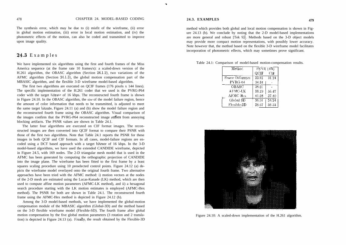
478 CHAPTER 24. MODEL-BASED CODING
The synthesis error, which may be due to (i) misfit of the wireframe, (ii) errorin global motion estimation, (iii) error in local motion estimation, and (iv) thephotometric effects of the motion, can also be coded and transmitted to improveupon image quality.
24.3 Examples
We have implemented six algorithms using the first and fourth frames of the MissAmerica sequence (at the frame rate 10 frames/s): a scaled-down version of theH.261 algorithm, the OBASC algorithm (Section 24.1.2)) two variations of theAFMC algorithm (Section 24.1.3), the global motion compensation part of theMBASIC algorithm, and the flexible 3-D wireframe model-based algorithm.
The first two algorithms are executed on QCIF frames (176 pixels x 144 lines).The specific implementation of the H.261 coder that we used is the PVRG-P64coder with the target bitrate of 16 kbps. The reconstructed fourth frame is shownin Figure 24.10. In the OBASC algorithm, the size of the model failure region, hencethe amount of color information that needs to be transmitted, is adjusted to meetthe same target bitrate. Figure 24.11 (a) and (b) show the model failure region andthe reconstructed fourth frame using the OBASC algorithm. Visual comparison ofthe images confirm that the PVRG-P64 reconstructed image suffers from annoyingblocking artifacts. The PSNR values are shown in Table 24.1.
The latter four algorithms are executed on CIF format images. The recon-structed images are then converted into QCIF format to compare their PSNR withthose of the first two algorithms. Note that Table 24.1 reports the PSNR for theseimages in both QCIF and CIF formats. In all cases, model-failure regions are en-coded using a DCT based approach with a target bitrate of 16 kbps. In the 3-Dmodel-based algorithms, we have used the extended CANDIDE wireframe, depictedin Figure 24.5, with 169 nodes. The 2-D triangular mesh model that is used in theAFMC has been generated by computing the orthographic projection of CANDIDEinto the image plane. The wireframe has been fitted to the first frame by a leastsquares scaling procedure using 10 preselected control points. Figure 24.12 (a) de-picts the wireframe model overlayed onto the original fourth frame. Two alternativeapproaches have been tried with the AFMC method: i) motion vectors at the nodesof the 2-D mesh are estimated using the Lucas-Kanade (LK) method, which are thenused to compute affine motion parameters (AFMC-LK method), and ii) a hexagonalsearch procedure starting with the LK motion estimates is employed (AFMC-Hexmethod). The PSNR for both are shown in Table 24.1. The reconstructed fourthframe using the AFMC-Hex method is depicted in Figure 24.12 (b).
Among the 3-D model-based methods, we have implemented the global-motioncompensation module of the MBASIC algorithm (Global-3D) and the method basedon the 3-D flexible wireframe model (Flexible-SD). The fourth frame after globalmotion compensation by the five global motion parameters (3 rotation and 2 transla-tion) is depicted in Figure 24.13 (a). Finally, the result obtained by the Flexible-3D
24.3. EXAMPLES 479
method which provides both global and local motion compensation is shown in Fig-ure 24.13 (b). We conclude by noting that the 2-D model-based implementationsare more general and robust [Tek 951. Methods based on the 3-D object modelsmay provide more compact motion representations, with possibly lower accuracy.Note however that, the method based on the flexible 3-D wireframe model facilitatesincorporation of photometric effects, which may sometimes prove significant.
Table 24.1: Comparison of model-based motion-compensation results.
Figure 24.10: A scaled-down implementation of the H.261 algorithm.

480 CHAPTER 24. MODEL-BASED CODING
.
24.3. EXAMPLES
Figure 24.11: Flexible 2-D object based method: a) the model-failure region and b)the decoded the third frame of Miss America. (Courtesy Francoise Aurtenechea)
Figure 24.12: 2-D object-based coding using deformable mesh models: a) an irreg-ular mesh fitted to the first frame of Miss America and b) the decoded third frame.(Courtesy Yucel Altunbasak)
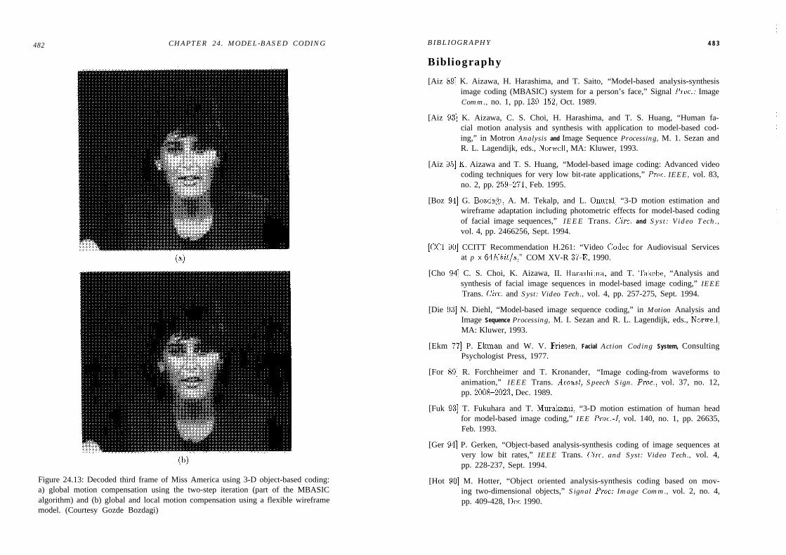
482 CHAPTER 24. MODEL-BASED CODING
(b)
Figure 24.13: Decoded third frame of Miss America using 3-D object-based coding:a) global motion compensation using the two-step iteration (part of the MBASICalgorithm) and (b) global and local motion compensation using a flexible wireframemodel. (Courtesy Gozde Bozdagi)
BIBLIOGRAPHY
Bibliography
4 8 3
[Aiz 891 K. Aizawa, H. Harashima, and T. Saito, “Model-based analysis-synthesisimage coding (MBASIC) system for a person’s face,” Signal Proc.: ImageComm., no. 1, pp. 139-152, Oct. 1989.
[Aiz 931 K. Aizawa, C. S. Choi, H. Harashima, and T. S. Huang, “Human fa-cial motion analysis and synthesis with application to model-based cod-ing,” in Motron Analysis and Image Sequence Processing, M. 1. Sezan andR. L. Lagendijk, eds., Norwell, MA: Kluwer, 1993.
[Aiz 951 K. Aizawa and T. S. Huang, “Model-based image coding: Advanced videocoding techniques for very low bit-rate applications,” Proc. IEEE, vol. 83,no. 2, pp. 2599271, Feb. 1995.
[Boz 941 G. Bozdagr, A. M. Tekalp, and L. Onural, “3-D motion estimation andwireframe adaptation including photometric effects for model-based codingof facial image sequences,” IEEE Trans. Circ. and Syst: Video Tech.,vol. 4, pp. 2466256, Sept. 1994.
[CC1 901 CCITT Recommendation H.261: “Video Codec for Audiovisual Servicesat p x 64Kbitfs,” COM XV-R 37-E) 1990.
[Cho 941 C. S. Choi, K. Aizawa, II. IIarashima, and T. Takebe, “Analysis andsynthesis of facial image sequences in model-based image coding,” IEEETrans. Circ. and Syst: Video Tech., vol. 4, pp. 257-275, Sept. 1994.
[Die 931 N. Diehl, “Model-based image sequence coding,” in Motion Analysis andImage Sequence Processing, M. I. Sezan and R. L. Lagendijk, eds., Norwell,MA: Kluwer, 1993.
[Ekm 771 P. Ekman and W. V. Friesen, Facial Action Coding System, ConsultingPsychologist Press, 1977.
[For $91 R. Forchheimer and T. Kronander, “Image coding-from waveforms toanimation,” IEEE Trans. Acousl, Speech Sign. Proc., vol. 37, no. 12,pp. 2008-2023, Dec. 1989.
[Fuk 931 T. Fukuhara and T. Murakami, “3-D motion estimation of human headfor model-based image coding,” IEE Proc.-I, vol. 140, no. 1, pp. 26635,Feb. 1993.
[Ger 941 P. Gerken, “Object-based analysis-synthesis coding of image sequences atvery low bit rates,” IEEE Trans. Circ. and Syst: Video Tech., vol. 4,pp. 228-237, Sept. 1994.
[Hot 901 M. Hotter, “Object oriented analysis-synthesis coding based on mov-ing two-dimensional objects,” Signal Proc: Image Comm., vol. 2, no. 4,pp. 409-428, Dee 1990.

484 BIBLIOGRAPHY
[Hua 911 T. S. Huang, S. C. Reddy, and K. Aizawa, “Human facial motion mod-eling, analysis, and synthesis for video compression,” SPIE Vis. Comm.and Image Proc’91, vol. 1605, pp. 234-241, Nov. 1991.
[Kan 861 K. Kanatani, “Structure and motion from optical flow under orthographicprojection,” Comp. Vis. Graph. Image Proc., vol. 35, pp. 181-199, 1986.
[Kan 911 M. Kaneko, A. Koike, and Y. Hatori, “Coding of facial image sequencebased on a 3D model of the head and motion detection,” J. Visual Comm.and Image Rep., vol. 2, no. 1, pp. 39954, March 1991.
[Kla 861 B. Klaus and I’. Horn, Robot Vision, Cambridge, MA: MIT Press, 1986
[Koc 931 R. Koch, “Dynamic 3-D scene analysis through synthesis feedback con-trol,” IEEE Trans. Patt. Anal. Mach. Intel., vol. 15, pp. 556-568,June 1993.
[Lav 901 F. Lavagetto and S. Zappatore, “Customized wireframe modeling for facialimage coding,” Thrrd Int. Workshop on 64kbits/s Coding of Moving Video,1990.
[Lee 891 H. Lee and A. Rosenfeld, “Improved methods of estimating shape fromshading using light source coordinate system,” in Shape from Shading, B.K. P. Horn and M. J. Brooks, eds., pp. 323-569, Cambridge, MA: MITPress, 1989.
[Li 931 H. Li, P. Roivainen, and R. Forchheimer, “3-D motion estimation in model-based facial image coding,” IEEE Trans. Pall. Anal. Mach. Intel., vol. 15,no. 6, pp. 5455555, June 1993.
[Li 941 H. Li, A. Lundmark, and R. Forchheimer, “Image sequence coding at verylow bitrates: A Review,” IEEE Trans. Image Proc., vol. 3, pp. 5899609,Sept. 1994.
[Mor 911 H. Morikawa and H. Harashima, “3D structure extraction coding of imagesequences,” J. Visual Comm. and Image Rep., vol. 2, no. 4, pp. 332-344,Dec. 1991.
[Mus 891 H. G. Musmann, M. Hotter, and J. Ostermann, “Object-oriented analysissynthesis coding of moving images,” Signal Proc: Image Comm., vol. 1,pp. 117-138,1989.
[Nak 941 Y. Nakaya and H. Harashima, “Motion compensation based on spa-tial transformations,” IEEE Trans. Circ. and Syst.: Video Tech., vol. 4,pp. 3399356, June 1994.
[Ost 901 J. Ostermann, “Modeling of 3D moving objects for an analysis-synthesiscoder ,” in Sensing and Reconstruction of Three-Dimensional Objects,B. Girod, ed., Proc. SPIE, vol. 1260, pp. 240-249, 1990.
BIBLIOGRAPHY
[Ost 931 J. Ostermann, “An analysis-synthesis coder based on moving flexible 3-Dobjects,” Proc. Pitt. Cod. Symp., Lausanne, Switzerland, Mar. 1993.
[Pea 901 D. Pearson, “Texture mapping in model-based image coding,” Signal Pro-cessing: Image Comm., vol. 2, pp. 377-395, 1990.
[Pen 821 A. Pentland, “Finding the illuminant direction,” J. Opt. Sot. Am.,vol. 72, pp. 4488455, April 1982.
[Pen 911 A. Pentland, “Photometric motion,” IEEE Trans. Patt. Anal. Mach. In-tel., vol. PAMI-13, no. 9, pp. 879-890, Sept. 1991.
[Rei 921 M. J. T. Reinders, B. Sankur, and J. C. A. van der Lubbe, “Transformationof a general 3D facial model to an actual scene face,” 11th Int. Conf. Patt.Rec., pp. 75579, 1992.
[Ryd 871 M. Rydfalk, “CANDIDE: A parametrised face,” Rep. LiTH-ISY-I-0866,Dept. Elec. Eng., Linkoping Univ., Sweeden, Oct. 1987.
[Sch 931 H. Schiller and M. Hotter, “Investigations on colour coding in an object-oriented analysis-synthesis coder,” Signal Proc.: Image Comm., vol. 5,pp. 319-326, Oct. 1993.
[Ter 901 D. Terzopoulos and K. Waters, “Physically-based facial modeling, analysisand animation,” J. of V’zsua iza zon and Computer, vol. 1, pp. 73380, 1990.1. 2’
[Tek 951 A. M. Tekalp, Y. Altunbasak, and G. Bozdagi, “Two- versus three-dimensional object-based coding,” Proc. SPIE Visual Comm. and ImageProc., Taipei, Taiwan May 1995.
[Wan 941 Y. Wang and 0. Lee, “Active mesh - A feature seeking and trackingimage sequence representation scheme,” IEEE Trans. Image Proc., vol. 3,pp. 610-624, Sept. 1994.
[We1 901 W. J. Welsh, S. Searby, and J. B. Waite, “Model based image coding,”J. Br. Telecom. Tech., vol. 8, no. 3, pp. 94-106, Jul. 1990.
[We1 911 W. J. Welsh, “Model-based coding of videophone images,” Electronics andCommunication Eng. Jour., pp. 29936, Feb. 1991.
[Yau 881 J. F. S. Yau and N. D. Duffy, “A texture mapping approach to 3-D facialimage synthesis,” Computer Graphics Forum, no. 7, pp. 1299134, 1988.
[Zeg 891 K. Zeger and A. Gersho, “Stochastic relaxation algorithm for improvedvector quantizer design,” Electronic Letters, vol. 25, pp. 96698, July 1989.
[Zhe 911 Q. Zheng and R. Chellappa, “Estimation of illuminant direction, albedo,and shape from shading,” IEEE Trans. Patt. Anal. Mach. Intel.,vol. PAMI-13, no. 7, pp. 680-702, July 1991.

7
25.1. VIDEOCONFERENCING
25.1 Videoconferencing
487
Chapter 25
DIGITAL VIDEOSYSTEMS
Developments in broadcasting, computers, communication technologies such as theemergence of better image compression algorithms, optical-fiber networks, fastercomputers, dedicated hardware, and digital recording promise a variety of digitalvideo and image communication products in the very near future. Driving the re-search and development in the field of digital video are the consumer and commercialapplications (ordered according to the bitrate requirement), such as
l Digital TV, including HDTV@ 20 Mbps over 6 Mhz taboo channels
. Multimedia, desktop video@ 1.5 Mbps CD-ROM or hard disk storage
. Videoconferencing@ 384 kbps using p x 64 kbps ISDN channels
. Videophone and mobile image communications@ lo-25 kbps
Other applications include surveillance imaging for military or law enforcement,intelligent vehicle highway systems, harbor traffic control, tine medical imaging,aviation and flight control simulation, and motion picture production. In the fol-lowing, we overview some of these applications in the order in which internationalcompression standards have become/are becoming available for them. In particular,we discuss video communication over ISDN (Integrated Services Digital Network)lines, multimedia in PC and workstation platforms, digital video broadcasting, andlow-bitrate applications, in Sections 25.1 through 25.4, respectively.
486
Videoconferencing using digital techniques has been in existence for some time.Generally speaking, it refers to interactive distance conferencing using ISDN ser-vices with clear sound and sharp full-motion video. Each videoconferencing siteemploys a codec that converts analog video signals to digital and compresses themfor transmission. At the receiver, digital signals are converted back to analog fordisplay.
Early systems required special videoconference rooms with high-cost equipmentand Tl links that operate at 1.544 Mbps. These systems were quite expensive foreveryday use; for example, a typical Tl system would cost $120,000, and the costof a Tl link would be about $750/hour. Advances in video compression and theadoption of the CCITT H.261 standard helped the emergence of several newer andbetter videoconferencing systems which cost about $30,000 to $40,000. The newersystems operate over ISDN lines at p x 64 kbps, ranging from 64 kbps up to 2 Mbps.A typical number for p is 6, putting the bandwidth at 384 kbps. Lower-bandwidthsystems that operate at 64 kbps (56 kbps for video and 8 kbps for audio), knownas desktop ISDN videophones [Ald 931, are also available. In comparison, the costof a 128 kbps line is about $35/hour. Some examples of existing videoconferencingequipment are listed in Table 25.1.
Table 25.1: Available videoconferencing products
VendorBT NorthAmerica
Name Codec Speed Max Frame Comp. Alg.Videocodec 56 and 30 per set H.261vc2200 112 kbpsVideocodec 56 kbps tovc2100 2048 kbps
GPT Video Svstem 261 56 and 30 per set H.261Systems Twin than. 112 kbps
System 261 56 kbps to I
Compres.Labs.NECAmerica
Universal 2048 kbpsRembrandt 56 kbps to 30 per set H.261, CTXII/VP 2048 kbps CTX PlusVisualLink 56 kbps to 30 per set H.261, NEC5000 M20 384 kbpsVisualLink 56 kbps to
proprietary
5000 Ml5 2048 kbpsPictureTel System 4000 56 kbps to 10 per set H.261, SG3Corp.VideoTelecom
cs350768 kbps56 kbps to768 kbps
mono15 per set
SG2/HVQH.261, BlueChip
.
488 CHAPTER 25. DIGITAL VIDEO SYSTEMS
Besides videoconferencing and desktop videophone, video communication usingan ISDN basic rate interface (BRI), operating at a total of 128 kbps, may be usedfor such applications as distance learning and access to multimedia informationservices. In distance learning, an instructor teaches students who are at remotelocations, The students can interact with the instructor, by direct talking or shar-ing a whiteboard [Ald 931. Multimedia information services include image-basedelectronic library systems and shopping-catalogs that can be browsed from home.
25.2 Interactive Video and Multimedia
Multimediacan mean different things to different people. Here it refers to the abilityto provide full-motion interactive digital video in the personal computer (PC) ordesktop workstation environment. Multimedia also involves text, graphics, sound,and still-images, which have long existed in the PC or workstation environment.The main components of a multimedia system are:
. data capture tools, such as video recorders and digitizers,
. data editors and authoring tools, for animation, audio and video editing, user-interface development, etc., and
l database storage and retrieval tools, for searching large databases, archiving,and backup.
The difficulty with full-motion video has been in the large data rates required.Multimedia workstations use CD-ROMs and hard disks for video storage at about1.5 Mbps, which require approximately 3O:l compression of standard TV resolutionimages. The latest developments in image compression make this possible in realtime. Two of the earliest initiatives in this area have been Intel’s digital videointeractive (DVI) technology, and compact disc-interactive (CD-I), jointly fundedby NV Philips and Sony.
DVI technology is a general-purpose hardware for providing full-motion videoin the PC environment, and uses CD-ROM for the storage medium. The designgoal is to provide multimedia functionality at a cost suitable for desktop comput-ers. It is based on two custom VLSI chips: the 82750PB pixel processor and the82750DB display processor. The pixel processor mainly performs compression anddecompression of images along with functions like YUV-RGB conversion, bilinearinterpolation, and so on. It is able to decompress 640 x 480 JPEG encoded im-ages in less than one second. The display processor retrieves decompressed imagesfrom memory, converts them to the format needed for display, and produces timingand control signals to drive various displays. Popular formats such as NTSC, PAL,VGA, and SVGA are supported. This chip set is compatible with 16 or 32 bit mi-croprocessors operating at 6 MHz or higher clock speed, and utilizes 16 Mbyte videoRAM (VRAM). The chip-set is programmable; that is, the compression algorithmscan be modified according to the application.
25.3. DIGITAL TELEVISION 489
The Compact Disc-Interactive (CD-I) system is a CD-based interactive au-dio/video special-purpose computer. It is based on Motorola’s 680X0 processor,and the CD-RTOS, an operating system developed for the CD-I environment. Itsoriginal design was capable of providing full-motion video only on part of the screen.However, full-screen, full-motion video has become available with an add-in module[Mee 921. This module reproduces video from an encoded bitstream with a framerate of 24 Hz, 25 Hz, or 30 Hz. The frame rate converter transforms this videoto 50 Hz or,60 Hz. Finally, the YUV representation of the encoded bitstream isconverted into RGB for display. It includes a number of multimedia capabilities,such as a CD file manager for audio, a user communication manager of the videosystem, and a motion picture file manager. CD-I players currently exist that canbe connected to standard TV sets to play back movies that are recorded on CDs.A full-length feature movie usually requires two CDs.
Recently, almost every computer and workstation manufacturer, including Ap-ple, IBM, SUN, and Silicon Graphics, have added full-motion video capabilities.However, no industry-wide standards have been established yet. Recall that theMPEG-1 video compression standard addresses video compression for multimediastations, but not full compatibility between various multimedia products. As com-puters and communication equipment move closer towards “grand unification,” theline between multimedia systems and videoconferencing and videophone productsis getting more and more blurred; that is, most multimedia systems can now beinterfaced with LAN (Local Area Networks), WAN (Wide Area Networks), ISDN,or ATM (Asynchronous Transfer Mode) networks for interactive desktop videocon-ferencing. At present several companies are introducing plug-in cards and softwarefor videoconferencing over LAN, WAN, and ATM networks. A nice feature of theseproducts is that they provide multiplatform support, so that people using differentworkstations and personal computers may still share a whiteboard, text tools, andfull-motion video.
With the newer generation of higher-speed CD-ROMs and faster processors en-tering the market every day, multimedia remains an active and exciting field. Anemerging technology in interactive multimedia is effective human/machine inter-action. Stereo vision, talker verification, speech synthesis, tactile interaction, andintegration of multiple sensor modalities are active research areas to expand thepresent capabilities for human/machine interaction.
25.3 Digital Television
TV is arguably the most commonly used image communication system in the worldtoday. However, present TV transmission standards are based on technology thatis more than 40 years old. As a result, there has been widespread interest in theconsumer electronics industry to develop more advanced TV systems that benefitfrom recent technological advances. The major advanced TV research programs inthe world are tabulated in Table 25.2.

490 CHAPTER 25. DIGITAL VIDEO SYSTEMS 25.3. DIGITAL TELEVISION 491
Table 25.2: Major programs for HDTV research.
JapanEuropeU.S.A.
NHKEUREKA 95Grand Alliance(AT&T, General Instrument, Mass. Inst. Tech., Philips N. A.David Sarnoff Res. Cen., Thomson Cons. El., Zenith)
Development efforts pioneered by the Japanese in late the 70s and early 80sresulted in hybrid advanced TV systems, with digital processing at the transmitterand receiver but using analog transmission. Later, in the early 90s studies in theU.S. proved the feasibility of the all-digital TV approach, which was believed to beunrealistic not too long ago. All-digital TV will not only offer better image quality,easy conversion between multiple standards, and more channels within the samebandwidth (thanks to advances in digital data compression technology), but moreimportant, it will unite computers with TV sets and telecommunication serviceswith cable TV services in a revolutionary fashion. In the following, we providean overview of the developments around the world that led to the advent of all-digital TV.
25.3.1 Digital Studio Standards
Although the present TV transmission standards are analog (see Chapter l), dig-ital TV signals find routine use in TV studios for image processing and digitalstorage. Digital techniques are commonly used for such tasks as program editing,generating special effects, and standards conversion. Digital storage is preferred atthe production level, because consumer-quality video storage devices, such as VHSrecorders, introduce degradations that are objectionable in the production studioenvironment.
In the following, we first summarize the existing analog TV standards. Thecorresponding CCIR 601 standards for digitization of the respective signals (alsoknown as digital studio standards) are listed in Table 25.3.
. NTSC (National Television Systems Committee) - Accepted for B&W in1941, and extended to color in 1954Used in the USA, Canada, Japan, and Latin America2:l interlace, 4:3 aspect ratio525 lines/frame, 29.97 frames/set (262.5 lines/field, 59.94 fields/set)Perceptually 340 lines/frame, 420 resolvable pels/line (Kell factor)Analog transmission over 6 MHz channelThere are 68 channels assigned in the US: 54-88 MHz (ch 2 to 6), 174-216 MHz(ch 7 to 13), 470-806 MHz (ch14 to 69). However, less than 20 channels areused in a locality to prevent interference.
Table 25.3: CCIR 601 standards.
Format Sampling Field rate Interlace/ Active ActiveFrequency Aspect lines/frame pixels/frameP/U IV)
NTSC 13.516.75 60 2:1/4:3 488 720PAL/ 13.5/6.75 50 2:1/4:3 576 720SECAM
l PAL (Phase Alternation Line) - Accepted in 1967 for color broadcastUsed in most of Europe, and Australia625 lines/frame, 2:l interlace, 50 fields/set, 4:3 aspect ratioAnalog transmission over 8 MHz channel.
l SECAM (Systeme Electronique Color Avec Memoire) - Accepted in 1967 forcolor broadcast, used in France, Russia, and Eastern Europe625 lines/frame, 2:l interlace, 50 fields/set, 4:3 aspect ratioAnalog transmission over 8 MHz channel.
Note that these standards are incompatible with each other, and conversion fromone to another requires digital techniques.
25.3.2 Hybrid Advanced TV Systems
There were several proposals, before the advent of all-digitalTV, that offered variousdegrees of improvements on the quality of present TV systems. We refer to themas “hybrid advanced TV (ATV) systems.” ATV systems generally feature betterspatial and/or temporal resolution, wider screens, improved color rendition, andCD-quality stereo sound. They fall under two broad categories: compatible ATVsystems and incompatible ATV systems.
1) Compatible system proposals may be summarized as follows:
l IDTV (improved definition TV) systems which use digital processing at the re-ceiver for picture quality improvement using existing analog TV transmissionstandards. Picture quality may be improved through: i) spatial and temporalresolution enhancement by nonlinear interpolation to recover super-Nyquistfrequencies, including motion-compensated deinterlacing and frame rate con-version, ii) luminance-chrominance separation to eliminate cross-luminanceand cross-chrominance artifacts due to imperfect Y/C separation in conven-tional NTSC demodulators, and iii) ghost elimination to reduce time-delayed,attenuated, and distorted versions of the TV signal.
l EQTV (extended-quality TV) systems which require transmission of an aug-mentation signal. They include systems that feature 16:9 aspect ratio by
492 CHAPTER 25. DIGITAL VIDEO SYSTEMS 25.3. DIGITAL TELEVISION 493
means of transmitting an augmentation signal at another frequency band.Conventional receivers that do not receive this augmentation signal can dis-play ordinary-quality TV signals.
Early efforts in Europe have been in the direction of EQTV system devel-opment. PAL-plus and D2-MAC are two examples of EQTV systems whichrequire transmission of augmentation signals. They have 16:9 aspect ratio,and are compatible with PAL and MAC (Multiplexed Analog Components),respectively. Note that MAC is a 625/50/2:1 analog satellite transmissionstandard developed by the British around 1970.
2) Incompatible systems are generally known as HDTV (high-definition TV).CCIR 801, adopted in 1990, defines HDTV as follows: “A high definition TV
system is a system designed to allow viewing at about three t&es picture heightsuch that the transmission system is virtually or nearly transparent to the levelof detail that would have been perceived in the original scene by a viewer withaverage visual acuity.” HDTV systems feature a video signal that has about twicethe current resolution in both the horizontal and vertical directions, a wider aspectratio of 16:9, separate luminance and chrominance signals, and CD-quality sound.Initial HDTV proposals, developed first in Japan and later in Europe, were hybrid(mixed analog/digital) systems, which use digital signal/image processing at thetransmitter and receiver, but transmission was by analog means. We elaborate onthese systems below.
ATV in Japan
Studies towards an advanced TV system were started in the 1970s in Japan at theNHK Laboratories. NHK applied to CCIR, a world standards organization, in 1974for the standardization of an analog HDTV format, called the MUSE (Multiplesub-Nyquist Sampling Encoding). CCIR Study Group 11 worked from 1974 to1986 to achieve a single world standard for production and international exchangeof HDTV signals with no apparent success.
The MUSE system is based on a motion adaptive subsampling strategy to reducethe transmission bandwidth requirement by a factor of 3:l. The HDTV signal isdefined by the following parameters:
1125 lines/frame, 60 fields/set, 2:l interlace, 16:9 aspect8.1 MHz DBS transmissionSampling rates: Y at 48.6 MHz and C at 16.2 MHz
It is primarily intended for broadcasting over 24 MHz direct broadcast satellite(DBS) channels, and is not compatible with other transmission standards. Thebasic idea of the MUSE system is motion-adaptive subsampling. That is, if motion isdetected at a certain region, spatial lowpass filtering is applied before subsampling.On the other hand, in still-image areas, subsampling is applied without any low-pass filtering. There is no motion estimation or motion compensation involved
in the MUSE system. Major electronic manufacturers in Japan have participatedin the project and builded mixed analog/digital HDTV receivers. First broadcastusing the MUSE system was realized on Nov. 25, 1991. At present, there are dailyHDTV broadcasts via DBS in Japan.
ATV in Europe
European efforts for HDTV research have been organized under the EUREKA-95project, which resulted in HD-MAC, an analog HDTV standard for DBS trans-mission developed around 1988. While the Japanese advocated an incompatibleHDTV approach, HD-MAC has emerged as a MAC-compatible standard with 1250lines/frame, 50 fields/set, 2:l interlace, and 16:9 aspect ratio.
HD-MAC achieves reduction of bandwidth from 54 MHz to 10.125 MHz byadvanced motion-compensated subsampling. Motion information is transmitteddigitally to assist, the decoding process. The first HD-MAC broadcast was madefrom the 1992 Winter Olympics in France to selected test centers in Europe viaDBS. The HD-MAC system has already been abondoned in Europe in favor ofall-digital systems currently under development in the U.S.A.
25.3.3 All-Digital TVAll-digital TV refers to digital representation and processing of the signal as wellas its digital transmission. The nature of the digital broadcast removes the syn-chronicity and real-time requirements of the analog TV, and offers many differentoptions. A digital TV standard will unify the computer/workstation and TV indus-tries in the future; hence, the introduction of the term “telecomputer.” Although astandard for all-digital HDTV has not yet been formally approved, there is steadyprogress toward the adoption of a standard by the FCC before the end of 1995, andthere are already some companies offering digital TV services conforming with thepresent standards using DBS broadcasting. Digital TV broadcast media include:
l Terrestial broadcast. Direct broadcast satellite. Cable and broadband ISDN distribution
In the U.S., the Federal Communications Commission (FCC) has ruled that theexisting 6 MHz taboo-channels will be used for terrestrial broadcast. For digitalterrestrial transmission, a 6 MHz channel can support about 20 Mbps data ratewith sophisticated digital vestigial sideband modulation. Considering the param-eters of a typical HDTV system, we still need about 545:20 = 28:l compressionto achieve this bitrate. Direct broadcast satellite (DBS) transmission is widelyused in Japan and Europe as an analog transmission medium. In the U.S., somecompanies have already started providing digital TV transmission (at the NTSCresolution) using DBS. Cable distribution systems are heavily employed in the U.S.at present. Each cable channel is allotted 6 MHz, and typically 30 to 50 channels

494 CHAPTER 25. DIGITAL VIDEO SYSTEMS
are available. All adjacent channels can be used. Some cable networks offer limitedtwo-way communication capability where upstream data transmission is allowed.With digital transmission and effective compression, cable companies may offerapproximately 150 channels using the presently available bandwidth. The broad-band ISDN (B-ISDN) offers a unified network capable of providing voice, data,video, LAN, and MAN services [Spe 911. The H4 access provides approximately135 Mbps. Asynchronous transfer mode (ATM) b gis em considered for standard-ization as the multiplexing and switching vehicle of various services. DBS, cable,and B-ISDN services offer the possibility of more advanced video services, such asvideo-on-demand [Spe 951. In the following, we summarize the all-digital HDTVand TV efforts in the U.S.A.
25.3. DIGITAL TELEVISION 495
U.S. Grand Alliance
In the U.S.A. efforts to establish a terrestrial HDTV broadcast standard were ini-tiated by the FCC in 1987. At the time, it was generally believed that more than6 MHz was required to broadcast analog HDTV, and nobody thought that a dig-ital HDTV broadcast would fit within a 6 MHz channel until 1990. In 1993, afteronly 6 years, it was decided that the HDTV standard in the U.S. will be an all-digital simulcast system. Simulcasting requires every existing TV broadcaster tohave a second 6 Mz channel for digital HDTV broadcast. The NTSC source with4.2 MHz bandwidth will continue to be transmitted through the usual existing 6MHz channels until the year 2008.
When the tests began at the Advanced TV Test Center (ATTC) in Alexandria,Virginiain 1991, there were six proposals: one NTSC-compatible system, one analogsimulcast system, and four digital systems. Early in 1993, all but the four digitalsystem proposals were eliminated. The remaining proposals were:
1) American TV Alliance - General Instruments and MITSystem: DigiCipher1050 lines/frame, 29.97 frames/set, 2:l interlaceHorizontal scan rate: 31.469 kHzSampling frequency: 53.65 MHzActive pixels: 1408 x 960 luma, 352 x 480 chromaVideo Comp.: MC 32 x 16, Field/Frame DCTRF Modulation: 32/16 &AM
2) Zenith and AT&T
System: Digital Spectrum Compatible (DSC-HDTV)787.5 lines/frame, 59.94 frames/set, progressive (1:l)Horizontal scan rate: 47.203 kHzSampling frequency: 75.3 MHzActive pixels: 1280 x 720 luma, 640 x 360 (chroma)Video Comp.: MC 32 x 16, 8 x 8 leaky pred., DCT, VQRF Modulation: 214 level VSB
3) Advanced TV Research Consortium - Thomson Consumer Electronics, PhilipsConsumer Electronics, NBC, David Sarnoff Res. Center, and Compression Labs.
System: AD-HDTV1050 lines/frame, 29.97 frames/set, 2:l interlaceHorizontal scan rate: 31.469 kHzSampling frequency: 54 MHzActive pixels: 1440 x 960 luma, 720 x 480 chromaVideo camp.: MPEG++ (MC-DCT)RF modulation: 32/16 SS-&AM
4) American TV Alliance - MIT and General InstrumentsSystem: CC-Digicipher787.5 lines/frame, 59.94 frames/set, progressive (1:l)Horizontal scan rate: 47.203 kHzSampling frequency: 75.3 MHzActive pixels: 1280 x 720 luma, 640 x 360 chromaVideo camp.: MC 16 x 16, 8 x 8 DCTRF modulation: 32/16 &AM
The following excerpt from Newslog, IEEE Spectrum, April 1993, summarizesthe recommendation of the FCC special panel. “On February 11, 1993, a specialFCC panel said there were flaws in all five of the systems. It is recommended thatthe FCC’s Advisory Committee on Advanced Television hold a new round of testingafter the four groups with all-digital systems fixed their problems. Officials fromthe four groups said they had begun talking about merging their systems into one -an idea that the FCC has been promoting.” In May 1993, the four groups agreed toform a “Grand Alliance” to merge their systems into a single system incorporatingthe best features of each.
In October 1993, the Grand Alliance announced i) that the video compressionalgorithm will be MPEG-2, main profile, high level, ii) that the MPEG-2 trans-port mechanism will be used, iii) that the Dolby AC-3 audio system will be used,and iv) that three modulation techniques, 4-level VSB, B-level VSB, and 32 &AM(quadrature amplitude modulation), will be tested to complete the specification. Inorder to facilitate interoperability of broadcasting, computer multimedia, computergraphics, industrial imaging, and the National Information Infrastructure multi-ple scanning formats have been adopted which resembles the open-architecture TVconcept [Bov 911. In an open-architecture video representation, the number of linesin the display depends on the display hardware, and is not coupled to the numberof lines employed by the production equipment. The scanning formats supportedby the Grand Alliance proposal include progressive and interlaced scanning, at twospatial resolutions 720 lines x 1280 pixels and 1080 lines x 1920 pixels. In ad-dition to 60 Hz and 30 Hz frame rates, a 24 Hz film mode is included with bothprogressive and interlaced scanning for motion-picture source material. The GrandAlliance scanning formats are summarized in Table 25.4. All formats support 16:9aspect ratio with square pixels.

496 CHAPTER 25. DIGITAL VIDEO SYSTEMS
Table 25.4: Grand Alliance HDTV formats.
Spatial resolution Line structure Frame rate
Because there exist multiple scanning formats, transconversion may be requiredat the transmitter and/or at the receiver. A transconverter at the decoder outputperforms the necessary format conversion if the display scanning parameters differfrom those of the received signal. The decoder accepts both 1080-line interlacedand 720-line progressive formats, and supports bidirectional prediction with motionestimation parameters up to *127 horizontal and *31 vertical, fully compliant withMPEG-2 requirements. Field tests of the proposed all-digital HDTV standard iscurrently underway.
Digital DBS TV
Digital transmission of TV signals at today’s TV resolution is already becomingavailable through DBS services using 18 in antennas and digital decoders. Theseservices use MPEG-2 compression starting with RGB source material to provide im-ages sharper than NTSC pictures. Hughes Communications and the United StatesSatellite Broadcasting Company have just announced digital DBS services, calledDIRECTVTM and USSBTM, respectively. At the moment, these services are avail-able only in selected test markets. However, they are expected to become availablenationally soon.
Interactive Networks and Video-on-Demand
The available cable TV networks today offer one-way traffic with a fixed set ofchannels. New high-bandwidth network architectures and protocols, such as fiberoptic networks with ATM switching, are needed to provide users with a variety ofinteractive services. Video-server computers will be integral components of theseinteractive services to offer customized programming and video-on-demand [Lin 951[Spe 951. With the adoption of digital signal formats and transmission standards,video storage is also expected to be dominated by digital technologies, such asCD-ROMs and VTRS [Eto 921.
25.4. LOW-BITRATE VIDEO AND VIDEOPHONE 497
25.4 Low-Bitrate Video and Videophone
Low-bitrate video (LBV) generally refers to applications that require less than64 kbps. There are many applications of low-bitrate coding, including:
l Videophone: Videophone service on PSTN (Public Switched Telephone Net-work), mobile, and LANs. Real-time encoder and decoder with easy imple-mentation.
. Mobile multimedia communication such as cellular videophones and other per-sonal communication systems.
l Remote senszng: One way communication of audio-visual information from aremote location, for example, surveillance, security, intelligent vehicle highwaysystems (IVHS), harbor traffic management.
. Electronic newspaper: Multimedia news service on PSTN, radio channels, andSmart cards.
. Multimedia videotex: Videotex is currently a multimedia database environ-ment but lacks capability for full-motion video.
. Multimedia electronic mail
These applications require huge compression factors which generally cannot be metsatisfactorily with the existing compression standards. Typical compression ratiosto reach 10 kbps starting from several video formats are shown in Table 25.5.
Table 25.5: Compression requirements to reach 10 kbps
] Frames/s ] CCIR 601 1 CIF 1 QCIF( (720x576) 1 (352x288) 1 (176x144)
7.5 1 4979:l 1 915:l 1 229:l
Videophone is at the low end of the videoconferencing market, where low costand operation over the existing subscriber network become extremely important.A basic setup requires at least one desktop monitor to view the video signals, acamera for capturing the video signal, and an audio connection. Due to high costand long timeframe associated with wide range deployment of a fiber/coaxial-basedlocal subscriber network, the target bitrate for videophone products has been setbelow 28.8 kbps (using the V.34 modems over the existing PSTN). Although, thereare no established video compression standards at such low bitrates, a few represen-tative products have already appeared in the market [Ear 931. These systems usevariations of the MC-DCT coding scheme, which are similar to the H.261 standard;

498 CHAPTER 25. DIGITAL VIDEO SYSTEMS
Table 25.6: Available videophone products
Data Rate Compression Algorithm
STU-3 Secure Videophone QCIF resolutionSharevision 14.4 kbps MC DCT I
that is, using the macroblock concept, DCT, motion estimation/compensation, andrun-length and VLC coding. Some examples of early videophones are listed inTable 25.6.
Recognizing the increasing demand for low bitrate applications, especially mo-bile video communications, efforts for standardization in low bitrate coding havebeen initiated in 1993 by the ISO/MPEG-4 Ad-Hoc Group and ITU-T/LBC (Ex-pert Group on Low Bitrate Coding). Because of the urgent need to provide acommon platform of communication between various products by different vendors(using the available technology) and the need for fundamentally different technolo-gies to provide improved performance and embedded functionality, the work hasbeen divided into two phases: a near-term solution and a far-term solution. Thenear-term solution has very recently resulted in the ITU Draft RecommendationH.263. The far-term solution refers to a fundamentally new standard expected tobe completed by November 1988. This task will be handled by ISO/MPEG-4, withliaison to the ITU.
25.4.1 The ITU Recommendation H.263
The ITU/LBC group has drafted the near-term H.324 specifications, that includeaudio/video coding, multiplexing, error control, and overall system integration tar-geted at videophone applications on PSTN and mobile channels. The ITU DraftRecommendation H.263 (frozen in March 1995) specifies the video coding algorithm,which is an “H.261” like (MC-DCT) algorithm, at about 22 kbps (out of 28.8 kbpsoverall).
The major differences between the H.263 and H.261 standards are:
. Motion estimation with one-half-pixel accuracy, which eliminates the need forloop filtering.
. Overlapped motion compensation to obtain a denser motion field at the ex-pense of more computation.
25.4. LOW-BITRATE VIDEO AND VIDEOPHONE 499
. Adaptive switching between motion estimation at macroblock (16 x 16) andblock (8 x 8) levels.
l Support for sub-QCIF bitstreams.
It has been claimed that the Test Model 5 (TMN5) provides 3-4 dB higher PSNRthan the H.261 algorithm at below 64 kbps. It can be used as a milestone to assessthe performance of future low-bitrate coding algorithms and standards.
25.4.2 The IS0 MPEG-4 Requirements
The MPEG-4 Ad-hoc group was organized in September 1993 with the mission ofdeveloping a fundamentally new generic video coding standard at rates below 64kbps. In November 1994, this mission has been modified as “to provide an audio-visual coding standard allowing for interactivity, high compression, and/or universalaccessibility, with high degree of flexibility and extensibility” [Zha 951.
The new MPEG4 vision includes eight functionalities that are not supported bythe existing standards. They are:
l Content-based manipulation and bitstream editing
. Content-based multimedia data access tools
l Content-based scalability
l Coding of multiple concurrent data streams
l Hybrid natural and synthetic data coding
l Improved coding efficiency
l Improved temporal access at very low bitrates
l Robustness in error-prone environments
MPEG-4 intends to cover a wide range of applications, including “virtual” con-ference and classroom; interactive mobile videophone; content-based multimediadatabase query, searching, indexing, and retrieval; interactive home shopping; wire-less monitoring; and so on. At present MPEG-4 structure consists of four elements:syntax, tools, algorithms, and profiles. The syntax is an extensible language thatallows selection, description, and downloading of tools, algorithms, and profiles.A tool is a specific method. An algorithm is a collection of tools that implementone or more functionalities. A profile is one or more algorithms to cover a specificclass of applications. Interested parties can submit proposals for potential tools,algorithms, and profiles. Deadline for submissions of proposals is October 1995.

500 BIBLIOGRAPHY
Bibliography
[Ald 931 H. Aldermeshian, W. H. Ninke, and R. 3. Pile, “The video communicationsdecade,” AT&T Tech. Jour., vol. 72, pp. 15521, Jan./Feb. 1993.
[Ana 941 D. Anastassiou, “Digital Television,” Proc. IEEE, vol. 82, pp. 510-519,Apr. 1994.
[Apo 931 J. G. Apostolopoulos and J. S. Lim, “Video compression for digitaladvanced television systems,” in Motion Analysis and Image SequenceProcessing, M. I. Sezan and R. L. Lagendijk, eds., Kluwer, 1993.
[Bar 841 M. Barton, “Encoding parameters for digital television studios,”West Indian J. Engineering, vol. 9, no. 1, pp. 29936, Jan. 1984.
[Bey 921 B. W. Beyers, “Digital television: Opportunities for change,” IEEE TransCons. Electronics, vol. 38, no. 1, pp. xiii-xiv, Feb. 1992.
[Bov 911 V. M. Bove and A. Lippman, “Open a rch i t ec tu re t e l ev i s ion , ”Proc. SMPTE 25th Conf., Feb. 1991.
[Byt 921 “HDTV is coming to desktop,” Byte, July 1992
[Cha 951 K. Challapali, X. Lebegue, J. S. Lim, W. H. Paik, R. S. Girons, E. Petajan,V. Sathe, P. A. Snopko, and J. Zdepski, “The Grand Alliance system forUS HDTV,” Proc. IEEE, vol. 83, no. 2, pp. 158174, Feb. 1995.
[Cor 901 I. Corbett, “Moving pictures,” IEE Review, pp. 257-261, Jul./Aug. 1990.
[Ear 931 S. H. Early, A. Kuzma, and E. Dorsey, “The Videophone 2500 - Videotechnology on the Public Switched Telephone Network,” AT&T Tech.Jour., vol. 72, pp. 22-32, Jan./Feb. 1993.
[Eto 921 Y. Eto, “Signal processing for future home-use digital VTR’s,”IEEE J. Selected Areas in Comm., vol. 10, no. 1, pp. 73-79, Jan. 1992.
[Fla 941 J. Flanagan, “Technologies for multimedia communications,” Proc. IEEE,vol. 82, pp. 590-603, Apr. 1994.
[Foe 921 P. Fockens and A. Netravali, “The digital spectrum-compatible HDTVsystem,” Signal Proc.: Image Comm., vol. 4, pp. 2933305, 1992.
[Fuj 851 T. Fujio, “High definition television systems,” Proc. IEEE, vol. 73, no. 4,pp. 6466655, Apr. 1985.
[Hop 941 R. Hopkins, “Choosing and American digital HDTV terrestrial broadcast-ing system,” Proc. IEEE, vol. 82, pp. 554-563, Apr. 1994.
BIBLIOGRAPHY 501
[Jos 921 K. Joseph, S. Ng, D. Raychaudhuri, R. Siracusa, J. Zdepski, R. S. Girons,and T. Savatier, “MPEG++: A robust compression and transport systemfor digital HDTV,” Signal Proc.: Image Comm., vol. 4, pp. 307-323, 1992.
[Kun 951 M. Kunt, ed. “Digital Television,” Special Issue Proc. IEEE, July 1995.
[Lin 951 D. W. Lin, C.-T. Chen, and T. R. Hsing, “Video on phone lines:Technology and applications,” Proc. IEEE, vol. 83, no. 2, pp. 175-193,Feb. 1995.
[Luc 871 K. Lucas and B. van Rassell, “HDB-MAC a new proposal for high-definition TV transmission,” IEEE Trans. Broadcasting, vol. BC-33,pp. 170~183, Dec. 1987.
[Mee 921 J. van der Meer, “The full motion system for CD-I,” IEEE Trans. Cons.Electronics, vol. 38, no. 4, pp. 910-920, Nov. 1992.
[Mil 941 M. D. Miller, “A scenario for the deployment of interactive multimediacable television systems in the United States in the 1990’s,” Proc. IEEE,vol. 82, pp. 585-589, Apr. 1994.
[Nin 871 Y. Ninomiya, Y. Ohtsuka, Y. Izumi, S. Gohshi and Y. Iwadate, “AnHDTV broadcasting system utilizing a bandwidth compression technique-MUSE,” IEEE Trans. Broadcasting, vol. BC-33, pp. 130-160, Dec. 1987.
[Pan 941 P. Pancha and M. E. Zarki, “MPEG coding for variable bitrate videotransmission,” IEEE Comm. Magazine, pp. 54466, May 1994.
[Pol 851 L. J. van de Polder, D. W. Parker, and J. Roos, “Evolution of televisionreceivers from analog to digital,” Proc. IEEE, vol. 73, no. 4, pp. 5999612,Apr. 1985.
[Ros 921 J. Rosenberg, R. E. Kraut, L. Gomez, and C. A. Buzzard, “Multimediacommunications for users,” IEEE Comm. Mug., pp. 23336, May 1992.
[San 851 C. P. Sandbank and I. Childs, “The evolution towards high-definitiontelevision,” Proc. IEEE, vol. 73, no. 4, pp. 6388645, April 1985.
[San 901 C. P. Sandbank, Digital Television, John Wiley & Sons, 1990.
[Spe 911 B-ISDN and How It Works, IEEE Spectrum, pp. 39-44, Aug. 1991.
[Spe 951 “Digital Television,” IEEE Spectrum, pp. 34-80, Apr. 1995.
[Zha 951 Y.-Q. Zhang, “Very low bitrate video coding standards,” Proc. Vis.Comm. Image Proc., SPIE vol. 2501, pp. 1016-1023, May 1995.
Appendix A
MARKOV AND GIBBSRANDOM FIELDS
Markov random fields specified in terms of Gibbs distributions have become a pop-ular tool as a priori signal models in Bayesian estimation problems that arisein complex image processing applications such texture modeling and generation[Cro 83, Che 931, image segmentation and restoration [Gem 84, Der 87, Pap 921,and motion estimation [Dub 931. In this appendix, we provide the definitions of aMarkov random field and the Gibbs distribution, and then describe the relationshipbetween them by means of the Hammersley-Clifford theorem. The specification ofMRFs in terms of Gibbs distributions led to the name “Gibbs random field” (GRF).We also discuss how to obtain the local (Markov) conditional pdfs from the Gibbsdistribution, which is a joint pdf.
A.1 Definitions
A scalar random $eEd z = {Z(X), x E A } is a stochastic process defined over alattice A. We let w denote a realization of the random field z. Recall that therandom field Z(X) evaluated at a fixed location x is a random variable. It followsthat a scalar random field is a collection of scalar random variables, where a randomvariable is associated with each site of the lattice A. A vector random field, such asthe velocity or the displacement field, is likewise a collection of random vectors. Inthe following, we limit our discussion to scalar random fields.
A. 1. DEFINITIONS 503
The first step in defining Markov random fields and Gibbs distributions is todevelop a neighborhood system on A. We let Nx to denote a neighborhood of a sitex in A, which has the properties:
(i) x $ .A&, and(ii)xiE&‘x +-+xjE,Vx,,forallxi,xjEA.3
In words, a site x does not belong to its own set of neighbors, and if xi is aneighbor of xj , then xj must be a neighbor of xi) and vice versa. Two examples ofneighborhood Nx of a site are depicted in Figure A.l. A neighborhood system Nover A is then defined as
N={Nx,xcA}, (A.1)the collection of neighborhoods of all sites
A.l.l Markov Random Fields
Markov random fields (MRF) are extensions of 1-D causal Markov chains to 2-D,and have been found useful in image modeling and processing. MRFs have beentraditionally specified in terms of local conditional probability density functions(pdf) which limit their utility.
Definition: The random field z = {2(x),x E A} is called a Markov random
field (MRF) with respect to N if
p(z) > 0, for all z
and
P(+) I +j),v’xj # xi) = P(+G) I +j),xj E Nx,)
where the pdf of a discrete-valued random variable/field is defined in terms of aDirac delta function.
The first condition states that all possible realizations should have nonzero prob-ability, while the second requires that the local conditional pdf at a particular sitexi depends only on the values of the random field within the neighborhood Nx, ofthat site.
The specification of an MRF in terms of local conditional pdfs is cumbersomebecause:i) the conditional pdfs must satisfy some consistency conditions [Gem 841 whichcannot be easily verified,ii) the computation of the joint pdf p(z) from the local conditional pdfs is notstraightforward, andiii) the relationship between the local spatial characteristics of a realization and theform of the local conditional pdf is not obvious.Fortunately enough, every MRF can be described by a Gibbs distribution (hence,the name Gibbs random field - GRF), which apparently overcomes all of the aboveproblems.
A random field z can be discrete-valued or real-valued. For a discrete-valuedrandom field, Z(X) assumes a set of discrete values, i.e., .z(x) E F = (0, 1, , L-I>,and for a real-valued random field Z(X) E R, where R denotes the set of realnumbers.
502
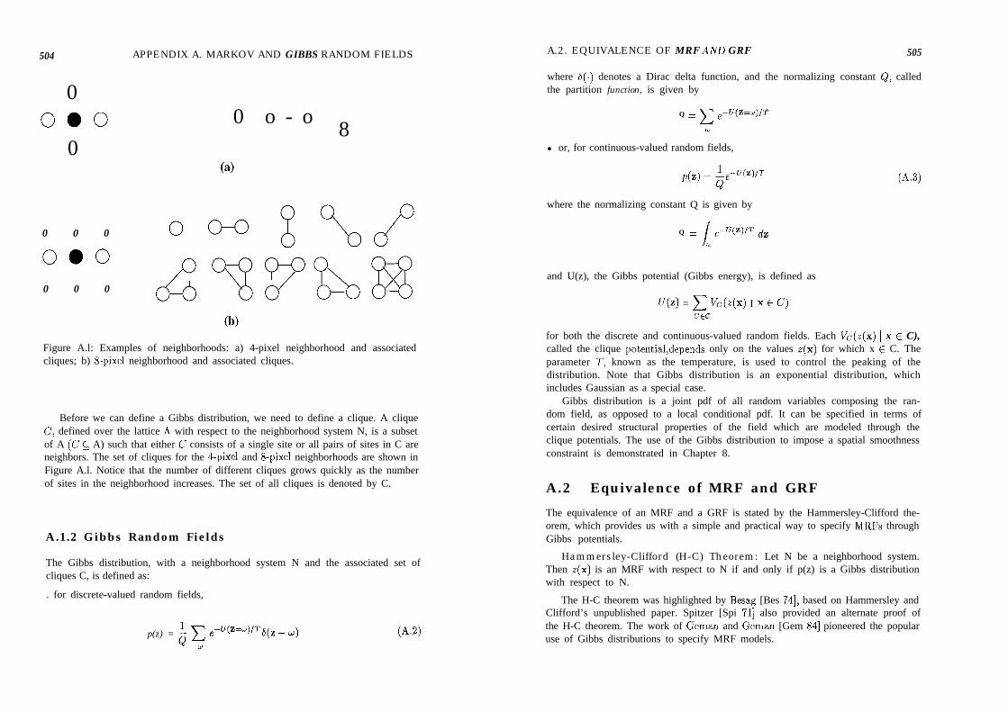
504
0oao
0
0 0 0
oeo
0 0 0
APPENDIX A. MARKOV AND GIBBS RANDOM FIELDS A.2. EQUIVALENCE OF MRF AND GRF 505
0 o - o 8
(4
(b)
Figure A.l: Examples of neighborhoods: a) 4-pixel neighborhood and associatedcliques; b) &pixel neighborhood and associated cliques.
Before we can define a Gibbs distribution, we need to define a clique. A cliqueC, defined over the lattice A with respect to the neighborhood system N, is a subsetof A (C C A) such that either C consists of a single site or all pairs of sites in C areneighbors. The set of cliques for the 4-pixel and &pixel neighborhoods are shown inFigure A.l. Notice that the number of different cliques grows quickly as the numberof sites in the neighborhood increases. The set of all cliques is denoted by C.
A.1.2 Gibbs Random Fields
The Gibbs distribution, with a neighborhood system N and the associated set ofcliques C, is defined as:
. for discrete-valued random fields,
p(z) = j!j C e- W=41TqZ _ u)w
644
where S(.) denotes a Dirac delta function, and the normalizing constant Q, calledthe partition function, is given by
Q = c e-W=wWw
l or, for continuous-valued random fields,
where the normalizing constant Q is given by
Q = J’ e-WW dz
w
and U(z), the Gibbs potential (Gibbs energy), is defined as
U(z) = c VC(~(X) I x E C)ccc
64.3)
for both the discrete and continuous-valued random fields. Each @(z(x) 1 x E C),called the clique potential,depends only on the values Z(X) for which x E C. Theparameter T, known as the temperature, is used to control the peaking of thedistribution. Note that Gibbs distribution is an exponential distribution, whichincludes Gaussian as a special case.
Gibbs distribution is a joint pdf of all random variables composing the ran-dom field, as opposed to a local conditional pdf. It can be specified in terms ofcertain desired structural properties of the field which are modeled through theclique potentials. The use of the Gibbs distribution to impose a spatial smoothnessconstraint is demonstrated in Chapter 8.
A.2 Equivalence of MRF and GRF
The equivalence of an MRF and a GRF is stated by the Hammersley-Clifford the-orem, which provides us with a simple and practical way to specify MRFs throughGibbs potentials.
Hammersley-Clifford (H-C) Theorem: Let N be a neighborhood system.Then Z(X) is an MRF with respect to N if and only if p(z) is a Gibbs distributionwith respect to N.
The H-C theorem was highlighted by Besag [Bes 741, based on Hammersley andClifford’s unpublished paper. Spitzer [Spi 711 also provided an alternate proof ofthe H-C theorem. The work of Geman and Geman [Gem 841 pioneered the popularuse of Gibbs distributions to specify MRF models.
506 APPENDIX A. MARKOV AND GIBBS RANDOM FIELDS
The Gibbs distribution gives the joint pdf of z(x), which can easily be expressedin terms of the clique potentials. The clique potentials effectively express the localinteraction between pixels and can be assigned arbitrarily, unlike the local pdfs inMRFs, which must satisfy certain consistency conditions. It turns out that the localconditional pdfs induced by a Gibbs distribution can easily be computed in the caseof discrete-valued GRFs. This is shown next.
A.3 Local Conditional Probabilities
In certain applications, such as in the Gibbs sampler method of optimization, itmay be desirable to obtain the local conditional pdfs from the joint pdf given interms of Gibbs potential functions. Derivation of the local conditional pdfs of adiscrete-valued GRF is shown in the following. Starting with the Bayes rule,
P(Z)d+Q) I4Xj)~VY #Xi) = p(z(xj),Vxj z xi)
=cP(44)
z(X,)# P(Z) ’XEA (A4
where the second line follows from the total probability rule. In particular, let A,denote the event z(x~) = y, for all y E I’, and B stand for a fixed realization of theremaining sites, xj # xi; then (A.4) is simply a statement of
where P(.) denotes probability (obtained by integrating the pdf p(.) over a suitablerange). Substituting the Gibbsian distribution for p(.) in (A.4), the local conditionalpdf can be expressed in terms of the Gibbs clique potentials (after some algebra) as
P@(X) I z(q),Vq # xi) = Qii,‘exp{-$ c &(4x) I x E C))CIX,EC
(A.5)
where
Q x , = c expi-$ c %(4x) lx E C)la(X,)U CIX,EC
The use of the expression (A.5) is illustrated by an example in Chapter 8.For a more detailed treatment of MRFs and GRFs the reader is referred to
[Gem 841. Vigorous treatment of the statistical formulations can also be found in[Bes 741 and [Spi 711.
BIBLIOGRAPHY
Bibliography
507
[Bes 741 J. Besag, “Spatial interaction and the statistical analysis of latticesystems,” J. Royal Stat. Sot. B, vol. 36, no. 2, pp. 1922236, 1974.
[Che 931 R. Chellappa and A. Jain, Markov Random Fields: Theory andApplication, Academic Press, 1993.
[Cro 831 G. R. Cross and A. K. Jain, “Markov random field texture models,” IEEETrans. Patt. Anal. Mach. Intel., vol. PAMI-5, pp. 25-39, Jan. 1983.
[Der 871 H. Derin and H. Elliott, “Modeling and segmentation of noisy andtextured images using Gibbs random field,” IEEE Trans. Patt. Anal.Much. Intel., vol. PAMI-9, pp. 39-55, Jan. 1987.
[Dub 931 E. Dubois and J. Konrad, “Estimation of 2-D motion fields fromimage sequences with application to motion-compensated processing,”in Motion Analysis and Image Sequence Processing, M. I. Sezan andR. L. Lagendijk, eds., Norwell, MA: Kluwer, 1993.
[Gem 841 S. Geman and D. Geman, “Stochastic relaxation, Gibbs distribution, andBayesian restoration of images,” IEEE Trans. Putt. Anal. Mach. Intel.,vol. 6, pp. 721-741, Nov. 1984.
[Pap 921 T. N. Pappas, “An adaptive clustering algorithm for imagesegmentation,”IEEE Trans. Signal Proc., vol. SP-40, pp. 901-914, April 1992.
[Spi 711 F. Spitzer, “Markov random fields and Gibbs ensembles,” Amer. Math.Mon., vol. 78, pp. 142-154, Feb. 1971.

Appendix B
BASICS OFSEGMENTATION
The goal of this appendix is to introduce those segmentation tools which are em-ployed in Chapter 11 for motion segmentation. In particular, we overview threshold-ing in Section B.l, clustering in Section B.2, and Bayesian methods in Section B.3,as they apply to image segmentation. Section B.4 generalizes Bayesian formulationto multichannel data.
B.l Thresholding
Thresholding is a popular tool for image segmentation. Consider an image s(zr, ~z),composed of a light object on a dark background. Such an image has a bimodalhistogram h(s), as depicted in Figure B.l. An intuitive approach to segment theobject from the background, based on gray-scale information, is to select a thresholdT that separates these two dominant modes (peaks). The segmentation of an imageinto two regions is also known as binarization.
Then the segmentation mask or the binarized image
if s(11, a) > Totherwise
identifies the object and background pixels.Thresholding techniques can be divided into two broad classes: global and local.
In general, the threshold T is a function of
T=T(x~,x~,s(x~,x~),P(x~,xz)) (B.2)
where (xl, x2) are the coordinates of a pixel, s(zi, ~2) is the intensity of the pixel,and p(zi, x2) is some local property of the pixel, such as the average intensity of
508
B.1. T H R E S H O L D I N G
smin T smax
Figure B.l: A bimodal histogram.
509
a local neighborhood. If T is selected based only on the statistics of individualpixel values s(xi) ~2) over the entire image, it is called a pixel-dependent globalthreshold. Alternatively, T can be a global threshold selected based on the statisticsof both s(xi, x2) and p(zi, x2) to reflect certain spatial properties of the image. If,in addition, it depends on (~1) x2), it is called a dynamic or adaptive threshold.Adaptive thresholds are usually computed based on a local sliding window about(xi, x2). Methods for determining the threshold(s) are discussed in the book byGonzalez and Woods [Gon 921 as well as in the review papers [Wes 78, Sah 88,Lee 901.
In some applications the histogram has K significant modes (peaks), whereI< > 2. Then we need K - 1 thresholds to separate the image into Ii segments.Of course, reliable determination of the thresholds becomes more difficult as thenumber of modes increases. In the following, we introduce a method for optimumthreshold determination.
B.1.1 Finding the Optimum Threshold(s)
Given a multimodal histogram, h(s), fo an image s(x~,x~), one can address theproblem of finding the optimal thresholds for separating the dominant modes byfitting the histogram with the sum of I< probability density functions. Assumingthese pdfs are Gaussian, the mixture density model takes the form
Kb(s)=~&exp{-v} (B.3)
where Pi denotes the a priori probability of the particular mode such thatC,“=, Pe = 1, and ,ui and ci denote the mean and the standard deviation of that
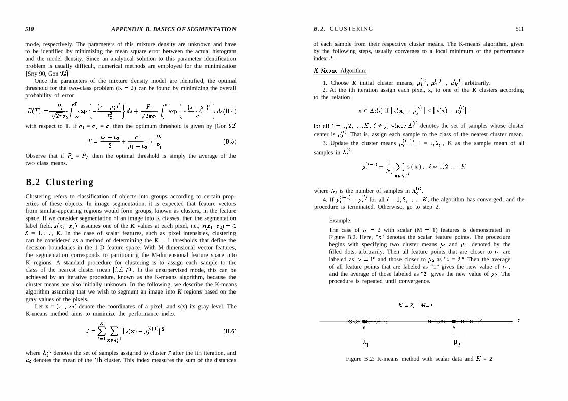
510 APPENDIX B. BASICS OF SEGMENTATION B.2. CLUSTERING 511
mode, respectively. The parameters of this mixture density are unknown and haveto be identified by minimizing the mean square error between the actual histogramand the model density. Since an analytical solution to this parameter identificationproblem is usually difficult, numerical methods are employed for the minimization[Sny 90, Gon 921.
Once the parameters of the mixture density model are identified, the optimalthreshold for the two-class problem (K = 2) can be found by minimizing the overallprobability of error
E(T) = gu2 -,““P- JT {-~}ds+&Jjm~xp{--y}ds(B.4)
with respect to T. If gr = us = u, then the optimum threshold is given by [Gon 921
Observe that if PI = Pz, then the optimal threshold is simply the average of thetwo class means.
B.2 ClusteringClustering refers to classification of objects into groups according to certain prop-erties of these objects. In image segmentation, it is expected that feature vectorsfrom similar-appearing regions would form groups, known as clusters, in the featurespace. If we consider segmentation of an image into K classes, then the segmentationlabel field, z(zr) xz), assumes one of the K values at each pixel, i.e., ~(21, 33) = e,e = l,... , K. In the case of scalar features, such as pixel intensities, clusteringcan be considered as a method of determining the K - 1 thresholds that define thedecision boundaries in the 1-D feature space. With M-dimensional vector features,the segmentation corresponds to partitioning the M-dimensional feature space intoK regions. A standard procedure for clustering is to assign each sample to theclass of the nearest cluster mean [Co1 791. In the unsupervised mode, this can beachieved by an iterative procedure, known as the K-means algorithm, because thecluster means are also initially unknown. In the following, we describe the K-meansalgorithm assuming that we wish to segment an image into K regions based on thegray values of the pixels.
Let x = (21, x2) denote the coordinates of a pixel, and s(x) its gray level. TheK-means method aims to minimize the performance index
(B.6)
where Af) denotes the set of samples assigned to cluster e after the ith iteration, and~1 denotes the mean of the Lth cluster. This index measures the sum of the distances
of each sample from their respective cluster means. The K-means algorithm, givenby the following steps, usually converges to a local minimum of the performanceindex J.
KMeans Algorithm:
1. Choose K initial cluster means, ~(11)) py), , pi), arbitrarily.2. At the ith iteration assign each pixel, x, to one of the K clusters according
to the relation
x E A,(i) if IIs - py)ll < IIs - py)ll
forall!=l,2 ,..., K!#j,whereRF) denotes the set of samples whose clustercenter is p!). That is, assign each sample to the class of the nearest cluster mean.
3. Update the cluster means prtl), I = 1,2, , K as the sample mean of allsamples in A!)
$+l) =$ c s ( x ) , e=l,2,...,K
XCAj”
where Ne is the number of samples in A!).4. If &+i) = pki) for all e = 1,2,. . . ) K, the algorithm has converged, and the
procedure is terminated. Otherwise, go to step 2.
Example:
The case of I< = 2 with scalar (M = 1) features is demonstrated inFigure B.2. Here, “x” denotes the scalar feature points. The procedurebegins with specifying two cluster means ~1 and ~2, denoted by thefilled dots, arbitrarily. Then all feature points that are closer to ~1 arelabeled as “z = 1” and those closer to ~2 as “Z = 2.” Then the averageof all feature points that are labeled as “1” gives the new value of ~1,and the average of those labeled as “2” gives the new value of 1-12. Theprocedure is repeated until convergence.
K=2, M=I
Figure B.2: K-means method with scalar data and K = 2
512 APPENDIX B. BASICS OF SEGMENTATION
The biggest obstacle to overcome in clustering procedures is the determinationof the correct number of classes, which is assumed to be known. In practice, thevalue of K is determined by trial and error‘. To this effect, measures of clusteringquality have been developed, such as the within-cluster and between-cluster scattermeasures. These measures are derived from the within-cluster and between-clusterscatter matrices [Fuk 721. Different values of K can be tried with the Kmeansalgorithm until a desired clustering quality is achieved.
Although we have presented the K-means algorithm here for the case of a scalarfirst-order (pixel-dependent) image feature, it can be straightforwardly extended tothe case of vector features and/or higher-order (region-based) image features. Theprocedure provides cluster means, which can be used for other purposes, as a by-product of the segmentation. However, it does not incorporate any spatial smooth-ness constraint on the estimated segmentation labels to ensure spatial connectivityof the image segments. The Bayesian segmentation, which is described next, canbe considered as a clustering method employing a statistical spatial smoothnessconstraint.
B.3 Bayesian Methods
In this section, we discuss the maximum a posterior-i probability (MAP) approach,which belongs to the class of Bayesian methods. The MAP approach is motivatedby the desire to obtain a segmentation that is spatially connected and robust inthe presence of noise in the image data. The MAP criterion functional consists oftwo parts, the class conditional probability distribution, which is characterized bya model that relates the segmentation to the data, and the a priori probability dis-tribution, which expresses the prior expectations about the resulting segmentation.The a priori model is usually selected to encourage spatially connected regions.
Derin and Elliott [Der 871 have proposed a MAP approach for the segmentationof monochromatic images, and have successfully used Gibbs random fields (GRF)as a priori probability models for the segmentation labels. The GRF prior modelexpresses our expectation about the spatial properties of the segmentation. In orderto eliminate isolated regions in the segmentation that arise in the presence of noise,the GRF model can be designed t,o assign a higher probability for segmentations thathave contiguous, connected regions. Thus, estimation of the segmentation is notonly dependent on the image intensity, but also constrained by the expected spatialproperties imposed by the GRF model. The solution to the MAP segmentationproblem is obtained via Monte-Carlo type methods. In particular, we use the sub-optimal method of iterated condition,al mode @CM), trading optimality for reducedcomputational complexity.
B.3. BAYESIAN METHODS 513
B.3.1 The MAP Method
In the MAP formulation, we take into account the presence of observationnoise in the image explicitly by modeling observed monochrome image data asg(x) = s(x) + a(x), hw ere u(x) denotes the observation noise. In vector no-tat,ion g denotes an N-dimensional vector obtained by lexicographical ordering ofthe image data. We wish to estimate a segmentation label field, denoted by theN-dimensional vector z. A label z(x) = 1, 1 = 1,. ) I<, implies that the pixel(site) x belongs to the &th class among the K classes.
The desired estimate of the segmentation label field, i, is defined as the one thatmaximizes the a posteriori pdf p(z ) g) of the segmentation label field, given theobserved image g. Using the Bayes rule,
P(Z I d 0: Pk I ZMZ) (B.7)
where p(g ] z) represents the conditional pdf of the data given the segmentationlabels, i.e., the class-conditional pdf. The term p(z) is the a priori probabilitydistribution that can be modeled to impose a spatial connectivity constraint on thesegmentation. In the following, we first provide a model for the a priori pdf, thenproceed to examine the assumptions used in characterizing the conditional pdf.
A Priori Probability Model
A spatial connectivity constraint on the segmentation field can be imposed by mod-eling it as a discrete-valued Gibbs random field (see Appendix A and Chapter 8).Then the a priori pdf p(z) of the label field can be expressed by an impulse trainwith Gibbsian weighting
p(z) = $ C exp{-U(z)/T}S(Z - ti)WER
WV
where R is the finite sample space of the random vector z, 5(.) denotes a Diracdelta function, Q is called the partition function (normalizing constant), T is thetemperature parameter, and U(z) is the Gibbs potential defined by
U(z) = c k(z)CEC
P.9)
Here C is the set of all cliques, and VC is the individual clique potential function.The single pixel clique potentials can be defined as
Vc(z(x)) = a’ if Z(X) = 1 and x E C, fore = 1,. . .,I(
They reflect our a priori knowledge of the probabilities of different region types.The smaller ae the higher the likelihood of region 1, 1 = 1,. , I<.
514 APPENDIX B. BASICS OF SEGMENTATION
Spatial connectivity of the segmentation can be imposed by assigning the fol-lowing two-pixel clique potential,
V&(Xi), z(q)) = { -fi f = z(xj) and xi, xj E Cif z(x~) # z(xj) and xi, xj E C (B.10)
where /3 is a positive parameter. The larger the value of p, the stronger the smooth-ness constraint.
Conditional Probability Model
The original image, s, will be modeled by a mean intensity function, denoted bythe vector p, plus a zero-mean, white Gaussian residual process, P, with varianceg,“, that is,
s=p+r (B.11)
where all vectors are respective N-dimensional lexicographic orderings of the re-spective arrays. Then,
g=p+rl (B.12)
where Q & P +v is a zero-mean Gaussian process with variance uz & c,” + 0,“) and c,”denotes the variance of the observation noise which is also taken to be a zero-mean,white Gaussian process. In what follows, we refer to this combined term, q, simplyas the additive noise term. In the context of segmenting an image into I< regions,the elements of p attain the values of the class means associated with each one ofthe regions.
The original formulation by Derin and Elliott [Der 871 for nontextured imagesmodels the mean intensity of each image region as a constant, denoted by thescalar pe, e = 1,2,. , I(. That is the elements of ,X attain K distinct values, ~1,! = 1,2, , K. Based on the model of the observed image in (B.12), the conditionalprobability distribution is expressed as
pklz) 0: ew 1 _ c b(x) - Pz(X)12 \X 23 I
(B.13)
where Z(X) = e designates the assignment of site x to region 1. Notice that (B.13)is the probability distribution that would be used in the maximum likelihood (ML)segmentation of the image.
Given (B.8) and (B.13), the a posteriori density has the form
p(z I 4 m exp1- c $ b(x) - h(X)] 2 - c k(z)x ‘I c 1
We maximize the posterior probability (B.14) to find an estimate of ~1,e = 1,2,. .,I(, and the desired segmentation labels z. This maximization canbe performed by means of simulated annealing. Observe that if we turn off the
B.3. BAYESIAN METHODS 515
spatial smoothness constraints, that is, neglect the second term, the result wouldbe identical to that of the K-means algorithm. Thus, the MAP estimation followsa procedure that is similar to that of the K-means algorithm, i.e., we start with aninitial estimate of the class means and assign each pixel to one of the K classes bymaximizing (B.14), then we update the class means using these estimated labels,and iterate between these two steps until convergence.
B.3.2 The Adaptive MAP Method
The MAP method can be made adaptive by letting the cluster means pi slowlyvary with the pixel location x. An adaptive clustering approach for monochromaticimages that is based on a more realistic image model has been proposed by Pappas[Pap 921. In earlier works on MAP segmentation, the image has been modeledas consisting of a finite number of regions, each with a constant mean intensity[Der 871. The adaptive method allows for slowly space-varying mean intensities foreach region.
Because the uniform mean intensity ,u~(~) may not be adequate in modelingactual image intensities within each region, a space variant mean intensity amwill be used in the class-conditional pdfs. Then the modified conditional pdf model
dglz) c( 9 1 _ c b(x) - PZ(X,(41”X
2a;I
(B.15)
There are several advantages in introducing space-varying class means. First, amore realistic image model yields better segmentation. Second, in parts of theimage where the local intensity contrast is low between two perceptually distinctregions, using a global mean usually yields a single label to both regions. Third, inthe case of spatially varying class means, fewer regions are required to segment animage into perceptually meaningful regions.
The adaptive algorithm follows a procedure that is similar to the nonadaptivealgorithm, except that the cluster means p!(x) at the site x for each region e areestimated as the sample mean of those pixels with label 1 within a local windowabout the pixel x (as opposed over the entire image). The local window is depictedin Figure B.3.
To reduce the computational burden of the algorithm to a reasonable level, thefollowing simplifications are usually performed: i) The space-varying mean estimatesare computed on a sparse grid, and then interpolated. ii) The optimization isperformed via the ICM method. Note that the ICM is equivalent to maximizingthe local a posteriori pdf
p(z(xi) I s(xi),4xj), all xj E Nx,)
cc exp1-$JdXi) - fqX,)G412 - c k(z)
II c I
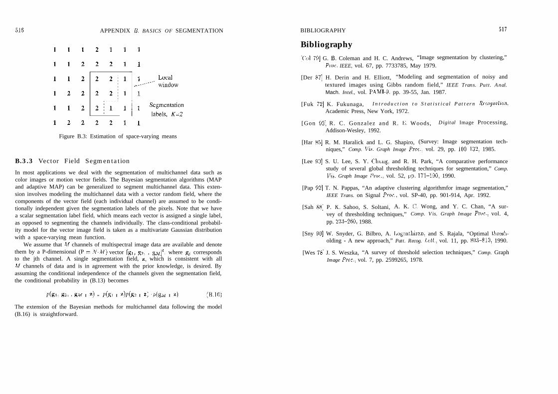
516 APPENDIX I?. BASICS OF SEGMENTATION BIBLIOGRAPHY 517
Figure B.3: Estimation of space-varying means
B.3.3 Vector Field Segmentation
In most applications we deal with the segmentation of multichannel data such ascolor images or motion vector fields. The Bayesian segmentation algorithms (MAPand adaptive MAP) can be generalized to segment multichannel data. This exten-sion involves modeling the multichannel data with a vector random field, where thecomponents of the vector field (each individual channel) are assumed to be condi-tionally independent given the segmentation labels of the pixels. Note that we havea scalar segmentation label field, which means each vector is assigned a single label,as opposed to segmenting the channels individually. The class-conditional probabil-ity model for the vector image field is taken as a multivariate Gaussian distributionwith a space-varying mean function.
We assume that M channels of multispectral image data are available and denotethem by a P-dimensional (P = N,M) vector [gi, g2, , g~]~, where gj correspondsto the jth channel. A single segmentation field, z, which is consistent with allM channels of data and is in agreement with the prior knowledge, is desired. Byassuming the conditional independence of the channels given the segmentation field,the conditional probability in (B.13) becomes
P(&, ga, > 04 I z) = P(B I Z)Pkz I z) .p(ghf I z) (B.IB)
The extension of the Bayesian methods for multichannel data following the model(B.16) is straightforward.
Bibliography[Co1 791 G. B. Coleman and H. C. Andrews, “Image segmentation by clustering,”
Proc. IEEE, vol. 67, pp. 7733785, May 1979.
[Der 871 H. Derin and H. Elliott, “Modeling and segmentation of noisy andtextured images using Gibbs random field,” IEEE Trans. Putt. Anal.Mach. Intel., vol. PAMI-9, pp. 39-55, Jan. 1987.
[Fuk 721 K. Fukunaga, I n t r o d u c t i o n t o S t a t i s t i c a l P a t t e r n Recognilion,Academic Press, New York, 1972.
[Gon 921 R. C. Gonzalez and R. E. Woods, Digital Image Processing,Addison-Wesley, 1992.
[Har 851 R. M. Haralick and L. G. Shapiro, (Survey: Image segmentation tech-niques,” Comp. Vzs. Graph Image Proc., vol. 29, pp. 100-132, 1985.
[Lee 901 S. U. Lee, S. Y. Chung, and R. H. Park, “A comparative performancestudy of several global thresholding techniques for segmentation,” Comp.VW. Graph Image Proc., vol. 52, pp. 171-190, 1990.
[Pap 921 T. N. Pappas, “An adaptive clustering algorithmfor image segmentation,”IEEE Trans. on Signal Proc., vol. SP-40, pp. 901-914, Apr. 1992.
[Sah 881 P. K. Sahoo, S. Soltani, A. K. C. Wong, and Y. C. Chan, “A sur-vey of thresholding techniques,” Comp. Vis. Graph Image Proc., vol. 4,pp. 233260, 1988.
[Sny 901 W. Snyder, G. Bilbro, A. Logenthiran, and S. Rajala, “Optimal thresh-olding - A new approach,” Patt. Recog. Lett., vol. 11, pp. 8033810, 1990.
[Wes 781 J. S. Weszka, “A survey of threshold selection techniques,” Comp. GraphImage Proc., vol. 7, pp. 2599265, 1978.

C.1, LINEAR STATE-SPACE MODEL 519
Appendix C
KALMAN FILTERING
A Kalman filter estimates the state of a dynamic system recursively at each time, inthe linear minimum mean square error (LMMSE) sense, given a time series of vectoror scalar observations that are linearly related to these state variables. If the statevariables and the noise are modeled as uncorrelated, Gaussian random processes,then the Kalman filter is the minimum mean square error estimator. This appendixbriefly reviews the basics of Kalman filtering and extended Kalman filtering (EKF).The reader is referred to [Bro 83, Fau 93, Men 871 for a more detailed treatment ofthe subject and the derivation of the equations.
C.l Linear State-Space ModelLet z(k) denote an M-dimensional state vector of a dynamic system at time k. Weassume that the propogation of the state in time can be expressed in the form of alinear state-transition equation given by
z(k) = 8(k, k - l)z(k - 1) + w(k), k = 1,. .) N cc.11
where +(k, k - 1) is the state-transition matrix and w(k) is a zero-mean, whiterandom sequence, with the covariance matrix Q(k), representing the state modelerror.
Suppose that a time-series of observations or measurements, y(k), are available,which are linearly related to the state variables as
y(k) = H(k)z(k) f v(k), k = 1,. .) N ((3.2)where H(k) is called the observation matrix, and v(k) denotes a zero-mean, whiteobservation noise sequence, with the covariance matrix R(k), which is uncorrelatedwith w(k).
The Kalman filter minimizes, at each time k, the trace of the error covariancematrix conditioned on all observations up to time k, defined as
[
E {e~(k)“lu(k)l...,Y(l)} ... Wel(k) e~@)ly(~),...,~(l)~
P,(k) =.
i
E{e~(k) ei(k)ly(k),...,y(l)} :.. E{e~(k)*/y(k),...,y(l)} 1
(G.3)
where
ei(k)=zi(k)-&(k), i=l,...,M (G.4)
ii(k) denotes an estimate of the state ri(k), and E{ .} denotes the expectation oper-ator. It consists of two steps: i) the prediction step, comprising the state and errorcovariance prediction, and ii) an update step, comprising Kalman gain computationfollowed by state and error covariance update. They are described below, where thesubscripts “b” and “a” denote before and after the update, respectively.State-prediction equation
2*(k) = +(k, k - l)&(k - 1) (G.5)
Covariance-prediction equation
P*(k) = G(k, k - l)Pa(k - l)@(k, k - l)T + Q(k) (C.6)
Kalman-gain equation
K(k) = Pb(k)HT(k)(H(k)Pb(k)HT(k) + R(k))-i
State-update equation
(G.7)
h(k) = h(k) + K(k)[y(k) - H(k)h(k)] CC4
Covariance-update equation
Pa(k) = Pb(k) - K(k)H(k)Pa(k) (C.9)
Observe that the covariance prediction, Kalman gain, and covariance updateequations are independent of the observations, and can be processed off-line pro-vided that state propagation and the observation models are known. TWO specialcases are of interest:
1. Steady-state filter: If the state propagation and the observation matricesare time-invariant, that is, 8(k, k - 1) = a, Q(k) = Q, H(k) = H, andR(k) = R, then the Kalman gain matrix converges to a steady-state valueK after some recursions, In this case, the covariance and the gain equationscan be turned off after convergence, resulting in computational savings. Notethat the steady-state filter is a linear time-invariant (LTI) filter.
2. Recursive least squares filter: If there is no temporal dynamics, that is,+(k, k - 1) = I and Q(k) = 0 for all k, then the state consists of constant(but unknown) parameters, and the Kalman filter reduces to the recursiveleast squares parameter identification filter.
518
520 APPENDIX C. KALMAN FILTERING BIBLIOGRAPHY 521
C .2 Extended Kalman FilteringIn some applications, the state-transition equation, the observation equation, orboth may be nonlinear in the state variables, given by
and
z(k) = f(z(k - 1)) + w(k), k = 1,. , N (C.10)
y(k) = h@(k)) + v(k), k = 1,. ;N (C.11)
where f(.) and h(.) are nonlinear, vector-valued functions of the state.In order to apply the Kalman filtering equations presented in Section C.l, Equa-
tions (C.10) and/or (C.ll) must be linearized about the best available estimate ofthe state vector at that instant. To this effect, we expand f(z(k - 1)) and h(z(k))into first-order Taylor series about &(k - 1) and S*(k), respectively, as follows:
f(z(k - 1)) = f(;,(k - 1)) + af:$k$;)]z(xlj,iZ a ck-ll(z(k - 1) - &(k - 1))
(C.12)
(C.13)
Substituting (C.12) into (C.lO), we obtain the linearized state-transition equation
z(k) M 6(k, k - 1) z(k - 1) + u(k) + w(k), k = 1,. .) N (C.14)
where u(k) is a deterministic input, given by
u(k) = f(&(k - 1)) - Q(k, k - l)&(k - 1)
and the state-transition matrix of the linearized model is
Likewise, substituting (C.13) into (C.11) results in the modified observationequation
f(k) M H(k) z(k) + v(k), k = 1,. . , N (C.15)
where y(k) denotes-t&modified observation given by
Y(k) = y(k) -h&(k)) + H(k)&(k)
and the observation matrix of the linearized system is
The Kalman filtering equations (C.5)(C.9) apply to the case of the linearizedmodels (C.14) and (C.15) straightforwardly. However, neither optimality nor con-vergence of this extended Kalman filter can be guaranteed. Indeed, the success ofthe filter strongly depends on the goodness of the predicted estimate about whicha linearization has been performed.
In some cases, additional performance improvement can be achieved using aniterated extended Kalman filter (IEKF), which carries out the linearization in aniterative fashion about the best available estimate from the previous iteration atthat instant.
Bibliography
[Bro 831 R. G. Brown, Introduction to Random Signal Analysis and KalmanFiltering, New York, NY: Wiley, 1983.
[Fau 931 0. Faugeras, Three-Dimensional Computer Vision, Cambridge, MA: MITPress, 1993.
[Men 871 J. Mendel, Lessons in Digital Estimation Theory, Englewood Cliffs, NJ:Prentice Hall, 1987.
H(k) = dh(z(k))az(k)la(k)=LdE)

INDEX 523
Index
Aacceleration 249, 256AC coefficient 384adaptive
DPCM 376LMMSE filtering 267, 274weighted averaging (AWA) 275
affine transformation 20, 153, 182aliasing 54, 63, 252, 332all-digital HDTV 494analog video 2, 4, 8analysis-synthesis coding 426, 457angular velocity 25, 178, 236anti-aliasing filter 64, 65, 305aperture problem 78a posteriori probability 136, 207, 225a priori probability 137, 207, 211arithmetic coding 357aspect ratio 6, 493
Bbackward motion estimation 77bandlimited 43, 54, 248batch methods 231Bayesian methods 130, 207, 225, 512B-frames 441) 445bidirectional
interpolative mode 446motion estimation 317
bilinearinterpolation 61transformation 98
binary image compressionstandards 389
bit allocation 381
bit-plane coding 363block matching 101block motion 83, 95, 124blocking artifacts 385, 426blur 284, 332boundary effects 100, 380
Ccamera calibration 221Cartesian coordinates 20CCIR 601 standard 11, 490CCITT
Group 3 and 4 codes 389Recommendation H.261 432
center of rotation 230, 236change detection 200clustering 205, 206, 510coding 353, 360, 381,414, 420color image compression 395component analog video (CAV) 5composite video 5compression 349, 388, 419, 432conditional replenishment 424constrained least squares filter 287correspondence field 74
2-D to 2-D 76, 1522-D to 3-D 2233-D to 3-D 223
critical velocity 252, 307, 321cubic spline interpolation 62
DDC coefficient 384decimation 62deformable motion 27, 97, 109, 463
de-interlacing 312, 315, 322delta modulation 377depth estimation 164, 181, 219differential methods 72digital video 9direct methods 187directional cosines 23directional filtering 269, 313discontinuity models 139discrete cosine transform (DCT) 380displaced frame difference 80, 118displacement
field 73models 79
down-conversion 66DPCM 373dynamic programming 231
Eedge adaptive filtering 269, 313entropy 351
coding 354epipolar constraint 159, 220essential
matrix 159parameters 159
Euler angles 21even field 308, 450extended Kalman filter 231,520
Ffeature
correspondence 76, 152tracking 232
field-quincunx sampling 39filtering 54, 60, 254, 262finite difference 85focus of expansion (FOE) 180forward motion estimation 76Fourier transform 41, 44, 247fractal coding 409frame difference 90, 200frame rate conversion 309, 314frequency domain 41, 44, 247
GGaussian distribution 137, 514generalized block matching 109Gibbs
distribution 130, 502random field 130, 504sampler 132
global motion 20, 322, 465, 478gradient
-based optimization 119estimation 85spatio-temporal 81
Gray codes 364
HH.261 standard 432hexagonal sampling 38hexagonal search 110hierarchical methods 88, 106high resolution 336, 341highest confidence first (HCF) 135histogram 509homogeneous coordinates 26, 29homotopy method 161Horn-Schunck method 84Hough transform
modified 205Huffman coding 354hybrid coding 420
II-frames 441image model 20, 28, 32, 332impulse response 55, 61, 284information theory 350interactive video 488interframe
coding 419, 444filtering 270
interlaced 38, 448vertically aligned 2:l line 39
IS0 388, 393, 440interpolation 58intraframe
522
524
compression 420, 443filtering 263, 286, 309
inverse filteringpseudo- 286
ISDN 12, 487iterated conditional modes 134iterated EKF 521
JJBIG standard 393JPEG standard 394judder postprocessing 322
KKalman filtering 231, 518Karhunen-Loeve transform 379Kell factor Gkinematics 229, 238Ii-means algorithm 206, 511knowledge-based coding 428, 464Konrad-Dubois algorithm 144
LLaplacian 288, 289
distribution 372, 376lattice 47layered video representation 206least squares estimation 156, 160
nonlinear LSE 238likelihood model 137, 140line field 142line-quincunx sampling 40Lloyd-Max quantization 369, 372LMMSE estimation 264
adaptive (local) 267FIR 266IIR (unrealizable) 264
local motion 468, 470, 471lossless compression 350, 360lossy compression 350, 352
Mmacroblock 434, 442MAP estimation 136, 207, 225, 513MBASIC algorithm 155, 470
INDEX
mapping parameters 188, 203Markov random fields (MRF) 502maximum likelihood 227, 238mean field annealing 135median filtering 270, 315Metropolis algorithm 131MMSE estimation 264, 519minimum variance estimation 519model-based coding 426, 457motion
blur 296, 332compensation 109, 245, 424detection 272, 314, 316estimation 72, 76, 152tracking 229trajectory 229, 236
motion-compensatedcompression 424filtering 245
MPEG standard 448MPEG-2 profiles/levels 455
multiframe image restoration 292multimedia 488multiresolution 88, 106
NNetravali-Robbins algorithm 122nonlinear filtering 255, 270nonparametric motion estimation 80nonrigid motion 27normal flow 82NTSC video 6
0object-based coding 427, 457observation equation 231, 518occlusion 78, 139odd field 308, 450optical flow 74
equation 81methods 81
optimization 119, 130orthogonal
sampling 39
INDEX
orthographic projection 30, 153, 178outlier rejection 146
Pparametric motion models 79pel-recursive methods 117perspective projection 28, 154, 178P-frames 441, 444phase correlation method 99photometric effects 33, 471planar surface 165, 188point correspondence 76, 152, 232point spread function 283, 332polynomial fitting 86precession 236probability density 136, 207, 225progressive
compression 400scanning 441
projection onto convex sets 290, 341
Qquadratic flow 183quantization 368
adaptive 376matrix 382, 397nonuniform 369uniform 370scalar 368vector 369, 404
quaternion 24quincunx sampling
field 39line 40
Rraster scan 2rate-distortion function 352reconstruction from samples 53recursive estimation 231, 518region-labeling 147region tracking 233RGB space 5, 395rigid motion 20, 153
525
rotation 21axis of 23center of 235
run-length coding 363
Ssampling structure 46
conversion 57scalable video 452scan rate doubling 315search procedures 104, 131second-generation coding 415segmentation 198, 508
optical flow 204Bayesian 207, 512
semantic coding 429, 464sensor aperture
size 333time 332
shift-varying PSF 285simulated annealing 131simultaneous motion estimation
- and segmentation 209singular value decomposition 167smoothness constraint 80, 84, 137source coding 352spatio-temporal
filtering 256, 274Fourier transform 47, 246sampling 36
spectralleakage 100replications 43, 50, 250
spectrum of sampled video 49, 251standards conversion 302state-space model 518stereo
-motion fusion 224triangulation 219video 219
subband coding 411sub-Nyquist sampling 250superresolution 331symbol coding 353

526 INDEX
Ttelevision
digital 489studio standards 490
temporal filtering 256three-D waveform coding 420three-step search 104thresholding 200, 508threshold coding 382time-varying images 19token tracking 232transform coding 378Tsai-Huang algorithm 188two-D run-length coding 391
Uuniqueness 155, 160, 167, 230up-conversion 308, 317
Vvariable-length coding 353vector quantization 404
codebook design 408gain-shape VQ 409mean-residual VQ 409tree VQ 408
velocityfield 74model 177
very-low-bitrate video 497videoconferencing 487videophone 498
wwaveform coding
three-dimensional 420wavelet transform coding 415weighted median filtering 270white noise 268Wiener based motion estimation 125Wiener filtering 264
YYCbCr (YUV) color space 5, 395
Zzero-crossing 287zero-order hold filter 61zigzag scanning 383Ziv-Lempel coding 364zonal coding 381zoom 24