arX

iv:0

811.

0825

v1 [

astr

o-ph

] 5

Nov

200

8

Digging into the surface of the icy dwarf

planet Eris

M. R. Abernathy

Dept. Physics & Astronomy, Northern Arizona Univ, Flagstaff, AZ 86011

E-mail: mra66@nau.edu

S. C. Tegler1

Dept. Physics & Astronomy, Northern Arizona Univ, Flagstaff, AZ 86011

E-mail: Stephen.Tegler@nau.edu

W. M. Grundy

Lowell Observatory, 1400 W. Mars Hill Rd., Flagstaff, AZ 86001

E-mail: W.Grundy@lowell.edu

J. Licandro

Instituto de Astrofisica de Canarias, via Lactea s/n, E38205, La Laguna, Tenerife, Spain

Email: jlicandr@iac.es

1

W. Romanishin1

Dept. Physics & Astronomy, Univ of Oklahoma, Norman, OK 73019

E-mail: wjr@nhn.ou.edu

D. Cornelison

Dept. Physics & Astronomy, Northern Arizona Univ, Flagstaff, AZ 86011

E-mail: David.Cornelison@nau.edu

F. Vilas1

MMT Observatory, PO Box 210065, University of Arizona, Tucson, AZ, 85721

Email: fvilas@mmto.org

Pages: 26; Tables 3; Figures: 5

1 Observer at the MMT Observatory. Observations reported here were obtained at the MMT Observatory,

a joint facility of the University of Arizona and the Smithsonian Institution.

2

Proposed Running Head: Eris

Editorial Correspondence to:

Dr. Stephen C. Tegler

Dept Physics & Astronomy

Northern Arizona University

Flagstaff, AZ 86011

Phone: 928-523-9382

FAX: 928-523-1371

E-mail: Stephen.Tegler@nau.edu

3

Abstract

We describe optical spectroscopic observations of the icy dwarf planet Eris with the 6.5 meter MMT

telescope and the Red Channel Spectrograph. We report a correlation, that is at the edge of statistical

significance, between blue shift and albedo at maximum absorption for five methane ice bands. We interpret

the correlation as an increasing dilution of methane ice with another ice component, probably nitrogen, with

increasing depth into the surface.

We suggest a mechanism to explain the apparent increase in nitrogen with depth. Specifically, if we are

seeing Eris 50 degrees from pole-on (Brown and Schaller, 2008), the pole we are seeing now at aphelion was

in winter darkness at perihelion. Near perihelion, sublimation could have built up atmospheric pressure on

the sunlit (summer) hemisphere sufficient to drive winds toward the dark (winter) hemisphere, where the

winds would condense. Because nitrogen is more volatile and scarcer than methane, it sublimated from the

sunlit hemisphere relatively early in the season, so the early summer atmosphere was nitrogen rich, and so

was the ice deposited on the winter pole. Later in the season, much of the nitrogen was exhausted from the

summer pole, but there was plenty of methane, which continued to sublimate. At this point, the atmosphere

was more depleted in nitrogen, as was the ice freezing out on top of the earlier deposited nitrogen rich ice.

Our increasing nitrogen abundance with depth apparently contradicts the Licandro et al. (2006) result

of a decreasing nitrogen abundance with depth. A comparison of observational, data reduction, and analysis

techniques between the two works, suggests the difference betweeen the two works is real. If so, we may

be witnessing the signature of weather on Eris. The work reported here is intended to trigger further

observational effort by the community.

Key Words: Kuiper Belt Objects, Spectroscopy, Trans-Neptunian Objects

4

1. Introduction

Triton, Pluto, Eris (136199 and 2003 UB313), and Makemake (136472 and 2005 FY9) form a natural class

of outer Solar System objects for comparative studies, since their spectra are dominated by strong methane

ice absorption bands (see e.g. Cruikshank et al., 1993; Owen et al., 1993; Brown et al., 2005; Licandro et

al., 2006). Furthermore, the same methane ice bands can be used as an important diagnostic tool in the

chemical and physical characterization of icy dwarf planets.

Specifically, it is possible to use the bands to measure the abundance of methane relative to another

ice component, probably nitrogen ice. Laboratory studies showed that the wavelengths of near-infrared

methane ice absorption bands shift to shorter wavelengths when methane is diluted by nitrogen ice (Quirico

and Schmitt, 1997). Triton and Pluto exhibit a nitrogen ice band at 2.15 µm (Cruikshank et al., 1993; Owen

et al., 1993). Triton’s methane ice bands are blue shifted by 7 nm, suggesting methane is highly diluted

by nitrogen ice (Cruikshank et al., 1993). Pluto’s methane ice band shifts are smaller, suggesting Pluto’s

methane occurs in a mixture of diluted and undiluted phases (Owen et al., 1993). No one has detected the

2.15 µm nitrogen ice band in the spectrum of Eris, and its near-infrared methane bands exhibit even smaller

blue shifts which may be due to the presence of even smaller amounts of nitrogen (Brown et al., 2005; Dumas

et al., 2007).

Second, it is possible to measure the CH4/N2 abundance as a function of depth into the surface of these

objects. The average penetration depth of a photon at a particular wavelength depends on the reciprocal of

the absorption coefficient at that wavelength, e.g. photons corresponding to larger absorption coefficients are

absorbed more, preventing them from penetrating as deeply into the surface. In other words, stronger bands

in the spectrum of an icy dwarf planet probe, on average, shallower into the surface than weaker bands. So,

it is possible to use blue shifts and albedos at maximum absorption of two or more methane ice bands to

measure the trend of CH4/N2 into the surface of an icy dwarf planet.

5

Licandro et al. (2006) applied such a technique to Eris. They found the weaker 729.6 nm band had a shift

of 0.1 ± 0.3 nm and the stronger 889.7 nm band had a shift of 1.5 ± 0.3 nm. Their measurements suggested a

decreasing nitrogen abundance with increasing depth. They speculated that as Eris moved toward aphelion

during the last 200 years, and as its atmosphere cooled, less volatile methane began to condense out first.

As the atmosphere cooled further, it became more and more nitrogen rich, until the much more volatile

nitrogen could condense out on top of the methane rich ice.

The technique applied by Licandro et al. (2006) is diagnostically rich. They demonstrated it was possible

to put constraints on atmosphere-surface interactions of icy dwarf planets. So, we set out to confirm their

result by observing additional methane bands in the spectrum of Eris. Below we describe our blue shift and

albedo measurements and analysis for five methane bands.

2. Observations

We obtained optical spectra of Eris on the nights of 2007 September 8 − 11 UT with the 6.5 meter MMT

telescope on Mt. Hopkins, Arizona, the Red Channel Spectrograph, and a new red sensitive, deep depletion

CCD. We used a 1 × 180 arc sec entrance slit and a 600 g mm−1 grating that provided wavelength coverage

of 660.2 − 853.0 nm in first order on the night of 2007 September 8 UT, and 758.7 − 951.3 nm in first order

on the nights of 2007 September 9, 10, and 11 UT. All spectra had a dispersion of 0.20 nm pixel−1, and a

full-width at half-maximum resolution of 0.63 nm. There were high, thin cirrus clouds and the seeing was

variable, 1 − 2 arc sec on all nights. Eris was placed at the center of the slit and the telescope was tracked

at Eris’ rate. In Table 1, we present the number of 600 second exposures taken on each night, range of UT

times, and range of airmass values for our Eris observations. Eris had an airmass of 1.25 at transit.

We used the same calibration techniques on Eris spectra as on Makemake spectra (Tegler et al. 2007;

Tegler et al. 2008). HeNeAr spectra were taken before and after each set of object spectra to obtain

an accurate wavelength calibration. Telluric and Fraunhofer lines were removed from the Eris spectra by

6

dividing each Eris spectrum by the spectrum of a solar analog star, SA 93−101. The airmass difference

between each Eris spectrum and its corresponding solar analog spectrum was < 0.1.

Since we saw no significant difference between the individual 600 second exposures of a night, we summed

the exposures of each night to yield four spectra with exposure times of 2 hr 20 min (2007 Sep 8 UT), 2 hr

20 min (2007 Sep 9 UT), 3 hr 00 min (2007 Sep 10 UT), and 2 hr 50 min (2007 Sep 11 UT). In Figure 1, we

present our reflectance spectra of September 9, 10, and 11 UT, and a spectrum of pure methane ice. The

spectra were normalized to a reflectance of 1.0 between 820 and 840 nm. The September 9 and 10 spectra

were shifted upward on Figure 1 by 1.0 and 0.5. Clearly, methane ice bands are present in our spectra.

To assess the uncertainty in our wavelength calibration, we measured the wavelengths of 16 well-resolved

sky emission lines across our spectra and compared them to the VLT high−spectral resolution sky line

atlas of Hanuschik (2003). In Table 2, we present the sky line measurements. Columns 1 − 4 contain our

values, column 5 contains Hanuschik’s values, and columns 6 − 9 contain the differences between our and

Hanuschik’s values, all entries are in units of nm. The average difference and standard deviation of the

differences for each night are given at the bottom of columns 6 − 9. The four average differences for the four

nights are less than ∼ 0.03 nm. So, it appears our sky lines, and hence our wavelength measurements, are

accurate to ∼ 0.03 nm.

3. Analysis

In order to accurately measure methane band shifts in the spectra of Eris, it is necessary to compare

the Eris spectra to a pure methane ice spectrum. We used Hapke theory to transform laboratory optical

constants of pure methane ice at 30 K (Grundy et al., 2002) into a spectrum suitable for comparison to Eris

spectra by accounting for the multiple scattering of light within a surface composed of particulate methane

ice (Hapke, 1993). We used Hapke model parameters of h = 0.1, Bo = 0.8, θ = 30◦, P(g) = a two component

Henyey-Greenstein function with 80% in the forward scattering lobe and 20% in the back scattering lobe,

7

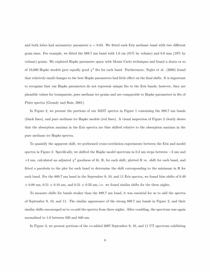
and both lobes had asymmetry parameter a = 0.63. We fitted each Eris methane band with two different

grain sizes. For example, we fitted the 889.7 nm band with 1.0 cm (81% by volume) and 0.8 mm (19% by

volume) grains. We explored Hapke parameter space with Monte Carlo techniques and found a dozen or so

of 10,000 Hapke models gave equally good χ2 fits for each band. Furthermore, Tegler et al. (2008) found

that relatively small changes to the best Hapke parameters had little effect on the final shifts. It is important

to recognize that our Hapke parameters do not represent unique fits to the Eris bands; however, they are

plausible values for transparent, pure methane ice grains and are comparable to Hapke parameters in fits of

Pluto spectra (Grundy and Buie, 2001).

In Figure 2, we present the portions of our MMT spectra in Figure 1 containing the 889.7 nm bands

(black lines), and pure methane ice Hapke models (red lines). A visual inspection of Figure 2 clearly shows

that the absorption maxima in the Eris spectra are blue shifted relative to the absorption maxima in the

pure methane ice Hapke spectra.

To quantify the apparent shift, we performed cross-correlation experiments between the Eris and model

spectra in Figure 2. Specifically, we shifted the Hapke model spectrum in 0.2 nm steps between −3 nm and

+3 nm, calculated an adjusted χ2 goodness of fit, R, for each shift, plotted R vs. shift for each band, and

fitted a parabola to the plot for each band to determine the shift corresponding to the minimum in R for

each band. For the 889.7 nm band in the September 9, 10, and 11 Eris spectra, we found blue shifts of 0.49

± 0.08 nm, 0.51 ± 0.10 nm, and 0.31 ± 0.23 nm, i.e. we found similar shifts for the three nights.

To measure shifts for bands weaker than the 889.7 nm band, it was essential for us to add the spectra

of September 9, 10, and 11. The similar appearance of the strong 889.7 nm bands in Figure 2, and their

similar shifts encouraged us to co-add the spectra from three nights. After coadding, the spectrum was again

normalized to 1.0 between 820 and 840 nm.

In Figure 3, we present portions of the co-added 2007 September 9, 10, and 11 UT spectrum exhibiting

8

the 869.1 nm band, 889.7 nm band, and the 896.8 nm band with the 901.9 nm band (black lines). In

addition, we present a portion of the 2007 September 8 UT spectrum exhibiting the 729.6 nm band (black

line). The red lines represent our pure methane Hapke models. The absorption maxima of the Eris methane

bands appear blue shifted relative to the absorption maxima of the pure methane ice models. In Table 3,

we present the results of our cross correlation experiments between the Eris bands and the pure methane ice

bands in Figure 3. We point out that even in the co-added spectrum with a total exposure time of 8 hr 10

min, the signal precision was insufficient for us to measure shifts for the 786.2 nm, 799.3 nm, 841.5 nm, and

844.2 nm methane bands.

We calculated the uncertainties in the blue shifts as follows. For each methane band, the best fit (shifted)

model was subtracted from the corresponding Eris band, giving us the noise in the astronomical spectrum.

We note that the noise in the astronomical spectrum dominates noise in the Hapke model spectrum. Next,

we calculated the standard deviation of the noise. Then, we applied Gaussian noise with the same standard

deviation to the model spectrum. Next, we applied our cross correlation technique to the noisy model and the

original model spectra. We generated 1000 different noisy model spectra and repeated the cross correlation

experiment for each noisy model and the original model spectra. A histogram of the resulting 1000 shifts

was fit with a Gaussian distribution, the standard deviation of the fit giving the uncertainty in our shift

measurement. We give the uncertainties in Table 3.

Next, we measured albedos at maximum absorption for each band. Specifically, normalizing our spectrum

to 1.0 between 820 and 840 nm makes our relative reflectance spectrum consistent with albedo measurements

of Stansberry et al. (2008). Therefore, our relative reflectance spectrum is also an albedo spectrum.

In addition, we estimated the average depths sampled by photons corresponding to different methane

ice bands. The average penetration depth of a photon depends not only on its corresponding absorption

coefficient, but also on the amount of scattering, which in turn depends on particle size, shape, and spacing.

9

We used a Monte Carlo ray tracing model to explore the trajectories followed by observable photons at

different wavelengths, and thereby estimated the average depths sampled by photons corresponding to the

different methane ice bands (Grundy and Stansberry, 2000).

In Figure 4, we present a plot of blue shift (which we take as a proxy for nitrogen dilution) vs. albedo

at maximum absorption (horizontal scale at the bottom of the plot) and average sample depth estimated

from the Monte Carlo model (horizontal scale at the top of the plot) for the five methane bands in our study

(solid squares).

A visual inspection of the solid squares in Figure 4, suggests there is a correlation between blue shift and

albedo. The solid line is a least square fit to the five points. In order to estimate the statistical significance

of the apparent correlation in Figure 4, we computed the Spearman rank correlation coefficient, r, using the

function CORR in the MATLAB programming environment. The coefficient takes on values in the range

− 1 < r < +1, where −1 indicates a perfect anti-correlation, 0 indicates no correlation, and +1 indicates

a perfect correlation. We computed r = 0.97 for the five points in Figure 4. Furthermore, we computed a

probability of r = 0.97 occurring for an uncorrelated sample at 0.03. It appears the correlation is statistically

significant at the 2 sigma level.

4. Atmosphere−Surface Interaction Model

Is it possible to come up with a mechanism to explain an increasing nitrogen abundance with increasing

depth into the surface of Eris? We start with two observational constraints. First, the lack of the nitrogen

ice band at 2.15 µm in the spectrum of Eris (Brown et al., 2005; Dumas et al., 2007) suggests the CH4/N2

abundance may be significantly larger on Eris than on Pluto. Furthermore, Eris has much smaller blue

shifts of the 729.6 nm and 889.7 nm bands (0.70 nm and 0.46 nm) compared to Pluto (about 3 nm and

1 nm), again suggesting a larger CH4/N2 abundance on Eris compared to Pluto. Second, Eris likely has

strong seasonal effects. Its orbit carries it from a perihelion distance of 38 AU to an aphelion distance of

10

97 AU, its current position. Furthermore, Eris may have a sub-solar latitude of 40◦ at present (Brown and

Schaller, 2008). Hence, we may be seeing Eris about 50◦ from pole-on, and if so the pole we are seeing

now near aphelion was in permanent winter darkness at perihelion. Near perihelion, sublimation could have

built up atmospheric pressure on the sunlit hemisphere (summer pole) sufficient to drive winds toward the

dark hemisphere (winter pole), where the winds would condense, i.e. the winter pole acted as a cold trap.

Because nitrogen was more volatile and scarcer than methane, it sublimated from the summer hemisphere

relatively early in the season, so the early summer atmosphere was comparatively nitrogen rich, and so was

the early season ice deposited on the winter pole. Later in the season, much of the nitrogen was exhausted

from the summer pole, but there was still plenty of methane, which continued to sublimate. At this point,

the atmospheric composition was more depleted in nitrogen, as was the ice freezing out on the winter pole

on top of the earlier deposited nitrogen rich ice. In this way, we would observe methane becoming more

diluted with increasing depth into the surface of Eris.

Atmospheric models of Pluto suggest about one meter of frost was transported across the surface of Pluto

during its last seasonal cycle (Spencer et al., 1997). If a similar amount of frost was transported across the

surface of Eris, our Monte Carlo ray tracing model depths in Figure 2 are consistent with our observations

probing the atmospheric condensation of Eris during its last perihelion passage.

5. Discussion

Next, we compare the results reported here with results in the literature. In Figure 5, we plot the 729.6

nm and 889.7 nm bands reported here (black lines) and in Licandro et al. (2006; red lines). The most

striking difference occurs between observations of the 889.7 nm band. Not only does Licandro’s 889.7 nm

band have a larger blue shift than the band reported here, but it is also deeper.

Are the differences in Figure 5 real or the result of differences in observation or analysis techniques? Both

sets of data were reduced in the same fashion (Massey et al., 1992). The same solar analog star (SA 93-101)

11

was used to remove telluric bands and Fraunhofer lines from both sets of Eris spectra. Furthermore, sky

line measurements indicate the wavelength calibration of the work reported here is accurate to 0.03 nm (see

Table II). The same sky line measurements indicate the wavelength calibration of Licandro et al. is accurate

to 0.1 nm. It is possible that incomplete subtraction of strong sky lines could be affecting our shifts; however,

removal of the strong 888.586 nm sky line ranges from excellent (top and middle panels) to poor (bottom

panel) in Figure 2, yet the shifts of the three 889.7 nm bands are statistically the same. Furthermore,

we re-analyzed Licandro’s published Eris spectrum using the Hapke model and cross correlation software

described here. We found blue shifts of 0.08 ± 0.12 nm and 1.38 ± 0.12 nm for the 729.6 nm and 889.7 nm

bands (see Table 3 and Figure 4), i.e. we found shifts consistent with those reported in Licandro et al. So, it

appears to us that the analysis software is not inducing the differences. We suspect the differences between

the spectra are real.

Are there any other measurements of methane band shifts in optical spectra of Eris that support either

correlation? Alvarez-Candal et al. (2008) reported a shift of 0.8 nm for the 729.6 nm band (i.e. a shift

quite similar to the 0.7 nm shift reported here), but a shift of 1.2 nm for the 889.7 nm band (i.e. a shift

quite similar to the 1.38 nm shift calculated here from Licandro’s spectrum). Their measurements support

a decrease in nitrogen with an increase in depth.

Do Eris’ near-infrared methane ice bands support either correlation? These bands are much stronger

than the optical bands, so they probe material closer to the surface than the optical bands. These bands

are blue shifted by about 1 nm; however, the uncertainty in the shifts is about 1 nm (Brown et al., 2005;

Dumas et al., 2007). Near-infrared spectra of Eris with ten times higher spectral resolution are necessary to

discriminate between the correlations in Figure 4.

Do other icy dwarf planets exhibit correlations between shift and albedo? Pluto’s 729.6 nm band appears

to have a significantly larger blue shift than the 889.7 nm band (Grundy and Fink, 1996). Such shifts suggest

12

the nitrogen abundance increases with depth. Unfortunately, there are no measurements of other methane

bands in optical spectra of Pluto. Makemake’s optical methane ice bands exhibit small blue shifts much

like Eris; however, the spectra have insufficient spectral resolution or too few bands and a limited range of

albedo to test for a correlation (Tegler et al., 2007; Tegler et al., 2008).

It is difficult for either the atmosphere−surface model put forth here or in Licandro et al. (2006) to

easily explain the Eris shifts reported here and in the literature. Perhaps the easiest explanation of the

different observations is that they are the result of surface heterogeneity. It is possible the observations were

all taken at significantly different longitudes. We point out that Triton is about 40◦ from pole-on, yet it

exhibits nitrogen ice bands that vary in strength by a factor of two as it rotates on its axis (Grundy and

Young, 2004). It seems to us that the next step is to obtain high signal precision optical spectra of opposite

hemispheres of Eris in order to test for surface heterogeneity, and thereby help sort out what is happening

on its surface.

Acknowledgements

S.C.T., W.R., and D.C. gratefully acknowledge support from NASA Planetary Astronomy grant NNG06G138G

to Northern Arizona University and the University of Oklahoma. W.M.G. gratefully acknowledges support

from Planetary Geology and Geophysics grant NNG04G172G to Lowell Observatory. We thank Steward

Observatory for consistent allocation of telescope time on the MMT.

13

References

Alvarez-Candal, A., Fornasier, S., Barucci, M. A., de Bergh, C., Merlin, F., 2008. Visible spectroscopy of

the new ESO large program on trans-Neptunian objects and Centaurs. Astron. Astrophys. 487, 741-748.

Brown, M. E., Schaller, L., 2008. The mass of the dwarf planet Eris. Science 316, 1585.

Brown, M. E., Trujillo, C. A., Rabinowitz, D. L., 2005. Discovery of a planetary-sized object in the scattered

Kuiper belt. Astrophys. J. 636, L97-L100.

Cruikshank, D. P., Roush, T. L., Owen, T. C., Geballe, T. R., de Bergh, C., Schmitt, B., Brown, R. H.,

Bartholomew, M. J., 1993. Ices on the surface of Triton. Science 261, 742-745.

Dumas, C., Merlin, F., Barucci, M. A., de Bergh, C., Hainaut, O., Guilbert, A., Vernazza, P., Dores-

soundiram, A., 2007. Surface composition of the largest dwarf planet 136199 Eris (2003 UB313). Astron.

Astrophys. 471, 331-334.

Grundy, W. M., Buie, M. W., 2001. Distribution and evolution of CH4, N2, and CO ices on Pluto’s surface:

1995 to 1998. Icarus 153, 248-263.

Grundy, W. M., Fink, U., 1996. Synoptic CCD spectrophotometry of Pluto over the past 15 years. Icarus

124, 329-343.

Grundy, W. M., Stansberry, J. A., 2000. Solar gardening and the seasonal evolution of nitrogen ice on Triton

and Pluto. Icarus 148, 340-346.

Grundy, W. M., Young, L. A., 2004. Near-infrared spectral monitoring of Triton with IRTF/Spex I: estab-

lishing a baseline for rotational variability. Icarus 172, 455-465.

14

Grundy, W. M., Schmitt, B., Quirico, E., 2002. The temperature-dependent spectrum of methane ice I

between 0.7 and 5 µm and opportunities for near-infrared remote thermometry. Icarus 155, 486-496.

Hanuschik, R. W., 2003. A flux-calibrated, high-resolution, atlas of optical sky emission lines from UVES.

Astron. Astrophys. 407, 1157-1164.

Hapke, B., 1993. Theory of Reflectance and Emittance Spectroscopy. Cambridge Univ. Press, New York.

Licandro, J., Grundy, W. M., Pinilla-Alonso, N., Leisy, P., 2006. Visible spectroscopy of 2003 UB313:

evidence for N2 ice on the surface of the largest TNO? Astron. Astrophys. 458, L5-L8.

Massey, P., Valdes, F., Barnes, J. 1992. A user’s guide to reducing slit spectra with IRAF. NOAO, Tucson.

http://iraf.noao.edu/iraf/ftp/iraf/docs/spect.ps.Z.

Owen, T. C., Roush, T. L., Cruikshank, D. P., Elliot, J. L., Young, L. A., de Bergh, C., Schmitt, B., Geballe,

T. R., Brown, R. H., Bartholomew, M. J., 1993. Surface ices and the atmospheric composition of Pluto.

Science 261, 745-748.

Quirico, E., Schmitt, B., 1997. Near-infrared spectroscopy of simple hydrocarbons and carbon oxides diluted

in solid N2 and as pure ices: Implications for Triton and Pluto. Icarus 127, 354-378.

Spencer, J. R., Stansberry, J. A., Trafton, L. M., Young, E. F., Binzel, R. P., Croft, S. K., 1997. Volatile

transport, seasonal cycles, and atmospheric dynamics on Pluto. In: Stern, S. A., Tholen, D. J, (Eds.), Pluto

and Charon, Univ. Arizona Press, Tucson, pp. 435-473.

Stansberry, J., Grundy, W., Brown, M., Cruikshank, D., Spencer, J., Trilling, D., Margot, J., 2008. Physical

properties of Kuiper belt and Centaur objects: Constraints from Spitzer Space Telescope. In: Barucci, A.,

15

Boehnhardt, H., Cruikshank, D., Morbidelli, A., (Eds.), The Solar System beyond Neptune, Univ. Arizona

Press, Tucson, pp. 161-179.

Tegler, S. C., Grundy, W. M., Romanishin, W., Consolmagno, G. J., Mogren, K., Vilas, F., 2007. Optical

spectroscopy of the large Kuiper belt objects 136472 (2005 FY9) and 136108 (2003 EL61). Astron. J. 133,

526-530.

Tegler, S. C., Grundy, W. M., Vilas, F., Romanishin, W., Cornelison, D., Consolmagno, G. J., 2008. Evidence

of N2-ice on the surface of the icy dwarf Planet 136472 (2005 FY9). Icarus 195, 844-850.

16

Table 1

Eris Observations

UT Date No. Exp.a Tot Exp UT Range Airmass Range Wavelength(hh:mm) (hh:mm) (nm)

2007 Sep 08 14 02:20 07:49 − 11:29 1.48 − 1.25 − 1.37 660.2 − 853.02007 Sep 09 14 02:20 08:26 − 11:33 1.34 − 1.25 − 1.39 758.7 − 951.32007 Sep 10 18 03:00 07:42 − 11:32 1.47 − 1.25 − 1.40 758.7 − 951.32007 Sep 11 17 02:50 07:39 − 11:32 1.47 − 1.25 − 1.41 758.7 − 951.3

a Number of 600 sec exposures.

17

Table 2

Night Sky Lines

Sep08a Sep09a Sep10a Sep11a VLTb Sep08c Sep09c Sep10c Sep11c

692.326 692.319 +0.007731.620 731.629 −0.009732.953 732.916 +0.037734.101 734.090 +0.011757.188 757.175 +0.013779.411 779.357 779.355 779.361 779.412 −0.001 −0.055 −0.057 −0.051782.161 782.117 782.119 782.122 782.152 +0.009 −0.035 −0.033 −0.030799.361 799.363 799.360 799.364 799.333 +0.028 +0.030 +0.027 +0.031839.893 839.880 839.887 839.881 839.918 −0.025 −0.038 −0.031 −0.037

886.731 886.683 886.672 886.761 −0.030 −0.078 −0.089888.580 888.530 888.535 888.586 −0.006 −0.056 −0.051890.323 890.270 890.278 890.312 +0.011 −0.042 −0.034891.966 891.917 891.921 891.964 +0.002 −0.047 −0.043894.358 894.308 894.308 894.341 +0.017 −0.033 −0.033898.887 898.855 898.838 898.838 +0.049 +0.017 +0.000903.842 903.808 903.803 903.806 +0.036 +0.002 −0.003

Avg Dif +0.008 −0.002 −0.030 −0.031Std Dev +0.018 +0.034 +0.033 +0.032

a MMT values from our spectra in nm.

b VLT values from Hanuschik (2003) in nm.

c Difference between MMT and VLT sky line measurements in nm.

18

Table 3

Blue Shifts of Methane Ice Bandsa

Band Wavelength Blue Shifta Albedoa Blue Shiftb Albedob

(nm) (nm ) (nm)

3ν1 + 4ν4 729.6 0.70 ± 0.11 0.79 0.08 ± 0.12 0.773ν3 + 2ν4 869.1 0.60 ± 0.10 0.792ν1 + ν3 + 2ν4 889.7 0.46 ± 0.18 0.52 1.38 ± 0.12 0.313ν1 + 2ν4 896.8 0.56 ± 0.13 0.692ν3 + 4ν4 901.9 0.56 ± 0.13 0.69

918.0 0.77 ± 0.16 0.94

a This work. Single cross correlation on 896.8 and 901.9 nm bands.

b Licandro et al. (2006).

19

Figure Captions

Fig. 1. Reflectance spectra of Eris taken with the 6.5 meter MMT telescope on 2007 September 9, 10, and

11 UT, and a spectrum of pure methane ice. Methane ice bands are present in the Eris spectra.

Fig. 2. Portions of the Eris spectra in Figure 1 containing the 889.7 nm methane band (black lines), and

pure methane ice Hapke models (red lines). From cross correlation experiments, we found the 889.7 nm

band is blue shifted by 0.49 ± 0.08 nm, 0.51 ± 0.10 nm, and 0.31 ± 0.23 nm relative to pure methane ice

on the nights of 2007 September 9 UT (top panel), September 10 UT (middle panel), and September 11 UT

(bottom panel). The blue shifts suggest the presence of another ice component, probably nitrogen ice.

Fig. 3. MMT spectra of Eris (black lines) and pure methane ice Hapke models (red lines). Starting in the

upper left corner and then clockwise are the 729.6 nm band (MMT exposure time of 2hr 20 min on 2007

September 8 UT ), 869.1 nm band, 889.7 nm band, and the 896.8 nm band with the 901.9 nm band (all with

MMT exposure time of 8 hr 10 min from 2007 September 9, 10, and 11 UT).

Fig. 4. Blue shift vs. albedo at maximum absorption for five methane ice bands in MMT spectra of Eris

(solid squares; Table 3). The scale across the top of the diagram, approximate mean depth sampled, comes

from a Monte Carlo ray tracing model (Grundy and Stansberry, 2000). The solid line is a least squares fit

to the five points. The Spearman rank correlation coefficient for the five points is r = 0.97. The correlation

suggests methane ice becomes more diluted by another ice component, possibly nitrogen ice, with increasing

depth into the surface of Eris. Shifts and albedos from a re-analysis of Licandro’s spectrum (solid circles;

Table 3). Licandro’s measurements suggest methane ice becomes less diluted with an increase in depth. We

suspect the differences between the two works are real and may be the result of a heterogeneous surface.

Fig. 5. Portions of Eris reflectance spectra containing the 729.6 nm band (top panel) and the 889.7 nm band

(bottom panel) reported here (black lines) and by Licandro et al. (red lines). The most striking difference

20

occurs between the 889.7 nm bands. The band reported by Licandro not only has a larger blue shift, but it

is also deeper than the band reported here. We suspect the differences between the two sets of observations

are real.

21

780 800 820 840 860 880 900 920

0.6

0.8

1

1.2

1.4

1.6

1.8

2

2.2

2.4

2.6

nm

Rel

ativ

e R

efle

ctan

ce Sep 9

Sep 10

Sep 11

Pure CH4

| | | |

|

|

| |

|

Figure 1:

22

875 880 885 890 8950.4

0.6

0.8

1

nm

Rel

Ref

lect

ance

875 880 885 890 8950.4

0.6

0.8

1

nm

Rel

Ref

lect

ance

875 880 885 890 8950.4

0.6

0.8

1

nm

Rel

Ref

lect

ance

Figure 2:

23

715 720 725 730 735 7400.75

0.8

0.85

0.9

0.95

1

nm

Rel

ativ

e R

efle

ctan

ce

855 860 865 870 8750.75

0.8

0.85

0.9

0.95

1

nm

Rel

ativ

e R

efle

ctan

ce

875 880 885 890 8950.5

0.6

0.7

0.8

0.9

1

nm

Rel

ativ

e R

efle

ctan

ce

890 895 900 905 910 915

0.7

0.8

0.9

1

nm

Rel

ativ

e R

efle

ctan

ce

Figure 3:

24

0.5 0.6 0.7 0.8 0.9 1.0Geometric albedo at maximum band absorption

0.0

0.5

1.0

1.5

Obs

erve

d bl

ue s

hift

(nm

)

Approximate mean depth sampled (cm)7 10 15 20

Figure 4:

25

715 720 725 730 735 7400.75

0.8

0.85

0.9

0.95

nm

Rel

ativ

e R

efle

ctan

ce

875 880 885 890 895

0.4

0.6

0.8

1

1.2

nm

Rel

ativ

e R

efle

ctan

ce

Figure 5:

26