Differential cross sections and spin density matrix elements for the reaction γp→ pω

M. Williams,1, ∗ D. Applegate,1, † M. Bellis,1 C.A. Meyer,1 K. P. Adhikari,27 M. Anghinolfi,18

H. Baghdasaryan,36, 27 J. Ball,7 M. Battaglieri,18 I. Bedlinskiy,21 B.L. Berman,14 A.S. Biselli,11, 1 C. Bookwalter,13

W.J. Briscoe,14 W.K. Brooks,35, 33 V.D. Burkert,33 S.L. Careccia,27 D.S. Carman,33 P.L. Cole,16 P. Collins,3

V. Crede,13 A. D’Angelo,19, 30 A. Daniel,26 R. De Vita,18 E. De Sanctis,17 A. Deur,33 B Dey,1 S. Dhamija,12

R. Dickson,1 C. Djalali,32 G.E. Dodge,27 D. Doughty,8, 33 M. Dugger,3 R. Dupre,2 A. El Alaoui,20, ‡ L. Elouadrhiri,33

P. Eugenio,13 G. Fedotov,31 S. Fegan,15 A. Fradi,20 M.Y. Gabrielyan,12 M. Garcon,7 N. Gevorgyan,38

G.P. Gilfoyle,29 K.L. Giovanetti,22 F.X. Girod,7, § W. Gohn,9 E. Golovatch,31 R.W. Gothe,32 K.A. Griffioen,37

M. Guidal,20 L. Guo,33, ¶ K. Hafidi,2 H. Hakobyan,35, 38 C. Hanretty,13 N. Hassall,15 K. Hicks,26 M. Holtrop,24

Y. Ilieva,32, 14 D.G. Ireland,15 B.S. Ishkhanov,31 E.L. Isupov,31 S.S. Jawalkar,37 H. S. Jo,20 J.R. Johnstone,15

K. Joo,9 D. Keller,26 M. Khandaker,25 P. Khetarpal,28 W. Kim,23 A. Klein,27, ¶ F.J. Klein,6 Z. Krahn,1, ∗∗

V. Kubarovsky,33, 28 S.V. Kuleshov,35, 21 V. Kuznetsov,23 K. Livingston,15 H.Y. Lu,32 M. Mayer,27 J. McAndrew,10

M.E. McCracken,1 B. McKinnon,15 K. Mikhailov,21 M. Mirazita,17 V. Mokeev,31, 33 B. Moreno,20 K. Moriya,1

B. Morrison,3 H. Moutarde,7 E. Munevar,14 P. Nadel-Turonski,6 C.S. Nepali,27 S. Niccolai,20 G. Niculescu,22

I. Niculescu,22 M.R. Niroula,27 R.A. Niyazov,28, 33 M. Osipenko,18 A.I. Ostrovidov,13 M. Paris,33, †† K. Park,32, 23, §

S. Park,13 E. Pasyuk,3 S. Anefalos Pereira,17 Y. Perrin,20, ‡ S. Pisano,20 O. Pogorelko,21 S. Pozdniakov,21

J.W. Price,4 S. Procureur,7 D. Protopopescu,15 B.A. Raue,12, 33 G. Ricco,18 M. Ripani,18 B.G. Ritchie,3

G. Rosner,15 P. Rossi,17 F. Sabatie,7 M.S. Saini,13 J. Salamanca,16 C. Salgado,25 D. Schott,12 R.A. Schumacher,1

H. Seraydaryan,27 Y.G. Sharabian,33 E.S. Smith,33 D.I. Sober,6 D. Sokhan,10 S. S. Stepanyan,23 P. Stoler,28

I.I. Strakovsky,14 S. Strauch,32, 14 M. Taiuti,18 D.J. Tedeschi,32 S. Tkachenko,27 M. Ungaro,9, 28 M.F. Vineyard,34

E. Voutier,20, ‡ D.P. Watts,15, ‡‡ L.B. Weinstein,27 D.P. Weygand,33 M.H. Wood,5, 32 J. Zhang,27 and B. Zhao9, §§

(The CLAS Collaboration)1Carnegie Mellon University, Pittsburgh, Pennsylvania 15213

2Argonne National Laboratory, Argonne, Illinois 604413Arizona State University, Tempe, Arizona 85287-1504

4California State University, Dominguez Hills, Carson, CA 907475Canisius College, Buffalo, NY 14208

6Catholic University of America, Washington, D.C. 200647CEA, Centre de Saclay, Irfu/Service de Physique Nucleaire, 91191 Gif-sur-Yvette, France

8Christopher Newport University, Newport News, Virginia 236069University of Connecticut, Storrs, Connecticut 06269

10Edinburgh University, Edinburgh EH9 3JZ, United Kingdom11Fairfield University, Fairfield CT 06824

12Florida International University, Miami, Florida 3319913Florida State University, Tallahassee, Florida 32306

14The George Washington University, Washington, DC 2005215University of Glasgow, Glasgow G12 8QQ, United Kingdom

16Idaho State University, Pocatello, Idaho 8320917INFN, Laboratori Nazionali di Frascati, 00044 Frascati, Italy

18INFN, Sezione di Genova, 16146 Genova, Italy19INFN, Sezione di Roma Tor Vergata, 00133 Rome, Italy

20Institut de Physique Nucleaire ORSAY, Orsay, France21Institute of Theoretical and Experimental Physics, Moscow, 117259, Russia

22James Madison University, Harrisonburg, Virginia 2280723Kyungpook National University, Daegu 702-701, Republic of Korea

24University of New Hampshire, Durham, New Hampshire 03824-356825Norfolk State University, Norfolk, Virginia 23504

26Ohio University, Athens, Ohio 4570127Old Dominion University, Norfolk, Virginia 23529

28Rensselaer Polytechnic Institute, Troy, New York 12180-359029University of Richmond, Richmond, Virginia 2317330Universita’ di Roma Tor Vergata, 00133 Rome Italy

31Skobeltsyn Nuclear Physics Institute, Skobeltsyn Nuclear Physics Institute, 119899 Moscow, Russia32University of South Carolina, Columbia, South Carolina 29208

33Thomas Jefferson National Accelerator Facility, Newport News, Virginia 2360634Union College, Schenectady, NY 12308

35Universidad Tecnica Federico Santa Marıa, Casilla 110-V Valparaıso, Chile36University of Virginia, Charlottesville, Virginia 22901

arX

iv:0

908.

2910

v3 [

nucl

-ex]

8 D

ec 2

009

2

37College of William and Mary, Williamsburg, Virginia 23187-879538Yerevan Physics Institute, 375036 Yerevan, Armenia

(Dated: December 8, 2009)

High-statistics differential cross sections and spin density matrix elements for the reaction γp→ pωhave been measured using the CEBAF large acceptance spectrometer (CLAS) at Jefferson Lab forcenter-of-mass (c.m.) energies from threshold up to 2.84 GeV. Results are reported in 112 10-MeV wide c.m. energy bins, each subdivided into cos θωc.m. bins of width 0.1. These are the mostprecise and extensive ω photoproduction measurements to date. A number of prominent structuresare clearly present in the data. Many of these have not previously been observed due to limitedstatistics in earlier measurements.

PACS numbers: 11.80.Cr,11.80.Et,13.30.Eg,14.20.Gk,25.20.Lj,23.75.Dw

I. INTRODUCTION

Studying low-energy ω photoproduction presents aninteresting opportunity to search for new baryon res-onances. Previous experiments have produced cross-section measurements with relatively high precision atmost production angles; however, precise spin densitymatrix elements have only been measured at very forwardangles [1, 2, 3, 4, 5]. Theoretical interpretation of thesedata indicate strong t-channel contributions from both π0

and Pomeron exchange, while the backward peak in thecross section has been interpreted as evidence of nucleonu-channel contributions [6, 7, 8, 9]. Several attemptshave been made to extract resonant contributions thathave obtained conflicting results [8, 10, 11, 12, 13, 14].Precise polarization information is needed in order toplace stringent constraints on the physics interpretationof ω photoproduction data.

The impact of polarization information can be seenby comparing the partial wave analysis results ob-tained using only cross-section data [13] to those thatalso included the low-precision polarization results fromSAPHIR [14]. The former found that at threshold thedominant s-channel contributions are from the P13(1720)and F15(1680), while the latter found that the D15(1675)and F15(1680) are dominant in this region. Including po-larization information, even with very limited precision,provided strong additional constraints on the interpreta-tion of the data. Thus, obtaining high-precision polariza-

∗Current address: Imperial College London, London SW7 2AZ,UK.†Current address: Stanford University, Stanford, CA 94305, USA.‡Current address:LPSC-Grenoble, France.§Current address:Thomas Jefferson National Accelerator Facility,Newport News, Virginia 23606, USA.¶Current address:Los Alamos National Laborotory, New Mexico,NM, USA.∗∗Current address:University of Minnesota, Minneapolis, MN55455, USA.††Current address:The George Washington University, Washing-ton, DC 20052, USA.‡‡Current address:Edinburgh University, Edinburgh EH9 3JZ, UK.§§Current address:College of William and Mary, Williamsburg, Vir-ginia 23187, USA.

tion results is a vital step towards understanding baryonresonance contributions to ω photoproduction.

Beyond this, quark model calculations of baryon de-cays [15] predict that a number of the so-called missingbaryons should couple to ωN final states. In particu-lar, in the above model, nearly all of the missing posi-tive parity N∗ states are expected to have non-negligiblecouplings to ωN . Thus, good data on ω photoproductioncoupled with a partial wave analysis (PWA) could pro-vide important new information on light-quark baryons.

The data presented here are part of a larger programto simultaneously measure photoproduction of mesonsand then carry out partial wave analyses on the resultingdata. This article presents differential cross section andspin density matrix element measurements for ω photo-production. In a companion article published concurrentto this one [16], we present a detailed partial wave analy-sis of these data where clear s-channel resonance contri-butions are identified. A forthcoming article will discussthe impact on current theoretical models and coupled-channel analyses of these new precise measurements [17].

II. EXPERIMENTAL SETUP

The data were obtained using the CEBAF large ac-ceptance spectrometer (CLAS) housed in Hall B at theThomas Jefferson National Accelerator Facility. Realphotons were produced via bremsstrahlung from a 4 GeVelectron beam hitting a 10−4 radiation length gold foil.The recoiling electrons were then analyzed using a dipolemagnet and scintillator hodoscopes in order to obtain, or“tag”, the energy of the photons [18] (the so-called pho-ton tagger). The tagging range and energy resolutionwere 20% − 95% and 0.1% of the electron beam energy,respectively. The useful center-of-mass (c.m.) energy(W ) range for this analysis was from ω-photoproductionthreshold at W = 1.72 GeV up to 2.84 GeV. In thisrange, the data were analyzed in 10-MeV wide W bins.

The physics target, which was filled with liquid hydro-gen, was a 40-cm long cylinder with a radius of 2 cm.Continuous monitoring of the temperature and pressurepermitted determination of the density with uncertaintyof 0.2%. The target cell was surrounded by 24 “startcounter” scintillators that were used in the event trigger.

3

confidence level0 0.2 0.4 0.6 0.8 1

co

un

ts

0

10000

20000

30000

40000

50000

(a)

pull-π

p-4 -2 0 2 4

cou

nts

0

5000

10000

15000

20000

25000

(b)

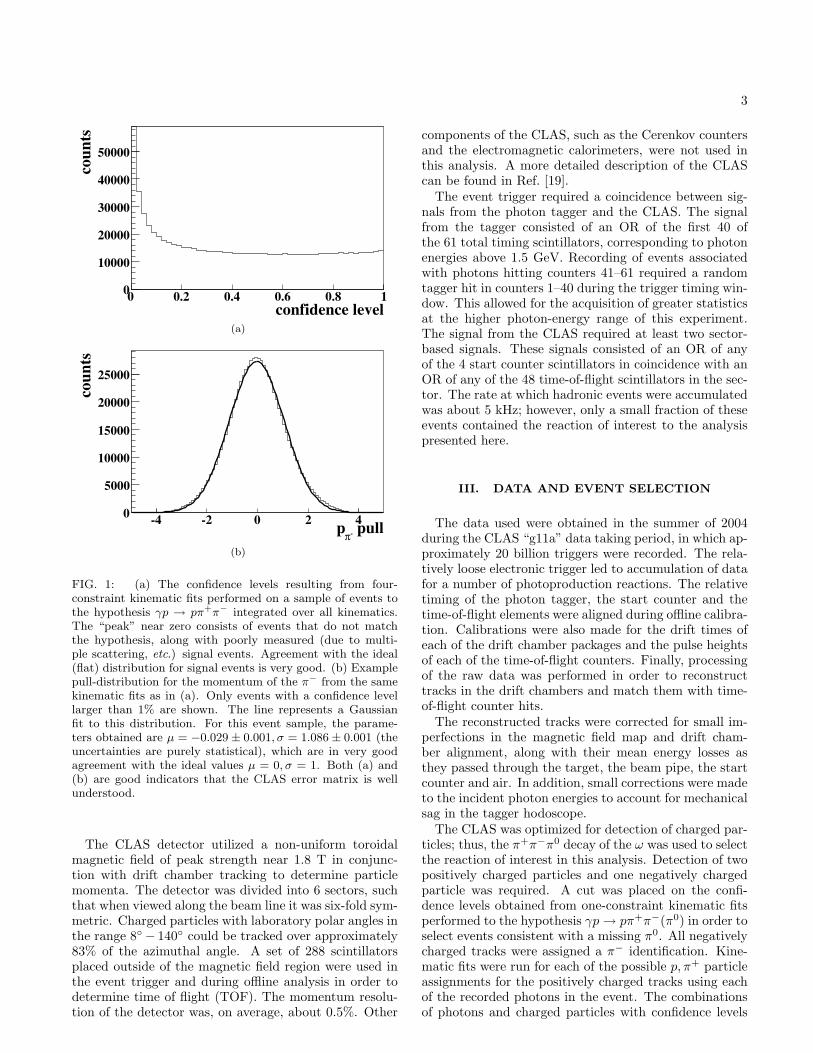
FIG. 1: (a) The confidence levels resulting from four-constraint kinematic fits performed on a sample of events tothe hypothesis γp → pπ+π− integrated over all kinematics.The “peak” near zero consists of events that do not matchthe hypothesis, along with poorly measured (due to multi-ple scattering, etc.) signal events. Agreement with the ideal(flat) distribution for signal events is very good. (b) Examplepull-distribution for the momentum of the π− from the samekinematic fits as in (a). Only events with a confidence levellarger than 1% are shown. The line represents a Gaussianfit to this distribution. For this event sample, the parame-ters obtained are µ = −0.029± 0.001, σ = 1.086± 0.001 (theuncertainties are purely statistical), which are in very goodagreement with the ideal values µ = 0, σ = 1. Both (a) and(b) are good indicators that the CLAS error matrix is wellunderstood.

The CLAS detector utilized a non-uniform toroidalmagnetic field of peak strength near 1.8 T in conjunc-tion with drift chamber tracking to determine particlemomenta. The detector was divided into 6 sectors, suchthat when viewed along the beam line it was six-fold sym-metric. Charged particles with laboratory polar angles inthe range 8◦− 140◦ could be tracked over approximately83% of the azimuthal angle. A set of 288 scintillatorsplaced outside of the magnetic field region were used inthe event trigger and during offline analysis in order todetermine time of flight (TOF). The momentum resolu-tion of the detector was, on average, about 0.5%. Other

components of the CLAS, such as the Cerenkov countersand the electromagnetic calorimeters, were not used inthis analysis. A more detailed description of the CLAScan be found in Ref. [19].

The event trigger required a coincidence between sig-nals from the photon tagger and the CLAS. The signalfrom the tagger consisted of an OR of the first 40 ofthe 61 total timing scintillators, corresponding to photonenergies above 1.5 GeV. Recording of events associatedwith photons hitting counters 41–61 required a randomtagger hit in counters 1–40 during the trigger timing win-dow. This allowed for the acquisition of greater statisticsat the higher photon-energy range of this experiment.The signal from the CLAS required at least two sector-based signals. These signals consisted of an OR of anyof the 4 start counter scintillators in coincidence with anOR of any of the 48 time-of-flight scintillators in the sec-tor. The rate at which hadronic events were accumulatedwas about 5 kHz; however, only a small fraction of theseevents contained the reaction of interest to the analysispresented here.

III. DATA AND EVENT SELECTION

The data used were obtained in the summer of 2004during the CLAS “g11a” data taking period, in which ap-proximately 20 billion triggers were recorded. The rela-tively loose electronic trigger led to accumulation of datafor a number of photoproduction reactions. The relativetiming of the photon tagger, the start counter and thetime-of-flight elements were aligned during offline calibra-tion. Calibrations were also made for the drift times ofeach of the drift chamber packages and the pulse heightsof each of the time-of-flight counters. Finally, processingof the raw data was performed in order to reconstructtracks in the drift chambers and match them with time-of-flight counter hits.

The reconstructed tracks were corrected for small im-perfections in the magnetic field map and drift cham-ber alignment, along with their mean energy losses asthey passed through the target, the beam pipe, the startcounter and air. In addition, small corrections were madeto the incident photon energies to account for mechanicalsag in the tagger hodoscope.

The CLAS was optimized for detection of charged par-ticles; thus, the π+π−π0 decay of the ω was used to selectthe reaction of interest in this analysis. Detection of twopositively charged particles and one negatively chargedparticle was required. A cut was placed on the confi-dence levels obtained from one-constraint kinematic fitsperformed to the hypothesis γp→ pπ+π−(π0) in order toselect events consistent with a missing π0. All negativelycharged tracks were assigned a π− identification. Kine-matic fits were run for each of the possible p, π+ particleassignments for the positively charged tracks using eachof the recorded photons in the event. The combinationsof photons and charged particles with confidence levels

4

greater than 10% were retained for further analysis.The covariance matrix was studied using four-

constraint kinematic fits (energy and momentum con-servation imposed) performed on the exclusive reactionγp→ pπ+π− in both real and Monte Carlo data samples.The confidence levels in all kinematic regions were foundto be sufficiently flat and the pull-distributions (stretchfunctions) were Gaussians centered at zero with σ = 1(see Fig. 1). The uncertainty in the extracted yields dueto differences in signal lost because of this confidence-level cut in real as compared to Monte Carlo data is es-timated to be 3%− 4%.

The tagger signal time, which was synchronized withthe accelerator radio-frequency (RF) timing, was propa-gated to the reaction vertex in order to obtain the starttime for the event. The stop time for each track was ob-tained from the TOF scintillator element hit by the track.The difference between these two times was the measuredtime of flight, tmeas. Track reconstruction through theCLAS magnetic field yielded both the momentum, ~p, ofeach track, along with the path length, L, from the reac-tion vertex to the time-of-flight counter hit by the track.The expected time of flight for a mass hypothesis, m, isthen given by

texp =L

c

√1 +

(m

p

)2

. (1)

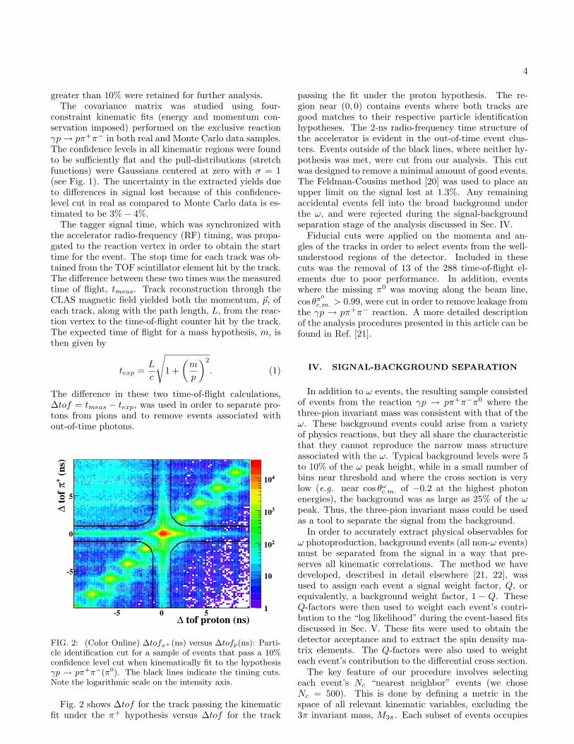
The difference in these two time-of-flight calculations,∆tof = tmeas − texp, was used in order to separate pro-tons from pions and to remove events associated without-of-time photons.

tof proton (ns)∆-5 0 5

(n

s)+

π t

of

∆

-5

0

5

1

10

210

310

410

FIG. 2: (Color Online) ∆tofπ+(ns) versus ∆tofp(ns): Parti-cle identification cut for a sample of events that pass a 10%confidence level cut when kinematically fit to the hypothesisγp → pπ+π−(π0). The black lines indicate the timing cuts.Note the logarithmic scale on the intensity axis.

Fig. 2 shows ∆tof for the track passing the kinematicfit under the π+ hypothesis versus ∆tof for the track

passing the fit under the proton hypothesis. The re-gion near (0, 0) contains events where both tracks aregood matches to their respective particle identificationhypotheses. The 2-ns radio-frequency time structure ofthe accelerator is evident in the out-of-time event clus-ters. Events outside of the black lines, where neither hy-pothesis was met, were cut from our analysis. This cutwas designed to remove a minimal amount of good events.The Feldman-Cousins method [20] was used to place anupper limit on the signal lost at 1.3%. Any remainingaccidental events fell into the broad background underthe ω, and were rejected during the signal-backgroundseparation stage of the analysis discussed in Sec. IV.

Fiducial cuts were applied on the momenta and an-gles of the tracks in order to select events from the well-understood regions of the detector. Included in thesecuts was the removal of 13 of the 288 time-of-flight el-ements due to poor performance. In addition, eventswhere the missing π0 was moving along the beam line,cos θπ

0

c.m. > 0.99, were cut in order to remove leakage fromthe γp → pπ+π− reaction. A more detailed descriptionof the analysis procedures presented in this article can befound in Ref. [21].

IV. SIGNAL-BACKGROUND SEPARATION

In addition to ω events, the resulting sample consistedof events from the reaction γp → pπ+π−π0 where thethree-pion invariant mass was consistent with that of theω. These background events could arise from a varietyof physics reactions, but they all share the characteristicthat they cannot reproduce the narrow mass structureassociated with the ω. Typical background levels were 5to 10% of the ω peak height, while in a small number ofbins near threshold and where the cross section is verylow (e.g. near cos θωc.m. of −0.2 at the highest photonenergies), the background was as large as 25% of the ωpeak. Thus, the three-pion invariant mass could be usedas a tool to separate the signal from the background.

In order to accurately extract physical observables forω photoproduction, background events (all non-ω events)must be separated from the signal in a way that pre-serves all kinematic correlations. The method we havedeveloped, described in detail elsewhere [21, 22], wasused to assign each event a signal weight factor, Q, orequivalently, a background weight factor, 1 − Q. TheseQ-factors were then used to weight each event’s contri-bution to the “log likelihood” during the event-based fitsdiscussed in Sec. V. These fits were used to obtain thedetector acceptance and to extract the spin density ma-trix elements. The Q-factors were also used to weighteach event’s contribution to the differential cross section.

The key feature of our procedure involves selectingeach event’s Nc “nearest neighbor” events (we choseNc = 500). This is done by defining a metric in thespace of all relevant kinematic variables, excluding the3π invariant mass, M3π. Each subset of events occupies

5

)2 (GeV/cπ3M

0.7 0.75 0.8 0.850

2000

4000

6000

8000

10000

)2 (GeV/cπ3M

0.7 0.75 0.8 0.850

2000

4000

6000

8000

10000

(a)

λ

0 0.2 0.4 0.6 0.8 10

500

1000

1500

2000

2500

λ

0 0.2 0.4 0.6 0.8 10

500

1000

1500

2000

2500

(b)

FIG. 3: (Color Online) (a) The 3π invariant mass distri-bution in the W = 2.205 GeV bin, integrated over all kine-matics, for all events (unshaded) and for events weighted bythe background factors, 1 −Q (shaded). (b) The λ distribu-tion of events in the same W bin that satisfy |M3π −Mω| <25 MeV/c2 (unshaded), the same events weighted by signalfactors Q (dashed-red), and by background factors 1 − Q(shaded). The line represents a fit of the signal to the functionaλ.

a very small region of phase space; thus, the M3π dis-tribution can safely be used to determine each event’sQ-factor, while preserving the correlations present in theremaining kinematic variables. This method facilitatesseparation of the signal and background without havingto resort to dividing the data up into bins. Binning thedata is undesirable due to the high dimensionality of thereaction being studied in this analysis.

To this end, unbinned maximum likelihood fits werecarried out for each event, using its nearest neighbors,

to determine the parameters ~α = (b0, b1, b2, b3, b4, s, σ) inthe probability density function

F (M3π, ~α) =B(M3π, ~α) + S(M3π, ~α)∫

(B(M3π, ~α) + S(M3π, ~α)) dM3π, (2)

where

S(M3π, ~α) = s · V (M3π,Mω,Γω, σ) (3)

parametrizes the signal as a Voigtian (con-volution of a Breit-Wigner and a Gaussian)with mass Mω = 0.78256 GeV/c2, natural widthΓω = 0.00844 GeV/c2 and resolution σ. The parameters sets the overall strength of the signal. The backgroundin each small phase space region was parametrized as afourth order polynomial,

B(M3π, ~α) = b4M43π+b3M

33π+b2M

23π+b1M3π+b0. (4)

The Q-factor for the event was then calculated as

Qi =S(M i

3π, αi)S(M i

3π, αi) +B(M i3π, αi)

, (5)

where M i3π is the event’s 3π invariant mass and αi are

the estimators for the parameters obtained from the ithevent’s fit. The signal yield could then be obtained inany kinematic bin as

Yω =N∑i

Qi, (6)

where N is the number of events in the bin.The full covariance matrix obtained from each fit was

used to obtain the uncertainty in Q, σQ. This varied de-pending on kinematics; however, it was typically about3%. The uncertainty of the extracted yield, in any kine-matic bin, was obtained by adding the Q-factor uncer-tainties (assuming 100% correlation) to the statistical un-certainty of the yield:

σ2Yω =

N∑i

Q2i +

(N∑i

σQi

)2

. (7)

Studies were performed using various backgroundparametrizations, including polynomials of different or-ders, all of which yielded results within the values ob-tained for σQ. Therefore, we conclude that no additionalsystematic uncertainty is required.

Fig. 3 demonstrates the effectiveness of applying thisprocedure in a single center-of-mass energy bin. Fig. 3(a)shows the M3π distribution, integrated over all kinemat-ics, and the estimated background using the proceduredescribed above. The results are quite plausible; how-ever, ω photoproduction provides us with a more strin-gent test of this procedure.

6

The distribution of the decay quantity λ, which can bewritten in terms of the pion momenta in the ω rest frameas

λ =|~pπ+ × ~pπ− |2

MAX (|~pπ+ × ~pπ− |2), (8)

must be linear in shape and intersect 0 at λ = 0 for ωevents — this follows directly from the ω → π+π−π0

amplitude defined in Eq. (10). Fig. 3(b) shows the λdistribution, integrated over all kinematics, for events inthe same bin shown in Fig. 3(a) in the region±25 MeV/c2around the ω peak, along with the extracted signal andbackground distributions. The signal distribution is welldescribed by the function aλ. The small discrepancy nearλ = 0 is the result of detector resolution.

The method we have employed has cleanly separatedsignal from background in the quantity λ, even thoughthe known linear behavior of the signal was not enforcedin the fits. In fact, this method has effectively separatedsignal from background in all distributions, successfullypreserving all kinematic correlations.

A detailed study of the systematic biases of the back-ground subtraction technique was carried out as part ofthis analysis. Not only was the function that was usedto parametrize the background varied, but the numberof nearest neighbor events was varied over a wide rangeand several different metrics were used to determine thenearest neighbors events. The observed physical mea-surements were found to be completely insensitive tochanges in these parameters over any reasonable set ofvalues. Because of this, we associate no additional sys-tematic error with these choices. A detailed descriptionof this study is contained in Ref. [22].

For energy bins near threshold and for “edge” regions(i.e. forward- and backward-most angles) in some en-ergy bins, the lack of events on both sides of the peakleaves the fits unconstrained. In these regions, the en-ergy dependence of the Q-factors obtained in the closestenergy bins for which fitting could be used were projecteddown to the regions in question in order to obtain the Q-factors. Fig. 4 shows the results of this procedure in theW = 1.735 GeV bin. By studying the λ distributionsin these bins, the systematic uncertainty associated withthe projected Q-factors in the edge regions is estimatedto be 5%. In the first two energy bins above threshold,the uncertainties are estimated to be 15% and 10% forthe W = 1.725 GeV and 1.735 GeV bins, respectively.

V. ACCEPTANCE

The efficiency of the detector was modeled using thestandard CLAS GEANT-based simulation package andthe Monte Carlo technique. A total of 200 million eventswas generated pseudo-randomly, sampled from a phasespace distribution. Each particle was propagated fromthe event vertex through the CLAS resulting in a simu-lated set of detector signals for each track. The simulated

)2 (GeV/cπ3M

0.74 0.76 0.78 0.8 0.820

200

400

600

800

1000

1200

1400

1600

1800

2000

2200

2400

)2 (GeV/cπ3M

0.74 0.76 0.78 0.8 0.820

200

400

600

800

1000

1200

1400

1600

1800

2000

2200

2400

FIG. 4: The 3π invariant mass distribution in theW = 1.735 GeV bin, integrated over all kinematics, for allevents (unshaded) and for events weighted by the backgroundfactors, 1−Q (shaded).

events were then processed using the same reconstructionsoftware as the data. In order to account for the eventtrigger used in this experiment (see Sec. II), a study wasperformed to obtain the probability of a track satisfyingthe sector-based coincidences required by the trigger as afunction of kinematics and struck detector elements. Theaverage effect of this correction in our analysis, which re-quires three detected particles, is about 5%–6%.

An additional momentum smearing algorithm was ap-plied in order to better match the resolution of the MonteCarlo to that of the data. Its effects were studied us-ing four-constraint kinematic fits performed on simulatedγp → pπ+π− events. After applying the momentumsmearing algorithm, the same covariance matrix used forthe data also produced flat confidence level distributionsin all kinematic regions for the Monte Carlo data as well.The simulated ω events were then processed with thesame analysis software as the data, including the one-constraint kinematic fits. At this stage, all detector andsoftware efficiencies were accounted for.

In order to evaluate the CLAS acceptance for theγp→ pω reaction, all kinematic correlations between thefinal state particles must be accurately reproduced bythe simulated data. Typically, this is done by using aphysics model when generating Monte Carlo events. Dueto the lack of any pre-existing precise polarization mea-surements in the kinematic regions that contain most ofour data, this was not an option. Instead, we chose to ex-pand the scattering amplitude, M, in a very large basis

7

of s-channel waves as follows:

Mmi,mγ ,mf ,mω (~x, ~α)

≈212∑

J= 12

∑P=±

AJP

mi,mγ ,mf ,mω(~x, ~α), (9)

where ~α denotes a vector of 108 fit parameters, ~x de-notes the complete set of kinematic variables describingthe reaction, mi,mγ ,mf ,mω are the spin projections onthe incident photon direction in the center-of-mass frame,and A are the s-channel partial wave amplitudes.

The ω → π+π−π0 amplitude, which is included in theA’s above, can be written in terms of the isovectors andthe 4-momenta of the pions, ~Iπ and pπ respectively, aswell as the ω 4-momentum (q) and polarization (ε) as

Aω→π+π−π0 ∝(

(~Iπ+ × ~Iπ0) · ~Iπ−)

×εµναβpνπ+pαπ−pβπ0ε

µ(q,mω), (10)

which is fully symmetric under interchange of the threepions. For this reaction, where all final states containω → π+π−π0, the isovector triple product simply con-tributes a factor to the global phase of all amplitudes. Inthe ω rest frame, Eq. (10) simplifies to

Aω→π+π−π0 ∝ (~pπ+ × ~pπ−) · ~ε(mω). (11)

The remaining s-channel structure of the amplitudes A,as well as the details concerning the fit parameters, isdescribed in [21].

Unbinned maximum likelihood fits were performed ineach W bin in order to obtain the estimators α for theparameters ~α in Eq. (9). The results of these fits wereused to obtain a weight, Ii, for each Monte Carlo eventaccording to

Ii =∑

mi,mγ ,mf

∣∣∣∣∣∑mω

Mmi,mγ ,mf ,mω (~xi, αi)

∣∣∣∣∣2

, (12)

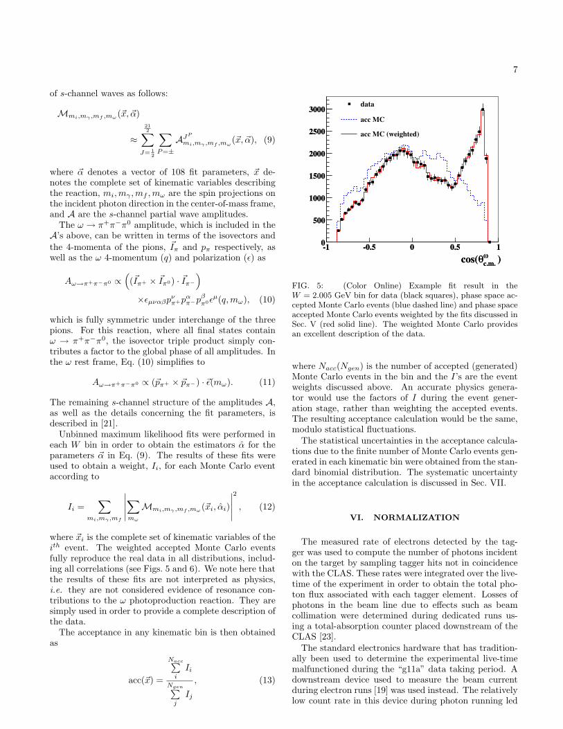
where ~xi is the complete set of kinematic variables of theith event. The weighted accepted Monte Carlo eventsfully reproduce the real data in all distributions, includ-ing all correlations (see Figs. 5 and 6). We note here thatthe results of these fits are not interpreted as physics,i.e. they are not considered evidence of resonance con-tributions to the ω photoproduction reaction. They aresimply used in order to provide a complete description ofthe data.

The acceptance in any kinematic bin is then obtainedas

acc(~x) =

Nacc∑i

Ii

Ngen∑j

Ij

, (13)

)c.m.

ωθcos(

-1 -0.5 0 0.5 10

500

1000

1500

2000

2500

3000

)c.m.

ωθcos(

-1 -0.5 0 0.5 10

500

1000

1500

2000

2500

3000data

acc MC

acc MC (weighted)

FIG. 5: (Color Online) Example fit result in theW = 2.005 GeV bin for data (black squares), phase space ac-cepted Monte Carlo events (blue dashed line) and phase spaceaccepted Monte Carlo events weighted by the fits discussed inSec. V (red solid line). The weighted Monte Carlo providesan excellent description of the data.

where Nacc(Ngen) is the number of accepted (generated)Monte Carlo events in the bin and the I’s are the eventweights discussed above. An accurate physics genera-tor would use the factors of I during the event gener-ation stage, rather than weighting the accepted events.The resulting acceptance calculation would be the same,modulo statistical fluctuations.

The statistical uncertainties in the acceptance calcula-tions due to the finite number of Monte Carlo events gen-erated in each kinematic bin were obtained from the stan-dard binomial distribution. The systematic uncertaintyin the acceptance calculation is discussed in Sec. VII.

VI. NORMALIZATION

The measured rate of electrons detected by the tag-ger was used to compute the number of photons incidenton the target by sampling tagger hits not in coincidencewith the CLAS. These rates were integrated over the live-time of the experiment in order to obtain the total pho-ton flux associated with each tagger element. Losses ofphotons in the beam line due to effects such as beamcollimation were determined during dedicated runs us-ing a total-absorption counter placed downstream of theCLAS [23].

The standard electronics hardware that has tradition-ally been used to determine the experimental live-timemalfunctioned during the “g11a” data taking period. Adownstream device used to measure the beam currentduring electron runs [19] was used instead. The relativelylow count rate in this device during photon running led

8

) = -0.9ω

c.m.θcos(

) θcos(-1 -0.5 0 0.5 1

φ

-2

0

2

) = -0.7ω

c.m.θcos( ) = -0.5

ω

c.m.θcos( ) = -0.3

ω

c.m.θcos( ) = -0.1

ω

c.m.θcos(

data

acc

mc

wtd

mc

(a)

) = 0.1ω

c.m.θcos(

) θcos(-1 -0.5 0 0.5 1

φ

-2

0

2

) = 0.3ω

c.m.θcos( ) = 0.5

ω

c.m.θcos( ) = 0.7

ω

c.m.θcos( ) = 0.9

ω

c.m.θcos(

data

acc

mc

wtd

mc

(b)

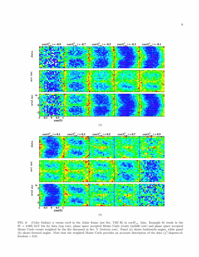
FIG. 6: (Color Online) φ versus cos θ in the Adair frame (see Sec. VIII B) in cos θωc.m. bins: Example fit result in theW = 2.005 GeV bin for data (top row), phase space accepted Monte Carlo events (middle row) and phase space acceptedMonte Carlo events weighted by the fits discussed in Sec. V (bottom row). Panel (a) shows backwards angles, while panel(b) shows forward angles. Note that the weighted Monte Carlo provides an accurate description of the data (χ2/degrees-of-freedom ∼ 0.6).

9

to increased uncertainty in the live-time measurement.The stability of normalized ω yields for runs with differ-ent beam currents was used to estimate this uncertaintyto be about 3%.

As was stated in Sec. II, only 40 of the 61 timing el-ements of the photon tagger were included in the eventtrigger. Events associated with hits in the “untriggered”counters, 41-61, were only recorded if a random hit incounters 1-40 occurred during the trigger time window.The electron rates used to measure the photon flux, dis-cussed above, were used to calculate the probability ofsuch an occurrence, Ptrig = 0.467. The measured fluxfor tagger counters 41–61 was scaled down by Ptrig toaccount for the event trigger.

Defective electronics in one of the tagger channels ledto inaccurate flux measurements in the energy bins atW = 2.735 and 2.745 GeV. The flux in the energy binat W = 1.955 GeV was also deemed unreliable due to itsinclusion of events associated with both triggered and un-triggered tagger counters. Differential cross sections arenot reported in these three energy bins; however, spindensity matrix elements, which do not require normal-ization information, are reported.

VII. SYSTEMATIC UNCERTAINTIES

The ω photoproduction cross section, for the case withan unpolarized beam and an unpolarized target, must beisotropic in the azimuthal angle. Thus, the acceptance-corrected ω yields, each obtained in an individual CLASsector, must be consistent with each other. By exam-ining the consistency of these yields, we estimated therelative uncertainty in the acceptance correction to be be-tween 4%–6%, depending on center-of-mass energy. Thisis added in quadrature with uncertainties due to parti-cle identification (1.3%) and confidence level (3%) cutsto obtain an overall estimated acceptance uncertainty of5%–7%.

It is common practice in photoproduction experimentsto check the quality of the normalization calculation bycomputing the single pion cross section and comparing itto the world’s data; however, the two-track trigger usedin this experiment does not permit such a calculation.In order to check our normalization, cross sections werealso computed for several other reactions from the “g11a”data set and compared to previously published CLASdata. The run-to-run consistency of the normalized ωyield was also examined. Based on these studies, we es-timate the normalization uncertainty to be 7.3%. Whencombined with contributions from photon transmissionefficiency (0.5%) and live-time (3%), the total estimatednormalization uncertainty is 7.9%.

The acceptance and normalization uncertainties dis-cussed above were then combined with contributionsfrom target density and length (0.2%), along withbranching fraction (0.7%) to obtain a total uncertainty,excluding contributions from signal-background separa-

tion that are calculated “point-to-point”, of about 9%–11%. In the first two energy bins above threshold, theadditional uncertainties in the signal-background separa-tion method (see Sec. IV) increase this number to 13%–17%.

VIII. RESULTS

A. Differential cross sections

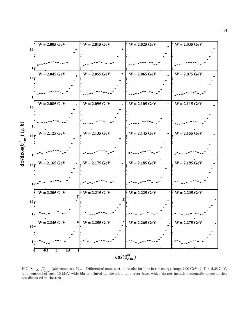
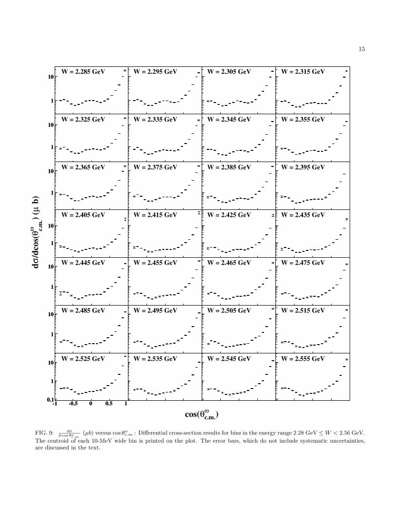
Differential cross sections, dσ/d cos θωc.m., were com-puted in 109 10-MeV wide bins in W . Each energy binwas divided into 20 bins in cos θωc.m. of width 0.1, al-though results could not be extracted in every bin dueto limitations in the detector acceptance. In total, 1960cross-section points are reported here. The centroid ofeach bin is reported as the mean of the range of thebin with nonzero acceptance. The results are shown inFigs. 7, 8, 9 and 10. The error bars contain the un-certainties of the yield extraction, discussed in Sec. IV,along with statistical uncertainties from the Monte Carloacceptance calculations. The overall systematic uncer-tainty, discussed in Sec. VII, is estimated to be between9%–11%, depending on center-of-mass energy.

In the “transverse direction”, which we can loosely de-fine as | cos θωc.m.| < 0.8, there are several prominent fea-tures present in the data. Near threshold, the transversecross section is mostly flat. Around W ∼ 1.9 GeV itbegins to develop a humped shape and by W ∼ 2.1 GeVthe cross section has two dips. In a concurrent article,we present partial wave analysis results obtained fromthis data which attribute these features to various baryonresonance contributions [16]. For now, we simply aimto draw attention to some of the prominent structurespresent in our measurements.

A very prominent forward peak begins to rise justabove threshold and continues to be the dominant fea-ture of the cross section up through our highest energies.This type of behavior typically indicates the presenceof strong t-channel contributions. Models of ω photo-production, e.g. Refs. [6, 7, 8, 9], typically associatethis peak with t-channel contributions from π0, η andPomeron exchange. A backwards peak begins to emergearound W ∼ 2.2 GeV, whose prominence increases as theenergy increases (although it is always at least one orderof magnitude smaller than the forward peak). This couldbe indicative of the presence of contributions in the u-channel. Many models of this reaction attribute this peakto u-channel nucleon exchange [6, 7, 8, 9]; however, com-parisons of the spin density matrix elements predictedby these models to the new high-precision measurementspresented in this article casts doubt on the validity ofthese models (see Sec. VIII C).

10

2

4

6 W = 1.725 GeV

2

4

6

2

4

6

8 W = 1.765 GeV

2

4

6

8

2

4

6

8 W = 1.805 GeV

2

4

6

8

2

4

6W = 1.845 GeV

2

4

6

2

4

6W = 1.885 GeV

2

4

6

2

4

6W = 1.925 GeV

2

4

6

-1 -0.5 0 0.5 1

1

10 W = 1.965 GeV

-1 -0.5 0 0.5 1

1

10

2

4

6 W = 1.735 GeV

2

4

6

2

4

6

8 W = 1.775 GeV

2

4

6

8

2

4

6

8 W = 1.815 GeV

2

4

6

8

2

4

6W = 1.855 GeV

2

4

6

2

4

6W = 1.895 GeV

2

4

6

2

4

6W = 1.935 GeV

2

4

6

1

10 W = 1.975 GeV

1

10

2

4

6 W = 1.745 GeV

2

4

6

2

4

6

8 W = 1.785 GeV

2

4

6

8

2

4

6

8 W = 1.825 GeV

2

4

6

8

2

4

6W = 1.865 GeV

2

4

6

2

4

6W = 1.905 GeV

2

4

6

2

4

6W = 1.945 GeV

2

4

6

1

10 W = 1.985 GeV

1

10

2

4

6 W = 1.755 GeV

2

4

6

2

4

6

8 W = 1.795 GeV

2

4

6

8

2

4

6

8 W = 1.835 GeV

2

4

6

8

2

4

6W = 1.875 GeV

2

4

6

2

4

6W = 1.915 GeV

2

4

6

2

4

6

1

10 W = 1.995 GeV

1

10

b)

µ)

(ω c.m

.θ

/dcos(

σd

)ωc.m.θcos(

FIG. 7: dσd cos θωc.m.

(µb) versus cos θωc.m.: Differential cross-section results for bins in the energy range 1.72 GeV ≤W < 2.00 GeV.

The centroid of each 10-MeV wide bin is printed on the plot. The lack of reported data points in the W = 1.955 GeV bin isdiscussed in Sec. VI. The error bars, which do not include systematic uncertainties, are discussed in the text. The additionalnear-threshold background separation uncertainties, discussed in Sec. IV, are clearly visible in the first four center-of-massenergy bins. Note that the vertical scales are linear up to W of 1.945 GeV and logarithmic above that.

11

B. Spin density matrix elements

The polarization of the ω can be studied by examiningthe distributions of its decay products. Since the ω is aspin-1 particle, its spin density matrix has nine complexelements; however, parity, hermiticity and normalizationreduce the number of independent elements (for an un-polarized beam) to four real quantities (of which, threeare measurable). Traditionally, these are chosen to beρ000, ρ0

1−1 and Re(ρ010). Our results cover a large range

of energies and angles; thus, we chose the quantizationaxis to be the photon direction in the overall c.m. frame,known as the Adair frame [24].

The spin density matrix elements can be written interms of the production amplitudes A (i.e. the scatteringamplitudesM introduced in Sec. V without the ω decaypiece), as

ρ0MM ′ =

1N

∑mγ ,mi,mf

Ami,mγ ,mf ,MA∗mi,mγ ,mf ,M ′ , (14)

where the M,M ′ refer to the spin projection of the ω (onthe photon direction in the c.m. frame) and

N =∑

mi,mγ ,mf

∑M

|Ami,mγ ,mf ,M |2, (15)

is a normalization factor. Using the production ampli-tudes obtained from the event-based fits described inSec. V, the spin density matrix elements were projectedout of the partial wave expansion at 2015 (W, cos θωc.m.)points. These data points correspond to the centroidsof the bins for which cross-section results are reported,along with additional points in the W = 1.955 GeV,2.735 GeV and 2.745 GeV center-of-mass energy bins forwhich cross-sections results are not reported due to nor-malization issues (see Sec. VI).

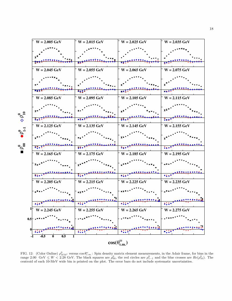
Figs. 11, 12, 13 and 14 show the ρ0MM ′ results extracted

using the partial wave expansion technique. The errorbars are purely statistical. The spin density matrix el-ements do not rely on normalization information; thus,only the acceptance can contribute to the systematic un-certainty. Possible effects due to systematic problemsin the acceptance calculation were examined by analyz-ing decay distributions distorted by our estimated accep-tance uncertainty. Based on this study, we estimate thesystematic uncertainties in our results to be as follows:

σ00 = 0.0175 (16a)σ1−1 = 0.0125 (16b)σ10 = 0.01. (16c)

Over most of our kinematics, these results representthe first high-precision measurements of ρ0

MM ′ for ω pho-toproduction. Near threshold and at forward angles, thecross section develops a strong forward peak, which is in-dicative of t-channel contributions. In this same region,the diagonal ρ0

00 element decreases sharply as the energy

increases, or equivalently, as the forward peak increasesin significance. This is typical of exchange of a spin-0 par-ticle in the t-channel where the ω is forced to carry thespin of the photon at forward angles. This new precisepolarization information should help determine the rela-tive strengths of the scalar and pseudoscalar exchanges(see Sec. VIII C).

At higher energies, starting near W ∼ 2.1 GeV, a dipin ρ0

00 appears at cos θωc.m. ∼ 0.4, which continues to in-crease in prominence until about W ∼ 2.5 GeV. Abovethis energy, its significance slowly decreases; however, itis still present at our highest energies. This dip is locatednear where the forward peak (typically associated with t-channel contributions) has decreased in significance suchthat it is approximately the same size as the cross sec-tion in the region 0 < cos θωc.m. < 0.4. Thus, it is pos-sible that this dip results from interference between thet-channel and larger-angle production mechanisms. Inthe kinematic regions where the cross section possessesthe humps and dips discussed in Sec. VIII A, there are anumber of interesting features found in the spin densitymatrix elements as well. The partial wave analysis weperformed on this data found that these features are welldescribed by baryon resonance contributions [16].

C. Interpretation of the data

In the low-energy regime, these new measurementshave been used to carry out a mass-independent par-tial wave analysis of the reaction γp → ωp. The resultsof this analysis, which are presented in a concurrent arti-cle [16] and are not discussed in detail here, show clear ev-idence of s-channel resonance contributions. This PWA,the results of which are different from previous analy-ses [8, 10, 11, 12, 13, 14], was the first to benefit fromthe strong additional constraints provided by the high-precision polarization results obtained from these data.

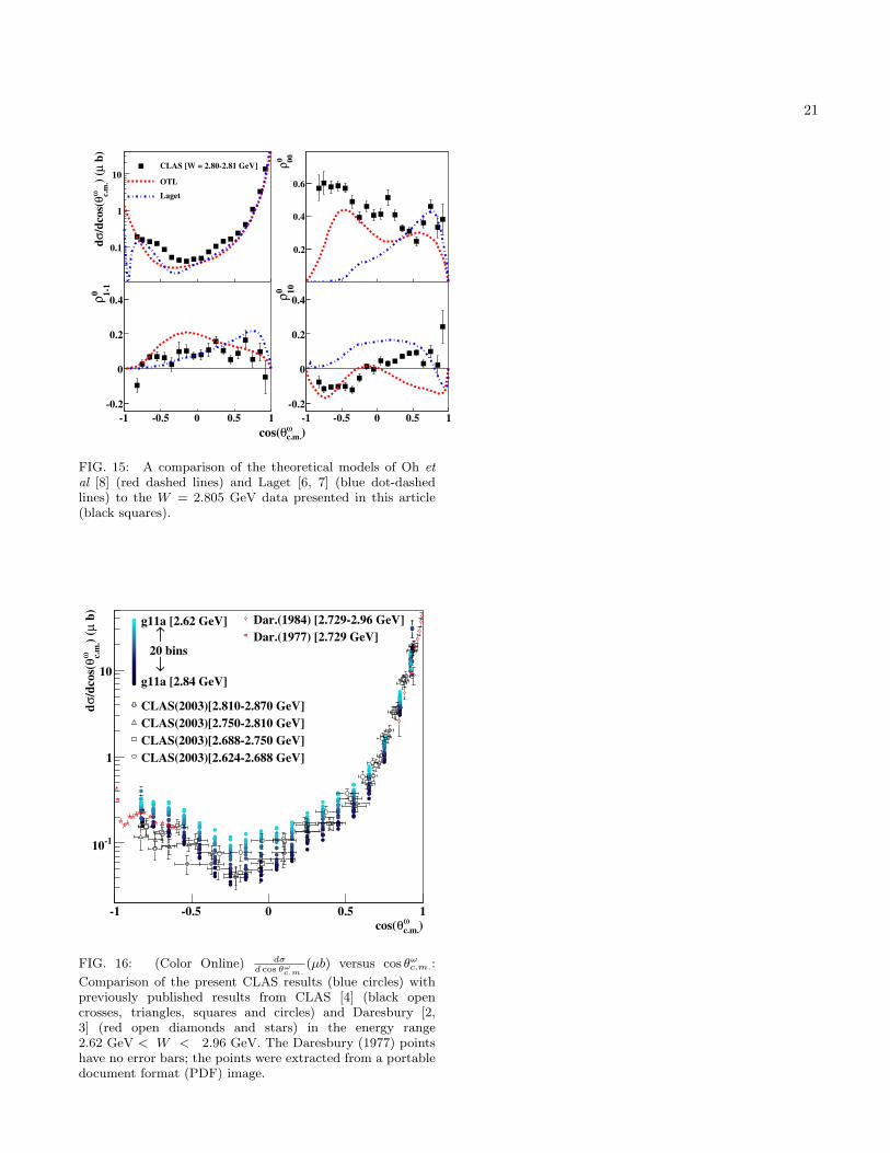
The high-energy measurements have been comparedto two existing models for ω photoproduction. Thefirst is the model of Oh et al [8] which includes pseu-doscalar meson (π0 and η) and Pomeron exchange in thet-channel, along with nucleon exchange in both the s-and u-channel. It also includes s-channel contributions,which are necessary to describe the data in the centralregion of the angular range. The second model is thatof Laget [6, 7] which includes t- and u-channel contri-butions similar to that of Ref. [8], but also allows fora contribution from two-gluon exchange. In this lattermodel, the two-gluon term is required to describe the φphotoproduction data.

Fig. 15 shows comparisons of these models to our dataat W = 2.8 GeV. Both models do a reasonable jobof reproducing the cross-section measurements. The t-channel terms drive the very forward-angle data wherethe agreement is very good. At backwards angles, wherethe u-channel terms dominate, the agreement is not asgood as it is at forward angles. In the central region,

12

both models agree with the overall shape of the crosssection; however, the finer structure in the data is notreproduced.

Neither model is able to reproduce the new high-precision spin density matrix element measurements pre-sented in this article. While some regions are reason-ably well described by one model or the other, neithergives anything close to good overall agreement. Perhapsthe most striking discrepancy is that at forward angles,where the cross sections are described very well by bothmodels, neither provides an excellent description of thespin density matrix elements. The high-precision mea-surements presented in this article clearly provide newstringent constraints on both the nature of the produc-tion mechanisms in the high-energy regime, as well as onthe search for missing baryon resonances.

D. Comparison to previous measurements

Previous experimental measurements that overlap ourenergy range have been made at CLAS in 2003 [4],at SAPHIR in 2003 [5], at Daresbury in 1984 [3] and1977 [2], and at SLAC in 1973 [1]. Below we compareour measurements with each of these previous results.The cross sections will be examined first, followed by thespin density matrix elements.

Fig. 16 shows a comparison of the cross-section re-sults presented in this article with previously publishedresults from CLAS [4] and Daresbury [2, 3]. Theprevious CLAS results, four energy bins in the range2.624 GeV < W < 2.87 GeV, cover virtually the sameangular range as the current results. The agreement isvery good for cos θωc.m. > −0.1; however, there is a siz-able discrepancy in the backward direction. At the timeof the earlier CLAS measurement, the ω polarization hadonly been measured in the forward direction (see Fig. 19);thus, these values of the spin density matrix elementswere used in the acceptance calculation. Our results showthat the polarization is quite different at backward andforward angles. Near the edges of the CLAS acceptance,e.g. in the backward direction, an incorrect description ofthe polarization can lead to large errors in the acceptancecalculation. This is most likely the cause of the discrep-ancy in the cross sections. The Daresbury results, whichwere only published in the very forward and backwardregions, are in good agreement with our measurements.

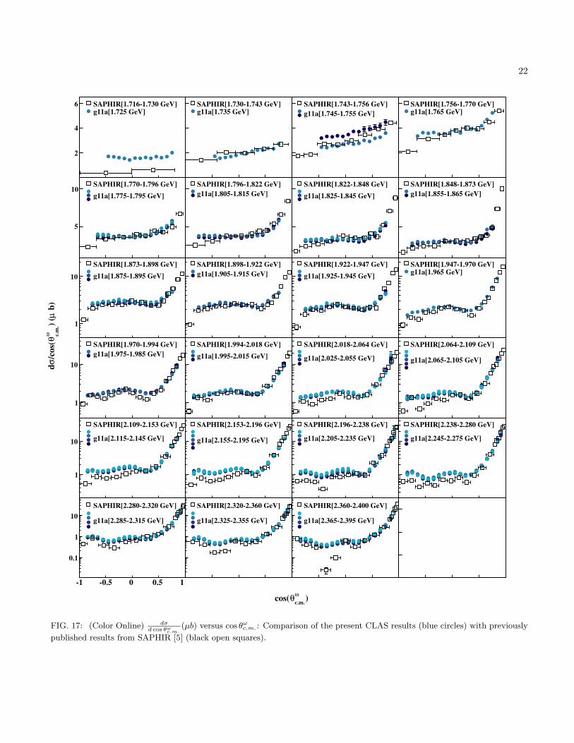
For W < 2.4 GeV, the previous large acceptance re-sults come from SAPHIR [5]. Fig. 17 shows a compari-son of the SAPHIR cross-section measurements with thepresent CLAS results. The error bars shown for theSAPHIR points do not include systematic uncertainties.The agreement is fair, but there are some discrepancies.The SAPHIR experiment had better angular coverage;however, the CLAS results are more precise. In the for-ward direction, the agreement is very good at all energies.At moderate angles, | cos θωc.m.| < 0.5, the agreement isgood at lower energies but the CLAS results tend to be

higher as the energy increases. In the backward direc-tion, where the CLAS has acceptance, the CLAS pointsare almost always higher than the SAPHIR points.

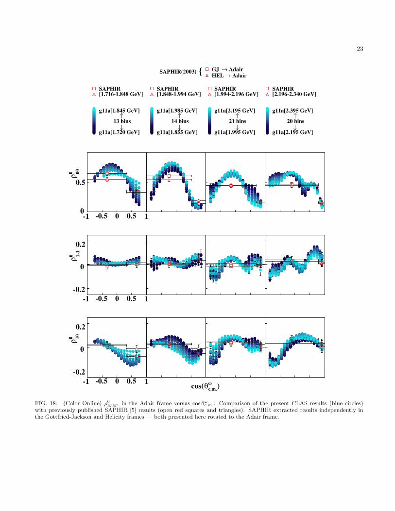
Previous spin density matrix element measurementsare much less precise. The only results published forW < 2.4 GeV come from SAPHIR [5]. Fig. 18 showsa comparison of the SAPHIR results, which consist onlyof four energy bins, each with two angular points, andthe present CLAS results, which include 1371 total datapoints in this energy range. We note here that theSAPHIR collaboration published their results in both theGottfried-Jackson and Helicity frames, with each mea-surement constituting an independent fit to their data.Both results were rotated into the Adair frame for com-parison. Overall, the SAPHIR results are in good agree-ment with our measurements.

At higher energies, previously published results onlyexist at very forward angles. Fig. 19 shows a compari-son of our forward high energy results with those fromDaresbury [3] and SLAC [1]. The agreement is good.For W > 2.4 GeV, the results presented in this ar-ticle for ρ0

MM ′ are the world’s first measurements forcos θωc.m. < 0.8.

IX. CONCLUSIONS

In summary, experimental results for ω photoproduc-tion from the proton have been presented in the energyregime from threshold up to W = 2.84 GeV. Both differ-ential cross section and spin density matrix element mea-surements are reported. The cross-section results are themost precise to date and provide the largest energy andangular coverage. The results are in fair to good agree-ment with previous experiments. For W < 2.4 GeV,we present 1181 ρ0

MM ′ data points; the previous world’sdata consisted of 8 points. At higher energies, we havemade the first spin density matrix element measurementsfor cos θωc.m. < 0.8. Our ρ0

MM ′ measurements are ingood agreement with the, rather sparse, existing data.The 1960 (W, cos θωc.m.) cross-section points, along withthe 2015 (W, cos θωc.m.) spin density matrix element datapoints can be obtained at Ref. [25].

These new data will have a large impact on our cur-rent understanding of vector-meson photoproduction, aswell as provide a crucial data set in the search for miss-ing baryon resonances. A mass-independent partial waveanalysis performed on these data, which is the first suchanalysis to benefit from the strong constraints providedby high-precision polarization information, found strongevidence for baryon resonance contributions [16]. Fur-thermore, none of the current models of high-energy ωphotoproduction are able to describe the precise spindensity matrix element measurements presented in thisarticle. We look forward to seeing what impact thesenew results will have on future models of vector-mesonphotoproduction.

13

Acknowledgments

We thank the staff of the Accelerator and the PhysicsDivisions at Thomas Jefferson National Accelerator Fa-cility who made this experiment possible. This work wassupported in part by the U.S. Department of Energy (un-der grant No. DE-FG02-87ER40315), the National Sci-ence Foundation, the Italian Istituto Nazionale di Fisica

Nucleare, the French Centre National de la RechercheScientifique, the French Commissariat a l’Energie Atom-ique, the Science and Technology Facilities Council(STFC), and the Korean Science and Engineering Foun-dation. The Southeastern Universities Research Associa-tion (SURA) operated Jefferson Lab under United StatesDOE contract DE-AC05-84ER40150 during this work.

[1] J. Ballam et al., Phys. Rev. D 7, 3150 (1973).[2] R.W. Clift et al., Phys. Lett. B 72, 144 (1977).[3] D.P. Barber et al. (LAMP2 Group Collaboration), Z.

Phys. C 26, 343 (1984).[4] M. Battaglieri et al. (CLAS Collaboration), Phys. Rev.

Lett. 90, 022002 (2003).[5] J. Barth et al. (SAPHIR Collaboration), Eur. Phys. J. A

18, 117 (2003).[6] J.-M. Laget, Phys. Lett. B 489, 313 (2000).[7] J.-M. Laget, Nucl. Phys. A 699, 184c (2002).[8] Y. Oh, A. I. Titov and T.-S. H. Lee, Phys. Rev. C 63,

025201 (2001).[9] A. Sibirtsev, K. Tsushima and S. Krewald, arXiv:nucl-

th/0202083 (2002).[10] Mark Paris, Phys. Rev. C79, 025208 (2009).[11] Q. Zhao., Phys. Rev. C 63, 025203 (2001).[12] A.I. Titov and T.-S.H. Lee, Phys. Rev. C 66, 015204

(2002).[13] G. Penner and U. Mosel, Phys. Rev. C 66, 055212 (2002).[14] V. Shklyar, H. Lenske, U. Mosel, and G. Penner, Phys.

Rev. C 71, 055206 (2005).[15] S. Capstick and W. Roberts, Phys. Rev. D 49, 4570

(1993).[16] M. Williams et al. (CLAS Collaboration), Submitted to

Phys. Rev. C (2009), arXiv:0908:2911 [nucl-ex].[17] M. Williams et al., The impact on the phenomenology of

γp → pω of the first high-precision measurements of ωpolarization observables, to be submitted to Phys. Rev.Lett. (2009).

[18] D.I. Sober, et al., Nucl. Instrum. Methods A440, 263(2000).

[19] B. A. Mecking et al., Nucl. Instrum. Methods A503, 513(2003).

[20] G. Feldman and R. Cousins, Phys. Rev. D 57, 3873(1998).

[21] M. Williams, Ph.D. thesis, Carnegie Mellon University,2007,www.jlab.org/Hall-B/general/clas thesis.html.

[22] M. Williams, M. Bellis and C. A. Meyer, JINST 4,P10003, (2009).

[23] J. Ball and E. Pasyuk. CLAS Note 2005-002 (2005),www.jlab.org/Hall-B/notes/.

[24] K. Schilling, P. Seyboth and G. Wolf, Nucl. Phys. B15,397 (1970).

[25] The CLAS physics database,clasweb.jlab.org/physicsdb.

14

1

10

W = 2.005 GeV

1

10

1

10W = 2.045 GeV

1

10

1

10W = 2.085 GeV

1

10

1

10W = 2.125 GeV

1

10

1

10W = 2.165 GeV

1

10

1

10

W = 2.205 GeV

1

10

-1 -0.5 0 0.5 1

1

10

W = 2.245 GeV

-1 -0.5 0 0.5 1

1

10

1

10

W = 2.015 GeV

1

10

1

10W = 2.055 GeV

1

10

1

10W = 2.095 GeV

1

10

1

10W = 2.135 GeV

1

10

1

10W = 2.175 GeV

1

10

1

10

W = 2.215 GeV

1

10

1

10W = 2.255 GeV

1

10

1

10

W = 2.025 GeV

1

10

1

10W = 2.065 GeV

1

10

1

10W = 2.105 GeV

1

10

1

10W = 2.145 GeV

1

10

1

10W = 2.185 GeV

1

10

1

10

W = 2.225 GeV

1

10

1

10W = 2.265 GeV

1

10

1

10

W = 2.035 GeV

1

10

1

10W = 2.075 GeV

1

10

1

10W = 2.115 GeV

1

10

1

10W = 2.155 GeV

1

10

1

10W = 2.195 GeV

1

10

1

10

W = 2.235 GeV

1

10

1

10W = 2.275 GeV

1

10

b)

µ)

(ω c.m

.θ

/dcos(

σd

)ωc.m.θcos(

FIG. 8: dσd cos θωc.m.

(µb) versus cos θωc.m.: Differential cross-section results for bins in the energy range 2.00 GeV ≤W < 2.28 GeV.

The centroid of each 10-MeV wide bin is printed on the plot. The error bars, which do not include systematic uncertainties,are discussed in the text.

15

1

10W = 2.285 GeV

1

10

1

10W = 2.325 GeV

1

10

1

10W = 2.365 GeV

1

10

1

10

W = 2.405 GeV

1

10

1

10W = 2.445 GeV

1

10

1

10W = 2.485 GeV

1

10

-1 -0.5 0 0.5 10.1

1

10W = 2.525 GeV

-1 -0.5 0 0.5 10.1

1

10

1

10W = 2.295 GeV

1

10

1

10W = 2.335 GeV

1

10

1

10W = 2.375 GeV

1

10

1

10

W = 2.415 GeV

1

10

1

10W = 2.455 GeV

1

10

1

10W = 2.495 GeV

1

10

0.1

1

10W = 2.535 GeV

0.1

1

10

1

10W = 2.305 GeV

1

10

1

10W = 2.345 GeV

1

10

1

10W = 2.385 GeV

1

10

1

10

W = 2.425 GeV

1

10

1

10W = 2.465 GeV

1

10

1

10W = 2.505 GeV

1

10

0.1

1

10W = 2.545 GeV

0.1

1

10

1

10W = 2.315 GeV

1

10

1

10W = 2.355 GeV

1

10

1

10W = 2.395 GeV

1

10

1

10

W = 2.435 GeV

1

10

1

10W = 2.475 GeV

1

10

1

10W = 2.515 GeV

1

10

0.1

1

10W = 2.555 GeV

0.1

1

10

b)

µ)

(ω c.m

.θ

/dcos(

σd

)ωc.m.θcos(

FIG. 9: dσd cos θωc.m.

(µb) versus cos θωc.m.: Differential cross-section results for bins in the energy range 2.28 GeV ≤W < 2.56 GeV.

The centroid of each 10-MeV wide bin is printed on the plot. The error bars, which do not include systematic uncertainties,are discussed in the text.

16

0.1

1

10 W = 2.565 GeV

0.1

1

10

0.1

1

10 W = 2.605 GeV

0.1

1

10

0.1

1

10 W = 2.645 GeV

0.1

1

10

0.1

1

10 W = 2.685 GeV

0.1

1

10

0.1

1

10W = 2.725 GeV

0.1

1

10

0.1

1

10W = 2.765 GeV

0.1

1

10

-1 -0.5 0 0.5 1

0.1

1

10 W = 2.805 GeV

-1 -0.5 0 0.5 1

0.1

1

10

0.1

1

10 W = 2.575 GeV

0.1

1

10

0.1

1

10 W = 2.615 GeV

0.1

1

10

0.1

1

10 W = 2.655 GeV

0.1

1

10

0.1

1

10 W = 2.695 GeV

0.1

1

10

20

40

0.1

1

10W = 2.775 GeV

0.1

1

10

0.1

1

10 W = 2.815 GeV

0.1

1

10

0.1

1

10 W = 2.585 GeV

0.1

1

10

0.1

1

10 W = 2.625 GeV

0.1

1

10

0.1

1

10 W = 2.665 GeV

0.1

1

10

0.1

1

10 W = 2.705 GeV

0.1

1

10

20

40

0.1

1

10W = 2.785 GeV

0.1

1

10

0.1

1

10 W = 2.825 GeV

0.1

1

10

0.1

1

10 W = 2.595 GeV

0.1

1

10

0.1

1

10 W = 2.635 GeV

0.1

1

10

0.1

1

10 W = 2.675 GeV

0.1

1

10

0.1

1

10 W = 2.715 GeV

0.1

1

10

0.1

1

10W = 2.755 GeV

0.1

1

10

0.1

1

10W = 2.795 GeV

0.1

1

10

0.1

1

10 W = 2.835 GeV

0.1

1

10

b)

µ)

(ω c.m

.θ

/dcos(

σd

)ωc.m.θcos(

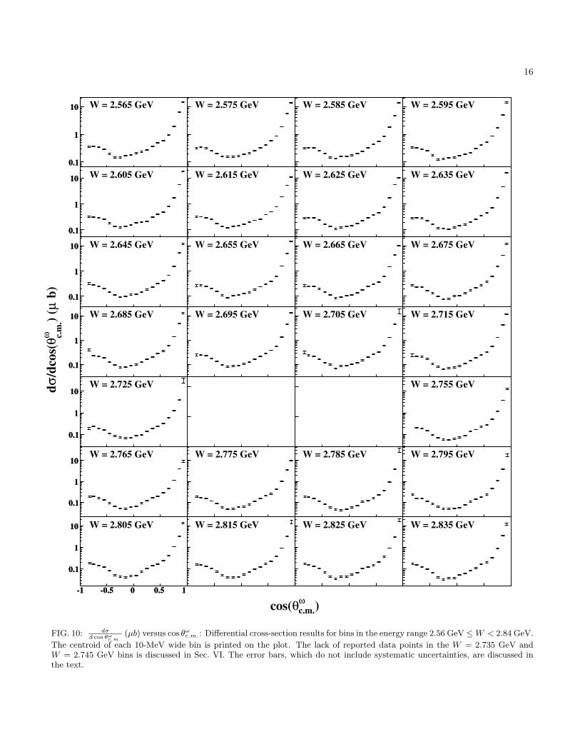
FIG. 10: dσd cos θωc.m.

(µb) versus cos θωc.m.: Differential cross-section results for bins in the energy range 2.56 GeV≤W < 2.84 GeV.

The centroid of each 10-MeV wide bin is printed on the plot. The lack of reported data points in the W = 2.735 GeV andW = 2.745 GeV bins is discussed in Sec. VI. The error bars, which do not include systematic uncertainties, are discussed inthe text.

17

W = 1.725 GeV

W = 1.765 GeV

W = 1.805 GeV

W = 1.845 GeV

W = 1.885 GeV

W = 1.925 GeV

-1 -0.5 0 0.5 1

0

0.5

1 W = 1.965 GeV

-1 -0.5 0 0.5 1

0

0.5

1

W = 1.735 GeV

W = 1.775 GeV

W = 1.815 GeV

W = 1.855 GeV

W = 1.895 GeV

W = 1.935 GeV

W = 1.975 GeV

W = 1.745 GeV

W = 1.785 GeV

W = 1.825 GeV

W = 1.865 GeV

W = 1.905 GeV

W = 1.945 GeV

W = 1.985 GeV

W = 1.755 GeV

W = 1.795 GeV

W = 1.835 GeV

W = 1.875 GeV

W = 1.915 GeV

W = 1.955 GeV

W = 1.995 GeV

00

0ρ

1-1

0ρ

10

0ρ

)ωc.m.θcos(

FIG. 11: (Color Online) ρ0MM′ versus cos θωc.m.: Spin density matrix element measurements, in the Adair frame, for bins in the

range 1.72 GeV ≤ W < 2.00 GeV. The black squares are ρ000, the red circles are ρ0

1−1 and the blue crosses are Re(ρ010). The

centroid of each 10-MeV wide bin is printed on the plot. The error bars do not include systematic uncertainties.

18

W = 2.005 GeV

W = 2.045 GeV

W = 2.085 GeV

W = 2.125 GeV

W = 2.165 GeV

W = 2.205 GeV

-1 -0.5 0 0.5 1

0

0.5

1 W = 2.245 GeV

-1 -0.5 0 0.5 1

0

0.5

1

W = 2.015 GeV

W = 2.055 GeV

W = 2.095 GeV

W = 2.135 GeV

W = 2.175 GeV

W = 2.215 GeV

W = 2.255 GeV

W = 2.025 GeV

W = 2.065 GeV

W = 2.105 GeV

W = 2.145 GeV

W = 2.185 GeV

W = 2.225 GeV

W = 2.265 GeV

W = 2.035 GeV

W = 2.075 GeV

W = 2.115 GeV

W = 2.155 GeV

W = 2.195 GeV

W = 2.235 GeV

W = 2.275 GeV

00

0ρ

1-1

0ρ

10

0ρ

)ωc.m.θcos(

FIG. 12: (Color Online) ρ0MM′ versus cos θωc.m.: Spin density matrix element measurements, in the Adair frame, for bins in the

range 2.00 GeV ≤ W < 2.28 GeV. The black squares are ρ000, the red circles are ρ0

1−1 and the blue crosses are Re(ρ010). The

centroid of each 10-MeV wide bin is printed on the plot. The error bars do not include systematic uncertainties.

19

W = 2.285 GeV

W = 2.325 GeV

W = 2.365 GeV

W = 2.405 GeV

W = 2.445 GeV

W = 2.485 GeV

-1 -0.5 0 0.5 1

0

0.5

1 W = 2.525 GeV

-1 -0.5 0 0.5 1

0

0.5

1

W = 2.295 GeV

W = 2.335 GeV

W = 2.375 GeV

W = 2.415 GeV

W = 2.455 GeV

W = 2.495 GeV

W = 2.535 GeV

W = 2.305 GeV

W = 2.345 GeV

W = 2.385 GeV

W = 2.425 GeV

W = 2.465 GeV

W = 2.505 GeV

W = 2.545 GeV

W = 2.315 GeV

W = 2.355 GeV

W = 2.395 GeV

W = 2.435 GeV

W = 2.475 GeV

W = 2.515 GeV

W = 2.555 GeV

00

0ρ

1-1

0ρ

10

0ρ

)ωc.m.θcos(

FIG. 13: (Color Online) ρ0MM′ versus cos θωc.m.: Spin density matrix element measurements, in the Adair frame, for bins in the

range 2.28 GeV ≤ W < 2.56 GeV. The black squares are ρ000, the red circles are ρ0

1−1 and the blue crosses are Re(ρ010). The

centroid of each 10-MeV wide bin is printed on the plot. The error bars do not include systematic uncertainties.

20

W = 2.565 GeV

W = 2.605 GeV

W = 2.645 GeV

W = 2.685 GeV

W = 2.725 GeV

W = 2.765 GeV

-1 -0.5 0 0.5 1

0

0.5

1 W = 2.805 GeV

-1 -0.5 0 0.5 1

0

0.5

1

W = 2.575 GeV

W = 2.615 GeV

W = 2.655 GeV

W = 2.695 GeV

W = 2.735 GeV

W = 2.775 GeV

W = 2.815 GeV

W = 2.585 GeV

W = 2.625 GeV

W = 2.665 GeV

W = 2.705 GeV

W = 2.745 GeV

W = 2.785 GeV

W = 2.825 GeV

W = 2.595 GeV

W = 2.635 GeV

W = 2.675 GeV

W = 2.715 GeV

W = 2.755 GeV

W = 2.795 GeV

W = 2.835 GeV

00

0ρ

1-1

0ρ

10

0ρ

)ωc.m.θcos(

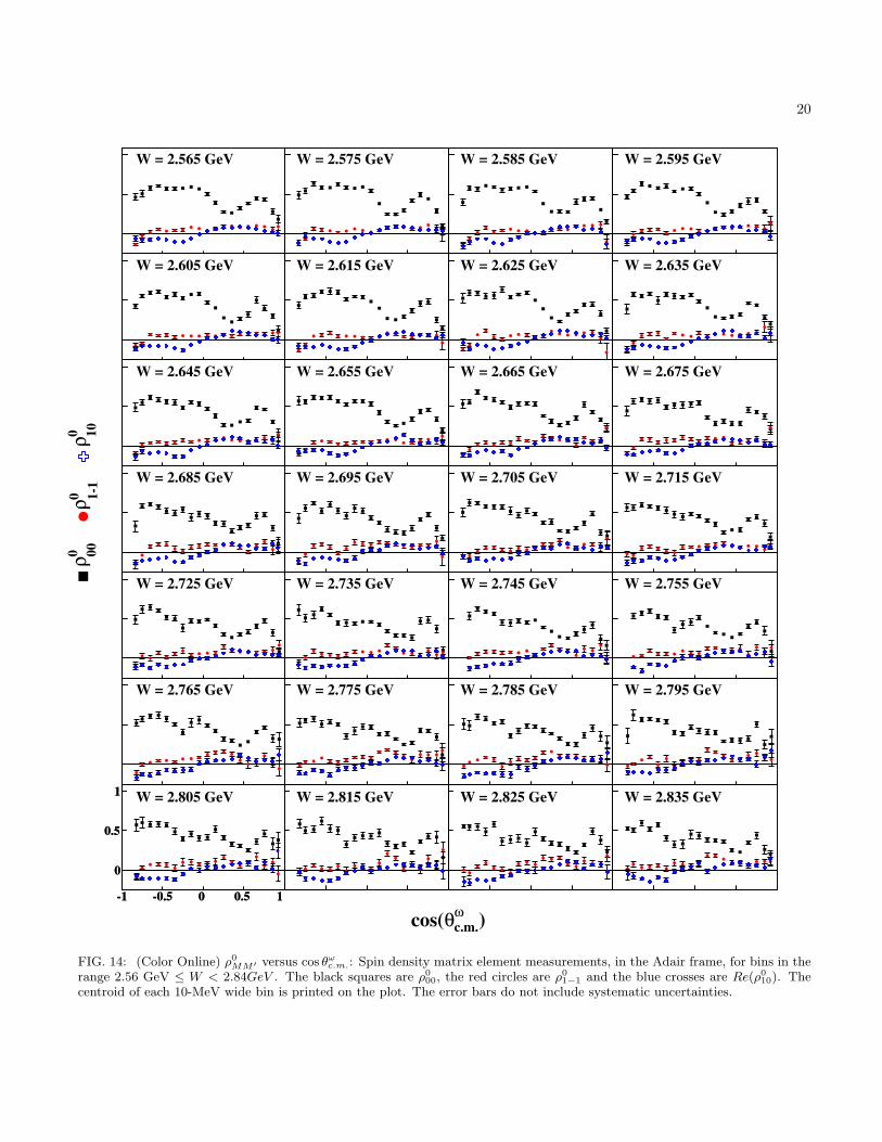
FIG. 14: (Color Online) ρ0MM′ versus cos θωc.m.: Spin density matrix element measurements, in the Adair frame, for bins in the

range 2.56 GeV ≤ W < 2.84GeV . The black squares are ρ000, the red circles are ρ0

1−1 and the blue crosses are Re(ρ010). The

centroid of each 10-MeV wide bin is printed on the plot. The error bars do not include systematic uncertainties.

21

-1 -0.5 0 0.5 1

b)

µ)

(ω c.

m.

θ/d

cos(

σd

0.1

1

10CLAS [W = 2.80-2.81 GeV]

OTL

Laget

-1 -0.5 0 0.5 1

1

-10ρ

-0.2

0

0.2

0.4

-1 -0.5 0 0.5 1

000

ρ

0.2

0.4

0.6

-1 -0.5 0 0.5 1

1

00ρ

-0.2

0

0.2

0.4

)ωc.m.θcos(

FIG. 15: A comparison of the theoretical models of Oh etal [8] (red dashed lines) and Laget [6, 7] (blue dot-dashedlines) to the W = 2.805 GeV data presented in this article(black squares).

)ωc.m.θcos(

-1 -0.5 0 0.5 1

b)

µ)

(ω c.

m.

θ/d

cos(

σd

-110

1

10

g11a [2.62 GeV]

g11a [2.84 GeV]

20 bins

↓

↑

CLAS(2003)[2.624-2.688 GeV]

CLAS(2003)[2.688-2.750 GeV]

CLAS(2003)[2.750-2.810 GeV]

CLAS(2003)[2.810-2.870 GeV]

Dar.(1977) [2.729 GeV]

Dar.(1984) [2.729-2.96 GeV]

FIG. 16: (Color Online) dσd cos θωc.m.

(µb) versus cos θωc.m.:

Comparison of the present CLAS results (blue circles) withpreviously published results from CLAS [4] (black opencrosses, triangles, squares and circles) and Daresbury [2,3] (red open diamonds and stars) in the energy range2.62 GeV < W < 2.96 GeV. The Daresbury (1977) pointshave no error bars; the points were extracted from a portabledocument format (PDF) image.

22

2

4

6g11a[1.725 GeV]SAPHIR[1.716-1.730 GeV]

5

10g11a[1.775-1.795 GeV]

SAPHIR[1.770-1.796 GeV]

1

10 g11a[1.875-1.895 GeV]

SAPHIR[1.873-1.898 GeV]

1

10

g11a[1.975-1.985 GeV]

SAPHIR[1.970-1.994 GeV]

1

10g11a[2.115-2.145 GeV]

SAPHIR[2.109-2.153 GeV]

-1 -0.5 0 0.5 1

0.1

1

10g11a[2.285-2.315 GeV]

SAPHIR[2.280-2.320 GeV]

g11a[1.735 GeV]SAPHIR[1.730-1.743 GeV]

g11a[1.805-1.815 GeV]

SAPHIR[1.796-1.822 GeV]

g11a[1.905-1.915 GeV]

SAPHIR[1.898-1.922 GeV]

g11a[1.995-2.015 GeV]

SAPHIR[1.994-2.018 GeV]

g11a[2.155-2.195 GeV]

SAPHIR[2.153-2.196 GeV]

g11a[2.325-2.355 GeV]

SAPHIR[2.320-2.360 GeV]

g11a[1.745-1.755 GeV]

SAPHIR[1.743-1.756 GeV]

g11a[1.825-1.845 GeV]

SAPHIR[1.822-1.848 GeV]

g11a[1.925-1.945 GeV]

SAPHIR[1.922-1.947 GeV]

g11a[2.025-2.055 GeV]

SAPHIR[2.018-2.064 GeV]

g11a[2.205-2.235 GeV]

SAPHIR[2.196-2.238 GeV]

g11a[2.365-2.395 GeV]

SAPHIR[2.360-2.400 GeV]

g11a[1.765 GeV]SAPHIR[1.756-1.770 GeV]

g11a[1.855-1.865 GeV]

SAPHIR[1.848-1.873 GeV]

g11a[1.965 GeV]SAPHIR[1.947-1.970 GeV]

g11a[2.065-2.105 GeV]

SAPHIR[2.064-2.109 GeV]

g11a[2.245-2.275 GeV]

SAPHIR[2.238-2.280 GeV]

)ω

c.m.θcos(

b)

µ)

(ω c.

m.

θ/c

os(

σd

FIG. 17: (Color Online) dσd cos θωc.m.

(µb) versus cos θωc.m.: Comparison of the present CLAS results (blue circles) with previously

published results from SAPHIR [5] (black open squares).

23

SAPHIR(2003) { Adair→HEL

Adair→GJ

SAPHIR[1.716-1.848 GeV]

g11a[1.720 GeV]

g11a[1.845 GeV]

↓

↑13 bins

SAPHIR[1.848-1.994 GeV]

g11a[1.855 GeV]

g11a[1.985 GeV]

↓

↑14 bins

SAPHIR[1.994-2.196 GeV]

g11a[1.995 GeV]

g11a[2.195 GeV]

↓

↑21 bins

SAPHIR[2.196-2.340 GeV]

g11a[2.195 GeV]

g11a[2.395 GeV]

↓

↑20 bins

00

0ρ

0.5

0-1 -0.5 0 0.5 1

1-1

0ρ

0.2

0

-0.2

-1 -0.5 0 0.5 1

)ω

c.m.θcos(

10

0ρ

0.2

0

-0.2

-1 -0.5 0 0.5 1

FIG. 18: (Color Online) ρ0MM′ in the Adair frame versus cos θωc.m.: Comparison of the present CLAS results (blue circles)

with previously published SAPHIR [5] results (open red squares and triangles). SAPHIR extracted results independently inthe Gottfried-Jackson and Helicity frames — both presented here rotated to the Adair frame.

24

0.7 0.8 0.9 1

00

0 ρ

0

0.5

0.7 0.8 0.9 1

1-1

0 ρ

0

0.5

0.7 0.8 0.9 1

10

0 ρ

0

0.5

)ωc.m.

θcos(

g11a(2.475 GeV)

g11a(2.835 GeV)↓

↑37 bins

Daresbury (1984)[2.477-2.729 GeV]

Daresbury (1984)[2.729-2.960 GeV]SLAC (1973)[2.477 GeV]

FIG. 19: (Color Online) ρ0MM′ in the Adair frame versus cos θωc.m.: Comparison of the present CLAS results (blue circles) with

previously published Daresbury [3] (open red circles and triangles) and SLAC [1] (open black squares).