Diaphragm Performance in Steel Frame Structures Under ...
701
Diaphragm Performance in Steel Frame Structures Under Lateral Loading A thesis submitted in partial fulfilment of the requirements for the Degree of Doctor of Philosophy in The Department of Civil and Natural Resources Engineering University of Canterbury By Saeid Alizadeh University of Canterbury Christchurch, New Zealand 2018
-
Upload
khangminh22 -
Category
Documents
-
view
0 -
download
0
Transcript of Diaphragm Performance in Steel Frame Structures Under ...

Diaphragm Performance in Steel Frame
Structures Under Lateral Loading
A thesis submitted in partial fulfilment of the requirements for the Degree
of Doctor of Philosophy
in
The Department of Civil and Natural Resources Engineering
University of Canterbury
By
Saeid Alizadeh
University of Canterbury
Christchurch, New Zealand
2018


i
Abstract
Significant advances have been made over recent years in the design of vertical lateral
force resisting (VLFR) systems such as frames and walls in buildings subject to earthquake
loading. However, the in-plane seismic performance of floor diaphragms and connections of
such diaphragms to the VLFR elements has received relatively little attention. This is despite
the fact that the diaphragms are essential for maintaining building integrity and good frame
performance. In this research, a number of diaphragm in-plane design issues are investigated.
In this study, building, diaphragm and connection model numerical analyses are conducted
to better understand the behaviour of composite concrete-steel floor diaphragms for steel
buildings under seismic loading, and to improve the diaphragm design process. The work
conducted relates to diaphragm in-plane modelling, the performance and design of gravity
beam-end connections, shear stud behaviour under lateral loading, diaphragm buckling, and
assessing the demands on the building/ diaphragm for design. Key findings of this work are
given below.
A new diamond truss method was proposed and calibrated to model diaphragm in-plane
stiffness and strength. This method provides benefits, compared to the previously used diagonal
truss method, such as: easy incorporation of local diaphragm details; reduced mesh sensitivity;
clear load paths; better diaphragm in-plane stiffness estimation; and more reasonable beam-
column connection axial and shear stud demands.
A method to assess gravity beam web side plate (WSP) connection axial strength is
proposed. This strength is required to resist beam axial demands imposed by in-plane
diaphragm forces and it considers beam dimensions, cope length, packing effect, and shear
forces.
The performance of beam shear studs groups subjected to horizontal demands from in-
plane diaphragm forces was shown to be sensitive to gravity loading. As the shear studs yielded

ii
under lateral loading, beam composite action was lost. A method to assess shear stud group
lateral force resistance, considering the possibility of shear stud fracture, was developed.
Methods were developed to assess the composite diaphragm buckling strengths due to in-
plane loading considering initial out-of-plane deformation. From the analyses conducted it was
found that the diaphragm buckling modes are not likely to govern the in-plane strength in
conventional buildings with typical minimum diaphragm topping thicknesses.
Current methods to estimate building diaphragm in-plane demands were assessed, and a
new “Diaphragm Equivalent Static Analysis” (DESA) method was proposed. This method has
similar accuracy to some previous methods has more general and easier application.
Finally, findings from all parts of the study are combined to develop a step-by-step design
procedure considering the possibility of gap or no gap conditions between the slab and
columns. The procedure was then applied in a design example and confirmed by time-history
analysis.

iii
Acknowledgements
I would like to express my deepest gratitude to my senior supervisor Associate Professor
Gregory MacRae for the continuous support of my PhD study, for his patience, motivation,
enthusiasm, and immense knowledge. His guidance helped me in all the time of research and
writing of this thesis. I wish to sincerely thank my co-supervisor Professor Des Bull for his
support, guidance and offering valuable comments throughout this project. I also would like to
thank Associate Professor Charles Clifton whose involvement was extremely helpful.
I gratefully acknowledge the financial support of this study provided by the University of
Canterbury Doctoral scholarship. I am thankful to all my fellow postgraduate and
undergraduate students for their help, advice and friendship over my time at the University.
I would like to express my appreciation to Professor Robert Tremblay and Professor Keh-
Chyuan Tsai for their time and reviewing this thesis.
Finally, but by no means least, I would like to give special thanks to my family for your
support and encouragement. To my parents, Nader Alizadeh and Roya Bateni, my brother
Navid and my wife Shima, thank you so much for always being there with unwavering love,
encouragement and patience through my numerous years at University.

iv

v
Table of Contents
1 Introduction
1.1 Objective and scope ......................................................................................... 1-3
1.2 Preface ............................................................................................................... 1-4
2 An Overview of In-plane Diaphragm Considerations for Steel
Buildings in Seismic Zones
2.1 Introduction ...................................................................................................... 2-1
2.2 Floor diaphragm issues.................................................................................... 2-3
2.2.1 Rigid diaphragm assumption ..................................................................... 2-3
2.2.2 Neglecting the beam axial force in beam and connection design .............. 2-7
2.2.3 Acceptable floor slab thickness ................................................................. 2-8
2.2.4 Elongation in composite beam elements.................................................. 2-10
2.2.5 Load path concept in diaphragms ............................................................ 2-11
2.2.6 Slab effects on subassembly strength and degradation ............................ 2-11
2.3 Methods to estimate diaphragm in-plane forces ......................................... 2-13
2.3.1 Full-3D non-linear time history analysis (NLTH) ................................... 2-13
2.3.2 Method proposed by Sabelli et al. 2011................................................... 2-13
2.3.3 Equivalent Static Analysis (ESA) and Over-strength ESA (OESA) ....... 2-14
2.3.4 pseudo Equivalent Static Analysis (pESA).............................................. 2-15
2.3.5 Parts and Components method (P&C) ..................................................... 2-16
2.3.6 Pushover analysis ..................................................................................... 2-16
2.3.7 Modal response spectrum method ........................................................... 2-17
2.3.8 Discussion on methods to estimate diaphragm forces ............................. 2-17
2.4 Slab in-plane demands ................................................................................... 2-18
2.4.1 Inertia forces ............................................................................................ 2-18
2.4.2 Transfer forces ......................................................................................... 2-20
2.4.3 Slab bearing forces ................................................................................... 2-23
2.4.4 Compatibility forces................................................................................. 2-25
2.4.5 Forces due to interaction with other elements ......................................... 2-26
2.5 Slab analysis ................................................................................................... 2-27
2.5.1 Detailed finite element method analysis .................................................. 2-28
2.5.2 Deep Beam ............................................................................................... 2-28
2.5.3 Truss model .............................................................................................. 2-30
2.5.4 Strut-and-Tie ............................................................................................ 2-32
2.6 Gapping issues ................................................................................................ 2-33
2.7 Load transfer from diaphragm to frame ..................................................... 2-37

vi
2.7.1 Designing diaphragms to transfer horizontal force only through the seismic
frame beams .........................................................................................................
.................................................................................................................. 2-37
2.7.2 Designing diaphragms to transfer horizontal force also through beams outside
the seismic frame ......................................................................................... 2-39
2.8 Conclusions ..................................................................................................... 2-40
References ................................................................................................................ 2-42
3 Floor Diaphragm In-Plane Modelling Using Truss Elements .......... 3-1
3.1 Introduction ...................................................................................................... 3-1
3.2 Literature review ............................................................................................. 3-2
3.2.1 Different slab analysis methods ................................................................. 3-3
3.2.2 Hrennikoff diagonal model ........................................................................ 3-6
3.3 Truss element modelling................................................................................ 3-13
3.3.1 Diamond shape model......................................................................... 3-13
3.3.2 Comparison of the diagonal and diamond models.......................... 3-15
3.3.2.1 Mesh sensitivity .............................................................................................. 3-15
• Closed form assessment ........................................................................................ 3-15
• Numerical validation ............................................................................................. 3-21
3.3.2.2 Beam axial forces and shear stud demands ..................................................... 3-23
• Beam axial and shear stud forces concept ............................................................ 3-23
• Beam axial and shear stud forces in truss modelling ............................................ 3-24
3.4 Truss element modelling with different element aspect ratio .................... 3-28
3.5 Different truss element modelling types ...................................................... 3-32
3.5.1 Elastic truss modelling (all members carry both tension and compression) ........ 3-33
3.5.2 Compression-only diagonal members with compression/tension orthogonal
members ............................................................................................................................. 3-33
3.5.3 Compression-only diagonal members with reinforcement tension/concrete
compression orthogonal members ...................................................................................... 3-39
3.5.3.1 Tension stiffening considerations.................................................................... 3-43
3.5.4 Compression-only diagonal member, tension-only orthogonal member............. 3-46
3.5.5 Compression-only diagonal members with compression/tension orthogonal
members (based on “The Seismic Assessment of Existing Buildings (2017)” Section C5
recommendations) .............................................................................................................. 3-48
3.5.6 Nonlinear truss element modelling ...................................................................... 3-49
3.5.7 Comparison of different truss element modelling techniques ............................. 3-50
3.6 Effect of truss element modelling error on structure behaviour ............... 3-61
3.7 Conclusions ..................................................................................................... 3-63

vii
References ................................................................................................................ 3-67
4 Web-Side-Plate Connection Axial Strength...................................... 4-1
4.1 Introduction ...................................................................................................... 4-1
4.2 Beam axial force ............................................................................................... 4-3
4.2.1 Gap not provided around column .......................................................................... 4-3
4.2.2 Gap provided around column ................................................................................ 4-4
4.3 Literature review ............................................................................................. 4-5
4.3.1 Past studies ............................................................................................................ 4-5
4.3.2 WSP connection design for gravity loads ............................................................ 4-13
4.3.2.1 AISC steel construction manual (2011) .......................................................... 4-13
4.3.2.2 New Zealand design procedure (HERA R4-100, 2003).................................. 4-16
4.4 Axial behaviour of WSP connection ............................................................. 4-17
4.4.1 Geometry of selected model and analysis assumptions ....................................... 4-17
4.4.1.1 Boundary conditions ....................................................................................... 4-18
4.4.1.2 Connection design ........................................................................................... 4-19
4.4.2 FEM modelling .................................................................................................... 4-20
4.4.2.1 Model geometry .............................................................................................. 4-20
4.4.2.2 Material properties .......................................................................................... 4-20
4.4.2.3 Interactions ...................................................................................................... 4-21
4.4.2.4 Bolt pre-tensioning .......................................................................................... 4-21
4.4.2.5 Meshing ........................................................................................................... 4-21
4.4.2.6 Axial compression and tension behaviour of the base model ......................... 4-22
• Compression behaviour ........................................................................................ 4-23
• Tension behaviour ................................................................................................. 4-26
4.5 Parameters affecting the axial behaviour of WSP connections ................. 4-28
4.5.1 Boundary conditions ............................................................................................ 4-29
4.5.2 Connection geometry ........................................................................................... 4-30
4.5.3 Initial loading condition ...................................................................................... 4-32
4.6 Parametric study ............................................................................................ 4-33
4.6.1 Parametric matrix ................................................................................................ 4-40
4.6.2 Un-coped beams .................................................................................................. 4-42
4.6.2.1 Gravity loads ................................................................................................... 4-42
4.6.2.2 Bolt pre-tensioning .......................................................................................... 4-43
4.6.2.3 Beam lateral restraint ...................................................................................... 4-44
4.6.2.4 Lateral drift effect ........................................................................................... 4-45
4.6.2.5 Cleat plate location on beam sides .................................................................. 4-46

viii
4.6.2.6 Effect of cleat plate height .............................................................................. 4-47
4.6.2.7 Top flange torsional restraint .......................................................................... 4-49
4.6.3 Double-coped beams ........................................................................................... 4-50
4.6.3.1 Coping effect ................................................................................................... 4-50
4.6.3.2 Cope length effect ........................................................................................... 4-52
4.6.3.3 Packing effect .................................................................................................. 4-53
4.7 Estimating axial strength of WSP connections ........................................... 4-54
4.7.1 Behaviour of laterally restraint and free WSP connections ................................. 4-54
4.7.2 Method of estimating WSP axial compression strength ...................................... 4-58
4.7.2.1 Basic concepts ................................................................................................. 4-58
4.7.2.2 Double coped, laterally unrestrained connection ............................................ 4-59
• Considering cleat plate only .................................................................................. 4-59
• Considering cleat plate and beam web .................................................................. 4-61
a) Boundary and support conditions ................................................................. 4-62
b) Beam web contributing length, Lweb ............................................................ 4-63
c) Cleat effective length factor (kc) ................................................................... 4-67
d) Effective beam web height contributing in WSP axial strength (hwe) ........... 4-74
e) Cleat plate and beam web axial capacity estimation .................................... 4-75
4.7.2.3 Uncoped, beam top flange restrained laterally ................................................ 4-77
• Beam web effective height .................................................................................... 4-78
4.7.2.4 Double coped, top flange restrained laterally .................................................. 4-80
4.7.2.5 Effect of gravity loads on the axial strength of WSP connections .................. 4-82
4.7.3 WSP axial tension strength .................................................................................. 4-85
4.7.3.1 Tension strength of WSP connection .............................................................. 4-86
4.7.4 Verification of the proposed method against FEM models ................................. 4-87
4.8 Conclusion ...................................................................................................... 4-91
4.9 Summary of the proposed method ............................................................... 4-94
4.9.1 Case one, beam top flange not restrained laterally .............................................. 4-94
4.9.1.1 Checking the cleat plate .................................................................................. 4-94
4.9.1.2 Checking the beam web: ................................................................................. 4-95
4.9.2 Case two, beam top flange restrained laterally .................................................... 4-96
4.9.2.1 Checking the cleat plate .................................................................................. 4-96
4.9.2.2 Checking the beam web: ................................................................................. 4-97
References ................................................................................................................ 4-99
5 Shear Studs Considerations ................................................................. 5-1

ix
5.1 Introduction ...................................................................................................... 5-1
5.2 Literature review ............................................................................................. 5-3
5.2.1 Available provision/recommendations to design shear studs for lateral forces in
combination with gravity loads ............................................................................................ 5-3
5.2.2 Force-slip behaviour of shear studs ....................................................................... 5-6
5.2.2.1 Ultimate slip capacity of a ductile shear stud .................................................... 5-7
5.2.2.2 Shear stud force-slip relationship ...................................................................... 5-8
5.2.2.3 Cyclic behaviour of shear stud .......................................................................... 5-9
5.3 Effects of slab lateral force on composite beams subject to gravity loading ....
.......................................................................................................................... 5-10
5.3.1 Combination of gravity loads and lateral forces on composite beams ................ 5-10
5.3.2 Total lateral force resistance of shear studs on a beam ....................................... 5-13
5.3.3 Effective shear stud zone ..................................................................................... 5-19
5.3.4 Composite action-lateral force interaction .......................................................... 5-21
5.3.5 Composite beam vertical deflection subjected to lateral force ............................ 5-27
5.4 Estimation of required number of shear studs on beam for lateral loading
considering beam gravity effects .................................................................................. 5-30
5.4.1 Shear stud slip calculation ................................................................................... 5-31
5.4.1.1 Propped composite beam ................................................................................ 5-32
5.4.1.2 Unpropped composite beam ............................................................................ 5-34
5.4.2 Obtaining effective shear stud zone..................................................................... 5-34
5.5 Case study ....................................................................................................... 5-36
5.5.1 Models geometry and material properties ........................................................... 5-37
5.5.2 Loading and analysis assumptions ...................................................................... 5-38
5.5.3 Modelling method ............................................................................................... 5-39
5.5.4 Results ................................................................................................................. 5-40
5.5.4.1 Lateral force-slip behaviour ............................................................................ 5-40
5.5.4.2 Proposed method strength verification ............................................................ 5-49
5.5.4.3 Vertical deflection of beam mid-point ............................................................ 5-51
5.6 Preventing large beam vertical deflections for low damage structures .... 5-54
5.7 Conclusion ...................................................................................................... 5-56
5.8 Summary of the proposed method for calculating lateral force resistance of
shear studs ...................................................................................................................... 5-57
5.8.1 Calculating 𝑆𝑚𝑎𝑥 for propped composite beams ................................................. 5-57
5.8.2 Calculating 𝑆𝑚𝑎𝑥 for unpropped beams .............................................................. 5-58
5.8.3 Calculating lateral force resistance ...................................................................... 5-59
5.8.3.1 Obtaining effective shear stud zone ................................................................ 5-59
5.8.3.2 Calculating lateral force resistance of shear studs .......................................... 5-59

x
5.8.4 Design considerations for composite beams in low-damage structures .............. 5-59
References ................................................................................................................ 5-61
6 Floor Diaphragm Buckling .................................................................. 6-1
6.1 Introduction ...................................................................................................... 6-1
6.2 Methodology and scope ................................................................................... 6-3
6.3 Typical composite floor details in steel frame structures ............................. 6-4
6.4 Diaphragm buckling modes ............................................................................ 6-7
6.4.1 Buckling mode 1, inter-rib (local) buckling .......................................................... 6-9
6.4.1.1 Slab subjected to pure shear, pre-crack condition ........................................... 6-12
6.4.1.2 Composite slab subjected to strut forces, (post-cracking condition) ............... 6-17
6.4.2 Buckling mode 2, intra-panel buckling ............................................................... 6-23
6.4.2.1 Intra-panel subjected to uniform shear stress (pre-cracking) .......................... 6-25
• Equivalent orthotropic plate .................................................................................. 6-25
• Buckling of an orthotropic plate ........................................................................... 6-33
6.4.2.2 Intra-panel subjected to diagonal force (strut force), post-cracking stage ...... 6-40
6.4.3 Buckling mode 3, Global buckling (intra-bay buckling) ..................................... 6-56
6.4.3.1 Intra-bay buckling, slab subjected to pure shear (pre-cracking) ..................... 6-57
• Equivalent orthotropic plate .................................................................................. 6-57
• Buckling of an orthotropic plate ........................................................................... 6-61
6.4.3.2 Global buckling, subjected to diagonal force (strut force), post-cracking ...... 6-67
6.5 Effect of gravity forces on the ultimate diaphragm buckling loads .......... 6-69
6.6 Discussion and conclusion ............................................................................. 6-80
6.7 Summary of the method for calculating the diaphragm critical buckling loads
.......................................................................................................................... 6-82
References ................................................................................................................ 6-89
7 Diaphragm Lateral Force Method ...................................................... 7-1
7.1 Introduction ...................................................................................................... 7-1
7.2 Slab in-plane demands ..................................................................................... 7-2
7.2.1 Diaphragm global in-plane demands ..................................................................... 7-2
7.2.2 Diaphragm local in-plane demands ....................................................................... 7-3
7.3 Available diaphragm force methods, limitations and possible solutions .... 7-5
7.3.1 Available method ................................................................................................... 7-5
7.3.2 Available method limitations ................................................................................ 7-7

xi
7.4 Proposed diaphragm force method, Diaphragm ESA (DESA) ................. 7-11
7.4.1 Structures within CESA method limitations ....................................................... 7-11
7.4.2 Structures beyond CESA method limitations ...................................................... 7-15
7.5 Comparing lateral force methods ................................................................. 7-16
7.5.1 NLTH analyses .................................................................................................... 7-16
7.5.1.1 Model selection ............................................................................................... 7-16
7.5.1.2 Design parameters and analysis assumptions .................................................. 7-19
7.5.1.3 Modelling method and verification ................................................................. 7-22
7.5.2 Results and discussion ......................................................................................... 7-24
7.5.2.1 Moment frame structures ................................................................................ 7-24
7.5.2.2 Dual VLFR system structures ......................................................................... 7-32
7.5.3 Discussion on the proposed method .................................................................... 7-45
7.6 Conclusion ...................................................................................................... 7-47
References ................................................................................................................ 7-49
8 Diaphragm Stiffness and Strength Considerations ........................... 8-1
8.1 Introduction ...................................................................................................... 8-1
8.2 Diaphragm design/assessment process ........................................................... 8-2
8.2.1 General concept ..................................................................................................... 8-2
8.2.2 Diaphragm in-plane stiffness considerations ......................................................... 8-4
8.3 FE modelling................................................................................................... 8-11
8.3.1 Model geometry and design assumptions ............................................................ 8-11
8.3.2 Structural elements design ................................................................................... 8-12
8.3.3 Analysis assumptions .......................................................................................... 8-12
8.3.4 WSP connection nonlinear behaviour ................................................................. 8-13
8.3.5 Shear stud force-slip behaviour ........................................................................... 8-19
8.3.6 Slab bearing force-displacement behaviour ........................................................ 8-22
8.4 Nonlinear-static and NLTH analyses ........................................................... 8-24
8.4.1 Lateral force distribution between VLRF systems, NL-static analyses ............... 8-24
8.4.2 WSP axial force and shear stud demands, NLTH analyses ................................. 8-26
8.5 Load transfer from diaphragm to VLFR system ........................................ 8-33
8.5.1 Case study ............................................................................................................ 8-34
8.6 Gapping effect ................................................................................................ 8-37
8.6.1 Gapping/no gapping forces .................................................................................. 8-39
8.6.1.1 Inertia forces govern diaphragm in-plane demands ........................................ 8-41
8.6.1.2 Transfer forces govern diaphragm in-plane demands ..................................... 8-42
8.6.2 FE modelling of gapping effect ........................................................................... 8-43

xii
8.7 Composite beam vertical deflection ............................................................. 8-45
8.7.1 Modelling ............................................................................................................ 8-46
8.8 Conclusions ..................................................................................................... 8-52
References ................................................................................................................ 8-55
9 Conclusions and Future Research Works
9.1 Summary ........................................................................................................... 9-1
9.2 Key findings ...................................................................................................... 9-2
9.2.1 Truss element modelling ............................................................................ 9-2
9.2.2 Web-Side-Plate connection axial strength ................................................. 9-3
9.2.3 Shear studs design to transfer lateral forces ............................................... 9-3
9.2.4 Floor diaphragm buckling .......................................................................... 9-4
9.2.5 Diaphragm lateral force method ................................................................ 9-5
9.2.6 Diaphragm stiffness and strength considerations ...................................... 9-6
9.3 Suggested future research ............................................................................... 9-8
9.3.1 Investigating axial behaviour of different simple beam-column connections .....
.................................................................................................................... 9-8
9.3.2 Investigating the behaviour of the top-plate connection ............................ 9-9
9.3.3 Performing experimental tests on axial behaviour of the WSP connections .......
.................................................................................................................... 9-9
9.3.4 Performing experimental tests on lateral force resistance of shear studs on
composite beam and its effect on the vertical beam deflection ..................... 9-9
9.3.5 Further research on the diaphragm lateral force method ......................... 9-10
9.3.6 Obtaining reasonable reduction factor for in-plane stiffness of diaphragms
considering concrete cracking...................................................................... 9-10
9.3.7 Experimental investigation on the slab forces ......................................... 9-10
References ................................................................................................................ 9-11
Appendix A: Transfer Forces ..................................................................A-1
A.1 VFLR element differential stiffness/strength ................................................ A-1
A.2 Multi-storey effects .......................................................................................... A-3
References .................................................................................................................. A-6
Appendix B: Diamond Model Cross-Section Areas ......................... B-1
References .................................................................................................................. B-8
Appendix C: Non-Square Elastic Framework Properties ....................C-1
References .................................................................................................................. C-9

xiii
Appendix D: FEM Modelling Parameters .............................................D-1
D.1 Element selection .......................................................................................... D-1
D.2 Material properties ...................................................................................... D-1
D.3 Mesh sensitivity study .................................................................................. D-2
D.4 Geometric nonlinearity ................................................................................ D-4
References .................................................................................................................. D-5
Appendix E: FEM Model Verification with Astaneh et al. (1988)
Experimental Results............................................................................ E-1
E.1 Description of experimental study .................................................................. E-1
E.1.1 Specimen 2 details ..................................................................................... E-1
E.1.2 Test setup ................................................................................................... E-2
E.2 FEM modelling ................................................................................................. E-4
E.2.1 Model geometry ......................................................................................... E-4
E.2.2 Material properties ..................................................................................... E-5
E.2.3 Interactions ................................................................................................. E-5
E.2.4 Bolt pre-tensioning..................................................................................... E-7
E.2.5 Boundary conditions and loading method ................................................. E-7
E.2.6 Mesh ........................................................................................................... E-8
E.3 FEM results ...................................................................................................... E-9
E.3.1 Shear force-vertical deformation behaviour ............................................ E-10
E.3.2 Beam web local buckling ......................................................................... E-11
E.3.3 Failure mode ............................................................................................ E-12
E.3.4 Connection free body diagram ................................................................. E-13
References ................................................................................................................ E-15
Appendix F: FEM Model Verification with Sherman and Ghorbanpoor
(2002) Experimental Results ................................................................ F-1
F.1 Description of experimental study .................................................................. F-1
F.1.1 Specimen 3U details .................................................................................. F-1
F.1.2 Test setup ................................................................................................... F-2
F.2 FEM modelling ................................................................................................. F-3
F.2.1 Model geometry ......................................................................................... F-3
F.2.2 Material properties ..................................................................................... F-4
F.2.3 Interactions ................................................................................................. F-5
F.2.4 Boundary conditions and loading method ................................................. F-7
F.2.5 Mesh ........................................................................................................... F-7
F.3 FEM results ...................................................................................................... F-9

xiv
F.3.1 Shear force-vertical deformation behaviour .............................................. F-9
F.3.2 Beam and column rotation ......................................................................... F-9
F.3.3 Failure mode ............................................................................................ F-11
References ................................................................................................................ F-14
Appendix G: Cleat Plate Effective Length Factor and Verification ... G-1
G.1 Configuration 1 ........................................................................................... G-1
G.1.1 Model 1 ...................................................................................................... G-2
G.1.2 Model 2 ...................................................................................................... G-4
G.2 Configuration 2 ........................................................................................... G-5
G.2.1 Model 1 ...................................................................................................... G-8
G.2.2 Model 2 .................................................................................................... G-10
G.2.3 Model 1 .................................................................................................... G-11
G.3 Configuration 3 ......................................................................................... G-12
G.3.1 Model 1 .................................................................................................... G-16
G.3.2 Model 2 .................................................................................................... G-17
G.3.3 Model 3 .................................................................................................... G-19
G.4 Configuration 4 ......................................................................................... G-20
G.4.1 Model 1 .................................................................................................... G-23
G.4.2 Model 2 .................................................................................................... G-25
G.4.3 Model 2 .................................................................................................... G-26
Appendix H: Closed-Form Assessment of Shear Stud Slip in Composite
Beams .................................................................................................... H-1
H.1 Elastic shear stud behaviour ...................................................................... H-1
H.2 Nonlinear shear stud behaviour ................................................................ H-5
H.3 Verification of the closed-form assessment............................................... H-9
H.3.1 FEM models ............................................................................................... H-9
H.3.2 Modelling method .................................................................................... H-10
H.3.3 Results ...................................................................................................... H-11
References ............................................................................................................... H-12
Appendix I: ComFlor 60 and 80 Gravity Design Reports ..................... I-1
I.1 ComFlor 60 ........................................................................................................ I-1
I.2 ComFlor 80 ........................................................................................................ I-6
References ................................................................................................................. I-11
Appendix J: Simplified 2D Structural Modelling Verification ............ J-1
J.1 Simplified 2D modelling method .................................................................... J-1

xv
J.2 Analysis results ................................................................................................. J-2
J.2.1 Modal periods of 2D and 3D models .......................................................... J-2
J.2.2 Diaphragm in-plane forces .......................................................................... J-3
Appendix K: Diaphragm Inertia and Transfer Forces of the Studied
Dual Structures .................................................................................... K-1
Appendix L: Lateral Force Distribution Between VLFR Systems
Considering Diaphragm Flexibility .................................................... L-1
Appendix M: Base Model Diaphragm Design ...................................... M-1
M.1 Structure details .......................................................................................... M-1
M.1.1 Geometry and VLFR system .................................................................... M-1
M.1.2 Material properties .................................................................................... M-1
M.1.3 Loading ..................................................................................................... M-2
M.2 Structure design steps ................................................................................. M-3
M.2.1 Structural elements design ........................................................................ M-3
M.2.2 Floor-slab design for gravity loads ........................................................... M-3
M.3 Diaphragm in-plane design ........................................................................ M-4
M.3.1 Step 1, Structure 3D modelling ................................................................. M-5
M.3.2 Step 2, Diaphragm lateral forces ............................................................... M-5
M.3.3 Step 3, Diaphragm in-plane forces from VLFR elements ........................ M-6
M.3.4 Step 4, Diaphragm truss modelling ........................................................... M-7
M.3.5 Step 5, Applying diaphragm in-plane forces to the truss model ............. M-10
M.3.6 Step 6, Obtaining diaphragm internal forces and load path to VLFR system .
................................................................................................................. M-11
M.3.7 Step 7, Beam design for axial forces ...................................................... M-13
M.3.8 Step 8, Beam-column connection design ................................................ M-14
M.3.8.1 WSP axial compression strength calculation ..................................... M-17
M.3.8.2 Check the beam web axial strength ................................................... M-20
M.3.9 Step 9, Shear studs design ....................................................................... M-22
M.3.9.1 Calculating shear stud strength considering gravity load and lateral force
interaction ................................................................................................... M-22
M.3.10 Step 10, Diaphragm in-plane strength check ...................................... M-24
M.3.10.1 Compression strut and tension ties .................................................. M-24
M.3.10.2 Diaphragm buckling check .............................................................. M-25
References ............................................................................................................... M-33
Appendix N: Glossary ..............................................................................N-1

xvi
List of Figures
Figure 2-1. Component modelling scheme showing degrees of freedom (Kunnath et al. 1991)
.............................................................................................................................. 2-5
Figure 2-2. Example of structural configurations used for floor flexibility effects (Sadashiva
et al. 2012) ........................................................................................................... 2-6
Figure 2-3. Diaphragm flexibility effect (Fleischman et al. 2002) ...................................... 2-7
Figure 2-4. Beam axial forces (MacRae and Clifton, 2015a) .............................................. 2-8
Figure 2-5. Diaphragm buckling due to large in-plane imposed forces (MacRae and Bull,
2015) .................................................................................................................. 2-10
Figure 2-6. Steel beam elongation (MacRae et al. 2013) .................................................. 2-11
Figure 2-7. Force distribution for considering transfer and inertial forces at each storey
(Sabelli et al. 2011) ............................................................................................ 2-14
Figure 2-8. Schematic force distributions of ESA and pESA (MacRae and Bull, 2015) ..........
............................................................................................................................ 2-15
Figure 2-9. Inertia forces in floor diaphragm .................................................................... 2-20
Figure 2-10. Transfer forces due to deformation incompatibility (Paulay and Priestley, 1992)
............................................................................................................................ 2-20
Figure 2-11. Decreasing transfer forces by detailing column splices as pins (MacRae and Bull,
2015) .................................................................................................................. 2-21
Figure 2-12. Column mechanism (Haselton and Deierlein, 2007) .................................... 2-22
Figure 2-13. Transfer force effect example (MacRae and Bull, 2015) ............................. 2-23
Figure 2-14. Numerical study on slab performance (Luo et al., 2015) ............................. 2-23
Figure 2-15. Mp, beam composite degrades to Mp, bare beam due to lack of confinement
(Chaudhari et al., 2015) ..................................................................................... 2-25
Figure 2-16. Intentional gap between the column and the slab (MacRae and Bull, 2015) .......
............................................................................................................................ 2-25
Figure 2-17. Modelling the composite action effect (Umarani and MacRae, 2007 and Ahmed
et al., 2013) ........................................................................................................ 2-26
Figure 2-18. Diaphragm forces due to sloped column (Scarry, 2014) .............................. 2-27
Figure 2-19. Graphical representation of a beam analogy (NZCS, Technical Report No. 15,
1994) .................................................................................................................. 2-29
Figure 2-20. Typical deep beam on springs model (Moehle et al., 2010) ......................... 2-29
Figure 2-21. Patterns of truss elements investigated by Hrennikoff (1941) ...................... 2-30

xvii
Figure 2-22. Truss model assigned to a typical floor diaphragm (Holmes Consulting Group
2014) .................................................................................................................. 2-31
Figure 2-23. Details for providing slab confinement (MacRae et al. 2013) ...................... 2-34
Figure 2-24. Gapping around column ............................................................................... 2-35
Figure 2-25. Isolating column and attachments (MacRae and Bull, 2015) ....................... 2-35
Figure 2-26. Limiting column twisting in gapped slabs (MacRae and Bull, 2015) .......... 2-36
Figure 2-27. Typical floor plan with braced frames if shear studs are only provided on beam
5 and 6 ................................................................................................................ 2-39
Figure 2-28. Typical cleat connection for gravity frames ................................................. 2-39
Figure 3-1. Patterns of truss elements investigated (Hrennikoff, 1941) .............................. 3-4
Figure 3-2. Strut-and-tie solution in a typical diaphragm (MacRae and Bull, 2015) .......... 3-6
Figure 3-3. General loading conditions for determining truss framework properties, p is the
normal edge force to each element where 𝑝 = 𝑃𝑎, truss framework continues in
both directions ...................................................................................................... 3-7
Figure 3-4. Truss framework subjected to normal force p in the X-direction and νp in the Y-
direction ............................................................................................................... 3-8
Figure 3-5. Square pattern deformed shape subjected to shear stress ............................... 3-11
Figure 3-6. Framework deformation in the X-direction subjected to normal force p in the X-
direction and νp in the Y-direction .................................................................... 3-12
Figure 3-7. Diamond shape model .................................................................................... 3-14
Figure 3-8. A plate member under axial force................................................................... 3-15
Figure 3-9. Diagonal and diamond truss models subjected to an axial tension force 3-16
Figure 3-10. Diagonal and diamond truss models under shear forces ...................... 3-18
Figure 3-11. The trend of change in moment of inertia of the truss models with an increasing
number of elements ............................................................................................ 3-21
Figure 3-12. Comparison of diagonal and diamond truss models ............................ 3-22
Figure 3-13. Slab-column interaction, a gap opens at Point A due to joint rotation ......... 3-23
Figure 3-14. Strut placed at the corner truss mesh unit ..................................................... 3-25
Figure 3-15. Model considered for investigating the beam axial and shear stud forces ... 3-27
Figure 3-16. Beam axial and shear stud forces in elastic models ...................................... 3-28
Figure 3-17. Non-square truss framework ......................................................................... 3-29
Figure 3-18. Putting nodes at the centre of the beams....................................................... 3-30
Figure 3-19. Beam axial and shear stud force in single truss element model ................... 3-31

xviii
Figure 3-20. General loading conditions for determining framework properties, 𝑝 is the
normal edge force to each element where 𝑝 = 𝑃𝑎 ............................................ 3-34
Figure 3-21. Deformation of the truss unit under axial compression ................................ 3-36
Figure 3-22. Poisson’s ratio (ν) versus reinforcement ratio (ρ) for compression-only diagonal-
reinforcement tension orthogonal member ........................................................ 3-42
Figure 3-23. Orthogonal and diagonal compression cross-section areas, 𝐴𝑂𝐶 and 𝐴𝐷, versus
reinforcement ratio (𝜌) for compression-only diagonal-reinforcement tension
orthogonal member ............................................................................................ 3-42
Figure 3-24. Tension-stiffening mechanism ...................................................................... 3-44
Figure 3-25. Axial stress-strain behaviour of a reinforced concrete member ................... 3-45
Figure 3-26. Recommended truss modelling at corner columns to account for anticipated
diaphragm damage/deterioration (Holmes, 2015) ............................................. 3-49
Figure 3-27. Cantilever beam-plate considered for comparing truss element modelling
techniques .......................................................................................................... 3-52
Figure 3-28. Stiffness ratio of different modelling methods respect to Model 6 .............. 3-54
Figure 3-29. Orthogonal member axial force due to applied shear force .......................... 3-55
Figure 3-30. Truss model with aspect ratio 4 considered to investigate internal truss element
forces .................................................................................................................. 3-56
Figure 3-31. Stress-strain relations for short-term loading of concrete in compression based
on FIB model code, (2010) ................................................................................ 3-58
Figure 3-32. Stress-strain relations for reinforcement steel .............................................. 3-58
Figure 3-33. Link properties for nonlinear truss modelling in SAP2000 .......................... 3-59
Figure 3-34. Force-displacement results of FEM models and nonlinear truss element
modelling ........................................................................................................... 3-60
Figure 3-35. Schematic view of single-bay two-storey structure and the analytical model
(Sadashiva et al., 2012) ...................................................................................... 3-62
Figure 3-36. Possible change in total structure response considering 10% difference in
estimating diaphragm flexibility in one and three storey structures studied ..... 3-63
Figure 4-1. Simple beam-column connection types (Astaneh, 1989b) ............................... 4-2
Figure 4-2. Slab-column interaction, a gap opens at Point A due to joint rotation ............. 4-4
Figure 4-3. Beam-column connection axial force when a gap is provided around the column
.............................................................................................................................. 4-5
Figure 4-4. Proposed shear-rotation relationship for simple beams (Astaneh, 1989b) ....... 4-7

xix
Figure 4-5. Failure limit states of WSP connections (Astaneh, 1989a) .............................. 4-8
Figure 4-6. Free body diagram of connection under gravity load considering composite action
(Ren, 1995) .......................................................................................................... 4-9
Figure 4-7. Test setup (Patrick et al., 2002) ...................................................................... 4-10
Figure 4-8. Unstiffened extended WSP connections (Sherman and Ghorbanpoor, 2002) 4-10
Figure 4-9. FEM models (Weir and Clarke, 2016)............................................................ 4-12
Figure 4-10. Test setup (Thomas et al., 2017) ................................................................... 4-13
Figure 4-11. Conventional WSP connection (AISC steel construction Manual 2011) ..... 4-15
Figure 4-12. Extended WSP connection (AISC steel construction Manual 2011) ........... 4-16
Figure 4-13. Geometry of selected beams ......................................................................... 4-18
Figure 4-14. Boundary conditions for the base model ...................................................... 4-19
Figure 4-15. Base-model connection details (all dimensions in mm) ............................... 4-19
Figure 4-16. Interaction surfaces between bolt, cleat plate and beam ............................... 4-21
Figure 4-17. Base model meshing ..................................................................................... 4-22
Figure 4-18. WSP axial force behaviour ........................................................................... 4-23
Figure 4-19. Starting point of cleat buckling at 0.8 mm axial compression deformation . 4-24
Figure 4-20. Deformed shape of WSP connection under compression force at 8mm axial
deformation ........................................................................................................ 4-24
Figure 4-21. Stress and equivalent plastic strain of bolts, cleat plate and beam web at 8mm
axial deformation under compression ................................................................ 4-26
Figure 4-22. Stress and equivalent plastic strain of bolts at 5.5mm axial deformation under
tension ................................................................................................................ 4-27
Figure 4-23. Equivalent plastic strains of cleat plate and beam web at 5.5 mm axial
deformation under tension ................................................................................. 4-28
Figure 4-24. Effect of steel deck rib direction on top flange torsional stiffness ............... 4-29
Figure 4-25. Typical steel structure floor plan with different types of WSP connections 4-31
Figure 4-26. Initial conditions due to gravity load and storey drift ................................... 4-33
Figure 4-27. Lateral support for beam bottom flange ....................................................... 4-34
Figure 4-28. Effect of composite slab direction on top flange torsional stiffness ............. 4-34
Figure 4-29. Schematic view of models with the filler plate ............................................ 4-35
Figure 4-30. Location of cleat plates at the beam-ends ..................................................... 4-36
Figure 4-31. Beam gravity loading .................................................................................... 4-39
Figure 4-32. Beam axial force and structure lateral drift .................................................. 4-40
Figure 4-33. WSP axial behaviour under different levels of shear forces ......................... 4-43

xx
Figure 4-34. WSP axial behaviour with different cleat height under shear forces ............ 4-43
Figure 4-35. Effect of bolt tightening level, base model with snug-tightened and proof-loaded
bolts .................................................................................................................... 4-44
Figure 4-36. Lateral bracing of beam web and bottom flange .......................................... 4-45
Figure 4-37. Axial behaviour of WSP connections under different levels of inter-storey drift
............................................................................................................................ 4-46
Figure 4-38. Axial behaviour of WSP connections with cleat plates located at different sides
and the same side ............................................................................................... 4-47
Figure 4-39. Effect of cleat plate height on WSP axial behaviour .................................... 4-48
Figure 4-40. Ultimate tension and compression capacities versus cleat plate height........ 4-48
Figure 4-41. Deformed shape of beam-end at the compression side with and without beam
top flange torsional restraint .............................................................................. 4-49
Figure 4-42. Effect of beam top flange torsional restraint ................................................ 4-50
Figure 4-43. Beam flange coping effect on the axial behaviour of WSP connection ....... 4-51
Figure 4-44. Behaviour of models with different cope lengths ......................................... 4-52
Figure 4-45. Peak compression force of the studied models versus the cope length to beam
height ratio, cleat plate height=200mm ............................................................. 4-53
Figure 4-46. Axial force-displacement plots of WSP connection with different filler plate
thicknesses ......................................................................................................... 4-53
Figure 4-47. Axial behaviour of a double coped, laterally unrestrained connection ......... 4-56
Figure 4-48. Axial behaviour of uncoped laterally restrained top flange connection ....... 4-57
Figure 4-49. Geometry of eccentrically loaded cleat ........................................................ 4-60
Figure 4-50. Axial force-deformation plots of the eccentrically loaded cleat and general FEM
model shown in Figure 4-49a ............................................................................ 4-61
Figure 4-51. Geometry of unrestrained-coped connection ................................................ 4-62
Figure 4-52. Schematic deformed shape of beam and connection under axial compression
force ................................................................................................................... 4-63
Figure 4-53. Part of the beam web beyond the coped area that contributes to beam web
stiffness, stress field recorded at 0.5mm axial deformation............................... 4-64
Figure 4-54. Beam rotations .............................................................................................. 4-65
Figure 4-55. Simple plate model for finding the equivalent length of beam web ............. 4-66
Figure 4-56. Equivalent length of beam web .................................................................... 4-67
Figure 4-57. Cleat and beam pinned together.................................................................... 4-68
Figure 4-58. Cleat effective length factor with different beam to cleat length ratios........ 4-69

xxi
Figure 4-59. Model considered for calculating cleat effective length factor..................... 4-71
Figure 4-60. 3D plot indicating kc for cleat member with different length and stiffness ratios
............................................................................................................................ 4-72
Figure 4-61. Effective length factor, kc, for cleat member with different length and stiffness
ratios ................................................................................................................... 4-73
Figure 4-62. Effective length factor kc and linear approximation plots ............................ 4-74
Figure 4-63. von Mises stresses of a 2-bolt and 3-bolt WSP connections under axial
compression force at 0.5mm axial deformation, showing hwe ......................... 4-75
Figure 4-64. Considering the effect of beam web in estimating WSP connection axial strength
............................................................................................................................ 4-76
Figure 4-65. WSP connection with top flange restrained laterally.................................... 4-78
Figure 4-66. Plate under axial force (Ziemian 2010) ........................................................ 4-79
Figure 4-67. Axial behaviour of WSP connection with restrained top flange and the estimated
axial capacity ..................................................................................................... 4-80
Figure 4-68. Double coped I-shape member ..................................................................... 4-81
Figure 4-69. Shear and axial forces acting on cleat plate and beam web .......................... 4-83
Figure 4-70. Ratio of reduced gravity load combination to ultimate load combination versus
different live load to dead load ratio .................................................................. 4-85
Figure 4-71. Tension behaviour of base model and calculated tensile strengths .............. 4-87
Figure 4-72. Connections recorded strength and calculated strength ................................ 4-90
Figure 4-73. Elevation and section of typical WSP connection ........................................ 4-94
Figure 5-1. Gapped and non-gapped slab-column details ................................................... 5-2
Figure 5-2. Shear flow at collector beam (AISC/ANSI 360-16) ......................................... 5-5
Figure 5-3. Schematic force-slip of shear stud (Eurocode 4, 2004) .................................... 5-8
Figure 5-4. Shear stud behaviour subjected to loading and unloading (Gattesco and Giuriani,
1996) .................................................................................................................... 5-9
Figure 5-5. Shear stud behaviour subjected to fully reversed cyclic loading, 13mm diameter
shear stud (Nakajima et al., 2003) ..................................................................... 5-10
Figure 5-6. Schematic view of a composite beam subjected to gravity loads ................... 5-12
Figure 5-7. Schematic view of a composite beam subjected to a combination of gravity loads
and lateral forces ................................................................................................ 5-13
Figure 5-8. Schematic view of lateral force resistance mechanism of shear studs on a beam
............................................................................................................................ 5-15

xxii
Figure 5-9. Schematic view of model ................................................................................ 5-16
Figure 5-10. Composite beam modelling method ............................................................. 5-17
Figure 5-11. Idealized shear stud behaviour ...................................................................... 5-18
Figure 5-12. Lateral force-slip behaviour of model with 360UB50.7 beam section ......... 5-18
Figure 5-13. Effective shear studs in lateral force carrying mechanism ........................... 5-20
Figure 5-14. Axial force diagram of steel beam and concrete slab due to composite action ....
............................................................................................................................ 5-21
Figure 5-15. Axial force diagram of steel beam and concrete slab due to composite action and
lateral forces assuming elastic shear studs ......................................................... 5-22
Figure 5-16. Axial force diagram of steel beam and concrete slab due to composite action and
lateral forces considering the nonlinear behaviour of shear studs ..................... 5-24
Figure 5-17. Addition shear slip imposed to shear studs due to loss of composite action 5-25
Figure 5-18. Vertical deflection of the model studied ....................................................... 5-27
Figure 5-19. Increase in beam vertical deflection due to shear stud fracture .................... 5-28
Figure 5-20. Vertical deflection of beam mid-point versus lateral deformation of the concrete
slab ..................................................................................................................... 5-30
Figure 5-21. Schematic view of composite beam subjected to gravity loads.................... 5-32
Figure 5-22. Normalised slip versus normalised beam length .......................................... 5-35
Figure 5-23. An example for calculating effective shear stud zone .................................. 5-36
Figure 5-24. Schematic view of the studied models .......................................................... 5-37
Figure 5-25. Method used for modelling composite beam ................................................ 5-40
Figure 5-26. Lateral force-slip of non-composite beams .................................................. 5-42
Figure 5-27. Lateral force-slip of models with 25% composite actions ............................ 5-44
Figure 5-28. Lateral force-slip of models with 50% composite actions ............................ 5-45
Figure 5-29. Lateral force-slip of models with 100% composite actions .......................... 5-46
Figure 5-30. Composite beam moment of inertia at peak lateral force ............................. 5-48
Figure 5-31. Calculated lateral force resistance compared with FEM results ................... 5-51
Figure 5-32. Beam vertical deflection behaviour subject to lateral loading ...................... 5-53
Figure 5-33. Lateral slip-vertical deflection of beam mid-point of the studied models .... 5-54
Figure 5-34. An example for calculating effective shear stud zone .................................. 5-59
Figure 6-1. Typical floor plan layout showing composite floor ......................................... 6-5
Figure 6-2. ComFlor 60, 80 and 210 section details (https://www.comflor.nz) ................. 6-6
Figure 6-3. Post-buckling behaviour of elastic flat and curved plate (small deformation)
(Szilard, 1974)...................................................................................................... 6-7

xxiii
Figure 6-4. Diaphragm buckling modes .............................................................................. 6-9
Figure 6-5. Typical steel deck section and local buckling ................................................ 6-10
Figure 6-6. Stresses at inter-rib concrete element ............................................................. 6-11
Figure 6-7. Rectangular plate member subjected to edge stresses (Szilard, 1974) ........... 6-12
Figure 6-8. Plate buckling coefficient subjected to pure shear stress (Ziemian, 2010) ..... 6-13
Figure 6-9. Simplified steel deck profiles cross-section.................................................... 6-14
Figure 6-10. Elastic critical shear stress of ComFlor 60, 80 and 210 subjected to pure shear
............................................................................................................................ 6-16
Figure 6-11. Transforming the axial force from truss element modelling to the axial and shear
for the inter-rib element considering 45º angle between the strut and decking
directions ............................................................................................................ 6-17
Figure 6-12. The axial force from truss element modelling used for the inter-rib element
buckling considering the strut and decking directions are parallel .................... 6-18
Figure 6-13. Plate buckling coefficient for plates under axial load, β=a/b, m=number of
buckled half-waves along the length of the plate (Yu and Schafer, 2006) ........ 6-19
Figure 6-14. Interaction curve for buckling of flat plates subjected to uniform shear and
compression (Ziemian, 2010) ............................................................................ 6-20
Figure 6-15. Shear and axial stress interaction plot (material capacity) (Bresler and Pister,
1958) .................................................................................................................. 6-21
Figure 6-16. Intra-panel loading conditions ...................................................................... 6-24
Figure 6-17. Neutral surfaces in composite slab and equivalent orthotropic plate ........... 6-26
Figure 6-18. Composite slab cross-section ........................................................................ 6-28
Figure 6-19. Flexural stiffness in the X direction, Dx, ribs and concrete topping are considered
as series of springs ............................................................................................. 6-29
Figure 6-20. Effective height of the ribs contributing to the plate flexural stiffness ........ 6-29
Figure 6-21. Parameter β against rib aspect ratio .............................................................. 6-31
Figure 6-22. Shear buckling coefficient for orthotropic plates (Ziemian, 2010), as adapted
from Johns and Kirkpatrick (1971) .................................................................... 6-35
Figure 6-23. ComFlor 60 and 80 with 60 mm concrete topping (ComFlor software) ...... 6-36
Figure 6-24. Shear force-displacement plot of a diaphragm with and without considering
geometric nonlinearity ....................................................................................... 6-38
Figure 6-25. FEM model of ComFlor 60 subjected to a pure shear condition .................. 6-38
Figure 6-26. FEM model of ComFlor 80 subjected to a pure shear condition .................. 6-39
Figure 6-27. Concrete strut in the topping and the ribs acting as lateral supports ............ 6-41

xxiv
Figure 6-28. Schematic view of ribs and struts in an intra-panel ...................................... 6-42
Figure 6-29. Compression strut supported with a number of rotational and translational
springs ................................................................................................................ 6-42
Figure 6-30. Deformation compatibility of struts and ribs ................................................ 6-43
Figure 6-31. Compatibility forces between the strut and rib (f(x) and g(v)) ..................... 6-44
Figure 6-32. Free body diagram of strut and rib................................................................ 6-46
Figure 6-33. Intra-panel zone imposed forces (kN) derived from truss element modelling .....
............................................................................................................................ 6-49
Figure 6-34. FEM model and the critical buckling force of an arbitrary strut .................. 6-50
Figure 6-35. Floor diaphragms and the strut models with different number of ribs ......... 6-52
Figure 6-36. Strut buckling modes with one and two spring supports .............................. 6-54
Figure 6-37. Strut buckling load ratio versus rib stiffness ratio ........................................ 6-55
Figure 6-38. Intra-bay loading conditions ......................................................................... 6-56
Figure 6-39. Composite slab with secondary beams ......................................................... 6-58
Figure 6-40. Composite slab and the secondary beams cross-section ............................... 6-59
Figure 6-41. ComFlor 60 and 80 with secondary beams ................................................... 6-63
Figure 6-42. FEM models of ComFlor 60 and 80 subjected to pure shear condition ....... 6-65
Figure 6-43. Possible mode shapes of strut buckling in an intra-bay ................................ 6-68
Figure 6-44. Diaphragm out-of-plane deformation and imposed shear loads ................... 6-70
Figure 6-45. Effect of out-of-plane deformation on intra-panel slab ................................ 6-70
Figure 6-46. Effect of out-of-plane deformation on intra-bay slab ................................... 6-71
Figure 6-47. Strut formed in diaphragm with initial out-of-plane deformation ................ 6-72
Figure 6-48. The gravity force distributed between the struts and the ribs ....................... 6-72
Figure 6-49. Free body diagram of the strut and the rib .................................................... 6-73
Figure 6-50. Plot of the displacement ratio 𝛿𝑀𝑎𝑥
𝛿𝑅𝑖𝑏 against different
𝑃
𝑃𝑐𝑟 .............................. 6-76
Figure 6-51. Effective stiffness of rectangular beam with grade 500 reinforcement, NZS3101
(2006) Clause C6.9.1 ......................................................................................... 6-79
Figure 6-52. An enlarged view of Figure 6-50, showing the strut buckling capacity is about
0.75𝑃𝑐𝑟 with the out of plane deflections........................................................... 6-80
Figure 6-53. Calculated values of √𝐷𝑥𝐷𝑦34 for ComFlor 60 and 80 against different concrete
topping thickness ............................................................................................... 6-85

xxv
Figure 7-1. Schematic representation of base shear-overall drift response of a structure with
ductility μ=α ....................................................................................................... 7-13
Figure 7-2. Schematic loading pattern of the proposed method (DESA) .......................... 7-14
Figure 7-3. The DESA method for structures beyond CESA limitations ......................... 7-15
Figure 7-4. Floor plan of investigated structures ............................................................... 7-18
Figure 7-5. Deformed shape pattern of CD and CS structures, (Sadashiva, 2010) ........... 7-19
Figure 7-6. Two storey structure and the simplified model .............................................. 7-23
Figure 7-7. Modelling methods for obtaining inertia and transfer forces ......................... 7-24
Figure 7-8. In-plane diaphragm inertia forces for five-storey moment frame structures with
different ductility (T=0.6s)................................................................................. 7-26
Figure 7-9. In-plane diaphragm inertia forces for nine-storey moment frame structures with
different ductility (T=1.0 s)................................................................................ 7-27
Figure 7-10. In-plane diaphragm inertia forces for moment frame structures with different
number of storeys ............................................................................................... 7-29
Figure 7-11. In-plane diaphragm inertia forces for elastic five-storey structures with different
storey stiffness distribution and ductility μ=1 ................................................... 7-30
Figure 7-12. In-plane diaphragm inertia forces for nine-storey structures with different
ductility and subsoil types .................................................................................. 7-32
Figure 7-13. Diaphragm forces for Model 11.................................................................... 7-33
Figure 7-14. In-plane diaphragm total forces of structures with different ductility .......... 7-36
Figure 7-15. In-plane diaphragm total forces of structures with different number of stories ...
............................................................................................................................ 7-38
Figure 7-16. In-plane diaphragm total forces of five-storey structures with different wall to
frame stiffness ratios .......................................................................................... 7-40
Figure 7-17. In-plane diaphragm total forces of nine-storey structures with different ductility
and subsoil types ................................................................................................ 7-43
Figure 7-18. Lateral force pattern obtained using the proposed method ........................... 7-43
Figure 7-19. Total in-plane diaphragm forces of twenty-storey structures ....................... 7-45
Figure 8-1. Diaphragm design flowchart ............................................................................. 8-4
Figure 8-2. Flowchart of Approach One ............................................................................. 8-8
Figure 8-3. Flowchart of Approach Two ........................................................................... 8-10
Figure 8-4. Structure dimensions and lateral force resisting systems ............................... 8-12
Figure 8-5. WSP connection axial force-deformation behaviour ...................................... 8-15

xxvi
Figure 8-6. WSP connection details, loading and boundary conditions ............................ 8-16
Figure 8-7. Cyclic plot of the WSP connection, FE model (ABAQUS) ........................... 8-17
Figure 8-8. Pivot hysteresis behaviour, SAP2000 (2015) ................................................. 8-18
Figure 8-9. Detailed FEM and pivot Hysteresis behaviours of the WSP connection ....... 8-19
Figure 8-10. Shear stud behaviour considered .................................................................. 8-20
Figure 8-11. Shear stud behaviour subjected to fully reversed cyclic loading, 13mm diameter
shear stud, Nakajima et al. (2003) ..................................................................... 8-21
Figure 8-12. Force-slip behaviour of shear stud, experimental (Nakajima et al., 2003) and
Pivot Hysteresis model ...................................................................................... 8-22
Figure 8-13. Slab element at beam-column connection .................................................... 8-22
Figure 8-14. Slab-column bearing strut behaviour (Nslab = 675kN in this case) ........... 8-24
Figure 8-15. Reaction forces of each VLFR system ......................................................... 8-26
Figure 8-16. Frame 2 elevation, BC beam connected to the column using WSP connections
............................................................................................................................ 8-27
Figure 8-17. Model 1 WSP and shear stud demands to 3 records ..................................... 8-28
Figure 8-18. Model 4 WSP demands to 3 records ............................................................. 8-29
Figure 8-19. Shear stud demand of Model 4 obtained from NLTH and elastic analysis .. 8-30
Figure 8-20. Model 5 WSP demands to 3 records ............................................................. 8-31
Figure 8-21. Shear stud demand of Model 5 obtained from NLTH and elastic analysis .. 8-32
Figure 8-22. Models with different number of gravity bays ............................................. 8-35
Figure 8-23. Likely strut and tie formed in diaphragm with three gravity bays................ 8-37
Figure 8-24. Gapping around column ............................................................................... 8-38
Figure 8-25. Specimen tested by Astaneh et al. (2002) ..................................................... 8-40
Figure 8-26. Lateral deformation of slab and columns subject to lateral forces ............... 8-41
Figure 8-27. Gap opening properties in dual type structure system .................................. 8-43
Figure 8-28. Beam axial force, FB, and shear stud displacements, 𝛿𝑠, with and without slab-
column gap ......................................................................................................... 8-44
Figure 8-29. Beam axial force, FB, and shear stud displacements, 𝛿𝑠, without slab-column
gap ...................................................................................................................... 8-45
Figure 8-30. Beam mid-point vertical deflection and shear stud demand, Model 8 with 25%
composite action (record: El Centro 1940) ........................................................ 8-47
Figure 8-31. Beam mid-point vertical deflection and shear stud demand, Model 8 with 100%
composite action (record: El Centro 1940) ........................................................ 8-48

xxvii
Figure 8-32. Model 8 with multiple bays, 50% composite action for beam between axis 2-AB
............................................................................................................................ 8-49
Figure 8-33. Beam mid-point vertical deflection and shear stud demand, Model 8 with 50%
composite action and multiple bays (record: El Centro 1940) .......................... 8-50
Figure 8-34. Schematic view of composite beam under gravity and cyclic lateral forces 8-52
Figure 9-1. Simple beam-column connection types, (Astaneh, 1989b) .............................. 9-8
Figure 9-2. Top plate connection to transfer collector beam axial forces (Cowie et al., 2014)
.............................................................................................................................. 9-9
Figure A-1. Simple floor plan of one storey building (MacRae and Bull, 2015) ................ A-1
Figure A-2. Possibilities for diaphragm transfer forces in a single storey structure (MacRae
and Bull, 2015)..................................................................................................... A-3
Figure A-3. Simplified elevation and free body diagram of two storey structure (MacRae and
Bull, 2015) ........................................................................................................... A-3
Figure A-4. Frame and wall forces when Vfy1 = Vfy2 = Vb and Vw = Vf = Vb (MacRae and
Bull, 2015) ........................................................................................................... A-4
Figure A-5. Frame and wall forces when Vfy1 = 1.5Vfy2 = Vb and Vw = Vfy1 = Vb (MacRae
and Bull, 2015)..................................................................................................... A-4
Figure B-1. General loading conditions for determining truss framework properties, p is the
normal edge force to each element where 𝑝 = 𝑃𝑎, truss framework continues in
both directions ...................................................................................................... B-2
Figure B-2. Diamond truss framework subjected to normal force 𝑝 in the X-direction and 𝜈𝑝
in the Y-direction ................................................................................................. B-3
Figure B-3. Diamond model deformed shape subjected to shear force............................... B-5
Figure B-4. Diamond framework deformation in the X-direction subjected to normal force 𝑝
in the X-direction and 𝜈𝑝 in the Y-direction ........................................................ B-6
Figure C-1. General loading conditions for determining truss framework properties, truss
framework continues in both directions ............................................................... C-2
Figure C-2. Truss framework subjected to normal force 𝑃𝑎 per truss mesh unit in the X-
direction and 𝜈𝑃𝑏 in the Y-direction ................................................................... C-4
Figure C-3. Truss framework deformed shape subjected to shear forces ........................... C-6
Figure C-4. Truss framework deformation in the X-direction subjected to normal force 𝑃𝑎 in
the X-direction and 𝜈𝑃𝑏 in the Y-direction ......................................................... C-7
Figure D-1. C3D8R and S4R elements (Hibbitt, 2010) ...................................................... D-1

xxviii
Figure D-2. Stress-strain relationships for FE simulations ................................................. D-2
Figure D-3. Cleat plate with different mesh size ................................................................. D-3
Figure D-4. Vertical displacement of the cleat plate versus shear force reaction curves of
models with 2,5,10 and 20mm mesh size ............................................................ D-4
Figure E-1. Specimen 2 details (Astaneh et al., 1988) ........................................................ E-2
Figure E-2. Test setup (Astaneh et al., 1988) ...................................................................... E-3
Figure E-3. Shear-rotation curve used for loading specimens (Astaneh 1989) ................... E-4
Figure E-4. FEM model parts .............................................................................................. E-5
Figure E-5. Interaction surfaces between bolts, cleat plate and beam ................................. E-6
Figure E-6. Bolt pre-tension force (ABAQUS) ................................................................... E-7
Figure E-7. Loading method ................................................................................................ E-8
Figure E-8. Mesh on different parts of the model ............................................................... E-9
Figure E-9. Vertical deformation of beam and cleat plate versus connection shear force ........
............................................................................................................................ E-11
Figure E-10. Beam web local buckling from FEM simulation, (U1 presents out-of-plane
deformation, X-direction, in mm) ...................................................................... E-12
Figure E-11. Stress-strain relationship for different bolt grades (Kulak et al., 2001) ....... E-13
Figure E-12. Bolt shear failure at the end of analysis ....................................................... E-13
Figure E-13. Connection free body diagram ..................................................................... E-14
Figure F-1. Specimen 3U of Sherman and Ghorbanpoor (2002) experimental study ......... F-2
Figure F-2. Test setup (Sherman and Ghorbanpoor, 2002) ................................................. F-3
Figure F-3. FEM model parts .............................................................................................. F-4
Figure F-4. Interaction surfaces between bolts, cleat plate, beam and support column ...... F-6
Figure F-5. Boundary condition and loading of FEM model .............................................. F-7
Figure F-6. Mesh on different parts of the model ............................................................... F-8
Figure F-7. Shear force-vertical deformation of the connection for both FEM model and tested
specimen .............................................................................................................. F-9
Figure F-8. Location of tilt-meters on column flange and beam web (Sherman and
Ghorbanpoor, 2002) ........................................................................................... F-10
Figure F-9. Beam web and column flange rotations, experimental and FEM modelling results
............................................................................................................................ F-10
Figure F-10. Cleat plate twist and column web mechanism plots ..................................... F-12
Figure F-11. Stress-strain relationship for different bolt grades (Kulak et al., 2001) ....... F-13
Figure F-12. Bolt shear failure at the end of analysis ........................................................ F-13

xxix
Figure G-1. Cleat plate and beam web pinned together ...................................................... G-1
Figure G-2. Cleat plate effective length factor obtained from stability function ................ G-2
Figure G-3. FEM model with beam web length to cleat plate length ratio of 1.5 ............... G-2
Figure G-4. Axial force-deformation of FE model, 𝑃𝑐𝑟 = 2448 𝑁 ..................................... G-3
Figure G-5. FEM model with beam web length to cleat plate length ratio of 0.5 ............... G-4
Figure G-6. Axial force-deformation of FE model, 𝑃𝑐𝑟 = 1428 𝑁 ..................................... G-4
Figure G-7. Cleat plate and beam web rigidly connected ................................................... G-5
Figure G-8. 3D plot indicating 𝑘𝑐 for cleat member with different length and stiffness ratios
.............................................................................................................................. G-7
Figure G-9. Effective length factor, 𝑘𝑐 , for cleat member with different length and stiffness
ratios ..................................................................................................................... G-7
Figure G-10. An enlarged view of Figure G-9 .................................................................... G-8
Figure G-11. FEM model with beam web length to cleat plate length ratio of 3 and 𝐸𝐼𝑏/𝐸𝐼𝑐 =
1, (𝐸𝐼𝑐
𝐿𝑐2⁄ ) (
𝐸𝐼𝑏
𝐿𝑏2⁄ )⁄ = 9 ............................................................................. G-8
Figure G-12. Axial force-deformation of FE model, Pcr = 3847 N ................................... G-9
Figure G-13. FEM model with beam web length to cleat plate length ratio of 3 and 𝐸𝐼𝑏/𝐸𝐼𝑐 =
9, (𝐸𝐼𝑐
𝐿𝑐2⁄ ) (
𝐸𝐼𝑏
𝐿𝑏2⁄ )⁄ = 1 ........................................................................... G-10
Figure G-14. Axial force-deformation of FE model, 𝑃𝑐𝑟 = 15300 𝑁 .............................. G-10
Figure G-15. FEM model with beam web length to cleat plate length ratio of 3 and 𝐸𝐼𝑏/𝐸𝐼𝑐 =
25, (𝐸𝐼𝑐
𝐿𝑐2⁄ ) (
𝐸𝐼𝑏
𝐿𝑏2⁄ )⁄ = 0.45 ................................................................... G-11
Figure G-16. Axial force-deformation of FE model, 𝑃𝑐𝑟 = 17788 𝑁 .............................. G-12
Figure G-17. Cleat plate and beam web rigidly connected ............................................... G-13
Figure G-18. 3D plot indicating 𝑘𝑐 for cleat member with different length and stiffness ratios
............................................................................................................................ G-14
Figure G-19. Effective length factor, 𝑘𝑐, for cleat member with different length and stiffness
ratios ................................................................................................................... G-15
Figure G-20. An enlarged view of Figure G-19 ................................................................ G-15
Figure G-21. FEM model with beam web length to cleat plate length ratio of 3 and 𝐸𝐼𝑏/𝐸𝐼𝑐 =
1, (𝐸𝐼𝑐
𝐿𝑐2⁄ ) (
𝐸𝐼𝑏
𝐿𝑏2⁄ )⁄ = 9 ........................................................................... G-16
Figure G-22. Axial force-deformation of FE model, 𝑃𝑐𝑟 = 1971 𝑁 ................................. G-16

xxx
Figure G-23. FEM model with beam web length to cleat plate length ratio of 3 and 𝐸𝐼𝑏/𝐸𝐼𝑐 =
9, (𝐸𝐼𝑐
𝐿𝑐2⁄ ) (
𝐸𝐼𝑏
𝐿𝑏2⁄ )⁄ = 1 ........................................................................... G-17
Figure G-24. Axial force-deformation of FE model, 𝑃𝑐𝑟 = 10247 𝑁 .............................. G-18
Figure G-25. FEM model with beam web length to cleat plate length ratio of 3 and 𝐸𝐼𝑏/𝐸𝐼𝑐 =
20, (𝐸𝐼𝑐
𝐿𝑐2⁄ ) (
𝐸𝐼𝑏
𝐿𝑏2⁄ )⁄ = 0.45 ................................................................... G-19
Figure G-26. Axial force-deformation of FE model, 𝑃𝑐𝑟 = 13583 𝑁 .............................. G-19
Figure G-27. Cleat plate and beam web rigidly connected ............................................... G-20
Figure G-28. 3D plot indicating 𝑘𝑐 for cleat member with different length and stiffness ratios
............................................................................................................................ G-22
Figure G-29. Effective length factor, 𝑘𝑐, for cleat member with different length and stiffness
ratios ................................................................................................................... G-22
Figure G-30. An enlarged view of Figure G-29 ................................................................ G-23
Figure G-31. FEM model with beam web length to cleat plate length ratio of 3 and 𝐸𝐼𝑏/𝐸𝐼𝑐 =
1, (𝐸𝐼𝑐
𝐿𝑐2⁄ ) (
𝐸𝐼𝑏
𝐿𝑏2⁄ )⁄ = 9 ........................................................................... G-23
Figure G-32. Axial force-deformation of FE model, 𝑃𝑐𝑟 = 945 𝑁 ................................... G-24
Figure G-33. FEM model with beam web length to cleat plate length ratio of 3 and 𝐸𝐼𝑏/𝐸𝐼𝑐 =
9, (𝐸𝐼𝑐
𝐿𝑐2⁄ ) (
𝐸𝐼𝑏
𝐿𝑏2⁄ )⁄ = 1 ........................................................................... G-25
Figure G-34. Axial force-deformation of FE model, 𝑃𝑐𝑟 = 3792 𝑁 ................................. G-25
Figure G-35. FEM model with beam web length to cleat plate length ratio of 3 and 𝐸𝐼𝑏/𝐸𝐼𝑐 =
20, (𝐸𝐼𝑐
𝐿𝑐2⁄ ) (
𝐸𝐼𝑏
𝐿𝑏2⁄ )⁄ = 0.45 ................................................................... G-26
Figure G-36. Axial force-deformation of FE model, 𝑃𝑐𝑟 = 7005𝑁.................................. G-27
Figure H-1. Elevation of element of composite beam ......................................................... H-2
Figure H-2. Shear stud nonlinear behaviour and linear approximation .............................. H-5
Figure H-3. Elastic-perfectly plastic behaviour of shear studs considered in this study ..... H-7
Figure H-4. Shear stud behaviour ...................................................................................... H-10
Figure H-5. Method used for modelling composite beam ................................................. H-10
Figure I-1. ComFlor 60 with 60 mm concrete topping (ComFlor software) ........................ I-1
Figure I-2. ComFlor 80 with 60 mm concrete topping (ComFlor software) ........................ I-6
Figure J-1. Two storey structure and the simplified model .................................................. J-1
Figure J-2. Five storey structure and its simplified model ................................................... J-2

xxxi
Figure J-3. Diaphragm in-plane forces of the 3D and 2D models ........................................ J-4
Figure J-4. Floor plan consisting of two shear walls and three moment frames .................. J-5
Figure K-1. Diaphragm in-plane forces of model 11 .......................................................... K-2
Figure K-2. Diaphragm in-plane forces of model 12 .......................................................... K-3
Figure K-3. Diaphragm in-plane forces of model 13 .......................................................... K-5
Figure K-4. Diaphragm in-plane forces of model 14 .......................................................... K-6
Figure K-5. Diaphragm in-plane forces of model 15 .......................................................... K-8
Figure K-6. Diaphragm in-plane forces of model 16 .......................................................... K-9
Figure K-7. Diaphragm in-plane forces of model 17 ........................................................ K-11
Figure K-8. Diaphragm in-plane forces of model 18 ........................................................ K-12
Figure K-9. Diaphragm in-plane forces of model 19 ........................................................ K-14
Figure K-10. Diaphragm in-plane forces of model 20 ...................................................... K-15
Figure K-11. Diaphragm in-plane forces of model 21 ...................................................... K-17
Figure L-1. Model considered to demonstrate the effect of diaphragm flexibility on lateral
force distribution between VLFR frames ............................................................ L-1
Figure L-2. Frame 1 base shear ........................................................................................... L-3
Figure L-3. Diaphragm in-plane force ................................................................................. L-4
Figure M-1.Base model floor plan and lateral force resisting systems .............................. M-1
Figure M-2. Composite slab details .................................................................................... M-4
Figure M-3. Diaphragm in-plane design flowchart ............................................................ M-5
Figure M-4. Diaphragm imposed forces from VLFR elements ......................................... M-7
Figure M-5. Composite slab cross-section ......................................................................... M-8
Figure M-6. Inertia forces and VLFR system forces imposed on the diaphragm in the Y-
direction ............................................................................................................ M-10
Figure M-7. Axial force diagram of truss elements.......................................................... M-11
Figure M-8. Beam axial force diagram ............................................................................ M-12
Figure M-9. Top plate connection to transfer collector beam axial forces, (Cowie et al., 2014)
........................................................................................................................... M-14
Figure M-10. Schematic view of pinned beam in frame 2 (middle frame) ...................... M-15
Figure M-11. Spreadsheet developed according to SCNZ report 14.1 (2007) ................. M-16
Figure M-12. Connection details ...................................................................................... M-17
Figure M-13. Top plate connection detail ........................................................................ M-21

xxxii
Figure M-14. Calculated values of √𝐷𝑥𝐷𝑦34 for ComFlor 60 and 80 against different concrete
topping thickness .............................................................................................. M-28

xxxiii
List of Tables
Table 3-1. Mesh size effect on cantilever plate beam lateral deformation ........................ 3-22
Table 3-2. Cross-section properties of truss element modelling methods ......................... 3-51
Table 3-3. Stiffness of investigated modelling techniques for different aspect ratios ...... 3-53
Table 3-4. Truss element forces and support reactions ..................................................... 3-56
Table 4-1. Design values for conventional single-plate shear connections (AISC steel
construction Manual 2011) ................................................................................ 4-14
Table 4-2. Material tensile properties ................................................................................ 4-20
Table 4-3. FEM models detail ........................................................................................... 4-41
Table 4-4. FEM model details, obtained and calculated strengths .................................... 4-88
Table 5-1. Summary of vertical deflection and shear stud slip of 180UB section models 5-46
Table 5-2. Summary of vertical deflection and shear stud slip of 360UB section models 5-47
Table 5-3. Summary of vertical deflection and shear stud slip of 610UB section models 5-47
Table 5-4. Calculated lateral force resistance and the FEM results for models with 180UB
section ................................................................................................................ 5-49
Table 5-5. Calculated lateral force resistance and the FEM results for models with 360UB
section ................................................................................................................ 5-50
Table 5-6. Calculated lateral force resistance and the FEM results for models with 610UB
section ................................................................................................................ 5-50
Table 5-7. Ratio of the lateral force resistance corresponding to a 10% increase of the beam
mid-point vertical deflection to peak FE lateral strength ................................... 5-55
Table 6-1. Diaphragm failure modes (Bolluyt, 1980) ......................................................... 6-3
Table 6-2. Steel decking dimensions ................................................................................. 6-15
Table 6-3. Elastic critical shear stress (MPa) of ComFlor 60, 80 and 210 subjected to pure
shear ................................................................................................................... 6-16
Table 6-4. Interaction values for ComFlor 60, 80 and 210 subjected to shear and uniform
compression (demand to capacity ratio) ............................................................ 6-22
Table 6-5. Concrete topping thickness, ribs dimensions and distance for the studied models
............................................................................................................................ 6-30
Table 6-6. Flexural stiffness of steel deck sections ........................................................... 6-32
Table 6-7. Parameter η (Szilard, 1974).............................................................................. 6-33
Table 6-8. Critical edge shear stress for ComFlor 60 and 80 with 60 mm topping (𝑓𝑐′ =
30 𝑀𝑃𝑎, 𝐸𝑐 = 25 𝐺𝑃𝑎 and decking thickness 1.2mm) .................................... 6-37

xxxiv
Table 6-9. Calculated shear strength and the critical shear buckling loads for infinitely long
ComFlor 60 and 80 ............................................................................................ 6-40
Table 6-10. Flexural stiffness of the composite floors ...................................................... 6-60
Table 6-11. Critical shear stresses for ComFlor 60 and 80 with secondary beams (L1 = L2 =
6 m) .................................................................................................................... 6-62
Table 6-12. The calculated shear strength values and the critical shear buckling stresses for
ComFlor 60 and 80 intra-bays with secondary beams at 3m spacing (concrete
stiffness reduction factor=0.35) ......................................................................... 6-67
Table 6-13. Analysis results for ComFlor 80 .................................................................... 6-78
Table 6-14. Analysis results for ComFlor 60 .................................................................... 6-78
Table 6-15. Ratio of ultimate deflection to the allowable deflection for all investigated 24
slabs.................................................................................................................... 6-79
Table 6-16. Notations used in the formulation of diaphragm buckling considerations .... 6-82
Table 7-1. Models investigated to compare different lateral loading methods ................. 7-17
Table 7-2. Models investigated to compare the DESA method with NLTH analysis ...... 7-17
Table 7-3. Selected earthquake records for NLTH analysis .............................................. 7-20
Table 7-4. Storey structural mass used for FE modelling ................................................. 7-21
Table 8-1. Selected earthquake records for NLTH analysis .............................................. 8-13
Table 8-2. Pivot hysteresis parameters for WSP connection............................................. 8-19
Table 8-3. Pivot hysteresis parameters for shear stud modelling ...................................... 8-21
Table 8-4. Model details .................................................................................................... 8-25
Table 8-5. Frame base shear of Models 1-5 ...................................................................... 8-26
Table 8-6. Maximum beam axial forces at the beam-column connections considering gap
around the column, Frame 2, Model 1 static analysis........................................ 8-27
Table 8-7. Summary of peak connection axial and shear stud forces from NLTH and elastic
static analyses..................................................................................................... 8-33
Table 8-8. WSP axial force and deformations obtained from analyses............................. 8-35
Table D-1. Information of models for mesh sensitivity analysis ........................................ D-4
Table F-1. Material tensile strengths (Sherman and Ghorbanpoor, 2002) .......................... F-5
Table H-1. FEM and closed-form solution results ............................................................ H-11
Table J-1. Modal periods of the 3D and 2D models ............................................................. J-3
Table M-1. Gravity loads assumed for analysis ................................................................. M-2
Table M-2. Composite slab design assumptions ................................................................ M-4
Table M-3. Cross-section properties of Truss models 2 and 3 ........................................... M-7

xxxv
Table M-4. Maximum strut and tie forces obtained from both elastic and cracked diaphragm
analysis .............................................................................................................. M-12
Table M-5. Maximum beam axial demands at the beam-column connections and beam mid-
span ................................................................................................................... M-12
Table M-6. Maximum shear stud demands ...................................................................... M-13
Table M-7. Maximum beam axial forces at the beam-column connections considering gapped
and no gap conditions ....................................................................................... M-13
Table M-8. Shear stud demands for gapped and no gap conditions ................................. M-22

xxxvi

Introduction Chapter 1
1-1
1 Introduction
Floor diaphragms are structural elements that play a key role in providing the building’s
integrity. They resist gravity loads, transfer such loads to the vertical gravity force resisting
(VGFR) system, provide lateral support to vertical elements, resist horizontal forces from a
number of sources (including from exterior walls and cladding, inertia, transfer effects, and
inclined columns), and transfer these to vertical lateral force resisting (VLFR) systems.
Despite the crucial roles of the diaphragm in structures, there has been relatively little
attention paid to diaphragm in-plane performance and design. This may be because diaphragms
are different in shape from building to building, and sometimes they are complex to analyse
and design. As a result, rigorous design for in-plane forces is often not conducted.
A robust diaphragm design could be performed using three major steps as follows:
1. Obtaining diaphragm lateral forces
Diaphragm strength, stiffness and detailing requirements are related to the diaphragm
in-plane demands. For designing the structural elements, structural engineers have often
used Equivalent Static Analysis (ESA) together with other requirements. Such
approaches are used because of their simplicity to obtain satisfactory results in many
cases, based on comparison with field and experimental studies, as well as indications
of behaviour from more advanced methods (e.g. Nonlinear Time History analysis).
While the simplified lateral force methods have been developed for, and are accepted in
designing structural elements, such as beams and columns, different methods are
required to obtain diaphragm in-plane demands. This is because even for the elastic
response, the dynamic floor demands are different from that of the ESA, and therefore
other effects determining the required floor diaphragm strength. As a result, some
simplified methods have been proposed by different researchers to obtain diaphragm

Introduction Chapter 1
1-2
global in-plane demands. However, none of them is widely accepted, and each has
advantages and disadvantages.
2. Diaphragm analysis and modelling technique
In practice, the elastic analysis is commonly used by engineers to perform structural
analysis and design. In order to analyse a 3D building to assess its likely seismic
performance, decisions need to be made about the in-plane modelling characteristic of
the floor diaphragm. The assumptions made regarding the diaphragm in-plane stiffness
affect the forces and displacements in both the diaphragm and the vertical lateral force
resisting (VLFR) system of the structure. Furthermore, a modelling method is required
to obtain the load path through diaphragm so that it can be detailed appropriately. For
this to be used by designers, it should be compatible with commonly available analysis
software packages. A number of truss modelling methods exist, and are included in some
design guidelines. However, these generally lack a robust basis.
3. Diaphragm strength calculation and load path to VLFR system
Floor diaphragms in most steel structures consist of composite (cold-formed steel
decking with concrete and reinforcing bar) slabs because of high construction speed, low
costs (as there is no need for other formwork), and lighter weight (reducing the sizes of
other frame elements and foundation). Despite these benefits, thin composite slabs may
be flexible both out-of-plane and in-plane. The out-of-plane flexibility may increase the
chance of diaphragm instability under imposed lateral forces.
Meanwhile, during earthquake events, in-plane diaphragm forces need to be transferred
to the structural frames. Generally, force transfer directly from the diaphragm into the
column cannot always be considered as a reliable load path since a gap may open
between the diaphragm and vertical lateral force resisting element (e.g. column).
Therefore, the diaphragm in-plane forces should transfer into the steel beam through

Introduction Chapter 1
1-3
friction and mechanical attachments (e.g. shear studs), along with the beam and to the
connection, and from the connection into the column. As a result there are forces on the
shear studs, in the beam, and beam-column connection which are often not considered
directly in traditional diaphragm design resulting in the possibility of failure.
The above discussion shows that there is a need to address the issues above to achieve a
robust diaphragm design procedure that engineers can use with confidence.
1.1 Objective and scope
This project aims to address the need above by seeking answers to the following questions:
1) What are the floor diaphragm in-plane issues?
2) How can diaphragm modelling be undertaken in a simple way that will provide
sufficient accuracy, and provide information in a form that is useful to designers?
3) How can the axial compression/tension force capacity of WSP connection be
estimated?
4) What are the effects of lateral forces on composite action and how should the
number of shear studs be considered in the design of traditional and low damage
structures?
5) What are the possible buckling modes in composite floor diaphragms and how
should these be considered in design?
6) How can likely diaphragm in-plane demands be estimated using a simple lateral
force method which is better than the other methods proposed?
7) How can standard diaphragm design/assessment processes be modified and applied
while explicitly considering diaphragm stiffness and strength, shear stud
behaviour, and beam system axial strength?

Introduction Chapter 1
1-4
1.2 Preface
Chapter 2 presents an overview of diaphragm in-plane design issues related to steel frame
structures. These include methods to estimate diaphragm imposed forces, diaphragm in-plane
demands, slab analysis methods, gapping issue, and load transfer mechanism from diaphragm
to the VLFR system of the structure. This chapter seeks to answer Question 1.
Chapter 3 presents a diaphragm in-plane modelling method using truss elements. Here a
new truss modelling pattern called the “Diamond shape” model is proposed. The diamond
shape model is compared with the diagonal shape model in terms of accuracy in assessing beam
axial forces and shear stud demands. Also, different truss element methods, using a
combination of compression/tension, compression-only and tension-only members are
investigated and compared in terms of obtaining in-plane stiffness and internal load path. This
chapter seeks to answer Question 2.
Chapter 4 investigates the axial behaviour of web-side-plate (WSP) connections
considering the effects of different boundary conditions, connection geometry and initial
loading condition. A method is proposed to estimate the axial compressive strength of WSP
connections. The proposed method is verified against a number of FE models. This chapter
seeks to answer Question 3.
Chapter 5 investigates the effects of slab lateral forces on composite beams subjected to
gravity loads. A method is proposed to estimate the lateral force resistance of shear studs placed
on a composite/non-composite beam considering gravity load effects. Some recommendations
are provided to design composite beams that are part of the diaphragm load path to VLFR
systems in both traditional and low damage structures. This chapter seeks to answer Question
4.
Chapter 6 presents diaphragm buckling strength under in-plane forces. Three buckling
modes are considered which include 1) inter-rib local buckling, 2) intra-panel diaphragm

Introduction Chapter 1
1-5
buckling and 3) intra-bay diaphragm buckling. All these buckling modes are investigated
before and after concrete crack formation. In addition, the effects of gravity loads on the
diaphragm buckling loads are studied. This chapter seeks to answer Question 5.
Chapter 7 proposes a diaphragm force method to obtain diaphragm in-plane demands.
This method is based on the equal displacement assumption considering elastic ESA lateral
forces. The accuracy of the proposed method is compared to the available diaphragm force
methods such as ESA, pESA, pushover and NLTH analyses. This chapter seeks to answer
Question 6.
Chapter 8 presents steps for diaphragm design based on the findings from the earlier
chapters. These are illustrated with a design example. Some parameter studies show the
significance of different parameters, including the effect of gapping between the diaphragm
and the column. The demands obtained from the design methods are compared with the results
of time history analysis. This chapter seeks to answer Question 7.
Chapter 9 presents the overall conclusions from the research and discusses possible future
work.

An Overview of In-plane Diaphragm Considerations Chapter 2
2-1
2 An Overview of In-plane Diaphragm Considerations
for Steel Buildings in Seismic Zones
2.1 Introduction
Significant advances have been made over recent years in the design of Vertical Lateral
Force Resisting (VLFR) systems such as frames and walls in buildings subject to earthquake
loading. However, the in-plane seismic performance of floor diaphragms, and connections of
such diaphragms to the VLFR elements, has received relatively little attention. This is despite
the fact that their integrity is essential for robust building performance. This was shown in the
recent February 2011 Canterbury earthquake, where several buildings exhibited diaphragm
distress and damage. In particular, one concrete building, the CTV building collapsed killing
some 115 persons, and the inadequate diaphragm connection to the lift shaft/stair core was
considered to be one of the major causes (Canterbury Earthquakes Royal Commission, 2012).
Standards do consider diaphragm in-plane stiffness, and generally categorise diaphragms
as either ‘rigid’ or ‘flexible’ for subsequent analysis. The majority of multi-storey buildings
with concrete floors are characterised as having rigid diaphragms. While standards require
load paths to be followed, specific efforts to perform this are not always undertaken. This is
because (i) reasonable methods to do this are still under development and detailed guidance is
not incorporated in standards, and (ii) while commonly used building design software can
allow flexible shell/plate diaphragm modelling, or truss analysis, most engineers use the rigid
diaphragm option which makes it difficult to obtain diaphragm forces.
In the 1980s, precast floor diaphragm became popular for concrete buildings. This
generally consisted of precast beams with timber in-fills and a concrete topping, or hollow
core units with a concrete topping. These floor diaphragms often comprised a thin lightly
reinforced topping slab on precast units. Since the 1990s, thinner composite floors, consisting

An Overview of In-plane Diaphragm Considerations Chapter 2
2-2
of concrete on cold-formed corrugated steel decking, all supported on a grid-work of steel
beams, have increased in dominance. This decking was originally designed to span 3.5m, but
different decking profiles, with un-propped spans up to 5.5m and propped spans up to 8.5m,
together with simple design tools, were developed in the late 1990s. Such composite slabs are
economical as there is no need for other formwork. There is a high construction speed, and
the light weight reduces the sizes of other frame elements and foundations. These were
implemented in several buildings around New Zealand before the Christchurch earthquake
sequence. They are most suitable for steel buildings where through-deck welding is used to
connect decking to the beams and place shear studs (Bruneau and MacRae, 2017).
For the reasons listed above it may be seen that it is necessary to understand diaphragm
in-plane behaviour so that guidelines can be developed which will ensure robust and
desirable diaphragm performance during strong earthquake shaking.
This Chapter seeks to overview diaphragm in-plane issues to progress the understanding
of behaviour for an appropriate design. As part of this, answers are sought to the following
questions:
1) What are the floor diaphragm in-plane issues?
2) How can seismic demands on diaphragms be obtained?
3) What are the mechanisms by which in-plane forces enter the diaphragms?
4) How can diaphragm internal forces be evaluated?
5) Is it beneficial to provide a gap between the concrete diaphragm and the column?
6) How can diaphragm forces be transferred to VLFR systems?

An Overview of In-plane Diaphragm Considerations Chapter 2
2-3
2.2 Floor diaphragm issues
2.2.1 Rigid diaphragm assumption
Diaphragm in-plane stiffness in a structure can vary between being fully rigid and fully
flexible depending on the relative stiffness of the diaphragm and VLFR system. For
simplicity, many standards consider that a diaphragm can be treated as being either “fully
rigid”, or “not rigid” (e.g. “semi-rigid”), which is often termed flexible. Most diaphragms in
multi-storey buildings with concrete floors are considered to be rigid, and the building as a
whole is generally analysed with software that incorporates the rigid-diaphragm assumption.
Such software commonly does not make it easy for designers to consider how load paths
should be followed, so separate analyses are required to obtain the likely forces within the
diaphragm and the axial forces in the beams. Furthermore, there is currently no accepted
consensus about the best way to perform such analyse, and various methods have only
recently been proposed.
Several studies have been conducted to investigate the influence of diaphragm flexibility
on building dynamic response. In 1961 the validity of the rigid-floor assumption was
questioned by Blume et al. (1961). Goldberg and Herness (1965) investigated the dynamic
properties of multi-storey buildings considering floor and wall deformations using
generalized slope deflection equations. Analyses of a ten storey building with a 1:8 plan
aspect ratio indicated that the first two mode shapes and frequencies were similar for both
flexible and rigid diaphragm assumptions. While, higher modes showed considerable bending
forces and floor deformations. Such higher modes are generally overlooked when floor
deformation is neglected as a result of the rigid diaphragm assumption.
Shepherd and Donald (1967) investigated the influence of floor flexibility on structure
modal properties. They found that neglect of in-plane floor flexibility did not significantly
change the computed dynamic properties.

An Overview of In-plane Diaphragm Considerations Chapter 2
2-4
Nakashima et al. (1981) investigated the effects of RC floor slab diaphragms on building
response. A building with a 1:6 plan aspect ratio was analysed under earthquake loading. It
was found that diaphragm flexibility did not significantly alter the structure fundamental
period or total base shear. However, the rigid diaphragm assumption caused significant
changes in base shear distribution between the lateral load resisting systems.
Jain and Jennings (1985) presented an analytical model for dynamic analysis of one and
two storey structures with flexible diaphragms spanning between end walls. For a two storey
building with a 1:5 plan aspect ratio, the first two modes, which were dominated by floor or
roof in-plane deformations, made the largest contributions to the total base shear.
Celebi et al. (1989) observed mid-span floor acceleration magnifications of a single story
gymnasium building during the 1984 Morgan Hill earthquake. Although the plan aspect ratio
of the building was about 1:1.25, the recorded acceleration amplifications of 4.2 and 5.0 in N-
S and E-W directions respectively were attributed to being due to diaphragm flexibility.
Kunnath et al. (1991) found that for reinforced concrete buildings with narrow
rectangular plans and end walls as shown in Figure 2-1, when floor flexibility and inelasticity
were considered the rigid diaphragm assumption led to non-conservative estimations of
strength and ductility demands on interior frames. The demands increased with increasing
numbers of longitudinal spans and decreasing numbers of stories.

An Overview of In-plane Diaphragm Considerations Chapter 2
2-5
Figure 2-1. Component modelling scheme showing degrees of freedom (Kunnath et al. 1991)
Similar studies by Suto and Asayama (1988), Aktan and Nelson (1988), Yang and Liu
(1988), Moon and Lee (1992), Saffarini and Qudaimat (1992), Dolce et al. (1994), Colunga
and Abrams (1996), Tremblay and Stiemer (1996), Masi et al. (1997), Ju and Lin (1999),
Fleischman et al. (2002), Barron and Hueste (2004), Kim and White (2004), Basu and Jain
(2004), Lee et al. (2007), Hadianfard and Sedaghat (2012) and Humar and Popovski (2013)
reached similar conclusions.
Sadashiva et al. (2012) studied diaphragm flexibility effects on symmetrical structures
using elastic and inelastic time history analysis and proposed a methodology for quantifying
diaphragm flexibility effects in symmetrical structures considering different deformation
types, different vertical lateral force resisting element configurations and different structural
heights. Figure 2-2 shows examples of structural configurations considered. The results

An Overview of In-plane Diaphragm Considerations Chapter 2
2-6
indicated that the fundamental natural period of structures increases with increasing
diaphragm flexibility. This effect is more significant in one storey structures and reduces with
increasing structure height.
Figure 2-2. Example of structural configurations used for floor flexibility effects (Sadashiva et al.
2012)
Moroder (2016) studied the dynamic behaviour of multi-storey post-tensioned timber
frame and wall structures using non-linear time history analyses considering diaphragm
flexibility. The parameters investigated include number of storeys, diaphragm flexibility and
hysteretic damping. Based on the analyses performed, the fundamental period of stiff
structures was found to be more sensitive to diaphragm flexibility than it was for flexible
structures. The influence of higher modes was most significant for shear and moment
distributions in frame structures with four or more storeys and wall structures with six or
more storeys.

An Overview of In-plane Diaphragm Considerations Chapter 2
2-7
Based on the literature above, overestimating the diaphragm stiffness (e.g. rigid
diaphragm) may have the following consequences:
1) Structural periods may be underestimated resulting in higher acceleration and lower
displacement estimates.
2) Underestimation of demands on components not designated as being part of the
seismic force-resistance system. This includes:
a) Gravity frames located at the position of highest drift, as shown in Figure 2-3,
where demands may be underestimated by the rigid diaphragm assumption. This
may lead to non-ductile diaphragm failure or structural instability due to high
drift demands in the gravity system (Fleischman et al. 2002).
b) Elements such as slab-column and slab-wall connections, and non-structural
elements such as cladding attachments (Moehle et al. 2010).
3) The floor rigidity assumption affects lateral force distributions between VLFR
systems.
Figure 2-3. Diaphragm flexibility effect (Fleischman et al. 2002)
2.2.2 Neglecting the beam axial force in beam and connection
design
Beams in moment-frames are often considered to carry only bending and shear with the
slab transferring inertia and other lateral forces to the VLFR system through compression

An Overview of In-plane Diaphragm Considerations Chapter 2
2-8
bearing of the slab on the column faces. However, since slab inertia forces act in the same
direction as the frame sways, the column moves away from the slab at location “A” shown in
Figure 2-4, and a gap between the slab and column opens. Because of this, slab inertia forces
cannot go directly from the slab into the column. Instead, the forces must move into the steel
beam through friction and mechanical transfer using studs (MacRae and Clifton, 2015a).
These axial forces must pass through the beam plastic hinge regions and through the
connections at the beam ends. Consideration of such forces should be part of the design
procedure. It seldom seems to be incorporated in practice. Also, if there is no construction
gap between the slab and column then, as the column sways, the column bears against the
concrete slab on the far side of the column as shown on the right hand of the column in
Figure 2-4. This increases the forces that the slab must transfer into the beam, and which the
beam must transfer back to the columns, often through the plastic hinge regions and
connections. These beam axial forces may decrease the structure’s lateral strength and
deformation capacity.
Figure 2-4. Beam axial forces (MacRae and Clifton, 2015a)
2.2.3 Acceptable floor slab thickness
The minimum thickness of concrete required on top of the steel decking (i.e. the topping)
is specified in different building standards and design guides. This may be governed by fire

An Overview of In-plane Diaphragm Considerations Chapter 2
2-9
insulation, shear stud, acoustic insulation, seismic or in-service vibration considerations.
ANSI/SDI (2011) and NZS3101 (2006) both require that the minimum concrete thickness on
top of the steel deck shall not be less than 50 mm. The background to this dimension is not
clear.
The ANSI/SDI (2011) states that “the concrete thickness above the top of the steel deck
shall not be less than 2 inches (50mm), nor that required by any applicable fire-resistance
rating requirements”. The Canadian steel design standard (CSA C. S16-14) requires 65mm
effective thickness, which effective thickness is defined as overall slab thickness minus the
height of the steel decking corrugation. The same minimum slab thickness, 50mm, on top of
the steel deck is specified in NZS3404 (2007) Clause 13.3.2.2.1(e). However, another
limitation specified in Clause 13.3.2.3(e) relates to the minimum concrete cover required on
top of the shear studs which is based on the concrete cover criteria for different
environmental conditions from NZS3101 (2006). This has a minimum value of 20 mm for
indoor condition and intended minimum life of 50 years, which makes the total minimum
topping thickness equal to 40+20=60 mm. The topping thickness is above the top of the steel
decking, rather than above the depth of the main trough, as some decking profiles have a
significant height above the main trough depth (e.g. ComFlor 80).
Out-of-plane global, or local, buckling due to slab in-plane forces, together with any
initial out-of-plane forces/deformations, is not explicitly considered in design standards such
as NZS3404 (2007). These buckling, and the related crushing, modes may limit the ability of
the slab to reliably carry diaphragm in-plane transfer forces during earthquake shaking as
shown in Figure 2-5. The diaphragm buckling is investigated in Chapter 6 in detail.
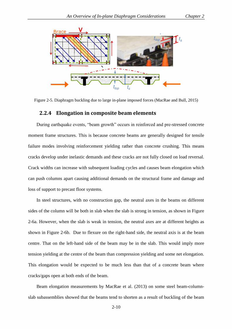
An Overview of In-plane Diaphragm Considerations Chapter 2
2-10
Figure 2-5. Diaphragm buckling due to large in-plane imposed forces (MacRae and Bull, 2015)
2.2.4 Elongation in composite beam elements
During earthquake events, “beam growth” occurs in reinforced and pre-stressed concrete
moment frame structures. This is because concrete beams are generally designed for tensile
failure modes involving reinforcement yielding rather than concrete crushing. This means
cracks develop under inelastic demands and these cracks are not fully closed on load reversal.
Crack widths can increase with subsequent loading cycles and causes beam elongation which
can push columns apart causing additional demands on the structural frame and damage and
loss of support to precast floor systems.
In steel structures, with no construction gap, the neutral axes in the beams on different
sides of the column will be both in slab when the slab is strong in tension, as shown in Figure
2-6a. However, when the slab is weak in tension, the neutral axes are at different heights as
shown in Figure 2-6b. Due to flexure on the right-hand side, the neutral axis is at the beam
centre. That on the left-hand side of the beam may be in the slab. This would imply more
tension yielding at the centre of the beam than compression yielding and some net elongation.
This elongation would be expected to be much less than that of a concrete beam where
cracks/gaps open at both ends of the beam.
Beam elongation measurements by MacRae et al. (2013) on some steel beam-column-
slab subassemblies showed that the beams tend to shorten as a result of buckling of the beam

An Overview of In-plane Diaphragm Considerations Chapter 2
2-11
and spalling of the concrete at the slab/column interface. The residual shortening, measured
as the shortening at zero column drift, was less than 2mm during cycles up to about 3.5%
drift. This would probably not be significant for a typical structural beam, but subassemblies
showing gap opening characteristics such as those with reinforced concrete beams, can place
much greater demands on the diaphragm (SESOC 2011).
a) Strong slab around column
b) Weak slab around column
Figure 2-6. Steel beam elongation (MacRae et al. 2013)
2.2.5 Load path concept in diaphragms
Although the load path concept is emphasized in undergraduate structural classes around
the world, it is not generally considered in diaphragm design. One reason may be that there is
currently no generally accepted procedure for evaluating diaphragm forces during an
earthquake event. Some methods to estimate diaphragm forces are discussed in Section 2.3.
In addition, even if the diaphragm-imposed forces are evaluated realistically, an
appropriate method is needed to analyse the floor diaphragm in a rational and suitable manner
for a design office. Several methods have been proposed by researchers in this regard. These
are mostly for pre-cast and cast in-situ concrete floors and they might need some
modification for diaphragms using cold-formed decking.
2.2.6 Slab effects on subassembly strength and degradation
For floor slabs on steel beams, shear studs are generally provided to make a steel-
concrete composite member which is considered to have greater strength and stiffness than

An Overview of In-plane Diaphragm Considerations Chapter 2
2-12
the steel beam alone under gravity loads. Also, in the case of lateral loading, the beam is
generally considered to have an increase in stiffness and strength along its length as a result
of the composite action. However, the current NZ design approach (NZS3404, 2007) states
that under lateral seismic loading:
1) The strength at the end of the beam should be that due to the non-composite steel
beam alone. (This is because the effect of the slab is not considered to be
reliable.)
2) For determining the beam over-strength effects to compute column demands, the
slab effect should be explicitly considered (if the slab is in contact with the
column) and methods to do this are specified. This over-strength requirement is
unique to NZS3404 (2007).
MacRae et al. (2013) recommend that when:
1) Slabs are cast against the column and where no special detailing is provided to
confine the concrete at the member ends, then NZS3404 (2007) method should be
followed.
2) Slabs which are not cast against the column, but which are isolated/separated by
means of a gap placed between the concrete and the column, slab effects should
not be considered on the flexural strengths at the end of the beam for either beam
design, or beam over-strength calculation. However, there are concerns that
making a gap in the slab may increase beam axial forces and decrease the flexural
resistance available of beam ends. Gapping issues are discussed in Section 2.6 in
more detail.
3) Slabs that are full depth for a significant distance from the column face, and
where special detailing is provided to effectively confine the slab concrete at the

An Overview of In-plane Diaphragm Considerations Chapter 2
2-13
beam-ends against the column, then the slab effect may be considered both for
beam strength design and for over-strength design.
2.3 Methods to estimate diaphragm in-plane forces
In order to conduct a realistic analysis of floor diaphragms, global force demands
affecting the diaphragms are required. Procedures for estimating floor diaphragm imposed
forces for design must:
1) Be simple enough to be used in design offices,
2) Be compatible with the commonly used elastic 3D software,
3) Indicate likely magnitude of demands.
The following methods have been proposed:
2.3.1 Full-3D non-linear time history analysis (NLTH)
This method evaluates the nonlinear response of a structure, including the diaphragm, to
given ground motion, or suite of records. To do this, it requires the diaphragm to be modelled
as an assemblage of elements and members with appropriate boundary conditions and
member properties, not just modelled using a rigid diaphragm option. Although this method
presents the closest results to the exact solution for any given ground motion, it is difficult to
implement it appropriately in a conventional design. This is because it requires considerable
technical knowledge and information about the nonlinear behaviour of different structural
elements.
2.3.2 Method proposed by Sabelli et al. 2011
Sabelli et al. (2011) suggested conducting a number of frame analyses to capture the
likely combination of transfer and inertial effects. N different analyses are needed in each
direction for a frame with N levels. In the equivalent static analysis method, floor forces

An Overview of In-plane Diaphragm Considerations Chapter 2
2-14
reduced for ductility are applied at each level, but greater forces, corresponding to the
acceleration expected of the diaphragm, are applied at the level of diaphragm considered. The
diaphragm acceleration may be found using response spectrum analysis. The force
distributions are shown in Figure 2-7. A significant issue is that the determination of these
diaphragm specific forces requires judgement from the user to extract meaningful
information from the response spectrum analysis. Because forces lose their sign during modal
combination process and they are not in equilibrium.
Figure 2-7. Force distribution for considering transfer and inertial forces at each storey (Sabelli et al.
2011)
2.3.3 Equivalent Static Analysis (ESA) and Over-strength ESA
(OESA)
The Equivalent Static Analysis (ESA), and the other methods below, are applied to an
elastic model of the structure such as those commonly considered in design.
The ESA method is based on the assumption that the first mode dominates the building
deformation and all the structure mass participates in this mode. Although this method can be
used for obtaining frame and wall design forces in some cases, it underestimates diaphragm
in-plane demands especially in lower stories (Bull, 1997, Nakaki, 2000, and Fleischman et al.
2002).
The ΦESA method is the ESA scaled by the building’s over-strength factor. It better
estimates floor diaphragm forces, but the floor diaphragm forces near the base of the structure
may be underestimated.

An Overview of In-plane Diaphragm Considerations Chapter 2
2-15
An alternative method by Tiong and Lyes (2014), applies the over-strength force
distribution to the frame, but making sure that the forces at the level considered are no less
than those resulting from the anticipated in the Parts and Components section of the loading
standard. This method has similarities to that of Sabelli et al. (2011) but it is more
conservative. This approach is more suitable for diaphragms that do not act as transfer
diaphragm which means the inertia forces govern the design criteria.
2.3.4 pseudo Equivalent Static Analysis (pESA)
The pseudo Equivalent Static Analysis (pESA) method (Bull, 1997 and Gardiner, 2011)
modifies the ESA method to account for:
1) Increased forces in the lower levels of structure, and
2) Over-strength actions, which develop in the lateral force resisting systems.
Both inertia and transfer force effects result from the analysis with one lateral force
distribution. Figure 2-8 illustrates the ESA, in the blue line, and pESA forces, in the yellow
line.
The pESA is only recommended for structures up to about nine stories in height because
for taller (longer period) structures, the forces associated with the peak ground acceleration
unrealistically dominate the floor in-plane demands at all periods.
Figure 2-8. Schematic force distributions of ESA and pESA (MacRae and Bull, 2015)

An Overview of In-plane Diaphragm Considerations Chapter 2
2-16
2.3.5 Parts and Components method (P&C)
The “Parts and Components” method is a force-based design approach, which is used for
design of “parts” or “components” of a structure. These forces are considered to be applied at
every level independently and not together with those at other levels. In this case, inertial
effects on the diaphragm are obtained, the transfer forces due to the deformations of the other
stories are not considered. On the other hand, if these forces are applied simultaneously to the
whole structure, the demands are likely to be overestimated, because the peak floor
accelerations at different floors do not occur at the same time.
This method is applicable to floors in structures where the transfer forces are not
significant. If the seismic resisting systems acting in the same direction of loading are
different, or if they change location in plan, then the P&C method does not take into account
the actions from transfer diaphragm effects.
A variation of this method is proposed by Cowie et al. (2014) where the floor height
coefficient (𝐶𝐻𝑖) is considered equal to 1.6 instead of using Clause 8.3 of NZS1170.5 (2004).
2.3.6 Pushover analysis
Pushover is a nonlinear-static analysis method where a structure is subjected to gravity
loading and a monotonic displacement-controlled lateral load pattern. The lateral forces are
increased until either the total capacity of the structure is exceeded, or a predetermined
displacement of the structure is reached. A variation of the pushover method is adaptive
pushover method that was developed to mitigate the uncertainties related to the lateral force
pattern. In this method, the lateral loading pattern is updated at each loading step according to
the structure lateral deformation and structure stiffness matrix.
The results of this method may be sensitive to the selected loading pattern and target
displacement. Pushover analysis may underestimate storey drifts at lower levels (Fenwick

An Overview of In-plane Diaphragm Considerations Chapter 2
2-17
and Davidson 1991, 1997). Also, the maximum diaphragm force may not occur at the
maximum lateral displacement of the structure as shown in Appendix A.
2.3.7 Modal response spectrum method
Modal response spectrum method (RSA) is a linear-dynamic statistical analysis
method which measures the contribution from each vibration mode to indicate the likely
maximum seismic response of an elastic structure. The modal response spectrum analysis is
generally used when the higher mode effects are considered to be significant. Modal response
spectrum analysis accounts for higher mode effects. However, its results cannot directly be
used for diaphragm analysis and need engineering judgment. The design actions lose their
sign through the modal combination process and are not in equilibrium.
2.3.8 Discussion on methods to estimate diaphragm forces
As described above, several methods exist for evaluating diaphragm in-plane demands.
These range from advanced methods, like the use of nonlinear time history analysis, to simple
methods, like ESA. Amongst the simple methods that are used with elastic frame analysis
there is no correct method for estimation of diaphragm in-plane demands. The following
points are noted:
1) For elastic multi-story buildings, peak floor forces are greater from those implied
from methods used to obtain peak shears at each level for elastically responding
structures due to the way individual storey higher mode accelerations need to be
combined. Therefore, scaling the ESA method forces to the elastic level does not
strictly estimate the likely peak elastic floor forces at that particular level.
2) Many studies have been conducted to estimate peak floor accelerations at specific
floor levels. These differ markedly between researchers because they depend on

An Overview of In-plane Diaphragm Considerations Chapter 2
2-18
the structural framing type, the records used, and the analysis assumptions. (E.g.
Dantanarayana et al., 2012).
3) Demands based solely on peak accelerations considered on a floor diaphragm at
one level by itself are not generally appropriate for use in design because
associated inertial forces are not generally large. (They can generally be carried
by a low number of shear studs). Transfer, bearing and compatibility forces can
cause much larger diaphragm demands.
4) The duration of the peak force/acceleration demand may significantly affect the
structural response. For example, if high force/acceleration demands occur only
briefly, causing a small inelastic displacement, then its effect may be minor.
Designing for the peak values may therefore be conservative (MacRae and Bull,
2015, Bruere and Colley, 2015).
Methods to estimate diaphragm in-plane forces are discussed and investigated in
Chapter 7 in more detail.
2.4 Slab in-plane demands
In Section 2.3, the total in-plane demands on the diaphragm at any level for frame
analysis were described. Here, more specific details about how force gets into a diaphragm
are discussed.
2.4.1 Inertia forces
In steel frame structures, concrete diaphragms comprise a significant portion of the
building mass. Therefore, higher inertia forces may be imposed on the floor diaphragm and
consequently on the connections between the diaphragm and the steel frame. Diaphragms are
expected to remain elastic, or almost so, during seismic shaking, while other elements are
expected to dissipate the seismic energy.

An Overview of In-plane Diaphragm Considerations Chapter 2
2-19
Inertia forces of floor slabs are often considered to be transferred to the steel frame
through compression of the slab on the column faces. However, as was shown in Figure 2-4,
since slab inertia forces act in the same direction as the frame sways, a partial gap opens at
location “A”. Therefore, slab inertia forces cannot directly transfer into the columns. Instead,
the forces must move into the steel beams through friction and mechanical transfer using
shear studs, along the beam causing axial force, through the beam plastic hinge and
connection into the columns (MacRae and Clifton, 2015b).
Figure 2-9 shows two cases of transferring the inertia forces from the slab to the frames.
Jensen (2004) conducted finite element analyses of a floor slab assumed to be restrained at
the columns as shown in Figure 2-9a. This was assumed to be representative of a column in a
reinforced concrete frame. Here, it is assumed that the slab bears onto the column and inertia
forces are directly transferred to the column, so compression struts are formed in the slab
with the beams acting as tension ties. The forces tend to be carried by the nearest columns.
Beams between the columns are assumed to carry forces perpendicular to the direction of
loading to balance the diagonal strut forces. Figure 2-9b shows the situation in steel frame
structures where the gap occurs between the slab and column, so the inertial forces are
transferred to the steel frame not at the column location, but through shear studs along the
beam length. The beam then carries these forces through axial tension/compression to the
column. It may be seen that tension ties are needed within the slab perpendicular to the
direction of loading to balance the diagonal strut forces.

An Overview of In-plane Diaphragm Considerations Chapter 2
2-20
a) Slab bears on columns (Jensen, 2004)
b) Actual case in steel structures (MacRae and
Bull, 2015)
Figure 2-9. Inertia forces in floor diaphragm
2.4.2 Transfer forces
Transfer forces are diaphragm in-plane shear forces, which occur as a result of
deformation incompatibility of different VLFR systems such as moment frames and RC walls
wanting to move different amounts at different levels under the applied lateral forces. The
classic illustration of transfer forces is shown in Figure 2-10 (Paulay and Priestley, 1992).
Here the wall and frame want to move together at the base, and apart near the top. This
causes compression and tension in the links between these two VLFR systems. These links
represent the diaphragms, which must carry these forces as in-plane diaphragm transfer
forces.
Figure 2-10. Transfer forces due to deformation incompatibility (Paulay and Priestley, 1992)
While transfer forces are generally illustrated as being an issue for multi-storey
structures, they can also affect single storey structures. This is shown in Appendix A where:

An Overview of In-plane Diaphragm Considerations Chapter 2
2-21
1) The magnitude of the transfer force can depend on the strength and stiffness of
the VLFR elements, and
2) The peak transfer force demands do not necessarily occur at the peak floor lateral
displacement.
In multi-storey structures the magnitude of transfer forces in diaphragms may be
significantly increased where there are discontinuities in plan location of the VLFR elements,
generating the need to transfer forces between the two displaced VLFR systems above and
below. A common discontinuity in plan in the vertical elements is at a podium slab.
It has been suggested that transfer forces in multi-storey frames may be reduced by
detailing column splices as pins as shown in Figure 2-11 (MacRae and Bull, 2015). However,
making all columns in the building effectively continuous provides additional redundancy
and helps with frame self-centring, both desirable features that may be reduced if the splices
are designed as pins.
Figure 2-11. Decreasing transfer forces by detailing column splices as pins (MacRae and Bull, 2015)
Overall, the magnitude of transfer forces may be limited by the following:
1) The shear stud strength
2) Beam/connection axial strength
3) Concrete diaphragm compression/ tension /shear capacity, and
4) A column mechanism, such as that shown in Figure 2-12. It is indicated as being
a possibility in studies by Haselton and Deierlein, (2007) on building collapse

An Overview of In-plane Diaphragm Considerations Chapter 2
2-22
under very severe motions. It is recognized that this is not a desirable mechanism
for overall frame performance.
Figure 2-12. Column mechanism (Haselton and Deierlein, 2007)
Where beams in the gravity system are used to transfer diaphragm forces into the seismic
resisting system, such as shown in Figure 2-13a, the gravity beams form collectors (both
tension and compression) and must be designed appropriately. To carry these forces, an
additional plate may be required above the beam at the connection of the beam to the column
as shown in Figure 2-13b. Recent studies by Weir and Clarke (2016) have indicated that the
axial strength of an eccentric shear cleat connection may be less than one-half of that of a
yielding connection with no cleat eccentricity for a typical connection.
The slab must also be strong enough to reliably carry the transfer forces illustrated in
Figure 2-13a without buckling or crushing. Studies, similar to that initiated by Luo et al.
(2015), are therefore required to evaluate slab performance for design (Figure 2-14).

An Overview of In-plane Diaphragm Considerations Chapter 2
2-23
a) Transfer forces
b) Increasing connection axial strength using top plate
detail
Figure 2-13. Transfer force effect example (MacRae and Bull, 2015)
Figure 2-14. Numerical study on slab performance (Luo et al., 2015)
2.4.3 Slab bearing forces
If there is no construction gap between the slab and column, then as the column sways, it
bears against the concrete slab on the far side of the column from point “A” in Figure 2-4
(MacRae and Clifton, 2015b). This causes an extra bearing force on the slab. This force must
be transferred through the slab, shear studs, beam, and back to the column.
The magnitude of slab bearing forces is a function of concrete compressive strength,
number and strength of shear studs, and force transferring mechanisms into the column.
Force limiting mechanisms depend on parameters such as shear key types between column

An Overview of In-plane Diaphragm Considerations Chapter 2
2-24
flanges, beam/connection strength, and concrete confinement as discussed by Chaudhari et al.
(2015) and MacRae and Bull (2015). If confinement of the top surface of the concrete slab is
not provided beside the column, the slab can spall due to bearing during the large
deformations. Other mechanisms of slab strength loss, such as shear key fracture, and
longitudinal splitting, can also occur (Chaudhari et al. 2015, MacRae et al. 2013 and Hobbs et
al. 2013).
Disadvantages of allowing the concrete slab to bear against the column include the
following:
1) Bearing of the concrete against the column increases the beam moment input into
the column, 𝑀𝑝,𝑏𝑒𝑎𝑚. This is typically about 30% for typical members and it
requires larger column sizes (MacRae and Bull, 2015).
2) Since it is difficult to confine the concrete slab properly, after spalling of the
concrete occurs, the composite beam strength, 𝑀𝑝,𝑏𝑒𝑎𝑚, degrades to that of the
bare steel beam alone, 𝑀𝑝,𝑏𝑎𝑟𝑒 𝑏𝑒𝑎𝑚, as shown in Figure 2-15 (Chaudhari et al.
2015).
3) Once spalling of the concrete occurs in one direction, the strength of the
subassembly in different directions changes increasing the likelihood of
deformations ratcheting in one direction only (MacRae and Bull, 2015).
4) The composite action increases the beam axial forces, which act through the
connection and beam plastic hinge (MacRae and Bull, 2015). Some beam growth
effects are also possible.

An Overview of In-plane Diaphragm Considerations Chapter 2
2-25
Figure 2-15. 𝑀𝑝,𝑏𝑒𝑎𝑚 composite degrades to 𝑀𝑝,𝑏𝑎𝑟𝑒 𝑏𝑒𝑎𝑚 due to lack of confinement (Chaudhari et al.,
2015)
In order to avoid these effects, there have been efforts to more economically design
frames with slabs. These include:
1) Designing the slab around the column to limit strength degradation during large
deformations by special detailing around the column (MacRae et al. 2013 and
Chaudhari et al. 2015).
2) Providing a gap between the column and the slab as shown in Figure 2-16 to
avoid bearing effects. This gapping issue is discussed further in Section 2.6.
Figure 2-16. Intentional gap between the column and the slab (MacRae and Bull, 2015)
2.4.4 Compatibility forces
When neutral axes of beams on either side of the column are at different heights due to
the composite action of slab as shown in Figure 2-6b, the distance between beam-ends tends
to increase, causing slab (compression) forces and beam (tension) forces (MacRae and

An Overview of In-plane Diaphragm Considerations Chapter 2
2-26
Clifton, 2015b). This elongation would be expected to be much less than that of a concrete
beam where cracks/gaps open at both ends of the beam (MacRae et al. 2013) but it should be
taken into account in analysis because it can impose extra forces on column as well as on
beam plastic hinge region and beam-column connection. As shown in Figure 2-17, the slab
effect on moment-resisting structural systems can be modelled (Umarani and MacRae, 2007
and Ahmed et al., 2013), but it is not considered in most analyses.
Figure 2-17. Modelling the composite action effect (Umarani and MacRae, 2007 and Ahmed et al.,
2013)
2.4.5 Forces due to interaction with other elements
As floor diaphragms tie structural elements together, they interact with other elements.
This interaction may impose various forces on the diaphragms. Inclined columns, as shown in
Figure 2-18, can develop diaphragm in-plane tension and compression forces due to gravity
and overturning actions (Moehle et al. 2010 and Scarry, 2014). These forces should be taken
into account in diaphragm design.

An Overview of In-plane Diaphragm Considerations Chapter 2
2-27
Figure 2-18. Diaphragm forces due to sloped column (Scarry, 2014)
Ramps and sloping diaphragms are another sources of interaction forces. The effect of
ramps can be more significant especially where they connect different stories of a structure
and story shear can migrate out of the vertical elements of the seismic force resisting system
through the ramp in the form of shear or axial forces (Moehle et al., 2010). This effect should
be considered in analyses and modelling the structure. It is particularly important in car
parking structures if the lower end of the ramp cannot slide.
2.5 Slab analysis
After evaluating the global diaphragm lateral forces using the methods described in
Section 2.3, separate diaphragm analysis is required to determine the load paths and
diaphragm internal forces for design purposes. The forces on the diaphragm are obtained
from the difference in shear above and below each vertical element passing through the floor
system. These, together with the applied inertia forces at the diaphragm, result in a floor
system that is in equilibrium, and the different components can be designed (Fenwick et al.
2012). Slab analysis methods include ‘detailed Finite Element Method (FEM)’, ‘Deep Beam’,
and ‘Truss model’. These methods vary in the level of complexity and accuracy.

An Overview of In-plane Diaphragm Considerations Chapter 2
2-28
2.5.1 Detailed finite element method analysis
The finite element method is one of the most widely accepted numerical solutions for
exploring engineering problems. Modelling a diaphragm using FEM (include shell or solid
elements) can be beneficial for evaluating the transfer forces among vertical lateral load
resistance elements and inertia forces, especially for irregular diaphragms in shape and
around large openings in the floor plan as well as the impact of ramps in parking garages
(Moehle et al., 2010).
When using a finite element model, the continuous nature of the floor diaphragm is
considered. This advantage helps to capture the stresses around the floor openings. Also
zones where stress concentrations may be expected to occur are readily identified (Gardiner,
2011). In spite of this,
1) FEM programs are often expensive, difficult to use and require significant pre
and post-processing times for each analysis (Scarry, 2014), and
2) stresses and strains do not relate directly to design and it may be difficult to
estimate how much reinforcing steel is required in specific locations.
2.5.2 Deep Beam
The ‘Deep Beam’ method is appreciated because of its simplicity. It considers the
diaphragm as a deep beam with a distributed load. The approximation of a deep beam method
is only appropriate in regular floor plans. Figure 2-19 illustrates the deep beam design
analogy of a typical floor diaphragm.

An Overview of In-plane Diaphragm Considerations Chapter 2
2-29
Figure 2-19. Graphical representation of a beam analogy (NZCS, Technical Report No. 15, 1994)
This method provides adequate demand for buildings with regular geometries and two
lines of continuous vertical elements as support of floor slabs. In floor slabs with more than
two supports (VLFR elements), the equivalent beam on springs model, which is more
complex, may be appropriate to determine diaphragm demands (Moehle et al. 2010). Figure
2-20 shows a typical equivalent beam on springs model. This method is usually used for one
storey buildings because the stiffness of springs can be calculated easily, while for multi-
storey buildings, computer models are needed.
Figure 2-20. Typical deep beam on springs model (Moehle et al., 2010)
In buildings with more complex configurations of VLFR elements, another approach is
to use the distribution of diaphragm inertial forces to vertical elements from a computer
model and then implement the corrected equivalent beam model to determine the diaphragm
demands (Moehle et al. 2010).

An Overview of In-plane Diaphragm Considerations Chapter 2
2-30
2.5.3 Truss model
Diaphragms can be modelled and analysed by creating an elastic framework of truss
elements. The idea of replacing the continuous material of an elastic body with a framework
of truss elements according to a definite pattern and suitable element properties was
introduced by Hrennikoff (1941).
Hrennikoff proposed the framework method for solving two-dimensional stress
problems, bending of plates, bending of cylindrical shells and also the general case of three-
dimensional stress. This method is based on replacing continuous material of an elastic body
with a definite pattern of one-dimensional truss elements. It can be shown that if the size of
the truss unit pattern be small enough, the results of the framework method are the same as
the exact differential equation solution. Hrennikoff investigated various framework patterns
that some of them are shown in Figure 2-21.
Figure 2-21. Patterns of truss elements investigated by Hrennikoff (1941)
Gardiner (2011) used the lattice element which is based on the Hrenikoff (1941) lattice
analogy for modelling and analysing diaphragms. Hrenikoff provides the strut effective
widths of 0.53 times a and orthogonal elements effective widths of 0.75 times a (a is truss
mesh unit dimension for a square shape), for material with a Poison’s ratio of 0.33, where the
compression struts go between corners in both directions.
Holmes Consulting Group (2014) prepared a practice note about modelling and
analysing diaphragms using truss elements based on Hrenikoff (1941). It is suggested in order

An Overview of In-plane Diaphragm Considerations Chapter 2
2-31
to get higher accuracy, truss mesh unit size should be reduced, while maintaining the square
format for the following situations:
a) around the nodes where vertical elements would be connected to the floor plate,
b) around floor penetrations like stairs or lifts,
c) at re-entrant corners, and
d) around collectors.
Scarry (2014), proposed a modification on Hrenikoff (1941) method to consider the
diagonal elements carry compression only and orthogonal elements carry both tension and
compression. Figure 2-22 shows a diaphragm modelled using truss elements with
compression-only pairs of diagonals to allow for strut action.
Figure 2-22. Truss model assigned to a typical floor diaphragm (Holmes Consulting Group 2014)
Another advantage of using the truss model is that multiple load cases can be analysed
by one model and the struts and ties can be identified more easily. Stress concentration zones
around openings and at re-entrant corners can be captured. Also, in this method, complex
diaphragms consisting of vertical steps (three-dimensional diaphragms), can be modelled by
employing beam elements and rigid links (Scarry, 2014).

An Overview of In-plane Diaphragm Considerations Chapter 2
2-32
2.5.4 Strut-and-Tie
The truss model with compression-only diagonal members and compression/tension
orthogonal members may be called ‘Strut-and-Tie’ model. The ‘Strut-and-Tie’ approach has
also been advocated for diaphragm analysis (Bull 1997, Gardiner 2011, Bull 2004 and Bull
2014). Clause 13.3.9 of NZS3101 (2006) states that “the strength design of diaphragms for
shear shall be based upon strut-and-tie models”. This can be used for general floor plan
layouts with irregularities, such as openings in the diaphragm. In the strut-and-tie method,
compression struts and tension ties are placed throughout the floor slab to develop a truss
system of admissible force paths (Gardiner, 2011). One of the good examples of representing
strut-and-tie in different problems is published by Schlaich et al. (1987).
In the references above, compression struts representing the diaphragm stiffness have
been placed between column-to-beam, or beam-to-beam, nodes. In a building with an
orthogonal plan, the steel (beams or reinforcing) run in the orthogonal directions.
An alternative, recently proposed by MacRae and Bull (2015) places the nodes at the
centres of the beams. This nodal position represents the centroid of the shear studs on top of
the beam. It may be regarded as an effective shear stud for the beam. Actual shear studs will
be spread out along the beam. Compression struts representing the concrete strut effects run
diagonally between these nodes. Tension ties, representing the steel, run perpendicular to the
beam. This approach has some advantages compared to the previous approach which
includes:
a) Axial forces in (and parallel to) the beam can be obtained directly from the
analysis.
b) The number of studs required can be easily obtained from the difference in axial
force along the beam either side of the central node.

An Overview of In-plane Diaphragm Considerations Chapter 2
2-33
c) The tension steel required as reinforcing bars in the slab is easily obtained from
the force in this tension element perpendicular to the beam. This can be
distributed to the shear studs acting along the beam.
This modelling method is discussed in Chapter 3 in more detail.
2.6 Gapping issues
Based on the current NZ design approach (NZS3404, 2007), structural steel beams are
designed for earthquake-induced forces without considering the slab effect. This is because
the slab is unconfined and beam composite strength degrades to the bare beam strength due to
concrete failure as discussed with regard to Figure 2-15. Columns and connections are
required to be designed to resist beam over-strength actions considering the slab effects. The
NZ standard therefore considers the most conservative scenario by (a) ignoring the strength
increase from the slab in design of the beam to resist the seismic loads in a force-based
design, and (b) considering its influence when determining the over-strength actions at the
column and joint from the inelastically responding composite beam. With an unconfined slab
this may be appropriate as the slab strength is not dependable due to the possibilities of
spalling and shear key fracture, as described in Section 2.4.3.
To consider the slab strength for design at the expected peak displacement, the slab
should not degrade in strength and should therefore be well confined as shown in Figure
2-23. MacRae et al. (2013) have suggested special detailing for concrete slab around the
column such that the slab be able to sustain its strength at higher drifts. Some economical
ways of providing this detailing have been described by Chaudhari et al. (2015). Figure 2-23
illustrates some examples of detailing to confine the slab.
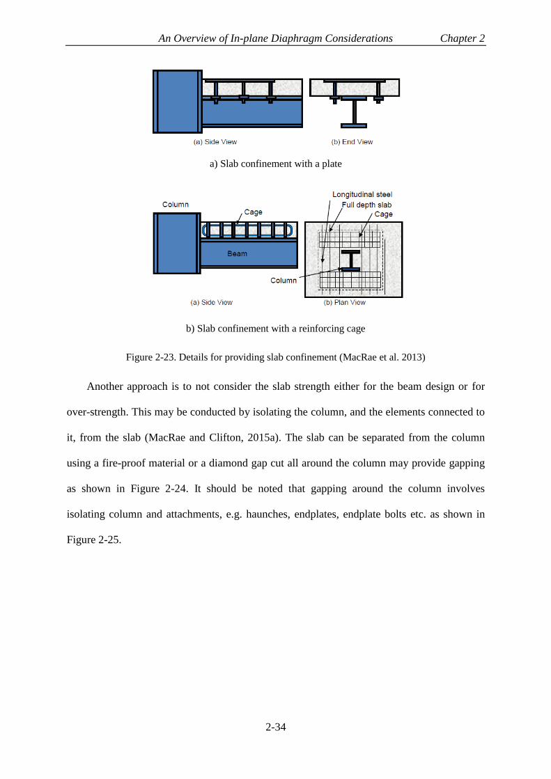
An Overview of In-plane Diaphragm Considerations Chapter 2
2-34
a) Slab confinement with a plate
b) Slab confinement with a reinforcing cage
Figure 2-23. Details for providing slab confinement (MacRae et al. 2013)
Another approach is to not consider the slab strength either for the beam design or for
over-strength. This may be conducted by isolating the column, and the elements connected to
it, from the slab (MacRae and Clifton, 2015a). The slab can be separated from the column
using a fire-proof material or a diamond gap cut all around the column may provide gapping
as shown in Figure 2-24. It should be noted that gapping around the column involves
isolating column and attachments, e.g. haunches, endplates, endplate bolts etc. as shown in
Figure 2-25.

An Overview of In-plane Diaphragm Considerations Chapter 2
2-35
a) Gap around the column (Chaudhari et al. 2015)
b) Gap within the slab (MacRae and Clifton,
2015b)
Figure 2-24. Gapping around column
Figure 2-25. Isolating column and attachments (MacRae and Bull, 2015)
Chaudhari et al. (2015) indicate that gapping around column can provide good
performance. It also decreases bearing and compatibility stresses which:
1) Eliminates the slab effect on beam over-strength, resulting in smaller columns.
2) Reduces slab damage and strength degradation.
3) Has the possibility of reducing ratcheting where the structure tends to yield
predominantly in one direction because the same strength is in each direction of
loading (MacRae and Clifton, 2015b).
4) Decreases beam/connection axial forces.
The disadvantages of gapping may be the following:

An Overview of In-plane Diaphragm Considerations Chapter 2
2-36
1) Increasing the chance of column instability by twisting due to having no slab to
restrain it, such instability has been seen in columns with beams tested with
reduced beam sections by Chi and Uang (2002). Details such as those shown in
Figure 2-26 may reduce the propensity for such twist.
2) The initial stiffness and strength of the structure decrease (in the first cycle) so
the period increases and the structure is likely to have greater displacements
(MacRae and Clifton, 2015b).
3) Gap installation costs may be significant (MacRae and Bull, 2015).
Figure 2-26. Limiting column twisting in gapped slabs (MacRae and Bull, 2015)
Whether or not gaps are provided between the slab and column, diaphragm forces are
likely to be transferred to the column through axial force in the beam. For beam axial forces
greater than about 0.2𝐴𝑓𝑦 the lateral resistance of the frame may decrease, where 𝐴 and 𝑓𝑦 are
beam cross-section area and yielding stress respectively. It has therefore been suggested that
design should be conducted to ensure the beam axial force is less than this value (MacRae
and Bull, 2015).

An Overview of In-plane Diaphragm Considerations Chapter 2
2-37
2.7 Load transfer from diaphragm to frame
Many buildings have a limited number of seismic frames, which are designed to carry
horizontal forces from the diaphragms to the foundation. Two options to transfer this
horizontal force are discussed below.
2.7.1 Designing diaphragms to transfer horizontal force only
through the seismic frame beams
In this case, forces on the diaphragm, including inertial and transfer forces, are
transferred to the seismic beam via shear studs on the beam. In general, transfer of forces
directly from the diaphragm into the column should not be used as it is not a reliable load
path because:
1) A gap opens between the slab and column face, as discussed in Section 2.2.2 and
Figure 2-4, since slab inertia forces act in the same direction as the frame sways.
Slab inertia forces therefore cannot go directly into the column.
2) The slab is not generally confined and it may break down under the first cycle of
displacement so it cannot transfer subsequent load to the column.
For this mechanism, with force only considered to be transferred into the seismic
frame(s):
a) Sufficient shear studs should only be placed on the seismic beam and all force
transfer should occur here.
b) The ability of diaphragms on the gravity beams to transfer horizontal force
should be limited by:
i. ensuring that there are no shear studs on the gravity beams,
ii. reducing friction on the top of these gravity beams, or

An Overview of In-plane Diaphragm Considerations Chapter 2
2-38
iii. minimising the possibility of interaction between the slab and the gravity
columns (possibly by providing a seismic gap), as any force there would
need to be transferred through the beams as an axial force.
c) A strut-and-tie mechanism needs to be developed. Schlaich et al. (1987) have
shown that the pattern is typically like that in Figure 2-27. Here the compression
struts become inclined at a distance of about 𝐿/2 from the beam carrying the
lateral force, where 𝐿 is the frame width as shown in Figure 2-27. The change in
orientation of compression forces at this location causes extra forces
perpendicular to the direction of earthquake shaking that need to be considered in
design. Here Beams 1, 2, 3 and 4 are gravity beams, and all the forces from the
diaphragm must be transferred through the composite seismic beams 5 and 6, in
the braced seismic bays. The strut-and-tie mechanism involves:
i. Providing sufficient shear studs in Beams 5 and 6 to transfer expected
forces.
ii. Providing sufficient transverse tie steel to balance the forces. The steel
decking is not always considered to be continuous so it cannot be relied
on to carry these tension forces even if it is spanning in the appropriate
direction.
iii. Ensuring that the beam, and its connections, can transfer the axial forces
induced into the columns, while still carrying the other forces expected
for them to fulfil their purpose as part of the seismic frame.

An Overview of In-plane Diaphragm Considerations Chapter 2
2-39
Figure 2-27. Typical floor plan with braced frames if shear studs are only provided on beam 5 and 6
The advantage of this method is that very small horizontal force on the gravity beams is
expected, so beam axial tension/compression does not need to be considered. The gravity
beams and their connections can be designed for vertical forces only. In this case, a simple
shear connection from the gravity beams to the column, such as that shown in Figure 2-28,
may be appropriate.
Figure 2-28. Typical cleat connection for gravity frames
2.7.2 Designing diaphragms to transfer horizontal force also
through beams outside the seismic frame
When the composite action of the gravity beams is desired, these beams and their
connections need to be designed for the expected forces. In this case, strut-and-tie mechanism
with reinforcing steel perpendicular to all beams is required.

An Overview of In-plane Diaphragm Considerations Chapter 2
2-40
Apart from designing the beam itself for axial force, in conjunction with other imposed
forces, appropriate connection design is also required. Some ways of detailing the connection
include:
1) Using a bolted end plate connection at the beam end, or
2) Placing a top flange plate on the beam as shown in Figure 2-26.
If design is conducted assuming the seismic beams carry all horizontal forces from the
diaphragms (including those from inertial and transfer effects), yet shear connectors are
placed on the gravity beams, forces in the gravity beam connections may be greater than their
capacities, and this may result in connection failure (Weir and Clarke, 2016). The
deformation of these eccentric cleat connections are subject to, and is limited by, the
deformations of the diaphragm on the seismic frame beams. In some cases this displacement
compatibility limits the demands on the gravity beam end connections.
2.8 Conclusions
In-plane design considerations for floor diaphragms in steel buildings were described. It
was shown that:
1) A number of issues that are not generally explicitly considered in current
standards or current design, were described. These included: (a) diaphragm
rigidity/flexibility considerations, (b) beam/connection axial forces, (c) thin
diaphragm buckling, (d) elongation issues in composite beams, (d) load paths
within a diaphragm to the supports, and (f) slab effects on subassembly strength
and degradation.
2) A number of methods proposed to estimate forces on a building to evaluate
global diaphragm in-plane demands were described. These vary in complexity
and rationality. While no one method has been accepted as being appropriate for
design using commonly available design software, it is beneficial to select one

An Overview of In-plane Diaphragm Considerations Chapter 2
2-41
distribution of forces which can capture the likely inertial and transfer effects
considering over-strength.
3) Five types of diaphragm in-plane forces were discussed: (i) inertia forces, (ii)
transfer forces, (iii) slab bearing, (iv) compatibility, and (v) interaction with other
elements. It was shown that because of the way frames move, diaphragm inertial
forces cannot generally be transferred directly from the slab into the columns, so
appropriate consideration of the shear studs, and axial forces in the beam and end
connections are required. Transfer forces are affected by the distributions of
stiffness and strength not only over the building height, but also within one
storey. Slab bearing and compatibility forces are affected by any gap provided
between the concrete slab and column.
4) The strut-and-tie method was considered the most general and appropriate means
of obtaining forces for design. Nodes placed at the beam centres to allow beam
axial demands, shear stud demands and reinforcing steel demands to be captured
directly. The automated strut-and-tie method also considers diaphragm flexibility.
5) Providing a gap in the slab around a column can reduce beam over-strength
forces but the possibility of column twisting should be considered in design.
6) The number of bays over which force is transferred from the diaphragm to the
frame should be considered explicitly in design.

An Overview of In-plane Diaphragm Considerations Chapter 2
2-42
References
[1] Ahmed S. M., Umarani C. and MacRae G. A. (2013). “Slab Effects on Building
Seismic Performance: State of The Art”, Journal of Structural Engineering, 40
(2): 136-141.
[2] Aktan A. E. and Nelson G. E. (1988). “Problems in predicting seismic responses
of RC buildings”, Journal of Structural Engineering, 114(9): 2036-2056.
[3] ANSI/SDI (2011). American National Standards Institute/Steel Deck Institute, C-
2011 Standard for Composite Steel Floor Deck-Slabs.
[4] Barron J. M. and Hueste M. B. D. (2004). “Diaphragm effects in rectangular
reinforced concrete buildings”, Structural Journal, 101(5): 615-624.
[5] Basu D. and Jain S. K. (2004). “Seismic analysis of asymmetric buildings with
flexible floor diaphragms”, Journal of structural engineering, 130(8): 1169-1176.
[6] Blume J. A., Sharpe R. L. and Elsesser E. (1961). “A structural dynamic
investigation of fifteen school buildings subjected to simulated earthquake
motion”. Division of Agriculture, Sacramento, Calif.
[7] Bruere R. J. and Davies-Colley M. (2015). “Effect of Reducing Maximum
Response on Concrete Floor Diaphragms”, Final Year Projects, Dept. of Civil
and Natural Resources Engineering, University of Canterbury. Project
supervisors: MacRae G. A. and Bull D. K.
[8] Bruneau M. and MacRae G. (2017). “Reconstructing Christchurch: A Seismic
Shift in Building Structural Systems”, Quake Centre, University of Canterbury.
[9] Bull D. (1997). “Diaphragms, Seismic Design of Reinforced Concrete
Structures”, Technical Report No. 20, New Zealand Concrete Society.
[10] Bull D. K. (2004). “Understanding the Complexities of Designing diaphragms
in Buildings for Earthquakes”, Bulletin of the New Zealand Society for
Earthquake Engineering, 37 (2): 70-88.

An Overview of In-plane Diaphragm Considerations Chapter 2
2-43
[11] Bull D. K. (2014). “Module-2 ENCI429:2014 [PowerPoint slides]”. University
of Canterbury, Christchurch, New Zealand.
[12] Canterbury Earthquakes Royal Commission (2012): Final Report Volume 1.
[13] Celebi M., Bongiovanni G., Safak E. and Brady A. G. (1989). “Seismic
response of a large-span roof diaphragm”, Earthquake Spectra, 5(2): 337-350.
[14] Chaudhari T. D., MacRae G. A., Bull D., Chase G., Hicks S., Clifton G. C.
and Hobbs M. (2015). “Composite Slab Effects on Beam–Column Subassembly
Seismic Performance”, 8th International Conference on Behavior of Steel
Structures in Seismic Areas, Shanghai, China.
[15] Chi B. and Uang C. M. (2002). “Cyclic Response and Design
Recommendations of Reduced Beam Section Moment Connections with Deep
Columns”, J. Struct. Engrg., ASCE, 128(4): 464-473
[16] Clifton G. C. (2015). “Determination of Diaphragm Actions and Distribution
into the Frames; section 9.4 of the Civil 714 Multistorey Building Design Steel
Notes”, University of Auckland, Auckland, New Zealand.
[17] Cowie K. A., Fussell A. J., Clifton G. C., MacRae G. A. and Hicks S. J.
(2014). “Seismic Design of Composite Metal Deck and Concrete-Filled
Diaphragms–A Discussion Paper”, NZSEE Conference.
[18] CSA, C. (2014). S16-14. Design of Steel Structures, Canadian Standards
Association, Toronto, ON.
[19] Dantanarayana H. N., MacRae G. A., Dhakal R. P., Yeow T. Z. & Uma S. R.
(2012) “Quantifying Building Engineering Demand Parameters in Seismic
Events”, 14 World Conference on Earthquake Engineering, Lisbon, Portugal,
August 2012. Paper number 3424.
[20] Dolce M., Lorusso V. D. and Masi A. (1994). "Seismic response of building
structures with flexible inelastic diaphragm", Structural Design of Tall
Buildings 3(2): 87-106.

An Overview of In-plane Diaphragm Considerations Chapter 2
2-44
[21] Fenwick R., Bull D. and Gardiner D. (2012). “Assessment of Hollow-Core
Floors for Seismic Performance”, Research Report 2010-02, Department of Civil
and Natural Resource Engineering, University of Canterbury, Christchurch, New
Zealand.
[22] Fenwick R. C. and Davidson B. J. (1991). “The Seismic Response of Multi-
storey Buildings”, Department of Civil Engineering, University of Auckland.
Report number 495.
[23] Fenwick R. C. and Davidson B. J. (1997). “P-delta Actions and the Loadings
Code” SESOC 10(1): 58-62.
[24] Fleischman R. B., Farrow K. T. and Eastman K. (2002). “Seismic performance
of perimeter lateral-system structures with highly flexible
diaphragms”. Earthquake Spectra, 18(2), 251-286.
[25] Gardiner D. R. (2011). “Design Recommendations and Methods for
Reinforced Concrete Floor Diaphragms Subjected to Seismic Forces”, PhD
Thesis, University of Canterbury.
[26] Goldberg J. E. and Herness E. (1965). “Vibration of Multistory Buildings
Considering Floor and Wall Deformations”, Bulletin of the Seismological
Society of America. 55(1): 181-200.
[27] Hadianfard M. A. and Sedaghat S. (2013). “Investigation of joist floor
diaphragm flexibility on inelastic behavior of steel braced structures”, Scientia
Iranica, 20(3): 445-453.
[28] Haselton C. B. and Deierlein G. G. (2007). “Assessing Seismic Collapse
Safety of Modern Reinforced Concrete Moment Frame Buildings”, Report No.
156, Department of Civil and Environmental Engineering, Stanford University.
[29] Hobbs M., MacRae G. A., Bull D., Gunasekaran U., Leon R. and Clifton G. C.
(2013). “Slab Column Interaction ‐ Significant Or Not?”, Steel Innovations
Conference, Christchurch, New Zealand.

An Overview of In-plane Diaphragm Considerations Chapter 2
2-45
[30] Holmes Consulting Group, Practice Note No. 8.1, Version No. 1, (2014).
“Modelling Diaphragm Force Distributions - Simple Grillage Method” by Bull
DK and Galloway B.
[31] Hrennikoff A. (1941). “Solution of problems of elasticity by the framework
method”, Journal of applied mechanics, 8 (4):169-75.
[32] Humar J. and Popovski M. (2013). :Seismic response of single-storey
buildings with flexible diaphragms”, Canadian Journal of Civil Engineering,
40(9): 875-886.
[33] Jain S. K., Jennings P. C. (1985). “Analytical models for low-rise buildings
with flexible floor diaphragms” Journal of Earthquake Engineering and Structural
Dynamics, 13(2):225-241.
[34] Jensen J. (2004). “Diaphragm Action Issues in a Jointed Precast Concrete
System”, A final year project report submitted in partial fulfilment of the
requirements for the degree of Bachelor of Engineering, Department of Civil
Engineering, University of Canterbury, New Zealand.
[35] Ju S. H. and Lin M. C. (1999). “Building analyses comparisons assuming rigid
or flexible floors”, Journal of Structural Engineering ASCE, 125: 25-31.
[36] Kim S. C. and White D. W. (2004). “Linear static analysis of low-rise
buildings with flexible diaphragms using the structural separation
method”, Engineering Structures, 26(1): 83-93.
[37] Kunnath S. K., Panahshahi N., Reinhorn A. M. (1991). “Seismic response of
RC buildings with inelastic floor diaphragms”, Journal of Structural Engineering,
117(4): 1218-1237.
[38] Lee H. J., Aschheim M. A. and Kuchma D. (2007). “Interstory drift estimates
for low-rise flexible diaphragm structures”, Engineering structures, 29(7): 1375-
1397.

An Overview of In-plane Diaphragm Considerations Chapter 2
2-46
[39] Luo F., Gholamhoseini A. and MacRae G. A. (2015). “Analytical Study of
Seismic Behaviour of Composite Slabs”, Steel Innovations Conference,
Auckland, New Zealand.
[40] MacRae G. A. and Bull D. (2015). “Diaphragm Design, ENEQ650: Seismic
Design of Steel and Composite Structures”, Postgraduate Class notes, University
of Canterbury, 2015.
[41] MacRae G. A. and Clifton G. C. (2015a). “NZ Research on Steel Structures in
Seismic Areas”, 8th International Conference on Behavior of Steel Structures in
Seismic Areas, Shanghai, China.
[42] MacRae G. A. and Clifton G. C. (2015b). “Research on Seismic Performance
of Steel Structures”, Steel Innovations Conference, Auckland, New Zealand.
[43] MacRae G. A., Hobbs M., Bull D., Chaudhari T., Leon R., Clifton G. C. and
Chase C. (2013). “Slab Effects on Beam-Column Subassemblies – Beam
Strength and Elongation Issues”, Composite Construction VII Conf., Palm Cove,
Queensland, Australia.
[44] Masi A., Dolce M. and Caterina F. (1997). “Seismic response of irregular
multi-storey buildings with flexible inelastic diaphragms”, Structural Design of
Tall Buildings, 6(2): 99-124.
[45] Moehle J. P., Hooper J. D., Kelly D. J. and Meyer T. R. (2010). “Seismic
Design of Cast-in-Place Concrete Diaphragms, Chords, and Collectors”, NEHRP
Seismic Design Technical Brief No. 3.
[46] Moon S. K. and Lee D. G. (1994). “Effects of in plane floor slab flexibility on
the seismic behaviour of building structures”, Engineering Structures, 16(2): 129-
144.
[47] Moroder D. (2016) "Floor diaphragms in multi-storey timber buildings" PhD
Thesis, University of Canterbury.

An Overview of In-plane Diaphragm Considerations Chapter 2
2-47
[48] Nakaki S. D. (2000). “Design Guidelines for Precast and Cast-in-place
Concrete Diaphragms”, Technical Report. E. P. Fellowship, Earthquake Research
Institute.
[49] Nakashima M., Huang T. and Lu L. W. (1981). "Effect of diaphragm
flexibility on seismic response of building structures”, 1983 National Science
Foundation Washington, DC 20550 October 30, 1981 Professor Ti Huang Fritz
Engineering Laboratory Lehigh University Bethlehem, PA 18015.
[50] NZCS (1994). Revisions to the New Zealand Standard for the design of
concrete structures: NZS 3101, Technical report No. 15, New Zealand concrete
society.
[51] NZS 3101 (2006). Concrete structures standard. Standards New Zealand,
Wellington, NZ.
[52] NZS 3404 (2007). Steel Structures Standard. Standards New Zealand,
Wellington, New Zealand. Including Amendments 1 and 2, 2001/2007.
[53] NZS 1170.5 (2004). Structural Design Actions-Part, 5. Standards New
Zealand, Wellington, New Zealand. Including Amendment 1, 2016.
[54] Paulay T. and Priestley M. J. N. (1992). “Seismic Design of Reinforced
Concrete and Masonary Buildings”, John Wiley and Sons, New York.
[55] Sabelli R., Sabol T. A. and Easterling W. S. (2011). “Seismic Design of
Composite Steel Deck and Concrete-filled Diaphragms A Guide for Practicing
Engineers”, NEHRP Seismic Design Technical Brief No. 5.
[56] Sadashiva V. K., MacRae G. A., Deam B. L. and Spooner M. S. (2012).
“Quantifying the seismic response of structures with flexible diaphragms”,
Earthquake Engineering & Structural Dynamics, 41(10): 1365-1389.
[57] Saffarini H. S. and Qudaimat M. M. (1992). “In-plane floor deformations in
RC structures”, Journal of Structural Engineering 118(11): 3089-3102.
[58] Scarry J. M. (2014). “Floor diaphragms – Seismic bulwark or Achilles’ heel”,
NZSEE Conference Paper Number O19.

An Overview of In-plane Diaphragm Considerations Chapter 2
2-48
[59] Scarry J. M. (2015). “Floor Diaphragms and a Truss Method for Their
Analysis”, Bulletin of the New Zealand Society for Earthquake Engineering, 48
(1).
[60] Schlaich J., Schäfer K. and Jennewein M. (1987). “Toward a consistent design
of structural concrete”, PCI Journal, 6;32(3):74-150.
[61] SESOC (2011). Design of Conventional Structural Systems Following the
Canterbury Earthquakes: Structural Engineering Society of New
Zealand, ENG.SESOC.0016.1, Version No. 4:21.
[62] Shepherd R. and Donald R. A. H. (1967). “The Influence of In-Plane Floor
Flexibility on the Normal Mode Properties of Buildings” J. Sound VS. 5(I): 29-
36.
[63] Suto F. and Asayama S. (1988). “Experimental considerations on earthquake
behaviours of a large long strip-type of actual structure”, In Proc. 9th World
Conf. on Earthquake Engineering, 503-508.
[64] Tena-Colunga A., Abrams D. P. (1996). “Seismic Behavior of Structures with
Flexible Diaphragms”, J. Struct. Eng., 122(4): 439-445
[65] Tiong D. and Lyes D. (2014). “Minimum Slab Thickness for Composite Floor
Diaphragms”, Final Year Project Report, Supervised by MacRae, Bull and
Cowie, Dept. of Civil and Natural Resources Engineering, University of
Canterbury.
[66] Tremblay R. and Stiemer S. F. (1996). “Seismic behavior of single-storey steel
structures with a flexible roof diaphragm”, Canadian Journal of civil
engineering, 23(1): 49-62.
[67] Umarani C. and MacRae G. A. (2007). “A New Concept For Consideration Of
Slab Effects On Building Seismic Performance”, Journal of Structural
Engineering, Structural Engineering Research Centre, Chennai, India, 34 (1): 25–
32.

An Overview of In-plane Diaphragm Considerations Chapter 2
2-49
[68] Weir C. and Clarke H. (2016). “Eccentric cleat connection”, Undergraduate
Final Year Project Report, Supervised by Scarry JM and MacRae GA, Dept. of
Civil and Natural Resources Engineering, University of Canterbury.
[69] Yang C. and Liu D. (1988). “The effect of stiffness degradation of shear wall
and floor horizontal deformation on the frame-shear wall buildings”, In Proc. 9th
World Conf. on Earthquake Engineering, 17-22.

Floor Diaphragm In-Plane Modelling Using Truss Elements Chapter 3
3-1
3 Floor Diaphragm In-Plane Modelling Using Truss
Elements
3.1 Introduction
In order to analyse a 3D building to assess its likely seismic performance, decisions need
to be made about the in-plane modelling characteristic of the floor diaphragm. Many
standards categorise diaphragms as being either ‘rigid’ or ‘flexible’. However, in reality,
diaphragms have a quantifiable stiffness. This stiffness depends on whether the diaphragm is
cracked or not. The assumption made regarding diaphragm in-plane stiffness may affect the
forces and displacements in both the diaphragm and the vertical lateral force resisting
(VLFR) system of the structure.
To obtain realistic structural response/behaviour a realistic diaphragm in-plane stiffness
is required. Furthermore, the stiffness effect must be able to simply be used in available
structural analysis software packages.
It should be noted that diaphragm stiffness can be modelled in most common building
analysis software using shell/plate elements. However, this is not often performed as the rigid
diaphragm assumption is simpler to use. Also, post-processing the outputs to obtain useful
design parameters, such as the concrete strut compression force or the steel tie tension force
may be difficult.
In this study a number of truss element modelling methods are proposed and investigated
as to their suitability for use in structural design/assessment. This is achieved by seeking
answers to the following questions:
1) How have diaphragms been modelled/analysed for design in the past?
2) How can diaphragm modelling be undertaken using truss elements?

Floor Diaphragm In-Plane Modelling Using Truss Elements Chapter 3
3-2
3) Do diagonal or diamond truss element modelling methods provide the greatest
accuracy?
4) What element stiffness values are required for general rectangular truss model
with different aspect ratio?
5) Which truss models are best in design?
6) What is the effect of diaphragm elastic stiffness assumptions on simple structures
considering earthquake shaking?
3.2 Literature review
Diaphragm in-plane stiffness can vary between being fully rigid and fully flexible. For
simplicity, many standards (e.g. ASCE7-10 and NZS1170.5, 2004) consider that a diaphragm
can be treated as being fully rigid or flexible. Some FEM software (e.g. ETABS and
SAP2000, 2013) exists which allows diaphragm flexibility to be considered; however, most
engineers consider concrete floor diaphragms in multi-storey buildings to be rigid. Using the
rigid diaphragm assumption does not make it easy for designers to consider how load paths
should be followed, so separate analyses are required to find the likely in-plane forces within
the diaphragm and the axial forces in the beams. Diaphragms can be modelled using shell
elements, but interpreting stress contours to find the required amount of reinforcing is not
direct. Strut-and-ties can also be used, but these are not generally placed within the structure
to obtain the desired engineering parameters, and it is not clear what stiffness and strength are
appropriate.
Several modelling techniques have been used by previous researchers to take into
account the diaphragm flexibility in a structure. In the three-dimensional analysis,
diaphragms have generally been modelled using shell elements (Barron and Hueste 2004,
Saffarini and Qudaimat 1992, Ju and Lin 1999 and Tena-Colunga and Abrams 1996) or beam

Floor Diaphragm In-Plane Modelling Using Truss Elements Chapter 3
3-3
elements (Jain and Jennings 1985, Tremblay and Stiemer 1996, Lee et al. 2007 and Sadashiva
et al. 2012).
3.2.1 Different slab analysis methods
In order to design the floor diaphragms, an appropriate method is needed to analyse the floor
diaphragm and also be suitable for a design office. Several methods have been proposed by
researchers in this regard which these methods vary in the level of complexity and accuracy.
Slab analysis methods include:
1) Detailed Finite Element Method (FEM)
2) Deep Beam
3) Truss Method
• Detailed Finite Element Method (FEM)
Modelling a diaphragm using FEM software can be beneficial for evaluating the transfer
forces among vertical lateral force resistance elements as well as inertia forces. Particularly
for irregular diaphragms in shape and around large openings in the floor plan. Despite this,
FEM programs are often expensive, difficult to use and require significant process and post-
processing times for each analysis, also stresses and strains do not relate directly to design,
and it may be difficult to estimate how much reinforcing steel is required in specific
locations.
• Deep Beam
The ‘Deep Beam’ technique (e.g. Naeim and Boppana, 2001 and Sabelli et al., 2011) is a
simple method for regular floor plans. It considers the diaphragm as a beam with a distributed
load. The approximation of the deep beam method is only appropriate in regular floor plans.

Floor Diaphragm In-Plane Modelling Using Truss Elements Chapter 3
3-4
• Truss Method
Buildings with complex floor plans can be modelled and analysed by creating a
framework of truss elements. The idea of replacing the continuous material of an elastic body
with a framework of truss elements according to a definite pattern and suitable element
properties was introduced by Hrennikoff (1941). In the truss model all actions including
global shear, bending and axial demands, are resisted by strut-and-tie action. The truss model
evaluates internal floor forces by linear finite element method using simple truss elements
instead of triangular or rectangular shell elements (Scarry, 2014).
Hrennikoff (1941) proposed the framework method for solving two-dimensional stress
problems such as flat and cylindrical shells. This method is based on replacing continuous
material of an elastic body with a definite pattern of one-dimensional truss elements.
Hrennikoff investigated various framework patterns shown in Figure 3-1.
Figure 3-1. Patterns of truss elements investigated (Hrennikoff, 1941)
To obtain properties of the framework elements, the necessary and sufficient condition is
equality in deformability of continuum body and the framework under all possible loading
conditions. Characteristics of truss framework that should be determined include the cross-
section area of truss elements and the angle between them.
Gardiner (2011) used the truss model which is based on the Hrennikoff (1941) truss
model for modelling and analysing diaphragms. She studied the effect of considering
concrete tensile strength in modelling and found that it could change the internal diaphragm

Floor Diaphragm In-Plane Modelling Using Truss Elements Chapter 3
3-5
load paths in comparison with the compression-only concrete assumption. For example,
forces in the most largely loaded elements changed as much as 40%. Holmes Consulting
Group (2014) prepared a practice note about modelling and analysing diaphragms using truss
elements based on the Hrennikoff truss framework pattern. This practice note also is being
referred to in part C of the “Seismic Assessment of Existing Buildings, 2017” guideline for
modelling/analysing of floor diaphragms. Moroder (2016) proposed enhancements for
applying the truss model to timber diaphragms.
The advantage of using the truss model is that multiple load cases can be analysed using
one model and the struts and ties can be identified more easily. Stress concentration zones
around openings and at re-entrant corners can be captured. Moreover, the analysis results
could be more directly used for design or assessment of concrete compression struts and
tension reinforcements (ties).
The truss model with compression-only diagonal members and compression/tension
orthogonal members may be called ‘Strut-and-Tie’ model. One of the good examples of
representing strut-and-tie in different problems is published by Schlaich et al. (1987). This
method can be used easily for general floor plan layouts with different irregularities such as
openings in diaphragm. In the strut-and-tie method, compression struts and tension ties are
placed throughout the floor slab to develop a truss system of acceptable force paths. It
provides information that is more useful for a designer than the deep beam method. Figure
3-2 shows the implementation of the strut-and-tie method in a simple diaphragm for inertia
and transfer forces.

Floor Diaphragm In-Plane Modelling Using Truss Elements Chapter 3
3-6
a) Inertial forces
b) Transfer forces
Figure 3-2. Strut-and-tie solution in a typical diaphragm (MacRae and Bull, 2015)
3.2.2 Hrennikoff diagonal model
Figure 3-3 shows three general loading conditions that were used for determining the
framework properties in Hrennikoff studies. The plate is assumed to continue in both
directions and only two truss mesh units in each direction are shown in this Figure. In the first
loading condition, Figure 3-3a, the plate is loaded uniformly with normal load per unit length
𝑃 in the 𝑋-direction and 𝜈𝑃 (υ is Poisson’s ratio of the plate material) in the 𝑌-direction. The
second loading condition, Figure 3-3b, is achieved by changing the 𝑋 and 𝑌-directions. The
third loading condition, Figure 3-3c, includes uniform tangential loading per unit length 𝑃,
applied to the plate edges in the 𝑋 and 𝑌-directions. The right hand side of each Figure shows
the square truss mesh unit where diagonal members are at 45°.
a) Plate and truss framework subjected to normal force per unit length, 𝑃, in the 𝑋-direction and 𝜈𝑃
in the 𝑌-direction

Floor Diaphragm In-Plane Modelling Using Truss Elements Chapter 3
3-7
b) Plate and truss framework subjected to normal force per unit length, 𝑃, in the 𝑌-direction and 𝜈𝑃
in the 𝑋-direction
c) Plate and truss framework subjected to pure shear force per unit length, 𝑃
Figure 3-3. General loading conditions for determining truss framework properties, 𝑝 is the normal
edge force to each element where 𝑝 = 𝑃𝑎, truss framework continues in both directions
Strains in the truss framework for each case in Figure 3-3 can be calculated based on the
applied forces, 𝑝, truss element stiffnesses, 𝐸𝑡𝑎, and the configuration represented by the
angle 𝛼. Then the framework strains are equated to the corresponding strains in the plate
member 휀𝑥, 휀𝑦 and 𝛾𝑥𝑦 loaded the same way.
Based on solid mechanics (e.g. Timoshenko and Goodier, 1970), the axial strains in the
𝑋 and 𝑌-directions, 휀𝑥 and 휀𝑦 for the first case of loading (Figure 3-3a), can be obtained as
follows for a plate member.
휀𝑥 =𝑝(1−𝜈2)
𝐸𝑡𝑎 Eq. (3-1)

Floor Diaphragm In-Plane Modelling Using Truss Elements Chapter 3
3-8
휀𝑦 = 0 Eq. (3-2)
Here 𝑝 is the normal edge force to each element (𝑝 = 𝑃𝑎) and E and 𝜈 are the elastic
modulus and Poisson’s ratio of plate material respectively. The horizontal and vertical
dimensions of each square truss mesh unit and the plate thickness are denoted as 𝑎 and 𝑡
respectively. The same equations are applicable to the second case by changing the 𝑋 and 𝑌-
directions.
Shear deformation of the plate subjected to tangential force can be obtained using Eq. (3-
3) (e.g. Timoshenko and Goodier, 1970).
𝛾𝑥𝑦 =2(1+𝜈)𝑝
𝐸𝑡𝑎 Eq. (3-3)
By equating the truss framework and the plate strains, Eqs. (3-1 to 3-3), the truss element
characteristics can be obtained. Figure 3-4 presents an enlarged view of Figure 3-3a with
more details. The equations used for finding the truss element characteristics are presented in
the following.
Figure 3-4. Truss framework subjected to normal force 𝑝 in the X-direction and 𝜈𝑝 in the Y-direction
Force equilibrium in the 𝑋-direction at Point 1 shown in Figure 3-4, gives:

Floor Diaphragm In-Plane Modelling Using Truss Elements Chapter 3
3-9
𝐹𝑂1 + 2𝐹𝐷 cos 𝛼 − 𝑝 = 0 Eq. (3-3a)
Where 𝐹𝑂1 is the internal force of orthogonal member in the 𝑋-direction and 𝐹𝐷 is the
diagonal member internal force. Writing the force equilibrium in the 𝑌-direction at Point 2
also gives:
𝐹𝑂2 + 2𝐹𝐷 cos 𝛼 − 𝜈𝑝 = 0 Eq. (3-3b)
It is known that the lateral deformation (deformation in the 𝑌-direction, Eq. (3-2)) is zero
due to applied 𝜈𝑝 in this direction. Therefore 𝐹𝑂2 = 0 and by substituting this in the force
equilibrium in the 𝑌-direction, Eq. (3-3b), the diagonal member force can be obtained:
𝐹𝐷 =𝜈𝑝
2 cos 𝛼 Eq. (3-3c)
Considering the truss framework units are square (𝛼 = 45°), by substituting 𝐹𝐷 into the
force equilibrium in the 𝑋-direction, Eq. (3-3a), the orthogonal member force (𝐹𝑂1) can be
obtained as:
𝐹𝑂1 = 𝑝(1 − 𝜈)
The 𝑋-direction axial strain of the orthogonal truss member, which needs to be equal to
the axial strain of the corresponding plate member, can be calculated using:
휀𝑥 =𝑝(1−𝜈)
𝐸𝐴1
By equating the axial strain of the plate given in Eq. (3-1) and the truss element axial
strain above, the cross-section area of the orthogonal truss element member can be found:
𝐴1 = 𝑎𝑡(1 + 𝜈)⁄ Eq. (3-4)
By changing the loading condition to normal force 𝑝 in 𝑌-direction and 𝜈𝑝 in 𝑋-
direction, the same result can be obtained for the orthogonal member in the 𝑌-direction.
In case of tangential (shear) forces applied to the truss framework as shown in Figure
3-3c, all orthogonal members are unstressed due to the symmetry in the truss pattern.
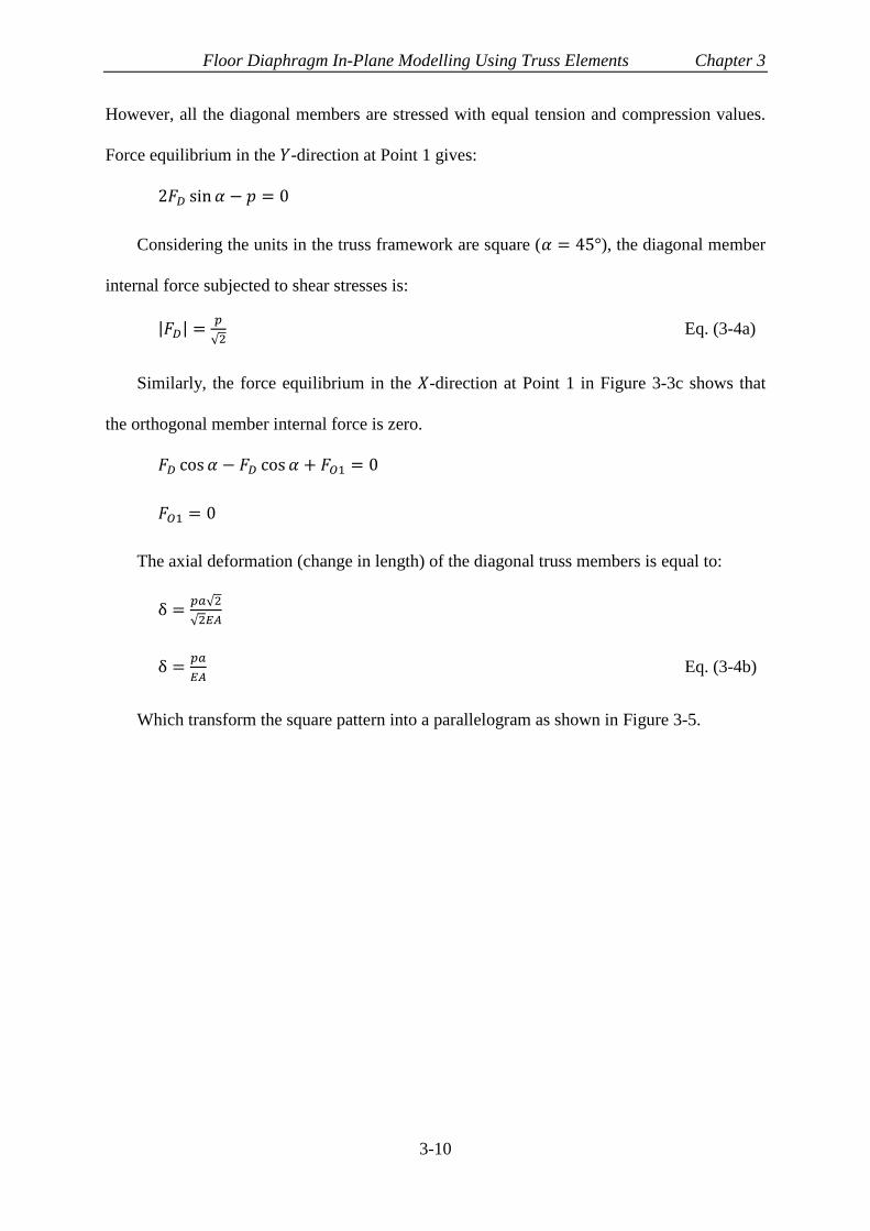
Floor Diaphragm In-Plane Modelling Using Truss Elements Chapter 3
3-10
However, all the diagonal members are stressed with equal tension and compression values.
Force equilibrium in the 𝑌-direction at Point 1 gives:
2𝐹𝐷 sin 𝛼 − 𝑝 = 0
Considering the units in the truss framework are square (𝛼 = 45°), the diagonal member
internal force subjected to shear stresses is:
|𝐹𝐷| =𝑝
√2 Eq. (3-4a)
Similarly, the force equilibrium in the 𝑋-direction at Point 1 in Figure 3-3c shows that
the orthogonal member internal force is zero.
𝐹𝐷 cos 𝛼 − 𝐹𝐷 cos 𝛼 + 𝐹𝑂1 = 0
𝐹𝑂1 = 0
The axial deformation (change in length) of the diagonal truss members is equal to:
δ =𝑝𝑎√2
√2𝐸𝐴
δ =𝑝𝑎
𝐸𝐴 Eq. (3-4b)
Which transform the square pattern into a parallelogram as shown in Figure 3-5.

Floor Diaphragm In-Plane Modelling Using Truss Elements Chapter 3
3-11
Figure 3-5. Square pattern deformed shape subjected to shear stress
As shown in Figure 3-5, the shear strain in the framework, 𝛾𝑥𝑦, can be calculated from:
tan (𝜋
4+
𝛾𝑥𝑦
2) =
𝑎
√2−
𝛿
2𝑎
√2+
𝛿
2
=1−
𝛿
𝑎√2
1+𝛿
𝑎√2
Eq. (3-4c)
Also, from the mathematical rule of trigonometric addition formulas (e.g. Abramowitz
and Stegun, 1965) and assuming small deformations which, tan(𝛾) ≅ 𝛾,
tan (𝜋
4+
𝛾𝑥𝑦
2) =
tan𝜋
4−tan
𝛾𝑥𝑦
2
1+tan𝜋
4tan
𝛾𝑥𝑦
2
=1−
𝛾𝑥𝑦
2
1+𝛾𝑥𝑦
2
By equating the above equation with Eq. (3-4c) and substituting Eq. (3-4b), the shear
strain, 𝛾𝑥𝑦, can be obtained as:

Floor Diaphragm In-Plane Modelling Using Truss Elements Chapter 3
3-12
𝛾𝑥𝑦 =𝑝√2
𝐸𝐴 Eq. (3-4d)
By equating the plate and truss framework shear strains, using Eq. (3-3) and Eq. (3-4d),
the diagonal truss element cross-section area can be obtained:
𝐴 =𝑎𝑡
√2(1+𝜈) Eq. (3-5)
Poisson’s ratio, 𝜈, should be found to satisfy the deformation compatibility equation.
Figure 3-6 shows the framework deformation in the 𝑋-direction subjected to normal force, 𝑝,
in the 𝑋-direction and 𝜈𝑝 in the 𝑌-direction.
Figure 3-6. Framework deformation in the X-direction subjected to normal force 𝑝 in the X-direction
and 𝜈𝑝 in the Y-direction
The deformation compatibility could be simply found by writing the relationship
between the orthogonal and diagonal member deformations as:
𝛿𝐷
2=
𝛿𝑂
2cos 45 Eq. (3-5a)
The truss element axial deformations are denoted by 𝛿𝐷 and 𝛿𝑂 for diagonal and
orthogonal members respectively.

Floor Diaphragm In-Plane Modelling Using Truss Elements Chapter 3
3-13
Considering the truss element axial forces obtained using equilibrium in the 𝑋-direction,
Eq. (3-3a), and truss member cross-section areas given in Eqs. (3-4 and 3-5), 𝛿𝐷 and 𝛿𝑂 may
be calculated as:
𝛿 𝐷 =𝜈𝑝√2(1+𝜈)
𝐸𝑡
𝛿𝑂 =𝑝(1−𝜈2)
𝐸𝑡
Substituting these axial deformations into Eq. (3-5a), gives:
𝜈𝑝√2(1+𝜈)
𝐸𝑡=
𝑝(1−𝜈2)
√2𝐸𝑡
From which 𝜈 =1
3 results.
Considering the Poisson’s ratio 𝜈 =1
3, the cross-section area of the orthogonal and the
diagonal members are obtained using Eqs. (3-4 and 3-5) respectively as:
𝐴1 = 0.75𝑎𝑡 (Orthogonal member)
𝐴 = 0.53𝑎𝑡 (Diagonal member)
Where 𝑎 is the dimension of the framework pattern and 𝑡 is the plate thickness.
3.3 Truss element modelling
3.3.1 Diamond shape model
In steel frame structures with composite floor system, shear studs on the top of any beam
can be represented by one effective stud at the centre of the beam span (MacRae and Bull,
2015). In this configuration, axial forces parallel to the beam are resisted by the beam, tension
force demands perpendicular to the beam can be resisted by reinforcing steel placed in the
slab, and compression forces at different angles to the beam axis are resisted by the concrete.
This approach also gives axial forces in the beams which also must be considered in design
(MacRae and Clifton, 2015). A diamond shape model for this purpose is proposed below.

Floor Diaphragm In-Plane Modelling Using Truss Elements Chapter 3
3-14
This model can be achieved by putting nodes at the centre of the beams (or at the shear
stud locations) to be able to capture beam axial forces more effectively and also be able to
capture shear stud demands. This framework pattern is shown in Figure 3-7. Similar to the
diagonal model, the cross-section area of members can be derived by equating framework
deformations with elastic strains of the plate. It is noted that in this modelling method
boundary elements, as shown in Figure 3-7 with dashed lines, are required to provide overall
stability for the truss framework. These boundary elements may represent beams, walls or
any other element that can restraint diaphragm boundaries.
Figure 3-7. Diamond shape model
Using the same method as obtaining the cross-section areas of the diagonal model, the
cross-section areas of diamond truss elements can be calculated. As shown in Appendix B,
𝐴1 = 0.75𝑎𝑡 (orthogonal members) and 𝐴 = 0.53 𝑎𝑡 (diagonal members) are calculated for a
square truss mesh unit (with 𝑎 = 𝑏), where 𝑎 is the dimension of framework pattern and 𝑡 is
the plate thickness.
If a non-square truss mesh unit be considered, by solving the equilibrium and
compatibility equations, the Poisson’s ratio for the framework is related to the truss mesh unit
dimensions as:

Floor Diaphragm In-Plane Modelling Using Truss Elements Chapter 3
3-15
𝜈 =𝑎𝑏
a2+b2+𝑎𝑏
Eq. (3-6)
Where 𝑎 and 𝑏 are the framework pattern dimensions in Figure 3-7.
Therefore for modelling a concrete material with Poisson’s ratio equal to 0.2, the
framework aspect ratio (𝑎𝑏⁄ ) should be 3.73. Although this is correct mathematically, this
value is not practical in modelling and more importantly by taking this value as truss
modelling aspect ratio, the cross-section area of the orthogonal truss element results in a
negative value that does not have physical meaning.
3.3.2 Comparison of the diagonal and diamond models
The diagonal (Hrennikoff, 1941) and the diamond models are compared in this section.
Here all elements are considered to carry both tension and compression forces. The
comparison is made in terms of mesh sensitivity and beam axial and shear stud force results.
3.3.2.1 Mesh sensitivity
Mesh sensitivity for the diamond and the diagonal truss models is investigated both
using closed-form solutions and also some numerical examples.
• Closed form assessment
Consider the plate in Figure 3-8 subjected to axial force only. Based on the mechanics of
material, the axial strain in the plate member can be easily found using Eq. (3-7).
a) Plan
b) Cross-section
Figure 3-8. A plate member under axial force

Floor Diaphragm In-Plane Modelling Using Truss Elements Chapter 3
3-16
휀𝑥 =𝑁
𝐸𝑡𝑏 Eq. (3-7)
Where 𝑁 is the applied axial force, 𝑡 and 𝑏 are thickness and width of the plate section
and 𝐸 is the plate elastic modulus. Here, the same plate member is modelled using the
diagonal and the diamond truss models and the axial strain is calculated. Figure 3-9a
and b show the models schematically. In both models, the axial strain of the truss mesh unit is
equal to the axial strain of member 𝑇1 as shown in Figure 3-9. This can easily be found by
analysing one unit of the truss model.
a) Diagonal truss model of a plate member
b) Diamond truss model of a plate member
Figure 3-9. Diagonal and diamond truss models subjected to an axial tension force
Considering the cross-section area of the elements obtained in Section 3.2.2 and the axial
force of member 𝑇1 in the diamond and the diagonal models, the axial strain can be
obtained. The axial force of member 𝑇1 is 𝐹1 =3𝑁
4𝑛 for both the diagonal and the diamond

Floor Diaphragm In-Plane Modelling Using Truss Elements Chapter 3
3-17
models. Where 𝑛 is the number of elements in plate width. Element/model axial strain in
both truss models is equal to:
휀𝑥 =3𝑁 (4𝑛)⁄
3𝐸𝑏𝑡 (4𝑛)⁄=
𝑁
𝐸𝑡𝑏
Note that in the diagonal model, the stiffness of boundary elements are half the
internal elements. Also, it may be seen that if there were no diagonal members, then 𝐹1 =
𝑁 𝑛⁄ . The fact that 𝑇1 is only 75% of this value indicates that the diagonals carry 25% of the
force.
The calculated strain shows that the axial deformation in both models is independent of
the number of elements and it results in the same axial deformations as plate member. In the
case of biaxial loading, when the Poisson’s ratio of the plate is equal to 0.33, similar results
are obtained.
For truss models subjected to shear force as shown in Figure 3-10, shear deformations
can also be obtained without error for materials with a Poisson’s ratio equal to 0.33. The
shear strain of the plate can be easily obtained using Eq. (3-8).
𝛾𝑥𝑦 =2(1+𝜈)𝑁
𝐸𝑡𝑏= 2.66
𝑁
𝐸𝑡𝑏 Eq. (3-8)
In both models, there are 2𝑛 diagonal members that resist shear forces; the stiffness of
each of these members in the direction of applied force is equal to 𝐸𝐴
𝐿cos2 𝜃. Here 𝐴 and 𝐿
are the cross-section area and length of diagonal members respectively, and 𝜃 is the angle
between the diagonal member and the direction of applied force (here 𝜃 = 45°). By
substituting 𝐴, 𝐿 and 𝜃, the stiffness of diagonal element is equal to 3𝐸𝑡
16 for the diagonal
model and 3𝐸𝑡
8 for the diamond model. Therefore, the shear strains, 𝛾𝑥𝑦, in both models can
be obtained.
For the diagonal model this is calculated as:

Floor Diaphragm In-Plane Modelling Using Truss Elements Chapter 3
3-18
𝛾𝑥𝑦 =(
𝑁
2n×
16
3𝐸𝑡)
𝑏/𝑛=
8𝑁
3𝐸𝑡𝑏= 2.66
𝑁
𝐸𝑡𝑏
For the diamond model this is calculated as:
𝛾𝑥𝑦 =(
𝑁
2n×
8
3𝐸𝑡)
1
2×𝑏/𝑛
=8𝑁
3𝐸𝑡𝑏= 2.66
𝑁
𝐸𝑡𝑏
It is obvious from shear strain equations that both models can capture shear deformations
independent of the number of elements.
a) Diagonal truss model of a plate member
b) Diamond truss model of a plate member
Figure 3-10. Diagonal and diamond truss models under shear forces
In the case of bending moments, the error is related to finding the moment of inertia of
the plate cross-section. For truss models, the moment of inertia can be obtained from Eq. (3-
9) where 𝐴𝑘 is the equivalent cross-section area of diagonal and orthogonal elements at each

Floor Diaphragm In-Plane Modelling Using Truss Elements Chapter 3
3-19
node of a section and 𝑦𝑘 is the distance of each elements to the section neutral axis. The
equation that is used to calculate 𝐼, depends on whether the number of elements, 𝑛, is even or
odd.
𝐼 = ∫ 𝑦2𝑑𝐴 = ∑ 𝐴𝑘𝑦𝑘2𝑛
𝑘=1𝐴 Eq. (3-9)
For the diagonal model when the number of elements is even:
𝐼 = 2 ∑ 𝐴𝑘𝑦𝑘2
(𝑛/2)−1
𝑘=1
+𝑏3𝑡
4𝑛= 2 ∑
𝑏𝑡
𝑛(
𝑘𝑏
𝑛)
2(𝑛/2)−1
𝑘=1
+𝑏3𝑡
4𝑛= 2
𝑏3𝑡
𝑛3∑ 𝑘2
(𝑛/2)−1
𝑘=1
+𝑏3𝑡
4𝑛
For the diagonal model when the number of elements is odd:
𝐼 = 2 ∑ 𝐴𝑘𝑦𝑘2
(𝑛−1)/2
𝑘=1
+𝑏3𝑡
4𝑛= 2 ∑
𝑏𝑡
𝑛(
(2𝑘 − 1)𝑏
2𝑛)
2(𝑛−1)/2
𝑘=1
+𝑏3𝑡
4𝑛
=𝑏3𝑡
2𝑛3∑ (2𝑘 − 1)2
(𝑛−1)/2
𝑘=1
+𝑏3𝑡
4𝑛
For the diamond model when the number of elements is even:
𝐼 = 2 ∑ 𝐴𝑘𝑦𝑘2
𝑛/2
𝑘=1
= 2 ∑𝑏𝑡
𝑛(
(2𝑘 − 1)𝑏
2𝑛)
2𝑛/2
𝑘=1
=𝑏3𝑡
2𝑛3∑(2𝑘 − 1)2
𝑛/2
𝑘=1
For the diamond model when the number of elements is odd:
𝐼 = 2 ∑ 𝐴𝑘𝑦𝑘2
(𝑛−1)/2
𝑘=1
= 2 ∑𝑏𝑡
𝑛(
𝑘𝑏
𝑛)
2
= 2𝑏3𝑡
𝑛3∑ 𝑘2
(𝑛−1)/2
𝑘=1
(𝑛−1)/2
𝑘=1
Using Faulhaber's formula for sum of the power series, the above equations can be
simplified as below:
For the diagonal model when the number of elements is even:
𝐼 = 2𝑏3𝑡
𝑛3∑ 𝑘2(𝑛/2)−1
𝑘=1 +𝑏3𝑡
4𝑛= 2
𝑏3𝑡
𝑛3 ((
𝑛
2−1)
3
3+
(𝑛
2−1)
2
2+
(𝑛
2−1)
6) +
𝑏3𝑡
4𝑛 Eq. (3-10)
For the diagonal model when the number of elements is odd:

Floor Diaphragm In-Plane Modelling Using Truss Elements Chapter 3
3-20
𝐼 =𝑏3𝑡
2𝑛3∑ (2𝑘 − 1)2(𝑛−1)/2
𝑘=1 +𝑏3𝑡
4𝑛=
𝑏3𝑡
2𝑛3 [4 ((
𝑛−1
2)
3
3+
(𝑛−1
2)
2
2+
(𝑛−1
2)
6) − 4 (
(𝑛−1
2)
2
2+
(𝑛−1
2)
2) +
𝑛−1
2] +
𝑏3𝑡
4𝑛 Eq. (3-11)
For the diamond model when the number of elements is even:
𝐼 =𝑏3𝑡
2𝑛3∑ (2𝑘 − 1)2 =
𝑛/2𝑘=1
𝑏3𝑡
2𝑛3 [4 ((
𝑛
2)
3
3+
(𝑛
2)
2
2+
(𝑛
2)
6) − 4 (
(𝑛
2)
2
2+
(𝑛
2)
2) +
𝑛
2] Eq. (3-12)
For the diamond model when the number of elements is odd:
𝐼 = 2𝑏3𝑡
𝑛3∑ 𝑘2(𝑛−1)/2
𝑘=1 = 2𝑏3𝑡
𝑛3 ((
𝑛−1
2)
3
3+
(𝑛−1
2)
2
2+
(𝑛−1
2)
6) Eq. (3-13)
Based on the above equations, the moment of inertia of the truss models is dependent on
the number of elements. For instance, for the diagonal model with three elements, the
moment of inertia is 1.22 times the actual plate moment of inertia. For the diamond model
with three elements, the moment of inertia is 0.889 times the actual plate moment of inertia.
Figure 3-11 shows the moment of inertia of the truss models with a different number of
elements from Eqs. (3-10) to (3-13) divided by that of the plate moment of inertia as well as
some specific numerical results. Based on the analytical and numerical results, the diamond
model is less sensitive to a number of elements than the diagonal model, but the
diamond model underestimates 𝐼, while the diagonal model overestimates it.

Floor Diaphragm In-Plane Modelling Using Truss Elements Chapter 3
3-21
Figure 3-11. The trend of change in moment of inertia of the truss models with an increasing number
of elements
• Numerical validation
In order to validate the results of the analytical mesh sensitivity study, a short numerical
study is conducted with different mesh sizes varying between 100mm and 500mm for a 9m
tall cantilever plate beam. The beam width and thickness are 3000mm and 300mm
respectively. A 1000 kN lateral force is applied at the top of the beam and the material is
considered to be concrete with an elastic modulus of 27GPa. The deformed shapes and lateral
displacements are shown in Figure 3-12 and Table 3-1, respectively. The expected behaviour
is calculated based on the formulation provided by Timoshenko (1940), Eq. (3-13a). This
Equation is for a cantilever beam that the cross-section is prevented from warping at the
support and is loaded at the other end. Based on Eq. (3-13a) the expected deformation at the
top of the cantilever plate beam is 14.33 mm.
𝛿 =𝑃𝐿3
3𝐸𝐼[1 + 0.71 (
ℎ
𝐿)
2
− 0.10 (ℎ
𝐿)
3
] Eq. (3-13a)
Where 𝑃 is the applied force, 𝐸 and 𝐼 are the elastic modulus and moment of inertia of
the cantilever plate beam. Section height and beam length are denoted by ℎ and 𝐿
respectively. Note that Poisson’s ratio is considered 0.3 for obtaining this equation.
0.4
0.6
0.8
1
1.2
1.4
1.6
2 5 8 11 14 17 20 23 26 29 32
I Tru
ss m
odel
/IP
late
mem
br
Number of elements
Diagonal model
Diamond model
Diagonal model, numerical validation
Diamond model, numerical validation

Floor Diaphragm In-Plane Modelling Using Truss Elements Chapter 3
3-22
a) Diagonal model,
200mm mesh size
b) Diagonal model,
500mm mesh size
c) Diamond model,
200mm mesh size
d) Diamond model,
500mm mesh size
Figure 3-12. Comparison of diagonal and diamond truss models
Table 3-1. Mesh size effect on cantilever plate beam lateral deformation
Mesh size
(number of
elements)
Deformation (mm)
Diagonal model Diamond model
500mm (18×6) 13.77 14.81
200mm (45×15) 14.22 14.40
100mm (90×30) 14.29 14.35
The lateral displacement from hand calculation is 14.33 mm
The results indicate that the stiffness of the diagonal model decreases with finer mesh
size while for the diamond model the stiffness increases with a finer mesh and converge to
the expected value. This is because in the diagonal model the actual width of the truss
model is greater than the actual wall width due to the cross-section area of orthogonal
boundary members and by decreasing the mesh size, the width of the plate in truss model
reaches to the actual size. The stiffness ratio of cantilever beam plate models to the hand
calculation is also plotted in Figure 3-11 which show good agreement with the closed-form
assessment.

Floor Diaphragm In-Plane Modelling Using Truss Elements Chapter 3
3-23
3.3.2.2 Beam axial forces and shear stud demands
• Beam axial and shear stud forces concept
Beams in structural frames are often considered to carry bending and shear forces.
However, during an earthquake event, inertia and transfer forces act on the diaphragm need to
be transferred to the structural frames. Some mechanisms contribute to transferring these
forces to the structural frame. It is often assumed that the slab transfers the lateral forces to
the column through compression on the column face. While, in frame structures, since slab
inertia forces act in the same direction as the frame sways, due to the beam-column joint
rotation, a gap opens at location “A”, shown in Figure 3-13. Because of this, slab inertia
forces cannot go directly into the column. Instead, the forces must transfer into the steel beam
through friction and mechanical attachments (shear studs) (MacRae and Clifton, 2015); this
situation imposes axial forces to beam plastic hinge regions and connections at the beam ends
that may need to be considered in design procedure. Also, if there is no construction gap
between the slab and column, as the column sways, it bears against the concrete slab on the
far side of the column causing a slab-interaction effect that increases the forces that the slab
must transfer into the beam, and the beam must transfer it back to the columns. Axial forces
in the beams may decrease the structure’s lateral strength and deformation capacity.
Figure 3-13. Slab-column interaction, a gap opens at Point A due to joint rotation

Floor Diaphragm In-Plane Modelling Using Truss Elements Chapter 3
3-24
Overall, it should be noted that whether a gap opens or not, part of diaphragm forces will
be transferred to the column or vertical lateral force resisting system through the beams
because the diaphragm is not fully rigid.
• Beam axial and shear stud forces in truss modelling
In truss element modelling, the beam axial forces and shear stud demands may be
obtained directly from the analysis. However, the pattern of truss framework used for truss
modelling can affect the results and the analysis assumptions. Therefore extra care should be
made for selecting an appropriate truss model. In this study, differences between the diamond
and the diagonal truss modelling methods are described.
Generally, the beam axial forces can be obtained if the rigid diaphragm assumption is not
considered in the structural analysis, for shell, solid, or truss element modelling. However,
the results from each of these modelling techniques are different and mainly represents a
certain situation. For instance, if the diaphragm is modelled using shell or solid elements, part
of the diaphragm forces is transferred directly to the column because the corner elements of
the diaphragm are connected to the column nodes. This situation represents a full contact
between the diaphragm and the column. Experimental tests that had been done by Chaudhari
et al. (2015) showed that even when the slab is not isolated from the column, a gap opens
between the slab and column in the moment frame structure and the slab forces cannot be
transferred to the column directly.
Therefore, diaphragm forces need to be transferred into the steel beam through
mechanical attachments, e.g. shear studs. This can be achieved using the diamond truss
model directly because the diagonal members which represent the concrete struts are not
connected to the beam-column joints. Consequently, the strut compression force transfers to
VLFR system through beam axial forces as shown in Figure 3-14a. This means that in the
case of truss modelling using the diamond pattern, the slab is totally isolated. However, in

Floor Diaphragm In-Plane Modelling Using Truss Elements Chapter 3
3-25
the diagonal truss element method, struts are connected to the beam-column joints and part of
the slab forces transfers directly to the column as shown in Figure 3-14b. This results in
lower beam axial and shear stud demands.
Therefore, using the diamond model gives more reasonable results in terms of the
beam axial forces for designing the beams and beam-column connections. On the other hand,
the truss modelling nodes could be placed at the shear stud locations to directly record the
shear stud demands. Similar results may be obtained using the diagonal truss element
modelling or shell element modelling by removing the corner elements that are connected to
the column nodes. However, it may decrease the total diaphragm in-plane stiffness based on
the selected mesh size.
a) Diamond model
b) Diagonal model
Figure 3-14. Strut placed at the corner truss mesh unit

Floor Diaphragm In-Plane Modelling Using Truss Elements Chapter 3
3-26
In addition to the strut locations, it should be noted that in the diagonal truss element
modelling, the orthogonal members are required to be placed at the beam locations to
complete the square framework pattern as shown in Figure 3-14b. These orthogonal elements
also carry some portion of the beam axial and shear stud demands directly to the column
which is not realistic due to gap opens, or due to an initial physical gap being placed around
the column.
A one-storey two-bay braced frame, with the dimensions shown in Figure 3-15, is
considered to investigate the beam axial and shear stud forces using both truss element
modelling methods. In this model, it is assumed that a gap is provided around the column and
there is no slab-column interaction. Also, a detailed elastic FEM model was created using
ABAQUS software to compare the results with truss element modelling. The truss models
were created using SAP2000 (2015) software. The simulated structure is designed using New
Zealand building standards (e.g. NZS1170.5 2004 and NZS3404 2007) and the elastic ESA
method is used to find the diaphragm imposed forces for performing the following analysis.
The lateral inertia force was distributed to truss element nodes based on the tributary area
of each node. This was conducted in the detailed FEM, ABAQUS, model by defining a
uniform horizontal surface traction force.
a) Floor plan dimensions and beam sections

Floor Diaphragm In-Plane Modelling Using Truss Elements Chapter 3
3-27
b) SAP2000 model
c) ABAQUS model
Figure 3-15. Model considered for investigating the beam axial and shear stud forces
Figure 3-16 shows the beam axial force diagram for the beam located in the middle of
the simulated diaphragm. In the detailed FEM model physical gap has been provided between
the slab and column to prevent the slab forces being transferred to the column directly and
slab bearing forces to occur on the other side of the beam. As can be seen, the diamond
model indicate similar results to the detailed FEM model, the maximum difference in the
peak values at the beams ends is less than 10%. The overall behaviour of the diagonal
model is similar to the diamond model, while, the peak beam axial forces in the diagonal
model is considerably lower (about 35%). This is because, in the diagonal model, the
slab is connected to the column and part of the diaphragm force transfers to the column
directly as was shown in Figure 3-14.
a) Beam axial force diagram
-100
-50
0
50
100
150
Ax
ial
forc
e (k
N)
FEM (Gap provided) AbaqusDiamond truss model, SAP2000Diagonal truss model, SAP2000

Floor Diaphragm In-Plane Modelling Using Truss Elements Chapter 3
3-28
b) Shear stud forces in the shell/solid element model (ABAQUS), Average for left beam 17.6kN,
right beam 7.4kN
c) Shear stud forces (SAP2000) in the diamond model, Average for left beam 15kN, right beam
6 kN
d) Shear stud forces (SAP2000) in the diagonal model, Average for left beam 10.5kN, right
beam 4.4kN
Figure 3-16. Beam axial and shear stud forces in elastic models
Regarding shear stud demands, the trend of changing the shear forces in all models are
similar. However, the average forces in the diamond and the diagonal models are 15%
and 50% lower than the detailed FEM model respectively.
3.4 Truss element modelling with different element aspect ratio
In Section 3.3.2, it has been shown that truss element modelling can effectively obtain
diaphragm in-plane stiffness, and beam axial and shear stud forces. All of the examples used
in this study consist of one or two bays structures, where it is possible to use a large number
of truss elements to model diaphragm. For instance, the mesh size in the studied model

Floor Diaphragm In-Plane Modelling Using Truss Elements Chapter 3
3-29
shown in Figure 3-15 was considered to be 300mm. However, in a real structure with several
bays and storeys, it is not practical to create a fine mesh model and investigate the load path
through the diaphragm. Therefore, it may be beneficial to model every bay with a limited
number of elements (based on the diaphragm aspect ratio and geometry) considering an
acceptable error in results.
Most floor plans consist of a number of bays with different aspect ratio due to
architectural or geometry limitations. Therefore, the cross-section area of truss elements
considering non-square units needs to be derived. Figure 3-17 shows a non-square truss
framework.
Figure 3-17. Non-square truss framework
Using the same method that was discussed in Section 3.2.2, the cross-section areas of the
non-square truss framework can be found as follows according to Appendix C.
A1=at(1-
𝜈b2
a2 )
1-𝜈2 Eq. (3-14)
A2=bt(1-
𝜈a2
b2 )
1-𝜈2 Eq. (3-15)
A3=√𝑎2+𝑏2(𝑎2+𝑏2)
4𝑎𝑏(1+𝜈)𝑡 Eq. (3-16)

Floor Diaphragm In-Plane Modelling Using Truss Elements Chapter 3
3-30
Where 𝑎 and 𝑏 are the dimensions of the framework pattern, 𝑡 is the plate thickness and
𝜈 is Poisson’s ratio of the plate material. It can be shown that in the case of the square mesh
unite and 𝜈 = 1/3, truss element cross-section areas are 𝐴1 = 0.75𝑎𝑡, 𝐴2 = 0.75𝑎𝑡 and
𝐴3 = 0.53𝑎𝑡.
• Beam axial and shear stud forces
The studied model in Section 3.3.2.2 is regenerated using one truss element between
steel beams by putting the nodes at the centre of the beams as shown in Figure 3-18. In this
example, the lateral load is distributed based on the tributary area of each node.
Figure 3-18. Putting nodes at the centre of the beams
The beam axial forces for the beam at the middle bay is plotted in Figure 3-19. As can be
seen, the peak beam axial force values show less than 20% difference from the fine mesh
truss model.

Floor Diaphragm In-Plane Modelling Using Truss Elements Chapter 3
3-31
a) Beam axial force diagram
b) Average shear stud forces of single truss element model
Figure 3-19. Beam axial and shear stud force in single truss element model
Also, the average shear stud forces in this model was obtained by dividing the total shear
force by the number of shear studs. The computed shear stud force was about 5% lower at the
left beam and about 1% higher at the right beam compared with the detailed FEM model of
Figure 3-16.
In most real structures even if the floor plan is rectangular, there are openings with
various sizes in different locations for stairs, lifts, mechanical or electrical ducts. Therefore
using a small number of large elements may be unsuitable for diaphragm modelling to obtain
the likely load path through the diaphragm or in-plane deformations. However, it can be used
for estimating the maxima of beam axial force at the beam ends, and average shear stud
demands.
-100
-50
0
50
100
150
200
Ax
ial
forc
e (k
N)
FEM (Gap provided) ABAQUSDiamond truss model, SAP2000Diamond truss model with one element, SAP2000Diagonal truss model, SAP2000

Floor Diaphragm In-Plane Modelling Using Truss Elements Chapter 3
3-32
3.5 Different truss element modelling types
The concept of truss modelling method and both diagonal and diamond models were
introduced in the previous sections. Generally, the truss method first was developed
considering the elastic behaviour of a plate member, and it was assumed that all truss
elements can carry tension and compression forces to satisfy the equilibrium and
compatibility equations. However, for modelling a diaphragm consist of concrete material,
the tension behaviour of the concrete (cracking) should be taken into account to achieve more
realistic results. Therefore, different modelling techniques are introduced and compared here
to find out the best method for modelling concrete diaphragms in design. The modelling
methods considered on a square truss mesh unit include the following.
Model 1. Elastic truss modelling
Model 2. Compression-only diagonal members with elastic orthogonal members
(compression and tension)
Model 3. Compression-only diagonal members with considering reinforcements as
orthogonal members (concrete compression, tension reinforcement)
Model 4. Compression-only diagonal members with tension-only orthogonal
members
Model 5. Compression-only diagonal members with elastic orthogonal members
(based on “The Seismic Assessment of Existing Buildings” Section C5
recommendations)
Model 6. Truss modelling considering nonlinear properties of the concrete and
reinforcements
Note that, as it was shown the diamond model has advantages over the diagonal model
such as i) it has less mesh sensitivity, ii) provides more reasonable beam axial force and shear
stud demands and iii) considers gap around the column, all the different truss modelling types
are investigated using the diamond model in the following sections.

Floor Diaphragm In-Plane Modelling Using Truss Elements Chapter 3
3-33
3.5.1 Elastic truss modelling (all members carry both tension
and compression)
This method was described comprehensively in Section 3.2.2. It was shown that this
method gives accurate results for materials with Poisson’s ratio 𝜈 = 0.33 and considering a
sufficient number of elements. The orthogonal and diagonal member cross-section areas are
𝐴1 = 0.75𝑎𝑡 and 𝐴 = 0.53 𝑎𝑡 respectively. Where 𝑎 is the dimension of the framework
pattern and 𝑡 is the plate thickness.
3.5.2 Compression-only diagonal members with
compression/tension orthogonal members
The elastic truss model can effectively model the shell element behaviour. However, it
does not provide good information about the actual strut compression forces and tension tie
forces because the diagonal members are assumed to carry both tension and compression
forces. Therefore, the truss element method with compression-only diagonal members (which
represents concrete struts) may be used for finding more realistic load paths through the
diaphragm.
Considering that the diagonal members act in compression only (strut) and the
orthogonal members act in both compression and tension, the tension and compression
behaviour of the truss model will be different. Which means the truss model subjected to
orthogonal compression forces in one direction acts like an elastic plate because all the
elements are contributing in load carrying mechanism. While in tension the truss model
works independently in perpendicular directions and the longitudinal and transverse
deformations are not related to the Poisson’s ratio. Thus, for calculating the truss element
cross-section areas three loading conditions considered, include 1) uniaxial tension, 2)
uniaxial compression and, 3) pure shear as shown in Figure 3-20.

Floor Diaphragm In-Plane Modelling Using Truss Elements Chapter 3
3-34
a) Normal tension force per unit length, 𝑃 in the 𝑋-direction
b) Normal compression force per unit length, 𝑃 in the 𝑋-direction
c) Pure shear force per unit length, 𝑃
Figure 3-20. General loading conditions for determining framework properties, 𝑝 is the normal edge
force to each element where 𝑝 = 𝑃𝑎
Similar to the method discussed in Section 3.2.2, using equilibrium and compatibility
conditions the cross-section area of the truss elements can be obtained as shown below. Note
that these areas are different from those assuming all fully elastic elements as described by
Hrennikoff (1941). The truss element strains are obtained in terms of element cross-section
area and the angle between them. Then the framework strains are equated to the

Floor Diaphragm In-Plane Modelling Using Truss Elements Chapter 3
3-35
corresponding strains in the plate member 휀𝑥 and 휀𝑦 with the same loading condition. Based
on solid mechanics, the plate strain in the 𝑋-direction, 휀𝑥, for the first case of loading is
휀𝑥 =𝑃
𝐸𝑡 Eq. (3-17)
Where 𝑃 is uniform force per unit length, 𝐸 is the elastic modulus of the plate material
and 𝑡 is the plate thickness.
As it was mentioned in the previous paragraph, when tension is applied in one direction
there is no deformation in the orthogonal direction in this method because the diagonal
members work in compression only. Therefore, the cross-section area of orthogonal members
in tension, 𝐴𝑂𝑇, could simply be found by equating the strains in the plate and the truss
element subjected to tension forces only. Note that the cross-section areas of orthogonal
members in tension, 𝐴𝑂𝑇, and compression, 𝐴𝑂𝐶, may not be equal necessarily.
The tensile strain in the truss element can be found using:
휀𝑥 =𝑃𝑎
𝐸𝐴𝑂𝑇 Eq. (3-18)
By equating Eq. (3-17) and Eq. (3-18), 𝐴𝑂𝑇 can be found as
𝐴𝑂𝑇 = 𝑎𝑡 Eq. (3-19)
The shear deformation of the plate subjected to a tangential load, 𝛾𝑥𝑦, can be calculated
using Eq. (3-3) for an elastic plate member as shown in Figure 3-20c.
𝛾𝑥𝑦 =2(1+𝜈)𝑃
𝐸𝑡 Eq. (3-3)
Similar to the elastic truss element model in Section 3.2.2, by equating the framework
shear strain with the plate shear strain, the cross-section area of the compressive diagonal
member, 𝐴𝐷, can be found as:
𝐴𝐷 =√2𝑎𝑡
(1+𝜈) Eq. (3-20)

Floor Diaphragm In-Plane Modelling Using Truss Elements Chapter 3
3-36
To find the cross-section area of the orthogonal member in compression, 𝐴𝑂𝐶,
deformation compatibility and force equilibrium should be satisfied simultaneously.
Based on the force equilibrium in the 𝑋 and 𝑌-directions:
𝐹𝑂𝐶 + 2𝐹𝐷 cos 45 = 𝑝 Eq. (3-21)
2𝐹𝐷 cos 45 = 𝐹𝑂𝑇 Eq. (3-22)
Where 𝐹𝐷, 𝐹𝑂𝑇 and 𝐹𝑂𝐶 are diagonal member compression force, orthogonal member
tension and compression forces respectively.
Substituting Eq. (3-22) into Eq. (3-21) gives:
𝐹𝑂𝐶 + 𝐹𝑂𝑇 = 𝑝
Figure 3-21 shows the deformation of the truss unit subjected to an axial compression
force, 𝑝. It can be seen that the axial deformation 𝛿𝑥 is equal to the lateral expansion 𝛿𝑦 plus
the component from the axial contraction in the diagonal members that is denoted by 𝛿𝐷.
Figure 3-21. Deformation of the truss unit under axial compression
Considering the relationship between the diagonal and orthogonal member deformations,
𝛿𝐷 and 𝛿𝑥, and substituting the diagonal cross-section area, 𝐴𝐷 from Eq. (3-20) and
orthogonal tension cross-section area, 𝐴𝑂𝑇 from Eq. (3-19), the orthogonal compression
cross-section area, 𝐴𝑂𝐶, can be found which is discussed below in detail.

Floor Diaphragm In-Plane Modelling Using Truss Elements Chapter 3
3-37
Based on the deformation compatibility, shown in Figure 3-21, which 𝛿𝑥 is the axial
deformation of the truss element under axial compression force and 𝛿𝑦 is the transverse
deformation:
𝛿𝑥 = 𝛿𝑦 + 𝛿𝐷 Eq. (3-23)
Substituting Eqs. (3-17, 3-19 and 3-20) into Eq. (3-23) gives
𝑝
2𝐸𝑡=
𝐹𝑂𝑇𝑎
2𝐸𝑡𝑎+
𝐹𝐷(√2𝑎
2)(1+𝜈)
(√2
2)√2𝐸𝑡𝑎
Eq. (3-24)
Considering Eq. (3-24) and Eq. (3-22), the axial force in the diagonal member, 𝐹𝐷, can
be obtained as:
𝐹𝐷 =𝑝
√2(2+𝜈)
Also, the axial tension force in the vertical orthogonal member, 𝐹𝑂𝑇, is
𝐹𝑂𝑇 =𝑝
(2+𝜈)
And using Eq. (3-21)
𝐹𝑂𝐶 =𝑝(1+𝜈)
(2+𝜈) Eq. (3-25)
The compression cross-section area of the orthogonal members, 𝐴𝑂𝐶, may simply be
found using the axial strain Eq. (3-17) and the truss member axial force, 𝐹𝑂𝐶 of Eq. (3-25) as:
𝐹𝑂𝐶
𝐸𝐴𝑂𝐶=
𝑝
𝐸𝑡𝑎
Substituting 𝐹𝑂𝐶 from Eq. (3-25) gives
𝐴𝑂𝐶 =𝑎𝑡(1+𝜈)
(2+𝜈) Eq. (3-26)
Based on the Poisson’s ratio definition:
𝜈 =𝛿𝑦
𝛿𝑥

Floor Diaphragm In-Plane Modelling Using Truss Elements Chapter 3
3-38
By substituting the axial deformations 𝛿𝑦 and 𝛿𝑥 in the above equation, it can be found
that
𝛿𝑦 =𝑝
(2+𝜈)𝐸𝑎𝑡
𝛿𝑥 =𝑝
𝐸𝑎𝑡
𝜈 =
𝑝
(2+𝜈)𝐸𝑎𝑡𝑝
𝐸𝑎𝑡
𝜈 =1
2+𝜈 Eq. (3-26a)
By solving Eq. (3-26a), 𝜈 = 0.414. That is, this framework with compression-only
diagonal members is only accurate for material with Poisson’s ratio, 𝜈, equal to 0.414.
Considering this Poisson’s ratio, the truss element cross-section areas are equal to:
𝐴𝐷 = 𝑎𝑡
𝐴𝑂𝑇 = 𝑎𝑡
𝐴𝑂𝐶 = 0.585𝑎𝑡
These values show that orthogonal members in tension should have the same width as
the truss mesh unit, 𝐴𝑂𝑇 = 𝑎𝑡, because diagonal members cannot act in tension and
participate in force carrying mechanism. But in compression some part of the axial
compression force can be carried by the diagonal members and therefore smaller orthogonal
cross-section in compression, 𝐴𝑂𝐶 = 0.585𝑎𝑡, is required to achieve the same axial strain as
the plate member.

Floor Diaphragm In-Plane Modelling Using Truss Elements Chapter 3
3-39
3.5.3 Compression-only diagonal members with reinforcement
tension/concrete compression orthogonal members
In this case it is assumed that all the tension forces are carried by slab reinforcements in a
fully cracked situation. Therefore the tension cross-sectional area of the orthogonal members,
𝐴𝑂𝑇, is equal to the steel reinforcement area, 𝐴𝑠, within the element width as:
𝐴𝑂𝑇 = 𝐴𝑠 Eq. (3-27)
Similar to the Section 3.5.2, since the diagonal members are in compression only, the
tensile deformations in perpendicular directions are independent.
The shear deformation of the plate, 𝛾𝑥𝑦, subjected to tangential force, 𝑝, as shown in
Figure 3-20c, can be found using Eq. (3-3) similar to the elastic plate member.
𝛾𝑥𝑦 =2(1+𝜈)𝑝
𝐸𝑡𝑎 Eq. (3-3)
By equating the framework shear strain obtained in Section 3.2.2 Eqs. (3-4 and 3-5) with
the plate shear strain, 𝛾𝑥𝑦, the cross-section area of the diagonal member, 𝐴𝐷, is
𝐴𝐷 =√2𝑎𝑡
(1+𝜈) Eq. (3-20)
To find the compression cross-section area of the orthogonal member, 𝐴𝑂𝐶, the
deformation compatibility and force equilibrium conditions should be satisfied. Based on the
force equilibrium in the 𝑋 and 𝑌-directions:
𝐹𝑂𝐶 + 2𝐹𝐷 cos 45 = 𝑝 Eq. (3-21)
2𝐹𝐷 cos 45 = 𝐹𝑂𝑇 Eq. (3-22)
Where 𝐹𝐷, 𝐹𝑂𝑇 and 𝐹𝑂𝐶 are diagonal member compression force, orthogonal member
tension and compression forces respectively.
Substituting Eq. (3-22) into Eq. (3-21) gives:
𝐹𝑂𝐶 + 𝐹𝑂𝑇 = 𝑝

Floor Diaphragm In-Plane Modelling Using Truss Elements Chapter 3
3-40
Similar to the previous modelling method in Section 3.5.2, the deformation of the truss
unit under an axial compression force, 𝑝, is shown in Figure 3-21. It can be seen that the axial
deformation 𝛿𝑥 is equal to the lateral expansion 𝛿𝑦 plus the contribution from the axial
contraction in the diagonal members that is denoted by 𝛿𝐷. Considering the relationship
between the diagonal and orthogonal member deformations (𝛿𝐷, 𝛿𝑥 and 𝛿𝑦) and substituting
the diagonal cross-section area, 𝐴𝐶 , and orthogonal tension cross-section (reinforcement
cross-section area), 𝐴𝑂𝑇, the orthogonal compression cross-section area, 𝐴𝑂𝐶, can be obtained
as is discussed below.
The plate axial compression strain equals to
휀𝑥 =𝑃
𝐸𝑡 Eq. (3-17)
Based on the deformation compatibility, where 𝛿𝑥 is the axial deformation of the truss
element under axial compression and 𝛿𝑦 is the transverse deformation as shown in Figure
3-21.
𝛿𝑥 = 𝛿𝑦 + 𝛿𝐷 Eq. (3-23)
Substituting Eqs. (3-17, 3-27 and 3-20) into Eq. (3-23) gives
𝑝
2𝐸𝑡=
𝐹𝑂𝑇𝑎
2𝐸𝑠𝐴𝑠+
𝐹𝐷(√2𝑎
2)(1+𝜈)
(√2
2)√2𝐸𝑡𝑎
Eq. (3-28)
Where 𝐸𝑠 and 𝐴𝑠 are the elastic modulus and area of the reinforcements placed within
each element. Considering Eq. (3-28) and Eq. (3-22) the axial force in the diagonal member
can be found as
𝐹𝐷 =𝑝
2𝐸𝑡(𝑎
√2𝐸𝑠𝐴𝑠+
(1+𝜈)
√2𝐸𝑡) Eq. (3-29)
Substituting Eq. (3-29) into Eq. (3-21) gives
𝐹𝑂𝐶 = 𝑝 (1 −√2
2𝐸𝑡(√2
2𝐸𝑠𝑡𝜌+
(1+𝜈)
√2𝐸𝑡)) Eq. (3-30)

Floor Diaphragm In-Plane Modelling Using Truss Elements Chapter 3
3-41
Where 𝜌 is the reinforcement ratio 𝐴𝑠
𝑎𝑡=
𝐴𝑂𝑇
𝑎𝑡.
The compression cross-section area of the orthogonal members, 𝐴𝑂𝐶, can simply be
found using the axial strain Eq. (3-17) and the orthogonal member axial force, 𝐹𝑂𝐶 (Eq. 3-30)
as:
𝐴𝑂𝐶 = 𝑎𝑡 (1 −√2
2𝐸𝑡(√2
2𝐸𝑠𝑡𝜌+
(1+𝜈)
√2𝐸𝑡)) Eq. (3-30)
This equation shows that the cross-section area of the orthogonal member in
compression, 𝐴𝑂𝐶, is dependent on the reinforcement ratio provided in the slab, 𝜌, and hence
on 𝐴𝑂𝑇.
Based on the Poisson’s ratio, 𝜈, definition
𝜈 =𝛿𝑦
𝛿𝑥
By substituting the axial deformations in the above equation, it can be found that the
Poisson’s ratio is related to the reinforcement ratio.
𝜈 =1
1+(1+𝜈)𝐸𝑠𝜌
𝐸
Eq. (3-30a)
or
𝜌 =𝐸(1−𝜈)
𝜈(1+𝜈)𝐸𝑠
Figure 3-22 plots the Poisson’s ratio (𝜈) versus the reinforcement ratio (𝜌). Note that this
Figure is plotted considering 𝐸𝑠
𝐸= 9, where 𝐸𝑠 and 𝐸 are the elastic modulii of reinforcements
and concrete respectively.

Floor Diaphragm In-Plane Modelling Using Truss Elements Chapter 3
3-42
Figure 3-22. Poisson’s ratio (ν) versus reinforcement ratio (ρ) for compression-only diagonal-
reinforcement tension orthogonal member
This plot shows that increasing the reinforcement ratio decreases the Poisson’s ratio of
the truss model. Which is because more reinforcement in the slab decreases the lateral
deformations. Also, it is noted that for reinforcement ratio less than 7.4% the Poisson’s ratio
becomes more than 0.5.
Figure 3-23 plots the 𝐴𝑂𝐶 and 𝐴𝐷 versus reinforcement ratio (𝜌).
Figure 3-23. Orthogonal and diagonal compression cross-section areas, 𝐴𝑂𝐶 and 𝐴𝐷, versus
reinforcement ratio (𝜌) for compression-only diagonal-reinforcement tension orthogonal member
According to the plots in Figure 3-23, there is no specific value for diagonal and
orthogonal cross-section areas in compression, 𝐴𝐷 and 𝐴𝑂𝐶, to be applicable for all situations.
0
20
40
60
80
100
0 0.2 0.4 0.6 0.8 1 1.2
Rei
nfo
rcem
ent
rati
o(%
)
Poisson's ratio
0
0.2
0.4
0.6
0.8
1
1.2
0 5 10 15
Com
pre
ssio
n c
ross
-sec
tion
area
(at
)
Reinforcement ratio (%)
Orthogonal cross-section
Diagonal cross-section
Likely range

Floor Diaphragm In-Plane Modelling Using Truss Elements Chapter 3
3-43
These cross-section areas vary depending on the amount of reinforcement, 𝐴𝑠 or 𝐴𝑂𝑇,
provided in slab.
Considering the fact that the reinforcement ratio in steel deck composite slabs usually is
between 0.2% to 0.4% according to AS/NZS2327 (2017) Table 2.2.1, the truss element cross-
sectional areas may be taken as that based on a 0.3% reinforcement ratio without significant
error, as shown in Figure 3-23, as:
𝐴𝐷 = 0.725𝑎𝑡
𝐴𝑂𝑇 = 𝐴𝑠
𝐴𝑂𝐶 = 0.97𝑎𝑡
These values show that orthogonal members in tension should have the same area as slab
reinforcement, 𝐴𝑂𝑇 = 𝐴𝑠. This is because it was assumed all tension forces will be carried by
reinforcement and diagonal members cannot act in tension and participate in the force-
carrying mechanism. In compression, some part of the axial compression force can be carried
by the diagonal members, however, this is limited by the amount of reinforcement provided
in the orthogonal member as shown in Figure 3-21. Therefore, a larger orthogonal cross-
section in compression, 𝐴𝑂𝐶 = 0.97𝑎𝑡, is required compare to “compression-only diagonal
members with compression/tension orthogonal members truss model” to achieve the same
axial strain as a plate member.
Note that 0.2% to 0.4% reinforcement ratios result in Poisson’s ratio about 0.95
according to Eq. (3-30a). Although this value is impossible considering elastic material
behaviour, the error associated with this will be checked later.
3.5.3.1 Tension stiffening considerations
When a reinforced concrete member is loaded in tension, the axial stress-elongation
diagram of the member shows that the concrete contributes to carrying tension forces even

Floor Diaphragm In-Plane Modelling Using Truss Elements Chapter 3
3-44
after severe cracking has developed. This effect which increases the stiffness of bare steel
reinforcements in tension is called tension-stiffening.
The tension stiffening mechanism is shown in Figure 3-24. This shows a prism loaded in
tension and the stress distribution of concrete and reinforcement along the specimen length.
At cracks, the entire force is transferred across the reinforcement. Between the cracks, axial
tension force transfers from steel to concrete through bond stress and the force is carried by
both steel and concrete. The total applied force is equal to the sum of the force in the
reinforcement and the force in the concrete at any section. At the cracked locations, stress in
concrete is assumed to be zero.
Figure 3-24. Tension-stiffening mechanism
Figure 3-25 presents a schematic stress-strain behaviour of a reinforced concrete member
in tension. It shows that the axial tension stiffness of the reinforced concrete decreases by
increasing the axial tension strain to reach the bare steel stiffness. Therefore the axial
stiffness of the member is a function of the axial strain.

Floor Diaphragm In-Plane Modelling Using Truss Elements Chapter 3
3-45
Figure 3-25. Axial stress-strain behaviour of a reinforced concrete member
To consider the tension-stiffening effect in the truss modelling method, the cross-
sectional area of the orthogonal member in tension, 𝐴𝑂𝑇, should be modified using a try and
error procedure knowing the likely tensile behaviour of the reinforced concrete member as
shown in Figure 3-25. To conduct this modelling, an arbitrary cross-sectional area in between
the reinforcement, 𝐴𝑠, and the concrete, 𝐴𝑂𝑇, cross-sectional areas should be selected. Using
the analysis results, the assumed tension cross-sectional area for the orthogonal members may
be corrected according to the strain of the orthogonal members.
In this study, the tension-stiffening effects are not considered because:
1. The try and error method is not practical in design and also the level of tension
force in orthogonal members is different for each truss mesh unit. Therefore, each
truss mesh unit should have a unique cross-section area depending on the tension
forces.
2. The tension-stiffening effects depend on various parameters (Massicotte et al.
1990, Moehle 2015 and Carreira and Chu 1986) such as:
a) Bond properties between the reinforcement and the concrete
b) Level of the imposed tension forces
c) Reinforcement ratio of the member

Floor Diaphragm In-Plane Modelling Using Truss Elements Chapter 3
3-46
d) Loading strain rate
e) The thickness of the concrete cover
f) Effective tension area of the concrete surrounding the tension reinforcement
In this study, the upper and lower bounds of the concrete slab in-plane stiffnesses are
investigated considering the compression-only diagonal members with compression/tension
orthogonal members model described in Section 3.5.2 and the compression-only diagonal
members with reinforcement tension/concrete compression orthogonal members model
described in Section 3.5.3.
3.5.4 Compression-only diagonal member, tension-only
orthogonal member
Another potential method for truss element modelling is to consider compression-only
diagonal members and tension-only orthogonal members. This method seems to be easier to
use because diagonal members act in compression only and orthogonal members in tension-
only. Therefore the results may be easier to interpret for designer. However, this method does
not satisfy compatibility equations as is discussed in the following.
Similar to the previous methods, the shear deformation of the plate subjected to
tangential force can be calculated using Eq. (3-3) similar to the elastic plate member.
By equating the framework shear strain with the plate shear strain, the cross-section area
of the diagonal member can be found from Eq. (3-20).
Based on the force equilibrium in the 𝑋 and 𝑌-directions:
2𝐹𝐷 cos 45 = 𝑝 Eq. (3-31)
2𝐹𝐷 cos 45 = 𝐹𝑂𝑇 Eq. (3-32)
Therefore,
𝐹𝑂𝑇 = 𝑝

Floor Diaphragm In-Plane Modelling Using Truss Elements Chapter 3
3-47
Where 𝐹𝐷 and 𝐹𝑂𝑇 are the diagonal member compression force and the orthogonal
member tension force respectively.
The tension cross-section area of the orthogonal member, 𝐴𝑂𝑇, can simply be found by
equating the strain in the plate and the truss element. The tensile strain in the truss element
can be found using:
휀𝑥 =𝑝
𝐸𝐴𝑂𝑇 Eq. (3-33)
Where 𝐴𝑂𝑇 is the cross-section area of the orthogonal member in tension. By equating
Eq. (3-17) and Eq. (3-33), 𝐴𝑂𝑇 is found.
𝐴𝑂𝑇 = 𝑎𝑡
Using deformation compatibility equation, Eq. (3-28) and substituting Eq. (3-20) and
𝐴𝑂𝑇:
𝛿𝑥 = 𝛿𝑦 + 𝛿𝐷
𝑝
2𝐸𝑡𝑎=
𝑝
2𝐸𝑎𝑡+
𝐹𝐷(√2𝑎
2)(1+𝜈)
(√2
2)√2𝐸𝑡𝑎
Which means
𝐹𝐷(√2𝑎
2)(1+𝜈)
(√2
2)√2𝐸𝑡𝑎
= 0
The force in the diagonal member cannot be zero due to the force equilibrium, Eq. (3-
31), therefore, 𝐴𝐷 needs to be infinitely large. This is in contradictory with 𝐴𝐷 found using
the shear deformation equation in Eq. (3-20). This modelling method cannot satisfy
deformation compatibility, and cannot be considered as a possible truss modelling method.

Floor Diaphragm In-Plane Modelling Using Truss Elements Chapter 3
3-48
3.5.5 Compression-only diagonal members with
compression/tension orthogonal members (based on “The Seismic
Assessment of Existing Buildings (2017)” Section C5
recommendations)
In “The Seismic Assessment of Existing Buildings (2017)” guideline, it is suggested that
for buildings that are essentially rectangular with a relatively uniform distribution of vertical
lateral force-resisting systems across the plan of the building, and have no significant change
of plan with height, simple hand-drawn strut-and-tie solutions can be used. However,
buildings with significant asymmetry in the location of lateral force-resisting elements
(distribution across the building plan, termination up the height of the building, varying
stiffness and/or strength between vertical elements) may require more sophisticated analysis.
For these irregular types of structures, the truss model is recommended to obtain
diaphragm design actions based on the practice note prepared by Holmes Consulting Group,
(2015). This document was prepared based on Hrennikoff’s (1941) study. The effective width
of truss elements was recommended for orthogonal and diagonal members equal to 0.75×grid
spacing and 0.53×grid spacing respectively. Note that the diagonal members carry
compression forces only. This assumption contradicts Hrennikoff’s (1941) study assumptions
which assume all elements carry compression and tension forces.
Also, this guideline provides some recommendations regarding the effective thickness of
the truss elements. For in situ slabs and flat slabs, the combined thickness of the topping and
units (if present) parallel and transverse to the units (if present) was considered. And for steel
profile composite floors it is suggested that, the average of the flange and web cross-section
areas for elements parallel to the webs. The thickness of the flange for truss members
transverse to the webs was also suggested.
The Holmes Practice Note (Holmes, 2015) was prepared based on the diagonal
modelling method of Hrennikoff (1941). A modification to the framework was included in

Floor Diaphragm In-Plane Modelling Using Truss Elements Chapter 3
3-49
the Practice Note to account for anticipated diaphragm damages/deterioration such as floor to
beam separation due to beam elongation in concrete structures or column separation from
slab due to the beam-column rotation as discussed in Section 3.3.2.2. It was also
recommended to remove the diagonal strut to the corner column in the corner element
because these compression struts may not be able to transfer the axial force to the VLFR
system as shown in Figure 3-26.
Figure 3-26. Recommended truss modelling at corner columns to account for anticipated diaphragm
damage/deterioration (Holmes, 2015)
Note that the cross-section areas that are mentioned in Holmes (2015) Practice Note were
developed for the diagonal truss element model. However, they can equally be used for
diamond truss modelling because in the elastic truss element models the cross-section areas
of the diagonal and the diamond models are the same.
3.5.6 Nonlinear truss element modelling
Nonlinear truss element method may also be employed for modelling a diaphragm. This
allows the nonlinear behaviour of the reinforcement and concrete material to be considered. If
the tensile strength of the concrete material is ignored (for simplicity), then the truss model

Floor Diaphragm In-Plane Modelling Using Truss Elements Chapter 3
3-50
has compression-only diagonal members and orthogonal members that carry tension
represents the reinforcement and compression represents the concrete as mentioned in
Section 3.5.3. Considering the same method used in Section 3.5.3, the cross-section area of
the orthogonal and diagonal members are equal to:
𝐴𝐷 = 0.725𝑎𝑡
𝐴𝑂𝑇 = 𝐴𝑠
𝐴𝑂𝐶 = 0.97𝑎𝑡
Note that as shown in Section 3.5.3, using a cross-section reinforcement ratio of 0.3% is
reasonable for the range of reinforcement ratio likely in practice.
3.5.7 Comparison of different truss element modelling
techniques
In order to compare the truss modelling methods, the cantilever beam-plate shown in
Figure 3-27 is modelled with the different techniques. The results are compared in terms of
global stiffness and internal forces on specific plate elements. Table 3-2 firstly summarises
the modelling methods and cross-section properties of each truss element. The diamond truss
framework is used without beam members.

Floor Diaphragm In-Plane Modelling Using Truss Elements Chapter 3
3-51
Table 3-2. Cross-section properties of truss element modelling methods
Diagonal member Orthogonal member
Model Model description Compression Tension Compression Tension
1 Truss elastic
0.53 𝑎𝑡 0.53 𝑎𝑡 0.75𝑎𝑡 0.75𝑎𝑡
2 Diagonal Compression-
only-1 (elastic)
𝑎𝑡 0 0.585𝑎𝑡 𝑎𝑡
3 Diagonal Compression-
only-2 (cracked)
0.725𝑎𝑡 0 0.97𝑎𝑡 𝐴𝑠
4
Diagonal Compression-
only, Orthogonal tension-
only
0.949𝑎𝑡 0 0 𝑎𝑡
5
Diagonal Compression-
only “seismic assessment
guideline”
0.53 𝑎𝑡 0 0.75𝑎𝑡 0.75𝑎𝑡
6 Shell elastic - -
7 Nonlinear truss
0.725𝑎𝑡 0 0.97𝑎𝑡 𝐴𝑠
8 Nonlinear FEM - -
• Stiffness investigation
Aspect ratios, 𝐿/𝑤, of 1, 2, 4, and 10 are investigated and the stiffnesses of Model 1-6
are presented in Table 3-2. Figure 3-27 shows the geometry of the investigated model where
𝑤 is equal to 1.5m and 𝐿 is changing with aspect ratio. Shear force is applied at the far end of

Floor Diaphragm In-Plane Modelling Using Truss Elements Chapter 3
3-52
the diaphragm and the other end is fixed. The cantilever beam-plate is considered to be
reinforced with φ8@250mm mesh which is equal to 0.33% reinforcement ratio. The concrete
elastic modulus, Poisson’s ratio and the reinforcements elastic modulus are considered 32
GPa, 0.2 and 200 GPa respectively. The slab topping thickness is 50mm. Note that the truss
mesh unit dimension in all the models is equal to 250mm.
Figure 3-27. Cantilever beam-plate considered for comparing truss element modelling techniques
Table 3-3 summarises the stiffness of all models. Also the results are plotted in Figure
3-28. In this Figure, the stiffness of each model is normalised by the stiffness of Model 6,
shell elastic, which is considered as the most accurate elastic (non-cracking) solution.
Model 1, truss elastic, gives the closest result to the shell element in terms of stiffness.
However, in this model diagonal members act in both compression and tension making it
difficult to directly obtain compression strut and tension tie demands. The reason for the
difference between the shell (Model 6) and elastic truss model (Model 1) is different
Poisson’s ratio and the number of elements used for modelling. The difference due to
different Poisson’s ratio is higher at lower aspect ratios and as the beam length increases the
effect of Poisson’s ratios decreases. The required Poisson’s ratio is 0.33 to match the results
as described in Section 3.2.2, however, a Poisson’s ratio of 0.2 for concrete is used in Model
6.

Floor Diaphragm In-Plane Modelling Using Truss Elements Chapter 3
3-53
Table 3-3. Stiffness of investigated modelling techniques for different aspect ratios
Stiffness (kN/mm)
Aspect
ratio
(L/w)
Model
1,
Truss
elastic
Model 2,
Diagonal
Compression
-only-1
(elastic)
Model 3,
Diagonal
Compression
-only-2
(cracked)
Model 4,
Diagonal
Compression
-only,
Orthogonal
tension-only
Model 5,
Diagonal
Compression
-only
“seismic
assessment
guideline”
Model
6,
Shell
elastic
1 260.41 187.05 13.44 155.28 123.76 299.94
2 48.73 40.63 2.80 28.37 30.69 52.19
4 6.93 6.35 0.47 4.05 5.22 7.22
10 0.46 0.44 0.036 0.27 0.38 0.47
Model 2, diagonal compression-only elastic, presents a good stiffness especially for large
aspect ratios. Also its results are easier to investigate and obtain design parameters. Model 3,
diagonal compression-only cracked, is suitable for considering cracking in the diaphragm.
Note that this model does not consider the tension-stiffening effects, therefore it may
represent the lower bond in-plane stiffness of a cracked diaphragm. This model is similar to
Model 2, diagonal compression-only elastic, and its results can easily be used for design.
Model 4, diagonal compression-only, orthogonal tension-only, underestimated the beam
stiffness by up to 45% and also shows independent behaviour with respect to aspect ratio.
Model 5, shows the same trend as Model 2, diagonal compression-only elastic, while it
underestimated the stiffness by up to 60% for aspect ratio one and it reached to nearly 20%
for aspect ratio 10 and larger.

Floor Diaphragm In-Plane Modelling Using Truss Elements Chapter 3
3-54
Figure 3-28. Stiffness ratio of different modelling methods respect to Model 6
Models 2, 3 and 5 that are compression-only diagonal members, showed sensitivity to
aspect ratio. This is because these models have larger deformations under shear force as the
applied shear forces need to be carried by one diagonal member only. The other diagonal
member is in tension and therefore carries no force. The net result is an axial force in the
orthogonal members as shown in Figure 3-29a. While in the elastic truss model subjected to
shear forces the orthogonal member force is zero as shown in Figure 3-29b. Therefore with
increasing the model aspect ratio the share of bending deformation increases and the share of
shear deformation decreases causing the plots in Figure 3-28 tend to converge to a certain
value at larger aspect ratios.
0
0.2
0.4
0.6
0.8
1
1.2
0 2 4 6 8 10Sti
ffnes
s ra
tio (
Model
X/M
odel
1)
Aspect ratio
Model 1, Truss elastic
Model 2, Diagonal Compression-only-1 (elastic)
Model 3, Diagonal Compression-only-2 (cracked)
Model 4, Diagonal Compression-only, Orthogonal tension-only
Model 5, Diagonal Compression-only “seismic assessment guideline”
Model 6, Shell elastic

Floor Diaphragm In-Plane Modelling Using Truss Elements Chapter 3
3-55
a) Compression-only diagonal member model
b) Elastic truss model
Figure 3-29. Orthogonal member axial force due to applied shear force
• Investigating element forces in truss models
The stiffness study showed that Model 2, diagonal compression-only elastic, gives good
results in terms of stiffness and also because of using compression-only diagonal members,
its results can directly be used for design. Also, Model 3, diagonal compression-only cracked,
presented the same situation considering the fully cracked in-plane stiffness of the concrete
diaphragm. In this Section, the truss element internal forces which represent the load path
through the diaphragm are studied. Figure 3-30 shows the investigated truss model with an
aspect ratio of 4.0. Compression and tension forces in two horizontal orthogonal members
and one diagonal member of different truss modelling types are presented in Table 3-4. In
addition, two support reactions are also recorded to make a comparison with the elastic shell
and nonlinear FEM model. Here, 𝐹𝑂𝑡 and 𝐹𝑂𝑐 are orthogonal member tension and
compression forces respectively. The diagonal member compression force is denoted by 𝐹𝐷𝑐,
and the support compression and tension reactions are denoted by 𝐹𝑅𝑐 and 𝐹𝑅𝑡 respectively.

Floor Diaphragm In-Plane Modelling Using Truss Elements Chapter 3
3-56
Figure 3-30. Truss model with aspect ratio 4 considered to investigate internal truss element forces
Table 3-4. Truss element forces and support reactions
# Model description 𝑭𝑶𝒕(kN) 𝑭𝑶𝒄(kN) 𝑭𝑫𝒄(kN) 𝑭𝑹𝒕(kN) 𝑭𝑹𝒄(kN)
1 Truss elastic 12.70 12.70 1.41 17.90 17.90
2
Diagonal
Compression-only-
1(elastic)
14.40 11.50 2.15 14.47 21.80
3
Diagonal
Compression-only-2
(cracked)
10.06 28.80 1.86 10.05 33.10
4
Diagonal
Compression-only,
Orthogonal tension-
only
17.79 0.00 4.19 17.80 18.60
5
Diagonal
Compression-only
“seismic assessment
guideline”
13.80 15.60 2.00 13.84 22.57
6 Shell elastic -- -- 1.35 18.60 18.60
7 Nonlinear truss 10.07 28.60 1.90 10.07 32.90
8 Nonlinear FEM -- -- 0.90 9.92 32.50
The truss element forces in Model 1 are similar to the elastic shell element model (Model
6) as it was expected. The internal element forces of Model 3 show good agreement with
Models 7 and 8, which means the fully cracked elastic model (Model 3) is able to estimate
compression and tension demands reasonably considering concrete cracking. The internal

Floor Diaphragm In-Plane Modelling Using Truss Elements Chapter 3
3-57
truss element forces of Model 4 do not provide any useful information about the load path as
the axial compression force of the orthogonal member is zero, and all the force is transferred
to the supports through diagonal members. Models 2 and 5 show similar results with a small
variation in orthogonal member compression force which is due to the difference in diagonal
member cross-section areas.
In conclusion, considering both stiffness and simplicity in internal truss element forces,
Model 2 is suitable for elastic diaphragm modelling and Model 3 can be effectively be used
for considering cracked stiffness of the diaphragm.
• Comparison of nonlinear truss model and detailed FEM model
The nonlinear truss model, Model 7, is compared to the nonlinear solid element and
beam element FE models. The comparison is made in terms of overall behaviour, initial
stiffness and the ultimate strength. The nonlinear solid FEM modelling was conducted using
ABAQUS. The ABAQUS model consists of detailed FEM model using 3D solid elements for
concrete and one-dimensional truss elements for the reinforcement. An additional beam
model was created in OpenSees software with distributed plasticity fibre sections to consider
the nonlinear behaviour of the concrete and reinforcement.
The FIB model code for concrete structures (2010) is used to obtain the stress-strain
relation for short-term loading of concrete in compression. The stress-strain relation of
concrete is shown in Figure 3-31, considering 33MPa concrete strength, 32 GPa elastic
modulus and 0.0035 ultimate strain.

Floor Diaphragm In-Plane Modelling Using Truss Elements Chapter 3
3-58
Figure 3-31. Stress-strain relations for short-term loading of concrete in compression based on FIB
model code, (2010)
A bilinear material is used for modelling reinforcement steel considering 0.01% strength
hardening for better numerical convergence. The reinforcement yield stress of 𝐹𝑦 = 300𝑀𝑃𝑎
is used in this study as shown in Figure 3-32.
Figure 3-32. Stress-strain relations for reinforcement steel
“Concrete damaged plasticity” material is used for modelling concrete in ABAQUS
software. This material model assumes that the two main concrete failure mechanisms are
tensile cracking and compressive crushing of the concrete material. Note that the tensile
behaviour of concrete is not considered in the OpenSees beam model while the “concrete
0
5
10
15
20
25
30
35
0 0.001 0.002 0.003 0.004
Str
ess
(MP
a)
Strain (mm/mm)
Concrete
0
50
100
150
200
250
300
350
0 0.05 0.1
Str
ess
(MP
a)
Strain (mm/mm)
Steel

Floor Diaphragm In-Plane Modelling Using Truss Elements Chapter 3
3-59
damaged plasticity” material in the ABAQUS solid elements considers 0.01𝑓𝑐′ as the
minimum tensile strength of concrete as the default value. The reinforcing bars were
modelled using the ABAQUS “plastic” model with isotropic hardening with the von-Mises
yield criterion.
For creating the truss element model, SAP2000 (2015) software is used. Nonlinear link
elements were used for modelling the orthogonal and diagonal elements. These can provide
similar behaviour to the truss elements for elastic deformation, but also allow non-linear
properties to be considered. Since the link elements have zero length, modifications for the
cross-section properties and element length needs to be considered. Figure 3-33 shows the
force-displacement curves of orthogonal and diagonal elements. This Figure shows the
diagonal member is stiffer than the orthogonal member, which is due to different length and
cross-section areas of these elements.
Figure 3-33. Link properties for nonlinear truss modelling in SAP2000
Note that concrete tension behaviour cannot be considered in the truss element model.
This is because when concrete cracks, the properties of the orthogonal (tension and
compression) and diagonal (compression) elements should change from Model 1 to Model 3
-550
-450
-350
-250
-150
-50
50
-1 -0.5 0 0.5 1
Ax
ial
forc
e (k
N)
Axial displacement (mm)
Orthogonal member
Diagonal member

Floor Diaphragm In-Plane Modelling Using Truss Elements Chapter 3
3-60
listed in Table 3-4. However, due to the limitation of SAP2000 software, this was not able to
be performed within the analysis.
Since the material properties are nonlinear, the displacement-control analysis is chosen
for better convergence. The edge of the model was pushed to 100mm and reaction forces
were recorded. Results of FEM models (ABAQUS and OpenSees) and truss element
modelling are shown in Figure 3-34.
a) Force-displacement plots
b) Enlarged view of Figure (a)
Figure 3-34. Force-displacement results of FEM models and nonlinear truss element modelling
0
2
4
6
8
10
12
0 20 40 60 80 100
Appli
ed f
orc
e (k
N)
Displacement (mm)
NL Truss model (SAP2000)NL beam model (OpenSees)NL solid model (ABAQUS)Elastic Truss model, Model 1
0
0.5
1
1.5
2
2.5
3
3.5
4
0 1 2 3 4 5
Appli
ed f
orc
e (k
N)
Displacement (mm)
NL Truss model (SAP2000)NL beam model (OpenSees)NL solid model (ABAQUS)Elastic Truss model, Model 1
Concrete cracking

Floor Diaphragm In-Plane Modelling Using Truss Elements Chapter 3
3-61
As can be seen, the overall behaviour of all three models is similar. The total difference
in the ultimate strength is about 15% which is due to a smaller lever arm in the truss model.
The stiffness of all three models is similar with small differences. The beam model
(OpenSees) indicates larger stiffness, because the distributed plasticity fibre element cannot
capture shear deformations. The loading stiffness of the ABAQUS model is nearly equal to
the elastic model, Model 1, which represents the pre-cracking stiffness of the model.
3.6 Effect of truss element modelling error on structure
behaviour
Based on the mathematical equations and considering different mesh size, aspect ratios
and Poisson’s ratios mentioned in Section 3.3, it was shown that the elastic stiffness of an
elastic diaphragm can be obtained using a reasonable number of truss elements with less than
10% error. Here, the question is, how much does this error can affect the overall response of a
structure?
This section aims to obtain the effect of possible errors in determining diaphragm
flexibility in total structure behaviour. In this study, the results and methods from the study
that was conducted by Sadashiva et al. (2012) are used.
Sadashiva et al. (2012) studied the diaphragm flexibility effects on symmetrical
structures using elastic and inelastic time history analysis and proposed a method for
quantifying diaphragm flexibility effects in symmetrical structures considering different
deformation types, different vertical lateral force resisting element configurations, and
different structural heights. They studied symmetric one-bay and two-bay structures as shown
in Figure 3-35, with a different number of storeys. Time-history analyses were employed for
both rigid and flexible diaphragms using 20 SAC (SEAOC-ATC-CUREE) LA earthquake
ground motion records with probabilities of exceedance of 10% in 50 years. In their research,
the soil-foundation interaction and foundation flexibility effects were ignored. In each time

Floor Diaphragm In-Plane Modelling Using Truss Elements Chapter 3
3-62
history analysis, the peak value of frame and diaphragm displacement were recorded. Peak
lateral displacement value of the rigid diaphragm model 𝛿𝑇𝑜𝑡𝑎𝑙−𝑟𝑖𝑔 , total in-plane
displacement at diaphragm mid-span 𝛿𝑇𝑜𝑡𝑎𝑙−𝑓𝑙𝑥 and diaphragm mid-span displacement
𝛿𝑑−𝑓𝑙𝑥 are used to define static flexibility ratio as:
𝛾𝑠 =𝛿𝑑−𝑓𝑙𝑥
𝛿𝑇𝑜𝑡𝑎𝑙−𝑓𝑙𝑥 −𝛿𝑑−𝑓𝑙𝑥
Which is zero for rigid diaphragms and greater than zero for flexible diaphragms. Also
𝛿𝑡𝑜𝑡𝑎𝑙−𝑟𝑎𝑡𝑖𝑜 was defined to investigate the effect of diaphragm flexibility in increasing the
total structure drift.
𝛿𝑡𝑜𝑡𝑎𝑙−𝑟𝑎𝑡𝑖𝑜 =𝛿𝑇𝑜𝑡𝑎𝑙−𝑓𝑙𝑥
𝛿𝑇𝑜𝑡𝑎𝑙−𝑟𝑖𝑔
Figure 3-35. Schematic view of single-bay two-storey structure and the analytical model (Sadashiva et
al., 2012)
Figure 3-36 shows the recorded peak values of time-history analysis for one and three-
story buildings with a fundamental period of 0.3s (this fundamental period is calculated based
on rigid diaphragm assumption). As can be seen, a 10% increase/decrease in diaphragm
flexibility, 𝛾𝑠, (shown with dotted and dashed lines) causes a total diaphragm displacement,
𝛿𝑡𝑜𝑡𝑎𝑙−𝑟𝑎𝑡𝑖𝑜, increase/decrease for the one-story structure up to 7%. This effect decreased by
increasing the number of storeys, so that in the three-story building, a 10% difference in
diaphragm flexibility, 𝛾𝑠, changed the 𝛿𝑡𝑜𝑡𝑎𝑙−𝑟𝑎𝑡𝑖𝑜 by only 2%.

Floor Diaphragm In-Plane Modelling Using Truss Elements Chapter 3
3-63
Figure 3-36. Possible change in total structure response considering 10% difference in estimating
diaphragm flexibility in one and three storey structures studied
As it can be seen in Figure 3-36, the absolute value of error increased with increasing
diaphragm flexibility ratio, 𝛾𝑠. Increasing 𝛾𝑠 implies that the ratio of diaphragm stiffness to
the frame stiffness increases. Based on this it is possible that in a structure, yielding of VLFR
systems during earthquake events which decreases the frame stiffness, hence 𝛾𝑠 decreases (as
𝛿𝑇𝑜𝑡𝑎𝑙−𝑓𝑙𝑥 increases) so the 𝛿𝑡𝑜𝑡𝑎𝑙−𝑟𝑎𝑡𝑖𝑜 decreases indicating that the diaphragm flexibility
effect becomes less.
3.7 Conclusions
In this Chapter, a number of truss modelling methods were evaluated to determine their
suitability for use in design. This includes a new diamond model truss framework which was
proposed. Differences between the performance of the diamond model and the well-
established Hrennikoff diagonal model were evaluated. Also, different possible truss element
1
1.5
2
2.5
3
3.5
0 0.5 1 1.5 2 2.5
δto
tal−
rati
o
Diaphragm flexibility ratio (𝛾𝑠)
One storey structure (Sadashiva et al., 2012)One storey, 10% overestimating diaphragm flexibilityOne storey, 10% underestimating diaphragm flexibilityThree storey structure (Sadashiva et al., 2012)Three storey, 10% overestimating diaphragm flexibilityThree storey, 10% underestimating diaphragm flexibility
Flexible Diaphragm based on ASCE 7-10 and NZS 1170.5
Rigid Diaphragm based on ASCE 7-10 and NZS 1170.5
One storey
Three storey

Floor Diaphragm In-Plane Modelling Using Truss Elements Chapter 3
3-64
modelling methods were studied. Comparisons of elastic stiffness and internal forces from
these models were made. The models studied included:
1. Elastic truss.
2. Diagonal compression-only truss members with compression/tension orthogonal
members. Here the concrete is assumed to be un-cracked.
3. Diagonal compression-only truss members considering reinforcement as
orthogonal members, with concrete compression and, tension reinforcement.
Here the concrete is assumed to be cracked.
4. Diagonal compression-only truss members with tension-only orthogonal
members.
5. Diagonal compression-only truss members with compression/tension orthogonal
members based on “The Seismic Assessment of Existing Buildings” Section C5
recommendations (2017) which follows Holmes Practice Note, (2014).
6. Nonlinear truss considering likely properties of the steel and concrete material.
In this study it was found that:
1) While building diaphragms have often been considered to be rigid in-plane during
analysis, there are some cases where flexibility have also been directly considered. In
these cases modelling has been conducted using plate/shell elements, beam elements,
truss elements and deep beam approaches. While the truss models are most suitable for
design, little work has been conducted to obtain stiffness parameters for these truss
models.
2) Cross-section properties of truss elements of a square truss mesh unit were obtained
using two conditions:
i. by equating the strains of the truss framework with the corresponding plate
strains and

Floor Diaphragm In-Plane Modelling Using Truss Elements Chapter 3
3-65
ii. satisfying deformation compatibility condition within each truss mesh unit.
Contrary to existing truss model where diagonal elements are placed between the far
corner nodes of the truss mesh units, it is proposed that nodes be placed at the centres of
beams and diagonal (concrete) as well as orthogonal (steel and/or concrete) elements
interact there. This is advantageous for design allowing beam axial demands, shear stud
demands, and reinforcing steel demands to be obtained directly. This gives a diamond (
) shape truss mesh unit as opposed to the diagonal ( ) one used previously.
3) For elastic truss models where all elements have the same stiffness in tension and
compression, the error in estimating diaphragm deformations was reduced to less than
10% for the diaphragm alone when a sufficient number of element were used. However,
the diamond configuration was more accurate requiring fewer elements to obtain the
same accuracy. For example, for 3 elements in the direction of loading, the deformation
error was 22% for the diagonal model but 11% for the diamond model. In addition,
using the diamond model gives more realistic results in terms of the beam axial forces
and shear stud demands.
4) Truss element cross-section areas and stiffnesses were obtained for elastic rectangular
truss frameworks with different aspect ratio to match the analytical solutions. It was
noted that for realistic concrete slabs, the aspect ratio required was inconsistent for use in
design, and some elements were required to have negative stiffnesses.
5) Different possible diamond truss models, placed in a framework to represent a
diaphragm, were compared with shell elastic and nonlinear solid element FEM models in
terms of their in-plane stiffness and internal forces. Based on the analyses conducted,
Truss Model 2 with diagonal compression-only and orthogonal compression/tension
elements (representing un-cracked diaphragm properties), and Truss Model 3 with
diagonal compression-only and orthogonal reinforcement tension/concrete compression

Floor Diaphragm In-Plane Modelling Using Truss Elements Chapter 3
3-66
members (representing cracked diaphragm properties) satisfied the criteria of providing
simple outputs usable for design and reasonable accuracy. They were recommended for
use in design. Note that the tension-stiffening effect was not considered in Truss Model
3 in this study. It was assumed Truss Model 3 may conservatively estimate the lower
bond in-plane stiffness of the diaphragm considering concrete cracking.
6) For analyses conducted of a one-storey and a three storey structure, a 10% increase in
diaphragm flexibility caused 7% and 2% increase in total structural displacement at the
diaphragm levels respectively.

Floor Diaphragm In-Plane Modelling Using Truss Elements Chapter 3
3-67
References
[1] Abramowitz, M., & Stegun, I. A. (1965). Handbook of mathematical functions: with
formulas, graphs, and mathematical tables (Vol. 55). Courier Corporation.
[2] ASCE/SEI 7-10 Minimum Design Loads For Buildings and Other Structures, American
Society of Civil Engineers, 2010.
[3] Barron, J. M., & Hueste, M. B. D. (2004). Diaphragm effects in rectangular reinforced
concrete buildings. Structural Journal, 101(5), 615-624.
[4] Bull, D. K. (1997). Diaphragms, Seismic Design of Reinforced Concrete Structures.
Technical Report No. 20, New Zealand Concrete Society.
[5] Bull, D. K. (2004). Understanding the complexities of designing diaphragms in buildings
for earthquakes. Bulletin of the New Zealand Society for Earthquake Engineering, 37(2),
70-88.
[6] Canterbury Earthquakes Royal Commission (2012): Final Report Volume 1.
[7] Carreira, D. J., & Chu, K. H. (1986, January). Stress-strain relationship for reinforced
concrete in tension. In Journal Proceedings (Vol. 83, No. 1, pp. 21-28).
[8] Chaudhari, T. D., MacRae, G. A., Bull, D. K., Chase, G., Hicks, S., Clifton, G. C., &
Hobbs, M. (2015, July). Composite slab effects on beam-column subassembly seismic
performance. In NZSEE Conference.
[9] Code, M. (2010). Fib model code for concrete structures 2010. Document Competence
Center Siegmar Kästl eK, Germany.
[10] CSI Analysis Reference Manual. (2013). CSI Analysis Reference Manual for
SAP2000®, ETABS®, SAFE® and CSiBridge®.
[11] Gardiner, D. R. (2011). Design recommendations and methods for reinforced concrete
floor diaphragms subjected to seismic forces.
[12] Holmes Consulting Group, Practice Note No. 8.1, Version No. 1, (2014). Modelling
Diaphragm Force Distributions - Simple Grillage Method. by Bull DK and Galloway B.

Floor Diaphragm In-Plane Modelling Using Truss Elements Chapter 3
3-68
[13] Hrennikoff, A. (1941). Solution of problems of elasticity by the framework method.
Journal of applied mechanics, 8 (4):169-75.
[14] Jain, S. K., & Jennings, P. C. (1985). Analytical models for low‐rise buildings with
flexible floor diaphragms. Earthquake engineering & structural dynamics, 13(2), 225-241.
[15] Ju, S. H., & Lin, M. C. (1999). Building analyses comparisons assuming rigid or
flexible floors. Journal of Structural Engineering (ASCE), 125, 25-31.
[16] Lee, H. J., Aschheim, M. A., & Kuchma, D. (2007). Interstory drift estimates for low-
rise flexible diaphragm structures. Engineering structures, 29(7), 1375-1397.
[17] MacRae, G. A., & Clifton, G. C. (2015, September). Research on seismic
performance of steel structures. In Proc of Steel Innovations 2015 Conference. Auckland,
New Zealand (Vol. 3, No. 4).
[18] MacRae, G. A. & Bull, D. K. (2015). Diaphragm Design, ENEQ650: Seismic Design
of Steel and Composite Structures. Postgraduate Class notes, University of Canterbury.
[19] Massicotte, B., Elwi, A. E., & MacGregor, J. G. (1990). Tension-stiffening model for
planar reinforced concrete members. Journal of Structural Engineering, 116(11), 3039-
3058.
[20] Moehle, J. P. (2015). Seismic design of reinforced concrete buildings (pp. 230-235).
New York: McGraw-Hill Education.
[21] Moroder, D. (2016). Floor diaphragms in multi-storey timber buildings.
[22] Naeim, F., & Boppana, R. R. (2001). Seismic Design of Floor Diaphragms. In The
Seismic Design Handbook (pp. 373-407). Springer, Boston, MA.
[23] Sabelli, R., Sabol, T. A., & Easterling, W. S. (2011). Seismic design of composite
steel deck and concrete-filled diaphragms. NEHRP Seismic Design Technical Brief
No, 5.
[24] Sadashiva, V. K., MacRae, G. A., Deam, B. L., & Spooner, M. S. (2012). Quantifying
the seismic response of structures with flexible diaphragms. Earthquake Engineering &
Structural Dynamics, 41(10), 1365-1389.

Floor Diaphragm In-Plane Modelling Using Truss Elements Chapter 3
3-69
[25] Saffarini, H. S., & Qudaimat, M. M. (1992). In-plane floor deformations in RC
structures. Journal of Structural Engineering, 118(11), 3089-3102.
[26] Scarry, J. M. (2014). Floor diaphragms–Seismic bulwark or Achilles’ heel. In NZSEE
Conference.
[27] Schlaich, J., Schäfer, K., & Jennewein, M. (1987). Toward a consistent design of
structural concrete. PCI journal, 32(3), 74-150.
[28] NZS 1170.5 (2004). Structural Design Actions-Part, 5. Standards New Zealand,
Wellington, New Zealand. Including Amendment 1, 2016.
[29] AS/NZS 2327 (2017). Composite structures - Composite steel-concrete construction
in buildings. Standards New Zealand, Wellington, New Zealand.
[30] NZS 3404 (2007). Steel Structures Standard. Standards New Zealand, Wellington,
New Zealand. Including Amendments 1 and 2, 2001/2007.
[31] Tena-Colunga, A., & Abrams, D. P. (1996). Seismic behavior of structures with
flexible diaphragms. Journal of Structural Engineering, 122(4), 439-445.
[32] The Seismic Assessment of Existing Buildings, Technical Guidelines for Engineering
Assessments, (2017).
[33] Timoshenko, S. (1940). Strength of materials Part 1. D. Van Nostrand Co., Inc.
[34] Timoshenko, S. P., & Goodier, J. N. (1970). Theory of Elasticity, (216).
[35] Tremblay, R., & Stiemer, S. F. (1996). Seismic behavior of single-storey steel
structures with a flexible roof diaphragm. Canadian journal of civil engineering, 23(1),
49-62.

Web-Side-Plate Connection Axial Strength Chapter 4
4-1
4 Web-Side-Plate Connection Axial Strength
4.1 Introduction
Buildings in many western countries are generally designed with different frames carrying
lateral force, than those carrying gravity force. Many research has been conducted on the lateral
force resistance frames, but less has been done on the gravity frames which need to maintain
their integrity as they follow through the lateral deformation of the lateral force resistance
frames. The evaluations that have been conducted on gravity frames have generally been
undertaken on gravity frame subassemblies, (columns, beams and connections) to evaluate
their flexural behaviour.
It has recently been shown (Alizadeh et al. 2017) that significant horizontal forces may
occur in slabs of buildings, especially during earthquake shaking. Which, these are often not
able to be transferred directly from the slab to the column, because a gap can occur between
the slab and column due to frame lateral movements. As a result, the slab forces must be
transferred through the shear studs to the beam and from the beam to the column.
Simple/pinned beam-end shear connections are usually used at the ends of gravity beams.
In such beams, the beam-end is usually assumed to carry shear forces only as part of a gravity
load system and the connection is designed for the shear force and a moment due to the shear
force eccentricity. However, during earthquake shaking, significant horizontal forces may be
transferred to the beam from the floor diaphragm, column-slab interaction and also interaction
with other structural elements. These forces must be transferred through beam axial force to
the vertical lateral force resisting elements of the structure. Since these forces are not usually
considered directly in beam and beam-column design, there is a possibility of connection
failure and collapse.

Web-Side-Plate Connection Axial Strength Chapter 4
4-2
There are several types of beam-column connections in gravity frames of steel structures
as shown in Figure 4-1, such as i) double-angle, ii) shear end plate, iii) unstiffened seated, iv)
stiffened seated, v) web-side-plate (WSP), vi) single angle and, vii) tee connections. WSP
connections are widely used due to low construction costs and simplicity of fabrication. These
connections usually take the form of a single plate welded to the support element (column or
girder) and bolted to the web at the beam-end. WSP connection also known as shear tab in the
United States or fin plate in other countries (Australia, Japan, and United Kingdom).
a) Double angle connection
b) Single plate connection
c) Tee connection
d) Shear end plate
e) Seated beam
f) Stiffed seated beam
Figure 4-1. Simple beam-column connection types (Astaneh, 1989b)
Unfortunately, a method to determine the axial tension/compression capacity of the most
common simple beam-column connection in gravity frames, the WSP connection, is not
available.
This research aims to answer the following questions:
1) What causes beam axial forces during earthquake shaking?
2) What studies have been conducted in the past regarding WSP shear or axial
behaviour?

Web-Side-Plate Connection Axial Strength Chapter 4
4-3
3) How are the deformations and mechanisms of a typical WSP connection perform
under compression/tension axial force?
4) Which parameters axial force capacity of WSP connections most sensitive to?
5) How can the axial compression/tension force capacity of WSP connection be
estimated?
4.2 Beam axial force
Diaphragm in-plane demands include i) inertia forces, ii) transfer forces, iii) compatibility
forces, iv) slab bearing forces and, v) interaction with other elements. These are described in
detail in Chapter 2. These diaphragm in-plane forces need to be transferred to the ground
through vertical lateral force resisting (VLFR) system of the structure. The axial forces
generated in a beam as a part of the load transfer mechanism are different depending on whether
a gap is provided between the slab and the column or not.
4.2.1 Gap not provided around column
In traditional construction, the concrete slab is cast up to the column face and no gap exists.
It is often assumed that the slab transfers the lateral forces to the column through compression
on the column face. While, in frame structures, since slab inertia forces act in the same direction
as the frame sways, due to the beam-column joint rotation, a gap opens at location “A”, shown
in Figure 4-2. Because of this, slab forces cannot go directly into the column. Instead, the forces
transfer into the steel beam through friction and mechanical attachments (e.g. shear studs)
(MacRae and Clifton, 2015); this situation imposes axial forces to beam plastic hinge regions
(assuming rigid end connection) and connections at the beam-ends that may need to be
considered in design procedure. Also, when there is no construction gap between the slab and
column, as the column sways, it bears against the concrete slab on the far side of the column

Web-Side-Plate Connection Axial Strength Chapter 4
4-4
causing a slab-interaction effect that increases the forces that the slab must transfer into the
beam, and the beam must transfer it back to the columns.
Figure 4-2. Slab-column interaction, a gap opens at Point A due to joint rotation
Furthermore, the load path through slab bearing is not reliable due to concrete crushing,
which may occur in high-stress locations during earthquake events. Therefore, it is more
reliable to consider diaphragm forces mainly should be transferred to the columns through
beams.
4.2.2 Gap provided around column
In order to minimize column-slab interaction, and the moment imposed on the column
when the beam yields, gaps have been placed between the column and slab as shown in Figure
4-3. Some ways of providing gap around column and proper filling material have been
described by Chaudhari et al. (2015).
In this case, the only load path for transferring diaphragm in-plane forces to the VLFR
system of the structure is through beams which causes beam axial forces.

Web-Side-Plate Connection Axial Strength Chapter 4
4-5
Figure 4-3. Beam-column connection axial force when a gap is provided around the column
It should be noted that whether a gap is provided or not, part of diaphragm in-plane forces
is transferred to the column or VLFR system through the beams. This is because the diaphragm
is not entirely rigid in reality.
4.3 Literature review
4.3.1 Past studies
The shear force resistance mechanism in WSP connections is complicated because the
applied shear force should be transferred from the beam web through the bolts and cleat plate
to the support member. Many parameters may affect the connection behaviour. Many
researchers have investigated the behaviour of this type of connection over the past few decades
and a number of design methods have been proposed for calculating shear strength of WSP
connections.
Lipson (1968) investigated the behaviour of single angle and single plate connections as
an alternative to double angle connections in shear. Three different shear connections consist
of bolted-bolted angle connections, welded-bolted angle connections, and welded-bolted plate
connections were studied. The aims of this research were to study the shear behaviour of these
connections, maximum rotation, failure limit states and, whether the connections could be
classified as simply-supported under the AISC Design Specification (1963). It was found that

Web-Side-Plate Connection Axial Strength Chapter 4
4-6
welded-bolted plates could be classified as “flexible” according to the AISC Design
Specification (1963).
Caccavale (1975) investigated the strength and ductility of WSP connections using the FE
method. This study showed that the ductility of WSP connection is because of the plate
distortion at the bolts and not from shear deformation of the bolt itself.
Hormby (1981) conducted an experimental study on WSP connections bolted using A307
and A325 bolts. Connections with A307 bolts were tested with slotted holes and connections
with A325 bolts were tested in both round and slotted holes. It was shown that A307 bolts
require a bolt diameter to plate thickness ratio, 𝐷/𝑡, of at least four to assure ductile behaviour
and they are not practical in WSP connections with round holes. Also A325 bolts tightened up
to the bolt proof load behaved essentially the same in round or slotted holes.
Richard et al. (1982) studied A325 and A490 bolts with A36 (𝐹𝑦 = 250 𝑀𝑃𝑎) plates to
achieve ductile connection behaviour. They found that this can be achieved when the diameter
of the bolt to plate (or web) thickness ratio (𝐷/𝑡) is greater than 2.0 for A325 and 1.5 for A490
bolts. Also, edge distance to prevent bolt tear-out failure mode was required to be at least twice
the bolt diameter.
Astaneh et al. (1989a) investigated the shear resistance and the rotational ductility of WSP
connections by testing five full-scale specimens, with an increasing number of bolts. All
specimens had a single vertical row of bolts. In order to achieve realistic loading, the likely
relationship between the shear force and the connection rotational demand was required. To
obtain this relationship, Astaneh (1989b) defined the shear-rotation behaviour of simply
supported beams considering different steel beam cross-sections and span lengths. Figure 4-4
shows the resulting tri-linear shear-rotation behaviour used for loading the tested specimens.
This plot accounts for both the elastic and the inelastic shear behaviour of WSP connections.

Web-Side-Plate Connection Axial Strength Chapter 4
4-7
Figure 4-4. Proposed shear-rotation relationship for simple beams (Astaneh, 1989b)
Astaneh et al. (1989c) proposed design equations considering the ultimate limit state
hierarchy, as shown in Figure 4-5, such that ductile failure modes (e.g. shear plate yielding)
occur before brittle failure modes such as bolt and weld fracture. It was found that WSP
connections can undergo a large level of rotation (e.g. 0.04-0.05 rad) and they may be
considered as pinned connections.

Web-Side-Plate Connection Axial Strength Chapter 4
4-8
Figure 4-5. Failure limit states of WSP connections (Astaneh, 1989a)
WSP connections that support floor slabs, may have an axial force acting on the connection
due to the composite action. The presence of the concrete slab in a composite member causes
the neutral axis to move toward the concrete slab. In this situation the steel beam is more in
tension in positive moment regions and compression in negative moment regions. Due to the
concrete cracking in the negative moment regions the amount of slab reinforcement controls
the amount of the beam axial compression force. This compression axial force transfers directly
to the connection. This force, due to gravity loads only, is shown in Figure 4-6. This effect first

Web-Side-Plate Connection Axial Strength Chapter 4
4-9
was investigated by Ren (1995) in beam-column connections. Ahmed et al. (1997) studied
WSP and shear angle connections considering the axial force due to composite effect and
proposed a method to consider this effect in design.
Figure 4-6. Free body diagram of connection under gravity load considering composite action (Ren,
1995)
Patrick et al. (2002) also studied this effect on WSP connections. They used the test setup,
shown in Figure 4-7 that enabled them to eliminate most parts of the connection and only study
the behaviour of the connection region. They tested 50 specimens considering plate thickness,
steel grade and different bolt group arrangements.
In the above-mentioned investigations, the axial behaviour of WSP connections due to the
composite effect was investigated. However, beam axial forces due to earthquake shakings
were not considered.

Web-Side-Plate Connection Axial Strength Chapter 4
4-10
Figure 4-7. Test setup (Patrick et al., 2002)
Sherman and Ghorbanpoor (2002) conducted an experimental study to develop a design
procedure and explore failure modes unique to the extended WSP configuration with 31 full-
scale specimens. In the extended WSP configuration the distance between bolt-line to weld-
line on the cleat plate is greater than 89mm according to AISC manual (2011). Figure 4-8
shows typical unstiffened extended WSP connections. The design equations to evaluate force
eccentricity in the extended WSP connections proposed by Sherman and Ghorbanpoor (2002),
were adopted by the AISC 13th Edition Manual (2005) and later editions as an alternative
method.
a) Beam-column
b) Beam-beam
Figure 4-8. Unstiffened extended WSP connections (Sherman and Ghorbanpoor, 2002)

Web-Side-Plate Connection Axial Strength Chapter 4
4-11
Many other researchers such as Ashakul (2004), Creech (2005), Rahman et al. (2007),
Mahamid et al. (2007), Marosi (2011), Suleiman (2013), D’Aronco (2014), Ashakul and
Khampa (2014), Abou-zidan and Liu (2015) and Koia et al. (2018) investigated the WSP
connection performance to improve the methods for obtaining the shear strength and increasing
the connection rotational ductility.
Weir and Clarke (2016) investigated the axial force capacity of WSP connections using
the FE models. They used ABAQUS software to model connections considering 310UB40
beam grade 300 and different boundary conditions with and without copping. Figure 4-9 shows
the geometry of un-coped, single-coped, and double-coped beams connected to the cleat plate.
Restraints were applied at the centreline of the members (although it is shown differently in
Figure 4-9). Shear and axial forces were not considered in their study. They found that failure
occurred through local buckling of the beam web and plastic hinge formation in the cleat plate.
In the un-coped case, the flanges stiffened the web, resulted in a complex yield line pattern,
and increased the axial capacity. Also it was shown that connection eccentricity of 6mm
reduced the connection’s compressive axial strength up to 70% in the studied case. An
empirical hand method to assess beam strength was proposed, but it was not generalized to
other beam sections.
a) Geometry of connections

Web-Side-Plate Connection Axial Strength Chapter 4
4-12
b) Boundary conditions
Figure 4-9. FEM models (Weir and Clarke, 2016)
Thomas et al. (2017) performed experimental studies on extended WSP connections under
the combination of shear, axial force and rotation, as shown in Figure 4-10, to define the shear
capacity of WSP connections under a particular axial force. They tested 23 full-scale extended
WSP connections. The studied parameters include i) stabilizer plates, ii) plate thickness, iii)
plate height, and iv) number of bolt lines. The test procedure consisted of three stages. Firstly,
a rotation up to 0.03 rad was applied to connections. Then the axial force was applied up to the
target level. Finally, the vertical shear force was applied until the connection failure. Horizontal
forces in these tests varied from about 0.1𝐹𝑦𝐴𝑏𝑒𝑎𝑚 in compression to 0.04𝐹𝑦𝐴𝑏𝑒𝑎𝑚 in tension.
Results indicated that the connections tend to be ductile, and the shear capacities of the
connections without stiffeners and without axial force were greater than those predicted by
available design provisions.

Web-Side-Plate Connection Axial Strength Chapter 4
4-13
Figure 4-10. Test setup (Thomas et al., 2017)
4.3.2 WSP connection design for gravity loads
Here, the design considerations of the 14th edition of AISC steel construction manual
(2011) and New Zealand design procedure (HERA R4-100 2003) are described.
4.3.2.1 AISC steel construction manual (2011)
14th Edition of AISC steel construction manual (2011) includes detailed provisions for
designing WSP connections referred to as “single plate connections”. This design guide
categorizes the WSP connections into two groups based on the distance between the bolt-line
to the weld-line, 𝑎. A conventional WSP connection refers to the group where the distance “𝑎”
is less than or equal to 89mm. an extended WSP connection refers to the group where the
distance “𝑎” is greater than 89mm.
For both of these connections, fillet welds are to be sized at 5/8 of the plate thickness and
design recommendations are equally applicable to plate and beam web material with 𝐹𝑦 =
250𝑀𝑃𝑎 𝑜𝑟 344 𝑀𝑃𝑎. The design procedure is valid for bolts that are snug-tightened, or pre-

Web-Side-Plate Connection Axial Strength Chapter 4
4-14
tensioned/slip-critical. Specific considerations for each type of WSP connection are described
below.
1. Conventional WSP connection
Conventional WSP connections are limited to a single vertical row of two to 12 bolts, as
shown in Figure 4-11. In this connection type, bolts and plate capacities are required to be
checked considering an eccentricity, 𝑒. The eccentricity should be chosen based on the number
of bolts, 𝑛, and the type of bolt-holes as shown in Table 4-1, where STD and SSLT are standard
holes and short-slotted holes respectively. Also minimum horizontal edge distance should be
greater than or equal to 2𝑑 (𝑑 is the bolt diameter). In this design guide, maximum plate and
beam web thicknesses are specified to ensure ductile behaviour.
Table 4-1. Design values for conventional single-plate shear connections (AISC steel construction
Manual 2011)
Design Values for Conventional WSP Connections
n Hole Type e Maximum 𝑡𝑝 or 𝑡𝑤
(in)
2 to 5 SSLT 𝑎/2 None
STD 𝑎/2 𝑑2⁄ + 1 16⁄
6 to 12 SSLT 𝑎/2 𝑑
2⁄ + 1 16⁄
STD 𝑎 𝑑2⁄ − 1 16⁄
Design considerations for this type of WSP connection include:
i. The bolts must be designed for required shear with the in-plane eccentricity, 𝑒, as
shown in Figure 4-11, which is given in Table 4-1.
ii. The beam web must be designed for bolt bearing and block shear.
iii. The cleat plate must be designed for the required shear with the in-plane
eccentricity, e (given in Table 4-1), both in the net and gross sections.
iv. Plate buckling is not required to be controlled explicitly for the conventional WSP
connection.

Web-Side-Plate Connection Axial Strength Chapter 4
4-15
Figure 4-11. Conventional WSP connection (AISC steel construction Manual 2011)
2. Extended WSP connection
The design method of extended WSP connections is applicable for “𝑎” distances greater
than 89mm and/or multiple vertical bolt rows as shown in Figure 4-12. In this case the number
of bolts is not limited.
Design considerations for this type of connections include:
i. The bolts must be designed for required shear with the in-plane eccentricity e,
defined as the distance from the support to the centroid of the bolt group, as shown
in Figure 4-12.
ii. Maximum plate thickness must be checked such that the moment strength of the
plate does not exceed that of the bolt group.
iii. The cleat plate must be designed for the limit states of shear yielding, rupture, block
shear and shear and flexural failure.
iv. Buckling of the cleat plate over the unsupported length must be considered.
v. The supported beam should be braced laterally.

Web-Side-Plate Connection Axial Strength Chapter 4
4-16
a) Extended WSP connection with stabilizer
plates
b) Extended WSP connection with two vertical
bolt rows
Figure 4-12. Extended WSP connection (AISC steel construction Manual 2011)
4.3.2.2 New Zealand design procedure (HERA R4-100, 2003)
New Zealand Heavy Engineering Research Association (HERA R4-100, 2003) has
published a design guide for different types of structural connections, which also includes
specifications for WSP connection. In this design guide the effect of structure drift is also
considered.
Design considerations for this type of connections include:
i. In the beam-column connections, in addition to factored gravity shear forces,
seismic drift induced shear forces should be considered.
ii. The bolts must be checked for required shear with an eccentricity equal to the bolt-
line to the weld-line distance.
iii. The cleat plate gross and net sections must be designed for shear, flexure and shear-
flexure limit states.
iv. For the single coped beams, the gross cross-section must be checked for shear,
flexure, shear-flexure and block shear limit states. (note that block shear is not
considered in the NZS3404 (2007) standard)

Web-Side-Plate Connection Axial Strength Chapter 4
4-17
v. For the double coped beams, the gross and net cross-sections must be checked for
shear, flexure, shear-flexure and block shear limit states.
vi. WSP connections must be able to sustain gravity loads and also be ductile enough
to accommodate seismic drift induced rotations up to 0.03 rad. To prevent the
possibility of bolt shear failure under extreme seismic drift rotations the cleat plate
thickness is limited to half the bolt diameter. Also, the flexural capacity of the bolt
group must be greater than the flexural capacities of the beam web and the cleat
plate. The tension capacity of the weld between the cleat plate and the support
member shall not be less than the ultimate tension capacity of the cleat plate to
ensure weld fracture mechanism does not govern the connection ultimate capacity.
4.4 Axial behaviour of WSP connection
In this section, the behaviour of WSP connections subjected to axial force is investigated
using FEM. Different parameters that may affect the axial behaviour of WSP connections are
studied. ABAQUS software is employed for numerical investigations. The geometry of the
studied models, assumptions, boundary conditions and the investigated parameters are
described in the following.
4.4.1 Geometry of selected model and analysis assumptions
Figure 4-13 shows the geometry of the selected steel beams for numerical simulations. To
study different beam sizes three beam spans (three, six and nine meters long) are considered.
The tributary area of each beam for calculating gravity loads is assumed 5m. Dead and live
loads are assumed 5kPa and 3kPa respectively. A composite slab with a total height of 140mm
is considered on top of the steel beams so that the composite slab ribs are perpendicular to the
beam direction as shown in Figure 4-13b. For calculating the beam moment capacity and
stiffness, 50% composite action is considered as per typical beams (NZS3404, 2007).

Web-Side-Plate Connection Axial Strength Chapter 4
4-18
a) Beam lengths and tributary area
b) Composite slab orientation
Figure 4-13. Geometry of selected beams
4.4.1.1 Boundary conditions
To simulate the boundary conditions, the entire beam including the compression and
tension sides are modelled. This allows both compression and tension behaviour of the WSP
connections to be investigated and compared simultaneously.
The boundary conditions of the base model are shown in Figure 4-14 schematically. The
base model is considered to have single shear studs at 300mm spacing on the steel beam top
flange. The beam top flange is restraint laterally at the shear stud locations, and the axial force
is applied to these locations as well. It is assumed that the beam is connected to a stiff column
at its ends. Therefore, in models, cleat plates are supported by a rigid plate to reduce the
computational costs. All other parameters, which may affect the boundary conditions, are
described in the parametric study section.

Web-Side-Plate Connection Axial Strength Chapter 4
4-19
Figure 4-14. Boundary conditions for the base model
It is assumed that a gap is provided between the column and the slab, such that the force
transfer is not possible through slab bearing and all the beam axial forces need to be transferred
to the support through the WSP connections.
4.4.1.2 Connection design
“Structural steelwork connection guide” (SCNZ report 14.1, 2007) published by SCNZ is
used in this research to design WSP connections under gravity loads. Details of the base model
connection are shown in Figure 4-15.
Figure 4-15. Base-model connection details (all dimensions in mm)

Web-Side-Plate Connection Axial Strength Chapter 4
4-20
4.4.2 FEM modelling
The FE models are first verified with the experimental results of Astaneh et al. (1988) and
Sherman and Ghorbanpoor (2002). Then the verified models are used to perform the
simulations of the WSP connections under axial force.
Element selection, material properties and mesh sensitivity study are described in
Appendix D. The modelling method, assumptions and the results of verification with Astaneh
et al. (1988) and Sherman and Ghorbanpoor (2002) studies are described in Appendices E and
F respectively.
4.4.2.1 Model geometry
Similar assumptions and FEM modelling techniques that were used for verifying the FE
models are employed for the parametric models. Three different universal beams, UB, sections
with various cleat plate heights, different beam flange coping conditions, and boundary
conditions are investigated. For the base model a 6-meter long beam using 310UB32 steel
section is selected.
4.4.2.2 Material properties
Elastic-perfectly plastic stress-strain relationship is used to model the high-strength bolt
material, and a bilinear stress-strain relationship with 1% strain hardening is used for the steel
beam and cleat plates. These stress-strain relationships had been used by Mahamid et al. (2007)
for FEM modelling of WSP connections. The elastic modulus and Poisson’s ratio of the steel
material are considered 200GPa and 0.3 respectively. Table 4-2 shows the engineering stress
of the material used for modelling.
Table 4-2. Material tensile properties
Member Yield strength (MPa) Ultimate strength (MPa) Strain hardening (%)
Cleat plate 320 440 1%
Beam 360 480 1%
Bolt 830 830 0

Web-Side-Plate Connection Axial Strength Chapter 4
4-21
4.4.2.3 Interactions
Similar to the verified models, the interaction between contact surfaces are considered
using “surface-to-surface” interaction option available in ABAQUS software. To define the
“surface-to-surface” interaction, “hard” contact with allowing separation is used for normal
contact behaviour. To define “Tangential behaviour”, “Penalty” friction formulation with a
friction coefficient of 0.3 is used. The contact surfaces for the base model are shown in Figure
4-16.
a) Cleat plate and beam web
surfaces in contact with bolts
b) Bolts surfaces in contact
with cleat plate and beam
web
c) Contact surface between
beam web and cleat plate
Figure 4-16. Interaction surfaces between bolt, cleat plate and beam
4.4.2.4 Bolt pre-tensioning
Bolt pre-tensioning needs to be considered in simulation to get more realistic results. The
base model was simulated without bolt pre-tension. The effect of bolt pre-tension (proof
loading) is also investigated in the parametric study section.
4.4.2.5 Meshing
According to the mesh sensitivity study presented in Appendix D, 5 mm mesh size is used
for modelling the cleat plate and the beam web close to the connection. Finer mesh size, 2mm,
is used for modelling curved surfaces such as bolts and bolt-holes. It should be noted that four

Web-Side-Plate Connection Axial Strength Chapter 4
4-22
layers of elements are used along the thickness of the beam web and the cleat plate to obtain
the interaction between the bolts and the plates. Three dimensional 8-node reduced integration
solid elements, (which are called C3D8R in ABAQUS element library) are used for modelling
the cleat plate, bolts and part of the steel beam. Also, two dimensional 4-node reduced
integration shell elements, (which are called S4R in ABAQUS element library) are used for
modelling the middle part of the steel beam far from the connections. It was found that this
area does not experience high-stress levels and modelling with shell elements may not affect
the results. These elements are used for reducing the computational costs and analysis time.
Figure 4-17 shows the meshing on different parts of the base model.
a) Overall model view
b) Connection zone
Figure 4-17. Base model meshing
4.4.2.6 Axial compression and tension behaviour of the base model
Axial force versus axial deformation for both tension and compression sides of the base
model are plotted in Figure 4-18a. The axial force is obtained through recording reaction forces
of the rigid plate (support), and the axial deformation is recorded from a selected node on the
beam top flange at 300 mm from the beam-end as shown in Figure 4-18b.
As can be seen in Figure 4-18a, the axial compression strength of the WSP connection is
lower than its axial tensile strength. This behaviour was expected due to the innate out-of-plane
(OOP) eccentricity of this type of connection and also the cleat plate slenderness. The axial
force OOP eccentricity imposes additional moment to the cleat plate and the beam web.

Web-Side-Plate Connection Axial Strength Chapter 4
4-23
Furthermore, the connection eccentricity results in P-Δ effect and the cleat plate buckles at
lower axial forces. The axial force of the tension side increases until it reaches the first
controlling limit state which in this case was beam web tear-out failure.
a) Axial force-displacement plot of both tension and compression sides
b) Selected node for obtaining axial deformation
Figure 4-18. WSP axial force behaviour
In the following Sections, the failure modes and deformed shapes of the base model are
discussed.
• Compression behaviour
Figure 4-19 and Figure 4-20 show the connection deformed shape under axial compression
force at the initiation of the cleat plate buckling, 0.8mm axial deformation, and at the ultimate
deformation, 8 mm, respectively.
0
50
100
150
200
250
300
350
400
0 1 2 3 4 5 6 7 8
Ax
ial
Forc
e (k
N)
Axial displacement (mm)
Base model (C)
Base model (T)
Cleat buckling
initiation
Beam web tear-
out failure

Web-Side-Plate Connection Axial Strength Chapter 4
4-24
The behaviour of the WSP connection under the axial loading of Figure 4-14 on the
compression side is shown in Figure 4-18a. It indicates an elastic part at the beginning of
loading. Then the cleat plate starts to yield due to the combination of the axial force and
corresponding moment. The cleat plate yielding decreases the stiffness and increases the lateral
deformations which lead the cleat plate to buckle and experience large lateral deformations as
shown in Figure 4-20.
a) Deformed and un-deformed shape of WSP
connection on compression side of beam
b) Equivalent plastic strains
Figure 4-19. Starting point of cleat buckling at 0.8 mm axial compression deformation
a) 3D view of the model
b) Front view (deformed and un-deformed shape)
Figure 4-20. Deformed shape of WSP connection under compression force at 8mm axial deformation

Web-Side-Plate Connection Axial Strength Chapter 4
4-25
In the base model, lateral support was not provided for the beam bottom flange and the top
flange was restrained laterally at the shear stud points. Although the presence of composite slab
on the top flange can provide some level of torsional restraint for the beam top flange, lack of
torsional restraint can lead to lower strength and more conservative results. In this model it was
assumed that the top flange is not restrained torsionally.
Figure 4-20 shows that the pattern of cleat buckling is complex and its final deformed
shape depends on various parameters. Some of these parameters are investigated in Section
4.6.
Investigating the base model for finding the failure modes showed that the bolts did not
experience large deformations and significant yielding. The equivalent plastic strain of the bolts
at 8 mm axial deformation was obtained lower than 0.004 which means bolt shear failure did
not occur. This is shown in Figure 4-21a and b, where the bolts section cut is presented. The
cleat plate and the beam web equivalent plastic strains of Figure 4-21c and d were as large as
0.027 and the deformed shape indicated that out-of-plane plastic hinge occurred at both the
cleat plate and in the beam web. The plastic hinges were formed after the peak strength was
reached at a displacement of 0.8mm according to Figure 4-18a.

Web-Side-Plate Connection Axial Strength Chapter 4
4-26
a) Bolts equivalent plastic strain
b) Bolts von Mises stress
c) Equivalent plastic strain of cleat plate and
beam web (front view)
d) Equivalent plastic strain of cleat plate and
beam web (back view)
Figure 4-21. Stress and equivalent plastic strain of bolts, cleat plate and beam web at 8mm axial
deformation under compression
• Tension behaviour
Tension force-displacement of the WSP connection is plotted in Figure 4-18a. It shows a
stable behaviour which the tension force increases up to the point that the weakest element

Web-Side-Plate Connection Axial Strength Chapter 4
4-27
fails. Here, investigating the FEM results of the base model indicated that the bolts did not
experience large plastic strains. The maximum equivalent plastic strain was limited to 0.004 as
shown in Figure 4-22.
a) Equivalent plastic strain of bolts
b) von Mises stresses of bolts
Figure 4-22. Stress and equivalent plastic strain of bolts at 5.5mm axial deformation under tension
Since the fracture of materials is not defined in the FE models in this study, the equivalent
plastic strain is used as a tool to judge failure initiation in each element. When the equivalent
plastic strain reaches 0.2 in steel material, it is assumed it starts to fracture, and this point is
considered as a failure point. The strain value of 0.2 is considered as lower bound elongation
of steel material in accordance with AS/NZS3697 (2016). Also, this value can be used for the
bolt material based on the test results provided by Kulak et al. (2001).
The equivalent plastic strain in the cleat plate and the beam web indicated that bolt tear-
out failure controlled the ultimate tensile strength of the base model. Figure 4-23 shows the
regions near the bolt holes in the cleat plate and the beam web that started to fracture with
tension on the effective net area.

Web-Side-Plate Connection Axial Strength Chapter 4
4-28
a) Material failure zones at the cleat plate
b) Material failure zones at the beam web
Figure 4-23. Equivalent plastic strains of cleat plate and beam web at 5.5 mm axial deformation under
tension
4.5 Parameters affecting the axial behaviour of WSP connections
Many parameters may affect the axial behaviour of WSP connections. When the axial
compression force is applied to the WSP connection, the load transfer mechanism is more
complicated than the tension force behaviour due to stability issues.
Parameters affecting the axial behaviour and ultimate strength of the WSP connections
may be categorised in the following groups:
1) Boundary conditions
2) Connection geometry
3) Initial loading conditions
Each of these parameters is described in the following section.

Web-Side-Plate Connection Axial Strength Chapter 4
4-29
4.5.1 Boundary conditions
Various boundary conditions that may affect the axial performance of WSP connections
include:
i) Beam lateral restraints, such as secondary beams. Beam lateral restraint can decrease the
beam effective length which may increase the connection axial compression strength.
ii) Top flange lateral restraint due to using shear connectors to connect the slab to the
beam. The beam-slab connection can restrain the beam top flange laterally. This may increase
the WSP axial compression strength.
iii) Direction of the composite slab ribs on the beam. Composite slab direction can affect
the torsional rigidity of the beam top flange as shown in Figure 4-24. Providing torsional
restraint for the beam top flange may increase the axial compression strength of the WSP
connection by decreasing beam web lateral deformations. If the connection between the
composite slab and the beam top flange is considered fully rigid, then the ribs orientation can
affect the top flange torsional stiffness. As shown in Figure 4-24, when the ribs are
perpendicular to the beam longitudinal direction, Figure 4-24b, the beam top flange is more
restrained than when the ribs are parallel to the beam, Figure 4-24a.
a) Ribs parallel to beam direction
b) Ribs perpendicular to beam direction
Figure 4-24. Effect of steel deck rib direction on top flange torsional stiffness
iv) Cleat plate support condition. The cleat plate support condition may also affect the
WSP axial compression strength by changing the cleat effective length factor. For example in
connection type A shown in Figure 4-25, the cleat plate is connected to the column flange
which is relatively stiffer than the cleat plate and provides more end-restraint, even though the
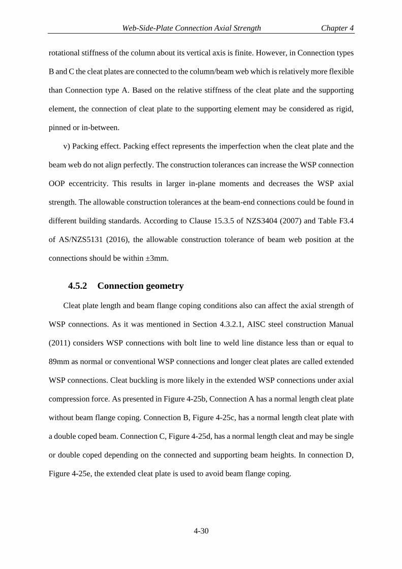
Web-Side-Plate Connection Axial Strength Chapter 4
4-30
rotational stiffness of the column about its vertical axis is finite. However, in Connection types
B and C the cleat plates are connected to the column/beam web which is relatively more flexible
than Connection type A. Based on the relative stiffness of the cleat plate and the supporting
element, the connection of cleat plate to the supporting element may be considered as rigid,
pinned or in-between.
v) Packing effect. Packing effect represents the imperfection when the cleat plate and the
beam web do not align perfectly. The construction tolerances can increase the WSP connection
OOP eccentricity. This results in larger in-plane moments and decreases the WSP axial
strength. The allowable construction tolerances at the beam-end connections could be found in
different building standards. According to Clause 15.3.5 of NZS3404 (2007) and Table F3.4
of AS/NZS5131 (2016), the allowable construction tolerance of beam web position at the
connections should be within ±3mm.
4.5.2 Connection geometry
Cleat plate length and beam flange coping conditions also can affect the axial strength of
WSP connections. As it was mentioned in Section 4.3.2.1, AISC steel construction Manual
(2011) considers WSP connections with bolt line to weld line distance less than or equal to
89mm as normal or conventional WSP connections and longer cleat plates are called extended
WSP connections. Cleat buckling is more likely in the extended WSP connections under axial
compression force. As presented in Figure 4-25b, Connection A has a normal length cleat plate
without beam flange coping. Connection B, Figure 4-25c, has a normal length cleat plate with
a double coped beam. Connection C, Figure 4-25d, has a normal length cleat and may be single
or double coped depending on the connected and supporting beam heights. In connection D,
Figure 4-25e, the extended cleat plate is used to avoid beam flange coping.

Web-Side-Plate Connection Axial Strength Chapter 4
4-31
a) Typical steel structure floor plan for different WSP connections
b) Connection A, conventional WSP
c) Connection B, conventional WSP
d) Connection C, extended WSP
e) Connection D, extended WSP
Figure 4-25. Typical steel structure floor plan with different types of WSP connections
The size and thickness of the cleat plate, height and thickness of the beam web and the
number of bolts can also affect the axial behaviour of WSP connections. However, these
parameters usually are limited to some pre-defined values in design guides to prevent brittle
failure modes under shear forces. For example, the cleat thickness is limited to half the bolt
diameter to facilitate bearing yielding of the bolt holes rather than bolt shear failure in both

Web-Side-Plate Connection Axial Strength Chapter 4
4-32
AISC steel construction manual (2011) and New Zealand design procedure (HERA R4-100
2003) as described in Sections 4.3.2.1 and 4.3.2.2 respectively.
4.5.3 Initial loading condition
Initial gravity loading may exist on a WSP connection at the time that beam axial force is
imposed to the beam. This can affect the axial behaviour and ultimate strength of the WSP
connection. Beam gravity loads can impose shear force, 𝑉𝐺, at the bolt centroid, and a moment,
𝑀𝐺 . This will cause a rotation, 𝜃𝐺 , at the beam-end as shown on the left hand side of Figure
4-26a. During an earthquake event, these shear force and rotation may be increased or
decreased because of the earthquake vertical excitation. The rotation, shear force and moment
due to the earthquake vertical excitation are respectively denoted by 𝜃𝐸𝑉, 𝑉𝐸𝑉 and 𝑀𝐸𝑉 in
Figure 4-26.
Furthermore, beam axial forces mainly occur due to lateral loading events. Lateral forces
acting on the structure cause lateral deformations and inter-storey drifts. These drifts impose
additional rotation and moments to the connections. The beam-column rotation due to inter-
storey drift is shown on the right-hand side of Figure 4-26a denoted by 𝜃𝐸 . Depending on the
relative direction of the beam axial force and the inter-storey drift, shown in Figure 4-26a and
b, the drift rotation may decrease or increase the effect of gravity loads on the compression side
of the beam.
a) Drift increases the WSP rotation on the compression side and decreases on the tension side

Web-Side-Plate Connection Axial Strength Chapter 4
4-33
b) Drift increases the WSP rotation on the tension side and decreases on the compression side
Figure 4-26. Initial conditions due to gravity load and storey drift
Considering that the beam axial force can occur in the gravity beams of steel buildings,
the axial capacity of WSP connections is required to be quantified to ensure robust load path
for design.
4.6 Parametric study
As it was discussed in Section 4.5, various parameters can affect the axial behaviour of
WSP connections. In this section some of the affecting parameters are investigated. Parameters
that are studied include:
1) Boundary conditions including
i. Beam lateral restraint along the length
As it was mentioned in Section 4.4.2.6, cleat buckling can be a possible failure mode of
the WSP connections under axial compression force. Therefore, providing lateral support for
the beam may increase the axial compression capacity of the WSP connection by preventing
buckling or decreasing the effective length.
The beam top flange usually is laterally supported due to the presence of floor slab and
mechanical attachments such as shear studs. However, the beam web and bottom flange may
be free to move out-of-plane as shown in Figure 4-27a. Lateral restraint for beam web and
bottom flange can be provided by the secondary beams like beam 3 shown in Figure 4-27b. In
this section, the effect of distance between the secondary beams is investigated considering 2m
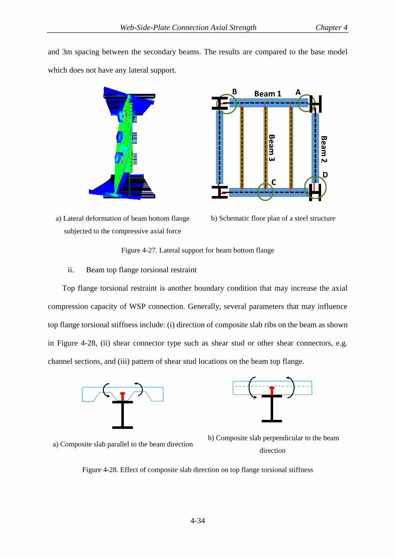
Web-Side-Plate Connection Axial Strength Chapter 4
4-34
and 3m spacing between the secondary beams. The results are compared to the base model
which does not have any lateral support.
a) Lateral deformation of beam bottom flange
subjected to the compressive axial force
b) Schematic floor plan of a steel structure
Figure 4-27. Lateral support for beam bottom flange
ii. Beam top flange torsional restraint
Top flange torsional restraint is another boundary condition that may increase the axial
compression capacity of WSP connection. Generally, several parameters that may influence
top flange torsional stiffness include: (i) direction of composite slab ribs on the beam as shown
in Figure 4-28, (ii) shear connector type such as shear stud or other shear connectors, e.g.
channel sections, and (iii) pattern of shear stud locations on the beam top flange.
a) Composite slab parallel to the beam direction
b) Composite slab perpendicular to the beam
direction
Figure 4-28. Effect of composite slab direction on top flange torsional stiffness

Web-Side-Plate Connection Axial Strength Chapter 4
4-35
It is expected that top flange torsional restraint increases the axial compression strength by
increasing the cleat-buckling capacity and decreasing the out-of-plane deformations of the
beam web. Here, this parameter is investigated by comparing two models with and without top
flange torsional restraint.
i. Packing effect representing the imperfection when the cleat plate and the beam
web do not align perfectly
The allowable construction tolerances at the beam-end connections could be found in
different building standards. According to Clause 15.3.5 of NZS3404 (2007) and Table F3.4
of AS/NZS5131 (2016), the allowable construction tolerance of beam web position at the
connections should be within ±3mm.
In this study, the base model is selected to investigate the packing effect on the axial
capacity of the WSP connection. Here, the construction tolerance is modelled by putting a filler
plate with different thicknesses ranging from one to 5mm between the beam web and the cleat
plate as shown in Figure 4-29. This method is used to avoid increasing the complexity of
models instead of modelling a twisted or skewed cleat plate.
Figure 4-29. Schematic view of models with the filler plate
2) Connection geometry, including
i. Cleat plate located on one side or opposite sides at beam-ends

Web-Side-Plate Connection Axial Strength Chapter 4
4-36
Cleat plates at both beam-end connections can be placed at one side or opposite sides of
the beam web. When the cleat plates are placed at the different sides of the beam web, the
imposed in-plane moment to the beam due to axial force eccentricity is in the opposite direction
as shown in Figure 4-30a. In this case, the moment at the tension side may increase the beam
out of plane deformation and consequently decrease the axial compression strength of the
connection. On the contrary, when the cleat plates are on the same side of the beam, the
imposed moments are in the same direction, Figure 4-30b. In this case, double curvature
deformation of the beam may help to reduce the unrestraint length of the beam and increase
the axial force carrying capacity of connection at the compression side.
a) Cleat plates at different sides
b) Cleat plates at the same sides
Figure 4-30. Location of cleat plates at the beam-ends
ii. Cleat plate height ranging from 0.5 to 0.8 times of beam height
Cleat plate dimension can directly affect the axial behaviour of WSP connection. Cleat
plate length and the distance between bolt-line and weld-line, can directly affect the ultimate
axial compression capacity of the connection. In design guidelines, there is a limitation for
bolt-line to weld-line distance, and this length cannot be increased more than a specified

Web-Side-Plate Connection Axial Strength Chapter 4
4-37
amount. Cleat plate height can also affect the ultimate capacity of the WSP connection. Three
plate heights 150mm, 200mm and 250mm with 2, 3 and 4 bolts respectively, are modelled and
analysed.
iii. Beam flange coping effects
In some cases such as a beam to beam connection or beam to column web connection
(connections B and C shown in Figure 4-25a) because of constructability considerations, beam
flanges need to be coped. In this situation, the effect of beam flanges on providing lateral
restraint for the beam web and the cleat plate decreases. This cause lower axial compression
force capacity. Here, the behaviour of WSP connections with coped and un-coped beams are
compared, and the behaviour of coped beam-column connections with different cope lengths
is studied.
iv. Cope length effects
Beam flange cope length is usually governed by the geometry of supporting member, but
due to the plate buckling considerations, cope length cannot be more than a specified value that
is related to the beam web thickness and height. By increasing the cope length, the effect of
beam flange on restraining the beam web and cleat plate decreases and consequently the
ultimate capacity of the connection reduces.
3) Initial loading conditions including
i. Gravity loads causing a beam shear up to 60% of the WSP capacity
During an earthquake event, a combination of gravity loads and beam axial forces act on
the beam and the beam-column connection. Gravity loads on a simply supported beam impose
a shear force and rotation to the beam-column connection. The amount of shear can simply be
calculated using equilibrium equation. However, the amount of beam-end rotation relates to
several parameters such as connection rigidity, gravity load distribution on the beam, and level
of beam composite action.

Web-Side-Plate Connection Axial Strength Chapter 4
4-38
As it was mentioned in Section 4.4.1, steel beams in this research are designed using 5kPa
dead load, G, and 3kPa live load, Q. The critical load combination for beam design under
gravity loads based on AS/NZS1170.0 (2002) may be 1.5Q+1.2G, which is equal to 10.5kPa.
The load combination considering the combination factor given in AS/NZS1170.0 (2002)
Table 4.1 for the amount of gravity loads during earthquake is 0.4Q+G, which is equal to
6.2kPa. Therefore, the ratio of the imposed gravity loads at the time of earthquake event to the
factored design loads is equal to 0.6 in this case. This value is used in this study to impose
different levels of shear force to the WSP connections and investigate their axial behaviour.
Steel beams are designed with considering 50% composite action. In the FEM modelling
the concrete slab was not modelled for simplicity. Consequently, the steel beam in the FE
models has less flexural stiffness than a corresponding composite beam with 50% composite
action. When the serviceability loads are applied to the bare beam in the FE models, it causes
the same shear force at the connection. However, the rotation may be more than the composite
beam due to lower stiffness. To overcome this problem, part of the gravity load which is equal
to 𝑔𝑟𝑎𝑣𝑖𝑡𝑦 𝑙𝑜𝑎𝑑 ×𝐼𝑏𝑎𝑟𝑒 𝑏𝑒𝑎𝑚
𝐼𝑐𝑜𝑚𝑝𝑜𝑠𝑖𝑡𝑒 𝑏𝑒𝑎𝑚 is applied as distributed uniform load on the beam and the
rest are imposed to the beam-ends as concentrated loads to avoid increasing the beam-ends
rotation. Here, 𝐼𝑏𝑎𝑟𝑒 𝑏𝑒𝑎𝑚 and 𝐼𝑐𝑜𝑚𝑝𝑜𝑠𝑖𝑡𝑒 𝑏𝑒𝑎𝑚 are moments of inertia of the bare beam and the
composite beam with 50% composite action respectively. Figure 4-31 shows the gravity
loading in FEM models schematically.

Web-Side-Plate Connection Axial Strength Chapter 4
4-39
a) Designed beam
b) FE modelling method
Figure 4-31. Beam gravity loading
ii. Bolt pre-loading from zero to 100% of the proof load
Another parameter that may affect WSP connection axial behaviour is the bolt tightening
level. Although in most construction projects, snug-tightened bolts are used in the WSP
connections, here a short study is conducted to investigate the effect of bolt proof loading on
the WSP axial behaviour.
ABAQUS software provides a method for applying bolt pre-tension force by using “bolt-
load” option in the software “load” module. Using this feature, a certain amount of pre-tension
load can be applied to the bolts. The amount of bolt pre-tension load or the bolt length can be
chosen to remain the same in all the following analysis steps. When the bolt length is chosen
to remain constant, the bolt behaves with its mechanical properties plus existing pre-tension
force; this option is used in the FE simulations of this study.
iii. Lateral storey drift
As it was described in Section 4.5.3, structure drifts impose additional rotation and bending
moment to the beam-column connections. In the structural steel-work connections guide
(SCNZ report 14.1, 2007) design procedure, the imposed moments due to the drift rotations
are also considered to prevent connection failure during lateral drifts. Also a gap is required to

Web-Side-Plate Connection Axial Strength Chapter 4
4-40
be provided between the beam-end and column to ensure beam does not touch the column
during lateral movements.
Beam axial force and the storey drift may act in the same direction or the opposite direction
as shown in Figure 4-32. Here the effect of additional rotation due to the structure inter-storey
drift is investigated in both possible directions. Also, to simulate a more realistic situation, a
gravity load corresponding to 0.5𝑉𝑦 of the cleat plate is applied to all models as an initial
condition.
a) Positive storey drift
b) Negative storey drift
Figure 4-32. Beam axial force and structure lateral drift
4.6.1 Parametric matrix
In this study, thirty-one models are investigated to obtain the effect of each parameter on
the axial behaviour of WSP connections. Table 4-3 summarises the models detail and the
parameters investigated. Letter “C” in the model number is used for coped beam models.

Web-Side-Plate Connection Axial Strength Chapter 4
4-41
Table 4-3. FEM models detail
Late
ral
bra
cing
Gra
vity
load, V
ϴ
Eart
hquake
Num
ber
of
bolt
s
Bea
m
sect
ion
Des
crip
tion
Sec
tion
1 (Base
model) --- --- --- 3 Bolts 310UB32
2 --- V/Vy*=0.15 --- 3 Bolts 310UB32 4.6.2.1
3 --- V/Vy*=0.3 --- 3 Bolts 310UB32 4.6.2.1
4 --- V/Vy*=0.5 --- 3 Bolts 310UB32 4.6.2.1
5 --- V/Vy*=0.6 --- 3 Bolts 310UB32 4.6.2.1
6 --- --- --- 3 Bolts 310UB32 Bolts proof
loaded 4.6.2.2
7
at
2000
mm
--- --- 3 Bolts 310UB32 4.6.2.3
8
at
3000
mm
--- --- 3 Bolts 310UB32 4.6.2.3
9 --- V/Vy*=0.5 +0.5%
drift 3 Bolts 310UB32 4.6.2.4
10 --- V/Vy*=0.5 -0.5%
drift 3 Bolts 310UB32 4.6.2.4
11 --- V/Vy*=0.5 +1.0%
drift 3 Bolts 310UB32 4.6.2.4
12 --- V/Vy*=0.5 -1.0%
drift 3 Bolts 310UB32 4.6.2.4
13 --- V/Vy*=0.5 +2.0%
drift 3 Bolts 310UB32 4.6.2.4
14 --- V/Vy*=0.5 -2.0%
drift 3 Bolts 310UB32 4.6.2.4
15 --- --- --- 3 Bolts 310UB32
Cleat plates
located at
different sides of
beam
4.6.2.5
16 --- --- --- 2 Bolts 310UB32 4.6.2.6
4.6.3.1
17 --- --- --- 4 Bolts 310UB32 4.6.2.6
4.6.3.1
18 --- --- --- 3 Bolts 310UB32
Top flange is
restraint
laterally and
torsionally
4.6.2.7
19 --- V/Vy*=0.5 --- 2 Bolts 310UB32 4.6.2.1
20 --- V/Vy*=0.5 --- 4 Bolts 310UB32 4.6.2.1
21 --- --- --- 3 Bolts 310UB32 1mm packing 4.6.3.3
22 --- --- --- 3 Bolts 310UB32 2mm packing 4.6.3.3
23 --- --- --- 3 Bolts 310UB32 3mm packing 4.6.3.3
24 --- --- --- 3 Bolts 310UB32 4mm packing 4.6.3.3
25 --- --- --- 3 Bolts 310UB32 5mm packing 4.6.3.3
26C --- --- --- 2 Bolts 310UB32 , Cope
length=100mm 4.6.3.1

Web-Side-Plate Connection Axial Strength Chapter 4
4-42
27C --- --- --- 3 Bolts 310UB32 Cope
length=100mm
4.6.3.1
4.6.3.2
28C --- --- --- 4 Bolts 310UB32 Cope
length=100mm 4.6.3.1
29C --- --- --- 3 Bolts 310UB32 Cope
length=200mm 4.6.3.2
30C --- --- --- 3 Bolts 310UB32 Cope
length=150mm 4.6.3.2
31C --- --- --- 3 Bolts 310UB32 Cope
length=75mm 4.6.3.2
Vy: shear strength of cleat plate gross section
4.6.2 Un-coped beams
4.6.2.1 Gravity loads
Figure 4-33 presents the results of the base model subjected to four different level of shear
forces (gravity load). In this Figure 𝑉𝑦 is the shear strength of cleat gross section, 0.6𝑓𝑦𝑡𝑐ℎ,
where 𝑡𝑐 and ℎ are the cleat thickness and height respectively. As it is expected, the
compressive axial force capacity decreased with increasing the shear force. Similar results are
observed in Figure 4-34, for different cleat heights when the applied shear force of about 50%
of the cleat gross section shear strength was imposed to the connections. From these analysis,
it was found that the gravity load reduced the connection compressive axial strength by up to
15% when the applied shear force is about 0.6 times the yield shear strength of the cleat plate
compared to the connections without gravity loads.

Web-Side-Plate Connection Axial Strength Chapter 4
4-43
Figure 4-33. WSP axial behaviour under different levels of shear forces
Figure 4-34. WSP axial behaviour with different cleat height under shear forces
4.6.2.2 Bolt pre-tensioning
Figure 4-35 shows the base model, with snug-tightened bolts and proof-loaded bolts. As
can be seen in this Figure, in both models the ultimate tension and compression capacities were
similar with less than 3% difference at the ultimate axial strength. However, the only noticeable
difference in their axial force-displacement behaviours was a slight increase in the initial
stiffness of the proof-loaded model.
0
50
100
150
200
250
300
350
400
0 2 4 6 8
Ax
ial
Forc
e (k
N)
Axial displacement (mm)
Base model (C)
Base model (T)
V/Vy=0.15 (C)
V/Vy=0.15 (T)
V/Vy=0.31 (C)
V/Vy=0.31 (T)
V/Vy=0.5 (C)
V/Vy=0.5 (T)
V/Vy=0.62 (C)
V/Vy=0.62 (T)
Tension
Increasing gravity Compression
0
100
200
300
400
500
600
0 2 4 6 8
Ax
ial
Forc
e (k
N)
Axial displacement (mm)
h=150mm (C)
h=150mm, V/Vy=0.5 (C)
h=150mm (T)
h=150mm, V/Vy=0.5 (T)
h=200mm (C)
h=200mm, V/Vy=0.5 (C)
h=200mm (T)
h=200mm, V/Vy=0.5 (T)
h=250mm (C)
h=250mm, V/Vy=0.5 (C)
h=250mm (T)
h=250mm, V/Vy=0.5 (T)
Tension
Compression

Web-Side-Plate Connection Axial Strength Chapter 4
4-44
Figure 4-35. Effect of bolt tightening level, base model with snug-tightened and proof-loaded bolts
4.6.2.3 Beam lateral restraint
Figure 4-36 shows the effects of providing the lateral bracing at the mid-point and third
points along the beam length which restrains the section against twist. Lateral movement is
already restrained at the shear stud locations on the top flange. It may be seen that restraining
the beam twist by providing lateral bracing did not alter the tensile strength and the
compression strength increased by less than 4%. This indicates that the connection was not
affected much by the beam lateral restraint away from the ends. Other parameters such as
bottom flange dimensions and cleat plate height, also may affect the WSP compressive strength
when the lateral support is provided, but investigating these parameters is not in the scope of
this research.
0
50
100
150
200
250
300
350
400
0 2 4 6 8
Ax
ial
Forc
e (k
N)
Axial displacement (mm)
Snug tightened (C)
Snug tightened (T)
Bolt proof loaded (C)
Bolt proof loaded (T)

Web-Side-Plate Connection Axial Strength Chapter 4
4-45
Figure 4-36. Lateral bracing of beam web and bottom flange
4.6.2.4 Lateral drift effect
Figure 4-37 plots the axial force behaviour of the studied WSP connections under different
levels of inter-storey drift. In the positive storey drifts, beam-end rotation due to the inter-storey
drift decreases the beam-end rotation due to gravity loads on the compression side and for the
negative storey drifts it increases the beam-end rotation on the compression side.
a) Axial force and storey drift in the same direction
0
50
100
150
200
250
300
350
400
0 2 4 6 8
Ax
ial
Forc
e (k
N)
Axial displacement (mm)
Base model (c)
Base model (T)
Lateral bracing at
3000mm (C)
Lateral bracing at
2000mm (C)
Lateral bracing at
3000mm (T)
Lateral bracing at
2000mm (T)
Tension
Increasing number of lateral restraints
Compression
0
50
100
150
200
250
300
350
400
0 2 4 6 8
Ax
ial
Forc
e (k
N)
Axial displacement (mm)
V/Vy=0.5 (C)
V/Vy=0.5 (T)
V/Vy=0.5 (C), -0.5%
DriftV/Vy=0.5 (T), -0.5%
DriftV/Vy=0.5 (C), -1%
DriftV/Vy=0.5 (C), -1%
DriftV/Vy=0.5 (C), -2%
DriftV/Vy=0.5 (T), -2%
Drift
Tension
Increasing lateral driftCompression

Web-Side-Plate Connection Axial Strength Chapter 4
4-46
b) Axial force and storey drift in the opposite direction
Figure 4-37. Axial behaviour of WSP connections under different levels of inter-storey drift
Based on the results plotted in Figure 4-37, when the lateral drift decreased the rotation
due to gravity loads on the compression side (Figure 4-37a), connection compressive capacity
showed an increasing trend. On the contrary, when the lateral drift increased the effect of
gravity loads (Figure 4-37b), connection compressive capacity showed a decreasing trend with
increasing the storey drift level. Also, it was found that additional rotation did not have a
noticeable effect on the tension behaviour of WSP connections.
Overall, the increase or decrease of ultimate capacity of the studied connections under
axial compression force was measured less than ±8% for 2% drift angle.
4.6.2.5 Cleat plate location on beam sides
Figure 4-38 plots axial force-displacement of both conditions for the base model. The
results showed that the effect of placing cleat plates at different sides of the beam was less than
1% for the studied case. It should be noted that the beam length and the ratio of the cleat plate
stiffness to the beam weak axis stiffness may also affect this behaviour.
0
50
100
150
200
250
300
350
400
0 2 4 6 8
Ax
ial
Forc
e (k
N)
Axial displacement (mm)
V/Vy=0.5 (C)
V/Vy=0.5 (T)
V/Vy=0.5 (C),
+0.5% DriftV/Vy=0.5 (T),
+0.5% DriftV/Vy=0.5 (C), +1%
DriftV/Vy=0.5 (T), +1%
DriftV/Vy=0.5 (C), +2%
DriftV/Vy=0.5 (T), +2%
Drift
Tension
Increasing lateral driftCompression

Web-Side-Plate Connection Axial Strength Chapter 4
4-47
Figure 4-38. Axial behaviour of WSP connections with cleat plates located at different sides and the
same side
4.6.2.6 Effect of cleat plate height
Figure 4-39 plots the tension and compression force-displacement of models with different
cleat plate heights. The plots indicate that the compression and tension capacities of the WSP
connection increased with increasing the cleat plate height. The ultimate tension and
compression capacities versus cleat plate heights are shown in Figure 4-40. This plot shows
that tensile strength more increased than compression capacity by increasing the cleat plate
height. This is because the compression capacity of the cleat plate is more affected by the
boundary conditions.
0
50
100
150
200
250
300
350
400
0 2 4 6 8
Ax
ial
Forc
e (k
N)
Axial displacement (mm)
Cleat plates at one side
(C)
Cleat plates at one side
(T)
Cleat plates at different
sides (C)
Cleat plates at different
sides (T)
Tension
Compression

Web-Side-Plate Connection Axial Strength Chapter 4
4-48
Figure 4-39. Effect of cleat plate height on WSP axial behaviour
In these models, the distance between the cleat plate and the beam top flange, which is
restraint laterally, is constant and the cleat plate height is increased toward the bottom flange
which is free laterally. Part of the cleat plate closer to the bottom flange has less effect on the
axial compression capacity of the connection due to lack of lateral support. Note that in the
studied cases beam top flanges are restrained, and bottom flanges are free laterally similar to
the base model.
Figure 4-40. Ultimate tension and compression capacities versus cleat plate height
0
100
200
300
400
500
600
0 2 4 6 8
Ax
ial
Forc
e (k
N)
Axial displacement (mm)
h=150mm (C)
h=150mm (T)
h=200mm (C)
h=200mm (T)
h=250mm (C)
h=250mm (T)
TensionDecreasing cleat plate height
Compression
0
100
200
300
400
500
600
100 150 200 250 300
Pea
k a
xia
l fo
rce
(kN
)
Cleat plate height (mm)
Compression capacity
Tension capacity

Web-Side-Plate Connection Axial Strength Chapter 4
4-49
4.6.2.7 Top flange torsional restraint
Figure 4-41 shows the deformed shape patterns of the compression side of both models at
8mm axial deformation. As can be seen from this Figure, torsional restraint of the beam top
flange can effectively decrease the bottom flange lateral deformations.
(a) Top flange unrestraint
(b) Top flange restraint
Figure 4-41. Deformed shape of beam-end at the compression side with and without beam top flange
torsional restraint
Axial force-displacements of the studied models are plotted in Figure 4-42. The tension
behaviour did not show any change, while the compression capacity was increased by about
14% in the top flange torsionally restrained model.

Web-Side-Plate Connection Axial Strength Chapter 4
4-50
Figure 4-42. Effect of beam top flange torsional restraint
Evaluating the realistic level of torsional restraint can be very complicated and may depend
on various parameters such as relative stiffness of the slab to the beam top flange, the beam
web thickness and also, the shear connectors’ stiffness. Therefore, in this study it is considered
that the top flange is free to twist for all other models to obtain more conservative axial
compression capacity.
4.6.3 Double-coped beams
4.6.3.1 Coping effect
Figure 4-43 shows the axial behaviour of the coped and un-coped connections with
different cleat plate heights. In these models, cope length is considered equal to 100mm.
0
50
100
150
200
250
300
350
400
0 2 4 6 8
Ax
ial
Forc
e (k
N)
Axial displacement (mm)
Base model (C)
Base model (T)
Top flange restrained
rotationally (C)
Top flange restrained
rotationally (T)
Tension
Compression

Web-Side-Plate Connection Axial Strength Chapter 4
4-51
a) Two bolts connection
b) Three bolts connection
c) Four bolts connection
Figure 4-43. Beam flange coping effect on the axial behaviour of WSP connection
0
50
100
150
200
250
300
0 2 4 6 8
Ax
ial
Forc
e (k
N)
Axial displacement (mm)
h=150mm (C) Un-
coped
h=150mm (C) Double
coped
h=150mm (T) Un-
coped
h=150mm (T) Double
coped
Tension
CompressionDouble coped
0
50
100
150
200
250
300
350
400
0 2 4 6 8
Ax
ial
Forc
e (k
N)
Axial displacement (mm)
h=200mm (C) Un-
coped
h=200mm (C) Double
coped
h=200mm (T) Un-
coped
h=200mm (T) Double
coped
Tension
Compression
Double coped
0
100
200
300
400
500
600
0 2 4 6 8
Ax
ial
Forc
e (k
N)
Axial displacement (mm)
h=250mm (C) Un-
coped
h=250mm (C) Double
coped
h=250mm (T) Un-
coped
h=250mm (T) Double
coped
Tension
Compression
Double coped

Web-Side-Plate Connection Axial Strength Chapter 4
4-52
Based on the results, the tensile capacity of the studied models decreased by about 2%
because of the reduction in the beam web cross-section area. However, the axial behaviour of
compression side experienced a more decline, such that, 2, 3 and 4 bolts connections
experienced 16%, 24% and 48% reduction in the ultimate capacity.
4.6.3.2 Cope length effect
Figure 4-44 plots the axial force-displacement behaviour of four models with different
cope lengths. The results indicated that increasing the cope length does not affect the tensile
capacity of the WSP connections. However, the connection compression capacity is directly
related to the cope length.
Figure 4-44. Behaviour of models with different cope lengths
Figure 4-45 plots the peak compression forces versus the cope length to beam height ratio.
Results indicate that axial compression strength decreased linearly with increasing the cope
length.
0
50
100
150
200
250
300
350
400
0 2 4 6 8
Ax
ial
Forc
e (k
N)
Axial displacement (mm)
Cope length=200mm
(L/d=0.67) (C)Cope length=150mm
(L/d=0.5) (C)Cope length=100mm
(L/d=0.33) (C)Cope length=75mm
(L/d=0.25) (C)Cope length=200mm
(L/d=0.67) (T)Cope length=150mm
(L/d=0.5) (T)Cope length=100mm
(L/d=0.33) (T)Cope length=75mm
(L/d=0.25) (T)
Tension
CompressionIncreasing cope length

Web-Side-Plate Connection Axial Strength Chapter 4
4-53
Figure 4-45. Peak compression force of the studied models versus the cope length to beam height
ratio, cleat plate height=200mm
4.6.3.3 Packing effect
The axial force-displacement results of the WSP connections with different filler plates
are plotted in Figure 4-46. The results indicate that 3mm eccentricity in the studied connection
caused more than 25% decrease in the axial compression strength of the WSP connection.
Increasing the axial force eccentricity in the compression side increase the imposed moment
and cause cleat buckling to occur at lower axial forces.
Figure 4-46. Axial force-displacement plots of WSP connection with different filler plate thicknesses
0
0.1
0.2
0.3
0.4
0.5
0.6
0.7
0.8
0.5 0.6 0.7 0.8 0.9 1
L/d
Coped/Un-coped strength
0
50
100
150
200
250
300
350
400
0 2 4 6 8
Ax
ial
forc
e (k
N)
Axial displacement (mm)
Base model C
Base model T
1mm packing C
1mm packing T
2mm packing C
2mm packing T
3mm packing C
3mm packing T
4mm packing C
4mm packing T
5mm packing C
5mm packing T
Tension
Packing increaseCompression

Web-Side-Plate Connection Axial Strength Chapter 4
4-54
Based on the results, the ultimate tensile strength of the WSP connection changed by about
7% due to increasing the load eccentricity up to 3mm. This is because of increase in the
imposed moment to the connection due to axial force eccentricity. These results emphasize the
importance of considering the additional eccentricity due to the packing effect in calculating
WSP connection axial strength.
4.7 Estimating axial strength of WSP connections
In this section, the axial force carrying mechanism of WSP connections is investigated and
a method for estimating the axial force capacity is proposed. The proposed method is based on
the material mechanic principles and it is verified with FEM results. Note that the proposed
method is required to be verified by experimental tests which is out of the scope of this research.
4.7.1 Behaviour of laterally restraint and free WSP connections
The cleat plate and the beam web in WSP connections act as a beam-column member
under axial force because of the connection out-of-plane eccentricity. Generally, the out-of-
plane stiffness of the cleat plate is considerably lower than the steel beam; therefore, the cleat
plate performance may govern the overall behaviour of the connection.
The behaviour of WSP connection under the axial compression force may vary from a
simple to a complicated behaviour based on the boundary conditions and the beam flange
coping. For instance, when both beam flanges are coped and the beam is not restrained laterally,
the behaviour can be predicted using column equations available in building standards (e.g.
NZS3404, 2007). However, when the beam is restrained laterally, the deformed shape and
buckling pattern become complicated and different parameters may affect the connection
capacity.
Here, the behaviour of two connection types are studied,

Web-Side-Plate Connection Axial Strength Chapter 4
4-55
1. The WSP connection that the beam flanges are coped and the beam is not restrained
laterally
2. The WSP connection that the beam flanges are not coped and the top flange is
restrained laterally
The first is simple, so methods described are easily understood. The second is perhaps
more realistic for beams used in buildings. Together they can be considered to be bounds on
the behaviour of some typical beams.
Figure 4-47 shows the coped beam connected to the cleat plate and the axial force-
deformation plot of the connection. The behaviour of this connection is defined in three stages.
i. Elastic part, which the connection does not experience any inelastic deformations.
Typically this is about up to 0.3-0.4mm axial deformation.
ii. The second part is from the first yield to the formation of plastic hinges in the cleat
and the beam web. First yielding may occur either in the cleat or the beam web
depending on their relative stiffness and cross-sectional properties.
iii. In the third part, plastic hinges are formed and the strength of the connection
decreases due to large lateral deformations and the P-Δ effect.
a) 3-bolts connection with coped flanges
b) Deformed shape of the FE model at 4mm
axial deformation

Web-Side-Plate Connection Axial Strength Chapter 4
4-56
c) Axial force-deformation plot and loading stages
Figure 4-47. Axial behaviour of a double coped, laterally unrestrained connection
In case of the uncoped beam and the presence of lateral restraints on the beam top flange,
the force carrying mechanism becomes more complicated than the double coped laterally free
connection. Figure 4-48 shows a WSP connection where the top flange is restrained laterally
without beam flange coping. Overall, the force carrying stages are similar to the connection in
Figure 4-47, but the stresses are not uniformly distributed:
i. In the first part of the axial compression loading (up to about 0.4mm axial
deformation) the connection is elastic.
ii. By increasing the axial deformation, some part of the cleat that is far from the beam
top flange, experience large lateral deformations and start to yield. By increasing
the axial force, more regions yield and plastic hinges form in the cleat plate and the
beam web. The difference between this connection and the coped-unrestrained one
is that in the coped-unrestrained connection the plastic hinge forms quickly after
the first yield but in this connection plastic hinge forms at larger axial deformations
due to non-uniform stress distribution.

Web-Side-Plate Connection Axial Strength Chapter 4
4-57
iii. In the third stage, similar to the previous model, the plastic hinges are formed and
the connection strength decreases due to large lateral deformations.
a) 3-bolts connection without beam flange
coping
a) Deformed shape of the FE model at 4mm
axial deformation
c) Axial force-deformation plot and loading stages
Figure 4-48. Axial behaviour of uncoped laterally restrained top flange connection
As can be seen from these models, the axial force carrying mechanism of WSP connections
may considerably vary based on the boundary conditions and the geometry of the connection.

Web-Side-Plate Connection Axial Strength Chapter 4
4-58
Methods to estimate the axial compression capacity of three WSP connection configurations
are investigated in this study including:
1. Double coped, laterally unrestrained connection
2. Un-coped, top flange restrained laterally
3. Double coped, top flange restrained laterally
4.7.2 Method of estimating WSP axial compression strength
4.7.2.1 Basic concepts
Building standards have different approaches for finding the capacity of a structural
element under specific loading condition. For instance, in NZS3404 (2007) building standard,
the capacity of a structural element is calculated based on the section considerations and the
member considerations separately. While, in AISC 360-16, the member and section
considerations are considered together. In this study, it is tried to use simple equations and
consider both the section and member capacities together.
The issue of estimating the axial compression capacity of a WSP connection is the method
of considering the interaction between the axial force and the corresponding bending moment.
The simplest equation to consider the interaction of the axial force and bending moment is
presented in Eq. (4-1). This equation is a conservative way of considering axial force-bending
moment interaction. Although, the effect of buckling of the member can be considered to obtain
the cleat compression strength, 𝑃𝑢, the effect of secondary moments due to lateral deformations
of the element is not considered in this equation. The secondary moments are more important
in slender beam-column elements because of larger lateral deformations. In Eq. (4-1), 𝑃 is the
applied axial force, 𝑃𝑢 is the ultimate strength of a centrally loaded column (considering
buckling). The applied moment due to axial force eccentricity and the moment capacity of the
member (without axial force) are donated by 𝑀0 and 𝑀𝑢 respectively.

Web-Side-Plate Connection Axial Strength Chapter 4
4-59
𝑃
𝑃𝑢+
𝑀0
𝑀𝑢≤ 1 Eq. (4-1)
Johnston (1976) recommended modification for Eq. (4-1) to account for secondary
moments given in Eq. (4-2). Here, the term (1
1−𝑃 𝑃𝑐𝑟⁄) is the moment magnification factor for
considering secondary moments caused by the combined action of the axial force and lateral
deformations produced by the primary moment. The Euler critical buckling force, 𝑃𝑐𝑟, can be
calculated using 𝜋2𝐸𝐼
(𝑘𝐿)2, where 𝐸, 𝐼 and 𝑘𝐿 are the elastic modulus, moment of inertia and the
effective length of the member respectively.
𝑃
𝑃𝑢+
𝑀0
𝑀𝑢(1−𝑃 𝑃𝑐𝑟⁄ )≤ 1 Eq. (4-2)
Most design standards (e.g. AISC-360-16) use this equation with some modifications. In
this study, Eq. (4-2) is used to calculate the axial capacity of WSP connections.
4.7.2.2 Double coped, laterally unrestrained connection
• Considering cleat plate only
In the first step, it is assumed that only the cleat plate governs the overall behaviour of the
WSP connection. Therefore, an axial force is applied to the cleat plate alone with an OOP
eccentricity equal to half the cleat and beam web thicknesses. Here, the results of the studied
model in Section 4.7.1 are used to verify the calculated strength using Eq. (4-2).
Figure 4-49a shows the dimensions and material properties of the studied connection. The
axially loaded cleat plate acts similar to a beam-column member as shown in Figure 4-49b. It
should be noted that the beam web must be checked to make sure the cleat axial strength is not
larger than the beam web axial strength.

Web-Side-Plate Connection Axial Strength Chapter 4
4-60
a) Dimensions and material properties of the
model
b) Considering cleat plate alone
Figure 4-49. Geometry of eccentrically loaded cleat
To estimate the cleat ultimate axial strength, the cleat moment capacity, 𝑀𝑢 should be
calculated using the fully plastic moment capacity of the cross-section (𝑆 × 𝐹𝑦). The effective
length factor, 𝑘, in this case is equal to 2 based on the geometry of the cleat which is fully fixed
at one end and is laterally free at the other end. In the next sections the effective length factor
is discussed in detail for different cases.
A simple FEM model using beam elements (similar to Figure 4-49b) is created to study
the nonlinear behaviour of eccentrically loaded cleat only and compare the results with the
estimated capacity. Figure 4-50 shows the axial force-deformation plots of the eccentrically
loaded cleat and FEM results of the WSP connection shown in Figure 4-49a.

Web-Side-Plate Connection Axial Strength Chapter 4
4-61
Figure 4-50. Axial force-deformation plots of the eccentrically loaded cleat and general FEM model
shown in Figure 4-49a
Figure 4-50 shows that Eq. (4-2) may be used to calculate the axial force carrying capacity
of an eccentrically loaded cleat. However, the simple model strength, using the configuration
showed in Figure 4-49b which is of the cleat alone, is about 30% lower than the strength of the
WSP connection from the model in Figure 4-49a in this case. Therefore, considering the cleat
only may provide conservative results.
• Considering cleat plate and beam web
If the beam web effect is considered, the model showed in Figure 4-49b changes to the
model presented in Figure 4-51. In this case, the imposed moment due to the axial force
eccentricity is distributed between the cleat plate and the beam web. Thus, the axial force
capacity of the cleat increases.
The rotational stiffness of the beam web is represented by a rotational spring at the cleat
plate end for simplicity. There are some parameters that need to be obtained before proceeding
to calculate the WSP axial capacity of this case, such as:
i. Boundary and support conditions of the beam web end,
0
20
40
60
80
100
120
0 0.5 1 1.5 2
Ax
ial
Forc
e (k
N)
Axial deformation, δ (mm)
Simple model (FEM using beam elements)
WSP connection (FEM results)
Estimated capacity Eq. (2)
Eq. (4-2)

Web-Side-Plate Connection Axial Strength Chapter 4
4-62
ii. Beam web effective length contributing in the rotational stiffness of the spring
shown in Figure 4-51c, and
iii. The cleat plate effective length factor considering the beam web
a) Realistic model
b) Equivalent model
c) Simple model
Figure 4-51. Geometry of unrestrained-coped connection
a) Boundary and support conditions
Figure 4-52 shows a schematic view of the beam and connection deformed shape under
axial compression force. As it was mentioned, it is assumed that the beam is not supported
laterally in this case. Two possible deformed shapes can be considered for this model as:
1. When the lateral stiffness of the connection is relatively low compared to lateral
stiffness of the beam member, Mode 1, as shown in Figure 4-52a is likely to occur.
2. When the beam member is relatively stiff compared to the connection region, the
lateral deformation may be concentrated in the connection area (either in the beam
web or the cleat plate) and Mode 2, as shown in Figure 4-52b, may occur.

Web-Side-Plate Connection Axial Strength Chapter 4
4-63
Figure 4-52. Schematic deformed shape of beam and connection under axial compression force
In connections with coped beam flanges, connection stiffness is usually controlled by the
cleat plate and/or the beam web stiffnesses. Since the connection stiffness is lower than the
lateral stiffness of the beam member, Mode 2 of deformation shown in Figure 4-52 is more
likely to occur in most cases.
When Mode 2 is governing the deformed shape of an axially loaded beam member, it can
be assumed that the beam web rotation is much larger than the beam rotation, 𝜃𝑤𝑒𝑏 >> 𝜃𝑏𝑒𝑎𝑚,
for a specific lateral displacement. This is because the beam length is normally much longer
than the connection length. Assuming that 𝜃𝑤𝑒𝑏 >> 𝜃𝑏𝑒𝑎𝑚, the beam-web end connection
may be taken as a fixed support where rotation is not allowed but it is free to translate in the
out-of-plane direction, as shown in Figure 4-52c.
b) Beam web contributing length, 𝑳𝒘𝒆𝒃
Figure 4-53 shows the von Mises stress field of the beam web of the studied model in
Section 4.7.1 at the peak axial force. It can be seen that at the beam web mid-height, part of the
beam web beyond the coped area experiences stress and out-of-plane deformation. In the
design model, the beam web stiffness needs to be represented by one rotational spring.

Web-Side-Plate Connection Axial Strength Chapter 4
4-64
Therefore the equivalent beam web length contributing to rotational stiffness should be
obtained.
Figure 4-53. Part of the beam web beyond the coped area that contributes to beam web stiffness, stress
field recorded at 0.5mm axial deformation
Beam local deformations are because of the beam web flexibility. While beam global
deformations are the result of beam lateral movements due to the web moments. Figure 4-54a-
c show both local and global deformations schematically. The local, global and the total
(global+local) rotations of the 6m long 310UB32 beam subjected to a web moment are plotted
in Figure 4-54d. These plots are normalised to the total rotation. Here, the effect of global
rotation is about 4% of the total rotation.
The effect of global rotations, 𝜃𝑔, is neglected in this study because:
i. in real structures, secondary beams are usually connected to the primary beams and
provide lateral support which decreases the global deformation of the primary
beam,
ii. in some other cases, the beam top flange is restrained laterally because of
connection to the composite slab, which helps to reduce the lateral movements of
the beam

Web-Side-Plate Connection Axial Strength Chapter 4
4-65
iii. the beam weak-axis flexural stiffness is much higher than that of the beam web
alone, therefore when the moment is applied to the beam web, the beam web local
rotation is expected to be larger than the global beam-end rotation.
a) Model geometry b) Local deformation c) Total deformation
d) Rotation over beam height, 𝜃𝑡𝑜𝑡𝑎𝑙 = 𝜃𝑙 + 𝜃𝑔
Figure 4-54. Beam rotations
To obtain the beam web contributing length, a simple plate model with ideal boundary
conditions is created as shown in Figure 4-55. Here, a long plate member with the aspect ratio
of 10 is selected to represent a beam web. The plate is fixed at three edges and a uniform
moment is applied at the free left-hand side. The plate rotation on the free side is recorded. This
rotation is equal to the local rotation, 𝜃𝑙, because the fixed edges cannot move in the out-of-
plane directions (i.e. 𝜃𝑔 = 0 and 𝜃𝑡𝑜𝑡𝑎𝑙 = 𝜃𝑙).
0.00
0.10
0.20
0.30
0.40
0.50
0.60
0.70
0.80
0.90
1.00
0 0.2 0.4 0.6 0.8 1
Norm
aliz
ed b
eam
web
hei
ght
Rotation/Total rotation
Total rotation (Global+Local), θ total
Local rotation, θl
Global rotation, θg

Web-Side-Plate Connection Axial Strength Chapter 4
4-66
a) Model geometry
b) Model deformed shape
Figure 4-55. Simple plate model for finding the equivalent length of beam web
The beam web is divided into virtual strips. Based on the recorded rotations at the end of
the plate and the imposed moment magnitude, equivalent strip length is calculated for each
strip. Figure 4-56a shows the calculated strip lengths of the plate model schematically. The
strip length at the plate mid-height is about 0.25 of the plate height.
For calculating the WSP connection strength, the beam web needs to be considered as one
beam-column element connected to the cleat plate. Therefore, the average of the parabolic
function is derived using integration over the beam web height and the result is shown in Figure
4-56b schematically. The average is appropriate since stiffness is a function of EI/L. The beam
web effective length that can be used for the beam web rotational spring is equal to the average
of all the strip lengths which is about ℎ/5 (ℎ is beam web height) plus the coped length.

Web-Side-Plate Connection Axial Strength Chapter 4
4-67
a) Actual strips lengths b) Average of strips
lengths
Figure 4-56. Equivalent length of beam web
c) Cleat effective length factor (𝒌𝒄)
The cleat plate effective length factor, 𝑘𝑐 is required for calculating the critical buckling
load, 𝑃𝑐𝑟, of the cleat plate. In Section 4.7.2.2 where the cleat plate only was considered for
calculating the axial capacity of the WSP connection, the effective length factor for the cleat
plate was considered 2. However, the presence of the beam web and different boundary
conditions can affect the cleat effective length factor. In this section, the cleat plate effective
length factor, 𝑘𝑐, is discussed and equations for estimating 𝑘𝑐 are proposed.
• Case 1: Pinned connection
It can conservatively be assumed that the cleat plate and the beam are connected with a
pin connection for simplicity, as shown in Figure 4-57. Although this case is not realistic, it
can provide a good understanding of why the effective length factor increases or even decreases
when the cleat is connected to another element. Also, this case can provide an upper bound for
𝑘𝑐. Here, it is assumed that the beam does not buckle under axial forces due to lower
slenderness than the cleat plate. Since the beam element is pinned to the cleat and has a roller
support at the far end, it can just transfer axial forces similar to a truss member. Applying an
axial force to the cleat plate through another element, beam, can impose a lateral force which
is the horizontal component of the axial force, as shown in Figure 4-57b. This lateral force
leads the cleat to buckle at lower axial forces.

Web-Side-Plate Connection Axial Strength Chapter 4
4-68
a) Simplified model
b) Model deformation and horizontal force
Figure 4-57. Cleat and beam pinned together
In order to find the effective length factor, one method is using stability functions. The
stability function is the general stiffness matrix of an element that also considers the effect of
axial force. If the axial force is considered equal to zero, the stability function becomes equal
to the beam stiffness matrix. The stability function of the cleat plate shown in Figure 4-57a is
presented in Eq. (4-3).
𝐾𝑐𝑙𝑒𝑎𝑡 =𝐸𝐼𝑐
𝐿𝑐[
𝑓𝑐𝐿𝑐2⁄
𝑔𝑐𝐿𝑐⁄
𝑔𝑐𝐿𝑐⁄ 𝑠𝑐
] Eq. (4-3)
The horizontal component of the axial force is equal to 𝑃 × 𝑡𝑎𝑛 𝛾 and for small angles,
𝑡𝑎𝑛 𝛾 can be approximated by 𝑈𝑎
𝐿𝑏. Using this approximation the lateral force can be combined
with the stability function which gives the stability function for the whole system (Eq. (4-4)).
𝐾𝑡𝑜𝑡𝑎𝑙 =𝐸𝐼𝑐
𝐿𝑐[
𝑓𝑐𝐿𝑐2⁄ − (𝑃 𝐿𝑏
⁄ )𝐿𝑐
𝐸𝐼𝑐
𝑔𝑐𝐿𝑐⁄
𝑔𝑐𝐿𝑐⁄ 𝑠𝑐
] Eq. (4-4)
Where,

Web-Side-Plate Connection Axial Strength Chapter 4
4-69
𝑠 =∅𝑐(sin∅𝑐−∅𝑐 cos∅𝑐)
2(1−cos∅𝑐)−∅𝑐 sin∅𝑐 Eq. (4-5)
𝑟 =∅𝑐2−∅𝑐 sin∅𝑐
2(1−cos∅𝑐)−∅𝑐 sin∅𝑐 Eq. (4-6)
𝑓𝑐 = 2(𝑠 + 𝑟) − ∅𝑐2 Eq. (4-7)
𝑔𝑐 = 𝑠 + 𝑟 Eq. (4-8)
∅𝑐 = √𝑃𝐿𝑐
2
𝐸𝐼𝑐 Eq. (4-9)
𝑘𝑐 =𝜋
∅c Eq. (4-10)
When the determinant of the stability function matrix, Eq. (4-4), is equal to zero,
𝑑𝑒𝑡[𝐾𝑡𝑜𝑡𝑎𝑙] = 0, it means the inverse of this matrix does not exist and the system is unstable.
The applied force at this stage is equal to the critical buckling load. By solving the determinant
equation (𝑑𝑒𝑡[𝐾𝑡𝑜𝑡𝑎𝑙] = 0), ∅𝑐 can be obtained and then using Eq. (4-10), 𝑘𝑐 can simply be
calculated.
MatLab software was employed to calculate 𝑘𝑐 for different beam to cleat length ratios.
The effect of different length ratios is plotted in Figure 4-58. The calculated effective length
factor, 𝑘𝑐, is verified with FEM models and the results are presented in Appendix G.
Figure 4-58. Cleat effective length factor with different beam to cleat length ratios
0
1
2
3
4
5
6
7
0 2 4 6 8 10⁄𝐿𝑏 𝐿𝑐𝑙𝑒𝑎𝑡
Kc

Web-Side-Plate Connection Axial Strength Chapter 4
4-70
This plot shows that 𝑘𝑐 has large values when the beam length is smaller than the cleat
length and it gradually decreases to reach to 2 with large beam to cleat plate length ratios. This
is because as the beam length increases the horizontal force component decreases and the cleat
behaves similar to a cantilever column.
The above results can also be obtained by solving the determinate equation using the first
order approximations (Taylor series) of the stability function parameters (s,r,f and g). Equation
(4-12) presents a closed form solution for 𝑘𝑐.
∅𝒄 = √𝟏𝟓𝟔∝−24√(31∝2+55∝+25)+120
9∝+8 Eq. (4-11)
∅𝒄 ≅ √3∝
9
8∝+1
Eq. (4-12)
Where,
∝=𝐿𝑏
𝐿𝑐𝑙𝑒𝑎𝑡 Eq. (4-13)
𝑘𝑐 =𝜋
∅c Eq. (4-14)
• Case 1: Fixed connection
Another approach for determining the cleat plate effective length factor, is to consider the
beam web flexibility and its effect on the cleat buckling load. The configuration shown in
Figure 4-59 is considered for obtaining 𝑘𝑐, which is the same as Figure 4-51 without the axial
force eccentricity. It should be noted that the moment due to the axial force eccentricity does
not affect the stiffness matrix and the effective length factor, 𝑘𝑐.
It is assumed that the cleat plate is fixed at one end and connected to the beam web at the
other end. The boundary condition assumptions for the beam web element is based on the
deformed shape observed in the FE models, in accordance with Section 4.7.2.2.a. The length
of the beam web element should be taken as the equivalent beam web length that was obtained
in Section 4.7.2.2.b to be consistent.

Web-Side-Plate Connection Axial Strength Chapter 4
4-71
Figure 4-59. Model considered for calculating cleat effective length factor
Equations (4-15) and (4-16) present the stability functions of the cleat and the beam web
members.
𝐾𝑐𝑙𝑒𝑎𝑡 =𝐸𝐼𝑐
𝐿𝑐[
𝑓𝑐𝐿𝑐2⁄
𝑔𝑐𝐿𝑐⁄
𝑔𝑐𝐿𝑐⁄ 𝑠𝑐
] Eq. (4-15)
𝐾𝑤𝑒𝑏 =𝐸𝐼𝑤
𝐿𝑤[0 0
0 𝑠𝑤 −𝑔𝑤2
𝑓𝑤⁄
] Eq. (4-16)
The total stiffness matrix is obtained by assembling the stiffness matrices of each member
at node “a” shown in Figure 4-59. Equation (4-17) shows the total stiffness matrix for the
system. The parameters that are used in this matrix are similar to the previous case, Eqs. (4-5
to 4-11).
𝐾𝑡𝑜𝑡𝑎𝑙 = [
𝐸𝐼𝑐
𝐿𝑐×𝑓𝑐𝐿𝑐2⁄
𝐸𝐼𝑐
𝐿𝑐×𝑔𝑐
𝐿𝑐⁄
𝐸𝐼𝑐
𝐿𝑐×𝑔𝑐
𝐿𝑐⁄
𝐸𝐼𝑐
𝐿𝑐× 𝑠𝑐 +
𝐸𝐼𝑤
𝐿𝑤× (𝑠𝑤 −
𝑔𝑤2
𝑓𝑤⁄ )
] Eq. (4-17)
By solving the determinate equation of the total stiffness matrix, 𝑑𝑒𝑡[𝐾𝑡𝑜𝑡𝑎𝑙] = 0, critical
axial force can be obtained. MatLab software is used to calculate 𝑘𝑐 for different stiffness and
length ratios. To show the effect of different length and stiffness ratios together the results are

Web-Side-Plate Connection Axial Strength Chapter 4
4-72
plotted in a 3D plot as shown in Figure 4-60. The calculated effective length factor, 𝑘𝑐, is
verified with FEM models and the results are presented in Appendix G.
Figure 4-60. 3D plot indicating 𝑘𝑐 for cleat member with different length and stiffness ratios
To show the cleat plate effective length factor, 𝑘𝑐, for a range of stiffness, the results are
non-dimensionalised in terms of (EI
𝐿2)𝑐𝑙𝑒𝑎𝑡 (
EI
𝐿2)𝑤𝑒𝑏⁄ shown in Figure 4-61. These plots are
provided for a range of different length ratios and each ratio is plotted separately. Figure 4-61b
shows an enlarged view of Figure 4-61a, for stiffness ratios up to 2.
a) Cleat effective length factor
0.11.1
2.1
3.1 0
2
4
6
8
10
12
14
0.10.61.11.62.12.63.13.6
0-2 2-4 4-6 6-8 8-10 10-12 12-14
0
2
4
6
8
10
12
14
0 50 100 150
10
5
2.5
1
0.5
0.25

Web-Side-Plate Connection Axial Strength Chapter 4
4-73
b) An enlarged view of Figure a
Figure 4-61. Effective length factor, 𝑘𝑐, for cleat member with different length and stiffness ratios
The plots shown in Figure 4-61 indicate that 𝑘𝑐 starts at 1 and increases as the stiffness of
the cleat increases. Also, it can be seen that 𝑘𝑐 is a function of the cleat to the beam web length
ratio. Here, the effective length factor is calculated for EI𝑤
EI𝑐 and
L𝑤
L𝑐 ranging between 0.1 to 4,
therefore, plots for L𝑐
L𝑤 equal to 10 and 5, end at lower values in terms of [(
EI
𝐿2)𝑐𝑙𝑒𝑎𝑡
/ (EI
𝐿2)𝑤𝑒𝑏
].
Figure 4-62 plots the cleat plate effective length factor in terms of the square root of
((EI
𝐿2)𝑐𝑙𝑒𝑎𝑡
/ (EI
𝐿2)𝑤𝑒𝑏
), for all range of length and stiffness ratios. The results show nearly a
linear trend. This may be beneficial for finding a simple equation to estimate 𝑘𝑐 for design.
In this study, the upper bound of the 𝑘𝑐 results is estimated by a bilinear function as the
following:
𝒌𝒄 =
{
1.05 × √𝐸𝐼𝑐
𝐸𝐼𝑤×𝐿𝑤
𝐿𝑐+ 1.2 𝑓𝑜𝑟 √
𝐸𝐼𝑐
𝐸𝐼𝑤×𝐿𝑤
𝐿𝑐 < 2
0.9 × √𝐸𝐼𝑐
𝐸𝐼𝑤×𝐿𝑤
𝐿𝑐+ 1.5 𝑓𝑜𝑟 √
𝐸𝐼𝑐
𝐸𝐼𝑤×𝐿𝑤
𝐿𝑐 ≥ 2
Eq. (4-18)
0.5
1
1.5
2
2.5
0 0.5 1 1.5 2
10
5
2.5
1
0.5
0.25

Web-Side-Plate Connection Axial Strength Chapter 4
4-74
Figure 4-62. Effective length factor 𝒌𝒄 and linear approximation plots
As discussed in Section 4.5.1, the end of the cleat is not fully rigid, so 𝑘𝑐 may be greater
than that calculated here.
d) Effective beam web height contributing in WSP axial strength (𝒉𝒘𝒆)
Another parameter that is required for obtaining the capacity of the axially loaded WSP
connection is the effective beam web height. The effective beam web height is part of the beam
web that contributes to supporting axial force and bending moment. In this study, it is suggested
to use the minimum beam web height or 1.5 times the cleat height. This value is achieved based
on observations of the studied FEM models. Figure 4-63 shows the von Mises stresses of a 2-
bolt and 3-bolt WSP connections under axial compression force at 0.5mm axial deformation.
The effective beam web height is shown in this Figure for these connections.
0
2
4
6
8
10
12
14
0 5 10 15
1052.510.50.25Part 1-linear approximationPart 2-linear approximation
Part 1 Part 2

Web-Side-Plate Connection Axial Strength Chapter 4
4-75
a) 2-bolt WSP connection
b) 3-bolt WSP connection
Figure 4-63. von Mises stresses of a 2-bolt and 3-bolt WSP connections under axial compression
force at 0.5mm axial deformation, showing 𝒉𝒘𝒆
Based on SCNZ report 14.1(2007), the cleat plate height cannot be less than 0.45 times
the beam height. Therefore, the effective beam web height can be between 0.675 to 1 times the
beam height minus beam flange thicknesses or coped area.
e) Cleat plate and beam web axial capacity estimation
As it was discussed in Section 4.7.2.2, Eq. (4-2) can be used to obtain the cleat plate axial
strength alone. However, in the case of considering the beam web effect, this equation needs
to be modified. This is because the imposed moment due to axial force OOP eccentricity
distributes between the cleat plate and the beam web based on their stiffness. So, the applied
moment, 𝑀0, in the Eq. (4-2) is multiplied by a modification factor, 𝛼, in Eq. (4-19). This
modification factor is the ratio of the cleat stiffness to the sum of the cleat plate and the beam
web stiffnesses. Note that 𝑃𝑢 and 𝑀𝑢 are calculated based on NZS3404 (2007). For calculating
𝑃𝑢, 𝛼𝑏 = 0.5 is considered.
𝑃
𝑃𝑢+
𝛼×𝑀0𝑀𝑢(1−𝑃 𝑃𝑐𝑟⁄ )
≤ 1 Eq. (4-19)
Where,

Web-Side-Plate Connection Axial Strength Chapter 4
4-76
𝛼 = (𝐼𝑐𝑙𝑒𝑎𝑡
𝐿𝑐𝑙𝑒𝑎𝑡⁄
𝐼𝑐𝑙𝑒𝑎𝑡𝐿𝑐𝑙𝑒𝑎𝑡⁄ +
𝐼𝑤𝑒𝑏𝐿𝑤𝑒𝑏⁄
) Eq. (4-20)
In this equation, 𝐿𝑤𝑒𝑏 is based on the recommended value in Sections 4.7.2.2.b, and 𝑃𝑐𝑟 is
calculated using the effective length factor, 𝒌𝒄, provided in Section 4.7.2.2.c.
A simple beam model using the beam elements is created to check the accuracy of the
assumptions such as the boundary condition and the beam web contributing length. The results
of the simple model and the corresponding full 3D FEM model are compared as shown in
Figure 4-64.
a) Simplified FE model
b) Results of general FE model, simple model and calculated capacity
Figure 4-64. Considering the effect of beam web in estimating WSP connection axial strength
As can be seen in Figure 4-64b, the simple beam element model and the general FE model
show similar behaviour. The ultimate strength of the simple model is about 12% lower than the
general FEM model. The difference between the elastic stiffness of both models is due to using
perfect boundary conditions in the simple FE model, while in the general FE model the stiffness
of the beam flange and the bolts are also contributing in the overall behaviour and cause lower
stiffness. At the post-peak zone, the simple model shows lower strength, which is due to the
0
20
40
60
80
100
120
0 0.5 1 1.5 2
Ap
pli
ed f
orc
e (k
N)
Axial deformation (mm)
WSP connection (FEM model)
Beam model with cleat and beam web
Estimated capacity, Eq. (19)
Eq. (4-19)

Web-Side-Plate Connection Axial Strength Chapter 4
4-77
difference between the location of the plastic hinge in the beam web of the simple model in
comparison with the general FE model.
The ultimate strength of the connection is obtained using Eq. (4-19) and is plotted in Figure
4-64b. The result of the proposed method underestimated the ultimate strength of the simple
beam model and the general FE model by about 7% and 18% respectively.
It should be noted that the beam web also needs to be checked with the same procedure to
make sure that the beam web is able to sustain this level of axial force and bending moment.
4.7.2.3 Uncoped, beam top flange restrained laterally
The overall behaviour of WSP connection under axial compression force with laterally
restrained top flange was described in Section 4.7.1. This boundary condition is more common
in residential and office buildings due to the presence of a composite slab on the beam. The
slab is usually connected to the beam top flange through shear studs to take advantage of the
composite action and also transferring lateral forces to VLFR system of the structure.
Since the behaviour of WSP connection with laterally restrained top flange is more
complicated, it cannot be simply modelled as two beam-column members representing the
beam web and the cleat plate similar to the laterally unrestrained WSP connection described in
Section 4.7.2.2. This is because the presence of lateral support for the beam top flange prevents
part of the cleat plate near the top flange to experience large lateral deformations. Also part of
the bending moment due to the axial force OOP eccentricity transfers to the beam top flange.
Based on the observations of the FE models, it was found that the idea of effective width
can be employed for estimating the axial capacity of WSP connections when the top flange is
retrained laterally. In this method, part of the beam web near the beam top flange is identified
as the effective restrained height. And part of the cleat plate height that lays in this area is
considered as column member without axial force eccentricity, as shown in Figure 4-65. The
rest of the cleat height is considered similar to the laterally unrestrained WSP connection that

Web-Side-Plate Connection Axial Strength Chapter 4
4-78
was explained in Section 4.7.2.2. Total connection capacity is equal to the sum of these two
simplified models, 𝑃1 + 𝑃2.
a) Effective height of beam web
b) Simplified
model for zone 1
c) Simplified
model for zone 2
Figure 4-65. WSP connection with top flange restrained laterally
In this case the beam web effective length could be taken equal to ℎ/5 similar to the
laterally unrestrained WSP condition, which ℎ is the beam web clear height.
• Beam web effective height
The effective height/width concept is a semi-empirical method for estimating the ultimate
strength of plates subjected to axial compression forces. Stress distribution after plate buckling
is not uniform and most of the applied force is carried by regions of the plate in the vicinity of
restrained edges. For example when a plate is under uniform axial force longitudinally, and the
other two edges parallel to the loading direction are restrained from out of plane movement or
rotation, most of the axial force may be carried by regions of the plate near the edges as shown
in Figure 4-66a (Ziemian, 2010).
The effective height/width concept assumes that the maximum edge stress acts uniformly
over parts of the plate that do not experience large out-of-plane deformations. Figure 4-66b

Web-Side-Plate Connection Axial Strength Chapter 4
4-79
shows the true and simplified stress distributions for a plate member under axial compression
force based on the effective width concept.
a) Buckling shape
b) Actual and simplified stress distributions
Figure 4-66. Plate under axial force (Ziemian 2010)
The effective width concept has been using in many design standards (e.g. AISC 360-16
and NZS3404, 2007) for designing structural members having plates with 𝑏/𝑡 ratios greater
than a specified limit. In this study, the specifications of NZS3404 (2007) are used for obtaining
the effective height of the beam web for calculating the axial force capacity of WSP
connections.
In NZS3404 (2007) Clause 6.2.4, the effective height/width, 𝑏𝑒, for a flat plate members
can be calculated as follow:
𝑏𝑒 = min {𝑏 (
𝜆𝑒𝑦
𝜆𝑒)
𝑏 Eq. (4-21)
Where,
𝜆𝑒 =𝑏
𝑡√(
𝑓𝑦 (𝑀𝑃𝑎)
250) Eq. (4-22)
In these equations, 𝑏 is the beam web height, 𝑡 is the beam web thickness and 𝜆𝑒𝑦 is the
element yield slenderness limit. Using Table 6.2.4 of NZS3404 (2007), 𝜆𝑒𝑦 can be taken equal

Web-Side-Plate Connection Axial Strength Chapter 4
4-80
to 16 for hot rolled plate that is supported at one end. The “supported at one end” category is
selected because only the beam top flange is restrained laterally. If in some cases both flanges
are restrained, then 𝜆𝑒𝑦 can be taken equal to 45 and half the effective length should be placed
near the top flange and half near the bottom flange.
Figure 4-67 shows the axial behaviour of a WSP connection with a restrained top flange
and the estimated axial capacity using the calculated effective height.
Figure 4-67. Axial behaviour of WSP connection with restrained top flange and the estimated axial
capacity
This plot shows that the proposed method underestimated the axial strength of the studied
WSP connection with less than 4% in this case.
4.7.2.4 Double coped, top flange restrained laterally
The double-coped laterally unrestrained and the no-cope laterally restrained conditions
were investigated in Sections 4.7.2.2 and 4.7.2.3. Another boundary condition for WSP
connection that may frequently be used in construction is a double-coped connection with the
beam top flange laterally restrained. The behaviour of double-coped WSP connection with
different cope lengths was studied in Section 4.6.2.2. It was shown that the cope length does
not affect the tensile strength of the WSP connections. However, the compression capacity was
0
50
100
150
200
250
0 0.5 1 1.5 2
Ax
ial
forc
e (k
N)
Axial deformation (mm)
WSP connection (FEM model)
Estimated capacity (P1+P2)

Web-Side-Plate Connection Axial Strength Chapter 4
4-81
directly related to the cope length, such that the axial strength decreased linearly with
increasing the cope length, as shown in Figure 4-45.
The cope length is usually governed by the support geometry and the beam web buckling
considerations. Cope length cannot be more than a certain value that is related to the beam web
thickness and height. A limitation on the cope length was provided by Steel Construction
Institute & British Constructional Steelwork Association (2002) which applies to the beams
restrained against lateral torsional buckling, as follows:
Figure 4-68. Double coped I-shape member
𝑑𝑐𝑡, 𝑑𝑐𝑏 ≤ 0.20𝑑 Eq. (4-23)
𝐿𝑐 ≤ 𝑑 𝑓𝑜𝑟 𝑑
𝑡𝑤𝑏≤
900
√𝑓𝑦𝑤 Eq. (4-24)
𝐿𝑐 ≤730×106𝑑
√𝑓𝑦𝑤3 (
𝑑
𝑡𝑤𝑏)3 𝑓𝑜𝑟
𝑑
𝑡𝑤𝑏>
900
√𝑓𝑦𝑤 Eq. (4-25)
Where, 𝑡𝑤𝑏 is the beam web thickness and 𝑓𝑦𝑤 is the beam web yield stress.
The method of estimating the axial capacity of this type of connection is similar to the
uncoped laterally restrained top flange connections with only one modification. By increasing
the cope length, the distance between the beam flange, which is restrained laterally, and bolt-
line increases. Therefore the effect of lateral restraint of the beam top flange on increasing the

Web-Side-Plate Connection Axial Strength Chapter 4
4-82
connection strength decreases. Based on Figure 4-45, the relationship between increasing the
cope length and decline in WSP axial strength is approximately a linear function. Based on the
results of the analysed FEM models, Equation (4-26), is proposed to obtain the effective width
of the beam web for double-coped connection and laterally restrained top flange.
𝑏𝑒𝑐
𝑏𝑒= 1 − 0.5
𝐿𝑐
𝑑 Eq. (4-26)
Where, 𝑏𝑒𝑐 is the effective height of the beam web of the coped member, 𝑏𝑒 should be
calculated using Eq. (4-21) and 𝐿𝑐 and 𝑑 are the coped length and the beam height respectively
as shown in Figure 4-68.
4.7.2.5 Effect of gravity loads on the axial strength of WSP
connections
WSP connections subjected to the pure axial compression force were studied in Sections
4.7.2.1-4.7.2.4 and a method for estimating the axial compression capacity was developed. In
real structures, the WSP connections are generally designed for supporting vertical loads in
gravity frames. Therefore, in an earthquake event the connections may experience a
combination of gravity and axial forces.
Figure 4-69 shows the forces acting on the cleat plate and the beam web due to the shear
and the axial compression force. It is noted that the torsional moment (𝑀1) due to gravity load
OOP eccentricity is not illustrated in this Figure. It was shown that Eq. (4-19) can estimate the
axial force capacity in situations that only 𝑀3 and 𝑃 exist. In this section the proposed method
is developed to account for the interaction of the axial force and gravity loads considering 𝑃 −
𝑀2 −𝑀3 interaction and vertical shear force effects.

Web-Side-Plate Connection Axial Strength Chapter 4
4-83
Figure 4-69. Shear and axial forces acting on cleat plate and beam web
The applied gravity loads on a simply supported beam, impose shear force and moment to
the beam-column connection. In “Structural steelwork connection guide” (SCNZ report 14.1,
2007), the effect of this moment due to connection rigidity is ignored for calculating the shear
strength of the connection and the cleat plate is only required to be designed for the moment
produced by the shear force acting on the bolt line as was mentioned in Section 4.3.2.2.
Many research studies have been conducted to obtain the interaction relationship between
the axial force, bending moment and the shear force on a steel section. Neal (1961) proposed
an interaction relationship Eq. (4-27) for a fully plastic steel section. This equation gives an
approximation for all values of 𝑃, 𝑉, and 𝑀. This relationship is exact for 𝑉 = 0, and the
divergence never exceeds 5% over the full range of values of 𝑃, 𝑉, and 𝑀.
𝑀
𝑀𝑢+ (
𝑃
𝑃𝑢)2 +
(𝑉
𝑉𝑣)4
(1−(𝑃
𝑃𝑢)2)= 1 Eq. (4-27)
It should be noted that this equation only considers the section properties, and the member
characteristic such as global or local buckling modes and out-of-straightness are not included
in this equation.
In this study, equations provided in NZS3404 (2007) are employed to account for the
interaction of shear force and the corresponding bending moment due to gravity loads on WSP
connections. This is because to provide consistency between the developed method and the

Web-Side-Plate Connection Axial Strength Chapter 4
4-84
standard design equations and also, to achieve more conservative results. The more exact
interaction relationships such as Eq. (4-27) may provide a more accurate result, however, in
the absence of experimental tests, it is suggested to use the more conservative approach.
Based on Section 8.4.2 of NZS3404 (2007), the effect of the bending moment, 𝑀2, can
simply add to Eq. (4-19). To obtain the effect of secondary moments, the applied moment
should be increase by a factor of 1
1−𝑃 𝑃𝑐𝑟⁄. However, the 𝑃𝑐𝑟 for the strong axis of the cleat plate
results in large value and the factor 1
1−𝑃 𝑃𝑐𝑟⁄ becomes close to 1. Therefore, Eq. (4-19) may be
rewritten as:
𝑃
𝑃𝑢+
𝛼×𝑀3𝑀𝑢3(1−𝑃 𝑃𝑐𝑟⁄ )
+𝑀2
𝑀𝑢2≤ 1 Eq. (4-28)
For considering the shear force interaction with other force components, the simplified
shear-moment interaction relationship, Eq. (4-29), according to Clause 5.12.2 of NZS3404
(2007) can be used. This equation considers the interaction of 𝑀2 − 𝑉 . It can be seen that for
the shear force values up to 0.6𝑉𝑣 (𝑉𝑣 is the shear strength of the cleat plate), the effect of shear
force can be ignored.
{
𝑉
𝑉𝑣+1.6𝑀𝑢2
∅𝑀𝑠≤ 2.2 𝑓𝑜𝑟 𝑉 ≥ 0.6𝑉𝑣
𝑀𝑢2 = ∅𝑀𝑠 𝑓𝑜𝑟 𝑉 < 0.6𝑉𝑣 Eq. (4-29)
Where, 𝑉𝑣 is the nominal shear capacity of the cleat plate and 𝑀𝑠 is the nominal section
moment capacity of the cleat gross cross-section about strong axis. The value of 𝑀𝑢2 in Eq. (4-
28) should be updated using this equation to consider the shear force effect on the axial capacity
of WSP connection.
Simply supported beams are usually designed for critical gravity load combination which
is 1.5𝑄 + 1.2𝐺 according to AS/NZS1170.0 (2002). In this load combination, 𝑄 is live load
and 𝐺 is dead load. The reduced load combination that is considered acting on the structure at
the time of earthquake event is 𝜓𝑄 + 𝐺. The factor 𝜓 accounts for reducing live loads based

Web-Side-Plate Connection Axial Strength Chapter 4
4-85
on the functionality of the structure. For a wide range of building types, except for storage or
other buildings with a high level of live loads, 𝜓 = 0.3 may be used. Based on these load
combinations and considering different values for dead and live load, the ratio of the reduced
gravity load to the ultimate design load combination can be obtained. This ratio is plotted
versus different live load to dead load ratios in Figure 4-70. This plot shows the average value
for the ratio of reduced gravity load to the ultimate design load combination is about 0.5.
Therefore, if as a worst case scenario it is assumed that the shear strength of the cleat plate or
the beam web governs the shear strength of the connection, in most cases the applied gravity
loads on the connection may be about 0.5𝑉𝑉. Thus, in most conventional cases, the shear force
may not have a significant effect on the WSP axial capacity. It is noted that the shear strength
of the cleat plate is usually larger than the connection shear capacity due to other failure modes.
Figure 4-70. Ratio of reduced gravity load combination to ultimate load combination versus different
live load to dead load ratio
4.7.3 WSP axial tension strength
Based on the FEM models that were studied in this research, it was found that the tension
force-displacement of the WSP connections shows a stable behaviour so that tension force
increases up to the point that weakest element starts to yield or fail.
0
0.5
1
0 0.5 1 1.5 2E/U
LS
gra
vit
y l
oad
com
bin
atio
n
rati
o
(Live load/Dead load) ratio (Q/G)
𝐸 → 0.3𝑄 + 𝐺𝑈𝐿𝑆 → 1.5𝑄 + 1.2𝐺

Web-Side-Plate Connection Axial Strength Chapter 4
4-86
4.7.3.1 Tension strength of WSP connection
The tension behaviour of WSP connections is more predictable than the compression
behaviour, because it does not involve nonlinear geometry issues like buckling. However, all
the possible tension failure modes need to be checked to obtain the controlling failure
mechanism. The tension failure modes may be different based on the copping situation of the
beam-end. For a WSP connection without copping the limit states include:
i. Cleat plate weld fracture,
ii. Bolt shear failure,
iii. Cleat plate net section fracture,
iv. Cleat plate yielding,
v. Cleat plate bearing yielding,
vi. Cleat plate tear-out failure,
vii. Beam web bearing yielding,
viii. Beam web tear-out failure,
ix. Beam web block shear failure.
If the beam flanges are coped the following limit states also need to be checked.
x. Beam web net section fracture
xi. Beam web yielding
Equations for calculation all these limit states are available in the literature and they can
easily be obtained from different building standards.
Here, all of the above-mentioned limit states are calculated for the base model and are
shown in Figure 4-71. The tensile force-displacement of WSP connection is plotted up to the
point that equivalent plastic strain in the first element reached to 0.20. In calculating these limit
states the reduction factors are not considered as they are being compared with the FEM model
with known material strength.

Web-Side-Plate Connection Axial Strength Chapter 4
4-87
The beam web block shear is the lowest predicted failure mode that was not observed in
the FEM model. This may be because of the bilinear stress-strain relationship of the steel
material that was used in the FE model. Alternatively, it may be due to the fact that the block
shear formulations are conservative in the standards. The second lowest calculated failure mode
is beam web tear-out failure which was observed in the FE model as the main failure mode.
Figure 4-71. Tension behaviour of base model and calculated tensile strengths
Based on this plot, calculating the tensile strength of WSP connections using the above
limit states and considering relevant strength reduction factors may be appropriate in design.
4.7.4 Verification of the proposed method against FEM models
The proposed method for calculating the axial compression strength of WSP connection
is verified by comparing the results of thirty-four FEM models considering
i. different beam sections,
ii. cleat plate sizes,
iii. number of bolts and
iv. different level of shear forces.
0
100
200
300
400
500
600
0 2 4 6 8
Con
nec
tion
ten
sio
n f
orc
e (k
N)
Axial displacement (mm)
Beam web bearing failure
Bolt shear failure
Cleat plate tear-out failure
Cleat plate yield on gross areaCleat plate fracture on net area
Beam web tear-out failure
Beam web block shear failure
Cleat Plate bearing failure
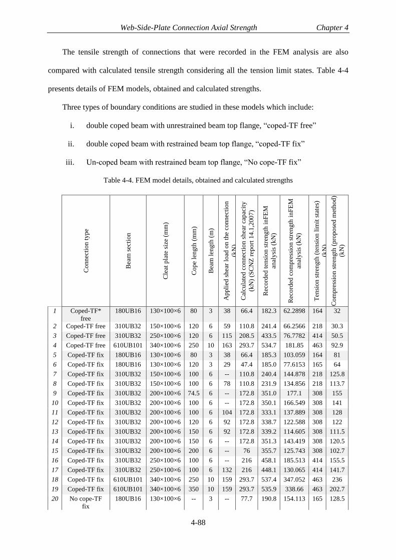
Web-Side-Plate Connection Axial Strength Chapter 4
4-88
The tensile strength of connections that were recorded in the FEM analysis are also
compared with calculated tensile strength considering all the tension limit states. Table 4-4
presents details of FEM models, obtained and calculated strengths.
Three types of boundary conditions are studied in these models which include:
i. double coped beam with unrestrained beam top flange, “coped-TF free”
ii. double coped beam with restrained beam top flange, “coped-TF fix”
iii. Un-coped beam with restrained beam top flange, “No cope-TF fix”
Table 4-4. FEM model details, obtained and calculated strengths
Co
nn
ecti
on
ty
pe
Bea
m s
ecti
on
Cle
at p
late
siz
e (m
m)
Co
pe
len
gth
(m
m)
Bea
m l
eng
th (
m)
Ap
pli
ed s
hea
r lo
ad o
n t
he
conn
ecti
on
(kN
)
Cal
cula
ted
co
nn
ecti
on
sh
ear
cap
acit
y
(kN
) (S
CN
Z r
epo
rt 1
4.1
,200
7)
Rec
ord
ed t
ensi
on
str
eng
th i
nF
EM
anal
ysi
s (k
N)
Rec
ord
ed c
om
pre
ssio
n s
tren
gth
in
FE
M
anal
ysi
s (k
N)
Ten
sio
n s
tren
gth
(te
nsi
on
lim
it s
tate
s)
(kN
)
Co
mp
ress
ion
str
eng
th (
pro
po
sed
met
hod
)
(kN
)
1 Coped-TF*
free
180UB16 130×100×6 80 3 38 66.4 182.3 62.2898 164 32
2 Coped-TF free 310UB32 150×100×6 120 6 59 110.8 241.4 66.2566 218 30.3
3 Coped-TF free 310UB32 250×100×6 120 6 115 208.5 433.5 76.7782 414 50.5
4 Coped-TF free 610UB101 340×100×6 250 10 163 293.7 534.7 181.85 463 92.9
5 Coped-TF fix 180UB16 130×100×6 80 3 38 66.4 185.3 103.059 164 81
6 Coped-TF fix 180UB16 130×100×6 120 3 29 47.4 185.0 77.6153 165 64
7 Coped-TF fix 310UB32 150×100×6 100 6 -- 110.8 240.4 144.878 218 125.8
8 Coped-TF fix 310UB32 150×100×6 100 6 78 110.8 231.9 134.856 218 113.7
9 Coped-TF fix 310UB32 200×100×6 74.5 6 -- 172.8 351.0 177.1 308 155
10 Coped-TF fix 310UB32 200×100×6 100 6 -- 172.8 350.1 166.549 308 141
11 Coped-TF fix 310UB32 200×100×6 100 6 104 172.8 333.1 137.889 308 128
12 Coped-TF fix 310UB32 200×100×6 120 6 92 172.8 338.7 122.588 308 122
13 Coped-TF fix 310UB32 200×100×6 150 6 92 172.8 339.2 114.605 308 111.5
14 Coped-TF fix 310UB32 200×100×6 150 6 -- 172.8 351.3 143.419 308 120.5
15 Coped-TF fix 310UB32 200×100×6 200 6 -- 76 355.7 125.743 308 102.7
16 Coped-TF fix 310UB32 250×100×6 100 6 -- 216 458.1 185.513 414 155.5
17 Coped-TF fix 310UB32 250×100×6 100 6 132 216 448.1 130.065 414 141.7
18 Coped-TF fix 610UB101 340×100×6 250 10 159 293.7 537.4 347.052 463 236
19 Coped-TF fix 610UB101 340×100×6 350 10 159 293.7 535.9 338.66 463 202.7
20 No cope-TF
fix
180UB16 130×100×6 -- 3 -- 77.7 190.8 154.113 165 128.5

Web-Side-Plate Connection Axial Strength Chapter 4
4-89
21 No cope-TF
fix
180UB16 130×100×6 -- 3 41 77.7 189.2 150.527 165 115.2
22 No cope-TF
fix
310UB32 150×100×6 -- 6 -- 110.8 244.0 168.547 218 161
23 No cope-TF
fix
310UB32 150×100×6 -- 6 77 110.8 237.2 165.414 218 144.2
24 No cope-TF
fix
310UB32 150×100×6 -- 6 57 110.8 238.9 168.961 218 149
25 No cope-TF
fix
310UB32 200×100×6 -- 6 -- 172.8 352.2 207.922 308 186
26 No cope-TF
fix
310UB32 200×100×6 -- 6 34 172.8 349.8 204.523 308 179
27 No cope-TF
fix
310UB32 200×100×6 -- 6 69 172.8 349.1 197.65 308 172.8
28 No cope-TF
fix
310UB32 250×100×6 -- 6 -- 216 454.0 262.614 414 210
29 No cope-TF
fix
310UB32 250×100×6 -- 6 109 216 447.9 226.882 414 192.4
30 No cope-TF
fix
310UB32 250×100×6 -- 6 129 216 442.1 219.443 414 189
31 No cope-TF
fix
610UB101 340×100×6 -- 10 -- 293.7 554.2 496.084 463 371
32 No cope-TF
fix
610UB101 340×100×6 -- 10 165 293.7 540.2 486.505 463 347.5
33 No cope-TF
fix
610UB101 500×100×6 -- 10 -- 432 863.8 705.266 740 476
34 No cope-TF
fix
610UB101 500×100×6 -- 10 239 432 802.1 642.539 740 449.4
TF→ Top Flange
Note: the tension capacity of connections are obtained without strength reduction factors to be compared with
FE results
The recorded and calculated tension and compression strengths of FEM models are plotted in
Figure 4-72. The average ratio of the calculated compression strength to the recorded strength
of FEM analysis is about 80.1% with a standard deviation of 13.7%. For the tension side, the
average ratio of the calculated tensile strength to the recorded strength from FEM analysis is
about 89.3% with a standard deviation of 2.8%. Based on the results, the proposed method
indicates good agreement with the FEM models for estimating axial compression strength of
WSP connections. However, there is a need for an experimental investigation to verify this
method.

Web-Side-Plate Connection Axial Strength Chapter 4
4-90
a) Connection tension and compression strengths calculated using the developed method and
FEM
b) Ratio of FEM strength to calculated axial strength
Figure 4-72. Connections recorded strength and calculated strength
Note that the packing effect was not considered in the FE models as well as out-of-
straightness and residual stresses in the members. Therefore, in this study it is recommended
to use strength reduction factor of 𝜙 = 0.75 for WSP axial compression capacity to account
for packing effect and other parameters that were not possible to be considered in the FEM
0
100
200
300
400
500
600
700
800
900
0 10 20 30
Connec
tion a
xia
l st
rength
(kN
)
Model number
FEM tension strength
FEM compression strength
Calculated tension strength
Calculated compression strength
0
0.5
1
1.5
2
2.5
0 5 10 15 20 25 30 35
Rat
io o
f F
EM
str
ength
to
calc
ula
ted s
tren
gth
Model number
Compression Tension
Safe zone

Web-Side-Plate Connection Axial Strength Chapter 4
4-91
analysis explicitly. An experimental study is required to achieve more accurate results and
confirm the findings of this study which is out of the scope of this research.
4.8 Conclusion
In this chapter, the axial behaviour of WSP connections was investigated and a method to
assess the axial compressive strength of WSP connections considering the gravity loads effect
was proposed. The main findings of this study include:
1) Diaphragm in-plane forces need to be transferred to the ground through VLFR system of
the structure. Structural beams as a part of the load path transfer the diaphragm in-plane
forces to VLFR system. The axial forces generated in a beam as a part of the load transfer
mechanism may depend on whether a gap is provided between the slab and the column or
not.
2) Based on the literature, many research studies have been conducted to investigate the shear
force and rotation capacity of the WSP connections since the 1960s. The results of these
studies were employed by different building standards to calculate the shear strength of
WSP connections. However, the axial behaviour of this type of connection was only
investigated by few researchers focusing on connection axial forces due to the beam
composite action.
3) From the analysis conducted in this study, it was found that the axial compression capacity
of a WSP connection is lower than the axial tensile capacity because of the axial force
eccentricity, the cleat plate slenderness, and P-Δ effect. The axial force eccentricity
imposes additional moment to the cleat plate and the beam web, and initiates the cleat
buckling at lower axial forces compared to a centrally loaded cleat plate. For the
connection subjected to the axial tension force, axial force increases to reach the first
controlling failure limit state.

Web-Side-Plate Connection Axial Strength Chapter 4
4-92
4) A number of parameters that can affect the axial behaviour of WSP connections are
investigated, the results found include:
i. Beam lateral restraint at the mid-point and third points along the beam length did
not alter the tensile strength and the compression strength increased by less than
4% in the studied case.
ii. Top flange torsional restraint did not change the tensile strength of the WSP
connection. However, the compression capacity increased by about 14% for the
studied case compared to the unrestrained beam.
v. The effect of cleat plate location on only one side or opposite sides at beam-ends
was less than 1% for the studied case.
vi. Compression and tension capacities of the WSP connection increased with
increasing cleat plate height. The ultimate tension and compression capacities
showed that the tensile strength more increased than compression capacity by
increasing the cleat plate height.
vii. For the models studied, the tensile capacity decreased by about 2% because of the
reduction in the beam web cross-section area due to copping. The compression
behaviour experienced a significant reduction, so that, the 2, 3 and 4 bolts
connections experienced 16%, 24% and 48% reduction in the ultimate compression
capacity.
viii. Cope length did not significantly affect the tensile capacity of the WSP connection.
However, the connection compression capacity decreased with increasing the cope
length. For the range of cases studied the axial compression strength decreased
linearly with increasing the cope length.
iv. Gravity loads causing a beam shear force up to 60% of cleat plate shear yield
strength reduced the connection compressive axial strength by up to 15%.

Web-Side-Plate Connection Axial Strength Chapter 4
4-93
v. It was found that for connections with both snug-tightened and proof loaded bolts
the ultimate tension and compression capacities were almost the same with less
than 3% difference at the ultimate axial strength.
vi. Based on the results of the studied cases, column lateral drift increased or decreased
the ultimate capacity of the studied connections under axial compression by less
than ±8% for a 2% drift angle. Also, it was found that additional rotation did not
affect the tension behaviour of WSP connections.
vii. Considering 3mm eccentricity in the studied connection caused up to 25% decrease
in the axial compression strength and the ultimate tensile strength of the WSP
connection changed by about 7% due to increasing the load eccentricity up to 3mm.
5) For the proposed method to calculate WSP axial compression strength, it was found that
considering the cleat plate alone may result in a conservative estimate of compression
strength. Therefore, the effect of the beam web and different boundary conditions should
be considered. The proposed method covers the connections with the following
conditions:
1. Double coped, laterally unrestrained connection
2. Un-coped, top flange restrained laterally
3. Double coped, top flange restrained laterally
The axial compression strengths obtained using the proposed method were compared with
thirty-four models considering different parameters. The average ratio of calculated
compression strength to the strength obtained from FEM analysis was 80.1% with standard
deviation of 13.7% and for tension side, the average ratio of calculated tension strength to
the strength obtained from FEM analysis was about 89.3% with standard deviation of
2.8%. Note that some parameters considered in the analytical strength calculation
approach were not considered in the numerical models. These included: residual stress

Web-Side-Plate Connection Axial Strength Chapter 4
4-94
effect and out-of-straightness effect. To consider these and also possible packing effect in
design it is therefore suggested that the calculated compression capacity be multiplied by
a strength reduction factor of 𝜙 = 0.75. However, further experimental investigation is
required.
4.9 Summary of the proposed method
In this section a summary of the proposed method for estimating axial strength of WSP
connections is presented. Figure 4-73 shows elevation and section views of a typical WSP
connection.
a) Elevation
b) Section view
Figure 4-73. Elevation and section of typical WSP connection
4.9.1 Case one, beam top flange not restrained laterally
4.9.1.1 Checking the cleat plate
1) Obtain effective length of the beam web (𝐿𝑤)
{𝐿𝑤 =
ℎ𝑤5+ 𝐿𝑐𝑜𝑝𝑒 − 𝑎𝑒1 → 𝑓𝑜𝑟 𝑐𝑜𝑝𝑒𝑑 𝑏𝑒𝑎𝑚
𝐿𝑤 =ℎ𝑤5 → 𝑓𝑜𝑟 𝑢𝑛 − 𝑐𝑜𝑝𝑒𝑑 𝑏𝑒𝑎𝑚
Note: 𝑎𝑒1 is the distance between the beam-end and bolt line as shown in Figure 4-73.

Web-Side-Plate Connection Axial Strength Chapter 4
4-95
2) Obtain contributing height of the beam web, ℎ𝑤𝑒 = 𝑚𝑖𝑛[ℎ𝑤, 1.5ℎ𝑐]
3) Calculate effective length factor for the cleat plate
{
𝑘𝑐 = 1.05𝐿𝑤𝐿𝑐√𝐸𝐼𝑐𝐸𝐼𝑤
+ 1.2 → 𝑓𝑜𝑟 𝐿𝑤𝐿𝑐√𝐸𝐼𝑐𝐸𝐼𝑤
< 2
𝑘𝑐 = 0.9𝐿𝑤𝐿𝑐√𝐸𝐼𝑐𝐸𝐼𝑤
+ 1.5 → 𝑓𝑜𝑟 𝐿𝑤𝐿𝑐√𝐸𝐼𝑐𝐸𝐼𝑤
≥ 2
Note: 𝐼𝑤 is calculated based on the effective beam web height (ℎ𝑤𝑒)
4) Calculate elastic buckling load for the cleat plate, 𝑃𝑐𝑟 =𝜋2𝐸𝐼𝑐
(𝑘𝑐𝐿𝑐)2
5) Obtain 𝑃𝑢 for the cleat plate based on Section 6 of NZS3404 (2007) considering 𝛼𝑏 =
0.5
6) Obtain 𝑀𝑢3 (plastic moment) of the cleat plate about weak axis
7) Calculate moment participation factor, 𝛼 = (𝐼𝑐𝐿𝑐⁄
𝐼𝑐𝐿𝑐⁄ +
𝐼𝑤𝐿𝑤⁄)
8) Calculate 𝑒 (axial load eccentricity) using 𝑒 =𝑡𝑐+𝑡𝑤
2
9) Obtain 𝑀𝑢2 (plastic moment) of the cleat plate about strong axis
• Note: the plastic moment of the cleat plate about strong axis should be modified using
shear-moment interaction
{
𝑉
𝑉𝑣+1.6𝑀𝑢2∅𝑀𝑠2
≤ 2.2 𝑓𝑜𝑟 𝑉 ≥ 0.6𝑉𝑣
𝑀𝑢2 = ∅𝑀𝑠2 𝑓𝑜𝑟 𝑉 < 0.6𝑉𝑣
10) Calculate the cleat plate capacity (𝑃𝑐) using
𝑃𝑐𝑃𝑢+
𝛼×𝑃𝑐×𝑒𝑀𝑢3(1−𝑃 𝑃𝑐𝑟⁄ )
+𝑀2𝑀𝑢2
≤ 1
4.9.1.2 Checking the beam web:
The process of checking the beam web is similar to calculating the cleat plate axial
strength. Only the effective length factor and moment participation factors are different for the
beam web as follow:
𝑘𝑤 = 𝑘𝑐𝐿𝑐𝐿𝑤√𝐸𝐼𝑤𝐸𝐼𝑐

Web-Side-Plate Connection Axial Strength Chapter 4
4-96
𝛼 = (𝐼𝑤
𝐿𝑤⁄
𝐼𝑐𝐿𝑐⁄ +
𝐼𝑤𝐿𝑤⁄)
𝑃𝑤𝑃𝑢+
𝛼×𝑃𝑤×𝑒𝑀𝑢3(1−𝑃 𝑃𝑐𝑟⁄ )
+𝑀2𝑀𝑢2
≤ 1
• WSP compression strength is equal to minimum of {𝑃𝑤, 𝑃𝑐}.
4.9.2 Case two, beam top flange restrained laterally
4.9.2.1 Checking the cleat plate
1) Obtain ℎ𝑒𝑓𝑓 based on Clause 6.2.4 of NZS3404 (2007)
ℎ𝑒𝑓𝑓 = 16𝑡𝑤√250
𝑓𝑦𝑤≤ ℎ𝑤
• Note: if the beam top flange is retrained and the beam is coped, the ℎ𝑒𝑓𝑓 should be
modified using:
ℎ𝑒𝑐ℎ𝑒= 1− 0.5
𝐿𝑐𝑑
2) Calculate ℎ1 and ℎ2
ℎ1 = ℎ𝑒𝑓𝑓 + 𝑡𝑓 − 𝑎+ 𝑎𝑒6
ℎ2 = ℎ𝑐 − ℎ1
Note: 𝑎𝑒6 is the vertical edge distance at top of the cleat plate
3) Calculate cleat axial capacity at zone 1 (𝑃𝑐1) shown in Figure 4-65
𝑃𝑐1 = ℎ1𝑡𝑐𝑓𝑦𝑐
4) Calculate 𝑃2, this stage is the same as the case one, while the ℎ𝑐 should be substituted
by ℎ2
4.1) Obtain effective length of the beam web (𝐿𝑤)
{𝐿𝑤 =
ℎ𝑤5+ 𝐿𝑐𝑜𝑝𝑒 − 𝑎𝑒1 → 𝑓𝑜𝑟 𝑐𝑜𝑝𝑒𝑑 𝑏𝑒𝑎𝑚
𝐿𝑤 =ℎ𝑤5 → 𝑓𝑜𝑟 𝑢𝑛 − 𝑐𝑜𝑝𝑒𝑑 𝑏𝑒𝑎𝑚

Web-Side-Plate Connection Axial Strength Chapter 4
4-97
4.2) Obtain contributing height of the beam web, ℎ𝑤𝑒 = 𝑚𝑖𝑛[ℎ𝑤, 1.5ℎ2]
4.3) Calculate effective length factor for the cleat plate
{
𝑘𝑐 = 1.05𝐿𝑤𝐿𝑐√𝐸𝐼𝑐2𝐸𝐼𝑤
+ 1.2 → 𝑓𝑜𝑟 𝐿𝑤𝐿𝑐√𝐸𝐼𝑐2𝐸𝐼𝑤
< 2
𝑘𝑐 = 0.9𝐿𝑤𝐿𝑐√𝐸𝐼𝑐2𝐸𝐼𝑤
+ 1.5 → 𝑓𝑜𝑟 𝐿𝑤𝐿𝑐√𝐸𝐼𝑐2𝐸𝐼𝑤
≥ 2
• Note: 𝐼𝑤 is calculated based on effective beam web height (ℎ𝑤𝑒) and 𝐼𝑐2 is
calculated using ℎ2
4.4) Calculate elastic buckling force for the cleat plate, 𝑃𝑐𝑟 =𝜋2𝐸𝐼𝑐2
(𝑘𝑐𝐿𝑐)2
4.5) Obtain 𝑃𝑢 for the cleat plate based on Section 6 of NZS3404 (2007) considering 𝛼𝑏 =
0.5
4.6) Obtain 𝑀𝑢3 (plastic moment) of the cleat plate about weak axis (using ℎ2)
4.7) Calculate moment participation factor, 𝛼 = (𝐼𝑐2
𝐿𝑐⁄
𝐼𝑐2𝐿𝑐⁄ +
𝐼𝑤𝐿𝑤⁄)
4.8) Calculate 𝑒 (axial load eccentricity) using 𝑒 =𝑡𝑐+𝑡𝑤
2
4.9) Finding 𝑀𝑢2 (plastic moment) of the cleat plate about strong axis
• Note: the plastic moment of cleat plate about strong axis should be modified using
shear-moment interaction
{
𝑉
𝑉𝑣+1.6𝑀𝑢2∅𝑀𝑠2
≤ 2.2 𝑓𝑜𝑟 𝑉 ≥ 0.6𝑉𝑣
𝑀𝑢2 = ∅𝑀𝑠2 𝑓𝑜𝑟 𝑉 < 0.6𝑉𝑣
4.10) Calculate the cleat plate capacity at zone 2 (𝑃𝑐2) shown in Figure 4-65
𝑃𝑐2𝑃𝑢+
𝛼×𝑃𝑐2×𝑒𝑀𝑢3(1−𝑃 𝑃𝑐𝑟⁄ )
+𝑀2𝑀𝑢2
≤ 1
5) Calculate total cleat capacity
𝑃𝑐 = 𝑃𝑐1 +𝑃𝑐2
4.9.2.2 Checking the beam web:
1) Calculate beam web strength at zone 1 (𝑃𝑤1)

Web-Side-Plate Connection Axial Strength Chapter 4
4-98
𝑃𝑤1 = (ℎ𝑒𝑓𝑓 − ℎ2)𝑡𝑤𝑓𝑦𝑤
The process for calculating 𝑃𝑤2 is similar to the cleat axial strength calculation and the
effective length and moment participation factors are different in this case as follows:
𝑘𝑤 = 𝑘𝑐𝐿𝑐𝐿𝑤√𝐸𝐼𝑤𝐸𝐼𝑐2
𝛼 = (𝐼𝑤
𝐿𝑤⁄
𝐼𝑐2𝐿𝑐⁄ +
𝐼𝑤𝐿𝑤⁄)
𝑃𝑤2𝑃𝑢+
𝛼×𝑃𝑤2×𝑒𝑀𝑢3(1−𝑃 𝑃𝑐𝑟⁄ )
+𝑀2𝑀𝑢2
≤ 1
𝑃𝑤 = 𝑃𝑤1 +𝑃𝑤2
❖ WSP compression nominal strength is equal to minimum of {𝑃𝑤, 𝑃𝑐}
❖ Here it is suggested that the calculated compression capacity be multiplied by a
strength reduction factor of 𝜙 = 0.75.
An example of WSP axial strength calculation is provided in Appendix M.

Web-Side-Plate Connection Axial Strength Chapter 4
4-99
References
[1] ABAQUS, analysis user’s guide, version 6.14, Dassault systemes solidworks corp,
Waltham, Massachusetts, 2014.
[2] Abou-zidan, A., & Liu, Y. (2015). Numerical study of unstiffened extended shear
tab connections. Journal of Constructional Steel Research, 107, 70-80.
[3] Ahmed, B., Li, T. Q., & Nethercot, D. A. (1997). Design of composite finplate and
angle cleated connections. Journal of Constructional Steel Research, 41(1), 1-29.
[4] AISC (1963). Manual of Steel Construction, 6th Edition. American Institute of
Steel Construction. Chicago, IL.
[5] AISC (2010). Specification for structural steel buildings (ANSI/AISC 360-
10). American Institute of Steel Construction, Chicago-Illinois.
[6] AISC (2016). Specification for structural steel buildings (ANSI/AISC 360-
16). American Institute of Steel Construction, Chicago-Illinois.
[7] AISC, L. (2001). Manual of steel construction, load and resistance factor design.
[8] Alizadeh, S., MacRae, G. A., Bull, D., & Clifton, G. C. (2017). In-Plane
Diaphragm Issues for Steel Buildings in Seismic Zones. In 16th World Conference
on Earthquake, 16WCEE.
[9] American Institute of Steel Construction. (2005). Steel construction manual.
[10] AS/NZS 1170.0 (2002), Structural design actions-Part 0: General principles.
[11] AS/NZS 3679.1 (2016), Structural steel - Part 1: Hot-rolled bars and sections
[12] AS/NZS 5131 (2016), Structural steelwork - Fabrication and erection.
[13] Ashakul, A. (2004). Finite element analysis of single plate shear
connections (Doctoral dissertation, Virginia Tech).
[14] Ashakul, A., & Khampa, K. (2014). Effect of plate properties on shear strength
of bolt group in single plate connection. Steel and Composite Structures, 16(6),
611-637.

Web-Side-Plate Connection Axial Strength Chapter 4
4-100
[15] Astaneh, A. (1989a). New concepts in design of single plate shear connections.
In Proc., National Steel Construction Conf (pp. 3-1).
[16] Astaneh, A. (1989b). Demand and supply of ductility in steel shear
connections. Journal of Constructional Steel Research, 14(1), 1-19.
[17] Astaneh, A., Call, S. M., & McMULLIN, K. M. (1989c). Design of single plate
shear connections. Engineering Journal, 26(1), 21-32.
[18] Astaneh, A., McMULLIN, K. M. & Call, S. M. (1988). Design of single plate
framing connections,” Report No. UCB/SEMM-88/12 to the American Institute of
Steel Construction. University of California at Berkeley.
[19] Caccavale, S. E. (1975). Ductility of single plate framing connections.
[20] Chaudhari TD, MacRae GA, Bull D, Chase G, Hicks S, Clifton GC and Hobbs
M (2015). “Composite Slab Effects on Beam–Column Subassembly Seismic
Performance”, 8th International Conference on Behavior of Steel Structures in
Seismic Areas, Shanghai, China.
[21] Creech, D. D. (2005). Behavior of single plate shear connections with rigid and
flexible supports.
[22] D'Aronco, M. (2013). Behaviour of double and triple vertical rows of bolts
shear tab connections and weld retrofits(Doctoral dissertation, École
Polytechnique de Montréal).
[23] Goodrich, W. S. (2005). Behavior of extended shear tabs in stiffened beam-to-
column web connections.
[24] Hormby, D. E. (1981). Design of single plate framing connections.
[25] Hyland, C., Cowie, K., & Clifton, C. (2008). Structural Steelwork Connections
Guide: Design Procedures, SCNZ 14.1 2007. Steel Construction New Zealand
(Inc), Manukau City.
[26] Johnston, B. G. (1976). Guide to stability design criteria for metal structures.

Web-Side-Plate Connection Axial Strength Chapter 4
4-101
[27] Kulak, G. L., Fisher, J. W., & Struik, J. H. (2001). Guide to Design Criteria for
Bolted and Riveted Joints Second Edition.
[28] Lipson, S. L. (1968, February). Single-angle and single-plate beam framing
connections. In Canadian Structural Engineering Conference, Toronto,
Ontario (pp. 141-162).
[29] Mahamid, M., Rahman, A. D. E. E. B., & Ghorbanpoor, A. (2007). The
Analyses of Extended Shear Tab Steel Connections Part II: Stiffened
Connections. ENGINEERING JOURNAL-AMERICAN INSTITUTE OF STEEL
CONSTRUCTION, 44(2), 133.
[30] Manual of Steel Construction, 14th Edition, American Institute of Steel
Construction, Chicago: AISC, 2011.
[31] Marosi, M. (2011). Behaviour of single and double row bolted shear tab
connections and weld retrofits. In Masters Abstracts International (Vol. 50, No.
02).
[32] Neal, B. G. (1961). The effect of shear and normal forces on the fully plastic
moment of a beam of rectangular cross section. Journal of Applied
Mechanics, 28(2), 269-274.
[33] Needham, J., Koia, R., Alizadeh, S., Scarry, J. and MacRae, G.A. (2018). Beam
Shear Connections. Steel Structures in Seismic Areas (STESSA) Conference,
Christchurch, 14-16 February 2018.
[34] New Zealand Heavy Engineering Research Association, structural steelwork
connections guide, design procedures. HERA R4-100 2003.
[35] NZS 3404 (2007). Steel Structures Standard. Standards New Zealand,
Wellington, New Zealand. Including Amendments 1 and 2, 2001/2007.
[36] Patrick, M., Berry, P. A., & Wheeler, A. T. (2002). -Web-side-plate framing
connections in both steel and composite construction. In Advances in Building
Technology (pp. 199-206).

Web-Side-Plate Connection Axial Strength Chapter 4
4-102
[37] Rahman, A., Mahamid, M., Amro, A., & Ghorbanpoor, A. L. (2007). The
analyses of extended shear tab steel connections-Part I: The unstiffened
connections. ENGINEERING JOURNAL-AMERICAN INSTITUTE OF STEEL
CONSTRUCTION INC, 44(2), 117-132.
[38] Ren, P. (1995). Numerical modelling and experimental analysis of steel beam-
to-column connections allowing for the influence of reinforced-concrete slabs (No.
THESIS_LIB). EPFL.
[39] Richard, R. M., Gillett, P. E., Kriegh, J. D., & Lewis, B. A. (1980). The analysis
and design of single plate framing connections. Engineering Journal, 17(2).
[40] Sherman, D. R., & Ghorbanpoor, A. (2002). Design of Extended Shear Tabs,”
Final report for the American Institute of Steel Construction. October, University
of Wisconsin, Milwaukee, Wisconsin.
[41] Steel Construction Institute (Great Britain) & British Constructional Steelwork
Association (2002). Joints in steel construction: simple connections. Steel
Construction Institute, Ascot
[42] Suleiman, M. F. (2013). Non-Linear Finite Element Analysis of Extended Shear
Tab Connections (Doctoral dissertation, University of Cincinnati).
[43] Thomas, K., Driver, R. G., Oosterhof, S. A., & Callele, L. (2017, May). Full-
scale Tests of Stabilized and Unstabilized Extended Single-plate Connections.
In Structures (Vol. 10, pp. 49-58). Elsevier.
[44] Weir, C., & Clarke, H. (2016). Web Side Plate Connections under Axial Load.
Final Year Projects, Dept. of Civil and Natural Resources Engineering, University
of Canterbury.
[45] Ziemian, R. D. (Ed.). (2010). Guide to stability design criteria for metal
structures. John Wiley & Sons.

Shear Studs Considerations Chapter 5
5-1
5 Shear Studs Considerations
5.1 Introduction
Composite beams typically consist of a steel beam with a concrete slab on top of the beam.
Composite action increases the beam stiffness and strength. Therefore, smaller beam section
sizes can be used compared to the non-composite situation. Composite beams are commonly
used in steel structures.
Composite action is developed between the concrete slab and the steel beam through the
use of mechanical attachments which transfer longitudinal shear between the concrete slab and
the steel beam. There are different types of mechanical attachments such as bar connectors,
angle connectors, channel connectors and steel headed-studs, also referred to as shear studs.
The most widely used type of shear connector is the shear stud. The advantages of the shear
stud connectors include i) rapid welding process, ii) little obstruction to reinforcement in the
concrete slab and, iii) equal strength and stiffness in shear in all directions normal to the
longitudinal axis of the stud (Johnson, 2008).
Equations for determining composite beam strength and stiffness to carry gravity loads are
provided by different building standards (e.g. AISC/ANSI 360-16 and NZS3404, 2007). The
flexural strength of a composite beam is normally derived from standard rigid-plastic
equilibrium analyses of the forces across the beam section.
During earthquake events, in-plane diaphragm forces due to inertia, transfer, compatibility,
slab bearing and interaction with other structural elements need to be transferred to the
structural frames (Alizadeh et al. 2017). In general, force transfer directly from the diaphragm
into the column should not be used as it is not a reliable load path. This is because if a gap is
provided around the column during construction, as shown in Figure 5-1a, the diaphragm forces
need to be transferred to the VLFR system of the structure through the beam axial forces.

Shear Studs Considerations Chapter 5
5-2
However, even if there is no construction gap around the column, since the slab inertia forces
act in the same direction as the frame sways, due to the beam-column joint rotation, a gap opens
at location “A”, shown in Figure 5-1c. Because of this, the slab forces cannot transfer directly
into the column through slab bearing. Instead, the diaphragm in-plane forces transfer into the
steel beam through friction and mechanical attachments (e.g. shear studs) and from the beam
to the column (MacRae and Clifton, 2015).
In addition, when there is no construction gap between the slab and column, as the column
sways, it bears against the concrete slab on the far end of the beam. This is the left side of the
beam, at location “B”, in Figure 5-1c. This slab bearing force is likely to increase the slab forces
that must transfer into the beam using shear studs, and the beam must transfer it back to the
columns.
a) Gap provided around the column
b) Free body diagram
c) No gap provided
d) Free body diagram
Figure 5-1. Gapped and non-gapped slab-column details
Note that when there is no construction gap around the column and a gap is opened due to
the frame lateral drifts at point “A”; slab lateral movements (because of the shear stud and
beam-column flexibility) may close the gap and form a load path through the slab bearing.
However, the existence of this load path depends on the relative displacement of the slab to the
beam/column, and even after contact is made, the load path is not reliable due to concrete
Shear Studs Considerations Chapter 5
5-3
crushing. Therefore, it is more reliable and conservative for shear stud design to consider forces
transferred from the diaphragm to the beam through shear studs.
In this study, the behaviour of composite beams subjected to lateral forces are investigated
by answering the following questions:
1) What design recommendations exist for shear studs subject to lateral forces in
combination with gravity loads?
2) What are the effects of lateral forces on composite action and beam vertical
deflection?
3) How should the number of shear studs be considered in design of traditional
structures?
4) If undesirable effects of lateral force on beam behaviour are to be mitigated, how
should this be done?
5.2 Literature review
A summary of the available provisions/recommendations to design beams subject to lateral
force in combination with the gravity loads are presented. Also, a brief review of the research
works and building standards relevant to the monotonic and cyclic force-slip behaviour of shear
studs is conducted.
5.2.1 Available provision/recommendations to design shear studs for
lateral forces in combination with gravity loads
There are few documents in the literature that consider the lateral force resistance of shear
studs on a composite beam. Mullett (1998) states that it is not normally necessary to provide
additional shear connectors to carry diaphragm in-plane forces except close to points of local
transfer of shear forces such as adjacent to VLFR systems.
Shear Studs Considerations Chapter 5
5-4
• Composite beams
Burmeister and William (2008) state that for the beams that are designed as composite
members to carry gravity loads, additional shear studs to transfer the superimposed horizontal
forces into the beam may not be required. This is because:
1) The quantity of shear studs used for a composite beam is usually determined based
on an ultimate gravity load combination, such as 1.2𝐺 + 1.5𝑄 based on NZS
1170.0 (2002). However, at the time that the lateral forces are imposed the reduced
gravity loads include the dead load, 𝐺, and a part of the live load, 𝑄, act on the
beam. The load combination for this situation is provided by loading standards. In
NZS1170.0 (2002) this is 𝐺 + 𝜓𝐸𝑄 where 𝜓𝐸 = 0.3 for most buildings (except
storage and structures with installed heavy machinery). Under the reduced gravity
load combinations, the shear studs will be under-used and thus have additional
capacity available to transfer the diaphragm in-plane forces.
2) The interaction of the shear flow from the different loading conditions is additive
for some studs but opposite for others. The distribution of horizontal shear from
the beam flexure is assumed to flow in two directions from the point of the
maximum moment to the point of zero moments as shown in Figure 5-2.
Based on Burmeister and William (2008) study, when the shear studs have sufficient
ductility to distribute the horizontal shears evenly along the beam, the composite beam can
transfer the horizontal shear due to lateral forces equal to the sum of the strengths of all the
shear studs on the beam regardless of the gravity load demand on the shear studs. Similar
provisions were given in AISC/ANSI 360-16.

Shear Studs Considerations Chapter 5
5-5
Figure 5-2. Shear flow at collector beam (AISC/ANSI 360-16)
Based on Cowie et al. (2014) the number of shear studs required should be computed as
that needed to develop composite action to resist the gravity loads from the 1.0𝐺 + 1.0𝑄 load
combination in addition to the number of shear studs required for lateral forces. Using 1.0𝑄 in
this combination instead of 𝜓𝐸𝑄 is in accordance with the requirements of Clause 12.10.2.2
NZS 3404 (2007) to prevent uniaxial beam hinging (shakedown) in moment resisting frames.
Although this recommendation is for beams in moment resisting frames, it may be applied to
any beam forming a key component of the diaphragm force transfer system (Cowie et al.,
2014).
• Non-composite beams
Burmeister and William (2008) state that in the non-composite beams, that the shear studs
are only placed to transfer lateral forces, shear studs still will be subjected to horizontal shears
due to flexural effects from gravity loads. In order to ensure the shear studs are not overloaded

Shear Studs Considerations Chapter 5
5-6
under the gravity loads, it was recommended that all beams have enough shear studs to achieve
a minimum of 25% partial composite action. This provides some lateral force resistance. When
fewer shear studs than this are provided, large slips may occur in the shear studs under gravity
loads limiting the ability of the beam to function as intended under lateral forces. Similar
provisions were given in AISC/ANSI 360-16.
Other research (e.g. Cowie et al., 2014 and Sabelli et al., 2011) also endorsed the
provisions given in AISC/ANSI 360-10 which are similar to AISC/ANSI 360-16.
NZS 3404 (2007) provides equations for determining the ultimate composite beam
strength and stiffness for supporting gravity loads. However, there is only one clause in this
standard regarding the seismic design of composite floor slabs. Clause 13.2.3.2 of NZS 3404
(2007) states that the actions induced in shear connectors by seismic-induced diaphragm effects
shall be added to any design actions from the composite action using appropriate design load
combinations from loading standard. There is no further information about how many shear
studs contribute to lateral force resistance or the appropriate method for combining these
actions.
Some provisions (Clause 8.3.2) are also provided in AS/NZS 2327 (2017) about
considering the stiffness of composite members on the frame lateral stiffness. However, there
is no guidance about considering the interaction of gravity loads and lateral forces on composite
beams.
5.2.2 Force-slip behaviour of shear studs
Behaviour of steel-concrete composite beams under gravity loads, lateral forces or
combination of these forces, highly depends on the shear connector stiffness, force-slip
relationship and ductility. In the following, the shear behaviour of shear studs as the most
widely used shear connectors is described.

Shear Studs Considerations Chapter 5
5-7
Three parameters that are considered as the main characteristics of shear studs in this study
include:
i. Ultimate slip capacity of a ductile shear stud
ii. Force-slip relationship of shear stud
iii. Cyclic behaviour of shear stud
5.2.2.1 Ultimate slip capacity of a ductile shear stud
Shear connectors (e.g. shear studs) in a composite beam experience a level of shear slip
under the imposed gravity loads. The amount of this slip depends on the shear stud stiffness,
strength, the composite action level and also the imposed gravity loads. The slip is higher in
partially composite beams because a lower number of shear studs are provided to carry steel-
concrete interface shear forces in comparison with a fully composite beam. The shear stud
ductility is an important parameter to avoid unexpected failure under gravity load.
Meanwhile, shear studs in a composite beam subjected to the combination of gravity and
lateral forces require more ductility to accommodate deformations than those due to lateral
forces alone. This situation will be discussed in more detail in Section 5.3.
The minimum ultimate slip, 𝑆𝑢, to consider a shear stud as a ductile shear connector is
6mm based on Eurocode 4 (2004). The same limitation is also given in AS/NZS 2327 (2017)
Clause 3.6.1.1. Figure 5-3 presents a schematic force-slip behaviour of shear studs from a push-
out test indicating 𝑆𝑢.

Shear Studs Considerations Chapter 5
5-8
Figure 5-3. Schematic force-slip of shear stud (Eurocode 4, 2004)
Johnson and Molenstra (1991) conducted an extensive study on shear stud behaviour in
partially composite beams. They used the result of available shear stud tests at the time to
obtain the ultimate slip capacity of shear studs. Based on their study, the ultimate slip, 𝑆𝑢, of
shear studs with 13mm, 16mm and 22mm diameter can be considered 4𝑚𝑚, 6𝑚𝑚 and 8.5𝑚𝑚
respectively. The ultimate slip capacity of 19mm diameter shear studs is 𝑆𝑢 = 7.25𝑚𝑚 by
linear interpolation between 16mm and 22mm shear studs.
5.2.2.2 Shear stud force-slip relationship
The shear strength of an individual shear stud depends on the shear stud diameter, the
materials properties, the concrete slab properties, the orientation of the steel decking, the
position of the stud within the ribs, and the number of studs. Some force-slip relationships for
shear studs are available in the literature. The force-slip curves are usually obtained using
monotonic push-out tests on shear studs.
Johnson and Molenstra (1991) proposed an empirical equation to represent the force-slip,
𝑞 − 𝑆, relationship of shear studs, using the shear stud ultimate strength, 𝑞𝑟.
𝑞 = 𝑞𝑟(1 − 𝑒−𝛽𝑆)𝛼
Eq. (5-1)
In this equation, 𝛼 and 𝛽 are empirical values that in this study are considered equal to
0.989 and 1.535 respectively. These values are based on Johnson and Molenstra (1991) results

Shear Studs Considerations Chapter 5
5-9
for 19mm shear studs. Shear stud strength, 𝑞𝑟, can be calculated using equations provided in
different building standards e.g. NZS3404 (2007), Eurocode 4 (2004), AS/NZS 2327 (2017)
and AISC/ANSI 360-16 (2016).
5.2.2.3 Cyclic behaviour of shear stud
The horizontal shear flow of shear studs due to the beam bending is in opposite directions
from the point of the maximum moment to the point of zero moments as was shown in Figure
5-2. When lateral forces are applied to the slab, the interaction of the shear flow and lateral
forces is additive for some studs but opposite for the others. Therefore some studs experience
unloading and with increasing the imposed lateral force some may be reloaded in the opposite
direction compared to their initial force. Because of this, cyclic behaviour of shear studs plays
a key role in identifying the lateral force behaviour of composite beams.
Most of the research studies in the literature have focused on the monotonic behaviour of
the shear studs. This is because the gravity load capacity and stiffness of composite beams were
mostly in the interest of researchers. The cyclic loading-unloading behaviour of shear studs
was also investigated to obtain the fatigue behaviour of shear connectors in the bridge
construction by some researchers (e.g. Slutter and Fisher, 1966 and Gattesco and Giuriani,
1996) as shown in Figure 5-4.
Figure 5-4. Shear stud behaviour subjected to loading and unloading (Gattesco and Giuriani, 1996)

Shear Studs Considerations Chapter 5
5-10
The behaviour of shear studs subjected to fully reversed cyclic loading was investigated
by Oehlers and Coughlan (1986), Nakajima et al. (2003) and Civjan and Singh (2003). Figure
5-5 shows an example of force-slip hysteresis curve for shear studs.
Figure 5-5. Shear stud behaviour subjected to fully reversed cyclic loading, 13mm diameter shear stud
(Nakajima et al., 2003)
Based on these studies, for stable hysteresis behaviour, it would be expected that the shear
studs reach the same absolute force due to the same slip in the opposite direction. This
assumption is used in this study to obtain the gravity and lateral force interaction behaviour of
composite beams.
5.3 Effects of slab lateral force on composite beams subject to
gravity loading
5.3.1 Combination of gravity loads and lateral forces on composite
beams
As it was described in Section 5.1, transferring diaphragm in-plane forces to the structural
frames during earthquake events imposes additional shear force on the shear connectors placed
on the beams. These shear connectors may primarily be placed on the beam to provide
composite action under gravity loading, or may have been designed considering lateral force.

Shear Studs Considerations Chapter 5
5-11
It is noted that lateral forces may also be transferred through friction between the slab and the
steel beam. This is described in Section 5.5.2 in more detail.
The total number of shear studs determines the level of composite action. In the fully
composite beam, there are enough shear studs between the maximum bending moment and
zero moment location to develop the full flexural strength of the composite beam. To decrease
construction costs the number of shear studs can be reduced, which makes the beam partially
composite. The composite action percentage can be expressed as the ratio of the total shear
resistance of the shear studs provided to the limiting shear force that is the minimum of tensile
yielding of the steel beam or the compression capacity of the concrete slab.
Figure 5-6a shows the shear flow at the steel beam and concrete slab interface
schematically. In this Figure, a uniform distributed gravity load is considered on the beam. The
horizontal shear at the steel beam-concrete slab interface from the beam flexure is assumed to
flow in opposite directions from the point of the maximum moment to the point of zero
moments. The magnitude of shear forces also increases from the point of the maximum moment
to the point of zero moments. Shear force demand of the shear studs is shown in Figure 5-6b
schematically. In this Figure the sum of all shear stud forces is zero, ∑ 𝐹𝑖𝐿 + ∑ 𝐹𝑖
𝑅 = 0.
a) Shear flow at steel beam-concrete slab interface

Shear Studs Considerations Chapter 5
5-12
b) Shear stud demands subjected to gravity load
Figure 5-6. Schematic view of a composite beam subjected to gravity loads
When the slab is subjected to an in-plane force, 𝑃, additional shear force is imposed on the
shear studs as shown in Figure 5-7. The interaction of the shear flow from gravity loads with
shear forces from diaphragm in-plane forces is additive for some studs and the opposite for the
others as shown in Figure 5-7. This is consistent with Figure 5-2. The shear studs on the
additive side experience additional shear force and slip. However, the shear studs on the
opposite side experience unloading. In this case the sum of all shear stud forces is equal to the
lateral imposed force, ∑ 𝐹𝑖𝐿 + ∑ 𝐹𝑖
𝑅 = 𝑃.
With increasing the lateral imposed force, 𝑃, left hand to the right, the slab moves to the
right and the shear studs on the left hand side of the beam unload. For example, shear stud 3L
has a new displacement 𝛿 to the right, and a reduced force as shown by the point 3L’. Shear
studs on the right hand side of the beam also move approximately the same displacement, 𝛿, to
the right. Often this does not result in a significant change in force (e.g. stud 3R has a similar

Shear Studs Considerations Chapter 5
5-13
demand to that in its translocated position 3R’), but its deformation demand is increased. If the
displacement demand is too large, fracture and strength loss may occur.
Figure 5-7. Schematic view of a composite beam subjected to a combination of gravity loads and
lateral forces
5.3.2 Total lateral force resistance of shear studs on a beam
Figure 5-8 shows the step by step lateral force resistance behaviour of shear studs on a
beam schematically.
i. Initially, in Step 1, the composite beam is subjected to gravity loads only and lateral
force is zero, ∑ 𝐹𝑖 = 0.
ii. In Step 2, a small lateral force is imposed which increases the shear stud force/slip
on the additive side of the beam and unloads the shear studs on the opposite side.

Shear Studs Considerations Chapter 5
5-14
The sum of the shear stud forces is equal to the lateral force, ∑ 𝐹𝑖 = 𝑃. In this step,
some shear studs on the additive side are yielded.
iii. By increasing the lateral force in Step 3, more shear studs yield and the shear stud
at the far end of the beam on the additive side reaches to fracture slip limit. In this
step some of the shear studs on the opposite side still experiencing unloading or
early levels of loading depending on the shear stud slip under gravity loads. After
this step the lateral force cannot be increased because shear studs have
displacements greater than that corresponding to their peak strength.
iv. At step four of loading with increasing the lateral slip, the lateral force resistance
of shear studs decreases due fracture in some shear studs on the additive side.
For a composite beam without gravity load, the ultimate lateral force resistance of shear
studs is equal to the sum of the shear capacity of each stud. This is because all shear studs
experience a similar level of slip at each step of loading. However, in the presence of gravity
loads, the total lateral force resistance of shear studs may not reach the sum of the ultimate
capacity of all shear studs. This is because of the shear force and slip that are imposed on the
shear studs due to the gravity load. On the additive side of the beam some studs may fracture
before some shear studs on the opposite side reach their ultimate capacity. Therefore the
maximum lateral force resistance of all shear studs is related to the shear stud slip under gravity
load.

Shear Studs Considerations Chapter 5
5-15
Figure 5-8. Schematic view of lateral force resistance mechanism of shear studs on a beam
• FEM model example
A FEM model can be used to show the behaviour of shear studs on a composite beam
subjected to gravity loads and lateral forces. The model consists of a six-meter-long composite
beam, using steel beam section 360𝑈𝐵50.7 and 1500 × 150𝑚𝑚 cross-section concrete slab

Shear Studs Considerations Chapter 5
5-16
as shown in Figure 5-9. The yield stress and elastic modulus of the steel material were
considered to be 340𝑀𝑃𝑎 and 200𝐺𝑃𝑎 respectively and the compressive strength and elastic
modulus of the concrete material were considered 30𝑀𝑃𝑎 and 25𝐺𝑃𝑎 respectively.
A schematic view of the model is presented in Figure 5-9. Shear studs are provided to
achieve 50% composite action. The analysis is performed in two steps. First, the gravity load
is applied, and then the lateral force is imposed on the slab using displacement control analysis.
Figure 5-9. Schematic view of model
To obtain an appropriate gravity load for the first step of loading (Gravity load), the
strength and stiffness of the composite beam shown in Figure 5-9 were calculated using the
equations provided in Clause C13.1.2.6 of NZS3404 (2007). Both strength and stiffness
(maximum recommended vertical deflection) criteria were considered to obtain a reasonable
gravity load for analysis. Two different uniformly distributed loads were considered for the
composite beam considering partial composite action of 50%:
i. The load corresponding to the composite beam strength, 𝑀𝑝𝑏, 94𝑘𝑁/𝑚
ii. The second related to the maximum recommended vertical deflection, 𝐿/300,
328𝑘𝑁/𝑚. Since this value is about three time the beam capacity, it was not
considered further.
The final gravity load selected for use in the step one of analysis was taken as 0.6 times
the gravity load corresponding to the ultimate composite beam strength, 𝑀𝑝𝑏, (= 0.6 × 94 =
55 𝑘𝑁/𝑚).

Shear Studs Considerations Chapter 5
5-17
To model the composite beam subjected to gravity and lateral forces SAP2000 software
(2015) is used. Figure 5-10 shows the modelling method used in this study. The beam and
concrete elements are placed at the centre of the steel beam and the concrete slab respectively.
Nonlinear link elements are used to model shear stud connections between the concrete slab
and the steel beam. The shear stud nonlinear links are connected to the concrete slab and the
steel beam elements using rigid links as shown in Figure 5-10. In this model, the flexural
stiffness of the concrete slab is ignored due to concrete cracking.
Figure 5-10. Composite beam modelling method
As mentioned in Section 5.2.2.2, Johnson and Molenstra (1991) proposed an equation for
the shear force-slip behaviour of shear studs, Eq. (5-1). In this study, the shear force-slip
behaviour of shear studs is idealised as shown in Figure 5-11. The idealisation is performed to
obtain the same energy using elastic-perfectly plastic behaviour. Considering 𝑆𝑚𝑎𝑥 and 𝑆𝑒 are
the ultimate slip and yield slip of a shear stud respectively, the yield slip can be obtained in Eqs
(5-2) and (5-3) equal to 𝑆𝑒 = 1.3𝑚𝑚. where, 𝛽 = 1.535 and 𝑆𝑚𝑎𝑥 = 7.2𝑚𝑚 in this study.
𝑆𝑒𝑞𝑟
2+ 𝑞𝑟(𝑆𝑚𝑎𝑥 − 𝑆𝑒) = ∫ 𝑞𝑟(1 − 𝑒−𝛽𝑆)
𝑆𝑚𝑎𝑥
0𝑑𝑆 Eq. (5-2)
𝑆𝑒 =2
𝛽(1 − 𝑒−𝛽𝑆𝑚𝑎𝑥) Eq. (5-3)
After 7.2𝑚𝑚 slip, 𝑆𝑚𝑎𝑥, the shear stud strength is decreased to 0.1𝑞𝑟 at 8𝑚𝑚 slip to help
numerical convergence.

Shear Studs Considerations Chapter 5
5-18
Figure 5-11. Idealized shear stud behaviour
Figure 5-12 shows the lateral force-slip behaviour of the model with and without gravity
loads. As can be seen, in the absence of the gravity load, the total lateral force resistance of
shear studs is equal to the sum of all shear stud strengths. However, in the presence of the
gravity load, 55𝑘𝑁/𝑚, the ultimate lateral force resistance is decreased up to 18% in this case.
The stiffness is also decreases because some shear studs experience unloading and some others
yield at early stages of lateral loading.
Note that the maximum shear stud slip under gravity load was obtained 0.98mm in this
model.
Figure 5-12. Lateral force-slip behaviour of model with 360UB50.7 beam section
0
500
1000
1500
2000
2500
0 2 4 6 8 10
Shea
r st
ud t
ota
l st
rength
(kN
)
Slip due to lateral force (mm)
360UB50.7, 50% Composite action
Without gravity load
With gravity load (0.6 M ULS)

Shear Studs Considerations Chapter 5
5-19
5.3.3 Effective shear stud zone
Based on the lateral load carrying behaviour of shear studs on a beam described in Section
5.3.2, the total lateral force resistance of all shear studs is related to the level of shear stud slip
under gravity loads and the fracture slip capacity of the shear studs. Increasing the gravity load
or decreasing the composite action level may increase the interface shear force for the critical
shear studs and/or slip of shear studs under gravity load.
Assume a situation that the strength capacity of all shear studs on a beam shown in Figure
5-13 is required to carry lateral forces. Considering the hysteresis behaviour of shear studs
mentioned in Figure 5-5, the shear stud 3𝐿 on the left hand side of the beam, needs to
experience lateral deformation 𝛿 = 2𝑆3 to the right to reach a similar strength in the reversed
direction. Similarly, after 𝛿 = 2𝑆3 lateral slip, shear stud 3𝑅 on the right hand side of the beam
experiences 𝑆3 + 2𝑆3 = 3𝑆3 slip. This is based on the assumption that the diaphragm is stiffer
than shear studs and axial deformation of the concrete slab is negligible in comparison with the
lateral slip.
After imposing gravity load and lateral forces, if the maximum slip of the shear stud 3𝑅
on the right hand side of the beam is less than the ultimate slip capacity, 𝑆𝑢, it can still carry
lateral forces when the shear stud 3𝐿 reaches its ultimate strength. This means the maximum
slip of shear stud 3𝑅 under gravity load should be:
3𝑆3 < 𝑆𝑢 Eq. (5-4)
Alternatively,
𝑆3 <𝑆𝑢
3⁄ Eq. (5-5)
Otherwise, it fails before other shear studs on the opposite side reach their ultimate
capacity, as was shown in Figure 5-8 Step 4.

Shear Studs Considerations Chapter 5
5-20
Based on the above discussion, shear studs that experience slip larger than 𝑆𝑢
3⁄ under
gravity load should be excluded from calculating the total lateral force resistance of shear studs
on a composite beam. Figure 5-13 shows the region of the beam that shear studs can carry
lateral forces referred to as “effective shear stud zone”. Note that due to the cyclic nature of the
lateral deformations, shear studs with slip larger than 𝑆𝑢
3⁄ are excluded from both sides of the
beam.
Figure 5-13. Effective shear studs in lateral force carrying mechanism
As it was mentioned in Section 5.2.2.1, the minimum slip limit for categorizing a shear
stud as a ductile shear connector is 6mm under monotonic loading according to Eurocode 4
(2004) and Clause 3.6.1.1 of AS/NZS 2327 (2017). Johnson and Molenstra (1991) showed that
the ultimate slip capacity of 19mm diameter shear studs under monotonic loading could be
considered 𝑆𝑢𝑚 = 7.25𝑚𝑚. Note that the maximum shear stud slip capacity was mainly
obtained using monotonic test results in the literature. However, shear studs on the composite
beams may be under cyclic loading and the ultimate slip limit may be lower than those of
monotonic loading, 𝑆𝑢 ≤ 𝑆𝑢𝑚. In this study 𝑆𝑢 = 𝑆𝑢𝑚 is considered due to lack of information
about ultimate shear stud slip limit under reversed cyclic loading.

Shear Studs Considerations Chapter 5
5-21
5.3.4 Composite action-lateral force interaction
The composite action between the steel beam and the concrete slab forms by transferring
shear forces due to flexural moments at the steel-concrete interface. This causes axial
compression forces in the concrete slab and tension forces in the steel beam as shown in Figure
5-14. The resultant moment of these compression and tension forces increase the beam strength
compared to that of the steel beam alone.
Figure 5-14. Axial force diagram of steel beam and concrete slab due to composite action
When the concrete slab is subjected to lateral forces as was explained in Section 5.3.1 the
shear studs on the additive side of the beam experience loading while the others experience
unloading and change in the force direction. Assume that the behaviour of all shear studs is
elastic without any yielding. Therefore, the applied lateral force may increase or decrease the
shear forces of the shear studs uniformly. This imposes additional axial forces to the steel beam
and the concrete slab as shown in Figure 5-15.
As can be seen in Figure 5-15b-ii, the axial force diagram of the concrete slab is not
changed due to lateral loading from that under gravity loading only as shown in Figure 5-15a-
ii. While the axial force diagram of the steel beam is changed due to lateral forces (compare

Shear Studs Considerations Chapter 5
5-22
Figure 5-15a-iii and b-iii). Decomposing the beam axial force diagram in Figure 5-15b-iv
shows that it is the sum of axial forces due to composite action (gravity load) and lateral forces.
Therefore the elastic assumption of shear stud behaviour leads to addition of the beam shear
stud forces and maintaining the composite action between the concrete slab and the steel beam
regardless of the level of imposed lateral force. The composite action effect shown in Figure
5-15b-ii and b-iv-α is the same as that in Figure 5-15a-ii and a-iii for concrete and steel
respectively. The peak beam axial demands in Figure 5-15b-iii due to lateral force can increase
or decrease depending on the sharing of force at the reactions.
a) Composite beam subjected to gravity
load
b) Composite beam subjected to gravity load and
lateral forces
Figure 5-15. Axial force diagram of steel beam and concrete slab due to composite action and lateral
forces assuming elastic shear studs

Shear Studs Considerations Chapter 5
5-23
For yielding studs, such as those with the characteristics in Figure 5-11, lateral forces can
cause different member axial forces, depending on the gravity load magnitude, composite
action level, total beam height and lateral force level. When some shear studs yield, the gravity-
induced axial forces and the lateral force induced axial forces can no longer be computed
separately and added together to obtain the total force as interaction occurs. Figure 5-16
presents a situation that all shear studs are yielded in the same direction under lateral force and
they all have the same shear force. Here, with the horizontal forces applied at the shear stud
locations, each shear stud resists the horizontal force applied causing no net axial force in the
concrete slab and axial force in the steel beam relates to the applied horizontal forces. Here,
the applied gravity load has no effect on the concrete or steel beam axial forces and the
composite beam has effectively lost its composite action to resist gravity loads.
Because composite action is lost, the flexural stiffness of the composite beam reduces to
the sum of that from the bare steel beam alone plus that from the concrete slab alone. Since the
concrete slab stiffness is small and the concrete cracks, the flexural stiffness to resist vertical
loading is that from the steel beam alone. The maximum beam deflection may be computed
considering the flexural stiffness of the steel beam alone.

Shear Studs Considerations Chapter 5
5-24
Figure 5-16. Axial force diagram of steel beam and concrete slab due to composite action and lateral
forces considering the nonlinear behaviour of shear studs
An interesting consequence of this redistribution of shear stud forces due to shear stud
yield is that the likelihood of failure of the critical shear studs (i.e. those at the beam end subject
to deformation in the same direction from gravity and lateral forces) is greater than that if shear
stud deformations were computed from either of these causes alone and then added. This is
because the shear studs slip under gravity loads directly relates to the vertical deflection of the
beam. Thus the loss of composite action which causes an increase of beam vertical deflecting
increases the shear stud slips under gravity loads. This can be understood considering the beam
in Figure 5-17a where under gravity loads alone shear stud “A” is subject to a shear slip, S, as
shown in Figure 5-17a-iii. When lateral force is imposed, then shear stud “A” will undergo
further deformation, 𝛿, to the right as 𝑃𝑇𝑜𝑡𝑎𝑙 is applied to the right. When some or all of shear
studs yield under lateral force, then shear stud “A” will undergoes further deformation, 𝛥, due

Shear Studs Considerations Chapter 5
5-25
to loss of composite action and increase of beam vertical deflection as shown in Figure 5-17b-
iii.
Considering the combination of lateral force and gravity loads, by increasing the lateral
force, the shear slip demand of shear studs increases due to:
1) Lateral forces
2) Loss of composite action and increase of shear stud slip under gravity loads
These cause some shear studs to reach their maximum slip capacity before that sum of the
initial shear stud slip under gravity load only, S, (composite beam) and the lateral deformation,
𝛿, reach the ultimate slip capacity of the shear stud.
a) Gravity load alone b) Lateral + gravity load
Figure 5-17. Addition shear slip imposed to shear studs due to loss of composite action

Shear Studs Considerations Chapter 5
5-26
For example, shear slips of the shear stud 𝐴, shown in Figure 5-17, under gravity loads
considering 100% composite action and without composite action are 𝑆 = 1.4𝑚𝑚 and 𝑆 + ∆=
3.5𝑚𝑚 respectively. The maximum slip capacity of this 19mm shear stud, 𝑆𝑢, is assumed to
be 6𝑚𝑚. After imposing lateral forces and without considering the loss of composite action
effects, it is expected that the shear stud 𝐴 can sustain 6 − 1.4 = 4.6𝑚𝑚 before failure.
However, because of loss of composite action due to yielding of some or all of shear studs, this
shear stud reaches to fracture after 6 − 3.5 = 2.5𝑚𝑚 lateral deformation.
• FEM model example
The FEM model used in Section 5.3.3 and Figure 5-9 for the 6m long beam is considered
here to investigate the effect of lateral forces in decreasing the composite action. Vertical
deflection of the composite beam mid-point under 55𝑘𝑁/𝑚 gravity load (causing 0.6 𝑀𝑈𝐿𝑆
from 1.2𝐺 + 1.5𝑄) is obtained from the FEM model equal to 16.2𝑚𝑚, shown in Figure 5-18a.
After imposing lateral force, the vertical deflection at the mid-point at the peak lateral force
resistance (3.9𝑚𝑚 lateral deformation as shown in Figure 5-12) increases from 16.2mm to
29.6𝑚𝑚 as shown in Figure 5-18b. This shows that after imposing lateral force, composite
action decreased and in this case the vertical deflection of the mid-point of the beam increase
by about 82%.
a) Vertical deflection due to gravity loads only

Shear Studs Considerations Chapter 5
5-27
b) Vertical deflection at the peak lateral force resistance of shear studs
Figure 5-18. Vertical deflection of the model studied
Another effect of a decrease in composite action is an increase in the slip of shear studs
under gravity load that was shown in Figure 5-17. In this model, the maximum shear stud slip
at the beam ends was 0.98𝑚𝑚 under gravity load only as shown in Figure 5-18a. Therefore
considering an ultimate shear stud slip of 7.2𝑚𝑚 and without considering the loss of composite
action, it is expected that at (7.2 − 0.98 =)6.22𝑚𝑚 lateral displacement the lateral force
resistance start decreasing due to the failure of shear studs at the far end of the beam. However,
Figure 5-12 shows that the maximum lateral force resistance occurs at 3.9𝑚𝑚. This is due to
the fact that after imposing lateral force, composite action decreases gradually which increases
the shear stud slip under gravity loads. This finding is consistent with the schematic slip
diagram shown in Figure 5-17.
5.3.5 Composite beam vertical deflection subjected to lateral force
Beam vertical deflection is usually considered in design to prevent large deformations
which may cause damage in non-structural elements or sensitive equipment that may be
installed in special buildings.
In Section 5.3.4 it was shown that lateral force may decrease or eliminate the composite
action. It was shown in Figure 5-16, when all shear studs yield, the beam vertical deflection
becomes equal to the vertical deflection of the bare steel beam under gravity loads. This means
the resisting moment provided in the steel beam due to the composite action (as shown in Stage
1 of lateral loading in Figure 5-19) eliminates when the direction and magnitude of all shear

Shear Studs Considerations Chapter 5
5-28
stud forces are similar, as shown in Stage 3 of lateral loading in Figure 5-19. Further increasing
lateral forces may cause failure in some shear studs on the additive (right hand) side of the
beam. Failure of a number of shear studs changes the lateral force diagram imposed on the
beam as shown in Stage 4 of lateral loading in Figure 5-19. This non-uniform reduction in the
shear stud forces imposes additional moment to the beam adding the effect of gravity loads.
Figure 5-19. Increase in beam vertical deflection due to shear stud fracture
This may increase the vertical deflection of the composite beam more than the bare steel
beam deflection under gravity loads.

Shear Studs Considerations Chapter 5
5-29
• FEM model example
Vertical deflection of the beam mid-point of the studied model in Section 5.3.2 (Figure
5-9) is plotted against the lateral deformation of the concrete slab in Figure 5-20b. These results
are obtained from the same analysis as those in Figure 5-12 which is replotted in Figure 5-20a
for more convenience. This plot shows that with increasing the lateral deformation, composite
action decreases and vertical deflection increases. At point 2, with 3.9𝑚𝑚 lateral deformation
the shear studs on the beam reached the maximum lateral force resistance, the vertical
deflection of the beam mid-point obtained 29.6𝑚𝑚.
The maximum elastic vertical deflection of the bare steel beam can be calculated 37.6𝑚𝑚
for this case under 55𝑘𝑁/𝑚 gravity load. This vertical deflection is shown in Figure 5-19.
Here, the vertical deflection of the beam increased further than the vertical deflection of the
bare steel beam (0% composite action) by up to 46% at 8mm lateral deformation. This is
consistent with the above explanations and Figure 5-19.
a) Lateral force-slip behaviour of FE model
0
200
400
600
800
1000
1200
1400
1600
1800
2000
0 2 4 6 8 10
Sh
ear
stud t
ota
l st
rength
(kN
)
Slip due to lateral force (mm)
360UB50.7, 50% Composite action
Gravity load, Wg=55kN/m

Shear Studs Considerations Chapter 5
5-30
b) Beam mid-point vertical deflection
Figure 5-20. Vertical deflection of beam mid-point versus lateral deformation of the concrete slab
5.4 Estimation of required number of shear studs on beam for
lateral loading considering beam gravity effects
In this section a method is proposed to obtain the total lateral force resistance of the shear
studs when the beam is subject to the combination of gravity and lateral forces.
In Section 5.3.3 it was shown that the total number of shear studs that can contribute to the
lateral force resistance is related to the shear stud behaviour and the level of maximum slip, 𝑆,
that the shear studs experience under gravity loads. This can be achieved by excluding the shear
studs that experience larger slip than the cyclic shear stud slip limit, 𝑆𝑢
3⁄ , under gravity loads.
Therefore, shear stud slip under gravity load is required to obtain the number of shear studs on
the beam contributing in lateral force resistance.
In Section 5.3.4 it was shown that imposing lateral force to the concrete slab can decrease
or eliminate the composite action effects depending on the number of yielded shear studs.
Therefore, for calculating shear stud slip demands under gravity loads, shear stud slip due to
loss of composite action, 𝛥, as shown in Figure 5-17, should be considered. Generally,
calculating the level of composite action loss is a complex problem because:
0
10
20
30
40
50
60
0 2 4 6 8 10
Ver
tica
l def
lect
ion a
t bea
m m
id-
poin
t (m
m)
Slip due to lateral force (mm)
FEM model, Composite beam L/300
Peak lateral force resistance
Maximum vertical deflection under gravity load considering bare steel beam
2
3

Shear Studs Considerations Chapter 5
5-31
i. Yield/fracture of shear studs occurs on one side of the beam (where the slip due to
gravity load and lateral force are additive), and
ii. The shear stud behaviour is nonlinear
Here, it is conservatively assumed that at peak lateral force resistance, all composite action
is lost. Therefore, the non-composite beam properties are used to calculate the steel beam-
concrete interface slip.
5.4.1 Shear stud slip calculation
Calculating the shear stud slip in a composite beam is a complex problem and it requires
consideration of equilibrium and compatibility conditions simultaneously. This may be
conducted using either differential equations or numerical solutions. The closed form solution
to calculate the shear stud slip considering totally elastic shear studs was provided by Johnson
(2008). Considering the nonlinear behaviour of shear studs increases the complexity and
requires to solve a second order nonlinear differential equation or a system of linear differential
equations. Appendix H presents a closed-form solution for calculating the shear stud slip in
composite beams considering the nonlinear behaviour of shear studs. In this analytical solution,
the shear stud behaviour is idealised with an elastic-perfectly plastic behaviour.
Two construction conditions, propped and unpropped, can be considered for calculating
the shear stud slip. For a propped composite beam, both the steel beam and the concrete slab
contribute in carrying gravity loads from the point that the props are removed. In an unpropped
composite beam, the bare steel beam carries the gravity load of the steel beam and the concrete
slab or any other gravity loads that are imposed before concrete hardening. After concrete
hardening, shear forces can be transferred between the steel beam and the concrete slab to form
the composite action and carry additional gravity loads compositely. The shear stud slips for
both propped and unpropped beams are investigated in the following.

Shear Studs Considerations Chapter 5
5-32
5.4.1.1 Propped composite beam
The shear slip value at the beam-slab interface at every point of the beam is equal to the
sum of the elongation of the bottom fibre of the slab cross-section, 휀𝑐(𝑥), and contraction of
the top fiber of the beam cross-section, 휀𝑏(𝑥), over the length. For calculating the elongation
and contraction of the concrete and the steel members, the beam moment equation, 𝑀(𝑥), is
required. In this study, it is assumed that the beam is subjected to uniformly distributed gravity
load, 𝑊.
Bending moment demand of the beam shown in Figure 5-21 at every point along the beam
length, 𝑀(𝑥), can be obtained using:
𝑀(𝑥) =𝑊
2[𝐿 (
𝐿
2− 𝑥) − (
𝐿
2− 𝑥)
2
] Eq. (5-6)
= −𝑊𝑥2
2+
𝑊𝐿2
8
Figure 5-21. Schematic view of composite beam subjected to gravity loads
Solid mechanics relationships can be used to calculate the strain at the top fibre of the steel
beam in the composite beam cross-section, 휀𝑏(𝑥). The steel beam total height, moment of
inertia and elastic modulus are denoted by ℎ𝑏, 𝐼 and 𝐸 respectively. Here, it is assumed that all
moment is carried by the steel beam (non-composite beam).
휀𝑏(𝑥) =𝑀(𝑥)ℎ𝑏
2𝐸𝐼 Eq. (5-7)

Shear Studs Considerations Chapter 5
5-33
The flexural stiffness of the concrete is ignored due to the concrete cracking. To calculate
the elongation of the bottom fibre of the slab cross-section, 휀𝑐(𝑥), it is assumed that the
concrete slab curvature is equal to the steel beam curvature. The strain, 휀𝑐(𝑥), does not occur
in the concrete because of the concrete cracks. Instead, this represents an average strain at the
level of the bottom of the concrete.
휀𝑐(𝑥) =𝑀(𝑥)ℎ𝑐
𝐸𝐼 Eq. (5-8)
Where ℎ𝑐 is the concrete slab thickness. Note that if a steel decking composite floor was
used, the total slab height is equal to the rib height and the topping.
Total slip, 𝑆(𝑥), at every point of the beam is equal to the integration of the sum of 휀𝑏(𝑥)
and 휀𝑐(𝑥) from the maximum moment location to the point of interest. It is zero at the center
of the beam where 𝑥 = 0. Here, 𝑑 is equal to 2ℎ𝑐 + ℎ𝑏. Substituting Eq. (5-6) into Eq. (5-10)
and knowing 𝑆(𝑥) = 0 where 𝑥 = 0 gives:
𝑆(𝑥) = ∫ 휀𝑐(𝑥) + 휀𝑏(𝑥)𝑥
0𝑑𝑥 Eq. (5-9)
𝑆(𝑥) = ∫𝑀(𝑥)𝑑
2𝐸𝐼
𝑥
0𝑑𝑥 Eq. (5-10)
=𝑑
2𝐸𝐼[−
𝑊𝑥3
6+
𝑊𝑥𝐿2
8] + 𝐶
𝑆(𝑥) =𝑊𝑑
4𝐸𝐼[
𝐿3
12− (
𝑥+𝐿
3) (
𝐿
2− 𝑥)
2
] Eq. (5-11)
The maximum slip occurs at 𝑥 = ±𝐿
2 which equals to:
𝑆𝑚𝑎𝑥 =𝑊𝑑𝐿3
48𝐸𝐼 Eq. (5-12)
The vertical deflection, ∆𝑣, of a simply supported general beam under gravity load, 𝑊,
may be obtained as:
∆𝑣=5𝑊𝐿4
384𝐸𝐼 Eq. (5-13)

Shear Studs Considerations Chapter 5
5-34
Substituting Eq. (5-13) into Eq. (5-12), maximum shear stud slip, 𝑆𝑚𝑎𝑥, can be obtained
in terms of the vertical beam deflection, ∆𝑣:
𝑆𝑚𝑎𝑥 = 1.6∆𝑣𝑑
𝐿 Eq. (5-14)
Note that ∆𝑣 should be calculated using the bare steel beam stiffness without considering
composite action.
In Equations (5-5 to 5-13), 𝑊 is considered as the total available dead load and the live
load at the time that lateral force is imposed. This gravity load level can be used for calculating
the maximum slip for a propped beam which all the imposed gravity loads contribute in the
beam-slab interface slip.
5.4.1.2 Unpropped composite beam
For an unpropped composite beam, parts of the dead load which usually are the self-weight
of the concrete slab and the steel beam are carried by the bare steel beam. Shear stud
deformations and slip at beam-slab interface occur after concrete hardening. Thus the gravity
load of the unpropped condition, 𝑊𝑢𝑛𝑝𝑟𝑜𝑝𝑝𝑒𝑑, can be obtained by reducing the concrete slab
self-weight. i.e. 𝑊𝑢𝑛𝑝𝑟𝑜𝑝𝑝𝑒𝑑 = 𝑊 − 𝑊𝑠𝑒𝑙𝑓 𝑤𝑒𝑖𝑔ℎ𝑡 𝑜𝑓 𝑠𝑡𝑒𝑒𝑙 𝑎𝑛𝑑 𝑐𝑜𝑛𝑐𝑟𝑒𝑡𝑒.
Similarly, for an unpropped case, the beam deflection, ∆, may be obtained as:
∆𝑣=5(𝑊𝑢𝑛𝑝𝑟𝑜𝑝𝑝𝑒𝑑)𝐿4
384𝐸𝐼 Eq. (5-15)
The maximum shear stud slip, 𝑆𝑚𝑎𝑥, can be obtained similar to the propped composite
beam using Eq. (5-14).
5.4.2 Obtaining effective shear stud zone
To calculate the lateral force resistance of shear studs on a beam, shear studs that are
expected to experience shear slip larger than their ultimate shear slip capacity should be
excluded. This may be achieved by using the maximum shear stud slip, 𝑆𝑚𝑎𝑥, derived for both

Shear Studs Considerations Chapter 5
5-35
propped and unpropped beams in Sections 5.4.1.1 and 5.4.1.2, and the effective shear stud zone
discussed in Section 5.3.3. For obtaining the effective shear stud zone on a beam, shear studs
that experience cyclic slip larger than 𝑆𝑢
3⁄ under gravity loads should be excluded.
Using Eq. (5-11), the magnitude of shear stud slip at any point on the beam length can be
obtained considering uniform distributed gravity load. Figure 5-22 plots the normalised slip
versus normalised beam length using Eq. (5-11). This plot shows the trend of change in the
shear stud slip demand along the beam length.
Figure 5-22. Normalised slip versus normalised beam length
Using this plot, parts of the beam that experience larger slips than the specified limit can
be obtained. Alternatively, shear studs that are required to carry lateral forces, should be placed
within the region that the shear stud slip under gravity loads is lower than 𝑆𝑢
3⁄ .
-1
-0.5
0
0.5
1
-0.5 -0.4 -0.3 -0.2 -0.1 0 0.1 0.2 0.3 0.4 0.5
Norm
alis
ed s
hea
r st
ud s
lip
Normalised beam length

Shear Studs Considerations Chapter 5
5-36
For example, if the maximum allowable cyclic slip, 𝑆𝑢
3⁄ , is assumed 2.4mm and the
maximum slip demand, Eq. (5-14), is calculated 3mm, then using Figure 5-23, it can be found
that 0.6𝐿 (i.e. from −0.3𝐿 to +0.3𝐿) of the middle part of the beam experience lower slip than
2.4mm. The number of shear studs placed within this zone can be used for carrying lateral
force. Note that due to the cyclic nature of the lateral forces, shear studs with slips larger than
𝑆𝑢3⁄ are excluded from both sides of the beam. If more shear resistance is required, more shear
studs need to be placed at the effective shear stud zone.
Figure 5-23. An example for calculating effective shear stud zone
A designer can select an appropriate shear connector deformation limit and the amount of
gravity load, 𝑊, at the time of the earthquake event to calculate bare steel beam vertical
deflection, ∆𝑣. The gravity load, 𝑊, may also include vertical earthquake excitation and
account for the propped and unpropped conditions.
5.5 Case study
In this section thirty-three FE models including non-composite, partially-composite and
fully-composite beams with different span lengths and section heights are studied. This study
investigates:
i. Parameters, such as composite level and total beam height, on the lateral force-
gravity load interaction
-1
-0.5
0
0.5
1
-0.5 -0.4 -0.3 -0.2 -0.1 0 0.1 0.2 0.3 0.4 0.5
Norm
alis
ed s
hea
r st
ud
slip
Normalised beam length
𝑆𝑚𝑎𝑥 = 3𝑚𝑚
𝑆𝑢3⁄ = 2.4𝑚𝑚
Effective shear stud zone
𝑆𝑢3⁄ = 2.4𝑚𝑚

Shear Studs Considerations Chapter 5
5-37
ii. The accuracy of the proposed method to calculate the lateral force resistance of
shear studs on a composite beam
iii. The vertical deflection of the beam mid-point
5.5.1 Models geometry and material properties
Three steel beam sections; 180UB22.2, 360UB50.7 and 610UB125, are considered for
modelling 4m, 6m and 10m long span beams respectively. The spacing between the beams is
assumed 2000mm. The dimensions of the concrete slabs on top of each steel beam section are
shown in Figure 5-24. The effective width of each beam is determined considering the beam
span according to NZS3404 (2007) Clause 13.4.2.1. Here, it is given as:
𝑏𝑒𝑓𝑓 = 𝑚𝑖𝑛 {𝐵𝑒𝑎𝑚 𝑠𝑝𝑎𝑐𝑖𝑛𝑔
𝑆𝑝𝑎𝑛/4 Eq. (5-16)
Figure 5-24. Schematic view of the studied models
The yield stress, 𝐹𝑦, and elastic modulus, 𝐸𝑠, of the steel material are considered to be
340𝑀𝑃𝑎 and 200𝐺𝑃𝑎 respectively. The compressive strength, 𝑓𝑐′, and elastic modulus, 𝐸𝑐, of
concrete are considered 30𝑀𝑃𝑎 and 25𝐺𝑃𝑎 respectively. In the models the concrete and the
steel materials are considered elastic up to their yield point while yielding is allowed in the
shear studs using the idealized shear stud behaviour shown in Figure 5-11.

Shear Studs Considerations Chapter 5
5-38
5.5.2 Loading and analysis assumptions
In these analyses all the beams are considered simply supported for carrying gravity loads.
The analyses are performed in two steps. First, the gravity load is applied. In this step, one end
of the beam has a pinned support and the other end has a roller connection. This is because the
steel beam may experience some elongation due to composite action and with this support
configuration the elongation is allowed without any axial force reaction. The steel beam axial
elongation under gravity loads in Model 11 with 180UB, 360UB and 610UB beam sections
was obtained 1.5mm, 2.5mm and 3.4mm respectively. In the second step, after imposing the
gravity loads the roller support changes to the pinned support to carry lateral forces. Then the
lateral force is imposed on the concrete slab using the displacement-control analysis.
The strength and stiffness of all the studied beams shown in Figure 5-24 were calculated
using equations provided in NZS3404 (2007) to obtain an appropriate gravity load for the step
one of the analyses. The uniformly distributed gravity load corresponding to both the beam
strength and the beam stiffness (maximum recommended vertical deflection, 𝐿/300) were
considered to obtain a reasonable gravity load for analysis. The gravity load was calculated
equal to the minimum of 0.6 times the gravity load corresponding to the composite beam
strength, 𝑀𝑝𝑏, (representing reduced gravity load at the time of earthquake) and the gravity
load correspond to the vertical deflection limit, Eq. (5-17). All models with different composite
actions are analysed with and without the gravity loads to compare the lateral force carrying
behaviour considering the interaction with the gravity loads.
𝑊𝑔 = 𝑚𝑖𝑛 {𝑊 𝑐𝑎𝑢𝑠𝑖𝑛𝑔 ∆= 𝐿/300
𝑊 𝑐𝑎𝑢𝑠𝑖𝑛𝑔 0.6𝑀𝑝 Eq. (5-17)
Four composite action levels considered in this study were 10%, 25%, 50% and 100%.
Models with 10% composite action represent a condition that the beam is not designed as a
composite member and the shear studs are placed to carry lateral forces only. Models with 25%

Shear Studs Considerations Chapter 5
5-39
composite action are considered to investigate the design recommendations provided by
AISC/ANSI 360-16. Where this value of 25% was recommended as a minimum composite
action as described in Section 5.2.1.
Friction between the concrete slab and the steel beam is not considered in these models
and it is assumed its effect may be negligible. For example, consider a composite beam with a
dead load of G=5kPa and live load of Q=3kPa with 5m tributary area and load combination of
G+0.3Q, will provide 5.9×5=29.9 kN/m gravity load acting on the beam. Assuming friction
coefficient of μ=0.3 between the steel beam and concrete slab result in shear force transfer
capacity of 0.3×29.9=8.85 kN/m. Assuming maximum longitudinal spacing of shear studs to
be 400mm according to Clause 13.3.2.3 of NZS3404, the shear force transfer through friction
over this length would be 8.85kN/m×0.4m=3.54kN. Comparing this value with the shear
capacity of a 19mm shear stud in a 30MPa concrete which is about 80kN (per stud), shows that
the shear force transfer through friction may be neglected. Note that shear stud strength has
been obtained from tests which implicitly include the friction effect however, it was not
explicitly considered in this study.
5.5.3 Modelling method
To model the composite beams SAP2000 software (2015) is used. Figure 5-25 shows the
modelling method used in this study. The beam and concrete elements are placed at the centre
line of the steel beam and the concrete slab respectively. In the slab chosen, the centre of the
slab differed from the centre of elastic compressive part of the slab (considering concrete
cracking) by up to 15mm. The difference in the maximum shear stud slip from the FE model
and the closed form solution, described in Appendix H, was less than 10%.
Nonlinear link elements are used to model shear studs. The shear stud nonlinear links are
connected to the concrete slab and the steel beam elements using rigid links as shown in Figure
5-25. In this model the flexural stiffness of the concrete slab is ignored due to concrete cracking.

Shear Studs Considerations Chapter 5
5-40
Figure 5-25. Method used for modelling composite beam
5.5.4 Results
Results of the analysed models are investigated in terms of i) lateral force-slip behaviour,
ii) accuracy of the proposed method, and iii) vertical deflection of the beam mid-point.
5.5.4.1 Lateral force-slip behaviour
Figure 5-26 to Figure 5-29 show the lateral force-slip behaviour of the studied models with
and without gravity load. As can be seen in these Figures, in the absence of gravity load
(Models 1, 3, 6 and 9 with different beam sections), the total lateral force resistance of shear
studs is equal to the sum of all shear stud strengths. However, in the presence of gravity loads
(Models 2, 4, 5, 7, 8, 10 and 11 with different beam sections), the ultimate lateral force
resistance is decreased in some cases and the overall stiffness is decreased in all the models.
From the analyses conducted it is found that increasing the level of gravity load, 𝑊𝑔,
decreased the total lateral force resistance provided by the shear studs. This is because higher
gravity load, 𝑊𝑔, leads to larger shear stud slip, 𝑆𝑚𝑎𝑥, as described in Section 5.3.2. The results
are consistent with the explanations provided in that Section. Also, in the presence of gravity
loads, increasing the beam total height decreased the lateral force resistance of the shear studs.
In the beams with low (10%) composite action and low gravity load, 𝑊𝑔, that the shear
studs are provided to carry lateral forces only, it is found that the ultimate total lateral force
resistance of shear studs for the beam section 180UB is equal to the sum of all shear stud
strength as shown in Figure 5-26a. The 360UB model with 10% composite action showed a

Shear Studs Considerations Chapter 5
5-41
similar behaviour, as shown in Figure 5-26b. However, the lateral force-slip plot for 180UB
model shows more ductile behaviour than for the 360UB model. In the model with the 610UB
steel section with a 10% composite action, the lateral force resistance of the shear studs was
about 18% lower than the sum of all shear stud strengths. This is because increasing the total
beam height increases the shear slip at the concrete slab-steel beam interface. This was shown
in Eq. (5-14) where the shear stud slip has a linear correlation with the total beam height in a
non-composite beam. Calculated values of 𝑆𝑚𝑎𝑥 were 1.48mm, 2.76mm and 4.06mm for the
180UB, 360UB and 610UB beams respectively. Note that here 𝑑 is considered equal to ℎ𝑐 +
ℎ𝑏 to be consistence with the FE models because the concrete cracking was not considered in
these models.
a) 10% composite action, 180UB22.2
b) 10% composite action, 360UB50.7
0
50
100
150
200
250
0 2 4 6 8
Tota
l sh
ear
stud s
tren
gth
(kN
)
Slip due to lateral force (mm)
180UB22.2, 10% Composite action
Model 1, Wg=0
Model 2, Wg=12 kN/m
Calculated capacity Model 2
0
100
200
300
400
500
0 2 4 6 8
Tota
l sh
ear
stud s
tren
gth
(kN
)
Slip due to lateral force (mm)
360UB50.7, 10% Composite action
Model 1, Wg=0Model 2, Wg=30 kN/mCalculated capacity Model 2

Shear Studs Considerations Chapter 5
5-42
c) 10% composite action, 610UB125
Figure 5-26. Lateral force-slip of non-composite beams
Considering the beam vertical deflection limit of 𝐿/300 and assuming the shear stud slip
limit of 2.4𝑚𝑚 (=𝑆𝑢
3⁄ as discussed in Section 5.3.3), the maximum beam total height of a
non-composite beam at which all shear studs can be used to provide lateral force resistance, to
prevent all shear studs from fracture, is found using Eq. (5-14).
1.6∆𝑣𝑑
𝐿≤ 2.4𝑚𝑚 Eq. (5-18)
Substituting ∆𝑣= L/300 gives
d ≤ 450𝑚𝑚 Eq. (5-19)
Eq. (5-19) shows that in a non-composite beam, with total beam height lower than 450mm,
all shear studs can be considered for lateral force resistance. The total height of models with
180UB, 360UB and 610UB beam sections including the concrete slab thicknesses are equal to
279mm, 506mm and 762mm respectively. This equation provides consistent results with FEM
models where all shear studs of 180UB beam contributed in lateral force resistance for this low
(10%) level of composite action. In 360UB model some shear studs fractured after reaching to
the ultimate strength and in 610UB the ultimate strength was lower than the sum of all shear
stud strengths.
0
200
400
600
800
1000
1200
0 2 4 6 8
Tota
l sh
ear
stud s
tren
gth
(kN
)
Slip due to lateral force (mm)
610UB125, 10% Composite action
Model 1, Wg=0Model 2, Wg=50 kN/mCalculated capacity Model 2

Shear Studs Considerations Chapter 5
5-43
The results of partially composite beams with 25% composite action show similar trends
to the non-composite beams. Again, lateral force resistance decreases with increasing the total
beam depth. The behaviour of the 610UB composite beam with 25% composite action is shown
in Figure 5-27c. This Figure indicates that the total lateral force resistance of shear studs on the
25% partially composite beam is lower than the sum of all shear stud strength. In Model 4,
shown in Figure 5-27c, which is considered as bare steel beam and 25% composite action is
provided only to carry lateral forces, the total lateral force resistance of shear studs is lower
than the sum of all shear stud strength. Therefore, providing 25% composite action cannot
ensure that the shear studs do not experience large slips under the gravity loads. Based on these
results it is recommended to calculate the lateral force resistance of shear studs even though
more composite action than the required level was provided.
a) 25% composite action, 180UB22.2
0
100
200
300
400
500
600
0 2 4 6 8
Tota
l sh
ear
stud s
tren
gth
(kN
)
Slip due to lateral force (mm)
180UB22.2, 25% Composite action
Model 3, Wg=0
Model 4, Wg=12 kN/m
Model 5, Wg=25 kN/m
Calculated capacity Model 4
0
200
400
600
800
1000
1200
1400
0 2 4 6 8
Tota
l sh
ear
stud s
tren
gth
(kN
)
Slip due to lateral force (mm)
360UB50.7, 25% Composite action
Model 3, Wg=0Model 4, Wg=30 kN/mModel 5, Wg=45 kN/mCalculated capacity Model 4Calculated capacity Model 5

Shear Studs Considerations Chapter 5
5-44
b) 25% composite action, 360UB50.7
c) 25% composite action, 610UB125
Figure 5-27. Lateral force-slip of models with 25% composite actions
Similar results as 25% composite action were found for 50% partially composite beams
and fully composite beams as shown in Figure 5-28 and Figure 5-29.
a) 50% composite action, 180UB22.2
0
500
1000
1500
2000
2500
3000
0 2 4 6 8
Tota
l sh
ear
stud s
tren
gth
(kN
)
Slip due to lateral force (mm)
610UB125, 25% Composite action
Model 3, Wg=0Model 4, Wg=50 kN/mModel 5, Wg=70 kN/mCalculated capacity Model 4Calculated capacity Model 5
0
200
400
600
800
1000
1200
0 2 4 6 8
Tota
l sh
ear
stud s
tren
gth
(kN
)
Slip due to lateral force (mm)
180UB22.2, 50% Composite action
Model 6, Wg=0Model 7, Wg=12 kN/mModel 8, Wg=32 kN/mCalculated capacity Model 7Calculated capacity Model 8

Shear Studs Considerations Chapter 5
5-45
b) 50% composite action, 360UB50.7
c) 50% composite action, 610UB125
Figure 5-28. Lateral force-slip of models with 50% composite actions
a) 100% composite action, 180UB22.2
0
500
1000
1500
2000
2500
0 2 4 6 8
Tota
l sh
ear
stud s
tren
gth
(kN
)
Slip due to lateral force (mm)
360UB50.7, 50% Composite action
Model 6, Wg=0
Model 7, Wg=30 kN/m
Model 8, Wg=55 kN/m
Calculated capacity Model 7
Calculated capacity Model 8
0
1000
2000
3000
4000
5000
6000
0 2 4 6 8
Tota
l sh
ear
stud s
tren
gth
(kN
)
Slip due to lateral force (mm)
610UB125, 50% Composite action
Model 6, Wg=0Model 7, Wg=50 kN/mModel 8, Wg=80 kN/mCalculated capacity Model 7Calculated capacity Model 8
0
500
1000
1500
2000
2500
0 2 4 6 8
Tota
l sh
ear
stud s
tren
gth
(kN
)
Slip due to lateral force (mm)
180UB22.2, 100% Composite action
Model 9, Wg=0
Model 10, Wg=12 kN/m
Model 11, Wg=40 kN/m
Calculated capacity Model 10

Shear Studs Considerations Chapter 5
5-46
b) 100% composite action, 360UB50.7
c) 100% composite action, 610UB125
Figure 5-29. Lateral force-slip of models with 100% composite actions
The behaviour of the FEM models are summarised in Table 5-1 to Table 5-3 in terms of
1. maximum shear stud slip under gravity load at the beam ends, 𝑆,
2. vertical deflection of the beam mid-point under gravity load, ∆g, and
3. vertical deflection of the beam mid-point at the peak lateral force, ∆Hmax.
Also the beam mid-point vertical deflection of the bare steel beam is calculated to compare
with the composite beam vertical deflection, ∆gb.
Table 5-1. Summary of vertical deflection and shear stud slip of 180UB section models
180UB22.2, L=4m
Composite action 10% 25% 50% 100%
Model number 1 2 3 4 5 6 7 8 9 10 11
Gravity load (kN/m), 𝑊𝑔 0 12* 0 12 25* 0 12 32* 0 12 40*
0
1000
2000
3000
4000
5000
0 2 4 6 8
Tota
l sh
ear
stud s
tren
gth
(kN
)
Slip due to lateral force (mm)
360UB50.7, 100% Composite action
Model 9, Wg=0Model 10, Wg=30 kN/mModel 11, Wg=70 kN/mCalculated capacity Model 10Calculated capacity Model 11
0
2000
4000
6000
8000
10000
12000
0 2 4 6 8
Tota
l sh
ear
stud s
tren
gth
(kN
)
Slip due to lateral force (mm)
610UB125, 100% Composite action
Model 9, Wg=0
Model 10, Wg=50 kN/m
Model 11, Wg=90 kN/m
Calculated capacity Model 10

Shear Studs Considerations Chapter 5
5-47
Maximum slip under gravity (mm), 𝑆 0 0.97 0 0.57 1.19 0 0.35 0.9 0 0.18 0.6
Gravity deflection (mm), ∆𝑔 0 9 0 6.7 14 0 5.3 14.3 0 4.4 14.7
Deflection at peak lateral force (mm),
∆𝑃𝑚𝑎𝑥 0 13.3 0 13.4 27.5 0 13.4 28.5 0 14 29.7
Deflection bare steel beam (mm), ∆𝑔𝑏 0 13.3 0 13.3 27.7 0 13.3 35.5 0 13.3 44.5
* 𝑊𝑔=Min { 𝑊 causing 0.6 𝑀𝑝𝑏 and 𝑊 causing L/300 deflection}
Table 5-2. Summary of vertical deflection and shear stud slip of 360UB section models
360UB50.7, L=6m
Composite action 10% 25% 50% 100%
Model number 1 2 3 4 5 6 7 8 9 10 11
Gravity load (kN/m), 𝑾𝒈 0 30* 0 30 45* 0 30 55* 0 30 70*
Maximum slip under gravity (mm), 𝑺 0 1.64 0 0.91 1.41 0 0.54 0.98 0 0.29 0.68
Gravity deflection (mm), ∆𝒈 0 14.4 0 10.7 16.2 0 8.8 16.2 0 7.5 17.5
Deflection at peak lateral force
(mm), ∆𝑷𝒎𝒂𝒙 0 20.5 0 20.5 31.1 0 20.8 29.7 0 20.3 31.1
Deflection bare steel beam (mm),
∆𝒈𝒃 0 20.5 0 20.5 30.7 0 20.5 37.6 0 20.5 47.8
* 𝐖𝐠=Min { 𝐖 causing 0.6 𝐌𝐩𝐛 and 𝐖 causing L/300 deflection}
Table 5-3. Summary of vertical deflection and shear stud slip of 610UB section models
610UB125, L=10m
Composite action 10% 25% 50% 100%
Model number 1 2 3 4 5 6 7 8 9 10 11
Gravity load (kN/m), 𝑾𝒈 0 50* 0 50 70* 0 50 80* 0 50 90*
Maximum slip under gravity (mm),
𝑺 0 2.46 0 1.07 1.75 0 0.6 0.96 0 0.31 0.74
Gravity deflection (mm), ∆𝒈 0 25.3 0 18.9 27.3 0 16.6 26.6 0 15.2 27.4
Deflection at peak lateral force
(mm), ∆𝑷𝒎𝒂𝒙 0 31.9 0 30.6 39.4 0 29.4 39.2 0 26.9 39.3
Deflection bare steel beam (mm),
∆𝒈𝒃 0 33.3 0 33.3 46.6 0 33.3 53.3 0 33.3 60
* 𝐖𝐠=Min { 𝐖 causing 0.6 𝐌𝐩𝐛 and 𝐖 causing L/300 deflection}
The FEM shear stud slip under gravity loads increased with increasing the beam total
height and the level of gravity load as shown in Table 5-1 to Table 5-3. While it decreased with
increasing the composite action. These are consistent with Eq. (5-14).
Appendix H presents the closed form solution for calculating shear stud slips under gravity
loads considering different composite action levels and nonlinear behaviour of shear studs. The
shear stud slips of similar FE models were verified with the closed-form solution and it was

Shear Studs Considerations Chapter 5
5-48
found that the difference between the slip calculated and obtained from the FEM models was
less than 10% for the studied cases.
The results also show that at the peak lateral force, 𝑃𝑚𝑎𝑥, the beam mid-point vertical
deflection, ∆𝑷𝒎𝒂𝒙, increased in all models. However, in some models it reached to the bare steel
beam deflection, ∆𝒈𝒃, under the same gravity load. This means the composite action was
completely eliminated. This occurred in the models that the peak lateral force resistance, 𝑃𝑚𝑎𝑥,
reached to the sum of shear strengths of all shear studs, 𝑃𝑡𝑜𝑡𝑎𝑙. In other models that the lateral
force resistance was lower than the total shear stud strengths, which means some shear studs
failed before others reach to their ultimate strength, some level of composite action may still
exist. Figure 5-30 plots the composite beam moment of inertia using the beam mid-point
vertical deflection at the peak lateral force, 𝐼𝑏𝑒𝑎𝑚 𝑎𝑡 𝑝𝑒𝑎𝑘 𝑙𝑎𝑡𝑒𝑟𝑎𝑙 𝑓𝑜𝑟𝑐𝑒. This plot shows that the
moment of inertia of the beam varies between the composite beam and the bare steel beam
moment of inertia, closer to 𝐼𝑏𝑎𝑟𝑒 𝑠𝑡𝑒𝑒𝑙 𝑏𝑒𝑎𝑚.
Figure 5-30. Composite beam moment of inertia at peak lateral force
Since the moment of inertia of the composite beam at the peak lateral force depends on
different parameters and is hard to estimate. Here, it is recommended to use the bare steel beam
moment of inertia for beams in buildings expected to be used after they have been subject to at
0.5
1
1.5
2
2.5
3
3.5
180UB22.2 Composite beam moment of inertia
360UB50.7 Composite beam moment of inertia
610UB125 Composite beam moment of inertia
Bare steel beam moment of inertia
𝐼 𝑏𝑒
𝑎𝑚
𝑎𝑡
𝑝𝑒
𝑎𝑘
𝑙𝑎
𝑡𝑒𝑟
𝑎𝑙
𝑓𝑜
𝑟𝑐𝑒
𝐼 𝑏𝑎
𝑟𝑒
𝑠𝑡𝑒
𝑒𝑙
𝑏𝑒
𝑎𝑚

Shear Studs Considerations Chapter 5
5-49
least one significant lateral load event and shear studs are required to transfer slab in-plane
forces to the beams.
The increase in the beam vertical deflection should be observed after real earthquake
events. However no literature indicating measurements of this effect was found.
Based on the behaviour of the composite beam subjected to lateral forces that was
discussed in Section 5.3, and the findings of this case study, it is recommended that when all
shear studs on a composite beam are required to carry lateral forces, the bare steel beam
designed to carry unfactored gravity loads, 𝐷 + 𝐿 to prevent collapse under gravity loads. This
is because the composite action may be eliminated during the lateral loading. The load
combination 𝐷 + 𝐿 is selected instead of reduces serviceability load combination, 𝐷 + 𝜓𝐿,
because:
i. The reduced load combination represents an average of imposed gravity forces on
a wide range of structures and this level of force may be exceeded.
ii. Vertical earthquake excitation may also increase the beam vertical imposed forces
5.5.4.2 Proposed method strength verification
The method proposed in Section 5.4 is used here to calculate the lateral force resistance of
the models studied. The calculated lateral force resistances are plotted in Figure 5-26 to Figure
5-29 for each model. Also the calculated (analytical) and FEM (numerical) lateral force
resistances are presented in Table 5-4 to Table 5-6.
Table 5-4. Calculated lateral force resistance and the FEM results for models with 180UB section
180UB22.2, L=4m
Composite action 10% 25% 50% 100%
Model number 1 2 3 4 5 6 7 8 9 10 11
Sum of all shear stud
strengths (kN), 𝑃𝑡𝑜𝑡𝑎𝑙 195 195 491 491 491 983 983 983 1966 1966 1966
Lateral force
resistance, FEM
models (kN), 𝑃𝑚𝑎𝑥,𝐹𝐸
195 195 491 491 446 983 983 842 1966 1966 1657

Shear Studs Considerations Chapter 5
5-50
Calculated lateral force
resistance (kN),
𝑃𝑚𝑎𝑥,𝐶𝑎𝑙𝑐
195 195 491 491 393 983 983 698 1966 1966 1317
𝑃𝑚𝑎𝑥,𝐹𝐸
𝑃𝑚𝑎𝑥,𝐶𝑎𝑙𝑐 1 1 1 1 1.13 1 1 1.20 1 1 1.26
Table 5-5. Calculated lateral force resistance and the FEM results for models with 360UB section
360UB50.7, L=6m
Composite action 10% 25% 50% 100%
Model number 1 2 3 4 5 6 7 8 9 10 11
Sum of all shear stud
strengths (kN), 𝑃𝑡𝑜𝑡𝑎𝑙 447 447 1119 1119 1119 2239 2239 2239 4481 4481 4481
Lateral force
resistance, FEM
models (kN), 𝑃𝑚𝑎𝑥,𝐹𝐸
447 447 1119 1119 966 2239 2239 1848 4481 4473 3589
Calculated lateral force
resistance (kN),
𝑃𝑚𝑎𝑥,𝐶𝑎𝑙𝑐
447 380 1119 952 795 2239 1903 1500 4481 3809 2823
𝑃𝑚𝑎𝑥,𝐹𝐸
𝑃𝑚𝑎𝑥,𝐶𝑎𝑙𝑐 1 1.18 1 1.18 1.22 1 1.18 1.23 1 1.18 1.27
Table 5-6. Calculated lateral force resistance and the FEM results for models with 610UB section
610UB125, L=10m
Composite action 10% 25% 50% 100%
Model number 1 2 3 4 5 6 7 8 9 10 11
Sum of all shear stud
strengths (kN), 𝑃𝑡𝑜𝑡𝑎𝑙 1074 1074 2678 2678 2678 5356 5356 5356 10738 10738 10738
Lateral force
resistance, FEM
models (kN), 𝑃𝑚𝑎𝑥,𝐹𝐸
1074 887 2678 2378 1839 5356 4933 3905 10738 9916 8366
Calculated lateral force
resistance (kN),
𝑃𝑚𝑎𝑥,𝐶𝑎𝑙𝑐
1074 762 2678 1901 1714 5356 3803 3348 10738 7624 6604
𝑃𝑚𝑎𝑥,𝐹𝐸
𝑃𝑚𝑎𝑥,𝐶𝑎𝑙𝑐 1 1.16 1 1.25 1.08 1 1.3 1.16 1 1.3 1.27
Here it is shown that the ratio of the FEM lateral force resistance of shear studs, 𝑃𝑚𝑎𝑥,𝐹𝐸,
to the calculated strength using the proposed method, 𝑃𝑚𝑎𝑥,𝐶𝑎𝑙𝑐, is between 1.0 to 1.25. Figure
5-31 plots the calculated lateral force resistance against the FEM results. It is noted that part of
this difference between the calculated and the FEM strengths is because in the calculated

Shear Studs Considerations Chapter 5
5-51
method the shear studs with slips larger than 𝑆𝑢
3⁄ are excluded from both sides of the beam.
However, in the FE models only one side of the beam experienced shear stud failure. This is
because the lateral force was only applied in one direction monotonically.
Figure 5-31. Calculated lateral force resistance compared with FEM results
5.5.4.3 Vertical deflection of beam mid-point
Increasing both the lateral force, and the concrete slab lateral displacement, increases the
beam vertical deflection when shear studs start to yield or fracture. This effect was described
in Sections 5.3.4 and 5.3.5 in detail.
Figure 5-32 shows the behaviour of the 180UB22.2 partially (50%) composite beam under
a combination of gravity and lateral forces. The vertical deflection behaviour of the beam mid-
point is described as follows:
• Zone 1: at this stage lateral force did not cause any yielding in the shear studs and
they were in elastic range. As it was shown in Figure 5-15, when the shear studs
are elastic, lateral force does not decrease composite action. In can be seen that the
vertical deflection is equal to the initial gravity deflection at this zone.
• Zone 2: at this stage some shear studs on the additive side of the beam started to
yield. Increasing the lateral force/displacement caused more shear studs to yield.
0
2000
4000
6000
8000
10000
12000
0 2000 4000 6000 8000 10000 12000
𝑃(𝑚
𝑎𝑥
, 𝐹𝐸
) (k
N)
𝑃(𝑚𝑎𝑥,𝐶𝑎𝑙𝑐) (kN)
180UB22.2
360UB50.7
610UB125

Shear Studs Considerations Chapter 5
5-52
In this case, at 𝛿 = 3.2𝑚𝑚 lateral slip, all shear studs yielded. As can be seen the
vertical deflection gradually increased until it reached to the bare steel beam
vertical deflection when all shear studs yielded. This was shown in Figure 5-19
Loading Step 3.
• Zone 3: at this stage all shear studs yielded and the beam vertical deflection was
equal to the bare steel beam vertical deflection. Between lateral slips, 𝛿 = 3.2𝑚𝑚
to 𝛿 = 5.6𝑚𝑚 no increase in the vertical deflection was observed in this case.
• Zone 4: increasing lateral slip (more than 5.6mm in this case) caused some shear
studs to reach their maximum slip capacity and fracture. This decreased the lateral
force resistance. In this zone the beam vertical deflection increased more than bare
steel beam deflection. This was shown in Figure 5-19 Loading Step 4.
a) Lateral force-slip behaviour
δ=1.2
δ=3.2
δ=5.6
0
200
400
600
800
1000
1200
0 2 4 6 8
Tota
l sh
ear
stud s
tren
gth
(kN
)
Slip due to lateral force, δ (mm)
180UB22.2, 50% Composite action, L=4m
Model 7,
Wg=12 kN/m
Zone 1Zone 2 Zone 3
Zone 4

Shear Studs Considerations Chapter 5
5-53
b)Vertical deflection- slip behaviour
Figure 5-32. Beam vertical deflection behaviour subject to lateral loading
The vertical deflection of the beam mid-point of all the studied FEM models is obtained
and plotted in Figure 5-33. These show that the beam vertical deflection of a fully composite
beam increased more in compared to a non-composite or partially composite beam. For
example, the ratio of the beam mid-point vertical deflection at 6mm lateral deformation to the
deflection under gravity load only of models with 360UB50.7 steel section are 3.2 and 2.4 for
the fully (100%) composite and 25% partially composite beams respectively. This is because
in a fully composite beam the stiffness reduction due to the imposed lateral force is higher than
a partially composite beam. Also in a fully composite beam more shear studs are provided
therefore failure of some shear studs at one side of the beam may impose larger moments to
increase the beam vertical deflection as was shown in Figure 5-19 Loading Step 4.
δ=1.2δ=3.2
δ=5.6
0
5
10
15
20
25
30
35
0 2 4 6 8
Ver
tica
l D
efle
ctio
n (
mm
)
Slip due to lateral force, δ (mm)
180UB22.2, 50% Composite action, L=4m
Model 7, Wg=12 kN/m
Bare steel beam deflection
Zone 1 Zone 2 Zone 3 Zone 4
0
20
40
60
80
0 2 4 6 8
Ver
tica
l D
efle
ctio
n (
mm
)
Slip due to lateral force, δ (mm)
180UB22.2, L=4m Model 2, Wg=12 kN/m
Model 4, Wg=12 kN/m
Model 5, Wg=25 kN/m
Model 7, Wg=12 kN/m
Model 8, Wg=32 kN/m
Model 10, Wg=12 kN/m
Model 11, Wg=40 kN/m
L/300

Shear Studs Considerations Chapter 5
5-54
a) Models with 180UB steel beam section
b) Models with 360UB steel beam section
c) Models with 610UB steel beam section
Figure 5-33. Lateral slip-vertical deflection of beam mid-point of the studied models
5.6 Preventing large beam vertical deflections for low damage
structures
The interaction of the lateral forces and composite action of composite beams were studied
in Section 5.3. It was shown that with increasing the lateral imposed forces on the concrete
slab, composite action gradually decreases. Considering a situation that all shear studs are
required to transfer lateral forces, a large vertical deflection due to gravity loads may be
expected due to loss of composite action. However, when the objective of structural design is
the low-damage construction, structural components are required to be designed to avoid
damage during the expected earthquake shaking level. This requires preventing the large beam
0
10
20
30
40
50
60
70
0 2 4 6 8
Ver
tica
l D
efle
ctio
n (
mm
)
Slip due to lateral force, δ (mm)
360UB50.7, L=6m Model 2, Wg=30 kN/m
Model 4, Wg=30 kN/m
Model 5, Wg=45 kN/m
Model 7, Wg=30 kN/m
Model 8, Wg=55 kN/m
Model 10, Wg=30 kN/m
Model 11, Wg=70 kN/m
L/300
0
20
40
60
80
100
0 2 4 6 8
Ver
tica
l D
efle
ctio
n (
mm
)
Slip due to lateral force, δ (mm)
610UB125, L=10mModel 2, Wg=50 kN/m
Model 4, Wg=50 kN/m
Model 5, Wg=70 kN/m
Model 7, Wg=50 kN/m
Model 8, Wg=80 kN/m
Model 10, Wg=50 kN/m
Model 11, Wg=90 kN/m
L/300

Shear Studs Considerations Chapter 5
5-55
deflections. In this section recommendations are developed to limit damage to the composite
beams subjected to lateral forces by controlling the beam vertical deflection.
Evaluating the amount of composite action lost due to lateral forces may be difficult using
analytical methods because the loss depends on many parameters including the beam support
conditions, lateral force distribution on the concrete slab, shear connector type, and shear
connector cyclic behaviour. Therefore the numerical models are used. A 10% (for example)
increase in the beam vertical deflection due to the imposed lateral forces is considered to be
acceptable. The lateral force resistance corresponding to a 10% increase of vertical deflection,
𝑃∆10%, for all models is given in Table 5-7.
Table 5-7. Ratio of the lateral force resistance corresponding to a 10% increase of the beam mid-point
vertical deflection to peak FE lateral strength
Composite action 10% 25% 50% 100%
Model number 2 4 5 7 8 10 11
180U
B
Gravity load level (kN/m), Wg 12 12 25 12 32 12 40
𝑃∆10%𝑃𝑚𝑎𝑥,𝐹𝐸
⁄ 0.63 0.67 0.59 0.78 0.57 0.79 0.68
360U
B
Gravity load level (kN/m), Wg 30 30 45 30 55 30 70
𝑃∆10%𝑃𝑚𝑎𝑥,𝐹𝐸
⁄ 0.47 0.54 0.44 0.65 0.51 0.64 0.71
610U
B
Gravity load level (kN/m), Wg 50 50 70 50 80 50 90
𝑃∆10%𝑃𝑚𝑎𝑥,𝐹𝐸
⁄ 0.49 0.51 0.49 0.71 0.64 0.58 0.81
It may be seen that the ratio of the imposed lateral force at 10% increase in vertical
deflection, 𝑃∆10%, to the maximum numerical lateral force resistance, 𝑃𝑚𝑎𝑥,𝐹𝐸, is more than 0.5
in most cases considering a range of composite actions, gravity loads and beam sizes. Therefore
if the imposed lateral force be limited to 50% of the ultimate total shear studs strength, 𝑃𝑚𝑎𝑥,𝐹𝐸 ,
or alternatively the shear studs be designed for twice the expected lateral force, large vertical
deflections may be avoided. This may prevent loss of composite action in the composite beams
for low-damage construction. A designer is not able to compute 𝑃𝑚𝑎𝑥,𝐹𝐸 easily, therefore
𝑃𝑚𝑎𝑥,𝐶𝑎𝑙𝑐 can be used which may provide more conservative results. In this case it is still

Shear Studs Considerations Chapter 5
5-56
recommended that the bare steel beam be able to carry un-factored gravity loads, 𝐷 + 𝐿, to
prevent collapse under gravity loads in case of loss of composite action.
5.7 Conclusion
From studying the behaviour of composite and non-composite beams subjected to gravity
loads and lateral forces, it was found that:
1) The literature indicates that very little consideration of lateral forces on shear studs has
been undertaken. Based on the available literature, additional shear studs to transfer
diaphragm horizontal forces into the beam may not be required in composite beams
designed to carry gravity loads. This is because the quantity of shear studs used for a
composite beam is usually determined based on an ultimate gravity load combination
and the interaction of the shear flow from the gravity and lateral loading conditions is
additive for some studs but opposite for others. Also for the beams that are designed as
non-composite members under gravity loads, it is recommended that beams that
transfer diaphragm in-plane forces have enough shear studs to achieve a minimum of
25% partial composite action, or else have sufficient capacity to resist 1.0𝐺 + 1.0𝑄
non-composite to avoid large shear slips on shear studs under gravity load.
2) Considering the interaction of gravity loads and lateral forces on shear studs on a steel
beam, it was shown that: (i) the maximum total lateral force resistance of shear studs
depends on the level of shear stud slip under gravity load. So that in the absence of
gravity load, the total lateral force resistance of shear studs is equal to the sum of all
shear stud strengths. (ii) Yielding of the shear studs under a combination of gravity and
lateral loads reduced or eliminated the shear flow at the steel beam-concrete slab
interface and decreased composite action. This caused loss of composite action and
increased the beam vertical deflection. (iii) Increasing the lateral force may cause

Shear Studs Considerations Chapter 5
5-57
fracture in a number of shear studs and change the lateral force imposed on the steel
beam top flange. This imposed additional moment to the beam and increased the effect
of gravity loads. Therefore, the beam vertical deflection even more than the bare steel
beam deflection under gravity loads was obtained.
3) A design method was developed to estimate the lateral force resistance of a beam shear
stud group considering gravity forces and shear stud fracture. Numerical FEM studies
indicated strengths in the range of 1.0-1.25 times that from the design method. Also the
steel beam alone should be designed to carry un-factored gravity loads, 𝐷 + 𝐿 to
prevent collapse under gravity loads. This is because the composite action of the beams
subject to lateral forces may be eliminated or decreased under lateral loading.
4) For composite beams in low damage structures, or structures where it is desired that the
building be permitted to continue operation after at least one major earthquake, a
maximum acceptable increase in vertical deflection of gravity beams was arbitrarily
chosen to be 10%. To meet this limit, the ratio of slab lateral force demand applied to
the shear studs in a bay should be less than 50% of the peak total resistance of these
shear studs. This value is appropriate for the likely range of gravity loading, beam depth
and level of composite action. Also the steel beam alone should be designed to carry
un-factored gravity loads, 𝐷 + 𝐿.
5.8 Summary of the proposed method for calculating lateral
force resistance of shear studs
For both composite and non-composite beams that are subjected to lateral forces the total
shear strength of shear studs may be calculated using the following method.
5.8.1 Calculating 𝑺𝒎𝒂𝒙 for propped composite beams
The maximum shear stud slip, 𝑆𝑚𝑎𝑥, can be obtained for propped composite beams as:

Shear Studs Considerations Chapter 5
5-58
𝑆𝑚𝑎𝑥 = 1.6∆𝑣𝑑
𝐿
Where
∆𝑣: Vertical deflection of the bare steel beam mid-point under gravity loads (5𝑊𝐿4
384𝐸𝐼)
𝑑: ℎ𝑏 + 2ℎ𝑐
𝐿: Beam span
ℎ𝑏: Steel beam total height
ℎ𝑐: Concrete slab total height
Note that ∆𝑣 should be calculated using the bare steel beam stiffness without considering
composite action effects.
5.8.2 Calculating 𝑺𝒎𝒂𝒙 for unpropped beams
The maximum shear stud slip, 𝑆𝑚𝑎𝑥, for unpropped beams can be obtained using the
similar equation:
𝑆𝑚𝑎𝑥 = 1.6∆𝑣𝑑
𝐿
While ∆𝑣 should be calculated using the reduced gravity load, 𝑊𝑢𝑛−𝑝𝑟𝑜𝑝𝑝𝑒𝑑, to decrease
the effect of dead loads imposed before concrete hardening.
∆𝑣=5(𝑊𝑢𝑛−𝑝𝑟𝑜𝑝𝑝𝑒𝑑)𝐿4
384𝐸𝐼
Note 1: ∆𝑣 should be calculated using the bare beam stiffness without considering
composite action.
Note 2: earthquake vertical excitation can be included in the gravity load, 𝑊 or
𝑊𝑢𝑛−𝑝𝑟𝑜𝑝𝑝𝑒𝑑.

Shear Studs Considerations Chapter 5
5-59
5.8.3 Calculating lateral force resistance
5.8.3.1 Obtaining effective shear stud zone
For obtaining the effective shear stud zone the shear stud slip limit is required. Here the
value of 𝑆𝑢
3⁄ is recommended for the shear stud slip limit. The maximum shear stud slip
capacity, 𝑆𝑢, of a 19mm shear stud is about 7.2mm based on Johnson and Molenstra (1991)
study.
The normalised slip versus normalised beam length plot is shown in Figure 5-34. For
calculating the effective shear stud zone, the point on the horizontal axis corresponding to the
value of 𝑆𝑢
3𝑆𝑚𝑎𝑥 on the vertical axis should be obtained. This point represent the length of the
beam from the beam center-line that the shear stud slips are lower than the shear stud slip limit.
Figure 5-34. An example for calculating effective shear stud zone
5.8.3.2 Calculating lateral force resistance of shear studs
Lateral force resistance of the shear studs on a beam is equal to the sum of the strengths of
all shear studs placed within the effective shear stud zone as shown in Figure 5-34.
5.8.4 Design considerations for composite beams in low-damage
structures
To prevent vertical deflections more than 10% of the beam vertical deflection under
gravity loads, it is recommended that the imposed lateral forces be limited to 50% of the
-1
-0.5
0
0.5
1
-0.5 -0.4 -0.3 -0.2 -0.1 0 0.1 0.2 0.3 0.4 0.5
Norm
alis
ed s
hea
r st
ud s
lip
Normalised beam length
𝑆𝑚𝑎𝑥 = 3𝑚𝑚
𝑆𝑢3⁄ = 2.4𝑚𝑚
Effective shear stud zone
𝑆𝑢3⁄ = 2.4𝑚𝑚

Shear Studs Considerations Chapter 5
5-60
ultimate shear studs strength. Alternatively, the shear studs may be designed for twice the
expected lateral force. In addition it is recommended that the bare steel beam be able to carry
un-factored gravity loads, 𝐷 + 𝐿 to prevent collapse under gravity loads.

Shear Studs Considerations Chapter 5
5-61
References
[1] Alizadeh, S., MacRae, G. A., Bull, D., & Clifton, G. C. (2017). In-Plane
Diaphragm Issues for Steel Buildings in Seismic Zones. In 16th World Conference
on Earthquake, 16WCEE.
[2] ANSI, A. 360–10.(2010). Specification for structural steel buildings
[3] ANSI, A. 360–16.(2016). Specification for structural steel buildings
[4] AS/NZS 1170.0 (2002), Structural design actions-Part 0: General principles.
[5] AS/NZS 2327 (2017). Composite structures - Composite steel-concrete
construction in buildings. Standards New Zealand, Wellington, New Zealand.
[6] Burmeister, S., & William, P. J. (2008). Horizontal floor diaphragm load effects
on composite beam design, December 2008. Modern Steel Construction.
[7] EN, C. 1994. 1-1, (2004) Eurocode 4: Design of composite steel and concrete
structures.
[8] Civjan, S. A., & Singh, P. (2003). Behavior of shear studs subjected to fully
reversed cyclic loading. Journal of Structural Engineering, 129(11), 1466-1474.
[9] Cowie, K. A., Fussell, A. J., Clifton, G. C., MacRae, G. A., & Hicks, S. J. (2014,
March). Seismic design of composite metal deck and concrete-filled diaphragms–
A discussion paper. In NZSEE Conference.
[10] Gattesco, N., & Giuriani, E. (1996). Experimental study on stud shear
connectors subjected to cyclic loading. Journal of Constructional Steel
Research, 38(1), 1-21.
[11] Johnson, R. P. (2008). Composite structures of steel and concrete: beams, slabs,
columns, and frames for buildings. John Wiley & Sons.
[12] Johnson, R. P., Molenstra, N., & EPPIB. (1991). Partial shear connection in
composite beams for buildings. Proceedings of the Institution of Civil
Engineers, 91(4), 679-704.

Shear Studs Considerations Chapter 5
5-62
[13] MacRae G. A. and Clifton G. C. (2015). “Research on Seismic Performance of
Steel Structures”, Steel Innovations Conference, Auckland, New Zealand.
[14] Mullett, D. L. (1998). Composite floor systems. Blackwell Science.
[15] Nakajima, A., Saiki, I., Kokai, M., Doi, K., Takabayashi, Y., & Ooe, H. (2003).
Cyclic shear force–slip behavior of studs under alternating and pulsating load
condition. Engineering Structures, 25(5), 537-545.
[16] NZS 3404 (2007). Steel Structures Standard. Standards New Zealand,
Wellington, New Zealand. Including Amendments 1 and 2, 2001/2007.
[17] Oehlers, D. J., & Coughlan, C. G. (1986). The shear stiffness of stud shear
connections in composite beams. Journal of Constructional Steel Research, 6(4),
273-284.
[18] Sabelli, R., Sabol, T. A., & Easterling, W. S. (2011). Seismic design of
composite steel deck and concrete-filled diaphragms. NEHRP Seismic Design
Technical Brief No, 5.
[19] SAP2000, C. S. I. (2015). Structural Analysis Program. Berkeley, California.
[20] Slutter, R. G., & Fisher, J. W. (1966). Fatigue strength of shear connectors,
December 1966, Reprint 315 (66-21).

Floor Diaphragm Buckling Chapter 6
6-1
6 Floor Diaphragm Buckling
6.1 Introduction
Floor diaphragms in most structures consist of a flat slab designed primarily to carry
gravity forces. However, they also tie the vertical lateral force resisting systems of the structure
together. During an earthquake event floor diaphragms experience various demands depending
on the floor plan configuration, the location, stiffness, strength and deformation mode of the
vertical lateral force resisting (VLFR) systems and many other parameters. It is generally
assumed that the floor diaphragms will remain elastic during wind and earthquake shaking.
However, in previous earthquakes, some inelastic behaviour, concrete damage and shear
failures in diaphragms are reported (e.g. Henry et al. 2017).
In the 1980s, precast floor diaphragm became popular for concrete buildings. This
generally consisted of precast beams with timber in-fills and a concrete topping, or hollow core
units with a concrete topping. These floor diaphragms often comprised a thin lightly reinforced
topping slab on precast units. Since the 1990s, thinner composite floors, consisting of concrete
on cold-formed corrugated steel decking, all supported on a grid-work of steel beams, have
increased in dominance. This decking was originally designed to span 3.5m, but different
decking profiles, with un-propped spans up to 5.5m and propped spans up to 8.5m, together
with simple design tools, were developed in the late 1990s. These were implemented in several
buildings around New Zealand before the Christchurch earthquake sequence. They are most
suitable for steel buildings where through-deck welding is used to connect decking to the beams
and place shear studs (Bruneau and MacRae, 2017). Such composite slabs are economical as
there is no need for other formwork, the construction speed is high, and the light weight reduces
the sizes of other frame elements and foundations. Despite the benefits, thin composite slabs
may be flexible both out-of-plane and in-plane. The out-of-plane flexibility may increase the

Floor Diaphragm Buckling Chapter 6
6-2
chance of diaphragm instability under imposed lateral forces. Although the diaphragm buckling
has not been reported yet, there is a need for understanding the mechanics and nature of
diaphragm buckling, especially with the increasing number of steel frame construction in recent
years.
Many studies have been conducted to investigate shear resistance of composite floors
subject to lateral forces in the literature. Bolluyt (1980) has prepared a list of composite
diaphragm failures based on experimental studies as shown in Table 6-1. These composite floor
failure modes under lateral force include:
i) Diagonal tension failure which occurs when the concrete stress reaches its tensile
limit.
ii) Direct concrete shearing, which may occur along a line parallel to the deck
corrugations and the ultimate strength depends on the shear strength of the
concrete.
iii) Stability failure which may occur in the long span floors, and the presence of
gravity loads may increase the chance of out-of-plane buckling.
iv) Localized failure when there is a non-uniform shear distribution in the diaphragm
that causes regions of high stress (Bolluyt, 1980).
v) Decking/concrete interface, and diaphragm/edge member interface failures are also
described.

Floor Diaphragm Buckling Chapter 6
6-3
Table 6-1. Diaphragm failure modes (Bolluyt, 1980)
The stability limit state is more complicated than the other failure modes and it has not
been studied in the literature. This study aims to find out the importance of diaphragm buckling
and to develop a method for calculating the buckling strength of composite floor diaphragms
by answering the following questions:
1. What are the possible buckling modes in the composite floor diaphragms?
2. What is the critical buckling strength for each buckling mode?
3. How do gravity loads affect the ultimate buckling strength of a composite floor
diaphragm?
6.2 Methodology and scope
In this study, three failure modes of the composite floor diaphragms which include 1) Inter-rib
buckling (local buckling), 2) intra-panel buckling (between secondary beams) and 3) global

Floor Diaphragm Buckling Chapter 6
6-4
buckling (between primary beams) are investigated. Each of these buckling modes is studied
before and after cracking of the concrete. These are referred to as the i) pre-cracking, and ii)
post-cracking stages. In the pre-cracking stage, the concrete material is considered homogenous
and elastic shear buckling strength of the diaphragm is investigated. In the second stage (post-
cracking) it is considered that the struts and ties are formed in the concrete. Therefore, the
buckling strength of the concrete strut is studied. Furthermore, the reduction in the buckling
strength of the composite floor due to the presence of gravity forces is also investigated.
Finally, a design procedure is provided to assess the diaphragm buckling for composite slabs.
Limitations of this study include:
1. The steel deck sheet is not considered in finding the composite floor in-plane
stiffness.
2. Non-structural elements such as partitions that may affect the boundary conditions
and buckling capacity are not considered.
3. It is assumed the concrete is homogenous before cracking. Creep and shrinkage
cracks are not considered in finding the floor slab stiffness.
4. The boundary conditions are assumed to be simply supported because the concrete
topping is lightly reinforced and after cracking it is not able to transfer bending
moments.
5. It is assumed that the floor diaphragm in-plane forces are applied to the floor
diaphragm boundaries without any eccentricity.
6.3 Typical composite floor details in steel frame structures
Figure 6-1 shows a floor plan layout of a typical steel frame structure which consists of a
composite slab sitting on the gridwork of secondary beams. These secondary beams are
supported by primary beams. The primary beams are connected to the vertical lateral force
resisting (VLFR) systems or the gravity columns. The composite slab is usually connected to

Floor Diaphragm Buckling Chapter 6
6-5
both primary and secondary beams using shear studs. This increases the strength and stiffness
of the beams by taking the advantages of composite action. The number of shear studs that
transfer forces from the composite slab to the beams controls the level of composite action.
Figure 6-1. Typical floor plan layout showing composite floor
The steel decking sections/profiles vary between different manufacturers but the general
floor layout is the same for all of them. Different steel decking section profiles are available,
but the most common profiles used in New Zealand are shown in Figure 6-2. In general, the
deeper the steel decking section, the further the span of the composite slab, and also the greater
likelihood that propping is required for the long spans. The noticeable differences in the steel
deck sections are i) the total steel deck height and ii) the distance required between secondary
beams. Figure 6-2 shows the details of three steel deck sections known as “ComFlor” from
S&T Stainless Ltd that are the most widely used in New Zealand.

Floor Diaphragm Buckling Chapter 6
6-6
a) ComFlor 60 and 80 details
b) ComFlor 210 details
Figure 6-2. ComFlor 60, 80 and 210 section details (https://www.comflor.nz)

Floor Diaphragm Buckling Chapter 6
6-7
According to the ComFlor product guides provided by S&T Stainless Ltd, the ComFlor
60 is capable of supporting un-propped continuous spans up to 4.5 metres and propped spans
up to 6.8 metres. ComFlor 80 can have un-propped continuous spans up to 5.3 metres and
propped spans up to 7.1 metres. These large spans emphasize the importance of studying the
diaphragm buckling considering the thin (as low as 50mm) concrete topping on the steel
decking.
6.4 Diaphragm buckling modes
While the in-plane composite floor strength is governed by the modes listed in Table 6-1,
one of the most difficult modes to assess is that of buckling. This is described in detail below.
When a plate element is subjected to compression, bending, shear or combination of these
forces in its plane, the plate may buckle locally or globally before reaching the material yield
stress. The plate buckling occurs by gradual distortion of the cross-section of the member.
Therefore, contrary to the definition of buckling in columns, elastic plate members experience
a gradual increase in strength as they buckle as shown in Figure 6-3. Other failure modes such
as material yield and initial geometric imperfections may also control the strength.
Figure 6-3. Post-buckling behaviour of elastic flat and curved plate (small deformation) (Szilard,
1974)

Floor Diaphragm Buckling Chapter 6
6-8
This buckling problem is more complicated in the case of the composite slabs due to the
corrugated nature of the slab and also the secondary beams supporting the slab which act like
stiffeners.
Based on the floor plan layout shown in Figure 6-1, three different buckling modes are
considered.
1) Inter-rib (local) buckling which consists of buckling of concrete topping
between the steel deck ribs.
2) Intra-panel buckling which can occur for the composite slab between the
secondary beams.
3) Global (or intra-bay) buckling, which may occur for the composite floor
located between the primary beams of the structure.
These buckling modes are shown in Figure 6-4 schematically. In the first mode, the slab
between the ribs is assumed to have a uniform thickness. Therefore it could be assumed as a
flat plate with a thickness equal to that of the topping for buckling investigations. While in the
modes two and three, the corrugated nature of the composite slab and the presence of secondary
beams significantly increase the buckling resistance of the topping.
Note that, in this study, the interaction between modes is assumed not to govern the
behaviour.

Floor Diaphragm Buckling Chapter 6
6-9
Figure 6-4. Diaphragm buckling modes
6.4.1 Buckling mode 1, inter-rib (local) buckling
Typical composite slabs consist of a corrugated steel sheet on to which concrete is poured.
Therefore the concrete thickness of the ribs is equal to the steel deck depth plus the concrete
topping. Between the ribs, the concrete thickness is just equal to the concrete topping as shown
in Figure 6-5.

Floor Diaphragm Buckling Chapter 6
6-10
Figure 6-5. Typical steel deck section and local buckling
• Minimum concrete topping thickness
The minimum thickness of concrete required on top of the steel decking (i.e. the topping)
is specified in different building codes and design guides. These recommendations seem to be
arbitrary but they provide some floor integrity, some sound resistance and vibration control
and some ability for the floor diaphragm to transfer lateral forces. Note that some of these
benefits may be lost if conduit or other ducts are placed within this region. In addition specific
fire and shear stud cover checks may be required.
ANSI/SDI (2011) states that “the concrete thickness above the top of the steel deck shall
not be less than 2 inches (50mm), nor that required by any applicable fire-resistance rating
requirements”. The Canadian steel design standard (CSA C. S16-14) requires 65mm effective
thickness, which effective thickness is defined as overall slab thickness minus the height of the
steel decking corrugation.
The same minimum slab thickness, 50mm, on top of the steel deck is specified in NZS3404
(2007) Clause 13.3.2.2.1(e). However, another limitation specified in Clause 13.3.2.3(e) relates
to the minimum concrete cover required on top of the shear studs which is based on the concrete
cover criteria for different environmental conditions from NZS3101 (2006). This has a
minimum value of 20 mm for indoor condition and intended minimum life of 50 years, which
makes the total minimum topping thickness equal to 40+20=60 mm.

Floor Diaphragm Buckling Chapter 6
6-11
• Effect of pre and post-cracking stages on inter-rib buckling
Local buckling of the concrete topping can be investigated in pre and post-cracking stages
of the concrete. This is because, the concrete may crack at low tension stresses, therefore the
state of the pure shear can change to diagonal compression due to concrete strut formation after
the cracking.
In this study, it is assumed that the major applied loads to the diaphragms are the form of
shear that comes from “transfer” forces between different VLFR systems. These imposed shear
forces are being carried by
(a) the diaphragm through shear stresses before crack formation in the concrete (which the
concrete material can be assumed to be homogeneous), and
(b) after the crack formation in the concrete, the imposed shear forces are transferred by
the compression struts and tension ties in the concrete.
Figure 6-6 shows the stress situations in a concrete topping element (between ribs). In this
study, the pure shear condition and the combination of shear and axial stresses are investigated.
It should be noted that other possible stress combinations can also be investigated using the
buckling interaction formula.
a) Concrete topping subjected to the pure shear
stress (pre-cracking)
b) Concrete topping subjected to the shear and
axial stress (post-cracking)
Figure 6-6. Stresses at inter-rib concrete element

Floor Diaphragm Buckling Chapter 6
6-12
6.4.1.1 Slab subjected to pure shear, pre-crack condition
Studying the buckling of plate members under axial, shear or combination of these stresses
started in the early 1900s (Szilard, R., 1974). Eq. (6-1) presents the general governing
differential equation of the plate elastic stability. With solving this differential equation for
various boundary conditions and loading patterns, the critical buckling load can be obtained.
𝜕4𝑤
𝜕𝑥4+ 2
𝜕4𝑤
𝜕𝑥2𝜕𝑦2+𝜕4𝑤
𝜕𝑦4=
1
𝐷(�̅�𝑥
𝜕2𝑤
𝜕𝑥2+ 2�̅�𝑥𝑦
𝜕2𝑤
𝜕𝑥 𝜕𝑦+ �̅�𝑦
𝜕2𝑤
𝜕𝑦2) Eq. (6-1)
Where �̅�𝑥, �̅�𝑦 and �̅�𝑥𝑦 are the in-plane axial and shear stresses applied at the boundaries
of the middle surface of the plate. And 𝐷 is the plate flexural stiffness. A schematic view of a
general plate member subjected to edge forces is shown in Figure 6-7.
Figure 6-7. Rectangular plate member subjected to edge stresses (Szilard, 1974)
Considering the plate member in Figure 6-7 that is subjected to pure shear (�̅�𝑥 = �̅�𝑦 = 0)
stress, the solution of the differential equation (Szilard, 1974) for the elastic critical shear stress
(buckling stress) is expressed as Eq.(6-2):
𝑁𝑥𝑦1 = 𝑘𝑠𝐸𝜋2
12(1−𝜈2)(𝑏/𝑡)2 Eq. (6-2)
Where 𝑁𝑥𝑦1 is the elastic critical shear stress (�̅�𝑥𝑦 = �̅�𝑦𝑥), 𝑏 and 𝑡 are the plate width and
thickness respectively and 𝐸 and 𝜈 are the elastic modulus and Poisson’s ratio of the plate

Floor Diaphragm Buckling Chapter 6
6-13
material. The parameter 𝑘𝑠 is the plate elastic buckling coefficient determined by a theoretical
critical-load analysis. This parameter is a function of plate geometry and boundary conditions.
The parameter 𝑘𝑠 is plotted for three edge support conditions in Figure 6-8 (Ziemian, 2010). In
this plot, the plate aspect ratio is used, considering that the plate width (𝑏) used in Eq. (6-2) is
shorter in length.
Figure 6-8. Plate buckling coefficient subjected to pure shear stress (Ziemian, 2010)

Floor Diaphragm Buckling Chapter 6
6-14
Based on the plots in Figure 6-8, the plate buckling coefficient (𝑘𝑠) has the lowest value
when the plate is infinitely long (𝑏/𝑎 = 0) for all support conditions. The lowest value that can
be used for 𝑘𝑠 is equal to 5.4, where the plate is infinitely long and all four edges are simply
supported. It increases by up to about 75% for a square plate (𝑏 = 𝑎).
• Case study
The elastic shear buckling of all three ComFlor sections, shown in Figure 6-2, is
investigated here. Since the steel deck profiles usually have complex shapes for higher
efficiency and construction considerations, in this study the cross-sections are simplified as
shown in Figure 6-9.
Figure 6-9. Simplified steel deck profiles cross-section
It is assumed that the concrete compressive strength is 30 MPa with an elastic modulus of
25 GPa. The concrete shear strength, 𝜏𝑚𝑎𝑥, calculated based on NZS 3101 (2006) Clause 7.5.2,
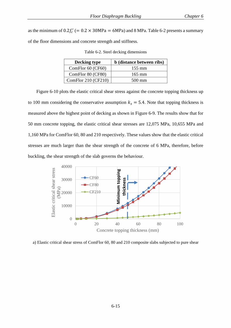
Floor Diaphragm Buckling Chapter 6
6-15
as the minimum of 0.2𝑓𝑐′ (= 0.2 × 30MPa = 6MPa) and 8 MPa. Table 6-2 presents a summary
of the floor dimensions and concrete strength and stiffness.
Table 6-2. Steel decking dimensions
Decking type b (distance between ribs)
ComFlor 60 (CF60) 155 mm
ComFlor 80 (CF80) 165 mm
ComFlor 210 (CF210) 500 mm
Figure 6-10 plots the elastic critical shear stress against the concrete topping thickness up
to 100 mm considering the conservative assumption 𝑘𝑠 = 5.4. Note that topping thickness is
measured above the highest point of decking as shown in Figure 6-9. The results show that for
50 mm concrete topping, the elastic critical shear stresses are 12,075 MPa, 10,655 MPa and
1,160 MPa for ComFlor 60, 80 and 210 respectively. These values show that the elastic critical
stresses are much larger than the shear strength of the concrete of 6 MPa, therefore, before
buckling, the shear strength of the slab governs the behaviour.
a) Elastic critical shear stress of ComFlor 60, 80 and 210 composite slabs subjected to pure shear
0
10000
20000
30000
40000
0 20 40 60 80 100
Ela
stic
cri
tica
l sh
ear
stre
ss
(MP
a)
Concrete topping thickness (mm)
CF60
CF80
CF210
Min
imu
mto
pp
ing
thic
knes
s

Floor Diaphragm Buckling Chapter 6
6-16
b) An enlarged view of Figure 6-10a
Figure 6-10. Elastic critical shear stress of ComFlor 60, 80 and 210 subjected to pure shear
Table 6-3. Elastic critical shear stress (MPa) of ComFlor 60, 80 and 210 subjected to pure shear
CF60 CF80 CF210
Concrete topping
thickness (mm) Critical shear stress (MPa)
1 4.83 4.26 0.46
2 19.32 17.05 1.86
5 120.75 106.56 11.6
50 12075.23 10655.92 1160.43
60 17388.34 15344.53 1671.02
Table 6-3 presents the values of elastic critical shear stress for selected thicknesses. The
underlined values are lower than the shear strength of the concrete. The critical thickness is
between 1 to 2 mm for ComFlor 60 and 80 and it is between 2 to 5 mm for ComFlor 210. It
should be noted that the boundary conditions are considered simply supported and the plate is
assumed infinitely long. Changing these assumptions to clamped edges or rectangular plate
with lower aspect ratio result in higher elastic critical shear stress.
Considering the values in Table 6-3, it can be concluded that the elastic shear buckling
stress is much larger than the concrete shear strength for minimum slab thickness (50 mm).
Therefore the elastic shear buckling will not occur for the inter-rib section of the above-
mentioned composite slabs.
0
20
40
60
80
100
0 10 20 30 40 50
Ela
stic
cri
tica
l sh
ear
stre
ss
(MP
a)
Concrete topping thickness (mm)
CF60
CF80
CF210
Concrete shear strength
Possible buckling region

Floor Diaphragm Buckling Chapter 6
6-17
6.4.1.2 Composite slab subjected to strut forces, (post-cracking condition)
As it was discussed in Chapter 3, (truss modelling) after concrete cracking compression
struts form and the diaphragm imposed forces are transferred by strut and tie mechanism. In
this situation, it could be assumed that in the compression strut zone (between cracks) the
concrete material is still homogeneous. Based on this assumption, the concrete topping element
(between ribs) experiences high axial forces in the direction of the concrete strut. For
investigating the state of the concrete topping in this condition, the axial force is transformed
to a combination of axial and shear stresses as shown in Figure 6-11. The maximum strut axial
force could be found using truss element modelling described in Chapter 3.
The angle of the concrete strut may be any value between 0º and 90º for satisfying the
equilibrium conditions based on the imposed forces to the diaphragm, floor plan dimensions
and location of VLFR systems. In this study, because of using the strut forces from the truss
modelling method, 45º angle for struts is assumed for simplicity.
a) Axial force obtained from the
truss element modelling
b) Mohr’s circle
c) Concrete topping
element between ribs
Figure 6-11. Transforming the axial force from truss element modelling to the axial and shear for the
inter-rib element considering 45º angle between the strut and decking directions
Note that if the steel decking ribs be parallel or perpendicular to the concrete struts as
shown in Figure 6-12, then only 𝑁𝑐𝑟 could be used as critical axial buckling stress.

Floor Diaphragm Buckling Chapter 6
6-18
Figure 6-12. The axial force from truss element modelling used for the inter-rib element buckling
considering the strut and decking directions are parallel
Considering the plate member subjected to axial stress, the solution of the general plate
differential equation, Eq. (6-1), for elastic critical axial stress can be expressed as the following
(Ziemian, 2010):
𝑁𝑐𝑟 = 𝑘𝐸𝜋2
12(1−𝜈2)(𝑏/𝑡)2 Eq. (6-3)
Where 𝑁𝑐𝑟 is the critical axial stress (�̅�𝑥), parameter 𝑘 is the plate buckling coefficient
determined by a theoretical critical-load analysis. This parameter is a function of the plate
geometry and boundary conditions same as 𝑘𝑠. This parameter (𝑘) is plotted against the plate
aspect ratio for different edge support conditions in Figure 6-13. In this plot, the aspect ratio of
the plate is used, considering the width of the plate (𝑏) is perpendicular to the loading direction.

Floor Diaphragm Buckling Chapter 6
6-19
Figure 6-13. Plate buckling coefficient for plates under axial load, β=a/b, m=number of buckled half-
waves along the length of the plate (Yu and Schafer, 2006)
Based on the plots in Figure 6-13, the lowest value of the plate buckling coefficient (𝑘𝑚𝑖𝑛)
when the plate is simply supported along all four edges is 𝑘 = 4. This value can be increased
by considering different aspect ratios. However, in this study, the lowest value is used to obtain
conservative results.
On the other hand, in this case, both the shear and axial stresses are acting on the plate
element simultaneously, therefore the interaction between shear and axial stresses need to be
investigated. Iguchi (1938) suggested the following interaction formula:
(𝜕𝑐
𝑁𝑐𝑟) + (
𝜏𝑐
𝑁𝑥𝑦1)2
≤ 1 Eq. (6-4)

Floor Diaphragm Buckling Chapter 6
6-20
Where 𝑁𝑐𝑟 and 𝑁𝑥𝑦1 denote the critical axial and shear stress capacities, respectively, and
𝜕𝑐 and 𝜏𝑐 represent the imposed axial and shear stress demands. Figure 6-14 plots the Eq. (6-
4).
Figure 6-14. Interaction curve for buckling of flat plates subjected to uniform shear and compression
(Ziemian, 2010)
• Case study
The elastic critical stress for three steel deck sections (ComFlor 60, 80 and 210) are
investigated under the shear and compression stress. The assumptions for material properties
and dimensions are the same as the previous section. It is considered that the plate buckling
coefficient for the axial compression is 𝑘 = 4 to obtain conservative results.
The imposed axial and shear stresses should be extracted from floor diaphragm analysis
results, however, it is known that the shear stress cannot exceed the shear strength of concrete
and also the axial compression stress is limited to concrete strut compression strength. In this
section, the ultimate concrete strength in compression (strut strength) and shear are used as
imposed forces to find out the possibility of inter-rib buckling mode.

Floor Diaphragm Buckling Chapter 6
6-21
The effective compressive strength of a concrete strut can be calculated based on Appendix
A of NZS 3101 (2006) using the following equation:
𝑓𝑐𝑢 = 𝛽𝑠𝛼1𝑓𝑐′ Eq. (6-5)
Where, 𝛽𝑠 is equal to unity when the strut has the same width along its length. This
parameter can get lower values based on the concrete type and geometry of the strut. Using
𝛽𝑠 = 1 gives higher axial strength which turns to more conservative results in the case
considered. The parameter 𝛼1 accounts for equivalent rectangular concrete stress distribution
which can be taken as 0.85 for concrete strengths up to 55 MPa.
The ultimate values of the shear and axial strengths are controlled by concrete failure
mechanism under combined shear an axial stresses. Figure 6-15 shows the shear and axial stress
interaction plot of concrete material which was found by Bresler and Pister (1958). Therefore
the ultimate shear and axial compression that are acting simultaneously on the concrete plate
are lower than the ultimate strength under uniaxial compression or pure shear conditions due
to shear and axial stress interaction.
Figure 6-15. Shear and axial stress interaction plot (material capacity) (Bresler and Pister, 1958)
As a conservative assumption, the ultimate shear and axial compressive strengths of the
concrete material are considered as imposed forces to the plate member without taking into
account the material interaction failure.
The critical elastic buckling interaction values (demand to capacity ratio) using Eq. (6-4)
are presented in Table 6-4 for selected concrete topping thicknesses.

Floor Diaphragm Buckling Chapter 6
6-22
Table 6-4. Interaction values for ComFlor 60, 80 and 210 subjected to shear and uniform compression
(demand to capacity ratio)
CF60 CF80 CF210
Concrete topping
thickness (mm)
Interaction values
(DCR)
1 8.70 10.09 244.54
2 1.88 2.15 29.12
3 0.81 0.92 10.34
4 0.45 0.51 5.30
5 0.28 0.32 3.24
10 0.07 0.08 0.76
20 0.01 0.02 0.18
30 0.008 0.009 0.08
40 0.004 0.005 0.04
50 0.003 0.003 0.03
60 0.002 0.002 0.02
70 0.001 0.002 0.01
80 0.001 0.001 0.01
90 0.001 0.001 0.009
Note: 𝐷𝐶𝑅 = (𝜕𝑐
𝑁𝑐𝑟) + (
𝜏𝑐
𝑁𝑥𝑦1)2
and
𝐷𝐶𝑅 < 1 → 𝑠𝑎𝑓𝑒 𝑧𝑜𝑛𝑒
As it is shown in this Table, when DCR is less than unity means the buckling criteria does
not govern. The critical thickness for ComFlor 60 and 80 is between 2 and 3 mm and it is about
9 mm for ComFlor 210. It should be noted that the boundary conditions are considered simply
supported and the lowest buckling coefficient is used. Changing these assumptions to clamped
edges or rectangular plate with lower aspect ratio result in lower DCR values.
Considering the values in Table 6-4, it can be concluded that the elastic buckling strength
under a combination of axial and shear stresses is much larger than the concrete strength for
minimum slab thickness (50 mm). Therefore, buckling will not occur for the inter-rib section
of the above-mentioned floor slabs subjected to strut forces. Any other floor slab section with
different cross-section and geometry can also be investigated using the presented equations.

Floor Diaphragm Buckling Chapter 6
6-23
6.4.2 Buckling mode 2, intra-panel buckling
Another buckling mode that may occur in the composite floor slabs is “intra-panel
buckling”. In this buckling mode, the composite slab in the panel between the secondary beams
is considered to experience instability under the in-plane imposed forces and the secondary
beams act as nodal lines for the panels.
The intra-panel buckling mode was also investigated in pre and post-cracking stages of the
concrete. This is because, the concrete can crack at low tension stresses, therefore the state of
the pure shear can change to diagonal compression due to concrete strut formation after the
cracking. Figure 6-16 shows the intra-panel subjected to pure shear (pre-crack) and
compression strut force (post-crack) conditions.
a) Intra-panel subject to pure shear, (pre-crack)
b) Intra-panel subject to diagonal strut forces,
(post-crack)

Floor Diaphragm Buckling Chapter 6
6-24
c) Intra-panel cross-section
Figure 6-16. Intra-panel loading conditions
The composite floor slab is not a flat plate member because of the ribs shown in Figure
6-16. The ribs stiffen the concrete topping. Therefore, this situation is more complicated than
the buckling of a simple uniform plate.
There are two methods for finding the critical buckling loads of such stiffened plate
member,
1) analytical approach and
2) FEM modelling.
It is obvious that using FEM would be easier and in some cases more precise because, in
numerical investigations, imperfections, realistic boundary conditions and also residual
stresses could be included in the model. However, the disadvantage of FEM modelling is that
the numerical study is limited to a number of models and limited results. However, the
analytical method is more difficult to obtain due to mathematical works, but the results are
more general and the upper and lower limits could be investigated more easily. Using the
analytical approach, a general method for investigating any other case could be developed. In
this section, the critical buckling loads are investigated analytically and the results are verified
with the FEM models.
Investigating the critical buckling load of the intra-panel subjected to non-uniform loads
and different loading conditions is complicated. Also, the nature of imposed loads are not fully
known, therefore in this study two loading scenarios are investigated include

Floor Diaphragm Buckling Chapter 6
6-25
1) the intra-panel subjected to uniform pure shear stress (pre-cracking) and
2) the intra-panel subjected to diagonal compression (strut force) after concrete cracking.
6.4.2.1 Intra-panel subjected to uniform shear stress (pre-cracking)
The critical buckling load of the intra-panel zone is investigated by studying the buckling
behaviour of the equivalent orthotropic plate member. In the next sections, the method for
finding an equivalent orthotropic plate and the critical buckling load of the orthotropic plate is
discussed.
• Equivalent orthotropic plate
The composite floor slab is like a plate member that is stiffened by ribs. Generally, the
stiffened plate members have been used in civil, marine, aerospace and lots of other
engineering fields. Steel bridges, ship and aeroplane structure are the examples of using
stiffened plate elements. Since decreasing the structure weight was and is the most important
parameter in design especially for marine and aerospace applications, the buckling
phenomenon and stability was the main concern in these elements. Investigating the critical
buckling load of stiffened plates was in the focus of researchers during the 1940s and 1950s
(e.g. Wittrick 1954, Seide and Stein 1949, Seide 1953).
Generally, an orthotropic plate is defined as a plate member that has different elastic
material properties in two perpendicular directions. The orthotropic plate theory has the same
assumptions as the isotropic plate theory, include:
1. The plate material is homogenous and also continuous between outer surfaces of
the plate.
2. The plate thickness is uniform and is small compared to the other plate dimensions.
3. The plate material is in accordance with Hooke’s law.
4. The plate deformations are small compared to plate thickness.

Floor Diaphragm Buckling Chapter 6
6-26
It should be considered that the composite slab differs in several aspects from an ideal
orthotropic plate. The most important difference is that the composite slab is not continuous
which means the material does not fill the space between outer plate surfaces (between ribs).
Also, unlike the ideal orthotropic plate, the different rigidities in two perpendicular directions
come from different geometric properties rather than from difference in material properties.
Also, due to eccentric arrangements of ribs, the neutral surfaces for bending in two directions
do not coincide (Figure 6-17).
Although the actual structural behaviour of the composite floor slab cannot be exactly
replaced with an orthotropic plate, this method has been used in other engineering fields like
marine and aerospace and past experimental results indicated good agreement between this
idealisation and the real stiffened plate.
a) Composite slab schematic view
b) Equivalent orthotropic plate
Figure 6-17. Neutral surfaces in composite slab and equivalent orthotropic plate
To obtain an equivalent orthotropic plate for the composite slab, two conditions need to
be satisfied

Floor Diaphragm Buckling Chapter 6
6-27
1) the stiffness of the composite slab and the equivalent orthotropic plate need to be equal
and
2) the stresses in the equivalent orthotropic plate and the composite slab need to be equal.
The thickness of the equivalent orthotropic plate, and the elastic modulus and Poisson’s
ratio of both perpendicular directions (𝐸𝑥, 𝐸𝑦 , 𝜗𝑥 𝑎𝑛𝑑 𝜈𝑦) need to be obtained to satisfy these
conditions.
The flexural stiffness of the composite floor (that is equal to the equivalent orthotropic
plate) is required to calculate the critical buckling loads using orthotropic plate theory.
For an isotropic plate the flexural rigidity can be calculated using:
𝐷 =𝐸𝑡3
12(1−𝜈2)
Where 𝑡 is the plate thickness and 𝐸 and 𝜈 are the elastic modulus and Poisson’s ratio of
the slab material respectively. Similar to the beam theory, the flexural moment (𝑚𝑥) is equal
to flexural stiffness (𝐷) multiplied by the plate curvature (𝜕2𝑤
𝜕𝑥2+ 𝜈
𝜕2𝑤
𝜕𝑦2).
𝑚𝑥 = −𝐷 (𝜕2𝑤
𝜕𝑥2+ 𝜈
𝜕2𝑤
𝜕𝑦2) Eq. (6-6)
𝑚𝑦 = −𝐷 (𝜕2𝑤
𝜕𝑦2+ 𝜈
𝜕2𝑤
𝜕𝑥2) Eq. (6-7)
𝑚𝑥𝑦 = −2𝐵 (𝜕2𝑤
𝜕𝑥𝜕𝑦) Eq. (6-8)
For simplicity in finding the flexural rigidities of the composite slab, a long simply
supported slab is assumed. In this case the curvature in the direction perpendicular to the
direction under study (𝜈𝜕2𝑤
𝜕𝑦2 or 𝜈
𝜕2𝑤
𝜕𝑥2) could be considered equal to zero. Therefore the Eqs. (6-
6) and (6-7) change to Eqs. (6-9) and (6-10) respectively:
𝑚𝑥 = −𝐷𝑥 (𝑑2𝑤
𝑑𝑥2) Eq. (6-9)

Floor Diaphragm Buckling Chapter 6
6-28
𝑚𝑦 = −𝐷𝑦 (𝑑2𝑤
𝑑𝑦2) Eq. (6-10)
Where 𝐷𝑥 and 𝐷𝑦 could be found using cross-section properties of the composite slab. The
flexural stiffness of the composite slab in the Y direction (𝐷𝑦), which includes the concrete
topping and the ribs cross-section, could be found using the parallel axis theorem. The only
difference is that the plate part (concrete topping) should be divided by (1 − 𝜈2) for
considering the plate action. Eq. (6-11) shows the flexural stiffness of the composite slab in the
Y direction. The first bracket in this equation relates to zone 1 and the second bracket relates
to zone 2, shown in Figure 6-18.
𝐷𝑦 = [𝐸𝑡3
12(1−𝜈2)+
𝐸𝑡𝑒𝑦2
(1−𝜈2)]1+ [
𝐸𝑎ℎ3
12(𝑎+𝑏)+𝐸ℎ𝑎(
ℎ
2+𝑡
2−𝑒𝑦)
2
(𝑎+𝑏)]
2
Eq. (6-11)
Where 𝐸 and 𝜈 are the elastic modulus and Poisson’s ratio of the concrete material
respectively. Other parameters are shown in Figure 6-18. It should be noted that 𝑒𝑦 is the
distance between the neutral axis and mid-height of the concrete topping.
Figure 6-18. Composite slab cross-section
The flexural stiffness in the X direction, 𝐷𝑥, could not be found simply using cross-
sectional properties because the thickness of the composite slab is not uniform in this direction
and it changes between the ribs and concrete topping. Therefore the problem can be solved
assuming series of flexural springs (ribs and concrete topping). Considering that the concrete
topping and the ribs are acting as a flexural spring, the total stiffness of the composite slab can
be found using Eq. (6-12). Where 𝐷𝑎 and 𝐷𝑏 are the flexural stiffness of one rib and one
concrete topping respectively as shown in Figure 6-19.

Floor Diaphragm Buckling Chapter 6
6-29
Figure 6-19. Flexural stiffness in the X direction, 𝐷𝑥, ribs and concrete topping are considered as
series of springs
However, since the thickness changes suddenly from the concrete topping to the ribs, and
also the ribs are not eccentric with concrete topping, a part of the ribs flexural stiffness
contribute in the total slab stiffness as shown in Figure 6-20.
𝐷𝑥 =𝐷𝑎𝐷𝑏(𝑎+𝑏)
(𝑏𝐷𝑎+𝑎𝐷𝑏) Eq. (6-12)
Figure 6-20. Effective height of the ribs contributing to the plate flexural stiffness
To address this issue, the parameter 𝛽 (ribs height modification factor) is introduced for
adjusting the ribs height to calculate the effective thickness of the ribs that contribute in the
flexural stiffness of the slab (Eqs. (6-13) and (6-14)).
𝐷𝑎 =𝐸(𝑡+𝛽ℎ)3
12(1−𝜈2) Eq. (6-13)
𝐷𝑏 =𝐸𝑡3
12(1−𝜈2) Eq. (6-14)
In this study, 𝛽 is found using a comprehensive FEM parametric study. A series of FEM
models with different dimensions are created and the flexural stiffness of the models are

Floor Diaphragm Buckling Chapter 6
6-30
recorded. Then the parameter 𝛽 is obtained by adjusting the FEM stiffness and the calculated
stiffness using Eq. (6-12).
Models included a 20×3m panel which was loaded with uniform moment along the 20m
long edge. The concrete topping thickness, ribs dimensions and the distance between ribs for
different models are presented in Table 6-5.
Table 6-5. Concrete topping thickness, ribs dimensions and distance for the studied models
t
(mm)
a
(mm)
b
(mm)
h
(mm)
b/a h/a Dx FEM
(N.mm/mm)
β
50 100 20 20 0.2 0.2 3.63E+09 0.5381
50 100 20 50 0.2 0.5 3.86E+09 0.2495
50 100 20 100 0.2 1 3.88E+09 0.1263
50 100 20 200 0.2 2 3.89E+09 0.0636 50 100 50 20 0.5 0.2 3.24E+09 0.5319
50 100 50 50 0.5 0.5 3.44E+09 0.2615
50 100 50 100 0.5 1 3.49E+09 0.1365
50 100 50 200 0.5 2 3.5E+09 0.0692 25 100 50 20 0.5 0.2 5.08E+08 0.5313
25 100 50 50 0.5 0.5 5.47E+08 0.2603
25 100 50 100 0.5 1 5.54E+08 0.1344
25 100 50 200 0.5 2 5.56E+08 0.0680 25 50 50 10 1 0.2 3.65E+08 0.5155
25 50 50 25 1 0.5 3.79E+08 0.2521
25 50 50 50 1 1 3.82E+08 0.1311
25 50 50 100 1 2 3.83E+08 0.0665 50 100 200 5 2 0.05 2.46E+09 0.7996
50 100 200 10 2 0.1 2.57E+09 0.6978
50 100 200 15 2 0.15 2.64E+09 0.6150
50 100 200 25 2 0.25 2.71E+09 0.4627
50 100 200 30 2 0.3 2.72E+09 0.3980
50 100 200 35 2 0.35 2.73E+09 0.3507
50 100 200 40 2 0.4 2.73E+09 0.3080
50 100 200 75 2 0.75 2.73E+09 0.1667
50 100 200 100 2 1 2.74E+09 0.1256
50 100 200 150 2 1.5 2.74E+09 0.0839
𝐸 = 200 𝐺𝑃𝑎,𝜈 = 0.3
The results show that the parameter 𝛽 is directly related to the ribs aspect ratio (ℎ/𝑎) and
other parameters such as 𝑏/𝑎 did not have any significant effect. Figure 6-21 plots 𝛽 against
the rib aspect ratio (ℎ/𝑎). In order to find an equation that fits best to the plot, the curve is

Floor Diaphragm Buckling Chapter 6
6-31
divided in two parts for ℎ/𝑎 values less than 0.4 and greater than 0.4. Eq. (6-15) shows the
relationship between 𝛽 and the rib aspect ratio.
{𝛽 = 0.9224𝑒(
−2.756ℎ
𝑎)
𝛽 =𝑎
8ℎ
𝑓𝑜𝑟
ℎ
𝑎≤ 0.4 (a)
𝑓𝑜𝑟 ℎ
𝑎> 0.4 (b)
Eq. (6-15)
Alternatively, the following equation could be used for ℎ
𝑎> 0.1.
𝛽 = 0.136𝑒(−0.745ℎ
𝑎) 𝑓𝑜𝑟
ℎ
𝑎> 0.1 Eq. (6-16)
a) Eq. (6-15) plot
b) Eq. (6-16) plot
Figure 6-21. Parameter β against rib aspect ratio
0
0.1
0.2
0.3
0.4
0.5
0.6
0.7
0.8
0.9
0 0.5 1 1.5 2 2.5
β
h/a
Eq. (6-15a)
Eq. (6-15b)
𝛽 =𝑎
8ℎ
𝛽 = 0.9224𝑒(−2.756ℎ
𝑎)
0
0.2
0.4
0.6
0.8
1
1.2
1.4
0 0.5 1 1.5 2 2.5
β
h/a
Eq. (6-16)
𝛽 = 0.136𝑒(−0.745ℎ
𝑎)

Floor Diaphragm Buckling Chapter 6
6-32
• Verification of plate stiffness equations with FEM models
Two steel deck sections (ComFlor 60 and 80) are modelled to check the accuracy of the
flexural rigidity equations presented in the previous section. The geometry of the ComFlor steel
deck sections are shown in Figure 6-9. Table 6-6 presents the flexural rigidity of the FEM
models and the calculated values using Eqs. (6-11) and (6-12).
Table 6-6. Flexural stiffness of steel deck sections
Flexural rigidities
ComFlor 80
a=135mm,
b=165mm,
h=80mm,
t=50mm,
Error (%)
ComFlor 60
a=145mm,
b=155mm,
h=60mm,
t=50mm,
Error (%)
𝑫𝒙 (N.mm) FEM 375187359.2
2.04 389578768
1.61 Eq. (6-12) 367533583.7 383277897.1
𝐿1 = 20𝑚, 𝐿2 = 4𝑚, 𝐸 = 25 𝐺𝑃𝑎, 𝜈 = 0.2
𝑫𝒚 (N.mm) FEM 2932455769
2.32 1861889197
1.94 Eq. (6-11) 3000582869 1898051939
𝐿1 = 6𝑚, 𝐿2 = 4𝑚, 𝐸 = 25 𝐺𝑃𝑎, 𝜈 = 0.2
The results show that the differences in the stiffness values were less than 2.5%. It should
be noted that the FEM modelling parameters such as mesh size, element type and also
numerical error could also have some share in this error.
• Torsional stiffness of the orthotropic plate
The torsional stiffness of the orthotropic plate is another parameter that is needed for
calculating the critical elastic buckling load. Generally, the torsional rigidity is more difficult
to obtain and usually it is calculated with a reasonable approximation. The torsional stiffness
of two-way reinforced concrete slab of uniform thickness could be obtained using Eq. (6-17)
(Szilard, 1974).
𝐵 = √𝐷𝑥𝐷𝑦 Eq. (6-17)
To calculate the torsional stiffness of the composite slabs, the ribs and the slab are
considered separately in Eq. (6-18) (Szilard, 1974).

Floor Diaphragm Buckling Chapter 6
6-33
𝐵 =𝐸𝑡3
12(1−𝜈2)+𝐺𝑥𝑦
2
ℎ𝑎3𝜂
(𝑎+𝑏)𝑘𝐵 Eq. (6-18)
Where 𝐺𝑥𝑦 is the concrete shear modulus and 𝜂 is a numerical factor depending on the ribs
aspect ratios which is presented in Table 6-7. The parameter 𝑘𝐵 is a reduction factor accounting
for the decrease in the torsional stiffness of the reinforced concrete beams due to concrete
cracking. This parameter relates to ribs aspect ratio, reinforcement and also applied bending
moment to the member (Szilard, 1974). In this study 𝑘𝐵 is taken as zero conservatively.
Table 6-7. Parameter η (Szilard, 1974)
𝒂/𝒉 1 1.2 1.5 2 2.5 3 4 6 8 10 ∞
𝜼 0.140 0.166 0.196 0.229 0.249 0.263 0.281 0.299 0.307 0.313 0.333
• Buckling of an orthotropic plate
The critical elastic buckling load of the composite slab (between secondary beams) is
investigated using the plate flexural stiffness found in the previous section. Generally,
investigating the buckling behaviour of an intra-panel section is more complicated than the
inter-rib (local) buckling of the concrete topping. This complexity is due to the fact that
1) the intra-panel usually is subjected to a combination of different stresses,
2) boundary conditions might vary from simply supported to fully clamped and
3) the imposed forces to the panel usually are not uniform.
In this research, it is assumed that the governing in-plane imposed force to the diaphragm
is in the form of shear stress coming from transfer forces. For simplicity, it is assumed that
these shear forces are applied uniformly to the floor slab edges. And for obtaining more
conservative results, all edges are considered simply supported.
Equation (6-19) presents the general governing differential equation of elastic stability for
an orthogonal plate. This equation is similar to Eq. (6-1) for isotropic plates and only the
flexural stiffness are different. With solving this differential equation for various boundary
conditions and loading patterns, the critical buckling load �̅�, can be calculated. For solving the

Floor Diaphragm Buckling Chapter 6
6-34
differential equation Eq. (6-19) the in-plane stresses, �̅�𝑥0, �̅�𝑦0 and �̅�𝑥𝑦0, are applied singly or
in a certain combination.
𝐷𝑥𝜕4𝑤
𝜕𝑥4+ 2B
𝜕4𝑤
𝜕𝑥2𝜕𝑦2+ 𝐷𝑦
𝜕4𝑤
𝜕𝑦4= (�̅�𝑥0
𝜕2𝑤
𝜕𝑥2+ 2�̅�𝑥𝑦0
𝜕2𝑤
𝜕𝑥 𝜕𝑦+ �̅�𝑦0
𝜕2𝑤
𝜕𝑦2) Eq. (6-19)
Where �̅�𝑥0, �̅�𝑦0 and �̅�𝑥𝑦0 are the axial and shear in-plane stresses applied at the
boundaries of the middle surface of the orthotropic plate, and 𝐷𝑥, 𝐷𝑦 and B are the orthotropic
plate flexural stiffness in 𝑥 and 𝑦 directions and the torsional rigidity, respectively.
Considering the intra-panel member subjected to the pure shear (�̅�𝑥0 = �̅�𝑦0 = 0) stress,
the solution of the differential equation (Ziemian, 2010) for the elastic critical shear stress
(buckling stress) is expressed as Eq. (6-20):
𝑁𝑥𝑦2 = 𝐾𝑠𝜋2
𝑡𝐿22 √𝐷𝑥𝐷𝑦
34 Eq. (6-20)
Where 𝑁𝑥𝑦2 is the elastic critical shear stress for the intra-panel zone, 𝐷𝑥 and 𝐷𝑦 are the
orthotropic plate stiffness, and 𝐿2 is the length perpendicular to X-axis as shown in Figure 6-17.
The parameter 𝐾𝑠 is the plate buckling coefficient determined by a theoretical critical-load
analysis. This parameter is a function of plate geometry and boundary conditions. The
parameter 𝐾𝑠 is plotted for three edge support conditions in Figure 6-22 (Ziemian, 2010). In
these plots 𝐷1, 𝐷2 and 𝐷3 are 𝐷𝑥, 𝐷𝑦 and 𝐵 respectively.
a) All edges simply supported

Floor Diaphragm Buckling Chapter 6
6-35
b) Edges perpendicular to y-axis clamped, other edges simply supported
c) All edges clamped
Figure 6-22. Shear buckling coefficient for orthotropic plates (Ziemian, 2010), as adapted from Johns
and Kirkpatrick (1971)
Based on the orthotropic plate stiffness, the parameter 𝐾𝑠 can be extracted from the plots
presented in Figure 6-22. It is noted that in this study all the boundary conditions are considered
as simply supported, so Figure 6-22a is used, to obtain conservative results.
• Case study
The intra-panel elastic shear buckling for two ComFlor profiles (60 and 80), shown in
Figure 6-9, is investigated both using Eq. (6-20) and the FEM model. Two floor slabs were
designed using ComFlor Steel Composite Metal Deck Design software and they are used for
the buckling study.
The gravity loads used for the design of ComFlor floor slabs include: 3 kPa imposed action
(Q), 1 kPa for ceiling/services and finishes, 1 kPa for partitions, and self-weight of the floor

Floor Diaphragm Buckling Chapter 6
6-36
slab (G) was calculated by the software based on the slab thickness and the steel decking
weight. It is assumed that the concrete compressive strength is 30 MPa with an elastic modulus
of 25 GPa. It was tried to find the maximum possible span with 60 mm concrete topping for
both ComFlor 60 and 80 steel decks. Figure 6-23 shows the assumptions and parameters used
for design. The full design reports are presented in Appendix I.
a) ComFlor 60, 4.4 m span, propped during
construction
b) ComFlor 60, steel deck thickness 1.2 mm
c) ComFlor 80, 5.1 m span, propped during
construction
d) ComFlor 80, steel deck thickness 1.2 mm
Figure 6-23. ComFlor 60 and 80 with 60 mm concrete topping (ComFlor software)
The critical buckling loads of the floor slabs are studied with and without considering
the stiffness reduction factor accounting for concrete cracking due to flexural moments.
The stiffness reduction factor of 0.35 is selected based on Table C6.5 NZS3101 (2006) for
members subjected to bending moments. Although the elastic shear buckling here is based
on the assumption that the concrete is un-cracked, the cracking reduction factor is just
considered for decreasing the bending rigidity which yields to lower buckling loads and
gives more conservative result considering the tension behaviour of the concrete material.
Table 6-8 shows the results of critical shear stress using Eq. (6-20) for a 5 m long panel
and also an infinite length panel, and widths, 𝐿2, of 4.4m and 5m.

Floor Diaphragm Buckling Chapter 6
6-37
Table 6-8. Critical edge shear stress for ComFlor 60 and 80 with 60 mm topping (𝑓𝑐′ = 30 𝑀𝑃𝑎, 𝐸𝑐 =
25 𝐺𝑃𝑎 and decking thickness 1.2mm)
ComFlor 60 ComFlor 80
𝐿2 = 4.4 𝑚 𝐿2 = 5.1 𝑚
Total slab thickness =120 mm Total slab thickness =140
mm
𝑁𝑥𝑦2 (MPa)
Total Elastic 𝐿1 = 5 𝑚 101.7 93.5
𝐿1 → ∞ 80.8 73.9
Considering
stiffness
reduction
factors
𝐿1 = 5 𝑚 35.6 33.8
𝐿1 → ∞ 28.3 26.9
To verify the results obtained using the analytical approach, the FEM modelling is used.
Two ComFlor profiles (60 and 80) with 5m long are modelled in ABAQUS software. The
material was considered to be elastic with 25 GPa elastic modulus and 0.2 Poisson’s ratio. The
intra-panel was subjected to pure shear loading and the shear forces and the corresponding
shear displacement were recorded during the analysis.
As it was mentioned before, the plate buckling occurs by gradual distortion of the cross-
section of the member. Therefore, for finding the buckling load, the models are analysed with
and without geometric nonlinearity. The shear force-displacement of a model is shown in
Figure 6-24 schematically. Where 𝐹𝐸 is the analysis without the geometric nonlinearity and
𝐹𝑁𝐺 is the force-displacement plot considering the geometric nonlinearity. In this study, the
buckling load is defined at the point where the difference between these two plots (𝐹𝐸 − 𝐹𝑁𝐺)
becomes more than 1% of the corresponding 𝐹𝐸 value.

Floor Diaphragm Buckling Chapter 6
6-38
Figure 6-24. Shear force-displacement plot of a diaphragm with and without considering geometric
nonlinearity
Figure 6-25 and Figure 6-26 show the FEM model and the floor slab deformed shape at
the buckling step of the analysis and the recorded shear force-displacement.
a) FEM model of ComFlor 60
b) Out-of-plane displacement of the panel
(displacement contour)
c) Shear force-displacement plot for ComFlor 60
Figure 6-25. FEM model of ComFlor 60 subjected to a pure shear condition
0
50
100
150
200
250
300
0 20 40 60
Sh
ear
Str
ess
(MP
a)
Shear dispalcement (mm)
Elastic without geometric nonlinearityElastic with geometric nonlinearity

Floor Diaphragm Buckling Chapter 6
6-39
a) FEM model of ComFlor 80
b) Out-of-plane displacement of the panel
(displacement contour)
c) Shear force-displacement plot for ComFlor 80
Figure 6-26. FEM model of ComFlor 80 subjected to a pure shear condition
Each model was analysed two times with considering the geometric nonlinearity and
without the geometric nonlinearity to find the critical buckling load. Based on these plots, the
buckling stresses for ComFlor 60 and 80 are found 97.9 MPa and 95.1 MPa respectively. These
are similar to the values from Eq. (6-20) given in Table 6-8 of 101.7 MPa and 93.5 MPa with
errors being 3.7% and -1.8% respectively.
The results show that the analytical approach is able to estimate the critical buckling load
reasonably compared to FEM models. In the next step, these critical buckling loads are
compared with the ultimate shear strength of the panel to find out the possibility of the shear
buckling for the studied intra-panels.
0
50
100
150
200
250
300
0 20 40 60
Shea
r S
tres
s (M
Pa)
Shear dispalcement (mm)
Elastic without geometric nonlinearity
Elastic with geometric nonlinearity

Floor Diaphragm Buckling Chapter 6
6-40
• Slab shear strength
The shear strength of the composite slabs can be calculated using the equation provided
by NZS3404 (2007) Clause 13.4.10.2.
𝑉𝑟 = min {(0.8∅𝐴𝑟𝑡𝑓𝑦𝑟 + 2.76∅𝑐𝐴𝑐𝑣)
0.5∅𝑐𝑓𝑐′𝐴𝑐𝑣
Eq. (6-21)
Where 𝐴𝑟𝑡 is the area of transverse reinforcements crossing shear planes, 𝐴𝑐𝑣 is the area
of concrete in shear planes and 𝑓𝑦𝑟 is the yield stress of tension reinforcement. The reduction
factors ∅ and ∅𝑐 are equal to 0.9 and 0.6 respectively. Here the upper bond value of this formula
(0.5∅𝑐𝑓𝑐′𝐴𝑐𝑣) is considered as the shear strength of the composite slabs. The calculated shear
strength values and the critical shear buckling loads for the infinitely long panel considering
stiffness reduction factors are presented in Table 6-9.
Table 6-9. Calculated shear strength and the critical shear buckling loads for infinitely long ComFlor
60 and 80
ComFlor 60 ComFlor 80
Shear stress (MPa)
𝐿2 = 4.4 𝑚 𝐿2 = 5.1 𝑚
critical shear buckling
stress (Eq. (6-20)) 28.2 26.9
shear strength (𝟎. 𝟓∅𝒄𝒇𝒄′ ) 9 9
The results show that the elastic shear buckling loads are about three times the upper bound
shear strength of the composite slab. Therefore, it can be concluded that the elastic shear
buckling does not govern in the studied cases. The critical shear buckling capacity of any other
type of floor slab can be investigated using Eq. (6-20) and the orthotropic plate stiffness
formulations (Eqs. (6-11) to (6-18)).
6.4.2.2 Intra-panel subjected to diagonal force (strut force), post-cracking stage
• Theoretical development
After crack formation in the concrete of the composite slab, the stress distribution changes
and concrete compression struts form and the diaphragm imposed forces are transferred by a

Floor Diaphragm Buckling Chapter 6
6-41
strut-and-tie mechanism. The compression struts that are formed between secondary beams
(i.e. within the panel) may experience instability under high axial loads. In this section, the
critical compressive buckling load of a strut in the intra-panel zone is investigated.
The ribs in composite slab act as stiffeners for the concrete topping and also support the
gravity forces. When the panel is subjected to in-plane shear forces, concrete strut forces are
carried by the concrete topping because the ribs are not continuous. Here, the ribs provide out-
of-plane restraint for the concrete struts as shown in Figure 6-27.
Figure 6-27. Concrete strut in the topping and the ribs acting as lateral supports
The angle of the concrete strut may be between 0º and 90º for satisfying the equilibrium
conditions based on the imposed forces to the diaphragm, floor plan dimensions, and location
of VLFR systems. In this study, it is assumed the struts are formed at a 45º angle for simplicity.
Within a panel, a number of struts form diagonally in the concrete topping between cracks. The
ribs, provided at a specific spacing provide lateral support for a number of compression struts
as shown in Figure 6-28.

Floor Diaphragm Buckling Chapter 6
6-42
Figure 6-28. Schematic view of ribs and struts in an intra-panel
Considering this situation, the strut buckling model can be considered as a compression
member that is supported by some rotational and translational springs at the intersection
locations with ribs as shown in Figure 6-29. Which the stiffnesses and degrees of freedom of
these springs are related to each other as it forms a mesh type system. Also, from Figure 6-28
it can be found that the degree of freedoms of each strut has a symmetry with respect to the
strut mid-point due to the repetitive nature of the problem.
Figure 6-29. Compression strut supported with a number of rotational and translational springs

Floor Diaphragm Buckling Chapter 6
6-43
Part of the rotational stiffness provided for the struts is due to the torsional stiffness of the
ribs (due to the angle between the struts and the ribs). The rotational DOFs are considered to
be pinned for simplicity in the models described here thereby ignoring this effect.
By looking at only one strut and one rib, it can be found that the out-of-plane deformation
of each strut corresponds to each rib as shown in Figure 6-30a. Therefore, the buckling problem
here consists of the buckling of a compression member that has deformation compatibility with
other flexural members with different stiffnesses (due to the location of rib intersection) at
different locations along the strut length as shown in Figure 6-30b.
a) Out-of-plane deformation compatibility of struts and ribs
b) Buckling of the strut considering deformation compatibility with the rib
Figure 6-30. Deformation compatibility of struts and ribs

Floor Diaphragm Buckling Chapter 6
6-44
The limitations and assumptions of this buckling model include:
1. It is assumed the distance between the ribs and struts are equal and the rib and strut
widths are infinitely small.
2. The effect of concrete topping reinforcement is not considered.
3. Each strut is considered separated from the neighbour strut because of the cracks.
4. The connections between the struts and the ribs are considered as pinned
connections.
5. The panel length is considered infinite.
6. The depth of the rib is assumed to be the full slab depth including topping and the
rib height. The breadth is the average through widths as shown in Figure 6-27.
To solve this problem the X-Y coordinate is selected for the strut and V-W coordinate is
used for the rib to derive the mathematical equations. As shown in Figure 6-31, the
compatibility force 𝑓(𝑥) is acting on the strut from the rib and 𝑔(𝑣) is the reaction of the 𝑓(𝑥)
that is acting against the rib. Therefore, from equilibrium, the total applied force to the rib and
the strut must be equal:
∫ 𝑓(𝑥)𝑑𝑥𝐿𝑠
0= ∫ 𝑔(𝑣)𝑑𝑣
𝐿2
0 Eq. (6-22)
Figure 6-31. Compatibility forces between the strut and rib (f(x) and g(v))

Floor Diaphragm Buckling Chapter 6
6-45
Considering the geometry of the problem, the rib length is equal to 𝐿𝑠 𝑠𝑖𝑛 𝛼, where 𝛼 is
the angle between the rib and the strut as shown in Figure 6-27 and Figure 6-28. Since the out-
of-plane displacements of any point on a rib (𝑤(𝑣)) is equal to the corresponding point on the
strut (𝑦(𝑥)):
𝑦(𝑥) = 𝑤(𝑣) Eq. (6-23)
According to Figure 6-31:
𝑥
𝐿𝑠=
𝑣
𝐿2 Eq. (6-24)
And taking the derivative of Eq. (6-24) gives
𝑑𝑣 =𝐿2
𝐿𝑠 𝑑𝑥 Eq. (6-25)
Substitution of Eqs. (6-24) and (6-25) into Eq. (6-22) leads to finding the relationship
between 𝑓(𝑥) and 𝑔(𝑣)
∫ 𝑓(𝑥)𝑑𝑥𝐿𝑠
0= ∫ 𝑔 (
𝑥𝐿2
𝐿𝑠)𝐿2
𝐿𝑠 𝑑𝑥
𝐿s
0
𝑓(𝑥) = 𝑔(𝑣)𝐿2
𝐿𝑠 Eq. (6-25a)
Figure 6-32 shows the free body diagram of the rib and strut considering the imposed axial
force to the strut. The equilibrium equations for each strut and rib are:
−𝐸𝐼𝑠𝑑2𝑦
𝑑𝑥2− 𝑃𝑦 + ∫𝑥𝑓(𝑥)𝑑𝑥 + 𝑥𝑉𝑠 = 0 Eq. (6-26)
−𝐸𝐼𝑟𝑑2𝑤
𝑑𝑣2− ∫𝑣𝑔(𝑣)𝑑𝑣 − 𝑣𝑉𝑟 = 0 Eq. (6-27)

Floor Diaphragm Buckling Chapter 6
6-46
Figure 6-32. Free body diagram of strut and rib
For combining these two equilibrium equations, the relationships between ∫ 𝑣𝑔(𝑣)𝑑𝑣 and
∫𝑥𝑓(𝑥) 𝑑𝑥, 𝑑2𝑤
𝑑𝑣2 and
𝑑2𝑦
𝑑𝑥2 need to be found. By substituting Eqs. (6-23) and (6-24) into
∫𝑣𝑔(𝑣)𝑑𝑣, leads to:
∫𝑣𝑔(𝑣)𝑑𝑣 = ∫ (𝑥𝐿2
𝐿𝑠) (
𝐿s
𝐿2𝑓(𝑥))
𝐿2
𝐿𝑠 𝑑𝑥
∫𝑣𝑔(𝑣)𝑑𝑣 =𝐿2
𝐿𝑠∫𝑥𝑓(𝑥) 𝑑𝑥 Eq. (6-28)
Note 𝑉𝑟 = 𝑉𝑠, because 𝑓(𝑥) = 𝑔(𝑣)𝐿2
𝐿𝑠 and 𝑥 =
𝐿𝑠
𝐿2𝑣, therefore:
∫𝑣𝑔(𝑣)𝑑𝑣 + 𝑣𝑉𝑟 =𝐿2
𝐿𝑠(∫ 𝑥𝑓(𝑥)𝑑𝑥 + 𝑥𝑉𝑠) Eq. (6-29)
The relationships between 𝑑2𝑤
𝑑𝑣2 and
𝑑2𝑦
𝑑𝑥2 could be found by taking the second derivative of
𝑤 with respect to 𝑣 and using the chain rule as the following:
𝑑𝑤
𝑑𝑣=
𝑑𝑤
𝑑𝑥
𝑑𝑥
𝑑𝑣=
𝑑𝑤
𝑑𝑥
𝐿𝑠
𝐿2
𝑑
𝑑𝑣(𝑑𝑤
𝑑𝑥
𝐿𝑠
𝐿2) =
𝑑
𝑑𝑥(𝑑𝑤
𝑑𝑥
𝐿𝑠
𝐿2)𝑑𝑥
𝑑𝑣=
𝑑2𝑤
𝑑𝑥2(𝐿𝑠
𝐿2)2
𝑑2𝑤
𝑑𝑣2=
𝑑2𝑤
𝑑𝑥2(𝐿𝑠
𝐿2)2
=𝑑2𝑦
𝑑𝑥2(𝐿𝑠
𝐿2)2
Eq. (6-30)

Floor Diaphragm Buckling Chapter 6
6-47
Substitution of Eq. (6-29) and (6-30) into the equilibrium equation of the rib (Eq. (6-27))
leads to:
−𝐿𝑠
𝐿2𝐸𝐼𝑟
𝑑2𝑦
𝑑𝑥2(𝐿𝑠
𝐿2)2
= ∫𝑥𝑓(𝑥) 𝑑𝑥 + 𝑥𝑉𝑠 Eq. (6-31)
Using Eq. (6-31), the equilibrium equation of the strut changes to:
−𝐸𝐼𝑠𝑑2𝑦
𝑑𝑥2− 𝑃𝑦 − 𝐸𝐼𝑟
𝑑2𝑦
𝑑𝑥2(𝐿𝑠
𝐿2)3
= 0 Eq. (6-32)
Rearranging this equation yields to find the basic differential equation for the buckling of
compression members which is:
−𝑑2𝑦
𝑑𝑥2(𝐸𝐼𝑠 + 𝐸𝐼𝑟 (
𝐿𝑠
𝐿2)3
) − 𝑃𝑦 = 0 Eq. (6-33)
Considering:
𝑘2 = 𝑃
(𝐸𝐼𝑠 + 𝐸𝐼𝑟 (𝐿𝑠
𝐿2)3
)⁄
The differential equation becomes:
−𝑑2𝑦
𝑑𝑥2− 𝑘2𝑦 = 0 Eq. (6-34)
The general solution of this differential equation can be written in the form of
𝑦 = 𝐴 sin 𝑘𝑥 + 𝐵 cos 𝑘𝑥 Eq. (6-35)
To evaluate the arbitrary constants 𝐴 and 𝐵, the boundary conditions are used as the
following:
𝑦 = 0 𝑎𝑡 𝑥 = 0
𝑦 = 0 𝑎𝑡 𝑥 = 𝐿𝑠
The first of these conditions when substituted into Eq. (6-35) leads to
𝐵 = 0
Consequently,

Floor Diaphragm Buckling Chapter 6
6-48
𝑦 = 𝐴 sin 𝑘𝑥
And from the second condition, it is found that:
𝐴 sin 𝑘𝑥 = 0
Where it leads to
𝑘 =𝑛𝜋
𝐿𝑠
Therefore
𝑃𝑐𝑟 =𝜋2(𝐸𝐼𝑠+𝐸𝐼𝑟(
𝐿𝑠𝐿2)3)
𝐿𝑠2 Eq. (6-36)
Which can be rewritten as,
𝑃𝑐𝑟 =𝜋2𝐸𝐼𝑠 sin
3𝛼+𝜋2𝐸𝐼𝑟
𝐿𝑠2 sin3𝛼
Eq. (6-36) is the critical buckling load of the strut that is supported by floor ribs. For
simplicity in finding the slab strength, 𝑃𝑐𝑟 can be expressed in terms of critical buckling load
per unit width of the intra-panel. For this, both 𝐼𝑠 and 𝐼𝑟 need to be divided by (𝑎 + 𝑏). For
considering the effect of stiffness reduction due to concrete cracking, the stiffness reduction
factor of 0.35 is selected for the ribs which are subjected to bending moments and 0.8 for the
struts which are in compression based on Table C6.5 NZS3101 (2006), therefore:
𝐼𝑟 = 0.35𝑎(𝑡+ℎ)3
12(𝑎+𝑏)
𝐼𝑠 = 0.8𝑡3 sin𝛼
12
When the strut critical buckling capacity is found, it may be compared with the intra-panel
imposed forces (demands). However, it should be noted that the demands always are not
uniformly distributed. Figure 6-33 shows a situation where diagonal strut forces are applied to
the intra-panel zone. These applied forces have different magnitudes. But the sum of the
imposed strut forces can be used due to stiff boundary members providing redistribution. In

Floor Diaphragm Buckling Chapter 6
6-49
this study it is suggested that the sum of the imposed strut forces (demands) and the sum of
intra-panel strut critical buckling strengths (capacity) be compared. This is because the struts
are connected by the ribs, so diaphragm buckling only occurs when all struts reach their critical
buckling force. This behaviour is consistent with the assumption used to develop the strut
critical buckling load equation (Eq. (6-36)). It should be noted that the strut critical buckling
load is calculated based on an infinite intra-panel length. Therefore, panels with finite length
have more strut buckling resistance as it consists of a number of smaller struts (which also
increase the ribs stiffness by providing out-of-plane support), near the end of the panel.
Figure 6-33. Intra-panel zone imposed forces (kN) derived from truss element modelling
• Verification of the strut critical buckling load with FEM model
FEM modelling is used to verify the results of the critical buckling load of a strut supported
by ribs according to Eq. (6-36). The model consists of the concrete topping and the ribs. The
concrete topping is subjected to the strut forces. The model is created based on the assumptions
that were used to solve the strut buckling problem, therefore the struts are modelled separately
and are connected to the ribs at the points of intersection using pinned connections. All the
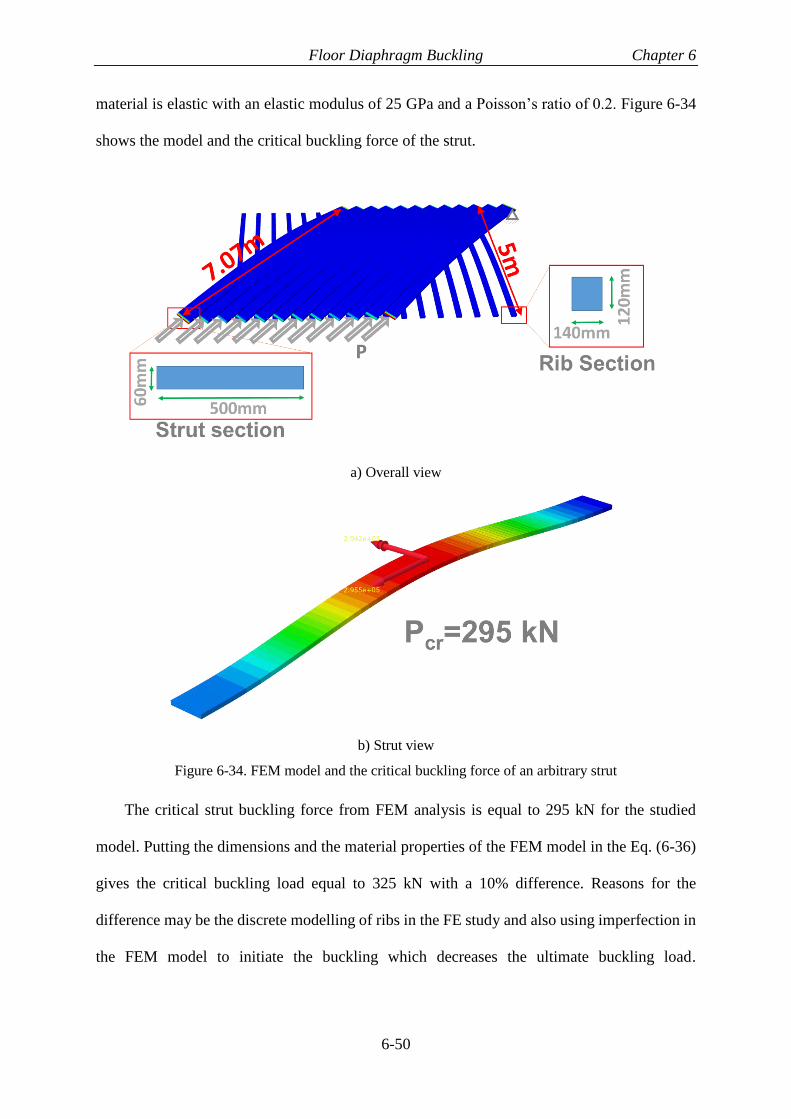
Floor Diaphragm Buckling Chapter 6
6-50
material is elastic with an elastic modulus of 25 GPa and a Poisson’s ratio of 0.2. Figure 6-34
shows the model and the critical buckling force of the strut.
a) Overall view
b) Strut view
Figure 6-34. FEM model and the critical buckling force of an arbitrary strut
The critical strut buckling force from FEM analysis is equal to 295 kN for the studied
model. Putting the dimensions and the material properties of the FEM model in the Eq. (6-36)
gives the critical buckling load equal to 325 kN with a 10% difference. Reasons for the
difference may be the discrete modelling of ribs in the FE study and also using imperfection in
the FEM model to initiate the buckling which decreases the ultimate buckling load.

Floor Diaphragm Buckling Chapter 6
6-51
Nevertheless, the answers are similar indicating consistency between the derivation and the FE
study.
• Discussion on the strut critical buckling strength (Eq. (6-36))
One of the assumptions for finding the strut buckling formula that was mentioned in the
previous section is that “it is assumed the distance between the ribs and struts are equal and the
rib and strut widths are infinitely small”. However, in a real floor slab, the ribs are located at a
certain distance that means the struts are connected to the ribs at some points. This might cause
an error in finding the strut critical buckling load. Here, the accuracy of the above assumption
is examined by comparing the results of the Eq. (6-36) and the cases that the strut is supported
with only one or two springs which they represent the rib stiffness. Figure 6-35 shows the cases
considered and the corresponding model for each of them.
a) Many struts and ribs

Floor Diaphragm Buckling Chapter 6
6-52
b) One rib per strut
c) Two ribs per strut
Figure 6-35. Floor diaphragms and the strut models with different number of ribs
As it was discussed comprehensively in the previous section, the buckling load for the first
model with many ribs per strut shown in Figure 6-35a can be calculated using Eq. (6-36).
When only one point of the rib (midpoint) is connected to the mid-point of the strut as per
Figure 6-35b, the rib stiffness may be represented by a spring. In this case the spring stiffness

Floor Diaphragm Buckling Chapter 6
6-53
is 𝑘𝑟1 =48𝐸𝐼𝑟
𝐿23 . The same method may be used for a strut with two points of connection as
shown in Figure 6-35c. Here the rib stiffness is replaced by two springs. In this case, the spring
stiffness of each rib at each location along the rib is 𝑘𝑟2 =162𝐸𝐼𝑟
5𝐿23 . Note that if there are more
ribs, all springs will not have the same stiffness.
The buckling load of this column could be found using various methods. These include
stability functions, energy methods and solving the differential equation of the strut. The
solutions to these problems are available in the literature. Here the solution presented is based
on Shou-Ngo Tu (1944). The following equations give the strut elastic buckling load for one
and two spring models.
For the one spring problem the following equations govern the critical buckling load:
𝑚𝑖𝑛
{
4𝑃√
𝑃
4𝐸𝐼
√𝑃𝐿2
4𝐸𝐼−tan(√
𝑃𝐿2
4𝐸𝐼)
= 𝑘𝑟1
𝑝 =4𝜋2𝐸𝐼
𝐿2
Eq. (6-37)
Eq. (6-37) shows the buckling modes of the strut. When the spring is placed at the mid-
point of the strut, with increasing the spring stiffness, buckling load increases until it reaches
the point that the spring acts as lateral support. In this condition, the strut reaches the second
Euler critical buckling load.
For the strut that is supported by two springs the following equations govern the critical
buckling load:
𝑚𝑖𝑛
{
3𝑃√
𝑃
9𝐸𝐼
√𝑃𝐿2
9𝐸𝐼+[sin(√
𝑃𝐿2
9𝐸𝐼) (1−2cos(√
𝑃𝐿2
9𝐸𝐼))⁄ ]
= 𝑘𝑟2
3𝑃√𝑃
9𝐸𝐼
((√𝑃𝐿2
9𝐸𝐼) 3⁄ )−[sin(√
𝑃𝐿2
9𝐸𝐼) (1+2cos(√
𝑃𝐿2
9𝐸𝐼))⁄ ]
= 𝑘𝑟2
𝑝 =9𝜋2𝐸𝐼
𝐿2
Eq. (6-38)

Floor Diaphragm Buckling Chapter 6
6-54
The possible buckling modes of each model are presented in Figure 6-36.
Figure 6-36. Strut buckling modes with one and two spring supports
In order to compare these three cases, the buckling load versus rib stiffness ratios are
plotted in Figure 6-37. The strut buckling in the intra-panel zone is governed by the first mode
(lowest force) for the continues model. In Figure 6-37 the first buckling mode of the continues
model is compared with one and two spring models. The strut buckling loads are normalised
by 𝑃𝐸𝑟, which is the critical buckling load with no springs.

Floor Diaphragm Buckling Chapter 6
6-55
a) Strut buckling load ratio versus rib stiffness ratio
b) Enlarged view
Figure 6-37. Strut buckling load ratio versus rib stiffness ratio
Based on the plots in Figure 6-37, the difference between the critical buckling load at the
ultimate strength of the first mode in the one spring model is less than 7.5% compared to the
continuous model (rib connected continuously to the strut). This value is less than 1% for the
two spring problem.
0
5
10
15
20
25
30
35
0 10 20 30
Τ𝑃𝑃𝐸𝑟
One Spring
Two Springs
Continuous model
Buckling Mode 1 Buckling Mode 2
Buckling Mode 1
Buckling Mode 2
Buckling Mode 3
(𝐸𝐼𝑟 𝐿𝑟3Τ )
(𝐸𝐼 𝐿3Τ )
0
1
2
3
4
5
6
7
0 2 4 6
Τ𝑃𝑃𝐸𝑟
One Spring
Two Springs
Continuousmodel
Buckling Mode 1
Buckling Mode 2
Buckling Mode 1
Buckling Mode 2
(𝐸𝐼𝑟 𝐿𝑟3Τ )
(𝐸𝐼 𝐿3Τ )
Less than 1% difference
7.5% difference

Floor Diaphragm Buckling Chapter 6
6-56
Therefore, considering that in a composite slab a strut is supported with a number of ribs
(more than 2), the assumption of continuously connected ribs and struts provides a reasonable
result.
6.4.3 Buckling mode 3, Global buckling (intra-bay buckling)
Another buckling mode that may occur in the composite floors is the “Global buckling”
mode. In this buckling mode, the composite floor between the primary beams is considered to
experience instability under the lateral imposed forces. The secondary beams act as the plate
stiffeners for the composite slab.
Similarly to the intra-panel buckling modes investigated in the previous sections, buckling
mode 3 also needs to be investigated in pre and post-cracking stages of the concrete. This is
because, the concrete can crack at low tension stresses, therefore the state of the pure shear can
change to diagonal compression due to concrete strut formation after the cracking. Figure 6-38
shows the composite floor between primary beams subjected to pure shear (pre-crack) and
compression strut force (post-crack) conditions.
a) Intra-bay subject to pure shear, (pre-crack)
b) Intra-bay subject to diagonal strut forces,
(post-crack)
Figure 6-38. Intra-bay loading conditions

Floor Diaphragm Buckling Chapter 6
6-57
Investigating the critical intra-bay buckling load subjected to non-uniform loads and
different loading conditions is complicated. Also, the nature of imposed loads is not precisely
known as they may vary during the earthquake. Therefore in this study the two scenarios
investigated are:
1) When the bay carries force as uniform pure shear stress (pre-cracking) and
2) When the bay carries the applied forces using diagonal compression (struts) after
concrete cracking.
In this section, the critical buckling loads are investigated analytically and the results are
verified with the FEM models.
6.4.3.1 Intra-bay buckling, slab subjected to pure shear (pre-cracking)
Similarly to the intra-panel buckling discussion in Section 6.4.2, the method used for
investigating the critical buckling load of the intra-bay is to study the buckling behaviour of
the equivalent orthotropic plate member. In the next sections, the method for finding an
equivalent orthotropic plate and the critical buckling load of the orthotropic plate is discussed.
• Equivalent orthotropic plate
In the previous sections, the composite slab between secondary beams was considered,
which was like a plate member that was stiffened by ribs in one direction. For the global
buckling, the composite floor is supported by some secondary beams as well. These beams are
placed perpendicular to the ribs direction. Thus the concrete topping is stiffened in two
perpendicular directions (two-way stiffened plate).
Similarly to the intra-panel buckling mode, only finding the flexural stiffness of the
composite floor (that is equal to the equivalent orthotropic plate) is required to find the critical
buckling load using orthotropic plate theory.
The flexural stiffness of the composite floor in the Y direction (𝐷𝑦) is the same as the intra-
panel stiffness, this is because the secondary beams do not provide flexural stiffness in this

Floor Diaphragm Buckling Chapter 6
6-58
direction. So the flexural stiffness in the Y direction (𝐷𝑦) could be found using the same rules
as finding the moment of inertia of a simple beam section. The only difference is that the plate
part (concrete topping) should be divided by (1 − 𝜈2) for considering the plate action. Eq. (6-
11) shows the flexural stiffness of the composite floor in the Y direction.
𝐷𝑦 =𝐸𝑡3
12(1−𝜈2)+
𝐸𝑡𝑒𝑦2
(1−𝜈2)+
𝐸𝑎ℎ3
12(𝑎+𝑏)+𝐸ℎ𝑎(
ℎ
2+𝑡
2−𝑒𝑦)
2
(𝑎+𝑏) Eq. (6-11)
Where 𝐸 and 𝜈 are the elastic modulus and Poisson’s ratio of the concrete material
respectively. Other parameters are shown in Figure 6-39. It should be noted that 𝑒𝑦 is the
distance between the section neutral axis and the mid-height of the concrete topping.
Figure 6-39. Composite slab with secondary beams
The flexural stiffness in the X direction, 𝐷𝑥, cannot be found simply using cross sectional
properties because the thickness of the composite floor is not uniform and also the secondary
beams increase the flexural stiffness in this direction. The method that is proposed here for
finding the flexural stiffness of the composite slab stiffened with the secondary beams include
finding the equivalent uniform plate thickness of the composite floor. Then, using the same
rules as finding the moment of inertia of a composite beam section, the total slab stiffness
including the secondary beams can be calculated.

Floor Diaphragm Buckling Chapter 6
6-59
Figure 6-40 shows the composite slab on the secondary beams and the equivalent uniform
plate of the composite floor (𝑡𝑒𝑞).
a) Composite slab on secondary beams
b) Equivalent uniform plate on secondary beams
Figure 6-40. Composite slab and the secondary beams cross-section
The equivalent uniform plate thickness can be calculated using the Eq. (6-39). The 𝐷𝑥𝑠 is
the composite slab stiffness same as Eq. (6-12) that was used in intra-panel buckling
consideration.
𝑡𝑒𝑞 = √12(1−𝜈2)𝐷𝑥𝑠
𝐸
3
Eq. (6-39)
Using the equivalent uniform plate thickness 𝑡𝑒𝑞 the intra-bay flexural stiffness 𝐷𝑥 can be
found using:
𝐷𝑥 =𝐸𝑡𝑒𝑞
3
12(1−𝜈2)+𝐸𝑡𝑒𝑞𝑒𝑥
2
(1−𝜈2)+𝐸𝑠𝐼𝑦
𝑐1+𝐸𝑠𝐴𝑠(
ℎ12+𝑡+ℎ−
𝑡𝑒𝑞
2−𝑒𝑥)
2
𝑐1 Eq. (6-40)
Where 𝐸 and 𝜈 are the elastic modulus and Poisson’s ratio of the concrete material
respectively, 𝐸𝑠 and 𝐼𝑦 are the elastic modulus and moment of inertia of the secondary beams
respectively. Other parameters are shown in Figure 6-39 and Figure 6-40. It should be noted

Floor Diaphragm Buckling Chapter 6
6-60
that 𝑒𝑥 is the distance between the section neutral axis and mid-height of the equivalent uniform
plate thickness.
• Verification of plate stiffness equations with FEM models
Three composite floors (ComFlor 80) are modelled with different secondary beams to
check the accuracy of the flexural stiffness equations presented in the previous section. Table
6-10 presents the flexural stiffness of the FEM models and the calculated values using Eqs. (6-
11) and (6-40). Note that fine mesh size was used in FEM models.
Table 6-10. Flexural stiffness of the composite floors
Steel beam properties
𝐼𝑦 = 4.5e8 𝑚𝑚4
𝐴𝑠 = 6e4 𝑚𝑚2
𝑐1 = 2000 mm
ℎ1 = 300 mm
𝐼𝑦 = 1.3e8 𝑚𝑚4
𝐴𝑠 = 4e4 𝑚𝑚2
𝑐1 = 2000 mm
ℎ1 = 200 mm
𝐼𝑦 = 10.7e8 𝑚𝑚4
𝐴𝑠 = 8e4 𝑚𝑚2
𝑐1 = 2000 mm
ℎ1 = 400 mm
Flexural stiffnesses
𝑫𝒙 (N.mm) FEM 38438212709 17851617357 69295053719
Eq. (6-40) 38907462634 17924970510 70387129883
Error (%) 1.22 0.41 1.58
𝐸 = 25 𝐺𝑃𝑎, 𝜈 = 0.2
** ComFlor 80: a=135mm, b=165mm, h=80mm, t=50mm,
The results show that the differences in the stiffness values are less than 2%. It should be
noted that the FEM modelling parameters such as mesh size, element type and other numerical
effects could also have some share in this error.
• Torsional stiffness of the orthotropic plate
For finding the torsional stiffness of the composite slab stiffened by secondary beams, the
ribs, beams and the slab are considered separately in Eq. (6-41) (Szilard, 1974).
𝐵 =𝐸𝑡𝑒𝑞
3
12(1−𝜈2)+𝐺𝑥𝑦
2
ℎ𝑎3𝜂
(𝑎+𝑏)𝑘𝐵 +
𝐺𝑥𝑦𝑠
6(∑𝑑𝑖𝑡𝑖
3
𝑐1) Eq. (6-41)
Where 𝐺𝑥𝑦 and 𝐺𝑥𝑦𝑠 are the concrete and steel shear modulus respectively. The parameter
𝜂 is a numerical factor depending on the rib aspect ratios presented in Table 6-7. The parameter
𝑘𝐵 is a reduction factor accounting for the decrease in the torsional stiffness of reinforced

Floor Diaphragm Buckling Chapter 6
6-61
concrete beams due to the concrete cracking. This parameter relates to ribs aspect ratio,
reinforcement and also applied bending moment to the member (Szilard, 1974). In this study
𝑘𝐵 is taken as zero conservatively. Also, 𝑑𝑖 and 𝑡𝑖 are the width and thickness of the secondary
beam flanges and web.
• Buckling of an orthotropic plate
The critical elastic buckling load of the composite floor is investigated using the plate
flexural stiffness found in the previous section. The same method as was presented in the intra-
panel buckling subjected to pure shear is used here considering the effect of secondary beams.
Using the intra-bay stiffness, the elastic critical shear stress (buckling stress) is expressed
as Eq. (6-20):
𝑁𝑥𝑦3 = 𝐾𝑠𝜋2
𝑡𝐿22 √𝐷𝑥𝐷𝑦
34 Eq. (6-20)
Where 𝑁𝑥𝑦3 is the elastic critical shear stress, 𝐷𝑥 and 𝐷𝑦 are the orthotropic plate stiffness,
and 𝐿2 is the length perpendicular to the 𝑥 axis as shown in Figure 6-39. The parameter 𝐾𝑠 is
the plate buckling coefficient determined by a theoretical critical-load analysis. This parameter
is a function of the plate geometry and the boundary conditions. The parameter 𝐾𝑠 is plotted
for three edge support conditions in Figure 6-22 (Ziemian, 2010). In these plots 𝐷1, 𝐷2 and 𝐷3
are 𝐷𝑥, 𝐷𝑦 and 𝐵 respectively. Based on the orthotropic plate stiffness the parameter 𝐾𝑠 can be
extracted from the plots in Figure 6-22. In this study, all the boundary conditions are considered
to be simply supported to obtain conservative results.
• Case study
The global elastic shear buckling strength of the intra-bay region for two ComFlor profiles
(60 and 80), supported by one and two secondary beams are investigated using both Eq. (6-20)
and FEM model. The studied models are shown in Figure 6-41.

Floor Diaphragm Buckling Chapter 6
6-62
The forces used for gravity design of the secondary beams include: 3 kPa imposed action
(Q), and 5 kPa permanent action (G). It is assumed that the concrete compressive strength is
30 MPa with elastic modulus of 25 GPa.
The critical buckling load of the floor slabs is studied with and without considering the
stiffness reduction factors accounting for concrete cracking due to flexural moments. The
stiffness reduction factor of 0.35 is selected based on Table C6.5 NZS3101 (2006) for members
subjected to bending moments. Although the elastic shear buckling here is based on the
assumption that the concrete is un-cracked, the cracking reduction factor is considered for
decreasing the bending rigidity which yields to lower buckling loads.
Table 6-11 presents the results of critical shear stress using Eq. (6-20) for floor slabs shown
in Figure 6-41.
Table 6-11. Critical shear stresses for ComFlor 60 and 80 with secondary beams (𝐿1 = 𝐿2 = 6 𝑚)
𝑵𝒙𝒚𝟑 (MPa)
Secondary beams at 2 m
(180UB18)
Secondary beams at 3 m
(200UB22.3)
Total Elastic
Com
Flo
r 60
112.3 99.9
Considering stiffness
reduction factors 69.6 59.8
Total Elastic
Com
Flo
r 80
142.6 125.7
Considering stiffness
reduction factors 89.1 54

Floor Diaphragm Buckling Chapter 6
6-63
a) ComFlor 80 supported with one secondary
beam
b) ComFlor 80 supported with two secondary
beams
c) ComFlor 60 supported with one secondary
beam
a) ComFlor 60 supported with two secondary
beams
Figure 6-41. ComFlor 60 and 80 with secondary beams
To verify the results obtained using the analytical approach, the FEM modelling is used.
Four models including two ComFlor profiles (60 and 80) with 2m and 3m spacing secondary
beams were created in ABAQUS software. A 6×6m composite floor is selected for the
modelling. The intra-bay region was subjected to pure shear loading and the shear force and
corresponding shear displacement were recorded during analysis. Figure 6-42 shows the
deformed shapes of the FEM models at the end of the analysis and the recorded shear force-
displacement plots.

Floor Diaphragm Buckling Chapter 6
6-64
a) Deformed shape of the ComFlor 60 intra-
bay (displacement contour at the buckling
step), Secondary beams at 2m
b) Shear force-displacement plot for ComFlor 60,
secondary beams at 2m
c) Deformed shape of the ComFlor 60 intra-bay
(displacement contour at the buckling step),
Secondary beams at 3m
d) Shear force-displacement plot for ComFlor 60,
secondary beams at 3m
0
50
100
150
200
250
0 20 40 60
Shea
r S
tres
s (M
Pa)
Shear dispalcement (mm)
Elastic without geometric
nonlinearityElastic with geometric
nonlinearity
0
50
100
150
200
250
0 20 40 60
Str
ess
Str
ess
(MP
a)
Shear dispalcement (mm)
Elastic without geometric
nonlinearity
Elastic with geometric
nonlinearity

Floor Diaphragm Buckling Chapter 6
6-65
e) Deformed shape of the ComFlor 80 intra-bay
(displacement contour at the buckling step),
Secondary beams at 2m
f) Shear force-displacement plot for ComFlor 80,
secondary beams at 2m (note: the analysis failed
to converge after 36mm)
g) Deformed shape of the ComFlor 80 intra-bay
(displacement contour at the buckling step),
Secondary beams at 3m
h) Shear force-displacement plot for ComFlor
80, secondary beams at 2m Figure 6-42. FEM models of ComFlor 60 and 80 subjected to pure shear condition
The shear force-displacement of all models are plotted in Figure 6-42. Each model is
analysed two times considering geometric nonlinearity and without geometric nonlinearity.
Same as intra-panel buckling investigations, the buckling load is defined at the point where the
difference between these two plots (𝐹𝐸 − 𝐹𝑁𝐺) becomes more than 1% of the corresponding 𝐹𝐸
value as shown in Figure 6-24 schematically. Where 𝐹𝐸 is the analysis without the geometric
nonlinearity and 𝐹𝑁𝐺 is the force-displacement plot considering the geometric nonlinearity.
0
20
40
60
80
100
120
140
160
180
0 20 40
Shea
r S
tres
s (M
Pa)
Shear dispalcement (mm)
Elastic without geometric
nonlinearity
Elastic with geometric
nonlinearity
0
50
100
150
200
250
0 20 40 60
Shea
r S
tres
s (M
Pa)
Shear dispalcement (mm)
Elastic without geometric
nonlinearity
Elastic with geometric
nonlinearity

Floor Diaphragm Buckling Chapter 6
6-66
Based on these plots, the critical buckling stress for ComFlor 60 and 80 with secondary
beams at 2m spacing were 120.2MPa and 148.6MPa respectively. Similarly, the critical
buckling stress for ComFlor 60 and 80 with secondary beams at 3m spacing were 91.2MPa and
120.3MPa respectively. These are similar to the values obtained from Eq. (6-20) given in Table
6-11 of 112.3MPa, 142.6MPa, 99.9MPa and 125.7MPa with errors being -6.5%, -4.1%, 9.5%
and 4.4% respectively. The answers are similar indicating consistency between the values from
Eq. (6-20) and the FE study.
These also show that the analytical approach is able to estimate the critical buckling load
with less than 10% error compared to the FEM models. In the next step, these critical buckling
loads are compared with the ultimate intra-bay shear strength to determine the likelihood of the
shear buckling.
• Slab shear strength
As mentioned in Section 6.4.2, the intra-panel buckling, the shear strength of the
composite slabs can be calculated using the equation provided by NZS3404 (2007) Clause
13.4.10.2.
𝑉𝑟 = min {(0.8∅𝐴𝑟𝑡𝑓𝑦𝑟 + 2.76∅𝑐𝐴𝑐𝑣)
0.5∅𝑐𝑓𝑐′𝐴𝑐𝑣
Eq. (6-21)
Where 𝐴𝑟𝑡 is the area of transverse reinforcements crossing shear planes, 𝐴𝑐𝑣 is the area
of concrete in shear planes and 𝑓𝑦𝑟 is the yield stress of tension reinforcement. The reduction
factors ∅ and ∅𝑐 are equal to 0.9 and 0.6 respectively. Here the upper bond value of this formula
(0.5∅𝑐𝑓𝑐′𝐴𝑐𝑣) is considered as the shear strength of the composite slab. The calculated shear
strength values and the critical shear buckling loads for the studied intra-bays with 3m spacing
between secondary beams are presented in Table 6-12. It should be noted that critical shear
buckling loads are calculated using stiffness reduction factors.

Floor Diaphragm Buckling Chapter 6
6-67
Table 6-12. The calculated shear strength values and the critical shear buckling stresses for ComFlor
60 and 80 intra-bays with secondary beams at 3m spacing (concrete stiffness reduction factor=0.35)
ComFlor 60 ComFlor 80
Shear stress (MPa)
Critical shear buckling stress
(Eq. (6-20)), considering
stiffness reduction factor
59.7 73.9
Slab shear strength (𝟎. 𝟓∅𝒄𝒇𝒄′ ) 9 9
The results show that the elastic shear buckling loads are more than six times the upper
bound shear strength of the composite slab. Therefore, it can be concluded that the elastic shear
buckling does not govern in the studied cases. The critical shear buckling of any other type of
floor slab could be investigated using Eq. (6-20) and the orthotropic plate stiffness formulations
given in Eqs. (6-39) to (6-41).
6.4.3.2 Global buckling, subjected to diagonal force (strut force), post-cracking
The same method as the one was used for finding the strut buckling load of the intra-panel
(Section 6.4.2) is used here. The only difference is that the strut is supported by the ribs and
the secondary beams simultaneously. Therefore, adding the stiffness of the secondary beams
changes Eq. (6-36) into:
𝑃𝑐𝑟 =𝜋2𝐸𝐼𝑠
𝐿𝑠2 +
𝜋2𝐸𝐼𝑟
𝐿22 sin𝛼
+ 𝜓𝜋2𝐸𝑠𝐼𝑠𝑏
𝐿12 cos𝛼
Eq.(6-42)
Where 𝐸𝑠 and 𝐼𝑠𝑏 are the elastic modulus and moment of inertia of secondary beams per
unit length of the slab, respectively. The length of the secondary beams is denoted by 𝐿1. The
parameter 𝜓 is the buckling correction factor. This parameter is found based on the solution of
the strut buckling loads supported with one and two springs along the length as discussed in
Section 6.4.2.2. It was shown that when the strut is supported by only one spring at the mid-
point, the maximum difference in the critical buckling load compare to the continuous model
is less than 7.5% (see Figure 6-37). For the strut supported with two springs this value is less

Floor Diaphragm Buckling Chapter 6
6-68
than 1%. Therefore, 𝜓 = 0.9 is suggested when the intra-bay is supported with one secondary
beam and 𝜓 = 1.0 for more than one secondary beams.
When the stiffnesses of the secondary beams increase, they laterally restrain the
compression strut as shown in Figure 6-43. This leads the strut to buckle at higher loads
corresponding to higher buckling modes. Therefore, the critical buckling load of the strut
should be found using Eq. (6-43) which considers the strut higher buckling modes. In this
equation, 𝑛 is the number of secondary beams within each bay.
𝑃𝑐𝑟 = 𝑚𝑖𝑛 {
𝜋2𝐸𝐼𝑠
𝐿𝑠2 +
𝜋2𝐸𝐼𝑟
𝐿22 sin𝛼
+ 𝜓𝜋2𝐸𝑠𝐼𝑠𝑏
𝐿12 cos𝛼
(𝑛 + 1)2 (𝜋2𝐸𝐼𝑠
𝐿𝑠2 +
𝜋2𝐸𝐼𝑟
𝐿22 sin𝛼
) Eq. (6-43)
Figure 6-43. Possible mode shapes of strut buckling in an intra-bay
Similarly to the intra-panel strut buckling, when the strut critical buckling capacity is
found, it may be compared with the intra-bay imposed forces (demands). It is suggested that
the sum of the imposed strut forces (demands) and sum of intra-panel strut critical buckling
strengths (capacity) be compared. The sum of the imposed strut forces can be used due to stiff
boundary members providing force redistribution.

Floor Diaphragm Buckling Chapter 6
6-69
6.5 Effect of gravity forces on the ultimate diaphragm buckling
loads
Floor slabs in the structures are primarily designed to carry gravity forces and transfer
them to other structural elements. The gravity forces acting on the diaphragms cause some out-
of-plane deformation. Maximum allowable values of this deformation are generally given in
the literature.
These out-of-plane deformations can affect the in-plane buckling behaviour of the floor
slab. Note that the out-of-plane deformations cannot change the elastic buckling load of a
member, however, these can considerably increase the out-of-plane deformations. These large
lateral deformations may cause yielding in the material. When material yields, the elastic
buckling load calculated is no longer valid as the material properties have changed. Therefore,
in this study only the initiation of the buckling is investigated providing that the material is still
elastic. In the following, the effect of gravity forces on the buckling behaviour of the
diaphragms is investigated.
• Effect of gravity forces on the ultimate shear buckling load (pre-crack)
Figure 6-44 shows the diaphragm out-of-plane deformation and the imposed shear loads
schematically. To obtain the effect of out-of-plane deformations on the shear buckling capacity
of the diaphragms, a number of FEM models are created considering maximum out-of-plane
deformations ranging from L/800 to L/200. In these models both the intra-panel (between
secondary beams) and the intra-bay (between primary beams and considering the secondary
beams) modes are investigated.

Floor Diaphragm Buckling Chapter 6
6-70
Figure 6-44. Diaphragm out-of-plane deformation and imposed shear loads
For the FEM models, a 6m×6 m composite slab with ComFlor 80 is selected both with and
without secondary beams. Two 180UB18 steel beams are used as secondary beams and
different level of out-of-plane deformations are applied to the floor slabs prior to imposing the
lateral forces. Figure 6-45 shows the intra-panel buckling loads corresponding to each level of
out-of-plane deformation. It can be seen that with increasing the initial out-of-plane
deformations, the critical buckling load decreased.
Figure 6-45. Effect of out-of-plane deformation on intra-panel slab
According to the linear regression shown in Figure 6-45, the buckling force at zero initial
deflection may be about 21,300 kN, therefore the ratio of buckling force at L/300 (assuming
the allowable initial deflection is L/300) to zero initial deflection is about 0.85 for the studied
≈L/200
≈L/300
≈L/400
≈L/800
y = -1.41E+02x + 2.13E+04
16000
17000
18000
19000
20000
21000
0 5 10 15 20 25 30 35
Ela
stic
Buck
ling S
hea
r fo
rce
(kN
)
Initial Deflection (mm)

Floor Diaphragm Buckling Chapter 6
6-71
intra-panel model. The same method is used for the intra-bay as shown in Figure 6-46. Note
that a certain amount of initial deflection is required to obtain a buckling load. Therefore,
buckling load corresponding to zero initial deflection could not be computed using the created
FEM model.
Figure 6-46. Effect of out-of-plane deformation on intra-bay slab
Similar to the intra-panel model, if the initial deflection considered to be L/300, based on
the linear regression shown in Figure 6-46, the buckling force at zero initial deflection could
be about 48,300 kN, therefore the ratio of the buckling force at L/300 to zero initial deflection
is about 0.875 for the studied intra-bay.
• Effect of gravity forces on the ultimate strut buckling strength (post-crack)
Figure 6-47 shows the strut formed in the diaphragm with some initial out-of-plane
deformation (δ). In this section, the initial deflection is explicitly considered in solving the
differential equation of the strut buckling. It is assumed that the out-of-plane deflection is due
to a uniformly distributed gravity force acting on the diaphragm.
≈L/200
≈L/300
≈L/400
≈L/800
y = -3.09E+02x + 4.83E+04
39000
40000
41000
42000
43000
44000
45000
46000
47000
0 5 10 15 20 25 30 35
Ela
stic
Buck
ling S
hea
r fo
rce
(kN
)
Initial Deflection (mm)

Floor Diaphragm Buckling Chapter 6
6-72
Figure 6-47. Strut formed in diaphragm with initial out-of-plane deformation
The gravity force reactions are distributed between the struts and the ribs based on their
flexural stiffnesses as shown in Figure 6-48. Also, based on deformation compatibility the
maximum deflection of both the strut and the rib, which occurs at the middle of the panel should
be the same.
Figure 6-48. The gravity force distributed between the struts and the ribs
Using deformation compatibility, the relation between the components of the gravity force
carried by the strut and the rib in the panel can be found. The mid-point deflections of the rib
and strut are equal to:
𝛿𝑅𝑖𝑏 =5𝑞′𝐿2
4
384𝐸𝐼𝑟

Floor Diaphragm Buckling Chapter 6
6-73
𝛿𝑆𝑡𝑟𝑢𝑡 =5𝑞′′𝐿𝑠
4
384𝐸𝐼𝑠
Where 𝑞′ and 𝑞′′ are the gravity forces per unit length carried by the rib and the strut
respectively. Deformation compatibility leads to:
𝛿𝑆𝑡𝑟𝑢𝑡 = 𝛿𝑅𝑖𝑏 Eq. (6-44)
𝑞′
𝑞′′=
𝐿𝑠4𝐼𝑟
𝐿24𝐼𝑠
Eq. (6-45)
The free body diagram of the strut and the rib is shown in Figure 6-49. Based on these
diagrams the differential equations can be written as:
Figure 6-49. Free body diagram of the strut and the rib
∑ 𝑀𝑆𝑡𝑟𝑢𝑡𝐴 = 0
−𝐸𝐼𝑠𝑑2𝑦
𝑑𝑥2− 𝑃𝑦 + ∫ 𝑥𝑓(𝑥)𝑑𝑥
𝑥
0− 𝑥𝑉′′ − ∫ 𝑥𝑞′′𝑑𝑥
𝑥
0= 0 Eq. (4-46)
∑ 𝑀𝑅𝑖𝑏𝐵 = 0
−𝐸𝐼𝑟𝑑2𝑤
𝑑𝑣2− ∫ 𝑣𝑔(𝑣)𝑑𝑣
𝑣
0− 𝑣𝑉′ − ∫ 𝑣𝑞′𝑑𝑣
𝑣
0= 0 Eq. (4-47)
Where 𝑉′′ and 𝑉′ are the strut and the rib shear forces respectively, and can be written as:

Floor Diaphragm Buckling Chapter 6
6-74
𝑉′′ = 𝑅𝐿𝑠 + ∫ 𝑓(𝑥) 𝑑𝑥
𝑥
0− ∫ 𝑞′′𝑑𝑥
𝑥
0 Eq. (6-48)
𝑉′ = 𝑅𝐿𝑟 − ∫ 𝑔(𝑣)𝑑𝑣
𝑣
0− ∫ 𝑞′𝑑𝑣
𝑣
0 Eq. (6-49)
Substituting Eq. (6-22) in Eqs. (6-48) and (6-49) leads to:
𝑉′′ + 𝑉′ = 𝑅𝐿𝑠 − 𝑥𝑞′′ + 𝑅𝐿
𝑟 − 𝑣𝑞′ Eq. (6-50)
Also, substituting Eq. (6-28) into the differential equation of the rib Eq. (6-47) gives:
∫𝑥𝑓(𝑥) 𝑑𝑥 =𝐿𝑠
𝐿2[−𝑣𝑉′ −
𝑣2
2𝑞′ − 𝐸𝐼𝑟
𝑑2𝑦
𝑑𝑥2(𝐿𝑠
𝐿2)2
] Eq. (6-51)
Using Eq. (6-51) the equilibrium differential equation of the strut can be rewritten as:
−𝐸𝐼𝑠𝑑2𝑦
𝑑𝑥2− 𝑃𝑦 +
𝐿𝑠
𝐿2[−𝑣𝑉′ −
𝑣2
2𝑞′ − 𝐸𝐼𝑟
𝑑2𝑦
𝑑𝑥2(𝐿𝑠
𝐿2)2
] − 𝑥𝑉′′ − ∫ 𝑥𝑞′′𝑑𝑥𝑥
0= 0
Eq. (6-52)
Substituting Eq. (6-50) into Eq. (6-52) gives the differential equation of the system
considering the initial deflection due to the gravity forces, which is:
−𝐸𝐼𝑠𝑑2𝑦
𝑑𝑥2− 𝑃𝑦 − 𝐸𝐼𝑟
𝑑2𝑦
𝑑𝑥2(𝐿𝑠
𝐿2)3
+𝐿2
𝐿𝑠𝑞′
𝑥2
2−𝐿2
2𝑞′𝑥 −
𝐿𝑠
2𝑞′′𝑥 + 𝑞′′
𝑥2
2= 0 Eq. (6-53)
By defining the 𝛼, 𝛽 and 𝛾 parameters as the following
𝛼 = 𝐸𝐼𝑠 + (𝐿𝑠
𝐿2)3
𝐸𝐼𝑟
𝛽 = 𝑞′′𝐿𝑠
2+ 𝑞′
𝐿2
2
𝛾 =𝑞′′
2+𝐿2
𝐿𝑠
𝑞′
2
The differential Eq. (6-53) becomes:
−𝛼𝑑2𝑦
𝑑𝑥2− 𝑃𝑦 = 𝛽𝑥 − 𝛾𝑥2 Eq. (6-54)
Considering:
𝑘2 = 𝑃 𝛼⁄

Floor Diaphragm Buckling Chapter 6
6-75
The solution to Eq. (6-54) consists of a complementary and a particular part. The solution
for the homogeneous linear differential equation is the same as Eq. (6-36) and the particular
solution is any solution to the entire equation such as 𝑦 = −𝛽
𝑃𝑥 +
𝛾
𝑃𝑥2 −
2𝛾𝛼
𝑃2. Therefore the
entire solution can be written as:
𝑦 = 𝐴 sin 𝑘𝑥 + 𝐵 cos 𝑘𝑥 −𝛽
𝑃𝑥 +
𝛾
𝑃𝑥2 −
2𝛾𝛼
𝑃2 Eq. (6-55)
To evaluate the arbitrary constants 𝐴 and 𝐵, the boundary conditions are used as the
following:
(𝑦)𝑥=0,𝐿𝑠 = 0
(𝑑𝑦
𝑑𝑥)𝑥=
𝐿𝑠2
= 0
The first of these conditions when substituted into Eq. (6-55) leads to
𝐵 =2𝛾𝛼
𝑃2 Eq. (6-56)
And from the second condition, it is found that:
𝐴 =2𝛾𝛼𝑘 sin(𝑘
𝐿𝑠2)+𝑃𝛽−𝑃𝛾𝐿𝑠
𝑃2𝑘 cos(𝑘𝐿𝑠2)
Eq. (6-57)
By substituting 𝐴 and 𝐵 into Eq. (6-55) and putting 𝑥 = 𝐿𝑠
2, the maximum out-of-plane
deformation of the strut considering the compression axial force can be calculated as:
𝛿𝑀𝑎𝑥 = 𝑦𝑥=
𝐿𝑠
2 =(𝛽−𝛾𝐿𝑠)
𝑃𝑘tan (𝑘
𝐿𝑠
2) +
2𝛾𝛼
𝑃2sec (𝑘
𝐿𝑠
2) −
2𝛽𝐿𝑠𝑃+𝛾𝐿𝑠2𝑃−2𝛾𝛼
4𝑃2 Eq. (6-58)
Figure 6-50 plots 𝛿𝑀𝑎𝑥
𝛿𝑅𝑖𝑏 for different
𝑃
𝑃𝑐𝑟 where the 𝑃𝑐𝑟 is found using Eq. (6-36). Now, if the
limiting value for 𝛿𝑀𝑎𝑥
𝛿𝑅𝑖𝑏 be estimated, the critical strut buckling load considering the gravity
forces (out-of-plane deflection) can simply be found using this plot.

Floor Diaphragm Buckling Chapter 6
6-76
𝛿𝑅𝑖𝑏 is given in Eq. (6-43b) as a function of the gravity force per unit length carried by the
rib, 𝑞′. This 𝑞′ does not need to be computed as it cancels out in 𝛿𝑀𝑎𝑥
𝛿𝑅𝑖𝑏 ratio.
Figure 6-50. Plot of the displacement ratio 𝛿𝑀𝑎𝑥
𝛿𝑅𝑖𝑏 against different
𝑃
𝑃𝑐𝑟
To obtain 𝛿𝑀𝑎𝑥
𝛿𝑅𝑖𝑏, the maximum value for 𝛿𝑅𝑖𝑏 under serviceability limit state is considered
to be 𝐿/300 (NZS1170.0 2002, Table C1). Also, it is assumed that 𝛿𝑀𝑎𝑥 corresponds to the rib
deflection when the first yield occurs in the rib section (𝑀𝑦). Considering 𝑞𝑟𝑖𝑏,𝑈 is the ultimate
gravity load per unit length causing 𝑀𝑦 in the rib, 𝛿𝑀𝑎𝑥
𝛿𝑅𝑖𝑏 can be found as:
𝑀𝑦 =𝑞𝑟𝑖𝑏,𝑈𝐿2
2
8
𝛿𝑀𝑎𝑥 =5𝑞𝑟𝑖𝑏,𝑈𝐿2
4
384𝐸𝐼𝑟=
5𝐿22𝑀𝑦
48𝐸𝐼𝑟
𝛿𝑀𝑎𝑥
𝛿𝑅𝑖𝑏=(5𝐿2
2𝑀𝑦
48𝐸𝐼𝑟)
(𝐿2
300)
⁄
𝛿𝑀𝑎𝑥
𝛿𝑅𝑖𝑏=
31.25𝐿2𝑀𝑦
𝐸𝐼𝑟 Eq. (6-59)
0
5
10
15
20
25
30
35
40
45
50
0 20 40 60 80 100
𝛿𝑀𝑎𝑥
𝛿𝑅𝑖𝑏
𝑃
𝑃𝑐𝑟 (%)
Floor Diaphragm Buckling Chapter 6
6-77
Where 𝑀𝑦 is the yield moment of the rib section, 𝐿2 and 𝐼𝑟 are the rib length and moment
of inertia respectively. And 𝐸 is the elastic modulus of the concrete which is calculated based
on NZS3101 (2006) Clause 5.2.3 using Eq. (6-60).
𝐸(𝑀𝑃𝑎) = 3320√𝑓𝑐′(𝑀𝑃𝑎) + 6900 Eq. (6-60)
Therefore for finding the ratio 𝛿𝑀𝑎𝑥
𝛿𝑅𝑖𝑏, the yield moment (𝑀𝑦) and the rib length (𝐿2) are
required. For this, the steel deck profiles, ComFlor 60 and 80, are selected and designed for
gravity loads using ComFlor Steel Composite Metal Deck Design software.
The gravity forces used for the design of ComFlor floor slabs include: 3 kPa imposed
action (Q), 1 kPa for ceiling/services and finishes, 1 kPa for partitions, and self-weight of the
floor slab (G) was calculated by the software based on the slab thickness and section details. It
is assumed that the concrete compressive strength is 30 MPa with an elastic modulus of 25
GPa. Four steel plate thicknesses (0.75, 0.9, 1 and 1.2 mm) and three topping thickness (60, 70
and 90 mm) are considered for design. To achieve larger spans that decrease the buckling
strength, it is assumed that the floors are propped during construction.
For finding the yield moment (𝑀𝑦) of the rib of each designed floor slab, section analysis
is used to calculate the yield moment corresponding to the first yield in the steel decking or
concrete compressive strain equal to 0.003. Table 6-13 and Table 6-14 are presenting the
analysis result in terms of the yield moment (𝑀𝑦), section reinforcement ratio (𝜌) and the
maximum possible span (𝐿2) with that particular floor slab and gravity forces. The value of 𝑀𝑦
obtained using this method was the same as that from the ComFlor Steel Composite Metal
Deck Design software. The value of 𝜌 was computed considering the tension area of the steel
decking. The 𝐿2 was taken from ComFlor Steel Composite Metal Deck Design software. The
limit states considered by ComFlor software include strength, deflection and vibration. These

Floor Diaphragm Buckling Chapter 6
6-78
are described in detail in the ComFlor manual. The design summary of two sample slabs are
presented in Appendix I.
Table 6-13. Analysis results for ComFlor 80
Steel deck plate thickness
Concrete
topping 0.75 0.9 1 1.2
60 mm
𝑀𝑦 (kN.m) 10.5 12.1 13.3 15.6
𝜌 (%) 1.17 1.4 1.56 1.87
𝐿2 (m) 4.7 4.8 4.9 5
70 mm
𝑀𝑦 (kN.m) 11.5 13.5 14.8 17.3
𝜌 (%) 1.09 1.31 1.46 1.75
𝐿2 (m) 4.9 5 5.1 5.3
90 mm
𝑀𝑦 (kN.m) 13.4 16 17.5 20.5
𝜌 (%) 0.96 1.16 1.29 1.54
𝐿2 (m) 5.1 5.3 5.4 5.6
Table 6-14. Analysis results for ComFlor 60
Steel deck plate thickness
Concrete
topping 0.75 0.9 1 1.2
60 mm
𝑀𝑦 (kN.m) 8.8 10.4 11.4 13.2
𝜌 (%) 1.14 1.37 1.52 1.83
𝐿2 (m) 4.1 4.2 4.3 4.4
70 mm
𝑀𝑦 (kN.m) 10.6 11.5 12.6 14.7
𝜌 (%) 1.05 1.27 1.41 1.69
𝐿2 (m) 4.4 4.5 4.5 4.6
90 mm
𝑀𝑦 (kN.m) 11.6 13.9 15.2 17.9
𝜌 (%) 0.91 1.1 1.22 1.46
𝐿2 (m) 4.7 4.9 5 5.2
From Table 6-13 and Table 6-14 it can be seen that the reinforcement ratio of all 24 slabs
is between 0.9% and 1.9%. Using the reinforcement ratios and based on Figure 6-51 from
NZS3101 (2006) Clause C6.9.1 which represents effective stiffness of rectangular beams with
grade 500 reinforcement against reinforcement ratio, shows the stiffness reduction factor due
to flexural cracking is between 0.38 and 0.58 for 30 MPa concrete. In this study, the reduction
factor was selected to be 0.40 as a lower bound value when 30MPa concrete is used.

Floor Diaphragm Buckling Chapter 6
6-79
Figure 6-51. Effective stiffness of rectangular beam with grade 500 reinforcement, NZS3101 (2006)
Clause C6.9.1
The value of 𝛿𝑀𝑎𝑥
𝛿𝑅𝑖𝑏 is obtained using Eq. (6-59). The rib stiffness, 𝐼𝑟, is computed using
𝐼𝑔𝑟𝑜𝑠𝑠 and the stiffness reduction factor of 0.40. The yield moment is from Table 6-13 and
Table 6-14. The maximum possible length, 𝐿2, is from Table 6-13 and Table 6-14 to obtain the
maximum 𝛿𝑀𝑎𝑥
𝛿𝑅𝑖𝑏. The results are presented in Table 6-15.
Table 6-15. Ratio of ultimate deflection to the allowable deflection for all investigated 24 slabs
𝜹𝑴𝒂𝒙𝜹𝑹𝒊𝒃
Steel deck plate thickness
ComFlor
type Concrete topping 0.75 0.9 1 1.2
ComFlor
80
60 mm 4.96 5.9 6.59 7.85
70 mm 4.63 5.54 6.18 7.51
90 mm 3.86 4.78 5.33 6.5
ComFlor
60
60 mm 5.39 6.52 7.31 8.71
70 mm 5.47 6.08 6.66 7.95
90 mm 4.18 5.2 5.83 7.12
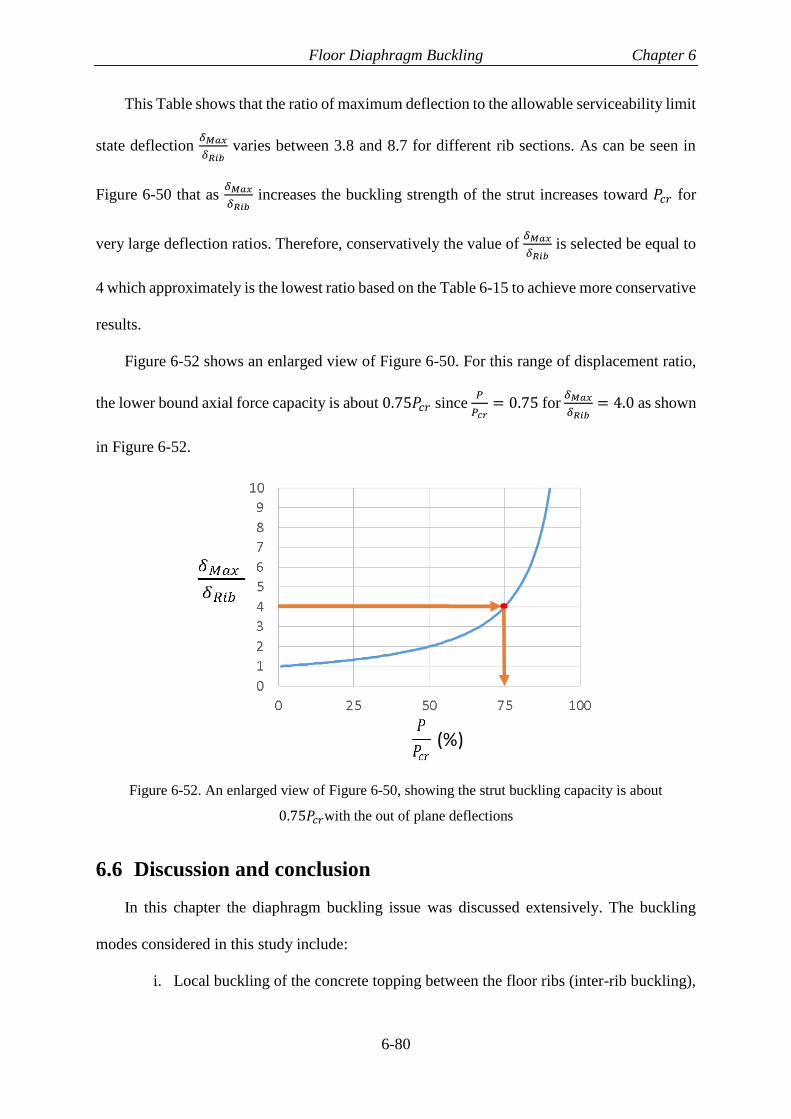
Floor Diaphragm Buckling Chapter 6
6-80
This Table shows that the ratio of maximum deflection to the allowable serviceability limit
state deflection 𝛿𝑀𝑎𝑥
𝛿𝑅𝑖𝑏 varies between 3.8 and 8.7 for different rib sections. As can be seen in
Figure 6-50 that as 𝛿𝑀𝑎𝑥
𝛿𝑅𝑖𝑏 increases the buckling strength of the strut increases toward 𝑃𝑐𝑟 for
very large deflection ratios. Therefore, conservatively the value of 𝛿𝑀𝑎𝑥
𝛿𝑅𝑖𝑏 is selected be equal to
4 which approximately is the lowest ratio based on the Table 6-15 to achieve more conservative
results.
Figure 6-52 shows an enlarged view of Figure 6-50. For this range of displacement ratio,
the lower bound axial force capacity is about 0.75𝑃𝑐𝑟 since 𝑃
𝑃𝑐𝑟= 0.75 for
𝛿𝑀𝑎𝑥
𝛿𝑅𝑖𝑏= 4.0 as shown
in Figure 6-52.
Figure 6-52. An enlarged view of Figure 6-50, showing the strut buckling capacity is about
0.75𝑃𝑐𝑟with the out of plane deflections
6.6 Discussion and conclusion
In this chapter the diaphragm buckling issue was discussed extensively. The buckling
modes considered in this study include:
i. Local buckling of the concrete topping between the floor ribs (inter-rib buckling),

Floor Diaphragm Buckling Chapter 6
6-81
ii. Buckling of the diaphragm between secondary beams (intra-panel buckling), and
iii. Global buckling of the diaphragm between primary beams (intra-bay buckling).
All of the buckling modes are studied for both pre-crack and post-crack conditions of the
concrete slab. The critical buckling of each mode is calculated using analytical methods, and
in some cases, the results are verified with FEM modelling using ABAQUS software. It was
found that:
i. Local buckling will not occur for conventional floor slabs. This is because the
minimum thickness required results in high buckling forces and concrete shear or
crushing are likely to occur much earlier than buckling as described in Section
6.4.1.
ii. For the intra-panel and intra-bay buckling modes the critical slab in-plane shear
forces which cause buckling need to be checked both before and after cracking. A
simple formula is provided to do this. It considered pinned end condition, out-of-
plane deformations and the corrugated nature of the composite slab. It was shown
that in the studied examples the shear buckling does not govern. The strut buckling
is more probable to occur due to the high axial strength of concrete material.
The reduction in the horizontal critical buckling loads due to vertical gravity forces that
cause initial vertical deflection in the floor slabs is also investigated. It was found that:
i. The intra-panel critical elastic buckling capacity decreased by up to 15%
considering the initial deflection equal to L/300.
ii. The Global buckling mode (intra-bay) critical elastic buckling capacity decreased
by up to 12.5% considering the initial deflection equal to L/300.
iii. For the strut buckling of intra-panel and intra-bay modes, it was found that for the
ComFlor 60 and 80 profiles with 60 mm to 90 mm concrete topping thicknesses,

Floor Diaphragm Buckling Chapter 6
6-82
the strut buckling capacity decreased to about 0.75 times the critical buckling
capacity corresponding to the zero initial deflection.
Based on the results of studying the effect of initial deflection, the elastic buckling strength
reduction factor accounting for the presence of gravity forces on the floor slab can
conservatively be considered equal to 0.75. This value may be used in design.
6.7 Summary of the method for calculating the diaphragm
critical buckling loads
Notations used in the following formulations are presented in Table 6-16.
Table 6-16. Notations used in the formulation of diaphragm buckling considerations
𝑁𝑥𝑦1 Elastic critical shear stress (MPa)
𝑏 Plate width (distance between ribs) (mm)
𝑡 Concrete topping thickness (mm)
𝐸 Concrete elastic modulus (MPa)
𝜈 Concrete Poisson’s ratio
𝑘𝑠 Plate shear buckling coefficient
𝑁𝑐𝑟 Elastic critical axial stress (MPa)
𝑘 Plate axial buckling coefficient
𝜏𝑐 and 𝜕𝑐 Imposed shear and axial stresses to the concrete topping (MPa)
𝑒𝑦 Distance between concrete topping centre line to the section neutral axis
(mm)
ℎ Steel deck height (mm)
𝑎 Steel deck rib width (mm)
𝛽 Ribs height modification factor
𝐺𝑥𝑦 Elastic shear modulus of concrete (MPa)
𝜂 Numerical factor depending on the ribs aspect ratios
𝑘𝐵 Reduction factor accounting for the decrease in the torsional stiffness of
reinforced concrete beams due to concrete cracking
𝑁𝑥𝑦2 Elastic critical shear stress of intra-panel orthogonal plate (MPa)
𝐷𝑥 Flexural stiffness of the composite slab in the direction perpendicular to ribs
(N.mm)
𝐷𝑦 Flexural stiffness of the composite slab in the ribs direction (N.mm)
𝐿2 Slab length parallel to the ribs (mm)
𝑓𝑐′ Concrete compressive strength (MPa)
𝐼𝑠 Moment of inertia of the concrete strut per unit width (mm4)
𝐼𝑟 Moment of inertia of the rib per unit width(mm4)
𝐿𝑠 Strut length (mm)
𝛼 The angle between the concrete strut and the ribs
𝐿1 Slab length perpendicular to the ribs (mm)

Floor Diaphragm Buckling Chapter 6
6-83
𝐿2 Slab length parallel to the ribs (mm)
𝑉𝑆𝐵2 Slab shear buckling strength per unit length due to intra-panel buckling
(N/mm)
𝑉𝑠𝑡𝑟𝑢𝑡2 Slab shear from strut buckling capacity per unit length (intra-panel buckling)
(N/mm)
𝑡𝑒𝑞 Equivalent plate thickness to the composite slab in the X direction (mm)
𝑒𝑥 Distance between equivalent slab centre line to the section neutral axis (mm)
𝐸𝑠 Steel elastic modulus (MPa)
𝐼𝑦 Moment of inertia of secondary beams (mm4)
𝐴𝑠 Cross-section area of secondary beams (mm2)
ℎ1 Steel beam height (secondary beam) (mm)
𝑐1 Distance between secondary beams (mm)
𝑑𝑖 Width of steel beam flanges and web (mm)
𝑡𝑖 Thickness of steel beam flanges and web (mm)
𝐺𝑥𝑦𝑠 Elastic shear modulus of steel (MPa)
𝑁𝑥𝑦3 Elastic critical shear stress of intra-bay orthogonal plate (MPa)
𝑉𝑆𝐵3 Slab shear buckling strength per unit length due to intra-bay buckling
(N/mm)
𝐼𝑠𝑏 Is the secondary beam moment of inertia per unit width of the slab (𝐼𝑦/𝑐1)
(mm3)
𝜓 Buckling correction factor, 0.9 for a composite floor with one secondary
beam, 1 for more than one
𝑛 Number of secondary beams per bay
𝑉𝑠𝑡𝑟𝑢𝑡3 Slab shear from strut buckling capacity per unit length (intra-bay buckling)
(N/mm)
𝑃𝑐𝑟3 Strut buckling capacity per unit length (intra-bay) (N/mm)
𝑃𝑐𝑟2 Strut buckling capacity per unit length (intra-panel buckling) (N/mm)
𝑁𝑒𝑥𝑖𝑠𝑡𝑖𝑛𝑔 Maximum imposed shear stress to intra-panel (MPa)
➢ Buckling mode 1, inter-rib (local) buckling
1. Calculate critical shear buckling of the inter-rib subjected to pure shear, (pre-crack
condition)
𝑁𝑥𝑦1 = 𝑘𝑠𝐸𝜋2
12(1−𝜈2)(𝑏/𝑡)2
The 𝑘𝑠 can conservatively considered equal to 5.4.
2. Calculate critical buckling load of the inter-rib subjected to strut forces, (post-crack
condition)
𝑁𝑐𝑟 = 𝑘𝐸𝜋2
12(1−𝜈2)(𝑏/𝑡)2
The 𝑘 can considered equal to 4 conservatively.

Floor Diaphragm Buckling Chapter 6
6-84
The imposed shear and axial stresses on the inter-rib zone can be obtained from truss
element modelling results considering the rib and the strut relative directions. In the following
the angle between the strut and ribs is considered 45° and 𝑃 is the maximum recorded strut
force.
𝜏𝑐 = 𝜕𝑐 =0.5𝑃
𝐴𝑡𝑟𝑢𝑠𝑠
Find the demand to capacity ratio (DCR) using the following equation:
(𝜕𝑐
𝑁𝑥𝑦1) + (
𝜏𝑐
𝑁𝑐𝑟)2
≤ 1
➢ Buckling mode 2, Intra-panel buckling
1. Calculate critical shear buckling of the intra-panel subjected to pure shear, (pre-
crack condition)
2. Preliminary check:
If the equation below is satisfied, there is no need to check the critical shear buckling of
the intra-panel subjected to pure shear:
𝑁𝑒𝑥𝑖𝑠𝑡𝑖𝑛𝑔 ≤ 0.75 × 3.5𝜋2
𝑡𝐿22 √𝐷𝑥𝐷𝑦
34
Where √𝐷𝑥𝐷𝑦34 for different topping thickness can be found using the plots shown in
Figure 6-53 for ComFlor 60 and 80 (these values are calculated using flexural stiffness
reduction factor 0.35 based on Table C6.5 NZS3101, 2006). And 𝑁𝑒𝑥𝑖𝑠𝑡𝑖𝑛𝑔 is the maximum
imposed shear stress to the intra-panel.

Floor Diaphragm Buckling Chapter 6
6-85
Figure 6-53. Calculated values of √𝐷𝑥𝐷𝑦34 for ComFlor 60 and 80 against different concrete topping
thickness
First, the properties of the equivalent orthotropic plate need to be found:
Find the flexural stiffness of the composite slab in the ribs direction (𝐷𝑦):
𝐷𝑦 = 0.35(𝐸𝑡3
12(1−𝜈2)+
𝐸𝑡𝑒𝑦2
(1−𝜈2)+
𝐸𝑎ℎ3
12(𝑎+𝑏)+𝐸ℎ𝑎(
ℎ
2+𝑡
2−𝑒𝑦)
2
(𝑎+𝑏))
Find the flexural stiffness of the composite slab in the direction perpendicular to ribs (𝐷𝑥):
𝐷𝑥 = 0.35 (𝐷𝑎𝐷𝑏(𝑎+𝑏)
(𝑏𝐷𝑎+𝑎𝐷𝑏))
𝐷𝑎 =𝐸(𝑡+𝛽ℎ)3
12(1−𝜈2)
𝐷𝑏 =𝐸𝑡3
12(1−𝜈2)
{𝛽 = 0.9224𝑒
(−2.756ℎ
𝑎)
𝛽 =𝑎
8ℎ
𝑓𝑜𝑟
ℎ
𝑎≤ 0.4
𝑓𝑜𝑟 ℎ
𝑎> 0.4
Alternatively, the following equation could be used for ℎ
𝑎> 0.1.
𝛽 = 0.136𝑒(−0.745ℎ
𝑎) 𝑓𝑜𝑟
ℎ
𝑎> 0.1
Find the torsional stiffness of the composite slab (𝐵):
0
1E+09
2E+09
3E+09
4E+09
5E+09
6E+09
0 50 100 150 200
(N.m
m)
Concrete topping thickness (mm)
CF 80
CF 60
√𝐷𝑥𝐷𝑦
34

Floor Diaphragm Buckling Chapter 6
6-86
𝐵 =𝐸𝑡3
12(1−𝜈2)+𝐺𝑥𝑦
2
ℎ𝑎3𝜂
(𝑎+𝑏)𝑘𝐵
Where 𝑘𝐵 can be considered zero conservatively.
Table 6-7. Parameter η (Szilard, 1974)
𝑎/ℎ 1 1.2 1.5 2 2.5 3 4 6 8 10 ∞
𝜂 0.140 0.166 0.196 0.229 0.249 0.263 0.281 0.299 0.307 0.313 0.333
To calculate the critical buckling shear loads the flexural stiffness 𝐷𝑥 and 𝐷𝑦 could be
multiplied by flexural stiffness reduction factor (0.35) to account for concrete flexural cracking.
𝑁𝑥𝑦2 = 𝐾𝑠𝜋2
𝑡𝐿22 √𝐷𝑥𝐷𝑦
34
𝑉𝑆𝐵2 = 0.75 × 𝑡𝑁𝑥𝑦2
The calculated buckling load is multiplied by 0.75 to account for the out-of-straightness
effect due to existing gravity forces.
Figure 6-22. Shear buckling coefficient for orthotropic plates (Ziemian, 2010), as adapted from
Johns and Kirkpatrick (1971)
3. Intra-panel subjected to diagonal force (strut force), post-crack condition
The strut critical buckling load per unit width of the strut is calculated using:
𝑃𝑐𝑟2 = 0.75 ×𝜋2(𝐸𝐼𝑠+𝐸𝐼𝑟(
𝐿𝑠𝐿2)3)
𝐿𝑠2 =
𝜋2𝐸𝐼𝑠 sin3𝛼+𝜋2𝐸𝐼𝑟
𝐿𝑠2 sin3𝛼
𝐼𝑟 = 0.35𝑎(𝑡+ℎ)3
12(𝑎+𝑏)
𝐼𝑠 = 0.8𝑡3 sin𝛼
12

Floor Diaphragm Buckling Chapter 6
6-87
𝐿𝑠 =𝐿2
sin𝛼
In this study, it is suggested that the sum of the imposed strut forces (demands) and the
sum of intra-panel strut critical buckling strengths (capacity) be compared.
➢ Buckling mode 3, Global buckling
1. Calculate critical shear buckling of the intra-bay subjected to pure shear, (pre-
crack condition)
❖ Preliminary check:
If the equation below is satisfied, there is no need to check the critical shear buckling of
the intra-bay subjected to pure shear:
𝑁𝑒𝑥𝑖𝑠𝑡𝑖𝑛𝑔 ≤ 0.75 × 3.5𝜋2
𝑡𝐿22 √𝐷𝑥𝐷𝑦
34
Where √𝐷𝑥𝐷𝑦34 for different topping thickness can be found using the plots shown in
Figure 6-53 for ComFlor 60 and 80 ignoring the secondary beams (these values are calculated
using flexural stiffness reduction factor 0.35 based on Table C6.5 NZS3101, 2006). And
𝑁𝑒𝑥𝑖𝑠𝑡𝑖𝑛𝑔 is the maximum imposed shear stress to the intra-bay.
First, the properties of the equivalent orthotropic plate need to be found:
Find the flexural stiffness of the composite floor in the ribs direction (𝐷𝑦) same as the
intra-panel:
𝐷𝑦 = 0.35(𝐸𝑡3
12(1−𝜈2)+
𝐸𝑡𝑒𝑦2
(1−𝜈2)+
𝐸𝑎ℎ3
12(𝑎+𝑏)+𝐸ℎ𝑎(
ℎ
2+𝑡
2−𝑒𝑦)
2
(𝑎+𝑏))
Find the flexural stiffness of the composite floor in the direction perpendicular to ribs (𝐷𝑥):
The equivalent plate thickness to the composite slab should be calculated: (𝐷𝑥𝑠 is the
composite slab stiffness equal to 𝐷𝑥 for the intra-panel without considering stiffness reduction
factor)
𝐷𝑥𝑠 =𝐷𝑎𝐷𝑏(𝑎+𝑏)
(𝑏𝐷𝑎+𝑎𝐷𝑏)

Floor Diaphragm Buckling Chapter 6
6-88
𝑡𝑒𝑞 = √12(1−𝜈2)𝐷𝑥𝑠
𝐸
3
𝐷𝑥 =𝐸𝑡𝑒𝑞
3
12(1−𝜈2)+𝐸𝑡𝑒𝑞𝑒𝑥
2
(1−𝜈2)+𝐸𝑠𝐼𝑦
𝑐1+𝐸𝑠𝐴𝑠(
ℎ12+𝑡+ℎ−
𝑡𝑒𝑞
2−𝑒𝑥)
2
𝑐1
The torsional stiffness of the composite slab is calculated using:
𝐵 =𝐸𝑡𝑒𝑞
3
12(1−𝜈2)+𝐺𝑥𝑦
2
ℎ𝑎3𝜂
(𝑎+𝑏)𝑘𝐵 +
𝐺𝑥𝑦𝑠
6(∑𝑑𝑖𝑡𝑖
3
𝑐1)
Where 𝑘𝐵 can be considered zero conservatively.
Elastic critical shear stress (buckling stress) is expressed as:
𝑁𝑥𝑦3 = 𝐾𝑠𝜋2
𝑡𝐿22 √𝐷𝑥𝐷𝑦
34
𝑉𝑆𝐵3 = 0.75 × 𝑡𝑁𝑥𝑦3
Parameter 𝐾𝑠 should be found using Figure 6-22.
2. Intra-bay subjected to diagonal force (strut force), post-crack
The strut critical buckling load per unit width of the strut is calculated using:
𝑃𝑐𝑟3 = 0.75 ×𝑚𝑖𝑛 {
𝜋2𝐸𝐼𝑠
𝐿𝑠2 +
𝜋2𝐸𝐼𝑟
𝐿22 sin𝛼
+ 𝜓𝜋2𝐸𝑠𝐼𝑠𝑏
𝐿12 cos𝛼
(𝑛 + 1)2 (𝜋2𝐸𝐼𝑠
𝐿𝑠2 +
𝜋2𝐸𝐼𝑟
𝐿22 sin𝛼
)
Same as the intra-panel buckling mode, it is suggested that the sum of the imposed strut
forces (demands) and the sum of intra-bay strut critical buckling strengths (capacity) be
compared.

Floor Diaphragm Buckling Chapter 6
6-89
References
[1] AS/NZS 1170.0 (2002), Structural design actions-Part 0: General principles.
[2] Bolluyt, J. E. (1980). Behavior of composite steel deck diaphragms.
[3] Bresler, B., & Pister, K. S. (1958, September). Strength of concrete under
combined stresses. In Journal Proceedings (Vol. 55, No. 9, pp. 321-345).
[4] Bruneau, M., MacRae, G. (2017). “Reconstructing Christchurch: A Seismic Shift
in Building Structural Systems”, Quake Centre, University of Canterbury.
[5] ANSI/SDI (2011). American National Standards Institute/Steel Deck Institute, C-
2011 Standard for Composite Steel Floor Deck-Slabs.
[6] ComFlor Steel Composite Metal Deck Design software, Ver 9.0.33.0
[7] CSA, C. (2014). S16-14. Design of Steel Structures, Canadian Standards
Association, Toronto, ON.
[8] Henry, R. S., Dizhur, D., Elwood, K. J., Hare, J., & Brunsdon, D. (2017). Damage
to concrete buildings with precast floors during the 2016 Kaikoura
earthquake. Bulletin of the New Zealand Society for Earthquake
Engineering, 50(2), 174-186.
[9] https://www.comflor.nz/technical-resources/#AP
[10] Iguchi, S. (1938). Die knickung der rechteckigen platte durch
Schubkräfte. Ingenieur-Archiv, 9(1), 1-12.
[11] Johns, D. J., & Kirkpatrick, D. L. I. (1971). Shear buckling of isotropic and
orthotropic plates: a review. HM Stationery Office.
[12] NZS 3101 (2006). Concrete structures standard. Standards New Zealand,
Wellington, NZ.
[13] NZS 3404 (2007). Steel Structures Standard. Standards New Zealand,
Wellington, New Zealand. Including Amendments 1 and 2, 2001/2007.
[14] Product guide, ComFlor 210 composite floor decking, S&T Stainless Ltd.

Floor Diaphragm Buckling Chapter 6
6-90
[15] Product guide, ComFlor 60 composite floor decking, S&T Stainless Ltd.
[16] Product guide, ComFlor 80 composite floor decking, S&T Stainless Ltd.
[17] Seide, P., & Stein, M. (1949). Compressive buckling of simply supported plates
with longitudinal stiffeners.
[18] Seide, P. (1953). The effect of longitudinal stiffeners located on one side of a
plate on the compressive buckling stress of the plate-stiffener combination.
[19] Shou-Ngo Tu. (1944). Column with Equal-Spaced Elastic Supports. Journal of
the Aeronautical Sciences, 11(1), 67-72.
[20] Szilard, R. (1974). Theory and analysis of plates: classical and numerical
methods. 1974. Prentice-Hall, Englewood, 10, 35-48.
[21] Wittrick, W. H. (1954). Correlation between some stability problems for
orthotropic and isotropic plates under bi-axial and uni-axial direct stress. The
Aeronautical Quarterly, 4(1), 83-92.
[22] Yu, C., & Schafer, B. W. (2006). Effect of longitudinal stress gradient on the
ultimate strength of thin plates. Thin-walled structures, 44(7), 787-799.
[23] Ziemian, R. D. (Ed.). (2010). Guide to stability design criteria for metal
structures. John Wiley & Sons.

Diaphragm Lateral Force Method Chapter 7
7-1
7 Diaphragm Lateral Force Method
7.1 Introduction
The issue of finding a simplified lateral force method/pattern that can predict likely
earthquake force and deformation demands has been studied for decades by many researchers
(e.g. Veletsos and Newmark, 1960). Structural engineers have been using simplified lateral
force methods considering some assumptions for designing structural elements. This is
because a simplified method (e.g. Equivalent Static Analysis) may obtain relatively
reasonable results in comparison with complex and more realistic methods (e.g. Linear Time
History analysis but reduced for ductility) in most cases. These simplified methods may be
found in most loading standards.
The simplified lateral force methods are well developed for designing structural elements
such as beams and columns. However, different methods are required for obtaining
diaphragm in-plane demands. There are some simplified methods proposed by different
researchers for obtaining diaphragm global in-plane demands. However, none of them is
widely accepted and each has some advantages and disadvantages.
Methods for estimating floor diaphragm global demands need to have the following
features to be used in design offices widely:
1) Simplicity
2) Compatibility with commonly used analysis software packages
3) Accuracy: indicate likely in-plane demands from the different causes
In this study a diaphragm lateral force method is proposed based on an elastic structure
deformation hypothesis to satisfy (1) and (2) above. This is conducted by seeking answers to
the following questions:
1. What causes the diaphragm in-plane demands?

Diaphragm Lateral Force Method Chapter 7
7-2
2. What are the available lateral force methods have been proposed to estimate
diaphragm in-plane demands for design/assessment?
3. Can an improved method obtain diaphragm in-plane forces be proposed?
4. Which lateral force methods are best to meet the requirements of simplicity,
compatibility with existing design tools and accuracy?
7.2 Slab in-plane demands
Diaphragm in-plane demands originate from different sources such as i) inertia forces, ii)
transfer forces, iii) slab bearing forces, iv) compatibility forces and v) interaction with other
elements as described in Chapter 2. These in-plane forces could be categorised into global
and local demand groups based on their effect on the diaphragm. Global diaphragm demands
may be obtained from structural analysis using proper lateral loading method or NLTH
analysis. However, local demands need to be considered for designing different components
of the diaphragm locally. In the following both global and local demands are described in
detail.
7.2.1 Diaphragm global in-plane demands
Diaphragm global demands may be defined as diaphragm imposed forces that act on
most areas of the diaphragm. Failure to resist these forces may lead to damage to the
structure, a significant change in force distribution between vertical lateral force resisting
(VLFR) systems of the structure, and possibility to collapse.
• Inertia forces
Considering the above definition, inertia forces (referred as i above) which are a product
of diaphragm mass times the diaphragm accelerations during ground shaking can be
categorised as global demand. Although these inertia forces usually are not significant to
cause damage to diaphragms, in some situations such as long narrow diaphragms with few

Diaphragm Lateral Force Method Chapter 7
7-3
lines of VLFR system along the length, inertia forces may cause large lateral displacements
and damage to the diaphragm and the gravity load carrying system of the structure.
• Transfer forces
Another global diaphragm demand is diaphragm transfer force (which is ii above).
Transfer forces may occur as a result of deformation incompatibility of different VLFR
elements of a structure such as moment frames and RC walls wanting to move different
amounts at different levels under the applied loading. Also, structure irregularities in height
or discontinuities in plan location of the VLFR elements, may generate transfer forces
between the two displaced VLFR systems above and below the level. A common
discontinuity of vertical elements in the plan is at a podium level.
7.2.2 Diaphragm local in-plane demands
In contrary to the global demands, diaphragm local demands can be defined as the forces
that effect on some areas of the diaphragm and may cause local damage to the diaphragm.
• Slab bearing forces
One example of diaphragm local demand is the slab bearing forces (which is iii above).
These occur when a construction gap is not provided between the slab and column. As the
column sways, it bears against the concrete slab that imposes an extra bearing force on the
slab. This force must be transferred through the slab to the shear studs and the beam, and
back to the column. The magnitude of slab bearing forces is a function of concrete
compressive strength, number and strength of shear studs, and force transferring mechanisms
into the column. Slab bearing forces may cause local damage to the concrete near the column.
This has been discussed by Chaudhari et al. (2015) and MacRae and Bull (2015) in detail as
well as Section 2.6 of Chapter 2.

Diaphragm Lateral Force Method Chapter 7
7-4
• Compatibility forces
Another source of diaphragm local demands is the compatibility force (which is iv
above). When neutral axes of composite beams on either side of the column are at different
heights due to the composite action, the distance between the beam-ends tends to increase,
causing slab tension forces and beam compression forces (MacRae and Clifton, 2015). This
elongation in steel beams is expected to be much less than that of a concrete beam where
cracks/gaps open at both ends of the beam (MacRae et al. 2013). However, it should be
considered in the analysis because it can impose extra forces on the columns as well as on the
beam plastic hinge region and the beam-column connections. Beam elongation measurements
by MacRae et al. (2013) on some steel beam-column-slab subassemblies showed that the
beams tend to shorten as a result of buckling of the beam and spalling of the concrete at the
slab/column interface. The residual shortening, measured as the shortening at zero column
drift, was less than 2mm during cycles up to about 3.5% drift. This may not be significant for
a typical steel beam, but subassemblies showing gap opening characteristics such as those
with reinforced concrete beams may place much higher demands on the diaphragm (SESOC
2011). This diaphragm local demand is out of the scope of this research.
• Interaction with other elements
Interaction with other elements (which is v above) may also impose in-plane forces on
the diaphragms. This can be categorised as another source of diaphragm local demands.
Inclined columns, ramps and stairs can develop diaphragm in-plane tension and compression
forces due to gravity and lateral forces and they should be considered in diaphragm design.
Interaction of the diaphragm with other structural elements should be considered in every
design project specifically and a general method could not be developed for obtaining this
diaphragm local demand.

Diaphragm Lateral Force Method Chapter 7
7-5
7.3 Available diaphragm force methods, limitations and possible
solutions
7.3.1 Available method
A number of lateral force methods have been proposed for obtaining diaphragm global
in-plane demands. These methods range from a simple static method (e.g. ESA) to a more
complex and realistic methods, like NLTH analysis. Amongst the simple methods that are
used with elastic frame analysis there is no widely accepted method to obtain diaphragm in-
plane demands. Every simplifying assumption results in losing a level of accuracy. Some
lateral force methods include:
1) ESA considering structure ductility (CESA)
The ESA method is based on the assumption that the first mode behaviour dominates the
building deformation and all the structure mass participates in this mode. The lateral forces in
this method are reduced based on structural ductility considering yielding in VLFR system.
Although this method can be used for obtaining frame and wall design forces in some cases,
it underestimates diaphragm inertial demands especially in lower stories (Bull, 1997, Nakaki,
2000, and Fleischman et al. 2002).
2) Overstrength ESA (OESA)
The OESA method is the CESA scaled by the building’s overstrength factor. It better
estimates floor diaphragm forces, but the diaphragm inertial demands near the base of the
structure may be underestimated.
3) Elastic ESA, (EESA)
The elastic ESA, EESA, is similar to the ESA method without considering structure
ductility. This method may provide a better estimation of diaphragm inertial forces as well as
lateral deformation of the structure. The lateral deformation estimation can help to obtain

Diaphragm Lateral Force Method Chapter 7
7-6
likely diaphragm transfer forces. This method also underestimates diaphragm inertial
demands in lower stories.
4) Parts and Components method (P&C)
The “Parts and Components” method is a force-based design approach, which is used for
the design of “parts” or “components” of a structure. These forces are designed to be applied
at every level independently and not together with those at other levels. This method is
applicable to floors in structures where the seismic resisting systems for a given direction of
loading are the same type, and of similar stiffness, so that transfer forces are not significant.
5) pseudo-Equivalent Static Analysis (pESA)
The pseudo-Equivalent Static Analysis (pESA) method (Bull, 1997 and Gardiner, 2011)
modifies the ESA method to account for increased forces in the lower levels of structure, and
overstrength actions, which develop in the lateral force resisting systems. Both inertia and
transfer force effects result from the analysis with one lateral force distribution.
6) Sabelli et al. (2011) method
Sabelli et al. (2011) suggest conducting a number of frame analyses to capture the likely
combination of transfer and inertial effects. N different analyses are needed in each direction
for a frame with N levels. In the equivalent static analysis method, floor forces reduced for
ductility are applied at each level, but greater forces, corresponding to the acceleration
expected of the diaphragm, are applied at the level of diaphragm considered.
An alternative method (Tiong and Lyes, 2014) applies the overstrength force distribution
to the frame, but make sure that the forces at the level considered are no less than those
resulting from the anticipated in the Parts and Components method. This method has
similarities to that of Sabelli et al. (2011) but it is more conservative. This approach is more
suitable for diaphragms that do not act as transfer diaphragm which means the inertia forces
govern the design criteria.

Diaphragm Lateral Force Method Chapter 7
7-7
7) Pushover analysis
Pushover is a static-nonlinear analysis method where a structure is subjected to gravity
loading and a monotonic displacement-controlled lateral load pattern. The lateral forces are
increased until either the total capacity of the structure is exceeded, or a predetermined
displacement of the structure is reached. A variation of the pushover method is adaptive
pushover method that was developed to mitigate the uncertainties related to the lateral force
pattern. In this method the lateral loading pattern is updated at each loading step according to
the structure lateral deformation and structure stiffness matrix. This model explicitly
considers the structure overstrength.
8) Modal response spectrum method (RSA)
Modal response spectrum method (RSA) is a linear-dynamic statistical analysis
method which measures the contribution from each mode of vibration to indicate the likely
maximum seismic response of an elastic structure. The modal response spectrum analysis is
generally used when the higher mode effects are considered to be significant. In this method
one analysis is performed to obtain diaphragm in-plane demands.
9) NLTH
This method evaluates the nonlinear response of a structure, including the diaphragm, to
given ground motion, or suite of records. To do this, it requires the diaphragm to be modelled
as an assemblage of elements and members with appropriate boundary conditions and
member properties, not just modelled using a rigid diaphragm option.
7.3.2 Available method limitations
Here, some of the disadvantages of these lateral force models are presented as follows.
• ESA considering structure ductility (CESA)
➢ For a multi-story building, peak floor accelerations may be greater than those
implied from methods used to obtain peak storey shears at each level. This is

Diaphragm Lateral Force Method Chapter 7
7-8
because the peak floor accelerations may be due to the higher mode accelerations.
Therefore, the CESA method forces do not strictly estimate likely peak elastic
floor accelerations at a particular level.
➢ The CESA forces are calibrated to estimate storey shears rather than level forces
and forces are assumed to be applied at all stories simultaneously. They are
reduced from the elastic level due to ductility.
➢ CESA method may underestimate the diaphragm inertia forces in lower floors
(Gardiner 2011).
• Overstrength ESA (OESA)
➢ This method needs to obtain building overstrength. The lateral forces are also
reduced from the elastic level due to ductility.
➢ The OESA also may underestimate the diaphragm inertia forces in lower floors
because it is based on CESA method.
• Elastic ESA (EESA)
➢ For a regular structure with similar VLFR systems (such that transfer forces are
unlikely to occur), inertia forces govern the floor diaphragm design. In this case,
using the EESA method may underestimate the diaphragm inertia forces in lower
floors (Gardiner 2011).
➢ Does not consider yielding in VLFR system of structure and may overestimate
diaphragm transfer forces.
• Parts and Components method (P&C)
➢ Demands in P&C method based solely on the peak floor accelerations at one
level by itself. These forces are not generally appropriate for use in diaphragm
design because they are applied on one storey at a time so transfer force effects
are not included. There is no clear rationale for applying floor forces all at once.

Diaphragm Lateral Force Method Chapter 7
7-9
➢ The duration of the peak force/acceleration demand may significantly affect the
structural response. For example, if a high force/acceleration demand occurs only
briefly, causing a very small inelastic displacement, then its effect may be small.
Designing for the peak values may, therefore, result in conservative forces
(MacRae and Bull, 2015, Bruere and Colley 2015).
➢ Many studies have been conducted to estimate the peak floor accelerations at
different floor levels. These differ markedly between researchers because the
results depend on the structural framing type, selected acceleration records, and
the analysis assumptions. (e.g. Dantanarayana et al. 2012).
➢ This method does not consider yielding in VLFR system of the structure.
• pseudo-Equivalent Static Analysis (pESA)
➢ pESA method accounts for the structure overstrength and higher mode effects.
However it has some limitations such as i) it is limited for up to nine storey
structures, ii) it is calibrated with moment resisting frame and dual system
structures, and iii) for structures with longer periods the bottom portion of the
lateral loading pattern may govern over the height of the structure which may
provide over-conservative results (Gardiner 2011).
• Sabelli et al. (2011) method
➢ Sabelli et al. (2011) method require N different analyses in each direction for an
N storey structure. Also it does not consider structure over-strength.
➢ Determination of diaphragm specific forces requires judgement from the user to
extract meaningful information from the response spectrum analysis. This is
because the design actions lose their sign through modal combination process and
are not in equilibrium.

Diaphragm Lateral Force Method Chapter 7
7-10
➢ This method considers reduced design level forces depending on the assumed
ductility of the structure.
• Pushover analysis
➢ First mode static pushover analysis does not provide information about higher
mode effects but it does include frame overstrength effects. Material/member
overstrength may also be included in the analysis.
➢ The maximum diaphragm force may not occur at the maximum lateral
displacement of the structure as shown in Appendix A.
➢ The results of this method may be sensitive to the selected loading pattern and
target displacement. Pushover analysis may underestimate storey drifts at lower
levels (Fenwick and Davidson 1991, 1997).
• Modal response spectrum method (RSA)
➢ Modal response spectrum analysis accounts for higher mode effects. However, its
results cannot directly be used for diaphragm analysis and need engineering
judgment. The design actions lose their sign through the modal combination
process and are not in equilibrium.
➢ Does not directly consider yielding explicitly.
➢ In a structure that is designed to sustain some level of inelastic deformation, the
higher modes effects may be underestimated in the response of the structure.
• NLTH
➢ Nonlinear time history analysis (NLTH) may be used to find likely diaphragm
forces for a set of earthquake records. This method presents more realistic results
compare to other methods accounting for structure nonlinear behaviour, higher
mode effects, strength degradation, hysteresis effects and structure overstrength.
The NLTH analysis should be performed by an experienced engineer and the

Diaphragm Lateral Force Method Chapter 7
7-11
results may be affected by the analysis assumptions and the ground motion
selection.
➢ The NLTH analyses are time-consuming in terms of modelling, analysis and
post-processing the analysis results.
Considering the above discussions about different lateral force methods, in this study it is
clear that all methods have applications/conceptual limitations. Below a simple method is
proposed to overcome some of the above issues. This method will be included in the accuracy
evaluation with some of the methods above.
7.4 Proposed diaphragm force method, Diaphragm ESA (DESA)
The proposed DESA method may be applied to both structures within and beyond CESA
method limitations. These situations are described as follows.
7.4.1 Structures within CESA method limitations
Building loading standards (e.g. NZS1170.5, 2004 and ASCE 7-16) usually use the
equivalent static analysis method, CESA, to estimate likely demands in VLFR systems of the
structure. The CESA method has some limitations because of the simplifying assumptions
used in this method. A number of these limitations include:
I. It is suitable for regular structures, the definition of regular structure is usually
provided in the relevant lateral loading standard (e.g. NZS1170.5, 2004).
II. It is limited to a certain building height or structural period.
III. It is developed to obtain earthquake-induced storey shear forces in VLFR systems
of the structure, considering a reduction for ductility.
If the CESA method is used to obtain the diaphragm in-plane global demands, it may
underestimate diaphragm in-plane forces because it does not account for diaphragm likely
accelerations (inertial forces) and the structure likely lateral deformation (transfer effects).

Diaphragm Lateral Force Method Chapter 7
7-12
However, EESA may provide reasonable diaphragm forces for upper-level floors, however
for lower-levels, it may underestimate the diaphragm demands (Gardiner, 2011 and
NZS1170.5 2004 Appendix A to C5.7). This underestimation is mainly because the floor
accelerations are usually larger than the EESA method estimations at lower levels.
Based on these, some modifications to the CESA method may make it applicable for
calculating diaphragm in-plane demands. The modifications include:
1. The intensity of the CESA method forces should be scaled to present likely
diaphragm in-plane demands.
As it was mentioned in Section 7.2.1, diaphragm transfer forces are mainly
due to deformation incompatibility of different VLFR systems of the
structure. In this study, the hypothesis is that if a lateral force method can
represent likely deformed shape of a structure, it can obtain likely
diaphragm transfer forces.
Figure 7-1 shows the base shear versus the overall drift behaviour of a
structure schematically. As can be seen from this Figure, based on the
general concept of designing a structure for lateral actions, the lateral
deformation of a structure at the design level may be obtained using the
EESA (𝜇 = 1) method. The EESA method is the simplest tool that can be
used for finding likely deformed shape of a structure.
To determine the structure horizontal deformations according to NZS
1170.5 (2004), the horizontal deformations obtained from CESA method (𝜇
design) should be multiplied by a scale factor equal to the structure ductility
factor, 𝜇 design. This gives a similar result as EESA analysis for long
period structures (e.g. 𝑇1 > 0.7𝑠). However, for shorter period structures

Diaphragm Lateral Force Method Chapter 7
7-13
the EESA lateral deformations should be multiplied by 𝜇
𝑘𝜇⁄ to obtain
likely lateral deformation based on equal displacement assumption.
In the proposed method, DESA, the EESA lateral forces are considered to
be used for all structural periods ignoring the magnification factor 𝜇
𝑘𝜇⁄ for
short period structures.
Figure 7-1. Schematic representation of base shear-overall drift response of a structure with ductility
μ=α
2. The EESA method can estimate likely diaphragm accelerations at upper floors,
but for estimating likely accelerations at lower floors the calculated forces from
the EESA method need to be increased.
Gardiner (2011) proposed an increase to the OESA method, pESA, at lower
levels. It was conducted by developing spectral shape curves based on
NLTH analyses results. A horizontal design coefficient factor was obtained
using the proposed spectral shape curves and multiplied by floor weights
directly to increase the lateral forces at lower levels. It was shown that this
method predicted diaphragm global in-plane demands with more accuracy
compared to other simplified elastic methods. However, this method has

Diaphragm Lateral Force Method Chapter 7
7-14
some limitations as described in Section 7.3.1 and cannot be used as for all
cases that the CESA method is applicable.
By investigating the spectral shape curves developed by Gardiner (2011) it
can be found that the modified spectral shape values for different soil
categories and structural systems are nearly equal or below the NZS1170.5
(2004) spectral shape values and only for soil type C these are above
NZS1170.5 (2004) spectral shape values.
In this study it is suggested to use NZS1170.5 (2004) spectral shapes in the
lack of accurate spectral shape values to obtain diaphragm in-plane
demands.
Based on the above discussions, some modifications to the CESA method are proposed
to estimate diaphragm in-plane demands. The proposed lateral force at any level, 𝐹𝑑𝑖, is the
maximum of the EESA horizontal forces at each level, 𝐹𝑖𝜇=1
, and the elastic horizontal design
action coefficient times the storey weight, 𝐶𝑑𝜇=1(𝑇1)𝑊𝑖, according to Eq. (7-1). The proposed
method, DESA, is shown in Figure 7-2 schematically. The forces are applied at the same
time.
𝐹𝑑𝑖 = 𝑀𝑎𝑥 {𝐶𝑑𝜇=1(𝑇1)𝑊𝑖, 𝐹𝑖
𝜇=1 } Eq. (7-1)
Figure 7-2. Schematic loading pattern of the proposed method (DESA)

Diaphragm Lateral Force Method Chapter 7
7-15
These modifications to the CESA method may improve the underestimation of
diaphragm in-plane demand at lower levels. Also may provide more reasonable results in
term of transfer forces by estimating likey deformed shape of the structure (EESA).
7.4.2 Structures beyond CESA method limitations
In high-rise buildings that are beyond the CESA method height limitations and/or
irregular structures that the CESA method is not suggested to be used by different loading
standards (e.g. NZS1170.5, 2004), response spectrum or time history analysis should be used
to design VLFR elements.
In this study it is suggested to use the first mode lateral forces scaled to the EESA base
shear force. Similar to the EESA method, this may estimate likely diaphragm accelerations at
upper floors, but it does not consider higher mode effects. Therefore, the lateral forces at
lower floors need to be increased. Here, it is suggested to use the maximum of 1) the first
mode lateral forces scaled to the EESA base shear at each level, 𝐹(𝑚𝑜𝑑𝑒 1)𝑖𝜇=1
, and 2) the
elastic horizontal design action coefficient times the storey weight, 𝐶𝑑𝜇=1(𝑇1)𝑊𝑖, according to
Eq. (7-2). The proposed method, DESA, is shown in Figure 7-3 schematically. The forces are
applied at the same time.
𝐹𝑑𝑖 = 𝑀𝑎𝑥 {𝐶𝑑𝜇=1(𝑇1)𝑊𝑖, 𝐹(𝑚𝑜𝑑𝑒 1)𝑖
𝜇=1 } Eq. (7-2)
Figure 7-3. The DESA method for structures beyond CESA limitations

Diaphragm Lateral Force Method Chapter 7
7-16
To investigate the proposed method and compare its results with other lateral force
methods, a number of NLTH analysis are conducted considering different parameters which
are described in the next section.
7.5 Comparing lateral force methods
7.5.1 NLTH analyses
In this section the proposed lateral force method, DESA, is compared with a number of
available loading methods. Twenty-three models are studied in which the details are
described in the following sections. The investigated methods include:
i. CESA
ii. EESA
iii. pESA
iv. OESA
v. DESA
vi. P&C
vii. Pushover analysis
viii. NLTH analysis
7.5.1.1 Model selection
Different parameters such as VLFR system type, stiffness distribution along the structure
height, number of storey and structure ductility are investigated. Table 7-1 presents a
summary of the FE models.

Diaphragm Lateral Force Method Chapter 7
7-17
Table 7-1. Models investigated to compare different lateral loading methods
Model Stiffness
type
No. storeys T (s) W/F stiffness Ductility Structure type Soil
type
Mom
ent
fram
e
Model 1 CS 5 0.6 - 1 Shear type D
Model 2 CS 5 0.6 - 2 Shear type D
Model 3 CD 5 0.6 - 1 Shear type D
Model 4 CS 5 0.6 - 4 Shear type D
Model 5 CS 2 0.3 - 1 Shear type D
Model 6 CS 9 1 - 1 Shear type D
Model 7 CS 9 1 - 1 Shear type C
Model 8 CS 9 1 - 4 Shear type D
Model 9 CS 9 1 - 4 Shear type C
Model 10 CS 15 1.8 - 1 Shear type D
Dual
Model 11 CS 5 0.6 1 1 Dual system D
Model 12 CS 5 0.6 1 2 Dual system D
Model 13 CS 5 0.6 1 4 Dual system D
Model 14 CS 5 0.6 5 1 Dual system D
Model 15 CS 5 0.6 10 1 Dual system D
Model 16 CS 2 0.3 1 1 Dual system D
Model 17 CS 9 1 1 1 Dual system D
Model 18 CS 9 1 1 1 Dual system C
Model 19 CS 9 1 1 4 Dual system D
Model 20 CS 9 1 1 4 Dual system C
Model 21 CS 15 1.8 1 1 Dual system D
Two 20-storey structures with moment frame and dual VLFR systems are also
investigated using the DESA method. Both models are designed for 𝜇 = 1 and subsoil type
D. Table 7-2 presents details of the FE models. Note that the structural periods are obtained
from Modal analyses.
Table 7-2. Models investigated to compare the DESA method with NLTH analysis
Model Stiffness
type No. storeys T (s) W/F stiffness Ductility Structure type
Soil type
Model 22 CS 20 2.5 - 1 Moment frame D Model 23 CS 20 2.5 1 1 Dual D
The selected structures are categorised as “moment frame” and “dual” based on the
VLFR systems. Moment frame structures refer to the structures with one type of VLFR
system such as moment resisting frame. For dual models, a combination of moment resisting
frame and shear wall is considered to achieve large transfer forces. The reason for selecting

Diaphragm Lateral Force Method Chapter 7
7-18
the combination of shear wall and moment frame is to obtain the largest transfer forces
considering the lateral deformation incompatibility of these systems. Braced frames may
perform between moment frames (shear behaviour) and shear walls (flexural behaviour)
depending on the design assumptions and lateral imposed forces. Therefore, the combination
of moment frames and braced frames may not provide the largest transfer forces. Figure 7-4
shows the floor plan of “moment frame” and “dual” structures schematically. Torsion is
restrained in all models.
a) Moment frame structure
b) Dual structure
Figure 7-4. Floor plan of investigated structures
One of the parameters that may affect the results is the storey stiffness distribution in
height. It is expected that the stiffness of a realistic frame falls between two extreme design
models of “constant stiffness, CS” and “constant drift, CD” (Sadashiva, 2010). The constant
stiffness, CS, models are designed such that all the storeys have similar stiffness. The
constant drift, CD, models are designed such that all the storeys have a constant inter-storey
drift under a specific lateral force. These two model types and their deflection profiles are
shown in Figure 7-5. In this study, the storey stiffness distribution is only investigated in the
moment frame models, while the dual type models are only considered as constant stiffness,
CS.
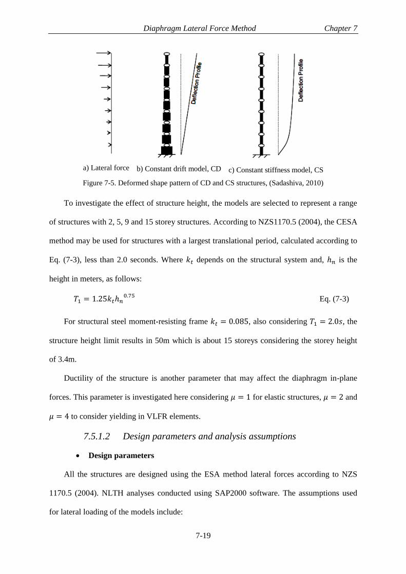
Diaphragm Lateral Force Method Chapter 7
7-19
a) Lateral force
b) Constant drift model, CD
c) Constant stiffness model, CS
Figure 7-5. Deformed shape pattern of CD and CS structures, (Sadashiva, 2010)
To investigate the effect of structure height, the models are selected to represent a range
of structures with 2, 5, 9 and 15 storey structures. According to NZS1170.5 (2004), the CESA
method may be used for structures with a largest translational period, calculated according to
Eq. (7-3), less than 2.0 seconds. Where 𝑘𝑡 depends on the structural system and, ℎ𝑛 is the
height in meters, as follows:
𝑇1 = 1.25𝑘𝑡ℎ𝑛0.75
Eq. (7-3)
For structural steel moment-resisting frame 𝑘𝑡 = 0.085, also considering 𝑇1 = 2.0𝑠, the
structure height limit results in 50m which is about 15 storeys considering the storey height
of 3.4m.
Ductility of the structure is another parameter that may affect the diaphragm in-plane
forces. This parameter is investigated here considering 𝜇 = 1 for elastic structures, 𝜇 = 2 and
𝜇 = 4 to consider yielding in VLFR elements.
7.5.1.2 Design parameters and analysis assumptions
• Design parameters
All the structures are designed using the ESA method lateral forces according to NZS
1170.5 (2004). NLTH analyses conducted using SAP2000 software. The assumptions used
for lateral loading of the models include:

Diaphragm Lateral Force Method Chapter 7
7-20
1) The structure location is assumed in Wellington, New Zealand with subsoil types
C and D.
2) The shortest distance from the site to the nearest fault, D = 0;
3) Return period factor, 𝑅𝑢 = 1;
4) Zone hazard factor, 𝑍 = 0.4 (Wellington),
5) Structural ductility factors, 𝜇 = 1, 2, 4;
• Analysis and modelling assumptions
Four ground motion records were chosen to represent likely earthquakes in Wellington,
New Zealand, considering motion characteristics based on Gardiner (2011) study. The
selected ground motions are listed in Table 7-3. All the time history records were scaled
according to NZS 1170.5 (2004) loading standard. The scaling procedure minimises the
difference between the design response spectra and spectral acceleration of the time history
records over the range of 0.4 to 1.3 times the fundamental period of the structure.
Table 7-3. Selected earthquake records for NLTH analysis
Location Station Date Magnitude
Landers, California Lucerne 28 June 1992 7.3
USA, El Centro, Imperial Valley El Centro 19 May 1940 7.0
Iran, Tabas Tabas 16 September 1978 7.2
Kocaeli, Turkey Izmit 17 August 1999 7.4
The NZS 1170.5 (2004) requires that for time history analysis the time step shall not be
greater than the step at which the records are digitised. Also it is required that the time step
shall be less than or equal to the minimum of i) 𝑇1/100, ii) 𝑇𝑛 and iii) 0.01 second. Where 𝑇1
is the largest translational period of the first mode in the direction of interest and 𝑇𝑛 is the
period of the highest mode in the same direction required to achieve 90% mass participation.
The time step used for all analyses in this study was considered 0.003s based on the
fundamental period of the 2-storey structure, 0.3s.

Diaphragm Lateral Force Method Chapter 7
7-21
The damping model that is used in this research is the Proportional Rayleigh Damping
model. For all models, 5% damping ratio was considered in the first and third modes. The
damping ratio of the mode 𝑛, which represent the highest mode that achieves 90% mass
participation, was checked to be less than 40% based on Clause 6.4.6 of NZS1170.5 (2004).
Note that the damping ratio of the steel structures is usually between 2-3%, however in
this study 5% damping ratio is selected foe NLTH analyses. This is because the ESA method
lateral forces are obtained from 1170.5 (2004) based on considering 5% damping ratio and
since the aim of this study is to compare the results of different methods with NLTH analysis,
assumptions should be consistent. Furthermore, if different damping ratio is used in NLTH
analysis, the lateral forces obtained using ESA method should also be changed using
equations provided in the literature to account for that damping ratio.
The weights used in the analysis are based on the values in Table 7-4. The reduced
gravity load combination considered as 𝐺 + 𝜓𝐸𝑄, where 𝜓𝐸 = 0.3 for most of the structures
other than storage or structures with installed heavy machinery. Therefore, considering a
tributary area of 162 𝑚2 for each frame, the lumped mass on each frame for every storey is
equal to 97.5ton.
Table 7-4. Storey structural mass used for FE modelling
Dead Load, 𝐺 5 kPa
Live Load, 𝑄 3 kPa
Tributary areas for each frame 162 𝑚2
Lumped mass on each frame 97.5ton
Note that The NLTH analysis results reported in this study are the average of results
obtained from four NLTH analyses using the selected ground motions.
In pushover analysis, first mode lateral loads are selected as the lateral load pattern. Also,
diaphragm in-plane forces were obtained at the loading step that the lateral displacement of
the top of the structure reached to the lateral displacement corresponding to EESA method.
The general modelling assumptions include:

Diaphragm Lateral Force Method Chapter 7
7-22
1. Diaphragm stiffness is much larger than frame and wall stiffness
2. Flexural deformation of moment frames due to columns axial deformations and
shear deformation of the wall elements are ignored
3. It is assumed both moment frame and shear wall systems have the same tributary
area for lateral loading
4. Elastic-perfectly plastic moment-curvature is assumed for both frame and wall
elements
5. Masses are lumped at the nodes in the analytical models
6. Soil-structure interaction is ignored
7. Rayleigh damping is used in all models
8. Storey height is considered 3.4m
7.5.1.3 Modelling method and verification
Since the aim of this study is to investigate the diaphragm in-plane forces, the models are
simplified. The simplified models include a cantilever column representing the wall system,
and a column with rotational restraints at each storey to represent the behaviour of the
moment frame structure as shown in Figure 7-6c-d. The rotational restraint at the beam-
column nodes on the moment frame column causes the point of contraflexure to be at the
mid-height of each storey under the lateral loading.
Columns representing VLFR system, are connected at every storey with a horizontal
member representing the diaphragm as shown in Figure 7-6b-d. Verification of the simplified
2D model with the corresponding 3D model is presented in Appendix J.

Diaphragm Lateral Force Method Chapter 7
7-23
a) Floor plan
b) Schematic elevation view
c) Simplified model
d) Deformed shape of the simplified model
subjected to lateral forces
Figure 7-6. Two storey structure and the simplified model
To obtain inertia and transfer forces two models are created for each structure. In one
model inertia forces and transfer forces are obtained separately and in the other model the
combination of these forces is obtained. This is because the maximum diaphragm force does
not necessarily equal to the sum of maximum inertia and transfer forces because these may
not occur at the same time. Figure 7-7 shows the modelling methods for obtaining inertia and
transfer forces combined and separately.

Diaphragm Lateral Force Method Chapter 7
7-24
a) Simplified model for obtaining inertia and
transfer forces together
b) Simplified model for obtaining inertia and transfer
forces separately
Figure 7-7. Modelling methods for obtaining inertia and transfer forces
In the simplified 2D model shown in Figure 7-7a, the storey mass is located at the mid-
point of the diaphragm element. In this model, maxima of the diaphragm element force
represents the maxima of the combination of inertia and transfer forces. However, in the
model shown in Figure 7-7b, the storey masses are attached to the VLFR systems with rigid
links. This modelling method allows obtaining the inertia and transfer forces separately.
7.5.2 Results and discussion
7.5.2.1 Moment frame structures
In moment frame structures described in Table 7-1, there is no diaphragm transfer forces
and the only source of diaphragm global in-plane demand is the inertia force. In this section
the effect of different parameters on the diaphragm inertia forces is investigated.
• Effect of ductility
Figure 7-8 presents the magnitude of inertia forces obtained from the diaphragms of five
storey structures with different design ductility according to NZS1170.5 (2004). As can be
seen in this Figure, the EESA method predicted likely diaphragm demands in upper floors.
However, the inertia forces on the lower floors were underestimated. The proposed method

Diaphragm Lateral Force Method Chapter 7
7-25
shows better agreement with NLTH results in comparison with the EESA method because of
the increase in diaphragm forces at the lower levels.
It also indicates that the proposed method, DESA, underestimated the diaphragm forces
of the structure with ductility 𝜇 = 1 by up to 20% in lower levels. The proposed method
estimations for the structure with ductility 𝜇 = 2 were less than 10% compared to NLTH
analyses. For 𝜇 = 4 the DESA overestimated the NLTH response by about 30%. These
results were expected as the DESA method does not consider structure ductility and uses
elastic forces to obtain diaphragm in-plane demands.
P&C diaphragm forces are much larger than other methods. This was consistent in all
graphs. Therefore, the P&C analysis result is only shown in Figure 7-8a and in the following
plots these have been removed to allow easier interpretation of graphs.
a) Model 1, five-storey structure with ductility 𝜇 = 1
1
2
3
4
5
0 2000 4000 6000 8000
STO
REY
DIAPHRAGM INERTIA FORCE (KN)
EESA pESA OESA P&C Pushover NLTH DESA
1
2
3
4
5
0 500 1000 1500 2000 2500 3000 3500
STO
REY
DIAPHRAGM INERTIA FORCE (KN)
EESA pESA OESA Pushover
NLTH CESA DESA

Diaphragm Lateral Force Method Chapter 7
7-26
b) Model 2, five-storey structure with ductility 𝜇 = 2
c) Model 4, five-storey structure with ductility 𝜇 = 4
Figure 7-8. In-plane diaphragm inertia forces for five-storey moment frame structures with different
ductility (T=0.6s)
The same behaviour was observed for the nine-storey structure with ductility 𝜇 = 1 and
4 as shown in Figure 7-9a and b. The diaphragm forces obtained using the proposed DESA
method, underestimated the diaphragm inertia forces by about 30% on average compared to
NLTH analysis for the nine-storey elastic structure, Figure 7-9a. However, the DESA
overestimated the NLTH response by about 100% for the structure with 𝜇 = 4, Figure 7-9b.
a) Model 6, nine-storey structure with ductility 𝜇 = 1
1
2
3
4
5
0 500 1000 1500 2000 2500 3000 3500
STO
REY
DIAPHRAGM INERTIA FORCE (KN)
EESA pESA OESA Pushover
NLTH CESA DESA
123456789
0 500 1000 1500 2000 2500 3000 3500
STO
REY
DIAPHRAGM INERTIA FORCE (KN)
EESA pESA OESA Pushover NLTH DESA

Diaphragm Lateral Force Method Chapter 7
7-27
b) Model 8, nine-storey structure with ductility 𝜇 = 4
Figure 7-9. In-plane diaphragm inertia forces for nine-storey moment frame structures with different
ductility (T=1.0 s)
• Effect of structure height
The analyses results of Models 5, 1, 6 and, 10, indicate the effect of structural height, are
plotted in Figure 7-10. As can be seen, the proposed method improved the ESA method
results for lower floor levels. However, similar to Figure 7-8a, the proposed method
underestimated the diaphragm in-plane demands on the lower floors for structures with
ductility 𝜇 = 1.
The average underestimation of diaphragm in-plan forces using the proposed method,
DESA, for the bottom half portion of the models studied in comparison with the NLTH
analyses results is 22%, 17%, 12% and 40% respectively for two, five, nine and fifteen storey
structures with 𝜇 = 1.
123456789
0 500 1000 1500 2000 2500 3000
STO
REY
DIAPHRAGM INERTIA FORCE (KN)
EESA pESA OESA Pushover NLTH DESA

Diaphragm Lateral Force Method Chapter 7
7-28
a) Model 5, two-storey structure with ductility 𝜇 = 1
b) Model 1, five-storey structure with ductility 𝜇 = 1
c) Model 6, nine-storey structure with ductility 𝜇 = 1
1
2
0 500 1000 1500 2000 2500 3000 3500
STO
REY
DIAPHRAGM INERTIA FORCE (KN)
EESA pESA OESA Pushover NLTH DESA
1
2
3
4
5
0 1000 2000 3000 4000
STO
REY
DIAPHRAGM INERTIA FORCE (KN)
EESA pESA OESA Pushover NLTH DESA
123456789
0 1000 2000 3000 4000
STO
REY
DIAPHRAGM INERTIA FORCE (KN)
EESA pESA OESA Pushover NLTH DESA

Diaphragm Lateral Force Method Chapter 7
7-29
d) Model 10, fifteen-storey structure with ductility 𝜇 = 1
Figure 7-10. In-plane diaphragm inertia forces for moment frame structures with different number of
storeys
Despite the underestimation mentioned in the previous paragraph, the proposed method
presented more reasonable results than other studied methods in terms of lower story in-plane
demands. This conclusion is based on the models studied here and other methods may be
developed to increase the accuracy.
• Storey stiffness distribution
Figure 7-11 presents the magnitude of inertia forces obtained from the diaphragms of
elastic five-storey moment frame structures with constant drift and constant stiffness VLFR
systems. As can be seen in this Figure, the proposed method provided more reasonable results
in comparison with other static methods. The peak diaphragm in-plane forces obtained from
the NLTH analyses showed that different storey stiffness distributions, CS and CD, may
change the distribution of peak diaphragm in-plane forces. However, the average was similar
in the studied case.
13579
111315
0 500 1000 1500 2000 2500 3000
STO
REY
DIAPHRAGM INERTIA FORCE (KN)
EESA pESA OESA Pushover NLTH DESA

Diaphragm Lateral Force Method Chapter 7
7-30
a) Model 1, constant stiffness VLFR system
b) Model 3, constant drift VLFR system
Figure 7-11. In-plane diaphragm inertia forces for elastic five-storey structures with different storey
stiffness distribution and ductility μ=1
• Subsoil type effect
Figure 7-12 presents the behaviour of Models 6 to 9 considering ductility 𝜇 = 1 and 4
and subsoil types C and D. From Figure 7-12a and b it can be seen that pESA method
underestimated diaphragm in-plane forces at lower levels for structure on subsoil D, however,
they are overestimated for the same structure on subsoil type C. This is because of the
modified spectral shape values obtained by Gardiner (2011) which result in larger lateral
forces for subsoil C. The same situation occurred for the structure with 𝜇 = 4 as shown in
Figure 7-12c and d, where the proposed method overestimated the diaphragm in-plane forces
1
2
3
4
5
0 1000 2000 3000 4000 5000
STO
REY
DIAPHRAGM INERTIA FORCE (KN)
EESA pESA OESA Pushover NLTH DESA
1
2
3
4
5
0 1000 2000 3000 4000 5000
STO
REY
DIAPHRAGM INERTIA FORCE (KN)
EESA pESA OESA Pushover NLTH DESA

Diaphragm Lateral Force Method Chapter 7
7-31
by about 100%. While, the pESA method provided results that are more reasonable compared
to NLTH analysis specially for subsoil type C.
a) Model 6, nine-storey structure with ductility 𝜇 = 1 and subsoil D
b) Model 7, nine-storey structure with ductility 𝜇 = 1 and subsoil C
c) Model 8, nine-storey structure with ductility 𝜇 = 4 and subsoil D
123456789
10
0 1000 2000 3000 4000
STO
REY
DIAPHRAGM INERTIA FORCE (KN)
EESA pESA OESA Pushover NLTH DESA
123456789
10
0 500 1000 1500 2000 2500
STO
REY
DIAPHRAGM INERTIA FORCE (KN)
EESA pESA OESA Pushover NLTH DESA
123456789
10
0 500 1000 1500 2000 2500 3000
STO
REY
DIAPHRAGM INERTIA FORCE (KN)
EESA pESA OESA Pushover NLTH DESA

Diaphragm Lateral Force Method Chapter 7
7-32
d) Model 9, nine-storey structure with ductility 𝜇 = 4 and subsoil C
Figure 7-12. In-plane diaphragm inertia forces for nine-storey structures with different ductility and
subsoil types
7.5.2.2 Dual VLFR system structures
Structures consist of two VLFR systems, a shear wall and a moment resisting frame, are
considered as Dual type structures. In these structures, the diaphragm in-plane force is a
combination of inertia and transfer forces. The imposed transfer forces are due to deformation
incompatibility of different VLFR systems. Figure 7-13 shows the analysis results of Model
11 which is a five storey elastic structure with shear wall to moment resisting frame stiffness
ratio of one. The analysis results are obtained in terms of peak inertia and transfer forces and
also peak total in-plane forces. The peak total in-plane diaphragm force in NLTH analysis is
not necessarily equal to the sum of the peak inertia and transfer forces because they may
occur at different time steps.
123456789
10
0 500 1000 1500 2000
STO
REY
DIAPHRAGM INERTIA FORCE (KN)
EESA pESA OESA Pushover NLTH DESA

Diaphragm Lateral Force Method Chapter 7
7-33
a) Diaphragm inertia forces
b) Diaphragm transfer forces
c) Total diaphragm forces
Figure 7-13. Diaphragm forces for Model 11
0 1000 2000 3000 4000 5000
St 1
St 2
St 3
St 4
St 5
Diaphragm inertia forces
DESA
NLTH
Pushover
OESA
pESA
EESA
0 1000 2000 3000 4000 5000
St 1
St 2
St 3
St 4
St 5
Diaphragm transfer forces
DESA
NLTH
Pushover
OESA
pESA
EESA
1
2
3
4
5
0 2000 4000 6000 8000
STO
REY
DIAPHRAGM TOTAL FORCE (KN)
EESA pESA OESA Pushover NLTH DESA

Diaphragm Lateral Force Method Chapter 7
7-34
In the following only the total diaphragm in-plane forces are presented. The peak inertia
and transfer forces of all dual-type models are presented in Appendix K.
• Effect of ductility
Figure 7-14 shows the total diaphragm in-plane forces for five and nine storey structures
with different ductilities. In these models, the diaphragm transfer forces govern the total
diaphragm in-plane demand. Therefore, the effect of inertia forces decreased. In these models
the shear wall to moment resisting frame stiffness ratio equal to one was selected in order to
maximize transfer forces according to Gardiner’s (2011) study.
Figure 7-14a shows that the ESA method presents similar results to NLTH analysis for
both the bottom and the top portion of the structure. This is because the effect of inertia
forces are less than transfer forces in these models and the effect of underestimation of
diaphragm accelerations on the lower levels decreased. It is noted that with changing the wall
to frame stiffness ratio these results may change and inertia forces may increase in
comparison with transfer forces and govern the diaphragm in-plane demands.
The proposed method overestimated the diaphragm total in-plane demands of the studied
models. For example, the total in-plane demands of the third floor of five-storey structures as
shown in Figure 7-14a,b and c were overestimated by about 75%, 24% and 37% for
structures with 𝜇 = 1, 2 and 4 respectively.
The same behaviour was observed for the nine-storey structure with ductility 𝜇 = 1 and
4 as shown in Figure 7-14d and e. The diaphragm forces obtained using the proposed
method, and the pESA overestimated the diaphragm inertia forces of Model 17 up to about
45% and 60% on average compared to NLTH analysis. However, for the nine-storey
structure with 𝜇 = 4, Figure 7-14e they were overestimated with about 200% and 40% using
the proposed, DESA, and the pESA methods.

Diaphragm Lateral Force Method Chapter 7
7-35
a) Model 11, five-storey structure with ductility 𝜇 = 1
b) Model 12, five-storey structure with ductility 𝜇 = 2
c) Model 13, five-storey structure with ductility 𝜇 = 4
1
2
3
4
5
0 2000 4000 6000 8000
STO
REY
DIAPHRAGM TOTAL FORCE (KN)
EESA pESA OESA Pushover NLTH DESA
1
2
3
4
5
0 1000 2000 3000 4000 5000 6000
STO
REY
DIAPHRAGM TOTAL FORCE (KN)
EESA pESA OESA Pushover NLTH CESA DESA
1
2
3
4
5
0 1000 2000 3000 4000 5000 6000
STO
REY
DIAPHRAGM TOTAL FORCE (KN)
EESA pESA OESA Pushover NLTH CESA DESA
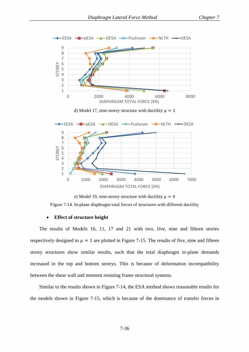
Diaphragm Lateral Force Method Chapter 7
7-36
d) Model 17, nine-storey structure with ductility 𝜇 = 1
e) Model 19, nine-storey structure with ductility 𝜇 = 4
Figure 7-14. In-plane diaphragm total forces of structures with different ductility
• Effect of structure height
The results of Models 16, 11, 17 and 21 with two, five, nine and fifteen stories
respectively designed to 𝜇 = 1 are plotted in Figure 7-15. The results of five, nine and fifteen
storey structures show similar results, such that the total diaphragm in-plane demands
increased in the top and bottom storeys. This is because of deformation incompatibility
between the shear wall and moment resisting frame structural systems.
Similar to the results shown in Figure 7-14, the ESA method shows reasonable results for
the models shown in Figure 7-15, which is because of the dominance of transfer forces in
123456789
0 2000 4000 6000 8000
STO
REY
DIAPHRAGM TOTAL FORCE (KN)
EESA pESA OESA Pushover NLTH DESA
123456789
0 1000 2000 3000 4000 5000 6000 7000
STO
REY
DIAPHRAGM TOTAL FORCE (KN)
EESA pESA OESA Pushover NLTH DESA

Diaphragm Lateral Force Method Chapter 7
7-37
these models. These results support the hypothesis that the ESA method may estimate likely
transfer forces because it can obtain the likely lateral deformed shape of the structure.
The analyses results presented in Figure 7-15 indicate that the proposed method
overestimated diaphragm in-plane demands of two, five and nine storey structures in
comparison with NLTH analysis. However, in Model 21, fifteen-storey structure, the pESA
method overestimated the total diaphragm in-plane forces by about 130% on average
compared to NLTH analysis and the proposed, DESA, method overestimated the total
diaphragm in-plane forces by about 60% on average compared to NLTH analysis.
a) Model 16, two-storey structure with ductility 𝜇 = 1
b) Model 11, five-storey structure with ductility 𝜇 = 1
1
2
0 1000 2000 3000 4000 5000
STO
REY
DIAPHRAGM TOTAL FORCE (KN)
EESA pESA OESA Pushover NLTH DESA
1
2
3
4
5
0 2000 4000 6000 8000
STO
REY
DIAPHRAGM TOTAL FORCE (KN)
EESA pESA OESA Pushover NLTH DESA

Diaphragm Lateral Force Method Chapter 7
7-38
c) Model 17, nine-storey structure with ductility 𝜇 = 1
d) Model 21, fifteen-storey structure with ductility 𝜇 = 1
Figure 7-15. In-plane diaphragm total forces of structures with different number of stories
Similar results may be obtained for structures designed for 𝜇 = 4, Models 13 and 19, as
shown in Figure 7-14c and e. These indicated that the proposed method overestimated
diaphragm in-plane demands of five and nine storey structures designed with 𝜇 = 4 in
comparison with NLTH analysis by about 68% and 230% on average. However, the pESA
method underestimated the total diaphragm in-plane forces of the five-storey structure by
about 20% and overstimated the total diaphragm in-plane forces of the nine-storey structure
by about 40% on average compared to NLTH analysis.
It is noted that these results may change with changing the structure configuration,
design ductility, period and VLFR system relative stiffnesses.
123456789
0 1000 2000 3000 4000 5000 6000 7000
STO
REY
DIAPHRAGM TOTAL FORCE (KN)
EESA pESA OESA Pushover NLTH DESA
123456789
101112131415
0 2000 4000 6000 8000 10000 12000
STO
REY
DIAPHRAGM TOTAL FORCE (KN)
EESA pESA OESA Pushover NLTH DESA

Diaphragm Lateral Force Method Chapter 7
7-39
• Effect of different wall to frame stiffness ratios
Figure 7-16 shows the analysis results of five storey structures with wall to frame
stiffness ratios, WTFSR, of 1, 5 and 10. These stiffness ratios were calculated as the relative
base shears of the elastically responding frame and the wall elements when subjected to the
CESA load distribution. In all of these three cases, the stiffnesses were modified to obtain the
same fundamental period of 0.6s.
When 𝑊𝑇𝐹𝑆𝑅 = 0, this implies frame action. when 𝑊𝑇𝐹𝑆𝑅→∞, this is all wall action.
In both of these cases, there are no transfer forces, so inertial forces control the response.
Transfer forces are more significant in the intermediate WTFSR ratios. Gardiner (2011)
showed that the “fighting effect” between the wall and the frame systems is maximum when
the wall to frame stiffness ratio is one.
Figure 7-16 shows that with increasing the wall to frame stiffness ratio, the effect of
diaphragm transfer force decreased. These results are consistent with findings of Gardiner
(2011).
a) Model 11, WTFSR=1
1
2
3
4
5
0 2000 4000 6000 8000
STO
REY
DIAPHRAGM TOTAL FORCE (KN)
EESA pESA OESA Pushover NLTH DESA

Diaphragm Lateral Force Method Chapter 7
7-40
b) Model 14, WTFSR=5
c) Model 15, WTFSR=10
Figure 7-16. In-plane diaphragm total forces of five-storey structures with different wall to frame
stiffness ratios
As can be seen from the analyses results shown in Figure 7-16, the EESA method
provides similar results as NLTH analysis for the structure with wall to frame stiffness ratio
of one. With increasing the wall to frame stiffness ratio, the effect of transfer forces
decreases, therefore the diaphragm in-plane demands of lower levels were underestimated.
The proposed method overestimated the diaphragm in-plane demands for all three models
shown in Figure 7-16 by up to 60% on average.
• Subsoil type effect
Figure 7-17 presents the behaviour of Models 17 to 20 considering ductility 𝜇 = 1 and 4
and subsoil types C and D. Figure 7-17a and b show that the pESA and DESA methods
1
2
3
4
5
0 2000 4000 6000 8000
STO
REY
DIAPHRAGM TOTAL FORCE (KN)
EESA pESA OESA Pushover NLTH DESA
1
2
3
4
5
0 1000 2000 3000 4000 5000 6000
STO
REY
DIAPHRAGM TOTAL FORCE (KN)
EESA pESA OESA Pushover NLTH DESA

Diaphragm Lateral Force Method Chapter 7
7-41
overestimated diaphragm in-plane forces for elastic structure (𝜇 = 1) on subsoil D by about
60% and 45% on average compared to NLTH analysis respectively. However, the diaphragm
in-plane forces for the same structure on subsoil C were overestimated by about 200% and
85% using the pESA and DESA methods respectively. This is because of the modified
spectral shape values obtained by Gardiner (2011). For the structure with 𝜇 = 4 as shown in
Figure 7-17c and d, the proposed method overestimated the diaphragm in-plane forces by
about 200% for both subsoils D and C. While, the pESA method provided more reasonable
diaphragm total in-plane forces compared to NLTH analysis with up to 40% and 80%
overestimation on average for subsoils D and C respectively.
a) Model 17, nine-storey structure with ductility 𝜇 = 1 and subsoil D
1
2
3
4
5
6
7
8
9
0 2000 4000 6000 8000
STO
REY
DIAPHRAGM TOTAL FORCE (KN)
EESA pESA OESA Pushover NLTH DESA
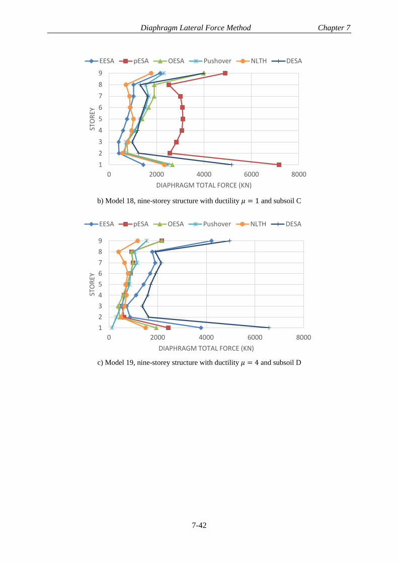
Diaphragm Lateral Force Method Chapter 7
7-42
b) Model 18, nine-storey structure with ductility 𝜇 = 1 and subsoil C
c) Model 19, nine-storey structure with ductility 𝜇 = 4 and subsoil D
1
2
3
4
5
6
7
8
9
0 2000 4000 6000 8000
STO
REY
DIAPHRAGM TOTAL FORCE (KN)
EESA pESA OESA Pushover NLTH DESA
1
2
3
4
5
6
7
8
9
0 2000 4000 6000 8000
STO
REY
DIAPHRAGM TOTAL FORCE (KN)
EESA pESA OESA Pushover NLTH DESA
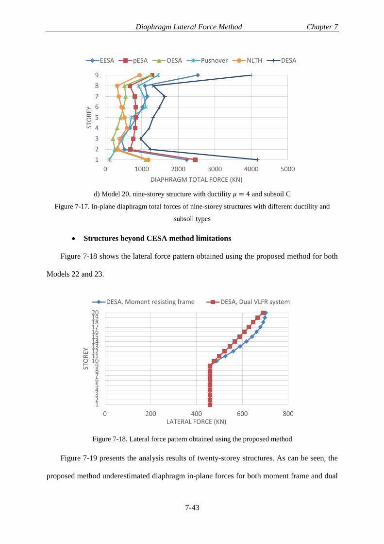
Diaphragm Lateral Force Method Chapter 7
7-43
d) Model 20, nine-storey structure with ductility 𝜇 = 4 and subsoil C
Figure 7-17. In-plane diaphragm total forces of nine-storey structures with different ductility and
subsoil types
• Structures beyond CESA method limitations
Figure 7-18 shows the lateral force pattern obtained using the proposed method for both
Models 22 and 23.
Figure 7-18. Lateral force pattern obtained using the proposed method
Figure 7-19 presents the analysis results of twenty-storey structures. As can be seen, the
proposed method underestimated diaphragm in-plane forces for both moment frame and dual
1
2
3
4
5
6
7
8
9
0 1000 2000 3000 4000 5000
STO
REY
DIAPHRAGM TOTAL FORCE (KN)
EESA pESA OESA Pushover NLTH DESA
123456789
1011121314151617181920
0 200 400 600 800
STO
REY
LATERAL FORCE (KN)
DESA, Moment resisting frame DESA, Dual VLFR system

Diaphragm Lateral Force Method Chapter 7
7-44
type structure with about 75% and 55% on average compared to NLTH analysis for the FE
models studied.
In the moment frame structure, Model 22, there is no transfer forces and the governing
diaphragm in-plane demand is the inertia forces. Therefore a method that is able to estimate
likely diaphragm accelerations may provide more accurate results than the DESA method.
The proposed method is based on estimating likely structure lateral deformation to obtain
diaphragm transfer forces. Note in cases that inertial forces control the response, perhaps it is
not necessary to consider peak diaphragm accelerations, because the duration of the peak
force/acceleration demand may significantly affect the structural response. For example, if
high force/acceleration demands occur only briefly, causing a small inelastic displacement,
then its effect may be minor on the global diaphragm performance. Therefore designing for
the peak values may be conservative (MacRae and Bull, 2015, Bruere and Colley 2015).
Also, the analysis and modelling assumptions such as damping and nonlinear behaviour of
the structural elements may affect the peak accelerations recorded.
a) Model 22, twenty-storey structure with ductility 𝜇 = 1 and moment frame system
0
2
4
6
8
10
12
14
16
18
20
0 500 1000 1500
STO
REY
DIAPHRAGM INERTIA FORCE (KN)
DESA Mode 1 NLTH

Diaphragm Lateral Force Method Chapter 7
7-45
b) Model 23, twenty-storey structure with ductility 𝜇 = 1 and dual VLFR system
Figure 7-19. Total in-plane diaphragm forces of twenty-storey structures
Here, both Models 22 and 23 shown in Figure 7-19 are designed for 𝜇 = 1. It is expected
that the diaphragm in-plane demands decrease with increasing ductility due to yielding in
VLFR system members. Therefore, here elastic structures are considered to be compared with
the proposed method that is based on EESA method.
7.5.3 Discussion on the proposed method
As mentioned in Section 7.4, a hypothesis used in the proposed method is that diaphragm
transfer forces may be obtained using elastic ESA (𝜇 = 1) lateral forces because they provide
the likely deformed shape of a long period structure according to the equal displacement
assumption. However, they ignore important response features, such as structure ductility,
redistribution of internal forces due to yielding of structural elements, hysteretic effects and,
degradation due to stiffness and strength. Despite all these limitations, the ESA method is a
widely accepted method in many loading standards (e.g. NZS1170.5 2004 and ASCE/SEI 7–
16).
The results of the FE models studied in Section 7.5.2 showed that the proposed method
may be used as a more general method because it is based on EESA method. In addition, it
02468
101214161820
0 500 1000 1500 2000 2500 3000
STO
REY
DIAPHRAGM TOTAL FORCE (KN)
NLTH DESA

Diaphragm Lateral Force Method Chapter 7
7-46
may remove some limitations of the CESA and pESA methods such as height limitation and
overstrength calculation. However, it may result in some overestimation and underestimation
of response in different cases. In the following the limitations of the proposed method are
discussed.
Based on the analyses conducted it was found that:
1. The proposed method underestimated diaphragm in-plane demands for structures
with low ductility (e.g. 𝜇 < 2) these include any structure where the actual
overall lateral strength (𝜙𝑜𝑏𝑉𝑑𝑒𝑠𝑖𝑔𝑛 shown in Figure 7-1) is greater than that
required from the EESA forces. For steel structures it is common that members
are sized to meet deflection limits causing higher force strength.
2. The proposed method overestimated diaphragm in-plane forces for the ductile
structures (e.g. 𝜇 ≥ 3) analysed. This is because the proposed method use the
EESA lateral forces, while increasing the structure ductility may reduce the
diaphragm in-plane force due to yielding in some structural elements.
3. In the process of assessment or retrofit of an existing building, this method may
result in large diaphragm in-plane demands which cause the retrofit process
impossible or result in a large demand to capacity ratios.
4. The proposed method considers peak demands. It is possible that some
inelasticity (e.g. shear stud inelastic deformation) may result in very small
inelastic demands and provide satisfactory behaviour. This is described further in
Chapter 8.

Diaphragm Lateral Force Method Chapter 7
7-47
7.6 Conclusion
Based on the analyses conducted in this study, it was found that:
1) Diaphragm in-plane force demands include i) inertia forces, ii) transfer forces, iii) slab
bearing forces, iv) compatibility forces, and v) forces from interaction with other
elements. These in-plane forces may be categorised into global demand (i and ii) and
local demand (iii, iv and v) groups based on their effect on the diaphragm. The global
diaphragm demands may be obtained using lateral force methods or NLTH analysis.
However, the local demands need to be considered for designing different
components of the diaphragm locally.
2) The available lateral force methods to obtain diaphragm in-plane demands range from
a simple static method, (e.g. CESA), to complex and more realistic methods, (e.g.
NLTH). A number of lateral force methods that have been used for obtaining
diaphragm global in-plane demands include: 1) ESA considering structure ductility
(CESA), 2) Overstrength ESA (OESA), 3) Elastic ESA, (EESA), 4) Parts and
Components method (P&C), 5) pseudo-Equivalent Static Analysis (pESA), 6) Sabelli
et al. (2011) method, 7) Pushover analysis, 8) Modal response spectrum method
(RSA), and 9) NLTH. These were evaluated for their suitability for use in design.
3) A new method, Diaphragm ESA (DESA), was proposed based on the hypothesis that
if a lateral loading method can represent likely deformed shape of a structure, it can
obtain likely diaphragm transfer forces. This is because diaphragm transfer forces are
mainly due to deformation incompatibility of different VLFR systems. This method
assumes the lateral deformation of a long period structure at the design level may be
estimated using the EESA (𝜇 = 1) method according to the equal displacement
assumption. Also, the bottom portion of the EESA lateral forces are increased in the
proposed method to approximate the higher mode effects.

Diaphragm Lateral Force Method Chapter 7
7-48
For high-rise buildings beyond the CESA method limitations, it is suggested to use
the first mode lateral forces scaled to the EESA base shear and increase the lateral
forces at lower floors. In the studied models, this method underestimated likely
diaphragm acceleration by up to 55% on average; however, it estimated the likely
diaphragm transfer forces with 75% underestimation on average compared to NLTH
analysis. Note that high force/acceleration demands obtained from analyses may
occur only briefly, causing a small inelastic displacement, then its effect may be
minor. Designing for the peak values may therefore be conservative.
4) The analyses results showed that the proposed method may remove some
limitations of the CESA and pESA methods such as height limit and overstrength
calculation process. However, it may result in some overestimation and
underestimation of response in different cases and ignore some important response
features, such as structure ductility, redistribution of internal forces, hysteretic effects,
stiffness and strength degradation. The advantages and disadvantages of different
lateral force methods were discussed so that one can decide which method can
provide more reasonable results based on the accuracy and time required for the
analysis.
Note that the proposed method needs more research and study to show its limitations
and the level of conservatism it may provide. The primary aims of proposing this
method were a) to introduce the concept that transfer forces may be obtained using
elastic ESA method that can predict likely lateral deformations of the structure, b) to
provide a method which usually obtains conservative results in absence of any other
widely accepted method, c) to be applicable to structures with wide range of hights
and d) to be simple enough for use in a design office and do not require to calculate
the structure over-strength to obtain lateral forces.

Diaphragm Lateral Force Method Chapter 7
7-49
References
[1] American Society of Civil Engineers, Structural Engineering Institute (2016),
Minimum Design Loads for Buildings and Other Structures. American Society of
Civil Engineers, Structural Engineering Institute, Reston, Virginia. ASCE/SEI 7–
16
[2] Bruere R. J. and Davies-Colley M. (2015). “Effect of Reducing Maximum
Response on Concrete Floor Diaphragms”, Final Year Projects, Dept. of Civil
and Natural Resources Engineering, University of Canterbury. Project
supervisors: MacRae GA and Bull DK.
[3] Chaudhari T. D., MacRae G. A., Bull D., Chase G., Hicks S., Clifton G. C. and
Hobbs M. (2015). “Composite Slab Effects on Beam-Column Subassembly
Seismic Performance”, 8th International Conference on Behavior of Steel
Structures in Seismic Areas, Shanghai, China.
[4] Dantanarayana H. N., MacRae G. A., Dhakal R. P., Yeow T. Z. & Uma S. R.
(2012) “Quantifying Building Engineering Demand Parameters in Seismic
Events”, 14 World Conference on Earthquake Engineering, Lisbon, Portugal,
August 2012. Paper number 3424.
[5] Fenwick, R. C. and Davidson, B. J. (1991). The Seismic Response of Multi-
storey Buildings, Department of Civil Engineering, University of Auckland.
Report number 495.
[6] Fenwick, R. C. and Davidson, B. J. (1997). "P-delta Actions and the Loadings
Code." SESOC 10(1): 58-62.
[7] Gardiner D. R. (2011). “Design Recommendations and Methods for Reinforced
Concrete Floor Diaphragms Subjected to Seismic Forces”, PhD Thesis,
University of Canterbury.
[8] MacRae G. A. and Bull D. (2015). “Diaphragm Design, ENEQ650: Seismic
Design of Steel and Composite Structures”, Postgraduate Class notes, University
of Canterbury, 2015.

Diaphragm Lateral Force Method Chapter 7
7-50
[9] MacRae G. A. and Clifton G. C. (2015). “Research on Seismic Performance of
Steel Structures”, Steel Innovations Conference, Auckland, New Zealand.
[10] MacRae G. A., Hobbs M., Bull D., Chaudhari T., Leon R., Clifton G. C. and
Chase C. (2013). “Slab Effects on Beam-Column Subassemblies – Beam
Strength and Elongation Issues”, Composite Construction VII Conf., Palm Cove,
Queensland, Australia.
[11] NZS 1170.5 (2004). Structural Design Actions-Part, 5. Standards New
Zealand, Wellington, New Zealand. Including Amendment 1, 2016.
[12] Sabelli R., Sabol T. A. and Easterling W. S. (2011). “Seismic Design of
Composite Steel Deck and Concrete-filled Diaphragms A Guide for Practicing
Engineers”, NEHRP Seismic Design Technical Brief No. 5.
[13] Sadashiva, V. K. (2010). Quantifying structural irregularity effects for simple
seismic design.
[14] SESOC (2011). Design of Conventional Structural Systems Following the
Canterbury Earthquakes: Structural Engineering Society of New
Zealand, ENG.SESOC.0016.1, Version No. 4:21.
[15] Veletsos, A. S., & Newmark, N. M. (1960, July). Effect of inelastic behaviour
on the response of simple systems to earthquake motions. Department of Civil
Engineering, University of Illinois.

Diaphragm Stiffness and Strength Considerations Chapter 8
8-1
8 Diaphragm Stiffness and Strength Considerations
8.1 Introduction
In practice, the elastic analysis is commonly used by engineers to perform structural
analysis and design. The elastic analysis only considers one stiffness of each element (which
may be the initial stiffness, or the cracked stiffness of an RC member) and does not provide
information about the nonlinear behaviour of different structural elements or the force
redistribution due to change of stiffness or yielding of structural members. Also in the elastic
analysis the main structural members are usually modelled and the effect of other elements
(e.g. beam-column connections, shear studs and slab bearing elements) are often ignored.
Ignoring these factors may cause:
1) different lateral forces between vertical lateral force resisting (VLFR) systems,
2) an over or underestimate of a) diaphragm transfer forces, b) beam-column
connection axial forces, and c) shear stud demands
To obtain a more realistic result, the effects of different structural components need to be
incorporated into the model, and nonlinear analysis should be performed. However, this may
not be easily achieved due to limitations in most of commonly used engineering software
packages and lack of knowledge about the nonlinear behaviour of some structural elements.
Therefore, the force redistribution, and possible effects of nonlinear behaviour of different
structural elements, needs to be considered using rational assumptions.
In this chapter, a number of FE models are used to investigate:
1. How can standard diaphragm design/assessment processes be modified to consider
diaphragm stiffness (considering cracking) and strength, shear stud behaviour, and
beam system axial strength?
Diaphragm Stiffness and Strength Considerations Chapter 8
8-2
2. How do beam-end connection and shear stud demands obtained from the proposed
diaphragm design process compare with those from NLTH analysis?
3. What is the effect of providing intentional gaps between the slab and columns
particularly on the beam-end connections and shear studs?
4. What is the amount of composite beam mid-point vertical deflection due to gravity
and earthquake lateral loading?
8.2 Diaphragm design/assessment process
8.2.1 General concept
In practice, diaphragms may not be designed explicitly as it is usually assumed these
structural elements are very stiff and strong in-plane. However, in cases that diaphragms are
explicitly designed, the assumed diaphragm in-plane stiffness and the adequacy of the provided
in-plane strength may be questionable because there is no commonly accepted diaphragm
analysis method and design procedure.
Diaphragm in-plane design and diaphragm components design have been discussed by
many researchers such as Bull (2004), Naeim and Boppana (2001), Sabelli et al. (2011), Scarry
(2014), Cowie et al. (2014), and Moehle (2015). Section C5 of The Seismic Assessment of
Existing Buildings (2017), hereafter referred to as the Assessment Guideline is the only one of
the above that provides step-by-step diaphragm design/assessment procedures.
The design/assessment flowchart of the Assessment Guideline (2017) for designing
diaphragms is shown in Figure 8-1 in the boxes 1 to 6. Diaphragm in-plane design process
shown in Figure 8-1 includes two major parts:
1) Obtaining diaphragm in-plane demands using appropriate lateral force method and
reasonable diaphragm in-plane stiffness assumption (Steps 1-3 shown in Figure 8-1).

Diaphragm Stiffness and Strength Considerations Chapter 8
8-3
To obtain diaphragm in-plane forces/demands, the entire structure is first modelled.
This is because diaphragm transfer forces, and interaction with other elements, are
usually the result of deformation incompatibility of different structural elements and/or
discontinuities in plan location of the VLFR elements. Therefore, modelling only one
storey of the structure and imposing inertia forces to the diaphragm may not provide
likely diaphragm in-plane demands.
The term “out-of-plane forces”, 𝐹𝑣𝑖, refers to the reaction of VLFR elements to the
diaphragm. This can be changed to "vertical element lateral reactions", however to
keep consistency with Assessment Guideline (2017) it is written “out-of-plane forces”
in the following flowcharts.
2) Modelling and obtaining diaphragm internal forces to check diaphragm strength (Steps 4-
6 shown in Figure 8-1).
Section C5.5.4.2 of the Assessment Guideline (2017) state that for buildings with
significant asymmetry in the location of lateral force-resisting elements, such as the
distribution across the building plan, termination up the height of the building, varying
stiffness and/or strength between vertical elements, may require a more advanced
analysis than simple hand-drawn strut and tie solutions (described in Section 3.2.1).
For these types of structures, the truss element method (described in Section 3.3) was
suggested to be used to obtain diaphragm design actions.
Modifications/amplifications of concepts in this flowchart include:
1. Beam axial capacity check, shown in Box 7 in Figure 8-1 and the method of Cowie
et al. (2014) may be followed.
2. Proposing diamond truss model to improve beam axial force and shear stud
demand estimations and obtain more accurate result using less truss mesh units
(Chapter 3). This modifies Box 4.

Diaphragm Stiffness and Strength Considerations Chapter 8
8-4
3. Web-Side-Plate connection axial strength check (Chapter 4). This modifies Box 8.
4. Shear stud lateral strength check (Chapter 5). This modifies Box 9.
5. Diaphragm buckling strength check (Chapter 6). This modifies Box 10.
6. Proposing DESA method to obtain diaphragm lateral forces (Chapter 7). This
affects Box 2.
7. Diaphragm in-plane stiffness consideration (Chapter 8 Section 8.2.2). This
modifies Box 1.
Start diaphragm in-plane design
For each principal direction
End
Obtain diaphragm
lateral forces using an
appropriate loading method,
Fdi
2
Model entire structure
considering reasonable diaphragm
stiffness
1
Determine vertical element
out-of-plane forces, Fvi
3
Model each diaphragm using
appropriate truss element
model
4
Apply Fdi, to the truss model and
Fvi, to the corresponding
nodes.
5
Determine force demands
in concrete struts, tension
ties, beam/connection axial force and shear stud demands
6
Diaphragm strength
check
10
Shear stud strength
check
9
Beam axial capacity
check
7
Beam/column
connection capacity
check
8
Figure 8-1. Diaphragm design flowchart
8.2.2 Diaphragm in-plane stiffness considerations
The reaction forces of VLFR elements obtained from the structural model (Box 3 in the
above flowchart) may depend on the relative diaphragm in-plane stiffness to the VLFR system
stiffness. Standards do consider diaphragm in-plane stiffness, and categorize diaphragms as

Diaphragm Stiffness and Strength Considerations Chapter 8
8-5
either ‘rigid’ or ‘flexible’ for analysis. Different building standards require different limitations
for considering the flexibility of diaphragm in the analysis. Clause 6.1.4 of NZS 1170.5 (2004)
state that diaphragms may be considered as infinitely rigid in-plane where the maximum lateral
deformation of the diaphragm itself is less than or equal to twice the average of floor lateral
deflections. Based on these categories, the majority of diaphragms in multi-storey buildings
with concrete floors may be characterized as rigid (NZS 1170.5, 2004).
Diaphragms are usually considered to remain elastic during the expected design
earthquake level allowing minor local inelastic deformations. However, concrete cracking may
occur under large diaphragm forces. In some concrete buildings, the diaphragm consists of a
thick concrete slab and the cracking effects may not significantly decrease diaphragm in-plane
stiffness. However, in steel frame structures diaphragms usually consist of a thin concrete
topping above the steel decking that may crack under a lower level of in-plane forces and
decrease the in-plane stiffness.
According to the commentary of Section 6 of NZS 1170.5, 2004 (C6.1.4) one approach
for diaphragm modelling is to undertake nonlinear modelling of all the structural elements
including the diaphragms. In this case, all the inertia and transfer forces may be obtained
considering more realistic stiffness and strength and also stiffness reduction due to cracking of
the VLFR systems and the diaphragm. However, the accuracy of such an analysis depends on
the modelling assumptions and requires considerable experience and technical knowledge to
obtain reasonable results.
In Appendix L, a simple one-storey structure is investigated to demonstrate the effect of
diaphragm stiffness assumption on distributing lateral forces between VLFR systems. The
analysis conducted showed that the lateral force distribution between VLFR systems may
change by up to 60% by increasing the frame to diaphragm stiffness ratio from 1 to 10 where
the relative stiffness of VLFR systems is 0.1. Also, the diaphragm in-plane force ratio and

Diaphragm Stiffness and Strength Considerations Chapter 8
8-6
therefore the force itself may increase by about 185% by decreasing the frame to diaphragm
stiffness ratio from 10 to 1 where the relative stiffness of VLFR systems is 3. These values
indicate the importance of using a reasonable diaphragm in-plane stiffness in the analysis to
obtain likely lateral force distribution between VLFR systems and diaphragm in-plane
demands.
Here, two approaches are recommended to address the issue of diaphragm cracking effects
on distributing lateral forces between VLFR systems and obtaining diaphragm in-plane
demands. In approach one, the diaphragm is assumed to remain elastic and is modelled using
elastic in-plane properties. Then using the obtained internal forces, the assumption of the elastic
diaphragm will be checked. If the assumption is correct, design/assessment may be continued
using the obtained results. Otherwise, the diaphragm in-plane stiffness should be reduced to
account for concrete cracking. In approach two, it is suggested to perform two analyses using
both elastic and cracked diaphragm in-plane stiffnesses and use the envelope values for
design/assessment. These approaches are presented here as step-by-step procedures.
• Approach one
Step 1. Obtain “diaphragm lateral forces” (e.g. DESA method in Chapter 7).
Step 2. Impose the “diaphragm lateral forces” on the whole structure model.
Note that elastic diaphragm stiffness should be considered in the analysis.
Step 3. Obtain VLFR element reaction forces by calculating the difference in
shear forces above and below the diaphragm.
Step 4. Model each storey separately using Truss Model 2 (Chapter 3) with
diagonal compression-only and orthogonal compression/tension elements
(representing un-cracked diaphragm properties)
Step 5. Compute the tensile forces in the orthogonal truss members.

Diaphragm Stiffness and Strength Considerations Chapter 8
8-7
Step 6. Check the maximum orthogonal member tension force, 𝐹𝑇𝑖, and
compare with the concrete tension capacity according to NZS3101 (2006), 𝐹𝑐𝑟 =
0.6𝑎𝑡√𝑓𝑐′(𝑀𝑃𝑎), where 𝐹𝑐𝑟, 𝑎 and 𝑡 are the tensile strength of orthogonal member
considering concrete tensile capacity (MPa), truss mesh unit width (mm) and
concrete topping thickness (mm) respectively. Note: considering the topping
thickness is reasonable for the decking transverse direction, but conservative for
the longitudinal direction.
Step 7. If the orthogonal member tension forces are less than the concrete
tension capacity, 𝐹𝑇𝑖 < 𝐹𝑐𝑟, then the assumption of using elastic diaphragm (un-
cracked) stiffness may be valid and design with this assumption may be continued.
Step 8. Otherwise, if 𝐹𝑇𝑖 > 𝐹𝑐𝑟, then the assumption of elastic diaphragm
stiffness is not correct and analysis should be performed from Step 2 using the
cracked diaphragm in-plane stiffness. Note: standard methods to obtain diaphragm
cracked stiffness are not available. In the absence of these, in this study the cracked
stiffness is considered as 10% of the elastic in-plane stiffness.
Step 9. Obtain the load path through the diaphragm and check different
components such as the in-plane strength of the diaphragm, beam, and shear studs.
A flowchart of the above steps is presented in Figure 8-2.

Diaphragm Stiffness and Strength Considerations Chapter 8
8-8
Start diaphragm in-plane design
Impose Fdi to structure model
considering elastic
diaphragm stiffness
Obtain diaphragm
lateral forces using an
appropriate loading method,
Fdi
Determine vertical element
out-of-plane forces, Fvei
Model each diaphragm using
Truss Model 2
Apply Fdi, to the truss model and
Fvei, to the corresponding
nodes.
Obtaining maximum orthogonal
member tension force, FTi
End
FTi > Fcr
No
Assumption of using elastic
diaphragm (un-cracked)
stiffness was valid
Yes
Model entire structure
considering cracked
diaphragm stiffness
Determine vertical element
out-of-plane forces, Fvci
Model each diaphragm using
Truss Model 3
Determine force demands
in concrete struts, tension
ties, beam/connection axial force and shear stud demands
Apply Fdi, to the truss model and
Fvci, to the corresponding
nodes. Diaphragm strength
check
Shear stud strength
check
Beam axial capacity
check
Beam/column
connection capacity
check
Figure 8-2. Flowchart of Approach One
• Approach two
Step 1. Obtain “diaphragm lateral forces” (e.g. DESA method in Chapter 7).
Step 2. Impose the “diaphragm lateral forces” on the whole structure model.
Note that elastic diaphragm stiffness should be considered in the analysis.
Step 3. Obtain VLFR element reaction forces by calculating the difference in
shear forces above and below the diaphragm.

Diaphragm Stiffness and Strength Considerations Chapter 8
8-9
Step 4. Model each storey separately using Truss Model 2 (Chapter 3) with
diagonal compression-only and orthogonal compression/tension elements
(representing un-cracked diaphragm properties)
Step 5. Compute diaphragm internal forces, beam axial forces, beam-column
connection forces and shear stud demands for design. These forces are denoted by
ME.
Step 6. Impose the “diaphragm lateral forces” (from Step 1) to the whole
structure model. Note that cracked diaphragm stiffness should be considered in the
analysis. Standard methods to obtain diaphragm cracked stiffness are not available.
In the absence of these, in this study the cracked stiffness is considered as 10% of
the elastic in-plane stiffness.
Step 7. Obtain VLFR element reaction forces by calculating the difference in
shear forces above and below the diaphragm.
Step 8. Model each storey separately using Truss Model 3 (Chapter 3) with
diagonal compression-only and orthogonal reinforcement tension/concrete
compression members (representing cracked diaphragm properties).
Step 9. Compute diaphragm internal forces, beam axial forces, beam-column
connection forces and shear stud demands for design. These forces are denoted by
MC.
Step 10. Check different components such as the in-plane strength of the
diaphragm, beam, and shear studs using envelope values (i.e. the maximum) of ME
(Step 5 above) and MC (Step 8 above) forces.
A flowchart of the above steps is presented in Figure 8-3.

Diaphragm Stiffness and Strength Considerations Chapter 8
8-10
Start diaphragm in-plane design
Impose Fdi to structure model
considering elastic
diaphragm stiffness
Obtain diaphragm
lateral forces using an
appropriate loading method,
Fdi
Determine vertical element
out-of-plane forces, Fvei
Model each diaphragm using
Truss Model 2
Apply Fdi, to the truss model and
Fvei, to the corresponding
nodes.
Obtaining load path through
diaphragm, ME
Impose Fdi to structure model
considering cracked
diaphragm stiffness
Determine vertical element
out-of-plane forces, Fvci
Model each diaphragm using
Truss Model 3
Apply Fdi, to the truss model and
Fvci, to the corresponding
nodes.
Obtaining load path through
diaphragm, MC
Determine force demands
in concrete struts, tension
ties, beam/connection axial force and shear stud demands using envelope values from ME
and MC
End
Diaphragm strength
check
Shear stud strength
check
Beam axial capacity
check
Beam/column
connection capacity
check
Figure 8-3. Flowchart of Approach Two
The concrete material in diaphragms may crack before lateral forces are imposed to the
diaphragm due to different causes such as shrinkage, creep, gravity loads and diaphragm in-
plane forces from interaction with other elements. Also, the expected lateral forces may be
larger than the calculated in-plane demands and cause diaphragm cracking. Considering these
effects, it is recommended to use the second approach in design. Also, it is recommended to
use the same approach to design VLFR systems of the structure; this allows consideration of
force redistribution due to diaphragm cracking and reduction in diaphragm in-plane stiffness.

Diaphragm Stiffness and Strength Considerations Chapter 8
8-11
8.3 FE modelling
To verify the proposed diaphragm design flowchart, a simple steel structure is assumed
and designed using NZS3404 (2007). Also, the floor diaphragm of the selected model is
designed using elastic analysis according to the flowchart shown in Figure 8-3. Design
assumptions and loadings are presented in Appendix M in detail. Here also, the designed
structure is analysed using NLTH analysis to compare the results with the design values.
8.3.1 Model geometry and design assumptions
Figure 8-4 shows the selected one-storey model. The storey height is considered 3.5m. The
structure has two bays in both X and Y directions with 8m and 6m long spans respectively. The
lateral force resisting system of the structure in the X-direction is moment resisting frame,
MRF, and in the Y-direction is a combination of moment resisting frame (exterior frames) and
braced frame (interior frame). The composite slab ribs are assumed to be placed parallel to the
X-direction. One secondary beam is used in each bay, parallel to the Y-direction to support the
composite slab in the 8m long span as shown in Figure 8-4.
a) Schematic 3D model view

Diaphragm Stiffness and Strength Considerations Chapter 8
8-12
b) Plan view
Figure 8-4. Structure dimensions and lateral force resisting systems
8.3.2 Structural elements design
Structural elements include beams, columns, and braces were designed according to
NZS3404 (2007) assuming design ductility 𝜇 = 1. This design ductility, 𝜇 = 1, is selected to
avoid inelasticity in the VLFR systems under expected lateral forces and simplify FE
modelling. All the steel beams are considered to have the same size. This simplifies the
modelling process and helps to use the same offset value for all the beams in models that the
composite beam effects are investigated. The floor diaphragm of the selected model is also
designed using elastic analysis according to the flowchart shown in Figure 8-3. Design
assumptions and loadings are presented in Appendix M in detail.
8.3.3 Analysis assumptions
Three ground motion records were chosen to represent the likely earthquakes in
Wellington, New Zealand, considering motion characteristics (Gardiner 2011, NZS1170.5
2004). The selected ground motions are listed in Table 8-1. All the time history records were
scaled according to the NZS 1170.5 (2004) loading standard. This scaling procedure minimises

Diaphragm Stiffness and Strength Considerations Chapter 8
8-13
the difference between the design response spectra and spectral acceleration of the time history
records over the range of 0.4 to 1.3 times the fundamental period of the structure.
Table 8-1. Selected earthquake records for NLTH analysis
Location Station Date Magnitude
Landers, California Lucerne 28 June 1992 7.3
El Centro, Imperial Valley El Centro 19 May 1940 7.0
Kocaeli, Turkey Izmit 17 August 1999 7.4
The NZS 1170.5 (2004) requires that for time history analysis the analysis time-step shall
not be greater than the step at which the records are digitised. Also it is required that the time
step shall be less than or equal to the minimum of i) 𝑇1/100, ii) 𝑇𝑛 and iii) 0.01 second. Where
𝑇1 is the largest translational period of the first mode in the direction of interest and 𝑇𝑛 is the
period of the highest mode in the same direction required to achieve the 90% mass. The time
step used for all analyses in this study was 0.0015s since the fundamental period was 0.15s for
the base model. Note that different floor models were used in the global analysis, Section 8.4.
The damping model that is used in this research is the Initial stiffness Proportional
Rayleigh Damping model. For all models, 5% damping ratio was considered in the first and
third modes. The damping ratio of mode 𝑛, which represent the highest mode that achieves
90% mass participation, was checked to be less than 40% based on Clause 6.4.6 of NZS1170.5
(2004).
The structural weights used in the analysis are based on the values used for design in
Appendix M. The gravity load combination is considered as 𝐺 + 𝜓𝐸𝑄, where 𝐺 = 5𝑘𝑃𝑎, 𝑄 =
3𝑘𝑃𝑎 and 𝜓𝐸 = 0.3.
8.3.4 WSP connection nonlinear behaviour
The axial behaviour of WSP connections was investigated in Chapter 4 in detail. For the
FE models studied, it was found that the axial compression behaviour of the WSP connections
considered was elastic up to 𝛿𝑦𝑐 = 0.4 − 0.5mm axial deformation. After this point the cleat

Diaphragm Stiffness and Strength Considerations Chapter 8
8-14
plate started to yield and buckled due to lateral deformations and the P-Δ effect. Also, it was
shown that the post-peak behaviour of WSP connections depended on the connection geometry
and boundary conditions such that for a laterally unrestraint double coped connection, the post-
peak strength (at about 4mm axial deformation) was as low as 50% of the peak strength for the
connection considered as shown in Figure 4-47. However, for an uncoped laterally restrained
connection, the post-peak strength (at about 4mm axial deformation) decreased from the peak
strength by about 10% as shown in Figure 4-48.
In this chapter the axial behaviour of the WSP connections is assumed to be elastic-
perfectly plastic for structural analysis. The yield axial compression deformation, 𝛿𝑦𝑐, is
assumed to be 0.5mm. From the FE analyses conducted in Chapter 4, the ratio of the peak axial
compression strength, 𝑃𝑐−𝐹𝐸𝑀, to the peak axial tension strength, 𝑃𝑡−𝐹𝐸𝑀, for the range of WSP
connections was between 0.3 and 0.5. However, the design axial tension strength calculated by
the hand methods of Section 4.9 and including a strength reduction factors considering material
and section property uncertainty as well as construction imperfections, ∅𝑃𝑡−𝐶𝑎𝑙𝑐, of the WSP
connections was lower than that from the FE analyses results. This is because of modelling
inaccuracy as well as the strength reduction factor effect. Also the elastic stiffnesses in
compression and tension were found to be similar for a WSP connection.
In WSP analyses to be used in design, the connection tension strength is obtained using
the design strength, ∅𝑃𝑡−𝐶𝑎𝑙𝑐, to be consistent with the diaphragm design assumptions and
calculations. The yield axial tension deformation can be obtained assuming the same elastic
stiffness for both tension and compression behaviours. Figure 8-5 shows the axial behavior of
a WSP connection considered for structural analysis in this Chapter. This force-displacement
behaviour was assigned to the beam-ends using nonlinear link elements in SAP2000 (2015).
Note that the hole oversize effect was not considered here.

Diaphragm Stiffness and Strength Considerations Chapter 8
8-15
Figure 8-5. WSP connection axial force-deformation behaviour
Since the connection force-displacement behaviour needs to be used in NLTH analysis,
the hysteresis behaviour of the connection is an important parameter that may affect the results.
All WSP connections in Chapter 4 were studied under monotonic axial force alone. The WSP
connection that was investigated in Section 4.6.1 is analysed under reversed cyclic loading to
obtain the cyclic hysteretic characteristics for frame modelling. Figure 8-6 presents the
connection details, loading and boundary conditions of the model studied. In this model the top
flange is restrained against lateral movements at the locations of shear studs. The connection
between the beam web and cleat plate explicitly considered the bolt action with the nonlinear
bolt behaviour described in Section 4.4.2.
a) Boundary conditions for WSP connection model

Diaphragm Stiffness and Strength Considerations Chapter 8
8-16
b) WSP connection details (all dimensions in mm)
Figure 8-6. WSP connection details, loading and boundary conditions
Figure 8-7 shows the hysteresis behaviour of the connection. As can be seen, the hysteresis
plot shows a pinched behaviour. This is because the cleat plate lateral deformation is opposite
under tension and compression forces. Therefore, changing from compression to tension or
vice versa requires large lateral deformations and creates pinching behaviour. The inelastic
mechanism is primarily due to cleat yielding in compression, and cleat or web yielding in
tension.
a) Loading pattern
-6
-4
-2
0
2
4
6
0 20 40 60 80 100 120
Ax
ial
dis
pla
cem
ent
(mm
)
Cycle No.
Cycle 2Cycle 1 Cycle 3 Cycle 4

Diaphragm Stiffness and Strength Considerations Chapter 8
8-17
b) Axial force-displacement
Figure 8-7. Cyclic plot of the WSP connection, FE model (ABAQUS)
There are few hysteresis models available in SAP2000 (2015) software that can be used
for nonlinear link elements. In this study the “Pivot hysteresis model” from the SAP2000
(2015) library is used to simulate the axial force behaviour of WSP connections. This model
was developed by Dowell et al. (1998). It is particularly well suited for reinforced concrete
members, and is based on the observation that unloading and reverse loading tend to be directed
toward specific points, called pivots points, in the action-deformation plane. The following
parameters are required for the Pivot model (http://docs.csiamerica.com):
• 𝛼1, which locates the pivot point, 𝑃1, for unloading to zero force from the positive
force. Unloading occurs toward, 𝑃1, a point on the extension of the positive elastic
line, but at a negative force value of 𝛼1;times the positive yield force.
• 𝛼2, which locates the pivot point, 𝑃2, for unloading to zero from the negative force.
Unloading occurs towards a point on the extension of the negative elastic line, but
at a positive force value of 𝛼2 times the negative yield force.
• 𝛽1, which locates the pivot point for loading from zero in the direction of positive
force. Loading occurs toward a point on the positive elastic line at a force value
-300
-200
-100
0
100
200
300
400
500
-10 -5 0 5 10
Ax
ial
forc
e (k
N)
Axial displacement (mm)
Cyclic behaviour, FEM
Monotonic compression behaviour, FEM
Monotonic tension behaviour, FEM

Diaphragm Stiffness and Strength Considerations Chapter 8
8-18
of 𝛽1 times the positive yield force, where 0.0 < 𝛽1 < 1.0. Beyond that point,
loading occurs along a secant line to the point of maximum previous positive
deformation on the backbone curve.
• 𝛽2 , which locates the pivot point for reverse loading from zero toward negative
force. Reloading occurs toward a point on the positive elastic line at a force value
of 𝛽2 times the positive yield force, where 0.0 < 𝛽2 < 1.0. Beyond that point,
loading occurs along a secant line to the point of maximum previous negative
deformation on the backbone curve.
• 𝜂, which determines the amount of degradation of the elastic slopes after plastic
deformation, where 0.0 < 𝜂 < 1.0. Here 𝜂 = 0.0 indicates no degradation, and
𝜂 = 1.0 indicates unloading occurs along a secant curves to the origin.
These parameters and the hysteresis behaviour are shown in Figure 8-8.
Figure 8-8. Pivot hysteresis behaviour, SAP2000 (2015)
Pivot hysteresis parameters for the hysteresis behaviour of the WSP connection are
presented in Table 8-2. Using these parameters the hysteresis force-displacement behaviour of
the nonlinear link element representing the WSP connection in SAP2000 (2015) is shown in
Figure 8-9. As can be seen, the Pivot hysteresis model can represent likely hysteresis behaviour
of WSP connection reasonably.

Diaphragm Stiffness and Strength Considerations Chapter 8
8-19
Table 8-2. Pivot hysteresis parameters for WSP connection
Parameter Value
𝛼1 100
𝛼2 4
𝛽1 0.3
𝛽2 0.6
𝜂 0
Figure 8-9. Detailed FEM and pivot Hysteresis behaviours of the WSP connection
8.3.5 Shear stud force-slip behaviour
The shear strength of an individual shear stud depends on the shear stud diameter, the
materials properties, the concrete slab properties, the orientation of the steel decking, the
position of the stud within the ribs, and the number of studs. A number of force-slip
relationships for shear studs are available in the literature. The force-slip curves are usually
obtained using push-out tests on shear studs.
Johnson and Molenstra (1991) proposed an empirical equation to represent the monotonic
force-slip, 𝑞 − 𝑆, relationship of shear studs, Eq. (8-1), using the shear stud ultimate strength,
𝑞𝑟.
𝑞 = 𝑞𝑟(1 − 𝑒−𝛽𝑆)𝛼
Eq. (8-1)
-300
-200
-100
0
100
200
300
400
500
-10 -5 0 5 10
Ax
ial
forc
e (k
N)
Axial displacement (mm)
Cyclic behaviour, FEM
Nonlinear link element,
Pivot hysteresis,
SAP2000

Diaphragm Stiffness and Strength Considerations Chapter 8
8-20
In this equation, 𝛼 and 𝛽 are empirical values that in this study are considered equal to
0.989 and 1.535 respectively. These values are based on Johnson and Molenstra (1991) results
for 19mm shear studs. Shear stud strength, 𝑞𝑟, can be calculated using equations provided in
different building standards e.g. NZS3404 (2007), Eurocode 4 (2004), AS/NZS 2327 (2017)
and AISC/ANSI 360-16 (2016).
In this study, the shear force-slip behaviour of shear studs is idealised as shown in Figure
8-10. The idealisation is performed to obtain the same energy using elastic-perfectly plastic
behaviour. Considering 𝑆𝑚𝑎𝑥 and 𝑆𝑒 are the ultimate slip and yield slip of a shear stud
respectively, the yield slip can be obtained in Eqs (8-2) and (8-3) equal to 𝑆𝑒 = 1.3𝑚𝑚. where,
𝛽 = 1.535 and 𝑆𝑚𝑎𝑥 = 7.2𝑚𝑚 in this study.
𝑆𝑒𝑞𝑟
2+ 𝑞𝑟(𝑆𝑚𝑎𝑥 − 𝑆𝑒) = ∫ 𝑞𝑟(1 − 𝑒−𝛽𝑆)
𝑆𝑚𝑎𝑥
0𝑑𝑆 Eq. (8-2)
𝑆𝑒 =2
𝛽(1 − 𝑒−𝛽𝑆𝑚𝑎𝑥) Eq. (8-3)
Figure 8-10. Shear stud behaviour considered
As it was explained in Chapter 5 in detail, the hysteresis behaviour of shear studs plays a
key role in identifying the behaviour of composite beams under lateral forces. Most of the
research studies in the literature have focused on the monotonic behaviour of shear studs. This
is because the gravity load capacity and stiffness of composite beams were mostly of interest

Diaphragm Stiffness and Strength Considerations Chapter 8
8-21
to the researchers. The behaviour of shear studs subjected to fully reversed cyclic loading was
investigated by Oehlers and Coughlan (1986), Nakajima et al. (2003) and Civjan and Singh
(2003). Figure 8-11 shows an example of force-slip hysteresis curve for shear studs.
Figure 8-11. Shear stud behaviour subjected to fully reversed cyclic loading, 13mm diameter shear
stud, Nakajima et al. (2003)
Here, the hysteresis behaviour of the shear studs is simulated using Pivot hysteresis model
that was described in Section 8.3.4. Pivot hysteresis parameters calibrated to the hysteresis
behaviour of the shear stud shown in Figure 8-11 are presented in Table 8-3.
Table 8-3. Pivot hysteresis parameters for shear stud modelling
Parameter Value
𝛼1 20
𝛼2 20
𝛽1 0.3
𝛽2 0.3
𝜂 0
Using these parameters, the hysteresis force-slip behaviour of shear stud shown in Figure
8-11 is presented in Figure 8-12. As can be seen, Pivot hysteresis model shows a good
agreement with the experimental results in terms of representing overall behaviour.

Diaphragm Stiffness and Strength Considerations Chapter 8
8-22
Figure 8-12. Force-slip behaviour of shear stud, experimental (Nakajima et al., 2003) and Pivot
Hysteresis model
8.3.6 Slab bearing force-displacement behaviour
Slab-column interaction may affect the frame seismic behaviour. It may increase or
decrease the beam and beam-column connection axial force and there is a possibility of slab
damage due to high bearing forces. Figure 8-13 shows the method used in this study to consider
the slab bearing effects (no gap condition) in the FE models.
Figure 8-13. Slab element at beam-column connection
The slab bearing force can be calculated using Clause 12.10.2.4 of NZS3404 (2007) as
shown in Eq. (8-4). Where 𝑡𝑒𝑓 and 𝑏𝑠𝑒𝑓 are the thickness and width of the concrete in direct
contact with the column. The long term increase in concrete stress, 𝑓𝑐𝑜𝑠′ , is taken as 10 𝑀𝑃𝑎.
This equation shows that the slab bearing force may be limited by the total strength of the steel
-50
-40
-30
-20
-10
0
10
20
30
40
50
-6 -4 -2 0 2 4 6
Shea
r fo
rce
(kN
)
Shear slip (mm)
Experimental results,
Nakajima et al. (2003)
Nonlinear link element,
Pivot hysteresis,
SAP2000
Diaphragm Stiffness and Strength Considerations Chapter 8
8-23
beams connected to the column in the loading direction, ∑(𝐴𝑔𝐹𝑦)𝑖. Note that, this equation is
suitable for beams in moment resisting frames, and for simply supported beams the connection
axial strengths should be used instead of ∑(𝐴𝑔𝐹𝑦)𝑖. In Eq. (8-4) only Mechanism 1, direct
compression on the column flange, is considered and Mechanism 2 which is due to concrete
struts inclined at 45° to the column sides (Braconi et al. 2010), is ignored in this equation.
𝑁𝑠𝑙𝑎𝑏 = 𝑚𝑖𝑛 {1.3𝑡𝑒𝑓𝑏𝑠𝑒𝑓(𝑓𝑐′ + 𝑓𝑐𝑜𝑠
′ ); ∑(𝐴𝑔𝐹𝑦)𝑖} Eq. (8-4)
In this study the slab bearing force-displacement behaviour is defined using the unconfined
concrete stress-strain curve provided by Park and Paulay (1975). The maximum compressive
concrete stress, 1.3(𝑓𝑐′ + 𝑓𝑐𝑜𝑠
′ ) = 52𝑀𝑃𝑎, is multiplied by the contact area with the outer
column flange, 𝑡𝑒𝑓𝑏𝑠𝑒𝑓, to obtain the slab bearing force, 𝑁𝑠𝑙𝑎𝑏. To calculate the strut axial
deformation, it is arbitrarily considered that the distance between the column face to the first
effective shear stud is 500mm and the strains are multiplied by this length to obtain axial
deformations. To consider the hysteresis behaviour of the slab strut, Takeda hysteresis
behaviour (Takeda et al. 1970), available in the SAP2000 (2015) library is used. Note that the
tension behaviour of the concrete contact element is ignored. Figure 8-14 presents the
hysteresis behaviour of the slab strut, between the column face and the first shear stud, 𝑁𝑠𝑙𝑎𝑏 =
675kN in this case.

Diaphragm Stiffness and Strength Considerations Chapter 8
8-24
Figure 8-14. Slab-column bearing strut behaviour (𝑁𝑠𝑙𝑎𝑏 = 675kN in this case)
Although the concrete strut considers the slab bearing effects, it has the following
limitations:
1. Bending strength and stiffness of the slab are ignored
2. Force transfer along the column sides and within the shear key between column
flanges are ignored
3. Effects of concrete reinforcement are ignored
4. The slab strut is located at the mid-height of the concrete topping thickness in this
case, considering transverse decking direction
8.4 Nonlinear-static and NLTH analyses
8.4.1 Lateral force distribution between VLRF systems, NL-static
analyses
Models 1-5, shown in Table 8-4, are considered to investigate the effect of diaphragm
cracking and nonlinear behaviour of WSP connections and shear studs on the lateral force
distribution between VLFR systems. Model 1 is the same as the selected model that was shown
in Figure 8-4. The diaphragm in Model 1 is simulated using elastic shell elements considering
-900
-800
-700
-600
-500
-400
-300
-200
-100
0
100
-2 -1.5 -1 -0.5 0 0.5 1
Sla
b b
eari
ng f
orc
e (k
N)
Axial deformation (mm)
Monotonic Force-Displacement
Cyclic behaviour, Nonlinear link element, SAP2000

Diaphragm Stiffness and Strength Considerations Chapter 8
8-25
no reduction in stiffness due to concrete cracking. In Model 2 the diaphragm is modelled using
elastic compression only diagonal truss element modelling method (Truss Model 2) that was
described in Table 3.2. The effect of concrete cracking is also considered in Model 3 using the
cracked compression only diagonal truss element modelling (Truss Model 3). The effects of
considering WSP axial stiffness and shear stud stiffness are also considered in Models 4 and 5.
In all models, it was assumed that a gap is provided around columns, and the composite beam
effect was not considered. Note that the fundamental period of structures changed by less than
1% for Models 1-5 even though WSP axial and shear stud stiffnesses considered.
Table 8-4. Model details
WSP axial stiffness Shear stud stiffness Diaphragm modelling
Model 1 Full* Full* Elastic shell
Model 2 Full* Full* C-only diagonal member,
Diamond truss method (elastic)
Model 3 Full* Full* C-only diagonal member,
Diamond truss method (cracked)
Model 4 Computed according to
Section 8.3.4 Full*
C-only diagonal member,
Diamond truss method (elastic)
Model 5 Computed according to
Section 8.3.4
Computed according
to Section 8.3.5
C-only diagonal member,
Diamond truss method (elastic)
* The WSP axial stiffness and shear stud stiffness was considered infinitely stiff.
Note: gap was provided around the columns and the slab was modelled at the beam centreline level
without considering vertical offset.
Figure 8-15 shows the base reaction forces of each frame of the models studied. These
reaction forces are presented in Table 8-5 for Models 1-5. It can be seen that,
i) by decreasing diaphragm stiffness from elastic stiffness, Model 1, to cracked in-plane
stiffness, Model 3, the reaction force on the braced frame decreased and transferred to moment
resisting frames. Such that the moment frame base shear increased by 50% in Model 3
compared to Model 1.
ii) adding the beam-column connection axial behaviour based on Section 8.3.2, Model 4,
the lateral stiffness of the braced frame decreased and lateral forces more transferred to the
moment frames compared to Model 2.

Diaphragm Stiffness and Strength Considerations Chapter 8
8-26
iii) similar to Model 4, adding shear stud stiffness in Model 5, decreased diaphragm in-
plane stiffness and caused more force to be transferred to moment frames compared to Model
2 and 4. This is because decreasing diaphragm stiffness caused lateral forces to be distributed
more based on tributary area rather than the relative stiffness of VLFR systems as described in
Appendix L.
Figure 8-15. Reaction forces of each VLFR system
Table 8-5. Frame base shear of Models 1-5
Frame base shears (kN)
V2 V1+V3
Model 1, shell elastic 887.4 63
Model 2, truss elastic 882.9 67.5
Model 3, truss cracked 853 97.4
Model 4, truss elastic+WSP 881.4 69
Model 5, truss elastic+WSP+shear stud 868.4 82
8.4.2 WSP axial force and shear stud demands, NLTH analyses
The beam-column connection axial forces were obtained in the diaphragm design process
of Model 1 presented in Appendix M. These beam-column connection axial forces are shown
in Table 8-6 for the middle frame (braced frame), Frame 2. These values were obtained from
diaphragm truss model without considering beam-column connection and shear stud
stiffnesses. Here, Models 1, 4 and 5 above are investigated using NLTH analysis to compare

Diaphragm Stiffness and Strength Considerations Chapter 8
8-27
the WSP connection and shear stud demands obtained from more realistic Models 4 and 5 in
comparison with the demands used in design, Appendix M.
Table 8-6. Maximum beam axial forces at the beam-column connections considering gap around the
column, Frame 2, Model 1 static analysis
Braced bay (kN) Pinned beam (kN)
Axis A B B C
Elastic diaphragm model +408 +218 +294 +14
-404 -138 -214 -14
In Model 4 only WSP connection behaviour is considered and in Model 5 both WSP
connection and shear studs stiffnesses are modelled. In these models, it is assumed that the
beam between axes B and C in the middle frame, Frame 2, is connected to the columns using
WSP connections as shown in Figure 8-16.
Figure 8-16. Frame 2 elevation, BC beam connected to the column using WSP connections
• Model 1
Figure 8-17a plots the beam-end axial force of Model 1 shown in Figure 8-16 by a red
circle. The axial force demands obtained from NLTH analysis were larger than the static elastic
analysis results by up to 35%. This is consistent with the results obtained in Chapter 7 for
structures with low ductility. Figure 8-17b plots the shear stud demands on the beam B-C from
NLTH analysis. In Appendix M it was shown that the maximum shear stud demand on this
beam from the static elastic analysis was 308kN. Shear stud forces obtained from NLTH
analysis were larger than the static elastic analysis results by up to 12%.

Diaphragm Stiffness and Strength Considerations Chapter 8
8-28
a) WSP axial force, connection B-C
b) Shear stud demand of Model 1, beam B-C
Figure 8-17. Model 1 WSP and shear stud demands to 3 records
• Model 4
Figure 8-18 plots the beam-column connection axial forces and axial deformations for
WSP connection of Model 4 shown in Figure 8-16 by a red circle. The axial force demands
obtained from NLTH analysis shown in Figure 8-18 were about 20% lower than the elastic
analysis results without considering beam-column connection axial stiffness. According to the
-400
-300
-200
-100
0
100
200
300
400
0 10 20 30
Bea
m-c
olu
mn c
onnec
tion a
xia
l
forc
es (
kN
)
Time (s)
2-B, Beam-column axial force, El Centro
2-B, Beam-column axial force, Izmit
2-B, Beam-column axial force, Lucerne
Elastic Analysis (C), Model 1 design
Elastic Analysis (T), Model 1 design
-400
-300
-200
-100
0
100
200
300
400
0 5 10 15 20 25 30
Shea
r st
ud d
eman
d (
kN
)
Time (s)
Shear stud demands on beam B-C, El CentroShear stud demands on beam B-C, IzmitShear stud demands on beam B-C, LucerneShear stud demands, elastic analysis, Model 1 designShear stud demands, elastic analysis, Model 1 design

Diaphragm Stiffness and Strength Considerations Chapter 8
8-29
WSP axial forces and deformations obtained from NLTH analysis shown in Figure 8-18, no
yielding was observed in the WSP connection.
a) WSP axial force, connection B-C
b) WSP axial deformation, connection B-C
Figure 8-18. Model 4 WSP demands to 3 records
Figure 8-19 plots the shear stud demands on the beam B-C from NLTH analysis. In
Appendix M it was shown that the maximum shear stud demand on this beam from the elastic
analysis was 308kN. NLTH analysis results reached about 97% of the calculated elastic value
for the ground motions considered here. Note that shear studs were assumed infinitely stiff and
strong in Model 4, and the effect of shear stud stiffness is considered in Model 5.
-300
-200
-100
0
100
200
300
400
0 5 10 15 20 25 30
Bea
m-c
olu
mn c
onnec
tion a
xia
l
forc
e (k
N)
Time (s)
2-B, Beam-column axial force, El Centro
2-B, Beam-column axial force, Izmit
2-B, Beam-column axial force, Lucerne
Elastic Analysis (T), Model 1 design
Elastic Analysis (C), Model 1 design
-0.6
-0.4
-0.2
0
0.2
0.4
0.6
0.8
1
0 5 10 15 20 25 30
Connec
tion a
xia
l def
orm
atio
n
(mm
)
Time (s)
2-B, Beam-column axial deformation, El Centro2-B, Beam-column axial deformation, Izmit2-B, Beam-column axial deformation, LandersYield displacement (T)Yield displacement (C)

Diaphragm Stiffness and Strength Considerations Chapter 8
8-30
Figure 8-19. Shear stud demand of Model 4 obtained from NLTH and elastic analysis
• Model 5
Figure 8-20 plots the beam-column connection axial forces and axial deformations for
WSP connection of Model 5 shown in Figure 8-16 by a red circle. The axial force demands
obtained from NLTH analysis shown in Figure 8-20 were about 10% higher than the elastic
analysis results without considering beam-column connection and shear stud stiffnesses.
According to WSP axial forces and deformations obtained from NLTH analysis, no yielding
was observed in the WSP connection. However, the axial force reached to about 96% of the
connection yield strength.
The beam-column connection axial compression forces obtained from Model 5 showed an
increase by up to 50% compared to Model 4. This is because of considering shear stud stiffness
in this model. Modelling the shear studs decreased the total beam axial stiffness of both beams
A-B and B-C because the shear studs and the beam axial behaviour are series springs. The
stiffness and strength of shear studs placed on all beams were the same in Model 5. Therefore,
the stiffness of beam A-B decreased more than beam B-C and more force transferred to the
beam B-C.
-400
-300
-200
-100
0
100
200
300
400
0 5 10 15 20 25 30
Shea
r st
ud d
eman
d (
kN
)
Time (s)
Shear stud demands on beam B-C, El CentroShear stud demands on beam B-C, IzmitShear stud demands on beam B-C, LucerneShear stud demands, elastic analysis, Model 1 designShear stud demands, elastic analysis, Model 1 design

Diaphragm Stiffness and Strength Considerations Chapter 8
8-31
a) WSP axial force, connection B-C
b) WSP axial deformation, connection B-C
Figure 8-20. Model 5 WSP demands to 3 records
Figure 8-21 plots the shear stud demands on the beam B-C of Model 5 from NLTH
analysis. The maximum shear stud demand from the elastic analysis was 308kN for beam B-C
and 622 for beam A-B in Appendix M. NLTH analysis results reached to about 6% higher
demands than that obtained from the elastic analysis for the beam B-C. The maximum shear
stud demand on Beam A-B obtained from NLTH analysis was 1008kN in Model 4 and decrease
to 703kN in Model 5 (30% decrease).
-300
-200
-100
0
100
200
300
400
0 10 20 30
Bea
m-c
olu
mn
co
nn
ecti
on
ax
ial
forc
es (
kN
)
Time (s)
2-B, Beam-column axial force, El Centro
2-B, Beam-column axial force, Izmit
2-B, Beam-column axial force, Lucerne
Elastic Analysis (T), Model 1 design
Elastic Analysis (C), Model 1 design
-0.6
-0.4
-0.2
0
0.2
0.4
0.6
0.8
1
0 5 10 15 20 25 30
Connec
tion a
xia
l def
orm
atio
n
(mm
)
Time (s)
2-B, Beam-column axial deformation, El Centro
2-B, Beam-column axial deformation, Izmit
2-B, Beam-column axial deformation, Landers
Yield displacement (C)
Yield displacement (T)
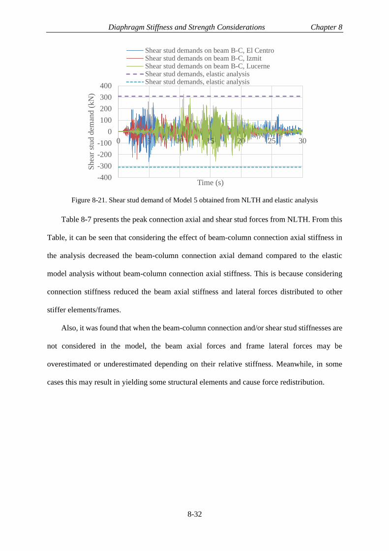
Diaphragm Stiffness and Strength Considerations Chapter 8
8-32
Figure 8-21. Shear stud demand of Model 5 obtained from NLTH and elastic analysis
Table 8-7 presents the peak connection axial and shear stud forces from NLTH. From this
Table, it can be seen that considering the effect of beam-column connection axial stiffness in
the analysis decreased the beam-column connection axial demand compared to the elastic
model analysis without beam-column connection axial stiffness. This is because considering
connection stiffness reduced the beam axial stiffness and lateral forces distributed to other
stiffer elements/frames.
Also, it was found that when the beam-column connection and/or shear stud stiffnesses are
not considered in the model, the beam axial forces and frame lateral forces may be
overestimated or underestimated depending on their relative stiffness. Meanwhile, in some
cases this may result in yielding some structural elements and cause force redistribution.
-400
-300
-200
-100
0
100
200
300
400
0 5 10 15 20 25 30
Shea
r st
ud d
eman
d (
kN
)
Time (s)
Shear stud demands on beam B-C, El CentroShear stud demands on beam B-C, IzmitShear stud demands on beam B-C, LucerneShear stud demands, elastic analysisShear stud demands, elastic analysis

Diaphragm Stiffness and Strength Considerations Chapter 8
8-33
Table 8-7. Summary of peak connection axial and shear stud forces from NLTH and elastic static
analyses
Connection
tension force (kN)
Connection
compression force
(kN)
Shear stud
demands (kN)
Design
forces 294 -214 308
TH record 1,
El Centro
Model 1 227 -258 284
Model 4 142 -128 167
Model 5 229 -227 261
TH record 2,
Izmit
Model 1 175 -283 312
Model 4 118 -139 171
Model 5 140 -211 242
TH record 3,
Lucerne
Model 1 315 -210 348
Model 4 252 -122 297
Model 5 290 -225 327
8.5 Load transfer from diaphragm to VLFR system
Lateral force transfer issue from diaphragm to the VLFR systems of structure was
discussed in Chapter 2. Usually, buildings have a limited number of lateral force resisting
frames, which are designed to carry horizontal forces from the diaphragms to the foundation.
These horizontal forces could either
i. be transferred only through the seismic frame beams or
ii. be transferred through beams in gravity frames (collectors) as well as the seismic
frames.
In the first case, forces on the diaphragm, including inertial and transfer forces, are
transferred to the seismic beam via shear studs on the beam. For this mechanism, with force
only considered to be transferred into the seismic frame(s), sufficient shear studs should only
be placed on the seismic beam and ensuring that the beam, and its connections, can transfer the
axial forces induced into the columns. Also, the ability of gravity beams lateral force transfer
should be limited. This may be achieved by ensuring that there are no shear studs on the gravity
beams and reducing the friction between the top of these gravity beams and the diaphragm.

Diaphragm Stiffness and Strength Considerations Chapter 8
8-34
In the second case, when the composite action of the gravity beams is desired and shear
studs are placed on these beams, these beams and their connections need to be designed for the
expected axial forces from diaphragm. In this case, strut-and-tie mechanism with reinforcing
steel perpendicular to all beams is required.
When design is conducted assuming the seismic beams carry all horizontal forces from the
diaphragm (including those from inertial and transfer effects), yet shear connectors are placed
on the gravity beams, axial force demands in the gravity beam connections may be greater than
their axial strength, and this may result in beam/connection yielding and in some cases
failure/collapse.
8.5.1 Case study
In this section, Model 5 that was introduced in Section 8.4 is considered to investigate a
case when beams in the gravity frames are not designed to carry lateral forces while having
shear studs to take the advantages of the composite action to carry gravity loads. Different
number of gravity bays connected to the seismic frame is considered, as shown in Figure 8-22,
to increase the diaphragm in-plane forces that need to be transferred to the braced frame.
The axial behaviour of the WSP connections is defined according to Section 8.3.4 using
the axial strengths obtained in Appendix M (234kN compression and 361kN tension). In all
models, enough shear studs to carry total diaphragm lateral force are provided on the braced
bay beam, 2-AB in Figure 8-5. Note that in these models yielding of slab reinforcements is
considered in defining the orthogonal truss members’ behaviour.

Diaphragm Stiffness and Strength Considerations Chapter 8
8-35
a) Model 5 with one gravity bay b) Model 5 with two gravity bays
c) Model 5 with three gravity bays
d) Model 5 with four gravity bays
Figure 8-22. Models with different number of gravity bays
These models are investigated under nonlinear static analysis. The maximum tension and
compression forces and deformations of the WSP connection located on the 2-B axis of each
model, shown in Figure 8-16, are obtained. Table 8-8 presents the analyses results for these
models. As can be seen, the axial force and deformation demands on WSP connections
increased with increasing the number of gravity bays. In models with three and four gravity
bays, the axial tensile deformation of the WSP connections under negative earthquake force,
EN, exceeded its maximum tensile deformation capacity, 6mm in this case. This means these
connections fractured in tension. For the positive earthquake force, EP, the WSP connections
yielded in models with three and four gravity bays, however, their maximum deformation did
not reach to the axial fracture deformation.
Table 8-8. WSP axial force and deformations obtained from analyses
EP EN
Axial compression
deformation (kN)
Axial
compression
force (mm)
Axial tension
deformation
(mm)
Axial tension
force (kN)
Model 5 with one
gravity bay
-0.22 104 0.45 215
Model 5 with two
gravity bays
-0.37 175 4.66 361
Model 5 with
three gravity bays
-0.83 234 16.22 361
Model 5 with
four gravity bays
-0.84 234 19.32 361

Diaphragm Stiffness and Strength Considerations Chapter 8
8-36
The difference observed between the axial deformation demands of WSP connections
shown in Table 8-8 is because of the in-plane behaviour and load transfer mechanism of the
slab. For the positive earthquake direction, EP, The deformation of these WSP connections are
subject to and is limited by the deformations of the diaphragm and shear studs on the seismic
frame beams. Therefore, the diaphragm forces were transferred to the braced frame through
compression struts in the slab and axial forces in the WSP connections as shown in Figure
8-23a. As the compression concrete struts were stiffer than the WSP connection axial stiffness,
most of the in-plane force was transferred through these struts and the axial deformation of the
WSP connection was limited to the axial deformation of the concrete struts. In the negative
earthquake direction, EN, the diaphragm in-plane forces transferred to the braced bay using
tension ties (slab reinforcements) and collector beams (WSP connections). Therefore,
increasing the number of bays increased the reinforcement axial demands and caused yielding
in reinforcements causing high axial tension demands in the WSP connections as shown in
Figure 8-23b.
a) Positive earthquake direction

Diaphragm Stiffness and Strength Considerations Chapter 8
8-37
b) Negative earthquake direction
Figure 8-23. Likely strut and tie formed in diaphragm with three gravity bays
This issue may be mitigated by putting more reinforcements in the slab. However the
reinforcement ratio cannot be increased more than a certain value as it may cause other
problems for the slab such as concrete delamination. In this study, it is suggested to design
WSP connections for likely axial forces obtained from elastic analysis to avoid yielding or
failure of these connections under the expected level of earthquake. In Section 8.4.2 it was
shown that the axial forces obtained from elastic design analysis were higher than those from
the more detailed nonlinear analysis because of considering the axial flexibility of the WSP
connection. Therefore designing the WSP connection axial behaviour for forces obtained from
the elastic analysis may provide conservative results and prevent undesirable failure in these
connections under the expected level of earthquake.
8.6 Gapping effect
The concrete slabs in steel frame structures are often cast without providing any gap
around the columns. Based on the current NZ design approach in NZS 3404 (2007), structural
steel beams are designed for earthquake-induced forces without considering the slab effects.
This is because the top of the slab is unconfined and the beam composite strength degrades to
the bare beam strength due to concrete failure/crushing (Chaudhari et al. 2015). However, the
NZ design approach (NZS 3404, 2007) states that columns and connections are required to be

Diaphragm Stiffness and Strength Considerations Chapter 8
8-38
designed to resist beam over-strength actions considering slab effects. The NZ standard
therefore considers the most conservative scenario by (a) ignoring the strength increase from
the slab in design of the beam to resist the seismic loads in a force-based design, and (b)
considering its effect when determining the over-strength actions at the column and beam-
column connection from the inelastically responding composite beams.
Another approach is not to consider the slab effects either for the beam design or for
columns and connections design. This may be conducted by isolating the column, and the
elements connected to it, from the slab (MacRae and Clifton, 2015a). The slab can be separated
from the column using a fire-proof material or a diamond gap cut all around the column as
shown in Figure 8-24.
a) Gap around the column (Chaudhari et al.
2015)
b) Gap within the slab (MacRae and Clifton,
2015b)
Figure 8-24. Gapping around column
Chaudhari et al. (2015) indicate that gapping around column
1) eliminates the slab effect on beam over-strength, resulting in smaller columns,
2) reduces slab damage and strength degradation
3) has the possibility of reducing ratcheting where the structure tends to yield
predominantly in one direction because the same strength is in each direction of
loading (MacRae and Clifton, 2015b), and
4) decreases beam/connection axial forces.
The disadvantages of gapping may be

Diaphragm Stiffness and Strength Considerations Chapter 8
8-39
1) Increasing the chance of column instability by twisting due to having no slab to
restrain it, such instability has been seen in columns with beams tested with
reduced beam sections by Chi and Uang (2002).
2) The initial stiffness and strength of the structure decrease (in the first cycle) so the
period increases and the structure is likely to have greater displacements (MacRae
and Clifton, 2015b).
3) Gap installation costs may be significant (MacRae and Bull, 2015).
8.6.1 Gapping/no gapping forces
Whether gaps are provided between the slab and column or not, diaphragm forces are more
likely to be transferred to the column through the beam axial forces at least on the hogging side
of the beam. This is because it is assumed that as the frame sways, a gap opens between the
concrete slab and the column and diaphragm forces need to be transferred through the shear
stud to the beam and from the beam to the column. Also, on the far side of the beam, the column
bears against the slab and impose additional force to the slab that needs to be transferred back
to the column through the beam.
These bearing forces were observed in Chaudhari (2017) experimental tests that the
column bears against the slab and impose additional forces to the beam. A similar observation
was made by Astaneh et al. (2002) which investigated the seismic behaviour of WSP
connections supporting floor slabs. Figure 8-25 shows one of the specimens investigated by
Astaneh et al. (2002) and the cleat plate fracture due to the column rotation and axial tension
forces at the end of the test.

Diaphragm Stiffness and Strength Considerations Chapter 8
8-40
a) Elevation of a specimen with slab, (Astaneh et al. 2002)
b) Fracture of cleat plate for 6-bolt specimen, (Astaneh et al. 2002)
Figure 8-25. Specimen tested by Astaneh et al. (2002)
Note that the slab bearing forces in Chaudhari (2017) and Astaneh et al. (2002)
experiments were obtained using reversed cyclic loading tests that the lateral forces were
applied at the column/beam ends. However, in an earthquake event, lateral forces are mainly
caused by diaphragm accelerations and are applied to the diaphragms not to column/beam ends.
Therefore, shear stud flexibility and possible lateral movements of the diaphragm are not
considered in the tests. The diaphragm in-plane movements may increase or decrease the slab
bearing effects. According to the above discussion, the gap opening issue and slab bearing
forces can be investigated in two scenarios depending on the relative lateral deformation of the
frame and diaphragm force direction.

Diaphragm Stiffness and Strength Considerations Chapter 8
8-41
1. Inertia forces govern diaphragm in-plane demands
2. Transfer forces govern diaphragm in-plane demands
8.6.1.1 Inertia forces govern diaphragm in-plane demands
Figure 8-26 shows the condition that inertia forces govern diaphragm in-plane demands
schematically. The slab bearing force (on the left-hand side) and gap opening (on the right-
hand side of the beam) depend on the relative stiffness of shear studs and storey stiffness. Such
that when the shear stud deformation, 𝛿𝑠, is larger than the column lateral deformation due to
storey drift, 𝛿𝑐, the slab bears against the column on the left hand side, as shown in Figure
8-26b, and a part of diaphragm in-plane forces may be transferred to the column through slab
bearing. This means that slab-column bearing forces on the right hand side of the beam
decrease, and some slab force is transferred directly to the column on the beam left hand side.
Note that if the shear stud slip 𝛿𝑠 is greater than the lateral shear stud slip capacity calculated
in Chapter 5 considering gravity load effects, the shear stud fracture may occur.
When the column lateral displacement, 𝛿𝑐, on the beam hogging side is greater than the
slab lateral movement, 𝛿𝑠, in the same direction, then the slab bears against the column face on
the right hand side shown in Figure 8-26b. Therefore, additional diaphragm in-plane force may
be imposed on the diaphragm from the right hand column thereby increasing both shear stud
and right hand side beam-column connection demands.
a) Un-deformed shape
b) Deformed shape
Figure 8-26. Lateral deformation of slab and columns subject to lateral forces

Diaphragm Stiffness and Strength Considerations Chapter 8
8-42
8.6.1.2 Transfer forces govern diaphragm in-plane demands
In the second scenario where transfer forces govern diaphragm in-plane demands, lateral
forces are mostly applied to the diaphragm from deformation incompatibility of different
VLFR systems (transfer forces). Figure 8-27 shows a dual VLFR system structure with shear
wall and moment resisting frame under lateral forces. The in-plane forces imposed on the
diaphragms at the first and top floors are presented schematically. It is shown that at the lower
storeys, the diaphragm in-plane force transferred to the frames is opposite to the frame lateral
deformation. While at the upper floors the diaphragm in-plane force transferred to the frames
is in the same direction as frame lateral deformation. These are shown in Figure 8-27c and d.
As can be seen in Figure 8-27c, in the lower floors a gap opens on the right-hand side of
the beam, and slab bears against the column on the left. Since the slab in-plane forces are in
the opposite direction, they may help to reduce beam-column connection tension forces. For
the upper floors, the slab in-plane forces are in the same direction as the frame deformation and
it is similar to the condition that only inertia forces govern the diaphragm in-plane demands.
a) Floor plan
b) Lateral forces and shear wall/moment
frame deformed shapes

Diaphragm Stiffness and Strength Considerations Chapter 8
8-43
c) First floor, Diaphragm 1, lateral forces and deformations
d) Fourth floor, Diaphragm 4, lateral forces and deformations
Figure 8-27. Gap opening properties in dual type structure system
8.6.2 FE modelling of gapping effect
Two FE truss models are created to investigate the gapping effect on beam-column
connection axial force and shear stud demands. Diaphragms in these models are simulated
using one truss mesh unit per bay for simplicity. In Model 6, a gap is provided around the
columns. In the diagonal truss modelling method a gap is considered around the columns due
to the configuration of truss elements by default as was discussed in Chapter 3. An additional
compression-only truss element can be used to consider slab-column interaction in such a slab-
offset model as described in Section 8.3.6. This is conducted in Model 7 where the concrete
slab is placed on top of the steel beams with an offset equal to 𝑑𝑐 =𝑑𝑏𝑒𝑎𝑚+𝑡𝑠𝑙𝑎𝑏
2 as shown in
Figure 8-13.
Figure 8-28 shows the beam axial forces and slab-column bearing forces on frame 2
(Figure 8-4) for Models 6 and 7. In Model 6 shown in Figure 8-28a all diaphragm in-plane
forces transferred through beam axial force, however, in Model 7, some diaphragm in-plane
force transferred through the bearing of the slab against the column. This decreased the shear

Diaphragm Stiffness and Strength Considerations Chapter 8
8-44
stud and beam axial force demands. In this case the shear stud deformation, 𝛿𝑠, is larger than
the column lateral deformation due to storey drift, 𝛿𝑐, and the slab bears against the column on
the left hand side shown in Figure 8-28b.
a) Model 6, (gap provided)
b) Model 7, (without gap)
Figure 8-28. Beam axial force, 𝐹𝐵, and shear stud displacements, 𝛿𝑠, with and without slab-column
gap
Another case was also considered where the brace area was reduced to zero. This decreased
the storey stiffness, and all three frames in the structure (Frames 1, 2 and 3 in Figure 8-4) had
the same member sizes. It is noted that some transfer forces still exist as the tributary area to
stiffness ratio for frames 1 and 3 is lower than it is for frame 2. Figure 8-29 shows the axial
force diagram for no gapping. This is referred to as Model 7-1. It can be seen that slab bearing
forces were on the beam right-hand side, while they were on the left-hand side in Figure 8-28b.
Also, the tension on the right-hand side of beams in both bays increased significantly causing

Diaphragm Stiffness and Strength Considerations Chapter 8
8-45
a significant increase in beam connection demands. The beam-column connections on the beam
2-BC, are yielded under axial forces and limited the slab bearing force on this beam.
Figure 8-29. Beam axial force, 𝐹𝐵, and shear stud displacements, 𝛿𝑠, without slab-column gap
From the above discussion and modelling, it is recommended that a gap be provided
around the columns to prevent large axial forces due to slab bearing on the beam-column
connection. It is noted that diaphragm in-plane forces should be transferred to the VLFR system
through beam axial forces. Therefore, most diaphragm in-plane forces need to be transferred
to the VLFR systems using shear studs. The full load path should be considered as well as the
possibility of shear stud yielding which decreases composite action. In this case, loss of
composite action should be considered in design using recommendations provided in Chapter
5 and the beam should be designed to carry gravity loads without composite action. Design
steps, given in Figure 8-1, are applied to an example given in Appendix M.
When the gap is not provided around the column the slab bearing force in Clause 12.10.2.4
of NZS3404 (2007) is calculated based on the minimum of the concrete bearing capacity and
the steel beam axial strength. However, for gravity beams, the sum of the beam-column
connection tension and compression strengths should be used as a limiting case in this equation.
8.7 Composite beam vertical deflection
In Chapter 5 it was shown that diaphragm in-plane forces may cause yielding in shear
studs on the steel beams. Shear stud yielding eliminates shear flow between the concrete slab

Diaphragm Stiffness and Strength Considerations Chapter 8
8-46
and the steel beam, causing loss of composite action. Here, Model 8, is created considering
composite beam effects (offsetting the concrete slab from the steel beam) to study composite
beam vertical deflection under earthquake loading using NLTH analysis. Also, different
parameters such as composite action level and lateral force magnitude on the composite beam
behaviour are studied. These are achieved by changing the shear stud strength representing
different composite action levels and increasing the number of bays to increase diaphragm in-
plane demands.
8.7.1 Modelling
The vertical deflection of the beam mid-point at the braced bay (beam 2-AB) and shear
stud forces obtained from NLTH analysis are shown in Figure 8-30. This beam was designed
considering 25% composite action. The total lateral strength of shear stud on the beam was
calculated using the proposed method in Chapter 5 equal to the sum of all shear stud strengths
in this case. The total lateral force strength of shear studs on the braced bay (25% composite
action) was assumed to be 1100kN.
As can be seen from Figure 8-30a, vertical deflection of the beam mid-point increased
from 9.8mm to about 10.9mm at the end of the analysis. This is about an 11% increase in the
initial vertical deflection under gravity loads. The maximum shear stud demands from NLTH
analysis was about 600kN as shown in Figure 8-30b. This is about 54% of the total shear stud
lateral strength. This is consistent with the design recommendation provided in Chapter 5 to
design beams in low-damage structures; which was recommended that if the lateral shear force
demand on shear studs of a composite beam is limited to 50% of the shear studs lateral strength,
the beam mid-point vertical deflection may not increase by more than 10% under lateral
loading. It is also noted that for larger earthquakes, further beam deflection could occur.

Diaphragm Stiffness and Strength Considerations Chapter 8
8-47
a) Beam mid-point vertical deflection
b) Shear stud demands
Figure 8-30. Beam mid-point vertical deflection and shear stud demand, Model 8 with 25% composite
action (record: El Centro 1940)
In order to investigate the effect of composite action level, Model 8 was analysed
considering 100% composite action. Figure 8-31 shows the beam mid-point vertical deflection
and shear stud lateral force demand. As can be seen in Figure 8-31b, maximum shear stud
demand is limited to 15% of the total shear studs strength, and no residual deformation was
obtained at the beam mid-span. This is because the lateral forces did not cause yielding in any
shear stud.
-14
-13
-12
-11
-10
-9
0 5 10 15 20 25 30
Bea
m m
id-s
pan
ver
tica
l
def
lect
ion
, δ
(mm
)
Time (s)
Bare steel beam vertical deflection
C.A.=25%
-1500
-1000
-500
0
500
1000
1500
0 5 10 15 20 25 30
Shea
r st
ud l
ater
al d
eman
d,
P (
kN
)
Time (s)
Total shear stud lateral strength
Total shear stud lateral strength
C.A.=25%

Diaphragm Stiffness and Strength Considerations Chapter 8
8-48
a) Beam mid-point vertical deflection
b) Shear stud demands
Figure 8-31. Beam mid-point vertical deflection and shear stud demand, Model 8 with 100%
composite action (record: El Centro 1940)
In another model, the number of bays was increased and the shear studs on the beams of
gravity frames were removed to transfer all the lateral forces to the shear studs on the beam in
the braced bay, 2-AB, as shown in Figure 8-32. This beam was designed considering 50%
composite action.
-14
-13
-12
-11
-10
-9
-8
-7
-6
0 5 10 15 20 25 30
Bea
m m
id-s
pan
ver
tica
l
def
lect
ion,
δ(m
m)
Time (s)
Bare steel beam vertical deflection
C.A=100%
-5000
-4000
-3000
-2000
-1000
0
1000
2000
3000
4000
5000
0 5 10 15 20 25 30
Shea
r st
ud l
ater
al d
eman
d,
P (
kN
)
Time (s)
Total shear stud lateral strength
Total shear stud lateral strength
C.A.=100%

Diaphragm Stiffness and Strength Considerations Chapter 8
8-49
Figure 8-32. Model 8 with multiple bays, 50% composite action for beam between axis 2-AB
In this case, shear studs yielded under lateral loading as shown in Figure 8-33. At about a
time of 2.5s into the record, shear studs reached the total lateral force resistance and at the same
time, the beam mid-point vertical deflection reached to the bare steel beam deflection. After
this point, some of the beam vertical deflection was recovered. The vertical deflection of the
beam mid-point increased from 8.5mm to about 10.9mm at the end of the analysis, which is
about 28% increase in the initial vertical deflection under gravity loads.
a) Beam mid-point vertical deflection
-14
-13
-12
-11
-10
-9
-8
-7
-6
0 5 10 15 20 25 30
Bea
m m
id-s
pan
ver
tica
l
def
lect
ion,
δ(m
m)
Time (s)
Bare steel beam vertical deflection
C.A.=50%
Lost all C.A., C.A.=0%

Diaphragm Stiffness and Strength Considerations Chapter 8
8-50
b) Shear stud demands
Figure 8-33. Beam mid-point vertical deflection and shear stud demand, Model 8 with 50% composite
action and multiple bays (record: El Centro 1940)
The reason for recovering a part of the beam vertical deflection as was shown in Figure
8-33a, may be due to the level of lateral slip that each shear stud experiences on different
locations of the beam. Figure 8-34a shows a schematic composite beam subjected to gravity
and lateral forces and the location of shear studs (3𝐿 − 3𝑅). The lateral force is assumed to be
initially to the left, causing all studs to yield (Figure 8-34c). The positions of shear studs on the
shear force-slip plot are shown with 3𝐿 − 3𝑅 points. When the direction of imposed in-plane
force changes, unloading occurs, and with a force to the right, each shear stud follows the
unloading path corresponding to the level of slip experienced. Therefore, the shear stud with
the lowest slip, 3𝑅, will reach to higher shear force level, as shown in Figure 8-34d. The shear
stud, 3𝐿, with the highest slip in Figure 8-34c will have the lowest force level as shown in
Figure 8-34d. Figure 8-34e shows the shear forces imposed to the beam top flange from shear
studs, and the beam moment diagram corresponding to that. This shows that the resulting
imposed moment from shear studs to the beam is opposite to the moment due to gravity loads
and may decrease the beam vertical deflection and recover some of the vertical deflection
caused by loss of composite action.
-2500
-2000
-1500
-1000
-500
0
500
1000
1500
2000
2500
0 5 10 15 20 25 30
Shea
r st
ud l
ater
al d
eman
d,
P (
kN
)
Time (s)
Total shear stud lateral strength
Total shear stud lateral strength
C.A.=50%

Diaphragm Stiffness and Strength Considerations Chapter 8
8-51
a) Shear stud, labelling, deformations under gravity and lateral forces
b) Shear stud forces under gravity loads
c) Shear stud forces under gravity and lateral force to the left

Diaphragm Stiffness and Strength Considerations Chapter 8
8-52
d) Shear stud forces after unloading and a small loading to the right
e) Shear stud forces on beam top flange from Figure 8-34d and the corresponding moment diagram
Figure 8-34. Schematic view of composite beam under gravity and cyclic lateral forces
8.8 Conclusions
This chapter described considerations directly related to the design of composite floors in
steel buildings subjected to lateral forces. It is shown that:
1) The Assessment Guideline (2017) procedure may be modified to consider i) beam axial
capacity, ii) beam-column connection capacity, iii) shear stud strength, and iv) diaphragm
buckling strength. In addition, modifications were suggested to model the structure, and to

Diaphragm Stiffness and Strength Considerations Chapter 8
8-53
obtain appropriate forces for design. Two approaches are recommended considering
diaphragm cracking effects to obtain diaphragm in-plane demands.
Approach One. In this approach, the diaphragm is assumed to remain elastic and is
modelled using elastic in-plane properties. Then using the obtained internal forces the
assumption of the elastic diaphragm should be checked. If the assumption is correct,
design/assessment may be continued using the obtained results. Otherwise, the
diaphragm in-plane stiffness should be reduced to account for concrete cracking.
Approach Two. In this approach, it is suggested to perform two analyses using both
elastic and cracked diaphragm in-plane stiffnesses and use the envelope values for
design/assessment of the diaphragm.
The diaphragm design approach seeks to:
i. Keep the diaphragm elastic without buckling.
ii. Have WSP demands lower that the WSP axial capacity.
iii. Prevent shear studs from fracture under the combination of earthquake lateral
forces and gravity load effects.
iv. Ensure that fixed-end beam capacities are not reduced due to axial force effects.
2) The beam-end connection and shear stud demands depend on the records considered and on
the modelling assumptions. For the structure selected and designed according to the
proposed DESA method, individual frame demands increased by up to 50% as a result of
diaphragm cracking. Considering the beam-column connection axial stiffness in the analysis
decreased the beam-column connection axial demands compared to the model without
beam-column connection axial stiffness. This is because it reduced the beam axial stiffness
and lateral forces distributed to other stiffer elements/frames through the floor diaphragm.
Also, it was shown that if the axial stiffness of the beam-column connection and/or shear
stud stiffness are not considered in modelling, the beam axial forces and frame lateral forces

Diaphragm Stiffness and Strength Considerations Chapter 8
8-54
may be overestimated or underestimated depending on their relative stiffness. It is suggested
to design WSP connections for likely axial forces obtained from elastic analysis even if they
are not considered as part of diaphragm in-plane load transfer to the VLFR system but are
connected to the slab through mechanical attachments (e.g. shear studs).
4) The load path through collector beams should be considered in design even if it is assumed
that all diaphragm in-plane forces are directly transferred to the lateral force resisting frames.
This should be conducted to obtain robust load path and avoid beam-column connection
failure and possible collapse.
3) The slab-bearing forces can be obtained by modelling the frame with appropriate beam-
connection axial stiffnesses, slab offset and imposed displacements. They depend on the
relative stiffness of the frame, which affects the column deformations, and the shear stud
group stiffness affecting the slab slip. For design without considering such an analysis it is
recommended that i) a gap be provided around the columns to prevent large axial forces due
to slab bearing on the beam-column connection. ii) When the gap is not provided around the
column the slab bearing force should be considered when designing beam end connections,
beams and shear studs. Note that in both cases above, general load path and column stability
considerations should be considered.
4) It was shown, by means of time history analyses, that the static beam vertical deflection
increased after the shear studs yielded in cyclic action by up to 28% in the cases considered.
This was consistent with the findings of Chapter 5. It emphasises the need to design beams
to carry the seismic gravity loads without composite action.

Diaphragm Stiffness and Strength Considerations Chapter 8
8-55
References
[1] ANSI, A. 360-16. (2016). Specification for structural steel buildings
[2] AS/NZS 2327 (2017). Composite structures, Composite steel-concrete
construction in buildings.
[3] Astaneh-Asl, A., Liu, J., & McMullin, K. M. (2002). Behavior and design of single
plate shear connections. Journal of Constructional Steel Research, 58(5-8), 1121-
1141.
[4] Braconi, A., Elamary, A., and Salvatore, W. 2010. Seismic behaviour of beam-to-
column partial-strength joints for steel-concrete composite frames, Journal of
Constructional Steel Research, (66), 1431-1444.
[5] Bull, D. K. (2004). “Understanding the Complexities of Designing diaphragms in
Buildings for Earthquakes”, Bulletin of the New Zealand Society for Earthquake
Engineering, 37 (2): 70-88.
[6] Chaudhari, T. D. (2017). “Seismic performance evaluation of steel frame building
with different composite slab configurations”, PhD Thesis, University of
Canterbury.
[7] Chaudhari, T. D., MacRae, G. A., Bull, D., Chase, G., Hicks, S., Clifton, G. C. and
Hobbs, M. (2015). “Composite Slab Effects on Beam–Column Subassembly
Seismic Performance”, 8th International Conference on Behavior of Steel
Structures in Seismic Areas, Shanghai, China.
[8] Chi, B. and Uang, C. M. (2002). “Cyclic Response and Design Recommendations
of Reduced Beam Section Moment Connections with Deep Columns”, J. Struct.
Engrg., ASCE, 128(4): 464-473
[9] Civjan, S. A., & Singh, P. (2003). Behavior of shear studs subjected to fully
reversed cyclic loading. Journal of Structural Engineering, 129(11), 1466-1474.
[10] Cowie, K. A., Fussell, A. J., Clifton, G. C., MacRae, G. A. and Hicks, S. J.
(2014). “Seismic Design of Composite Metal Deck and Concrete-Filled
Diaphragms–A Discussion Paper”, NZSEE Conference.

Diaphragm Stiffness and Strength Considerations Chapter 8
8-56
[11] Dowell, O. K., Seible, F., & Wilson, E. L. (1998). Pivot hysteresis model for
reinforced concrete members. ACI Structural Journal, 95, 607-617.
[12] EN, C. 1994. 1-1, (2004) Eurocode 4: Design of composite steel and concrete
structures.
[13] Gardiner, D. R. (2011). “Design Recommendations and Methods for Reinforced
Concrete Floor Diaphragms Subjected to Seismic Forces”, PhD Thesis, University
of Canterbury.
[14] Holmes Consulting Group, Practice Note No. 8.1, Version No. 1, (2014).
Modelling Diaphragm Force Distributions - Simple Grillage Method. by Bull D.
K. and Galloway B.
[15] http://docs.csiamerica.com
[16] Johnson, R. P., Molenstra, N., & EPPIB. (1991). Partial shear connection in
composite beams for buildings. Proceedings of the Institution of Civil
Engineers, 91(4), 679-704.
[17] MacRae, G. A. and Bull, D. (2015). “Diaphragm Design, ENEQ650: Seismic
Design of Steel and Composite Structures”, Postgraduate Class notes, University
of Canterbury, 2015.
[18] MacRae, G. A. and Clifton, G. C. (2015a). “Research on Seismic Performance
of Steel Structures”, Steel Innovations Conference, Auckland, New Zealand.
[19] MacRae, G. A. and Clifton, G. C. (2015b). “Research on Seismic Performance
of Steel Structures”, Steel Innovations Conference, Auckland, New Zealand.
[20] Moehle, J. P. (2015). Seismic design of reinforced concrete buildings (pp. 230-
235). New York: McGraw-Hill Education.
[21] Naeim, F., & Boppana, R. R. (2001). Seismic Design of Floor Diaphragms. In
The Seismic Design Handbook (pp. 373-407). Springer, Boston, MA.

Diaphragm Stiffness and Strength Considerations Chapter 8
8-57
[22] Nakajima, A., Saiki, I., Kokai, M., Doi, K., Takabayashi, Y., & Ooe, H. (2003).
Cyclic shear force–slip behavior of studs under alternating and pulsating load
condition. Engineering Structures, 25(5), 537-545.
[23] NZS 1170.5 (2004). Structural Design Actions-Part, 5. Standards New Zealand,
Wellington, New Zealand. Including Amendment 1, 2016.
[24] NZS 3101 (2006). Concrete structures standard. Standards New Zealand,
Wellington, NZ.
[25] NZS 3404 (2007). Steel Structures Standard. Standards New Zealand,
Wellington, New Zealand. Including Amendments 1 and 2, 2001/2007.
[26] Oehlers, D. J., & Coughlan, C. G. (1986). The shear stiffness of stud shear
connections in composite beams. Journal of Constructional Steel Research, 6(4),
273-284.
[27] Park, R. L., Park, R., & Paulay, T. (1975). Reinforced concrete structures. John
Wiley & Sons.
[28] Sabelli, R., Sabol, T. A. and Easterling, W. S. (2011). “Seismic Design of
Composite Steel Deck and Concrete-filled Diaphragms A Guide for Practicing
Engineers”, NEHRP Seismic Design Technical Brief No. 5.
[29] SAP2000, C. S. I. (2015). Computer & Structures Inc. Linear and nonlinear
static and dynamic analysis of three-dimensional structures. Berkeley (CA):
Computer & Structures.
[30] Scarry, J. M. (2014). “Floor diaphragms – Seismic bulwark or Achilles’ heel”,
NZSEE Conference Paper Number O19.
[31] Takeda, T., Sozen, M. A., & Nielsen, N. N. (1970). Reinforced concrete
response to simulated earthquakes. Journal of the Structural Division, 96(12),
2557-2573.
[32] The Seismic Assessment of Existing Buildings, Technical Guidelines for
Engineering Assessments, (2017).

Conclusions and Future Research Works Chapter 9
9-1
9 Conclusions and Future Research Works
9.1 Summary
Diaphragm design issues were investigated in this research include: i) diaphragm in-plane
modelling method using truss elements, ii) diaphragm in-plane load path through shear studs
to the beam and from the beam to the column through the WSP connection, iii) diaphragm
buckling strength, iv) global diaphragm in-plane demands, and v) diaphragm design steps.
In summary, the unique contributions this research make to the field of diaphragm design
include:
1) A new diamond shape truss framework was proposed.
2) The stiffness/strength performance of truss models considering compression-only
diagonal members, which is appropriate for design, was quantified.
3) A method to assess the axial compressive strength of steel beam web side plate
(WSP) connections, considering the gravity loads effect, was proposed.
4) A method was proposed to estimate the lateral shear strength of a group of shear
studs on a steel beam in the presence of gravity loads and considering shear stud
fracture.
5) A method was developed to estimate diaphragm buckling strength considering
gravity loads and possible out-of-straightness.
6) A lateral force method, removing some limitations of existing methods, to estimate
diaphragm likely in-plane demands was proposed.
7) A step-by-step diaphragm design approach, with a corresponding example, was
provided.

Conclusions and Future Research Works Chapter 9
9-2
9.2 Key findings
From the analytical investigations and analyses conducted in this research, the main
findings obtained include:
9.2.1 Truss element modelling
A new Diamond truss framework model was proposed and compared with the diagonal
truss model. Also, different possible truss element modelling methods considering the
combination of compression/tension, compression only and tension only truss elements were
studied. It was found that:
1) For elastic truss models where all elements were tension/compression, the error in
estimating diaphragm deformations was reduced to less than 10% for the
diaphragm alone when a sufficient number of elements were used. However, the
diamond configuration was more accurate requiring fewer elements to obtain
the same accuracy. In addition, using the diamond model gives more realistic
results in terms of the beam axial forces.
2) Different possible diamond truss models, placed in a framework to represent a
diaphragm, were compared with a nonlinear solid element FEM model in terms of
their in-plane stiffness and internal forces. Based on the analyses conducted, Truss
Model 2, with diagonal compression-only and orthogonal compression/tension
elements (representing un-cracked diaphragm properties), and Truss Model 3, with
diagonal compression-only and orthogonal reinforcement tension/concrete
compression members (representing cracked diaphragm properties) satisfied the
criteria of providing simple outputs usable for design and reasonable accuracy.
3) For analyses conducted of a one-storey and a three storey structure, a 10% increase
in diaphragm flexibility caused 7% and 2% increase in total structural displacement
at the diaphragm levels respectively.

Conclusions and Future Research Works Chapter 9
9-3
9.2.2 Web-Side-Plate connection axial strength
The axial behaviour of WSP connections was investigated considering different geometry,
boundary condition and initial conditions. A method to assess the axial compressive strength
of WSP connections considering gravity loads was proposed. In this study it was found that:
1) The axial compression capacity of a WSP connection is lower than the axial tensile
capacity because of axial force eccentricity, cleat plate slenderness, and the P-Δ
effect. For the connection subjected to the axial tension force, axial force increases
to reach the first controlling failure limit state.
2) The axial compression strengths obtained using the proposed method were
compared with thirty-four FE models considering different parameters. The
average calculated compression strength according to the proposed method was
80% with a standard deviation of 14% that obtained from FEM analysis. For
tension side, the average of calculated tension strength from the proposed method
was about 89% with a standard deviation of 3% that obtained from FEM analysis.
Note that the following parameters considered in the proposed strength approach
were not considered in the FEM models. These included: residual stress effect and
out-of-straightness effect. To consider these and also possible packing effect in
design, a strength multiplier of 0.75 was suggested.
9.2.3 Shear studs design to transfer lateral forces
A method was proposed to calculate the lateral strength of shear studs on composite and
non-composite beams in the presence of gravity loads. It was found that:
1) The maximum total lateral force resistance of shear studs depends on the level of
shear stud slip under gravity load. In the absence of gravity load, the total lateral
force resistance of shear studs is equal to the sum of all shear stud strengths.

Conclusions and Future Research Works Chapter 9
9-4
2) Yielding of the shear studs under a combination of gravity and lateral loads reduced
or eliminated the shear flow at the steel beam-concrete slab interface and decreased
composite action. This caused loss of composite action and increased the beam
vertical deflection.
3) A design method was developed to estimate the lateral force resistance of a beam
shear stud group considering gravity loads and shear stud fracture. Numerical FEM
studies indicated strengths in the range of 1.0-1.25 times that from the design
method. Also the steel beam alone should be designed to carry un-factored gravity
loads, 𝐷 + 𝐿 to prevent collapse under gravity loads. This is because the composite
action of the beams subjected to lateral forces may be eliminated or decreased.
4) For composite beams in low damage structures, or structures where it is desired
that the building be permitted to continue operation after at least one major
earthquake, a maximum acceptable increase in vertical deflection of gravity beams
was arbitrary chosen to be 10%. To meet this limit, the ratio of slab lateral force
demand applied to the shear studs in a bay should be less than 50% of the peak
total resistance of these shear studs. This value is appropriate for the likely range
of gravity loading, beam depth and level of composite action. Also the steel beam
alone should be designed to carry un-factored gravity loads, 𝐷 + 𝐿.
9.2.4 Floor diaphragm buckling
The floor diaphragm buckling modes under in-plane forces that were considered in this
research include:
i. Local buckling of the concrete topping between the slab ribs (inter-rib buckling),
ii. Buckling of the diaphragm between secondary beams (intra-panel buckling), and
iii. Global buckling of the diaphragm between primary beams (intra-bay buckling).

Conclusions and Future Research Works Chapter 9
9-5
All of the buckling modes were studied for both pre-crack and post-crack conditions of the
concrete slab. The critical buckling of each mode was calculated using analytical methods, and
in cases, the results were verified with FEM modelling using ABAQUS software. It was found
that:
1) For the local buckling, the minimum topping thickness results in high buckling
forces, therefore concrete shear or crushing are likely to occur much earlier than
buckling. Local buckling is therefore not likely to occur in conventional floor slabs.
2) for the intra-panel and intra-bay buckling modes the critical slab in-plane shear
forces which cause buckling need to be checked both before and after cracking. A
simple formula was provided to do this. It considered pinned end condition, out-
of-plane deformations and the corrugated nature of the composite slab. It was
shown that in the studied examples the shear buckling did not govern.
3) initial deflection effects on the elastic buckling strength due to gravity loads on the
floor slab could be conservatively considered by a strength multiplier of 0.75 in
design.
9.2.5 Diaphragm lateral force method
Global diaphragm in-plane force demands resulting from inertia forces and transfer forces
may be obtained using lateral force methods or NLTH analysis. A lateral force method was
proposed, called Diaphragm ESA (DESA). It removes some of the limitations of the available
lateral force methods. The proposed method was compared with a number of available lateral
force methods that have been used for obtaining diaphragm global in-plane demands including:
1) ESA considering structure ductility (CESA), 2) Overstrength ESA (OESA), 3) Elastic ESA,
(EESA), 4) Parts and Components method (P&C), 5) pseudo-Equivalent Static Analysis
(pESA), 7) Pushover analysis, and 9) NLTH. It was found that:
Conclusions and Future Research Works Chapter 9
9-6
1) The DESA method was proposed based on the hypothesis that if a lateral loading
method can represent likely deformed shape of a structure, it can obtain likely
diaphragm transfer forces. This is because diaphragm transfer forces are mainly
due to the deformation incompatibility of different VLFR systems. This method
assumes the lateral deformation of a long period structure at the design level may
be estimated using the EESA (𝜇 = 1) method according to the equal displacement
assumption. Also, the bottom portion of the EESA lateral forces are increased in
the proposed method to approximate the higher mode effects.
2) For high-rise buildings beyond the CESA method limitations, it is suggested to use
the first mode lateral forces scaled to the EESA base shear and increase the lateral
forces at lower floors.
3) The analyses results showed that the proposed method may remove some
limitations of the CESA and pESA methods such as height limit and overstrength
calculation process. However, it may result in some overestimation and
underestimation of response in different cases and ignore some important response
features, such as structure ductility, redistribution of internal forces, hysteretic
effects, stiffness and strength degradation. The advantages and disadvantages of
different lateral force methods were discussed so that one can decide which method
can provide more reasonable results based on the accuracy and time required for
the analysis.
9.2.6 Diaphragm stiffness and strength considerations
Design considerations directly related to the composite floors in steel buildings subjected
to lateral forces described. A number of FE analyses performed to investigate the effects of
reduction in diaphragm in-plane stiffness, shear stud stiffness and WSP connection axial

Conclusions and Future Research Works Chapter 9
9-7
stiffness in the analyses. Some diaphragm design issues such as slab-column gapping effect
and the vertical deflection of composite beams were also investigated. It was found that:
1) The Assessment Guideline (2017) procedure may be modified to consider i) beam
axial capacity, ii) beam-column connection capacity, iii) shear stud strength, and
iv) diaphragm buckling strength. In addition, modifications were suggested to
model the structure, and to obtain appropriate forces for design. Two approaches
were recommended to obtain diaphragm in-plane demands considering diaphragm
cracking effects. The proposed diaphragm design approaches seek to:
a) Keep the diaphragm elastic without buckling.
b) Have WSP demands lower that the WSP axial capacity.
c) Prevent shear studs from fracture under the combination of earthquake lateral
forces and gravity loads effects.
d) Ensure that beam fixed-end capacity is not reduced due to axial force effects.
2) For the structure selected and designed according to the DESA method, individual
frame demands increased by up to 50% as a result of diaphragm cracking. Also,
considering the beam-column connection axial stiffness in the analysis decreased
the beam-column connection axial demands compared to the model without beam-
column connection axial stiffness. This is because it reduced the beam axial
stiffness and lateral forces distributed to other stiffer elements/frames through the
floor diaphragm.
3) The load path through collector beams should be considered in design even if it is
assumed that all diaphragm in-plane forces are directly transferred to the lateral
force resisting frames. This should be conducted to obtain robust load path and
avoid beam-column connection failure and possible collapse.

Conclusions and Future Research Works Chapter 9
9-8
4) It was shown, by means of time history analyses, that the static beam vertical
deflection increased after the shear studs yielded in cyclic action by up to 28% in
the cases considered. This was consistent with the findings of Chapter 5. It
emphasises the need to design beams to carry the seismic gravity loads without
composite action.
9.3 Suggested future research
Research topics, following on from the studies conducted here, that have the potential to
make a significant impact include the following.
9.3.1 Investigating axial behaviour of different simple beam-column
connections
The axial behaviour of WSP connections, as the most common simple beam-column
connection used in the steel frame structures, was investigated in this research. However, there
are other types of pinned connections as shown in Figure 9-1.
a) Double angle connection
b) Single plate connection
a) Tee connection
a) Shear end plate
a) Seated beam
a) Stiffed seated beam
Figure 9-1. Simple beam-column connection types, (Astaneh, 1989b)

Conclusions and Future Research Works Chapter 9
9-9
Here it is suggested to investigate the axial force carrying behaviour of other commonly
used simple beam-column connections and provide design methods for them.
9.3.2 Investigating the behaviour of the top-plate connection
The top-plate connection detail is shown in Figure 9-2. This connection may be used where
the WSP connection axial strength (or any other simple beam-column connection) is less than
the demand from the beam axial forces.
Figure 9-2. Top plate connection to transfer collector beam axial forces (Cowie et al., 2014)
9.3.3 Performing experimental tests on axial behaviour of the WSP
connections
The axial force behaviour of the WSP connections was studied using analytical and
numerical methods in this research. It may be beneficial to perform an experimental
investigation of the axial behaviour of WSP connections and compare the results (stiffness,
strength and deformation capacity) obtained from the experiments with the proposed method.
9.3.4 Performing experimental tests on lateral force resistance of shear
studs on composite beam and its effect on the vertical beam
deflection
The lateral force resistance of shear studs under monotonic and cyclic loads has been
investigated by many researchers (e.g. Johnson and Molenstra 1991). However, the lateral

Conclusions and Future Research Works Chapter 9
9-10
force carrying of shear studs placed on a composite beam in combination of gravity loads is
not investigated. Here, it is suggested to perform a lateral pushover tests on composite beams
in the presence of gravity loads to investigate the effects of gravity loads on the lateral force
resistance of shear studs. This may also provide some information about the loss of composite
action under lateral forces.
9.3.5 Further research on the diaphragm lateral force method
Lateral force method to obtain diaphragm in-plane demands was investigated in Chapter
7 of this research. It is suggested to perform more NLTH analysis on different structural
systems to further improve methods of diaphragm force prediction.
9.3.6 Obtaining reasonable reduction factor for in-plane stiffness of
diaphragms considering concrete cracking
In Chapter 8, it was shown that the reduction in the diaphragm in-plane stiffness due to the
concrete cracking may change the lateral force distribution between the different VLFR
systems and also the diaphragm itself. It was recommended to consider the possibility of
cracked diaphragm stiffness in the analysis and design. However, there is a need to obtain a
diaphragm stiffness reduction factor to use in the elastic analyses with more realistic tension
stiffening effects.
9.3.7 Experimental investigation on the slab forces
There is not much published experimental test information about the behaviour of slabs
subject to in-plane forces. In-plane slab forces in experimental investigations are most easily
applied to the slab boundary elements. However inertia forces are generated within the slab
itself and should also be considered in testing with realistic gravity forces, shear studs,
connections and boundary conditions. Such testing can be used to evaluate the methods
proposed in this thesis, and to improve them.

Conclusions and Future Research Works Chapter 9
9-11
References
[1] Astaneh, A. (1989b). Demand and supply of ductility in steel shear
connections. Journal of Constructional Steel Research, 14(1), 1-19.
[2] Cowie, K. A., Fussell, A. J., Clifton, G. C., MacRae, G. A., & Hicks, S. J. (2014,
March). Seismic design of composite metal deck and concrete-filled diaphragms–
A discussion paper. In NZSEE Conference.
[3] Johnson, R. P., Molenstra, N., & EPPIB. (1991). Partial shear connection in
composite beams for buildings. Proceedings of the Institution of Civil
Engineers, 91(4), 679-704.
[4] NZS 3404 Parts 1 and 2:1997, Steel Structures Standard.
[5] The Seismic Assessment of Existing Buildings, Technical Guidelines for
Engineering Assessments, (2017).

Appendix A
A-1
A Appendix A: Transfer Forces
Different parameters may affect the magnitude of diaphragm transfer forces such as
stiffness, strength and location of vertical lateral force resisting (VLFR) elements in plan. In
this Appendix, the possibilities for transfer forces considering the following are described
(MacRae and Bull, 2015):
1. VFLR element differential stiffness/strength on single storey structures
2. Multi-storey effects.
A.1 VFLR element differential stiffness/strength
In this case, a simple floor plan is considered for evaluating transfer forces in a one-storey
building, as shown in Figure A-1a. Different possibilities in terms of VFLR element strength
and stiffness are considered for evaluating transfer forces in the diaphragm. To avoid torsional
effects, the floor plan is considered symmetric. Figure A-1b presents the simplified elevation
of this floor plan.
a) Floor plan
b) Simplified elevation
Figure A-1. Simple floor plan of one storey building (MacRae and Bull, 2015)
Two stages considered here for evaluating the transfer forces are:
1. The elastic stage in which all lateral force resistance elements are elastic (at the
point the first yield occur in one of the elements)

Appendix A
A-2
2. The post-yield stage, where one lateral force resisting element (in Figure A-1b) has
yielded, and the second is about to yield
The maximum transfer force can occur either before or after yield so both stages need to
be considered to find the maximum diaphragm transfer force, 𝐹𝑡:
Elastic stage:
The total lateral force imposed on the floor is denoted by 𝐹𝑎, and 𝐹𝑎1, 𝐹𝑎2 are forces in
each lateral load-resisting element.
𝐹𝑎 = 𝐹𝑎1 + 𝐹𝑎2
Here, 𝐹𝑎1 = 𝐹𝑎2 due to the equal tributary area.
If 𝑘1 = 0, |𝐹𝑡 | = 𝐹𝑎1 = 𝐹𝑎/2
If 𝑘2 = 0, |𝐹𝑡 | = 𝐹𝑎2 = 𝐹𝑎/2
If 𝑘1 = 𝑘2, 𝐹𝑡 = 0
In general, before yield
𝐹1 = 𝐹𝑎[𝑘1/(𝑘1 + 𝑘2)]
𝐹2 = 𝐹𝑎[𝑘2/(𝑘1 + 𝑘2)]
𝐹𝑡 = 𝐹𝑎[0.5 − 𝑘1/(𝑘1 + 𝑘2)]
Post-yield stage:
𝐹𝑡 =𝐹𝑦1+ 𝐹𝑦2
2− 𝐹𝑦1
𝐹𝑡 =𝐹𝑦1− 𝐹𝑦2
2− 𝐹𝑦1
Where 𝐹y1 and 𝐹y2 are the yield strength of VFLR elements 1 and 2 respectively. Based
on these equations and considering different stiffness and strength for lateral load resisting
elements, different possibilities for transfer forces can be obtained as shown in Figure A-2
(MacRae and Bull, 2015).

Appendix A
A-3
Figure A-2. Possibilities for diaphragm transfer forces in a single storey structure (MacRae and Bull,
2015)
A.2 Multi-storey effects
In this case, a shear-type frame and a wall are connected with diaphragms, in a two-storey
building. The simplified elevation of the studied structure is shown in Figure A-3a.
In this case, it is assumed that the frame has uniform strength and stiffness over the height,
and the wall yields in flexure only at the base.
a) Simplified elevation
b) Free body diagram
Figure A-3. Simplified elevation and free body diagram of two storey structure (MacRae and Bull,
2015)
Here 𝐹t1 and 𝐹t2 are diaphragm transfer forces at the first and second floor respectively,
𝐹f and 𝐹w represents the frame and wall forces, and 𝑉f and 𝑉w represent the frame and wall
shear reaction forces respectively. The transfer forces are only obtained at the formation of a
full mechanism in this example.

Appendix A
A-4
1) Considering a mechanism with 𝑉fy1 = 𝑉fy2 = 𝑉b and 𝑉w = 𝑉f = 𝑉b
Figure A-4 shows the frame and wall forces for this case. The diaphragm transfer forces
are evaluated as 𝐹t2 =2𝑉b
3−
𝑉b
3=
𝑉b
3 (tension) for the second floor and 𝐹t1 =
𝑉b
3 (compression)
for the first floor.
Figure A-4. Frame and wall forces when 𝑉fy1 = 𝑉fy2 = 𝑉b and 𝑉w = 𝑉f = 𝑉b (MacRae and Bull,
2015)
2) Considering a mechanism with frame 𝑉fy1 = 1.5𝑉fy2 = 𝑉b and 𝑉w = 𝑉fy1 = 𝑉b
Figure A-5 shows the frame and wall forces for this case. The diaphragm transfer forces
are evaluated as 𝐹t2 = 𝐹t1 = 0. The different distribution of shear strength causes different
transfer forces.
Figure A-5. Frame and wall forces when 𝑉fy1 = 1.5𝑉fy2 = 𝑉b and 𝑉w = 𝑉fy1 = 𝑉b (MacRae and Bull,
2015)
It may be seen that transfer forces are affected by

Appendix A
A-5
1) The displacement at which it is considered (sometimes it increases or decreases)
2) The strengths/stiffness magnitudes and distributions of VLFR elements
3) The lateral force distribution
Simple elastic design methods, such as ESA and pESA, do not explicitly consider all these
effects, but if strength is somewhat proportional to stiffness, the peak transfer force is likely to
occur at the peak displacement.

Appendix A
A-6
References
[1] MacRae GA and Bull D (2015). “Diaphragm Design, ENEQ650: Seismic Design
of Steel and Composite Structures”, Postgraduate Class notes, University of
Canterbury, 2015.

Appendix B
B-1
B Appendix B: Diamond Model Cross-Section Areas
Similar to the diagonal model (Hrennikoff, 1941), the cross-section area of truss
members can be derived by equating the framework deformations with elastic strains of the
corresponding plate member. Figure B-1 shows three general loading conditions that are used
to determine the framework properties. The plate is assumed to continue in both directions,
and only two truss mesh units in each direction are shown in this Figure. In the first loading
condition, Figure B-1a, the plate is loaded uniformly with normal load per unit length 𝑃 in
the 𝑋-direction and 𝜈𝑃 (υ is Poisson’s ratio of the plate material) in the 𝑌-direction. The
second loading condition, Figure B-1b, is achieved by changing the 𝑋 and 𝑌-directions. The
third loading condition, Figure B-1c, includes uniform tangential loading per unit length 𝑃,
applied to the plate edges in the 𝑋 and 𝑌-directions. The right hand side of each Figure shows
the square truss mesh unit of the diamond model.
a) Plate and truss framework subjected to normal force per unit length, 𝑃, in the 𝑋-direction and 𝜈𝑃
in the 𝑌-direction

Appendix B
B-2
b) Plate and truss framework subjected to normal force per unit length, 𝑃, in the 𝑌-direction and 𝜈𝑃
in the 𝑋-direction
c) Plate and truss framework subjected to pure shear force per unit length, 𝑃
Figure B-1. General loading conditions for determining truss framework properties, 𝑝 is the normal
edge force to each element where 𝑝 = 𝑃𝑎, truss framework continues in both directions
Based on solid mechanics (e.g. Timoshenko and Goodier, 1970), the axial strains in the
𝑋 and 𝑌-directions, 휀𝑥 and 휀𝑦 for the first case of loading (Figure B-1a), can be obtained as
follows for a plate member.
휀𝑥 =𝑝(1−𝜈2)
𝐸𝑡𝑎 Eq. (B-1)
휀𝑦 = 0 Eq. (B-2)
Here, 𝑝 is the normal edge force to each element (𝑝 = 𝑃𝑎) and E and 𝜈 are the elastic
modulus and Poisson’s ratio of plate material respectively. The horizontal and vertical
dimensions of each square truss mesh unit and the plate thickness are denoted as 𝑎 and 𝑡

Appendix B
B-3
respectively. The same equations are applicable to the second case by changing the 𝑋 and 𝑌-
directions.
Shear deformation of the plate subjected to tangential force can be obtained using Eq.
(B-3) (e.g. Timoshenko and Goodier, 1970).
𝛾𝑥𝑦 =2(1+𝜈)𝑝
𝐸𝑡𝑎 Eq. (B-3)
By equating the strains of the truss framework and the plate, Eqs. (B-1) to (B-3), the
truss element characteristics can be obtained. Figure B-2 presents an enlarged view of
Figure B-1a with more details. The equations used for finding the truss element cross-
sections are presented in the following.
Figure B-2. Diamond truss framework subjected to normal force 𝑝 in the X-direction and 𝜈𝑝 in the Y-
direction
Force equilibrium in the 𝑋-direction at Point 1 shown in Figure B-2, gives:
𝐹𝑂1 + 2𝐹𝐷 cos 𝛼 − 𝑝 = 0 Eq. (B-3a)
Where 𝐹𝑂1 is the internal force of the orthogonal member in the 𝑋-direction and 𝐹𝐷 is the
diagonal member internal force. Writing the force equilibrium in the 𝑌-direction at Point 2
also gives:
𝐹𝑂2 + 2𝐹𝐷 cos 𝛼 − 𝜈𝑝 = 0 Eq. (B-3b)

Appendix B
B-4
It is known that the lateral deformation (deformation in the 𝑌-direction, Eq. (B-2)) is
zero due to applied 𝜈𝑝 in this direction. Therefore 𝐹𝑂2 = 0 and by substituting this in the 𝑌-
direction force equilibrium, Eq. (B-3b), the diagonal member force can be found:
𝐹𝐷 =𝜈𝑝
2 cos 𝛼 Eq. (B-3c)
Considering the truss framework units are square (𝛼 = 45°), by substituting 𝐹𝐷 into the
force equilibrium in the 𝑋-direction, Eq. (B-3a), the orthogonal member force (𝐹𝑂1) can be
obtained as:
𝐹𝑂1 = 𝑝(1 − 𝜈)
The axial strain of the orthogonal truss member in the 𝑋-direction, which needs to be
equal to the axial strain of the corresponding plate member, can be calculated using:
휀𝑥 =𝑝(1−𝜈)
𝐸𝐴1
By equating the axial strain of the plate given in Eq. (B-1) and the truss element axial
strain above, the cross-section area of the orthogonal truss element member can be found:
𝐴1 = 𝑎𝑡(1 + 𝜈)⁄ Eq. (B-4)
By changing the loading condition to normal force 𝑝 in 𝑌-direction and 𝜈𝑝 in 𝑋-
direction, the same result can be found for the orthogonal member cross-section area in the 𝑌-
direction.
In case of tangential (shear) forces applied to the truss framework as shown in
Figure B-1c, all orthogonal members are unstressed due to the symmetry in the truss pattern.
However, all the diagonal members are stressed with equal tension and compression values.
Force equilibrium in the 𝑌-direction at Point 1 gives:
2𝐹𝐷 sin 𝛼 − 𝑝 = 0

Appendix B
B-5
Considering square truss mesh units (𝛼 = 45°), the diagonal member internal force
subjected to shear stresses is:
|𝐹𝐷| =𝑝
√2 Eq. (B-4a)
Similarly, the force equilibrium in the 𝑋-direction at Point 1 in Figure B-1c shows that
the orthogonal member internal force is zero.
𝐹𝐷 cos 𝛼 − 𝐹𝐷 cos 𝛼 + 𝐹𝑂1 = 0
𝐹𝑂1 = 0
The axial deformation (change in length) of the diagonal truss members is equal to:
δ =𝑝𝑎√2
√2𝐸𝐴
δ =𝑝𝑎
𝐸𝐴 Eq. (B-4b)
Which transforms the square pattern into a parallelogram as shown in Figure B-3.
Figure B-3. Diamond model deformed shape subjected to shear force
As shown in Figure B-3, the shear strain in the framework, 𝛾𝑥𝑦, can be found from:
tan (𝜋
4+
𝛾𝑥𝑦
2) =
𝑎
√2−
𝛿
2𝑎
√2+
𝛿
2
=1−
𝛿
𝑎√2
1+𝛿
𝑎√2
Eq. (B-4c)

Appendix B
B-6
From the mathematical rule of trigonometric addition formulas (e.g. Abramowitz and
Stegun, 1965) and assuming small deformations which, tan(𝛾) ≅ 𝛾,
tan (𝜋
4+
𝛾𝑥𝑦
2) =
tan𝜋
4−tan
𝛾𝑥𝑦
2
1+tan𝜋
4tan
𝛾𝑥𝑦
2
=1−
𝛾𝑥𝑦
2
1+𝛾𝑥𝑦
2
By equating the above equation with Eq. (B-4c) and substituting Eq. (B-4b), the shear
strain, 𝛾𝑥𝑦, can be obtained as:
𝛾𝑥𝑦 =𝑝√2
𝐸𝐴 Eq. (B-4d)
By equating the plate and truss framework shear strains, using Eq. (B-3) and Eq. (B-4d),
the diagonal truss element cross-section area can be found:
𝐴 =𝑎𝑡
√2(1+𝜈) Eq. (B-5)
Poisson’s ratio, 𝜈, should be calculated to satisfy the deformation compatibility equation.
Figure B-4 shows the framework deformation in the 𝑋-direction subjected to normal force, 𝑝,
in the 𝑋-direction and 𝜈𝑝 in the 𝑌-direction.
Figure B-4. Diamond framework deformation in the X-direction subjected to normal force 𝑝 in the X-
direction and 𝜈𝑝 in the Y-direction

Appendix B
B-7
The deformation compatibility can be achieved by writing the relationship between the
orthogonal and diagonal member deformations as:
𝛿𝐷
2=
𝛿𝑂
2cos 45 Eq. (B-5a)
The truss element axial deformations are denoted by 𝛿𝐷 and 𝛿𝑂 for diagonal and
orthogonal members respectively.
Considering the truss element axial forces obtained using equilibrium in the 𝑋-direction,
Eq. (B-3a), and truss member cross-section areas given in Eqs. (B-4) and (B-5), 𝛿𝐷 and 𝛿𝑂
are calculated as:
𝛿 𝐷 =𝜈𝑝√2(1+𝜈)
𝐸𝑡
𝛿𝑂 =𝑝(1−𝜈2)
𝐸𝑡
Substituting these axial deformations into Eq. (B-5a), gives:
𝜈𝑝√2(1+𝜈)
𝐸𝑡=
𝑝(1−𝜈2)
√2𝐸𝑡
From which 𝜈 =1
3 results.
Considering the Poisson’s ratio 𝜈 =1
3, the cross-section area of the orthogonal and the
diagonal members are obtained using Eqs. (B-4) and (B-5) respectively as:
𝐴1 = 0.75𝑎𝑡 (Orthogonal member)
𝐴 = 0.53𝑎𝑡 (Diagonal member)
Where 𝑎 is the dimension of the framework pattern and 𝑡 is the plate thickness.

Appendix B
B-8
References
[1] Abramowitz, M., & Stegun, I. A. (1965). Handbook of mathematical functions:
with formulas, graphs, and mathematical Tables (Vol. 55). Courier Corporation.
[2] Hrennikoff, A. (1941). Solution of problems of elasticity by the framework
method. Journal of applied mechanics, 8 (4):169-75.
[3] Timoshenko, S. P., & Goodier, J. N. (1970). Theory of Elasticity, (216).

Appendix C
C-1
C Appendix C: Non-Square Elastic Framework
Properties
The cross-section area of the truss members of a non-square elastic framework can be
obtained using a similar method to the diagonal (Hrennikoff, 1941) and the diamond truss
frameworks. The cross-section area of truss members can be derived by equating the
framework deformations with elastic strains of the corresponding plate member. Figure C-1
shows three general loading conditions that are used to determine the framework properties.
The plate is assumed to continue in both directions, and only two truss mesh units in each
direction are shown in this Figure. In the first loading case, Figure C-1a, the plate is loaded
uniformly with normal load per unit length 𝑃 in the 𝑋-direction and 𝜈𝑃 (υ is Poisson’s ratio
of the plate material) in the 𝑌-direction. The second loading condition, Figure C-1b, is
achieved by changing the 𝑋 and 𝑌-directions. The third loading condition, Figure C-1c,
includes uniform tangential loading per unit length 𝑃, applied to the plate edges in the 𝑋 and
𝑌-directions. The right hand side of each Figure shows the square truss mesh unit of the
diamond model.
a) Plate and truss framework subjected to normal force per unit length, 𝑃, in the 𝑋-direction and 𝜈𝑃

Appendix C
C-2
in the 𝑌-direction
b) Plate and truss framework subjected to normal force per unit length, 𝑃, in the 𝑌-direction and 𝜈𝑃
in the 𝑋-direction
c) Plate and truss framework subjected to pure shear force per unit length, 𝑃
Figure C-1. General loading conditions for determining truss framework properties, truss framework
continues in both directions
Strains in the truss framework for each case in Figure C-1 can be calculated based on the
applied normal/tangential force per unit length, 𝑃, truss element cross-sections, 𝐴𝑖, and the
configuration represented by the angles 𝛼 and 𝛽. Then the framework strains are equated to
the corresponding strains in the plate member 휀𝑥, 휀𝑦 and 𝛾𝑥𝑦 loaded the same way.

Appendix C
C-3
Based on solid mechanics (e.g. Timoshenko and Goodier, 1970), the axial strains in the
𝑋 and 𝑌-directions, 휀𝑥 and 휀𝑦 for the first case of loading (Figure C-1a), can be obtained as
follows for a plate member.
휀𝑥 =𝑃𝑎(1−𝜈2)
𝐸𝑡𝑎 Eq. (C-1)
휀𝑦 = 0 Eq. (C-2)
Here 𝑃𝑎 is the normal edge force to each element in the 𝑋-direction and E and 𝜈 are the
elastic modulus and Poisson’s ratio of plate material respectively. The horizontal and vertical
dimensions of each square truss mesh unit and the plate thickness are denoted as 𝑏, 𝑎 and 𝑡
respectively. The plate strains for the second loading case, shown in Figure C-1b, can be
obtained by replacing a by b in Eq. () as:
휀𝑦 =𝑃𝑏(1−𝜈2)
𝐸𝑡𝑏 Eq. (C-3)
휀𝑥 = 0 Eq. (C-4)
Shear deformation of the plate subjected to tangential force can be obtained using Eq.
(C-5) (e.g. Timoshenko and Goodier, 1970).
𝛾𝑥𝑦 =2(1+𝜈)𝑃𝑎
𝐸𝑡𝑎 Eq. (C-5)
By equating the strains of the truss framework and the plate, Eqs. (C-1) to (C-5), the
truss element characteristics can be obtained. Figure C-2 presents an enlarged view of
Figure C-1a with more details. The equations used for finding the truss element cross-
sections are presented in the following.

Appendix C
C-4
Figure C-2. Truss framework subjected to normal force 𝑃𝑎 per truss mesh unit in the X-direction and
𝜈𝑃𝑏 in the Y-direction
Force equilibrium in the 𝑋-direction at Point 1 shown in Figure C-2, gives:
𝐹𝑂1 + 2𝐹𝐷 cos 𝛼 − 𝑃𝑎 = 0 Eq. (C-6)
Where 𝐹𝑂1 is the internal force of the orthogonal member in the 𝑋-direction and 𝐹𝐷 is the
diagonal member internal force. Writing the force equilibrium in the 𝑌-direction at Point 2
also gives:
𝐹𝑂2 + 2𝐹𝐷 sin 𝛼 − 𝜈𝑃𝑏 = 0 Eq. (C-7)
It is known that the lateral deformation (deformation in the 𝑌-direction, Eq. (C-2)) is
zero due to applied 𝜈𝑃𝑏 in this direction. Therefore 𝐹𝑂2 = 0 and by substituting this in the 𝑌-
direction force equilibrium, Eq. (C-7), the diagonal member force can be found:
𝐹𝐷 =𝜈𝑃𝑏
2 sin 𝛼 Eq. (C-8)
By substituting 𝐹𝐷 into the force equilibrium in the 𝑋-direction, Eq. (C-6), the orthogonal
member force (𝐹𝑂1) can be obtained as:
𝐹𝑂1 = 𝑃(𝑎 − 𝜈𝑏 𝑐𝑜𝑡 𝛼) Eq. (C-9)
Using 𝑐𝑜𝑡 𝛼 = 𝑏𝑎⁄ ,

Appendix C
C-5
𝐹𝑂1 = 𝑃(𝑎 −𝜈𝑏2
𝑎) Eq. (C-10)
The axial strain of the orthogonal truss member in the 𝑋-direction, which should to be
equal to the axial strain of the corresponding plate member, can be calculated using:
휀𝑥 =𝑃(a−
𝜈𝑏2
𝑎)
𝐸𝐴1 Eq. (C-11)
By equating the axial strain of the plate given in Eq. (C-1) and the truss element axial
strain, Eq. (C-11) , the cross-section area of the orthogonal truss element member in the 𝑋-
direction can be found:
A1=at(1-𝜈b2
a2⁄ )
1-𝜈2 Eq. (C-12)
By changing the loading condition to normal force 𝑃𝑏 in the 𝑌-direction and 𝜈𝑃𝑎 in the
𝑋-direction, Figure C-1b, the same result can be found for the orthogonal member cross-
section area in the 𝑌-direction.
A2=bt(1-𝜈a2
b2⁄ )
1-𝜈2 Eq. (C-13)
In case of tangential (shear) forces applied to the truss framework as shown in
Figure C-1c, all orthogonal members are unstressed due to the symmetry in the truss
framework pattern. However, all the diagonal members are stressed with equal tension and
compression values. Force equilibrium in the 𝑌-direction at Point 1, shown in Figure C-1c,
gives:
2𝐹𝐷 sin 𝛼 − 𝑃𝑎 = 0 Eq. (C-14)
Using 𝑠𝑖𝑛 𝛼 = 𝑎√𝑎2 + 𝑏2⁄ , the diagonal member force subjected to shear stresses is:
|𝐹𝐷| =𝑃√𝑎2+𝑏2
2 Eq. (C-15)

Appendix C
C-6
Similarly, the force equilibrium in the 𝑋-direction at Point 1 in Figure C-1c shows that
the orthogonal member internal force is zero.
𝐹𝐷 cos 𝛼 − 𝐹𝐷 cos 𝛼 + 𝐹𝑂1 = 0
𝐹𝑂1 = 0 Eq. (C-16)
The axial deformation (change in length) of the diagonal truss members is equal to:
δ𝐷 =𝑃(𝑎2+𝑏2)
4𝐸𝐴 Eq. (C-17)
Which transforms the rectangular mesh unit into a parallelogram as shown in Figure C-3.
Figure C-3. Truss framework deformed shape subjected to shear forces
By writing the law of cosines for the deformed triangle shown in Figure C-3, the shear
strain in the framework, 𝛾𝑥𝑦, is found:
𝑐2
4=
𝑎2
4+
𝑏2
4−
2𝑎𝑏 cos(𝜋
2−𝛾𝑥𝑦)
4 Eq. (C-18)
Using 𝑐𝑜𝑠 (𝜋
2− 𝛾𝑥𝑦) = 𝑠𝑖𝑛(𝛾𝑥𝑦) and considering small deformations assumption,
𝑠𝑖𝑛(𝛾𝑥𝑦) ≅ 𝛾𝑥𝑦,
𝑐2 = 𝑎2 + 𝑏2 − 2𝑎𝑏𝛾𝑥𝑦 Eq. (C-19)

Appendix C
C-7
Considering 𝑐
2= (
√𝑎2+𝑏2
2− 𝛿𝐷) and expanding Eq. (C-19) gives:
4 (𝑎2+𝑏2
4−
𝑃(𝑎2+𝑏2)√𝑎2+𝑏2
4𝐸𝐴𝐷) = 𝑎2 + 𝑏2 − 2𝑎𝑏𝛾𝑥𝑦 Eq. (C-20)
In Eq. (C-20), 𝛿𝐷2 is taken zero because of small deformation assumption. By
substituting 𝛾𝑥𝑦 from Eq.(C-5) into Eq. (C-20), 𝐴𝐷 is obtained as:
𝐴 =√𝑎2+𝑏2(𝑎2+𝑏2)
4𝑎𝑏(1+𝜈)𝑡 Eq. (C-21)
Poisson’s ratio, 𝜈, should be calculated to satisfy the deformation compatibility equation.
Figure C-4 shows the framework deformation in the 𝑋-direction subjected to normal force,
𝑃𝑎, in the 𝑋-direction and 𝜈𝑃𝑏 in the 𝑌-direction.
Figure C-4. Truss framework deformation in the X-direction subjected to normal force 𝑃𝑎 in the X-
direction and 𝜈𝑃𝑏 in the Y-direction
The deformation compatibility can be achieved by writing the relationship between the
orthogonal and diagonal member deformations as:
𝛿𝐷
2=
𝛿𝑂
2cos α Eq. (C-22)
The truss element axial deformations are denoted by 𝛿𝐷 and 𝛿𝑂 for diagonal and
orthogonal members respectively.

Appendix C
C-8
Considering the truss element axial forces obtained using equilibrium in the 𝑋-direction,
Eq. (C-10), and truss member cross-sections given in Eqs. (C-12) and (C-21), 𝛿𝐷 and 𝛿𝑂 are
calculated as:
𝛿 𝐷 =𝜈𝑃𝑏22(1+𝜈)
E√𝑎2+𝑏2𝑡 Eq. (C-23)
𝛿𝑂 =𝑃𝑏(1−𝜈2)
𝐸𝑡 Eq. (C-24)
Substituting these axial deformations, Eq. (C-23) and (C-24), into Eq. (C-22), gives:
𝜈𝑃𝑏22(1+𝜈)
E√𝑎2+𝑏2𝑡=
𝑃𝑏(1−𝜈2)
𝐸𝑡
𝑏
√𝑎2+𝑏2 Eq. (C-25)
From which 𝜈 =1
3 results.
Considering a square mesh unite, 𝑎 = 𝑏, and Poisson’s ratio 𝜈 =1
3, the cross-section area
of the orthogonal and the diagonal members are obtained using Eqs. (C-12), (C-13) and (C-
21) respectively as 𝐴1 = 0.75𝑎𝑡, 𝐴2 = 0.75𝑎𝑡 and 𝐴 = 0.53𝑎𝑡.

Appendix C
C-9
References
[1] Hrennikoff, A. (1941). Solution of problems of elasticity by the framework
method. Journal of applied mechanics, 8 (4):169-75.
[2] Timoshenko, S. P., & Goodier, J. N. (1970). Theory of Elasticity, (216).

Appendix D
D-1
D Appendix D: FEM Modelling Parameters
D.1 Element selection
ABAQUS is a powerful software in offering a wide range of element types for the FE
modelling. These include one-dimensional beam elements, two-dimensional shell, three-
dimensional solid elements, connector elements and membrane elements.
In this research, three dimensional 8-node reduced integration solid elements, which are
called C3D8R in ABAQUS element library, are used to model the cleat plates, bolts and parts
of the beam. Also, two dimensional 4-node reduced integration shell elements, which are
called S4R in ABAQUS element library, are used to model the middle part of the steel beam.
These elements are used to reduce the computational costs and analysis time. Figure D-1
shows 3D8R and S4R elements used in this study.
Figure D-1. C3D8R and S4R elements (Hibbitt, 2010)
D.2 Material properties
Nonlinear behaviour of the steel beam, cleat plate and bolts are simulated using an
isotropic hardening material model based on the von-Mises yield criterion. This material
model is called “Plastic” in ABAQUS material library.
An elastic-perfectly plastic stress-strain relationship is used to model the high-strength
bolts material, and a bilinear stress-strain relationship with 1% hardening is used for the steel

Appendix D
D-2
beam and cleat plate. These stress-strain relationships were used by Mahamid et al. (2007) for
FEM modelling of WSP connections. All the engineering stress-strain data converted into
true stress-strain as required for ABAQUS material input (Hibbitt, 2010). The Elastic
modulus and Poisson’s ratio of the steel material are considered 200GPa and 0.3 respectively.
Figure D-2 shows the engineering stress-strain relationships of the beam and cleat plate
and bolt materials schematically. The values of yield and ultimate stresses are selected based
on the experimental studies that were used for the FEM model verification described in
Appendices E and F.
a) Bolt material
b) Steel beam and cleat plate material
Figure D-2. Stress-strain relationships for FE simulations
D.3 Mesh sensitivity study
In FEM analysis, results may be sensitive to the number and size of elements used in the
model. Generally, in highly stressed zones such as the cleat plate, bolts and the beam web
fine mesh is required to achieve more accurate results. However, at regions far from the
connection that may have less effect on the connection axial behaviour, coarse mesh can be
used to decrease computational costs and analysis time.
Here, a short parametric study is conducted to obtain adequate mesh size in high stresses
regions. A cleat plate with one bolt subjected to shear force applied to the bolt-ends is
considered. The results are compared in terms of the vertical displacement versus the shear
force reactions of the cleat plate.

Appendix D
D-3
As mentioned in Section D.1, C3D8R solid elements are used to model the cleat plate,
beam and bolts. Therefore around curved surfaces such as bolt holes, more elements are
required to be able to simulate a smooth curved surface. In this study, 2mm mesh size is used
for bolts and bolt-holes in the cleat plate and the beam web. Figure D-3 shows the models
with different mesh sizes.
(a) Cleat plate with 2mm mesh size
(b) Cleat plate with 5mm mesh size
(c) Cleat plate with 10mm mesh size
(d) Cleat plate with 20mm mesh size
Figure D-3. Cleat plate with different mesh size
Vertical displacement of the cleat plate versus shear force reaction plots of each model
are presented in Figure D-4. It shows that models with mesh size 2 and 5mm were reasonably
similar. However, Model with 10mm mesh size showed 5% higher reaction force compared
to the 2mm mesh size model. Also, the 20mm mesh size model indicated nearly 8% higher
reaction force than the 2mm mesh size model. Table D-1 indicates total number of elements

Appendix D
D-4
and analysis time for these models. In this study, 5mm mesh size is selected as a reasonable
mesh size based on the analysis time and the results obtained.
Figure D-4. Vertical displacement of the cleat plate versus shear force reaction curves of models with
2,5,10 and 20mm mesh size
Table D-1. Information of models for mesh sensitivity analysis
Model Cleat mesh size (mm) Number of total elements Analysis time (s)
1 2 11354 186
2 5 6218 93
3 10 5162 70
4 20 4619 61
D.4 Geometric nonlinearity
ABAQUS software is able to consider geometric nonlinearities when the “NLGEOM”
option is activated in the analysis steps. Nonlinear geometry was activated for all models
analysed in Chapter 4 to capture local or global buckling modes and/or instability of models.
0
10
20
30
40
50
60
70
80
90
0 1 2 3 4 5 6
Rea
ctio
n f
orc
e (k
N)
Vertical displacement (mm)
2mm
5mm
10mm
20mm
Appendix D
D-5
References
[1] Hibbitt, K., Karlsson, B., & Sorensen, P. (2010). ABAQUS/Standard User's
Manual. Version 6.11. Providence, RI: Dassault Systèmes Simulia Corp.
[2] Mahamid, M., Rahman, A. D. E. E. B., & Ghorbanpoor, A. (2007). The Analyses
of Extended Shear Tab Steel Connections Part II: Stiffened
Connections. ENGINEERING JOURNAL-AMERICAN INSTITUTE OF
STEEL CONSTRUCTION, 44(2), 133.

Appendix E
E-1
E Appendix E: FEM Model Verification with Astaneh et
al. (1988) Experimental Results
Experimental investigation on shear force carrying behaviour of WSP connections that
conducted by Astaneh et al. (1988) is used to verify the FEM models of this study. In the
following sections a brief description of the test details, results, and FEM model verification
are presented.
E.1 Description of experimental study
Astaneh et al. (1988) investigated the shear resistance and rotational ductility of WSP
connections by testing three full-scale specimens. All specimens were considered to have a
single vertical row of bolts. Specimen 1, 2 and 3 had three, five and seven bolts respectively.
In this study, specimen 2 is selected for FEM model verification.
E.1.1 Specimen 2 details
The specimen 2 consisted of W10×77 wide flange section for the column and W18×55
wide flange section for the beam and 15×3/8×4-1/4 in. (381×9.5×108 mm) cleat plate. The
cleat plate was connected to the column using ¼ in. (6.35mm) fillet weld.
Bolts used for connecting the beam web to the cleat plate were ¾ in. (19mm) Grade
A325-N. All bolts were tightened up to 70% of the proof load by using turn of the nut
method. The bolt-holes were standard round hole with a nominal diameter of 13/16 in.
(20.6mm). The bolt spacing was 3 in. (76mm) centre by centre, and the edge distances was
1.5 in. (38mm) from top and bottom of the cleat plate. Figure E-1 shows the 5-bolt specimen
schematically.

Appendix E
E-2
Figure E-1. Specimen 2 details (Astaneh et al., 1988)
E.1.2 Test setup
Figure E-2 shows the test setup of the experiments. In this test setup, two actuators were
used to control the amount of imposed shear force and the rotation to the connection.
Actuator S shown in Figure E-2 was force-control to apply shear force to the connection and
actuator R was displacement-control to impose rotation to the connection.

Appendix E
E-3
Figure E-2. Test setup (Astaneh et al., 1988)
The shear force-rotation relationship used for loading the specimens is shown in
Figure E-3. Astaneh (1989) studied the shear-rotation relationship for the end supports of
simply supported beams using a computer program considering different beam cross-sections
and span lengths. These shear force-rotations covered the elastic loading part up to the beam
failure. Figure E-3 shows three shear force-rotation curves. Two dashed curves shown in this
Figure represent the shear force-rotation values for a shallow beam with large span and a
deep beam with a small span as an upper and lower bonds. The solid line which is between
these two upper and lower bonds was used to apply loads and deformations to the specimen.
Segment AB on the loading curve shown in Figure E-3 corresponds to the elastic
behaviour of the beam. At the point B the beam mid-span starts to yield. In segment BC the
beam at the mid-span experiences yielding. Therefore the connection rotation demand
increases without much increase in the connection shear force demand. At the point C the
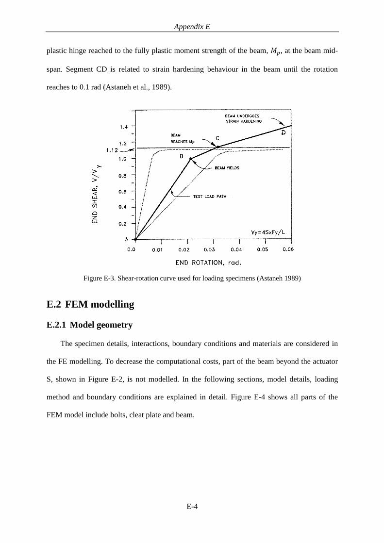
Appendix E
E-4
plastic hinge reached to the fully plastic moment strength of the beam, 𝑀𝑝, at the beam mid-
span. Segment CD is related to strain hardening behaviour in the beam until the rotation
reaches to 0.1 rad (Astaneh et al., 1989).
Figure E-3. Shear-rotation curve used for loading specimens (Astaneh 1989)
E.2 FEM modelling
E.2.1 Model geometry
The specimen details, interactions, boundary conditions and materials are considered in
the FE modelling. To decrease the computational costs, part of the beam beyond the actuator
S, shown in Figure E-2, is not modelled. In the following sections, model details, loading
method and boundary conditions are explained in detail. Figure E-4 shows all parts of the
FEM model include bolts, cleat plate and beam.

Appendix E
E-5
a) Beam
b) Cleat plate
c) Bolts
d) Model assembly
Figure E-4. FEM model parts
E.2.2 Material properties
The steel materials yield strengths used in this model are based on the reported values by
Astaneh et al. (1988). It was reported that the structural steel Grade A36 with the yield
strength of 35.5 ksi (244.7 MPa) and the ultimate strength of 60 ksi (413.6 MPa) was used for
the beam and the cleat plate. Also, A325 bolts were used for connecting the cleat plate to the
beam web. In the FEM model, the bolt material is simulated using the elastic-perfectly plastic
behaviour considering the bolt ultimate strength. The cleat and the steel beam material are
simulated using the bilinear stress-strain behaviour considering 1% strain hardening as
described in Appendix D.
E.2.3 Interactions
The behaviour of this type of connection is highly associated with the forces that transfer
from one part to another. Therefore, interaction between the parts of the FEM model is a key
parameter in this simulation. Here, the “Surface-to-Surface” interaction existing in ABAQUS
interaction options is used between the in contact surfaces of cleat plate, beam web, and the
bolts.

Appendix E
E-6
In the “Surface-to-Surface” interaction, two main interaction behaviours include
“normal” and “tangential” should be defined. For the “normal” behaviour, “hard” contact is
used. Separation of parts is allowed during the analyses. For the “tangential behaviour”,
“Penalty” friction formulation with a friction coefficient of 0.3 is defined. The contact
surfaces used in the model are shown in Figure E-5.
a) Cleat plate and beam web surfaces in contact
with bolts
b) Bolts surfaces in contact with cleat plate and
beam web
c) Contact surface between beam web and cleat plate
Figure E-5. Interaction surfaces between bolts, cleat plate and beam

Appendix E
E-7
E.2.4 Bolt pre-tensioning
Bolt pre-tensioning is considered in the FE model as the bolts in the tests were tightened
up to 70% of proof-load. ABAQUS software provides a method to apply bolt pre-tension
force by using “bolt-load” option in the “load” module. Using this feature, a certain amount
of pre-tension force can be applied to the bolts. The amount of bolt pre-tension load or the
bolt length can be chosen to remain the same in all the following analysis steps. When the
bolt length is chosen to remain constant, the bolt behaves with its mechanical properties plus
the existing pre-tension force; this option is used in the FE simulations of this study.
Figure E-6 shows the bolt cross-section with the bolt pre-tension forces.
Figure E-6. Bolt pre-tension force (ABAQUS)
E.2.5 Boundary conditions and loading method
As it was mentioned in Section E.1.2, the loading method used by Astaneh et al. (1988)
consisted of imposing shear force and rotation to the connection at the same time according
to the shear-rotation curve shown in Figure E-3. Thus, they used two actuators, one for
applying shear force (force-control) and one for applying rotation (displacement-control) to
the connection. In ABAQUS software it is possible to impose shear force at the location of
the load-control actuator and apply displacement at the location of the displacement-control
actuator. However, when a displacement is applied at the end of the beam, it can change the

Appendix E
E-8
amount of imposed shear force to the connection. Therefore, in the FE model, the loading
pattern is applied to the end of the cleat plate instead of the beam, which provides similar
results.
As shown in Figure E-7, part of the beam with is located between the force-control
actuator and the connection is modelled. One end of the beam is fully restraint and the other
end is connected to the cleat plate. Both shear force and rotation are applied to the cleat plate
support.
a) Loading method used in the experiments (Astaneh
et al. 1988)
b) Loading method used in the FEM model
Figure E-7. Loading method
E.2.6 Mesh
Based on the mesh sensitivity study described in Appendix D, 5mm mesh size is used to
model the cleat plate and the beam web near connection area and 2mm mesh size is used to
model the curved surfaces such as bolts and bolt-holes. Four elements were used along the
thickness of the beam web and the cleat plate to capture the contact forces along the thickness
of the plates. Figure E-8 shows the meshing on different parts of the model. The total number
of elements is 30,585 in this model.

Appendix E
E-9
a) Beam web
b) Cleat plate
c) Bolts
d) Full model
Figure E-8. Mesh on different parts of the model
E.3 FEM results
Astaneh et al. (1988) reported that the slip between the cleat plate and the beam web of
the specimen 2 (which is modelled in this study) occurred when the connection shear force
reached to 54 kips (231 kN). Local yielding of the beam web due to bolt bearing was also
observed at 83 kips (369 kN) and at 130 kips (578 kN) buckling occurred at the bottom of the

Appendix E
E-10
beam web. It caused 3.1mm gap between the beam web and the cleat plate. Connection
failure occurred at 137k kips (610 kN) with 0.054 rad rotation.
The FEM modelling results are compared with the experimental results in terms of:
i) Shear force-vertical deformation of the connection and shear force-vertical
deformation of the cleat plate
ii) Beam web local buckling
iii) Failure modes
iv) Connection free body force diagram
E.3.1 Shear force-vertical deformation behaviour
Figure E-9 shows the vertical deformation versus connection shear force of the beam and
the cleat plate for both the experimental test of Astaneh et al. (1988) and the FEM model. The
computed total connection deformation, plotted in Figure E-9a, and the cleat plate
deformation, plotted in Figure E-9b, showed good agreement with the experimental results
with less than 3% difference at the maximum shear force recorded.
a) Shear force-total connection deformation
0
100
200
300
400
500
600
700
0 2 4 6 8 10
Shea
r fo
rce
(kN
)
Displacement (mm)
Experimental result (Astaneh et al. 1988)
FEM (ABAQUS)

Appendix E
E-11
b) Shear force-cleat plate deformation
Figure E-9. Vertical deformation of beam and cleat plate versus connection shear force
E.3.2 Beam web local buckling
The value of reported out-of-plane deformation due to the web local buckling was 3.1
mm in the experimental study for the specimen 2. Figure E-10 shows the beam web local
buckling obtained from the FEM simulation. The maximum out-of-plane displacements of
the beam web recorded near the uppermost bolt and the bottom bolt are about 3.7mm and
3mm respectively. These values are respectively 19% higher and 3% lower than the reported
value from the experimental study by Astaneh et al. (1988).
0
100
200
300
400
500
600
700
0 1 2 3 4
Sh
ear
forc
e (k
N)
Displacement (mm)
Experimental (Astaneh et al. 1988)
FEM (ABAQUS)

Appendix E
E-12
Figure E-10. Beam web local buckling from FEM simulation, (U1 presents out-of-plane deformation,
X-direction, in mm)
E.3.3 Failure mode
The main failure mode that was reported by Astaneh et al. (1988) for specimen 2 was
bolt shear failure. Since the failure of the materials is not considered in the simulations, the
failure state is predicted by using “equivalent plastic strain” which can be obtained from
ABAQUS software results. This parameter shows the level of plastic deformation of each
element in terms of equivalent uniaxial strain. Therefore, the “equivalent plastic strain” may
be compared with the material ultimate strain to identify the failure point.
Based on the stress-strain relationship of A325 bolts that was investigated by Kulak et al.
(2001), shown in Figure E-11, the ultimate strain of A325 bolts may be considered equal to
0.20. Figure E-12a,b show the bolt group in the FEM model. Places at the bolts cross-section
that experienced “equivalent plastic strain” larger than 0.20 are shown in Figure E-12b as
failure zones.

Appendix E
E-13
Figure E-11. Stress-strain relationship for different bolt grades (Kulak et al., 2001)
a) Bolt ultimate deformation
b) Bolt failure zones
c) Deformation and fracture of bolt in the experimental study (Astaneh et al., 1988)
Figure E-12. Bolt shear failure at the end of analysis
E.3.4 Connection free body diagram
The free body diagram of the cleat plate, the bolts and the beam web were sketched by
Astaneh et al. (1988) based on the experimental observations and bolt bearing deformations
as shown in Figure E-13a. The free body diagram of the FEM model is also presented in

Appendix E
E-14
Figure E-13b,c and d. It can be seen in this Figure that the direction of forces in both
experimental and FEM model match.
a) Free body diagram of experimental tests (Astaneh et al., 1988)
b) Forces on the beam web (FEM)
c) Forces on the bolt
(FEM)
d) Forces on the cleat plate
(FEM)
Figure E-13. Connection free body diagram

Appendix E
E-15
References
[1] Astaneh, A., McMULLIN, K. M. & Call, S. M. (1988). Design of single plate
framing connections,” Report No. UCB/SEMM-88/12 to the American Institute
of Steel Construction. University of California at Berkeley.
[2] Astaneh, A. (1989b). Demand and supply of ductility in steel shear
connections. Journal of Constructional Steel Research, 14(1), 1-19.
[3] Kulak, G. L., Fisher, J. W., & Struik, J. H. (2001). Guide to Design Criteria for
Bolted and Riveted Joints Second Edition.

Appendix F
F-1
F Appendix F: FEM Model Verification with Sherman
and Ghorbanpoor (2002) Experimental Results
Experimental investigation on shear force carrying behaviour of extended WSP
connections conducted by Sherman and Ghorbanpoor (2002) is used to verify the FEM
models of this study. In the following sections, a brief description of the test details, results
and FEM modelling verification are presented.
F.1 Description of experimental study
Sherman and Ghorbanpoor (2002) investigated thirty-one extended WSP connections
experimentally. The purpose of their research was to develop a design procedure for extended
WSP connections under shear forces. Based on the AISC steel construction Manual (2011),
when the distance between the bolt-line and the weld-line is greater than 89mm, the
connection is considered as extended WSP connection.
Here, specimen 3U of Sherman and Ghorbanpoor (2002) study is selected for FEM
model verification.
F.1.1 Specimen 3U details
The specimen 3U consisted of W8×31 wide flange section for the column, W12×87 wide
flange section for the beam and 9×3/8×9 in. (228×9.4×228 mm) cleat plate. The beams and
columns material were ASTM A-572 Grade-50 and the cleat plate material was ASTM A36
Grade 36. Cleat plate was connected to the column with 5/16-in. (8mm) fillet weld on both
sides of the plate.
The bolts used for connecting the beam web to the cleat plate were ¾ in. (19mm) Grade
A325-X. The bolt-holes were standard round hole with a nominal diameter of 13/16 in.
(20.6mm). The bolt spacing was 3 in. (76mm) centre by centre, and the edge distances was

Appendix F
F-2
1.5 in. (38mm) from top and bottom of the cleat plate. Figure F-1 shows the specimen 3U
schematically.
Figure F-1. Specimen 3U of Sherman and Ghorbanpoor (2002) experimental study
F.1.2 Test setup
Figure F-2 shows the test setup that was used by Sherman and Ghorbanpoor (2002). In
this test setup, the far end of the beam was supported by a roller connection as shown in
Figure F-2a. The support column was connected to the reaction wall using cross beams and
steel rods as shown in Figure F-2b and c.
a) Beam far end support
b) Support column connection to
reaction wall

Appendix F
F-3
c) Details of support column connection to reaction wall
Figure F-2. Test setup (Sherman and Ghorbanpoor, 2002)
The location of the point load shown in Figure F-1 and the beam length were selected
such that the beam end rotation and the shear reaction be similar to a corresponding
uniformly loaded simply supported beam. The shear force was applied by a hydraulic jack at
1600mm distance from the WSP connection.
F.2 FEM modelling
F.2.1 Model geometry
The specimen details, interactions, boundary conditions and materials are considered in
the FE modelling. To decrease the computational costs, part of the beam, which may not
experience high-stress levels, is modelled using the shell elements instead of the solid
elements, as shown in Figure F-3a. In the following sections, specimen details, loading
method and boundary conditions are explained in detail. Figure F-3 shows all parts of the
FEM model include bolts, cleat plate and beam.

Appendix F
F-4
a) Model assembly
b) Beam end
c) Bolts
d) Cleat plate
e) Support column
f) Back view
g) Front view
Figure F-3. FEM model parts
F.2.2 Material properties
Material properties used in this model are based on the reported values by Sherman and
Ghorbanpoor (2002). It was reported that the beams and columns material was ASTM A-572
Grade-50 steel and the cleat plate material was ASTM A36 Grade 36 steel. Also, A325 bolts

Appendix F
F-5
were used for connecting the cleat plate to the beam web. In the FEM model, the bolt
material is simulated using the elastic-perfectly plastic behaviour considering the bolt
ultimate strength. The cleat and the steel beam material are simulated using the bilinear
stress-strain behaviour considering 1% strain hardening as described in Appendix D.
Table F-1 presents the material strengths for the cleat plate, the beam and the column parts.
Table F-1. Material tensile strengths (Sherman and Ghorbanpoor, 2002)
Member Yield strength
(MPa)
Ultimate strength
(MPa)
Elongation
(%)
Cleat plate 293 458.5 34
Column (W8×31) web 380.6 519.2 31
Beam (W12×87) web 391 494.3 37
F.2.3 Interactions
The behaviour of this type of connection is highly associated with the forces that transfer
from one part to another. Therefore, interaction between the parts of the FEM model is a key
parameter in this simulation. Here, the “Surface-to-Surface” interaction existing in ABAQUS
interaction options is used between the cleat plate, the beam web, and the bolts.
In the “Surface-to-Surface” interaction, two main interaction behaviours which include
“normal” and “tangential” should be defined. For the “normal” behaviour, “hard” contact
with allowing separation after contact is used. For the “tangential behaviour”, “Penalty”
friction formulation with a friction coefficient of 0.3 is defined. The contact surfaces defined
in the model are shown in Figure F-4.

Appendix F
F-6
a) Cleat plate and beam web surfaces in
contact with bolts
b) Bolts
surfaces in
contact with
cleat plate
and beam
web
c) Contact surface between beam web
and cleat plate
d) Tied surface of support column to cleat plate
e) Tied surface of cleat plate to support column
Figure F-4. Interaction surfaces between bolts, cleat plate, beam and support column
According to the experimental results, the welded connection between the cleat plate and
the support column web did not experience any damage or fracture. Therefore, in this study it
is considered the cleat plate is fully connected to the support column web using “Tie”
interaction available in ABAQUS interaction options.

Appendix F
F-7
F.2.4 Boundary conditions and loading method
The loading configuration and boundary conditions are modelled similarly to the
experimental specimen of Sherman and Ghorbanpoor (2002). The point load is applied at
1600mm distance from the connection. The far end of the beam is supported using roller
support. For preventing stress concentration and localised deformations, the point load is
applied to 100mm length of the beam. The top end of the column is restraint with roller
support and a pinned connection is used at the bottom end of the column. The shear force
reaction of the connection is obtained through the column vertical reaction force. Figure F-5
shows the loading configuration in the FE model.
a) Schematic view of tested specimen
b) FEM model
Figure F-5. Boundary condition and loading of FEM model
F.2.5 Mesh
Based on the mesh sensitivity study described in Appendix D, 5mm mesh size is used to
model the cleat plate, the column web near the connection and the beam web. Also, 2mm
mesh size is used to model curved surfaces such as bolts and bolt-holes. Four elements were
used along the thickness of the beam web and the cleat plate to capture the contact forces
along the thickness of the plates. Figure F-6 shows the meshing on different parts of the
model. The total number of nodes and elements in this model are 74903 and 62015
respectively.

Appendix F
F-8
a) Beam web
b) Cleat plate
c) Bolt
d) Support column
e) Connection assembly
Figure F-6. Mesh on different parts of the model

Appendix F
F-9
F.3 FEM results
The FEM modelling results are compared with the experimental results of Sherman and
Ghorbanpoor (2002) in terms of:
i) Shear force-vertical deformation of the connection
ii) Shear force-beam rotation and shear force-column rotation
iii) Specimen failure modes
F.3.1 Shear force-vertical deformation behaviour
Figure F-7 shows the beam vertical deformation versus the connection shear force for the
experimental test of Sherman and Ghorbanpoor (2002) and the FEM model. This Figure
shows good agreement between the experimental and the FEM simulation results with less
than 10% error in estimating connection ultimate strength at 9mm vertical deflection.
Figure F-7. Shear force-vertical deformation of the connection for both FEM model and tested
specimen
F.3.2 Beam and column rotation
In the experimental tests of Sherman and Ghorbanpoor (2002), two tilt-meters were used
to measure the rotation of the column web (support member) and the beam rotation near the
connection. One tilt-meter was attached to the centreline of the column flange in the same
0
50
100
150
200
250
300
0 2 4 6 8 10 12
Connec
tion s
hea
r fo
rec
(kN
)
Vertical displacement (mm)
Experimental result [Sherman andGhorbanpoor (2002)]
FEM (Abaqus)

Appendix F
F-10
vertical location as the other tilt-meter was attached to the beam web. Figure F-8 shows the
location of tilt-meters on the tested specimen. The rotations of the same points in the FEM
models are obtained. Figure F-9 presents the experimental results as well as the FE model
results.
Figure F-8. Location of tilt-meters on column flange and beam web (Sherman and Ghorbanpoor,
2002)
Figure F-9. Beam web and column flange rotations, experimental and FEM modelling results
0
50
100
150
200
250
300
0 0.2 0.4 0.6 0.8 1
Conn
ecti
on s
hea
r fo
rec
(kN
)
Rotation (deg)
Beam rotation, Sherman and Ghorbanpoor (2002)Column rotation, Sherman and Ghorbanpoor (2002)
Column rotation (FEM)
Beam rotation (FEM)

Appendix F
F-11
As can be seen in Figure F-9, the beam and column rotations of the FEM model are
lower than the experimental results. This may be because of perfect boundary conditions and
the connection assumptions that are used in the FEM model.
F.3.3 Failure mode
The failure modes of the tested specimens were identified with visual inspection and
monitoring parameters such as:
i) Shear force-twist angle of the cleat plate
ii) Shear force-vertical displacement of the connection
iii) Shear force-rotation of the support column web
When any of the above parameters first started to decrease stiffness, that parameter was
identified as the primary failure mode. The failure modes that were reported for the specimen
3U by Sherman and Ghorbanpoor 2002 include column web mechanism followed by bolt
shear failure.
Figure F-10 shows the shear force-twist angle of the cleat plate and the column web
rotation versus the connection shear force. These plots indicate that web mechanism failure
occurred at about 170 kN and after that the stiffness decreased. Similar to the experimental
results, the column web mechanism is identified as the first failure mode in the FEM model,
as shown in Figure F-10b and c

Appendix F
F-12
a) Cleat plate twist-connection shear force plot
b) Column web rotation-connection shear force plot
c) Column web deformation at
10mm vertical deflection
Figure F-10. Cleat plate twist and column web mechanism plots
Another failure mode that was mentioned in the experimental report, was bolt shear
failure. Since the failure of the materials is not considered in the simulations, the failure state
is predicted by using “equivalent plastic strain” which can be obtained from ABAQUS
software results. This parameter shows the level of plastic deformation of each element in
terms of equivalent uniaxial strain. Therefore, the “equivalent plastic strain” may be
compared to the material ultimate strain to identify the failure point. Based on the stress-
strain relationship of A325 bolts that was investigated by Kulak et al. (2001), shown in
Figure F-11, the ultimate strain of A325 bolts may be considered equal to 0.20.
0
50
100
150
200
250
0 0.005 0.01 0.015 0.02
Connec
tion s
hea
r fo
rec
(kN
)
Cleat plate twist (rad)
Cleat plate twist (FEM)
0
50
100
150
200
250
0 0.02 0.04 0.06
Connec
tion s
hea
r fo
rec
(kN
)
Rotation (Rad)
Column web mechanism (FEM ABAQUS)

Appendix F
F-13
Figure F-11. Stress-strain relationship for different bolt grades (Kulak et al., 2001)
Figure F-12a,b show the bolt group in the FEM model. Places at the bolts cross-section
that experienced “equivalent plastic strain” larger than 0.20 are shown in Figure F-12b as
material failure zones.
a) Bolts ultimate deformation
b) Bolts failure zones
c) Deformation and fracture of bolt in the experimental study (Sherman and Ghorbanpoor, 2002)
Figure F-12. Bolt shear failure at the end of analysis

Appendix F
F-14
References
[1] Sherman, D. R., & Ghorbanpoor, A. (2002). Design of Extended Shear Tabs,”
Final report for the American Institute of Steel Construction. October, University
of Wisconsin, Milwaukee, Wisconsin.
[2] Kulak, G. L., Fisher, J. W., & Struik, J. H. (2001). Guide to Design Criteria for
Bolted and Riveted Joints Second Edition.

Appendix G
G-1
G Appendix G: Cleat Plate Effective Length Factor and
Verification
The effect of different support conditions and cleat plate to beam web connections on the
cleat plate effective length factor are investigated. Comparisons are made between the cleat
effective length factor derived from solving stability functions and FEM models.
G.1 Configuration 1
In this case, the cleat plate and the beam web are connected with a pinned connection.
The far end of the beam web is restrained from lateral translation but it is free to rotate as
shown in Figure G-1.
Figure G-1. Cleat plate and beam web pinned together
Figure G-2 plots the cleat plate effective length factor in terms of the cleat plate length to
the beam web length ratio. This plot is derived from solving the stability function of the
structure shown in Figure G-1.

Appendix G
G-2
Figure G-2. Cleat plate effective length factor obtained from stability function
Two cases with the beam web to the cleat plate length ratios of 1.5 and 0.5 are
investigated using FE models.
G.1.1 Model 1
a) FEM model
b) Deformed shape
Figure G-3. FEM model with beam web length to cleat plate length ratio of 1.5
0.5, 3.244
1.5, 2.482
0
1
2
3
4
5
6
7
0 2 4 6 8 10
k
Lb/Lc
Cleat plate effective length factor

Appendix G
G-3
Figure G-4. Axial force-deformation of FE model, 𝑃𝑐𝑟 = 2448 𝑁
Cleat effective length calculation based on the FE model result:
𝑃𝑐𝑟 =𝜋2𝐸𝐼𝑐𝑙𝑒𝑎𝑡(𝑘𝐿𝑐𝑙𝑒𝑎𝑡)2
𝑃𝑐𝑟 = 2448 𝑁
𝐸 = 200 𝐺𝑃𝑎
𝐼 = 7854 𝑚𝑚4
𝐿 = 1000 𝑚𝑚
𝑘 = 2.49 (FEM)
𝑘 = 2.482 (Stability Function)
0
500
1000
1500
2000
2500
3000
0 0.5 1 1.5 2
Ax
ial
forc
e (N
)
Axial deformation, δ (mm)

Appendix G
G-4
G.1.2 Model 2
a) FEM model
b) Deformed shape
Figure G-5. FEM model with beam web length to cleat plate length ratio of 0.5
Figure G-6. Axial force-deformation of FE model, 𝑃𝑐𝑟 = 1428 𝑁
Cleat effective length calculation based on the FE model result:
𝑃𝑐𝑟 =𝜋2𝐸𝐼𝑐𝑙𝑒𝑎𝑡(𝑘𝐿𝑐𝑙𝑒𝑎𝑡)2
𝑘 = 3.295 (FEM)
0
200
400
600
800
1000
1200
1400
1600
0 0.05 0.1 0.15 0.2 0.25
Ax
ial
forc
e (N
)
Axial deformation, δ (mm)

Appendix G
G-5
𝑃𝑐𝑟 = 1428 𝑁
𝐸 = 200 𝐺𝑃𝑎
𝐼 = 7854 𝑚𝑚4
𝐿 = 1000 𝑚𝑚
𝑘 = 3.244 (Stability Function)
G.2 Configuration 2
In this case, the cleat plate and the beam web are rigidly connected. The far end of the
beam web is restrained from lateral translation and rotation as shown in Figure G-7.
Figure G-7. Cleat plate and beam web rigidly connected
The cleat plate effective length factor is calculated using the stability function. The
stability function of the cleat plate shown in Figure G-7 can be obtained as:
Cleat plate stiffness matrix: 𝐾1 =𝐸𝐼1
𝐿1[
𝑓1𝐿12⁄
𝑔1𝐿1⁄
𝑔1𝐿1⁄ 𝑠1
]

Appendix G
G-6
Beam web stiffness matrix: 𝐾2 =𝐸𝐼2
𝐿2[
𝑓2𝐿22⁄
𝑔2𝐿2⁄
𝑔2𝐿2⁄ 𝑠2
]
Where,
𝑠𝑖 =∅𝑖(sin∅𝑖−∅𝑖 cos∅𝑖)
2(1−cos∅𝑖)−∅𝑖 sin∅𝑖
𝑟𝑖 =∅𝑖
2−∅𝑖 sin∅𝑖
2(1−cos∅𝑖)−∅𝑖 sin∅𝑖
𝑓𝑖 = 2(𝑠 + 𝑟) − ∅𝑖2
𝑔𝑖 = 𝑠𝑖 + 𝑟𝑖
∅𝑖 = √𝑃𝐿𝑖
2
𝐸𝐼𝑖
𝑘𝑖 =𝜋
∅i
Assembling stiffness matrices:
𝐾𝑡𝑜𝑡𝑎𝑙 = [
𝐸𝐼1
𝐿1×𝑓1
𝐿12⁄ +
𝐸𝐼2
𝐿2×𝑓2
𝐿22⁄
𝐸𝐼1
𝐿1×𝑔1
𝐿1⁄ +
𝐸𝐼2
𝐿2×𝑔2
𝐿2⁄
𝐸𝐼1
𝐿1×𝑔1
𝐿1⁄ +
𝐸𝐼2
𝐿2×𝑔2
𝐿2⁄
𝐸𝐼1
𝐿1× 𝑠1 +
𝐸𝐼2
𝐿2× 𝑠2
]
By solving the determinant equation 𝑑𝑒𝑡[𝐾𝑡𝑜𝑡𝑎𝑙] = 0, ∅𝑖 and the cleat effective length
factor can be obtained.

Appendix G
G-7
Figure G-8. 3D plot indicating 𝒌𝒄 for cleat member with different length and stiffness ratios
Figure G-9. Effective length factor, 𝑘𝑐, for cleat member with different length and stiffness ratios
161116
0123456789
1011
1 31 61 91121 151 181
211241
271
0-1 1-2 2-3 3-4 4-5 5-6 6-7 7-8 8-9 9-10 10-11
𝑳𝒃
𝑳𝒄⁄
𝒌𝒄
𝑬𝑰𝒃
𝑬𝑰𝒄⁄
0
2
4
6
8
10
12
0 100 200 300 400
1
0.5
0.25
0.2
0.125
0.1
0.05
𝒌𝒄
𝑳𝒄𝑳𝒃⁄
𝑬𝑰𝒄
𝑳𝒄𝟐⁄
𝑬𝑰𝒃𝑳𝒃
𝟐⁄ ⁄

Appendix G
G-8
Figure G-10. An enlarged view of Figure G-9
G.2.1 Model 1
a) FEM model
b) Deformed shape
Figure G-11. FEM model with beam web length to cleat plate length ratio of 3 and 𝐸𝐼𝑏/𝐸𝐼𝑐 = 1,
𝐸𝐼𝑐
𝐿𝑐2⁄
𝐸𝐼𝑏𝐿𝑏
2⁄ ⁄ = 9
0.4
0.6
0.8
1
1.2
1.4
1.6
0 1 2 3 4 5
1
0.5
0.25
0.2
0.125
0.1
0.05
𝒌𝒄
𝑳𝒄𝑳𝒃⁄
𝑬𝑰𝒄
𝑳𝒄𝟐⁄
𝑬𝑰𝒃𝑳𝒃
𝟐⁄ ⁄

Appendix G
G-9
Figure G-12. Axial force-deformation of FE model, 𝑃𝑐𝑟 = 3847 𝑁
Cleat effective length calculation based on the FE model result:
𝑃𝑐𝑟 =𝜋2𝐸𝐼𝑐𝑙𝑒𝑎𝑡(𝑘𝐿𝑐𝑙𝑒𝑎𝑡)2
𝑃𝑐𝑟 = 3847 𝑁
𝐸 = 200 𝐺𝑃𝑎
𝐼 = 7854 𝑚𝑚4
𝐿 = 1000 𝑚𝑚
𝑘 = 2.007 (FEM)
𝑘 = 1.994 (Stability function)
0
500
1000
1500
2000
2500
3000
3500
4000
4500
1 1.2 1.4 1.6 1.8 2
Ax
ial
forc
e (N
)
Axial deformation, δ (mm)

Appendix G
G-10
G.2.2 Model 2
a) FEM model
b) Deformed shape
Figure G-13. FEM model with beam web length to cleat plate length ratio of 3 and 𝐸𝐼𝑏/𝐸𝐼𝑐 = 9
𝐸𝐼𝑐
𝐿𝑐2⁄
𝐸𝐼𝑏𝐿𝑏
2⁄ ⁄ = 1
Figure G-14. Axial force-deformation of FE model, 𝑃𝑐𝑟 = 15300 𝑁
Cleat effective length calculation based on the FE model result:
0
2000
4000
6000
8000
10000
12000
14000
16000
18000
1 1.2 1.4 1.6 1.8 2
Ax
ial
forc
e (N
)
Axial deformation, δ (mm)

Appendix G
G-11
𝑃𝑐𝑟 =𝜋2𝐸𝐼𝑐𝑙𝑒𝑎𝑡(𝑘𝐿𝑐𝑙𝑒𝑎𝑡)2
𝑃𝑐𝑟 = 15300 𝑁
𝐸 = 200 𝐺𝑃𝑎
𝐼 = 7854 𝑚𝑚4
𝐿 = 1000 𝑚𝑚
𝑘 = 1.006 (FEM)
𝑘 = 0.9995 (Stability function)
G.2.3 Model 1
a) FEM model
b) Deformed shape
Figure G-15. FEM model with beam web length to cleat plate length ratio of 3 and 𝐸𝐼𝑏/𝐸𝐼𝑐 = 25
𝐸𝐼𝑐
𝐿𝑐2⁄
𝐸𝐼𝑏𝐿𝑏
2⁄ ⁄ = 0.45

Appendix G
G-12
Figure G-16. Axial force-deformation of FE model, 𝑃𝑐𝑟 = 17788 𝑁
Cleat effective length calculation based on the FE model result:
𝑃𝑐𝑟 =𝜋2𝐸𝐼𝑐𝑙𝑒𝑎𝑡(𝑘𝐿𝑐𝑙𝑒𝑎𝑡)2
𝑃𝑐𝑟 = 17788 𝑁
𝐸 = 200 𝐺𝑃𝑎
𝐼 = 7854 𝑚𝑚4
𝐿 = 1000 𝑚𝑚
𝑘 = 0.9335 (FEM)
𝑘 = 0.9272 (Stability function)
G.3 Configuration 3
In this case, the cleat plate and the beam web are rigidly connected. The far end of the
beam web is restrained from lateral translation but it is free to rotate as shown in Figure G-17.
0
2000
4000
6000
8000
10000
12000
14000
16000
18000
20000
1 1.2 1.4 1.6 1.8 2
Ax
ial
forc
e (N
)
Axial deformation, δ (mm)

Appendix G
G-13
Figure G-17. Cleat plate and beam web rigidly connected
The cleat plate effective length factor is calculated using stability function. The stability
function of the cleat plate shown in Figure G-17 can be obtained as
Cleat plate stiffness matrix: 𝐾1 =𝐸𝐼1
𝐿1[
𝑓1𝐿12⁄
𝑔1𝐿1⁄
𝑔1𝐿1⁄ 𝑠1
]
Beam web stiffness matrix: 𝐾2 =𝐸𝐼2
𝐿2[
𝑓2𝐿22⁄ −
𝑔22
𝑠2𝐿22⁄
𝑔2𝐿2⁄ −
𝑔2𝑟2𝑠2𝐿2⁄
𝑔2𝐿2⁄ −
𝑔2𝑟2𝑠2𝐿2⁄ 𝑠2 −
𝑟22
𝑠2⁄
]
Where,
𝑠𝑖 =∅𝑖(sin∅𝑖−∅𝑖 cos∅𝑖)
2(1−cos∅𝑖)−∅𝑖 sin∅𝑖
𝑟𝑖 =∅𝑖
2−∅𝑖 sin∅𝑖
2(1−cos∅𝑖)−∅𝑖 sin∅𝑖
𝑓𝑖 = 2(𝑠 + 𝑟) − ∅𝑖2
𝑔𝑖 = 𝑠𝑖 + 𝑟𝑖

Appendix G
G-14
∅𝑖 = √𝑃𝐿𝑖
2
𝐸𝐼𝑖
𝑘𝑖 =𝜋
∅i
Assembling stiffness matrices:
𝐾𝑡𝑜𝑡𝑎𝑙 =
[
𝐸𝐼1
𝐿1×𝑓1
𝐿12⁄ +
𝐸𝐼2
𝐿2× (
𝑓2𝐿22⁄ −
𝑔22
𝑠2𝐿22⁄ )
𝐸𝐼1
𝐿1×𝑔1
𝐿1⁄ −
𝐸𝐼2
𝐿2× (
𝑔2𝐿2⁄ −
𝑔2𝑟2𝑠2𝐿2⁄ )
𝐸𝐼1
𝐿1×𝑔1
𝐿1⁄ −
𝐸𝐼2
𝐿2× (
𝑔2𝐿2⁄ −
𝑔2𝑟2𝑠2𝐿2⁄ )
𝐸𝐼1
𝐿1× 𝑠1 +
𝐸𝐼2
𝐿2× (𝑠2 −
𝑟22
𝑠2⁄ )
]
By solving the determinant equation 𝑑𝑒𝑡[𝐾𝑡𝑜𝑡𝑎𝑙] = 0, ∅𝑖 and the cleat effective length
factor can be obtained.
Figure G-18. 3D plot indicating 𝑘𝑐 for cleat member with different length and stiffness ratios
1 6 11 16
0
2
4
6
8
10
12
14
16
131
6191
121151
181211
241271
0-2 2-4 4-6 6-8
8-10 10-12 12-14 14-16
𝑬𝑰𝒃
𝑬𝑰𝒄⁄
𝑳𝒃
𝑳𝒄⁄
𝒌𝒄

Appendix G
G-15
Figure G-19. Effective length factor, 𝑘𝑐, for cleat member with different length and stiffness ratios
Figure G-20. An enlarged view of Figure G-19
0
3
6
9
12
15
0 100 200 300 400
1
0.5
0.25
0.1
0.05
𝒌𝒄
𝑳𝒄𝑳𝒃⁄
𝑬𝑰𝒄
𝑳𝒄𝟐⁄
𝑬𝑰𝒃𝑳𝒃
𝟐⁄ ⁄
0.6
0.8
1
1.2
1.4
1.6
1.8
0 0.5 1 1.5 2
10.50.250.10.05
𝒌𝒄
𝑬𝑰𝒄
𝑳𝒄𝟐⁄
𝑬𝑰𝒃𝑳𝒃
𝟐⁄ ⁄
𝑳𝒄𝑳𝒃⁄

Appendix G
G-16
G.3.1 Model 1
a) FEM model
b) Deformed shape
Figure G-21. FEM model with beam web length to cleat plate length ratio of 3 and 𝐸𝐼𝑏/𝐸𝐼𝑐 = 1
𝐸𝐼𝑐
𝐿𝑐2⁄
𝐸𝐼𝑏𝐿𝑏
2⁄ ⁄ = 9
Figure G-22. Axial force-deformation of FE model, 𝑃𝑐𝑟 = 1971 𝑁
Cleat effective length calculation based on the FE model result:
0
500
1000
1500
2000
2500
1 1.2 1.4 1.6 1.8 2
Ax
ial
forc
e (N
)
Axial deformation, δ (mm)

Appendix G
G-17
𝑃𝑐𝑟 =𝜋2𝐸𝐼𝑐𝑙𝑒𝑎𝑡(𝑘𝐿𝑐𝑙𝑒𝑎𝑡)2
𝑃𝑐𝑟 = 1971 𝑁
𝐸 = 200 𝐺𝑃𝑎
𝐼 = 7854 𝑚𝑚4
𝐿 = 1000 𝑚𝑚
𝑘 = 2.804 (FEM)
𝑘 = 2.794 (Stability function)
G.3.2 Model 2
a) FEM model
b) Deformed shape
Figure G-23. FEM model with beam web length to cleat plate length ratio of 3 and 𝐸𝐼𝑏/𝐸𝐼𝑐 = 9
𝐸𝐼𝑐
𝐿𝑐2⁄
𝐸𝐼𝑏𝐿𝑏
2⁄ ⁄ = 1

Appendix G
G-18
Figure G-24. Axial force-deformation of FE model, 𝑃𝑐𝑟 = 10247 𝑁
Cleat effective length calculation based on the FE model result:
𝑃𝑐𝑟 =𝜋2𝐸𝐼𝑐𝑙𝑒𝑎𝑡(𝑘𝐿𝑐𝑙𝑒𝑎𝑡)2
𝑃𝑐𝑟 = 10247 𝑁
𝐸 = 200 𝐺𝑃𝑎
𝐼 = 7854 𝑚𝑚4
𝐿 = 1000 𝑚𝑚
𝑘 = 1.229 (FEM)
𝑘 = 1.223 (Stability function)
0
2000
4000
6000
8000
10000
12000
1 1.2 1.4 1.6 1.8 2
Ax
ial
forc
e (N
)
Axial deformation, δ (mm)

Appendix G
G-19
G.3.3 Model 3
a) FEM model
b) Deformed shape
Figure G-25. FEM model with beam web length to cleat plate length ratio of 3 and 𝐸𝐼𝑏/𝐸𝐼𝑐 = 20
𝐸𝐼𝑐
𝐿𝑐2⁄
𝐸𝐼𝑏𝐿𝑏
2⁄ ⁄ = 0.45
Figure G-26. Axial force-deformation of FE model, 𝑃𝑐𝑟 = 13583 𝑁
Cleat effective length calculation based on the FE model result:
0
2000
4000
6000
8000
10000
12000
14000
16000
1 1.2 1.4 1.6 1.8 2
Ax
ial
forc
e (N
)
Axial deformation, δ (mm)

Appendix G
G-20
𝑃𝑐𝑟 =𝜋2𝐸𝐼𝑐𝑙𝑒𝑎𝑡(𝑘𝐿𝑐𝑙𝑒𝑎𝑡)2
𝑃𝑐𝑟 = 13583 𝑁
𝐸 = 200 𝐺𝑃𝑎
𝐼 = 7854 𝑚𝑚4
𝐿 = 1000 𝑚𝑚
𝑘 = 1.068 (FEM)
𝑘 = 1.061 (Stability function)
G.4 Configuration 4
In this case, the cleat plate and the beam web are rigidly connected. The far end of the
beam web is free to move laterally but it cannot rotate as shown in Figure G-27.
Figure G-27. Cleat plate and beam web rigidly connected
The cleat plate effective length factor is calculated using stability function. The stability
function of the cleat plate shown in Figure G-27 can be obtained as
Cleat plate stiffness matrix: 𝐾1 =𝐸𝐼1
𝐿1[
𝑓1𝐿12⁄
𝑔1𝐿1⁄
𝑔1𝐿1⁄ 𝑠1
]

Appendix G
G-21
Beam web stiffness matrix: 𝐾2 =𝐸𝐼2
𝐿2[0 0
0 𝑠2 −𝑔22
𝑓2⁄ ]
Where,
𝑠𝑖 =∅𝑖(sin∅𝑖−∅𝑖 cos∅𝑖)
2(1−cos∅𝑖)−∅𝑖 sin∅𝑖
𝑟𝑖 =∅𝑖
2−∅𝑖 sin∅𝑖
2(1−cos∅𝑖)−∅𝑖 sin∅𝑖
𝑓𝑖 = 2(𝑠 + 𝑟) − ∅𝑖2
𝑔𝑖 = 𝑠𝑖 + 𝑟𝑖
∅𝑖 = √𝑃𝐿𝑖
2
𝐸𝐼𝑖
𝑘𝑖 =𝜋
∅i
Assembling stiffness matrices:
𝐾𝑡𝑜𝑡𝑎𝑙 = [
𝐸𝐼1
𝐿1×𝑓1
𝐿12⁄
𝐸𝐼1
𝐿1×𝑔1
𝐿1⁄
𝐸𝐼1
𝐿1×𝑔1
𝐿1⁄
𝐸𝐼1
𝐿1× 𝑠1 +
𝐸𝐼2
𝐿2× (𝑠2 −
𝑔22
𝑓2⁄ )
]
By solving the determinant equation 𝑑𝑒𝑡[𝐾𝑡𝑜𝑡𝑎𝑙] = 0, ∅𝑖 and the cleat effective length
factor can be obtained.

Appendix G
G-22
Figure G-28. 3D plot indicating 𝒌𝒄 for cleat member with different length and stiffness ratios
Figure G-29. Effective length factor, 𝑘𝑐, for cleat member with different length and stiffness ratios
1 6 11 16
02468
10121416182022
131
6191
121151
181211
241271
0-2 2-4 4-6 6-88-10 10-12 12-14 14-1616-18 18-20 20-22
𝑬𝑰𝒃
𝑬𝑰𝒄⁄
𝑳𝒃
𝑳𝒄⁄
𝒌𝒄
0
3
6
9
12
15
18
21
0 100 200 300 400
1
0.5
0.25
0.1
0.05
𝑬𝑰𝒄
𝑳𝒄𝟐⁄
𝑬𝑰𝒃𝑳𝒃
𝟐⁄ ⁄
𝑳𝒄𝑳𝒃⁄
𝒌𝒄

Appendix G
G-23
Figure G-30. An enlarged view of Figure G-29
G.4.1 Model 1
a) FEM model
b) Deformed shape
Figure G-31. FEM model with beam web length to cleat plate length ratio of 3 and 𝐸𝐼𝑏/𝐸𝐼𝑐 = 1
𝐸𝐼𝑐
𝐿𝑐2⁄
𝐸𝐼𝑏𝐿𝑏
2⁄ ⁄ = 9
0.5
0.7
0.9
1.1
1.3
1.5
1.7
1.9
2.1
2.3
2.5
2.7
2.9
0 0.5 1 1.5 2
1
0.5
0.25
0.1
0.05
𝒌𝒄
𝑬𝑰𝒄
𝑳𝒄𝟐⁄
𝑬𝑰𝒃𝑳𝒃
𝟐⁄ ⁄
𝑳𝒄𝑳𝒃⁄

Appendix G
G-24
Figure G-32. Axial force-deformation of FE model, 𝑃𝑐𝑟 = 945 𝑁
Cleat effective length calculation based on the FE model result:
𝑃𝑐𝑟 =𝜋2𝐸𝐼𝑐𝑙𝑒𝑎𝑡(𝑘𝐿𝑐𝑙𝑒𝑎𝑡)2
𝑃𝑐𝑟 = 945 𝑁
𝐸 = 200 𝐺𝑃𝑎
𝐼 = 7854 𝑚𝑚4
𝐿 = 1000 𝑚𝑚
𝑘 = 4.050 (FEM)
𝑘 = 3.989 (Stability function)
0
100
200
300
400
500
600
700
800
900
1000
1 1.2 1.4 1.6 1.8 2
Ax
ial
forc
e (N
)
Axial deformation, δ (mm)

Appendix G
G-25
G.4.2 Model 2
a) FEM model
b) Deformed shape
Figure G-33. FEM model with beam web length to cleat plate length ratio of 3 and 𝐸𝐼𝑏/𝐸𝐼𝑐 = 9
𝐸𝐼𝑐
𝐿𝑐2⁄
𝐸𝐼𝑏𝐿𝑏
2⁄ ⁄ = 1
Figure G-34. Axial force-deformation of FE model, 𝑃𝑐𝑟 = 3792 𝑁
Cleat effective length calculation based on the FE model result:
0
500
1000
1500
2000
2500
3000
3500
4000
1 1.2 1.4 1.6 1.8 2
Ax
ial
forc
e (N
)
Axial deformation, δ (mm)

Appendix G
G-26
𝑃𝑐𝑟 =𝜋2𝐸𝐼𝑐𝑙𝑒𝑎𝑡(𝑘𝐿𝑐𝑙𝑒𝑎𝑡)2
𝑃𝑐𝑟 = 3792 𝑁
𝐸 = 200 𝐺𝑃𝑎
𝐼 = 7854 𝑚𝑚4
𝐿 = 1000 𝑚𝑚
𝑘 = 2.021 (FEM)
𝑘 = 1.999 (Stability function)
G.4.3 Model 2
a) FEM model
b) Deformed shape
Figure G-35. FEM model with beam web length to cleat plate length ratio of 3 and 𝐸𝐼𝑏/𝐸𝐼𝑐 = 20
𝐸𝐼𝑐
𝐿𝑐2⁄
𝐸𝐼𝑏𝐿𝑏
2⁄ ⁄ = 0.45

Appendix G
G-27
Figure G-36. Axial force-deformation of FE model, 𝑃𝑐𝑟 = 7005𝑁
Cleat effective length calculation based on the FE model result:
𝑃𝑐𝑟 =𝜋2𝐸𝐼𝑐𝑙𝑒𝑎𝑡(𝑘𝐿𝑐𝑙𝑒𝑎𝑡)2
𝑃𝑐𝑟 = 7005 𝑁
𝐸 = 200 𝐺𝑃𝑎
𝐼 = 7854 𝑚𝑚4
𝐿 = 1000 𝑚𝑚
𝑘 = 1.487 (FEM)
𝑘 = 1.472 (Stability function)
0
1000
2000
3000
4000
5000
6000
7000
8000
1 1.2 1.4 1.6 1.8 2
Ax
ial
forc
e (N
)
Axial deformation, δ (mm)

Appendix H
H-1
H Appendix H: Closed-Form Assessment of Shear Stud
Slip in Composite Beams
Composite beam design is usually based on the assumption that shear connectors are
sufficiently stiff and longitudinal shear forces are transferred with nearly zero slip. This may
be correct in the case of full composite action, however for partially composite beams, larger
slips may occur to transfer longitudinal shear between the concrete slab and the steel beam. In
this study, the shear stud slip demands under gravity loads are investigated using a closed
form solution. The closed-form solution results are verified with a number of FE models.
In this study the main assumptions to obtain the shear stud slips include:
1. Concrete does not carry bending moment and shear due to cracking.
2. Creep and shrinkage effects of the concrete material are ignored.
3. The shear force-slip behaviour of shear studs is considered either elastic or elastic
perfectly-plastic.
H.1 Elastic shear stud behaviour
The solution to this problem was provided by Johnson (2008). Here the method is
described and a similar procedure is derived for the elastic-perfectly plastic shear stud
behaviour. Figure H-1 shows an elevation of a composite beam of length 𝑑𝑥.

Appendix H
H-2
Figure H-1. Elevation of element of composite beam
To calculate the slip at the steel beam and concrete slab interface, equilibrium, elasticity
and compatibility conditions should be satisfied. The problem could be solved with different
methods such as energy method, differential equations and numerical solutions. In this study,
differential equations are used to obtain the shear stud slips at any point along the beam
length.
The shear stud forces at the concrete-steel interface are considered as longitudinal shear
per unit length, 𝑉𝑠, for simplicity. If the distance between the shear studs denoted by 𝐷, then
the shear force-slip relationship for each elastic shear stud can be obtained as:
𝐷𝑉𝑆 = 𝑘𝑆 Eq. (H-1)
Where 𝑘 is the shear stud linear stiffness and 𝑆 is the shear stud slip. This equation can
be rewritten with nonlinear behaviour of shear studs using the shear force-slip relationship
provided by Johnson and Molenstra (1991) as:
𝐷𝑉𝑆 = 𝑞𝑟(1 − 𝑒−𝛽𝑆)𝛼
Eq. (H-2)
In this equation, 𝛼 and 𝛽 are empirical values that in this study are considered equal to 1
and 1.535 respectively. These values are based on Johnson and Molenstra (1991) results for

Appendix H
H-3
19mm shear studs. Shear stud strength, 𝑞𝑟, can simply be calculated using equations provided
in different building standards (e.g. NZS3404 (2007), Eurocode 4 (2004) and AISC/ANSI
360-16).
From the equilibrium of the composite beam element shown in Figure H-1:
∑ 𝐹𝑥 = 0 → 𝑑𝐹
𝑑𝑥= −𝑉𝑆 Eq. (H-3)
∑ 𝐹𝑦 = 0 → 𝑉 = 𝑊𝑥 Eq. (H-4)
∑ 𝑀𝑜 = 0 → 𝑑𝑀
𝑑𝑥+ 𝑉 = 𝑉𝑆
𝑑
2 Eq. (H-5)
Using elasticity equations the composite beam curvature is equal to:
𝜅 =𝑀
𝐸𝐼 Eq. (H-6)
Since it is assumed the concrete slab does not carry bending moment, its curvature is
assumed to be equal to the steel beam curvature. Maximum compression and tension strains
of the steel beam and the concrete slab can be obtained from:
𝜀𝑆𝑡𝑒𝑒𝑙 = −1
2𝜅ℎ𝑠 +
𝐹
𝐸𝐴 Eq. (H-7)
𝜀𝐶𝑜𝑛𝑐𝑟𝑒𝑡𝑒 =1
2𝜅ℎ𝑐 −
𝐹
𝐸𝑐𝐴𝑐 Eq. (H-8)
Where ℎ𝑠 and ℎ𝑐 are the steel beam and the concrete slab heights respectively. The
elastic modulus and cross-section area of the steel beam and the concrete slab are respectively
denoted by 𝐸𝐴 and 𝐸𝑐𝐴𝑐. The difference between 𝜀𝑆𝑡𝑒𝑒𝑙 and 𝜀𝐶𝑜𝑛𝑐𝑟𝑒𝑡𝑒 gives the slip strain, 𝑑𝑆
𝑑𝑥.
𝑑𝑆
𝑑𝑥= 𝜀𝐶𝑜𝑛𝑐𝑟𝑒𝑡𝑒 − 𝜀𝑆𝑡𝑒𝑒𝑙 Eq. (H-9)
𝑑𝑆
𝑑𝑥= 𝜅
𝑑
2− 𝐹 (
1
𝐸𝐴+
1
𝐸𝑐𝐴𝑐) Eq. (H-10)
By taking derivative of Eq. (H-10) with respect to 𝑥 gives:
𝑑2𝑆
𝑑𝑥2 =𝑑𝜅
𝑑𝑥
𝑑
2−
𝑑𝐹
𝑑𝑥(
1
𝐸𝐴+
1
𝐸𝑐𝐴𝑐) Eq. (H-11)

Appendix H
H-4
Based on the equilibrium condition in the 𝑥 direction, 𝑑𝐹
𝑑𝑥 is equal to −𝑉𝑆 which is related
to the shear stud slip, 𝑆. However, 𝑑𝜅
𝑑𝑥 should be eliminated from this equation to achieve a
differential equation for 𝑆. For this, the derivative of Eq. (H-6) is taken with respect to 𝑥:
𝑑𝜅
𝑑𝑥=
𝑑
𝑑𝑥
𝑀
𝐸𝐼 Eq. (H-12)
𝑑𝜅
𝑑𝑥=
1
𝐸𝐼(𝑉𝑆
𝑑
2− 𝑊𝑥) Eq. (H-13)
By substituting Eq. (H-13) into Eq. (H-11), the differential equation for 𝑆 is obtained:
𝑑2𝑆
𝑑𝑥2 =𝑑
2𝐸𝐼(𝑉𝑆
𝑑
2− 𝑊𝑥) −
𝑑𝐹
𝑑𝑥(
1
𝐸𝐴+
1
𝐸𝑐𝐴𝑐) Eq. (H-14)
Considering,
𝛾 = (1
𝐸𝐴+
1
𝐸𝑐𝐴𝑐) Eq. (H-15)
𝛼 =𝑑𝑊
2𝐸𝐼 Eq. (H-16)
𝜂 =𝑑2
4𝐸𝐼 Eq. (H-17)
𝜆 =𝑘
𝐷(𝛾 + 𝜂) Eq. (H-18)
The differential equation (H-14) can be rewritten using Eqs. (H-15) to (H-18) as:
𝑑2𝑆
𝑑𝑥2 − 𝜆𝑆 = −𝑥𝛼 Eq. (H-19)
Solving Eq. (H-19) for 𝑆 gives:
𝑆 = 𝐶1𝑒√𝜆𝑥 + 𝐶2𝑒−√𝜆𝑥 +𝛼
𝜆𝑥 Eq. (H-20)
Boundary and initial conditions are required to obtain 𝐶1 and 𝐶2 coefficients. From the
symmetry of the beam, it is known that the slip is zero at the beam mid-span:
𝑆 = 0 𝑎𝑡 𝑥 = 0 Eq. (H-21)
At the supports 𝜀𝑆𝑡𝑒𝑒𝑙 and 𝜀𝐶𝑜𝑛𝑐𝑟𝑒𝑡𝑒 are equal to zero which results in zero slip strain:

Appendix H
H-5
𝑑𝑆
𝑑𝑥= 0 𝑎𝑡 𝑥 = ±
𝐿
2 Eq. (H-22)
Using the above boundary conditions, 𝐶1 and 𝐶2 can simply be obtained. However, slips
that are calculated using Eq. (H-20) are only valid for elastic shear studs. Figure H-2 plots the
shear stud force-slip behaviour provided by Johnson and Molenstra (1991) and the
corresponding linear behavior.
Figure H-2. Shear stud nonlinear behaviour and linear approximation
This plot shows that the shear stud behaviour may be assumed elastic up to nearly
0.6mm slip in this case. Therefore the results obtained from Eq. (H-20) are valid for shear
slips less than 0.6mm. This slip value may be changed considering different shear stud sizes
and the parameters affecting shear stud stiffness and ductility.
H.2 Nonlinear shear stud behaviour
In Section H.1 the shear slip calculation assuming elastic shear stud behaviour was
investigated. Here, nonlinear behaviour of shear studs is considered to obtain the shear stud
slips under gravity loads up to the shear stud failure. If instead of using the shear stud elastic
behaviour, Eq. (H-1), the nonlinear shear force-slip behaviour, Eq. (H-2), be substituted in
-1.5
-1
-0.5
0
0.5
1
1.5
-8 -4 0 4 8
Norm
aliz
ed s
tud s
hea
r fo
rce
Shear stud slip (mm)
Johnson & Molenstra (1991)
Linear approximation

Appendix H
H-6
Eq. (H-14), the differential equation (H-19) will be changed to a nonlinear differential
equation as:
𝑑2𝑆
𝑑𝑥2 − 𝜓(1 − 𝑒−𝛽𝑆)𝛼
= −𝑥𝛼 Eq. (H-23)
Where,
𝜓 =𝑞𝑟
𝐷(𝛾 + 𝜂) Eq. (H-24)
By the author’s knowledge, there is no explicit solution for this differential equation
while it can be solved using numerical techniques. The numerical solution needs to be
performed for each case separately and cannot be generalised for all cases. To overcome this
problem and obtain a closed form solution for calculating the slip which considers the
nonlinear behaviour of the shear studs, the shear stud behaviour is approximated by an
elastic-perfectly plastic curve as shown in Figure H-3. The yield point of the elastic-perfectly
plastic curve is obtained using the equal energy approach. Equating the area under each curve
by taking integration from Eq. (H-2) gives the yield slip as:
𝑆𝑒 =2
𝛽(1 − 𝑒−𝛽𝑆𝑚𝑎𝑥) Eq. (H-25)
Where 𝛽 is an empirical parameter. In this study 𝛽 = 1.535 is considered according to
Johnson and Molenstra (1991) research for 19mm shear studs. Also, For a 19mm diameter
shear stud, 𝑆𝑚𝑎𝑥 can be considered equal to 7.2mm based on Johnson and Molenstra (1991)
study. Therefore the yield slip, 𝑆𝑒, is calculated equal to 1.3mm in this case.

Appendix H
H-7
Figure H-3. Elastic-perfectly plastic behaviour of shear studs considered in this study
The elastic perfectly-plastic longitudinal shear behaviour at the concrete-steel interface,
𝑉𝑠, can be written as:
𝐷𝑉𝑆 = {
𝑞𝑟
𝑆𝑒𝑆 𝑓𝑜𝑟 𝑆 ≤ 𝑆𝑒
𝑞𝑟 𝑓𝑜𝑟 𝑆𝑒 < 𝑆 ≤ 𝑆𝑚𝑎𝑥 Eq. (H-26)
Using the above shear-slip behaviour a closed form solution for the slip problem can be
derived by solving a system of differential equations using two longitudinal shear equations,
𝑉𝑠. For 𝑆 ≤ 𝑆𝑒 the differential equation is similar to the first case, described in Section H.1,
that the shear stud behaviour was considered elastic. The elastic solution is valid for shear
studs between the beam centre line and point 𝑥1 or −𝑥1 on the beam. Where, at point 𝑥1 and
−𝑥1, the shear slip reaches to the elastic slip value, 𝑆𝑒.
𝑑2𝑆1
𝑑𝑥2 − 𝜆1𝑆1 = −𝑥𝛼 𝑓𝑜𝑟 −𝑥1 ≤ 𝑥 ≤ 𝑥1 Eq. (H-27)
Where,
𝜆1 =𝑞𝑟
𝑆𝑒𝐷(𝛾 + 𝜂) Eq. (H-28)
Solving Eq. (H-27) for 𝑆1 gives:

Appendix H
H-8
𝑆1 = 𝐶1𝑒√𝜆1𝑥 + 𝐶2𝑒−√𝜆1𝑥 +𝛼
𝜆1𝑥 𝑓𝑜𝑟 −𝑥1 ≤ 𝑥 ≤ 𝑥1 Eq. (H-29)
For the second part of the shear stud behaviour, the plastic zone, the slip differential
equation changes to:
𝑑2𝑆2
𝑑𝑥2 − 𝜆2𝑆2 = −𝑥𝛼 𝑓𝑜𝑟 𝑥1 ≤ 𝑥 ≤𝐿
2 𝑎𝑛𝑑 −
𝐿
2≤ 𝑥 ≤ −𝑥1 Eq. (H-30)
Where,
𝜆2 =𝑞𝑟
𝐷(𝛾 + 𝜂) Eq. (H-31)
Solving Eq. (H-30) for 𝑆2 gives:
𝑆2 = −𝛼
6𝑥3 +
𝜆2
2𝑥2 + 𝐶3𝑥 + 𝐶4 𝑓𝑜𝑟 𝑥1 ≤ 𝑥 ≤
𝐿
2 𝑎𝑛𝑑 −
𝐿
2≤ 𝑥 ≤ −𝑥1Eq. (H-32)
Boundary and initial conditions are required to obtain 𝐶1, 𝐶2, 𝐶3 and 𝐶4 coefficients in
both equations simultaneously. From the symmetry of the beam, it is known that the slip is
zero at the beam mid-span:
𝑆1 = 0 𝑎𝑡 𝑥 = 0 Eq. (H-33)
Also at the supports 𝜀𝑆𝑡𝑒𝑒𝑙 and 𝜀𝐶𝑜𝑛𝑐𝑟𝑒𝑡𝑒 are equal to zero which gives zero slip strain:
𝑑𝑆2
𝑑𝑥= 0 𝑎𝑡 𝑥 = ±
𝐿
2 Eq. (H-34)
At point 𝑥 = 𝑥1 the slip and the slip strain of both equations are equal to satisfy the
compatibility condition.
𝑆1 = 𝑆2 𝑎𝑡 𝑥 = 𝑥1 Eq. (H-35)
𝑑𝑆1
𝑑𝑥=
𝑑𝑆2
𝑑𝑥 𝑎𝑡 𝑥 = 𝑥1 Eq. (H-36)
Using the above boundary conditions 𝐶1, 𝐶2, 𝐶3 and 𝐶4 coefficients are obtained as:
𝐶1 =−
𝛼
2𝑥1
2+𝜆2𝑥1−𝛼
𝜆2+
𝛼
8𝐿2−
𝜆22
𝐿
√𝜆1(𝑒√𝜆1𝑥1+𝑒−√𝜆1𝑥1) Eq. (H-37)

Appendix H
H-9
𝐶2 = −−
𝛼
2𝑥1
2+𝜆2𝑥1−𝛼
𝜆2+
𝛼
8𝐿2−
𝜆22
𝐿
√𝜆1(𝑒√𝜆1𝑥1+𝑒−√𝜆1𝑥1) Eq. (H-38)
𝐶3 =𝛼
8𝐿2 −
𝜆2
2𝐿 Eq. (H-39)
𝐶4 = 𝐶1 (𝑒√𝜆1𝑥1 − 𝑒−√𝜆1𝑥1) +𝛼
𝜆1𝑥1 +
𝛼
6𝑥1
3 −𝜆2
2𝑥1
2 −𝛼𝐿2
8𝑥1 +
𝜆2𝐿
2𝑥1 Eq. (H-40)
As can be seen from the above equations, all the parameters are known except 𝑥1 which
is required to be obtained by a try and error procedure. For example, 𝑥1 should be assumed
and the corresponding 𝑆1 be calculated, if 𝑆1 = 𝑆𝑒, then the selected 𝑥1 is correct. If 𝑆1 > 𝑆𝑒
then smaller 𝑥1 should be selected and vice versa. If 𝑆1 < 𝑆𝑒 at 𝑥 = ±𝐿
2 shows that the shear
studs are elastic and 𝑆2 equation is not required. In this study a spreadsheet was developed to
calculate the shear stud slip by conducting the try and error procedure automatically.
H.3 Verification of the closed-form assessment
H.3.1 FEM models
Three FE models consist of a 6m long beam are considered to verify the closed-form
solution developed in Section H.2. In the studied models 360UB50.7 steel section is used
considering 50% composite action. The cross-section dimension of the concrete slab on top
of the steel beam is 1500×150mm. The yield stress and the elastic modulus of the steel
material are considered 340𝑀𝑃𝑎 and 200𝐺𝑃𝑎 respectively. The compressive strength and
the elastic modulus of the concrete are considered 30𝑀𝑃𝑎 and 25𝐺𝑃𝑎 respectively. In the
models both the concrete and the steel materials are considered elastic while yielding was
allowed in the shear studs. The idealized shear stud behaviour is considered as shown in
Figure H-4.

Appendix H
H-10
Figure H-4. Shear stud behaviour
The beam-end supports are considered as simply supported. The imposed uniform
gravity load on models 1-3 are 60N/mm, 90N/mm and 110N/mm respectively.
H.3.2 Modelling method
To model the composite beams, SAP2000 software is used. Figure H-5 shows the
modelling method that was used in this study. The steel beam and the concrete slab elements
are placed at the centre line of the steel beam and the concrete slab respectively. Nonlinear
link elements are used for modelling shear studs. The shear stud nonlinear links are
connected to the concrete slab and the steel beam elements using rigid links as shown in
Figure H-5. In this model the flexural stiffness of the concrete slab is ignored due to the
concrete cracking.
Figure H-5. Method used for modelling composite beam

Appendix H
H-11
H.3.3 Results
The maximum slip of each model at the beam ends are obtained. The obtained slips are
compared with the calculated slip using the closed-form solution developed in Section H.2.
Table H-1 summarizes the results.
Table H-1. FEM and closed-form solution results
Shear stud slip (mm)
Model-1
W=60N/mm
Model-2
W=90N/mm
Model-3
W=110N/mm
FEM model 1.15 2.47 4.06
Closed-form solution 1.22 2.7 4.38
Error (%) 6% 9% 8%
360UB50.7 steel section, 50% composite action
The results indicate that the closed form solution estimated the shear stud slip with less
than 10% error for the studied models. The difference between the FEM model results and
the closed form solution may be due to using a number of discrete shear studs in the model
instead of a distributed shear force per unit length at the steel-concrete interface.

Appendix H
H-12
References
[1] ANSI, A. 360–16.(2016). Specification for structural steel buildings
[2] EN, C. 1994. 1-1, (2004) Eurocode 4: Design of composite steel and concrete
structures.
[3] Johnson, R. P. (2008). Composite structures of steel and concrete: beams, slabs,
columns, and frames for buildings. John Wiley & Sons.
[4] Johnson, R. P., Molenstra, N., & EPPIB. (1991). Partial shear connection in
composite beams for buildings. Proceedings of the Institution of Civil
Engineers, 91(4), 679-704.
[5] NZS 3404 (2007). Steel Structures Standard. Standards New Zealand,
Wellington, New Zealand. Including Amendments 1 and 2, 2001/2007.

Appendix I
I-1
I Appendix I: ComFlor 60 and 80 Gravity Design
Reports
I.1 ComFlor 60
a) ComFlor 60, 4.4 m span, propped
b) ComFlor 60, steel deck thickness 1.2 mm
Figure I-1. ComFlor 60 with 60 mm concrete topping (ComFlor software)

Appendix I
I-2

Appendix I
I-3

Appendix I
I-4

Appendix I
I-5

Appendix I
I-6
I.2 ComFlor 80
c) ComFlor 80, 5.1 m span, propped
d) ComFlor 80, steel deck thickness 1.2 mm
Figure I-2. ComFlor 80 with 60 mm concrete topping (ComFlor software)

Appendix I
I-7

Appendix I
I-8

Appendix I
I-9

Appendix I
I-10

Appendix I
I-11
References
[1] ComFlor Steel Composite Metal Deck Design software, Ver 9.0.33.0

Appendix J
J-1
J Appendix J: Simplified 2D Structural Modelling
Verification
J.1 Simplified 2D modelling method
Simplified 2D modelling method is verified with the corresponding 3D model for using
in NLTH analyses. The simplified model includes a cantilever column representing the wall
system and a column with rotational restraints at each storey to represent the moment frame
structure. For the moment frame structure, it is assumed that the point of contraflexure is at
the mid-height of each storey under lateral loading. These columns, representing VLFR
systems, are connected at every storey with a horizontal member representing the diaphragm
as shown in Figure J-1.
a) Floor plan
b) Simplified model
Figure J-1. Two storey structure and the simplified model
A five storey structure shown in Figure J-2 is selected to verify the simplified modelling
method. Similar lateral forces are applied to both 3D and 2D models. The lateral forces are

Appendix J
J-2
applied at the lumped mass locations in the 2D model, while they are applied to the 3D model
as a uniformly distributed force on each floor.
a) 3D model
b) Simplified 2D model
Figure J-2. Five storey structure and its simplified model
J.2 Analysis results
The analysis results of the 3D and the simplified 2D models are investigated in terms of
building modal periods and diaphragm in-plane forces.
J.2.1 Modal periods of 2D and 3D models
Table J-1 presents the periods of first three modes of the 3D and 2D models. These
indicate that the simplified model has similar dynamic properties to the 3D model. Since the
lumped mass placed on the 2D model is similar to the mass of the 3D model, the modal
periods indicate that the stiffness matrix of the 2D and 3D models are similar.

Appendix J
J-3
Table J-1. Modal periods of the 3D and 2D models
3D model (s) 2D model (s)
Mode 1 0.605 0.602
Mode 2 0.191 0.191
Mode 3 0.101 0.101
J.2.2 Diaphragm in-plane forces
The simplified model can only provide one value as diaphragm in-plane inertia and/or
transfer force in each level. Therefore, the in-plane diaphragm shear force distribution cannot
be obtained using the simplified model. Here the correlation between the values obtained
using the simplified model with the diaphragm in-plane forces in the 3D model is
investigated. The diaphragm forces of the fifth floor of the selected model shown in Figure
J-2 is used to investigate both inertia and transfer forces in both models. The results are
presented in Figure J-3.
The maximum diaphragm transfer force in the 3D model that was obtained was equal
to1028kN. However, the transfer force of the fifth floor of the simplified 2D model is about
2074kN. This shows that the maximum diaphragm transfer force obtained from the simplified
model is twice the diaphragm in-plane shear force for the floor plan configuration shown in
Figure J-1a. Similarly, the maximum diaphragm inertia force in the 3D model is 730kN,
while the diaphragm inertia force in the 2D model is 2920kN. This shows that the maximum
diaphragm inertia force obtained from the simplified model is four times the diaphragm in-
plane shear force in this floor plan configuration.

Appendix J
J-4
a) Diaphragm in-plane forces of the fifth floor, 3D model
b) 2D model results
Figure J-3. Diaphragm in-plane forces of the 3D and 2D models
Note that if instead of the floor plan shown in Figure J-1a, the floor plan shown in Figure
J-4 be considered, then the total inertia forces obtained from the 2D model should be
multiplied by 0.125 to provide similar values as the diaphragm in-plane shear force in the 3D
model. Similarly, the transfer forces obtained from the 2D model should be multiplied by
0.25 to provide similar values as the diaphragm in-plane shear force in the 3D model.

Appendix J
J-5
Figure J-4. Floor plan consisting of two shear walls and three moment frames

Appendix K
K-1
K Appendix K: Diaphragm Inertia and Transfer Forces
of the Studied Dual Structures
Model 11
a) Diaphragm inertia forces
b) Diaphragm transfer forces
0 1000 2000 3000 4000 5000
St 1
St 2
St 3
St 4
St 5
Diaphragm inertia forces
DESA NLTH Pushover OESA pESA EESA
0 1000 2000 3000 4000 5000
St 1
St 2
St 3
St 4
St 5
Diaphragm transfer forces
DESA NLTH Pushover OESA pESA EESA
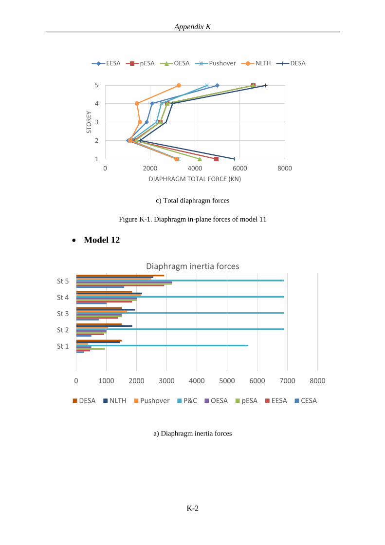
Appendix K
K-2
c) Total diaphragm forces
Figure K-1. Diaphragm in-plane forces of model 11
Model 12
a) Diaphragm inertia forces
1
2
3
4
5
0 2000 4000 6000 8000
STO
REY
DIAPHRAGM TOTAL FORCE (KN)
EESA pESA OESA Pushover NLTH DESA
0 1000 2000 3000 4000 5000 6000 7000 8000
St 1
St 2
St 3
St 4
St 5
Diaphragm inertia forces
DESA NLTH Pushover P&C OESA pESA EESA CESA

Appendix K
K-3
b) Diaphragm transfer forces
c) Total diaphragm forces
Figure K-2. Diaphragm in-plane forces of model 12
0 2000 4000 6000 8000 10000 12000
St 1
St 2
St 3
St 4
St 5
Diaphragm transfer forces
DESA NLTH Pushover P&C OESA pESA EESA CESA
1
2
3
4
5
0 1000 2000 3000 4000 5000 6000
STO
REY
DIAPHRAGM TOTAL FORCE (KN)
EESA pESA OESA Pushover
NLTH CESA DESA

Appendix K
K-4
Model 13
a) Diaphragm inertia forces
b) Diaphragm transfer forces
0 500 1000 1500 2000 2500 3000 3500
St 1
St 2
St 3
St 4
St 5
Diaphragm inertia forces
DESA NLTH Pushover OESA pESA EESA CESA
0 500 1000 1500 2000 2500 3000 3500
St 1
St 2
St 3
St 4
St 5
Diaphragm transfer forces
DESA NLTH Pushover OESA pESA EESA CESA

Appendix K
K-5
c) Total diaphragm forces
Figure K-3. Diaphragm in-plane forces of model 13
Model 14
a) Diaphragm inertia forces
1
2
3
4
5
0 1000 2000 3000 4000 5000 6000
STO
REY
DIAPHRAGM TOTAL FORCE (KN)
EESA pESA OESA Pushover NLTH CESA DESA
0 1000 2000 3000 4000 5000
St 1
St 2
St 3
St 4
St 5
Diaphragm inertia forces
DESA NLTH Pushover OESA pESA EESA

Appendix K
K-6
b) Diaphragm transfer forces
c) Total diaphragm forces
Figure K-4. Diaphragm in-plane forces of model 14
0 500 1000 1500 2000 2500 3000 3500
St 1
St 2
St 3
St 4
St 5
Diaphragm transfer forces
DESA NLTH Pushover OESA pESA EESA
1
2
3
4
5
0 2000 4000 6000 8000
STO
REY
DIAPHRAGM TOTAL FORCE (KN)
EESA pESA OESA Pushover NLTH DESA

Appendix K
K-7
Model 15
a) Diaphragm inertia forces
b) Diaphragm transfer forces
0 1000 2000 3000 4000 5000 6000 7000 8000
St 1
St 2
St 3
St 4
St 5
Diaphragm inertia forces
DESA NLTH Pushover P&C OESA pESA EESA
0 1000 2000 3000 4000 5000 6000 7000
St 1
St 2
St 3
St 4
St 5
Diaphragm transfer forces
DESA NLTH Pushover P&C OESA pESA EESA

Appendix K
K-8
c) Total diaphragm forces
Figure K-5. Diaphragm in-plane forces of model 15
Model 16
a) Diaphragm inertia forces
1
2
3
4
5
0 1000 2000 3000 4000 5000 6000
STO
REY
DIAPHRAGM TOTAL FORCE (KN)
EESA pESA OESA Pushover NLTH DESA
0 1000 2000 3000 4000 5000 6000 7000 8000
St 1
St 2
Diaphragm inertia forces
DESA NLTH Pushover P&C OESA pESA EESA

Appendix K
K-9
b) Diaphragm transfer forces
c) Total diaphragm forces
Figure K-6. Diaphragm in-plane forces of model 16
0 1000 2000 3000 4000 5000 6000
St 1
St 2
Diaphragm transfer forces
DESA NLTH Pushover P&C OESA pESA EESA
1
2
0 1000 2000 3000 4000 5000
STO
REY
DIAPHRAGM TOTAL FORCE (KN)
EESA pESA OESA Pushover NLTH DESA

Appendix K
K-10
Model 17
a) Diaphragm inertia forces
b) Diaphragm transfer forces
0 1000 2000 3000 4000 5000 6000 7000 8000
St 1
St 2
St 3
St 4
St 5
St 6
St 7
St 8
St 9
Diaphragm inertia forces
DESA NLTH Pushover P&C OESA pESA EESA
0 5000 10000 15000 20000 25000
St 1
St 2
St 3
St 4
St 5
St 6
St 7
St 8
St 9
Diaphragm transfer forces
DESA NLTH Pushover P&C OESA pESA EESA

Appendix K
K-11
c) Total diaphragm forces
Figure K-7. Diaphragm in-plane forces of model 17
Model 18
a) Diaphragm inertia forces
1
2
3
4
5
6
7
8
9
0 1000 2000 3000 4000 5000 6000 7000
STO
REY
DIAPHRAGM TOTAL FORCE (KN)
EESA pESA OESA Pushover NLTH DESA
0 1000 2000 3000 4000 5000 6000 7000 8000
St 1
St 2
St 3
St 4
St 5
St 6
St 7
St 8
St 9
Diaphragm inertia forces
DESA NLTH Pushover P&C OESA pESA EESA

Appendix K
K-12
b) Diaphragm transfer forces
c) Total diaphragm forces
Figure K-8. Diaphragm in-plane forces of model 18
0 5000 10000 15000 20000 25000
St 1
St 2
St 3
St 4
St 5
St 6
St 7
St 8
St 9
Diaphragm transfer forces
DESA NLTH Pushover P&C OESA pESA EESA
1
2
3
4
5
6
7
8
9
0 2000 4000 6000 8000
STO
REY
DIAPHRAGM TOTAL FORCE (KN)
EESA pESA OESA Pushover NLTH DESA

Appendix K
K-13
Model 19
a) Diaphragm inertia forces
b) Diaphragm transfer forces
0 1000 2000 3000 4000 5000 6000 7000 8000
St 1
St 2
St 3
St 4
St 5
St 6
St 7
St 8
St 9
Diaphragm inertia forces
DESA NLTH Pushover P&C OESA pESA EESA
0 5000 10000 15000 20000 25000
St 1
St 2
St 3
St 4
St 5
St 6
St 7
St 8
St 9
Diaphragm transfer forces
DESA NLTH Pushover P&C OESA pESA EESA

Appendix K
K-14
c) Total diaphragm forces
Figure K-9. Diaphragm in-plane forces of model 19
Model 20
a) Diaphragm inertia forces
1
2
3
4
5
6
7
8
9
0 2000 4000 6000 8000
STO
REY
DIAPHRAGM TOTAL FORCE (KN)
EESA pESA OESA Pushover NLTH DESA
0 1000 2000 3000 4000 5000 6000 7000 8000
St 1
St 2
St 3
St 4
St 5
St 6
St 7
St 8
St 9
Diaphragm inertia forces
DESA NLTH Pushover P&C OESA pESA EESA

Appendix K
K-15
b) Diaphragm transfer forces
c) Total diaphragm forces
Figure K-10. Diaphragm in-plane forces of model 20
0 5000 10000 15000 20000 25000
St 1
St 2
St 3
St 4
St 5
St 6
St 7
St 8
St 9
Diaphragm transfer forces
DESA NLTH Pushover P&C OESA pESA EESA
1
2
3
4
5
6
7
8
9
0 1000 2000 3000 4000 5000
STO
REY
DIAPHRAGM TOTAL FORCE (KN)
EESA pESA OESA Pushover NLTH DESA

Appendix K
K-16
Model 21
a) Diaphragm inertia forces
b) Diaphragm transfer forces
0 1000 2000 3000 4000 5000 6000 7000 8000
St 2
St 4
St 6
St 8
St 10
St 12
St 14
Diaphragm inertia forces
DESA NLTH Pushover P&C OESA pESA EESA
0 5000 10000 15000 20000 25000
St 2
St 4
St 6
St 8
St 10
St 12
St 14
Diaphragm transfer forces
NLTH Pushover P&C OESA pESA EESA

Appendix K
K-17
c) Total diaphragm forces
Figure K-11. Diaphragm in-plane forces of model 21
123456789
101112131415
0 2000 4000 6000 8000 10000 12000
STO
REY
DIAPHRAGM TOTAL FORCE (KN)
EESA pESA OESA Pushover NLTH DESA

Appendix L
L-1
L Appendix L: Lateral Force Distribution Between VLFR
Systems Considering Diaphragm Flexibility
A simple one-storey structure shown in Figure L-1, is selected to demonstrate the effect
of diaphragm in-plane stiffness assumption on distributing lateral forces between VLFR
systems. The floor plan and the equivalent simplified model that are used to calculate the
force distribution and diaphragm in-plane forces are shown in Figure L-1b and c. In this
model the total inertia force, 𝐹𝑎, is imposed uniformly to the floor slab. The lateral forces
imposed to the frames 1 and 2, 𝐹𝑎1 and 𝐹𝑎2, are assumed equal, 𝐹𝑎1 = 𝐹𝑎2, due to the same
tributary area of each VLFR frame.
𝐹𝑎 = 𝐹𝑎1 + 𝐹𝑎2 Eq. (L-1)
a) Floor plan
b) Schematic lateral deformation
c) Simplified model
Figure L-1. Model considered to demonstrate the effect of diaphragm flexibility on lateral force
distribution between VLFR frames

Appendix L
L-2
The stiffness matrix of the structure shown in Figure L-1c considering two degrees of
freedom, 𝑢1 and 𝑢2, can be written as Eq. (L-2). Where 𝑘1 and 𝑘2 are the frames 1 and 2
stiffnesses respectively and 𝑘𝑑 is the diaphragm in-plane stiffness.
[𝐾] = [𝑘1 + 𝑘𝑑 −𝑘𝑑−𝑘𝑑 𝑘2 + 𝑘𝑑
] Eq. (L-2)
By solving the force equation, [𝐹] = [𝐾][𝑢], lateral displacements of frames 1 and 2, 𝑢1
and 𝑢2, can be obtained considering the effect of diaphragm stiffness, 𝑘𝑑, as:
𝑢1 =(0.5𝑘2+𝑘𝑑)𝐹𝑎
𝑘1𝑘𝑑+𝑘1𝑘2+𝑘2𝑘𝑑 Eq. (L-3)
𝑢2 =(0.5𝑘1+𝑘𝑑)𝐹𝑎
𝑘1𝑘𝑑+𝑘1𝑘2+𝑘2𝑘𝑑 Eq. (L-4)
Knowing the lateral displacement of each frame, 𝑢i, and its stiffness, 𝑘i, the base shears
𝐹1 and 𝐹2 of each frame can be obtained as:
𝐹1 =(0.5𝑘1𝑘2+𝑘1𝑘𝑑)𝐹𝑎
𝑘1𝑘𝑑+𝑘1𝑘2+𝑘2𝑘𝑑 Eq. (L-5)
𝐹2 =(0.5𝑘1𝑘2+𝑘2𝑘𝑑)𝐹𝑎
𝑘1𝑘𝑑+𝑘1𝑘2+𝑘2𝑘𝑑 Eq. (L-6)
The diaphragm in-plane force can also be calculated by multiplying the diaphragm in-
plane stiffness, 𝑘𝑑, by the difference between the lateral deformations of frames 1 and 2 as:
𝐹𝑑 = 𝑘𝑑(𝑢1 − 𝑢2) Eq. (L-7)
𝐹𝑑 = 𝑘𝑑 (0.5(𝑘1−𝑘2)𝐹𝑎
𝑘1𝑘𝑑+𝑘1𝑘2+𝑘2𝑘𝑑) Eq. (L-8)
Figure L-2 plots the ratio of frame 1 base shear to the total lateral force, 𝐹1
𝐹𝑎, against the
stiffness ratio of frame 1 to frame 2, 𝑘1
𝑘2, for different frame 1 to diaphragm stiffness ratios,
𝑘1
𝑘𝑑.
This plot shows where the VLFR system stiffness is much larger than the diaphragm in-plane
stiffness, 𝑘1
𝑘𝑑= ∞, lateral force is distributed based on the tributary area of each frame.

Appendix L
L-3
However, for rigid diaphragms, 𝑘1
𝑘𝑑= 0, the lateral force is distributed based on the relative
stiffness of frames. It can be seen from this Figure that the base shear of frame 1 increases by
up to 60% by changing 𝑘1
𝑘𝑑 from 1 to 10 where
𝑘1
𝑘2 is 0.1.
Figure L-2. Frame 1 base shear
Figure L-3 plots the ratio of diaphragm in-plane force to the total lateral force, 𝐹𝑑
𝐹𝑎, against
frame 1 to frame 2 stiffness ratio, 𝑘1
𝑘2, for different frame 1 to diaphragm stiffness ratios,
𝑘1
𝑘𝑑.
This Figure shows the diaphragm in-plane force is maximum where the diaphragm in-plane
stiffness is much larger than VLFR systems, 𝑘1
𝑘𝑑= 0. The diaphragm in-plane force decreases
with decreasing the diaphragm in-plane stiffness. For example, diaphragm in-plane force
increases up to 185% by increasing the diaphragm stiffness ratio, 𝑘1
𝑘𝑑, from 10 to 1 where
𝑘1
𝑘2 is
3.
0
0.1
0.2
0.3
0.4
0.5
0.6
0.7
0.8
0.9
1
0.1 1 10
K1/Kd= 0
K1/Kd= 0.1
K1/Kd= 1
K1/Kd= 10
K1/Kd= ∞
𝐹1𝐹𝑎
𝑘1𝑘2

Appendix L
L-4
Figure L-3. Diaphragm in-plane force
Figure L-2 and Figure L-3 indicate the importance of using reasonable diaphragm in-
plane stiffness in the analysis to obtain likely lateral force distribution between VLFR
systems and diaphragm in-plane demands.
-0.5
-0.4
-0.3
-0.2
-0.1
0
0.1
0.2
0.3
0.4
0.5
0.1 1 10
K1/Kd= 0
K1/Kd= 0.1
K1/Kd= 1
K1/Kd= 10
K1/Kd= ∞
𝑘1𝑘2
𝐹𝑑𝐹𝑎
3

Appendix M
M-1
M Appendix M: Base Model Diaphragm Design
M.1 Structure details
M.1.1 Geometry and VLFR system
Figure M-1 shows the base model floor plan. Storey height is considered 3.5m. The
structure has two bays in both X and Y directions with 8m and 6m long spans respectively.
The lateral force resisting system of the structure in the X-direction is assumed moment
resisting frame, MRF. In the Y-direction, the lateral force resisting system is assumed a
combination of moment resisting frames (exterior frames) and braced frame (interior frame).
Torsion is restrained in this model.
Figure M-1.Base model floor plan and lateral force resisting systems
M.1.2 Material properties
The concrete compressive strength is considered 30MPa with an elastic modulus of
25GPa in design. The steel material strength for structural members such as beams and
columns is considered 340MPa. The slab reinforcement strength is considered 460MPa.

Appendix M
M-2
M.1.3 Loading
Gravity loading
Gravity loads used in the structural analyses are based on the values given in Table M-1.
The reduced gravity load combination of 𝐺 + 0.3𝑄 is considered to calculate the structure
weight for lateral loading calculations. This load combination was also used to assign the
storey mass to the models in NLTH analysis.
Table M-1. Gravity loads assumed for analysis
Live load (Q) 3 kPa Imposed action
Dead load (G)
1 kPa Ceiling/Services and finishes
1 kPa Partitions
3 kPa Structural elements and floor slab self-weight
Lateral loading
The earthquake lateral loads are obtained using NZS1170.5 (2004) loading standard
considering ductility 𝜇 = 1. This ductility is assumed because the focus of this study is to
investigate the diaphragm performance considering the WSP beam-column connection and
shear stud flexibilities. Also it helps to reduce the numerical modelling complexity.
The lateral loading parameters assumed in this study are summarised below:
Subsoil type D
Near Fault Factor N(T,D) = 1
Building Importance Level IL2
Hazard Factor (Wellington, New Zealand) Z =0.4
Performance Factor Sp(ULS)=0.7
Risk Factor ULS (1/500 years) Ru(ULS)=1.0
Fundamental period of structure T(1)=0.15s
Based on the above assumptions the horizontal design action coefficient in the Y-
direction, 𝐶𝑑𝑦(𝑇1), is calculated 𝐶𝑑𝑦(𝑇1) = 0.84. The effective structure mass considering

Appendix M
M-3
the reduced gravity load combination, 𝐺 + 0.3𝑄, is equal to 𝑀1 = 115𝑡𝑜𝑛. Therefore the
total base shear is 951kN for the base model.
M.2 Structure design steps
M.2.1 Structural elements design
Structural elements include beams, columns, and braces are designed according to
NZS3404 (2007) standard. In this study, all the steel beams are considered to have the same
size. This can simplify the numerical models and also in the models that the composite beams
are modelled by offsetting the slab from the steel beam, it helps to use the same offset value
for all the beams in each floor. Note that the structural members were designed for the
envelope of forces obtained from structural analysis using elastic and cracked diaphragm
stiffness as described in Section 8.2.
M.2.2 Floor-slab design for gravity loads
The floor slabs are designed using ComFlor Steel Composite Metal Deck Design
software under gravity loading. The direction of composite slab ribs is assumed to be parallel
to the X-direction. Considering the secondary beams at the mid-span of 8-meter bays, the
maximum unsupported span is 4m.
The gravity loads used for the design are in accordance with Table M-1. Note that the
self-weight of the floor slab (G) was calculated by the software using the slab thickness and
steel decking details. Figure M-2 and Table M-2 show the assumptions and parameters used
in design.

Appendix M
M-4
Figure M-2. Composite slab details
Table M-2. Composite slab design assumptions
FLOOR PLAN DATA :
(unpropped composite
construction with ComFlor
80/0.9/G550 decking)
Beam centres - equal 4.00 m Span type DOUBLE
Beam or wall width 150 mm Propping NONE
PROFILE DATA : (ComFlor
80/0.9/G550 decking)
Depth 80 mm Pitch of deck ribs 300 mm
Trough width 120 mm Crest width 150.0 mm
Nominal sheet thickness 0.90 mm Design sheet
thickness 0.86 mm
Deck weight 0.11 kN/m² Yield strength 550 N/mm²
CONCRETE SLAB :
[Normal Weight Concrete ;
Mesh : 664/188]
Overall slab depth 145 mm
Concrete characteristic strength 30 N/mm² Concrete
wet density 2400 kg/m³
Bar reinforcement NONE
Mesh reinforcement
Mesh 664/188 Yield strength 460 N/mm²
Cover to Mesh 30 mm Mesh Layers Single
Account for End Anchorage Diameter of Shear
Connectors 19 mm
M.3 Diaphragm in-plane design
Figure M-3 shows the diaphragm design flowchart that is used here to design the
diaphragm of the base model. Each design step is described in the following in detail.

Appendix M
M-5
Start diaphragm in-plane design
For each principal direction
End
Obtain diaphragm
lateral forces using an
appropriate loading method,
Fdi
2
Model entire structure
considering reasonable diaphragm
stiffness
1
Determine vertical element
out-of-plane forces, Fvi
3
Model each diaphragm using
appropriate truss element
model
4
Apply Fdi, to the truss model and
Fvi, to the corresponding
nodes.
5
Determine force demands
in concrete struts, tension
ties, beam/connection axial force and shear stud demands
6
Diaphragm strength
check
10
Shear stud strength
check
9
Beam axial capacity
check
7
Beam/column
connection capacity
check
8
Figure M-3. Diaphragm in-plane design flowchart
M.3.1 Step 1, Structure 3D modelling
The structure model in this step is the same as the model used for structural elements
design. In this model appropriate diaphragm stiffness should be considered. According to the
diaphragm design approaches described in Section 8.2, structural analyses are performed two
times considering elastic and cracked diaphragm in-plane stiffness. The diaphragm in-plane
stiffness reduction factor is considered 0.1 in this study.
M.3.2 Step 2, Diaphragm lateral forces
Here, diaphragm lateral forces are obtained using the DESA method described in
Chapter 7. According to the DESA method:

Appendix M
M-6
𝐶𝑑𝑦(𝑇1) = 0.84 considering ductility factor 𝜇 = 1
Lateral force per unit area of the floor slab is 4.95𝑘𝑃𝑎
M.3.3 Step 3, Diaphragm in-plane forces from VLFR elements
Diaphragm in-plane forces from VLFR elements can be obtained by calculating the
difference between the shear forces of the structural elements above and below the
diaphragm. These forces should be in equilibrium with the imposed lateral forces, DESA, in
each level. Figure M-4 shows the diaphragm imposed forces from VLFR elements for elastic
and cracked diaphragms.
a) Elastic diaphragm

Appendix M
M-7
a) Cracked diaphragm
Figure M-4. Diaphragm imposed forces from VLFR elements
M.3.4 Step 4, Diaphragm truss modelling
According to the findings of Chapter 3, Truss Model 2 and Truss Model 3 are used to
model and analyse the diaphragm of the base model considering elastic and cracked in-plane
behaviour respectively. Table M-3 shows the cross-section properties of the truss members.
To model the diaphragm using truss elements, 2×2m mesh size is considered in this study.
Table M-3. Cross-section properties of Truss models 2 and 3
Diagonal member Orthogonal member
Model description Compression Tension Compression Tension
Truss Model 2 (elastic)
𝑎𝑡 0 0.585𝑎𝑡 𝑎𝑡
Truss Model 3 (cracked)
0.725𝑎𝑡 0 0.97𝑎𝑡 𝐴𝑠

Appendix M
M-8
As can be seen from Figure M-5, the concrete thickness above the highest point of the
steel decking is equal to 50mm. However, the effective concrete thickness that may be used
for calculating the cross-section properties of truss element is equal to 65mm in this case.
This is because small portions on top of the flat surface of the steel decking may not affect
the diaphragm in-plane stiffness significantly. Meanwhile, to calculate the diaphragm
strength (diagonal strut strength and buckling) 50mm concrete topping is considered.
Figure M-5. Composite slab cross-section
Truss Model 2
Diagonal truss element properties, 𝑎 = 2000𝑚𝑚, 𝑡 = 65𝑚𝑚, 𝐿 = 1414𝑚𝑚
𝐴𝐷 = 𝑎𝑡
= 130000𝑚𝑚2
𝐴𝑥𝑖𝑎𝑙 𝑠𝑡𝑖𝑓𝑓𝑛𝑒𝑠𝑠 (𝐴𝐷) =𝐸𝐴
𝐿𝐷⁄
= 2298𝑘𝑁/𝑚𝑚
Orthogonal element properties, 𝑎 = 2000𝑚𝑚, 𝑡 = 65𝑚𝑚, 𝐿 = 2000𝑚𝑚
𝐴𝑂𝑇 = 𝑎𝑡
= 130000𝑚𝑚2
𝐴𝑥𝑖𝑎𝑙 𝑠𝑡𝑖𝑓𝑓𝑛𝑒𝑠𝑠 (𝐴𝑂𝑇) =𝐸𝐴
𝐿𝑂⁄

Appendix M
M-9
= 1625𝑘𝑁/𝑚𝑚
𝐴𝑂𝐶 = 0.585𝑎𝑡
= 76050𝑚𝑚2
𝐴𝑥𝑖𝑎𝑙 𝑠𝑡𝑖𝑓𝑓𝑛𝑒𝑠𝑠 (𝐴𝑂𝐶) =𝐸𝐴
𝐿𝑂⁄
= 950𝑘𝑁/𝑚𝑚
Truss Model 3
Diagonal truss element properties, 𝑎 = 2000𝑚𝑚, 𝑡 = 65𝑚𝑚, 𝐿 = 1414𝑚𝑚
𝐴𝐷 = 0.725𝑎𝑡
= 94250𝑚𝑚2
𝐴𝑥𝑖𝑎𝑙 𝑠𝑡𝑖𝑓𝑓𝑛𝑒𝑠𝑠 (𝐴𝐷) =𝐸𝐴
𝐿𝐷⁄
= 1667𝑘𝑁/𝑚𝑚
Orthogonal element properties, 𝑎 = 2000𝑚𝑚, 𝑡 = 65𝑚𝑚, 𝐿 = 2000𝑚𝑚 and
188𝑚𝑚2/𝑚 reinforcement
𝐴𝑂𝑇 = 𝐴𝑠
= 376𝑚𝑚2
𝐴𝑥𝑖𝑎𝑙 𝑠𝑡𝑖𝑓𝑓𝑛𝑒𝑠𝑠 (𝐴𝑂𝑇) =𝐸𝐴
𝐿𝑂⁄
= 37.6𝑘𝑁/𝑚𝑚
𝐴𝑂𝐶 = 0.97𝑎𝑡
= 126100𝑚𝑚2
𝐴𝑥𝑖𝑎𝑙 𝑠𝑡𝑖𝑓𝑓𝑛𝑒𝑠𝑠 (𝐴𝑂𝐶) =𝐸𝐴
𝐿𝑂⁄
= 1576𝑘𝑁/𝑚𝑚

Appendix M
M-10
M.3.5 Step 5, Applying diaphragm in-plane forces to the truss model
The diaphragm lateral forces obtained from the DESA method are distributed based on
the tributary area of each node as shown in Figure M-6. VLFR system reactions are also
applied at the corresponding nodes in the truss model in this Figure.
a) Elastic diaphragm
b) Cracked diaphragm
Figure M-6. Inertia forces and VLFR system forces imposed on the diaphragm in the Y-direction

Appendix M
M-11
M.3.6 Step 6, Obtaining diaphragm internal forces and load path to VLFR
system
Figure M-7 shows the axial force diagram of truss elements for the elastic diaphragm.
a) Lateral loading in the negative Y-direction
b) Lateral loading in the positive Y-direction
Figure M-7. Axial force diagram of truss elements

Appendix M
M-12
Maximum compression strut axial forces and tension tie axial forces of both elastic and
cracked diaphragm models are presented in Table M-4.
Table M-4. Maximum strut and tie forces obtained from both elastic and cracked diaphragm analysis
Maximum Strut
compression force (kN)
Maximum Tie tension force
(kN)
Elastic diaphragm model -186 117
Cracked diaphragm model -166 26
Figure M-8 shows the beam axial forces obtained from elastic and cracked diaphragm
analysis. Maximum compression and tension forces at the beam-ends (beam-column
connections) and the beam mid-span are presented in Table M-5.
Figure M-8. Beam axial force diagram
Table M-5. Maximum beam axial demands at the beam-column connections and beam mid-span
Left beam, braced bay (kN) Right beam (kN)
Axis A Mid-span B B Mid-span C
Elastic diaphragm model EP +408 +169 +218 +294 +135 +14
EN -404 -134 -138 -214 -76 -14
Cracked diaphragm model EP +386 +341 +233 +474 +317 +12
EN -386 -120 0 -192 -85 0
Shear stud demands can be calculated using the difference of the beam axial forces at the
beam-ends. The maximum shear stud demands obtained from analyses are presented in
Table M-6.
-500
-400
-300
-200
-100
0
100
200
300
400
500
600
-6 -4 -2 0 2 4 6
Bea
m a
xia
l fo
rce
(kN
)
Cracked, EP
Cracked, EN
Elastic, EP
Elastic, EN

Appendix M
M-13
Table M-6. Maximum shear stud demands
Left beam, braced bay (kN) Right beam (kN)
Elastic diaphragm model 622 308
Cracked diaphragm model 599 470
M.3.7 Step 7, Beam design for axial forces
Beam axial forces should be considered in beam design. This may be performed by
considering two critical sections along the beam length:
1. At the maximum axial force which is usually at the beam-ends and
2. At the maximum bending moment location to consider bending moment-axial
force interaction.
The beam axial force diagrams plotted in Figure M-8 show that the maximum beam axial
force at the beam-mid point (maximum bending moment) is about 317kN. The axial strength
of the steel beam section considering 460UB67.1 is 2917kN. The maximum beam axial force
is about 10% of the nominal section strength of the steel beam and axial force-bending
moment interaction can be ignored.
Table M-7 presents the beam-column connection forces considering both gapped and no
gap conditions. Here it is assumed the slab bearing force is transferred to the beam-column
connection on the tension side.
Table M-7. Maximum beam axial forces at the beam-column connections considering gapped and no
gap conditions
Braced bay (kN) Pinned beam (kN)
Axis A B B C
Elastic diaphragm
model
+408G,
+1084NG
+218G,
+894NG
+294G,
+970NG
+14G,
+690NG
Cracked diaphragm
model
+386G,
+1062NG
+233G,
+909NG
+474G,
+1150NG
+12G,
+688NG
GGapped, NGNo Gap
Cowie et al. (2014) recommended to use a bolted top flange connection that looks the
same as the top flange connection in a Sliding Hinge Joint to carry axial forces in conjunction

Appendix M
M-14
with the flexible end plate (FE) or web side plate (WSP) connection to carry the vertical shear
as shown in Figure M-9. The net effective tensile area was considered to be the top flange
and half the beam web. The connection also has to be detailed to develop inelastic rotation
without bolt or weld failure and so will handle the connection rotation due to the top flange
pin. Also, the stiffener must be welded to the column to develop the full tension capacity of
the top plate and transfer this into the column web.
Figure M-9. Top plate connection to transfer collector beam axial forces, (Cowie et al., 2014)
Considering Cowie et al. (2014) recommendations, the beam tensile strength using the
net tensile area is 8580
2× 340 = 1458𝑘𝑁, which is larger than the maximum of beam tensile
forces, 1150kN, in Table M-8.
M.3.8 Step 8, Beam-column connection design
Figure M-10 shows a schematic view of the beam in the frame 2 (middle frame) and the
applied gravity loads. The connection shear force demand using 1.2G+1.5Q load combination
is 126kN.

Appendix M
M-15
Figure M-10. Schematic view of pinned beam in frame 2 (middle frame)
The beam-column connection design to carry gravity loads was performed according to
SCNZ report 14.1 (2007). Figure M-11 shows a snapshot of the spreadsheet developed to
design these connections.
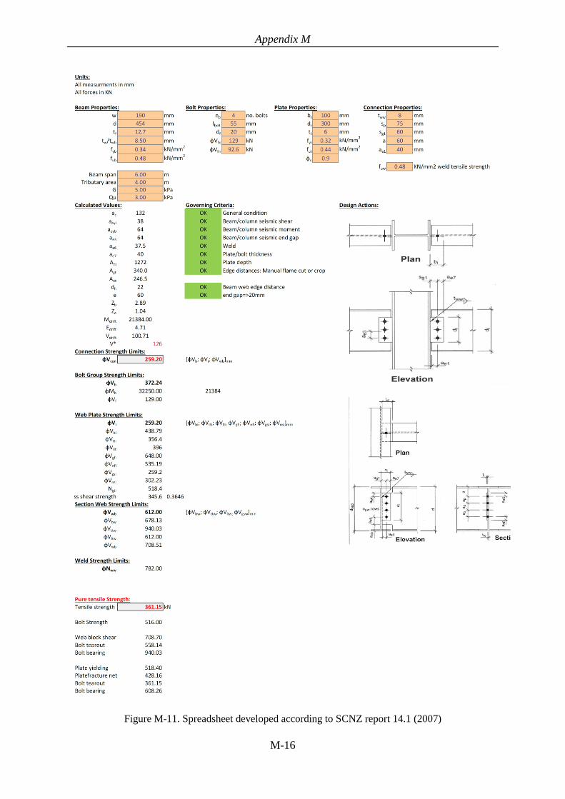
Appendix M
M-16
Figure M-11. Spreadsheet developed according to SCNZ report 14.1 (2007)

Appendix M
M-17
Figure M-12 shows details of the connection designed to carry gravity loads. Connection
shear capacity was calculated 259.2kN and connection tensile capacity was calculated 361.15kN.
Figure M-12. Connection details
Applied shear force to the connection considering the reduced gravity load combination,
0.3Q+G, is 70.8kN. This value should be used to calculate the axial compression capacity of
the WSP connection considering axial-shear force interaction.
M.3.8.1WSP axial compression strength calculation
According to the proposed method in Chapter 4:
Case two, beam top flange restrained laterally
Here it is assumed that the top flange is restrained laterally due to the presence of shear
studs.
Checking the cleat plate axial strength:
1) Obtain ℎ𝑒𝑓𝑓 according to Clause 6.2.4 of NZS 3404 (2007)
ℎ𝑒𝑓𝑓 = 𝑚𝑖𝑛 [16𝑡𝑤√
250
𝑓𝑦𝑤
ℎ𝑤

Appendix M
M-18
𝑓𝑦𝑤 = 340𝑀𝑃𝑎
ℎ𝑒𝑓𝑓 = 116.7𝑚𝑚
Note: if the beam top flange is retrained and the beam is coped, the ℎ𝑒𝑓𝑓 should
be modified using:
ℎ𝑒𝑐
ℎ𝑒= 1 − 0.5
𝐿𝑐
𝑑
2) Calculate ℎ1 and ℎ2
ℎ1 = ℎ𝑒𝑓𝑓 + 𝑡𝑓 − 𝑎 + 𝑎𝑒6
ℎ1 = 116.7 + 12.7 − 60 + 37.5
= 106𝑚𝑚
ℎ2 = ℎ𝑐 − ℎ1
ℎ2 = 300 − 106
= 194𝑚𝑚
Note: 𝑎𝑒6 is the vertical edge distance at top of the cleat plate
3) Calculate the cleat axial capacity at zone 1 (𝑃𝑐1).
𝑃𝑐1 = ℎ1𝑡𝑐𝑓𝑦𝑐
= 205𝑘𝑁
4) Calculate 𝑃2,
4.1) Obtain the effective length of the beam web (𝐿𝑤)
{𝐿𝑤 =
ℎ𝑤
5+ 𝐿𝑐𝑜𝑝𝑒 − 𝑎𝑒1 → 𝑓𝑜𝑟 𝑐𝑜𝑝𝑒𝑑 𝑏𝑒𝑎𝑚
𝐿𝑤 =ℎ𝑤
5 → 𝑓𝑜𝑟 𝑢𝑛 − 𝑐𝑜𝑝𝑒𝑑 𝑏𝑒𝑎𝑚
𝐿𝑤 = 85.8𝑚𝑚
4.2) Obtain contributing height of the beam web, ℎ𝑤𝑒 = 𝑚𝑖𝑛[ℎ𝑤, 1.5ℎ2]

Appendix M
M-19
ℎ𝑤𝑒 = 289𝑚𝑚
4.3) Calculate the effective length factor for the cleat plate
{
𝑘𝑐 = 1.05𝐿𝑤
𝐿𝑐√𝐸𝐼𝑐2
𝐸𝐼𝑤+ 1.2 → 𝑓𝑜𝑟
𝐿𝑤
𝐿𝑐√𝐸𝐼𝑐2
𝐸𝐼𝑤< 2
𝑘𝑐 = 0.9𝐿𝑤
𝐿𝑐√𝐸𝐼𝑐2
𝐸𝐼𝑤+ 1.5 → 𝑓𝑜𝑟
𝐿𝑤
𝐿𝑐√𝐸𝐼𝑐2
𝐸𝐼𝑤≥ 2
𝑘𝑐 = 1.92
Note: 𝐼𝑤 is calculated based on effective beam web height (ℎ𝑤𝑒) and 𝐼𝑐2 is
calculated using ℎ2
4.4) Calculate the elastic buckling force for the cleat plate, 𝑃𝑐𝑟 =𝜋2𝐸𝐼𝑐2
(𝑘𝑐𝐿𝑐)2
𝑃𝑐𝑟 = 512kN
4.5) Obtain 𝑃𝑢 for the cleat plate based on Section 6 of NZS 3404 (2007) considering
𝛼𝑏 = 0.5
𝑃𝑢 = 238kN
4.6) Obtain 𝑀𝑢3 (plastic moment) of the cleat plate about the weak axis (using ℎ2)
𝑀𝑢3 = 0.55𝑘𝑁.𝑚
4.7) Calculate moment participation factor, 𝛼 = (𝐼𝑐2
𝐿𝑐⁄
𝐼𝑐2𝐿𝑐⁄ +
𝐼𝑤𝐿𝑤⁄)
𝛼 = 0.25
4.8) Calculate 𝑒 (axial load eccentricity) using 𝑒 =𝑡𝑐+𝑡𝑤
2
𝑒 = 7.25𝑚𝑚
4.9) Find 𝑀𝑢2 (plastic moment) of the cleat plate about the strong axis
Note: the plastic moment of cleat plate about the strong axis should be modified
using shear-moment interaction relationship

Appendix M
M-20
{
𝑉
𝑉𝑣+1.6𝑀𝑢2
∅𝑀𝑠2≤ 2.2 𝑓𝑜𝑟 𝑉 ≥ 0.6𝑉𝑣
𝑀𝑢2 = ∅𝑀𝑠2 𝑓𝑜𝑟 𝑉 < 0.6𝑉𝑣
𝑓𝑜𝑟 𝑉 < 0.6𝑉𝑣 → 𝑀𝑢2 = 43𝑘𝑁.𝑚
4.10) Calculate the cleat plate capacity at zone 2 (𝑃𝑐2) 𝑃𝑐2
𝑃𝑢+
𝛼×𝑃𝑐2×𝑒
𝑀𝑢3(1−𝑃 𝑃𝑐𝑟⁄ )+
𝑀2
𝑀𝑢2≤ 1
𝑃𝑐2 = 108𝑘𝑁
5) Calculate total cleat capacity
𝑃𝑐 = 𝑃𝑐1 + 𝑃𝑐2
𝑃𝑐 = 313𝑘𝑁
M.3.8.2 Check the beam web axial strength
1) Calculate beam web strength at zone 1 (𝑃𝑤1)
𝑃𝑤1 = (ℎ𝑒𝑓𝑓 − ℎ2)𝑡𝑤𝑓𝑦𝑤
𝑃𝑤1 = 337𝑘𝑁
The process of calculating 𝑃𝑤2 is similar to the cleat plate axial strength calculation, only
the effective length factor and moment participation factor are different as:
𝑘𝑤 = 𝑘𝑐𝐿𝑐
𝐿𝑤√𝐸𝐼𝑤
𝐸𝐼𝑐2
𝛼 = (𝐼𝑤
𝐿𝑤⁄
𝐼𝑐2𝐿𝑐⁄ +
𝐼𝑤𝐿𝑤⁄)
𝑃𝑤2
𝑃𝑢+
𝛼×𝑃𝑤2×𝑒
𝑀𝑢3(1−𝑃 𝑃𝑐𝑟⁄ )+
𝑀2
𝑀𝑢2≤ 1
𝑃𝑤 = 𝑃𝑤1 + 𝑃𝑤2
𝑃𝑤2 = 135𝑘𝑁
𝑃𝑤 = 472𝑘𝑁

Appendix M
M-21
Nominal compression strength of the WSP connection is equal to the minimum of
{𝑃𝑤, 𝑃𝑐}
It is suggested that the calculated compression capacity is multiplied by a
strength reduction factor of 𝜙 = 0.75 to account for packing effects.
𝑊𝑆𝑃 𝑐𝑜𝑚𝑝𝑟𝑒𝑠𝑠𝑖𝑜𝑛 𝑠𝑡𝑟𝑒𝑛𝑔𝑡ℎ = 0.75 ×𝑚𝑖𝑛𝑖𝑚𝑢𝑚 𝑜𝑓 {472, 313}
𝑊𝑆𝑃 𝑐𝑜𝑚𝑝𝑟𝑒𝑠𝑠𝑖𝑜𝑛 𝑠𝑡𝑟𝑒𝑛𝑔𝑡ℎ = 234𝑘𝑁
Table M-5 presented the beam-end forces for gapped and no gap conditions. The WSP
axial tension and compression strengths are equal to 361kN and 234kN respectively.
Therefore the steel beams on axis B-C need the top-plate detail (Cowie et al. 2014) shown in
Figure M-9.
The maximum tensile force demand on the beam-column connection was 1150kN (Beam
on axis B-C). Here, 500×200×20mm Grade 350 steel plate is considered to transfer the beam
axial forces to the columns.
𝑇𝑜𝑝 𝑝𝑙𝑎𝑡𝑒 𝑠𝑡𝑟𝑒𝑛𝑔𝑡ℎ = 20 × 200 × 340𝑀𝑃𝑎 = 1224𝑘𝑁
Figure M-13 shows the details of the top plate connection.
Figure M-13. Top plate connection detail

Appendix M
M-22
Note that this connection requires further research and development to investigate the
axial force behaviour, possible failure modes and the amount of bending resistance that the
top plate may add to the connection.
M.3.9 Step 9, Shear studs design
Shear stud demand on beams of the frame 2 can be obtained using the beam axial force
diagrams provided in Figure M-5. The magnitude of shear stud demands was shown in
Table M-6 for the gapped condition.
The slab bearing forces should be considered for shear stud design as well as beam axial
and beam-column connection design where the gap is not provided around the column. The
maximum bearing force may be calculated using Clause 12.10.2.4 of NZS3404 (2007):
𝑁𝑠𝑙𝑎𝑏 = 𝑚𝑖𝑛 {1.3𝑡𝑒𝑓𝑏𝑠𝑒𝑓(𝑓𝑐′ + 𝑓𝑐𝑜𝑠
′ ); ∑(𝐴𝑔𝐹𝑦)𝑖}
𝑁𝑠𝑙𝑎𝑏 = 𝑚𝑖𝑛{1.3 × 65𝑚𝑚 × 200𝑚𝑚 × (30 + 10)𝑀𝑃𝑎; ∑(𝐴𝑔𝐹𝑦)𝑖 }
The bearing force depends on the slab area in contact with the column face. It can either
be the concrete topping or total slab thickness (rib zone). Here only concrete topping is
considered to be in contact with the column face.
𝑁𝑠𝑙𝑎𝑏 = 𝟔𝟕𝟔𝒌𝑵
The slab bearing force is considered to be distributed between shear studs uniformly.
Table M-8. Shear stud demands for gapped and no gap conditions
Left beam, braced bay (kN) Right beam (kN)
Elastic diaphragm model Gapped 622 308
No gap 1298 984
Cracked diaphragm model Gapped 599 470
No gap 1275 1146
M.3.9.1Calculating shear stud strength considering gravity load and lateral
force interaction
According to Chapter 5 findings:

Appendix M
M-23
Calculating 𝑺𝒎𝒂𝒙 for propped beams
The maximum shear stud slip, 𝑆𝑚𝑎𝑥, can be obtained for propped beams as
𝑆𝑚𝑎𝑥 = 1.6∆𝑣𝑑
𝐿
Where
∆𝑣: is a mid-point vertical deflection of the bare steel beam under gravity loads (5𝑊𝐿4
384𝐸𝐼).
𝑑: is total beam height including the steel beam and the concrete slab.
𝐿: is the beam span.
Note that ∆𝑣 should be calculated using the bare steel beam stiffness without considering
composite action.
𝑊 = 23.6 𝑘𝑁/𝑚 𝑜𝑟 𝑁/𝑚𝑚
𝐼 = 296𝑒6 𝑚𝑚4
∆𝑣=6.72mm
𝑑 = 454 + 80 + 65
= 599
𝑆𝑚𝑎𝑥 = 1.07𝑚𝑚
Calculating lateral force resistance
Obtaining effective shear stud zone:
To obtain the effective shear stud zone the shear stud slip limit is required. Here the
value of 𝑆𝑢
3⁄ is recommended to be assumed as the shear stud slip limit. The maximum
monotonic shear slip capacity, 𝑆𝑢, of 19mm shear studs is 7.2mm.
Lateral force resistance of shear studs on the beam is equal to the sum of the strengths of
all shear studs, because the maximum calculated slip is less than 2.4mm (𝑆𝑢
3⁄ ) therefore all
shear studs may be used to carry lateral forces.

Appendix M
M-24
Here 25% composite action is considered:
𝐶𝑜𝑚𝑝𝑜𝑠𝑖𝑡𝑒 𝑓𝑜𝑟𝑐𝑒
= 0.25 × 𝑚𝑖𝑛{65𝑚𝑚 × 1500𝑚𝑚 × 30𝑀𝑃𝑎; 8580 × 340 }
𝐶𝑜𝑚𝑝𝑜𝑠𝑖𝑡𝑒 𝑓𝑜𝑟𝑐𝑒 = 621𝑘𝑁
Total shear stud strength on the beam is 2 × 621 = 1242𝑘𝑁 based on 25% composite
action.
Note that the composite action is not considered to carry gravity loads in this example.
The minimum allowable composite action level to carry gravity loads is given by Clause
3.5.8.3 of NZS2327 (2017) equal to 40%.
M.3.10 Step 10, Diaphragm in-plane strength check
M.3.10.1 Compression strut and tension ties
According to NZS3101 (2006) Clause 13.3.9, the strength design of diaphragms for
shear shall be based on strut and tie models in accordance with Appendix A of NZS3101
(2006). Here, the compression strength of struts and tensile strength of ties are calculated to
compare with the analysis results presented in Table M-4.
Nominal compression strut strength may be calculated according to Clause A5.2
NZS3101 (2006). Here the concrete thickness is considered equal to the concrete topping as
described in Section M.3.4.
Strut strength:
𝑓𝑐𝑢 = 𝛽𝑠𝛼1𝑓𝑐′
= 0.6 × 0.85 × 30
= 15.3𝑀𝑃𝑎
𝐹𝑛𝑠 = 15.3 × 𝑎𝑡
= 15.3 × 50 × 2000

Appendix M
M-25
= 554𝑘𝑁
Maximum strut force obtained from the analysis (Table M-4) was -186kN.
554𝑘𝑁 > 186𝑘𝑁 𝑂𝐾
Nominal tension tie strength may be calculated according to Clause A6.1 NZS3101
(2006). It is assumed 664/188mesh is used in the concrete topping with 𝑓𝑦 = 460𝑀𝑃𝑎. This
mesh provides 188𝑚𝑚2/𝑚 steel cross-section.
Tie strength:
𝐹𝑛𝑡 = 𝐴𝑠𝑡𝑓𝑦
= 188 × 2 × 460
= 86.5𝑘𝑁
Maximum tension force obtained from diaphragm analysis was 117kN (see Table M-4).
86.5𝑘𝑁 ≱ 117𝑘𝑁 𝑁𝐺
This shows that additional reinforcement is required to carry diaphragm tension tie
forces.
M.3.10.2 Diaphragm buckling check
Diaphragm buckling check can be performed according to the finding of Chapter 6. The
buckling strength of diaphragms is obtained for both elastic (un-cracked) and cracked (strut
buckling) situations. Here, the diaphragm shear strength obtained according to Clause
13.4.10.2 of NZS3404 (2007) is considered as the upper bound of diaphragm shear strength
to compare with the calculated buckling strengths. Also the maximum strut compression
forces obtained from the analyses, Table M-4, are used to be compared with the strut
buckling capacity.
According to NZS3404 (2007), Clause 13.4.10.2 the diaphragm shear strength may be
calculated as

Appendix M
M-26
𝑉𝑟 = 𝑚𝑖𝑛 {0.8∅𝐴𝑟𝑡𝑓𝑦𝑟 + 2.76∅𝐶𝐴𝐶𝑉
0.5∅𝐶𝑓𝐶′𝐴𝐶𝑉
𝑉𝑟𝑥 = 𝑚𝑖𝑛 {0.8 × 0.9 × 188 × 460 × 8 + 2.76 × 0.6 × 50 × 8000
0.5 × 0.6 × 30 × 50 × 8000
= 892𝑘𝑁
𝑉𝑟𝑦 = 𝑚𝑖𝑛 {0.8 × 0.9 × 188 × 460 × 6 + 2.76 × 0.6 × 50 × 6000
0.5 × 0.6 × 30 × 50 × 6000
= 617 𝑘𝑁
Diaphragm buckling mode 1, inter-rib (local) buckling
The mode one buckling (local buckling) was shown that does not govern for ComFlor 80
and 60 for 50mm concrete topping thickness in Chapter 6.
The other buckling modes (intra-panel and intra-bay) are investigated in the following:
Notations:
𝑵𝒙𝒚𝟏 Elastic critical shear stress (MPa)
𝒃 Plate width (distance between ribs) (mm)
𝒕 Concrete topping thickness (mm)
𝑬 Concrete elastic modulus (MPa)
𝝂 Concrete Poisson’s ratio
𝒌𝒔 Plate shear buckling coefficient
𝑵𝒄𝒓 Elastic critical axial stress (MPa)
𝒌 Plate axial buckling coefficient
𝝉𝒄 and 𝝏𝒄 Imposed shear and axial stresses to the concrete topping (MPa)
𝒆𝒚 Distance between concrete topping centre line to the section neutral axis
(mm)
𝒉 Steel deck height (mm)
𝒂 Steel deck rib width (mm)
𝜷 Ribs height modification factor
𝑮𝒙𝒚 Elastic shear modulus of concrete (MPa)
𝜼 Numerical factor depending on the ribs aspect ratios

Appendix M
M-27
𝒌𝑩 Reduction factor accounting for the decrease in the torsional stiffness of
reinforced concrete beams due to concrete cracking
𝑵𝒙𝒚𝟐 Elastic critical shear stress of intra-panel orthogonal plate (MPa)
𝑫𝒙 Flexural stiffness of the steel deck slab in the direction perpendicular to ribs
(N.mm)
𝑫𝒚 Flexural stiffness of the steel deck slab in the ribs direction (N.mm)
𝑳𝟐 Slab length parallel to the ribs (mm)
𝒇𝒄′ Concrete compressive strength (MPa)
𝑰𝒔 Moment of inertia of the concrete strut per unit width (mm4)
𝑰𝒓 Moment of inertia of the rib per unit width(mm4)
𝑳𝒔 Strut length (mm)
𝜶 The angle between the concrete strut and the ribs
𝑳𝟏 Slab length perpendicular to the ribs (mm)
𝑳𝟐 Slab length parallel to the ribs (mm)
𝑽𝑺𝑩𝟐 Slab shear buckling strength per unit length due to intra-panel buckling
(N/mm)
𝑽𝒔𝒕𝒓𝒖𝒕𝟐 Slab shear from strut buckling capacity per unit length (intra-panel buckling)
(N/mm)
𝒕𝒆𝒒 Equivalent plate thickness to the steel deck slab in the X direction (mm)
𝒆𝒙 Distance between equivalent slab centre line to the section neutral axis (mm)
𝑬𝒔 Steel elastic modulus (MPa)
𝑰𝒚 Moment of inertia of secondary beams (mm4)
𝑨𝒔 Cross section area of secondary beams (mm2)
𝒉𝟏 Steel beam height (secondary beam) (mm)
𝒄𝟏 Distance between secondary beams (mm)
𝒅𝒊 Width of steel beam flanges and web (mm)
𝒕𝒊 Thickness of steel beam flanges and web (mm)
𝑮𝒙𝒚𝒔 Elastic shear modulus of steel (MPa)
𝑵𝒙𝒚𝟑 Elastic critical shear stress of intra-bay orthogonal plate (MPa)
𝑽𝑺𝑩𝟑 Slab shear buckling strength per unit length due to intra-bay buckling
(N/mm)
𝑰𝒔𝒃 Is the secondary beam moment of inertia per unit width of the slab (𝐼𝑦/𝑐1)
(mm3)
𝝍 Buckling correction factor, 0.9 for a composite floor with one secondary
beam, 1 for more than one
𝒏 Number of secondary beams per bay
𝑽𝒔𝒕𝒓𝒖𝒕𝟑 Slab shear from strut buckling capacity per unit length (intra-bay buckling)
(N/mm)
𝑷𝒄𝒓𝟑 Strut buckling capacity per unit length (intra-bay) (N/mm)
𝑷𝒄𝒓𝟐 Strut buckling capacity per unit length (intra-panel buckling) (N/mm)
𝑵𝒆𝒙𝒊𝒔𝒕𝒊𝒏𝒈 Maximum imposed shear stress to intra-panel (MPa)
Diaphragm buckling mode 2, Intra-panel buckling
1. Calculating critical shear buckling of the intra-panel subjected to pure shear, (pre-
crack condition)
Preliminary check:

Appendix M
M-28
If the equation below is satisfied, there is no need to check the critical shear buckling of
the intra-panel subjected to pure shear:
0.3𝑓𝑐′ ≤ 0.75 × 3.5
𝜋2
𝑡𝐿22 √𝐷𝑥𝐷𝑦
34
9 ≤ 0.75 × 3.5𝜋2
65 × 400029.6 × 108
9 ≤ 23.8 𝑂𝐾 This failure mode does not need to be checked
Where √𝐷𝑥𝐷𝑦34 for different topping thickness is presented in plots shown in
Figure M-14 for ComFlor 60 and 80 (these values are calculated using flexural stiffness
reduction factor 0.35 based on Table C6.5 NZS 3101, 2006).
Figure M-14. Calculated values of √𝐷𝑥𝐷𝑦34 for ComFlor 60 and 80 against different concrete topping
thickness
1. Intra-panel subjected to diagonal force (strut force), post-crack condition
The critical strut buckling load per unit width of the strut is calculated using:
𝑃𝑐𝑟2 = 0.75𝜋2(𝐸𝐼𝑠+𝐸𝐼𝑟(
𝐿𝑠𝐿2)3)
𝐿𝑠2
Where,
60,
834435336.
6
70,
108731684
3
0
1E+09
2E+09
3E+09
4E+09
5E+09
6E+09
0 50 100 150 200
(N.m
m)
Concrete topping thickness (mm)
CF 80
CF 60
√𝐷𝑥𝐷𝑦
34

Appendix M
M-29
𝐼𝑟 = 0.35𝑎(𝑡+ℎ)3
12(𝑎+𝑏)
𝐼𝑠 = 0.8𝑡3 𝑠𝑖𝑛 𝛼
12
𝐿𝑠 =𝐿2
𝑠𝑖𝑛 𝛼
Considering 𝑎 = 135𝑚𝑚, 𝑏 = 165𝑚𝑚, 𝑡 = 65𝑚𝑚, ℎ = 80𝑚𝑚 and 𝐿2 = 4000𝑚𝑚
𝐼𝑟 = 40013 𝑚𝑚3
𝛼 = 45°
𝐼𝑠 = 12011 𝑚𝑚3
𝐿𝑠 = 5656𝑚𝑚
𝑃𝑐𝑟2 = 0.75 ×𝜋2 × 25000 × 12011 × 𝑠𝑖𝑛3(45) + 𝜋2 × 25000 × 40013
56562 × 𝑠𝑖𝑛3(41)
= 743𝑁/𝑚𝑚 capacity
186000 (𝑀𝑎𝑥 𝑠𝑡𝑟𝑢𝑐 𝑓𝑜𝑟𝑐𝑒 𝑓𝑟𝑜𝑚 𝑇𝑎𝑏𝑙𝑒 𝑀−4)
2000= 93𝑁/𝑚𝑚 Demand
743 𝑁/𝑚𝑚 > 93 𝑁/𝑚𝑚 𝑂𝐾
Diaphragm buckling mode 3, Global buckling
1. Calculating critical shear buckling of the intra-bay subjected to pure shear, (pre-
crack condition)
Preliminary check:
First, the effect of the secondary beam could be ignored and the same as the intra-bay the
following equation could be used as a preliminary check. If the equation below is satisfied,
there is no need to check the critical shear buckling of the intra-bay subjected to pure shear:
0.3𝑓𝑐′ ≤ 0.75 × 3.5
𝜋2
𝑡𝐿22 √𝐷𝑥𝐷𝑦
34
9 ≰ 0.75 × 3.5𝜋2
65 × 800029.6 × 108

Appendix M
M-30
9 > 5.96 𝑁𝐺 This failure mode needs to be checked
First, the properties of the equivalent orthotropic plate need to be calculated:
Finding the flexural stiffness of the steel deck slab in the ribs direction (𝐷𝑦) same as the
intra-panel:
𝐷𝑦 = 0.35(𝐸𝑡3
12(1 − 𝜗2)+
𝐸𝑡𝑒𝑦2
(1 − 𝜗2)+
𝐸𝑎ℎ3
12(𝑎 + 𝑏)+𝐸ℎ𝑎 (
ℎ2 +
𝑡2 − 𝑒𝑦)
2
(𝑎 + 𝑏))
𝐷𝑦 = 1457977781 𝑁.𝑚𝑚
Finding the flexural stiffness of the steel deck slab in the direction perpendicular to the
ribs (𝐷𝑥):
First, the equivalent plate thickness to the steel deck slab should be calculated: (𝐷𝑥𝑠 is
the steel deck slab stiffness equal to 𝐷𝑥 for the intra-panel)
Finding the flexural stiffness of the steel deck slab in the direction perpendicular to ribs
(𝐷𝑥):
{𝛽 = 0.9224𝑒(
−2.756ℎ
𝑎)
𝛽 =𝑎
8ℎ
𝑓𝑜𝑟
ℎ
𝑎≤ 0.4
𝑓𝑜𝑟 ℎ
𝑎> 0.4
𝛽 = 0.21
𝐷𝑎 =𝐸(𝑡 + 𝛽ℎ)3
12(1 − 𝜗2)
= 1.19 × 10⁹𝑁.𝑚𝑚
𝐷𝑏 =𝐸𝑡3
12(1 − 𝜗2)
= 5.96 × 10⁸𝑁.𝑚𝑚
𝐷𝑥𝑠 =𝐷𝑎𝐷𝑏(𝑎 + 𝑏)
(𝑏𝐷𝑎 + 𝑎𝐷𝑏)

Appendix M
M-31
= 7.69 × 10⁸𝑁.𝑚𝑚
𝑡𝑒𝑞 = √12(1 − 𝜗2)𝐷𝑥𝑠
𝐸
3
= 70.45𝑚𝑚
Then:
𝐷𝑥 =𝐸𝑡𝑒𝑞
3
12(1 − 𝜗2)+𝐸𝑡𝑒𝑞𝑒𝑥
2
(1 − 𝜗2)+𝐸𝑠𝐼𝑦
𝑐1+𝐸𝑠𝐴𝑠 (
ℎ12 + 𝑡 + ℎ −
𝑡𝑒𝑞2 − 𝑒𝑥)
2
𝑐1
𝐷𝑥 = 7.69 × 10¹⁰N.mm
The torsional stiffness of the steel deck slab is calculated using:
𝐵 =𝐸𝑡𝑒𝑞
3
12(1 − 𝜗2)+𝐺𝑥𝑦
2
ℎ𝑎3𝜂
(𝑎 + 𝑏)𝑘𝐵 +
𝐺𝑥𝑦𝑠6
(∑𝑑𝑖𝑡𝑖
3
𝑐1)
= 601124761.3 N.mm
Where 𝑘𝐵 can be considered zero conservatively.
Elastic critical shear stress (buckling stress) is expressed as:
𝑁𝑥𝑦3 = 𝐾𝑠𝜋2
𝑡𝐿22 √𝐷𝑥𝐷𝑦
34
From Figure 6-22: 𝐾𝑠 = 3.75
𝑁𝑥𝑦3 = 254𝑁/𝑚𝑚2
254 × 65 ×6000
1000= 99060𝑘𝑁
𝑁𝑥𝑦3 ≫ 𝑉𝑟𝑥
99060𝑘𝑁 ≫ 892𝑘𝑁 𝑂𝐾
2. Intra-bay subjected to diagonal force (strut force), post-crack
The strut critical buckling load per unit width of the strut is calculated using:

Appendix M
M-32
𝑃𝑐𝑟3 = 0.75 ×𝑚𝑖𝑛 {
𝜋2𝐸𝐼𝑠
𝐿𝑠2 +
𝜋2𝐸𝐼𝑟
𝐿22 𝑠𝑖𝑛 𝛼
+ 𝜓𝜋2𝐸𝑠𝐼𝑠𝑏
𝐿12 𝑐𝑜𝑠 𝛼
(𝑛 + 1)2 (𝜋2𝐸𝐼𝑠
𝐿𝑠2 +
𝜋2𝐸𝐼𝑟
𝐿22 𝑠𝑖𝑛 𝛼
)
Considering 𝑎 = 135𝑚𝑚, 𝑏 = 165𝑚𝑚, 𝑡 = 65𝑚𝑚, ℎ = 80𝑚𝑚 and 𝐿2 = 4000𝑚𝑚
𝐼𝑟 = 40013 𝑚𝑚3
𝐼𝑠 = 12011 𝑚𝑚3
𝐿2 = 8000𝑚𝑚
𝐿𝑠 = 11313𝑚𝑚
𝑃𝑐𝑟3 = 0.75 ×
𝑚𝑖𝑛 {
𝜋2×25000×12011
113132+𝜋2×25000×40013
80002×𝑠𝑖𝑛41+ 0.9
𝜋2×200000×875000000/8000
60002×𝑐𝑜𝑠 41
(1 + 1)2 (𝜋2×25000×12011
113132+𝜋2×25000×40013
80002×𝑠𝑖𝑛41)
𝑃𝑐𝑟3 = 765𝑁/𝑚𝑚 Capacity
Same as the intra-panel strut buckling:
186000 (𝑠𝑡𝑟𝑢𝑐 𝑓𝑜𝑟𝑐𝑒 𝑓𝑟𝑜𝑚 𝑇𝑎𝑏𝑙𝑒 𝑀−4)
2000= 93𝑁/𝑚𝑚 Demand
765 𝑁/𝑚𝑚 > 93 𝑁/𝑚𝑚 𝑂𝐾
The calculated buckling strengths are multiplied by 0.75 to account for the out-of-
straightness effect due to existing gravity forces.

Appendix M
M-33
References
[1] AS/NZS 2327 (2017). Composite structures, Composite steel-concrete
construction in buildings.
[2] ComFlor Steel Composite Metal Deck Design software, Ver 9.0.33.0
[3] Cowie, K. A., Fussell, A. J., Clifton, G. C., MacRae, G. A., & Hicks, S. J. (2014,
March). Seismic design of composite metal deck and concrete-filled diaphragms–
A discussion paper. In NZSEE Conference.
[4] Hyland, C., Cowie, K., & Clifton, C. (2008). Structural Steelwork Connections
Guide: Design Procedures, SCNZ 14.1 2007. Steel Construction New Zealand
(Inc), Manukau City.
[5] NZS 1170.5 (2004). Structural Design Actions-Part, 5. Standards New Zealand,
Wellington, New Zealand. Including Amendment 1, 2016.
[6] NZS 3101 (2006). Concrete structures standard. Standards New Zealand,
Wellington, NZ.
[7] NZS 3404 (2007). Steel Structures Standard. Standards New Zealand,
Wellington, New Zealand. Including Amendments 1 and 2, 2001/2007.

Appendix N
N-1
N Appendix N: Glossary
Bay Area of composite floor between primary beams Chapter 6
Composite floor Composite slabs plus supporting (secondary and/or
primary) beams
Chapter 6
Composite slab Decking, concrete and any reinforcement (without
supporting beams)
Chapter 6
Decking (or steel
decking, cold-formed
steel decking)
The steel profile used to support the concrete (and
any reinforcement) in a composite slab. The decking
is usually cold-formed from steel sheets
Chapter 6
Floor diaphragm Horizontal floor used to carry horizontal (as well as
vertical) forces
Chapter 2
Chapter 3
Chapter 6
Inter Between Chapter 6
Intra Within Chapter 6
Panel Area of composite slab between secondary beams Chapter 6
Primary beams Beams that transfer the floor forces to the
secondary beams
Chapter 6
Secondary beams Beams connecting columns in a normal building
frame
Chapter 6
Strut-and-Tie model
A subset of truss model with a combination of
compression-only diagonal members and
compression/tension orthogonal members
Chapter 2
Chapter 3
Chapter 6
Topping Concrete placed above highest point of decking
Chapter 2
Chapter 6
Chapter 8
Truss element Orthogonal and diagonal axial members that form a
truss model
Chapter 3
Truss framework A number of truss mesh units placed together to
represent floor slab in-plane behaviour
Chapter 3
Truss mesh unit Square or rectangular block consists of several truss
elements
Chapter 3
Truss model
A truss framework that may have different truss
element properties such as elastic, tension-only,
compression-only, or different stiffness in each
direction
Chapter 3
Vertical lateral load
resisting (VLFR)
system
Vertical elements used to resist horizontal forces
such as those coming from wind or earthquake
All
Chapters