Ray-Casting Time-varying Volume Data Sets with

Frame-to-frame coherence

Dani Tost, Sergi Grau a

Maria Ferre b

Anna Puig c

aComputer Graphics Division. CREBEC & UPCb URV Computer Science and Math. Dept.

c UB Applied Mathematics Dept

ABSTRACT

The goal of this paper is the proposal and evaluation of a ray-casting strategy that takes advantage of the spatial andtemporal coherence in image-space as well as in object-space in order to speed up rendering. It is based on a doublestructure: in image-space, a temporal buffer that stores for each pixel the next instant of time in which the pixel must berecomputed, and in object-space a Temporal Run-Length Encoding of the voxel values through time. The algorithm skipsempty and unchanged pixels through three different space-leaping strategies. It can compute the images sequentially intime or generate them simultaneously in batch. In addition, it can handle simultaneously several data modalities. Finally, anon-purpose out-of-core strategy is used to handle large datasets. The tests performed on two medical datasets and variousphantom datasets show that the proposed strategy significantly speeds-up rendering.

Keywords: Time-varying volume rendering. Temporal coherence. Ray-casting.

1. INTRODUCTION

The fast rendering of time-varying data is today one of the major challenges of Visualization.1 This work focuses onbiomedical applications such as the study of the evolution of bone fractures and the analysis of time-varying functionaldata such as cerebral activity. Many of these medical studies require the analysis of several modalities, some of them staticand other ones time-varying. On one hand, because of the large size of time-varying multimodal datasets, rendering is slow.On the other hand, there is generally a high degree of similarity or temporal coherence in the data at successive moments.Thus, some of the rendering computations made for one frame could be used for the next one.

The idea of taking profit of temporal coherence to speed up rendering of polygon-based time-varying scenes was earlyintroduced by Hubshman and Zucker2 . Since then, many frame-to-frame techniques have been proposed for polygon-basedscenes in the context of visibility culling3,4 and global illumination5,6 . Temporal coherence has also been exploited forvolume datasets in the extraction of isosurfaces from time-varying volumes7,8,9,10 , as well as for Direct Volume Rendering(DVR)11,12,13,14,15,16,17,8,18,19,20 . We here focus on the latter approach.

Some of these previous works extend to the temporal dimension data structures often used for static volume render-ing. For example, Temporal-Space-Partition (TSP)8 extend octrees, Temporal-Branch-on-Need (T-BON) octrees13 extendBranch-on-Need octrees and Temporal Hierarchical Index Trees (THIT)21 extend the span-space. Spatial Run-Length En-coding (RLE) has often been used in static volume rendering, specially for shear-warp22 , in order to provide a fast accessto the non-empty voxels of a model. An incremental version of the shearp-warp algorithm for time-varying data has beenproposed18 that updates the spatial RLE at each frame. However, up to our knowledge, the possibility of run-length en-coding the temporal dimension rather than space has not been explored yet in the bibliography. In this paper, we proposea direct volume rendering strategy based on a temporal run-length encoding of time-varying data, that allows us to takeprofit of temporal coherence to speed up rendering.

Further author information: (Send correspondence to D. Tost) Avda. Diagonal, 647 08028 Barcelona SpainE-mail: dani@lsi.upc.edu, Telephone: (034) 934016076, Fax: 934016050

The main contributions of this paper are: (i) the analysis of the suitability of a Run-Length Encoding (RLE) of thevoxels values throughout time (Temporal RLE) instead of in space, (ii) the use of this encoding to predict changes in thevoxel values from frame to frame, (iii) the proposal of a frame-to-frame coherent ray casting based on this capacity ofprediction that allows to only cast modified rays, and (iv) the proposal and comparation of three different time and spaceleaping methods along the recomputed rays.

2. RELATED WORK

We here survey the previous work on direct time-varying volume rendering more closely related to our work. We do notsurvey surface extraction algorithms7,8,9,10 , high performance time-varying rendering using parallel supercomputers23

, rendering strategies based on compressing and decompressing the volume for animation24,25 and those that animatevolumetric models using a skeleton26 , because they fall far from our work.

Direct time-varying volume rendering can be subdivided into two main categories: one that treats time-varying dataas a special case of an n-D model14,15,16,17 , and the other, that treats separately the time dimension from the spatialdimensions11,12,8,18,24,27 . In our biomedical applications, the number of frames of the animation is small in comparisonto the number of samples of the datasets. Because of this asymmetry, a 4-D representation is not convenient. Therefore,the approach followed in this paper belongs to the DVR methods that separate time from space.

Yagel and Shi11 propose a frame-to-frame coherent ray-casting that stores in a C-Buffer the coordinates of the firstnon-transparent voxel encountered by the ray emitted at each pixel. If the light conditions or the transfer function changesin successive frames, the ray sampling can start at this location and skip the previous empty voxels. Moreover, the C-Buffercan be re-used if the model rotates by reprojecting the intersection points. Actually, Wan et al.19 found that the originalpoint-based reprojection method can create artificial hole pixels, that can be corrected using a cell-reprojection scheme.Both approaches speed up ray casting computations when the camera or the transfer function change. However, whenthe property varies inside the voxels and the empty voxels change along time, the C-Buffer must be recomputed. Thereprojection technique has also been used to track points across frames in order to reduce temporal aliasing28 .

Shen and Johnson12 focuses on exploiting ray coherence when the property values inside the voxels change along timeand the camera remains static. Given the initial data sets, this method constructs a voxel model for the first frame and aset of incremental models for the successive frames, composed of the coordinates of the modified voxels and their values.The first frame is computed from scratch. The next frames are computed by determining which pixels are affected by themodified voxels of the corresponding incremental file, updating the voxel model and recasting only the modified rays. Thisstrategy produces a significant speed up of the animation if the incremental files are small, i.e., the number of modifiedvoxels is low. However, the incremental files do not keep the spatial ordering of the voxel models. Therefore, the method isnot suitable to visualize sub-models or specific features in a model. In a recent paper, Liao et al.20 propose an improvementof this technique consisting of computing an additional differential file, called SOD (Second Order Differential file) thatstores the changed pixels positions. At each frame, the rays are either computed following Shen et al.’s strategy12 or usingthe SOD, i.e. accessing directly to the modified pixels, avoiding the cost of projection of the modified voxels.

Reinhard et al.29 address the I/O bottleneck of time-varying fields in the context of ray-casting isosurfaces. Theypropose to partition each time step into a number of small files containing a small range of iso-values. They use a multi-processor architecture such that, during rendering, while one processor reads the next step time, the other ones render thedata currently in memory. Their results show that partitioning data is an effective out-of-core solution.

Ma et al.13 explore the use of a BON (Branch-On-Need) octree30 for time-varying data. The construction of the treeconsists of three steps: quantization of the volume, construction of a BON for every instant of time and merging of thesubtrees that are identical in successive BONs. This data structure is rendered with ray-casting by processing the first BONcompletely, and only the modified subtrees of the following BONs. To do so, an auxiliary octree, called the compositingtree, is constructed, similar to the BON, that stores at each node the partial image corresponding to the subtree. Atsuccessive frames, when a subtree changes, its sub-image is recomputed and composited at its parent level in the hierarchy.The TSP Temporal Space Tree8 is a spatial octree that stores at each node a binary tree that represents the evolution ofthe subtree through time. The TSP tree can also store partial sub-images to accelerate ray-casting rendering. It has alsobeen used to speed up texture-based rendering15 . This structure is particularly suitable for datasets in which most of thevolume remains almost static and only specific regions vary through time. Otherwise, the tree can be highly subdividedand only few partial images can be re-used. The extension of these octree-based methods to multimodality would require

the datasets to be aligned. In addition, the sub-images would hardly be re-usable, since the fusion of different modalitiesmust be done at the sample level and not at sub-images in order to preserve correct depth integration.

The Chronovolumes method31 is also based on ray-casting. However, it does not compute a sequence of frames but aunique frame representing the evolution of the volume throughout all the time span.

The temporal extension of the shear-warp technique22 proposed by Anagnostou et al.18 uses an incremental Run-LengthEncoding (RLE) of the volume. Whenever a change is detected over time, the RLE is updated by properly inserting themodified runs in the volume scan-line. In addition, the volume is processed by slabs, recomputing only the modified slabsand compositing them with the unchanged slabs.

Finally, Lum et al’s approach27 is based on hardware assisted texture mapping. The time-varying volume over a givenspan of time is compressed using the Discrete Cosine Transform (DCT). Every sample within the span is encoded as asingle index. The volume is represented as a set of 2D paletted textures. The textures are decoded using a time-varyingpalette. In order to keep a constant frame rate, the texture slices re-encoding at the end of each time-span is interleaved. Aparallel implementation is also described.

The strategy proposed in this paper is based on ray-casting. We have chosen this rendering method because it can beeasily adapted to non-aligned multimodal datasets. Our goal is to exploit spatial and temporal coherence in image-spaceas well as in object-space in order to speed up rendering. Spatial coherence in image-space allows us to skip rays that donot intersect the volume of interest, and in object-space to avoid samples that are not relevant for rendering. Similarly, weuse temporal coherence in image-space to skip pixels that haven’t changed since the previous frame, and in object-space toskip voxels that have kept the same value.

Our approach shares the idea of Shen and Johnsons12 and Liao at al20 of re-casting only modified rays when the camerais static. By opposite to their approach, we use a global representation of the voxel model instead of an incremental modelover time. This avoids updating the model at each frame and it allows us to do space leaping along the rays. In addition,we use an image-space buffer that avoids computing the modified pixels given the set of modified voxels. This bufferis somewhat similar to the C-Buffer11,19 , but instead of storing the positions of the first non-empty voxels, it stores afitted sampling interval and the next instant in time at which the pixel should be recomputed. Thus, our approach is validwhen the property value changes in the model, and the position of the first empty voxel along a ray varies along time.Nevertheless, our approach still allows changing the viewpoint following the reprojection technique proposed in thesepapers. In comparison to the 4D octree13 and the TSP tree8 , we use an object-space Temporal Run-Length Encoded(TRLE) model. However, our Run-Length Encoding differs from the classical RLE used in static volumes for shear-warpfactorization22 and from the incremental RLE18 for time-varying data. Instead of encoding voxels in space, our TRLEencodes the voxels through time. For each voxel, it stores a set of codes composed of the value of the voxel and the numberof frames in which this value remains constant. Finally, as Reinhart et al.29 , we partition data in order to reduce the I/Obottleneck. Instead of partitioning for instant of time, though, we subdivide data both in space and time. Our approachemphasizes the use of spatial and temporal coherence and it is suitable for multimodal studies.

3. OVERVIEW

Volume datasets are composed of empty space and relevant structures. Usually, during data exploration, not all the struc-tures are rendered simultaneously. In multimodal rendering specially, users rarely choose to select all the non-empty voxelsof all the modalities, because it is too much visual information to process. On the contrary, they typically prefer to performvarious visualizations selecting different combinations of property ranges32 . In Section 7, we show two examples of thistype of selection: the animation of high SPECT values merged with MR brain and the animation of any SPECT value in theleft brain hemisphere. Skipping not only empty but also non-selected voxels can drive to substantial computational timesavings for static data and moreover for time-varying ones. From now on, we will call selected samples, the ray samplesthat are inside a selected region.

The goal of this paper is to propose a frame-to-frame coherent strategy such that, if the camera is static during animationand the sampling rate is constant, at each frame, only the rays whose contribution to the image has changed in relation tothe previous frame are computed. Moreover, empty and non-selected samples are skipped along these rays. If the camerachanges through animation, the reprojection technique proposed by Yagel and Shi11 and improved by Wan at al.19 can stillbe used in order to skip empty space.

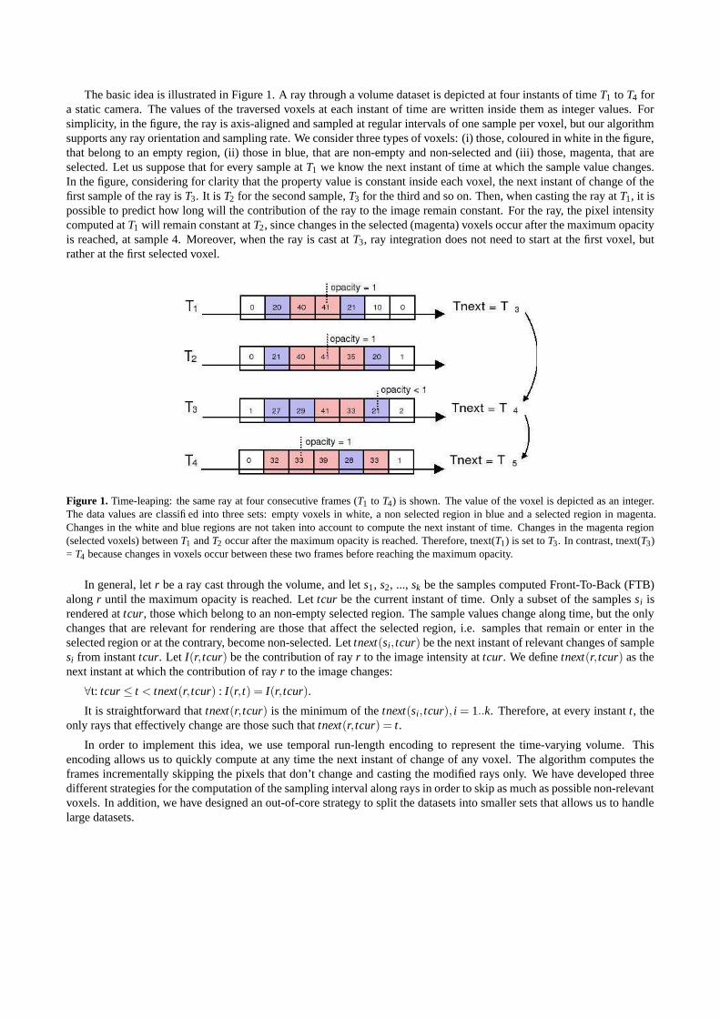
The basic idea is illustrated in Figure 1. A ray through a volume dataset is depicted at four instants of time T1 to T4 fora static camera. The values of the traversed voxels at each instant of time are written inside them as integer values. Forsimplicity, in the figure, the ray is axis-aligned and sampled at regular intervals of one sample per voxel, but our algorithmsupports any ray orientation and sampling rate. We consider three types of voxels: (i) those, coloured in white in the figure,that belong to an empty region, (ii) those in blue, that are non-empty and non-selected and (iii) those, magenta, that areselected. Let us suppose that for every sample at T1 we know the next instant of time at which the sample value changes.In the figure, considering for clarity that the property value is constant inside each voxel, the next instant of change of thefirst sample of the ray is T3. It is T2 for the second sample, T3 for the third and so on. Then, when casting the ray at T1, it ispossible to predict how long will the contribution of the ray to the image remain constant. For the ray, the pixel intensitycomputed at T1 will remain constant at T2, since changes in the selected (magenta) voxels occur after the maximum opacityis reached, at sample 4. Moreover, when the ray is cast at T3, ray integration does not need to start at the first voxel, butrather at the first selected voxel.

Figure 1. Time-leaping: the same ray at four consecutive frames (T1 to T4) is shown. The value of the voxel is depicted as an integer.The data values are classified into three sets: empty voxels in white, a non selected region in blue and a selected region in magenta.Changes in the white and blue regions are not taken into account to compute the next instant of time. Changes in the magenta region(selected voxels) between T1 and T2 occur after the maximum opacity is reached. Therefore, tnext(T1) is set to T3. In contrast, tnext(T3)= T4 because changes in voxels occur between these two frames before reaching the maximum opacity.

In general, let r be a ray cast through the volume, and let s1, s2, ..., sk be the samples computed Front-To-Back (FTB)along r until the maximum opacity is reached. Let tcur be the current instant of time. Only a subset of the samples si isrendered at tcur, those which belong to an non-empty selected region. The sample values change along time, but the onlychanges that are relevant for rendering are those that affect the selected region, i.e. samples that remain or enter in theselected region or at the contrary, become non-selected. Let tnext(si, tcur) be the next instant of relevant changes of samplesi from instant tcur. Let I(r, tcur) be the contribution of ray r to the image intensity at tcur. We define tnext(r, tcur) as thenext instant at which the contribution of ray r to the image changes:

∀t: tcur ≤ t < tnext(r, tcur) : I(r, t) = I(r, tcur).

It is straightforward that tnext(r, tcur) is the minimum of the tnext(si, tcur), i = 1..k. Therefore, at every instant t, theonly rays that effectively change are those such that tnext(r, tcur) = t.

In order to implement this idea, we use temporal run-length encoding to represent the time-varying volume. Thisencoding allows us to quickly compute at any time the next instant of change of any voxel. The algorithm computes theframes incrementally skipping the pixels that don’t change and casting the modified rays only. We have developed threedifferent strategies for the computation of the sampling interval along rays in order to skip as much as possible non-relevantvoxels. In addition, we have designed an out-of-core strategy to split the datasets into smaller sets that allows us to handlelarge datasets.

4. DATA STRUCTURES

The T-Buffer is a buffer of the same size as the rendered image, that stores for every pixel the next frame at which thecorresponding color of the image buffer is expected to change. It is computed from scratch at the first frame and updatedat successive frames only at the pixels whose value in the T-Buffer coincides with the current frame.

The Temporal Run-Length (TRL) representation of the different modalities stores for every voxel vi a sequence of codescomposed of the voxel value and the next frame at which this value changes: codes(vi)=< valuek, tnextk >,k = 1...ncodes(vi).For each modality, a different TRL is computed.

The query for the value of a voxel vi at a given frame t requires, with this structure, a search in codes(vi) of the codewhose time span contains frame t. In order to avoid this search and access directly to the searched code, we add to thestructure a pointer that is set to the first code at the beginning of the sequence and that is updated to the current code duringthe traversal. We call this pointer curcode(v). Therefore, assuming that a simple byte is sufficient to store the numberof frames of the codes and that curcode(v) is also a byte, the occupancy in bytes of the TRL structure for a modality moccupying nbm bytes per voxel of a voxel model composed of nvm voxels is:

Occup(T RLm) = ∑nvmi=1(1+ncodes(vi)∗ (nbm +1))

This occupancy can be compared to the occupancy of the regular voxel model along time:

Occup(VoxelModelm) = nvm ∗n fm ∗nbm, being n fm the number of frames of modalitity m.

We call rocc the ratio between the occupancy of the TRL and the regular voxel model:

rocc = Occup(T RL)Occup(VoxelModel) .

This ratio has a direct relationship with the temporal coherency of the voxel model, since it depends on the number ofvoxels that change. As it is obvious, the TRL cannot be constructed on static models, composed of one frame, because itwould increase their size. For instance, if the number of bytes per voxel (nbm) is 1, the TRL would triplicate the occupancyof the static model. In the worst case, for an animated model all the voxels change at every frame. Thus, the number ofcodes of every voxel is equal to the number of frames. Therefore, the ratio of occupancy is: rocc = 1 + nbm+n fm+1

nbm∗n fm, more

than 2 when the bytes per property of modality m is nbm = 1. However, this is less than the worst case of the incrementalmodel proposed by Shen and Johnsons12 which can be four times more the original one.

Nevertheless, as it will be shown in the tests, if the temporal coherency is high, this ratio can be very small (less than0.13 in the rabbit dataset). In these cases, the TRL is a compressed representation of the temporal evolution of the model.

The TRL is totally computed in a pre-process. First, the voxel model corresponding to the first frame is loaded andthe list of codes is initialized for every voxel. Next, the voxel models at the following frames are loaded one-by-one andtraversed. For every voxel, the value of the current code in the TRL is compared to the value of the loaded voxel model. Ifthe two values are equal, the frame of the current code is updated, otherwise a new code is constructed. Variations of theproperty values of empty voxels are not considered for the creation of new codes. Therefore, if a voxel has a variable value,but empty through all the sequence, it has a unique code. This pre-processing has a cost complexity CostPP = O(nvm ∗n fm).

5. PROPOSED ALGORITHMS

We have designed two algorithms based on these data structures: the simultaneous algorithm that computes all the imagesat the same time, and the frame-to-frame one, which computes incrementally one image after the other. Both algorithmsuse the TRL structure in order to predict changes in the image. They exploit temporal coherence by casting only modifiedrays. These algorithms use three different Space-Leaping (SL) strategies (SL1, SL2 and SL3) that are next described.

5.1. Simultaneous algorithm

The simultaneous algorithm constructs simultaneously all the frames of the sequence. It is not interactive, but it is usefulif the sequence can be generated in batch.

The algorithm computes for every pixel of the image-buffer its value at every frame instant. For every pixel, theassociated ray is cast at the first frame instant (T1). During this ray-casting, we compute the frame instant at which thepixel value changes (tnext(r,T1)). As described in Section 3, tnext(r,T1) is the minimum of the next instants of changeof all the samples si along the ray (tnext(si,T1)). The value of (tnext(si,T1)) is provided by the TRL. The pointer to the

current code of every sample (curcod(si)), which is initialized at the first frame instant, is updated during ray sampling.The pixel value computed at the first frame instant is copied into all the following frames until tnext(r,T1). At that frameinstant, the ray is recast and the algorithm proceeds iteratively in the same way as for the first frame instant, copying thenew pixel value to the next frames until the next change.

5.2. Frame-to-frame algorithm

This algorithm proceeds incrementally: it casts rays only through pixels that have changed in relation to the previous frame.More specifically, it starts by initializing the value tnext of all the pixels of the T-Buffer at the first frame instant. This forcesto cast all the rays of the first frame. Next, for every frame instant of the sequence, the algorithm traverses the T-Bufferand casts rays only at the pixels whose tnext value in the T-Buffer is equal to the current frame. The other pixels of thebuffer remain unchanged. During ray casting the tnext values in the T-Buffer are updated as according the tnext of the raysamples. The pointer to the current code of every voxel (curcod(v)), initialized at the first frame instant, is also updatedduring ray sampling.

5.3. Space leaping

Spatial coherency is exploited with three different space-leaping strategies whose efficiency is tested in Section 7. Thethree strategies are illustrated in Figure 2.

Ray

1

T-Buffer

Voxel Model

Temporal Bounding Box

SL2/SL3

SL1/SL3

2

SL3 n

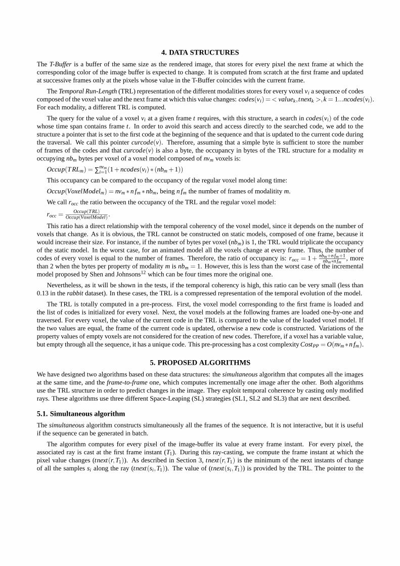
Figure 2. Space-leaping: The gray region represents the set of voxels that have a relevant value at some frame of the sequence. Thetemporal bounding box encloses this region. The intersection of the ray with the temporal bounding box defines the space-leapinginterval of SL1 strategy. The intersection of the ray with the gray region defines the sampling interval of SL2. Finally, the samplinginterval of SL3 is refined through time: at the first frame it is the same as SL1 (SL31 = SL1), at the second frame, it is the same as SL2and after successive frames it diminishes to SL3n

.

Space-Leaping 1 (SL1): temporal bounding box

We define the temporal bounding box as the bounding box of the voxels that are non-empty at some instant during thetemporal sequence During the pre-process of construction of the TRL, the temporal bounding box is also computed. Whenthe rendering starts, the sampling interval of every ray is computed as its intersection with the temporal bounding box (seethe dot box in Figure 2) . The cost of the pre-processing is still O(nvm) but increased by a comparison per voxel. However,the bounding box is valid for any camera position. This strategy provides space-leaping over empty voxels, but it doesnot skip non-selected voxels. Since the temporal bounding box is computed in the pre-process, it cannot take into accountuser’s queries.

For multimodal studies, the temporal bounding boxes are computed separately for each modality. Each ray is intersectedwith these bounding boxes. Thus, every pixel of the T-Buffer stores instead of one sampling interval, a list of samplingintervals. Each of these intervals corresponds to a combination of modalities. During the integration of an interval, onlythe TRL of its modalities are consulted.

Space-Leaping 2 (SL2): temporal ray sampling intervals

The second strategy adds a view-dependent preprocessing that computes the sampling interval of each pixel of theT-Buffer as the position of the first and the last samples along the ray that have a relevant value at some frame. Thispreprocessing consists of a traversal of all the samples codes for every ray. It should be re-done for any change in theviewpoint, but precisely because of that, it can skip not only empty voxels but also non-selected ones. This strategy has ahigher pre-processing cost but it provides a more efficient space-leaping for the successive frames. In multimodal datasets,these intervals are computed separately for each modality and processed in the same way as SL1 strategy.

Space-Leaping 3 (SL3): run-time adjustment of ray sampling intervals

The third space-leaping strategy computes ray sampling intervals as in the SL2 strategy, but instead of a per-viewpre-process, it does it during the rendering samples traversal. Whenever a non-relevant voxel is sampled along a ray, itsnext relevant value is searched. If the voxel is never relevant during the sequence, its current code curcode(v) is set tothe last frame, independently from its possible variation through time. Then, it is not processed in the successive frames.The ray integration interval is defined by the first and last non-relevant voxels encountered along the ray in the previouscasting of that ray. This interval is refined at each frame. By opposite to SL2, this strategy does not require a costly per-raypre-process. Since the intervals are successively refined, the cost per frame tends to diminish. However, at the first frames,this cost can be greater than in the SL2 strategy. This is illustrated in Figure 2: the sampling interval SL3 at the first instant(SL31) is larger than SL2, but it is smaller than SL2 at the n− th instant (SL3n). This method adapts to multimodality as theprevious two ones.

6. OUT-OF-CORE RENDERING

When the datasets are larger than the main memory, input/output communication becomes the bottleneck of rendering33

. In the context of our investigation, this is serious problem since our datasets are multimodal and vary in time. Eventhough the Run-Length Encoding compresses efficiently the model in time, the size of the models and the number of bytesper voxel even for a one-frame dataset may be larger than the memory. Subdividing the volume can solve this problem.29

In order to overcome the I/O bottleneck while keeping the benefits of the proposed method, we subdivide the modelsinto blocks both in space and time. First, long sequences are subdivided into smaller time spans. Next, the models aresubdivided following the BON (Branch-On-Need) octree strategy30 . The leaf nodes are the voxel model blocks. Thecriterion to divide a node of the octree is its memory occupancy. Thus, the more temporal variation of the voxels into anode, the more subdivided it is. The octree hierarchy is used only for the creation. Only leaf nodes (blocks) are stored indisk. The files are labelled according to the position of the blocks into the octree in order to allow us a sorted traversal.Therefore, during rendering, the leaf nodes are processed orderly: read from disk and rendered. The resulting subimagesare composed FTB. For the simultaneous algorithm, each block of a time span is stored in one file and read only once.For the frame-to-frame algorithm, the blocks must be read from disk at each frame. Therefore, they are stored into variousfiles, such that only the current codes of the voxels are read from disk at a given frame. Besides the capacity of handlinglarge datasets, this strategy brings the advantage of improving time and space leaping: if the pixels of the subimage of ablock in the main buffer have already reached the maximum opacity at a given frame, the block is skipped. Moreover, theblock is rendered only if at least one of the pixels of its subimage changes at that frame.

7. TESTS

7.1. Description

We have performed tests on four different datasets:

• two phantom datasets that help us to better understand the behaviour of the algorithms,

• a real multimodal dataset of the brain composed of a dynamic SPECT and a static MR.

• a real dataset corresponding to the temporal evolution of a biomaterial implant in a rabbit femur at two differentspatial resolutions (SRabbit and LRabbit).

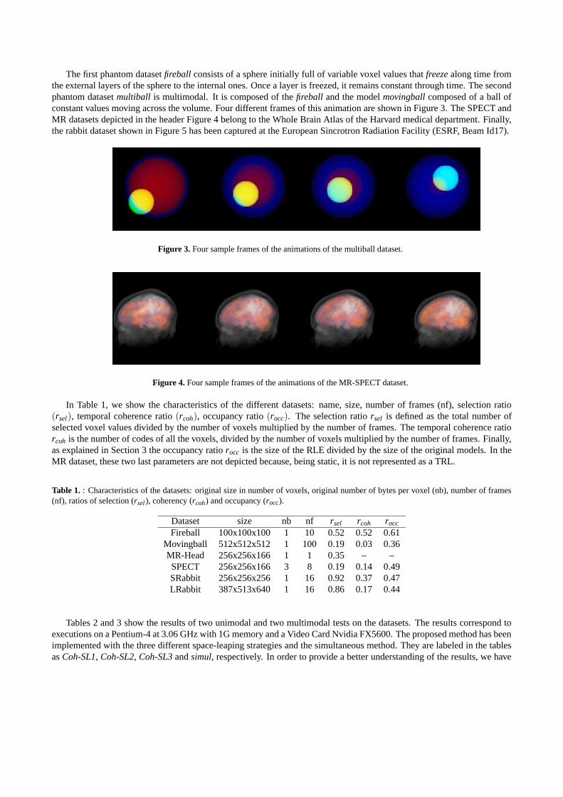
The first phantom dataset fireball consists of a sphere initially full of variable voxel values that freeze along time fromthe external layers of the sphere to the internal ones. Once a layer is freezed, it remains constant through time. The secondphantom dataset multiball is multimodal. It is composed of the fireball and the model movingball composed of a ball ofconstant values moving across the volume. Four different frames of this animation are shown in Figure 3. The SPECT andMR datasets depicted in the header Figure 4 belong to the Whole Brain Atlas of the Harvard medical department. Finally,the rabbit dataset shown in Figure 5 has been captured at the European Sincrotron Radiation Facility (ESRF, Beam Id17).

Figure 3. Four sample frames of the animations of the multiball dataset.

Figure 4. Four sample frames of the animations of the MR-SPECT dataset.

In Table 1, we show the characteristics of the different datasets: name, size, number of frames (nf), selection ratio(rsel), temporal coherence ratio (rcoh), occupancy ratio (rocc). The selection ratio rsel is defined as the total number ofselected voxel values divided by the number of voxels multiplied by the number of frames. The temporal coherence ratiorcoh is the number of codes of all the voxels, divided by the number of voxels multiplied by the number of frames. Finally,as explained in Section 3 the occupancy ratio rocc is the size of the RLE divided by the size of the original models. In theMR dataset, these two last parameters are not depicted because, being static, it is not represented as a TRL.

Table 1. : Characteristics of the datasets: original size in number of voxels, original number of bytes per voxel (nb), number of frames(nf), ratios of selection (rsel), coherency (rcoh) and occupancy (rocc).

Dataset size nb nf rsel rcoh rocc

Fireball 100x100x100 1 10 0.52 0.52 0.61Movingball 512x512x512 1 100 0.19 0.03 0.36MR-Head 256x256x166 1 1 0.35 – –SPECT 256x256x166 3 8 0.19 0.14 0.49SRabbit 256x256x256 1 16 0.92 0.37 0.47LRabbit 387x513x640 1 16 0.86 0.17 0.44

Tables 2 and 3 show the results of two unimodal and two multimodal tests on the datasets. The results correspond toexecutions on a Pentium-4 at 3.06 GHz with 1G memory and a Video Card Nvidia FX5600. The proposed method has beenimplemented with the three different space-leaping strategies and the simultaneous method. They are labeled in the tablesas Coh-SL1, Coh-SL2, Coh-SL3 and simul, respectively. In order to provide a better understanding of the results, we have

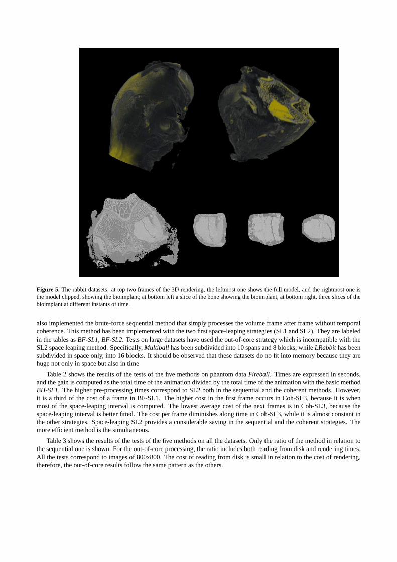
Figure 5. The rabbit datasets: at top two frames of the 3D rendering, the leftmost one shows the full model, and the rightmost one isthe model clipped, showing the bioimplant; at bottom left a slice of the bone showing the bioimplant, at bottom right, three slices of thebioimplant at different instants of time.

also implemented the brute-force sequential method that simply processes the volume frame after frame without temporalcoherence. This method has been implemented with the two first space-leaping strategies (SL1 and SL2). They are labeledin the tables as BF-SL1, BF-SL2. Tests on large datasets have used the out-of-core strategy which is incompatible with theSL2 space leaping method. Specifically, Multiball has been subdivided into 10 spans and 8 blocks, while LRabbit has beensubdivided in space only, into 16 blocks. It should be observed that these datasets do no fit into memory because they arehuge not only in space but also in time

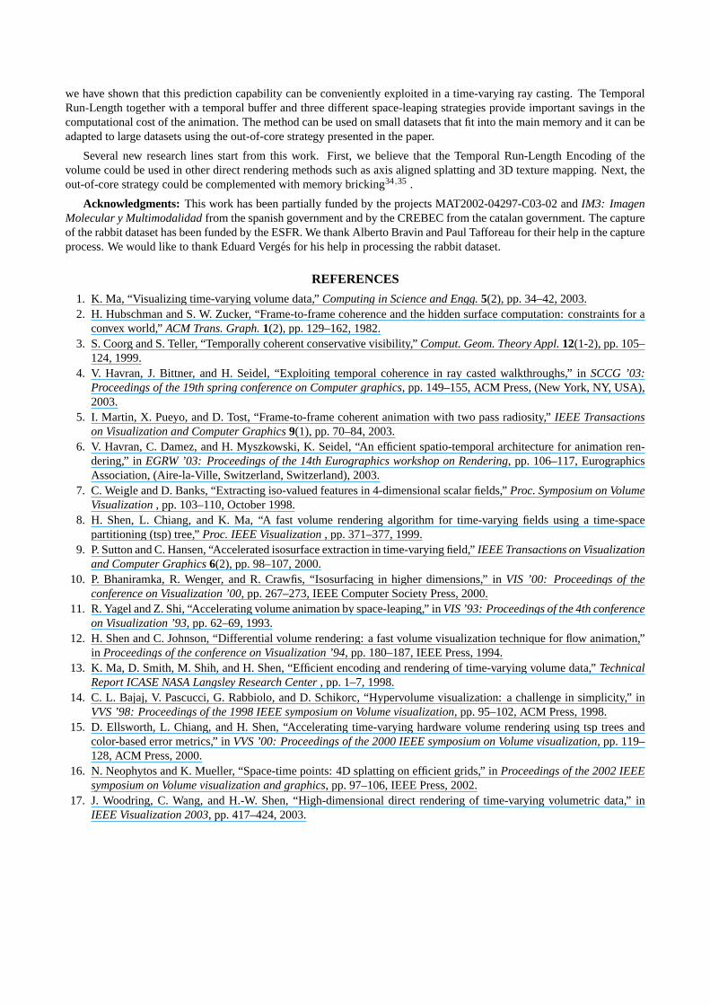
Table 2 shows the results of the tests of the five methods on phantom data Fireball. Times are expressed in seconds,and the gain is computed as the total time of the animation divided by the total time of the animation with the basic methodBH-SL1. The higher pre-processing times correspond to SL2 both in the sequential and the coherent methods. However,it is a third of the cost of a frame in BF-SL1. The higher cost in the first frame occurs in Coh-SL3, because it is whenmost of the space-leaping interval is computed. The lowest average cost of the next frames is in Coh-SL3, because thespace-leaping interval is better fitted. The cost per frame diminishes along time in Coh-SL3, while it is almost constant inthe other strategies. Space-leaping SL2 provides a considerable saving in the sequential and the coherent strategies. Themore efficient method is the simultaneous.

Table 3 shows the results of the tests of the five methods on all the datasets. Only the ratio of the method in relation tothe sequential one is shown. For the out-of-core processing, the ratio includes both reading from disk and rendering times.All the tests correspond to images of 800x800. The cost of reading from disk is small in relation to the cost of rendering,therefore, the out-of-core results follow the same pattern as the others.

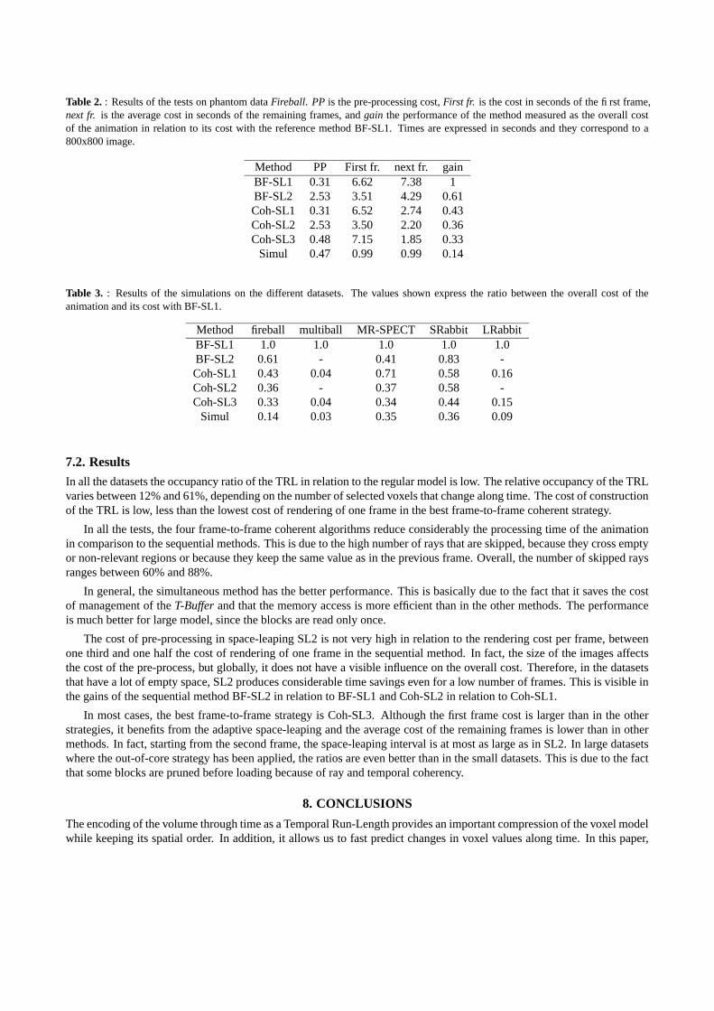
Table 2. : Results of the tests on phantom data Fireball. PP is the pre-processing cost, First fr. is the cost in seconds of the first frame,next fr. is the average cost in seconds of the remaining frames, and gain the performance of the method measured as the overall costof the animation in relation to its cost with the reference method BF-SL1. Times are expressed in seconds and they correspond to a800x800 image.

Method PP First fr. next fr. gainBF-SL1 0.31 6.62 7.38 1BF-SL2 2.53 3.51 4.29 0.61Coh-SL1 0.31 6.52 2.74 0.43Coh-SL2 2.53 3.50 2.20 0.36Coh-SL3 0.48 7.15 1.85 0.33

Simul 0.47 0.99 0.99 0.14

Table 3. : Results of the simulations on the different datasets. The values shown express the ratio between the overall cost of theanimation and its cost with BF-SL1.

Method fireball multiball MR-SPECT SRabbit LRabbitBF-SL1 1.0 1.0 1.0 1.0 1.0BF-SL2 0.61 - 0.41 0.83 -Coh-SL1 0.43 0.04 0.71 0.58 0.16Coh-SL2 0.36 - 0.37 0.58 -Coh-SL3 0.33 0.04 0.34 0.44 0.15

Simul 0.14 0.03 0.35 0.36 0.09

7.2. Results

In all the datasets the occupancy ratio of the TRL in relation to the regular model is low. The relative occupancy of the TRLvaries between 12% and 61%, depending on the number of selected voxels that change along time. The cost of constructionof the TRL is low, less than the lowest cost of rendering of one frame in the best frame-to-frame coherent strategy.

In all the tests, the four frame-to-frame coherent algorithms reduce considerably the processing time of the animationin comparison to the sequential methods. This is due to the high number of rays that are skipped, because they cross emptyor non-relevant regions or because they keep the same value as in the previous frame. Overall, the number of skipped raysranges between 60% and 88%.

In general, the simultaneous method has the better performance. This is basically due to the fact that it saves the costof management of the T-Buffer and that the memory access is more efficient than in the other methods. The performanceis much better for large model, since the blocks are read only once.

The cost of pre-processing in space-leaping SL2 is not very high in relation to the rendering cost per frame, betweenone third and one half the cost of rendering of one frame in the sequential method. In fact, the size of the images affectsthe cost of the pre-process, but globally, it does not have a visible influence on the overall cost. Therefore, in the datasetsthat have a lot of empty space, SL2 produces considerable time savings even for a low number of frames. This is visible inthe gains of the sequential method BF-SL2 in relation to BF-SL1 and Coh-SL2 in relation to Coh-SL1.

In most cases, the best frame-to-frame strategy is Coh-SL3. Although the first frame cost is larger than in the otherstrategies, it benefits from the adaptive space-leaping and the average cost of the remaining frames is lower than in othermethods. In fact, starting from the second frame, the space-leaping interval is at most as large as in SL2. In large datasetswhere the out-of-core strategy has been applied, the ratios are even better than in the small datasets. This is due to the factthat some blocks are pruned before loading because of ray and temporal coherency.

8. CONCLUSIONS

The encoding of the volume through time as a Temporal Run-Length provides an important compression of the voxel modelwhile keeping its spatial order. In addition, it allows us to fast predict changes in voxel values along time. In this paper,

we have shown that this prediction capability can be conveniently exploited in a time-varying ray casting. The TemporalRun-Length together with a temporal buffer and three different space-leaping strategies provide important savings in thecomputational cost of the animation. The method can be used on small datasets that fit into the main memory and it can beadapted to large datasets using the out-of-core strategy presented in the paper.

Several new research lines start from this work. First, we believe that the Temporal Run-Length Encoding of thevolume could be used in other direct rendering methods such as axis aligned splatting and 3D texture mapping. Next, theout-of-core strategy could be complemented with memory bricking34,35 .

Acknowledgments: This work has been partially funded by the projects MAT2002-04297-C03-02 and IM3: ImagenMolecular y Multimodalidad from the spanish government and by the CREBEC from the catalan government. The captureof the rabbit dataset has been funded by the ESFR. We thank Alberto Bravin and Paul Tafforeau for their help in the captureprocess. We would like to thank Eduard Verges for his help in processing the rabbit dataset.

REFERENCES

1. K. Ma, “Visualizing time-varying volume data,” Computing in Science and Engg. 5(2), pp. 34–42, 2003.2. H. Hubschman and S. W. Zucker, “Frame-to-frame coherence and the hidden surface computation: constraints for a

convex world,” ACM Trans. Graph. 1(2), pp. 129–162, 1982.3. S. Coorg and S. Teller, “Temporally coherent conservative visibility,” Comput. Geom. Theory Appl. 12(1-2), pp. 105–

124, 1999.4. V. Havran, J. Bittner, and H. Seidel, “Exploiting temporal coherence in ray casted walkthroughs,” in SCCG ’03:

Proceedings of the 19th spring conference on Computer graphics, pp. 149–155, ACM Press, (New York, NY, USA),2003.

5. I. Martin, X. Pueyo, and D. Tost, “Frame-to-frame coherent animation with two pass radiosity,” IEEE Transactionson Visualization and Computer Graphics 9(1), pp. 70–84, 2003.

6. V. Havran, C. Damez, and H. Myszkowski, K. Seidel, “An efficient spatio-temporal architecture for animation ren-dering,” in EGRW ’03: Proceedings of the 14th Eurographics workshop on Rendering, pp. 106–117, EurographicsAssociation, (Aire-la-Ville, Switzerland, Switzerland), 2003.

7. C. Weigle and D. Banks, “Extracting iso-valued features in 4-dimensional scalar fields,” Proc. Symposium on VolumeVisualization , pp. 103–110, October 1998.

8. H. Shen, L. Chiang, and K. Ma, “A fast volume rendering algorithm for time-varying fields using a time-spacepartitioning (tsp) tree,” Proc. IEEE Visualization , pp. 371–377, 1999.

9. P. Sutton and C. Hansen, “Accelerated isosurface extraction in time-varying field,” IEEE Transactions on Visualizationand Computer Graphics 6(2), pp. 98–107, 2000.

10. P. Bhaniramka, R. Wenger, and R. Crawfis, “Isosurfacing in higher dimensions,” in VIS ’00: Proceedings of theconference on Visualization ’00, pp. 267–273, IEEE Computer Society Press, 2000.

11. R. Yagel and Z. Shi, “Accelerating volume animation by space-leaping,” in VIS ’93: Proceedings of the 4th conferenceon Visualization ’93, pp. 62–69, 1993.

12. H. Shen and C. Johnson, “Differential volume rendering: a fast volume visualization technique for flow animation,”in Proceedings of the conference on Visualization ’94, pp. 180–187, IEEE Press, 1994.

13. K. Ma, D. Smith, M. Shih, and H. Shen, “Efficient encoding and rendering of time-varying volume data,” TechnicalReport ICASE NASA Langsley Research Center , pp. 1–7, 1998.

14. C. L. Bajaj, V. Pascucci, G. Rabbiolo, and D. Schikorc, “Hypervolume visualization: a challenge in simplicity,” inVVS ’98: Proceedings of the 1998 IEEE symposium on Volume visualization, pp. 95–102, ACM Press, 1998.

15. D. Ellsworth, L. Chiang, and H. Shen, “Accelerating time-varying hardware volume rendering using tsp trees andcolor-based error metrics,” in VVS ’00: Proceedings of the 2000 IEEE symposium on Volume visualization, pp. 119–128, ACM Press, 2000.

16. N. Neophytos and K. Mueller, “Space-time points: 4D splatting on efficient grids,” in Proceedings of the 2002 IEEEsymposium on Volume visualization and graphics, pp. 97–106, IEEE Press, 2002.

17. J. Woodring, C. Wang, and H.-W. Shen, “High-dimensional direct rendering of time-varying volumetric data,” inIEEE Visualization 2003, pp. 417–424, 2003.

18. K. Anagnostou, T. Atherton, and A. Waterfall, “4D volume rendering with the Shear-Warp factorization,” Proc. Symp.Volume Visualization and Graphics’00 , pp. 129–137, 2000.

19. M. Wan, A. Sadiq, and A. Kaufman, “Fast and reliable space leaping for interactive volume rendering,” in VIS’02:Proceedings of the conference on Visualization ’02, IEEE Computer Society, 2002.

20. S. Liao, Y. Chung, and J. Lai, “A two-level differential volume rendering method for time-varying volume data,” TheJournal of Winter School in Computer Graphics 10(1), pp. 287–316, 2002.

21. H.-W. Shen, “Isosurface extraction in time-varying fields using a temporal hierarchical index tree,” in Proceedings ofthe conference on Visualization ’98, pp. 159–166, IEEE Computer Society Press, 1998.

22. P. Lacroute and M. Levoy, “Fast volume rendering using a Shear-Warp factorization of the viewing transformation,”ACM Computer Graphics 28, pp. 451–458, July 1994.

23. K. Ma and D. Camp, “High performance visualization of time-varying volume data over a wide-area network status,”in Supercomputing ’00: Proceedings of the 2000 ACM/IEEE conference on Supercomputing (CDROM), p. 29, IEEEComputer Society, 2000.

24. R. Westermann, “Compression domain rendering of time-resolved volume data,” in VIS ’95: Proceedings of the 6thconference on Visualization ’95, p. 168, IEEE Computer Society, 1995.

25. S. Guthe and W. Strasser, “Real-time decompression and visualization of animated volume data,” in Proceedings ofthe conference on Visualization 2001, pp. 349–356, IEEE Press, 2001.

26. N.Gagvani and D. Silver, “Animating volumetric models,” Graph. Models 63(6), pp. 443–458, 2001.27. E. Lum, K. Ma, and J. Clyne, “A hardware-assisted scalable solution for interactive volume rendering of time-varying

data,” IEEE Transactions on Visualization and Computer Graphics 8(3), pp. 286–301, 2002.28. M. Martin, E. Reinhard, P. Shirley, S. Parker, and W. Thompson, “Temporally coherent interactive ray tracing,”

Journal of Graphics Tools 1(72), pp. 41–48, 2003.29. E. Reinhard, C.Hansen, and S.Parker, “Interactive ray-tracing of time varying data,” in Eurographics Workshop on

Parallel Graphics and Visualisation 2002, pp. 77–82, Eurographics, 2002.30. J. Wilhems and A. V. Gelder, “Multidimensional trees for controlled volume rendering and compression,” Proc ACM

Symposium on Volume Visualization 11, pp. 27–34, October 1994.31. J. Woodring and H. Shen, “Chronovolumes: a direct rendering technique for visualizing time-varying data,” in VG

’03: Proceedings of the 2003 Eurographics/IEEE TVCG Workshop on Volume graphics, pp. 27–34, ACM Press,2003.

32. M. Ferre, A. Puig, and D. Tost, “A fast hierachical traversal strategy for multimodal visualization,” Visualization andData Analysis 2004 , pp. 1–8, 2004.

33. R. Farias and C. T. Silva, “Out-of-core rendering of large, unstructured grids,” IEEE Comput. Graph. Appl. 21(4),pp. 42–50, 2001.

34. A. S. G. Sakas, M. Grimm, “Optimized maximum intensity projection (mip),” 6th Eurographics Workshop on Ren-dering , pp. 81–93, June 1995.

35. S. Parker, M. Parker, Y. Livnat, P. Sloan, C. Hansen, and P. Shirley, “Interactive ray tracing for volume visualization,”IEEE Transactions on Visualization and Computer Graphics 5(3), pp. 238–250, 1999.