
Development of Java Acoustic Model Interface (JAMI)
96
Development of Java Acoustic Model Interface (JAMI) Dr. Gary Brooke Dr. Dave Thomson Brooke Numerical Services Prepared By: Brooke Numerical Services 3440 Seaton Street, Victoria, BC Canada V8Z 3V9 Contract Project Manager: Dr. Gary Brooke, (250) 475-3440 PWGSC Contract number: W7707-125424/001/HAL CSA: Dr. Nicos Pelavas, (902) 426-3100 The scientific or technical validity of this Contract Report is entirely the responsibility of the Contractor and the contents do not necessarily have the approval or endorsement of Defence R&D Canada. Defence R&D Canada – Atlantic Contract Report DRDC Atlantic CR 2012-105 April 2014
-
Upload
khangminh22 -
Category
Documents
-
view
2 -
download
0
Transcript of Development of Java Acoustic Model Interface (JAMI)
Development of Java Acoustic Model Interface (JAMI) Dr. Gary Brooke Dr. Dave Thomson Brooke Numerical Services Prepared By: Brooke Numerical Services 3440 Seaton Street, Victoria, BC Canada V8Z 3V9 Contract Project Manager: Dr. Gary Brooke, (250) 475-3440 PWGSC Contract number: W7707-125424/001/HAL CSA: Dr. Nicos Pelavas, (902) 426-3100
The scientific or technical validity of this Contract Report is entirely the responsibility of the Contractor and the contents do not necessarily have the approval or endorsement of Defence R&D Canada.
Defence R&D Canada – Atlantic Contract Report
DRDC Atlantic CR 2012-105
April 2014

This document contains Crown-owned proprietary information that may be subject to a license agreement.
Unauthorized use is expressly prohibited.
Direct inquiries to the Director General, Defence Research & Development Canada – Atlantic.
© Her Majesty the Queen in Right of Canada, as represented by the Minister of National Defence, 2014
© Sa Majesté la Reine (en droit du Canada), telle que représentée par le ministre de la Défense nationale,
2014

DRDC Atlantic CR 2012-105 i
Abstract …
The Low Complexity Access Network (LCAN) project has a requirement for propagation studies
that involve both acoustic and electromagnetic signals. Specifically, acoustic propagation effects
associated with communication signals up to 1 MHz are to be modelled. The electromagnetic
propagation modelling is to be carried out using the ‘so-called’ Weaver model. Also, there is a
requirement for incorporation of the latest improvements in the DRDC Clutter Model into the
Java Acoustic Model Interface (JAMI) Client-Server framework.
This contract work, in part, has been designed to integrate DRDC Atlantic’s LCAN requirements
with those associated with the Clutter model through integration of both into the JAMI
application.
Résumé ….
Le projet de réseau à accès simplifié (LCAN) a besoin d’études de propagation portant sur les
signaux acoustiques et les signaux électromagnétiques. Plus particulièrement, il faut modéliser les
effets de la propagation acoustique associés aux signaux de communication jusqu’à 1 MHz. La
modélisation de la propagation électromagnétique doit être réalisée à l’aide de ce qu’on appelle le
modèle Weaver. De plus, il faut intégrer les dernières améliorations du modèle de fouillis de
RDDC au cadre client-serveur de l’interface du modèle acoustique en Java (JAMI).
Les travaux du présent contrat visent en partie à intégrer les besoins du LCAN de
RDDC Atlantique à ceux associés au modèle de fouillis grâce à l’intégration de ces deux modèles
à l’application JAMI.

ii DRDC Atlantic CR 2012-105
This page intentionally left blank.
DRDC Atlantic CR 2012-105 iii
Executive summary
Development of Java Acoustic Model Interface (JAMI)
Gary Brooke, Dave Thompson; DRDC Atlantic CR 2012-105; Defence R&D Canada - Atlantic; March 2012.
Introduction: The Java Acoustic Model Interface (JAMI) is a Brooke Numerical Services (BNS)
initiative that is under development with the intent of providing a framework for a Client-Server
approach to performance prediction in which the problem configuration and display reside on a
thin Client and the models and other computational engines are centralized on a more powerful
backend computer or Server.
In JAMI, the Client is programmed exclusively in Java whereas the backend consists of a
combination of C and Fortran code designed to take advantage of as many existing and publicly
available codes as possible. JAMI is designed for, and partially supports, access to SAFARI [4],
PECan [5], POPP [6], and BellHop [7] for simple propagation studies and to some aspects of the
DRDC Clutter model [8] for reverberation and target predictions. A Windows-based, C-interface
layer has been written that provides seamless interaction of all three languages. This same
interface also provides the links to public domain environmental databases for bathymetry (Gebco
[9]), sound speed via temperature and salinity (World Oceanographic Atlas, WOA [10]), and
bottom composition (Deck41 [11]).
JAMI represents an extension of the concepts and methodology underlying the JACI application
[12] which was developed under contract for DRDC.
Results: A functional Java-C-Fortran coded interface has been developed that links a Graphical
User Interface (data input and data display) to acoustic models (including the DRDC clutter
model) through a C-layer interface. The C-coded interface also is designed to provide access to
several public-domain environmental databases and in conjunction with JAMI yields a standalone
operational capability. In addition, the JAMI-C-Fortran combination has been extended to include
an electromagnetic component by incorporating the DRDC Weaver model.
Significance: The developments described above (and to follow) has been carried out with a view
to compatibility with the STB application supporting the notion that the latter can be transitioned
from a conceptual framework to a more operational entity that includes interaction with external
applications as represented by the DRDC Acoustic Clutter Library. Moreover, the standalone
configuration of the JAMI application, the environmental databases, and the ACL gives the
DRDC modellers (acoustic and electromagnetic) increased flexibility in modelling and display of
real-time data.
Future plans: Implementation of the set of recommendations will lead to a more robust,
production-grade integration of a reverberation and clutter modeling capability with the STB and
in the standalone JAMI application.

iv DRDC Atlantic CR 2012-105
Sommaire ..
Development of Java Acoustic Model Interface (JAMI)
Gary Brooke, Dave Thompson; DRDC Atlantic CR 2012-105; R & D pour la défense Canada – Atlantique; mars 2012.
Introduction : L’interface du modèle acoustique en Java (JAMI) est une initiative en cours
d’élaboration de Brooke Numerical Services (BNS). Elle vise à fournir un cadre à une approche
client-serveur pour la prédiction de la performance; approche pour laquelle la configuration et
l’affichage des problèmes reposent sur un client léger, et les modèles et d’autres moteurs de
calcul sont centralisés sur un ordinateur ou un serveur à application dorsale plus puissante.
Dans JAMI, le client est programmé exclusivement en Java, tandis que l’application dorsale
comprend une combinaison de code C et Fortran visant à exploiter le plus possible de codes
existants et accessibles au public. JAMI est conçu pour accéder, et appuyer partiellement l’accès,
à SAFARI [4], PECan [5], POPP [6] et BellHop [7] pour les études simples sur la propagation,
ainsi qu’à certains aspects du modèle de fouillis de RDDC [8] pour les prédictions de
réverbération et de cibles. Une couche d’interface en C pour Windows a été écrite pour fournir
une interaction continue aux trois langages. Cette même interface fournit aussi les liens aux bases
de données environnementales du domaine public pour la bathymétrie (Gebco [9]), la vitesse du
son en fonction de la température et de la salinité (World Oceanographic Atlas, WOA [10]) et la
composition du fond (Deck41 [11]).
JAMI représente un prolongement des concepts et de la méthodologie sous-jacents à l’application
JACI [12] développée dans le cadre d’un contrat pour RDDC.
Résultats : Une interface fonctionnelle codée en Java-C-Fortran a été développée pour lier une
interface utilisateur graphique (entrée de données et affichage de données) aux modèles
acoustiques (y compris le modèle de fouillis de RDDC) au moyen d’une interface de couche en C.
L’interface codée en C permet aussi d’accéder à plusieurs bases de données environnementales du
domaine public, et, en combinaison avec JAMI, elle donne une capacité opérationnelle autonome.
De plus, la combinaison JAMI-C-Fortran a été étendue pour inclure une composante
électromagnétique en intégrant le modèle Weaver de RDDC.
Portée : Les développements susmentionnés (et à venir) ont été réalisés en vue d’assurer la
compatibilité avec l’application du système de banc d’essai (STB) à l’appui de la notion selon
laquelle cette application peut être transférée d’un cadre conceptuel à une entité plus
opérationnelle comprenant une interaction avec des applications externes, représentées par la
bibliothèque de fouillis acoustiques (Acoustic Clutter Library [ACL]) de RDDC. Par ailleurs, la
configuration autonome de l’application JAMI, les bases de données environnementales et l’ACL
donnent plus de souplesse aux modélisateurs (acoustique et électromagnétique) de RDDC pour la
modélisation et l’affichage des données en temps réel.
Recherches futures : La mise en place de la série de recommandations permettra une intégration
plus solide et exploitable d’une capacité de modélisation de la réverbération et du fouillis au STB
et à une application JAMI autonome.
DRDC Atlantic CR 2012-105 v
Table of contents
Abstract … ....................................................................................................................................... i
Résumé …. ....................................................................................................................................... i
Executive summary ....................................................................................................................... iii
Sommaire .. ..................................................................................................................................... iv
Table of contents ............................................................................................................................ v
List of figures ............................................................................................................................... vii
List of tables .................................................................................................................................. ix
Acknowledgements ........................................................................................................................ x
1 Overview ................................................................................................................................... 1
2 Background and Objectives ...................................................................................................... 2
3 Summary of Project Results ..................................................................................................... 4
3.1 Tasking .......................................................................................................................... 4
3.2 Chronology of Effort ..................................................................................................... 5
3.3 Deliverables ................................................................................................................... 6
3.3.1 Meetings .......................................................................................................... 6
3.3.2 Other Communications ................................................................................... 6
3.3.3 Software, Databases and Documentation ........................................................ 6
3.3.4 Reports ............................................................................................................ 6
3.4 Functional Results ......................................................................................................... 7
3.4.1 Compilers ........................................................................................................ 7
3.4.2 The jAMI GUI (Client Application) ............................................................... 7
3.4.3 The Clutter Model (Tasks 1 – 2 ) .................................................................. 14
3.4.4 The Acoustic Propagation Models (Tasks 4 - 5) ........................................... 22
3.4.4.1 SAFARI ...................................................................................... 23
3.4.4.2 PECan ......................................................................................... 25
3.4.4.3 POPP ........................................................................................... 28
3.4.4.4 Bellhop ....................................................................................... 30
3.4.5 The Acoustic Propagation Model Displays ................................................... 31
3.4.6 The Weaver Model (Task 6) ......................................................................... 34
3.4.7 Interfacing to the Environmental Databases ................................................. 49
4 Conclusions and Proposed Future Work ................................................................................ 50
4.1 Conclusions ................................................................................................................. 50
4.2 Proposed Future Work ................................................................................................. 51
References .. .................................................................................................................................. 53
Annex A .. Supplementary Information ......................................................................................... 55
A.1 Weaver Model Routines .............................................................................................. 55
vi DRDC Atlantic CR 2012-105
A.2 Bellhop Inputs ............................................................................................................. 63
A.3 SAFARI - BELLHOP PROPAGATION STUDY ...................................................... 69
Annex B ... Environmental Databases ............................................................................................ 73
B.1 Introduction ................................................................................................................. 73
B.2 Bathymetry .................................................................................................................. 73
B.3 Sound Speed ................................................................................................................ 73
B.4 Bottom Data................................................................................................................. 74
Annex C ... Software Installation .................................................................................................... 75
C.1 Introduction ................................................................................................................. 75
C.2 jAMI Client ................................................................................................................. 75
C.3 NetBeans Project Files ................................................................................................ 75
C.3.1 Operational Distribution Kit ......................................................................... 77
C.4 Server and Databases ................................................................................................... 78
C.5 Networking and Connectivity ...................................................................................... 78
List of symbols/abbreviations/acronyms/initialisms .................................................................... 81
DRDC Atlantic CR 2012-105 vii
List of figures
Figure 1: Selecting the host computer for the Server. ..................................................................... 8
Figure 2: jAMI initiation of the Server. ........................................................................................... 9
Figure 3: Server initiated – waiting for input from the Client (jAMI). ........................................... 9
Figure 4: The jAMI application main screen. ................................................................................ 10
Figure 5: Running the model and displaying the results. .............................................................. 11
Figure 6: Server terminal screen output (computation complete). ................................................ 12
Figure 7: Choice of displays. ......................................................................................................... 12
Figure 8: Display of Beam reverberation versus beam angle and time. ........................................ 13
Figure 9: Display of Beam reverberation versus range and azimuth (clutter map display). ......... 13
Figure 10: Configuration of the Clutter Model ............................................................................. 14
Figure 11: Configuration of the Clutter Model. ............................................................................ 15
Figure 12: The jAMI Environmental Parameter Specification and Display screen. ..................... 16
Figure 13: The jAMI Rx Sensor Specification screen. .................................................................. 17
Figure 14: The jAMI Tx Sensor Specification screen. .................................................................. 18
Figure 15: The jAMI POPP Parameter Specification screen......................................................... 19
Figure 16: The jAMI Target Specification screen. ........................................................................ 20
Figure 17: The jAMI Clutter Target Specification screen. ............................................................ 20
Figure 18: The jAMI Polar plot selection. ..................................................................................... 21
Figure 19: The jAMI Polar plot selection. ..................................................................................... 21
Figure 20: Standard JAMI List Box Parameter entry controls. ..................................................... 22
Figure 21: Standard jAMI input parameter button controls. ......................................................... 23
Figure 22: The jAMI: SAFARI FIP Parameter Specification screen. ........................................... 24
Figure 23: The SAFARI Options Selection. .................................................................................. 24
Figure 24: The special JAMI SAFARI Options. ........................................................................... 25
Figure 25: A SAFARI input file. ................................................................................................... 25
Figure 26: The jAMI: PECan Parameter Specification screen. ..................................................... 26
Figure 27: A typical pe.dat input file. ............................................................................................ 28
Figure 28: The jAMI: POPP Parameter Specification screen. ...................................................... 29
Figure 29: The POPP n3a.inp file format. ..................................................................................... 29
Figure 30: The jAMI: Bellhop Parameter Specification screen. ................................................... 30
viii DRDC Atlantic CR 2012-105
Figure 31: The Bellhop n3a.env file format. ................................................................................. 31
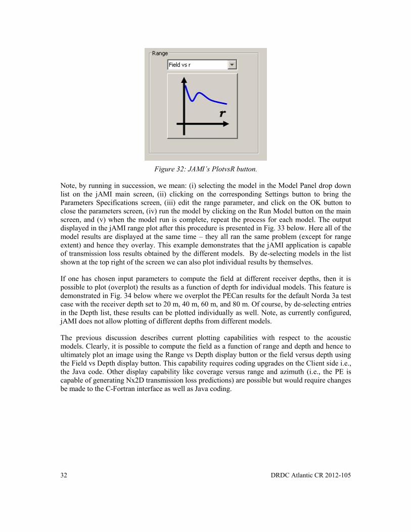
Figure 32: JAMI’s PlotvsR button. ............................................................................................... 32
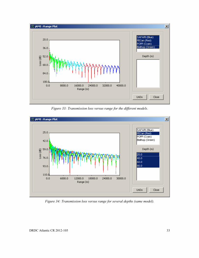
Figure 33: Transmission loss versus range for the different models. ............................................ 33
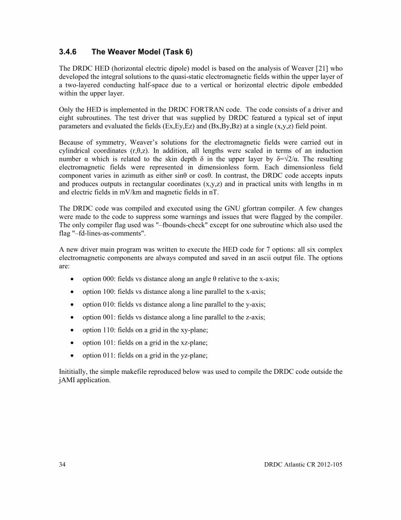
Figure 34: Transmission loss versus range for several depths (same model). ............................... 33
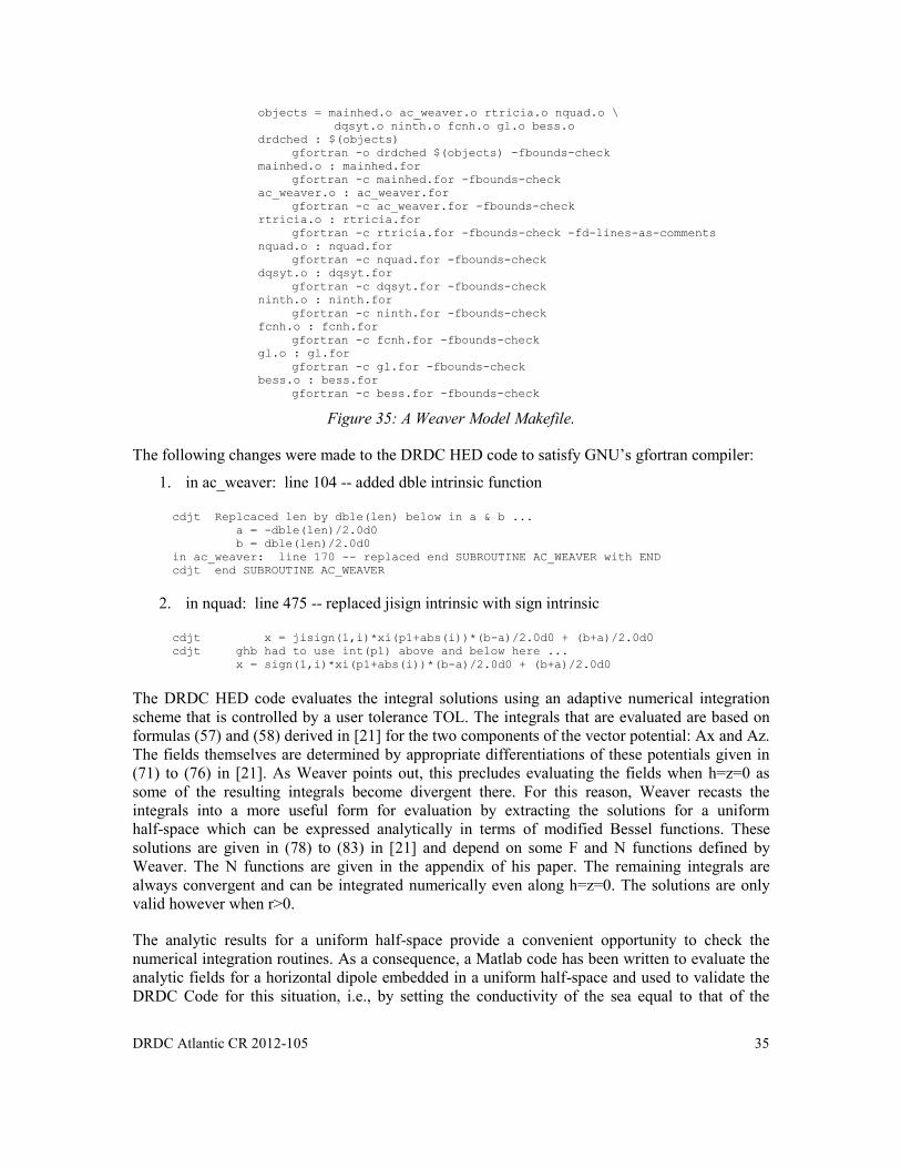
Figure 35: A Weaver Model Makefile. ......................................................................................... 35
Figure 36: Ss Main screen setting for the Weaver Model. ............................................................ 38
Figure 37: Ss Input parameter screen for the Weaver Model. ....................................................... 39
Figure 38: Ss Input parameter screen for the Weaver Model. ....................................................... 40
Figure 39: Test Input File for the Weaver Model. code 100: hed100.dat. ................................... 41
Figure 40: Running and displaying Weaver model data. .............................................................. 42
Figure 41: The Ex field component. .............................................................................................. 43
Figure 42: The Ey field component. .............................................................................................. 44
Figure 43: The Ez field component. .............................................................................................. 45
Figure 44: The Bx field component. .............................................................................................. 46
Figure 45: The By field component. .............................................................................................. 47
Figure 46: The Bz field component. .............................................................................................. 48
Figure A.1: Routines for JAMI Weaver. ....................................................................................... 55
Figure A.2: The mainhed.for routine. ............................................................................................ 63
Figure A.3: Bellhop Documentation. ............................................................................................ 69
Figure A.4: Environment for the propagation study. ..................................................................... 70
Figure A.5: Transmission loss comparison between SAFARI and Bellhop at 10 KHz. ............... 70
Figure A.6: Transmission loss comparison between SAFARI and Bellhop at 100 KHz. ............. 71
Figure A.7: Transmission loss comparison between SAFARI and Bellhop at 1 MHz. ................ 71
Figure A.8: jAMI predictions for SAFARI and Bellhop at 1 MHz. .............................................. 72

DRDC Atlantic CR 2012-105 ix
List of tables
Table 1: Chronology of Effort. ........................................................................................................ 5
Table 2: Meetings. ........................................................................................................................... 6

x DRDC Atlantic CR 2012-105
Acknowledgements
BNS would like to thank Mr. Steve Kilistoff for advice and consulting work concerning the GNU
compilers and various Client-Server issues.
DRDC Atlantic CR 2012-105 1
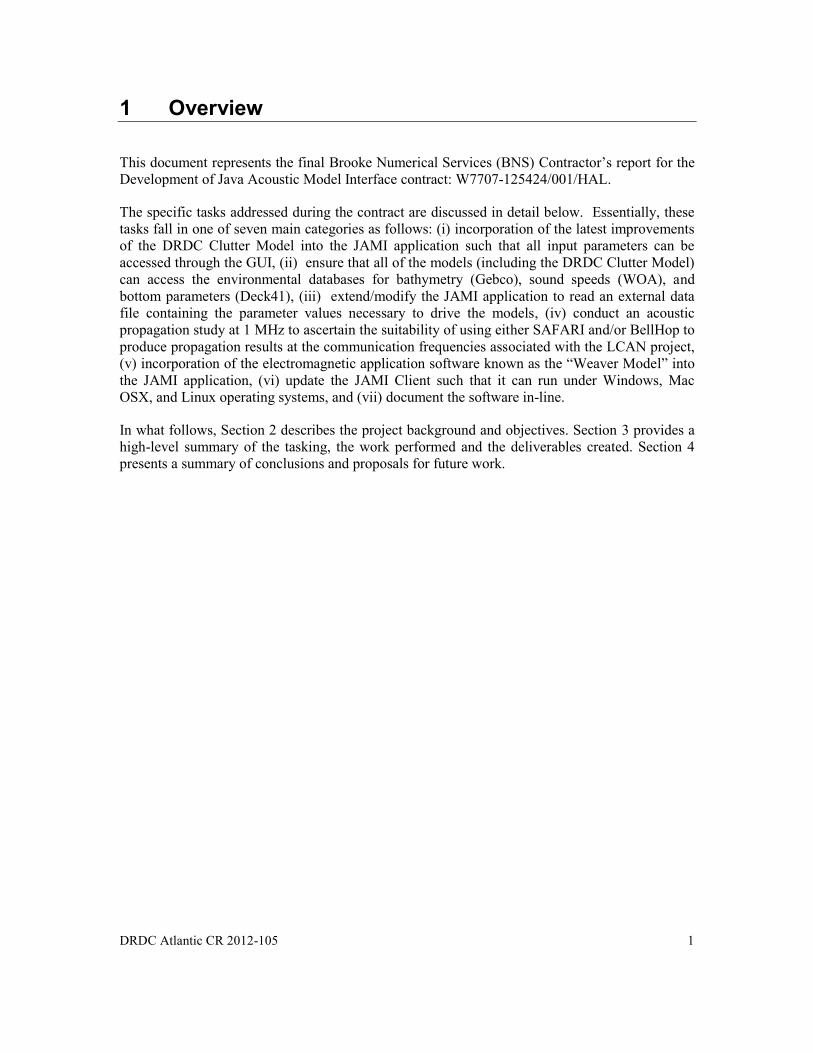
1 Overview
This document represents the final Brooke Numerical Services (BNS) Contractor’s report for the
Development of Java Acoustic Model Interface contract: W7707-125424/001/HAL.
The specific tasks addressed during the contract are discussed in detail below. Essentially, these
tasks fall in one of seven main categories as follows: (i) incorporation of the latest improvements
of the DRDC Clutter Model into the JAMI application such that all input parameters can be
accessed through the GUI, (ii) ensure that all of the models (including the DRDC Clutter Model)
can access the environmental databases for bathymetry (Gebco), sound speeds (WOA), and
bottom parameters (Deck41), (iii) extend/modify the JAMI application to read an external data
file containing the parameter values necessary to drive the models, (iv) conduct an acoustic
propagation study at 1 MHz to ascertain the suitability of using either SAFARI and/or BellHop to
produce propagation results at the communication frequencies associated with the LCAN project,
(v) incorporation of the electromagnetic application software known as the “Weaver Model” into
the JAMI application, (vi) update the JAMI Client such that it can run under Windows, Mac
OSX, and Linux operating systems, and (vii) document the software in-line.
In what follows, Section 2 describes the project background and objectives. Section 3 provides a
high-level summary of the tasking, the work performed and the deliverables created. Section 4
presents a summary of conclusions and proposals for future work.
2 DRDC Atlantic CR 2012-105
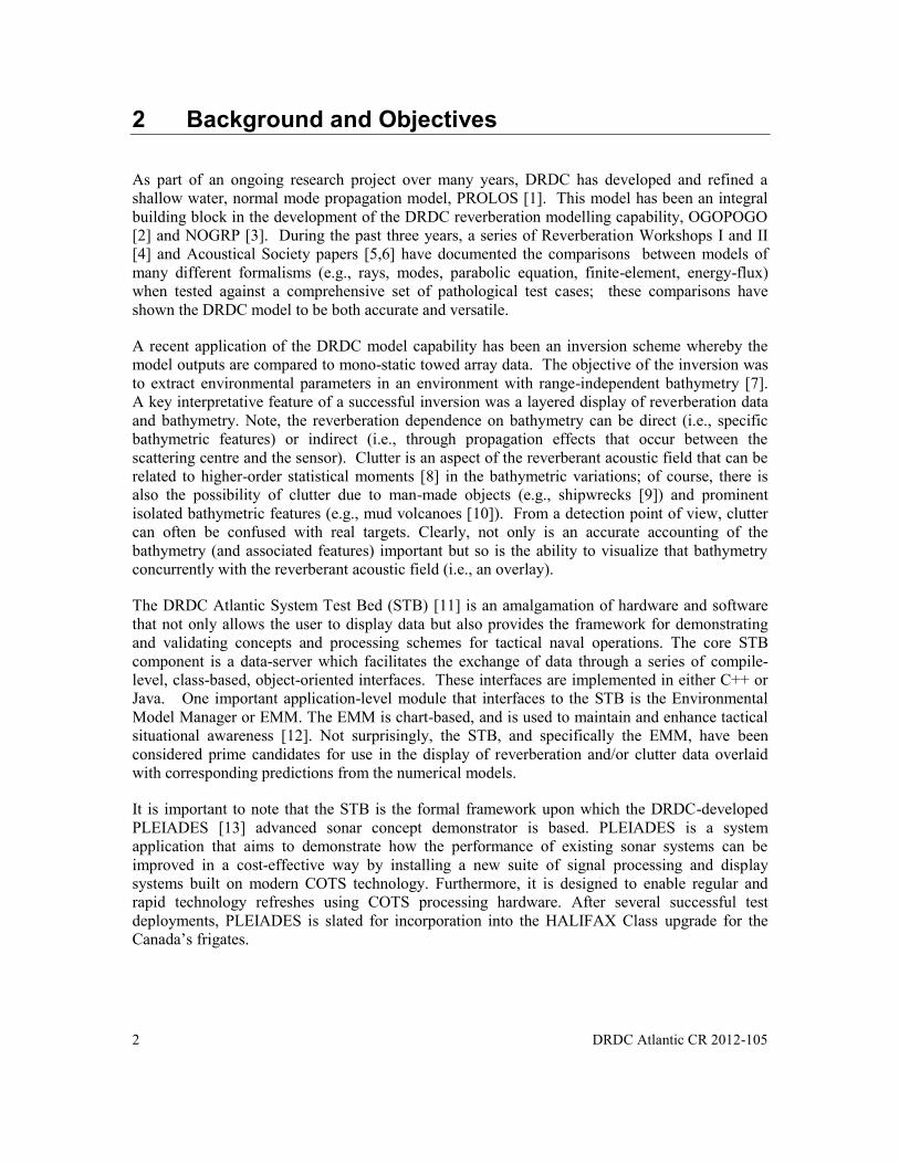
2 Background and Objectives
As part of an ongoing research project over many years, DRDC has developed and refined a
shallow water, normal mode propagation model, PROLOS [1]. This model has been an integral
building block in the development of the DRDC reverberation modelling capability, OGOPOGO
[2] and NOGRP [3]. During the past three years, a series of Reverberation Workshops I and II
[4] and Acoustical Society papers [5,6] have documented the comparisons between models of
many different formalisms (e.g., rays, modes, parabolic equation, finite-element, energy-flux)
when tested against a comprehensive set of pathological test cases; these comparisons have
shown the DRDC model to be both accurate and versatile.
A recent application of the DRDC model capability has been an inversion scheme whereby the
model outputs are compared to mono-static towed array data. The objective of the inversion was
to extract environmental parameters in an environment with range-independent bathymetry [7].
A key interpretative feature of a successful inversion was a layered display of reverberation data
and bathymetry. Note, the reverberation dependence on bathymetry can be direct (i.e., specific
bathymetric features) or indirect (i.e., through propagation effects that occur between the
scattering centre and the sensor). Clutter is an aspect of the reverberant acoustic field that can be
related to higher-order statistical moments [8] in the bathymetric variations; of course, there is
also the possibility of clutter due to man-made objects (e.g., shipwrecks [9]) and prominent
isolated bathymetric features (e.g., mud volcanoes [10]). From a detection point of view, clutter
can often be confused with real targets. Clearly, not only is an accurate accounting of the
bathymetry (and associated features) important but so is the ability to visualize that bathymetry
concurrently with the reverberant acoustic field (i.e., an overlay).
The DRDC Atlantic System Test Bed (STB) [11] is an amalgamation of hardware and software
that not only allows the user to display data but also provides the framework for demonstrating
and validating concepts and processing schemes for tactical naval operations. The core STB
component is a data-server which facilitates the exchange of data through a series of compile-
level, class-based, object-oriented interfaces. These interfaces are implemented in either C++ or
Java. One important application-level module that interfaces to the STB is the Environmental
Model Manager or EMM. The EMM is chart-based, and is used to maintain and enhance tactical
situational awareness [12]. Not surprisingly, the STB, and specifically the EMM, have been
considered prime candidates for use in the display of reverberation and/or clutter data overlaid
with corresponding predictions from the numerical models.
It is important to note that the STB is the formal framework upon which the DRDC-developed
PLEIADES [13] advanced sonar concept demonstrator is based. PLEIADES is a system
application that aims to demonstrate how the performance of existing sonar systems can be
improved in a cost-effective way by installing a new suite of signal processing and display
systems built on modern COTS technology. Furthermore, it is designed to enable regular and
rapid technology refreshes using COTS processing hardware. After several successful test
deployments, PLEIADES is slated for incorporation into the HALIFAX Class upgrade for the
Canada’s frigates.
DRDC Atlantic CR 2012-105 3
The DRDC reverberation modelling formulation has recently been extended to handle bistatic
geometry and range-dependent environments [14]. Concurrently, the target echo modelling
capability has been extended to include a representation of clutter object and these advancements
have undergone successful testing against the so-called energy flux method [15].
Previous contract work [16] initiated the development of the Java Acoustic Clutter Interface
(JACI) standalone application that would support further development of the DRDC Clutter
model, provide a display mechanism for Clutter model results, and at the same time be
compatible with the STB.
This contract work constitutes an enhancement to the JACI capabilities. The enhanced standalone
application, to be known as the Java Acoustic Model Interface (JAMI) has been developed to
provide the following:
an interface to the DRDC Clutter model including configuration, execution, and display;
an interface to the SAFARI [17], PECan [18], POPP [19], and Bellhop [20], acoustic
propagation models including configuration, execution, and display; and
an interface to the DRDC electromagnetic model (the Weaver Model [21]) including
configuration, execution, and display.
In addition, this contract work has examined the prospects for employing both the SAFARI and
Bellhop models for acoustic modelling at frequencies associated with the LCAN [22] project i.e.,
as high 1 MHz.

4 DRDC Atlantic CR 2012-105
3 Summary of Project Results
This section contains a summary review of the progress that BNS made during the project.
3.1 Tasking
The tasks initiated by the project team are as follows:
Task 1: Incorporate the latest improvements of the DRDC Clutter Model (Fortran) into the
Jami Server (Back-End);
Task 2: Extend the jACI interface (of April 2010) to include all the inputs for the Clutter
Model;
Task 3: upgrade JAMI software to hook into environmental databases and extract relevant
environmental parameters appropriate for each model;
Task 4: upgrade JAMI software so that the User can export *.env files based on the
parameter set in the GUI; in addition, JAMI shall be able to load parameters from a
standard file and populate the GUI (*.env is taken to mean ‘input file(s)’ appropriate to
each model;
Task 5: produce a report comparing the applicability of using either Bellhop or Safari to
study underwater propagation at 1 MHz acoustic signals;
Task 6: incorporate E/M capability in JAMI via the Weaver model (Fortran) and provide a
new GUI screen allowing the User to access parameters associated with the Weaver model;
Task 7: configure JAMI to run on Windows, Linux, and Mac OSx; and
Task 8: write a Contractor’s Report.
All of the above tasks were advanced during this contract. The latest DRDC Clutter model has
been incorporated along with the acoustic models: SAFARI, PECan, POPP, and Bellhop and with
the electromagnetic Weaver model. Parameters required by each of the models can be supplied
either through the JAMI Graphical User Interface or by reading from the standard model input
files – JAMI can also write the parameters to these same standard files in the appropriate formats.
A propagation study undertaken to frequencies as high as 1 MHz indicate that Bellhop is the
logical candidate for modelling at these high frequencies; SAFARI does not appear to be capable
of modelling beyond 150 m or so at these frequencies. Note, Bellhop within JAMI has been tested
at these frequencies.
Although, software links to the databases have been coded in all cases except the Weaver model,
this capability has not been tested thoroughly. Currently, the acoustic propagation models
SAFARI, Pecan, POPP, and Bellhop can access the databases but the Clutter Model cannot.
Moreover, in-line documentation (in the form of *.html files that come up in a Browser) were not
completed.
DRDC Atlantic CR 2012-105 5
Finally, it must be said that JAMI works well in a Windows environment but less so in Linux
configuration. This may be due to the fact that the developer (Brooke) is more comfortable in the
Windows world and did most of the development in that environment. No substantial attempt
was made to implement the application in conjunction with Mac OSx – however, given the open
source nature of the compilers, this should be relatively straightforward task. BNS upgraded its
Mac capability in order to facilitate this feature but was not able to complete the tasking in the
allotted time.
3.2 Chronology of Effort
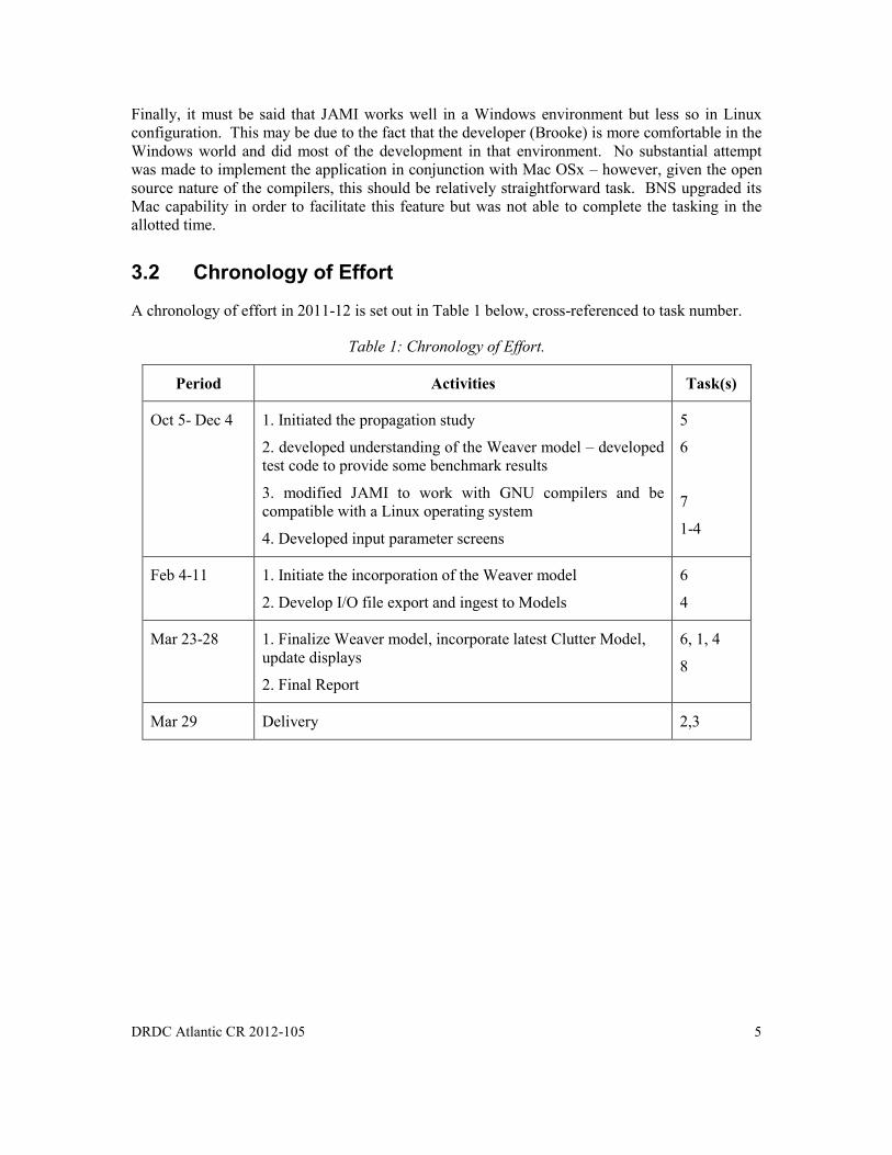
A chronology of effort in 2011-12 is set out in Table 1 below, cross-referenced to task number.
Table 1: Chronology of Effort.
Period Activities Task(s)
Oct 5- Dec 4 1. Initiated the propagation study
2. developed understanding of the Weaver model – developed
test code to provide some benchmark results
3. modified JAMI to work with GNU compilers and be
compatible with a Linux operating system
4. Developed input parameter screens
5
6
7
1-4
Feb 4-11 1. Initiate the incorporation of the Weaver model
2. Develop I/O file export and ingest to Models
6
4
Mar 23-28 1. Finalize Weaver model, incorporate latest Clutter Model,
update displays
2. Final Report
6, 1, 4
8
Mar 29 Delivery 2,3

6 DRDC Atlantic CR 2012-105
3.3 Deliverables
3.3.1 Meetings
Formal project meetings were held in 2010 as set out in Table 2 below.
Table 2: Meetings.
Date Type Comments
October 2011 Kick-Off
(Teleconference)
Discussion of priorities
December 2011 Demo at DRDC Showed use of the acoustic models
February 2012 Progress #2, by email Discussion of progress
March 2012 Progress #3, by email Discussion of the latest Clutter Model
3.3.2 Other Communications
There were no other formal communications.
3.3.3 Software, Databases and Documentation
All software and documentation are to be supplied in electronic form. As a result of the jACI
contract, DRDC already has copies of the ETOP02, ETOP05, and Gebco bathymetry databases,
the Deck41 bottom type database, and the WOA (World Oceanographic Atlas) salinity and
temperature databases (for sound speed definition). Detailed instructions for the installation of the
software is given in Annex D of this report. The software modules include:
1. the CtoF interface (comment in-line in the code);
2. the Clutter model, SAFARI, PECan, POPP, Bellhop, and the Weaver model (comments in-
line in the code); and
3. the java GUI (comments in-line in the code and a built in help facility).
3.3.4 Reports
A Contract Report in the DRDC format will be supplied on March 31, 2012, the termination date
of the contract.
DRDC Atlantic CR 2012-105 7
3.4 Functional Results
In this section an overview of the functional results of the contract work will be given. More
detailed information is supplied in the form of Annexes where appropriate.
3.4.1 Compilers
This project involves programming languages Java, FORTRAN, and C. Java is used for the
standalone Graphical User Interface for the jAMI application, FORTRAN is used in the Clutter
Model as well as the acoustic propagation models: SAFARI, PECan, POPP, and Bellhop. The C
language is used to bridge Java to Fortran models and each other to the environmental databases.
Clearly, the conglomeration of languages presents challenges. These challenges are exacerbated
by the requirement that the JAMI application run under three different operating systems i.e.,
Windows XP and Windows 7, Ubuntu 11.0 (Linux), and Mac OSx (Snow Leopard). These
challenges made the use of the Gnu compiler suite imperative.
Significant progress has been made in making the JAMI application machine and operating
system independent. All development has employed the GCC 4.4.2 suite. Additionally, all code
development, including Java, C, and Fortran has been carried out in the Netbeans 7.0.1 IDE in
conjunction with JDK1.6.0_17. The development has been based on the jACI application [16]
produced under contract with DRDC.
3.4.2 The jAMI GUI (Client Application)
As mentioned, one of the objectives of this contract work was to enhance the jACI graphical front
end to the DRDC Clutter Model. The jAMI application not only interfaces to the Clutter Model
but also to acoustic propagation models (SAFARI, PECan, POPP, and Bellhop). In addition, we
have added an electromagnetic component in the form of the DRDC Weaver Model. In this
section we present a brief overview of the GUI, herein called the java Acoustic Model Interface
(jAMI) – a full tutorial on its use can be accessed directly inside the application from the Menu
Bar.
For the purposes of this discussion, we assume that the software has been installed appropriately.
Specific instructions are given in Annex E of this report. The application is currently invoked by
double clicking on the JAMI.jar file in the \dist subfolder of the distribution directory. As has
been outlined above, the jAMI acts as a Client to the backend Server which includes the DRDC
Clutter model, the other acoustic models, and the Weaver model. Not surprising then that the first
screen that appears (Fig. 1 below) involves the selection of the host computer for the Server and
consequently the host computer for the models. The default configuration is to have the Client
and Server reside on the same computer (the true standalone application). This is reflected in the
screen controls in Fig.1(a) below in which LocalHost is the default selection and can be selected
simply by clicking on the OK button. If a remote host is necessary, then the RemoteHost radio
button should be selected in which case the screen controls in Fig. 1(b) now allow entry of either
the IP Address or the DNS address of the remote computer. Clearly, if Remote operation is
selected, the Client must be connected to the local network or the internet.
8 DRDC Atlantic CR 2012-105
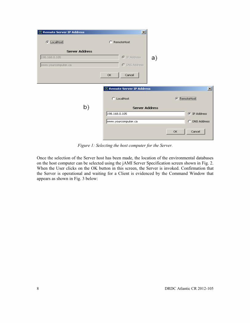
Figure 1: Selecting the host computer for the Server.
Once the selection of the Server host has been made, the location of the environmental databases
on the host computer can be selected using the jAMI Server Specification screen shown in Fig. 2.
When the User clicks on the OK button in this screen, the Server is invoked. Confirmation that
the Server is operational and waiting for a Client is evidenced by the Command Window that
appears as shown in Fig. 3 below:

DRDC Atlantic CR 2012-105 9
Figure 2: jAMI initiation of the Server.
Figure 3: Server initiated – waiting for input from the Client (jAMI).
Coincident with the appearance of the command window is the Main Screen of the jACI shown
below in Fig. 4. Note, one could access the Tutorial immediately by clicking on Help in the Menu
bar and then selecting jAMI Tutorial which in turn brings up the tutorial in a Browser.
10 DRDC Atlantic CR 2012-105
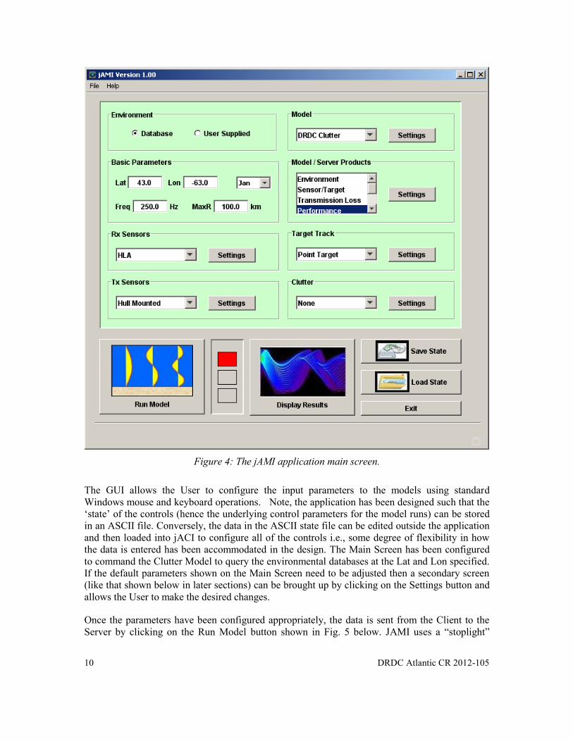
Figure 4: The jAMI application main screen.
The GUI allows the User to configure the input parameters to the models using standard
Windows mouse and keyboard operations. Note, the application has been designed such that the
‘state’ of the controls (hence the underlying control parameters for the model runs) can be stored
in an ASCII file. Conversely, the data in the ASCII state file can be edited outside the application
and then loaded into jACI to configure all of the controls i.e., some degree of flexibility in how
the data is entered has been accommodated in the design. The Main Screen has been configured
to command the Clutter Model to query the environmental databases at the Lat and Lon specified.
If the default parameters shown on the Main Screen need to be adjusted then a secondary screen
(like that shown below in later sections) can be brought up by clicking on the Settings button and
allows the User to make the desired changes.
Once the parameters have been configured appropriately, the data is sent from the Client to the
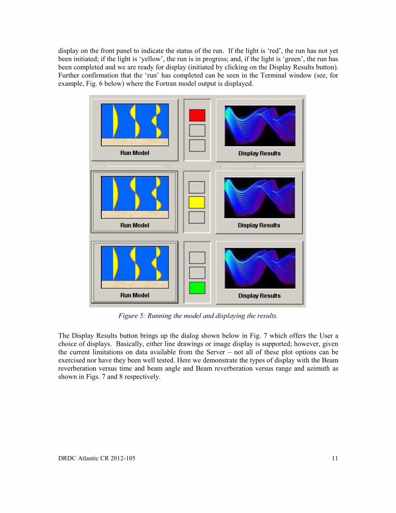
Server by clicking on the Run Model button shown in Fig. 5 below. JAMI uses a “stoplight”
DRDC Atlantic CR 2012-105 11
display on the front panel to indicate the status of the run. If the light is ‘red’, the run has not yet
been initiated; if the light is ‘yellow’, the run is in progress; and, if the light is ‘green’, the run has
been completed and we are ready for display (initiated by clicking on the Display Results button).
Further confirmation that the ‘run’ has completed can be seen in the Terminal window (see, for
example, Fig. 6 below) where the Fortran model output is displayed.
Figure 5: Running the model and displaying the results.
The Display Results button brings up the dialog shown below in Fig. 7 which offers the User a
choice of displays. Basically, either line drawings or image display is supported; however, given
the current limitations on data available from the Server – not all of these plot options can be
exercised nor have they been well tested. Here we demonstrate the types of display with the Beam
reverberation versus time and beam angle and Beam reverberation versus range and azimuth as
shown in Figs. 7 and 8 respectively.

12 DRDC Atlantic CR 2012-105
Figure 6: Server terminal screen output (computation complete).
Figure 7: Choice of displays.

DRDC Atlantic CR 2012-105 13
Figure 8: Display of Beam reverberation versus beam angle and time.
Figure 9: Display of Beam reverberation versus range and azimuth (clutter map display).
In the following sections we describe the various models input parameters screens and
demonstrate these displays through an examination of the results of running the models.

14 DRDC Atlantic CR 2012-105
3.4.3 The Clutter Model (Tasks 1 – 2 )
The original driving force behind the jACI contract work was to provide an interface to the
DRDC Clutter Model. Indeed, in the jACI application, the GUI functionality was tailored
specifically to this model. The requirements of this contract were to incorporate the latest Clutter
Model upgrades as provided by the Dr. Dale Ellis of DRDC (circa March 22, 2012). To this end,
we have made the necessary adjustments to jAMI implementation of the Clutter Model and it runs
inside the application and affords the User control over all of the inputs.
The Clutter Model is still the focus of the jAMI application – unfortunately, with the inclusion of
the other models (each with their own parameter input screens as we will see below) the use of
jAMI to drive the Clutter model seems rather ‘clunky’ in the sense that in order to configure the
model (or reconfigure it) several different input screens need to be invoked from the main screen.
In order to demonstrate jAMI’s implementation of the latest Clutter Model, we generate results
for a test case that we part of a Canadian Acoustical Society meeting presentation [23]. The test
case is illustrated below in Fig. 10. It consists of a shallow water region 100 km by 100 km in
which is situated a sea mount (upper left), two bathymetric ridges (lower left and upper right),
and a clutter object (lower right); otherwise the bathymetry is constant and equal to 100 m. Both
the sea mount and the ridges come to within 30 m of the ocean surface. The water column is iso-
speed at 1500 m/s and the ocean bottom is sand with parameters (c = 1700 m/s, ρ = 2 gm/cc, α =
0.5 dB/λ). The Clutter Model will perform bistatic adiabatic normal mode computations on an 11
by 11 rectangular grid as illustrated – the frequency is 250 Hz and we separate the transmitter and
receiver in both range and depth as shown.
Figure 10: Configuration of the Clutter Model
The task at hand is to compute the Echo Excess assuming a source level equal to 10 dB for a 0.1
sec CW pulse. A detection threshold of 12 dB is used to generate the echo excess performance
statistic. In order the configure the jAMI application consider the main screen shown below in
Fig. 11 with several features identified.
DRDC Atlantic CR 2012-105 15
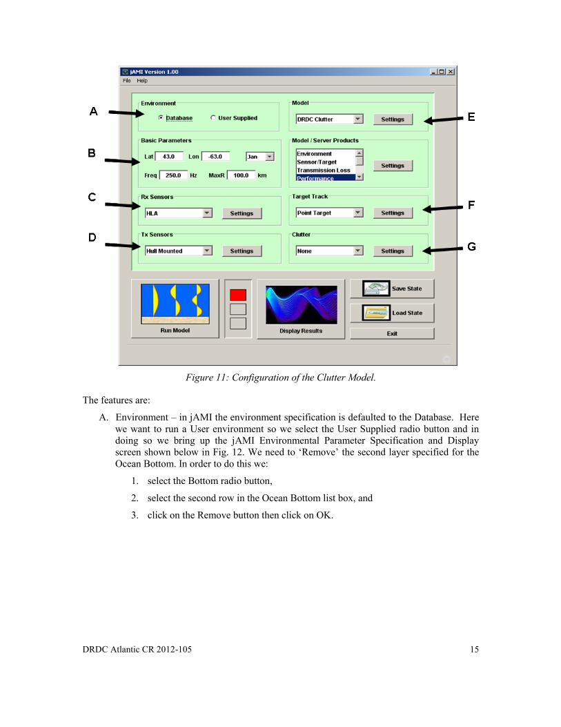
Figure 11: Configuration of the Clutter Model.
The features are:
A. Environment – in jAMI the environment specification is defaulted to the Database. Here
we want to run a User environment so we select the User Supplied radio button and in
doing so we bring up the jAMI Environmental Parameter Specification and Display
screen shown below in Fig. 12. We need to ‘Remove’ the second layer specified for the
Ocean Bottom. In order to do this we:
1. select the Bottom radio button,
2. select the second row in the Ocean Bottom list box, and
3. click on the Remove button then click on OK.
16 DRDC Atlantic CR 2012-105
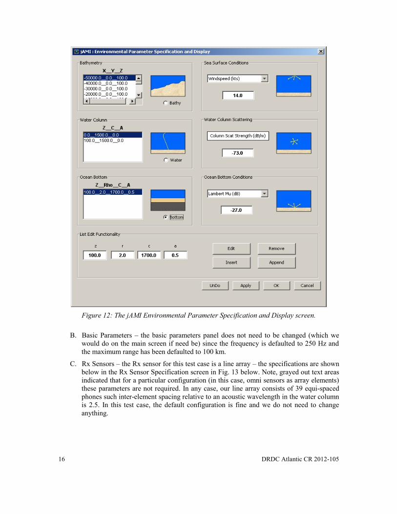
Figure 12: The jAMI Environmental Parameter Specification and Display screen.
B. Basic Parameters – the basic parameters panel does not need to be changed (which we
would do on the main screen if need be) since the frequency is defaulted to 250 Hz and
the maximum range has been defaulted to 100 km.
C. Rx Sensors – the Rx sensor for this test case is a line array – the specifications are shown
below in the Rx Sensor Specification screen in Fig. 13 below. Note, grayed out text areas
indicated that for a particular configuration (in this case, omni sensors as array elements)
these parameters are not required. In any case, our line array consists of 39 equi-spaced
phones such inter-element spacing relative to an acoustic wavelength in the water column
is 2.5. In this test case, the default configuration is fine and we do not need to change
anything.
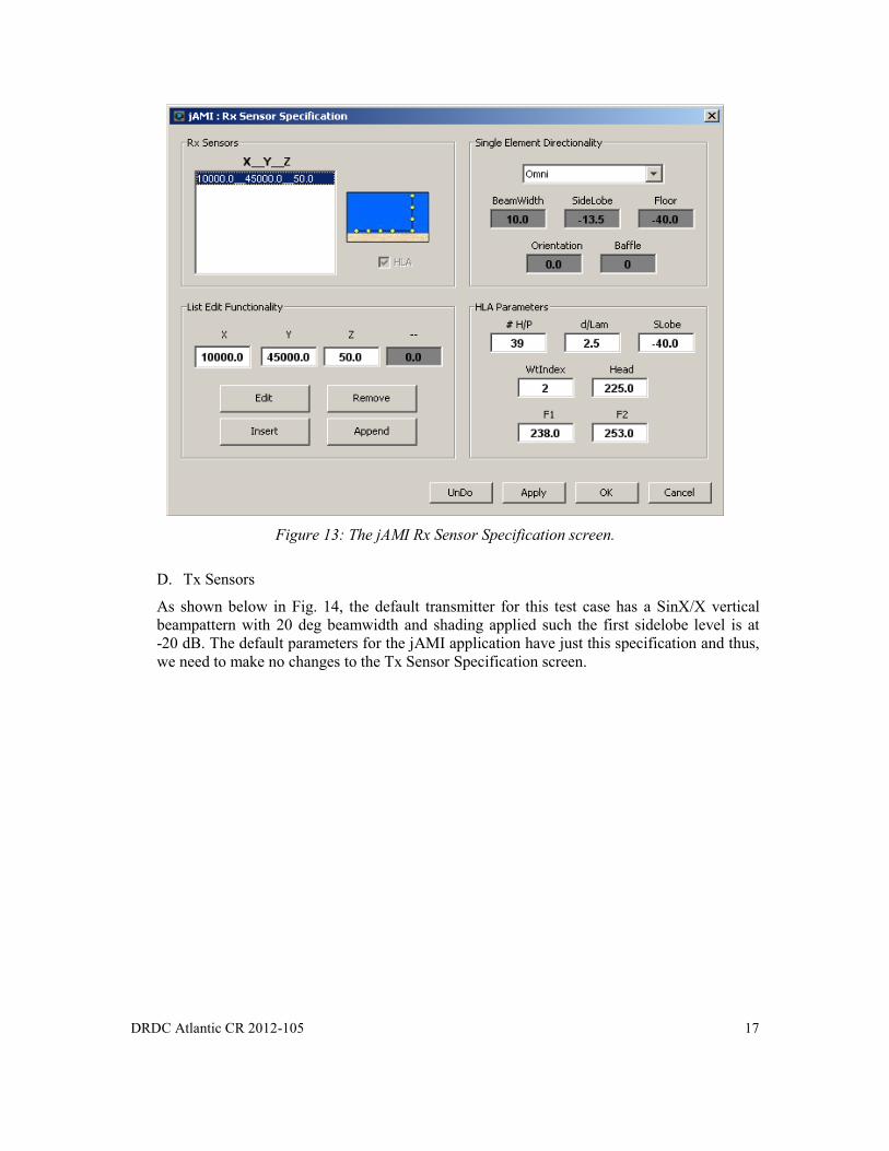
DRDC Atlantic CR 2012-105 17
Figure 13: The jAMI Rx Sensor Specification screen.
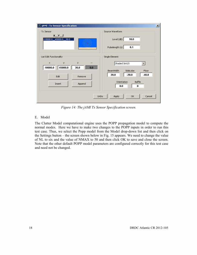
D. Tx Sensors
As shown below in Fig. 14, the default transmitter for this test case has a SinX/X vertical
beampattern with 20 deg beamwidth and shading applied such the first sidelobe level is at
-20 dB. The default parameters for the jAMI application have just this specification and thus,
we need to make no changes to the Tx Sensor Specification screen.
18 DRDC Atlantic CR 2012-105
Figure 14: The jAMI Tx Sensor Specification screen.
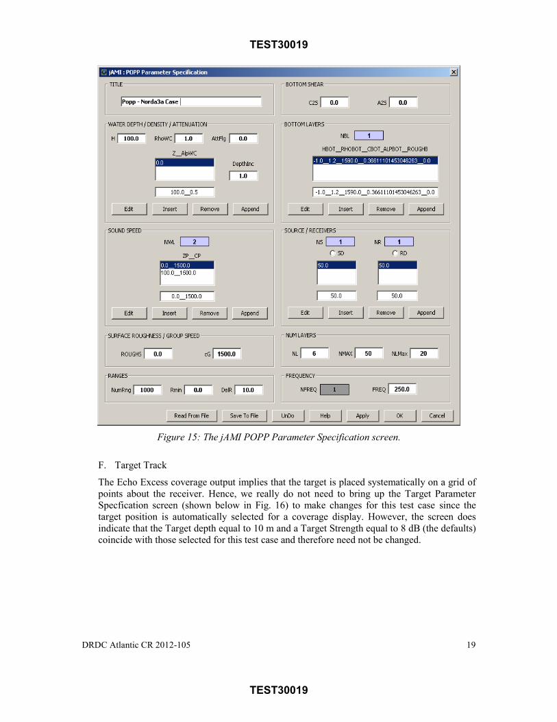
E. Model
The Clutter Model computational engine uses the POPP propagation model to compute the
normal modes. Here we have to make two changes to the POPP inputs in order to run this
test case. Thus, we select the Popp model from the Model drop-down list and then click on
the Settings button – the screen shown below in Fig. 15 appears. We need to change the value
of NL to six and the value of NMAX to 50 and then click OK to save and close the screen.
Note that the other default POPP model parameters are configured correctly for this test case
and need not be changed.
TEST30019
DRDC Atlantic CR 2012-105 19
TEST30019
Figure 15: The jAMI POPP Parameter Specification screen.
F. Target Track
The Echo Excess coverage output implies that the target is placed systematically on a grid of
points about the receiver. Hence, we really do not need to bring up the Target Parameter
Specfication screen (shown below in Fig. 16) to make changes for this test case since the
target position is automatically selected for a coverage display. However, the screen does
indicate that the Target depth equal to 10 m and a Target Strength equal to 8 dB (the defaults)
coincide with those selected for this test case and therefore need not be changed.

20 DRDC Atlantic CR 2012-105
Figure 16: The jAMI Target Specification screen.
G. Clutter
As mentioned above this test case involves a clutter object. In fact, for this test case, that
clutter object is just a grid point with artificially high scattering loss – a condition which we
specify using the Environmental Parameters Specification screen shown above in Fig. 12.
However, we could have used the Clutter Target Parameter Specification screen shown below
in Fig. 17. That is, we could have treated the clutter object like a ‘false’ target and given a
position and a scattering strength using the entry boxes in this screen. This was not done in
this case simply because it was easy to specify a grid point with an artificially high value of
scattering loss.
Figure 17: The jAMI Clutter Target Specification screen.
DRDC Atlantic CR 2012-105 21
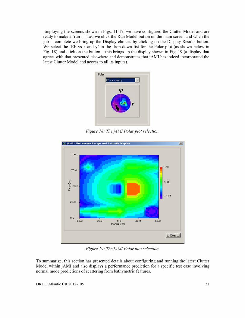
Employing the screens shown in Figs. 11-17, we have configured the Clutter Model and are
ready to make a ‘run’. Thus, we click the Run Model button on the main screen and when the
job is complete we bring up the Display choices by clicking on the Display Results button.
We select the ‘EE vs x and y’ in the drop-down list for the Polar plot (as shown below in
Fig. 18) and click on the button – this brings up the display shown in Fig. 19 (a display that
agrees with that presented elsewhere and demonstrates that jAMI has indeed incorporated the
latest Clutter Model and access to all its inputs).
Figure 18: The jAMI Polar plot selection.
Figure 19: The jAMI Polar plot selection.
To summarize, this section has presented details about configuring and running the latest Clutter
Model within jAMI and also displays a performance prediction for a specific test case involving
normal mode predictions of scattering from bathymetric features.

22 DRDC Atlantic CR 2012-105
3.4.4 The Acoustic Propagation Models (Tasks 4 - 5)
One of the objectives of this contract was to provide a single interface point to several acoustic
propagation models that are used at DRDC Atlantic. Currently, jAMI has been configured to
support four different acoustic propagation models, namely (i) SAFARI, (ii) PECan, (iii) POPP,
and (iv) Bellhop. Each of these models utilizes a different computational framework from the
integral transform technique of SAFARI, the PE technique associated with PECan, the normal
model method of POPP, to the ray theory associated with Bellhop. Consequently, it is a challenge
to provide input parameters to all. This is accomplished in two ways in jAMI i.e., through a
dedicated parameter entry screen in the JAMI GUI or by reading from an input file associated
with the model. Both aspects are outlined in the following sections. As is the case for each model,
we have attempted to provide access to all model input parameters even though the JAMI
application may not use them; this is done to allow legacy model input files to be read and written.
A common convention for the JAMI parameter input screens is to use a particular type of
controlled input as is illustrated below in Fig. 20. It involves entering data into a list box, in this
case, the sound speed profile versus depth.
Figure 20: Standard JAMI List Box Parameter entry controls.
These controls have the following functionality:
Edit – by clicking the Edit button one replaces the highlighted row in the environmental
data list box above with the entry in the text box just above the button. Values are
separated by “__” or double underscore so that the Java code can parse the list box
appropriately.
Insert – by clicking the Insert button one ‘inserts’ the data in the text box ‘above’ the
highlighted row in the environmental data list box above.
Remove – by clicking the Remove button, one deletes the highlighted row in the
environmental data list box (note, there must be at least two rows of data i.e., two layers).
Append – by clicking the Append button, one appends the data in the text box to the end
of the list in the environmental data list box above.
A second feature of the parameter input screens are the control buttons at the bottom of the screen
as illustrated below in Fig. 21.

DRDC Atlantic CR 2012-105 23
Figure 21: Standard jAMI input parameter button controls.
These buttons have the following functionality:
Load From File – populates the input screen parameter controls by reading values from
a standard (to the specific model) input file;
Save to File – archives the input screen parameter controls by saving values to a file in
the standard (to the specific model) input file format;
UnDo – ‘undoes’ any text entry made to a screen control prior to application of the Apply
button;
Help – brings up a Browser window in which “help” information about the functionality
of the input screen is presented or about the model itself;
Apply – saves parameter changes locally;
OK – makes parameter changes permanent and exits the screen;
Cancel – exits the screen without saving any changes to the parameter values.
3.4.4.1 SAFARI
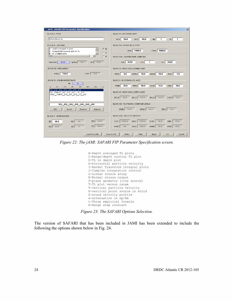
The jAMI: SAFARI FIP Parameter Specification screen is shown below in Fig. 22. The
controls on this screen directly mimic the parameters found in the SAFARI User’s
Manual [] and the reader is referred to that manual for further explanation. Many of the
parameters are linked to the specification of ‘options’ for the model – in the GUI, these
options are selected via a drop-down list in the Options panel of the screen. For reference,
a list of the options is presented in Fig. 23 below. The ‘grayed’ out text areas of the
screen are controlled by the Options block – when appropriate, the disabled text boxes are
enabled and accept data as expected. Environmental information is input to the model
using the controls in the Environment Data block – these controls have been described
above.
24 DRDC Atlantic CR 2012-105
Figure 22: The jAMI: SAFARI FIP Parameter Specification screen.
A-Depth averaged TL plots
C-Range/depth contour TL plot
D-TL vs depth plot
H-horizontal particle velocity
I-Hankel Transform integral plots
J-Complex integration contour
L-Linear source array
N-Normal stress output
P-plane geometry (line source)
T-TL plot versus range
V-vertical particle velocity
X-vertical point source in solid
Z-sound velocity profile
a-attenuation in np/km
t-Thorp empirical formula
R-Range step constant
Figure 23: The SAFARI Options Selection.
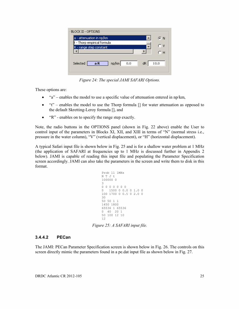
The version of SAFARI that has been included in JAMI has been extended to include the
following the options shown below in Fig. 24.
DRDC Atlantic CR 2012-105 25
Figure 24: The special JAMI SAFARI Options.
These options are:
“a” – enables the model to use a specific value of attenuation entered in np/km,
“t” – enables the model to use the Thorp formula [] for water attenuation as opposed to
the default Skretting-Leroy formula [], and
“R” - enables on to specify the range step exactly.
Note, the radio buttons in the OPTIONS panel (shown in Fig. 22 above) enable the User to
control input of the parameters in Blocks XI, XII, and XIII in terms of “N” (normal stress i.e.,
pressure in the water column), “V” (vertical displacement), or “H” (horizontal displacement).
A typical Safari input file is shown below in Fig. 25 and is for a shallow water problem at 1 MHz
(the application of SAFARI at frequencies up to 1 MHz is discussed further in Appendix 2
below). JAMI is capable of reading this input file and populating the Parameter Specification
screen accordingly. JAMI can also take the parameters in the screen and write them to disk in this
format.
Prob 11 1MHz
N T J t
100000 0
3
0 0 0 0 0 0 0
0 1500 0 0.0 0 1.0 0
100 1700 0 0.5 0 2.0 0
30
50 50 1 1
1450 1800
65536 1 65536
0 40 20 1
50 100 12 10
12
Figure 25: A SAFARI input file.
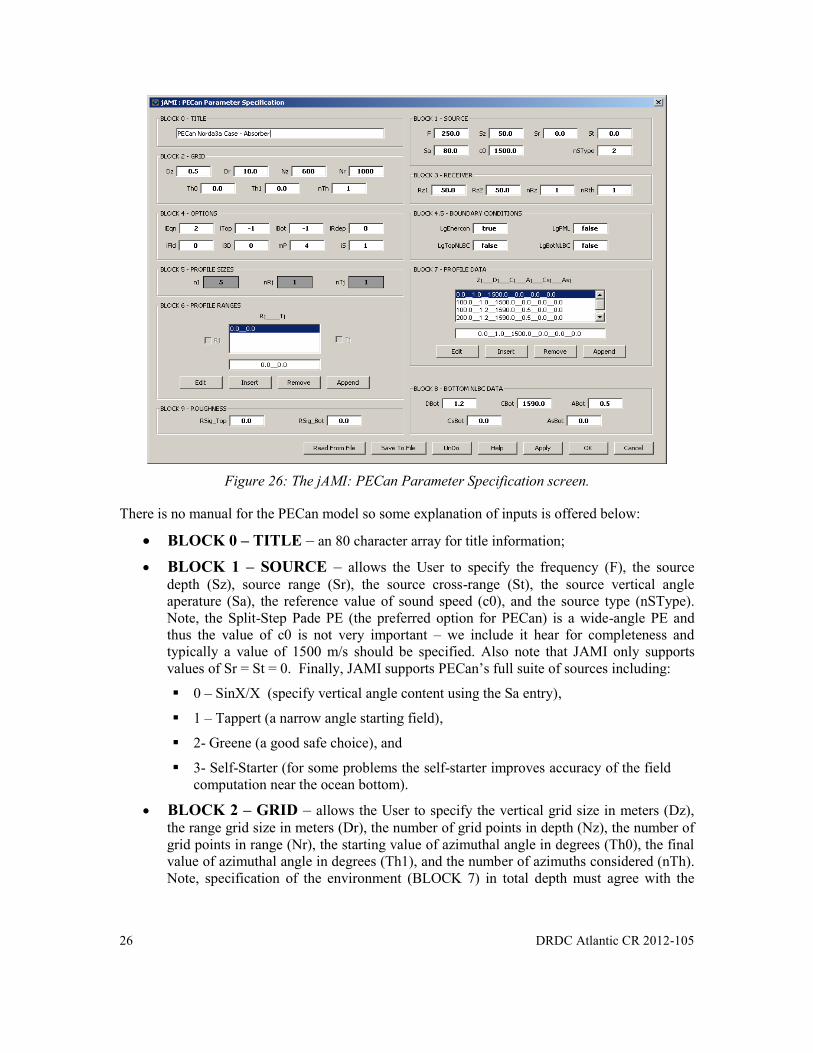
3.4.4.2 PECan
The JAMI: PECan Parameter Specification screen is shown below in Fig. 26. The controls on this
screen directly mimic the parameters found in a pe.dat input file as shown below in Fig. 27.
26 DRDC Atlantic CR 2012-105
Figure 26: The jAMI: PECan Parameter Specification screen.
There is no manual for the PECan model so some explanation of inputs is offered below:
BLOCK 0 – TITLE – an 80 character array for title information;
BLOCK 1 – SOURCE – allows the User to specify the frequency (F), the source
depth (Sz), source range (Sr), the source cross-range (St), the source vertical angle
aperature (Sa), the reference value of sound speed (c0), and the source type (nSType).
Note, the Split-Step Pade PE (the preferred option for PECan) is a wide-angle PE and
thus the value of c0 is not very important – we include it hear for completeness and
typically a value of 1500 m/s should be specified. Also note that JAMI only supports
values of Sr = St = 0. Finally, JAMI supports PECan’s full suite of sources including:
0 – SinX/X (specify vertical angle content using the Sa entry),
1 – Tappert (a narrow angle starting field),
2- Greene (a good safe choice), and
3- Self-Starter (for some problems the self-starter improves accuracy of the field
computation near the ocean bottom).
BLOCK 2 – GRID – allows the User to specify the vertical grid size in meters (Dz),
the range grid size in meters (Dr), the number of grid points in depth (Nz), the number of
grid points in range (Nr), the starting value of azimuthal angle in degrees (Th0), the final
value of azimuthal angle in degrees (Th1), and the number of azimuths considered (nTh).
Note, specification of the environment (BLOCK 7) in total depth must agree with the

DRDC Atlantic CR 2012-105 27
depth obtained through the product of Nz*Dz. Also, the range extent of the calculations
is equal to Nr*Dr.
BLOCK 3 – RECEIVER – allows the User to specify depths at which transmission
loss is computed. Output is computed for Rz1 through Rz2 in NRz equi-spaced depth
intervals that include the endpoints i.e., if Rz1 = 20 and Rz2 = 40 and NRz is 3 then
transmission loss is output at depths of 20, 30, and 40 m.
BLOCK 4 – OPTIONS – the parameters in this block allow the User to specify the
type of PE solution (IEqn), the top boundary condition (iTop), the bottom boundary
condition (iBot), a range-dependence flag (iRDep), a full-field storage flag (iFld), a full
3D calculation flag (i3D), the number of Pade terms (mP), and a flag that controls
computation of Pade coefficients (iS). IEqn = 2 specifies the Split-Step Pade solution and
should always be used. iTop = 0 specifies a free surface termination at the top of the
ocean (iTop = 1 specifies a rigid surface), iBot = 0 specifies a free surface termination at
the bottom of the PE grid (iBot = 1 specifies a rigid surface termination). Providing some
form of absorption is used above the termination, iBot = 0 is the usual choice. The iRDep
flag must be set to one for range-dependent calculations. The iFld = 1 implies huge storage
requirements and hence is seldom used. The i3D = 1 invokes full 3D modelling (i.e., not
just Nx2D modelling) and requires at least 1024 azimuths and lots of computing power.
The number of Pade terms affects the accuracy of the PE solution – nominally, 4 is a good
choice for this parameter. The iS parameter is always set equal to a value equal to one.
BLOCK 4.5 – BOUNDARY CONDITIONS – these logical-valued controls allow
the User to specify which boundary condition is used. Normally, energy conservation is a
desirable thus this control is ‘always’ true. The top NLBC would only be true if surface
roughness effects are required. The Perfectly Matched Layer (PML) option is generally
preferred (rule of thumb is that one needs 3 wavelengths of material in the ocean bottom
before applying the PML) because it allows the vertical grid to be minimized i.e., makes
for more efficient operation of the model. If bottom roughness is to be included then the
bottom NLBC must be used. Note, even in the absence of roughness, the bottom NLBC
can be used to terminate the waveguide in depth. Otherwise, a rather large absorbing
layer must be specified (typically, one specifies a few hundred metres of bottom material
with a small attenuation added i.e., ~1dB/λ or so).
BLOCK 5 – PROFILE SIZES – these controls are ‘labels’ and do not accept input;
however, they do reflect changes made to the controls in BLOCKS 6 and 7.
BLOCK 6 – PROFILE RANGES – the PECan environment is specified on a coarse
grid in range, R, and cross range, T, coordinates. This block of controls allows the User to
specify the grid points in these two coordinates. These values are used in conjunction
with the entries made in BLOCK 7 to completely specify the layering in the waveguide.
BLOCK 7 – PROFILE DATA – these controls allow the User to input sound speed
profile data at the grid points in range and cross-range specified by the parameters in
BLOCK 6.
BLOCK 8 – BOTTOM NLBC DATA – when the non-local boundary condition
selection is made for the ocean bottom in BLOCK 4.5, these parameters represent the
homogeneous ocean bottom and are used in the application of the non-local boundary
condition. If the bottom NLBC option is ‘false’ then these inputs are ignored.

28 DRDC Atlantic CR 2012-105
BLOCK 9 – ROUGHNESS – allows the User to specify surface roughness in meters
for the ocean surface and the ocean bottom. Computations for loss due to these roughness
parameters are made using non-local boundary conditions.
A typical pe.dat input file is shown below in Fig.27. JAMI can read this file and populate the
controls accordingly. JAMI can also transfer the parameters values in the screen to a like file with
similar format.
ASA Benchmark Wedge Parameters
3500 15 0 0 80 1500 2
0.02 2.5 6000 20000 0 0 1
50 50 1 1
2 -1 -1 0 0 0 4 1
T F F T
4 1 1
0 0
0.0 1.0 1500.0 0.0 0 0
100 1.0 1500.0 0.0 0 0
100 2.0 1700.0 0.5 0 0
120 2.0 1700.0 0.5 0 0
2.0 1700. 0.5 0 0
0 0
Figure 27: A typical pe.dat input file.
3.4.4.3 POPP
The JAMI: POPP Parameter Specification screen is shown below in Fig. 28. The controls on this
screen directly mimic the parameters found in an input file (*.inp) as shown below in Fig. 29.
This screen makes liberal use of the list box data entry controls in several panels, namely (i)
WATER DEPTH / DENSITY /ATTENUATION in which the depth-attenuation profile can be
specified, (ii) BOTTOM LAYERS in which the bottom layering for the model can be specified,
(iii) SOUND SPEED in which the depth-speed profile for the water column is entered, and (iv)
SOURCE / RECEIVERS in which the source depth and/or receiver depths are specified. Note,
the radio buttons in the SOURCE / RECEIVERS panel controls which list box is active with the
buttons. Also, the POPP model can be configured to run several frequencies – the JAMI version
only runs a single frequency at a time; hence, the NFREQ text box is disabled and set equal to 1.
The only other parameters of note are the NL and NMAX specifications – setting both to -1 is
interpreted by the POPP model to mean that NL is internally set to a value equal to 251 and
NMAX is internally set to the maximum number of modes.

DRDC Atlantic CR 2012-105 29
Figure 28: The jAMI: POPP Parameter Specification screen.
Norda3a Case ... (S=R=50 m, f=250 Hz, 5 km <= r <= 10 km)
100. 1.0 0.
0. 1500.
100. 1500.
-1. -1.
0. 0.
-1. 1.2 1590. 0.3144
0. 0.
1 250.
1 50.
1 50.
-1 -1
10. 10. 1001
Figure 29: The POPP n3a.inp file format.
Finally, it is worth mentioning that the input associated with the WATER DEPTH / DENSITY /
ATTENUATION / panel is a bit tricky. If the ATTFLG parameter is set to an irrational number
greater than zero the attenuation profile is specified in the list box. Otherwise, the attenuation is
set to the ATTFLG value with a depth increment equal to 1.0.

30 DRDC Atlantic CR 2012-105
3.4.4.4 Bellhop
The JAMI: POPP Parameter Specification screen is shown below in Fig. 30. The controls on this
screen directly mimic the parameters found in an input file (*.env) as shown below in Fig. 31.
The reader is referred to Appendix 2 for a complete description of the input parameters – JAMI
has conformed to this documentation. However, not all features have been fully tested. With
regard to the Bellhop parameter input screen, the only unconventional aspect is the SOURCE /
RECEIVER DEPTHS AND RANGES panel in which some shorthand notation is employed
whereby if the value of NR is negative then the entries in the corresponding list box below are
limited to two and they are interpreted as the upper and lower bounds respectively or the range
interval with abs(NR) range points equally spaced between these two limits i.e., this functionality
mimics Bellhop’s shorthand notation on input as described in Appendix 2.
Figure 30: The jAMI: Bellhop Parameter Specification screen.
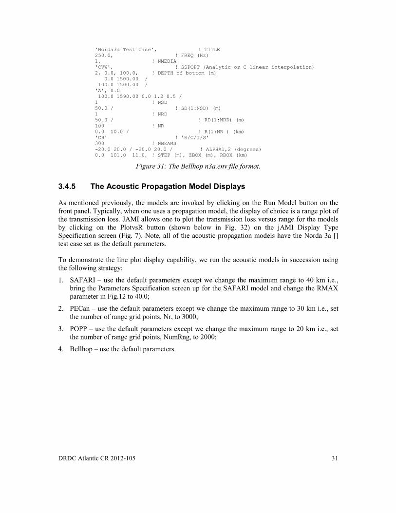
DRDC Atlantic CR 2012-105 31
'Norda3a Test Case', ! TITLE
250.0, ! FREQ (Hz)
1, ! NMEDIA
'CVW', ! SSPOPT (Analytic or C-linear interpolation)
2, 0.0, 100.0, ! DEPTH of bottom (m)
0.0 1500.00 /
100.0 1500.00 /
'A', 0.0
100.0 1590.00 0.0 1.2 0.5 /
1 ! NSD
50.0 / ! SD(1:NSD) (m)
1 ! NRD
50.0 / ! RD(1:NRD) (m)
100 ! NR
0.0 10.0 / ! R(1:NR ) (km)
'CB' ! 'R/C/I/S'
300 ! NBEAMS
-20.0 20.0 / -20.0 20.0 / ! ALPHA1,2 (degrees)
0.0 101.0 11.0, ! STEP (m), ZBOX (m), RBOX (km)
Figure 31: The Bellhop n3a.env file format.
3.4.5 The Acoustic Propagation Model Displays
As mentioned previously, the models are invoked by clicking on the Run Model button on the
front panel. Typically, when one uses a propagation model, the display of choice is a range plot of
the transmission loss. JAMI allows one to plot the transmission loss versus range for the models
by clicking on the PlotvsR button (shown below in Fig. 32) on the jAMI Display Type
Specification screen (Fig. 7). Note, all of the acoustic propagation models have the Norda 3a []
test case set as the default parameters.
To demonstrate the line plot display capability, we run the acoustic models in succession using
the following strategy:
1. SAFARI – use the default parameters except we change the maximum range to 40 km i.e.,
bring the Parameters Specification screen up for the SAFARI model and change the RMAX
parameter in Fig.12 to 40.0;
2. PECan – use the default parameters except we change the maximum range to 30 km i.e., set
the number of range grid points, Nr, to 3000;
3. POPP – use the default parameters except we change the maximum range to 20 km i.e., set
the number of range grid points, NumRng, to 2000;
4. Bellhop – use the default parameters.
32 DRDC Atlantic CR 2012-105
Figure 32: JAMI’s PlotvsR button.
Note, by running in succession, we mean: (i) selecting the model in the Model Panel drop down
list on the jAMI main screen, (ii) clicking on the corresponding Settings button to bring the
Parameters Specifications screen, (iii) edit the range parameter, and click on the OK button to
close the parameters screen, (iv) run the model by clicking on the Run Model button on the main
screen, and (v) when the model run is complete, repeat the process for each model. The output
displayed in the jAMI range plot after this procedure is presented in Fig. 33 below. Here all of the
model results are displayed at the same time – they all ran the same problem (except for range
extent) and hence they overlay. This example demonstrates that the jAMI application is capable
of transmission loss results obtained by the different models. By de-selecting models in the list
shown at the top right of the screen we can also plot individual results by themselves.
If one has chosen input parameters to compute the field at different receiver depths, then it is
possible to plot (overplot) the results as a function of depth for individual models. This feature is
demonstrated in Fig. 34 below where we overplot the PECan results for the default Norda 3a test
case with the receiver depth set to 20 m, 40 m, 60 m, and 80 m. Of course, by de-selecting entries
in the Depth list, these results can be plotted individually as well. Note, as currently configured,
jAMI does not allow plotting of different depths from different models.
The previous discussion describes current plotting capabilities with respect to the acoustic
models. Clearly, it is possible to compute the field as a function of range and depth and hence to
ultimately plot an image using the Range vs Depth display button or the field versus depth using
the Field vs Depth display button. This capability requires coding upgrades on the Client side i.e.,
the Java code. Other display capability like coverage versus range and azimuth (i.e., the PE is
capable of generating Nx2D transmission loss predictions) are possible but would require changes
be made to the C-Fortran interface as well as Java coding.
DRDC Atlantic CR 2012-105 33
Figure 33: Transmission loss versus range for the different models.
Figure 34: Transmission loss versus range for several depths (same model).
34 DRDC Atlantic CR 2012-105
3.4.6 The Weaver Model (Task 6)
The DRDC HED (horizontal electric dipole) model is based on the analysis of Weaver [21] who
developed the integral solutions to the quasi-static electromagnetic fields within the upper layer of
a two-layered conducting half-space due to a vertical or horizontal electric dipole embedded
within the upper layer.
Only the HED is implemented in the DRDC FORTRAN code. The code consists of a driver and
eight subroutines. The test driver that was supplied by DRDC featured a typical set of input
parameters and evaluated the fields (Ex,Ey,Ez) and (Bx,By,Bz) at a single (x,y,z) field point.
Because of symmetry, Weaver’s solutions for the electromagnetic fields were carried out in
cylindrical coordinates (r,θ,z). In addition, all lengths were scaled in terms of an induction
number α which is related to the skin depth δ in the upper layer by δ=√2/α. The resulting
electromagnetic fields were represented in dimensionless form. Each dimensionless field
component varies in azimuth as either sinθ or cosθ. In contrast, the DRDC code accepts inputs
and produces outputs in rectangular coordinates (x,y,z) and in practical units with lengths in m
and electric fields in mV/km and magnetic fields in nT.
The DRDC code was compiled and executed using the GNU gfortran compiler. A few changes
were made to the code to suppress some warnings and issues that were flagged by the compiler.
The only compiler flag used was "–fbounds-check" except for one subroutine which also used the
flag "–fd-lines-as-comments".
A new driver main program was written to execute the HED code for 7 options: all six complex
electromagnetic components are always computed and saved in an ascii output file. The options
are:
option 000: fields vs distance along an angle θ relative to the x-axis;
option 100: fields vs distance along a line parallel to the x-axis;
option 010: fields vs distance along a line parallel to the y-axis;
option 001: fields vs distance along a line parallel to the z-axis;
option 110: fields on a grid in the xy-plane;
option 101: fields on a grid in the xz-plane;
option 011: fields on a grid in the yz-plane;
Inititially, the simple makefile reproduced below was used to compile the DRDC code outside the
jAMI application.
DRDC Atlantic CR 2012-105 35
objects = mainhed.o ac_weaver.o rtricia.o nquad.o \
dqsyt.o ninth.o fcnh.o gl.o bess.o
drdched : $(objects)
gfortran -o drdched $(objects) -fbounds-check
mainhed.o : mainhed.for
gfortran -c mainhed.for -fbounds-check
ac_weaver.o : ac_weaver.for
gfortran -c ac_weaver.for -fbounds-check
rtricia.o : rtricia.for
gfortran -c rtricia.for -fbounds-check -fd-lines-as-comments
nquad.o : nquad.for
gfortran -c nquad.for -fbounds-check
dqsyt.o : dqsyt.for
gfortran -c dqsyt.for -fbounds-check
ninth.o : ninth.for
gfortran -c ninth.for -fbounds-check
fcnh.o : fcnh.for
gfortran -c fcnh.for -fbounds-check
gl.o : gl.for
gfortran -c gl.for -fbounds-check
bess.o : bess.for
gfortran -c bess.for -fbounds-check
Figure 35: A Weaver Model Makefile.
The following changes were made to the DRDC HED code to satisfy GNU’s gfortran compiler:
1. in ac_weaver: line 104 -- added dble intrinsic function
cdjt Replcaced len by dble(len) below in a & b ...
a = -dble(len)/2.0d0
b = dble(len)/2.0d0
in ac_weaver: line 170 -- replaced end SUBROUTINE AC_WEAVER with END
cdjt end SUBROUTINE AC_WEAVER
2. in nquad: line 475 -- replaced jisign intrinsic with sign intrinsic
cdjt x = jisign(1,i)*xi(p1+abs(i))*(b-a)/2.0d0 + (b+a)/2.0d0
cdjt ghb had to use int(p1) above and below here ...
x = sign(1,i)*xi(p1+abs(i))*(b-a)/2.0d0 + (b+a)/2.0d0
The DRDC HED code evaluates the integral solutions using an adaptive numerical integration
scheme that is controlled by a user tolerance TOL. The integrals that are evaluated are based on
formulas (57) and (58) derived in [21] for the two components of the vector potential: Ax and Az.
The fields themselves are determined by appropriate differentiations of these potentials given in
(71) to (76) in [21]. As Weaver points out, this precludes evaluating the fields when h=z=0 as
some of the resulting integrals become divergent there. For this reason, Weaver recasts the
integrals into a more useful form for evaluation by extracting the solutions for a uniform
half-space which can be expressed analytically in terms of modified Bessel functions. These
solutions are given in (78) to (83) in [21] and depend on some F and N functions defined by
Weaver. The N functions are given in the appendix of his paper. The remaining integrals are
always convergent and can be integrated numerically even along h=z=0. The solutions are only
valid however when r>0.
The analytic results for a uniform half-space provide a convenient opportunity to check the
numerical integration routines. As a consequence, a Matlab code has been written to evaluate the
analytic fields for a horizontal dipole embedded in a uniform half-space and used to validate the
DRDC Code for this situation, i.e., by setting the conductivity of the sea equal to that of the

36 DRDC Atlantic CR 2012-105
sea-bottom or by letting the thickness of the upper layer become very large. A limited check was
performed for a typical set of parameter values. In order to compare these analytic solutions with
those produced by the DRDC code, the analytic field components were converted from
cylindrical into rectangular coordinates and then from dimensionless to physical units (mV/km
and nT). Excellent agreement was obtained with the DRDC code out to a range of 10 skin depths
for all field components for the case considered. A tolerance of 1e-3 was required in the DRDC
code to improve the agreement beyond 7 skin depths for the Ez component.
A brief description of input parameter field sequence is given by the list below:
line 1: Title -- max 80-character string,
line 2: opt -- 3-character xyz-option code,
000: line along ang with nx=ny>1, nz=1,
-- 001: line along x with nx>1, ny=nz=1,
-- 010: line along y with ny>1, nx=nz=1,
-- 001: line along z with nz>1, nx=ny=1,
110: slice along xy with nx,ny>1, nz=1,
101: slice along xz with nx,nz>1, ny=1,
011: slice along yz with ny,nz>1, nx=1,
line 3: freq -- frequency [Hz],
line 4: len -- length of dipole source [m],
len<1e-5 for infinitesimal dipole,
line 5: current -- current [A],
line 6: seadep -- depth of sea layer [m],
line 7: consea -- conductivity of sea in [S],
line 8: conbed -- conductivity of seabed [S],
line 9: xdip -- x-coordinate of dipole [m],
line 10: ydip -- y-coordinate of dipole [m],
line 11: ddip -- z-coordinate of dipole [m],
line 12: xarr -- initial x-coordinate of receiver array [m],
line 13: yarr -- initial y-coordinate of receiver array [m],
line 14: darr -- initial z-coordinate of receiver array [m],
line 15: nx -- no. of grid steps from xarr along x-coordinate,
line 16: ny -- no. of grid steps from yarr along y-coordinate,
line 17: nz -- no. of grid steps from darr along z-coordinate,
line 18: dx -- grid spacing along x-coordinate [m],
line 19: dy -- grid spacing along y-coordinate [m],
except for code 000 when dx=dy=dr,
along ang [m]. dx & dy reset internally,
line 20: dz -- grid spacing along z-coordinate [m],
line 21: ang -- bearing angle for opt code 000 [Deg],
line 22: tol -- tolerance parameter for adaptive integrator.

DRDC Atlantic CR 2012-105 37
The Weaver model as outlined above has been incorporated into the JAMI application. To invoke
the model, select ‘Weaver’ in the Model drop box control on the Main screen as shown below in
Fig. 36. To view or change the model parameters, click on the Settings button just right of the
drop box. This action will bring up the jAMI Weaver Model Parameter Specification screen as
shown in Fig. xx below. This parameter screen allows the User to configure the Weaver model
through selection of the parameter values associated with the various controls. The inputs are
more or less straightforward and self-explanatory with the following exceptions:
1. Dipole Length – for an infinitesimal dipole, specify a length < 10-5
.
2. Grid Selection – as shown, the parameter screen accepts a field point specification (the
point at which the E/M field will be calculated) in a regular Cartesian coordinate system
X-Y-Z. One can specify Minimum and Maximum values in each coordinate and the
number of points even spaced between the Min and Max (including endpoints) at which
fields will be calculated. The six components (Ex, Ey, Ez, Bx, By, Bz) are calculated at
each grid point. Note, the actual number of calculation points is increased by one
internally such that the origin can be included in grids symmetric about the origin. The
Checkboxes allow the User to make 1D, 2D, or even 3D computations – to date, only 1D
calculations have been tested in jAMI.
3. R-Theta grid – the radio button in the Grid Selection panel can be toggled between
X-Y-Z (as above) or R-Theta-Z. If the latter is chosen then calculations then the
parameter specification window changes as shown in Fig. xx below. In this case, one can
proceed along a radial out from the dipole position. This option has not yet been tested
fully but one will be able to make 1D or 2D predictions along any radial and display
those fields using the jAMI display capability.
4. Skin depth – this is ‘label’ control and cannot be edited. However, when the
corresponding Update button is activated, the skin depth is calculated and displayed in
this label based on the parameters specified by the other controls.
5. ReadFromFile (SaveToFile) – these buttons allow the User to populate/save the input
model parameters from/to an ASCII data file. In other words, the User can bypass
populating the controls by hand if a file with the format shown below in Fig. 37 is
available. Upon activation, the ReadFromFile and SaveToFile buttons bring up a
FileChooser window that allows the User to navigate to the file on disk and open it for
reading or writing.
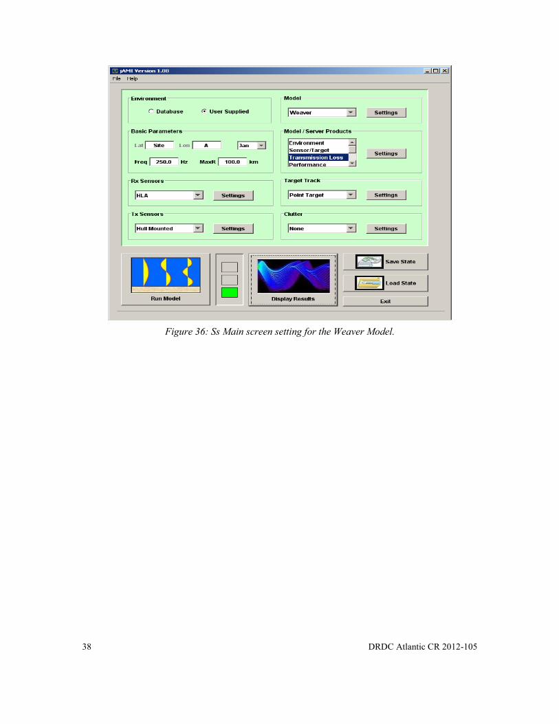
38 DRDC Atlantic CR 2012-105
Figure 36: Ss Main screen setting for the Weaver Model.
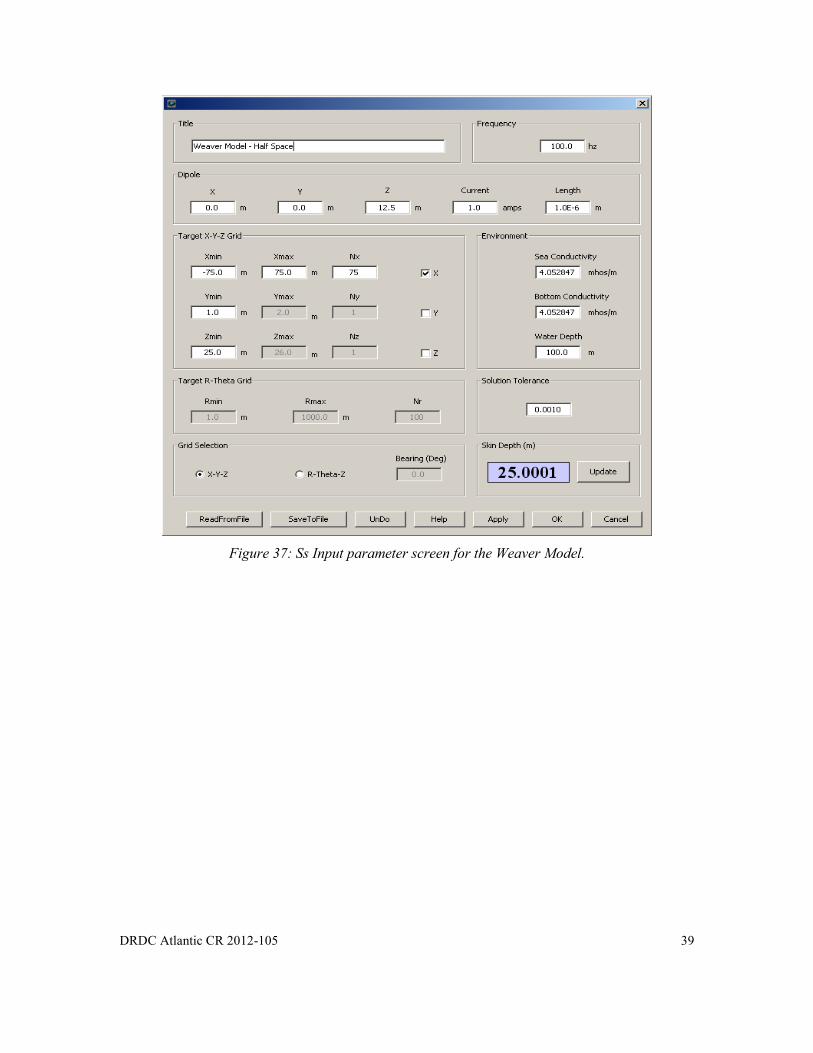
DRDC Atlantic CR 2012-105 39
Figure 37: Ss Input parameter screen for the Weaver Model.
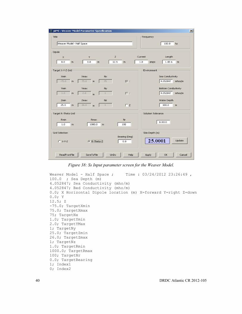
40 DRDC Atlantic CR 2012-105
Figure 38: Ss Input parameter screen for the Weaver Model.
Weaver Model - Half Space ; Time : 03/24/2012 23:26:49 ,
100.0 ; Sea Depth (m)
4.052847; Sea Conductivity (mho/m)
4.052847; Bed Conductivity (mho/m)
0.0; X Horizontal Dipole location (m) X=forward Y=right Z=down
0.0; Y
12.5; Z
-75.0; TargetXmin
75.0; TargetXmax
75; TargetNx
1.0; TargetYmin
2.0; TargetYMax
1; TargetNy
25.0; TargetZmin
26.0; TargetZmax
1; TargetNz
1.0; TargetRmin
1000.0; TargetRmax
100; TargetNr
0.0; TargetBearing
1; Index1
0; Index2
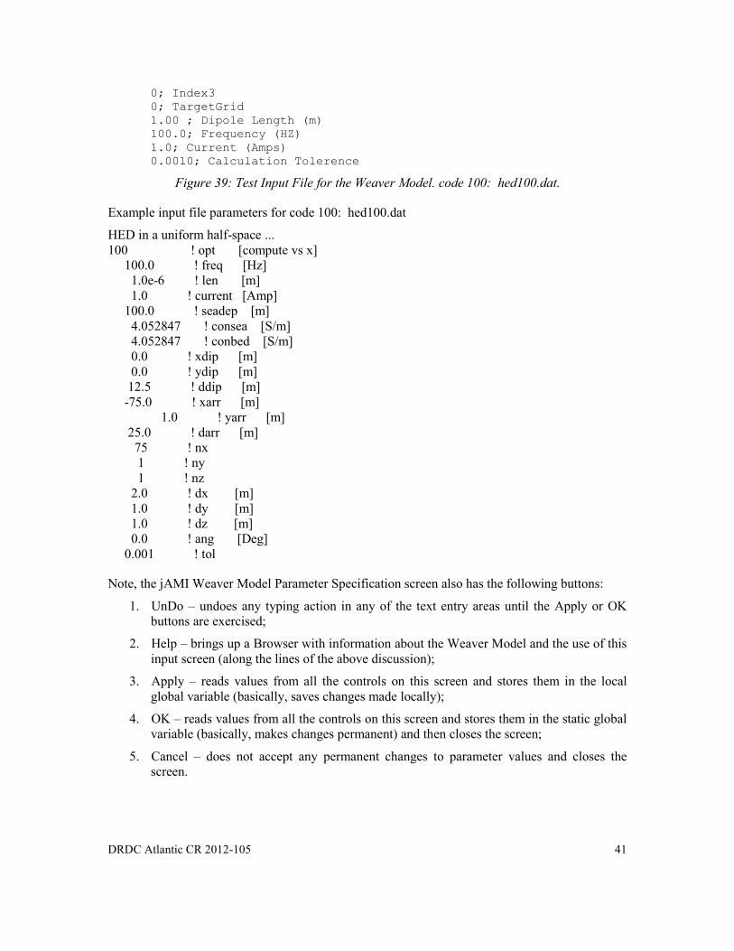
DRDC Atlantic CR 2012-105 41
0; Index3
0; TargetGrid
1.00 ; Dipole Length (m)
100.0; Frequency (HZ)
1.0; Current (Amps)
0.0010; Calculation Tolerence
Figure 39: Test Input File for the Weaver Model. code 100: hed100.dat.
Example input file parameters for code 100: hed100.dat
HED in a uniform half-space ...
100 ! opt [compute vs x]
100.0 ! freq [Hz]
1.0e-6 ! len [m]
1.0 ! current [Amp]
100.0 ! seadep [m]
4.052847 ! consea [S/m]
4.052847 ! conbed [S/m]
0.0 ! xdip [m]
0.0 ! ydip [m]
12.5 ! ddip [m]
-75.0 ! xarr [m]
1.0 ! yarr [m]
25.0 ! darr [m]
75 ! nx
1 ! ny
1 ! nz
2.0 ! dx [m]
1.0 ! dy [m]
1.0 ! dz [m]
0.0 ! ang [Deg]
0.001 ! tol
Note, the jAMI Weaver Model Parameter Specification screen also has the following buttons:
1. UnDo – undoes any typing action in any of the text entry areas until the Apply or OK
buttons are exercised;
2. Help – brings up a Browser with information about the Weaver Model and the use of this
input screen (along the lines of the above discussion);
3. Apply – reads values from all the controls on this screen and stores them in the local
global variable (basically, saves changes made locally);
4. OK – reads values from all the controls on this screen and stores them in the static global
variable (basically, makes changes permanent) and then closes the screen;
5. Cancel – does not accept any permanent changes to parameter values and closes the
screen.
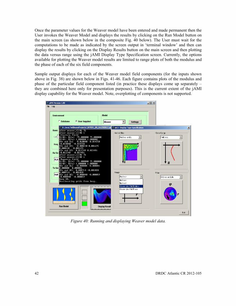
42 DRDC Atlantic CR 2012-105
Once the parameter values for the Weaver model have been entered and made permanent then the
User invokes the Weaver Model and displays the results by clicking on the Run Model button on
the main screen (as shown below in the composite Fig. 40 below). The User must wait for the
computations to be made as indicated by the screen output in ‘terminal window’ and then can
display the results by clicking on the Display Results button on the main screen and then plotting
the data versus range using the jAMI Display Type Specification screen. Currently, the options
available for plotting the Weaver model results are limited to range plots of both the modulus and
the phase of each of the six field components.
Sample output displays for each of the Weaver model field components (for the inputs shown
above in Fig. 38) are shown below in Figs. 41-46. Each figure contains plots of the modulus and
phase of the particular field component listed (in practice these displays come up separately –
they are combined here only for presentation purposes). This is the current extent of the jAMI
display capability for the Weaver model. Note, overplotting of components is not supported.
Figure 40: Running and displaying Weaver model data.

DRDC Atlantic CR 2012-105 43
Figure 41: The Ex field component.
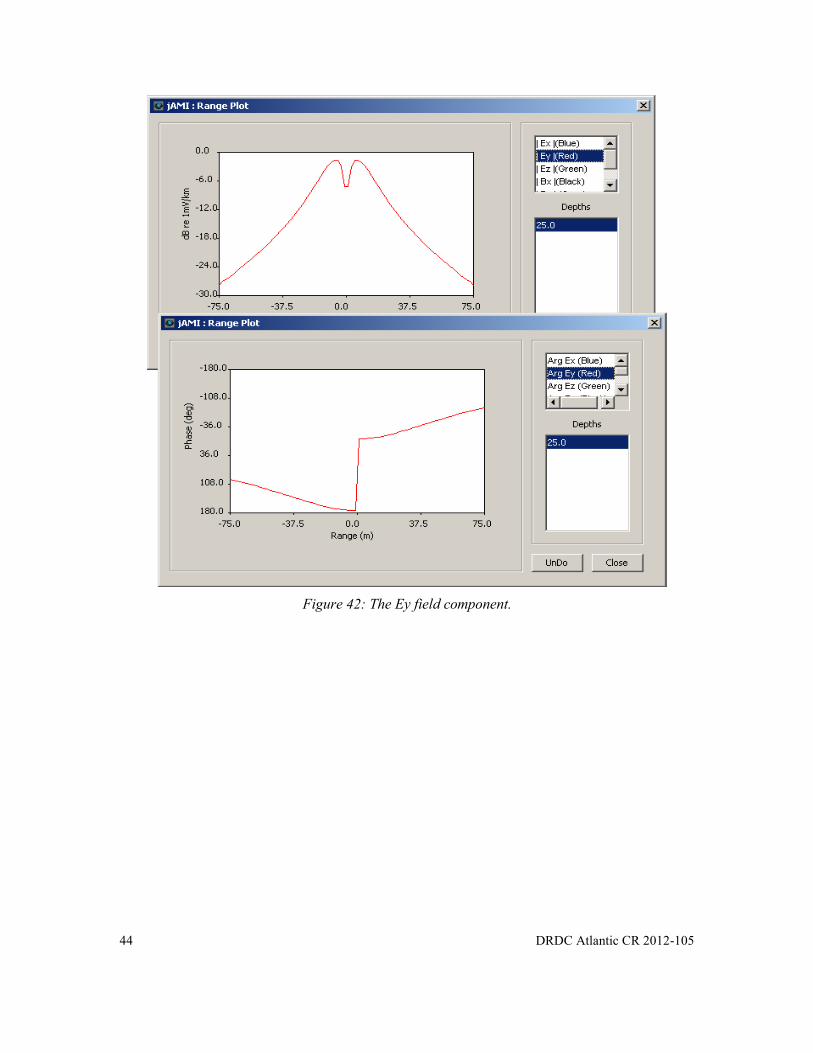
44 DRDC Atlantic CR 2012-105
Figure 42: The Ey field component.
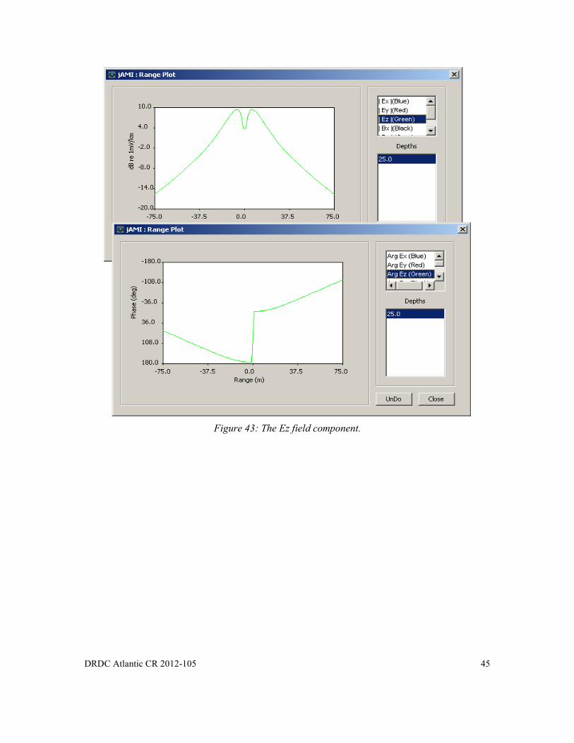
DRDC Atlantic CR 2012-105 45
Figure 43: The Ez field component.

46 DRDC Atlantic CR 2012-105
Figure 44: The Bx field component.

DRDC Atlantic CR 2012-105 47
Figure 45: The By field component.

48 DRDC Atlantic CR 2012-105
Figure 46: The Bz field component.
Summary
The Weaver model has been implemented within the jAMI Client-Server framework. Capabilities
are still somewhat limited however, input parameters can be specified from the GUI or from a
file, the model run and the results displayed thereby laying the groundwork for future expansion
of capabilities.
DRDC Atlantic CR 2012-105 49
3.4.7 Interfacing to the Environmental Databases
The environmental databases used in conjunction with the jAMI system are described at
Annex C. A low-level and database-specific API was created previously to pre-process the
environmental data passing the data to the C-interface and the models. As discussed in the Annex,
the following databases can be accessed by the ACL:
Bathymetry – Gebco [16]
Water Column Temperature and Salinity – World Oceanographic Atlas (WOA) [19].
Sound speed extracted using the Chen-Millero [20] empirical formula.
Ocean Bottom Type – USN Deck41 [21].
Code is in place to ‘hook’ all of the models into the databases. Unfortunately, there was not
enough time in this contract to actually make the connections and test them.

50 DRDC Atlantic CR 2012-105
4 Conclusions and Proposed Future Work
4.1 Conclusions
There were several broad objectives for this contract, namely (i) to fully consolidate the rapidly
changing and expanding Clutter Model software into the jAMI application (ii) to provide access
of the acoustic models within jAMI to environmental databases associated with previous work
(i.e., the jACI application) (iii) to provide capability within jAMI to allow the models to have
their input parameters specified by reading standard ASCII input files normally associated with
each model (e.g., the *.env file for the Bellhop model) and (iv) to conduct an investigation into
the capabilities of the SAFARI and Bellhop models to produce acoustic predictions at frequencies
up to 1 MHz, (v) to incorporate DRDC’s electromagnetic Weaver model into the jAMI
application, and (vi) to configure the jAMI application such that it run under Windows, Linux,
and Mac OS operating systems.
Considerable progress can be claimed on all fronts and is summarized as follows:
1. Task 1 – The latest Clutter Model (as of March 22, 2012) has been included in jAMI;
2. Task 2 – Access to, and control of, the inputs to the Clutter Model are provided to the
User through the jAMI GUI. This can be effected by manipulating controls on input
screens or by reading from a ASCII input file.
3. Task 3 – the SAFARI, PECan, POPP, and Bellhop models can have their environments
specified by querying the environmental databases. Currently, the Clutter Model cannot
although the software hooks are there. Most testing on all fronts and particularly with the
Clutter Model is required.
4. Task 4 – all of the models can access their unique and standard input files through the
jAMI GUI. This feature also needs more testing but preliminary testing indicates correct
operation.
5. Task 5 – an investigation into the capabilities of the SAFARI and Bellhop models to
produce acoustic predictions up to and including frequencies as high as 1 MHz has been
completed. While both models can operate at 1 MHz, Bellhop seems to have less
restrictions in terms of range from the source and therefore is recommended for use by
DRDC at these frequencies. Note, the jAMI application can run Bellhop at these
frequencies.
6. Task 6 – the DRDC Weaver model has been incorporated into the jAMI application. The
User can configure and run the model and then display field component modulus and
phase as a function of range from the receiver. Moreover, a separate study has been done
that provides a benchmark of the DRDC model.
7. Task 7 – the jAMI application has been run under Windows (most of the development has
occurred in Windows) and Linux (with some problems still to be sorted). The application
has not been tested under the Max OS; however, BNS is set up to do that when time
permits.

DRDC Atlantic CR 2012-105 51
4.2 Proposed Future Work
This project has been much more challenging that what might appear on the surface. Of course,
as is most always the case, the scope of the work allows for an interpretation that far exceeds the
available time and resources. This fact notwithstanding, there are few items worth re-
emphasizing:
1. The combination of three different programming languages (Java, C, and Fortran)
coupled with three different operating systems (Windows, Linux, and Mac OS) have
presented severe challenges to the jAMI development. It is clear that some reassessment
of the jAMI interface is required simply because what ‘works’ in Windows does not
translate easily to Linux (and I assume the Mac). Specifically, the parameter inputs
screens are too big and involve too many controls on a single screen – when ported to a
different computer with a different screen size and resolution, the application is simply
not robust enough. It is not clear to the author how much effort is required to rectify this
deficiency but one possible approach is to replace the parameter input screens with
either a tabbed screen with fewer controls on each tab or to use a ‘Wizard’ approach that
leads the User through the parameters.
2. As it now stands, the jAMI application is severely ‘undertested’. It has become a rather
large and complicated application and needs some serious testing on all fronts.
3. Work needs to be done to make the Clutter Model talk to the databases – this has been
one of the prime objectives from the start and it is somewhat disappointing that we are
not there yet; some dedicated time is required.
4. As always, the display of the model results is important and needs refinement. The
jAMI application would be enhanced if capability was added to allow the displays to
captured and exported for inclusion in reports etc.
Finally, it must be stated that the project would have been far more challenging without the
interest and guidance provided by the SA and others at DRDC Atlantic.

52 DRDC Atlantic CR 2012-105
This page intentionally left blank.
DRDC Atlantic CR 2012-105 53
References ..
[1] Dale D. Ellis, A Two-ended ShootingTechnique for Calculating Normal Modes in
Underwater Acoustic Propagation, DREA Report 85/105, (1985).
[2] Dale D. Ellis, “A Shallow Water Normal Modes Reverberation Model,” in J. Acoust. Soc.
Am., 97, 2804-2814 (1995).
[3] D. D. Ellis, “Normal-mode models OGOPOGO and NOGRP applied to the 2006 ONR
Reverberation Modeling Workshop problems,” DRDC Atlantic Technical Memorandum,
DRDC Atlantic TM 2006-289, June 2008. 84 pp.
[4] Reverberation Modeling Workshop, ftp://ftp.ccs.nrl.navy.mil/pub/ram/RevModWkshp,
Post_Workshop_Results_Summary_111306 (Nov 2006).
[5] D.D. Ellis, M.A. Ainslie, and C.H. Harrison, “A comparison of ray, normal-mode, and energy
flux results for reverberation in a Pekeris waveguide,” J. Acoust. Soc. Am., 122, s3075
(2007).
[6] Ellis D.D. and Pecknold S.P., (2010), Range-Dependent Reverberation and Target Echo
Calculations Using the DRDC Atlantic Clutter Model, in proceedings of the 2010 Annual
Conference of the Canadian Acoustical Association, 13-15 October 2010, Victoria, BC.
[7] J. R. Preston and D. D. Ellis, “Extracting bottom information from towed array data Part I:
Measurement methodology,” J. Marine Systems 78, S359-S371 (2009).
[8] J.R. Preston, “Studies on Sonar Clutter and Reverberation,” 06: Studies on Sonar Clutter and
Reverberation.
[9] J. R. Preston, “Statistical characterization of bistatic echoes of a shipwreck from the
CLUTTER’07 experiments,” International Symposium on Underwater Reverberation and
Clutter, Lerici, Italy, September 2008.
[10] C. W. Holland, J. R. Preston, D. A. Abraham, “Long-range acoustic scattering from a
shallow-water mud-volcano cluster,” J. Acoust. Soc. Am. 122, 1946-1958 (2007).
[11] T. Johnson, B. Martin, “DRDC Atlantic System Test Bed (STB) Overview”, Defence R&D
Canada – Atlantic, DRDC Atlantic CR 2007-271 (2007).
[12] G. Inglis, “Networked Underwater Warfare (NUW) Networked Combat System (NECS)
Tactical oceanography Tools”, Defence R&D Canada – Atlantic, DRDC Atlantic
CR 2008-204 (2008).
[13] “New Challenges, New Opportunities: Annual Report for the Year Ending 31 March 2007,
www.drdc-rddc.gc.ca/publications/ar-ra/cap-eng.asp .

54 DRDC Atlantic CR 2012-105
[14] D. D. Ellis, J. R. Preston, P. C. Hines, and V.W. Young, “Bistatic signal excess calculations
over variable bottom topography using adiabatic normal modes,” in International
Symposium on Underwater Reverberation and Clutter, P. L. Nielsen, C. H. Harrison and
J.-C. Le Gac, eds., NATO Undersea Research Centre, La Spezia, Italy, 2008, pp. 97-104.
[15] C. H. Harrison, “Fast bistatic signal-to-reverberation-ratio calculation,” J. Comp. Acoust.
13, 317-340 (2005).
[16] Steve Kilistoff, Gary Brooke, Peter Giles, “Integrate Shallow-Water Clutter Model with the
DRDC System Test Bed,” DRDC Atlantic CR 2009-068, June 2009.
[17] http://www.gebco.net/
[18] http://www.ngdc.noaa.gov/mgg/fliers/01mgg04.html
[19] http://www.ngdc.noaa.gov/mgg/global/etopo5.HTML
[20] http://www.nodc.noaa.gov/OC5/WOA05/pr_woa05.html
[21] “APL-UW High-Frequency Ocean Environmental Acoustic Models Handbook,” Applied
Physics Laboratory, University of Washington, APL-UW TR 9407, October 1994.
[22] http://www.ngdc.noaa.gov/mgg/geology/deck41.html
[23] H. Schmidt, “SAFARI Seismo-Acoustic Fast Field Algorithm for Range-Independent
environments,” Rep. SR-113, SACLANTCEN ASW Research Centre, San Bartolomeo,
Italy (1988).
[24] D.J. Thomson, personal communications.
[25] J.A. Davis, D. White & R.C. Cavanagh, eds., “NORDA Parabolic Equation Workshop, 31
March - 3 April 1981,” NORDA Tech. Note 143, September (1982).
[26] M. Jiang (University of Victoria, School of Earth and Ocean Sciences), personal
communication.
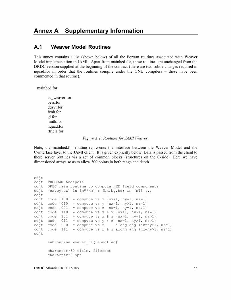
DRDC Atlantic CR 2012-105 55
Annex A Supplementary Information
A.1 Weaver Model Routines
This annex contains a list (shown below) of all the Fortran routines associated with Weaver
Model implementation in JAMI. Apart from mainhed.for, these routines are unchanged from the
DRDC version supplied at the beginning of the contract (there are two subtle changes required in
nquad.for in order that the routines compile under the GNU compilers – these have been
commented in that routine).
mainhed.for
ac_weaver.for
bess.for
dqsyt.for
fcnh.for
gl.for
ninth.for
nquad.for
rtricia.for
Figure A.1: Routines for JAMI Weaver.
Note, the mainhed.for routine represents the interface between the Weaver Model and the
C-interface layer to the JAMI client. It is given explicitly below. Data is passed from the client to
these server routines via a set of common blocks (structures on the C-side). Here we have
dimensioned arrays so as to allow 300 points in both range and depth.
cdjt
cdjt PROGRAM hedipole
cdjt DRDC main routine to compute HED field components
cdjt (ex,ey,ez) in [mV/km] & (bx,by,bz) in [nT] ...
cdjt
cdjt code '100' = compute vs x (nx>1, ny=1, nz=1)
cdjt code '010' = compute vs y (nx=1, ny>1, nz=1)
cdjt code '001' = compute vs z (nx=1, ny=1, nz>1)
cdjt code '110' = compute vs x & y (nx>1, ny>1, nz=1)
cdjt code '101' = compute vs x & z (nx>1, ny=1, nz>1)
cdjt code '011' = compute vs y & z (nx=1, ny>1, nz>1)
cdjt code '000' = compute vs r along ang (nx=ny>1, nz=1)
cdjt code '111' = compute vs r & z along ang (nx=ny>1, nz>1)
cdjt
subroutine weaver_tl(Debugflag)
character*80 title, fileroot
character*3 opt
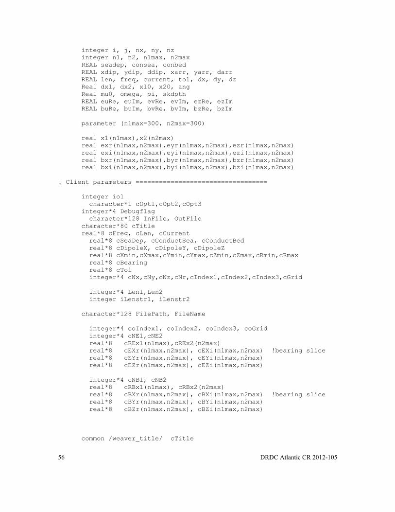
56 DRDC Atlantic CR 2012-105
integer i, j, nx, ny, nz
integer n1, n2, n1max, n2max
REAL seadep, consea, conbed
REAL xdip, ydip, ddip, xarr, yarr, darr
REAL len, freq, current, tol, dx, dy, dz
Real dx1, dx2, x10, x20, ang
Real mu0, omega, pi, skdpth
REAL euRe, euIm, evRe, evIm, ezRe, ezIm
REAL buRe, buIm, bvRe, bvIm, bzRe, bzIm
parameter (n1max=300, n2max=300)
real x1(n1max),x2(n2max)
real exr(n1max,n2max),eyr(n1max,n2max),ezr(n1max,n2max)
real exi(n1max,n2max),eyi(n1max,n2max),ezi(n1max,n2max)
real bxr(n1max,n2max),byr(n1max,n2max),bzr(n1max,n2max)
real bxi(n1max,n2max),byi(n1max,n2max),bzi(n1max,n2max)
! Client parameters ==================================
integer io1
character*1 cOpt1,cOpt2,cOpt3
integer*4 Debugflag
character*128 InFile, OutFile
character*80 cTitle
real*8 cFreq, cLen, cCurrent
real*8 cSeaDep, cConductSea, cConductBed
real*8 cDipoleX, cDipoleY, cDipoleZ
real*8 cXmin,cXmax,cYmin,cYmax,cZmin,cZmax,cRmin,cRmax
real*8 cBearing
real*8 cTol
integer*4 cNx,cNy,cNz,cNr,cIndex1,cIndex2,cIndex3,cGrid
integer*4 Len1,Len2
integer iLenstr1, iLenstr2
character*128 FilePath, FileName
integer*4 coIndex1, coIndex2, coIndex3, coGrid
integer*4 cNE1,cNE2
real*8 cREx1(n1max),cREx2(n2max)
real*8 cEXr(n1max,n2max), cEXi(n1max,n2max) !bearing slice
real*8 cEYr(n1max,n2max), cEYi(n1max,n2max)
real*8 cEZr(n1max,n2max), cEZi(n1max,n2max)
integer*4 cNB1, cNB2
real*8 cRBx1(n1max), cRBx2(n2max)
real*8 cBXr(n1max,n2max), cBXi(n1max,n2max) !bearing slice
real*8 cBYr(n1max,n2max), cBYi(n1max,n2max)
real*8 cBZr(n1max,n2max), cBZi(n1max,n2max)
common /weaver_title/ cTitle
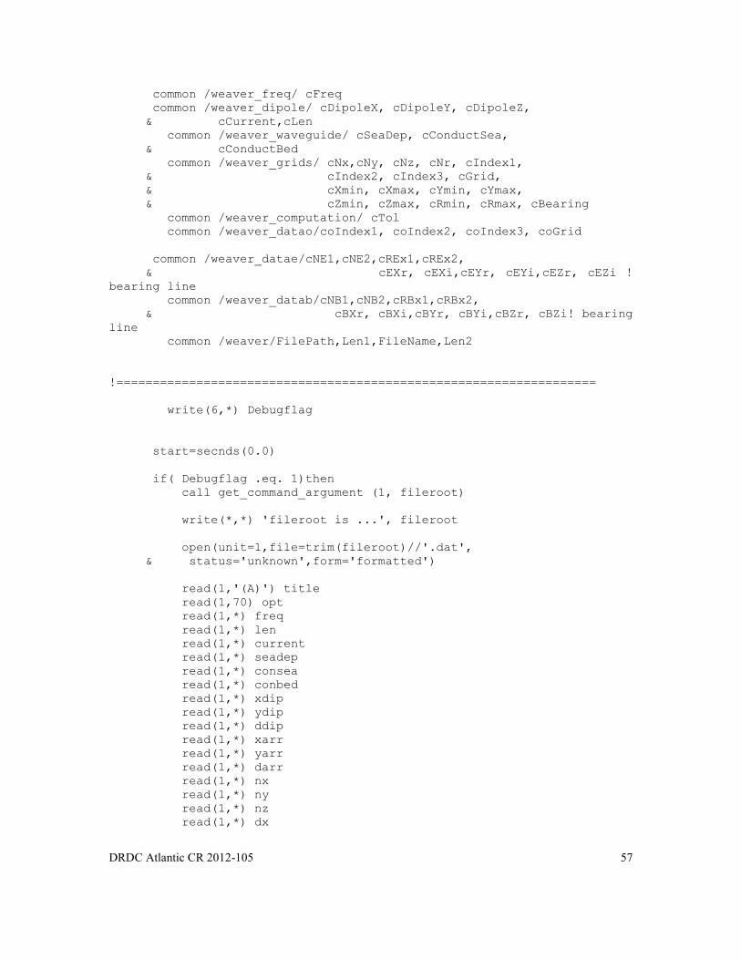
DRDC Atlantic CR 2012-105 57
common /weaver_freq/ cFreq
common /weaver_dipole/ cDipoleX, cDipoleY, cDipoleZ,
& cCurrent,cLen
common /weaver_waveguide/ cSeaDep, cConductSea,
& cConductBed
common /weaver_grids/ cNx,cNy, cNz, cNr, cIndex1,
& cIndex2, cIndex3, cGrid,
& cXmin, cXmax, cYmin, cYmax,
& cZmin, cZmax, cRmin, cRmax, cBearing
common /weaver_computation/ cTol
common /weaver_datao/coIndex1, coIndex2, coIndex3, coGrid
common /weaver_datae/cNE1,cNE2,cREx1,cREx2,
& cEXr, cEXi,cEYr, cEYi,cEZr, cEZi !
bearing line
common /weaver_datab/cNB1,cNB2,cRBx1,cRBx2,
& cBXr, cBXi,cBYr, cBYi,cBZr, cBZi! bearing
line
common /weaver/FilePath,Len1,FileName,Len2
!==================================================================
write(6,*) Debugflag
start=secnds(0.0)
if( Debugflag .eq. 1)then
call get_command_argument (1, fileroot)
write(*,*) 'fileroot is ...', fileroot
open(unit=1,file=trim(fileroot)//'.dat',
& status='unknown',form='formatted')
read(1,'(A)') title
read(1,70) opt
read(1,*) freq
read(1,*) len
read(1,*) current
read(1,*) seadep
read(1,*) consea
read(1,*) conbed
read(1,*) xdip
read(1,*) ydip
read(1,*) ddip
read(1,*) xarr
read(1,*) yarr
read(1,*) darr
read(1,*) nx
read(1,*) ny
read(1,*) nz
read(1,*) dx
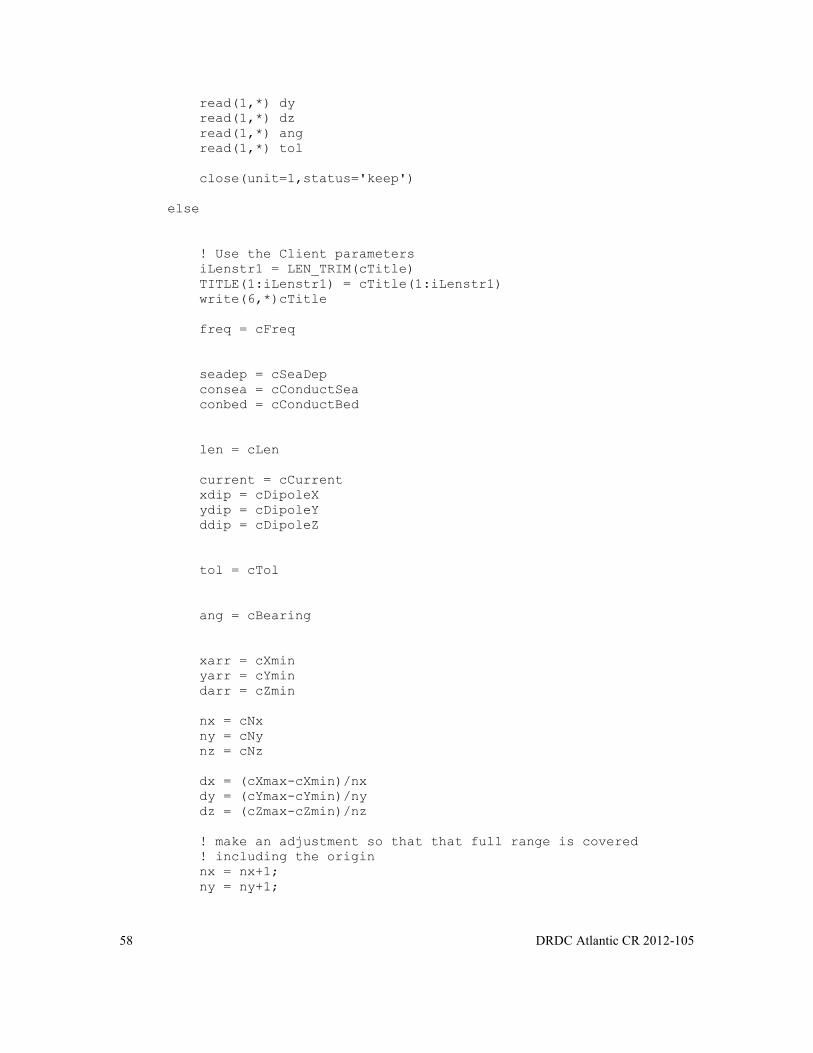
58 DRDC Atlantic CR 2012-105
read(1,*) dy
read(1,*) dz
read(1,*) ang
read(1,*) tol
close(unit=1,status='keep')
else
! Use the Client parameters
iLenstr1 = LEN_TRIM(cTitle)
TITLE(1:iLenstr1) = cTitle(1:iLenstr1)
write(6,*)cTitle
freq = cFreq
seadep = cSeaDep
consea = cConductSea
conbed = cConductBed
len = cLen
current = cCurrent
xdip = cDipoleX
ydip = cDipoleY
ddip = cDipoleZ
tol = cTol
ang = cBearing
xarr = cXmin
yarr = cYmin
darr = cZmin
nx = cNx
ny = cNy
nz = cNz
dx = (cXmax-cXmin)/nx
dy = (cYmax-cYmin)/ny
dz = (cZmax-cZmin)/nz
! make an adjustment so that that full range is covered
! including the origin
nx = nx+1;
ny = ny+1;

DRDC Atlantic CR 2012-105 59
write(cOpt1,'(i1)')cIndex1
write(cOpt2,'(i1)')cIndex2
write(cOpt3,'(i1)')cIndex3
opt(1:1) = cOpt1
opt(2:2) = cOpt2
opt(3:3) = cOpt3
coIndex1 = cIndex1
coIndex2 = cIndex2
coIndex3 = cIndex3
coGrid = cGrid
endif
pi=4.*atan(1.)
mu0=4.*pi*1e-7
omega=2.*pi*freq
skdpth=sqrt(2./(mu0*omega*consea))
if( Debugflag .eq. 1 )then
open(unit=2,file=trim(fileroot)//'.xyz',
& status='unknown',form='formatted')
write(2,'(A)') title
write(2,70) opt
write(2,80) freq, len, current
write(2,80) seadep, consea, conbed
write(2,80) xdip, ydip, ddip
write(2,80) xarr, yarr, darr
write(2,80) dx, dy, dz
write(2,85) nx, ny, nz
write(2,90) ang, tol
write(2,100)
write(2,110)
endif
if (opt .EQ. '000') then
n1=nx
n2=1
x10=xarr
x20=yarr
dx1=dx*cos(ang*pi/180.)
dx2=dx*sin(ang*pi/180.)
else if (opt .EQ. '100') then
n1=nx
n2=1
x10=xarr
x20=yarr
dx1=dx

60 DRDC Atlantic CR 2012-105
dx2=dy
else if (opt .EQ. '010') then
n1=ny
n2=1
x10=yarr
x20=xarr
dx1=dy
dx2=dx
else if (opt .EQ. '001') then
n1=nz
n2=1
x10=darr
x20=xarr
dx1=dz
dx2=dx
else if (opt .EQ. '110') then
n1=nx
n2=ny
x10=xarr
x20=yarr
dx1=dx
dx2=dy
else if (opt .EQ. '101') then
n1=nx
n2=nz
x10=xarr
x20=darr
dx1=dx
dx2=dz
else if (opt .EQ. '011') then
n1=ny
n2=nz
x10=yarr
x20=darr
dx1=dy
dx2=dz
cdjt else if (opt .EQ. '111') then
cdjt n1=nx
cdjt n2=nz
cdjt x10=xarr
cdjt x20=darr
cdjt dx1=sqrt(dx*dx+dy*dy)
cdjt dx2=dz
else
write(*,*) 'Invalid opt code. Abort run ...'
stop
end if
write(*,*) 'Starting DRDCHED: n1=',n1,' & n2=', n2
cNE1 = n1

DRDC Atlantic CR 2012-105 61
cNE2 = n2
cNB1 = n1
cNB2 = n2
do j=1,n2
x2(j)=x20+float(j-1)*dx2
cREx2(j) = x2(j)
cRBx2(j) = x2(j)
if (mod(j,10) .EQ. 0) then
write(*,*) '% Done ...', 100.*float(j)/float(n2)
end if
do i=1,n1
x1(i)=x10+float(i-1)*dx1
cREx1(i) = x1(i)
cRBx1(i) = x1(i)
if (opt .EQ. '000') then
x2(i)=x20+float(i-1)*dx2
cREx2(i) = x2(i)
cRBx2(i) = x2(i)
xarr=x1(i)
yarr=x2(i)
else if (opt .EQ. '100') then
xarr=x1(i)
yarr=x2(j)
else if (opt .EQ. '010') then
xarr=x2(j)
yarr=x1(i)
else if (opt .EQ. '001') then
xarr=x2(j)
darr=x1(i)
else if (opt .EQ. '110') then
xarr=x1(i)
yarr=x2(j)
else if (opt .EQ. '101') then
xarr=x1(i)
darr=x2(j)
else if (opt .EQ. '011') then
yarr=x1(i)
darr=x2(j)
end if
call ac_weaver( seadep, consea, conbed,
& xdip, ydip, ddip, xarr, yarr, darr,
& len, freq, current, tol,
& euRe, euIm, evRe, evIm, ezRe, ezIm,
& buRe, buIm, bvRe, bvIm, bzRe, bzIm )

62 DRDC Atlantic CR 2012-105
write(*,*)euRe
write(*,*)euIm
write(*,*)evRe
write(*,*)evIm
write(*,*)ezRe
write(*,*)ezIm
write(*,*)buRe
write(*,*)buIm
write(*,*)bvRe
write(*,*)bvIm
write(*,*)bzRe
write(*,*)bzIm
exr(i,j)=euRe
exi(i,j)=euIm
eyr(i,j)=evRe
eyi(i,j)=evIm
ezr(i,j)=ezRe
ezi(i,j)=ezIm
bxr(i,j)=buRe
bxi(i,j)=buIm
byr(i,j)=bvRe
byi(i,j)=bvIm
bzr(i,j)=bzRe
bzi(i,j)=bzIm
cEXr(i,j) = euRe
cEXi(i,j) = euIm
cEYr(i,j) = evRe
cEYi(i,j) = evIm
cEZr(i,j) = ezRe
cEZi(i,j) = ezIm
cBXr(i,j) = buRe
cBXi(i,j) = buIm
cBYr(i,j) = bvRe
cBYi(i,j) = bvIm
cBZr(i,j) = bzRe
cBZi(i,j) = bzIm
enddo
enddo
do j=1,n2
do i=1,n1
if (opt .EQ. '000') then
x2(j)=x2(i)
end if
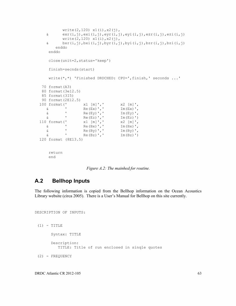
DRDC Atlantic CR 2012-105 63
write(2,120) x1(i),x2(j),
& exr(i,j),exi(i,j),eyr(i,j),eyi(i,j),ezr(i,j),ezi(i,j)
write(2,120) x1(i),x2(j),
& bxr(i,j),bxi(i,j),byr(i,j),byi(i,j),bzr(i,j),bzi(i,j)
enddo
enddo
close(unit=2,status='keep')
finish=secnds(start)
write(*,*) 'Finished DRDCHED: CPU=',finish,' seconds ...'
70 format(A3)
80 format(3e12.5)
85 format(3I5)
90 format(2E12.5)
100 format(' x1 [m]',' x2 [m]',
& ' Re(Ex)',' Im(Ex)',
& ' Re(Ey)',' Im(Ey)',
& ' Re(Ez)',' Im(Ez)')
110 format(' x1 [m]',' x2 [m]',
& ' Re(Bx)',' Im(Bx)',
& ' Re(By)',' Im(By)',
& ' Re(Bz)',' Im(Bz)')
120 format (8E13.5)
return
end
Figure A.2: The mainhed.for routine.
A.2 Bellhop Inputs
The following information is copied from the Bellhop information on the Ocean Acoustics
Library website (circa 2005). There is a User’s Manual for Bellhop on this site currently.
DESCRIPTION OF INPUTS:
(1) - TITLE
Syntax: TITLE
Description:
TITLE: Title of run enclosed in sinqle quotes
(2) - FREQUENCY
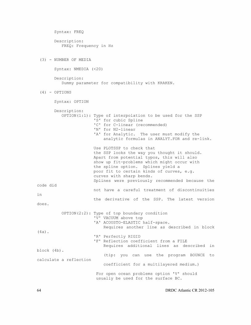
64 DRDC Atlantic CR 2012-105
Syntax: FREQ
Description:
FREQ: Frequency in Hz
(3) - NUMBER OF MEDIA
Syntax: NMEDIA (<20)
Description:
Dummy parameter for compatibility with KRAKEN.
(4) - OPTIONS
Syntax: OPTION
Description:
OPTION(1:1): Type of interpolation to be used for the SSP
'S' for cubic Spline
'C' for C-linear (recommended)
'N' for N2-linear
'A' for Analytic. The user must modify the
analytic formulas in ANALYT.FOR and re-link.
Use PLOTSSP to check that
the SSP looks the way you thought it should.
Apart from potential typos, this will also
show up fit-problems which might occur with
the spline option. Splines yield a
poor fit to certain kinds of curves, e.g.
curves with sharp bends.
Splines were previously recommended because the
code did
not have a careful treatment of discontinuities
in
the derivative of the SSP. The latest version
does.
OPTION(2:2): Type of top boundary condition
'V' VACUUM above top
'A' ACOUSTO-ELASTIC half-space.
Requires another line as described in block
(4a).
'R' Perfectly RIGID
'F' Reflection coefficient from a FILE
Requires additional lines as described in
block (4b).
(tip: you can use the program BOUNCE to
calculate a reflection
coefficient for a multilayered medium.)
For open ocean problems option 'V' should
usually be used for the surface BC.
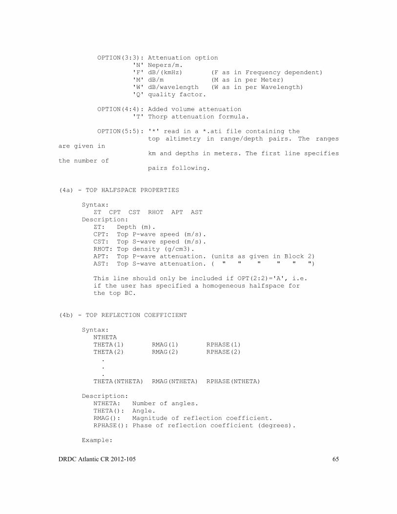
DRDC Atlantic CR 2012-105 65
OPTION(3:3): Attenuation option
'N' Nepers/m.
'F' dB/(kmHz) (F as in Frequency dependent)
'M' dB/m (M as in per Meter)
'W' dB/wavelength (W as in per Wavelength)
'Q' quality factor.
OPTION(4:4): Added volume attenuation
'T' Thorp attenuation formula.
OPTION(5:5): '*' read in a *.ati file containing the
top altimetry in range/depth pairs. The ranges
are given in
km and depths in meters. The first line specifies
the number of
pairs following.
(4a) - TOP HALFSPACE PROPERTIES
Syntax:
ZT CPT CST RHOT APT AST
Description:
ZT: Depth (m).
CPT: Top P-wave speed (m/s).
CST: Top S-wave speed (m/s).
RHOT: Top density (g/cm3).
APT: Top P-wave attenuation. (units as given in Block 2)
AST: Top S-wave attenuation. ( " " " " " ")
This line should only be included if OPT(2:2)='A', i.e.
if the user has specified a homogeneous halfspace for
the top BC.
(4b) - TOP REFLECTION COEFFICIENT
Syntax:
NTHETA
THETA(1) RMAG(1) RPHASE(1)
THETA(2) RMAG(2) RPHASE(2)
.
.
.
THETA(NTHETA) RMAG(NTHETA) RPHASE(NTHETA)
Description:
NTHETA: Number of angles.
THETA(): Angle.
RMAG(): Magnitude of reflection coefficient.
RPHASE(): Phase of reflection coefficient (degrees).
Example:
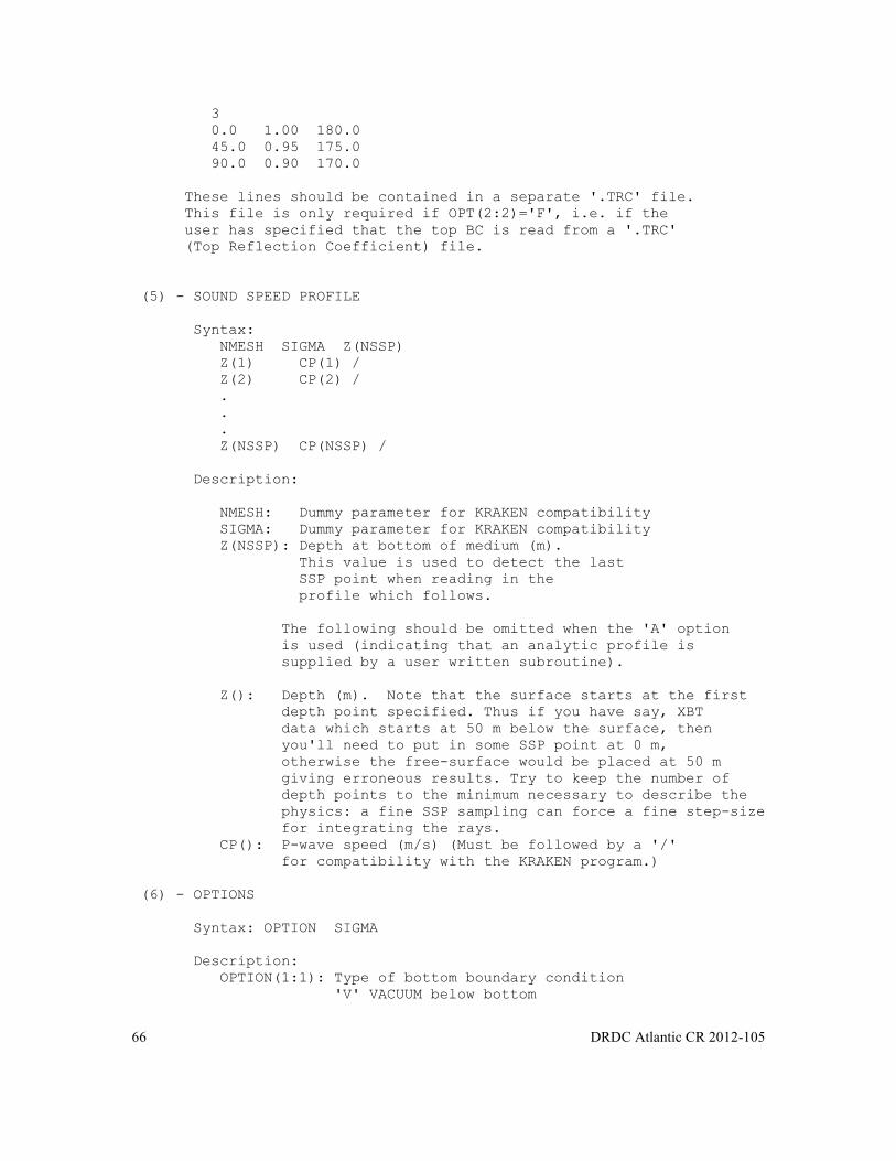
66 DRDC Atlantic CR 2012-105
3
0.0 1.00 180.0
45.0 0.95 175.0
90.0 0.90 170.0
These lines should be contained in a separate '.TRC' file.
This file is only required if OPT(2:2)='F', i.e. if the
user has specified that the top BC is read from a '.TRC'
(Top Reflection Coefficient) file.
(5) - SOUND SPEED PROFILE
Syntax:
NMESH SIGMA Z(NSSP)
Z(1) CP(1) /
Z(2) CP(2) /
.
.
.
Z(NSSP) CP(NSSP) /
Description:
NMESH: Dummy parameter for KRAKEN compatibility
SIGMA: Dummy parameter for KRAKEN compatibility
Z(NSSP): Depth at bottom of medium (m).
This value is used to detect the last
SSP point when reading in the
profile which follows.
The following should be omitted when the 'A' option
is used (indicating that an analytic profile is
supplied by a user written subroutine).
Z(): Depth (m). Note that the surface starts at the first
depth point specified. Thus if you have say, XBT
data which starts at 50 m below the surface, then
you'll need to put in some SSP point at 0 m,
otherwise the free-surface would be placed at 50 m
giving erroneous results. Try to keep the number of
depth points to the minimum necessary to describe the
physics: a fine SSP sampling can force a fine step-size
for integrating the rays.
CP(): P-wave speed (m/s) (Must be followed by a '/'
for compatibility with the KRAKEN program.)
(6) - OPTIONS
Syntax: OPTION SIGMA
Description:
OPTION(1:1): Type of bottom boundary condition
'V' VACUUM below bottom
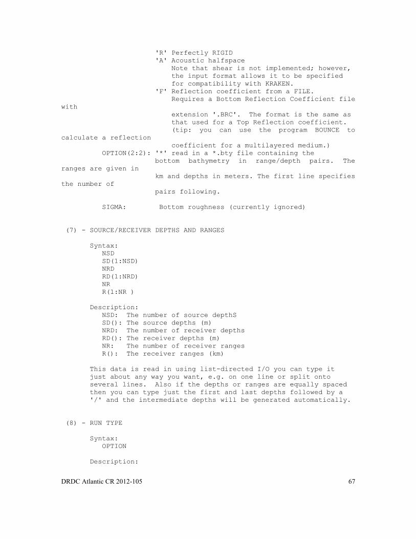
DRDC Atlantic CR 2012-105 67
'R' Perfectly RIGID
'A' Acoustic halfspace
Note that shear is not implemented; however,
the input format allows it to be specified
for compatibility with KRAKEN.
'F' Reflection coefficient from a FILE.
Requires a Bottom Reflection Coefficient file
with
extension '.BRC'. The format is the same as
that used for a Top Reflection coefficient.
(tip: you can use the program BOUNCE to
calculate a reflection
coefficient for a multilayered medium.)
OPTION(2:2): '*' read in a *.bty file containing the
bottom bathymetry in range/depth pairs. The
ranges are given in
km and depths in meters. The first line specifies
the number of
pairs following.
SIGMA: Bottom roughness (currently ignored)
(7) - SOURCE/RECEIVER DEPTHS AND RANGES
Syntax:
NSD
SD(1:NSD)
NRD
RD(1:NRD)
NR
R(1:NR )
Description:
NSD: The number of source depthS
SD(): The source depths (m)
NRD: The number of receiver depths
RD(): The receiver depths (m)
NR: The number of receiver ranges
R(): The receiver ranges (km)
This data is read in using list-directed I/O you can type it
just about any way you want, e.g. on one line or split onto
several lines. Also if the depths or ranges are equally spaced
then you can type just the first and last depths followed by a
'/' and the intermediate depths will be generated automatically.
(8) - RUN TYPE
Syntax:
OPTION
Description:
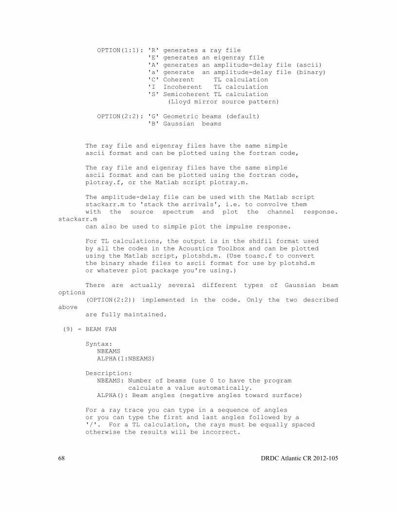
68 DRDC Atlantic CR 2012-105
OPTION(1:1): 'R' generates a ray file
'E' generates an eigenray file
'A' generates an amplitude-delay file (ascii)
'a' generate an amplitude-delay file (binary)
'C' Coherent TL calculation
'I Incoherent TL calculation
'S' Semicoherent TL calculation
(Lloyd mirror source pattern)
OPTION(2:2): 'G' Geometric beams (default)
'B' Gaussian beams
The ray file and eigenray files have the same simple
ascii format and can be plotted using the fortran code,
The ray file and eigenray files have the same simple
ascii format and can be plotted using the fortran code,
plotray.f, or the Matlab script plotray.m.
The amplitude-delay file can be used with the Matlab script
stackarr.m to 'stack the arrivals', i.e. to convolve them
with the source spectrum and plot the channel response.
stackarr.m
can also be used to simple plot the impulse response.
For TL calculations, the output is in the shdfil format used
by all the codes in the Acoustics Toolbox and can be plotted
using the Matlab script, plotshd.m. (Use toasc.f to convert
the binary shade files to ascii format for use by plotshd.m
or whatever plot package you're using.)
There are actually several different types of Gaussian beam
options
(OPTION(2:2)) implemented in the code. Only the two described
above
are fully maintained.
(9) - BEAM FAN
Syntax:
NBEAMS
ALPHA(1:NBEAMS)
Description:
NBEAMS: Number of beams (use 0 to have the program
calculate a value automatically.
ALPHA(): Beam angles (negative angles toward surface)
For a ray trace you can type in a sequence of angles
or you can type the first and last angles followed by a
'/'. For a TL calculation, the rays must be equally spaced
otherwise the results will be incorrect.
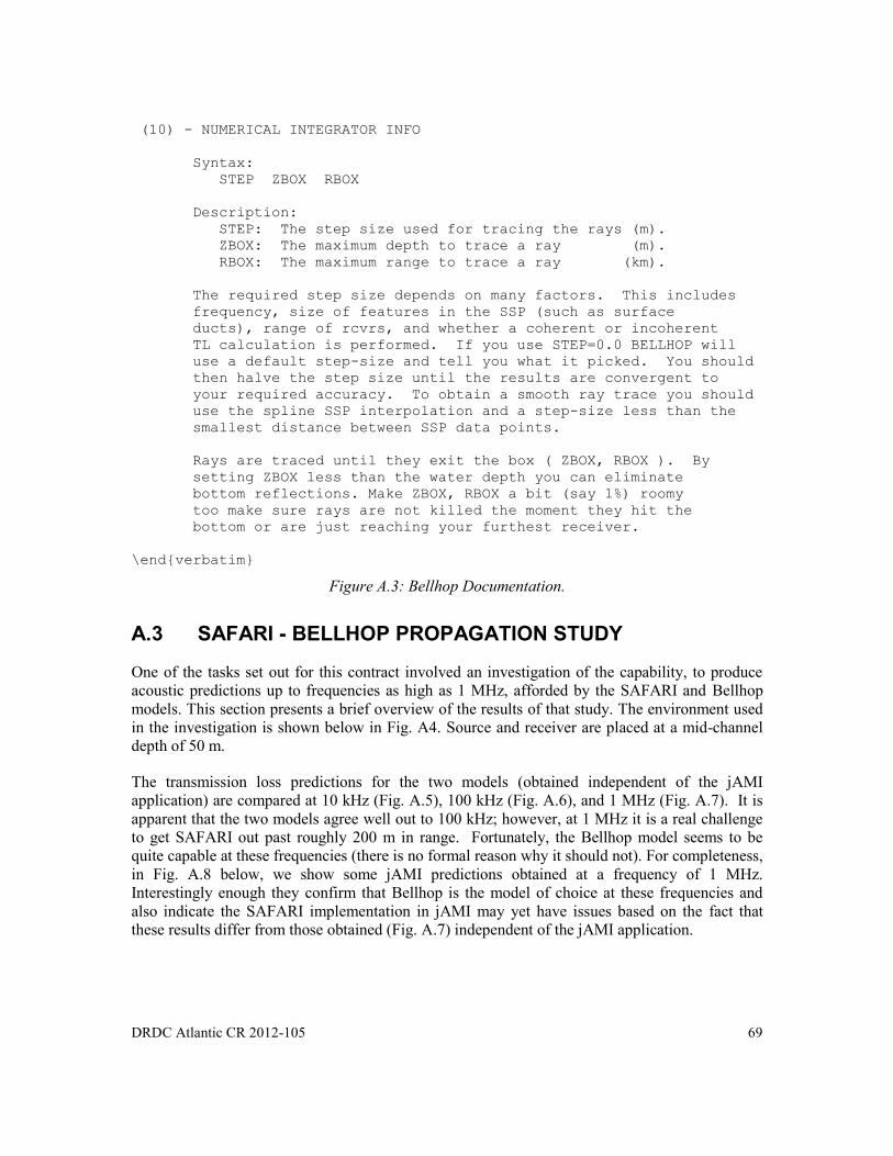
DRDC Atlantic CR 2012-105 69
(10) - NUMERICAL INTEGRATOR INFO
Syntax:
STEP ZBOX RBOX
Description:
STEP: The step size used for tracing the rays (m).
ZBOX: The maximum depth to trace a ray (m).
RBOX: The maximum range to trace a ray (km).
The required step size depends on many factors. This includes
frequency, size of features in the SSP (such as surface
ducts), range of rcvrs, and whether a coherent or incoherent
TL calculation is performed. If you use STEP=0.0 BELLHOP will
use a default step-size and tell you what it picked. You should
then halve the step size until the results are convergent to
your required accuracy. To obtain a smooth ray trace you should
use the spline SSP interpolation and a step-size less than the
smallest distance between SSP data points.
Rays are traced until they exit the box ( ZBOX, RBOX ). By
setting ZBOX less than the water depth you can eliminate
bottom reflections. Make ZBOX, RBOX a bit (say 1%) roomy
too make sure rays are not killed the moment they hit the
bottom or are just reaching your furthest receiver.
\end{verbatim}
Figure A.3: Bellhop Documentation.
A.3 SAFARI - BELLHOP PROPAGATION STUDY
One of the tasks set out for this contract involved an investigation of the capability, to produce
acoustic predictions up to frequencies as high as 1 MHz, afforded by the SAFARI and Bellhop
models. This section presents a brief overview of the results of that study. The environment used
in the investigation is shown below in Fig. A4. Source and receiver are placed at a mid-channel
depth of 50 m.
The transmission loss predictions for the two models (obtained independent of the jAMI
application) are compared at 10 kHz (Fig. A.5), 100 kHz (Fig. A.6), and 1 MHz (Fig. A.7). It is
apparent that the two models agree well out to 100 kHz; however, at 1 MHz it is a real challenge
to get SAFARI out past roughly 200 m in range. Fortunately, the Bellhop model seems to be
quite capable at these frequencies (there is no formal reason why it should not). For completeness,
in Fig. A.8 below, we show some jAMI predictions obtained at a frequency of 1 MHz.
Interestingly enough they confirm that Bellhop is the model of choice at these frequencies and
also indicate the SAFARI implementation in jAMI may yet have issues based on the fact that
these results differ from those obtained (Fig. A.7) independent of the jAMI application.
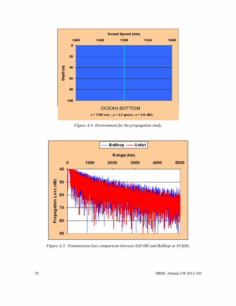
70 DRDC Atlantic CR 2012-105
Figure A.4: Environment for the propagation study.
Figure A.5: Transmission loss comparison between SAFARI and Bellhop at 10 KHz.

DRDC Atlantic CR 2012-105 71
Figure A.6: Transmission loss comparison between SAFARI and Bellhop at 100 KHz.
Figure A.7: Transmission loss comparison between SAFARI and Bellhop at 1 MHz.

72 DRDC Atlantic CR 2012-105
Figure A.8: jAMI predictions for SAFARI and Bellhop at 1 MHz.
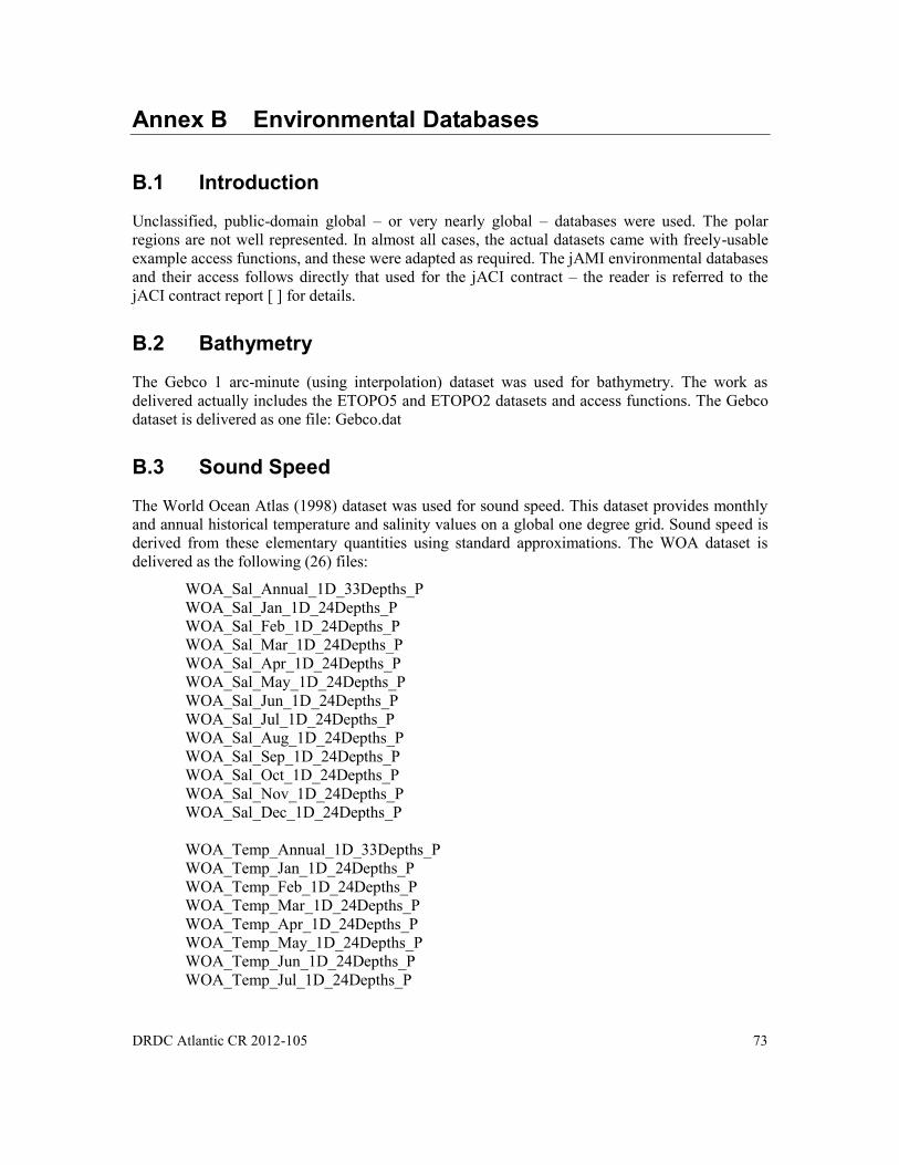
DRDC Atlantic CR 2012-105 73
Annex B Environmental Databases
B.1 Introduction
Unclassified, public-domain global – or very nearly global – databases were used. The polar
regions are not well represented. In almost all cases, the actual datasets came with freely-usable
example access functions, and these were adapted as required. The jAMI environmental databases
and their access follows directly that used for the jACI contract – the reader is referred to the
jACI contract report [ ] for details.
B.2 Bathymetry
The Gebco 1 arc-minute (using interpolation) dataset was used for bathymetry. The work as
delivered actually includes the ETOPO5 and ETOPO2 datasets and access functions. The Gebco
dataset is delivered as one file: Gebco.dat
B.3 Sound Speed
The World Ocean Atlas (1998) dataset was used for sound speed. This dataset provides monthly
and annual historical temperature and salinity values on a global one degree grid. Sound speed is
derived from these elementary quantities using standard approximations. The WOA dataset is
delivered as the following (26) files:
WOA_Sal_Annual_1D_33Depths_P
WOA_Sal_Jan_1D_24Depths_P
WOA_Sal_Feb_1D_24Depths_P
WOA_Sal_Mar_1D_24Depths_P
WOA_Sal_Apr_1D_24Depths_P
WOA_Sal_May_1D_24Depths_P
WOA_Sal_Jun_1D_24Depths_P
WOA_Sal_Jul_1D_24Depths_P
WOA_Sal_Aug_1D_24Depths_P
WOA_Sal_Sep_1D_24Depths_P
WOA_Sal_Oct_1D_24Depths_P
WOA_Sal_Nov_1D_24Depths_P
WOA_Sal_Dec_1D_24Depths_P
WOA_Temp_Annual_1D_33Depths_P
WOA_Temp_Jan_1D_24Depths_P
WOA_Temp_Feb_1D_24Depths_P
WOA_Temp_Mar_1D_24Depths_P
WOA_Temp_Apr_1D_24Depths_P
WOA_Temp_May_1D_24Depths_P
WOA_Temp_Jun_1D_24Depths_P
WOA_Temp_Jul_1D_24Depths_P

74 DRDC Atlantic CR 2012-105
WOA_Temp_Aug_1D_24Depths_P
WOA_Temp_Sep_1D_24Depths_P
WOA_Temp_Oct_1D_24Depths_P
WOA_Temp_Nov_1D_24Depths_P
WOA_Temp_Dec_1D_24Depths_P
B.4 Bottom Data
The USN Deck41 dataset was used to create the bottom type database. This dataset is the result of
a global but irregularly-sampled bottom survey by the USN in the 1960s. There is one major
lacuna in the vicinity of the South China Sea. The original Deck41 data have been converted to an
APL/UW bottom type [20] at each sample point. A demanded latitude and longitude is resolved
to the nearest (actual) neighbour sample.
The bottom is presented to the clutter model as two variable-thickness, variable-type layers.
However, the first layer is presently fixed at 50m in thickness – i.e. pending the use of a global
sediment thickness database. The second or bottom layer is presently fixed to rock and a
thickness of 500m. This dataset is delivered as a single file: Deck41APLUW.dat.
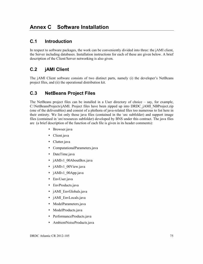
DRDC Atlantic CR 2012-105 75
Annex C Software Installation
C.1 Introduction
In respect to software packages, the work can be conveniently divided into three: the jAMI client,
the Server including databases. Installation instructions for each of these are given below. A brief
description of the Client/Server networking is also given.
C.2 jAMI Client
The jAMI Client software consists of two distinct parts, namely (i) the developer’s NetBeans
project files, and (ii) the operational distribution kit.
C.3 NetBeans Project Files
The NetBeans project files can be installed in a User directory of choice – say, for example,
C:\NetBeansProjects\jAMI. Project files have been zipped up into DRDC_jAMI_NBProject.zip
(one of the deliverables) and consist of a plethora of java-related files too numerous to list here in
their entirety. We list only those java files (contained in the \src subfolder) and support image
files (contained in \src\resources subfolder) developed by BNS under this contract. The java files
are (a brief description of the function of each file is given in its header comments):
Browser.java
Client.java
Clutter.java
ComputationalParameters.java
DateTime.java
jAMIv1_00AboutBox.java
jAMIv1_00View.java
jAMIv1_00App.java
EnvUser.java
EnvProducts.java
jAMI_EnvGlobals.java
jAMI_EnvLocals.java
ModelParameters.java
ModelProducts.java
PerformanceProducts.java
AmbientNoiseProducts.java

76 DRDC Atlantic CR 2012-105
TLProducts.java
PlotversusR.java
PlotversusRPhi.java
PlotversusRZ.java
PlotversusZ.java
RxSensors.java
ServerSpecification.java
Targets.java
TxSensors.java
jRay.java
Model_DRDCModes.java
Model_Bellhop.java
Model_BellhopGlobals.java
Model_BellhopLocals.java
Model_Pecan.java
Model_PecanGlobals.java
Model_PecanLocals.java
Model_Safari.java
Model_SafariGlobals.java
Model_SafariLocals.java
Model_Popp.java
Model_PoppGlobals.java
Model_PoppLocals.java
Model_Weaver.java
Model_WeaverGlobals.java
Model_WeaverLocals.java
and image files (required to support the visual appearance of the application):
ModesIcon.jpg
ColorField3.jpg
DiskBlackc.jpg
FileFolderWhiteonBlacka.jpg
VolcanoIcon.jpg

DRDC Atlantic CR 2012-105 77
BeamsIcon.jpg
jAMIAbout1.jpg
jAMIYellow1.jpg
BathyLightIcon.jpg
SSPIcon.jpg
BottomIcon.jpg
SurfaceRvbIcon.jpg
VolumeRvbIcon.jpg
BottomReverbIcon.jpg
RxIcon.jpg
TgtIcon.jpg
TxIcon.jpg
rvsZ1Icon.jpg
fvsZ1Icon.jpg
fvsR2Icon.jpg
rvsPhiIcon.jpg .
The above files will be placed appropriately by ‘unzipping’ DRDC_jAMI_NBProject.zip. Note,
the NetBeans project also requires that Server.exe, jAMI_IconWhite.jpg, and jAMI_Tutorial.htm
be in the top level directory of the project i.e., in C:\NetBeansProjects\jAMI as per above (these
three files should automatically be placed appropriately by the unzip procedure).
With the files so-installed, the jAMI application should be able to executed completely within the
NetBeans IDE. Note, the jAMI_Tutorial.htm and associated files are to be installed with the
operational kit discussed below and so-installed can be accessed directly from the NetBeans IDE
by entering the appropriate directory path on the Server Specification screen at the outset i.e., the
tutorial files need only be installed in one place and can then accessed from either the developers
environment or the operational environment.
C.3.1 Operational Distribution Kit
The operational distribution kit assumes that the User does not intend to utilize the
NetBeans IDE. To support this option, we have zipped up the appropriate files into
DRDC_jACI_OperationalKit.zip (also one of the deliverables for this contract). The
DRDC_jACI_OperationalKit.zip contains the \dist folder from the NetBeans project discussed
above. The zip file also contains Server.exe, jAMI_IconWhite.jpg, and jAMI_Tutorial.htm. The
zip file should be unzipped to a User directory of choise – say, C:\jACI_Operational for example.
When unzipped the directory structure should look like:
C:\jAMI_Operational
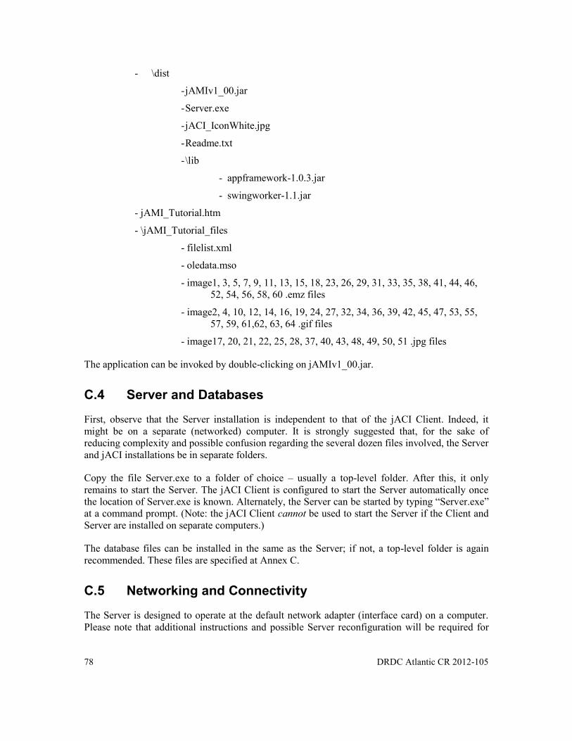
78 DRDC Atlantic CR 2012-105
- \dist
- jAMIv1_00.jar
- Server.exe
- jACI_IconWhite.jpg
- Readme.txt
- \lib
- appframework-1.0.3.jar
- swingworker-1.1.jar
- jAMI_Tutorial.htm
- \jAMI_Tutorial_files
- filelist.xml
- oledata.mso
- image1, 3, 5, 7, 9, 11, 13, 15, 18, 23, 26, 29, 31, 33, 35, 38, 41, 44, 46,
52, 54, 56, 58, 60 .emz files
- image2, 4, 10, 12, 14, 16, 19, 24, 27, 32, 34, 36, 39, 42, 45, 47, 53, 55,
57, 59, 61,62, 63, 64 .gif files
- image17, 20, 21, 22, 25, 28, 37, 40, 43, 48, 49, 50, 51 .jpg files
The application can be invoked by double-clicking on jAMIv1_00.jar.
C.4 Server and Databases
First, observe that the Server installation is independent to that of the jACI Client. Indeed, it
might be on a separate (networked) computer. It is strongly suggested that, for the sake of
reducing complexity and possible confusion regarding the several dozen files involved, the Server
and jACI installations be in separate folders.
Copy the file Server.exe to a folder of choice – usually a top-level folder. After this, it only
remains to start the Server. The jACI Client is configured to start the Server automatically once
the location of Server.exe is known. Alternately, the Server can be started by typing “Server.exe”
at a command prompt. (Note: the jACI Client cannot be used to start the Server if the Client and
Server are installed on separate computers.)
The database files can be installed in the same as the Server; if not, a top-level folder is again
recommended. These files are specified at Annex C.
C.5 Networking and Connectivity
The Server is designed to operate at the default network adapter (interface card) on a computer.
Please note that additional instructions and possible Server reconfiguration will be required for

DRDC Atlantic CR 2012-105 79
installation on a computer with two or more network cards. In the short term, therefore, the Server
should be installed only of computers with a single network adapter.
The Server must be given a TCP/IP port number to use, and also the location of the database files.
This information can be supplied in two ways. The preferred way is to use the command line in
the invocation of the Server, thus:
Server.exe 2004 “c:\databases”
invokes the Server to run at port 2004 and look for the database files in the folder c:\databases.
Note that the database folder should be enclosed in double quotes. If the Server fails to detect a
command line of the above form, then it will prompt for the port number and database folder.
The jACI client is configured to start the Server with a command line per above. The jACI Client
must coordinate its port number with the Server – i.e. these must be identical. The jACI Client
must also be configured with the IP address of the Server. If the Client and Server and installed
on the same computer, the so-called loopback address – valid for all computers with a network
adapter – of 127.0.0.1 can be used.

80 DRDC Atlantic CR 2012-105
This page intentionally left blank.
DRDC Atlantic CR 2012-105 81
List of symbols/abbreviations/acronyms/initialisms
2D Two dimensional
3D Three dimensional
ACL Acoustic Clutter Library
API Application Programmers Interface
APL/UW Applied Physics Laboratory, University of Washington
BNS Brooke Numerical Services
C Programming language
C++ Programming language
COTS Commercial Off The Shelf
Deck41 Bottom type database
DRDC Defence Research & Development Canada
EMM Environmental Model Manager
ETOPO2 Bathymetric database
ETOPO5 Bathymetric database
FORTRAN Programming language
GD Canada General Dynamics Canada Ltd.
Gebco Bathymetric database
Gnu Software compiler
GUI Graphical User Interface
HLA Horizontal Line Array
IDL Interactive Data Language
Java Programming language
jACI java Acoustic Clutter Interface
Matlab Programming and display application
NOGRP DRDC Reverberation modelling software
PC Personal Computer
PE Parabolic Equation
PLEIADES DRDC Advanced sonar concept demonstrator
POPP DRDC Propagation modelling software
PROLOS DRDC Propagation modelling software

82 DRDC Atlantic CR 2012-105
OGOPOGO DRDC Reverberation modelling software
OModes DRDC Normal modes modelling software
OS Operating System
SA Scientific Authority
SAFARI Propagation modelling software
STB System Test Bed
TCP/IP Transmission Control Protocol/Internet Protocol
TL Transmission Loss
ULGG Universal Linearized Geo-Grid
USN US Navy
WOA World Oceanographic Atlas
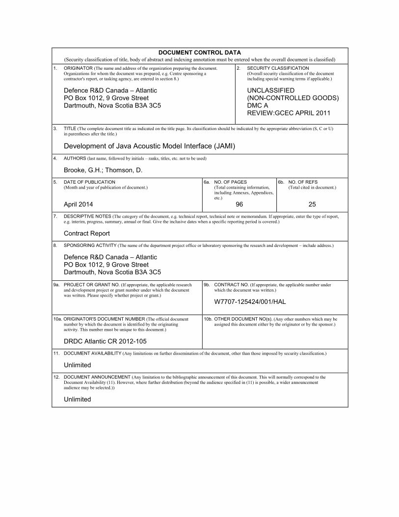
DOCUMENT CONTROL DATA (Security classification of title, body of abstract and indexing annotation must be entered when the overall document is classified)
1. ORIGINATOR (The name and address of the organization preparing the document.
Organizations for whom the document was prepared, e.g. Centre sponsoring a
contractor's report, or tasking agency, are entered in section 8.)
Defence R&D Canada – Atlantic PO Box 1012, 9 Grove Street Dartmouth, Nova Scotia B3A 3C5
2. SECURITY CLASSIFICATION (Overall security classification of the document
including special warning terms if applicable.)
UNCLASSIFIED (NON-CONTROLLED GOODS) DMC A REVIEW:GCEC APRIL 2011
3. TITLE (The complete document title as indicated on the title page. Its classification should be indicated by the appropriate abbreviation (S, C or U)
in parentheses after the title.)
Development of Java Acoustic Model Interface (JAMI)
4. AUTHORS (last name, followed by initials – ranks, titles, etc. not to be used)
Brooke, G.H.; Thomson, D.
5. DATE OF PUBLICATION
(Month and year of publication of document.)
April 2014
6a. NO. OF PAGES
(Total containing information,
including Annexes, Appendices,
etc.)
96
6b. NO. OF REFS
(Total cited in document.)
25
7. DESCRIPTIVE NOTES (The category of the document, e.g. technical report, technical note or memorandum. If appropriate, enter the type of report,
e.g. interim, progress, summary, annual or final. Give the inclusive dates when a specific reporting period is covered.)
Contract Report
8. SPONSORING ACTIVITY (The name of the department project office or laboratory sponsoring the research and development – include address.)
Defence R&D Canada – Atlantic PO Box 1012, 9 Grove Street Dartmouth, Nova Scotia B3A 3C5
9a. PROJECT OR GRANT NO. (If appropriate, the applicable research
and development project or grant number under which the document
was written. Please specify whether project or grant.)
9b. CONTRACT NO. (If appropriate, the applicable number under
which the document was written.)
W7707-125424/001/HAL
10a. ORIGINATOR'S DOCUMENT NUMBER (The official document
number by which the document is identified by the originating
activity. This number must be unique to this document.)
DRDC Atlantic CR 2012-105
10b. OTHER DOCUMENT NO(s). (Any other numbers which may be
assigned this document either by the originator or by the sponsor.)
11. DOCUMENT AVAILABILITY (Any limitations on further dissemination of the document, other than those imposed by security classification.)
Unlimited
12. DOCUMENT ANNOUNCEMENT (Any limitation to the bibliographic announcement of this document. This will normally correspond to the
Document Availability (11). However, where further distribution (beyond the audience specified in (11) is possible, a wider announcement
audience may be selected.))
Unlimited

13. ABSTRACT (A brief and factual summary of the document. It may also appear elsewhere in the body of the document itself. It is highly desirable
that the abstract of classified documents be unclassified. Each paragraph of the abstract shall begin with an indication of the security classification
of the information in the paragraph (unless the document itself is unclassified) represented as (S), (C), (R), or (U). It is not necessary to include
here abstracts in both official languages unless the text is bilingual.)
The Low Complexity Access Network (LCAN) project has a requirement for propagation
studies that involve both acoustic and electromagnetic signals. Specifically, acoustic
propagation effects associated with communication signals up to 1 MHz are to be modelled. The
electromagnetic propagation modelling is to be carried out using the ‘so-called’ Weaver model.
Also, there is a requirement for incorporation of the latest improvements in the DRDC Clutter
Model into the Java Acoustic Model Interface (JAMI) Client-Server framework.
This contract work, in part, has been designed to integrate DRDC Atlantic’s LCAN
requirements with those associated with the Clutter model through integration of both into the
JAMI application.
Le projet de réseau à accès simplifié (LCAN) a besoin d’études de propagation portant sur les
signaux acoustiques et les signaux électromagnétiques. Plus particulièrement, il faut modéliser
les effets de la propagation acoustique associés aux signaux de communication jusqu’à 1 MHz.
La modélisation de la propagation électromagnétique doit être réalisée à l’aide de ce qu’on
appelle le modèle Weaver. De plus, il faut intégrer les dernières améliorations du modèle de
fouillis de RDDC au cadre client-serveur de l’interface du modèle acoustique en Java (JAMI).
Les travaux du présent contrat visent en partie à intégrer les besoins du LCAN de
RDDC Atlantique à ceux associés au modèle de fouillis grâce à l’intégration de ces deux
modèles à l’application JAMI.
14. KEYWORDS, DESCRIPTORS or IDENTIFIERS (Technically meaningful terms or short phrases that characterize a document and could be
helpful in cataloguing the document. They should be selected so that no security classification is required. Identifiers, such as equipment model
designation, trade name, military project code name, geographic location may also be included. If possible keywords should be selected from a
published thesaurus, e.g. Thesaurus of Engineering and Scientific Terms (TEST) and that thesaurus identified. If it is not possible to select
indexing terms which are Unclassified, the classification of each should be indicated as with the title.)