Development of data-based model-free representation of non-conservative dissipative systems

International Journal of Non-Linear Mechanics 42 (2007) 99–117www.elsevier.com/locate/nlm

Development of data-based model-free representation of non-conservativedissipative systems�

Farzad Tasbihgooa, John P. Caffreyb, Sami F. Masria,∗aCivil Engineering Department, University of Southern California, Los Angeles, CA, USA

bMechanical Engineering Department, California State Polytechnic University, Pomona, CA, USA

Received 5 July 2006; received in revised form 24 July 2006; accepted 6 October 2006

Abstract

A general procedure is presented for developing data-based, non-parametric models of non-linear multi-degree-of-freedom, non-conservative,dissipative systems. Two broad classes of methods are discussed: one relying on the representation of the system restoring forces in a polynomial-basis format, and the other using artificial neural networks to map the complex transformations relating the system state variables to the neededsystem outputs. A non-linear two-degree-of-freedom system is used to formulate the approach under discussion and to generate synthetic datafor calibrating the efficiency of the two methods in capturing complex non-linear phenomena (such as dry friction, hysteresis, dead-space non-linearities, and polynomial-type non-linearities) that are widely encountered in the applied mechanics field. Subsequently, a reconfigurable testapparatus was used to generate experimental measurements from a physical non-linear “joint” involving two-dimensional motion (translationand rotation) and complicated interaction forces between the different motion axes, among its internal elements. Both the polynomial-basisapproach and the neural network method were used to develop high-fidelity, non-parametric models of the physical test article. The ability ofthe identified models to accurately “generalize” the essential features of the non-linear system was verified by comparing the predictions ofthe models with experimental measurements from data sets corresponding to different excitations than those used for identification purposes.It is shown that the identification techniques under discussion can be useful tools for developing accurate simulation models of complexmulti-dimensional non-linear systems under broadband excitation.� 2007 Elsevier Ltd. All rights reserved.

Keywords: Non-linear; Identification; Modeling; Non-parametric; Hysteresis; Friction; Experimental; Data-based; Joints

1. Introduction

1.1. Background and motivation

The modeling and identification of non-linear non-conservative dissipative systems is a task that occurs frequentlywhen dealing with problems that arise in the active control ofstructures, aircraft flutter, ships in motion, etc. This is a chal-lenging problem that has been studied by many researchersin the past several decades [1–8]. The conventional method-ology of modeling non-conservative dissipative systems, is by

� Special issue on non-conservative dissipative systems.∗ Corresponding author. Tel.: +1 213 740 0602; fax: +1 213 740 3984.

E-mail addresses: [email protected] (F. Tasbihgoo),[email protected] (J.P. Caffrey), [email protected] (S.F. Masri).

0020-7462/$ - see front matter � 2007 Elsevier Ltd. All rights reserved.doi:10.1016/j.ijnonlinmec.2006.10.021

representing the underlying non-linear dynamics of the systemwith a parametric model whose unknown parameters reflect thecharacteristics of the physical system. In general, this is quite achallenging approach, and usually the derived parametric mod-els are constrained by the assumptions embedded in the selec-tion of the model class to be identified [9–11].

In this study, a fairly recent modeling technique, based ondata-based non-parametric system identification, is presentedfor modeling non-conservative systems with generic non-lineardissipative “joint” elements. The “joint” elements, in this study,are representatives of a class of dynamical systems with non-linear characteristics such as dissipative damping, hysteresis,gaps, etc., which are typical of problems that arise in the dy-namics of large-scale civil structures with energy dissipatingdevices, aerospace structures incorporating joints, systems withdamaged elements, etc. [12–17].

http://www.elsevier.com/locate/nlm

mailto:[email protected]



100 F. Tasbihgoo et al. / International Journal of Non-Linear Mechanics 42 (2007) 99–117

Two of the promising non-parametric techniques have beenutilized here to model the non-conservative dissipative restor-ing forces of a non-linear “joint” element. These techniquesfit a “black-box” mathematical model to the input and outputmeasurements of the system response [18]. The first techniqueis based on a polynomial-basis model, and the second methodis based on artificial neural networks (ANNs). Both modelingtechniques have been shown to be powerful tools for modelingnon-linear dynamical system [19–24]. These models are usefulin applications where the overall fidelity of the model, in repre-senting the system, are important, such as health monitoring orcontrol applications [25–30]. Moreover, it is shown herein thatthese models can be efficiently used in computational engines[31], for an accurate prediction and estimation of the non-linearresponse of the system to broadband excitations.

The non-parametric modeling techniques presented in thisstudy have been a subject of research by many investigators;however, there are few reported studies concerning the mod-eling of the non-linear dissipative behavior of multi-degree-of-freedom (MDOF) systems through hybrid experimental andanalytical studies, which is an essential step in understandingthe actual characteristics and behavior of non-linear MDOF

dynamical systems [32,9].

1.2. Scope

This study proceeds along two fronts: (1) an analytical phasefocused on the development of a theoretical framework for pro-cessing experimental structural response measurements fromuncertain systems, to develop and evaluate the utility of somepromising analytical tools, based on polynomial basis modelsand neural networks, for developing reduced-order, data-basedcomputational representations of non-linear dynamic systems,and (2) an experimental phase involved in the design and fabri-cation of an adjustable test apparatus for conducting studies ona generic two-dimensional “joint” element which incorporatesimportant non-linear characteristics such as non-linear elas-tic properties, hysteretic characteristics, and dead-space non-linearities involving friction.

The paper is organized as follows: Section 2 presentsthe mathematical background and formulation of data-basedmodel-free representations of a non-linear dissipative 2DOF

system based on a polynomial basis model and neural net-works, Section 3 presents the simulation studies, Section 4details the experimental test setup, Section 5 demonstratesthe application of the methodology through experimental datasets, Section 6 discuss the results, and concluding remarks arecontained in Section 7.

2. Formulation of data-based model-free representationsof non-linear element

2.1. Equation of motion

Consider a discrete n-degrees-of-freedom (nDOF) system in-corporating non-linear non-conservative dissipative elements,which is subjected to directly applied excitation forces F(t).

The motion of this non-linear system is assumed to be governedby the set of equations,

Mx(t) + R(x, x, p) = F(t), (1)

where x(t) is the displacement vector of order n, M is a constantmatrix that characterizes the inertia forces, R(x, x, p) is therestoring force vector of non-linear non-conservative forces, p

is the vector of system-specific parameters, and F(t) is the n-column vector of directly applied forces.

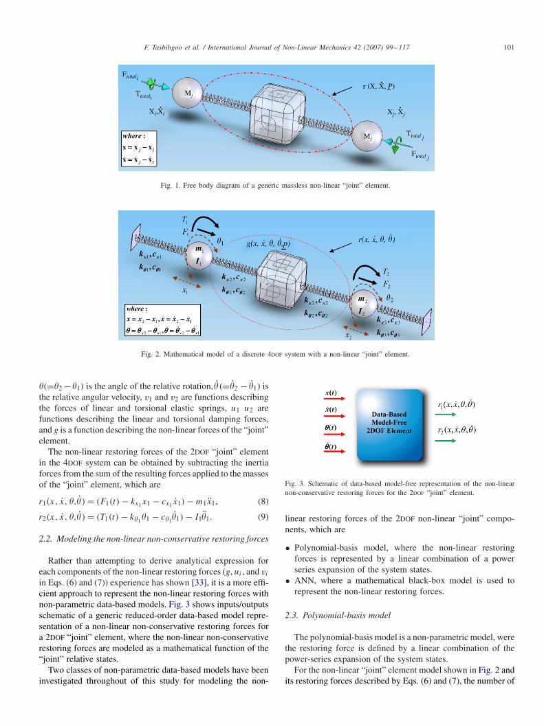
The non-linear non-conservative components, in this study,are presented as massless non-linear “joint” elements, that arelocated between two lumped masses of the system. Fig. 1 showsthe free body diagram of a massless non-linear “joint” elementthat is located between DOF-i and -j, with constant mass matri-ces of Mi and Mj that characterizes the inertia forces; xi , xi , xj ,and xj which are the state of the DOFs; r(x, x, p) which repre-sents the restoring force vector of non-linear non-conservativeforces of the “joint” element; and Ftotali , Ftotalj ,Ttotali , and Ttotaljwhich are the sum of the resulting forces (external and inter-nal) applied to the DOFs-i and -j of the system. The non-linearrestoring force of the “joint” element shown in Fig. 1, can beobtained by subtracting the corresponding inertia forces of eachDOFs from the sum of the resulting forces applied to the “joint”element of the system.

For illustration of the methodology, consider a 4DOFs sys-tem shown in Fig. 2, where the system has two lumped masses,m1 and m2, with rotational mass moments of inertias, I1 andI2, and it is subjected to external forces F1(t) and F2(t), andtorques T1(t) and T2(t). The masses have axial motion and ro-tation about their axes, which are uncoupled. The system con-sists of linear and torsional elastic springs kx and k�, linear andtorsional viscous dampers cx and c�, and a non-linear elementg(x, x, �,�, p), where restoring force characteristics is a func-tion of the system states and set of element-specific parametersp. The non-linear element is connected to the system throughset of elastic springs.

The equations-of-motion for the 4DOFs system shown inFig. 2 are governed by

m1x1 + kx1x1 + cx1 x1 + r1(x, x, �,�) = F1(t), (2)

m2x2 + kx2x2 + cx2 x2 − r1(x, x, �,�) = F2(t), (3)

I1�1 + k�1�1 + c�1�1 + r2(x, x, �,�) = T1(t), (4)

I2�2 + k�2�2 + c�2�2 − r2(x, x, �,�) = T2(t), (5)

where x1 and x2 are the displacement of the masses, �1 and �2are the angle of rotation of the masses, and r1 and r2 are thenon-linear restoring forces.

In general, the non-linear restoring forces are functions of thesystem states, where in this example, the non-linear restoringforces of the 2DOF “joint” element are

r1(x, x, �,�) = g(x, x, �,�, p) + v1(x) + u1(x), (6)

r2(x, x, �,�) = g(x, x, �,�, p) + v2(�) + u2(�), (7)

where x(=x2 − x1) is the relative axial displacement of thetwo masses, x (=x2 − x1) is the relative linear velocity,

F. Tasbihgoo et al. / International Journal of Non-Linear Mechanics 42 (2007) 99–117 101

Fig. 1. Free body diagram of a generic massless non-linear “joint” element.

Fig. 2. Mathematical model of a discrete 4DOF system with a non-linear “joint” element.

�(=�2 −�1) is the angle of the relative rotation,�(=�2 − �1) isthe relative angular velocity, v1 and v2 are functions describingthe forces of linear and torsional elastic springs, u1 u2 arefunctions describing the linear and torsional damping forces,and g is a function describing the non-linear forces of the “joint”element.

The non-linear restoring forces of the 2DOF “joint” elementin the 4DOF system can be obtained by subtracting the inertiaforces from the sum of the resulting forces applied to the massesof the “joint” element, which are

r1(x, x, �,�) = (F1(t) − kx1x1 − cx1 x1) − m1x1, (8)

r2(x, x, �,�) = (T1(t) − k�1�1 − c�1�1) − I1�1. (9)

2.2. Modeling the non-linear non-conservative restoring forces

Rather than attempting to derive analytical expression foreach components of the non-linear restoring forces (g, ui , and vi

in Eqs. (6) and (7)) experience has shown [33], it is a more effi-cient approach to represent the non-linear restoring forces withnon-parametric data-based models. Fig. 3 shows inputs/outputsschematic of a generic reduced-order data-based model repre-sentation of a non-linear non-conservative restoring forces fora 2DOF “joint” element, where the non-linear non-conservativerestoring forces are modeled as a mathematical function of the“joint” relative states.

Two classes of non-parametric data-based models have beeninvestigated throughout of this study for modeling the non-

Fig. 3. Schematic of data-based model-free representation of the non-linearnon-conservative restoring forces for the 2DOF “joint” element.

linear restoring forces of the 2DOF non-linear “joint” compo-nents, which are

• Polynomial-basis model, where the non-linear restoringforces is represented by a linear combination of a powerseries expansion of the system states.

• ANN, where a mathematical black-box model is used torepresent the non-linear restoring forces.

2.3. Polynomial-basis model

The polynomial-basis model is a non-parametric model, werethe restoring force is defined by a linear combination of thepower-series expansion of the system states.

For the non-linear “joint” element model shown in Fig. 2 andits restoring forces described by Eqs. (6) and (7), the number of


DOFs representing the “joint” is 2 and the number of requiredstates for the models is 4. The polynomial-basis model repre-senting the non-linear restoring forces, for each DOF would be

r1(x, x, �,�, p) ≈ r1(x, x, �,�)

=m∑

i=0

n∑j=0

o∑k=0

p∑l=0

aijkl(xi xj�k�

l), (10)

r2(x, x, �,�, p) ≈ r2(x, x, �,�)

=m∑

i=0

n∑j=0

o∑k=0

p∑l=0

bijkl(xi xj�k�

l), (11)

where m, n, o, and p are integer numbers indicating the max-imum order of each state, aijkl and bijkl are the unknown co-efficients of the basis, and ri is the estimate of the non-linearrestoring force for DOF-i.

The number of unknown coefficients for the polynomial-basis model depends on the largest power of each stateand number of states. For the 2DOF polynomial-basis model(Eqs. (10) and (11)), the number of the unknown coefficientsfor each DOF is (m + 1)(n + 1)(o + 1)(p + 1). For example,if the powers m, n, o, and p are set to 3, then �(x, x) wouldconsist of 512 unknown terms (q1 and q2 each would havetotal of 256 coefficients) in the form of

r1(x, x, �,�) = a0000(x0x0�0�

0) + a0001(x

0x0�0�1)

+ · · · + a1012(x1x0�1�

2)

+ · · · + a3333(x3x3�3�

3), (12)

r2(x, x, �,�) = b0000(x0x0�0�

0) + b0001(x

0x0�0�1)

+ · · · + b2313(x2x3�1�

3)

+ · · · + b3333(x3x3�3�

3). (13)

The unknown coefficients, aijkl and bijkl , can be identified byapplying standard non-linear least-squares estimation methods[11,34] to the above equations.

2.4. ANN model

ANNs are a powerful non-parametric modeling technique,inspired by the human brain’s biological neural network archi-tecture, that one is capable of modeling and identification va-riety of complex non-linear systems [35]. The application ofneural network modeling approaches in non-linear system iden-tification and structural dynamics have been demonstrated byseveral researchers [19,36,37]. The neural network modelingapproaches are based on “black-box” mathematical modeling,without incorporating any physical characteristics of the sys-tem, and by only providing the input and output measurementsof the system. The main limitation of ANN is the absence ofthe physical characteristics of the system in the identificationmodel. For particular applications, where the physics of thesystem is not as important as the performance of the model,the ANN would be the ideal modeling technique.

Fig. 4. Schematic of the neural network architecture for modeling thenon-linear restoring forces of the coupled non-linear system shown in Fig. 2.

Fig. 5. Mathematical model of non-linear coupled 2DOF system used togenerate the synthetic data sets.

The architecture and training algorithms are two importantmeasures in modeling any system with neural networks, whichare controlled by the application type and the problem charac-teristics [38].

2.4.1. Network architectureIn the data-based modeling approach, the restoring forces of

the non-linear “joint” element (Fig. 1) are modeled as a non-linear function of the system states. Therefore, the neural net-work architecture selected for modeling the non-linear restoringforces of the 2DOF “joint” component (Fig. 2), is a multilayerfeedforward network, which is the recommended architecture,for function approximation applications, using the neural net-works [38,39].

A multilayer feedforward neural network is capable of ap-proximating any function, provided there are enough neuronsin hidden layers [40]. Moreover, it has been mathematicallyproven that a two-layer (an input layer and a hidden layer) feed-forward network with a sigmoid function in the first layer, anda linear function in the second layer, provided a sufficient num-ber of neurons is used in the hidden layer, would approximateany function [38]. The linear function of the output layer en-ables the network of generalization beyond the input range ofthe input signals, whereas the sigmoid transfer function in thehidden layer allows the network to learn the non-linear as wellas linear relation between the input and output vectors [39].

The schematic of the network architecture for modeling thenon-linear restoring forces of the non-linear 2DOF “joint” sys-


tem is shown in Fig. 4. The number of neurons in the inputlayer depends on the number of relative states in the model,whereas the number of the neurons in the output layer dependson the number of the DOFs of the “joint”.

The mathematical model of the designed two-layer feedfor-ward neural network is

{a1}l×1 = tanh([W1]l×2n1 × {P }2n1×1︸︷︷︸inputs

+{b1}l×1), (14)

{T }n1×1︸︷︷︸outputs

=[W2]n1×l × {a1}l×1 + {b2}n1×1, (15)

where {a1} is the hidden layer output, {P } = [x, x, �,� ]T is theinput vector constructed from the relative states of the “joint”,the {T } = [r1, r2]T is the output vector containing the non-linear restoring forces of the system, n1 is the number of DOFsof the non-linear “joint” element (which in this study is 2),l is the number of neurons in the hidden layer, W1 and W2are the network weights, and b1 and b2 are the networkbiases.

2.4.2. Network trainingThe backpropagation training algorithm was used to train

the neural network model (Eq. (15)), where the weights andbiases values are updated based on Levenberg–Marquardt op-timization (Bayesian regularization) method, which allows thetrained network to generalize well [38,39].

For improving the training performance, the training wasperformed in several stages [19]. First, the weights and biasesof the network were initialized with random values, then partof the data were fed to the network and trained the networkto reach a relatively high error tolerance level (the networkperformance indicator for error tolerance level was normalizedmean-square error), thereafter, the values of the weights andbiases which were obtained by the first training were used as aninitial value for the second stage of training. In the second stage,the number of training data points was increased to twice asmuch as the first training data set, with the error tolerance levelset to half of the first stage. This incremental training procedurewas repeated till all the data points were fed to the network inthe last stage. The optimum values of the weights and biases atthe end of the last stage of the training was considered as theoptimum values of the trained network.

However, there is a possibility that the obtained weights andbiases were not the global optimum values for the trained net-work with the given data sets. In order to be certain that theglobal optimum values of the network parameters have beenobtained, the incremental training procedure was repeated sev-eral times (about five repetitions) with different initial randomvalues for the network parameters. If the values of the param-eters after all the reparations remains close, then those valuesare considered as the optimum parameter values for the trainednetwork.

It is worth noting that another data manipulation procedurethat could improve the network training performance and gen-eralization capability, is to normalize the input and output data

sets, prior to the network training procedure, to have a rangeof ±1, and zero mean [38,39].

3. Simulation of a 2DOF coupled non-linear “joint”component

3.1. Mathematical model

In order to illustrate and calibrate the methods under dis-cussion, consider the example of finite element model shownin Fig. 5. This two-dimensional model (linear motion in x-axisand rotation � about the x-axis) consists of four masses mi , withmoment of inertia Imi

, i = 1, 2, 3, 4, that are interconnectedwith elastic elements between masses m1–m2 and m3–m4, andwith a non-linear element between m2–m3 consisting of a gapelement in both directions with a clearance of dx and d�, and acoupling element defined mathematically as a function of sys-tem relative states (g(x, x, �, �)) in form of Eq. (16).

The coupling element, g(x, x, �, �), adds a non-linear forcein either direction when the relative displacement of the otherdirection, exceeds the gap size, in the gap element. The combi-nation of the coupling element and the gap element, emulatesa non-linear 2DOF “joint” component, where the friction forceis a function of the relative velocity and position. Note that thenon-linear coupling force term is added to the system whenboth DOFs are in motion. Fig. 6 shows phase-plots of the non-linear “joint” model responses, when the system was subjectedto broadband random excitations. Further details regarding thismathematical model and the specific values selected for its pa-rameters are available in [31].

The functional dependence of g on its state variables waschosen to be

g(x, x, �,�) =

⎧⎪⎪⎪⎨⎪⎪⎪⎩

− 13k0x x� if |x|�dx and |�| < d�,

− 13k0��x, if |x| < dx and |�|�d�,

− 13k0x x�− 1

3k0��x if |x|�dx and |�|�d�,

0 if |x| < dx and |�| < d�.

(16)

3.1.1. Training data setsFor an accurate identification of non-linear dynamical sys-

tems, it is essential that the identification data sets provide acomplete representation of the non-linear characteristics of thesystem [9,33,41–43]. Therefore, the data sets selected for theidentification of the simulation model, were data sets of thesystem responses when subjected to broadband random exci-tations, in order to capture all the modes of the system withinthe excitation frequency range. However, for capturing the cou-pling effects of the non-linear component through the identifi-cation process, it was necessary that the data sets incorporatethe coupling effects of the DOFs, because the identified modeldepends on the input and output data. Therefore, three data setswere required to capture the correct behavior of the system.These data sets, which are shown in Fig. 6, represent the sys-tem response when there was excitation on each of the axesindividually, and when the excitation forces were applied toboth axes simultaneously. Moreover, the data were normalized


Fig. 6. Synthetic data sets used for identification of non-linear coupled “joint”: (a) data set 1: external force applied to x-axis only; (b) data set 2: externalforce applied to �-axis only; and (c) data set 3: external force applied to both x and � axes.


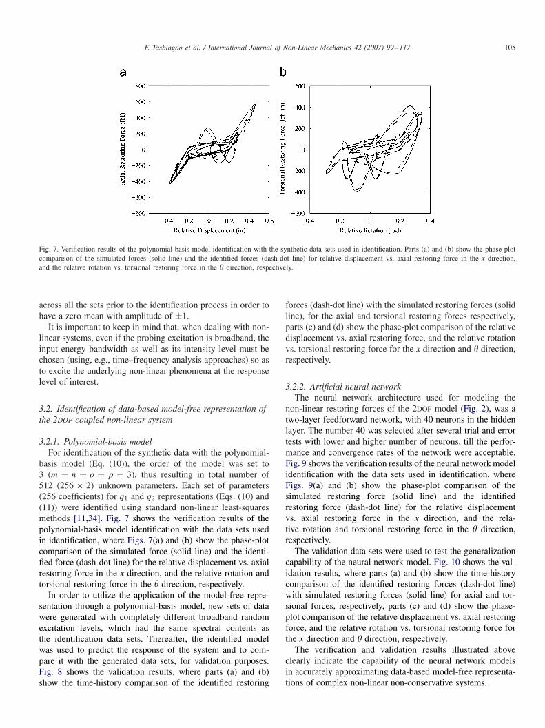
Fig. 7. Verification results of the polynomial-basis model identification with the synthetic data sets used in identification. Parts (a) and (b) show the phase-plotcomparison of the simulated forces (solid line) and the identified forces (dash-dot line) for relative displacement vs. axial restoring force in the x direction,and the relative rotation vs. torsional restoring force in the � direction, respectively.

across all the sets prior to the identification process in order tohave a zero mean with amplitude of ±1.

It is important to keep in mind that, when dealing with non-linear systems, even if the probing excitation is broadband, theinput energy bandwidth as well as its intensity level must bechosen (using, e.g., time–frequency analysis approaches) so asto excite the underlying non-linear phenomena at the responselevel of interest.

3.2. Identification of data-based model-free representation ofthe 2DOF coupled non-linear system

3.2.1. Polynomial-basis modelFor identification of the synthetic data with the polynomial-

basis model (Eq. (10)), the order of the model was set to3 (m = n = o = p = 3), thus resulting in total number of512 (256 × 2) unknown parameters. Each set of parameters(256 coefficients) for q1 and q2 representations (Eqs. (10) and(11)) were identified using standard non-linear least-squaresmethods [11,34]. Fig. 7 shows the verification results of thepolynomial-basis model identification with the data sets usedin identification, where Figs. 7(a) and (b) show the phase-plotcomparison of the simulated force (solid line) and the identi-fied force (dash-dot line) for the relative displacement vs. axialrestoring force in the x direction, and the relative rotation andtorsional restoring force in the � direction, respectively.

In order to utilize the application of the model-free repre-sentation through a polynomial-basis model, new sets of datawere generated with completely different broadband randomexcitation levels, which had the same spectral contents asthe identification data sets. Thereafter, the identified modelwas used to predict the response of the system and to com-pare it with the generated data sets, for validation purposes.Fig. 8 shows the validation results, where parts (a) and (b)show the time-history comparison of the identified restoring

forces (dash-dot line) with the simulated restoring forces (solidline), for the axial and torsional restoring forces respectively,parts (c) and (d) show the phase-plot comparison of the relativedisplacement vs. axial restoring force, and the relative rotationvs. torsional restoring force for the x direction and � direction,respectively.

3.2.2. Artificial neural networkThe neural network architecture used for modeling the

non-linear restoring forces of the 2DOF model (Fig. 2), was atwo-layer feedforward network, with 40 neurons in the hiddenlayer. The number 40 was selected after several trial and errortests with lower and higher number of neurons, till the perfor-mance and convergence rates of the network were acceptable.Fig. 9 shows the verification results of the neural network modelidentification with the data sets used in identification, whereFigs. 9(a) and (b) show the phase-plot comparison of thesimulated restoring force (solid line) and the identifiedrestoring force (dash-dot line) for the relative displacementvs. axial restoring force in the x direction, and the rela-tive rotation and torsional restoring force in the � direction,respectively.

The validation data sets were used to test the generalizationcapability of the neural network model. Fig. 10 shows the val-idation results, where parts (a) and (b) show the time-historycomparison of the identified restoring forces (dash-dot line)with simulated restoring forces (solid line) for axial and tor-sional forces, respectively, parts (c) and (d) show the phase-plot comparison of the relative displacement vs. axial restoringforce, and the relative rotation vs. torsional restoring force forthe x direction and � direction, respectively.

The verification and validation results illustrated aboveclearly indicate the capability of the neural network modelsin accurately approximating data-based model-free representa-tions of complex non-linear non-conservative systems.


Fig. 8. Validation results of the polynomial-basis model with the synthetic data sets, which were not used in the identification process. Parts (a) and (b)show the time-history comparison of the identified restoring forces (dash-dot line) with the simulated restoring forces (solid line) for the axial and torsionalrestoring forces respectively, parts (c) and (d) show the phase-plot comparison of the relative displacement vs. axial restoring force, and the relative rotationvs. torsional restoring force for the x direction and � direction, respectively.

4. Experimental studies

4.1. Test setup of a 2DOF non-conservative dissipative “joint”system

A test apparatus was designed to simulate the behavior of anon-linear non-conservative dissipative 2DOF “joint” element,in order to utilize the application of the discussed algorithmsfor derivation of data-based model-free representations of such

systems. Photographs of the completely assembled test and thenon-linear “joint” element are shown in Fig. 11. The labelsindicate the major subcomponents of the test apparatus anddirections of the relative motion within the “joint” element.The solid model design and the details of the non-linear “joint”design are shown in Fig. 12.

The test setup consists of two computer-controlled electro-mechanical servo drives that generate external excitations intwo independent directions. The motion of the drives is trans-


Fig. 9. Verification of the neural network identification with the synthetic data sets used in identification. Parts (a) and (b) show the phase-plot comparison ofthe simulated restoring forces (solid line) and the identified restoring forces (dash-dot line) for relative displacement vs. axial restoring force in the x direction,and the relative rotation vs. torsional restoring force in the � direction, respectively.

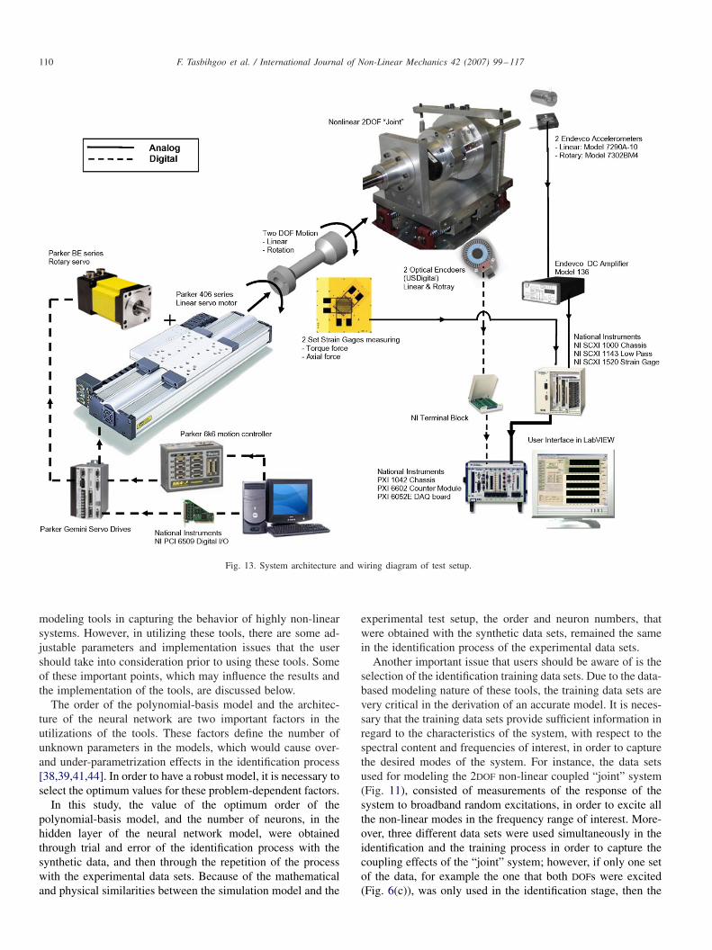
ferred through a shaft, with universal joints at each end to pro-vide decoupled motions, to the non-linear “joint” element. Theapplied forces to the system are measured through two sets ofstrain gauges mounted on the shaft in axial and torsional con-figurations. The relative motions, in the axial and rotational di-rections, of the “joint” are measured with four sets of opticalencoders. Two linear and angular accelerometers are used tomeasure the absolute acceleration of the “joint”. The data ac-quisition system included a DAQ-board, three counter-boards,controller, and a chassis, in order to have synchronized mea-surements. A pictorial diagram indicating the inter-connectionof the main system components, including the mechanical as-sembly, excitation sources, instrumentation network, and sen-sors, is provided in Fig. 13.

Three different programs were developed for the discussedexperimental test setup. These programs were: (a) a data acqui-sition program developed in LabVIEW programming environ-ment for real-time recording and analysis of the data; (b) a lowlevel program written in “C” language for simulating the broad-band random excitation for the servo motors; and (c) a controlprogram written in Visual Basic for the servo controller. Therewere some programming and practical challenges involved inthe discussed programmes, few can be pointed here which were:synchronization of the clocks on the counter-boards and theDAQ-board; mix sensors/signal data collection (digital signalsfrom optical counters and continuous signals from accelerom-eters and strain gages); over-writing the servo controllers inorder to follow random signals; the process automation, etc.

5. Application

In this section the identification results of the experimentaldata sets for the 2DOF non-linear “joint” test setup is presentedfor the polynomial-basis and neural network model. In this sec-tion description of the identification (training) data set is dis-cussed, followed by the identification results for both methods.The identification methods are performed in the verification

and validation stages. In the verification stage, a set of data isused in the identification task, and then another set of data, withsimilar dynamic characteristics to the identification data set, isused for the validation of the identified model from the firststage.

5.1. Identification data sets

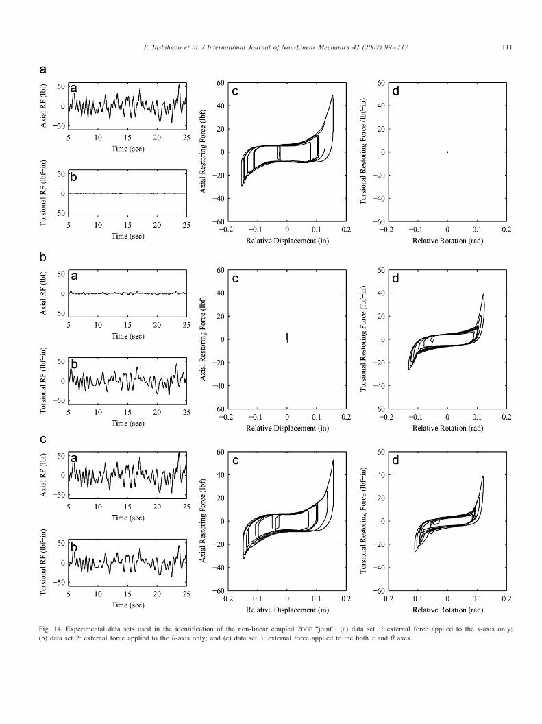
The experimental data sets used for identification, corre-sponded to measurements obtained from the system’s responseswhen it was subjected to broadband random excitations. Be-cause of the coupling effects between the DOFs on the “joint”component in the experimental test setup, three different datasets were used simultaneously for identification process, in or-der to capture the correct physics of the system. The data setsused for identification are shown in Fig. 14, where part (a) isthe response of the “joint” element when it was subjected tobroadband excitation only on the x-axis, part (b) is when therewas broadband excitation only on the �-axis, and part (c) isthe response of the system when there were two uncorrelatedbroadband random excitations on both x and � axes at the sametime.

5.2. Polynomial-basis model

5.2.1. Identification and verificationFor modeling the 2DOF non-linear “joint” with the

polynomial-basis model, the order of the model ((10) and (11))was set to 3 (m = n = o = p = 3), in which the total numberof unknown parameters would be 512 (2 × 256). The valuesof the unknown parameters were obtained by using standardnon-linear least-squares identification methods [11,34].

Fig. 15 shows the verification results of the identifiedpolynomial-basis model, where parts (a) and (b) show thetime-history comparison of the measured resorting forces(solid line) with the identified restoring forces (dash-dot line)for the axial and torsional directions, respectively. Parts (c) and


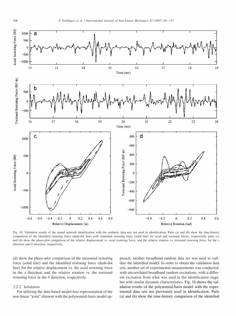
Fig. 10. Validation results of the neural network identification with the synthetic data sets not used in identification. Parts (a) and (b) show the time-historycomparison of the identified restoring force (dash-dot line) with simulated restoring force (solid line) for axial and torsional forces, respectively, parts (c)and (d) show the phase-plot comparison of the relative displacement vs. axial restoring force, and the relative rotation vs. torsional restoring force, for the xdirection and � direction, respectively.

(d) show the phase-plot comparison of the measured restoringforce (solid line) and the identified restoring force (dash-dotline) for the relative displacement vs. the axial restoring forcein the x direction, and the relative rotation vs. the torsionalrestoring force in the � direction, respectively.

5.2.2. ValidationFor utilizing the data-based model-free representation of the

non-linear “joint” element with the polynomial-basis model ap-

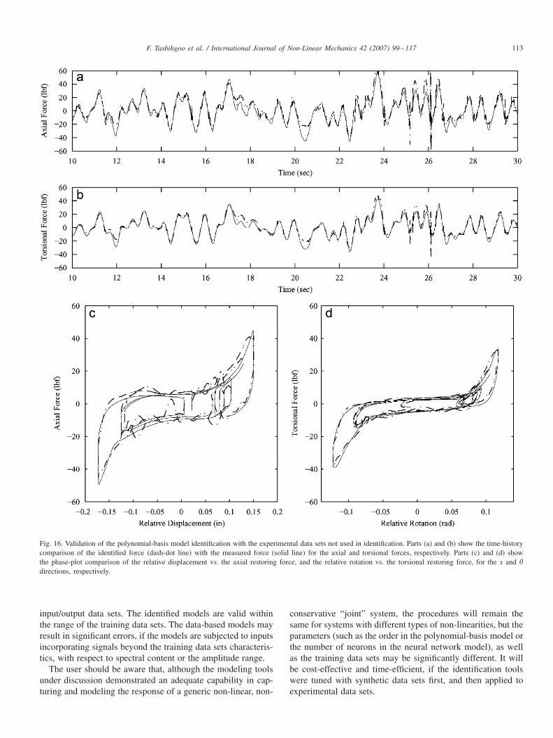
proach, another broadband random data set was used to vali-date the identified model. In order to obtain the validation datasets, another set of experimental measurements was conducted,with uncorrelated broadband random excitations, with a differ-ent excitation from what was used in the identification stage,but with similar dynamic characteristics. Fig. 16 shows the val-idation results of the polynomial-basis model with the exper-imental data sets not previously used in identification. Parts(a) and (b) show the time-history comparison of the identified


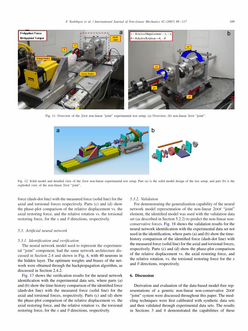
Fig. 11. Overview of the 2DOF non-linear “joint” experimental test setup; (a) Overview; (b) non-linear 2DOF “joint”.

Fig. 12. Solid model and detailed view of the 2DOF non-linear experimental test setup. Part (a) is the solid model design of the test setup, and part (b) is theexploded view of the non-linear 2DOF “joint”.

force (dash-dot line) with the measured force (solid line) for theaxial and torsional forces respectively. Parts (c) and (d) showthe phase-plot comparison of the relative displacement vs. theaxial restoring force, and the relative rotation vs. the torsionalrestoring force, for the x and � directions, respectively.

5.3. Artificial neural network

5.3.1. Identification and verificationThe neural network model used to represent the experimen-

tal “joint” component, had the same network architecture dis-cussed in Section 2.4 and shown in Fig. 4, with 40 neurons inthe hidden layer. The optimum weights and biases of the net-work were obtained through the backpropagation algorithm, asdiscussed in Section 2.4.2.

Fig. 17 shows the verification results for the neural networkidentification with the experimental data sets, where parts (a)and (b) show the time-history comparison of the identified force(dash-dot line) with the measured force (solid line) for theaxial and torsional forces, respectively. Parts (c) and (d) showthe phase-plot comparison of the relative displacement vs. theaxial restoring force, and the relative rotation vs. the torsionalrestoring force, for the x and � directions, respectively.

5.3.2. ValidationFor demonstrating the generalization capability of the neural

network model representation of the non-linear 2DOF “joint”element, the identified model was used with the validation dataset (as described in Section 5.2.2) to predict the non-linear non-conservative forces. Fig. 18 shows the validation results for theneural network identification with the experimental data set notused in the identification, where parts (a) and (b) show the time-history comparison of the identified force (dash-dot line) withthe measured force (solid line) for the axial and torsional forces,respectively. Parts (c) and (d) show the phase-plot comparisonof the relative displacement vs. the axial restoring force, andthe relative rotation, vs. the torsional restoring force for the xand � directions, respectively.

6. Discussion

Derivation and evaluation of the data-based model-free rep-resentations of a generic non-linear non-conservative 2DOF

“joint” system were discussed throughout this paper. The mod-eling techniques were first calibrated with synthetic data setsand then validated through experimental data sets. The resultsin Sections 3 and 4 demonstrated the capabilities of these


Fig. 13. System architecture and wiring diagram of test setup.

modeling tools in capturing the behavior of highly non-linearsystems. However, in utilizing these tools, there are some ad-justable parameters and implementation issues that the usershould take into consideration prior to using these tools. Someof these important points, which may influence the results andthe implementation of the tools, are discussed below.

The order of the polynomial-basis model and the architec-ture of the neural network are two important factors in theutilizations of the tools. These factors define the number ofunknown parameters in the models, which would cause over-and under-parametrization effects in the identification process[38,39,41,44]. In order to have a robust model, it is necessary toselect the optimum values for these problem-dependent factors.

In this study, the value of the optimum order of thepolynomial-basis model, and the number of neurons, in thehidden layer of the neural network model, were obtainedthrough trial and error of the identification process with thesynthetic data, and then through the repetition of the processwith the experimental data sets. Because of the mathematicaland physical similarities between the simulation model and the

experimental test setup, the order and neuron numbers, thatwere obtained with the synthetic data sets, remained the samein the identification process of the experimental data sets.

Another important issue that users should be aware of is theselection of the identification training data sets. Due to the data-based modeling nature of these tools, the training data sets arevery critical in the derivation of an accurate model. It is neces-sary that the training data sets provide sufficient information inregard to the characteristics of the system, with respect to thespectral content and frequencies of interest, in order to capturethe desired modes of the system. For instance, the data setsused for modeling the 2DOF non-linear coupled “joint” system(Fig. 11), consisted of measurements of the response of thesystem to broadband random excitations, in order to excite allthe non-linear modes in the frequency range of interest. More-over, three different data sets were used simultaneously in theidentification and the training process in order to capture thecoupling effects of the “joint” system; however, if only one setof the data, for example the one that both DOFs were excited(Fig. 6(c)), was only used in the identification stage, then the


Fig. 14. Experimental data sets used in the identification of the non-linear coupled 2DOF “joint”: (a) data set 1: external force applied to the x-axis only;(b) data set 2: external force applied to the �-axis only; and (c) data set 3: external force applied to the both x and � axes.


Fig. 15. Verification results of the polynomial-basis model identification with the experimental data sets used in identification. Parts (a) and (b) show thetime-history comparison of the measured resorting forces (solid line) with the identified restoring forces (dash-dot line) for the axial and torsional directions,respectively. Parts (c) and (d) show the phase-plot comparison of the measured restoring force (solid line) and the identified restoring force (dash-dot line) forthe relative displacement vs. the axial restoring force in the x direction, and the relative rotation vs. the torsional restoring force in the � direction, respectively.

models would have failed in the generalization tests, due tothe lack of information about the coupling of the DOFs in thetraining data set.

The knowledge of the system mass matrix is not crucial forthe discussed modeling and identification techniques. If thevalue of the mass matrix is not available, the absolute accel-eration data will be added to the list of the inputs, and theoutput data will be the sum of the applied forces from the sys-

tem, instead of only the non-linear restoring forces (Fig. 3),and the mass and moment of inertia terms will be added tothe list of unknown parameters in the polynomial basis model(Eqs. (10) and (11)). However, the two-layer feedforward archi-tecture (Fig. 4) remains the same for the neural network model.

Despite the excellent capability of these models for the iden-tification and modeling non-linear systems, it is important topoint out that these models rely heavily on the nature of the


Fig. 16. Validation of the polynomial-basis model identification with the experimental data sets not used in identification. Parts (a) and (b) show the time-historycomparison of the identified force (dash-dot line) with the measured force (solid line) for the axial and torsional forces, respectively. Parts (c) and (d) showthe phase-plot comparison of the relative displacement vs. the axial restoring force, and the relative rotation vs. the torsional restoring force, for the x and �directions, respectively.

input/output data sets. The identified models are valid withinthe range of the training data sets. The data-based models mayresult in significant errors, if the models are subjected to inputsincorporating signals beyond the training data sets characteris-tics, with respect to spectral content or the amplitude range.

The user should be aware that, although the modeling toolsunder discussion demonstrated an adequate capability in cap-turing and modeling the response of a generic non-linear, non-

conservative “joint” system, the procedures will remain thesame for systems with different types of non-linearities, but theparameters (such as the order in the polynomial-basis model orthe number of neurons in the neural network model), as wellas the training data sets may be significantly different. It willbe cost-effective and time-efficient, if the identification toolswere tuned with synthetic data sets first, and then applied toexperimental data sets.


Fig. 17. Verification results for the neural network identification with the experimental data sets used in identification. Parts (a) and (b) show the phase-plotcomparison of the measured force (solid line) and the identified force (dash-dot line) for relative displacement vs. axial restoring force in the x direction, andthe relative rotation vs. torsional restoring force in the � direction, respectively.

6.1. Comparison of the two non-parametric methods

The modeling techniques discussed in this study are twocompletely different approaches from the mathematical for-mulation and implementation aspects; however, both methodswould result in data-based model-free representations of non-linear systems. The selection of which method to use is basedon the identification application and objectives. For example,for a fast model identification, the polynomial-basis model

would be a better choice, or for a high-fidelity representationthe neural network approach would be the ideal method. Inthe simulation phase of this study, the neural network modeltook a longer duration in the training stage in comparison tothe identification stage of the polynomial-basis model (about180 times longer), although the performance (accuracy) of thetrained neural network model was much higher than the identi-fied polynomial-basis model (about 16 times lower percentageerror in the validation test cases).


Fig. 18. Validation results for the neural network identification with the experimental data sets not used in identification. Parts (a) and (b) show the time-historycomparison of the identified force (dash-dot line) with the measured force (solid line) for the axial and torsional forces, respectively. Parts (c) and (d) showthe phase-plot comparison of the relative displacement vs. the axial restoring force, and the relative rotation vs. the torsional restoring force, for the x and �directions, respectively.

Among the issues that need further investigation is howthe relative “efficiency” of the non-parametric methods usedherein depends on the nature of the specific non-linear system,the number of degrees of freedom, and the excitation/responselevel. Furthermore, additional studies are needed to assess therange of validity of the above-referenced methods for dealingwith non-smooth systems.

7. Conclusion

In the present study, the application of two non-parametricmodeling approaches, one using a polynomial-basis modeland the other based on ANNs, were discussed and evaluatedfor modeling non-linear, non-conservative, dissipative sys-tems. The tools use input/output data of the system to obtain


data-based, model-free computational models of complexnon-linear systems, which subsequently can be used in compu-tational engines for simulation studies, condition assessment,and damage detection applications. The methods were firstcalibrated through simulation studies and thereafter appliedto experimental data sets corresponding to a 2DOF couplednon-linear “joint” system. The generalization capability ofthe methods were demonstrated through validation tests usingsynthetic and experimental data sets.

Acknowledgments

This study was supported in part by grants from the US AirForce Office of Scientific Research, the National Science Foun-dation, and the National Aeronautics and Space Administration.

References

[1] Y. Sugiyama, K. Katayama, S. Kinoi, Flutter of cantilevered columnunder rocket thrust, J. Aerosp. Eng. 8 (1995) 9–15.

[2] A.N. Kounadis, Hamiltonian weakly damped autonomous systemsexhibiting periodic attractors, Z. Angew. Math. Phys. 57 (2) (2006)324–349.

[3] V.V. Bolotin, A.A. Grishko, A.N. Kounadis, C.J. Gantes, Non-linearpanel flutter in remote post-critical domains, Int. J. Non-Linear Mech.33 (5) (1998) 753–764.

[4] V.V. Bolotin, A.A. Grishko, A.N. Kounadis, C.J. Gantes, Influence ofinitial conditions on the postcritical behavior of a nonlinear aeroelasticsystem, Nonlinear Dyn. 15 (1998) 63–81.

[5] A.N. Kounadis, Non-potential dissipative systems exhibiting periodicattractors in regions of divergence, Chaos Solitons Fractals 8 (4) (1997)583–612.

[6] A.N. Kounadis, On the failure of static stability analyses ofnonconservative systems in regions of divergence instability, Int. J. SolidsStruct. 31 (15) (1994) 2099–2120.

[7] A.N. Kounadis, On the paradox of the destabilizing effect of dampingin non-conservative systems, Int. J. Non-Linear Mech. 27 (4) (1992)597–609.

[8] V.V. Bolotin, A.A. Grishko, M.Y. Panov, Effect of damping on thepostcritical behaviour of autonomous non-conservative systems, Int.J. Non-Linear Mech. 37 (7) (2002) 1163–1179.

[9] G. Kerschen, K. Worden, A.F. Vakakis, J.-C. Golinval, Past, present andfuture of nonlinear system identification in structural dynamics, Mech.Syst. Signal Process. 20 (3) (2006) 505–592.

[10] K. Worden, G.R. Tomlinson, Nonlinearity in Structural Dynamics:Detection, Identification and Modelling, Institute of Physics Publications,2001.

[11] L. Ljung, System Identification, Theory for the User, Prentice-Hall,Upper Saddle River, NJ, 1999.

[12] G.W. Housner, L.A. Bergman, T.K. Caughey, A.G. Chassiakos, R.O.Claus, S.F. Masri, R.E. Skelton, T.T. Soong, B.F. Spencer, J.T.P. Yao,Special issue: structural control: past, present and future, ASCE J. Eng.Mech. 123 (9) (1997) 897–971.

[13] B.F. Spencer Jr., S. Nagarajaiah, State of the art of structural control,J. Struct. Eng. (2003) 845–856.

[14] R.W. Wolfe, S.F. Masri, J.P. Caffrey, Some structural health monitoringapproaches for nonlinear hydraulic dampers, J. Struct. Control 9 (1)(2002) 5–18.

[15] D.J. Segalman, A four-parameter Iwan model for lap-type joints, ASMEJ. Appl. Mech. 72 (5) (2005) 752–760.

[16] D.J. Segalman, Modelling joint friction in structural dynamics, Struct.Control Health Monit. 13 (1) (2006) 430–453.

[17] D.D. Quinn, D.J. Segalman, Using series–series Iwan-type models forunderstanding joint dynamics, ASME J. Appl. Mech. 72 (5) (2005)666–673.

[18] J. Sjöberg, Q. Zhang, L. Ljung, A. Benveniste, B. Delyon, P.-Y.Glorennec, H. Hjalmarsson, A. Juditsky, Nonlinear black-box modelingin system identification: a unified overview, Automatica 31 (12) (1995)1691–1724.

[19] S.F. Masri, A.G. Chassiakos, T.K. Caughey, Structure-unknown non-linear dynamic systems: identification through neural networks, SmartMater. Struct. 1 (1) (1992) 45–56.

[20] S.F. Masri, A.G. Chassiakos, T.K. Caughey, Identification of nonlineardynamic systems using neural networks, ASME J. Appl. Mech. 60 (1993)123–133.

[21] S.F. Masri, A.W. Smyth, A.G. Chassiakos, M. Nakamura, T.K. Caughey,Training neural networks by adaptive random search techniques, ASCEJ. Eng. Mech. 125 (2) (1999) 123–132.

[22] S.F. Masri, T.K. Caughey, A nonparametric identification technique fornonlinear dynamic problems, ASME J. Appl. Mech. 46 (2) (1979)433–447.

[23] S.F. Masri, R.K. Miller, A.F. Saud, T.K. Caughey, Identification ofnonlinear vibrating structures; part I: formulation, ASME J. Appl. Mech.109 (1987) 918–922.

[24] S.F. Masri, R.K. Miller, A.F. Saud, T.K. Caughey, Identification ofnonlinear vibrating structures; part II: applications, ASME J. Appl. Mech.109 (1987) 923–929.

[25] S.F. Masri, M. Nakamura, A.G. Chassiakos, T.K. Caughey, Neuralnetwork approach to detection of changes in structural parameters,J. Eng. Mech. 122 (4) (1996) 350–360.

[26] S.F. Masri, R.K. Miller, T.J. Dehghanyar, T.K. Caughey, Active parametercontrol of nonlinear vibrating structures, ASME J. Appl. Mech. 56(1989) 658–666.

[27] S.F. Masri, A.W. Smyth, A.G. Chassiakos, T.K. Caughey, N.F. Hunter,Application of neural networks for detection of changes in nonlinearsystems, ASCE J. Eng. Mech. 126 (7) (2000) 666–676.

[28] M.A. Al-Hadid, J.R. Wright, Developments in the force–state mappingtechnique for non-linear systems and the extension to the location ofnon-linear elements in a lumped-parameter system, Mech. Syst. SignalProcess. 3 (3) (1989) 269–290.

[29] K. Worden, G.R. Tomlinson, W. Lim, G. Sauer, Modeling andclassification of non-linear systems using neural networks—ii. apreliminary experiment, Mech. Syst. Signal Process. 8 (4) (1994)395–419.

[30] K. Worden, G.R. Tomlinson, W. Lim, G. Sauer, Modeling andclassification of non-linear systems using neural networks—i. simulation,Mech. Syst. Signal Process. 8 (3) (1994) 319–356.

[31] F. Tasbihgoo, Analytical and experimental studies in the developmentof reduced-order computational models for non-linear systems, Ph.D.Thesis, University of Southern California, 2006.

[32] J.P. Caffrey, S.F. Masri, F. Tasbihgoo, A.W. Smyth, A.G. Chassiakos, Are-configurable test apparatus for complex nonlinear dynamic systems,Nonlinear Dyn. 36 (2-4) (2004) 181–201.

[33] S.F. Masri, F. Tasbihgoo, J.P. Caffrey, A.W. Smyth, A.G. Chassiakos,Data-based model-free representation of complex hysteretic MDOF

systems, Struct. Control Health Monit. 13 (1) (2006) 365–387.[34] J.M. Mendel, Lessons in Estimation Theory for Signal Processing

Communications and Control, second ed., Prentice-Hall, Upper SaddleRiver, NJ, 1995.

[35] J.E. Dayhoff, Neural Network Architectures, An Introduction, VanNostran Reinhold, New York, 1990.

[36] K. Bani-Hani, J. Ghaboussi, Nonlinear structural control using neuralnetworks, ASCE J. Eng. Mech. 124 (3) (1998) 319–327.

[37] E.B. Kosmatopoulos, A.W. Smyth, S.F. Masri, A.G. Chassiakos, Robustadaptive neural estimation of restoring forces in nonlinear structures,ASME J. Appl. Mech. 68 (2001) 880–893.

[38] M.T. Hagan, H.B. Demuth, M.H. Beale, Neural Network Design, PWSPublishing Company, 1995.

[39] H. Demuth, M. Beale, Neural Network Toolbox User’s Guide, Version4, The MathWorks, Inc., 〈http://www.mathworks.com〉, 2005.

[40] K. Hornik, M. Stinchcombe, H. White, Multilayer feedforward networksare universal approximators, Neural Networks 2 (5) (1989) 359–366.

http://www.mathworks.com


[41] F. Tasbihgoo, R.W. Wolfe, S.F. Masri, J.P. Caffrey, H. Yun, On-line monitoring of nonlinear viscous dampers, ASCE J. Eng. Mech.,submitted for publication.

[42] P.A. Ioannou, J. Sun, Robust Adaptive Control, Prentice-Hall, UpperSaddle River, NJ, 1996.

[43] A.W. Smyth, J.S. Pei, Integration of response measurements for nonlinearstructural health monitoring, in: Proceedings of Third US–Japan

Workshop on Nonlinear System Identification and Structural HealthMonitoring, 2000.

[44] A.W. Smyth, Analytical and experimental studies in nonlinear systemidentification and modeling for structural control Ph.D. Thesis, Universityof Southern California, 1998.

Development of data-based model-free representation of non-conservative dissipative systems

Documents

Transcript of Development of data-based model-free representation of non-conservative dissipative systems