Development of Crime Forecasting and Mapping Systems for ...

The author(s) shown below used Federal funds provided by the U.S. Department of Justice and prepared the following final report: Document Title: Development of Crime Forecasting and Mapping

Systems for Use by Police Author(s): Jacqueline Cohen Document No.: 211973 Date Received: January 2006 Award Number: 2001-IJ-CX-0018 This report has not been published by the U.S. Department of Justice. To provide better customer service, NCJRS has made this Federally-funded grant final report available electronically in addition to traditional paper copies.

Opinions or points of view expressed are those

of the author(s) and do not necessarily reflect the official position or policies of the U.S.

Department of Justice.

i

DRAFT Final Report

Development of Crime Forecasting and Mapping Systems for Use by Police

2001-IJ-CX-0018

By

Jacqueline Cohen Wilpen L. Gorr

February 9, 2005

H. John Heinz III School of Public Policy and Management Carnegie Mellon University

This document is a research report submitted to the U.S. Department of Justice. This report has not been published by the Department. Opinions or points of view expressed are those of the author(s) and do not necessarily reflect the official position or policies of the U.S. Department of Justice.

Executive Summary

This report provides the results from the second of two grants funded by the

National Institute of Justice for research on the new field of crime forecasting. This

second grant replicates results from the first grant using new data, including crime data

from a second city, and develops and evaluates advanced crime forecasting models.

Our test bed for comparing and evaluating forecast methods and models now

includes 6 million offense incident reports and CAD calls from Pittsburgh, Pennsylvania

and Rochester, New York which we have processed into monthly time series data over

the period 1990 through 2001 and five geographies (census tracts, 4,000 foot grid cells,

car beats, an aggregation of car beats we call car beats plus, and precincts) for 24 crime

types. We expanded our crime forecasting methods and models from the our original set

of so-called naïve methods, univariate methods, and single lag leading indicator model

estimated via linear regression and non-linear neural network to include 1) a multivariate

model for estimating crime seasonality based on demographic and land use demographics

and 2) leading indicator models with 4 and 12 time lags. We also introduce an

application of tracking signals as a supporting crime analysis tool to automatically detect

crime series pattern changes.

We determined requirements for a crime forecasting and mapping system, the

Crime Early Warning System (CEWS), through our efforts establishing a new

classification of macro, meso, and micro levels police decision making. From this

classification emerge requirements for meso-level crime forecasting in support of

CompStat meetings or other such periodic evaluation and planning activities of police

departments. The requirements include 1) the need to apply “business-as-usual” forecasts


2

as counterfactuals to evaluate police performance in crime prevention and enforcement as

evaluated using mean forecast error criteria (mean absolute percentage error and mean

squared error) and 2) the need to forecast large increases (or decreases) in crime for

tactical deployment of crime analysis micro-level resources and police manpower.

The results of extensive forecast experiments, using hold-out samples in a rolling

horizon design, are definitive. Exponential smoothing with seasonality estimated with

pooled city-wide data is the best method for producing counterfactual forecasts. Our

multivariate seasonality model, while theoretically appealing and well implemented,

nevertheless did not improve forecast accuracy over simple methods for estimating

seasonality. The worst methods are the current naïve approach commonly used in

CompStat meetings and the leading indicator models. In sharp contrast, the leading

indicator models, especially as implemented via neural networks, are the best for

forecasting large crime changes. Exponential smoothing is the worst method for this

purpose (we did not evaluate the naïve methods because they are inappropriate).

Depending on the needs, opposite forecasting models are best.

The accuracy attained for counterfactual forecasts is sufficient to support

evaluating car beat-level crime aggregates such as part 1 property crimes and an

aggregate of violence leading indicators that we propose. At the precinct level, many

high-volume individual crime types can also be evaluated. For deployment purposes, it is

possible to adequately forecast part 1 crimes that have good part 2 crime or CAD leading

indicators down to districts as small as census tracts. We have successfully forecasted

aggregates including part 1 property crimes and violent crimes at that fine-grained

geography.


3

Table of Contents

1. Introduction……………………………………………………………..……………1

2. Time Series Data and Forecast Methods………………………………….………….5

2.1 Naïve Forecast Methods……………………………………………………..6

2.2 Univariate Forecast Methods………………………………………………..6

2.3 Leading Indicator Forecast Methods…………………………...…..……..…9

2.4 Time Series Tracking Signals…………………………………..…..………10

3. Police Decision Making and Crime Forecasting……………………………..………11

3.1 Macro Level Crime Analysis……………………………………………….12

3.2 Meso Level Crime Analysis………………………………………..………13

3.2.1 Evaluating Past Performance……………………………………..13

3.2.2 Planning Next Month’s Policing: Crime Early Warning System...15

3.3 Micro Level Crime Analysis……………………………….……………….19

3.4 Summary of Crime Forecasting Requirements…….……….………………20

4. Data Collection and Processing………………………………………………………21

4.1 Pittsburgh Data Processing…………………………………………….……22

4.2. Rochester Data Processing………………………………………………….27

4.3 Statistics and Charts………………………………………………….……..28

5. Experimental Design………………………………………………………………....36

5.1 Rolling Horizon Experimental Design……………………………..……….36

5.2 Treatments: Forecast Methods and Geographic Scale…………..………….37

5.3 Crimes Forecasted………………………………………………..…………39

5.4 Forecast Accuracy Measures……………………………………………….39


4

5.4.1 Average Forecast Error Measure………………….…………….40

5.4.2 Decision Rule Forecast Criterion…………………….………….41

6. Results……………………………………………………….…………….……….44

6.1 Results on Forecast Mean Absolute Percentage Error……………………44

6.2 Decision Rule Forecast Performance……………………………………..52

7. Recommendations…………………………………………………………….……70

7.1 Build a Spatial Data Warehouse for Crime Forecasting………….………70

7.2 Implement Crime Forecasting Methods…………………….….…..…….72

Appendix A: Multivariate Estimation of Crime Seasonality: An Extension to Classical Decomposition………………………………..……….…78

Appendix B: Leading Indicators and Spatial Interactions: A Crime Forecasting Model for Proactive Police Deployment…………..……..….109

Appendix C: Application of Tracking Signals to Detect Time Series Pattern Changes in Crime Early Warning Systems…………………...140


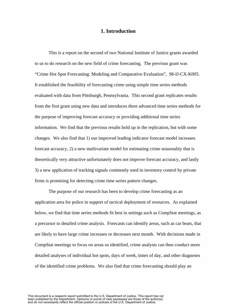
1. Introduction

This is a report on the second of two National Institute of Justice grants awarded

to us to do research on the new field of crime forecasting. The previous grant was

“Crime Hot Spot Forecasting: Modeling and Comparative Evaluation”, 98-IJ-CX-K005.

It established the feasibility of forecasting crime using simple time series methods

evaluated with data from Pittsburgh, Pennsylvania. This second grant replicates results

from the first grant using new data and introduces three advanced time series methods for

the purpose of improving forecast accuracy or providing additional time series

information. We find that the previous results hold up in the replication, but with some

changes. We also find that 1) our improved leading indicator forecast model increases

forecast accuracy, 2) a new multivariate model for estimating crime seasonality that is

theoretically very attractive unfortunately does not improve forecast accuracy, and lastly

3) a new application of tracking signals commonly used in inventory control by private

firms is promising for detecting crime time series pattern changes.

The purpose of our research has been to develop crime forecasting as an

application area for police in support of tactical deployment of resources. As explained

below, we find that time series methods fit best in settings such as CompStat meetings, as

a precursor to detailed crime analysis. Forecasts can identify areas, such as car beats, that

are likely to have large crime increases or decreases next month. With decisions made in

CompStat meetings to focus on areas so identified, crime analysts can then conduct more

detailed analyses of individual hot spots, days of week, times of day, and other diagnoses

of the identified crime problems. We also find that crime forecasting should play an


2

important role in evaluating the most recent month’s performance, as also done in

CompStat meetings. Forecasts should be used as the counterfactuals or bases of

comparison to judge performance.

The approach of the research in both grants has been to attempt a comprehensive

assessment of time series methods for use in tactical deployment of police resources. We

did not approach this research with a favorite method that we wished to promote.

Instead, we used methods from all three of the relevant short-term, time series method

types (see Section 2 below). These included the simplest (so-called) naïve methods,

univariate methods, and leading indicator models. We follow the approach of the

forecasting literature that suggests starting with simple methods and to use advanced

methods only if they forecast more accurately than the simple methods. Often it is

difficult to improve forecast accuracy beyond that of the good simple methods.

The forecasting literature has developed empirical approaches for validating the

forecast accuracy of competing methods based on hold-out samples. For example, for

one-month-ahead forecasts an evaluator uses times series data as if it were a past time

point, say the end of December 1995. The evaluator 1) estimates parameters for each

forecast method or model using historical time series data through December 1995,

without knowledge of any of the time series data after that date; 2) makes a forecast using

each forecast method being compared; 3) behaves as if another month has past so that the

actual crime count for January 1996 (the hold-out sample) is available; 4) calculates the

forecast error for each forecast method; and 5) stores the forecast errors for later analysis.

We used the rolling horizon design (Swanson and White 1997), in which the research


3

continues to move through time in the same fashion making additional forecasts until all

data are used up.

By including data from two cities (Pittsburgh, Pennsylvania and Rochester, NY)

and over a long time period (January 1990 through December 2001), we have sufficient

data and varying conditions to claim that we have somewhat generalizable results. Of

course, many more studies over more conditions are needed to make the results on crime

forecasting truly comprehensive. For example, crime data from cities in the American

west or south may have much different behavior.

With results in hand on which crime forecasting methods are best, another

purpose of our research is to shed light on the question of whether crime forecasting will

be useful for police. We have two approaches to address this question. One is to pick

thresholds for forecast accuracy and see which crimes, geographic areas, etc. can attain

the threshold or better accuracy. A second more innovative approach based on decision

rules matching application needs is to identify which methods forecast large changes in

crime levels most accurately. The analysis includes statistics on positives and false

positives resulting from the forecast-based decision rules. An important result of our new

research is that the forecast methods that perform best for identifying large crime changes

are those that perform worst for the traditional forecast error summaries (and visa versa),

and dramatically so.

The organization of the rest of this report is as follows.

• Section 2 summarizes the nature of time series data and the major approaches to

forecasting them. In this section we describe each of the forecast methods or


4

models that we evaluate in this report in general terms and provide appendices

with detailed developments and descriptions of methods and models.

• Section 3 provides a new classification of police decision making and supporting

crime analysis and mapping tools. We define the macro, meso, and micro levels

of crime analysis and argue that crime forecasting fits at the meso level, while

many well-known crime analysis tools, such as hot spot analysis and pin mapping,

fit at the micro level. Important crime forecasting requirements that result from

this section are the need for counterfactual forecasts for use in evaluation of past

police performance and the need for forecast methods that accurately forecast

large changes in crime levels.

• Section 4 summarizes data collection and processing for this grant, which were

extensive. Of particular interest is that we have aggregated point crime incidents

to several geographies ranging from precincts down to census tracts. Hence a

treatment in our experiments is the geography used to aggregate and forecast

crime levels.

• Section 5 summarizes our experimental design, which is a state-of-art rolling

horizon forecast experiment. Critically important for the analysis of results are

the two approaches and measures for assessing forecast accuracy, a traditional

average forecast error criterion and an innovative decision rule criterion.

• Section 6 presents the results of extensive forecast experiments. We provide both

tables with overall summaries and other tables with detailed results.

• Finally, Section 7 summarizes results and provides recommendations


5

2. Time Series Data and Forecast Methods

Time series data consist of repeated measurements for a fixed observation unit

(e.g., census tract, grid cell, car beat, or precinct) and fixed time interval (such as month,

quarter, or year), sequenced by time period. An example is the monthly time series of

part 1 property crimes for Pittsburgh Police car beat 21. Our data includes this time

series for January 1990 through December 2001, a total of 144 monthly observations or

data points, along with many other time series. (See Figures 8 and 9 below for time

series plots of this and an aggregate of violent crime leading indicators in Pittsburgh and

Rochester.)

Time series methods are the most widely researched and used forecast methods.

The past twenty-five years has seen many advances in these methods, approaches for

their evaluation, and applications. The Journal of Forecasting published by Wiley

Interscience, The International Journal of Forecast, published by Elsevier document the

many advances. Our research draws heavily on this literature.

There are three major types of time series methods: so-called naïve methods,

univariate time series methods, and leading indicator models. We review each of the

methods briefly in the following subsections. When more details are needed; for

example, to describe how we have applied or adapted time series methods for crime

forecasting, we have included appendices consisting of working papers we have written.


6

2.1 Naïve Forecast Methods

The naïve methods are not model-based, but use time series data points

themselves as forecasts. The most used naïve method is the random walk [Makridakis,

and Wheelright, 1978] which uses the last historical data point as the forecast. For

example, if it is the end of January 2005, we would use the January 2005 count of part 1

property crimes in Pittsburgh car beat 21 to forecast February 2005’s property crimes in

the same car beat. The random walk is a good straw man method for evaluating the

forecast accuracy of other time series methods: if another method cannot forecast more

accurately than the naïve random walk, it should not be used. For certain kinds of time

series, such as stock market prices, it is hard to find time series methods more accurate

than the random walk.

Another naïve method is widely used in CompStat meetings, so we call it the

CompStat method. The forecast for February 2005 is the actual crime count from

February 2004, the same month a year ago. CompStat meetings use this method

primarily as the counterfactual or basis of evaluation for the current month’s crime-

fighting performance.

2.2 Univariate Forecast Methods

There are many univariate time series methods. Two of the more widely known

univariate methods are the Box-Jenkins models [Box and Jenkins 1970] and the family of

exponential smoothing models [Makridakis and Wheelwright, 1978]. Box-Jenkins


7

models are appealing theoretically but are complicated to use and generally are not the

most accurate forecasting methods. Exponential smoothing methods are widely used in

practice, are simple to understand and use, and have consistently yielded good, if not the

best forecast accuracy [e.g., Makridakis et al. 1982]. Our research thus uses smoothing

methods.

Exponential smoothing methods estimate the mean of time series data with

weights applied to the data that fall off exponentially with the age of data points.

Consequently these methods automatically adapt to and smoothly track changing time

series patterns, albeit with a lag determined by the method’s learning rates or smoothing

parameters. Our implementation of exponential smoothing uses traditional optimization

methods for selecting smoothing parameter values (complete enumeration of a grid of

values) that minimize the mean squared error of one-step-ahead forecast error within the

historical or estimation data set [ Makridakis and Wheelwright 1978]. We use two

different exponential smoothing methods. First is simple exponential smoothing [Brown

1963] which estimates the current mean of a time series. Its forecasts are simply the last

estimated value. Second is Holt two-parameter smoothing [Holt 1957] which includes a

second parameter for time trend. This method’s forecasts are straight lines increasing or

decreasing at the rate of the estimated time trend slope.

Crime data have seasonal patterns; for example, property crimes have a peak in

the late fall, are low in the winter, and have a major peak in the summer. We

deseasonalize crime time series data using classical decomposition [Bowerman and

O’Connell 1993], apply smoothing to forecast, and then reseasonalize forecasted values

with the appropriate seasonal adjustment. The X-12-ARIMA method [U.S. Census


8

Bureau 2005] is based on classical decomposition and more widely used today for

estimating seasonality, but is somewhat more complicated. We leave it to others to see if

that methods can improve crime forecasting.

Seasonal adjustments can be additive or multiplicative. Multiplicative

adjustments are more desirable for crime series forecasting because they are

dimensionless and can be more easily used for many time series (e.g., for several

different car beats). Example values for such seasonal factors might be 0.85 (15% lower

than typical) or 1.20 (20% higher than typical). Figures 9 and 10 below display such

seasonal factors estimated for crime data. We estimate 12 seasonal factors for monthly

data in two ways. Either we estimate the factors separately for each geographic unit (e.g.,

car beat) or we pool (add) data across all car beats to estimate city-wide seasonal factors.

Pooling eliminates any neighborhood type effects on seasonality, but increases the

reliability of estimates. Seasonal estimates are typically quite unreliable because the

effect of a given month is only observed once per year. Recently there has been

increased interest in pooling data to increase reliability, and in reducing seasonal

estimates toward zero (damping) to increase forecast accuracy [Derek and Vassilopoulos

1999, Miller and Williams 2004].

We introduce a new multivariate extension to classical decomposition that uses

fixed effects for population and land use characteristics to estimate seasonal factors by

geographic unit, car beats and census tracts. Based on ecological crime theories, we

selected 20 census and land use variables that we believed would lead to different

seasonal patterns in different areas. For example, indicators for youth and transient

populations identify neighborhoods with high numbers of college students. The


9

academic calendar imparts unique flows and ebbs to this population, giving it perhaps

unique seasonal crime patterns. See Appendix A for a paper on this method.

2.3 Leading Indicator Forecast Methods

Univariate methods provide extrapolations of existing time series patterns and

thus provide “business as usual” forecasts. Thus they make good counterfactuals for

evaluating the current month’s performance. Univariate methods cannot forecast time

series pattern changes, such as sudden step jumps up or down in time series data. Such

changes are common in crime series data, increasing in number as the size of geographic

units decrease, say from precincts to car beats to census tracts. Such changes are due to

discrete changes in crime patterns; for example, reprisal in gang turf wars, displacement

due to crackdowns, introduction of a new source of illegal drugs, release from prison of a

serial criminal, etc.

To forecast crime series pattern changes, one must use leading indicator models.

For example, if simple assault offenses and shots fired CAD calls are leading indicators

of part 1 violent crimes, then a sudden increase in either one or both of these leading

indicators this past month may predict an increase in part 1 violent crimes next month. In

our first grant we developed a set of part 2 offenses and CAD calls as leading indicators

for part 1 violent crimes and part 1 property crimes. We conducted preliminary tests of

leading indicators in forecast models and found them to have increased forecast accuracy

over univariate methods for large changes in crime counts. The models in grant 1 used a

single month’s lag of the leading indicators and the current work extends these models by


10

including lags of up to 12 months. We estimate these models using ordinary least squares

regression and neural network models. We also made advances in the theories for

leading indicators and spatial interactions for crime. More on these advances is included

in the paper of Appendix B.

One final note on leading indicator crimes is that they are valuable crime series to

analyze for two reasons. They themselves are of course important to prevent and enforce

for the safety and welfare of the public. In addition, if leading indicators truly lead

changes in more serious crimes, then examining time series data and maps of current

mapped points of them is important for prevention of serious crimes. Our introduction of

tracking signals in the next section as a crime analysis tool builds on this observation.

Tracking signals automatically detect time series pattern changes, such as large increases

in the most recent month’s data. An area with such a large increase should be monitored

and patrolled as a means to prevent future hardening of the leading indicator crimes into

more serious crimes. Thus, pin maps displaying hot spots of leading indicator crimes are

needed by crime analysts to recommend patrol targets.

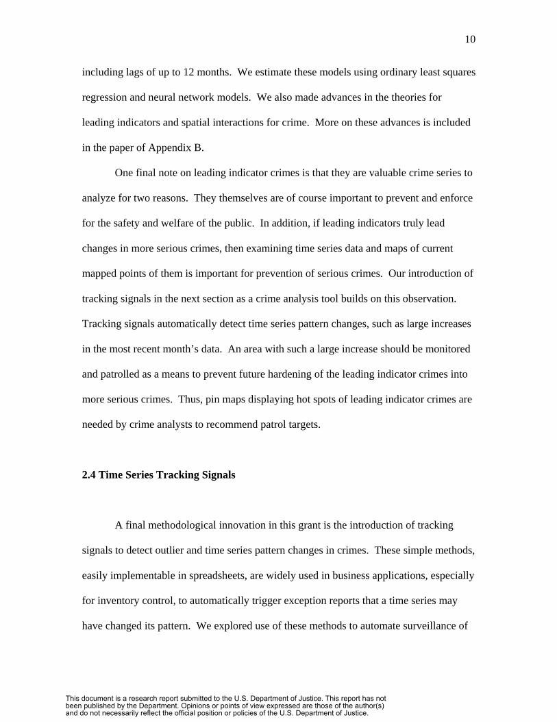
2.4 Time Series Tracking Signals

A final methodological innovation in this grant is the introduction of tracking

signals to detect outlier and time series pattern changes in crimes. These simple methods,

easily implementable in spreadsheets, are widely used in business applications, especially

for inventory control, to automatically trigger exception reports that a time series may

have changed its pattern. We explored use of these methods to automate surveillance of


11

crime series methods for such changes; especially in leading indicator crimes. Even in

medium-sized cities such as Pittsburgh or Rochester, there are easily 1,000 to 2,000 time

series per month of interest, far too many to investigate manually.

Our approach to testing these methods was thus to determine whether tracking

signals could make the same decisions as crime analysts in identifying time series pattern

changes. At this point it appears as if tracking signals have promise for automating

carrying out this task thereby saving crime analysts much labor. The smaller the district

size, such as for census tracts or our original grid maps, the more likely that there are

crime pattern changes, many of them worthy of police attention. For small district sizes,

discrete events such as the release of a prisoner who returns to a life of crime, retaliation

of a gang against another gang, etc. have large relative impacts on crime counts and thus

become prominent in time series (instead of being netted out in the error term as noise).

The paper in Appendix C is a completed exploratory study by us on tracking

signals for use in crime analysis. Nothing more is included in this report on this topic.

3. Police Decision Making and Crime Forecasting

One of the National Institute of Justice’s interests in funding research on crime

forecasting was to develop new tools for use in crime mapping and crime analysis. In

this section we examine police decision making in relationship to crime analysis for the

purposes of 1) determining where crime forecasting fits into police decision making and

crime analysis, and 2) determining the requirements for crime forecasting, in support of


12

decision making. As shown in Figure 1, we identified three levels of police decision

making in regard to crime analysis, which we term the macro, meso, and micro levels.

• Macro: policies, design/staffing levels of precincts, car beats, shifts – Allocation of resources – Multiple-year horizon

• Meso: monthly Comstat meetings (major crimes) – Evaluate past month – Plan next month

• Micro: crime analysis (all crimes) – Determine where to intervene, patrol next – Conduct hot spot analysis, serial criminal profiling

Figure 1. Levels of Police Decision Making

3.1 Macro Level Crime Analysis

At the macro (policy/planning) level, police use crime mapping primarily for the

design of precinct and car beat boundaries, in response to changing population and crime

patterns (and perhaps budget limitations). The tasks are to design boundaries and staffing

levels by precinct and car beat for the purpose of balancing workloads and achieving

acceptable response times to calls for service. The corresponding planning horizon is

three to five years, requiring long-range forecasts based on demographic trends and

forecasts. While an important problem, the macro-scale problem is not the one we chose

to investigate.


13

3.2 Meso Level Crime Analysis

The meso-level of decision-making, as we define it, corresponds to monthly

CompStat meetings for precincts (or similar meetings). While CompStat meetings may

be held weekly to accommodate review of a large number of precincts, such as in New

York City, each precinct is reviewed only once per month. Hence the planning horizon is

a month and monthly time series data are most relevant. Furthermore, CompStat has

focused on part 1 or major crimes.

The purpose of CompStat meetings is many fold [Henry and Bratton 2002], but

two major purposes relative to crime analysis are 1) to evaluate last month’s crime

prevention and enforcement performance and 2) plan for next month’s crime analysis and

police activities. Time series forecasting has the potential to play an important role for

both these purposes, providing the basis for evaluation and forecasts of areas with

potential crime increases next month. It is here, at the meso level that crime forecasting

fits best into crime analysis.

3.2.1 Evaluating Past Performance

Evaluation of performance within a specific area and month requires making a

counterfactual forecast; that is, a forecast of crime level for “business as usual

conditions” and no changes in policies or practices from historical conditions. Then if

police intervened in special ways for prevention or enforcement during the month for

evaluation, or just worked smarter and harder, the difference in the actual crime level


14

from the counterfactual forecast can be attributed to police efforts. Alternatively,

changes in the wrong direction might be attributed to changes in criminal activity (e.g., a

gang war flare up).

An effective counterfactual forecast is a univariate forecast as described in

Section 2.2. Univariate methods capture the existing seasonal and time trend patterns in a

time series and then extrapolate or extend them into the future, assuming no pattern

changes. For example, the counterfactual forecast for January 2005 would be based on

historical data for January 2000 through December 2004, would extend the estimated

mean number of crimes for December 2004 by the estimated growth rate (or decline rate)

per month to January, and adjust this value for the estimated January seasonal effect. All

estimates are based on the historical data.

CompStat does not use univariate forecasts for evaluation, but rather uses what

we are calling the CompStat method. For this method, for example, the counterfactual

value for evaluating January 2005 crimes is January 2004 crimes for the same crime type

and location. The virtue of this method is that it provides some information on the

changes in crime levels over a year’s time and at the same seasonal point. Its problems

are first that the counterfactual value is a single data point, which is noisy and thus can

yield false information.

Better would be to use an estimate of the mean crime level for January 2004, to

screen out the noise component, as the comparison level. Even better for evaluating

long-term changes would be also to use an estimated value for January 2005. Both of

these means should be fitted values from univariate methods. Any changes that are

calculated over the year may be due to long-term trends, such as gentrification, and not


15

related to any police actions. Thus the framework for using comparisons over a year’s

time cannot be limited to police actions in the past month, but must be expanded to

reviewing the entire time series and context over the past year.

In summary of performance estimation in regard to crime levels, we have argued

that univariate forecasts should be the basis for comparison, and not the previous year’s

data value, whether interested in long-term or short-term impacts of police, or changing

crime conditions. Univariate estimates and forecasts have all of the right properties for

this role.

3.2.2 Planning Next Month’s Policing: Crime Early Warning System

Planning for next month’s activities may take many specific forms, but in the end

results in allocation of short-term resources, primarily personnel and equipment. In a

planning meeting of a few hours, it is not possible nor desirable to work out all of the

details of plans for the coming weeks and month – the details are left for the micro level

of crime analysis. At the meso level of decision making, potential targets of crime

prevention and enforcement become narrowed to specific crime series, hot spot areas, and

other problems. With priorities thus set, crime analysts then use their mapping and other

tools, sources of information, and expertise to develop specific plans; for example,

exactly where and when to patrol, what MOs to be on the outlook for, etc.

The meso level of crime analysis is the right setting for using short-term time

series forecasting. Crime forecasts by car beat can bring attention to those parts of a

jurisdiction that are likely to have large changes in crime levels in the coming month,


16

narrowing the focus of attention, but they cannot provide the details necessary for the

micro level crime analysis. The reason for this limitation of time series forecasting is that

the average crime level per geographic unit (say car beat) must be large enough to allow

reliable estimation of time series models from historical data. Results from our first grant

[Gorr, Olligschlaeger, and Thompson 2003] showed that average crime level for the

crime type being forecasted needs to be on the order of 25 to 35 crimes per month. Car

beats are among the smallest geographic areas that have such crime levels in high crime

areas for our data sets. New results using our leading indicator forecast models and

decision rule forecast criterion in Section 6.2 however provide evidence that we may be

able to successfully forecast smaller areas such as census tracts.

An important consequence of our distinction of and emphasis on the meso level of

crime analysis is it that places a focus on management-level data in crime analysis, as

opposed to just the individual crime incidents of the micro level. Management in all sorts

of organization needs aggregate-level data, such as monthly time series of crime counts

by car beat for police use. For example, it is at this level that we can estimate and use the

seasonality of crime. We also need this level to identify major changes in crime patterns,

such as step increases as can be found using tracking signals and leading indicator

forecast models (see Appendices B and C). Even more, it is useful to aggregate crime

types to collections such as the count of part 1 property crimes, part 1 violent crimes, and

violent crime leading indicators for analysis of overall trends (See Section 5). With an

understanding of such trends, we can always break down aggregate crime types to

specific crime types at the micro level of crime analysis.


17

The implementation of time series forecasting for use by police takes the form of

a crime mapping system which we call an crime early warning system (CEWS). It serves

both the meso and micro levels of crime analysis. Figures 2 through 4 illustrate such a

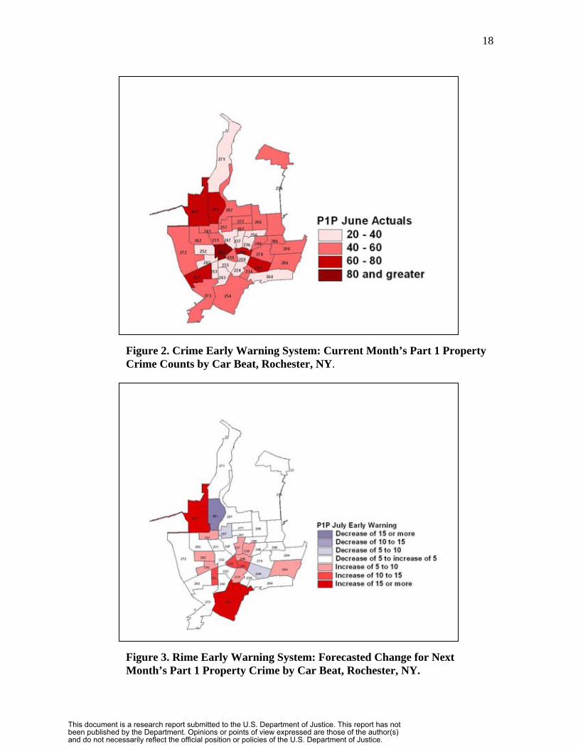
system using actual data and forecasts for Rochester, New York. Suppose that it is the

end of June and that we have just made a forecast for the coming month, July, using a

time series forecasting method (in this case it is simple exponential smoothing with

multivariate estimates for seasonality). Figure 2 is a choropleth map of car beats

displaying experienced part 1 property crime levels for June. You can see that the center

of Rochester, its central business district (CBD), had high property crime; the first ring of

car beats around the CBD had relatively low property crime levels; and the outer ring of

car beats had mostly moderately high property crime levels.

Figure 3 is the forecasted change in part 1 property crime for June, calculated as

the July forecast minus the June actual property crime level by car beat. The seasonal

effect of property crime has a large increase for July over June, so we expect some

increases. Indeed some car beats have large increases of 15 or more: car beat 261 in the

upper left and 254 at the bottom. Other car beats have forecasted decreases such as 251

adjacent to 261. This map is the early warning component of CEWS. It suggests that we

focus further crime analysis initially on car beats 261 and 254 in the outlying areas of

Rochester, and then perhaps car beats 239, 253, and 259 in the central parts of the city.

(Note that an additional, valuable choropleth map simply displays forecasted crime levels

by geographic area. Areas that had high crime levels last month and are forecasted to

have little change, remaining high, also have a high priority for micro level crime

analysis.)


18

Figure 2. Crime Early Warning System: Current Month’s Part 1 Property Crime Counts by Car Beat, Rochester, NY.

Figure 3. Rime Early Warning System: Forecasted Change for Next Month’s Part 1 Property Crime by Car Beat, Rochester, NY.


19

3.3 Micro Level Crime Analysis

This level of crime analysis includes the familiar day-to-day tasks of crime analysts:

reading crime reports, identifying patterns in MO data, mapping crime points, identifying

hot spots, etc. CEWS includes the point data and records that support these activities.

For example, Figure 4 is a zoomed-in map for car beats 261 and 251 from the Rochester

prototype CEWS. At this scale, the map adds streets and selected crime points

Figure 4. Crime Early Warning System: Drill down to Current Month’s Part 1 Property Crimes and Leading Indicator Crimes.


20

from the past month (June) for micro-level crime analysis. The crime points include a

major part 1 property crime, larcenies, and two leading indicator crimes for part 1

property crimes, disorderly conduct and criminal mischief. Crime analysts can then

review crime reports for MOs, time of day, and other patterns; apply hot spot analysis

methods; and so forth at the micro level. The current larceny hot spots would likely

remain patrol targets and perhaps some of the leading hot spots also need patrolling.

Also, detectives might be sent to emerging problem areas with concentrations of leading

indicator crimes. While not shown here, it would be possible to drill down further to add

layers for buildings, land uses, etc. in further support of detailed analysis.

3.4 Summary of Crime Forecasting Requirements

The three-level portrayal of crime analysis in this section placed crime forecasting

in its proper place and context. It is not a micro-level tool for detailed crime analysis, but

rather a middle or meso-level tool for settings such as monthly CompStat meetings.

While not a part of our forecasting research, the macro-level of crime analysis rounds out

the total crime analysis framework.

Several requirements for crime forecasting result from the decision-making frame for

crime analysis that we have presented in this section. They include:

1. Offense crime types - for forecasting are the aggregate of part 1 property crimes,

aggregate part 1 violent crimes, the individual part 1 crimes, aggregates of leading

indicators for part 1 crimes, and individual leading indicator crimes. Some of the

leading indicators can be CAD call data. Aggregates, such as total part 1 property


21

crimes, are needed to provide average monthly data volumes large enough to

yield reliable time series model estimates and forecasts.

2. The time interval - for time series is monthly data.

3. Geographic areas - for aggregating crime time series include police

administrative boundaries (precincts and car beats) as well as possibly smaller

areas of census tracts or square grid cells. The smaller the geographic area, the

smaller average monthly crime counts and forecast accuracy.

4. Forecast horizon – is one month ahead for forecasts.

5. Counterfactual forecasts – such as provided by univariate forecast methods are

needed as business-as-usual bases of comparison for evaluating the most recent

month’s crime levels.

6. CEWS – is a crime early warning system and uses crime forecasts to draw

attention to geographic areas; for example, areas that may experience large

increases or decreases in crime levels next month or are forecast to remain high

crime areas. CEWS also includes pin maps of current crimes for use in detailed

crime analyses of targeted areas.

4. Data Collection and Processing

Our crime data are from two northeastern, mid-sized cities: Pittsburgh,

Pennsylvania and Rochester, New York. We have conducted a number of studies and

grants with both cities’ police departments over the past 15 years, including building

crime mapping systems. Based on this relationship, we were able to collect and use


22

individual offense incident and CAD call data for the period of 1990 – 2001 for

Pittsburgh and 1991 – 2001 for Rochester.

A few basic statistics on both cities are in Table 1. The cities are similar in size

and population density, but of course have many important differences in population

composition, topography, land uses, city layout, industries, etc. not pursued here.

Table 1 City Statistics.

City Area (sq. miles) 2000 Population Population Density (persons/sq. mile)

Pittsburgh 55.58 334,563 6,019 Rochester 35.83 219,773 6,134

4.1 Pittsburgh Data Processing

In our first grant we collected all crime offense reports and CAD calls from the

Pittsburgh Bureau of Police for the years 1990 through 1998. In this second grant, we

added the years 1999-2001. Pittsburgh started using a new record management system in

2000. We found that we had to reprocess all of the 1990 – 1999 Pittsburgh data to ensure

that 1999 data were treated identically to the 1990 – 1998 data and to make as smooth a

connection as possible to the new format 2000 and 2001 data.

The 1990-1999 offense datasets were in 17 flat files extracted from an old

mainframe system. We used Oracle SQL Loader to import the data into an Oracle

database. The imported data are in 13 tables. We then exported the major tables into an

Access database. In Access we created links between the tables and created various


23

queries to limit crime records to offense crime only. We concatenated several fields to

get a complete street address for each crime record. We joined a crime code table that we

created to the database so that each crime record has a consistent descriptive crime name

that matches the Rochester data. The resultant table containing the Pittsburgh 1990-1999

offense data has 637,166 records.

The Pittsburgh Police Bureau’s new records management system is an Oracle

database. Therefore, the 2000 and 2001 offense data were in a good format for

processing and appending to the earlier data. There are 132,127 records in the two years

data. Again, we added the crime code table so that each crime record has a descriptive

major code.

The Pittsburgh computer aided dispatch (CAD) data have 874,535 records. The

original data were either in text files or dbase files. While various years have different

fields and formats, these data are easy to integrate. We could not obtain the CAD data for

November and December of 1999. Instead, we used simple exponential smoothing to

forecast those two months and use the forecasts as data values in our datasets. While we

had many CAD nature codes, we have only used CAD drugs and CAD shots in our

forecast models. We used a SAS program to eliminate duplicate CAD calls based on the

time and location of calls. The grand total of offense and CAD records for Pittsburgh is

1,643,828.

We used ArcView 3.3 and GDT Dynamap 2000 Street centerline maps to address

match the Pittsburgh data. This work included data cleaning to fix obvious errors and

increase address match percentages. Table 2 is a summary of address match rates. We

found that the quality of address data in offense reports declined in the new record


24

management system. The new CAD system supplies incident coordinates and thus has a

100% match rate. These address rates are generally quite good. In another large address

matching project using a national sample of police incidents obtained from the ATF, we

found the national average address match rate to be 85%, so for the most part, Pittsburgh

data are average or better.

Table 2. Address Match Rates for Pittsburgh

Data Type Years Address Match Rate

Offense 1990-1999 91% 2000-2001 72%

CAD 1990-1999 85% 2000-2001 100%

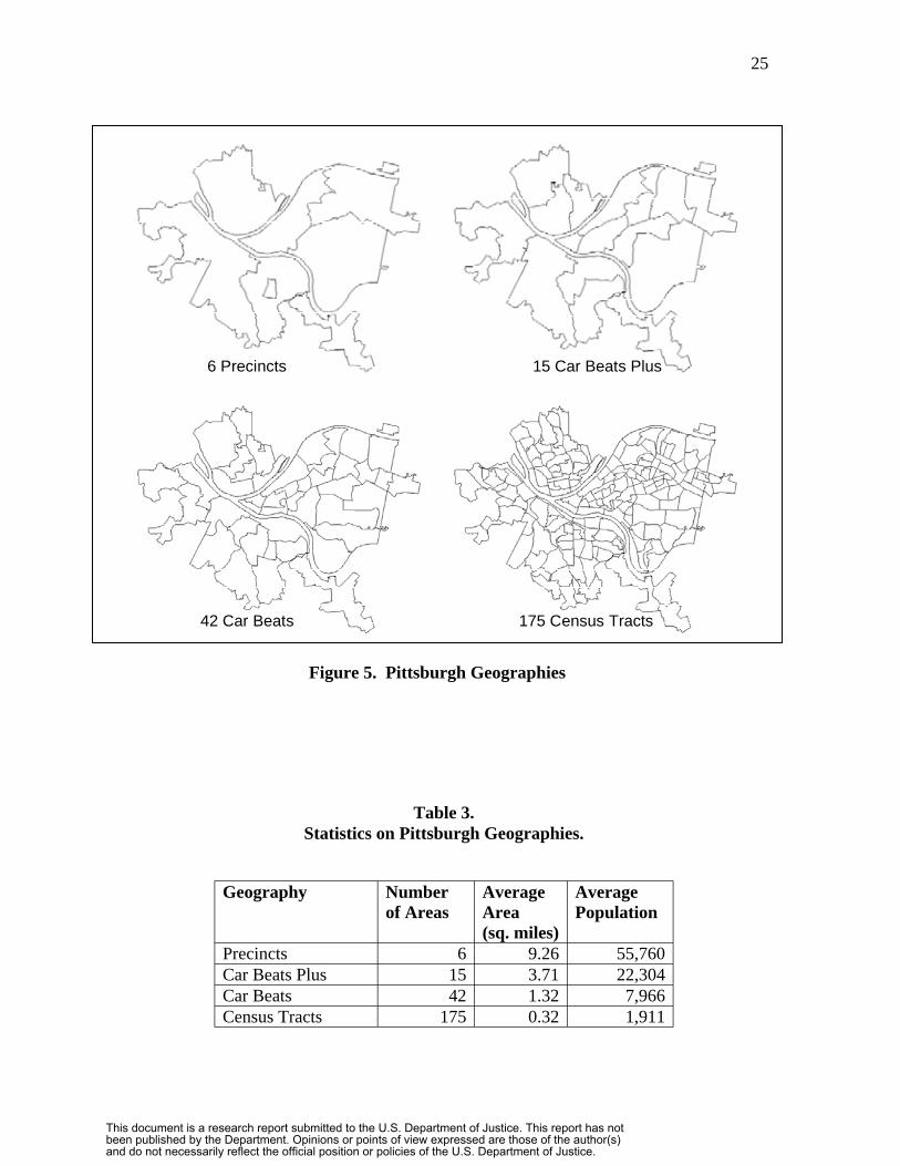
With the data address matched, we used spatial overlay in ArcView to add

geographic area identifiers for each data point: precinct, car beat, car beat plus, and 1990

census tracts. Car beats plus is an aggregation of car beats we designed to increase data

volumes to a degree that we believed would yield more accurate forecasts. Car beats in

turn are aggregations of census tracts and are the patrol districts used by the Pittsburgh

Bureau of Police during the study period. See Figure 5 for a display of these areas.

Table 3 provides statistics on average areas and populations for the four geographies.

The reader can see that there are very large differences in the average sizes of the areas

within the four geographies with a 30-fold reduction in size from the largest to the

smallest.

Our previous grant used precincts and uniform grid cells 4,000 feet long on a side

and we started research on this grant using the same grid maps for data aggregation.


6 Precincts 15 Car Beats Plus

42 Car Beats 175 Census Tracts

25

i lus6 Prec ncts 15 Car Beats P

42 Car Beats 175 Census Tracts

Figure 5. Pittsburgh Geographies

Table 3. Statistics on Pittsburgh Geographies.

Geography Number of Areas

Average Area (sq. miles)

Average Population

Precincts 6 9.26 55,760 Car Beats Plus 15 3.71 22,304 Car Beats 42 1.32 7,966 Census Tracts 175 0.32 1,911


26

There were slightly over 100 grid cells for Pittsburgh, placing them between car beats

and census tracts in size. While we still favor grid cells for their ease of visual

interpretation, based on uniform district shape and size, we nevertheless decided to

switch primarily to using administrative and statistical boundaries in our research:

precincts and car beats (which are have districts about twice as large in area as our grid

cells). We included tracts for use with the second of two forecast accuracy measures

employed (decision rule forecast criterion, see Section 5.4.2) in our research.

Our decision on geographies leads to many advantages, in addition to the obvious

one of providing the most easily used information for police. Pittsburgh geographies are

coterminous meaning that car beats are aggregates of tracts, car beats plus are aggregates

of car beats, and precincts are aggregates of car beats plus. Thus forecasts or other crime

analysis made for one geography can be related spatially to forecasts at another level.

One strategy for forecasting would be to forecast for tracts and then aggregate the tract

forecasts to other, larger district geographies. (While not pursued in our research, some

informal trials of this approach produced somewhat more accurate forecasts for larger

geographies than forecasting directly with aggregated input data.) Another advantage of

using census tract-based geographies is that multivariate models, such as our model for

neighborhood-level seasonality (see Appendix A), is that it is then easy to use census data

for independent variables.

The next step was to aggregate a number of crime types to monthly time series for

each geography. The crimes included for both Pittsburgh and Rochester are part 1

offenses and leading indicators (part 2 crimes and CAD calls) determined in our first

grant as follows:


Aggravated Assault Robbery Arson Simple Assaults Burglary Trespassing Criminal Mischief Vandalism Disconduct Weapons Family Violence CAD Drugs Gambling CAD Shots Fired Larceny Part 1 Property Crimes = Burglary + Liquor Law Violations Larceny + Motor Vehicle Theft + Motor Vehicle Theft Robbery Murder/Manslaughter Part 1 Violent Crimes (= Aggravated Prostitution Assault + Murder/Manslaughter + Rape Public Drunkenness + Robbery) Rape

4.2. Rochester Data Processing

While the Rochester Police Department also switched to a new records

management system in 2000, its older records were in dBase relational table format and

thus in good shape. We had no difficulty in importing and processing all records in

Access. Rochester Offense data contains data from January 1991 to December 2001. It

has in total 530,050 records.

Rochester CAD records contain data from January 1993 to May 2001 and

3,767,002 records. We only used the CAD shots and drugs data which in total have 8,843

records. Again we used the same algorithm to get rid of duplicate CAD calls. Thus the

grand total number of records used from Rochester is 538,893.

Again, we used ArcView 3.3 and GDT Dynamap 2000 Street centerline maps to

address match the Rochester data. No data cleaning was necessary. Address match rates

for Rochester data are excellent: 96% for offenses and 95% for CAD data. RPD requires


28

each incident to have a street address and does not allow place names (like Carnegie

Mellon University).

Spatial overlay followed in the same fashion as in Pittsburgh. Table 4 has

corresponding statistics and Figure 6 has maps of the geographies.

Table 4. Statistics on Rochester Geographies.

Geography Number of Areas

Average Area (sq. miles)

Average Population

Precincts 7 5.11 31,396 Car Beats Plus 18 1.99 12,210 Car Beats 38 0.94 5,784 Census Tracts 90 0.40 2,442

4.3 Statistics and Charts

This section provides an overall understanding of the data and time series patterns

in the Pittsburgh and Rochester data collections. We decided to only forecast a subset of

all crimes for the practical reason of reducing our workload and also because many crime

types have volumes too low to yield accurate forecasts. Our research results from grant 1

provided evidence that the average number of crimes per month for a geography, for a

region, need to be or exceed around 25 per month in order to yield acceptable forecast

accuracy. Hence the crimes we forecast are the highest volume and fortunately, also

among the most important for prevention and enforcement.

Three of the crimes that we forecast are aggregates of other crime types:

• Part 1 Property (P1P) crimes is the sum of Burglary, Larceny, Motor Vehicle

Theft, and Robbery.


29

• Part 1 Violent (P1V) crimes is the sum of Aggravated Assault, Murder, Rape, and

Robbery.

• Violent Crime Index is the sum of Arson, Criminal Mischief , Disconduct , Simple

Assault, CAD Drugs, and CAD Shots Fired for Pittsburgh and sum of Arson,

Criminal Mischief , Disconduct , Simple Assault, Drug Offenses, and Weapons

offenses for Rochester.

Precincts Car Beats Plus

Car Beats Census Tracts

Figure 6. Rochester Geographies


30

Robbery is a special case, having characteristics of both violent and property crimes.

Generally robbery is included in P1V, however, some researchers (including one of the

authors of this report) make the case that robbery shares many characteristics with

property crimes. Our options for the treatment of robbery were thus to include it in either

P1V or P1P, or in both aggregates. In the end we decided to include it in both. It has

very little influence on P1P, being a small part of the total, but has a major impact on

P1V, increasing its average crime count by a factor of 2.5. Consequently, P1V consists

of about two parts robbery and one part aggravated assaults with small amounts attributed

to rape and murder.

We designed the violent crime index as a leading indicator for violent crimes by

correlating P1V with one month lags of several leading indicator variables. Any leading

indicator with a simple correlation coefficient of 0.2 or higher was included in the violent

crime index. We decided to create and use this index because P1V cannot be forecasted

with any accuracy using traditional forecast error measures, let alone any of its

component crimes. The violent crime index has high crime volumes, comparable to that

of P1P, and thus can be forecasted accurately. This index has value for crime analysis

because it directs attention to areas that might harden to serious violent crimes. For the

case of Rochester, CAD data are only available over a limited time period in our sample,

so we used drug offenses instead of CAD drug calls and weapons offenses instead of

CAD shots fired calls.

Tables 5 and 6 present descriptive statistics for Pittsburgh and Rochester car

beats, the most useful geography for meso-scale crime analysis. The data in these tables

have been sorted in descending order by the average monthly crime count. Using the


31

Table 5. Descriptive Statistics on Forecasted Crimes for Pittsburgh Car Beats

and Months: January 1990 – December 2001 (n=6,048).

Crime Minimum Average 75th Maximum Percentile

Violent Crime Index 1 52.4 66 225 P1P 1 42.6 55 206 Larceny 0 18.9 24 119 Criminal Mischief 0 16.4 22 68 Simple Assaults 0 15.9 21 81 Motor Vehicle Theft 0 13.1 17 95 CAD Drugs 0 7.9 9 116 Burglary 0 7.6 10 57 CAD Shots 0 6.6 9 69 Disconduct 0 5.1 17 32 P1V 0 4.9 7 37 Robbery 0 3.0 4 30

Table 6. Descriptive Statistics on Forecasted Crimes for Rochester Car Beats

and Months: January 1991 – December 2001 (n=5,016).

Crime Minimum Average 75th Maximum Percentile

P1P 7 Violent Crime Index 4 Larceny 1 Disconduct 1 Criminal Mischief 0 Burglary 0 Simple Assaults 0 Motor Vehicle Theft 0 P1V 0 Robbery 0

45 56 150 39 48 109 27 33 127 18 22 52 14 18 66 10 13 55

7 10 31 6 8 28 5 7 23 3 4 19

guideline of average crime level of 25 or greater per month to achieve acceptable average

forecast errors, we see that only the violent crime index and P1P potentially have

sufficient crime volume in both cities across the entire cities for the car beat geography.

Larcenies also meeting this criterion in Pittsburgh. By restricting interest to only, say, the


32

top 25% high crime car beats it should be possible to achieve acceptable accuracy for

more crime types, for those smaller areas. It is also possible to get acceptable accuracy

for more crime types by using more spatial aggregation, using the larger car beat plus and

precinct geographies. None of the crime types in Tables 5 and 6 has sufficient volume

for acceptable average forecast errors at the census tract level.

Note that when using a forecast change error measure, as we discuss in Section

5.4.2 below for the decision rule forecast criterion, different rules apply as to what

geographies and crime types can be forecasted accurately. In that case, part 1 crimes

with good leading indicator models can be forecast accurately for smaller districts

including census tracts and the low volume P1V which has a good leading indicator

model.

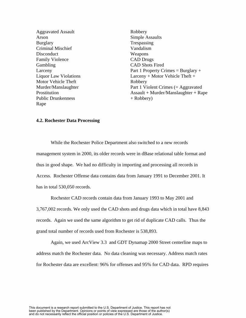
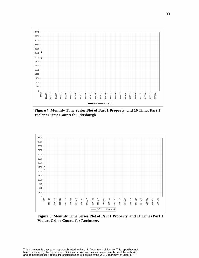
Figures 7 and 8 present city-wide time series plots for P1P and P1V for Pittsburgh

and Rochester respectively. Figure 7 shows the monthly time series plot for Pittsburgh’s

P1P and ten times P1V (to make the plots comparable in scale). The overall time trends

were steady to slightly increasing from 1990 through 1992, decreased strongly from 1993

through 1995, and then held steady or increased slightly until 2001. Our forecast

experiments, described in the next section, start with one-month-ahead forecasts for

January 1995 and roll along through one-month ahead forecasts all the way through

December 2001. The trends evident in Figure 7 make for a difficult circumstance for

methods that include a time trend, because these methods have to self-learn that the time

trend transitions from negative to zero or mildly positive in the forecast period. Methods

that do not have time trends or can adapt very quickly to ignore them have an advantage

for Pittsburgh. Seasonality is somewhat difficult to see in Figure 7, however examination


33

3500

3250

3000

2750

2500

2250

2000

1750

1500

1250

1000

750

500

250

0

P1P P1V x 10

Figure 7. Monthly Time Series Plot of Part 1 Property and 10 Times Part 1 Violent Crime Counts for Pittsburgh.

3500

3250

3000

2750

2500

2250

2000

1750

1500

1250

1000

750

500

250

0

P1P P1V x 10

Figure 8. Monthly Time Series Plot of Part 1 Property and 10 Times Part 1 Violent Crime Counts for Rochester.

Dat

e YM

1991

06

1991

12

1992

06

1992

12

1993

06

1993

12

1994

06

1994

12

1995

06

1995

12

1996

06

1996

12

1997

06

1997

12

1998

06

1998

12

1999

06

1999

12

2000

06

2000

12

2001

06

1990

06

1990

12

1991

06

1991

12

1992

06

1992

12

1993

06

1993

12

1994

06

1994

12

1995

06

1995

12

1996

06

1996

12

1997

06

1997

12

1998

06

1998

12

1999

06

1999

12

2000

06

2000

12

2001

06


34

of the plot and horizontal time scale reveals that there are summer peaks and winter

troughs. Seasonality flattens out in the last few years.

Figure 8 is the similar plot for Rochester. Here the time trend has mostly steady

decline over the entire time period. Seasonality is much more evident, with a secondary

peak readily observable in late fall. Like Pittsburgh, seasonality flattens out in the last

few years of the data set. It should be easier to forecast Rochester crime one month

ahead because of the steady time trend and strong seasonality.

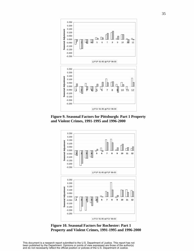
Figure 9 displays seasonal adjustments, factors above and below the trend line to

account for Pittsburgh’s seasonality of P1P and P1V crimes (i.e., the time series data in

Figure 7). We used multiplicative form classical decomposition to estimate seasonality

for two non-overlapping time intervals: 1990-1995 and 1996-2000. Here we see

moderate levels of seasonality for P1P with a maximum adjustment of almost -15% in

February and +10% for August. A secondary peak in October is at about +6% to +7%.

Overall, seasonality declined slightly over the two time periods. Seasonality for P1V has

summer peaks and winter troughs, with secondary peaks in October and December;

however, the seasonality is relatively mild and irregular.

Figure 10 has the comparable seasonality estimates for Rochester. Here

seasonality follows similar patterns to those in Pittsburgh, but is much stronger and

regular for both crime types. Again, seasonality declines for both crime types in the

second five-year interval.


35

1 2 3 4 5 6 7 8 9

j

1 2 3 4 5 6 7 8 9

lj

-0.250 -0.200

-0.150 -0.100

-0.050 0.000

0.050 0.100

0.150 0.200

0.250

10 11 12

Seas

onal

Ad

utsm

ent

P1P 91-95 P1P 96-00

-0.250

-0.200

-0.150 -0.100

-0.050

0.000

0.050

0.100 0.150

0.200

0.250

10 11 12

Sea

sona

Ad

ustm

ent

P1V 91-95 P1V 96-00

Figure 9. Seasonal Factors for Pittsburgh: Part 1 Property and Violent Crimes, 1991-1995 and 1996-2000

1 2 3 4 5 6 7 8 9

1 2 3 4 5 6 7 8 9

-0.250

-0.200 -0.150

-0.100 -0.050

0.000

0.050 0.100

0.150 0.200

0.250

10 11 12

Sea

sona

l Adj

ustm

ent

P1P 91-95 P1P 96-00

-0.250

-0.200 -0.150

-0.100 -0.050

0.000

0.050 0.100

0.150 0.200

0.250

10 11 12

Sea

sona

l Adj

ustm

ent

P1V 91-95 P1V 96-00

Figure 10. Seasonal Factors for Rochester: Part 1 Property and Violent Crimes, 1991-1995 and 1996-2000


36

5. Experimental Design

5.1 Rolling Horizon Experimental Design

Our forecast validation study uses the rolling-horizon experimental design (e.g.,

Swanson and White 1997), which maximizes the number of forecasts for a given time

series at different times and under different conditions. This design includes several

alternative, parallel forecast methods. For each forecast method included in the

experiment, we estimate models on training data, forecast one month ahead to new data

not previously seen by the model, and then calculate and save the forecast errors. Next

we roll forward one month, adding the observed value of the previously forecasted data

point to the training data, dropping the oldest historical data point, and forecasting ahead

to the next month. This process repeats until all data are exhausted.

The time periods forecasted in this way for both cities are as follows:

• Rochester Forecasts

– Offense reports: January 1996 through December 2001

– Computer aided dispatch calls : January 1998 through May 2001

• Pittsburgh Forecasts

– Offenses reports: January 1995 through December 2001

– Computer aided dispatch calls: January 1995 through December 2001


37

5.2 Treatments: Forecast Methods and Geographic Scale

We used a total of 15 forecast methods in parallel (see Table 7). These include

several naïve methods, two exponential smoothing methods combined with three ways to

estimate seasonality, and four leading indicator models with three linear models

estimated via ordinary least squares regression and nonlinear neural network model.

As seen in Figures 9 and 10, seasonality plays an important role in crime

forecasting. Recently there have been efforts in the forecast literature to improve

seasonality estimates by pooling data in a variety of ways. Seasonal factors are difficult

to estimate accurately because, for example, the effect of July on crime patterns is only

observed once per year, so even though we include 5 years of data, 60 months, in our

estimation data sets there are only 5 July data points on which to estimate its seasonal

factor. Hence, we used three methods of estimating multiplicative seasonality: 1) P

denotes that seasonality was estimated using city-wide pooled data in classical

decomposition, 2) D (for District) denotes that seasonality was estimated separately for

each district (precinct, beat plus, beat, or census tract) using classical decomposition, and

3) M denotes that seasonality was estimated using our multivariate extension to classical

decomposition which like P draws on all districts in a geography to estimate seasonal

factors.

Perhaps unique to this research, in reference to the forecast literature, is that we

have systematically varied the scale of geographic units for data aggregation from

precincts, to beats plus, to beats, and census tracts. Other studies tend to accept data in


38

Table 7. Forecast Methods Applied to Pittsburgh and Rochester Crime Data

Naïve Forecast Methods CS C SRW Random W

andom Walk DRWP Random Walk Pooled City Deseasonalization

Univariate Forecast Methods E EED Exponential Smoothing DDeseasonalization EP Exponential Smoothing PDeseasonalization EM Exponential Smoothing MDeseasonalization H HHD H DHP H Pooled City Deseasonalization

Leading Indicator Forecast Models LN Distributed L

squares regression analysis for N=1, 4, and 12. Note

NN

omp tat Method (last year’s data point is forecast) alk (last historical data point is forecast)

RWD R istrict Deseasonalization

Simple xponential Smoothing (no time trend) Simple istrict

Simple ooled City

Simple ultivariate

olt Exponential Smoothing (with time trend) olt Exponential Smoothing istrict Deseasonalization olt Exponential Smoothing

ag Model estimated via ordinary least

that the lag models include spatial lags (sum of crimes from contiguous areas to the observation area lagged in time) as well as time lags within the same area unit. Neural Network model and estimation for the distributed lag model for lags of 1 to 4

whatever single geography is available. We were able use geography as a treatment

because we collected individual crime reports, address matched them, and then were able

to aggregate them to any geographic areas desired.


39

5.3 Crimes Forecasted

As discussed above, we only forecasted a subset of all offense crime codes and

CAD nature codes available in our data. Many have volumes too small to support

accurate model estimation and forecasting. Ones that we included are as follows:

Serious Property Crimes: Leading Indicator Crimes:

P1P CAD Drugs

Burglary CAD Shots Fired

Larceny Criminal Mischief

Motor Vehicle Theft Disorderly Conduct

Robbery Simple Assault

Serious Violent Crimes: Violent Crime Index

P1V

5.4 Forecast Accuracy Measures

A final aspect of our experimental design is the choice of forecast accuracy

measures. We chose two types: 1) overall average forecast accuracy and 2) decision rule

criterion for large crime changes. The former is the traditional measure while the latter is

innovative and is designed to test for the most valuable information for tactical

deployment of police.


-40-

Average forecast accuracy is the right criterion for evaluating counterfactual

forecasts to be used in evaluating past police performance. Most of the time, there are no

major changes in crime time series patterns, so that average forecast accuracy judges how

well forecast methods do typically, in business-as-usual conditions. Such conditions are

the basis to judge innovations in police actions or the criminal element. For example, to

judge the nature of crime experienced in January 2005, we would use an exponential

smoothing model with seasonality, say HP from Table 7, to estimate the time series

patterns in the data from January 2000 through December 2004. Then we would forecast

one month ahead by taking the smoothed value for December 2004, adding the smoothed

estimate for time trend change for one month, and finally make a seasonal adjustment for

January. The resulting estimate is what we would expect, given the same police and

criminal patterns as in the past. With this estimate we can judge if the actual crime count

experienced in January was unusually high or low. The tracking signal investigated in

Appendix C uses this principle.

As desirable as average forecast accuracy is for evaluation, perhaps it is not the

best criterion for tactical deployment of police resources in crime prevention and

enforcement. That is why we introduced and used a second criterion for this purpose: the

decision rule criterion which we report on below.

5.4.1 Average Forecast Error Measure

There are many average forecast error measures available, and each has some

benefits or limitations [Armstrong and Collopy 1992]. In general, such error measures


-41-

are meaningful for decision making with repeated trials, day in and day out. Having

accurate forecasts is analogous to a casino’s advantage in games of chance: in the long

run the casino makes a profit even though it also loses regularly. Perhaps police can

benefit over the long run with an edge from crime forecasting, even if there are high

forecast errors.

We chose the mean absolute percentage error (MAPE) for crime forecasting.

This measure has the benefits of being easily interpreted and used to compare forecast

errors across time series that have different scales or volumes, being unitless. For one-

month ahead forecasts such as we make, it is calculated as the mean of the absolute value

of 100[F(t+1)-A(t+1)]/A(t+1) where t is the forecast origin or last month of historical

data, A(t+1) is the actual data value for the forecast period seen only after the forecast is

made and F(t+1) is its forecast. We suggest a threshold of 20% or smaller MAPE to

define acceptable forecast errors for police work. For example if the actual value being

forecast is 40 crimes in a month, the forecast will typically be within the range of 32 to

48. While having no firm basis for making this suggestion, we like having a cutoff point

for reporting forecast results. We also report results for cutoff points of 15% and 25%

MAPE.

5.4.2 Decision Rule Forecast Criterion

Our experience in building crime mapping systems over the years has taught us

that police have a good idea of what crime levels exist in their car beats or precincts.

Crime mapping has certainly helped to determine the current situation. What is difficult


-42-

to obtain, and most valuable, is information on how crime might change. For our second

error measure, we thus focus on forecasted change in crime, Delta(t+1) = F(t+1) – A(t)

which has positive values for forecasted crime increases and negative values for

forecasted decreases. Here A(t) is the crime level just experienced in the most recent

month.

This measure is appealing from a psychological viewpoint. Suppose that we are

at the end of time period t. Police have just experienced and responded to A(t) and have

resources deployed to handle that crime level. Consequently, we can imagine that

thinking and deployment are anchored on A(t) [Tversky and Kahneman 1974]. Next, if

we introduce new information, forecast F(t+1), and the resulting Delta(t+1) is large and

positive, then police should consider changing their thinking and deployment of resources

in the subject area in an attempt to thwart the forecasted crime increase. Without the

forecast, there is no impetus to change what police will be doing next month,

preemptively and proactively.

Suppose that crime analysts have a rule: if Delta is sufficiently high (or sufficiently

low; i.e., a large crime decrease is forecasted) then conduct detailed crime analysis,

possibly surveillance, interviews of uniformed officers, etc. to determine if new actions

are necessary in the subject area. For implementing such a rule, we break the range of

Delta values up into roughly three categories: 1) low change (middle 50% of the

distribution of delta), 2) medium change (next 15% of higher change values, moving in

both direction from the middle, to total 30% of all cases), and 3) high change with 10% in

each tail of the distribution. Of course other percentages can be used depending on

preferences of police.


-43-

Evaluation of forecasts based on these categories proceeds as follows. We examine

all cases in which there is forecasted high change, broken into high increases and high

decreases. Take the case of high increases. We tabulate the:

1. Number of positives (i.e., cases in which the actual change was high) – the larger

the better,

2. Percentage of positives (total positives divided total number of actual high change

cases) – the larger the better,

3. Percentage of negatives (cases in which the forecast was for high change but the

actual was not high change, divided by the total number of high change forecasts)

– the smaller and the better, and the

4. Percentage of adjusted negatives (in which we count the number of medium

change cases as positives, thereby reducing the percentage of negatives, because

such cases have some merit for enforcement or prevention) – the smaller the

better.

Measures such as positives and false positives are associated with contingency tables

in statistics. Quite often, a forecast method that maximizes the number or percentage of

positives will unfortunately do the same for negatives, which is undesirable. The choice

of a best forecast method should therefore consider all four of these measures, although

we place the greatest weight on positives and the positive rate.

Besides better mirroring the decision problem of police, the decision rule criterion

reduces the need for point accuracy as measured by the forecast MAPE. Instead, here we


-44-

seek interval accuracy, that Delta lies with certain intervals such as defined by small,

medium, and large changes.

6. Results

We break the results of forecast experiments up into two parts: 1) using forecast

error as the performance measure and traditional mean forecast error summaries and 2)

using forecasted change as the performance measure and the decision rule criterion.

6.1 Results on Forecast Mean Absolute Percentage Error

As discussed in Section 5, our research uses the mean absolute percentage error

(MAPE) to compare and evaluate forecast methods. Tables 8 provides an overall

summary for forecast accuracy attained in our experiments, reporting the best forecast

accuracy attained: 15%, 20%, or 25% MAPE. This summary is for high crime areas: the

25 percent highest crime districts for beats and beats plus, and the highest 50 percent for

precincts. The high crime areas need the most attention and hence we focus on them. An

evaluation for all areas will simply have worse forecast performance.

Note that we have also analyzed the forecast mean squared error criterion (MSE),

which compares the average forecast errors squared, but do not report the results in detail

here. The MSE places more weight on large errors than the MAPE and thus large actual

and forecast values, the region of most interest for crime analysis. Nevertheless, nearly

all conclusions and patterns observed in the tables below for the forecast MAPE also


-45-

follow through for the forecast MSE. In particular, simple exponential smoothing with

pooled city-wide seasonality (EP) is the best forecast method and the leading indicator

models (L1, L4, L12, and NN) are among the worst according to either the MAPE or

MSE.

Precinct-level reporting is a good staring point for crime fighting evaluation and

planning at the meso-level crime analysis. At this level, there is considerable forecast

accuracy. Most of the crimes studied in Pittsburgh attain the 15% or 20% forecast MAPE

thresholds with some exceptions. Rochester fairs a bit worse, with no attainment of

accuracy for P1V or robbery. Arson and shots fired do not attain forecast accuracy in

either city or for any geography. Their crime volumes are too low.

Table 8. MAPE Forecast Accuracy Attained in Pittsburgh and Rochester:

High Crime Areas.

Precincts Car Car Beats Beats Plus

P1P Burglary Larceny Motor Vehicle Theft

Robbery P1V Violent Crime Index

Arson Criminal Mischief Disorderly Conduct Drug Calls Simple Assault Shots Fired Calls

P, R P, R P, R R

P, R P, R P P

P P P, R P, R P, R

P, R P, R P, R R R

P, R P, R R

P, R P, R

P=Pittsburgh R= Rochester P, R = 15% or better MAPE P, R = 20% or better MAPE P, R = 25% or better MAPE


-46-

As the reader can see, only P1P and the violent crime index attain 20% MAPE

accuracy at the car beat level. The violent crime index for car beats is better in Rochester

and attains 15% MAPE accuracy. The result here is clear: if either police department

wishes to forecast at the beat level, it can only do so for P1P and the violent crime index

out of the crimes and aggregates that we have considered, based on the forecast MAPE.

For car beats plus, larceny forecasts attain 20% MAPE accuracy in both Pittsburgh

and Rochester as do several of the higher volume leading indicator crimes. There are

gains in accuracy for this geography, and police departments may wish to use the

approach of aggregating car beats here as we have, to gain this accuracy.

In summary, the results of Table 8 are that acceptable average forecast accuracy is

widely available at the precinct level, but at the car beat level is possible only for P1P and

the violent crime index (or other sufficiently large crime aggregates). Hence, we only

provide more detailed results, next, on individual forecast methods on these two crime

types, although we compiled similar tables for all crime types studied.

Tables 9 and 10 have results for P1P forecasts and hot crime areas (top 25% beats and

beats plus districts and top 50% precincts) in Pittsburgh and Rochester, respectively using

the forecast MAPE criterion. These tables have a very compact format, that we designed

in our previous crime forecasting grant. It need some explanation.

• In the left column is the notation for forecasting methods (see Table 7 above for

definitions).

• Across the top are columns reporting results for the three geographies, precincts,

beats plus, and beats.


-47-

• The Min MAPE row near the bottom is the forecast MAPE for the most accurate

forecast method calculated over the experiment of all areas a geography included

and months forecasted (84 one-month-ahead forecasts for Pittsburgh and 72 for

Rochester).

• The cell entry for the most accurate method is the value 1.00. The cell entries for

all other methods are numbers greater than 1, giving the factor worse than the

best. For example, in Table 9 for precincts, the best method is EP (simple

exponential smoothing with city-wide pooled seasonality) and it has a forecast

MAPE of 9.4%. The worst method is L12, the 12 lag leading indicator model,

which 2.75 times worse than the best and has a forecast MAPE of 2.75 x 9.4% =

25.9%.

• The shaded cells provide a measure of the benefit of including seasonality

modeling in forecasts. It is the best non-seasonal method, compared to the best

method. Again, for Table 9 precincts, E (simple exponential smoothing) is the

best non-seasonal method. It is a factor 1.12 (12%) worse than the best seasonal

method. So we can say that ignoring seasonality makes the MAPE 12% worse.

• The tables are sorted in descending order of the Beats column.

• The N row is the number of forecast errors averaged using the MAPE criterion.

• The No. Areas row at the bottom is the number of districts in a geography, for

example 6 precincts for Pittsburgh in Table 9.

Starting with Table 9 and Pittsburgh P1P, we see that the smoothing methods were

the most accurate for beats and the leading indicator lag models were by far the worst,


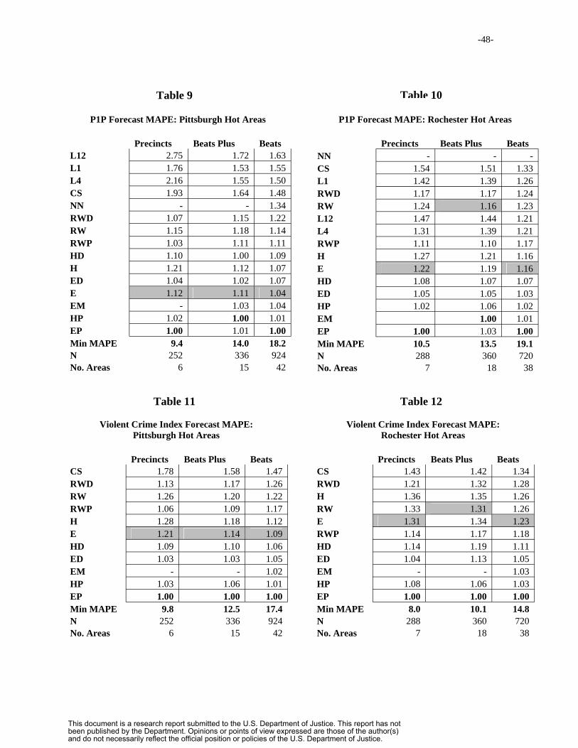
-48-

Table 9

P1P Forecast MAPE: Pittsburgh Hot Areas

Precincts Beats Plus Beats

Table 10

P1P Forecast MAPE: Rochester Hot Areas

Precincts Beats Plus Beats L12 L1 L4 CS NN RWD RW RWP HD H ED E EM HP EP

2.75 1.72 1.63 1.76 1.53 1.55 2.16 1.55 1.50 1.93 1.64 1.48

- - 1.34 1.07 1.15 1.22 1.15 1.18 1.14 1.03 1.11 1.11 1.10 1.00 1.09 1.21 1.12 1.07 1.04 1.02 1.07 1.12 1.11 1.04

- 1.03 1.04 1.02 1.00 1.01

1.00 1.01 1.00

NN CS L1 RWD RW L12 L4 RWP H E HD ED HP EM EP

- - -1.54 1.51 1.33 1.42 1.39 1.26 1.17 1.17 1.24 1.24 1.16 1.23 1.47 1.44 1.21 1.31 1.39 1.21 1.11 1.10 1.17 1.27 1.21 1.16 1.22 1.19 1.16 1.08 1.07 1.07 1.05 1.05 1.03 1.02 1.06 1.02

1.00 1.01 1.00 1.03 1.00

Min MAPE 9.4 14.0 18.2 N 252 336 924 No. Areas 6 15 42

Min MAPE 10.5 13.5 19.1 N 288 360 720 No. Areas 7 18 38

Table 11 Table 12

Violent Crime Index Forecast MAPE: Violent Crime Index Forecast MAPE: Pittsburgh Hot Areas Rochester Hot Areas

Precincts Beats Plus Beats Precincts Beats Plus Beats CS RWD RW RWP H E HD ED EM HP EP

1.78 1.58 1.47 1.13 1.17 1.26 1.26 1.20 1.22 1.06 1.09 1.17 1.28 1.18 1.12 1.21 1.14 1.09 1.09 1.10 1.06 1.03 1.03 1.05

- - 1.02 1.03 1.06 1.01

1.00 1.00 1.00

CS RWD H RW E RWP HD ED EM HP EP

1.43 1.42 1.34 1.21 1.32 1.28 1.36 1.35 1.26 1.33 1.31 1.26 1.31 1.34 1.23 1.14 1.17 1.18 1.14 1.19 1.11 1.04 1.13 1.05

- - 1.03 1.08 1.06 1.03

1.00 1.00 1.00 Min MAPE 9.8 12.5 17.4 Min MAPE 8.0 10.1 14.8 N 252 336 924 N 288 360 720 No. Areas 6 15 42 No. Areas 7 18 38


-49-

having factors worse in excess of 1.5. The CompStat method (CS) also performs poorly

with a factor of 1.48 and the neural network version of the leading indicator model

similarly did very poorly with a factor of 1.34. Then come the rest of the naïve methods

ranging in factors worse from 1.11 to 1.22. The best method is EP: simple exponential

smoothing with seasonality estimated using city-wide data and a forecast MAPE of 18.2.

Seasonality does not help very much for beats. The best non-seasonal method is only 4%

worse than the best method, EP. These results hold up for the most part for the two other

geographies, although seasonality is more important for beats plus and precincts. In

regards to the method of estimating seasonality, city-wide pooling of data yielded the best

forecast accuracy. ED, with seasonality computed separately using each beat’s own data,

was 7% worse. Our multivariate estimate of seasonality, EM, was 4% worse.

Because seasonality does not add much to accuracy and leading indicators are

terrible, we conclude that crime forecasting for P1P in Pittsburgh car beats is accurate

enough, but not very informative. About all we learn is that such data are regressive and

return to the mean, which is what simple exponential smoothing implies. If a month has

unusually high or low crime in a month, most of the time it will return to the current

mean crime level next month. Because most large crime changes are increases, this could

mean that the Pittsburgh police are effective in enforcing property crimes in cases with

increased criminal activity.

Table 10 has comparable results for Rochester P1P. Here the CompStat method is the

worst for car beats, with a factor worse of 1.33 times the best forecast MAPE of 19.1 for

EP. The leading indicator models do better than in Pittsburgh, but still are relatively poor

forecasters with factors worse ranging from 1.21 to 1.26. The naïve methods also fall in


-50-

the same range. This time, seasonality adds a good bit more to forecast accuracy, the best

non-seasonal method is 16% worse than EP. For beats plus, our multivariate seasonality

methods with exponential smoothing, EM, is best. EP is best again for precincts.

Forecasting P1P in Rochester is more informative than in Pittsburgh. Besides regression

to the mean behavior, there are fairly large seasonal effects that result in large forecasted

changes in crime levels.

Tables 11 and 12 have average forecast accuracy for the violent crime index that we

are proposing. In this case, we have no leading indicator models because we are

forecasting the leading indicators themselves: there are no leading indicators of the

leading indicators. The CompStat method is consistently the worst method in both tables.

The violent crime index has accurate and informative forecasts, given the large seasonal

factors.

One last topic for discussion in regard to Tables 9 through 12 is the effect of

geographic scale on forecast accuracy. These tables provide information on three

geographies, which is graphed in Figures 11 and 12. The vertical axii in these figures are

the minimum forecast MAPE for a crime type and the horizontal axii are the average area

(sq. miles) of districts within each geography. Both cities have a nonlinear relationship

between these two quantities, with decreasing gains in forecast accuracy as district area

increases.

Pittsburgh’s relationship is closer to linear than is Rochester’s. Furthermore, the

gains in accuracy in Rochester are much more rapidly attained by increasing area. As a

rough approximation, the slope of lines connecting the two extreme points for each crime

in Pittsburgh is very nearly -1.0 for both P1P and the violent crime index; for every 1


-51-

Ave

rage

For

ecas

t MA

PE

19

17

15

13

11

9

7

P1P

VCI

0 2 4 6 8 10 Average Area

Figure 11. Minimum Forecast MAPE versus Average District Area of Geographies in Pittsburgh.

19

P1P

VCI

Ave

rage

For

ecas

t MA

PE 17

15

13

11

9

7 0 2 4 6 8 10

Average Area

Figure 12. Minimum Forecast MAPE versus Average District Area of Geographies in Rochester.


-52-

square mile increase in district area there is a 1% decrease in the minimum forecast

MAPE. The same slope in Rochester is -1.6 for the violent crime index and -2.0 for P1P.

The bottom line is that Rochester can achieve acceptable crime forecast accuracy with

smaller geographic areas than can Pittsburgh.

6.2 Decision Rule Forecast Performance

We turn attention now to results for the decision rule forecast criterion. An

example of a decision rule is as follows:

Decision Rule for Forecasted Large P1V Increases for Pittsburgh Census Tracts:

If the forecasted change in P1V for a census tract is large (an increase greater than

or equal to 2 or a decrease greater than or equal to 2), then issue an exception

report on that tract for the coming month for possible further analysis and action.

P1V crimes at the census tract level are infrequent, hence the low cut point value of 2 in

these rules. Our design of cut points for large changes attempts to place 20% of the

actual census tract-month observations in the tails of the crime change distribution (10%

of the top increases and 10% of the top decreases). We also include low and middle

change categories, which come into play for evaluation below. The low change has cut

points to capture the middle 50% of the actual crime change distribution and for this case

is a forecasted change between -0.499 to 0.499, or no change after rounding. For other

crimes and geographies low change cut points are higher numbers. The middle change


-53-

categories are the two 15% intervals between the low change and two large change tails

of the distribution. Below in the analysis, we give credit to the decision rule for catching

medium changes of the intended kind of change (increase of decrease) even though the

rule is designed to catch large changes. Enforcement or prevention efforts in such cases

are not entirely wasted, because there is still a sizable crime change in the predicted

direction.

Our experiments included the exponential smoothing methods EP, ED, EM, and

HD in the comparisons, along with the leading indicator models. We chose these

smoothing models because EP is the best overall in forecast MAPE comparisons. The

others are among those that have the most capacity for yielding large change forecasts;

for example, HD includes a trend term and has seasonality estimated by district. Such a

seasonality estimate yields more variation in seasonal factors than that of the city-wide

method as in EP. Also EM uses the multivariate seasonality model which can vary

seasonality by neighborhood type and also allows more range in seasonal factors than the

city-wide seasonality estimates.

The models that we expect will perform the best, however, for forecasting large

changes in crime levels are the leading indicator models, estimated by ordinary least

squares regression in linear form and neural networks in nonlinear form. We test three

versions of the regression models for P1P and P1V: 1) L1 has a single month’s lag of the

leading indicator crimes (within a district and summed for contiguous districts for the

spatial lags), 2) L4 has 1, 2, 3, and 4 month lags of the same variables, and 3) L12 has 1,

2, …, 12 month lags. Of course, all of these lagged variables have estimated coefficients


-54-

from historical data that translate their impact into dependent variable values. These

models have several advantages for estimating extreme values in small geographic areas:

• The many lagged independent variables have data that vary for each district of a

geography, thus tailoring models for local conditions in detailed and rich ways.

These variables can change radically from one month to the next, permitting large

changes in forecasted values from month to month. The smoothing models only

have at most two factors that can vary by district, time trend slope and

seasonality, and they must change smoothly and predictably.

• A specific application of the previous point is that the lagged models can harness

large changes in leading indicators at the end of a time series to forecast a large

change in the dependent variable crime. That is a major impetus for developing

these models. The smaller the district size the more large changes expected (step

jumps, turning points, etc.) in the leading indicator time series.

• The lagged models provide a crude approximation of seasonality estimation,

based on individual values of independent variables that can vary quickly.

Seasonality roughly follows a sinusoidal patter over the 12 months of a year, so

L1 can capture last month’s seasonal adjustment which is still relevant this month

Furthermore, the decision rule forecast criterion relaxes demands on forecast

methods. Instead of being judged on point accuracy (each forecast is compared to its

corresponding actual crime count), forecast methods are judged on interval accuracy (the

forecasted change is in the high range, is the actual change also in the high range?). This


-55-

is all to say that the leading indicator, lagged models should do well in small geographic

areas for large changes, and better than the smoothing models which have less capacity to

produce quickly changing forecasts.

Before proceeding to results we need to make a note about the implementation of

the neural network method. Application of neural networks was not included in the

scope or budget of this grant. We nevertheless used it on an experimental basis with our

own research-based computer code, as programmed and run by Andreas Olligschlaeger

[Olligschlaeger 1997a, 1997b]. The corresponding results, designated by NN in the

tables that follow, have two limitations: 1) the neural networks were only presented with

lags 1 through 4 of the leading indicators whereas the ordinary least squares used lags 1

through 12 in various models, and 2) the neural network architectures (model

specification) were not optimized or objectively determined but rather was set through

informal trial and error. Hence, we believe that neural network results could be improved

with a more systematic implementation in future work.

While more detailed explanations and results follow in the discussion of Tables

14 through 21, there are several immediate conclusions from summary Table 13. For this

table, we chose the best method base on the number of positives and positive rates; that

is, on the total number of times the decision rule correctly identified high crime changes

and the percentage of total actual high change cases forecasted by the decision rule.

Observations on the results in Table 13 include:

• Because we designed our decision rules to place roughly 10% of observations in

each of the tails of actual crime change distributions, using random numbers to

fire the decision rule by chance alone would yield on average a 10% positive rate.


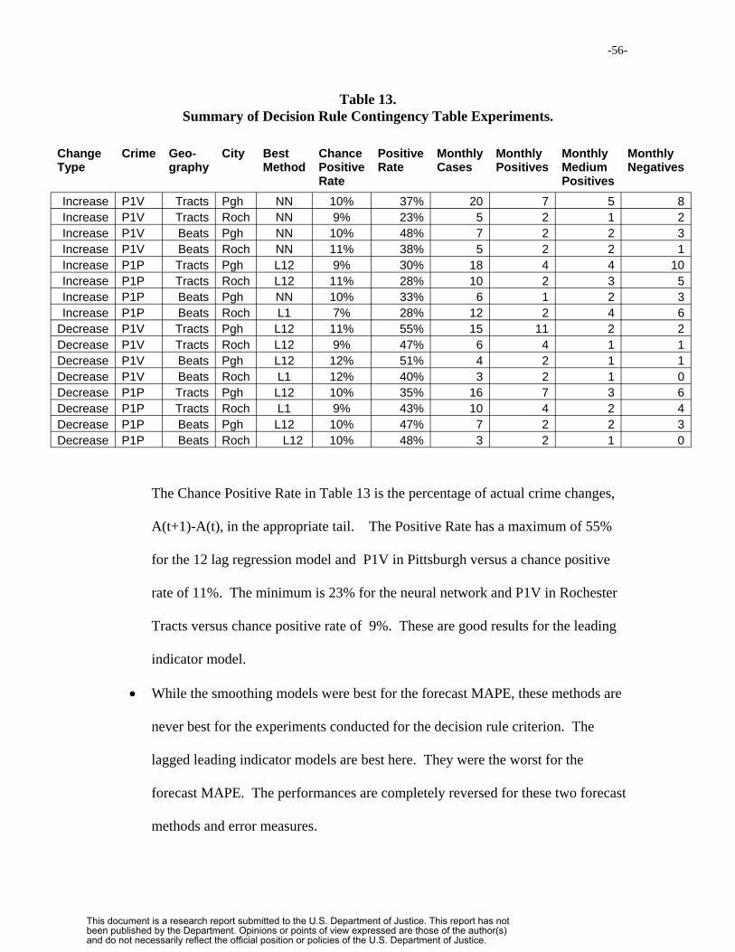
-56-

Table 13. Summary of Decision Rule Contingency Table Experiments.

Change Type

Crime Geography

City Best Method

Chance Positive Rate

Positive Rate

Monthly Cases

Monthly Positives

Monthly Medium Positives

Monthly Negatives

Increase P1V Tracts Pgh NN 10% 37% 20 7 5 8 Increase P1V Tracts Roch NN 9% 23% 5 2 1 2 Increase P1V Beats Pgh NN 10% 48% 7 2 2 3 Increase P1V Beats Roch NN 11% 38% 5 2 2 1 Increase P1P Tracts Pgh L12 9% 30% 18 4 4 10 Increase P1P Tracts Roch L12 11% 28% 10 2 3 5 Increase P1P Beats Pgh NN 10% 33% 6 1 2 3 Increase P1P Beats Roch L1 7% 28% 12 2 4 6

Decrease P1V Tracts Pgh L12 11% 55% 15 11 2 2 Decrease P1V Tracts Roch L12 9% 47% 6 4 1 1 Decrease P1V Beats Pgh L12 12% 51% 4 2 1 1 Decrease P1V Beats Roch L1 12% 40% 3 2 1 0 Decrease P1P Tracts Pgh L12 10% 35% 16 7 3 6 Decrease P1P Tracts Roch L1 9% 43% 10 4 2 4 Decrease P1P Beats Pgh L12 10% 47% 7 2 2 3 Decrease P1P Beats Roch L12 10% 48% 3 2 1 0

The Chance Positive Rate in Table 13 is the percentage of actual crime changes,

A(t+1)-A(t), in the appropriate tail. The Positive Rate has a maximum of 55%

for the 12 lag regression model and P1V in Pittsburgh versus a chance positive

rate of 11%. The minimum is 23% for the neural network and P1V in Rochester

Tracts versus chance positive rate of 9%. These are good results for the leading

indicator model.

• While the smoothing models were best for the forecast MAPE, these methods are

never best for the experiments conducted for the decision rule criterion. The

lagged leading indicator models are best here. They were the worst for the

forecast MAPE. The performances are completely reversed for these two forecast

methods and error measures.


-57-

• The more important kind of crime changes are increases. It is in this case that

crime prevention and enforcement interventions are needed. Here the neural

network models are overall best, in 5 out of 8 cases. We have not seen any other

models capable of forecasting P1V for small sized districts. Moreover, the neural

network is best for all 4 P1V experiments. Note that as seen in Appendix B, the

P1V leading indicator model is the better in terms of fit, compared to P1P

• The results for forecasting crime decreases are better than those for crime

increases. The average positive rate for the former is 46% while for the latter is

33%. As explained in Appendix B, there is a bias in crime data that makes it easy

to forecast decreases: high outliers are large increases that are impossible to

forecast but predictably are immediately followed by large decreases. Forecast

models do not adapt much to the outliers and hence continue to forecast at normal

crime levels, to which the actual crime level returns. Hence high outliers lead to

poor increase forecast performance and good decrease performance. Low outliers

are rare in crime time series, so the opposite effect does not occur often.

• Included in Table 13 is an estimate of monthly workloads for crime analysts; that

is, drilling down into details and doing micro-level crime analysis to diagnose the

exception reports generated by the decision rules. This workload is in the

Monthly Exception Reports column and is the number of car beats or tracts to be

so analyzed on average each month. This number ranges from 3 to 20 districts

(whereas the total number of districts ranges from a low of 38 car beats for

Rochester to a high of 175 tracts for Pittsburgh.


-58-

• This work load pays off by forecasting an average number of true large change

cases (Monthly Positives) and true medium change cases (Monthly Medium

Positives), but fails by falsely forecasting true low changes as large changes

(Monthly Adjusted Negatives). Much of police work is on following up on good

leads that do not pan out. Crime forecasting and the decision rule criterion fall

into that category. On average, the workload for each crime analyzed by tract

generates 12 exception reports per month, with a breakdown to 5 positives, 3

medium change positives, and 4 adjusted false positives (low changes or changes

in the wrong direction). By car beats the workload per crime type is 6 exception

reports per month, with 2 positives, 2 medium change positives, and 2 adjusted

false positives.

Tables 14 through 21, while numerous, have a streamlined presentation over those

included in our previous grant. Here we have only one table per crime type and

geography, whereas before we had three. Table 14 is for P1V and census tracts in

Pittsburgh. P1V has relatively low levels and especially for areas as small as census

tracts (there are 175 tracts in Pittsburgh). We didn’t report on tracts for the forecast

MAPE assessments of the previous section because this measure is very high in this case.

Definitions of columns and examples for Table 14 (through Table 21) follow:

• A Positive is forecasted increase or decrease that satisfies this rule for which the

actual change (learned after the following month passes in practice) is as

predicted, an increase or decrease greater that or equal to 2. For neural networks


-59-

Table 14 P1V Forecast Validation Results for Pittsburgh Census Tracts:

Change of 1 or 2 or More Crimes One Month Ahead Out of 14,525 Forecasts

Increases: Actual number cases with 2 or more crimes increase: 1,603

Method No. 2 or More Increase Forecasts

No. 2 or More Increase Positives

2 or More Increase Positive Rate

2 or More Increase False Positive Rate

No. 1 Increases Caught

Adjusted False Positive Rate

EP 678 337 21.0% 50.0% 170 25.2% ED 1,452 458 28.6% 68.5% 346 44.6% HD 1,722 421 26.3% 75.6% 377 53.7% NN 1,653 596 37.2% 63.9% 433 37.7% L1 988 353 22.0% 64.3% 271 36.8% L4 1,052 402 25.1% 61.8% 278 35.4% L12 1,142 419 26.1% 63.3% 278 39.0%

Decreases: Actual number of cases with 2 or more crimes decrease: 1,610

Method No. 2 or More Decrease Forecasts

No. 2 or More Decrease Positives

2 or More Decrease Positive Rate

2 or More Decrease False Positive Rate

No. 1 Decreases Caught

Adjusted False Positive Rate

EP 953 738 45.8% 22.6% 107 11.3% ED 950 678 42.1% 28.6% 141 13.8% HD 903 617 38.3% 31.7% 139 16.3% NN 828 661 41.1% 20.2% 79 10.6% L1 1,218 828 51.4% 32.0% 180 17.2% L4 1,238 878 54.5% 29.1% 171 15.3% L12 1,294 884 54.9% 31.7% 201 16.2%


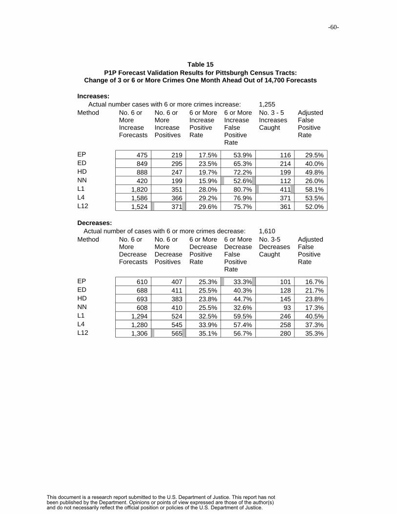
-60-

Table 15 P1P Forecast Validation Results for Pittsburgh Census Tracts:


Increases: Actual number cases with 6 or more crimes increase: 1,255

Method No. 6 or No. 6 or 6 or More 6 or More No. 3 - 5 Adjusted More More Increase Increase Increases False Increase Increase Positive False Caught Positive Forecasts Positives Rate Positive Rate

Rate

EP ED HD NN L1 L4 L12

475 219 17.5% 53.9% 116 29.5% 849 295 23.5% 65.3% 214 40.0% 888 247 19.7% 72.2% 199 49.8% 420 199 15.9% 52.6% 112 26.0%

1,820 351 28.0% 80.7% 411 58.1% 1,586 366 29.2% 76.9% 371 53.5% 1,524 371 29.6% 75.7% 361 52.0%

Decreases: Actual number of cases with 6 or more crimes decrease: 1,610

Method No. 6 or No. 6 or 6 or More 6 or More No. 3-5 Adjusted More More Decrease Decrease Decreases False Decrease Decrease Positive False Caught Positive Forecasts Positives Rate Positive Rate

Rate

EP ED HD NN L1 L4 L12

610 407 25.3% 33.3% 101 16.7% 688 411 25.5% 40.3% 128 21.7% 693 383 23.8% 44.7% 145 23.8% 608 410 25.5% 32.6% 93 17.3%

1,294 524 32.5% 59.5% 246 40.5% 1,280 545 33.9% 57.4% 258 37.3% 1,306 565 35.1% 56.7% 280 35.3%


-61-

Table 16 Part 1 Violent Crime Forecast Validation Results for Pittsburgh Car Beats:

Change of 2 to 3 or 4 or More Crimes One Month Ahead out of 2,982 Forecasts

Increases: Actual number cases with 4 or more crimes increase: 338

Method No. 4 or No. 4 or 4 or More 4 or More No. 2, 3 Adjusted More More Increase Increase Increases False Increase Increase Positive False Caught Positive Forecasts Positives Rate Positive Rate

Rate

EP ED EM HD NN L1 L4 L12

119 59 17.5% 50.4% 34 21.8% 239 85 25.1% 64.4% 61 38.9% 155 70 20.7% 54.8% 43 27.1% 282 83 24.6% 70.6% 64 47.9% 571 163 48.2% 71.5% 154 44.5% 224 69 20.4% 69.2% 61 42.0% 248 77 22.8% 69.0% 61 44.4% 380 106 31.4% 72.1% 96 46.8%

Decreases: Actual number of cases with 4 or more crimes decrease: 348

Method No. 4 or No. 4 or 4 or More 4 or More No. 2, 3 Adjusted More More Decrease Decrease Decreases False Decrease Decrease Positive False Caught Positive Forecasts Positives Rate Positive Rate

Rate

EP ED EM HD NN L1 L4 L12

159 124 35.6% 22.0% 22 8.2% 165 124 35.6% 24.8% 25 9.7% 175 131 37.6% 25.1% 26 10.3% 160 111 31.9% 30.6% 23 16.3% 121 87 25.0% 28.1% 16 14.9% 274 156 44.8% 43.1% 54 23.4% 296 162 46.6% 45.3% 68 22.3% 322 177 50.9% 45.0% 63 25.5%


-62-

Table 17 P1P Forecast Validation Results for Pittsburgh Car Beats:


Increases: Actual number cases with 14 or more crimes increase: 346

Method No. 14 or No. 14 or 14 or 14 or No. 4-13 Adjusted More More More More Increases False Positive Increase Increase Increase Increase Caught Rate Forecasts Positives Positive False

Rate Positive Rate

EP 139 64 18.5% 54.0% 45 21.6% ED 206 66 19.1% 68.0% 67 35.4% EM 179 65 18.8% 63.7% 60 30.2% HD 204 63 18.2% 69.1% 65 37.3% NN 545 114 32.9% 79.1% 177 46.6% L1 612 77 22.3% 87.4% 193 55.9% L4 582 98 28.3% 83.2% 193 50.0% L12 675 104 30.1% 84.6% 215 52.7%

Decreases: Actual number of cases with 14 or more crimes decrease: 348

Method No. 14 or No. 14 or 14 or 14 or No. 4-13 Adjusted More More More More Decreases False Positive Decrease Decrease Decrease Decrease Caught Rate Forecasts Positives Positive False

Rate Positive Rate

EP 34.4% 23 16.4% ED

128 84 24.1% 151 92 26.4% 39.1% 29 19.9%

EM 147 93 26.7% 36.7% 28 17.7% HD 174 91 26.1% 47.7% 39 25.3% NN 117 61 17.5% 47.9% 25 26.5% L1 484 145 41.7% 70.0% 122 44.8% L4 546 163 46.8% 70.1% 164 40.1% L12 578 164 47.1% 71.6% 174 41.5%


-63-

Table 18 Part 1 Violent Crime Forecast Validation Results for Rochester Tracts:

Change of 1 to 2 or 3 More Crimes One Month Ahead Out of 6,462 Forecasts

Increases: Number cases with 3 or more crimes increase: 574 Method No. 3 or No. 3 or 3 or More 3 or More No. 1 to 2 Adjusted

More More Increase Increase Increases False Increase Increase Positive False Caught Positive Forecasts Positives Rate Positive Rate

Rate

EP 58 10.1% 58.0% 26 39.1% ED

138 490 121 21.1% 75.3% 81 58.8%

HD 591 117 20.4% 80.2% 89 65.1% Neural Network 393 130 22.6% 66.9% 89 44.3% Regression Lag 1 234 75 13.1% 67.9% 50 46.6% Regression Lag 4 220 85 14.8% 61.4% 50 38.6% Regression Lag12 229 91 15.9% 60.3% 51 38.0%

Decreases: Number of cases with 3 or more crimes decrease: 564 Method No. 3 or No. 3 or 3 or More 3 or More No. 1 to 2 Adjusted

More More Decrease Decrease Decreases False Decrease Decrease Positive False Caught Positive Forecasts Positives Rate Positive Rate

Rate

EP 27.7% 38 12.6% ED

253 183 32.4% 270 170 30.1% 37.0% 44 20.7%

HD 264 160 28.4% 39.4% 40 24.2% Neural Network 268 186 33.0% 30.6% 34 17.9% Regression Lag 1 403 250 44.3% 38.0% 67 21.3% Regression Lag 4 386 246 43.6% 36.3% 63 19.9% Regression Lag12 429 265 47.0% 38.2% 70 21.9%


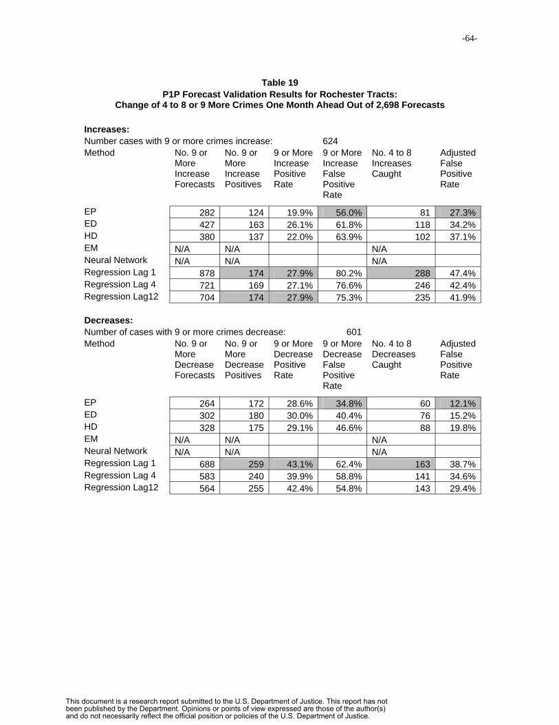
-64-

Table 19 P1P Forecast Validation Results for Rochester Tracts:




Rate

EP 56.0% 81 27.3% ED

282 124 19.9% 427 163 26.1% 61.8% 118 34.2%

HD 380 137 22.0% 63.9% 102 37.1% EM N/A N/A N/A Neural Network N/A N/A N/A Regression Lag 1 878 174 27.9% 80.2% 288 47.4% Regression Lag 4 721 169 27.1% 76.6% 246 42.4% Regression Lag12 704 174 27.9% 75.3% 235 41.9%



Rate

EP 264 172 28.6% 34.8% 60 12.1% ED 302 180 30.0% 40.4% 76 15.2% HD 328 175 29.1% 46.6% 88 19.8% EM N/A N/A N/A Neural Network N/A N/A N/A Regression Lag 1 688 259 43.1% 62.4% 163 38.7% Regression Lag 4 583 240 39.9% 58.8% 141 34.6% Regression Lag12 564 255 42.4% 54.8% 143 29.4%


-65-

Table 20 P1V Forecast Validation Results for Rochester Beats:




Rate

EP 53.7% 27 31.4% ED

121 56 19.0% 233 79 26.8% 66.1% 49 45.1%

HD 232 62 21.0% 73.3% 42 55.2% EM 167 70 23.7% 58.1% 41 33.5% Neural Network 360 112 38.0% 68.9% 116 36.7% Regression Lag 1 212 76 25.8% 64.2% 68 32.1% Regression Lag 4 209 72 24.4% 65.6% 72 31.1% Regression Lag12 241 80 27.1% 66.8% 80 33.6%



Rate

EP 123 93 31.6% 24.4% 20 8.1% ED 152 95 32.3% 37.5% 37 13.2% HD 159 101 34.4% 36.5% 39 11.9% EM 137 98 33.3% 28.5% 26 9.5% Neural Network 205 113 38.4% 44.9% 48 21.5% Regression Lag 1 190 117 39.8% 38.4% 40 17.4% Regression Lag 4 178 115 39.1% 35.4% 35 15.7% Regression Lag12 200 115 39.1% 42.5% 47 19.0%


-66-

Table 21 P1P Crime Forecast Validation Results for Rochester Beats:




Rate

EP 61.5% 46 19.3% ED

109 42 17.7% 164 54 22.8% 67.1% 62 29.3%

HD 144 46 19.4% 68.1% 53 31.3% EM 139 48 20.3% 65.5% 59 23.0% Neural Network N/A N/A N/A Regression Lag 1 27.8% 84.6% 164 46.4% Regression Lag 4

429 66 354 63 26.6% 82.2% 145 41.2%

Regression Lag12 393 72 30.4% 81.7% 159 41.2%



Rate

EP 112 79 33.3% 29.5% 25 7.1% ED 131 80 33.8% 38.9% 34 13.0% HD 140 75 31.6% 46.4% 41 17.1% EM 116 77 32.5% 33.6% 30 7.8% Neural Network N/A N/A N/A Regression Lag 1 261 111 46.8% 57.5% 65 32.6% Regression Lag 4 236 108 45.6% 54.2% 65 26.7% Regression Lag12 243 113 47.7% 53.5% 67 25.9%


-67-

(NN), the best method in the top half of Table 13 for forecasted increases, this is

596.

• The Positive Rate for a set of forecasted changes is the 100 times number of

positives divided by the total number of actual positives. For NN and increases

this is 100 x 596/1,603 = 37%. This is quite good for this case.

• A Negative is a forecasted change that satisfies the decision rule but has an actual

forecasted change that is not a large increase for increases or large decrease for

decreases. The number of negatives for NN and increases is calculated in table 13

as the Number of 2 or More Increase Forecasts – Positives = 1,653 – 596 =

1,057.The False Negative Rate is 100 times the number of negatives divided by

the total number of forecasted large changes. For NN and increases this is 100 x

(1,653-596)/1,653 = 63.9%. This is too high.

• An Adjusted Negative gives credit for identifying medium-sized crime changes, in

this case being defined to be an increase of 1 or decrease of 1. We reclassify such

cases as positives. For the case of the NN and increases in Table 13, this is

number of 2 or more increase forecasts – positives – no. of 1 increases caught =

1,653 – 596 – 433 = 624.

• The Adjusted False Negative Rate and is 100 times the Number of Adjusted

Negatives divided by the total number of forecasted large changes. For NN and

increases this is 100 x 624/1,653 = 37.7%

Highlighted in gray shading in Tables 14 through 21 are the best methods for each

criterion of the decision rule forecast performance. For increases in Table 14, we see that


-68-

the neural network is by far the best method for identifying the number of positives (569),

the positive rate (37.0%), and number of 1 increases caught by the decision rule (433).

Simple exponential smoothing with city-wide pooling for seasonality (EP) has the best

false positive rate (50%) and the leading indicator model with 4 time lags estimated by

OLS regression (L4) has the best adjusted false positive rate (35%). Overall NN is

clearly the best, with its far superior positive performance and adjusted false positive rate

of 37.7% near that of L4. L12 is the best method for large decreases in Table 14. It’s

number of positives and positive rate is only slightly better than that of L1 and L4, but

much better than NN or the smoothing models.

There are many additional specific statements that can be made about the remaining

Tables 15 through 21. Rather than making statements table by table, here we make note

of tendencies in all of these tables:

• If NN is the best, it generally has a good deal larger positive rate than the second

best. If a lag model is best, the rest of the lag models generally have similar but

smaller positive rates, but NN and the exponential smoothing models have much

smaller positive rates.

• Our NN model was designed to do well making large forecasted values. We see

the results in the tables that NN thus does better for large increases than large

decreases.

• The D seasonality (with seasonality estimated separately for each district) is

generally the best for smoothing models. It has the largest ranges in seasonality

factors, enabling it to make the most extreme forecasts of the smoothing models.


-69-

• EP often has the lowest false negative rate, but it also the worst positive rate by

far. It simply does not produce extreme forecast values because its seasonal

factors are averaged across entire cities.


-70-

7. Recommendations

This research has reached some clear and definitive results on the potential of

crime forecasting for support of short-term decision making by police. We have

recommendations on how to conceptualize crime analysis and crime forecasting’s role in

it, how to organize and process data for time series forecasting, how to make the best

forecasts for use as counterfactuals to evaluate recent police performance, and how to do

the same for support of proactive tactical deployment of police. The results of

experiments are definitive, with large and consistent differences in the performance of

alternative forecast models.

7.1 Build a Spatial Data Warehouse for Crime Forecasting

In order to forecast crime on a monthly basis, an information system needs to be

built and maintained. Crime analysts already address match offense and CAD reports to

produce pin maps and support micro-level crime analysis. Less common is further

processing of those data to yield aggregate crime counts by geographic district and time

interval. A system that spatially enables and aggregates data is know as a spatial data

warehouse. Below are our recommendations for building such a system.

Decision Framework:

• Conceptualize police decision making and crime analysis into macro, meso, and

micro levels.


-71-

• Incorporate crime forecasts into CompStat meetings to support evaluation of the

past month’s performance and to plan tactical resource deployment for the

coming month.

Geographies:

• Adopt several administrative and statistical geographies for support of macro and

meso level crime analysis including precincts, car beats, census tracts, and square

grid cells.

• Build car beats and precincts as aggregations of census tracts so that the major

geographies are coterminous.

• If a jurisdiction has sparsely populated car beats, consider aggregating car beats

to large statistical areas, within and smaller than precincts for evaluation

purposes.

Spatial Data Warehouse:

• Address match and overlay crime offense report and CAD data to yield

aggregated monthly crime time series data for each geography.

• Implement procedures to append new data on a monthly basis.

• Include monthly crime counts for each individual part 1 crime and at least part 2

crimes and CAD calls that are leading indicators of part 1 crimes.

• Process leading indicator crimes to produce time lags, from 1 up to 12 months.

• Build contiguity matrices for each geography (e.g., queens or rooks case with 1

spatial lag) and use them to tabulate spatial lags of leading indicator crimes: sum


-72-

up the crime counts for each neighbor of a district and store it as a spatial lag.

Then process to produce space and time lags of 1 and up to 12 months.

7.2 Implement Crime Forecasting Methods

Crime forecasting is integrally linked to crime mapping. Crime forecasts are

displayed as choropleth maps providing the means to scan an entire jurisdiction to

identify future problem areas. Such maps then lead to geographic drill-down for

interactive, micro-level crime analysis such as hot spot identification, geographic

profiling, and so forth. Following are specific recommendations for making and using

crime forecasts in policing.

Counterfactual Forecasts:

• Implement exponential smoothing, both simple and Holt two-parameter

smoothing. Optimize smoothing parameters using one-step-ahead forecast errors

to minimize mean square error before every forecast. Use simple smoothing if

there are no recent strong time trends in time series plots. Otherwise use Holt.

Use a rolling 5 year window of data, dropping the oldest data point and adding a

new one every month.

• Deseasonalize crime time series using multiplicative classical decomposition or

the X-12-ARIMA method. Aggregate the crime series to the jurisdiction (city)

level and estimate seasonality from these data. Then apply smoothing and

forecast one month ahead. Finally, reseasonalize the forecast with the appropriate

seasonal factor. Re-estimate seasonal factors once per year.


-73-

• Compute and store forecast errors for analysis. Evaluate forecast performance

using the forecast MAPE criterion.

• Choose a cutoff forecast MAPE to define acceptable forecast errors; for example,

15%, 20%, or 25% MAPE.

Tactical Deployment Forecasts:

• Implement multivariate leading indicator models using 12 time and time/space

lags at the fine-grained census tract or grid cell levels using a commercial neural

network package. Forecast aggregates for part 1 property and violent crimes.

Consider forecasting the large volume, individual part 1 crimes such as larceny,

burglary, robbery, and aggravated assaults. Forecast large increases and large

decreases in crime, using the measure Delta(t+1) = F(t+1) – A(t) where F is the

forecast for next month and A is the actual from last month.

• Choose cut points that define large, medium, and small crime increases that target

desired percentages of actual crime changes. For example, choose a cut point that

yields 10% of increases in the large category, a medium increase cut point that

yields 15% of increases up to the large category cut point, etc.

• When Delta(t+1) exceeds the large increase or decrease cut point, issue an

exception report for possible micro-level crime analysis of the flagged districts.

Build a Crime Early Warning System

• Add maps for crime forecasts to crime mapping systems that display forecasted

changes and levels.


-74-

• Add threshold scales so that users can drill down to recent point data on the crime

of interest and its leading indicators, is it has any.

Acknowledgements

We wish to thank the many police and city officials who helped us collect crime

data for this research including Commanders Kathleen McNeilly and William Valenta of

the Pittsburgh Bureau of Police; John Shultie of Pittsburgh City Information Systems;

and Chief Robert Duffy, Lt. Michael Wood, Sgt. Tony Debellis, and Jeff Cheal of the

Rochester Police Department. We also thank many colleagues for help and advice,

especially Andreas Olligschlaeger of TruNorth Data Systems, Don Brown of the

University of Virginia, and Andrew Ware and Jon Corcoran of University of Glamorgan

in Wales. Many thanks to Juxin Chen of the Heinz School who did much of the

programming and data processing for our research.


-75-

References

Armstrong, J.S. and F. Collopy (1992), “Error Measures for Generalizing about

Forecasting Methods: Empirical Comparisons,” International Journal of Forecasting, 8,

69-80.

Brown, R. G. 1963. Smoothing Forecasting and Prediction of Discrete Time Series .

Englewood Clifffs, NJ: Prentice Hall .

Bowerman, B.L. and O’Connell, R.T., Forecasting and Time Series: An Applied

Approach 1993, Duxbury Press, Belmont CA, pages 355-370, 379-386, 400-403.

Box, G.E.P. and G.M. Jenkins. Time Series Analysis: Forecasting and Control, Holden

Day, 1970.

Bunn Derek W., A.I. Vassilopoulos I. (1999), “Comparison of seasonal estimation

methods in multi-item short-term forecasting,” International Journal Of Forecasting (15)

4 pp. 431-443.

Gorr, W.L. (2001), CrimeMapTutorial: ArcView Version, (available from

http://www.icpsr.umich.edu/NACJD/cmtutorial.html, accessed 2/7/2005)


-76-

Gorr, W.L. and McKay, S.A. (2004). “Application of Tracking Signals to Detect Time

Series Pattern Changes in Crime Mapping Systems,“ to appear in Wang, F. (ed.) Crime

Mapping and Beyond: GIS Applications in Crime Studies, Hershey, PA: Idea Group

Publishing .

Gorr, W.L., Olligschlaeger, A., and Thompson, Y. (2003). “Short-term Forecasting of

Crime,” International Journal of Forecasting, Special Section on Crime Forecasting,

Vol. 19, pp. 579-594.

Henry, V.E., Bratton, W.J. (2002). The CompStat Paradigm: Management

Accountability in Policing, Business and The Public Sector, Flushing, NY:

Looseleaf Law Publications.

Holt, C. C. 1957. Forecasting Seasonality and Trends by Exponentially Weighted Moving

Averages. Pittsburgh: Carnegie Institute of Technology.

Makridakis, S., A. Andersen, R. Carbone, R. Fildes, M. Hibon, R. Lewandowski, J.

Newton, E. Parzen, & R. Winkler (1982), “The accuracy of extrapolation (time series)

methods: results of forecasting competition,” Journal of Forecasting 1, 111-153.

Makridakis, S., and S.C. Wheelright. 1978. Interactive Forecasting: Univariate and

Multivariate Methods. SanFrancisco: Holden-Day. 2nd Ed.


-77-

Miller, D.M. and D. Williams (2004), “Damping Seasonal Factors: Shrinkage Estimators

for the X-12-ARIMA Program,” International Journal of Forecasting, 20 529-549.

Olligschlaeger, A.M. (1997a). Spatial Analysis of Crime Using GIS-Based Data:

Weighted Spatial Adaptive Filtering and Chaotic Cellular Forecasting with Applications

to Street Level Drug Markets, unpublished dissertation, Carnegie Mellon University.

Olligschlaeger, A. M. 1997b. Artificial neural networks and crime mapping. Crime

Mapping, Crime Prevention. D. Weisburd, and T. McEwen (eds) Money, NY: Criminal

Justice Press.

Swanson N.R., White H. (1997), “Forecasting economic time series using flexible versus

fixed specification and linear versus nonlinear econometric models,” International J.

Forecasting (13)4 pp. 439-461.

Tversky, A. and D. Kahneman (1974), “Judgment Under Uncertainty: Heuristics and

Biases,” Science 185: 1124-31

U.S. Census Bureau (2002), X-12-ARIMA Reference Manual, Version 0.2.10.

(http://www.census.gov/srd/www/x12a/, accessed 2/72005).


-78-

Appendix A

Multivariate Estimation of Crime Seasonality:

An Extension to Classical Decomposition1

This appendix provides the approach and model for multivariate estimation of

crime seasonality as a function of neighborhood characteristics, including population

demographics and land uses. We believed, at the start of our research on this topic, that

this approach would yield the most accurate crime forecasts. Seasonality accounts for

large variations in crime levels from month to month and varies by neighborhood type.

The problem with existing methods of estimating seasonality is that there were no

sophisticated means of pooling data in order to provide the reliability needed for accurate

seasonal factors. Our multivariate extension of classical decomposition uses all of a

city’s panel data simultaneously to estimate seasonality. As a result it uses data from

different parts of a city for the same kind of neighborhood, pooled, to estimate seasonal

effects. The model produces seasonality tuned for a neighborhood type while using as

much data as possible for estimates.

The end result has not lived up to expectations. The resulting forecasts are at best

the same in accuracy as those from simply pooling city-wide data and applying classical

decomposition. Our implementation of the model in this appendix differs in some details

from city to city and geography to geography; nevertheless, this appendix accurately

documents the approach.

This appendix appears as Cohen, J., C.K. Durso, and W.L. Gorr, "Estimation of Crime Seasonality: A Cross-Sectional Extension to Time Series Classical Decomposition," Heinz School Working paper 200318, August 2003.

1


-79-

A.1 Introduction

Researchers have studied the seasonality of crime for more than 100 years with

sometimes-contradictory results (Block, 1984; Baumer and Wright, 1996). Despite

variation in the findings of this literature, researchers often point out two conclusions;

namely, that property crimes peak in the fall and winter and violent crimes peak in the

summer months (Baumer and Wright, 1996; Gorr et al., 2001). While these conclusions

likely stand in many settings, there is a serious shortcoming in this literature because

studies that use large spatial units of aggregation at the city, regional, and national levels

dominate the literature (Farrell and Pease, 1994; Feldman and Jarmon, 1979). Research

at such scales can mask variation at smaller areas (Sherman et al., 1989). For example,

seasonality could vary across neighborhoods of a city but examining the seasonality at

the citywide level would mask this variation. Suppose larcenies show no increase during

the holiday season for the entire city, but there is a large increase in one part of the city

while the rest of the city experiences a moderate decline in larcenies. These two

opposing sub-patterns cancel each other out at the city level. While the part of the city

with the large seasonal increase is a potential target for police interventions during the

holidays, its seasonal peak would be missed. This is exactly the case that we find in

Pittsburgh, Pennsylvania for several crime types, including larceny as we show below.

With the widespread use of geographic information systems (GIS) in crime

mapping and increased attention given by criminologists to the role of places in crime

and the criminology of place (Eck and Weisburd, 1995; Weisburd, 1997; Taylor, 1998;

Sherman, 1995), studies such as those on topics like hot spots (Sherman et al., 1989;

Sherman 1995; Weisburd et al., 1993; Braga, 2001), are using ever-smaller spatial units


-80-

of analysis. We continue this trend by attempting to model crime seasonality at small-

scales. In order to determine the extent to which seasonality varies across a city, this

study develops multivariate models of crime seasonality for several crime types within

the city of Pittsburgh, Pennsylvania, from 1990 to 1998.

There are many motivations for undertaking this research. Among the most

important are the practical implications that a sub-city model of crime seasonality has for

policing. First, Lebeau and Langworthy (1986) indicated more than a decade ago that

police administrators were primarily interested in the “daily and seasonal fluctuations of

calls-for-service” for making personnel decisions. In addition, good estimates of

seasonality are critical for evaluating the impacts of police interventions. We discuss

each of these needs in turn next.

A long-term horizon police personnel decision is the number of police to assign to

each precinct to meet response time standards for high priority calls for service. Many

planning models require estimates of both average and peak seasonal demand. In the

middle term are decisions such as when to schedule vacations and training (during low

seasonal demand periods). In the short term are tactical decisions on targeted patrol and

special interventions aimed to impact hot spots or serial criminals.

There are three major time series components that can impact such decisions: 1)

time trend or the steady increase or decrease of crime from month to month over a

sustained period of months or years, 2) an innovation or shock such as the start of a

neighborhood gang war or release of a serial criminal from jail, and 3) seasonality. For

short-term tactical allocation of police or targeting patrol, seasonality has the most

reliable information on potential large changes in crime. Time trends generally consist of


-81-

a series of small, relatively steady changes that accumulate. Innovations or shocks are

somewhat rare but can produce the largest crime increases. Intelligence information or

leading indicator forecast models are needed for short-term forecasting of innovations.

Seasonality, as revealed by our models developed in this paper, can account for 15

percent to nearly as much 50 percent increases in crime in one month faithfully every

year. To find such increases, however, we show that crime analysts must estimate

seasonality on small geographic scales and then map next month’s seasonality for tactical

support.

A model of small-scale crime seasonality would not only allow police to make

more effective human resource decisions, but also to better design, implement, and

evaluate neighborhood-level intervention activities. A hypothetical example, motivated

by our results below, is useful. Suppose that the crime analysis unit in a certain city

estimates and tracks seasonality at the neighborhood level, producing thematic maps of

neighborhood seasonality, which display next month’s forecasted crime which is

dominated by seasonality. Furthermore, in September suppose the map of October

seasonality predicts that a certain neighborhood of the city has a large October increase of

12 burglaries above the mean. Based on this, the police department sends an alert to

persons living in the neighborhood to close and lock their garages, windows, and doors

during that month. Following the end of October, the crime statistics reveal that the

October spike in burglaries was only four above the mean, thus providing evidence that

the intervention was successful. In contrast, just examining month-to-month variations in

burglary data, without considering seasonality, would indicate an increase for October,

signaling a failure of the intervention, when in fact there was a relative decrease in


-82-

seasonality. This simple hypothetical example suggests that a reliable model of sub-city

seasonality would have clear benefits for policing and crime prevention.

Along these same lines, recent crime forecasting research offers further

motivation for this study. Gorr et al. (2001) suggest that improved estimates of sub-city

crime seasonality could improve the accuracy of one-month-ahead crime forecasts. In

their paper, Gorr and colleagues succeeded in using simple one-month-ahead rolling

horizon univariate forecasting models to improve forecast accuracy by 20 to 40 percent

over common police practices.2 Their best forecasts, however, used city-wide estimates

of seasonality and, furthermore, they indicated that forecast accuracy might improve by

using sub-city level estimates of seasonality.

The next section of this paper critically reviews the relevant crime seasonality

literature. A description of our model, the data, and our methodology follows the

literature review. A section on the estimation results and some conclusions end the

paper.

A.2 Literature Review

The oldest theory on seasonality is the “temperature aggression hypothesis,”

stating that weather increases violent crime by means of ambient temperature and anger

arousal (Guerry 1833; Ferri 1882; Baron 1972; Rotton and Frey 1985; Anderson 1987,

1989; Cohn, 2000; Baumer and Wright, 1996; Feldman and Jarmon, 1979; LeBeau and

Langworthy, 1986; DeFronzo, 1984). Ambient temperature, humidity, and other weather

variables, however, are not well suited for the purposes of explaining variation in sub-city

2 Gorr and colleagues state that police commonly use crime data from the previous year alone to make their personnel allocation decisions.


-83-

seasonality because these measures do not vary over the space of a city. If the same

weather has different effects on different people then the characteristics of the people and

their neighborhood (i.e. local urban ecology) are the appropriate explanatory variables for

small-scale crime seasonality.

The crime seasonality literature mostly fails to examine the phenomenon at small

scales. A single study in the literature examines inter-neighborhood variation in the

seasonality of assaults in Dallas (Harries et al., 1984). This study bases its conclusions

on only eight months of data and therefore concentrates on exploratory analysis rather

than modeling seasonality, attributing inter-neighborhood variation in seasonality to the

differential affects of weather on the populations of different neighborhoods with varying

socioeconomic status.3

Another area of theory building, predicated on a needs-based view of property

crime suggests that seasonal unemployment and increased living expenses influence

levels of criminal activity at different times of year (Falk, 1952). Census data on income,

educational attainment, and other economic characteristics of the population are available

at small scales within cities to represent this view on crime seasonality.

Routine activity theory (Cohen and Felson 1979) holds that crime opportunities

are concentrated in time and place, with spatial-temporal differences affecting the

probability of convergence of three conditions: 1) motivated offenders, 2) suitable targets

and 3) the absence of a capable guardian. Recently, this theory of crime has had much

application and success. Many demographic, socioeconomic, and land use variables are

available at the neighborhood level for representation of these conditions.

3 Harries et al., (1984) develop what they call an urban pathology index (UPI) to characterize the socioeconomic status of Dallas neighborhoods.


-84-

We hypothesize that the varying ecological structures of small areas within a city

are vital to understanding the variation in crime seasonality that exists within a city. The

rhythms of life in such small areas or neighborhoods of a city might follow distinct

patterns that fluctuate with the seasons. If the rhythms of neighborhood life determine

the likelihood of crime, then they might also influence the seasonality of crime. There is

a long tradition of using urban ecology to explain crime and other social phenomena

(Shaw and McKay, 1969). For our purposes, the ecological structure of a place to

consists of local businesses, land uses, and the socioeconomic status and demographic

characteristics of visitors and residents. We develop a corresponding model of crime

seasonality starting with the next section of this paper.

A.3 Seasonality Model

This study uses principal component analysis, a method of data reduction closely

related to factor analysis, to characterize the ecological structure of each spatial unit or

place. Although used extensively in sociology (Heise, 1984; Marini et al., 1996) and

other social sciences, factor analysis and principal component analysis originated in the

field of psychology. Several latent factors result from the principal component analysis,

and, in our case, describe the spatial units of analysis. We construct a factorial ecology

(Janson, 1980) where we cluster similar spatial units into “reasonably homogeneous

categories”. These categories (factors) help describe the characteristics of the spatial units

and thereby describe their ecological structures. The scores for each of the spatial units

on each of the factors provide a causal element in the model of seasonality.


-85-

Our model is analogous to classical decomposition, a common forecasting method

for estimating seasonality (Makridakis et al., 1978). Like classical decomposition, we

mechanically remove the temporal variation in our model. We extend the decomposition,

however, by also mechanically removing or controlling for the spatial variation in the

data. As a result, the variation accounted for by seasonality and random error is left and

available for further modeling using causal variables, our factor scores, to explain

seasonality.

The dependent variables in our models of seasonality for each crime type are the

monthly crime counts. Recognizing that the spatial units in our analysis vary not only in

their seasonality but also in their relative overall levels of crime, we add a dummy

variable for each spatial unit. A time trend cubic (time, time2, and time3) is also included

in the model to account for the overall time trend present in the data. Furthermore, the

spatial unit dummies are interacted with the time trend variables to allow each spatial unit

to have a unique time trend. It is important to note that the portion of the model

described to this point does not account for seasonality, but attempts to thoroughly

remove or control for time and space variations.

A common additive linear model for seasonality uses dummy variables. The

s

model is of the form y =∑γ D + ε : where s is the number of seasons (in our case t i it ti=1

s=12 months), and the γ i represent coefficients for the different seasons. The seasonal

component of our model, and the focus of our analysis, includes eleven seasonal dummy

variables each one indicating a month with an intercept term corresponding to the

suppressed month. As mentioned, we use ecological factor scores to account for the

variation in seasonality within a city. These enter the model as interactions with the


-86-

eleven monthly seasonal dummy variables and the factors that result from the principal

components analysis. A summary of the model and its parts is as follows:

Y = f (Intercept, Place, Time, Place x Time Interactions, Seasonality, Seasonality

x Factor Interactions) where:

Place Time

= =

dummy variables for every place but one, time trend variables for time, time2, and time3 ,

Place x Time Interactions = interactions between the PLACE dummy variables and each of the time trend variables,

Seasonality = 11 monthly dummy variables, Seasonality x Factor = Monthly dummy variables interacted with the Interactions factors that result from the principal components

analysis.

A.4 Data

Our spatial units of analysis consist of a grid system containing 103 square grid

cells 4000 feet (or roughly 10 city blocks) to a side overlaid on a map of Pittsburgh,

Pennsylvania (see Figure A1). These spatial units of analysis provide us with several

useful features. Instead of neighborhoods or police precincts, which have varying shapes

and sizes, our grid cells hold these features constant. This simplification makes grid cells

ideal for visual interpretation. Furthermore, researchers can control grid cell size to

match the scale of the phenomenon under study. In this case, the grid cells are large

enough to offer sufficient monthly observations of crime to estimate our models, while

they are also small enough for small-scale analysis and application. For example,

Pittsburgh has 6 police precincts or districts and 43 car beats. Hence, our grid cells are

generally half as small as the smallest police administrative area in Pittsburgh. Crime-

mapping analysts can always overlay precinct or car beat boundaries on top of thematic

maps made from the grid cells and easily relate both sets of boundaries. Furthermore,


-87-

they can drill down to individual crime points in areas of interest identified by the

thematic maps.

Our crime data consist of nine years of data (1990 to 1998) for selected 911

computer-aided dispatch (CAD) calls and offense reports as provided by the Pittsburgh

Bureau of Police.4 CAD data, because they represent citizen calls for police emergency

services, represent citizen perceptions of crime. We use CAD data for shots fired and

drug calls. Our analysis uses offense report data for robbery, larceny, motor vehicle theft,

simple assault, and aggravated assault. We mapped the offense records and CAD calls by

address matching using a geographic information system (GIS), which yielded points on

a street map. Spatial aggregations of these points provided the monthly time series of

crime counts for each grid cell.

Figure A1: Map of Pittsburgh with 4000 Foot Grid Cells as Spatial Units

4 See Sherman et al. (1989) for a clear and concise description of the limitations and strengths of using police call data. They indicate that data on calls for service are subject to both underreporting and overreporting.


-88-

In addition to the crime data, we utilized several data sources to represent the

ecological characteristics of our grid cells. Demographic and socioeconomic

characteristics of each grid cell are based on block group data from the 1990 U.S. Census

apportioned to our grid cells.5 Street address data from the 1997 PhoneDisc™ CD

provided counts of crime-prone business types located in the grid cells. We used the data

from both the census and the counts of certain business types by grid cell as inputs in the

principal component analysis. Our belief that the grid cells used in this study possess

relatively constant ecological characteristics during the study period is the basis for using

the census data and the 1997 PhoneDisc data, which do not change over the course of the

study period. We believe our results are robust without including the changing

characteristics over time, but our future work in this area should improve on the results of

this study by using data that change over time.

Before discussing the methodology used in the estimation of our models, some

descriptive information about Pittsburgh is worth mentioning. Pittsburgh is a medium-

sized city located in southwestern Pennsylvania. The city’s weather is temperate with

four seasons. Pittsburgh is typical of post-industrial American central cities in the

northeast and Midwest as it experienced steady population loss over the last fifty years.

During the most recent decade (1990 to 2000), which includes the study period,

Pittsburgh lost 9.5 percent of its population going from 369,879 to 334,563.

In sum, we have nine years of crime data with 12 observations for each year in

each of 103 grid cells yielding 11,124 data points for each crime type. We adjusted the

monthly data by the number of days in the month. Table A1 gives descriptive statistics

5 The block group census data were apportioned to grid cells using a weighting scheme based 2000 block population assigned to block centroids. This is a reasonably accurate method of estimating the grid cell variables.


-89-

for each crime type. It is important to note that the crime types with the highest mean

monthly crime counts are larceny, motor vehicle theft, and simple assault.

A.5 Methodology

There are some common problems encountered in the estimation of time-series,

cross-sectional data including serial correlation and heteroscedasticity, which can result

in inconsistent estimation and standard error estimates that are biased low. Simply using

ordinary least squares (OLS) to estimate the model, without correcting for these

problems, leads to overly optimistic results from significance testing. The methodology

we used for the estimation to correct for this problem, OLS with panel-corrected

standard errors (PCSEs), was introduced by Beck and Katz (1995) in a study they did

criticizing the Parks Method, a commonly used method for estimating time-series cross-

sectional data. Our data includes 108 months (time periods) from 1990 to 1998 and 103

grid cells (cross-sections). Thus, our data fit the description of what Stimson (1985) calls

“time-serially dominated time-series cross-sectional data,” which simply refers to the

case

Table A1: Descriptive Statistics for Dependent Variables

(Number of observations = 11,124; Minimum = 0)

Standard 75% Mean Deviation Quartile

CAD Drugs 3.09 7.91 2.82

CAD Shots Fired 2.20 5.18 1.96

Motor Vehicle Theft 5.73 7.10 7.85

Robbery 1.48 2.74 1.96


-90-

Burglary 3.19 4.19 4.05

Larceny 5.58 8.19 7.09

Simple Assault 8.51 10.30 11.14

Aggravated Assault 0.81 1.54 1.01

where the number of times is greater than the number of cross-sections. Beck and Katz

(1995) designed their estimation method for this time-serially dominated case; hence, we

use it.

A.6 Results

This section begins with a discussion of the results from the principal components

analysis and then moves on to a description of the results from the estimation of our

models for seasonality. Rather than use all of the many demographic, socioeconomic,

and land use variables from our data sets to describe the ecological structure of the grid

cells, we used principal components analysis as a data reduction tool. This is a practical

consideration for estimation of our seasonality model, because we intend to interact

ecological variables with the seasonal dummies. It is much easier to estimate and

interpret a model with five factor scores instead of 20 original variables (see Table A2).

Research in the criminology and public health literatures offer compelling reasons for the

inclusion of many of these variables. The input variables, listed in Table A2, in general

relate to seasonal fluctuations in human behavior, or fluctuations in the rhythms of life in

a grid cell.

Five factors result from running the principal components analysis with the

varimax rotation technique, as shown in Table A3. Several of the factors echo major

themes in the criminology literature. The low human capital factor is the first factor


-91-

listed in Table A3. Highly weighted input variables on this factor include the rental

proportion of housing, the dropout rate among young adults, the unemployment rate, the

proportion of households that are female headed, the poverty rate, and the black

proportion of the population. The social control literature and the public health literature

indicate that socioeconomic status and human capital hold some importance in

determining health of residents and social control in the neighborhood (Sampson and

Raudenbush, 1999; Sampson et al., 1997; Bursik, 1988; Velez, 2001). High proportions

of female-headed households in a neighborhood, for instance, might contribute to a lack

of social control over the children of these mothers. The sections of Pittsburgh that score

high on this low human capital factor are the solid fill shaded grid cells shown in the first

map in Figure A2.

Table A2: Input Variables for the Principal Components Analysis:

Demographic and Socioeconomic Variables: POPDENS Population Density RENTRAT Rental Proportion of grid cell population DROPRAT Dropout rate of young adults PCAPINC Per Capita Income

PUNEMP Unemployment Rate of Grid Cell PFHH Percent of grid cell households that are female-headed POVRAT Poverty rate PAYAD Young adult percent of grid cell population PHPIN1Y Percent of all households in the grid cell that moved to the grid cell in the

last year (1989-1990) PCTBLK Percent of total population that is African-American

Count Variables Related to Land Usage: NUMSCHLS Number of schools in the grid cell SIC5311 Department stores SIC5471 Convenience stores


-92-

SIC5812 Eating places SIC5813 Drinking places SIC6099 Check cashing establishments SIC7011 Hotels and motels SIC7021 Rooming and boarding houses SIC7251 Parking Lots

Table A3: Five Factors Resulting from the Principal Components Analysis

Factor: Definition: Factor 1 Low human capital Factor 2 Young adults/ Transient populations Factor 3 Population density Factor 4 Retail establishments (i.e. department stores, check cashing, etc.) Factor 5 Convenience stores & drinking places

The number of young adults in the population weighs heavily in the creation of

the second factor resulting from the principal component analysis. High scoring grid

cells on this factor contain the colleges and universities located in Pittsburgh. These grid

cells therefore possess clear seasonal patterns of behavior associated with them that

follow the college calendar. Grid cells with numerous hotels and motels also score high

on this young adult/transient population factor. Hotels and motels also have seasonal

trends related to holidays, conventions, and local tourism.

Our third factor is the population density factor, but another input variable, the

number of schools in the grid cell is also highly weighted in the composition of this

factor. High population densities likely influence the routine activities of place by

increasing the likelihood that potential offenders are in close proximity to potential

targets in the absence of guardianship (Cohen and Felson, 1979). Furthermore, the

presence of neighborhood schools in a grid cell suggests seasonal behavior patterns


-93-

related to the school calendar. Some researchers have found a relationship between the

presence of a high school and nearby crime rates (Roncek and Faggiani, 1985). For the

most part high scoring grid cells on the population density factor are located in the

eastern portion of Pittsburgh, a highly residential portion of the city (see Figure A2).

The close relationship between factors four and five (both represent commercial

activities and are often located in proximity to each other) merits discussing them

together. First of all department stores and retail establishments along with check

cashing businesses score high on the fourth factor, the retail establishment factor. These

areas have distinct seasonal patterns of behavior associated with shopping. One expects

areas scoring high on these factors to exhibit extraordinary seasonal peaks in larceny

during the months of the holiday shopping season.

The fifth factor indicates the presence of drinking places (pubs, taverns, and bars)

and convenience stores in high scoring grid cells. An extensive literature exists

examining the relationship between crime and drinking places like bars and pubs (Roncek

and Maier, 1991; Roncek and Pravatiner, 1989; Sherman, 1995). This factor will help us

determine whether there is a distinct seasonal crime pattern related to the presence of

drinking places or convenience stores. If heat increases the violence associated with

alcohol consumption then we might expect distinct summer peaks in violent crimes in

places that score high on this convenience stores and drinking places factor.

The principal component analysis scores each grid cell on each of the five factors

described above. The maps in Figure A2, which map these scores in terms of standard

deviations, reveal the heterogeneous ecologies of the 103 grid cells. The interaction of

these factor scores for each grid cell with the monthly dummy variables creates the


-94-

seasonal interactions, described earlier in the model section of the paper. Hence, we

integrate the results from the principal components analysis into our models for

estimation in the form of the seasonal interactions.

This paper’s primary hypothesis is that crime seasonality varies across the space

of a city. The results from our model estimations for the eight crime types provide

evidence to support this claim. The discussion of the estimation results in this section

centers around the spatial heterogeneity of seasonality that is shown with our model

results.

The overall regressions results for each crime type (shown in Table A4) indicate

that the most successful models were those for larceny, simple assaults, robbery, and

motor vehicle theft, though all had excellent explanatory power by most standards. The

high R-square values in Table A4 are due mostly to the vary large space and time trends

extracted by our polynomial time trend, fixed effects grid cell dummies, and interactions

of those components. Nevertheless, there remains many significant seasonal dummies

and seasonal - urban ecology factor interactions. Figures A3 through A10 were designed

to illustrate spatial heterogeneity of crime seasonality. Each chart displays the estimated

seasonality for the two grid cells which have the highest scores for the two neighborhood

types that have the most opposing seasonality patterns. These grid cells represent the

extreme cases but, of course, police desire information on hot spots for targeting

interventions and extreme seasonality yields a form of hot spot.

First, note in Figures A3 through A10 that the citywide estimate of seasonality,

obtained from our model with seasonal-factor interaction terms deleted, in every instance

is much closer to zero than for the reported individual grid cells. The muted citywide


-95-

seasonality results from the spatial heterogeneity of seasonality, a canceling-out effect,

and from the combined effect of many low crime cells with relatively few high crime

cells. Very likely then from these results, past studies on crime seasonality, most of

which have been at the city or even larger scales, have


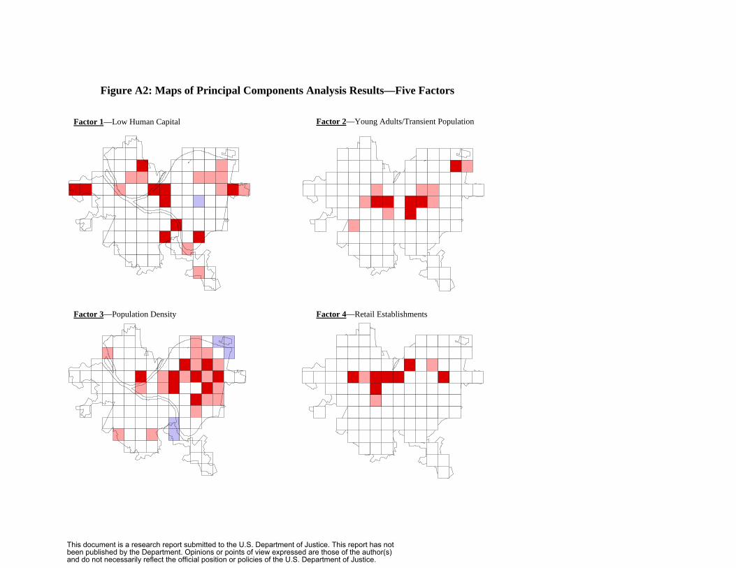
Figure A2: Maps of Principal Components Analysis Results—Five Factors

Factor 1—Low Human Capital Factor 2—Young Adults/Transient Population

Factor 3—Population Density Factor 4—Retail Establishments


-97-

Factor 5—Convenience Stores & Drinking Places

LEGEND: < - 2 S t d . D e v . - 2 . 0 - - 0 . 5 1 S t d . D e v . - 0 . 5 - 0 . 5 S t d . D e v . 0 . 5 1 - 2 . 0 S t d . D e v . > 2 S t d . D e v .


Table A4: Results from Models for the Eight Crime Types

Crime Type Adjusted R2

Motor Vehicle Theft .75 Larceny .87 Simple Assault .80 Robbery .79 CAD Shots Fired .36 Burglary .64 CAD Drug Calls .70 Aggravated Assault .53

vastly underestimated the magnitude and impact of seasonality. Law enforcement takes

place in neighborhoods or car beats and thus small-scale variation in seasonality matters

to police, not overall citywide seasonality. Grid cells or neighborhoods with large

seasonal fluctuations can make good targets for interventions. Thus mapping seasonality

for small areas across a city is important in making our results useful for policing

purposes.

Another feature of Figures A3 through A10 for many of the crime types and grid

cells displayed is that seasonality is a relatively large potion of total crime variation.

Reported in these figures is the nine-year average crime count for each grid cell with

seasonal estimates plotted. The averages include full annual cycles of seasonality and

thus have seasonality removed through cancellation. These means thus provide a good

basis for judging the relative magnitude of seasonality. In Figure A3, the peak of 3.2

seasonality for the retail establishment grid cell is 28 percent of the mean of 11.4. For

larceny in Figure A4, the peak of 3.3 seasonality for the high population density grid is

17 percent of the mean of 13.4. For simple assaults in Figure A5, the peak of 3.8


-99-

seasonality is 47 percent of the mean of 8.07 for the low human capital grid cell. For

shots fired, the peak of 1.9 seasonality in the high density grid cell is 32 percent of the

mean of 5.9. In the remaining cases, seasonality is not as large a portion of total

variation.

It is clear in several of the charts shown in Figures A3 through A10 that the

ecological characteristics of place often contribute to opposing seasonality results. This

results in the canceling-out effect mentioned above. Several noteworthy examples have

both of the opposing coefficients are significant. For motor vehicle thefts in Figure A3,

the highest scoring retail grid cell has April as the minimum seasonal effect while August

is the peak month. In contrast, the highest scoring young adults grid cell, which has a

high college student population, has a peak in April and a negative seasonal factor in

August – the opposite of the retail area. A pronounced case of is that of larceny (Figure

A4) in November and December. In those holiday shopping months, larcenies peak in

the grid cell scoring highest on the retail establishment factor. In contrast, the grid cell

scoring highest on the population density factor, located in a largely residential section of

the city, has a seasonal trough for larcenies in November and December. Robberies

(Figure A6) have a peak in December in the young adult grid cell while the low capital

grid cell is positive but near zero. Shots fired (Figure A7) have a peak in June for the

grid cell with highest population density, but a negative value for young adults (who are

for the large part away in June). Burglaries (Figure A8) have a peak in August for the

high population density grid cell, while a near-zero positive value for the low human

capital grid cell. Aggravated assaults (Figure A10) has several opposing months for the

high population density and young adults grid cells.


-100

The evidence for simple assaults (Figure A1) supports the seasonality literature,

that violent crimes peak during the summer. Our model for simple assaults reveals a very

similar seasonal pattern in grid cells scoring high on the low human capital factor, the

population density factor, and citywide. Throughout the city, therefore, simple assaults

exhibit a summer peak and a winter trough and only the magnitude of the seasonal

pattern varies. Drug calls (Figure A9) also do not exhibit spatial heterogeneity, but have

an unusual seasonal pattern with peaks in spring and fall, trough in winter, but low values

in the summer when we might expect peaks. One explanation is that so many people are

on the streets in drug dealing areas in the summer that drug dealing does not stand out.

Also, at the time period of the data, there were no cell phones and low-income people are

often in public places, away from their home phones, in the summer.

Our results indicate that property crimes tend to have seasonal fluctuations, and

even opposing seasonal patterns when compared with other parts of the city, heavily

influenced by variations in urban ecology. Urban ecology also plays a role in the

seasonality of violent crimes. In this case ecological variations helps determine the

magnitude of the seasonality; as violent crimes in all grid cells tends to increase with the

heat of the summer months, and decrease in the cold of winter.

A.7 Conclusion

Using monthly crime data for 4000 feet square grid cells for Pittsburgh,

Pennsylvania from 1990 to 1998, we were able to model crime seasonality at the sub-city

level for eight crime types. The discussion in this final section of the paper will focus on

detailing how this study fulfills much of the motivations for its undertaking by


-101

contributing to the crime seasonality literature, possessing practical policing and crime

mapping-related implications, and providing a model for sub-city seasonality to be used

in future crime forecasting efforts.

The results from the empirical models clearly reveal that crime seasonality varies

considerably across the space of a city. This is most evident for several crime types. As

mentioned, previous research on crime seasonality for the most part used large levels of

data aggregation. Our results indicate that these large levels of data aggregation mask

variation in seasonality within the city. Hence, the models of sub-city crime seasonality

created for this research fill a void in the crime seasonality literature.

In addition, there are clear practical implications of this research for policing,

mostly related to the use of maps, created from the models of sub-city seasonality, to plan

and evaluate monthly police interventions. With the results from the models, urban crime

analysts could map each month’s predicted seasonal pattern using color-coded grid cells.

Grid cells with seasonal peaks might be represented in shades of red, while grid cells

experiencing troughs might be colored with shades of blue. With the colored map in

hand, police could target the “hot” grid cells for interventions and then evaluate the

success or failure of the intervention based on its variation from the seasonality model’s

predictions. Finally, closely related to this topic of predictions, this study provides the

basis for improving the forecast accuracy in the models presented by Gorr et al. (2003).


-102

Figures A3 through A10: Results for Estimates of Seasonal Factors and Selected Seasonal Interactions for all Eight Crime Types

Note: Each bar represents the seasonality of the highest scoring grid cells for the respective factor. The means reported are the 9-year mean for that crime type in the respective grid cell. An asterisk above or below a bar indicates a significant seasonality coefficients at the 5% level or better significance level.

l

il i / i i i

l

/ i ions l i

l

i i l i

l

il i i i i

*

*

*

**

*

* *

* *

*

* *

* * *

*

* **

* *

*

*

* *

*

*

Figure 3: Motor Vehicle Theft Seasonality

-3.0

-2.0

-1.0

0.0

1.0

2.0

3.0

4.0

Jan Feb Mar Apr May Jun Ju Aug Sep Oct Nov Dec Month

Add

itive

Sea

sona

l Fac

tor

Reta Establ shments Young Adults Trans ent Populat on Cityw de

Figure 6: Robbery Seasonality

-0.8

-0.6

-0.4

-0.2

0.0

0.2

0.4

0.6

0.8

1.0


Add

itive

Sea

sona

l Fac

tor

Young Adults Trans ent Populat Low Human Capita Cityw de

Figure 5: Simple Assault Seasonality

-5.0

-4.0

-3.0

-2.0

-1.0

0.0

1.0

2.0

3.0

4.0

5.0


Add

itive

Sea

sona

l Fac

tor

Populat on Dens ty Low Human Capita Cityw de

Figure 4: Larceny Seasonality

-8.0

-6.0

-4.0

-2.0

0.0

2.0

4.0

6.0

8.0


Add

itive

Sea

sona

l Fac

tor

Reta Establ shments Populat on Dens ty Cityw de Mean = 13.39 Mean = 61.93 Mean = 11.44 Mean = 14.61

Mean = 8.07 Mean = 22.93 Mean= 8.52 Mean= 0.65 This document is a research report submitted to the U.S. Department of Justice. This report has not been published by the Department. Opinions or points of view expressed are those of the author(s) and do not necessarily reflect the official position or policies of the U.S. Department of Justice.

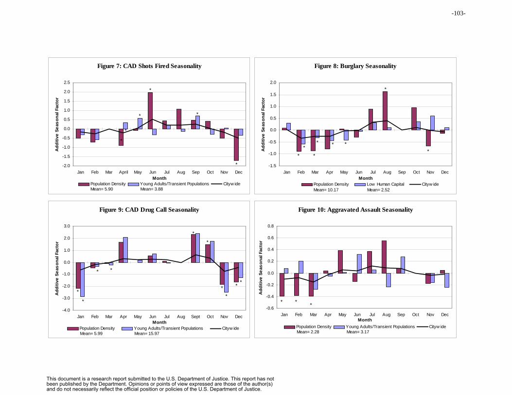
-103

0.0

0.2

0.4

0.6

0.8

l

i i l / i i i

* **

l

l i i l i

0.0

0.5

1.0

1.5

2.0

2.5

il l

i i / i l i i

0.0

1.0

2.0

3.0

l

i i / i l ions i

* *

*

*

*

*

* *

*

*

*

* *

*

*

*

* *

*

* * *

*

*

Figure 10: Aggravated Assault Seasonality

-0.6

-0.4

-0.2


Add

itive

Se a

sona

l Fac

tor

Populat on Dens ty Young Adu ts Trans ent Populat ons Cityw de

Figure 8: Burglary Seasonality

-1.5

-1.0

-0.5

0.0

0.5

1.0

1.5

2.0


Add

itive

Sea

s ona

l Fac

tor

Popu at on Dens ty Low Human Capita Cityw de

Figure 7: CAD Shots Fired Seasonality

-2.0

-1.5

-1.0

-0.5


Add

itive

Sea

s ona

l Fac

tor

Populat on Dens ty Young Adults Trans ent Popu at ons Cityw de

Figure 9: CAD Drug Call Seasonality

-4.0

-3.0

-2.0

-1.0

Jan Feb Mar Apr May Jun Ju Aug Sept Oct Nov Dec Month

Add

itive

Sea

sona

l Fac

tor

Populat on Dens ty Young Adults Trans ent Popu at Cityw de

Mean= 2.52 Mean= 10.17

Mean= 2.28 Mean= 3.17 Mean= 15.97 Mean= 5.99

Mean= 5.90 Mean= 3.88


References

Anderson, C.A. 1987 Temperature and aggression: Effects on quarterly, yearly, and city rates of

violent and non-violent crimes. Journal of Personal and Social Psychology.

52:1161-73.

1988 Temperature and aggression: Ubiquitous effects of heat on occurrence of human violence. Psychology Bulletin. 106:74-96

Baron, Robert A. 1972 Aggression as a function of ambient temperature and prior anger arousal.

183-189.

Baumer, Eric and Richard Wright 1996 Crime seasonality and serious scholarship: A comment on Farrell and

Pease. British Journal of Criminology 36:579-581.

Beck, Nathaniel and Jonathan N. Katz 1995 What to do (and not to do) with time-series cross-section data. The

American Political Science Review 89:634-647.

1996 Nuisance vs. substance: Specifying and estimating time-series cross-section data. Political Analysis 6:1-36.

Block, Carolyn R. 1984 Is crime seasonal? Illinois Criminal Justice Information Authority.

Braga, Anthony A. 2001 The effects of hot spots policing on crime. Annals, AAPSS 578:104-125.

Brantingham, Patricia L. and Paul J. Brantingham 1993 Environment, routine, and situation: Toward a pattern theory of crime. In

Clarke, Ronald V. and Marcus Felson (eds.), Routine Activity and Rational Choice: Advances in Criminological Theory, Vol. 5. New Brunswick, N.J.: Transaction Publishers, 259-293.

Bursik, Robert J., Jr. 1988 Social disorganization and theories of crime and delinquency: Problems and

prospects. Criminology 26:519-551.

Cohen, Lawrence E. and Marcus Felson 1979 Social change and crime rate trends: A routine activity approach. American

Sociological Review 44:588-608.


105

Cohn, Ellen G. and James Rotton 2000 Weather, seasonal trends and property crimes in Minneapolis, 1987-1988. A

moderator-variable time-series analysis of routine activities. Journal of Environmental Psychology 20:257-272.

Cubbin, Catherine, Felicia B. LeClere, and Gordon S. Smith 2000 Socioeconomic status and the occurrence of fatal and nonfatal injury in the

United States. American Journal of Public Health 90:70-77.

2000 Socioeconomic status and injury mortality: Individual and neighbourhood determinants. Journal of Epidemiology and Community Health 54:517-524.

DeFronzo, J. 1984 Climate and crime: Tests of an FBI assumption. Environment and Behavior

16:185-210.

Eck, John E. and David Weisburd 1995 Crime places in crime theory. In Eck, John E. and David Weisburd (eds.).

Crime and Place: Crime Prevention Studies, Vol. 4. Monsey, NY: Criminal Justice Press, 1-33.

Farrell, Graham and Ken Pease 1994 Crime seasonality: Domestic disputes and residential burglary in

Merseyside 1988-1990. British Journal of Criminology 34:487-498.

Feldman, H. and Jarmon, R. 1979 Factors influencing criminal behaviour in Newark: A local study in forensic

psychiatry. Journal of Forensic Science. 24:234-239.

Ferri, Enrico 1882 Das Verbrechen in seiner Abhaangigkeit von dem jahrlichen

tempuraturwechsel.

Gorr, Wilpen, Andreas Olligschlaeger, and Yvonne Thompson 2003 Short-term forecasting of crime. To appear, International Journal of

Forecasting, Special Section on Crime Forecasting.

Guerry, A. M. 1833 Essau syr ka statistique moral de la France. Cologne: Bohlanverlag.

Harries, Keith D., Stephen J. Stadler, and R. Todd Zdorkowski 1984 Seasonality and assault: Explorations in inter-neighborhood variation,

Dallas 1980. Annals of the Association of American Geographers 74:590-604.


106

Harries, Keith D. 1989 Homicide and assault: A comparative analysis of attributes in Dallas

neighborhoods, 1981-1985. Professional Geographer 41:29-38.

Heise, David R. 1973 Some issues in sociological measurement. Sociological Methodology 5:1-

16.

Janson, Carl-Gunnar 1980 Factorial social ecology: An attempt at summary and evaluation. Annual

Review of Sociology 6:433-456.

Lab, Steven P. and J. David Hirschel 1988 Climatological conditions and crime: The forecast is…? Justice Quarterly

5:281-299.

Landau, Simha F. and Daniel Fridman 1993 The seasonality of violent crime: The case of robbery and homicide in

Israel. Journal of Research in Crime and Delinquency 30:163-191.

LeBeau, James L. and Robert H. Langworthy 1986 The linkages between routine activities, weather, and calls for police

services. Journal of Police Science and Administration 14:137-145.

Makridakis, S., and S.C. Wheelright. 1978. Interactive forecasting: Univariate and multivariate methods. SanFrancisco:

Holden-Day. 2nd Ed.

Marini, Margaret Mooney, Xiaoli Li, and Pi-Ling Fan 1996 Characterizing latent structure: Factor analytic and grade of membership

models. Sociological Methodology 26:133-164.

Osgood, D. Wayne et al. 1996 Routine activities and individual deviant behavior. American Sociological

Review 61:635-655.

Ousey, Graham C. 2000 Explaining regional and urban variation in crime: A review of recent research. In

Criminal Justice 2000, Vol. 2 The Nature of Crime: Continuity and Change. Washington, D.C.: National Institute of Justice.

Pickett, K. E. and M. Pearl 2001 Multilevel analyses of neighbourhood socioeconomic context and health


107

outcomes: A critical review. Journal of Epidemiology and Community Health 55:111-122.

Rengert, George F., Alex R. Piquero, and Peter R. Jones 1999 Distance decay reexamined. Criminology 37:427-445.

Robert, Stephanie A. 1999 Socioeconomic position and health: The independent contribution of

community socioeconomic context. Annual Review of Sociology 25:489-516.

Roncek, Dennis W. and Donald Faggiani 1985 High schools and crime: A replication. The Sociological Quarterly 26:491-

505.

Roncek, Dennis W. and Mitchell A. Pravatiner 1989 Additional evidence that taverns enhance nearby crime. Sociology and

Social Research 73:185-188.

Roncek, Dennis W. and Pamela A. Maier 1991 Bars, blocks, and crimes revisited: Linking the theory of routine activities to

the empiricism of “hot spots.” Criminology 29:725-753.

Sampson, Robert J. and Stephen W. Raudenbush 1999 Systematic social observation of public spaces: A new look at disorder in

urban neighborhoods. American Journal of Sociology 105:603-651.

Sampson, Robert J., Stephen W. Raudenbush, and Felton Earls 1997 Neighborhoods and violent crime: A multilevel study of collective efficacy.

Science 277: 918-924.

Sampson, Robert J. and W. Byron Groves 1989 Community structure and crime: Testing social-disorganization theory.

American Journal of Sociology 94:774-802.

Shaw, Clifford R. and Henry D. McKay 1969 Juvenile Delinquency and Urban Areas: A study of rates of delinquency in

relation to differential characteristics of local communities in American cities. Chicago: The University of Chicago Press.

Sherman, Lawrence W., Patrick R. Gartin, and Michael E. Buerger 1989 Hot spots of predatory crime: Routine activities and the criminology of

place. Criminology 27:27-55.

Sherman, Lawrence W.


108

1995 Hot spots of crime and criminal careers of places. In Eck, John E. and David Weisburd (eds.). Crime and Place: Crime Prevention Studies, Vol. 4. Monsey, NY: Criminal Justice Press, 35-52.

Stimson, James A. 1985 Regression in space and time: A statistical essay. American Journal of

Political Science 29:914-947.

Taylor, Ralph B. 1997 Crime and small-scale places: What we know, what we can prevent, and

what else we need to know. In Crime and place: Plenary papers of the 1997 Conference on Criminal Justice Research and Evaluation. Washington, D.C.: National Institute of Justice, 1-22.

Vélez, María B. 2001 The role of public social control in urban neighborhoods: A multi-level analysis

of victimization risk. Criminology 39:837-863.

Weisburd, David, Lisa Maher, Lawrence Sherman et al. 1993 Contrasting crime general and crime specific theory: The case of hot spots

of crime. in Adler, Freda and William S. Laufer (eds.) New Directions in Criminological Theory: Advances in Criminological Theory, Vol. 4. New Brunswick, NJ: Transaction Publishers, 45-70.

Weisburd, David 1997 Reorienting crime prevention research and policy: From the causes of

criminality to the context of crime. Washington, D.C.: National Institute of Justice Research Report.

Yen, I. H. and S. L. Syme 1999 The social environment and health: A discussion of the epidemiological

literature. Annual Review of Public Health 20:287-308.


109

Appendix B

Leading Indicators and Spatial Interactions: A Crime Forecasting Model for Proactive Police Deployment6

This appendix provides underlying theories for our leading indicator models.

While state in terms of a grid cell geography, it applies to any geography with small

districts in area. To date we have applied the models to car beats, grid cells, and the

smallest districts considered, census tracts.

We develop a leading indicator model for forecasting serious property and violent crimes

based on the crime attractor and displacement theories of environmental criminology. The

model, intended for support of tactical deployment of police resources, is at the micro-

level scale; namely, one-month-ahead forecasts over a grid system of 141 square grid cells

4,000 feet on a side (with approximately 100 blocks per grid cell). The leading indicators

are selected lesser crimes and incivilities entering the model in two ways: 1) as time lags

within grid cells and 2) time and space lags averaged over grid cells contiguous to

observation grid cells. We estimated the leading indicator model using a robust linear

regression model, a neural network, and a proven univariate, extrapolative forecast method

for use as a benchmark in Granger causality testing. We find evidence of both the crime

attractor and displacement theories.

This appendix is extracted from Cohen, J., W.L. Gorr, and A. Olligschlaeger, “Leading Indicators and Spatial Interactions: A Crime Forecasting Model for Proactive Police Deployment” Geographical Analysis, to Appear 2005.

6


B1. Introduction

Geography has become increasingly important in law enforcement and crime

prevention. Criminology has long focused on individual propensities toward crime, but it

was only during the last few decades that the criminogenic features of settings began to

take on importance in research and practice. Environmental criminology gained in

development, empirical verification, and practical applications by police (Cohen and

Felson 1977; Brantingham and Brantingham 1981, 1984; Cornish and Clarke 1986; Eck

and Weisburd 1995; Cohen and Clarke 1998, p. 2 ). Places, besides persons, became

targets for allocation of police resources, and fields including crime mapping (Harries

1999), geographic profiling (Rossmo 2000), and (most recently) crime forecasting (Gorr

and Harries 2003) arose in support of the new-found law enforcement opportunities.

This paper introduces a leading-indicator crime forecasting model for proactive

policing and crime prevention, building on the work of Olligschlaeger (1997, 1998).

Police, like other professionals delivering services, generally know the current locations

and intensities of demand for services. Indeed, crime mapping based on near real-time

input of police reports has made the current picture for police more complete, integrating

data from various officers, shifts, and neighborhoods. With the current situation in hand,

the next step and most difficult new information to obtain is making forecasts of large

changes in crime. If it were possible to get such forecasts, in the short term of up to a

month ahead, then police could focus crime analysts’ activities and build up intelligence

on highlighted areas, target patrols, reallocate detective squads, and carry out other police

interventions to prevent crimes.


111

Attempting to make accurate forecasts of the relatively rare, large changes in

crime from month to month is an ambitious and difficult undertaking; however, the

expectations of police can adapt to accepting good leads mixed in with false positives.

For example, if 50 percent of forecasted large changes actually have large changes, then

we claim that this would be an excellent result. Such forecasts would provide an entirely

new kind of valuable information for police. Police practices already involve following

up on many leads before success.

It is not difficult to get accurate extrapolative forecasts of crime. Gorr,

Olligschlaeger, and Thompson (2003), using the same case study data as this paper,

demonstrated that exponential smoothing methods and classical decomposition yield

accurate one-month-ahead forecasts for areas that have average historical crime volumes

in excess of 25 to 35 crimes per month. Unfortunately these “business-as-usual”

forecasts cannot foresee the largest changes in crime levels; namely, those involving

breaks in time series patterns such as step jumps up or down.

The leading indicator model presented in this paper is promising for forecasting

breaks. If leading indicators experience a break from previous patterns during the last

month of the estimation data set, they are capable of forecasting a similar break in the

dependent crime variable in the next month. The present paper develops and evaluates

crime-based leading indicators and spatial interactions as a means to forecast breaks in

serious crime levels. Another paper (Gorr and McKay 2004), applying tracking signals

to identify breaks in crime trends, finds that there are roughly 2 breaks every 3 years in

high crime volume, square grid cells (4000 feet on a side) in Pittsburgh. Note that the

leading indicator model of this paper has not been used in practice by police as yet.


112

Section 2 provides a literature review and model specification. We draw on crime

theories and police requirements to build our model. Section 3 presents the case study of

Pittsburgh, Pennsylvania with 141 grid cell locations and 96 months of crime data. This

section includes an experimental design for validation of the leading indicator model,

drawing on the forecasting literature. Results are in Section 4, and Section 5 concludes

the paper.

B2. Model Specification

Our leading indicator forecasts for serious crimes are based on a lag model for

panel data. This section specifies the dependent variables, time-lagged leading indicator

variables, and spatial interactions in the form of space and time lags. While multiple time

lags are possible, our preliminary research indicated that a single time lag of independent

variables was often the most accurate forecasting model. While lag models with up to

four or more lags may ultimately prove to be the most accurate forecast models for

leading indicators, we chose to keep the model in this first paper on crime spatial

interactions simple. Hence, we limit attention to a single time lag model in this paper.

The choice of dependent variables depends on police requirements and data

limitations. Municipal police in the U.S. have widely implemented a management by

objectives approach known as CompStat, first developed by the New York City Police

Department (Henry and Bratton 2002). CompStat focuses on reducing serious crimes,

which in the U.S. consist of the index or part 1 crimes in the FBI’s Uniform Crime

Reporting program (UCR): murder, rape, robbery, aggravated assault, burglary, larceny,


113

and motor vehicle theft. Part 1 crimes are the dependent variables of our model;

however, police requirements and data limitations both argue for using aggregates of part

1 crimes instead of individual crimes.

Police desire information on crime for the smallest geographic areas possible in

order to precisely target patrols and investigative efforts. The smallest administrative

unit of police departments is the patrol district or car beat, which is the territory of a

single unit (usually a patrol car). Clearly, areas studied need to be the size of car beats or

smaller. We use square grid cells 4,000 feet on a side (yielding approximately 100 city

blocks) in our case study of Pittsburgh, Pennsylvania. Grid cells have the advantage of

easy visual interpretation on maps, given their uniform size and shape. During the time

of study, Pittsburgh had 42 car beats and 141 grid cells. We experimented with several

grid cell sizes and found 4,000 feet to be roughly the smallest possible for Pittsburgh

while still yielding reasonable model estimates.

A necessary concession to working at this level is to sum all property crimes

(robbery, burglary, larceny, and motor vehicle theft) to a single dependent variable, P1P,

and similarly all violent crimes (murder, rape, and aggravated assault) to P1V for

forecasting.7 This aggregation is necessary to yield monthly crime time series with

sufficient data volumes for accurate model estimation. For example, it is impossible to

forecast murder at the grid cell level, with 40 to 60 murders per year in Pittsburgh.

Nevertheless, use of P1P and P1V as the dependent variables is compatible with

the top-down analysis process used in CompStat in which participants need to make

Standard crime reporting by police to the FBI’s Uniform Crime Reporting program includes robbery as a violent offense because of the risk of injury it poses for victims. We include robbery with property offenses because it shares many features (e.g., offender attributes, crime location, and time of day) with other offenses involving theft.

7


114

monthly, jurisdiction-wide scans for crime problems to allocate limited analytical,

investigative, and patrol resources. Leading indicator forecasts help make such a scan,

with areas having a large forecasted increase in crime getting priority and perhaps those

areas with opposite forecasts getting resources withdrawn. With such decisions made,

crime analysts can “drill down” into selected areas for diagnosis and tactical-level

planning of targeted patrols, assignment of detectives, etc. It is in the second stage of

crime analysis that information on individual part 1 and leading indicator crimes is

needed.

Lesser crimes and incivilities, represented by selected part 2 crimes in police

offense reports and citizen 911 complaints, comprise the leading indicators in our model.

In general, these variables are suggested by two crime theories on spatial interactions:

crime attractors and crime displacement, which we discuss below. It is fortunate for

police (and perhaps unique) that they collect their own transactional data on leading

indicators, thus enabling timely forecasts. Other, well-known economic indicators (Klein

and Moore 1983) that are related to crime at national or regional levels (Deadman, 2003;

Harries 2003) change too slowly and are not available at the micro-geographic levels and

time frames needed for tactical law enforcement within municipalities. Today police

have real-time information systems and can process and aggregate individual crime

incidents to any desired variables to support forecasting.

Lesser crimes, like serious crimes, also receive intense enforcement because they

too are costly to the public and because it is believed that they are precursors to serious

crimes. The Broken Windows theory of crime (Wilson and Kelling 1982; Kelling and

Coles 1996) argues that tolerance of minor incivilities and infractions of the law in


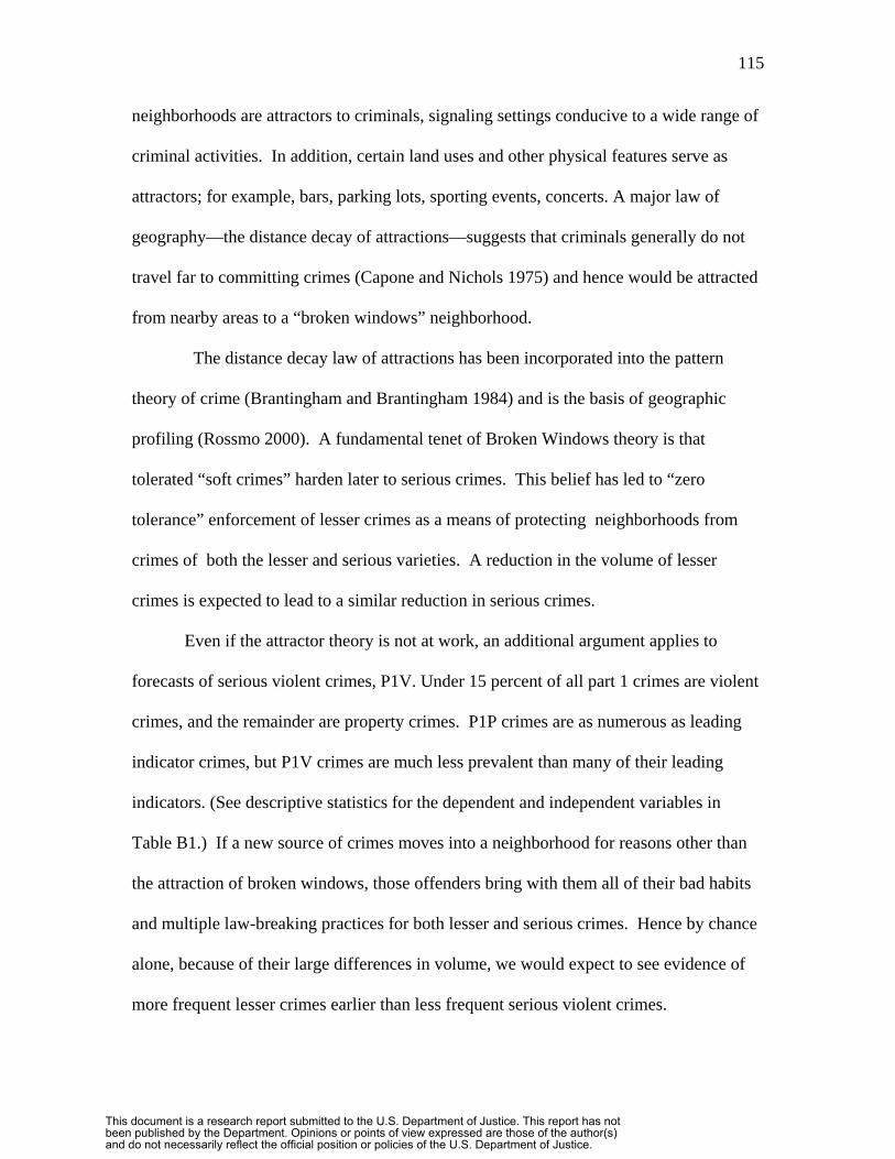
115

neighborhoods are attractors to criminals, signaling settings conducive to a wide range of

criminal activities. In addition, certain land uses and other physical features serve as

attractors; for example, bars, parking lots, sporting events, concerts. A major law of

geography—the distance decay of attractions—suggests that criminals generally do not

travel far to committing crimes (Capone and Nichols 1975) and hence would be attracted

from nearby areas to a “broken windows” neighborhood.

The distance decay law of attractions has been incorporated into the pattern

theory of crime (Brantingham and Brantingham 1984) and is the basis of geographic

profiling (Rossmo 2000). A fundamental tenet of Broken Windows theory is that

tolerated “soft crimes” harden later to serious crimes. This belief has led to “zero

tolerance” enforcement of lesser crimes as a means of protecting neighborhoods from

crimes of both the lesser and serious varieties. A reduction in the volume of lesser

crimes is expected to lead to a similar reduction in serious crimes.

Even if the attractor theory is not at work, an additional argument applies to

forecasts of serious violent crimes, P1V. Under 15 percent of all part 1 crimes are violent

crimes, and the remainder are property crimes. P1P crimes are as numerous as leading

indicator crimes, but P1V crimes are much less prevalent than many of their leading

indicators. (See descriptive statistics for the dependent and independent variables in

Table B1.) If a new source of crimes moves into a neighborhood for reasons other than

the attraction of broken windows, those offenders bring with them all of their bad habits

and multiple law-breaking practices for both lesser and serious crimes. Hence by chance

alone, because of their large differences in volume, we would expect to see evidence of

more frequent lesser crimes earlier than less frequent serious violent crimes.


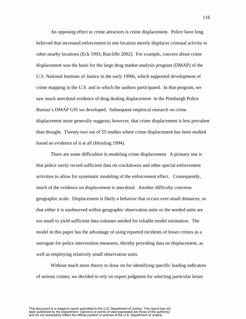
116

An opposing effect to crime attractors is crime displacement. Police have long

believed that increased enforcement in one location merely displaces criminal activity to

other nearby locations (Eck 1993; Ratcliffe 2002). For example, concern about crime

displacement was the basis for the large drug market analysis program (DMAP) of the

U.S. National Institute of Justice in the early 1990s, which supported development of

crime mapping in the U.S. and in which the authors participated. In that program, we

saw much anecdotal evidence of drug dealing displacement in the Pittsburgh Police

Bureau’s DMAP GIS we developed. Subsequent empirical research on crime

displacement more generally suggests; however, that crime displacement is less prevalent

than thought. Twenty-two out of 55 studies where crime displacement has been studied

found no evidence of it at all (Hessling 1994).

There are some difficulties in modeling crime displacement. A primary one is

that police rarely record sufficient data on crackdowns and other special enforcement

activities to allow for systematic modeling of the enforcement effect. Consequently,

much of the evidence on displacement is anecdotal. Another difficulty concerns

geographic scale. Displacement is likely a behavior that occurs over small distances, so

that either it is unobserved within geographic observation units or the needed units are

too small to yield sufficient data volumes needed for reliable model estimation. The

model in this paper has the advantage of using reported incidents of lesser crimes as a

surrogate for police intervention measures, thereby providing data on displacement, as

well as employing relatively small observation units.

Without much more theory to draw on for identifying specific leading indicators

of serious crimes, we decided to rely on expert judgment for selecting particular lesser


117

crimes as leading indicators. Our first step was to compile a list of all lesser offense

types and all codes characterizing complaints in citizen 911 calls for police services. We

then asked police crime analysts in two cities to select leading indicators from this list.

With the initial selection in hand, we then asked two criminologists to further refine and

classify the list. The resulting final list of leading indicators for P1P and P1V crimes is in

Table B1.

Offense data are based on incidents reported to or discovered by police and

recorded as crimes in police offense reports. Under-reported crimes (like sex crimes and

assaults between family and friends) or victimless crimes (like illegal drug use or

prostitution) are under-represented in police offense data. Citizen 911 calls for service

are more inclusive of complaints about criminal and public disorder activities, but are

vulnerable to overestimates arising from untrained observers or complainants attempting

to manipulate the system (e.g., claiming a more serious problem than existing to get a

quick response by police).

Table B1 includes descriptive statistics for all variables. Note that 5 of the 14

leading indicators (C_TRUAN, C_VICE, LIQUOR, PROST, PUBDRUN, and

TRESPAS) have low means of under one incident per month per grid cell, and high

standard deviations and maximums. We retained these variables as leading indicators

under the expectation that relatively high numbers of these measures are concentrated in

a few areas and would be discriminating for those areas.

Application of the theories discussed above and expert-based efforts on our part

thus led to a leading indicator forecast model with P1P or P1V as dependent variables

and the two sets of independent variables in Table B1. The analysis includes one month


118

time lags for each leading indicator in the same grid cell, and averages of each leading

indicator in neighboring contiguous grid cells (queens case spatial lags) also lagged by

one month.

If attractor theory is correct, we expect the signs of coefficients for time-lagged

independent variables in the same grid cell to be positive, reflecting the direct effects of

lesser crimes on subsequent serious crimes in the same location. Operating under the

same attractor mechanism, we expect the coefficients of the spatial lags to be negative,

with nearby high activity grid cells drawing offenders and their criminal activity away

from the local grid cell. In contrast, if displacement is the operant mechanism, and police

actively target high levels of lesser crimes for enforcement, then we expect the coefficient

signs of local time lags to be negative and those of the spatial lags to be positive as

criminal activity moves away from higher levels of enforcement directed against lesser

crimes. Displacement of otherwise non-violent offending could have an immediate effect

on violent crimes if displacement results in turf wars between already established and

newly-arriving displaced offenders.

If both attractor and displacement processes are at work, and these operate locally

and between neighbors, the results may be net zero changes in local levels of serious

crimes. Our estimates will only be able to detect the presence of significant non-zero net

effects, and any estimated significant effects will thus represent net effects of the

dominant process.

Estimation of our model includes robust linear regressions and a non-linear neural

network. Early in our research we compared results from Poisson regressions suitable for

crime counts, and found coefficient estimates to be similar to those from linear


119

regressions, and so we use linear regressions for forecasting. We use STATA software

to estimate robust linear regressions with observations clustered within grid cells to

estimate the standard errors of coefficient estimates. These standard errors relax the

usual OLS assumptions of independent and identically distributed errors to yield

consistent estimates for arbitrary variance/covariance error structure. The nonlinear

neural network model (Olligschlaeger 1998), with a single middle layer and standard feed

forward estimation, provides an exploratory, self-adjusting mechanism to find additional

patterns in the independent variables beyond the linear regression specification.

B3. Case Study and Validation Approach

We collected approximately 1.3 million individual crime incident data records

(crime offense reports and 911 calls for service) for Pittsburgh, Pennsylvania over the

period 1991 through 1998. We used a geographic information system to geocode the

points, with overall address match rates of 90 percent for offense records and 80 percent

for 911 call records. Overall, these rates are at the U.S. national average for police data,

which is on the order of 85 percent. With data points and grid cells on a GIS map, we

used spatial joins to assign grid cell identifiers to crime points, and then used database

queries to create monthly series for each grid cell.

Our forecast validation study uses the rolling-horizon experimental design (e.g.,

Swanson and White 1997), which maximizes the number of forecasts for a given time

series at different times and under different conditions. This design includes two or more

alternative parallel forecasts. For each forecast included in an experiment, we estimate


120

models on training data, forecast one month ahead to new data not previously seen by the

model, and then calculate and save the forecast errors. Next we roll forward one month,

adding the observed value of the previously forecasted data point to the training data,

dropping the oldest historical data point, and forecasting ahead to the next month. This

process repeats until all data are exhausted.

The regression model uses a three-year estimation window, the extrapolative

method explained below requires a five-year estimation window, and neural network

estimation start with the earliest five years of data and retain all historic data as the

horizon rolls forward. The rolling three-year window for regression estimation allows

estimated parameters to vary over time, thus capturing effects of unmeasured factors such

as changes in police policies or innovations in crime. The extrapolative univariate

method needs at least five years of data to estimate seasonal effects. In the data sample

used here the earliest forecast origin is December 1995, retaining January 1991 through

December 1995 for estimation. One-month-ahead forecasts are available for January

1996 through December 1998 for a total of 36 months times 141 grid cells to yield 5,076

forecast errors per forecast method.

We used Granger causality testing (Granger 1969) to determine the relative value

of leading indicators for serious crimes. A variable X Granger-causes Y if Y can be

better predicted using the histories of both X and Y than it can using the history of Y

alone. Our use of this concept for leading indicators determines whether they forecast

serious crimes significantly better than the best univariate, extrapolative method,

especially for large crime changes. To develop benchmark accuracy measures, we first


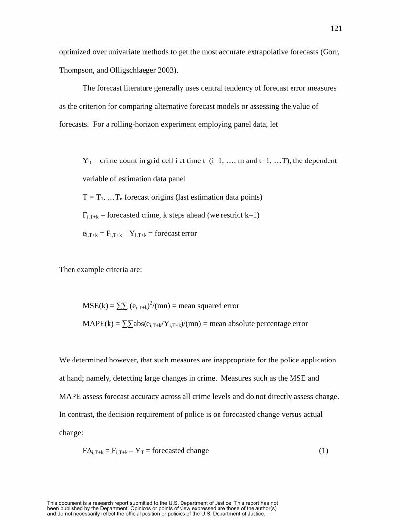
121

optimized over univariate methods to get the most accurate extrapolative forecasts (Gorr,

Thompson, and Olligschlaeger 2003).

The forecast literature generally uses central tendency of forecast error measures

as the criterion for comparing alternative forecast models or assessing the value of

forecasts. For a rolling-horizon experiment employing panel data, let

Yit = crime count in grid cell i at time t (i=1, …, m and t=1, …T), the dependent

variable of estimation data panel

T = T1, …Tn forecast origins (last estimation data points)

Fi,T+k = forecasted crime, k steps ahead (we restrict k=1)

ei,T+k = Fi,T+k – Yi,T+k = forecast error

Then example criteria are:

MSE(k) = ∑∑ (ei,T+k)2/(mn) = mean squared error

MAPE(k) = ∑∑abs(ei,T+k/Yi,T+k)/(mn) = mean absolute percentage error

We determined however, that such measures are inappropriate for the police application

at hand; namely, detecting large changes in crime. Measures such as the MSE and

MAPE assess forecast accuracy across all crime levels and do not directly assess change.

In contrast, the decision requirement of police is on forecasted change versus actual

change:

F∆i,T+k = Fi,T+k – YT = forecasted change (1)


122

A∆i,T+k = Yi,T+k – YT = actual change (2)

Hence we use a forecast error criterion that contrasts (1) and (2).

A common practice of crime analysts, and basis of our forecast performance

measure, is the use threshold crime levels as triggers for exception reports for possible

action. An example rule using a threshold level is as follows: if P1V crimes are

forecasted to increase by more than 6 in any given grid cell, then that cell merits

attention. Hence, rather than assessing accuracy based on the performance of individual

point forecasts for each grid cell, we examined forecast performance within ranges of

changes for both decreases and increases. Using contingency tables based on measures

(1) and (2), we contrast forecasted and actual changes within each range and designate

correctly triggered decisions as positives and negatives, and incorrect decisions as false

negatives and false positives. We apply pairwise comparison t-tests within classes to

determine if leading indicator forecasts are significantly better than univariate forecasts.

Before proceeding to the results of forecasting experiments, we address two issues

regarding the contingency table analysis for forecasted change; namely, that of outliers

and the related issue of forecasting large crime-volume decreases. First, it is necessary to

remove outliers from the contingency table analysis (they are retained in estimation of

models). By outlier, we mean a crime count in one month that is unusually higher or

lower than months preceding and following it. If we were to include outliers in the

assessment of forecast accuracy using (1) and (2), there would mostly be good

performance in forecasting large decreases in crime levels, but this is a mere artifact of

forecasting outliers in a moving horizon. Most outliers are high, yielding a large increase

in crime level during the outlier month. Forecast models of course cannot forecast the


123

outlier accurately and hence have poor accuracy for corresponding increases. The month

following the outlier has a large decrease, a return to the long-term trend. Forecast

models adjust minimally to the outlier and thus still forecast at levels corresponding to

the long-term trend. Hence by default they accurately forecast the return of crime levels

after an outlier. We identify and remove outliers from assessments of forecast accuracy

to avoid such spurious results on forecasting large crime decreases.

We reject classical approaches to identifying outliers based on tolerance limits for

two reasons. First, besides outliers, crime series data exhibit pattern changes such as step

jumps. Tolerance limits incorrectly identify step jumps as outliers. Second, we desired a

method of identifying outliers that match decision rules employed in this paper. We thus

decided to use ad hoc decision rules as follows:

Property Crime Outlier Rule:

if (A∆i,T+k >= 15 and A∆i,T <= -15) or

(A∆i,T+k <= -15 and A∆i,T >= 15) then YT is an outlier.

This rule simply states that if the monthly crime count changes in one direction by more

than 15 and immediately reverses with the same change in the opposite direction, it is an

outlier. The similar rule for violent crimes is as follows:

Violent Crime Outlier Rule:

if (A∆i,T+k >= 6 and A∆i,T <= -6) or

(A∆i,T+k <= -6 and A∆i,T >= 6) then YT is an outlier.

For property crimes, there are 122 records with |A∆i,T| >=15. Of these there are 26 pairs

of consecutive records satisfying the outlier identification criteria above. Five of the

pairs are in the CBD where crime volume is very high so that these are not outliers. Thus


124

there are 21 pairs of records that are outlier cases. Sixteen out of the 21 are high outliers.

We dropped all 21 outliers from the contingency table analysis. For violent crimes, there

are 119 records with |A∆i,T| >=6. There are 42 pairs of consecutive records satisfying the

outlier criteria; however, there are 3 grid cells with high crime volume and 5 or more

pairs identified in each. We designate these as non-outliers. Thus in the end the

procedure identifies 24 outliers and of these 17 are high outliers. We dropped all 24

outliers from the contingency table analysis of violent crimes.

The second issue is similar to that of outliers. Our models have greater success

in forecasting large crime decreases than large crime increases, as will be seen in the next

section of this paper. Of course, the latter are more important for prevention of crime and

also, we believe, provide the true test of crime leading indicator forecast models. The

following scenario describes the issue at hand. Suppose that a time series has been

moving along a steady, long-term trend for a large number of months but then has a step

jump increase. The majority of such step jumps in crime time series are increases, likely

reflecting a new criminal element in a neighborhood. After a period of time, police

recognize the increased activity, investigate it, and likely are successful in suppressing it,

causing crime to decrease and return to the long-term trend.

The ability to forecast a step jump increase depends directly on the predictive

ability of the leading indicators and corresponding model. Only the neural network

model for violent part 1 crimes in Tables B7 through B9 below is successful for this case.

In contrast, the ability to forecast the return to the long-term trend can be independent of

leading indicators. All that is necessary is to have a model that is non-reactive to change,


125

and thus persists in estimating and forecasting the long-range trend at every forecast

origin.

B4. Results

Tables B2 and B3 present sample regression estimates for P1P and P1V leading

indicator models for the first three-year data window (January 1993 through December

1995) and last window (January 1996 through December 1998) out of 36 sets of such

regressions used for forecasting. All models displayed have relatively high R-Square

values, in the range 0.69 to 0.79, and many significant coefficients. Out of the 42

estimated coefficients for time-lagged leading variables (not the time and space lagged

variables) in Tables B2 and 3, 25 are significant at traditional levels and only one of those

is negative. All but 3 are significant at the .01 level or better. Thus there is some

evidence that the proposed leading indicators do lead serious crimes, although

comparisons below with extrapolative models have stronger evidence of this.

Figures B1 and B2 provide time series plots of robust-regression estimated

parameters of crime variables that have both space and time lags. These plots have the

purpose of examining attractor (negative coefficients) versus displacement (positive

coefficients) behavior. Figure B1 has parameter paths predictive of property crimes that

have at least one significant coefficient in TableB2 at the 0.10 level or better. (Table B2

denotes significance levels down to only the 0.05 level with two space and time-lagged

variable coefficients significant at this level or better. The 0.10 level admits one more

coefficient, for NDisord.) Figure B2 for violent crimes has similarly identified parameter


126

paths for variables that are significant at the 0.10 level in Table B3. We plotted each

estimate at the center of its data window, thus providing estimates of conditions at correct

times on the horizontal scale.

In Figure B1 for P1P, coefficients had time parameter paths that remained roughly

stable, except for weapons offenses. Criminal mischief and weapons violations have

displacement behavior while disorderly conduct has attractor behavior. The weapons

coefficient started positive and then rapidly and markedly increased, more than doubling

in the latter months of 1995 as a displacement factor. This corresponds to a period during

which the Pittsburgh Bureau of Police started aggressively enforcing gun laws, and so

perhaps explains the increasing displacement effect. Disorderly conduct (NDISORD in

Figure B1) has crime attractor behavior, because of its negative coefficient. This is

sensible because disorderly conduct is the most visible of the three crimes, perhaps

signaling deteriorating conditions.

The patterns in Figure B2 for part 1 violent crimes are quite different than those

of Figure B1. The parameter path for 911 calls on public disturbances remained roughly

constant, around -0.05 as a crime attractor. Estimated parameter paths for simple assaults

and prostitution, that were significantly positive or negative in the beginning,

deteriorated over time with parameter paths approaching zero. In general, crime levels

were declining during this time period, but we have no explanation for the decline of

significance in these leading indicators. Prostitution and public disturbances are good

candidates as crime attractors because of their visibility in neighborhoods. If simple

assaults were associated with gang violence, then these crimes are good candidates for


127

displacement effects either because of increased police attention or retaliation on the

opposing gang’s turf.

Figures B3 and B4 provide another assessment of leading indicators, their

practical significance in predicting volume of serious crimes. In this case, we estimated

the model by OLS regression over the entire study period for regression analysis of 1993

1998. Each of the bar charts in these figures was obtained by averaging the leading

indicators across “active” grid cells, defined to be cells with average dependent variable

crime counts of 10 or more for property crimes and 6 or more for violent crimes. Then

we multiplied the averaged leading indicators by estimated regression coefficients, with

the results displayed as bar charts indicating the average contribution of each term. For

example, Figure B3 shows that criminal mischief typically is correlated with about 13

part 1 property crimes and in Figure B4 that simple assaults is correlated with nearly 3

part 1 violent crimes.

There are relatively few practical leading indicators for part 1 property crimes

(Figure B3). Criminal mischief has the largest impact, with disorderly conduct next,

followed by criminal mischief in neighboring grid cells, and then trespassing. For part 1

violent crimes (Figure B4), simple assaults in the same grid cell dominate; however, a

number of other leading indicators contribute practically including citizen calls for shots

fired, criminal mischief, simple assaults in neighboring grid cells, citizen drug calls,

disorderly conduct, and citizen weapons calls. On the negative, attractor side, public

disorder citizen calls has the largest impact.


128

B5. Conclusion

At the theoretical level, we drew on environmental crime theories to determine

leading indicators for serious crimes and interpret signs of estimated coefficients. If

coefficients for space and time-lagged independent variables (selected lesser crimes and

incivilities) are negative, the variables correspond to attractors, drawing crimes away

from an observation area. Otherwise, positive coefficients correspond to crime

displacement from nearby areas to the observation area. Coefficients of time-lagged

independent variables are all expected to be positive reflecting crime attraction and

leading behaviors. The design of the leading indicator forecast model and its empirical

tests are intended to provide information needed by police for deploying resources to

prevent crime increases (or to retract resources from areas forecasted to have large crime

decreases).

The results are promising. Estimated models have coefficients with expected

positive signs for time lagged independent variables and a mixture of positive and

negative coefficients for time and space lagged independent variables, reflecting crime

attractor and displacement crime theories


129

References

Brantingham, P.J and Brantingham, P.L. (Eds.) (1981). Environmental Criminology,

Beverly Hills: Sage.

Brantingham, P.J and Brantingham, P.L. (1984). Patterns in Crime, New York:

Macmillan.

Capone, D.L. and Nichols, Jr., W.W. (1975). “Crime and Distance: An Analysis of

Offender Behavior in Space,” Proceedings of the Association of American Geographers,

Vol. 7, pp. 45-49.

Cohen, L. and Felson, M. (1977). “Social Change and Crime Rate Trends: A Routine

Activities Approach, American Sociological Review, Vol. 44, pp. 588-608.

Cohen, J., Gorr, W.L. and Singh, P. (2003). “Estimating Intervention Effects in Varying

Risk Settings: Do Police Raids Reduce Illegal Drug Dealing at Nuisance Bars?,”

Criminology, Vol. 41, pp. 257-292.

Cornish. D.B. and Clarke, R.V. (Eds.) (1986). The Reasoning Criminal: Rational Choice

Perspectives on Offending, New York, Springer-Verlag.


130

Deadman, D. (2003). “Forecasting Residential Burglary,” International Journal of

Forecasting, Special Section on Crime Forecasting, Vol. 19, pp. 567-578.

Eck, J.E. (1993). The Threat of Displacement, Problem Solving Quarterly, Police

Executive Research Forum, Vol. 6, pp 1-2

Eck, J.E. and Weisburd, D. (eds.) (1995) Crime and Place Vol. 4 Crime and Prevention

Studies, Monsey, NY: Criminal Justice Press.

Felson, M. and Clarke, R.V. (1998). Opportunity Makes the Thief: Practical Theory for

Crime Prevention, London: Home Office Policing and Reducing Crime Unit.

Gorr, W.L. and Harries, R. (2003). “Introduction to Crime Forecasting,” International

Journal of Forecasting, Special Section on Crime Forecasting, Vol. 19, pp. 551-555.

Gorr, W.L. and McKay, S.A. (2004). “Application of Tracking Signals to Detect Time

Series Pattern Changes in Crime Mapping Systems,“ to appear in Wang, F. (ed.) Crime

Mapping and Beyond: GIS Applications in Crime Studies, Hershey, PA: Idea Group

Publishing .

Gorr, W.L., Olligschlaeger, A., and Thompson, Y. (2003). “Short-term Forecasting of

Crime,” International Journal of Forecasting, Special Section on Crime Forecasting,

Vol. 19, pp. 579-594.


131

Granger, E.S. (1969). “Investigating Causal Relationships by Econometric Models and

Cross-Spectral Models,” Econometrica, Vol. 37, pp 424-438

Harries, K. (1999), Mapping Crime Principle and Practice, Washington D.C.:U.S.

Department of Justice Office of Justice Programs.

Harries, R. (2003). “Modelling and Predicting Recorded Property Crime Trends in

England and Wales – A Retrospective,” International Journal of Forecasting, Special

Section on Crime Forecasting, Vol. 19, pp. 557-566.

Hesseling, R. (1994). “Displacement: A Review of the Empirical Literature”,

in R. Clarke (ed.), Crime Prevention Studies, vol. 3, Criminal Justice

Press, Monsey, New Jersey, pp. 197–230.

Henry, V.E., Bratton, W.J. (2002). The CompStat Paradigm: Management

Accountability in Policing, Business and The Public Sector, Flushing, NY:

Looseleaf Law Publications.

Kelling, G. L. and C.M. Coles (1996), Fixing Broken Windows: Restoring Order and

Reducing Crime in Our Communities, NY: Free Press.

Klein, A.K. and Moore, G.H. (1983). “The Leading Indicator Approach to Economic

Forecasting – Retrospective and Prospect,” Journal of Forecasting,Vol. 2, pp.119-135.


132

Olligschlaeger, A.M. (1997). Spatial Analysis of Crime Using GIS-Based Data: Weighted

Spatial Adaptive Filtering and Chaotic Cellular Forecasting with Applications to Street

Level Drug Markets, unpublished dissertation, Carnegie Mellon University.

Olligschlaeger, A.M. (1998). “Artificial Neural Networks and Crime Mapping,” in

Weisburd, D. and McEwen, T. (eds.), Crime Mapping Crime Prevention, Monsey, New

York: Criminal Justice Press.

Ratcliffe, J. (2002). “Burglary Reduction and the Myth of Displacement,” Trends and

Issues in Crime and Justice, No. 232, Australian Institute of Criminology.

Rossmo, K. (2000). Geographic Profiling, Boca Raton: CRC Press.

Swanson N.R., White H. (1997). “Forecasting Economic Time Series Using Flexible

Versus Fixed Specification And Linear Versus Nonlinear Econometric Models,”

International J. Forecasting, Vol. 13, pp. 439-461.

Wilson, J.Q. and Kelling, G.L. (1982). “Broken Windows: The Police and Neighborhood

Safety,” Atlantic Monthly 249: 29- 38.

.


133

Table B1. Crime Leading Indicator and Dependent Variables.

Data Type Crime Code Variable Leading Indicators Mean Standard Maximum Name Property Violent Deviation C_DOMES X 10.7 15.8 132Citizen 911 Call DOMESTIC

Types DRUGS C_DRUGS X X 1.9 4.6 95 PUBLIC DISORDER C_PUBLIC X 6.2 8.3 75 SHOTS FIRED C_SHOTS X 2.5 5.4 66 TRUANCY C_TRUAN X VICE C_VICE X WEAPONS C_WEAPO X

Offense Crime CRIMINAL MISCHIEF CRIMIS X Types DISORDERLY CONDUCT DISORD X

LIQUOR LAW VIOLATION LIQUOR X PROSTITUTION PROST PUBLIC DRUNKENESS PUBDRUNSIMPLE ASSAULT SIMPASS TRESPASS TRESPAS X

Dependent PART 1 PROPERTY P1P

0.0 0.2 4 X 0.3 1.5 41 X 2.5 4.4 53 X 5.1 6.5 50 X 2.7 5.1 97 X 0.4 1.5 34 X 0.4 2.1 54 X 0.4 1.6 46 X 6.5 9.6 82 X 0.7 1.4 17

10.3 14.6 115 Variables PART 1 VIOLENT P1V 1.7 3.3 31


134

Table B2.

Estimated Coefficients for Leading Indicator Forecast Model:Part 1 Property Crimes (P1P)

Estimated Coefficients

Variable 1993-1995 1996-1998 Intercept -1.10487 * -0.63315 C_DRUGS 0.03421 -0.08362 NC_DRUGS 0.06626 0.13656 C_TRUAN 0.21061 1.62792 *** NC_TRUAN -0.34338 -0.59283 C_VICE -0.99699 *** 0.12639 NC_VICE -0.45854 -0.46786 CRIMIS 1.12172 *** 0.74551 *** NCRIMIS 0.50151 *** 0.44472 ** DISORD 0.74668 * 1.04442 *** NDISORD -0.13513 -0.25105 LIQUOR 0.25334 0.82613 *** NLIQUOR -0.01709 0.26481 TRESPAS 1.37588 *** 1.05194 *** NTRESPAS 0.53914 0.57485 WEAPO 0.69690 0.94968 *** NWEAPO 0.72023 2.18272 ***

N = 5,076 in each time period.

R-Square = 0.79 for 1993-1995; = 0.76 for 1996-1998

Two-tail significance levels using robust estimates of standard error that account for non-independent clustering of observations over time in same grid cell: * p<.05, ** p<.01, *** p<.001

Variable names starting with N and shaded are space and time lags; other variables are simple time lags.


135

Table B3.

Estimated Coefficients for Leading Indicator Forecast Model:

Variable

Intercept

C_DOMES

NC_DOMES 0.00073 0.01346 C_DRUGS

C_PUBLIC

C_SHOTS

C_VICE

C_WEAPO

CRIMIS

DISORD

LIQUOR

PROST

PUBDRUN

SIMPASS

TRESPAS

NC_DRUGS -0.04740 0.00549

NC_PUBLIC -0.07115 *** -0.03823

NC_SHOTS 0.00042 -0.01492

NC_VICE 0.09459 -0.10392

NC_WEAPO -0.04256 0.00860

NCRIMIS 0.02641 0.01478

NDISORD 0.00315 0.01797

NLIQUOR -0.02362 0.02496

NPROST -0.11611 0.01516

NPUBDRUN -0.03453 0.08649

NSIMPASS 0.07719 ** 0.01037

Part 1 Violent Crimes (P1V)

Estimated Coefficients

1993-1995

-0.24545 ***

0.000973

1996-1998 -0.23292 ***

0.01672

0.08572 *** 0.05347 ***

-0.00298 0.00239

0.06798 *** 0.08168 *

-0.00811 0.02605

0.03947 0.05960 **

0.04894 ** 0.04291 ***

0.04835 * 0.09128 **

0.00875 0.08745

0.10139 ** 0.12945 ***

0.20295 *** 0.06443

0.12191 *** 0.07472 **

0.04523 0.10623 ** NTRESPAS 0.09618 -0.02356

N = 5,076 in each time period.

R-Square = 0.76 for 1993-1995; = 0.69 for 1996-1998


136

Two-tail significance levels using robust estimates of standard error that account for non-independent clustering of observations over time in same grid cell: * p<.05, ** p<.01, *** p<.001

Variable names starting with N and shaded are space and time lags; other variables are simple time lags.

-1.0

-0.5

0.0

0.5

1.0

1.5

2.0

Mon

th

1994

12

1995

06

1995

12

1996

06

1996

12

Para

met

er E

stim

ate

NCRIMIS

NDISORD

NWEAPO

Figure B1. Estimated Parameter Paths from Moving Three-Year Data Window: Space and Time Lagged Variables, Part 1 Property Crime (P1P).


137

-0.10

-0.05

0.00

0.05

0.10

Mon

th

1994

12

1995

06

1995

12

1996

06

1996

12

Para

met

er E

stim

ates

NC_PUBLIC

NPROST

NSIMPASS

Figure B2. Estimated Parameter Paths from Moving Three-Year Data Window: Space and Time Lagged Variables, Part 1 Violent Crime (P1V).


138

0 5 10 15

ICE

ICE

I

DI

-15 -10 -5

INTERCEPT

N_DISORDERLY CONDUCT

C_V

NC_V

C_DRUGS

NC_TRUANCY

C_TRUANCY

N_L QUOR

NC_DRUGS

N_TRESPASSING

LIQUOR

WEAPONS

N_WEAPONS

TRESPASSING

N_CRIMINAL MISCHIEF

SORDLY CONDUCT

CRIMINAL MISCHIEF

Property Crime Count

Figure B3. Average Term Contributions: Part 1 Property Crime Leading Indicator Regression Model (based on average indicators for grid months with 10 or more property crimes)


139

-2 -1 0 1 2 3

I

I

IC

I

IIC

CRI I

-3

NC_PUBLIC DISORDER INTERCEPT

NC_WEAPONS NC_DRUGS

N_PROSTITUTION N_PUBL C DRUNKENESS

NC_SHOTS N_L QUOR

C_VICE NC_VICE

N_DISORDERLY CONDUCT C_PUBLIC DISORDER

N_TRESPASSING NC_DOMEST

LIQUOR TRESPASSING

N_CR MINAL MISCHIEF PROSTITUTION

PUBL C DRUNKENESS C_DOMESTC_WEAPONS

DISORDERLY CONDUCT C_DRUGS

N_SIMPLE ASSAULT MINAL M SCHIEF

C_SHOTS SIMPLE ASSAULT

Violent Crime Count

Figure B4. Average Term Contributions: Part 1 Violent Crime Leading Indicator Regression Model (based on average indicators for grid months with 5 or more violent crimes)


140

Appendix C

Application of Tracking Signals to Detect Time Series Pattern Changes in

Crime Early Warning Systems8

Crime early warning systems use crime forecasts displayed as choropleth maps to

scan jurisdiction-wide for areas that potentially will experience crime flare ups. This

appendix introduces an application of tracking signals for use in such systems. These

signals, which are widely used in industry to monitor inventory and sales forecasts,

automatically identify time series pattern changes such as step jumps or turning points.

Detecting such changes through visual examination of time series plots, while effective,

creates too large a work load for crime analysts, on the order of 1,000 time series per

month. We demonstrate the smoothed-error-term tracking signal and carry out an

exploratory validation on 10 grid cells for Pittsburgh, Pennsylvania. The validation is

based on the assumption that we wish the tracking signal to mimic decisions made by

crime analysts on identifying pattern changes. The tracking signal is a promising tool for

crime analysts.

C1. Introduction

A crime early warning system (CEWS) maps crime forecasts by geographic area

to provide a jurisdiction-wide scan for areas perhaps needing changes in tactical

deployment of police. The forecasts are generally one-month-ahead extrapolations of

This appendix also appears as Gorr, W.L. and S.A. McKay, “Application of Tracking Signals to Detect Time Series Pattern Changes in Crime Mapping Systems,“ to appear in F. Wang [ed.] Crime Mapping and Beyond: GIS Applications in Crime Studies, Hershey, PA: Idea Group Publishing in 2005.

8


141

time trend and seasonality for each area on the CEWS choropleth map. Figure C1 is an

example for Pittsburgh, Pennsylvania where the areas are uniform grid cells 4,000 feet on

a side. The plotted values are forecasted changes in serious (part 1) property crimes in

December made at the end of November in a particular year. Increasingly dark shading

shows areas of increasingly larger forecasted increases and increasingly dark cross

hatching shows areas of increasingly larger forecasted decreases. While there are 103

grid cells, only nine have forecasts of sizable increases and of those only two have large

increases (grid cells 61 and 77). Thus crime analysts would likely start working with the

two worst cases, and then proceed to the other seven.

The early warning system includes drill-down to individual crime points of the

most recent month – either for the crime type of the choropleths (serious property crimes)

or corresponding leading indicator crimes (such as criminal mischief, disorderly conduct,

and trespassing). Figure C2 is a drill down (zoom in) to grid cell 77 showing crime

points for two serious property crime types, burglary and larceny, in November. Clearly,

there are hot spot clusters for both crime types. Based on an assumption of persistence

for the hot spots, and a study of corresponding crime reports and modus operandi data, it

is likely that crime analysts could suggest places and times to patrol hot spot areas within

grid


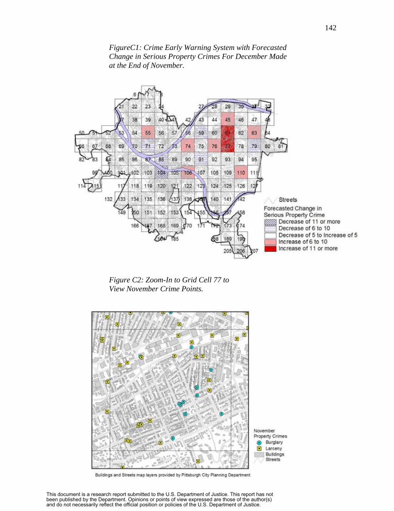
142

at the End of November.

View November Crime Points.

FigureC1: Crime Early Warning System with Forecasted Change in Serious Property Crimes For December Made

Figure C2: Zoom-In to Grid Cell 77 to


143

cell 77, to prevent the forecasted increase and apprehend perpetrators.

Several rule types are possible for symbolizing choropleth maps such as in Figure

C1. Some of these are:

Hot Areas – Emphasize areas where the forecasted crime level exceeds a threshold

level.

Forecasted Change – Emphasize areas where the difference between the current

actual and forecasted levels exceeds a threshold.

Forecasted Average Change - Emphasize areas where the difference between the

current estimated and forecasted levels exceeds a threshold.

Time Series Pattern Change Signaled - Emphasize areas where a time series tracking

signal exceeds its control limit.

One or more of these rules can be used in tandem. All are commonly known except

perhaps number 4, which we are introducing in this paper.

A problem with attempting to identify crime time series pattern changes is that the

analyst must examine time series plots of about five years length each month. This can

be done by visual examination, but generates a large workload. For example, in

Pittsburgh, there are approximately 100 grid cell areas to examine and 10 crimes of

interest, yielding 1,000 crime series plots to generate and examine each month. Clearly it

is infeasible to implement pattern change detection with visual examination. This is

where tracking signals come into play. They automatically flag exceptional time series.


144

Time series tracking signals are widely used by businesses for sales forecasting

and inventory control to generate exception reports of time series that are likely deviating

from their historical time trend. Very often it is this sort of information that is critical to

police. Our purpose in this chapter is to introduce and examine tracking signals as a

potential tool for crime analysts. We also undertake an exploratory empirical validation

of tracking signals. We have not seen any such studies in the literature, which has relied

on simulated data for this purpose.

The next section of this chapter briefly reviews tracking signals. Following that is

a section on our experimental design for validation, followed by a section on results, and

then a conclusion.

C2. Tracking Signals

An approach to evaluating a phenomenon at a point in time is to make a

counterfactual forecast for the point, which predicts the point under business-as-usual

conditions. This provides a good basis for assessing the actual value of the variable of

interest, whether it seems to be part of the existing pattern or is something new and

extraordinary. We use extrapolative time series forecasts for this purpose; in particular,

the most accurate as determined by Gorr et al. (2003) for one-month-ahead crime

forecasts. This is Holt exponential smoothing with smoothing parameters optimized and

using time series data deseasonalized with multiplicative seasonal factors estimated from

jurisdiction-wide data.

Tracking signals put counterfactuals to work in order to generate exception

reports. They generally are ratios in which the numerator is a sum or weighted sum of


145

forecast errors that has an expected value of zero when time series patterns (time trend

and seasonality) are stable. When there is a pattern change, such as a step jump or

turning point, the numerator moves away from zero. The denominator’s purpose is to

normalize by the long-term average variability of forecast errors. Of the common

tracking signals, the smoothed error signal due to Trigg (1964) is a good choice

(McClain, 1988). The equations are as follows:

Et = α1et + (1- α1)Et-1 (1)

MADt = α2|et| + (1- α2)MADt-1 (2)

Tt = |Et/MADt| (3)

where

t = month being assessed

Et = smoothed forecast error

et = forecast error

α1 = smoothing factor for numerator

MAD = mean absolute deviation of forecast errors

α2 = smoothing factor for denominator

We implement this signal with smoothing parameter values as suggested by McClain:

α1=0.4 for the smoothed sum of errors for the numerator (in order to quickly detect

pattern changes) and α2=0.05 for the denominator of smoothed mean absolute deviations

of forecast errors.


146

These equations are easily implemented in a spreadsheet package for

experimentation, but normally would be programmed to work automatically within a

CEWS. Figure C3 is an example of equations 1-3 applied to monthly time series data for

911 drug calls in grid cell 120 of Figure C1. Marked for comparison purposes are two

pattern changes and an outlier (more on this is in the next section). The actual and

forecasted crime levels have been rescaled to match the vertical scale of the tracking

signal. When the tracking signal crosses above the control limit line, it issues (trips) an

exception report, warranting analysis of this time series. As J. McClain (1988, p. 563)

states “A perfect tracking signal

Figure C3: Sample Tracking Signal for 911 Drug Calls in Grid Cell 120 with Marked Pattern Changes and Outlier.


147

would detect an out-of-control forecast [i.e., a time series pattern change] immediately,

and would never give a false alarm.” Of course, this is not possible, so in Figure C3 the

reader can see false positives (the first and third trips), actual positives detected

immediately (the second and fourth trips), and a delay in detecting an actual positive (the

last trip which appears as if it would be detected if one more data point were available).

C3. Experimental Design

We have not seen any attempts in the literature to validate tracking signals with

actual data, as in Figure C3. All validations appear to have used simulated data with

known pattern changes and outliers. Hence, we needed to invent a validation procedure

for working with actual data. For this purpose, we assumed that the purpose of tracking

signals is to mimic a trained, human judge (the crime analyst), and simply automate

his/her decisions on pattern changes and outliers.

We did not have the resources to embark on a full-scale validation; hence, we

decided to carry out an exploratory study to determine the feasibility of our approach and

provide preliminary results. We choose 10 crime time series from the Pittsburgh grid

system of Figure C1. They consist of a variety of crime types with five time series

having pattern changes and the other five not having any.

Both authors independently marked-up each of the time series for pattern changes

and outliers, as in Figure C3, under the guideline that we would only mark those that are

large and obvious. We then compared results and reconciled differences. One of us had

merely admitted some smaller pattern changes in interpreting “large and obvious”. The


148

result was 18 instances ultimately used in our analysis of pattern changes or outliers in

five of the time series.

Our treatment of the smoothed signal tracking signal is to use it with a variety of

control limits. After some trial and error, we decided to use values of 0.84, 1.05, 1.26,

and 1.47. This range starts at a low value (0.84) that detects most of the actual positives,

but at the cost of tripping many false positives (false alarms). At the other extreme

(1.47), there are fewer detections of actual positives, but also many fewer false positives.

The forecast errors are from 36 one-month-ahead forecasts made with Holt

smoothing and classical decomposition as described above (Gorr et al., 2003). Each

forecast was made using 5 years of monthly data ending the month before the forecasted

month.

C.4 Results

We applied equations 1-3 on the 10 time series over the 36 month period in which

forecasts were made. In reporting results, we decided to exclude the first six months of

tracking signals for burn-in so that the tracking signal could “forget” arbitrary initial

values and start tracking correctly. Hence there were 10 time series times 30 months

each for a total of 300 signals estimated. Also, this translates to 300 time series plots that

a crime analyst would have had to examine to accomplish the same task.

We define an exception report “epoch” to be the total number of time periods that

the tracking signal is above its control limit, including the first month

that it trips. We assume that the crime analysis protocol is that the crime analyst must

investigate each time series plot and corresponding crime maps for each month of epochs.


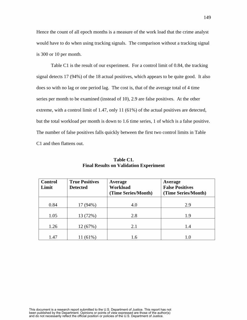
149

Hence the count of all epoch months is a measure of the work load that the crime analyst

would have to do when using tracking signals. The comparison without a tracking signal

is 300 or 10 per month.

Table C1 is the result of our experiment. For a control limit of 0.84, the tracking

signal detects 17 (94%) of the 18 actual positives, which appears to be quite good. It also

does so with no lag or one period lag. The cost is, that of the average total of 4 time

series per month to be examined (instead of 10), 2.9 are false positives. At the other

extreme, with a control limit of 1.47, only 11 (61%) of the actual positives are detected,

but the total workload per month is down to 1.6 time series, 1 of which is a false positive.

The number of false positives falls quickly between the first two control limits in Table

C1 and then flattens out.

Table C1. Final Results on Validation Experiment

Control Limit

True Positives Detected

Average Workload (Time Series/Month)

Average False Positives (Time Series/Month)

0.84 17 (94%) 4.0 2.9

1.05 13 (72%) 2.8 1.9

1.26 12 (67%) 2.1 1.4

1.47 11 (61%) 1.6 1.0


150

We believe that these results are promising. They show a 60% work reduction for

the most stringent case and up to an 84% work load reduction for the least stringent case.

C5. Conclusion

This chapter has introduced crime early warning systems and tracking signals for

detecting time series pattern changes in crime maps. The basis of the tracking signal is

information obtained from counter-factual forecasts for each point examined. These are

forecasts providing business-as-usual estimates for a point in time, as if no pattern

changes existed. The tracking signal automates detection of pattern changes by

mimicking the decisions of crime analysts as to what data points constitute the start of a

new time series pattern. We varied the control limit of the tracking signal, making it

more or less sensitive to information in the time series data.

Future work is clear on this topic. It is necessary to take a large sample of time

series, have crime analysts mark them up for pattern change points and outliers, and rerun

the experiments. Additional tracking signals may be tried, as well as varying the tracking

signal numerator’s smoothing factor (which we did not do).

References

Gorr, W.L., Olligschlaeger, A.M., Thompson, Y. (2003). Short-term time series

forecasting of crime. The International Journal of Forecasting (forthcoming).

McClain, J.O. (1988). Dominant Tracking Signals. The International Journal of

Forecasting 4, 563-572.

Trigg, D. W. (1964). Monitoring a forecasting system. Operational Research

Quarterly 15, 271-274.


Development of Crime Forecasting and Mapping Systems for ...

Documents

Transcript of Development of Crime Forecasting and Mapping Systems for ...