Development of an automated trace analyser and a novel passive sampling

device for the monitoring of ammonia in marine environments

Lenka O’Connor Šraj

ORCID: 0000-0002-2353-1037

Doctor of Philosophy (Chemistry)

School of Chemistry, The University of Melbourne

ii

ABSTRACT

Ammonia is commonly used as an indicator of water quality, to assess the impacts of

anthropogenic activity on ecosystem function and health. Water quality assessment often

relies on the use of expensive equipment requiring a high degree of operator skill, or periodic,

discrete, manual sampling and laboratory-based analysis, which is laborious, costly and without

the guarantee that episodic pollution events will be detected. Low-cost, portable and/or field-

deployable analytical tools are required to overcome this challenge. Hence, research

conducted in the context of this thesis involves the development of novel analytical tools for

the monitoring of ammonia in marine waters, covering both active and passive sampling.

A flow-based analytical method was designed and developed for the determination of total

ammonia over a wide concentration range in marine waters using the gas-diffusion

spectrophotometric method. Limits of detection similar to that of highly sensitive fluorometric

methods was achieved. A novel flow approach was adopted whereby a continuous stream of

sample was merged with the sodium hydroxide reagent stream and delivered to a gas-diffusion

ammonia separation unit, allowing large sample volumes to be used, rather than being limited

by the use of discrete samples. The working range and sensitivity of the method could be

tailored by simple modification of the sample volumes used, and by minor adjustments to the

program used to control the instrument, without the need to make changes to the manifold.

Three working ranges were obtained, and the analytical figures of merit are described. This

project was an enabling step in the development of an ammonia gas-diffusion passive sampling

device, as it allowed the measurement of low concentrations often found in field samples, as

well as high concentrations accumulated in the passive sampler’s receiving solution, using the

same instrumentation and reagents.

A passive sampling device based on gas-diffusion across a hydrophobic membrane was

developed and successfully applied for the determination of the time-weighted average

concentration (CTWA) of ammonia in marine waters for a period of 3 to 7 days. Molecular

ammonia (NH3) present in the sampled source solution (SS) diffuses through a hydrophobic

membrane into an acidic receiving solution where it is ionised and accumulated as NH4+ which

iii

is directly proportional to the NH3 concentration in the SS. Biofouling limited the application of

the first gas-diffusion-based passive sampler (GD-PS) prototype to 3 days, and a number of

antifouling strategies were therefore assessed, with a copper mesh enabling the sampling

period to be extended to 7 days. The effects of environmental variables (temperature, pH and

salinity) on NH3 accumulation were also investigated, and the Group Method of Data Handling

(GMDH) Algorithm was used to develop a single calibration model for a range of environmental

conditions (10 to 30 °C, pH 7.8 to 8.2, salinity 20 to 35). PSDs were deployed at four estuarine

and marine sites in Nerm (Port Phillip Bay), south eastern Australia, achieving good agreement

between passive and automated discrete sampling methods (maximum relative error between

-12 % to -19 %). The GD-PS covers the revised water quality trigger value (160 µg L-1 NH3-N)

and allows for episodic pollution events to be successfully detected, highlighting this as an

exciting new tool for water quality assessment.

iv

DECLARATION

I, Lenka O’Connor Šraj, declare that:

1. This thesis comprises only my original work, except where indicated, and withappropriate acknowledgement provided

2. Due acknowledgment has been made in the text to all other material used, particularlywith respect to third-party copyright material

3. Permissions were obtained in all cases to use third-party copyright material in the openaccess version of this thesis

4. The thesis is less than the maximum word limit in length

v

PREFACE AND ACKNOWLEDGEMENT

I would like to acknowledge the Boon Wurrung, Wurundjeri and Wathaurong Sovereign Clans

of the Kulin Nation as the Traditional Custodians of the waterways and lands upon which

research for my doctoral studies was undertaken. I currently live on Wurundjeri Country and I

would like to pay my respects to all First Nations elders, past, present and emerging.

Furthermore, I recognise the significant contributions made by our First Nations custodians in

terms of Indigenous knowledge and understandings of sustainability and caring for Country,

including for our precious waterways and coastal areas. Throughout this work, the original First

Nations place names have been used, italicised, together with the colonial place names in

brackets.

All research work and thesis preparation were carried out under the supervision of Professor

Spas D. Kolev with guidance, advice, support and editorial assistance provided by Professor

Stephen Swearer (co-supervisor), Dr Ian D. McKelvie, Dr Richard Morrison, and Dr Maria Inês

G. S. Almeida.

I would like to thank Ms Chelsea Bassett for assistance with preliminary passive sampling

experiments, and the Environment Protection Authority Victoria for the loan of field

equipment and assistance from staff, including Chris Garland, Adele McKenzie and Mick Ernest,

and also Professor Vincent Pettigrove (RMIT University, former CEO of the Centre for Aquatic

Pollution Identification and Management) for the loan of field equipment and assistance in

setting up field experiments. I would also like to thank Mr Simon Sharp and Mr Andrew

Longmore who provided extensive assistance in setting up field experiments and sampling

guidance, Mr. Roger Eastham and the Royal Yacht Club of Victoria for allowing field work in

their marina, Parks Victoria for permitting field work in the coastal waters of Nerm (Port Phillip

Bay) and the Werribee River estuary, and Melbourne Ports for allowing field work to be

undertaken in the Birrarung (Yarra River) estuary.

Mr Marcus Hammarstedt and Mr Benham Rasooli assisted with digitising graphics for

publication, and I am grateful to the University of Melbourne for the award of a postgraduate

scholarship.

~

vi

Firstly, I would like to thank my wonderful family for their support and encouragement over

the years, particularly my mother and father who worked tirelessly to provide me with an

incredible education. I dedicate this thesis to you both, as you were instrumental in getting me

to a point where I could take on this project. To my brothers and my partner, you are the most

amazing people, and I am so lucky to have your continued and ongoing friendship and your

help and assistance along this journey. On many occasions you helped me with my field work,

with editorial and design assistance, you have looked after me when I have been busy trying

to get my work done, and so thank you. I am so grateful to you all for being there for me,

supporting me in this endeavour and for helping me along the way.

I would like to thank my encouraging and incredibly supportive supervisors Professor Spas D.

Kolev and Professor Stephen Swearer firstly for taking me on as a PhD student, and for

providing me with inspiration and assistance over the course of my graduate studies. It has

been an honour to work with Professor Kolev. You taught me to be an inquisitive and

independent researcher and you have often challenged me to think more broadly about my

work. I am so grateful to have been given the opportunity to work with such an amazing

scientist, and to be a member of the Kolev research group. I would like to thank Professor Kolev

for being a most wonderful supervisor and mentor over the years. Professor Stephen Swearer

you were always there when I needed assistance and always offered a fresh and invaluable

perspective to the challenges I faced during the course of my research. I have thoroughly

enjoyed our discussions over the years and look forward to continuing these into the future.

I would like to thank Dr Ian McKelvie and Dr Richard Morrison for all their assistance, guidance,

mentorship and life-changing advice over the years. I feel so lucky to have been able to

collaborate with you both on a multitude of projects, and I look forward to our continued work

with the Kolev research group. You have given me so much inspiration, support and friendship

over the years and I am forever grateful.

Finally, I would like to thank Dr Maria Inês G. S. Almeida for your supervision, guidance,

mentorship, and friendship over the years. You were there for me every single day and I am so

thankful for the many hours you have spent teaching me new techniques, working through

problems with me, helping me with both lab and field work and supporting and encouraging

me when experiments didn’t go to plan. I feel so privileged to have been able to work with you

and you have been an inspiration to me. I look forward to many years of friendship to come.

vii

TABLE OF CONTENTS

CHAPTER 1:

General introduction 1 1.1 Aquatic ammonia pollution 3 1.2 Challenges for the analytical chemist 5 1.3 Flow-based methodologies 8 1.4 Passive sampling 28 1.5 General comments and research objectives 60

CHAPTER 2:

Determination of trace levels of ammonia in marine waters using a simple environmentally-friendly ammonia (SEA) analyser

84 2.1 Introduction 88 2.2 Materials and methods 91 2.3 Results and discussion 99 2.4 SEA analyser system performance 105 2.5 Validation of the SEA analyser 107 2.6 Conclusions 109 2.7 Appendix 111

viii

CHAPTER 3:

Gas-diffusion-based passive sampler for ammonia monitoring in marine waters 116 3.1 Introduction 120 3.2 Materials and methods 121 3.3 Results and discussion 124 3.4 Conclusions 130

CHAPTER 4:

Monitoring of ammonia in marine waters using a passive sampler with biofouling resistance and neural network-based calibration

133 4.1 Introduction 137 4.2 Materials and methods 139 4.3 Results and discussion 144 4.4 Conclusions 157 4.5 Appendix 158

CHAPTER 5:

Conclusions and future work 177

ix

LIST OF FIGURES CHAPTER 1

Figure 1-1. Biogeochemical cycling of aquatic nitrogen and transformations in the water column.

4

Figure 1-2. Average concentration of the major ions in seawater accounting for the overall total salinity of 34.5.

6

Figure 1-3. Schematic diagrams of commonly used flow systems. 8

Figure 1-4. Distribution graph of flow-based methodologies developed for the determination of total ammonia in estuarine and marine waters.

9

Figure 1-5. Results obtained by different sampling methods commonly used in environmental monitoring.

29

Figure 1-6. Schematic diagrams and typical deployment configuration of a SPMD filled with triolein receiving phase.

35

Figure 1-7. Single-phase polymer-based PSDs. 41

Figure 1-8. Schematic diagrams and typical deployment configuration of the POCIS for the passive sampling of hydrophilic organic compounds.

44

Figure 1-9. Schematic diagram and typical deployment configuration of the Chemcatcher®.

46

Figure 1-10. Summary of the log Kow ranges successfully tested for various Chemcatcher® receiving phase and membrane combinations.

48

Figure 1-11. Schematic diagram and typical deployment configuration of the diffusive gradient in thin-films passive sampling device.

54

CHAPTER 2

Figure 2-1. Schematic diagram of the fully automatic SEA analyser using a FiaLab 3500 flow system and Cetac autosampler.

94

Figure 2-2. Different GDU configurations tested in order to select the configuration that achieved the highest sensitivity.

97

Figure 2-3. (a) Effect of the donor stream flow rate on the analytical signal for three different ammonium standards; (b) effect of the sample and reagent volume on the maximum absorbance for three different ammonium standards.

100

Figure 2-4. (a) Performance of different GDU configurations; (b) Performance of different porous hydrophobic membranes was examined using the sandwich type GDU.

103

Figure 2-5. (a) Blank corrected absorbance response for for 1.4 μM (○) and 2.8 μM (◊) ammonium standards as a function of baseline absorbance; (b) absorbance response for different colour indicator dye solutions, as single dyes or as mixtures; (c) the working range of the method can be extended when mixed indicator solutions are used.

105

x

Figure 2-6. Three typical concentration working ranges based on sample volume 106

Figure 2-7. Sampling sites around the Port Phillip Bay Study Area with the average range of concentrations of ammonia nitrogen measured with the SEA analyser

108

Figure 2-8. Spiked recoveries of seawater samples of varying salinity from around Port Phillip Bay (PPB), and Bancoora Surf Beach.

109

CHAPTER 3

Figure 3-1. (a) Gas-diffusion-based PS assembly; (b) cross section of the gas-diffusion-based PS (membrane thickness not drawn to scale), and schematic illustration of the diffusion process of dissolved ammonia (NH3(aq)) from the source solution through the pores of the hydrophobic GDM

124

Figure 3-2. (a) Transient concentration of ammonium in the receiving solution versus sampling time; (b) laboratory-based calibration of the gas-diffusion PS

129

CHAPTER 4

Figure 4-1. A) GD-PS assemblage with antifouling mesh. B) Cross-section of the GD-PS showing the process of selective accumulation of dissolved NH3(aq) from the source solution.

143

Figure 4-2. Membrane antifouling strategies under laboratory conditions. A) Effect of the different antifouling strategies on the ammonium concentration accumulated in the receiving solution after 7 or 8 days of sampling in the laboratory; B) effect of the different antifouling strategies on the extent of biofilm formation on the surface of the GDMs

146

Figure 4-3. Effect of salinity (A), pH (B) and temperature (C) on the GD-PS accumulation

150

Figure 4-4. Field validation of the GD-PS with copper mesh (Cu-100) using the GMDH calibration model, A) Birrarung (Yarra River) estuary (Site 1) and B) Werribee River estuary mouth (Site 3)

154

Figure S4-1. Port Phillip Bay field study sites and water collection point (datum: GDA94).

159

Figure S4-2. Receiving solution composition and membrane optimisation 160

Figure S4-3. GD-PS accumulation over 7 days using Cu-100 (♦), Cu-200 (○) and

AgNP (◊) antifouling mesh and no treatment (●).

160

Figure S4-4. Multivariate study of temperature, salinity and pH parameters 161

Figure S4-5. GMDH model for GD-PS between pH 7.8 to 8.2 and temperature 10 to 30 °C.

164

Figure S4-6. GMDH model figures of merit. 164

xi

Figure S4-7. Field validation of the GD-PS with copper mesh (Cu-100) using the GMDH calibration model, A) Hobsons Bay (Site 2) and B) Werribee River estuary 5 km upstream from river mouth (Site 4).

166

Figure S4-8. Linear calibration of GD-PS with studentised residuals. 168

Figure S4-9. Werribee river estuary mouth (Site 3) dissolved oxygen and tidal data. A) Tide and salinity data; B) pH and dissolved oxygen data; C) calculated source solution molecular ammonia and measured total ammonia data.

169

Figure S4-10. Satellite images showing proximity of stockpiled agricultural chemicals to Werribee River estuary (Sites 3 and 4).

170

xii

LIST OF TABLES CHAPTER 1

Table 1-1. Analytical features of flow-based methodologies using the indophenol blue reaction.

11

Table 1-2. Analytical features of flow-based methodologies using analyte separation and/or preconcentration.

16

Table 1-3. Analytical features of flow-based methodologies using fluorometric detection.

20

Table 1-4. Stability and storage of reagents involved in the determination of ammonium.

27

CHAPTER 2

Table 2-1. Gas-diffusion configurations comparing various aspect ratios (exposed membrane area to channel volume ratio).

97

Table 2-2. Hydrophobic membranes tested. 98

Table 2-3. Analytical figures of merit of the SEA analyser for three typical working ranges.

107

Table 2-4. Method validation using a diluted CRM in 0.6 M NaCl, for the calibration range 0.28 – 13.9 µM NH4

+. 107

Table A2-1. Programmable flow procedure for the determination of ammonia nitrogen in seawater.

111

CHAPTER 3

Table 3-1. Membrane characteristics. 122

Table 3-2. Study of the gas-diffusion membranes and the receiving solution composition.

126

CHAPTER 4

Table 4-1. Comparison between discrete grab sampling and GD-based passive sampling (time-weighted average ammonia concentration ([NH3]TWA)) using the GMDH model.

154

Table S4-1. Field site codes, location and GPS coordinates (datum: GDA94) 159

Table S4-2. Experimental conditions for the multivariate study. 161

Table S4-3. Experimental conditions for the univariate study. 162

Table S4-4. Effect of the flow pattern on the error obtained when comparing discrete grab sampling (SS) and GD-based passive sampling ([NH3]TWA determined using the GMDH model).

168

xiii

ABBREVIATIONS

ABA, Autonomous batch analysis

AgNP, Silver nanoparticle

ANAMOX, Anaerobic ammonium oxidation

ANZG, Australian and New Zealand Guidelines

AOA, Ammonia oxidizing archaea

AQUA-GAPS, Aquatic global passive sampling program

BTB, Bromothymol blue

CA, Cellulose acetate

CRM, Certified reference material

CTWA, Time-weighted average concentration

CyDTA, 1,2 Cyclohexane diamine tetraacetic acid

DGT, Diffusive gradients in thin films

DIC, Dichloroisocyanurate

DRP, Dissolved reactive phosphorous

EDTA, Ethylenediaminetetraacetic acid

EU-WFD, European Union Water Framework Directive

EVA, Ethylvinyl acetate

FIA, Flow injection analysis

FL, Fluorescence

GBR, Great Barrier Reef

GC-MS, Gas chromatograph mass spectrometry

GD, Gas-diffusion

GDM, Gas-diffusion membrane

GDU, Gas-diffusion unit

µGDU, Micro gas-diffusion unit

GMDH, Group Method Data Handling

HAB, Harmful algal bloom

HLB, Hydrophilic-Lipophilic Balance

HOC, Hydrophobic organic compound

HF, Hollow fibre

HPLC, High-performance liquid chromatography

H-SDME: Headspace single-drop microextraction

IC, Ion chromatography

IDA, Iminodiacetate groups

IL, Ionic liquid

IPB, Indophenol blue

iSEA, Integrated syringe-pump-based environmental-water analyser

LDPE, Low-density polyethylene

LED, Light emitting diode

LFA, Loop flow analysis

LOD, Limit of detection

LOQ, Limit of quatification

LWCC, Liquid waveguide capillary cell

MCFIA, Multicommutated FIA

MOPA, 4-methoxypthaldealdehyde

M2OPA, 4,5-dimethoxypthaldealdehyde

MPFS, Multipumping flow systems

MPV, Multiposition valve

MSA, Methane sulphonic acid

MSFIA, Multi-syringe FIA

N2, Nitrogen

NH3, Molecular ammonia

NH4+, Ammonium

NH3/NH4+, Total ammonia

NPOE, Nitrophenyl octyl ether

xiv

OPA, Orthophtaldialdehyde

OPP, o-phenylphenol

PAH, Polyaromatic hydrocarbon

PBDE, Polybrominated diphenyl ethers

PCB, Polychlorinated biphenyl

PDMS, Polydimethylsiloxane

PES, Polyethersulfone

PFAS, Perfluoroalkyl substances

PFC, Perfluorinated chemicals

PIM, Polymer inclusion membrane

PIMS, Passive integrative mercury sampler

PMT, Photomultiplier tube

POCIS, Polar organic chemical integrative sampler

POM, Polyoxymethylene

PP, Polypropylene

PPB, Nerm (Port Phillip Bay)

PS, Passive sampler

PSD, Passive sampling device

PRC, Performance reference compound

PTFE, Polytetrafluoroethylene

P&T, Purge-and-trap

PVDF, polyvinylidene difluoride

rFIA, Reversed FIA

RTD, resistance temperature detector

Rs, Sampling rate

SBSE, Solventless stir bar sorptive extraction

SD, Steam distillation

SFA, Segmented flow analysis

SIA, Sequential injection analysis

SLM, Supported liquid membranes

SPATT, Solid-phase adsorption toxin tracking

SP, Syringe pump

SPE, Solid-phase extraction

SPMD, Semipermeable membrane device

SR, Silicone rubber

TOMAS, Trioctylmethylammonium salicylate

TOMATS, Trioctylmethylammonium thiosalicylate

UV, Ultraviolet

WTP, Western Treatment Plan

1

CHAPTER 1: General introduction

Foreword This thesis has been written in the format of a ‘Thesis by Publication’. The chapters of this work

comprise a series of peer-reviewed papers which have been published in high-impact factor

journals. These chapters are bookended by a substantial General introduction chapter and a

Conclusions and future work chapter. Where a chapter (or section of a chapter) of this thesis

has been published, it will be highlighted in the Foreword section at the beginning of each

chapter, with information on the journal article appearing as a citation for the readers easy

reference.

The following section encompasses a literature review looking at flow-based methodologies

developed to monitor ammonia in marine waters, in addition to a description of passive

sampling technologies that have been developed for monitoring environmental pollutants in

natural waters, with a particular emphasis on those applied to estuarine, coastal and marine

environments. The advantages and challenges of flow methods and passive sampling

techniques is evaluated.

The content of the sections describing flow techniques for ammonia determination in

estuarine and marine waters was published in 2014 in the journal Trends in Analytical

Chemistry, and it has been further updated to cover the period 2014-2020. The section

describing passive sampling techniques applied to high salinity matrices is currently in the

process of being prepared for submission to a journal and is thus written in the style of a review

paper.

O'Connor Šraj, L., Almeida, M. I. G. S., Swearer, S. E., Kolev, S. D., McKelvie, I. D. Analytical

challenges and advantages of using flow-based methodologies for ammonia determination in

estuarine and marine waters, TrAC Trends Analytical Chemistry, 59 (2014) 83-92,

doi.org/10.1016/j.trac.2014.03.012

2

Contents 1.1 Aquatic ammonia pollution 3

1.2 Challenges for the analytical chemist 5

1.3 Flow-based methodologies 8

1.3.1 Indophenol blue method 10

1.3.2 Gas-diffusion method 16

1.3.3 Fluorometric method 20

1.3.4 Field applications 24

1.4 Passive Sampling 28

1.4.1 Semipermeable membrane devices (SPMDs) 34

1.4.1.1 Single-phase passive samplers 38

1.4.1.1.1 Low-density polyethylene (LDPE) 39

1.4.1.1.2 Silicone Rubber (SR) 40

1.4.1.1.3 Polyoxymethylene (POM) & ethylene-vinyl acetate (EVA)

42

1.4.2 Polar organic chemical integrative sampler (POCIS) 42

1.4.3 Chemcatcher® 46

1.4.3.1 Chemcatcher® for non-polar compounds 48

1.4.3.2 Chemcatcher® for polar compounds 49

1.4.3.3 Chemcatcher® for metals and organometallics 50

1.4.4 Solid-phase adsorption toxin tracking (SPATT) 52

1.4.5 Diffusive gradients in thin-films (DGT) 53

1.4.6 GELLYFISH for metals 56

1.4.7 Liquid membrane-based passive samplers 57

1.4.8 Ammonium PSDs applied to freshwaters 59

1.5 General comments and research objectives 60

References 63

3

1.1 Aquatic ammonia pollution Ammonia is an ecologically important nutrient in the nitrogen cycle of coastal and oceanic

waters (Figure 1-1). It is naturally found at low concentrations in the environment as a by-

product of protein metabolism and the decomposition of organic matter. However, it is

increasingly entering the environment as a result of urban, industrial and agricultural

processes, predominantly as a result of large-scale diffuse run-off from agricultural land [1].

Hence, the creation of guidelines for ammonia in estuarine and marine water systems is critical

in order to achieve a sustainable use of water resources, and for the protection of aquatic life

from acute and chronic effects of ammonia. Although this issue remains a challenge [2], some

countries have established guideline values for ammonia in marine or salt waters [3-6].

The toxicity of ammonium/ammonia is dependent on pH. Below pH 8.75, ammonium (NH4+) is

the predominant relatively non-toxic form, and above pH 9.75, ammonia (NH3), the toxic form,

is dominant [7]. Therefore, in most aquatic environments, ammonium is the major form and

ammonia is present to a much lesser extent. Despite the lower toxicity of ammonium, it should

be considered important because of its much greater concentrations than un-ionised ammonia

[8].

There are several consequences of excessive ammonia/ammonium concentrations in the

aquatic environment. In the presence of nitrifying bacteria, ammonium and ammonia can be

converted to nitrate [1], both of which are utilised by phytoplankton, macrophytes and

cyanobacteria. At elevated concentrations, ammonia/ammonium can stimulate primary

production in planktonic communities causing rapid algal growth and eutrophication,

contributing to widespread and even irreversible changes to a whole range of coastal and

marine ecosystems [1, 9]. Microbial respiration fuelled by an increase in dissolved organic

matter from algal senescence causes dissolved oxygen depletion, resulting in hypoxia in the

water column [10]. The sensitivity of marine fish and invertebrates to ammonia toxicity is

amplified in hypoxic waters, with both stressors exhibiting a synergistic effect [1]. Most marine

fish and invertebrates excrete ammonia and ammonium directly, as the major metabolic waste

products, to the surrounding water [11]. Although the precise mechanisms of excretion in fish

are still the subject of research, it is believed that this process occurs via passive diffusion, from

blood plasma to the water surrounding the gills [11]. The high ionic permeability of the gills of

4

marine fish allows for ammonia to enter as either the un-ionised or ionised forms, which may

make them more prone to ammonia and ammonium toxicity than their fresh water

counterparts [11]. Ammonia exposure is particularly detrimental to the growth and

development of larval and juvenile life stages of fish and invertebrates. In mature fish, exposure

to ammonia is known to cause pathohistological damage to the gills, kidneys and blood,

neurotoxicity, hyperventilation, and convulsions. Over sustained periods of time, build-up of

the toxin in the blood can result in the extinction of entire populations, thus threatening many

globally important ecosystems and fisheries [12].

Figure 1-1. Biogeochemical cycling of aquatic nitrogen and transformations in the water column.

5

The global nitrogen cycle is complex and dynamic, and many aspects are still not fully

understood. For example, it is only recently that ammonia oxidizing archaea (AOA) have been

discovered in the oceans. These may be the key organism responsible for production of the

potent greenhouse gas nitrous oxide (N2O) [13], which has been described as having a global

warming potential 310 times greater than CO2 [14]. The rate of N2O produced by AOA from

ammonia is high under hypoxic conditions. The occurrence of hypoxic waters is predicted to

increase exponentially with continual anthropogenic nutrient loading of coastal waters and

global climatic changes, and this in turn may lead to increased production of N2O in the oceans,

and higher concentrations of N2O in the atmosphere [13].

The total ammonia concentration (i.e. the sum of both ammonia and ammonium) is thus an

indicator of water quality as well as an ecological stressor [7]. The measurement of total

ammonia concentrations and fluxes, coupled with an understanding of the complex bio-

geochemical processes, is imperative for sustainable management and conservation of

important marine ecosystems and their catchments [15]. Analytical methods that are fast,

sensitive, reliable and preferably portable or capable of in situ analysis, are therefore essential

tools in achieving such goals. The following section will thus review the challenges facing the

analytical chemist as well as the flow-based and in situ methodologies developed for the

determination of ammonia in marine, coastal and estuarine waters. Furthermore, an overview

of the passive sampling techniques described in the literature will be provided, specifically

when applied to high salinity matrices. Passive sampling has become a popular technique for

in situ monitoring of environmental pollutants in aquatic environments, however passive

sampling techniques specifically for ammonia monitoring in marine waters have not previously

been described prior to the gas-diffusion-based passive samplers developed as part of the

research reported in this thesis (see Chapters 3 and 4).

1.2 Challenges for the analytical chemist Marine environments, including estuarine, coastal and open ocean waters are increasingly the

focus of research with respect to the detection of anthropogenic pollutants [16]. However, the

low analyte concentrations, variable salinity and matrix complexity of these waters (e.g. the

potential interferences from cations such as Mg2+ and Ca2+) make that task difficult [17]. To

6

illustrate the complexity of the seawater matrix, Figure 1-2 summarizes the average

concentrations of the major ions in seawater, accounting for the overall total salinity of 34.5

[18]. Additionally, estuarine, coastal and oceanic waters represent different ecological systems

which have substantially different chemical environments (as described below), and it is often

difficult to find analytical methods that can be applied universally to all three types of matrix.

Figure 1-2. Average concentration of the major ions in seawater accounting for the overall total salinity of 34.5 [18].

Estuarine environments are where fresh water from rivers mix with saline water from the

ocean and are characterised by salinities ranging from 0.5 to 35 [19]. They are dynamic,

transient and exhibit a unique and complex biogeochemistry, with a wide range of chemical

compositions (they often exhibit salinity stratification) that change with the tides, season,

weather, biota, surrounding landscape and anthropogenic inputs of dissolved organic and

inorganic materials [19]. Estuaries are some of the most biologically diverse and productive

ecosystems, providing habitat for a variety of unique plants and animals (i.e. marine fish and

invertebrates) [20].

In the oceans, salinity, temperature and nutrient-concentration profiles are typically vertically

stratified [21]. The euphotic zone at the surface exhibits relatively uniform physicochemical

properties due to winds, shallow currents and small-scale eddies that facilitate mixing [21].

However, due to mainly thermohaline stratification, the upper ocean surface is generally

characterised by warm, highly saline, nutrient deficient waters, whereas the deeper water

masses tend to be cooler, denser and containing higher concentrations of re-mineralised

7

inorganic nutrients, which have been accumulated by the gravitational sinking of decomposing

phytoplankton and dissolved organic matter from the euphotic zone [21]. Essential nutrients

are redistributed in the water column as a result of mesoscale ocean currents and circulation

patterns, resulting in diapycnal three-dimensional mixing, coastal upwelling of cold, nutrient

rich waters along western coastlines in the Pacific, Indian and Atlantic oceans, and to a lesser

extent, contributions from diazotrophic nitrogen fixation, atmospheric deposition and inputs

from river run-offs into estuaries and coastal waters [22].

Another challenge often encountered by the analytical chemist is the collection, storage and

preservation of estuarine or marine water samples. Samples collected manually should be

stored in glass or polyethylene bottles (0.5 – 1 L capacity) and analysed immediately. If that is

not logistically feasible, they should be at least refrigerated or preferably deep-frozen [23].

Changes in analyte concentration may however be significant after more than a few days

storage [24]. Acid preservation (i.e. conversion of all ammonia to ammonium) is used to extend

the period between sample collection and analysis, however prior to analysis, samples must

be neutralised [25].

Additionally, the exposure of reagents and standards to ambient air can potentially lead to

contamination; this can be minimised by using a nitrogen glove box to keep and process all

solutions [26], or by using acidic treatment [27].

The chemical variability of estuarine and marine systems significantly affects the selection and

performance of the analytical method used for ammonia analysis. Most of the analytical

methods available for ammonia determine not only ammonia but the combination of both

molecular ammonia and ammonium (i.e. total ammonia). However, for consistency, the term

‘ammonium’ is used throughout this chapter to express the total ammonia.

The indophenol blue (IPB) method based on the Berthelot reaction is most commonly used as

the reference method for the determination of ammonium in aqueous samples [28-30]. Other

analytical methods have been proposed in the past 30 years including the fluorometric

method, and methods involving analyte separation and preconcentration techniques, such as

the gas-diffusion (GD) method. These analytical methods and their various automated versions

have been applied in estuarine and marine waters for the determination of ammonium and

are described in detail in the following sections. Automatic methodologies of analysis are flow-

8

based and have been developed with the aim of meeting the challenges mentioned above,

thus providing fast, sensitive, accurate and even portable analytical tools. A brief and general

description regarding flow-based methodologies (viz. principle, advantages, and

disadvantages) is given in the following section. However, the focus will be on the analytical

strategies used, rather than on a comparison between the various methods.

1.3 Flow-based methodologies The flow analysis concept emerged during the 1950’s, with the advent of segmented flow

analysis, where the aim was to perform chemical analysis in an automatic fashion. Since then

the concept has evolved and several flow-based methodologies have been developed [31].

Figure 1-3 shows schematic diagrams of basic and commonly used flow systems.

Figure 1-3. Schematic diagrams of commonly used flow systems: Carrier (C); Reagent (R); Air (A); Sample (S); Air bubble (B); Detector (D); Waste (W); Reaction coil (RC); Peristaltic pump (PP); Debubbler (DB); Syringe pump (SP); Holding coil (HC); Selection valve (SV); Solenoid valve (SnV); Multisyringe pump (MS); Solenoid micro-pumps (P1, P2).

9

The distribution of flow-based techniques that have been applied to the determination of

ammonium in estuarine and marine waters is illustrated in Figure 1-4.

Figure 1-4. Distribution graph of flow-based methodologies developed for the determination of total ammonia in estuarine and marine waters (according to ISI Web of Knowledge, February 2020).

Segmented flow analysis (SFA), was designed to perform measurements similarly to discrete

analysis, and consists of a continuous flowing stream segmented by air bubbles (Figure 1-3).

Despite the disadvantages of air bubble segmentation (e.g. slow start-up times, higher reagent

use and waste production), this technique has been widely adopted to automate

oceanographic analytical methods including those for ammonium determination [32]. Unlike

SFA, flow injection analysis (FIA) is characterized by a non-segmented flow stream where the

sample is inserted in a carrier/reagent stream through an injection valve, in a reproducible

fashion and with controlled dispersion (Figure 1-3). Consequently, enhanced sample

throughput, simplicity of operation, low cost and greater potential for portability are some of

the advantages of this technique, features that are particularly useful in oceanographic studies.

Accordingly, more than half of the papers regarding the determination of ammonium in

estuarine and marine waters apply FIA as the flow technique (Figure 1-4).

Apart from FIA, there are more recent flow techniques such as sequential injection analysis

(SIA) and multicommutated flow techniques (e.g. multicommutated FIA (MCFIA), multi-syringe

FIA (MSFIA), multipumping flow systems (MPFS)) that offer additional advantages and also with

their own limitations (Figure 1-3). SIA was conceived to sequentially aspirate sample and

10

reagent plugs through a selection valve toward a holding coil, which are directed to the

detector by flow reversal. Versatility, reagent saving, computer control and robustness are the

main advantages of this technique.

Multicommutated flow techniques, highlighted by Cerdà and Pons [33], are based on a flow

network comprising individual solenoid devices (valves in MCFIA/MSFIA and pumps in MPFS)

controlled by computer software. These techniques have similar features as SIA, with the

added potential of miniaturization and portability. A few studies have shown the potential of

these techniques to assist in the challenge of ammonium monitoring in estuarine and seawater

samples (Figure 1-4). Some batch-analysis systems have also been proposed in the context of

this application (e.g. loop flow analysis (LFA), autonomous batch analysis (ABA)).

Flow-based methodologies have the advantage of not only performing automated analysis, but

also of improving sensitivity, with the possibility of miniaturization and/or portability (e.g.

shipboard measurements). Such features are ideal for the nanomolar level ammonium

concentrations and analysis can even be performed on-line or immediately after sample

collection, thus avoiding sample storage issues (e.g. loss of analyte).

With an emphasis on the strategies adopted to face the challenges described above, the

following sections describe the flow techniques that have been developed for the

determination of ammonium in estuarine and marine waters (including other saline samples)

according to the analytical method applied, namely the IPB method, the GD method (this may

need to be updated) and the fluorometric method (the analytical features of each method are

described in Tables 1-1 to 1-3 below).

1.3.1 Indophenol blue method

Molecular absorption spectrophotometry is one of the most widely used analytical detection

techniques, as it is accessible, versatile, accurate and generally inexpensive. Most colorimetric

methods published for ammonia determination in estuarine and marine waters use some

variation of the IPB chemistry, based on the reaction between ammonia and hypochlorite to

form monochloroamine that then reacts with a phenolic compound to produce the coloured

indophenol blue complex, which is measured spectrophotometrically [24]. To increase the

reaction kinetics, a catalyst (e.g. nitroprusside) and reaction temperatures of the order of 60

11

°C are usually applied [24, 34]. Additionally, the reaction occurs at high pH which makes the

method prone to interference from the precipitation of Mg2+ and Ca2+ hydroxides [35, 36].

This, together with the lack of sensitivity, comprises the main drawbacks of this method.

Nevertheless, these issues can be overcome by using chelating agents and an absorption cell

with a longer optical path, respectively [24, 37]. The analytical features and performance of

methods using indophenol blue chemistry are listed in Table 1-1.

Table 1-1. Analytical features of flow-based methodologies using the indophenol blue reaction.

Analytical method

Reagent Flow method

Optical path length (cm)

LOD (µM)

Concentration range (µM)

Sampling rate (h-1)

Type of sample

Ref.

Indo

phen

ol b

lue

(Spe

ctro

phot

omet

ry)

Phenol SFA 3 0.12 Up to 40 90 Seawater [38] FIA 1 < 278 278 - 4444 40 Aquaculture [39] FIA 1 1.4 Up to 107 - Aquaculture [40] SIA-SPE 3 0.0035 Up to 0.428 3 Seawater [41] LFA 5 0.36 Up to 1.07 24 Spiked

seawater [36]

SFA 200 0.005 Up to 1 30 Seawater [42] FIA 250 0.0036 0.02 to 0.5 22 Surface

seawater [43]

SFA-GD 100 5.5 13

Up to 0.2 Up to 10

10 Oligotrophic seawaters, excretion planktonic copepods

[44]

Salicylate FIA Not quoted < 35.7 35.7 - 214 36 Fish farming, seawater

[45]

1-Naphthol

FIA 1 0.72 Up to 222 26 River, lake and seawater

[46]

OPP rFIA 3 0.08 Up to 35 30 Estuarine and coastal

[47]

SIA (iSEA)

3 0.15 Up to 200 12 Underway coastal

[48]

SFA 100/200 6/4 Up to 200 < 4 Oligotrophic seawaters

[49]

Tartrate, citrate or ethylene diamine tetraacetic acid (EDTA) are typically used as chelating

agents. As an alternative, Jodo et al. [38] proposed the use of 1,2-cyclohexane diamine

tetraacetic acid (CyDTA) to mask the interference from magnesium in an SFA method to

determine ammonium, nitrite, nitrate and phosphate in seawater. CyDTA proved to be more

effective than citrate/tartrate for masking magnesium interference, although no information

is given regarding other interferents. A mixture of both citrate and EDTA has also been used

12

for the same purpose [36, 42], and Li et al. [42] developed a SFA system using a mixture of

citrate (54 mM) and EDTA (5.4 mM) which was shown to be enough to prevent the

precipitation of divalent metal ions in seawater in a pH range between 11 and 12. Additionally,

matching the salinity of the wash solution with that of the sample was required in order to

avoid pronounced refractive index differences, which are problematic when analysing samples

with different salinities.

FIA systems have been developed using indophenol blue chemistry for the simultaneous

monitoring of ammonium and nitrite [39] and phosphate [40] in aquaculture. In the FIA system

described by Ariza et al. [39], no complexing agent was used and a tolerance ratio between

foreign ion (e.g. Na+, K+, Hg2+, NO3-, CN-, SCN-) and ammonium of 100:1 was achieved. No

mention was given to the formation of precipitate, which would be expected since the phenol

solution was adjusted to pH 12. The FIA system proposed by Tovar et al. [40] used citrate as

complexing agent.

Chen et al. [41] used solid-phase extraction (SPE) coupled to a SIA system as a strategy to

enhance the sensitivity of the IPB method. Phenol, sodium dichloroisocyanurate (DIC) mixed

with citrate, and nitroprusside were sequentially added into a vessel containing exactly 200 mL

of sample where the indophenol blue compound was formed. After 10 min this solution was

pumped through a commercial Oasis® Hydrophilic-Lipophilic Balance (HLB) cartridge where the

indophenol blue compound was extracted, followed by elution with a mixture of ethanol and

NaOH and spectrophotometric monitoring. No salt effect was observed, (i.e. no difference was

observed between the reference signal in freshwater (low ionic strength) and seawater). Thus,

a calibration curve prepared in deionized water could be used to analyse samples with different

salinities. An LOD of 3.5 nM was achieved, although the sample throughput was compromised

(i.e. 3 samples per hour).

As an alternative to the toxic phenol reagent, salicylate [45], 1-naphthol [46] and o-

phenylphenol (OPP) [49], 4-methoxypthaldealdehyde (MOPA) [50], and 4,5-

dimethoxypthaldealdehyde (M2OPA) [51], have been used to form an IPB azo dye derivative

for the spectrophotometric determination of ammonium. Muraki et al. [45] employed the

sodium salicylate-hypochlorite reaction in a simple flow system for application in seawater

from fish farms. The authors used potassium sodium tartrate to mask the interference from

13

Ca2+ and Mg2+, however, precipitates were formed at pH 10-11 and consequently the pH of the

samples had to be adjusted to 6-7 prior to injection.

A FIA system based on a modified Berthelot reaction was proposed by Shoji and Nakamura

[46]. 1-Naphthol was used as an alternative to phenol and DIC instead of sodium hypochlorite.

Citrate was used as a complexing reagent and no interference of foreign ions was observed.

Good recoveries were obtained for the analysis of ammonium in river, lake and seawater

samples.

Ma et al. [52], Lin et al. [47], and Li et al. [48], all reported the development of methods using

the OPP-phenate chemistry with DIC in the presence of sodium nitroprusside (sodium

nitroferricyanide) catalyst. Trisodium citrate was employed as the complexing agent to prevent

precipitation of divalent alkaline metals (Ca2+ and Mg2+) at high pH, and each method used a

3-cm optical pathlength detection cell. Ma et al. [52] described the use of a manually operated

colorimetric method where the authors undertook a comprehensive study of the reaction

kinetics of the OPP-IPB chemistry under different reagent concentrations and temperature

conditions, and the potential salinity interference effects were also investigated. Under

optimised reaction conditions a limit of detection (LOD) of 200 nM was achieved with a linear

calibration range up to 100 µM and no salinity effect observed. Reagents were shown to be

stable for a period of up to 10 days and heating was shown to increase the rate of colour

development which in turn improved the sample throughput. However, temperature

conditions chosen (room temperature 20 – 30 °C) to minimise hydrolysis of organic nitrogen

compounds resulted in a low sample throughput of 3 h-1. Reverse FIA (rFIA) involves the

injection of reagents into a carrier stream of sample, allowing for reagent consumption to be

minimised when sample volumes are not restricted [53], and Lin et al. [47] developed an auto-

mated method based on this approach with a sample throughput of approximately 30 h-1, an

LOD of 80 nM and a linear range of up to 35 µM in seawater. The salinity effect was

investigated, and correction equations were necessary when the method was applied to

estuarine and coastal water samples. An integrated syringe-pump-based (iSEA) system was

developed by Li et al. [48] in the same research laboratory as the previous two studies, utilising

an on-line filtration system for underway analysis of coastal environments over the course of

7 cruises and 716 analyses. Sample throughput of 12 h-1, LOD of 150 nM and a linear range of

up to 200 µM were described. Ma et al. [52] and Lin et al. [47] validated their methods against

14

two reference methods including the IPB-method described by the U.S. Environment

Protection Authority [29], and the commonly used fluorescence method using OPA and

sulphite. Li et al. [48] only used the batch method described by Ma et al. [52] for validation

purposes. All comparisons showed good agreement, and a recovery study with spiked samples

was performed to show method reliability.

However, spectrophotometric methods may be insufficiently sensitive, particularly when

applied to oligotrophic waters containing trace levels of total ammonia. Several techniques are

commonly applied to overcome this limitation, including chemical derivatisation to a species

with a higher molar absorptivity [54, 55] , analyte separation and preconcentration (see 1.3.2

Analyte separation and preconcentration methods), and increasing the optical pathlength of

the detection flow cell [56]. According to the Beer-Lambert law, increasing the optical

pathlength will result in an increase in the sensitivity of the colorimetric method, and several

flow-based analytical methods have capitalised on the incorporation of a long path liquid

waveguide capillary cell (LWCC) to enhance sensitivity and decrease LODs [42-44, 49]. LWCCs

are typically low volume (125 to 1250 µL) and long optical pathlength (50 to 500 cm) detection

cells which are connected to a light source and spectrophotometer via fiber optic cables [56].

Light is confined to the ‘liquid’ core of the LWCC by total internal reflection at the interface of

the low refractive index core/wall, passing through the sample at specific angles. An in-depth

review of recent analytical applications and performance of LWCCs is provided by Pascoa et al.

[56].

In the SFA system described by Li et al. [42] the incorporation of a LWCC allowed the optical

path length to be increased significantly (i.e., to 2 m) and consequently an LOD in the

nanomolar range was achieved (i.e., 5 nM). Zhu et al. [43] likewise developed an automated,

on-line colorimetric method for trace ammonium analysis in seawater using an FIA system

coupled with a 2.5-meter LWCC. Phenol and DIC were used as colorimetric reagents with

sodium nitroprusside as catalyst. Citrate or EDTA were used as chelating agents and the

method was optimised to obtain high signal to noise ratio and sensitivity by decreasing reagent

injection volumes, allowing for an LOD of 3.6 nM to be achieved. The authors report linearity

from 20 to 500 nM, with the possibility of achieving a wider linear range (at the expense of

sensitivity) by adjusting the detection wavelength and reaction temperature. An overall sample

throughput of 22 h-1 was achieved, and the method was applied for 24-h on-line monitoring of

15

ammonium in the surface seawater of Wuyuan Bay and South China Sea. The method was

compared to its batch-analysis counterpart (using IPB-chemistry) and a good agreement was

shown between both methods.

Kodama et al. [44] employed two strategies to increase method sensitivity, namely GD-based

analyte separation and preconcentration coupled with a 1.0-meter LWCC in a gas-segmented

flow analysis colorimeter using IPB chemistry and sodium hypochlorite in place of DIC. The

minimum LOD reported was 5.5 ± 1.8 nM at a wavelength of 630 nm, with linearity up to 0.2

µM. Similarly to what was reported by Zhu et al. [43], Kodama et al. [44] were also able to

extend the working range by measuring the absorbance at a lower wavelength (530 nm)

allowing for concentrations up to 10 µM to be determined. The LOD at 530 nm was 13 ± 5.3

nM and a sample throughput of 10 h-1 was reported. The method was used to determine the

vertical distribution of ammonium concentrations in the vicinity of the Kuroshio current

oligotrophic waters off the coast of Japan, in addition to estimating the ammonium excretion

rates from planktonic copepods.

Hashihama et al. [49] used OPP as an alternative to phenol for the determination of nanomolar

concentrations of ammonium in seawater with a long pathlength LWCC (100 cm and 200 cm)

and an UltraPath (200 cm), with internal diameters of 0.55 mm and 2 mm, respectively. The

larger internal core of the UltraPath minimised baseline drift due to cell clogging, and the LODs

determined for the 100 cm and 200 cm LWCCs, and the 200 cm UltraPath were 6, 4, and 4 nM,

respectively, with a linear range up to 200 nM and an approximate sampling rate of ≤ 4 h-1. The

system was applied to underway surface monitoring and vertical profiling was undertaken in

the South Pacific oligotrophic waters.

While the incorporation of LWCCs has the clear advantage of increasing method sensitivity and

LODs, they present challenges to their successful use, specifically the necessity to perform

some type of sample filtration to remove suspended particulates, complications associated

with the formation and expulsion of bubbles which are more likely to form in longer pathlength

optical cells, longer sample residence time in the cell which will invariably affect the rate of

analysis, and difficulties associated with removal and cleaning of solid particulates from the

internal cell, and biofilm formation during extended periods of use [56].

16

1.3.2 Analyte separation and preconcentration methods

The introduction of a gas-diffusion (GD) unit to the flow system offers another means for

improving selectivity by separating the analyte from interferences and thus minimizing matrix

effects. The sample is merged with sodium hydroxide in the donor channel of the GD device,

thus converting ammonium ions into ammonia. Ammonia thus produced diffuses through the

gas-permeable membrane (e.g. PTFE plumbing tape, Durapore® hydrophobic membrane [57])

present in the GD device into the acceptor channel which contains an acceptor solution. The

diffused ammonia in the acceptor stream is detected using either the indophenol blue

reaction, a pH sensitive indicator in the acceptor stream, or by measurement of the resultant

pH or ionic strength change of the acceptor solution [57]. This can be achieved using

spectrophotometric detection if the acceptor stream contains an acid-base indicator [35, 58-

60], potentiometric pH [61] or conductimetric [62-64] measurements. This approach has

allowed the determination of ammonium in samples with wide ranging salinities (Table 1-2).

Table 1-2. Analytical features of flow-based methodologies using analyte separation and/or preconcentration.

Analytical method

Acceptor stream

Flow method

LOD (M) Concentration range (µM)

Sampling rate (h-1)

Type of sample Ref.

Anal

yte

sepa

ratio

n an

d pr

econ

cent

ratio

n

BTB GD-FIA 1 Up to 100 100 Canal water [58] GD-FIA 0.2 1 - 50 30 Seawater [61] GD-rFIA 0.21a/0.64 Up to

11.4a/214 60a/135 Estuarine water [59]

GD-SIA 1.5b/3 Up to 55.6b/222

20b/28 Estuarine, coastal and well water

[60]

GD-MCFIA

1 2.8 – 55.6 20 Estuarine and seawater

[35]

H-SDME 1.8 Up to 25 17 Seawater [65] Phenol red GD-FIA 0.05 Up to 10 60 Ammonia excretion,

ocean mapping [66]

HCl GD-MPFS

< 0.2 Up to 252 < 9 Estuarine, coastal and shelf water*

[62]

GD-MSFIA

2.5 4.2 – 20,000 32 Coastal water [63]

GD-MPFS

0.27 0.5 - 25 17 Coastal seawater [64]

GD-FIA-IC

0.02-0.04 Up to 2 Very low Estuarine, sea, aquaria and pore waters

[67]

MSA GD-FIA-IC

0.03 Up to 1 Very low Seawater [68]

OPA-Sulphite

P&T-FIA 0.0074 0.01 – 0.2 < 4 Seawater [69]

* Field application

17

A further advantage of this approach is that it obviates any Schlieren effects (i.e. the refractive

index effect that is observed in conventional flow analysis systems when samples of different

concentrations or salinities are injected into a carrier with a different refractive index) because

the process of analyte detection occurs after ammonia diffusion into the acceptor stream has

occurred. Moreover, different parameters can be optimized in order to enhance sensitivity,

namely the GD configuration and surface area [70] as well as the flow pattern [71].

Fluorometric detection after GD separation has also been used (see Section 3.3 Fluorometric

method).

Even though the gas-permeable membrane used in GD-based flow methods separates the

donor stream from the acceptor stream, the formation of insoluble Mg2+ and Ca2+ hydroxides

as a consequence of the addition of base to the seawater sample can block the membrane

pores and the system manifold, thus compromising precision, sensitivity and sample

throughput [61]. The formation of hydroxide precipitates, however, can be reduced by adding

a chelating agent such as citrate or EDTA to the sodium hydroxide stream. Even using this

strategy, Willason and Johnson [66] noticed gradual clogging of the membrane over time.

Flushing the FIA system with 1% HCl every 5 h was shown to remedy this problem allowing the

membrane to last for at least 24 h of continuous sampling. Good sensitivity was achieved due

to the large diffusion area attained with an “S” shaped GD unit with a swept length of at least

240 mm.

Aiming to reduce the reagent consumption and waste generation, Gray et al. [59] proposed a

reversed FIA (rFIA) system where the reagent (sodium hydroxide) was injected into a sample

stream instead of injecting sample into a reagent stream. A multiple injection sequence of

NaOH/sample/NaOH produced good sensitivity. To minimize interference from dissolved

carbon dioxide, the sample stream was buffered at pH 8.4. Under these conditions, ammonium

could be detected even in the presence of a wide range of alkalinity (29-131 mg CaCO3 L-1) and

salinity (0.02-36). This approach also avoided the addition of complexing agents because the

amount of Ca(OH)2 or Mg(OH)2 precipitate formed was small and was flushed out of the system

by the continuously flowing stream of sample.

Segundo et al. [60] developed an SIA system where two dynamic ranges could be obtained

according to the number of sample plugs aspirated. Thus, a concentration range between 5.56

and 55.6 µM was attained with the sequence NaOH/sample/NaOH, and the range 55.6-222

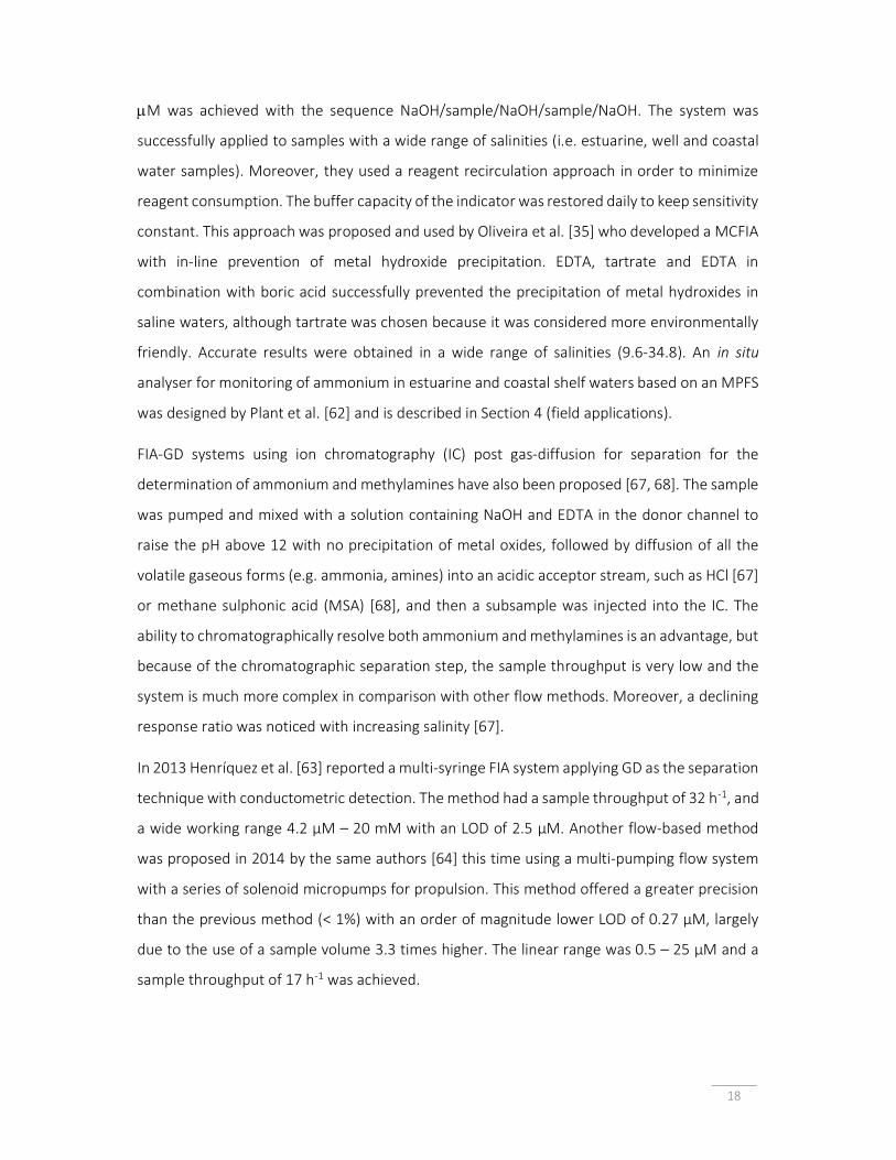
18

M was achieved with the sequence NaOH/sample/NaOH/sample/NaOH. The system was

successfully applied to samples with a wide range of salinities (i.e. estuarine, well and coastal

water samples). Moreover, they used a reagent recirculation approach in order to minimize

reagent consumption. The buffer capacity of the indicator was restored daily to keep sensitivity

constant. This approach was proposed and used by Oliveira et al. [35] who developed a MCFIA

with in-line prevention of metal hydroxide precipitation. EDTA, tartrate and EDTA in

combination with boric acid successfully prevented the precipitation of metal hydroxides in

saline waters, although tartrate was chosen because it was considered more environmentally

friendly. Accurate results were obtained in a wide range of salinities (9.6-34.8). An in situ

analyser for monitoring of ammonium in estuarine and coastal shelf waters based on an MPFS

was designed by Plant et al. [62] and is described in Section 4 (field applications).

FIA-GD systems using ion chromatography (IC) post gas-diffusion for separation for the

determination of ammonium and methylamines have also been proposed [67, 68]. The sample

was pumped and mixed with a solution containing NaOH and EDTA in the donor channel to

raise the pH above 12 with no precipitation of metal oxides, followed by diffusion of all the

volatile gaseous forms (e.g. ammonia, amines) into an acidic acceptor stream, such as HCl [67]

or methane sulphonic acid (MSA) [68], and then a subsample was injected into the IC. The

ability to chromatographically resolve both ammonium and methylamines is an advantage, but

because of the chromatographic separation step, the sample throughput is very low and the

system is much more complex in comparison with other flow methods. Moreover, a declining

response ratio was noticed with increasing salinity [67].

In 2013 Henríquez et al. [63] reported a multi-syringe FIA system applying GD as the separation

technique with conductometric detection. The method had a sample throughput of 32 h-1, and

a wide working range 4.2 µM – 20 mM with an LOD of 2.5 µM. Another flow-based method

was proposed in 2014 by the same authors [64] this time using a multi-pumping flow system

with a series of solenoid micropumps for propulsion. This method offered a greater precision

than the previous method (< 1%) with an order of magnitude lower LOD of 0.27 µM, largely

due to the use of a sample volume 3.3 times higher. The linear range was 0.5 – 25 µM and a

sample throughput of 17 h-1 was achieved.

19

Several methods have recently been reported involving the use of a variety of matrix

separation and preconcentration techniques: steam distillation, purge-and-trap (P&T), and

headspace single-drop microextraction (H-SDME). These techniques are used as sample pre-

treatment steps and are described below. While the LODs reported are mostly higher when

compared to the earlier GD-based separation methods, their advantage is that they don’t

suffer from membrane longevity issues or blocking by the precipitation of divalent cations

present in the sample, and therefore the use of complexing agents is not necessary.

P&T has commonly been applied as a separation technique for volatile organic compounds in

wastewater and other complex matrices. It has been successfully applied to ammonia

separation and preconcentration in seawater, and the process involves bubbling an inert gas

through a sample of seawater that has been made basic by the addition of sodium hydroxide

to convert total ammonia to molecular ammonia. Dissolved ammonia then moves from the

aqueous to the vapour phase and is collected by a trap [72]. Compared to the GD separation

method, P&T can process very large sample volumes increasing the enrichment factor and in

turn facilitating improved method sensitivity. Ferreira et al. [73] developed a steam distillation

separation technique coupled with an IC detection method which was capable of resolving

monomethyl- and monoethylamine from total ammonia without interference from sodium

and potassium ions. The LOD for this method was 1.7 µM with a linear range of 13.9 – 55.6

µM, a sample throughput of less than 4 h-1, and the method was successfully applied to high

salinity samples from the Brazilian oil industry with spiked recoveries in the order of 90 – 105%.

Ferreira et al. [74] further described a P&T extraction system using ultrasonication to

accelerate the extraction process, again using IC as the detection method. The sample

throughput described by Ferreira et al. was, however, very low (i.e., < 2 h-1). The LOD was 1.1

µM with a linear range of 13.9 – 111.1 µM and an optimum extraction time of 30 minutes per

sample was chosen. Zhu et al. [69] proposed a more sensitive method by coupling a home-

made P&T system with fluorescence spectrometry using the OPA-sulphite chemistry which is

described in Section 1.3.3 Fluorometric method.

Šrámková et al. [65] developed a novel system for the separation and preconcentration of

ammonia using in-syringe analysis and H-SDME with colorimetric detection. Drop formation

was accurately controlled by a syringe pump. The drop reagent was pumped through a channel

drilled into the syringe piston, and the drop was formed at the end that channel. The syringe

20

barrel was filled with the sample, which was made basic while stirring a magnetic stirring bar,

allowing for total ammonia to be converted to molecular ammonia. Ammonia then evaporated

into the syringe headspace reacting with the droplet containing an acid-base indicator, and on-

drop spectrophotometric analysis was performed. An LOD of 1.8 µM was reported with

method linearity of up to 25 µM. Washing the syringe between each sample took a

considerable amount of time and a sample throughput of 17 h-1 was reported.

1.3.3 Fluorometric method

The fluorometric method involves the reaction of ammonium with orthophtaldialdehyde (OPA)

in alkaline medium and in the presence of a strong reducing agent (e.g. 2-mercaptoethanol or

sodium sulphite) [55]. An intensely fluorescent product is formed which allows the

fluorometric assay to reach the nanomolar range [26]. However, the method can be used to

measure either ammonium or amino acids [75]. Therefore, if ammonium determination is the

main goal, some strategies must be adopted to avoid the interference by primary amines thus

improving the selectivity of the method (described further in this section). Table 1-3

summarizes the analytical features of flow-based methods using the fluorometric method.

Table 1-3. Analytical features of flow-based methodologies using fluorometric detection.

Analytical method

Reagents Flow method

LOD (nM) Concentration range (µM)

Sampling rate (h-1)

Type of sample Ref.

Fluo

rimet

ry

OPA-2-Mercaptoethanol

FIA-GD ~ 1 > 2 30 Fresh and seawater [55]

FIA-GD ~ 1 Not quoted 18 Seawater* [76] OPA-sulphite SFA 1.5/7a Up to 0.16/12a 20/40 Estuarine and

seawaters [54]

FIA-GD 7 Up to 4 30 Seawater* [26] FIA 30 Up to 50 9b/40 Coastal, estuarine

and fresh waters [77]

FIA 1.1 Up to 0.6 8/3600c Seawater* [27] FIA < 5 Up to 25 12 Seawater* [78] SIA 1000 Up to 20 120 River and marine

waters* [79]

SIA 60 Up to 20 > 100 River and marine waters*

[80]

MPFS 13/210 Up to 1/16 32 Surface seawater [81] ABA 1/4.6/58 Up to 1/4/25 8 Coastal seawater* [82] ABA 10 0.05 – 10 4 Marine waters* [83] Flow-

batch < 1.2 Up to 0.3 5 Open ocean water* [84]

FIA 2.1 Up to 0.3 36 Estuarine and seawater*

[85]

a On-line dilution; b Stop-flow mode; c rFIA mode. * Field application

21

Jones [55] developed an FIA-GD system using fluorescence detection with OPA with 2-

mercaptoethanol as the reducing agent. The GD step reduced interferences from primary

amines and dissolved amino acids, but nevertheless was subject to likely interference from

volatile amines. A similar version of a fluorescent-based FIA-GD system was used by Masserini

and Fanning [76] in a sensor package for the simultaneous determination of nitrite, nitrate and

ammonium in seawater.

Use of sodium sulphite as the reductant instead of 2-mercaptoethanol, reduces the sensitivity

to amino acids, thus making the method more specific to ammonium [86]. Watson et al. [26]

developed an FIA-GD system for seagoing applications that aimed to combine the advantages

of Jones’s GD method [55] with the OPA-sulphite approach. A GD cell, placed between the

NaOH reservoir and the peristaltic pump, was used to remove ammonia contamination from

the NaOH reagent (using 10% H2SO4 as a trap). Consequently, lower blank concentrations were

obtained, thus improving the LOD. A comparison between 35 g L-1 NaCl standards and

standards made in seawater showed similar results in the absence of chelating agents. Since

the reaction of ammonium with OPA and sulphite is more selective to ammonium than to

primary amines, the GD unit becomes unnecessary, as shown by Kérouel and Aminot [54]. They

developed an SFA system for the direct analysis of ammonium in estuarine and seawaters,

which was not only free from primary amine interferences (including volatile amines) but also

from a salt effect (less than 3.1% deviation in the salinity range of 0.2 to 35). Three ammonium

concentration ranges were attained: nanomolar range (up to 100 nM), micromolar range (up

to 12 µM) and submillimolar range (up to 250 µM), the last one was attained by adding on-line

dilution to the SFA system. This method was adapted to FIA by Aminot et al. [77], for a potential

in situ application. No salt effect was noticed in the salinity range of 5-35. No other

interferences were observed, except for sulfide (deviation of -9% at 100 µM S2-). Using the

same chemistry, Horstkotte et al. [81] designed a portable multipumping flow analyser system

for possible shipboard monitoring. The method sensitivity was adjustable by the gain of the

photomultiplier tube, thus allowing for applications across a wide range of concentrations (up

to 16 µM). A detection cell was specially made and combined with a commercial

photomultiplier tube, a long-pass optical filter and a UV-LED as the excitation light source.

When using the fluorometric method for the determination of ammonium in aquatic matrices,

background fluorescence is frequently reported. This fluorescence results from substances in

22

the sample that autofluoresce, thus this effect can be corrected by measuring the sample

fluorescence in the absence of OPA. A GD unit could also be used to avoid this issue,

nevertheless a salt effect might be noticeable due to change in the ammonia solubility [55].

The fluorometric method involving the reaction of ammonium with OPA in the presence of

sulphite reducing agent is attractive largely due to its high sensitivity and selectivity, allowing

for nanomolar concentrations of ammonia nitrogen to be determined in complex high-salinity

matrices. While the stability of reagent solutions has been identified as a disadvantage of the

method, the addition of stabilising reagents such as formaldehyde to prevent oxidation of

sulphite have shown promise in extending the lifetime of reagents and applicability to in situ

shipboard analysis.

Hu et al. [75] developed a manual operation method using OPA, sulphite and formaldehyde

reagents with EDTA-NaOH used to make the sample medium alkaline. EDTA was used to

prevent precipitation of divalent alkaline earth metals from solution at high pH, which could

interfere and depress the fluorescence signal. At high pH the amount of reaction product was

increased thus enhancing the method sensitivity to nanomolar levels without enrichment. The

working range of the method could be tailored to the desired range by changing the

excitation/emission slit used, and an LOD of 9.9 nM was reported and linearity in the range of

32 – 500 nM was achieved when using an excitation/emission slit of 3 nm/5 nm, respectively.

While the sampling rate reported was low (1.2 h-1), the authors stated that it was possible to

perform up to 10 samples simultaneously. Nevertheless, given many automated techniques

using fluorescence have been described in the literature, manual methods seem only to

provide interesting insights to reaction kinetics of novel reagent and chemical combinations.

Zhu et al. [85] used the same chemistry as described by Hu et al. [75] with the only difference

being the choice of chelating agent (sodium tetraborate buffer instead of EDTA). Zhu et al.

described the development of a portable home-made fluorescence detector comprising a UV-

LED, two band pass filters, a photomultiplier tube (PMT), a modified flow-cell to reduce the

interference of air bubbles in the fluorescence signal, and an electronic circuit with a constant

voltage and current supply. The detector described was smaller than its commercially available

PMT-FL counterpart with an increase in sensitivity greater than 11%. The detector was

incorporated into an FIA system using OPA, sulphite and formaldehyde as reagents and the

system was used for underway sampling in the Jiulongjiang estuary.

23

While the OPA-sulphite reaction is the most widely reported fluorescence method for

ammonium determination in natural waters, functionalisation of OPA with the electron-

donating methoxy groups to form 4-methoxypthaldealdehyde (MOPA) and 4,5-

dimethoxypthaldealdehyde (M2OPA) has been recently described showing promise to increase

method sensitivity as the reaction products exhibit higher fluorescence intensity when

compared to the ammonium-OPA product [50, 51]. MOPA was successfully synthesised by

Liang et al. [50] and used in a manual batch method using sulphite, formaldehyde and sodium

tetraborate buffer. The MOPA rapidly reacted with ammonium at room temperature and a 15-

minute reaction time was selected as a compromise between sample throughput and

sensitivity. An LOD of 5.8 nM was reported for the linear calibration range of 25 – 300 nM. The

synthesis and use of M2OPA in a custom-made hand-held portable fluorometer with a laser

diode as the light source was reported by Zhang et al. [51] allowing for in situ analysis. M2OPA

was reported to have a rapid reaction time and enhanced fluorescence intensity when

compared to the OPA and MOPA reaction products, and the hand-help portable laser diode

fluorometer was reportedly used in single- or dual-laser beam modes, allowing for different

working ranges to be achieved (0 – 5 µM and 0 – 2 µM, respectively) with different LODs (6.5

nM and 3.5 nM, respectively). While the newly developed device was suitable for field use, it

was nevertheless still used in ‘batch mode’ where a sampling rate of 1 h-1 was described.

The major limitation of the fluorescence methods described above, is the slow reaction

kinetics, which can be improved by increasing reaction temperature. However, the need for an

energy intensive heating device incorporated into the manifold, limits the use and application

of fluorescence methods in long-term monitoring and field based applications. Nevertheless,

a few shipboard FIA [26, 27, 76, 78], SIA [79, 80] and autonomous batch analysers (ABA) [82,

83] systems have been described for field applications using the fluorometric reaction NH4+-

OPA with sulphite reduction, and these are described in the following section.

1.3.4 Field applications

In situ monitoring has the potential to reduce or even avoid all the problems commonly

encountered during manual collection, storage and preservation of samples of estuarine or

marine waters. In the last decade there has been substantial progress in the development of

24

portable and miniaturised flow analysis devices which has allowed for shipboard laboratories

to conduct real-time monitoring and mapping of nutrient distributions [27, 76, 79].

The fluorometric method with the OPA-sulphite reaction has been employed as the preferred

method for in situ field analysis of ammonium, with one exception where the GD method with

conductimetric detection was used [62]. This particular in situ flow analyser (called NH4+-

Digiscan) used micro-solenoid pumps to promote the flow. For in situ application all the

electronic components were placed in housings and reagents in bags. The system was shown

to be suitable for fixed location monitoring of ammonium in estuarine and coastal shelf

environments at depths of up to 3 m. It was capable of performing in situ auto-calibration and

exhibited stability when deployed for 30 days, without the loss of drift or analytical signal. An

adequate LOD was achieved (Table 1-2), although the rate of analysis was relatively low (< 9 h-

1) when compared with other flow systems.

Several FIA systems have been developed and used in shipboard laboratories [26, 27, 76, 78] .

Masserini and Fanning [76] developed a sensor package capable of simultaneous fluorometric

detection of nitrite, nitrate and ammonium in oligotrophic seawater. Jones’s technique [55]

was used to determine ammonium, although slightly modified in order to adapt it to the

nutrient sensor package. Discrete sections of tubing were carried through a heat exchanger as

opposed to heating the entire manifold, and a larger flow-cell was used in the fluorescence

detector (i.e. 40 µL instead of 12 µL) allowing for an LOD of approximately 1 nM to be achieved

with a throughput of 18 samples per hour. Watson et al. [26] combined the OPA-sulphite

chemistry with GD for the determination of ammonium. Samples were collected manually and

immediately analysed or stored frozen. To avoid atmospheric contamination, a 150 L glove box

flushed with N2 was used for storing reagents and handling samples. Removal of ammonia

contamination from reagents required the use of an in-line diffusion cell placed between the

reagent reservoir and the peristaltic pump, using H2SO4 to remove the ammonia from the

reagent stream.

Amornthammarong et al. [27] proposed an FIA analyser for the measurement of wastewater

discharges into Florida coastal waters, incorporating a modified OPA-sulphite reaction, in

which sodium sulphite was dissolved in 5 mM formaldehyde solution. They suggested that the

precipitates did not form at high pH due to the high concentration of sulphite, dilution of

seawater by reagents, and kinetic hindrance. A sample throughput of 8 h-1 was achieved when

25

manual injection was performed, but for high-resolution analysis, rFIA was used, which

increased the sample throughput to an incredible 1 s-1 (i.e. 3600 h-1). Such high frequency

measurements allowed for the modelling of an ammonium outfall plume and its dispersion by

ocean currents. Rapid changes in ammonium concentrations were detected in only 2 h, clearly

demonstrating the importance of high-frequency analysis.

The ammonium flow analyser described by Abi Kaed Bey et al. [78] was designed to determine

ammonium in oligotrophic seawater. The instrument was designed “in-house” and allowed for

the automated switching between reagent, sample and standard streams, which were

sequentially pumped into the analyser mixing chamber. The mixed solution was then pumped

to the heater and the detection unit, which included the following: a quartz flow-cell; a low-

power UV-LED excitation source; a photon multiplier tube as the emission detector; and, two

optical filters. The system described suffered from up to 85% reductions in signal at low

concentration (5 nM) due to salinity variations, and the potential fluorescence interference

from phytoplankton was found to be up to 12% by artificial simulation of a bloom. Interference

from commonly encountered amines and amino acids at low concentrations were negligible,

however at high concentrations the signal was depressed. The analyser was used for field

analysis in the North Atlantic Ocean, and seawater was pumped from 5 m below to the bow of

the ship towards the analyser.

Frank et al. [79, 80] developed an SIA system for the determination of both phosphate and

ammonium as part of a “ferrybox” system that operated autonomously and continuously at

sea in commercial ferry vessels. The “ferrybox” consisted of an automated sampling system.

Samples were thus collected automatically and on-line, through a system comprising a

centrifugal pump constantly directing sample from the hull of the ship to the “ferrybox”, which

is connected with the SIA instrument. The flow rate of the sample was maintained high enough

to ensure sample freshness, with the excess sample being diverted to waste. The sample

stream was pumped via a peristaltic pump to the SIA system, where further samples were

drawn from the continuously supplied filtrate stream. Off-line samples were simultaneously

taken and analysed by an SFA system in order to validate the on-line system. However, the

correlation between the ammonium results of the two methods was described as only

“acceptable” [79]. This was due to the on-line results being contaminated by the destruction

of plankton cells in the secondary centrifugal pump of the “ferrybox”, resulting in the release

26

of cell contents into the on-line sample stream. The off-line results were also affected by

contamination, inappropriate sample storage and detector noise. Additional data analysis was

outlined in a further paper, in order to verify the performance of the system [80].

More recently, Amornthammarong et al. proposed the design and use of a portable ABA for

the determination of trace amounts of ammonium in coastal seawater [82, 83]. The ABA

described utilizes a carefully designed mixing chamber, comprising one syringe pump (where

the syringe acts as the primary mixing chamber), an eight-way distribution valve and a 5 mL

pipette tip (which acts as the secondary mixing chamber). The standards and sample were

mixed with the reagent in the syringe chamber, and the mixture was then pumped into the top

of the pipette and drawn back into the syringe chamber from the pipette tip. Complete mixing

occurred after 5 mixing cycles and the solution was then injected to the fluorescence detector.

The syringe chamber, pipette tip and detector were flushed with deionized water three times

prior to every subsequent measurement, which resulted in a sample frequency of

approximately 8 h-1.

In an improved version of the ABA, the commercial fluorescence detector [82] was replaced

by an LED photodiode-based fluorescence detector, which was more sensitive and allowed for

the assembly of a smaller apparatus [83]. This ABA system was also equipped with a filtering

system allowing for measurements to be conducted in turbid waters. It was deployed at two

field sites for measurement of ammonium concentrations in the intracoastal waterways of

Florida, and diurnal ammonium concentration cycles were recorded. The advantages of such

batch analysers include their low reagent consumption and ability to construct a calibration

curve by auto-dilution from a single standard solution. However, one of the major drawbacks

of batch analysers is their lower sampling frequency, due to the need for thorough washing of

the mixing chamber to prevent sample cross contamination.

For the determination of ultra-trace (< 1 nM) ammonium in seawater, Zhu et al. [84] used a

flow-batch system accommodating a HLB cartridge to perform SPE. The OPA method as

described by Amornthammarong et al. [83] was used, and the fluorescence reaction product

was extracted onto the SPE cartridge, separating the analyte complex from the seawater

matrix. The fluorescent products were eluted with ethanol and delivered to the fluorescence

detector, and each cartridge could be used for over 50 seawater sample analyses. The benefits

of employing SPE with the fluorescence method as described include improved sensitivity,

27

reduced reagent consumption and negligible salinity and matrix effects. This method was

applied in the field in the South China Sea during a cruise in August 2012, and vertical

ammonium profiles were determined as well as the distribution of ammonium in surface

seawater.

The stability of reagents might not be an issue when working under laboratory conditions,

however for analysis in the field, (e.g. in shipboard laboratories), it should be taken into

consideration as it could be a limitation. Table 1-4 presents the stability of the main reagents

involved in each of the methods described.

Table 1-4. Stability and storage of reagents involved in the determination of ammonium.

Method Reagents Stability and storage Ref. Indophenol blue Spectrophotometry

Phenol Prepared fresh daily [29] Salicylate Prepared fresh daily [45] 1-Naphthol Not listed [46] Sodium nitroprusside 0.5% Store in an amber bottle for up to 1 month [87] Sodium hypochlorite Unstable, prolonged storage should be avoided [87]

Gas-diffusion Bromothymol Blue* Stored in gas-tight containers with CO2 traps [35] Phenol red* Stored in a bottle with an Ascarite guard to avoid

CO2 uptake [60]

Methane sulfonic acid 40 mM† Prepared routinely via a stock solution [77] Fluorimetry 2-Mercaptoethanol Stable for at least 72 h [78] Sodium sulphite 8 g L-1 Stable for at least 2 months at room temp. in a

glass bottle [81]

Sulphite in phosphate buffer Prepared daily [80] OPA 10 mM (no buffer) Stored refrigerated for 1 week [80] OPA 40 g L-1 (no buffer) Stored refrigerated in a glass bottle for at least 2

months [81]

OPA 0.37 M + sulphite (buffered) Stored for several weeks in the dark at room temp. [26] Mixed Reagent (OPA, sulphite,

buffer, wetting agent) Stored in the dark at room temp. for at least 2 months

[81]

MOPA 7.8 g L-1 in MeOH and water + sulphite + formaldehyde

Prepared fresh daily [50]

M2OPA 1.8 g L-1 in MeOH and water + sulphite + formaldehyde

Prepared fresh daily [51]

* Spectrophotometric detec on, † Ion chromatography

Flow-methodologies have the capability to provide high frequency data and pollutant

concentration profiles, which is important when monitoring ammonium concentrations in

highly variable estuarine and marine environments, with the added benefit of sample

collection and pre-treatment steps being automated. However, many flow methods require

the use of specialised and sometimes expensive or custom-made equipment and are often not

28

commercially available off-the-shelf instruments. Therefore, deploying flow systems over large

spatiotemporal scales relevant for extensive water quality monitoring may be prohibitively

laborious and expensive, especially as most equipment requires an energy source to control

mechanical parts. Passive sampling could be used as an alternative in situ monitoring strategy,

as it provides the average concentration of the target chemical species for the period that the

sampler was deployed without the need for power, moving parts or complicated electronics.

In comparison with flow-based methodologies, passive sampling is a cheaper and simpler

water quality monitoring technique, which can be advantageous in allowing for sampling

programs to be developed over large spatial and temporal scales. An overview of the passive

sampling techniques reported in the literature for the monitoring of aquatic environments with

high or variable salinity is provided in the following section.

1.4 Passive sampling Most water quality monitoring programs involve the collection of periodic discrete grab or spot

samples. Spot samples should be collected in a way that ensures they are representative of the

medium being sampled, and when undertaking trace analysis, it may be necessary for very

large volumes of sample to be collected [88, 89]. After collection, spot samples are transported

to a laboratory for analysis, during which time they often need to be preserved [24]. The

analytical procedure may involve some type of sample pre-treatment, including sample

filtration, analyte preconcentration and separation from the matrix and/or derivatisation prior

to analysis [24]. These sample handling steps are commonly laborious and expensive.

Moreover, it is possible that during sample collection, transport or during any manual handling,

contamination may occur leading to inaccurate results [24]. Additionally, periodic spot

sampling only provides a snapshot of the levels of pollutants in the sampled medium at the

time of collection, and episodic pollution events may be missed leading to an under

representation of pollution concentrations in the environment (Figure 1-5) [89, 90]. Even

though flow-based methodologies can be used to automate the overall analytical process, such

systems are rarely used in commercial laboratories or in routine field monitoring applications,

largely owing to the significant upfront costs of purchasing a system, the complexity and high

degree of operator skill required for successful operation and maintenance, and high energy

29

consumption which may prohibit long-term deployment of the equipment in the field.

Automatic water sampling units (autosamplers) are commonly used in routine water quality

monitoring programs and can be programmed to collect composite or discrete samples over

time, which can then be analysed in a laboratory [91]. While an autosampler allows for high-

frequency spot sampling which increases the likelihood of pollution event detection,

autosamplers have the disadvantage of being expensive, having significant energy

requirements for long-term deployment, still suffer from the need for significant sample

handling and manipulation, and can be difficult to deploy in coastal settings where sampling

often requires the use of a boat (Figure 1-5).

Figure 1-5. Results obtained by different sampling methods commonly used in environmental monitoring (data discussed in detail in Section 4.3.2 of Chapter 4).

Significant progress has been made over the past few decades in the field of aquatic passive

sampling techniques, which essentially overcomes several challenges of spot sampling-based

monitoring programs and the difficulties associated with the deployment of flow-based

systems for in situ analysis, especially with respect to associated costs, both in terms of energy

requirements and labour [91].

Passive sampling techniques have gained popularity over the last three decades and

considerable work has been undertaken to improve and standardise passive sampling

30

methodologies in order to enable their incorporation into regulatory water quality monitoring

programs globally [92-97].

The ideal passive sampling device (PSD) should be inexpensive, commercially available, and

simple to assemble, prepare, deploy, retrieve and analyse, while being precise, accurate,

sensitive and selective towards the analyte(s) of interest [88, 92]. Aquatic passive sampling has

been defined as any sampling technique involving the free flow and accumulation of analyte

molecules from the sampled medium (sampling source solution) to the PSDs collecting medium

(receiving phase), with mass transfer driven by a difference in the chemical potential of the

analyte molecules between the sample and collecting mediums [98].

A PSD generally consists of a receiving phase which is separated from the external environment

being sampled by a semi-permeable membrane and/or a diffusion-limiting barrier. The uptake

and accumulation of the target analyte(s) from the bulk matrix being sampled into the receiving

phase occurs via processes of diffusion, permeation or chemically facilitated transport of the

analyte through the membrane/barrier to the receiving phase, although in some applications

(e.g., single-phase passive samplers) the membrane itself can act as the primary accumulation

site for the analyte [99].

The process of passive sampling usually involves deployment of a PSD into the aquatic

environment being monitored and subsequent collection of the sampler after a given period

of time, after which the receiving phase can either be directly analysed or the analyte can be

chemically stripped and processed.

PSDs are commonly categorised by their sampling regime with two types of samplers described

in the literature, including the equilibrium-based and the integrative or kinetic passive

samplers. Equilibrium passive sampling involves exposing the PSD to the aquatic environment

to be sampled for a sufficient amount of time to reach a thermodynamic equilibrium, allowing

for a stable concentration of analyte(s) between the sampled medium and the PSDs receiving

phase to be achieved [89, 100, 101]. Mayer et al. provided an in-depth review of the principles

and operation of equilibrium-based PSDs, highlighting three basic requirements for their

successful operation, including ensuring that the capacity of the sampler is not overcome,

avoiding saturation during analyte uptake, and making sure that the device response time is

shorter than any fluctuations in analyte concentrations experienced in the environment being

31

sampled [100]. When using equilibrium-based PSDs the concentration of analyte(s) measured

in the receiving phase will be similar to that measured using spot sampling, however there are

advantages to using this sampling approach over conventional sampling methods, especially

when measuring the partitioning and fugacity of analyte(s) in multicompartment systems such

as sediments, pore waters and/or their overlying waters [100].

While some PSDs can be used in both equilibrium and integrative accumulation regimes

(depending on the analyte class and sampler type), many of the samplers discussed below are

used exclusively in the integrative (linear) uptake mode. Integrative or kinetic passive samplers

work on the assumption that the rate of mass transfer of analyte from the bulk sample to the

receiving phase is linearly proportional to the difference between the activity of the analyte in

the water and receiving phase [89]. An integrative PSD should exhibit ‘zero sink’ behaviour,

where analyte species are effectively accumulated, and trapped species are retained even if

their concentration around the sampler decreases to zero [98]. However, whilst some PSDs

exhibit this behaviour, it is not always the case, and modelling approaches and corrections have

been developed to describe mass accumulation in the PSD and to offset deviations from ideal

behaviour [101].

During deployment, the analyte(s) of interest are passively accumulated from the aquatic

environment to the receiving phase where they can be selectively pre-concentrated, allowing

for the time-weighted average concentration (CTWA) to be determined for the duration of

deployment (Figure 1-5). The CTWA is representative of the concentration of analyte(s) in the

sampled medium for the duration of deployment, thus allowing for transient pollution events

to be captured where they could be missed with infrequent spot sampling programs. The

integrative uptake phase can be described by Equation (1-1) below [89]:

CTWA = Ms /Rs(t) (1-1)

where the term Ms refers to the mass of analyte accumulated in the receiving phase of the PSD

after a given exposure time (t), Rs is the sampling rate, and CTWA is the time-weighted average

concentration of analyte in the sampled medium over the period of PSD deployment [89]. The

Rs is dependent on the first-order rate constant for the accumulation of the analyte from the

sampled medium to the receiving phase [89], and is commonly measured in laboratory-based

calibration experiments for each analyte of interest [102]. The Rs can be affected by water

32

temperature, hydrodynamic conditions around the sampler, degree of biofouling and on the

diffusional surface area of the PSD [102]. The CTWA can be determined for the duration of the

PSD exposure (t), when a) the Rs is known, and b) by quantifying the amount of analyte

accumulated in the receiving phase post deployment (Ms) [89].

Environmental conditions have been reported to affect the diffusion of analytes across the

semi-permeable barrier, thus affecting accumulation in the PSD receiving phase. For example,

the effect of temperature on passive sampling results has been studied and shown to affect

the sampling rate and the sampler-water partition coefficient [88, 103-105]. Water flow

velocity and turbulence has also been shown to affect the mass transfer of analyte when

uptake is controlled by diffusion through the water boundary layer [88]. In addition to

temperature and turbulence or flow pattern of water around the device, there are several

other environmental factors that can affect the performance of a PSD, namely salinity, pH,

dissolved organic matter (DOM) and biofouling of the device. [89, 96, 106-109].

Biofouling is known to limit the deployment lifetime of scientific instruments especially when

immersed in nutrient rich and productive aquatic environments [110, 111]. Biofouling occurs

when exposed surfaces are colonised by periphytic microorganisms forming a biofilm, allowing

further attachment of macroorganisms such as macrofauna [112]. The presence of a biofilm

on the surface of passive sampling membranes and/or exposed receiving phases will increase

the tortuous pathway of the diffusing analyte(s) from the bulk sample phase to the receiving

phase, reducing the overall accumulation efficiency of the PSD [99].

The effect of biofouling on the performance of various passive sampling tools is well

documented in the literature [89, 113-116]. Richardson et al. [117] found that the uptake of a

range of organic contaminants was reduced in a semi-permeable membrane device (SPMD) by

up to 50% under fouling conditions, and Huckins et al. [118] similarly observed that in severe

cases the uptake of polyaromatic hydrocarbons (PAHs) was reduced by 20 – 70%.

Strategies to reduce microalgal colonisation of the SPMD, including mounting the device in

between copper mesh screens [119], and the addition of the antifouling agents Irgarol and

capsaicin to the receiving phase, were shown to be largely ineffective in mitigating the effects

of biofilm formation on the surface of the SPMD studied [116]. Performance reference

compounds having similar chemical properties to the analyte(s) under investigation, were used

33

to correct the sampling rate, by dissipating at a similar rate to the assimilation of analyte(s)

into the passive sampler [106, 116]. The effects of biofouling, temperature and water

turbulence could be corrected for using the PRCs, however, this approach is limited to isotropic

exchange in hydrophobic passive sampling, and it is not suitable for sorption-based PSDs [107].

Whilst many researchers have documented the effects of biofouling on the performance of

PSDs, different approaches to reducing or quantifying the effects have been shown to be

effective, with no universally applicable strategy. Schäfer et al. observed that fouling did not

occur in their 1-day pulse contamination experiments using a Chemcatcher® when a

polyethersulfone diffusion-limiting membrane was used compared the configuration without

the membrane which exhibited fouling and a four-fold reduction in analyte uptake [120].

Harman et al. observed that fouling between both SPMD and POCIS samplers varied when

immersed in the same media, with markedly different effects in performance, where a SPMD

exhibited a reduction in analyte uptake due to fouling, whereas a POCIS saw a significant

increase in the uptake of alkylated phenols [121]. When sampling for metals [122, 123] and

orthophosphate [124], the performance of a diffusive gradients in thin films (DGT) passive

sampler was also reportedly impacted by the presence of biofilm, which blocked the pores of

the device and changed the way analyte molecules were able to move through the diffusive

gel layer. Uher et al. [125] found that the addition of a polycarbonate protective membrane

minimised the effect of biofouling on some target metals, but adversely affected others. DGTs

treated with silver nanoparticles were shown to inhibit the growth of biofilms without affecting

the performance of a device for mercury determination [123], and antifouling efficacy of the

antibiotic chloramphenicol and two metal iodides (copper and silver) was tested for a DGT

technique for monitoring reactive phosphorus [126]. The silver iodide provided the longest

protection (21 days), followed by the copper iodide (14 days), however, the antibiotic

chloramphenicol did not appear to be effective in preventing the colonisation of

microorganisms on the device for any of the deployment times tested.

Over the last two decades, several reviews have described and assessed a variety of passive

sampling techniques applied to water quality monitoring in aquatic environments for a range

of chemical species including organics, inorganics and heavy metals [89, 98, 127-132], with a

particular emphasis on the monitoring of polar [104, 109, 133-135], and non-polar pollutants

of concern [88, 96, 136]. While many reviews have focussed on the development and

34

application of passive sampling techniques for low salinity freshwater matrices, Mills et al.

[137] and Schintu et al. [102] provide comprehensive book chapters evaluating passive

sampling technologies commonly applied for water quality monitoring specifically in coastal

and marine environments.

Two passive sampling devices have been developed and applied for the monitoring of

ammonium in freshwaters including DGTs comprising a protective filter membrane, a diffusive

gel layer and various sorbent receiving phases [138-142], and the polymer inclusion membrane

based passive sampler using a membrane bound ionic liquid to facilitate transport and

accumulation across the membrane using ion exchange processes [143]. However, both

methods suffer from interference from competing alkali (Na+ and K+) and alkaline earth (Ca2+,

Mg2+ and Sr2+) metal cations in solution, which in estuarine and seawaters are several orders

of magnitude higher in concentration, leaving these PSDs ineffective for use in saline matrices.

A summary of the PSDs developed and applied for water quality monitoring in marine

environments will be outlined in the following section, highlighting their construction,

operation, application to water quality monitoring and their respective advantages and

limitations. Moreover, an outline of the steps that were taken to study or mitigate the effect

of the environmental variables above mentioned, in addition to a description of the calibration

procedures applied to ensure appropriate quality control, will also be provided.

1.4.1 Semipermeable membrane devices (SPMDs)

SPMDs were first reported in 1990 by Huckins et al. [144], and are one of the most widely

studied passive samplers, commonly used to monitor the concentration, occurrence,

transport, fate and bioavailability of semi-volatile, non-polar, persistent organic pollutants in

aquatic environments and air [88, 145-147]. The hydrophilicity/hydrophobicity of nonionic

compounds can be described by the octanol-water partition coefficient (log Kow) which is a

measure of a compound’s partition between the lipophilic octanol and the hydrophilic water

phase [148]. The more positive the value of log Kow, the more hydrophobic the compound,

whereas hydrophilic compounds tend to exhibit low or even negative log Kow values. SPMDs

are suitable for hydrophobic compounds with log Kow values ≥ 3 [147].

35

The most widely used SPMD comprises a 91.4 cm long by 2.5 cm wide sealed, transparent low-

density polyethylene (LDPE) tube, commonly filled with 1 mL of a high purity, high molecular

weight lipid such as triolein as the receiving phase (Figure 1-6A) [144]. The LDPE is an

amorphous non-porous plastic, containing transient cavities up to 10 Å in size [89, 145, 146],

allowing for small hydrophobic molecules to be absorbed by the polymer and excluding larger

molecules or those adsorbed to suspended colloids, particulates or humic acids [89]. Triolein

is the most common receiving phase used in SPMDs, primarily due to similarities between the

octanol-water and triolein-water partition coefficients for a number of important hydrophobic

organic compounds (HOCs) [89, 146], its low permeability in LDPE membranes [147], and as it

is a major storage lipid found in a wide range of aquatic organisms thus allowing for PSDs to

mimic uptake rates in the fatty tissue of marine invertebrates [145, 147, 149].

To ensure consistent surface area exposure during deployment, the layflat tubes of the SPMD

are threaded between several spindles in a ‘spider carrier’ to prevent the tubes from self-

adhering, and to minimise contact between the SPMD and the deployment canister walls

(Figure 1-6B) [150]. The ‘spider carrier’ is mounted into a marine-grade stainless steel mesh

deployment canister (Figure 1-6B) designed to protect the SPMD from mechanical damage

during deployment, periods of which can range from one week to several months [151], or

even over a year in deep-ocean environments [152].

Figure 1-6. Schematic diagrams and typical deployment configuration of a SPMD filled with triolein receiving phase. (A) highlights the mechanism of analyte accumulation, and (B) showing the SPMD threaded onto the spindles of a ‘spider carrier’ and fitted into a commercially available cannister. Figure 1-6A is reproduced from ref. [146] with permission from Elsevier, and 1-6B is from ref. [151] with permission from the Office of Ocean Exploration and Research, National Oceanic and Atmospheric Administration.

36

A significant advancement in the development and application of SPMDs has been the use of

performance reference compounds (PRCs), which are spiked into the lipid receiving phase prior

to membrane enclosure, allowing for site-specific sampling rates to be determined and in situ

calibration to be performed [99, 106, 153, 154]. If isotropic exchange kinetics apply to the

uptake of analyte(s) and dissipation of PRCs then the respective uptake and dissipation rates

can be correlated [106, 153, 154]. PRCs should be analytically non-interfering compounds such

as isotopically labelled analogues of the analyte(s) under investigation (e.g., deuterium and/or 13C and 14C labelled), exhibit similar physicochemical properties to the analyte(s), and in the

case of surrogate compounds should not be present in the environment in quantities above

the limit of detection of the analytical method [99, 155]. Using PRCs, allows for exposure-

specific effects (flow/turbulence, biofouling and temperature) and compound-specific effects

(diffusion coefficients and sampler-water partition coefficients) to be compensated for during

deployment, thus allowing for in-field calibration to be performed [96, 106]. The use of PRCs

is commonplace with SPMDs having also been applied successfully to a small number of other

aquatic PSDs for measuring HOCs.

SPMDs have been widely adopted for monitoring HOCs in the aquatic environment, and are

well described in the literature with extensive studies outlining sampler performance and

application in the field, including for use in complex matrices such as estuarine [156, 157],

deep-ocean [152], tropical [158, 159], and cold polar environments [160, 161]. Concurrent

monitoring of atmospheric concentrations allows for mass-transfer of HOCs at the air-water

interface to be determined [162], and similarly the monitoring of pore waters and sediments

has allowed for quantification of sediment-water mass transfer to be studied [163-165]. The

SPMD with triolein lipid receiving phase was intended to be biomimetic, essentially acting as

an effective surrogate for HOC accumulation in animal tissue. However, studies where SPMDs

were deployed alongside trophically diverse biota have shown that substantial differences in

HOC accumulation ratios can occur [149, 166, 167], largely due to environmental factors

affecting the study organisms such as temperature, salinity, dissolved oxygen concentrations,

or due to physiological parameters such as foraging behaviours, reproductive status, exposure

to environmental stressors, metabolic activity and excretion of harmful substances [168].

Nevertheless, SPMDs provide a good tool for understanding the concentration of dissolved

37

HOCs (i.e., not bound to particulates or organic acids) in the aquatic environment, including in

marine waters.

In marine environments SPMDs have been used to assess environmental concentrations of

non-polar organochlorine pesticides [152, 167, 169-171], polyaromatic hydrocarbons (PAHs)

[166, 170, 172-174], dioxins and furans [175-177], polychlorinated biphenyls (PCBs) [170, 174],

polybrominated diphenyl ethers (PBDEs) [178], organotin [179, 180], and halogenated natural

products produced by algae, sponges and other marine organisms [158].

As many HOCs are commonly found in air, precautions must be taken to minimise vapour phase

contamination during deployment and transport, and strategies to minimise exposure to UV

radiation should be used to minimise the possibility of photodegradation of PRCs and/or

sequestered analytes which would lead to an underrepresentation in CTWA estimates [150,

181].

Besides the relatively high cost of triolein-based SPMDs compared to other commercially

available PSDs, one of the main limitations of this technique includes time-consuming and

labour-intensive sample handling steps required for the recovery of analytes from the triolein

receiving phase prior to analysis. These steps usually involve dialysis (requiring large amounts

of organic solvents), pre-concentration, solvent exchange, and complicated extract clean-up

prior to chromatographic separation [88, 146, 182]. In order to simplify the method, Leonard

et al. [183] replaced the triolein receiving phase with isooctane, and Zhao et al. [184] with the

ionic liquid (IL) 1-butyl-3-methylimidazolium hexafluorophosphate. The use of isooctane

inhibited periphytic growth and biofouling of the PSD and analysis of the receiving phase did

not require clean-up or back-extraction procedures. However, one of the main disadvantages

of the isooctane-based SPMD is the leaching of the solvent receiving phase to the surrounding

environment during deployment [183]. The benefit to using the IL as receiving phase was that

it was retained by the semipermeable LDPE membrane, and it has been described as an

environmentally friendly alternative to conventional organic solvents, able to be directly

analysed by high performance liquid chromatography (HPLC) without the need for dialysis or

clean-up procedures as required by the triolein-filled SPMD. However the IL-based SPMD

exhibited reduced sensitivity when compared to its triolein-SPMD counterpart [184].

38

Similar in principle to the triolein filled SPMD, Brumbaugh et al. [185] described the

development of a passive integrative mercury sampler for monitoring neutral Hg0 species in

air, synthetic fresh and seawater, comprising a lay-flat LDPE tube and a receiving phase of nitric

acid and gold chloride. This sampler was able to extract dissolved gaseous mercury species,

and Hg0 uptake rates were shown to be linear for a period of two weeks, with the sampling in

freshwater being more efficient than in seawater, likely due to a large fraction of aqueous

mercury present as the charged chloro-anion complex preventing it from permeating through

the transient cavities of the LDPE membrane [185]. This sampler was described as useful for

screening applications in environmental waters primarily due to its ‘proof of concept’ stage of

development, requiring further work to evaluate the usefulness of the sampler in water, in

particular its ability to differentiate between dissolved gaseous and other neutral Hg0 species.

Research was undertaken by Booij et al. to examine the uptake kinetics of the SPMD compared

to triolein-free SPMD to determine the effect of triolein on HOC partition, with results

highlighting that the LDPE membrane alone was only slightly less efficient at accumulating

HOCs than the triolein-filled SPMD [154]. This encouraged further research into the suitability

of membrane-water partitioning as a passive sampling method [186-188], giving rise to the

development of several monophasic polymer based PSDs, several of which are described in the

following section below (1.4.1.1 Single-phase passive samplers).

1.4.1.1 Single-phase passive samplers

Single-phase PSDs generally comprise a non-polar polymer membrane which acts as the

receiving phase allowing for absorption of the analyte(s) directly into the elastomer. The

polymer membrane of such samplers usually has a pre-determined thickness and surface area

to volume ratio, which can be tailored to the analytes(s) of interest, and can determine the

sampling regime of the PSD (equilibrium or kinetic) [189]. A wide variety of configurations have

been described in the literature, including strips or sheets [176, 190, 191], as well as thin-film

coatings on glass substrates such as capillaries [192], fibres [193] and beads [194].

Adams et al. [195] reported the first comprehensive study into the application of single-phase

polyethylene membranes as PSDs in 2007, and in the same year Rusina et al. [196] published

their investigating into the critical properties of 13 different single-phase polymer membranes

39

and their suitability for use as aquatic PSDs. In the last decade, single-phase PSDs have

increased in popularity for monitoring HOCs, largely due to the simplicity of their preparation,

ease of analyte stripping for analysis, and economical cost. However inconsistencies in polymer

formulation between different manufacturers and suppliers and a lack of commercial

availability of some single-phase PSDs may limit their widespread use and adoption as water

quality monitoring tools [88].

The majority of studies reported in the literature describing the use of single-phase polymers

as PSDs in marine environments have focussed on LDPE, silicone rubber also known as

polydimethylsiloxane (PDMS), polyoxymethylene (POM) and ethylene-vinyl acetate (EVA) [88].

A summary of each of these PSDs is provided in the following sections.

1.4.1.1.1 Low-density polyethylene (LDPE)

The first study investigating the potential use of low density polyethylene (LDPE) sheets as an

alternative to triolein-filled SPMDs was undertaken by Müller et al. in 2001 [186]. LDPE polymer

consists of repeating ethylene units [-CH2-CH2-]n and its structure comprises highly branched

chains, yielding a low-density amorphous polymer. Comparatively, high density polyethylene

exhibits minimal branching, is semi-crystalline and has very different physicochemical

characteristics, making it unsuitable for use in passive sampling.

Single-phase PSDs are becoming popular, as strips of polymer are simply cut up and deployed

(Figure 1-7C), and analyte absorption processes into the polymer matrix are considered more

straightforward compared to the SPMD-based PSDs, and difficult analyte stripping and

purification procedures are avoided [88, 186]. It was not until 2007, that Adams et al. [195]

undertook a comprehensive study into the use of polyethylene devices as PSDs for HOCs in

aquatic matrices, investigating the effects of temperature, salinity and exposure time on the

polyethylene-water partition coefficients and uptake of a number of PAHs, PCBs and one

dioxin. Diffusion coefficients for a number of HOCs with wide ranging hydrophobicities were

determined for LDPE in addition to two types of commercially available silicone rubber [197].

A review regarding LDPEs partition and diffusion coefficients for trace organic contaminants

including an assessment of the implications of its use as a PSD was published in 2011 by

Lohmann [198]. Similarly to triolein-based SPMDs, in situ exchange kinetics can be established

40

with the use of PRCs, which are equilibrated with the LDPE [198]. LDPE-PSDs have been found

to have a high reproducibility compared to other commonly used single-phase PSDs [199]. The

benefits of using single-phase LDPE-PSDs for environmental analysis is the facile preparation

and straightforward stripping of analytes for analysis, the low cost of the material [92], and the

fact that mechanical damage will not affect the performance of the PSD, as there is no risk of

the receiving phase leaking due to its absence [195]. LDPE-PSDs have been selected alongside

silicone rubber (SR) as the PSD of choice for the aquatic global passive sampling program

(AQUA-GAPS) (Figure 1-7D) [92, 95], and have been successfully deployed to provide a) high

resolution vertical distributions of organic contaminants in surface and sub-surface waters

[200], b) to monitor the mass flux of HOCs between coastal waters and the overlying

atmosphere [191, 201], and c) to monitor HOC concentrations between marine sediments and

overlying waters [202, 203].

1.4.1.1.2 Silicone Rubber (SR)

Similar to LDPE, polydimethylsiloxane (PDMS) or more commonly known as SR has become a

popular and well characterised single-phase polymeric PSD used to measure lipophilic organic

compounds in aquatic environments [88, 197, 204, 205]. SR is a simple organosilicon polymer

made up of repeating [-SiO(CH3)2-]n units. It has been extensively used for a range of analytical

applications [206], including as a stationary phase in gas chromatographic separation columns

[207], as a sorbent in solventless stir bar sorptive extraction (SBSE) [208, 209] and in solid-

phase microextraction (SPME) techniques (Figure 1-7A and 1-7B) [192, 210-212], and as

personal passive samplers in the form of wristbands [213-216]. A significant advantage of using

SBSE and SPME is the ability for the PSDs to be directly analysed using on-line thermal

desorption gas chromatography mass spectrometry (GC-MS), thereby greatly simplifying the

overall analytical procedure [192, 206]. However, SPME and SBSE techniques are limited by

the dimensions of the glass capillary and stir bar, respectively, which may reduce the sensitivity

of the PSD, and limit their use for trace analysis [217].

Sampling cages have been designed to accommodate 30 (LDPE/SR or other polymer) strips

(Figure 1-7D), and each strip can be placed in a Soxhlet extraction tube allowing for sequential

solvent extraction and concentration of the analytes into a refluxing solvent [218]. The simple

construction, facile stripping of analyte(s) and high partition coefficients and low transport

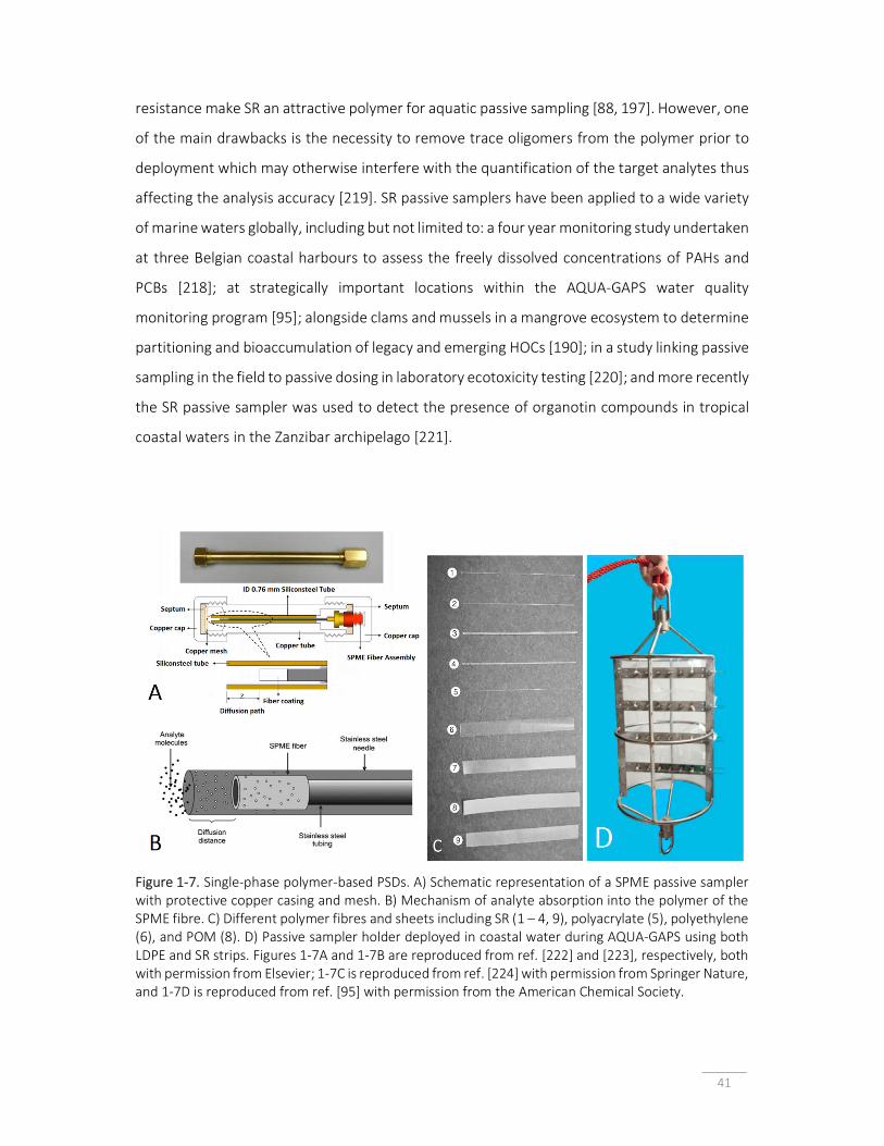
41

resistance make SR an attractive polymer for aquatic passive sampling [88, 197]. However, one

of the main drawbacks is the necessity to remove trace oligomers from the polymer prior to

deployment which may otherwise interfere with the quantification of the target analytes thus

affecting the analysis accuracy [219]. SR passive samplers have been applied to a wide variety

of marine waters globally, including but not limited to: a four year monitoring study undertaken

at three Belgian coastal harbours to assess the freely dissolved concentrations of PAHs and

PCBs [218]; at strategically important locations within the AQUA-GAPS water quality

monitoring program [95]; alongside clams and mussels in a mangrove ecosystem to determine

partitioning and bioaccumulation of legacy and emerging HOCs [190]; in a study linking passive

sampling in the field to passive dosing in laboratory ecotoxicity testing [220]; and more recently

the SR passive sampler was used to detect the presence of organotin compounds in tropical

coastal waters in the Zanzibar archipelago [221].

Figure 1-7. Single-phase polymer-based PSDs. A) Schematic representation of a SPME passive sampler with protective copper casing and mesh. B) Mechanism of analyte absorption into the polymer of the SPME fibre. C) Different polymer fibres and sheets including SR (1 – 4, 9), polyacrylate (5), polyethylene (6), and POM (8). D) Passive sampler holder deployed in coastal water during AQUA-GAPS using both LDPE and SR strips. Figures 1-7A and 1-7B are reproduced from ref. [222] and [223], respectively, both with permission from Elsevier; 1-7C is reproduced from ref. [224] with permission from Springer Nature, and 1-7D is reproduced from ref. [95] with permission from the American Chemical Society.

42

1.4.1.1.3 Polyoxymethylene (POM) & ethylene-vinyl acetate (EVA)

The polymer polyoxymethylene (POM) contains a repeating polar (H-bond accepting) group [-

CH2-O-]n in its molecular structure making it suitable as a PSD for a diverse range of polar and

non-polar compounds including hormones, pharmaceuticals and biocides [225]. It exhibits a

higher resistance to analyte mass transfer for a range of HOCs compared to the very lipophilic

LDPE and SR membranes, and uptake and selectivity is defined as being polymer controlled

rather than water boundary layer controlled [196]. This characteristic allows for typically long

exposure/deployment times to be applied without reaching partitioning equilibrium [189], and

for sampling work to be undertaken in highly contaminated environments where LDPE and SR

samplers would become rapidly oversaturated. POM samplers (used as strips) (Figure 1-7C,

number 8) have been deployed alongside passive air samplers in the overlying atmosphere to

monitor the aerosol-water distribution of dioxins and PCBs and in marine waters in the Baltic

Sea [226], and at surface and seafloor depths to investigate the flux of HOCs from the sediment

pore water to the overlying waters [176].

Like POM, ethylene-vinyl acetate (EVA) is a hydrophilic polymer due to its polar acetate group

[-CH2-CH2-]n[CH2-CH(OCOCH3)-]m, and it is, therefore, expected that its hydrophilic properties

will allow for its use over an expanded range of target analytes that are currently not

accommodated for in other more lipophilic passive sampling polymers (LDPE/SR) [194]. EVA

has been used for passive sampling of cypermerthrin in the salmon farm industry [193], and

more recently for soluble munitions compounds in marine and freshwater environments,

where the polymer composition could be tailored to the analyte of interest [227].

1.4.2 Polar organic chemical integrative sampler (POCIS) The polar organic chemical integrative sampler (POCIS) has been developed to accumulate a

broad spectrum of hydrophilic organic compounds, which characteristically have one or more

polar functional groups or a significant dipole moment, such as polar pesticides,

pharmaceuticals, illicit drugs, antibiotics, hormones, personal care products, phosphate based

flame retardants, surfactants, and their metabolites and degradation products [102]. Over 300

chemicals have been reported in the literature as having been detected and quantified by

POCIS in both the laboratory setting and in situ in environmental waters [113]. The POCIS is

43

commonly deployed in conjunction with SPMDs to enable monitoring of a diverse range of

persistent organic pollutants and emerging contaminants in environmental waters, including

75% of the priority substances listed under the European Union’s Water Framework Directive

(EU-WFD) [102].

POCIS samplers are most commonly applied to monitoring hydrophilic organic compounds

with log Kow values ≤ 3, however Alvarez et al. (2007) illustrated the performance of both

POCISs and SPMDs as a function of log Kow values, highlighting the overlap in their suitability

for detection and accumulation of organics in the range of log Kow 3 to 4 [228]. Furthermore,

POCISs have been successfully applied to monitoring a range of priority pollutants (log Kow > 4)

identified in the EU-WFD [229], with some compounds exhibiting both polar and non-polar

physicochemical characteristics (e.g., octylphenol and nonylphenol with log Kow values from

4.1 to 4.5, respectively [230]), and other compounds being ionisable (e.g., pentachlorophenol

log Kow 5.1 [231]) and existing as both deprotonated or neutral species based on matrix pH

[232-234].

The POCIS comprises a solid receiving phase (sorbent), sandwiched in between two identical

microporous diffusion-limiting membranes (usually polyethersulphone (PES) with a pore size

of 0.1 µm) compressed together by two stainless steel washers that hold the sampler together

[232]. The ‘membrane-sorbent-membrane’ sandwich configuration maximises the surface

area (commonly 45.8 cm2) of the PSD as both sides of the sampler are exposed to the sampled

medium and are able to accumulate analyte from the solution (Figure 1-8) [235]. Unlike the

polyethylene membrane in the SPMD which is transparent, the PES membrane in POCIS is

opaque, and therefore photodegradation is less likely to affect the performance of the device

[233]. Arrays of POCIS are commonly deployed at each sampling location by mounting several

samplers on a support rod with the advantage of combining the sorbents from multiple

samplers to increase the sensitivity of measurements (Figure 1-8) [223].

44

Figure 1-8. Schematic diagrams and typical deployment configuration of the POCIS for the passive sampling of hydrophilic organic compounds. A) and B) typical construction of POCIS; C) array of POCIS mounted on a support rod for field deployment. Figure 1-8A is reproduced from ref. [223] and 1-8B is reproduced from ref. [129], both with permission from Elsevier. Figure 1-8C is reproduced from ref. [236] with permission from the Springer eBook.

The POCIS is versatile as the receiving phase (sorbent) can be changed to target a specific

chemical or class of compounds, and there are two commercially available configurations

available, including the pesticide-POCIS and the pharmaceutical-POCIS. The pesticide-POCIS

incorporates a receiving phase comprising a triphasic admixture of Isolute ENV+ (hyper cross-

linked hydroxylated polystyrene-divinylbenzene polymeric resin) with Ambersorb 1500

(carbonaceous adsorbent) dispersed on S-X3 Bio Beads (styrene divinylbenzene copolymer),

and the pharmaceutical-POCIS incorporates only one phase; an Oasis hydrophilic-lipophilic

balanced (HLB) copolymer sorbent [109]. As the different sorbents are optimised for specific

classes or types of hydrophilic organic compounds, it is common to co-deploy both pesticide-

and pharmaceutical-POCIS simultaneously, to maximise the detection of these compounds at

any given sampling site [228].

The triphasic admixture is considered the generic sorbent for hydrophilic organic compounds,

however the Oasis configuration exhibits advantageous properties. Analyte molecules with

multiple functional groups bind strongly to the carbonaceous component of the triphasic

receiving phase resulting in difficult and complex extraction with poor recoveries [228], and

more toxic elution solvents (dichloromethane as opposed to methanol) are required for

analyte stripping with the pesticide-POCIS [237]. Vermeirssen et al. (2012) undertook a study

using pesticide-POCIS to assess the partition of analytes between both sorbent and PES

45

membrane for a range of compounds (herbicides, pharmaceuticals and industrial chemicals)

with log Kow values between -2.6 to 3.8 [238], and Silvani et al. (2017) likewise undertook a

similar study using pharmaceutical-POCIS to monitor a range of alkylphenols between log Kow

2.5 to 5.8 [234]. Both studies showed that compounds with higher log Kow values tended to be

retained by the PES membrane with a lag-phase prior to their detection in the sorbent receiving

phase where compounds with low log Kow values were efficiently retained. This demonstrates

the importance of analysing both the sorbent and membrane phases to correctly determine

environmentally relevant concentrations of pollutants with a varying degree of hydrophilicity

[234, 238].

More recently a number of specialised receiving phases have been reported in the literature

specifically for strongly polar and ionisable compounds including a) the Strata™ weak anion

exchange (X-AW) sorbent deployed in estuarine environments for the detection of

perfluorinated chemicals [239], b) a commercially available molecularly imprinted polymer

receiving phase for the determination of glyphosate and its degradation product

aminomethylphosphonic acid [240, 241], c) imidazolium ionic liquids immobilised on silica gel

used to monitor five perfluoroalkyl substances (PFAS) in waste water effluent [242], and d) the

IL trihexyl(tetradecyl)phosphonium dicyanamide as the receiving phase for monitoring

pharmaceuticals in a POCIS like passive sampling technique (termed PASSIL, short for passive

sampling with ionic liquids) which has been applied to high salinity seawater matrices [243].

A number of calibration strategies for POCIS are outlined in the literature, namely static

renewal, static depletion, flow-through systems and in situ calibration [133]. The choice of

calibration method has been shown to have a significant impact on the sampling rate (Rs) [244],

and one of the biggest challenges to the widespread use of POCIS for quantitative analysis is

the lack of a robust method to correct for in situ environmental conditions such as

hydrodynamics (flow rate and pattern), temperature, salinity, pH and dissolved organic matter

[107, 109]. In order to obtain quantitative data from POCIS (i.e., CTWA determination), a number

of in situ calibration methods have been proposed with varying degrees of success, including

the PRC approach, surrogate PRC systems based around the co-deployment with hydrophobic

samplers, and calibration of the POCIS against the dissolution of calcium sulfate decahydrate

casts [133]. Interactions between polar analyte molecules, polar sorbents and the PES diffusion

limiting membrane in the POCIS are fundamentally different to isotropic uptake and exchange

46

dynamics in hydrophobic samplers between analytes and PRCs, and thus the classic PRC

calibration approach may continue to provide limited success for POCIS-based passive

sampling for polar and ionisable compounds [107].

1.4.3. Chemcatcher® The Chemcatcher® was first described by Kingston et al. [245] and has been applied to

measuring the CTWA for both polar/non-polar organics [245, 246] and heavy metals [247], in

aquatic environments. The Chemcatcher® comprises a reusable polytetrafluoroethylene

(PTFE) assembly, a commercially available receiving phase (solid sorbent), and in some

applications a diffusion-limiting membrane can be added to regulate and facilitate analyte

uptake [245] (Figure 1-9).

Figure 1-9. Schematic diagram and typical deployment configuration of the Chemcatcher®, (A) for non-polar analyte passive sampling, with B) showing multiple replicate devices mounted in a cage for field deployment. Figure 1-9A is reproduced from ref. [129] with permission from Elsevier, and 1-9B is from ref. [248] with permission from the Royal Society of Chemistry.

The most common Chemcatcher® prototype employs a 47-mm C18 Empore™ disk as the

receiving phase, and either a polysulfone (PES) or a low density polyethylene (LDPE) rate-

limiting membrane for monitoring of polar or non-polar organic compounds, respectively

[245]. Studies have shown that temperature impacts the rate of analyte accumulation in both

polar and non-polar Chemcatcher®, with the authors concluding that it is necessary to

determine the effects of temperature in the laboratory for each analyte of interest so that

calibrations can be appropriately adjusted and field results corrected [245, 246]. The effect of

water turbulence was likewise studied showing a quantifiable effect with increasing

47

turbulence, especially for smaller molecules, suggesting that uptake rates are analyte specific

and controlled by both diffusion through the aqueous boundary layer and by affinity of the

analyte for the diffusion-limiting membrane material [245, 246].

The applicability of using PRCs with Chemcatcher® samplers to compensate for the effects of

environmental variables (i.e., temperature, turbulence/flow conditions and biofouling) and for

in situ calibration has been investigated. Lissalde et al. [249] provided an extensive summary

of their research into this topic, highlighting that PRCs have been successfully used, and are

appropriate for establishing in situ sampling kinetics especially for the non-polar

Chemcatcher®. However, for the polar configuration there has been limited success using this

approach, with the authors suggesting further research was warranted.

The performance of the Chemcatcher® in high ionic strength matrices has rarely been

evaluated, however, some Chemcatcher® studies have been undertaken in a range of marine

environments where the PSD have been deployed as part of wider water quality monitoring

programs and where optimisation studies were not central to the study.

Petersen et al. [108] undertook calibration experiments using a non-polar Chemcatcher® in

fresh and seawater matrices for selected PBDEs, PCBs and organochlorine pesticides, showing

a salinity effect, whereby a higher offload of PRCs and a slightly lower sampling rate (Rs) were

observed as a function of increasing salinity. Allan et al. [250] recommended that the effect of

water hardness (i.e., interference of Ca2+ and Mg2+) on the Chemcatcher® measurements for

metals should be investigated, however, this study is yet to be undertaken. It has been

suggested that the pH could affect Chemcatcher® sampling rates through both pH effects

influencing the properties of the sampler membrane and receiving phase, and modifications

of analyte speciation or partition between protonated and deprotonated forms [249]. Other

studies have also reported pH effects when monitoring inorganic mercury and organotin

compounds [251], and for a range of herbicides and pesticides with differing polarities [252,

253].

A large variety of receiving phase and membrane combinations (spanning a wide range of log

Kow values) have been described in the literature for Chemcatcher® (Figure 1-10) covering a

range of non-polar to polar organics, allowing for the Chemcatcher® sorbent and diffusion

48

membranes to be tailored to the polarity of the target analyte(s) and the desired deployment

period/integration time [114].

Figure 1-10. Summary of the log Kow ranges successfully tested for various Chemcatcher® receiving phase and membrane combinations. This figure is reproduced from ref. [114] with permission from Elsevier.

1.4.3.1 Chemcatcher® for non-polar compounds The Chemcatcher® used for monitoring non-polar compounds commonly employs a C18

Empore™ disk as its receiving phase, overlain by a thin (40 µm thickness) commercially

available LDPE membrane [245]. Vrana et al. [254] were able to significantly improve the

performance of the hydrophobic Chemcatcher® by filling the interstitial space between the

receiving sorbent phase and the diffusion-limiting membrane with a small volume of n-octanol,

having a high permeability (solubility x diffusivity) for lipophilic HOCs, and reducing the internal

resistance to mass transfer within the device [246].

In situ exchange kinetics of PRCs allowed for corrections to be made to laboratory derived

sampling rates using an empirical model that corrected for environmental flow/turbulence and

temperature conditions [255]. However, since their development, non-polar Chemcatcher®

samplers have not been widely applied in marine or even more generally freshwater passive

sampling field experiments. This is likely due to the costs involved with deployment given their

small and restricted surface area, which may require the deployment of multiple devices to

allow for the receiving phases to be combined in order to achieve the desired sensitivities, and

this then becomes expensive compared to other commercially available passive samplers

(SPMDs or LDPE/SR strips) for this class of compounds [245].

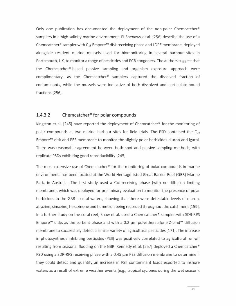
49

Only one publication has documented the deployment of the non-polar Chemcatcher®

samplers in a high salinity marine environment. El-Shenawy et al. [256] describe the use of a

Chemcatcher® sampler with C18 Empore™ disk receiving phase and LDPE membrane, deployed

alongside resident marine mussels used for biomonitoring in several harbour sites in

Portsmouth, UK, to monitor a range of pesticides and PCB congeners. The authors suggest that

the Chemcatcher®-based passive sampling and organism exposure approach were

complimentary, as the Chemcatcher® samplers captured the dissolved fraction of

contaminants, while the mussels were indicative of both dissolved and particulate-bound

fractions [256].

1.4.3.2 Chemcatcher® for polar compounds

Kingston et al. [245] have reported the deployment of Chemcatcher® for the monitoring of

polar compounds at two marine harbour sites for field trials. The PSD contained the C18

Empore™ disk and PES membrane to monitor the slightly polar herbicides diuron and igarol.

There was reasonable agreement between both spot and passive sampling methods, with

replicate PSDs exhibiting good reproducibility [245].

The most extensive use of Chemcatcher® for the monitoring of polar compounds in marine

environments has been located at the World Heritage listed Great Barrier Reef (GBR) Marine

Park, in Australia. The first study used a C18 receiving phase (with no diffusion limiting

membrane), which was deployed for preliminary evaluation to monitor the presence of polar

herbicides in the GBR coastal waters, showing that there were detectable levels of diuron,

atrazine, simazine, hexazinone and flumetron being recorded throughout the catchment [159].

In a further study on the coral reef, Shaw et al. used a Chemcatcher® sampler with SDB-RPS

Empore™ disks as the sorbent phase and with a 0.2 µm polyethersulfone Z-bind™ diffusion

membrane to successfully detect a similar variety of agricultural pesticides [171]. The increase

in photosynthesis inhibiting pesticides (PSII) was positively correlated to agricultural run-off

resulting from seasonal flooding on the GBR. Kennedy et al. [257] deployed a Chemcatcher®

PSD using a SDR-RPS receiving phase with a 0.45 µm PES diffusion membrane to determine if

they could detect and quantify an increase in PSII contaminant loads exported to inshore

waters as a result of extreme weather events (e.g., tropical cyclones during the wet season).

50

Two of the PSII herbicides, tebuthiuron and metolachlor, were shown to exceed their Water

Quality Guideline values during the 2010 – 2011 wet season, and both passive and spot

sampling methods were in good agreement highlighting the potential of this passive sampling

tool to be used for long-term monitoring in remote areas of the GBR for this class of priority

pesticides. Additional research was undertaken in which the passive sampling technology using

Chemcatcher® was combined with remote sensing for coloured dissolved organic matter (a

proxy for measuring incursions of freshwater and therefore run-off) to assess the possibility of

integrating the two techniques to monitor improvements in water quality entering the GBR

catchment [258].

1.4.3.3 Chemcatcher® for metals and organometallics

The majority of studies using Chemcatcher® for trace metals sampling has been undertaken in

freshwater environments. Nevertheless, Chemcatcher® technology has been applied in high

salinity matrices to monitor the concentrations of organometallic pollutants (monobutyltin,

dibutyltin, tributyltin), and inorganic mercury [251, 259, 260]. The first sampler for the

organotin pollutants comprised a C18 Empore™ disk and cellulose acetate (CA) diffusion

membrane. It was calibrated under laboratory conditions with the effect of water temperature

and flow pattern/turbulence on the uptake rate evaluated. Limits of detection were reported

for the different organotin compounds in the range of 0.2 – 7.5 ng L-1. The PSDs were deployed

in the Alicante Harbour, Spain, for a period of 14 days, with performance evaluated alongside

spot sampling (every second day) [259]. However, there was a significant discrepancy between

mean spot sample concentrations over the period of deployment and the CTWA determined

from passive sampling. The authors suggest that this is likely due to a) the spot samples

containing both the dissolved fraction and the bound fractions (particulate and organic matter

bound), where the PSD would only accumulate the dissolved fraction that can diffuse through

the pores of the diffusion limiting membrane, and b) there was a significant variation in the

concentrations returned in the spot samples over the monitoring period where the frequency

of sample collection (every two days) may have been insufficient to provide a representative

reflection of the true CTWA concentration.

51

A Chemcatcher® sampler selective for inorganic mercury was developed and optimised under

laboratory conditions, and subsequently applied in the Alicante Harbor in Spain. During this

study, further optimisation experiments were also conducted for the monitoring of organotin

using the Chemcatcher® sampler described above. Empore™ C18 disks were used for

monitoring the organotins, and two receiving phase sorbents were tested for the detection of

inorganic mercury, namely the Empore™ SDB-RPS cation-exchange disks and the Empore™

chelating disks containing iminodiacetic (IDA) groups, with the latter being selected [260].

Optimisation studies for both the organotin and inorganic mercury sampler were undertaken

to select an appropriate diffusion-limiting membrane for the target analytes, and to study the

effect of pH, salinity and biofouling on sampler performance [260]. Cellulose acetate (CA),

polyethersulfone (PES), polyethylene (PE) and dialysis membranes were tested, with CA and

PES being chosen for the organotin and inorganic mercury Chemcatcher® samplers,

respectively. Salinity appeared to have no significant effect on both samplers, however, a

change in pH from 7 – 8 was found to affect the performance of the inorganic mercury PSD

likely due to pH affecting the speciation of inorganic mercury to form more hydroxide

complexes which are accumulated to a lesser extent in the PSD. However, the pH did not affect

the performance of the organotin PSD. The use of PRCs could not be applied for this sampler,

as the analytes exhibited anisotropic exchange kinetics, and thus a laboratory-based calibration

was performed under controlled temperature and turbulence conditions that were chosen to

mimic common environmental conditions. The authors suggest that for wider applicability of

the device, further work is required under a range of hydrodynamic and temperature

conditions to extend the calibration data available [260]. Extensive field trials in ten locations

over Europe, featuring a diversity of aquatic matrices, were performed using the laboratory

calibrated and optimised Chemcatcher® passive samplers for organotins and for inorganic

mercury [251]. Spot sampling was conducted in tandem, however, once again the PSDs

accumulated less of the target analytes when comparing with the average concentration

recorded for the spot samples collected. This was likely due to the samplers only collecting the

soluble fraction of the target pollutants. Nevertheless, the preconcentration capabilities of

these PSDs have been identified as a significant advantage, especially in environments where

concentrations in spot samples fall below the limits of detection of the analytical

instrumentation.

52

A Chemcatcher® sampler was used by Petersen et al. [261] in the first passive sampling

experiment to monitor rare earth elements in aquatic environments. The experiments were

undertaken in estuarine waters, using the 3M Empore™ chelating disk as the receiving phase,

and a CA diffusion limiting membrane (pore size of 0.45 µm). Temperature and water

turbulence effects were studied, with turbulence shown to have a significant influence on

uptake rates. The PSDs were shown to accumulate a number of rare earth metals commonly

found in trace concentrations in matrices with high salt concentrations, highlighting this

passive sampler as an effective monitoring tool [261]. A further improvement to this sampler

was described where a continuous flow-through set-up was employed to minimise the

artefacts from variable hydrodynamic conditions as the PRC calibration approach could not be

used for this configuration of sampler [262].

1.4.4 Solid-phase adsorption toxin tracking (SPATT) Algal blooms are a global phenomenon and a natural part of seasonal cycles in aquatic

ecosystems [263]. However, increasing ecosystem disturbance and pollution has resulted in

the proliferation of harmful algal blooms (HABs), having a deleterious impact on the health of

fresh, brackish and marine waters. The solid-phase adsorption toxin tracking tool was first

introduced by MacKenzie et al. [264], and was developed as an early HAB detection and

surveillance tool to monitor the occurrence of potentially harmful microalgalalgal and

cyanobacterial blooms and their biotoxins [265, 266]. A SPATT passive sampler is conceptually

similar to the Chemcatcher® and POCIS passive samplers. The receiving phase comprises beads

of porous synthetic resin capable of adsorbing toxins from the water column, contained in an

inert mesh, typically polyester [264] or nylon [266]. A suite of different resins have been

investigated for a variety of lipophilic and hydrophilic toxins, with the most common resin

Diaion® HP20 made from cross-linked styrene-divinylbenzene beads [267]. Similarly to other

passive sampling devices, the challenges limiting the widespread adoption of SPATT samplers

as a regulatory monitoring tool include calibration, and standardisation of methods and

procedures [268]. However, SPATT samplers have been deployed in Monterey Bay, California,

and were found to be successful in detecting the presence of phycotoxins in seawater three

and seven weeks prior to a major HAB event, and seven to eight weeks prior to the detection

53

of toxins in sentinel shellfish [266], allowing for appropriate management strategies to be

implemented predominantly to protect human health.

1.4.5. Diffusive gradients in thin-films (DGT) Diffusive gradients in thin-films (DGT) technique was first proposed by Davison et al. (1994) for

the determination of in situ trace-metal concentrations in natural waters, with zinc being the

target analyte investigated in seawater [269]. A DGT passive sampler generally comprises a

chelating resin or metal oxide adsorbent (analyte binding site) separated from the sample

solution by a thin-film of an ion-permeable hydrogel where analyte mass transfer is controlled

by diffusion through the gel. In addition, it contains a protective pre-filter membrane exposed

to the sampled medium, which is employed to prevent suspended particles from adhering to

the diffusive hydrogel, which may inhibit analyte uptake over time by minimising the surface

area of the exposed PSD (Figure 1-11) [269].

Diffusion of analyte through the hydrogel is largely dependent on the physicochemical

properties of the gel including pore size and density, and the swelling factor which reflects the

uptake of water by the suspended/submerged gels [270]. Zhang and Davison (1999) reported

that polyacrylamide gel cross-linked with agarose derivative produced an ‘open-pore’, high

swelling gel with a water content of 95%, which allowed almost unrestricted diffusion of metal

ions through the gel, and an indistinguishable analyte diffusion coefficient between water and

the gel [270].

Early development of the DGT passive sampling method focused on the determination of

cadmium (Cd), iron (Fe), manganese (Mg), and copper (Cu) in coastal environments using a

Chelex-100 cation exchange resin, a polyacrylamide hydrogel and a cellulose nitrate pre-filter

membrane [271]. Experiments undertaken showed that for the Chelex-100 resin, uptake of Cd

was dependent on temperature, however, it was independent of a) ionic strength (10 nM – 1

M), b) pH in the range of 5 – 8.3, and c) hydrodynamic effects as long as solution flow rates

were above a certain threshold [271].

54

Figure 1-11. Schematic diagram and typical deployment configuration of the diffusive gradient in thin-films passive sampling device. A) Schematic representation of DGT showing analyte uptake mechanism through a pre-filter membrane, diffusive gel, and resin gel (binding site). B) replicates of DGT samplers mounted in a Perspex block which was deployed in the field. Figure 1-11A is reproduced from ref. [132] with permission from Elsevier, and Figure 1-11B is reproduced from ref. [272] with permission from The Royal Society of Chemistry.

Chelex-100 has been the most frequently applied resin binding gel for heavy metal

determination, separated by an ion-permeable hydrogel layer of thickness Δg (Figure 1-11A).

According to Fick’s first law of diffusion, the concentration in bulk solution (Cb) can be

determined from the mass (m) of accumulated analyte in the resin layer after a known

deployment time (t) using Equation (1-2):

Cb = mΔg / (DAt) (1-2)

Where D is the experimental diffusion coefficient of the metal in the gel, and A is the exposed

surface area of the DGT sampler (A = 3.14 cm2).

Chelex-100 consists of a styrene divinylbenzene copolymer containing paired iminodiacetate

ions, making it an effective polyvalent metal ion chelating resin. Garmo et al. [273] undertook

a comprehensive study to determine diffusion coefficients and evaluate the performance of

the Chelex-100 resin for 55 elements including alkali and alkaline earth metals and their

respective halide ion pairs, transition metals and lanthanides. The authors found that 24 of the

elements examined showed an affinity for the binding resin (mostly transition metals), and the

alkali and alkaline earth metals and their halide ions did not appear to interfere, indicating that

dissolved salts would be unlikely to compete with transition metals in high salinity matrices

[273].

A comparison between uptake of dissolved aluminium (Al) species by Chelex-100 and Metsorb

(titanium dioxide-based adsorbent) in fresh and marine waters found that both Chelex-100 and

55

Metsorb exhibited similar diffusion coefficients at pH 5.0. However, in the pH range of

seawater, and with increasing ionic strength, a considerable underestimation of Al

concentration was observed in the Chelex-100-DGT sampler (40 – 70% lower than predicted),

while the Metsorb-DGT sampler measurements were described as independent of pH (5.0 –

8.5) and ionic strength (0.001 – 0.7 M NaNO3) [274]. It was proposed that the Metsorb-DGT

sampler generated more accurate results and that Chelex-100-DGT sampler, which was

unsuitable for monitoring dissolved Al in seawater. Ferrihydrite-DGT containing a ferric

oxyhydroxide mineral binding phase was compared to Metsorb for the determination of the

oxyanions of dissolved reactive phosphorus (DRP), arsenic (As(V)), vanadium (V(V)), antimony

(Sb(V)), molybdenum (Mo(VI)), and tungsten (W(VI)). The Metsorb-DGT exhibited superior

performance in both fresh and seawaters for measuring As, Sb, W and DRP, nevertheless

neither Metsorb-DGT nor Fehhihydrite-DGT samplers performed well at estimating Mo(VI)

concentrations [275].

Mercury(II) ions bond covalently with the amide nitrogen groups of polyacrylamide gels, and

thus both Chelex-100 binding resin and Spheron-thiol based resin were compared in terms of

specificity for Hg, using an agarose gel as the diffusive layer [276]. Both resins exhibited

different affinities for bound Hg and were therefore able to be used to differentiate

measurable fractions of Hg complexes [276]. Ren et al. (2018) have proposed the use of a

highly selective macroporous poly-isothiouronium chelating resin (Tulsion® CH-95) for the

simultaneous measurement of methyl mercury and mercuric ion, with uptake rates being

independent of both pH and ionic strength in the range of 4.1 – 8.1 pH units and 0.1 – 1000

mM respectively [277].

While DGT samplers have been successfully applied for widespread monitoring of heavy metals

in marine environments, DGT technology does not easily discriminate between complexed

metal ions (generally less bioavailable and therefore less toxic) and free metal ions (highly

bioavailable exhibiting high toxicity), with the concentrations accumulated by DGT tending to

reflect total dissolved concentrations [278, 279].

DGT samplers for inorganic nutrient monitoring have been developed for use in freshwater

matrices, specifically for ammonium [140, 280], nitrate [139, 280] and phosphate [126, 141,

280, 281]. DGT samplers developed for inorganic nutrient monitoring utilise an ion-exchange

resin as the binding phase, however, in high salinity matrices this phase is unable to

56

discriminate between the low concentration of analyte molecules compared to the high

concentrations of dissolved salts.

While the DGT technology was initially developed for detecting in situ trace metals and labile

inorganics in fresh and marine waters, the application and scope was extended by Chen et al.

(2012) who developed the first DGT sampler for polar organic contaminants such as

sulfamethoxazole antibiotics using a XAD18 binding resin and agarose hydrogel [282]. While

most DGT samplers for organics have been applied to freshwater matrices, there are a few

examples in the literature where they are applied to high salinity matrices. Xie et al. (2018)

described a DGT sampler for monitoring a suite of 20 antibiotics in seawater using the XDA-1

binding resin as the receiving phase [283], and Ren et al. (2018) developed a porous carbon

material derived from metal-organic frameworks as the binding phase for monitoring in

synthetic and natural seawater, with both DGT samplers for the polar organics showing little

sensitivity to pH and ionic strength [284]. Endocrine disrupting chemicals (three hormones,

two pesticides and bisphenol A) were monitored in seawaters using XDA-1 resin as the binding

agent, showing linear accumulation over the period of deployment and accumulation was

independent of pH and salinity over the range pH 7 – 9 and ionic strength of 0.4 – 0.8 M [285].

Guibal et al. (2019) provide a comprehensive review on DGT passive samplers for polar

organics, emphasising similarities with other polar organic passive samplers, and showing that

environmental conditions including temperature, pH, analyte pKa, ionic strength and the

concentration of dissolved organic matter can have a significant impact on the performance of

these PSDs [134]. However, due to the ability of the diffusive gel to mitigate the effect of

hydrodynamic conditions on the sampling rate, this makes the DGT samplers for organics

inherently more reliable and easier to calibrate, making them a promising and competitive new

tool for in situ monitoring of polar organic chemicals [286].

1.4.6 GELLYFISH for metals The Gellyfish is an inexpensive, equilibrium-based passive sampler developed specifically for

monitoring toxic free metal ions in the divalent form (M2+) dissolved in seawater, using a thin

disk of polyacrylamide gel with beads immobilised in the polymer matrix containing

iminodiacetate groups (IDA) that are highly selective for divalent metal cations. The first

57

Gellyfish sampler developed was tested with the cupric ion (Cu2+) [287]. Dong et al. (2015)

described several improvements that were made to the Gellyfish-PSD, namely a significantly

reduced equilibration time, and the capability to monitor multiple free metal ions

simultaneously, including Cu, Zn, Ni, Pb and Cd ions [288]. The authors developed an R-based

model (called GELLYMOD) to correct for ionic strength and account for competitive binding

between the different metals and the IDA [288]. Large scale and repeated monitoring of the

free ion concentrations of five metals was undertaken using Gellyfish at five inshore locations

in the Boston Harbour, with concurrent measurements of ten biogeochemical variables being

undertaken. Using the Gellyfish to obtain high resolution data over important spatiotemporal

scales, the authors found that there were significant correlations among the metals which

varied seasonally, with pH, salinity, temperature and rainfall as key determinants of free metal

ion variability [289].

1.4.7 Liquid membrane-based passive samplers Liquid membranes combine the concept of solvent extraction (i.e., liquid-liquid extraction) with

that of membrane-based separation. A liquid membrane is composed of an organic liquid

phase immiscible with water, containing an extractant (also known as carrier), and is used to

separate two aqueous liquid phases, thus allowing simultaneous extraction and stripping

(back-extraction) on each side of the membrane. In the context of passive sampling, the liquid

membrane plays the role of the semi-permeable barrier between the aqueous sampled

medium and an aqueous liquid receiving phase. The target analyte(s) are first extracted into

the membrane, forming adducts with the extractant, which are transported across the

membrane by diffusion, and then the analytes are back-extracted into the receiving solution

containing a suitable stripping reagent [89, 290, 291]. The fact that the receiving phase is an

aqueous liquid offers a great advantage because the receiving solution can be analysed directly

without the necessity of analyte stripping from a solid receiving phase as is the case with most

other PSDs, thus simplifying the overall analytical procedure [292].

Two types of liquid membranes have been applied in passive sampling, namely supported

liquid membranes (SLMs) and polymer inclusion membranes (PIMs). Both consist of an organic

liquid phase impregnated within a base polymer, although the binding interactions between

58

the two components are different in each case as described below. Recently, liquid membrane-

based passive sampling techniques have been described in the literature and applied to

freshwaters [143, 293, 294]. As their passive sampling mechanism is based on ion-exchange,

the complex ionic composition of marine waters tends to supress the extraction of the target

ionic species of interest, thus limiting the use of SLM- and PIM-based passive samplers for such

matrices. However, a few liquid membrane-based systems have been reported for application

in seawaters, which have great potential to be used as passive samplers. These include a hollow

fibre-SLM for the separation and preconcentration of cadmium (Cd) [295], and a PIM for the

monitoring of Cd [296], and mercury (Hg) [297].

An SLM comprises an inert microporous thin-film polymeric support, whose pores are filled

with a liquid phase (containing the extractant), which is held by capillary forces [298]. The SLM-

based enrichment device developed for the monitoring of Cd consisted of a polyvinylidene

difluoride (Durapore) support impregnated with the IL Aliquat 336 (a mixture of quaternary

alkylammonium chlorides, (R3R’N)Cl) as carrier dissolved in decaline [295]. Optimisation of the

SLM was undertaken including the IL concentration and the receiving solution composition.

The Cd present in the sampled source solution was extracted into the liquid membrane in the

form of CdCl42- which was proposed to form an ion pair with the cationic component of the

Aliquat 336 ((R3R’N)2CdCl4) by exchange with Cl- (Aliquat 336 anion). The performance of the

device was not compromised by the highly saline matrix or due to the presence of other

dissolved trace metals (Cu, Ni, Pb) [295].

A PIM-device was developed for Cd preconcentration from high salinity seawater matrices,

showing little interference by the high ionic strength of seawater [296]. The PIM-device was

composed of a PIM containing the IL trihexyl (tetradecyl)phosphonium chloride as the

extractant, cellulose triacetate as the base polymer and nitrophenyl octyl ether as the

plasticiser, and 0.5 M nitric acid as the receiving solution. The Cd transport from seawater

samples containing 10 µg L-1 Cd was achieved in 24 h allowing for preconcentration and matrix

separation in a single step [296].

A PIM-device was also developed for the monitoring of mercury (Hg) in natural waters

including rivers, groundwater and seawater, again with no matrix effects observed [297]. The

PIM composition was studied in terms of type of extractant to assess the performance between

two ILs, both having the same cation (trioctylmethylammonium) and having different anions

59

(thiosalicylate or salicylate with acronyms TOMATS and TOMAS, respectively). The TOMATS-

based PIM showed better performance than the PIM with TOMAS (using a solution of 10-3 M

cysteine as the receiving phase) and was therefore chosen for field deployment experiments.

Furthermore, the effect of biofilm growth on the performance of the device was assessed,

showing that there was no measurable effect observed after a 7-day deployment. The method

reported an LOD of 0.29 µg L-1 showing promise as a passive sampling tool for the monitoring

of mercury pollution in waters with complex matrices.

1.4.8 Ammonium PSDs applied to freshwaters As mentioned earlier, two passive sampling methods have been reported to monitor

ammonium in low ionic strength matrices, including a PIM-based PSD [143], and a DGT sampler

[138-142]. The PIM device consists of an acidic receiving solution (0.8 M HCl) separated from

the sampled aquatic medium by a membrane composed of 55 wt% poly(vinyl chloride) as the

base polymer, 35 wt% commercial dionylnapthalene sulfonic acid as the extractant, and 10%

1-tetradecanol as a plasticiser [143]. This PSD exhibited a linear accumulation over a period of

7 days, and was deployed in the field as a water quality monitoring tool to track sources of

fecal pollution in storm water drains [299]. Several DGT samplers are described in the

literature and are constructed using a protective membrane filter overlaid on a diffusive

hydrogel layer, with various sorbent receiving phases assessed including a) zeolite gel

comprising microporous hydrated aluminosilicate [138], b) CMI-7000 or Microlite PrCH cation

exchange resins [139, 140], c) a mixed inorganic nitrogen binding gel composed of ion

exchange resins PrCH and A520E [141], and a mixed binding layer for simultaneous sampling

of orthophosphate and ammonium using a micro-sized biochar-zeolite-zirconium oxide

binding phase [142]. Both DGT and PIM-based passive samplers for ammonium monitoring are

susceptible to interference from dissolved salts and are therefore not able to be used in high

salinity matrices, such as estuarine and marine waters.

60

1.5 General comments and research objectives Ammonia is an important nutrient in coastal and oceanic waters due to its role in the aquatic

nitrogen cycle and its potential to cause eutrophication of marine environments when

concentrations are sufficient to cause prolific algal growth [1, 9]. However, in the open ocean

and oligotrophic environments the presence of this analyte at trace concentrations

(nanomolar) and the high salinity and matrix complexity of the water make its analysis a real

challenge [44].

Choosing an appropriate method for a particular environmental water quality monitoring

application is important as no method can be universally applied, with every method exhibiting

advantages and disadvantages. It is therefore essential to consider a number of important

factors such as cost of analysis in terms of operational complexity, ease of instrumental set-up

and operation, in addition to sensitivity and accuracy requirements, duration of analysis,

reagent stability and potential interferences as well as logistics associated with sample

availability and frequency of collection [91].

To ensure water quality standards are maintained now and into the future, it is important to

understand the challenges of analysing ammonia in estuarine and marine waters. Historically,

flow-based methodologies, such as segmented flow analysis [38, 54], and more recently flow

injection analysis [45, 77], and sequential injection analysis [60, 71], have been used to assist

with this difficult task. Several flow-based methodologies have been developed for monitoring

ammonia in marine waters, and on-line sample pre-treatment strategies employed and

different detection methods have been discussed, highlighting the need to improve limits of

detection, need for miniaturisation and lower energy consumption, and to reduce and

eliminate interferences.

While significant research efforts have been focused on the development of flow-based

methodologies for measuring pollutants in aquatic environments, considerable advances have

been made over the last three decades to develop passive sampling technologies for water

quality monitoring particularly as a diagnostic tool to identify point-source and pollution events

[89, 223]. Whilst passive sampling technologies are often semi-quantitative in that laboratory

calibration does not always allow for sufficiently accurate CTWA concentrations to be

determined, they are an effective screening tool for many important aquatic pollutants, and

61

they can be used as an early detection method for areas of concern for regulators and water

quality managers [91]. The advantages of passive sampling (i.e., affordability, ease of use,

minimal sample handling required, and the capacity to provide time-weighted average

concentrations of analytes for the period of deployment) make this a desirable technique for

routine monitoring of pollutants, especially for identifying pollution hotspots and episodic

pollution events.

Different types of passive sampling techniques have been developed to detect a wide range of

important aquatic pollutants including both non-polar and polar organics,

metallic/organometallic and some inorganic compounds, and a number of passive samplers

have been described and evaluated, including for environmental monitoring of seawater [89,

102]. While many PSDs have been developed and applied to freshwater environments,

seawater environments pose several additional challenges [102]. While two passive samplers

have been developed for the monitoring of ammonium in low salinity freshwater matrices,

including DGT- and PIM-based PSDs, these cannot be applied to estuarine or marine

environments due to interference from the high concentration of dissolved salts [139, 140,

143].

The objective of this PhD research was therefore to develop novel analytical methods for the

monitoring of ammonia in high salinity marine waters and dynamic estuarine environments,

able to cover the revised water quality guideline values for high conservation value waters in

Australia and New Zealand (160 µg NH3-N L-1 [3]), and with the additional capability of being

able to be used over a wide range of environmental ammonia concentrations.

This thesis is presented in a ‘thesis by publication’ style and comprises 5 chapters. Chapters 2,

3 and 4 are experimental chapters, and are written in a style accepted by journals for

publication.

Chapter 1 includes a comprehensive literature review of flow methods developed for

monitoring total ammonia in high salinity and complex matrices, including in estuarine, coastal,

and open ocean environments, the subject of which was published in 2014 in the journal

Trends in Analytical Chemistry. It also includes a comprehensive review of the passive sampling

literature, focussing on PSDs applied to high salinity matrices.

62

Chapter 2 describes the development of a simple and environmentally-friendly flow-based

analyser for the monitoring of total ammonia in marine waters over a wide range of

concentrations, without the need to make any changes to the manifold or reagent solutions.

This chapter has been published in the journal Marine Chemistry. This flow-based analytical

system has also been used in the experimental work described in Chapters 3 and 4 to analyse

all samples collected from the sampled medium (generally containing very low ammonia

concentrations) as well as the passive samplers’ receiving solutions (containing ammonia

concentrations several orders of magnitude higher than the sampled medium).

Chapter 3 reports the development of a passive sampler based on gas-diffusion separation,

where dissolved molecular ammonia present in the sampled medium diffuses across a

hydrophobic porous gas-diffusion membrane into an aqueous receiving solution, where it is

accumulated. Since the membrane is only permeable to gaseous species, this approach

effectively eliminates the interference of ionic species present in the high salinity sampled

medium. This initial design was able to be applied to estuarine and coastal waters for a

deployment period of 3-days, however significant biofouling impeded analyte accumulation

after a period of 4 days thus limiting the usability of the device for periods longer than 3 days.

This chapter has been published in the journal Talanta.

Chapter 4 describes a further improvement to the gas-diffusion passive sampling device by

adopting an antifouling strategy. A number of biofouling resistance strategies were tested,

allowing for a 7-day deployment period to be achieved. Moreover, a single calibration model

was developed using a neural network based-calibration approach that was able to take into

account the effects of several environmental factors that influence the sampling rate, including

the environmental temperature and pH. The newly developed gas-diffusion passive sampling

device was successfully applied to a range of field environments, and the neural network-based

calibration approach allowed for one calibration only to be employed when the environmental

conditions (temperature and pH) varied between different deployment sites. This chapter has

been submitted for publication to the journal Environmental Pollution and is currently under

review.

Chapter 5 summarises the main achievements of the research work described in this thesis,

and several improvements are proposed which could be performed in future work.

63

References 1. Camargo, J.A. and A. Alonso, Ecological and toxicological effects of inorganic nitrogen

pollution in aquatic ecosystems: A global assessment. Environ. Int., 2006. 32: p. 831-849.

2. Borja, Á., The European water framework directive: A challenge for nearshore, coastal and continental shelf research. Continental Shelf Research, 2005. 25(14): p. 1768-1783.

3. Batley, G.E. and S.L. Simpson, Development of guidelines for ammonia in estuarine and marine water systems. Mar. Pollut. Bull., 2009. 58 (10): p. 1472-1476.

4. ANZG, Australian and New Zealand guidelines for fresh and marine water quality. 2018, Australian and New Zealand Governments and Australian state and territory governments: Canberra ACT, Australia.

5. US Environmental Protection Agency, Ambient Water Quality Criteria for Ammonia (Saltwater), EPA 440/5-88-004. US EPA Office of Water, Washington, DC, USA. 1989.

6. I. Johnson, N. Sorokin, C. Atkinson, K. Rule, and S.J. Hope, Proposed environemntal quality standards for water framework directive annex viii substances: Ammonia (un-ionised), Environmnet Agency, UK. 2007.

7. Molins-Legua, C., S. Meseguer-Lloret, Y. Moliner-Martinez, and P. Campins-Falco, A guide for selecting the most appropriate method for ammonium determination in water analysis. Trends in Analytical Chemistry, 2006. 25(3): p. 282-290.

8. US Environmental Protection Agency. Update of Ambient Water Quality Criteria for Ammonia EPA 822-R-99-014. 1999, US EPA Office of Water: Washington, DC, USA.

9. Vitousek, P.M.A., John D.; Howarth, Robert W.; Likens, Gene E.; Matson, Pamela A.; Schindler, David W.; Schlesinger, William H.; Tilman, David G., Human Alteration of the Global Nitrogen Cycle: Sources and Consequences. Ecological Applications, 1997. 7(3): p. 737-750.

10. Diaz, R.J.R., Rutger, Spreading Dead Zones and Consequences for marine Ecosystems. Science, 2008. 321: p. 926-929.

11. Wilkie, M.P., Ammonia Excretion and Urea Handling by Fish Gills: Present Understanding and Future Research Challenges. Journal of Experimental Zoology, 2002. 293: p. 284-301.

12. Vosyliene, M.Z.S., G.; Kazlauskiene, N. Fish Physiology, Toxicology, and Water Quality. in Proceedings of the Seventh International Symposium. 2003. Tallnin, Estonia: Ecosystems Research Division.

13. Löscher, C.R., A. Kock, M. Könneke, J. LaRoche, H.W. Bange, and R.A. Schmitz, Production of oceanic nitrous oxide by ammonia-oxidizing archaea. Biogeosciences, 2012. 9(7): p. 2419-2429.

14. United States Environmental Protection Agency. Overview of Greenhouse Gases. Accessed 16 August 2013; Available from: http://epa.gov/climatechange/ghgemissions/gases/n2o.html.

15. Boesch, D.F., Challenges and opportunities for science in reducing nutrient over-enrichment in coastal ecosystems. Estuaries, 2002. 25: p. 886-900.

16. Pawar, P.R., Anthropogenic threats to coastal and marine biodiversity : A review. Interntaional Journal of Modern Biological Research, 2016. 4: p. 35-45.

17. Aminot, A., R. Kérouel, and S. Coverly, Chapter 8 Nutrients in Seawater Using Segmented Flow ANalysis, in Practical Guidelines for the Analysis of Seawater, O. Wurl, Editor. 2009, CRC Press, Taylor & Francis Group: Boca Raton. p. 143.

64

18. Salinity in the Oceans in: Seawater: Its Composition, Properties and Behaviour. 1995, The Open University. p. 29.

19. National Oceanic and Atmospheric Administration. What is an estuary? ; Available from: https://oceanservice.noaa.gov/education/tutorial_estuaries/est01_whatis.html, Accessed: 10 October 2020.

20. Levinton, J.S., Marine Biology: Function, Biodiversity, Ecology. Oxford University Press, New York, 3rd.ed. . 1995.

21. Talley, L.D.P., George L.; Emery, William J.; Swift, James H., Descriptive Physical Oceanography: An Introduction. 6th ed. 2011, United States: Academic Press.

22. MacKinnon, J., L. St Laurent, and A.C. Naveira Garabato, Chapter 7 - Diapycnal Mixing Processes in the Ocean Interior, in International Geophysics, G. Siedler, et al., Editors. 2013, Academic Press. p. 159-183.

23. Ma, J., L. Adornato, R.H. Byrne, and D. Yuan, Determination of nanomolar levels of nutrients in seawater. TrAC Trends in Analytical Chemistry, 2014. 60: p. 1-15.

24. Grasshoff, K., M. Ehrhardt, and K. Kremling, Methods of seawater analysis. 1983, Weinheim: Verlag Chemie.

25. APHA, Method 4500-NH3 C. Titrimetric Method, in Standard Methods For the Examination of Water and Wastewater. 2000, America Public Health Association: Washington, D.C.

26. Watson, R.J., E.C. Butler, L.A. Clementson, and K.M. Berry, Flow-injection analysis with fluorescence detection for the determination of trace levels of ammonium in seawater. Journal of Environmental Monitoring, 2005. 7(1): p. 37-42.

27. Amornthammarong, N. and J.Z. Zhang, Shipboard fluorometric flow analyzer for high-resolution underway measurement of ammonium in Seawater. Analytical Chemistry, 2008. 80(4): p. 1019-1026.

28. Standard methods for the examination of water and wastewater. 22nd ed, ed. E.W. Rice and L. Bridgewater. 2012, Washington, D.C.: American Public Health Association, American Water Works Association, Water Environment Federation.

29. Zhang, J., P.B. Ortner, C.J. Fischer, and L.D. Moore, Method 349.0 Determination of ammonia in estuarine and coastal waters by gas segmented continuous flow colorimetric analysis. U. S. Environmental Protection Agency, Washington, DC, EPA/600/R-15/013. 1997.

30. U.S. EPA. Method 350.1: Nitrogen, Ammonia (Colorimetric, Automated Phenate), Revision 2.0. Cinncinati, OH. 1993.

31. Víctor Cerdà, Jessica Avivar, and A. Cerdá, Laboratory automation based on flow techniques. Pure. Appl. Chem. , 2012. 84: p. 1983-1998.

32. Coverly, S., R. Kérouel, and A. Aminot, A re-examination of matrix effects in the segmented-flow analysis of nutrients in sea and estuarine water. Analytica Chimica Acta, 2012. 712(0): p. 94-100.

33. Cerdà, V. and C. Pons, Multicommutated flow techniques for developing analytical methods. TrAC Trends in Analytical Chemistry, 2006. 25(3): p. 236-242.

34. Grasshoff, K. and H. Johannsen, A New Sensitive and Direct Method for the Automatic Determination of Ammonia in Sea Water. ICES Journal of Marine Science, 1972. 34(3): p. 516-521.

35. Oliveira, S.M., T. Lopes, I.V. Tóth, and A.O.S.S. Rangel, Determination of ammonium in marine waters using a gas diffusion multicommuted flow injection system with in-line

65

prevention of metal hydroxides precipitation. Journal of Environmental Monitoring, 2009. 11(1): p. 228-234.

36. Azzaro, F. and M. Galletta, Automatic colorimetric analyzer prototype for high frequency measurement of nutrients in seawater. Marine Chemistry, 2006. 99(1-4): p. 191-198.

37. T. R. Crompton, Analysis of Seawater: A Guide for the Analytical and Environmnetal Chemist, Springer, Berlin and Heidelberg, Germany. 2006.

38. Jodo, M., K. Kawamoto, M. Tochimoto, and S.C. Coverly, Determination of nutrients in seawater by segmented-flow analysis with higher analysis rate and reduced interference on ammonia. Journal of Automatic Chemistry, 1992. 14(5): p. 163-167.

39. Ariza, A.C., P. Linares, M.D.L. Decastro, and M. Valcarcel, Flow-injection analysis for online monitoring of nutrients (ammonia and nitrite) in aquaculture. Journal of Automatic Chemistry, 1992. 14(5): p. 181-183.

40. Tovar, A., C. Moreno, M.P. Manuel-Vez, and M. Garcia-Vargas, Simultaneous determination of nutrients (ammonium and phosphate) in marine aquaculture effluents by flow analysis. Quimica Analitica, 2001. 20(1): p. 37-45.

41. Chen, G.H., M. Zhang, Z. Zhang, Y.M. Huang, and D.X. Yuan, On-line solid phase extraction and spectrophotometric detection with flow technique for the determination of nanomolar level ammonium in seawater samples. Analytical Letters, 2011. 44(1-3): p. 310-326.

42. Li, Q.P., J.Z. Zhang, F.J. Millero, and D.A. Hansell, Continuous colorimetric determination of trace ammonium in seawater with a long-path liquid waveguide capillary cell. Marine Chemistry, 2005. 96(1-2): p. 73-85.

43. Zhu, Y., D. Yuan, Y. Huang, J. Ma, S. Feng, and K. Lin, A modified method for on-line determination of trace ammonium in seawater with a long-path liquid waveguide capillary cell and spectrophotometric detection. Marine Chemistry, 2014. 162: p. 114-121.

44. Kodama, T., T. Ichikawa, K. Hidaka, and K. Furuya, A highly sensitive and large concentration range colorimetric continuous flow analysis for ammonium concentration. Journal of Oceanography, 2015. 71(1): p. 65-75.

45. Muraki, H., K. Higuchi, M. Sasaki, T. Korenaga, and K. Tôei, Fully automated system for the continuous monitoring of ammonium ion in fish farming plant sea water by flow-injection analysis. Analytica Chimica Acta, 1992. 261(1): p. 345-349.

46. Shoji, T. and E. Nakamura, Flow injection analysis with spectrophotometry for ammonium ion with 1-naphthol and dichloroisocyanurate. Journal of Flow Injection Analysis, 2009(26): p. 37-42.

47. Lin, K., P. Li, Q. Wu, S. Feng, J. Ma, and D. Yuan, Automated determination of ammonium in natural waters with reverse flow injection analysis based on the indophenol blue method with o-phenylphenol. Microchemical Journal, 2018. 138: p. 519-525.

48. Li, P., Y. Deng, H. Shu, K. Lin, N. Chen, Y. Jiang, J. Chen, D. Yuan, and J. Ma, High-frequency underway analysis of ammonium in coastal waters using an integrated syringe-pump-based environmental-water analyzer (iSEA). Talanta, 2019. 195: p. 638-646.

49. Hashihama, F., J. Kanda, A. Tauchi, T. Kodama, H. Saito, and K. Furuya, Liquid waveguide spectrophotometric measurement of nanomolar ammonium in seawater based on the indophenol reaction with o-phenylphenol (OPP). Talanta, 2015. 143: p. 374-380.

66

50. Y. Liang, Y. Pan, Q. Guo, H. Hu, C. Wu, and Q. Zhang, A novel analytical method for trace ammonium in freshwater and seawater using 4-methoxypthaldealdehyde as fluorscent reagent. J. Anal. Methods. Chem, 2015. 2015(387207).

51. Zhang, M., T. Zhang, Y. Liang, and Y. Pan, Toward sensitive determination of ammonium in field: A novel fluorescent probe, 4,5-dimethoxyphthalaldehyde along with a hand-held portable laser diode fluorometer. Sensors and Actuators B: Chemical, 2018. 276: p. 356-361.

52. Ma, J., P. Li, K. Lin, Z. Chen, N. Chen, K. Liao, and D. Yuan, Optimization of a salinity-interference-free indophenol method for the determination of ammonium in natural waters using o-phenylphenol. Talanta, 2018. 179: p. 608-614.

53. Mansour, F.R. and N.D. Danielson, Reverse flow-injection analysis. TrAC Trends in Analytical Chemistry, 2012. 40: p. 1-14.

54. Kérouel, R. and A. Aminot, Fluorometric determination of ammonia in sea and estuarine waters by direct segmented flow analysis. Marine Chemistry, 1997. 57(3): p. 265-275.

55. Jones, R.D., An improved fluorescence method for the determination of nanomolar concentrations of ammonium in natural waters. Limnology and Oceanography, 1991. 36(4): p. 814-819.

56. Páscoa, R.N.M.J., I.V. Tóth, and A.O.S.S. Rangel, Review on recent applications of the liquid waveguide capillary cell in flow based analysis techniques to enhance the sensitivity of spectroscopic detection methods. Analytica Chimica Acta, 2012. 739: p. 1-13.

57. Cerdà, A., M.T. Oms, R. Forteza, and V. Cerdà, Evaluation of flow injection methods for ammonium determination in wastewater samples. Anal. Chim. Acta, 1995. 311(2): p. 165-173.

58. Van Son, M., R.C. Schothorst, and G. Den Boef, Determination of total ammoniacal nitrogen in water by flow-injection analysis and a gas-diffusion membrane. Analytica Chimica Acta, 1983. 153: p. 271-275.

59. Gray, S.M., P.S. Ellis, M.R. Grace, and I.D. McKelvie, Spectrophotometric determination of ammonia in estuarine waters by hybrid reagent-injection gas-diffusion flow analysis. Spectroscopy Letters, 2006. 39(6): p. 737-753.

60. Segundo, R.A., R.B.R. Mesquita, M. Ferreira, C. Teixeira, A.A. Bordalo, and A.O.S.S. Rangel, Development of a sequential injection gas diffusion system for the determination of ammonium in transitional and coastal waters. Analytical Methods, 2011. 3(9): p. 2049-2055.

61. Hunter, D.A. and R.F. Uglow, A technique for the measurement of total ammonia in small volumes of seawater and hemolymph. Ophelia, 1993. 37(1): p. 31-40.

62. Plant, J.N., K.S. Johnson, J.A. Needoba, and L.J. Coletti, NH4-Digiscan: an in situ and laboratory ammonium analyzer for estuarine, coastal, and shelf waters. Limnology and Oceanography-Methods, 2009. 7: p. 144-156.

63. Henríquez, C., B. Horstkotte, and C. Víctor, Conductometric determination of ammonium by a multisyringe flow injection system applying gas diffusion. International Journal of Environmental Analytical Chemistry, 2013. 93(12): p. 1236-1252.

64. Henríquez, C., B. Horstkotte, and V. Cerdà, A highly reproducible solenoid micropump system for the analysis of total inorganic carbon and ammonium using gas-diffusion with conductimetric detection. Talanta, 2014. 118: p. 186-194.

67

65. Šrámková, I., B. Horstkotte, H. Sklenářová, P. Solich, and S.D. Kolev, A novel approach to Lab-In-Syringe Head-Space Single-Drop Microextraction and on-drop sensing of ammonia. Analytica Chimica Acta, 2016. 934: p. 132-144.

66. Willason, S.W. and K.S. Johnson, A rapid, highly sensitive technique for the determination of ammonia in seawater. Marine Biology, 1986. 91(2): p. 285-290.

67. Gibb, S.W., R.F.C. Mantoura, and P.S. Liss, Analysis of ammonia and methylamines in natural waters by flow-injection gas-diffusion coupled to ion chromatography. Analytica Chimica Acta, 1995. 316(3): p. 291-304.

68. Gibb, S.W., J.W. Wood, R. Fauzi, and C. Mantoura, Automation of flow injection gas diffusion ion chromatography for the nanomolar determination of methylamines and ammonia in seawater and atmospheric samples. Journal of Automatic Chemistry, 1995. 17(6): p. 205-212.

69. Zhu, Y., D. Yuan, H. Lin, and T. Zhou, Determination of Ammonium in Seawater by Purge-and-Trap and Flow Injection with Fluorescence Detection. Analytical Letters, 2016. 49(5): p. 665-675.

70. Oliveira, S.M., T.I.M.S. Lopes, I.V. Tóth, and A.O.S.S. Rangel, A multi-commuted flow injection system with a multi-channel propulsion unit placed before detection: Spectrophotometric determination of ammonium. Analytica Chimica Acta, 2007. 600(1–2): p. 29-34.

71. Kolev, S.D., P.R.L.V. Fernandes, D. Satinsky, and P. Solich, Highly sensitive gas-diffusion sequential injection analysis based on flow manipulation. Talanta, 2009. 79(4): p. 1021-1025.

72. Wang, P.-Y., J.-Y. Wu, H.-J. Chen, T.-Y. Lin, and C.-H. Wu, Purge-and-trap ion chromatography for the determination of trace ammonium ion in high-salinity water samples. Journal of Chromatography A, 2008. 1188(2): p. 69-74.

73. Ferreira, F.N., J.C. Afonso, F.V.M. Pontes, M.C. Carneiro, A.A. Neto, M.L.B. Tristão, and M.I.C. Monteiro, Determination of low-molecular-weight amines and ammonium in saline waters by ion chromatography after their extraction by steam distillation. Journal of Separation Science, 2016. 39(8): p. 1454-1460.

74. Ferreira, F.N., J.C. Afonso, F.V.M. Pontes, M.C. Carneiro, A.A. Neto, R.E. Junior, and M.I.C. Monteiro, Ultrasound-assisted purge-and-trap extraction for simultaneous determination of low-molecular weight amines and ammonium in high salinity waters by ion chromatography. Microchemical Journal, 2017. 133: p. 658-662.

75. Hongzhi Hu, Ying Liang, Shuo Li, Qing Guo, and C. Wu, A modified o-phthalaldehyde fluorometric analytical method for ultratrace ammonium in natural waters using EDTA-NaOH as buffer. J. Anal. Methods. Chem, 2014. 2014(728068).

76. Masserini, R.T. and K.A. Fanning, A sensor package for the simultaneous determination of nanomolar concentrations of nitrite, nitrate, and ammonia in seawater by fluorescence detection. Marine Chemistry, 2000. 68(4): p. 323-333.

77. Aminot, A., R. Kérouel, and D. Birot, A flow injection-fluorometric method for the determination of ammonium in fresh and saline waters with a view to in situ analyses. Water Research, 2001. 35(7): p. 1777-1785.

78. Abi Kaed Bey, S.K., D.P. Connelly, F.-E. Legiret, A.J.K. Harris, and M.C. Mowlem, A high-resolution analyser for the measurement of ammonium in oligotrophic seawater. Ocean Dynamics, 2011. 61(10): p. 1555-1565.

68

79. Frank, C., F. Schroeder, R. Ebinghaus, and W. Ruck, A fast sequential injection analysis system for the simultaneous determination of ammonia and phosphate. Microchimica Acta, 2006. 154(1-2): p. 31-38.

80. Frank, C. and F. Schroeder, Using sequential injection analysis to improve system and data reliability of online methods: Determination of ammonium and phosphate in coastal waters. Journal of Automated Methods & Management in Chemistry, 2007. 2007(49535): p. 1-6.

81. Horstkotte, B., C.M. Duarte, and V. Cerdà, A miniature and field-applicable multipumping flow analyzer for ammonium monitoring in seawater with fluorescence detection. Talanta, 2011. 85(1): p. 380-385.

82. Amornthammarong, N., J.Z. Zhang, and P.B. Ortner, An autonomous batch analyzer for the determination of trace ammonium in natural waters using fluorometric detection. Analytical Methods, 2011. 3(7): p. 1501-1506.

83. Amornthammarong, N., J.Z. Zhang, P.B. Ortner, J. Stamates, M. Shoemaker, and M.W. Kindel, A portable analyser for the measurement of ammonium in marine waters. Environmental Science-Processes & Impacts, 2013. 15(3): p. 579-584.

84. Zhu, Y., D. Yuan, Y. Huang, J. Ma, and S. Feng, A sensitive flow-batch system for on board determination of ultra-trace ammonium in seawater: method development and shipboard application. Analytica chimica acta, 2013. 794: p. 47-54.

85. Y. Zhu, J. Chen, X. Shi, D. Yuan, S. Feng, T. Zhou, and Y. Huang, Development and application of a portable fluorescence detector for shipboard analysis of ammonium in estuarine and coastal waters. Analytical methods, 2018. v. 10(no. 15): p. pp. 1781-1787-2018 v.10 no.15.

86. Genfa, Z. and P.K. Dasgupta, Fluorometric measurement of aqueous ammonium ion in a flow injection system. Analytical Chemistry, 1989. 61(5): p. 408-412.

87. APHA, Method 4500-NH3 F. Phenate Method in Standard Methods For the Examination of Water and Wastewater. 2000, America Public Health Association: Washington, D.C.

88. Taylor, A.C., G.R. Fones, B. Vrana, and G.A. Mills, Applications for Passive Sampling of Hydrophobic Organic Contaminants in Water—A Review. Critical Reviews in Analytical Chemistry, 2019: p. 1-35.

89. Vrana, B., I.J. Allan, R. Greenwood, G.A. Mills, E. Dominiak, K. Svensson, J. Knutsson, and G. Morrison, Passive sampling techniques for monitoring pollutants in water. TrAC Trends Anal. Chem., 2005. 24 (10): p. 845-868.

90. Novic, A.J., D.S. O’Brien, S.L. Kaserzon, D.W. Hawker, S.E. Lewis, and J.F. Mueller, Monitoring Herbicide Concentrations and Loads during a Flood Event: A Comparison of Grab Sampling with Passive Sampling. Environ. Sci. Tech., 2017. 51(7): p. 3880-3891.

91. Dressing, S.A., D.W. Meals, J.B. Harcum, J. Spooner, J.B. Stribling, R.P. Richards, C.J. Millard, S.A. Lanberg, and J.G. O’Donnell. Monitoring and Evaluating Nonpoint Source Watershed Projects. 2016 10 October 2020]; Available from: https://www.epa.gov/polluted-runoff-nonpoint-source-pollution/monitoring-and-evaluating-nonpoint-source-watershed.

92. Lohmann, R. and D. Muir, Global Aquatic Passive Sampling (AQUA-GAPS): Using Passive Samplers to Monitor POPs in the Waters of the World. Environmental Science & Technology, 2010. 44(3): p. 860-864.

93. ISO (International Organisation for Standardisation), ISO 5667-23:2011 Water Quality - Sampling - Part 23: Guidance on Passive Sampling in Surface Waters; ISO (International Organisation for Standardisation). 2011: Switzerland.

69

94. Miège, C., N. Mazzella, I. Allan, V. Dulio, F. Smedes, C. Tixier, E. Vermeirssen, J. Brant, S. O’Toole, H. Budzinski, J.-P. Ghestem, P.-F. Staub, S. Lardy-Fontan, J.-L. Gonzalez, M. Coquery, and B. Vrana, Position paper on passive sampling techniques for the monitoring of contaminants in the aquatic environment – Achievements to date and perspectives. TrAC Trends Anal. Chem., 2015. 8: p. 20-26.

95. Lohmann, R., D. Muir, E.Y. Zeng, L.-J. Bao, I.J. Allan, K. Arinaitwe, K. Booij, P. Helm, S. Kaserzon, J.F. Mueller, Y. Shibata, F. Smedes, M. Tsapakis, C.S. Wong, and J. You, Aquatic Global Passive Sampling (AQUA-GAPS) Revisited: First Steps toward a Network of Networks for Monitoring Organic Contaminants in the Aquatic Environment. Environmental Science & Technology, 2017. 51(3): p. 1060-1067.

96. Booij, K., C.D. Robinson, R.M. Burgess, P. Mayer, C.A. Roberts, L. Ahrens, I.J. Allan, J. Brant, L. Jones, U.R. Kraus, M.M. Larsen, P. Lepom, J. Petersen, D. Pröfrock, P. Roose, S. Schäfer, F. Smedes, C. Tixier, K. Vorkamp, and P. Whitehouse, Passive Sampling in Regulatory Chemical Monitoring of Nonpolar Organic Compounds in the Aquatic Environment. Environ. Sci. Technol., 2016. 50 (1): p. 3-17.

97. Miège, C., S. Schiavone, A. Dabrin, M. Coquery, N. Mazzella, C. Berho, J.P. Ghestem, A. Togola, C. Gonzalez, J.L. Gonzalez, B. Lalere, S. Lardy-Fontan, B. Lepot, D. Munaron, and C. Tixier, An in situ intercomparison exercise on passive samplers for monitoring metals, polycyclic aromatic hydrocarbons and pesticides in surface waters. TrAC Trends in Analytical Chemistry, 2012. 36: p. 128-143.

98. Górecki, T. and J. Namieśnik, Passive sampling. TrAC Trends in Analytical Chemistry, 2002. 21(4): p. 276-291.

99. Booij, K., B. Vrana, J.N. Huckins, R. Greenwood, G. Mills, and B. Vrana, Chapter 7 Theory, modelling and calibration of passive samplers used in water monitoring, in Comprehensive Analytical Chemistry. 2007, Elsevier. p. 141-169.

100. Mayer, P., J. Tolls, J.L.M. Hermens, and D. Mackay, Equilibrium Sampling Devices. Environmental Science & Technology, 2003. 37(9): p. 184A-191A.

101. Salim, F. and T. Górecki, Theory and modelling approaches to passive sampling. Environmental Science: Processes & Impacts, 2019. 21(10): p. 1618-1641.

102. Schintu, M., A. Marrucci, and B. Marras, Passive Sampling Technologies for the Monitoring of Organic and Inorganic Contaminants in Seawater, in Current Environmental Issues and Challenges, G. Cao and R. Orrù, Editors. 2014, Springer Netherlands: Dordrecht. p. 217-237.

103. Booij, K., H.E. Hofmans, C.V. Fischer, and E.M. Van Weerlee, Temperature-Dependent Uptake Rates of Nonpolar Organic Compounds by Semipermeable Membrane Devices and Low-Density Polyethylene Membranes. Environmental Science & Technology, 2003. 37(2): p. 361-366.

104. Gong, X., K. Li, C. Wu, L. Wang, and H. Sun, Passive sampling for monitoring polar organic pollutants in water by three typical samplers. Trends in Environmental Analytical Chemistry, 2018. 17: p. 23-33.

105. Valenzuela, E.F., H.C. Menezes, and Z.L. Cardeal, Passive and grab sampling methods to assess pesticide residues in water. A review. Environmental Chemistry Letters, 2020.

106. Huckins, J.N., J.D. Petty, J.A. Lebo, F.V. Almeida, K. Booij, D.A. Alvarez, W.L. Cranor, R.C. Clark, and B.B. Mogensen, Development of the Permeability/Performance Reference Compound Approach for In Situ Calibration of Semipermeable Membrane Devices. Environmental Science & Technology, 2002. 36(1): p. 85-91.

70

107. Harman, C., I.J. Allan, and P.S. Bäuerlein, The Challenge of Exposure Correction for Polar Passive Samplers—The PRC and the POCIS. Environmental Science & Technology, 2011. 45(21): p. 9120-9121.

108. Petersen, J., A. Paschke, R. Gunold, and G. Schüürmann, Calibration of Chemcatcher® passive sampler for selected highly hydrophobic organic substances under fresh and sea water conditions. Environmental Science: Water Research & Technology, 2015. 1(2): p. 218-226.

109. Godlewska, K., P. Stepnowski, and M. Paszkiewicz, Application of the Polar Organic Chemical Integrative Sampler for Isolation of Environmental Micropollutants – A Review. Critical Reviews in Analytical Chemistry, 2020. 50(1): p. 1-28.

110. Manov, D.V., G.C. Chang, and T.D. Dickey, Methods for Reducing Biofouling of Moored Optical Sensors. Journal of Atmospheric and Oceanic Technology, 2004. 21(6): p. 958-968.

111. Smith, M.J., A. Kerr, and M.J. Cowling, Effects of marine biofouling on gas sensor membrane materials. J. Environ. Monitor., 2007. 9(12): p. 1378-1386.

112. Nandakumar, K. and T. Yano, Biofouling and Its Prevention: A Comprehensive Overview. Biocontrol Science, 2003. 8(4): p. 133-144.

113. Morin, N., C. Miège, M. Coquery, and J. Randon, Chemical calibration, performance, validation and applications of the polar organic chemical integrative sampler (POCIS) in aquatic environments. TrAC Trends in Analytical Chemistry, 2012. 36: p. 144-175.

114. Charriau, A., S. Lissalde, G. Poulier, N. Mazzella, R. Buzier, and G. Guibaud, Overview of the Chemcatcher® for the passive sampling of various pollutants in aquatic environments Part A: Principles, calibration, preparation and analysis of the sampler. Talanta, 2016. 148: p. 556-571.

115. Galceran, J. and J. Puy, Interpretation of diffusion gradients in thin films (DGT) measurements: a systematic approach. Environmental Chemistry, 2015. 12(2): p. 112-122.

116. Booij, K., R. van Bommel, A. Mets, and R. Dekker, Little effect of excessive biofouling on the uptake of organic contaminants by semipermeable membrane devices. Chemosphere, 2006. 65(11): p. 2485-2492.

117. Richardson, B.J., P.K.S. Lam, G.J. Zheng, K.E. McClellan, and S.B. De Luca-Abbott, Biofouling confounds the uptake of trace organic contaminants by semi-permeable membrane devices (SPMDs). Marine Pollution Bulletin, 2002. 44(12): p. 1372-1379.

118. Huckins, J.N., K. Booij, and J.D. Petty, Monitors of Organic Chemicals in the Environment: Semipermeable Membrane Devices, ed. J.N. Huckins, K. Booij, and J.D. Petty. 2006, Boston, MA: Springer US.

119. Ellis, G.S., C.E. Rostad, J.N. Huckins, C.J. Schmitt, J.D. Petty, and P. Maccarthy, Evaluation of lipid-containing semipermeable membrane devices for monitoring organochlorine contaminants in the Upper Mississippi river. Environmental Toxicology and Chemistry, 1995. 14(11): p. 1875-1884.

120. Schäfer, R.B., A. Paschke, and M. Liess, Aquatic passive sampling of a short-term thiacloprid pulse with the Chemcatcher: impact of biofouling and use of a diffusion-limiting membrane on the sampling rate. J Chromatogr A, 2008. 1203(1): p. 1-6.

121. Harman, C., O. Bøyum, K.V. Thomas, and M. Grung, Small but Different Effect of Fouling on the Uptake Rates of Semipermeable Membrane Devices and Polar Organic Chemical Integrative Samplers. Environmental Toxicology and Chemistry, 2009. 28(11): p. 2324-2332.

71

122. Devillers, D., R. Buzier, M. Grybos, A. Charriau, and G. Guibaud, Key role of the sorption process in alteration of metal and metalloid quantification by fouling development on DGT passive samplers. Environmental Pollution, 2017. 230: p. 523-529.

123. Díez, S. and R. Giaggio, Do biofilms affect the measurement of mercury by the DGT technique? Microcosm and field tests to prevent biofilm growth. Chemosphere, 2018. 210: p. 692-698.

124. Feng, Z., P. Zhu, H. Fan, S. Piao, L. Xu, and T. Sun, Effect of Biofilm on Passive Sampling of Dissolved Orthophosphate Using the Diffusive Gradients in Thin Films Technique. Analytical Chemistry, 2016. 88(13): p. 6836-6843.

125. Uher, E., H. Zhang, S. Santos, M.-H. Tusseau-Vuillemin, and C. Gourlay-Francé, Impact of Biofouling on Diffusive Gradient in Thin Film Measurements in Water. Analytical Chemistry, 2012. 84(7): p. 3111-3118.

126. Pichette, C., H. Zhang, W. Davison, and S. Sauvé, Preventing biofilm development on DGT devices using metals and antibiotics. Talanta, 2007. 72(2): p. 716-722.

127. Namieśnik, J., B. Zabiegała, A. Kot-Wasik, M. Partyka, and A. Wasik, Passive sampling and/or extraction techniques in environmental analysis: a review. Analytical and Bioanalytical Chemistry, 2005. 381(2): p. 279-301.

128. Stuer-Lauridsen, F., Review of passive accumulation devices for monitoring organic micropollutants in the aquatic environment. Environmental Pollution, 2005. 136(3): p. 503-524.

129. Kot-Wasik, A., B. Zabiegała, M. Urbanowicz, E. Dominiak, A. Wasik, and J. Namieśnik, Advances in passive sampling in environmental studies. Analytica Chimica Acta, 2007. 602(2): p. 141-163.

130. Mills, G.A., R. Greenwood, B. Vrana, I.J. Allan, and T. Ocelka, Measurement of environmental pollutants using passive sampling devices – a commentary on the current state of the art. Journal of Environmental Monitoring, 2011. 13(11): p. 2979-2982.

131. Mills, G.A., A. Gravell, B. Vrana, C. Harman, H. Budzinski, N. Mazzella, and T. Ocelka, Measurement of environmental pollutants using passive sampling devices – an updated commentary on the current state of the art. Environmental Science: Processes & Impacts, 2014. 16(3): p. 369-373.

132. Warnken, K.W., H. Zhang, and W. Davison, Chapter 11 In situ monitoring and dynamic speciation measurements in solution using DGT, in Comprehensive Analytical Chemistry, R. Greenwood, G. Mills, and B. Vrana, Editors. 2007, Elsevier. p. 251-278.

133. Harman, C., I.J. Allan, and E.L.M. Vermeirssen, Calibration and use of the polar organic chemical integrative sampler--a critical review. Environmental toxicology and chemistry, 2012. 31(12): p. 2724-2738.

134. Guibal, R., R. Buzier, S. Lissalde, and G. Guibaud, Adaptation of diffusive gradients in thin films technique to sample organic pollutants in the environment: An overview of o-DGT passive samplers. Science of The Total Environment, 2019. 693: p. 133537.

135. Taylor, A.C., G.R. Fones, and G.A. Mills, Trends in the use of passive sampling for monitoring polar pesticides in water. Trends in Environmental Analytical Chemistry, 2020. 27: p. e00096.

136. Kot, A., B. Zabiegała, and J. Namieśnik, Passive sampling for long-term monitoring of organic pollutants in water. TrAC Trends in Analytical Chemistry, 2000. 19(7): p. 446-459.

137. Mills, G.A., G.R. Fones, K. Booij, and R. Greenwood, Passive Sampling Technologies, in Chemical Marine Monitoring: Policy Framework and Analytical Trends, Philippe

72

Quevauviller, Patrick Roose, and G. Verreet., Editors. 2011, John Wiley & Sons, Inc. p. 397-432.

138. Feng, Z., T. Guo, Z. Jiang, and T. Sun, Sampling of ammonium ion in water samples by using the diffusive-gradients-in-thin-films technique (DGT) and a zeolite based binding phase. Microchimica Acta, 2015. 182(15): p. 2419-2425.

139. Huang, J., W.W. Bennett, D.T. Welsh, and P.R. Teasdale, Determining time-weighted average concentrations of nitrate and ammonium in freshwaters using DGT with ion exchange membrane-based binding layers. Environ. Sci. Proc. Imp., 2016. 18 (12): p. 1530-1539.

140. Huang, J., W.W. Bennett, D.T. Welsh, T. Li, and P.R. Teasdale, Development and evaluation of a diffusive gradients in a thin film technique for measuring ammonium in freshwaters. Anal. Chim. Acta, 2016. 904 (Supplement C): p. 83-91.

141. Huang, J., W.W. Bennett, P.R. Teasdale, N.R. Kankanamge, and D.T. Welsh, A modified DGT technique for the simultaneous measurement of dissolved inorganic nitrogen and phosphorus in freshwaters. Anal. Chim. Acta, 2017. 988: p. 17-26.

142. Feng, Z., N. Wang, M. He, L. Yang, Y. Wang, and T. Sun, Simultaneous sampling of dissolved orthophosphate and ammonium in freshwaters using diffusive gradients in thin films with a mixed binding phase. Talanta, 2018. 186: p. 176-182.

143. Almeida, M.I.G.S., A.M. Silva, R.A. Coleman, V.J. Pettigrove, R.W. Cattrall, and S.D. Kolev, Development of a passive sampler based on a polymer inclusion membrane for total ammonia monitoring in freshwaters. Anal. Bioanal. Chem., 2016. 408 (12): p. 3213-22.

144. Huckins, J.N., M.W. Tubergen, and G.K. Manuweera, Semipermeable membrane devices containing model lipid: A new approach to monitoring the bioavaiiability of lipophilic contaminants and estimating their bioconcentration potential. Chemosphere, 1990. 20(5): p. 533-552.

145. Esteve-Turrillas, F.A., A. Pastor, V. Yusà, and M. de la Guardia, Using semi-permeable membrane devices as passive samplers. TrAC Trends in Analytical Chemistry, 2007. 26(7): p. 703-712.

146. Esteve-Turrillas, F.A., V. Yusà, A. Pastor, and M. de la Guardia, New perspectives in the use of semipermeable membrane devices as passive samplers. Talanta, 2008. 74(4): p. 443-457.

147. Huckins, J.N., K. Booij, and J.D. Petty, Chapter 2 Fundamentals of SPMDs, in Monitors of Organic Chemicals in the Environment, Semipermeable Membrane Devices. 2006, Springer: Boston, MA.

148. Moldoveanu, S. and V. David, Chapter 5 - Phase Transfer in Sample Preparation, in Modern Sample Preparation for Chromatography, S. Moldoveanu and V. David, Editors. 2015, Elsevier: Amsterdam. p. 105-130.

149. Huckins, J.N., H.F. Prest, J.D. Petty, J.A. Lebo, M.M. Hodgins, R.C. Clark, D.A. Alvarez, W.R. Gala, A. Steen, R. Gale, and C.G. Ingersoll, Overview and comparison of lipid-containing semipermeable membrane devices and oysters (Crassostrea gigas) for assessing organic chemical exposure. Environmental Toxicology and Chemistry, 2004. 23(7): p. 1617-1628.

150. Huckins, J.N., K. Booij, and J.D. Petty, Chapter 4 Study Considerations, in Monitors of Organic Chemicals in the Environment, Semipermeable Membrane Devices. 2006, Springer: Boston, MA.

73

151. NOAA. Semipermeable Membrane Devices. 2013 Revised April 16 2013 [cited 2020 16 April 2020]; Available from: http://oceanexplorer.noaa.gov/technology/tools/spmds/spmds.html.

152. Booij, K., R. van Bommel, H.M. van Aken, H. van Haren, G.-J.A. Brummer, and H. Ridderinkhof, Passive sampling of nonpolar contaminants at three deep-ocean sites. Environmental Pollution, 2014. 195: p. 101-108.

153. Huckins, J.N., G.K. Manuweera, J.D. Petty, D. Mackay, and J.A. Lebo, Lipid-containing semipermeable membrane devices for monitoring organic contaminants in water. Environmental Science & Technology, 1993. 27(12): p. 2489-2496.

154. Booij, K., H.M. Sleiderink, and F. Smedes, Calibrating the uptake kinetics of semipermeable membrane devices using exposure standards. Environmental Toxicology and Chemistry, 1998. 17(7): p. 1236-1245.

155. Huckins, J.N., K. Booij, and J.D. Petty, Chapter 3 Theory and Modelling, in Monitors of Organic Chemicals in the Environment, Semipermeable Membrane Devices. 2006, Springer: Boston, MA. p. 45-85.

156. Chang, W.-T., M.-D. Fang, C.-L. Lee, and P. Brimblecombe, Measuring bioavailable PAHs in estuarine water using semipermeable membrane devices with performance reference compounds. Mar. Pollut. Bull., 2014. 89(1): p. 376-383.

157. Bustamante, J., G. Arana, A. de Diego, and J.M. Madariaga, The use of SPMDs and implanted oysters for monitoring PAHs and PCBs in an aquatic environment in the estuary of Urdaibai (Western Pyrenees). Environmental Engineering & Management Journal (EEMJ), 2012. 11(9): p. 1707-1714.

158. Vetter, W., P. Haase-Aschoff, N. Rosenfelder, T. Komarova, and J.F. Mueller, Determination of Halogenated Natural Products in Passive Samplers Deployed along the Great Barrier Reef, Queensland/Australia. Environmental Science & Technology, 2009. 43(16): p. 6131-6137.

159. Shaw, M. and J.F. Müller, Preliminary evaluation of the occurrence of herbicides and PAHs in the Wet Tropics region of the Great Barrier Reef, Australia, using passive samplers. Marine Pollution Bulletin, 2005. 51(8): p. 876-881.

160. Schintu, M., A. Marrucci, B. Marras, M. Atzori, and D. Pellegrini, Passive sampling monitoring of PAHs and trace metals in seawater during the salvaging of the Costa Concordia wreck (Parbuckling Project). Marine Pollution Bulletin, 2018. 135: p. 819-827.

161. Cleveland, L., E.E. Little, J.D. Petty, B.T. Johnson, J.A. Lebo, C.E. Orazio, J. Dionne, and A. Crockett, Toxicological and chemical screening of Antarctica sediments: Use of whole sediment toxicity tests, microtox, mutatox and semipermeable membrane devices (SPMDs). Marine Pollution Bulletin, 1997. 34(3): p. 194-202.

162. Booij, K. and B.L. van Drooge, Polychlorinated biphenyls and hexachlorobenzene in atmosphere, sea-surface microlayer, and water measured with semi-permeable membrane devices (SPMDs). Chemosphere, 2001. 44(2): p. 91-98.

163. Zhao, Z., L. Zhang, J. Wu, and C. Fan, Application of Semipermeable Membrane Devices (SPMDs) and Benthic Mussels to Evaluate the Bioavailability of Sediment-associated DDTs. Soil and Sediment Contamination: An International Journal, 2013. 22(3): p. 351-364.

164. Hong, Y., D. Wetzel, E.L. Pulster, P. Hull, D. Reible, H.-M. Hwang, P. Ji, E. Rifkin, and E. Bouwer, Significant spatial variability of bioavailable PAHs in water column and sediment porewater in the Gulf of Mexico 1 year after the Deepwater Horizon oil spill. Environmental Monitoring and Assessment, 2015. 187(10): p. 646.

74

165. Eek, E., G. Cornelissen, and G.D. Breedveld, Field Measurement of Diffusional Mass Transfer of HOCs at the Sediment-Water Interface. Environmental Science & Technology, 2010. 44(17): p. 6752-6759.

166. Baussant, T., S. Sanni, G. Jonsson, A. Skadsheim, and J.F. Børseth, Bioaccumulation of polycyclic aromatic compounds: 1. Bioconcentration in two marine species and in semipermeable membrane devices during chronic exposure to dispersed crude oil. Environmental Toxicology and Chemistry, 2001. 20(6): p. 1175-1184.

167. Granmo, Å., R. Ekelund, M. Berggren, E. Brorström-Lundén, and P.-A. Bergqvist, Temporal Trend of Organochlorine Marine Pollution Indicated by Concentrations in Mussels, Semipermeable Membrane Devices, and Sediment. Environmental Science & Technology, 2000. 34(16): p. 3323-3329.

168. Booij, K., F. Smedes, E.M. Van Weerlee, and P.J.C. Honkoop, Environmental Monitoring of Hydrophobic Organic Contaminants:  The Case of Mussels versus Semipermeable Membrane Devices. Environmental Science & Technology, 2006. 40(12): p. 3893-3900.

169. Bergqvist, P.-A., B. Strandberg, R. Ekelund, C. Rappe, and Å. Granmo, Temporal Monitoring of Organochlorine Compounds in Seawater by Semipermeable Membranes following a Flooding Episode in Western Europe. Environmental Science & Technology, 1998. 32(24): p. 3887-3892.

170. Zhao, D., P. Zhang, L. Ge, G.J. Zheng, X. Wang, W. Liu, and Z. Yao, The legacy of organochlorinated pesticides (OCPs), polycyclic aromatic hydrocarbons (PAHs) and polychlorinated biphenyls (PCBs) in Chinese coastal seawater monitored by semi-permeable membrane devices (SPMDs). Marine Pollution Bulletin, 2018. 137: p. 222-230.

171. Shaw, M., M.J. Furnas, K. Fabricius, D. Haynes, S. Carter, G. Eaglesham, and J.F. Müller, Monitoring pesticides in the Great Barrier Reef. Marine Pollution Bulletin, 2010. 60(1): p. 113-122.

172. Shaw, M., I.R. Tibbetts, and J.F. Müller, Monitoring PAHs in the Brisbane River and Moreton Bay, Australia, using semipermeable membrane devices and EROD activity in yellowfin bream, Acanthopagrus australis. Chemosphere, 2004. 56(3): p. 237-246.

173. Røe Utvik, T.I. and S.a. Johnsen, Bioavailability of Polycyclic Aromatic Hydrocarbons in the North Sea. Environmental Science & Technology, 1999. 33(12): p. 1963-1969.

174. Marrucci, A., B. Marras, S.S. Campisi, and M. Schintu, Using SPMDs to monitor the seawater concentrations of PAHs and PCBs in marine protected areas (Western Mediterranean). Marine Pollution Bulletin, 2013. 75(1): p. 69-75.

175. Berge, J.A., K. Hylland, M. Schlabach, and A. Ruus, Accumulation of Polychlorinated Dibenzo-p-Dioxins and Furans in Atlantic Cod (Gadus morhua)—Cage Experiments in a Norwegian Fjord. Journal of Toxicology and Environmental Health, Part A, 2011. 74(7-9): p. 455-465.

176. Cornelissen, G., K. Wiberg, D. Broman, H.P.H. Arp, Y. Persson, K. Sundqvist, and P. Jonsson, Freely Dissolved Concentrations and Sediment-Water Activity Ratios of PCDD/Fs and PCBs in the Open Baltic Sea. Environmental Science & Technology, 2008. 42(23): p. 8733-8739.

177. Roach, A.C., R. Muller, T. Komarova, R. Symons, G.J. Stevenson, and J.F. Mueller, Using SPMDs to monitor water column concentrations of PCDDs, PCDFs and dioxin-like PCBs in Port Jackson (Sydney Harbour), Australia. Chemosphere, 2009. 75(9): p. 1243-1251.

75

178. Booij, K., B.N. Zegers, and J.P. Boon, Levels of some polybrominated diphenyl ether (PBDE) flame retardants along the Dutch coast as derived from their accumulation in SPMDs and blue mussels (Mytilus edulis). Chemosphere, 2002. 46(5): p. 683-688.

179. Følsvik, N., E.M. Brevik, and J.A. Berge, Organotin compounds in a Norwegian fjord. A comparison of concentration levels in semipermeable membrane devices (SPMDs), blue mussels (Mytilus edulis) and water samples. Journal of Environmental Monitoring, 2002. 4(2): p. 280-283.

180. Følsvik, N., E.M. Brevik, and J.A. Berge, Monitoring of organotin compounds in seawater using semipermeable membrane devices (SPMDs)—tentative results. Journal of Environmental Monitoring, 2000. 2(4): p. 281-284.

181. Allan, I.J., G. Christensen, K. Bæk, and A. Evenset, Photodegradation of PAHs in passive water samplers. Marine Pollution Bulletin, 2016. 105(1): p. 249-254.

182. Wenzel, K.D., B. Vrana, A. Hubert, and G. Schüürmann, Dialysis of Persistent Organic Pollutants and Polycyclic Aromatic Hydrocarbons from Semipermeable Membranes. A Procedure Using an Accelerated Solvent Extraction Device. Analytical Chemistry, 2004. 76(18): p. 5503-5509.

183. Leonard, A.W., R.V. Hyne, and F. Pablo, Trimethylpentane-containing passive samplers for predicting time-integrated concentrations of pesticides in water: Laboratory and field studies. Environmental Toxicology and Chemistry, 2002. 21(12): p. 2591-2599.

184. Zhao, W., M. Han, S. Dai, J. Xu, and P. Wang, Ionic liquid-containing semipermeable membrane devices for monitoring the polycyclic aromatic hydrocarbons in water. Chemosphere, 2006. 62(10): p. 1623-1629.

185. Brumbaugh, W.G., J.D. Petty, T.W. May, and J.N. Huckins, A passive integrative sampler for mercury vapor in air and neutral mercury species in water. Chemosphere - Global Change Science, 2000. 2(1): p. 1-9.

186. Müller, J.F., K. Manomanii, M.R. Mortimer, and M.S. McLachlan, Partitioning of polycyclic aromatic hydrocarbons in the polyethylene/water system. Fresenius’ Journal of Analytical Chemistry, 2001. 371(6): p. 816-822.

187. Booij, K., F. Smedes, and E.M. van Weerlee, Spiking of performance reference compounds in low density polyethylene and silicone passive water samplers. Chemosphere, 2002. 46(8): p. 1157-1161.

188. Carls, M.G., L.G. Holland, J.W. Short, R.A. Heintz, and S.D. Rice, Monitoring polynuclear aromatic hydrocarbons in aqueous environments with passive low-density polyethylene membrane devices. Environ Toxicol Chem, 2004. 23(6): p. 1416-24.

189. Belles, A., C. Alary, and Y. Mamindy-Pajany, Thickness and material selection of polymeric passive samplers for polycyclic aromatic hydrocarbons in water: Which more strongly affects sampler properties? Environmental Toxicology and Chemistry, 2016. 35(7): p. 1708-1717.

190. Bayen, S., E. Segovia Estrada, H. Zhang, W.K. Lee, G. Juhel, F. Smedes, and B.C. Kelly, Partitioning and Bioaccumulation of Legacy and Emerging Hydrophobic Organic Chemicals in Mangrove Ecosystems. Environmental Science & Technology, 2019. 53(5): p. 2549-2558.

191. Lohmann, R., J. Klanova, P. Kukucka, S. Yonis, and K. Bollinger, Concentrations, Fluxes, and Residence Time of PBDEs Across the Tropical Atlantic Ocean. Environmental Science & Technology, 2013. 47(24): p. 13967-13975.

76

192. Lang, S.-C., P. Mayer, A. Hursthouse, D. Kötke, I. Hand, D. Schulz-Bull, and G. Witt, Assessing PCB pollution in the Baltic Sea - An equilibrium partitioning based study. Chemosphere, 2018. 191: p. 886-894.

193. Tucca, F., H. Moya, and R. Barra, Ethylene vinyl acetate polymer as a tool for passive sampling monitoring of hydrophobic chemicals in the salmon farm industry. Marine Pollution Bulletin, 2014. 88(1): p. 174-179.

194. St. George, T., P. Vlahos, T. Harner, P. Helm, and B. Wilford, A rapidly equilibrating, thin film, passive water sampler for organic contaminants; characterization and field testing. Environmental Pollution, 2011. 159(2): p. 481-486.

195. Adams, R.G., R. Lohmann, L.A. Fernandez, and J.K. MacFarlane, Polyethylene Devices:  Passive Samplers for Measuring Dissolved Hydrophobic Organic Compounds in Aquatic Environments. Environmental Science & Technology, 2007. 41(4): p. 1317-1323.

196. Rusina, T.P., F. Smedes, J. Klanova, K. Booij, and I. Holoubek, Polymer selection for passive sampling: A comparison of critical properties. Chemosphere, 2007. 68(7): p. 1344-1351.

197. Rusina, T.P., F. Smedes, and J. Klanova, Diffusion coefficients of polychlorinated biphenyls and polycyclic aromatic hydrocarbons in polydimethylsiloxane and low-density polyethylene polymers. Journal of Applied Polymer Science, 2010. 116(3): p. 1803-1810.

198. Lohmann, R., Critical Review of Low-Density Polyethylene’s Partitioning and Diffusion Coefficients for Trace Organic Contaminants and Implications for Its Use As a Passive Sampler. Environmental Science & Technology, 2012. 46(2): p. 606-618.

199. Allan, I.J., K. Booij, A. Paschke, B. Vrana, G.A. Mills, and R. Greenwood, Field Performance of Seven Passive Sampling Devices for Monitoring of Hydrophobic Substances. Environmental Science & Technology, 2009. 43(14): p. 5383-5390.

200. Aminot, Y., A. Belles, C. Alary, and J.W. Readman, Near-surface distribution of pollutants in coastal waters as assessed by novel polyethylene passive samplers. Marine Pollution Bulletin, 2017. 119(1): p. 92-101.

201. Friedman, C.L., M.G. Cantwell, and R. Lohmann, Passive sampling provides evidence for Newark Bay as a source of polychlorinated dibenzo-p-dioxins and furans to the New York/New Jersey, USA, atmosphere. Environmental Toxicology and Chemistry, 2012. 31(2): p. 253-261.

202. Fernandez, L.A., W. Lao, K.A. Maruya, C. White, and R.M. Burgess, Passive Sampling to Measure Baseline Dissolved Persistent Organic Pollutant Concentrations in the Water Column of the Palos Verdes Shelf Superfund Site. Environmental Science & Technology, 2012. 46(21): p. 11937-11947.

203. Fernandez, L.A., W. Lao, K.A. Maruya, and R.M. Burgess, Calculating the Diffusive Flux of Persistent Organic Pollutants between Sediments and the Water Column on the Palos Verdes Shelf Superfund Site Using Polymeric Passive Samplers. Environmental Science & Technology, 2014. 48(7): p. 3925-3934.

204. Yates, K., I. Davies, L. Webster, P. Pollard, L. Lawton, and C. Moffat, Passive sampling: partition coefficients for a silicone rubber reference phase. Journal of Environmental Monitoring, 2007. 9(10): p. 1116-1121.

205. Jonker, M.T.O., S.A. van der Heijden, M. Kotte, and F. Smedes, Quantifying the Effects of Temperature and Salinity on Partitioning of Hydrophobic Organic Chemicals to Silicone Rubber Passive Samplers. Environmental Science & Technology, 2015. 49(11): p. 6791-6799.

77

206. Baltussen, E., C. Cramers, and P. Sandra, Sorptive sample preparation – a review. Analytical and Bioanalytical Chemistry, 2002. 373(1): p. 3-22.

207. Seethapathy, S. and T. Górecki, Applications of polydimethylsiloxane in analytical chemistry: A review. Analytica Chimica Acta, 2012. 750: p. 48-62.

208. Vrana, B., L. Komancová, and J. Sobotka, Calibration of a passive sampler based on stir bar sorptive extraction for the monitoring of hydrophobic organic pollutants in water. Talanta, 2016. 152: p. 90-97.

209. David, F. and P. Sandra, Stir bar sorptive extraction for trace analysis. Journal of Chromatography A, 2007. 1152(1): p. 54-69.

210. DiFilippo, E.L. and R.P. Eganhouse, Assessment of PDMS-Water Partition Coefficients: Implications for Passive Environmental Sampling of Hydrophobic Organic Compounds. Environmental Science & Technology, 2010. 44(18): p. 6917-6925.

211. Ouyang, G. and J. Pawliszyn, SPME in environmental analysis. Analytical and Bioanalytical Chemistry, 2006. 386(4): p. 1059-1073.

212. Lin, K., W. Lao, Z. Lu, F. Jia, K. Maruya, and J. Gan, Measuring freely dissolved DDT and metabolites in seawater using solid-phase microextraction with performance reference compounds. Science of The Total Environment, 2017. 599-600: p. 364-371.

213. O’Connell, S.G., L.D. Kincl, and K.A. Anderson, Silicone Wristbands as Personal Passive Samplers. Environmental Science & Technology, 2014. 48(6): p. 3327-3335.

214. Donald, C.E., R.P. Scott, K.L. Blaustein, M.L. Halbleib, M. Sarr, P.C. Jepson, and K.A. Anderson, Silicone wristbands detect individuals' pesticide exposures in West Africa. Royal Society Open Science, 2016. 3(8): p. 160433.

215. Anderson, K.A., G.L. Points, 3rd, C.E. Donald, H.M. Dixon, R.P. Scott, G. Wilson, L.G. Tidwell, P.D. Hoffman, J.B. Herbstman, and S.G. O'Connell, Preparation and performance features of wristband samplers and considerations for chemical exposure assessment. J Expo Sci Environ Epidemiol, 2017. 27(6): p. 551-559.

216. Donald, C.E., R.P. Scott, G. Wilson, P.D. Hoffman, and K.A. Anderson, Artificial turf: chemical flux and development of silicone wristband partitioning coefficients. Air Quality, Atmosphere & Health, 2019. 12(5): p. 597-611.

217. Burgess, R.M., R. Lohmann, J.P. Schubauer-Berigan, P. Reitsma, M.M. Perron, L. Lefkovitz, and M.G. Cantwell, Application of passive sampling for measuring dissolved concentrations of organic contaminants in the water column at three marine superfund sites. Environmental Toxicology and Chemistry, 2015. 34(8): p. 1720-1733.

218. Monteyne, E., P. Roose, and C.R. Janssen, Application of a silicone rubber passive sampling technique for monitoring PAHs and PCBs at three Belgian coastal harbours. Chemosphere, 2013. 91(3): p. 390-398.

219. Smedes, F. and K. Booij, Guidelines for passive sampling of hydrophobic contaminants in water using silicone rubber samplers. ICES Techniques in Marine Environmental Sciences, 2012. 52: p. 20.

220. Claessens, M., E. Monteyne, K. Wille, L. Vanhaecke, P. Roose, and C.R. Janssen, Passive sampling reversed: Coupling passive field sampling with passive lab dosing to assess the ecotoxicity of mixtures present in the marine environment. Marine Pollution Bulletin, 2015. 93(1): p. 9-19.

221. Sheikh, M.A., M.M. Fasih, J. Strand, H.R. Ali, A.H. Bakar, and H.M. Sharif, Potential of silicone passive sampler for Tributyltin (TBT) detection in tropical aquatic systems. Regional Studies in Marine Science, 2020. 35: p. 101171.

78

222. Ouyang, G., W. Zhao, M. Alaee, and J. Pawliszyn, Time-weighted average water sampling with a diffusion-based solid-phase microextraction device. J. Chromatog. A., 2007. 1138(1): p. 42-46.

223. Seethapathy, S., T. Górecki, and X. Li, Passive sampling in environmental analysis. J. Chromatogr. A., 2008. 1184(1): p. 234-253.

224. Jonker, M.T.O., R.M. Burgess, U. Ghosh, P.M. Gschwend, S.E. Hale, R. Lohmann, M.J. Lydy, K.A. Maruya, D. Reible, and F. Smedes, Ex situ determination of freely dissolved concentrations of hydrophobic organic chemicals in sediments and soils: basis for interpreting toxicity and assessing bioavailability, risks and remediation necessity. Nature Protocols, 2020. 15(5): p. 1800-1828.

225. Endo, S., S.E. Hale, K.-U. Goss, and H.P.H. Arp, Equilibrium Partition Coefficients of Diverse Polar and Nonpolar Organic Compounds to Polyoxymethylene (POM) Passive Sampling Devices. Environmental Science & Technology, 2011. 45(23): p. 10124-10132.

226. Sobek, A., H.P.H. Arp, K. Wiberg, J. Hedman, and G. Cornelissen, Aerosol–Water Distribution of PCDD/Fs and PCBs in the Baltic Sea Region. Environmental Science & Technology, 2013. 47(2): p. 781-789.

227. Warren, J.K., P. Vlahos, R. Smith, and C. Tobias, Investigation of a new passive sampler for the detection of munitions compounds in marine and freshwater systems. Environmental Toxicology and Chemistry, 2018. 37(7): p. 1990-1997.

228. Alvarez, D.A., J.N. Huckins, J.D. Petty, T. Jones-Lepp, F. Stuer-Lauridsen, D.T. Getting, J.P. Goddard, A. Gravell, R. Greenwood, G. Mills, and B. Vrana, Chapter 8 Tool for monitoring hydrophilic contaminants in water: polar organic chemical integrative sampler (POCIS), in Comprehensive Analytical Chemistry. 2007, Elsevier. p. 171-197.

229. Bergqvist, P.-A. and A. Zaliauskiene, Chapter 14 Field study considerations in the use of passive sampling devices in water monitoring, in Comprehensive Analytical Chemistry, R. Greenwood, G. Mills, and B. Vrana, Editors. 2007, Elsevier. p. 311-328.

230. Groshart, C.P., P.C. Okkerman, W.B.A. Wassenberg, and A.M. Pijnenburg, Chemical Study on Alkylphenols. 2001, Report: RIKZ/2001.029. Directoraat-General Rijkswaterstaat.

231. Hansch, C., A. Leo, and D. Hoekman, Exploring QSAR - Hydrophobic, Electronic, and Steric Constants. 1995, Washington DC: American Chemical Society. 16.

232. Alvarez, D.A., J.D. Petty, J.N. Huckins, T.L. Jones-Lepp, D.T. Getting, J.P. Goddard, and S.E. Manahan, Development of a passive, in situ, integrative sampler for hydrophilic organic contaminants in aquatic environments. Environmental Toxicology and Chemistry, 2004. 23(7): p. 1640-1648.

233. Alvarez, D.A., Guidelines for the Use of the Semipermeable Membrane Device (SPMD) and the Polar Organic Chemical Integrative Sampler (POCIS) in Environmental Monitoring Studies. U. S. Geological Survey, Techniques and Methods, 2010. 1-D4(28): p. 1-28.

234. Silvani, L., C. Riccardi, E. Eek, M.P. Papini, N.A.O. Morin, G. Cornelissen, A.M.P. Oen, and S.E. Hale, Monitoring alkylphenols in water using the polar organic chemical integrative sampler (POCIS): Determining sampling rates via the extraction of PES membranes and Oasis beads. Chemosphere, 2017. 184: p. 1362-1371.

235. Miège, C., H. Budzinski, R. Jacquet, C. Soulier, T. Pelte, and M. Coquery, Polar organic chemical integrative sampler (POCIS): application for monitoring organic micropollutants in wastewater effluent and surface water. Journal of Environmental Monitoring, 2012. 14(2): p. 626-635.

79

236. Budzinski, H. and M.-H. Dévier, POCIS Passive Samplers in Combination with Bioassay-Directed Chemical Analyses, in Encyclopedia of Aquatic Ecotoxicology, J.-F. Férard and C. Blaise, Editors. 2013, Springer Netherlands: Dordrecht. p. 873-882.

237. Li, H., E.L.M. Vermeirssen, P.A. Helm, and C.D. Metcalfe, Controlled field evaluation of water flow rate effects on sampling polar organic compounds using polar organic chemical integrative samplers. Environmental Toxicology and Chemistry, 2010. 29(11): p. 2461-2469.

238. Vermeirssen, E.L.M., C. Dietschweiler, B.I. Escher, J. van der Voet, and J. Hollender, Transfer Kinetics of Polar Organic Compounds over Polyethersulfone Membranes in the Passive Samplers Pocis and Chemcatcher. Environmental Science & Technology, 2012. 46(12): p. 6759-6766.

239. Kaserzon, S.L., K. Kennedy, D.W. Hawker, J. Thompson, S. Carter, A.C. Roach, K. Booij, and J.F. Mueller, Development and Calibration of a Passive Sampler for Perfluorinated Alkyl Carboxylates and Sulfonates in Water. Environmental Science & Technology, 2012. 46(9): p. 4985-4993.

240. Berho, C., B. Claude, E. Coisy, A. Togola, S. Bayoudh, P. Morin, and L. Amalric, Laboratory calibration of a POCIS-like sampler based on molecularly imprinted polymers for glyphosate and AMPA sampling in water. Analytical and Bioanalytical Chemistry, 2017. 409(8): p. 2029-2035.

241. Claude, B., C. Berho, S. Bayoudh, L. Amalric, E. Coisy, R. Nehmé, and P. Morin, Preliminary recovery study of a commercial molecularly imprinted polymer for the extraction of glyphosate and AMPA in different environmental waters using MS. Environmental Science and Pollution Research, 2017. 24(13): p. 12293-12300.

242. Wang, L., X. Gong, R. Wang, Z. Gan, Y. Lu, and H. Sun, Application of an immobilized ionic liquid for the passive sampling of perfluorinated substances in water. Journal of Chromatography A, 2017. 1515: p. 45-53.

243. Męczykowska, H., P. Stepnowski, and M. Caban, Effect of salinity and pH on the calibration of the extraction of pharmaceuticals from water by PASSIL. Talanta, 2018. 179: p. 271-278.

244. Zhang, Z., A. Hibberd, and J.L. Zhou, Analysis of emerging contaminants in sewage effluent and river water: Comparison between spot and passive sampling. Analytica Chimica Acta, 2008. 607(1): p. 37-44.

245. Kingston, J.K., R. Greenwood, G.A. Mills, G.M. Morrison, and L. Björklund Persson, Development of a novel passive sampling system for the time-averaged measurement of a range of organic pollutants in aquatic environments. Journal of Environmental Monitoring, 2000. 2(5): p. 487-495.

246. Vrana, B., G.A. Mills, E. Dominiak, and R. Greenwood, Calibration of the Chemcatcher passive sampler for the monitoring of priority organic pollutants in water. Environmental Pollution, 2006. 142(2): p. 333-343.

247. Persson, L.B., G.M. Morrison, J.-U. Friemann, J. Kingston, G. Mills, and R. Greenwood, Diffusional behaviour of metals in a passive sampling system for monitoring aquatic pollution. Journal of Environmental Monitoring, 2001. 3(6): p. 639-645.

248. Ahkola, H., S. Herve, and J. Knuutinen, Study of different Chemcatcher configurations in the monitoring of nonylphenol ethoxylates and nonylphenol in aquatic environment. Environmental Science and Pollution Research, 2014. 21(15): p. 9182-9192.

249. Lissalde, S., A. Charriau, G. Poulier, N. Mazzella, R. Buzier, and G. Guibaud, Overview of the Chemcatcher® for the passive sampling of various pollutants in aquatic

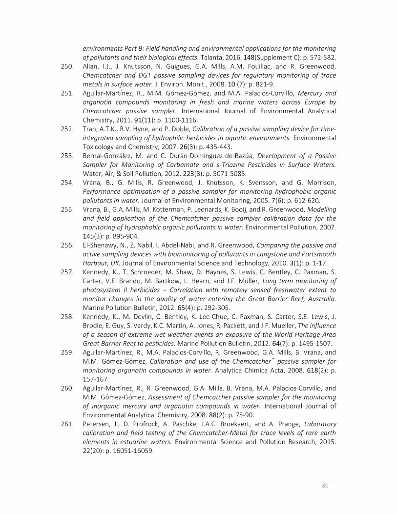
80

environments Part B: Field handling and environmental applications for the monitoring of pollutants and their biological effects. Talanta, 2016. 148(Supplement C): p. 572-582.

250. Allan, I.J., J. Knutsson, N. Guigues, G.A. Mills, A.M. Fouillac, and R. Greenwood, Chemcatcher and DGT passive sampling devices for regulatory monitoring of trace metals in surface water. J. Environ. Monit., 2008. 10 (7): p. 821-9.

251. Aguilar-Martínez, R., M.M. Gómez-Gómez, and M.A. Palacios-Corvillo, Mercury and organotin compounds monitoring in fresh and marine waters across Europe by Chemcatcher passive sampler. International Journal of Environmental Analytical Chemistry, 2011. 91(11): p. 1100-1116.

252. Tran, A.T.K., R.V. Hyne, and P. Doble, Calibration of a passive sampling device for time-integrated sampling of hydrophilic herbicides in aquatic environments. Environmental Toxicology and Chemistry, 2007. 26(3): p. 435-443.

253. Bernal-González, M. and C. Durán-Domínguez-de-Bazúa, Development of a Passive Sampler for Monitoring of Carbamate and s-Triazine Pesticides in Surface Waters. Water, Air, & Soil Pollution, 2012. 223(8): p. 5071-5085.

254. Vrana, B., G. Mills, R. Greenwood, J. Knutsson, K. Svensson, and G. Morrison, Performance optimisation of a passive sampler for monitoring hydrophobic organic pollutants in water. Journal of Environmental Monitoring, 2005. 7(6): p. 612-620.

255. Vrana, B., G.A. Mills, M. Kotterman, P. Leonards, K. Booij, and R. Greenwood, Modelling and field application of the Chemcatcher passive sampler calibration data for the monitoring of hydrophobic organic pollutants in water. Environmental Pollution, 2007. 145(3): p. 895-904.

256. El-Shenawy, N., Z. Nabil, I. Abdel-Nabi, and R. Greenwood, Comparing the passive and active sampling devices with biomonitoring of pollutants in Langstone and Portsmouth Harbour, UK. Journal of Environmental Science and Technology, 2010. 3(1): p. 1-17.

257. Kennedy, K., T. Schroeder, M. Shaw, D. Haynes, S. Lewis, C. Bentley, C. Paxman, S. Carter, V.E. Brando, M. Bartkow, L. Hearn, and J.F. Müller, Long term monitoring of photosystem II herbicides – Correlation with remotely sensed freshwater extent to monitor changes in the quality of water entering the Great Barrier Reef, Australia. Marine Pollution Bulletin, 2012. 65(4): p. 292-305.

258. Kennedy, K., M. Devlin, C. Bentley, K. Lee-Chue, C. Paxman, S. Carter, S.E. Lewis, J. Brodie, E. Guy, S. Vardy, K.C. Martin, A. Jones, R. Packett, and J.F. Mueller, The influence of a season of extreme wet weather events on exposure of the World Heritage Area Great Barrier Reef to pesticides. Marine Pollution Bulletin, 2012. 64(7): p. 1495-1507.

259. Aguilar-Martínez, R., M.A. Palacios-Corvillo, R. Greenwood, G.A. Mills, B. Vrana, and M.M. Gómez-Gómez, Calibration and use of the Chemcatcher® passive sampler for monitoring organotin compounds in water. Analytica Chimica Acta, 2008. 618(2): p. 157-167.

260. Aguilar-Martínez, R., R. Greenwood, G.A. Mills, B. Vrana, M.A. Palacios-Corvillo, and M.M. Gómez-Gómez, Assessment of Chemcatcher passive sampler for the monitoring of inorganic mercury and organotin compounds in water. International Journal of Environmental Analytical Chemistry, 2008. 88(2): p. 75-90.

261. Petersen, J., D. Pröfrock, A. Paschke, J.A.C. Broekaert, and A. Prange, Laboratory calibration and field testing of the Chemcatcher-Metal for trace levels of rare earth elements in estuarine waters. Environmental Science and Pollution Research, 2015. 22(20): p. 16051-16059.

81

262. Petersen, J., D. Pröfrock, A. Paschke, J.A.C. Broekaert, and A. Prange, Development and field test of a mobile continuous flow system utilizing Chemcatcher for monitoring of rare earth elements in marine environments. Environmental Science: Water Research & Technology, 2016. 2(1): p. 146-153.

263. Sarkar, S.K., Marine Algal Bloom: Characteristics, Causes and Climate Change Impacts. 2018, Singapore: Springer.

264. MacKenzie, L., V. Beuzenberg, P. Holland, P. McNabb, and A. Selwood, Solid phase adsorption toxin tracking (SPATT): a new monitoring tool that simulates the biotoxin contamination of filter feeding bivalves. Toxicon, 2004. 44(8): p. 901-918.

265. Roué, M., H.T. Darius, and M. Chinain, Solid Phase Adsorption Toxin Tracking (SPATT) Technology for the Monitoring of Aquatic Toxins: A Review. Toxins, 2018. 10(4): p. 167.

266. Lane, J.Q., C.M. Roddam, G.W. Langlois, and R.M. Kudela, Application of Solid Phase Adsorption Toxin Tracking (SPATT) for field detection of the hydrophilic phycotoxins domoic acid and saxitoxin in coastal California. Limnology and Oceanography: Methods, 2010. 8(11): p. 645-660.

267. Kudela, R.M., Chapter Eleven - Passive Sampling for Freshwater and Marine Algal Toxins, in Comprehensive Analytical Chemistry, J. Diogène and M. Campàs, Editors. 2017, Elsevier. p. 379-409.

268. MacKenzie, L.A., In situ passive solid-phase adsorption of micro-algal biotoxins as a monitoring tool. Current Opinion in Biotechnology, 2010. 21(3): p. 326-331.

269. Davison, W. and H. Zhang, In situ speciation measurements of trace components in natural waters using thin-film gels. Nature, 1994. 367(6463): p. 546-548.

270. Zhang, H. and W. Davison, Diffusional characteristics of hydrogels used in DGT and DET techniques. Analytica Chimica Acta, 1999. 398(2): p. 329-340.

271. Zhang, H. and W. Davison, Performance Characteristics of Diffusion Gradients in Thin Films for the in Situ Measurement of Trace Metals in Aqueous Solution. Anal. Chem., 1995. 67(19): p. 3391-3400.

272. Turner, G.S.C., G.A. Mills, M.J. Bowes, J.L. Burnett, S. Amos, and G.R. Fones, Evaluation of DGT as a long-term water quality monitoring tool in natural waters; uranium as a case study. Environmental Science: Processes & Impacts, 2014. 16(3): p. 393-403.

273. Garmo, Ø.A., O. Røyset, E. Steinnes, and T.P. Flaten, Performance Study of Diffusive Gradients in Thin Films for 55 Elements. Analytical Chemistry, 2003. 75(14): p. 3573-3580.

274. Panther, J.G., W.W. Bennett, P.R. Teasdale, D.T. Welsh, and H. Zhao, DGT Measurement of Dissolved Aluminum Species in Waters: Comparing Chelex-100 and Titanium Dioxide-Based Adsorbents. Environmental Science & Technology, 2012. 46(4): p. 2267-2275.

275. Panther, J.G., R.R. Stewart, P.R. Teasdale, W.W. Bennett, D.T. Welsh, and H. Zhao, Titanium dioxide-based DGT for measuring dissolved As(V), V(V), Sb(V), Mo(VI) and W(VI) in water. Talanta, 2013. 105: p. 80-86.

276. Dočekalová, H. and P. Diviš, Application of diffusive gradient in thin films technique (DGT) to measurement of mercury in aquatic systems. Talanta, 2005. 65(5): p. 1174-1178.

277. Ren, M., Y. Wang, S. Ding, L. Yang, Q. Sun, and L. Zhang, Development of a new diffusive gradient in the thin film (DGT) method for the simultaneous measurement of CH3Hg+ and Hg2+. New Journal of Chemistry, 2018. 42(10): p. 7976-7983.

82

278. Twiss, M.R. and J.W. Moffett, Comparison of Copper Speciation in Coastal Marine Waters Measured Using Analytical Voltammetry and Diffusion Gradient in Thin-Film Techniques. Environmental Science & Technology, 2002. 36(5): p. 1061-1068.

279. Dunn, R.J.K., P.R. Teasdale, J. Warnken, and R.R. Schleich, Evaluation of the Diffusive Gradient in a Thin Film Technique for Monitoring Trace Metal Concentrations in Estuarine Waters. Environ. Sci. Tech., 2003. 37(12): p. 2794-2800.

280. Ren, M., S. Ding, D. Shi, Z. Zhong, J. Cao, L. Yang, D.C.W. Tsang, D. Wang, D. Zhao, and Y. Wang, A new DGT technique comprised in a hybrid sensor for the simultaneous measurement of ammonium, nitrate, phosphorus and dissolved oxygen. Sci. Total. Environ., 2020. 725: p. 138447.

281. Huang, J., W.W. Bennett, D.T. Welsh, T. Li, and P.R. Teasdale, “Diffusive Gradients in Thin Films” Techniques Provide Representative Time-Weighted Average Measurements of Inorganic Nutrients in Dynamic Freshwater Systems. Environ. Sci. Technol., 2016. 50 (24): p. 13446-13454.

282. Chen, C.-E., H. Zhang, and K.C. Jones, A novel passive water sampler for in situ sampling of antibiotics. Journal of Environmental Monitoring, 2012. 14(6): p. 1523-1530.

283. Xie, H., J. Chen, Q. Chen, C.-E.L. Chen, J. Du, F. Tan, and C. Zhou, Development and evaluation of diffusive gradients in thin films technique for measuring antibiotics in seawater. Science of The Total Environment, 2018. 618: p. 1605-1612.

284. Ren, S., J. Tao, F. Tan, Y. Cui, X. Li, J. Chen, X. He, and Y. Wang, Diffusive gradients in thin films based on MOF-derived porous carbon binding gel for in-situ measurement of antibiotics in waters. Science of The Total Environment, 2018. 645: p. 482-490.

285. Xie, H., Q. Chen, J. Chen, C.-E.L. Chen, and J. Du, Investigation and application of diffusive gradients in thin-films technique for measuring endocrine disrupting chemicals in seawaters. Chemosphere, 2018. 200: p. 351-357.

286. Challis, J.K., M.L. Hanson, and C.S. Wong, Development and Calibration of an Organic-Diffusive Gradients in Thin Films Aquatic Passive Sampler for a Diverse Suite of Polar Organic Contaminants. Analytical Chemistry, 2016. 88(21): p. 10583-10591.

287. Senn, D.B., S.B. Griscom, C.G. Lewis, J.P. Galvin, M.W. Chang, and J.P. Shine, Equilibrium-Based Sampler for Determining Cu2+ Concentrations in Aquatic Ecosystems. Environmental Science & Technology, 2004. 38(12): p. 3381-3386.

288. Dong, Z., C.G. Lewis, R.M. Burgess, and J.P. Shine, The Gellyfish: An in situ equilibrium-based sampler for determining multiple free metal ion concentrations in marine ecosystems. Environmental Toxicology and Chemistry, 2015. 34(5): p. 983-992.

289. Dong, Z., C.G. Lewis, R.M. Burgess, B. Coull, and J.P. Shine, Statistical evaluation of biogeochemical variables affecting spatiotemporal distributions of multiple free metal ion concentrations in an urban estuary. Chemosphere, 2016. 150: p. 202-210.

290. Almeida, M.I.G.S., R.W. Cattrall, and S.D. Kolev, Polymer inclusion membranes (PIMs) in chemical analysis - A review. Analytica Chimica Acta, 2017. 987: p. 1-14.

291. Kuswandi, B., F. Nitti, M.I.G.S. Almeida, and S.D. Kolev, Water monitoring using polymer inclusion membranes: a review. Environmental Chemistry Letters, 2020. 18(1): p. 129-150.

292. Kolev, S.D., M.I.G.S. Almeida, and R.W. Cattrall, Chapter 27, Polymer Inclusion Membranes, in Handbook of Membrane Separations: Chemical, Pharmaceutical, Food and Biotechnological Applications, S.S.H.R. Editors: A. K. Pabby, A. M. S. Requena, Editor. 2015: CRC Press, Boca Raton. p. 723-739.

83

293. Almeida, M.I.G.S., C. Chan, V.J. Pettigrove, R.W. Cattrall, and S.D. Kolev, Development of a passive sampler for Zinc(II) in urban pond waters using a polymer inclusion membrane. Environmental Pollution, 2014. 193(Supplement C): p. 233-239.

294. Garcia-Rodríguez, A., C. Fontàs, V. Matamoros, M.I.G.S. Almeida, R.W. Cattrall, and S.D. Kolev, Development of a polymer inclusion membrane-based passive sampler for monitoring of sulfamethoxazole in natural waters. Minimizing the effect of the flow pattern of the aquatic system. Microchemical Journal, 2016. 124(Supplement C): p. 175-180.

295. Pont, N., V. Salvadó, and C. Fontàs, Applicability of a Supported Liquid Membrane in the Enrichment and Determination of Cadmium from Complex Aqueous Samples. Membranes, 2018. 8(2): p. 21.

296. Ait Khaldoun, I., L. Mitiche, A. Sahmoune, and C. Fontàs, An Efficient Polymer Inclusion Membrane-Based Device for Cd Monitoring in Seawater. Membranes, 2018. 8(3): p. 61.

297. Elias, G., S. Díez, and C. Fontàs, System for mercury preconcentration in natural waters based on a polymer inclusion membrane incorporating an ionic liquid. Journal of Hazardous Materials, 2019. 371: p. 316-322.

298. Dżygiel, P. and P.P. Wieczorek, Chapter 3 - Supported Liquid Membranes and Their Modifications: Definition, Classification, Theory, Stability, Application and Perspectives, in Liquid Membranes, V.S. Kislik, Editor. 2010, Elsevier: Amsterdam. p. 73-140.

299. Tillett, B.J., D. Sharley, M.I.G.S. Almeida, I. Valenzuela, A.A. Hoffmann, and V. Pettigrove, A short work-flow to effectively source faecal pollution in recreational waters – A case study. Sci. Total. Environ., 2018. 644: p. 1503-1510.

84

CHAPTER 2: Determination of trace levels of ammonia in marine waters using a simple environmentally-friendly ammonia (SEA) analyser

Foreword In Chapter 1, a comprehensive review of the literature regarding flow-based methodologies

for ammonia monitoring and analysis in marine environments (including estuarine, coastal and

oligotrophic ocean waters) was undertaken to develop an understanding of the advantages

and limitations of existing analytical techniques already described in the literature. While many

of the described methods were sensitive (e.g., fluorometric method), they often exhibited a

narrow working range with a complicated manifold (e.g., requiring heating of manifold

components) and or custom-made parts. This chapter describes the development and

validation of a sensitive and robust analyser, capable of ammonia determination in complex

matrices over a wide range of concentrations (relevant to both monitoring and analysis of

environmental samples and passive sampling receiving solutions), with a reasonable sample

throughput, and without requiring expensive or toxic reagents with stability issues.

The following section contains an original research paper describing the development of a

simple and environmentally-friendly ammonia (SEA) analyser to measure ammonia

concentrations in coastal and estuarine waters, the content of which was published in 2017 in

the journal Marine Chemistry.

The SEA analyser was used for the analysis of ammonia in aqueous samples collected in the

context of the development of the gas-diffusion passive sampler (Chapters 3 and 4).

O'Connor Šraj, L., Almeida, M. I. G. S., McKelvie, I. D., Kolev, S. D., (2017) Determination of trace

levels of ammonia in marine waters using a simple environmentally-friendly ammonia (SEA)

analyser, Marine Chemistry, 194, 133-145, doi.org/10.1016/j.marchem.2017.06.008

85

Graphical abstract

86

Contents Abstract 87

2.1 Introduction 88

2.2 Materials and methods 91

2.2.1 Reagents 91

2.2.2 Acceptor solution 91

2.2.3 Donor solution 92

2.2.4 Ammonia standards 93

2.2.5 Sample flushing solution 93

2.2.6 Seawater samples 93

2.2.7 Apparatus and manifold 94

2.2.8 Gas-diffusion cell and membranes 97

2.2.9 Program 98

2.2.10 Data processing 98

2.3 Results and discussion 99

2.3.1 Flow system optimisation 99

2.3.2 Flow rate and sample volume 99

2.3.3 Gas-diffusion apparatus 101

2.3.4 Acid-base indicator dyes 103

2.4 SEA analyser system and performance 105

2.4.1 Analytical figures of merit 105

2.5 Validation of SEA analyser 107

2.5.1 Measurement of certified reference materials 107

2.5.2 Spike-and-recovery studies 108

2.6 Conclusions 109

2.7 Appendix 111

Acknowledgements 112

References 113

87

Abstract A simple and environmentally-friendly ammonia (SEA) analyser based on programmable flow

was developed for the determination of trace levels of ammonia nitrogen in marine waters.

The proposed SEA analyser was based on a gas-diffusion spectrophotometric method. High

sensitivity was achieved through the use of large sample volumes and a programmable-flow

approach. The degree of pre-concentration of ammonia in the acceptor stream was

determined by the controlled and programmable delivery of the sample to the gas-diffusion

unit, and the sensitivity of the method was tailored to the concentration range of interest by

simple modification of the sample volume used for analysis. Three different working

concentration ranges were defined by varying the volume of the sample, thus making the SEA

analyser versatile and applicable for use in estuarine or coastal seawaters: 0.028 – 5.6 μM (2.0

mL), 0.28 – 13.9 μM (1.0 mL), and 1.4 – 55.6 μM (0.25 mL). Typical limits of detection of 15, 88

and 440 nM, and repeatability of 0.71, 1.2 and 0.97% RSD (n = 10), were attained for each

range, respectively. Good sample throughput was achieved with approximately 20 samples per

hour for the lower concentration range, 30 samples per hour for the middle concentration

range, and 40 samples per hour for the upper concentration range. Method validation involved

the analysis of a certified reference material in artificial seawater, and spike-and–recovery

analysis for seawater and estuarine samples collected from various locations around Nerm

(Port Phillip Bay, Victoria, Australia). Small volumes of waste (i.e. alkaline seawater feedstock

and 1.5 mL indicator solution) were generated per sample. The reagents used were non-toxic,

suitable for long-term storage, and cheap, costing as little as $2.40 AUD per 1,000

determinations.

Keywords: Ammonia; Flow analysis; Environmental monitoring; Seawater, Estuarine water

88

2.1 Introduction Ammonia nitrogen is naturally found at low concentrations in the marine environment and is

cycled in the water column by a number of different biological processes with perhaps the

most important of these processes being the assimilation of ammonium (NH4+) by

phytoplankton, nitrification and de-nitrification by bacteria and the excretion of both ammonia

(NH3) and ammonium (NH4+) by fish, invertebrates and other marine biota. It is estimated that

between 70 - 90% of gross primary production in the open oceans is based on the uptake and

assimilation of nitrogen in the ammonium form, via a process referred to as regenerated

production [1].

Higher levels of ammonia nitrogen in the marine environment can be directly and indirectly

toxic to many marine organisms. Nitrogenous pollution is increasing in aquatic ecosystems as

a result of large-scale anthropogenic run-off from agricultural land and industrial processes,

resulting in nitrogenous compounds accumulating in estuarine waters and coastal

environments [2]. Estuaries form part of a network of important nursery habitat for many

marine fish species, and high nitrogen loads in these environments can have a deleterious

impact on organism and ecosystem health [3]. Additionally, episodic pollution events may

result in large phytoplankton blooms, rapid algal growth and eutrophication, which can result

in the development of hypoxic waters [4], and/or the release of algal toxins into the water body

[5].

Monitoring of ammonia nitrogen is important in providing information about water quality to

policy makers, regulatory bodies and the community, and supports the development of

strategies to manage and conserve important fisheries, catchments and marine reserves. In

order to develop an understanding of how this chemical enters, cycles and persists in the

environment, sensitive, reliable, and preferably fast analytical methods with a wide working

concentration range are required.

Flow analysis techniques have played an important role in water analysis and monitoring [6,

7]. Several flow-based methods have been described in the literature for the photometric

determination of ammonia nitrogen in marine waters based on different chemistries, namely

the phenate method, gas-diffusion methods and the orthophthaldialdehyde (OPA) based

fluorimetric method [8]. The phenate method, known also as the Berthelot method, involves

89

the reaction between ammonia and hypochlorite to form monochloroamine, which then reacts

with phenol in the presence of catalytic quantities of nitroprusside to form the coloured

product indophenol blue [9-11]. This method is commonly employed as the standard reference

photometric method [12], however it requires the use of toxic reagents such as phenol and

nitroprusside [13], which are harmful to human health and aquatic life. Salicylate [11] and 1-

napthol [14] have been proposed as less toxic phenolic alternatives, however, when using

these reagents method sensitivity is compromised. In order to increase sensitivity, large

amounts of these reagents are required to achieve a sensitivity comparable to that in the case

of the use of phenol [15]. Furthermore, since the reaction is slow, reaction temperature of

around 80 ᵒC is required, adding extra complexity to the flow system. The use of long-path

liquid waveguide capillary cells (LWCC) (2 – 2.5 m) has been shown to provide a substantial

increase in sensitivity for the phenol-hypochlorite reaction for ammonia determination (i.e.

limit of detection in the range of 3.6 – 5 nM) [16, 17], however LWCCs are susceptible to in-

cell bubble formation as a function of increased cell length and sample filtration despite being

time consuming and laborious, is advisable to prevent difficulties with cleaning particulate

blockages [18]. In-line solid-phase extraction (SPE) has also been employed to improve method

sensitivity (i.e. limit of detection 3.5 nM), however, this is at the expense of sample throughput

with a sampling rate of 3 samples per hour achievable [19]. Hence, the use of toxic reagents,

matrix effects (such as Schlieren effects), interference from precipitation of divalent metal

cations and lack of sensitivity are the main drawbacks of the phenate method and its less toxic

versions.

Flow-based methodologies using gas-diffusion separation coupled with colorimetric pH

sensitive indicator dyes have also been employed for monitoring ammonia nitrogen in marine

water environments. By introducing a gas-diffusion unit (GDU) into the flow analysis system,

total ammonia nitrogen can be determined by alkalising the sample, converting the soluble

ammonium to gaseous ammonia, which can then diffuse across a hydrophobic porous

membrane into an acceptor solution containing an acid-base indicator, whose absorbance can

be measured using photometry [20-22]. The GDU effectively separates the analyte from the

sample matrix, allowing for improved selectivity. Refractive index (Schlieren) effects are

eliminated with the use of a GDU, and an acidic flushing solution can be used periodically to

remove any build-up of divalent metal hydroxide precipitate [22]. Unless samples are very

90

turbid, and likely to block the flow manifold, filtration is not normally needed when using a

GDU, as its hydrophobic membrane physically separates the donor stream, where the sample

is injected, from the acceptor stream, where detection takes place, thus minimizing sample

pretreatment and associated contamination risks. This method involves non-toxic reagents

that are easy to prepare and are stable. Specific flow pattern manipulations (e.g. oscillating

flow, stop-flow) [23] as well as increasing diffusion area [24] have been described to improve

method sensitivity, however, until now, reported detection limits for spectrophotometric gas-

diffusion methods have been characteristically high when compared to other methods

described in the literature (i.e. best limits of detection in the range of 50 – 210 nM) [20, 22,

25].

The fluorometric method is the most sensitive method described in the literature for the

determination of ammonia nitrogen in marine waters, with detection limits reported to be as

low as 1 - 13 nM [26-34]. The method involves the reaction of OPA with ammonia in the

presence of a reducing agent, commonly 2-mercaptoethanol or sodium sulphite, resulting in

the formation of an intensely fluorescing product. The fluorescence method has also been

coupled with gas-diffusion separation [26, 28, 32] in order to reduce interference from primary

ammines and dissolved amino acids when 2-mercaptoethanol has been used as the reducing

agent [26, 28]. Sodium sulphite, which has exhibited higher selectivity towards ammonia over

primary amines, is non-toxic and easier to handle compared to 2-mercaptoethanol because of

its superior stability, making it suitable for long-term storage and ship-board analysis [27, 32].

Under ambient temperature conditions, the OPA chemistry has a slow reaction rate (typically

3 – 4 h), requiring the incorporation of a heating unit into the manifold [35] and similarly to the

indophenol blue method, adding complexity to the analytical system. However, the major

drawbacks of the fluorescence method are the toxicity and cost of the OPA reagent.

In addition to the frequently used spectrophotometric detection, conductometric detection

has also been utilised in several flow analysis systems with gas-diffusion separation for the

determination of ammonia nitrogen in seawater [36, 37]. Conductometric detection does not

require in most cases the use of additional reagents which could be toxic, unstable or expensive

and generally provides a linear response. However, the temperature of the flow must be

strictly controlled [36] or temperature compensation mechanisms must be used [37].

Henríquez et al. reported a limit of detection in the range of 2.5 – 5 μM with a sample

91

throughput of 32 samples per hour [36] while Plant et al. achieved limits of detection for

coastal and shelf waters of 200 and 14 nM, respectively, with a sample throughput of 9 and 3

samples per hour [37].

The method described in this work aims to utilise enhanced flow manipulation in a gas-

diffusion flow system with spectrophotometric detection. Rather than injecting a discrete

sample into a flowing stream of reagents (i.e. Flow Injection Analysis) or sequential aspiration

of sample and reagents into a holding coil (i.e. Sequential Injection Analysis), both methods

being restricted by sample volume, the SEA analyser involves the continuous merging and

mixing of large sample volumes and small reagent volumes for a given period of time

depending only on the volumes necessary to achieve the desired sensitivity.

The method sensitivity was tailored to cover the range of ammonia concentrations usually

found in marine waters by simple flow manipulation, in order to achieve a limit of detection

comparable to flow-based fluorimetric methods. Hence, a simple and environmentally-friendly

ammonia (SEA) analyser is proposed.

2.2 Materials and methods

2.2.1 Reagents

Analytical grade chemicals were used for the preparation of all reagent solutions and were

used without further purification. Deionized water from a Millipore Milli-Q system (Synergy

185, France, resistivity >18 MΩ cm) was used throughout this study if not stated otherwise.

2.2.2 Acceptor solution

A 5 mM stock solution of indicator dye was prepared by dissolving 313 mg of bromothymol

blue (BDH Chemicals – pKa 7.3) and 1 mL of 1 M NaOH in 99 mL Milli-Q water and stored at

room temperature away from ambient light. The acceptor solution was prepared by 50 fold

dilution of the bromothymol blue stock into a 0.68 M NaCl solution, resulting in a final

concentration of 100 µM. Spectral scanning over the range 350 – 750 nm was used to

determine the wavelength at the absorbance maximum of the basic form of the deprotonated

92

dye (I2-), which was selected for absorbance monitoring. The pH of the acceptor solution was

adjusted by drop wise addition of 0.01 M NaOH and/or 0.01 M HCl to achieve an absorbance

of between 0.180 - 0.200 absorbance units at 615 nm, corresponding to the baseline

absorbance.

Prior to analysis, the acceptor solution was sonicated for 20 min in a glass bottle and a syringe

barrel filled with self-indicating soda lime was fitted to one of two airtight ports on the cap of

the bottle. After degassing, the headspace of the bottle was flushed with N2, and before use,

the soda lime syringe was replaced with a N2–filled balloon. As the indicator solution was

consumed during the course of analysis, the same volume of N2 was replaced in the air-tight

bottle thus preventing contact between the acceptor solution and the ambient air.

5 mM stock solutions of the indicator dyes (all Indicator Grade chemicals) bromocresol green

(BDH Chemicals – pKa 4.9), bromocresol purple (BDH Chemicals – pKa 6.4), cresol red (May &

Baker Laboratory Chemicals – pKa 8.3), meta-cresol purple (ACROS Organics – pKa 8.3), and

thymol blue (May & Baker Laboratory Chemicals– pKa 9.2) were likewise prepared according

to the procedure outlined above, resulting in final acceptor solution concentrations of 100 µM

dye. For each indicator, the wavelength at the absorbance maximum of the fully deprotonated

basic form of the dye (I2-) was determined, i.e. bromocresol green (610 nm), bromocresol

purple (590 nm), cresol red (572 nm), meta-cresol purple (578 nm), and thymol blue (596 nm).

In order to determine which dye, or dye combination exhibited the highest sensitivity, all

indicator acceptor solutions were set to a baseline absorbance of 0.200 ± 0.005 units for

comparison. For mixed indicator solutions, the desired ratios of stock solutions were mixed

and diluted with 0.68 M NaCl solution as described above, and for the dye mixtures

wavelengths were selected to fall in between the two basic absorbance maxima for the

respective indicator species.

2.2.3 Donor solution

40 g of NaOH (Chem Supply, Analytical Reagents, 98% purity) and 150 g

ethylenediaminetetraacetic acid disodium salt dihydrate (EDTA) (Chem Supply, Analytical

Reagents, ≥ 99%) were dissolved in 1 L of water and used to convert the ammonium ions

93

present in the sample solution into molecular ammonia. This solution was prepared weekly,

stored at 4 °C and sonicated for 20 min prior to use.

2.2.4 Ammonia standards

A primary stock solution of ammonium was prepared by dissolving 741.4 mg of ammonium

chloride salt (BDH Chemicals, 99.8%), oven dried at 105 °C overnight, in 250.0 mL water, having

a final concentration of 55.56 mM NH4+. A secondary stock solution was prepared by 100 times

dilution of the primary stock solution into water (i.e. 0.5556 mM NH4+). Both solutions were

stored in Teflon sealed glass bottles in the dark at 4 °C. Working solutions were prepared by

dilution of the secondary stock solution into solutions comprising 0.6 M NaCl, or with real

seawater samples for recovery and standard addition experiments.

A certified reference material (CRM) for ammonia as NH3 1,000 ± 6 mg L-1 (ERA, A Waters

Company, Lot no. 080715, Traceability against NIST SRM (194) 99.1%) was diluted and used to

determine the method accuracy by preparing solutions with known concentrations of NH4+ in

0.6 M NaCl in Milli-Q water.

2.2.5 Sample flushing solution

A solution of approximately 5 mM HCl was used to flush the donor channel of the GDU prior

to the introduction of each new sample, in order to avoid cross-contamination. A mildly acidic

solution was used instead of water, in the event that a small amount of divalent metal cation

precipitation would accumulate over long periods of analysis time, contributing to membrane

clogging, as was observed by Willason and Johnson [22].

2.2.6 Seawater samples

Sea and estuarine water samples were collected from locations in the area of Nerm (Port Phillip

Bay), Victoria, Australia. Samples were collected in 500 mL amber glass bottles and

immediately acidified with 50 µL of 10.2 M HCl to achieve an approximate pH of 3 (monitored

with universal indicator paper) and kept on ice during transport. All samples were transferred

94

to high density polyethylene plastic bottles and stored for no longer than 3 days in the dark at

4 C. The clean-up protocol for all collection and storage containers, and other equipment that

came into contact with the samples involved a 3 x wash with water, followed by 3 x wash with

5 mM HCl, and finally a 3 x wash with water. Clean equipment was dried and stored in zip-lock

bags, and clean glassware was dried, and lids were used to seal containers from dust.

The seawater samples collected at the Werribee study sites were visibly turbid and required

filtration using 0.45 μm syringe filters. Spike-and-recovery tests were performed for seven

marine water samples, including estuarine water samples collected from the Yarra River at

Docklands.

2.2.7 Apparatus and manifold

The flow manifold of the SEA analyser developed for the spectrophotometric detection of

ammonia nitrogen in seawater using gas-diffusion separation is shown in Figure 2-1.

Figure 2-1. Schematic diagram of the fully automatic SEA analyser using a FiaLab 3500 flow system and Cetac autosampler. SP, syringe pump; BTB, bromothymol blue; N2, nitrogen.

A FIAlab 3500 flow injection analyser fitted with a 10 mL syringe pump (Tecan, Cavro XLP), an

8 port multiposition valve (MPV) and a peristaltic pump (FIAlab instruments, Bellevue, WA,

95

USA) controlled by FIAlab software (version 5.9.314 for Windows) was used for all experiments.

The syringe pump (SP 1) was connected to a 5 mL holding coil, constructed from Teflon® tubing

(1/8” OD and 0.062” ID) and two Peek flangless nuts. Teflon tubing (1/16” OD and 0.03” ID)

and a mixture of Peek and Acetal flangeless nuts were used for connecting all other parts of

the flow system.

Two GDUs were used in the SEA analyser: one for the alkaline solution clean-up (the ‘scrubber’)

and another for the separation and pre-concentration of ammonia from the marine samples

into a solution containing a pH sensitive colorimetric indicator dye. The ‘scrubber’ comprised

a straight-channelled sandwich style GDU with 31.5 cm channel length, 2 mm width and 1.5

mm depth (i.e. 945 µL volume). The acceptor stream of this GDU contained a stripping solution

(i.e. 0.5 M H2SO4 and crystal violet indicator), which was recirculated via the peristaltic pump

and removed trace ammonia contamination from the NaOH/EDTA reagent solution. Crystal

violet was added to this solution to indicate if the membrane in the scrubber had become

compromised.

The main GDU used for the majority of the experiments comprised a sandwich-type

configuration, with serpentine-shaped channels made from 9.5 cm Perspex blocks that were

sandwiched together with 8 stainless steel screws. The height and width of the unit were 1.5

cm and 2.3 cm, respectively. Two identical 100 mm long serpentine channels were bored into

each piece of Perspex at a depth of 0.5 mm and width of 2 mm [23]. Each end of the Perspex

blocks had an inlet and an outlet port that were connected to the tubing with flangeless nuts

(for 1/16” tubing). The donor channel was always facing downwards and the acceptor channel

was always facing upwards in order to facilitate the migration of ammonia gas from the donor

to the acceptor channel [23]. Both channels of the GDU were separated by a mechanically

stable, super hydrophobic gas-diffusion membrane with 0.1 μm pore size (SureVent®, Merck

Millipore), which was suitable for use under high flow rate conditions. Flow rates of 4.5 mL

min-1 and 1.2 mL min-1 were used for delivery of the indicator solution to the acceptor channel,

and the sample and alkaline solutions to the donor channel of the GDU, respectively (refer to

the Programmable Flow Procedure, Table A2-1 in the Appendix).

Where possible, short lines were used to reduce sample dispersion and enhance sensitivity.

Therefore, the tubing connecting the acceptor channel to the flow cell was 11.5 cm in length,

96

allowing for the reference absorbance measurement to be taken before the indicator sample

plug entered the flow cell. The two external Cavro Tecan syringe pumps (SP 2 and SP 3), fitted

with 2.5 mL syringe barrels (Tecan, Cavro, XC/XP), and the autosampler (Teledyne, CETAC

Technologies, ASX-260) were programmed for use with the FIAlab 3500 analyser.

The detection system comprised a USB4000 CCD spectrophotometer (Ocean Optics) and a LS-

1 tungsten-halogen light source (Ocean Optics) connected by two 200 µm quartz optical fibres

(Ocean Optics) to the 1 cm flow cell of the in-built MPV (Figure 2-1). SP 1 was used for the

aspiration of large sample volumes into the holding coil, subsequent propulsion of the sample

to the 20 cm mixing coil and donor channel of the GDU, and for cleaning the lines with a mildly

acidic sample flushing solution (5 mM HCl). A 20 μL air bubble was aspirated into the holding

coil to separate the sample plug from the 5 mM HCl in order to prevent dispersion when

aspirating or dispensing the sample.

SP 2 was used to deliver the indicator solution to the acceptor channel of the main GDU, which

was connected to the 1 cm flow cell of the MPV. Bromothymol blue in 0.68 M NaCl solution

was the indicator used for most experiments and monitoring of the basic indicator species was

undertaken at 615 nm. A reference wavelength of 750 nm was selected to correct for any

optical interferences in the acceptor solution.

SP 3 was used to deliver a solution of NaOH and EDTA to the two GDUs, the former being the

‘scrubber’ and the latter being the main GDU (Figure 2-1). The NaOH and EDTA stream passed

through the ‘scrubber’ GDU, prior to being merged with the sample stream.

The peristaltic pump was operated with Tygon pump tubing (TACS, Australia), orange-yellow

(0.51 mm ID) for the recirculation of 0.5 M H2SO4 stripping solution and grey-grey (1.30 mm

ID) for sample delivery to Port 5 (sample port) of the MPV. Approximately 1.5 mL of sample is

required to prime the autosampler tubing and the sample port of the MPV, prior to

introduction of a sample into the holding coil.

The autosampler tubing was modified to allow for rapid aspiration of samples into the holding

coil, by connecting the autosampler needle to Port 5 of the MPV with white-white (1.02 mm

ID) Tygon tubing.

97

2.2.8 Gas-diffusion cells and membranes

A number of different GDU configurations (Figure 2-2) were performance tested alongside a

number of different porous hydrophobic membranes, with the specifications listed in Tables

2-1 and 2-2, respectively.

Figure 2-2. Different GDU configurations tested in order to select the configuration that achieved the highest sensitivity. The SureVent® membrane was used for the sandwich type GDUs, including the single (Serpentine x1) (a), double (Serpentine x2) (b), micro (μGDU) (c). Accurel® capillaries were used for the construction of the single (d), and multi hollow fibre (e) tubular GDUs.

Table 2-1. Gas-diffusion configurations comparing various aspect ratios (exposed membrane area to channel volume ratio).

Configuration Aspect ratio (cm2 mL-1)

Channel length (mm)

Width (mm)

Depth (mm)

Diameter (mm)

Pore size (μm)

Hydrophobic membrane (supplier)

Sandwich – serpentine channel (Figure 2-2a)

20 100 2 0.5 - 0.1 SureVent super hydrophobic PVDF (Millipore)

Sandwich – double serpentine channel (Figure 2-2b)

20 220 2 0.5 - 0.1 SureVent super hydrophobic PVDF (Millipore)

Sandwich – straight channel μGDU (Figure 2-2c)

10 20 1 1 - 0.1 SureVent super hydrophobic PVDF (Millipore)

Single tubular membrane (Figure 2-2d)

52 110 - - 0.75 0.2 Accurel PP capillary (Membrana)

Multi tubular membrane (n=6) (Figure 2-2e)

241 150 - - 0.75 0.2 Accurel PP capillary (Membrana)

PP – polypropylene

98

Table 2-2. Hydrophobic membranes tested.

Configuration Hydrophobic membrane Pore size (μm)

Channel length (mm)

Width (mm)

Diffusion area

(mm2)

Flat membrane, serpentine flow path

SureVent Superhydrophobic PVDF (Millipore)

0.1 100 2 200

Flat membrane serpentine flow path

Durapore PVDF (Millipore) 0.2 100 2 200

Flat membrane serpentine flow path

Plumbers tape PTFE (Reece) Un-specified 100 2 200

Flat membrane serpentine flow path

High density PTFE (Shamban) Un-specified 100 2 200

Flat membrane serpentine flow path

Heavy duty pink PTFE (Boston) Un-specified 100 2 200

Single tubular membrane

Accurel PP hollow fibre (Membrana)

0.2 110 - 260

PVDF – polyvinylidene difluoride, PTFE – polytetrafluoroethylene, PP – polypropylene

The sandwich type single block serpentine GDU described above using SureVent®

superhydrophobic 0.1 μm pore size membrane was robust under high flow rates and provided

good sensitivity. Therefore, it was used for all experiments except for the GDU and membrane

optimisation experiments.

2.2.9 Program

Determination of ammonia nitrogen in seawater using the SEA analyser was achieved using

the programmable flow procedure outlined in Table A2-1 (Appendix).

2.2.10 Data processing

FIAlab software version 5.9.314 for Windows was used with Microsoft Excel for data processing

of all experimental data. Peak maximum (‘local maximum’) was used as the analytical signal,

and each sample was measured in triplicate with the average signal used for all calculations.

The Excel Solver function was used to compute the sample concentrations utilizing non-linear

calibration equations, and the limits of detection and quantification were determined using

99

the error of the lower linear portion of the calibration equations, as described by Miller and

Miller [38].

2.3 Results and discussion

2.3.1 Flow system optimization

Flow system optimisation experiments were undertaken to improve method sensitivity and are

described in detail below. The effects of varying matrix salinity and interference from primary,

secondary and tertiary amines were not assessed in this work, as such studies were undertaken

and described in detail by Segundo et al. [21] and Oliviera et al. [24], respectively, showing

there was no interference from solutions prepared with differing salinities, and no statistically

significant difference in peak response between spiked and un-spiked samples for a number of

ammine species, even when present in concentrations higher than those expected in marine

waters.

2.3.2 Flow rate and sample volume

A stop-flow approach [24] was chosen as a strategy to maximize the SEA analyser efficiency. In

all optimization experiments the acceptor stream was stopped in the GDU until the sample

zone had passed through the donor channel of the GDU.

The flow rate of the donor stream is expected to affect how much ammonia can pass through

the hydrophobic membrane into the acceptor solution. A low flow rate will result in the sample

zone spending a longer duration of time in the GDU, thus facilitating the diffusion of molecular

ammonia into the acceptor stream. However, this is at the expense of sample throughput. In

turn a higher flow rate will result in the sample passing through the GDU more quickly and thus

the efficiency of mass transfer of molecular ammonia across the membrane is reduced. There

is a trade-off between achieving high sensitivity whilst simultaneously achieving an acceptable

sample throughput. Low flow rates provided relatively higher absorbance signals when

compared to higher flow rates (Figure 2-3a), however, sample throughput was reduced by

decreasing the flow rates. For a 1 mL sample volume (where 0.2 mL alkaline solution was used

to increase the sample pH), the flow rate of 1.2 mL min-1 was chosen as the optimum flow rate,

as it allowed for sufficient amount of molecular ammonia to diffuse into the acceptor solution,

100

whilst ensuring a reasonable sample throughput of 2 min per sample volume of 1 mL. However,

whilst lower flow rates prolonged the lifetime of the GDU membrane (i.e. Millipore SureVent®

‘super-hydrophobic’ membrane), flow rates higher than 4 mL min-1 required the membrane to

be changed more frequently, and given that priming the membrane was a time-consuming

process, it was decided that such high flow rates for sample delivery should be avoided.

Similarly, to flow rate, the sample volume is likewise expected to affect how much analyte can

be pre-concentrated into the acceptor solution. By simply increasing the sample volume

dispensed through the donor channel of the GDU, the number of ammonia molecules diffusing

across the porous hydrophobic membrane into the stagnant acceptor solution also increased,

thus improving analyte pre-concentration (Figure 2-3b). However, larger sample volumes

allowed for an increase in sensitivity at the expense of sample throughput. Therefore, it was

important to determine the appropriate sample volume to use for each ammonia

concentration range of interest. A 2 mL sample with 0.4 mL of alkaline reagent, 1 mL sample

with 0.2 mL of alkaline reagent and 0.25 mL sample with 0.05 mL of alkaline reagent were the

optimal sample and reagent volumes found to provide good sensitivity and sample throughput

for the concentration ranges 0.028 – 5.6, 0.28 – 13.9, 1.4 – 55.6 μM NH4+, respectively.

Figure 2-3. (a) Effect of the donor stream flow rate on the analytical signal for three different ammonium standards: blank (○), 1.4 μM () and 2.8 μM ().The conditions of the experiment are as follows: Sample volume, 1 mL; alkaline solution volume (NaOH and EDTA), 0.2 mL; acceptor stream flow rate, stop-flow, each data point is the average of 3 replicate injections. (b) Effect of the sample and reagent volume on the maximum absorbance for three different ammonium standards: blank (○), 1.4 μM () and 2.8 μM (). The conditions of the experiment are as follows: Alkaline solution volume (NaOH and EDTA), 0.2 mL; donor stream flow rate, 1.2 mL min-1; acceptor stream flow rate, stop-flow, each data point is the average of 3 replicate injections.

(a) (b)

101

2.3.3 Gas-diffusion apparatus

Parameters such as surface area, GDU configuration and membrane porosity, are known to

affect gas-diffusion and were investigated. For large sample volumes, GDUs with a large aspect

ratio are desirable to facilitate high contact between the sample and the membrane, which will

in turn allow for greater diffusion and mass transfer of molecular ammonia to the indicator

solution resulting in enhanced sensitivity. Pore size is likewise an important factor to consider

in terms of mass transfer efficiency.

Several GDU configurations (Figure 2-2, Table 2-1) were tested, namely sandwich-style GDUs

and hollow fibre type [39]. A small increase in sensitivity was achieved using the double

serpentine GDU (i.e. two serpentine GDUs) when compared to the single serpentine GD cell

(Figure 2-4a). However, as the double serpentine GDU consisted of two single GDUs joined

together by two Teflon two-way flangeless connectors for 1/16” tubing (one connecting the

donor channels and the other connecting the acceptor channels), a double-humped peak

appeared, where the dip between the two humps resulted from the acceptor solution held

static in the connecting tubing, where no diffusion had occurred. For this reason, it was not

used further.

A tubular GDU was constructed using a single hydrophobic microporous hollow fibre (0.03” ID,

Accurel®, Membrana) inserted into a piece of silicone tubing (red – red, Tygon) where each

end was fitted with a glass T-piece, with the hollow fibre being fixed into place using epoxy

glue and pipette tips. The space between the silicone tube and the hollow fibre corresponded

to the donor channel, and the hollow fibre was the acceptor channel. The pipette tips and the

glass T-piece ends were connected to the two ends of the hollow fibre using small pieces of

silicone tubing. Whilst this GDU provided an approximate three-fold increase in sensitivity

compared to the sandwich style GDUs (Figure 2-4a), there was a significant contamination

problem when using epoxy glue to fix the hollow fibre in place. Many commercial epoxy resin

glues consist of one part epoxide and one part tertiary ammine. The unreacted ammines on

the surface of the hardened resin, when in contact with the alkaline solution, diffused across

the hollow fibre walls resulting in a very large blank response. After several hours of flushing

with water to remove unreacted tertiary ammine on the surface of the epoxy glue, the blank

signal appeared to decrease. However, it was still present and the standard deviation for

replicate samples was high. Due to these interference effects the tubular GDU was discarded.

102

The small surface area of the μGDU resulted in insufficient sensitivity (Figure 2-4a), and the

multi hollow fibre in chamber GDU had substantial problems with bubbles getting trapped in-

between each of the fibres, where it was impossible to dislodge them, reducing the sensitivity

of this type of GDU despite the high aspect ratio (Figure 2-4a, Table 2-1). Moreover, it was

similarly constructed with expoy glue, which also meant it had a large blank response.

The sandwich-style single serpentine GDU was therefore chosen for further experiments. It

was easy to use, as bubbles did not present as a problem, and it could be easily flushed out

with each new sample. High flow rates were able to be used with this GDU configuration with

little problem.

A number of different porous hydrophobic membranes were tested (Figure 2-4b), with pore

sizes specified for some, and pore sizes un-specified for commercial plumbing membranes

(Table 2-2). All membranes required some degree of priming (a process where water is

continuously flushed through the GDU to remove all bubbles appearing on the surface of the

porous hydrophobic membrane), with the PTFE membrane requiring on average a couple of

hours compared to the SureVent® and Durapore® membranes requiring between one to two

days. However, despite longer priming times when compared to their PTFE counterparts, both

Durapore® and SureVent® membranes exhibited superior mechanical stability. Durapore® was

able to be used for approximately 1 week under high flow rate conditions, and SureVent® for

several months. All other membranes exhibited some degree of membrane deformation under

high flow rate conditions. Despite the long priming time, and slightly lower sensitivity (Figure

2-4b) SureVent® was the membrane of choice. SureVent® is a mechanically stable membrane,

which has been treated to give extra hydrophobicity compared to its Durapore® counterpart.

As a result of this treatment, these membranes lasted longer under high flow rate conditions.

The smaller pore size of the SureVent® membrane is likewise desirable, as although it may

compromise sensitivity a little, it provides better membrane stability at higher flow rates and

can be expected to be more effective at reducing interference from large molecular mass

ammines. All commercial plumbing tapes were very soft and prone to distortion.

103

Figure 2-4. (a) Performance of different GDU configurations where the blank response which was different for each type of GDU configuration, was subtracted from the two ammonium standards (grey bar, 1.4 μM and the black bar, 5.6 μM) in order to simplify the comparison of GDU configuration sensitivity. The SureVent® membrane was used for the single (Serpentine x1), double (Serpentine x2), and micro (μGDU) sandwich type GDUs and Accurel® filaments were used in the construction of the single and multi hollow fibre tubular GDUs. Each data point is the average of 3 replicate injections. (b) Performance of different porous hydrophobic membranes was examined using the sandwich type GDU for all membranes except for the Accurel® tubular filaments from Membrana. The blank signal for each different membrane was subtracted from the signals for the two ammonium standards (grey bar, 1.4 μM; black bar, 5.6 μM) to allow for a comparison of membrane sensitivity. HF is defined as hollow fibre for both figures (a) and (b). Each data point is the average of 3 replicate injections.

2.3.4 Acid-base indicator dyes

In order to determine the optimum acceptor solution composition for trace determination of

ammonia nitrogen in seawater, a number of spectrophotometric acid-base indicator dyes were

examined. Factors known to affect the sensitivity of the acceptor solution are the pKa and

molar absorptivity of the indicator [40], acceptor solution pH, buffering capacity and indicator

concentration [41-43], and ionic strength [22]. Additionally, Schulze et al. [40] describe that

the pH of the acceptor solution should be adjusted close to the equivalence point of the

indicator in order to achieve maximum sensitivity. However, it should be taken into

consideration that the higher the baseline absorbance, the narrower the working range. The

baseline absorbance for this method was therefore set to between 0.180 - 0.200 (Figure 2-5a)

when running real samples.

Several indicator dyes and dye mixtures were selected for analysis according to their respective

pKa values. Acceptor solutions were prepared by making small adjustments to the pH in order

(a) (b)

104

to achieve a baseline absorbance of 0.200 ± 0.005 for each solution. The analytical signals for

the ammonium standards (1.4 and 2.8 μM) after blank correction, were used to compare the

sensitivity of each acceptor solution (Figure 2-5b). Bromothymol blue (BTB) was the indicator

chosen for method development, because it exhibited the highest sensitivity compared to all

indicator solutions tested.

A mixture of several indicators can increase the working range of the method, whilst

maintaining sensitivity, provided there is a maximum of 1 pH unit difference between the pKa

values of the individual indicators, the basic forms have similar molar absorptivity values and

that the respective indicator dyes absorb at approximately the same wavelength [44].

The dynamic range of the method using a quadratic calibration equation can be extended by

simply combining two or more different indicators as shown in Figure 2-5c, where the range

was extended by 2.8 μM NH4+ when thymol blue was used in combination with BTB. However,

whilst the working range of the method can be extended by using a combination of indicators,

sensitivity is slightly compromised. Therefore, one must decide which of these factors is more

important when choosing an appropriate acceptor solution composition.

105

Figure 2-5. (a) Blank corrected absorbance response for for 1.4 μM (○) and 2.8 μM (◊) ammonium standards as a function of baseline absorbance (100 µM bromothymol blue acceptor solution containing 0.68 M NaCl). Each data point is the average of 3 replicate injections. (b) Absorbance response for different colour indicator dye solutions, as single dyes or as mixtures. The graph shows the blank corrected response for 1.4 μM (grey bar) and 2.8 μM (black bar) ammonium standards to highlight the sensitivity in the case of each indicator solution. Mixed indicator solutions were prepared in equal proportions of each indicator, and the numbers in brackets indicate the pH of the indicator solution at which the experiment was undertaken. Each data point is the average of 3 replicate injections. (c) The working range of the method can be extended when mixed indicator solutions are used, provided the pKa’s of the respective indicators selected do not vary by more than 1 pH unit. The range of the 1:1 ratio BTB + thymol blue solution (○)(y = (8.1186x10-4)x2 + (4.8406 x10-2)x + 5.0921x10-

2, R2 = 99.737) could be extended by up to 2.4 μM NH4+ compared to the solution of BTB only () (y =

(1.7778x10-3)x2 + (4.7322x10-2)x + 7.7463x10-2, R2 = 99.938). Each data point is the average of 3 replicate injections.

2.4 SEA analyser system performance

2.4.1 Analytical figures of merit

Three different working ranges were obtained by simple manipulation of the analyser control

program, specifically by setting different sample volumes, namely 2.0, 1.0 and 0.25 mL, with

typical calibration curves provided in Figure 2-6. For low concentration ammonia nitrogen

(a)

(c)

(b)

106

samples, larger volumes were required to achieve sufficient pre-concentration in the GDU, and

conversely for high concentration samples, smaller volumes sufficed. Hence, an overall range

of 0.028 – 55.6 μM NH4+ could be covered.

Figure 2-6. Three typical concentration working ranges based on sample volume: (a) () 0.028 – 5.6 μM NH4

+, sample volume 2.0 mL; (b) () 0.28 – 13.9 μM NH4+, sample volume 1.0 mL; and (c) (○) 1.4 – 55.6

μM NH4+, sample volume 0.25 mL. The corresponding calibration equations and coefficients of

determination are shown in Table 2-3. Each data point is the average of 3 replicate injections.

The respective analytical figures of merit for each typical working range are outlined in Table

2-3. The limits of detection and limits of quantification were determined using the error of the

regression described by Miller and Miller [38], and second order polynomial regressions were

used to describe the dynamic range. The LINEST function in Microsoft Excel was used to

calculate the standard deviation of the estimate of the regression coefficients.

(a) (b)

(c)

107

Table 2-3. Analytical figures of merit of the SEA analyser for three typical working ranges (Figure 2-6).

Ammonium concentration range

0.028 – 5.6 µM Figure 2-6(a)

0.28 – 13.9 µM Figure 2-6(b)

1.4 – 55.6 µM Figure 2-6(c)

Repeatability (% RSD) n=10

± 0.71 (0.556 µM)* ± 1.2 (4.16 µM)* ± 0.97 (13.89 µM)*

LOD (nM) 15 88 440

LOQ (nM) 50 290 1,500

Sampling rate (h-1) 20 30 40

Sample volume (mL) 2.0 1.0 0.25

Calibration equation y = (1.6157 ± 0.0852)x10 -5 x2 + (6.8460 ± 0.0827)x10-3 x + (1.6499 ± 0.0089)

y = (5.0627 ± 0.5173)x10-6 x2 + (2.2094 ± 0.1280)x10-3 x + (0.12862 ± 0.0052)

y = (4.8545 ± 0.4860)x10-7 x2 + (4.3545 ± 0.4725)x10-4 x +(2.6182 ±0.6314)x10-2

Coefficient of determination, R2

99.994 99.921 99.886

* Concentration used to determine the repeatability

2.5 Validation of the SEA analyser

2.5.1 Measurement of certified reference materials

The accuracy of the newly developed SEA system was determined using a Certified Reference

Material (CRM). Four different dilutions of the CRM spanning the concentration range 0.28 –

11.1 μM NH4+ were analysed. The results for the lower concentrations (0.28 and 0.56 μM) had

predictably higher errors than those for the higher concentrations (5.0 and 11.1 μM NH4+), as

shown in Table 2-4. These observations are consistent with results achieved for similar

analytical methods developed for the monitoring of nutrients [45], and dissolved Fe(II) [46] in

complex matrices, and in line with guidelines established for the validation of analytical

methods that specify that the concentration of CRMs should be between 75 % - 80 % at the

lower end, and 120% - 125% at the upper end of the stated or known value [47, 48].

Table 2-4. Method validation using a diluted CRM in 0.6 M NaCl, for the calibration range 0.28 – 13.9 µM NH4

+ (Table 2-3).

Nominal Concentration of Standards (μM NH4

+) Concentration of Standards

Measured (μM NH4+)

Relative Standard Deviation (%)

Relative Error (%)

0.28 0.20 ± 0.03 12.6 ± 29.3 0.56 0.60 ± 0.04 6.5 ± 8.5 5.0 4.9 ± 0.05 1.0 ± 1.9

11.1 11.2 ± 0.04 0.4 ± 0.5

108

2.5.2 Spike-and-recovery studies

Seawater and estuarine samples collected from around Nerm (Port Phillip Bay) and Bancoora

Surf Beach, (Victoria, Australia) were analysed directly by the proposed SEA analyser and the

results are shown in Figure 2-7.

Figure 2-7. Sampling sites around the Port Phillip Bay Study Area with the average range of concentrations of ammonia nitrogen measured with the SEA analyser (○).

Seawater and estuarine water of seven locations was used for spike-and-recovery analysis. In

one of the locations (South Melbourne) seawater was collected on two different days. The

concentrations obtained fell between 0.56 – 2.2 μM NH4+ at the different locations, allowing

for the 0.28 – 13.9 µM calibration equation (Table 2-3) to be used with 1.0 mL sample volumes.

These samples were spiked with three different concentrations of ammonium stock solution,

namely 0.56, 5.0 and 10.6 μM, which were selected in order to test the performance of the

method at the low, mid and upper sections of the calibration range. The recoveries obtained

for the spiked samples are presented in Figure 2-8. At the lower end of the range (i.e. samples

spiked with 0.56 μM ammonia) some variability was observed with recoveries between 83.5 –

109

116.5 %, which is reasonable considering this falls at the lower end of the calibration curve

where there is a greater inherent error due to the lower signal to noise ratio. Recoveries within

90.0 – 99.4 % and 97.0 – 103.3 % were obtained for the samples spiked with 5.0 and 10.6 μM,

respectively.

Figure 2-8. Spiked recoveries of seawater samples of varying salinity from around Port Phillip Bay (PPB), and Bancoora Surf Beach. Three different ammonium concentrations were used to spike the samples: 0.56 (grey bar), 5.0 (crosshatched bar) and 10.6 µM (black bar), respectively. The numeric values after the location description indicate the date of sample collection (dd.mm.yy) and the value in brackets corresponds to the salinity of the samples using the Practical Salinity Scale 1978 [49].

2.6 Conclusions A highly sensitive programmable flow analysis method for the trace determination of ammonia

nitrogen in seawater has been described using the newly developed SEA analyser. This flow

system enables the sensitivity of the method to be tailored to the concentration range of

interest, by simple modification of the program involving appropriate adjustment of the

sample volume. Manifold changes are not necessary to achieve a wide working range, making

this method practical, versatile and applicable for use in coastal and oceanic environments.

The method developed employs a novel flow approach whereby large sample volumes and

small reagent volumes are continuously merged and delivered to the donor channel of the

110

GDU under stop-flow conditions, rather than using discrete sample plugs as described in the

literature for flow injection and sequential injection analysis methods for ammonia nitrogen

determination in natural waters [20-22, 26, 28, 50]. Whilst Segundo et al. described a

spectrophotometric sequential injection method capable of achieving two dynamic ranges by

making small changes in the protocol sequence (i.e. 5.5 – 55 and 55 - 222 μM NH4+) for example

by doubling the number of sample and sodium hydroxide plugs aspirated into the holding coil

[21], the range achieved was narrower than that of the newly developed method, with a

detection limit of two orders of magnitude higher (i.e. 1.5 μM NH4+). The conductometric

method developed by Plant et al. provided comparable detection limits to those described in

this work (i.e. 14 nM for shelf waters), by increasing the number of sample pulses delivered to

the GDU and decreasing the flow rate, however the sample throughput was compromised

allowing for a little over 3 samples per hour to be measured [37]. Whilst this sampling

frequency may be appropriate for in situ analysis, it would be unsuitable for use during

shipboard analysis or for use in a laboratory setting. In addition, while the components used in

the method of Plant et al. are commercially available, the in-house modification of the

conductivity cell, manufacturer modification of the micro solenoid pumps and detector board,

and the use of custom software to control the data logger/controller may impede the

accessibility of this method to potential users.

In the proposed method, high flow rates of the donor stream under stop-flow conditions for

the acceptor stream were achievable using the mechanically stable superhydrophobic

SureVent® microfiltration membrane (Millipore) in the GDU, allowing for good sample

throughput to be achieved for all ranges with approximately 20 samples per hour achieved for

the low concentration range, 30 samples per hour for the mid-range and 40 samples per hour

for the upper range. The following working ranges were obtained by sample volume

adjustment, 0.028 – 5.6 (2.0 mL sample volume), 0.28 – 13.9 (1.0 mL sample volume), 1.4 –

55.6 μM NH4+ (0.25 mL sample volume). These ranges are characterised by typical limits of

detection of 0.015, 0.088 and 0.44 μM NH4+, respectively, with the sensitivity for the lowest

range comparable to some fluorometric detection methods described in the literature [30, 33,

51].

Spike-and-recovery analysis produced good results, and method validation using a CRM

showed that in the mid-to upper calibration range the error was minimal. These results

111

illustrate the potential of the newly developed method for reliably determining ammonia

nitrogen in seawater samples over a wide and realistic concentration range.

2.7 Appendix Table A2-1. Programmable flow procedure for the determination of ammonia nitrogen in seawater.

Step Commands Corresponding Actions 0 Hardware Settings Wavelength 1 (nm) 615

Hardware Settings Wavelength 4 (nm) 750 Hardware Use Wavelength 4 as Reference Hardware Settings Optimize Integration Peristaltic Pump Clockwise(%) 65

Instrument settings and measurement parameters defined at the outset of experiment. Ensure all lines have been primed, bubbles expelled and syringe barrels emptied prior to analysis.

1 Loop Start (#) 3 Next Sample Analyte New Sample Peristaltic Pump On SP Sample Valve Out SP Sample Flowrate (microliter/sec) 200 SP Sample Aspirate (microliter) 1500* SP Indicator Valve Out SP Indicator Flowrate (microliter/sec) 200 SP Indicator Aspirate (microliter) 1500 SP NaOH Valve Out SP NaOH Flowrate (microliter/sec) 100 SP NaOH Aspirate (microliter) 200* SP Indicator Delay Until Done Autosampler Pump Off

Define next sample, and send autosampler to sample reservoir. 3 replicates to be analysed defined by Loop Start (#) 3. SP-Sample, SP-Indicator and SP-NaOH syringes fill, whilst the peristaltic pump delivers sample to port 5 of MPV ensuring that ample sample passes through the tubing to prime lines. SP-Sample fills with an acidic flushing solution, which is delivered to the GDU after each aliquot of sample, to prevent clogging of the gas-diffusion membrane by divalent cations precipitating from the highly alkaline seawater. Autosampler pump switched off after washing from previous sample.

2 SP Indicator Valve In SP Indicator Flowrate (microliter/sec) 75 SP Indicator Dispense (microliter) 750 Peristaltic Pump Off SP Sample Valve In Multiposition Valve AIR SP Sample Aspirate (microliter) 20 SP Sample Delay Until Done Multiposition Valve Sample SP Sample Flowrate (microliter/sec) 200 SP Sample Aspirate (microliter) 1000* SP Sample Delay Until Done

Indicator solution is dispensed to the acceptor chamber of the GDU where it is held static. A 20 μL air bubble is aspirated into the holding coil to prevent contact and subsequent dispersion of the sample with the acidic flushing solution. Sample is aspirated into the holding coil at a high flow rate of 200 L min-1.

3 SP NaOH Valve In Multiposition Valve GD Cell SP Sample Flowrate (microliter/sec) 20 SP Sample Dispense (microliter) 2500* SP NaOH Flowrate (microliter/sec) 4 SP NaOH Dispense (microliter) 200** SP NaOH Delay Until Done

Sample and alkaline solution are merged in the mixing coil and continuously delivered to the donor chamber of the GDU. During this time, the acceptor channel is held static allowing pre-concentration of ammonia into the acceptor solution in the GDU. Once the sample has passed through the GDU, the bubble will pass and the acidic flushing solution will clean the donor chamber of the GDU and all tubing.

4 SP Indicator Flowrate (microliter/sec) 10 SP Indicator Dispense (microliter) 750 Spectrometer Reference Scan Spectrometer Absorbance Scanning Autosampler Pump On Delay (sec) 10 SP Indicator Flowrate (microliter/sec) 30

SP-Indicator is engaged and the spectrometer takes the reference scan, immediately followed by continuous absorbance scanning. It takes approximately 5 seconds before the plug of indicator where the ammonia has been concentrating passes through the spectrophotometric flow-through cell.

Continued on next page

112

SP Sample Flowrate (microliter/sec) 75 Delay (sec) 2 Spectrometer Stop Scanning

The autosampler pump is turned on to flush the needle washing chamber with fresh water.

5 Peristaltic Pump On Autosampler Wash Autosampler Wash Peristaltic Pump Off SP Sample Stop*** Multiposition Valve Waste*** SP Sample Flowrate (microliter/sec) 200*** SP Sample Empty*** SP Sample Delay Until Done*** Loop End

Peristaltic pump is switched on whilst the autosampler needle is washed. This allows for small volumes of water to be drawn into the tubing flushing any residual sample to waste prior to aspiration of next sample.

***Any remaining flushing solution is expelled from the SP-Sample and holding coil via the waste port of the MPV.

* Commands highlighted in BOLD can be modified to achieve desired sensitivity and concentration range. ** For every 1 mL sample, 200 μL NaOH/citrate are needed, therefore this volume is adjusted according to the sample volume used. *** These commands are only used for samples larger than 1 mL. This is because it takes longer for the SP-Sample to deliver 1.5 mL of flushing solution, than it does for the program to run to the end of the loop. Therefore, for samples larger than 1 mL SP-Sample is flushed with acidic flushing solution whilst the absorbance measurements are being collected, however, after the run is finished and prior to the loop end, the MPV is directed to waste, and the remaining solution is dispensed to at a rate much more rapid than what could be passed through the GDU. No carryover was observed.

Acknowledgements We are grateful to the Australian Research Council (Linkage Grant LP110200595)) for financial

support and to Mr Andrew Longmore and the Centre for Aquatic Pollution Identification and

Management in assisting with the collection of samples in the Nerm (Port Phillip Bay study

area). Lenka O’Connor Šraj is grateful to the University of Melbourne for the award of a

postgraduate scholarship.

113

References 1. Karl, D.M., R.R. Bidigare, M.J. Church, J.E. Dore, R.M. Letelier, C. Mahaffey, and J.P. Zehr,

Chapter 16 - The Nitrogen Cycle in the North Pacific Trades Biome: An Evolving Paradigm, in Nitrogen in the Marine Environment (2nd Edition). 2008, Academic Press: San Diego. p. 705-769.

2. Camargo, J.A. and A. Alonso, Ecological and toxicological effects of inorganic nitrogen pollution in aquatic ecosystems: A global assessment. Environ. Int., 2006. 32: p. 831-849.

3. Schlacher, T.A., J.A. Mondon, and R.M. Connolly, Estuarine fish health assessment: Evidence of wastewater impacts based on nitrogen isotopes and histopathology. Marine Pollution Bulletin, 2007. 54(11): p. 1762-1776.

4. CENR, An Assessment of Coastal Hypoxia and Eutrophication in U.S. Waters, N.S.a.T.C.C.o.E.a.n. Resources, Editor. 2003: Washington D.C.

5. Anderson, D.M., P.M. Glibert, and J.M. Burkholder, Harmful algal blooms and eutrophication: Nutrient sources, composition, and consequences. Estuaries, 2002. 25 (4): p. 704-726.

6. Gray, S., G. Hanrahan, I. McKelvie, A. Tappin, F. Tse, and P. Worsfold, Flow analysis techniques for spatial and temporal measurement of nutrients in aquatic systems. Environmental Chemistry, 2006. 3(1): p. 3-18.

7. Worsfold, P.J., R. Clough, M.C. Lohan, P. Monbet, P.S. Ellis, C.R. Quetel, G.H. Floor, and I.D. McKelvie, Flow injection analysis as a tool for enhancing oceanographic nutrient measurements-A review. Analytica Chimica Acta, 2013. 803: p. 15-40.

8. O'Connor Šraj, L., M.I.G.S. Almeida, S.E. Swearer, S.D. Kolev, and I.D. McKelvie, Analytical challenges and advantages of using flow-based methodologies for ammonia determination in estuarine and marine waters. TrAC Trend. Anal. Chem., 2014. 59: p. 83-92.

9. Jodo, M., K. Kawamoto, M. Tochimoto, and S.C. Coverly, Determination of nutrients in seawater by segmented-flow analysis with higher analysis rate and reduced interference on ammonia. Journal of Automatic Chemistry, 1992. 14(5): p. 163-167.

10. Ariza, A.C., P. Linares, M.D.L. Decastro, and M. Valcarcel, Flow-injection analysis for online monitoring of nutrients (ammonia and nitrite) in aquaculture. Journal of Automatic Chemistry, 1992. 14(5): p. 181-183.

11. Muraki, H., K. Higuchi, M. Sasaki, T. Korenaga, and K. Toei, Fully automated system for the continuous monitoring of ammonium ion in fish farming plant seawater by flow-injection analysis. Analytica Chimica Acta, 1992. 261(1-2): p. 345-349.

12. Eaton, A., L.S. Clesceri, and A.E. Greenberg, Standard Methods for the Examination of Water and Wastewater. 19th ed ed. 1995, Alexandra, VA: American Public Health Association, American Water Works Association, Water Environment Federation.

13. Molins-Legua, C., S. Meseguer-Lloret, Y. Moliner-Martinez, and P. Campins-Falco, A guide for selecting the most appropriate method for ammonium determination in water analysis. Trends in Analytical Chemistry, 2006. 25(3): p. 282-290.

14. Shoji, T. and E. Nakamura, Flow injection analysis with spectrophotometry for ammonium ion with 1-naphthol and dichloroisocyanurate. Journal of Flow Injection Analysis, 2009(26): p. 37-42.

15. Kempers, A.J. and C.J. Kok, Re-examination of the determination of ammonium as the indophenol blue complex using salicylate. Analytica Chimica Acta, 1989. 221: p. 147-155.

16. Li, Q.P., J.Z. Zhang, F.J. Millero, and D.A. Hansell, Continuous colorimetric determination of trace ammonium in seawater with a long-path liquid waveguide capillary cell. Marine Chemistry, 2005. 96(1-2): p. 73-85.

17. Zhu, Y., D. Yuan, Y. Huang, J. Ma, S. Feng, and K. Lin, A modified method for on-line determination of trace ammonium in seawater with a long-path liquid waveguide capillary cell and spectrophotometric detection. Marine Chemistry, 2014. 162: p. 114-121.

114

18. Páscoa, R.N.M.J., I.V. Tóth, and A.O.S.S. Rangel, Review on recent applications of the liquid waveguide capillary cell in flow based analysis techniques to enhance the sensitivity of spectroscopic detection methods. Analytica Chimica Acta, 2012. 739: p. 1-13.

19. Chen, G.H., M. Zhang, Z. Zhang, Y.M. Huang, and D.X. Yuan, On-line solid phase extraction and spectrophotometric detection with flow technique for the determination of nanomolar level ammonium in seawater samples. Analytical Letters, 2011. 44(1-3): p. 310-326.

20. Hunter, D.A. and R.F. Uglow, A technique for the measurement of total ammonia in small volumes of seawater and hemolymph. Ophelia, 1993. 37(1): p. 31-40.

21. Segundo, R.A., R.B.R. Mesquita, M. Ferreira, C. Teixeira, A.A. Bordalo, and A. Rangel, Development of a sequential injection gas diffusion system for the determination of ammonium in transitional and coastal waters. Analytical Methods, 2011. 3(9): p. 2049-2055.

22. Willason, S.W. and K.S. Johnson, A rapid, highly sensitive technique for the determination of ammonia in seawater. Marine Biology, 1986. 91(2): p. 285-290.

23. Kolev, S.D., P.R.L.V. Fernandes, D. Satinsky, and P. Solich, Highly sensitive gas-diffusion sequential injection analysis based on flow manipulation. Talanta, 2009. 79(4): p. 1021-1025.

24. Oliveira, S.M., T. Lopes, I.V. Toth, and A. Rangel, Determination of ammonium in marine waters using a gas diffusion multicommuted flow injection system with in-line prevention of metal hydroxides precipitation. Journal of Environmental Monitoring, 2009. 11(1): p. 228-234.

25. Gray, S.M., P.S. Ellis, M.R. Grace, and I.D. McKelvie, Spectrophotometric determination of ammonia in estuarine waters by hybrid reagent-injection gas-diffusion flow analysis. Spectroscopy Letters, 2006. 39(6): p. 737-753.

26. Jones, R.D., An improved fluorescence method for the determination of nanomolar concentrations of ammonium in natural waters. Limnology and Oceanography, 1991. 36(4): p. 814-819.

27. Kérouel, R. and A. Aminot, Fluorometric determination of ammonia in sea and estuarine waters by direct segmented flow analysis. Marine Chemistry, 1997. 57(3): p. 265-275.

28. Masserini, R.T. and K.A. Fanning, A sensor package for the simultaneous determination of nanomolar concentrations of nitrite, nitrate, and ammonia in seawater by fluorescence detection. Marine Chemistry, 2000. 68(4): p. 323-333.

29. Amornthammarong, N. and J.-Z. Zhang, Shipboard Fluorometric Flow Analyzer for High-Resolution Underway Measurement of Ammonium in Seawater. Analytical Chemistry, 2008. 80(4): p. 1019-1026.

30. Amornthammarong, N., J.Z. Zhang, and P.B. Ortner, An autonomous batch analyzer for the determination of trace ammonium in natural waters using fluorometric detection. Analytical Methods, 2011. 3(7): p. 1501-1506.

31. Zhu, Y., D. Yuan, Y. Huang, J. Ma, and S. Feng, A sensitive flow-batch system for on board determination of ultra-trace ammonium in seawater: method development and shipboard application. Analytica chimica acta, 2013. 794: p. 47-54.

32. Watson, R.J., E.C. Butler, L.A. Clementson, and K.M. Berry, Flow-injection analysis with fluorescence detection for the determination of trace levels of ammonium in seawater. Journal of Environmental Monitoring, 2005. 7(1): p. 37-42.

33. Horstkotte, B., C.M. Duarte, and V. Cerdà, A miniature and field-applicable multipumping flow analyzer for ammonium monitoring in seawater with fluorescence detection. Talanta, 2011. 85(1): p. 380-385.

34. Abi Kaed Bey, S.K., D.P. Connelly, F.-E. Legiret, A.J.K. Harris, and M.C. Mowlem, A high-resolution analyser for the measurement of ammonium in oligotrophic seawater. Ocean Dynamics, 2011. 61(10): p. 1555-1565.

35. Kerouel, R. and A. Aminot, Fluorometric determination of ammonia in sea and estuarine waters by direct segmented flow analysis. Marine Chemistry, 1997. 57(3-4): p. 265-275.

115

36. Henríquez, C., B. Horstkotte, and C. Víctor, Conductometric determination of ammonium by a multisyringe flow injection system applying gas diffusion. International Journal of Environmental Analytical Chemistry, 2013. 93(12): p. 1236-1252.

37. Plant, J.N., K.S. Johnson, J.A. Needoba, and L.J. Coletti, NH4-Digiscan: an in situ and laboratory ammonium analyzer for estuarine, coastal, and shelf waters. Limnology and Oceanography-Methods, 2009. 7: p. 144-156.

38. Miller, J.N. and J.C. Miller, Statistics and chemometrics for analytical chemistry. 2005: Pearson Education.

39. Luque de Castro, M.D., Chapter 8. Membrane Based-Separation Techniques: Dialysis, Gas Diffusion and Pervaporation, in Advances in Flow Injection Analysis and Related Techniques, S.D. Kolev and I.D. McKelvie, Editors. 2008, Elsevier: Hungary.

40. Schulze, G., C.Y. Liu, M. Brodowski, O. Elsholz, W. Frenzel, and J. Möller, Different approaches to the determination of ammonium ions at low levels by flow injection analysis. Analytica Chimica Acta, 1988. 214: p. 121-136.

41. Van Der Linden, W.E., Membrane separation in flow injection analysis. Analytica Chimica Acta, 1983. 151: p. 359-369.

42. Nakata, R., T. Kawamura, H. Sakashita, and A. Nitta, Determination of ammonium ion in a flow-injection system with a gas-diffusion membrane. Analytica Chimica Acta, 1988. 208: p. 81-90.

43. Van Son, M., R.C. Schothorst, and G. Den Boef, Determination of total ammoniacal nitrogen in water by flow-injection analysis and a gas-diffusion membrane. Analytica Chimica Acta, 1983. 153: p. 271-275.

44. Ramsing, A., J. Růžička, and E.H. Hansen, A new approach to enzymatic assay based on flow-injection spectrophotometry with acid-base indicators. Analytica Chimica Acta, 1980. 114: p. 165-181.

45. Dafner, E.V., Segmented continuous-flow analyses of nutrient in seawater: intralaboratory comparison of Technicon AutoAnalyzer II and Bran+Luebbe Continuous Flow AutoAnalyzer III. Limnology and Oceanography: Methods, 2015. 13(10): p. 511-520.

46. Paluch, J., P. Kościelniak, I. Molęda, K. Machowski, S. Kalinowski, S. Koronkiewicz, and J. Kozak, Novel approach to determination of Fe(II) using a flow system with direct-injection detector. Monatshefte für Chemie - Chemical Monthly, 2020. 151(8): p. 1305-1310.

47. Food and Drug Administration Offive of Regulatory Affairs. Methods, Methods Verification and Validation. ORA-LAB 5.4.5 Laboratory Manual Volume II 2020; Available from: https://www.fda.gov/media/73920/download, Accessed: 10 October 2020.

48. Australian Pesticides & Veterinary Medicines Authority. Guidelines for the Validation of Analytical Methods for Active Constituent, Agricultural and Veterinary Chemical Products. 2004; Available from: https://apvma.gov.au/sites/default/files/docs/guideline-69-analytical-methods.pdf, Accessed: 10 October 2020.

49. Lewis, E., The practical salinity scale 1978 and its antecedents. IEEE Journal of Oceanic Engineering, 1980. 5(1): p. 3-8.

50. Frank, C. and F. Schroeder, Using sequential injection analysis to improve system and data reliability of online methods: Determination of ammonium and phosphate in coastal waters. Journal of Automated Methods & Management in Chemistry, 2007. 2007(49535): p. 1-6.

51. Aminot, A., R. Kérouel, and D. Birot, A flow injection-fluorometric method for the determination of ammonium in fresh and saline waters with a view to in situ analyses. Water Research, 2001. 35(7): p. 1777-1785.

116

CHAPTER 3: Gas-diffusion based passive sampler for ammonia monitoring in marine waters

Foreword Chapter 2 outlines the development and validation of a simple yet sensitive, environmentally

friendly ammonia analyser, whereby large volumes of sample can be used to achieve the

required high sensitivity for environmental waters, and programmable flow allows the analysis

to be tailored to the concentration range of interest (with three ranges described and

validated). The development of this analyser was an enabling step toward developing the gas-

diffusion-based ammonia passive sampler, as it enabled easy determination of ammonia

concentrations in both typically low concentration marine field samples and in high

concentration acidic passive sampling receiving solutions. The first prototype of a gas-diffusion

based passive sampling device (GD-PS) for ammonia monitoring in marine waters is described

in this chapter, showing that the developed GD-PS is efficient at determining a time-weighted

average ammonia concentration over the period of deployment, and is able to overcome

several disadvantages associated with the use of spot sampling for water quality monitoring.

The content of this chapter was published in 2017 in the journal Talanta, and later the research

was featured on Elsevier’s, New Chemistry Research news page in 2018:

https://www.elsevier.com/physical-sciences-and-engineering/chemistry/journals/new-

chemistry-research/stopping-aquatic-ammonia-pollution

O'Connor Šraj, L., Almeida, M. I. G. S., Bassett, C., McKelvie, I. D., Kolev, S. D., (2017) Gas-

diffusion based passive sampler for ammonia monitroing in marine waters, Talanta, 181, 52-

56, doi.org/10.1016/j.talanta.2017.12.076

117

Graphical abstract

118

Contents Abstract 119

3.1 Introduction 120

3.2 Materials and methods 121

3.2.1 Reagents and solutions 121

3.2.2 pH and total ammonia determination 121

3.2.3 Gas-diffusion membranes 122

3.2.4 Passive sampling experiments and assemblage 123

3.3 Results and discussion 124

3.3.1 Gas-diffusion based passive sampler 124

3.3.2 Membrane permeability study and receiving solution optimisation

125

3.3.3 Flow pattern effects on the ammonia uptake 127

3.3.4 Calibration of the GD-PS 128

3.3.5 Validation 129

3.3.5.1 Laboratory application 129

3.3.5.2 Field application 130

3.4 Conclusions 130

Acknowledgements 131

References 132

119

Abstract A novel passive sampler based on gas-diffusion across a hydrophobic membrane is described

for the determination of the time-weighted average concentration of dissolved molecular

ammonia in high ionic strength aquatic environments, such as sea, coastal and estuarine

waters, for a period of 3 days. The passive sampler developed is cheap, easy-to-use, reusable,

and has a dynamic concentration range of 1.0 to 12 µM, which covers the water quality

guideline trigger value of 11.4 µM (160 µg L-1 NH3-N) for high conservation value waters,

making this a powerful new tool for water quality managers involved in long-term ammonia

monitoring. The gas-diffusion-based passive sampler was calibrated under laboratory

conditions and deployed in a tank of seawater in the laboratory and at an estuarine site for

proof of concept, and a good agreement between passive and spot sampling was achieved in

both cases.

Keywords: Passive sampling; Ammonia; Seawater sampling; Gas-diffusion membrane.

120

3.1 Introduction Ammonia nitrogen is a biologically important nutrient found naturally at low concentrations in

aquatic environments. However, inorganic nitrogen runoff as a result of anthropogenic activity

is increasing the nutrient loading of estuarine and coastal waters [1]. Ammonia is therefore

monitored in these ecosystems as an indicator of water quality [2]. Effective monitoring of this

analyte is not without its challenges. Most water quality monitoring programs involve periodic

‘spot’ sampling (i.e. the collection of discrete water samples). The overall analytical process

involves sample collection, preservation, storage, and analysis, which can be laborious, time

consuming, and expensive, without the guarantee that episodic pollution events will be

detected, resulting in a poor understanding of nutrient sources and fluxes.

Integrative and passive sampling techniques are an efficient alternative to ‘spot’ sampling as

they allow for the collection and accumulation of the analyte from the aquatic environment to

be performed in situ and over extended periods of time [3]. Linear uptake passive samplers,

such as Chemcatcher®, polar organic chemical integrative samplers (POCIS), semipermeable

membrane devices (SPMDs), and diffusion gradients in thin-film (DGT) samplers have been

described in the literature for the monitoring of a wide range of analytes of environmental

interest [4, 5], and allow for the time-weighted average concentration (CTWA) of an analyte to

be determined for the period of deployment. To the best of our knowledge, only two passive

sampling devices have been reported for the determination of CTWA of ammonium (NH4+) in

environmental waters, namely DGT with a Microlite cation-exchange resin [6] and polymer

inclusion membrane based passive sampler (PIM-PS) [7]. However, both devices were applied

to low salinity freshwater matrices only. Neither of these samplers is suitable for monitoring

ammonia in marine waters (viz. estuarine and coastal waters), because of interference from

alkali and alkaline earth metals in the ion-exchange process, which are found in concentrations

several orders of magnitude higher than the ammonia concentration. The aim of the present

work is thus to develop a passive sampler which can be applied to the monitoring of total

ammonia nitrogen in marine waters, and for this purpose a gas-diffusion membrane (GDM)

was used as the selective barrier between the sampled medium and the receiving solution.

121

3.2 Materials and methods

3.2.1 Reagents and solutions

Analytical grade chemicals were used without further purification for the preparation of

synthetic seawater and for the GD-PS receiving solutions. Deionized water (Synergy 185,

Millipore, France, resistivity ≥18 MΩ cm) was used throughout this study.

A stock solution of 55.56 mM NH4+ was prepared by dissolving NH4Cl (BDH Chemicals, 99.8%),

previously oven dried at 105 °C overnight, in 250.0 mL of deionised water.

The un-buffered source solution (2 L) used in the GDM study contained 2 g L-1 NaCl (Merck

Millipore). Its pH was adjusted to 7.2 using a few drops of a 0.1 M NaOH (Chem-supply)

solution.

Synthetic seawater was composed of 34 g L-1 NaCl and 1 g L-1 Trizma® base (Aldrich), and the

desired pH was achieved by the addition of concentrated HCl (32 % RCI Labscan) solution. This

synthetic seawater solution was then spiked with the appropriate volumes of ammonium stock

solution to prepare source solutions with different ammonium concentrations.

The GD-PS receiving solution comprised 0.1 M HCl and 0.2 M NaCl when the salinity of the

source solution was between 33 – 35, and 0.1 M HCl and 0.02 M NaCl when the source solution

salinity was below 25. For the receiving solution optimisation study, varying concentrations of

HCl and NaCl were tested.

A solution of 7.2 mM methylene blue (UniLab) in deionised water with a few drops of a 1 M

NaOH solution was used to determine the degree of biofouling of the GDMs [8].

3.2.2 pH and total ammonia determination

The pH of marine and estuarine water samples and synthetic seawater was measured using

the standard reference spectrophotometric method in a flow system, following the procedure

outlined in SOP 6b by Dickson et al [9]. The pH of the un-buffered source solution used in the

GDM study was measured using a multi-parameter laboratory analyser (smartChem-Lab, TPS,

Australia) fitted with an intermediate junction pH electrode (TPS, Australia).

122

The concentration of accumulated ammonium in the receiving solution and total ammonia in

the source solution was determined using the flow analysis method developed for trace

determination of ammonia nitrogen in marine waters described by O’Connor Šraj et al [10].

A portable conductivity meter (TPS WP-84, TPS, Australia) and a thermometer coupled with a

high accuracy immersion probe (Precision Plus, ThermoWorks, USA) were used to measure

solution conductivity and temperature, respectively.

3.2.3 Gas diffusion membranes

Three commercially available porous and hydrophobic GDMs supplied by Merck Millipore were

tested. These included SureVent®, Fluoropore™ and Durapore®, and the membrane

characteristics are described in Table 3-1.

Table 3-1. Membrane characteristics. SureVent Durapore Fluoropore

Product code* VVSP GVHP GPTFEPE

Membrane Material*

Modified PVDF PVDF PTFE - polyester support

Average pore size (μm)*

0.1

0.22

0.22

Thickness (μm)*

115

125

150

Water breakthrough pressure (psi)

≥ 73

≥ 30

≥ 60

SEM Image**

N/A

VVSP, GVHP, GPTFEPE – Manufacturer product codes PVDF – poly(vinylidene fluoride), PTFE – polytetrafluoroethylene * Information obtained from Millipore, Product Selection Guide for Microfiltration Membranes [11]. ** Scanning Electron Microscope images were obtained on a FEI Teneo Volumescope system under high vacuum with an accelerating voltage of 500 V, beam deceleration of -4 kV and a beam current of 13 pA at a magnification 10,000x. The PTFE membrane was incompatible with the scanning process of the SEM, and thus membrane images for this material were not able to be captured.

123

3.2.4 Passive sampling experiments and assemblage

The passive sampling device was assembled as described by Almeida et al. [7], however a GDM

was used rather than a PIM, and two Viton gaskets (Gasketech, Australia) replaced the Teflon

washer and the rubber O-ring (Figure 3-1a). Laboratory-based passive sampling experiments

were conducted as described by Almeida et al. [7], using aquarium pumps to promote flow,

and adhesive door/window strips (Raven, Australia) to seal the 10 L plastic containers and lids.

Flow pattern effects on ammonia accumulation were studied under laboratory conditions

using cylindrical flow shields made from pieces of polypropylene (11 cm diameter x 4 cm

height), which were tightly fixed to the passive sampling devices’ caps with aperture, leaving

approximately 2 cm of the shield exposed to the source solution (Figures 3-1a(1) and 1b) [12].

The same study was also conducted in the Yarra River estuary at Newport (37ᵒ 50’31.5”S,

144ᵒ53’51.1”E), and at the Environment Protection Authority - Victoria water sampling site at

Long Reef (38ᵒ 01’50.9”S, 144ᵒ35’29.8”E), 1.8 km off the Werribee Coast. The receiving

solution compositions used were 0.1 M HCl and 0.1 M NaCl, and 0.1 M HCl and 0.2 M NaCl,

respectively.

Laboratory-based calibration of the passive sampling devices was performed using synthetic

seawater (34 g L-1 NaCl, 1 g L-1 Trizma® base and 4.85 mM HCl, salinity of 35, and pH 8.0) as the

source solution. The corresponding experiments were undertaken at 22.2 o C in a temperature-

controlled cabinet (Clegg, Australia; with E5CN OMRON temperature controller). The

calibration was performed over a range of ammonia concentrations spanning between 0.97 –

11.5 μM NH4+ using a second order polynomial. A linear calibration curve, based on the lower

concentration range between 0.97 and 6.62 μM NH4+, was utilised for determining the limit of

detection using the error of the regression described by Miller and Miller [13].

For validation purposes, a laboratory-based experiment using seawater collected from the

Lagoon Pier in Port Melbourne (37ᵒ 50’45.0”S, 144ᵒ56’20.7”E) was undertaken by spiking it

with 8.02 µM ammonium, and testing the performance of the passive samplers under the same

experimental conditions as those used for the construction of the laboratory-based calibration

curve. Real seawater was collected and stored in the dark at 4 ᵒC, and was used unfiltered,

without the addition of biocides. A field-based passive sampling experiment was also

conducted in the Werribee River estuary (37ᵒ 56’34.0”S, 144ᵒ40’12.3”E) over a period of 3

days. Daily spot samples were collected during the 3-day deployment period to allow total

124

ammonia monitoring alongside temperature, pH, and salinity. The receiving solution

composition used in both studies was 0.1 M HCl and 0.02 M NaCl.

Figure 3-1. (a) GD-PS assembly (1) and PSs without (2) and with (3) a flow shield. (b) Cross section of the GD-PS (membrane thickness not drawn to scale), and schematic illustration of the diffusion process of dissolved ammonia (NH3(aq)) from the source solution through the pores of the hydrophobic GDM (NH3(g)) and its reaction with hydrogen ions in the receiving solution resulting in its conversion to the ammonium cation (NH4

+(aq)).

3.3 Results and discussion

3.3.1 Gas-diffusion based passive sampler

A schematic of the GD-PS, developed in this study, is shown in Figure 3-1b. The sampler

contains an acidic receiving solution (10 mL), which is separated from the source solution by a

porous and hydrophobic GDM. The ammonia accumulation mechanism involves ammonia

evaporating from the source solution into the pores of hydrophobic GDM and then diffusing

to the membrane/acidic receiving solution interface to readily react with hydrogen ions and

forming ammonium. Molecular ammonia is effectively accumulated in the receiving solution

as the ammonium ion, as GDMs are highly impermeable to ions and polar molecules. Due to

the hydrophobic character of the membrane and the high acidity of the receiving solution,

interference from solutes and dissolved gases with acidic character such as CO2 and SO2 can

be eliminated.

a

1

2 3

b

125

The sum of both the molecular (NH3) and ionised (NH4+) forms of ammonia is referred to as

total ammonia. In the marine environment the speciation of ammonia is largely dependent on

pH, temperature and to a lesser extent to salinity [14]. At pH 8.0 and a temperature of 20 ᵒC,

molecular ammonia is 2.98% of total ammonia, however, even a small increase of 0.2 pH units

and 2 ᵒC will result in a relatively large increase in the percentage of molecular ammonia, i.e.

3.38% [14].

3.3.2 Membrane permeability study and receiving solution optimisation

When the salt concentrations of the solutions on both sides of the membrane are different,

mild osmotic pressure effects involving movement of water from a region of low to high salt

concentration can be observed which is accompanied by diffusive transport of solutes along

their concentration gradients. These effects are undesirable in the operation of the GD-PS and

therefore possibilities for their minimization were explored (Table 3-2). The GD-PSs were

submerged in 2 L of un-buffered source solution to determine the degree of the osmotic

effects mentioned above. After 19 h, the pH of the source solution was measured. The

SureVent® membrane exhibited the best performance since insignificant pH change in the

source solution was observed (Table 3-2). This is due most likely to the membrane smaller pore

size in comparison with the other two GDMs (0.1 µm versus 0.22 µm) and the manufacturer’s

treatment of the membrane to enhance its hydrophobicity (proprietary information not

provided by manufacturer). The SureVent® membrane was thus selected for all further

experiments.

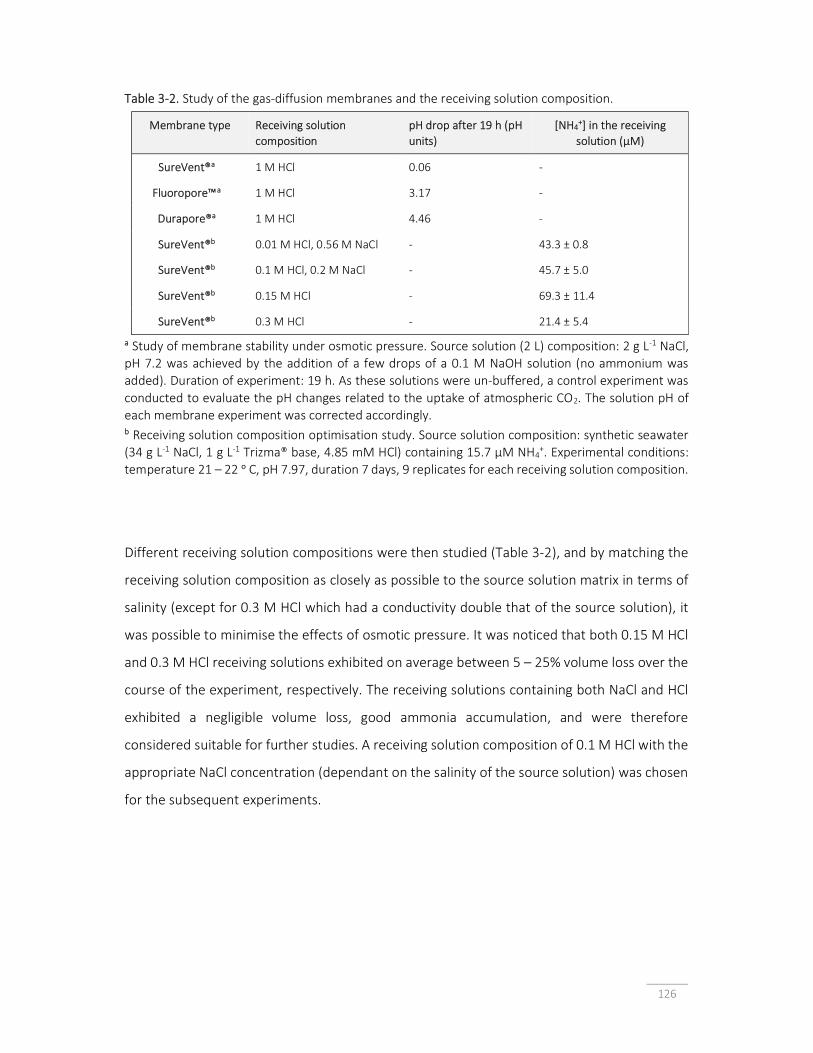
126

Table 3-2. Study of the gas-diffusion membranes and the receiving solution composition.

Membrane type Receiving solution composition

pH drop after 19 h (pH units)

[NH4+] in the receiving solution (µM)

SureVent®a 1 M HCl 0.06 -

Fluoropore™a 1 M HCl 3.17 -

Durapore®a 1 M HCl 4.46 -

SureVent®b 0.01 M HCl, 0.56 M NaCl - 43.3 ± 0.8

SureVent®b 0.1 M HCl, 0.2 M NaCl - 45.7 ± 5.0

SureVent®b 0.15 M HCl - 69.3 ± 11.4

SureVent®b 0.3 M HCl - 21.4 ± 5.4

a Study of membrane stability under osmotic pressure. Source solution (2 L) composition: 2 g L-1 NaCl, pH 7.2 was achieved by the addition of a few drops of a 0.1 M NaOH solution (no ammonium was added). Duration of experiment: 19 h. As these solutions were un-buffered, a control experiment was conducted to evaluate the pH changes related to the uptake of atmospheric CO2. The solution pH of each membrane experiment was corrected accordingly. b Receiving solution composition optimisation study. Source solution composition: synthetic seawater (34 g L-1 NaCl, 1 g L-1 Trizma® base, 4.85 mM HCl) containing 15.7 μM NH4

+. Experimental conditions: temperature 21 – 22 ᵒ C, pH 7.97, duration 7 days, 9 replicates for each receiving solution composition.

Different receiving solution compositions were then studied (Table 3-2), and by matching the

receiving solution composition as closely as possible to the source solution matrix in terms of

salinity (except for 0.3 M HCl which had a conductivity double that of the source solution), it

was possible to minimise the effects of osmotic pressure. It was noticed that both 0.15 M HCl

and 0.3 M HCl receiving solutions exhibited on average between 5 – 25% volume loss over the

course of the experiment, respectively. The receiving solutions containing both NaCl and HCl

exhibited a negligible volume loss, good ammonia accumulation, and were therefore

considered suitable for further studies. A receiving solution composition of 0.1 M HCl with the

appropriate NaCl concentration (dependant on the salinity of the source solution) was chosen

for the subsequent experiments.

127

3.3.3 Flow pattern effects on the ammonia uptake

The effect of the aquatic flow patterns on the analyte uptake has been studied by comparing

the accumulation of GD-PSs with and without flow shields (Figures 3-1a and 3-1b) as described

by Garcia-Rodríguez et al [12]. Laboratory-based experiments were conducted by dipping

devices with and without flow shields (n = 8 each) in 9 L of synthetic seawater spiked with 6.62

µM of ammonium for a period of 7 days and using aquarium pumps to promote synthetic

seawater mixing. The uptake of the un-shielded and shielded samplers was 10.7 ± 0.98 µM and

9.46 ± 0.80 µM, respectively. A 2-tail Student’s t-test was performed, where the null hypothesis

was accepted (i.e. no statistically significant difference between the two experimental results)

if the calculated t-value was lower than the critical t-value at the selected confidence level. The

t- value calculated for the laboratory-based flow pattern study was 2.72 and the critical t-value

was 2.15 at the 95% confidence level. Therefore, there was a statistically significant difference

between the results for the un-shielded and shielded sampling devices. These results are in

accordance with the observations published by Garcia-Rodríguez et al [12].

The same experiment was repeated in estuarine water (Yarra River at Newport) and in

seawater (Long Reef, Port Phillip Bay). The total ammonia concentrations of spot samples were

measured as 2.77 – 2.95 µM between the two sites, with temperature and salinity ranging

between 14.0 – 14.4 ᵒC and 31.3 – 34.5, respectively. The ammonia uptake of the un-shielded

and shielded samplers at the Yarra River estuary site was 3.67 ± 0.61 µM and 3.18 ± 0.70 µM,

respectively, and at Long Reef - 2.52 ± 1.06 µM and 2.92 ± 1.35 µM, respectively. A 2-tail

Student’s t-test was performed for both locations showing no statistically significant difference

between the results for un-shielded and shielded samplers at the 95% confidence level (Yarra

estuary: 0.697 < 2.12 and Long Reef: 1.59 < 2.12).

In the marine environment, water movement tends to be multi-directional as a result of wave

and tidal action, however, in rivers and streams it tends to be unidirectional. Whilst flow shields

have been shown to assist in minimising the effects of the aquatic flow pattern under

laboratory conditions [12], in marine and estuarine environments, the use of flow shields did

not provide any benefits and thus they were not used in the subsequent experiments.

128

3.3.4 Calibration of the GD-PS

The GD-PS accumulates dissolved ammonia from the source solution, and by performing its

laboratory-based calibration under controlled environmental conditions (temperature, pH and

salinity) it is possible to determine the CTWA of total ammonia at the sampling site in the aquatic

system over the period of sampling time. However, the ability of these devices to accumulate

molecular ammonia from the source solution was drastically inhibited after a period of 4-5

days (Figure 3-2a). In order to assess whether biofouling was inhibiting uptake, the membranes

were immersed in a solution of 7.2 mM methylene blue, which is commonly used as a biological

stain, before and after use. Prior to immersion in the source solution, the GDMs did not take

up the stain, but post 7 day immersion, all GDMs exhibited some degree of staining, indicative

of the presence of bacterial biofilms on their surfaces, which has likely resulted in some degree

of blockage of their pores thus supressing ammonia uptake. Despite this issue, the ammonia

uptake was linear up to 3 days, and hence a calibration curve was plotted for this sampling

period (Figure 3-2b). Under the experimental conditions described for the laboratory-based

calibration (Section 3.2.4) the detection limit of the passive samplers was determined as 1.64

µM NH4+ and the repeatability (%RSD) at a source solution concentration of 3.54 µM was 11.9%

(n = 7).

The rate of molecular ammonia uptake from the source solution to the receiving solution

appears to have a non-linear response at higher concentrations (Figure 3-2b.), which may be

due to the equilibrium partition of NH3/NH4+ favouring greater production of molecular

ammonia as it is removed from the solution by the GD-PS. Additionally, while the first data

point on the calibration curve (i.e. 0.97 mM) was supposed to represent the blank, daily

measurements of ammonia nitrogen present in the source solution blank indicated the

presence of trace contamination of ammonia, most likely originating from atmospheric inputs,

and/or from reagents used to prepare the artificial seawater.

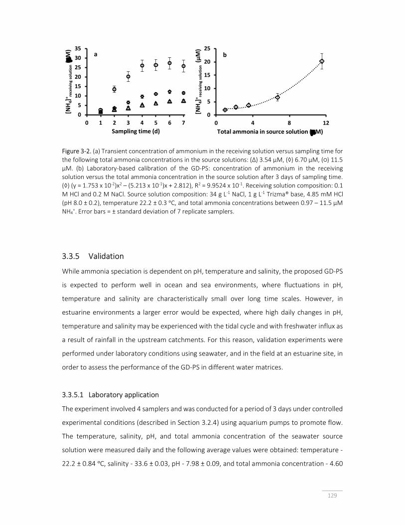
129

Figure 3-2. (a) Transient concentration of ammonium in the receiving solution versus sampling time for the following total ammonia concentrations in the source solutions: (Δ) 3.54 µM, (◊) 6.70 µM, (○) 11.5 µM. (b) Laboratory-based calibration of the GD-PS: concentration of ammonium in the receiving solution versus the total ammonia concentration in the source solution after 3 days of sampling time. (◊) (y = 1.753 x 10-2)x2 – (5.213 x 10-1)x + 2.812), R2 = 9.9524 x 10-1. Receiving solution composition: 0.1 M HCl and 0.2 M NaCl. Source solution composition: 34 g L-1 NaCl, 1 g L-1 Trizma® base, 4.85 mM HCl (pH 8.0 ± 0.2), temperature 22.2 ± 0.3 ᵒC, and total ammonia concentrations between 0.97 – 11.5 μM NH4

+. Error bars = ± standard deviation of 7 replicate samplers.

3.3.5 Validation

While ammonia speciation is dependent on pH, temperature and salinity, the proposed GD-PS

is expected to perform well in ocean and sea environments, where fluctuations in pH,

temperature and salinity are characteristically small over long time scales. However, in

estuarine environments a larger error would be expected, where high daily changes in pH,

temperature and salinity may be experienced with the tidal cycle and with freshwater influx as

a result of rainfall in the upstream catchments. For this reason, validation experiments were

performed under laboratory conditions using seawater, and in the field at an estuarine site, in

order to assess the performance of the GD-PS in different water matrices.

3.3.5.1 Laboratory application

The experiment involved 4 samplers and was conducted for a period of 3 days under controlled

experimental conditions (described in Section 3.2.4) using aquarium pumps to promote flow.

The temperature, salinity, pH, and total ammonia concentration of the seawater source

solution were measured daily and the following average values were obtained: temperature -

22.2 ± 0.84 ᵒC, salinity - 33.6 ± 0.03, pH - 7.98 ± 0.09, and total ammonia concentration - 4.60

05

10

1520

25

3035

0 1 2 3 4 5 6 7

[NH

4]+ re

ceiv

ing

solu

tion

(mM

)

Sampling time (d)

a

0

5

10

15

20

25

0 4 8 12

[NH

4]+ re

ceiv

ing

solu

tion

(µM

)

Total ammonia in source solution (mM)

b

130

± 3.32 µM. The initial ammonia concentration of the seawater source solution of 8.02 µM

decreased to 0.31 µM at the end of the sampling period due to the rapid growth of bacteria.

The laboratory-based calibration (Figure 3-2b) was used to determine the CTWA for total

ammonia and was found to be 4.42 ± 0.20 µM (n=5). No statistically significant difference was

found at the 95% confidence level (2-tail Student’s t-test: 0.111 < 2.37) between the average

total ammonia concentration measured in the seawater source solution mentioned above and

the total ammonia CTWA. The excellent agreement between the two sampling methods

characterised by a relative error of 4.03% demonstrated the suitability of the newly developed

GD-PS for environmental monitoring of ammonia in sea and ocean environments.

3.3.5.2 Field application

A field study was undertaken in the Werribee River estuary for a 3-day deployment period,

with 5 gas-diffusion passive sampling devices, containing receiving solution (0.1 M HCl and 0.02

M NaCl) with a salinity similar to that of the matrix. Spot samples were collected daily at

different tidal heights, and the average temperature (22.5 ± 2.8 o C), salinity (23.2 ± 5.2) and pH

(8.04 ± 0.16) were determined over the period of deployment. The CTWA for total ammonia was

determined on the basis of the concentrations of ammonia in the receiving solutions of the

five samplers after a 3-day deployment. The laboratory-based calibration curve (Figure 3-2b)

was used. No statistically significant difference was found at the 95% confidence level (2-tail

Student’s t-test: 0.735 < 2.37) between the average total ammonia concentration measured in

the estuarine spot samples (5.41 ± 0.30 µM) and the total ammonia CTWA (6.21 ± 2.18 µM).

There was thus good agreement between the two sampling methods, with a relative error of

13.0%, which is considered to be reasonable for passive sampling in waters with a highly

complex and variable matrix [15].

3.4 Conclusions A novel passive sampler based on gas-diffusion has been developed and applied as a proof of

concept for the monitoring of ammonia in marine waters. The performance of the GD-PS

device was tested under laboratory conditions using seawater under stable and controlled pH,

temperature and salinity conditions, and in the field at an estuarine site. The relative error

131

between the concentration of ammonia nitrogen measured, and the experimentally

determined time weighted average concentration for the seawater matrix was 4.03% and for

the estuarine environment it was 13.0%. In an environment where the variables affecting

ammonia speciation (pH, temperature and salinity) are stable over long periods of time, these

devices can be used for studies aimed at understanding complex biogeochemical cycling of

ammonia nitrogen in the water column, however, in more complex and variable environments

the same GD-PS devices would be more suitable for monitoring point-source nutrient inputs

and episodic pollution events. While the GD-PS described in this study was successfully applied

in the field for a 3-day deployment period, this time-frame may be short for large-scale

environmental monitoring. Therefore, a number of different strategies to minimise the effects

of biofouling are currently being investigated, in addition to a detailed evaluation of the effect

of temperature, matrix pH and salinity. On the basis of the results obtained it can be concluded

that the newly developed gas-diffusion-based passive sampling approach offers a cheap, easy-

to-use and reliable alternative to conventional spot sampling, and it does not require sample

pre-treatment steps prior to analysis unlike existing passive sampling techniques. All these

features make the GD-PS an attractive new tool for marine and estuarine water quality

monitoring.

Acknowledgements This article is dedicated to Professor Purnendu (Sandy) Dasgupta, the recipient of the 2017

Talanta Medal.

The authors would like to thank the Australian Research Council (ARC) and Melbourne Water

Corporation for funding this research in the framework of the ARC Linkage Scheme (Grant

LP160100687). We also acknowledge Mr. Edward Nagul for assisting with the collection of SEM

images, and Mr. Marcus Hammarstedt for creating Figure 3-1b. L. O’Connor Šraj is grateful to

the University of Melbourne for the award of a postgraduate scholarship

132

References 1. Camargo, J.A. and A. Alonso, Ecological and toxicological effects of inorganic nitrogen

pollution in aquatic ecosystems: A global assessment. Environ. Int., 2006. 32: p. 831-849.

2. Batley, G.E. and S.L. Simpson, Development of guidelines for ammonia in estuarine and marine water systems. Mar. Pollut. Bull., 2009. 58 (10): p. 1472-1476.

3. Roll, I.B. and R.U. Halden, Critical review of factors governing data quality of integrative samplers employed in environmental water monitoring. Water Res, 2016. 94: p. 200-7.

4. Vrana, B., I.J. Allan, R. Greenwood, G.A. Mills, E. Dominiak, K. Svensson, J. Knutsson, and G. Morrison, Passive sampling techniques for monitoring pollutants in water. TrAC Trends Anal. Chem., 2005. 24 (10): p. 845-868.

5. Zabiegała, B., A. Kot-Wasik, M. Urbanowicz, and J. Namieśnik, Passive sampling as a tool for obtaining reliable analytical information in environmental quality monitoring. Analytical and Bioanalytical Chemistry, 2010. 396(1): p. 273-296.

6. Huang, J., W.W. Bennett, D.T. Welsh, T. Li, and P.R. Teasdale, Development and evaluation of a diffusive gradients in a thin film technique for measuring ammonium in freshwaters. Anal. Chim. Acta, 2016. 904 (Supplement C): p. 83-91.

7. Almeida, M.I.G.S., A.M. Silva, R.A. Coleman, V.J. Pettigrove, R.W. Cattrall, and S.D. Kolev, Development of a passive sampler based on a polymer inclusion membrane for total ammonia monitoring in freshwaters. Anal. Bioanal. Chem., 2016. 408 (12): p. 3213-22.

8. Aneja, K.R., Experiments in Microbiology, Plant Pathology and Biotechnology. Fourth Edition ed. 2003, New Delhi: New Age International. 97-100.

9. Dickson, A.G., C.L. Sabine, J.R. Christian, and Eds, SOP 6B Determination of the pH of sea water using the indicator dye m-cresol purple. In Guide to Best Practices for Ocean CO2 Measurements. PICES Special Publication 3. 2007: p. 1-7.

10. O'Connor Šraj, L., M.I.G.S. Almeida, I.D. McKelvie, and S.D. Kolev, Determination of trace levels of ammonia in marine waters using a simple environmentally-friendly ammonia (SEA) analyser. Mar. Chem., 2017. 194 (Supplement C): p. 133-145.

11. Corporation, M., Microfiltration Membranes, Microfiltration Membranes for Filtration and Venting Applications. 2009: USA.

12. Garcia-Rodríguez, A., C. Fontàs, V. Matamoros, M.I.G.S. Almeida, R.W. Cattrall, and S.D. Kolev, Development of a polymer inclusion membrane-based passive sampler for monitoring of sulfamethoxazole in natural waters. Minimizing the effect of the flow pattern of the aquatic system. Microchemical Journal, 2016. 124(Supplement C): p. 175-180.

13. Li, Q.P., J.Z. Zhang, F.J. Millero, and D.A. Hansell, Continuous colorimetric determination of trace ammonium in seawater with a long-path liquid waveguide capillary cell. Marine Chemistry, 2005. 96(1-2): p. 73-85.

14. Bower, C.E. and J.P. Bidwell, Ionization of Ammonia in Seawater: Effects of Temperature, pH, and Salinity. J. Fish. Res. Board Can., 1978. 35 (7): p. 1012-1016.

15. EU, Commission Directive 2009/90/EC of 31 July 2009 laying down, pursuant to Directive 2000/60/EC of the European Parliament and of the Council, technical specifications for chemical analysis and monitoring of water status. Official Journal of the European Union, L210: 36–38. 2009.

133

CHAPTER 4: Monitoring of ammonia in marine waters using a passive sampler with biofouling resistance and neural network-based calibration

Foreword In Chapter 3, the development of the first prototype of a gas-diffusion based passive sampling

device (GD-PS) for ammonia monitoring in marine waters and its application as a proof of

concept for a 3-day deployment in an estuary and in a tank with recirculated natural seawater

is described. Whilst the device showed promise, it was unable to be deployed for periods of

more than three days due to biofilm formation on the surface of the gas-diffusion membrane

thus limiting the uptake of ammonia from the sampled medium. Additionally, in order to

determine the time-weighted average concentration during the period of deployment,

calibration of the device was required in the laboratory under the same environmental

temperature and pH conditions at which the GD-PS was deployed, which limited the usability

of the device for widespread water quality monitoring programs.

The research described in this chapter looks at a) a number of different antifouling strategies

to reduce the impact of biofouling on the device and improve its deployment longevity, b)

assessing the impact of the environmental variables temperature, pH and salinity on the

performance of the device, and c) developing a universal calibration model over a range of

commonly occurring environmental conditions, by applying the Group Method Data Handling

algorithm as a neural network-based calibration approach. The content of this chapter was

published in 2020 in the journal Environmental Pollution.

O'Connor Šraj, L., Almeida, M. I. G. S., Sharp, S., McKelvie, I. D., Morrison, R., Kolev, S. D., (2020)

Monitoring of ammonia in marine waters using a passive sampler with biofouling resistance

and neural network-based calibration, Environmental Pollution, 267, 115457,

https://doi.org/10.1016/j.envpol.2020.115457

134

Graphical abstract

135

Contents

Abstract 136

4.1 Introduction 137

4.2 Materials and methods 139

4.2.1 Reagents and solution 139

4.2.2 Analytical tools and methods 140

4.2.3 Gas-diffusion membranes 141

4.2.4 Antifouling strategies 141

4.2.5 Passive sampler assembly and calibration 141

4.2.6 Field deployment 143

4.3 Results and discussion 144

4.3.1 Membrane selection and receiving solution optimisation

144

4.3.2 Membrane antifouling strategies 145

4.3.3 Influence of temperature, salinity and pH on the GD-PS performance

148

4.3.4 GD-PS calibration using GMDH model 152

4.3.5 Field validation 153

4.3.6 Method performance 155

4.3.7 GD-PS: A tool for ammonia screening 156

4.4 Conclusions 157

4.5 Appendix 158

Acknowledgements 171

References 172

136

Abstract A biofouling resistant passive sampler for ammonia, where the semi-permeable barrier is a

microporous hydrophobic gas-diffusion membrane, has been developed for the first time and

successfully applied to determine the time-weighted average concentration of ammonia in

estuarine and coastal waters for 7 days. Strategies to control biofouling of the membrane were

investigated by covering it with either a copper mesh or a silver nanoparticle functionalised

cotton mesh, with the former approach showing better performance. The effects of

temperature, pH and salinity on the accumulation of ammonia in the newly developed passive

sampler were studied and the first two parameters were found to influence it significantly. A

universal calibration model for the passive sampler was developed using the Group Method

Data Handling algorithm based on seawater samples spiked with known concentrations of total

ammonia under conditions ranging from 10 to 30 °C, pH 7.8 to 8.2 and salinity 20 to 35. The

newly developed passive sampler is affordable, user-friendly, reusable, sensitive, and can be

used to detect concentrations lower than the revised default guideline value of 160 μg total

NH3-N L-1, for a 99% species protection level, with the lowest concentration measured at 17

nM molecular NH3 (i.e., 8 μg total NH3-N L-1 at pH 8.0 and 20 °C). It was deployed at four field

sites in the coastal waters of Nerm (Port Phillip Bay), Victoria, Australia. Good agreement was

found between molecular ammonia concentrations obtained with passive and discrete grab

sampling methods (relative difference, - 12% to - 19%).

Keywords: Passive sampling; ammonia; marine water sampling; gas-diffusion membrane.

137

4.1 Introduction Globally nutrient pollution is a major threat to the health of aquatic ecosystems [1, 2].

Increasingly large-scale anthropogenic run-off from agricultural land, industrial processes and

atmospheric deposition, results in the nutrient enrichment of natural waters causing increased

primary production and eutrophication [1-4]. Estuarine and coastal waters are susceptible to

eutrophication from total nitrogen and total phosphorus, which can lead to oxygen depletion

in the water column and benthic environments [5].

Ammonia is commonly monitored as an indicator of water quality by regulatory bodies

responsible for monitoring and providing information about the health of aquatic ecosystems.

The sources, dispersal and fate of ammonia are of concern to water quality managers, and

efficient and reliable monitoring approaches are needed, especially during pollution events.

The speciation of ammonia in aquatic environments (NH3/NH4+) is dependent on pH and

temperature, and to a lesser extent salinity [6]; the sum of both molecular ammonia (NH3) and

ammonium (NH4+) are referred to as total ammonia.

Current Australian and New Zealand Guidelines (ANZG) for fresh and marine water quality

specify the default guideline value for total ammonia in marine waters as 500 µg NH3-N L-1

(equivalent to 1.06 µM molecular NH3 at pH 8 and 20 °C) for a 99% species protection level [7].

However, additional data will likely result in further revisions to these guidelines, with a

guideline value of 160 µg NH3-N L-1 (i.e., 340 nM molecular NH3 at pH 8 and 20 °C) determined

to be more appropriate for maintaining ecosystem function and health [8], highlighting the

need for more sensitive, but still reliable, ammonia monitoring methods.

Most water quality monitoring programs involve intermittent (i.e., in response to pollution

events) or routine (baseline) spot sampling during daylight hours, preservation and sample pre-

treatment (i.e., filtration) prior to sample analysis. Such methods can be time-consuming,

expensive, weather dependent (or unsafe), and prone to sample contamination [9]. Passive

sampling techniques overcome many of the disadvantages of grab sampling by collecting and

accumulating the analyte of interest in-situ, providing a time-weighted average concentration

for the period of deployment [9, 10]. The advantages of passive sampling make this a desirable

tool for routine monitoring and for identifying pollution hotspots. Over the last three decades,

various passive sampling techniques were developed to monitor a wide range of important

aquatic pollutants [9-11]. Passive sampling allows for the time-weighted average concentration

138

of the analyte(s) of interest to be determined over the period of deployment. This technique

has been successfully used to overcome a number of limitations of traditional water quality

monitoring programs using intermittent spot sampling. The fundamental advantages of passive

sampling include allowing for lower levels of target species to be detected (due to the

preconcentration ability of passive samplers) [12], and more representative data to be

collected, especially in highly dynamic environments such as estuaries, and over large

spatiotemporal scales to account for tidal cycles, flood events and even seasonal variability

over longer deployment times [13-15].

Diffusive gradients in thin films (DGT) samplers have been described in the literature for

monitoring nutrient concentrations including ammonia [16, 17], nitrate [17, 18] and phosphate

[17, 19-23]. Using ion-exchange resins as binding agents, DGTs have been applied to different

freshwater systems, including streams and wetlands, as well as in the assessment of lake

sediment remediation techniques [16, 18-20, 24]. A passive sampling device using a polymer

inclusion membrane (PIM) for ammonia monitoring in freshwaters has been successfully

developed [25]. This device consists of a receiving solution separated from the sampled aquatic

medium by a PIM. Subsequent ammonia monitoring using PIM-based passive samplers in

combination with standard microbial faecal indicators was applied to identify dry-weather

leaks (i.e., cracked sewer pipe) and episodic pollution events (e.g., sewer spills) [26]. However,

both DGT- and PIM-based passive samplers are susceptible to interference from dissolved salts

and therefore not appropriate for use in high salinity matrices, such as estuarine and marine

waters.

Ammonia determination using gas-diffusion separation has been widely used in automated

flow analysis methods [27], in potentiometric ion selective electrodes (ISEs) [28-34], and more

recently in a gas-permeable membrane-based conductivity (GPMCP) probe deployed in an

estuary for 24 hours [35]. Automated methods commonly require the use of expensive and

sometimes custom-made equipment, a high degree of operator skill and are predominantly

used in a laboratory setting, although in situ and shipboard underway applications have been

described [27]. ISEs require the use of a gas-diffusion membrane to eliminate interference

from K+, Na+ and Ca2+ ions whose concentrations are commonly several orders of magnitude

higher in seawater than that of the NH4+ ion. This results in characteristically poor sensitivities

and slow response times, which can be improved by the addition of an alkalising reagent to the

sample. Ammonia ISEs are typically used in laboratories for measuring ammonia [31, 32], and

139

have not been tested and validated for long-term, in situ field deployment in saline waters.

While the GPMCP probe shows promise in terms of in situ monitoring capability, the sensitivity

of the sensor decreases as a function of deployment time [36], and the complexity and cost of

fabrication of custom-made electronic components and the need for power to operate the

instrument may limit its usability in widespread environmental monitoring campaigns.

Am ammonia gas-diffusion passive sampler (GD-PS) for use in marine waters using a gas-

diffusion membrane instead of a PIM has previously been described [37], however, membrane

biofouling inhibited the performance of the GD-PS after three days. In addition, this passive

sampler required calibration at the specific temperature and pH of the water of each

deployment site. Hence, in the present work, strategies to overcome the effects of biofilm

formation on the ammonia accumulation by the GD-PS were investigated and they involved

covering the GD membrane with either a copper mesh or a silver nanoparticle functionalised

mesh. This article also reports the development of a single calibration model, involving the use

of the Group Method Data Handling (GMDH) algorithm [38], to calibrate the GD-PS over a

range of environmental pH (7.8 to 8.2), temperature (10 to 30 °C) and salinity (20 – 35)

conditions, allowing for a universal calibration to be used in determining the ammonia time-

weighted average concentration ([NH3]TWA) in a wide range of marine waters.

4.2 Materials and methods

4.2.1. Reagents and solutions

The preparation of reagents, GD-PS receiving solutions, and synthetic source solutions are

described in Section A (Appendix).

140

4.2.2 Analytical tools and methods

The pH of synthetic seawater and discrete grab samples (also known as spot samples) was

measured using a flow system utilising a spectrophotometric method [39, 40]. The system was

assembled using an Ocean Optics spectrophotometer (USB4000), a tungsten halogen light

source (LS-1) with a blue filter (BG-34), and a 10 cm optical path length flow cell. A certified

reference material (Batch 141 Certified Seawater) from the Scripps Institute of Oceanography

was used to assess the performance of the pH flow system, which was accurate to within ±

0.005 pH units of the reported value (pH 7.887 at 25 °C) and with an interquartile range of

0.001.

The concentration of accumulated ammonia in the receiving solution (measured as

ammonium) and total ammonia in the sample source solution were determined using a

Sensitive Environmentally-friendly Ammonia (SEA) analyser [41]. Two working ranges were

used, namely 0.28 – 13.9 µM for the source solution samples and 1.4 – 55.6 µM for the GD-PS

receiving solutions. Typical limits of detection were 88 nM and 440 nM for the lower and upper

concentration ranges, respectively. A certified reference material (ERA A Waters Company, Lot

no. 080715 Traceability against NIST SRM (194) 99.1% concentration 1,000 ± 6 mg L-1) diluted

to 5.0 µM for the lower range and 30.0 µM for the upper range was used to assess the

performance of the SEA analyser with errors in the order of ± 1.9% for the lower range and ±

1.3% for the upper range. Molecular ammonia in the sample source solution was calculated by

multiplying the total ammonia concentration by the fraction of un-ionised ammonia in

solution, which was determined using an empirical model described by Bower and Bidwell [6],

when the temperature (°C), pH values, and salinity were known.

To measure solution conductivity and temperature, a portable conductivity meter (TPS WP-84,

TPS, Australia) calibrated using a 36 ppK salinity standard (TPS, Australia) alongside a high

accuracy thermometer coupled with a platinum resistance temperature detector (RTD)

immersion probe (Precision Plus Thermometer with RTD High Accuracy Freezer Probe, 1/10

DIN, ThermoWorks, USA) were used.

141

4.2.3 Gas-diffusion membranes

Three commercially available hydrophobic gas-diffusion membranes (GDM’s) were tested, viz.

SureVent® (0.1 µm pore size), Fluoropore™ (0.22 µm pore size) and Durapore™ (0.22 µm pore

size) (Merck Millipore). Membrane characteristics have been described previously [37].

4.2.4 Antifouling strategies

Two types of copper mesh and a cotton mesh functionalised with silver nanoparticles (AgNP)

were investigated for control of membrane biofouling. The copper mesh (TWP Inc., California)

was supplied in an overall thickness of 112 µm and two different weave densities (100 wires

per inch with 60% opening, and 200 wires per inch with 35% opening). The AgNP cotton mesh

was prepared according to the method described by Rehan et al. [42] using 45 g of muslin

(Grade 80, thread count 40 x 32 per square inch), 1 L solution of 1200 mg L-1 AgNO3 (Chem-

Supply) and 5% (w/w) solution of trisodium citrate (Chem-Supply) added drop wise. In order to

test the efficacy of the silver nanoparticle treatment, three layers of the AgNP cotton mesh

were sandwiched together as the muslin cloth had a low specific surface area, due to a low

thread count. A single layer of copper mesh was employed in the copper-based experiments.

Biofouling on the surface of each GDM was quantified by immersion of the membrane in a

methylene blue stain for 60 seconds [43], followed by photo scanning of the stained membrane

using a CanoScan Lide220. The image was processed using ImageJ software, using the red

colour channel to determine the extent of biofouling by monitoring the intensity of colour

change between the unstained and stained GDM immersed in the field, or in real seawater

solutions in the laboratory.

4.2.5 Passive sampler assembly and calibration

The GD-PSs were assembled as described previously [37], with the addition of an antifouling

mesh between the outer surface of the GDM and the sampled medium (i.e., source solution)

(Figure).

142

Laboratory experiments were performed using unfiltered low-nutrient seawater collected

from Half Moon Bay, Victoria, Australia as the source solution (Figure S4-1, Table S4-1,

Appendix), spiked with the appropriate volume of ammonia stock solution prepared by using

NH4Cl. Experiments were conducted as previously described [37], using 10 L tanks in a

temperature controlled cabinet with 500 L h-1 aquarium pumps to promote flow. For

laboratory calibration experiments, the pH was adjusted by the addition of small volumes of 5

M HCl or NaOH solutions, and the salinity was adjusted with the addition of deionized water.

All experiments were conducted for a period of 7 days, except for the field biofouling

experiment that was conducted over 8 days, with 10 GD-PSs used for each

condition/concentration tested.

The Group Method Data Handling (GMDH) algorithm [38] was used to model the behaviour of

the GD-PS under a wide range of environmental variables (salinity 20 – 36, temperature 10 –

30 °C and pH 7.8 – 8.2), using the commercially available GMDH predictive analytics software

package (GMDH Shell version 3.8.9) [44]. Seawater pH was adjusted and thermostated at the

desired temperatures. Daily pH, temperature and total ammonia measurements of the source

solution were performed over a 7-day period. Receiving solutions were analysed at the

completion of the experiments (i.e., after 7 days) and used to determine the [NH3]TWA. The

concentrations greater than the 90th or less than the 10th percentile were removed (10 percent

trimmed mean) in order to minimise the influence of outliers, and to provide a better

estimation of central tendency of data both for model calibration and validation [45]. The

temperature, pH, average molecular ammonia concentration of the source solution, and the

10 percent trimmed mean receiving solution ammonia concentration were used to develop

the GMDH calibration model.

The linear concentration range of the proposed GD-PS was determined using a range of

standard source solutions prepared under the following conditions: salinity 35, 20 °C and pH

8.0.

143

Figure 4-1. A) GD-PS assemblage with antifouling mesh. B) Cross-section of the GD-PS showing the process of selective accumulation of dissolved NH3(aq) from the source solution, where the gas diffuses into the pores of the hydrophobic gas-diffusion membrane (not to scale) and the subsequent reaction of NH3(g) at the membrane/receiving solution interface where the molecular ammonia is converted to ammonium ion (NH4

+(aq)) by reaction with a hydrogen ion (H+

(aq)) in the receiving solution. Inset: Proposed antifouling mechanism when using the copper mesh, involving the oxidation of elemental copper and subsequent generation of the toxic cuprous and cupric ions.

4.2.6 Field deployment

Four field-based passive sampling experiments were conducted in Victoria, Australia, i.e., the

Birrarung (Yarra River) estuary (Site 1), Hobsons Bay (Site 2), the Werribee River estuary mouth

(Site 3) and approximately 5 kilometres upstream (Site 4) (Figure S4-1, Table S4-1, Appendix).

These sites are part of the larger coastal area of Nerm (Port Phillip Bay).

During the GD-PS deployment, 250 mL discrete grab samples were collected every 2 hours at

each site during the 7 day deployment period, using a Hach Sigma autosampler (model 900)

fitted with 24 x 1 L polyethylene bottles, each of which contained 50 μL H2SO4 (98% RCI

Labscan) to preserve samples. Samples remained in the dark and on ice until collection, and

new bottles and ice were replaced every 48 hours. A Durapore™ 0.45 μm syringe filter

(Millipore) was used for sample filtration, and samples were kept at ≤ 4 °C and analysed within

3 days of collection using the SEA analyser described above.

Multiparameter water quality sondes with sensors for pH, electrical conductivity (EC) and

temperature were deployed at each site during field work. Hanna Instruments (H17629829)

144

was deployed at Sites 1, 2 and 3, the Hydrolab (DS5X) was used at Site 4, and YSI (EXO2) was

used at Site 4 for the biofouling experiment. The GD-PSs were fitted to a floating cage [26], to

which an autonomous sonde was attached prior to submerging both just beneath the surface

of the water. At Sites 1 and 3, the GD-PS and sondes were deployed from a floating jetty, at

Site 2 from a fixed pier, and at Site 4 the GD-PS were deployed from a partially submerged tree

where the sonde had been secured to a steel post driven into the river bed.

A three-point calibration of the pH glass electrodes was carried out using standard pH buffers,

pH 4, 7 and 10 (TPS, Australia). Such electrodes are susceptible to liquid junction potential

errors in saline matrices [46]. Hence, five grab samples were manually collected from each site

during the 7-day deployment period (on days 0, 2, 4, 6 and 7, with day 0 being the deployment

day, and day 7 the collection day), and pH and temperature were measured using the

instrumentation described in the ‘Analytical tools and methods’ Section 4.2.2. This allowed for

liquid junction potential errors to be corrected on the multiparameter autonomous sondes

used in the field. A 36 ppK calibration solution (TPS, Australia) was used to calibrate the EC

probes of the sondes at the beginning of each experiment and was used again at the

completion of the experiment to check for sensor drift.

GD-PS receiving solutions contained 0.01 M HCl and an appropriate concentration of NaCl to

approximately match the conductivity of the source solution. For Site 2 and 3, a receiving

solution composition of 0.01 M HCl and 0.56 M NaCl was used, for Site 1 a 0.01 M HCl and 0.48

M NaCl receiving solution was used, and for Site 4 a 0.01 M HCl and 0.40 M NaCl receiving

solution was used.

4.3 Results and discussion

4.3.1 Membrane selection and receiving solution optimisation

Three different hydrophobic porous GDMs were tested in a tris-buffered synthetic seawater

source solution (salinity 35, 20 °C) with different receiving solution compositions to determine

which combination provided the highest ammonia accumulation and best precision (Figure S4-

2, Appendix). It was previously shown that maintaining a similar conductivity between source

145

and receiving solutions was important to minimise the movement of water by osmosis across

the porous hydrophobic GDM [37]. Thus all three membranes, SureVent®, Fluoropore™ and

Durapore™ were tested with solutions containing mixtures of HCl and NaCl (viz., 0.01 M HCl +

0.56 M NaCl and 0.1 M HCl + 0.2 M NaCl) alongside 0.15 M and 0.3 M HCl (all with conductivities

of approximately 5.0 S m-1, except for the 0.3 M HCl solution, which was approximately twice

as high).

Whilst the GD-PS with the SureVent® membrane exhibited an overall higher precision when

compared to those with Fluoropore™ and Durapore™ membranes, it exhibited lower

accumulation of ammonia, likely due to the smaller pore size of the SureVent® membrane in

comparison with that of the other two (0.1 µm vs. 0.2 µm).

In the previous study, a 0.1 M HCl + 0.02 M NaCl receiving solution was used [37], which

allowed the GD-PS to be applied to water salinity of around 25. However, in this study both

low- and high-conductivity marine waters were monitored. Hence, a 0.01 M HCl solution was

selected as it allowed for greater flexibility in terms of matching the conductivity of the

receiving solution to that of the sampled medium by adding NaCl to achieve the final desired

conductivity. There was no flexibility with the 0.15 M HCl receiving solution as its conductivity

was effectively the same as seawater with a salinity of 35. Hence, a receiving solution

composed of 0.01 M HCl and 0.56 M NaCl was selected as it provided the highest overall

precision while allowing for the GD-PS to be deployed in a range of ionic strength

environments, from low ionic strength estuarine to high ionic strength marine environments

with good ammonia accumulation. The Fluoropore™ membrane was selected for further

experiments because it provided the best compromise between ammonia accumulation and

precision in comparison with the other two membranes with 0.01 M HCl and 0.56 M NaCl as

the receiving solution.

4.3.2 Membrane antifouling strategies

Bacterial and microalgal biofilm formation on the surface of the porous hydrophobic GDM

impacted the previously described GD-PS, where the accumulation of ammonia in the device

was observed to ‘plateau’ after a period of 3-4 days limiting its usability [37]. Membrane

biofouling is known to limit the operating lifetime of gas sensing instruments deployed in

146

marine environments [47], and both copper and silver have successfully been used as biocides

to limit biofilm formation in membrane facilitated separation technologies [21, 48, 49]. Hence,

several antifouling strategies were tested with the aim of extending the sampling period of the

GD-PS, namely, two different wire count densities of copper mesh, including Cu-100 (60%

opening) and Cu-200 (35% opening), and three layers of a silver nanoparticle (AgNP)

functionalised cotton mesh.

When performing laboratory-based experiments it is difficult to simulate the specific

environmental conditions experienced in the field, especially in relation to the volume of water

into which the GD-PSs are submerged in the laboratory (i.e., 10 L), and the composition of

microorganisms in the matrix. Therefore, the likelihood of bacterial and microalgal growth in

this low volume, nutrient enhanced, closed body of water is very high, and may not mimic real

conditions. These experiments were therefore performed under both laboratory and field

conditions.

The performance of the different antifouling strategies tested using the Fluoropore™

membrane-based GD-PS is illustrated in Figure.

Figure 4-2. Membrane antifouling strategies under laboratory conditions. A) Effect of the different antifouling strategies on the ammonium concentration accumulated in the receiving solution after 7 or 8 days of sampling in the laboratory or field study – Site 2, respectively. B) Effect of the different antifouling strategies on the extent of biofilm formation on the surface of the GDMs, where the intensity of blue colour after staining with methylene blue is proportional to the extent of biofouling. Laboratory experimental conditions: receiving solution, 10 mL of 0.01 M HCl + 0.56 M NaCl; source solution mean ammonia concentration 223 ± 10.7 nM at salinity 34.5, temperature 21 °C, pH 7.9, n(GD-

PS) = 5. Field study conditions: receiving solution, 10 mL of 0.01 M HCl + 0.56 M NaCl; source solution mean ammonia concentration 29.4 ± 14.9 nM at salinity 34.6, temperature 17 °C, pH 8.0, n(GD-PS) = 3. Error bars = ± standard deviation (SD) for n(GD-PS) = 5 (laboratory experiments) and n(GD-PS) = 3 (field study).

147

In the laboratory-based antifouling experiments, receiving solution samples were collected

daily and measured to monitor the uptake of ammonia into the GD-PS. In the presence of

antifouling treatments Cu-100, Cu-200 and AgNP, the ammonia accumulation was linear over

the course of seven days (Figure S4-3, Appendix), while for the control experiment (No

Treatment) the accumulation was non-linear. This is consistent with our previous work and

emphasises the importance of inhibiting biofilm formation which otherwise adversely affects

the performance of the GDM.

The results observed in Figure 4-2A can be understood in the context of Fick’s first law of

diffusion (Eqn. 1) [50], whereby the flux of total ammonia (JTA) will be reduced with any increase

in the diffusive pathlength from the bulk solution to the GDM, thus affecting the overall

accumulation rate in the receiving solution, where DTA is the effective diffusion coefficient of

total ammonia , C is the total ammonia concentration and 𝑥 is distance.

𝐽 = −𝐷 (Eqn. 1)

A diffusive boundary layer (DBL) will exist at the interface of any solid object in a flowing

solution such as the GDM of the GD-PS studied, where the mass transfer rate (MTA) (Eqn. 2)

and thus the amount of ammonia accumulated in the receiving solution of the newly

developed GD-PS, is controlled solely by molecular diffusion through the DBL [51], and S is

defined as the surface area through which diffusion takes place.

𝑀 = 𝑆 × 𝐽 (Eqn. 2)

The presence of an antifouling mesh placed in front of the GDM will create static solution

pockets between the mesh threads and the GDM, and depending on the diameter of the

threads (defining the mesh thickness), will increase the diffusional pathway. At the same time,

the presence of the mesh will decrease S (Eqn. 2). These two effects explain the observed lower

accumulation of ammonia in both the GD-PS fitted with the high density copper mesh (Cu-200)

and the sandwiched-three layers of AgNP functionalised cotton mesh (FigureA). The low

accumulation for the control GD-PS with no antifouling mesh (No Treatment) can be solely

attributed to the presence of a biofilm on the surface of the GDM. The tortuous diffusion

pathway of the ammonia molecules through the biofilm increases significantly the overall

diffusional pathway between the bulk source solution and the GDM of the GD-PS, which will

reduce the amount of ammonia accumulated in the sampler’s receiving solution [52, 53]

148

(Figure 4-2A). The GD-PS fitted with copper mesh (both densities Cu-100 and Cu-200) exhibited

minimal biofouling when compared to the AgNP and No Treatment conditions in the laboratory

(FigureB). This is likely due to the generation of the unstable cuprous (Cu+(aq)) ion, which rapidly

oxidises to the toxic cupric (Cu2+(aq)) ion, adjacent to the surface of the GDM creating a micro-

environment unfavourable for bacterial and microalgal colonisation [54, 55].

The antifouling strategy with the lower density copper mesh (Cu-100) characterised by 60%

opening, exhibited higher ammonia accumulation than the Cu-200 mesh with 35% opening

because of the difference in their respective diffusional areas (i.e., S, Eqn. 2). Additionally, the

copper itself was effective at inhibiting biofilm formation on the surface of the GDM, as well as

growth and multiplication of suspended bacteria and algae in the source solution.

In the biofouling field experiment, performed in the Hobsons Bay study, Williamstown (Site 2),

the highest ammonia accumulation was observed for the Cu-100 mesh-based GD-PS and the

control GD-PS (No Treatment), whose values were not statistically significantly different from

each other (2-Tail Student t-test 95% confidence interval: absolute value 1.63 < critical value

2.78; p-value: 0.179) (FigureA). Interestingly, since the amount of biofouling on the surface of

the GDMs in all cases was quite low for field deployed GD-PSs (FigureB), the above findings

suggested that the Cu-100 mesh did not present a significant analyte mass-transfer barrier. In

this field study, biofouling may not have presented as a significant issue in the accumulation

performance of the GD-PS likely due to low primary productivity in this environment,

characterised by the low ammonia concentration registered for the period of deployment (29.4

± 14.9 nM). However, when calibrating the GD-PS, and deploying in highly productive

environments (e.g., nutrient enhanced calibration solutions, eutrophic water bodies, such as

Sites 1, 3 and 4), biofouling control is imperative. As a compromise between the amount of

ammonia accumulated and the minimisation of the GDM biofouling, the Cu-100 mesh was

adopted for all further work.

4.3.3 Influence of temperature, salinity and pH on the GD-PS performance

In seawater, ammonia exists predominantly in the ammonium form (NH4+(aq)), with a small

fraction being in the more toxic form of molecular ammonia (NH3(aq)). The ammonia speciation

149

in marine waters has been well described, and is dependent on the environmental variables

temperature, pH and to a lesser extent salinity [6].

The mechanism of ammonia accumulation by the GD-PS involves the diffusion of dissolved

molecular ammonia present in the source solution through the pores of the hydrophobic GDM

into the GDM/receiving solution interface where it is ionised forming the ammonium ion as it

reacts with the hydrogen ions present in the receiving solution (NH3(g) + H+(aq) → NH4

+(aq)).

Ammonia is therefore selectively accumulated into the GD-PS receiving solution as ammonium

(Figure). However, in order to determine the time-weighted average molecular ammonia

concentration ([NH3]TWA), it is necessary to calibrate the GD-PS to establish the relationship

between the ammonium concentration in the receiving solution and ammonia concentration

in the sampled source solution.

To assess if the ammonia accumulation was independent of the environmental variables,

temperature, pH and salinity, an experiment was performed based on the empirical model of

Bower and Bidwell (1978). While varying the matrix conditions (i.e., salinity, pH and

temperature) appropriate amounts of ammonia were spiked into the source solutions to

maintain a constant molecular ammonia concentration between experiments, as determined

by the Bower and Bidwell model (Table S4-2, Appendix).

Two different total ammonia concentrations were assessed, namely, 4.4 ± 0.2 μM and 8.5 ±

0.1 μM (Figure S4-4, Appendix) in three different matrix compositions, each having effectively

the same concentration of molecular ammonia available to the GD-PS (2.93% to 2.99% NH3).

If no appreciable difference was observed in the amount of ammonia accumulated in the

receiving solutions, then the calibration of the GD-PS could be performed as a function of

available molecular ammonia independent of the variables, temperature, pH and salinity.

However, there was a statistically significant difference between each of the experiments in

the multivariate study, which is unsurprising, since it is well established that environmental

factors such as temperature will affect the analyte accumulation rate of diffusion-based PSDs

[56] (Figure S4-4, Appendix).

Since it is well known that diffusion rates are temperature dependent, and can be corrected

for by adjusting the diffusion coefficient for a given temperature [51, 53], it was necessary to

determine if the other variables, pH and salinity also exhibited an effect on the sampling rate.

The effect of the temperature, salinity and pH was therefore examined through the univariate

150

approach, where each variable was studied independently, again using the Bower and Bidwell,

(1978) ammonia speciation model (Table S4-3, Appendix).

The salinity study examined two concentrations of molecular ammonia in the source solution

at two different salinities (FigureA). There was no statistically significant difference between

the results for the different salinity matrices for the two concentrations analysed, and it was

thus concluded that this variable did not affect the performance of the GD-PS.

Figure 4-3. Effect of salinity (A), pH (B) and temperature (C) on the GD-PS accumulation. A) Salinity study experimental conditions: source solution, seawater (temperature 20 ᵒC, pH 8.0); n(GD-PS) = 8; receiving solution composition (salinity 20) = 0.01 M HCl and 0.34 M NaCl, and (salinity 35) = 0.01 M HCl and 0.56 M NaCl; statistical analysis using a 2-tail student t-test at the 95% confidence interval (t-value < 2.145), and t-value[147 nM] 1.376, t-value[311 nM] 0.414. B) pH study experimental conditions: source solution, seawater (salinity 34.5, temperature 20 ᵒC); n(GD-PS) = 8. C) Temperature study experimental conditions: source solution, seawater (salinity 34.5, pH 8.0). Error bars = ± SD (n(GD-PS) = 8).

The pH study involved two ammonia concentrations and three different pH conditions,

separated by 0.2 pH units (7.8 – 8.2), spanning the pH range commonly found in estuarine and

151

marine waters (FigureB). A statistically significant difference was observed for each data set,

and the GD-PS ammonia accumulation increased as pH was decreased. This result may seem

contrary to expectations, given the lower fraction of NH3 at lower pH values. However, it was

necessary to vary the source solution total ammonia concentration ([NH3]+[NH4+]) in order to

achieve the same molecular ammonia concentration ([NH3]) between the experiments with

matrices of different pH (Table S4-3, Appendix). This is because as the pH decreases, the

percentage of molecular ammonia also decreases, and as a result the total ammonia

concentration had to be increased in order to maintain the same concentration of molecular

ammonia for all source solutions with different pH. As molecular ammonia diffuses into the

pores of the GDM at the interface between the static solution layer and the membrane,

additional NH3 is rapidly formed from ammonium ions (NH4+ ↔ NH3 + H+) to compensate for

the depletion of NH3 so that the equilibrium described by K = [NH3][H+]/[NH4+] at the source

solution pH is satisfied. Therefore, it is suggested that the higher concentration of total

ammonia in the bulk solution will thus sustain a higher concentration of total ammonia at the

GDM/source solution interface due to Fickian diffusion (Eqn. 1), thus resulting in increased NH3

uptake and accumulation by the GD-PS. It is therefore reasonable to suggest that the total

ammonia concentration may be an important factor in the observed results, as the rate of

diffusion and thus the concentration at the membrane surface, depends on the total ammonia

concentration in the bulk solution. It is therefore not possible to undertake an examination of

the effect of pH on the accumulation efficiency of the GD-PS independent of the total ammonia

concentration.

The temperature study involved the use of source solutions at five different temperatures from

10 to 30 °C in 5 °C increments. The concentration of total ammonia was again varied between

solutions set at different temperatures, in order to maintain the same molecular ammonia

concentration available to the GD-PS (FigureC, Table S4-3, Appendix).

There was a statistically significant difference between the data sets, except for the data sets

at 20 °C and 25 °C. The response observed from the temperature study shows that the

accumulation efficiency of the GD-PS increased as a function of increasing temperature up to

approximately 20 °C, after which it decreased. In this instance, there are two competing effects

influencing the ability of the GD-PS to accumulate ammonia from the source solution.

Increased temperature will increase the rate of diffusion of total ammonia in the source

solution/DBL, and of gaseous ammonia through the pores of the GDM thus promoting

152

increased ammonia accumulation in the GD-PS. However, in order to maintain a constant

ammonia concentration in the source solution at different temperatures the total ammonia

concentration in this solution was decreased for experiments conducted at higher

temperatures (Table S4-3, Appendix). As a result of this, the concentration of total ammonia

at the GDM/source solution interface was likewise reduced at higher temperatures, and the

availability of NH3 for gas diffusion into the pores of the GDM was therefore lower at higher

temperatures. The dominance of the latter effect at higher temperatures may explain the

lower accumulation efficiencies for the GD-PS above 25 °C.

Given that pH, temperature and total ammonia concentration appear to affect the GD-PS

accumulation efficiency in a complex way, a simple regression equation would not be

appropriate for calibration of the GD-PS, as it would be necessary to perform a calibration at

every possible pH and temperature combination. In order to overcome this issue, the Group

Method Data Handling algorithm (GMDH Shell software version 3.8.9 [44]) was used, which

allowed for a high order polynomial regression model to be developed, applicable between the

pH range 7.8 – 8.2 and temperature range of 10 °C – 30 °C (refer to the Appendix Section E

GD-PS calibration).

4.3.4. GD-PS calibration using GMDH model

The GMDH algorithm introduced by Ivakheneko [38], was used to develop a calibration model

allowing the [NH3]TWA to be calculated in the sampled medium on the basis of the amount of

ammonia accumulated as ammonium in the receiving solution of the GD-PS after 7 days of

sampling, for pH and temperature of the sampled medium ranging from 7.8 to 8.2 and from

10 to 30 °C, respectively. Forty-nine laboratory experiments under different pH, temperature,

and total ammonia concentrations were performed, and these data were used to develop the

calibration model. The model (Figure S4-5) and its analytical figures of merit (Figure S4-6) are

discussed in Section E of the Appendix. While hydrodynamic conditions are known to affect

the thickness of the DBL of diffusion-based passive samplers and thus their accumulation rates

[53, 57, 58], calibration experiments for the GD-PS studied were undertaken under one single

flow condition designed to be representative of moderately fast moving waters such as tidal

153

estuaries, estuary openings and coastal seas. The impact of using only one flow condition is

discussed in Section 3.5. Field validation, and in Section H, Appendix.

4.3.5. Field validation

Four study sites were selected to assess the performance of the GD-PS in the field (Figure S4-

1, Table S4-1, Appendix). These sites were chosen as they were identified as significant nutrient

sources to the waters of Nerm (Port Phillip Bay, PPB). The Birrarung (Yarra River) and its

tributaries, the Western Treatment Plant, and the Werribee river contribute up to 32%, 54%

and 6% of the yearly nitrogen load to PPB respectively [59], and the Werribee river estuary has

been identified as a major source of ammonia nitrogen especially during periods of heavy

rainfall [60]. The physical characteristics and ecological importance of the coastal area of PPB

and surrounds are described in Section F (Appendix).

The GD-PSs, with the copper mesh (Cu-100) antifouling strategy, were deployed for 7 days at

each location. Discrete grab samples were collected every two hours and total ammonia

concentrations were measured for comparative purposes. Salinity, pH and temperature

measurements were taken at half-hour intervals, and these data were used to determine the

concentration of molecular ammonia in the source solution available to the GD-PS using the

empirical model [6]. The concentration of accumulated ammonium in the GD-PS receiving

solutions was measured and the mean pH and temperature values over the period of

deployment was used to calculate the [NH3]TWA using the GMDH model (Table 4-1 and Figure

4-4 for Sites 1 and 3, and Table 4-1 and Figure S4-7 for Sites 2 and 4).

There was good agreement between measured ammonia concentrations obtained by discrete

grab sampling and [NH3]TWA determined by the GD-PS over a range of environmental (pH,

temperature and salinity) conditions, with a percentage difference in the order of -12% to -

19% for the four field study sites (Table 4-1).

154

Figure 4-4. Field validation of the GD-PS with copper mesh (Cu-100) using the GMDH calibration model. The top graphs for both figures A) Birrarung (Yarra River) estuary (Site 1) and B) Werribee River estuary mouth (Site 3) compare the ammonia concentrations obtained from discrete grab samples (2 h sampling frequency) with the [NH3]TWA determined using the GD-PS in conjunction with the GMDH calibration model. The salinity, temperature (°C) and pH were monitored during the period of deployment and are represented in the bottom graphs.

Table 4-1. Comparison between discrete grab sampling and GD-based passive sampling (time-weighted average ammonia concentration ([NH3]TWA)) using the GMDH model.

Site Temperature

(°C)

pH Discrete grab

sampling

[NH3]/nM

GD-PS

[NH3]TWA/nM

%

Difference

n(GD-PS)

Site 1 17.8 ± 0.5 7.91 ± 0.04 82.7 ± 19.6 68.2 ± 3.5 -19.3 8

Site 2 * 17.6 ± 0.3 7.92 ± 0.02 49.1 ± 11.6 43.3 ± 5.0 -12.4 8

Site 3 19.4 ± 1.5 8.00 ± 0.19 285 ± 143 248 ± 26.7 -13.8 8

Site 4 19.9 ± 1.2 8.30 ± 0.27 575 ± 414 507 ± 22.8 -12.7 8

Site 2 * due to accidental removal of the GD-PSs, the receiving solution data from this site was linearly extrapolated from a 5-day study that was performed simultaneously with the 7-day study.

155

During field studies a systematic error was observed, with the [NH3]TWA being consistently

lower than the mean ammonia concentration in the source solution measured. It was

hypothesised, that the overall flow rate (promoted by the aquarium pump) in the calibration

experiments was higher than that in the field, resulting in a thinner DBL [61]. Therefore, this

resulted in a more rapid diffusional mass transfer of ammonia to the source solution/GDM

interface and thus resulted in an enhanced ammonia accumulation by the GD-PS. As a result

of this effect, the GMDH model would consistently underestimate the [NH3]TWA. Laboratory-

based experiments were therefore performed to assess the impact of flow pattern on the

accumulation of ammonia in the GD-PS (Table S4-4, Appendix), and the respective implications

for using the GMDH model to determine the [NH3]TWA (Section H, Appendix). By reducing the

flow on every second day to the minimum setting of the aquarium pump, as well as using static

flow conditions, it was observed that the flow rate and pattern were the likely cause of the

systematic error.

Water velocity and flow pattern are constantly changing variables in the field, which are

difficult to mimic under laboratory conditions. This limitation may be overcome by performing

in-field calibration [62, 63], the use of passive flow devices [64], or by employing the flow-

through passive sampling system described by Nitti et al., where a micropump was used to

deliver a constant flow of sample source solution to the passive sampling device [65]. However,

these options are either laborious, increase the overall cost and/or add additional layers of

complexity to the operation of the passive sampler.

4.3.6 Method performance

To determine the working range of the GD-PS, the sampler protected by the Cu-100 mesh was

immersed for 7 days in source solutions with different total ammonia concentrations, salinity

35, temperature of 20 °C and pH 8.0, after which time the total ammonia concentration was

monitored. A linear relationship between the source solution molecular ammonia

concentration and the accumulated ammonium in the receiving solution was obtained within

the range 17 to 413 nM NH3 (8 to 194 μg total NH3-N L-1) (Figure S4-8, Appendix). The

repeatability (expressed as % RSD) at source solution concentrations of 19 nM, 113 nM and

256 nM was 7.7 %, 6.4 % and 4.9 %, respectively (nGD-PS = 8).

156

4.3.7 GD-PS: A tool for ammonia screening

The Werribee river flows through Melbourne’s main market garden area, where 10 % of the

State of Victoria’s vegetables are grown [66]. A total of 62 km of agricultural drainage channels

discharge into the Werribee River estuary, which then flows into the coastal waters of PPB.

Study Sites 4 and 3 were located adjacent to an agricultural drainage discharge point, and

downstream of six drainage discharge points, respectively [67]. Over the last decade, the water

quality for the lower Werribee River, including at the estuary mouth, has been classified as

having poor to very poor river health [68], with blue green algal blooms common in the

summer months [67].

The observed spikes in pH at both Werribee estuary Sites 3 and 4, are likely due to the incursion

of fresh waters from up-stream during periods of low tide, where photosynthetic activity from

algal blooms are causing an increase in both pH and the concentration of dissolved oxygen

(Figure S4-9, Appendix). The decomposition of organic matter from senescent algae may be

contributing to the high concentrations of ammonia nitrogen in the water column, as may

surface run-off and the leaching of fertilisers and soil additives into the water body from

surrounding farmland, especially in areas where there are agricultural drainage discharge

points into the river (Figure S4-10, Appendix), and or areas with little to no riparian buffer along

the river’s edge to protect the estuary from wind and rain facilitated deposition. Nutrient

loading of the estuary is likely facilitating increased primary production and algal blooms,

resulting in periodic spikes in pH, and resulting in a higher percentage of the total ammonia in

the water column existing in the toxic molecular ammonia form.

The GD-PSs deployed in the upper and lower Werribee River estuary effectively identified

elevated concentrations of ammonia (Table 4-1), highlighting their applicability for monitoring

and detecting diffuse and point source pollution, especially in proximity to high intensity

agricultural areas. By using the GD-PS as a diagnostic tool to identify impacted environments,

water quality managers could develop strategies to identify areas requiring restoration or

comprehensive land use planning to mitigate adverse effects from intensive agricultural,

industrial or urban expansion.

157

4.4 Conclusions A biofouling resistant ammonia passive sampler based on gas-diffusion with a single calibration

for application to a wide range of marine waters was developed. The described GD-PS is cheap

to produce as it requires no mechanical or electronic components for operation. It is reusable

as only the GDM and copper mesh need to be replaced between deployments, and both are

commercially available. It is simple to fabricate and deploy requiring no specialised skills or

technical expertise, and it is sensitive, with the lowest concentration measured at 17 nM

molecular NH3 corresponding to 8 μg total NH3-N L-1 (pH 8.0 and 20 °C). The GD-PS can be used

to detect concentrations lower than the revised default guideline value of 160 μg total NH3-N

L-1 (i.e., 340 nM molecular NH3 at pH 8 and 20 °C) for a 99% species protection level, and its

performance is well within the minimum criteria set out in the European Union’s directive on

technical specifications for chemical analysis and monitoring of surface waters [69].

FluoroporeTM was chosen as the optimum GDM because it showed the best compromise

between ammonia accumulation and precision. The optimum receiving solution composition

was found to be 0.01 M HCl with an appropriate NaCl concentration according to the salinity

of the sampled source solution (e.g., estuarine or marine waters).

Covering the GDM with a copper mesh (Cu-100 mesh with 60% opening) was the preferred

antifouling strategy as it was shown to effectively inhibit biofilm formation while ensuring the

highest ammonia accumulation. This protective mesh allowed the deployment period to be

extended from 3 to 7 days. The accumulation of ammonia in the receiving solution was affected

by sample pH and temperature, but not salinity. Hence, to avoid the need to prepare a

calibration for every possible sample composition, a single calibration model based on the

GMDH algorithm was developed. Together with the GD-PS, this model was applied successfully

to the determination of the [NH3]TWA in estuarine and coastal waters in and around Nerm (Port

Phillip Bay), Australia. These results demonstrate that the GD-PS with GMDH calibration can be

universally applied to marine waters with typical ranges of temperature between 10 and 30 °C,

pH between 7.8 and 8.2, and salinity from 20 to 35.

158

4.5 Appendix

Section A Reagents and solutions Analytical grade chemicals were used for the preparation of all synthetic seawater and passive

sampling receiving solutions. Deionized water (Synergy 185, Millipore, France, resistivity ≥18

MΩ cm) was used for all solution preparation throughout this study.

NH4Cl (BDH Chemicals, 99.8%) was oven dried at 105 °C overnight and used to prepare a stock

solution of 55.6 mM NH4+ in deionised water.

Synthetic seawater was prepared using 34 g L-1 NaCl (Merck) and 1 g L-1 Trizma® base (Aldrich).

The desired pH was achieved by the addition of aliquots of concentrated HCl solution (RCI

Labscan 32%). Synthetic and natural seawaters were spiked with the appropriate volumes of

55.6 mM NH4+ stock solution to prepare source solutions with different total ammonia

concentrations for optimisation and calibration experiments.

For the receiving solution optimisation study, varying concentrations of HCl and NaCl were

tested including 0.01 M HCl and 0.56 M NaCl, 0.1 M HCl and 0.2 M NaCl, as well as 0.15 M HCl

and 0.3 M HCl (all 10 mL). For experiments where the source solution salinity deviated from

35, receiving solutions were prepared by modifying the added concentration of NaCl, to match

the conductivity of the source solution.

A solution of 7.2 mM methylene blue (UniLab) was prepared in deionised water with a few

drops of 1 M NaOH (Chem-Supply) solution to deprotonate the dye. This solution was used to

quantify the extent of biofouling on the surface of the porous gas-diffusion membranes of the

GD-PS after being deployed for 7 or 8 days under laboratory conditions or in the field,

respectively.

159

Section B Field deployment

Figure S4-1. Port Phillip Bay field study sites and water collection point (datum: GDA94). Red circle = Site1 (37°50'34.9"S 144°53'51.7"E); Blue diamond = Site 2 (37°51'37.2"S 144°54'28.4"E); Green square = Site 3 (37°58'22.0"S 144°41'11.7"E); Orange triangle = Site 4 (37°56'32.0"S 144°40'13.2"E); Pink star = Site 5 (37°58'05.8"S 145°00'35.1"E) (Source: NearMap accessed on 04/08/2019 http://maps.au.nearmap.com/)

Table S4-1. Field site codes, location and GPS coordinates (datum: GDA94)

Site Code Location Position Latitude Longitude

Site 1 Birrarung (Yarra River) estuary,

Newport

Estuary 37°50'34.9"S 144°53'51.7"E

Site 2 Hobsons Bay, Royal Yacht Club of

Victoria, Williamstown

Embayment 37°51'37.2"S 144°54'28.4"E

Site 3 Werribee River estuary mouth Embayment 37°58'22.0"S 144°41'11.7"E

Site 4 Werribee River estuary at K-Road

car park, approximately 5

kilometres upstream

Estuary 37°56'32.0"S 144°40'13.2"E

Site 5 Half Moon Bay, Black Rock Embayment 37°58'05.8"S 145°00'35.1"E

160

Section C Membrane selection & receiving solution optimisation

Figure S4-2. Receiving solution composition and membrane optimisation. Experimental conditions: receiving solution volume, 10 mL; source solution, 10 L of tris-buffered synthetic seawater, mean ammonia concentration 350 ± 6 nM NH3 at salinity 35, temperature 20 °C, pH 8, n(GD-PS) = 5.

Figure S4-3. GD-PS accumulation over 7 days using Cu-100 (♦), Cu-200 (○) and AgNP (◊) antifouling mesh and no treatment (●). Laboratory experimental conditions: receiving solution, 10 mL of 0.01 M HCl + 0.56 M NaCl; source solution natural seawater, mean ammonia concentration 223 ± 10.7 nM NH3 at salinity 34.5, temperature 21 °C, pH 7.9, n(GD-PS) = 5. Error bars = ± standard deviation (SD) for n(GD-PS) = 5

161

Section D Influence of temperature, salinity and pH on GD-PS performance

Table S4-2. Experimental conditions for the multivariate study. The values of the environmental variables salinity, temperature, and pH were chosen to ensure approximately 3% NH3 concentration in the source solution (SS) of each experiment. RS, receiving solution.

Salinity pH Temperature (°C)

% NH3 * SS [NH3]+[NH4+]

µM

SS [NH3] µM

SS [NH4+] µM

SS [NH4+] µM

20 8.2 12 2.99 4.40 0.13 4.27 42.2 ± 5.3

36 8.0 20 2.98 4.40 0.13 4.27 73.6 ± 3.0

25 7.8 25 2.93 4.40 0.13 4.27 125 ± 11

20 8.2 12 2.99 8.50 0.25 8.25 94.6 ± 9.0

36 8.0 20 2.98 8.50 0.25 8.25 135 ± 11

25 7.8 25 2.93 8.50 0.25 8.25 205 ± 21

* The Bower and Bidwell (1978) ammonia ionisation model was used to determine the % NH3 under the experimental salinity, pH and temperature conditions.

Figure S2-4. Multivariate study of temperature, salinity and pH parameters. T12-S20-pH8.2 = temperature 12 °C, salinity 20, pH 8.2, % NH3 = 2.99; T20-S36-pH8.0 = temperature 20 °C, salinity 36, pH 8.0, % NH3 = 2.98; T25-S25-pH7.8 = temperature 25 °C, salinity 25, pH 7.8, % NH3 = 2.93.

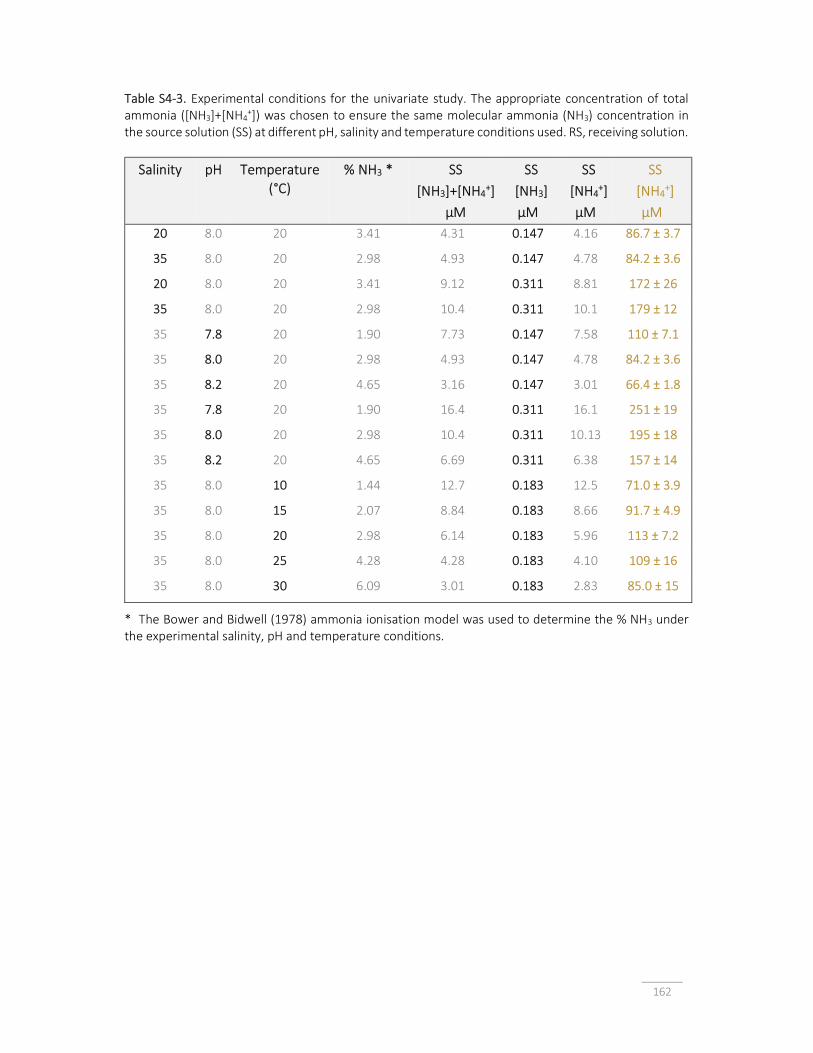
162

Table S4-3. Experimental conditions for the univariate study. The appropriate concentration of total ammonia ([NH3]+[NH4

+]) was chosen to ensure the same molecular ammonia (NH3) concentration in the source solution (SS) at different pH, salinity and temperature conditions used. RS, receiving solution.

Salinity pH Temperature (°C)

% NH3 * SS [NH3]+[NH4+]

µM

SS [NH3] µM

SS [NH4+] µM

SS [NH4+] µM

20 8.0 20 3.41 4.31 0.147 4.16 86.7 ± 3.7

35 8.0 20 2.98 4.93 0.147 4.78 84.2 ± 3.6

20 8.0 20 3.41 9.12 0.311 8.81 172 ± 26

35 8.0 20 2.98 10.4 0.311 10.1 179 ± 12

35 7.8 20 1.90 7.73 0.147 7.58 110 ± 7.1

35 8.0 20 2.98 4.93 0.147 4.78 84.2 ± 3.6

35 8.2 20 4.65 3.16 0.147 3.01 66.4 ± 1.8

35 7.8 20 1.90 16.4 0.311 16.1 251 ± 19

35 8.0 20 2.98 10.4 0.311 10.13 195 ± 18

35 8.2 20 4.65 6.69 0.311 6.38 157 ± 14

35 8.0 10 1.44 12.7 0.183 12.5 71.0 ± 3.9

35 8.0 15 2.07 8.84 0.183 8.66 91.7 ± 4.9

35 8.0 20 2.98 6.14 0.183 5.96 113 ± 7.2

35 8.0 25 4.28 4.28 0.183 4.10 109 ± 16

35 8.0 30 6.09 3.01 0.183 2.83 85.0 ± 15

* The Bower and Bidwell (1978) ammonia ionisation model was used to determine the % NH3 under the experimental salinity, pH and temperature conditions.

163

Section E GD-PS calibration

The GMDH algorithm is ideal for complex, multivariate systems, as the algorithm is able to

discriminate between relevant and irrelevant input variables, removing bias that could be

introduced by a researcher with prior knowledge [38]. The variables presented to the model

were temperature, and pH, with the output defined as the estimated concentration of

molecular ammonia in the source solution [NH3]TWA. The algorithm selected both temperature

and pH as relevant variables. As salinity between the ranges of 20 to 35 does not affect the

performance of the GD-PS (Figure 4-3A), salinity as a variable was not used for model

development.

The GMDH model has a self-organising approach, built with ‘layers’ of polynomial regressions,

whose coefficients are determined sequentially [38, 70]. The coefficients of the algorithm are

defined using inductive learning procedures that sort and select the most appropriate

regression, using the least squares fitting method [38, 70]. Once a ‘layer’ or polynomial

regression is defined, the algorithm proceeds to define and test the next, until the relationship

between input and output variables has been appropriately defined, and a model generated

(Figure S4-5). The input data for the development of the model are segregated into 80%

training and 20% randomly selected data used for model validation, and the model developed

had an inherent error of up to 10% according to the plot of residuals (Figure S4-6). GMDH Shell

(version 3.8.9) software was used for model generation [44], and the data was randomly sorted

prior to model generation.

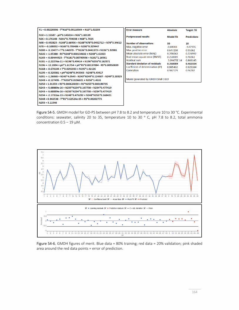
164

Figure S4-5. GMDH model for GD-PS between pH 7.8 to 8.2 and temperature 10 to 30 °C. Experimental conditions: seawater, salinity 20 to 35, temperature 10 to 30 ᵒ C, pH 7.8 to 8.2, total ammonia concentration 0.5 – 19 μM.

Figure S4-6. GMDH figures of merit. Blue data = 80% training; red data = 20% validation; pink shaded area around the red data points = error of prediction.

165

Section F Nerm (Port Phillip Bay) The coastal areas and waterways feeding into Nerm (Port Phillip Bay), have for thousands of

years been inhabited and managed by the Kulin nations, the waters which are today an area of

cultural, social, environmental and economic importance to all Victorians [71-75]. Port Phillip

Bay (PPB) is a semi-enclosed bay in south-eastern Australia, surrounded by the city of

Melbourne, Geelong and surrounding suburbs with an area just under 2,000 km2 (Figure S4-1)

[76]. The land catchment area of PPB comprises 21 natural drainage basins, the largest of these

being the Yarra River (known as Birrarung/Birrarang in the Woiwurrung and Boon Wurrung

languages) with 13 tributaries [76]. PPB is shallow for its size (24 meters maximum depth) with

flushing times of approximately ½ - 1 year in the farthest reaches, making it susceptible to

nutrient pollution leading to poor water quality due to eutrophication [76]. PPB is a dynamic

and self-sustaining ecosystem regulated by various important aquatic ecosystem processes

including the biogeochemical cycling of nutrients in the water column and sediments.

However, nutrient loading, particularly that of nitrogen, has been recognised as one of the

major threats to the health of the bay [76, 77], with treated wastewater from the Western

Treatment Plant (WTP), urban stormwater, agricultural runoff, and atmospheric deposition

identified as the main contributors to nutrient inputs. Ammonia is the major form of nitrogen

discharged from the WTP outfall into the coastal waters of Long Reef in western PPB [76]. It is

estimated that the Werribee Treatment Plant and the Yarra River contribute around 54% and

32% of the total annual nitrogen load to PPB, respectively, and the Werribee river contributes

around 6% [59].

The waters of PPB have been classified as nitrogen-limited, largely due to complex

biogeochemical cycling facilitated by phytoplankton and microphytobenthos in the water

column, the benthic bacterial and microalgal communities, and the burrowing invertebrates

and the subsequent redox environment created by these organisms in the sediments [76].

Microbial denitrification in the sediments has been identified as fundamental to the

‘assimilative capacity’ of nitrogen in the ecosystem, defined as the largest amount of nitrogen

loading that can be accommodated in the semi-enclosed bay, without there being a negative

impact on water quality, a deleterious impact on ecosystem function, or a rapid and irreversible

onset of eutrophication [76, 78]. Water quality managers are concerned with the fate and

dispersal of nutrients near input points, modelling biogeochemical nutrient cycling, in addition

166

to implementing programs and strategies to mitigate and reduce nutrient pollution from

entering the PPB catchment [78, 79]. Interestingly, the removal of bioavailable nitrogens,

known as the ‘denitrification efficiency’, has been identified as an important ecosystem service

to the cities of Melbourne, Geelong and surrounding suburbs, valued at an estimated $11

billion per year [80].

Section G Field validation

Figure S4-7. Field validation of the GD-PS with copper mesh (Cu-100) using the GMDH calibration model. The top graphs for both figures A) Hobsons Bay (Site 2) and B) Werribee River estuary 5 km upstream from river mouth (Site 4), highlight molecular ammonia concentrations measured by discrete grab sampling compared to the [NH3]TWA determined using the GD-PS in conjunction with the GMDH calibration model. The salinity, temperature (°C) and pH were monitored during the period of GD-PS deployment and are represented in the bottom graphs.

167

Section H Systematic error Calibration experiments were conducted with a near constant flow of 500 L h-1, however

environmental flow conditions in the field were very irregular. Some days water movement

especially in the upper estuaries appeared to flow very slowly and on other days wave action

and wind caused significant turbulence at the sea sites, followed by consecutive days where

there was very little water movement observed.

To assess if the flow rate was the cause of the systematic error, a number of laboratory-based

experiments (Table S4-4) were performed under three different flow conditions over the

course of 7 days, and the GMDH model was then used to predict the [NH3]TWA. In the first series

of experiments with maximum mixing, the 500 L h-1 aquarium pump in 10 L of solution was set

to the maximum setting for the duration of the experiment. This setting was used to generate

all calibration data used to develop the GMDH model, and a percentage difference of -9% was

recorded between the calculated source solution ammonia concentration and the [NH3]TWA. In

the second series of experiments, the intensity of mixing was reduced by adjusting the

aquarium pump speed to its minimal flow setting and switching this every second day to the

higher setting of 500 L h-1. Under these conditions the percentage difference recorded was in

the range of -21% to -22% between the calculated source solution ammonia concentration and

the [NH3]TWA. The percentage difference for the two mixing intensities mentioned above are of

a similar magnitude of that obtained during field work. A third series of experiments was

conducted by removing the aquarium pump from the tank altogether, and conducting the

passive sampling experiment under completely static conditions resulting in a difference of -

74% recorded between the calculated source solution ammonia concentration and the

[NH3]TWA (Table S4-4). These results confirm that the flow pattern is likely responsible for the

systematic error observed when comparing spot sampling with GD-based passive sampling.

168

Table S4-4. Effect of the flow pattern on the percentage difference (%) obtained when comparing discrete grab sampling (SS) and GD-based passive sampling ([NH3]TWA determined using the GMDH model).

Lab flow studies

Temperature (°C)

pH

SS [NH3]/nM

GD-PS [NH3]TWA nM

% Difference

n(GD-PS)

Intensive mixing

25.5 ± 0.3 7.99 ± 0.10 180 ± 59 164 ± 11.4 -9.4 5

Moderate mixing

28.0 ± 2.3 7.86 ± 0.06 154 ± 42 125 ± 15.6 -21.4 5

Moderate mixing

14.0 ± 7.1 8.13 ± 0.07 281 ± 184 225 ± 17.2 -22.2 5

No mixing 19.2 ± 3.7 7.88 ± 0.16 198 ± 151 91 ± 4.7 -74.2 5

Section I Method performance

Figure S4-8. Linear calibration with studentised residuals. Calibration of the GD-PS under the following experimental conditions: salinity 35, temperature 20 ᵒC, pH 8.0, and source solution ammonia concentrations 17 nM to 413 nM. The accumulated ammonia in the receiving solutions was measured as ammonium, and the source solution molecular ammonia was calculated by multiplying the total ammonia concentration by the fraction of un-ionised ammonia in solution, which was determined using the model described by Bower and Bidwell [6], when the temperature (°C), pH values, and salinity were known. A) Linear regression: y = (6.396 ± 0.1111) ᵡ 10-1 x – (12.359 ± 2.587), R² = 9.753 ᵡ 10-1; B) Studentized residuals showing a degree of increasing variance in the experiment, and an estimate of experimental error.

169

Section J GD-based passive sampling: A tool for ammonia screening and monitoring

Figure S4-9. Werribee river estuary mouth (Site 3) dissolved oxygen and tidal data. A) Tide and salinity data; B) pH and dissolved oxygen data; C) calculated source solution molecular ammonia and measured total ammonia data.

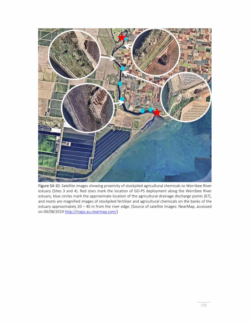
170

Figure S4-10. Satellite images showing proximity of stockpiled agricultural chemicals to Werribee River estuary (Sites 3 and 4). Red stars mark the location of GD-PS deployment along the Werribee River estuary, blue circles mark the approximate location of the agricultural drainage discharge points [67], and insets are magnified images of stockpiled fertiliser and agricultural chemicals on the banks of the estuary approximately 20 – 40 m from the river edge. (Source of satellite images: NearMap, accessed on 04/08/2019 http://maps.au.nearmap.com/)

171

Acknowledgements The authors of this work acknowledge the Boon Wurrung, Wurrundjerri and Wathaurong

Sovereign Clans of the Kulin Nation as the Traditional Custodians of the waterways and lands

upon which this research was undertaken. The authors acknowledge that the original

placename for Port Phillip Bay (PPB) is Nerm or Nairm in the Boon Wurrung language [46], and

the Yarra River is named Birrarung by the Wurundjeri and Boon Wurrung peoples meaning

‘river of mists’ [47, 48]. The Indigenous place names have been used, italicised, together with

the colonial place names, in brackets.

The authors would like to thank the EPA Victoria and CAPIM, for the loan of field equipment

and assistance from staff, namely, Chris Garland, Adele McKenzie and Mick Ernest, also

Professor Vincent Pettigrove (RMIT University, former CEO of CAPIM), and Mr. Andrew

Longmore for assistance with field work and sampling guidance. The authors would also like to

thank Mr. Roger Eastham and the Royal Yacht Club of Victoria for allowing field work in the

marina, Parks Victoria for permitting field work in the coastal waters of Nerm (PPB) and

Werribee River estuary, and Melbourne Ports for allowing field work in the Birrarung (Yarra

River) estuary. Mr. Marcus Hammarstedt assisted with the graphic design of Figure 4-1, and

Lenka O’Connor Šraj is grateful to the University of Melbourne for the award of a postgraduate

scholarship.

172

References 1. Anderson, D.M., P.M. Glibert, and J.M. Burkholder, Harmful algal blooms and eutrophication:

Nutrient sources, composition, and consequences. Estuaries, 2002. 25 (4): p. 704-726. 2. Smith, V.H., Eutrophication of freshwater and coastal marine ecosystems a global problem.

Environ. Sci. Pollut. Res., 2003. 10 (2): p. 126-139. 3. Smith, V.H., G.D. Tilman, and J.C. Nekola, Eutrophication: impacts of excess nutrient inputs on

freshwater, marine, and terrestrial ecosystems. Environ. Pollut., 1999. 100 (1): p. 179-196. 4. Battye, W., V.P. Aneja, and W.H. Schlesinger, Is nitrogen the next carbon? Earth's Future, 2017.

5 (9): p. 894-904. 5. Camargo, J.A. and A. Alonso, Ecological and toxicological effects of inorganic nitrogen pollution

in aquatic ecosystems: A global assessment. Environ. Int., 2006. 32: p. 831-849. 6. Bower, C.E. and J.P. Bidwell, Ionization of Ammonia in Seawater: Effects of Temperature, pH,

and Salinity. J. Fish. Res. Board Can., 1978. 35 (7): p. 1012-1016. 7. ANZG, Australian and New Zealand guidelines for fresh and marine water quality. 2018,

Australian and New Zealand Governments and Australian state and territory governments: Canberra ACT, Australia.

8. Batley, G.E. and S.L. Simpson, Development of guidelines for ammonia in estuarine and marine water systems. Mar. Pollut. Bull., 2009. 58 (10): p. 1472-1476.

9. Vrana, B., I.J. Allan, R. Greenwood, G.A. Mills, E. Dominiak, K. Svensson, J. Knutsson, and G. Morrison, Passive sampling techniques for monitoring pollutants in water. TrAC Trends Anal. Chem., 2005. 24 (10): p. 845-868.

10. Allan, I.J., J. Knutsson, N. Guigues, G.A. Mills, A.M. Fouillac, and R. Greenwood, Chemcatcher and DGT passive sampling devices for regulatory monitoring of trace metals in surface water. J. Environ. Monit., 2008. 10 (7): p. 821-9.

11. Booij, K., C.D. Robinson, R.M. Burgess, P. Mayer, C.A. Roberts, L. Ahrens, I.J. Allan, J. Brant, L. Jones, U.R. Kraus, M.M. Larsen, P. Lepom, J. Petersen, D. Pröfrock, P. Roose, S. Schäfer, F. Smedes, C. Tixier, K. Vorkamp, and P. Whitehouse, Passive Sampling in Regulatory Chemical Monitoring of Nonpolar Organic Compounds in the Aquatic Environment. Environ. Sci. Technol., 2016. 50 (1): p. 3-17.

12. ICES. 2013, Report of the Workshop on the Application of Passive Sampling and Pas-sive Dosing to Contaminants in Marine Media (WKPSPD). 29–31 January 2013, ICES CM 2013/SSGHIE:02. Copenhagen, Denmark.

13. Dunn, R.J.K., P.R. Teasdale, J. Warnken, M.A. Jordan, and J.M. Arthur, Evaluation of the in situ, time-integrated DGT technique by monitoring changes in heavy metal concentrations in estuarine waters. Environ. Pollut., 2007. 148(1): p. 213-220.

14. Vrana, B., V. Klučárová, E. Benická, N. Abou-Mrad, R. Amdany, S. Horáková, A. Draxler, F. Humer, and O. Gans, Passive sampling: An effective method for monitoring seasonal and spatial variability of dissolved hydrophobic organic contaminants and metals in the Danube river. Environ. Pollut., 2014. 184: p. 101-112.

15. Novic, A.J., D.S. O’Brien, S.L. Kaserzon, D.W. Hawker, S.E. Lewis, and J.F. Mueller, Monitoring Herbicide Concentrations and Loads during a Flood Event: A Comparison of Grab Sampling with Passive Sampling. Environ. Sci. Tech., 2017. 51(7): p. 3880-3891.

16. Huang, J., W.W. Bennett, D.T. Welsh, T. Li, and P.R. Teasdale, Development and evaluation of a diffusive gradients in a thin film technique for measuring ammonium in freshwaters. Anal. Chim. Acta, 2016. 904 (Supplement C): p. 83-91.

17. Ren, M., S. Ding, D. Shi, Z. Zhong, J. Cao, L. Yang, D.C.W. Tsang, D. Wang, D. Zhao, and Y. Wang, A new DGT technique comprised in a hybrid sensor for the simultaneous measurement of ammonium, nitrate, phosphorus and dissolved oxygen. Sci. Total. Environ., 2020. 725: p. 138447.

173

18. Huang, J., W.W. Bennett, D.T. Welsh, and P.R. Teasdale, Determining time-weighted average concentrations of nitrate and ammonium in freshwaters using DGT with ion exchange membrane-based binding layers. Environ. Sci. Proc. Imp., 2016. 18 (12): p. 1530-1539.

19. Huang, J., W.W. Bennett, P.R. Teasdale, N.R. Kankanamge, and D.T. Welsh, A modified DGT technique for the simultaneous measurement of dissolved inorganic nitrogen and phosphorus in freshwaters. Anal. Chim. Acta, 2017. 988: p. 17-26.

20. Huang, J., W.W. Bennett, D.T. Welsh, T. Li, and P.R. Teasdale, “Diffusive Gradients in Thin Films” Techniques Provide Representative Time-Weighted Average Measurements of Inorganic Nutrients in Dynamic Freshwater Systems. Environ. Sci. Technol., 2016. 50 (24): p. 13446-13454.

21. Pichette, C., H. Zhang, W. Davison, and S. Sauvé, Preventing biofilm development on DGT devices using metals and antibiotics. Talanta, 2007. 72(2): p. 716-722.

22. Panther, J.G., P.R. Teasdale, W.W. Bennett, D.T. Welsh, and H. Zhao, Titanium Dioxide-Based DGT Technique for In Situ Measurement of Dissolved Reactive Phosphorus in Fresh and Marine Waters. Environ. Sci. Tech., 2010. 44(24): p. 9419-9424.

23. Panther, J.G., P.R. Teasdale, W.W. Bennett, D.T. Welsh, and H. Zhao, Comparing dissolved reactive phosphorus measured by DGT with ferrihydrite and titanium dioxide adsorbents: Anionic interferences, adsorbent capacity and deployment time. Anal. Chim. Acta, 2011. 698(1): p. 20-26.

24. Zhu, Y., B. Shan, J. Huang, P.R. Teasdale, and W. Tang, In situ biochar capping is feasible to control ammonia nitrogen release from sediments evaluated by DGT. Chem. Eng. J., 2019. 374: p. 811-821.

25. Almeida, M.I.G.S., A.M. Silva, R.A. Coleman, V.J. Pettigrove, R.W. Cattrall, and S.D. Kolev, Development of a passive sampler based on a polymer inclusion membrane for total ammonia monitoring in freshwaters. Anal. Bioanal. Chem., 2016. 408 (12): p. 3213-22.

26. Tillett, B.J., D. Sharley, M.I.G.S. Almeida, I. Valenzuela, A.A. Hoffmann, and V. Pettigrove, A short work-flow to effectively source faecal pollution in recreational waters – A case study. Sci. Total. Environ., 2018. 644: p. 1503-1510.

27. O'Connor Šraj, L., M.I.G.S. Almeida, S.E. Swearer, S.D. Kolev, and I.D. McKelvie, Analytical challenges and advantages of using flow-based methodologies for ammonia determination in estuarine and marine waters. TrAC Trend. Anal. Chem., 2014. 59: p. 83-92.

28. Gilbert, T.R. and A.M. Clay, Determination of ammonia in aquaria and in sea water using the ammonia electrode. Anal. Chem., 1973. 45(9): p. 1757-1759.

29. Merks, A.G.A., Determination of ammonia in sea water with an ion-selective electrode. Neth. J. Sea. Res., 1975. 9(3): p. 371-375.

30. Walters, F.H., K.B. Griffin, and D.F. Keeley, Use of ammonia-sensing electrodes in salt media. Analyst, 1984. 109(5): p. 663-665.

31. APHA, Method 4500-NH3 D. Ammonia-Selective Electrode Method, in Standard Methods For the Examination of Water and Wastewater. 2000, America Public Health Association: Washington, D.C.

32. APHA, Method 4500-NH3 E. Ammonia-Selective Electrode Method Using Known Addition, in Standard Methods For the Examination of Water and Wastewater. 2000, America Public Health Association: Washington, D.C.

33. Ding, L., J. Ding, B. Ding, and W. Qin, Solid-contact Potentiometric Sensor for the Determination of Total Ammonia Nitrogen in Seawater. Int. J. Electrochem. Sci., 2017. 12(4): p. 3296-3308.

34. Cuartero, M., N. Colozza, B.M. Fernández-Pérez, and G.A. Crespo, Why ammonium detection is particularly challenging but insightful with ionophore-based potentiometric sensors – an overview of the progress in the last 20 years. Analyst, 2020. 145(9): p. 3188-3210.

35. Li, T., J. Panther, Y. Qiu, C. Liu, J. Huang, Y. Wu, P.K. Wong, T. An, S. Zhang, and H. Zhao, Gas-Permeable Membrane-Based Conductivity Probe Capable of In Situ Real-Time Monitoring of Ammonia in Aquatic Environments. Environ. Sci. Tech., 2017. 51(22): p. 13265-13273.

174

36. Li, T., M. Zhou, Y. Qiu, J. Huang, Y. Wu, S. Zhang, and H. Zhao, Membrane-based conductivity probe for real-time in-situ monitoring rice field ammonia volatilization. Sensor. Actuat. B-Chem., 2019. 286: p. 62-68.

37. O’Connor Šraj, L., M.I.G.S. Almeida, C. Bassett, I.D. McKelvie, and S.D. Kolev, Gas-diffusion-based passive sampler for ammonia monitoring in marine waters. Talanta, 2018. 181: p. 52-56.

38. Farlow, S.J., The GMDH Algorithm of Ivakhnenko. Am. Stat., 1981. 35 (4): p. 210-215. 39. Dickson, A.G., C.L. Sabine, and J.R. Christian, SOP 6B Determination of the pH of sea water using

the indicator dye m-cresol purple. In Guide to Best Practices for Ocean CO2 Measurements. PICES Special Publication 3. 2007: p. 1-7.

40. Douglas, N.K. and R.H. Byrne, Achieving accurate spectrophotometric pH measurements using unpurified meta-cresol purple. Mar. Chem., 2017. 190: p. 66-72.

41. O'Connor Šraj, L., M.I.G.S. Almeida, I.D. McKelvie, and S.D. Kolev, Determination of trace levels of ammonia in marine waters using a simple environmentally-friendly ammonia (SEA) analyser. Mar. Chem., 2017. 194 (Supplement C): p. 133-145.

42. Rehan, M., H.M. Mashaly, S. Mowafi, A. Abou El-Kheir, and H.E. Emam, Multi-functional textile design using in-situ Ag NPs incorporation into natural fabric matrix. Dyes Pigm., 2015. 118: p. 9-17.

43. Aneja, K.R., Experiments in Microbiology, Plant Pathology and Biotechnology. Fourth Edition ed. 2003, New Delhi: New Age International. 97-100.

44. GMDH, GMDH Shell Predictive Analytics Software, Version 3.8.9. 2019. 45. Helsel, D.R. and R.M. Hirsch, 3A. Statistical Methods in Water Resources, in Techniques of Water

Resources Investigations. 2002, U.S. Geological Survey. 46. Illingworth, J.A., A common source of error in pH measuremnet. Biochem. J., 1981. 195: p. 259-

262. 47. Smith, M.J., A. Kerr, and M.J. Cowling, Effects of marine biofouling on gas sensor membrane

materials. J. Environ. Monitor., 2007. 9(12): p. 1378-1386. 48. Ouyang, G., W. Zhao, M. Alaee, and J. Pawliszyn, Time-weighted average water sampling with

a diffusion-based solid-phase microextraction device. J. Chromatog. A., 2007. 1138(1): p. 42-46. 49. Li, J., X. Liu, J. Lu, Y. Wang, G. Li, and F. Zhao, Anti-bacterial properties of ultrafiltration

membrane modified by graphene oxide with nano-silver particles. J. Colloid. Interf. Sci., 2016. 484: p. 107-115.

50. Crank, J., The Mathematics of Diffusion. 2nd ed. 1975, Oxford, UK: Oxford Clarendon Press. 51. Zhang, H. and W. Davison, Performance Characteristics of Diffusion Gradients in Thin Films for

the in Situ Measurement of Trace Metals in Aqueous Solution. Anal. Chem., 1995. 67(19): p. 3391-3400.

52. Booij, K., B. Vrana, J.N. Huckins, R. Greenwood, G. Mills, and B. Vrana, Chapter 7 Theory, modelling and calibration of passive samplers used in water monitoring, in Comprehensive Analytical Chemistry. 2007, Elsevier. p. 141-169.

53. Warnken, K.W., H. Zhang, and W. Davison, Chapter 11 In situ monitoring and dynamic speciation measurements in solution using DGT, in Comprehensive Analytical Chemistry, R. Greenwood, G. Mills, and B. Vrana, Editors. 2007, Elsevier. p. 251-278.

54. Radford, G.J.W., F.C. Walsh, J.R. Smith, C.D.S. Tuck, and S.A. Campbell, 3 - Electrochemical and atomic force microscopy studies of a copper nicekl alloy in sulfide-contaminated sodium chloride solutions, in Developments in Marine Corrosion, S.A. Campbell, N. Campbell, and F.C. Walsh, Editors. 1998, Woodhead Publishing. p. 41-63.

55. Brooks, S. and M. Waldock, Chapter 19, The use of copper as a biocide in marine antifouling paints. In Hellio, C and Yebara, D. (Eds.), In Advances in Marine Antifouling Coatings and Technologies, Woodhead Publishing Series in Metals and Surface Engineering, 492-521 2009.

56. Seethapathy, S., T. Górecki, and X. Li, Passive sampling in environmental analysis. J. Chromatogr. A., 2008. 1184(1): p. 234-253.

175

57. Warnken, K.W., H. Zhang, and W. Davison, Accuracy of the diffusive gradients in thin-films technique: diffusive boundary layer and effective sampling area considerations. Anal Chem, 2006. 78(11): p. 3780-7.

58. Guibal, R., S. Lissalde, and G. Guibaud, Experimental Estimation of 44 Pharmaceutical Polar Organic Chemical Integrative Sampler Sampling Rates in an Artificial River under Various Flow Conditions. Environ. Toxicol. Chem., 2020. 39(6): p. 1186-1195.

59. DEWLP, Yarra River Protection Ministerial Advisory Committee, Protecting the Yarra River (Birrarung) Discussion Paper, Department of Environment, Land, Water & Planning, The State Government of Victoria, https://www.planning.vic.gov.au/__data/assets/pdf_file/0037/99766/Protecting-the-Yarra-River-Birrarung-discussion-paper-summary.pdf (accessed on: 10 October 2019). 2016.

60. Longmore, A.R., R.A. Cowdell, and R. Flint, Nutrient status of the water in Port Phillip Bay 1990-1994. Technical Report 24, CSIRO Port Phillip Bay Environmental Study. 1996.

61. Schlichting, H., Boundary Layer Theory. 7th ed. 1979, New York, USA: McGraw-Hill. 62. Ibrahim, I., A. Togola, and C. Gonzalez, In-situ calibration of POCIS for the sampling of polar

pesticides and metabolites in surface water. Talanta, 2013. 116: p. 495-500. 63. Moschet, C., E.L.M. Vermeirssen, H. Singer, C. Stamm, and J. Hollender, Evaluation of in-situ

calibration of Chemcatcher passive samplers for 322 micropollutants in agricultural and urban affected rivers. Water Res., 2015. 71: p. 306-317.

64. Sara O'Brien, D., B. Chiswell, and J.F. Mueller, A novel method for the in situ calibration of flow effects on a phosphate passive sampler. J. Environ. Monit., 2009. 11 (1): p. 212-219.

65. Nitti, F., M.I.G.S. Almeida, R. Morrison, R.W. Cattrall, V.J. Pettigrove, R.A. Coleman, and S.D. Kolev, Development of a portable 3D-printed flow-through passive sampling device free of flow pattern effects. Microchem. J., 2018. 143: p. 359-366.

66. Sheridan, J., K. Larsen, and R. Carey, Melbourne’s foodbowl: Now and at seven million, Victorian Eco-Innovation Lab, The University of Melbourne https://research.unimelb.edu.au/__data/assets/pdf_file/0008/2355155/Melbournes-Foodbowl-Now-and-at-seven-million.pdf (accessed on 12 November 2019). 2015.

67. SRW, Western Irrigation Futures Atlas, Southern Rural Water, http://www.srw.com.au/files/Technical_reports/Western_Irrigation_Furtures_WIF_atlas.pdf (accessed on 20 November 2019). 2009.

68. SGV. Werribee Catchment Report Card for July 2017 - June 2018, Yarra and Bay, State Government of Victoria https://yarraandbay.vic.gov.au/report-card/report-card-2018/port-phillip/werribee (accessed on 20 November 2019). 2019 4 June 2019; Available from: https://yarraandbay.vic.gov.au/report-card/report-card-2018/port-phillip/werribee#top_of_report.

69. EU, Commission Directive 2009/90/EC of 31 July 2009 laying down, pursuant to Directive 2000/60/EC of the European Parliament and of the Council, technical specifications for chemical analysis and monitoring of water status. Official Journal of the European Union, L210: 36–38. 2009.

70. Anastaski, I. and N. Mort, The Developemnt of Self-Organization Techniques in Modelling: A Review of the Group Method of Data Handling (GMDH), Department of Automatic Control & Systems Engineering, The University of Sheffield, Research Report No. 813, https://gmdhsoftware.com/GMDH_%20Anastasakis_and_Mort_2001.pdf (accessed on 10 October 2019). 2001.

71. BWF, Ngargee to Nerm: from ancient tree to ancient sea, Boon Wurrung Foundation; Port Phillip EcoCentre, City of Port Phillip, http://www.portphillip.vic.gov.au/default/Ngargee_to_Nerm_DL_V12-min.pdf (accessed on 20 November 2019). 2016.

176

72. Briggs, C., Boon Wurrung: The Filling of the Bay – The Time of Chaos, Culture Victoria, State Governmnet of Victorian, https://cv.vic.gov.au/stories/aboriginal-culture/nyernila/boon-wurrung-the-filling-of-the-bay-the-time-of-chaos/ (accessed on 20 November 2019). 2016.

73. Garvey-Wandin, D. Woiwurrung: The Durrung of the Yan-yan, Culture Victoria, Victorian Government, https://cv.vic.gov.au/stories/aboriginal-culture/nyernila/woiwurrung-the-durrung-of-the-yan-yan/ (accessed on 20 November 2019). 2016; Available from: https://cv.vic.gov.au/stories/aboriginal-culture/nyernila/woiwurrung-the-durrung-of-the-yan-yan/.

74. CV, Boon Wurrung: The Journey of the Iilk – Iilkyawa, Culture Victoria, State Government of Victoria, https://cv.vic.gov.au/stories/aboriginal-culture/nyernila/boon-wurrung-the-filling-of-the-bay-the-time-of-chaos/ (accessed on 20 November 2019). 2016.

75. Eidelson, M., Yalukit Willam: The River People of Port Phillip, City of Port Phillip, Art & Heritage Unit, https://heritage.portphillip.vic.gov.au/Aboriginal_heritage/Yalukit_Willam_The_River_People_of_Port_Phillip (accessed on 20 November 2019). 2014.

76. Harris, G., G. Batley, D. Fox, D. Hall, P. Jernakoff, R. Molloy, A. Murray, B. Newell, J. Parslow, G. Skyring, and S. Walker, Port Phillip Bay Environmental Study Final Report, CSIRO, Canberra, Australia. 1996.

77. EPA, Port Phillip Bay Water Quality Long-term Trends in Nutrients Status and Clairty, 1984 - 1999, Publication 806, Environment Protection Authority Victoria, Southbank, Victoria. 2002.

78. Murray, A.G. and J.S. Parslow, Modelling of nutrient impacts in Port Phillip Bay - a semi-enclosed marine Australian ecosystem. Mar. Fresh. Res., 1999. 50 (6): p. 597-612.

79. DELWP, Port Phillip Bay Environmental Management Plan 2017 - 2027, Department of Land Water and Planning, State Government of Victoria, https://www.marineandcoasts.vic.gov.au/coastal-programs/port-phillip-bay (accessed 5 October 2019). 2017.

80. DELWP, Marine and Coastal Ecosystem Accounting: Port Phillip Bay, Report to the Commissioner for Environmental Sustainability, Department of Environment, Land, Water & Planning, https://www.environment.vic.gov.au/__data/assets/pdf_file/0025/49813/Marine-and-Coastal-Ecosystem-Accounting-Port-Phillip-Bay.pdf (accessed on 5 October 2019). 2016.

81. Shaun, C. and F. Thiele, Indigenous Cultural Heritage and History within the Metropolitan Melbourne Investigation Area, A Report to the Victorian Environmental Asessment Council http://www.veac.vic.gov.au/documents/Indigenous%20Cultural%20Heritage%20and%20History%20within%20the%20VEAC%20Melbourne%20Metropolitan%20Investigation%20Area.pdf (accessed on 20 November 2019).

177

CHAPTER 5: Conclusions and future work

This thesis reports on the development of novel analytical tools for the monitoring of ammonia

in marine waters, including a flow-based analyser and a gas-diffusion-based passive sampler.

In Chapter 2, a simple and environmentally-friendly ammonia (SEA) analyser, was developed

for the determination of ammonia in a wide range of concentrations. The SEA analyser was

designed so that the desired concentration range could be tailored by simple modification of

the program used to control the system hardware, including suitable adjustments to the

sample and reagent volumes, making this an easy-to-use and versatile method. A gas-diffusion

unit (GDU) was used for analyte separation and pre-concentration, and instead of using

discrete, fixed volume samples, a flow approach was established where large sample volumes

were continuously delivered to the donor channel of the GDU, while the acceptor solution,

containing an acid-base indicator, was held static during this time. The acceptor stream was

then re-started and monitored spectrophotometrically, and the absorbance, corresponding to

the pH change caused by ammonia accumulated in the acceptor solution, was directly

proportional to its concentration in the sample stream.

Several GDUs were tested, to determine which would give the highest sensitivity and

repeatability, with two main configurations considered, including a sandwich style that

comprised a sheet of hydrophobic porous gas-diffusion membrane (GDM) in between two

Perspex blocks with drilled channels (identical in size), and a tubular design where either single

or multiple hollow fibre GDMs were fitted into a larger diameter tubing. While the tubular

configurations had a high membrane surface to solution volume ratio, these GDUs were

difficult to use and suffered from a large blank response due to interference from the adhesives

required for their fabrication which reacted with the acid-base indicator. The sandwich-style

serpentine unit was chosen as it exhibited good sensitivity and repeatability. The performance

of several different GDMs made from different porous hydrophobic materials and with

different pore sizes were tested, with the super hydrophobic SureVent® membrane chosen as

178

it exhibited good mechanical stability and durability, especially under high flow rate conditions

which allowed for increased sample throughput over prolonged periods of time.

Several acid-base indicators were tested to improve sensitivity and the working concentration

range, including mixtures of indicators with similar pKa values and colour changes.

Bromothymol blue exhibited the highest sensitivity and was therefore chosen as the preferred

indicator; however, the dynamic range could be extended by using the combination

bromothymol blue and thymol blue indicators in a 50:50 concentration ratio. The buffering

capacity of the acceptor stream was also examined, showing that large increases in sensitivity

could be achieved by a small adjustment in solution pH to achieve an initial absorbance in the

range of 0.180 – 0.200.

Three working ranges and their analytical figures of merit were described, including a low

concentration range (0.028 – 5.6 μM NH4+, 2.0 mL sample volume, LOD of 0.015 μM NH4+, and

a sample throughput of 20 h-1), a mid-concentration range (0.28 – 13.9 μM, NH4+, 1.0 mL

sample volume, LOD of 0.088 μM NH4+, and a sample throughput of 30 h-1), and an upper

concentration range (1.4 – 55.6 μM NH4+, 0.25 mL sample volume, LOD of 0.44 μM NH4+, and

a sample throughput of 40 h-1). The method is versatile and can be modified by simple

adjustment of the sample and reagent volumes. Hence, an infinite number of working ranges

could theoretically be defined. The system was validated against a certified reference material

and spike-and-recovery of estuarine and coastal seawater samples, showing good agreement,

especially in the middle to upper concentration ranges where the error was minimal. The

reagents used were affordable, non-toxic, suitable for long-term storage, and costing as little

as $2.40 per 1,000 determinations.

The SEA analyser was used as an analytical tool in the development of the gas-diffusion-based

passive sampling (GD-PS) device for ammonia monitoring in marine waters described in

Chapters 3 and 4, enabling the easy determination of ammonia in both typically low

concentrations found in marine water samples, and in high concentrations found in the passive

sampler’s acidic receiving solutions, without requiring any changes to the manifold.

179

The first prototype of an ammonia GD-PS for marine waters is described in Chapter 3. This

device utilises a porous hydrophobic GDM to separate the sampled medium from a 10 mL

acidic receiving solution. The dissolved ammonia present in the sampled medium diffuses

through the pores of the GDM towards the membrane/receiving solution interface, where it is

protonated to form the ammonium ion, and is thus accumulated in the receiving solution. The

described GD-PS selectively transfers ammonia molecules from the sample matrix into its

receiving solution, essentially acting as a zero sink by trapping the ammonia molecules as

ammonium in the receiving solution, which can be directly analysed using a variety of methods,

including the newly developed SEA analyser described in Chapter 2.

Membrane permeability and receiving solution optimisation studies showed that it was

necessary to match the ionic strength of the receiving solution as closely as possible to that of

the sampled medium, to minimise undesirable osmotic transport of solutes across the GDM.

This was achieved by adding sodium chloride to the acidic receiving solution (0.1 M HCl) in

order to achieve ion concentrations which would match that of the sampled medium where

the sampler would be deployed. The effect of flow pattern on the ammonia uptake was also

investigated, showing that in environments where multi-directional flow dominated (e.g.,

coastal areas subject to wave action and tidal estuaries) the use of flow restriction shields did

not provide any benefits.

Calibration of the GD-PS was performed under laboratory conditions using recirculated

synthetic seawater spiked with known concentrations of an ammonium stock solution.

However, after a period of approximately 4-5 days, biofouling inhibited further uptake of

ammonia into the receiving solution, limiting the use of the GD-PS to a deployment period of

3 days.

Validation experiments to assess the GD-PS performance for a sampling period of 3 days were

undertaken in the field at an estuarine site. Daily spot samples of the sampled medium were

collected in the field, and a comparison between the mean ammonia concentration found in

the spot samples and the time-weighted average concentration (CTWA) of ammonia determined

using the calibrated GD-PS was performed. Good agreement between the two sampling

methods was observed (relative error of 13.0%).

180

Chapter 4 describes how the limitations of the GD-PS outlined in Chapter 3 were overcome.

These limitations include the GDM biofouling after 3 days of deployment, and the need to

perform a calibration under matrix conditions (e.g., temperature and pH) that closely resemble

those of the aquatic system being sampled. Biofouling of the GDMs severely inhibited the

performance of the GD-PS after 4-5 days, and thus membrane antifouling strategies were

assessed. Each antifouling strategy was placed between the GDM and the sampled medium,

and included a silver nanoparticle (AgNP) functionalised mesh and two different weave

densities of a copper mesh. All antifouling strategies tested minimised the amount of biofilm

formation on the surface of the GDM after exposure to samples containing microalga, however

the copper meshes were more effective than the AgNP mesh. As expected, the control (with

no treatment) had the highest fouling. The GD-PS with the open weave copper mesh (Cu-100

with a weave of 100 wires per inch) exhibited the highest ammonia uptake in the high fouling

environment (nutrient enriched seawater) and this mesh was therefore chosen as the most

efficient antifouling strategy for all future experiments allowing for linear ammonia uptake in

the GD-PS for up to 7 days.

It is well documented that environmental variables, such as temperature, pH and salinity, may

affect the performance of passive sampling technologies in aquatic environments, as

summarised in Chapter 1. These environmental variables were also expected to affect the

performance of the described GD-PS, as the ammonia speciation in solution is affected by

temperature, pH, and to a lesser extent salinity. It was therefore important to assess the impact

of these variable on the performance of the GD-PS.

While salinity (in the range 20 – 35) did not impact the performance of the GD-PS in terms of

accumulation of ammonia in the receiving solution, both temperature and pH exhibited a

significant effect. Therefore, to enable use of the GD-PS in a wide range of matrix conditions,

numerous calibration experiments under different pH and temperature conditions were

undertaken. The Group Method Data Handling (GMDH) algorithm allows for the modelling of

complex systems affected by multiple variables. It was therefore chosen to model the GD-PS

behaviour allowing for the development of one single calibration model applicable over the

range of environmental conditions that were presented, that being temperature conditions

181

between 10 – 30° C and pH conditions within the range 7.8 – 8.2. These conditions were chosen

as they are commonly found in coastal and marine ecosystems around the world. The input

data for the model development were separated so that 80% were used for model

development and 20% were withheld and used for model validation. The model had an

approximate error of ± 10% according to the plot of residuals.

The model was used to determine the CTWA of ammonia at four field sites where the GD-PSs

were deployed, including three estuarine sites and one coastal site. At each location, an

autosampler was concurrently deployed to collect water spot samples every 2 hours over the

course of GD-PS deployment. The ammonia in these samples was measured and the mean

concentration was compared to the CTWA determined using the GD-PS and the GMDH

calibration model, and a good agreement between the two sampling methods was achieved.

However, a systematic error was observed, which was attributed to the effect of flow pattern.

In order to confirm this hypothesis, laboratory experiments were performed by immersing the

GD-PS under different flow conditions, and it was concluded that the systematic error was

likely due to differences in hydrodynamic conditions experienced by the GD-PS in the

laboratory-based calibration compared to the field environments. Whilst this was shown to be

most pronounced in near static solutions, estuaries and coastal aquatic environments should

have sufficient water movement to allow for the developed calibration model to be used with

minimal error.

While the use of performance reference compounds to overcome the effects of environmental

variables has been successful for some passive samplers, this approach is suitable when

partitioning is the dominant sorption mechanism. Hence, it would not be suitable for passive

samplers that act as a chemical trap, such as the GD-PS studied. The concurrent deployment

of passive flow monitors (containing gypsum or calcium sulfate dihydrate) have been

successfully applied by Obrien et al. [1] to correct for changes in hydrodynamic conditions

experienced by passive phosphate samplers in estuarine and marine waters, and it is possible

that such an approach could be applied to correct for the hydrodynamic exposure conditions

experienced by the newly developed GD-PSs, although this remains to be tested.

182

In order to determine the ammonia CTWA using the newly developed GD-PS, it is necessary to

measure the environmental variables temperature and pH over the course of the sampler’s

deployment, as these variables have been identified as inputs for the GMDH calibration model.

While accurate and affordable submersible temperature loggers are readily available (e.g.,

Tinytag and Hobo pendant), the accurate measurement of pH in high salinity matrices is far

more challenging, as commercial probes are expensive and generally require a certain level of

operator skill to perform the necessary calibrations. In highly dynamic estuarine environments,

a pH logging device would be necessary, as diurnal changes in pH can be significant. However,

in coastal seawaters that are buffered against pH changes, it would be possible to measure in

situ pH only on the GD-PS deployment and collection days, and input the average of these two

measurements into the GMDH calibration model.

A microfluidic paper-based analytical device (µPAD) calibrated for measuring seawater pH is

currently being developed by the author and will be used in the future in combination with the

newly developed GD-PS for ammonia monitoring in high salinity aquatic systems. Additionally,

the analysis of ammonia in the GD-PSs receiving solution could be further simplified and even

performed in the field, by using the µPADs for the determination of ammonia in wastewater

samples using gas-diffusion separation [2] and in freshwaters using micro distillation analyte

separation [3].

The newly developed GD-PS is affordable, user-friendly, reusable and can detect ammonia

concentrations lower than the revised water quality guideline value of 160 μg N L-1 (total

ammonia) for high conservation marine ecosystems, making this an exciting new tool for

regulators and managers responsible for monitoring the health of our estuaries and coastal

environments.

183

References

1. O’Brien, D.S., K. Booij, D.W. Hawker, and J.F. Mueller, Method for the in Situ Calibration of a Passive Phosphate Sampler in Estuarine and Marine Waters. Environmental Science & Technology, 2011. 45(7): p. 2871-2877.

2. Jayawardane, B.M., I.D. McKelvie, and S.D. Kolev, Development of a Gas-Diffusion Microfluidic Paper-Based Analytical Device (μPAD) for the Determination of Ammonia in Wastewater Samples. Analytical Chemistry, 2015. 87(9): p. 4621-4626.

3. Peters, J.J., M.I.G.S. Almeida, L. O'Connor Šraj, I.D. McKelvie, and S.D. Kolev, Development of a micro-distillation microfluidic paper-based analytical device as a screening tool for total ammonia monitoring in freshwaters. Analytica Chimica Acta, 2019. 1079: p. 120-128.

Minerva Access is the Institutional Repository of The University of Melbourne

Author/s:Sraj, Lenka O'Connor

Title:Development of an automated trace analyser and a novel passive sampling device for themonitoring of ammonia in marine environments

Date:2020

Persistent Link:http://hdl.handle.net/11343/252863

Terms and Conditions:Terms and Conditions: Copyright in works deposited in Minerva Access is retained by thecopyright owner. The work may not be altered without permission from the copyright owner.Readers may only download, print and save electronic copies of whole works for their ownpersonal non-commercial use. Any use that exceeds these limits requires permission fromthe copyright owner. Attribution is essential when quoting or paraphrasing from these works.