Development of A Virtual Intelligence Technique for the Upstream Oil Industry

Final Report

Reporting Period: Start Date: August 18, 2001 End Date: September 19, 2004

Principal Authors:

Iraj A. Salehi Gas Technology Institute

Shahab D. Mohaghegh Intelligent Solutions, Inc.

Samuel Ameri West Virginia University

Date of Issue: September, 2004 DOE Award Number: DE-FC26-01BC15271 Submitted by: Gas Technology Institute

1700 South Mount Prospect Road Des Plaines, Illinois 60018

Intelligent Solutions, Inc. P. O. Box 14 Morgantown, West Virginia 26507

West Virginia University 886 Chestnut Ridge Road Morgantown, West Virginia 26506-6845

1

DISCLAIMER This report was prepared as an account of work sponsored by an agency of the United States Government. Neither the United States Government nor any agency thereof, nor any of their employees, makes any warranty, express or implied, or assumes any legal liability or responsibility for the accuracy, completeness, or usefulness of any information, apparatus, product, or process disclosed, or represents that is use would not infringe privately owned rights. Reference herein to any specific commercial product, process, or service by trade name, trademark, manufacturer, or otherwise does not necessarily constitute or imply its endorsement, recommendation, or favoring by the United States Government or any agency thereof. The views and opinions of authors expressed herein do not necessarily state or reflect those of the United States Government or any agency thereof.

2

ABSTRACT The objective of the research and development work reported in this document was to develop a Virtual Intelligence Technique for optimization of the Preferred Upstream Management Practices (PUMP) for the upstream oil industry. The work included the development of a software tool for identification and optimization of the most influential parameters in upstream common practices as well as geological, geophysical and reservoir engineering studies.

The work was performed in cooperation with three independent producing companies – Newfield Exploration, Chesapeake Energy, and Triad Energy – operating in the Golden Trend, Oklahoma. In order to protect data confidentiality, these companies are referred to as Company One, Two, Three in a randomly selected order. These producing companies provided geological, completion, and production data on 320 wells and participated in frequent technical discussions throughout the project. Research and development work was performed by Gas Technology Institute (GTI), West Virginia University (WVU), and Intelligent Solutions Inc. (ISI). Oklahoma Independent Petroleum Association (OIPA) participated in technology transfer and data acquisition efforts.

Deliverables from the project are the present final report and a user-friendly software package (Appendix D) with two distinct functions: a characterization tool that identifies the most influential parameters in the upstream operations, and an optimization tool that seeks optimization by varying a number of influential parameters and investigating the coupled effects of these variations. The electronic version of this report is also included in Appendix D.

The Golden Trend data were used for the first cut optimization of completion procedures. In the subsequent step, results from soft computing runs were used as the guide for detailed geophysical and reservoir engineering studies that characterize the cause-and-effect relationships between various parameters. The general workflow and the main performing units were as follows:

• Data acquisition. (GTI, OIPA, Participating producers.) • Development of the virtual intelligence software. (WVU, ISI) • Application of the software on the acquired data. (GTI, ISI) • Detailed production analysis using conventional engineering techniques and the

DECICE neural network software. (GTI) • Detailed seismic analysis using InsPect spectral decomposition package and

Hapmson-Russell’s EMERGE inversion package. (GTI) Technology transfer took place through several workshops held at offices of the participating companies, at OIPA offices, and presentations at the SPE panel on soft computing applications and at the 2003 annual meeting of Texas Independent Producers and Royalty Owners Association (TIPRO). In addition, results were exhibited at the SPE annual meeting, published in GasTips, and placed on the GTI web page.

Results from the research and development work were presented to the producing companies as a list of recommended recompletion wells and the corresponding optimized operations parameters. By the end of the project, 16 of the recommendations have been implemented the majority of which resulted in increased production rates to several folds. This constituted a comprehensive field demonstration with positive results.

3

TABLE OF CONTENTS DISCLAIMER ................................................................................................................................ 2 ABSTRACT.................................................................................................................................... 3 1.0 INTRODUCTION ............................................................................................................ 13 2.0 Experimental Methods ...................................................................................................... 27

2.1. Geological and Geophysical Studies ............................................................................ 28 2.1.1. Historic production in area.................................................................................... 28 2.1.2. Stratigraphy........................................................................................................... 30 2.1.3. Structural overview............................................................................................... 31 2.1.4. Production potential .............................................................................................. 31 2.1.5. Field analyses, Development Area: Big 4............................................................. 37

2.1.5.1. Observations and interpretation, E-W line through 110 ............................... 39 2.1.5.2. Observations and interpretation, line 74-10-110-30-111-112 ...................... 40 2.1.5.3. Observations and interpretation, line 106-77-14-108 ................................... 41 2.1.5.4. Observations and interpretation, line 19-114-102-13-21-14-103-76............ 42 2.1.5.5. Observations and interpretation, line 105-104-19-121 ................................. 43 2.1.5.6. Discussion, geophysical analysis at development area................................. 44

2.1.6. Field Analysis, exploration area: Arbuckle area (Company Three) ..................... 45 2.1.7. Extension of results of geological and geophysical analyses ............................... 45

2.2. Reservoir Engineering Analysis ................................................................................... 46 2.2.1. Identification of candidate wells for recompletion ............................................... 46

2.2.1.1. Analysis of producing formation characteristics to determine untapped targets for recompletion and/or infill drilling ................................................................... 47 2.2.1.2. Estimation of remaining reserves.................................................................. 49 2.2.1.3. Comparison of production from neighboring wells...................................... 51 2.2.1.4. Self-organized map (SOM) analysis to study correlations between stimulation parameters and production............................................................................. 54

2.2.2. Confirmation of recompletion well candidates..................................................... 55 2.2.2.1. Blind Test...................................................................................................... 55 2.2.2.2. Recompletion Recommendations ................................................................. 58

2.3. Virtual Intelligence Techniques and Analysis .............................................................. 60 2.3.1. Introduction........................................................................................................... 60 2.3.2. Descriptive Best Practices Analysis...................................................................... 61 2.3.3. Decline Curve Analysis ........................................................................................ 71 2.3.4. Predictive Best Practices Analysis........................................................................ 72 2.3.5. Data Driven Predictive Model Development........................................................ 74 2.3.6. Neural Network Modeling .................................................................................... 76 2.3.7. Intelligent Production Data Analysis, IPDA-IDEA™.......................................... 79 2.3.8. Full Field Analysis................................................................................................ 84

2.3.8.1. Single Parameter Predictive Best Practices Analysis - Full Field Analysis . 84 2.3.8.2. Combinatorial Predictive Best Practices Analysis: Full Field Analysis....... 85 2.3.8.3. Conclusions................................................................................................... 90

2.3.9. Groups of Wells Analysis ..................................................................................... 90 2.3.9.1. Grouping Based on Operators....................................................................... 90

4

2.3.9.2. Single Parameter Predictive Best Practices Analysis - Grouping Based on Operators 92 2.3.9.3. Combinatorial Predictive Best Practices Analysis - Groupings Based on Operators 95 2.3.9.4. Analysis of Reservoir Qualities .................................................................... 98

2.3.10. Groupings Based on Average Reservoir Quality................................................ 101 2.3.10.1. Single Parameter Predictive Best Practices Analysis (Grouping Based on Relative Reservoir Quality) ............................................................................................ 103 2.3.10.2. Combinatorial Predictive Best Practices Analysis (Grouping Based on Relative Reservoir Quality) ............................................................................................ 107 2.3.10.3. Analysis of Reservoir Qualities .................................................................. 110

2.3.11. Individual Well Analysis .................................................................................... 112 2.3.11.1. Single Parameter Predictive Best Practices Analysis (Individual Well Analysis) 112 2.3.11.2. Combinatorial Predictive Best Practices Analysis (Based on Individual Well Analysis) 114

2.3.12. Applications to Gas Production .......................................................................... 117 2.3.12.1. Full Field Analysis...................................................................................... 128 2.3.12.2. Groups of Wells Analysis ........................................................................... 132 2.3.12.3. Individual Well Analysis ............................................................................ 141

2.4. Results from Virtual Intelligence Analyses ................................................................ 144 2.4.1. Formation Isolation............................................................................................. 144 2.4.2. Main Fracturing Fluid ......................................................................................... 144 2.4.3. Number of Perforations....................................................................................... 145 2.4.4. Proppant Concentration ...................................................................................... 145 2.4.5. Average Injection Rate ....................................................................................... 145

3.0 Conclusions..................................................................................................................... 147 References................................................................................................................................... 149 4.0 List of Acronyms and Abbreviations.............................................................................. 150 APPENDIX A: Result of Fuzzy Combination Analysis............................................................. 151 APPENDIX B: Linear Regression with Best Fit for all Parameters versus 30 Year EUR......... 164 APPENDIX C: Probability Distribution Function for all the parameters in the database.......... 171 APPENDIX D: Software and Tutorial on CD

5

LIST OF GRAPHICAL MATERIALS Figure 1: Projected US oil production from 2001 to 2025 ........................................................... 13 Figure 2: Projection of US lower 48 reserve from 2001 to 2025.................................................. 14 Figure 3: Supply-demand projection from 2001to 2025............................................................... 14 Figure 4: Functional structure of soft computing techniques. ...................................................... 16 Figure 5: The 30 Year EUR productivity fuzzy sets for wells in the Golden Trend Field. .......... 17 Figure 6: Examples of fuzzy classification................................................................................... 17 Figure 7: Distribution of the average value of oil as the main fracturing fluid in wells of different quality. .......................................................................................................................................... 18 Figure 8: Distribution of the average value of water as the main fracturing fluid in wells of different quality............................................................................................................................. 19 Figure 9: Example of production difference between two neighboring wells.............................. 20 Figure 10: Production bubble map for a field in the Oklahoma Golden Trend. Geographic coordinate values have been truncated to maintain data confidentiality. Note that some of the better wells with larger bubble sizes are quite close to poor wells indicating the presence of faults at reservoir level............................................................................................................................ 21 Figure 11: Production bubble map for a field in the Oklahoma Golden Trend. X coordinate is the time from first production in days and Y coordinate is production during the best 6 months of production. Note that production from several recent wells (e.g., wells 19, 26, and 74) is higher than production from many of older wells.................................................................................... 22 Figure 12: Broadband seismic data corresponding to figure 11. .................................................. 23 Figure 13: Sample of spectrally decomposed seismic data. ......................................................... 24 Figure 14: Map of Oklahoma with Golden Trend area shown in yellow. Areas studied in Phase II and described in this report are shown in red. .............................................................................. 28 Figure 15: Annual oil production in barrels (blue diamonds) and gas production in thousands of cubic feet (pink squares) for Garvin, Grady, and McClain counties, combined, based on data published in the Oklahoma Conservation Commission’s 2003 annual report.............................. 29 Figure 16: Generalized stratigraphic column for Mid-continent section, after McCaskill, 1998. Potential oil producing section (greater than 12,000’) is shaded in green. Gas production has been from the formations shaded in red........................................................................................ 30 Figure 17: Coverage of 3D seismic survey, portions of Garvin, Grady, and McClain Counties, Oklahoma. Studied data are a subset of this survey...................................................................... 33 Figure 18: After Castagna et al., 2002. Box at left shows synthetic seismic trace broken down into component wavelets. Boxes at right show comparison between spectra generated by the wavelet transform based method and the Fast Fourier Transform based method. Note windowing problems associated with the Fast Fourier Transform based method, as well as spectral notches, and lack of definition of high frequency components as shown at left. ....................................... 35 Figure 19: Q as a function of frequency. After Bourbie, et al., 1987. .......................................... 36 Figure 20: Map showing the distribution of wells for which data available (two-digit numbers) and proposed well locations (three-digit numbers)....................................................................... 38 Figure 21: Spectrally decomposed data at 50 Hz along line through good producer 73 (bright green vertical line) and proposed location 110. Inset shows line in map view. Vertical dimension is two-way travel time. Red represents high energy (amplitude) at this frequency, white intermediate, and blue low. The Woodford, Hunton, and Bromide horizons are highlighted for interpretation ................................................................................................................................. 39

6

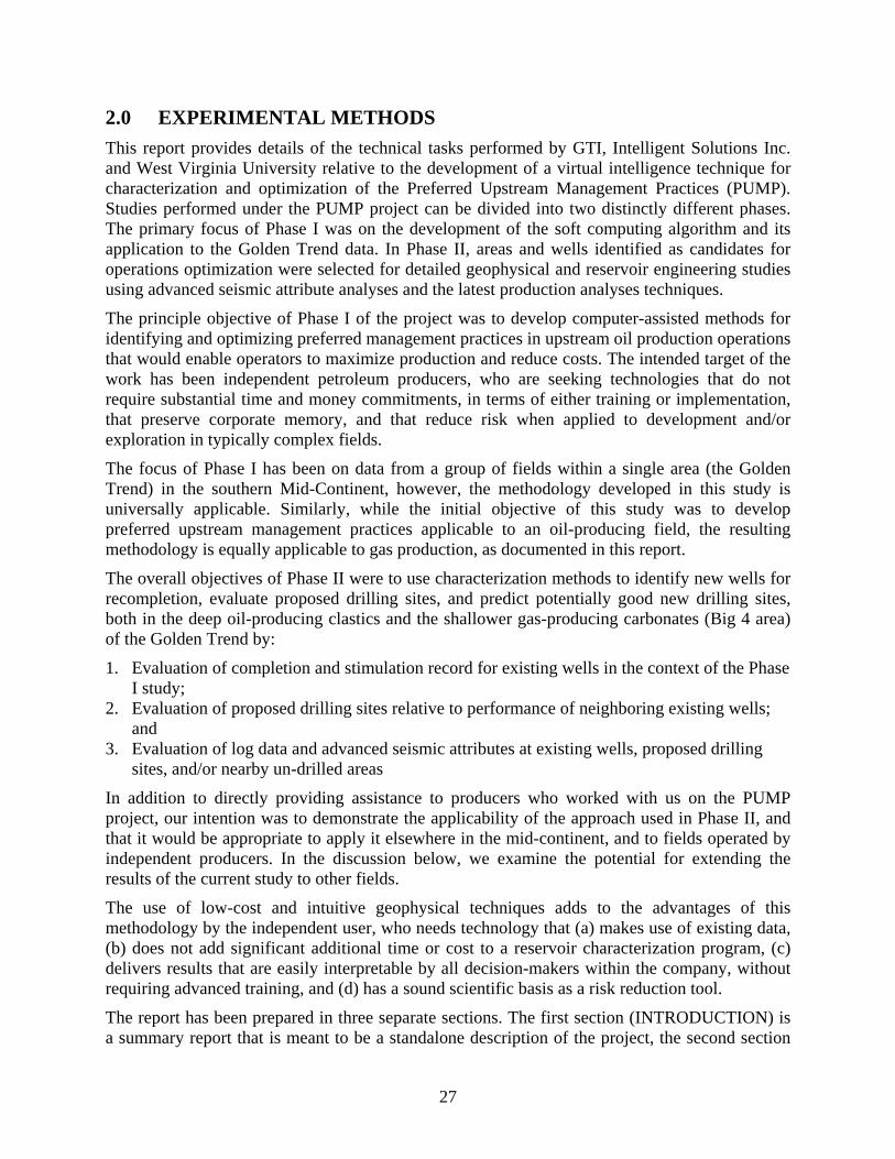
Figure 22: Amplitude data along E-W line through proposed location 110 (the same line as shown in Figure 21, above)........................................................................................................... 40 Figure 23: Spectrally decomposed data at 10 Hz along 2D line through good producing well 74 (bright green vertical line), and candidate for recompletion 10 (dull green line)......................... 41 Figure 24: Spectrally decomposed data at 60 Hz along 2D line through good producing well 14 (bright green vertical line), and candidate for recompletion 77(dull green line).......................... 42 Figure 25: Spectrally decomposed data at 60 Hz along 2D line through good producing wells 19 and 14 (bright green vertical lines), and candidate for recompletion 13. ..................................... 43 Figure 26: Spectrally decomposed data at 50 Hz along 2D line through good producing well 19 (bright green vertical line), and candidate for drilling to clastics (121). ...................................... 44 Figure 27: Selected Company Two (e.g., 67) and Company One (e.g., C:75) wells, and planned infill drilling locations. In the figure, best 6-month cumulative oil is shown as bubble size. The proposed new drilling sites are designated by three-digit numbers (e.g., 110). Data were available only for those wells shown on the map......................................................................................... 46 Figure 28: Best 6-month oil cumulative production as bubble size (vertical axis) as a function of date of first production, DOFP (horizontal axis). ......................................................................... 49 Figure 29: Oil cumulative production as bubble size (vertical axis) as a function of date of first production, DOFP (horizontal axis).............................................................................................. 50 Figure 30: Comparison of production for wells #13 and #26. Notice that #26 has much higher oil and gas production. ....................................................................................................................... 51 Figure 31: Comparison of production for wells #14 and #15. Note that well #14 has higher sustainable oil and gas production ................................................................................................ 52 Figure 32: Comparison of production for wells #73 and #10. Note that #73 has higher sustainable oil and gas production at later production dates. .......................................................................... 53 Figure 33: Self Organized Map (SOM) for parameters of average shots per foot (avgShotft), best 6-month's cumulative oil (b6cumo), date of first production (DOFP) and date of first stimulation (DOFS), and x-, y-coordinate. Notice the correspondence of patterns......................................... 54 Figure 34: Well #15 monthly production before and after recompletion work............................ 56 Figure 35: Well #62 monthly production before and after recompletion work............................ 56 Figure 36: Well #62 monthly production before and after recompletion work............................ 57 Figure 37: Well #77 monthly production before and after recompletion work............................ 57 Figure 38: Well #19 daily production before and after recompletion work ................................. 58 Figure 39: Well #19 monthly production before and after recompletion work............................ 59 Figure 40: Well #53 monthly production before and after recompletion work............................ 59 Figure 41: The schematic diagram of the tools used in Descriptive and Predictive Best Practices Analysis......................................................................................................................................... 60 Figure 42: The 30 Year EUR Productivity Fuzzy sets for wells in the Golden Trend Field........ 62 Figure 43: Classification of wells in the database using Fuzzy sets. ............................................ 63 Figure 44: Distribution of the wells based on 30 Year EUR. ....................................................... 64 Figure 45: Distribution of the average value of Number of Formations Present in wells of different quality............................................................................................................................. 65 Figure 46: Distribution of the average value of Number of Formations Stimulated in wells of different quality............................................................................................................................. 65 Figure 47: Distribution of the average value of Acid as the Main Stimulation Fluid in wells of different quality............................................................................................................................. 66

7

Figure 48: Distribution of the average value of number of formations stimulated by acid jobs in wells of different quality. .............................................................................................................. 66 Figure 49: Distribution of the average value of “Total Perforated Pay Thickness” ..................... 67 Figure 50: Distribution of the average value of Water as the Main Fracturing Fluid .................. 67 Figure 51: Distribution of the average value of Oil as the Main Fracturing Fluid ....................... 68 Figure 52: Distribution of the average value of “Other” as the Main Fracturing Fluid in wells of different quality............................................................................................................................. 68 Figure 53: Distribution of the average value of “Shot/ft” in wells of different quality................ 69 Figure 54: Distribution of the average value of “Total Fluid Amount (Mgal)/ft” in wells of different quality............................................................................................................................. 69 Figure 55: Distribution of the average value of “Total Propp Amount (Mlbs)/ft” in wells of different quality............................................................................................................................. 70 Figure 56: Distribution of the average value of “Average Proppant Concentration (lbs/gal/ft) in wells of different quality. .............................................................................................................. 70 Figure 57: Distribution of the average value of “Average Injection Rate (BPM)/ft” in wells of different quality............................................................................................................................. 71 Figure 58: Distribution of the average Initial Flow Rate from the Decline Curve Analysis in wells of different quality. .............................................................................................................. 71 Figure 59: Distribution of the average Initial Decline Rate from the Decline Curve Analysis in wells of different quality. .............................................................................................................. 72 Figure 60: The relationship of the best practices identified through these analyses to one another........................................................................................................................................................ 72 Figure 61: Schematic diagram showing the precision, averaging, and contribution to the future decision making of three different analysis offered by ISI’s Predictive Best Practices Analysis.73 Figure 62: Flow chart of Best Practices Analysis using Artificial Intelligence Techniques. ....... 74 Figure 63: Ranking of the parameters as a function of their influence on 30-Year EUR............. 75 Figure 64 : Ranking of categories of parameters as a function of their influence on 30 Year EUR........................................................................................................................................................ 75 Figure 65: Parameters used during the neural network modeling process. .................................. 76 Figure 66: Actual and predicted 30 year EUR of training data set upon completion of the training of the neural network model. ........................................................................................................ 77 Figure 67: Actual and predicted 30-year EUR of training data set upon completion of the training of the neural network model. ........................................................................................................ 77 Figure 68: Actual and predicted 30 year EUR of the calibration data set upon completion of the training of the neural network model............................................................................................ 78 Figure 69: Actual and predicted 30 year EUR of the verification data set upon completion of the training of the neural network model............................................................................................ 78 Figure 70: Original mapping of the wells in IPDA-IDEA™........................................................ 79 Figure 71: Final mapping of the wells in IPDA-IDEA™............................................................. 80 Figure 72: Main zones delineations. ............................................................................................. 81 Figure 73: Final delineations including main as well as sub zones. ............................................. 82 Figure 74: List of Reservoir Quality indices for all the wells in the dataset. ............................... 83 Figure 75: Example of a single parameter analysis for one well.................................................. 84 Figure 76: Full Field Combinatorial Predictive Best practices Analysis – Results for Water as main fracturing fluid. .................................................................................................................... 86

8

Figure 77: Full Field Combinatorial Predictive Best practices Analysis – Results for Oil as main fracturing fluid. ............................................................................................................................. 87 Figure 78: Full Field Combinatorial Predictive Best practices Analysis – Results for Acid as main fracturing fluid. .................................................................................................................... 87 Figure 79: Full Field Combinatorial Predictive Best practices Analysis – Results for Other as main fracturing fluid. .................................................................................................................... 88 Figure 80: Full Field Combinatorial Predictive Best practices Analysis – Results for number of perforations per foot of Pay Thickness. ........................................................................................ 88 Figure 81: Full Field Combinatorial Predictive Best practices Analysis. Results for proppant concentration in pounds per gallon of fluid per foot of pay thickness.......................................... 89 Figure 82: Full Field Combinatorial Predictive Best practices Analysis – Results for the averaged injection rate per foot of Pay Thickness. ...................................................................................... 89 Figure 83: Wells in the database grouped based on three operators............................................. 91 Figure 84: Incremental 30 year production as a result of using different fracturing fluids in wells operated by Company Three. ........................................................................................................ 93 Figure 85: Wells in the database identified by the operating companies. .................................... 94 Figure 86: Groups of wells Combinatorial Predictive Best practices Analysis – Results for Water as the main fracturing fluid. .......................................................................................................... 95 Figure 87: Groups of wells Combinatorial Predictive Best practices Analysis – Results for Diesel Oil as the main fracturing fluid..................................................................................................... 95 Figure 88: Groups of wells Combinatorial Predictive Best practices Analysis – Results for Acid as the main fracturing fluid. .......................................................................................................... 96 Figure 89: Groups of wells Combinatorial Predictive Best practices Analysis – Results for Other fracturing fluids............................................................................................................................. 96 Figure 90: Groups of wells Combinatorial Predictive Best practices Analysis – Results for number of perforations per foot of pay thickness. ........................................................................ 97 Figure 91: Groups of Wells Combinatorial Predictive Best practices Analysis – Results for proppant concentration per gallon pf fluid per foot of pay thickness. .......................................... 97 Figure 92: Groups of wells Combinatorial Predictive Best practices Analysis – Results for average injection rate per foot of pay thickness............................................................................ 98 Figure 93: Wells in the database grouped based on Relative Reservoir Quality using IPDA-IDEA™. ...................................................................................................................................... 101 Figure 94: Wells in the database grouped based on Relative Reservoir Quality using IPDA-IDEA™. ...................................................................................................................................... 102 Figure 95: Effect of Water as the main fracturing fluid on the wells grouped based on relative reservoir quality. ......................................................................................................................... 105 Figure 96: Effect of Acid as the main fracturing fluid on the wells grouped based on relative reservoir quality. ......................................................................................................................... 105 Figure 97: Effect of Other as the main fracturing fluid on the wells grouped based on relative reservoir quality. ......................................................................................................................... 106 Figure 98: Combinatorial Analysis for Poor Wells. ................................................................... 107 Figure 99: Combinatorial Analysis for Average Wells. ............................................................. 108 Figure 100: Combinatorial Analysis for Good Wells. ................................................................ 109 Figure 101: Combinatorial Analysis for Very Good Wells. ....................................................... 110 Figure 102: Sensitivity analysis for water as the main fracturing fluid for four wells in the database....................................................................................................................................... 113

9

Figure 103: Sensitivity analysis for number of perforations per foot of pay thickness for two wells in the database. .................................................................................................................. 113 Figure 104: Sensitivity analysis for “Shot/ft” and “Rate” for three wells in the database. ........ 114 Figure 105: Sensitivity analysis for “Proppant Concentration” and “Main Fracturing Fluids” for a well Operated by Company One. ................................................................................................ 115 Figure 106: Sensitivity analysis for three parameters simultaneously for Well C-1 Operated by Company One.............................................................................................................................. 116 Figure 107: Definitions of poor, average and good wells in terms of fuzzy sets. ...................... 118 Figure 108: Six wells in the database as examples of poor, average and good wells................. 119 Figure 109: Percent of wells in each of the poor, average and good well categories................. 120 Figure 110: Average Best 3 Months production for different categories of wells. .................... 120 Figure 111: Average Initial Flow Rate for different categories of wells. ................................... 120 Figure 112: Average Initial Decline Rate for different categories of wells................................ 121 Figure 113: Average number of Carbonate formations for different categories of wells........... 121 Figure 114: Average number of Clastic formations for different categories of wells. ............... 121 Figure 115: Average number of formations stimulated for different categories of wells. ......... 122 Figure 116: Average number of formations fractured for different categories of wells............. 122 Figure 117: Average number of formations with acid jobs for different categories of wells..... 122 Figure 118: Average number of formations using oil as the main stimulation fluid for different categories of wells....................................................................................................................... 123 Figure 119: Average number of formations using water as the main stimulation fluid for different categories of wells....................................................................................................................... 123 Figure 120: Average number of formations using acid as the main stimulation fluid for different categories of wells....................................................................................................................... 124 Figure 121: Average total perforated thickness for different categories of wells....................... 124 Figure 122: Average number of perforation per foot of pay zone for different categories of wells...................................................................................................................................................... 125 Figure 123: Average injection rate per foot of pay zone for different categories of wells......... 125 Figure 124: Decline curve versus network predicted gas 30 year EUR for the training set....... 126 Figure 125: Decline curve versus network predicted gas 30 year EUR for the training set....... 127 Figure 126: Decline curve versus network predicted gas 30 year EUR for the calibration set .. 127 Figure 127: Decline curve versus network predicted gas 30 year EUR for the verification set. 127 Figure 128: Full field combinatorial analysis for water as the main fracturing fluid. ................ 128 Figure 129: Full field combinatorial analysis for oil as the main fracturing fluid...................... 129 Figure 130: Full field combinatorial analysis for acid as the main stimulation fluid. ................ 129 Figure 131: Full field combinatorial analysis for number of perforations per foot of pay......... 130 Figure 132: Full field combinatorial analysis for amount of fluid pumped per foot of pay ....... 130 Figure 133: Full field combinatorial analysis for proppant concentration per foot of pay......... 131 Figure 134: Full field combinatorial analysis for average injection rate per foot of pay ........... 131 Figure 135: Map of well qualities for Groups of Wells Analysis............................................... 132 Figure 136: Groups of Wells Analysis for Acid as the main fracturing fluid............................. 133 Figure 137: Groups of Wells Analysis for number of perforations per foot of pay. .................. 134 Figure 138: Groups of Wells Analysis for number of perforations per foot of pay. .................. 134 Figure 139: Groups of Wells Analysis for proppant concentration per foot of pay. .................. 135 Figure 140: Groups of Wells Analysis for average injection rate per foot of pay...................... 135 Figure 141: Groups of Wells Analysis combinatorial analysis for very good wells. ................. 136

10

Figure 142: Groups of Wells Analysis combinatorial analysis for good wells. ......................... 137 Figure 143: Groups of Wells Analysis combinatorial analysis for average wells. ..................... 138 Figure 144: Groups of Wells Analysis combinatorial analysis for poor wells. .......................... 139 Figure 145: Individual Well Analysis, Single parameter analysis for several wells. ................. 141 Figure 146: Individual Well Analysis, Combinatorial analysis for two parameters for several wells. ........................................................................................................................................... 142 Figure 147: Individual Well Analysis, Combinatorial analysis using Monte Carlo simulation method for four parameters simultaneously performed for three wells...................................... 143 Figure 148: Probability distribution function for Shots/ft. ......................................................... 145 Figure 149: Logarithmic probability distribution function for Proppant Concentration. ........... 146 Figure 150:Probability distribution function for average injection rate. .................................... 146

11

List of Tables Table 1: Basic acquisition and processing parameters for the Golden Trend multiclient 3D seismic survey owned by WesternGeco. Information copywritten by WesternGeco. Additional post-processing has been used by some clients, including high frequency processing. ............... 33 Table 2: Locations of 2D lines through 3D data set on which spectral decomposition was performed. Highlighted lines (bold font) are discussed further in the text. .................................. 38 Table 3: Data on formation thickness, stimulation, and short-term production ........................... 48 Table 4: Confirmation Well Information...................................................................................... 55 Table 5: Confirmation Well Recompletion Details ...................................................................... 55 Table 6 – Well 19 Recommendation Well Information................................................................ 58 Table 7 –Well #53 Recommendation Well Recompletion Detail ................................................ 58 Table 8- Parameters in the database that were used during the “Best Practices” analysis. .......... 61 Table 9: Single parameter patterns for the full field analysis ....................................................... 85 Table 10: Summary of the full field analysis of predictive hydraulic fracturing best practices in Golden Trend. ............................................................................................................................... 90 Table 11: Average values of the wells from each company as compared to average well quality........................................................................................................................................................ 91 Table 12: Single parameter patterns for the groups of wells analysis – grouping based on operators........................................................................................................................................ 93 Table 13: Summary of the groups of wells analysis of predictive hydraulic fracturing best practices in Golden Trend based on the operators - Company One.............................................. 98 Table 14: Summary of the groups of wells analysis of predictive hydraulic fracturing best practices in Golden Trend based on the operators - Company Two. ............................................ 99 Table 15: Summary of the groups of wells analysis of predictive hydraulic fracturing best practices in Golden Trend based on the operators ........................................................................ 99 Table 16: Key for reading the conclusions/recommendations table in Tables 13 to 15. ............ 100 Table 17: Average values of the wells from each RRQ as compared to average well quality in the database....................................................................................................................................... 103 Table 18: Summary of Single Parameter Predictive Best Practice Analysis for wells grouped base on relative reservoir quality. ............................................................................................... 104 Table 19: Conclusions and recommendation for Very Good relative reservoir quality. ............ 111 Table 20: Conclusions and recommendation for Good relative reservoir quality. ..................... 111 Table 21: Conclusions and recommendation for Average relative reservoir quality. ................ 111 Table 22: Conclusions and recommendation for Poor relative reservoir quality. ...................... 111 Table 23: List of well-specific parameters used in the neural network model. .......................... 112 Table 24: List of hydraulic fracturing related parameters used in the neural network model. ... 112 Table 25: List of formations in The Golden Trend..................................................................... 117 Table 26: List of hydraulic fracturing related parameters used in the neural network model. ... 126 Table 27: Results of the full field single parameter analysis. ..................................................... 128 Table 28: Conclusion matrix for the full field analysis. ............................................................. 131 Table 29: Results of single parameter analysis for groups of wells. .......................................... 133 Table 30: Conclusion matrix for the Groups of wells analysis – Very Good wells. .................. 140 Table 31: Conclusion matrix for the Groups of wells analysis –Good wells. ............................ 140 Table 32: Conclusion matrix for the Groups of wells analysis – Average wells........................ 140 Table 33: Conclusion matrix for the Groups of wells analysis – Poor wells.............................. 140

12

1.0 INTRODUCTION This report provides details of the technical tasks performed by GTI, Intelligent Solutions Inc. and West Virginia University relative to the development of a virtual intelligence technique for characterization and optimization of the upstream oil industry operations. The work was performed in cooperation with three independent producing companies – Newfield Exploration, Chesapeake Energy, and Triad Energy – operating in the Golden Trend, Oklahoma. In order to protect data confidentiality, these companies are referred to as Company One, Two, Three in a randomly selected order. The report has been prepared in three separate sections to capture all elements of the program in detail. The first section (INTRODUCTION) is a summary report that is meant to be a standalone description of the project, the second section describes geological and engineering studies and the third section illustrates the fundamentals of the soft computing approach and describes the results from the Golden Trend data analysis. The software package, complete with tutorial, is being presented as Appendix D to this report. The electronic version of this report is also included in Appendix C.

Motivation The Annual Energy Outlook 2004, with Projections to 2025, published by the Energy Information Administration (EIA), projects that the total US production from onshore and offshore; excluding Alaska but including lease condensate, will decrease from 4.78 million barrels per day in 2001 to 4.11 million barrels per day in 2025 (Fig. 1) and the reserve will decrease from 19.14 billion barrels to 14.98 billion barrels during the same period (Fig. 2). (Ref. Annual Energy Outlook 2004 with Projections to 2025, Report #: DOE/EIA-0383-2004, January 2004).

Projected US Oil Production from Lower 48

0.00

1.00

2.00

3.00

4.00

5.00

6.00

2001

2004

2007

2010

2013

2016

2019

2022

2025

Years

Pro

duct

ion

in M

illio

n Ba

rrel

s pe

r Da

y

US Total Less Alaska Lower 48 Onshore Lower 48 Offshore

Figure 1: Projected US oil production from 2001 to 2025

The alarming feature of these projections, which are principally in line with all previous projections, is the steady decline of the lower 48 production and reserve (Figure 1 and 2). This situation, with a backdrop of steadily increasing demand (Figure 3) and driven by the incentive for energy independence, has been the primary motive for the US Department of Energy to develop a two-pronged research and development program: a long-term program aiming at

13

production from unconventional resources and a short-term program for increasing recovery from producing fields. The PUMP project relates to the second category of programs.

Lower 48 End of Year Reserves

0.00

5.00

10.00

15.00

20.00

25.00

1 3 5 7 9 11 13 15 17 19 21 23

Years

Rese

rve

(Bill

ion

Barr

els)

Lower 48 End of YearReserves

Figure 2: Projection of US lower 48 reserve from 2001 to 2025

0.00

10.00

20.00

30.00

40.00

50.00

60.00

2001

2003

2005

2007

2009

2011

2013

2015

2017

2019

2021

2023

2025

Consumption Import Production

Figure 3: Supply-demand projection from 2001to 2025

The primary driver behind the PUMP project is the fact that, in general, a high percentage of the technically recoverable oil remains un-produced; either due to high production cost or low production rate, resulting from application of non-optimal completion and production practices. As such, it is logical to focus on producing fields and develop methods and techniques to improve recovery efficiency through optimization of current practices as well as the development of means and methods for producing from in-field reserves such as those left behind pipe or entrapped in compartmented reservoirs.

Designs of the PUMP project was based on the fact that small to mid-size independent producers in the United States drill 85% of all oil and gas wells and produce 65% of the total gas and 40% of the total oil from onshore fields. (1996 Profile of Independent Producers, survey conducted by

14

the Independent Petroleum Association of America.) It is therefore obvious that those technologies that address the needs of independent producers are the ones with the highest impact relative to short-term production increase and reserve replacement.

The common approach for enhancing recovery from producing fields is correlation of production data with drilling and completion parameters and identification of the most influential parameters relative to production rate and ultimate recovery. As such, the foundation of the PUMP project is on determination of effects of various completion and production parameters on production.

Although petroleum engineering has matured to a profound scientific technology, its application to characterization of older onshore fields in the United States, particularly those operated by small and mid-size independent producers, is usually hindered by the lack of accurate data. In fact, the oilfield data available to small and mid-size independents have been, and will continue to be, inaccurate, imprecise, and incomplete. In addition, frequent mergers and takeovers have diminished the corporate memory to the level of virtual non-existence and endless downsizing has reduced the in-house workforce to the extent that the data that might be present in company files are rarely used by the busy engineers and geologists. Under these conditions, sound engineering analyses are difficult to impossible with unreliable and often misleading results. Being aware of this situation, the industry has had no choice but to rely on the raw experience of engineers and operators and devise a method for distilling their collective experience into what is known as “Best Practices”. However, results from best practice analyses are qualitative by nature and do not lend themselves to reliable technical analyses and sound engineering decisions.

In essence, the primary goal of PUMP project was quantification of “Best Practice” through the development of a computer-assisted engineering decision-support software that identifies the most influential parameters affecting overall well performance and recommends variations in these parameters for optimization of the processes. Considering the nature of the oilfield data, soft computing techniques such as fuzzy logic and neural networks, capable of handling imprecise and heterogeneous data, were the methods of choice. In practice, the project evolved to include two principal phases. In the first, the focus was on building a comprehensive database that included “appropriate” information; that is, geologic, completion, and/or stimulation data that could be shown to have an impact on production; and manipulating these data using soft computing data analysis techniques to characterize and optimize common practices. In the second phase, the focus was more applied, using conventional and cutting-edge seismic and production analyses for field application.

Production and completion data for 320 wells in the Golden Trend was acquired from files of the participating producing companies. The data was quite heterogeneous and inconsistent and 90 of the total data sets were eliminated for reasons of incompleteness and questionable data. A relational database was created and populated with the data from the remaining 230 wells. Soft computing data analysis Application of soft computing techniques in data analysis was by design. This was due to the fact that the data was expectedly incomplete, imprecise, and heterogeneous; and as such, conventional analytical work would be meaningless if not impossible. Soft computing refers to a class of computational modules that once linked together creates an "intelligence engine" capable of handling the complex oilfield data. The modules created within the intelligence engine for the Golden Trend data included neural networks, genetic algorithms, and fuzzy logic. Collectively, these applications are referred to as the “Virtual Intelligence” technique.

15

A neural network is a powerful data processing system whose structure resembles the interconnection of neurons in the human brain. It can mimic the brain to some degree in its ability to acquire knowledge through a learning process and to handle non-linear problems. A genetic algorithm is a model of machine learning that behaves in a manner similar to the selection processes seen in the evolution of living organisms. The algorithm evaluates a set of data, applies various tests of 'fitness,' and induces changes to create a 'next-generation' data set for further evaluation. Fuzzy logic is a multi-valued logic system that allows intermediate values between conventional yes/no, true/false, or black/white determinations. It can be used to examine the degree to which the data meets certain criteria. In general, soft computing data analysis can be described as a series of coupled descriptive and predictive analyses (Figure 4). Descriptive analyses lead to identification of the most influential controllable parameters and predictive analyses provide an estimate of the expected results from variations in single or multiple parameters in completion of new wells or re-completion of existing wells. A brief description of the process as applied to the Golden Trend data follows.

Figure 4: Functional structure of soft computing techniques. Fuzzy logic and descriptive analysis The descriptive best practices analysis starts by identifying a parameter that would be used to partition the wells in terms of their productivity. For this project, the 30-year Estimated Ultimate Recovery (EUR) was selected as the indicating parameter. The 30 year EUR was calculated for all wells using decline curve analysis. Conventionally, wells with EUR up to 30,000 barrels were defined as poor wells, wells with up to 60,000 barrels EUR as average wells, and those with more than 90,000 barrels EUR as good wells. It is obvious that in reality there is little difference between a well with 30,000 barrels EUR and the one with 31,000 barrels EUR. Therefore, an artificially crisp boundary between such wells should not be imposed and the use of fuzzy set concept is more appropriate. In a fuzzy set, everything is in a category at certain degree of belonging to that category so that near the boundary of two sets the subject can have one degree of belonging to the first category and another degree to the second category (Figure 5). The transition near boundary for two categories can be better explained by review of Figure 6. In this

16

example, for well B the range between poor and average wells is from 30,000 to 60,000 barrels and this well has an EUR of 35958 barrels. As such, the well has a membership (degree of belonging) of 0.8 to poor wells and 0.2 to average wells.

Figure 5: The 30 Year EUR productivity fuzzy sets for wells in the Golden Trend Field.

Figure 6: Examples of fuzzy classification.

In fuzzy categorization, when calculating an average property for one category, the membership will impose a weight influence according to the following equation.

17

∑

∑

=

=n

in

n

innx

1

1

µ

µ In this formula “ x ” represents the value of the parameter, “µ ” represents the fuzzy membership function of a well in a particular fuzzy set, and “n” is the number of the wells in a particular fuzzy set. Using the fuzzy classification it would be possible to study the influential parameters for each category of wells in a more generalized fashion. Following this procedure, it was possible to identify the most influential parameters affecting the EUR. For example, it was realized that using oil as the main fracturing fluid results in higher EURs and water fracs result in lower production as shown on figures 7 and 8.

Figure 7: Distribution of the average value of oil as the main fracturing fluid in wells of different

quality.

18

Figure 8: Distribution of the average value of water as the main fracturing fluid in wells of different

quality.

Neural Network Modeling Before performing neural network analyses, the data was quality checked and production decline analyses were carried out for production characterizations. Fuzzy combinatorial analysis of longitude and latitude (as proxy for geology) against 30 year EUR was conducted to define the reservoir quality indices.

Neural network models are usually used for predictions. In this work, the model was used for parameter sensitivity analysis, i.e., various parameters were changed from minimum to maximum to find out the trends. To develop the neural network model, the 30 Year EUR was selected as the output. The data set was divided into three smaller sets for training, calibration, and verification. The training data set included 147 records (wells), the calibration data set included 17 records (wells) and the verification data set included 18 records (wells). The training set was used to train the neural network model. The calibration data set was not used for training but served as a criterion in order to identify when the training process has been completed. Finally, the verification data set served for determination of the goodness of the model.

Genetic Algorithm and Combinatorial Prediction Analysis Genetic algorithm is a powerful tool for process optimization in cases where multiple parameters are involved. In essence, each well can be viewed as living matter that its survival depends on its degree of fit to the environment. In addition, there are multitudes of variations, or possibilities, caused through cross-breading and mutation and the members of the next generation that fit the environment the best will survive and dominate. In the case of our study, the measure of fitness was the expected EUR for each generation and the parameters were fracturing fluid, fracturing rate, proppant concentration, and the number of perforations per foot of pay. In this work the genetic optimization was used as a multivariable combinatorial predictive analysis.

Results from soft virtual intelligence analyses Results from virtual intelligence analyses were produced in several forms and formats. It was recognized that hydraulic fracturing and perforation density were the most influential controllable parameters impacting production rate and ultimate recovery. In a generalized sense,

19

the data recommended that oil-base fracturing fluid is more effective in the case of oil production while acid-fracs are more effective for gas production. In addition, lower pumping rate, higher proppant concentration, and smaller number of perforation per foot of pay showed to result in better production rate and higher ultimate recovery.

In addition to the generalized operational recommendations, several areas of high production potential were identified in the survey area. It was also observed that several wells located in the high potential area have not been producing at the expected rates. Further study of these wells resulted in the identification of 23 re-stimulation candidate wells for oil production, 25 wells for gas production, and 33 wells for combined oil and gas production.

Production and geophysical data analyses Results from virtual intelligence analyses indicated extreme inconsistency in that wells in close proximity of each other showed vastly different production history. To investigate this matter, production data for a subset of the area was closely examined and general findings of the virtual intelligence work were substantiated through conventional production analyses. Elaborate conventional production analyses resulted in two major findings. First, it was observed that in many cases the wells in general proximity of one another had distinctly different production history (Figures 9 and 10); and second, some of the wells that were completed in recent years had higher production as compared with the nearby older wells (Figure 11).

Well A

0

1000

2000

3000

4000

Aug-99 Mar-00 Oct-00 Apr-01 Nov-01 May-02

OIL

WATER

Well B

0

500

1,000

1,500

2,000

2,500

3,000

Aug-87 May-90 Jan-93 Oct-95 Jul-98 Apr-01 Jan-04

OIL

WATER

Figure 9: Example of production difference between two neighboring wells.

20

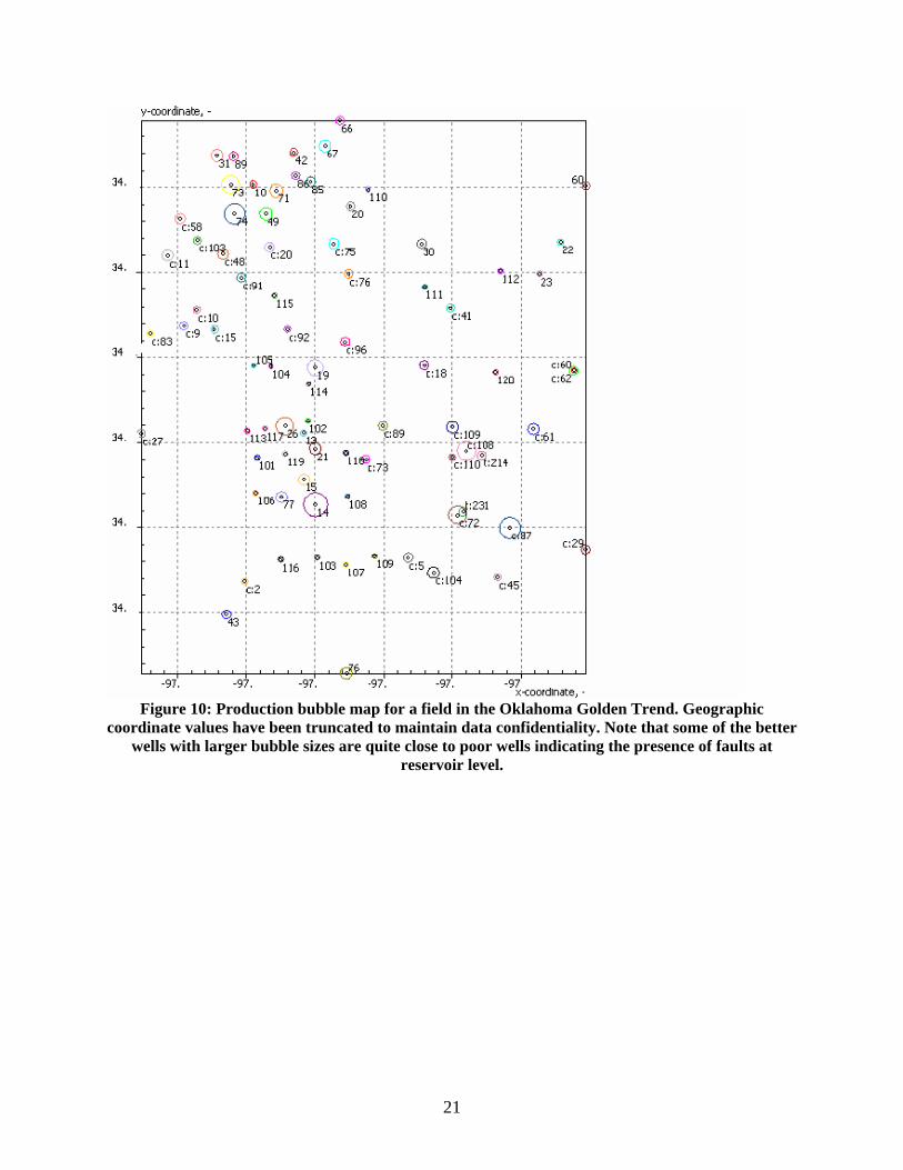
Figure 10: Production bubble map for a field in the Oklahoma Golden Trend. Geographic

coordinate values have been truncated to maintain data confidentiality. Note that some of the better wells with larger bubble sizes are quite close to poor wells indicating the presence of faults at

reservoir level.

21

Figure 11: Production bubble map for a field in the Oklahoma Golden Trend. X coordinate is the

time from first production in days and Y coordinate is production during the best 6 months of production. Note that production from several recent wells (e.g., wells 19, 26, and 74) is higher than

production from many of older wells.

These observations implied the presence of reservoir compartmentalization caused by faults or stratigraphic changes between wells. To investigate this matter, detailed seismic analyses were performed on a 3-D seismic volume belonging to one of the host companies. These studies

22

centered on spectral decomposition of seismic traces using the InSpectSM seismic attribute analysis package. InSpectSM is a powerful spectral analysis tool that decomposes the seismic trace to its constituting frequencies using the wavelet transform methodology. In this application, the seismic traces are visualized at discrete frequency intervals leading to recognition of subtle changes in seismic attributes and small-scale dislocations which are difficult to notice on broadband seismic sections. Figures 12 and 13 are samples of broadband and spectrally decomposed seismic sections from the survey area.

10 71 85 110

Figure 12: Broadband seismic data corresponding to figure 11.

73

C

B

A

23

85 110 73 10 71

Figure 13: Sample of spectrally decomposed seismic data.

The resolution difference between spectrally decomposed and broadband seismic data is quite noticeable as seen on figures 12 and 13. Detailed seismic analysis and interpretation provided some explanation for difference in production from neighboring wells. For example, the analyses showed that the low production for wells 10 and 71 is most likely because of their close proximity to fault zones while that of well 85 is because it penetrated the pay at the down-dip side of a down-thrown fault block. In addition, spectrally decomposed seismic data revealed that site 110 which was a candidate drilling location was directly above a fault and should be avoided. It was recommended that moving the site to the west of the fault would place the well on the up-dip section of the fault block offering higher production potential. It was also suggested that if surface conditions should not allow the proposed location change, the site could be moved eastward to penetrate the pay zones A, B, and C at an undisturbed horizon.

Results In general, results from geophysical and engineering studies confirmed those of virtual intelligence analyses. These results were presented to the producing companies as a list of recommended recompletion wells and the corresponding optimized operations parameters. By the end of the project, 16 of the recommendations have been implemented the majority of which resulted in increased production rates to several folds. This constituted a comprehensive field demonstration with positive results.

Formation B

Formation C

Formation A

24

EXECUTIVE SUMMARY A virtual intelligence (VI) technique was developed using state-of-the-art soft computing technologies including statistical analysis, Intelligent Production Data AnalysisTM, cluster analysis, artificial neural networks, genetic algorithms, fuzzy logic, and Monte Carlo simulation to synthesize basic geologic, completion and stimulation, and production data from a mature oil field, and to create a list of historic best practices. Results from application of the VI technique were used as a guide for selecting areas of interest for detailed geological, geophysical, and reservoir engineering studies. The integrated result from studies was a list recompletion recommendation and proposed infill drilling sites delivered to the participating producing companies.

The work was conducted in two complementary phases and partly concurrent phases. The project was a combination of analytic work and field-based studies. The objective of Phase I was the development of the VI system, while phase II was focused on geophysical and reservoir engineering studies and verification of results from VI modeling. The work was performed in cooperation with three independent producing companies – Newfield Exploration, Chesapeake Energy, and Triad Energy – operating in the Golden Trend, Oklahoma. In order to protect data confidentiality, these companies are referred to as Company One, Two, Three in a randomly selected order. The Golden Trend is an oil and gas producing region that has been in production for over fifty years, largely by small to midsize independent producers. The geology is locally complex and production tends to be compartmentalized. Companies operating in the Golden Trend area are currently developing mature fields and therefore, results from this work are timely for application in the area.

A comprehensive database was built from records of the participating independent producers. The VI software package, developed specifically for the Golden Trend, was applied to identify the most influential parameters affecting production. The VI technique was then used to vary these parameters between practical limits and identify the optimum range for each parameter and their combinations. The end result was a prioritized list of well candidates for recompletion together with the list of optimal ranges for the recommended recompletion parameters.

In support of the development of the virtual intelligence technique and application to existing data during an active drilling program, Phase II of the project - characterizing the fields through engineering and geologic/geophysical data analysis - was carried out. The objective of Phase II was to identify and rank recompletion and stimulation opportunities and optimal infill drilling locations, and compare the results of well-by-well analyses with the analysis performed in Phase I. Techniques applied in Phase II included reserve estimation and data mining from production data, and interpretation of advanced seismic attributes applying an advanced spectral decomposition technique to 3D seismic data provided by one of the producers. Phase II work revealed that reservoirs are highly compartmentalized laterally, and that several new locations could be suggested that will likely target untapped compartments.

Detail geophysical and reservoir engineering included the following tasks:

• Detailed seismic analysis using InsPect spectral decomposition package • Application of the Hapmson-Russell’s EMERGE inversion package • Detailed production analysis using conventional reservoir engineering techniques • Parameter optimization using the DECICE neural network software

25

Major results from these studies can be summarized as follows:

• The controllable parameters influencing production in the Golden Trend are, stimulation fluid, injection rate in hydraulic fracturing, proppant concentration with the fracturing fluid being the most influential parameter. It was demonstrated that oil-base fracturing fluid results in better oil production while acid fracturing, and not acidizing, is most effective for gas production.

• Low rate with highest achievable high proppant concentration is suggested. • It appears that high density perforation (number of perforations per foot of pay) does

not have a measurable positive impact. • Many of the wells can be re-stimulated using the optimal fracturing procedure. • Reservoir engineering studies showed the existence of reservoir compartmentalization

and identified a number of re-completion candidate wells. • Detailed geophysical studies revealed intensive faulting that confirmed reservoir

compartmentalization as inferred from engineering studies. • Detailed seismic analyses and inversions pointed to at least one location of untested

oil bearing horizon. • Changing the location of some of the planned infill wells to avoid faulting was also

proposed to the participating company. • Field verification and demonstration were achieved through correlation of post and

pre re-stimulation production data.

Results from Phase II studies were a well-by-well analysis that complemented the all-field analysis from Phase I. Top candidates for recompletion based on well-by-well analysis overlap the list of top-ranking wells for recompletion based on all-field analysis, but there is not a one-to-one correspondence. This result suggests that to reduce risk, the best approach is to apply both methods before determining optimal locations and/or target zones.

Outputs of Phases I and II, including specific target zones for recompletion and infill drilling, were communicated to the participating companies for use in their active drilling programs. The communication was in several technical discussion sessions and workshops that also covered the application of the VI software through hands-on training. By the end of the project, 16 of the recommendations were implemented resulting increase in production to several folds. This constituted a comprehensive field demonstration with positive results.

Technology transfer took place through several workshops held at offices of the participating companies, at OIPA offices, and presentations at the SPE panel on soft computing applications and at the 2003 annual meeting of Texas Independent Producers and Royalty Owners (TIPRO). In addition, results were exhibited at SPE annual conferences in 2002 and 2003, published in GasTips, and placed on the GTI web page.

26

2.0 EXPERIMENTAL METHODS This report provides details of the technical tasks performed by GTI, Intelligent Solutions Inc. and West Virginia University relative to the development of a virtual intelligence technique for characterization and optimization of the Preferred Upstream Management Practices (PUMP). Studies performed under the PUMP project can be divided into two distinctly different phases. The primary focus of Phase I was on the development of the soft computing algorithm and its application to the Golden Trend data. In Phase II, areas and wells identified as candidates for operations optimization were selected for detailed geophysical and reservoir engineering studies using advanced seismic attribute analyses and the latest production analyses techniques.

The principle objective of Phase I of the project was to develop computer-assisted methods for identifying and optimizing preferred management practices in upstream oil production operations that would enable operators to maximize production and reduce costs. The intended target of the work has been independent petroleum producers, who are seeking technologies that do not require substantial time and money commitments, in terms of either training or implementation, that preserve corporate memory, and that reduce risk when applied to development and/or exploration in typically complex fields.

The focus of Phase I has been on data from a group of fields within a single area (the Golden Trend) in the southern Mid-Continent, however, the methodology developed in this study is universally applicable. Similarly, while the initial objective of this study was to develop preferred upstream management practices applicable to an oil-producing field, the resulting methodology is equally applicable to gas production, as documented in this report.

The overall objectives of Phase II were to use characterization methods to identify new wells for recompletion, evaluate proposed drilling sites, and predict potentially good new drilling sites, both in the deep oil-producing clastics and the shallower gas-producing carbonates (Big 4 area) of the Golden Trend by:

1. Evaluation of completion and stimulation record for existing wells in the context of the Phase I study;

2. Evaluation of proposed drilling sites relative to performance of neighboring existing wells; and

3. Evaluation of log data and advanced seismic attributes at existing wells, proposed drilling sites, and/or nearby un-drilled areas

In addition to directly providing assistance to producers who worked with us on the PUMP project, our intention was to demonstrate the applicability of the approach used in Phase II, and that it would be appropriate to apply it elsewhere in the mid-continent, and to fields operated by independent producers. In the discussion below, we examine the potential for extending the results of the current study to other fields.

The use of low-cost and intuitive geophysical techniques adds to the advantages of this methodology by the independent user, who needs technology that (a) makes use of existing data, (b) does not add significant additional time or cost to a reservoir characterization program, (c) delivers results that are easily interpretable by all decision-makers within the company, without requiring advanced training, and (d) has a sound scientific basis as a risk reduction tool.

The report has been prepared in three separate sections. The first section (INTRODUCTION) is a summary report that is meant to be a standalone description of the project, the second section

27

describes geological and engineering studies, and the third section illustrates the fundamentals of the soft computing approach and describes the results from the Golden Trend data analysis. The software package, complete with tutorial, is being presented as Appendix D to this report. The electronic version of this report is also included in Appendix D.

2.1. Geological and Geophysical Studies The Golden Trend area covers portions of three counties (Grady, Garvin, and McClain) in southwest-central Oklahoma (Figure 14) and impinges on the Anadarko basin and the Arbuckle range.

Figure 14: Map of Oklahoma with Golden Trend area shown in yellow. Areas studied in Phase II

and described in this report are shown in red.

2.1.1. Historic production in area

The initial discovery in the Golden Trend was in Garvin County in 1946. The field has produced both oil and gas; recently, the focus has been on gas production from the carbonate section, in response to favorable gas pricing, and the challenges of producing oil from the deep clastic section. Figure 15 shows graphically the cumulative production annually of crude oil (blue diamond) and natural gas (pink square) for Garvin, Grady, and McClain counties, combined, based on data available from the 2003 annual report of the Oklahoma Corporation Commission, from 1976 through 2003. Trends of oil and gas production in the region undoubtedly reflect economic climate as well as technology availability. For example, there was a jump in both oil and gas production following the completion of a multi-client 3D seismic survey in the area in 1998.

28

0

20000000

40000000

60000000

80000000

100000000

120000000

140000000

1975 1980 1985 1990 1995 2000

oil production (bbl)gas production (mcf)

Figure 15: Annual oil production in barrels (blue diamonds) and gas production in thousands of

cubic feet (pink squares) for Garvin, Grady, and McClain counties, combined, based on data published in the Oklahoma Conservation Commission’s 2003 annual report.

29

2.1.2. Stratigraphy A generalized stratigraphic column for this region is shown in Figure 16 (formations are correlative across the Anadarko Basin and Southern Oklahoma Fold Belt provinces).

Deese Group-Hart Sand (Pennsylvanian) …

Springer Shale (Mississippian) Caney Shale (also Delaware Creek Shale)

Sycamore Limestone Woodford Shale (Devonian)

Hunton Group-Mannsville Dolomite (Silurian) Hunton Group-Bois D’Arc Limestone

Hunton Group-Haragan Marlstone Hunton Group-Henryhouse Marlstone Hunton Group-Chimneyhill Limestone

Upper Sylvan Shale (Ordivician) Lower Sylvan Shale

Fernvale Viola (Welling Formation) Upper Viola Limestone Middle Viola Limestone Lower Viola Limestone

Simpson Group-Bromide Dense Limestone Simpson Group-Bromide Green Shale

Simpson Group-Upper Bromide Sandstone Simpson Group-Tulip Creek Shale

Simpson Group-Basal Bromide Sandstone (Tulip Creek Sandstone) Simpson Group-Upper McLish Sandstone

Simpson Group-McLish Limestone and Shale Simpson Group-Basal McLish Sandstone

Simpson Group-Oil Creek Shale Simpson Group-Basal Oil Creek Sandstone

Simpson Group-Joins Limestone West Spring Creek Limestones and Dolomites (Arbuckle Group)

Figure 16: Generalized stratigraphic column for Mid-continent section, after McCaskill, 1998.

Potential oil producing section (greater than 12,000’) is shaded in green. Gas production has been from the formations shaded in red.

Thickness of these formations varies across the region, but typical average thicknesses (not necessarily pay thicknesses) of those formations addressed in this study are as follows.

o Sycamore, approximately 200 feet o Woodford, approximately 250 feet o Hunton, approximately 300 feet o Viola, approximately 570 feet o Tulip Creek plus Bromides One + Two, over 500 feet

30

In the study areas, the producing formations are typically lumped into the shallower gas-producing carbonates, and the deeper, dominantly oil-producing clastics (e.g., Bromide One, Bromide Two, Tulip Creek, McLish, and Oil Creek formations). Historically there has been some production from the Springer shale, higher in the section than current production, which focuses on reservoirs within or deeper than the Big Four carbonates, in which gas production is currently focused. (The Big Four carbonates consist of the Sycamore, Woodford, Hunton, and Viola formations.) It should be noted that the Springer formation is thought to have been sufficiently produced and is not currently considered a development target, although geophysical analysis suggests the potential for small untapped compartments. Gas production is typically from shallower than 9000 feet to greater than 12,000 feet in depth. Oil production is often from deeper than 12,000 feet in the region. Further notes on some of the key reservoir formations are as follows:

The Mississippian Sycamore formation is a limestone with eight to fifteen percent porosity and produces gas in the Golden Trend area. Locally, the Sycamore is modified by sub-aerial exposure and related diagenetic processes so that it is highly heterogeneous. Production is often from fractured zones. Principal trapping mechanisms in the Sycamore, throughout the region, include faulted anticlines, combinations of structure and facies changes, and erosional remnants sealed by tight limestone or shale.

The Woodford Shale, of Devonian to Mississippian age, produces gas in the region and is also a likely source for gas produced from some younger formations, e.g. the Sycamore.

The upper Ordovician Viola Group is comprised chiefly of limestone. According to a 1995 USGS report, the Viola may be self-sourced, and the principal trapping mechanisms are generally structure, followed by facies changes.

2.1.3. Structural overview As noted above, reservoirs in the Golden Trend are cut by structures related to deformation in the Arbuckle Mountains and Anadarko Basin. Large-scale reverse (dominantly in the southeastern Golden Trend) or roughly N-S trending normal faults (dominantly in the northwestern Golden Trend) may cut the producing units and compartmentalize the production in both the shallower gas-producing section and the deeper oil-producing section. Natural fracturing is also present and may be regional in nature or may be localized in the vicinity of large- and small-offset faults. It is inferred that fracturing is present in both carbonate and clastic reservoirs. Production history does not indicate that natural fracturing has an impact on production in all cases. The presence of natural fractures may or may not influence production after hydraulic fracturing.

In the study area, faults are mapped from interpretation of 3D seismic data where available. These interpreted faults follow regional trends. In addition to faults with mappable offsets, curvilinear discontinuities in seismic amplitude data mapped on key hydrocarbon-producing horizons and paralleling regional fault trends suggest structural or stratigraphic changes with no discernible offset at seismic resolution.

2.1.4. Production potential There continues to be production potential within the Golden Trend, particularly from mature fields, where untapped compartments may have been bypassed by prior production, or where new completion and stimulation technologies or strategies may enhance production from formations and areas previously thought to have been effectively produced. The impact on

31

production from the Golden Trend of the current study of an “independent-friendly” technology and approach could be quite large; literally hundreds of operators (according to Oklahoma Corporation Commission records for Garvin, Grady, and McClain Counties) have been active within the Golden Trend over the history of the field. The implication is two-fold; first, a number of smaller current operators can make use of the project results, and second, there is abundant information from wells drilled by operators who are no longer in business or drilling in the area that has been lost, but could prove useful to modern drilling and production programs.

In addition to enhancing current gas production programs from the carbonate section, and re-stimulating interest in the deeper oil-producing carbonates, it seems possible that formations that were once thought to have been fully produced (e.g., the Springer formation) may be shown to have untapped compartments.

Also, the usefulness of the methodology used in this study is not restricted to the Golden Trend. Results of this study show that it is applicable in a range of rock types, for both oil and gas, at moderate depths and depths greater than 12000 feet, and in structurally complex fields; making it a useful approach throughout the mid-continent as well as other oil- and gas-producing regions. One obvious application is to the deeper reservoirs in the Anadarko Basin which is anticipated to be of interest in the coming years and the approach used in this study can be easily applied to deep fields in the Anadarko Basin, provided existing well data and 2D or 3D seismic data would be available.

Structures, formations, and productive intervals in the Golden Trend have been identified based on log and seismic data. GTI used advanced geological and geophysical techniques to assist in the identification of productive intervals. These techniques include FMS (formation micro-scanning) logging to identify naturally fractured zones in otherwise tight carbonates and clastics in areas with or without much seismic coverage. 3D seismic was also used, where available, to map faults that may be associated with elevated fracture porosity or, alternatively, may compartmentalize reservoirs. The limitation of conventional 3D seismic interpretation for faults is that small offset faults (those with offsets less than 50 feet) may not be identified. Potentially, small-offset faults have local impact on production from relatively thin reservoirs. 3D seismic has also been used to map continuity and quality of reservoir rocks and/or units that act as vertical seals. Interpretation for reservoir quality can be made on the basis of amplitude, frequency, and other seismic attributes. Widely available 3D seismic covers only a portion of the Golden Trend. Coverage for this 3D seismic data set is shown in Figure 17.

32

Figure 17: Coverage of 3D seismic survey, portions of Garvin, Grady, and McClain Counties,

Oklahoma. Studied data are a subset of this survey.

Acquisition and processing parameters for the survey are described in Table 1. Table 1: Basic acquisition and processing parameters for the Golden Trend multiclient 3D seismic

survey owned by WesternGeco. Information copywritten by WesternGeco. Additional post-processing has been used by some clients, including high frequency processing.

Acquisition parameters Recording system 768-channel distributive system Energy Source East-Vibroseis West-Dynamite Spread Geometry 8 lines of 96 channels Sweep Frequency 8-96 Hz Charge 5 lb at 50 ft Receiver Lines 220 ft intervals, 880 ft apart, E/W Source Lines220 ft intervals, 1760 ft apart, N/S Nominal Fold 2400% Cell Size 110 x 110 ft Average Far Offset 10900 ft Survey Completed February, 1998

Processing Parameters Amplitude recovery/trace edits 3D Surface consistent deconvolution Refraction statics

33

3D Residual statics Dip moveout correction Normal moveout correction 3D Stack modified residual migration Final filtering/final scaling

As part of the PUMP work, wavelet-transform based spectral decomposition of seismic data using the InSpect(SM) algorithm was performed on existing 3D seismic data over a subset of the area shown in Figure 17 on the previous page.

There are two major approaches to identifying targets for oil production in the subsurface by imaging: imaging directly for oil, and imaging for zones of elevated porosity and/or permeability in beds assumed to be charged with oil. Spectral decomposition is a technology that is gaining ground in terms of fluid content prediction, particularly for identification of gas in clastic sequences, such as those present in the Gulf of Mexico region. However, there are isolated examples of its effectiveness at predicting changes in reservoir quality (e.g. fracture porosity) in tighter and/or carbonate reservoirs, as well. Spectral decomposition can be an attractive technology to apply because it uses existing stacked seismic data without necessarily requiring additional processing, thus reducing incremental cost and turn-around time to the end user. In fact, some independent producers may have access to seismic data for which they lack little information about the processing workflow that was used to generate the final data set. Spectral decomposition appears to yield acceptable results even under these circumstances.

Spectral decomposition breaks existing broadband seismic data into its component frequencies. Energy anomalies at different frequencies can be interpreted for information about reservoir rock and fluid properties. Specifically, a reservoir of a given thickness, with a given velocity (which results from a combination of rock properties including rock type, matrix porosity, and fracture porosity), and with a given fluid content (gas, oil, or brine) will preferentially illuminate at a particular frequency known as the tuning frequency. There are a number of algorithms for spectral decomposition (Figure 18), including Fourier-transform based methods, the Maximum Entropy Method, and wavelet-transform based spectral decomposition. This study used wavelet-transform based spectral decomposition, which optimizes resolution vertically (making it an effective tool for thin beds), laterally, and in frequency space (which means that small changes in reservoir properties are easier to discern as energy anomalies at different frequencies). All approaches appear to share a common benefit, which is that spectrally decomposed data show better lateral resolution over the broadband data, and are thus better suited for interpreting small-offset discontinuities (e.g., faults) in complex geology than conventional seismic attributes such as amplitudes.

34

Figure 18: After Castagna et al., 2002. Box at left shows synthetic seismic trace broken down into component wavelets. Boxes at right show comparison between spectra generated by the wavelet

transform based method and the Fast Fourier Transform based method. Note windowing problems associated with the Fast Fourier Transform based method, as well as spectral notches, and lack of

definition of high frequency components as shown at left.

Fourier transform based methods use a window that is moved down a seismic trace, blurring the resolution. Wavelet-transform based spectral decomposition (Castagna, et al., 2002, Sun et al., 2002) breaks down the trace at each instant in time (the vertical dimension of the trace) using an appropriate wavelet dictionary. With optimization of vertical resolution, the theoretical limit for detection of beds, ¼ wavelength, can be achieved. In practice, this lower limit for bed thickness varies with the frequency content of the seismic data for a given area, but may be as low as 15 feet or approximately 5 meters. Thus, wavelet-transform based spectral decomposition is an appropriate technology for reservoir interpretation in relatively thin-bedded sequences.

Because wavelet-transform based spectral decomposition also optimizes resolution in frequency space (the horizontal dimension on the frequency spectra shown in Figure 18), it is probably the most ideal spectral decomposition method for distinguishing between beds of different tuning frequency. The concept of tuning frequency replaces the concept of tuning thickness, and is defined as the frequency at which a bed of a given thickness exhibits maximum constructive interference. In other words, a reservoir of a given thickness and velocity exhibits maximum amplitude at its tuning frequency. In short, the tuning frequency depends on three reservoir attributes: bed thickness, fluid content, and rock properties. The better the resolution of the spectrally decomposed data in frequency space, the better the technology is for interpreting changes in any of these attributes.

35

Wavelet-transform based spectral decomposition has been successfully used commercially and in several case studies for gas detection, identification of stratigraphic features such as channels, and characterization of reservoir complexity where small-offset faults are present. Inherent in several of these applications has been the assumption that as one spectral-decomposition-indicated reservoir attribute varies, the other two remain constant. Modeling (generation of synthetic seismic with fluid substitution, or wedge models) has been used to verify results where some ambiguity exists (e.g., Burnett and Castagna, 2002). When modeling is an impractical approach, a qualitative interpretation may be made by calibrating the spectral decomposition response at a target zone to the response at a well with known well log attributes or production. While there is some inherent risk in taking this approach, it can be attractive in practice because it requires less in terms of time, personnel, and data.

In addition to tuning frequency, reservoirs of different rock types and thickness and with different fluid content will produce different attenuation. Anomalous attenuation can also be observed on spectrally-decomposed sections. For example, anomalous attenuation of high frequencies has been used to indicate the presence of gas. Figure 19 shows Q as a function of confining pressure for representative shale, sandstone and limestone, suggesting distinct behavior with respect to attenuation that may assist interpretation of results in field studies where more than one reservoir attribute acts as a variable. It is anticipated that extensive fracturing may reduce velocity and further increase attenuation. A similar argument may be extended to karst-porosity development in carbonates.

Interpretation of spectrally decomposed data, like interpretation of seismic amplitude data, is easily incorporated into a reservoir characterization workflow. In particular, the wavelet-transform based spectral decomposition algorithm used in this study produces output that is visually similar to the original data set and easily interpretable; in other words, if spectral decomposition is performed on a 2D line, the output will be a series of 2D lines with the same geometry as the input, but at different frequencies. For a 3D data set, the output will be a series of 3D volumes at different frequencies. Based on feedback from Company Two geologists, the spectral decomposition work added value to the study by (a) producing output that was interpretable at a glance, and (b) producing output for target areas that could be directly compared to spectral decomposition response at wells with known performance. For existing seismic data, the turn-around time to spectrally decompose data is short, which makes the technology compatible with the reservoir characterization needs of a company on a tight decision-making and drilling schedule.

Figure 19: Q as a function of frequency. After Bourbie, et al., 1987.

36

2.1.5. Field analyses, Development Area: Big 4 Available geological and geophysical data were analyzed, in the context of production information, for fields operated by Companies Two and Three. Geological and geophysical data from Company One were not available for analysis during Phase II of this project. The two fields that were studied represent two end-members in terms of operator objectives, as well as availability of data. The field operated by Company Two was mature and contained a number of candidate wells for recompletion, and target locations for infill drilling. Well log, and production data were available for many of these wells, and the area in question was covered by a 3D seismic survey, which was used to mine valuable information about the interwell subsurface. In the field operated by Company Three, in contrast, the target location for new drilling could be considered an exploration opportunity. The nearest available well data were from a location six miles from the proposed drilling location. No known 2D or 3D seismic were available across the area. Detailed information on stratigraphy and structure were inferred from an analog in the area.

Production from the field under development has been principally from the “Big 4” carbonates (gas) and Bromide (oil). Current interest is focused on gas production from the carbonates, which have variable reservoir quality across the field. Interpretation of log data from existing wells has had mixed success as a tool for predicting reservoir quality. In addition to log data, some cores (Woodford Shale, Bromide Formation) have been examined by the operating company, but there appears to be little available core data for the carbonate section. In general, it is inferred that better intergranular porosity indicates better reservoir quality overall; however, there is a lot of scatter in the data. The trend is for reservoir quality decreases to the west, with the best matrix and intergranular porosity in the eastern to middle part of the field. It had been previously inferred that this was a fracture play, but production data have not borne out this inference.

A number of large- and small-offset normal faults cross-cut the area of interest. Some small faults are discernible in map or cross-section view of 3D seismic amplitude data; others are below the resolution that is easily interpretable. Spectral decomposition was a useful tool in delineating some of the smaller-offset faults. Spectral decomposition was also the chief geophysical tool used in the Phase II study to look for changes in reservoir quality. Interpretation of spectrally decomposed data in target areas was qualitative, by comparison to wells with known production. These target areas were focused near wells with a good production history from the oil-producing clastics, the gas-producing Big 4 carbonates, or both.

The study focused on the available data for the wells shown in Figure 20. Data for existing wells and locations of proposed sites not shown on the map in Figure 20 were not available for this study.

37

Figure 20: Map showing the distribution of wells for which data available (two-digit numbers) and

proposed well locations (three-digit numbers).

Wavelet-transform based spectral decomposition of seismic data was performed on lines through target areas and nearby wells with known production history, from 1 to 90 Hz at 1 Hz increments. Data for the same line at different frequencies must be reviewed to make an accurate interpretation, as a one-line interpretation will be misleading. GTI reviewed all frequency data for each line. However, for brevity, only those frequencies demonstrating anomalies of interest are shown. Table 2 identifies the lines that were examined during Phase II:

East-west line through 110 (red line in Figure 20) 113-117-26-102 74-10-110-30-111-112 101-119-21-118 106-77-14-108 116-103-107-109 19-114-102-13-21-14-103-76 10-13-77-across large offset fault 105-104-19-121 115-104-26-119-77-116 43-76

Table 2: Locations of 2D lines through 3D data set on which spectral decomposition was performed. Highlighted lines (bold font) are discussed further in the text.

38

2.1.5.1. Observations and interpretation, E-W line through 110 Proposed location 110 was shown, by examination of spectrally decomposed seismic data (Figure 21) to fall on or near a small offset fault, making the original location high-risk. Based on the available data, it was recommended that the proposed site be moved slightly to the east, or significantly to the west, as shown by the arrows in the Figure 21. These locations are favored because they are not near faults, and because frequency anomalies are present in the carbonates and clastics that suggest production potential similar to that of well 73, which is known to be a good producer. Figure 22 shows amplitude data along the same line, for comparison.

Figure 21: Spectrally decomposed data at 50 Hz along line through good producer 73 (bright green

vertical line) and proposed location 110. Inset shows line in map view. Vertical dimension is two-way travel time. Red represents high energy (amplitude) at this frequency, white intermediate, and

blue low. The Woodford, Hunton, and Bromide horizons are highlighted for interpretation

39

Figure 22: Amplitude data along E-W line through proposed location 110 (the same line as shown

in Figure 21, above)

2.1.5.2. Observations and interpretation, line 74-10-110-30-111-112 Figure 23 shows a section at 10 Hz along the line 74-10-110-30-111-112. This section was analyzed to compare the anomalies of a known good producer well 74 with a candidate for recompletion, well 10. Data for well 10 indicated that it was not completed in the Tulip Creek or Bromide formation, while spectral decomposition data, which indicate anomalous energies at higher frequencies in the clastic section, suggest there is some potential for hydrocarbon production from those intervals.

40

Figure 23: Spectrally decomposed data at 10 Hz along 2D line through good producing well 74

(bright green vertical line), and candidate for recompletion 10 (dull green line)

2.1.5.3. Observations and interpretation, line 106-77-14-108 Figure 24 shows a section at 60 Hz along the line 106-77-14-108. This line was selected to assess two issues: the need for recompletion at well 77, and the need for drilling at location 106.

Data for well 77 indicate that it was completed in the Tulip Creek formation, but not the Bromide, and that acid fracing was not employed in the carbonate section. In the spectrally decomposed data, there is a faint anomaly in the clastic section, although not as pronounced as the anomaly in Well 14, which is a good producer. There is a somewhat stronger spectral decomposition response in the clastics at well 77. There is thus potential for hydrocarbon production from both intervals. However, based on interpretation of the geophysical data, recompletion of well 77 was not strongly recommended.

Based on the same seismic data, anomalies at location 106 in both the carbonate and clastic sections are similar to those at well 77; from this information we have inferred that production at this location would be better than at well 77, but not as good as at well 14. Again, this location is not a top pick for drilling to the Bromide for oil production.

41

Figure 24: Spectrally decomposed data at 60 Hz along 2D line through good producing well 14 (bright green vertical line), and candidate for recompletion 77(dull green line)

2.1.5.4. Observations and interpretation, line 19-114-102-13-21-14-103-76 Figure 25 shows a section at 60 Hz along the line 19-114-102-13-21-14-103-76. This line was selected to compare the response at a candidate for recompletion well (#13) with known good producer wells (#19 and #14), and with a poor producer (#21). Based on the well data for Well 13, the Tulip Creek section was water fraced with low production, while the Viola and Sycamore were acid fraced, also with low production. From the spectrally decomposed seismic data, the response in the carbonate section is strong but discontinuous, and interpretation for production potential is problematic. In the clastic section, there is an anomaly, but it is significantly less pronounced than for well 14. This site is therefore not a strong choice for recompletion in either the carbonate or clastic sections.

42

Figure 25: Spectrally decomposed data at 60 Hz along 2D line through good producing wells 19 and

14 (bright green vertical lines), and candidate for recompletion 13.

2.1.5.5. Observations and interpretation, line 105-104-19-121 Figure 26 shows a section at 50 Hz along the line 105-104-19-121. The objective of studying this line was to predict the performance at proposed location 121. Of the sites studied, this location had the strongest potential for production of oil from the clastic section (Bromide + Tulip Creek), based on anomalous spectral decomposition response. Actual production will depend on the thickness of the clastic section at this location.

43

Figure 26: Spectrally decomposed data at 50 Hz along 2D line through good producing well 19 (bright green vertical line), and candidate for drilling to clastics (121).

2.1.5.6. Discussion, geophysical analysis at development area In this area, most anomalies are between 10 and 60 Hz, generally at the higher end of that range, which is consistent with observations elsewhere for anomalies demonstrative of changes in reservoir quality of relatively tight rocks, both clastics and carbonates. Several of the lines, interpreted in the context of existing production data, suggest production potential from both the gas-producing carbonates and the deeper oil-producing clastics. Whether or not the operator will drill to the clastics to test the study results will depend on the near-future economic climate for oil production in this area.

The first useful application for spectrally decomposed data in the development area was to delineate small-offset faults, which led to the suggested relocation of proposed drilling site 110.

At this point, all interpretation of frequency anomalies has been qualitative, using comparisons to spectral decomposition response at wells with known production. The method is fast and has been regarded with interest by geologists, geophysicists and engineers of the operating company. However, the qualitative approach results in ambiguity with respect to reservoir attributes responsible for the anomaly, limiting its usefulness for predicting production potential. In the absence of supporting data, we infer that we are seeing a response to (a) gas content in the

44

carbonates, or the presence of gassy oil in the clastics, or (b) enhanced matrix, intergranular, or fracture porosity or (c) some combination of fluid content and reservoir quality.

In this application, attenuation did not turn out to be a useful tool in terms of interpreting for changes in reservoir fluid content or quality. However, attenuation still has potential as a useful tool if the overall methodology used in Phase II is applied in other fields.

2.1.6. Field Analysis, exploration area: Arbuckle area (Company Three) The objective, in Phase II, of work in the Arbuckle area was to apply new technology to drilling a new well in an exploration setting. The target zones were the Sycamore, Hunton (Chimney Hill plus Bois d’Arc) and Viola formations. The well was to be deeper, by 2000± thousand feet than prior wells, and it was hoped the well would produce both oil and gas. The nearest producing well prior to this program was six miles away. Drill stem tests from the nearby well indicated good pressures and nice recoveries for the Sycamore and Mannsville Formations. The critical issue in the drilling of this new well was the nature of the dolomitic Mannsville, at the top of the Hunton, which was inferred to be a possible productive zone in this area. Log data from the nearby well showed a signature that was similar to the Mannsville dolomite in the Eola field, where the formation was shown to be a good producer. In drilling the new well in the Arbuckle area, it would be critical to characterize matrix vs. fracture porosity.

No 2-D or 3-D seismic data were available for this area at the time of the study, because of logistical problems associated with acquiring seismic data from this location, which is located at the foot of the Arbuckle Mountains. Structural complexity in the region may make some correlation to nearby wells or to published subsurface geology problematic.

2.1.7. Extension of results of geological and geophysical analyses An obvious conclusions of this geophysical study is that the most information about subsurface reservoir continuity and quality can be obtained where seismic data are available. This is particularly true for the Golden Trend, where reservoirs are heterogeneous and the structure is complex. However, on a localized basis, the cost and logistics of acquiring new seismic data may be prohibitive and, for some independent operators, exploration through the drill bit may be a more practical strategy. In frontier areas in the mid-continent and elsewhere (for example, the deep Anadarko basin), new seismic acquisition may be profitable in the long run.

45

2.2. Reservoir Engineering Analysis

2.2.1. Identification of candidate wells for recompletion In addition to the geologic and geophysical analysis, we applied engineering analysis to the available production and stimulation data to identify recompletion candidate wells and new infill drilling locations. During the course of the field demonstration work, results from these studies were discussed with field engineers as they planned to expand their new well drilling program. Our study focused on the planned drilling areas. Three-digit numbers on the map (Figure 27) designates new drilling locations.

Figure 27: Selected Company Two (e.g., 67) and Company One (e.g., C:75) wells, and planned infill drilling locations. In the figure, best 6-month cumulative oil is shown as bubble size. The proposed

new drilling sites are designated by three-digit numbers (e.g., 110). Data were available only for those wells shown on the map.

46

2.2.1.1. Analysis of producing formation characteristics to determine untapped targets for recompletion and/or infill drilling

Formation characteristic analysis is an important tool for selection of recompletion and/or new infill drilling wells. Unlike the geologic analysis, engineering analysis focuses on available production data and analyses to develop an understanding of characteristics of producing formations.

Intuitively, we know that a "frontier" area (of lower well density) should be more promising for finding new reserves. Figure 27 shows several “frontier” areas with lower well density. GTI collected data for 19 wells from Companies One and Two, with most of the data coming from Company Two, and in the “frontier” areas. For the selected wells, Table 3 provides data on formation thickness, stimulation, and short-term production. Table 3 shows that the Tulip Creek and Bromide One and Two formations are good oil and gas production zones; Big Four carbonates are good gas production zones with reasonable oil production; and the shallow Deese Group/Hart sand is potentially a good oil and gas production zone. It also appears that better overall production would result from producing each formation separately and/or sequentially. In looking at data for the whole field, it becomes clear that the carbonates dominate gas production, while oil production is primarily from the deep clastics.

From this review, one recommendation is that, if the Big Four carbonates have not been recompleted and/or the oil productions have been dropped, one could recomplete or drill new wells to the Big Four carbonates for gas production. This analysis is consistent with the Company Two strategy for adding new gas well production. From a recompletion point of view, those wells that previously produced from only deeper clastic formations could also be recompleted in the Big Four carbonates for gas, while those only producing from the Big Four carbonates could be recompleted in the deeper clastic section to produce additional oil.

47

48

Table 3: Data on formation thickness, stimulation, and short-term production

2.2.1.2. Estimation of remaining reserves After identifying the formation production characteristics, an estimate of the volume of oil and gas that might be left in place is necessary to justify recompletion and/or additional drilling. To perform this analysis, GTI reviewed data for wells from which we obtained only production data. We focused on analysis over a short production history (3-6 months), consistent with the short time many of these wells had been on-line by the time of the study, and which allows us to compare the production behavior over these time frames. Production was measured in terms of 3 month cumulative (3cum), 6 month cumulative (6cum), best 3 month cumulative (b3cum) and best 6 month cumulative (b6cum) as a function of the first date of production and location. This data formed the basis for our analysis and development of the relationships among and between these variables. It was found that b6cum was the best indicator for distinguishing differences among wells. The results for oil are shown in Figures 28 and 29.

Figure 28: Best 6-month oil cumulative production as bubble size (vertical axis) as a function of

date of first production, DOFP (horizontal axis).

49

Figure 28 shows that the wells with the best 6-month cumulative production (larger bubble size) occur over a wide range of "date of first production" (DOFP), even at later DOFP values.

Figure 29 reflects the fact that longer production times equate to greater cumulative production. It also shows that in the "frontier" area, Company Two wells 74, 19, 14, 73, 26 and others could also have better total cumulative productions and higher energy supply. Figures 28 and 29 together show that the field is highly compartmentalized, and the wells drilled later can still have high productivity and energy. Furthermore, recompletion in the proper formations will result in incremental oil and gas production.

Figure 29: Oil cumulative production as bubble size (vertical axis) as a function of date of first

production, DOFP (horizontal axis).

50

2.2.1.3. Comparison of production from neighboring wells One observation from Figure 27 is that some neighboring wells have significantly different best 6-month cumulative productions. We selected three pairs of wells to show this phenomenon, and plotted their production data for comparison in Figures 30, 31, and 32.

Well #13 Production History

0

200

400

600

800

1000

Mar-00 Jun-00 Oct-00 Jan-01 Apr-01 Jul-01 Nov-01Date

Oil,

Wat

er R

ate,

BPM

0100200300400500600700

Gas

Rat

e, M

scf/M

OILWATERGAS

Well #26 Production History

010002000300040005000

Aug-99 Mar-00 Oct-00 Apr-01 Nov-01Date

Oil,

Wat

er R

ate,

BPM

0500010000150002000025000

Gas

Rat

e, M

scf/M

OILWATERGAS

Figure 30: Comparison of production for wells #13 and #26. Notice that #26 has much higher oil

and gas production.

51

Well #14 Production History

0

2000

4000

6000

8000

10000

Jul-99 Feb-00 Sep-00 Mar-01 Oct-01Date

Oil,

Wat

er R

ate,

BP

M

05000100001500020000250003000035000

Gas

Rat

e, M

scf/M

OILWATERGAS

Well #15 Production History

0500

10001500200025003000350040004500

Jun-01 Jul-01 Jul-01 Aug-01 Sep-01 Sep-01 Oct-01Date

Oil,

Wat

er R

ate,

BPM

0500100015002000250030003500

Gas

Rat

e, M

scf/M

OILWATERGAS

Figure 31: Comparison of production for wells #14 and #15. Note that well #14 has higher

sustainable oil and gas production

52

Well #73 Production History

0

500

1000

1500

2000

2500

3000

3500

4000

Oct-00 Jan-01 Apr-01 Jul-01 Nov-01 Feb-02 May-02 Sep-02 Dec-02Date

Oil,

Wat

er R

Ate

, BP

M

02000400060008000100001200014000160001800020000

Gas

Rat

e, M

scf/M

OILWATERGAS

Well #10 Production History

0

200

400

600

800

1000

1200

May-90 Sep-91 Jan-93 Jun-94 Oct-95 Mar-97 Jul-98 Dec-99 Apr-01 Sep-02Date

Oil,

Wat

er R

ate,

BP

M

0200040006000800010000120001400016000

Gas

Rat

e, M

scf/M

OILWATERGAS

Figure 32: Comparison of production for wells #73 and #10. Note that #73 has higher sustainable oil

and gas production at later production dates.

Several observations can be made from these neighboring-pair production comparison plots: around similar production dates, wells can have very different rates and sustainability; the well with later production can still have high sustainable production. To explain the difference, we revisit Table 3. For well #13, for example, the frac job used water as the frac fluid to stimulate the Tulip formation, while the Hunton/Woodford formations were not perforated. This may have caused the observed low and non-sustainable production. Additionally, production from this well may be possible if recompleted with oil frac for the clastic formations, and adding perforation and acid frac for the Hunton/Woodford formations. Low production from the Tulip/Bromide formations in well #5 cannot be explained, since engineering and geologic data are lacking. However, it appears to be a good candidate for Big Four carbonates recompletion. Based on the available data, well #10 might have been a candidate for recompletion in the deep clastic formations. However implementation was not feasible, due to a well bore problem.

In general, it is clear that well production analysis is valuable in terms of identifying the right well candidates for recompletion work.

53

2.2.1.4. Self-organized map (SOM) analysis to study correlations between stimulation parameters and production

We used the self-organized map (SOM) function of Decide! (a data mining software from Schlumberger) to analyze correlations between stimulation parameters and production.

Figure 33: Self Organized Map (SOM) for parameters of average shots per foot (avgShotft), best 6-

month's cumulative oil (b6cumo), date of first production (DOFP) and date of first stimulation (DOFS), and x-, y-coordinate. Notice the correspondence of patterns

Figure 33 shows that best 6-month's cumulative oil (b6cumo) production has a positive correlation with average shots per foot (avgShotft), date of first production (DOFP) and date of first stimulation (DOFS). Date of first production has a definite positive correlation with date of first stimulation, and average shots per foot have a good correlation with DOFP & DOFS. The SOM analysis shows that with newer formation completions, there it tends to be more shots per foot resulting in better production. This is in contrast to the conclusions of Phase I, using the virtual intelligence approach. Because the virtual intelligence and SOM analyses use data for the whole field, and because we have shown that well performance across the field is extremely heterogeneous, we recommend that in applying the virtual intelligence approach to determining the feasibility of recompletion or stimulation for an individual well location, sound engineering analyses of nearby wells must be conducted as well.

54

2.2.2. Confirmation of recompletion well candidates

2.2.2.1. Blind Test GTI obtained a list of recompletion candidate wells from the virtual intelligence and engineering analyses. Meanwhile, field engineers with Company Two conducted more recompletion jobs. Data collected prior to these recompletions are referred to as "pre" data, to distinguish them from "post" data acquired after the initial analysis. For example, well #19 has "pre" data from 11/30/99 to 11/30/01 and "post" data from 1/1/04 to 5/19/04. Some wells have overlapping dates for "pre" and "post" data sets, reflecting the fact that data were obtained from different sources. Company Two engineers helped us to collect all "post" (recompletion jobs) data (13 wells), and we analyzed them versus our initial results. Some wells were never entered into the initial database, while other wells have no “post” analysis data due to data collection discrepancies. We discarded all wells with inconsistent data, leaving four wells with clean data sets for analysis.

Table 4 shows "pre" and "post" analysis and recompletion dates, while Table 5 provides completion details.

Well Name Pre Analysis Data Post Analysis Data Recompletion Recommend

Start End Start End Date Formation (s) List Names 15 7/31/01 10/31/01 3/31/01 5/31/04 6/11/02 Big Four O,O-G, Table A1 21 3/31/00 8/31/01 2/28/01 5/31/04 7/25/02 Big Four Table A1 62 6/30/89 8/31/01 2/28/01 5/31/04 9/28/02 Big Four O,G,O-G

77 7/31/01 10/31/01 7/31/01 5/31/04 5/8/02 Bromide&Big Four O,O-G, TableA1

Table 4: Confirmation Well Information

Three of the four wells are identified by at least one of these lists for recompletion, based on virtual intelligence or other analyses. This shows that by combining virtual intelligence and engineering analyses the field engineer's expertise is captured, and can be used to make the right choices for recompletion of wells. One may argue that the sample size is small and may not tell the whole story. Nonetheless, for these wells, the validity of the methodology is demonstrated.

Well Name Formation Name Bromide Viola Hunton Sycamore Woodfort

15 -

Acid frac: 15%HCl +Econoprop

Acid frac: 15%HCl +Econoprop

Acid frac: 15%HCl +Econoprop

Acid frac: 15%HCl +Econoprop

21 -

Acid frac: 15%HCl + Ball sealer (no prop)

Acid frac: 15%HCl +Ball sealer (no prop)

Acid frac: 15%HCl +Ball sealer (no prop)

Acid frac: 15%HCl +Ball sealer (no prop)

62 -

Acid frac: 15%HCl + Ball sealer (no prop)

Acid frac: 15%HCl +Ball sealer (no prop)

Acid frac: 15%HCl +Ball sealer (no prop)

Acid frac: 15%HCl +Ball sealer (no prop)

77 Breakdown frac, diesel

Acid frac: 15%HCl +Econoprop

Acid frac: 15%HCl +Econoprop

Acid frac: 15%HCl +Econoprop

Acid frac: 15%HCl +Econoprop

Table 5: Confirmation Well Recompletion Details

55

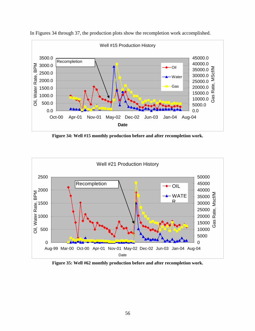
In Figures 34 through 37, the production plots show the recompletion work accomplished.

Well #15 Production History

0.0

500.0

1000.0

1500.0

2000.0

2500.0

3000.0

3500.0

Oct-00 Apr-01 Nov-01 May-02 Dec-02 Jun-03 Jan-04 Aug-04

Date

Oil,

Wat

er R

ate,

BP

M

0.05000.010000.015000.020000.025000.030000.035000.040000.045000.0

Gas

Rat

e, M

Scf

/MOil

Water

Gas

Recompletion

Figure 34: Well #15 monthly production before and after recompletion work.

Well #21 Production History

0

500

1000

1500

2000

2500

Aug-99 Mar-00 Oct-00 Apr-01 Nov-01 May-02 Dec-02 Jun-03 Jan-04 Aug-04Date

Oil,

Wat

er R

ate,

BP

M

05000100001500020000250003000035000400004500050000

Gas

Rat

e, M

scf/M

OIL

WATER

Recompletion

Figure 35: Well #62 monthly production before and after recompletion work.

56

Well #62 Production History

0

100

200

300

400

500

600

700

Oct-00 Apr-01 Nov-01 May-02 Dec-02 Jun-03 Jan-04 Aug-04Date

Oil,

Wat

er R

ate,

BP

M

0

1000

2000

3000

4000

5000

6000

7000

8000

Gas

Rat

e, M

Scf

/M

Oil

Water

Gas

Recompletion

Figure 36: Well #62 monthly production before and after recompletion work.

Well #77 Production History

0500

10001500200025003000350040004500

4/19/2001 12/25/2001 9/1/2002 5/9/2003 1/14/2004 9/20/2004Date

Oil,

Wat

er R

ate,

BP

M

02000400060008000100001200014000160001800020000

Gas

Rat

e, M

Scf

/M

OilWaterGas

Recompletion

Figure 37: Well #77 monthly production before and after recompletion work

From Figures 34 through 37, we can see that Big Four carbonates show strong initial and/or incremental gas production. The Viola formation in well #62 well was partially completed before this recompletion, thus we see little gas production change. The oil production increase in well #77 is more significant and sustainable. The possible reason for this is that the Bromides were recompleted simultaneously with Big Four carbonates. Both gas and oil production increments confirm that the reservoir is compartmentalized by nature, and demonstrative of the validity of VI and engineering analyses. In the next section, we discuss the results for the wells recommended for recompletion.

57

2.2.2.2. Recompletion Recommendations From virtual intelligence and engineering analysis recommendations, two wells were selected to test the effectiveness of our analyses. These two wells are well #19 and well #53. Recompletion information for these two wells is shown in Tables 6 and 7.

Well Name Pre Analysis Data Post Analysis Data Recompletion Recommend Start End Start End Date Formation List Names 19 11/30/99 11/30/01 1/1/04 5/19/04 2/9/04 Big 4 O,O-G

53 6/30/00 8/31/01 2/28/01 5/31/04 8/21/03 Bromide&Big4 O,G,O-G

Table 6 – Well 19 Recommendation Well Information

Well Name Formation Name Bromide Viola Hunton Sycamore Woodfort

19 - Acid frac: 15%HCl , no prop

Acid frac: 15%HCl, or slk wtr?

Acid frac: 15%HCl, or slk wtr?

Acid frac: 15%HCl, or slk wtr?

53

Breakdown frac, diesel, ball sealer

Acid frac: 15%HCl + Bio- Ball (no prop)

Acid frac: 15%HCl + Bio- Ball (no prop)

Acid frac: 15%HCl + Bio- Ball (no prop)

Acid frac: 15%HCl + Bio- Ball (no prop)

Table 7 –Well #53 Recommendation Well Recompletion Detail

The production data are shown in Figures 38, 39, and 40. Figure 38 is the daily rate for Well #19.

Well #19 Daily Production History

0

100

200

300

400

500

600

700

12/25/2003 2/3/2004 3/14/2004 4/23/2004

Date

Oil,

Wat

er R

ate,

BP

D

0

500

1000

1500

2000

2500

3000

3500

Gas

Rat

e, M

Scf

/D

OilWaterGas

Recompletion

Figure 38: Well #19 daily production before and after recompletion work

58

Well #19 Production Big4 Recompletion

0

1000

2000

3000

4000

5000

6000

Nov-99

Feb-00

May-00

Aug-00

Nov-00

Feb-01

May-01

Aug-01

Nov-01

Feb-02

May-02

Aug-02

Nov-02

Feb-03

May-03

Aug-03

Nov-03

Feb-04

May-04

Date

Oil,

Wat

er R

ate,

BP

M

0

10000

20000

30000

40000

50000

60000

70000

Gas

Rat

e, M

SC

F/M

OILWATERGAS

Recompletion

Figure 39: Well #19 monthly production before and after recompletion work

Well #53 Production History

0

500

1000

1500

2000

2500

3000

3500

Feb-00 Sep-00 Mar-01 Oct-01 Apr-02 Nov-02 May-03 Dec-03 Jul-04

Date

Oil,

Wat

er R

ate,

BP

M

050001000015000200002500030000350004000045000

Gas

Rat

e, M

scf/m

OILWATERGAS

Recompletion

Figure 40: Well #53 monthly production before and after recompletion work

Wells #39 and #40 both show a good increase in oil and gas production as a result of the recompletion jobs.

59

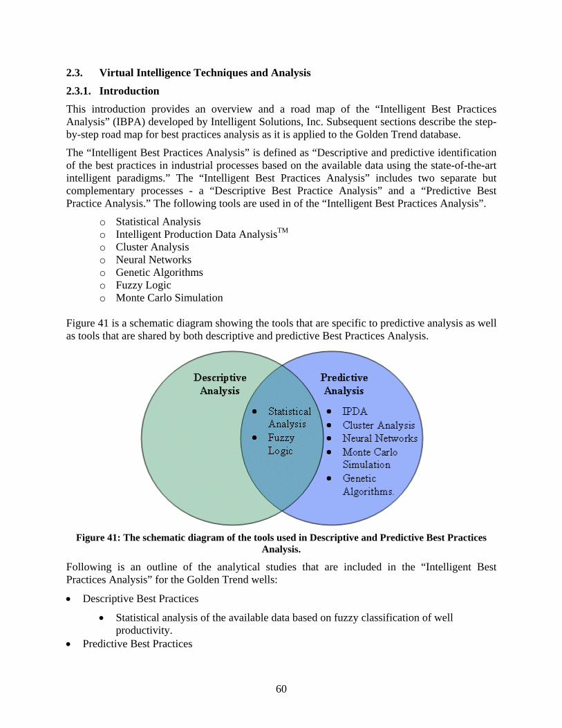
2.3. Virtual Intelligence Techniques and Analysis

2.3.1. Introduction This introduction provides an overview and a road map of the “Intelligent Best Practices Analysis” (IBPA) developed by Intelligent Solutions, Inc. Subsequent sections describe the step-by-step road map for best practices analysis as it is applied to the Golden Trend database.

The “Intelligent Best Practices Analysis” is defined as “Descriptive and predictive identification of the best practices in industrial processes based on the available data using the state-of-the-art intelligent paradigms.” The “Intelligent Best Practices Analysis” includes two separate but complementary processes - a “Descriptive Best Practice Analysis” and a “Predictive Best Practice Analysis.” The following tools are used in of the “Intelligent Best Practices Analysis”.

o Statistical Analysis o Intelligent Production Data AnalysisTM o Cluster Analysis o Neural Networks o Genetic Algorithms o Fuzzy Logic o Monte Carlo Simulation

Figure 41 is a schematic diagram showing the tools that are specific to predictive analysis as well as tools that are shared by both descriptive and predictive Best Practices Analysis.

Figure 41: The schematic diagram of the tools used in Descriptive and Predictive Best Practices

Analysis.

Following is an outline of the analytical studies that are included in the “Intelligent Best Practices Analysis” for the Golden Trend wells:

• Descriptive Best Practices

• Statistical analysis of the available data based on fuzzy classification of well productivity.

• Predictive Best Practices

60

o Intelligent Production Data Analysis o Cluster Analysis o Neural Network Predictive Model Building

Full Field Best Practices Analysis • Single Parameter Analysis • Combinatorial Analysis

Groups of Wells Best Practices Analysis • Grouping based on Operator

o Single Parameter Analysis o Combinatorial Analysis

• Grouping based on Reservoir Quality o Single Parameter Analysis o Combinatorial Analysis

• Single Well Best Practices Analysis o Single Parameter Analysis o Combinatorial Analysis

Once these analysis are completed, the results are compiled and conclusions are inferred.

2.3.2. Descriptive Best Practices Analysis The descriptive best practices analysis shows us the type of information available in the database. Table 8 shows the list of parameters that were analyzed. The list of parameters is a function of data availability in the database.

As shown in Table 8, we studied 18 parameters during the descriptive best practices analysis. The parameters used during the predictive best practices analysis are shown in the rows with shades of green.

No. Parameter 1 Number of formations present in the well 2 Number of formations stimulated 3 Number of formations with hydraulic fracturing 4 Number of formations with acid jobs 5 Total perforated pay thickness 6 Date of First Stimulation 7 Main Fracturing Fluid - Water 8 Main Fracturing Fluid - Oil 9 Main Fracturing Fluid - Acid 10 Main Fracturing Fluid - Other 11 Total Shots per foot of perforated pay 12 Total Fluid amount (Mgal) per foot of perforated pay 13 Total Proppant amount (Mlbs) per foot of perforated pay 14 Total Proppant Concentration (lbs/gal/ft) 15 Average Injection rate per foot of perforated pay 16 Date of First Production 17 Best 3 months of production 18 Initial Flow Rate – Decline Curve Analysis 19 Initial Decline Rate – Decline Curve Analysis

Table 8- Parameters in the database that were used during the “Best Practices” analysis.

61

The descriptive best practices analysis starts by identifying a parameter to partition the wells in terms of their productivity (e.g., what constitutes a well to be a poor, average or a good well). We selected the 30 Year EUR as the indicating parameter for this project, and calculated the 30-Year EUR for all wells as part of the “Intelligent Production Data AnalysisTM” process using decline curve analysis. On this basis, we identified a well that produces up to 30,000 barrels of oil during 30 years (about 1000 bbls/year) as a poor well. We identified a well that produces up to 60,000 barrels of oil during the 30 years (about 3000 bbls/year) as an average well, and wells that produce more than 90,000 barrels in 30 years as a good wells. Please note that these ranges are arbitrary and can be changed based on the economic practices of each operator.

In reality, there is little difference between a well that produces 1000 bbls/yr and one that produces 1001 bbls/yr. Therefore, we have not imposed an artificially crisp boundary between such wells. Instead, we define a series of “fuzzy sets” that resolve such unrealistic situations. This is done by identifying ranges of productivity within which wells are both poor and average, and productivity ranges within which wells are both average and good. In our classification each well is thus classified as poor, average, or good. Based on the fuzzy sets shown in Figure 42, the range between poor and average wells is from 30,000 to 60,000 barrels in 30 years or about 1,000 to 2,000 bbls/year (from 2.7 to 5.5 bbls/day).

Figure 42: The 30 Year EUR Productivity Fuzzy sets for wells in the Golden Trend Field.

The range between an average well and a good well would be from 90,000 to 120,000 barrels in 30 years or about 3,000 to 4,000 bbls/yr (from 8.2 to 11 bbls/day). Furthermore, based on these classification, a well that produces less than 2.7 bbls/day (on average throughout 30 years of production) is a poor well and a well that produces more than 11 bbls/day (on average throughout 30 years of production) is a good well.

62

In order to clarify the classification, Figure 43 shows five graphs, each pertaining to a particular well. The first graph belongs to Well A, which is a well operated by Company One. The 30 Year EUR for this well is 23,402. This measure of productivity makes this well a poor well. Well A has a membership of 1.0 in the set of poor wells. The graph on the top right shows a 30 Year EUR of 35,958 for Well B, which is also operated by Company One. This productivity level makes gives this well a membership of 0.8 in the set of poor wells and a membership of 0.2 in the set of average wells. In the second row on the left is Well C, which is operated by Company Two. This well has a 30 Year EUR of 65,996, which makes it an average well. Well D has a 30 Year EUR of 112,163 barrels, giving it a 0.26 in the set of average wells and a membership of 0.74 in the set of good wells. Well E has a 30 Year EUR of 333,940, which makes it clearly a good production well.

Figure 43: Classification of wells in the database using Fuzzy sets.

63

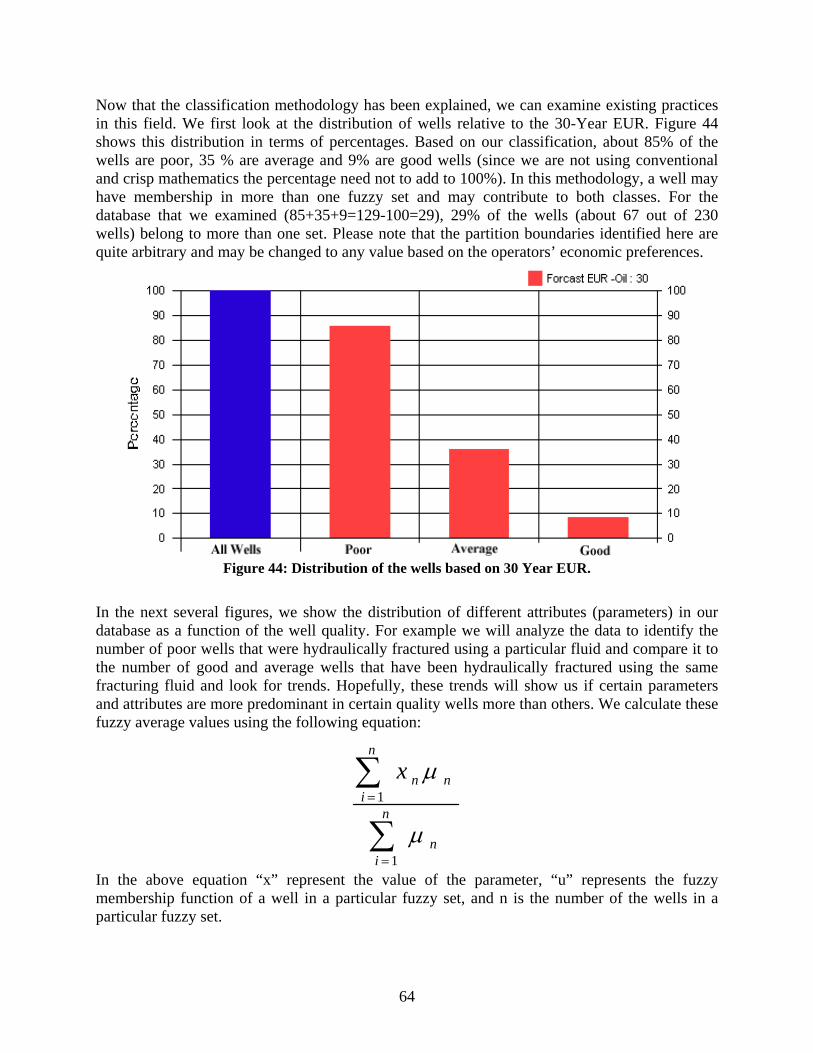
Now that the classification methodology has been explained, we can examine existing practices in this field. We first look at the distribution of wells relative to the 30-Year EUR. Figure 44 shows this distribution in terms of percentages. Based on our classification, about 85% of the wells are poor, 35 % are average and 9% are good wells (since we are not using conventional and crisp mathematics the percentage need not to add to 100%). In this methodology, a well may have membership in more than one fuzzy set and may contribute to both classes. For the database that we examined (85+35+9=129-100=29), 29% of the wells (about 67 out of 230 wells) belong to more than one set. Please note that the partition boundaries identified here are quite arbitrary and may be changed to any value based on the operators’ economic preferences.

Figure 44: Distribution of the wells based on 30 Year EUR.

In the next several figures, we show the distribution of different attributes (parameters) in our database as a function of the well quality. For example we will analyze the data to identify the number of poor wells that were hydraulically fractured using a particular fluid and compare it to the number of good and average wells that have been hydraulically fractured using the same fracturing fluid and look for trends. Hopefully, these trends will show us if certain parameters and attributes are more predominant in certain quality wells more than others. We calculate these fuzzy average values using the following equation:

∑

∑

=

=n

in

n

innx

1

1

µ

µ

In the above equation “x” represent the value of the parameter, “u” represents the fuzzy membership function of a well in a particular fuzzy set, and n is the number of the wells in a particular fuzzy set.

64

First let’s look at the parameters that seem not to have any effect on the well quality. Figure 45 provides an example. In this figure the average number of formations per well is approximately 3.5. This value hardly changes for poor, average, and good wells.

Figure 45: Distribution of the average value of Number of Formations Present in wells of different

quality

This means that this parameter (Number of Formations present in a Well) is not a factor in determination of a well quality. Figures 46 and 47 present two other parameters (Number of Formations Stimulated and Acid as Main Stimulation Fluid), that show little or no distinction in their average values between wells of different quality.

Figure 46: Distribution of the average value of Number of Formations Stimulated in wells of

different quality.

65

Although using acid as the main stimulation fluid seems not to have any major impact on the well productivity (Figure 47), Figure 48 demonstrates that wells that have been stimulated with acid fracturing have predominantly been poor wells. One may interpret this as acid fracturing has not been an effective way of stimulating wells in the Golden Trend.

Figure 47: Distribution of the average value of Acid as the Main Stimulation Fluid in wells of

different quality

We can explain the difference between Figures 47 and 48 as follows. Figure 47 shows the effect of Acid as the Main Fracturing and/or Stimulation fluid, where Figure 48 shows the number of times acid jobs performed on a well. By looking at these two figures, one may conclude that acid is not helping the stimulation of the wells in Golden Trend significantly, and that wells that have been stimulated with other fluids are among the better producing wells.

Figure 48: Distribution of the average value of number of formations stimulated by acid jobs in

wells of different quality.

66

Figure 49 shows the distribution of average “Total Perforated Pay Thickness” between poor, average and good wells. The average “Total Perforated Pay Thickness” for wells in our database is about 550 ft. Poor wells have slightly higher “Total Perforated Pay Thickness” (about 580 ft.) than average wells (about 510 ft.) and good wells (475 ft.). This indicates that good and average wells have lower “Total Perforated Pay Thickness,” which is counter-intuitive. The only logical explanation is that these wells are located in sweet spots with higher relative oil permeability. This finding makes the results of the IPDA (Intelligent Production Data Analysis) more important, as IPDA identifies productive regions by assigning them lower RRQI (Relative Reservoir Quality Index) values.

Figure 49: Distribution of the average value of “Total Perforated Pay Thickness”

Figures 50 through 52 show the effect of fracturing fluids (water, oil/diesel or “other”) used in the stimulation jobs in the Golden Trend. Figure 50 shows the results for “Water”, which does not seem to contribute to provide good fracturing. Poor wells have the highest average value (almost 0.6) of formations fractured using water. By comparison, this value is about 0.42 for average wells and 0.1 for good wells.

Figure 50: Distribution of the average value of Water as the Main Fracturing Fluid

67

Oil/Diesel as the main fracturing fluid shows exactly the opposite trend. Figure 51 shows that while the average number of formations that have been fractured using diesel oil as main fracturing fluid is about 0.35 for the entire dataset, it is more than 0.6 for good wells, about 0.5 for average wells and less than 0.3 for poor wells.

Figure 51: Distribution of the average value of Oil as the Main Fracturing Fluid

This trend is repeated in Figure 52 for “Other” fracturing fluids (most of the “Other” fluids in the database are essentially diesel oil or some sort of oil-based fracturing fluid). While the average value of “Other” fracturing fluid used during the hydraulic fracturing procedure for the entire data set is about 0.11, it increases to about 0.21 for average wells, while remaining at about 0.11 for good wells. The average value for poor wells is about 0.075.

Figure 52: Distribution of the average value of “Other” as the Main Fracturing Fluid in wells of

different quality.

We have concluded that future hydraulic fracturing procedures in this field should be performed using diesel oil as the fracturing fluid. Furthermore, we conclude that using acid as an alternative to hydraulic fracturing is not desirable. We recommend that hydraulic fracturing using diesel oil as for production enhancements be employed instead of acid for this field.

68

The next four figures (Figures 53, 54, 55 and 56) show the analysis on four stimulation parameters on “per foot of total perforated pay thickness” bases. These parameters are total shots, total fluid amount, total proppant amount, and average injection rate on “per foot of total perforated pay thickness”.

Figure 53 shows that there no identifiable trend in the average value of “Shot/ft” for different well qualities. This is expected since we had already established (Figure 49) that the “Total Perforated Pay Thickness” is not a determining factor in identifying the quality of the wells.

Figure 53: Distribution of the average value of “Shot/ft” in wells of different quality.

Figure 54 show that good wells have been fractured using a lower than average amount of fluid “per foot of total perforated pay thickness”. While the average for all the wells is about 1.6 Mgal/ft (which does not change for poor and average wells) the average amount of fluid pumped in good wells is only about 1.0 Mgal/ft.

Figure 54: Distribution of the average value of “Total Fluid Amount (Mgal)/ft” in wells of different

quality

69

Figure 55 show the amount of proppant used during the hydraulic fracturing treatment. This figure shows a general pattern of higher proppant amounts per foot of pay thickness for average and good wells as compared to poor wells.

Figure 55: Distribution of the average value of “Total Propp Amount (Mlbs)/ft” in wells of different

quality

In order to put Figures 54 and 55 in perspective, we examined the proppant concentration in pounds per gallon of fluid per foot of pay thickness. This is shown in Figure 56. This figure clearly shows higher proppant concentrations were used in the better wells. While good wells and average wells show an average of 0.73 and 0.64 pounds per gallon of fluid per foot of pay thickness, respectively, only about 0.27 lbs/gal/ft of proppant concentration was used, on average, for poor wells.

Figure 56: Distribution of the average value of “Average Proppant Concentration (lbs/gal/ft) in

wells of different quality

70

Figure 57 demonstrates the effect of average rate of injection “per foot of total perforated pay thickness.” This figure shows that it is preferable for the fluid and proppant to be pumped at lower rates. Good wells have been pumped at about 0.12 BPM/ft.

Figure 57: Distribution of the average value of “Average Injection Rate (BPM)/ft” in wells of

different quality

2.3.3. Decline Curve Analysis The previous section showed the effect of individual parameters on well “quality.” Next we examined the decline curve analysis parameters for these set of wells. Looking at the behavior of initial flow rate (Qi) and initial decline rate (Di) can confirm the general logic behind the methodology that used in the analysis of descriptive best practices for the Golden Trend.

As expected, better wells have relatively higher initial flow rates than average and poor wells, as well as lower initial decline rates. These phenomenon are shown in Figures 58 and 59. Again, this is simply to confirm that this analysis will provide consistent results when used properly.

Figure 58: Distribution of the average Initial Flow Rate from the Decline Curve Analysis in wells of

different quality

71

Figure 59: Distribution of the average Initial Decline Rate from the Decline Curve Analysis in wells

of different quality

2.3.4. Predictive Best Practices Analysis For this document, we define Predictive Best Practices Analysis as “the art and science of identifying the best combination of parameters in a particular industrial process that would optimize the process outcome using a predictive model based on the available data.” This definition implies development of a predictive model that would form the foundation of all analysis. We defined the process of developing and validating such a model in previous monthly reports. We used this process to identify the best hydraulic fracturing practices (for deliverability enhancement) in the Golden Trend.

The three components of Predictive Analysis for the Best Hydraulic Fracturing Practices in the Golden Trend are full field analysis, groups of wells analysis and individual well analysis. Figure 60 shows the relationship of these analyses to one another.

Full Field Analysis

Individual Well

Analysis

Groups of Wells Analysis

Figure 60: The relationship of the best practices identified through these analyses to one another.

72

The predictive best practices identified through full field analysis are general and were applied to the majority of the wells in the field. However, since we averaged values to develop our conclusions, some wells will not follow the general trend and, when we analyze groups of wells that are clustered based on reasonable criteria, the ‘best practices’ become tailored to that group of similar wells.

Individual well analysis places too much faith on a predictive model that is statistical by nature. The predictive model, although developed using the state-of-the-art integrated intelligent systems, is ultimately a product of data that is measured, collected, reported, and recorded by human subjects. It is therefore not free of errors, even if we assume that it is statistically representative of all the variations that are present in reality.

The issue of precision versus averaging must also be addressed. The precision of the analysis increases as we move from full field scale to groups of wells and finally to individual wells. During the ‘full field analysis’, we average the data to make statements that have the widest degree of applicability. Once we move into the ‘groups of wells’ analysis, our statements are more precise and the law of averages applies to a lesser degree, although we still apply some averaging. The most precise analysis is the ‘individual well analysis,’ during which we increase or decrease the controllable parameters and examine the output before making our final decision.

Figure 61 shows the degree of precision (high, moderate and low) offered by these analyses, as well as the degree of dominance of averaging in each of these analyses. Analysis precision decreases as one moves from single well analysis to full field analysis, while the amount of averaging increases. Figure 61 shows that, when it comes to decision making on the future wells, both precision and averaging are important role. Therefore, the “groups of wells analysis” is probably the more important analysis when making future decisions.

Figure 61: Schematic diagram showing the precision, averaging, and contribution to the future decision making of three different analysis offered by ISI’s Predictive Best Practices Analysis.

73

2.3.5. Data Driven Predictive Model Development Before starting the predictive best practices analysis we developed a predictive neural network model. The following section covers that neural network development, which includes training, calibration and verification processes.

Figure 62 provides a flow chart that shows different components that are involved in the development of the data driven predictive model in the context of the predictive best practices analysis. The process starts as soon as a database, which includes production data and data from the well files, is compiled. During data pre-processing, which can be summarized as a complete data mining practice, we patch the missing data in the database is patched and identify and manage the outliers. We then test the data set for contaminated or corrupted data records, and examine the relationships between database parameters. We also performed some statistical analysis during the pre-processing stage.

Upon completion of the data pre-processing, the data are passed on to IPDA-IDEATM.

The next section provides a summary of the results of IPDA-IDEATM analysis.

DATABASEProduction Data and Well Files

Data Pre-Processing

Relative Reservoir Quality Index (RRQI) Field Scale Model

ISI

IPDA-IDEATM

Intelligent Production Data Analysis

ISI

IDEATM

Intelligent Data Evaluation and Analysis

ISI

BP-IDEATM

Best Practices Analysis

Figure 62: Flow chart of Best Practices Analysis using Artificial Intelligence Techniques.

74

During data pre-processing, ‘Fuzzy Combinatorial Analysis’ was used to identify and rank the contribution of each parameter on the 30-year EUR in order to make the data ready for modeling. The 30-year EUR was calculated during the IPDA-IDEATM analysis. Figure 63 shows the ranking of the parameters in terms of their influence on the 30- Year EUR.

Appendix A at the end of this report includes the visual representation of the influence of each parameter on the 30-Year EUR. A high or low flat area in the Appendix figures indicates a high or low influence of the parameter on the 30-Year EUR. The slope in these graphs indicate the sensitivity of the 30-Year EUR to the parameter at those ranges.

During the fuzzy combinatorial analysis for this project, we established that the most influential category of parameters in The Golden Trend is reservoir quality. The second and third most influential categories of parameters were stimulation and completion, respectively. This finding is shown graphically in Figure 64. In this figure the “Fuzzy Combinatorial Analysis Score” is plotted for each of the categories. The lower is the FCA-Score for a category the higher would be its influence on the long-term production. The influence of each category was calculated by averaging the overall FCA-Score for all the parameter that belonged to a particular category.

Rank Feature1 Qi-12 Sub RRQI3 Date of First Stimulation4 RRQI5 Di-16 No# of Formation Stimulated7 Average Rate (BPM)8 MF - Acid9 MF - Oil10 MF - Water11 Latitude12 MF - Other13 Fluid Mgal/ft14 Total Fluid Mgal15 Shot / ft16 Longitude17 Total Shots18 b-119 Rate BPM/ft20 No# of Formation Present21 No# of Formation Fraced22 Propp Mlbs/ft23 No# of Formation Acid Jobs24 Total Proppant Mlbs25 Total Perfed Thickness

Figure 63: Ranking of the parameters as a function of their influence on 30-

Year EUR.

Figure 64: Ranking of categories of parameters as a function of their influence on 30 Year EUR.

75

The next step was a set of statistical analysis performed on all the parameters in the data base. These analyses included linear regression of each parameter versus the 30 Year EUR and each other and also the probability distribution function for each of the parameters. The regression analysis would show any potential relationship between any two parameters. This could be valuable information during the modeling process. A set of all the regression graphs including the best linear fit for all the parameters versus 30 Year EUR is shown in Appendix B. The figures demonstrating the probability distribution functions for each of the parameters are shown in Appendix C.

2.3.6. Neural Network Modeling After completing the pre-processing of the data and the IPDA-IDEATM analysis and a complete set of cluster analysis that included both K-Mean cluster analysis as well as Fuzzy C-Mean cluster analysis the best set of inputs for the neural network was selected. Figure 65 shows the list of the inputs to the neural network model.

QiDiLatitudeLongitudeSub - RRQIRRQIShots / ftDate of first stimulationMF - WaterMF - OilMF - AcidMF - OtherPorppant Concentration (lb/gal/ft)Ave. Inj. Rate (BMP/ft)

Figure 65: Parameters used during the neural network modeling process.

As shown in the above figure there are two parameters extracted from the Decline Curve Analysis of the production data. These are Qi and Di. There are two parameters that identify the location of the well. These parameters, Latitude and Longitude, can also be a proxy for the geology of the reservoir at the location where the well is drilled. The two parameters, RRQI and Sub RRQI, relative reservoir quality indices, are further indication of the reservoir quality in addition to latitude and longitude. These parameters are the result of IPDA-IDEATM analysis.

Number of perforations per foot of the pay zone (Shot / ft) was used to identify well completion. The next seven parameters are stimulation related. The first one, Date of the First Stimulation, identifies a time stamp for the well. The next four parameters identify the type of fluid that was used as the main fluid in the stimulation job. The next two parameters identify the amount of fluid and proppant and the rate of injection per foot of the pay zone.

The output of the neural network model is the 30-Year EUR. The data set was divided into three smaller sets. The data set that was used to ‘train’ the neural network included 147 records (wells). The calibration data, which was used to identify when the training process was complete, included 17 records (wells). The verification set, which served to judge the goodness of the model, included 18 records (wells).

76

Figures 66 and 67 show the result of the training process. The R2 for the training set was 0.904 and the correlation coefficient was 0.951. These high degrees of correlation indicate that the network has been ‘trained’ to analyze the data and predict the EUR with a high level of accuracy.

Figure 66: Actual and predicted 30 year EUR of training data set upon completion of the training

of the neural network model.

Figure 67: Actual and predicted 30-year EUR of training data set upon completion of the training

of the neural network model.

77

Figures 68 and 69 demonstrate the results of calibration and verification data sets. The calibration data set has a R2 of 0.642 and a correlation coefficient of 0.801. The R2 and correlation coefficient of the verification data set are 0.905 and 0.951, respectively. These high degrees of correlation indicate that the network can take new input and accurately predict the 30 -year EUR.

Figure 68: Actual and predicted 30 year EUR of the calibration data set upon completion of the

training of the neural network model.

Figure 69: Actual and predicted 30 year EUR of the verification data set upon completion of the

training of the neural network model.

One last step remains to be covered before the details of Intelligent Best Practices Analysis can be presented. The remaining step, mentioned earlier in this section, is Intelligent Solutions, Inc’s IPDA-IDEA™ process. This step is covered in the next section.

78

2.3.7. Intelligent Production Data Analysis, IPDA-IDEA™ IPDA-IDEA™ starts by identifying a production indicator as the target feature. Then we applied Fuzzy Combinatorial Analysis to the latitude and longitude, and plotted the results of the analysis beside the map of the wells involved in the study. Figure 70 shows the completion of this stage of the study. The purple lines represent the Fuzzy Combinatorial Analysis.

As shown in Figure 70, some wells are isolated from the main cluster. There is one cluster of wells found in the north. About six wells are scattered in the west, while two isolated wells are found in the southeast. Discounting (eliminating) these wells produces the picture shown in Figure 71 on the following page.

Once the final well mapping is accomplished, the field can be delineated based on the fuzzy combinatorial analysis of latitude and longitude.

Figure 70: Original mapping of the wells in IPDA-IDEA™.

79

Figure 71 shows the data from Figure 70 after we removed the isolated wells from the analysis. The fuzzy combinatorial analysis curves become more cohesive and continuous, and the curvature of the two curves is used in order to delineate the field.

Figure 71: Final mapping of the wells in IPDA-IDEA™.

This analysis process is accomplished by dividing each of the curves into high, medium and low values. Then, as different segments overlap, the relative reservoir quality is determined. For example, the best location in the field would be where high values of the latitude fuzzy combinatorial analysis curve coincide with high values of the longitude fuzzy combinatorial analysis curve.

The analysis is continued until all of the wells in the field are part of a delineated segment. This is a trial and error process. As each of the curves are partitioned, and the different segments of the filed are classified, the average value of the 30-year EUR for wells in each segment are examined to assure that they conform to the labels identified by the process.

80

Upon completion of the mapping process, we are able to identify a set of zones based on their Relative Reservoir Quality Index (RRQI). Lower RRQI values indicate better reservoir quality. Figure 72 portrays the information, with the darker colors representing the most productive zones.

In this example, the most productive area is zone #6, which has an RRQI of 1. The next most productive areas are zones #3, #5, and #9, which have an RRQI of 2. Zones #2 and #8 have an RRQI of 3, while zones #4 and #12 have an RRQI of 4. Zones #7, #11, and #13 have and RRQI of 5. Zone #10 has the lowest RRQI, which is 6. Zones with no coloration include no wells.

Figure 72: Main zones delineations.

Once the delineation of the field for the main zones is accomplished, the next step is to zoom into each of the main zones and identify sub zones using a similar process. The result is a more delineated field, as shown in Figure 73 on the following page.

Upon completion of this process, each well in the field will be assigned to both a main zone and a sub-zone, each of which will have a Relative Reservoir Quality Index. Therefore, each well in the group is assigned a RRQI and a sub-RRQI. The combination of these two numbers is an indication of the relative reservoir quality for a particular well based on porosity, net pay and permeability. This same process can be used to create maps that emphasize such factors as permeability or the role of natural fractures by using statistics from the best three month production indicator or other parameters.

81

Figure 73: Final delineations including main as well as sub zones.

The final result of the process is shown in Figure 74, which is a tabular summary of the data. The RRQI and sub-RRQI assigned to each well in this dataset is summarized in this tabular summary. These reservoir quality indices were used during the neural network predictive model building as well as during the Intelligent Best Practices Analysis, based on groups of wells.

82

Figure 74: List of Reservoir Quality indices for all the wells in the dataset.

83

2.3.8. Full Field Analysis The full field, predictive best practices analysis looks at all the wells in the database and identifies the major trends in the process. The adjective “Predictive” implies the fact that some of the patterns that are identified may not be based on practices that have been implemented. The analysis would thus predict what could potentially happen if certain practices are employed. Details of this analysis process are provided below.

2.3.8.1. Single Parameter Predictive Best Practices Analysis - Full Field Analysis The explanation of analysis process presented in this section for a single parameter best practices analysis for a full field is equally applicable to single parameter predictive best practices analysis for groups of wells.

In this process we first identify the parameter to be analyzed. For example, if we are examining the amount of fluid used in the fracture treatment process (in Mgal/foot of perforated pay thickness, or fluid/ft), we would establish the minimum and maximum value of this parameter from the database. The range of this parameter (max – min) is then calculated and divided by a large number (i.e. 100). The calculated value would be the increment. We then select the first well in the database and, while keeping all the parameters at their original value, vary the parameter under consideration (fluid/ft) from the minimum to the maximum value through a series of about computer 100 runs to predict the 30-Year EUR. Then the 100 outputs (30-Year EUR) are plotted against the 100 values of the parameter (fluid/ft) from minimum to maximum incremented each time by the calculated increment. This plot will show the changes in the 30-Year EUR as the value of the parameter (fluid/ft) is changed from min to max. This process is then for each wells in the database.

An example of such a run for one well is shown in Figure 75. This figure shows the changes in 30-Year EUR of a typical well operated by Company One as the value of the fluid/ft is changed from the minimum to the maximum in the database. The predictive best practices analysis for the entire field for this parameter is then identified as the major patterns that would develop on most of the wells in the field.

Figure 75: Example of a single parameter analysis for one well.

84

The major trends and patterns that are identified are then presented in the form of a table as shown in Table 9. Four parameters are analyzed in this table. We have further divided the ‘Main Fracturing Fluid’ into ‘Water’, ‘Oil’, ‘Acid’, and ‘Other’.

For each parameter we develop two sets of numbers. The top numbers, shown in blue, are the percentage of the wells in the field that show an increasing trend along with the average amount of 30-Year EUR increase in barrels. The red numbers represent decreasing trends. For example in case of ‘Water’ as the main fracturing fluid, 77% of the wells show an increasing trend, with an average increase of 53,914 barrels of oil in 30 years, while 23% of wells show a decreasing trend with an average decrease of 70,960 barrels of oil in 30 Years.

Important Note: The numbers presented in this analysis should be treated as “relative” rather than “absolute.” This simply means that although the actual number of barrels that are presented here may or may not be realistic their value relative to one another (percent increase or decrease) should be regarded as realistic. The unrealistic absolute values in some cases can be a byproduct of a non-uniform distribution of the well productivities in the database.

Parameter Percentage Average RangeWater 77% 53,914

23% 70,960

0% 0

97% 366,699

26% 83,989

100% 396,082

0% 1,715

100% 373,133

Oil 100% 382,150

Acid 3% 1,519

Other 74% 29,994

Shot/ft 0% 0

Propp Conc. 100% 391,577

Rate (BPM/ft) 0% 0

Mai

n Fl

uid

Table 9: Single parameter patterns for the full field analysis

Table 9 shows that ‘Oil’ is the most effective fracturing fluids that can be used in The Golden Trend. It also shows that a decrease in the number of perforations and an increase in proppant concentration are favorable trends. Furthermore, all the wells seem to favor a lower injection rate that can result in increase in wells productivity.

2.3.8.2. Combinatorial Predictive Best Practices Analysis: Full Field Analysis

The explanation of the details of the analysis that is presented here for the combinatorial predictive best practices analysis is equally applicable to combinatorial predictive best practices analysis for groups of wells.

During the combinatorial predictive best practices analysis several parameters were analyzed in combinations. This simply means that all the parameters are changes simultaneously and run through the data-driven model to calculate the 30 Year EUR. This process of changing all the parameters are continued until the combination that provides the highest 30 Year EUR is found.

85

The combination of parameters that results in the highest 30 Year EUR are then identified as the optimum values for that well and the process is repeated for all the wells in the database.

This search for the optimum combination of parameters that would result in the highest 30 Year EUR is not a blind search. ISI uses a genetic algorithm that evolves the best solutions through an intelligent search process in several generations of solutions. Upon completion of the process the top five solution of each generation for each well is saved and plotted (as frequency distribution) to identify the dominant trend of the successful solutions.

Figures 76 through 82 show the results of the combinatorial predictive best practices analysis for the entire field using 230 wells in the Golden Trend. Since the top five solution of each generation were saved, and the process simulation was run for 10 generations, each graph demonstrates the results from 230x10x10 = 23,000 simulation runs using the previously developed data-driven model.

Figure 76: Full Field Combinatorial Predictive Best practices Analysis – Results for Water as main

fracturing fluid.

The first four figures (76 through 79) clearly show that diesel oil dominates the optimized frac jobs as the main fracturing fluid. Water was used as the main fracturing fluid on one to two formations per well. The predictive analysis showed overwhelmingly (more than 97% of the 23,000 runs), that water was to be avoided in frac jobs with water in order for the formations to reach their optimum 30 Year EUR. This result is demonstrated in Figure 76.

Figure 77 on the following page shows the maximum number of formations treated with diesel oil as the main fracturing fluid. More than 42% of the wells in the predictive analysis had to be treated with the five frac jobs using diesel oil in order to reach their optimum potential. The number of formations that had to be treated with diesel oil is four for bout 21% of the wells, three for 13% of the wells, and two for 4% of the wells. Overall, 80% of the wells had to be hydraulically fractured using diesel oil in order to achieve optimum production. This is a compelling statistic for the use of diesel oil as the fracturing fluid of choice in the Golden Trend.

86

Figure 77: Full Field Combinatorial Predictive Best practices Analysis – Results for Oil as main

fracturing fluid.

Figures 78 and 79 show results that are similar to results from Figure 76. These figures emphasize that the used of acid and other fluids may not help in achieving optimum productivity from the wells in The Golden Trend.

Figure 78: Full Field Combinatorial Predictive Best practices Analysis – Results for Acid as main

fracturing fluid.

87

Figure 79: Full Field Combinatorial Predictive Best practices Analysis – Results for Other as main

fracturing fluid.

Figure 80 shows the result for the number of perforations per foot of the pay thickness for the optimum jobs in The Golden Trend. This figure clearly shows a decreasing trend. The 23,000 simulation runs show a skewed distribution toward the use of smaller number of perforations per foot of pay thickness. The conclusion from this analysis is that in The Golden Trend it is advisable to complete the wells with a lower number of perforations (average of 1 shot per foot based on the figure below) to maximize the effect of a hydraulic fracturing treatment.

Figure 80: Full Field Combinatorial Predictive Best practices Analysis – Results for number of

perforations per foot of Pay Thickness.

88

Figure 81 shows that increasing the proppant concentration in pounds per gallon of fluid per foot of pay thickness is quite favorable in The Golden Trend.

Figure 81: Full Field Combinatorial Predictive Best practices Analysis. Results for proppant

concentration in pounds per gallon of fluid per foot of pay thickness.

Figure 82 clearly shows a favorable trend for low injection rates. In 23,000 simulation runs, wells that have been stimulated with low injection rates have a much higher probability of reaching their optimum productivity than those with higher injection rates.

Figure 82: Full Field Combinatorial Predictive Best practices Analysis – Results for the averaged

injection rate per foot of Pay Thickness.

Figures 81 and 82 show that high proppant concentrations, injected at low injection rates, achieves maximum long-term production. By increasing the proppant concentration, the injection rate must decrease in order to properly place the proppant in the fracture and avoid the high net pressures that have been documented as a hurdle to post-fracture production.

89

2.3.8.3. Conclusions Table 10 summarizes the results of full field predictive hydraulic fracturing best practices analysis in The Golden Trend. This table combines the single parameter analysis with the combinatorial analysis and provides recommendations.

Percent of Population

Dominant Trend

Change in Value Distribution

Dominant Trend

Water Majority Increasing Moderate Skewed Use Little Use Not RecommendedOil All Incressing High Skewed Use A Lot Use RecommendedAcid Majority Decreasing High Skewed Use Little Use Not RecommendedOther Majority Increasing Low Skewed Use Little Use Not RecommendedShot/ft All Decreasing High Skewed Use Little Use Small NumbersProp Conc. (lbs/gal/ft) All Increasing High Skewed Use A Lot Use Large AmountsRate (BPM/ft) All Decreasing High Skewed Use Little Use Low Rates

Recommendations

Mai

n Fl

uid

Combinatorial AnalysisSingle Parameter AnalysisParameter

Table 10: Summary of the full field analysis of predictive hydraulic fracturing best practices in

Golden Trend.

We make recommendations when both the single parameter analysis and the combinatorial analysis seem to be pointing in the same direction. A good example of such case is use of diesel oil as the main fracturing fluid where during both analysis identify dominant trend toward its use in order to increase the well productivity.

Other parameters that seem to show clear signs of specific trends are number of perforations per foot of pay thickness, injection rate, and proppant concentration. The analysis indicates that the number of perforations per foot of the pay thickness should be low (around one shot per foot). Low injection rates are preferable, especially with increased proppant concentrations.

2.3.9. Groups of Wells Analysis This section covers predictive best practices analysis based on groups of wells. We considered two different grouping of the wells in this study. We based the first grouping on the operators and the second grouping on relative reservoir quality.

2.3.9.1. Grouping Based on Operators

We performed predictive best practices analysis on wells grouped by operator. For this study, we divided the wells in the database into three groups - Company One, Two, or Three – with the objective of identifying positive or negative practices (regarding hydraulic fracturing) that might exist within in a company. These practices may contributes to company success, in which case must be nurtured, or they may to be counter-productive, in which case management may want to revisit them. Some of these practices may exist in an implicit fashion rather than being enforced explicitly. In such cases, studies such as this one may prove helpful in starting productive discussions in the company.

Company policies and practices frequently have their roots in previous company success, making management reluctant to change. However, changes in the operational landscape can affect the technical or cost-effectiveness of previous practices. The type of analysis that we have done for these wells provides management and technical staff an unbiased way of reviewing operational practices, with the potential to increase the operational effectiveness and productivity, as well as enhancing well field life and production.

90

Figure 83 shows the location of the wells operated by different companies in the Golden Trend. Please note that the wells operated by Company One are more localized, while the wells operated by Company Two are more dispersed. Relatively few wells are operated by Company Three.

Table 11 shows the average values of the parameters for the three operators, as well as overall average values for poor, average and good wells. Sixty-five wells in this database belong to more than one fuzzy set. Some of them are partially poor/partially average, while others are partially average/partially good. Wells that fall into two categories are counted twice in our analysis.

Figure 83: Wells in the database grouped based on three operators.

Table 11: Average values of the wells from each company as compared to average well quality.

91

Wells operated by Company Two have the highest average 30-Year EUR, at about 49,600 bbls. Company Two’s wells are, on average, 156 % more productive than Company One wells and 250 % more productive than Company Three wells. Company One wells are about 160 % more productive than Company Three wells.

It is important to examine the well statistics grouped by operator and compare them with the typical poor, average, and good wells, with the assumption that porosity, permeability and pressure (as an indication of depletion) for wells from each company are comparable throughout this reservoir. Therefore, we are attributing the relative success and/or failure of the wells performances to the completion and stimulation practices.

Re-examining Table 11, Company Two wells have performed better, on average, compared to Company One and Company Three wells. It is noticeable that Company Two has used diesel oil as the main fracturing fluid more often, and on more formations, than the other operators. The average number of formations stimulated using diesel oil is 0.90 for Company Two, while it is, 0.15 for Company One, and 0.05 for Company Three. Furthermore, the average number of formations stimulated using diesel for a good well is 0.60, decreasing to 0.28 for poor wells.

Another pattern that is easily recognized is the average proppant concentration. Good wells have average proppant concentration of 0.45 pounds/gallon/foot, while average wells and poor wells have concentrations of 0.34 and 0.20, respectively. Our conclusion is thus that higher proppant concentrations produce wells that are more productive. Company Two, which has the more productive wells, used an average proppant concentration of 0.99 pounds/gallon/foot for its wells while Company One’s and Company Three’s proppant concentrations are 0.01 and 0.32 pounds/gallon/foot, respectively. It is noticeable that Company Three has used higher average proppant concentrations than Company One, but its wells are not as productive as Company One. This emphasizes the fact that, although our procedure identifies patterns, ultimately it is a combination of practices that makes one well more productive than another well. The objective of this study is to provide a tool to the operators that can identify such combinations.

2.3.9.2. Single Parameter Predictive Best Practices Analysis - Grouping Based on Operators

We described the procedure for the single parameter predictive best practices analysis in a previous section. The results of our analysis are shown in Table 12 (following page), which shows results from three groups of wells grouped based on the operating company.

A few items stand out in Table 12. First is that incremental production in 30-Year EUR for Company Three wells are lower than other two operators. This may be an artifact of the low number of wells represented in the database from Company Three, or that the wells operated by Company Three are in a less productive part of the formation. Grouping the wells based on the reservoir quality (geology) (see next section) is a means of analyzing this observation.

Table 12 also shows that using ‘Water’ as the main fracturing fluid has a negative effect on long-term well production, regardless of the operator. Therefore, we do not recommend water as the main fracturing fluid. This is consistent with recent findings from Core Laboratories, who have indicated that, in some cases, clay content in the formation is the main cause of this phenomenon. The water may be damaging the reservoir near the well bore by developing hydration spheres, which has negative effect on short and long-term production. As a note, the hydration sphere process seems to be reversible as long as the water saturation in the reservoir is

92

not at irreducible saturation. Core Labs has concluded that, at gas to water permeability ratios (kg/kw) higher than 3 (where Kilnkenberg gas permeability has been measured under reservoir stresses), oil seem to be a better choice for fracturing fluid. Our analyses show that the formations completed in The Golden Trend may possess the characteristics identified by Core Labs. This is consistent with the fact that wells in Table 12 for which ‘Oil’ was the main fracturing fluid have higher incremental production rates.

Table 12: Single parameter patterns for the groups of wells analysis – grouping based on operators

Another interesting phenomenon that is identified from Table 12 is the effect that “Acid” as the main fracturing fluid has on the wells operated by Company Three. Wells operated by Company Three are the only wells that show better 30-year incremental production when Acid is used as the main fracturing fluid. Figure 84 shows this phenomenon.

Figure 84: Incremental 30 year production as a result of using different fracturing fluids in wells

operated by Company Three

93

This result may be related to the fact that wells operated by Company Three are located in the south west of the field, as shown in Figure 85, and that wells from that part of the field are completed in parts of the formations that have characteristics that responds well to Acid. For example, the parts of formation in southwestern of the field contain carbonate, which responds positively to Acid.

Another trend, consistent with the full field study, is the use of high proppant concentrations at lower injection rates. These two trends, as with ‘oil’ as the main fracturing fluid, seem to be dominant no matter which company is operating the wells. The trend presented by decreasing the number of perforations per foot of pay thickness also shows an increase in the production. We will revisit this trend as we look at the wells when grouped based on relative reservoir quality.

Figure 85: Wells in the database identified by the operating companies

94

2.3.9.3. Combinatorial Predictive Best Practices Analysis - Groupings Based on Operators We covered the procedure for combinatorial predictive best practices analysis previously. Figures 86 to 89 show the results of the combinatorial analysis for the main fracturing fluid.

During the single parameter analysis all fluids but water seemed to be promising as long as they were used consistently for well fracturing. The combinatorial analysis allows us to determine which fluid performs best. Figures 86 through 89 clearly show that ‘oil’ is the fluid of the choice. Furthermore, these figures show that, no matter which company operates the wells, ‘oil’ is the preferred main fracturing fluid in The Golden Trend. Because of formation issues, acid may also have some credibility as a fracturing fluid for wells operated by Company Three.

Figure 86: Groups of wells Combinatorial Predictive Best practices Analysis – Results for Water as

the main fracturing fluid

Figure 87: Groups of wells Combinatorial Predictive Best practices Analysis – Results for Diesel Oil

as the main fracturing fluid

95

Figure 88: Groups of wells Combinatorial Predictive Best practices Analysis – Results for Acid as

the main fracturing fluid

Figure 89: Groups of wells Combinatorial Predictive Best practices Analysis – Results for Other

fracturing fluids

96

Figure 90 shows the results of combinatorial analysis for all three operators on number of perforations per foot of pay thickness. The distribution shows that a skewed distribution toward smaller numbers of perforations per foot of pay zone, but wells operated by Company One and Company Three would benefit more from such a practice than those by Company Two.

Figure 90: Groups of wells Combinatorial Predictive Best practices Analysis – Results for number

of perforations per foot of pay thickness.

Figure 91 shows the results of combinatorial analysis for the recommended proppant concentration per gallon of fluid injected per foot of pay thickness. This figure shows a skewed distribution toward higher amounts of concentration per foot of pay thickness for wells operated by all three operators. This result agrees with those found during the full field analysis.

Figure 91: Groups of Wells Combinatorial Predictive Best practices Analysis – Results for

proppant concentration per gallon pf fluid per foot of pay thickness.

97

Figure 92 shows the results of combinatorial analysis for the injection rate per foot of pay thickness. Again, the dominant trend in this figure for all three operators seems to be that lower average injection rates per foot of pay thickness optimize production.

The justification of the lower average injection rates during the hydraulic fracturing treatment usually is the invasion of the fracture into the formations immediately above or below the pay zone. This phenomenon may occur when the cap formations have natural fractures or possess lower in-situ stresses that are conducive to accepting hydraulic fractures by providing the path of the least resistance to the fracture propagation.

Figure 92: Groups of wells Combinatorial Predictive Best practices Analysis – Results for average

injection rate per foot of pay thickness.

2.3.9.4. Analysis of Reservoir Qualities Tables 13, 14, and 15 summarize the conclusions for each of the operators. Table 16 provides the key to the terms and the color codes used in Tables 13 to 15. These tables combine the single parameter analysis with combinatorial analysis to reach conclusions and make recommendations:

• For Company One wells, diesel oil is the most effective fracturing fluid

• High proppant concentrations, injected at low rates into wells that are completed with about one shot per foot of pay, is preferable for wells operated by Company One.

Table 13: Summary of the groups of wells analysis of predictive hydraulic fracturing best practices

in Golden Trend based on the operators - Company One.

98

Table 14 shows the results for Company Two wells. The conclusions reached for Company Two analogous to those from Company One, although some differences appear in the single parameter analysis. These differences do not change the recommendations, but do make them less assertive. Engineers need to keep an eye on these trends in order to make necessary adjustments when designing new treatments for wells operated by Company Two.

Table 14: Summary of the groups of wells analysis of predictive hydraulic fracturing best practices

in Golden Trend based on the operators - Company Two.

Table 15 shows the results for Company Three wells. The main fracturing fluid is still diesel oil, but in some cases, acid may provide results that are equal to or, in some cases better than oil. Wells operated by Company Three also seem to benefit from high proppant concentrations injected at low rates into wells that are completed with about one shot per foot of pay thickness.

The major difference between full field analysis and those made for wells grouped be operators was the clarification of lower number of perforations per foot of pay thickness, along with high proppant concentrations.

Table 15: Summary of the groups of wells analysis of predictive hydraulic fracturing best practices

in Golden Trend based on the operators

99

Percent of PopulationAll More than 95% of wells behave in a certain fashionMajority More than 60% of wells behave in a certain fashionHalf & Half Between 45 to 55 % of wells behave in a certain fashionDominant TrendIncreasing Use of this parameter causes an increase in incremental productionDecreasing Use of this parameter causes an increase in incremental productionMix incremental production is mixed (increase & decrease) for different wellsChange in ValueHigh The amount of increase in incremental production is HIGHLow The amount of increase in incremental production is LOWModerate The amount of increase in incremental production is MODERATE

DistributionSkewed Probability Distribution Function for this parameter is skewedUnifirm Probability Distribution Function for this parameter is UniformDominant TrendUse A Lot PDF skeweness is toward the HIGH end of this parameterUse Little PDF skeweness is toward the LOW end of this parameterNo Trends The Uniform PDF provides no trends for this parameter

Use Not Recommended Use of this fluid is NOT RecommendedUse Recommended Use of this fluid is RecommendedInconclusive No Recommendations can be made at this pointUse Large Amounts Use of high proppant concentration is recommendedUse Small Numbers Use of small number of perforations are recommendedUse Low Rates Use of low injection rates are recommended

SINGLE PARAMETER ANALYSIS

COMBINATORIAL ANALYSIS

RECOMMENDATIONS

Table 16: Key for reading the conclusions/recommendations table in Tables 13 to 15.

100

2.3.10. Groupings Based on Average Reservoir Quality We developed our second grouping based on Relative Reservoir Quality (RRQ). We extract Relative Reservoir Quality from IPDA-IDEA™. Although IPDA-IDEA™ bases its selection of the reservoir quality on the production from the wells, it does not solely assign the reservoir qualities on the individual performances of the wells, for two reasons:

• First, if we assigned reservoir quality based on individual well performance, good and bad sections of the reservoir scattered across the map in small, well-dependent, locations. This would not be inaccurate, since production is affected by both reservoir quality, and operational issues.

• Second, in order to be able to accurately assign small sections of the reservoir, based on production, to certain wells, we need pressure data to confirm the extent of depletion an the drainage area, a data that is not readily available.

IPDA-IDEA™ uses Fuzzy Combinatorial Analysis that takes into account production from each well and compares it to production from all the wells in the dataset. It then performs a sophisticated averaging scheme in order to conclude that a certain segment of the reservoir represents (on the average) a certain quality.

Figure 93 shows that wells are designated as Very Good, Good, Average, and Poor. These designations are relative and do not represent any specific sets of porosity, permeability combinations and other values regarding the reservoir characteristics. These designations simply mean that certain parts of the Golden Trend have been identified as the “Very Good” while parts, comparatively, are “Poor.” Figure 94 on the following page shows each group of wells individually.

Figure 93: Wells in the database grouped based on Relative Reservoir Quality using IPDA-IDEA™.

101

Figure 94: Wells in the database grouped based on Relative Reservoir Quality using IPDA-IDEA™.

102

Table 17 shows the average values of the designated parameters based on reservoir quality partitioning described above. This table compares Relative Reservoir Quality averaging based on IPDA-IDEA™ analysis with averaging based solely d on productivity. The averaging performed by IPDA-IDEA™ is based on space as well as productivity in order to provide some coherence relative to the geology of the.

Parameter Very Good Good Average Poor Poor Average GoodForcast E U R - Oil : 3 0 58,813 47,504 32,793 25,252 20,000 60,000 170,000N o# of Formation P resent 4.00 3.27 3.68 3.25 3.2 3.6 3.6N o# of Formation S timulated 3.67 3.05 3.45 3.08 3.2 3.3 2.6N o# of Formation Fraced 2.78 2.32 3.19 2.63 2.5 2.7 1.9N o# of Formation Acid Jobs 0.70 0.61 0.26 0.46 0.6 0.2 0.3Total P erfed Thickness 617 571 646 591 580 510 475M F- Water 0.63 0.56 0.71 0.60 0.58 0.42 0.11M F - Oil 0.52 0.76 0.55 0.10 0.28 0.50 0.60M F - Acid 1.59 0.71 0.97 1.51 1.35 1.53 1.28M F - Other 0.19 0.10 0.03 0.10 0.09 0.28 0.55S hot / ft 2.04 1.25 1.68 1.33 1.50 2.20 2.00C onc. lbs/ gal/ ft 0.41 0.70 0.29 0.21 0.20 0.34 0.45R ate BP M / ft 0.13 0.14 0.14 0.27 0.22 0.14 0.12Qi 3,240 2,935 2,278 2,677 1,900 3,900 8,800D i 0.38 0.53 0.53 0.65 0.61 0.41 0.17 Table 17: Average values of the wells from each RRQ as compared to average well quality in the

database

Table 17 shows, that on average, better wells were completed in more formations and were stimulated more often. However, they were not necessarily fractured more often or covered more perforated thickness. Use of acid does not correlate with well quality or relative reservoir quality, inferring that the use of acid in The Golden Trend is a well dependent issue or is dependent on the service company conducting the acid fracturing.

No specific trends stand out for any of the fluids, or for completion practice (in terms of number of perforations per foot of pay thickness). Proppant concentration show a trend toward advantages of higher concentrations, while injection rates show a positive trend toward lower average injection rates.

2.3.10.1. Single Parameter Predictive Best Practices Analysis (Grouping Based on Relative Reservoir Quality)

We have described the procedure for single parameter predictive best practices analysis in previous sections. Table 18 shows the results of single parameter predictive best practices analysis for wells grouped based on relative reservoir quality. This table has the same format as the previous single parameter analysis tables.

103

Parameter PercentageAverage Range Percentage

Average Range Percentage

Average Range Percentage

Average Range

Water 100% 95,126 1% 244 2% 524 11% 3,1700% 0 99% 212,646 98% 82,671 89% 76,647

0% 0 0% 0 0% 0 0% 0

0% 0 99% 351,384 97% 81,569 96% 139,762

35% 41,695 30% 112,326 26% 18,912 9% 19,899

100% 394,964 100% 378,909 100% 90,264 100% 126,056

Oil 100% 393,787 100% 384,537 100% 111,797 100% 174,737

Acid 100% 392,354 1% 75 3% 125 4% 1,389

Other 65% 21,522 70% 19,096 74% 21,816 91% 26,645

Shot/ft 0% 0 0% 0 0% 0 0% 0

Conc. (lbs/gal/ft 100% 242,539 100% 385,855 100% 156,845 100% 221,571

Rate (BPM/ft) 0% 0 0% 0 0% 0 0% 0

PoorM

ain

Flui

dVery Good Good Average

0% 0 0% 0 0% 0 0% 0

100% 392,701 100% 376,329 100% 80,971 100% 130,405 Table 18: Summary of Single Parameter Predictive Best Practice Analysis for wells grouped base

on relative reservoir quality.

Several of the dominant trends identified in this table confirm the trends identified during the full field analysis as well as the analysis performed on wells grouped by operator. This confirms the strength of our analysis approach, as trends seem to show up in the predictive best practices analysis regardless of level of detail. Examples of such trends are low average injection rates and relatively higher proppant concentration. Number of perforations per foot of pay thickness also shows a dominant trend toward use of a lower number of shots.

What remains is the identification of most appropriate fracturing fluid. The full field analysis as well as the analysis on wells grouped by the operator concluded that diesel oil seems to be the best fracturing fluid in The Golden Trend. Water appears not be a good choice, while Acid may or be an effective fluid in certain parts of the field.

However, a single parameter predictive best analysis comparing “quality” of the wells with the fracturing fluid produced some surprises.

Figure 95 shows the effect of water used as the main fracturing fluid on the long-term productivity of wells drilled in different part of the reservoir. Wells drilled in the “Very Good” part of the reservoir benefited from the use of water as the main fracturing fluid, although wells drilled in other parts of the reservoir still show a negative 30-year incremental.

The same trend is repeated with Acid as main fracturing fluid, as shown in Figure 96.

Figure 97 shows the result for “Other” fracturing fluids. In this figure a higher percent of wells will benefit from “Other” fracturing fluids than will be hurt by them, as shown in the upper graph in the Figure 97.

On the other hand the incremental benefits are not as much as the potential incremental losses in the productivity. Just keep in mind that most of the “Other” fracturing fluids are marked as “unknown” in the database as some very well might be diesel or some sort of synthetic oil.

104

Figure 95: Effect of Water as the main fracturing fluid on the wells grouped based on relative

reservoir quality.

Figure 96: Effect of Acid as the main fracturing fluid on the wells grouped based on relative

reservoir quality.

105

Figure 97: Effect of Other as the main fracturing fluid on the wells grouped based on relative

reservoir quality.

Looking at Table 18 one can see that oil is again the best fluid no matter which part of the reservoir the well is completed. Furthermore, these results show that for wells that are drilled in the “Very Good” part of the reservoir, you cannot go wrong, and these wells are good producers not matter what fracturing fluid you use during the stimulation. On the other hand, that are certain wells in the poor section of the reservoir that cannot be helped, again, no matter what kind of fracturing fluid is used. The target of this study is not the very good or very bad wells that are in the minority. Majority of the wells are in between, and can be helped by using the right fluid that has the right concentration of the proppant and is injected at the right rate.

106

2.3.10.2. Combinatorial Predictive Best Practices Analysis (Grouping Based on Relative Reservoir Quality)

Results of the combinatorial predictive analysis are presented on the basis of the average well quality. Figure 98 shows these results for wells drilled in the “Poor” section of the field.

Figure 98 shows that best fracturing fluid for the wells drilled in the poor section of the field is still diesel oil. The hydraulic fracturing jobs in this segment of the field are suggested to be injected at relatively low rates with high proppant concentrations.

Figure 98: Combinatorial Analysis for Poor Wells.

107

Figures 99 through 101 show the results of combinatorial predictive best practices analysis for wells drilled in average, good, and very good parts of the fields. These figures show no unexpected results.

Of note is the skew in the average injection rate trend. In most of these distributions, there seems to be more tolerance for slightly higher injection rates as the quality of the wells improves. This may be a result of higher initial pressure at better parts of the reservoir. Furthermore, the higher reservoir pressure, which is analogous to higher production rates, may mask the negative effects of higher injection rates that might ultimately have a damaging effect on long-term production.

Figure 99: Combinatorial Analysis for Average Wells.

108

Figure 100: Combinatorial Analysis for Good Wells.

109

Figure 101: Combinatorial Analysis for Very Good Wells.

2.3.10.3. Analysis of Reservoir Qualities

Tables 19 through 22 summarize the conclusions for each of the relative reservoir qualities.

In the “Very Good” reservoir quality water and acid can do fine jobs in the absence of oil as the main fracturing fluid. For wells located in other parts of the reservoir, diesel oil is recommended as the main fracturing fluid.

Furthermore, it is recommended that wells be completed with lower number perforations per foot of pay thickness (approximately one shot per foot) and that the fracturing treatment have higher concentrations of proppant and be injected at lower average injection rates in order to optimize long term production from these wells.

110

Percent of Population

Dominant Trend

Change in Value Distribution

Dominant Trend

Water All Incressing Moderate Skewed Use Little InconclusiveOil All Incressing High Skewed Use A Lot Use RecommendedAcid All Incressing High Skewed Use Little InconclusiveOther Majority Increasing Low Skewed Use Little Use Not RecommendedShot/ft All Decreasing High Skewed Use Little Use Small NumbersConc. (lbs/gal/ft) All Increasing High Skewed Use A Lot Use Large AmountsRate (BPM/ft) All Decreasing High Skewed Use Little Use Low Rates

Relative Reservoir Quality = Very Good

Recommendations

Mai

n Fl

uid

Combinatorial AnalysisSingle Parameter AnalysisParameter

Table 19: Conclusions and recommendation for Very Good relative reservoir quality.

Percent of Population

Dominant Trend

Change in Value Distribution

Dominant Trend

Water All Decreasing High Skewed Use Little Use Not RecommendedOil All Incressing High Skewed Use A Lot Use RecommendedAcid All Decreasing High Skewed Use Little Use Not RecommendedOther Majority Decreasing Moderate Skewed Use Little Use Not RecommendedShot/ft All Decreasing High Skewed Use Little Use Small NumbersConc. (lbs/gal/ft) All Incressing High Skewed Use A Lot Use Large AmountsRate (BPM/ft) All Decreasing High Skewed Use Little Use Low Rates

Mai

n Fl

uid

Relative Reservoir Quality = Good

RecommendationsCombinatorial AnalysisSingle Parameter Analysis

Parameter

Table 20: Conclusions and recommendation for Good relative reservoir quality.

Percent of Population

Dominant Trend

Change in Value Distribution

Dominant Trend

Water All Decreasing Moderate Skewed Use Little Use Not RecommendedOil All Incressing Moderate Skewed Use A Lot Use RecommendedAcid All Decreasing Moderate Skewed Use Little Use Not RecommendedOther Majority Incressing Low Skewed Use Little Use Not RecommendedShot/ft All Decreasing Moderate Skewed Use Little Use Small NumbersConc. (lbs/gal/ft) All Increasing High Skewed Use A Lot Use Large AmountsRate (BPM/ft) All Decreasing Moderate Skewed Use Little Use Low Rates

Relative Reservoir Quality = Average

ParameterSingle Parameter Analysis Combinatorial Analysis

Recommendations

Mai

n Fl

uid

Table 21: Conclusions and recommendation for Average relative reservoir quality.

Percent of Population

Dominant Trend

Change in Value Distribution

Dominant Trend

Water Majority Decreasing Moderate Skewed Use Little Use Not RecommendedOil All Incressing High Skewed Use A Lot Use RecommendedAcid All Decreasing High Skewed Use Little Use Not RecommendedOther Majority Incressing Low Skewed Use Little Use Not RecommendedShot/ft All Decreasing Moderate Skewed Use Little Use Small NumbersConc. (lbs/gal/ft) All Increasing High Skewed Use A Lot Use Large AmountsRate (BPM/ft) All Decreasing High Skewed Use Little Use Low Rates

Relative Reservoir Quality = Poor

ParameterSingle Parameter Analysis Combinatorial Analysis

Recommendations

Mai

n Fl

uid

Table 22: Conclusions and recommendation for Poor relative reservoir quality.

111

2.3.11. Individual Well Analysis Upon completion of full field and groups of wells analysis, the last part of the predictive best practices analysis includes the analysis of individual wells. By the time we get to the individual well analysis we usually have a clear idea of the best practices in a particular field. This is true in the case of The Golden Trend. Through the previous analysis, we have already established that a successful hydraulic fracturing treatment in The Golden Trend will most likely include a diesel oil-based fracturing fluid. We have also established that the successful hydraulic fracturing treatment in The Golden Trend will use a high proppant concentration and will be injected into the formation at low average injection rates. Furthermore, we concluded that the ideal completion in The Golden Trend includes about one perforation per foot of pay thickness.

The essence of individual well analysis is to look into details of a hydraulic fracture treatment with all the specifications of a particular well. Therefore, an individual well analysis includes running the simulation model for a given well for various stimulation treatments. Table 23 shows the list of parameters that we varied in the neural network model used for the simulation. Table 24 is the list of parameters that are controllable. These hydraulic fracturing related parameters are varied during the simulation runs to identify the most appropriate combination of parameters for specific wells. Combinations of the parameters shown in Tables 23 and 24 constitute the inputs into the neural network model. The model output is the forecasted 30-Year EUR for each well.

Parameter Description Latitude Latitude of Well Location Longitude Longitude of Well Location RRQI Relative Reservoir Quality Index – a proxy for reservoir characterization Sub-RRQI Relative Reservoir Quality Index – a proxy for reservoir characterization # of Formations Present Total Number of Formations present in the well DOFP Date of First Production Qi Initial Flow Rate – Decline Curve Analysis Di Initial Decline Rate – Decline Curve Analysis

Table 23: List of well-specific parameters used in the neural network model.

Parameter Description MF-Water Water is used as the main fracturing fluid in the stimulation process MF-Oil Diesel Oil is used as the main fracturing fluid in the stimulation process MF-Acid Acid is used as the main fracturing fluid in the stimulation process MF-Other A fluid other than the above is used as the main fracturing fluid Shots/Ft. Number of perforations per foot of pay thickness Concentration/Ft. Proppant Concentration in pounds/gallon/foot of thickness Rate/Ft Average Injection (BPM/ft)

Table 24: List of hydraulic fracturing related parameters used in the neural network model.

2.3.11.1. Single Parameter Predictive Best Practices Analysis (Individual Well Analysis) During the single parameter analysis, all the inputs for the well will be kelp at the original value and one by one the controllable parameters (those shown in Table 24) will be changed. The change in each of the parameter will start from the minimum value of the parameter in the database to the maximum value of the parameter in the database. This range is divided into 100 segments and this resulting increment is added to the minimum value and so on, until the maximum is reached. This way, about 100 simulations are made for each of these so called “sensitivity analysis” runs.

112

Figure 102 shows the results of the sensitivity analysis for four wells. These figures show that different behaviors might be observed from different wells. The blue dot represents the actual value of the specific parameter for that well. For example, the top left graph showing the sensitivity of Well A-1 to water as the main fracturing fluid. The A-1 graph shows that if water had been used for the fracture treatment for this well, its long-term production would have decreased. This same trend is observed for Wells A-2 and Well A-3. By contrast, the graph for Well A-4 shows that fracturing with water would have a positive long-term effect on this well.

Figure 102: Sensitivity analysis for water as the main fracturing fluid for four wells in the database.

Figure 103 shows the sensitivity analysis of two wells in the database to the number of perforations per foot of pay thickness. In both cases lower the number of perforations per foot results in better long term production.

Figure 103: Sensitivity analysis for number of perforations per foot of pay thickness for two wells in

the database.

113

2.3.11.2. Combinatorial Predictive Best Practices Analysis (Based on Individual Well Analysis)

Combinatorial analysis for individual wells can also be performed using two or more parameter in combination. Figure 104 shows the three-dimensional graphs that are used to show the sensitivity analysis for two simultaneous parameters. The X and Y-axes of the three-dimensional graphs are “Shot/ft” and “Injection Rate (BPM/ft)”. The Z-axis of the graph is 30- year EUR.

Figure 104: Sensitivity analysis for “Shot/ft” and “Rate” for three wells in the database.

Each graph includes 100 points. These points are identified by dividing each of the X and Y axes into ten equal parts (the range of each parameter in the X and Y axes which is equal to Max-Min) and then running the model for all of the 100 combinations in order to calculate the 30-year EUR. The result is then plotted on a three dimensional graph, (Figure 104), which shows the results for three wells numbered 1, 2, and 3 respectively.

These wells show different responses as the number of perforations and average rate of injection per foot of pay thickness changes. As expected, all show high production values at low injection rates and number of perforations. However, the production response is different for each of these wells as number of perforations and the average injection rates increases. Well number 3 shows a monotonic decline in production as these values increase, while well number 2 increases to values that are quite high at higher numbers of perforations and injection rates. All three wells show the same kind of behavior at small numbers of perforations that favors lower injection rates.

For all of the wells, as the number perforations increase, the role of injection rates becomes less relevant and the behavior is more constant, although at different production levels. Well 3 shows relatively low production (as compared to other combinations of shot/ft and injection rates) while well number 2 shows a considerable increase in production. Well number 1 also shows a moderate level of production but never reaches the high production levels of smaller numbers of perforations.

114

Figure 105 shows a well operated by Company One. Graph number 1 shows the well’s production behavior as a function of proppant concentration (in pounds of proppant per gallon of fluid per foot of pay thickness) and using diesel oil as the fracturing fluid. Graphs 2, 3, and 4 show the production behavior of this well as a function of proppant concentration along with water, other, or acid as the main fracturing fluid. While all four graphs show higher production for higher proppant concentrations, oil is the only fracturing fluid that shows higher production as the number of formations being fractured with oil increases. The other three graph show a decreasing production behavior as the number of formations using water, other, or acid as the fracturing fluid increase.

Figure 105: Sensitivity analysis for “Proppant Concentration” and “Main Fracturing Fluids” for a

well Operated by Company One.

If more than two parameters at a time are going to be analyzed, then using two and three dimensional graphs will be ineffective. In such cases a Monte Carlo simulation process is used to perform the analysis. A Monte Carlo simulation requires the following procedure:

1. Identify the number of parameters that are going to be studied simultaneously. 2. Identify a probability distribution function for each of the parameters.

115

3. Identify the number of simulation runs that should take place. 4. Make the simulation runs and plot the results as a probability distribution function.

The result of such a Monte Carlo mentioned in step 4 of the above procedure would be a probability distribution function that identifies the most probable 30 Year EUR that would result from the probability distribution functions that have been assigned to each of the parameters. Figure 106 shows the results of two different Monte Carlo simulations for Well C-1 operated by Company One.

The probability distribution function of 30 Year EUR on the left represents 1000 simulation runs when all the parameters were fixed for this well but the three parameters selected for analysis. These parameters were “Shot/ft” that was assigned a skewed triangular distribution function toward lower values, “Proppant Concentration” that was assigned a skewed triangular distribution function toward higher values, and “average injection rate” that was assigned a skewed triangular distribution function toward lower values. The 30 Year EUR shows a probability distribution function that is skewed toward 29,000 barrels. The figure shows that the probability of long term production slowly reduces toward the 60,000 to 70,000 barrels mark.

The probability distribution function of 30 Year EUR on the right represents 1000 simulation runs when all the parameters were fixed for this well but the same three parameters as mentioned above, this time all three parameters were assigned a uniform probability distribution function. In this case the probability distribution function of 30 Year EUR is closer to a Gaussian distribution than the graph on the left. The mean value of long term production seems to be closer to about 34,000 barrels.

Figure 106: Sensitivity analysis for three parameters simultaneously for Well C-1 Operated by

Company One.

This exercise clearly shows that each well has to be analyzed individually in order to see how the general best practices would apply to it.

116

2.3.12. Applications to Gas Production The Golden Trend includes several formations. Some of these formations are clastic and are believed to be the main sources of oil production, while others are carbonate and are believed to primarily produce gas. Therefore it is appropriate to study the best practices of The Golden Trend when the gas production is the targeted output for the analysis. Table 25 shows the list of formations that are present in the database for each of the operators.

Table 25: List of formations in The Golden Trend.

The process that would be followed for this analysis is the same as what was covered in the several previous sections where the target of the analysis was oil production. Therefore the details will not be repeated here and only the results will be presented.

117

The process starts with performing gas production decline curve analysis for all the wells in the database. The 30 year EUR (MMSCF) is then calculated based on the decline characteristics of the wells. Using the 30 Year EUR for gas we start by “Descriptive Best Practices Analysis”. Figure 107 shows the fuzzy sets used to define poor, average and good wells, as far as gas production is concerned.

Figure 107: Definitions of poor, average and good wells in terms of fuzzy sets.

Figure 108 shows several of the wells in the database as they are classified based on the above definitions.

Figure 109 shows the percent of wells that belong to each of the categories. As shown in this figure about 72% of the wells are categorized as poor wells, 53% are categorized as average wells and 28% are categorized as good wells. This means that 53% of the wells in the database have membership in more than one fuzzy set. In other words they belong to more than one category of wells.

Figures 110, 111 and 112 show the average best three months of production, the decline curve analysis-based initial flow rate and initial decline rate distributions, respectively for the three categories of the wells defined. These figures are mainly to confirm that the defined fuzzy sets shown in Figure 107 make sense.

118

Figure 108: Six wells in the database as examples of poor, average and good wells.

Figures 113 and 114 show the average number of carbonate and clastic formations, respectively, for each of the categories of wells in the database. Although a clear trend cannot be identified from these figures, it can be noted that the average number of formations in the case of carbonate is about three (3) while it is less than one (1) for clastic formations.

Figures 115, 116, and 117 show interesting results. There is a trend in Figures 115 and 116 that seems to suggest that stimulation in general and frac jobs, specifically, correlated with better gas production in The Golden Trend. On the other hand Figure 117, which shows the average number of formations with acid jobs (no fracs, no proppants), does not necessarily correlate with well quality and gas production. This may suggest that frac jobs are far more effective than acid jobs even in the carbonate formations that are believed to be the main source of gas production in this field.

119

Figure 109: Percent of wells in each of the poor, average and good well categories.

Figure 110: Average Best 3 Months production for different categories of wells.

Figure 111: Average Initial Flow Rate for different categories of wells.

120

Figure 112: Average Initial Decline Rate for different categories of wells.

Figure 113: Average number of Carbonate formations for different categories of wells.

Figure 114: Average number of Clastic formations for different categories of wells.

121

Figure 115: Average number of formations stimulated for different categories of wells.

Figure 116: Average number of formations fractured for different categories of wells.

Figure 117: Average number of formations with acid jobs for different categories of wells.

122

The next three Figures (Figures 118 through 120) show the results of descriptive analysis on the main stimulation fluids used in The Golden Trend. While oil and water do not display any specific trends, acid seem to suggest a clear trend correlating the use of acid with higher gas production.

Figure 118: Average number of formations using oil as the main stimulation fluid for different

categories of wells.

Figure 119: Average number of formations using water as the main stimulation fluid for different

categories of wells.

123

Figure 120: Average number of formations using acid as the main stimulation fluid for different

categories of wells.

This is an interesting finding, specifically when the results are compared to that of Figure 117 that shows no trend when acid jobs are performed. The combinations of these two trends shown in Figures 117 and 120 seem to suggest that acid fracs and not acid jobs are the primary reason for higher gas production.

Figure 121 shows the average total perforated thickness for different categories of wells. This figure does not show any detectable trends. This is consistent with the lack of trend for this parameter during the analysis based on oil production.

Figure 121: Average total perforated thickness for different categories of wells.

Unlike the analysis based on oil production Figure 122 shows that a higher number of perforations per foot of pay thickness is favorable in the case of carbonate reservoirs that believe to be the main contributors to the gas production in The Golden Trend.

124

Figure 122: Average number of perforation per foot of pay zone for different categories of wells.

Figure 123 shows the average injection rate per foot of pay thickness for different categories of wells. This figure shows that a lower average injection rate is favorable for higher gas production. This fining is in line with the similar finding in the case of oil production.

Figure 123: Average injection rate per foot of pay zone for different categories of wells.

The next step is the predictive best practices analysis. As was mentioned in the previous section, a predictive neural model needs to be developed for this section. The 30 year EUR is identified the correlation target for the predictive neural model development. All the data preprocessing are repeated for the new gas database. Table 19 shows the list of parameters that was used in the predictive neural model as input.

125

Qi - Initial Flow Rate (Decline Curve Analysis)Di - Initial Decline Rate (Decline Curve Analysis)LatitudeLongitudeClastic - Number of clastic formations completedCarbonate - Number of carbonate formations completedRRQI - Relative Reservoir Quality IndexSub-RRQI - Relative Reservoir Quality IndexShot/ft - Number of perforation per ft of payMF - Water - Main Fracturing Fluid (Water)MF - Oil - Main Fracturing Fluid (Oil)MF - Acid - Main Fracturing Fluid (Acid)MF - Other - Main Fracturing Fluid (Other)Fluid Mgal/ft - Mgallons of fluis used per ft of payRate BPM/ft - Average Injection rate per ft of payConcentration lb/gal/ft - Proppant concentration per ft of pay

Table 26: List of hydraulic fracturing related parameters used in the neural network model.

Figures 124 through 127 show the neural network model development results. Figure 124 and 125 show the decline curve analysis results versus neural model prediction for the training set, while Figures 126 and 127 show the same results for calibration and verification data sets, respectively.

Figure 124: Decline curve versus network predicted gas 30 year EUR for the training set.

126

Figure 125: Decline curve versus network predicted gas 30 year EUR for the training set

Figure 126: Decline curve versus network predicted gas 30 year EUR for the calibration set

Figure 127: Decline curve versus network predicted gas 30 year EUR for the verification set

127

2.3.12.1. Full Field Analysis Upon successful development of a predictive neural model, the full field analysis is performed. The first part of the full field analysis is the single parameter analysis. The results of the full field single parameter analysis are presented in Table 27.

Parameter Ascend / Descend

78% 3,696

47% 5,408

23% 4,872

93% 6,328

63% 3,564

28% 4,701

61% 5,686

Range22% 1,137

53% 1,265

77% 2,893

7% 1,401

37% 991

72% 2,788

39% 1,818Inj. Rate (BPM/ft)

Mai

n St

imul

atio

n Fl

uid

Shots / ft

Fluid Amount (Mgal/ft)

Conc. (lbs/gal/ft)

FULL FIELD ANALYSIS

Water

Oil

Acid

Table 27: Results of the full field single parameter analysis.

Figures 128 through 134 show the results of the full field combinatorial analysis. Figures 128, 129, and 130 show the results for the main stimulation fluid. The results of full field combinatorial analysis for the gas production, as far as the main stimulation fluids are concerned, are different from the results for the oil production.

Figure 128: Full field combinatorial analysis for water as the main fracturing fluid.

128

Figure 129: Full field combinatorial analysis for oil as the main fracturing fluid.

Figure 130: Full field combinatorial analysis for acid as the main stimulation fluid.

Figures 128 and 129 show that, when gas production is the correlation target, oil and water are not the fluids of choice. Based on the results shown in Figure 130 Acid is the fluid of choice in order to enhance the gas production in The Golden Trend. Furthermore, Figure 130 shows that certain number of the wells would not benefit from Acid as the main fracturing fluid. This phenomenon would make more sense if the results of oil production best practices are considered. In that case of oil production diesel oil showed to be the fracturing fluid of choice. The wells that include the formations that require lower amounts of acid as shown in Figure 130 are those that produce from clastic formations. These are wells that produce associated gas and their main production fluid is oil. These formations, as we saw in the previous sections, prefer oil as the main fracturing fluid.

129

Figure 131: Full field combinatorial analysis for number of perforations per foot of pay.

Figure 132: Full field combinatorial analysis for amount of fluid pumped per foot of pay

Results shown in Figure 131 are similar to those seen during the analysis of oil production. It seems that lower number of perforations per foot of pay thickness is favorable. Figure 132 shows that smaller amounts of fluid should be used for the frac jobs and Figure 133 shows that proppant concentration is favored toward the higher end, although the distribution shown in this figure is not as skewed toward the higher end as it was for the oil production.

Figure 134 demonstrates that similar to the oil production the lower injection rates are preferred, although the distribution is not as skewed toward the lower end as it was during the oil production analysis.

130

Figure 133: Full field combinatorial analysis for proppant concentration per foot of pay

Figure 134: Full field combinatorial analysis for average injection rate per foot of pay

Table 28 shows the conclusion matrix for the full filed analysis.

Percent of Population

Dominant Trend

Change in Value Distribution

Dominant Trend

Water Majority Decreasing High Skewed Use Little Use Not RecommendedOil Half & Half Mix Moderate Skewed Use Little Use Not RecommendedAcid Majority Increasing High Skewed Use A Lot Use RecommendedShot/ft Majority Decreasing High Skewed Use Little Use Small NumbersFluid (Mgal/ft) Majority Decreasing High Skewed Use Little Use Small AmountsProp Conc. (lbs/gal/ft) Majority Increasing High Skewed Use A Lot InconclusiveRate (BPM/ft) Majority Decreasing High Skewed Use Little Inconclusive

Recommendations

Mai

n Fl

uid

Combinatorial AnalysisSingle Parameter AnalysisParameter

Table 28: Conclusion matrix for the full field analysis.

131

2.3.12.2. Groups of Wells Analysis Wells were grouped based on their reservoir quality as far as gas production was concerned. Figure 135 shows a map of the reservoir quality that was assigned to each well in the database.

Figure 135: Map of well qualities for Groups of Wells Analysis.

132

Table 29 presents the results of the single parameter analysis.

ParameterAscend /

RangeAscend /

RangeAscend /

RangeDescend DescendDescendAscend /

Range18% 834 16% 623 24% 1,068 23% 608

20% 632 34% 743 62% 1,208 60% 1,165

45% 1,172 63% 1,553 80% 1,868 96% 2,818

0% 0 6% 181 5% 652 23% 1,756

9% 98 23% 567 43% 963 47% 851

59% 1,114 60% 1,340 75% 2,636 92% 2,397

23% 406 36% 1,076 35% 1,439 63% 1,616

GROUPS OF WELLS ANALYSISVERY GOOD GOOD AVERAGE POOR

Inj. Rate (BPM/ft)

Mai

n St

imul

atio

n Fl

uid

Shots / ft

Fluid Amount (Mgal/ft)Concentration (lbs/gal/ft)

Water

Oil

Acid

Descend

82% 2,810 84% 1,192 76% 1,966 77% 1,170

80% 5,143 66% 1,789 38% 3,225 40% 1,463

55% 4,652 37% 1,495 20% 3,085 4% 723

100% 5,112 94% 2,739 95% 3,939 77% 1,747

91% 2,755 77% 1,526 57% 2,604 53% 1,016

41% 5,879 40% 1,489 25% 2,319 8% 749

77% 6,365 65% 1,743 65% 2,827 37% 1,204 Table 29: Results of single parameter analysis for groups of wells.

Table 29 shows some interesting trends. For example, Figure 136 summarizes the results of the Table 29 for acid as the main fracturing fluid.

Figure 136: Groups of Wells Analysis for Acid as the main fracturing fluid.

This figure shows the percent of wells that would benefit from acid as the main fracturing fluid. It shows that as the well quality lowers from very good to good and finally to poor, larger number of the wells would benefit from using acid as the main fracturing fluid.

133

Figure 137 summarizes the results for number of perforations per foot of pay zone. This figure shows that a larger number of high quality wells will benefit from the number of perforations per foot of pay (major trend points toward lower number of perforations per foot) than poor wells.

Figure 137: Groups of Wells Analysis for number of perforations per foot of pay.

Figures 138, 139 and 140 summarize the results for fluid amount, proppant concentration and injection rate per foot of pay. The major trend for the amount of fluid used during hydraulic fracturing points toward using less fluid, and the trend for injection rate is toward lower rates. The major trend for the proppant concentration demonstrated a higher proppant concentration.

Figure 138: Groups of Wells Analysis for number of perforations per foot of pay.

134

Figure 139: Groups of Wells Analysis for proppant concentration per foot of pay.

Figure 140: Groups of Wells Analysis for average injection rate per foot of pay.

135

Figures 141 through 144 show the combinatorial analysis for different well qualities. Combining the combinatorial analysis and the single parameter analysis in the conclusion and recommendation matrix for different well qualities are shown in Tables 30 through 33.

Figure 141: Groups of Wells Analysis combinatorial analysis for very good wells.

136

Figure 142: Groups of Wells Analysis combinatorial analysis for good wells.

137

Figure 143: Groups of Wells Analysis combinatorial analysis for average wells.

138

Figure 144: Groups of Wells Analysis combinatorial analysis for poor wells.

139

Percent of Population

Dominant Trend

Change in Value Distribution

Dominant Trend

Water Majority Decreasing High Skewed Use Little Use Not RecommendedOil Majority Decreasing High Skewed Use Little InconclusiveAcid Half & Half Mix High Unifirm No Trends InconclusiveShot/ft Majority Decreasing High Skewed Use Little Use Small NumbersFluid (Mgal/ft) Majority Decreasing High Skewed Use Little Use Small AmountsProp Conc. (lbs/gal/ft) Half & Half Mix Moderate Unifirm No Trends InconclusiveRate (BPM/ft) Majority Decreasing High Unifirm No Trends Inconclusive

Mai

n Fl

uid

WELL QUALITY = VERY GOOD

ParameterSingle Parameter Analysis Combinatorial Analysis

Recommendations

Table 30: Conclusion matrix for the Groups of wells analysis – Very Good wells.

Percent of Population

Dominant Trend

Change in Value Distribution

Dominant Trend

Water Majority Decreasing High Skewed Use Little Use Not RecommendedOil Majority Decreasing High Skewed Use Little InconclusiveAcid Majority Increasing High Unifirm No Trends InconclusiveShot/ft Majority Decreasing High Skewed Use Little Use Small NumbersFluid (Mgal/ft) Majority Decreasing High Skewed Use Little Use Small AmountsProp Conc. (lbs/gal/ft) Half & Half Mix Moderate Unifirm No Trends InconclusiveRate (BPM/ft) Majority Decreasing High Unifirm No Trends Inconclusive

WELL QUALITY = GOOD

ParameterSingle Parameter Analysis Combinatorial Analysis

Recommendations

Mai

n Fl

uid

Table 31: Conclusion matrix for the Groups of wells analysis –Good wells.

Percent of Population

Dominant Trend

Change in Value Distribution

Dominant Trend

Water Majority Decreasing High Skewed Use Little Use Not RecommendedOil Majority Increasing High Skewed Use Little Use Not RecommendedAcid Majority Increasing High Skewed Use A Lot Use RecommendedShot/ft Majority Decreasing High Skewed Use Little Use Small NumbersFluid (Mgal/ft) Half & Half Mix Moderate Skewed Use Little Use Small AmountsProp Conc. (lbs/gal/ft) Majority Increasing High Unifirm No Trends InconclusiveRate (BPM/ft) Majority Decreasing High Skewed Use Little Use Low Rates

Mai

n Fl

uid

WELL QUALITY = AVERAGE

ParameterSingle Parameter Analysis Combinatorial Analysis

Recommendations

Table 32: Conclusion matrix for the Groups of wells analysis – Average wells.

Percent of Population

Dominant Trend

Change in Value Distribution

Dominant Trend

Water Majority Decreasing High Skewed Use Little Use Not RecommendedOil Majority Increasing High Skewed Use Little Use Not RecommendedAcid Majority Increasing High Skewed Use A Lot Use RecommendedShot/ft Majority Decreasing High Skewed Use Little Use Small NumbersFluid (Mgal/ft) Half & Half Mix Moderate Skewed Use Little Use Small AmountsProp Conc. (lbs/gal/ft) Majority Increasing High Skewed Use A Lot Use Small AmountsRate (BPM/ft) Majority Increasing High Skewed Use Little Inconclusive

WELL QUALITY = POOR

Recommendations

Mai

n Fl

uid

Combinatorial AnalysisSingle Parameter AnalysisParameter

Table 33: Conclusion matrix for the Groups of wells analysis – Poor wells.

140

2.3.12.3. Individual Well Analysis The individual well analysis process for gas production is performed similar to that of oil production. Figure 145 shows the single parameter analysis for four different wells.

Figure 145: Individual Well Analysis, Single parameter analysis for several wells.

Combinatorial analysis for individual wells can be performed for two parameters at a time as shown in Figure 146, or it can be performed for several parameters simultaneously using Monte Carlo simulation method. Figure 147 presents the results of Monte Carlo simulation for three wells.

141

Figure 146: Individual Well Analysis, Combinatorial analysis for two parameters for several wells.

142

Figure 147: Individual Well Analysis, Combinatorial analysis using Monte Carlo simulation

method for four parameters simultaneously performed for three wells.

143

2.4. Results from Virtual Intelligence Analyses Production and completion data for 320 wells in the Golden Trend was acquired from files of the participating producing companies. The data was heterogeneous and inconsistent and 90 of the data sets were eliminated because of incompleteness or questionable data. A relational database was created and populated with the data from the remaining 230 wells.

Results from virtual intelligence analyses were produced in several forms and formats. It was recognized that hydraulic fracturing and perforation density were the most influential controllable parameters impacting production rate and ultimate recovery. In a generalized sense, the data recommended that oil-base fracturing fluid is more effective in the case of oil production while acid-fracs are more effective for gas production. In addition, lower pumping rate, higher proppant concentration, and smaller number of perforation per foot of pay showed to result in better production rate and higher ultimate recovery.

In addition to the generalized operational recommendations, several areas of high production potential were identified in the survey area. It was also observed that several wells located in the high potential area have not been producing at the expected rates. Further study of these wells resulted in the identification of 23 re-stimulation candidate wells for oil production, 25 wells for gas production, and 33 wells for combined oil and gas production.

2.4.1. Formation Isolation Wells in The Golden Trend are completed in several formations. The formations that are present in almost all of the wells can be divided into two major categories, clastic and carbonate. Oil production in The Golden Trend is predominantly from the clastic formations while substantial amount of gas is produced from carbonate formations and some from the clastic formations. Base on the findings of this study, these formations in The Golden Trend respond positively to different types of hydraulic fractures. Therefore, it is highly recommended that the clastic and carbonate formations be isolated prior to stimulation jobs in order to achieve the best results.

2.4.2. Main Fracturing Fluid It was identified that the recommended main fracturing fluid for the clastic formations in The Golden Trend is Diesel Oil. Diesel Oil appeared as the fracturing fluid of choice throughout this study. From an engineering point of view it is concluded that the clastic formations that are producing oil in The Golden Trend seem to have certain amount of clay that is contributing to damage of the reservoir near the well bore by developing hydration spheres, a process that seem to be reversible as long as the water saturation in the reservoir is not at irreducible saturation. This phenomenon has shown to have negative effect on short and long term production. Core Labs has concluded that at gas to water permeability ratios (kg/kw) of higher than 3 (where Kilnkenberg gas permeability has been measured under reservoir stresses) oil seems to be a better choice for fracturing fluid4.

On the other hand it was identified that the carbonate formations that produce mainly gas in The Golden Trend respond positively to acid as the main fracturing fluids. It was further identified that “acid fracs” and not “acid jobs” are the stimulations that should be performed in these formations.

144

2.4.3. Number of Perforations It was identified that a relatively low number of perforations (may be less than or equal to one shot per foot of pay thickness) would be the most appropriate practice of completion for wells in The Golden Trend. This seems to be true for both clastic and carbonate formations. The current probability distribution function of number of perforations per foot of pay thickness in The Golden Trend is shown in Figure 148.

2.4.4. Proppant Concentration It was identified that higher proppant concentrations work better in the clastic formations of The Golden Trend. Figure 149 shows a logarithmic distribution function of the proppant concentration in The Golden Trend. This figure shows that most of the fracture treatments have used low proppant concentrations (less than 1.0 lbs/gal/ft). The recommendation is to use proppant concentrations of higher than 1.0 lbs/gal/ft.

2.4.5. Average Injection Rate

It is recommended to use average injection rates of less than or equal to 0.2 BMP per foot of pay thickness while stimulating the clastic formations in The Golden Trend. Figure 150 shows the distribution of the average injection rates that have been used in The Golden Trend.

The combination of above three parameters, namely injecting higher proppant concentrations at lower injection rates into smaller numbers of perforations is targeted at avoiding increasing of the bottom-hole pressure during the treatment. While higher proppant concentrations provide a better conduit for the fluid flow and stronger support for keeping the fracture open for longer periods of time, its combination with lower numbers of perforations may contribute to higher bottom-hole pressures that might impede short and long term production. By injecting the treatment at lower injection rates we will try to keep the bottom-hole pressure low. It has been shown that there is a correlation between low bottom-hole treating pressures with higher production indicators.

Figure 148: Probability distribution function for Shots/ft.

145

Figure 149: Logarithmic probability distribution function for Proppant Concentration.

Figure 150:Probability distribution function for average injection rate.

146

3.0 CONCLUSIONS A soft computing software package (The Virtual Intelligence Software) including neural network, genetic algorithm, and fuzzy logic modules, was developed. Production and completion data for 320 wells in the Golden Trend was acquired from files of the participating producing companies. The data was heterogeneous and inconsistent and 90 of the data sets were eliminated because of incompleteness or questionable data. A relational database was created and populated with the data from the remaining 230 wells. Using this database, the most influential parameters impacting production rate and ultimate recoveries were identified and finally, using statistical methods, genetic algorithm, and iterative simulations, the best combinations of completion parameters were identified. Although blind checks verified the validity of the identified completion procedures, detailed geophysical and reservoir engineering analyses were necessary to verify results and to determine the cause and effects relationships between completion parameters and actual production. In addition, because reservoir compartmentalization was suspected, detailed geophysical analysis was an imperative.

Results from virtual intelligence analyses were produced in several forms and formats. It was recognized that hydraulic fracturing and perforation density were the most influential controllable parameters impacting production rate and ultimate recovery. In a generalized sense, the data recommended that oil-base fracturing fluid is more effective in the case of oil production while acid-fracs are more effective for gas production. In addition, lower pumping rate, higher proppant concentration, and smaller number of perforation per foot of pay showed to result in better production rate and higher ultimate recovery.

In addition to the generalized operational recommendations, several areas of high production potential were identified in the survey area. It was also observed that several wells located in the high potential area have not been producing at the expected rates. Further study of these wells resulted in the identification of 23 re-stimulation candidate wells for oil production, 25 wells for gas production, and 33 wells for combined oil and gas production.

Results from virtual intelligence analyses indicated extreme inconsistency in that wells in close proximity of each other showed vastly different production history. To investigate this matter, the production data for a subset of the area was closely examined and general findings of the virtual intelligence work were substantiated through conventional production analyses. Elaborate conventional production analyses resulted in two major findings. First, it was observed that in many cases the wells in general proximity of one another had distinctly different production history; and second, some of the wells that were completed in recent years had higher production as compared with the nearby older wells.

These observations implied the presence of reservoir compartmentalization caused by faults or stratigraphic changes between wells. To investigate this matter, detailed seismic analyses were performed on a 3-D seismic volume belonging to one of the host companies. These studies centered on spectral decomposition of seismic traces using the InSpectSM seismic attribute analysis package. Detailed seismic analysis and interpretation provided some explanation for difference in production from neighboring wells. For example, the analyses showed that the low production for some of the wells is most likely because of their close proximity to fault zones.

Significant findings from our extremely elaborate work were:

147

1- In the absence of complete and reliable data, soft computing techniques can in fact provide generalized guidelines for operation optimization, and

2- Using the guideline from soft computing analyses, detailed geophysical and reservoir engineering studies can lead to specific recommendation.

Results from Phase II studies ( geophysical and reservoir engineering studies) were a well-by-well analysis that complemented the all-field analysis from Phase I. Top candidates for recompletion based on well-by-well analysis overlap the list of top-ranking wells for recompletion based on all-field analysis, but there is not a one-to-one correspondence. This result suggests that to reduce risk, the best approach is to apply both methods before determining optimal locations and/or target zones.

Outputs of Phases I and II, including specific target zones for recompletion and infill drilling, were communicated to the participating companies for use in their active drilling programs. The communication was in several technical discussion sessions and workshops that also covered the application of the VI software through hands-on training. By the end of the project, 16 of the recommendations were implemented resulting in substantial production increase. This constituted a comprehensive field demonstration with positive results.

Technology transfer took place through several workshops held at offices of the participating companies, at the offices of Oklahoma Independent Petroleum Association (OIPA); and presentations at the SPE panel on soft computing applications, and at the 2003 annual meeting of Texas Independent Producers and Royalty Owners (TIPRO). In addition, results were exhibited at SPE annual conferences in 2002 and 2003, published in GasTips, and placed on the GTI web page.

148

REFERENCES Bourbie, T., Coussy, O., and Zinszner, B., 1987. Acoustics of porous media, Gulf Publishing Company, Houston, 334 p.

Boyd, D.T., 2002, Oklahoma natural gas: past, present, and future, Oklahoma Geology Notes, 62, 4, 143-154.

Burnett, M. and J. Castagna, 2002, ISA method spotted gas anomalies, AAPG Explorer, 24, 1, 26-28.

Castagna, J., S. Sun, and R. Siegfried, 2002, The use of spectral decomposition as a hydrocarbon indicator, GasTips, 8, 3, 24-26.

Conversations with Dr. Mike Conway of Core Laboratories, June 2003.

Johnson, R. L., Dunn, K. P. Hopkins, C. W. and Conway, M. W. “The Pressure Dependence Ratio: A Bottomhole Treating Pressure Diagnostic Tool for Hydraulic Fracturing in Tight, Naturally Fractured Reservoirs,” SPE 77916. Presented at SPE Asia Pacific Oil & Gas Conference & Exhibition held in Melbourne, Australia, 8-10 October 2002.

Koch, R.L., 2002, Characterization of the Cunningham Sand in the Southeast Bradley Springer Unit of the Golden Trend: Identification of a Deltaic System. MS Thesis, University of Texas.

McCaskill, J., 1998, Multiple stratigraphic indicators of major strike-slip movement along the Eola fault, subsurface Arbuckle Mountains, Oklahoma, Shale Shaker, 48, 4, 93-109.

Mohaghegh, S., Mohamad, K., Popa, A. S. and Ameri, S.: "Performance Drivers in Restimulation of Gas Storage Wells", SPE 57453, Proceedings, 1999 SPE Eastern Regional Conference and Exhibition, October 21-22, Charleston, West Virginia.

Mohaghegh, S., Popa, A., Gaskari, R., Ameri, S., and Wolhart, S.: "Identifying Successful Practices in Hydraulic Fracturing Using Intelligence Data Mining Tools; Application to the Codell Formation in the DJ Basin", SPE 77597, Proceedings, 2002 SPE Annual Conference and Exhibition, September 29 – October 2, San Antonio, Texas.

Oklahoma Corporation Commission, 2004, 2003 Report on crude oil and natural gas activity within the state of Oklahoma, Oklahoma City, OK, 178 pp.

Popa, A., Mohaghegh, S.D., Gaskari, R., and Ameri, S.: "Identification of Contaminated Data in Hydraulic Fracturing Databases: Application to the Codell Formation in the DJ Basin", SPE 83446, Proceedings, 2003 SPE Western Regional Conference and Exhibition, May 20 – 24, Long Beach, California.

Sun, S., J. Castagna, and R. Siegfried, 2002, Examples of wavelet transform time-frequency analysis in direct hydrocarbon detection, SEG 72nd Annual Meeting, Salt Lake City, Utah, October 6-11, 2002

WesternGeco, 2002, Golden Trend Multiclient 3D Survey Oklahoma, information published online at http://www.westerngeco.slb.com/Hub/Docs/wg/multiclient/wgo_heritage/Golden_Trend_I_II_Flyer_April_28_2002.pdf

149

4.0 LIST OF ACRONYMS AND ABBREVIATIONS Acronym Meaning

avgShotft Average Shots per Foot BPM Barrels Per Minute Di Initial Decline Rate DOFP Date of First Production DOFS Date of First Stimulation EUR Estimated Ultimate Recovery Ft. Foot Gal Gallon IDEA Intelligent Data Evaluation and Analysis IPDA Intelligent Production Data Analysis Kg Kilogram Lbs Pounds Max Maximum MF Mean Fracturing (Fluid) Mgal Million Gallons Min Minimum MMSCF Millions of Standard Cubic Feet Qi Initial Flow Rate R2 Correlation Coefficient RRQI Relative Reservoir Quality Index SM Service Mark SOM Self Organized Map TM Trademark VI Virtual Intelligence

150

APPENDIX A: Result of Fuzzy Combination Analysis

Figure A-1. Influence of Total Perforated Thickness on 30 Year EUR.

Figure A-2. Influence of Total Shots per foot of pay on 30 Year EUR.

151

Figure A-3. Influence of Relative Reservoir Quality on 30 Year EUR.

Figure A-4. Influence of Decline Curve Analysis Initial Flow Rate on 30 Year EUR.

152

Figure A-5. Influence of Injection Rate per Foot of pay on 30 Year EUR.

Figure A-6. Influence of Proppant Amount of pay on 30 Year EUR.

153

Figure A-7. Influence of Number of month with production on 30 Year EUR.

Figure A-8. Influence of Water as the Main fluid on 30 Year EUR.

154

Figure A-9. Influence of Other Fluids as the Main fluid on 30 Year EUR.

Figure A-10. Influence of Diesel Oil as the Main fluid on 30 Year EUR.

155

Figure A-11. Influence of Acid as the Main fluid on 30 Year EUR.

Figure A-12. Influence of Longitude on 30 Year EUR.

156

Figure A-13. Influence of Latitude on 30 Year EUR.

Figure A-14. Influence of Last month of production on 30 Year EUR.

157

Figure A-15. Influence of Amount of Fluid per foot of pay on 30 Year EUR.

Figure A-16. Influence of First year cumulative production on 30 Year EUR.

158

Figure A-17. Influence of Data of First Production on 30 Year EUR.

Figure A-18. Influence of Decline Curve Analysis Initial Decline Rate on 30 Year EUR.

159

Figure A-19. Influence of Date of First Stimulation on 30 Year EUR.

Figure A-20. Influence of Best three months of production on 30 Year EUR.

160

Figure A-21. Influence of Decline Curve Analysis Hyperbolic Exponent on 30 Year EUR.

Figure A-22. Influence of Number of formations Fraced on 30 Year EUR.

161

Figure A-23. Influence of Number of formations Stimulated on 30 Year EUR.

Figure A-24. Influence of Number of formations Present on 30 Year EUR.

162

Figure A-25. Influence of Number of formations with Acid Jobs on 30 Year EUR.

Figure A-26. Influence of Proppant Concentration on 30 Year EUR.

163

APPENDIX B: Linear Regression with Best Fit for all Parameters versus 30 Year EUR.

Figure B-1. Regression analysis of four of the parameters versus 30 Year EUR.

164

Figure B-2. Regression analysis of four of the parameters versus 30 Year EUR.

165

Figure B-3. Regression analysis of four of the parameters versus 30 Year EUR.

166

Figure B-4. Regression analysis of four of the parameters versus 30 Year EUR.

167

Figure B-5. Regression analysis of four of the parameters versus 30 Year EUR.

168

Figure B-6. Regression analysis of four of the parameters versus 30 Year EUR.

169

Figure B-7. Regression analysis of four of the parameters versus 30 Year EUR.

170

APPENDIX C: Probability Distribution Function for all the parameters in the database.

Figure C-1. Probability Distribution Function of four of the parameters in the database.

171

Figure C-2. Probability Distribution Function of four of the parameters in the database.

172

Figure C-3. Probability Distribution Function of four of the parameters in the database.

173

Figure C-4. Probability Distribution Function of four of the parameters in the database.

174

Figure C-5. Probability Distribution Function of four of the parameters in the database.

175

Figure C-6. Probability Distribution Function of four of the parameters in the database.

176

Figure C-7. Probability Distribution Function of four of the parameters in the database.

177