
Development of a Simulation Environment for Water Drinking ...
68
IRI-TR-03-09 Development of a Simulation Environment for Water Drinking Networks: Application to the Validation of a Centralized MPC Controller for the Barcelona Case Study Elena Caini * Vicen¸cPuig ** Gabriela Cembrano
-
Upload
khangminh22 -
Category
Documents
-
view
6 -
download
0
Transcript of Development of a Simulation Environment for Water Drinking ...

IRI-TR-03-09
Development of a Simulation Environment forWater Drinking Networks: Application to theValidation of a Centralized MPC Controller
for the Barcelona Case Study
Elena Caini∗
Vicenc Puig∗∗
Gabriela Cembrano

Abstract
In this report, MPC strategies have been designed and tested for the global centralized controlof a drinking water network. Test have been implemented by using a software tool called PLIO,which allows the user to select the simulation parameters as well as the demands episodes inorder to obtain the desired results. Additionally, this report describes the implementation of aMATLAB-based simulator of a plant model related to the Barcelona drinking water network.Several simulations and test have been done and conclusions from the obtained results areoutlined and discussed.
∗ Elena Caini is with the Department of Information Engineering, University of Siena, ViaRoma 56, 53100 Siena, Italy.
∗∗ Vicenc Puig is with the Control Department (ESAII), Technical University of Catalo-nia (UPC), Rambla de Sant Nebridi, 10, 08222 Terrassa, Spain, e-mail: [email protected]
Institut de Robotica i Informatica Industrial (IRI)Consejo Superior de Investigaciones Cientıficas (CSIC)
Universitat Politecnica de Catalunya (UPC)Llorens i Artigas 4-6, 08028, Barcelona
Spain
Tel (fax): +34 93 401 5750 (5751)
http://www-iri.upc.es
Corresponding author:
G. Cembranotel: +34 93 401 5785
http:
//www-iri.upc.es/people/gcembrano
© Copyright IRI, 2009
Section 1 Introduction 1
1 Introduction
Earth’s surface consists of 70% water, but the 97.5% of water on Earth is salty water, while onlythe 2.5% is fresh water of which over two thirds is frozen in glaciers and polar ice caps. Theremaining unfrozen freshwater is mainly found as groundwater, with only a small fraction presentabove ground or in the air. Fresh water is a renewable resource, although the world’s supplyof clean, fresh water is steadily decreasing. Water demand already exceeds the one supplied inmany parts of the world, and as world population continues to rise at an unprecedented rate,many more areas are expected to experience this imbalance in the near future.Sources where usable water may be obtained are:
• ground sources such as groundwater, aquifers, wells;
• precipitation which includes rain, hail, snow, fog, etc;
• surface water such as rivers, streams, glaciers;
• the sea through de-salination.
As a country’s economy becomes richer, a larger percentage of its people tends to have access todrinking water and sanitation. Access to drinking water is measured by the number of peoplewho have a reasonable means of getting an adequate amount of water that is safe for drinking,washing, and essential household activities. The drinking water is the water that is of sufficientlyhigh quality so that it can be consumed or utilized without any risk of immediate or long termharm. Such water is commonly called potable water. In most developed countries, the watersupplied to households, commerce and industry is all of drinking water standard even thoughonly a very small proportion is actually consumed or used in food preparation (often 5% or evenless). As it is easy to understand, the drinking water management in urban areas is a subjectof increasing concern as conurbations growth.
Water supply networks are part of the master planning of communities, counties, and municipal-ities. Their planning and design requires the expertise of city planners and civil engineers, whomust consider many factors, such as location, current demand, future growth, leakage, pressure,pipe size, pressure loss, etc. The advent of these systems, along with comparable sewage sys-tems, was one of the great engineering advances that made urbanization possible. Improvementin the quality of the water has been one of the great advances in public health.Like electric power lines, roads, and microwave radio networks, water systems may have a loopor branch network topology, or a combination of both. The piping networks are circular orrectangular. If any one section of water distribution mains fails or needs repair, that sectioncan be isolated without disrupting all users on the network. While each zone may operate as astand-alone system, there is usually some arrangement to interconnect zones in order to manageequipment or system failures.In many cities where the conurbation has been growing fast and stormy rains are frequent, theexisting combined sewer systems are unable to carry all the rain and the wastewater to thetreatment plants when hight-intensity rain occurs. This result in flooding of certain areas andcombined sewer overflows which release untreated water to the environment. Is simple to un-derstand that this issue has an important impact in environmental and social areas.Limited water supplies, conservation and sustainability policies, as well as the infrastructurecomplexity for meeting consumer demands with appropriate flow pressure and quality levelsmake water management a challenging control problem. Decision support systems provide use-ful guidance for operators in complex networks, where resources management best actions arenot intuitive. Optimization and optimal control techniques provide an important contribution

2 Simulator for MPC Design over Drinking Water Networks
to strategy computation in drinking water management, as reported in [16]; [12]; and [15].Water systems are usually comprised of :
• Supplies, where raw water is drawn from superficial or underground sources, such asrivers, reservoirs or boreholes;
• Production facilities, where water is treated to meet consumer-use standards;
• Transport systems, consisting of canals and other natural or artificial open flow conduitswhich carry water from the sources to the treatment sites and to the distribution areas;
• Distribution areas, including consumer demands, storage tanks and pressurized pipenetworks, to which water must be supplied with appropriate pressure levels;
• Pressure and flow control elements in all the above-mentioned subsystems, whichmake possible to meet demands with the available resources.
These systems are composed of a large number of interconnected pipes, reservoirs, pumps, valvesand other hydraulic elements which carry water to demand nodes from the supply areas, withspecific pressure levels to provide a good service to consumers. The hydraulic elements in anetwork may be classified into two categories: active and passive one. The active elements arethose which can be used to control the flow and the pressure of water in specific parts of thenetwork, such as pumps, valves and turbines. The pipes and reservoirs are passive elements, asthey receive the effects of the operation of the active elements, in terms of pressure and flow,but they cannot be directly acted upon.The topology of the network determines how an action in a certain element of a water net-work affects the rest. For example, in some simple tree-like networks an action at the end ofa final branch may not affect the rest of the network at all and the sense of the flow into theelements is fixed, while in a mesh-like network, a more global influence of the actuation of mostof the hydraulic control elements is expected. In fact a mesh-structure network contains severalsources and it is highly interconnected so that the demands can be supplied from more than onesource and, in general, the sense is not fixed in some of the valves or pipes. The topology ofthe networks is usually an important factor to be taken into account for the selection of moreor less de-centralized schemes for the supervisory control system in general and for the controlstrategy optimization in particular.Optimal control in water networks deals with the problem of generating control strategies aheadof time, guaranteeing a proper service of the network, while achieving certain performance goals,which may include minimization of supply and pumping costs, maximization of water quality,pressure regulation for leak prevention, etc.
2 Drinking Water Network Mathematical Model
First of all, in the analysis of the water networks, and in particular in their control, it is neces-sary to provide a complete description of the model elements. In fact, in model-based controltechniques, like that of predictive control, the achievement of acceptable performance and satis-factory results mostly depend on the accuracy of the open-loop model. However, it is importantto consider the trade-off between model accuracy and model complexity during its implementa-tion and analysis.

Section 2 Drinking Water Network Mathematical Model 3
2.1 Network Description
The water network structure establishes flow and pressure relationships between different ele-ments, like, for example, mass conservation at a junction (node) or energy conservation in aclosed loop. Additionally, a water network system contains a lot of flow (or pressure) controlelements, controlled by the telecontrol system. These represent the active elements into thenetwork, the so-called actuators. A systematic description of the dynamical model of the waternetwork is achieved by considering the set of the flows through these m control elements, as thevector of control variables: u ∈ R
m.The state of the model is otherwise observed in the passive elements, such as the water storagetanks. Then, the set of the n reservoirs represents the vector of model state variables: x ∈ R
n.The demand sectors are considered like a stochastic disturbance in the model. Then, d ∈ R
q isa vector of know disturbances containing the values of the q demand sectors in the network. Inorder to use this model for predictive control, d should generally be a vector of demand forecasts,obtained through appropriate demand prediction models, based on the real data.The dynamic model of the network could be written, in discrete time, as:
x(k + 1) = f(x(k), u(k), d(k)) (1)
This expression describes the effect on the network, at time k+1, produced by the control actionu(k) and the prediction demand d(k) when the network state is x(k). The function f representsthe mass and energy balance in the water network and k denotes the instantaneous values atsampling time.In many drinking water systems, the sampling time used for the control is one hour.In the supervisory control system, the optimal control procedure receives informations about thecurrent state of the network through the SCADA (Supervisory Control and Data Acquisition)system. The main information which the SCADA provides are:
• storage volume of water in every tanks;
• status of the pumps and valves;
• latest demands readings;
• pressure and/or flow values readings at selected points.
The optimization module contains a hydraulic model of the network which allows to test theeffects produced by a control action on the network in terms of:
• water volume in the tanks;
• pressure and/or flow readings at selected points.
The optimal control procedure selects optimal strategies for the controllers of the active hydraulicelements, by searching in the space of possible controls and evaluating different alternatives. Inwater networks, where storage in tanks must be planned ahead to meet the future demands withspecific pressure levels, the optimization involves the generation of controller strategies over atime period, called the optimization horizon, which may consist of one day, at hourly intervals,in a case of water distribution utility.Considering all these things, it is now useful to give a detailed description of the different dynamicmodel of each hydraulic element. In addition, for every network element is set an operative range,for example the bounds for flow and pressure in the pipes or the volume in reservoirs are defined.
4 Simulator for MPC Design over Drinking Water Networks
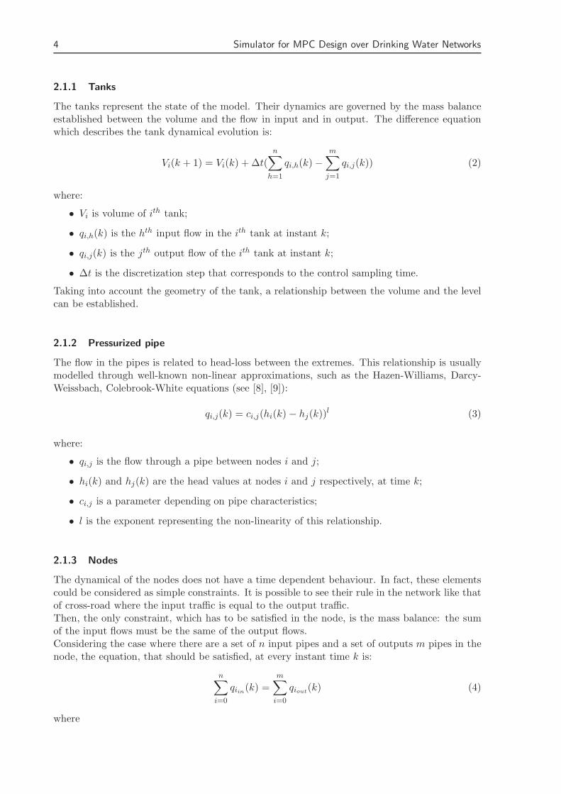
2.1.1 Tanks
The tanks represent the state of the model. Their dynamics are governed by the mass balanceestablished between the volume and the flow in input and in output. The difference equationwhich describes the tank dynamical evolution is:
Vi(k + 1) = Vi(k) + ∆t(
n∑
h=1
qi,h(k) −
m∑
j=1
qi,j(k)) (2)
where:
• Vi is volume of ith tank;
• qi,h(k) is the hth input flow in the ith tank at instant k;
• qi,j(k) is the jth output flow of the ith tank at instant k;
• ∆t is the discretization step that corresponds to the control sampling time.
Taking into account the geometry of the tank, a relationship between the volume and the levelcan be established.
2.1.2 Pressurized pipe
The flow in the pipes is related to head-loss between the extremes. This relationship is usuallymodelled through well-known non-linear approximations, such as the Hazen-Williams, Darcy-Weissbach, Colebrook-White equations (see [8], [9]):
qi,j(k) = ci,j(hi(k) − hj(k))l (3)
where:
• qi,j is the flow through a pipe between nodes i and j;
• hi(k) and hj(k) are the head values at nodes i and j respectively, at time k;
• ci,j is a parameter depending on pipe characteristics;
• l is the exponent representing the non-linearity of this relationship.
2.1.3 Nodes
The dynamical of the nodes does not have a time dependent behaviour. In fact, these elementscould be considered as simple constraints. It is possible to see their rule in the network like thatof cross-road where the input traffic is equal to the output traffic.Then, the only constraint, which has to be satisfied in the node, is the mass balance: the sumof the input flows must be the same of the output flows.Considering the case where there are a set of n input pipes and a set of outputs m pipes in thenode, the equation, that should be satisfied, at every instant time k is:
n∑
i=0
qiin(k) =m
∑
i=0
qiout(k) (4)
where

Section 2 Drinking Water Network Mathematical Model 5
• qiin(k) is the input flow in the pipe i at instant k;
• qiout(k) is the output flow in the pipe i at instant k.
2.1.4 Actuators
The actuators, pumps and valves, are assumed to be locally controlled. The set-point values ofthe flow in these elements is selected by the optimal MPC controller. At the first glance, thesetwo types of elements look the same, but there are some differences, regarding the economicalcost.This different cost is due to the fact that the valves function is only to regulate the flow inpipes which connect elements with the same ground elevation or from one with a bigger groundelevation to an other with a smaller one. The function of a pump is to push the water from onewith a smaller elevation to another with a bigger elevation.
2.2 PLIO as a Water Modelling Tool
PLIO software is a tool which allows to simulate and optimize the drinking water networks.This tool has been developed by UPC1 and AGBAR in a project previous to WIDE project andhas been applied to the control of the water networks in Santiago de Chile and Murcia cities.It has a graphical interface which allows to represent the water network, with every element andconnection, and to set the predictive control goal. The tool allows the whole operative planningof water cycle including supply, production, transport and distribution network in real-time.PLIO has been developed using standard GUI (graphical user interface) techniques and objectoriented programming using Visual Basic.NET2 how it is explained in [5].PLIO calls a commercial solver, GAMS3, to determine the optimal solutions of the optimizationproblem associated to the predictive optimal control using non-linear programming techniques.In a real time operation, an optimization problem is solved with a sampling time of a hour. Thistool allows to do a detailed network study and to elaborate a model that suitably represents thereality. Using this application, it is possible to draw the network model and all their elementscould be parametrized.
2.2.1 PLIO Operative Model
The PLIO software has four operation modes: editor, simulation, monitoring and reproductionmode as it is shown in Figure 1 [1].
Editor Mode This mode allows to graphically build and parametrize the network using apalette of building blocks, to define the control objectives and to generate the optimizationmodel equations. In PLIO there are many different elements in the libraries that allows to drawthe network easily. These elements include tanks, water demand sectors, sensors and actua-tors. The user positions the elements in the model dropping and connecting them with pipes oraqueducts. Each element of PLIO has a number of proprieties grouped in trees which identifythe element, parametrize its characteristics, provide goals to the optimizer and define links to
1Universitat Politcnica de Catalunya2Microsoft, 20023GAMS, 2004

6 Simulator for MPC Design over Drinking Water Networks
Figure 1: PLIO operating modes
SCADA and database. Once the network has been built, PLIO tests its consistency and con-nects it to the database. After the connection, it is necessary to synchronise PLIO model andthe database. Moreover, PLIO generates the set of the optimization equations using goals andconstrains defined in the proprieties of each element. In the window propriety, it is possible toset if an element is included or not in the optimization problem and its weight.
Simulation Mode The simulation consists in the off-line execution of a real scenario to checkhow the tool works in a water network. The simulations could be done with different forecastdemand methods to analyze if the results improve or not. The demand used in this type ofsimulations are loaded in the database that is connected to the PLIO model. All the results, interms of tanks volume, flow in the actuators or in the pipes, are then registered in the databaseso that it is also possible to draw their graphical evolution. At the end of the simulation, PLIOgenerates the optimal control using the GAMS solver.It is also possible to set some parameters in the simulation windows propriety, like the startingand ending data, the interval between every iteration and the number of the iterations. Thisparameters are included in the particular scenario.
Monitoring Mode The optimization in real time (on-line) is executed in the monitoringmode. This is done using the demand and the measurements of the network real state, comingfrom the telemetry system, provided by SCADA system. PLIO generates the optimal controls,which are applied to the real network only after confirmation by an operator. Like in simulationmodel, graphical results of main network variables and controls can be represented and registeredin the PLIO database for further studies.In the monitoring mode there are four steps:
1. connection to SCADA;
2. data readings and writings;

Section 2 Drinking Water Network Mathematical Model 7
3. optimization;
4. results treatment and graphical representation.
Steps number 2, 3 and 4 are repeated at each control cycle.
Reproduction Mode In this mode, it is possible to reproduce the state evolution under spe-cific conditions and control set-points (optimal or other). This mode allows to see, in a simplyway, through a graphical representation on the screen the values of flows or volume according tothe selected element. Then, the represented value depends on the chosen element, and the dis-play presents the element evolution for every reproduction iteration. Graphical interface couldrepresent the main variable behaviours in a real or in a simulated scenario.
2.2.2 Dynamical Modelling of the Elements
The PLIO tool generates several variables and equations for every hydraulic element which al-low to determine the model that describes the dynamical of the whole network. The type ofvariables and equations are different according to the elements role in the network. It is impor-tant to analyze the form of these equation in order to understand the optimization created byPLIO through the GAMS solver. For each element, in the following a detailed description of theequations and the variables is given. To simplify the understanding of this document the nameof the variables are the same generated by PLIO.In PLIO tool every variable has the unit of measurement according to the International System,thus, for example, the flows are given in m3/s, while the volumes in m3.
Tank The PLIO tool creates three positive variables for each tank: Vxx, Vsegxx, Vbajoxx,where xx corresponds to the name of the tank.These variables are defined through three equations with the following names:
• Volxx(t) corresponds to the instantaneous water level into the tank xx at time t. Its equa-tion is:
Volxx(t + 1) . . . Vxx(t + 1) = Vxx(t) +∑
i
Qini (t) −
∑
i
Qouti (t) (5)
where Qini (t) and Qout
i (t) are the input and output flows, respectively, of the tank xx attime t. The last variable present in the equation (5) is Vxx(t) which represents the volumeof the tank xx at time t.
• Volsegxx(t) corresponds to the security level in the tank and indicates if there is a penaltyor not, according to:
Volsegxx(t) . . . Vsegxx(t) = max(0,Vxxpenalty − Vxx(t)) (6)
where Vxxpenalty is the volume value under which there is a penalty.The way to determine this penalty value will be discussed later in the report. This volumeshould be used to minimize the electrical and water costs to satisfy the demands. Thisequation allows to penalize the cost function only when the actual level is below the securityone.
8 Simulator for MPC Design over Drinking Water Networks
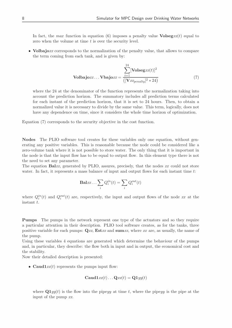
In fact, the max function in equation (6) imposes a penalty value Volsegxx(t) equal tozero when the volume at time t is over the security level.
• Volbajoxx corresponds to the normalization of the penalty value, that allows to comparethe term coming from each tank, and is given by:
Volbajoxx . . . Vbajoxx =
24∑
t=1
[Volsegxx(t)]2
(
[Vxxpenalty]2 ∗ 24) (7)
where the 24 at the denominator of the function represents the normalization taking intoaccount the prediction horizon. The summatory includes all prediction terms calculatedfor each instant of the prediction horizon, that it is set to 24 hours. Then, to obtain anormalized value it is necessary to divide by the same value. This term, logically, does nothave any dependence on time, since it considers the whole time horizon of optimization.
Equation (7) corresponds to the security objective in the cost function.
Nodes The PLIO software tool creates for these variables only one equation, without gen-erating any positive variables. This is reasonable because the node could be considered like azero-volume tank where it is not possible to store water. The only thing that it is important inthe node is that the input flow has to be equal to output flow. In this element type there is notthe need to set any parameter.The equation Balxx, generated by PLIO, assures, precisely, that the nodes xx could not storewater. In fact, it represents a mass balance of input and output flows for each instant time t:
Balxx . . .∑
i
Qini (t) =
∑
i
Qouti (t)
where Qini (t) and Qout
i (t) are, respectively, the input and output flows of the node xx at theinstant t.
Pumps The pumps in the network represent one type of the actuators and so they requirea particular attention in their description. PLIO tool software creates, as for the tanks, threepositive variable for each pumps: Qxx, Estxx and sumxx, where xx are, as usually, the name ofthe pump.Using these variables 4 equations are generated which determine the behaviour of the pumpsand, in particular, they describe: the flow both in input and in output, the economical cost andthe stability.Now their detailed description is presented:
• Caud1xx(t) represents the pumps input flow:
Caud1xx(t) . . . Qxx(t) = Q1yy(t)
where Q1yy(t) is the flow into the pipeyy at time t, where the pipeyy is the pipe at theinput of the pump xx.

Section 2 Drinking Water Network Mathematical Model 9
• Caud1xx(t) represents the pumps output flow:
Caud1xx(t) . . .Qxx(t) = Q2zz(t)
where Q2zz(t) is the flow into the pipe zz at time t, where the pipe zz is the pipe at outputof the pump xx.
• Totxx is the cost equation of the pump xx :
Totxx . . . sumxx =
24∑
t=1
(
Q1zz(t) ∗ CExx(t) ∗1
Qmaxxx
)
(8)
where Qmaxxx is the maximum admissible flow through the pipe xx (the maximal valuefor each pump is shown in the Table 2); Q1zz(t) is the flow through the pipe zz, which isthe pipe at output of the pump xx, at time t; CExx(t) is the electrical cost of the pump xxat time t. Dividing by Qmaxxx a sort of normalization is done. In fact, in this way, it ispossible compare the values coming from every pump. This term is the result of the costin the whole prediction horizon. Notice that the equation (8) is not depending on time.This values is included in the price objective of the cost function.
• Estabxx is the stability component for pump xx. This equation, also as the cost compo-nent, is not time depending. In fact, both these equations have a summatory for the wholeoptimization time horizon:
Estabxx . . .
. . .Estxx =
(
Qxx(0) − Qpastxx)2
+
24∑
t=1
(
Qxx(t + 1) − Qxx(t))2
(
Qmax)2 ∗ 25
(9)
where 25 is the normalization term of the sum of 25 elements. In fact, with the summa-tory, there are 24 additions, due to a 24 hours of prediction horizon, and also there isthe component concerning the initial condition
(
Qxx(0) − Qpastxx)
, which considers thegap with the resulting value of the previous iteration. The Qxx(0) is the flow through thepump xx at time 0, of this iteration. The equation (9) takes part in the cost function inthe stability objective.
Valves The valves represent the other type of actuators present in the network. So, PLIOsoftware deals with these elements in a similar way than the pumps. In fact, the variables andthe equations created are very similar to those concerning the pumps. The only difference,between these two type of actuators, is about the cost function, considering that the valves havenot an electrical cost coefficient.Therefore each valve has, only, two positive variable, instead of the three of the pumps: Qxx,Estxx, the last one is created only in the stabilized valves, which are obtained using the motorizedvalves element.The equations, which regulate the relationship between these two variables, are three:
• Caud1xx(t) represents the valve input flow at time t:
Caud1xx(t) . . .Qxx(t) = Q1yy(t)
10 Simulator for MPC Design over Drinking Water Networks
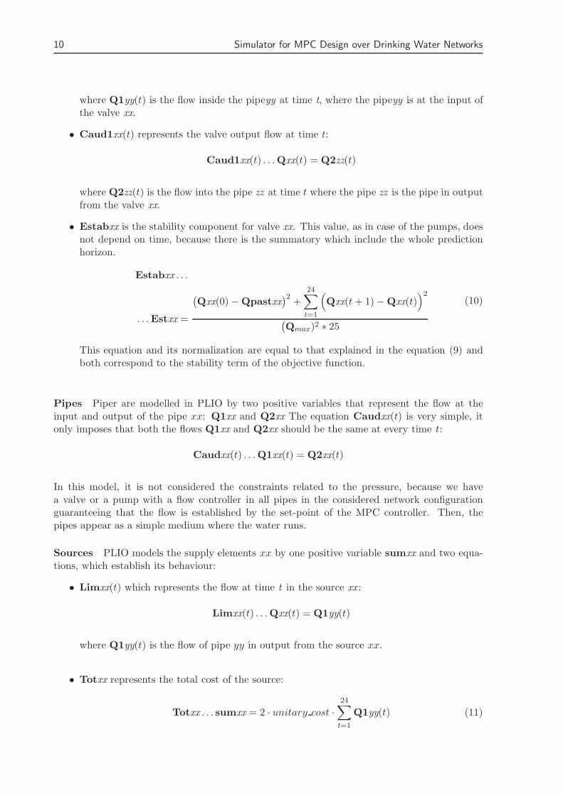
where Q1yy(t) is the flow inside the pipeyy at time t, where the pipeyy is at the input ofthe valve xx.
• Caud1xx(t) represents the valve output flow at time t:
Caud1xx(t) . . . Qxx(t) = Q2zz(t)
where Q2zz(t) is the flow into the pipe zz at time t where the pipe zz is the pipe in outputfrom the valve xx.
• Estabxx is the stability component for valve xx. This value, as in case of the pumps, doesnot depend on time, because there is the summatory which include the whole predictionhorizon.
Estabxx . . .
. . .Estxx =
(
Qxx(0) − Qpastxx)2
+24∑
t=1
(
Qxx(t + 1) − Qxx(t))2
(
Qmax)2 ∗ 25
(10)
This equation and its normalization are equal to that explained in the equation (9) andboth correspond to the stability term of the objective function.
Pipes Piper are modelled in PLIO by two positive variables that represent the flow at theinput and output of the pipe xx: Q1xx and Q2xx The equation Caudxx(t) is very simple, itonly imposes that both the flows Q1xx and Q2xx should be the same at every time t :
Caudxx(t) . . . Q1xx(t) = Q2xx(t)
In this model, it is not considered the constraints related to the pressure, because we havea valve or a pump with a flow controller in all pipes in the considered network configurationguaranteeing that the flow is established by the set-point of the MPC controller. Then, thepipes appear as a simple medium where the water runs.
Sources PLIO models the supply elements xx by one positive variable sumxx and two equa-tions, which establish its behaviour:
• Limxx(t) which represents the flow at time t in the source xx :
Limxx(t) . . . Qxx(t) = Q1yy(t)
where Q1yy(t) is the flow of pipe yy in output from the source xx.
• Totxx represents the total cost of the source:
Totxx . . . sumxx = 2 · unitary cost ·
24∑
t=1
Q1yy(t) (11)
Section 3 Model Predictive Control 11
where Q1yy(t) is the output flow of pipe yy at time t, and the unitary cost is the coefficientcost inserted in the source property.
This coefficient indicates the cost of the water withdrawal from the source xx. The sources havedifferent unitary costs depending on the different elevations, treatments and paths to arrive tothe users.
3 Model Predictive Control
Water supply and distribution systems are very complex multivariable systems. In order toimprove their performance, predictive optimal control provides suitable techniques to computeoptimal control strategies ahead in time for all the flow and pressure control elements.The optimal strategies are computed by optimizing a mathematical function describing theoperational goals in a given time horizon and using a representative model of the networkdynamics, as well as demand forecasts.The computation of optimal strategies must take into account the dynamics of the completewater system:
- 24-hour-ahead demand forecasts;
- 24-hour-ahead availability predictions in supply reservoirs and aquifers, defined by long-term planning for sustainable use;
- 24-hour-ahead predictions of production plant capacity and availability;
- current state of the water system provided by the telemetry system;
- 24-hour historic data in open channel sections, due to delays in water transport;
- physical and operational flow constraints in all the elements.
A model of a water system is a tool to predict the effect of control actions on all the networkelements. For the purpose of on-line optimal control, a large number of control actions mustbe tested and evaluated during the optimization process. Therefore, it is important for themathematical models developed to be:
· representative of the hydraulic dynamic response;
· simple enough to allow a large number of evaluations in a limited period of time, imposedby real-time operation.
An operational model of an urban drinking water network system is a set of equations whichprovide a fast approximate evaluation of the hydraulic variables of the network and its responseto control actions at the gates. This type of model is useful for the computation of optimalstrategies, because it makes possible to evaluate a large number of control actions in a shortcomputation time.One of the most used and effective control strategy for the drinking water control problem isthe Model Predictive Control (MPC) ([3]; [2]; [11]; [10]).The predictive controller usually deals with the middle level of a control structure where at thetop we can find the modules that provide state estimation and the demands forecast over thecontrol horizon. This information is the input into the MPC problem. The outputs of the MPCcontroller are reference values for the local controllers that implement the calculated set-points.The drinking water network has many control objectives and so also the optimization problem
12 Simulator for MPC Design over Drinking Water Networks
associated with the MPC controller is a multiple objective as well.Usually the approach to solve a multi-objective optimization problems is to form a scalar andlinear cost function, composed by a weighted sum of cost functions associated with each objec-tive. When the objectives have a priority, it is possible to select a bigger weight that representsthe importance of the objective in the optimization. It is quite difficult to find the appropri-ate weights for every component in the cost function. In fact in every different scenario withdifferent numerical value the appropriate weight could change. Moreover, the weights serve tonormalize the cost functions as well as manage their priority.An alternative to weight based method, is the lexicographic approach, see [13], which is based onassigning “a priori ”different priorities to the different objectives and then focus on optimizingthe objectives in their priority order.
3.1 MPC Strategy
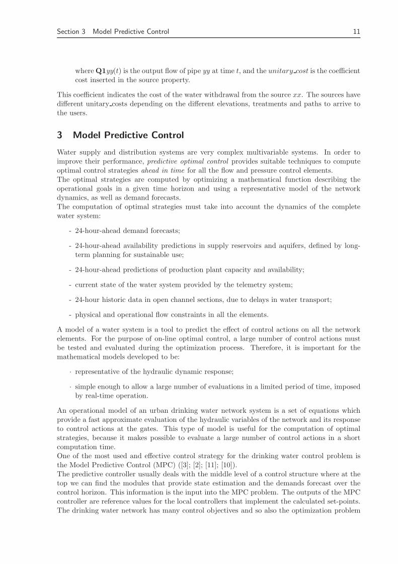
All the controllers in the MPC family are characterized by the receding horizon strategy shownin Figure 2, where N is the predictive horizon ([4]), that in the case of a drinking water network,
Figure 2: MPC strategy
usually, is set a 24 hours, as it is explained at the beginning of this chapter. In more detail:
1. A prediction of the N future outputs are calculated at each instant t:
y(k + i|k)4 for i = 1, · · · , N
These outputs depend on the known values at instant t and on the future control signals:
u(k + i|k) for i = 1, · · · , N − 1
which are the ones to be calculated.
2. The set of future control signals is calculated by optimizing a determinated criterion func-tion in order to keep the process as close as possible to a reference trajectory (which can bethe set-point itself or a close approximations of it). The most used criteria are based on aquadratic function error between the predicted output signals and the predicted referencetrajectory.
4the notation indicates the value of the variable at the instant k + i calculated at instant k

Section 3 Model Predictive Control 13
3. The control signal u(k|k) is sent to the process while the next control signals calculatedare rejected, because at the next sampling instant y(k + 1) is already known and the step1 is repeated with this new value and all sequences are brought up to date. Thus, thecontrol u(k + 1|k + 1) is calculated (which in principle would be different to the controlu(k + 1|k) because the new information is available) using the receding horizon concept.The basic structure of this strategy is shown in the Figure 3 where a model is used topredict the future plant outputs. The prediction is based on the past and current valuesand on the proposed optimal future control actions. These actions are calculated by theoptimizer taking in account both the cost function and the constraints.
Figure 3: Basic structure of MPC
The process model plays an important role in the control. Indeed, the chosen model must becapable of capturing the process dynamics so as to precisely predict the future outputs as wellas being simple to implement and to understand. Taking in account this, the formulation ofthe problem is a fundamental step in the building of MPC controller. MPC is not a uniquetechnique but it could be seen like a set of different methodologies since there are many typesof models used in various formulations.Logically, the optimizer is another fundamental part of the strategy since it provides the controlactions. If the cost function is quadratic, its minimum can be obtained as an explicit linearfunction. Otherwise, when there are some inequality constraints the solution it has to be ob-tained by more computationally demanding numerical algorithms.The size of the optimization problems depends on the number of variables and the predictionhorizon used. It is important to remind that the amount of time required in a constrained androbust case could be various order of magnitude higher than the one needed for the uncon-strained case.
3.2 Problem Formulation
The formulation used in the majority of predictive control literature [10], is based on a linearsystem, on a quadratic cost function and on a linear inequalities constrains. Moreover, it isassumed that the model is time invariant.The cost function used does not usually penalise particular values of the input vector u(k), butonly the changes of the input vector, ∆u(k). Then, it is considered the linear, discrete-time,invariant-time state-space model of the system:
14 Simulator for MPC Design over Drinking Water Networks
{
x(k + 1) = Ax(k) + Buu(k) + Bdd(k)y(k) = Cx(k)
(12)
where: A ∈ Rn×n, Bu ∈ R
n×m, C ∈ Rn×n are the state space matrices and Bd ∈ R
n×q isa known disturbance, in this particular models the demands. Then x is a n-dimensional statevector collecting to the n tanks volume; u is an m-dimensional input vector which representthe flows in the actuators and d(k) is a q different component corresponding to the q demandsectors. The index k counts the time step. So the sequence of actions at time step k is thefollow, according to the strategy described before (Figure 2), are the following:
1. To obtain measurements y(k);
2. To compute the required system input u(k);
3. To apply u(k) to the plant.
This implies that there is always some delay between measuring y(k) and applying u(k).The constrains, presented in this model, are those concerning the physical operational limits ofthe elements:
uimin < ui(k) < uimax for k = 0, · · · , N − 1i = 1, · · · ,m
yimin < yi(k) < yimax for k = 1, · · · , Ni = 1, · · · , n
(13)
3.2.1 Control Objectives
The various MPC algorithms propose different cost functions to obtain the control law. Thegeneral rule is that the future output on the considered horizon should follow a determinatedreference signal and, at the same time, the control effort (∆u) necessary for doing this shouldbe penalised.A drinking water network has multiple objectives which could assume different priority [5], [6].First of all, the main goal is that of satisfying the demands. Achieving this result, the predictivecontrol strategy has also to take into account the optimization of the system performance interms of different operational criteria. In general, the most common objectives are related to thephysical limits of the elements to avoid their damage, or to the minimization of the economicalcost.In detail, the criteria which could considered are:
• Security: this criteria maintains the volume in the tank over a threshold in order to avoidinfeasibilities.
• Quality: this objective is especially important when several sources exists with a differentwater quality, which could depend on the level or on the concentration of some ion thatdecays in time.
• Stability: this criteria aims to avoid continuous and abrupt set-point variations in thevalves or pumps which means that all treatment plants and actuators operate as smoothlyas possible. This point is very important to avoid damage in valves or pumps.

Section 3 Model Predictive Control 15
• Price: the electrical cost (price) in the network type is attributable to the water cost inthe source and to the electrical cost necessary for the pumping. The water cost could bedifferent at different sources with different elevation or treatment, while the electrical costchange depending to the hour of the day.
• Conservation: water sources such as reservoirs and rivers are usually subject to opera-tional constraints to maintain water levels, ecological flows and a sustainable water use.
The control strategy selection at each time k consists of posing and solving an optimal controlproblem. This means finding the set of admissible controls (within the physical and operationalconstraints) which optimize performance index J(x, u, d) over the optimization horizon. Theperformance index J is a general non-linear function of the state and control variables, whichmay contain:
• Non-linear, usually quadratic, penalty function for low storage tank levels, related to thesecurity objective. Then, this term depends on the state x(k). The component for everytank i (with i = 1, · · · , n) at each instant k (with k = 1, · · · , N) is called Seci(k):
Seci(k) = max{0, xi(k) − V peni}
where V peni is the threshold volume selected for every tank i. To obtain a quadratic indexthe value Seci(k) is squared, and after the index is normalized dividing by [V peni]
2:
peni(k) =[Seci(k)]2
[V peni]2(14)
• Linear or non-linear time-varying cost for water acquisition and pumping. This term,related to some values of the input vector u(k) is simply computed by multiplicationbetween the flow and the hourly cost.
• Non-linear (quadratic) penalty function of abrupt changes in control actions. This termoptimize the stability objective and it is related directly to the changes of the input vector∆u(k). In fact, this term could be defined, for each instant k (with k = 1, · · · , N − 1) andfor each input i (with i = 1, · · · ,m) as:
∆ui(k) = [ui(k) − ui(k − 1)] (15)
Like in the storage tank level in the cost function, it is better to consider the square valueof ∆u, with an appropriate normalization.
• Non-linear function of flow for quality regulation, related to the input vector.
• Other terms according to the operational goal.
The same normalization, as the one used in the equation (14), is necessary to allow to sumtogether these different objectives with different magnitudes.More precisely, at each time step, the MPC strategy computes a control input sequence ofpresent and future values:
[u(k), u(k + 1)..., u(k + N − 1)] (16)

16 Simulator for MPC Design over Drinking Water Networks
which allows to optimize an open-loop performance function, according to a prediction of thesystem dynamics over the horizon N . This prediction is performed using demand forecasts andthe network model, described in the equation (1).However, only the first control input of sequence [u(k)] is actually applied to the system, untilanother sequence based on more recent data is computed.The same procedure is restarted at time k + 1, using the new measurements obtained from sen-sors and the new model parameters obtained from the recursive parameter estimation algorithmthat is working in parallel.The resulting controller belongs to the class called open-loop optimal-feedback control. As thename suggests, feedback from the telemetry system is used, and the optimal control strategy isre-computed at each time k.
3.2.2 Multi-Objective Optimization
Considering what it is said above, the optimization problem associated with the MPC controlleris multi-objective.The general ideas for this problem type could be formulated as the minimization with respectto every objective fi(k).The functions fi(k) are obtained summing the costs introduced by every element which areincluded in i criteria at the instant k. For example, in the case of the security criteria, thefunction is obtained through the sum in equation (14):
f1(k) =
n∑
i=1
peni(k)
n(17)
where n is the number of the states in the system. In this way, the f1(k) is a normalized value.The normalization is done according to the square penalty for each tank in the term peni(k),and to the number of the tanks to obtain the function f1(k).A simple way to solve a multi-objective optimization is through scalarization. This means con-verting the problem into a single-objective optimization problem with a scalar-value objectivefunction.The most common form for a scalar objective function is a linearly weighted sum of the func-tions fi, which represents every objective that has to be optimized, like for example the securityobjective in the equation (17):
F (k) =
r∑
i=1
ωifi(k) (18)
where r is the number of objectives present in the problem.The priority of the objectives are reflected by the weights ωi: when there is a bigger weight thegoal has a bigger priority.For an evaluation over the entire value of the optimization horizon, the performance index hasto be summed as:
J =
N−1∑
k=1
F (k) (19)
where N is the optimization horizon, in a number of sampling periods.

Section 4 Case Study: Water Barcelona Network Description 17
Figure 4: Population behaviour of Barcelona city since 1900 to 2006
4 Case Study: Water Barcelona Network Description
4.1 System Model
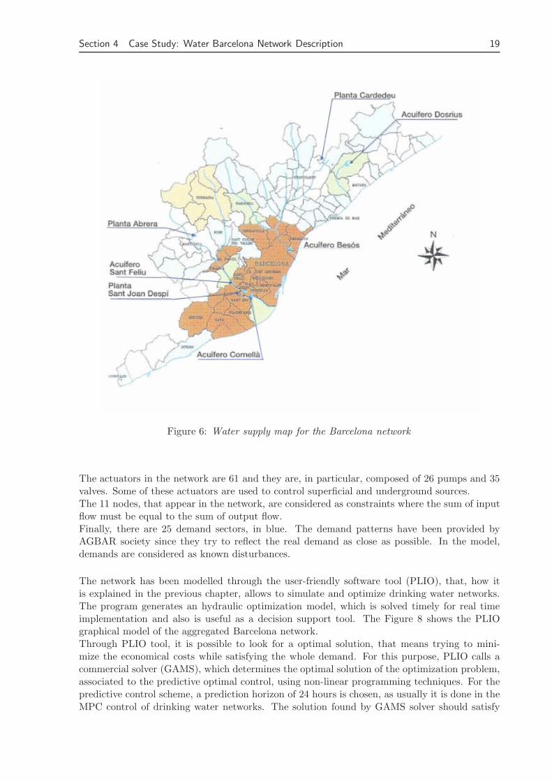
This report considers as a real application the case study of the Barcelona water network. Firstof all, it is important to notice the environment of the city that is presented to better understandthe problem we are facing. Geographically, Barcelona has a strong slope in the zone near to themountain, which decreases in direction towards the Mediterranean sea. The city of Barcelonahas a population of about 1.605.000 in an area of 98 Km2, that means a very high density ofpopulation (more than 16.000 per Km2). The fast growth of the city during the XX century, asit is showed in Figure 4, has lead to improve the drinking water network continuously.The weather of Barcelona is the typical of Mediterranean climate. The yearly rainfall is notvery high (600 mm/year), but it includes heavy storms, rains with great intensity which couldconcentrate in thirty minute the fourth part of the yearly precipitation. The two last issues areinterconnected. In fact the urban environment affect the local climate which cause a thermaldifference between Barcelona and its surroundings. This difference could reach 3 or 4 Celsiusdegree. This phenomenon increases the intensity of the storm.Considering all of these previous considerations, it is logical to think and understand that thedrinking water network of Barcelona is a very complex interconnected system, as shown in Fig-ure 5.The water supply of Barcelona network is basically constituted of three sources: the Ter riverthrough treatment station of Cardedeu, the superficial and the underground Llobregat river. Thesuperficial Llobregat river came from the treatment stations of Abrera and Sant Joan Despı,while the underground water is stored in the aquifer of Llobregat delta. The source situationsare shown in Figure 6.The company which manages the distribution of the water is AGBAR5. This society initiatedthe automatisation of the water distribution network in 1969 and in 1976, a first centralizedcontrol system was installed . Since this date this system is being continually improved, like ispossible to see in [14].In 1984, AGBAR and UPC developed an MPC controller on-line but the size of the network im-plies real-time constraints that were not easily feasible to satisfy with the computer computationspeed of that time. Later, in the 2002 AGBAR and UPC start the development of the PLIOtool that allows, as discussed in Chapter 2, the modelling and MPC control of water networks.Actually, there is a project running in parallel with WIDE project, named SOSTAQUA, whose
5Sociedad General De AGua de BARcelona, S.A.
18 Simulator for MPC Design over Drinking Water Networks
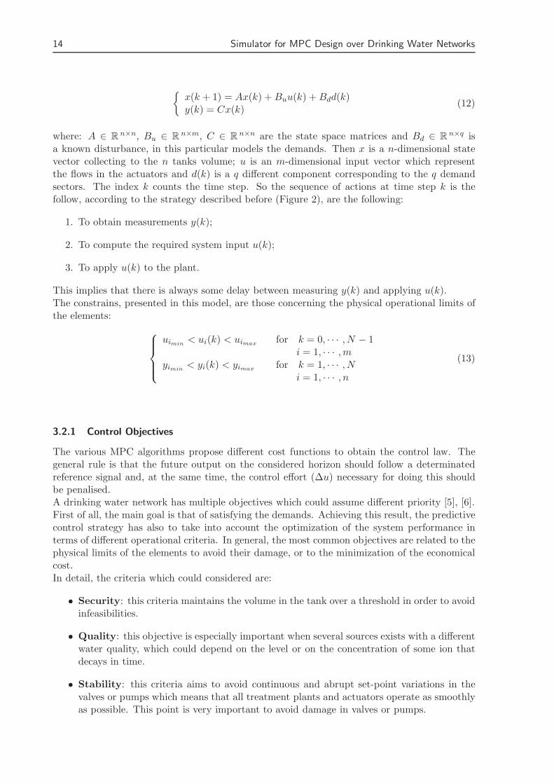
Figure 5: Complete Barcelona network model
aim is to apply PLIO to the Barcelona water network.The water supply to the users is done through a complex distribution network which allows toprovide the water at any different ground elevation, where usually there are several reservoirsto adapt pressure to ground topography and so it is possible to assure a supply with a correctpressure and quality.The model studied in this report is a prototype of the Barcelona urban water network. Thecomplete Barcelona water network is showed in Figure 5. The prototype network correspondsto an aggregated model of the real one. The Figure 7 shows the network conceptual model usingPLIO modelling methodology. It is possible to observe the whole set of the hydraulic elements,like pumps, valves, tanks, pipes and sources.
The aggregated model has 9 sources, corresponding to:
• 4 superficial resources:
– AportA which represents the water that come from the Abrera potabilisation station;
– AportLL1 and AportLL2 which come from underground and superficial water fromLlobregat river in the Sant Joan Despı potabilisation;
– AportT which corresponds to the water coming from the Ter river treated by Card-edeu potabilisation station.
• 5 underground resources aMS, aPousB, aPousE, aCast, aPouCast.
In addition to this, the Figure 7 shows 17 tanks in sky blue. These elements are the statevariables of the dynamical network model.
Section 4 Case Study: Water Barcelona Network Description 19
Figure 6: Water supply map for the Barcelona network
The actuators in the network are 61 and they are, in particular, composed of 26 pumps and 35valves. Some of these actuators are used to control superficial and underground sources.The 11 nodes, that appear in the network, are considered as constraints where the sum of inputflow must be equal to the sum of output flow.Finally, there are 25 demand sectors, in blue. The demand patterns have been provided byAGBAR society since they try to reflect the real demand as close as possible. In the model,demands are considered as known disturbances.
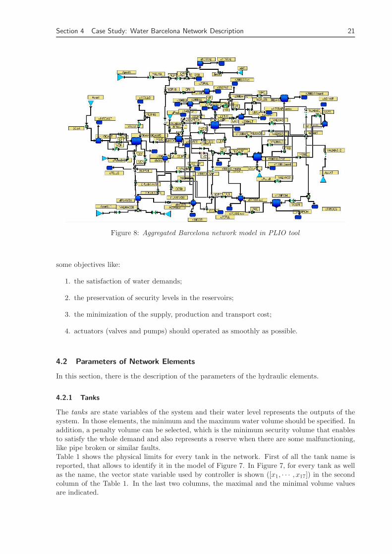
The network has been modelled through the user-friendly software tool (PLIO), that, how itis explained in the previous chapter, allows to simulate and optimize drinking water networks.The program generates an hydraulic optimization model, which is solved timely for real timeimplementation and also is useful as a decision support tool. The Figure 8 shows the PLIOgraphical model of the aggregated Barcelona network.Through PLIO tool, it is possible to look for a optimal solution, that means trying to mini-mize the economical costs while satisfying the whole demand. For this purpose, PLIO calls acommercial solver (GAMS), which determines the optimal solution of the optimization problem,associated to the predictive optimal control, using non-linear programming techniques. For thepredictive control scheme, a prediction horizon of 24 hours is chosen, as usually it is done in theMPC control of drinking water networks. The solution found by GAMS solver should satisfy

20 Simulator for MPC Design over Drinking Water Networks
Figure 7: Aggregated Barcelona model network
Section 4 Case Study: Water Barcelona Network Description 21
Figure 8: Aggregated Barcelona network model in PLIO tool
some objectives like:
1. the satisfaction of water demands;
2. the preservation of security levels in the reservoirs;
3. the minimization of the supply, production and transport cost;
4. actuators (valves and pumps) should operated as smoothly as possible.
4.2 Parameters of Network Elements
In this section, there is the description of the parameters of the hydraulic elements.
4.2.1 Tanks
The tanks are state variables of the system and their water level represents the outputs of thesystem. In those elements, the minimum and the maximum water volume should be specified. Inaddition, a penalty volume can be selected, which is the minimum security volume that enablesto satisfy the whole demand and also represents a reserve when there are some malfunctioning,like pipe broken or similar faults.Table 1 shows the physical limits for every tank in the network. First of all the tank name isreported, that allows to identify it in the model of Figure 7. In Figure 7, for every tank as wellas the name, the vector state variable used by controller is shown ([x1, · · · , x17]) in the secondcolumn of the Table 1. In the last two columns, the maximal and the minimal volume valuesare indicated.

22 Simulator for MPC Design over Drinking Water Networks
Tanks name Vectorstate
Minimum vol-ume [m3]
Maximum vol-ume [m3]
d125PAL x1 150 445d110PAP x2 375 960d115CAST x3 198 3870d80GAVi80CAS85CRO x4 480 3250dPLANTA x5 0 14450d54REL x6 800 3100d100FCE x7 16500 65200d10COR x8 0 11745d200BLL x9 700 7300d130BAR x10 3840 16000d176BARsud x11 200 1035d70BBEsud x12 22450 98041d200ALT x13 500 4240d100BLLnord x14 6000 37700d200BARnord x15 700 7300d101MIR x16 1403 4912d120POM x17 150 1785
Table 1: Tanks physical characteristics: the volume value is reported in cubic meters
4.2.2 Pumps
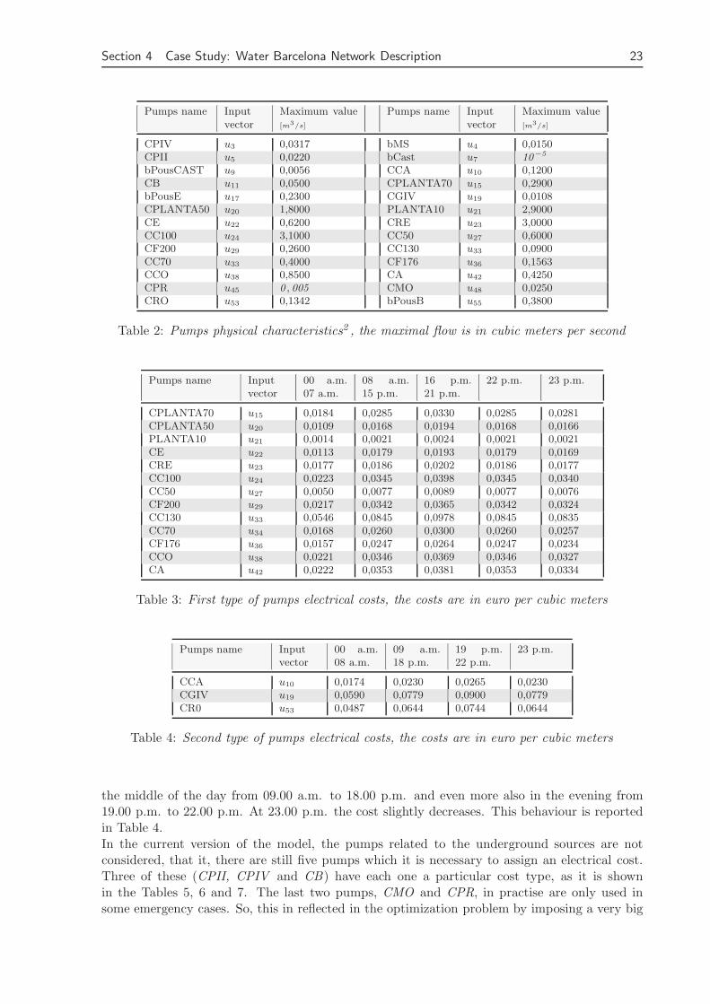
The pumps are one type of the actuators (active elements) in the network. The pumps, presentedinto the model, are 26: among of them, 5 (bMS, bCast, bPousCAST, bPousE, bPousB) areassociated to the underground sources and the others are used to carry the water where thereis an different ground elevation between two different elements.In case of pumps, two parameters should be specified: electrical costs for every hour and themaximum flow, which represents the maximum water’s amount of water that the pump is ableto pump out in one second, in m3/s. The minimal flow is not mentioned because it is alwayszero.For each pump, the maximum flows are reported in the Table 2. Moreover the position occupiedby every pumps i in the input vector u used by the controller is presented in the second column:
[ui with i = 1, · · · , 61]
and in the first column, as it is in the case of tanks, the name.The other parameters that have to be considered for the pumps are the electrical costs. These
parameters play a fundamental role in the computation of the production cost (FCP ), the partof the cost function which depends on the economical price.These costs change with the daily hours and they have some different behaviours.The first kind of pumps cost is the most common one: it can be divided into five time slots, asit can be seen in the Table 3.Analysing the Table 3, it can be noticed that these pumps have the same cost in the night from00.00 a.m. to 7.00 a.m. After this time, it increases in the morning from 8.00 a.m. to 15.00p.m., and even more in the afternoon from 16.00 p.m to 21.00 p.m. At this time, the costs slowlydecrease at 22.00 p.m. and something more at 23.00 p.m.The second type of pumps cost is characterised by 4 time slots.
These pumps have a fixed price in the night from 00.00 a.m. to 08.00 a.m., which increases in
2in italics there are the pumps with assumed maximal flow values, it was necessary for the lack of the realdata
Section 4 Case Study: Water Barcelona Network Description 23
Pumps name Inputvector
Maximum value[m3/s]
Pumps name Inputvector
Maximum value[m3/s]
CPIV u3 0,0317 bMS u4 0,0150CPII u5 0,0220 bCast u7 10−5
bPousCAST u9 0,0056 CCA u10 0,1200CB u11 0,0500 CPLANTA70 u15 0,2900bPousE u17 0,2300 CGIV u19 0,0108CPLANTA50 u20 1,8000 PLANTA10 u21 2,9000CE u22 0,6200 CRE u23 3,0000CC100 u24 3,1000 CC50 u27 0,6000CF200 u29 0,2600 CC130 u33 0,0900CC70 u33 0,4000 CF176 u36 0,1563CCO u38 0,8500 CA u42 0,4250CPR u45 0 , 005 CMO u48 0,0250CRO u53 0,1342 bPousB u55 0,3800
Table 2: Pumps physical characteristics2 , the maximal flow is in cubic meters per second
Pumps name Inputvector
00 a.m.07 a.m.
08 a.m.15 p.m.
16 p.m.21 p.m.
22 p.m. 23 p.m.
CPLANTA70 u15 0,0184 0,0285 0,0330 0,0285 0,0281CPLANTA50 u20 0,0109 0,0168 0,0194 0,0168 0,0166PLANTA10 u21 0,0014 0,0021 0,0024 0,0021 0,0021CE u22 0,0113 0,0179 0,0193 0,0179 0,0169CRE u23 0,0177 0,0186 0,0202 0,0186 0,0177CC100 u24 0,0223 0,0345 0,0398 0,0345 0,0340CC50 u27 0,0050 0,0077 0,0089 0,0077 0,0076CF200 u29 0,0217 0,0342 0,0365 0,0342 0,0324CC130 u33 0,0546 0,0845 0,0978 0,0845 0,0835CC70 u34 0,0168 0,0260 0,0300 0,0260 0,0257CF176 u36 0,0157 0,0247 0,0264 0,0247 0,0234CCO u38 0,0221 0,0346 0,0369 0,0346 0,0327CA u42 0,0222 0,0353 0,0381 0,0353 0,0334
Table 3: First type of pumps electrical costs, the costs are in euro per cubic meters
Pumps name Inputvector
00 a.m.08 a.m.
09 a.m.18 p.m.
19 p.m.22 p.m.
23 p.m.
CCA u10 0,0174 0,0230 0,0265 0,0230CGIV u19 0,0590 0,0779 0,0900 0,0779CR0 u53 0,0487 0,0644 0,0744 0,0644
Table 4: Second type of pumps electrical costs, the costs are in euro per cubic meters
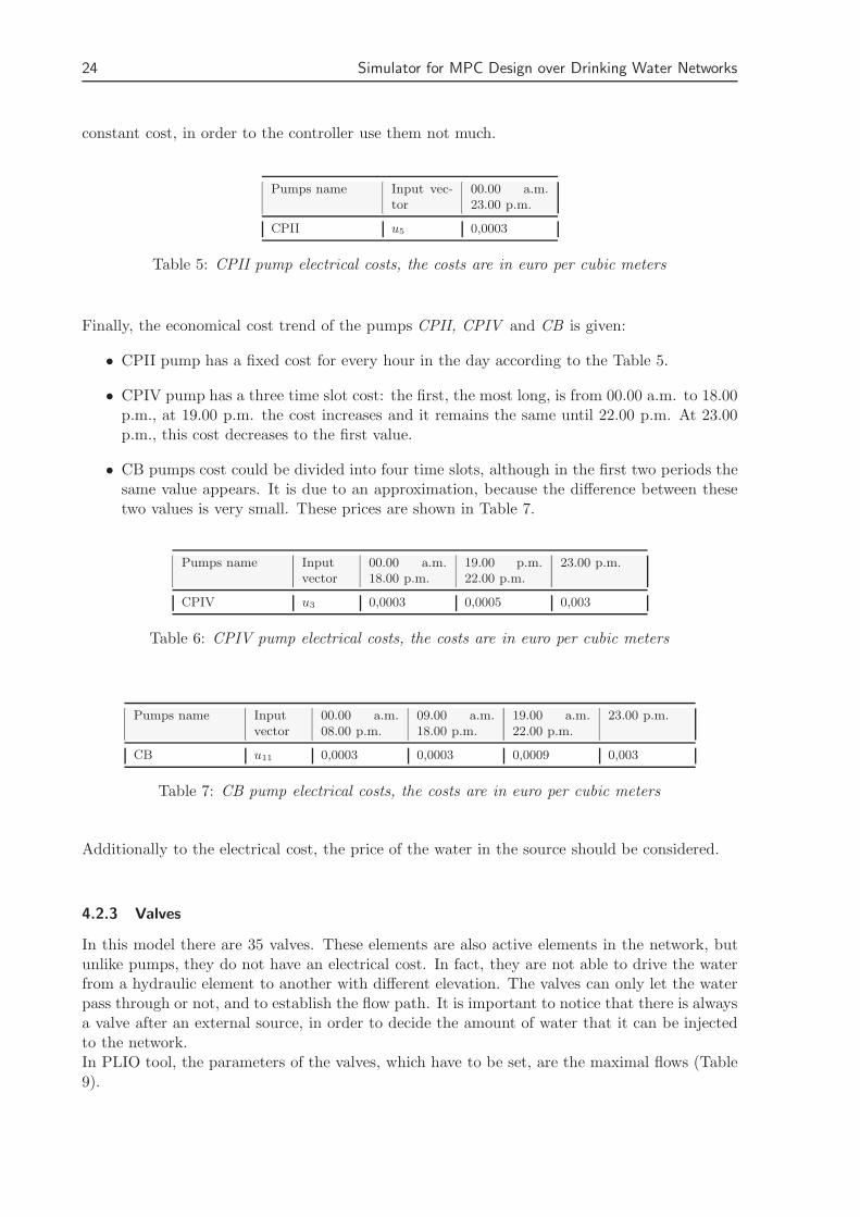
the middle of the day from 09.00 a.m. to 18.00 p.m. and even more also in the evening from19.00 p.m. to 22.00 p.m. At 23.00 p.m. the cost slightly decreases. This behaviour is reportedin Table 4.In the current version of the model, the pumps related to the underground sources are notconsidered, that it, there are still five pumps which it is necessary to assign an electrical cost.Three of these (CPII, CPIV and CB) have each one a particular cost type, as it is shownin the Tables 5, 6 and 7. The last two pumps, CMO and CPR, in practise are only used insome emergency cases. So, this in reflected in the optimization problem by imposing a very big
24 Simulator for MPC Design over Drinking Water Networks
constant cost, in order to the controller use them not much.
Pumps name Input vec-tor
00.00 a.m.23.00 p.m.
CPII u5 0,0003
Table 5: CPII pump electrical costs, the costs are in euro per cubic meters
Finally, the economical cost trend of the pumps CPII, CPIV and CB is given:
• CPII pump has a fixed cost for every hour in the day according to the Table 5.
• CPIV pump has a three time slot cost: the first, the most long, is from 00.00 a.m. to 18.00p.m., at 19.00 p.m. the cost increases and it remains the same until 22.00 p.m. At 23.00p.m., this cost decreases to the first value.
• CB pumps cost could be divided into four time slots, although in the first two periods thesame value appears. It is due to an approximation, because the difference between thesetwo values is very small. These prices are shown in Table 7.
Pumps name Inputvector
00.00 a.m.18.00 p.m.
19.00 p.m.22.00 p.m.
23.00 p.m.
CPIV u3 0,0003 0,0005 0,003
Table 6: CPIV pump electrical costs, the costs are in euro per cubic meters
Pumps name Inputvector
00.00 a.m.08.00 p.m.
09.00 a.m.18.00 p.m.
19.00 a.m.22.00 p.m.
23.00 p.m.
CB u11 0,0003 0,0003 0,0009 0,003
Table 7: CB pump electrical costs, the costs are in euro per cubic meters
Additionally to the electrical cost, the price of the water in the source should be considered.
4.2.3 Valves
In this model there are 35 valves. These elements are also active elements in the network, butunlike pumps, they do not have an electrical cost. In fact, they are not able to drive the waterfrom a hydraulic element to another with different elevation. The valves can only let the waterpass through or not, and to establish the flow path. It is important to notice that there is alwaysa valve after an external source, in order to decide the amount of water that it can be injectedto the network.In PLIO tool, the parameters of the valves, which have to be set, are the maximal flows (Table9).

Section 4 Case Study: Water Barcelona Network Description 25
Valves name Inputvector
Maximum value[m3/s]
Valves Inputvector
Maximum value[m3/s]
VALVA u1 1 , 297 1 VALVA45 u2 0,05VALVA47 u6 1,2 VCR u8 0,03VALVA308 u12 5 , 34 3 VALVA48 u13 0,22VCA u14 0,065 VALVA309 u16 2 , 5 3
VSJD u18 0,75 VALVA64 u25 no limits4
VALVA50 u26 0,1594 VF u28 0,29VE u30 0,45 VRM u31 3,5VZF u32 0,35 VB u35 0,15VCO u37 0,5249 VS u39 1,2VT u40 1,3 VCT u41 1,2VP u43 0,15 VBSLL u44 0,15VCOA u46 1,35 VPSJ u47 0,55VMC u49 0,24 VALVA60 u50 no limits4
VALVA56 u51 1,7 VALVA57 u52 0,4051VBNC u54 0,392 VALVA53 u56 1,5001VALVA54 u57 1,7361 VALVA61 u58 no limits4
VALVA55 u59 0,1852 VCON u60 0,035VALVA312 u61 6 , 27684 3
Table 9: Valve maximal flows
In the Table 9, as for the tanks and the pumps also, the name and the order in the input vectoru is reported.
In addition, it is possible to stabilise these element, by including them into the stability function.Stability could be enforced for every valve, and even to enforce it more in some valves than otherby specifying particular weights. This is the case, for example, in valves controlling externalsources that come from potabilization plants that can not be start and stop continuously.Some valves have the minimum value different from zero, but, for the moment they are fixedto zero. These minimal values different from zero are due to the fact that, sometimes, it isimpossible to close totally a valve, but a small amount of water continues to pass through it.
4.2.4 Sectors of Consume
The sector of consume represents the demands of users. It is considered like a known disturbance.The pattern demands used are provided by AGBAR. The demand patterns reflect the real profileof the city consume during the 24 hour of the day. For the moment every day has the sameprofile, but, in the future, it would be possible have a different pattern according the days inthe week.
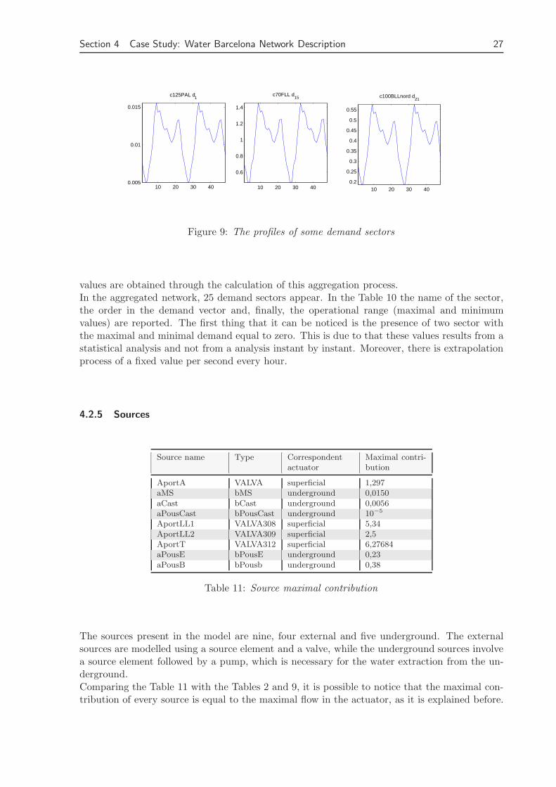
In the Figure 9, it is possible to notice that the profiles of the demand sectors are equal in eachof the three tanks, but the range is different since it has been scaled according to the totalconsume of the sector in a day. In the future, the particular demand profiles of each sector willbe used.The model, as it has been already explained, is an aggregation of the real network. The demand
3this values in italics, in the reality, are non limits but in the model they follow the external sources and sothey get the max water flow supplied by each sources
4This valves with a non limit flow, in the model, are set to 15m3/s, a very high value
26 Simulator for MPC Design over Drinking Water Networks
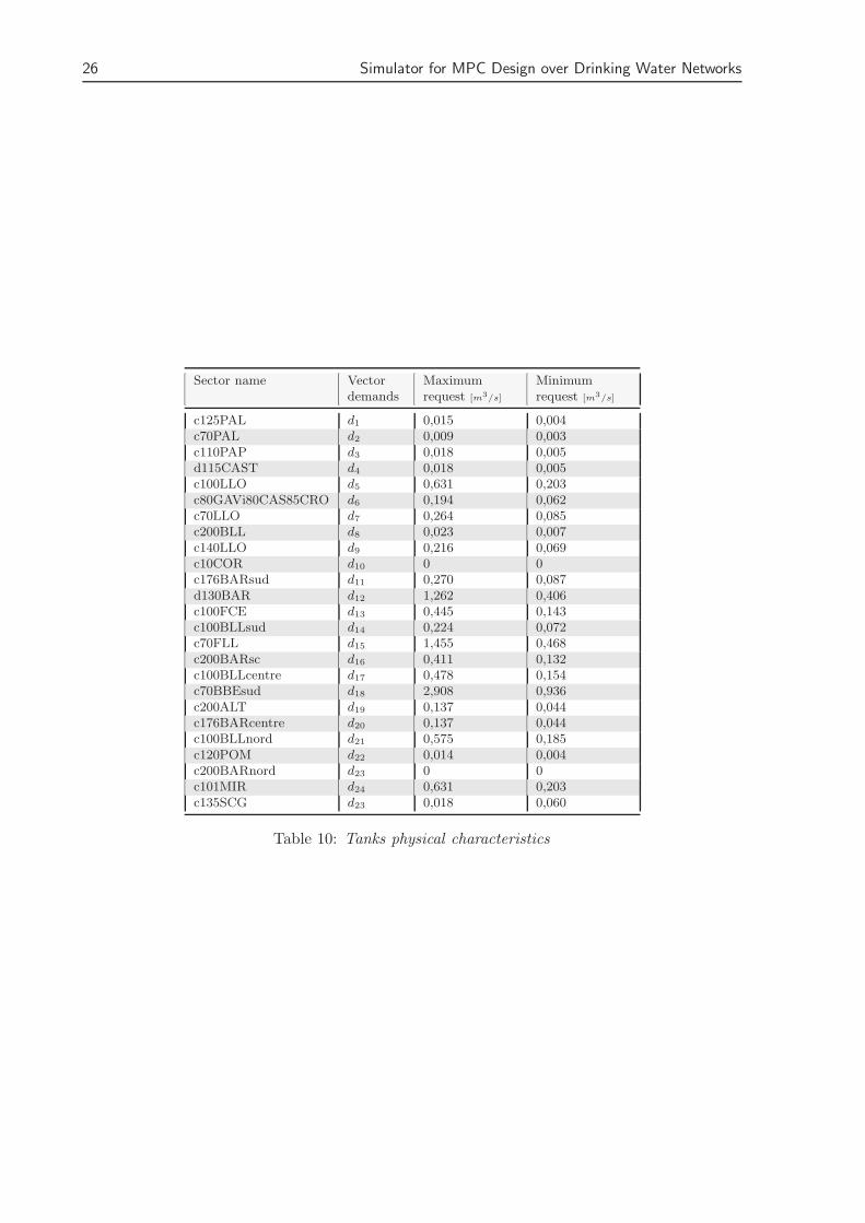
Sector name Vectordemands
Maximumrequest [m3/s]
Minimumrequest [m3/s]
c125PAL d1 0,015 0,004c70PAL d2 0,009 0,003c110PAP d3 0,018 0,005d115CAST d4 0,018 0,005c100LLO d5 0,631 0,203c80GAVi80CAS85CRO d6 0,194 0,062c70LLO d7 0,264 0,085c200BLL d8 0,023 0,007c140LLO d9 0,216 0,069c10COR d10 0 0c176BARsud d11 0,270 0,087d130BAR d12 1,262 0,406c100FCE d13 0,445 0,143c100BLLsud d14 0,224 0,072c70FLL d15 1,455 0,468c200BARsc d16 0,411 0,132c100BLLcentre d17 0,478 0,154c70BBEsud d18 2,908 0,936c200ALT d19 0,137 0,044c176BARcentre d20 0,137 0,044c100BLLnord d21 0,575 0,185c120POM d22 0,014 0,004c200BARnord d23 0 0c101MIR d24 0,631 0,203c135SCG d23 0,018 0,060
Table 10: Tanks physical characteristics
Section 4 Case Study: Water Barcelona Network Description 27
10 20 30 400.005
0.01
0.015
c125PAL d1
10 20 30 40
0.6
0.8
1
1.2
1.4
c70FLL d15
10 20 30 400.2
0.25
0.3
0.35
0.4
0.45
0.5
0.55
c100BLLnord d21
Figure 9: The profiles of some demand sectors
values are obtained through the calculation of this aggregation process.In the aggregated network, 25 demand sectors appear. In the Table 10 the name of the sector,the order in the demand vector and, finally, the operational range (maximal and minimumvalues) are reported. The first thing that it can be noticed is the presence of two sector withthe maximal and minimal demand equal to zero. This is due to that these values results from astatistical analysis and not from a analysis instant by instant. Moreover, there is extrapolationprocess of a fixed value per second every hour.
4.2.5 Sources
Source name Type Correspondentactuator
Maximal contri-bution
AportA VALVA superficial 1,297aMS bMS underground 0,0150aCast bCast underground 0,0056aPousCast bPousCast underground 10−5
AportLL1 VALVA308 superficial 5,34AportLL2 VALVA309 superficial 2,5AportT VALVA312 superficial 6,27684aPousE bPousE underground 0,23aPousB bPousb underground 0,38
Table 11: Source maximal contribution
The sources present in the model are nine, four external and five underground. The externalsources are modelled using a source element and a valve, while the underground sources involvea source element followed by a pump, which is necessary for the water extraction from the un-derground.Comparing the Table 11 with the Tables 2 and 9, it is possible to notice that the maximal con-tribution of every source is equal to the maximal flow in the actuator, as it is explained before.
28 Simulator for MPC Design over Drinking Water Networks
5 Construction of a Water Network Simulation Environment
This chapter provides a detailed description of the water network simulation environment de-velop using Simulinkr /Matlabr tool. As an application, it has been applied to the Barcelonanetwork.
Simulinkr is an environment for multi-domain simulation and model-based design of dynamicand embedded control systems. It provides an interactive graphical environment and a cus-tomizable set of block libraries that allow to design, simulate, implement, and test a variety ofsystems, used in communications, control, signal processing, video processing, and image pro-cessing. Thus, Simulinkr represents the appropriate tool to develop a water network simulationenvironment that allows to include both a network model and the cost function computation.This simulation environment allows to interface with the controller, by the moment developedin Matlabr or in PLIO, which are able to provide the set-points for the actuators. TheSimulinkr structure has been developed to obtain a tool easy to handle and where it is possi-ble to change the parameters and the cost function formulation in a simple way. In the future,the Simulinkr model could be connected to a whatever controller, and in a second stage, toclose the feedback control loop. The final purpose of this simulator is the evaluation of theperformances of the controller and the comparison of different controllers.
5.1 The Simulation Environment
The simulator, at the beginning, need the parameters of every element and the value of theactuator set-point or the demands. All this data, when generated using PLIO tool, is saved inan Microsoft Access6 database. In this database, there are the values of each element computedat every iteration. In Matlabr, it is possible to load values from the database, using a specifictoolbox, the Database Toolbox tm .The Database Toolbox tm is, indeed, a product that provides a tool to exchange data betweenMatlabr and any ODBC/JDBC-compliant database. With the Visual Query Builder toolwithin the toolbox, stored data can be querier without needing to use SQL. This gives the abil-ity to access, analyze, and store data quickly and easily from within Matlabr.It has been decided that the data loaded from the database in the workspace are saved into adifferent structure, for every different element. For simplicity these structures have the samename of every element in the network. The number of fields are different depending on theelement type. The structure is only created for the element for which it is necessary to set someparameters, as for the tanks, the pumps or the valves.When the Simulinkr model is connected directly to a controller developed in Matlabr, oth-erwise, the values of the simulation results are stored in the workspace, and it is sufficient toinsert them in the corresponding data structures.
Figure 11 present the main window of the water simulator environment. The blocks showedin Figure 11 provide a tool to load all the data necessary to parametrize every element in themodel.According to the origin of the data, there are two different blocks: one to load the data fromthe database (in blue), in the case of PLIO, the other to load the data from a mat file (in pink).Indeed, it is preferable, after extracting the data from the database, to save the data in a matfile in order to save computation time, since the access to the database is quite slow.
6Microsoft Access is a relational database management system from Microsoft that combines the relationalMicrosoft Jet Database Engine with a graphical user interface and software development tools.
Section 5 Construction of a Water Network Simulation Environment 29
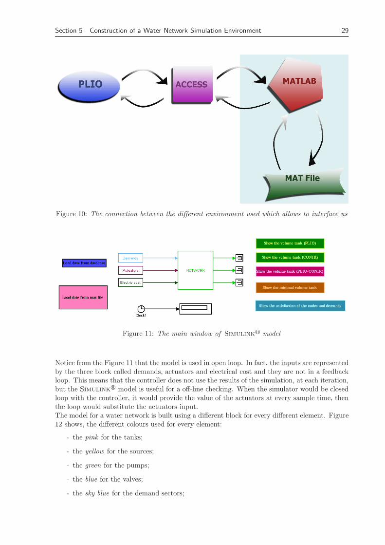
Figure 10: The connection between the different environment used which allows to interface us
Figure 11: The main window of Simulinkr model
Notice from the Figure 11 that the model is used in open loop. In fact, the inputs are representedby the three block called demands, actuators and electrical cost and they are not in a feedbackloop. This means that the controller does not use the results of the simulation, at each iteration,but the Simulinkr model is useful for a off-line checking. When the simulator would be closedloop with the controller, it would provide the value of the actuators at every sample time, thenthe loop would substitute the actuators input.The model for a water network is built using a different block for every different element. Figure12 shows, the different colours used for every element:
- the pink for the tanks;
- the yellow for the sources;
- the green for the pumps;
- the blue for the valves;
- the sky blue for the demand sectors;

30 Simulator for MPC Design over Drinking Water Networks
Figure 12: An example of a small network model
- the grey for the nodes.
Figure 12 is an simple example of a network where the different type of elements are presented. Inorder to manage all the connections between the network inputs and outputs, the input/outputblock in Figure 13 has been generated.
Figure 13: The input/output block in the network
This block is at the same level than the network, inside the green network block in the Figure11. Under this block there is a very complex subnetwork, which considers the necessary inputs,or outputs of the network. In addition, in this network there is the computation of the cost func-tion. In the following, a detailed description of the strategy used to implement every element typeis reported. Moreover, how the input-output block computes the cost function is also explained .
5.2 Element Analysis and Implementation
Every element has a particular implementation, based on a sub-network which allows to repro-duce its dynamical behaviour. Each element is always implemented using the same structure.The differences, that could appear in two subnetworks of the same element type, are due, only,to the output or input number in tanks or nodes model blocks.The actuators, otherwise, do not have differences in the number of inputs or outputs, since theyhave always only one input and one output. They present a different structure when they arebehind a source.

Section 5 Construction of a Water Network Simulation Environment 31
In addition, for every element, a structure in which stores all its parameters is created in theworkspace. This structure has a different number of fields for each different type of element.
5.2.1 Sources
The sources are the most simple type of element in the network for the Simulinkr implemen-tation. Every source is represented with a step, where its value is the max flow allowed. Thesource flows are controlled by means of the actuators which follow the sources. These elementsare implemented using the block step directly coming from the Simulinkr library.
5.2.2 Actuators
The actuator block models have only one input and one output, and take these values, directly,from the workspace. Their implementation aims, only, to guarantee that the value, computedoutside the simulator in the controller, are into the range of the particular element. This isassured by a saturation block that has as upper bound the maximal flow and as lower boundthe minimal flow allowed to pass through the actuator. When the element flow is out of itsoperating range, the saturation block assigns the upper or the lower bound value depending ifthe flow is bigger that the maximal or smaller than the minimal.In the actuator implementation there is, also, the determination of the term used to computethe objectives in the cost function. In particular, for the actuators, it is important the stabilityterm. Moreover, for the pumps, the economical term is computed such that it reflects the elec-trical hourly consume. This is the main difference between valves and pumps.When an actuator follows a source, the actuator structure need some modifications. In thisparticular case, is highlighted by the presence, into the subnetwork, of the block which loadsthe data from the workspace. In the other case, otherwise, it is presented in the subnetwork ofthe element which precedes the actuators.
Valves The valves are used to manage the flow of the water passing through. The structurecreated for the majority of the valves, has three fields:
1. data: the vector of the flow values with a dimension equals to the simulation horizon:there is a value for every sampling time;
2. flow max : the maximal flow allowed in the valve;
3. flow min: the minimal flow allowed in the valve;
This structure is valid not for all the valves because for the valves which follow a source it isnecessary to add another field in the structure: the cost. This cost is due to the price of thewater at every source, and it is the same for every hour in a day.In the implementation of this element in Simulinkr environment, a mask is created where it ispossible to set the maximal and the minimal flows. This could be useful for a future automati-sation of the model creation, where it would be possible to generate the network from a scriptfile.At the moment, the minimal flow is always zero, but, in the future studies, it would be neces-sary to set a different value, since in pratice sometimes it is not possible to close completely thevalves.Under the mask for every valve, it is found a subnetwork which, as it is explained above, mainly,

32 Simulator for MPC Design over Drinking Water Networks
simply checks if the values in the workspace are into the its operational range or not.There are two different types of networks which implements a valve element: one is used when avalve follows a source, the other in all others cases. The differences between these two schemesare, in this case two: the first consists in the presence of a term which comprises the economicalcost; the other in the place where the values are loaded form the workspace.In the valve, used after a source, this is done in the own sub-network of the valve, while in theother case it is implemented in the element which comes before the valve, and the value obtainedis sent to the valve block as a input.In the Figure 14 the implementation of a valve which follows a external source is shown .The switch block at the beginning is used to select the input. Indeed it is possible to choosebetween the source output flow or the flow values saved in the workspace. This option wouldbe useful for future studies. In fact, it could be necessary to modify the source implementationwhich would have different values from the maximal and would regulate the output flow alone.At this time, the different values are obtained trough the valve, so the switching block alwaysselect the value from the workspace.In addition, the structure in Figure 14 shows another branch which is used to compute theeconomical objective in the cost function. There is a multiplication between the flow and thecost, instant by instant. The meaning and the implementation of this term is explained in detailin the next Section 5.2.3, because it is equal to the electrical cost of the pumps.The other part of the subnetwork appears in both actuator types, as it is possible to see compar-ing the Figure 14 and 15, regarding the valves and the Figure 16 and 17, regarding the pumps,and it is used to compute the stability term.This term is obtained as:
valva stab = [u1(t) − u1(t − 1)]2
where the value u1(t − 1) is obtained using the memory block, and the square multiplying thedifference by itself. This term penalizes the differences between the flow value of the valve intwo consecutive sample times. This value is passed to the input-output block where the total
Figure 14: Implementation structure of a valve which follows a source

Section 5 Construction of a Water Network Simulation Environment 33
Figure 15: Implementation structure of a “normal” valve
cost function is computed, where all the coefficients for every actuator are considered.
5.2.3 Pumps
The pumps, the other type of actuators in the network, have a structure in the Simulinkr
model very similar to the valve. The difference in the implementations of these two actuatortype in the network is that the pumps are able to drive up the water from a ground elevation toan bigger other unlike the valves. In general, however, the role of both types of elements is thesame. They could decide the amount of water that could pass through by means of the localcontroller set-point established by the MPC controller. During the optimization, the best valuefor the actuators is selected according to the objective function.The structure created in the workspace for every pump includes four fields. The first three areequal to those explained in the “normal” valve while the last one depends on the economicalcost, as it was shown in the valve used after a source:
• data: the vector of the flow values, with a dimension equal to the simulation horizon;
• flow max : the maximal flow allowed in the pump;
• flow min: the minimal flow allowed in the pump;
• cost : the vector of economical costs that in this case the dimension of the vector is also toequal to the simulation horizon: there is a value for every time instant. The cost changesaccording to the hourly fare.
The difference between the cost in the pump and in the particular valve is due to the electricalcost of the pump changes hourly, while the water cost is considered always the same for everyhour in the day.As in the valve, there are two types of implementation: first type is used only when the pumpsfollow an underground source. Figure 16 shows the structure of a pump used after a source.The second type of implementation is represented in Figure 17, where it could be noticed that

34 Simulator for MPC Design over Drinking Water Networks
Figure 16: Implementation structure of a pump which follows a source
Figure 17: Implementation structure of a pump
the principal structure in Figure 16 is the same of that in Figure 14, as well as the structureshown in Figure 17 is equals to that in Figure 15. So, for these parts of the subnetworks, it ispossible to do the same consideration made above, (see Section 5.2.2 corresponding to the valve

Section 5 Construction of a Water Network Simulation Environment 35
description).However, in both pumps structures implementation, as in the valve which follows a source, thereis a branch where the economical cost coefficient is computed. This represents the only differencebetween “normal” valves and pumps.The hourly economical cost is loaded from the workspace in the main windows (Figure 11) andthrough the input/output block is sent as input to every corresponding pump, or valve. Con-sidering the example in Figure 17, the cost in input is represented by the variable pump2 ele,in dark green.The hourly cost has to be multiplied, instant by instant, for the flow in order to obtain thecoefficient used in the cost function. These values are saved in the variable pump2 cost andpassed to the input/output block where the total cost function is computed, considering theinfluence of every pump and valve.
5.2.4 Nodes
Dynamical models of the nodes are implemented as constraints, where the mass balance must besatisfied: that is the sum of the input flow has to be equal to the sum of output flow. The valuescomputed by the controller should satisfy this constraint. But, in the simulator, it is decided tocheck this balance and give a signal when it is not respected. In this way, the simulator becomes,also, a tool which is able to evaluate the controller operation.These elements, since are only constraints, do not need a structure, since they do not have par-ticular parameters which have to be set. The difference between a node to an another consistsonly of the different number of inputs and outputs.
Figure 18: Node implementation structure
In Figure 18 the model implementation of a node with one input and three output is reported.So, the equation implemented in this node is:

36 Simulator for MPC Design over Drinking Water Networks
u(1) − u(2) − u(3) − u(4) = 0 (20)
The mass balance of the flow in input and the flow in output has to be respected at every time.In fact the u(i) represents the instantaneous flow in the actuator i. The output in the sub-network in Figure 18 is shown with the green block. These blocks implement the loading fromthe workspace. The equation (20) is the same of the constraint imposed in the controller. Thesimulator checks if the constraint is satisfied and in reverse it re-computes the balance changingthe value of one output. This action is done in the part of network that is downstream theequation block. Here, there is a switch that checks, using a threshold, if the balance is satisfiedor not. The balance is satisfied when this equation is about zero. When the constraint is notrespected, one output has been considered like a free variable, and, instead of using the valuein the workspace, as output, the value computed in the second equation block is used. Thereare another two branches in the structure implemented that aim to check the satisfaction ofthe constraint and the demand. The block with the name of the node generates a variable inthe workspace which has as many ones as time instants in which the node balance is satisfied.When this constraint is not respected appears a minus one. Coming back to the main window ofthe model (Figure 11), there is a block which allows to visualize these variable and searches theminus ones. This block is on the right in sky-blue. When a minus one is found, in the commandwindow of Matlabr is displayed the number of the node and the corresponding instant whenthe balance is not satisfied.The other part of the scheme is used to check if the demand, connected to this node, is satisfiedat every instant or not. In fact, the sum in the lowest part computes the balance of the nodewithout the demand, and, only after, the demand is subtracted. If the results of this differenceis about zero the demand is satisfied, otherwise is not. The pale blue blocks in the Figure 24generate the variable which have to be sent to the input/output block, appearing a minus onewhen there is a infeasibility, in the same way as the node balance.
5.2.5 Tanks
The tanks are the dynamical elements in the system and they play a fundamental role in thesimulator. Indeed, known the inputs and the disturbances (the demands), the tank volumes arecalculated instant by instant.First of all, it is important to check if the behaviour of the tank volume computed in this way isequal to that computed in the controller. When there are no infeasibilities, which could modifysome actuator values, the results from the controller and the simulator are exactly the same.These results are showed in Figures 19, where the volume behaviour of a tank in a simulationof 48 hours is displayed.The two lines, in both figures, are completely overlapped, indicating that the Simulinkr simu-lator allows to obtain the same results of those obtained both in the PLIO tool and in Matlabr
controller.The structure of a typical tank implementation using Simulinkr blocks is shown in Figure 20.
Figure 20 shows the implementation of a tank. In fact, this tank has only one input and oneoutput. This structure could be more complicated when a tank has a bigger number of inputsor outputs.Observing the network in the Figure 12, it can be noticed that the tank has three inputs, onecorresponding to a demand. This is a trick to use the demand like a known disturbance and soit is necessary to load this data from the workspace. The demand is introduced in the equation
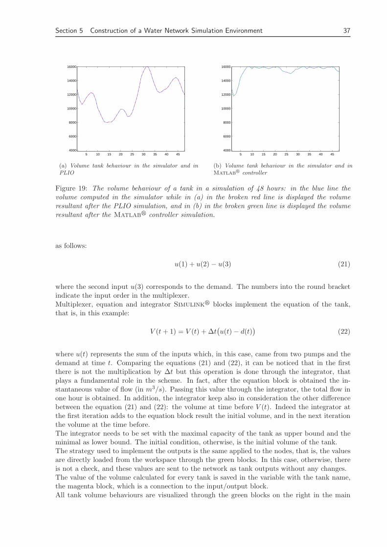
Section 5 Construction of a Water Network Simulation Environment 37
5 10 15 20 25 30 35 40 454000
6000
8000
10000
12000
14000
16000
(a) Volume tank behaviour in the simulator and inPLIO
5 10 15 20 25 30 35 40 454000
6000
8000
10000
12000
14000
16000
(b) Volume tank behaviour in the simulator and inMatlab
r controller
Figure 19: The volume behaviour of a tank in a simulation of 48 hours: in the blue line thevolume computed in the simulator while in (a) in the broken red line is displayed the volumeresultant after the PLIO simulation, and in (b) in the broken green line is displayed the volumeresultant after the Matlabr controller simulation.
as follows:
u(1) + u(2) − u(3) (21)
where the second input u(3) corresponds to the demand. The numbers into the round bracketindicate the input order in the multiplexer.Multiplexer, equation and integrator Simulinkr blocks implement the equation of the tank,that is, in this example:
V (t + 1) = V (t) + ∆t(
u(t) − d(t))
(22)
where u(t) represents the sum of the inputs which, in this case, came from two pumps and thedemand at time t. Comparing the equations (21) and (22), it can be noticed that in the firstthere is not the multiplication by ∆t but this operation is done through the integrator, thatplays a fundamental role in the scheme. In fact, after the equation block is obtained the in-stantaneous value of flow (in m3/s). Passing this value through the integrator, the total flow inone hour is obtained. In addition, the integrator keep also in consideration the other differencebetween the equation (21) and (22): the volume at time before V (t). Indeed the integrator atthe first iteration adds to the equation block result the initial volume, and in the next iterationthe volume at the time before.The integrator needs to be set with the maximal capacity of the tank as upper bound and theminimal as lower bound. The initial condition, otherwise, is the initial volume of the tank.The strategy used to implement the outputs is the same applied to the nodes, that is, the valuesare directly loaded from the workspace through the green blocks. In this case, otherwise, thereis not a check, and these values are sent to the network as tank outputs without any changes.The value of the volume calculated for every tank is saved in the variable with the tank name,the magenta block, which is a connection to the input/output block.All tank volume behaviours are visualized through the green blocks on the right in the main

38 Simulator for MPC Design over Drinking Water Networks
Figure 20: Tank implementation structure
windows (Figure 11). There are two different blocks: one used when the simulator runs withthe value actuators computed with the PLIO simulation, the other when they are calculated bythe controller simulation.The magenta block in the main window, on the right, allows to compare the simulation results ofPLIO tool or Matlabr controller. This is useful to show the differences of these two controllersin the same scenario.Coming back to the tank structure there are another three branches which have not been alreadyexplained.The first generates the coefficient of the penalty objective for every tank. The equation im-plemented is in (6), where the penalty volume is subtracted to the volume at every time andwhen this difference is bigger than zero, there is a penalty coefficient. This value is squared andafter, in the block input/output, the total penalty cost function, including all tanks component,is computed. This value, which has to be passed to the next computations, is saved in thesky-blue block.The second branch is equal to a part of the node implementation, indeed it generates the vectorthat indicates the demand satisfaction. In tanks case, it is necessary to take in account morethings than in node case. In particular, the check does not only consider the input/outputbalance but it has to consider the volume stored in the tank to see if there is enough water to
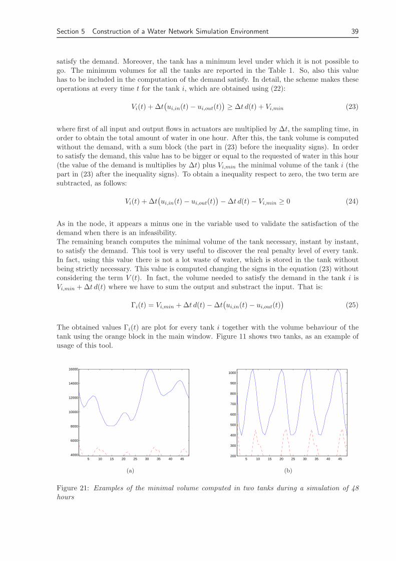
Section 5 Construction of a Water Network Simulation Environment 39
satisfy the demand. Moreover, the tank has a minimum level under which it is not possible togo. The minimum volumes for all the tanks are reported in the Table 1. So, also this valuehas to be included in the computation of the demand satisfy. In detail, the scheme makes theseoperations at every time t for the tank i, which are obtained using (22):
Vi(t) + ∆t(
ui,in(t) − ui,out(t))
≥ ∆t d(t) + Vi,min (23)
where first of all input and output flows in actuators are multiplied by ∆t, the sampling time, inorder to obtain the total amount of water in one hour. After this, the tank volume is computedwithout the demand, with a sum block (the part in (23) before the inequality signs). In orderto satisfy the demand, this value has to be bigger or equal to the requested of water in this hour(the value of the demand is multiplies by ∆t) plus Vi,min the minimal volume of the tank i (thepart in (23) after the inequality signs). To obtain a inequality respect to zero, the two term aresubtracted, as follows:
Vi(t) + ∆t(
ui,in(t) − ui,out(t))
− ∆t d(t) − Vi,min ≥ 0 (24)
As in the node, it appears a minus one in the variable used to validate the satisfaction of thedemand when there is an infeasibility.The remaining branch computes the minimal volume of the tank necessary, instant by instant,to satisfy the demand. This tool is very useful to discover the real penalty level of every tank.In fact, using this value there is not a lot waste of water, which is stored in the tank withoutbeing strictly necessary. This value is computed changing the signs in the equation (23) withoutconsidering the term V (t). In fact, the volume needed to satisfy the demand in the tank i isVi,min + ∆t d(t) where we have to sum the output and substract the input. That is:
Γi(t) = Vi,min + ∆t d(t) − ∆t(
ui,in(t) − ui,out(t))
(25)
The obtained values Γi(t) are plot for every tank i together with the volume behaviour of thetank using the orange block in the main window. Figure 11 shows two tanks, as an example ofusage of this tool.
5 10 15 20 25 30 35 40 454000
6000
8000
10000
12000
14000
16000
(a)
5 10 15 20 25 30 35 40 45200
300
400
500
600
700
800
900
1000
(b)
Figure 21: Examples of the minimal volume computed in two tanks during a simulation of 48hours

40 Simulator for MPC Design over Drinking Water Networks
When there is not an infeasibility, as in the case of in the Figure 21, the broken red line, whichrepresents the minimal value computed, is always below than of the blue one, which indicatesthe stored volume of water in the tank during the simulation. As it is explained in the nextchapters, many tests have to be done to identify the rigst penalty volume which allows to obtainthe minimal cost.
The tank dynamics plays a main role in the analysis of the network behaviour. Indeed thecomparisons between different controllers are done comparing the tank volumes.
5.3 Implementation of Barcelona Water Network Simulator
As an application of the library of elements built, a simulator for the aggregated network ofBarcelona is developed (see Figure 22). Every element in the network in Figure 22 has the samename of the VISIO model presented in Figure 7, so it is quite simple to relate both models.At the top left of Figure 11, there is a red block called input/output. This block takes careof all the connections between the network inputs/outputs and the element blocks. It is possi-ble to notice that in Figure 23, the subnetwork under the input/output block is very complex.Every coloured element, in Figure 23, corresponds to a different variable in every element. Inthis block, the cost function is computed, as well as saved the matrix of system states and thematrix which indicates the satisfaction of demands.Every block, in the network in Figure 22, respects the colour convention explained previously,as well as the subnetworks. The strategy used to create the dynamical model of every elementis already explained, but it is interesting and useful to provide some details on how the imple-mentation of the Barcelona aggregated model has been done. In particular, details about nodeand tank implementation, where the network has a great complexity due to the big number ofinputs/outputs, are given.
In the Figure 24, the node n70fll is shown. This node presents a very complex structure,due to a big number of inputs and outputs.In particular, the node n70fll (Figure 24) has 4 inputs and 3 outputs. One of the 3 outputs is ademand sector (the sector c70fll), but, as in the tank, it appears as an input. The other outputsin Figure 24 are represented by the green block, which are the connections with the input/outputblock and so to the workspace. In this block there is the value saved in the workspace for everyelement, in the field data.The equation of the mass balance, where the demand sector is considered as a negative input,is:
u(1) − u(2) + u(3) + u(4) + u(5) − u(6) − u(7)
where the number into the round brackets represents the order of the multiplex input. Thedemand sector is the second input in the multiplexer preceded by the minus sign.Using the variable name used in the controller (Tables 2, 9 and 10), the constraint is:
u25 − d15 + u32 + u33 + u40 − u26 − u41 = 0 (26)
This constraint is checked at every sample time, and it assures that there is not water stored inthe nodes.
The Figure 25 shows the subnetwork regarding the tank d130bar. The equation implemented inthe tank d130bar is very complex. This complexity is due to the number of inputs and outputs.

Section 5 Construction of a Water Network Simulation Environment 41
Figure 22: Aggregated Barcelona drinking network model in Simulinkr
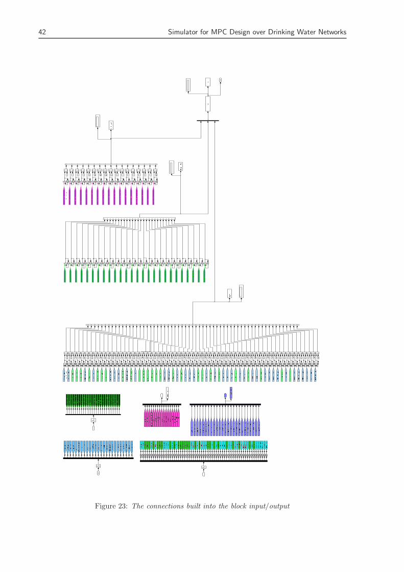
42 Simulator for MPC Design over Drinking Water Networks
Figure 23: The connections built into the block input/output

Section 6 Model Predictive Control of Barcelona Water Network 43
Figure 24: Node implementation structure: in particular it is showed the implementation of theelement n70fll
The tank d130bar has 5 inputs and 5 outputs which interact in the computation of the volumelevel.In this case, in the block equation it is found:
u(1) − u(2) + u(3) + u(4) + u(5) + u(6) − u(7) − u(8) − u(9) − u(10)
where the numbers into the bracket indicate the order of the multiplexer inputs. The secondinput is the demand sector c130bar and it is the reason of the minus sign before the u(2).The tank equation, implemented for this element in the simulator, corresponds to the controllerequation:
V (t + 1) = V (t) + ∆t (u30(t) + u38(t) + u45(t) + u51(t) + u52(t)+
− u29(t) − u36(t) − u37(t) − u42(t) − d12(t))
where it is used the name used by the controller.
6 Model Predictive Control of Barcelona Water Network
In this section, the model predictive control of the Barcelona water is presented. The modelpredictive controller uses a multi-objective cost function, which reflects the control strategy of

44 Simulator for MPC Design over Drinking Water Networks
the water network. The controller computes the optimal solution with a prediction horizon anddemand forecast of 24 hours. t any time, only the first value is used and at the next time startsa new computation. The results are obtained interfacing the simulator described in the Chap-ter 5 with the PLIO tool and the Matlabr controller developed in [7]. The last part showsthe differences obtained using the MPC controller implemented in MATLAB in centralized anddecentralized form.
6.1 MPC Cost Function
As we have already discussed, water networks are very complex multivariable systems. Inorder to improve their performance, predictive optimal control provides suitable techniques tocompute optimal control strategies ahead in time for all the flow and pressure control elements ofa water system, as discussed in Chapter 3. The optimal strategies are computed by optimizinga mathematical function describing the operative goals in a given time horizon and using arepresentative model of the network dynamics, as well as demand forecasts.The cost function of a MPC controller, as it has already explained, is composed by severalobjectives. In this study, the cost function includes three objectives, which have to be minimizedat the same time:
1. Security term FCS, that gives a penalization when the water level in the tanks goesbelow the security level. It is a operation-safety cost associated to not satisfying desiredsecurity storage volume in the tanks. The desired volume in the tank represents thesecurity level which is needed to guarantee the demand satisfaction. Then, this criterionaims to the maintenance of appropriate water storage levels in the network for demandsatisfaction. This level is chosen using the results obtained in the simulator, presented in
Figure 25: The tank implementation structure: in particular it is showed the implementation ofthe element d130bar
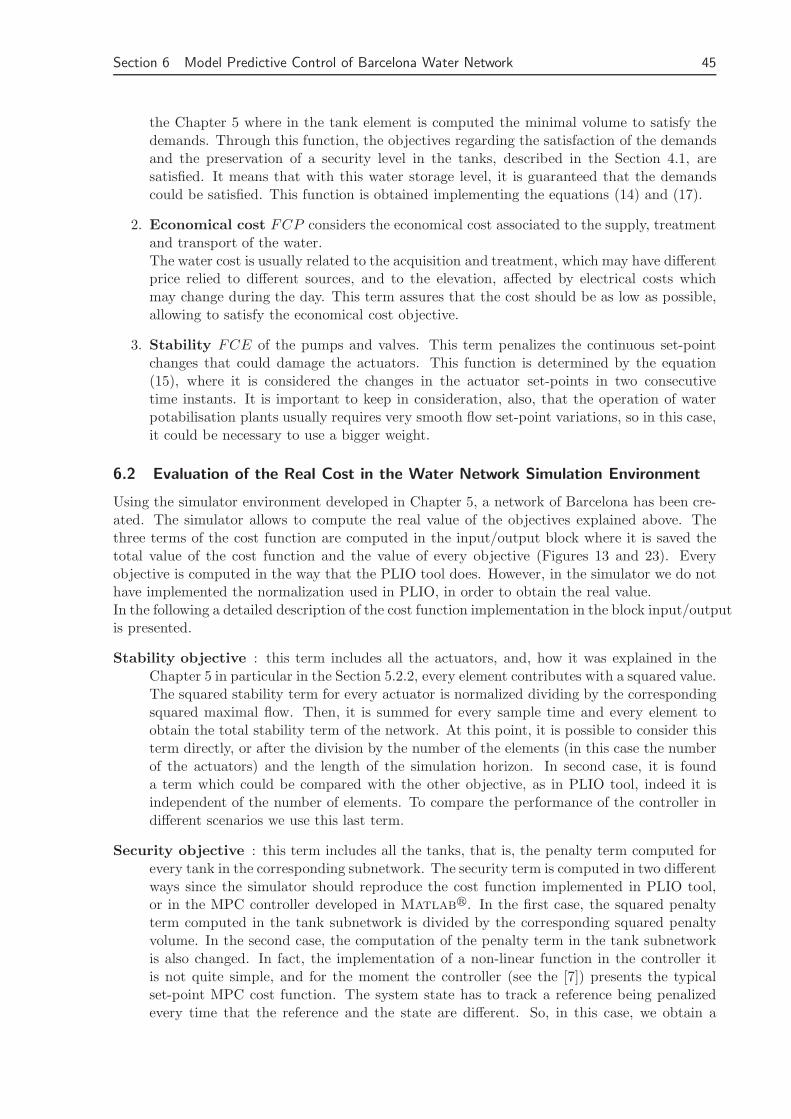
Section 6 Model Predictive Control of Barcelona Water Network 45
the Chapter 5 where in the tank element is computed the minimal volume to satisfy thedemands. Through this function, the objectives regarding the satisfaction of the demandsand the preservation of a security level in the tanks, described in the Section 4.1, aresatisfied. It means that with this water storage level, it is guaranteed that the demandscould be satisfied. This function is obtained implementing the equations (14) and (17).
2. Economical cost FCP considers the economical cost associated to the supply, treatmentand transport of the water.The water cost is usually related to the acquisition and treatment, which may have differentprice relied to different sources, and to the elevation, affected by electrical costs whichmay change during the day. This term assures that the cost should be as low as possible,allowing to satisfy the economical cost objective.
3. Stability FCE of the pumps and valves. This term penalizes the continuous set-pointchanges that could damage the actuators. This function is determined by the equation(15), where it is considered the changes in the actuator set-points in two consecutivetime instants. It is important to keep in consideration, also, that the operation of waterpotabilisation plants usually requires very smooth flow set-point variations, so in this case,it could be necessary to use a bigger weight.
6.2 Evaluation of the Real Cost in the Water Network Simulation Environment
Using the simulator environment developed in Chapter 5, a network of Barcelona has been cre-ated. The simulator allows to compute the real value of the objectives explained above. Thethree terms of the cost function are computed in the input/output block where it is saved thetotal value of the cost function and the value of every objective (Figures 13 and 23). Everyobjective is computed in the way that the PLIO tool does. However, in the simulator we do nothave implemented the normalization used in PLIO, in order to obtain the real value.In the following a detailed description of the cost function implementation in the block input/outputis presented.
Stability objective : this term includes all the actuators, and, how it was explained in theChapter 5 in particular in the Section 5.2.2, every element contributes with a squared value.The squared stability term for every actuator is normalized dividing by the correspondingsquared maximal flow. Then, it is summed for every sample time and every element toobtain the total stability term of the network. At this point, it is possible to consider thisterm directly, or after the division by the number of the elements (in this case the numberof the actuators) and the length of the simulation horizon. In second case, it is founda term which could be compared with the other objective, as in PLIO tool, indeed it isindependent of the number of elements. To compare the performance of the controller indifferent scenarios we use this last term.
Security objective : this term includes all the tanks, that is, the penalty term computed forevery tank in the corresponding subnetwork. The security term is computed in two differentways since the simulator should reproduce the cost function implemented in PLIO tool,or in the MPC controller developed in Matlabr. In the first case, the squared penaltyterm computed in the tank subnetwork is divided by the corresponding squared penaltyvolume. In the second case, the computation of the penalty term in the tank subnetworkis also changed. In fact, the implementation of a non-linear function in the controller itis not quite simple, and for the moment the controller (see the [7]) presents the typicalset-point MPC cost function. The system state has to track a reference being penalizedevery time that the reference and the state are different. So, in this case, we obtain a
46 Simulator for MPC Design over Drinking Water Networks
penalization also when the level is over the security level. This squared term, moreover, itis divided by the squared of maximal volume of the corresponding tank. In practise, thecost function implemented in PLIO tool is preferred, but it is interesting also to study thedifference obtained considering the typical MPC objective. As in the stability term, it ispossible and useful to normalize with the number of tanks and the length of the simulationhorizon. As in the stability term, the normalized value is used in the study of the controllerperformances in different scenarios.
Economical term : this term includes all the pumps and valves which follow a source. It iscomputed, simply, considering the total cost for every pump, or valve, in the simulationhorizon. To find the total economical cost of the network, all individual costs associatedto every element are added together such that a value in euros is obtained. In this case,is non sense to normalize it by the number of elements because the interest is in the totalcost. To study in detail the behaviour of the network, this term is divided in two differentsubcosts: one which considers the water cost and the other the electrical pumping cost.
All these terms represent the indicators to tune the MPC controller. In the following study thedifferences, in term of cost function, obtained changing the parameters of the network, like, forexample, initial condition, penalty level and weights in the PLIO simulations are analyzed. Theresults obtained with the Matlabr MPC controller are reported in Section 6.5.
6.3 Implementation of the Cost Function in PLIO
The multi-objective cost function in PLIO is thus chosen as the addition of a weighted sum ofthe terms, each one representing an objective:
FC = ω1 · FCS + ω2 · FCP + ω3 · FCE
where:
- ω1, ω2 and ω3 are the weights, which correspond to the priority level.
- FCS is the security cost;
- FCP is the economical cost;
- FCE is the stability cost.
The weights are selected on the basis of the priority order. It is possible to make some tests toevaluate which is the best choice of priority level. A technique that could be used to search theoptimal value of each optimization term is considering one objective at a time. Unfortunately,in this model it is not possible to use this technique, because, considering only one objective attime the computation time increases a lot. This happens because the cost function in this waybecomes very flat and so it is very difficult to find the optimal solution. The optimizer, in themajority of cases, chooses a local solution, and not a global optimal solution.In the following, a detailed description of the objective function used in PLIO tool is presented.These equations use the variables created by PLIO tool, which have already described in theChapter 4.The results computed in this way represent the value obtained for every objective function atthe end of the predictive horizon. In fact PLIO tool calculates the value of the cost functionconsidering the 24 hours of the prediction horizon. However, currently, this tool does not providedirectly a real value for the cost function but only an estimated in 24 hours. For this reason, itis also important the computation done using the Simulinkr model.

Section 6 Model Predictive Control of Barcelona Water Network 47
6.3.1 Security Term (FCS)
The security term assures that the water level into the tanks remains above a selected volume,called penalty value. This function considers the level of every tank into the model. Everytank may be weighted in this function with a different coefficient. This weight is the value thatappears in the tank property’s windows in PLIO tool, in Editor mode in the Section 2.2.1.As it has been done for every element in the Chapter 2 in the Section 2.2.2, now it is shownhow the PLIO tool, with the aid of GAMS solver, computes this function and what types ofnormalization are used.The security function is defined like a weighted sum of variables Vbajoxx, computed in theequation (7), that indicates, for each tankxx (with xx = 1, · · · , 17), whether the security levelis satisfied or not:
FCS =
17∑
i=1
ωiVbajoi
17(27)
where ωi is the weight concerning the tank i.Moreover, the equation (27) considers the normalization dividing by the number of elements. Infact, there is a division by 17, where 17 is the number of the tanks in the model. It is importantto remember that the term Vbajoxx includes, for every tank, the sum along all the predictionhorizon and the respectively normalization.
6.3.2 Price Term (FCP)
The FCP term represents the water and electrical costs, that are usually related to acquisitionand treatment, which have different prices at different sources due to the different chemicaltreatments and electrical pumping. The pump electrical cost, necessary to drive the water ata bigger elevation, has a different value at different hours of the day, as it is possible to see inthe Tables 3, 4, 5, 6, 7. Analogously to the security function, every pump or source may beweighted by a different coefficient, inserted in the property window of each element.The price function is a weighted sum of variable concerning the sources and the pumps:
FCP =
9∑
i=1
ωisumi
9 · 24 · max unitary+
26∑
j=1
ωjsumj
24 · 26 · max elect(28)
where the variables sumi and sumj are respectively, obtained in equations (8) and (11), whileωi and ωj are the weight concerning, respectively, the source i and the pump j. The variablesname max unitary and max elect, respectively, correspond to the maximal unitary cost whichappears considering all the sources, and the maximal electrical cost imposed by all 26 pumps.The number in the denominator is used to normalized the objective. In fact, every weightedsum is divided by the number of the elements and the prediction horizon length. All these nor-malizations allow to obtain values between zero and one. In this way, it is possible to comparethe different objectives and using different weights reflect the priority order.

48 Simulator for MPC Design over Drinking Water Networks
6.3.3 Stability Term (FCE)
The stability term preserves the actuator from both continuous and abrupt variations. Thisfunction is a weighted sum of variable concerning the actuators which should be stabilized. Allthe actuators, pumps and valves, have to be stabilized. To reach the goal of making the valvesstabilizable, the motorized valves, which are elements of the PLIO software tool, are used.The mathematical form of this function, considering the terms generated by every element, isthe following:
FCE =
p∑
i=1
ωi · Esti +
v∑
j=1
ωj · Estj
p + v(29)
where Esti and Estj are the variables obtained, respectively, from the equation (9) and (10) forevery pump or valve; p and v are the numbers of the pumps and the valves which have to bestabilized, respectively. The variables Esti and Estj have already been normalized with respectto the prediction horizon.
6.4 MPC Results obtained using PLIO
This section deals with the simulation results obtained using the PLIO tool. Several test sce-narios have been chosen to show the potential of predictive optimal control tool for computingcontrol strategies in complex operational situations. In addition, the results of these differentscenarios allow to select the element and cost function weight and the other parameters, as thepenalty or initial volume, in order to obtain a network with as possible.Each scenario shows the simulation of 2-days (48 hours), and in particular they include datarelative to 2 days of hourly demands. These demands represent the request in a standard dailysituation. Indeed the hourly values in one day are obtained considering the monthly amount ofwater request. The hourly values reflect, as is possible to view in the Figure 9, the same dailyforecast of every demand sector.The two days of demand considered have the same profile, but in the future study could beinteresting to use a different daily profiles for every different day in the week. This will allowto reflect the different behaviour of the users in the different day, as, for example, a Monday (aworking day) or a Sunday (a holiday day). It would also be interesting to study the user be-haviours in presence of some public events, in order to manage the forecast demands, in severalsituations.The first scenario shown is used as a starting point in the tuning process and it was used to findthe way to improve the control results following AGBAR suggestions.
6.4.1 Scenarios as Starting Points
The scenario I represents the starting point for our analysis. In fact, at the beginning, of thestudy it has been considered a typical scenario which allows to analyze the network behaviourand, from these results, decide the better optimization strategy and parameters.This scenario is planned using the 80% of the maximal volume of every tank both as its initialvolume and penalty level. The results obtained are used to find a penalty volume value lessrestrictive which allows to save more water and, then, money. This penalty value, as it has beenindicated before, is computed thanks to the simulator implemented in the Simulinkr environ-ment.

Section 6 Model Predictive Control of Barcelona Water Network 49
The weights are also selected in a very simple way in order to consider all objectives with thesame priority both the security and the stability term (using a weight of one), while the econom-ical cost (using a weight of zero) was not initially considered. The resulting cost function hasa very flat form, which increases a lot the computation time (for a simulation of 48 iteration itwas necessary about three hours and half). In fact, it is quite difficult to find a global minimum,and, the optimizer stacks in a local minimum encountering some numerical problems, whichwere indicated, in the files generated by PLIO, as “non-optimal ”. The optimization, if does notreach the optimal solution, is stopped by the GAMS solver after an imposed interval of time,which is 5 minutes by default. But to try to obtain a minor number of non optimal values itwas increased to 15 minutes.
10 20 30 40150
200
250
300
350
400
d125PAL x1
10 20 30 40400
500
600
700
800
900
d110PAP x2
10 20 30 40
500
1000
1500
2000
2500
3000
3500
d115CAST x3
10 20 30 40500
1000
1500
2000
2500
3000
d80GAVi80CAS85CRO x4
10 20 30 40
2000
4000
6000
8000
10000
12000
14000
dPLANTA x5
10 20 30 40
1000
1500
2000
2500
3000
d54REL x6
(a) Volume evolution of the first six tanks (from x1 to x6)
10 20 30 40
2
3
4
5
6
x 104 d100FCE x
7
10 20 30 40
2000
4000
6000
8000
10000
d10COR x8
10 20 30 401000
2000
3000
4000
5000
6000
7000
d200BLL x9
10 20 30 404000
6000
8000
10000
12000
14000
16000
d130BAR x10
10 20 30 40200
400
600
800
1000
d176BARsud x11
10 20 30 40
3
4
5
6
7
8
9
x 104 d70BBEsud x
12
(b) Volume evolution of six tanks (from x7 to x12)
10 20 30 40
1000
2000
3000
4000
d200ALT x13
10 20 30 40
1
1.5
2
2.5
3
3.5
x 104 d100BLLnord x
14
10 20 30 401000
2000
3000
4000
5000
6000
7000
d200BARnord x15
10 20 30 401500
2000
2500
3000
3500
4000
4500
d101MIR x16
10 20 30 40
500
1000
1500
d120POM x17
(c) Volume evolution of five tanks (from x13 tox17)
Figure 26: The volume evolution of a tanks in the scenario I: in blue is showed the valuescomputed by the simulator, in the broken red line that calculated by PLIO tool, and the brokengreen line indicate the 80% of the maximal volume, the penalty value.
The evolution of the 17 tank volumes, obtained in this case, is presented in the Figures 26 whereit is possible to compare the evolution computed by PLIO (in the broken red line) and by thesimulator developed in Chapter 5 are completely overlapped for every tank. In the broken greenline the 80% of the maximal tank volume is indicated, which, in this scenario, represents boththe initial volume and the penalty level. The range of the y-axis in all the plots reflects the
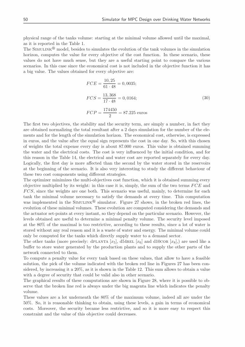
50 Simulator for MPC Design over Drinking Water Networks
physical range of the tanks volume: starting at the minimal volume allowed until the maximal,as it is reported in the Table 1.The Simulinkr model, besides to simulates the evolution of the tank volumes in the simulationhorizon, computes the value for every objective of the cost function. In these scenario, thesevalues do not have much sense, but they are a useful starting point to compare the variousscenarios. In this case since the economical cost is not included in the objective function it hasa big value. The values obtained for every objective are:
FCE =10, 25
61 · 48= 0, 0035;
FCS =13, 368
17 · 48= 0, 0164;
FCP =174450
2= 87.225 euros
(30)
The first two objectives, the stability and the security term, are simply a number, in fact theyare obtained normalizing the total resultant after a 2 days simulation for the number of the ele-ments and for the length of the simulation horizon. The economical cost, otherwise, is expressedin euros, and the value after the equal sign represents the cost in one day. So, with this chosenof weights the total expense every day is about 87.000 euros. This value is obtained summingthe water and the electrical costs. The cost is very influenced by the initial condition, and forthis reason in the Table 14, the electrical and water cost are reported separately for every day.Logically, the first day is more affected than the second by the water stored in the reservoirsat the beginning of the scenario. It is also very interesting to study the different behaviour ofthese two cost components using different strategies.The optimizer minimizes the multi-objectives cost function, which it is obtained summing everyobjective multiplied by its weight: in this case it is, simply, the sum of the two terms FCE andFCS, since the weights are one both. This scenario was useful, mainly, to determine for eachtank the minimal volume necessary to satisfy the demands at every time. This computationwas implemented in the Simulinkr simulator. Figure 27 shows, in the broken red lines, theevolution of these minimal volumes. These evolution are computed considering the demands andthe actuator set-points at every instant, so they depend on the particular scenario. However, thelevels obtained are useful to determine a minimal penalty volume. The security level imposedat the 80% of the maximal is too restrictive, according to these results, since a lot of water isstored without any real reason and it is a waste of water and energy. The minimal volume couldonly be computed for the tanks which directly supply water to a demand sector.The other tanks (more precisely: dplanta [x5], d54rel [x6] and d10cor [x8],) are used like abuffer to store water generated by the production plants and to supply the other parts of thenetwork connected to them.To compute a penalty value for every tank based on these values, that allow to have a feasiblesolution, the pick of the volume indicated with the broken red line in Figures 27 has been con-sidered, by increasing it a 20%, as it is shown in the Table 12. This sum allows to obtain a valuewith a degree of security that could be valid also in other scenario.The graphical results of these computations are shown in Figure 28, where it is possible to ob-serve that the broken line red is always under the big magenta line which indicates the penaltyvolume.These values are a lot underneath the 80% of the maximum volume, indeed all are under the50%. So, it is reasonable thinking to obtain, using these levels, a gain in terms of economicalcosts. Moreover, the security became less restrictive, and so it is more easy to respect thisconstraint and the value of this objective could decreases.
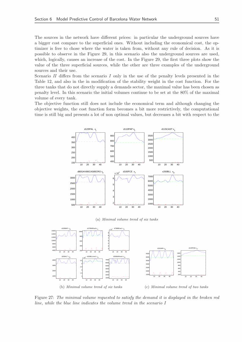
Section 6 Model Predictive Control of Barcelona Water Network 51
The sources in the network have different prices: in particular the underground sources havea bigger cost compare to the superficial ones. Without including the economical cost, the op-timizer is free to chose where the water is taken from, without any rule of decision. As it ispossible to observe in the Figure 29, in this scenario also the underground sources are used,which, logically, causes an increase of the cost. In the Figure 29, the first three plots show thevalue of the three superficial sources, while the other are three examples of the undergroundsources and their use.Scenario II differs from the scenario I only in the use of the penalty levels presented in theTable 12, and also in the in modification of the stability weight in the cost function. For thethree tanks that do not directly supply a demands sector, the maximal value has been chosen aspenalty level. In this scenario the initial volumes continue to be set at the 80% of the maximalvolume of every tank.The objective function still does not include the economical term and although changing theobjective weights, the cost function form becomes a bit more restrictively, the computationaltime is still big and presents a lot of non optimal values, but decreases a bit with respect to the
10 20 30 40150
200
250
300
350
400
d125PAL x1
10 20 30 40400
500
600
700
800
900
d110PAP x2
10 20 30 40
500
1000
1500
2000
2500
3000
3500
d115CAST x3
10 20 30 40500
1000
1500
2000
2500
3000
d80GAVi80CAS85CRO x4
10 20 30 40
2
3
4
5
6
x 104 d100FCE x
7
10 20 30 40
1000
2000
3000
4000
5000
6000
7000
x200BLL x9
(a) Minimal volume trend of six tanks
10 20 30 404000
6000
8000
10000
12000
14000
16000
d130BAR x10
10 20 30 40200
400
600
800
1000
d176BARsud x11
10 20 30 40
3
4
5
6
7
8
9
x 104 d70BBEsud x
12
10 20 30 40
1000
2000
3000
4000
d200ALT x12
10 20 30 40
1
1.5
2
2.5
3
3.5
x 104 d100BLLnord x
13
10 20 30 40
1000
2000
3000
4000
5000
6000
7000
d200BARnord x15
(b) Minimal volume trend of six tanks
10 20 30 401500
2000
2500
3000
3500
4000
4500
d101MIR x16
10 20 30 40200
400
600
800
1000
1200
1400
1600
d120POM x17
(c) Minimal volume trend of two tanks
Figure 27: The minimal volume requested to satisfy the demand it is displayed in the broken redline, while the blue line indicates the volume trend in the scenario I

52 Simulator for MPC Design over Drinking Water Networks
Tanks name Vectorstate
Minimalvolume pick
Penaltyvolume
d125PAL x1 172,40 200d110PAP x2 399,83 500d115CAST x3 256,01 400d80GAVi80CAS85CRO x4 693,10 850d100FCE x7 18.917 25.000d200BLL x9 1.005,3 1.500d130BAR x10 5.449,3 6.500d176BARsud x11 3.332,66 400d70BBEsud x12 26.787 30.000d200ALT x13 755,82 1.000d100BLLnord x14 8113,5 10.000d200BARnord x15 1.404,7 2.000d101MIR x16 2.070,5 2.500d120POM x17 160,54 400
Table 12: Tanks penalty volume level computed summing to the pick its 20%. All volumes areexpressed in [m3]
scenario I. For these reasons, the results obtained in this scenario are useful for a comparisonwith the other scenarios presented in the Table 14 but not very interesting to be studied alone.The values for the cost function reported in the Table 14, could be surprising, because the costresulting is bigger although the penalty level is lower. This is due to the fact that, no consid-ering the economical objective, the selection of which source or which pump to use is completeunconstrained. Thus, the obtained feasible solution is not the optimal solution.
6.4.2 Initial Condition
An important issue in the improvement of the predictive control results is to understand theeffect of the initial condition in the tanks in the cost function values. With this aim, we havesimulated three scenarios (called III, IV, V ) which have all the same weight and security levelin the tank, but with different initial conditions each one.The weights used in the cost function are: 10 for the security term, 0.1 for the stability and100 for the economical objective. This could be considered a good choice, since in the solutionprovided by the optimizer does not appears any “on-optimal” value. Then, in every of thesethree scenarios, the optimal solution is obtained improving also the computation time. In fact,in less than one hour and half for every scenario (with 48 iterations) is required. There are somesmall difference depending on the initial condition, which makes more or less restrictive (flat)the cost function.The penalty levels used in each one of these scenarios are those presented in the Table 12, inorder to not storing a lot unnecessary water in the tank.The initial conditions are chosen in this way:
• in the scenario III, the 80% of the maximal value in every tank is imposed.
• in the scenario IV, the volume obtained at the end of the scenario III is imposed, inorder to try to obtain the same evolution in every day. In order to guarantee perfectlysuch repetitive behaviour, it would be necessary to use a bigger number of iterations, todetermine the right initial condition, but also in this case we have obtained some interestingresults.

Section 6 Model Predictive Control of Barcelona Water Network 53
• in the scenario V, the penalty level used.
The different evolutions of the tanks with the different initial condition are shown in the Figure 30and 31, where, respectively the tanks evolution in the scenario III and V scenario are presented.According to what it is explained before, the effects of the initial condition are evident in thedaily water cost and particularly in the economical term. The water necessary to satisfy thedemand in the first day of simulation change according to the initial condition: when the systemstarts with the tank at the 80% less water is needed to satisfy the demands (scenario III ) whichimplies a save of money. Decreasing the initial volume, logically, increases the cost, as in thescenario IV and V. The numerical values are reported in Table 13. In particular in Table 13, itis shown the value of the three main objectives and, moreover, the difference between the firstand the second day in the water and electrical cost.In order to complete the analysis of these three scenarios, it is useful to see how they use thesources. Now the economical cost is included in the cost function so, in a standard day as theone to that is considered, the optimizer uses only the superficial sources. This behaviour is
10 20 30 40150
200
250
300
350
400
d125PAL x1
10 20 30 40400
500
600
700
800
900
d110PAP x2
10 20 30 40
500
1000
1500
2000
2500
3000
3500
d115CAST x3
10 20 30 40500
1000
1500
2000
2500
3000
d80GAVi80CAS85CRO x4
10 20 30 40
2
3
4
5
6
x 104 d100FCE x
7
10 20 30 40
1000
2000
3000
4000
5000
6000
7000
x200BLL x9
(a) Penalty volume chosen in six tanks
10 20 30 404000
6000
8000
10000
12000
14000
16000
d130BAR x10
10 20 30 40200
400
600
800
1000
d176BARsud x11
10 20 30 40
3
4
5
6
7
8
9
x 104 d70BBEsud x
12
10 20 30 40
1000
2000
3000
4000
d200ALT x12
10 20 30 40
1
1.5
2
2.5
3
3.5
x 104 d100BLLnord x
13
10 20 30 401000
2000
3000
4000
5000
6000
7000
d200BARnord x15
(b) Penalty volume chosen in six tanks
10 20 30 401500
2000
2500
3000
3500
4000
4500
d101MIR x16
10 20 30 40200
400
600
800
1000
1200
1400
1600
d120POM x17
(c) Penalty volume chosen in two tanks
Figure 28: Penalty volume chosen considering the minimal volume showed in the Figure 27: inthe broken red line it is found the minimal volume needed to satisfy the demand, in the blue linethe volume evolution in the scenario I and in the magenta line the penalty volume computed.
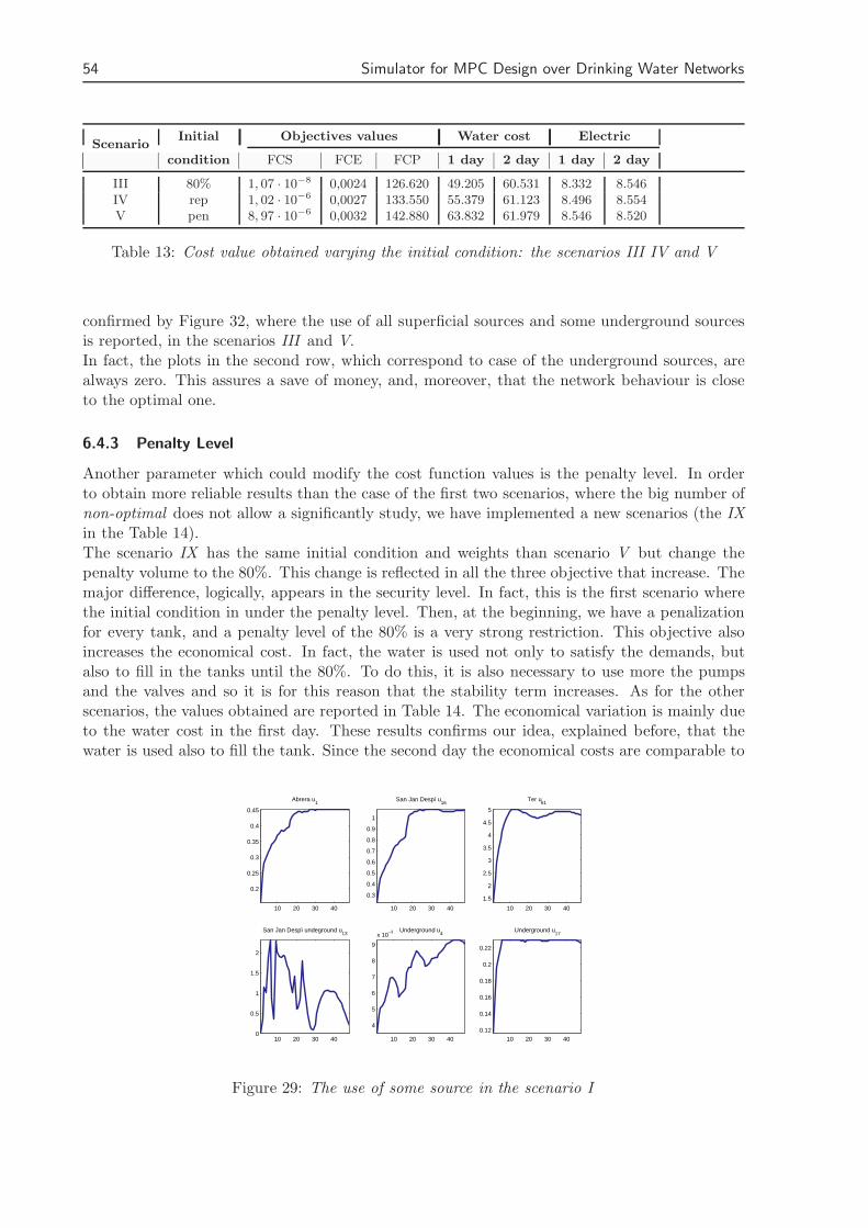
54 Simulator for MPC Design over Drinking Water Networks
ScenarioInitial Objectives values Water cost Electric
condition FCS FCE FCP 1 day 2 day 1 day 2 day
III 80% 1, 07 · 10−8 0,0024 126.620 49.205 60.531 8.332 8.546IV rep 1, 02 · 10−6 0,0027 133.550 55.379 61.123 8.496 8.554V pen 8, 97 · 10−6 0,0032 142.880 63.832 61.979 8.546 8.520
Table 13: Cost value obtained varying the initial condition: the scenarios III IV and V
confirmed by Figure 32, where the use of all superficial sources and some underground sourcesis reported, in the scenarios III and V.In fact, the plots in the second row, which correspond to case of the underground sources, arealways zero. This assures a save of money, and, moreover, that the network behaviour is closeto the optimal one.
6.4.3 Penalty Level
Another parameter which could modify the cost function values is the penalty level. In orderto obtain more reliable results than the case of the first two scenarios, where the big number ofnon-optimal does not allow a significantly study, we have implemented a new scenarios (the IXin the Table 14).The scenario IX has the same initial condition and weights than scenario V but change thepenalty volume to the 80%. This change is reflected in all the three objective that increase. Themajor difference, logically, appears in the security level. In fact, this is the first scenario wherethe initial condition in under the penalty level. Then, at the beginning, we have a penalizationfor every tank, and a penalty level of the 80% is a very strong restriction. This objective alsoincreases the economical cost. In fact, the water is used not only to satisfy the demands, butalso to fill in the tanks until the 80%. To do this, it is also necessary to use more the pumpsand the valves and so it is for this reason that the stability term increases. As for the otherscenarios, the values obtained are reported in Table 14. The economical variation is mainly dueto the water cost in the first day. These results confirms our idea, explained before, that thewater is used also to fill the tank. Since the second day the economical costs are comparable to
10 20 30 40
0.2
0.25
0.3
0.35
0.4
0.45
Abrera u1
10 20 30 40
0.3
0.4
0.5
0.6
0.7
0.8
0.9
1
San Jan Despì u16
10 20 30 40
1.5
2
2.5
3
3.5
4
4.5
5
Ter u61
10 20 30 400
0.5
1
1.5
2
San Jan Despì undeground u13
10 20 30 40
4
5
6
7
8
9
x 10−3 Underground u
4
10 20 30 400.12
0.14
0.16
0.18
0.2
0.22
Underground u17
Figure 29: The use of some source in the scenario I

Section 6 Model Predictive Control of Barcelona Water Network 55
the costs obtained in the scenario V.The Figure 33 shows the evolution of the tanks obtained in scenario IX. The convention used isthe same for the others figures, as for example in Figures 30 and 31. The different penalty levelinfluences a lot the evolution of the tanks, altouugh in this scenario, at the end of the two days,all volumes are all over the security level. In this way, we store more water which it is reflectedin the cost of the water that increases from the scenario V to the scenario IX.
6.4.4 Priority and Weights
Finally to close the study of the MPC using PLIO, the analysis regarding the change of thepriority order in the objectives is presented in order to discover the best wight choice to obtainin the minor time the best solution for all three objective. In fact, we search the best compromisebetween the objectives, taking into account that, in reality the main interest is to minimize the
10 20 30 40150
200
250
300
350
400
d125PAL x1
10 20 30 40
400
500
600
700
800
900
d110PAP x2
10 20 30 40
500
1000
1500
2000
2500
3000
3500
d115CAST x3
10 20 30 40500
1000
1500
2000
2500
3000
d80GAVi80CAS85CRO x4
10 20 30 40
2
3
4
5
6
x 104 d100FCE x
7
10 20 30 40
1000
2000
3000
4000
5000
6000
7000
x200BLL x9
(a) Evolution volume in the six tanks
10 20 30 404000
6000
8000
10000
12000
14000
16000
d130BAR x10
10 20 30 40200
400
600
800
1000
d176BARsud x11
10 20 30 40
3
4
5
6
7
8
9
x 104 d70BBEsud x
12
10 20 30 40500
1000
1500
2000
2500
3000
3500
4000
d200ALT x12
10 20 30 40
1
1.5
2
2.5
3
3.5
x 104 d100BLLnord x
13
10 20 30 40
1000
2000
3000
4000
5000
6000
7000
d200BARnord x15
(b) Evolution volume in six tanks
10 20 30 401500
2000
2500
3000
3500
4000
4500
d101MIR x16
10 20 30 40200
400
600
800
1000
1200
1400
1600
d120POM x17
10 20 30 40
2000
4000
6000
8000
10000
12000
14000
dPLANTA x5
10 20 30 40
1000
1500
2000
2500
3000
d54REL x6
10 20 30 40
2000
4000
6000
8000
10000
12000
d10COR x8
(c) Evolution volume in five tanks
Figure 30: Volume evolution obtained in the scenario III: the minimal volume needed to satisfythe demand is, as usually, in the broken red line, while in the blue line is shown the volumeevolution in the scenario III and in the broken green line the penalty volume. The last threetanks have not the minimal volume, because they are considered like a buffer.
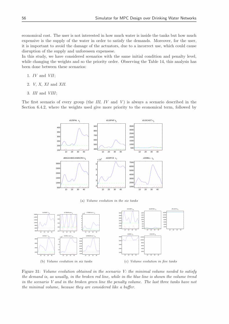
56 Simulator for MPC Design over Drinking Water Networks
economical cost. The user is not interested in how much water is inside the tanks but how muchexpensive is the supply of the water in order to satisfy the demands. Moreover, for the user,it is important to avoid the damage of the actuators, due to a incorrect use, which could causedisruption of the supply and unforeseen expensese.In this study, we have considered scenarios with the same initial condition and penalty level,while changing the weights and so the priority order. Observing the Table 14, this analysis hasbeen done between these scenarios:
1. IV and VII ;
2. V, X, XI and XII.
3. III and VIII ;
The first scenario of every group (the III, IV and V ) is always a scenario described in theSection 6.4.2, where the weights used give more priority to the economical term, followed by
10 20 30 40150
200
250
300
350
400
d125PAL x1
10 20 30 40400
500
600
700
800
900
d110PAP x2
10 20 30 40
500
1000
1500
2000
2500
3000
3500
d115CAST x3
10 20 30 40500
1000
1500
2000
2500
3000
d80GAVi80CAS85CRO x4
10 20 30 40
2
3
4
5
6
x 104 d100FCE x
7
10 20 30 40
1000
2000
3000
4000
5000
6000
7000
x200BLL x9
(a) Volume evolution in the six tanks
10 20 30 404000
6000
8000
10000
12000
14000
16000
d130BAR x10
10 20 30 40200
400
600
800
1000
d176BARsud x11
10 20 30 40
3
4
5
6
7
8
9
x 104 d70BBEsud x
12
10 20 30 40
1000
2000
3000
4000
d200ALT x12
10 20 30 40
1
1.5
2
2.5
3
3.5
x 104 d100BLLnord x
13
10 20 30 40
1000
2000
3000
4000
5000
6000
7000
d200BARnord x15
(b) Volume evolution in six tanks
10 20 30 401500
2000
2500
3000
3500
4000
4500
d101MIR x16
10 20 30 40200
400
600
800
1000
1200
1400
1600
d120POM x17
10 20 30 40
2000
4000
6000
8000
10000
12000
14000
dPLANTA x5
10 20 30 40
1000
1500
2000
2500
3000
d54REL x6
10 20 30 40
2000
4000
6000
8000
10000
12000
d10COR x8
(c) Volume evolution in five tanks
Figure 31: Volume evolution obtained in the scenario V: the minimal volume needed to satisfythe demand is, as usually, in the broken red line, while in the blue line is shown the volume trendin the scenario V and in the broken green line the penalty volume. The last three tanks have notthe minimal volume, because they are considered like a buffer.

Section 6 Model Predictive Control of Barcelona Water Network 57
10 20 30 40
0.01
0.015
0.02
0.025
0.03
Abrera u1
10 20 30 401.7
1.8
1.9
2
2.1
2.2
2.3
2.4
San Jan Despì u16
10 20 30 40
1
2
3
4
5
Ter u61
10 20 30 40−0.5
0
0.5
San Jan Despì undeground u13
10 20 30 40−0.5
0
0.5
Underground u4
10 20 30 40−0.5
0
0.5
Underground u17
(a) The use of some source in the scenario III
10 20 30 40
0.022
0.024
0.026
0.028
0.03
0.032
0.034
0.036
Abrera u1
10 20 30 401.8
1.9
2
2.1
2.2
2.3
2.4
2.5
San Jan Despì u16
10 20 30 40
2.5
3
3.5
4
4.5
5
5.5
6
Ter u61
10 20 30 40−0.5
0
0.5
San Jan Despì undeground u13
10 20 30 40−0.5
0
0.5
Underground u4
10 20 30 40−0.5
0
0.5
Underground u17
(b) The use of some source in the scenario V
Figure 32: The use of some source in the scenarios III and V
security and, at the end, by the stability.In the first group, the priority order has been maintained and it has been changed only theweight values. The values obtained are very similar what allows to state that without changingthe priority order the values of the weights are not very important.The real interesting study is represented by the other two comparisons where changing theweights is also changed the priority order. As it is reported in the Table 14 at the beginningin the scenario X, we have exchanged the weights between the penalty and the stability termmaintaining the economical cost as the highest priority.Notice from Figure 34 that weighting less the security term, the MPC strategy is more riskysince the tank evolution goes more often under the penalty level. This behaviour could generatein some particular scenarios some infeasibility. According to these plots, the value obtained com-puting the security level, which represent the risk in the tank volume, is the biggest between allscenarios presented in Table 14. The economical cost, instead, decreases as well as the stabilityterm. In particular, the cost of the water decreases, since in this case, rarely, useless water isstored in the tanks.In the comparison between the scenario V and the scenarios XI and XII, as well as betweenthe scenarios III and VIII, we have tried to consider the economical cost as the less importantterm in the cost function. The scenarios XI and VIII use the same combination of the weightswith a different initial condition, while the scenario XII use weights scaled in a different way.In these three scenarios, we have obtained an incredible increment of the economical cost, in allits components, without obtaining a significant improvement in the others terms. Therefore, wecould state that the economical cost must have the most important role in the cost function. Inthis case, it is not very evident, also, the dependence on the initial conditions in the water cost.Table 14 (the names are in the column Scen) reports, for every scenarios, the values of the allterm in the cost function and weights, highlighting, moreover, the difference cost obtained inthe two different days. The scenario VI, that has not been already explained, has been imple-mented to try to emphasise the economical cost, and considering with a very small weight theother term. The value obtained is not very relevant in terms of improvement in the economicalcost. On the contrary, a value bigger is obtained compared to the one obtained in the scenarioIV. The initial volume, called rep*, it has been obtained after a simulation long 72 iterationwith the same weights respect the scenarios VI. This choice, in these particular scenarios, ismore repetitive than that obtained in the case IV. Moreover, the other terms are increased a bitrespect with the other scenarios.

58 Simulator for MPC Design over Drinking Water Networks
6.5 Results obtained by MPC Controller
In this section, another possible interface of the simulator developed in the Chapter 5 is pre-sented. It shows that the simulator is a versatile tool, that it is able to obtain relevant resultsusing whatever controller.In particular, this section deals with the results obtained, in term of cost function, using thecentralized and decentralized MPC controller developed in the Matlabr described in [7]. Inthe report [7], an implementation of the centralized MPC for the Barcelona water network ispresented, and, moreover, an implementation of a decentralized MPC control which allows toobtain good results, diminishing a lot the computation time, applying the control to three sub-system of the network. In the last case, the computational time is almost reduced to the halfwith respect to that one needed by the centralized controller. These two controllers have thesame cost function, which, as is explained in the Section 6.2, is computed in a different wayrespect in the PLIO tool, regarding the security term. Moreover, the controller, by now, does
10 20 30 40150
200
250
300
350
400
d125PAL x1
10 20 30 40
400
500
600
700
800
900
d110PAP x2
10 20 30 40
500
1000
1500
2000
2500
3000
3500
d115CAST x3
10 20 30 40500
1000
1500
2000
2500
3000
d80GAVi80CAS85CRO x4
10 20 30 40
2
3
4
5
6
x 104 d100FCE x
7
10 20 30 40
1000
2000
3000
4000
5000
6000
7000
x200BLL x9
(a) Volume evolution in six tanks
10 20 30 404000
6000
8000
10000
12000
14000
16000
d130BAR x10
10 20 30 40200
400
600
800
1000
d176BARsud x11
10 20 30 40
3
4
5
6
7
8
9
x 104 d70BBEsud x
12
10 20 30 40500
1000
1500
2000
2500
3000
3500
4000
d200ALT x12
10 20 30 40
1
1.5
2
2.5
3
3.5
x 104 d100BLLnord x
13
10 20 30 40
1000
2000
3000
4000
5000
6000
7000
d200BARnord x15
(b) Volume evolution in six tanks
10 20 30 401500
2000
2500
3000
3500
4000
4500
d101MIR x16
10 20 30 40200
400
600
800
1000
1200
1400
1600
d120POM x17
10 20 30 40
2000
4000
6000
8000
10000
12000
14000
dPLANTA x5
10 20 30 40
1000
1500
2000
2500
3000
d54REL x6
10 20 30 40
2000
4000
6000
8000
10000
12000
d10COR x8
(c) Volume evolution in five tanks
Figure 33: Volume evolution obtained in the scenario IX: the minimal volume needed to satisfythe demand is, as usually, in the broken red line, while in the blue line is shown the volumeevolution in the scenario IX and in the broken green line the penalty volume. The last threetanks have not the minimal volume, because they are considered like a buffer.

Section 6 Model Predictive Control of Barcelona Water Network 59
10 20 30 40150
200
250
300
350
400
d125PAL x1
10 20 30 40
400
500
600
700
800
900
d110PAP x2
10 20 30 40
500
1000
1500
2000
2500
3000
3500
d115CAST x3
10 20 30 40500
1000
1500
2000
2500
3000
d80GAVi80CAS85CRO x4
10 20 30 40
2000
4000
6000
8000
10000
12000
14000
dPLANTA x5
10 20 30 40
1000
1500
2000
2500
3000
d54REL x6
(a) Volume evolution in the first six tanks (from x1 to x6)
10 20 30 40
2
3
4
5
6
x 104 d100FCE x
7
10 20 30 40
2000
4000
6000
8000
10000
d10COR x8
10 20 30 40
1000
2000
3000
4000
5000
6000
7000
d200BLL x9
10 20 30 404000
6000
8000
10000
12000
14000
16000
d130BAR x10
10 20 30 40200
400
600
800
1000
d176BARsud x11
10 20 30 40
3
4
5
6
7
8
9
x 104 d70BBEsud x
12
(b) Volume evolution in six tanks (from x7 to x12)
10 20 30 40500
1000
1500
2000
2500
3000
3500
4000
d200ALT x13
10 20 30 40
1
1.5
2
2.5
3
3.5
x 104 d100BLLnord x
14
10 20 30 40
1000
2000
3000
4000
5000
6000
7000
d200BARnord x15
10 20 30 401500
2000
2500
3000
3500
4000
4500
d101MIR x16
10 20 30 40200
400
600
800
1000
1200
1400
1600
d120POM x17
(c) Trend volume in five tanks (from x13 to x17)
Figure 34: Volume evolution obtained in the scenario X: in the blue-green line is shown thevolume trend in the scenario X and in the broken red line the penalty volume.
ScenPen Init Objectives weights Objectives values Water cost Electric
vol vol FCS FCE FCP FCS FCE FCP 1 day 2 day 1 day 2 day
I 80% 80% 1 1 0 0, 0164 0,0035 174.460 83.789 75.420 7.926 7.323II +20% 80% 1 0,1 0 3, 01 · 10−4 0,0024 179.450 68.898 75.420 7.926 7.323III +20% 80% 10 0,1 100 1, 07 · 10−8 0,0024 126.620 49.205 60.531 8.332 8.546IV +20% rep 10 0,1 100 1, 02 · 10−6 0,0027 133.550 55.379 61.123 8.496 8.554V +20% +20% 10 0,1 100 8, 97 · 10−6 0,0032 142.880 63.832 61.979 8.546 8.520VI +20% rep* 1 0,01 107 0,0180 0,0122 135.100 57.845 62.093 8.086 8.079VII +20% rep 10 100 104 8, 27 · 10−4 0,0021 127.370 50.733 59.491 8.423 8.724VIII +20% 80% 1.000 100 0.1 8, 26 · 10−5 0,0027 251.890 108.350 117.840 12.704 13.091IX 80% +20% 10 0.1 100 0,0160 0,0122 152.370 74.776 59.842 9.263 8.490X +20% +20% 0.1 10 100 0,0488 0,021 134.140 57.504 59.249 8.003 9.386XI +20% +20% 1.000 100 0.1 8, 87 · 10−5 0,0027 251.980 108.350 117.840 12.704 13.091XII +20% +20% 100 10 0.1 8, 91 · 10−5 0,0026 253.260 111.320 116.350 12.849 12.738
Table 14: Summary of cost function values in different scenarios with different weights obtainedwith PLIO tool.

60 Simulator for MPC Design over Drinking Water Networks
SimPen Cen/ Weights Objectives values Water cost Electric
vol Dec FCS FCE FCS FCE FCP 1 day 2 day 1 day 2 day
I 80% cent 1 19,4981 48,5806
220.080 140.030 90.531 13.108 12.411(0,0116) (0,0166)
II 80% cent 1 0,19,0197 48,5207
219.730 104.060 90.237 13.071 12.362(0,0111) (0,0166)
III γ cent 1 147,0024 27,002
197.850 85.466 89.923 11.975 12.487(0,0576) (0,0092)
IV γ cent 1 0,147,7435 26,6522
199.120 82.242 89.759 11.815 12.307(0,0585) (0,0091)
I 80% dec 1 19,8410 50,1138
223.490 106.570 91.252 13.240 12.434(0,0121) (0,0171)
II 80% dec 1 0,19,4317 49,6723
223.900 106.710 91.465 13.264 12.462(0,0116) (0,0170)
III γ dec 1 147,0877 29,0785
200.210 85.374 90.445 11.950 12.437(0,0577) (0,0099)
IV γ dec 1 0,148,6998 28,7983
200.430 85.490 90.556 11.957 12.427(0,0597) (0,0098)
Table 15: Summary of cost function values in different scenarios with different weights.
not consider the economical term into the cost function. However, the simulator could computethe value for the economical term, and computes the cost. In Table 15 the values, computedusing the Simulinkr model, regarding the term in the cost function are reported. Eight simu-lation have been done. In particular, four using the centralized and four using the decentralized.For both controllers the weights chosen for the security and the stability term are in the firstsimulation one and one, while in the second one and zero point one. In all the simulations theinitial condition is always the same: the 50% of the maximal volume, for this reason it is notreported in the table. The penalty volumes used are two: the 80% and the value reported in thefirst column in Table 12, which represents the picks of the minimal volume necessary to satisfythe demands, this choice in Table 14 is represented with the letter γ. In Table 15, the totalvalue obtained in the stability and security term is also reported, in order to compare the datacoming from the centralized and decentralized in a more simply and clear way, the normalizedvalue is into the round bracket. The use of a decentralized control, which considers the networkformed by three different subsystems, causes a small worsening of every objective term.It is possible to compare the results reported in the Tables 14 and 15 only regarding the stabilityand the economical terms. Indeed, the penalty term is computed differently in PLIO and inthe control implemented in Matlabr. The results, in terms of economical cost in euros, inthe Table 15 are very big since does not considers the economical term in the optimization.These results are comparable to those obtained in the last scenarios in the Table 14, where theeconomical term does not have the main priority in the optimization. These values could beconsidered as a upper bound for the price in this network with these particular choice of theparameters.
7 Conclusions and Future Work
7.1 Conclusion
In this report two different combined works have been presented. The first aims to the imple-mentation of a simulation water network environment which can be used to evaluate the best
Section 7 Conclusions and Future Work 61
parametrization of a MPC controller of water transport network.
In particular, this environment is developed in Simulinkr/Matlabr and is able to reproducethe behaviour of a water network, and it could be interfaced with whatever controller. It repre-sents an useful tool to evaluate the performance and the operation of any controller. It allowsto show the best choice of the MPC parameters in terms of cost function. In addition, to checkif the controller satisfies all the constraints presented in the model, as the satisfaction of thedemands or the mass balances.In particular, the case of the aggregated Barcelona water network has been studied. TheSimulinkr model for the Barcelona case has been developed and it has been interfaced withPLIO tool [5] and with the centralized and decentralized MPC controllers developed in [7].
7.1.1 Analysis using PLIO Tool
The PLIO tool allows to implement a centralized controller for water networks with the sameideas of the MPC with some variations which allow to render the cost function more close to thereal request. Using this type of controller, which uses the commercial solver GAMS, we havedeveloped an MPC controller and a studied the effect of the initial conditions, penalty volumesand weights in the cost function. This analysis has been done thanks to the results obtainedfrom the simulator which allows to compute the cost function term in a straightforward way.For every of the three elements, we have obtained some conclusions, which allow us and the userin general, to understand how to tuning the MPC controller:
Penalty volume : the minimal penalty volume which manages to satisfy the demands, themain objective of the controller, is determined. The controller is optimal when thenminimal penalty volume is used. To compute this penalty volume, the minimal volumenecessary to satisfy the demands at every time in a scenario quite general has been com-puted. After, in order to obtain a constant penalty level, with a degree to security, wehave computed the picks for every tanks and added to this a 20%.
Initial condition : first of all we have noticed that the initial condition influences a lot thecost of the water network operation, in particular in the first day. Moreover, our studyhas been concentrated also to search a particular initial condition which allows to obtainthe same evolution every day, but this issue need some further investigations.
Weights : the weights study includes the importance order of both the elements and the costfunction objectives.Concerning the elements we have decided to weight more the valve which follows a source.Indeed the actuators used during the water treatments need a major stability in the set-point respect with the others.The objectives of the cost function considered in this study are three: the stability of theactuators, the economical price and the security level in the tanks. We have found out,through the simulations reported in the Table 14, that the economical term have to bethe main important objective in the cost function in order to obtain a minimal economicalcost, and so to save money. The other two weights could be decided freely according bythe particular situation considered.

62 Simulator for MPC Design over Drinking Water Networks
7.1.2 Analysis using MPC Controller
The other part of the study is concentrated on the interfacing of the simulator with the con-troller developed in the [7]. Also in this case, several different simulations has been realizedwhich allow to highlight the different performances obtained with a centralized and a decen-tralized controller. These simulations are reported in Table 15. This type of controller doesnot include the economical term, and it is the cause of the big cost obtained, comparing tothat obtained through PLIO when the economical term is the term with the minor importance.Moreover, the security term it is computed in a different way.
All these analysis proved the importance of a predictive controller in this water network. Thepredictive controller could be of various types, with a correct parametrization, it manages alwaysto obtain a better solution with respect to that obtained with a manual regulation.
7.2 Future Works
This study has been developed for the aggregated model of the Barcelona water network. Thesame study should be made for the complete water network reported in the Figure 5, where,although the number of the variables increase a lot as well as the complexity, the strategy usedin the development of the simulator and in the parameters modelling of the network remainsthe same.To make the model, and the simulation, more realistic and useful for the daily use it could benecessary using several parameters with a degree of major accuracy, or in general with severalcharacteristics that allow to reproduce the reality. In particular the study would be concen-trated in the realization of a controller which should have the security volume in the tank notas a constant level but it could be an evolution which respects the profile of the demand intime. It could be something similar to that showed in the Figure 27 in the broken red line,but this figure represents the demands and the volume with a particular scenario. Instead, itwould be important to use an universal profile, valid for every simulation. In addition, it wouldbe interesting to define a different profile for every day of the week, which reflects the differ-ences between the day type (working or non working days). In order to obtain a standard andpredictable behaviour of the network the study concerning the search of a repetitive˝ initialcondition should be continued.Another thing that is missing in the model is the consideration of the pressure effect in thewater network, in order to study a real hydraulic model with its constraints. For the moment,the pressure constraints have been considered regulating the flow in the actuators, but it wouldbe necessary a more complex model.
The simulator developed would be applied to a whatever water network, but to simplify thebuilding it would be required an automatic generation of the blocks through a script file. Theconnections would be created, directly, since the state space description (the matrix A, B, C andD) generated and used in the MPC controller. At this point, it should be developed a downrighttoolbox for the hydraulic model. This toolbox would be included a different block for everydifferent elements that could be present in a water network. Generating the Simulinkr networkin an automatic method the building of a simulator of a water network become simply and fast.Moreover, this simulator should be closed in a feedback loop with the controller, in order toget a evaluation of the performance on-line instant by instant, which allows to influence thecontroller decision at the next step.

REFERENCES 63
References
[1] Manual de Usario PLIO, v12 edition, 06 2005.
[2] M.A. Brdys and B. Ulanicki. Operational control of water systems: structures, algorithms,and applications. Prentice Hall, 1994.
[3] E.F. Camacho and C. Bordons. Model Predictive Control. 1999.
[4] EF Camacho and C. Bordons. Model Predictive Control. Springer, 2004.
[5] G. Cembrano, J. Quevedo, V. Puig, R. Perez, and J. Figueras. Predictive Optimal controlof water supply and distribution in Santiago-Chile.
[6] G. Cembrano, G. Wells, J. Quevedo, R. Prez, and R. Argelaguet. Optimal control of awater distribution network in a supervisory control system. Control Engineering Practice,8(10):1177–1188, 2000.
[7] V. Fambrini and C. Ocampo-Martinez. Modelling and Decentralized Model PredictiveControl of Drinking Water Networks. Technical report, Institut de Robotica i InformaticaIndustrial, CSIC-UPC, 2009.
[8] RW Jeppson. Analysis of flow in pipe networks; R. Ann Arbor Science Publishers, AnnArbor, New York, 6th edition, 1983.
[9] R.W. Johnson. The handbook of fluid dynamics. Springer, 1998.
[10] J.M. Maciejowski. Predictive Control: With Constraints. Prentice Hall, 2002.
[11] E. Mosca and P. Optimal. Adaptive Control. PrenticeHall, Englewood Clis, NY, 1995.
[12] V. Nitivattananon, E.C. Sadowski, and R.G. Quimpo. Optimization of water supply systemoperation. Journal of Water Resources Planning and Management, 122(5):374–384, 1996.
[13] Carlos A. Ocampo-Martinez. Model Predictive Control of Complex Systems including FaultTolerance Capabilities: Application to Sewer Networks. PhD thesis, Automatic ControlDepartment (ESAII) Technical University of Catalonia, April 2007.
[14] Sociedad general de Agua de Barcelona, S.A. (AGBAR), Passeig de SAnt Joan, 39-43.Sistema Automtico de Explotacin (SAE), March 1999.
[15] M.Y. Tu, T.C.T. Frank, W.G.Y. William, et al. Optimization of water distribution andwater quality by hybrid genetic algorithm. Journal of water resources planning and man-agement, 131:431, 2005.
[16] K.S. Westphal, R.M. Vogel, P. Kirshen, and S.C. Chapra. Decision support system for adap-tive water supply management. Journal of Water Resources Planning and Management,129(3):165–177, 2003.

64 REFERENCES


IRI reports
This report is in the series of IRI technical reports.All IRI technical reports are available for download at the IRI websitehttp://www-iri.upc.edu.