
Development of a High Speed Data Acquisition System for ...
168
Georgia Southern University Digital Commons@Georgia Southern Electronic Theses and Dissertations Graduate Studies, Jack N. Averitt College of Summer 2011 Development of a High Speed Data Acquisition System for Spark Ignition Engine Cory Levette Griswold Follow this and additional works at: https://digitalcommons.georgiasouthern.edu/etd Recommended Citation Griswold, Cory Levette, "Development of a High Speed Data Acquisition System for Spark Ignition Engine" (2011). Electronic Theses and Dissertations. 775. https://digitalcommons.georgiasouthern.edu/etd/775 This thesis (open access) is brought to you for free and open access by the Graduate Studies, Jack N. Averitt College of at Digital Commons@Georgia Southern. It has been accepted for inclusion in Electronic Theses and Dissertations by an authorized administrator of Digital Commons@Georgia Southern. For more information, please contact [email protected].
-
Upload
khangminh22 -
Category
Documents
-
view
1 -
download
0
Transcript of Development of a High Speed Data Acquisition System for ...
Georgia Southern University
Digital Commons@Georgia Southern
Electronic Theses and Dissertations Graduate Studies, Jack N. Averitt College of
Summer 2011
Development of a High Speed Data Acquisition System for Spark Ignition Engine Cory Levette Griswold
Follow this and additional works at: https://digitalcommons.georgiasouthern.edu/etd
Recommended Citation Griswold, Cory Levette, "Development of a High Speed Data Acquisition System for Spark Ignition Engine" (2011). Electronic Theses and Dissertations. 775. https://digitalcommons.georgiasouthern.edu/etd/775
This thesis (open access) is brought to you for free and open access by the Graduate Studies, Jack N. Averitt College of at Digital Commons@Georgia Southern. It has been accepted for inclusion in Electronic Theses and Dissertations by an authorized administrator of Digital Commons@Georgia Southern. For more information, please contact [email protected].

1
DEVELOPMENT OF A HIGH SPEED DATA ACQUISITION SYSTEM FOR SPARK
IGNITION ENGINE
by
CORY GRISWOLD
(Under the Direction of Frank Goforth)
ABSTRACT
Full engine control can only be accomplished with multi-input multi-output (MIMO)
control system requiring measurement of variables for which no sensor/instrument is yet
available in the Renewable Energy and Engines Laboratory, therefore a less detailed single input
single output (SISO) engine model is developed. To develop the engine controller a model of
the engine had to first be determined. Known Discrete-Event and Mean-Value models were the
first choice, but could not be utilized because of the nature of the single cylinder intake manifold
pressure. Therefore an engine model based on experimental data had to be developed. Using
Matlab/ Simulink, xPC Target and data acquisition hardware a model of the single cylinder
engine was developed. These models were developed by taking measurements of the engines
dynamics such as engine speed, crank angle, air mass intake, spark timing, injection timing, and
intake temperatures at different engine speed set points while running gasoline and then a
gasoline and ethanol mix (E85). From which experimental coefficients were determined
necessary for the model.
INDEX WORDS: Spark Ignition, SI Engine, High Speed Data Acquisition,
Single Cylinder Engine
2
DEVELOPMENT OF A HIGH SPEED DATA ACQUISITION SYSTEM FOR SPARK
IGNITION ENGINE
by
CORY GRISWOLD
B.S., Georgia Southern University, 2008
A Thesis Submitted to the Graduate Faculty of Georgia Southern University in Partial
Fulfillment
of the Requirements of the Degree
MASTER OF SCIENCE
STATESBORO, GEORGIA
2011

3
© 2011
CORY GRISWOLD
All Rights Reserved

4
DEVELOPMENT OF A HIGH SPEED DATA ACQUISITION SYSTEM FOR SPARK
IGNITION ENGINE
by
CORY LEVETTE GRISWOLD
Major Professor: Frank Goforth
Committee: Valentin Soloiu
Yan Wu
Electronic Version Approved:
July 2011

5
ACKNOWLEDGMENTS
I would like to thank my Mom and Dad for support through my college career and especially
graduate school. Also thank my thesis advisor Dr. Goforth for coaching me through the thesis
process. Dr. Soloiu for his insight and allowing me to work inside the Renewable Energy
Laboratory. Last, the many other Georgia Southern Applied Engineering Graduate Students for
their help and knowledge.
6
TABLE OF CONTENTS
Page
ACKNOWLEDGMENTS ...............................................................................................................5
LIST OF TABLES ...........................................................................................................................9
LIST OF FIGURES .......................................................................................................................11
CHAPTER .....................................................................................................................................12
1 INTRODUCTION ..................................................................................................................13
1.1 Nomenclature ..................................................................................................................15
2 LITERATURE REVIEW .......................................................................................................17
2.1 Throttle Body/ Intake Manifold/ Air /Fuel Mixture Models and Engine .......................19
Quasi-Steady ........................................................................................................19 2.1.1
Filling and Emptying Model ................................................................................20 2.1.2
Gas Dynamic Models ...........................................................................................22 2.1.3
Extensions of Heywood’s Intake and Air/ Fuel Mixing Models .........................24 2.1.4
2.2 In-Cylinder Combustion Models ....................................................................................30
Thermodynamic/ In-Cylinder Combustion Models .............................................30 2.2.1
Spark-Ignition (SI) In-Cylinder Combustion Models ..........................................33 2.2.2
Fluid-Mechanic Model .........................................................................................34 2.2.3
Extension to Heywood’s In-Cylinder Combustion Models .................................35 2.2.4
2.2.4.1 Torque Production/ Combustion ......................................................................36
2.2.4.1.1 The Willan’s Approximation: .......................................................................36
2.2.4.1.2 Other Torque Models ....................................................................................38
2.2.4.1.3 Other Variations ............................................................................................42
3 ENGINE MODELING ...........................................................................................................44
3.1 Intake Manifold Dynamics ..............................................................................................44
3.2 Engine Air Mass Flow ....................................................................................................49
4 METHODOLOGY .................................................................................................................55
4.1 LabView for Data Acquisition ........................................................................................55
LabView Limit Testing ........................................................................................59 4.1.1
4.1.1.1 Sine Wave .........................................................................................................59
4.1.1.2 Quadrature Encoder ..........................................................................................63
4.1.1.3 Encoder Signal .................................................................................................64
4.1.1.4 LabView with Rotary Encoder .........................................................................64
4.1.1.5 Encoder Signal Testing ....................................................................................68

7
4.2 The Switch to MatLab/Simulink/xPC Target .................................................................70
Analog and Digital Signals ..................................................................................77 4.2.1
Target Machine Benchmark .................................................................................79 4.2.2
DC Motor and Offline Testing .............................................................................79 4.2.3
Building Stands and Assembly ............................................................................79 4.2.4
DC Motor Setup Issues ........................................................................................81 4.2.5
4.3 Preparation for System Testing .......................................................................................81
Control of DC Motor ............................................................................................82 4.3.1
4.4 Sensors ............................................................................................................................86
Crankshaft Rotary Encoder ..................................................................................86 4.4.1
Flow System Measurements ................................................................................87 4.4.2
Mass Air Flow ......................................................................................................89 4.4.3
Throttle Position Sensor (TPS) ............................................................................90 4.4.4
Injection Sampling Circuit ...................................................................................91 4.4.5
Second Injector Sampling Circuit ........................................................................94 4.4.6
Thermocouple ......................................................................................................95 4.4.7
Thermocouple Data Acquisition ..........................................................................96 4.4.8
Wideband O2 Sensor ............................................................................................97 4.4.9
4.5 Signal Conditioning and Sensors ....................................................................................98
First Attempt Encoder Dividers ...........................................................................98 4.5.1
Encoder Signal Issues ..........................................................................................99 4.5.2
Second Encoder Divider ....................................................................................101 4.5.3
Wiring of Signals ...............................................................................................101 4.5.4
Inductive Sensor .................................................................................................101 4.5.5
Preliminary Data from Inductive Clamp ............................................................104 4.5.6
Single Cable Connection ....................................................................................105 4.5.7
4.6 MatLab Code and System Status ..................................................................................105
5 ENGINE MAPS ...................................................................................................................107
5.1 Fuel Injection ................................................................................................................107
5.2 Spark Timing .................................................................................................................107
6 EXPERIMENTAL DATA ...................................................................................................109
7 RESULTS .............................................................................................................................118
8 CONCLUSION ....................................................................................................................128
REFERENCES ............................................................................................................................129

8
APPENDICES .............................................................................................................................132
Appendix A LINEARIZATION ..............................................................................................132
Appendix B SIGNAL GATHERING CODE ..........................................................................142
Appendix C EXPERIMENTAL DATA ...................................................................................153
9
LIST OF TABLES
Table 1.1: Small SI Non-Handheld Engine Exhaust Emission Standards .................................... 13
Table 4.1: Test Engine Characteristics ......................................................................................... 55
Table 4.2: List of Sensors, Measured Variables and Expected Maximum Frequency of Change 56
Table 4.3: LabView Settings for Quadrature Encoder Card ......................................................... 66
Table 4.4: PCI-QUAD04 settings in MatLab ............................................................................... 75
Table 4.5: Host and Target Computer System Properties ............................................................ 76
Table 4.6: Maximum Input Frequency of PCI Data Acquisition Cards ....................................... 76
Table 4.7: Settings for Analog Input for PCI-1602/16 ................................................................. 78
Table 4.8: Settings for Digital Input of PCI-1602/16 for Injector Timing ................................... 78
Table 4.9: Settings for Digital Input of PCI-1602/16 for Spark Timing ...................................... 78
Table 4.10: Sensors and Maximum Frequency of Measure ......................................................... 86
Table 4.11: Results of Dividing Encoder Counts on Resolution and Frequency ......................... 98
Table 4.12: Serial Connection Position ...................................................................................... 105
Table 7.1: Steady State Coefficients for Briggs and Stratton Engine ......................................... 120
Table 7.2: Gasoline: Average Injection Angle During Intake Stroke ......................................... 124
Table 7.3: Gasoline: Average Ignition Angle During Expansion Stroke ................................... 125
Table 7.4: Gasoline: Average Low Injection Duration ............................................................... 125
Table 7.5: Gasoline: Average High Injection Duration .............................................................. 125
Table 7.6: E85: Average Injection Angle ................................................................................... 126
Table 7.7: E85: Average Ignition Angle ..................................................................................... 126
Table 7.8: E85: High Average: Injection Duration in Seconds .................................................. 126
Table 7.9: E85: Low Average: Injection Duration in Seconds ................................................... 127
Table C.1: E85- Mass Air Flow and Intake Manifold Pressure .................................................. 153
Table C.2: Gasoline-Mass Air Flow and Intake Manifold Pressure ........................................... 154
Table C.3: Gasoline: Minimum Injection Angle ........................................................................ 161
Table C.4: Gasoline: Maximum Injection Angle ........................................................................ 161
Table C.5: Gasoline: Average Ignition Angle ............................................................................ 162
Table C.6: Gasoline: Maximum Ignition Angle ......................................................................... 162
Table C.7: Gasoline: Maximum Injection Angle ........................................................................ 162
Table C.8: Gasoline: Average Injection Angle ........................................................................... 162
Table C.9: Gasoline: Minimum Injection Angle ........................................................................ 163
Table C.10: Gasoline: Minimum Ignition Angle ........................................................................ 163
Table C.11: Gasoline: Maximum Ignition Angle ....................................................................... 163
Table C.12: Gasoline: Minimum Ignition Angle ........................................................................ 163
Table C.13: Gasoline: Minimum Low Injection Duration .......................................................... 163
Table C.14: Gasoline: Maximum Low Injection Duration ......................................................... 164
Table C.15: Gasoline: Maximum High Injection Duration ........................................................ 164
Table C.16: Gasoline: Minimum High Injection Duration ......................................................... 164
Table C.17: E85: Minimum Ignition Angle ................................................................................ 164
Table C.18: E85: Maximum Injection Angle ............................................................................. 164
Table C.19: E85: Minimum Injection Angle .............................................................................. 165
Table C.20: E85: Minimum Ignition Angle ................................................................................ 165
Table C.21: E85: Maximum Ignition Angle ............................................................................... 165
Table C.22: E85: Average Injection Angle ................................................................................. 165
Table C.23: E85: Maximum Injection Angle ............................................................................. 165
10
Table C.24: E85: Minimum Injection Angle .............................................................................. 166
Table C.25: E85: Average Ignition Angle .................................................................................. 166
Table C.26: E85: Maximum Ignition Angle ............................................................................... 166
Table C.27: E85: Minimum Ignition Angle ................................................................................ 166
Table C.28: E85: High Minimum: Injection Duration................................................................ 166
Table C.29: E85: High Maximum: Injection Duration ............................................................... 167
Table C.30: E85: Low Minimum: Injection Duration ................................................................ 167
Table C.31: E85: Low Maximum: Injection Duration ................................................................ 167
11
LIST OF FIGURES
Page
Figure 2.1: Engine Idle Speed System (Guzzella & Onder, 2004) ................................................18
Figure 4.1: Diagram for Hardware Setup with LabView ..............................................................58
Figure 4.2: Screen of LabView Program for Analog Input ...........................................................62
Figure 4.3: Front Panel of LabView Analog Input Program .........................................................63
Figure 4.4: Frame 0 LabView Block Diagram Code for Quadrature Encoder ..............................68
Figure 4.5: Frame 1 LabView Block Diagram Code for Quadrature Encoder ..............................69
Figure 4.6: Frame 2 LabView Block Diagram Code for Quadrature Encoder ..............................69
Figure 4.7: LabView Front Panel for Encoder Program ................................................................70
Figure 4.8: Diagram for Hardware Setup with for xPC Target .....................................................73
Figure 4.9: SimuLink Screen with xPC Target Blocks .................................................................74
Figure 4.10: Stand for Mounting Rotary Encoder to DC Motor Shaft ..........................................83
Figure 4.11: Top View of DC Motor with VR Sensor ..................................................................83
Figure 4.12: Stand for VR Sensor ..................................................................................................84
Figure 4.13: Output Tachometer Voltage versus NECO DC Motor Speed ..................................84
Figure 4.14: Plotted data of encoder position versus VR sensor ...................................................85
Figure 4.15: Laminar Flowmeter Analog Output (Meriam,2010 ) ................................................88
Figure 4.16: Meriam Laminar Flow System (LFS) (Meriam, 2010) .............................................89
Figure 4.17: Mariam Laminar Flow Element (LFE) Z50MC2-2 (Meriam, 2010) ........................89
Figure 4.18: Engine Throttle Positioning Sensor ..........................................................................90
Figure 4.19: Voltage versus Throttle Angle for TPS .....................................................................91
Figure 4.20: MOSFET Injector Sampling Circuit .........................................................................93
Figure 4.21: The Encoder Signal and Injector using First Injector Circuit ...................................94
Figure 4.22: Circuit for inverting injector signal ...........................................................................95
Figure 4.23: Wideband Air to Fuel Ratio Sensor (Bosch, n.d.) .....................................................97
Figure 4.24: Banebots Encoder Dividers to PCI-QUAD04 ...........................................................99
Figure 4.25: Inductive Clamp Signal Conditioning Circuit .........................................................103
Figure 4.26: Simulink Block for Injector Signal .........................................................................103
Figure 4.27: Inductive Clamp Signal versus Time ......................................................................104
Figure 4.28: Spark Signal versus Crank Angle ...........................................................................104
Figure 6.1: Gasoline: 1200 rpms at 0 Percent Open Throttle ......................................................111
Figure 6.2: Gasoline: 1200 rpms at 5 Percent Open Throttle. .....................................................111
Figure 6.3: Gasoline: 1200 rpms at 10 Percent Open Throttle. ...................................................112
Figure 6.4: Gasoline: 1200 rpms at 15 Percent Open Throttle. ...................................................112
Figure 6.5: Gasoline: 1200 rpms at 20 Percent Open Throttle. ...................................................113
Figure 6.6: E85: 1200 rpms at 0 Percent Open Throttle. .............................................................113
Figure 6.7: E85: 1200 rpms at 5 Percent Open Throttle. .............................................................114
Figure 6.8: E85: 1200 rpms at 10 Percent Open Throttle. ...........................................................114
Figure 6.9: E85: 1200 rpms at 15 Percent Open Throttle. ...........................................................115
Figure 6.10: E85: 1200 rpms at 20 Percent Open Throttle. .........................................................115
Figure 6.11: Gasoline: Contour Plot Engine Speed vs. Percentage of Throttle Opening and Intake
Mass Air Flow ............................................................................................................................ 116
Figure 6.12: E85: Contour Plot Engine Speed vs. Percentage of Throttle Opening and Intake
Mass Air Flow............................................................................................................................. 117
Figure 7.1: Estimation of Intake Air Mass Flow of Briggs and Stratton Engine ........................118
12
Figure 7.2: E85 Adjusted Predicted Intake Mass Air Flow .........................................................119
Figure 7.3: Gasoline Adjusted Predicted Intake Mass Air Flow .................................................119
Figure 7.4: Throttle Angle Signal Versus Time at 1200 rpm ......................................................121
Figure 7.5: Throttle Angle Signal Versus Time at 2400 rpm ......................................................121
Figure 7.6: Throttle Angle Signal Versus Crank Angle at 1200 rpm and 0% Throttle Opening 122
Figure 7.7: Throttle Angle Signal Versus Crank Angle at 2400 rpm and 20% Throttle Opening
..................................................................................................................................................... 123
Figure C.1: Mass Air Flow and 1200 rpm and 0% Throttle ........................................................155
Figure C.2: Mass Air Flow and 1200 rpm and 5% Throttle ........................................................156
Figure C.3: Mass Air Flow and 1200 rpm and 10% Throttle ......................................................156
Figure C.4: Mass Air Flow and 1200 rpm and 15% Throttle ......................................................157
Figure C.5: Mass Air Flow and 1200 rpm and 20% Throttle ......................................................157
Figure C.6: E85 Mass Air Flow and 1200 rpm and 0% Throttle ................................................158
Figure C.7: E85 Mass Air Flow and 1200 rpm and 0% Throttle ................................................159
Figure C.8: E85 Mass Air Flow and 1200 rpm and 10% Throttle ..............................................160
Figure C.9: E85 Mass Air Flow and 1200 rpm and 15% Throttle ..............................................160
Figure C.10: E85 Mass Air Flow and 1200 rpm and 20% Throttle ............................................161
CHAPTER

13
CHAPTER 1
1 INTRODUCTION
The objective of this thesis research is to develop an instrumentation system to measure
the operating characteristics of a single cylinder spark ignition fuel injection (SIFI) engine in
order to develop a mathematic model of said engine sufficient to control the engine in real time.
There are many of these small motors in use for various applications, and aspects of the motor’s
performance such as idle speed exhaust emissions and fuel efficiency can be better manipulated
by computer control. These aspects of the engine’s operations have an impact on the
environment and cost of operating these motors, however controlling such a nonlinear system
presents many challenges. The first challenge is to generate an accurate linear model that
represents the engine system.
The reason the single cylinder engine is the engine of choice for controls is because there
are millions of them and they are not very efficient in the amount of fuel it uses. The engines are
also not very clean which caused more stringent regulations on emissions being put in place by
the Environmental Protection Agency. The new regulations can be seen in Table 1.1 for non-
handheld engines.
Engine Class Model Year Model Year HC+NOx
[g/kW-hr]
COa
[g/kW-hr]
Class I (>80cc to <225cc)b 2012 10.0 610
Class II ( 225cc)a 2011 8.0 610
Table 1.1: Small SI Non-Handheld Engine Exhaust Emission Standards
a 5 g/kW-hr CO for Small SI engines powering marine generators.
bNonhandheld engines at or below 80cc will be subject to the emission standards for handheld
engines.
Environmental Protection Agency (2008)

14
These engines need to produce less pollutant emissions such as nitrogen oxide (NOx),
hydrocarbon (HC) and carbon monoxide (CO). These reductions in emissions can come from a
change in fuel from gasoline to Ethanol 85% mix (E85). Changes in the fueling map and spark
timing will be necessary.
A model of the engine must be researched, tested and then validated in order to complete
the controls task. The engine model details the engines physical parameters. There are different
models that can represent the same physical section of an engine, such as the filling and
emptying model or the wave action charge model for the air intake system. Certain assumptions
had to be made in order to simplify and generate a model that fit the needs of the research. For
example, an assumption the intake manifold is an isothermal orifice helps simplify calculations.
Not just any model would fit the criteria to effectively simulate the dynamics of the engine.
The engine model equations are comprised of engine level variables such as intake
manifold pressure and engine speed with constants that either pertains to the engine or
surrounding conditions. Some of the constant coefficients need to be found experimentally,
while some need to be pre-calculated. System identification must be performed using the
measured engine data in order to model the engine dynamics. The system identification will be
performed at idle speed for the first test with measurements of variables such as engine speed,
intake manifold pressure and intake air mass flow.
The non-linear engine model has to be linearized around several operating points. These
operating points are the engine speed and intake manifold air pressure. The resulting model will
be a linear gain schedule model in state space form.
The following constants, acronyms and variable notations will be used throughout this report.
15
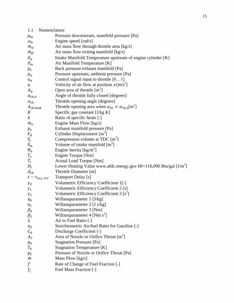
1.1 Nomenclature
Pressure downstream, manifold pressure [Pa]
Engine speed [rad/s]
Air mass flow through throttle area [kg/s]
Air mass flow exiting manifold [kg/s]
Intake Manifold Temperature upstream of engine cylinder [K]
Air Manifold Temperature [K]
Back pressure exhaust manifold [Pa]
Pressure upstream, ambient pressure [Pa]
Control signal input to throttle [0…1]
Velocity of air flow at position x [m/s2]
Open area of throttle [m2]
Angle of throttle fully closed [degrees]
Throttle opening angle [degrees]
Throttle opening area when [m2]
Specific gas constant [J/kg K]
Ratio of specific heats [-]
Engine Mass Flow [kg/s]
Exhaust manifold pressure [Pa]
Cylinder Displacement [m3]
Compression volume at TDC [m3]
Volume of intake manifold [m3]
Engine Inertia [kg/m2]
Engine Torque [Nm]
Actual Load Torque [Nm]
Lower Heating Value www.afdc.energy.gov Hl=116,090 Btu/gal [J/m3]
Throttle Diameter [m]
Transport Delay [s]
Volumetric Efficiency Coefficient 1[-]
Volumetric Efficiency Coefficient 2 [s]
Volumetric Efficiency Coefficient 3 [s2]
Willansparameter 1 [J/kg]
Willansparameter 2 [J s/kg]
Willansparameter 3 [Nm]
Willansparameter 4 [Nm s2]
Air to Fuel Ratio [-]
Stoichiometric Air/fuel Ratio for Gasoline [-]
Discharge Coefficient [-]
Area of Nozzle or Orifice Throat [m2]
Stagnation Pressure [Pa]
Stagnation Temperature [K]
Pressure of Nozzle or Orifice Throat [Pa]
Mass Flow [kg/s]
Rate of Change of Fuel Fraction [-]
Fuel Mass Fraction [-]

16
Fuel Fraction [-]
Density [kg/m3]
Volume [m3]
Total Heat Transfer Rate Across the Boundary [W]
Fuel/ Air Equivalence Ratio []
Mass flow through intake valve [kg/s]
Mass flow through exhaust valve [kg/s]
Cylinder pressure [Pa]
Connecting rode length [m]
Crank radius [m]
Crank angle [˚ or rad]
SI Effect of spark advance angle on the engine torque [-]
MBT Minimum spark advance for best brake torque [ -] Area of the piston [m
2]
Volume of cylinder [m3]
Work output of engine [J]
Number of cylinders [-]
Sound speed [m/s]
Internal Energy [J]
Friction Loss Coefficient [-]
Friction Loss Coefficient [-]
Friction Loss Coefficient [-]
Pumping Loss Coefficient [-]
Pumping Loss Coefficient [-]
N Pade Approximation Order [-]
MVM Mean Value Engine Model [-]
DEM Discrete Event Model [-]

17
CHAPTER 2
2 LITERATURE REVIEW
There have been many models created in the attempt to control the nonlinear engine
process. Previous researchers have used models to fit their control needs. For different control
strategies this portion of the thesis will outline the most commonly referenced engine models.
One very well referenced text on the internal combustion engine is Heywood’s (1988)
Internal Combustion Engine Fundamentals. Heywood gives details on real engine models that
take into account fluid dynamics, heat-transfer, thermodynamics and kinetics fundamentals, or
combinations of the four. Heywood gives details of models that simulate the engine dynamics,
such as intake and exhaust flow models, thermodynamic in-cylinder models, and fluid dynamic
models. The level of detail of these models is too complex for engine control purposes using
computers in real-time. (Heywood, 1988)
Heywood’s equations on engines start out as a basic, open thermodynamics system.
Systems that can be described in this form include the cylinder volume and the intake and
exhaust manifolds. This system can be used when the composition and state of the gas can be
assumed to be uniform and when variations of the state and composition occur over time because
of heat transfer, work transfer and mass flow across the systems boundaries. The important
equations for thermodynamic based systems are the conservation of mass and conservation of
energy; these equations use either time or crank angle as their independent variable.(J. Heywood,
1988)
Heywood defines the mass of fuel flow and the change in the fuel to air equivalence ratio,
using the equations of conservation of mass, while for the conservation of energy the first law of
thermodynamics is used. This set of equations fundamentally defines energy production of the
18
engine. The conservation of energy equations take into account the heat-transfer rate into the
system and work-transfer rate out of the system, which is defined by the position displacement
and equal to cylinder pressure times change in volume. The heat released by combustion is
defined in the energy and enthalpy terms. Heywood defines the internal energy, enthalpy and
density of the fluid as being characterized by the fluid temperature, pressure and fuel/air
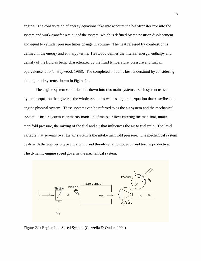
equivalence ratio (J. Heywood, 1988). The completed model is best understood by considering
the major subsystems shown in Figure 2.1.
The engine system can be broken down into two main systems. Each system uses a
dynamic equation that governs the whole system as well as algebraic equation that describes the
engine physical system. These systems can be referred to as the air system and the mechanical
system. The air system is primarily made up of mass air flow entering the manifold, intake
manifold pressure, the mixing of the fuel and air that influences the air to fuel ratio. The level
variable that governs over the air system is the intake manifold pressure. The mechanical system
deals with the engines physical dynamic and therefore its combustion and torque production.
The dynamic engine speed governs the mechanical system.
Figure 2.1: Engine Idle Speed System (Guzzella & Onder, 2004)
��𝛼 ��𝛽
𝑢𝛼
𝜗𝑚 𝑝𝛼 𝑝𝑒
Θ
𝑇𝑒
𝜆
19
2.1 Throttle Body/ Intake Manifold/ Air /Fuel Mixture Models and Engine
Heywood details three intake and exhaust flow models. These models fall into the
category of (1) quasi-steady model, (2) filling and emptying model and (3) gas dynamics model.
Each will be further explained.
Quasi-Steady 2.1.1
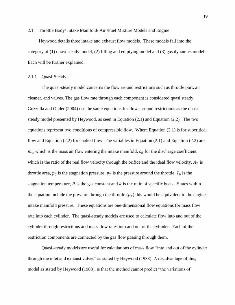
The quasi-steady model concerns the flow around restrictions such as throttle port, air
cleaner, and valves. The gas flow rate through each component is considered quasi steady.
Guzzella and Onder (2004) use the same equations for flows around restrictions as the quasi-
steady model presented by Heywood, as seen in Equation (2.1) and Equation (2.2). The two
equations represent two conditions of compressible flow. Where Equation (2.1) is for subcritical
flow and Equation (2.2) for choked flow. The variables in Equation (2.1) and Equation (2.2) are
which is the mass air flow entering the intake manifold, for the discharge coefficient
which is the ratio of the real flow velocity through the orifice and the ideal flow velocity, is
throttle area, is the stagnation pressure, is the pressure around the throttle, is the
stagnation temperature, is the gas constant and is the ratio of specific heats. States within
the equation include the pressure through the throttle ( ) this would be equivalent to the engines
intake manifold pressure. These equations are one-dimensional flow equations for mass flow
rate into each cylinder. The quasi-steady models are used to calculate flow into and out of the
cylinder through restrictions and mass flow rates into and out of the cylinder. Each of the
restriction components are connected by the gas flow passing through them.
Quasi-steady models are useful for calculations of mass flow ―into and out of the cylinder
through the inlet and exhaust valves‖ as stated by Heywood (1988). A disadvantage of this,
model as stated by Heywood (1988), is that the method cannot predict ―the variations of
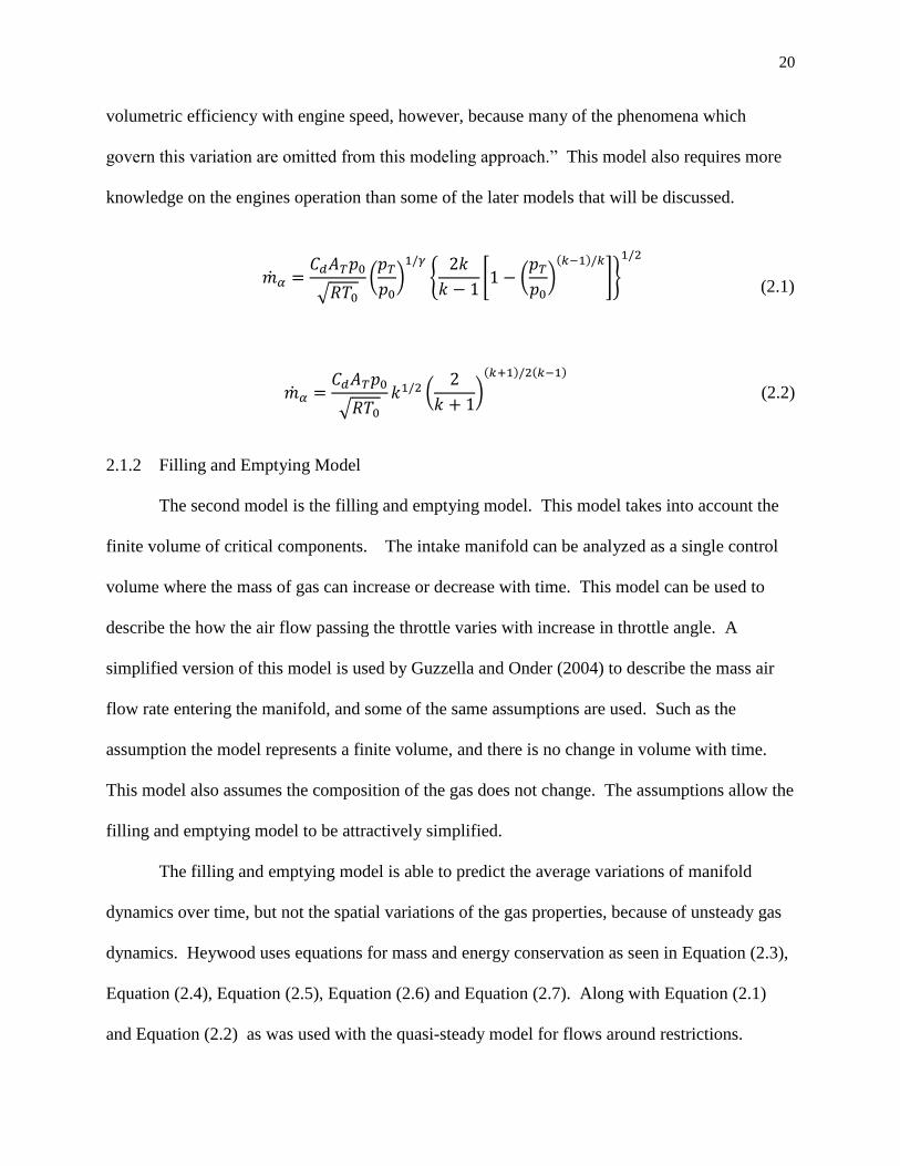
20
volumetric efficiency with engine speed, however, because many of the phenomena which
govern this variation are omitted from this modeling approach.‖ This model also requires more
knowledge on the engines operation than some of the later models that will be discussed.
√
(
*
,
* (
*( )
+-
(2.1)
√
(
*
( ) ( )
(2.2)
Filling and Emptying Model 2.1.2
The second model is the filling and emptying model. This model takes into account the
finite volume of critical components. The intake manifold can be analyzed as a single control
volume where the mass of gas can increase or decrease with time. This model can be used to
describe the how the air flow passing the throttle varies with increase in throttle angle. A
simplified version of this model is used by Guzzella and Onder (2004) to describe the mass air
flow rate entering the manifold, and some of the same assumptions are used. Such as the
assumption the model represents a finite volume, and there is no change in volume with time.
This model also assumes the composition of the gas does not change. The assumptions allow the
filling and emptying model to be attractively simplified.
The filling and emptying model is able to predict the average variations of manifold
dynamics over time, but not the spatial variations of the gas properties, because of unsteady gas
dynamics. Heywood uses equations for mass and energy conservation as seen in Equation (2.3),
Equation (2.4), Equation (2.5), Equation (2.6) and Equation (2.7). Along with Equation (2.1)
and Equation (2.2) as was used with the quasi-steady model for flows around restrictions.

21
Where Equation (2.3) is the sum of mass flow. The simplification of the models by assuming a
fixed volume and static gas composition makes calculations easier.(J. Heywood, 1988)
∑
(2.3)
Equation (2.4) details the rate of change of the fuel fraction which is a function of mass flows
and fuel fractions.
∑(
*
( ) (2.4)
Equation (2.5) details the dynamic of the pressure entering the open system. The variables
include the density( ), volume( ), fuel air equivalence ratio( ), temperature( ), and mass.
⁄(
) (2.5)
Then dynamic temperature of the open system can be solved using either Equation (2.6)
or Equation (2.7). Where new variable and are the specific internal energy and specific
enthalpy respectively.
*
(
)
+ (
*⁄ (2.6)
. ∑
/
22
0
(
*
.∑
/1 (2.7)
⁄
⁄(
*
( ⁄ )
⁄
⁄
⁄(
*
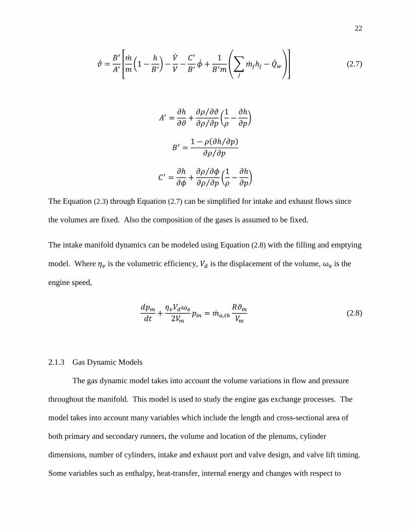
The Equation (2.3) through Equation (2.7) can be simplified for intake and exhaust flows since
the volumes are fixed. Also the composition of the gases is assumed to be fixed.
The intake manifold dynamics can be modeled using Equation (2.8) with the filling and emptying
model. Where is the volumetric efficiency, is the displacement of the volume, is the
engine speed,
(2.8)
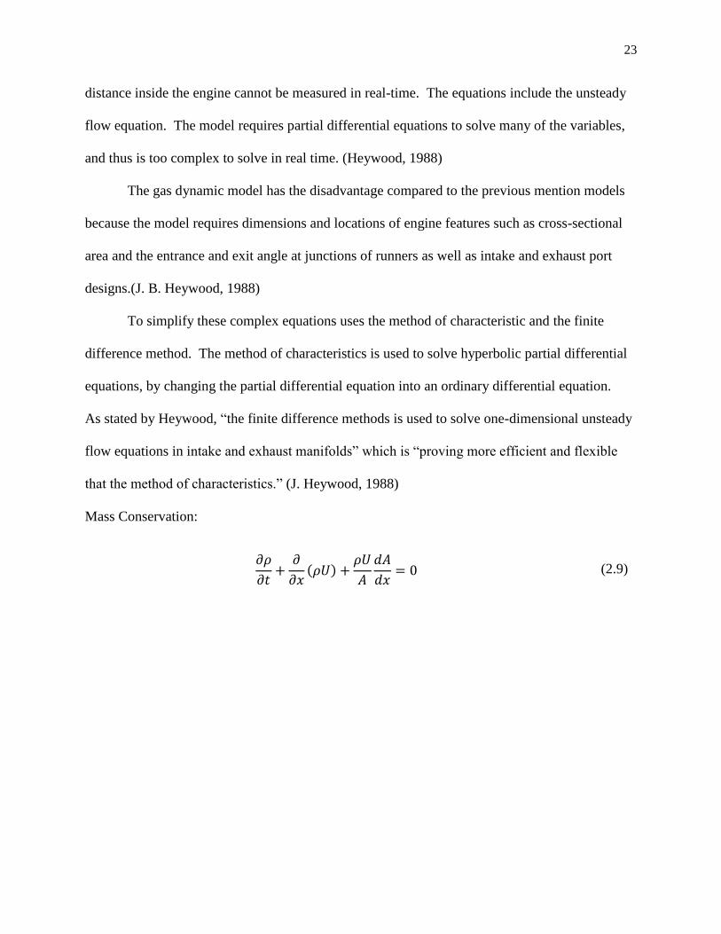
Gas Dynamic Models 2.1.3
The gas dynamic model takes into account the volume variations in flow and pressure
throughout the manifold. This model is used to study the engine gas exchange processes. The
model takes into account many variables which include the length and cross-sectional area of
both primary and secondary runners, the volume and location of the plenums, cylinder
dimensions, number of cylinders, intake and exhaust port and valve design, and valve lift timing.
Some variables such as enthalpy, heat-transfer, internal energy and changes with respect to
23
distance inside the engine cannot be measured in real-time. The equations include the unsteady
flow equation. The model requires partial differential equations to solve many of the variables,
and thus is too complex to solve in real time. (Heywood, 1988)
The gas dynamic model has the disadvantage compared to the previous mention models
because the model requires dimensions and locations of engine features such as cross-sectional
area and the entrance and exit angle at junctions of runners as well as intake and exhaust port
designs.(J. B. Heywood, 1988)
To simplify these complex equations uses the method of characteristic and the finite
difference method. The method of characteristics is used to solve hyperbolic partial differential
equations, by changing the partial differential equation into an ordinary differential equation.
As stated by Heywood, ―the finite difference methods is used to solve one-dimensional unsteady
flow equations in intake and exhaust manifolds‖ which is ―proving more efficient and flexible
that the method of characteristics.‖ (J. Heywood, 1988)
Mass Conservation:
( )
(2.9)

24
( ) (2.10)
(
*⁄ (2.11)
where t is time in seconds, x is the linear distance D is the equivalent diameter; ξ is the friction
coefficient and is the shear stress on the walls.
Mass and Momentum Conservation:
(2.12)
Energy Conservation:
(
* ( ) (
) (2.13)
(
*
(2.14)
where isentropic process is designated by the subscript s is used to solve for the sound speed (a)
of an ideal gas as seen in Equation (2.14).
Extensions of Heywood’s Intake and Air/ Fuel Mixing Models 2.1.4
The authors Kiencke and Nielson (2000) of ―Automotive Control Systems for Engine,
Driveline and Vehicles‖ introduces their models that depend on the control objective. Kiencke
and Nielson (2000) models the engine separately first with the intake manifold. Whereas
Heywood describes the IC engine models from a purely physical perspective, Kiencke and
Nielson (2000) approach the task of engine modeling from a control perspective, building on
Heywood’s models. Guzzella and Onder (2004) extended the work of Kiencke and Nielson
(2000).
25
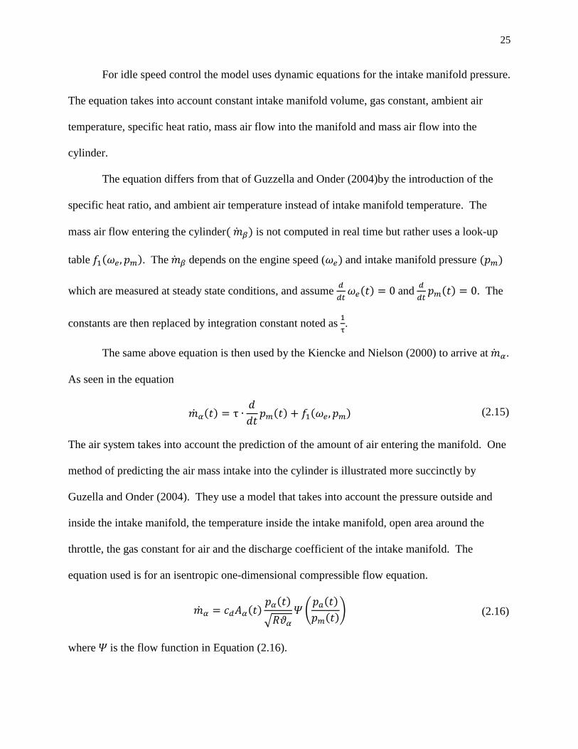
For idle speed control the model uses dynamic equations for the intake manifold pressure.
The equation takes into account constant intake manifold volume, gas constant, ambient air
temperature, specific heat ratio, mass air flow into the manifold and mass air flow into the
cylinder.
The equation differs from that of Guzzella and Onder (2004)by the introduction of the
specific heat ratio, and ambient air temperature instead of intake manifold temperature. The
mass air flow entering the cylinder( ) is not computed in real time but rather uses a look-up
table ( ). The depends on the engine speed ( ) and intake manifold pressure ( )
which are measured at steady state conditions, and assume
( ) and
( ) . The
constants are then replaced by integration constant noted as
.
The same above equation is then used by the Kiencke and Nielson (2000) to arrive at .
As seen in the equation
( )
( ) ( ) (2.15)
The air system takes into account the prediction of the amount of air entering the manifold. One
method of predicting the air mass intake into the cylinder is illustrated more succinctly by
Guzella and Onder (2004). They use a model that takes into account the pressure outside and
inside the intake manifold, the temperature inside the intake manifold, open area around the
throttle, the gas constant for air and the discharge coefficient of the intake manifold. The
equation used is for an isentropic one-dimensional compressible flow equation.
( ) ( )
√
( ( )
( )) (2.16)
where is the flow function in Equation (2.16).
26
For compressible fluids it is assumed that the orifice of the pipe is isothermal, which is
constant temperature. With compressible fluids there are two key assumptions that allow one to
separate the flow behavior. First, no losses occur in the accelerating part of the orifice up to the
narrowest point, which is the throttle valve opening. Also, the potential energy that is stored in
the flow is converted isentropically in kinetic energy. Second, after passing the throttle plate all
the flow is fully turbulent and the kinetic energy gained in the first assumption is dissipated into
thermal energy. Therefore, no recuperation of pressure takes place (Guzzella & Onder, 2004).
Given these assumptions the pressure downstream of the narrowest point and the pressure
at the narrowest point are equal. Also the temperature before and after the orifice is assumed to
be the same.
The equation used to calculate the mass air flow entering the engine is derived from the
thermodynamic relationships for isentropic expansion. This equation will take into account open
area of throttle for a given throttle input, ambient air pressure (which is pressure up stream of
throttle plate) the ambient air temperature, ideal gas constant, discharge coefficient, ratio of
specific heats, and pressure downstream of throttle plate (which is considered the manifold
pressure). The discharge coefficient has to be experimentally validated and is assumed constant
thereafter. Other assumed constants are the gas constant, ratio of specific heats, and ambient
pressure and temperature. The same equations as used by Guzzella and Onder (2004) when
modeling air intake is used by Wu, Chen, and Hsieh (2007) when modeling a single-cylinder
engine as seen in Equation (2.15), Equation (2.16) , Equation (3.2) and Equation (3.23). This
same model was also used by Yuh-Yih Wu, Bo-Chiuan Chen, Feng-Chi Hsieh, Ming-Lung
Huang and Ying-Huang Wu (2006) for modeling a 125 cc motorcycle engine, and is referred to
as a filling-and-emptying model.
27
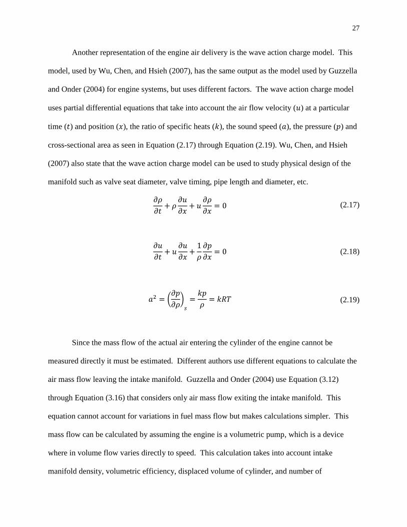
Another representation of the engine air delivery is the wave action charge model. This
model, used by Wu, Chen, and Hsieh (2007), has the same output as the model used by Guzzella
and Onder (2004) for engine systems, but uses different factors. The wave action charge model
uses partial differential equations that take into account the air flow velocity ( ) at a particular
time ( ) and position ( ), the ratio of specific heats ( ), the sound speed ( ), the pressure ( ) and
cross-sectional area as seen in Equation (2.17) through Equation (2.19). Wu, Chen, and Hsieh
(2007) also state that the wave action charge model can be used to study physical design of the
manifold such as valve seat diameter, valve timing, pipe length and diameter, etc.
(2.17)
(2.18)
(
*
(2.19)
Since the mass flow of the actual air entering the cylinder of the engine cannot be
measured directly it must be estimated. Different authors use different equations to calculate the
air mass flow leaving the intake manifold. Guzzella and Onder (2004) use Equation (3.12)
through Equation (3.16) that considers only air mass flow exiting the intake manifold. This
equation cannot account for variations in fuel mass flow but makes calculations simpler. This
mass flow can be calculated by assuming the engine is a volumetric pump, which is a device
where in volume flow varies directly to speed. This calculation takes into account intake
manifold density, volumetric efficiency, displaced volume of cylinder, and number of
28
revolutions per cycle. Some key assumptions are made by Guzzella and Onder (2004) in
calculating the air mass flow entering the engine. They include no drop in pressure in the intake
runners and the drop in temperature from the evaporation of fuel is disregarded because the
heating effect of the hot intake walls, the air/fuel ratio is assumed constant and at stoichiometric
value (14.7 for gasoline) for idle speed control, (and will be handled by a separate controller) and
the exhaust manifold pressure maybe assumed to be constant (if not measured will have to be
estimated) Guzzella and Onder (2004).
The volumetric efficiency of the engine must be calculated from experimental
measurements. The volumetric efficiency approximation is a multilinear formula that is
influenced by the manifold pressure and engine speed. The component dependent on the
pressure must take into account compression volume, displacement volume, exhaust pressure,
manifold pressure and ratio of specific heats. This portion of the volumetric efficiency describes
the effects caused by the trapped exhaust gas at top dead center (TDC). The speed dependent
component is a nonlinear equation that is comprised of multiple engine speed measurements and
three coefficients that must be experimentally validated. Experimental validation is done using
least-squares methods and measurements of manifold pressure, mass air flow and engine speed
(Guzzella & Onder, 2004). Guzzella and Onder (2004) also state that evaporation of fuel can
cause a change in temperature of the mixture and therefore an increase in volumetric efficiency.
Alternately, Wu, Chen and Hsieh (2007) use experimental regression that considered engine
speed and manifold pressure for finding volumetric efficiency.
Guzella and Onder (2004) also give a scenario for port injection engines where mass of
the fuel delivered to the cylinder can be taken into account. The fuel’s temperature, specific heat

29
and gas constant must be known. This also assumes that the fuel has been fully evaporated and
therefore the density of the air and fuel mixture must be calculated.
The filling and emptying model will be used to model the dynamics of the intake air.
This model was chosen for its simplicity compared to other models that require greater
knowledge of dynamic process within the intake manifold.

30
2.2 In-Cylinder Combustion Models
There exist several models for the combustion process within the engine producing
torque. These models have evolved over the years and become simplified to be better for
controls purposes. These models cover in-cylinder process and lead to estimation of torque
production.
Thermodynamic/ In-Cylinder Combustion Models 2.2.1
Thermodynamic-based in-cylinder models are used to predict the engine operating
characteristics, such as indicated power, mean effective pressure, specific fuel consumption, etc.
This model requires many of the engine dynamics to be known, Heywood (1988) states that
when ―the mass transfer into and out of the cylinder during intake and exhaust, the heat transfer
between the in-cylinder gases and the cylinder, piston, and cylinder liner, and rate of charge
during (or energy release from the fuel) are all known, the energy and mass conservation
equations permit the cylinder pressure and the work transfer to the piston to be calculated.‖
The thermodynamic-based in-cylinder model follows the changing states of the
thermodynamics, chemical states, and working fluid through the engine’s intake, compression,
combustion, expansion, and exhaust procedures. These are referred to as the four stroke cycle.
The intake and compression of the engine system is thought to be a single open system.
Heywood (1988) then uses the conservation of energy and mass equation to define the model. A
set of three equations is used for both intake and compression. There are three equations used
for , and to derive mass conservation, energy conservation and fuel. The intake stroke
Equation (2.20) through Equation (2.22) and three slightly different equations for these variables
during the compression stroke Equation (2.23) through Equation (2.25). The six equations are
then solved to find the pressure of the flow. During intake and compression the working fluid’s
31
composition is considered stationary. The compression and exhaust process can be calculated
using Equation (2.23) through Equation (2.25) and Equation (2.26) through Equation (2.28)
respectively. The thermodynamics and composition properties of the fluid can be determined
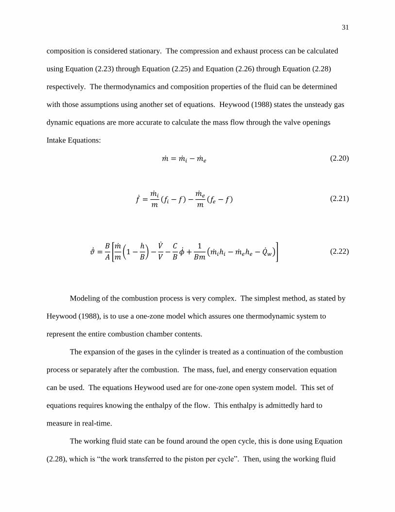
with those assumptions using another set of equations. Heywood (1988) states the unsteady gas
dynamic equations are more accurate to calculate the mass flow through the valve openings
Intake Equations:
(2.20)
( )
( ) (2.21)
*
(
*
( )+ (2.22)
Modeling of the combustion process is very complex. The simplest method, as stated by
Heywood (1988), is to use a one-zone model which assures one thermodynamic system to
represent the entire combustion chamber contents.
The expansion of the gases in the cylinder is treated as a continuation of the combustion
process or separately after the combustion. The mass, fuel, and energy conservation equation
can be used. The equations Heywood used are for one-zone open system model. This set of
equations requires knowing the enthalpy of the flow. This enthalpy is admittedly hard to
measure in real-time.
The working fluid state can be found around the open cycle, this is done using Equation
(2.28), which is ―the work transferred to the piston per cycle‖. Then, using the working fluid
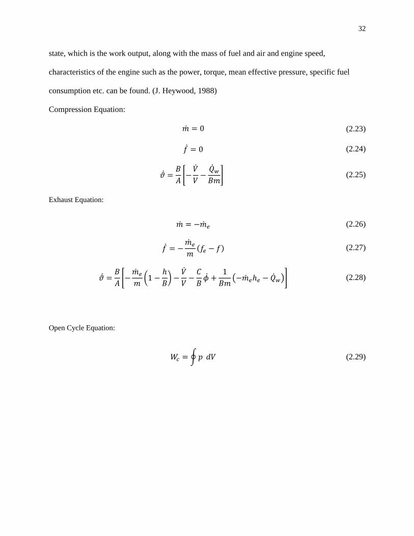
32
state, which is the work output, along with the mass of fuel and air and engine speed,
characteristics of the engine such as the power, torque, mean effective pressure, specific fuel
consumption etc. can be found. (J. Heywood, 1988)
Compression Equation:
(2.23)
(2.24)
*
+ (2.25)
Exhaust Equation:
(2.26)
( ) (2.27)
*
(
*
( )+ (2.28)
Open Cycle Equation:
∮ (2.29)
33
Spark-Ignition (SI) In-Cylinder Combustion Models 2.2.2
This model allows simplification of the thermodynamic model because the fuel, air, and
residual gas charge is essentially uniformly premixed. For the spark ignition engine model
Heywood (1988) focuses on the combustion sub-model. Modeling of the SI engine allows some
assumptions for simplification to be made. Heywood states some assumptions for the SI engine,
―thermodynamic modeling are: (1) the fuel, air, residual gas charge is essentially uniformly
premixed; (2) the volume occupied by the reaction zone where the fuel-air oxidation process
actually occurs is normally small compared with the clearance volume—the flame is a thin
reaction sheet even though it becomes highly wrinkled and convoluted by the turbulent flow as it
develops;‖ and ―(3) thermodynamic analysis, the contents of the combustion chamber during
combustion can be analyzed as two zones—an unburned and a burned zone.‖
The spark ignition engine model can be used for engine design. The model can be used
to calculate the flame geometry and predict the mass fraction burned of the fuel. Using the
thermodynamic-based simulation structure, when combined with a combustion model, can
predict the rate of fuel burning. The combustion model can either be empirically based, or
―based on the highly wrinkled, thin reaction-sheet flame model‖ states Heywood (1988). The
equations used in this model cannot be used for controls purposes because the equations require
the measurement of in-cylinder phenomena such as the shape of the combustion cylinder,
burning area, mass burning rate, etc. cannot be done in real-time. Variables such as spherical
burning area and burned gas volume require must be solved using partial differential equations
relative to burned gas radius.

34
( ) ( ) (2.30)
Fluid-Mechanic Model 2.2.3
The Fluid-Mechanics based models, as stated by Heywood, allow the modeling of fluids
within the intake and exhaust port. The models are three-dimensional and give more detail about
the working fluid in contrast to the one-dimensional models, since the flows inside the intake
manifold are inherently unstable and three dimensional.
Predictions of patterns of gas-flow can be done best by comparing to fuel spray and
combustion calculations. The partial differential equations that represent the conservation of
mass, momentum, energy, and species concentrations are solved by engine process. Heywood
states that for a computer to solve these partial differential equations the entire volume must be
decomposed into multiple finite volumes.
Heywood breaks down the multidimensional engine flow model as follows: (1) the
turbulence model is a mathematical model that describes the small-scale characteristics of the
flow which cannot be directed calculated. (2) The differential equations are transformed using
the discretization procedures into algebraic relations between discrete values of velocity,
pressure, temperature, etc. (3) Then there is the solution algorithm that solves the algebraic
equations. (4) Last, there is the computer code which provides an interface between input and
output for information and most importantly converts numerical algorithm into computer
language.
35
Extension to Heywood’s In-Cylinder Combustion Models 2.2.4
Other authors have taken models and derived control oriented models from Heywood
(1988) engine equations.
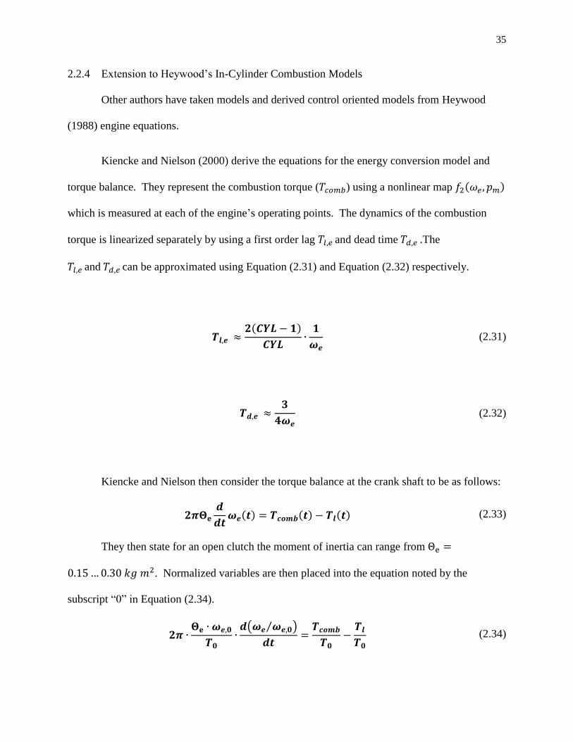
Kiencke and Nielson (2000) derive the equations for the energy conversion model and
torque balance. They represent the combustion torque ( ) using a nonlinear map ( )
which is measured at each of the engine’s operating points. The dynamics of the combustion
torque is linearized separately by using a first order lag and dead time .The
and can be approximated using Equation (2.31) and Equation (2.32) respectively.
( )
(2.31)
(2.32)
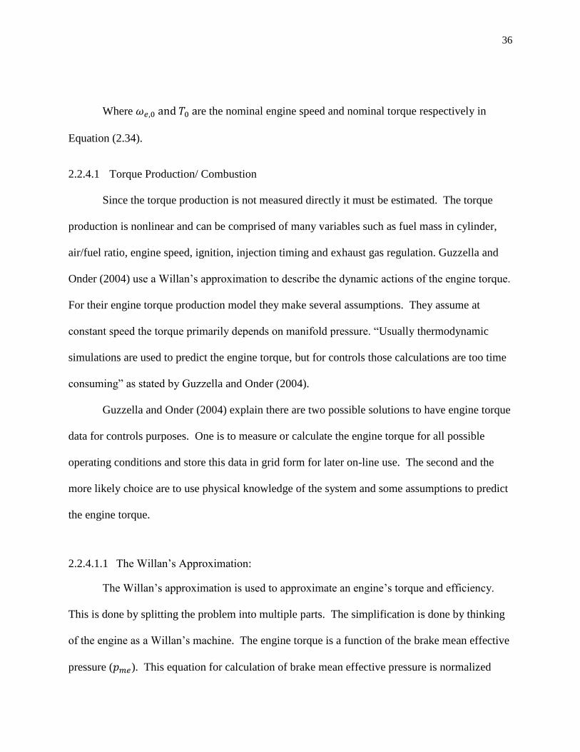
Kiencke and Nielson then consider the torque balance at the crank shaft to be as follows:
( ) ( ) ( ) (2.33)
They then state for an open clutch the moment of inertia can range from
. Normalized variables are then placed into the equation noted by the
subscript ―0‖ in Equation (2.34).
( ⁄ )
(2.34)
36
Where re the nominal engine speed and nominal torque respectively in
Equation (2.34).
2.2.4.1 Torque Production/ Combustion
Since the torque production is not measured directly it must be estimated. The torque
production is nonlinear and can be comprised of many variables such as fuel mass in cylinder,
air/fuel ratio, engine speed, ignition, injection timing and exhaust gas regulation. Guzzella and
Onder (2004) use a Willan’s approximation to describe the dynamic actions of the engine torque.
For their engine torque production model they make several assumptions. They assume at
constant speed the torque primarily depends on manifold pressure. ―Usually thermodynamic
simulations are used to predict the engine torque, but for controls those calculations are too time
consuming‖ as stated by Guzzella and Onder (2004).
Guzzella and Onder (2004) explain there are two possible solutions to have engine torque
data for controls purposes. One is to measure or calculate the engine torque for all possible
operating conditions and store this data in grid form for later on-line use. The second and the
more likely choice are to use physical knowledge of the system and some assumptions to predict
the engine torque.
2.2.4.1.1 The Willan’s Approximation:
The Willan’s approximation is used to approximate an engine’s torque and efficiency.
This is done by splitting the problem into multiple parts. The simplification is done by thinking
of the engine as a Willan’s machine. The engine torque is a function of the brake mean effective
pressure ( ). This equation for calculation of brake mean effective pressure is normalized
37
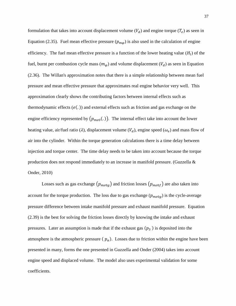
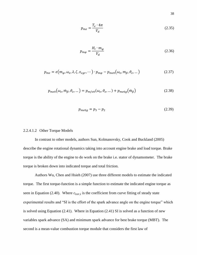
formulation that takes into account displacement volume ( ) and engine torque ( ) as seen in
Equation (2.35). Fuel mean effective pressure ( ) is also used in the calculation of engine
efficiency. The fuel mean effective pressure is a function of the lower heating value ( ) of the
fuel, burnt per combustion cycle mass ( ) and volume displacement ( ) as seen in Equation
(2.36). The Willan's approximation notes that there is a simple relationship between mean fuel
pressure and mean effective pressure that approximates real engine behavior very well. This
approximation clearly shows the contributing factors between internal effects such as
thermodynamic effects ( ( )) and external effects such as friction and gas exchange on the
engine efficiency represented by ( ( )). The internal effect take into account the lower
heating value, air/fuel ratio ( ), displacement volume ( ), engine speed ( ) and mass flow of
air into the cylinder. Within the torque generation calculations there is a time delay between
injection and torque center. The time delay needs to be taken into account because the torque
production does not respond immediately to an increase in manifold pressure. (Guzzella &
Onder, 2010)
Losses such as gas exchange ( ) and friction losses ( ) are also taken into
account for the torque production. The loss due to gas exchange ( ) is the cycle-average
pressure difference between intake manifold pressure and exhaust manifold pressure. Equation
(2.39) is the best for solving the friction losses directly by knowing the intake and exhaust
pressures. Later an assumption is made that if the exhaust gas ( ) is deposited into the
atmosphere is the atmospheric pressure ( ). Losses due to friction within the engine have been
presented in many, forms the one presented in Guzzella and Onder (2004) takes into account
engine speed and displaced volume. The model also uses experimental validation for some
coefficients.
38
(2.35)
(2.36)
( ) ( ) (2.37)
( ) ( ) ( ) (2.38)
(2.39)
2.2.4.1.2 Other Torque Models
In contrast to other models, authors Sun, Kolmanovsky, Cook and Buckland (2005)
describe the engine rotational dynamics taking into account engine brake and load torque. Brake
torque is the ability of the engine to do work on the brake i.e. stator of dynamometer. The brake
torque is broken down into indicated torque and total friction.
Authors Wu, Chen and Hsieh (2007) use three different models to estimate the indicated
torque. The first torque-function is a simple function to estimate the indicated engine torque as
seen in Equation (2.40). Where is the coefficient from curve fitting of steady state
experimental results and ―SI is the effort of the spark advance angle on the engine torque‖ which
is solved using Equation (2.41). Where in Equation (2.41) SI is solved as a function of new
variables spark advance (SA) and minimum spark advance for best brake torque (MBT). The
second is a mean-value combustion torque module that considers the first law of
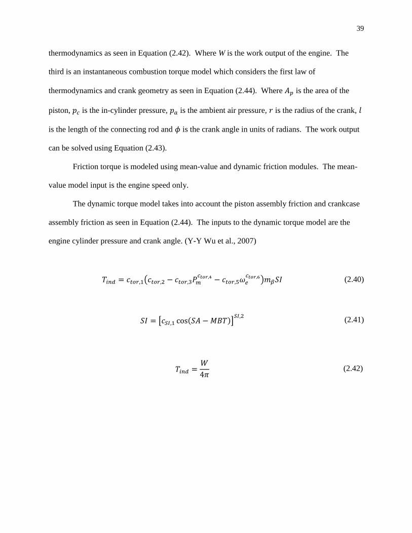
39
thermodynamics as seen in Equation (2.42). Where W is the work output of the engine. The
third is an instantaneous combustion torque model which considers the first law of
thermodynamics and crank geometry as seen in Equation (2.44). Where is the area of the
piston, is the in-cylinder pressure, is the ambient air pressure, is the radius of the crank,
is the length of the connecting rod and is the crank angle in units of radians. The work output
can be solved using Equation (2.43).
Friction torque is modeled using mean-value and dynamic friction modules. The mean-
value model input is the engine speed only.
The dynamic torque model takes into account the piston assembly friction and crankcase
assembly friction as seen in Equation (2.44). The inputs to the dynamic torque model are the
engine cylinder pressure and crank angle. (Y-Y Wu et al., 2007)
(
) (2.40)
[ ( )]
(2.41)
(2.42)

40
(2.43)
( ) * ( ⁄ ) ( )
√ ( ⁄ ) + (2.44)
(
)√
(2.45)
( ) (2.46)
Equation (2.46) the engine torque is solved as a function of the indicated torque, friction
torque and engine load. The variables are the crankshafts angular acceleration, b is the
damping constant of the crankshaft bearing and non-linear rotational inertia changes with the
rotation and movement of the crank assembly. The rotational inertia is a function of the
rotational inertia of crankshaft and connecting rod, mass of the piston and connecting rod, and
the length of the connecting rod. Wu, Chen and Hsieh (2007) also use a mean-value engine
model that simplifies the rotational inertia equation.
The torque equation takes into account the engines speed dynamics. This model deals
with the inertia of the engine, torque production and torque load which is considered a
disturbance by Guzzella and Onder (2004). The torque load in a real engine can take the form of
an alternator or power steering pump.
( )
[ ( ) ( )] (2.47)

41
The previous equations will need to be linearize around an operating point. Using the
equations described above or similar ones the model can be simulated in Matlab/ Simulink as
noted in Herman and Franchek (2000), Guzzella and Onder (2004). Wu, Y-Y., Chen, B-C., &
Hsieh, F-C. (2007) uses similar equations as Guzzella and Onder (2004). Wu, Y-Y., Chen, B-C.,
& Hsieh, F-C. (2007) use a detailed calculation that takes into account the variations in crank
shaft and piston geometry during engine operation.
42
2.2.4.1.3 Other Variations
Rajamani (2006) takes two approaches to the mean-value model of SI Engines. The first
uses parametric equations for the model and the second uses look-up tables with equations. The
focus of the model for a SI engine is the air flow model for the intake manifold and the rotational
dynamics of the crankshaft. Rajamani (2006) start off with the engine rotational dynamics. The
dynamics of the engine rotational moment of inertia, engine speed dynamics, indicated
combustion torque, external load torque and pumping and frictional torque are lumped as one
term.
For the indicated torque the authors use an equation from authors Hendricks and
Sorenson. The indicated torque is a function of the fuel energy constant, thermal efficiency
multiplier that accounts for the cooling and exhaust system losses, and the fuel mass flow rate
into the cylinder is a value in the Equation (2.48). (Rajamani, 2006)
(2.48)
The indicated and friction torque varies as the engine proceeds through cycles. Rajamani
(2006) also states that the dynamics of rotation are averaged with a mean value model.
The hydrodynamic and pumping friction losses are found using Equation (2.49) through
Equation (2.51). Both equations are polynomials with the hydrodynamic friction losses being a
function of engine speed which is taken from Heywood (1988). The pumping friction loss is a
function of engine speed and manifold pressure which is taken from Hendricks and Sorenson
(1990).

43
(2.49)
(2.50)
(2.51)
The manifold pressure equations are the same as used by Guzzella and Onder (2004).
The mass air flow going into the cylinder is as in Guzzella and Onder (2004). The only
unknown aspect is the volumetric efficiency, which Rajamani (2006) does not detail with the
simple mean-value engine model. The model for the intake into the intake manifold is similar to
Guzzella and Onder (2004).
Rajamani (2006) also details an engine model that includes look-up maps. Many of the
previously mentioned functions such as indicated torque, total friction and pumping loss, mass
air flow into the intake manifold and mass air flow into the cylinder are found using a
dynamometer. The look-up maps can be presented in tabular form or plotted data. These models
that use look-up tables are considered second order engine models because each function has two
dependent variables. (Rajamani, 2006)

44
CHAPTER 3
3 ENGINE MODELING
The initial intention of this research was to study, investigate and ultimately create a
model that represent a single cylinder engine, starting with studying ―Introduction to Modeling
and Control of Internal Combustion Engine Systems‖ written by Guzzella and Onder (2004),
which covers the creation of engine models for gasoline and diesel engines. The focus of this
thesis was to study port-injection gasoline engines. Within the text by Guzzella and Onder
(2004) the engine is broken down into sections in order to simplify the calculations.
The initial modeling attempt was to create an idle speed controller. This model was to be
created in order to simulate an engine running under idle conditions. This requires an
understanding of the various systems within an engine and the assumptions needed when
creating a control oriented model (COM). The sections are broken down into the air system
which includes throttle plate nonlinearities, mass air flow through throttle, and air mass flow into
engine cylinder and intake manifold pressure dynamics. Second is the mechanical system which
governs the mechanical output after engine combustion this includes the dynamics engine speed,
torque production and simulation of engine load.
3.1 Intake Manifold Dynamics
The intake manifold of an engine is modeled as a receiver as stated by Guzzella and
Onder (2004). Thus this receiver is considered a fix volume and therefore the thermodynamic
states are considered to be constant.
The engines air system is comprised of the fluid dynamics of the air charge from the
beginning of the intake manifold to air flow around the throttle and mass air flow or air and fuel
mixture entering the manifold. Also, since a lot of the various changes taking place inside the
45
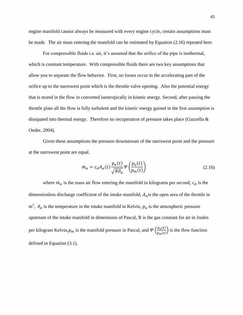
engine manifold cannot always be measured with every engine cycle, certain assumptions must
be made. The air mass entering the manifold can be estimated by Equation (2.16) repeated here.
For compressible fluids i.e. air, it’s assumed that the orifice of the pipe is isothermal,
which is constant temperature. With compressible fluids there are two key assumptions that
allow you to separate the flow behavior. First, no losses occur in the accelerating part of the
orifice up to the narrowest point which is the throttle valve opening. Also the potential energy
that is stored in the flow in converted isentropically in kinetic energy. Second, after passing the
throttle plate all the flow is fully turbulent and the kinetic energy gained in the first assumption is
dissipated into thermal energy. Therefore no recuperation of pressure takes place (Guzzella &
Onder, 2004).
Given these assumptions the pressure downstream of the narrowest point and the pressure
at the narrowest point are equal.
( ) ( )
√
( ( )
( )) (2.16)
where is the mass air flow entering the manifold in kilograms per second, is the
dimensionless discharge coefficient of the intake manifold, is the open area of the throttle in
m2, is the temperature in the intake manifold in Kelvin, is the atmospheric pressure
upstream of the intake manifold in dimensions of Pascal, R is the gas constant for air in Joules
per kilogram Kelvin, is the manifold pressure in Pascal, and ( ( )
( )) is the flow function
defined in Equation (3.1).
46
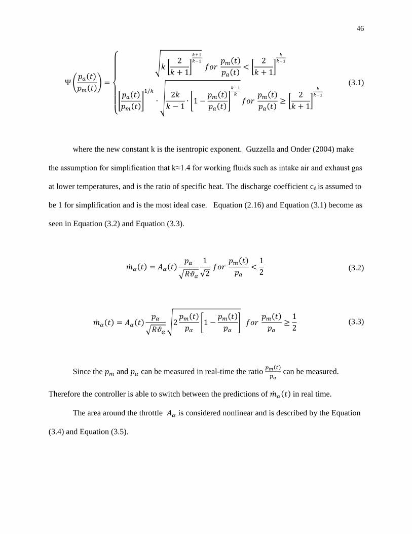
( ( )
( ))
{
√ [
]
( )
( ) [
]
* ( )
( )+
√
*
( )
( )+
( )
( ) [
]
(3.1)
where the new constant k is the isentropic exponent. Guzzella and Onder (2004) make
the assumption for simplification that k≈1.4 for working fluids such as intake air and exhaust gas
at lower temperatures, and is the ratio of specific heat. The discharge coefficient cd is assumed to
be 1 for simplification and is the most ideal case. Equation (2.16) and Equation (3.1) become as
seen in Equation (3.2) and Equation (3.3).
( ) ( )
√
√
( )
(3.2)
( ) ( )
√
√ ( )
*
( )
+
( )
(3.3)
Since the and can be measured in real-time the ratio ( )
can be measured.
Therefore the controller is able to switch between the predictions of ( ) in real time.
The area around the throttle is considered nonlinear and is described by the Equation
(3.4) and Equation (3.5).

47
(
) (3.4)
( )
(
) (3.5)
where is the angle of the throttle in units of degrees, is the angle of the throttle
when closed fully in the units of degrees, is the control signal input between 0% and 100%,
is the area of the throttle when and are equal in units of m2, is the diameter
in meters that becomes nonlinear.
To increase the accuracy of predictions of manifold pressure entering the intake manifold
an adjustment can be made to the nonlinear . This is performed by predicting from
known user selected throttle angle that will vary with each prediction and therefore will change
with each measurement.
For all operation conditions of the engine in idle speed control, the manifold pressure is
considered to be below 0.5 bars (50,000 Pascal). This assumption simplifies the calculations and
allows for the nonlinear function to be constant. The diameter of the throttle enters in a
nonlinear way as seen in Equation (3.6) a substitution must be made to form a linear in the
parameters problem. This substitution can be seen in the equation below
(3.6)
48
[
]
[
]
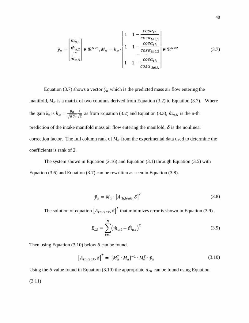
(3.7)
Equation (3.7) shows a vector which is the predicted mass air flow entering the
manifold, is a matrix of two columns derived from Equation (3.2) to Equation (3.7). Where
the gain kα is
√
√ as from Equation (3.2) and Equation (3.3), is the n-th
prediction of the intake manifold mass air flow entering the manifold, is the nonlinear
correction factor. The full column rank of from the experimental data used to determine the
coefficients is rank of 2.
The system shown in Equation (2.16) and Equation (3.1) through Equation (3.5) with
Equation (3.6) and Equation (3.7) can be rewritten as seen in Equation (3.8).
[ ] (3.8)
The solution of equation [ ] that minimizes error is shown in Equation (3.9) .
∑( )
(3.9)
Then using Equation (3.10) below can be found.
[ ]
[ ]
(3.10)
Using the value found in Equation (3.10) the appropriate can be found using Equation
(3.11)
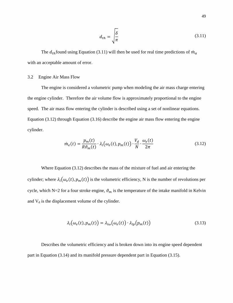
49
√
(3.11)
The found using Equation (3.11) will then be used for real time predictions of
with an acceptable amount of error.
3.2 Engine Air Mass Flow
The engine is considered a volumetric pump when modeling the air mass charge entering
the engine cylinder. Therefore the air volume flow is approximately proportional to the engine
speed. The air mass flow entering the cylinder is described using a set of nonlinear equations.
Equation (3.12) through Equation (3.16) describe the engine air mass flow entering the engine
cylinder.
( ) ( )
( ) ( ( ) ( ))
( )
(3.12)
Where Equation (3.12) describes the mass of the mixture of fuel and air entering the
cylinder; where ( ( ) ( )) is the volumetric efficiency, N is the number of revolutions per
cycle, which N=2 for a four stroke engine, is the temperature of the intake manifold in Kelvin
and Vd is the displacement volume of the cylinder.
( ( ) ( )) ( ( )) ( ( )) (3.13)
Describes the volumetric efficiency and is broken down into its engine speed dependent
part in Equation (3.14) and its manifold pressure dependent part in Equation (3.15).
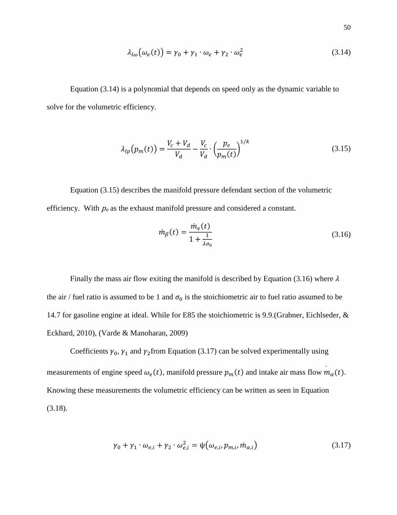
50
( ( )) (3.14)
Equation (3.14) is a polynomial that depends on speed only as the dynamic variable to
solve for the volumetric efficiency.
( ( ))
(
( )*
(3.15)
Equation (3.15) describes the manifold pressure defendant section of the volumetric
efficiency. With pe as the exhaust manifold pressure and considered a constant.
( ) ( )
(3.16)
Finally the mass air flow exiting the manifold is described by Equation (3.16) where
the air / fuel ratio is assumed to be 1 and is the stoichiometric air to fuel ratio assumed to be
14.7 for gasoline engine at ideal. While for E85 the stoichiometric is 9.9.(Grabner, Eichlseder, &
Eckhard, 2010), (Varde & Manoharan, 2009)
Coefficients , and from Equation (3.17) can be solved experimentally using
measurements of engine speed ( ), manifold pressure ( ) and intake air mass flow ( ).
Knowing these measurements the volumetric efficiency can be written as seen in Equation
(3.18).
( ) (3.17)
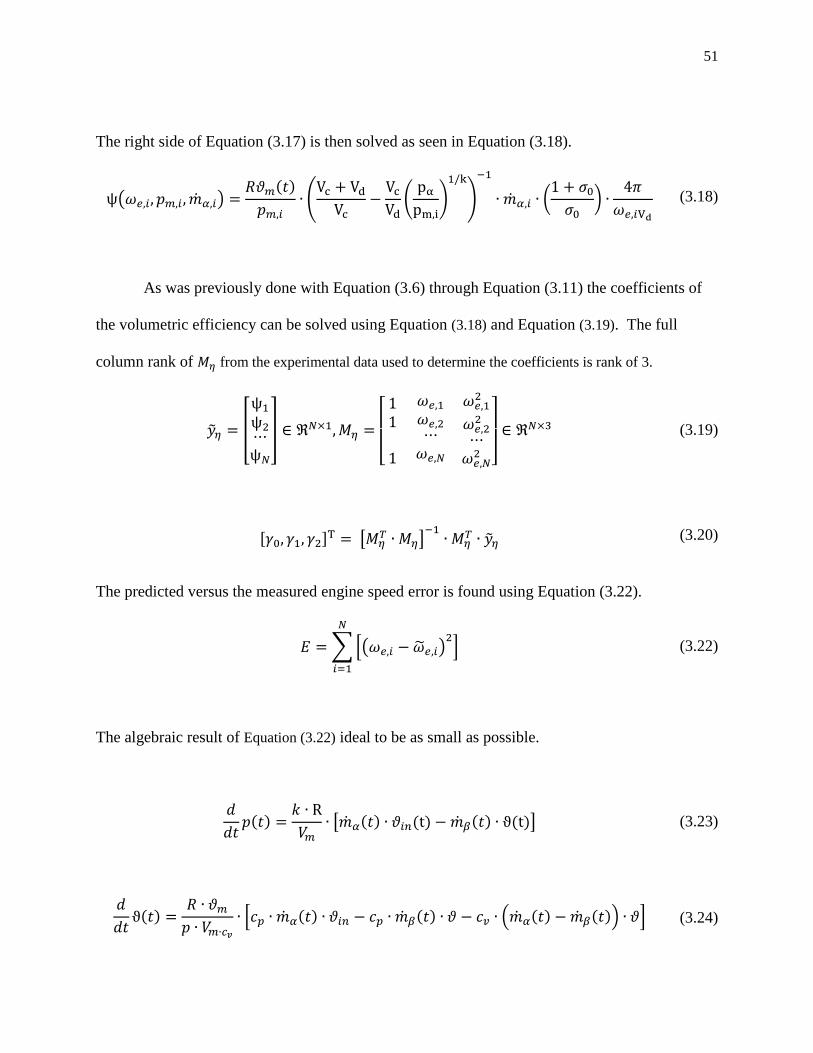
51
The right side of Equation (3.17) is then solved as seen in Equation (3.18).
( ) ( )
(
(
)
+
(
*
(3.18)
As was previously done with Equation (3.6) through Equation (3.11) the coefficients of
the volumetric efficiency can be solved using Equation (3.18) and Equation (3.19). The full
column rank of from the experimental data used to determine the coefficients is rank of 3.
[
]
[
] (3.19)
[ ] [
]
(3.20)
(3.21)
The predicted versus the measured engine speed error is found using Equation (3.22).
∑*( ) +
(3.22)
The algebraic result of Equation (3.22) ideal to be as small as possible.
( )
[ ( ) ( ) ( ) ( )] (3.23)
( )
* ( ) ( ) ( ( ) ( )) + (3.24)
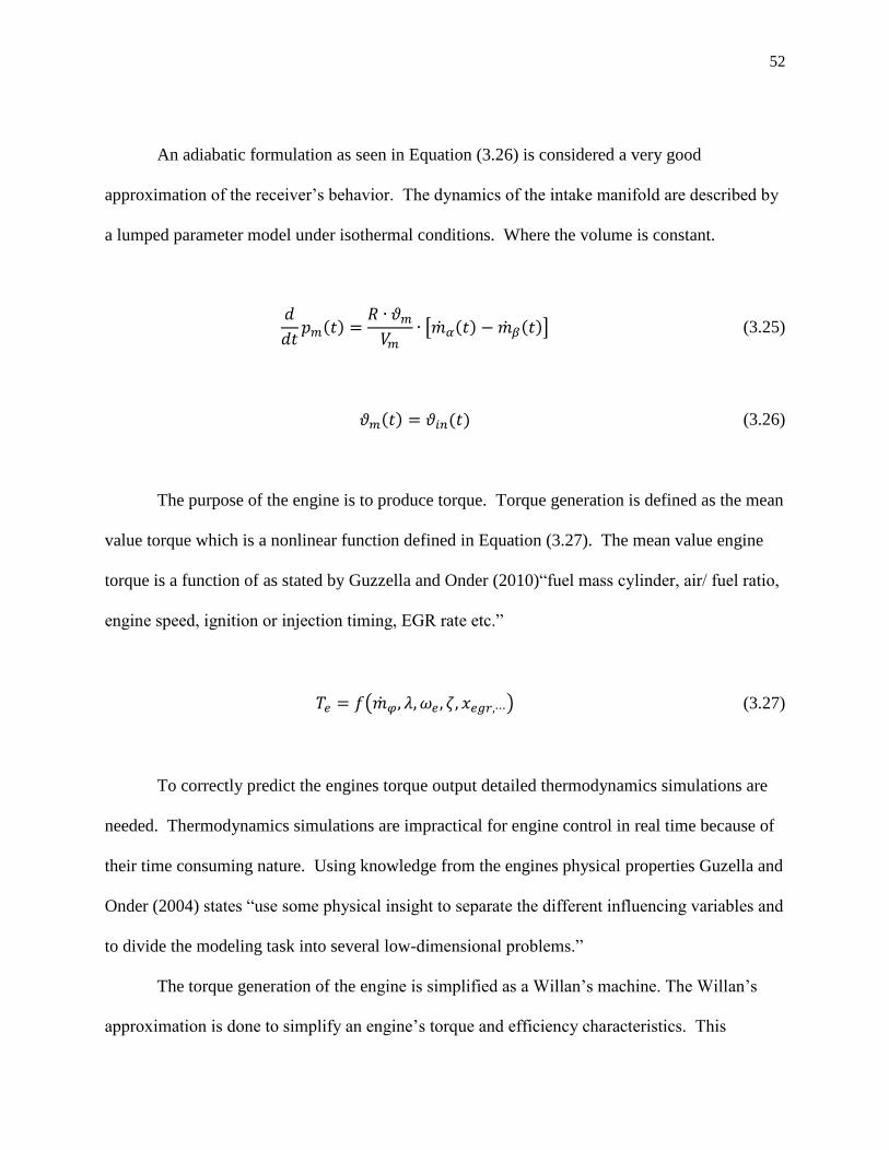
52
An adiabatic formulation as seen in Equation (3.26) is considered a very good
approximation of the receiver’s behavior. The dynamics of the intake manifold are described by
a lumped parameter model under isothermal conditions. Where the volume is constant.
( )
[ ( ) ( )] (3.25)
( ) ( ) (3.26)
The purpose of the engine is to produce torque. Torque generation is defined as the mean
value torque which is a nonlinear function defined in Equation (3.27). The mean value engine
torque is a function of as stated by Guzzella and Onder (2010)―fuel mass cylinder, air/ fuel ratio,
engine speed, ignition or injection timing, EGR rate etc.‖
( ) (3.27)
To correctly predict the engines torque output detailed thermodynamics simulations are
needed. Thermodynamics simulations are impractical for engine control in real time because of
their time consuming nature. Using knowledge from the engines physical properties Guzella and
Onder (2004) states ―use some physical insight to separate the different influencing variables and
to divide the modeling task into several low-dimensional problems.‖
The torque generation of the engine is simplified as a Willan’s machine. The Willan’s
approximation is done to simplify an engine’s torque and efficiency characteristics. This
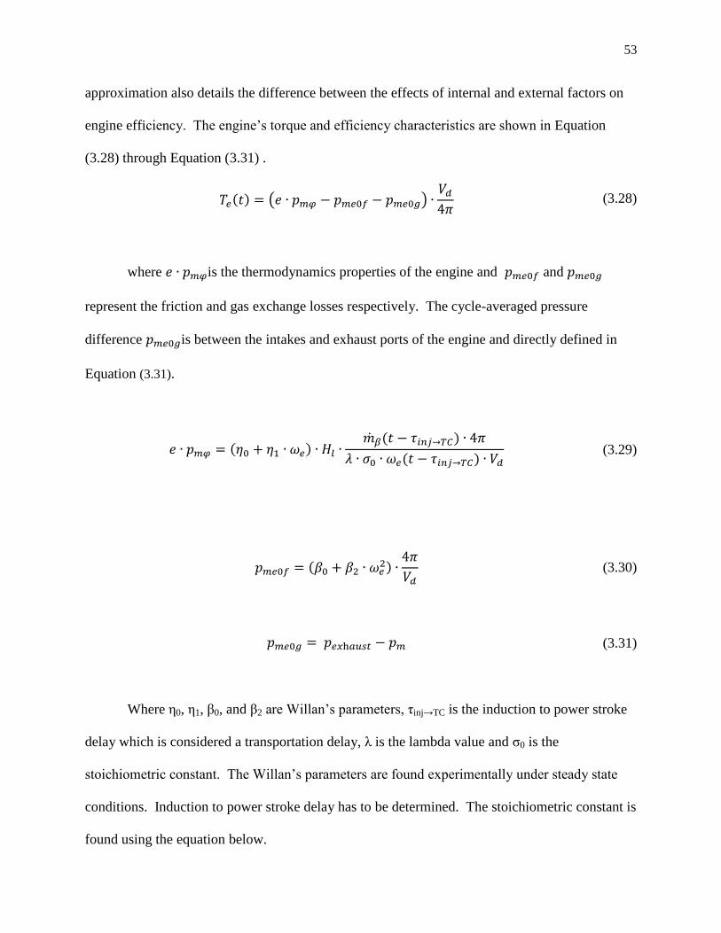
53
approximation also details the difference between the effects of internal and external factors on
engine efficiency. The engine’s torque and efficiency characteristics are shown in Equation
(3.28) through Equation (3.31) .
( ) ( )
(3.28)
where is the thermodynamics properties of the engine and and
represent the friction and gas exchange losses respectively. The cycle-averaged pressure
difference is between the intakes and exhaust ports of the engine and directly defined in
Equation (3.31).
( ) ( )
( ) (3.29)
( )
(3.30)
(3.31)
Where η0, η1, β0, and β2 are Willan’s parameters, τinj→TC is the induction to power stroke
delay which is considered a transportation delay, λ is the lambda value and σ0 is the
stoichiometric constant. The Willan’s parameters are found experimentally under steady state
conditions. Induction to power stroke delay has to be determined. The stoichiometric constant is
found using the equation below.

54
(3.32)
Where for hydrogen based fuel is for carbon atoms and is for hydrogen atoms. The change in
engine speed with respect to time is a level variable as shown in Equation (3.33).
( )
[ ( ) ( )] (3.33)
Using the above equations that represent the engines dynamics a model was to be created
under certain conditions. This model was intended to represent the engine dynamics under idle
conditions to be later linked with a controller. Within the next section the process of measuring
and determining the constants necessary to fully describe the state space model will be detailed.
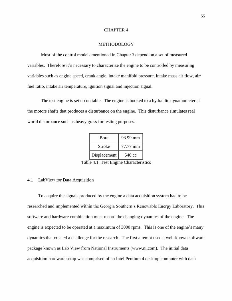
55
CHAPTER 4
4 METHODOLOGY
Most of the control models mentioned in Chapter 3 depend on a set of measured
variables. Therefore it’s necessary to characterize the engine to be controlled by measuring
variables such as engine speed, crank angle, intake manifold pressure, intake mass air flow, air/
fuel ratio, intake air temperature, ignition signal and injection signal.
The test engine is set up on table. The engine is hooked to a hydraulic dynamometer at
the motors shafts that produces a disturbance on the engine. This disturbance simulates real
world disturbance such as heavy grass for testing purposes.
Bore 93.99 mm
Stroke 77.77 mm
Displacement 540 cc
Table 4.1: Test Engine Characteristics
4.1 LabView for Data Acquisition
To acquire the signals produced by the engine a data acquisition system had to be
researched and implemented within the Georgia Southern’s Renewable Energy Laboratory. This
software and hardware combination must record the changing dynamics of the engine. The
engine is expected to be operated at a maximum of 3000 rpms. This is one of the engine’s many
dynamics that created a challenge for the research. The first attempt used a well-known software
package known as Lab View from National Instruments (www.ni.com). The initial data
acquisition hardware setup was comprised of an Intel Pentium 4 desktop computer with data

56
acquisition cards that will be described throughout sections of this paper. A diagram of this
system with the many connections can be seen in Figure 4.1.
In order to ensure this software will be able to keep track of the changing engine system
dynamics in real time simple tests needed to be performed to measure this accuracy, without
running the engine and using up fuel. It was chosen to substitute electric motors and function
generators to initially test the LabView response.
Measurement Computing Inc. (www.mccdaq.com) provided the data acquisition
hardware which connects sensors and instruments to the PCI communications backplane of a
personal computer. Measurement Computing also provided software drivers to move measured
data into LabView database. National Instruments measurement hardware was not sufficiently
fast to provide the speed of data acquisition required. Within Table 4.2 the types of
measurements needed, the sensors used to take those measurements and the expected maximum
frequency of change is shown.
Sensor Number Measurement Sensor Frequency of Measurement (Hz)
1 Engine Crank Angle
and Engine Speed
Rotary Encoder 100K (electrical)
2 Throttle Angle Potentiometer 100
3 Intake Air
Temperature
Thermal Couple Type: K 0.25
4 Exhaust Air
Temperature
Thermal Couple Type: K 0.25
5 Injector Timing Injector 200K
6 Intake Mass Air Flow Laminar Flow System 30
7 Ignition Timing Inductive Clamp 200K
Table 4.2: List of Sensors, Measured Variables and Expected Maximum Frequency of Change
57
DAQ Assistant is a tool implemented within LabView by the software creators National
Instruments. DAQ Assistant is made to work easily with National Instruments data acquisition
hardware and includes a nice user friendly graphical user interface (GUI). To program LabView
for data acquisition required the use of Measurement Computing Boards drivers. Therefore the
usual means of using LabView’s easily and familiar DAQ Assistant was not available and the
Measurement Computing boards would not even show up in DAQ Assistant. Therefore
implementing the new Measurement Computing hardware system presented a challenge when
trying to record data.
Measurement Computing Universal Libraries adds additional set of VIs (virtual
instruments) to LabView. The VI is LabView’s program file type. A LabView VI is represented
by an icon which is moveable blocks used as the user level programming language to provide an
interface with data acquisition hardware.
A second piece of software called InstaCal is necessary for the interface between
LabView and Measurement Computing data acquisition hardware. This software creates a
configuration file that lists details about the installed Measurement Computing data acquisition
boards. InstaCal also allows the data acquisition cards to be tested for proper operation.
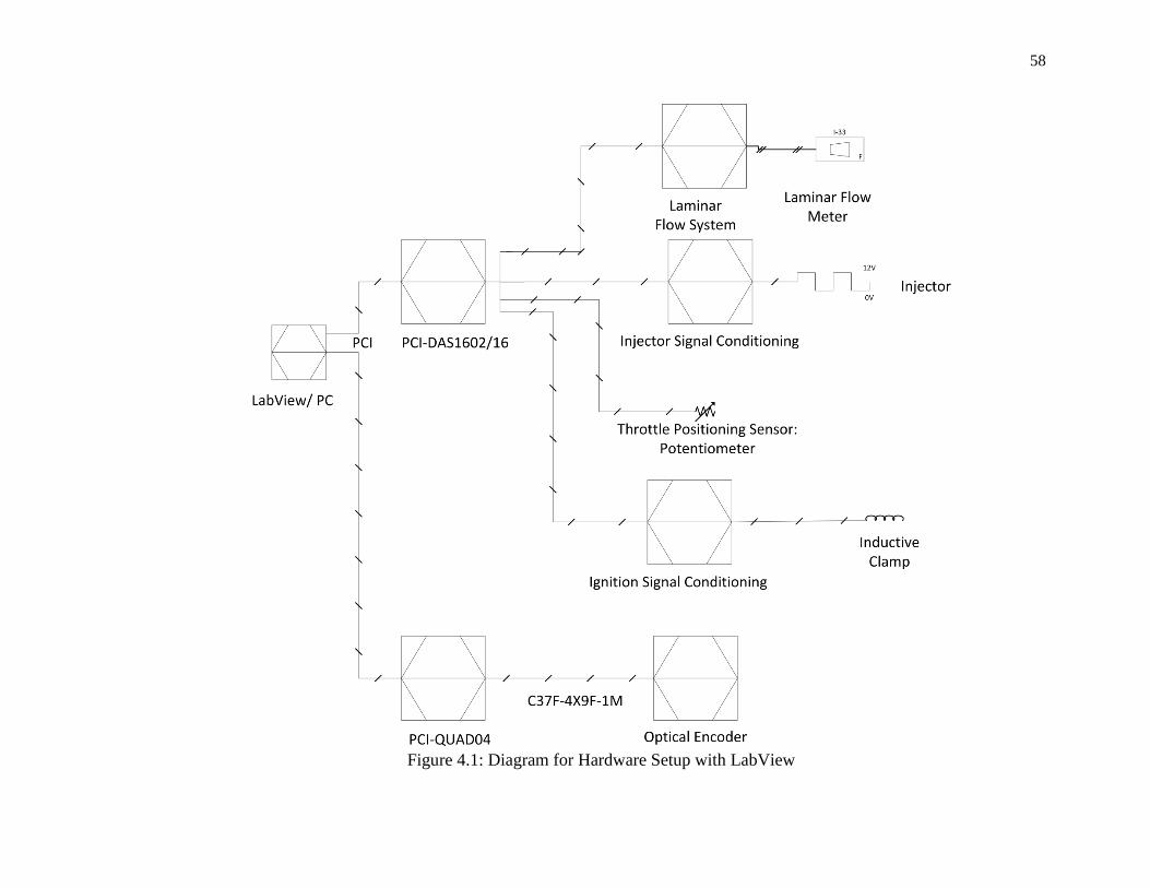
58
Figure 4.1: Diagram for Hardware Setup with LabView
59
LabView Limit Testing 4.1.1
4.1.1.1 Sine Wave
The first attempt at testing the limits of LabView was to use a function generator. The
function generator is used to input a sine wave at known frequency to see if the signal could be
recorded accurately. The signal was taken using Measurement Computing’s PCI-DAS1602/16.
This data acquisition card is able to sample signals at 200 kHz. An example provided by
Measurement Computing is seen in Figure 4.2. The example allows a range of signals to be
scanned, number of analog samples to collect, and sample rate in scans per second.
LabView uses many different data types. The different data types are designated by the
color of the lines that connect the virtual instruments. The blue lines on the top left side of
Figure 4.2 coming from inputs such as Count, LowChan, HighChan, BoardNum, Rate, and
Range are 32-bit integer data, which are inputs into AInScBg. While the green Cont/Sngl is a
Boolean data type that which is an input into AInScBg.
The new virtual instruments (VI) incorporated by Measurement Computing in Figure 4.2
include AInScBg, GetStatus, ToEng, OptAIn, StopBg, and ErrMsg. The inputs are first taken as
shown on the Front Panel as seen in Figure 4.3. The AInScBg, located in the middle left side, has
many inputs and outputs and is the main VI that defines the A/D data transfer for the background
operation. BoardNum which designates the board number as appointed in InstaCal is set. The
setting for LowChan and HighChan are set which designates which channels the program looks
for analog signals. The Count designates the number of samples taken for the analog to digital
conversion. The Rate designates the desired rate of scanning which is an input. The Range
designates the expected voltage level of the incoming signal. The option Continuous if set to
true the program runs in a never ending loop, else if false the program stops after the maximum
60
designated counts is reached as set in the Count argument. InterChannel Delay is used to specify
the time between scanning individual channels. Outputs of the block are either passed on to other
VIs or their individual status is displayed on the frontpanel. The Actual Rate of scanning shows
the real rate of scanning. The main output of the AInScBg is the Context, which carries the data
from a background process. Last, the error code is handling by the ErrCode output. The
AInScBg outputs are then taken in by other various VIs. The Options, located at the bottom left,
allows the method of trigger and transfer to be designated. The default option is DEFAULTIO
this option is the easiest and chooses the best sampling mode defined by the type of DAQ board
used.
The Context output goes to the GetStatus virtual instrument in bottom right of Figure 4.2.
The GetStatus outputs the status of the background process controlled by AInScBg. Other
outputs include the CurCount which is the current accumulated number of samples taken and is
displayed on the front panel. The DataArray is output to the Front Panel and into the ToEng VI.
The Context is sent to the StopBg for controlling the background process. Overall program is
kept running using the Running output, which is a Boolean true or false. Running is then
ANDed with a true false input located on the front panel in series with a not. This logic will then
be if the stop is pressed and the Running is true the program stops. If the Running is true and
the stop has not been pressed the process continues to run.
The output of the ToEng VI is the voltage value as being read by the data acquisition card.
Inputs of Range and BoardNum input from the front panel and DataArray from the GetStatus are
taken into the VI.
61
The ErrMsg VI takes the error Code designated by ErrCode which is an integer 32-bit data
type. The error code is then interpreted and displayed on the Front Panel through the ErrMsg
output as plain text.
Where the main VI AInScBg is used to scan analog input channels in the back ground and
exports the results to the GetStatus. The accumulated count gets displayed on the front panel out
of the GetStatus VI.
An analog signal was input in the data acquisition card using a differential wiring setup to
minimize interference. The sine wave data was outputted to an Excel readable file to better
observe what was recorded and insure that data could be recorded. The first attempts seemed to
acquire a signal accurately. Further testing using the data acquisition system needed to be
performed using sensors that would be used on the engine.
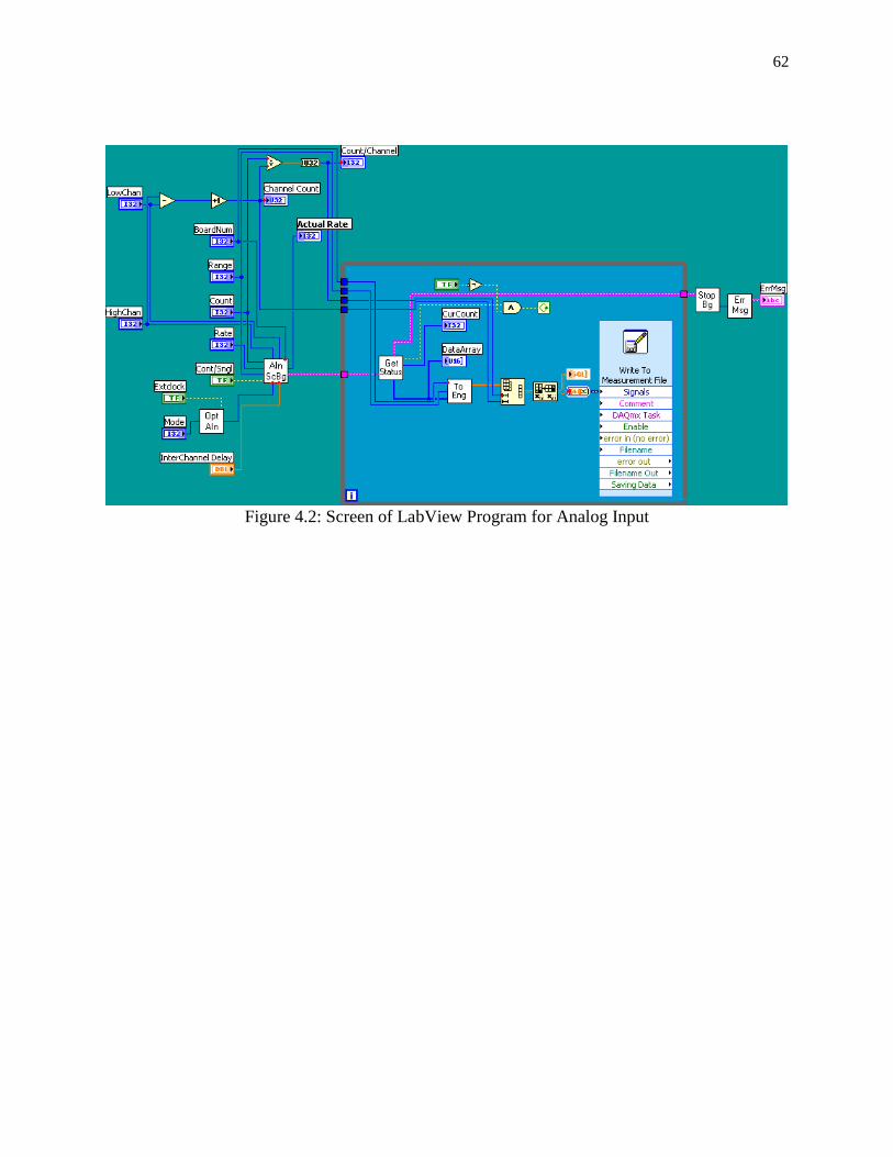
62
Figure 4.2: Screen of LabView Program for Analog Input
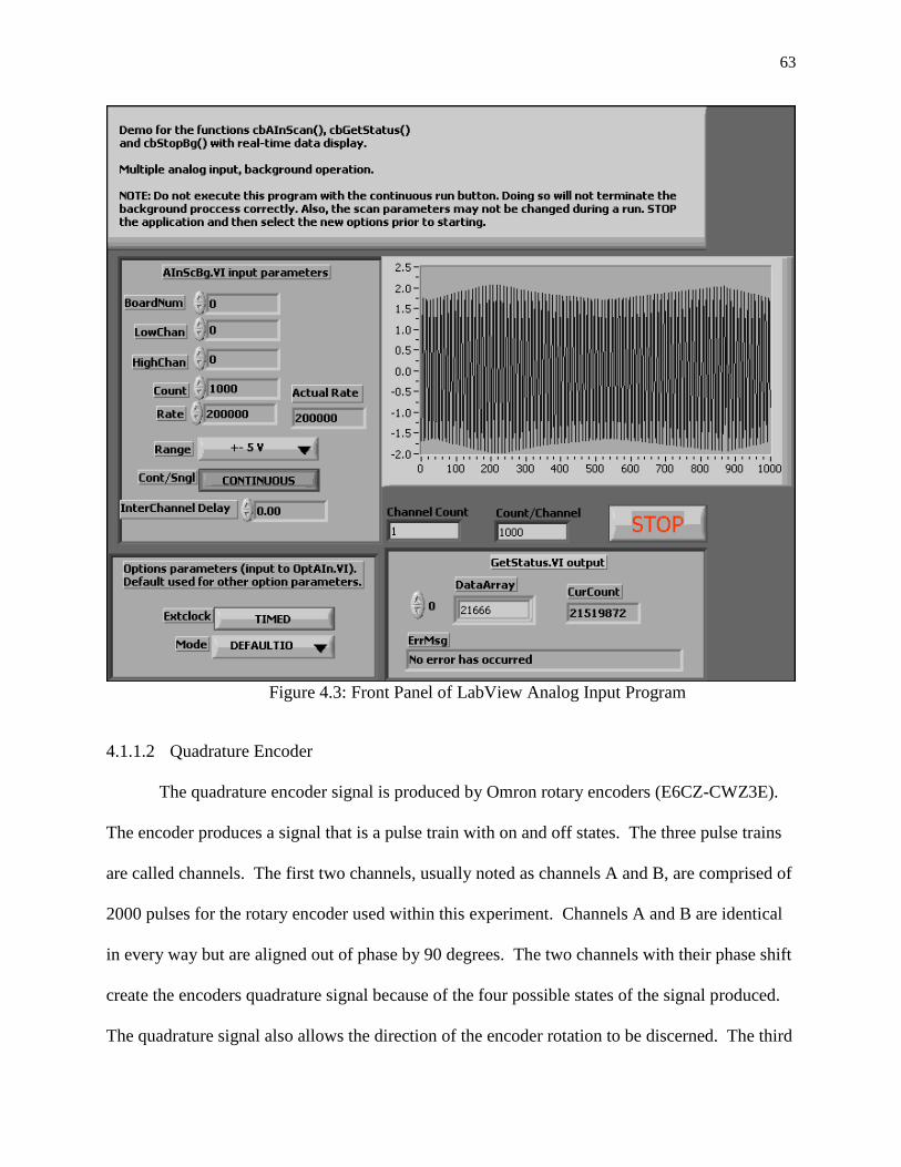
63
Figure 4.3: Front Panel of LabView Analog Input Program
4.1.1.2 Quadrature Encoder
The quadrature encoder signal is produced by Omron rotary encoders (E6CZ-CWZ3E).
The encoder produces a signal that is a pulse train with on and off states. The three pulse trains
are called channels. The first two channels, usually noted as channels A and B, are comprised of
2000 pulses for the rotary encoder used within this experiment. Channels A and B are identical
in every way but are aligned out of phase by 90 degrees. The two channels with their phase shift
create the encoders quadrature signal because of the four possible states of the signal produced.
The quadrature signal also allows the direction of the encoder rotation to be discerned. The third
64
channel is usually designated the Z channel or Index. The Z channel is used to given an absolute
starting position for the encoder and does this by generating one pulse per revolution. The Z
channel is used to reset the encoder counts in data acquisition and to sync the encoder with top
dead center (TDC) of the engine. With an encoder of such precision the encoder is able to have
an accuracy of 0.18 degrees per pulse. At the expected maximum speed of the engine the
encoder will be able to produce a signal with a frequency of 100 kHz.
4.1.1.3 Encoder Signal
To record the encoders pulse and therefore discern the engine speed and crank angle the
encoder signal is captured by the quadrature encoder card (PCI-QUAD04) input card. This card
is able to take the pulse train produced by the rotary encoder and at a clock frequency of 1.2
MHz maximum. This translates into 36,000 revolutions per minute (rpm) using the 2000 pulses
per revolution encoder, which is faster than the engine will ever operate.
(4.1)
The encoder card keeps track of the count and outputs the number of counts to the data
acquisition computer. The card is only required to keep up with no more than the maximum
expected encoder count of 500 pulses per revolution, after dividing.
4.1.1.4 LabView with Rotary Encoder
The LabView code example given by Measurement Computing for use with LabView
and the PCI-QUAD04 data acquisition card was the starting point of data acquisition. The
example uses modules specific to the counter IC on the PCI-QUAD04. The PCI-QUAD04 uses

65
a LS7266R1, which is a 24-bit dual axis quadrature counter. The LS7266R1 and LabView
interface for the chip gives many options for use with encoders.
The setting for the desired operation with the Omron rotary encoders (E6CZ-CWZ3E) are
shown in Table 4.3 below. These settings include specifying the board number (BoardNum),
counter number (CounterNum), the quadrature mode, counting mode (CountingMode), data
encoding type (DataEncoding), index mode (IndexMode), inverting of index signal
(InvertIndex), flag pin setting (FlagPins), gating and finally Load Value.
The code used is once again the block programming language as discussed in the
previous section. The code used can be seen in Figure 4.4 through Figure 4.6. The program
takes the inputs as mentioned in the previous paragraph and uses them to configure the chip used
in the PCI-QUAD04. The program uses multiple frames that give a sequential order to progress.
The first VI is the C7266Config which configures the 7266 chip to gather data and is located in
the first frame designated frame 0 as seen in Figure 4.4. Every setting as mentioned above is an
input into the C7266Config. The only output of the C7266Config is the error code that goes into
the ErrMsg VI. The ErrMsg VI then outputs an error message to the Front Panel if an error
occurs. On the second frame, marked as 1 at the top of the frame contains Cload32 and ErrMsg
VI with an output that displays the error message on the Front Panel as seen below in Figure 4.5.
For the third and last frame marked as 2 on the top of the frame as seen in Figure 4.6.
Within the final frame the results as the program runs are displayed onto the Front Panel. The
final frame contains the VIs CIn32 and CStatus as the main VIs. Where the CIn32 outputs a 32-
bit integer after reading the current count. This VI takes the BoardNum and CounterNum as
inputs and also outputs an ErrCode. The ErrCode is then output to an ErrMsg VI. The CStatus
VI used in this portion of the program to interpret the status of the encoder card and the signal
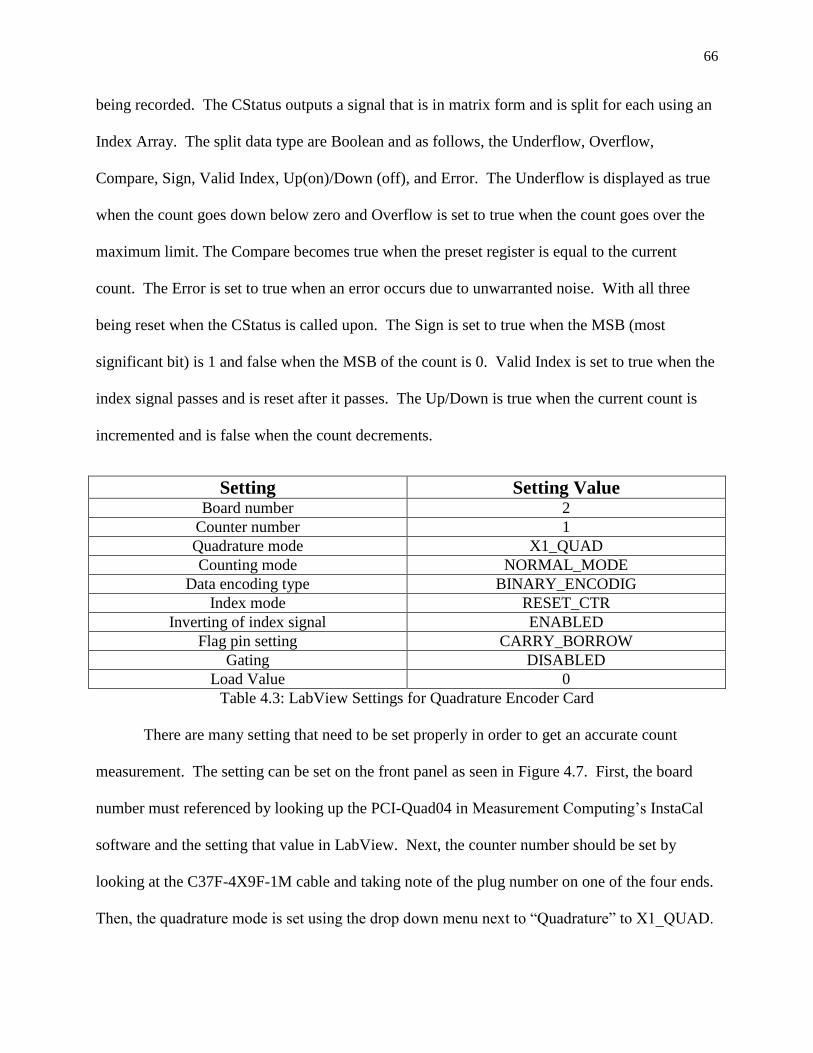
66
being recorded. The CStatus outputs a signal that is in matrix form and is split for each using an
Index Array. The split data type are Boolean and as follows, the Underflow, Overflow,
Compare, Sign, Valid Index, Up(on)/Down (off), and Error. The Underflow is displayed as true
when the count goes down below zero and Overflow is set to true when the count goes over the
maximum limit. The Compare becomes true when the preset register is equal to the current
count. The Error is set to true when an error occurs due to unwarranted noise. With all three
being reset when the CStatus is called upon. The Sign is set to true when the MSB (most
significant bit) is 1 and false when the MSB of the count is 0. Valid Index is set to true when the
index signal passes and is reset after it passes. The Up/Down is true when the current count is
incremented and is false when the count decrements.
Setting Setting Value Board number 2
Counter number 1
Quadrature mode X1_QUAD
Counting mode NORMAL_MODE
Data encoding type BINARY_ENCODIG
Index mode RESET_CTR
Inverting of index signal ENABLED
Flag pin setting CARRY_BORROW
Gating DISABLED
Load Value 0
Table 4.3: LabView Settings for Quadrature Encoder Card
There are many setting that need to be set properly in order to get an accurate count
measurement. The setting can be set on the front panel as seen in Figure 4.7. First, the board
number must referenced by looking up the PCI-Quad04 in Measurement Computing’s InstaCal
software and the setting that value in LabView. Next, the counter number should be set by
looking at the C37F-4X9F-1M cable and taking note of the plug number on one of the four ends.
Then, the quadrature mode is set using the drop down menu next to ―Quadrature‖ to X1_QUAD.
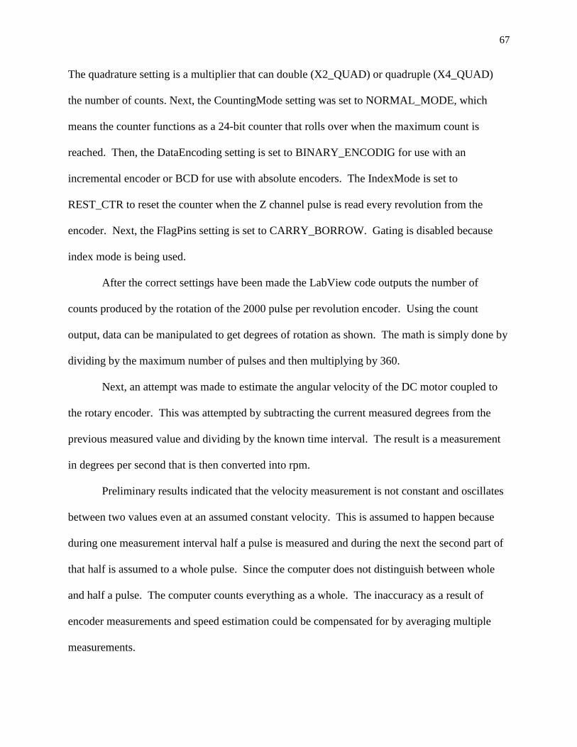
67
The quadrature setting is a multiplier that can double (X2_QUAD) or quadruple (X4_QUAD)
the number of counts. Next, the CountingMode setting was set to NORMAL_MODE, which
means the counter functions as a 24-bit counter that rolls over when the maximum count is
reached. Then, the DataEncoding setting is set to BINARY_ENCODIG for use with an
incremental encoder or BCD for use with absolute encoders. The IndexMode is set to
REST_CTR to reset the counter when the Z channel pulse is read every revolution from the
encoder. Next, the FlagPins setting is set to CARRY_BORROW. Gating is disabled because
index mode is being used.
After the correct settings have been made the LabView code outputs the number of
counts produced by the rotation of the 2000 pulse per revolution encoder. Using the count
output, data can be manipulated to get degrees of rotation as shown. The math is simply done by
dividing by the maximum number of pulses and then multiplying by 360.
Next, an attempt was made to estimate the angular velocity of the DC motor coupled to
the rotary encoder. This was attempted by subtracting the current measured degrees from the
previous measured value and dividing by the known time interval. The result is a measurement
in degrees per second that is then converted into rpm.
Preliminary results indicated that the velocity measurement is not constant and oscillates
between two values even at an assumed constant velocity. This is assumed to happen because
during one measurement interval half a pulse is measured and during the next the second part of
that half is assumed to a whole pulse. Since the computer does not distinguish between whole
and half a pulse. The computer counts everything as a whole. The inaccuracy as a result of
encoder measurements and speed estimation could be compensated for by averaging multiple
measurements.

68
4.1.1.5 Encoder Signal Testing
A small test apparatus was constructed next, consisting of a DC motor coupled to a rotary
encoder. The DC motor was simply a geared dc motor rated at 5 rpm for an input voltage of 4.5
volts. The encoder is a 2000 pulse per revolution optical encoder. Therefore at the maximum
operation speed the encoder is expected to have maximum change of frequency of 100 kHz. The
encoder’s quadrature signal was fed into the PCI-QUAD04. With an input voltage of 3 volts to
the motor, LabView only logged 1430 counts within one full rotation out of the maximum of
2000. This speed was noticeable less than the 5 rpm rated speed. This count will become more
sporadic with the increase in speed to 3000 rpm. Therefore simply using LabView running
under Windows XP will not suffice for the data acquisition needs. Sample of the data collected
is presented in the appendix of this report.
Figure 4.4: Frame 0 LabView Block Diagram Code for Quadrature Encoder
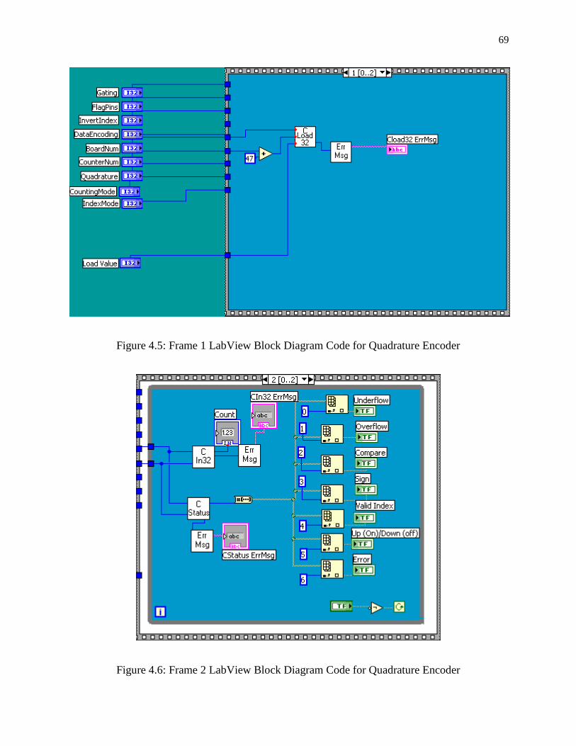
69
Figure 4.5: Frame 1 LabView Block Diagram Code for Quadrature Encoder
Figure 4.6: Frame 2 LabView Block Diagram Code for Quadrature Encoder
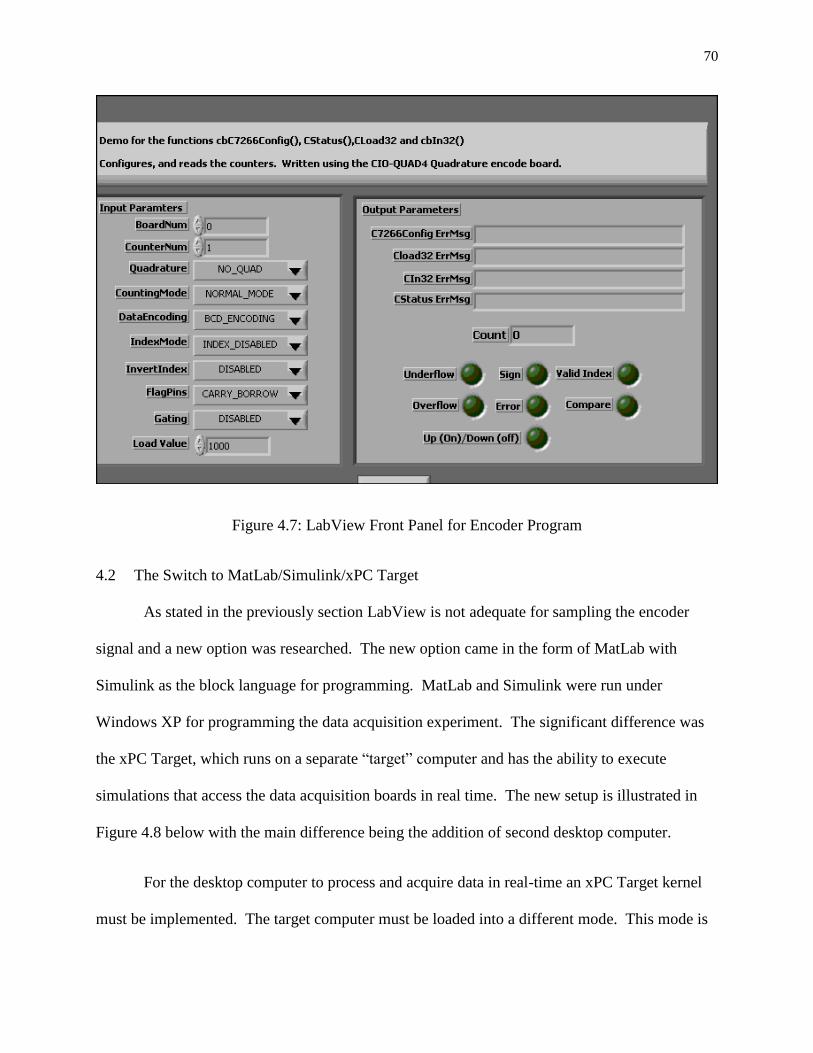
70
Figure 4.7: LabView Front Panel for Encoder Program
4.2 The Switch to MatLab/Simulink/xPC Target
As stated in the previously section LabView is not adequate for sampling the encoder
signal and a new option was researched. The new option came in the form of MatLab with
Simulink as the block language for programming. MatLab and Simulink were run under
Windows XP for programming the data acquisition experiment. The significant difference was
the xPC Target, which runs on a separate ―target‖ computer and has the ability to execute
simulations that access the data acquisition boards in real time. The new setup is illustrated in
Figure 4.8 below with the main difference being the addition of second desktop computer.
For the desktop computer to process and acquire data in real-time an xPC Target kernel
must be implemented. The target computer must be loaded into a different mode. This mode is

71
induced by what MatLab calls xPC Target kernel. This mode allows the Target computer to
execute Simulink models and gather data in real time.
The new data acquisition system is programmed by using the Simulink block
programming language. Boards can be found by simply searching by name or going through the
block libraries tree. MatLab provides a set of driver blocks sorted by signal type and board
manufacturer. For instance the PCI-QUAD04 is used to acquire quadrature encoder signals and
therefore is listed in the Simulink library tree under Encoder and then Measurement Computing
Inc. because they manufacture the board. The necessary sampling rate is set by double clicking
the source block.
The target machine also has a monitor to observe signal operations. Target Scopes are
added from the block library to view these signals on the monitor. The Target Scope is one of
three xPC Target specific scopes. To send data to the MatLab work space an Out1 block is
added. Depending on the automatically assigned Out1 block determines the position of the
signal in the acquired data matrix. This system helps keep track of the multiple signals being
acquired. The code used to import the data is shown in the Appendix section of this paper. The
Out blocks and xPC Target data acquisition blocks can be seen in Figure 4.9.
Using xPC Target system the options when scanning channels differs between analog and
digital inputs. For analog inputs the drivers provided by MathWorks only allows one to scan a
range of channels and not select individual channels. For instance, one cannot just scan channel
five, one must scan channels one through five. Therefore, if only the signal from channel five is
needed the connections must be switched or they could affect the overall bandwidth for a test.
Digital signals can be picked individually and scanned.

72
Once data acquisition is completed for one run the data is automatically sent to the host
machine. The data is in what is called a target object. This chunk of data is split up by using
specific xPC target commands. The first is ―tg.timelog‖ which acquires the target time. Another
is ―tg.outputlog‖ which is a matrix of all the output signals. The number of data points
remaining in the ―tg.outputlog‖ object is determined by the size of the data buffer. This buffer
rolls over after it is filled and starts writing over the first data set. The buffer size is limited by
the amount of RAM available on the Target Computer. The buffer size is set under View>
Configuration Parameters >Real-Time Workshop>xPC Target options>Data logging options.
This value also determines the overall maximum number of data points logged and for each
signal this value is divided. The way MatLab calculates this value is by dividing the maximum
by the number of signals taken. This calculation can be done in MatLab using the command
floor(x) and the command window, where x is simply replaced by the quotient equation.
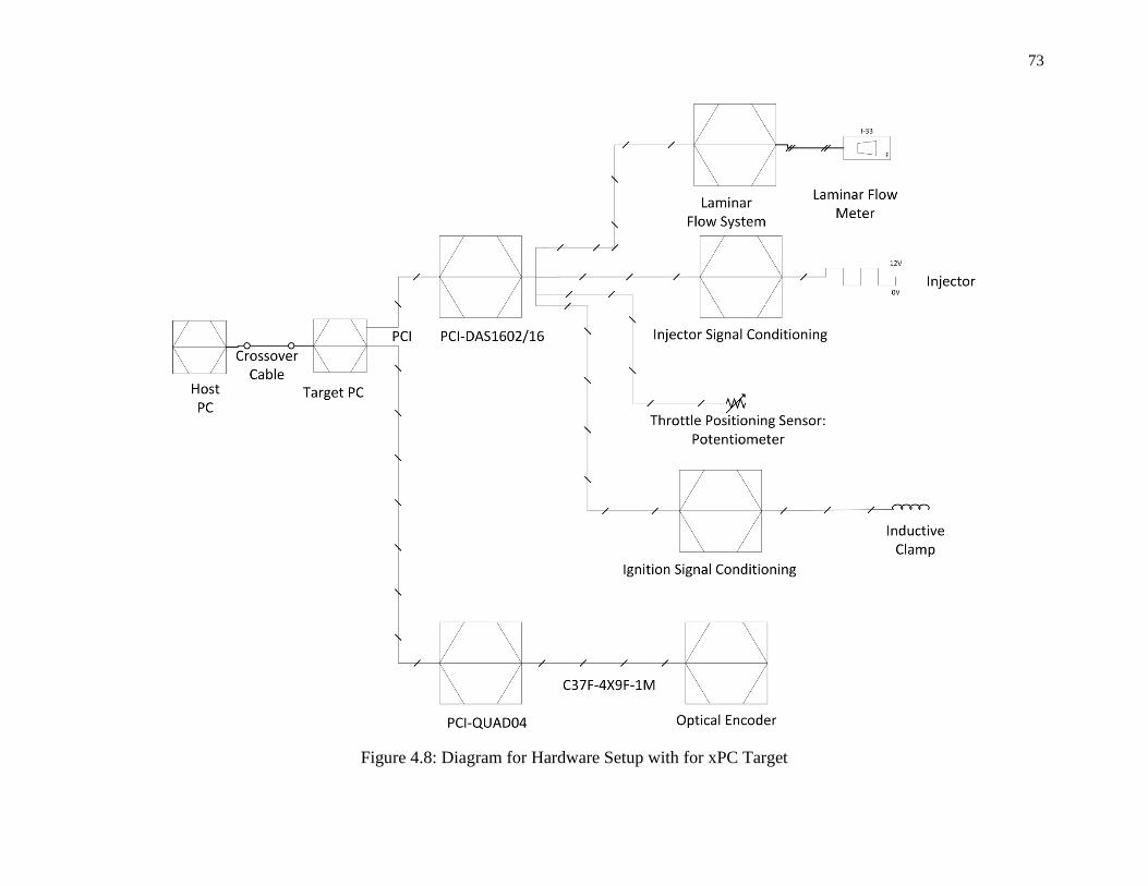
73
Figure 4.8: Diagram for Hardware Setup with for xPC Target
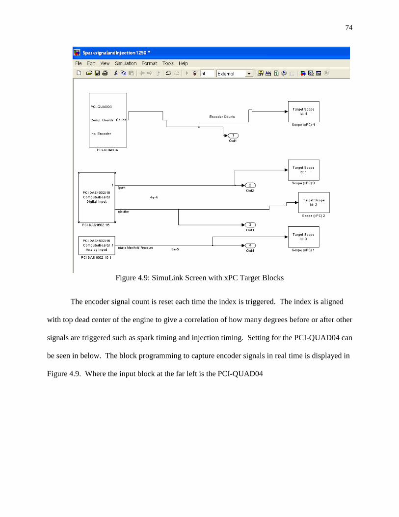
74
Figure 4.9: SimuLink Screen with xPC Target Blocks
The encoder signal count is reset each time the index is triggered. The index is aligned
with top dead center of the engine to give a correlation of how many degrees before or after other
signals are triggered such as spark timing and injection timing. Setting for the PCI-QUAD04 can
be seen in below. The block programming to capture encoder signals in real time is displayed in
Figure 4.9. Where the input block at the far left is the PCI-QUAD04

75
Parameter Parameter Value
Channel 1
Index input resets counter Check Mark
Index Polarity Negative Index
Counting Mode Normal
Count Limit or Reset Value 0
Count Range -2^23…+2^23-1
Count Speed 1x
Filter prescale factor 0
Sample Time 0.00004
PCI slot -1
Table 4.4: PCI-QUAD04 settings in MatLab
The engine sensors will be connected to a computer based data acquisition system. The
necessary equipment needed to acquire data from the engine and its various sensors includes a
variety of data acquisition boards placed within a personal desktop computer considered the
Target PC. The details on the host and target computer used in this study are detailed in Table
4.5 below. A list of these data acquisition boards, the type of signals they can acquire and
maximum input frequency can be seen in Table 4.6 below.
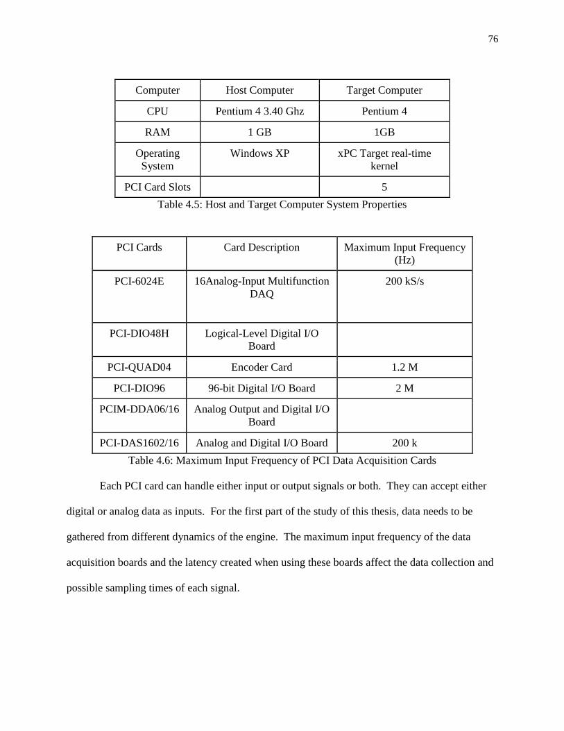
76
Computer Host Computer Target Computer
CPU Pentium 4 3.40 Ghz Pentium 4
RAM 1 GB 1GB
Operating
System
Windows XP xPC Target real-time
kernel
PCI Card Slots 5
Table 4.5: Host and Target Computer System Properties
PCI Cards Card Description Maximum Input Frequency
(Hz)
PCI-6024E 16Analog-Input Multifunction
DAQ
200 kS/s
PCI-DIO48H Logical-Level Digital I/O
Board
PCI-QUAD04 Encoder Card 1.2 M
PCI-DIO96 96-bit Digital I/O Board 2 M
PCIM-DDA06/16 Analog Output and Digital I/O
Board
PCI-DAS1602/16 Analog and Digital I/O Board 200 k
Table 4.6: Maximum Input Frequency of PCI Data Acquisition Cards
Each PCI card can handle either input or output signals or both. They can accept either
digital or analog data as inputs. For the first part of the study of this thesis, data needs to be
gathered from different dynamics of the engine. The maximum input frequency of the data
acquisition boards and the latency created when using these boards affect the data collection and
possible sampling times of each signal.

77
Analog and Digital Signals 4.2.1
Digital and analog signals are brought into the data acquisition computer using an Analog
and Digital input/ output (IO) board (PCI-DAS1602/16). This card is used to sample injector
signals, flow meter analog outputs i.e. the intake manifold pressure and intake mass air flow,
throttle angle and air/ fuel ratio.
For analog input signals the PCI-DAS1602/16 has software selectable input configuration
of 8 differential inputs or 16 single-ended inputs. The PCI-DAS1602/16 has a maximum
sampling rate of 200 kHz and a 512 FIFO to help with sampling data and not losing any data.
Setting used for analog connections can be seen in Table 4.7 below and digital connection
settings in Table 4.8 and Table 4.9. Differences in setting are based on expected input signal and
expected maximum frequency of change.
The Figure 4.9 shows the portion of the Simulink code used to program the xPC Target
machine for the injector signal. This block code contains a digital input block labeled with the
name of the data acquisition card and the type of signal input. An output block is added labeled
Out1 to get the gathered data into the MATLAB workspace. Finally a Target Scopes is added to
display the data as its being gathered.
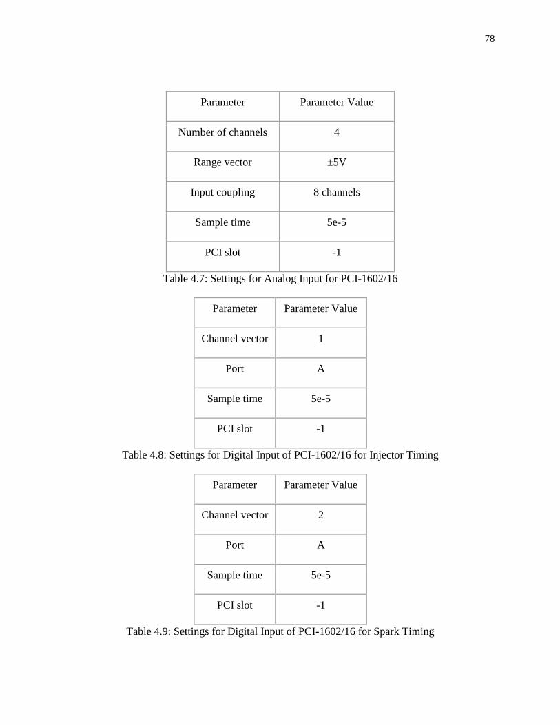
78
Parameter Parameter Value
Number of channels 4
Range vector ±5V
Input coupling 8 channels
Sample time 5e-5
PCI slot -1
Table 4.7: Settings for Analog Input for PCI-1602/16
Parameter Parameter Value
Channel vector 1
Port A
Sample time 5e-5
PCI slot -1
Table 4.8: Settings for Digital Input of PCI-1602/16 for Injector Timing
Parameter Parameter Value
Channel vector 2
Port A
Sample time 5e-5
PCI slot -1
Table 4.9: Settings for Digital Input of PCI-1602/16 for Spark Timing
79
Target Machine Benchmark 4.2.2
A benchmark was performed on the target machine to get some idea of the performance
capability of the target computer. The performance was done using the internal command
―xpcbench‖. This command runs the target machine through a battery of tests running increasing
more complex models. The does not take into account latency produced by the data acquisition
cards currently installed
DC Motor and Offline Testing 4.2.3
Further offline testing was needed to insure that signals could be recorded at the fastest
expected change of a signal while doing engine testing. This testing is considered offline
because the single cylinder Briggs and Stratton engine is not being used to simply test system
limits. The advantage of such testing is the gas is not wasted, the system is simple enough that
taking repeated measurements does not take much time and the quickest changing dynamics can
be tested i.e. the rotary encoder.
The test setup was comprised of a Normand Electrical Company (NECO) DC shunt
motor rated at a velocity of 3000 rpm. Sensors used for testing include a rotary encoder and
variable reluctance (VR) sensor. The motor can be seen in to Figure 4.11 below. The figures
show a side and top view. The encoder is used to discern crank angle and speed once again, and
the VR sensor is used as a second signal to sync with the encoder changes.
Building Stands and Assembly 4.2.4
To get this system put together two stands were made using scrap pieces of aluminum.
One stand will be used to hold the rotary encoder in line with the motor shaft and the other holds
the VR sensor near the engine shaft.
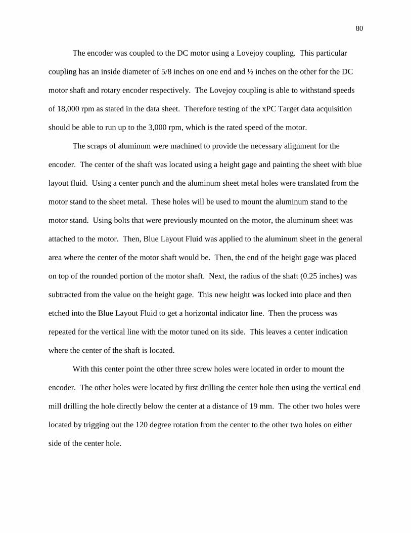
80
The encoder was coupled to the DC motor using a Lovejoy coupling. This particular
coupling has an inside diameter of 5/8 inches on one end and ½ inches on the other for the DC
motor shaft and rotary encoder respectively. The Lovejoy coupling is able to withstand speeds
of 18,000 rpm as stated in the data sheet. Therefore testing of the xPC Target data acquisition
should be able to run up to the 3,000 rpm, which is the rated speed of the motor.
The scraps of aluminum were machined to provide the necessary alignment for the
encoder. The center of the shaft was located using a height gage and painting the sheet with blue
layout fluid. Using a center punch and the aluminum sheet metal holes were translated from the
motor stand to the sheet metal. These holes will be used to mount the aluminum stand to the
motor stand. Using bolts that were previously mounted on the motor, the aluminum sheet was
attached to the motor. Then, Blue Layout Fluid was applied to the aluminum sheet in the general
area where the center of the motor shaft would be. Then, the end of the height gage was placed
on top of the rounded portion of the motor shaft. Next, the radius of the shaft (0.25 inches) was
subtracted from the value on the height gage. This new height was locked into place and then
etched into the Blue Layout Fluid to get a horizontal indicator line. Then the process was
repeated for the vertical line with the motor tuned on its side. This leaves a center indication
where the center of the shaft is located.
With this center point the other three screw holes were located in order to mount the
encoder. The other holes were located by first drilling the center hole then using the vertical end
mill drilling the hole directly below the center at a distance of 19 mm. The other two holes were
located by trigging out the 120 degree rotation from the center to the other two holes on either
side of the center hole.
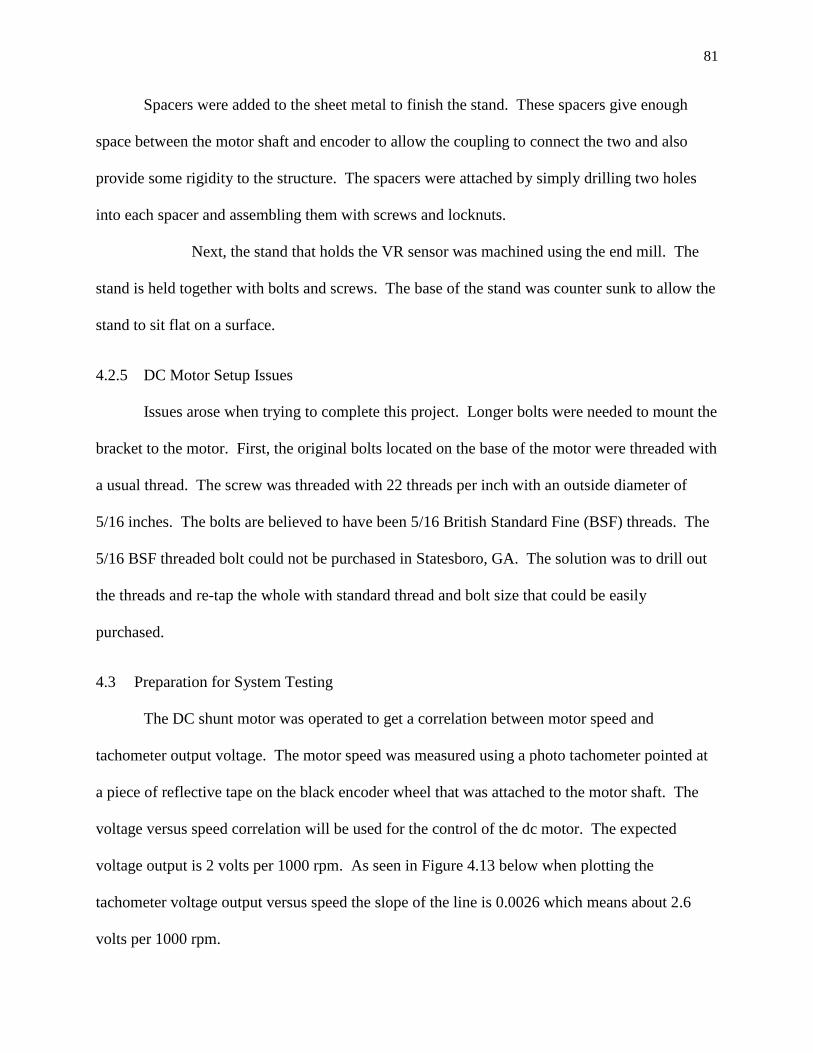
81
Spacers were added to the sheet metal to finish the stand. These spacers give enough
space between the motor shaft and encoder to allow the coupling to connect the two and also
provide some rigidity to the structure. The spacers were attached by simply drilling two holes
into each spacer and assembling them with screws and locknuts.
Next, the stand that holds the VR sensor was machined using the end mill. The
stand is held together with bolts and screws. The base of the stand was counter sunk to allow the
stand to sit flat on a surface.
DC Motor Setup Issues 4.2.5
Issues arose when trying to complete this project. Longer bolts were needed to mount the
bracket to the motor. First, the original bolts located on the base of the motor were threaded with
a usual thread. The screw was threaded with 22 threads per inch with an outside diameter of
5/16 inches. The bolts are believed to have been 5/16 British Standard Fine (BSF) threads. The
5/16 BSF threaded bolt could not be purchased in Statesboro, GA. The solution was to drill out
the threads and re-tap the whole with standard thread and bolt size that could be easily
purchased.
4.3 Preparation for System Testing
The DC shunt motor was operated to get a correlation between motor speed and
tachometer output voltage. The motor speed was measured using a photo tachometer pointed at
a piece of reflective tape on the black encoder wheel that was attached to the motor shaft. The
voltage versus speed correlation will be used for the control of the dc motor. The expected
voltage output is 2 volts per 1000 rpm. As seen in Figure 4.13 below when plotting the
tachometer voltage output versus speed the slope of the line is 0.0026 which means about 2.6
volts per 1000 rpm.

82
The VR sensor and two metal nuts and screws are used to generate a signal every time
one of the screws passes the sensor. The VR sensor with stand can be seen in Figure 4.12. The
VR signal will then be logged with the crank angle using xPC Target.
Control of DC Motor 4.3.1
In the attempt to control the DC motor to aid in the testing process digital control strategy
was attempted. The strategy included the use of a Basic Stamp 2 microcontroller, H-Bridge, and
Schottky Diodes. The assumption was that using the above components and pulse width
modulation to either the shunt or armature of the dc motor the motor could be controlled. The
DC motor already had a tachometer on the back of the motor that could be used as a feedback
signal. The output of the voltage of the tachometer was to be divided to protect the
microcontroller.
Reasons for the inability to drive the motor could come from lack of knowledge in how
shunt motor control works or the microcontroller being unable to produce encough pulses to
ultimately drive the test system.
The micrococontroller setup was abandoned and switched to using the DC power supplie.
Using the power supplie the armature and shunt of the motor were powered seperately. Using
this simple configuration and an oscilloscope to monitor the tachometer voltage for speed
confirmation the test set-up became very useful. The test setup still required a little tuning to
make the speed stable.
The test set could be used to generate data at up to 3000 rpms that then can be taken into
Matlab for further manipulation such as sending the data to Excel.
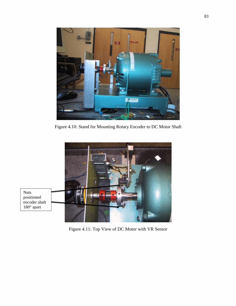
83
Figure 4.10: Stand for Mounting Rotary Encoder to DC Motor Shaft
Figure 4.11: Top View of DC Motor with VR Sensor
Nuts
positioned
encoder shaft
180° apart
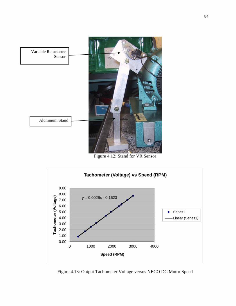
84
Figure 4.12: Stand for VR Sensor
Figure 4.13: Output Tachometer Voltage versus NECO DC Motor Speed
y = 0.0026x - 0.1623
0.00
1.00
2.00
3.00
4.00
5.00
6.00
7.00
8.00
9.00
0 1000 2000 3000 4000
Tach
om
ete
r (V
olt
ag
e)
Speed (RPM)
Tachometer (Voltage) vs Speed (RPM)
Series1
Linear (Series1)
Variable Reluctance
Sensor
Aluminum Stand
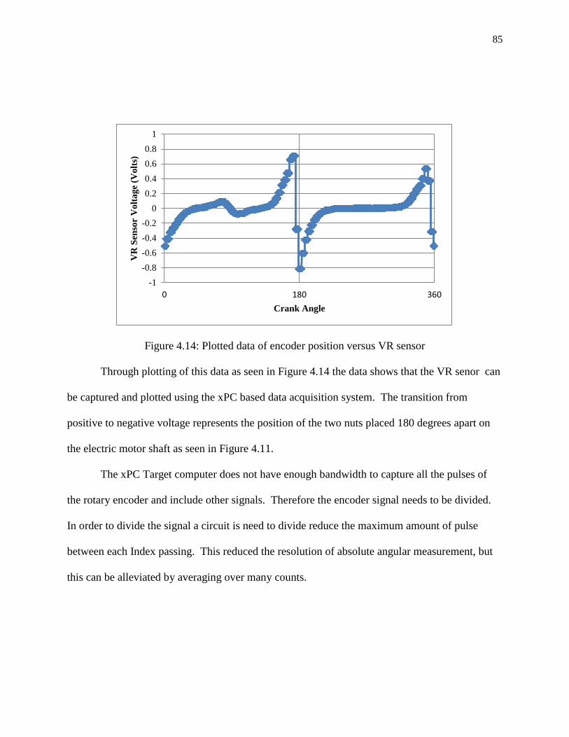
85
Figure 4.14: Plotted data of encoder position versus VR sensor
Through plotting of this data as seen in Figure 4.14 the data shows that the VR senor can
be captured and plotted using the xPC based data acquisition system. The transition from
positive to negative voltage represents the position of the two nuts placed 180 degrees apart on
the electric motor shaft as seen in Figure 4.11.
The xPC Target computer does not have enough bandwidth to capture all the pulses of
the rotary encoder and include other signals. Therefore the encoder signal needs to be divided.
In order to divide the signal a circuit is need to divide reduce the maximum amount of pulse
between each Index passing. This reduced the resolution of absolute angular measurement, but
this can be alleviated by averaging over many counts.
-1
-0.8
-0.6
-0.4
-0.2
0
0.2
0.4
0.6
0.8
1
0 180 360
VR
Sen
sor
Vo
lta
ge
(Vo
lts)
Crank Angle
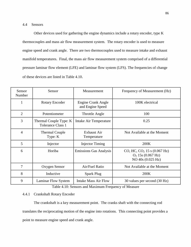
86
4.4 Sensors
Other devices used for gathering the engine dynamics include a rotary encoder, type K
thermocouples and mass air flow measurement system. The rotary encoder is used to measure
engine speed and crank angle. There are two thermocouples used to measure intake and exhaust
manifold temperatures. Final, the mass air flow measurement system comprised of a differential
pressure laminar flow element (LFE) and laminar flow system (LFS). The frequencies of change
of these devices are listed in Table 4.10.
Sensor
Number
Sensor Measurement Frequency of Measurement (Hz)
1 Rotary Encoder Engine Crank Angle
and Engine Speed
100K electrical
2 Potentiometer Throttle Angle 100
3 Thermal Couple Type: K
Tolerance Class 1
Intake Air Temperature 0.25
4 Thermal Couple
Type: K
Exhaust Air
Temperature
Not Available at the Moment
5 Injector Injector Timing 200K
6 Horiba Emissions Gas Analysis CO, HC, CO2 15 s (0.067 Hz)
O2 15s (0.067 Hz)
NO 40s (0.025 Hz)
7 Oxygen Sensor Air/Fuel Ratio Not Available at the Moment
8 Inductive Spark Plug 200K
9 Laminar Flow System Intake Mass Air Flow 30 values per second (30 Hz)
Table 4.10: Sensors and Maximum Frequency of Measure
Crankshaft Rotary Encoder 4.4.1
The crankshaft is a key measurement point. The cranks shaft with the connecting rod
translates the reciprocating motion of the engine into rotations. This connecting point provides a
point to measure engine speed and crank angle.
87
To measure the engines speed and crank angle an Omron incremental rotary encoder is
used. The encoder works by having a disc inside with multiple equally spaced slits cut out.
These slits allow light emitted from a LED internal to the encoder to hit a sensor inside the
encoder. Therefore, as the encoder spins pulses are generated when the sensor picks up the LED
light. There are three tracks of these slots called channels. The first two channels are usually
called channel A and B. Channel A and B generate a signal when the encoder is spun that is 90
degrees out of phase with each other. This difference in phase allows the direction the encoder
is spinning to be identified. The third channel usually designated the index or channel Z,
generates only one pulse per revolution. The Z channel is used to reset the encoder counts in
data acquisition and to sync the encoder with top dead center (TDC) of the engine.
The encoder is coupled to the engine crank shaft parallel with the engine spinning axis.
The rotary encoder has a resolution of 2,000 pulses per revolution. This resolution provides an
accuracy of 0.18 degrees per pulse. Therefore there are 4,000 pulses or counts within one four
stroke process. These 2,000 pulses per revolution can generate a change on frequency at 3,000
rpm engine speed of 100 kHz. At 100 kHz the bandwidth of the data acquisition computer will
be almost total used up on the one signal alone. Therefore the signal needs to be divided in order
to ensure the encoder signal is not sporadic. To divide the encoder signal a commercially
available encoder divider from BaneBots was selected. The encoder divider enables divisions of
4, 8 or 16. The results of this division and the effects on resolution and the bandwidth usage can
be seen in the table below.
Flow System Measurements 4.4.2
The Laminar Flow System requires a plug to connect to the two analog outputs. A Neutrik
NC5MX five pin plug is used to provide an external connection. Pins 1 and 2 are the positive
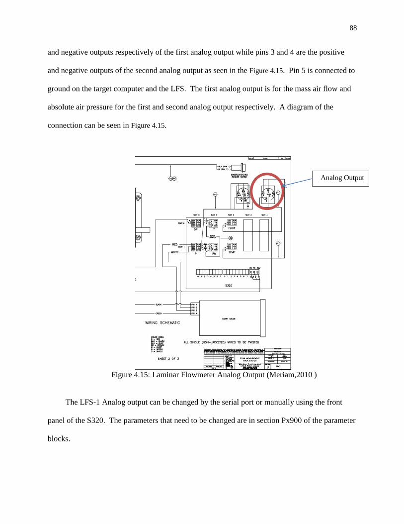
88
and negative outputs respectively of the first analog output while pins 3 and 4 are the positive
and negative outputs of the second analog output as seen in the Figure 4.15. Pin 5 is connected to
ground on the target computer and the LFS. The first analog output is for the mass air flow and
absolute air pressure for the first and second analog output respectively. A diagram of the
connection can be seen in Figure 4.15.
Figure 4.15: Laminar Flowmeter Analog Output (Meriam,2010 )
The LFS-1 Analog output can be changed by the serial port or manually using the front
panel of the S320. The parameters that need to be changed are in section Px900 of the parameter
blocks.
Analog Output
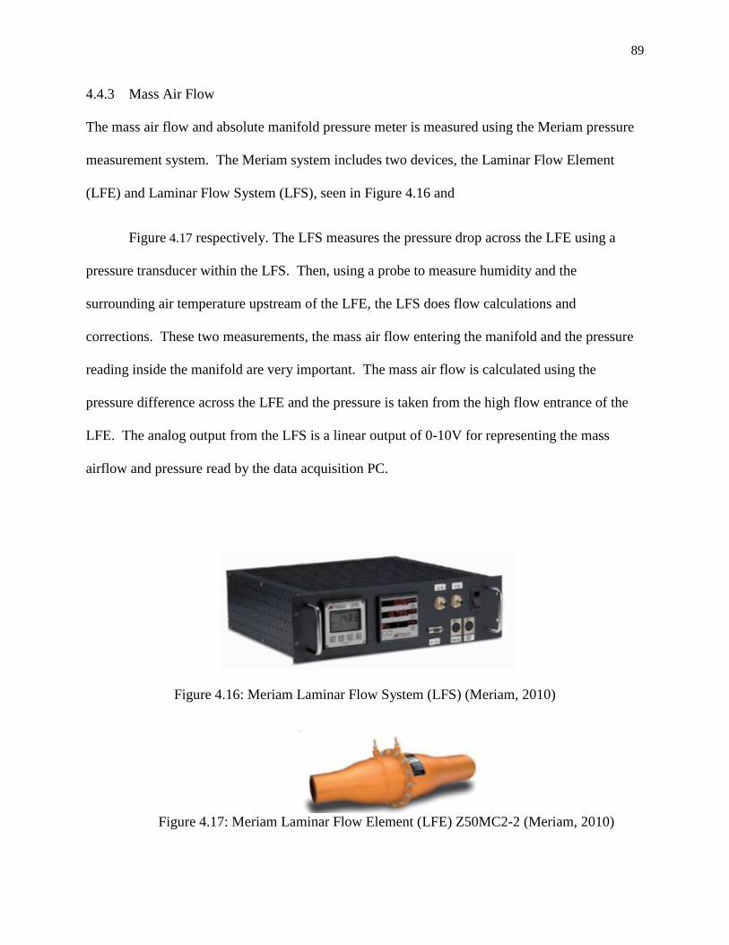
89
Mass Air Flow 4.4.3
The mass air flow and absolute manifold pressure meter is measured using the Meriam pressure
measurement system. The Meriam system includes two devices, the Laminar Flow Element
(LFE) and Laminar Flow System (LFS), seen in Figure 4.16 and
Figure 4.17 respectively. The LFS measures the pressure drop across the LFE using a
pressure transducer within the LFS. Then, using a probe to measure humidity and the
surrounding air temperature upstream of the LFE, the LFS does flow calculations and
corrections. These two measurements, the mass air flow entering the manifold and the pressure
reading inside the manifold are very important. The mass air flow is calculated using the
pressure difference across the LFE and the pressure is taken from the high flow entrance of the
LFE. The analog output from the LFS is a linear output of 0-10V for representing the mass
airflow and pressure read by the data acquisition PC.
Figure 4.16: Meriam Laminar Flow System (LFS) (Meriam, 2010)
Figure 4.17: Meriam Laminar Flow Element (LFE) Z50MC2-2 (Meriam, 2010)
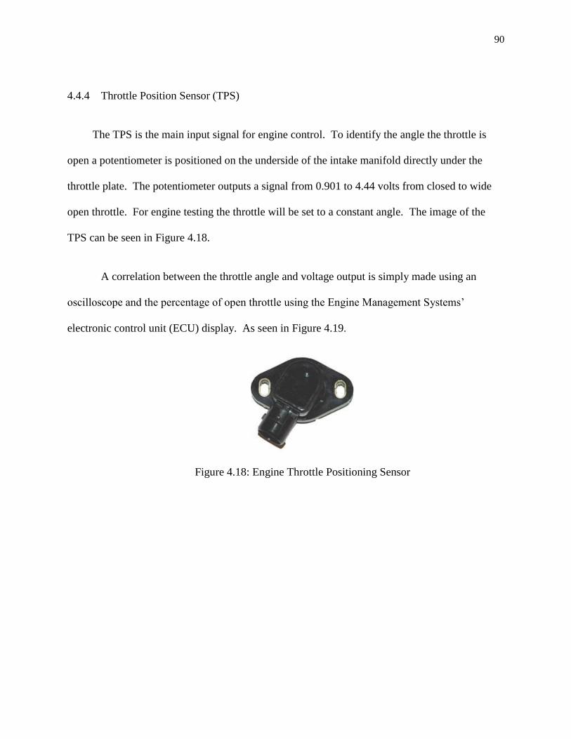
90
Throttle Position Sensor (TPS) 4.4.4
The TPS is the main input signal for engine control. To identify the angle the throttle is
open a potentiometer is positioned on the underside of the intake manifold directly under the
throttle plate. The potentiometer outputs a signal from 0.901 to 4.44 volts from closed to wide
open throttle. For engine testing the throttle will be set to a constant angle. The image of the
TPS can be seen in Figure 4.18.
A correlation between the throttle angle and voltage output is simply made using an
oscilloscope and the percentage of open throttle using the Engine Management Systems’
electronic control unit (ECU) display. As seen in Figure 4.19.
Figure 4.18: Engine Throttle Positioning Sensor
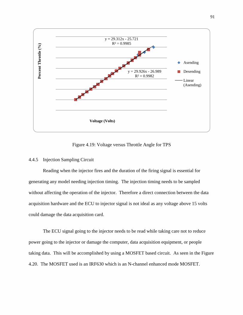
91
Figure 4.19: Voltage versus Throttle Angle for TPS
Injection Sampling Circuit 4.4.5
Reading when the injector fires and the duration of the firing signal is essential for
generating any model needing injection timing. The injection timing needs to be sampled
without affecting the operation of the injector. Therefore a direct connection between the data
acquisition hardware and the ECU to injector signal is not ideal as any voltage above 15 volts
could damage the data acquisition card.
The ECU signal going to the injector needs to be read while taking care not to reduce
power going to the injector or damage the computer, data acquisition equipment, or people
taking data. This will be accomplished by using a MOSFET based circuit. As seen in the Figure
4.20. The MOSFET used is an IRF630 which is an N-channel enhanced mode MOSFET.
y = 29.312x - 25.721
R² = 0.9985
y = 29.926x - 26.989
R² = 0.9982 Per
cen
t T
hro
ttle
(%
)
Voltage (Volts)
Asending
Desending
Linear
(Asending)

92
The MOSFET is will be setup with the 12 volt injector signal being applied to the gate. The
drain will have a constant 5 voltage signal coming from the PCI-DAS1602/16 digital and analog
card. A 1 kilo ohm resistor is placed in series with the source output. The voltage across the 1
kilo ohm resistor will then be read by the PCI-DAS1602 as a digital signal.
With the MOSFET setup for the injector signal when the injector fires a channel is
created within the MOSFET that allows the 5 volts from the PC to be sensed at the source. By
only reading the 5 volts that passes through the MOSFET and not the 12 volts directly from the
ECU, the data acquisition system will be safe. The circuit design can be seen in Figure 4.20.
A diode was added to the gate of the MOSFET as seen in the Figure 4.20. The diode was
added to fix a grounding issue. That was caused when the engines ECU tried to find a grounding
point on the data acquisition computer. The injector was a Bosch Suzuki injector with model
number 2500431 with impedance of 20 ohms. A diagram of the circuit can be seen in Figure
4.20.
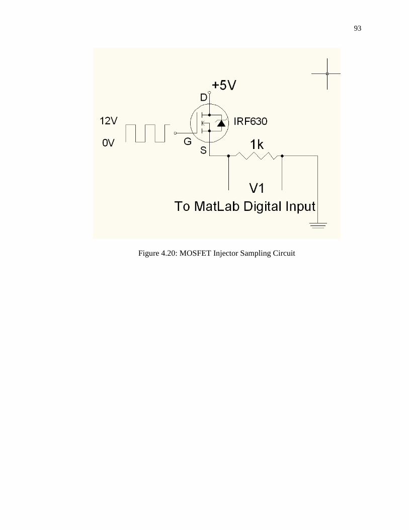
93
Figure 4.20: MOSFET Injector Sampling Circuit
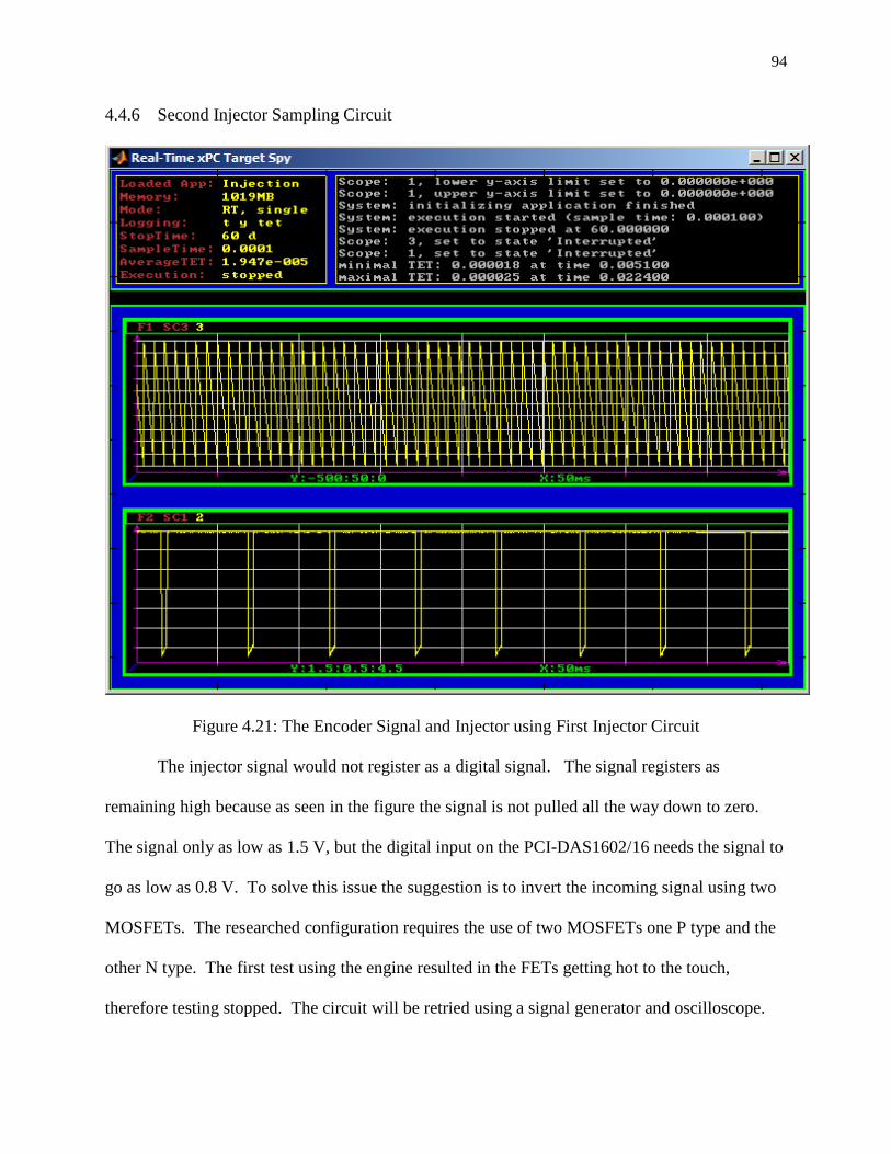
94
Second Injector Sampling Circuit 4.4.6
Figure 4.21: The Encoder Signal and Injector using First Injector Circuit
The injector signal would not register as a digital signal. The signal registers as
remaining high because as seen in the figure the signal is not pulled all the way down to zero.
The signal only as low as 1.5 V, but the digital input on the PCI-DAS1602/16 needs the signal to
go as low as 0.8 V. To solve this issue the suggestion is to invert the incoming signal using two
MOSFETs. The researched configuration requires the use of two MOSFETs one P type and the
other N type. The first test using the engine resulted in the FETs getting hot to the touch,
therefore testing stopped. The circuit will be retried using a signal generator and oscilloscope.
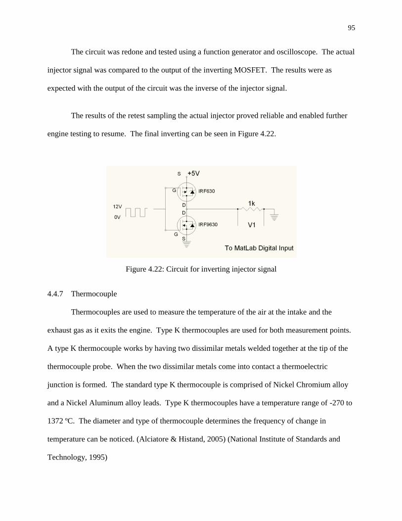
95
The circuit was redone and tested using a function generator and oscilloscope. The actual
injector signal was compared to the output of the inverting MOSFET. The results were as
expected with the output of the circuit was the inverse of the injector signal.
The results of the retest sampling the actual injector proved reliable and enabled further
engine testing to resume. The final inverting can be seen in Figure 4.22.
Figure 4.22: Circuit for inverting injector signal
Thermocouple 4.4.7
Thermocouples are used to measure the temperature of the air at the intake and the
exhaust gas as it exits the engine. Type K thermocouples are used for both measurement points.
A type K thermocouple works by having two dissimilar metals welded together at the tip of the
thermocouple probe. When the two dissimilar metals come into contact a thermoelectric
junction is formed. The standard type K thermocouple is comprised of Nickel Chromium alloy
and a Nickel Aluminum alloy leads. Type K thermocouples have a temperature range of -270 to
1372 ºC. The diameter and type of thermocouple determines the frequency of change in
temperature can be noticed. (Alciatore & Histand, 2005) (National Institute of Standards and
Technology, 1995)

96
Thermocouple Data Acquisition 4.4.8
The sensors for the current study will be attached as follows. The PCI-6024E is
connected to a SCC-2345 signal conditioning board. The SCC-2345 contains two SCC-TC01
thermocouple input modules. The SCC-TC01 takes in the thermocouple voltage and does cold-
junction compensation using a thermistor to measure the reference temperature. Then, the
thermocouple voltage and cold-junction compensation voltage are used to calculate the
thermocouple temperature. The temperature is correlated to the temperature voltage read by the
target machine.
To acquire temperature measurements from thermocouples a conversion is needed
between the thermocouple voltage and temperature. To get this correlation a known temperature
is compared to the voltage. The known temperature measurement was provided by an Extech
470 which can read between -20 to 750 Celsius with a resolution of 1 degree Celsius. The
Extech provides an accuracy of 3.0% for the reading for the measurement circuit and 3 digits for
the analog to digital converter. The correlation was attempted by using boiling water in beaker
and measuring the temperature with the Extech 470 and computer based data acquisition. Then
the voltage and temperature were recorded. With this method a temperature of only 94 degrees
Celsius can be reached because the water starts boil.
Since the above testing limits the range of possible temperatures to only 94 degrees
Celsius another method will be attempted. Using an E5CS Omron Temperature Controller to
read the exhaust temperature and comparing that to the actively recorded voltage of the data
acquisition system to get a new correlation at those extreme temperatures.
The second and final solution is to use the later purchased temperature controllers. The
controller is an Omega temperature controller with a linear output of 4 – 20 ma. A 250 ohm
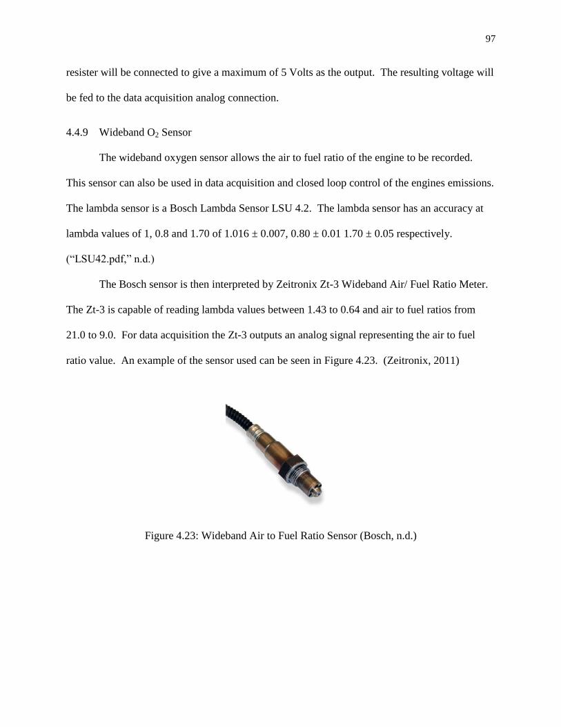
97
resister will be connected to give a maximum of 5 Volts as the output. The resulting voltage will
be fed to the data acquisition analog connection.
Wideband O2 Sensor 4.4.9
The wideband oxygen sensor allows the air to fuel ratio of the engine to be recorded.
This sensor can also be used in data acquisition and closed loop control of the engines emissions.
The lambda sensor is a Bosch Lambda Sensor LSU 4.2. The lambda sensor has an accuracy at
lambda values of 1, 0.8 and 1.70 of 1.016 ± 0.007, 0.80 ± 0.01 1.70 ± 0.05 respectively.
(―LSU42.pdf,‖ n.d.)
The Bosch sensor is then interpreted by Zeitronix Zt-3 Wideband Air/ Fuel Ratio Meter.
The Zt-3 is capable of reading lambda values between 1.43 to 0.64 and air to fuel ratios from
21.0 to 9.0. For data acquisition the Zt-3 outputs an analog signal representing the air to fuel
ratio value. An example of the sensor used can be seen in Figure 4.23. (Zeitronix, 2011)
Figure 4.23: Wideband Air to Fuel Ratio Sensor (Bosch, n.d.)

98
4.5 Signal Conditioning and Sensors
First Attempt Encoder Dividers 4.5.1
The rotary encoder has a resolution of 2,000 pulses per revolution. This resolution
provides an accuracy of 0.18 degrees per pulse. Therefore there are 4,000 pulses or counts
within one four stroke process. These 2,000 pulses per revolution can generate a change on
frequency at 3,000 rpm engine speed of 100 kHz. At 100 kHz the bandwidth of the data
acquisition computer will be almost completely used up on the one signal alone. Therefore the
signal needs to be divided in order to ensure the encoder signal is not sporadic. To divide the
encoder signal a commercially available encoder divider from BaneBots was selected. The
encoder divider enables divisions of 4, 8 or 16. The results of this division and the effects on
resolution and the bandwidth usage can be seen in the table below.
The data acquisition setup and encoder dividers were tested to ensure the set-up would
work. Two BaneBots encoder dividers are used for channels A and B. Each channel is fed into
both encoders, but the primary signal is switched to divide each channel. A diagram of the
connections can be seen in the Figure 4.24.
The ―division amount‖ affects the frequency of the input signal into the quadrature
encoder card PCI-QUAD04. In Table 4.11 the division amount can be seen.
Encoder Divide Amount
Maximum Encoder Counts
After Division
Resolution (Degrees per
Pulse)
Frequency of
change at 3000 rpm
4 500 0.72 25000
8 250 1.44 12500
16 125 2.88 6250
Table 4.11: Results of Dividing Encoder Counts on Resolution and Frequency

99
Figure 4.24: Banebots Encoder Dividers to PCI-QUAD04
Encoder Signal Issues 4.5.2
The process to diagnose the encoder issue will be presented in the section below.
Originally the encoder signal became unpredictable while running the engine and using the
simulation with the dc motor. The encoder signal would either become jagged with respect to
time or decrement when expected to increment upwards. From observing output of the encoder
dividers the signal became unpredictable.
In the attempt to sample data from the rotary encoder, injection signal, inductive clamp
and manifold pressure from the laminar flow meter simultaneously, the encoder failed to produce
a signal. In an attempt to solve the issue, the encoder was checked alone without encoder divider
to see if a signal could be produced and recorded by the data acquisition xPC Target machine
and host. This attempt was successful. The assumption was to then check the encoder divider
box.
100
The encoder divider box was checked to see if it would produce a signal. At first the
signal was not as expected. The encoder divider for dividing the B channel was not dividing the
channel as expected. Then a continuity check was done on the encoder divider to check
particularly the grounded points using the BaneBots Encoder Divider Card Manual and
schematic as a guide. It was found that the ground at block J4 was not soldered correctly. The
points were re-soldered and the encoder was checked again using the DC motor and
Oscilloscope. The connections appeared to be as expected with channel A and B having the
ideal 90 degrees phase shift and same amount of divisions. Last, a test was done again with
DAQ system and Briggs engine. No signal was seen on the target machine.
The next attempt used LabView to test the connection. With the encoder divider plugged
in between the encoder and the input to the encoder card a signal was recorded. The issue occurs
inconsistently.
The 90 degrees shift in phase usually need to discern the direction of rotation of the
encoder was not of the normal state, instead channel B seemed to be leading channel A versus
the norm of the reversal. Oddly the DAQ computer still read the signal proceeding in a clock
wise direction with the count value increasing from 0 to 500 and resetting back to zero. A
solution for this could be an opto-isolator or a D-Type Flip Flop to extend the signal.
The encoder issue was solved by not splitting each channel as they entered the signal
conditioning box. According to the encoder manual specification only one signal needs to be
divided, while the other is used for direction. Only the input into S1 is needed to divide the
encoder signal. The splitting of each of the encoder signal channels is believed to have caused
fan-out and therefore unpredictable results. Therefore channel A goes to S1 of one encoder
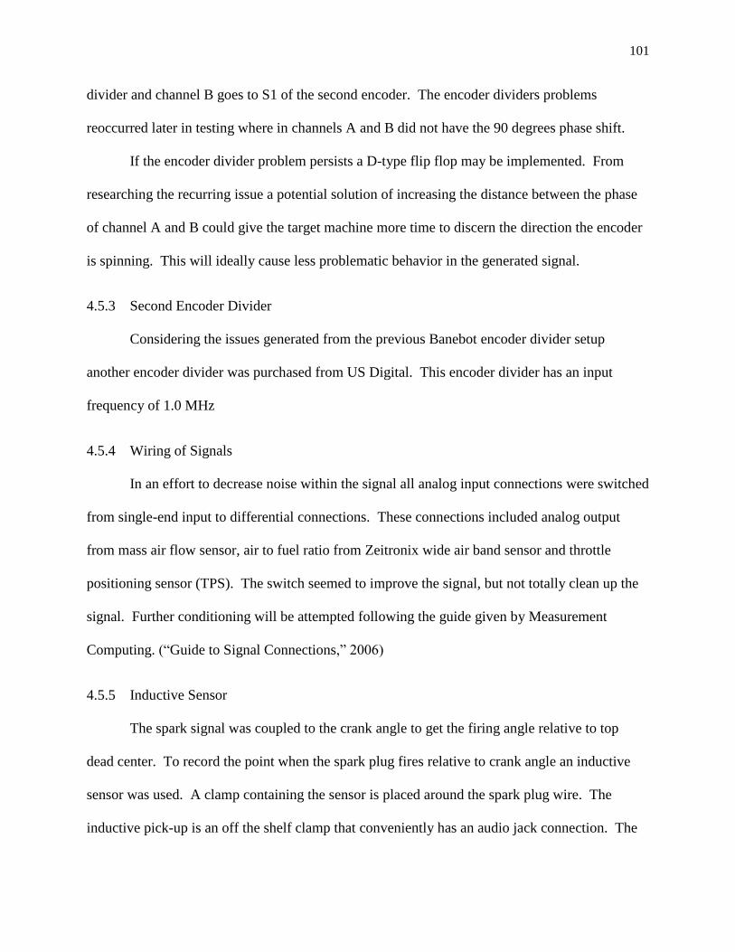
101
divider and channel B goes to S1 of the second encoder. The encoder dividers problems
reoccurred later in testing where in channels A and B did not have the 90 degrees phase shift.
If the encoder divider problem persists a D-type flip flop may be implemented. From
researching the recurring issue a potential solution of increasing the distance between the phase
of channel A and B could give the target machine more time to discern the direction the encoder
is spinning. This will ideally cause less problematic behavior in the generated signal.
Second Encoder Divider 4.5.3
Considering the issues generated from the previous Banebot encoder divider setup
another encoder divider was purchased from US Digital. This encoder divider has an input
frequency of 1.0 MHz
Wiring of Signals 4.5.4
In an effort to decrease noise within the signal all analog input connections were switched
from single-end input to differential connections. These connections included analog output
from mass air flow sensor, air to fuel ratio from Zeitronix wide air band sensor and throttle
positioning sensor (TPS). The switch seemed to improve the signal, but not totally clean up the
signal. Further conditioning will be attempted following the guide given by Measurement
Computing. (―Guide to Signal Connections,‖ 2006)
Inductive Sensor 4.5.5
The spark signal was coupled to the crank angle to get the firing angle relative to top
dead center. To record the point when the spark plug fires relative to crank angle an inductive
sensor was used. A clamp containing the sensor is placed around the spark plug wire. The
inductive pick-up is an off the shelf clamp that conveniently has an audio jack connection. The
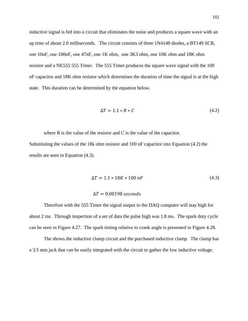
102
inductive signal is fed into a circuit that eliminates the noise and produces a square wave with an
up time of about 2.0 milliseconds. The circuit consists of three 1N4148 diodes, a BT149 SCR,
one 10nF, one 100nF, one 47nF, one 1K ohm, one 3K3 ohm, one 10K ohm and 18K ohm
resistor and a NE555 555 Timer. The 555 Timer produces the square wave signal with the 100
nF capacitor and 18K ohm resistor which determines the duration of time the signal is at the high
state. This duration can be determined by the equation below.
(4.2)
where R is the value of the resistor and C is the value of the capacitor.
Substituting the values of the 18k ohm resistor and 100 nF capacitor into Equation (4.2) the
results are seen in Equation (4.3).
(4.3)
s
Therefore with the 555 Timer the signal output to the DAQ computer will stay high for
about 2 ms. Through inspection of a set of data the pulse high was 1.8 ms. The spark duty cycle
can be seen in Figure 4.27. The spark timing relative to crank angle is presented in Figure 4.28.
The shows the inductive clamp circuit and the purchased inductive clamp. The clamp has
a 3.5 mm jack that can be easily integrated with the circuit to gather the low inductive voltage.
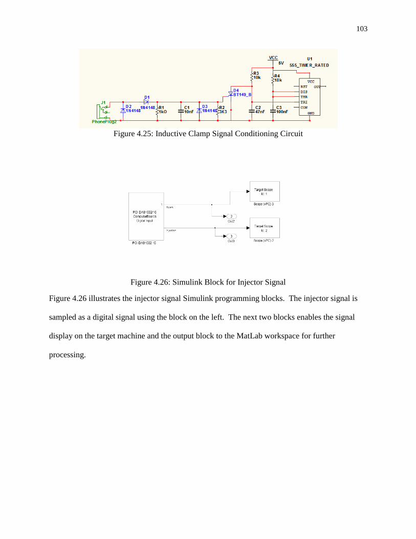
103
Figure 4.25: Inductive Clamp Signal Conditioning Circuit
Figure 4.26: Simulink Block for Injector Signal
Figure 4.26 illustrates the injector signal Simulink programming blocks. The injector signal is
sampled as a digital signal using the block on the left. The next two blocks enables the signal
display on the target machine and the output block to the MatLab workspace for further
processing.
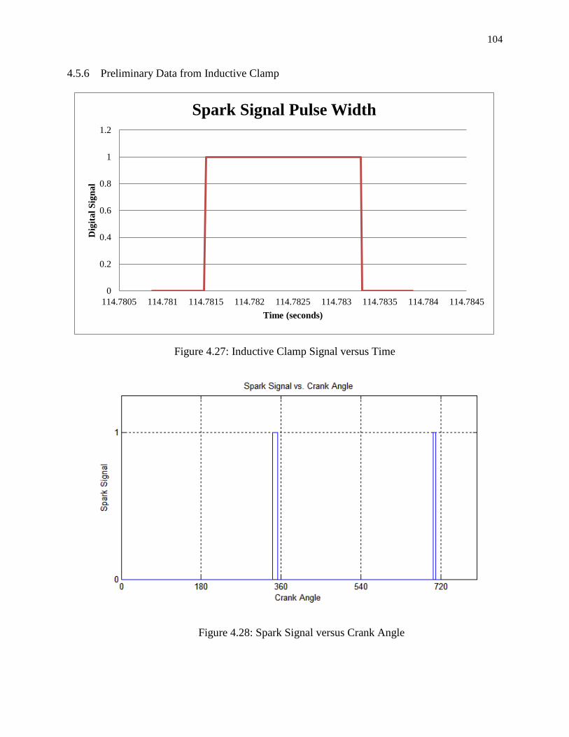
104
Preliminary Data from Inductive Clamp 4.5.6
Figure 4.27: Inductive Clamp Signal versus Time
Figure 4.28: Spark Signal versus Crank Angle
0
0.2
0.4
0.6
0.8
1
1.2
114.7805 114.781 114.7815 114.782 114.7825 114.783 114.7835 114.784 114.7845
Dig
ita
l S
ign
al
Time (seconds)
Spark Signal Pulse Width
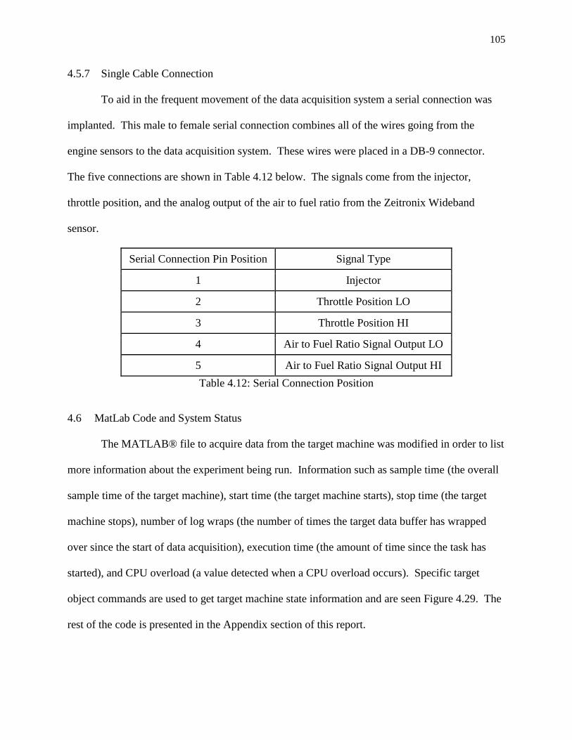
105
Single Cable Connection 4.5.7
To aid in the frequent movement of the data acquisition system a serial connection was
implanted. This male to female serial connection combines all of the wires going from the
engine sensors to the data acquisition system. These wires were placed in a DB-9 connector.
The five connections are shown in Table 4.12 below. The signals come from the injector,
throttle position, and the analog output of the air to fuel ratio from the Zeitronix Wideband
sensor.
Serial Connection Pin Position Signal Type
1 Injector
2 Throttle Position LO
3 Throttle Position HI
4 Air to Fuel Ratio Signal Output LO
5 Air to Fuel Ratio Signal Output HI
Table 4.12: Serial Connection Position
4.6 MatLab Code and System Status
The MATLAB® file to acquire data from the target machine was modified in order to list
more information about the experiment being run. Information such as sample time (the overall
sample time of the target machine), start time (the target machine starts), stop time (the target
machine stops), number of log wraps (the number of times the target data buffer has wrapped
over since the start of data acquisition), execution time (the amount of time since the task has
started), and CPU overload (a value detected when a CPU overload occurs). Specific target
object commands are used to get target machine state information and are seen Figure 4.29. The
rest of the code is presented in the Appendix section of this report.
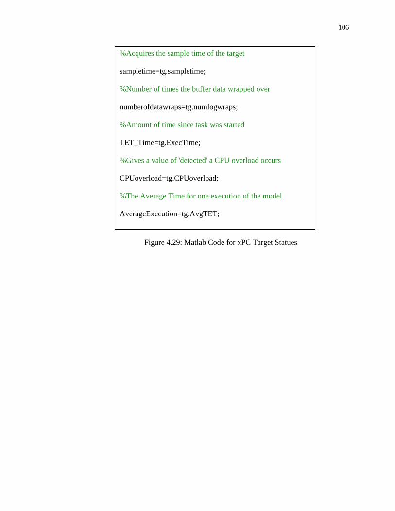
106
Figure 4.29: Matlab Code for xPC Target Statues
%Acquires the sample time of the target
sampletime=tg.sampletime;
%Number of times the buffer data wrapped over
numberofdatawraps=tg.numlogwraps;
%Amount of time since task was started
TET_Time=tg.ExecTime;
%Gives a value of 'detected' a CPU overload occurs
CPUoverload=tg.CPUoverload;
%The Average Time for one execution of the model
AverageExecution=tg.AvgTET;
107
CHAPTER 5
5 ENGINE MAPS
Using the above mentioned data acquisition equipment engine maps will be created. The
maps will include fuel injection timing, ignition timing, intake air mass flow into manifold,
throttle behavior, volumetric efficiency, air to fuel ratio correlated with engine speed, manifold
pressure and throttle angle.
5.1 Fuel Injection
The fuel injection timing is recorded from the current Engine Management System brand
electronic control unit (ECU). This ECU is able to successfully keep the engine running. The
purpose of collecting the injection timing is to learn what does work in order to duplicate on
future ECU designs that are planned for later research. The fuel injection map will include the
injection signal coming from the Engine Management System ECU, the current engine speed,
intake manifold pressure, and engine crank angle.
5.2 Spark Timing
The spark timing was measured to get a nominal spark timing map. The current spark
timing is being controlled mechanically by a magneto positioned next to the fly wheel. The fly
wheel contains a magnet and as the fly wheel spins a charge is generated in the magneto that
discharges at some angle. This map will include a representation of the spark signal, engine
speed, and intake manifold pressure. The crank angle was measured to get the actual point when
the spark fires relative to crank angle.
108
The engine testing was done by running the engine steady state conditions. The steady
state condition was achieved by maintaining a constant throttle opening from 0° to 20° in 5°
increments.
Changes in engine load are created by changing the resistance to the motor shaft turning.
This resistance is created using a hydraulic dynamometer. The resistance is varied by restricting
the flow going to the hydraulic pump. The pump is driven by the engine at a one to one gear
ratio, therefore as the fluid flow is more restricted therefore the energy required to maintain a
particular speed must increase. To maintain the idle speed of 1200 rpm at larger throttle
openings the load must increase with the throttle angel.
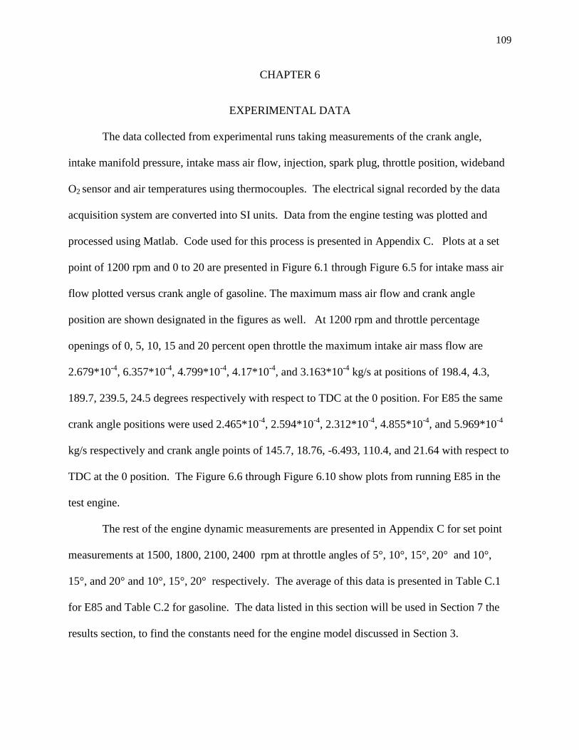
109
CHAPTER 6
6 EXPERIMENTAL DATA
The data collected from experimental runs taking measurements of the crank angle,
intake manifold pressure, intake mass air flow, injection, spark plug, throttle position, wideband
O2 sensor and air temperatures using thermocouples. The electrical signal recorded by the data
acquisition system are converted into SI units. Data from the engine testing was plotted and
processed using Matlab. Code used for this process is presented in Appendix C. Plots at a set
point of 1200 rpm and 0 to 20 are presented in Figure 6.1 through Figure 6.5 for intake mass air
flow plotted versus crank angle of gasoline. The maximum mass air flow and crank angle
position are shown designated in the figures as well. At 1200 rpm and throttle percentage
openings of 0, 5, 10, 15 and 20 percent open throttle the maximum intake air mass flow are
2.679*10-4
, 6.357*10-4
, 4.799*10-4
, 4.17*10-4
, and 3.163*10-4
kg/s at positions of 198.4, 4.3,
189.7, 239.5, 24.5 degrees respectively with respect to TDC at the 0 position. For E85 the same
crank angle positions were used 2.465*10-4
, 2.594*10-4
, 2.312*10-4
, 4.855*10-4
, and 5.969*10-4
kg/s respectively and crank angle points of 145.7, 18.76, -6.493, 110.4, and 21.64 with respect to
TDC at the 0 position. The Figure 6.6 through Figure 6.10 show plots from running E85 in the
test engine.
The rest of the engine dynamic measurements are presented in Appendix C for set point
measurements at 1500, 1800, 2100, 2400 rpm at throttle angles of 5°, 10°, 15°, 20° and 10°,
15°, and 20° and 10°, 15°, 20° respectively. The average of this data is presented in Table C.1
for E85 and Table C.2 for gasoline. The data listed in this section will be used in Section 7 the
results section, to find the constants need for the engine model discussed in Section 3.
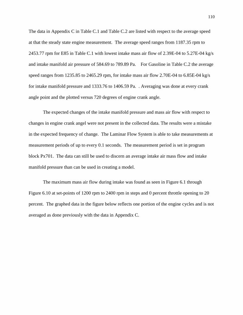
110
The data in Appendix C in Table C.1 and Table C.2 are listed with respect to the average speed
at that the steady state engine measurement. The average speed ranges from 1187.35 rpm to
2453.77 rpm for E85 in Table C.1 with lowest intake mass air flow of 2.39E-04 to 5.27E-04 kg/s
and intake manifold air pressure of 584.69 to 789.89 Pa. For Gasoline in Table C.2 the average
speed ranges from 1235.85 to 2465.29 rpm, for intake mass air flow 2.70E-04 to 6.85E-04 kg/s
for intake manifold pressure and 1333.76 to 1406.59 Pa. . Averaging was done at every crank
angle point and the plotted versus 720 degrees of engine crank angle.
The expected changes of the intake manifold pressure and mass air flow with respect to
changes in engine crank angel were not present in the collected data. The results were a mistake
in the expected frequency of change. The Laminar Flow System is able to take measurements at
measurement periods of up to every 0.1 seconds. The measurement period is set in program
block Px701. The data can still be used to discern an average intake air mass flow and intake
manifold pressure than can be used in creating a model.
The maximum mass air flow during intake was found as seen in Figure 6.1 through
Figure 6.10 at set-points of 1200 rpm to 2400 rpm in steps and 0 percent throttle opening to 20
percent. The graphed data in the figure below reflects one portion of the engine cycles and is not
averaged as done previously with the data in Appendix C.
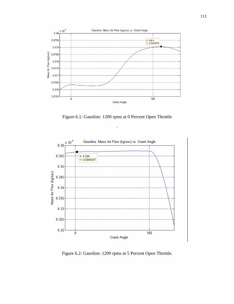
111
Figure 6.1: Gasoline: 1200 rpms at 0 Percent Open Throttle
.
Figure 6.2: Gasoline: 1200 rpms at 5 Percent Open Throttle.
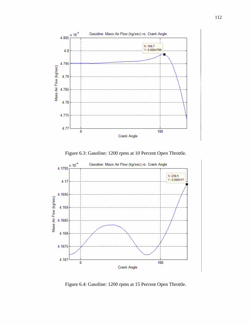
112
Figure 6.3: Gasoline: 1200 rpms at 10 Percent Open Throttle.
Figure 6.4: Gasoline: 1200 rpms at 15 Percent Open Throttle.

113
Figure 6.5: Gasoline: 1200 rpms at 20 Percent Open Throttle.
Figure 6.6: E85: 1200 rpms at 0 Percent Open Throttle.

114
Figure 6.7: E85: 1200 rpms at 5 Percent Open Throttle.
Figure 6.8: E85: 1200 rpms at 10 Percent Open Throttle.

115
Figure 6.9: E85: 1200 rpms at 15 Percent Open Throttle.
Figure 6.10: E85: 1200 rpms at 20 Percent Open Throttle.
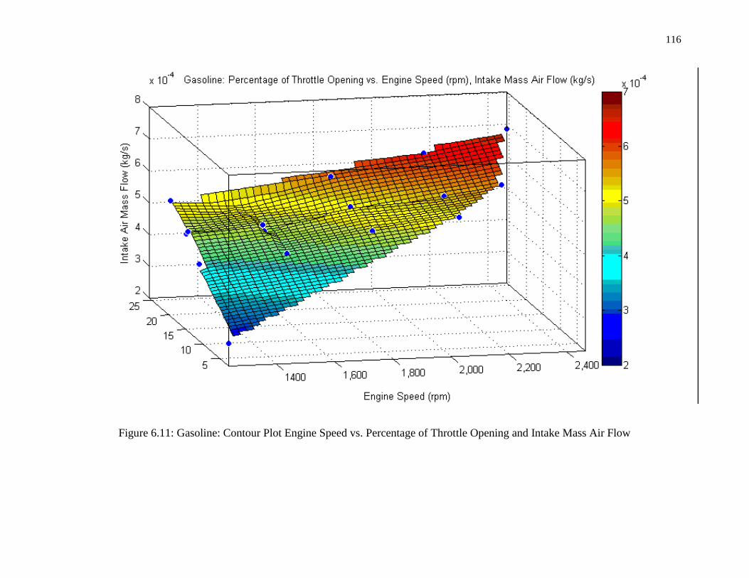
116
Figure 6.11: Gasoline: Contour Plot Engine Speed vs. Percentage of Throttle Opening and Intake Mass Air Flow

117
Figure 6.12: E85: Contour Plot Engine Speed vs. Percentage of Throttle Opening and Intake Mass Air Flow

118
CHAPTER 7
7 RESULTS
The estimation for the intake air mass flow was done using Equation (3.3)
through Equation (3.6). The estimation ranges from 9.933*10-4
kg/s at closed throttle to 0.041 at
20% throttle opening.
Figure 7.1: Estimation of Intake Air Mass Flow of Briggs and Stratton Engine
In order to characterize the engine, coefficients equations had to be determined using
experimental means. Measurements were taken of the intake air mass flow, throttle angle, intake
manifold pressure, and engine velocity. Using Equation (3.2) through Equation (3.11) for the
mass air flow coefficient. The results of the system identification are found in Figure 7.2, Figure
7.3 and Table 7.1. The prediction made in Figure 7.2 and Figure 7.3 had to be adjusted creating
a difference between the predictions. The adjustment was made by decreasing the throttle area
leak (Athleak) value. This adjustment had to be made due to a previously unknown bend in the
intake manifold.
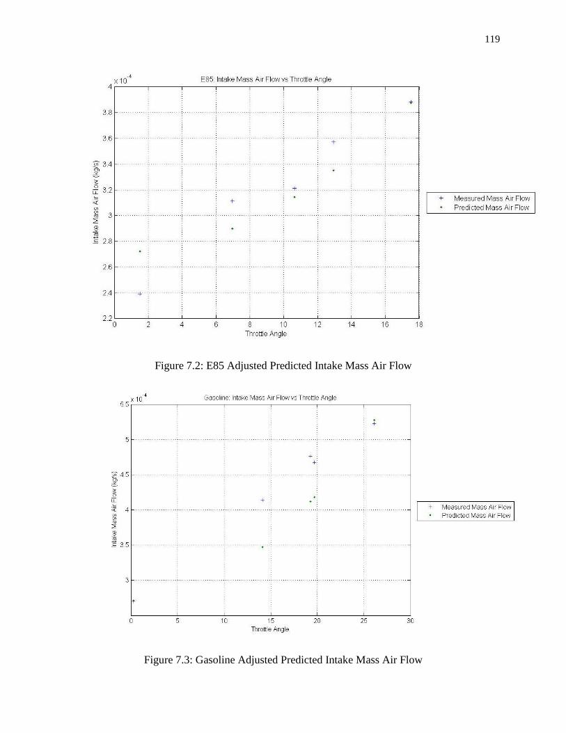
119
Figure 7.2: E85 Adjusted Predicted Intake Mass Air Flow
Figure 7.3: Gasoline Adjusted Predicted Intake Mass Air Flow
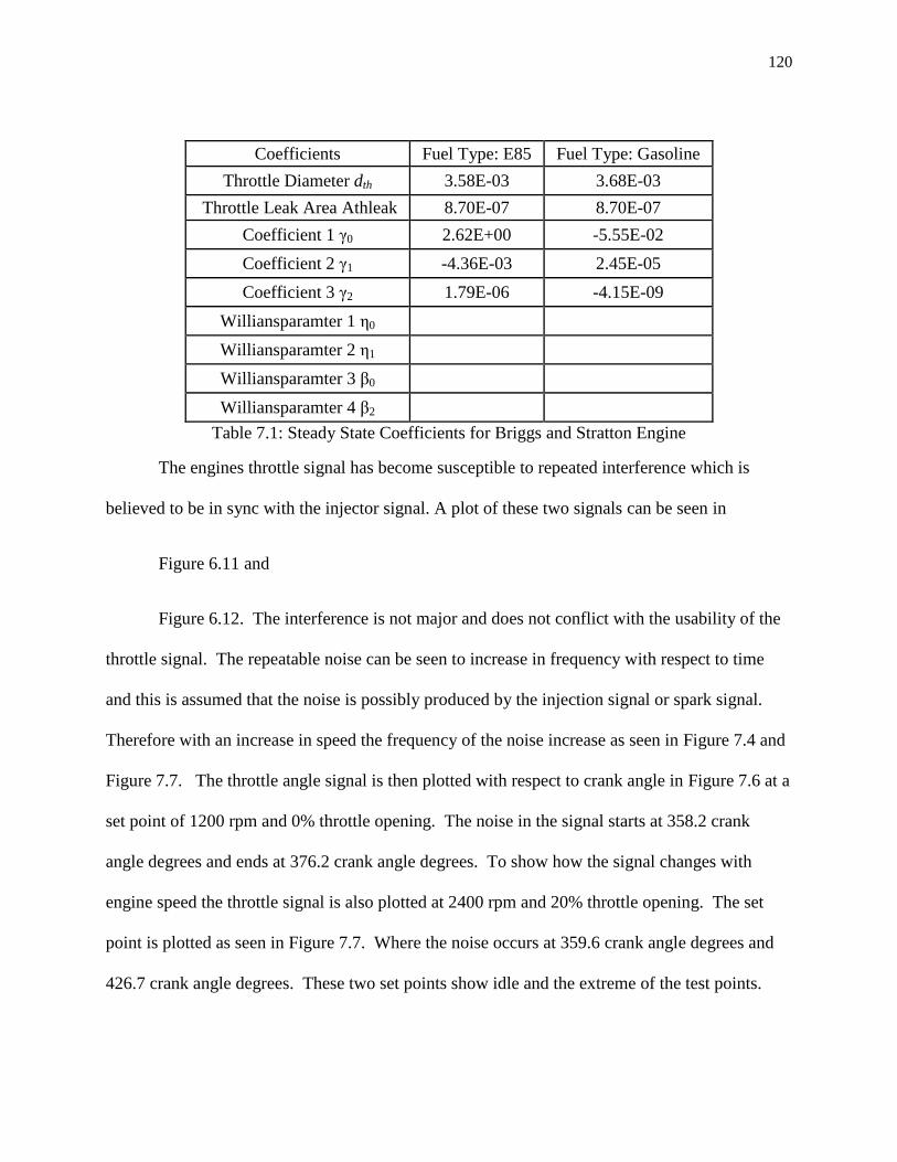
120
Coefficients Fuel Type: E85 Fuel Type: Gasoline
Throttle Diameter dth 3.58E-03 3.68E-03
Throttle Leak Area Athleak 8.70E-07 8.70E-07
Coefficient 1 γ0 2.62E+00 -5.55E-02
Coefficient 2 γ1 -4.36E-03 2.45E-05
Coefficient 3 γ2 1.79E-06 -4.15E-09
Williansparamter 1 η0
Williansparamter 2 η1
Williansparamter 3 β0
Williansparamter 4 β2
Table 7.1: Steady State Coefficients for Briggs and Stratton Engine
The engines throttle signal has become susceptible to repeated interference which is
believed to be in sync with the injector signal. A plot of these two signals can be seen in
Figure 6.11 and
Figure 6.12. The interference is not major and does not conflict with the usability of the
throttle signal. The repeatable noise can be seen to increase in frequency with respect to time
and this is assumed that the noise is possibly produced by the injection signal or spark signal.
Therefore with an increase in speed the frequency of the noise increase as seen in Figure 7.4 and
Figure 7.7. The throttle angle signal is then plotted with respect to crank angle in Figure 7.6 at a
set point of 1200 rpm and 0% throttle opening. The noise in the signal starts at 358.2 crank
angle degrees and ends at 376.2 crank angle degrees. To show how the signal changes with
engine speed the throttle signal is also plotted at 2400 rpm and 20% throttle opening. The set
point is plotted as seen in Figure 7.7. Where the noise occurs at 359.6 crank angle degrees and
426.7 crank angle degrees. These two set points show idle and the extreme of the test points.

121
Figure 7.4: Throttle Angle Signal Versus Time at 1200 rpm
Figure 7.5: Throttle Angle Signal Versus Time at 2400 rpm

122
Figure 7.6: Throttle Angle Signal Versus Crank Angle at 1200 rpm and 0% Throttle Opening
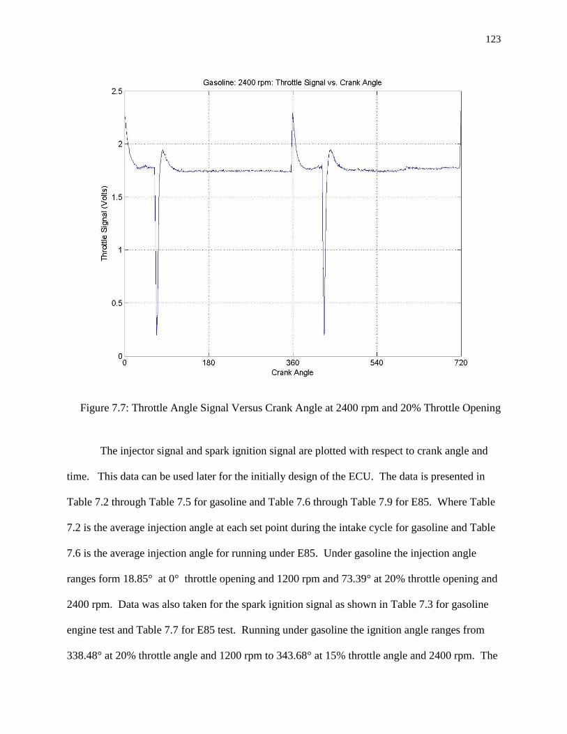
123
Figure 7.7: Throttle Angle Signal Versus Crank Angle at 2400 rpm and 20% Throttle Opening
The injector signal and spark ignition signal are plotted with respect to crank angle and
time. This data can be used later for the initially design of the ECU. The data is presented in
Table 7.2 through Table 7.5 for gasoline and Table 7.6 through Table 7.9 for E85. Where Table
7.2 is the average injection angle at each set point during the intake cycle for gasoline and Table
7.6 is the average injection angle for running under E85. Under gasoline the injection angle
ranges form 18.85° at 0° throttle opening and 1200 rpm and 73.39° at 20% throttle opening and
2400 rpm. Data was also taken for the spark ignition signal as shown in Table 7.3 for gasoline
engine test and Table 7.7 for E85 test. Running under gasoline the ignition angle ranges from
338.48° at 20% throttle angle and 1200 rpm to 343.68° at 15% throttle angle and 2400 rpm. The

124
current ECU also injects later during the engine cycle and that data will be presented in
Appendix C. The duration of the injection timing high and low are presented in Table 7.4 and
Table 7.5 respectively for gasoline and high and low under E85 in Table 7.8 and Table 7.9
respectively.
Percentage of
Throttle
Opening
1200 (rpm) 1500 (rpm) 1800 (rpm) 2100 (rpm) 2400 (rpm)
20 35 44 57 65 73
15 30 37 46 53 60
10 24 30 37 42
5 23 31 37
0 19
Table 7.2: Gasoline: Average Injection Angle During Intake Stroke
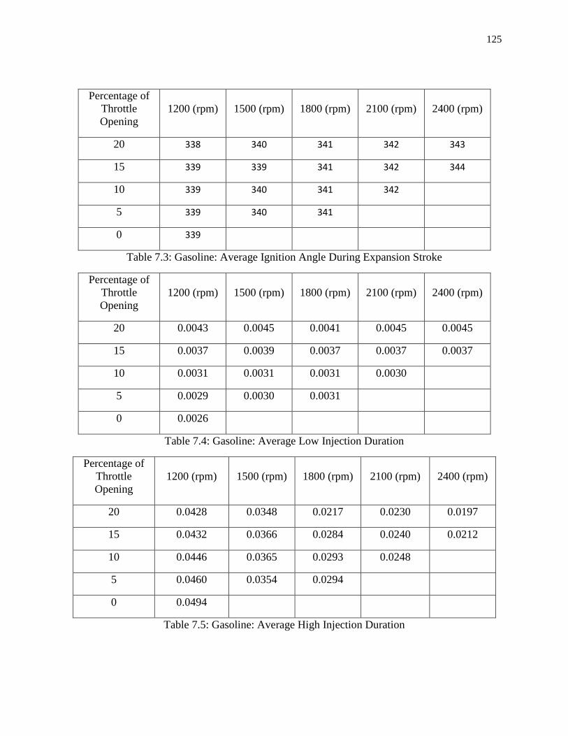
125
Percentage of
Throttle
Opening
1200 (rpm) 1500 (rpm) 1800 (rpm) 2100 (rpm) 2400 (rpm)
20 338 340 341 342 343
15 339 339 341 342 344
10 339 340 341 342
5 339 340 341
0 339
Table 7.3: Gasoline: Average Ignition Angle During Expansion Stroke
Percentage of
Throttle
Opening
1200 (rpm) 1500 (rpm) 1800 (rpm) 2100 (rpm) 2400 (rpm)
20 0.0043 0.0045 0.0041 0.0045 0.0045
15 0.0037 0.0039 0.0037 0.0037 0.0037
10 0.0031 0.0031 0.0031 0.0030
5 0.0029 0.0030 0.0031
0 0.0026
Table 7.4: Gasoline: Average Low Injection Duration
Percentage of
Throttle
Opening
1200 (rpm) 1500 (rpm) 1800 (rpm) 2100 (rpm) 2400 (rpm)
20 0.0428 0.0348 0.0217 0.0230 0.0197
15 0.0432 0.0366 0.0284 0.0240 0.0212
10 0.0446 0.0365 0.0293 0.0248
5 0.0460 0.0354 0.0294
0 0.0494
Table 7.5: Gasoline: Average High Injection Duration
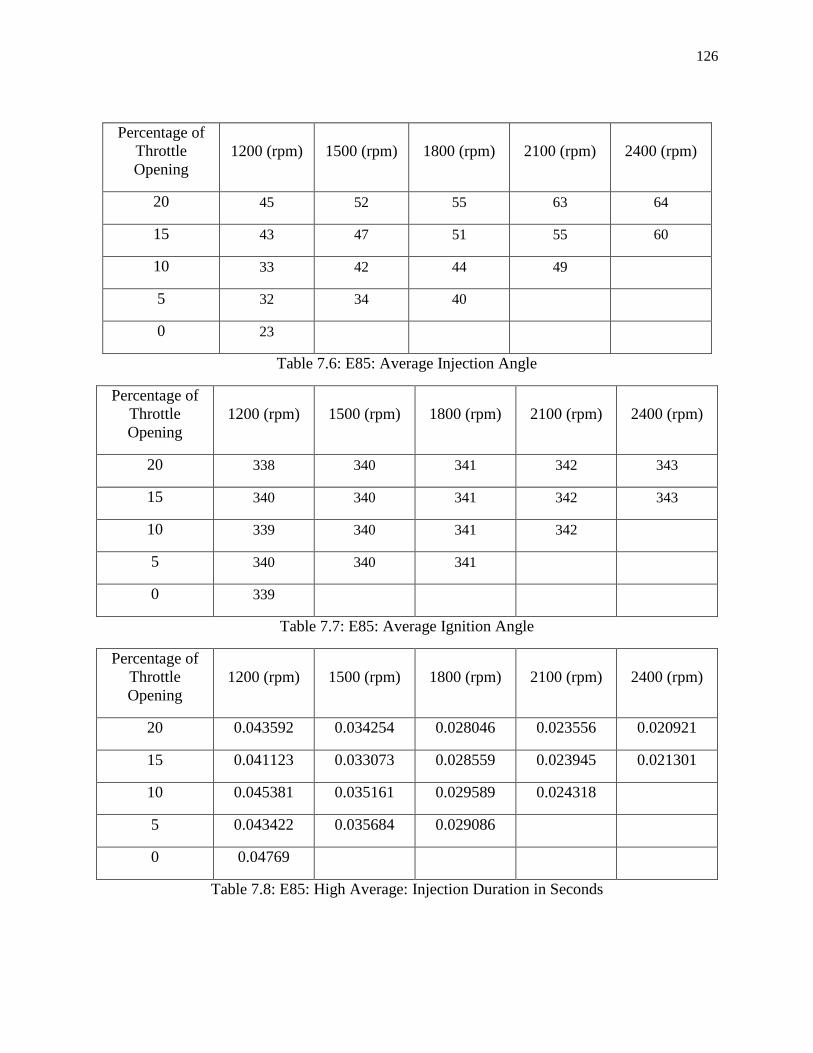
126
Percentage of
Throttle
Opening
1200 (rpm) 1500 (rpm) 1800 (rpm) 2100 (rpm) 2400 (rpm)
20 45 52 55 63 64
15 43 47 51 55 60
10 33 42 44 49
5 32 34 40
0 23
Table 7.6: E85: Average Injection Angle
Percentage of
Throttle
Opening
1200 (rpm) 1500 (rpm) 1800 (rpm) 2100 (rpm) 2400 (rpm)
20 338 340 341 342 343
15 340 340 341 342 343
10 339 340 341 342
5 340 340 341
0 339
Table 7.7: E85: Average Ignition Angle
Percentage of
Throttle
Opening
1200 (rpm) 1500 (rpm) 1800 (rpm) 2100 (rpm) 2400 (rpm)
20 0.043592 0.034254 0.028046 0.023556 0.020921
15 0.041123 0.033073 0.028559 0.023945 0.021301
10 0.045381 0.035161 0.029589 0.024318
5 0.043422 0.035684 0.029086
0 0.04769
Table 7.8: E85: High Average: Injection Duration in Seconds

127
Percentage of
Throttle
Opening
1200 (rpm) 1500 (rpm) 1800 (rpm) 2100 (rpm) 2400 (rpm)
20 0.005864 0.005286 0.004558 0.004497 0.004008
15 0.005154 0.004583 0.004284 0.003828 0.003801
10 0.004325 0.004263 0.003679 0.003477
5 0.004035 0.003467 0.003314
0 0.003049
Table 7.9: E85: Low Average: Injection Duration in Seconds

128
CHAPTER 8
8 CONCLUSION
In conclusion the data acquisition system was able to measure the dynamics of the
engine. Data such as mass air flow, intake manifold pressure, engine speed and crank angle,
engine injection and ignition signals. Engine coefficients need to discern an accurate model
could be determined using the data gathered with this system. Further, work will need to be
done to determine all of the coefficients need for an accurate model. Engine model coefficients
that require dynamic none steady statements need to be determined such as injection to top
center transportation delay, engine inertia and volume of the intake manifold.

129
REFERENCES
Environmental Protection Agency. (2008) Control of emissions from marine si and small si
engines, vessels, and equipment final regulatory impact analysis. Retrieved from
http://www.epa.gov/oms/regs/nonroad/marinesi-equipld/420r08014.pdf(EPA.gov)
Bosch. (n.d.). Wideband A/F Oxygen Sensors. Retrieved June 13, 2011, from
http://www.boschautoparts.com/OxygenSensors/Pages/WidebandOxygenSensors.aspx
Grabner, P., Eichlseder, H., & Eckhard, G. (2010). Potential of E85 Direct Injection for
Passenger Car Application ( No. 2010-01-2086). Warrendale, PA: SAE International.
Retrieved from http://papers.sae.org/2010-01-2086/
Greene, A. B., & Lucas, G. G. (1969). Testing of Internal Combustion Engines. Hodder &
Stoughton Ltd.
Guzzella, L., & Onder, C. (2010). Introduction to Modeling and Control of Internal Combustion
Engine Systems (1st ed.). Springer.
Hendricks, E., & Sorenson, S. C. (1990). Mean Value Modelling of Spark Ignition Engines ( No.
900616). Warrendale, PA: SAE International. Retrieved from
http://papers.sae.org/900616/
Herman, P., & Franchek, M. A. (2000). Engine idle speed control using actuator saturation.
Control Systems Technology, IEEE Transactions on, 8(1), 192-199.
doi:10.1109/87.817704
Heywood, J. (1988). Internal Combustion Engine Fundamentals (1st ed.). McGraw-Hill
Science/Engineering/Math.
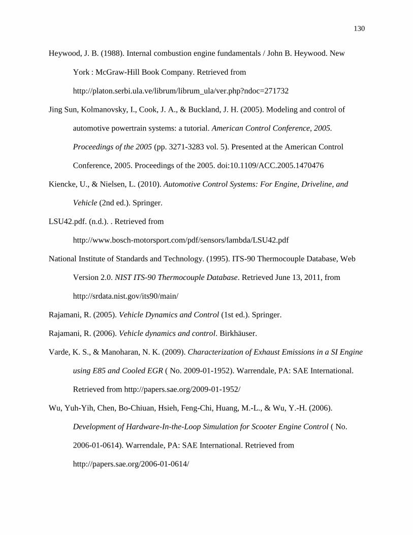
130
Heywood, J. B. (1988). Internal combustion engine fundamentals / John B. Heywood. New
York : McGraw-Hill Book Company. Retrieved from
http://platon.serbi.ula.ve/librum/librum_ula/ver.php?ndoc=271732
Jing Sun, Kolmanovsky, I., Cook, J. A., & Buckland, J. H. (2005). Modeling and control of
automotive powertrain systems: a tutorial. American Control Conference, 2005.
Proceedings of the 2005 (pp. 3271-3283 vol. 5). Presented at the American Control
Conference, 2005. Proceedings of the 2005. doi:10.1109/ACC.2005.1470476
Kiencke, U., & Nielsen, L. (2010). Automotive Control Systems: For Engine, Driveline, and
Vehicle (2nd ed.). Springer.
LSU42.pdf. (n.d.). . Retrieved from
http://www.bosch-motorsport.com/pdf/sensors/lambda/LSU42.pdf
National Institute of Standards and Technology. (1995). ITS-90 Thermocouple Database, Web
Version 2.0. NIST ITS-90 Thermocouple Database. Retrieved June 13, 2011, from
http://srdata.nist.gov/its90/main/
Rajamani, R. (2005). Vehicle Dynamics and Control (1st ed.). Springer.
Rajamani, R. (2006). Vehicle dynamics and control. Birkhäuser.
Varde, K. S., & Manoharan, N. K. (2009). Characterization of Exhaust Emissions in a SI Engine
using E85 and Cooled EGR ( No. 2009-01-1952). Warrendale, PA: SAE International.
Retrieved from http://papers.sae.org/2009-01-1952/
Wu, Yuh-Yih, Chen, Bo-Chiuan, Hsieh, Feng-Chi, Huang, M.-L., & Wu, Y.-H. (2006).
Development of Hardware-In-the-Loop Simulation for Scooter Engine Control ( No.
2006-01-0614). Warrendale, PA: SAE International. Retrieved from
http://papers.sae.org/2006-01-0614/
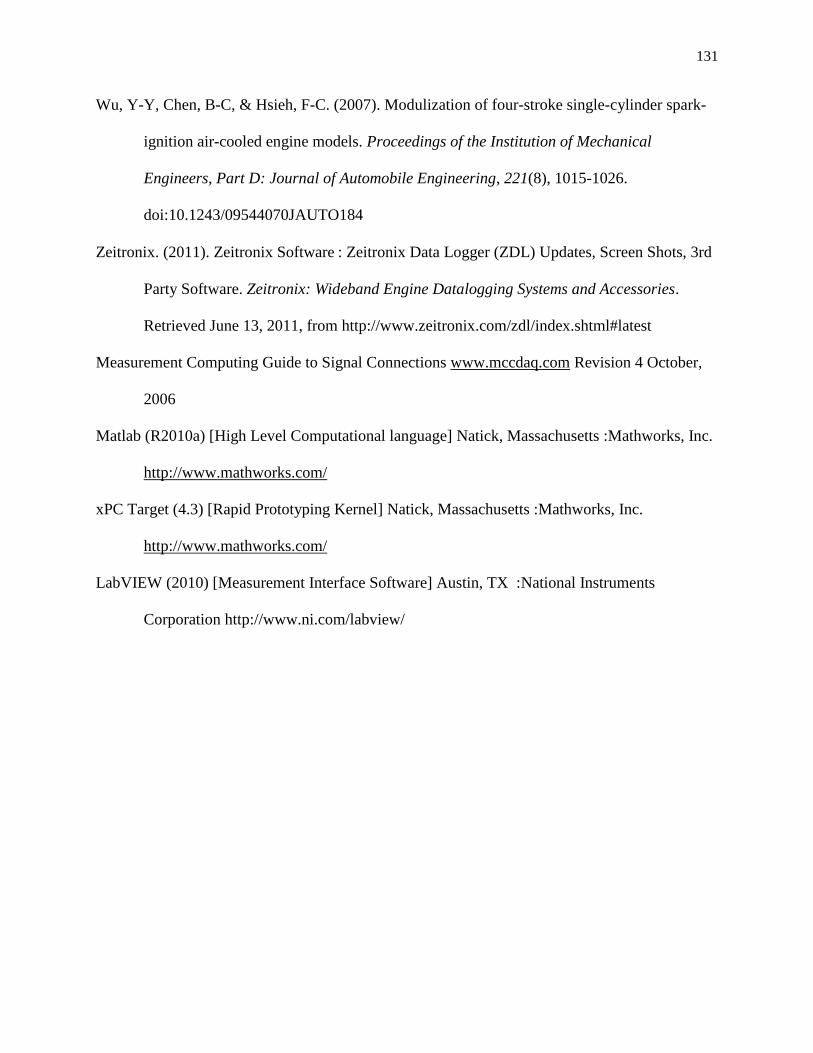
131
Wu, Y-Y, Chen, B-C, & Hsieh, F-C. (2007). Modulization of four-stroke single-cylinder spark-
ignition air-cooled engine models. Proceedings of the Institution of Mechanical
Engineers, Part D: Journal of Automobile Engineering, 221(8), 1015-1026.
doi:10.1243/09544070JAUTO184
Zeitronix. (2011). Zeitronix Software : Zeitronix Data Logger (ZDL) Updates, Screen Shots, 3rd
Party Software. Zeitronix: Wideband Engine Datalogging Systems and Accessories.
Retrieved June 13, 2011, from http://www.zeitronix.com/zdl/index.shtml#latest
Measurement Computing Guide to Signal Connections www.mccdaq.com Revision 4 October,
2006
Matlab (R2010a) [High Level Computational language] Natick, Massachusetts :Mathworks, Inc.
http://www.mathworks.com/
xPC Target (4.3) [Rapid Prototyping Kernel] Natick, Massachusetts :Mathworks, Inc.
http://www.mathworks.com/
LabVIEW (2010) [Measurement Interface Software] Austin, TX :National Instruments
Corporation http://www.ni.com/labview/
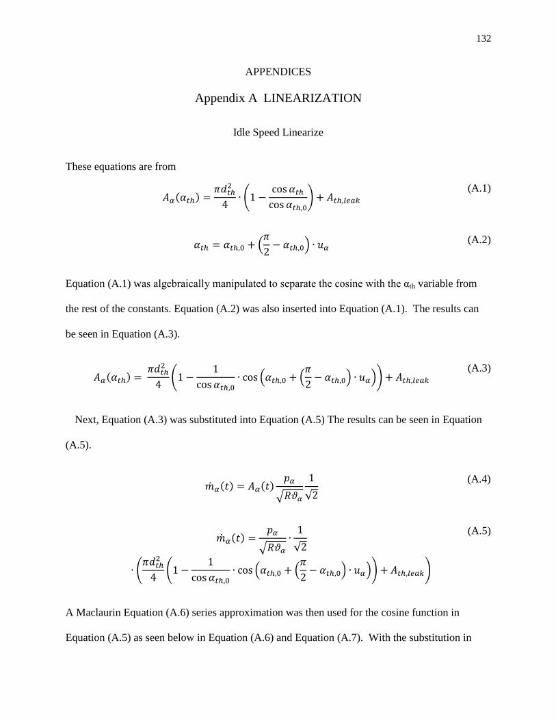
132
APPENDICES
Appendix A LINEARIZATION
Idle Speed Linearize
These equations are from
( )
(
)
(A.1)
(
)
(A.2)
Equation (A.1) was algebraically manipulated to separate the cosine with the αth variable from
the rest of the constants. Equation (A.2) was also inserted into Equation (A.1). The results can
be seen in Equation (A.3).
( )
(
( (
) ))
(A.3)
Next, Equation (A.3) was substituted into Equation (A.5) The results can be seen in Equation
(A.5).
( ) ( )
√
√
(A.4)
( )
√
√
(
(
( (
) )) )
(A.5)
A Maclaurin Equation (A.6) series approximation was then used for the cosine function in
Equation (A.5) as seen below in Equation (A.6) and Equation (A.7). With the substitution in
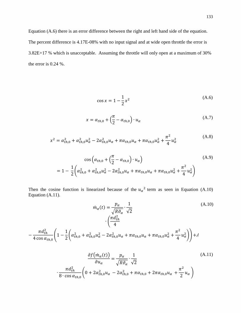
133
Equation (A.6) there is an error difference between the right and left hand side of the equation.
The percent difference is 4.17E-08% with no input signal and at wide open throttle the error is
3.82E+17 % which is unacceptable. Assuming the throttle will only open at a maximum of 30%
the error is 0.24 %.
(A.6)
(
)
(A.7)
(A.8)
( (
) )
(
)
(A.9)
Then the cosine function is linearized because of the term as seen in Equation (A.10)
Equation (A.11).
( )
√
√
(
(
(
)+ )
(A.10)
( ( ))
√
√
(
)
(A.11)
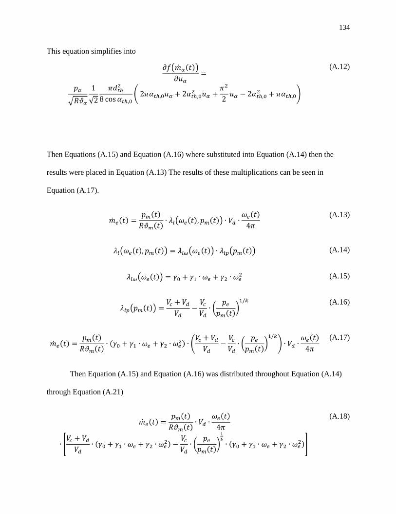
134
This equation simplifies into
( ( ))
√
√
(
)
(A.12)
Then Equations (A.15) and Equation (A.16) where substituted into Equation (A.14) then the
results were placed in Equation (A.13) The results of these multiplications can be seen in
Equation (A.17).
( ) ( )
( ) ( ( ) ( ))
( )
(A.13)
( ( ) ( )) ( ( )) ( ( )) (A.14)
( ( )) (A.15)
( ( ))
(
( )*
(A.16)
( ) ( )
( ) (
) (
(
( )*
) ( )
(A.17)
Then Equation (A.15) and Equation (A.16) was distributed throughout Equation (A.14)
through Equation (A.21)
( ) ( )
( )
( )
[
(
)
(
( )*
(
)]
(A.18)
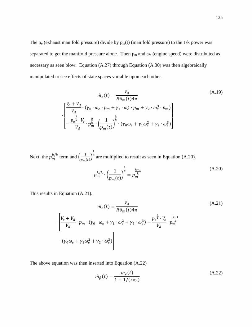
135
The pe (exhaust manifold pressure) divide by pm(t) (manifold pressure) to the 1/k power was
separated to get the manifold pressure alone. Then pm and ωe (engine speed) were distributed as
necessary as seen blow. Equation (A.27) through Equation (A.30) was then algebraically
manipulated to see effects of state spaces variable upon each other.
( )
( )
[
(
)
(
( )*
(
)]
(A.19)
Next, the
term and (
( ))
are multiplied to result as seen in Equation (A.20).
(
( )*
(A.20)
This results in Equation (A.21).
( )
( )
0
(
)
(
)1
(A.21)
The above equation was then inserted into Equation (A.22)
( ) ( )
( )
(A.22)
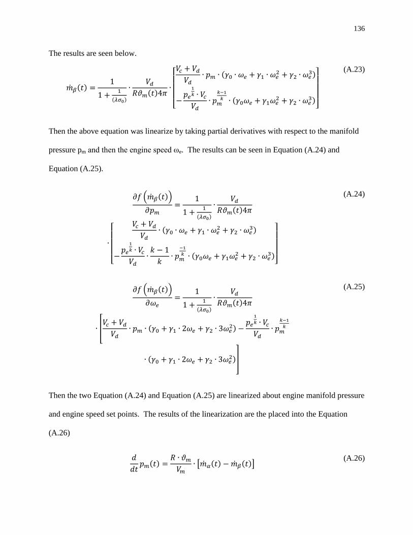
136
The results are seen below.
( )
( )
( )
[
(
)
(
)]
(A.23)
Then the above equation was linearize by taking partial derivatives with respect to the manifold
pressure pm and then the engine speed ωe. The results can be seen in Equation (A.24) and
Equation (A.25).
( ( ))
( )
( )
[
(
)
(
)]
(A.24)
( ( ))
( )
( )
0
(
)
( )1
(A.25)
Then the two Equation (A.24) and Equation (A.25) are linearized about engine manifold pressure
and engine speed set points. The results of the linearization are the placed into the Equation
(A.26)
( )
[ ( ) ( )]
(A.26)
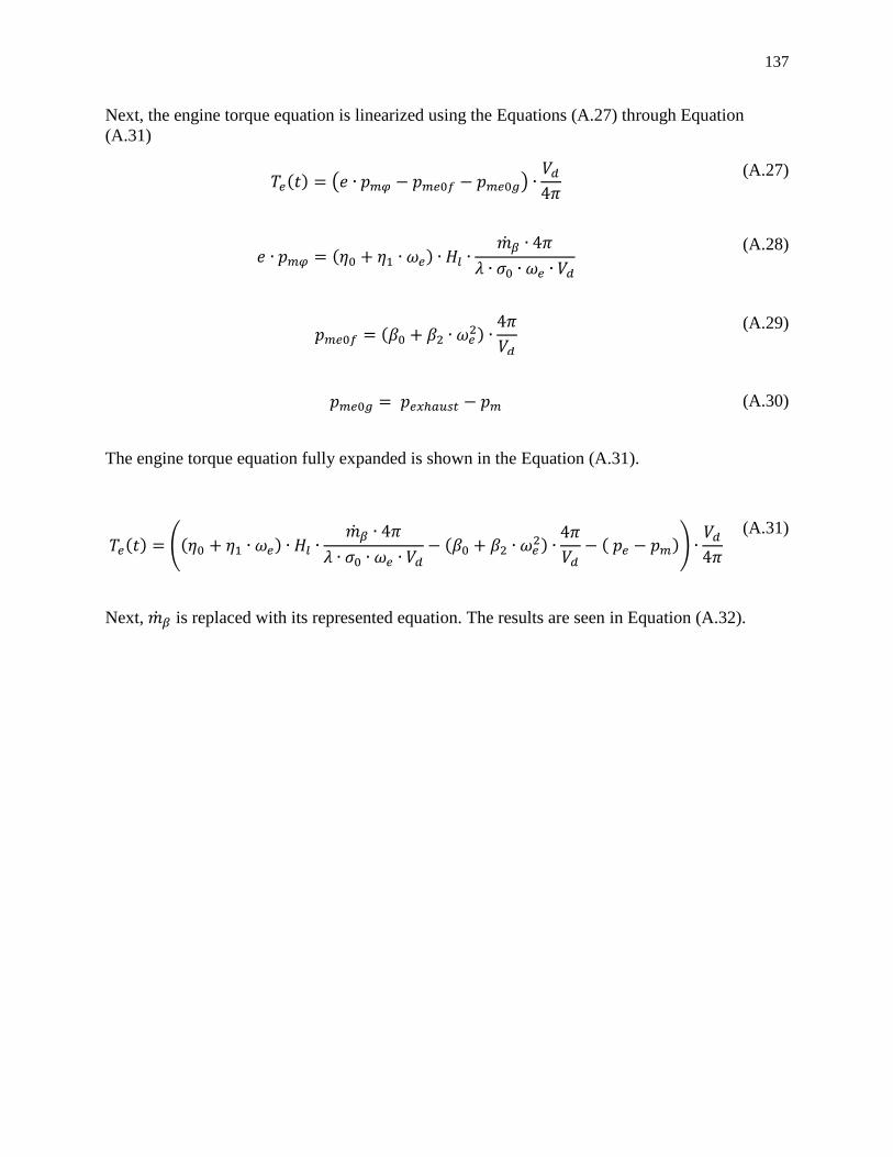
137
Next, the engine torque equation is linearized using the Equations (A.27) through Equation
(A.31)
( ) ( )
(A.27)
( )
(A.28)
( )
(A.29)
(A.30)
The engine torque equation fully expanded is shown in the Equation (A.31).
( ) (( )
(
)
( )+
(A.31)
Next, is replaced with its represented equation. The results are seen in Equation (A.32).
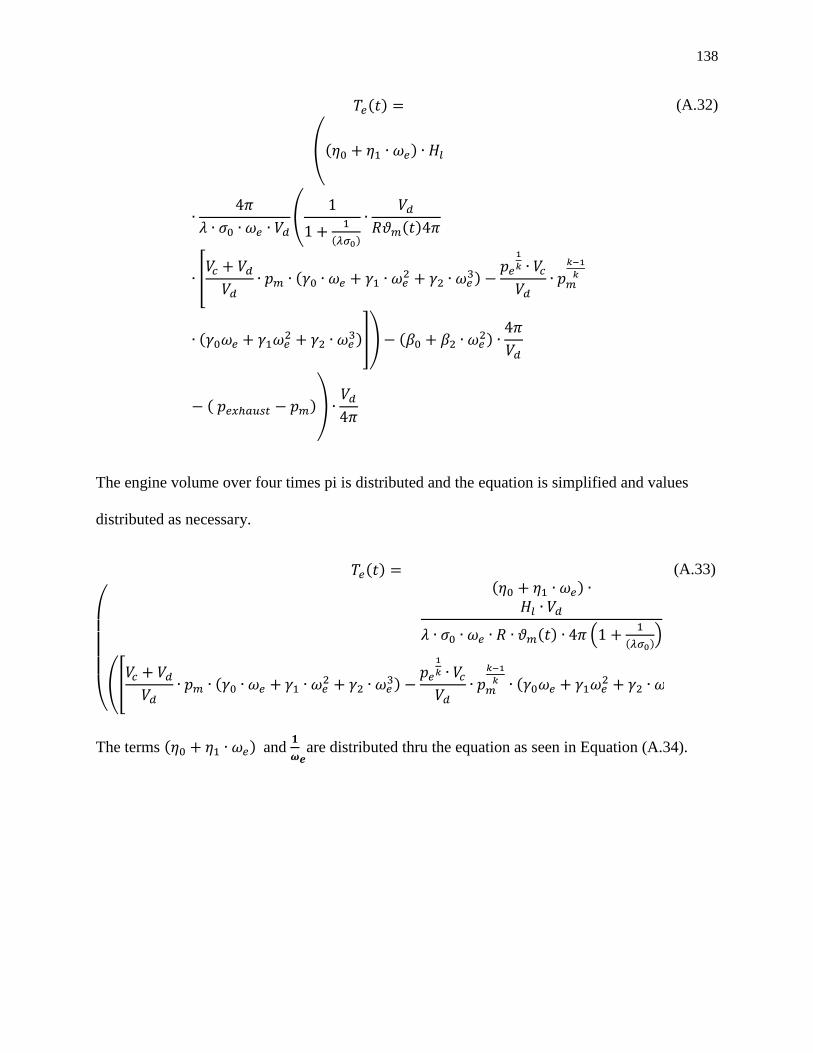
138
( )
(( )
.
( )
( )
0
(
)
(
)1/ ( )
( ),
(A.32)
The engine volume over four times pi is distributed and the equation is simplified and values
distributed as necessary.
( )
(
( )
( ) (
( ))
.0
(
)
(
)1/ ( ) ( )
)
(A.33)
The terms ( ) and
are distributed thru the equation as seen in Equation (A.34).
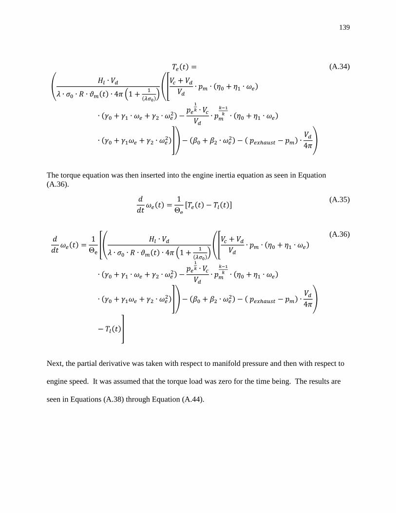
139
( )
.
( ) (
( )).0
( )
( )
( )
( )1/ (
) ( )
/
(A.34)
The torque equation was then inserted into the engine inertia equation as seen in Equation
(A.36).
( )
[ ( ) ( )] (A.35)
( )
0.
( ) (
( )).0
( )
( )
( )
( )1/ (
) ( )
/
( )1
(A.36)
Next, the partial derivative was taken with respect to manifold pressure and then with respect to
engine speed. It was assumed that the torque load was zero for the time being. The results are
seen in Equations (A.38) through Equation (A.44).
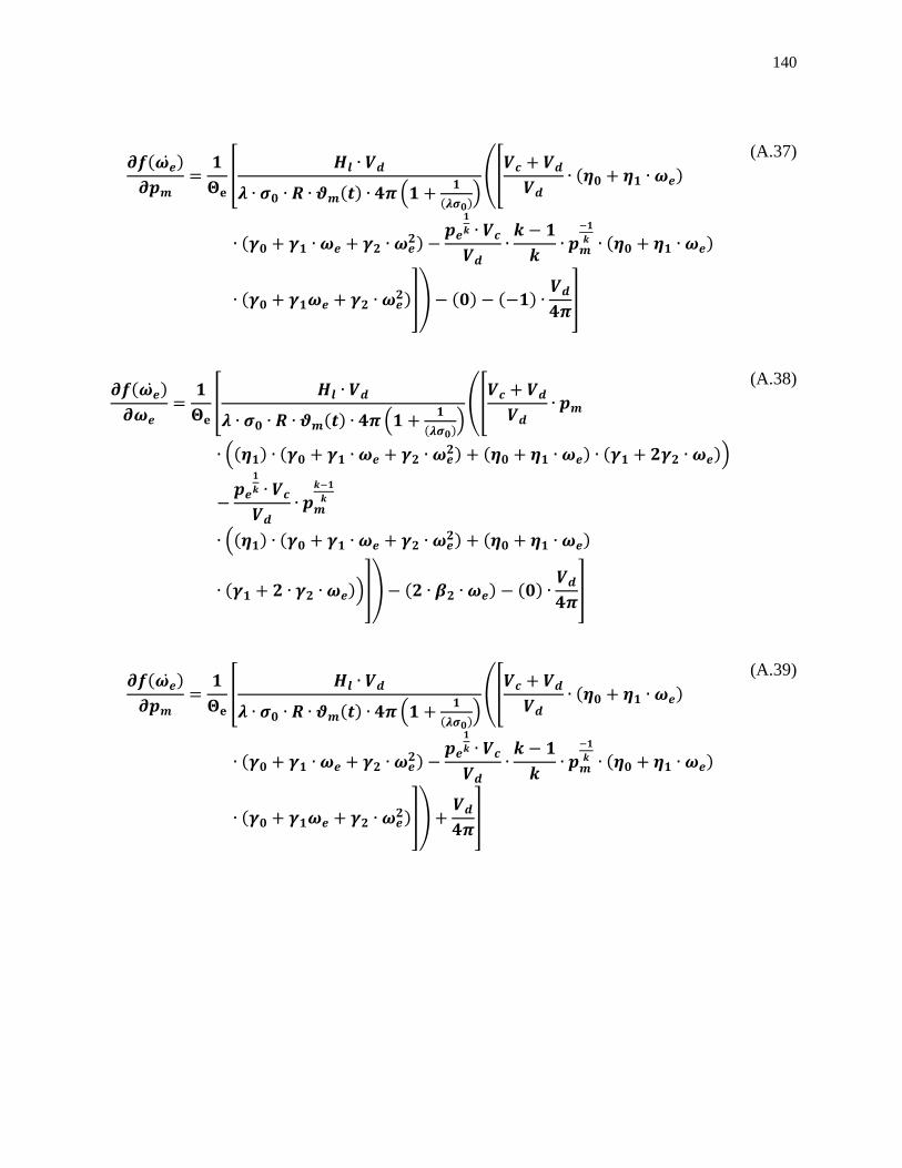
140
( )
0
( ) (
( )).0
( )
( )
( )
( )1/ ( ) ( )
1
(A.37)
( )
0
( ) (
( )).0
(( ) ( ) ( ) ( ))
(( ) ( ) ( )
( ))1/ ( ) ( )
1
(A.38)
( )
0
( ) (
( )).0
( )
( )
( )
( )1/
1
(A.39)
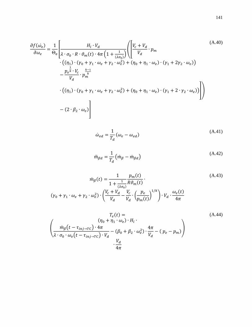
141
( )
0
( ) (
( )).0
(( ) ( ) ( ) ( ))
(( ) ( ) ( ) ( ))1/
( )1
(A.40)
( ) (A.41)
( )
(A.42)
( )
( )
( )
( )
( ) (
(
( )*
) ( )
(A.43)
( )
.
( )
( )
( )
( )
( )
/
(A.44)
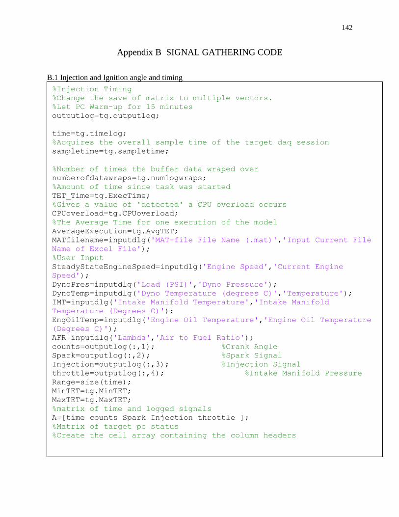
142
Appendix B SIGNAL GATHERING CODE
B.1 Injection and Ignition angle and timing
%Injection Timing
%Change the save of matrix to multiple vectors.
%Let PC Warm-up for 15 minutes
outputlog=tg.outputlog;
time=tg.timelog;
%Acquires the overall sample time of the target daq session
sampletime=tg.sampletime;
%Number of times the buffer data wraped over
numberofdatawraps=tg.numlogwraps;
%Amount of time since task was started
TET_Time=tg.ExecTime;
%Gives a value of 'detected' a CPU overload occurs
CPUoverload=tg.CPUoverload;
%The Average Time for one execution of the model
AverageExecution=tg.AvgTET;
MATfilename=inputdlg('MAT-file File Name (.mat)','Input Current File
Name of Excel File');
%User Input
SteadyStateEngineSpeed=inputdlg('Engine Speed','Current Engine
Speed');
DynoPres=inputdlg('Load (PSI)','Dyno Pressure');
DynoTemp=inputdlg('Dyno Temperature (degrees C)','Temperature');
IMT=inputdlg('Intake Manifold Temperature','Intake Manifold
Temperature (Degrees C)');
EngOilTemp=inputdlg('Engine Oil Temperature','Engine Oil Temperature
(Degrees C)');
AFR=inputdlg('Lambda','Air to Fuel Ratio');
counts=outputlog(:,1); %Crank Angle
Spark=outputlog(:,2); %Spark Signal
Injection=outputlog(:,3); %Injection Signal
throttle=outputlog(:,4); %Intake Manifold Pressure
Range=size(time);
MinTET=tg.MinTET;
MaxTET=tg.MaxTET;
%matrix of time and logged signals
A=[time counts Spark Injection throttle ];
%Matrix of target pc status
%Create the cell array containing the column headers
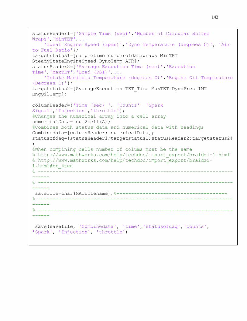
143
statusHeader1={'Sample Time (sec)','Number of Circular Buffer
Wraps','MinTET',...
'Ideal Engine Speed (rpms)','Dyno Temperature (degrees C)', 'Air
to Fuel Ratio'};
targetstatus1=[sampletime numberofdatawraps MinTET
SteadyStateEngineSpeed DynoTemp AFR];
statusHeader2={'Average Execution Time (sec)','Execution
Time','MaxTET','Load (PSI)',...
'Intake Manifold Temperature (degrees C)','Engine Oil Temperature
(Degrees C)'};
targetstatus2=[AverageExecution TET_Time MaxTET DynoPres IMT
EngOilTemp];
columnHeader={'Time (sec) ', 'Counts', 'Spark
Signal','Injection','throttle'};
%Changes the numerical array into a cell array
numericalData= num2cell(A);
%Combines both status data and numerical data with headings
Combinedata=[columnHeader; numericalData];
statusofdaq=[statusHeader1;targetstatus1;statusHeader2;targetstatus2]
;
%When compining cells number of colums must be the same
% http://www.mathworks.com/help/techdoc/import_export/braidzi-1.html
% http://www.mathworks.com/help/techdoc/import_export/braidzi-
1.html#br_4ten
% -------------------------------------------------------------------
------
% -------------------------------------------------------------------
------
savefile=char(MATfilename);%--------------------------------------
% -------------------------------------------------------------------
------
% -------------------------------------------------------------------
------
save(savefile, 'Combinedata', 'time','statusofdaq','counts',
'Spark', 'Injection', 'throttle')
144
B.2 Mass Air Flow
%Throttle Dynamic and Volumetric Efficenecy Measurement
%Let PC Warm-up for 15 minutes
outputlog=tg.outputlog;
time=tg.timelog;
%Acquires the sample time of the target
sampletime=tg.sampletime;
MinTET=tg.MinTET;
MaxTET=tg.MaxTET;
% not execute
%Number of times the buffer data wraped over
numberofdatawraps=tg.numlogwraps;
%Amount of time since task was started
TET_Time=tg.ExecTime;
%Gives a value of 'detected' a CPU overload occurs
CPUoverload=tg.CPUoverload;
%The Average Time for one execution of the model
AverageExecution=tg.AvgTET;
MATfilename=inputdlg('MAT-file File Name (.mat)','Input Current File
Name of Excel File');
% a={'ab','cde','fghi'};
% as1=char(Excelfilename) % note: a char mat
% as2=cat(2,Excelfilename{:}) % note: no spaces between cells
% as3=sprintf('%s|',Excelfilename{:}); % the most versatile
% as3(end)=''
SteadyStateEngineSpeed=inputdlg('Engine Speed','Current Engine
Speed');
DynoPres=inputdlg('Load (PSI)','Dyno Pressure');
DynoTemp=inputdlg('Dyno Temperature (degrees C)','Temperature');
IMT=inputdlg('Intake Manifold Temperature','Intake Manifold
Temperature (Degrees C)');
EngOilTemp=inputdlg('Engine Oil Temperature','Engine Oil Temperature
(Degrees C)');
AFR=inputdlg('Lambda','Air to Fuel Ratio');
MAF=outputlog(:,2); %Volume Air Flow L/m
Pressure=outputlog(:,1); %Intake Manifold Pressure mbar
Throttle=outputlog(:,3); %Throttle Angel
ENCounts=outputlog(:,4); %Encoder output count
Datamatrix=[time ENCounts Pressure MAF Throttle]; %matrix of
145
time and logged signals
%Create the cell array containing the column headers
%Create the cell array containing the column headers
statusHeader1={'Sample Time (sec)','Number of Circular
Buffer Wraps','MinTET',...
'Ideal Engine Speed (rpms)','Dyno Temperature (degrees
C)', 'Air to Fuel Ratio'};
targetstatus1=[sampletime numberofdatawraps MinTET
SteadyStateEngineSpeed DynoTemp AFR];
statusHeader2={'Average Execution Time (sec)','Execution
Time','MaxTET','Load (PSI)',...
'Intake Manifold Temperature (degrees C)','Engine Oil
Temperature (Degrees C)'};
targetstatus2=[AverageExecution TET_Time MaxTET DynoPres
IMT EngOilTemp];
columnHeader={'Time (sec) ', 'Encoder Counts', 'Intake
Manifold Pressure','Volume Air Flow'...
'Throttle Angel'};
%Changes the numerical array into a cell array
%Combines both status data and numerical data with headings
%Changes the numerical array into a cell array
numericalData= num2cell(Datamatrix);
%combube the two cell arrays into one
throttledynamic= [columnHeader; numericalData]; %Puts
all data and heading in Matrix
%Shows status of data collection
statusofdaq=[statusHeader1;targetstatus1;statusHeader2;targ
etstatus2];
savefile=char(MATfilename);%-------------------------------
-------
% ---------------------------------------------------------
----------------
% ---------------------------------------------------------
----------------
save(savefile, 'throttledynamic', 'statusofdaq',
'Pressure', 'MAF', 'Throttle', 'ENCounts');
146
B.3 Processing for throttle dynamic and volumetric efficiency coefficients
%Analysis of the first 180 degrees. Averageing over the first 180
degrees.
%% Loads each file to execute
% function intakeplotdynamic2()
clear
maActV=zeros(18,1);%the row value is the total number of data points
ThrActV=zeros(18,1);
PaActV=zeros(18,1);
weAct=zeros(18,1);
inTempAct=zeros(18,1);
savedir='C:\Documents and Settings\Cory\Desktop\Image';
Index=1;
rootname='thr_04212011_gas';%Root folder location of .mat files
fueltype='gas';
filename='thr_04212011_';
for I=0:5:20 %Loads the different files 1200
% directory='';
testpoint='1200';
ffilename=['_',int2str(I),'.mat'];
filenamesave=[filename, fueltype,'_', testpoint, ffilename];
file=[rootname filesep filenamesave]
[IMPmean0_180 MAFmean0_180 THRmean0_180 intaketemp
enginespeed]=searchandfifotest5(file,testpoint);
weAct(Index,1)=mean(enginespeed);
maActV(Index,1)=mean(MAFmean0_180);
ThrActV(Index,1)=mean(THRmean0_180);
PaActV(Index,1)=mean(IMPmean0_180);
inTempAct(Index,1)=intaketemp;
Index=Index+1;
end
for I=5:5:20%1500
testpoint='1500';
ffilename=['_',int2str(I),'.mat'];
filenamesave=[filename, fueltype,'_', testpoint, ffilename];
file=[rootname filesep filenamesave]
[IMPmean0_180 MAFmean0_180 THRmean0_180 intaketemp
enginespeed]=searchandfifotest5(file,testpoint);
weAct(Index,1)=mean(enginespeed);
maActV(Index,1)=mean(MAFmean0_180);
ThrActV(Index,1)=mean(THRmean0_180);
PaActV(Index,1)=mean(IMPmean0_180);
inTempAct(Index,1)=intaketemp;
Index=Index+1;
end
147
for I=5:5:20%1800
testpoint='1800';
ffilename=['_',int2str(I),'.mat'];
filenamesave=[filename, fueltype,'_', testpoint, ffilename];
file=[rootname filesep filenamesave]
[IMPmean0_180 MAFmean0_180 THRmean0_180 intaketemp
enginespeed]=searchandfifotest5(file,testpoint);
weAct(Index,1)=mean(enginespeed);
maActV(Index,1)=mean(MAFmean0_180);
ThrActV(Index,1)=mean(THRmean0_180);
PaActV(Index,1)=mean(IMPmean0_180);
inTempAct(Index,1)=intaketemp;
Index=Index+1;
end
for I=10:5:20%2100
testpoint='2100';
ffilename=['_',int2str(I),'.mat'];
filenamesave=[filename, fueltype,'_', testpoint, ffilename];
file=[rootname filesep filenamesave]
[IMPmean0_180 MAFmean0_180 THRmean0_180 intaketemp
enginespeed]=searchandfifotest5(file,testpoint);
weAct(Index,1)=mean(enginespeed);
maActV(Index,1)=mean(MAFmean0_180);
ThrActV(Index,1)=mean(THRmean0_180);
PaActV(Index,1)=mean(IMPmean0_180);
inTempAct(Index,1)=intaketemp;
Index=Index+1;
end
for I=15:5:20%2400
testpoint='2400';
ffilename=['_',int2str(I),'.mat'];
filenamesave=[filename, fueltype,'_', testpoint, ffilename];
file=[rootname filesep filenamesave]
[IMPmean0_180 MAFmean0_180 THRmean0_180 intaketemp
enginespeed]=searchandfifotest5(file,testpoint);
weAct(Index,1)=mean(enginespeed);
maActV(Index,1)=mean(MAFmean0_180);
ThrActV(Index,1)=mean(THRmean0_180);
PaActV(Index,1)=mean(IMPmean0_180);
inTempAct(Index,1)=intaketemp;
Index=Index+1;
end
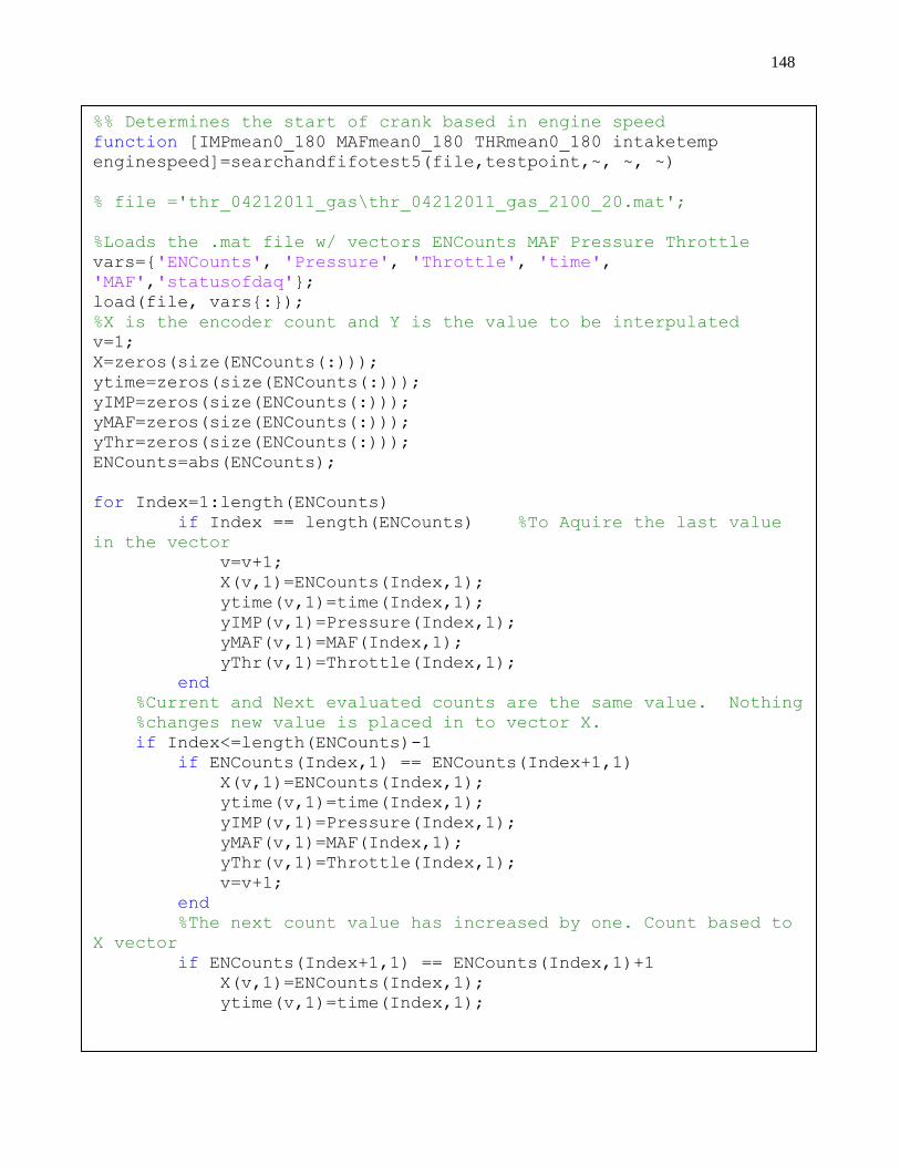
148
%% Determines the start of crank based in engine speed
function [IMPmean0_180 MAFmean0_180 THRmean0_180 intaketemp
enginespeed]=searchandfifotest5(file,testpoint,~, ~, ~)
% file ='thr_04212011_gas\thr_04212011_gas_2100_20.mat';
%Loads the .mat file w/ vectors ENCounts MAF Pressure Throttle
vars={'ENCounts', 'Pressure', 'Throttle', 'time',
'MAF','statusofdaq'};
load(file, vars{:});
%X is the encoder count and Y is the value to be interpulated
v=1;
X=zeros(size(ENCounts(:)));
ytime=zeros(size(ENCounts(:)));
yIMP=zeros(size(ENCounts(:)));
yMAF=zeros(size(ENCounts(:)));
yThr=zeros(size(ENCounts(:)));
ENCounts=abs(ENCounts);
for Index=1:length(ENCounts)
if Index == length(ENCounts) %To Aquire the last value
in the vector
v=v+1;
X(v,1)=ENCounts(Index,1);
ytime(v,1)=time(Index,1);
yIMP(v,1)=Pressure(Index,1);
yMAF(v,1)=MAF(Index,1);
yThr(v,1)=Throttle(Index,1);
end
%Current and Next evaluated counts are the same value. Nothing
%changes new value is placed in to vector X.
if Index<=length(ENCounts)-1
if ENCounts(Index,1) == ENCounts(Index+1,1)
X(v,1)=ENCounts(Index,1);
ytime(v,1)=time(Index,1);
yIMP(v,1)=Pressure(Index,1);
yMAF(v,1)=MAF(Index,1);
yThr(v,1)=Throttle(Index,1);
v=v+1;
end
%The next count value has increased by one. Count based to
X vector
if ENCounts(Index+1,1) == ENCounts(Index,1)+1
X(v,1)=ENCounts(Index,1);
ytime(v,1)=time(Index,1);
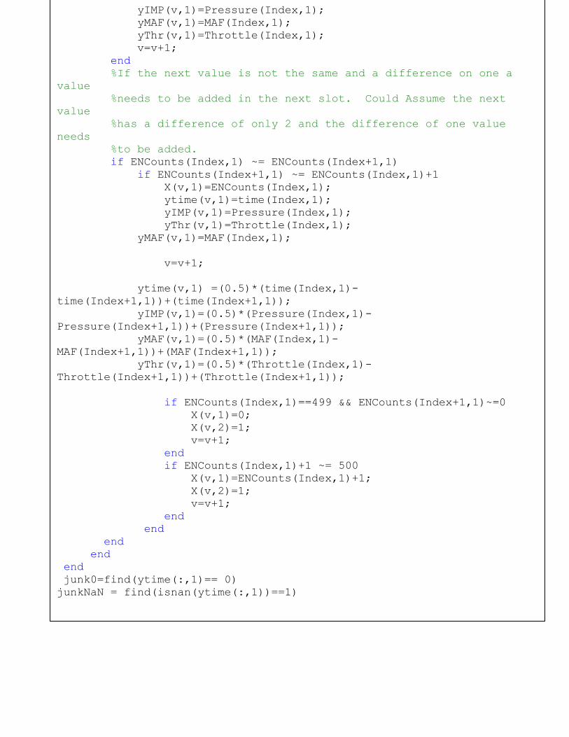
149
yIMP(v,1)=Pressure(Index,1);
yMAF(v,1)=MAF(Index,1);
yThr(v,1)=Throttle(Index,1);
v=v+1;
end
%If the next value is not the same and a difference on one a
value
%needs to be added in the next slot. Could Assume the next
value
%has a difference of only 2 and the difference of one value
needs
%to be added.
if ENCounts(Index,1) ~= ENCounts(Index+1,1)
if ENCounts(Index+1,1) ~= ENCounts(Index,1)+1
X(v,1)=ENCounts(Index,1);
ytime(v,1)=time(Index,1);
yIMP(v,1)=Pressure(Index,1);
yThr(v,1)=Throttle(Index,1);
yMAF(v,1)=MAF(Index,1);
v=v+1;
ytime(v,1) =(0.5)*(time(Index,1)-
time(Index+1,1))+(time(Index+1,1));
yIMP(v,1)=(0.5)*(Pressure(Index,1)-
Pressure(Index+1,1))+(Pressure(Index+1,1));
yMAF(v,1)=(0.5)*(MAF(Index,1)-
MAF(Index+1,1))+(MAF(Index+1,1));
yThr(v,1)=(0.5)*(Throttle(Index,1)-
Throttle(Index+1,1))+(Throttle(Index+1,1));
if ENCounts(Index,1)==499 && ENCounts(Index+1,1)~=0
X(v,1)=0;
X(v,2)=1;
v=v+1;
end
if ENCounts(Index,1)+1 ~= 500
X(v,1)=ENCounts(Index,1)+1;
X(v,2)=1;
v=v+1;
end
end
end
end
end
junk0=find(ytime(:,1)== 0)
junkNaN = find(isnan(ytime(:,1))==1)

150
%% Find the
clear ENCounts time Pressure MAF
ENCounts=X(:,1);
time=ytime(:,1);
Pressure=yIMP;
MAF=yMAF;
Throttle=yThr;
clear X ytime yIMP yMAF
ind0=find(ENCounts == 0); %Position of zero values
zerotime=time(ind0);
zerocount=[zerotime,ind0,zeros(length(ind0),1)];
ind499=find(ENCounts == 499); %Position of 499 aka end of
count
endtime=time(ind499);
endcount=[endtime,ind499,ones(length(ind499),1)*499];
sorted=sortrows([zerocount;endcount],1);
if sorted(1,2)>sorted(2,2)
sorted(1,:)=[];
end
%% Determining engine stroke based on encoder position and time
stamp
%Preallocation
cycle=zeros(10000,10); %Number of rows arbtrarily selected
K=0;
T=0;
%Determine the stroke four strokes.
% while loop continues until slower cycle ie (1) is smaller than
cycle(2)
%Where cycle(1) is considered the the 360 degrees of intake and
compression
%stroke and cycle(2) is the expansion to exhaust stroke.
if K<= length(sorted)%loop continues until the speed in cycle 1 is
greater than the speed in cycle 2
K=K+1; %Increments the K value.
T=T+1;
while (cycle(T,1) >= cycle(T,2)) && (K<length(sorted))%Stops the
loop when cycle(1) is greater than cycle(2)
if cycle(T,1) == 0
if sorted(K,3) == 0 && cycle(T,3) == 0
cycle(T,3) = sorted(K,1) ; %The first zero
value
cycle(T,5) = sorted(K,2) ; %The index of the
first value
K=K+1;
end
end
%Logic to acquire the end value for the cycle
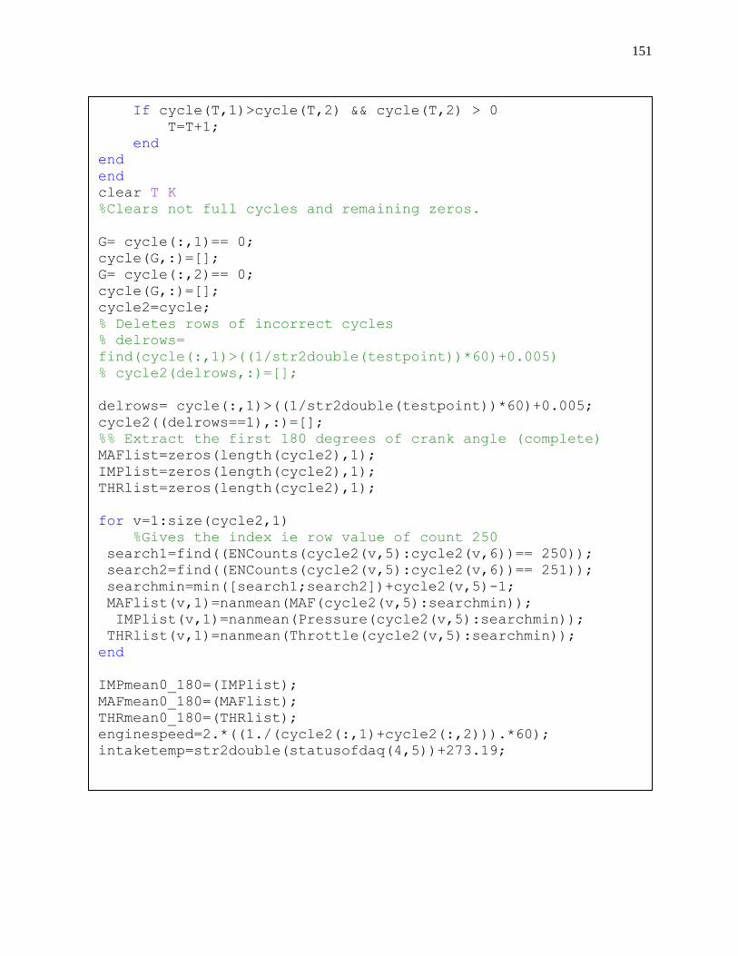
151
if sorted(K,3) == 499 && sorted(K+1,3) == 0 && cycle(T,5) > 0 &&
cycle(T,4) == 0
cycle(T,4) = sorted(K,1); %The end value of the
first revloution
cycle(T,6) = sorted(K,2); %The index of the end
first revolution
cycle(T,1)=cycle(T,4)-cycle(T,3); %The difference
between end values
end
if sorted(K,3) == 0 && sorted(K-1,3) ~= 0 && cycle(T,6) > 0
cycle(T,7) = sorted(K,1); %The first zero value of the
second revolution
cycle(T,9) = sorted(K,2); %The index of the first value
second revolution
end
if sorted(K,3) == 499 && sorted(K+1,3) == 0 && cycle(T,7) > 0
cycle(T,8) = sorted(K,1); %The end value of the
second revolution
cycle(T,10) = sorted(K,2); %The index of the end
value of the second revolution
%Does not execute the subtraction until there is a value above zero
in column 8
if cycle(T,8)>0
cycle(T,2)=cycle(T,8)-cycle(T,7); %The difference
between end values
end
end
K=K+1;
%Shift cycle(1) to cycle (2) if condition cycle(1)>cycle(2) is not met
if cycle(T,1) < cycle(T,2) %If the cycle(1) value is less than
cycle(2) shift cycle(1) to cycle(2)
cycle(T,1) = cycle(T,2);
cycle(T,3) = cycle(T,7); %The first zero value
cycle(T,5) = cycle(T,9);
cycle(T,4) = cycle(T,8); %The end value of the second
revolution
cycle(T,6) = cycle(T,10);
cycle(T,7) = 0; %The first zero value
cycle(T,8) = 0; %The end value of the cycle
cycle(T,9) = 0;
cycle(T,10) = 0;
cycle(T,2) = 0;
end
If cycle(T,1)>cycle(T,2) && cycle(T,2) > 0
T=T+1;
end
end
end
clear T K
%Clears not full cycles and remaining zeros.
G= cycle(:,1)== 0;
cycle(G,:)=[];
G= cycle(:,2)== 0;
cycle(G,:)=[];
cycle2=cycle;
% Deletes rows of incorrect cycles
% delrows=
find(cycle(:,1)>((1/str2double(testpoint))*60)+0.005)
% cycle2(delrows,:)=[];
delrows= cycle(:,1)>((1/str2double(testpoint))*60)+0.005;
cycle2((delrows==1),:)=[];
%% Extract the first 180 degrees of crank angle (complete)
MAFlist=zeros(length(cycle2),1);
IMPlist=zeros(length(cycle2),1);
THRlist=zeros(length(cycle2),1);
for v=1:size(cycle2,1)
%Gives the index ie row value of count 250
search1=find((ENCounts(cycle2(v,5):cycle2(v,6))== 250));
search2=find((ENCounts(cycle2(v,5):cycle2(v,6))== 251));
searchmin=min([search1;search2])+cycle2(v,5)-1;
MAFlist(v,1)=nanmean(MAF(cycle2(v,5):searchmin));
IMPlist(v,1)=nanmean(Pressure(cycle2(v,5):searchmin));
THRlist(v,1)=nanmean(Throttle(cycle2(v,5):searchmin));
end
IMPmean0_180=(IMPlist);
MAFmean0_180=(MAFlist);
THRmean0_180=(THRlist);
enginespeed=2.*((1./(cycle2(:,1)+cycle2(:,2))).*60);
intaketemp=str2double(statusofdaq(4,5))+273.19;
152
B.4 Willan's Line
The Willan’s Line is a method of approximating indicated power for either a multi or
single cylinder engine. The method is based on that at light engine load a little fuel is pumped
into the air stream entering the engine cylinder. Therefore there is a lot of air available for
combustion resulting in almost constant combustion efficiency. Greene and Lucas (1969) states
"this method is not suitable for use with petrol engines.‖ (Greene & Lucas, 1969) With the
constant speed approximation made by Guzzella and Onder (2004). This is approximation is
used in
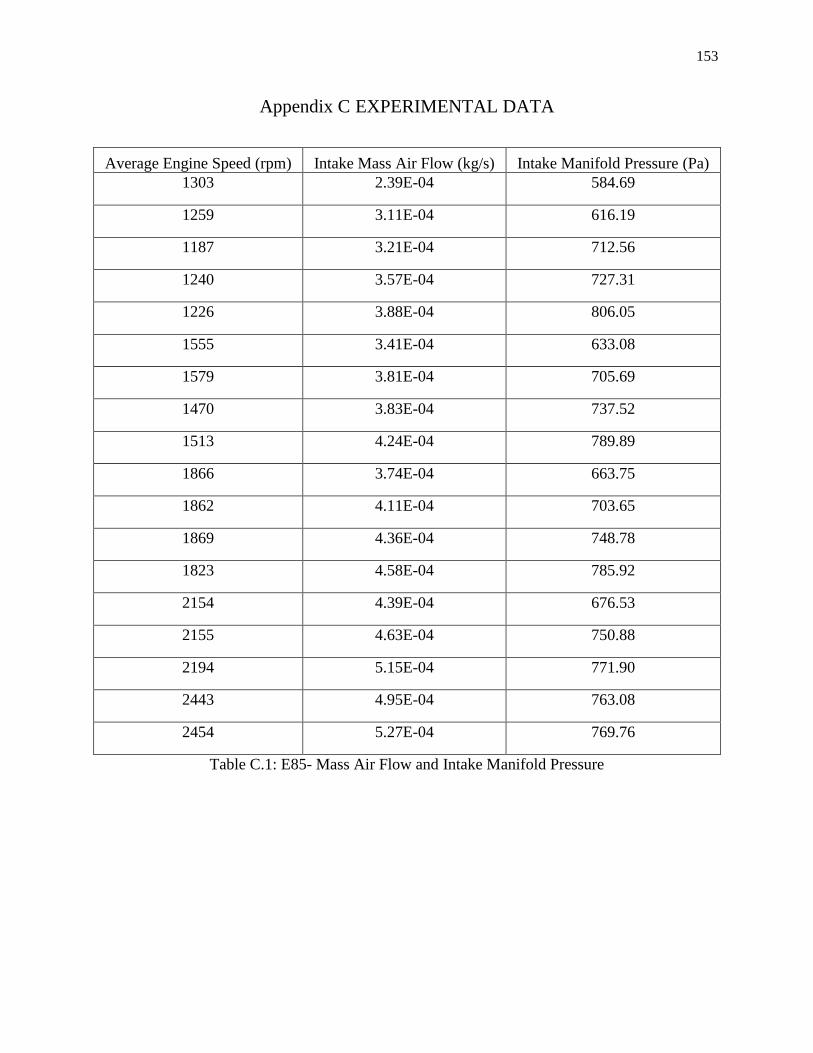
153
Appendix C EXPERIMENTAL DATA
Average Engine Speed (rpm) Intake Mass Air Flow (kg/s) Intake Manifold Pressure (Pa)
1303 2.39E-04 584.69
1259 3.11E-04 616.19
1187 3.21E-04 712.56
1240 3.57E-04 727.31
1226 3.88E-04 806.05
1555 3.41E-04 633.08
1579 3.81E-04 705.69
1470 3.83E-04 737.52
1513 4.24E-04 789.89
1866 3.74E-04 663.75
1862 4.11E-04 703.65
1869 4.36E-04 748.78
1823 4.58E-04 785.92
2154 4.39E-04 676.53
2155 4.63E-04 750.88
2194 5.15E-04 771.90
2443 4.95E-04 763.08
2454 5.27E-04 769.76
Table C.1: E85- Mass Air Flow and Intake Manifold Pressure
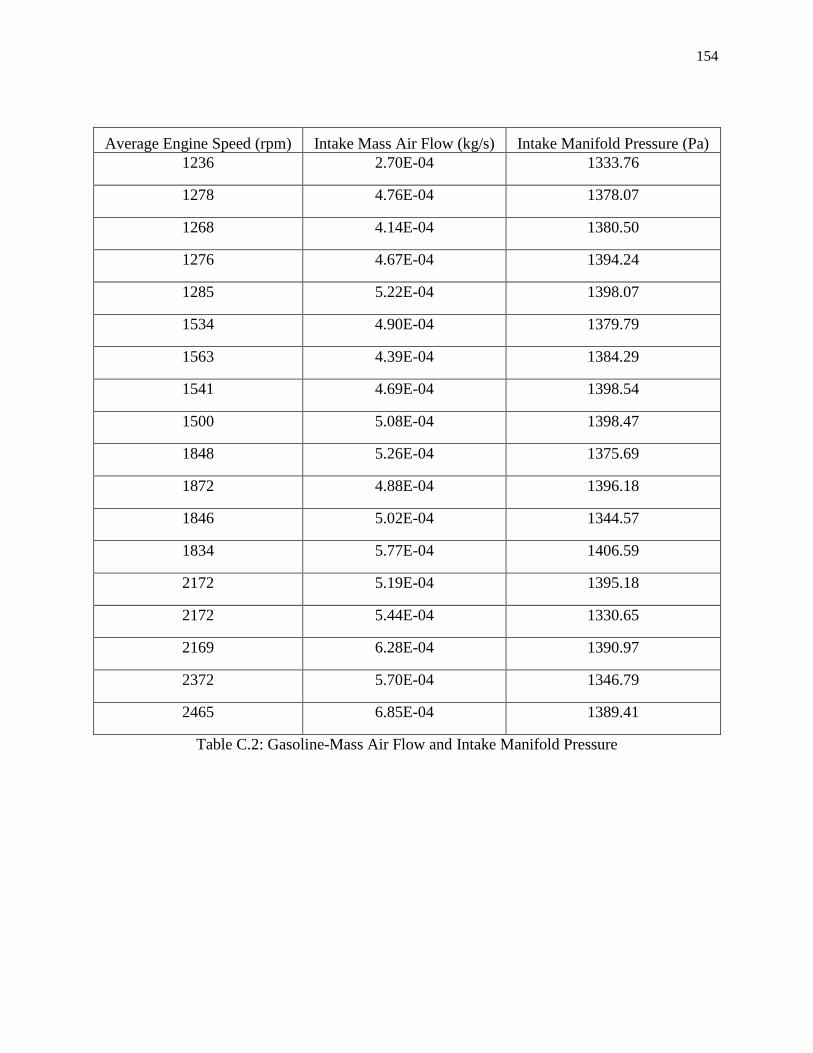
154
Average Engine Speed (rpm) Intake Mass Air Flow (kg/s) Intake Manifold Pressure (Pa)
1236 2.70E-04 1333.76
1278 4.76E-04 1378.07
1268 4.14E-04 1380.50
1276 4.67E-04 1394.24
1285 5.22E-04 1398.07
1534 4.90E-04 1379.79
1563 4.39E-04 1384.29
1541 4.69E-04 1398.54
1500 5.08E-04 1398.47
1848 5.26E-04 1375.69
1872 4.88E-04 1396.18
1846 5.02E-04 1344.57
1834 5.77E-04 1406.59
2172 5.19E-04 1395.18
2172 5.44E-04 1330.65
2169 6.28E-04 1390.97
2372 5.70E-04 1346.79
2465 6.85E-04 1389.41
Table C.2: Gasoline-Mass Air Flow and Intake Manifold Pressure
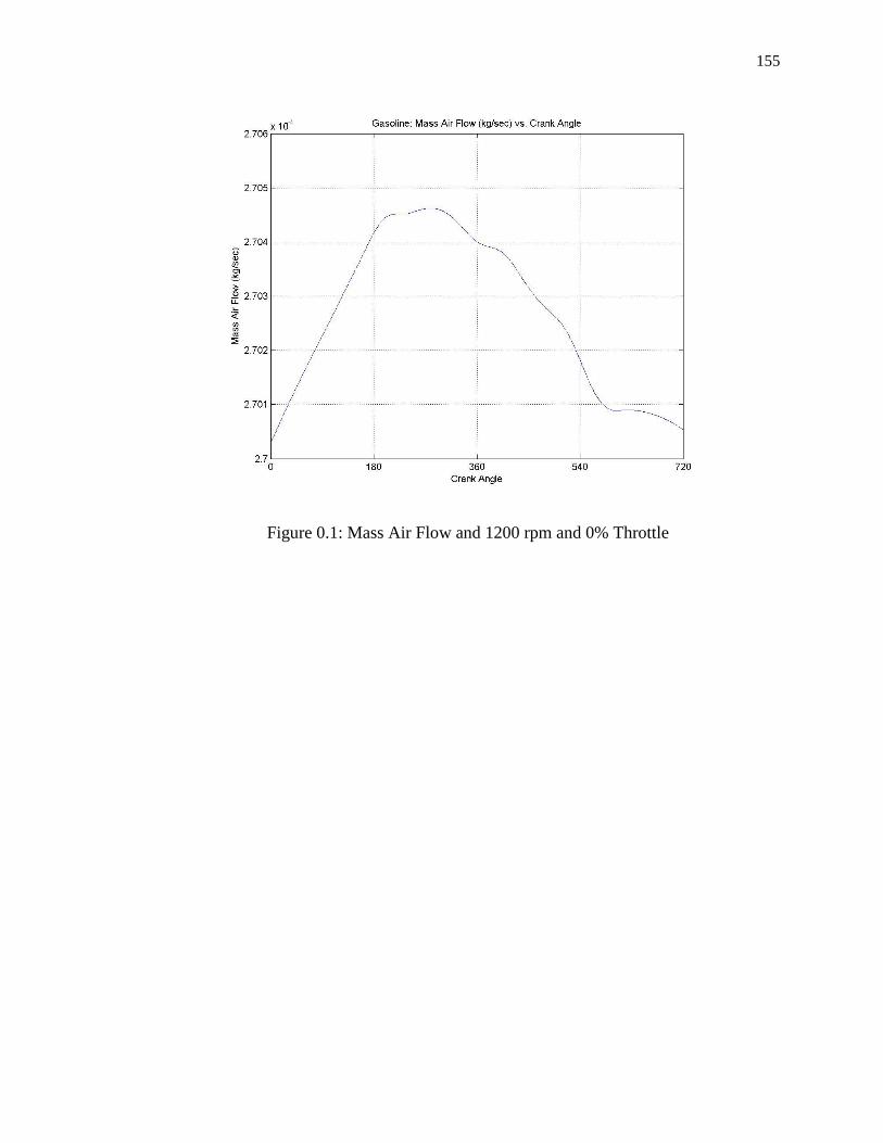
155
Figure 0.1: Mass Air Flow and 1200 rpm and 0% Throttle
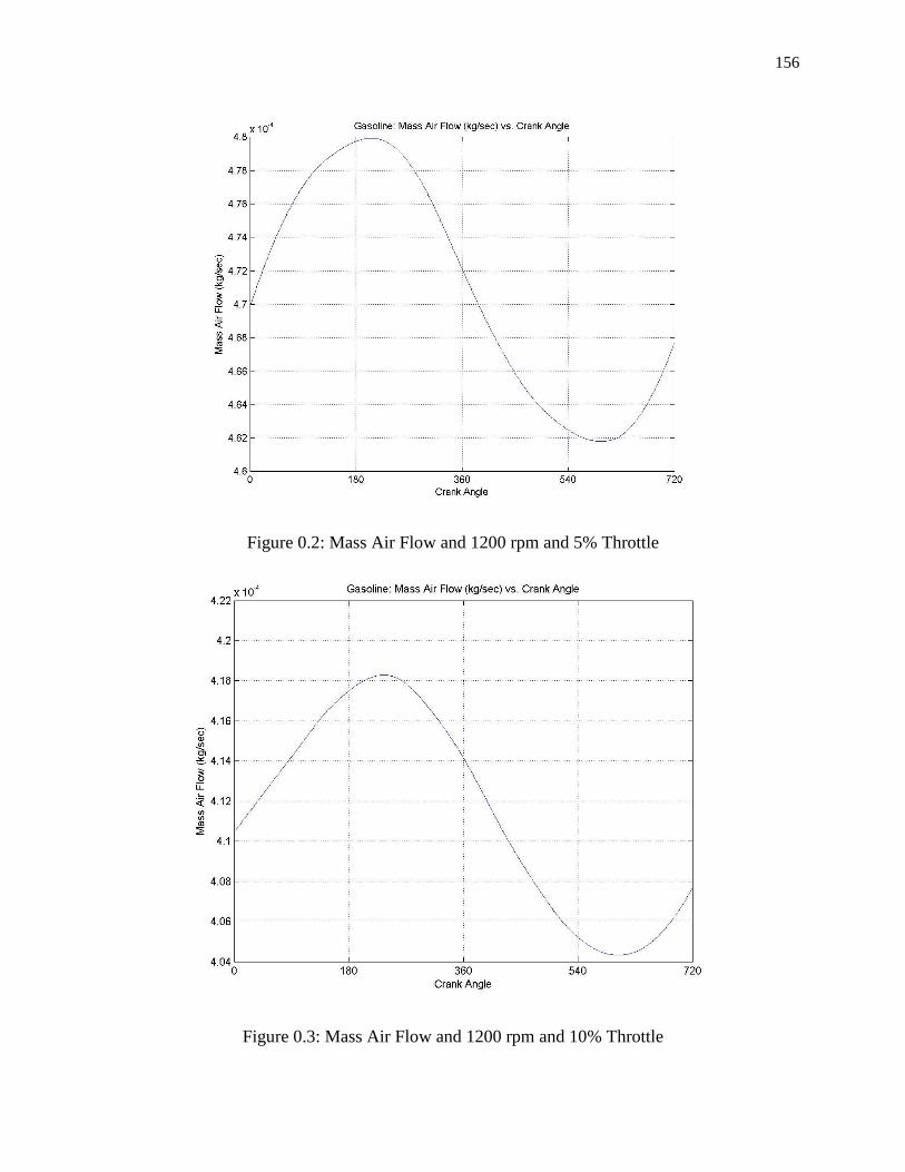
156
Figure 0.2: Mass Air Flow and 1200 rpm and 5% Throttle
Figure 0.3: Mass Air Flow and 1200 rpm and 10% Throttle

157
Figure 0.4: Mass Air Flow and 1200 rpm and 15% Throttle
Figure 0.5: Mass Air Flow and 1200 rpm and 20% Throttle
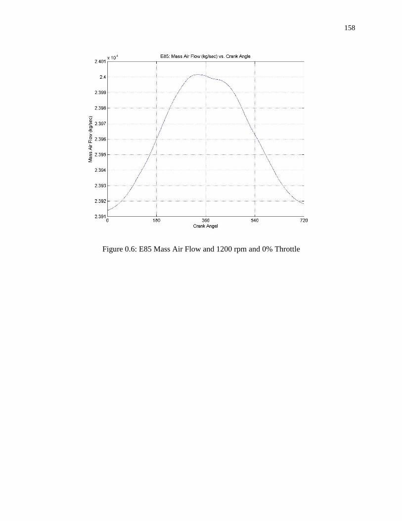
158
Figure 0.6: E85 Mass Air Flow and 1200 rpm and 0% Throttle

159
Figure 0.7: E85 Mass Air Flow and 1200 rpm and 0% Throttle
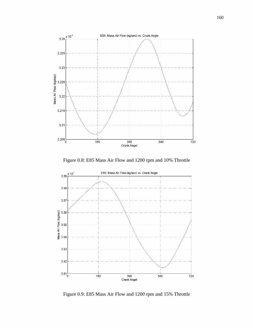
160
Figure 0.8: E85 Mass Air Flow and 1200 rpm and 10% Throttle
Figure 0.9: E85 Mass Air Flow and 1200 rpm and 15% Throttle
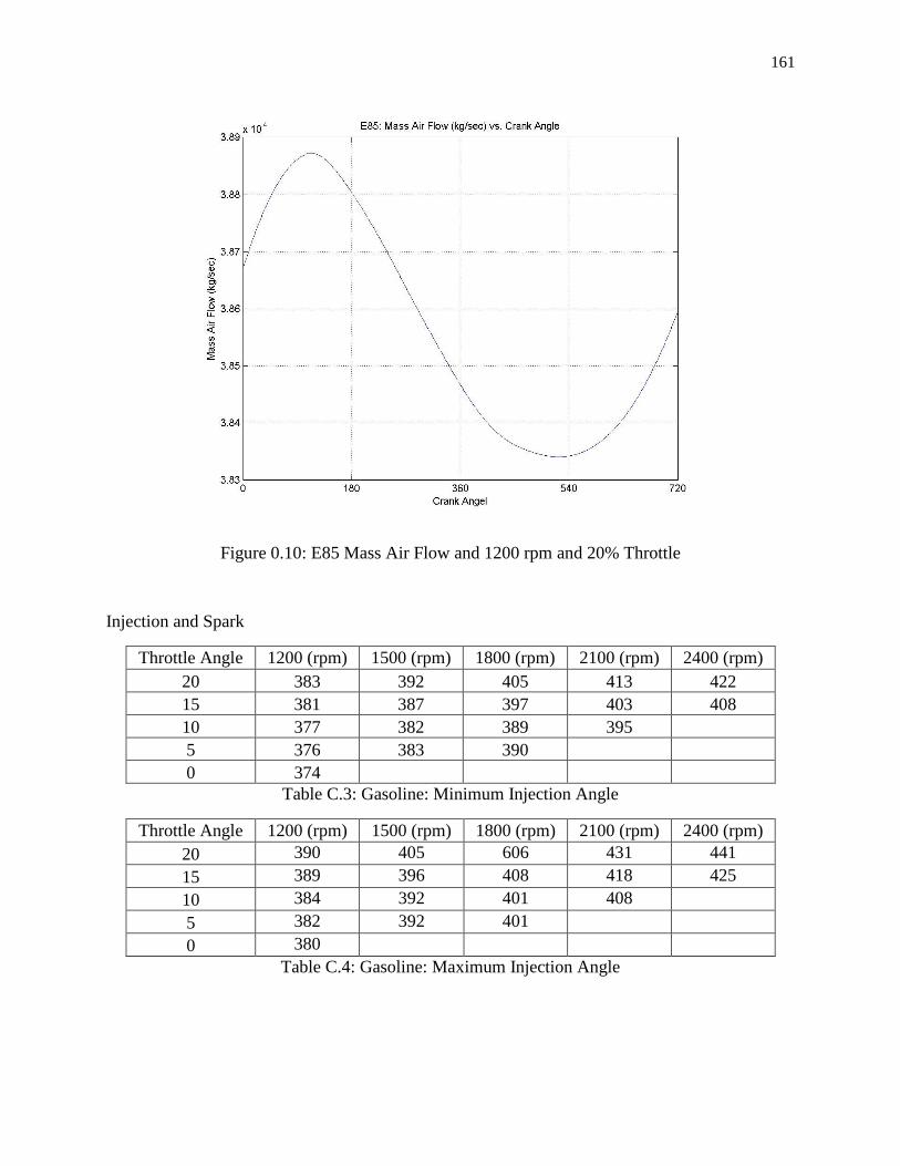
161
Figure 0.10: E85 Mass Air Flow and 1200 rpm and 20% Throttle
Injection and Spark
Throttle Angle 1200 (rpm) 1500 (rpm) 1800 (rpm) 2100 (rpm) 2400 (rpm)
20 383 392 405 413 422
15 381 387 397 403 408
10 377 382 389 395
5 376 383 390
0 374
Table C.3: Gasoline: Minimum Injection Angle
Throttle Angle 1200 (rpm) 1500 (rpm) 1800 (rpm) 2100 (rpm) 2400 (rpm)
20 390 405 606 431 441
15 389 396 408 418 425
10 384 392 401 408
5 382 392 401
0 380
Table C.4: Gasoline: Maximum Injection Angle
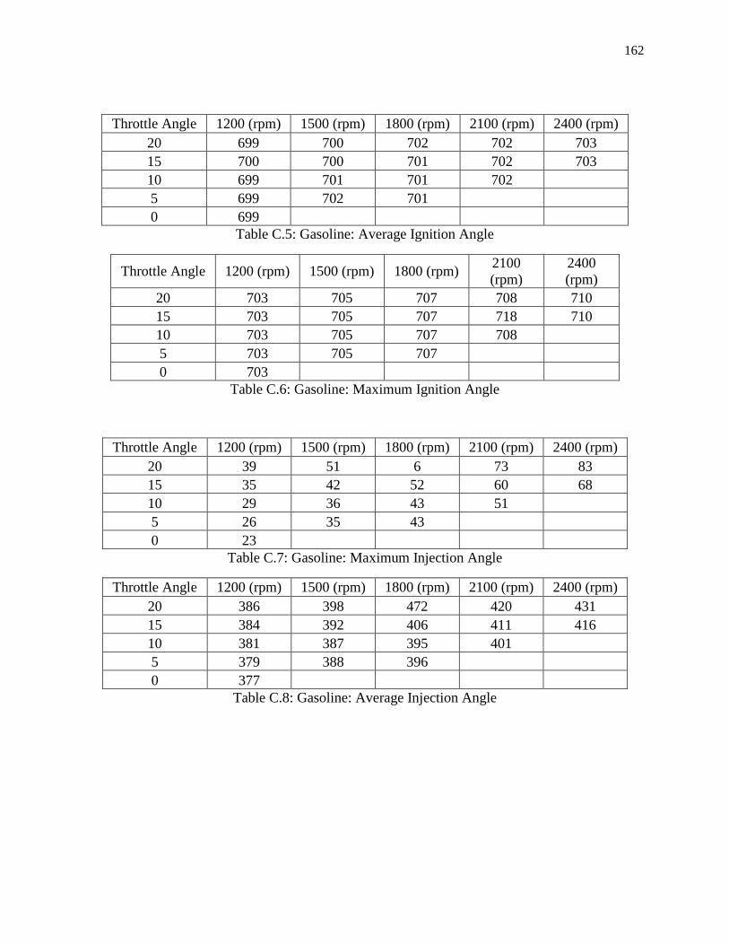
162
Throttle Angle 1200 (rpm) 1500 (rpm) 1800 (rpm) 2100 (rpm) 2400 (rpm)
20 699 700 702 702 703
15 700 700 701 702 703
10 699 701 701 702
5 699 702 701
0 699
Table C.5: Gasoline: Average Ignition Angle
Throttle Angle 1200 (rpm) 1500 (rpm) 1800 (rpm) 2100
(rpm)
2400
(rpm)
20 703 705 707 708 710
15 703 705 707 718 710
10 703 705 707 708
5 703 705 707
0 703
Table C.6: Gasoline: Maximum Ignition Angle
Throttle Angle 1200 (rpm) 1500 (rpm) 1800 (rpm) 2100 (rpm) 2400 (rpm)
20 39 51 6 73 83
15 35 42 52 60 68
10 29 36 43 51
5 26 35 43
0 23
Table C.7: Gasoline: Maximum Injection Angle
Throttle Angle 1200 (rpm) 1500 (rpm) 1800 (rpm) 2100 (rpm) 2400 (rpm)
20 386 398 472 420 431
15 384 392 406 411 416
10 381 387 395 401
5 379 388 396
0 377
Table C.8: Gasoline: Average Injection Angle

163
Throttle Angle 1200 (rpm) 1500 (rpm) 1800 (rpm) 2100 (rpm) 2400 (rpm)
20 31 38 51 56 64
15 27 32 40 46 52
10 21 26 31 36
5 19 27 31
0 16
Table C.9: Gasoline: Minimum Injection Angle
Throttle Angle 1200 (rpm) 1500 (rpm) 1800 (rpm) 2100 (rpm) 2400 (rpm)
20 695 695 696 695 695
15 695 695 695 696 695
10 695 695 695 695
5 695 696 695
0 695
Table C.10: Gasoline: Minimum Ignition Angle
Throttle Angle 1200 (rpm) 1500 (rpm) 1800 (rpm) 2100 (rpm) 2400 (rpm)
20 342 343 346 348 350
15 342 343 346 348 349
10 343 344 346 348
5 343 345 346
0 342
Table C.11: Gasoline: Maximum Ignition Angle
Throttle Angle 1200 (rpm) 1500 (rpm) 1800 (rpm) 2100 (rpm) 2400 (rpm)
20 335 335 335 335 335
15 335 335 336 336 336
10 336 335 335 336
5 336 335 336
0 335
Table C.12: Gasoline: Minimum Ignition Angle
Throttle Angle 1200 (rpm) 1500 (rpm) 1800 (rpm) 2100 (rpm) 2400 (rpm)
20 0.0040 0.0040 0.0010 0.0040 0.0040
15 0.0030 0.0030 0.0030 0.0030 0.0030
10 0.0030 0.0030 0.0030 0.0030
5 0.0020 0.0030 0.0030
0 0.0020
Table C.13: Gasoline: Minimum Low Injection Duration
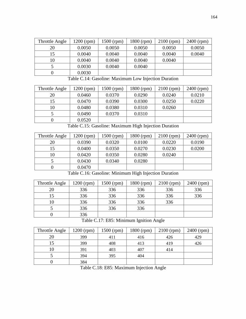
164
Throttle Angle 1200 (rpm) 1500 (rpm) 1800 (rpm) 2100 (rpm) 2400 (rpm)
20 0.0050 0.0050 0.0050 0.0050 0.0050
15 0.0040 0.0040 0.0040 0.0040 0.0040
10 0.0040 0.0040 0.0040 0.0040
5 0.0030 0.0040 0.0040
0 0.0030
Table C.14: Gasoline: Maximum Low Injection Duration
Throttle Angle 1200 (rpm) 1500 (rpm) 1800 (rpm) 2100 (rpm) 2400 (rpm)
20 0.0460 0.0370 0.0290 0.0240 0.0210
15 0.0470 0.0390 0.0300 0.0250 0.0220
10 0.0480 0.0380 0.0310 0.0260
5 0.0490 0.0370 0.0310
0 0.0520
Table C.15: Gasoline: Maximum High Injection Duration
Throttle Angle 1200 (rpm) 1500 (rpm) 1800 (rpm) 2100 (rpm) 2400 (rpm)
20 0.0390 0.0320 0.0100 0.0220 0.0190
15 0.0400 0.0350 0.0270 0.0230 0.0200
10 0.0420 0.0350 0.0280 0.0240
5 0.0430 0.0340 0.0280
0 0.0470
Table C.16: Gasoline: Minimum High Injection Duration
Throttle Angle 1200 (rpm) 1500 (rpm) 1800 (rpm) 2100 (rpm) 2400 (rpm)
20 336 336 336 336 336
15 336 336 336 336 336
10 336 336 336 336
5 336 336 336
0 336
Table C.17: E85: Minimum Ignition Angle
Throttle Angle 1200 (rpm) 1500 (rpm) 1800 (rpm) 2100 (rpm) 2400 (rpm)
20 399 411 416 426 429
15 399 408 413 419 426
10 391 403 407 414
5 394 395 404
0 384
Table C.18: E85: Maximum Injection Angle
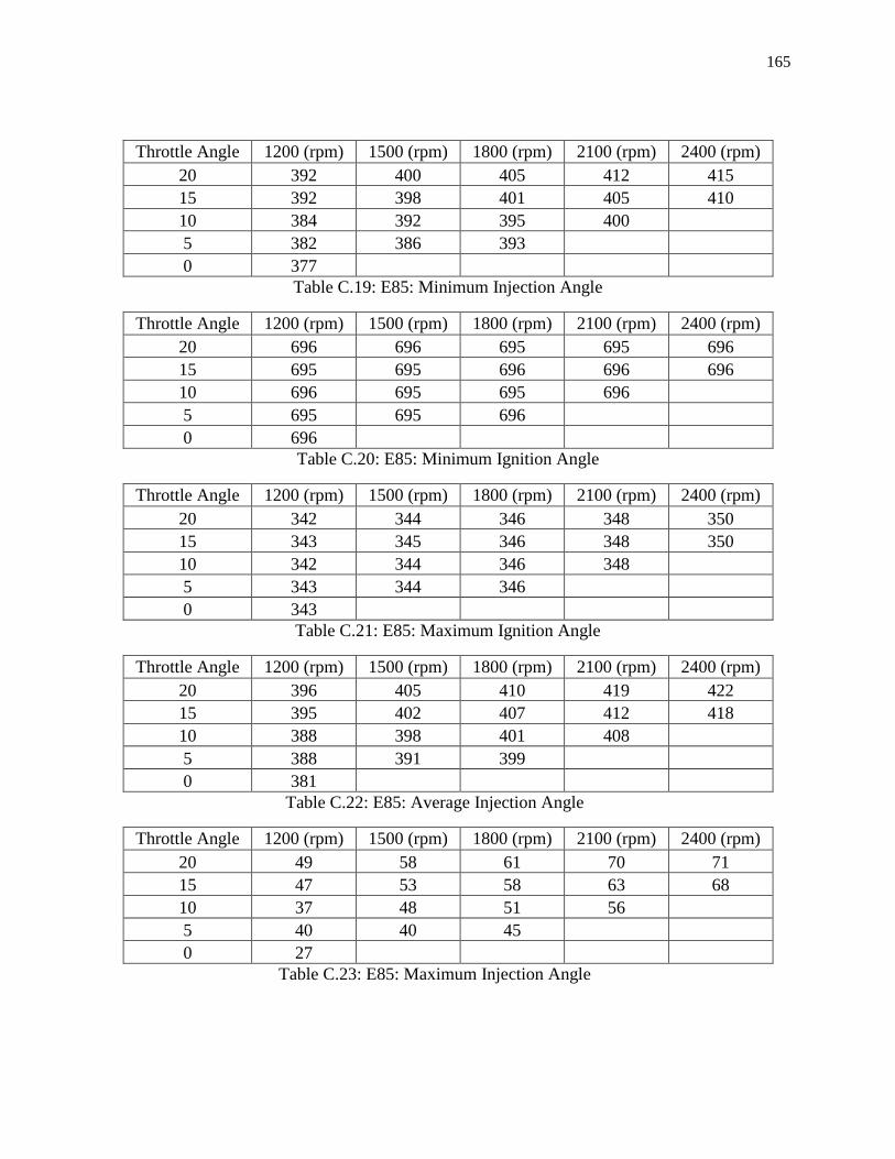
165
Throttle Angle 1200 (rpm) 1500 (rpm) 1800 (rpm) 2100 (rpm) 2400 (rpm)
20 392 400 405 412 415
15 392 398 401 405 410
10 384 392 395 400
5 382 386 393
0 377
Table C.19: E85: Minimum Injection Angle
Throttle Angle 1200 (rpm) 1500 (rpm) 1800 (rpm) 2100 (rpm) 2400 (rpm)
20 696 696 695 695 696
15 695 695 696 696 696
10 696 695 695 696
5 695 695 696
0 696
Table C.20: E85: Minimum Ignition Angle
Throttle Angle 1200 (rpm) 1500 (rpm) 1800 (rpm) 2100 (rpm) 2400 (rpm)
20 342 344 346 348 350
15 343 345 346 348 350
10 342 344 346 348
5 343 344 346
0 343
Table C.21: E85: Maximum Ignition Angle
Throttle Angle 1200 (rpm) 1500 (rpm) 1800 (rpm) 2100 (rpm) 2400 (rpm)
20 396 405 410 419 422
15 395 402 407 412 418
10 388 398 401 408
5 388 391 399
0 381
Table C.22: E85: Average Injection Angle
Throttle Angle 1200 (rpm) 1500 (rpm) 1800 (rpm) 2100 (rpm) 2400 (rpm)
20 49 58 61 70 71
15 47 53 58 63 68
10 37 48 51 56
5 40 40 45
0 27
Table C.23: E85: Maximum Injection Angle
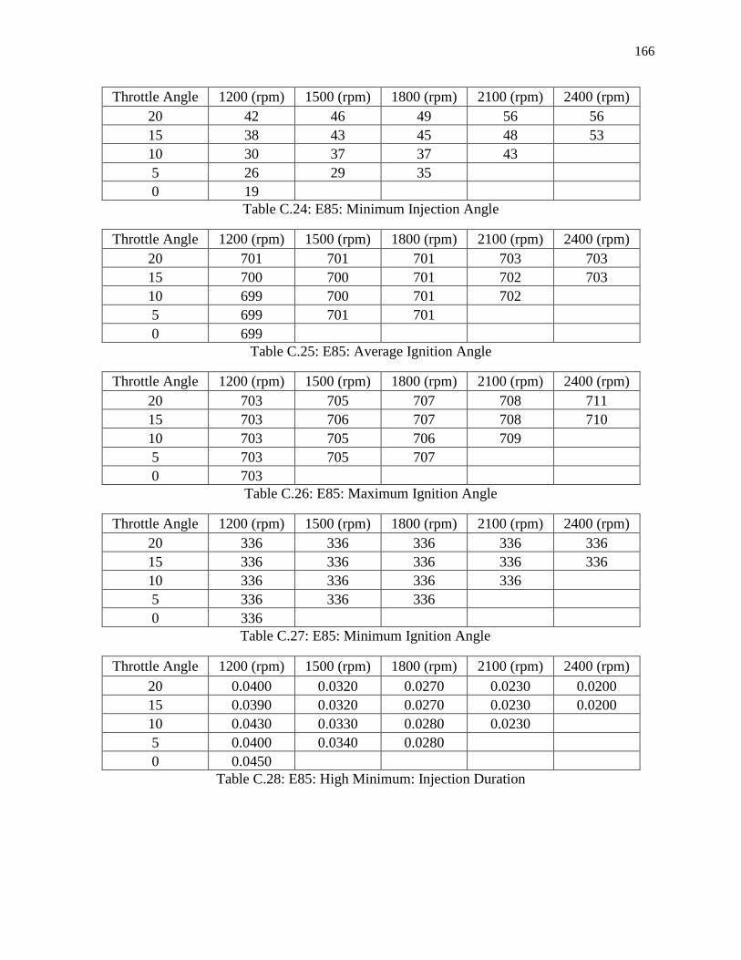
166
Throttle Angle 1200 (rpm) 1500 (rpm) 1800 (rpm) 2100 (rpm) 2400 (rpm)
20 42 46 49 56 56
15 38 43 45 48 53
10 30 37 37 43
5 26 29 35
0 19
Table C.24: E85: Minimum Injection Angle
Throttle Angle 1200 (rpm) 1500 (rpm) 1800 (rpm) 2100 (rpm) 2400 (rpm)
20 701 701 701 703 703
15 700 700 701 702 703
10 699 700 701 702
5 699 701 701
0 699
Table C.25: E85: Average Ignition Angle
Throttle Angle 1200 (rpm) 1500 (rpm) 1800 (rpm) 2100 (rpm) 2400 (rpm)
20 703 705 707 708 711
15 703 706 707 708 710
10 703 705 706 709
5 703 705 707
0 703
Table C.26: E85: Maximum Ignition Angle
Throttle Angle 1200 (rpm) 1500 (rpm) 1800 (rpm) 2100 (rpm) 2400 (rpm)
20 336 336 336 336 336
15 336 336 336 336 336
10 336 336 336 336
5 336 336 336
0 336
Table C.27: E85: Minimum Ignition Angle
Throttle Angle 1200 (rpm) 1500 (rpm) 1800 (rpm) 2100 (rpm) 2400 (rpm)
20 0.0400 0.0320 0.0270 0.0230 0.0200
15 0.0390 0.0320 0.0270 0.0230 0.0200
10 0.0430 0.0330 0.0280 0.0230
5 0.0400 0.0340 0.0280
0 0.0450
Table C.28: E85: High Minimum: Injection Duration

167
Throttle Angle 1200 (rpm) 1500 (rpm) 1800 (rpm) 2100 (rpm) 2400 (rpm)
20 0.0470 0.0370 0.0290 0.0240 0.0220
15 0.0440 0.0350 0.0300 0.0250 0.0220
10 0.0480 0.0380 0.0310 0.0250
5 0.0470 0.0370 0.0300
0 0.0500
Table C.29: E85: High Maximum: Injection Duration
Throttle Angle 1200 (rpm) 1500 (rpm) 1800 (rpm) 2100 (rpm) 2400 (rpm)
20 0.0050 0.0050 0.0040 0.0040 0.0040
15 0.0050 0.0040 0.0040 0.0030 0.0030
10 0.0040 0.0040 0.0030 0.0030
5 0.0030 0.0030 0.0030
0 0.0030
Table C.30: E85: Low Minimum: Injection Duration
Throttle Angle 1200 (rpm) 1500 (rpm) 1800 (rpm) 2100 (rpm) 2400 (rpm)
20 0.0060 0.0060 0.0050 0.0050 0.0050
15 0.0060 0.0050 0.0050 0.0040 0.0040
10 0.0050 0.0050 0.0040 0.0040
5 0.0050 0.0040 0.0040
0 0.0040
Table C.31: E85: Low Maximum: Injection Duration