Da

Sa

b

a

ARRAA

KULMSES

1

aqosltlimtdtde

se(

0d

Landscape and Urban Planning 103 (2011) 303– 317

Contents lists available at SciVerse ScienceDirect

Landscape and Urban Planning

jou rn al h om epa ge: www.elsev ier .com/ locate / landurbplan

evelopment of a composite index of urban compactness for land use modellingpplications

arah Mubarekaa,∗, Eric Koomenb, Christine Estreguil a, Carlo Lavallea

Land Management and Natural Hazards Unit, Institute for Environment and Sustainability, European Commission Joint Research Centre, ItalyVrije Universiteit Amsterdam (NL), Faculty of Economics and Business Administration, Department of Spatial Economics, The Netherlands

r t i c l e i n f o

rticle history:eceived 7 February 2011eceived in revised form 29 June 2011ccepted 3 August 2011vailable online 22 September 2011

eywords:rbanisationarge urban zonesathematical morphology

a b s t r a c t

This paper introduces a composite index to characterise urban expansion patterns based on four associ-ated indices that describe the degree of compactness of urban land: nuclearity, ribbon development,leapfrogging and branching processes. Subsequently, principal component and cluster analysis areapplied to build the composite index. Two baseline scenarios and three hypothetical policy alternatives,run from 2000 to 2030 using the pan-European EU-ClueScanner 1 km resolution land use model are thenused to test the sensitivity and robustness of the composite index in large urban zones (LUZs).

The second part of the paper is dedicated to the spatial analysis of a subset of large urban zones withthe largest area growth in all the model runs for the year 2030. The landscape context of all built-upland in the year 2000 is analysed for the newly created urban land. It is characterised according to the

patial indicatorsuClueScannercenarios

proportion of natural, agricultural, built-up areas within a 7 km radius. A stepwise multiple regressionanalysis relating the landscape mosaic types and the composite index allowed us to understand whetheror not the landscape surrounding the existing urban cores acts as the driving force responsible for the more“successful” policy alternatives in terms of urban compactness. Modellers may consider the landscapemosaic as one possible proxy to determine which urban areas are more likely to have less compact urbanexpansion patterns for scenarios with an increase in land claims for built-up areas.

. Introduction

When working with complex spatial land use models, modellersre faced with the challenge of translating a scenario story line intouantitative model parameters. Often however, the manipulationf parameters can lead to surprising and sometimes undesirableecondary effects, especially when working at a supra-nationalevel where many different localised elements, unbeknownst tohe modeller, may have different influences. In such complexand use systems the modeller normally has room to manoeuvren economic, social, cultural and biophysical realms through the

anipulation of different parameters within the model. In fact,he governing processes of change may go far beyond a singleomain and can be attributed to complex interactions of any of

hese driving forces. It is the modeller’s job to “. . . remove the ran-omness and reveal the order” (White & Engelen, 1994). This isasier said than done when working with complex land use models

∗ Corresponding author. Tel.: +39 0332 78 6741; fax: +39 0332 78 9085.E-mail addresses: sarah.mubareka@jrc.ec.europa.eu,

arah.mubareka@drawingdata.com (S. Mubareka),koomen@feweb.vu.nl (E. Koomen), christine.estreguil@jrc.ec.europa.euC. Estreguil), carlo.lavalle@jrc.ec.europa.eu (C. Lavalle).

169-2046/$ – see front matter © 2011 Elsevier B.V. All rights reserved.oi:10.1016/j.landurbplan.2011.08.012

© 2011 Elsevier B.V. All rights reserved.

that relate to a wide range of countries. In particular, the calibrationprocess is important in order to catch secondary effects of parame-terisation (Pinto & Anutnes, 2010). During the calibration process,general good practice is to alternate between singular parametermanipulation and checking results in order to assess the impactsof those changes and to check whether or not results are sensi-ble (van Delden, Luja, & Engelen, 2007). This iterative approach istime consuming but necessary, especially when modelling a largeterritory such as continental Europe. It is therefore necessary formodellers to have tools available in order to quickly assess theimpacts of the parameter changes. Such tools require a simpleand rapid methodology to produce indicators that can assess theimpacts of parameter settings on a specific process of land usechange. Indicators that help capture the essence of land use changeimpacts are furthermore essential to policy makers to interpret dif-ferent land use simulation results (Koomen, Rietveld, & De Nijs,2008). In this paper we focus on the development of an indicatorfor a land use change process that is useful not only for the modellerto test the model configuration, but also to policy oriented land usemodelling applications involving urban development.

The increase in land claims for built-up areas over time isreferred to as urbanisation. The emergence of quantitative meth-ods for the classification of the placement of this newly urbanisedland, the study of urban form, has greatly contributed to the

3 d Urba

cJutapc2ttetiwb(demoiottB

sfihatupuotqho

spotpcteasatmcbdiaiPac

cuC

04 S. Mubareka et al. / Landscape an

omparison of different urban areas (Huang, Lu, & Sellers, 2007;aeger, Bertiller, Schwick, Cavens, & Kienast, 2010). In this paper wese the terms ‘urban compactness’ and ‘urban sprawl’ as antonymso describe changes in urban form for scenarios in which themount of land allocated to urban areas is increasing. While com-actness is characterised by high density of built-up areas and shortommuting distances between homes, services and work (Schwarz,010); Torrens and Alberti (2000) define urban sprawl as beinghe wasteful method of urbanisation with an over-dependence onhe automobile to access services, thus leading to pollution andcological disturbance among other negative effects, and quantifyhe phenomenon using surfaces, gradients, fractals, image process-ng, ecological impacts and accessibility. Sprawl is an expression

hich is often used loosely to describe different concepts linkedoth to patterns and processes; to both causes and consequencesGalster et al., 2001; Irwin & Bockstael, 2007). These same authorsecompose sprawl into eight dimensions which encompass socio-conomic factors such as proximity, concentration of services andixed usages of the built-up land; which is beyond the scope

f this study. Regardless of nomenclature, the common threadn the literature is to quantify the infringement of built-up areasnto open areas and farmland in order to measure differences inhis encroachment between different development scenarios; andhe subsequent loss of landscape identity (Frenkel, 2004; Jaeger,ertiller, Schwick, Cavens, et al., 2010; Wissen Hayek et al., 2010).

Composite indices are often criticised as being misleading,implistic and non transparent due to the complexity in their con-guration and the differences in underlying indicators. On the otherand, composite indices can be helpful in monitoring progress;re able to measure different dimensions of a single problem; andhe outcomes, which usually one number or a ranking, are easy tonderstand and compare (OECD, 2008). A composite index is theerfect tool in this case whereby a benchmark for the degree ofrban sprawl given ex ante scenarios is compared to the outcomef different policy alternatives with regard to urban sprawl. Forhe purposes outlined in this paper, it is essential to have a single,uantitative measure of the overall impact of model configurations,ence policy alternatives, on the overall trends for a large numberf urban centres in Europe.

In response to the need to describe a complex phenomenonuch as sprawl with several indicators combined into one com-osite index (Siedentop & Fina, 2010), we combine several aspectsf urban form. The resulting composite index was to be appliedo future land change maps. The choice of which individual com-onents to include in the study therefore rested on physicalharacteristics which would not introduce further uncertainty intohe composite index, an approach also adopted by Wissen Hayekt al. (2010). Parameters that may introduce further uncertaintyre, for example, projected population density; changes in acces-ibility; or specific locations of services or residential areas whichre linked to mixed uses (Galster et al., 2001). We limit ourselveso describing urban form using a morphological series of measure-

ents because of their analytical soundness as contributors to aomposite indicator which, according to the OECD (2008), shoulde relevant and accessible. Within the context of this paper, theefinition of urban form is therefore only linked to the actual phys-

cal form of the built-up areas in Europe and not on their contentnd functionalities. In addition to this restriction, we do not exam-ne urban changes on a per pixel basis as do Wilson, Hurd, Civco,risloe, and Arnold (2003) because our main concern is in differenti-ting between policy alternatives and their impacts on the absolutehanges in urban form rather than on the per-pixel basis.

The focus of this research is to derive a simple and rapidlyomputed composite index and apply it to maps of future landse that are produced with a pan-European land use model: EU-lueScanner, a derivative of the widely known DynaClue model

n Planning 103 (2011) 303– 317

(Hellmann & Verburg, 2010; Verburg & Overmars, 2009; Verburg,Eickhout, & Van Meijl, 2008). The index is then confronted withscenario configurations in order to assess its uncertainty androbustness. First, a series of individual indicators was developedusing an available mathematical morphological tool. A compositeindex was then developed based on these, for the categorization ofbuilt-up area land use patterns and changes between scenarios runthrough the EU-ClueScanner land use model. In the second part ofthe study, the large urban zones (LUZs) with the highest increasesin built-up areas for all model runs were then used for further stud-ies linked to the landscape within LUZs. The outcome of this partof the study is a better understanding of what factors can influenceurban compactness.

2. Methods

The first step in our approach consists of a mathematicalmorphological analysis that was applied to the binary built-up/non-built-up maps for the year 2000 map and simulated year2030 maps derived from the EU-ClueScanner land use model.These maps are based on a modified Corine Land Cover (CLC) leg-end whereby a thematic aggregation had been made, includingthe merger of all “built-up” classes. The pan-European dataset oflarge urban zones was used to assign a well-known and accepteddelineation of European cities. Individual indicators expressing thedegree of sprawl in LUZ are identified and tested for correlations.Based on these results, a composite index expressing the level ofcompactness of a LUZ was created using these individual indicatorsfor sprawl and compactness.

In the second step of our approach the output from the EU-ClueScanner land use model for the year 2030 simulations wascompared to the year 2000 map for Europe. The net changes inurban areas were computed into a difference map. The LUZs fallinginto the top 5% of any of the scenarios or policy alternatives wereretained as a test bed for examining the landscape compositionsurrounding the urban fringe. The landscape in this selected setof urban fringes was examined in order to search for reasons fordifferent behaviours of the LUZ in terms of urban compactness.

The following subsections introduce the main components ofour approach: the spatial units of measure (Section 2.1), the defini-tion of individual indicators from urban morphology (Section 2.2),the creation of a composite indicator (Section 2.3) and the definitionof a landscape mosaic indicator (Section 2.4). In a final subsectionwe briefly describe the EU-ClueScanner model, scenarios and policyalternatives we used to test the indicators.

2.1. Unit of measure: large urban zones

The concept of “large urban zones” (LUZs) was initiated by theEuropean Commission’s Directorate General for Regional Policy inorder to systematically collect data for European cities and theirimmediate surroundings (http://www.urbanaudit.org/). Statisticsfor the LUZ are supplied by national statistical offices and Eurostat.Large urban zones provide a useful spatial dataset whereby a min-imum of 20% of Europe’s population resides. In addition to beingan up-to-date pan-European dataset, LUZs cover the urban coresand their surroundings, thus providing a good dataset for studyingurban morphological expansion for the future.

There are drawbacks to using this system for zoning, namelythat the delineation of the LUZ across Europe is not systematic.It is, in fact, one of those “modifiable areal units” referred to by

Openshaw (1983). There are three mechanisms in this study tocontend with this drawback. First, the statistics collected for eachLUZ is normalised into the percentage of a percentage in order toproduce comparable variables. Second, the LUZ is the only unit

S. Mubareka et al. / Landscape and Urba

Table 1The urban morphology legend.

Morphological outputpattern classes

Urban morphologicalpattern classes

Description

Core, edge of core,perforations

Core urban areas Built-up land whosedistance exceeds npixels from thenon-built-up land (n = 1in this application)

Islets Built-up clusters Built-up land notcontaining any corepixels

Bridges, loops Bridges between cores Connector pixels fromtwo or more cores

Branches Branches of built-upareas

Connector pixels withno end that do not

url

2

nsctettpvcts

uapstSsmapgdfhmpouTtlIpcsbic

belong to any otherpre-defined categories

sed throughout the study. Lastly, there are no amalgamations toegional or country level which would undermine the results at LUZevel. In other words, they are stand alone geographical units.

.2. Defining indicators from urban morphology

The interpretation and subsequent evaluation of different sce-arios depends on the indicators associated with the output. Theyhould be consistent for all scenarios and across the geographi-al areas of interest. Ritsema van Eck and Koomen (2008) outlinehe profile of a good indicator within the land use change mod-lling context: The indicator should: (1) relate to specific policyhemes; (2) be intuitive for policy-makers; (3) capture the simula-ion results; (4) capture the differences between scenarios. In thisaper, we focus on these criteria, in an attempt to tie several indi-idual indicators relating to the urban compactness theme into oneomposite index to answer a concise question: “to what degree hashe compactness of the LUZs across Europe been affected by thiscenario or policy alternative?”

Since the scope of this exercise is to develop a tool which isseful during the configuration phase of the modelling process,

rapidly computable approach based upon mathematical mor-hological spatial pattern analysis, was taken. In this approach,everal individual indicators related to urban form were iden-ified that are in line with the approach in Jaeger, Bertiller,chwick, Cavens, et al. (2010), whereby indicators should beimplistic, mathematical, and have modest data input require-ents. The proposed method and algorithm is described in Soille

nd Vogt (2009): it allows a generic segmentation of binaryatterns into mutually exclusive categories representing specificeometric features. The built-up/non-built-up binary maps, pro-uced with the Eu-ClueScanner model, were processed using theree software package GUIDOS available at the following URL:ttp://forest.jrc.ec.europa.eu/biodiversity/GUIDOS/. The speed ele-ent is important for modellers in the calibration and validation

hase of their work. After processing a scenario, the modeller hasnly to convert the output to a binary ascii map (built-up/non-built-p). It takes a few minutes to process Europe at a 1 km resolution.his approach was originally motivated by the need to describehe fragmentation of forest spatial patterns extracted from satel-ite images, see Vogt et al. (2007) and Estreguil and Mouton (2009).t is here tested for the first time to describe urban form. The originalattern outputs were simplified into four spatial pattern classes toharacterise all built-up areas based entirely on shape and dimen-

ion (Table 1 and Fig. 1). Later, differences in built-up area patternsetween the different scenarios and their policy alternatives will be

nterpreted on the basis of indices derived from these four patternlasses.

n Planning 103 (2011) 303– 317 305

This morphological urban pattern product enabled the deriva-tion of four different indicators that capture either compactness orsprawl and is robust for different spatial scales when used to com-pare maps of the same scale (Ostapowicz, Vogt, Riitters, Kozak, &Estreguil, 2008). In this application, all of the EU-ClueScanner out-put is at a 1 km resolution, as is the base map for the year 2000. Themodel output is itself based on an aggregation of the Corine LandCover classification. In this classification aggregation, all built-upareas are merged, with the least dense class in the merger being50–80% built-up. Given the minimum mapping unit of 25 ha forthe Corine product, we assume that the further thematic aggrega-tion of the classes as well as the spatial aggregation to 1 km gridcells will lead to a safe labelling of built-up areas.

2.2.1. CompactnessA “compact” LUZ is characterised by high density of built-up

areas and short commuting distances between homes, services andwork (Schwarz, 2010). The indicators belonging to this family arenuclearity, percent core area and average core size. According toGalster et al. (2001), “nuclearity” refers to the number of compactcore urban area within an urban zone. An urban area may eitherbe characterised as being mononuclear or polynuclear. Thus, thenumber of cores in a large urban zone is relative to the nuclearityof the LUZ. The nuclearity is used to compute the average core areafor each LUZ. The total amount of built-up land contributing to acore area is used as the first indicator. This indicator is analogousto the “Mean Patch Size” measure described in Torrens and Alberti(2000), an indicator used to establish the degree of fragmentationin the landscape. For example, Paris has ten cores within the LUZand more than half of the total built-up area belongs to a core; thePrague LUZ shows a total of three core areas and less than a thirdof the built-up area belongs to a core but the average core size islarger than for Paris (Fig. 2). The numbers in the cores in Fig. 2 arecore counts.

2.2.2. SprawlSeveral authors have described the various dimensions of

sprawl that include density, continuity, concentration, clustering,centrality, nuclearity, mixed uses and proximity (e.g. Frenkel &Ashkenazi, 2008; Galster et al., 2001). In this paper, we keep astrictly morphological definition of sprawl as being the built-uparea which is not part of that core and may, from a morphologi-cal point of view, have somewhat linear characteristics or be smallclusters and can be either physically dissociated from core areasor connect them, and as is described also in Wissen Hayek et al.(2010), are for the most part undesirable. Three indicators are pro-posed to measure sprawl: (1) leapfrogging, which refers to howtight urban land is with respect to the core areas and is describedas “isolated development” in Wilson et al. (2003); (2) branchingfrom core areas but not linking to another core unit, analogous to“linear branching” in Wilson et al. (2003) and “fringe belt” in Jonesand Larkham (1991); and (3) ribbon development, which indicateslinear features, segments of developed land compact within them-selves (Torrens & Alberti, 2000), but whose role is essentially toconnect core areas, thus they usually follow existing roads. Oneunique feature in MSPA is indeed its ability to detect corridorsbetween cores (Ostapowicz et al., 2008). Fig. 3 shows examples ofeach of these three different patterns of sprawl.

In order to quantify sprawl, the amount of built-up land belong-ing to a class associated with sprawl is normalised by the amountof core area in the LUZ. This transforms all indicators to representcompactness (Table 2). Thus high numbers in any of these individ-

ual indicators represents a high level of compactness.

While all three indicators say something about sprawl, mor-phologically speaking they can be distinguished. This means thatalthough branching and ribbon development may appear to be the

306 S. Mubareka et al. / Landscape and Urban Planning 103 (2011) 303– 317

ical ur

sbgTv“&ar.ts

Fig. 1. Morpholog

ame, they are distinguishable from a computational point of viewecause of their functionalities on the ground. The first refers torowth of residential areas around a core, but not connecting cores.hus it is not referring to urban growth between two poles of ser-ices but rather the development of a suburban fringe whereby. . . residents must navigate undeveloped tracts of land” (Torrens

Alberti, 2000). In the second case of ribbon development, there is development in between two poles of services. Rather than being

esidential, these are usually “. . . alleys of car parks and neon signs

. .” (Torrens & Alberti, 2000). Both of these indicators, as well ashe third “leapfrogging” all say something about sprawl. In the nexttep, we verify their degree of correlations in order to eliminate

ban pattern map.

redundancies and select the best indicators of sprawl to contributeto a composite index.

2.3. Creating the composite index

The individual indicators defined in the previous section andsummarised in Table 2 had been transformed so that they allrepresent compactness. In this way, they are easily compounded

into one morphological composite index for compactness in orderto facilitate further testing on the driving forces behind differencesin urban morphology for the different policy alternatives. This com-posite index is based on the year 2000 land use map in order to be

S. Mubareka et al. / Landscape and Urban Planning 103 (2011) 303– 317 307

ss: Pa

aa

uibcpi

Fig. 2. Illustration of two situations with respect to compactne

ble to measure the impact of the baseline scenarios and the policylternatives on this compound indicator for each LUZ.

According to Schwarz (2010), spatial indicators for urban formsually have a very strong relationship with one another, which

s cause for redundancies. It is for this reason that the correlation

etween all input variables was assessed. Second, a simple pro-ess to eliminate outliers was taken: The percent of built-up lander LUZ was examined. Since the purpose of the study is to exam-

ne the change in composite index for different LUZ according to

ris and Prague. Paris has ten cores and Prague has three cores.

different policies, our criterion was to maintain LUZ in the studywhose non-built-up area was adequate in order to permit an expan-sion of built-up land. The missing data were then imputed throughan unconditional sample mean approach whereby the sample meanof the recorded values for the given individual indicator is used as

an estimator for the missing values (OECD, 2008). Thus, when thepercent of clusters or bridges or branches is equal to zero but a corearea exists, a value equal to the average of the measured indicatorsis attributed. Imputations account for 8.5% of the dataset. In cases

308 S. Mubareka et al. / Landscape and Urban Planning 103 (2011) 303– 317

(a) lea

wwdcvfotna

TT

Fig. 3. Morphological indicators for urban sprawl:

here there is no core area, the composite index is computed any-ay and it is always attributed the minimum value (because of theivision of a zero value). In the exceptional cases where the nonore built-up areas exceed the core areas by more than 100%, thesealues are truncated to 100% (the maximum). This only occurs onceor the B1 scenario for The Hague. After imputation, the square rootf these was taken to reduce the skewedness in the distribution of

he base indicators. The data were then normalised to a standardormal distribution so that the mean was equal to zero and the vari-nce equal to 1. A principal components analysis (PCA) is performed

able 2he individual indicators used to express urban compactness.

Indicator (analysis unit LUZ) Indicator number Calculation

Normalised core coverage percore unit (compactness)

1 Core area share of totalbuilt-up/number ofcore units

Ratio of core area to built-upclusters, non-cores for totalbuilt-up (core:leapfrogging)

2 Percent core area oftotal built-up/percentclusters of totalbuilt-up

Ratio of core to bridgesbetween cores for the totalbuilt-up (core:ribbondevelopment)

3 Percent core area oftotal built-up/percentbridges of totalbuilt-up

Ratio of core per branches fromcores for the total built-up(core:branching)

4 Percent core area oftotal built-up/percentbranches of totalbuilt-up

pfrogging; (b) branching; (c) ribbon development.

on the normalised indicator dataset in order to assess the level ofimportance of each of the indicators for the purpose of assigninga weight however all indicators revealed to be equally important.The resulting linear equal weighted model yields a composite indexmeasured on a scale from −2 to +2. The uncertainty was assessedby taking the difference between the minimum and maximum ofthe four individual indicators.

2.4. Defining a landscape mosaic indicator

To analyse the landscape composition in the areas with thelargest increase in urban area we apply a landscape mosaic indica-tor. To identify the areas with the most important changes in termsof urban land for each of the policy alternatives, the large urbanzones were ranked according to the percent change they undergofor the policy alternatives in relation to each baseline scenario. Asubset was then selected based on the top 5% large urban zonessuccumbing to changes. In these areas the dynamics of the changesin built-up areas as a consequence of the different policy alter-natives were analysed with the landscape mosaic index describedby Estreguil and Mouton (2009) and Riitters, Wickham, and Wade(2009).

This approach is implemented in a Geographic Information Sys-tem and characterises the landscape context of a focal class on a

3-dimensional raster input map (for example, natural, agriculturaland urban). Landscape pattern types are defined by placing a “win-dow” on each pixel of the input map, calculating the proportionof the three classes within the window, and putting the result on

S. Mubareka et al. / Landscape and Urban Planning 103 (2011) 303– 317 309

es deF

amt

otWit

untscclappiabtloratwm

2

twm

Fig. 4. The fifteen landscape pattern typrom Estreguil and Mouton (2009).

new map at the same location. This landscape mosaic patternap has fifteen landscape pattern categories based on pre-defined

hresholds for the 3 classes (Fig. 4).A 7 × 7 km window is used for the analysis. This figure was based

n the assumption that the LUZs are all more or less a circular shape;he square root of the average size of all the LUZ is roughly 7 km.

e consider that in an urban reality, the urban core will affect, ands affected by, its surroundings with a 7 km radius. An excerpt ofhe resulting map is shown in Fig. 5.

The landscape mosaic is then examined under a mask of “newrban land”, created by taking the difference between the 2030 sce-ario and policy alternative output maps from EU-ClueScanner andhe 2000 Corine Land Cover input map. The aim is to better under-tand the landscape mosaic types which are more susceptible to beonverted to built-up areas, analogous to the Urban–Urban (UU)lass in the landscape mosaic. Finally, we investigate if there is aink between the landscape mosaic types and the way the urbanreas expanded morphologically (in particular towards more com-actness) as measured by the composite index of urban expansionattern. The analysis consists of using the difference of the compos-

te index between the year 2000 and 2030 for each of the scenariosnd their baselines i.e. a total of seven dependent variables (B1aseline + 2 policy alternatives and BF baseline + 3 policy alterna-ives). The share of each landscape mosaic types in the new urbanand is calculated in each LUZ. The pairwise comparison of eachf the seven model runs to all landscape mosaic classes is thenun through a stepwise multiple regression analysis in order tonswer the question: “Which, if any, landscape mosaic composi-ions induce an increase of urban compactness?” In other words,e would like to know whether or not landscape mosaic types areore likely to lead to changes in compactness.

.5. The included land use simulation alternatives

To test the applicability of the developed indicators simula-ion results from the recently developed EU-ClueScanner modelere used. This model is at the core of the multi-scale, multi-odel framework, referred to as the European Land Use Modelling

rived with the landscape mosaic index.

Platform, which aims to produce policy-relevant informationrelated to land-use/cover dynamics. It can support the creation ofex ante assessments of policies that impact spatial developments.Within the context of the work presented here, the EU-ClueScannermodel was run at a 1 km resolution and was developed on the Dataand Model Server (DMS) platform, driven by a land use demandthat is dictated by external models. The heart of the model is theDyna-Clue model which has been applied extensively in a Euro-pean context (Britz, Verburg, & Leip, 2011; Hellmann & Verburg,2010; Verburg & Overmars, 2009; Verburg et al., 2008). The EU-ClueScanner model is the result of a service contract, signed by theCommission of the European Community on December 2, 2008.The model layout and initial applications of the EU-ClueScannerare described extensively in the final report of the service con-tract (Perez-Soba et al., 2010). We limit ourselves to a very briefdescription of the baseline scenarios and policy alternatives thatwere implemented in the model within the context of this contract.The details, choices and modelling configuration underlying thescenarios and policy alternatives are described in detail in Perez-Soba et al. (2010).

2.5.1. Baseline scenariosTwo baseline scenarios were used in this study: the B1 Global

Cooperation IPCC-SRES scenario and the biofuel (BF) baseline sce-narios. These scenarios are developed and driven by exogenousmodels LEITAP and IMAGE (Banse, Van Meijl, Tabeau, & Woltjer,2008; Eickhout, van Meijl, Tabeau, & van Rheenen, 2007; van Meijl,van Rheenen, Tabeau, & Eickout, 2006), which take into accountglobal trade regimes, competition, demand on food, demographicpressure and environmental constraints on land use. Detaileddescriptions of the rational behind the baseline scenarios are avail-able elsewhere (Eickhout & Prins, 2008; Perez-Soba et al., 2010). Wewill therefore only touch upon factors that are salient to this studyon the impacts of the scenarios on urbanisation. The B1 scenario

was used as a baseline scenario to represent the current trends inthe evolution of the policies. In a nutshell, this scenario projectsthe stabilisation of global population to approximately 8 billioninhabitants; 500 million in EU27. This scenario foresees a strong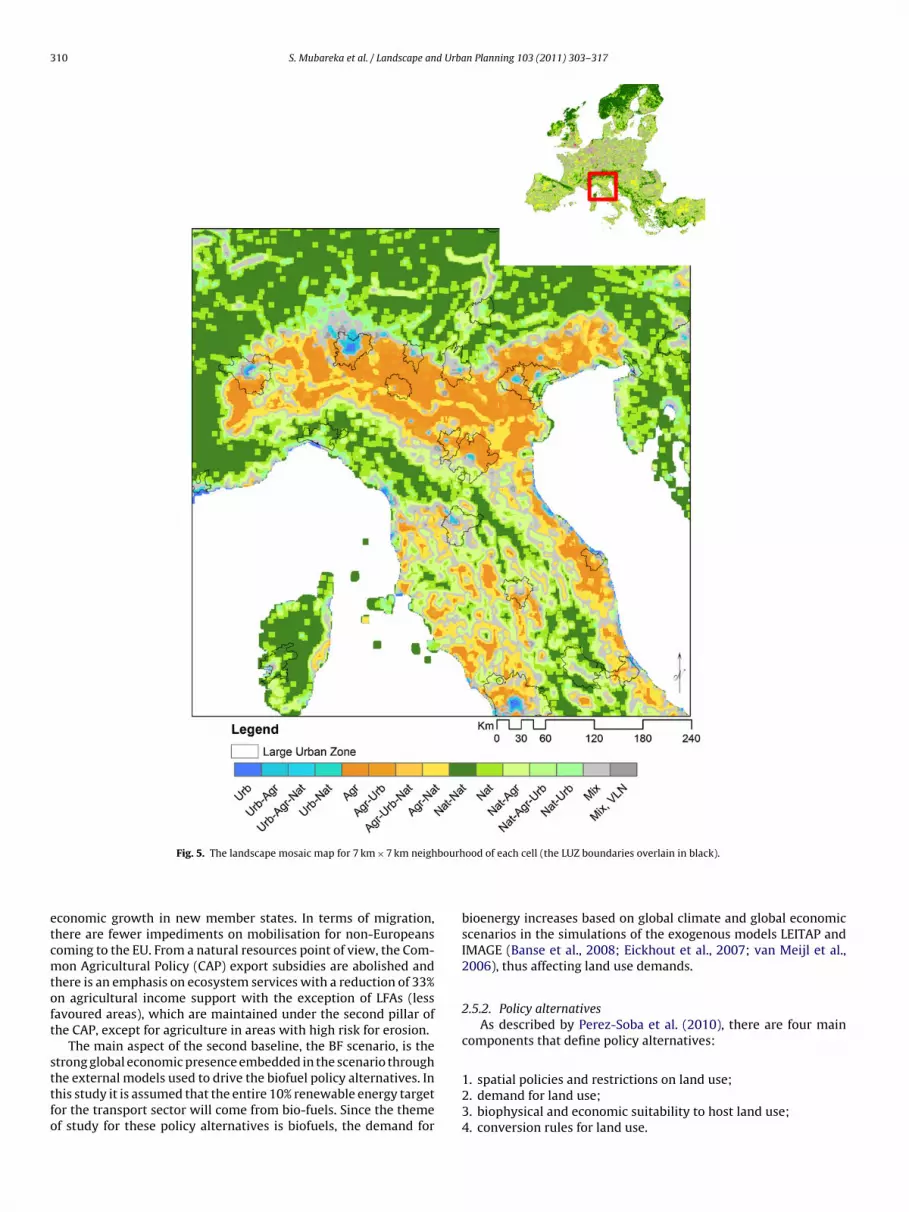

310 S. Mubareka et al. / Landscape and Urban Planning 103 (2011) 303– 317

bourh

etcmtoft

sttfo

Fig. 5. The landscape mosaic map for 7 km × 7 km neigh

conomic growth in new member states. In terms of migration,here are fewer impediments on mobilisation for non-Europeansoming to the EU. From a natural resources point of view, the Com-on Agricultural Policy (CAP) export subsidies are abolished and

here is an emphasis on ecosystem services with a reduction of 33%n agricultural income support with the exception of LFAs (lessavoured areas), which are maintained under the second pillar ofhe CAP, except for agriculture in areas with high risk for erosion.

The main aspect of the second baseline, the BF scenario, is thetrong global economic presence embedded in the scenario through

he external models used to drive the biofuel policy alternatives. Inhis study it is assumed that the entire 10% renewable energy targetor the transport sector will come from bio-fuels. Since the themef study for these policy alternatives is biofuels, the demand for

ood of each cell (the LUZ boundaries overlain in black).

bioenergy increases based on global climate and global economicscenarios in the simulations of the exogenous models LEITAP andIMAGE (Banse et al., 2008; Eickhout et al., 2007; van Meijl et al.,2006), thus affecting land use demands.

2.5.2. Policy alternativesAs described by Perez-Soba et al. (2010), there are four main

components that define policy alternatives:

1. spatial policies and restrictions on land use;2. demand for land use;3. biophysical and economic suitability to host land use;4. conversion rules for land use.

S. Mubareka et al. / Landscape and Urba

Table 3The baseline scenarios and their respective policy alternatives configured in EU-ClueScanner (adapted from Perez-Soba et al., 2010).

Baseline Policy alternative

B1: IPCC-SRES B1 “Global cooperation”whereby there is a global orientation.Global population stabilises at around8 billion in 2030; food safety standardsare raised, there is unlimited migrationbetween member states of the EU.

1. Biodiversity: policy aiming atpreserving biodiversity2. soilCC: soil and climate changealternative: policy aiming atmitigating and adapting toclimate change, also includes soilpreservation actions

BF: with assumption that 10%renewable energy target for transportsector will come from biofuels,including biofuel policy in OECD andEU.

1. Biodiversity (sameconfiguration as for B1)2. soilCC (same configuration asfor B1)3. BfNf: policy promoting use infive non-European countries(USA, Canada, Japan, Brazil andSouth Africa) and the EU with

cwaBi

ipwiaertdaat

a

ltntn

taautst

ffiAodartc

3.2.2. Uncertainty analysisIn order to assess uncertainty, the difference between the mini-

mum and maximum of the four individual indicators was taken.

restricted land conversion offorests into agricultural land

Table 3 summarises the baseline scenarios B1 and BF, and theharacteristics of the policy alternatives which are run in the modelith a time horizon of 2030. The biodiversity and soilCC policy

lternatives are associated with both baseline scenarios, while thefNf policy has a demand set of its own and spatial allocation rules

dentical to the BF baseline.Land use demand is passed on from the parent baseline scenar-

os to their respective policy alternatives. The parameters that makeolicy alternatives different from the baselines can be controlledithin the model in a variety of ways. Several data layers, described

n Perez-Soba et al. (2010), were created to reflect the restrictionsnd incentives related to the different policy alternatives. These lay-rs, such as High Nature Farmland (HNV), LFAs, ecological corridors,iver flood prone areas, Natura 2000 sites and topography, are spa-ial in nature (1 km resolution) and are therefore able to reflect theifferences in restrictions and incentives for different geographicalreas. In addition to the spatial data layers, conversion matrices,lso described in Perez-Soba et al. (2010), are used to control theransition potential from one land use to another.

The following policy alternatives from Perez-Soba et al. (2010)re included in our testing of the developed indicators:

A biodiversity policy alternative that focusses on the value ofandscape and ecosystem services through the introduction of pro-ective measures for natural corridors, Natura 2000 areas, highature value areas and peat land. The biodiversity policy alterna-ives are also regulated through the restriction of fragmentation ofatural areas and the control of urban growth.

A soil-climate change policy alternative (soilCC) aimed at pro-ecting soil and adapting to climate change. It focusses ondaptation and mitigation measures in terms of water managementnd soil protection. Permanent pastures and peatland are protectednder this policy alternative and soil erosion prevention is of par-icular importance for this policy alternative. Foresight of waterhortage promotes storage of rainwater in upper catchment areas,hus limiting these areas to urban development as well.

A biofuel policy alternative with restriction on the conversion oforests to agricultural lands (BfNf) whereby biofuels are promoted inve non-European countries (USA, Canada, Japan, Brazil and Southfrica) and in all European countries. Due to the restriction posedn the conversion of forest this alternative poses a relatively highemand on current agricultural land. Although urbanisation is not

specific issue in this alternative, we include it here because it

eflects a fairly different demand on agricultural land compared tohe baseline scenario and is thus likely to show different landscapeompositions.

n Planning 103 (2011) 303– 317 311

3. Results

3.1. Urban morphological changes

Since the main driving force behind built-up land increase forbaseline scenarios is the demand module in the model and the pol-icy alternatives are driven by the same demand module as theirbaseline scenarios, elements other than total land use demandcontrol land use allocation. This leads us to expect that the mor-phology of urban areas will change. The proportion of differencebetween the baseline scenarios and their policy alternatives foreach of the urban morphological classes was examined. Not only arethere significant variations in the composition of the built-up areaswithin the LUZ for the different policy alternatives, but also theLUZ affected by policy alternative choices vary. None of the policyalternatives systematically shows the same trend for all large urbanzones, although in theory they should since all policy alternativesaim to limit urban sprawl and encourage compactness. The com-posite index was created in order to better understand the overallimpact of the model configurations, or policy alternatives, on theLUZ in Europe.

3.2. Composite index of urban expansion pattern

3.2.1. Construction of the composite indexThe composite index is the result of the combination of the indi-

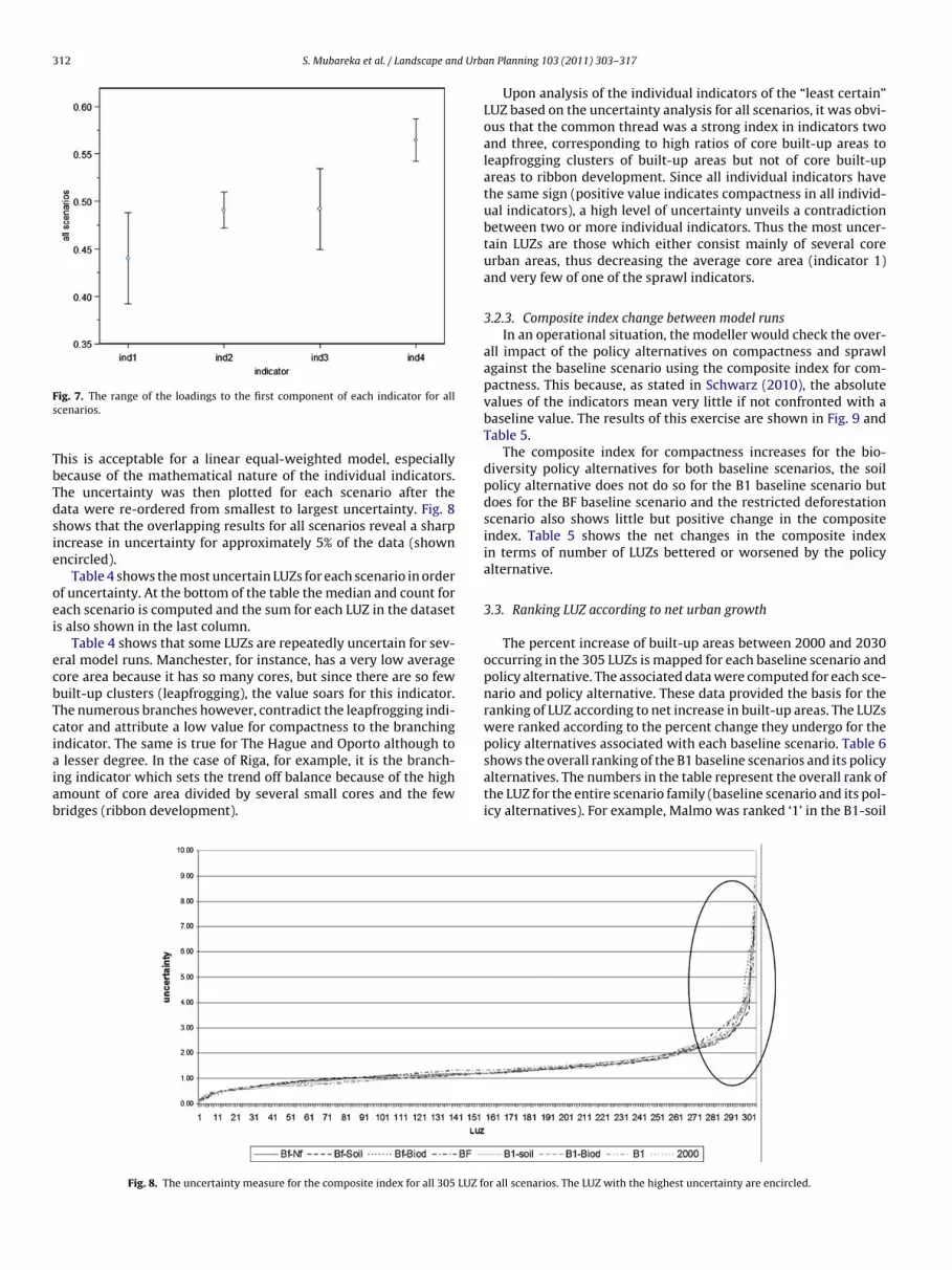
vidual morphological indicators for compactness and sprawl. Sincethere is no significant correlation between any two indicators, allwere retained to contribute to the composite. In terms of LUZ, allpassed the outlier test of the minimum amount of non-built-upland. The percent built-up land ranged from 0.87% (Umeo) to 65.5%(Portsmouth) within LUZ boundaries. We proceeded with the prin-cipal components analysis for the Corine Land Cover 2000 data inorder to assign weights to the individual indicators for the compos-ite. As the scree plot shows (Fig. 6), the majority of the informationis contained in the first component for all model runs and as shownin Fig. 7, the contribution of the individual indicators (loadings) tothe first component range from between 0.354 and 0.588.

Based on these results, the weighting was assigned as equal toeach of the input indicators. This, in a linear equation, was used asthe composite index. Scatterplots of each of the indicators vs. thecomposite index show a good positive fit with this approach.

Fig. 6. The scree plot showing the majority of the information is contained in thefirst component.

312 S. Mubareka et al. / Landscape and Urba

Fs

TbTdsie

oei

ecbTciaiab

shows the overall ranking of the B1 baseline scenarios and its policy

ig. 7. The range of the loadings to the first component of each indicator for allcenarios.

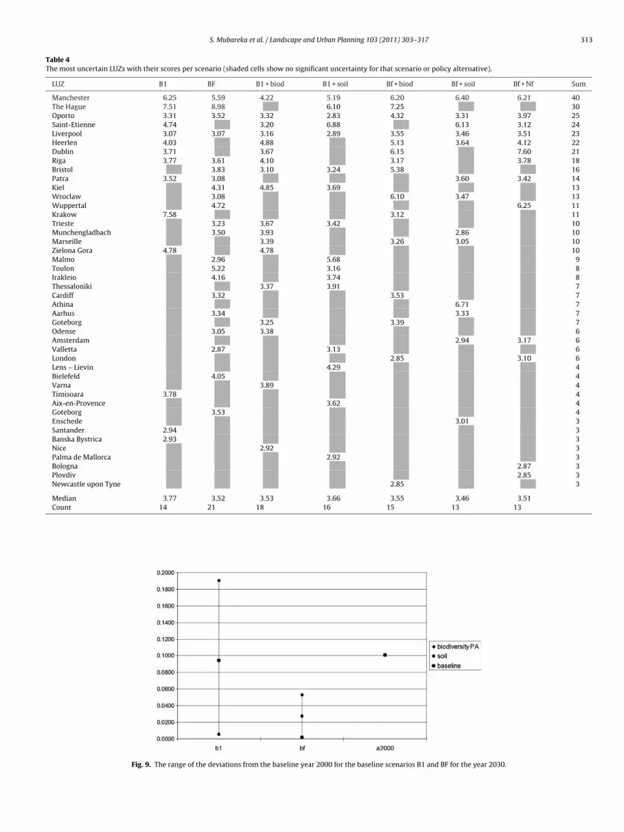
his is acceptable for a linear equal-weighted model, especiallyecause of the mathematical nature of the individual indicators.he uncertainty was then plotted for each scenario after theata were re-ordered from smallest to largest uncertainty. Fig. 8hows that the overlapping results for all scenarios reveal a sharpncrease in uncertainty for approximately 5% of the data (shownncircled).

Table 4 shows the most uncertain LUZs for each scenario in orderf uncertainty. At the bottom of the table the median and count forach scenario is computed and the sum for each LUZ in the datasets also shown in the last column.

Table 4 shows that some LUZs are repeatedly uncertain for sev-ral model runs. Manchester, for instance, has a very low averageore area because it has so many cores, but since there are so fewuilt-up clusters (leapfrogging), the value soars for this indicator.he numerous branches however, contradict the leapfrogging indi-ator and attribute a low value for compactness to the branchingndicator. The same is true for The Hague and Oporto although to

lesser degree. In the case of Riga, for example, it is the branch-

ng indicator which sets the trend off balance because of the highmount of core area divided by several small cores and the fewridges (ribbon development).

Fig. 8. The uncertainty measure for the composite index for all 305 LUZ fo

n Planning 103 (2011) 303– 317

Upon analysis of the individual indicators of the “least certain”LUZ based on the uncertainty analysis for all scenarios, it was obvi-ous that the common thread was a strong index in indicators twoand three, corresponding to high ratios of core built-up areas toleapfrogging clusters of built-up areas but not of core built-upareas to ribbon development. Since all individual indicators havethe same sign (positive value indicates compactness in all individ-ual indicators), a high level of uncertainty unveils a contradictionbetween two or more individual indicators. Thus the most uncer-tain LUZs are those which either consist mainly of several coreurban areas, thus decreasing the average core area (indicator 1)and very few of one of the sprawl indicators.

3.2.3. Composite index change between model runsIn an operational situation, the modeller would check the over-

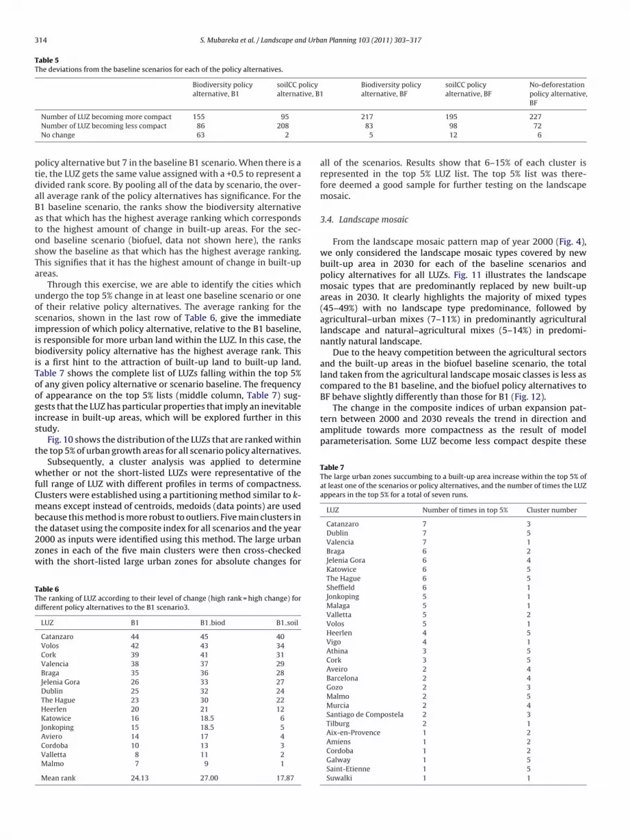
all impact of the policy alternatives on compactness and sprawlagainst the baseline scenario using the composite index for com-pactness. This because, as stated in Schwarz (2010), the absolutevalues of the indicators mean very little if not confronted with abaseline value. The results of this exercise are shown in Fig. 9 andTable 5.

The composite index for compactness increases for the bio-diversity policy alternatives for both baseline scenarios, the soilpolicy alternative does not do so for the B1 baseline scenario butdoes for the BF baseline scenario and the restricted deforestationscenario also shows little but positive change in the compositeindex. Table 5 shows the net changes in the composite indexin terms of number of LUZs bettered or worsened by the policyalternative.

3.3. Ranking LUZ according to net urban growth

The percent increase of built-up areas between 2000 and 2030occurring in the 305 LUZs is mapped for each baseline scenario andpolicy alternative. The associated data were computed for each sce-nario and policy alternative. These data provided the basis for theranking of LUZ according to net increase in built-up areas. The LUZswere ranked according to the percent change they undergo for thepolicy alternatives associated with each baseline scenario. Table 6

alternatives. The numbers in the table represent the overall rank ofthe LUZ for the entire scenario family (baseline scenario and its pol-icy alternatives). For example, Malmo was ranked ‘1’ in the B1-soil

r all scenarios. The LUZ with the highest uncertainty are encircled.

S. Mubareka et al. / Landscape and Urban Planning 103 (2011) 303– 317 313

Table 4The most uncertain LUZs with their scores per scenario (shaded cells show no significant uncertainty for that scenario or policy alternative).

LUZ B1 BF B1 + biod B1 + soil Bf + biod Bf + soil Bf + Nf Sum

Manchester 6.25 5.59 4.22 5.19 6.20 6.40 6.21 40The Hague 7.51 8.98 6.10 7.25 30Oporto 3.31 3.52 3.32 2.83 4.32 3.31 3.97 25Saint-Etienne 4.74 3.20 6.88 6.13 3.12 24Liverpool 3.07 3.07 3.16 2.89 3.55 3.46 3.51 23Heerlen 4.03 4.88 5.13 3.64 4.12 22Dublin 3.71 3.67 6.15 7.60 21Riga 3.77 3.61 4.10 3.17 3.78 18Bristol 3.83 3.10 3.24 5.38 16Patra 3.52 3.08 3.60 3.42 14Kiel 4.31 4.85 3.69 13Wroclaw 3.08 6.10 3.47 13Wuppertal 4.72 6.25 11Krakow 7.58 3.12 11Trieste 3.23 3.67 3.42 10Munchengladbach 3.50 3.93 2.86 10Marseille 3.39 3.26 3.05 10Zielona Gora 4.78 4.78 10Malmo 2.96 5.68 9Toulon 5.22 3.16 8Irakleio 4.16 3.74 8Thessaloniki 3.37 3.91 7Cardiff 3.32 3.53 7Athina 6.71 7Aarhus 3.34 3.33 7Goteborg 3.25 3.39 7Odense 3.05 3.38 6Amsterdam 2.94 3.17 6Valletta 2.87 3.13 6London 2.85 3.10 6Lens – Lievin 4.29 4Bielefeld 4.05 4Varna 3.89 4Timisoara 3.78 4Aix-en-Provence 3.62 4Goteborg 3.53 4Enschede 3.01 3Santander 2.94 3Banska Bystrica 2.93 3Nice 2.92 3Palma de Mallorca 2.92 3Bologna 2.87 3Plovdiv 2.85 3Newcastle upon Tyne 2.85 3

Median 3.77 3.52 3.53 3.66 3.55 3.46 3.51Count 14 21 18 16 15 13 13

Fig. 9. The range of the deviations from the baseline year 2000 for the baseline scenarios B1 and BF for the year 2030.

314 S. Mubareka et al. / Landscape and Urban Planning 103 (2011) 303– 317

Table 5The deviations from the baseline scenarios for each of the policy alternatives.

Biodiversity policyalternative, B1

soilCC policyalternative, B1

Biodiversity policyalternative, BF

soilCC policyalternative, BF

No-deforestationpolicy alternative,BF

ptdaBatosTa

uosiibiToogis

t

wfCmbt2zw

TTd

The change in the composite indices of urban expansion pat-tern between 2000 and 2030 reveals the trend in direction andamplitude towards more compactness as the result of modelparameterisation. Some LUZ become less compact despite these

Table 7The large urban zones succumbing to a built-up area increase within the top 5% ofat least one of the scenarios or policy alternatives, and the number of times the LUZappears in the top 5% for a total of seven runs.

LUZ Number of times in top 5% Cluster number

Catanzaro 7 3

Number of LUZ becoming more compact 155 95

Number of LUZ becoming less compact 86 208

No change 63 2

olicy alternative but 7 in the baseline B1 scenario. When there is aie, the LUZ gets the same value assigned with a +0.5 to represent aivided rank score. By pooling all of the data by scenario, the over-ll average rank of the policy alternatives has significance. For the1 baseline scenario, the ranks show the biodiversity alternatives that which has the highest average ranking which correspondso the highest amount of change in built-up areas. For the sec-nd baseline scenario (biofuel, data not shown here), the rankshow the baseline as that which has the highest average ranking.his signifies that it has the highest amount of change in built-upreas.

Through this exercise, we are able to identify the cities whichndergo the top 5% change in at least one baseline scenario or onef their relative policy alternatives. The average ranking for thecenarios, shown in the last row of Table 6, give the immediatempression of which policy alternative, relative to the B1 baseline,s responsible for more urban land within the LUZ. In this case, theiodiversity policy alternative has the highest average rank. This

s a first hint to the attraction of built-up land to built-up land.able 7 shows the complete list of LUZs falling within the top 5%f any given policy alternative or scenario baseline. The frequencyf appearance on the top 5% lists (middle column, Table 7) sug-ests that the LUZ has particular properties that imply an inevitablencrease in built-up areas, which will be explored further in thistudy.

Fig. 10 shows the distribution of the LUZs that are ranked withinhe top 5% of urban growth areas for all scenario policy alternatives.

Subsequently, a cluster analysis was applied to determinehether or not the short-listed LUZs were representative of the

ull range of LUZ with different profiles in terms of compactness.lusters were established using a partitioning method similar to k-eans except instead of centroids, medoids (data points) are used

ecause this method is more robust to outliers. Five main clusters in

he dataset using the composite index for all scenarios and the year000 as inputs were identified using this method. The large urbanones in each of the five main clusters were then cross-checkedith the short-listed large urban zones for absolute changes for

able 6he ranking of LUZ according to their level of change (high rank = high change) forifferent policy alternatives to the B1 scenario3.

LUZ B1 B1 biod B1 soil

Catanzaro 44 45 40Volos 42 43 34Cork 39 41 31Valencia 38 37 29Braga 35 36 28Jelenia Gora 26 33 27Dublin 25 32 24The Hague 23 30 22Heerlen 20 21 12Katowice 16 18.5 6Jonkoping 15 18.5 5Aviero 14 17 4Cordoba 10 13 3Valletta 8 11 2Malmo 7 9 1

Mean rank 24.13 27.00 17.87

217 195 22783 98 72

5 12 6

all of the scenarios. Results show that 6–15% of each cluster isrepresented in the top 5% LUZ list. The top 5% list was there-fore deemed a good sample for further testing on the landscapemosaic.

3.4. Landscape mosaic

From the landscape mosaic pattern map of year 2000 (Fig. 4),we only considered the landscape mosaic types covered by newbuilt-up area in 2030 for each of the baseline scenarios andpolicy alternatives for all LUZs. Fig. 11 illustrates the landscapemosaic types that are predominantly replaced by new built-upareas in 2030. It clearly highlights the majority of mixed types(45–49%) with no landscape type predominance, followed byagricultural–urban mixes (7–11%) in predominantly agriculturallandscape and natural–agricultural mixes (5–14%) in predomi-nantly natural landscape.

Due to the heavy competition between the agricultural sectorsand the built-up areas in the biofuel baseline scenario, the totalland taken from the agricultural landscape mosaic classes is less ascompared to the B1 baseline, and the biofuel policy alternatives toBF behave slightly differently than those for B1 (Fig. 12).

Dublin 7 5Valencia 7 1Braga 6 2Jelenia Gora 6 4Katowice 6 5The Hague 6 5Sheffield 6 1Jonkoping 5 1Malaga 5 1Valletta 5 2Volos 5 1Heerlen 4 5Vigo 4 1Athina 3 5Cork 3 5Aveiro 2 4Barcelona 2 4Gozo 2 3Malmo 2 5Murcia 2 4Santiago de Compostela 2 3Tilburg 2 1Aix-en-Provence 1 2Amiens 1 2Cordoba 1 2Galway 1 5Saint-Etienne 1 5Suwalki 1 1

S. Mubareka et al. / Landscape and Urban Planning 103 (2011) 303– 317 315

or all

plwrr

TTt

Fig. 10. The overall LUZ ranking of the top 5% hot spot areas for urbanisation f

arameter settings (see Table 8). We tested whether or not theandscape composition within the LUZ plays an important role in

hether or not the urban area becomes more or less compact byunning a stepwise multiple regression analysis using each modelun as a dependent variable and the landscape matrix classes,

able 8he results of stepwise multiple regression analysis for the difference in composite index ohe LUZ in 2000 (shaded cells show no significant relationship).

Landscape mosaic class B1 (p-value) B1 biodiversity(p-value)

B1 soilCC(p-value)

Ua 7 × 7 0.0139 0.0415

Uan 7 × 7

Aun 7 × 7

Na 7 × 7 0.0401Nu 7 × 7

Mix, with low natural cover 7 × 7 0.0457

p-Value, model 0.0034 0.0415 0.0401

R2, model 0.4507 0.1918 0.1942

scenarios and policy alternatives, covering all clusters of the composite index.

converted to percentage of total land, as individual independentvariables. The results summarised in Table 8 show a significant

contribution of the landscape mosaic types to all scenario andmodel runs, but never accounting for more than 45.53% of thecomposite.

f compactness for 2000 and 2030, to the landscape mosaic class proportions within

BF (p-value) BF biodiversity(p-value)

BF soilCC(p-value)

BfNf (p-value)

0.0623 0.07050.11420.0362 0.0034

0.01250.0623 0.03020.0200 0.0392 0.0302 0.01060.3375 0.2890 0.2140 0.4553

316 S. Mubareka et al. / Landscape and Urba

Fig. 11. The landscape mosaic types converted to built-up areas between 2000 and2030 according to the B1 baseline scenario and its policy alternatives.

F2

4

4

cioureaTtmwpiattwwcBcii

ig. 12. The landscape mosaic types converted to built-up areas between 2000 and030 according to the B1 and the BF baseline scenarios.

. Discussion

.1. Morphological input

This paper presented an approach for exploiting mathemati-al morphological concepts for the rapid extraction of meaningfulnformation from land use modelling output. As mentioned earlier,nly a few minutes are required to process the binary built-p/non-built-up output from EU-ClueScanner for Europe at a 1 kmesolution. The tool is therefore exceptional for this purpose how-ver, while certain aspects of the morphological output wereddressed in this paper, others could have been exploited further.he extent to which the morphological analysis is able to capturehe appearance of new urban land and the distances between the

orphological classes would have been added value. For example,hile the appearance of new built-up areas, whether they becomeart of a core, a ribbon development, branching or leapfrogging,

s taken into consideration through the composite index, the newppearance of an entirely new branch or brand new core is lost inhe composite index. Yet this could offer important information forhe modeller. Also not taken into consideration but probably worth-hile is measure of the distance between core zones because thisould indicate the degree of fragmentation of the landscape and

ontribute to knowledge of the degree of urban dispersion (Jaeger,

ertiller, Schwick, Cavens, et al., 2010). A connectivity analysisould be added as a fifth indicator in the future and the compositendex could be rebuilt with 5 components or better yet, calculat-ng the degree of dispersion among built-up clusters as proposed in

n Planning 103 (2011) 303– 317

Jaeger, Bertiller, Schwick, and Kienast (2010) would also be addedvalue, especially if working outside of large urban zone boundaries.

4.2. Model parameters

Throughout the study we have confirmed that the parameterisa-tion of the model affects the composite index for compactness, andalthough this impact is not always consistent, the overall score ofthe composite index is reliable. For example, for the “biodiversity”policy alternative, the parameters to encourage urban compactnessare very powerful and result in the representation of what the pol-icy alternative was attempting to forecast for built-up areas acrossEurope: more compact urban zones. While the soilCC policy alter-natives had the same goal, it was not accomplished with as muchsuccess. This is shown by the difference in the composite indexfor this policy alternative from the B1 baseline. Whereas the totalnumber of the 305 LUZ which improve in terms of compactness isbetween 95 and 195 for the soilCC policy alternative, it is between155 and 217 for the biodiversity policy alternative. Similarly, thenumber of LUZ for which compactness actually decreases is almostdouble in the soilCC policy alternative than in the biodiversity pol-icy alternative. Now the obvious question for the modeller is “Whydid the biodiversity policy alternative behave but not the soilCCpolicy alternative?” The answer lies in the limited efficiency of theconstraints used to configure the soilCC policy alternative. Whereasthe biodiversity policy alternative limits building in several specificareas, the soilCC policy alternative does this to a lesser degree. Thequestion is now: “Why did the soilCC policy alternative behave bet-ter for the BF baseline but not for the B1 baseline?” This can onlybe answered with certainty by measuring outside the LUZ, but weassume that the competition for agricultural land in the BF sce-nario plays a key role in forcing new urban land to be created notin agricultural areas as would be permitted in the B1 scenario, butcloser to current urban land. This occurs despite the neighbour-hood settings, a series of settings whereby the ability of a land useclass to attract another is described (see Perez-Soba et al., 2010 fordetails on scenario configurations). For the soilCC alternatives, theweight given to the built-up class is higher than for the biodiversityalternative and both are higher than for the baseline scenarios. Thisdoes not compensate the spatial maps restricting urbanisation inecologically sensitive areas however. Loosely translated, incentivesto build near current urban areas are not as strong as restrictionsof new building on certain areas.

In terms of the landscape mosaic composition, we can deducethat the landscape matrix is a significant but not unique con-tributor to urban compactness from Table 8. Whereas the modelparametrization attempted to conserve upper catchment areas inthe soilCC policy alternatives as opposed to the biodiversity alterna-tive, the biodiversity alternative focussed on the high nature valueland which is greatly composed of non-intensive agricultural areas.The data shown in Fig. 12 illustrate the success of the model inits attempts, but also emphasizes the trade off which is necessarywhen land use demand is equivalent. In other words, the built-up areas had to go somewhere; it is the “where” which changesdepending on the model parameters. The BfNf policy alternative,whereby the focus is on a higher demand for biofuel crops withoutinfringing upon forests, does not allow the conversion of agricul-tural land so easily and the areas needed which are suitable forproducing biofuels are designated as such. Not surprisingly, the netland use conversion to built-up areas occurs predominantly withinthe LUZ as opposed to other policy alternatives which seek to con-vert in the hinterland because there are few natural areas in the

LUZ. The BfNf policy alternative therefore shows a significant linkto the landscape mosaic classes with urban neighbours (Ua, Aun,Nua). These classes explain 45.5% of the compactness for this policyalternative.

d Urba

5

ttauktmgbz

ptebadvttotvcweumttptebitcaa

eastli

A

Etw

R

B

B

E

S. Mubareka et al. / Landscape an

. Summary and conclusions

Two baseline scenarios and three policy alternatives were run inhe EU-ClueScanner land use model from 2000 to 2030. Althoughhe policy alternatives were mainly focussed upon natural andgricultural land management, their configurations also impactedrban form. A composite index for urban compactness was tested,nowing the configuration of these scenarios and policy alterna-ives. Urban form was first quantified using different individual

orphological indicators. These were then concentrated into a sin-le composite index, simplifying the subsequent analyses not onlyetween different policy alternatives but also between large urbanones (LUZs).

Initially it was expected that the demand would override otherarameters of the land use model; this would have led to similarrends for the different policy alternatives. It was shown how-ver that this did not occur. The LUZs behaved differently in partecause the unique landscape in each LUZ, from a morphologicalnd compositional point of view caused the model to treat each oneifferently. Thus demand drove the overall number of cells con-erted to built-up for each country to which the LUZ belonged, buthe constraints and incentives placed upon the actual allocation ofhe built-up cells for each policy alternative determined whetherr not conversion occurred in the LUZ or elsewhere, for example inhe hinterland. This is evidenced when looking closely at the biodi-ersity policy alternative. There are several spatial datasets whichontribute to this policy alternative, thus really limiting the spacehere built-up cells could grow. This policy alternative, the mod-

ller can safely conclude, was well configured in terms of limitingrban sprawl. The soilCC alternative however, could have includedore spatial datasets in order to restrict urban sprawl. It succeeded

o a certain extent, having better values for compactness than didhe BF reference scenario, but the irregularity of the results in theolicy alternative suggest that there is room for improvement fromhe urban compactness perspective. The BfNf alternative whichndorses land allocation for agricultural use, forces most of the newuilt-up area to the LUZ, where little or no suitable agricultural land

s available. This does not however guarantee the compactness ofhe urban areas. It succeeds nonetheless however, by limiting theonversion of forest to agriculture, thus limiting the conversion ofgriculture to built-up because of the high level of competition forgricultural land in the biofuel scenario.

We can conclude that the results of the composite index reflectven subtle differences in model parameterisation. Two policylternatives with essentially the same goal of urban compactnesshow different levels of efficiency because of how their parame-erization was approached. We can furthermore conclude that theandscape mosaic surrounding urban areas is able to provide anndication of urban expansion patterns.

cknowledgments

Authors thank Paola Annoni and Stefano Tarantola from theconometrics and Applied Statistics (EAS) Unit of the Institute forhe Protection and Security of the Citizen, Joint Research Center,ho assisted with the statistics in this paper.

eferences

anse, M., Van Meijl, H., Tabeau, A., & Woltjer, G. (2008). Will EU biofuel policiesaffect global agricultural markets? European Review of Agricultural Economics,35(2), 117–141.

ritz, W., Verburg, P., & Leip, A. (2011). Modelling of land cover and agricultural

change in Europe: Combining the CLUE and CAPRI-Spat approaches. Agriculture,Ecosystems and Environment, 142(1–2), 40–50.

ickhout, B., & Prins, A. G. (Eds.). (2008). Eururalis 2.0 technical background andindicator documentation. Bilthoven, Netherlands: Wageningen University andResearch and the Netherlands Environmental Assessment Agency (MNP).

n Planning 103 (2011) 303– 317 317

Eickhout, B., van Meijl, H., Tabeau, A., & van Rheenen, T. (2007). Economic and eco-logical consequences of four European land use scenarios. Land Use Policy, 24(3),562–575.

Estreguil, C., & Mouton, C. (2009). Measuring and reporting on forest landscape pattern,fragmentation and connectivity in Europe: Methods and indicators. JRC Scientificand Technical report EUR23841EN. Office for Official Publications of the Euro-pean Communities.

Frenkel, A. (2004). The potential effect of national growth-management policy onurban sprawl and the depletion of open spaces and farmland. Land Use Policy,21(4), 357–369.

Frenkel, A., & Ashkenazi, M. (2008). The integrated sprawl index; measuring theurban landscape in Israel. Annals of Regional Science, 42(1), 99–121.

Galster, G., Hanson, R., Ratcliffe, M., Wolman, H., Coleman, S., & Freihage, J. (2001).Wrestling sprawl to the ground: Defining and measuring an elusive concept.Housing Policy Debate, 12(4), 681–717.

Hellmann, F., & Verburg, P. (2010). Impact assessment of the European biofueldirective on land use and biodiversity. Journal of Environment Management, 91,1389–1396.

Huang, J., Lu, X., & Sellers, J. (2007). A global comparative analysis of urban form:Applying spatial metrics and remote sensing. Landscape and Urban Planning, 82,184–197.

Irwin, E. G., & Bockstael, N. E. (2007). Land Change Science Special Feature: Theevolution of urban sprawl: Evidence of spatial heterogeneity and increasing landfragmentation. Proceedings of the National Academy of Sciences of the United Statesof America, 104(52), 20672–20677.

Jaeger, J., Bertiller, R., Schwick, C., & Kienast, F. (2010). Suitability criteria for mea-sures of urban sprawl. Ecological Indicators, 10, 387–406.

Jaeger, J. A. G., Bertiller, R., Schwick, C., Cavens, D., & Kienast, F. (2010). Urban per-meation of landscapes and sprawl per capita: New measures of urban sprawl.Ecological Indicators, 10, 427–441.

Jones, A. N., & Larkham, P. J. (1991). Glossary of Urban Form. Historical GeographyMonograph No. 26. Geo Books, Norwich for the Institute of British GeographersHistorical Geography Research Group. ISBN-10: 1870074084.

Koomen, E., Rietveld, P., & De Nijs, T. (2008). Modelling land use change for spatialplanning support. Annals of Regional Science, 42(1), 1–10 (editorial)

OECD. (2008). Handbook on constructing composite indicators: Methodology and userguide. ISBN 978-92-64-04345-9.

Openshaw, S. (1983). Modifiable areal unit problem. Concepts and Techniques inModern Geography, 38, 1–41.

Ostapowicz, K., Vogt, P., Riitters, K., Kozak, J., & Estreguil, C. (2008). Impact of scaleon morphological spatial pattern of forest. Landscape Ecology, 23, 1107–1117.

Perez-Soba, M., Verburg, P. H., Koomen, E., Hilferink, M., Benito, P., Lesschen, J. P.,et al. (2010). Land use modelling – Implementation; preserving and enhancingthe environmental benefits of “land use services”. Final report to the EuropeanCommission, DG Environment. Alterra Wageningen UR/Geodan Next/ObjectVision/BIOS/LEI and PBL, Wageningen.

Pinto, N., & Anutnes, A. (2010). A cellular automata model based on irregular cells:Application to small urban areas. Environment and Planning B, 37, 1095–1114.

Riitters, K. H., Wickham, J. D., & Wade, T. G. (2009). An indicator of forest dynamicsusing a shifting landscape mosaic. Ecological Indicators, 9, 107–117.

Ritsema van Eck, J., & Koomen, E. (2008). Characterising urban concentration andland use diversity in simulations of future land use. Annals of Regional Science,42(1), 123–140.

Schwarz, N. (2010). Urban form revisited – Selecting indicators for characterisingEuropean Cities. Landscape and Urban Planning, 96, 29–47.

Siedentop, S., & Fina, S. (2010). Monitoring urban sprawl in Germany: Towards aGIS-based measurement and assessment approach. Journal of Land Use Science,5(2), 73–104.

Soille, P., & Vogt, P. (2009). Morphological segmentation of binary patterns. PatternRecognition Letters, 30(4), 456–459.

Torrens, P., & Alberti, M. (2000). Measuring sprawl. London: Center for AdvancedSpatial Analysis Working Paper Series.

van Delden, H., Luja, P., & Engelen, G. (2007). Integration of multi-scale dynamicspatial models of sociao-economic and physical processes for river basin man-agement. Environmental Modelling & Software, 22, 223–238.

van Meijl, H., van Rheenen, T., Tabeau, A., & Eickout, B. (2006). The impact of differentpolicy environments on agricultural land use in Europe. Agriculture Ecosystems& Environment, 114(1), 21–38.

Verburg, P., & Overmars, K. (2009). Combining top-down and bottom-up dynamicsin land use modeling: Exploring the future of abandoned farmlands in Europewith the Dyna-Clue model. Landscape Ecology, 24(9), 1167–1181.

Verburg, P. H., Eickhout, B., & Van Meijl, H. (2008). A multi-scale, multi-modelapproach for analyzing the future dynamics of European land use. Annals ofRegional Science, 42(1), 57–77.

Vogt, P., Riitters, K., Estreguil, C., Kozak, J., Wade, T., & Wickham, J. (2007). Mappingspatial patterns with morphological image processing. Landscape Ecology, 22(2),171–177.

White, R., & Engelen, G. (1994). Cellular dynamics and GIS: Modelling spatial com-plexity. Geographical Systems, 1, 237–253.

Wilson, E., Hurd, J., Civco, D., Prisloe, M., & Arnold, C. (2003). Development of ageospatial model to quantify, describe and map urban growth. Remote Sensing

of Environment, 86, 275–285.

Wissen Hayek, U., Jaeger, J., Schwick, C., Jarne, A., & Schuler, M. (2010). Measuring andassessing urban sprawl: What are the remaining options for future settlementdevelopment in Switzerland for 2030? Applied Spatial Analysis and Policy, doi:10.1007/s12061-010-9055-3.