Development and implementation of the effective force testing method for seismic simulation of...

10.1098/rsta.2001.0879

Development and implementation of theeffective force testing method for seismic

simulation of large-scale structures

By Carol K. Shield, Catherine W. French and John Timm

Department of Civil Engineering. University of Minnesota,500 Pillsbury Drive SE, Minneapolis, MN 55455, USA

This paper describes the development and experimental implementation of a real-time earthquake simulation test method for large-scale structures. The method, effec-tive force testing (EFT), is based on a transformation of coordinates, in which casethe structure is fixed at the base (similar to the set-up for the pseudo-dynamic (PsD)test method); however, in the case of EFT, the method is based on a force-controlalgorithm rather than a displacement-control algorithm. Effective forces, equivalentto the mass of each storey level multiplied by the ground acceleration, are applied ateach respective storey. As such, the EFT forces are known a priori for any groundacceleration record. As opposed to the PsD test method in which the ground dis-placements to be imposed are affected by the measured structural response as thestiffness changes. As in the case of the PsD test method, the EFT method is suitablefor testing any type of structural system that can be idealized as a series of lumpedmasses (e.g. building or bridge structures).Research has been conducted on a linear elastic single-degree-of-freedom system

at the University of Minnesota to develop and investigate implementation of theEFT method. A direct application of the EFT method was found to be ineffectivebecause of a natural velocity feedback phenomenon between the actuator and thestructure to which it is attached. A detailed model of the control, hydraulic andstructural systems was developed to study the interaction problem and other nonlin-ear responses in the system. The implementation of an additional feedback loop usingthe measured velocity of the test structure was shown to be successful at overcomingthe problems associated with actuator–control–structure interaction, indicating thatEFT is a viable real-time method for seismic simulation studies.

Keywords: seismic simulation; testing methods; effective force testing;dynamics; control requirements; large-scale testing

1. Introduction

There have been three primary test methods used to investigate the performanceof structural systems subjected to seismic loadings: shaking-table studies, quasi-static cyclic studies of components, and pseudo-dynamic (PsD) test methods (Moehle1996). Each of these methods has advantages and disadvantages. For example, withshaking-table studies, test structures may be subjected to actual earthquake accel-eration records to investigate dynamic effects; however, the size of the structure is

Phil. Trans. R. Soc. Lond. A (2001) 359, 1911–19291911

c© 2001 The Royal Society

1912 C. K. Shield, C. W. French and J. Timm

..xg

m

c

x

xa

xg

..xa

k2

k2

cx.

kx 2

kx 2

..x

m

x

ck2

k2

cx.

kx2

kx2

globalreference

ground

actuatorpeff (t) = −mxg

..

mxa = mxg + mx.. .. ..

mx

−mxg..

..

(a) (b)

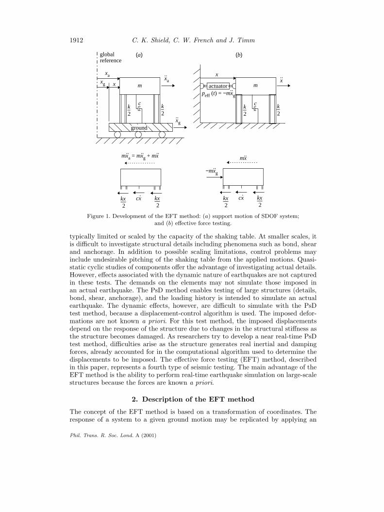
Figure 1. Development of the EFT method: (a) support motion of SDOF system;and (b) effective force testing.

typically limited or scaled by the capacity of the shaking table. At smaller scales, itis difficult to investigate structural details including phenomena such as bond, shearand anchorage. In addition to possible scaling limitations, control problems mayinclude undesirable pitching of the shaking table from the applied motions. Quasi-static cyclic studies of components offer the advantage of investigating actual details.However, effects associated with the dynamic nature of earthquakes are not capturedin these tests. The demands on the elements may not simulate those imposed inan actual earthquake. The PsD method enables testing of large structures (details,bond, shear, anchorage), and the loading history is intended to simulate an actualearthquake. The dynamic effects, however, are difficult to simulate with the PsDtest method, because a displacement-control algorithm is used. The imposed defor-mations are not known a priori. For this test method, the imposed displacementsdepend on the response of the structure due to changes in the structural stiffness asthe structure becomes damaged. As researchers try to develop a near real-time PsDtest method, difficulties arise as the structure generates real inertial and dampingforces, already accounted for in the computational algorithm used to determine thedisplacements to be imposed. The effective force testing (EFT) method, describedin this paper, represents a fourth type of seismic testing. The main advantage of theEFT method is the ability to perform real-time earthquake simulation on large-scalestructures because the forces are known a priori.

2. Description of the EFT method

The concept of the EFT method is based on a transformation of coordinates. Theresponse of a system to a given ground motion may be replicated by applying an

Phil. Trans. R. Soc. Lond. A (2001)

The effective force testing method 1913

effective force (−mxg) to each mass of the system. Figure 1a shows a single-degree-of-freedom (SDOF) system subjected to a base motion, xg. The following equationof motion may be obtained for this system:

mxa + cx+ kx = 0, (2.1)

where x is the displacement of the mass, m is the mass of the system, c is theviscous damping coefficient, and k is the system stiffness. Subscript ‘a’ refers tomotion relative to a fixed reference frame (absolute displacement). Motions of themass relative to the ground are non-subscripted.The absolute displacement of the system mass consists of the displacement of the

mass with respect to the ground and the ground displacement:

xa = x+ xg. (2.2)

Coordinate transformation of the acceleration results in

xa = x+ xg. (2.3)

Combining equations (2.1) and (2.3) yields

mx+ cx+ kx = −mxg = Peff(t). (2.4)

For a SDOF system, the mass multiplied by the ground acceleration is equivalent toan ‘effective force’, Peff(t), applied to the mass in a fixed reference frame (Clough &Penzien 1975; Chopra 1995).The proposed technique uses the same set-up as PsD testing (i.e. the test structure

is fixed to the ground, and all motions are measured relative to the ground, seefigure 1b), and restrictions on the type of structure that can be tested are similar tothose required by the PsD test method (i.e. structure must be idealized as a lumpedmass system). The effective force (−mxg) to be applied to the structure, in the EFTmethod, is a function of the mass of the structure, which is typically known or can beestimated with good accuracy before testing, and the earthquake ground accelerationrecord to be used. Consequently, the force-control loading history (−mxg) is knowna priori for any earthquake acceleration record.Theoretically, the EFT method can be applied directly to test systems with non-

linear stiffness and damping. As the structural system stiffness and damping change,the structural response will be affected, but the applied effective force should not beaffected, as shown by equation (2.4). No structural parameters (stiffness or damping)are needed to determine the effective (applied) force.The extension of the effective force technique to multiple-degree-of-freedom

(MDOF) systems is illustrated in figure 2. In this case, an effective force is appliedto each level (lumped mass) of the structure. The forces at each level are equal tothe mass at that level multiplied by the ground acceleration. Therefore, even for thecase of an MDOF system, each of the applied effective storey forces are known beforethe test begins.The concept of EFT is not new. It has been described in papers discussing the PsD

test method (Mahin & Shing 1985; Mahin et al . 1989; Thewalt & Mahin 1987). Thesepapers presented the possibility of using a PsD test set-up with explicit time-varyingforces imposed at each lumped mass to conduct real-time tests without the needfor computing and imposing required displacements. Because of the lack of displace-ment control and required integration algorithms, the EFT technique is conceptually



m2

m1

xa2

xa1

xg

k1, c1

k2, c2

xg

xg x1

x2xa2..

xa1..

xg..

actuator

actuator

ground

k2, c2

k1, c1

x1 = xa1 − xg

Peff1 = −m1xg..

x2 = xa2 − xg

Peff2 = −m2xg..

(a) (b)

Figure 2. Application of EFT to MDOF systems.

and physically different from ‘real-time pseudodynamic testing’ (Nakashima et al .1992).While the testing scheme is conceptually simple, its implementation has been con-

sidered to be problematic. Thewalt &Mahin (1987) stated that the technique requireshigh-quality controllers and servovalves, but the total test control problem may besimpler than that of a shaking table. Although S. A. Mahin (1987, unpublished data)indicated that shaking-table testing is probably more practical given both the powersupply capacity and the relative displacements required of the degree of freedommasses, the energy input to the structure would be expected to be the same forthe two testing techniques for equal structural deformation response. In fact thereis potential for laboratory energy and power savings for EFT, because there is noshaking table to be moved. As far as the authors know, no other researchers haveperformed experimental work on the EFT method.Although the implementation of the EFT method at first appears straightforward,

Murcek (1996) at the University of Minnesota demonstrated that with a direct appli-cation of the method, the actuator was unable to apply the effective force near thenatural frequency of the system on a linear elastic SDOF structure. The results ofMurcek’s (1996) research verified conclusions drawn by Dyke et al . (1995) regardingeffects of control–structure interaction; that is, for lightly damped structures, actu-ators have a severely limited ability to apply forces near the natural frequency ofthe structures to which they are attached. This inability to apply the correct forceat the natural frequency of the structure is due to ‘natural’ velocity feedback of theactuator; because the actuator is attached to the test structure, the actuator pistonmoves according to the response of the structure to the applied force, increasingthe flow required by the actuator to produce the correct force. Dimig et al . (1999)proposed a solution to the natural velocity feedback problem that comprised incor-poration of an additional feedback loop to negate the natural velocity feedback ofthe actuator.This paper describes improvements to the control–actuator–structural model and

an experimental implementation of the natural velocity feedback correction suggestedby Dimig et al . (1999).


Theeffective

forcetesting

method

1915

x

f

(i)

s.x 1

s

(k)

x

−

servovalve / actuator / structure interaction model

α q

1CF

IL

−

(d)gainILKdPd

1SF

(e)

gain

(c)−

DCerror

controllerinput

+

..mxg

(a)

1CF

Vc

sign

(g)

1*

*

qmax 1− ups

u

A

( j)

pA

(h)

(f)

.x 1

(m)(l)A

(n)

Vf(b)

kips to volts

kips to volts

VeVILc VILe

error

R (s + Pd)

VIL f

spool postionto volts

productC12s + G

.

ms2+cs+k

SDOF model

natural velocity feedback

phase adjustment

R1C1s+1

R2C2s+1 Rf Cf s+1

velocity feedback correction

Kv KIL gain

Vv f c

Figure

3.Model

ofthe

dynamicsystem

incorporatingthe

nonlinearrelationship

describingservovalve

flowwith

thelinearized

model

forvelocity

feedback.

Phil.

Trans.

R.Soc.

Lond.

A(2001)


3. Dynamic system model for a single degree of freedomwith a three-stage servovalve

Equations describing the system dynamics for an SDOF structure excited by ahydraulic actuator that account for actuator–structure interaction have been pro-posed by Merritt (1967). If the increased flow required by the actuator is supplied,it should be possible for the actuator to apply force to the system at its natural fre-quency. A means of supplying this correction flow is to modify the command signalto the controller, to account for the increase in flow. Figure 3 shows the dynamicsystem model for an SDOF structure excited by a hydraulic actuator with a three-stage servovalve in force control with the proposed correction for the natural velocityfeedback. A detailed derivation of the precursor to this model can be found in Dimiget al . (1999).The blocks in figure 3 are labelled with letters (a)–(n) for the purpose of describing

the model. The earthquake effective force (−mxg) is the model input. Blocks (a)and (b) represent the conversions of the effective force and actuator load cell feedbacksignals from load to volts, respectively. The gain factor in block (c) represents theproportional gain, which was set within the controller.Block (d) represents a simplified model for the three-stage valve driver, showing

the conversion from voltage to the servovalve main stage spool opening, α. Includedin this transfer function is a model for a single pole valve driver, with parameter Pd,which approximates the valve dynamics by representing the time delay associatedwith movement of the spool (F. N. Bailey 1987, unpublished notes). The mechanicalgain, Kd, represents the DC gain of the valve driver. Figure 4 is a schematic of afour-way servovalve. For this type of servovalve, the oil flow through the valve is anonlinear function of the servovalve spool opening and the pressure across the pistonis described by the following flow–pressure relationship:

q

qmax= α

√1− α

|α|pl

ps, (3.1)

where q is the flow through the actuator, qmax is the maximum flow with full effectivesupply pressure drop across the servovalve, pl is the difference in pressure across theactuator piston, and ps is the hydraulic supply pressure. Block (f) is a representationof this relationship.Blocks (g) and (h) represent the actuator, where C12 is the oil compressibility con-

stant, G is the sum of the actuator leakage constant and the valve leakage constant,and A is the cross-sectional area of the actuator piston (F. N. Bailey 1987, unpub-lished notes; Merritt 1967). The transfer function for the linear elastic test structureis shown in block (i). The velocity response of the SDOF system is integrated inblock (k) to obtain the displacement response. The ‘natural’ velocity feedback isrepresented by block (j).The natural velocity feedback correction is shown in blocks (l)–(n). The measured

velocity multiplied by the piston area is the flow which needs to be added to theactuator. Because the command signal is modified rather than the flow, all of themodel parameters that convert the command voltage, Vc, to flow, q, must be usedto convert the ‘correction flow’ to the correction voltage, Vvfc. Hence the measuredvelocity multiplied by the piston area is multiplied by an inverse of the transfer



functions in blocks (c)–(f) to produce the proper correction voltage:

Vvfc =A

KvKILgainx, (3.2)

where Kv and KIL are parameters discussed below, and ‘gain’ is the outer-loop gainsetting of the controller. This voltage is then summed with the effective force voltagesignal to produce the ‘corrected’ command signal, which is input to the controller. Forexperimental simplification, a linearized equivalent of equation (3.1) is used in thefeedback correction, where the flow in the servovalve is assumed to be proportionalto the spool opening, independent of the pressure across the actuator piston:

q = Kvα, (3.3)

where Kv is the null flow gain, qmax of equation (3.1).In the velocity feedback correction block (n), the factor KIL is introduced. This

factor represents the overall gain applied by the inner-loop parameters in block (d),which convert the inner-loop command signal, VILc, to the valve spool opening, α:

KIL =(gainIL)(Kd/R)

1 + (gainIL)(Kd/R)(1/SF ), (3.4)

where gainIL is the inner-loop gain setting on the controller, R is the nominal outputresistance of the controller, and SF is the known conversion factor for the controllerfrom spool opening to inner-loop voltage (VIL).The phase adjustment incorporated into the velocity feedback correction, shown

in blocks (l)–(m), was needed to offset time delays in the dynamic system, suchas those explicitly modelled in the servovalve dynamics (block (d)). The lead–lagcompensation network in block (l) was the primary means of adjusting the phase ofthe velocity feedback correction. As implemented, the magnitude and phase responseof the operational amplifier lag network were given by

M(ω) =

√1 + (ωR1C1)2√1 + (ωR2C2)2

,

φ(ω) = tan−1(R1C1ω)− tan−1(R2C2ω).

(3.5)

The resistance and capacitance values were chosen so that the magnitude of thetransfer function was near unity for all frequencies of interest, and the lag was closeto offsetting the delay in the servovalve. The low-pass filter (block (m)) was providedas a means of making small, ‘fine-tune’ adjustments to the phase of the velocity signal.The filter had amplitude and phase responses given by

M(ω) =1√

1 + (ωRfCf)2,

φ(ω) = − tan−1(RfCfω).

(3.6)

The amplitude of the transfer function was near unity for the frequency range atwhich the system was operating. Typical values for Rf and Cf were 12 kΩ and0.047 µF, respectively. The gain factor and phase adjustment factors described abovewere independent of the properties of the SDOF structure. The servovalve dynam-ics in block (d) and the phase adjustment in blocks (l)–(m) described further in



Return

supply

p = p1 − p2

q

po ≈ 0

ps q

q

q

α

p1

p2

Figure 4. Schematic of four-way servovalve.

Timm (1999) represent refinements over the model originally developed by Dimig etal . (1999). In addition, Dimig et al .’s model was based on a two-stage servovalve,whereas the current model is based on a simple three-stage servovalve model whichhas increased force–velocity capacity. As long as the force–velocity requirements ofthe structure for a given ground motion are within the servovalve force–velocity enve-lope, the EFT method is independent of the type of servovalve used. The velocityfeedback correction, however, requires modelling of the physical parameters of theservovalve. Because a three-stage valve has a higher flow rating than a two-stagevalve, it may be capable of accommodating the velocity feedback correction using alinearized model of the servovalve in the correction loop.Computer simulations of the SDOF system response using this model were con-

ducted using Simulink©R dynamic system simulation software available withinMat-lab©R, version 5.1. The method of integration chosen for solving the differential equa-tions was based on an explicit Runge–Kutta (4,5) formula, the Dormand–Prince pair.Results of the simulation using the model in figure 3 will be compared with the exper-imental results of a test structure described in the next section.

4. Description of test structure and experimental set-up

The model described above was experimentally implemented using a structure thatwas representative of a classic linear-elastic mass-spring-dashpot SDOF model shownin figure 5. The system consisted of a 7940 kg cart, which served as the mass, anda 7.0 m long, 25 mm nominal diameter grade 1.03 GPa Dywidag threadbar, whichacted as a spring when pre-tensioned. A pre-tension force of 67 kN was applied tothe rod to avoid development of compression forces in the rod and the possibilityof buckling. The size and length of the bar were chosen to enable a cart displace-ment that would provide adequate resolution with the measuring devices, while thebar remained linear elastic with an applied force within the capacity of the actua-tor. The measured system stiffness and damping ratio were 11.7 kN mm−1 in−1 and0.019, respectively. The natural frequency of the system was 6.1 Hz. A linear variable



actuator

cart

rod

K = 11 kN mm−1

actuator c = 12.2 kN s m−1m = 7940 kg

Figure 5. Laboratory set-up of an SDOF system.

R3 || R4R1 || R2

lead/lag compensation network

LF353N

one polelow-pass filter

Viph

LF353NLF353N

Rf

CfR1

R3

R4

C1

C2

Voph

R2

Figure 6. Phase adjustment circuit.

differential transformer (LVDT) and a velocity transducer were used to monitor thedisplacement and velocity response of the SDOF test structure, respectively.Force was applied to the SDOF structure using a 340 kN servohydraulic actuator

aligned with the centre of mass of the test structure. The actuator was controlledusing an analog controller with proportional gain only. Force–velocity analyses of thehydraulic system, equipped with a 5.7 l s−1 three-stage servovalve, indicated that thepower capacity of the system was adequate for the proposed tests (Timm 1999).The velocity feedback correction was implemented by applying the appropriate

correction factor (assumed constant) to the measured velocity signal and summingthis signal with the effective force input command signal. To accomplish this, ananalog op-amp circuit was built, and the correction factor was applied by meansof an adjustable resistor. The magnitude of the feedback correction gain factor wasslightly underestimated because an overestimate of the gain factor produced a poten-



Table 1. System parameters

parameter block value

CF (a), (b) 36 kN V−1

gain (c), (n) 1.05SF (e) 10 V/1000%gainIL (d) 2.0R (d) 200 ΩKd (d) 2000% A−1

Kv (n) 8.98× 106 mm3 s−1

C12 (g) 1.9× 106 mm5 kN−1

G (g) 0A (h), (j), (n) 17× 103 mm2

m (i) 7940 kgc (i) 12.2 kN s m−1

k (i) 11.7 kN mm−1

Pd (d) 352 s−1

Rf (m) 12 kWCf (m) 0.047 mFR1 = R4 (l) 39 kWR2 = R3 (l) 10 kWC1 (l) 0.1 mFC2 (l) 0.047 mF

tially unstable system response, and the response of the system was sensitive to smallchanges in the actuator supply pressure caused by other tests in the laboratory usingthe hydraulic power supply. A separate op-amp circuit, shown in figure 6, was builtto provide phase adjustment of the velocity feedback correction signal required tocompensate for time delays in the system dynamics. Circuit components for the leadcompensation network were chosen to optimize the applied force, yielding a phasechange of 1.02 Hz−1. This phase correction was 15% larger than was expected basedon the measured time delay of the servovalve. This difference may be attributedto additional sources of time delay in the system not accounted for in the model(e.g. actuator dynamics) or due to the method in which the time delay in the servo-valve was measured with the main hydraulic pressure shut off.The velocity sensor used to obtain the signal for the velocity feedback correction

had frequency response characteristics which depended on the load impedance ofthe instrument used to record the signal. To ensure that the load impedance of theanalog circuit was sufficiently large to avoid attenuation of the velocity signal, thesignal was passed through a unity gain buffer circuit immediately after the sensoroutput. Values for the parameters shown in figure 3 for the experimental systemare given in table 1. Manufacturer’s nominal values were used for the piston area(A), the mechanical gain (Kd), the maximum flow (qmax = Kv), and the controllerresistance (R). Both the inner-loop gain (gainIL) and the outer-loop gain (gain) werecontroller settings tuned for maximum performance. The time delay associated withthe movement of the spool (Pd) was measured under the conditions of low hydraulic



0

5

10

15

20

25

30

35

12 16 20

frequency (Hz)

Four

ier

ampl

itude

sine sweep inputapplied forcesimulation force

4 8

Figure 7. Fast Fourier transforms of the input signal, experimental applied force, andsimulation force for a 13 kN sine wave sweep without velocity feedback correction.

supply pressure. The conversion factors (CF and SF ) were both calibrated prior touse of the actuator. More detail on the evaluation of these parameters can be foundin Timm (1999).The earthquake record used for the experimental program was the 1940 N-S El

Centro record, in addition, sine wave sweeps over 0–10 Hz were used.

5. System response without velocity feedback correction

(a) Sine sweep tests

The EFT concept was originally explored by Murcek (1996) at the University of Min-nesota using experiments and computer simulations performed on the linear elasticSDOF test structure (figure 4). The research showed that the actuator was unableto apply components of the effective force with frequency content near the naturalfrequency of the SDOF system. An example of the system response without velocityfeedback correction is given in figure 7, which shows a comparison of the fast Fouriertransforms (FFTs) of the command signal, measured applied force, and simulation,that were obtained for a 13 kN sine wave sweep input with frequencies ranging from0 to 10 Hz. The applied-force FFT was at a minimum at the natural frequency ofthe system (6.1 Hz). The simulation model without the velocity feedback correctioncorrectly predicted the response of the system with the exception of portions of thesignal around 4, 9 and 18 Hz. The sharp drop in the applied-force FFT at 4 Hz wasindicative of an additional mode of vibration of the cart, believed to be associatedwith a bouncing or rocking motion (not included in the simulation model). The addi-tional discontinuity in the applied force at 9 and 18 Hz was attributed to transversevibrational modes of the bar.



0

2

4

6

8

10

10 15 20 25

frequency (Hz)

Four

ier

ampl

itude

sine sweep inputapplied forcesimulation force

5

Figure 8. FFTs of the input signal, experimental applied force and simulation force with thenonlinear servovalve flow model for a 2.2 kN sine sweep with velocity feedback correction.

6. Experimental implementation incorporatingthe velocity feedback correction

(a) Precorrected tests

Initial experimental implementation incorporating the velocity feedback correctionwas accomplished using a ‘precorrected’ command signal. Because the experimentalstructure was a linear elastic system, the velocity response could be calculated a pri-ori for the applied input ground motion. As a result, the velocity feedback correctioncould be determined a priori and was input directly, digitally superimposed with theeffective force command signal, to the controller. This initial implementation gaveexcellent results (Dimig et al . 1999), indicating the potential for the EFT method.Because there was no time delay associated with the analytically derived velocity,the correction consisted of applying the appropriate gains of block (n) to the calcu-lated velocity, no phase correction was required for this initial implementation. Toexpand the capabilities of the EFT method to test nonlinear structural systems, itwas necessary to further develop the method to incorporate the velocity feedbackcorrection using the real-time measured velocity of the test structure.

(b) Sine sweep tests

Tests implementing the velocity feedback correction using the measured velocitywere conducted with a 2.2 kN sine sweep input function. FFTs of the sine sweepinput, applied force and simulation force for this test are shown in figure 8. TheFFTs of the applied and simulation forces in figure 8 show a large spike around 12 Hz(approximately twice the natural frequency) and a drop in measured and simulatedresponse at the natural frequency. A discontinuity at 4 Hz, due to the additionalvibration mode of the system, as discussed in the previous section, was also evident.



0

2

4

6

8

10

10 15 20 25

frequency (Hz)

Four

ier

ampl

itude

5

0 kN pre-tension11 kN pre-tension22 kN pre-tension44 kN pre-tension

Figure 9. FFTs of simulation force for a 2.2 kN sine sweep with the nonlinearservovalve flow model for tests at different pre-tension levels.

The spike around 12 Hz (twice the natural frequency) was an indication of nonlin-earity in the flow–velocity relationship that was not taken into account in the simpli-fied linearized velocity feedback correction. Simulation studies considering the non-linear pressure–flow relationship in the velocity feedback correction loop (block (n)of figure 3) did not exhibit a spike at 12 Hz. The 67 kN pre-tension in the bar (toavoid bar buckling) was thought to be the cause of the inadequacy of the linearizedpressure–flow relationship in the velocity feedback correction. Figure 9 shows theresults of simulation studies where the bar pre-tension was varied. The results of thesimulation with no pre-tension do not show a spike in the FFT near 12 Hz. As thepre-tension was increased from 11 to 44 kN, the results of the simulation indicatedan increase in the nonlinear system response at 12 Hz.Simulation tests with the sine sweep input using the model in figure 3 indicated

that the drop in the applied-force FFT at the natural frequency was due to themagnitude of the gain factor in the velocity feedback correction being slightly lowerthan the required magnitude. In simulation tests, a slight reduction in the velocityfeedback correction gain factor (ca. 3%) produced results which corresponded to thedrop in the applied-force FFT in figure 8. Experimental tests in which the correctionfactor was increased were not successful in eliminating the drop in the applied-forceFFT at the natural frequency. Only a small reduction in the drop was obtained,while the applied-force FFT at frequencies slightly less than the natural frequencyincreased. The reason for the inability to eliminate the drop in the applied-forceFFT may have been due in part to the nonlinearity in the hydraulic system or thepossible result of a small discrepancy in the phase adjustment to correct for the timedelay in the system. This drop was not observed in the tests conducted using the‘precorrected’ command signal, which did not require phase correction, indicatingthat if the servovalve/actuator dynamics can be properly modelled, it should bepossible to improve the results shown in figure 8.



(c) Earthquake simulation tests

The primary earthquake ground acceleration used in the experimental investiga-tions was the first 10 s of the El Centro ground acceleration (Elcn10) at half scale witha peak ground acceleration of 0.17g. This earthquake segment contained a demand-ing portion of the El Centro record that had frequency content similar to that of theentire record, while reducing the amount of data to be collected.The system response to the Elcn10 (0.17g) effective force input function with

implementation of the velocity feedback correction is shown in figure 10. For compar-ison purposes, figure 11 illustrates the system response without the velocity feedbackcorrection. In general with the implementation of the velocity feedback correction,the FFTs show reasonable results over the entire frequency range (figure 10a). Aslight reduction of the FFT of the applied force relative to the effective force inputcan be seen at the natural frequency of the system (6.1 Hz). The reduction in forcewas not as noticeable as in the case of the sine sweep input, which may be due tolower demands on the hydraulic system for the Elcn10 input signal. The FFT of theapplied force without the velocity feedback correction (figure 11a) clearly shows asignificant drop in magnitude around the natural frequency of the system.The force time histories, shown in figures 10b and 11b appear to give reasonable

results, even for the case without implementation of the velocity feedback correction.The applied force history for Elcn10 (0.17g) closely matched the effective force input;however, portions of the applied force were shifted down in relation to the effectiveforce. The corresponding measured displacement response, plotted in figures 10cand 11c, exemplifies the need for the velocity feedback correction. With the correction(figure 10c), the measured response generally followed and was in phase with theexpected response, as determined by a piecewise linear integration of the equation ofmotion for the SDOF. The measured response tended to be less than the expectedresponse except for a portion of the Elcn10 response between 6 and 7.5 s, where themeasured response was slightly greater than the expected response. In comparisonwith the response observed without incorporation of the velocity feedback correction(figure 11c), the response was dramatically improved.In low-amplitude portions of the test shown in figure 10b between 0 and 1 s and

around 8 s, the SDOF system appeared to have some difficulty achieving the expectedresponse. This was attributed to the amplitude of the effective force input functionand the resolution of the electronics. For sinusoidal input at the natural frequencyof the SDOF system, an input function of ca. 0.24 kN is all that is theoreticallyrequired to produce a 0.51 mm displacement response. The 0.24 kN input functionthat would produce this displacement amplitude represents a voltage of less than7 mV (0.07% of full scale). At this small voltage, good resolution of the input signalwas difficult to achieve. Improved resolution at lower amplitudes could be providedwith a lower force capacity actuator. The pre-tension required to prevent bucklingof the rod in the test structure precluded the use of a lower force capacity actuatorfor this application.

7. Potential extensions of the EFT method

The method, as currently developed, may be used to test structural control devicesthat are meant to keep the structural response elastic. In the past it has been diffi-cult to test full-scale control devices because dynamic, real-time testing is required,



0

5

10

15

20

25

30

0 2 8 10

forc

e (k

N)

disp

lace

men

t (m

m)

Four

ier

ampl

itude

10 15 20 255frequency (Hz)

effective forceapplied forcesimulation force

(a)

(b)

−15

−10

−5

0

5

10

15

4 6time (s)

effective forceapplied force

(c) expected displacementmeasured displacement

0 2 8 104 6time (s)

−3

−2

−1

0

1

2

3

Figure 10. Comparison of the expected versus measured response for Elcn10 (0.17g) earthquakesegment with the velocity feedback correction: (a) FFT, (b) force and (c) displacement.

limiting meaningful testing to structures retrofitted with control devices that couldfit on shaking tables. The EFT method could be used to test control devices onlarge-scale structures in real time.



0

5

10

15

20

25

30

0 2 8 10

forc

e (k

N)

disp

lace

men

t (m

m)

Four

ier

ampl

itude

10 15 20 255frequency (Hz)

effective forceapplied forcesimulation force

(a)

(b)

−15

−10

−5

0

5

10

15

4 6time (s)

effective forceapplied force

(c) expected displacementmeasured displacement

0 2 8 104 6time (s)

−3

−2

−1

0

1

2

3

Figure 11. Comparison of the expected versus measured response for Elcn10 (0.17g) earthquakesegment without the velocity feedback correction: (a) FFT, (b) force and (c) displacement.

Ongoing work at the University of Minnesota involves extending implementationof the EFT method to nonlinear SDOF systems. Direct application of the velocityfeedback correction as described in this paper is theoretically appropriate; however, it



is possible that the nonlinearity of the structural response may prove more demandingon the servovalve than the linear elastic SDOF system with pre-tension used in theinitial implementation studies. If this is the case, it may require inclusion of theservovalve nonlinearites in the velocity feedback correction or improved modellingof the servovalve. These changes may necessitate a digital implementation of thecorrection.As mentioned in § 1, the theoretical extension of EFT to MDOF structures is also

straightforward. However, as more storeys are added to the structure, the velocity(flow) requirements for the actuators attached to the higher storeys increase, andspecialized large-flow servovalves will be required.Effective force testing might also be extended to tests of substructures. This poses

an additional complication due to the need to model the nonlinear behaviour of thevirtual portion of the structure. The development of real-time numerical models,which explicitly account for the change in the stiffness and damping of the mod-elled portion of the structure, would probably parallel the work being developed forsubstructuring employing real-time PsD testing (Nakashima & Masaoka 1999; Hori-uchi et al . 1999). The main differences between the two algorithms would be thatforces from the virtual structure would be applied to the test structure in EFT, asopposed to displacements in PsD testing. The advantage of using EFT for substruc-ture tests over real-time PsD testing is that real inertial forces and damping withinthe substructure would be developed, and would not have to be modelled.

8. Conclusion

Effective force testing (EFT) is a method of earthquake simulation for testing large-scale lumped-mass structural systems. EFT uses the same laboratory test set-up asPsD testing; however, EFT is conducted in real time using an effective force inputknown a priori in combination with a correction signal based on the measured real-time velocity response of the test structure. Because testing is conducted in realtime, the structure develops real inertial and damping forces as in shaking-tabletesting.Experimental tests on a linear elastic SDOF test structure demonstrated that real-

time dynamic tests could be performed using the EFT method, and implementationof this method is independent of the properties of the test structure.

Nomenclature

A cross-sectional area of the actuator pistonc viscous damping coefficientC12 oil compressibilityCF actuator load cell conversion factor from kips to voltsG sum of actuator leakage and the valve leakagegain outer-loop gain settinggainIL inner-loop gain settingk system stiffnessKd mechanical gain



KIL overall gain applied by the inner loopKv null flow gainm mass of the systemp difference in pressure across actuator pistonPd time delay associated with movement of the spoolPeff(t) effective forceps hydraulic power supply pressureq oil flow through actuatorqmax maximum flow with full effective supply pressureR nominal output resistance of the controllerSF conversion factor from spool opening to inner-loop voltageVc command voltageVe error voltageVvfc corrected command voltageVILc commanded inner-loop voltageVILf inner-loop feedback voltagex displacement of the massxg ground motionα spool opening

References

Chopra, A. K. 1995 Dynamics of structures: theory and applications to earthquake engineering,pp. 20–22. Englewood Cliffs, NJ: Prentice-Hall.

Clough, R. W. & Penzien, J. 1975 Dynamics of structures. New York: McGraw-Hill.Dimig, J., Shield, C., French, C., Bailey, F. & Clark, A. 1999 Effective force testing: a methodof seismic simulation for structural testing. J. Struct. Engng 125, 1028–1037.

Dyke, S. J., Spencer, B. F., Quast, P. & Sain, M. K. 1995 Role of control–structure interactionin protective system design. J. Engng Mech. 121, 322–338.

Horiuchi, T., Inoue, M., Konno, T. & Namita, Y. 1999 Real-time hybrid experimental systemwith actuator delay compensation and its application to a piping system with energy absorber.Earthquake Engng Struct. Dynam. 28, 1121–1141.

Mahin, S. A. & Shing, P. B. 1985 Pseudodynamic method for seismic testing. J. Struct. Engng111, 1482–1503.

Mahin, S. A., Shing, P. B., Thewalt, C. R. & Hanson, R. D. 1989 Pseudodynamic test method—current status and future directions. J. Struct. Engng 115, 2113–2128.

Merritt, H. E. 1967 Hydraulic control systems. Wiley.Moehle, J. P. (ed.) 1996 Earthquake spectra—theme issue: experimental methods, vol. 12, no. 1.Earthquake Engineering Research Institute.

Murcek, J. A. 1996 Evaluation of the effective force testing method using a SDOF model. Mastersthesis, University of Minnesota.

Nakashima, M. & Masaoka, N. 1999 Real-time on-line test for MDOF systems. EarthquakeEngng Struct. Dynam. 28, 393–420.



Nakashima, M., Kato, H. & Takaoka, E. 1992 Development of real-time pseudo dynamic testing.Earthquake Engng Struct. Dynam. 21, 79–92.

Thewalt, C. R. & Mahin, S. A. 1987 Hybrid solution techniques for generalized pseudodynamictesting. Report UBC/EERC-87/09, EERC, University of California, Berkeley, USA.

Timm, J. 1999 Natural velocity feedback correction for effective force testing. Masters thesis,University of Minnesota.


Development and implementation of the effective force testing method for seismic simulation of...

Documents

Transcript of Development and implementation of the effective force testing method for seismic simulation of...