
Development and HVS Validation of Design Tables ... - UCPRC
214
PREPARED FOR: Concrete Masonry Association of California and Nevada PREPARED BY: University of California Pavement Research Center UC Davis, UC Berkeley December 2014 Research Report: UCPRC-RR-2014-04 Authors: H. Li, D. Jones, R. Wu, and J. Harvey Concrete Masonry Association of California and Nevada. Grant Agreement UCPRC-PP-2011-01
-
Upload
khangminh22 -
Category
Documents
-
view
3 -
download
0
Transcript of Development and HVS Validation of Design Tables ... - UCPRC
PREPARED FOR: Concrete Masonry Association of California and Nevada
PREPARED BY:
University of California Pavement Research Center
UC Davis, UC Berkeley
December 2014Research Report: UCPRC-RR-2014-04
Authors:H. Li, D. Jones, R. Wu, and J. Harvey
Concrete Masonry Association of California and Nevada. Grant Agreement UCPRC-PP-2011-01

UCPRC-RR-2014-04 i
DOCUMENT RETRIEVAL PAGE Research Report: UCPRC-RR-2014-04
Title: Development and HVS Validation of Design Tables for Permeable Interlocking Concrete Pavement: Final Report
Authors: H. Li, D. Jones, R. Wu, and J. Harvey
Prepared for: Concrete Masonry Association of California and Nevada
Work submitted: December 2014
Date:December 2014
UC Davis Contract No: UCPRC-PP-2011-01
Status: Final
Version No.: 1
Abstract: This report details the research undertaken to develop revised design tables for permeable interlocking concrete pavement using a mechanistic-empirical design approach. The study included a literature review, field testing of existing projects and test sections, estimation of the effective stiffness of each layer in permeable interlocking concrete pavement structures, mechanistic analysis and structural design of a test track incorporating three different subbase thicknesses (low, medium, and higher risk), tests on the track with a Heavy Vehicle Simulator to collect performance data to validate the design approach using accelerated loading, refinement and calibration of the design procedure using the test track data, development of a spreadsheet based design tool, and development of revised design tables using the design tool. Key findings from the mechanistic analysis include:
• Higher shear stress/strength ratios at the top of the subgrade, which equate to a higher risk of rutting in the subgrade, require thicker subbase layers, as expected.
• An increase in the stiffness of the surface layer reduces the required subbase layer thickness to achieve the shear stress/strength ratio. However, the effect of the surface layer stiffness on overall pavement performance is not significant due to the relatively low thickness of the pavers (80 mm) and the reduced interlock between them compared to pavers with sand joints.
• For the same shear stress/strength ratio at the top of the subbase, an increase in the stiffness of the subbase layer reduces the required thickness of that subbase layer, especially when the subgrade has a low stiffness.
• For the same shear stress/strength ratio at the top of the subgrade, wet conditions require thicker subbase layers compared to the dry condition, confirming that wet conditions are the most critical condition for design.
A new example design table, based on the number of days with standing water in the subbase (zero, 10, 30, 50, 90, and 120) has been developed. The table uses a similar format to that currently used in the ICPI Permeable Interlocking Concrete Pavements guideline. The minimum design thicknesses required to prevent subgrade rutting that are proposed in the new table do not differ significantly from those in the current ICPI guide, and are mostly less conservative. Designs for a specific set of project circumstances can be undertaken using the same Excel® spreadsheet-based design tool used to develop the tables in conjunction with the hydrological design procedures provided in the ICPI guide.
Keywords: Permeable interlocking concrete pavement, permeable pavement, mechanistic-empirical design, accelerated pavement testing.
Proposals for implementation:
Related documents: UCPRC-TM-2013-03, UCPRC-TM-2013-09
Signatures:
H. Li 1st Author
J. Harvey Technical Review
D. Jones Principal Investigator
D.R. Smith For CMACN

ii UCPRC-RR-2014-04
DISCLAIMER
The contents of this report reflect the views of the authors who are responsible for the facts and accuracy
of the data presented herein. The contents do not necessarily reflect the official views or policies of the
Concrete Masonry Association of California and Nevada (CMACN), the California Nevada Cement
Association (CNCA), the Interlocking Concrete Pavement Institute Foundation for Education & Research
(ICPIF) or the Interlocking Concrete Pavement Institute (ICPI). This report does not constitute a standard,
specification, or regulation.
PROJECT OBJECTIVES/GOALS
The objective of this project was to produce thickness design tables for permeable interlocking concrete
pavement (PICP) based on mechanistic analysis and partially validated with accelerated pavement testing
(APT). The following tasks were completed to achieve this objective:
1. Perform a literature and field survey to identify critical responses, failure mechanisms, appropriate performance transfer functions, and modeling assumptions for mechanistic analysis of PICP under truck loading.
2. Measure pavement deflection in the field on several PICP locations to characterize effective stiffness of the different layers in the structure for use in modeling.
3. Perform mechanistic analyses of PICP to develop design tables following the approach documented in California Department of Transportation (Caltrans) Research Report CTSW-RR-09-249.04 for development of structural design tables for permeable/pervious/porous asphalt and concrete pavement.
4. Prepare a plan for validation with accelerated load testing based on the results of the mechanistic analysis.
5. Test responses and, if possible, failure of up to three PICP structures in dry and wet condition with a Heavy Vehicle Simulator (HVS).
6. Analyze the results of the HVS testing to revise/update the structural design tables where necessary.
7. Write a final report documenting the results of all tasks in the study and demonstrating the design tables.
8. Present findings to Caltrans Office of Concrete Pavements and Foundation Program and Office of Stormwater - Design staff in Sacramento, CA.
This report covers Tasks 1 through 7.
UCPRC-RR-2014-04 iii
ACKNOWLEDGEMENTS
The University of California Pavement Research Center acknowledges the following individuals and
organizations.
Financial Support: + ICPI Foundation for Education and Research, Chantilly, Virginia + Concrete Masonry Association of California and Nevada, Citrus Heights, California + California Nevada Cement Association, Yorba Linda, California
Material and Labor Donations: + Basalite Concrete Products, Dixon, California (donated concrete pavers) + Kessler Soils Engineering, Leesburg, Virginia (undertook lightweight deflectometer testing) + Tencate Mirafi, Pendergrass, Georgia (donated geotextile) + WeberMT, Bangor, Maine (loan of a CR-7 vibrator plate compactor with compaction indicator)
Project Support: + David R. Smith, Technical Director, Interlocking Concrete Pavement Institute, Chantilly,
Virgina + David K. Hein, PEng, Principal Engineer, Vice President, Applied Research Associates,
Toronto, Ontario, Canada + Dr. T. Joseph Holland, Caltrans, Sacramento, California + California Pavers, Lodi, California (Test section construction) + The UCPRC Heavy Vehicle Simulator crew and UCPRC laboratory staff, Davis and Berkeley,
California.

iv UCPRC-RR-2014-04
Blank page

UCPRC-RR-2014-04 v
EXECUTIVE SUMMARY
This report details the research undertaken to develop revised design tables for permeable interlocking
concrete pavement using a mechanistic-empirical design approach. The study included a literature review,
field testing of existing projects and test sections, estimation of the effective stiffness of each layer in
permeable interlocking concrete pavement structures, mechanistic analysis and structural design of a test
track incorporating three different subbase thicknesses (low, medium, and higher risk), tests on the track
with a Heavy Vehicle Simulator to collect performance data to validate the design approach using
accelerated loading, refinement and calibration of the design procedure using the test track data,
development of a spreadsheet based design tool, and development of design tables using the design tool.
Rut development rate as a function of the shear stress to shear strength to ratios at the top of the subbase
and the top of the subgrade was used as the basis for the design approach. This approach was selected
based on a review of the literature, past research on permeable pavements by the authors, and the results
of deflection testing on in-service permeable interlocking concrete pavements. The shear stress/strength
ratio was originally developed for airfield pavements where the shear stresses from aircraft loads and tire
pressures are high relative to the strengths of the subgrade materials. On permeable road pavements,
subgrade materials are often uncompacted or only lightly compacted and wet or saturated for much of the
service life, resulting in relatively low shear strengths compared with the high shear stresses from trucks.
Deeper ruts are usually also tolerated on permeable pavements due to the absence of ponding on the
surface during rainfall. The alternative approach of using a vertical strain criterion was considered
inappropriate for permeable pavements, given that this is typically used where the shear stresses relative to
the shear strains are relatively low, which typically results in low overall rutting.
Key observations from the study include:
Infiltration of water into the subgrade is significantly reduced when the subgrade is compacted prior to placing the subbase. In this study, light compaction of the subgrade soil (~ 91 percent of laboratory determined modified Proctor maximum dry density) added very little to the structural performance of the pavement and would not have permitted reducing the design thickness of the subbase layer.
There was a significant difference in rutting performance and rutting behavior between the wet and dry tests, as expected.
A large proportion of the rutting on all three sections occurred as initial embedment in the first 2,000 to 5,000 load repetitions of the test and again after each of the load changes, indicating that much of the rutting in the base and subbase layers was attributed to bedding in, densification, and/or reorientation of the aggregate particles. This behavior is consistent with rutting behavior on

vi UCPRC-RR-2014-04
interlocking concrete pavements with sand joints on dense-graded or stabilized bases as well as on other types of structures.
During testing under dry conditions, limited permanent deformation (< 4 mm) was recorded in the bedding and base layers on all three subsections, and most occurred very early in the test. On the subsection with the 450 mm subbase, rutting occurred in both the subbase (10 mm rut) and subgrade (13 mm rut). On the 650 mm and 950 mm subbase subsections, rutting occurred mostly in the subbase. Total permanent deformation on the 450 mm, 650 mm, and 950 mm subbase subsections was 27 mm, 23 mm and 17 mm respectively, implying a generally linear trend of increasing permanent deformation with decreasing subbase thickness.
During testing under wet conditions (i.e., water level maintained at the top of the subbase), rutting in the bedding and base layers was dependent on the thickness of the subbase (9 mm, 5 mm and 2 mm on the 450 mm, 650 mm, and 950 mm subbase subsections, respectively). Rutting occurred in both the subbase and the subgrade on all subsections, with rutting in the subbase consistent across all three sections (~ 25 mm). Rutting in the subgrade differed between sections relative to subbase thickness, with 15 mm, 6 mm, and 4 mm of rut recorded on the 450 mm, 650 mm, and 950 mm subbase subsections, respectively.
Although only limited testing was undertaken under drained conditions (i.e., wet subgrade but no standing water in the subbase), rutting behavior appeared to show similar trends and behavior to the test under dry conditions.
The thickness of the subbase influenced rut depth in the subgrade, as expected, but did not influence the rutting behavior in the subbase itself. Rutting in these layers is therefore governed by the aggregate properties and construction quality.
Deflection during dry testing was dependent on subbase thickness and it increased with increasing load. Deflections were relatively high compared to more traditional pavements with dense graded layers. Deflection during wet testing was higher compared to that recorded during dry testing, with deflection on the 450 mm subbase subsection significantly higher compared to that recorded on the 650 mm and 950 mm subbase subsections, indicating a load-sensitive, weaker overall structure as a result of the wet subgrade.
No distress was noted on any individual concrete pavers and no pavers were dislodged from the pavement during testing.
The infiltration rate of water through the joints between the pavers reduced over the course of HVS testing; however, it was still considered to be rapid and effective.
Key findings from the mechanistic analysis include:
The use of the shear stress to shear strength ratios at the top of the subbase and top of the subgrade as inputs for modelling the rut development rate at the top of these layers is considered to be an appropriate design approach for PICP.
Higher shear stress/strength ratios at the top of the subgrade, which equate to a higher risk of rutting in the subgrade, require thicker subbase layers, as expected.
An increase in the stiffness of the surface layer reduces the required subbase layer thickness to achieve the same shear stress/strength ratio. However, the effect of the surface layer stiffness on overall pavement performance is not significant due to the relatively small thickness of the pavers (80 mm) and the reduced interlock between them compared to pavers with sand joints.
UCPRC-RR-2014-04 vii
For the same shear stress/strength ratio at the top of the subbase, an increase in the stiffness of the subbase layer reduces the required thickness of that subbase layer, especially when the subgrade has a low stiffness.
For the same shear stress/strength ratio at the top of the subgrade, wet conditions require thicker subbase layers compared to the dry condition, confirming that wet conditions are the most critical condition for design.
A new example design table, based on the number of days with standing water in the subbase (zero, 10,
30, 50, 90, and 120) has been developed. The table uses a similar format to that currently used in the ICPI
Permeable Interlocking Concrete Pavements guideline. The minimum recommended design thicknesses
required to prevent rutting in the subgrade proposed in the new table do not differ significantly from those
in the current table and are mostly less conservative except when designing for a combination of high
traffic, weak subgrades and a high numbers of days with standing water in the subbase. Designs for a
specific set of project circumstances can be undertaken using the same Excel® spreadsheet-based design
tool used to develop the tables in conjunction with the hydrological design procedures provided in the
ICPI guide. The design too output and the corresponding values in the tables should be considered as best
estimate designs, since they were developed from the results of only two HVS tests. Designers should
continue to use sound engineering judgment when designing permeable interlocking concrete pavements
and can introduce additional conservatism/reliability by altering one or more of the design inputs, namely
the material properties, number of days that the subbase will contain standing water, and/or traffic.

viii UCPRC-RR-2014-04
Blank page
UCPRC-RR-2014-04 ix
TABLE OF CONTENTS
LIST OF TABLES .................................................................................................................................... xii LIST OF FIGURES .................................................................................................................................. xii 1. INTRODUCTION ............................................................................................................................. 1
1.1 Project Scope ............................................................................................................................ 1 1.2 Background to the Study ........................................................................................................... 1 1.3 Study Objective ........................................................................................................................ 1 1.4 Report Layout ........................................................................................................................... 2 1.5 Introduction to Accelerated Pavement Testing ......................................................................... 2 1.6 Measurement Units ................................................................................................................... 3
2. LITERATURE REVIEW ................................................................................................................. 5 3. DEFLECTION TESTING ON EXISTING PROJECTS .............................................................. 7
3.1 Introduction ............................................................................................................................... 7 3.2 Deflection Testing .................................................................................................................... 8
3.2.1 Deflection Measurement Method ................................................................................. 8 3.2.2 Test Section Locations ................................................................................................. 8
3.3 Deflection Measurement Analysis ............................................................................................ 9 3.4 Backcalculation of Stiffness for Davis and Sacramento Sections .......................................... 10
3.4.1 Backcalculated Effective Stiffness of the Surface Layers .......................................... 10 3.4.2 Backcalculated Effective Stiffness of the Base Layers .............................................. 11 3.4.3 Backcalculated Effective Stiffness of the Subgrade ................................................... 11 3.4.4 Effective Stiffness Analysis ....................................................................................... 11
3.5 Backcalculation of Stiffness for UCPRC Section ................................................................... 12 3.5.1 Backcalculated Effective Stiffness from RSD Measurements ................................... 12 3.5.2 Backcalculated Effective Stiffness from FWD Measurements .................................. 12
3.6 DCP Tests on the UCPRC Sections ........................................................................................ 12 4. TEST TRACK LOCATION AND DESIGN ................................................................................ 15
4.1 Test Track Location ................................................................................................................ 15 4.2 Test Track Design ................................................................................................................... 16
4.2.1 Design Criteria ........................................................................................................... 16 4.2.2 Design Variables ........................................................................................................ 16 4.2.3 Input Parameters for Mechanistic Modeling and Structural Analysis ........................ 18 4.2.4 Mechanistic Analysis Results ..................................................................................... 20 4.2.5 Test Track Layer Thickness Design ........................................................................... 22
5. TEST TRACK CONSTRUCTION ............................................................................................... 27 5.1 Introduction ............................................................................................................................. 27 5.2 Excavation (01/20/2014 – 01/21/2014) .................................................................................. 27 5.3 Subgrade Preparation (01/21/2014) ........................................................................................ 27 5.4 Subbase Placement (01/22/2014 – 01/23/2014) ..................................................................... 29 5.5 Curb Placement (01/23/2014 – 01/24/2014) ........................................................................... 31 5.6 Base Placement (01/27/2014) ................................................................................................. 32 5.7 Bedding Layer Placement (01/28/2014) ................................................................................. 33 5.8 Paver Placement (01/28/2014 – 01/29/2014) .......................................................................... 34 5.9 Surface Permeability ............................................................................................................... 35 5.10 Material Sampling .................................................................................................................. 36
6. TRACK LAYOUT, INSTRUMENTATION, AND TEST CRITERIA ..................................... 37 6.1 Test Track Layout ................................................................................................................... 37 6.2 HVS Test Section Layout ....................................................................................................... 37 6.3 Test Section Instrumentation and Measurements ................................................................... 38
6.3.1 Temperatures .............................................................................................................. 38 6.3.2 Water Level in the Pavement ..................................................................................... 38 6.3.3 Surface Permanent Deformation (Rut Depth) ............................................................ 39
x UCPRC-RR-2014-04
6.3.4 Permanent Deformation in the Underlying Layers ..................................................... 40 6.3.5 Surface Deflection ...................................................................................................... 41 6.3.6 Vertical Pressure (stress) at the Top of the Subbase and Top of the Subgrade .......... 42 6.3.7 Jointing Stone Depth .................................................................................................. 43
6.4 HVS Test Criteria ................................................................................................................... 43 6.4.1 Test Section Failure Criteria ....................................................................................... 43 6.4.2 Environmental Conditions .......................................................................................... 44 6.4.3 Test Duration .............................................................................................................. 44 6.4.4 Loading Program ........................................................................................................ 44
7. HEAVY VEHICLE SIMULATOR TEST DATA ........................................................................ 47 7.1 Introduction ............................................................................................................................. 47 7.2 Rainfall ................................................................................................................................... 47 7.3 Section 678HC: Dry Test ....................................................................................................... 48
7.3.1 Test Summary ............................................................................................................. 48 7.3.2 678HC: Water Level in the Pavement ....................................................................... 48 7.3.3 678HC: Temperatures ............................................................................................... 48 7.3.4 678HC: Permanent Deformation on the Surface (Rutting) ....................................... 49 7.3.5 678HC: Permanent Deformation in the Underlying Layers ...................................... 52 7.3.6 678HC: Surface Deflection ....................................................................................... 54 7.3.7 678HC: Vertical Pressure at the Top of the Subbase and Subgrade .......................... 55 7.3.8 678HC: Jointing Stone Depth .................................................................................... 56 7.3.9 678HC: Visual Assessment ....................................................................................... 56
7.4 Section 679HC: Wet Test ...................................................................................................... 58 7.4.1 Test Summary ............................................................................................................. 58 7.4.2 679HC: Water Level in the Pavement ....................................................................... 58 7.4.3 679HC: Temperatures ............................................................................................... 59 7.4.4 679HC: Permanent Deformation on the Surface (Rutting) ....................................... 60 7.4.5 679HC: Permanent Deformation in the Underlying Layers ...................................... 63 7.4.6 679HC: Surface Deflection ....................................................................................... 67 7.4.7 679HC: Vertical Pressure at the Top of the Subbase and Subgrade .......................... 67 7.4.8 679HC: Jointing Stone Depth .................................................................................... 69 7.4.9 679HC: Visual Assessment ....................................................................................... 69
7.5 Section 680HC: Drained Test ................................................................................................ 70 7.5.1 Test Summary ............................................................................................................. 70 7.5.2 680HC: Water Level in the Pavement ....................................................................... 71 7.5.3 680HC: Temperatures ............................................................................................... 71 7.5.4 680HC: Permanent Deformation on the Surface (Rutting) ....................................... 72 7.5.5 680HC: Permanent Deformation in the Underlying Layers ...................................... 74 7.5.6 680HC: Surface Deflection ....................................................................................... 74 7.5.7 680HC: Vertical Pressure at the Top of the Subbase and Subgrade .......................... 75 7.5.8 680HC: Jointing Stone Depth .................................................................................... 75 7.5.9 680HC: Visual Assessment ....................................................................................... 75
7.6 Surface Permeability ............................................................................................................... 76 7.7 HVS Test Summary ................................................................................................................ 77
8. DATA ANALYSIS .......................................................................................................................... 79 8.1 Design Criteria, Design Variables, and Critical Responses .................................................... 79 8.2 Rut Models for Different Layers ............................................................................................ 79
8.2.1 Combined Bedding and Base Layer ........................................................................... 79 8.2.2 Subbase Layer ............................................................................................................ 80 8.2.3 Subgrade ..................................................................................................................... 80
8.3 Input Parameters for M-E Design of PICP ............................................................................. 81 8.3.1 Pavement Structure ..................................................................................................... 81 8.3.2 Material Properties ..................................................................................................... 82
UCPRC-RR-2014-04 xi
8.3.3 Climate ....................................................................................................................... 83 8.3.4 Traffic ......................................................................................................................... 83
8.4 Design Tool and Validation .................................................................................................... 83 8.5 Design Tool Analysis of a Theoretical Structure with Pervious Concrete Subbase ............... 85
9. PROPOSED DESIGN TABLES .................................................................................................... 87 10. CONCLUSIONS ............................................................................................................................. 93
10.1 Summary ................................................................................................................................. 93 10.2 Recommendations ................................................................................................................... 95
REFERENCES .......................................................................................................................................... 97 APPENDIX A: LITERATURE REVIEW REPORT ........................................................................... 99 APPENDIX B: DEFLECTION TESTING REPORT ......................................................................... 123

xii UCPRC-RR-2014-04
LIST OF TABLES
Table 4.1: Summary of Input Factorials for Rutting Performance Modeling of PICP ............................... 19 Table 5.1: Subbase Aggregate Properties (ASTM #2) ............................................................................... 30 Table 5.2: Base Aggregate Properties (ASTM #57) .................................................................................. 32 Table 5.3: Bedding Layer Aggregate Properties (ASTM #8) .................................................................... 33 Table 6.1: Test Duration for Phase 1 HVS Rutting Tests .......................................................................... 44 Table 6.2: Summary of HVS Loading Program ......................................................................................... 45 Table 7.1: 678HC: Deformation in Each Layer ........................................................................................ 54 Table 7.2: 679HC: Deformation in Each Layer ........................................................................................ 65 Table 8.1: Summary of Rut Models Developed for Different Layers in a PICP........................................ 81 Table 8.2: Summary of Inputs for Performance Modeling and M-E Design of PICP ............................... 82 Table 8.3: Comparison of Measured and Calculated Rut Depth for the HVS Testing Sections ................ 85 Table 9.1: Example Design Table (Metric) ................................................................................................ 88 Table 9.2: Design Table for PICP (U.S. units) ........................................................................................... 90 Table 10.1: Repetitions and ESALs Required to Reach Terminal Rut ...................................................... 94
LIST OF FIGURES
Figure 1.1: Heavy Vehicle Simulator (HVS). .............................................................................................. 3 Figure 1.2: HVS test carriage. ...................................................................................................................... 3 Figure 1.3: HVS with environmental chamber. ............................................................................................ 3 Figure 1.4: Heavy Vehicle Simulator with extended beam. ......................................................................... 3 Figure 4.1: Aerial view of the UCPRC research facility. ........................................................................... 15 Figure 4.2: View of the test track site prior to construction. ...................................................................... 15 Figure 4.3: Suggested base layer thicknesses for different shear stress/strength ratios (ϕ ≠ 0 [dry]). ....... 23 Figure 4.4: Suggested base layer thicknesses for different shear stress/strength ratios (ϕ = 0 [wet]). ....... 24 Figure 4.5: Proposed pavement structure for PICP test track (not to scale). .............................................. 25 Figure 4.6: Proposed test track design supplied to the contractor. ............................................................. 26 Figure 5.1: Excavation. .............................................................................................................................. 27 Figure 5.2: Subgrade compaction. .............................................................................................................. 28 Figure 5.3: Permeability measurements. .................................................................................................... 28 Figure 5.4: Cumulative infiltration of water into subgrade. ....................................................................... 28 Figure 5.5: Density measurements. ............................................................................................................ 29 Figure 5.6: Dynamic cone penetrometer measurements. ........................................................................... 29 Figure 5.7: Geotextile placement. .............................................................................................................. 29 Figure 5.8: Placing and compacting the subbase. ....................................................................................... 30 Figure 5.9: Formwork for curb. .................................................................................................................. 31 Figure 5.10: Concrete curb placement. ...................................................................................................... 31 Figure 5.11: Completed curb after removal of formwork (pipes are for instrument wiring). .................... 31 Figure 5.12: Base layer placement. ............................................................................................................ 32 Figure 5.13: Light-weight deflectometer testing on the base. .................................................................... 33 Figure 5.14: Bedding layer placement........................................................................................................ 33 Figure 5.15: Paver placement and compaction. .......................................................................................... 34 Figure 5.16: Jointing stone placement and compaction. ............................................................................ 35 Figure 5.17: Completed test track. ............................................................................................................. 35 Figure 5.18: Surface permeability after construction. ................................................................................ 36 Figure 6.1: Plan view of test track layout. .................................................................................................. 37

UCPRC-RR-2014-04 xiii
Figure 6.2: Schematic of an extended HVS test section. ............................................................................ 38 Figure 6.3: Perforated pipe for water level measurements. ........................................................................ 39 Figure 6.4: Submersible water transmitter. ................................................................................................ 39 Figure 6.5: Laser profilometer. ................................................................................................................... 39 Figure 6.6: Illustration of maximum rut depth and deformation for a leveled profile. .............................. 40 Figure 6.7: Permanent deformation gauge. ................................................................................................ 41 Figure 6.8: Permanent deformation measurements. ................................................................................... 41 Figure 6.9: Road surface deflectometer. ..................................................................................................... 41 Figure 6.10: Pressure cell installation in the subgrade. .............................................................................. 42 Figure 6.11: Pressure cell installation on top of the subbase. ..................................................................... 42 Figure 6.12: Example pressure cell reading and definition of summary quantities. .................................. 43 Figure 6.13: Jointing stone depth measurement. ........................................................................................ 43 Figure 6.14: Flooded section during preparation for wet testing. .............................................................. 44 Figure 7.1: Measured rainfall during the study period. .............................................................................. 47 Figure 7.2: 678HC: HVS loading history. ................................................................................................. 48 Figure 7.3: 678HC: Daily average air and pavement temperatures. ......................................................... 49 Figure 7.4: 678HC (450 mm): Profilometer cross section at various load repetitions. ............................. 49 Figure 7.5: 678HC (650 mm): Profilometer cross section at various load repetitions. ............................. 50 Figure 7.6: 678HC (950 mm): Profilometer cross section at various load repetitions. ............................. 50 Figure 7.7: 678HC: Average maximum total rut. ...................................................................................... 51 Figure 7.8: 678HC: Contour plot of permanent surface deformation (340,000 repetitions). .................... 52 Figure 7.9: 678HC 450 mm: Permanent deformation in the underlying layers. ....................................... 53 Figure 7.10: 678HC 650 mm: Permanent deformation in the underlying layers. ..................................... 53 Figure 7.11: 678HC 950 mm: Permanent deformation in the underlying layers. ..................................... 54 Figure 7.12: 678HC: Surface deflection (RSD). ....................................................................................... 55 Figure 7.13: 678HC: Vertical pressure at the top of the subbase. ............................................................. 55 Figure 7.14: 678HC: Vertical pressure at the top of the subgrade. ........................................................... 56 Figure 7.15: 678HC: Jointing stone depth. ................................................................................................ 57 Figure 7.16: 678HC: Test section photographs. ........................................................................................ 57 Figure 7.17: 679HC: HVS loading history. ............................................................................................... 58 Figure 7.18: 679HC: Water level in the pavement (950 mm subbase subsection). ................................... 59 Figure 7.19: 679HC: Daily average air and pavement temperatures. ....................................................... 59 Figure 7.20: 679HC (450 mm): Profilometer cross section at various load repetitions. ........................... 60 Figure 7.21: 679HC (650 mm): Profilometer cross section at various load repetitions. ........................... 60 Figure 7.22: 679HC (950 mm): Profilometer cross section at various load repetitions. ........................... 61 Figure 7.23: 679HC: Average maximum total rut. .................................................................................... 62 Figure 7.24: 679HC: Contour plots of permanent surface deformation (340,000 repetitions). ................ 63 Figure 7.25: 679HC: Contour plots of permanent surface deformation (380,000 repetitions). ................ 63 Figure 7.26: 679HC 450 mm: Permanent deformation in the underlying layers. ..................................... 64 Figure 7.27: 679HC 650 mm: Permanent deformation in the underlying layers. ..................................... 64 Figure 7.28: 679HC 950 mm: Permanent deformation in the underlying layers. ..................................... 65 Figure 7.29: 679HC: Surface deflection (RSD). ....................................................................................... 67 Figure 7.30: 679HC: Vertical pressure at the top of the subbase. ............................................................. 68 Figure 7.31: 679HC: Vertical pressure at the top of the subgrade. ........................................................... 68 Figure 7.32: 679HC: Jointing stone depth. ................................................................................................ 69 Figure 7.33: 679HC: Test section photographs. ........................................................................................ 70 Figure 7.34: 680HC: HVS loading history. ............................................................................................... 71 Figure 7.35: 680HC: Daily average air and pavement temperatures. ....................................................... 72 Figure 7.36: 680HC (450 mm): Profilometer cross section at various load repetitions. ........................... 72 Figure 7.37: 680HC (650 mm): Profilometer cross section at various load repetitions. ........................... 73 Figure 7.38: 680HC (950 mm): Profilometer cross section at various load repetitions. ........................... 73 Figure 7.39: 680HC: Average maximum total rut. .................................................................................... 74 Figure 7.40: 680HC: Surface deflection (RSD). ....................................................................................... 74

xiv UCPRC-RR-2014-04
Figure 7.41: 680HC: Test section photographs. ........................................................................................ 75 Figure 7.42: Surface permeability before and after HVS testing. .............................................................. 76 Figure 8.1: User interface for the PICP design tool. .................................................................................. 84 Figure 8.2: Comparison of measured and calculated rut depth for the HVS testing sections. ................... 85

UCPRC-RR-2014-04 xv
SI* (MODERN METRIC) CONVERSION FACTORS APPROXIMATE CONVERSIONS TO SI UNITS
Symbol When You Know Multiply By To Find Symbol LENGTH
in inches 25.4 Millimeters mm ft feet 0.305 Meters m yd yards 0.914 Meters m mi miles 1.61 Kilometers Km
AREAin2 square inches 645.2 Square millimeters mm2 ft2 square feet 0.093 Square meters m2 yd2 square yard 0.836 Square meters m2 ac acres 0.405 Hectares ha mi2 square miles 2.59 Square kilometers km2
VOLUMEfl oz fluid ounces 29.57 Milliliters mL gal gallons 3.785 Liters L ft3 cubic feet 0.028 cubic meters m3 yd3 cubic yards 0.765 cubic meters m3
NOTE: volumes greater than 1000 L shall be shown in m3
MASSoz ounces 28.35 Grams g lb pounds 0.454 Kilograms kg T short tons (2000 lb) 0.907 megagrams (or "metric ton") Mg (or "t")
TEMPERATURE (exact degrees)°F Fahrenheit 5 (F-32)/9 Celsius °C
or (F-32)/1.8
ILLUMINATION fc foot-candles 10.76 Lux lx fl foot-Lamberts 3.426 candela/m2 cd/m2
FORCE and PRESSURE or STRESS lbf poundforce 4.45 Newtons N lbf/in2 poundforce per square inch 6.89 Kilopascals kPa
APPROXIMATE CONVERSIONS FROM SI UNITS
Symbol When You Know Multiply By To Find Symbol LENGTH
mm millimeters 0.039 Inches in m meters 3.28 Feet ft m meters 1.09 Yards yd km kilometers 0.621 Miles mi
AREAmm2 square millimeters 0.0016 square inches in2 m2 square meters 10.764 square feet ft2 m2 square meters 1.195 square yards yd2 ha Hectares 2.47 Acres ac km2 square kilometers 0.386 square miles mi2
VOLUMEmL Milliliters 0.034 fluid ounces fl oz L liters 0.264 Gallons gal m3 cubic meters 35.314 cubic feet ft3 m3 cubic meters 1.307 cubic yards yd3
MASSg grams 0.035 Ounces oz kg kilograms 2.202 Pounds lb Mg (or "t") megagrams (or "metric ton") 1.103 short tons (2000 lb) T
TEMPERATURE (exact degrees) °C Celsius 1.8C+32 Fahrenheit °F
ILLUMINATION lx lux 0.0929 foot-candles fc cd/m2 candela/m2 0.2919 foot-Lamberts fl
FORCE and PRESSURE or STRESSN newtons 0.225 Poundforce lbf
kPa kilopascals 0.145 poundforce per square inch lbf/in2
*SI is the symbol for the International System of Units. Appropriate rounding should be made to comply with Section 4 of ASTM E380 (Revised March 2003)

xvi UCPRC-RR-2014-04
Blank page
UCPRC-RR-2014-04 1
1. INTRODUCTION
1.1 Project Scope
This project was coordinated through the Interlocking Concrete Pavement Institute (ICPI) and the
Concrete Masonry Association of California and Nevada with additional support from the California
Nevada Cement Association. The objective of this project was to produce thickness design tables for
permeable interlocking concrete pavement (PICP) based on mechanistic analysis and partially validated
with accelerated pavement testing (APT).
1.2 Background to the Study
Although permeable pavements are becoming increasingly common across the United States, they are
mostly used in parking lots, basic access streets, recreation areas, and landscaped areas, all of which carry
very light, slow moving traffic. Only limited research has been undertaken on the mechanistic design and
long-term performance monitoring of permeable pavements carrying higher traffic volumes and heavier
loads, and the work that has been done has focused primarily on pavements with open-graded asphalt or
portland cement concrete surfacings. Very little research has been undertaken on the use of permeable
concrete paver surfaces on these more heavily trafficked pavements.
1.3 Study Objective
The objective of this project was to produce design tables for permeable interlocking concrete pavement
(PICP) based on mechanistic analysis and partially validated with accelerated pavement testing (APT).
The tasks to complete this objective include the following:
1. Perform a literature and field survey to identify critical responses, failure mechanisms, appropriate performance transfer functions, and modeling assumptions for mechanistic analysis of PICP under truck loading (completed in May 2013, UCPRC Technical Memorandum, TM-2013-03 [1]).
2. Measure pavement deflection in the field on several PICP locations to characterize effective stiffness of the different layers in the structure for use in modeling (completed in July 2013, UCPRC Technical Memorandum, TM-2013-09 [2]).
3. Perform mechanistic analyses of PICP to develop design tables following the approach documented in California Department of Transportation (Caltrans) Research Report CTSW-RR-09-249.04 for development of structural design tables for permeable/pervious/porous asphalt and concrete pavement (completed in November 2013, UCPRC Technical Memorandum, TM-2013-09 [2]).
4. Prepare a plan for validation with accelerated load testing based on the results of the mechanistic analysis (completed in November 2013, UCPRC Technical Memorandum, TM-2013-09 [2]).

2 UCPRC-RR-2014-04
5. Test responses and, if possible, failure of up to three PICP structures in dry and wet condition with a Heavy Vehicle Simulator (HVS) (this report).
6. Analyze the results of the HVS testing to revise/update the structural design tables where necessary (this report).
7. Write a final report documenting the results of all tasks in the study and demonstrating the design tables (this report).
8. Present findings to Caltrans Office of Concrete Pavements and Foundation Program and Office of Stormwater - Design staff in Sacramento, CA.
This report covers Tasks 1 through 7.
1.4 Report Layout
This report covers the research detailed in the tasks listed in Section 1.3 and required to meet the project
objective. Chapters in the report include the following:
Chapter 1 provides the background and introduction to the report.
Chapter 2 summarizes the findings from the literature review completed earlier in the study. The complete literature review is included as an appendix (Appendix A).
Chapter 3 summarizes the findings from pavement deflection testing on three existing permeable interlocking concrete pavement projects and details how the findings were used to design the test track for accelerated pavement testing. The complete report on deflection testing is included as an appendix (Appendix B).
Chapter 4 summarizes the test track location and design.
Chapter 5 provides an overview of the test track construction.
Chapter 6 details the test track layout, instrumentation, test criteria, and loading summary.
Chapter 7 presents a summary of the Heavy Vehicle Simulator test data.
Chapter 8 details the data analysis and development of mechanistic design criteria for permeable interlocking concrete pavements.
Chapter 9 presents example design tables.
Chapter 10 provides a summary of the research and lists key observations and findings.
Appendix A contains the complete literature review completed earlier in the study.
Appendix B contains the complete deflection testing report completed earlier in the study.
1.5 Introduction to Accelerated Pavement Testing
Accelerated pavement testing (APT) is defined as “the controlled application of a prototype wheel
loading, at or above the appropriate legal load limit to a prototype or actual, layered, structural pavement
system to determine pavement response and performance under a controlled, accelerated accumulation of
damage in a compressed time period” (3). APT at the UCPRC is carried out with a Heavy Vehicle
Simulator (HVS) (Figure 1.1 and Figure 1.2). The HVS applies half-axle wheel loads between 25 kN and
200 kN (5,625 lb and 45,000 lb). An aircraft wheel is required for loads greater than 100 kN (22,500 lb).
UCPRC-RR-2014-04 3
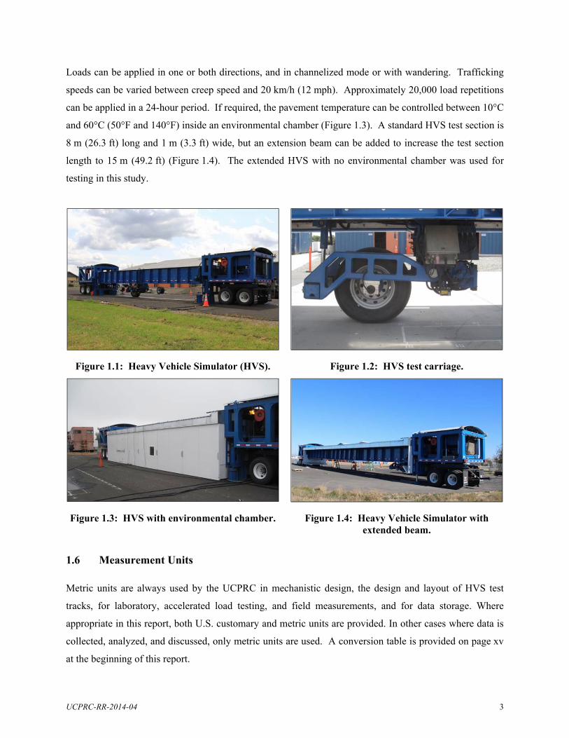
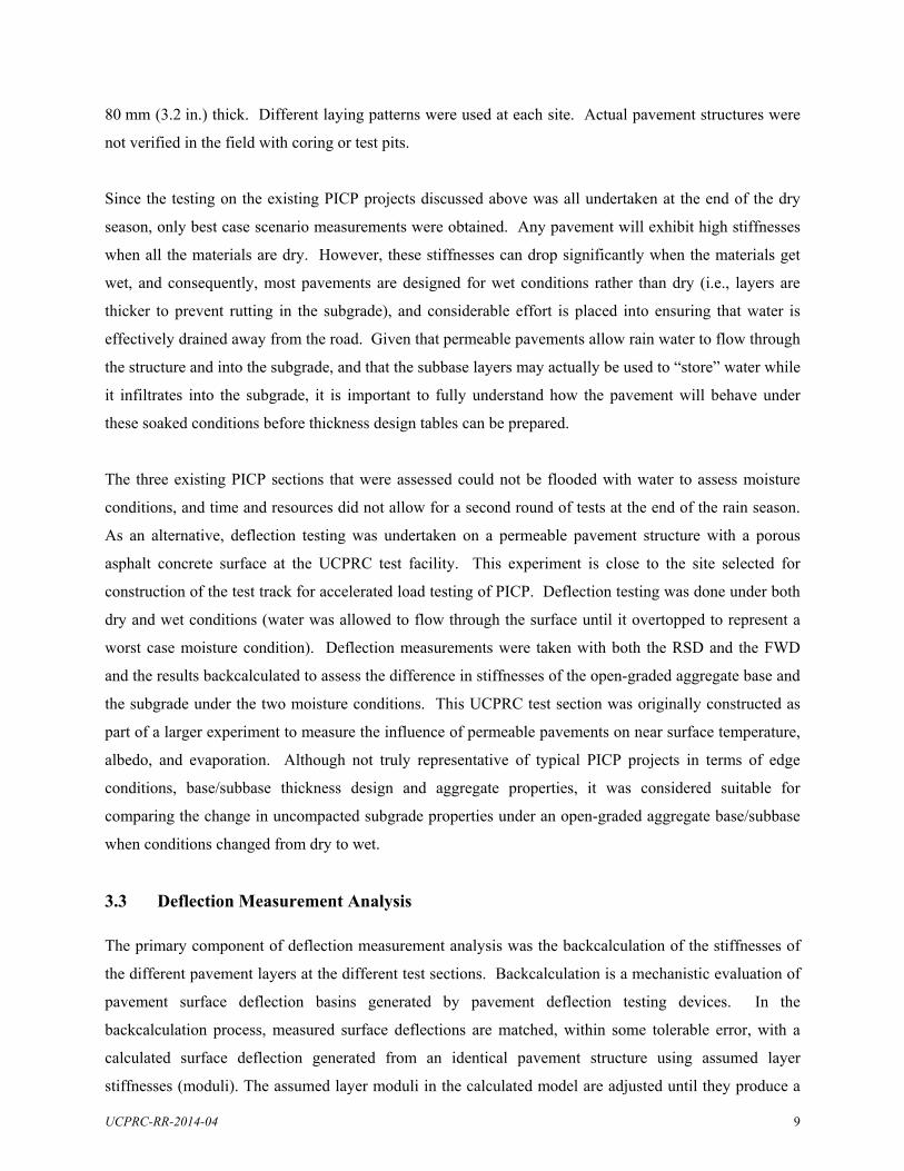
Loads can be applied in one or both directions, and in channelized mode or with wandering. Trafficking
speeds can be varied between creep speed and 20 km/h (12 mph). Approximately 20,000 load repetitions
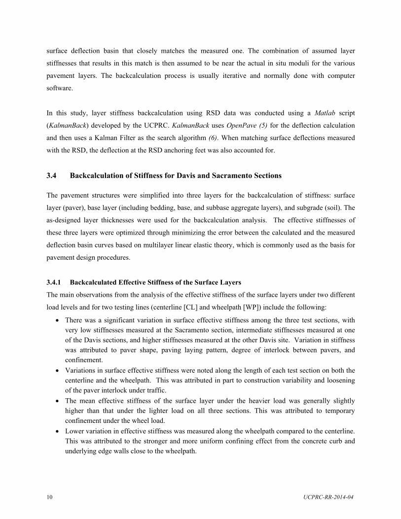
can be applied in a 24-hour period. If required, the pavement temperature can be controlled between 10°C
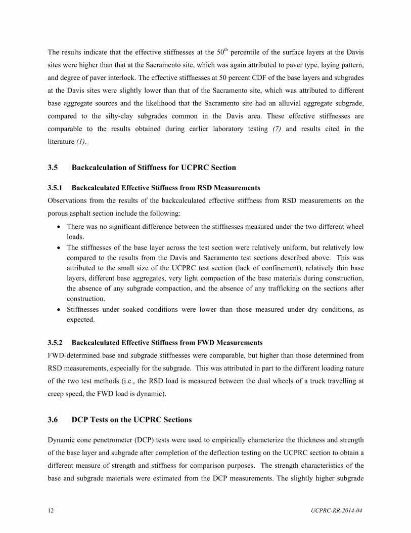
and 60°C (50°F and 140°F) inside an environmental chamber (Figure 1.3). A standard HVS test section is
8 m (26.3 ft) long and 1 m (3.3 ft) wide, but an extension beam can be added to increase the test section
length to 15 m (49.2 ft) (Figure 1.4). The extended HVS with no environmental chamber was used for
testing in this study.
Figure 1.1: Heavy Vehicle Simulator (HVS). Figure 1.2: HVS test carriage.
Figure 1.3: HVS with environmental chamber. Figure 1.4: Heavy Vehicle Simulator with extended beam.
1.6 Measurement Units
Metric units are always used by the UCPRC in mechanistic design, the design and layout of HVS test
tracks, for laboratory, accelerated load testing, and field measurements, and for data storage. Where
appropriate in this report, both U.S. customary and metric units are provided. In other cases where data is
collected, analyzed, and discussed, only metric units are used. A conversion table is provided on page xv
at the beginning of this report.

4 UCPRC-RR-2014-04
Blank page

UCPRC-RR-2014-04 5
2. LITERATURE REVIEW
A review of the recent literature on permeable interlocking concrete pavements was undertaken at the start
of the study and a summary report prepared (1). A copy of the complete report is included in Appendix A.
The literature review found that only a few organizations worldwide have undertaken detailed research on
permeable interlocking concrete pavements, with many studies focusing on infiltration on low volume
traffic roads, rather than structural design of roads carrying truck traffic. Limited published record was
found on controlled load testing on permeable pavements in general and permeable interlocking concrete
pavements in particular. No references were located with respect to accelerated testing as described in this
report.
Laboratory studies have focused on resilient modulus of saturated and unsaturated materials. Well-graded
materials with no fines (typical of that used under PICP) appeared to perform best under both conditions.
Permeable pavements are generally designed for the worst case condition (i.e., a saturated soil subgrade
and possibly a subbase/reservoir layer immersed in water). These conditions may (conservatively) require
a reduction in resilient modulus as much as 50 percent of the dry material value. The use of cemented
materials and geogrids in the base to compensate for this lower subgrade and aggregate base stiffness is
gaining interest.
Failure mechanisms appear to be mostly rutting of the surface layer due to shearing in the bedding, base
and/or subbase layers. Choice of paver thickness, paver shape, and paver laying pattern can limit this to a
certain extent. However, optimizing the base and subbase material grading and thickness, material
hardness, stabilization of the base and/or subbase materials with cement, asphalt, or a geogrid, quality of
construction, and the use of geosynthetics to prevent contamination of the subbase are all design
considerations with substantially greater influence on control of rutting and failure.
Mechanistic-empirical design has been considered in Australian and United Kingdom design procedures
to some extent, with the work done in Australia appearing to be the most comprehensive. For unstabilized
aggregates, these procedures typically use repetitive compressive strain at the top of the soil subgrade as
the mechanistic response that is correlated with the rutting failure mechanism. Tension was generally not
considered since these materials are not in tension. However, the measurement and understanding of
stress distribution within and at the bottom of an open-graded base is not well documented or understood
(compared to dense-graded materials), and this topic will likely require further research, modeling, and
full-scale verification beyond what was determined within the scope of this project. Measuring stiffness

6 UCPRC-RR-2014-04
and stress distributions within the open-graded bedding/base/subbase from repeated loads was identified
as a challenge, as was the need for undertaking research to enable the development of models/tools that
can predict permeable pavement performance, including surface distresses, maintenance/rehabilitation
remedies, and ultimate structural life.

UCPRC-RR-2014-04 7
3. DEFLECTION TESTING ON EXISTING PROJECTS
3.1 Introduction
Pavement surface deflection measurements are a primary method of evaluating the behavior of pavement
structures when subjected to a load, and to characterize the stiffness of the pavement layers for use in
mechanistic design. These measurements, which are non-destructive, are used to assess a pavement’s
structural condition, by taking most relevant factors into consideration, including traffic type and volume,
pavement structural section, temperature, and moisture condition. Deflection measurements can be used
in backcalculation procedures to determine pavement subgrade and structural layer stiffnesses, which are
used as input to structural models to calculate stress, strains, and deformations that are correlated to
distress mechanisms. Deflections can also be used directly in empirical design methods as an indicator to
determine what level of traffic loading the pavement can withstand (i.e., design life or remaining life in
terms of number of axle loads).
Deflection measurements are used by most departments of transportation as the basis for rehabilitation
designs and often as a trigger for when rehabilitation or reconstruction is required.
All pavements bend under loading to some degree. Although this bending can normally not be
distinguished with the naked eye (measurements are typically recorded in microns or mils) it has a
significant effect on the integrity of the different layers over time. Repeated bending and then relaxation
as the load moves onto and then off a point on a pavement is analogous to repeatedly bending a piece of
wire back and forth – it eventually breaks. In pavements, the “damage” usually materializes as
reorientation of the material particles, cracks and/or shearing, which leads to a reduction in stiffness over
time, which in turn leads to moisture ingress, rutting, and other associated problems. Since moisture
ingress and cracking are not relevant issues on permeable interlocking concrete pavements, this study
focused on shearing and resulting rutting in the surface and underlying layers.
This chapter summarizes the results of a deflection study on three existing permeable interlocking
concrete pavement projects in northern California (2) and backcalculation analysis of the test results. The
full report is included in Appendix B, and it includes chapters covering a description of pavement
deflection testing, the experiment plan for field deflection testing of existing PICP sections, results of the
deflection testing, results of the mechanistic analysis, preliminary structural designs, and the test plan for
thickness validation with accelerated pavement testing.

8 UCPRC-RR-2014-04
3.2 Deflection Testing
3.2.1 Deflection Measurement Method
Pavement deflection is most commonly measured with a falling weight deflectometer (FWD). However,
this equipment is designed for continuous (monolithic) asphalt concrete and portland cement concrete
pavements built on dense-graded aggregate bases, and was not considered appropriate for testing
deflection on pavements constructed with interlocking concrete pavers (because of the segmented nature
of the pavement surface), overlying open-graded aggregate bases. An FWD also applies an instantaneous
dynamic load onto the pavement surface to simulate a truck wheel load passing over that point at a speed
of about 60 km/h (40 mph). Deflection in the pavement is measured under this load. Open-graded
aggregate bases used in permeable pavements, are usually more stress dependent than dense-graded bases,
and can therefore have a bigger range of stiffness increase and relaxation as the wheel load passes over it.
Backcalculating stiffnesses based on deflection measurements using an FWD may therefore provide
incorrect results when analyzing PICP. A review of the literature on PICP (1) revealed that other
researchers had experienced problems with accurately analyzing the stiffness of PICP from FWD
deflection measurements.
Based on these concerns, a modified Benkelman beam (road surface deflectometer [RSD]) was instead
used to measure deflection on the test sections. This device, which is standard equipment for measuring
surface deflections on accelerated pavement tests at the UCPRC, measures the actual deflection between
the dual wheels of a truck as it passes at slow speed over the instrument (see Figure 6.9 in Chapter 6). The
RSD is not influenced by the segmental nature of the pavers (provided that the four reference points of the
device are in contact with the paver surface and not on a joint) and is considered more appropriate for
accommodating the stress dependent nature of the open-graded aggregate base. These deflection
measurements were used to backcalculate the effective stiffnesses of individual pavement layers based on
multilayer linear elastic theory. A comparison between the FWD and RSD was undertaken on a fully
permeable pavement with a continuous open-graded asphalt surface to compare the backcalculated
stiffnesses of the open-graded base using the two deflection methods. Testing was done under both dry
and wet conditions on this section.
3.2.2 Test Section Locations
Three sites in northern California were selected for the deflection measurements, two in Davis and one in
Sacramento. Construction records indicated that the pavement structures at the different sites consisted of
an ASTM No. 57 aggregate base layer 300 mm to 400 mm (12 to 16 in.) thick, underneath an ASTM
No. 8 aggregate bedding layer 25 mm to 50 mm (1 to 2 in.) thick (i.e., a very light traffic design per the
ICPI Permeable Interlocking Concrete Pavement guide [4]). The surface pavers used at all three sites were
UCPRC-RR-2014-04 9
80 mm (3.2 in.) thick. Different laying patterns were used at each site. Actual pavement structures were
not verified in the field with coring or test pits.
Since the testing on the existing PICP projects discussed above was all undertaken at the end of the dry
season, only best case scenario measurements were obtained. Any pavement will exhibit high stiffnesses
when all the materials are dry. However, these stiffnesses can drop significantly when the materials get
wet, and consequently, most pavements are designed for wet conditions rather than dry (i.e., layers are
thicker to prevent rutting in the subgrade), and considerable effort is placed into ensuring that water is
effectively drained away from the road. Given that permeable pavements allow rain water to flow through
the structure and into the subgrade, and that the subbase layers may actually be used to “store” water while
it infiltrates into the subgrade, it is important to fully understand how the pavement will behave under
these soaked conditions before thickness design tables can be prepared.
The three existing PICP sections that were assessed could not be flooded with water to assess moisture
conditions, and time and resources did not allow for a second round of tests at the end of the rain season.
As an alternative, deflection testing was undertaken on a permeable pavement structure with a porous
asphalt concrete surface at the UCPRC test facility. This experiment is close to the site selected for
construction of the test track for accelerated load testing of PICP. Deflection testing was done under both
dry and wet conditions (water was allowed to flow through the surface until it overtopped to represent a
worst case moisture condition). Deflection measurements were taken with both the RSD and the FWD
and the results backcalculated to assess the difference in stiffnesses of the open-graded aggregate base and
the subgrade under the two moisture conditions. This UCPRC test section was originally constructed as
part of a larger experiment to measure the influence of permeable pavements on near surface temperature,
albedo, and evaporation. Although not truly representative of typical PICP projects in terms of edge
conditions, base/subbase thickness design and aggregate properties, it was considered suitable for
comparing the change in uncompacted subgrade properties under an open-graded aggregate base/subbase
when conditions changed from dry to wet.
3.3 Deflection Measurement Analysis
The primary component of deflection measurement analysis was the backcalculation of the stiffnesses of
the different pavement layers at the different test sections. Backcalculation is a mechanistic evaluation of
pavement surface deflection basins generated by pavement deflection testing devices. In the
backcalculation process, measured surface deflections are matched, within some tolerable error, with a
calculated surface deflection generated from an identical pavement structure using assumed layer
stiffnesses (moduli). The assumed layer moduli in the calculated model are adjusted until they produce a
10 UCPRC-RR-2014-04
surface deflection basin that closely matches the measured one. The combination of assumed layer
stiffnesses that results in this match is then assumed to be near the actual in situ moduli for the various
pavement layers. The backcalculation process is usually iterative and normally done with computer
software.
In this study, layer stiffness backcalculation using RSD data was conducted using a Matlab script
(KalmanBack) developed by the UCPRC. KalmanBack uses OpenPave (5) for the deflection calculation
and then uses a Kalman Filter as the search algorithm (6). When matching surface deflections measured
with the RSD, the deflection at the RSD anchoring feet was also accounted for.
3.4 Backcalculation of Stiffness for Davis and Sacramento Sections
The pavement structures were simplified into three layers for the backcalculation of stiffness: surface
layer (paver), base layer (including bedding, base, and subbase aggregate layers), and subgrade (soil). The
as-designed layer thicknesses were used for the backcalculation analysis. The effective stiffnesses of
these three layers were optimized through minimizing the error between the calculated and the measured
deflection basin curves based on multilayer linear elastic theory, which is commonly used as the basis for
pavement design procedures.
3.4.1 Backcalculated Effective Stiffness of the Surface Layers
The main observations from the analysis of the effective stiffness of the surface layers under two different
load levels and for two testing lines (centerline [CL] and wheelpath [WP]) include the following:
There was a significant variation in surface effective stiffness among the three test sections, with very low stiffnesses measured at the Sacramento section, intermediate stiffnesses measured at one of the Davis sections, and higher stiffnesses measured at the other Davis site. Variation in stiffness was attributed to paver shape, paving laying pattern, degree of interlock between pavers, and confinement.
Variations in surface effective stiffness were noted along the length of each test section on both the centerline and the wheelpath. This was attributed in part to construction variability and loosening of the paver interlock under traffic.
The mean effective stiffness of the surface layer under the heavier load was generally slightly higher than that under the lighter load on all three sections. This was attributed to temporary confinement under the wheel load.
Lower variation in effective stiffness was measured along the wheelpath compared to the centerline. This was attributed to the stronger and more uniform confining effect from the concrete curb and underlying edge walls close to the wheelpath.

UCPRC-RR-2014-04 11
3.4.2 Backcalculated Effective Stiffness of the Base Layers
The main observations from the analysis of the effective stiffness of the base layers for the two load levels
and two testing paths at all three test sites include the following:
The mean effective stiffnesses of the base layers calculated for the three sites were in the range of 20 MPa to 120 MPa (2.9 ksi to 17.4 ksi). However, average effective base layer stiffnesses were more consistent across the three sections compared to the surface stiffnesses. It should be noted that calculated stiffnesses will be influenced by and are sensitive to layer thickness and that design thicknesses were used in the analysis. These were not verified with on-site excavation. Consequently, actual layer stiffnesses could be lower or higher if the as-built thicknesses were thinner or thicker than the design.
Effective stiffness along the wheelpath had lower variation compared to the centerline, which was again attributed to constraining effects of the curb and edge walls. The Sacramento test section had the highest variability.
In most instances, the effective stiffness of the base layer was slightly higher under the heavier load, as expected. This was attributed to the higher confining stresses under the heavier load.
3.4.3 Backcalculated Effective Stiffness of the Subgrade
The main observations from the analysis of the effective stiffnesses of the subgrade under dry conditions
for the three test sites include the following:
The mean effective stiffnesses of the subgrade varied between 20 MPa and 100 MPa (2.9 ksi and 14.5 ksi) for the three test sites.
The Sacramento section had the highest effective subgrade stiffness of the three sections, but also the highest variability. This was attributed to the likely alluvial (river gravel) nature of the subgrade material. The Davis sites had a similar range of subgrade stiffnesses consistent with silty-clay materials common in this area.
Trends and variation along the two test paths were similar to those observed for the surface and base layers.
The effect of the different load levels was less apparent on the subgrade stiffness compared to the effect it had on base and surface layer stiffnesses. This was attributed to the subgrade materials being of a less granular nature than the base materials and therefore less susceptible to confining stress.
3.4.4 Effective Stiffness Analysis
The distributed backcalculated effective stiffnesses of the surface layers, base layers, and subgrades at the
three test sites were analyzed using empirical cumulative distribution functions (CDF). The median
effective stiffnesses (50th percentile) for the surface and base layers and the subgrade were approximately
400 MPa, 40 MPa, and 40 MPa (58 ksi, 5.8 ksi, and 5.8 ksi), respectively. Given that subgrade conditions
at the Davis sites were likely different to the Sacramento site, the exercise was repeated for the two Davis
sites only. Effective stiffness values changed to approximately 500 MPa, 35 MPa and 35 MPa (73 ksi,
5.1 ksi, and 5.1 ksi), respectively.
12 UCPRC-RR-2014-04
The results indicate that the effective stiffnesses at the 50th percentile of the surface layers at the Davis
sites were higher than that at the Sacramento site, which was again attributed to paver type, laying pattern,
and degree of paver interlock. The effective stiffnesses at 50 percent CDF of the base layers and subgrades
at the Davis sites were slightly lower than that of the Sacramento site, which was attributed to different
base aggregate sources and the likelihood that the Sacramento site had an alluvial aggregate subgrade,
compared to the silty-clay subgrades common in the Davis area. These effective stiffnesses are
comparable to the results obtained during earlier laboratory testing (7) and results cited in the
literature (1).
3.5 Backcalculation of Stiffness for UCPRC Section
3.5.1 Backcalculated Effective Stiffness from RSD Measurements
Observations from the results of the backcalculated effective stiffness from RSD measurements on the
porous asphalt section include the following:
There was no significant difference between the stiffnesses measured under the two different wheel loads.
The stiffnesses of the base layer across the test section were relatively uniform, but relatively low compared to the results from the Davis and Sacramento test sections described above. This was attributed to the small size of the UCPRC test section (lack of confinement), relatively thin base layers, different base aggregates, very light compaction of the base materials during construction, the absence of any subgrade compaction, and the absence of any trafficking on the sections after construction.
Stiffnesses under soaked conditions were lower than those measured under dry conditions, as expected.
3.5.2 Backcalculated Effective Stiffness from FWD Measurements
FWD-determined base and subgrade stiffnesses were comparable, but higher than those determined from
RSD measurements, especially for the subgrade. This was attributed in part to the different loading nature
of the two test methods (i.e., the RSD load is measured between the dual wheels of a truck travelling at
creep speed, the FWD load is dynamic).
3.6 DCP Tests on the UCPRC Sections
Dynamic cone penetrometer (DCP) tests were used to empirically characterize the thickness and strength
of the base layer and subgrade after completion of the deflection testing on the UCPRC section to obtain a
different measure of strength and stiffness for comparison purposes. The strength characteristics of the
base and subgrade materials were estimated from the DCP measurements. The slightly higher subgrade

UCPRC-RR-2014-04 13
strengths on the test section compared to the adjacent area was attributed to the confinement provided by
the pavement structure. The results were consistent with silty clay subgrade materials in the Davis area.

14 UCPRC-RR-2014-04
Blank page

UCPRC-RR-2014-04 15
4. TEST TRACK LOCATION AND DESIGN
4.1 Test Track Location
The PICP experiment was located on a specially constructed test track adjacent to the Outer West Track at
the University of California Pavement Research Center facility in Davis, California. An aerial view of the
site is shown in Figure 4.1. Prior to construction of the Center, the area was used for agriculture
(primarily alfalfa cultivation) and consequently the soil was relatively undisturbed in terms of compaction.
A view of the test track site prior to construction is shown in Figure 4.2
Figure 4.1: Aerial view of the UCPRC research facility.
Figure 4.2: View of the test track site prior to construction.
PICP Test Track

16 UCPRC-RR-2014-04
4.2 Test Track Design
The test track design is discussed in detail in the interim report prepared after completion of pavement
deflection testing and mechanistic analysis (2). The full report is included in Appendix B.
The design was derived from a sensitivity analysis that considered a range of mechanistic values from
worst-case to best-case scenarios. Selection of the input values was based on previous work by the
authors, work by others on the topic identified during literature reviews, and the results of the deflection
testing study.
4.2.1 Design Criteria
The most likely failure mode of permeable interlocking concrete pavements is permanent deformation in
the base, subbase, and/or subgrade layers, which will manifest as rutting and/or paver displacement on the
surface. The design criteria for the test track were therefore focused on this type of distress.
4.2.2 Design Variables
Shear stress/strength ratio (SSR or τf /τmax) was used as the main design variable in this study. The basis
for the use of shear stress to shear strength ratio for design comes from work done at the University of
Illinois, primarily under Prof. Marshall Thompson and carried out by Prof. Erol Tutumleur (8,9). It is
based on decades of laboratory testing for permanent deformation, followed by field validation. The
concept was primarily developed for use in airfields where the shear stresses from aircraft loads and tire
pressures are high relative to the strengths of the subgrade materials. It was selected for use on this
permeable pavement project because of the low shear strengths of saturated, uncompacted or poorly
compacted subgrades (which are common conditions in permeable pavements) where the ratio between
shear stresses and strengths can also be high given highway loads and tire pressures.
The alternative approach considered was the use of a vertical strain criterion, which is typically used
where the shear stresses relative to shear strains are relatively low, which results in relatively low overall
rutting. In this approach, vertical strains are typically calculated from pavement deflection measured over
the full pavement structure. Strains in the localized areas at the top of the base layer and subgrade cannot
be directly measured unless a strain gauge has been specifically installed in that position. Consequently,
the damage and stiffness is calculated from measured deflections and then the strain is calculated from the
calibrated damage and stiffness model. Vertical strain based approaches are difficult to calibrate when
high shear stress to strength ratios occur in high water content environments, which in turn lead to large
ruts. This has been learned from UCPRC experience on other projects that investigated pavement
UCPRC-RR-2014-04 17
performance under soaked conditions and consequently the vertical strain approach was not considered
appropriate for designing permeable pavements.
Shear stress data has not been directly measured for ANY materials in the field because there is currently
no instrument that can effectively measure shear stresses under a wheel load in a pavement structure. In
the laboratory, shear stresses for all materials are calculated based on assumptions about the material and
mechanics. Only limited shear strength data is available from shear and resilient modulus laboratory tests
on open-graded granular bases and subbases. Similarly, there is very little laboratory or field data to
support a strain based rutting model for open graded granular bases. Given these limitations, the
stress/strength ratio concept was considered the most logical approach to accommodate the high stress to
strength ratios, and higher allowable ruts that are part of designing permeable pavements.
Shear Stress/Strength Ratio
Shear stress/strength ratio is defined as the ratio between the applied shear stress (τf) and the material shear
strength (τmax [τmax = c + σf tanϕ in a triaxial strength test, where c is the cohesion of the material]) on the
failure plane at a specific applied normal and confining stress state (8). The normal and shear stresses (σf
and τmax) acting on a failure plane (oriented at an angle of 45° + ϕ/2, where ϕ is the internal friction angle
of the material) can be calculated according to the Mohr-Coulomb failure theory for specific confining
(σ3) and deviator (σd) stresses applied to a laboratory specimen during triaxial testing.
Materials with lower shear stress/strength ratios are less likely to fail due to shear (i.e., rutting and
permanent deformation) than materials with higher shear stress/strength ratios. Research studies (10,11)
have shown that materials subjected to shear stress/strength ratios higher than 0.7 are likely to accumulate
high permanent deformation and present a higher rutting risk, leading to rapid shear failure in the
pavement. Materials with shear stress/strength ratios between 0.3 and 0.7 represent a medium risk with a
steady but reasonable rate of rutting, while those with shear stress/strength ratios less than about 0.3 are
expected to have little or no rutting after an initial small “bedding-in” rut. Based on these findings, the
following three shear stress ratio design variable categories aligned to the level of rutting risk were
defined for permeable interlocking concrete pavements (1,9):
SSR < 0.3, low risk of rutting;
0.3 ≤ SSR ≤ 0.7, medium risk of rutting;
SSR > 0.7, high risk of rutting.
The equations used to calculate the SSR corresponding to the stress state applied during triaxial testing or
other conditions are listed below:
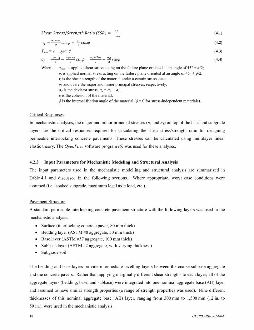
18 UCPRC-RR-2014-04
/
(4.1)
(4.2)
Τmax = c + σf tan (4.3)
(4.4)
Where: τmax is applied shear stress acting on the failure plane oriented at an angle of 45° + ϕ/2; σf is applied normal stress acting on the failure plane oriented at an angle of 45° + ϕ/2; τf is the shear strength of the material under a certain stress state; σ1 and σ3 are the major and minor principal stresses, respectively; σd is the deviator stress, σd = σ1 σ3; c is the cohesion of the material; ϕ is the internal friction angle of the material (ϕ = 0 for stress-independent materials).
Critical Responses
In mechanistic analyses, the major and minor principal stresses (σ1 and σ3) on top of the base and subgrade
layers are the critical responses required for calculating the shear stress/strength ratio for designing
permeable interlocking concrete pavements. These stresses can be calculated using multilayer linear
elastic theory. The OpenPave software program (5) was used for these analyses.
4.2.3 Input Parameters for Mechanistic Modeling and Structural Analysis
The input parameters used in the mechanistic modelling and structural analysis are summarized in
Table 4.1 and discussed in the following sections. Where appropriate, worst case conditions were
assumed (i.e., soaked subgrade, maximum legal axle load, etc.).
Pavement Structure
A standard permeable interlocking concrete pavement structure with the following layers was used in the
mechanistic analysis:
Surface (interlocking concrete paver, 80 mm thick)
Bedding layer (ASTM #8 aggregate, 50 mm thick)
Base layer (ASTM #57 aggregate, 100 mm thick)
Subbase layer (ASTM #2 aggregate, with varying thickness)
Subgrade soil
The bedding and base layers provide intermediate levelling layers between the coarse subbase aggregate
and the concrete pavers. Rather than applying marginally different shear strengths to each layer, all of the
aggregate layers (bedding, base, and subbase) were integrated into one nominal aggregate base (AB) layer
and assumed to have similar strength properties (a range of strength properties was used). Nine different
thicknesses of this nominal aggregate base (AB) layer, ranging from 300 mm to 1,500 mm (12 in. to
59 in.), were used in the mechanistic analysis.
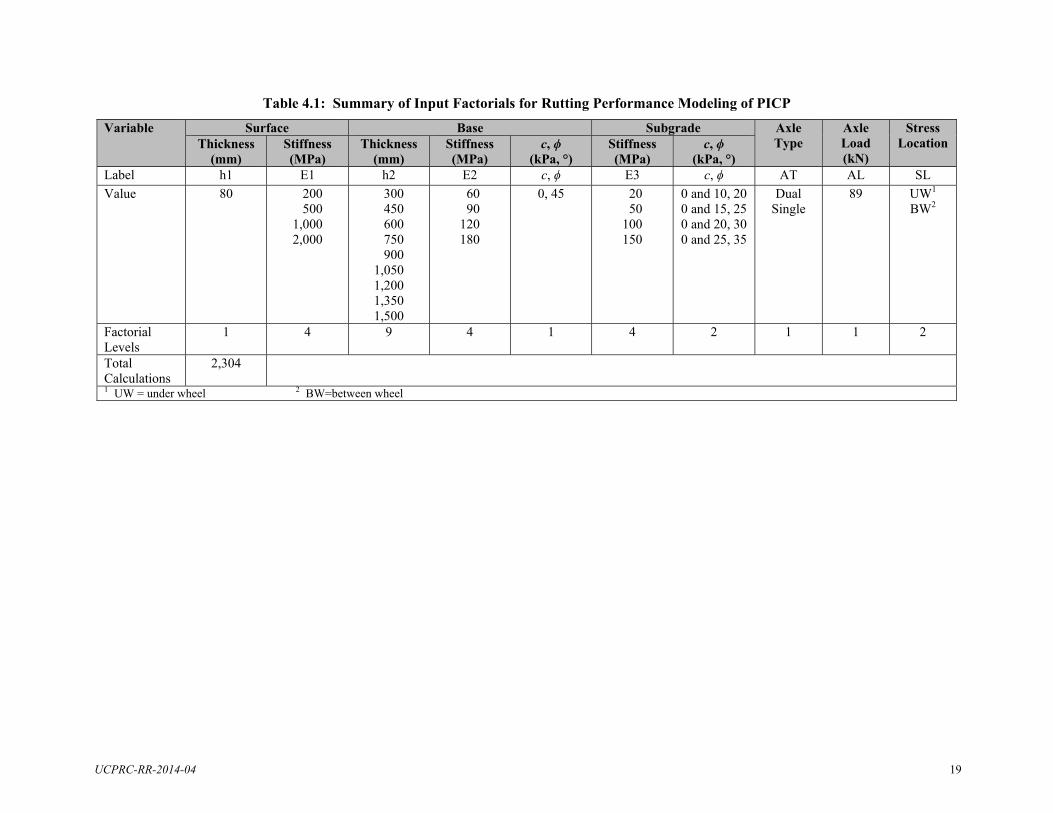
UCPRC-RR-2014-04 19
Table 4.1: Summary of Input Factorials for Rutting Performance Modeling of PICP
Variable Surface Base Subgrade Axle Type
Axle Load (kN)
Stress Location Thickness
(mm) Stiffness (MPa)
Thickness (mm)
Stiffness (MPa)
c, ϕ (kPa, °)
Stiffness (MPa)
c, ϕ (kPa, °)
Label h1 E1 h2 E2 c, ϕ E3 c, ϕ AT AL SL
Value 80 200 500 1,000 2,000
300 450 600 750 900 1,050 1,200 1,350 1,500
60 90 120 180
0, 45 20 50 100 150
0 and 10, 20 0 and 15, 25 0 and 20, 30 0 and 25, 35
Dual Single
89 UW1
BW2
Factorial Levels
1 4 9 4 1 4 2 1 1 2
Total Calculations
2,304
1 UW = under wheel 2 BW=between wheel

20 UCPRC-RR-2014-04
Materials Properties
The material properties used in the mechanistic analysis included stiffness and Poisson’s ratio for each
layer in the pavement structure, and cohesion and internal friction angle of the composite base aggregate
and subgrade soil materials. These properties were selected from the deflection testing analyses
(discussed in Chapter 3) and from the results of other studies documented in the literature. No laboratory
testing to measure actual material properties was undertaken in this study.
Four different stiffnesses were selected for each layer (surface, base and subgrade) based on the
backcalculated effective stiffnesses from the deflection testing analyses discussed in Chapter 3:
Surface (pavers): 200, 500, 1,000, and 2,000 MPa
Base (combined bedding, base, and subbase layers): 60, 90, 120, and 180 MPa
Subgrade: 20, 50, 100, and 150 MPa The Poisson’s ratio for each layer was assumed to be 0.35 based on measurements documented in other studies (10,12).
The cohesion and internal friction angle (c, ϕ) of the aggregate base material was assumed to be 0 kPa and
45° respectively, based on a review of the literature (10,12). For the subgrade material, both non-zero
(ϕ ≠ 0) and zero (ϕ = 0) internal friction angles were used in the analysis for all stiffness levels to simulate
drained and soaked, undrained soil conditions, respectively. Based on a review of the literature (13-17),
the subgrade cohesion and internal friction angles (c, ϕ) were set at the following levels for each of the
four subgrade stiffnesses:
20 MPa: 10 kPa and 20° and 0°
50 MPa: 15 kPa and 25° and 0°
100 MPa: 20 kPa and 30° and 0°
150 MPa: 25 kPa and 35° and 0°
Traffic Load
A single rear axle with dual wheels was used in the analysis. The axle load was set at 89 kN (20,000 lb)
and the tire pressure was set at 700 kPa (101 psi), which is the tire pressure used in accelerated load tests.
The distance between the two tire centers was set at 340 mm (13.4 in.). The stress under the wheel and the
stress between the wheels were both calculated to identify the most critical stress.
4.2.4 Mechanistic Analysis Results
Combined Base and Subbase Layer
The results of the mechanistic analysis for the different base layer (combined bedding, base, and subbase
layers) stiffness values and thicknesses include the major and minor principal stresses, normal stress at the
UCPRC-RR-2014-04 21
failure plane, shear strength at the selected stress state, shear stress at the failure plane, and the shear
stress/strength ratio at the failure plane at the top of the combined base layer. The results are detailed in
the full report in Appendix B and indicate that, according to the multilayer linear elastic design theory, an
increase in the thickness of the combined base and subbase layer does not necessarily reduce the stresses
at the top of that layer, as expected.
Subgrade
The results of the mechanistic analysis for the subgrade included the same parameters used in the
combined base and subbase layer analysis, except that the shear stress/strength ratio at the top of the
subgrade was calculated. The results are detailed in the full report in Appendix B and indicate that
increasing the thickness of the subbase layer (the coarse ASTM #2 aggregate subbase layer given that this
is the “strong” material) reduces the stresses (absolute values) at the top of the subgrade soil layer, as
expected.
During dry conditions, when the subgrade is relatively dry (or at equilibrium moisture content) and has a
nonzero internal friction angle (ϕ ≠ 0), the shear strength of the subgrade soil changes with the thickness
of the combined base and subbase layer. Interestingly, the effective shear strength of the subgrade soil
decreases slightly as the thickness of the base/subbase layer increases. This is attributed to the effective
shear strength of subgrade soils being positively correlated with the normal stress at the failure plane
under dry conditions (ϕ ≠ 0) (as defined in Equation 4.3), which provides confinement. An increase in the
thickness of the base/subbase layer significantly reduces the normal stress at the failure plane at the top of
the subgrade soil layer, and consequently, the effective shear strength of the subgrade soil decreases
slightly as the thickness of the base/subbase layer increases.
Under wet conditions (i.e., when the subgrade is soaked and has a zero internal friction angle [ϕ = 0]), the
effective shear strength of subgrade soils does not change with the thickness of the base/subbase layer.
This is because the shear strength of materials with zero internal friction angle is independent of the
normal stress applied and is determined only by the cohesion of the material (as defined in Equation 4.3).
Therefore, soaked subgrade soils will have constant effective shear strength regardless of an increase in
the thickness of the base/subbase layer. The effective shear strength will be equal to the cohesion of the
material which is slightly lower than the effective shear strength of the subgrade soil under dry conditions.
The normal stress and the shear stress are both higher under wet conditions than those under dry
conditions for an identical structure and identical material properties (plots illustrating this are included
the full report in Appendix B). The shear stress/strength ratio under wet conditions is also higher than the

22 UCPRC-RR-2014-04
shear stress/strength ratio under dry conditions for an identical structure and identical material properties,
as expected. This confirms that wet conditions are the most critical condition influencing rutting and
permanent deformation in the subgrade in pavements with permeable interlocking concrete paver surfaces.
Thickness of Base/Subbase Layers for Different Shear Stress/Strength Ratio Values
Based on the results discussed above, the base/subbase layer thicknesses with shear stress/strength ratios
of 0.8 (i.e., >0.7), 0.5 (i.e., intermediate between 0.3 and 0.7 [0.3 ≤ SSR ≤ 0.7]), and 0.2 (i.e., <0.3),
representing different rutting risk levels, were estimated using interpolation of the different material
properties and subgrade moisture conditions. The results are presented in Figure 4.3 and Figure 4.4. The
main observations with regard to required base/subbase layer thicknesses for PICP include the following:
Higher shear stress/strength ratios, which equate to a higher risk of rutting, require thicker base/subbase layers, as expected.
For the same shear stress/strength ratio, an increase in the effective stiffness of the base/subbase layer reduces the required thickness of that layer, especially when the subgrade has a low stiffness.
An increase in the stiffness of the surface layer reduces the required base/subbase layer thickness to achieve the same shear stress/strength ratio. However, the effect of the surface layer stiffness is not significant due to the relatively low thickness of the pavers (80 mm) and the reduced interlock between them compared to pavers with sand joints.
For the same shear stress/strength ratio, wet conditions require thicker base/subbase layers compared to the dry condition, confirming that undrained wet conditions are the most critical condition for design.
The theoretical optimal design base thicknesses (combined bedding, base, and subbase layers) for low, intermediate, and higher risk levels (subgrade shear stress/strength ratios of 0.2, 0.5 and 0.8, respectively) under dry subgrade moisture conditions are approximately 1,300 mm, 800 mm, and 500 mm (51 in., 32 in., and 20 in.), respectively. In wet conditions, the theoretical optimal design thicknesses increase to 1,400 mm, 1,000 mm and 600 mm (55 in., 39 in., and 24 in.), respectively.
4.2.5 Test Track Layer Thickness Design
Empirical Design
The design approach described in the ICPI Permeable Interlocking Concrete Pavements guide (4) was
followed to determine a benchmark design for the test track that could be used to compare with the results
from a mechanistic design. Using the pavement structure detailed in Section 4.2.3, and designing for a
subgrade soaked CBR of 4 percent (determined from DCP tests) and lifetime equivalent standard axle
loads (ESALs) of 1,000,000 (expected traffic loading with the HVS), a subbase thickness of 675 mm
(27 in.) under bedding and base layers of 50 mm (2 in.) and 100 mm (4 in.) respectively, would be
required.
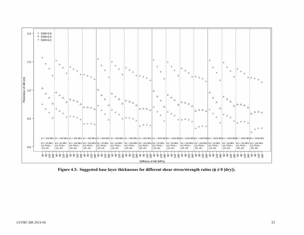
UCPRC-RR-2014-04 23
Figure 4.3: Suggested base layer thicknesses for different shear stress/strength ratios (ϕ ≠ 0 [dry]).
0.0
0.5
1.0
1.5
2.0
Thi
ckne
ss o
f A
B (
m)
60 90 120
180 60 90 120
180 60 90 120
180 60 90 120
180 60 90 120
180 60 90 120
180 60 90 120
180 60 90 120
180 60 90 120
180 60 90 120
180 60 90 120
180 60 90 120
180 60 90 120
180 60 90 120
180 60 90 120
180 60 90 120
180
Stiffness of AB (MPa)
SSR=0.8SSR=0.5SSR=0.2
E1 = 200 MPa
E3 = 20 MPa(c3, Phi3) = (10, 20)
E1 = 200 MPa
E3 = 50 MPa(c3, Phi3) = (15, 25)
E1 = 200 MPa
E3 = 100 MPa(c3, Phi3) = (20, 30)
E1 = 200 MPa
E3 = 150 MPa(c3, Phi3) = (25, 35)
E1 = 500 MPa
E3 = 20 MPa(c3, Phi3) = (10, 20)
E1 = 500 MPa
E3 = 50 MPa(c3, Phi3) = (15, 25)
E1 = 500 MPa
E3 = 100 MPa(c3, Phi3) = (20, 30)
E1 = 500 MPa
E3 = 150 MPa(c3, Phi3) = (25, 35)
E1 = 1000 MPa
E3 = 20 MPa(c3, Phi3) = (10, 20)
E1 = 1000 MPa
E3 = 50 MPa(c3, Phi3) = (15, 25)
E1 = 1000 MPa
E3 = 100 MPa(c3, Phi3) = (20, 30)
E1 = 1000 MPa
E3 = 150 MPa(c3, Phi3) = (25, 35)
E1 = 2000 MPa
E3 = 20 MPa(c3, Phi3) = (10, 20)
E1 = 2000 MPa
E3 = 50 MPa(c3, Phi3) = (15, 25)
E1 = 2000 MPa
E3 = 100 MPa(c3, Phi3) = (20, 30)
E1 = 2000 MPa
E3 = 150 MPa(c3, Phi3) = (25, 35)

24 UCPRC-TM-2013-09
Figure 4.4: Suggested base layer thicknesses for different shear stress/strength ratios (ϕ = 0 [wet]).
0.0
0.5
1.0
1.5
2.0
Thi
ckne
ss o
f A
B (
m)
60 90 120
180 60 90 120
180 60 90 120
180 60 90 120
180 60 90 120
180 60 90 120
180 60 90 120
180 60 90 120
180 60 90 120
180 60 90 120
180 60 90 120
180 60 90 120
180 60 90 120
180 60 90 120
180 60 90 120
180 60 90 120
180
Stiffness of AB (MPa)
SSR=0.8SSR=0.5SSR=0.2
E1 = 200 MPa
E3 = 20 MPa(c3, Phi3) = (10, 0)
E1 = 200 MPa
E3 = 50 MPa(c3, Phi3) = (15, 0)
E1 = 200 MPa
E3 = 100 MPa(c3, Phi3) = (20, 0)
E1 = 200 MPa
E3 = 150 MPa(c3, Phi3) = (25, 0)
E1 = 500 MPa
E3 = 20 MPa(c3, Phi3) = (10, 0)
E1 = 500 MPa
E3 = 50 MPa(c3, Phi3) = (15, 0)
E1 = 500 MPa
E3 = 100 MPa(c3, Phi3) = (20, 0)
E1 = 500 MPa
E3 = 150 MPa(c3, Phi3) = (25, 0)
E1 = 1000 MPa
E3 = 20 MPa(c3, Phi3) = (10, 0)
E1 = 1000 MPa
E3 = 50 MPa(c3, Phi3) = (15, 0)
E1 = 1000 MPa
E3 = 100 MPa(c3, Phi3) = (20, 0)
E1 = 1000 MPa
E3 = 150 MPa(c3, Phi3) = (25, 0)
E1 = 2000 MPa
E3 = 20 MPa(c3, Phi3) = (10, 0)
E1 = 2000 MPa
E3 = 50 MPa(c3, Phi3) = (15, 0)
E1 = 2000 MPa
E3 = 100 MPa(c3, Phi3) = (20, 0)
E1 = 2000 MPa
E3 = 150 MPa(c3, Phi3) = (25, 0)
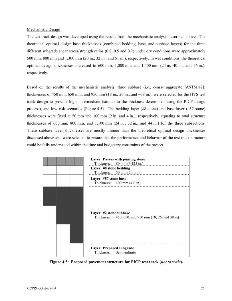
UCPRC-RR-2014-04 25
Mechanistic Design
The test track design was developed using the results from the mechanistic analysis described above. The
theoretical optimal design base thicknesses (combined bedding, base, and subbase layers) for the three
different subgrade shear stress/strength ratios (0.8, 0.5 and 0.2) under dry conditions were approximately
500 mm, 800 mm and 1,300 mm (20 in., 32 in., and 51 in.), respectively. In wet conditions, the theoretical
optimal design thicknesses increased to 600 mm, 1,000 mm and 1,400 mm (24 in, 40 in., and 56 in.),
respectively.
Based on the results of the mechanistic analysis, three subbase (i.e., coarse aggregate [ASTM #2])
thicknesses of 450 mm, 650 mm, and 950 mm (18 in., 26 in., and ~38 in.), were selected for the HVS test
track design to provide high, intermediate (similar to the thickness determined using the PICP design
process), and low risk scenarios (Figure 4.5). The bedding layer (#8 stone) and base layer (#57 stone)
thicknesses were fixed at 50 mm and 100 mm (2 in. and 4 in.), respectively, equating to total structure
thicknesses of 600 mm, 800 mm, and 1,100 mm (24 in., 32 in., and 44 in.) for the three subsections.
These subbase layer thicknesses are mostly thinner than the theoretical optimal design thicknesses
discussed above and were selected to ensure that the performance and behavior of the test track structure
could be fully understood within the time and budgetary constraints of the project.
Layer: Pavers with jointing stone Thickness: 80 mm (3.125 in.) Layer: #8 stone bedding Thickness: 50 mm (2.0 in.)
Layer: #57 stone base Thickness: 100 mm (4.0 in)
Layer: #2 stone subbase Thickness: 450, 650, and 950 mm (18, 26, and 38 in)
Layer: Prepared subgrade Thickness: Semi-infinite
Figure 4.5: Proposed pavement structure for PICP test track (not to scale).
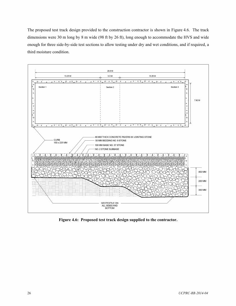
26 UCPRC-RR-2014-04
The proposed test track design provided to the construction contractor is shown in Figure 4.6. The track
dimensions were 30 m long by 8 m wide (98 ft by 26 ft), long enough to accommodate the HVS and wide
enough for three side-by-side test sections to allow testing under dry and wet conditions, and if required, a
third moisture condition.
Figure 4.6: Proposed test track design supplied to the contractor.
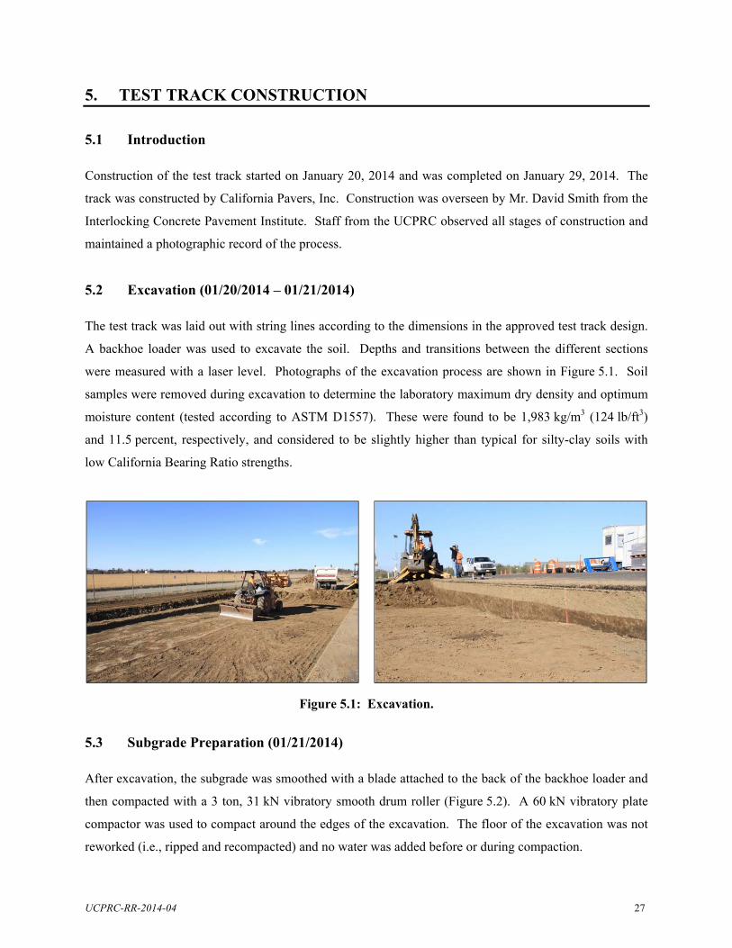
UCPRC-RR-2014-04 27
5. TEST TRACK CONSTRUCTION
5.1 Introduction
Construction of the test track started on January 20, 2014 and was completed on January 29, 2014. The
track was constructed by California Pavers, Inc. Construction was overseen by Mr. David Smith from the
Interlocking Concrete Pavement Institute. Staff from the UCPRC observed all stages of construction and
maintained a photographic record of the process.
5.2 Excavation (01/20/2014 – 01/21/2014)
The test track was laid out with string lines according to the dimensions in the approved test track design.
A backhoe loader was used to excavate the soil. Depths and transitions between the different sections
were measured with a laser level. Photographs of the excavation process are shown in Figure 5.1. Soil
samples were removed during excavation to determine the laboratory maximum dry density and optimum
moisture content (tested according to ASTM D1557). These were found to be 1,983 kg/m3 (124 lb/ft3)
and 11.5 percent, respectively, and considered to be slightly higher than typical for silty-clay soils with
low California Bearing Ratio strengths.
Figure 5.1: Excavation.
5.3 Subgrade Preparation (01/21/2014)
After excavation, the subgrade was smoothed with a blade attached to the back of the backhoe loader and
then compacted with a 3 ton, 31 kN vibratory smooth drum roller (Figure 5.2). A 60 kN vibratory plate
compactor was used to compact around the edges of the excavation. The floor of the excavation was not
reworked (i.e., ripped and recompacted) and no water was added before or during compaction.

28 UCPRC-RR-2014-04
Permeability measurements were taken before and after compaction using a Modified Philip-Dunne
Infiltrometer (100 mm, single ring tube) (18) (Figure 5.3). Before compaction, values averaged
0.03 cm/second, but after compaction, the permeability was less than 0.0001 cm/second (essentially not
measurable), indicating that infiltration of water into the subgrade would be very slow. A plot of
cumulative infiltration for six locations (two before compaction and four after compaction) on the
subgrade is shown in Figure 5.4. The plot clearly shows the effect of compaction on infiltration.
Figure 5.2: Subgrade compaction.
Figure 5.3: Permeability measurements. Figure 5.4: Cumulative infiltration of water into subgrade.
In situ density was measured with a nuclear density gauge after compaction (Figure 5.5). Relative
compaction (percent of laboratory determined modified Proctor density [ASTM D1557]) varied between
90 percent and 91 percent across the excavation. Compaction of the subgrade is listed as optional in the
ICPI guideline document (4), and if required by the designer, compaction to 95 percent of the laboratory
determined standard Proctor density (ASTM D698) is recommended.
Shear strength was measured with a dynamic cone penetrometer to a depth of 800 mm (~32 in.) below the
surface (Figure 5.6) and used to calculate an approximate in situ California Bearing Ratio (CBR). CBR
0
5
10
15
20
25
30
35
40
0 500 1,000 1,500 2,000 2,500 3,000 3,500 4,000
Cu
mu
lati
ve I
nfl
itar
ion
(cm
)
Cumulative Time (sec)
BC-1
BC-2
AC-1
AC-2
AC-3
AC-4
BC = Before Compaction, AC = After Compaction

UCPRC-RR-2014-04 29
values of three percent were consistent across the test track indicating that the subgrade was uniform, but
weak, and in line with the design criteria. A series of instruments (pressure cells, permanent deformation
gauges, and water level indicators) were also installed at this stage. Details on the instruments and
installation are provided in Section 6.3.
Figure 5.5: Density measurements. Figure 5.6: Dynamic cone penetrometer measurements.
Geotextile (Mirafi 160N) was placed on the floor and sides of the excavation to prevent pumping of
subgrade fines into the subbase material (Figure 5.7). Orange markers in the excavated area in the
photograph indicate location of the subgrade instrumentation on the three different depths.
Figure 5.7: Geotextile placement. 5.4 Subbase Placement (01/22/2014 – 01/23/2014)
Subbase aggregate was sourced from a quarry near Valley Springs, CA. The rhyolite aggregate is
described by the supplier as “#24 Rail Road Ballast”. The properties are summarized in Table 5.1 and for
the most part met the requirements for ASTM #2 stone listed in the ICPI guideline (4) and applicable
ASTM standards. The aggregate was end-dumped into the excavation from trucks or from a front loader,
and then spread with a loader into lifts approximately 30 cm (12 in.) thick (Figure 5.8). Each lift was
compacted with a 3 ton, 31 kN vibratory steel wheel roller and then a 60 kN vibratory plate compactor.
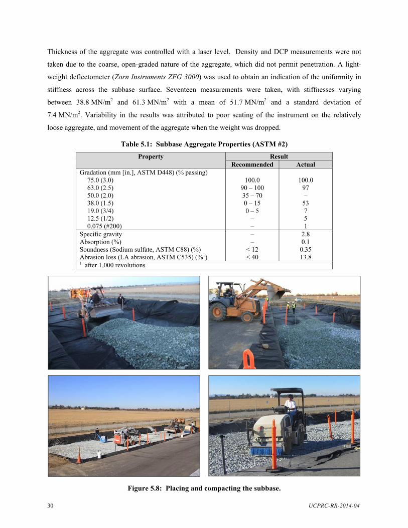
30 UCPRC-RR-2014-04
Thickness of the aggregate was controlled with a laser level. Density and DCP measurements were not
taken due to the coarse, open-graded nature of the aggregate, which did not permit penetration. A light-
weight deflectometer (Zorn Instruments ZFG 3000) was used to obtain an indication of the uniformity in
stiffness across the subbase surface. Seventeen measurements were taken, with stiffnesses varying
between 38.8 MN/m2 and 61.3 MN/m2 with a mean of 51.7 MN/m2 and a standard deviation of
7.4 MN/m2. Variability in the results was attributed to poor seating of the instrument on the relatively
loose aggregate, and movement of the aggregate when the weight was dropped.
Table 5.1: Subbase Aggregate Properties (ASTM #2)
Property Result Recommended Actual
Gradation (mm [in.], ASTM D448) (% passing) 75.0 (3.0) 63.0 (2.5) 50.0 (2.0) 38.0 (1.5) 19.0 (3/4) 12.5 (1/2) 0.075 (#200)
100.0
90 – 100 35 – 70 0 – 15 0 – 5
– –
100.0
97 –
53 7 5 1
Specific gravity Absorption (%) Soundness (Sodium sulfate, ASTM C88) (%) Abrasion loss (LA abrasion, ASTM C535) (%1)
– –
< 12 < 40
2.8 0.1
0.35 13.8
1 after 1,000 revolutions
Figure 5.8: Placing and compacting the subbase.
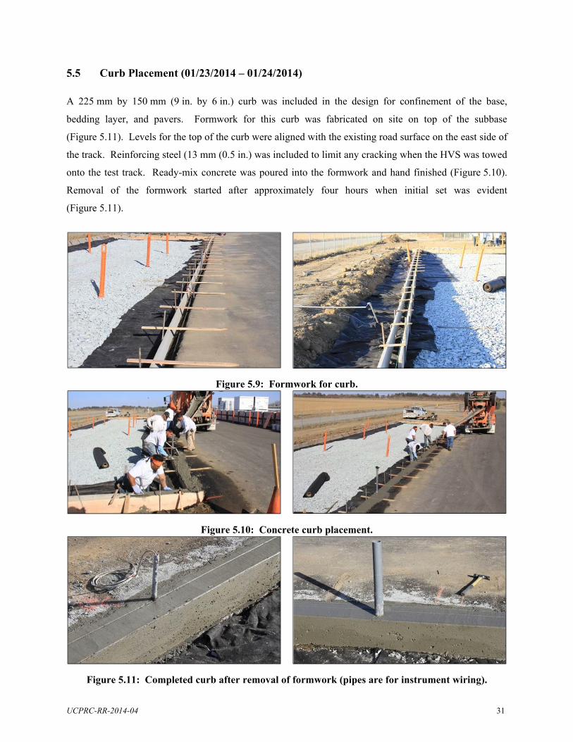
UCPRC-RR-2014-04 31
5.5 Curb Placement (01/23/2014 – 01/24/2014)
A 225 mm by 150 mm (9 in. by 6 in.) curb was included in the design for confinement of the base,
bedding layer, and pavers. Formwork for this curb was fabricated on site on top of the subbase
(Figure 5.11). Levels for the top of the curb were aligned with the existing road surface on the east side of
the track. Reinforcing steel (13 mm (0.5 in.) was included to limit any cracking when the HVS was towed
onto the test track. Ready-mix concrete was poured into the formwork and hand finished (Figure 5.10).
Removal of the formwork started after approximately four hours when initial set was evident
(Figure 5.11).
Figure 5.9: Formwork for curb.
Figure 5.10: Concrete curb placement.
Figure 5.11: Completed curb after removal of formwork (pipes are for instrument wiring).
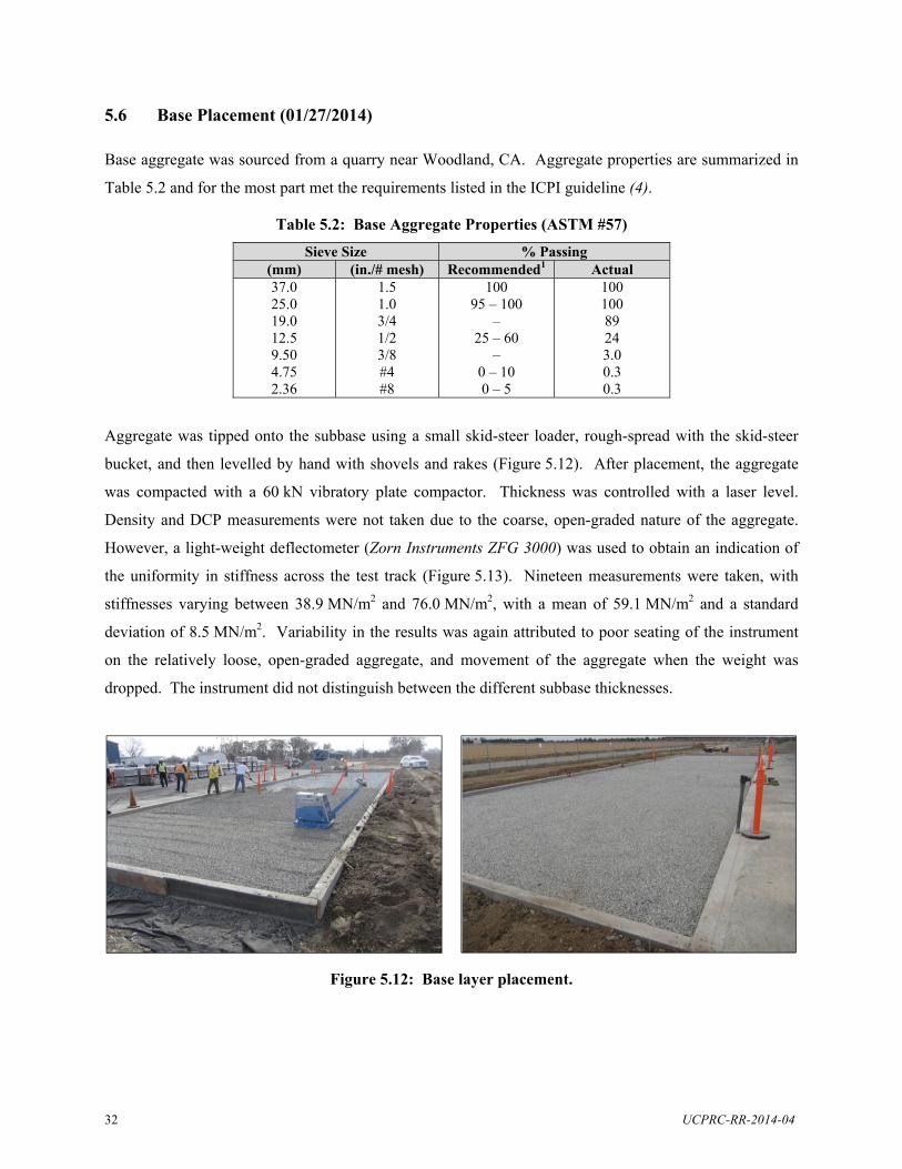
32 UCPRC-RR-2014-04
5.6 Base Placement (01/27/2014)
Base aggregate was sourced from a quarry near Woodland, CA. Aggregate properties are summarized in
Table 5.2 and for the most part met the requirements listed in the ICPI guideline (4).
Table 5.2: Base Aggregate Properties (ASTM #57)
Sieve Size % Passing (mm) (in./# mesh) Recommended1 Actual 37.0 25.0 19.0 12.5 9.50 4.75 2.36
1.5 1.0 3/4 1/2 3/8 #4 #8
100 95 – 100
– 25 – 60
– 0 – 10 0 – 5
100 100 89 24 3.0 0.3 0.3
Aggregate was tipped onto the subbase using a small skid-steer loader, rough-spread with the skid-steer
bucket, and then levelled by hand with shovels and rakes (Figure 5.12). After placement, the aggregate
was compacted with a 60 kN vibratory plate compactor. Thickness was controlled with a laser level.
Density and DCP measurements were not taken due to the coarse, open-graded nature of the aggregate.
However, a light-weight deflectometer (Zorn Instruments ZFG 3000) was used to obtain an indication of
the uniformity in stiffness across the test track (Figure 5.13). Nineteen measurements were taken, with
stiffnesses varying between 38.9 MN/m2 and 76.0 MN/m2, with a mean of 59.1 MN/m2 and a standard
deviation of 8.5 MN/m2. Variability in the results was again attributed to poor seating of the instrument
on the relatively loose, open-graded aggregate, and movement of the aggregate when the weight was
dropped. The instrument did not distinguish between the different subbase thicknesses.
Figure 5.12: Base layer placement.

UCPRC-RR-2014-04 33
Figure 5.13: Light-weight deflectometer testing on the base.
5.7 Bedding Layer Placement (01/28/2014)
Bedding layer aggregate was sourced from the same quarry as the base aggregate. Properties are
summarized in Table 5.3 and for the most part met the requirements listed in the ICPI guideline (4).
Table 5.3: Bedding Layer Aggregate Properties (ASTM #8)
Sieve Size % Passing (mm) (in./# mesh) Recommended Actual 12.5 9.50 4.75 2.36 1.18
1/2 3/8 #4 #8 #16
100 85 – 100 10 – 30 0 – 10 0 - 5
100.0 86 4.7 1.8 1.7
Aggregate was tipped onto the base using a small skid-steer loader, rough-spread with the skid-steer
bucket, then levelled by hand with shovels and rakes (Figure 5.14). Final smoothing was completed with
a straight edge run on two pipes that were positioned at the correct height. Depth was checked with a laser
level. The bedding layer was not compacted.
Figure 5.14: Bedding layer placement.

34 UCPRC-RR-2014-04
Figure 5.13: Bedding layer placement.
5.8 Paver Placement (01/28/2014 – 01/29/2014)
The pavers used to surface the test track were 195 mm x 95 mm x 80 mm (7.7 x 3.7 x 3.2 in.) in size and
reportedly met the requirements specified in ASTM C936 (Standard Specification for Solid Concrete
Interlocking Paving Units). Pavers were machine placed in a 90° herringbone pattern flush with the curb
using custom placing equipment (Figure 5.15).
Figure 5.15: Paver placement and compaction.

UCPRC-RR-2014-04 35
Edge (~100 x 100 mm) and full-size stitching pavers were placed by hand where required along the
concrete curbs. No pavers were cut. After placement, the pavers were compacted with 60 kN and 22 kN
vibratory plate compactors until a level surface was achieved. Jointing stone (crushed aggregate passing a
4.75 mm [#4]/ retained on a 2.36 mm [#8] sieve and meeting the requirements listed in Table 5.3) was
spread into the joints with brooms and then the surface was compacted again with a 22 kN plate
compactor (Figure 5.16). Photographs of the completed test track are shown in (Figure 5.17).
Figure 5.16: Jointing stone placement and compaction.
Figure 5.17: Completed test track.
5.9 Surface Permeability
Surface permeability was measured according to ASTM C1701 (Standard Test Method for Infiltration
Rate of In Place Pervious Concrete, which is similar to ASTM C1781 [Standard Test Method for Surface
Infiltration Rate of Permeable Unit Pavement Systems]). The results are summarized in Figure 5.18.
Permeability was consistent across the test track and considered to be rapid, with no water ponding on, or
running across, the surface.

36 UCPRC-RR-2014-04
Figure 5.18: Surface permeability after construction.
5.10 Material Sampling
Samples of all layers were collected during construction and retained for future testing if required. The
optimum moisture content and maximum dry density of the subgrade material were determined to
establish the degree of compaction (see Section 5.3).
0.00
0.05
0.10
0.15
0.20
0.25
0.30
0.35
450mm 650mm 950mm
Hyd
rau
lic C
on
du
ctiv
ity
(cm
/s)
Test Location
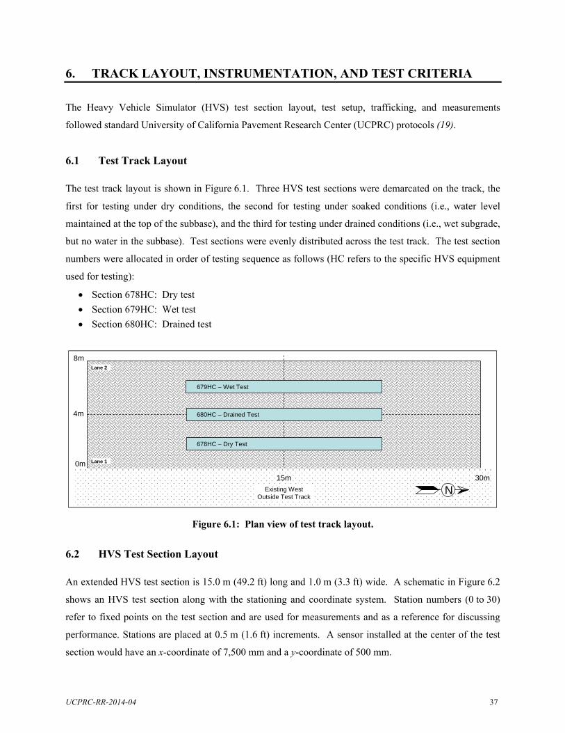
UCPRC-RR-2014-04 37
6. TRACK LAYOUT, INSTRUMENTATION, AND TEST CRITERIA
The Heavy Vehicle Simulator (HVS) test section layout, test setup, trafficking, and measurements
followed standard University of California Pavement Research Center (UCPRC) protocols (19).
6.1 Test Track Layout
The test track layout is shown in Figure 6.1. Three HVS test sections were demarcated on the track, the
first for testing under dry conditions, the second for testing under soaked conditions (i.e., water level
maintained at the top of the subbase), and the third for testing under drained conditions (i.e., wet subgrade,
but no water in the subbase). Test sections were evenly distributed across the test track. The test section
numbers were allocated in order of testing sequence as follows (HC refers to the specific HVS equipment
used for testing):
Section 678HC: Dry test
Section 679HC: Wet test
Section 680HC: Drained test
Figure 6.1: Plan view of test track layout.
6.2 HVS Test Section Layout
An extended HVS test section is 15.0 m (49.2 ft) long and 1.0 m (3.3 ft) wide. A schematic in Figure 6.2
shows an HVS test section along with the stationing and coordinate system. Station numbers (0 to 30)
refer to fixed points on the test section and are used for measurements and as a reference for discussing
performance. Stations are placed at 0.5 m (1.6 ft) increments. A sensor installed at the center of the test
section would have an x-coordinate of 7,500 mm and a y-coordinate of 500 mm.
0m
4m
8m
Lane 1
Lane 2
679HC – Wet Test
680HC – Drained Test
678HC – Dry Test
15m 30m
NExisting West Outside Test Track

38 UCPRC-RR-2014-04
Figure 6.2: Schematic of an extended HVS test section.
6.3 Test Section Instrumentation and Measurements
Measurements were taken with the equipment and instruments listed below. Instrument positions are
shown in Figure 6.2.
6.3.1 Temperatures
Type-K thermocouples were used to measure pavement and air temperatures at 60 minute intervals for the
duration of the test. Two thermocouples were bundled together to form a “thermocouple tree” for
measuring air and paver temperatures. Paver temperature was measured 25 mm below the surface.
Thermocouple trees were installed on the edge of each subsection (shaded by the HVS during part of the
day) and approximately 2.0 m from the center of the test section on the unshaded western side of the HVS.
Additional air temperatures were recorded at a weather station at the northern end of the test track.
6.3.2 Water Level in the Pavement
A perforated pipe (75 mm [3 in.] diameter) was installed on the east and west sides of the test track on
each subsection. The bottom of the pipe rested on the subgrade and the top of the pipe extended above the
Thermocouples (0 and 25mm) Thermocouple 80mm Paver
50mm Bedding Layer
0 2 4 6 8 10 12 14 16 18 20 22 24 26 28 30
y
x
Station Number (unit: 0.5m)
0.2 m0.2 m
1 m
Subgrade
N
Legend
NOT TO SCALE
Permanent deformation Road surface deflectometer Thermocouple
Surface profile measured at every station between Station 3 and Station 27
15 m
Subbase
Pressure cell
Top View
Cross Section
100mm Base
450mm 650mm 950mm
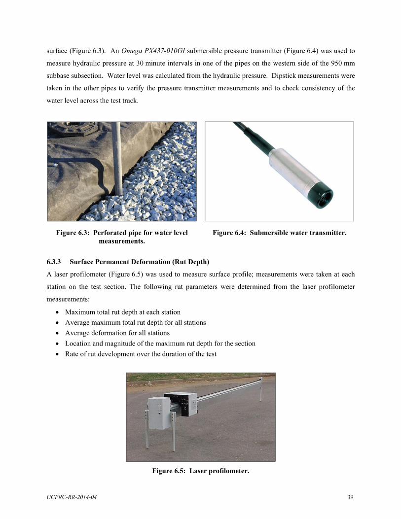
UCPRC-RR-2014-04 39
surface (Figure 6.3). An Omega PX437-010GI submersible pressure transmitter (Figure 6.4) was used to
measure hydraulic pressure at 30 minute intervals in one of the pipes on the western side of the 950 mm
subbase subsection. Water level was calculated from the hydraulic pressure. Dipstick measurements were
taken in the other pipes to verify the pressure transmitter measurements and to check consistency of the
water level across the test track.
Figure 6.3: Perforated pipe for water level measurements.
Figure 6.4: Submersible water transmitter.
6.3.3 Surface Permanent Deformation (Rut Depth)
A laser profilometer (Figure 6.5) was used to measure surface profile; measurements were taken at each
station on the test section. The following rut parameters were determined from the laser profilometer
measurements:
Maximum total rut depth at each station
Average maximum total rut depth for all stations
Average deformation for all stations
Location and magnitude of the maximum rut depth for the section
Rate of rut development over the duration of the test
Figure 6.5: Laser profilometer.
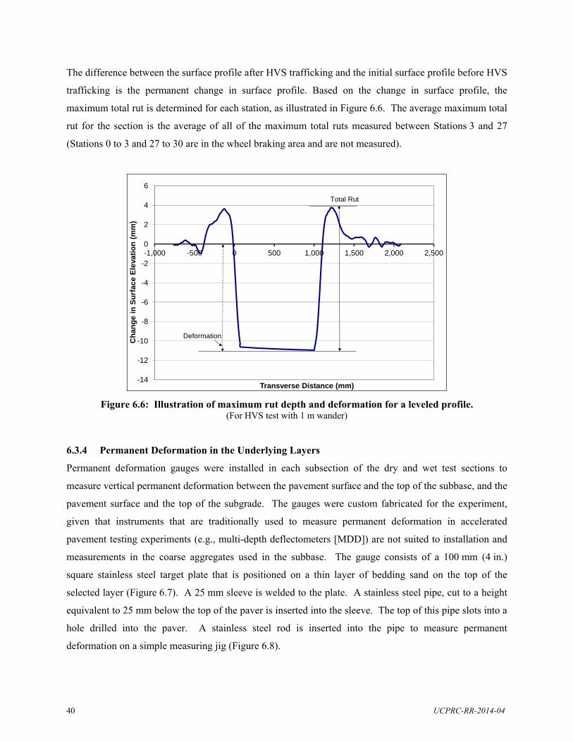
40 UCPRC-RR-2014-04
The difference between the surface profile after HVS trafficking and the initial surface profile before HVS
trafficking is the permanent change in surface profile. Based on the change in surface profile, the
maximum total rut is determined for each station, as illustrated in Figure 6.6. The average maximum total
rut for the section is the average of all of the maximum total ruts measured between Stations 3 and 27
(Stations 0 to 3 and 27 to 30 are in the wheel braking area and are not measured).
Figure 6.6: Illustration of maximum rut depth and deformation for a leveled profile. (For HVS test with 1 m wander)
6.3.4 Permanent Deformation in the Underlying Layers
Permanent deformation gauges were installed in each subsection of the dry and wet test sections to
measure vertical permanent deformation between the pavement surface and the top of the subbase, and the
pavement surface and the top of the subgrade. The gauges were custom fabricated for the experiment,
given that instruments that are traditionally used to measure permanent deformation in accelerated
pavement testing experiments (e.g., multi-depth deflectometers [MDD]) are not suited to installation and
measurements in the coarse aggregates used in the subbase. The gauge consists of a 100 mm (4 in.)
square stainless steel target plate that is positioned on a thin layer of bedding sand on the top of the
selected layer (Figure 6.7). A 25 mm sleeve is welded to the plate. A stainless steel pipe, cut to a height
equivalent to 25 mm below the top of the paver is inserted into the sleeve. The top of this pipe slots into a
hole drilled into the paver. A stainless steel rod is inserted into the pipe to measure permanent
deformation on a simple measuring jig (Figure 6.8).
-14
-12
-10
-8
-6
-4
-2
0
2
4
6
-1,000 -500 0 500 1,000 1,500 2,000 2,500
Ch
ang
e i
n S
urf
ace
Ele
vati
on
(m
m)
Transverse Distance (mm)
Total Rut
Deformation
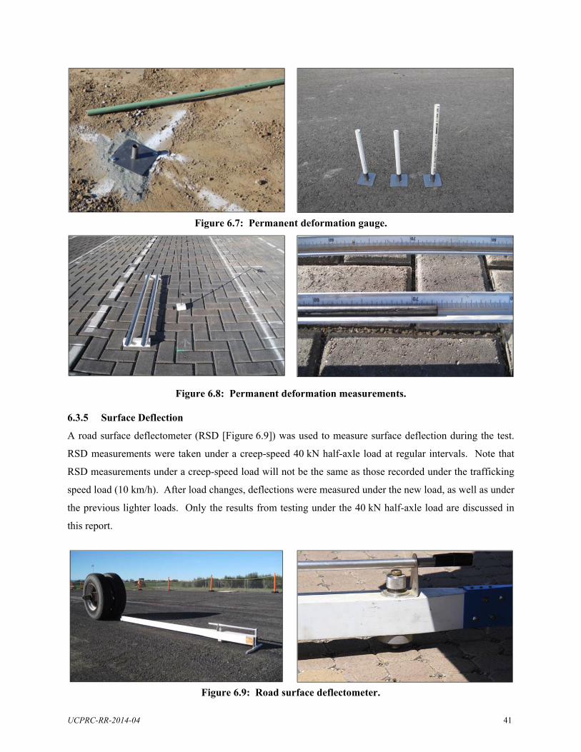
UCPRC-RR-2014-04 41
Figure 6.7: Permanent deformation gauge.
Figure 6.8: Permanent deformation measurements. 6.3.5 Surface Deflection
A road surface deflectometer (RSD [Figure 6.9]) was used to measure surface deflection during the test.
RSD measurements were taken under a creep-speed 40 kN half-axle load at regular intervals. Note that
RSD measurements under a creep-speed load will not be the same as those recorded under the trafficking
speed load (10 km/h). After load changes, deflections were measured under the new load, as well as under
the previous lighter loads. Only the results from testing under the 40 kN half-axle load are discussed in
this report.
Figure 6.9: Road surface deflectometer.

42 UCPRC-RR-2014-04
6.3.6 Vertical Pressure (stress) at the Top of the Subbase and Top of the Subgrade
Pressure cells were installed in each subsection of the dry and wet test sections to measure vertical
pressure (stress) under the moving wheel. One RST Instruments, Model #: LPTPC-09-S (1 MPa [150 psi]
range) pressure cell was installed level with the surface of the subgrade in each subsection after
excavation and compaction and before placement of the geotextile (Figure 6.10). A similar pressure cell
with 1.4 MPa (200 psi) range was installed on the top of the subbase. Bedding sand for the cells was
placed on top of a square of geotextile and used as a leveling course for the instrument to limit any
movement on top of the uneven coarse aggregate subbase (Figure 6.11).
Figure 6.10: Pressure cell installation in the subgrade.
Figure 6.11: Pressure cell installation on top of the subbase.
Example data recorded from one of the pressure cells is shown in Figure 6.12. Variation of the pressure
reading versus wheel position as the wheel travels from one end of the test section to the other is clearly
evident. Several quantities are summarized based on the raw readings. Specifically, the reference value is
the reading when the wheel is at the far end of the test section. The peak and valley are maximum and
minimum values deviating from the reference value, respectively.

UCPRC-RR-2014-04 43
Figure 6.12: Example pressure cell reading and definition of summary quantities.
6.3.7 Jointing Stone Depth
Jointing stone depth relative to the surface was measured with a depth gauge (Figure 6.13) at Stations 4
and 7 on the 450 mm subbase subsection, at Stations 12 and 14 on the 650 mm subbase subsection, at
Station 17 in a transition zone, and at Stations 25 and 26 on the 950 mm subbase subsection. Jointing
stone was replenished if the measured depth was below 25 mm (1 in.).
Figure 6.13: Jointing stone depth measurement.
6.4 HVS Test Criteria
6.4.1 Test Section Failure Criteria
An average maximum rut depth of 25 mm (1.0 in.) over the length of each subsection (Station 3 to
Station 10, Station 10 to Station 20, and Station 20 to Station 27) was set as the failure criteria for the
experiment. In some instances, HVS trafficking was continued past these points to fully understand
rutting behavior on the entire test section, given than the 450 mm subbase subsection would likely fail
before the thicker sections.
0
100
200
300
400
500
600
0 1 2 3 4 5 6 7 8
Raw
Pre
ssu
re C
ell
Rea
din
g (
kPa)
Wheel Position (m)
Raw_Reading
Valley
Peak
Reference = 341 kPa
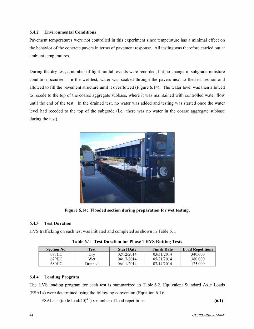
44 UCPRC-RR-2014-04
6.4.2 Environmental Conditions
Pavement temperatures were not controlled in this experiment since temperature has a minimal effect on
the behavior of the concrete pavers in terms of pavement response. All testing was therefore carried out at
ambient temperatures.
During the dry test, a number of light rainfall events were recorded, but no change in subgrade moisture
condition occurred. In the wet test, water was soaked through the pavers next to the test section and
allowed to fill the pavement structure until it overflowed (Figure 6.14). The water level was then allowed
to recede to the top of the coarse aggregate subbase, where it was maintained with controlled water flow
until the end of the test. In the drained test, no water was added and testing was started once the water
level had receded to the top of the subgrade (i.e., there was no water in the coarse aggregate subbase
during the test).
Figure 6.14: Flooded section during preparation for wet testing.
6.4.3 Test Duration
HVS trafficking on each test was initiated and completed as shown in Table 6.1.
Table 6.1: Test Duration for Phase 1 HVS Rutting Tests
Section No. Test Start Date Finish Date Load Repetitions 678HC 679HC 680HC
Dry Wet
Drained
02/12/2014 04/17/2014 06/11/2014
03/31/2014 05/21/2014 07/14/2014
340,000 380,000 125,000
6.4.4 Loading Program
The HVS loading program for each test is summarized in Table 6.2. Equivalent Standard Axle Loads
(ESALs) were determined using the following conversion (Equation 6.1):
ESALs = ((axle load/40)4.0) x number of load repetitions (6.1)

UCPRC-RR-2014-04 45
Table 6.2: Summary of HVS Loading Program
Section Test Half-Axle Wheel Load1 (kN)
Repetitions ESALs2
678HC Dry 25 40 60
100,000 100,000 140,000
15,259 100,000 708,750
Section Total 340,000 824,009 679HC Wet 25
40 60 80
100,000 100,000 140,000
40,000
15,259 100,000 708,750 640,000
Section Total 380,000 1,464,009 680HC Drained 25
40 100,000
25,000 15,259 25,000
Section Total 125,000 40,259 Project Total 845,000 2,328,277
1 40 kN = 9,000 lb.; 60 kN = 13,500 lb; 80 kN = 18,000 lb. 2 ESAL: Equivalent standard axle load
All trafficking was carried out with a dual-wheel configuration, using radial truck tires (Goodyear G159 -
11R22.5- steel belt radial) inflated to a pressure of 700 kPa (101 psi), in a bidirectional loading mode with
a one meter wide wander pattern (i.e., trafficking in both directions in line with standard procedures for
testing base layer performance). Load was checked with a portable weigh-in-motion pad at the beginning
of each test, after each load change, and at the end of each test.

46 UCPRC-RR-2014-04
Blank page
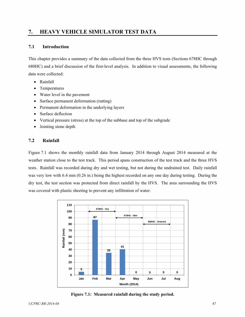
UCPRC-RR-2014-04 47
7. HEAVY VEHICLE SIMULATOR TEST DATA
7.1 Introduction
This chapter provides a summary of the data collected from the three HVS tests (Sections 678HC through
680HC) and a brief discussion of the first-level analysis. In addition to visual assessments, the following
data were collected:
Rainfall
Temperatures
Water level in the pavement
Surface permanent deformation (rutting)
Permanent deformation in the underlying layers
Surface deflection
Vertical pressure (stress) at the top of the subbase and top of the subgrade
Jointing stone depth
7.2 Rainfall
Figure 7.1 shows the monthly rainfall data from January 2014 through August 2014 measured at the
weather station close to the test track. This period spans construction of the test track and the three HVS
tests. Rainfall was recorded during dry and wet testing, but not during the undrained test. Daily rainfall
was very low with 6.4 mm (0.26 in.) being the highest recorded on any one day during testing. During the
dry test, the test section was protected from direct rainfall by the HVS. The area surrounding the HVS
was covered with plastic sheeting to prevent any infiltration of water.
Figure 7.1: Measured rainfall during the study period.
5
87
3541
0 0 0 00
10
20
30
40
50
60
70
80
90
100
110
Jan Feb Mar Apr May Jun Jul Aug
Rai
nfa
ll (
mm
)
Month (2014)
678HC - Dry
680HC - Drained
679HC - Wet
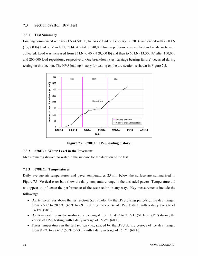
48 UCPRC-RR-2014-04
7.3 Section 678HC: Dry Test
7.3.1 Test Summary
Loading commenced with a 25 kN (4,500 lb) half-axle load on February 12, 2014, and ended with a 60 kN
(13,500 lb) load on March 31, 2014. A total of 340,000 load repetitions were applied and 26 datasets were
collected. Load was increased from 25 kN to 40 kN (9,000 lb) and then to 60 kN (13,500 lb) after 100,000
and 200,000 load repetitions, respectively. One breakdown (test carriage bearing failure) occurred during
testing on this section. The HVS loading history for testing on the dry section is shown in Figure 7.2.
Figure 7.2: 678HC: HVS loading history. 7.3.2 678HC: Water Level in the Pavement
Measurements showed no water in the subbase for the duration of the test.
7.3.3 678HC: Temperatures
Daily average air temperatures and paver temperatures 25 mm below the surface are summarized in
Figure 7.3. Vertical error bars show the daily temperature range in the unshaded pavers. Temperature did
not appear to influence the performance of the test section in any way. Key measurements include the
following:
Air temperatures above the test section (i.e., shaded by the HVS during periods of the day) ranged from 7.5°C to 20.5°C (46°F to 69°F) during the course of HVS testing, with a daily average of 14.1°C (58°F).
Air temperatures in the unshaded area ranged from 10.4°C to 21.5°C (51°F to 71°F) during the course of HVS testing, with a daily average of 15.7°C (60°F).
Paver temperatures in the test section (i.e., shaded by the HVS during periods of the day) ranged from 9.9°C to 22.6°C (50°F to 73°F) with a daily average of 15.5°C (60°F).
0
50
100
150
200
250
300
350
400
2/10/14 2/20/14 3/2/14 3/12/14 3/22/14 4/1/14 4/11/14
Nu
mb
er o
f L
oad
Rep
etit
ion
s (x
1,00
0)
Date
Loading Schedule
Number of Load Repetitions
25kN 40kN 60kN
Breakdown
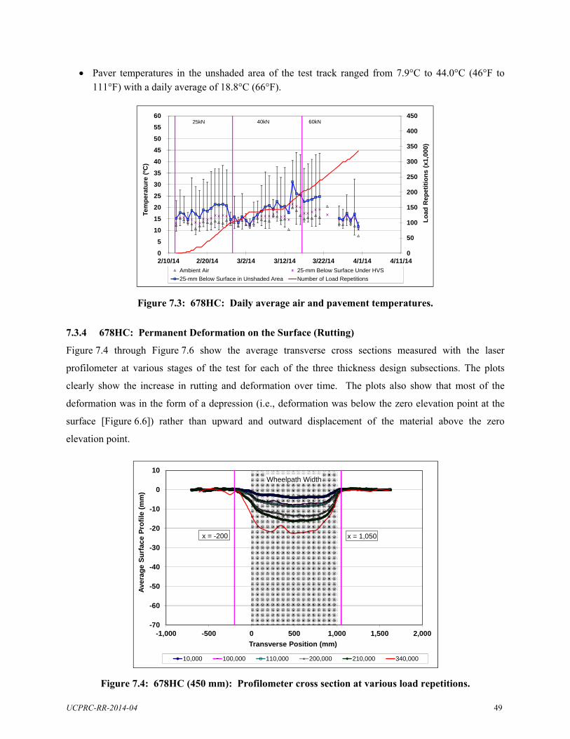
UCPRC-RR-2014-04 49
Paver temperatures in the unshaded area of the test track ranged from 7.9°C to 44.0°C (46°F to 111°F) with a daily average of 18.8°C (66°F).
Figure 7.3: 678HC: Daily average air and pavement temperatures.
7.3.4 678HC: Permanent Deformation on the Surface (Rutting)
Figure 7.4 through Figure 7.6 show the average transverse cross sections measured with the laser
profilometer at various stages of the test for each of the three thickness design subsections. The plots
clearly show the increase in rutting and deformation over time. The plots also show that most of the
deformation was in the form of a depression (i.e., deformation was below the zero elevation point at the
surface [Figure 6.6]) rather than upward and outward displacement of the material above the zero
elevation point.
Figure 7.4: 678HC (450 mm): Profilometer cross section at various load repetitions.
0
50
100
150
200
250
300
350
400
450
0
5
10
15
20
25
30
35
40
45
50
55
60
2/10/14 2/20/14 3/2/14 3/12/14 3/22/14 4/1/14 4/11/14
Lo
ad R
ep
etit
ion
s (x
1,00
0)
Tem
per
atu
re (
ºC)
DateAmbient Air 25-mm Below Surface Under HVS
25-mm Below Surface in Unshaded Area Number of Load Repetitions
25kN 60kN40kN
-70
-60
-50
-40
-30
-20
-10
0
10
-1,000 -500 0 500 1,000 1,500 2,000
Ave
rag
e S
urf
ace
Pro
file
(m
m)
Transverse Position (mm)
10,000 100,000 110,000 200,000 210,000 340,000
Wheelpath Width
x = -200 x = 1,050

50 UCPRC-RR-2014-04
Figure 7.5: 678HC (650 mm): Profilometer cross section at various load repetitions.
Figure 7.6: 678HC (950 mm): Profilometer cross section at various load repetitions.
Figure 7.7 shows the development of surface permanent deformation (average maximum total rut) with
load repetitions for the three subsections. Observations of surface rutting for each wheel load during the
dry test include the following:
25 kN (4,500 lb) Wheel Load + During HVS testing, rutting usually occurs at a high rate initially, and then it typically
diminishes as trafficking progresses until reaching a steady state. This initial phase is referred to
-70
-60
-50
-40
-30
-20
-10
0
10
-1,000 -500 0 500 1,000 1,500 2,000
Ave
rag
e S
urf
ace
Pro
file
(m
m)
Transverse Position (mm)
10,000 100,000 110,000 200,000 210,000 340,000
Wheelpath Width
x = -200 x = 1,100
-70
-60
-50
-40
-30
-20
-10
0
10
-1,000 -500 0 500 1,000 1,500 2,000
Ave
rag
e S
urf
ace
Pro
file
(m
m)
Transverse Position (mm)
100,000 110,000 200,000 210,000 340,000
Wheelpath Width
x = -150 x = 1,200
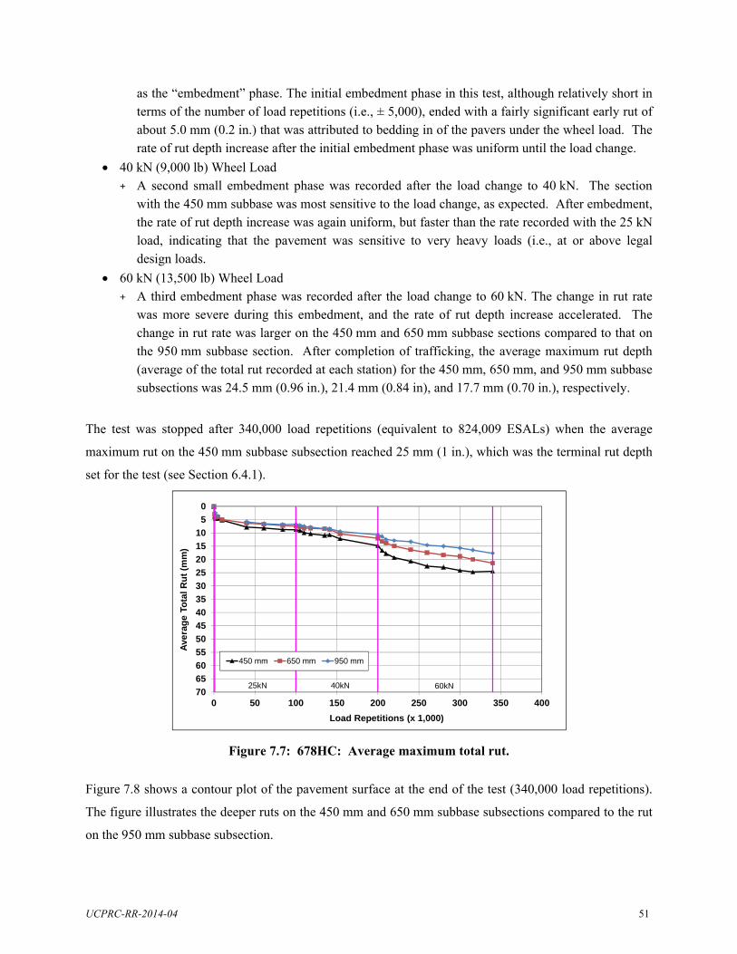
UCPRC-RR-2014-04 51
as the “embedment” phase. The initial embedment phase in this test, although relatively short in terms of the number of load repetitions (i.e., ± 5,000), ended with a fairly significant early rut of about 5.0 mm (0.2 in.) that was attributed to bedding in of the pavers under the wheel load. The rate of rut depth increase after the initial embedment phase was uniform until the load change.
40 kN (9,000 lb) Wheel Load + A second small embedment phase was recorded after the load change to 40 kN. The section
with the 450 mm subbase was most sensitive to the load change, as expected. After embedment, the rate of rut depth increase was again uniform, but faster than the rate recorded with the 25 kN load, indicating that the pavement was sensitive to very heavy loads (i.e., at or above legal design loads.
60 kN (13,500 lb) Wheel Load + A third embedment phase was recorded after the load change to 60 kN. The change in rut rate
was more severe during this embedment, and the rate of rut depth increase accelerated. The change in rut rate was larger on the 450 mm and 650 mm subbase sections compared to that on the 950 mm subbase section. After completion of trafficking, the average maximum rut depth (average of the total rut recorded at each station) for the 450 mm, 650 mm, and 950 mm subbase subsections was 24.5 mm (0.96 in.), 21.4 mm (0.84 in), and 17.7 mm (0.70 in.), respectively.
The test was stopped after 340,000 load repetitions (equivalent to 824,009 ESALs) when the average
maximum rut on the 450 mm subbase subsection reached 25 mm (1 in.), which was the terminal rut depth
set for the test (see Section 6.4.1).
Figure 7.7: 678HC: Average maximum total rut.
Figure 7.8 shows a contour plot of the pavement surface at the end of the test (340,000 load repetitions).
The figure illustrates the deeper ruts on the 450 mm and 650 mm subbase subsections compared to the rut
on the 950 mm subbase subsection.
0
5
10
15
20
25
30
35
40
45
50
55
60
65
700 50 100 150 200 250 300 350 400
Ave
rag
e T
ota
l R
ut
(mm
)
Load Repetitions (x 1,000)
450 mm 650 mm 950 mm
25kN 40kN 60kN

52 UCPRC-RR-2014-04
Figure 7.8: 678HC: Contour plot of permanent surface deformation (340,000 repetitions).
7.3.5 678HC: Permanent Deformation in the Underlying Layers
Permanent deformation in the underlying layers, recorded with a gauge in each subsection, and compared
to the surface layer (laser profilometer deformation [not total rut] measurement at the same measuring
stations), is shown in Figure 7.9, Figure 7.10, and Figure 7.11, for the 450 mm, 650 mm, and 950 mm
subbase subsections, respectively. The measurements were consistent with the laser profilometer
measurements. Deformation in each of the layers is summarized in Table 7.1. After 340,000 load
repetitions, permanent deformation in the bedding and base layer was consistent at about 3.8 mm
(0.15 in.) and was attributed to densification under the initial load. Other observations for the three
subsections include the following:
Subsection with 450 mm subbase layer + During the 25 kN wheel loading, most of the rutting occurred in the subbase, with very little
recorded in the subgrade. + After the load change to 40 kN, the rate of increase in permanent deformation in the subbase
remained relatively constant, but increased in the subgrade. + After completion of trafficking, permanent deformation was relatively evenly distributed
between the subbase (10.2 mm [0.4 in.]) and the subgrade (13.4 mm [0.53 in.]).
Subsection with 650 mm subbase layer + Throughout the test, most of the permanent deformation was recorded in the subbase, with
13.2 mm (0.52 in.) of deformation measured in this layer at the end of the test, with a smaller proportion recorded in the subgrade (6.0 mm [0.24 in.]). This implies that the thicker subbase limited deformation in the subgrade.
Subsection with 950 mm subbase layer + Almost all of the permanent deformation was recorded in the subbase on this subsection. At the
end of the test, the permanent deformation in the subbase was 12.5 mm (0.49 in.), with just
Stations
Tra
nsv
ers
e D
ista
nce
(m
m)
0 5 10 15 20 25 30
-500
0
500
1000
1500
Color Map for Profilometer Reading (mm)-24.3 -20.4 -16.4 -12.4 -8.5 -4.5 -0.6

UCPRC-RR-2014-04 53
0.7 mm (0.03 in.) recorded in the subgrade. Permanent deformation in the 650 mm and 950 mm subbase was therefore similar under dry conditions, but the thicker subbase essentially prevented any deformation in the subgrade.
Total permanent deformation measured with the gauge was 27.4 mm (1.08 in.), 23.0 mm (0.91 in.), and 17.0 mm (0.67 in.) on the three subsections (450 mm, 650 mm, and 950 mm subbase), respectively, implying a generally linear trend of increasing permanent deformation with decreasing subbase thickness.
There was a minor discrepancy between the permanent deformation measured on the surface with the laser profilometer and the gauge on the subsection with the 450 mm subbase, attributed to leveling of the baseline used as the zero measuring point.
Figure 7.9: 678HC 450 mm: Permanent deformation in the underlying layers.
Figure 7.10: 678HC 650 mm: Permanent deformation in the underlying layers.
05
10152025303540455055606570
0 50 100 150 200 250 300 350 400
Pe
rma
ne
nt
Def
orm
atio
n (
mm
)
Load Repetitions (x 1,000)
Top of Subbase Top of Subgrade Total Deformation
25kN 40kN 60kN
05
10152025303540455055606570
0 50 100 150 200 250 300 350 400
Pe
rma
ne
nt
Def
orm
atio
n (
mm
)
Load Repetitions (x 1,000)
Top of Subbase Top of Subgrade Total Deformation
25kN 40kN 60kN
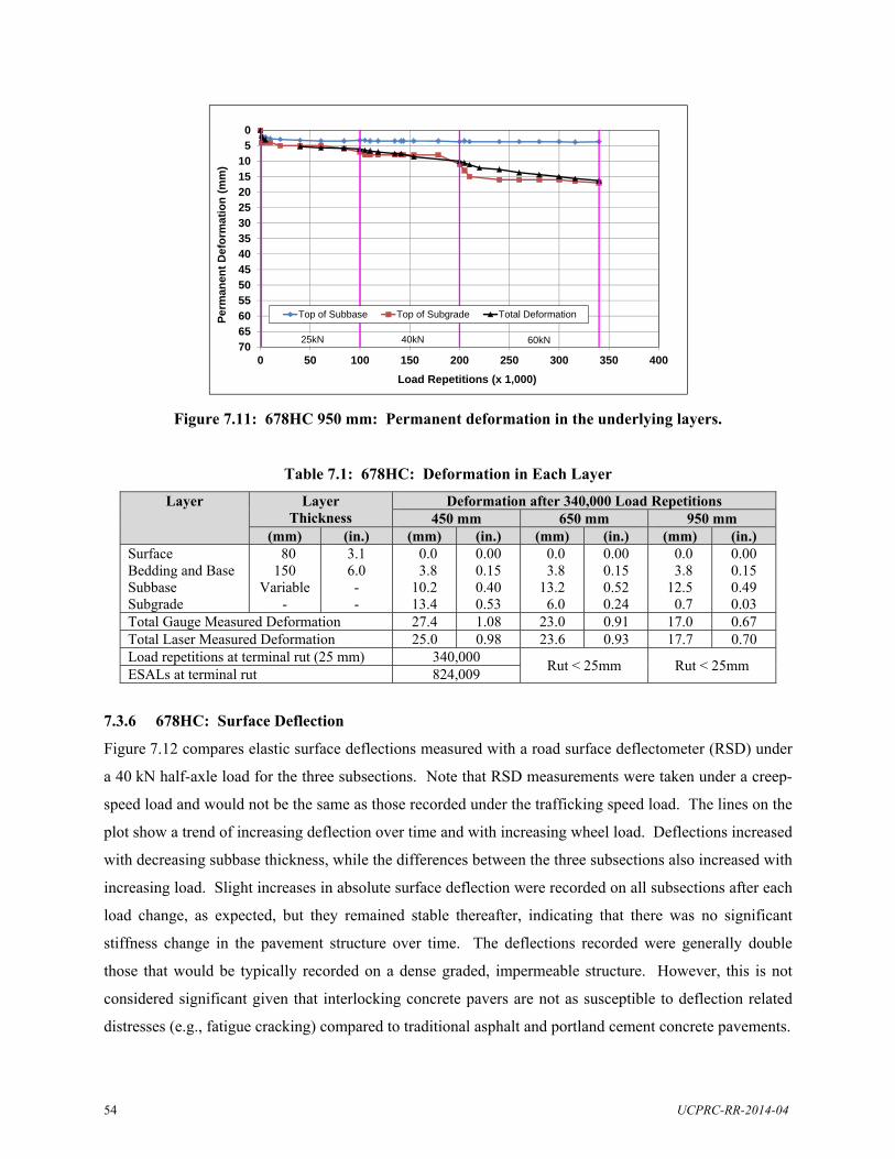
54 UCPRC-RR-2014-04
Figure 7.11: 678HC 950 mm: Permanent deformation in the underlying layers.
Table 7.1: 678HC: Deformation in Each Layer
Layer Layer Thickness
Deformation after 340,000 Load Repetitions 450 mm 650 mm 950 mm
(mm) (in.) (mm) (in.) (mm) (in.) (mm) (in.) Surface Bedding and Base Subbase Subgrade
80 150
Variable -
3.1 6.0 - -
0.0 3.8 10.2 13.4
0.00 0.15 0.40 0.53
0.0 3.8 13.2 6.0
0.00 0.15 0.52 0.24
0.0 3.8 12.5 0.7
0.00 0.15 0.49 0.03
Total Gauge Measured Deformation 27.4 1.08 23.0 0.91 17.0 0.67 Total Laser Measured Deformation 25.0 0.98 23.6 0.93 17.7 0.70 Load repetitions at terminal rut (25 mm) 340,000
Rut < 25mm Rut < 25mm ESALs at terminal rut 824,009
7.3.6 678HC: Surface Deflection
Figure 7.12 compares elastic surface deflections measured with a road surface deflectometer (RSD) under
a 40 kN half-axle load for the three subsections. Note that RSD measurements were taken under a creep-
speed load and would not be the same as those recorded under the trafficking speed load. The lines on the
plot show a trend of increasing deflection over time and with increasing wheel load. Deflections increased
with decreasing subbase thickness, while the differences between the three subsections also increased with
increasing load. Slight increases in absolute surface deflection were recorded on all subsections after each
load change, as expected, but they remained stable thereafter, indicating that there was no significant
stiffness change in the pavement structure over time. The deflections recorded were generally double
those that would be typically recorded on a dense graded, impermeable structure. However, this is not
considered significant given that interlocking concrete pavers are not as susceptible to deflection related
distresses (e.g., fatigue cracking) compared to traditional asphalt and portland cement concrete pavements.
05
10152025303540455055606570
0 50 100 150 200 250 300 350 400
Pe
rman
ent
De
form
ati
on
(m
m)
Load Repetitions (x 1,000)
Top of Subbase Top of Subgrade Total Deformation
25kN 40kN 60kN
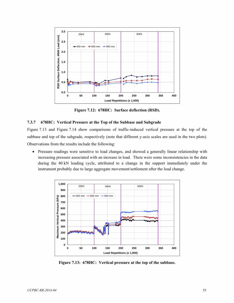
UCPRC-RR-2014-04 55
Figure 7.12: 678HC: Surface deflection (RSD).
7.3.7 678HC: Vertical Pressure at the Top of the Subbase and Subgrade
Figure 7.13 and Figure 7.14 show comparisons of traffic-induced vertical pressure at the top of the
subbase and top of the subgrade, respectively (note that different y-axis scales are used in the two plots).
Observations from the results include the following:
Pressure readings were sensitive to load changes, and showed a generally linear relationship with increasing pressure associated with an increase in load. There were some inconsistencies in the data during the 40 kN loading cycle, attributed to a change in the support immediately under the instrument probably due to large aggregate movement/settlement after the load change.
Figure 7.13: 678HC: Vertical pressure at the top of the subbase.
0.0
0.5
1.0
1.5
2.0
2.5
3.0
0 50 100 150 200 250 300 350 400
RS
D S
urf
ace
De
flec
tio
n,
40kN
Lo
ad (
mm
)
Load Repetitions (x 1,000)
450 mm 650 mm 950 mm
25kN 40kN 60kN
0
100
200
300
400
500
600
700
800
900
1,000
0 50 100 150 200 250 300 350 400
Ma
xim
um
Ve
rtic
al P
res
sure
(kP
a)
Load Repetitions (x 1,000)
450 mm 650 mm 950 mm
25kN 40kN 60kN

56 UCPRC-RR-2014-04
Figure 7.14: 678HC: Vertical pressure at the top of the subgrade.
At the top of the subbase, there was very little difference between the readings from the three subsections at the 25 kN and 40 kN load levels. After the load change to 60 kN, there was a more distinct difference between the three subsections, with higher pressures recorded on the thicker sections. This was attributed to the higher stiffnesses associated with the support from the thicker subbase layers.
Very low pressures were recorded at the top of the subgrade as expected; with higher pressures recorded under the 450 mm subbase subsection compared to those recorded under the 650 mm and 950 mm subbase subsections, respectively. The difference in the pressure recorded between the three subsections also increased with an increase in load, especially on the 450 mm subbase subsection, which relates to the permanent deformation measurements recorded on this subsection (Figure 7.9).
7.3.8 678HC: Jointing Stone Depth
Jointing stone depth at seven different locations for the duration of the test is shown in Figure 7.15. Stone
depth did not drop below 25 mm and the stone was not replenished. Stone loss was generally uniform
along the length of the section, with slightly higher stone loss on the 950 mm subbase subsection after the
load change to 60 kN. There were no known contributing factors to this higher stone loss and it did not
appear to influence behavior or performance on this subsection.
7.3.9 678HC: Visual Assessment
Apart from rutting, no other distress was recorded on the section. No cracked pavers were observed.
Some darkening of the paver surfaces was noted, attributed to rubber deposits and polishing from the HVS
tires. Photographs of the test section after HVS testing are shown in Figure 7.16.
0
20
40
60
80
100
120
140
160
180
200
0 50 100 150 200 250 300 350 400
Ma
xim
um
Ve
rtic
al P
ress
ure
(kP
a)
Load Repetitions (x 1,000)
450 mm 650 mm 950 mm
25kN 40kN 60kN

UCPRC-RR-2014-04 57
Figure 7.15: 678HC: Jointing stone depth.
Close up of 450 mm subbase subsection.
General view of test section looking from north to south Close up of 650 mm subbase subsection.
Figure 7.16: 678HC: Test section photographs.
0
5
10
15
20
25
30
350 50 100 150 200 250 300 350 400
Join
tin
g S
ton
e D
epth
(m
m)
Load Repetitions (x 1,000)
St-4 St-7 St-12 St-14 St-17 St-23 St-26
25kN 40kN 60kN
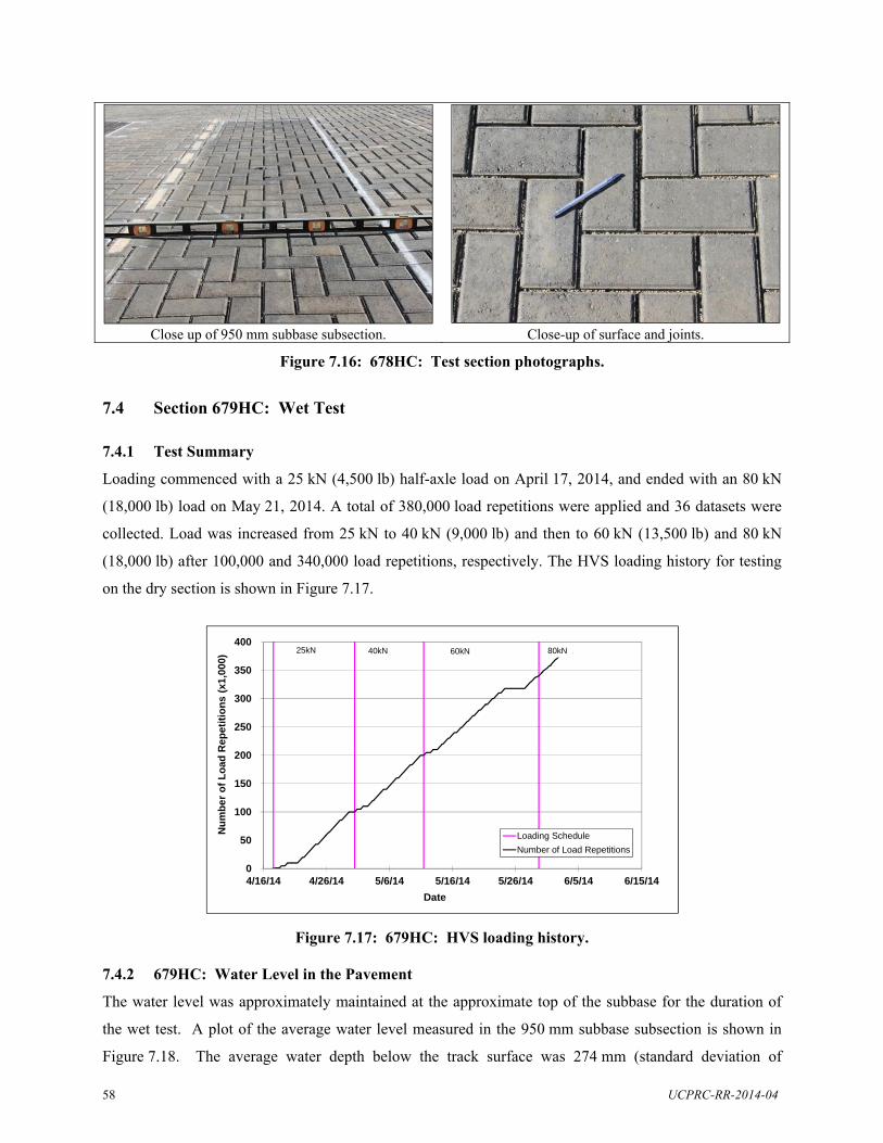
58 UCPRC-RR-2014-04
Close up of 950 mm subbase subsection. Close-up of surface and joints.
Figure 7.16: 678HC: Test section photographs.
7.4 Section 679HC: Wet Test
7.4.1 Test Summary
Loading commenced with a 25 kN (4,500 lb) half-axle load on April 17, 2014, and ended with an 80 kN
(18,000 lb) load on May 21, 2014. A total of 380,000 load repetitions were applied and 36 datasets were
collected. Load was increased from 25 kN to 40 kN (9,000 lb) and then to 60 kN (13,500 lb) and 80 kN
(18,000 lb) after 100,000 and 340,000 load repetitions, respectively. The HVS loading history for testing
on the dry section is shown in Figure 7.17.
Figure 7.17: 679HC: HVS loading history. 7.4.2 679HC: Water Level in the Pavement
The water level was approximately maintained at the approximate top of the subbase for the duration of
the wet test. A plot of the average water level measured in the 950 mm subbase subsection is shown in
Figure 7.18. The average water depth below the track surface was 274 mm (standard deviation of
0
50
100
150
200
250
300
350
400
4/16/14 4/26/14 5/6/14 5/16/14 5/26/14 6/5/14 6/15/14
Nu
mb
er
of
Lo
ad R
ep
eti
tio
ns
(x
1,0
00)
Date
Loading Schedule
Number of Load Repetitions
40kN 60kN25kN 80kN
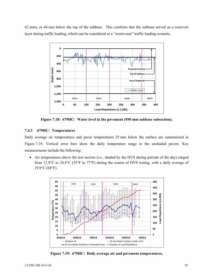
UCPRC-RR-2014-04 59
62 mm), or 44 mm below the top of the subbase. This confirms that the subbase served as a reservoir
layer during traffic loading, which can be considered as a “worst-case” traffic loading scenario.
Figure 7.18: 679HC: Water level in the pavement (950 mm subbase subsection).
7.4.3 679HC: Temperatures
Daily average air temperatures and paver temperatures 25 mm below the surface are summarized in
Figure 7.19. Vertical error bars show the daily temperature range in the unshaded pavers. Key
measurements include the following:
Air temperatures above the test section (i.e., shaded by the HVS during periods of the day) ranged from 12.8°C to 24.8°C (55°F to 77°F) during the course of HVS testing, with a daily average of 19.9°C (68°F).
Figure 7.19: 679HC: Daily average air and pavement temperatures.
0
200
400
600
800
1,000
1,200
1,4000 50 100 150 200 250 300 350 400
Dep
th (
mm
)
Load Repetitions (x 1,000)
Water Level
Top of Subbase
Pavement Surface
Top of Subgrade
25kN 40kN 60kN 80kN
0
50
100
150
200
250
300
350
400
450
0
5
10
15
20
25
30
35
40
45
50
55
60
4/16/14 4/26/14 5/6/14 5/16/14 5/26/14 6/5/14
Lo
ad
Re
pe
titi
on
s (
x1,
000
)
Tem
per
atu
re (
ºC)
DateAmbient Air 25-mm Below Surface Under HVS
25-mm Below Surface in Unshaded Area Number of Load Repetitions
40kN 60kN25kN 80kN
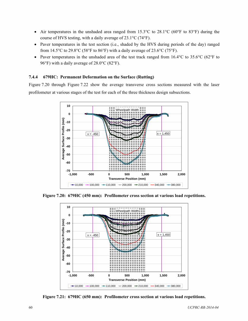
60 UCPRC-RR-2014-04
Air temperatures in the unshaded area ranged from 15.3°C to 28.1°C (60°F to 83°F) during the course of HVS testing, with a daily average of 23.1°C (74°F).
Paver temperatures in the test section (i.e., shaded by the HVS during periods of the day) ranged from 14.5°C to 29.8°C (58°F to 86°F) with a daily average of 23.6°C (75°F).
Paver temperatures in the unshaded area of the test track ranged from 16.4°C to 35.6°C (62°F to 96°F) with a daily average of 28.0°C (82°F).
7.4.4 679HC: Permanent Deformation on the Surface (Rutting)
Figure 7.20 through Figure 7.22 show the average transverse cross sections measured with the laser
profilometer at various stages of the test for each of the three thickness design subsections.
Figure 7.20: 679HC (450 mm): Profilometer cross section at various load repetitions.
Figure 7.21: 679HC (650 mm): Profilometer cross section at various load repetitions.
-70
-60
-50
-40
-30
-20
-10
0
10
-1,000 -500 0 500 1,000 1,500 2,000
Ave
rag
e S
urf
ace
Pro
file
(m
m)
Transverse Position (mm)
10,000 100,000 110,000 200,000 210,000 340,000 380,000
Wheelpath Width
x = -450 x = 1,450
-70
-60
-50
-40
-30
-20
-10
0
10
-1,000 -500 0 500 1,000 1,500 2,000
Ave
rag
e S
urf
ace
Pro
file
(m
m)
Transverse Position (mm)
10,000 100,000 110,000 200,000 210,000 340,000 380,000
Wheelpath Width
x = -450 x = 1,450

UCPRC-RR-2014-04 61
Figure 7.22: 679HC (950 mm): Profilometer cross section at various load repetitions.
The plots clearly show the increase in rutting and deformation over time. The plots also show that most of
the deformation was in the form of a depression rather than upward and outward displacement of the
material above the zero elevation point.
Figure 7.23 shows the development of permanent deformation (average maximum total rut and average
deformation) with load repetitions for the three subsections. This was significantly quicker compared to
the rut depths recorded during testing under dry conditions. Observations of surface rutting for each wheel
load during the wet test include the following:
25 kN (4,500 lb) Wheel Load + The initial embedment phase in this test, although relatively short in terms of the number of load
repetitions (i.e., ± 5,000), ended with much deeper ruts (6.5 mm on the 450 mm and 650 mm subbase subsections and 9.5 mm on the 950 mm subbase subsection) compared to the dry test. This was attributed partly to bedding in of the pavers under the wheel load and partly to early rutting in the underlying layers due to reorientation of the water-lubricated aggregates. The rate of rut depth increase after the initial embedment phase was uniform until the load change to 40 kN, but faster than that recorded on the dry section.
40 kN (9,000 lb) Wheel Load + A second small embedment phase was recorded after the load change to 40 kN. After
embedment, the rate of rut depth increase was again uniform, but faster than the rate recorded with the 25 kN load and with the 40 kN load on the dry test. The subsection with 450 mm subbase was notably more sensitive to loading compared to the subsections with 650 mm and 950 mm subbases.
-70
-60
-50
-40
-30
-20
-10
0
10
-1,000 -500 0 500 1,000 1,500 2,000
Ave
rag
e S
urf
ace
Pro
file
(m
m)
Transverse Position (mm)
10,000 100,000 110,000 200,000 210,000 340,000 380,000
Wheelpath Width
x = -300 x = 1,300

62 UCPRC-RR-2014-04
60 kN (13,500 lb) Wheel Load + A short but significant third embedment phase was recorded after the load change to 60 kN. The
rate of rut depth increase also accelerated compared to the 40 kN loading cycle, and to the dry test. The difference between the subsection with the 450 mm subbase and the subsections with the 650 mm and 950 mm subsections was again significant. After completion of trafficking at this load level (340,000 load repetitions), the average maximum rut depth for the 450 mm, 650 mm, and 950 mm subbase subsections was 50.5 mm (1.99 in.), 37.9 mm (1.49 in), and 33.7 mm (1.33 in.), respectively. These rut depths are approximately double those recorded on the dry test after the same traffic loading, indicating poorer performance when the subbase layer is serving as a reservoir for water that has drained through the pavers.
80 kN (18,000 lb) Wheel Load + A short test was conducted at an 80 kN wheel load to continue the assessment of load sensitivity
of the pavement structure under extreme moisture conditions. As expected, the rate of rut depth increase continued at a faster pace on all three subsections compared to that measured during the 60 kN loading. After completion of trafficking (additional 40,000 load repetitions [total 380,000]), the average maximum rut depth for the 450 mm, 650 mm, and 950 mm subbase subsections was 62.1 mm (2.44 in.), 46.8 mm (1.84 in), and 39.8 mm (1.57 in.), respectively.
Figure 7.23: 679HC: Average maximum total rut.
Terminal rut (25 mm [1 in.]) was reached after 180,000 load repetitions (95,259 ESALs) on the 450 mm
subbase subsection, after 210,000 load repetitions (165,884 ESALs) on the 650 mm subbase subsection,
and after 220,000 load repetitions (216,519 ESALs) on the 950 mm subbase subsection.
Figure 7.24 shows contour plots of the pavement surface after 340,000 load repetitions and at the end of
the test (380,000 load repetitions). The figures illustrate the deeper ruts on the 450 mm and 650 mm
subbase subsections compared to the rut on the 950 mm subbase subsection.
05
10
15
20
2530
35
40
45
5055
60
65
700 50 100 150 200 250 300 350 400
Ave
rag
e T
ota
l R
ut
(mm
)
Load Repetitions (x 1,000)
450 mm 650 mm 950 mm
25kN 40kN 60kN 80kN

UCPRC-RR-2014-04 63
Figure 7.24: 679HC: Contour plots of permanent surface deformation (340,000 repetitions).
Figure 7.25: 679HC: Contour plots of permanent surface deformation (380,000 repetitions).
7.4.5 679HC: Permanent Deformation in the Underlying Layers
Permanent deformation in the underlying layers, recorded with a gauge in each subsection, and compared
to the surface layer (laser profilometer deformation [not total rut] measurement at the same measuring
stations), is shown in Figure 7.26, Figure 7.27, and Figure 7.28, for the 450 mm, 650 mm, and 950 mm
Stations
Tra
nsv
ers
e D
ista
nce
(m
m)
0 5 10 15 20 25 30
-500
0
500
1000
1500
Color Map for Profilometer Reading (mm)-52.0 -43.9 -35.8 -27.8 -19.7 -11.6 -3.5
Stations
Tra
nsv
ers
e D
ista
nce
(m
m)
0 5 10 15 20 25 30
-500
0
500
1000
1500
Color Map for Profilometer Reading (mm)-63.8 -54.1 -44.3 -34.6 -24.9 -15.2 -5.5

64 UCPRC-RR-2014-04
subbase sections, respectively. The measurements were consistent with the laser profilometer
measurements. Deformation in each of the layers after 340,000 load repetitions (i.e., end of testing at
60 kN) is summarized in Table 7.2.
Figure 7.26: 679HC 450 mm: Permanent deformation in the underlying layers.
Figure 7.27: 679HC 650 mm: Permanent deformation in the underlying layers.
05
10152025303540455055606570
0 50 100 150 200 250 300 350 400
Pe
rma
nen
t D
efo
rmat
ion
(m
m)
Load Repetitions (x 1,000)
Top of Subbase Top of Subgrade Total Deformation
25kN 40kN 60kN 80kN
0
5
10
15
20
25
30
35
40
45
50
55
60
65
700 50 100 150 200 250 300 350 400
Per
man
en
t D
efo
rma
tio
n (
mm
)
Load Repetitions (x 1,000)
Top of Subbase Top of Subgrade Total Deformation
25kN 40kN 60kN 80kN
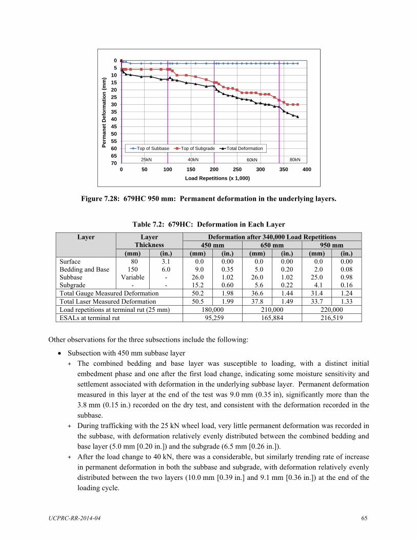
UCPRC-RR-2014-04 65
Figure 7.28: 679HC 950 mm: Permanent deformation in the underlying layers.
Table 7.2: 679HC: Deformation in Each Layer
Layer Layer Thickness
Deformation after 340,000 Load Repetitions 450 mm 650 mm 950 mm
(mm) (in.) (mm) (in.) (mm) (in.) (mm) (in.) Surface Bedding and Base Subbase Subgrade
80 150
Variable -
3.1 6.0 - -
0.0 9.0 26.0 15.2
0.00 0.35 1.02 0.60
0.0 5.0 26.0 5.6
0.00 0.20 1.02 0.22
0.0 2.0 25.0 4.1
0.00 0.08 0.98 0.16
Total Gauge Measured Deformation 50.2 1.98 36.6 1.44 31.4 1.24 Total Laser Measured Deformation 50.5 1.99 37.8 1.49 33.7 1.33 Load repetitions at terminal rut (25 mm) 180,000 210,000 220,000 ESALs at terminal rut 95,259 165,884 216,519
Other observations for the three subsections include the following:
Subsection with 450 mm subbase layer + The combined bedding and base layer was susceptible to loading, with a distinct initial
embedment phase and one after the first load change, indicating some moisture sensitivity and settlement associated with deformation in the underlying subbase layer. Permanent deformation measured in this layer at the end of the test was 9.0 mm (0.35 in), significantly more than the 3.8 mm (0.15 in.) recorded on the dry test, and consistent with the deformation recorded in the subbase.
+ During trafficking with the 25 kN wheel load, very little permanent deformation was recorded in the subbase, with deformation relatively evenly distributed between the combined bedding and base layer (5.0 mm [0.20 in.]) and the subgrade (6.5 mm [0.26 in.]).
+ After the load change to 40 kN, there was a considerable, but similarly trending rate of increase in permanent deformation in both the subbase and subgrade, with deformation relatively evenly distributed between the two layers (10.0 mm [0.39 in.] and 9.1 mm [0.36 in.]) at the end of the loading cycle.
0
5
10
15
20
25
30
35
40
45
50
55
60
65
700 50 100 150 200 250 300 350 400
Per
man
et D
efo
rmat
ion
(m
m)
Load Repetitions (x 1,000)
Top of Subbase Top of Subgrade Total Deformation
25kN 40kN 60kN 80kN

66 UCPRC-RR-2014-04
+ After the load change to 60 kN, permanent deformation in both the subbase and subgrade continued to increase at a much faster rate than that recorded in the dry test, with this trend continuing after the load change to 80 kN. However, unlike the dry test, more deformation was recorded in the subbase (26.0 mm [1.02 in.]) after 340,000 load repetitions than in the subgrade (15.2 mm [0.6 in.]), possibly indicating that the water-lubricated particles were susceptible to reorientation and further densification.
+ Increasing the load to 80 kN resulted in an increase in the rate of deformation, as expected, with a higher rate of deformation occurring in the subgrade, compared to the subbase. After the additional 40,000 load repetitions at 80 kN, deformation in the subbase had increased by 5.0 mm to 31.0 mm (1.2 in.), while deformation in the subgrade had increased by 6.4 mm to 21.7 mm (0.85 in.).
Subsection with 650 mm subbase layer + The combined bedding and base layer had less permanent deformation at the end of the test
compared to the thinner section, which was attributed to less deformation in the underlying layers. A small embedment was recorded after the first two load changes and thereafter permanent deformation in this layer remained relatively constant at 5.0 mm (0.2 in.)
+ In the first part of the test with 25 kN wheel loading, deformation was equally distributed between the base (3.7 mm [0.15 in.]), subbase (4.3 mm [0.17 in.]), and subgrade (3.1 mm [0.12 in.]).
+ After the load change to 40 kN, the rate of increase in permanent deformation was faster, with most occurring in the subbase (11 mm [0.43 in.]) rather than in the subgrade (3.6 mm [0.14 in.]) by the end of the loading cycle. This again implies that the thicker base limited deformation in the subgrade at design maximum axle loadings.
+ A similar trend continued after the load changes to 60 kN and 80 kn, but as with the 450 mm subbase subsection, the rate of increase in deformation with the subgrade started to increase at a faster rate, especially after the load change to 80 kN, indicating some load sensitivity in the soaked conditions. Permanent deformation of 26 mm (1.02 in.) and 5.6 mm (0.22 in.) was recorded in the subbase and subgrade respectively after 340,000 load repetitions, increasing to 29 mm (1.14 in.) and 11.7 mm (0.46 in.) respectively, after the additional 40,000 load repetitions.
+ Although considerably less permanent deformation was recorded on this subsection compared to the thinner subsection, it was still significantly higher than that recorded on the same subsection in the dry test. However, more deformation was recorded in the subbase compared to the subgrade in this subsection compared to the thinner one. The higher deformation recorded in the subbase compared to the subgrade was also consistent with the dry test.
Subsection with 950 mm subbase layer + Apart from minor embedment at the start of the test, permanent deformation in the combined
bedding and base layer (2 mm [0.08 in.]) did not increase during the test. + Similar trends to those recorded on the 650 mm subbase subsection were observed, although the
increase in the rate of deformation was slower, as expected. Most of the deformation again occurred in the subbase, with measurements of 25 mm (1.0 in) and 4.4 mm (0.17 in.) recorded in the subbase and subgrade respectively, after 340,000 load repetitions, and 28 mm (1.1 in.) and 8.2 mm (0.32 in.) respectively, after the additional 40,000 load repetitions at 80 kN.

UCPRC-RR-2014-04 67
Total permanent deformation measured with the gauge was 50.2 mm (1.98 in.), 36.6 mm (1.44 in.), and 31.4 mm (1.24 in.) on the three subsections (450 mm, 650 mm, and 950 mm subbase), respectively. This trend was not linear, with considerably more permanent deformation on the thin subsection compared to the thicker subsections, implying that thicker subbase layers will be necessary if water levels are maintained in the subbase.
There was a minor discrepancy between the permanent deformation measured on the surface with the laser profilometer and the gauge on the subsections with 450 mm and 650 mm subbase, which was again attributed to leveling of the baseline used as the zero measuring point.
7.4.6 679HC: Surface Deflection
Figure 7.29 compares elastic surface deflections under a 40 kN half-axle load for the three subsections.
The lines on the plot show a trend of increasing deflection over time and with increasing wheel load.
Deflections were considerably higher during all stages of this wet test compared to measurements during
the dry test, as expected. Deflections on the 450 mm subbase subsection were significantly higher than
those recorded on the subsections with thicker subbases, especially after the load changes, indicating a
load-sensitive, weaker overall structure as a result of the wet subgrade. The difference in deflection
between the 650 mm and 950 mm subbase subsections was distinct, but less significant.
Figure 7.29: 679HC: Surface deflection (RSD).
7.4.7 679HC: Vertical Pressure at the Top of the Subbase and Subgrade
Figure 7.30 and Figure 7.31 show comparisons of traffic-induced vertical pressure at the top of the
subbase and top of the subgrade, respectively (note that different y-axis scales are used in the two plots).
Observations from the results include the following:
Pressure readings were sensitive to load changes, and showed a generally linear relationship with increasing pressure associated with an increase in load. Inconsistencies (noise) in the data were
0.0
0.5
1.0
1.5
2.0
2.5
3.0
0 50 100 150 200 250 300 350 400
RS
D S
urf
ace
Def
lect
ion
, 40
kN L
oad
(m
m)
Load Repetitions (x 1,000)
450 mm 650 mm 950 mm
25kN 40kN 60kN 80kN25kN 40kN 60kN
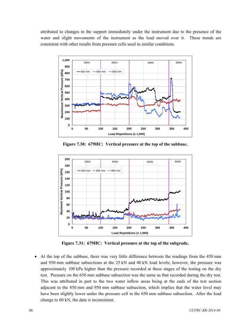
68 UCPRC-RR-2014-04
attributed to changes in the support immediately under the instrument due to the presence of the water and slight movements of the instrument as the load moved over it. These trends are consistent with other results from pressure cells used in similar conditions.
Figure 7.30: 679HC: Vertical pressure at the top of the subbase.
Figure 7.31: 679HC: Vertical pressure at the top of the subgrade.
At the top of the subbase, there was very little difference between the readings from the 450 mm and 950 mm subbase subsections at the 25 kN and 40 kN load levels; however, the pressure was approximately 100 kPa higher than the pressure recorded at these stages of the testing on the dry test. Pressure on the 650 mm subbase subsection was the same as that recorded during the dry test. This was attributed in part to the two water inflow areas being at the ends of the test section adjacent to the 450 mm and 950 mm subbase subsection, which implies that the water level may have been slightly lower under the pressure cell in the 650 mm subbase subsection. After the load change to 60 kN, the data is inconsistent.
0
100
200
300
400
500
600
700
800
900
1,000
0 50 100 150 200 250 300 350 400
Ma
xim
mu
m V
ert
ical
Pre
ssu
re (
kPa
)
Load Repetitions (x 1,000)
450 mm 650 mm 950 mm
25kN 40kN 60kN 80kN
0
20
40
60
80
100
120
140
160
180
200
0 50 100 150 200 250 300 350 400
Ma
xim
um
Ve
rtic
al P
ress
ure
(kP
a)
Load Repetitions (x 1,000)
450 mm 650 mm 950 mm
25kN 40kN 60kN 80kN
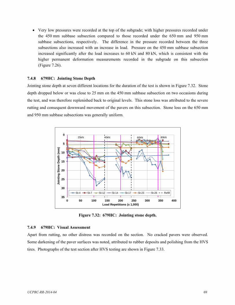
UCPRC-RR-2014-04 69
Very low pressures were recorded at the top of the subgrade; with higher pressures recorded under the 450 mm subbase subsection compared to those recorded under the 650 mm and 950 mm subbase subsections, respectively. The difference in the pressure recorded between the three subsections also increased with an increase in load. Pressure on the 450 mm subbase subsection increased significantly after the load increases to 60 kN and 80 kN, which is consistent with the higher permanent deformation measurements recorded in the subgrade on this subsection (Figure 7.26).
7.4.8 679HC: Jointing Stone Depth
Jointing stone depth at seven different locations for the duration of the test is shown in Figure 7.32. Stone
depth dropped below or was close to 25 mm on the 450 mm subbase subsection on two occasions during
the test, and was therefore replenished back to original levels. This stone loss was attributed to the severe
rutting and consequent downward movement of the pavers on this subsection. Stone loss on the 650 mm
and 950 mm subbase subsections was generally uniform.
Figure 7.32: 679HC: Jointing stone depth.
7.4.9 679HC: Visual Assessment
Apart from rutting, no other distress was recorded on the section. No cracked pavers were observed.
Some darkening of the paver surfaces was noted, attributed to rubber deposits and polishing from the HVS
tires. Photographs of the test section after HVS testing are shown in Figure 7.33.
0
5
10
15
20
25
30
350 50 100 150 200 250 300 350 400
Join
tin
g S
ton
e D
epth
(m
m)
Load Repetitions (x 1,000)
St-4 St-7 St-12 St-14 St-17 St-23 St-26 Refill
25kN 40kN 60kN 80kN

70 UCPRC-RR-2014-04
Close up of 450 mm subbase subsection.
General view of test section looking from north to south Close up of 650 mm subbase subsection.
Close up of 950 mm subbase subsection. Close-up of surface and joints.
Figure 7.33: 679HC: Test section photographs.
7.5 Section 680HC: Drained Test
7.5.1 Test Summary
This test was included to compare rate of rut increase on the section with no water in the subbase with rate
of rut increase on the dry and wet tests. This section did not contain pressure cells or permanent
deformation gauges. A limited number of load repetitions were applied, sufficient to compare surface
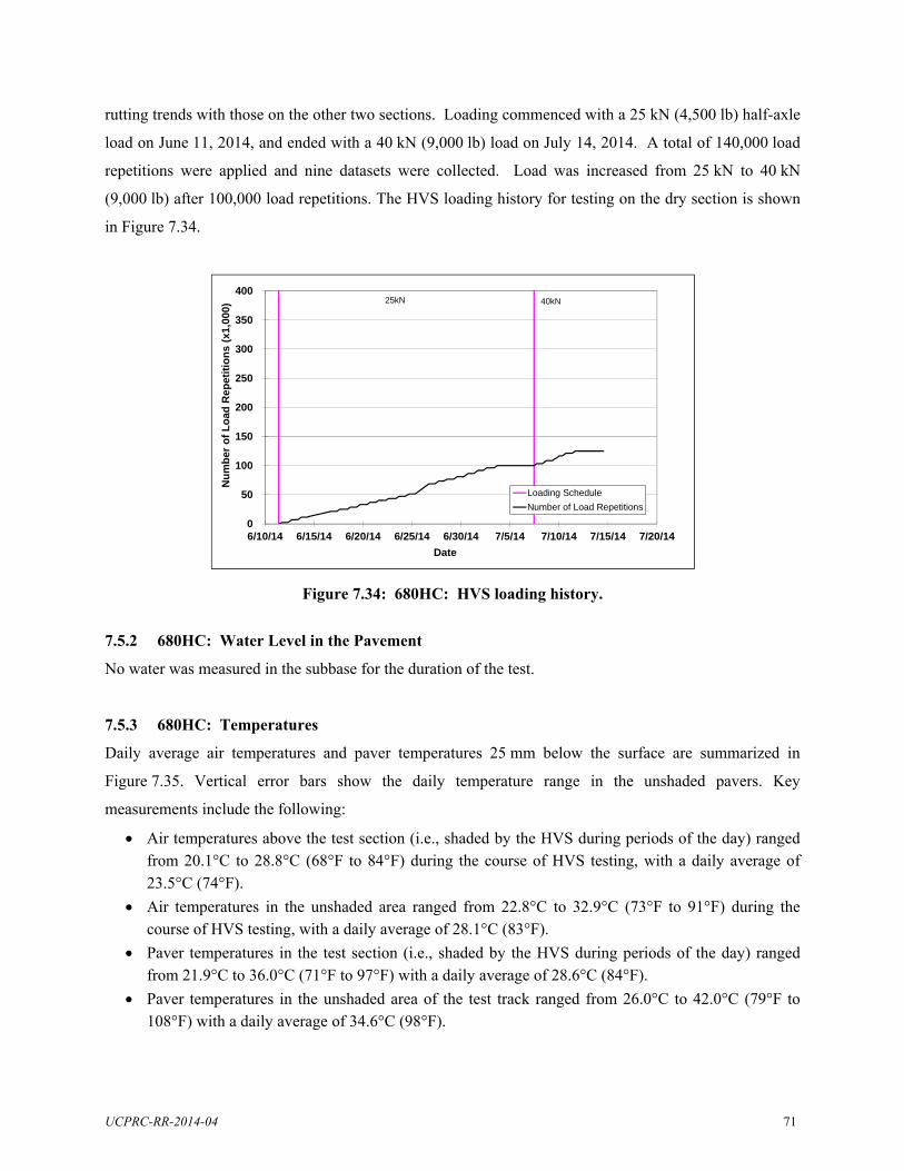
UCPRC-RR-2014-04 71
rutting trends with those on the other two sections. Loading commenced with a 25 kN (4,500 lb) half-axle
load on June 11, 2014, and ended with a 40 kN (9,000 lb) load on July 14, 2014. A total of 140,000 load
repetitions were applied and nine datasets were collected. Load was increased from 25 kN to 40 kN
(9,000 lb) after 100,000 load repetitions. The HVS loading history for testing on the dry section is shown
in Figure 7.34.
Figure 7.34: 680HC: HVS loading history.
7.5.2 680HC: Water Level in the Pavement
No water was measured in the subbase for the duration of the test.
7.5.3 680HC: Temperatures
Daily average air temperatures and paver temperatures 25 mm below the surface are summarized in
Figure 7.35. Vertical error bars show the daily temperature range in the unshaded pavers. Key
measurements include the following:
Air temperatures above the test section (i.e., shaded by the HVS during periods of the day) ranged from 20.1°C to 28.8°C (68°F to 84°F) during the course of HVS testing, with a daily average of 23.5°C (74°F).
Air temperatures in the unshaded area ranged from 22.8°C to 32.9°C (73°F to 91°F) during the course of HVS testing, with a daily average of 28.1°C (83°F).
Paver temperatures in the test section (i.e., shaded by the HVS during periods of the day) ranged from 21.9°C to 36.0°C (71°F to 97°F) with a daily average of 28.6°C (84°F).
Paver temperatures in the unshaded area of the test track ranged from 26.0°C to 42.0°C (79°F to 108°F) with a daily average of 34.6°C (98°F).
0
50
100
150
200
250
300
350
400
6/10/14 6/15/14 6/20/14 6/25/14 6/30/14 7/5/14 7/10/14 7/15/14 7/20/14
Nu
mb
er o
f L
oad
Rep
etit
ion
s (x
1,00
0)
Date
Loading Schedule
Number of Load Repetitions
40kN25kN
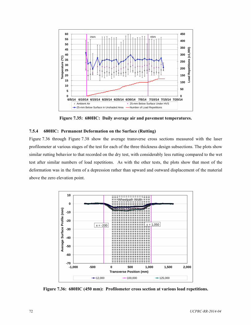
72 UCPRC-RR-2014-04
Figure 7.35: 680HC: Daily average air and pavement temperatures.
7.5.4 680HC: Permanent Deformation on the Surface (Rutting)
Figure 7.36 through Figure 7.38 show the average transverse cross sections measured with the laser
profilometer at various stages of the test for each of the three thickness design subsections. The plots show
similar rutting behavior to that recorded on the dry test, with considerably less rutting compared to the wet
test after similar numbers of load repetitions. As with the other tests, the plots show that most of the
deformation was in the form of a depression rather than upward and outward displacement of the material
above the zero elevation point.
Figure 7.36: 680HC (450 mm): Profilometer cross section at various load repetitions.
0
50
100
150
200
250
300
350
400
450
0
5
10
15
20
25
30
35
40
45
50
55
60
6/5/14 6/10/14 6/15/14 6/20/14 6/25/14 6/30/14 7/5/14 7/10/14 7/15/14 7/20/14
Lo
ad R
epet
itio
ns
(x1,
000
)
Tem
per
atu
re (
ºC)
DateAmbient Air 25-mm Below Surface Under HVS
25-mm Below Surface in Unshaded Area Number of Load Repetitions
40kN25kN
-70
-60
-50
-40
-30
-20
-10
0
10
-1,000 -500 0 500 1,000 1,500 2,000
Ave
rag
e S
urf
ace
Pro
file
(m
m)
Transverse Position (mm)
12,000 100,000 125,000
Wheelpath Width
x = -200 x = 1,050

UCPRC-RR-2014-04 73
Figure 7.37: 680HC (650 mm): Profilometer cross section at various load repetitions.
Figure 7.38: 680HC (950 mm): Profilometer cross section at various load repetitions.
Figure 7.39 shows the development of permanent deformation (average maximum total rut and average
deformation) with load repetitions for the three subsections. The plots show that rutting trends and rut
depths were similar to those recorded on the dry section.
-70
-60
-50
-40
-30
-20
-10
0
10
-1,000 -500 0 500 1,000 1,500 2,000
Ave
rag
e S
urf
ace
Pro
file
(m
m)
Transverse Position (mm)
12,000 100,000 125,000
Wheelpath Width
x = -200 x = 1,050
-70
-60
-50
-40
-30
-20
-10
0
10
-1,000 -500 0 500 1,000 1,500 2,000
Ave
rag
e S
urf
ace
Pro
file
(m
m)
Transverse Position (mm)
12,000 100,000 125,000
Wheelpath Width
x = -200 x = 1,050

74 UCPRC-RR-2014-04
Figure 7.39: 680HC: Average maximum total rut.
7.5.5 680HC: Permanent Deformation in the Underlying Layers
Permanent deformation in the underlying layers was not measured in this test.
7.5.6 680HC: Surface Deflection
Figure 7.40 compares elastic surface deflections under a 40 kN half-axle load for the three subsections.
Deflections were generally in between those recorded during the dry and wet tests, indicating that the still-
wet subgrade influenced the behavior of the structure, although not to the same extent as when the subbase
was serving as a reservoir.
Figure 7.40: 680HC: Surface deflection (RSD).
0
5
10
15
20
25
30
35
40
45
50
55
60
65
700 50 100 150 200 250 300 350 400
Ave
rag
e T
ota
l R
ut
(mm
)
Load Repetitions (x 1,000)
450 mm 650 mm 950 mm
25kN 40kN
0.0
0.5
1.0
1.5
2.0
2.5
3.0
0 50 100 150 200 250 300 350 400
RS
D S
urf
ace
De
flec
tio
n,
40k
N L
oa
d (
mm
)
Load Repetitions (x 1,000)
450 mm 650 mm 950 mm
25kN 40kN 60kN
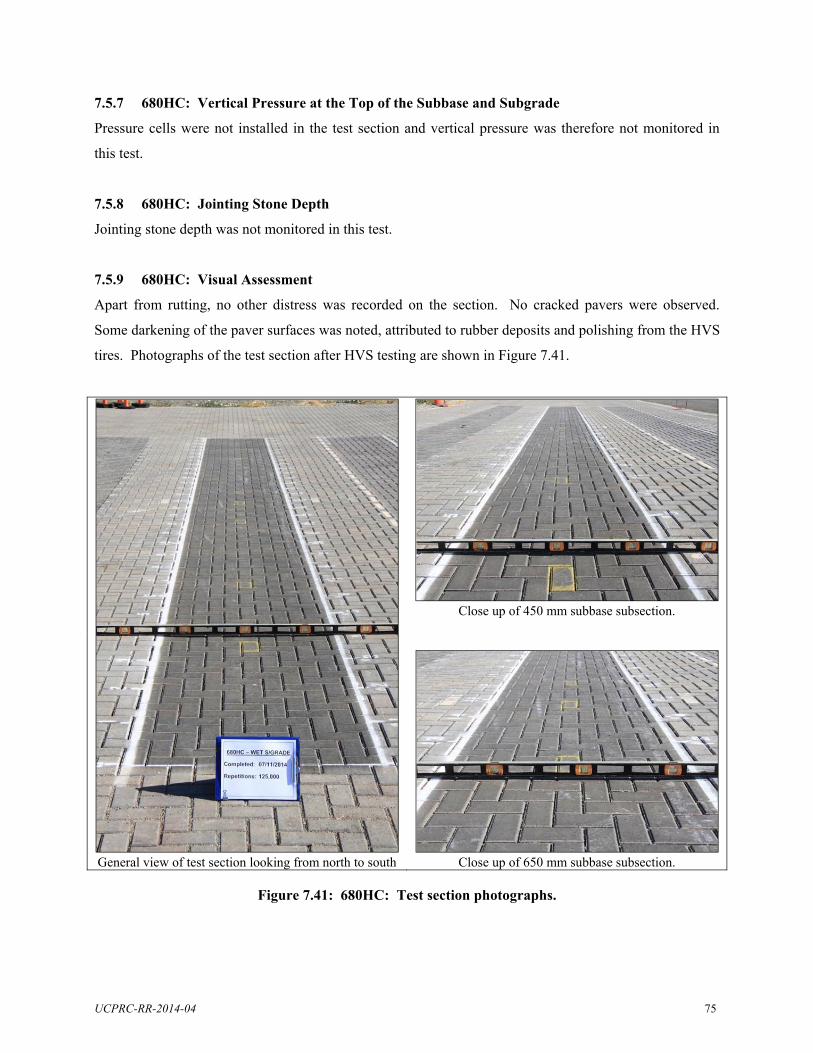
UCPRC-RR-2014-04 75
7.5.7 680HC: Vertical Pressure at the Top of the Subbase and Subgrade
Pressure cells were not installed in the test section and vertical pressure was therefore not monitored in
this test.
7.5.8 680HC: Jointing Stone Depth
Jointing stone depth was not monitored in this test.
7.5.9 680HC: Visual Assessment
Apart from rutting, no other distress was recorded on the section. No cracked pavers were observed.
Some darkening of the paver surfaces was noted, attributed to rubber deposits and polishing from the HVS
tires. Photographs of the test section after HVS testing are shown in Figure 7.41.
Close up of 450 mm subbase subsection.
General view of test section looking from north to south Close up of 650 mm subbase subsection.
Figure 7.41: 680HC: Test section photographs.
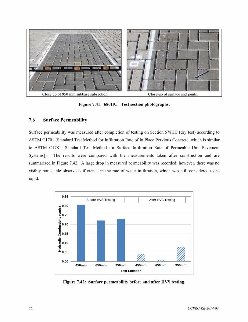
76 UCPRC-RR-2014-04
Close up of 950 mm subbase subsection. Close-up of surface and joints.
Figure 7.41: 680HC: Test section photographs.
7.6 Surface Permeability
Surface permeability was measured after completion of testing on Section 678HC (dry test) according to
ASTM C1701 (Standard Test Method for Infiltration Rate of In Place Pervious Concrete, which is similar
to ASTM C1781 [Standard Test Method for Surface Infiltration Rate of Permeable Unit Pavement
Systems]). The results were compared with the measurements taken after construction and are
summarized in Figure 7.42. A large drop in measured permeability was recorded; however, there was no
visibly noticeable observed difference in the rate of water infiltration, which was still considered to be
rapid.
Figure 7.42: Surface permeability before and after HVS testing.
0.00
0.05
0.10
0.15
0.20
0.25
0.30
0.35
450mm 650mm 950mm 450mm 650mm 950mm
Hyd
rau
lic C
on
du
ctiv
ity
(cm
/s)
Test Location
Before HVS Testing After HVS Testing

UCPRC-RR-2014-04 77
7.7 HVS Test Summary
Key observations from HVS testing include the following:
There was a significant difference in rutting performance and rutting behavior between the wet and dry tests, as expected.
A large proportion of the rutting on all three sections occurred as initial embedment in the first 2,000 to 5,000 load repetitions of the test and again after each of the load changes, implying that much of the rutting in the base and subbase layers was attributed to bedding in, densification, and/or reorientation of the aggregate particles. Although, this behavior is consistent with rutting behavior on other types of structures, better compaction of the base and subbase may have limited the extent.
During testing under dry conditions, limited permanent deformation (< 4 mm) was recorded in the bedding and base layers on all three subsections, and most occurred very early in the test. On the subsection with the 450 mm subbase, rutting occurred in both the subbase (10 mm rut) and subgrade (13 mm rut). On the 650 mm and 950 mm subbase subsections, rutting occurred mostly in the subbase. Total permanent deformation on the 450 mm, 650 mm, and 950 mm subbase subsections was 27 mm, 23 mm and 17 mm respectively, implying a generally linear trend of increasing permanent deformation with decreasing subbase thickness.
During testing under wet conditions, rutting in the bedding and base layers was dependent on the thickness of the subbase (9 mm, 5 mm and 2 mm on the 450 mm, 650 mm, and 950 mm subbase subsections, respectively). Rutting occurred in both the subbase and the subgrade on all subsections, with rutting in the subbase consistent across all three sections (~ 25 mm). Rutting in the subgrade differed between sections relative to subbase thickness, with 15 mm, 6 mm, and 4 mm of rut recorded on the 450 mm, 650 mm, and 950 mm subbase subsections, respectively.
Although only limited testing was undertaken under drained conditions (i.e., no water in the subbase), rutting behavior appeared to show similar trends and behavior to the test under dry conditions.
The thickness of the subbase influenced rut depth in the subgrade, as expected, but did not influence the rutting behavior in the subbase itself. Rutting in this layer therefore appears to be governed by the aggregate properties and construction methods and quality.
The rate of rut depth increase escalated with increasing load, indicating that the pavement structure was load sensitive, especially at load levels close to and above the legal design load.
Deflection during dry testing was dependent on subbase thickness and it increased with increasing load. Deflections were relatively high compared to more traditional pavements with dense graded layers. Deflection during wet testing was higher compared to that recorded during dry testing, with deflection on the 450 mm subbase subsection significantly higher compared to that recorded on the 650 mm and 950 mm subbase subsections, indicating a load-sensitive, weaker overall structure as a result of the wet subgrade.
No distress was noted on any individual pavers and no pavers were dislodged from the pavement during testing.
The measured infiltration rate of water through the joints between the pavers reduced marginally over the course of HVS testing; however, visually it was still considered to be both rapid and effective.

78 UCPRC-RR-2014-04
Blank page

UCPRC-RR-2014-04 79
8. DATA ANALYSIS
This chapter covers the development of a mechanistic-empirical (M-E) design method for permeable
interlocking concrete pavements (PICP) based on mechanistic analysis and partial validation with the
accelerated pavement testing results discussed in Chapter 7. The same approach to that described in
Chapter 4 was followed, but some of the assumptions were adjusted based on the results from the HVS
testing.
8.1 Design Criteria, Design Variables, and Critical Responses
The design criteria, design variables, and critical responses used in the original test track design and
discussed in Chapter 4 (Section 4.2) were used in the mechanistic analysis. However, in the initial design,
the bedding, base, and subbase layers were combined into a single aggregate base layer for purposes of the
design. The results of HVS testing indicated that rutting behavior in the bedding and base layers differed
from that in the subbase layer during the wet test, and consequently, the bedding and base layers were
combined into a single layer and analyzed separately from the subbase layer in this stage of the analysis.
8.2 Rut Models for Different Layers
Based on the observations made and measurements taken during HVS testing, it was concluded that no
deformation or distress occurred in the pavers, only in the underlying layers, which resulted in measurable
deformation on the surface. Consequently, although surface rutting is the primary criterion designed for
and predicted in the analysis, it is assumed that the pavers themselves would not deform. It should also be
noted that, although individual pavers have a relatively high stiffness, a permeable surface layer
constructed of pavers does not, due to the wider spacing and reduced interlock between the pavers
compared to pavers with sand joints.
8.2.1 Combined Bedding and Base Layer
During testing under dry conditions (see Section 7.3), a rapid embedment of about 4 mm was recorded in
the combined bedding and base layer on the three subsections in the first 2,000 load repetitions.
Thereafter, no further significant rutting was recorded for the remainder of the test on any of the
subsections. The rut depth model of this combined layer under dry conditions was therefore set as a
constant (4 mm).
Under wet conditions (see Section 7.4), the rut depth in the combined bedding and base layers varied
depending on the subgrade thickness. On the 650 mm and 950 mm subbase subsections, most of the
80 UCPRC-RR-2014-04
rutting occurred during early embedment after which it remained relatively constant. On the 450 mm
subbase subsection, rutting was influenced by changes in the load. The rut depth model of this combined
layer for wet conditions was therefore set as a linear function of the subbase thickness (Table 8.1).
8.2.2 Subbase Layer
A typical mechanistic approach using the general formula in Equation 8.1 was used to develop the rutting
model for the subbase layer.
RDSB = aNb (8.1)
Where: RDSB is the rut depth of the subbase layer, N is the number of load repetitions, a and b are constants and are a function of the shear stress/strength ratio (SSRSB) at the top of the subbase layer, calculated using Equations 4.1 through 4.4.
A two-step model development process was followed:
Step 1. Fit RDSB = a(dN+N0)b for each testing case with different subbase thickness (h_SB), test
load (L), and test moisture condition (Dry and Wet), considering the effect of early embedment in the initial stages of trafficking. RDSB is the total rut depth in the subbase for a load level i; dN is the incremental repetition under that load level i; N0 is a model constant for considering the effect of earlier loading.
Step 2. Fit a ~ f(SSRSB) and b ~ f(SSRSB) for all testing cases.
Using the rut test data from the HVS testing, it was found that the rut depth showed an approximately
linear relationship with load repetitions after early initial embedment for all testing cases. Consequently,
the power constant b was set as 1. The constant a is a function of SSRSB, calculated for each case using
Equations 4.1 through 4.4. The subbase rut model is summarized in Table 8.1.
8.2.3 Subgrade
The procedure for developing the rutting model for the subgrade was similar to that used for the subbase
layer. The general formula for the rut model is (Equation 8.2):
RDSG = aNb (8.2)
Where: RDSG is the rut depth in the subgrade, N is the number of load repetitions, a and b are constants and are a function of the shear stress/strength ratio (SSRSG) at the top of the subgrade, calculated using Equations 4.1 through 4.4.
A two-step model development process similar to that described above was followed:
Step 1. Fit RDSG = a(dN+N0)b for each testing case with different subbase thickness (h_SB), test
load (L), and test moisture condition (Dry and Wet), considering the effect of early embedment.

UCPRC-RR-2014-04 81
RDSG is the total rut depth in the subgrade for a load level i; dN is the incremental repetition under that load level i; N0 is a model constant for considering the effect of earlier loading.
Step 2. Fit a ~ f(SSRSG) and b ~ f(SSRSG) for all testing cases.
Using the rut test data from the HVS testing, it was found that the rut depth in the subgrade had a power
relationship of approximately 0.5 with load repetitions after early embedment for all testing cases.
Consequently, the power constant c was set as 0.5. The constant a is a function of SSRSB, calculated for
each case using Equations 4.1 through 4.4. The subgrade rut model is summarized in Table 8.1.
Table 8.1: Summary of Rut Models Developed for Different Layers in a PICP
Layer Rut Model1 Moisture Condition
Model Parameters a b c
Combined bedding and base RDBB = a × h_SB + b Dry Wet
0 -0.012
4.0 13.1
- -
Subbase RDSB = (a × SSRb) × Nc Dry Wet
3.10E-06 3.10E-06
2.70 2.70
1 1
Subgrade (Silty clay) RDSG = (a × SSR + b) × Nc Dry Wet
0.03 0.03
-0.01 -0.01
0.5 0.5
1 RDxx, rut depth of xx layer (BB=surface(paver, bedding and base); SB=subbase; SG=subgrade), mm; h_SB, thickness of subbase, mm; SSR, shear stress/strength ratio at the top of the layer; N, load repetition; a, b, c, model constants.
Given that rutting in the subbase cannot be prevented simply by increasing the thickness of this layer, only
rutting in the subgrade was used in the development of the design tables. Changing the rutting behavior of
the subbase would require tighter specifications for the properties of the materials used in this layer,
and/or the construction methods (e.g., higher relative compaction/lower air void content). Consideration
for these alternatives would require laboratory and additional accelerated pavement testing to quantify the
effects of the changes, which was beyond the scope of this study.
8.3 Input Parameters for M-E Design of PICP
The default input parameters for mechanistic-empirical design of PICP were revised from those used in
the earlier study (see Table 4.1) based on the HVS test results and are summarized in Table 8.2 and
discussed in the following sections.
8.3.1 Pavement Structure
The same standard permeable interlocking concrete pavement structure used in the initial analysis was
used. However, as discussed above, for this analysis, the bedding and base layers were combined with the
pavers into a single surface layer, and the subbase was analyzed as a separate layer.
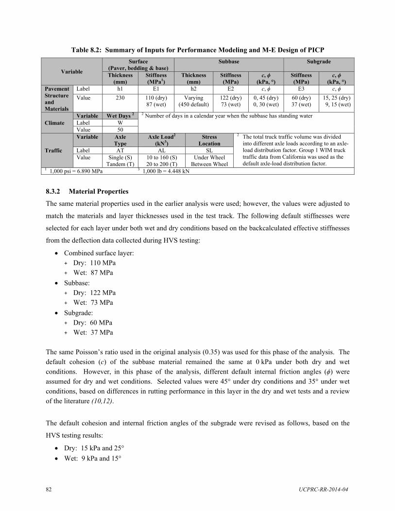
82 UCPRC-RR-2014-04
Table 8.2: Summary of Inputs for Performance Modeling and M-E Design of PICP
Variable
Surface (Paver, bedding & base)
Subbase Subgrade
Thickness (mm)
Stiffness (MPa1)
Thickness (mm)
Stiffness (MPa)
c, ϕ (kPa, °)
Stiffness (MPa)
c, ϕ (kPa, °)
Pavement Structure and Materials
Label h1 E1 h2 E2 c, ϕ E3 c, ϕ
Value 230 110 (dry) 87 (wet)
Varying (450 default)
122 (dry) 73 (wet)
0, 45 (dry) 0, 30 (wet)
60 (dry) 37 (wet)
15, 25 (dry) 9, 15 (wet)
Climate Variable Wet Days 2 2 Number of days in a calendar year when the subbase has standing water Label W Value 50
Traffic
Variable Axle Type
Axle Load2
(kN3) Stress
Location
2 The total truck traffic volume was divided into different axle loads according to an axle-load distribution factor. Group 1 WIM truck traffic data from California was used as the default axle-load distribution factor.
Label AT AL SL Value Single (S)
Tandem (T) 10 to 160 (S) 20 to 200 (T)
Under WheelBetween Wheel
1 1,000 psi = 6.890 MPa 3 1,000 lb = 4.448 kN
8.3.2 Material Properties
The same material properties used in the earlier analysis were used; however, the values were adjusted to
match the materials and layer thicknesses used in the test track. The following default stiffnesses were
selected for each layer under both wet and dry conditions based on the backcalculated effective stiffnesses
from the deflection data collected during HVS testing:
Combined surface layer: + Dry: 110 MPa + Wet: 87 MPa
Subbase: + Dry: 122 MPa + Wet: 73 MPa
Subgrade: + Dry: 60 MPa + Wet: 37 MPa
The same Poisson’s ratio used in the original analysis (0.35) was used for this phase of the analysis. The default cohesion (c) of the subbase material remained the same at 0 kPa under both dry and wet conditions. However, in this phase of the analysis, different default internal friction angles (ϕ) were assumed for dry and wet conditions. Selected values were 45° under dry conditions and 35° under wet conditions, based on differences in rutting performance in this layer in the dry and wet tests and a review of the literature (10,12).
The default cohesion and internal friction angles of the subgrade were revised as follows, based on the
HVS testing results:
Dry: 15 kPa and 25°
Wet: 9 kPa and 15°
UCPRC-RR-2014-04 83
8.3.3 Climate
Based on the HVS test results, the worse-case design condition for PICP would be when the subbase
contains standing water (i.e., the subbase is serving as a reservoir for collected rainwater while that water
infiltrates the subgrade or drains through a subsurface drainage system). The number of wet days when the
subbase contains standing water is required to distribute the traffic between dry and wet periods. The
default number of wet days was set at 50.
8.3.4 Traffic
Traffic input was expanded from that used in the original analysis. An axle load spectrum for single and
tandem axles with dual wheels was used to characterize traffic. Twelve single axle loads ranging between
10 kN and 160 kN (2,250 lb and 36,000 lb) and ten tandem axle loads ranging between 20 kN and 200 kN
(4,500 lb and 45,000 lb) were considered. Tire pressure was set at 700 kPa (101 psi). The tandem axle
load was treated as two independent single axle loads. The distance between the two tire centers was set at
340 mm (13.4 in.). The stress under the wheel and the stress between the wheels were both calculated to
identify the most critical stress.
The total truck traffic volume was calculated from two-way annual average daily traffic (AADT),
percentage of trucks, direction distribution factor, lane distribution factor, annual growth rate, design life,
and traffic safety factor. The total truck traffic volume was divided into different axle loads according to
the axle-load distribution factor. The equivalent single axle load (ESAL) was then calculated using the
4th-power law.
8.4 Design Tool and Validation
A mechanistic-empirical design tool for permeable interlocking concrete pavements was created in an
Excel® spreadsheet and used to run the analyses and prepare the example design tables provided in
Chapter 9. The critical responses, including the major and minor principal stresses (σ1 and σ3) on top of
the subbase and subgrade layers, required for calculating the shear stress/strength ratio (SSR), were
calculated with the inputs listed above using multilayer linear elastic theory. The OpenPave software
program (5) was used for these analyses. An incremental recursive analysis method (20) was then used to
calculate the rut depth in the M-E design tool. The user interface for this design tool is shown in
Figure 8.1. The tool was used in two ways in this analysis to provide the following:
The expected total rut depth (derived from the predicted rut depth in the subgrade) based on the input values of pavement structure, material properties, climate, and traffic.
The required minimum thickness of the subbase layer for a given allowable rut depth.

84 UCPRC-RR-2014-04
Figure 8.1: User interface for the PICP design tool.
The design tool was validated and the results calibrated with the data collected during the three HVS tests.
No independent validation of the calibration was undertaken since only one set of HVS test data, and no
comprehensive long-term performance measurements with traffic and subbase water content data from in-
service pavements were available.
The comparison of measured and calculated rut depth for the HVS test sections is presented in Table 8.3
and Figure 8.2 for both dry and wet conditions. The maximum error between the measured and calculated
rut depths ranged from -4 percent to +5 percent, with rut depth shift factors of 1.10 for dry conditions and
1.23 for wet conditions.
Layer Moisture Condition Thickness (mm) Stiffness (MPa) 1 Poisson's Ratio c (kPa) φ (°)
Wet 87 0.35 - -
Dry 110 0.35 - -
Wet 73 0.35 0 30Dry 122 0.35 0 45Wet 37 0.35 9 15Dry 60 0.35 15 25
Number of Days in a Year When the Subbase has Standing Water
(Wet Days) 2
50
Wet Season 2 Dry Season Total ESALs
AADT (two-way) 10 3.25 9,959 62,740 72,699 185,700 20 5.97 18,286 115,200 133,486 521
Percent Trucks, T 30 5.83 17,850 112,456 130,307 2,57710.0% 40 4.43 13,568 85,481 99,050 6,191
Direction Distribution Factor, D 50 3.23 9,896 62,345 72,241 11,0230.5 60 2.80 8,574 54,019 62,593 19,805
Lane Distribution Factor, L 70 3.13 9,594 60,443 70,037 41,0540.8 80 2.40 7,363 46,388 53,751 53,751
Annual Growth Rate, r 90 0.85 2,594 16,340 18,933 30,3273.0% 100 0.15 445 2,804 3,249 7,931
Design Life (years), Y 120 0.03 94 594 688 3,48520 160 0.01 31 194 225 3,596
Traffic Safety Factor, TSF 20 1.59 4,887 30,788 35,675 171.0 40 5.79 17,734 111,727 129,461 1,011
Truck Traffic Volume, V 60 6.76 20,729 130,591 151,319 5,9852,236,814 80 4.48 13,720 86,437 100,158 12,520
100 3.42 10,472 65,971 76,443 23,329120 3.86 11,815 74,432 86,247 54,578
140 4.12 12,630 79,569 92,199 108,091160 1.94 5,946 37,460 43,406 86,813180 0.29 900 5,670 6,570 21,048200 0.05 154 973 1,128 5,506
Layer Moisture Condition Shift FactorRut Depth by Layer (mm)
Expected Total Rut Depth (mm)
Allowable Rut Depth (mm)
Satisfactory ?
Wet 1.00 1.1
Dry 1.00 3.3Wet 1.23 15.0Dry 1.10 25.0Wet 1.23 9.0Dry 1.10 12.0
Subgrade (Clay)
V = 365 × AADT × T × D × L ×
(1+r )Y/2
× Y × TSF �
Axle Type
PICP Design Tool
450
Subgrade (Clay) -
Outcome
Axle-Load Distribution (%)
65.3 25.0Subbase (ASTM #2)
Input
1. The wet stiffness to dry stiffness ratio can be assumed as 0.8, 0.6 and 0.6 for surface, subbase abd subgrade layers,
respectively. 2.
Seasons when the subbase has standing water.
Lifetime ESALs
(Millions)
Structure & Materials
Subbase (ASTM #2)
Surface (80 mm concrete paver plus 50 mm #8 bedding and 100 mm #57 base)
Single
0.50
Tandem
Rut Depth
Lifetime Repetition
Surface (80 mm concrete paver plus 50 mm #8 bedding and 100 mm #57 base)
230
Climate
N
Axle Load (kN)
Traffic
Traffic Volume Calculation
Calculate Rut Depth Design Subbase Thickness
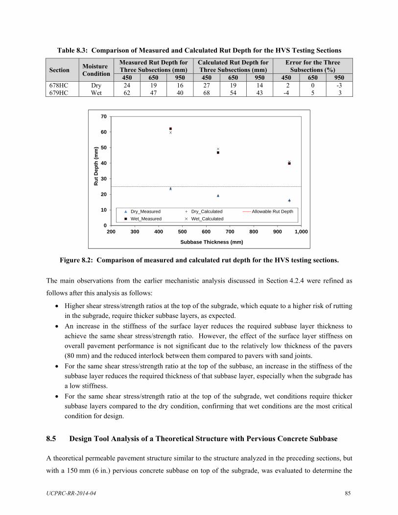
UCPRC-RR-2014-04 85
Table 8.3: Comparison of Measured and Calculated Rut Depth for the HVS Testing Sections
Section Moisture Condition
Measured Rut Depth for Three Subsections (mm)
Calculated Rut Depth for Three Subsections (mm)
Error for the Three Subsections (%)
450 650 950 450 650 950 450 650 950 678HC 679HC
Dry Wet
24 62
19 47
16 40
27 68
19 54
14 43
2 -4
0 5
-3 3
Figure 8.2: Comparison of measured and calculated rut depth for the HVS testing sections.
The main observations from the earlier mechanistic analysis discussed in Section 4.2.4 were refined as
follows after this analysis as follows:
Higher shear stress/strength ratios at the top of the subgrade, which equate to a higher risk of rutting in the subgrade, require thicker subbase layers, as expected.
An increase in the stiffness of the surface layer reduces the required subbase layer thickness to achieve the same shear stress/strength ratio. However, the effect of the surface layer stiffness on overall pavement performance is not significant due to the relatively low thickness of the pavers (80 mm) and the reduced interlock between them compared to pavers with sand joints.
For the same shear stress/strength ratio at the top of the subbase, an increase in the stiffness of the subbase layer reduces the required thickness of that subbase layer, especially when the subgrade has a low stiffness.
For the same shear stress/strength ratio at the top of the subgrade, wet conditions require thicker subbase layers compared to the dry condition, confirming that wet conditions are the most critical condition for design.
8.5 Design Tool Analysis of a Theoretical Structure with Pervious Concrete Subbase
A theoretical permeable pavement structure similar to the structure analyzed in the preceding sections, but
with a 150 mm (6 in.) pervious concrete subbase on top of the subgrade, was evaluated to determine the
0
10
20
30
40
50
60
70
200 300 400 500 600 700 800 900 1,000
Ru
t D
epth
(m
m)
Subbase Thickness (mm)
Dry_Measured Dry_Calculated Allowable Rut Depth
Wet_Measured Wet_Calculated
86 UCPRC-RR-2014-04
influence of having a stiff layer underneath the coarse aggregate subbase. This layer would typically serve
as a platform on which to compact the coarse aggregate subbase as well as contributing to the overall
stiffness of the structure, thereby potentially allowing for a reduction in the thickness of the coarse
aggregate layer. The same input values listed in Table 8.2 were used for this analysis. A stiffness of
6 GPa (870 ksi) was used for the pervious concrete layer.
The analysis found that for annual traffic up to two million ESALs, the 150 mm pervious concrete layer
could be used as an alternative to the coarse aggregate subbase in the design tables. No field testing was
undertaken to validate this finding. The influence of the stiff pervious concrete platform on improved
compaction of the coarse aggregate subbase and resulting reduced rutting in the subbase could not be
determined without field data. Based on these findings, the use of a pervious concrete subbase to replace
or supplement the coarse aggregate subbase should be investigated.

UCPRC-RR-2014-04 87
9. PROPOSED DESIGN TABLES
The proposed design tables, developed using the design tool discussed in Chapter 8, are provided in
Table 9.1 (metric) and Table 9.2 (U.S. units). The table format is similar to the current table in the ICPI
guide (4); however, the selection process includes the total number of days in a year that the subbase will
contain standing water above the top of the subgrade (i.e., the subbase is serving as a reservoir). Six
options are included (0, 10, 30, 50, 90, and 120 days). Traffic classes and subgrade modulus remain the
same as the current table in the ICPI guide; however, only four of the subgrade modulus categories are
included in the example table (40, 60, 80, and 100 MPa for dry conditions and 24, 36, 48, and 60 MPa for
wet conditions). A range of corresponding cohesion and internal friction angles for subgrade materials are
also included in the table for refining the selection. Designs for a specific set of project circumstances can
be undertaken using the same Excel® spreadsheet-based design tool used to develop the tables in
conjunction with the hydrological design procedures provided in the ICPI guide (4).
The design tool output and corresponding values in the tables should be considered as best estimate
designs, since they were developed from the results of only two HVS tests. Designers should continue to
use sound engineering judgment when designing permeable interlocking concrete pavements and can
introduce additional conservatism/reliability by altering one or more of the design inputs, namely the
material properties, number of days that the subbase will contain standing water, and/or traffic.
When compared to the values in the table in the ICPI guide (4), the new recommended minimum subbase
thicknesses required to prevent subgrade rutting do not differ significantly; with new thicknesses slightly
thinner or slightly thicker depending on the design traffic, resilient modulus, and number of days that the
subbase contains water. In scenarios where lower numbers of days with standing water in the subbase are
selected, the new recommended minimum subbase thicknesses are mostly less conservative than the
thicknesses proposed in the current ICPI guide. If the maximum number of days with standing water is
selected (i.e., 120), then the new recommended minimum subbase thickness is slightly more conservative
(e.g., 690 mm [27.5 in.] versus 675 mm [27.0 in.] for a design traffic of 1 million ESALs on the weakest
subgrade).
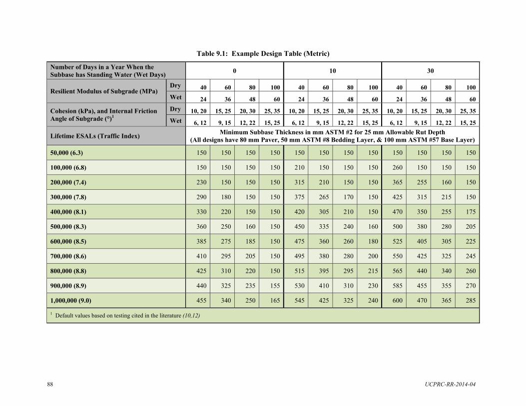
88 UCPRC-RR-2014-04
Table 9.1: Example Design Table (Metric)
Number of Days in a Year When the Subbase has Standing Water (Wet Days)
0 10 30
Resilient Modulus of Subgrade (MPa) Dry 40 60 80 100 40 60 80 100 40 60 80 100
Wet 24 36 48 60 24 36 48 60 24 36 48 60
Cohesion (kPa), and Internal Friction Angle of Subgrade (°)1
Dry 10, 20 15, 25 20, 30 25, 35 10, 20 15, 25 20, 30 25, 35 10, 20 15, 25 20, 30 25, 35
Wet 6, 12 9, 15 12, 22 15, 25 6, 12 9, 15 12, 22 15, 25 6, 12 9, 15 12, 22 15, 25
Lifetime ESALs (Traffic Index) Minimum Subbase Thickness in mm ASTM #2 for 25 mm Allowable Rut Depth
(All designs have 80 mm Paver, 50 mm ASTM #8 Bedding Layer, & 100 mm ASTM #57 Base Layer)
50,000 (6.3) 150 150 150 150 150 150 150 150 150 150 150 150
100,000 (6.8) 150 150 150 150 210 150 150 150 260 150 150 150
200,000 (7.4) 230 150 150 150 315 210 150 150 365 255 160 150
300,000 (7.8) 290 180 150 150 375 265 170 150 425 315 215 150
400,000 (8.1) 330 220 150 150 420 305 210 150 470 350 255 175
500,000 (8.3) 360 250 160 150 450 335 240 160 500 380 280 205
600,000 (8.5) 385 275 185 150 475 360 260 180 525 405 305 225
700,000 (8.6) 410 295 205 150 495 380 280 200 550 425 325 245
800,000 (8.8) 425 310 220 150 515 395 295 215 565 440 340 260
900,000 (8.9) 440 325 235 155 530 410 310 230 585 455 355 270
1,000,000 (9.0) 455 340 250 165 545 425 325 240 600 470 365 285
1 Default values based on testing cited in the literature (10,12)
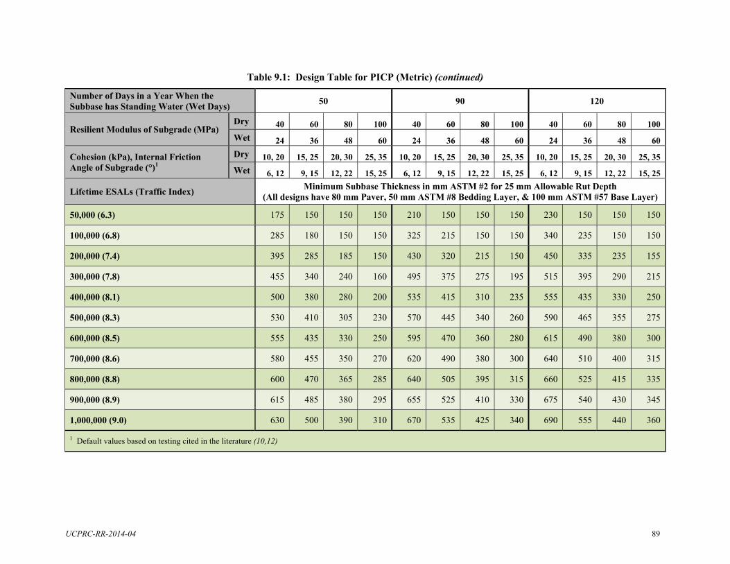
UCPRC-RR-2014-04 89
Table 9.1: Design Table for PICP (Metric) (continued)
Number of Days in a Year When the Subbase has Standing Water (Wet Days)
50 90 120
Resilient Modulus of Subgrade (MPa) Dry 40 60 80 100 40 60 80 100 40 60 80 100
Wet 24 36 48 60 24 36 48 60 24 36 48 60
Cohesion (kPa), Internal Friction Angle of Subgrade (°)1
Dry 10, 20 15, 25 20, 30 25, 35 10, 20 15, 25 20, 30 25, 35 10, 20 15, 25 20, 30 25, 35
Wet 6, 12 9, 15 12, 22 15, 25 6, 12 9, 15 12, 22 15, 25 6, 12 9, 15 12, 22 15, 25
Lifetime ESALs (Traffic Index) Minimum Subbase Thickness in mm ASTM #2 for 25 mm Allowable Rut Depth
(All designs have 80 mm Paver, 50 mm ASTM #8 Bedding Layer, & 100 mm ASTM #57 Base Layer)
50,000 (6.3) 175 150 150 150 210 150 150 150 230 150 150 150
100,000 (6.8) 285 180 150 150 325 215 150 150 340 235 150 150
200,000 (7.4) 395 285 185 150 430 320 215 150 450 335 235 155
300,000 (7.8) 455 340 240 160 495 375 275 195 515 395 290 215
400,000 (8.1) 500 380 280 200 535 415 310 235 555 435 330 250
500,000 (8.3) 530 410 305 230 570 445 340 260 590 465 355 275
600,000 (8.5) 555 435 330 250 595 470 360 280 615 490 380 300
700,000 (8.6) 580 455 350 270 620 490 380 300 640 510 400 315
800,000 (8.8) 600 470 365 285 640 505 395 315 660 525 415 335
900,000 (8.9) 615 485 380 295 655 525 410 330 675 540 430 345
1,000,000 (9.0) 630 500 390 310 670 535 425 340 690 555 440 360
1 Default values based on testing cited in the literature (10,12)

90 UCPRC-RR-2014-04
Table 9.2: Design Table for PICP (U.S. units) Number of Days in a Year When the Subbase has Standing Water (Wet Days)
0 10 30
Resilient Modulus of Subgrade (ksi) Dry 5.8 8.7 11.6 14.5 5.8 8.7 11.6 14.5 5.8 8.7 11.6 14.5
Wet 3.5 5.2 6.7 8.7 3.5 5.2 6.7 8.7 3.5 5.2 6.7 8.7
Cohesion (psi), Internal Friction Angle of Subgrade (°)1
Dry 1.5, 20 2.2, 25 2.9, 30 3.6, 35 1.5, 20 2.2, 25 2.9, 30 3.6, 35 1.5, 20 2.2, 25 2.9, 30 3.6, 35
Wet 0.9, 12 1.3, 15 1.7, 22 2.2, 25 0.9, 12 1.3, 15 1.7, 22 2.2, 25 0.9, 12 1.3, 15 1.7, 22 2.2, 25
Lifetime ESALs (Traffic Index) Minimum Subbase Thickness in inches2 ASTM #2 for 1 in. Allowable Rut Depth
(All designs have 3.2 in. Paver, 2 in. ASTM #8 Bedding Layer, & 4 in. ASTM #57 Base Layer)
50,000 (6.3) 6.0 6.0 6.0 6.0 6.0 6.0 6.0 6.0 6.0 6.0 6.0 6.0
100,000 (6.8) 6.0 6.0 6.0 6.0 8.5 6.0 6.0 6.0 10.5 6.0 6.0 6.0
200,000 (7.4) 9.0 6.0 6.0 6.0 12.5 8.5 6.0 6.0 14.5 10.0 6.5 6.0
300,000 (7.8) 11.5 7.0 6.0 6.0 15.0 10.5 7.0 6.0 17.0 12.5 8.5 6.0
400,000 (8.1) 13.0 9.0 6.0 6.0 17.0 12.0 8.5 6.0 19.0 14.0 10.0 7.0
500,000 (8.3) 14.5 10.0 6.5 6.0 18.0 13.5 9.5 6.5 20.0 15.0 11.0 8.0
600,000 (8.5) 15.5 11.0 7.5 6.0 19.0 14.5 10.5 7.0 21.0 16.0 12.0 9.0
700,000 (8.6) 16.5 12.0 8.0 6.0 20.0 15.0 11.0 8.0 22.0 17.0 13.0 10.0
800,000 (8.8) 17.0 12.5 9.0 6.0 20.5 16.0 12.0 8.5 22.5 17.5 13.5 10.5
900,000 (8.9) 17.5 13.0 9.5 6.0 21.0 16.5 12.5 9.0 23.5 18.0 14.0 11.0
1,000,000 (9.0) 18.0 13.5 10.0 6.5 22.0 17.0 13.0 9.5 24.0 19.0 14.5 11.5
1 Default values based on testing cited in the literature (10,12) 2 Subbase thickness calculated by dividing metric thickness by 25 and then rounding to nearest 0.5 in.

UCPRC-RR-2014-04 91
Table 9.2: Design Table for PICP (U.S. units) (continued)
Number of Days in a Year When the Subbase has Standing Water (Wet Days)
50 90 120
Resilient Modulus of Subgrade (ksi) Dry 5.8 8.7 11.6 14.5 5.8 8.7 11.6 14.5 5.8 8.7 11.6 14.5
Wet 3.5 5.2 6.7 8.7 3.5 5.2 6.7 8.7 3.5 5.2 6.7 8.7
Cohesion (psi), Internal Friction Angle of Subgrade (°)1
Dry 1.5, 20 2.2, 25 2.9, 30 3.6, 35 1.5, 20 2.2, 25 2.9, 30 3.6, 35 1.5, 20 2.2, 25 2.9, 30 3.6, 35
Wet 0.9, 12 1.3, 15 1.7, 22 2.2, 25 0.9, 12 1.3, 15 1.7, 22 2.2, 25 0.9, 12 1.3, 15 1.7, 22 2.2, 25
Lifetime ESALs (Traffic Index) Minimum Subbase Thickness in inches2 ASTM #2 for 1 in. Allowable Rut Depth
(All designs have 3.2 in. Paver, 2 in. ASTM #8 Bedding Layer, & 4 in. ASTM #57 Base Layer)
50,000 (6.3) 7.0 6.0 6.0 6.0 8.5 6.0 6.0 6.0 9.0 6.0 6.0 6.0
100,000 (6.8) 11.5 7.0 6.0 6.0 13.0 8.5 6.0 6.0 13.5 9.5 6.0 6.0
200,000 (7.4) 16.0 11.5 7.5 6.0 17.0 13.0 8.5 6.0 18.0 13.5 9.5 6.0
300,000 (7.8) 18.0 13.5 9.5 6.5 20.0 15.0 11.0 8.0 20.5 16.0 11.5 8.5
400,000 (8.1) 20.0 15.0 11.0 8.0 21.5 16.5 12.5 9.5 22.0 17.5 13.0 10.0
500,000 (8.3) 21.0 16.5 12.0 9.0 23.0 18.0 13.5 10.5 23.5 18.5 14.0 11.0
600,000 (8.5) 22.0 17.5 13.0 10.0 24.0 19.0 14.5 11.0 24.5 19.5 15.0 12.0
700,000 (8.6) 23.0 18.0 14.0 11.0 25.0 19.5 15.0 12.0 25.5 20.5 16.0 12.5
800,000 (8.8) 24.0 19.0 14.5 11.5 25.5 20.0 16.0 12.5 26.5 21.0 16.5 13.5
900,000 (8.9) 24.5 19.5 15.0 12.0 26.0 21.0 16.5 13.0 27.0 21.5 17.0 14.0
1,000,000 (9.0) 25.0 20.0 15.5 12.5 27.0 21.5 17.0 13.5 27.5 22.0 17.5 14.5
1 Default values based on testing cited in the literature (10,12) 2 Subbase thickness calculated by dividing metric thickness by 25 and then rounding to nearest 0.5 in.

92 UCPRC-RR-2014-04
Blank page
UCPRC-RR-2014-04 93
10. CONCLUSIONS
10.1 Summary
This report details the research undertaken to develop revised design tables for permeable interlocking
concrete pavement using a mechanistic-empirical design approach. The study included a literature review,
field testing of existing projects and test sections, estimation of the effective stiffness of each layer in
permeable interlocking concrete pavement structures, mechanistic analysis and structural design of a test
track incorporating three different subbase thicknesses (low, medium, and higher risk), tests on the track
with a Heavy Vehicle Simulator (HVS) to collect performance data to validate the design approach using
accelerated loading, refinement and calibration of the design procedure using the test track data,
development of a spreadsheet based design tool, and development of revised design tables using the
design tool.
Rut development rate as a function of the shear strength to shear stress ratios at the top of the subbase and
the top of the subgrade was used as the basis for the design approach. This approach was selected given
that low shear strengths of saturated and often poorly compacted subgrades are common in permeable
pavements and that higher allowable ruts are usually tolerated due to the absence of ponding on the
surface during rainfall. The alternative approach of using a vertical strain criterion was considered
inappropriate for permeable pavements.
Key observations from the study include:
Infiltration of water into the subgrade is significantly reduced when the subgrade is compacted prior to placing the subbase. In this study, compaction added very little to the structural performance of the pavement and would not have permitted reducing the thickness of the subbase layer.
There was a significant difference in rutting performance and rutting behavior between the wet and dry tests, as expected.
A large proportion of the rutting on all three sections occurred as initial embedment in the first 2,000 to 5,000 load repetitions of the test and again after each of the load changes, indicating that much of the rutting in the base and subbase layers was attributed to bedding in, densification, and/or reorientation of the aggregate particles. This behavior is consistent with rutting behavior on other types of structures.
During testing under dry conditions, limited permanent deformation (< 4 mm) was recorded in the bedding and base layers on all three subsections, and most occurred very early in the test. On the subsection with the 450 mm subbase, rutting occurred in both the subbase (10 mm rut) and subgrade (13 mm rut). On the 650 mm and 950 mm subbase subsections, rutting occurred mostly in the subbase. Total permanent deformation on the 450 mm, 650 mm, and 950 mm subbase subsections was 27 mm, 23 mm and 17 mm respectively, implying a generally linear trend of increasing permanent deformation with decreasing subbase thickness.
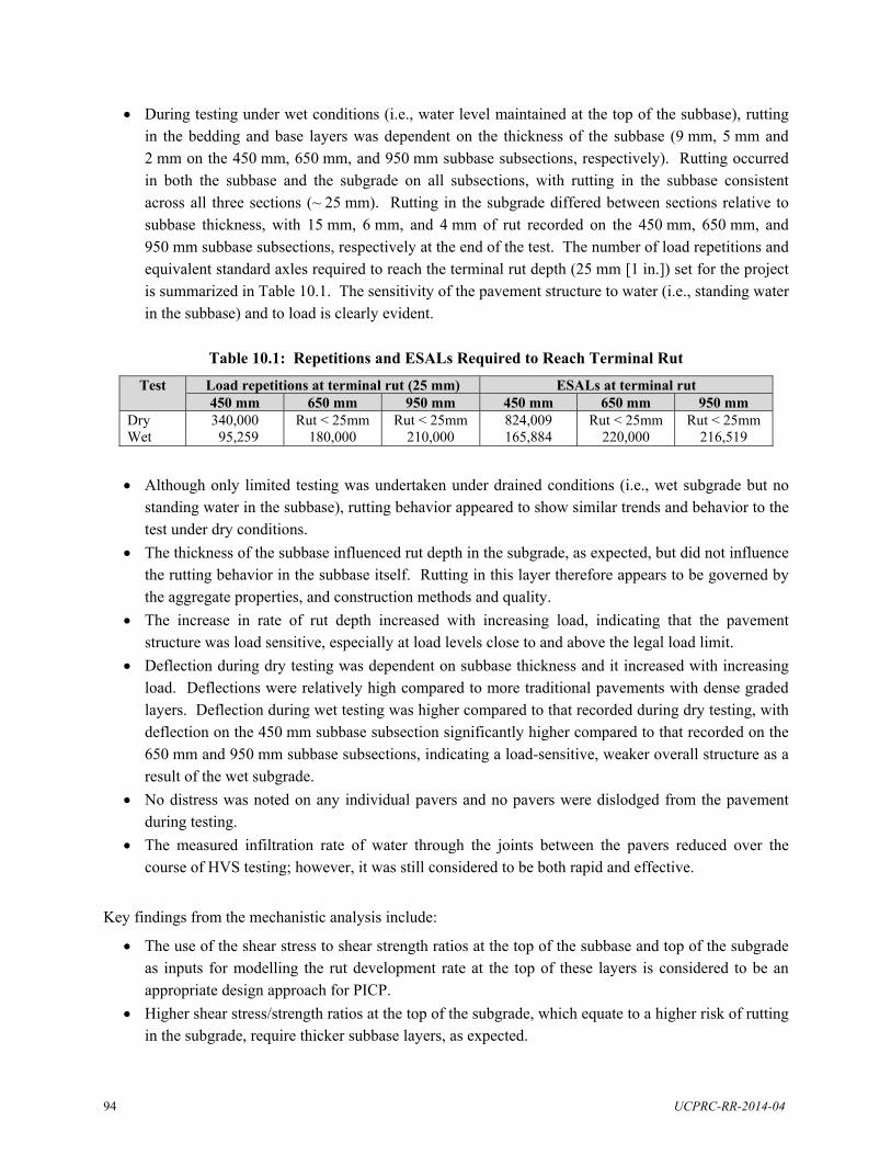
94 UCPRC-RR-2014-04
During testing under wet conditions (i.e., water level maintained at the top of the subbase), rutting in the bedding and base layers was dependent on the thickness of the subbase (9 mm, 5 mm and 2 mm on the 450 mm, 650 mm, and 950 mm subbase subsections, respectively). Rutting occurred in both the subbase and the subgrade on all subsections, with rutting in the subbase consistent across all three sections (~ 25 mm). Rutting in the subgrade differed between sections relative to subbase thickness, with 15 mm, 6 mm, and 4 mm of rut recorded on the 450 mm, 650 mm, and 950 mm subbase subsections, respectively at the end of the test. The number of load repetitions and equivalent standard axles required to reach the terminal rut depth (25 mm [1 in.]) set for the project is summarized in Table 10.1. The sensitivity of the pavement structure to water (i.e., standing water in the subbase) and to load is clearly evident.
Table 10.1: Repetitions and ESALs Required to Reach Terminal Rut
Test Load repetitions at terminal rut (25 mm) ESALs at terminal rut 450 mm 650 mm 950 mm 450 mm 650 mm 950 mm
Dry Wet
340,000 95,259
Rut < 25mm 180,000
Rut < 25mm 210,000
824,009 165,884
Rut < 25mm 220,000
Rut < 25mm 216,519
Although only limited testing was undertaken under drained conditions (i.e., wet subgrade but no standing water in the subbase), rutting behavior appeared to show similar trends and behavior to the test under dry conditions.
The thickness of the subbase influenced rut depth in the subgrade, as expected, but did not influence the rutting behavior in the subbase itself. Rutting in this layer therefore appears to be governed by the aggregate properties, and construction methods and quality.
The increase in rate of rut depth increased with increasing load, indicating that the pavement structure was load sensitive, especially at load levels close to and above the legal load limit.
Deflection during dry testing was dependent on subbase thickness and it increased with increasing load. Deflections were relatively high compared to more traditional pavements with dense graded layers. Deflection during wet testing was higher compared to that recorded during dry testing, with deflection on the 450 mm subbase subsection significantly higher compared to that recorded on the 650 mm and 950 mm subbase subsections, indicating a load-sensitive, weaker overall structure as a result of the wet subgrade.
No distress was noted on any individual pavers and no pavers were dislodged from the pavement during testing.
The measured infiltration rate of water through the joints between the pavers reduced over the course of HVS testing; however, it was still considered to be both rapid and effective.
Key findings from the mechanistic analysis include:
The use of the shear stress to shear strength ratios at the top of the subbase and top of the subgrade as inputs for modelling the rut development rate at the top of these layers is considered to be an appropriate design approach for PICP.
Higher shear stress/strength ratios at the top of the subgrade, which equate to a higher risk of rutting in the subgrade, require thicker subbase layers, as expected.
UCPRC-RR-2014-04 95
An increase in the stiffness of the surface layer reduces the required subbase layer thickness to achieve the same shear stress/strength ratio. However, the effect of the surface layer stiffness on overall pavement performance is not significant due to the relatively small thickness of the pavers (80 mm) and the reduced interlock between them compared to pavers with sand joints.
For the same shear stress/strength ratio at the top of the subbase, an increase in the stiffness of the subbase layer reduces the required thickness of that subbase layer, especially when the subgrade has a low stiffness.
For the same shear stress/strength ratio at the top of the subgrade, wet conditions require thicker subbase layers compared to the dry condition, confirming that wet conditions are the most critical condition for design.
A new example design table, based on the number of days with standing water in the subbase (zero, 10,
30, 50, 90, and 120) has been developed. The table uses a similar format to that currently used in the ICPI
Permeable Interlocking Concrete Pavements guideline. The design thicknesses proposed in the new table
do not differ significantly from those in the current table. Designs for a specific set of project
circumstances can be undertaken using the same Excel® spreadsheet-based design tool used to develop the
tables in conjunction with the hydrological design procedures provided in the ICPI guide. The design tool
output and corresponding values in the tables should be considered as best estimate designs, since they
were developed from the results of only two HVS tests. Designers should continue to use sound
engineering judgment when designing permeable interlocking concrete pavements and can introduce
additional conservatism/reliability by altering one or more of the design inputs, namely the material
properties, number of days that the subbase will contain standing water, and/or traffic.
10.2 Recommendations
Given that a large proportion of the permanent deformation measured on the test track occurred in the
subbase and that increasing the thickness of the subbase did not reduce this rutting, it is recommended that
the specifications of the aggregate properties used in this layer and the methods used to construct it are
reviewed to determine whether any reductions in rutting can be achieved by changing them. Further
research into stabilization of the subbase aggregate using geogrids, geocells, or cement, and the use of a
pervious concrete subbase on top of the subgrade to reduce the thickness of the coarse aggregate subbase,
or to replace it, should also be considered.
The pavement tested in this study appeared to be sensitive to very heavy loads and care should therefore
be taken when designing projects that will carry large numbers of heavy or overloaded trucks.

96 UCPRC-RR-2014-04
Blank page

UCPRC-RR-2014-04 97
REFERENCES
1. JONES, D., Li, H. and Harvey, J.T. 2013. Development and HVS Validation of Design Tables
for Permeable Interlocking Concrete Pavement: Literature Review. Davis and Berkeley, CA:
University of California Pavement Research Center. UCPRC-TM-2013-03)
2. JONES, D., Li, H. and Harvey, J.T. 2013. Development and HVS Validation of Design Tables
for Permeable Interlocking Concrete Pavement: Field Testing and Test Section Structural
Design. Davis and Berkeley, CA: University of California Pavement Research Center. (UCPRC-
TM-2013-09).
3. METCALF, J.B. 1996. NCHRP Synthesis of Highway Practice 235: Application of Full-Scale
Accelerated Pavement Testing. Washington, DC: Transportation Research Board.
4. SMITH, D.R. 2011. Permeable Interlocking Concrete Pavements (4th Edition). Herndon VA:
Interlocking Concrete Pavement Institute.
5. LEA, J. undated. OpenPave: An N-Layer, N-Load, N-Point Multi-Layer Elastic Half Space
Calculation. www.OpenPave.org. Accessed 2013/09/10.
6. CHOI, J.W., Wu, R., Pestana, J.H. and Harvey, J. 2010. New Layer-Moduli Back-Calculation
Method Based on the Constrained Extended Kalman Filter. Journal of Transportation
Engineering, 136(1). (pp 20–30).
7. TUTUMLUER, E. and Seyhan, U. 1999. Laboratory Determination of Anisotropic Aggregate
Resilient Moduli Using an Innovative Test Device. Transportation Research Record: Journal
of the Transportation Research Board, Vol. 1687. (pp. 13-21).
8. THOMPSON, M., Gomez-Ramirez, F. and Bejarano, M. 2002. Illi-Pave Based Flexible
Pavement Design Concepts for Multiple Wheel Heavy Gear Load Aircraft. Proceedings 9th
International Conference on Asphalt Pavements. Copenhagen, Denmark. International Society
of Asphalt Pavements.
9. TUTUMLUER, E., Kim, I. and Santoni, R. 2004. Modulus Anisotropy and Shear Stability of
Geofiber-Stabilized Sands. Transportation Research Record: Journal of the Transportation
Research Board, Vol. 1874. (pp. 125-135).
10. KIM, I. and Tutumluer, E. 2006. Field Validation of Airport Pavement Granular Layer Rutting
Predictions. Transportation Research Record: Journal of the Transportation Research
Board, Vol. 1952. (pp. 48-57).
11. LI, H., Harvey J.T. and Jones, D. 2010. Summary of a Computer Modeling Study to
Understand the Performance Properties of Fully Permeable Pavements. Davis and Berkeley,
CA: University of California Pavement Research Center. (UCPRC-TM-2010-04).
98 UCPRC-RR-2014-04
12. CHOW, L.C. and Tutumluer, E. 2014. Framework for Improved Unbound Aggregate Base Rutting
Model Development for Mechanistic-Empirical Pavement Design. Proceedings Transportation
Research Board 93rd Annual Meeting. Washington, D.C: Transportation Research Board.
13. DAS, B.M. 2007. Advanced Soil Mechanics. New York, NY: Taylor and Francis.
14. NOVA, R. 2012. Soil Mechanics. Hoboken, NJ: John Wiley and Sons.
15. CARTER, M. and Bentley, S.P. 1991. Correlations of Soil Properties. London, UK: Pentech
Press.
16. WNEK, M., Tutumluer, E., Moaveni, M. and Gehringer, E. 2013. Investigation of Aggregate
Properties Influencing Railroad Ballast Performance. Transportation Research Record: Journal
of the Transportation Research Board, Vol. 2374. (pp. 180-189).
17. HUANG, H., Tutumluer, E. and Dombrow, W. 2009. Laboratory Characterization of Fouled
Railroad Ballast Behavior. Transportation Research Record: Journal of the Transportation
Research Board, Vol. 2117. (pp. 93-101).
18. AHMED, F., Nestingen, R., Nieber, J.L., Gulliver, J.S., and Hozalski, R.M. 2014. A Modified
Philip-Dunne Infiltrometer for Measuring the Field-Saturated Hydraulic Conductivity of Surface
Soil. Vadose Zone Journal, 10/2136. Soil Science Society of America.
19. JONES, D. 2005. Quality Management System for Site Establishment, Daily Operations,
Instrumentation, Data Collection and Data Storage for APT Experiments. Pretoria, South
Africa: CSIR Transportek. (Contract Report CR-2004/67-v2.).
20. ULLIDTZ, P, Harvey, J.T., Basheer, I., Jones, D., Wu, R., Lea, J., and Lu, Q. 2010. CalME, a
Mechanistic-Empirical Program to Analyze and Design Flexible Pavement Rehabilitation.
Transportation Research Record: Journal of the Transportation Research Board, Vol. 2153.
(pp. 143-152).

UCPRC-RR-2014-04 99
APPENDIX A: LITERATURE REVIEW REPORT

100 UCPRC-RR-2014-04
Blank page
PREPARED FOR: Concrete Masonry Association of California and Nevada
PREPARED BY:
University of California Pavement Research Center
UC Davis, UC Berkeley
May 2013 Technical Memorandum: UCPRC-TM-2013-03
Authors:D. Jones, H. Li and J.T. Harvey
Concrete Masonry Association of California and Nevada. Grant Agreement UCPRC-PP-2011-01

UCPRC-TM-2013-03 i
DOCUMENT RETRIEVAL PAGE Technical Memorandum: UCPRC-TM-2013-03
Title: Development and HVS Validation of Design Tables for Permeable Interlocking Concrete Pavement: Literature Review
Authors: David Jones, Hui Li, and John T. Harvey
Prepared for: Concrete Masonry Association of California and Nevada
FHWA Report No: Not applicable
Work submitted: May 2013
Date:June 2013
UC Davis Contract No: UCPRC-PP-2011-01
Status: Final
Version No.: 2
Abstract: This report details a review of the recent literature on permeable interlocking concrete pavements. Field surveys were not conducted as part of this task, but will be incorporated in Task #2, which covers field testing of existing projects. Only a few organizations worldwide have undertaken detailed research on the topic, with many studies focusing on infiltration on low volume traffic roads, rather than structural design of roads carrying truck traffic. Laboratory studies have focused on resilient modulus of saturated and unsaturated materials. Well graded materials with no fines appeared to perform best under both conditions. Permeable pavements will need to be designed for the worst case condition (i.e., base/reservoir layer is full of water) indicating that a reduction in resilient modulus of about 50 percent of the dry material value can be expected. The use of cemented materials and geogrids in the base to compensate for this lower stiffness is gaining interest. Failure mechanisms appear to be mostly rutting of the surface layer due to shearing in the bedding and/or base layers. Choice of paver and paver laying pattern can limit this to a certain extent, but optimizing the base material grading and thickness, stabilizing base materials, quality of construction, and the use of geofabrics on top of the subgrade to prevent contamination of the base with fines will have the biggest influence. Mechanistic-empirical design has been considered in Australian and United Kingdom design procedures to some extent, with the work done in Australia appearing to be the most comprehensive. The Australian and United Kingdom design procedures should be used in conjunction with the ICPI and UCPRC design approaches in developing the design tables, choice of design for the test track, and in the analysis of test track performance when validating the final design tables.
Keywords: Permeable interlocking concrete pavement, permeable pavement, mechanistic-empirical design, accelerated pavement testing.
Proposals for implementation:
Related documents: None
Signatures:
D. Jones 1st Author
J. Harvey Technical Review
D. Jones Principal Investigator
D. Smith For CMACN

ii UCPRC-TM-2013-03
DISCLAIMER
The contents of this report reflect the views of the authors who are responsible for the facts and accuracy
of the data presented herein. The contents do not necessarily reflect the official views or policies of the
Concrete Masonry Association of California and Nevada (CMACN), the California Nevada Cement
Association (CNCA), or the Interlocking Concrete Pavement Institute (ICPI). This report does not
constitute a standard, specification, or regulation.
PROJECT OBJECTIVES/GOALS
The objective of this project is to produce design tables for permeable interlocking concrete pavement
(PICP) based on mechanistic analysis and partially validated with accelerated pavement testing (APT).
The following tasks will be completed to achieve this objective:
1. Perform a literature and field survey to identify critical responses, failure mechanisms, appropriate performance transfer functions and modeling assumptions for mechanistic analysis of PICP under truck loading.
2. Measure deflections in the field on several PICP locations to characterize effective stiffness of layers for use in modeling.
3. Perform mechanistic analyses of PICP to develop design tables following the approach documented in California Department of Transportation (Caltrans) Research Report CTSW-RR-09-249.04 for development of structural design tables for pervious concrete and porous asphalt.
4. Prepare a plan for validation with accelerated pavement testing based on the results of the mechanistic analysis.
5. Test responses and, if possible, failure of up to three PICP structures in dry and wet condition with the Heavy Vehicle Simulator (HVS), and revise the tables as needed.
6. Analyze the results of the HVS testing to update the structural design tables where necessary. 7. Write a final report documenting the results of all tasks in the study and demonstrating the design
tables. 8. Present findings to Caltrans Office of Concrete Pavements and Foundation Program and Office of
Stormwater - Design staff in Sacramento, CA.
This report covers Task 1.

UCPRC-TM-2013-03 iii
TABLE OF CONTENTS
1. INTRODUCTION ............................................................................................................................. 1 1.1 Project Scope ............................................................................................................................ 1 1.2 Background to the Study ........................................................................................................... 1 1.3 Study Objective/Goal ................................................................................................................ 1 1.4 Approach to the Literature Review ........................................................................................... 2 1.5 Report Layout ........................................................................................................................... 2
2. BACKGROUND ............................................................................................................................... 3 2.1 Permeable Pavement Design .................................................................................................... 3 2.2 California Department of Transportation/UCPRC Study ......................................................... 4 2.3 Mechanistic Pavement Design .................................................................................................. 4 2.4 Environmental Considerations for Permeable Pavements ........................................................ 5
3. LITERATURE REVIEW ................................................................................................................. 7 3.1 Introduction ............................................................................................................................... 7 3.2 Interlocking Concrete Pavement Institute (ICPI) (2) ................................................................ 7
3.2.1 Relevance to this Study ................................................................................................ 8 3.3 University of California Pavement Research Center (UCPRC) ............................................... 8
3.3.1 Summary Report (3) ..................................................................................................... 8 3.3.2 Laboratory Testing Report (4) ...................................................................................... 8 3.3.3 Computer Modeling Report (5) .................................................................................... 9 3.3.4 Life-Cycle Cost Analysis and Environmental Life-Cycle Assessment (6) .................. 9 3.3.5 Hydraulic Performance (7) ........................................................................................... 9 3.3.6 Relevance to this Study .............................................................................................. 10
3.4 Minnesota Department of Transport Study (MnROAD) (8,9,10) .......................................... 11 3.4.1 Relevance to this Study .............................................................................................. 11
3.5 University of Illinois (11) ....................................................................................................... 12 3.5.1 Relevance to this Study .............................................................................................. 12
3.6 Applied Research Associates (12) .......................................................................................... 12 3.6.1 Relevance to this Study .............................................................................................. 13
3.7 Texas A and M University (13) .............................................................................................. 13 3.7.1 Relevance to this Study .............................................................................................. 13
3.8 University of Alaska Fairbanks (14) ....................................................................................... 13 3.8.1 Relevance to this Study .............................................................................................. 14
3.9 University of New South Wales, Australia (15-20) ................................................................ 14 3.9.1 Relevance to this Study .............................................................................................. 14
3.10 University of South Australia (21) .......................................................................................... 14 3.10.1 Relevance to this Study .............................................................................................. 14
3.11 Interpave (Precast Concrete Paving and Kerb Association), United Kingdom (22) ............... 15 3.11.1 Relevance to this Study .............................................................................................. 15
3.12 John Knapton Consulting Engineers (23,24) .......................................................................... 15 3.12.1 Relevance to this Study .............................................................................................. 16
3.13 University of Canterbury (25) ................................................................................................. 16 3.13.1 Relevance to this Study .............................................................................................. 16
4. CONCLUSIONS AND RECOMMENDATIONS ........................................................................ 17 4.1 Review of Report Objective ................................................................................................... 17 4.2 Recommendations ................................................................................................................... 18
5. REFERENCES ................................................................................................................................ 19

iv UCPRC-TM-2013-03
SI* (MODERN METRIC) CONVERSION FACTORS APPROXIMATE CONVERSIONS TO SI UNITS
Symbol When You Know Multiply By To Find Symbol LENGTH
In inches 25.4 Millimeters mm Ft feet 0.305 Meters m Yd yards 0.914 Meters m Mi miles 1.61 Kilometers Km
AREAin2 square inches 645.2 Square millimeters mm2 ft2 square feet 0.093 Square meters m2 yd2 square yard 0.836 Square meters m2 Ac acres 0.405 Hectares ha mi2 square miles 2.59 Square kilometers km2
VOLUMEfl oz fluid ounces 29.57 Milliliters mL Gal gallons 3.785 Liters L ft3 cubic feet 0.028 cubic meters m3 yd3 cubic yards 0.765 cubic meters m3
NOTE: volumes greater than 1000 L shall be shown in m3
MASSOz ounces 28.35 Grams g Lb pounds 0.454 Kilograms kg T short tons (2000 lb) 0.907 megagrams (or "metric ton") Mg (or "t")
TEMPERATURE (exact degrees)°F Fahrenheit 5 (F-32)/9 Celsius °C
or (F-32)/1.8
ILLUMINATION Fc foot-candles 10.76 Lux lx Fl foot-Lamberts 3.426 candela/m2 cd/m2
FORCE and PRESSURE or STRESS Lbf poundforce 4.45 Newtons N lbf/in2 poundforce per square inch 6.89 Kilopascals kPa
APPROXIMATE CONVERSIONS FROM SI UNITS
Symbol When You Know Multiply By To Find Symbol LENGTH
mm millimeters 0.039 Inches in m meters 3.28 Feet ft m meters 1.09 Yards yd Km kilometers 0.621 Miles mi
AREAmm2 square millimeters 0.0016 square inches in2 m2 square meters 10.764 square feet ft2 m2 square meters 1.195 square yards yd2 Ha Hectares 2.47 Acres ac km2 square kilometers 0.386 square miles mi2
VOLUMEmL Milliliters 0.034 fluid ounces fl oz L liters 0.264 Gallons gal m3 cubic meters 35.314 cubic feet ft3 m3 cubic meters 1.307 cubic yards yd3
MASSg grams 0.035 Ounces oz kg kilograms 2.202 Pounds lb Mg (or "t") megagrams (or "metric ton") 1.103 short tons (2000 lb) T
TEMPERATURE (exact degrees) °C Celsius 1.8C+32 Fahrenheit °F
ILLUMINATION lx lux 0.0929 foot-candles fc cd/m2 candela/m2 0.2919 foot-Lamberts fl
FORCE and PRESSURE or STRESSN newtons 0.225 Poundforce lbf
kPa kilopascals 0.145 poundforce per square inch lbf/in2
*SI is the symbol for the International System of Units. Appropriate rounding should be made to comply with Section 4 of ASTM E380 (Revised March 2003)

UCPRC-TM-2013-03 1
1. INTRODUCTION
1.1 Project Scope
This project is being coordinated through the Interlocking Concrete Pavement Institute (ICPI) and the
Concrete Masonry Association of California and Nevada with additional support from the California
Nevada Cement Association. The objective of this project is to produce design tables for permeable
interlocking concrete pavement (PICP) based on mechanistic analysis and partially validated with
accelerated pavement testing (APT).
1.2 Background to the Study
Although permeable pavements are becoming increasingly common across the United States, they are
mostly used in parking lots, basic access streets, recreation areas, and landscaped areas, all of which carry
very light, slow moving traffic. Only limited research has been undertaken on the mechanistic design and
long-term performance monitoring of permeable pavements carrying higher traffic volumes and heavier
loads, and the work that has been done has focused primarily on pavements with open-graded asphalt or
portland cement concrete surfacings. Very little research has been undertaken on the use of permeable
concrete paver surfaces on these more heavily trafficked pavements.
1.3 Study Objective/Goal
The objective of this project is to produce design tables for permeable interlocking concrete pavement
(PICP) based on mechanistic analysis and partially validated with accelerated pavement testing (APT).
The following tasks will be completed to achieve this objective:
1. Perform a literature and field survey to identify critical responses, failure mechanisms, appropriate performance transfer functions and modeling assumptions for mechanistic analysis of PICP under truck loading.
2. Measure deflections in the field on several PICP locations to characterize effective stiffness of layers for use in modeling.
3. Perform mechanistic analyses of PICP to develop design tables following the approach documented in California Department of Transportation (Caltrans) Research Report CTSW-RR-09-249.04 for development of structural design tables for pervious concrete and porous asphalt pavements.
4. Prepare a plan for validation with APT based on the results of the mechanistic analysis. 5. Test responses and, if possible, failure of up to three PICP structures in dry and wet condition with
the Heavy Vehicle Simulator (HVS), and revise the tables as needed. 6. Analyze the results of the HVS testing to update the structural design tables where necessary.

2 UCPRC-TM-2013-03
7. Write a final report documenting the results of all tasks in the study and demonstrating the design tables.
8. Present findings to Caltrans Office of Concrete Pavements and Foundation Program and Office of Stormwater - Design staff in Sacramento, CA.
This report covers the literature review work completed in Task #1. Field surveys will be conducted as
part of Task #2.
1.4 Approach to the Literature Review
The ICPI regularly tracks the literature on the use of interlocking concrete pavers in pavement
applications. A list of publications and copies of available documents was provided to the UCPRC. In
addition to this, the UCPRC conducted a separate search using the University of California (UC) library
system to search journal articles, the Transportation Research Board (TRB) publications index to search
for papers in the Transportation Research Record and Annual Meeting Compendiums, and Google
Scholar and other internet searchers to identify papers, reports, and articles not located in the ICPI, UC
and TRB searches. Research conducted in the United States as well as internationally was reviewed.
Reference lists in sourced publications were also checked to identify any other potentially relevant
publications that were missed in the earlier searches. Searches of state and county departments of
transportation and university research center sites were not attempted.
1.5 Report Layout
The ICPI routinely updates their state-of-the-practice documentation with the latest research and it was not
the intent of this study to duplicate this effort. Instead, the available literature was reviewed in the context
of its relevance and contribution to the objectives of this UCPRC study. Consequently, this report is
limited to a brief description of the research conducted relevant to each objective and how the findings of
that research could be used to refine the UCPRC study, specifically in terms of developing the design
tables, designing the test track, the type of data collected, data analysis, and validation of the design tables.

UCPRC-TM-2013-03 3
2. BACKGROUND
2.1 Permeable Pavement Design
Permeable pavements are defined for the purposes of this study as those in which all layers are intended to
be permeable and water infiltrates into the underlying soil. The three major permeable pavement types are
porous asphalt, pervious concrete and permeable interlocking concrete pavement. Since the late 1970s, a
variety of permeable pavement projects have been constructed for low traffic areas carrying light vehicles
and occasional truck traffic. There have been both failures and successes. Sources of failures have been
described anecdotally. Variables contributing to successes have not been completely identified beyond
seemingly conservative hydrologic and structural designs. Unlike conventional pavements, permeable
pavements do not yet have decades of research and experience, Therefore, permeable pavements and the
benefits they potentially provide have been limited largely because of a lack of performance data and the
ability to consider different materials, climates, subgrades and structural cross-sections. Because of
durability concerns, most applications of permeable pavements in North America have been for parking
lots and very low-volume streets that are not subjected to high-speed traffic or to repeated truck traffic.
This data gap is in part being addressed by the American Society of Civil Engineers (ASCE) Technical
Committee on Permeable Pavements. This committee plans a 2013 release of a manual on permeable
pavement design, construction and maintenance. Performance information is largely experienced-based
and structural design methods for pervious concrete, porous asphalt and ICPI relies on industry
recommendations. This publication identifies structural design research as a pressing need.
The National Asphalt Pavement Association (NAPA), the American Concrete Pavement Association
(ACPA), and the Interlocking Concrete Pavement Institute (ICPI) have each produced a design manual for
permeable pavements for their surface type and for this type of low-volume traffic application. The ICPI
manual and the ACPA manual both include some consideration of structural design for trucks using
modifications of the AASHTO 1993 empirical design approach. These manuals, and the pavement
designs used to date, have been empirical in nature with little or no long-term monitoring data to support
the empiricism. These designs have, to date, generally been used in low-risk pavements, such as parking
lots, alleys, and low-speed, low-traffic roads. This approach and these designs may not work well for
pavements intended to carry any heavy truck traffic.
The Caltrans Office of Storm Water Management has drafted a design guide and construction
specifications for PICP, pervious concrete, and porous asphalt. These resources are intended for design of
non-highway facilities such as parking lots and low-speed, low-traffic roads. The guide includes
information on hydrologic design, which follows that for other infiltration practices used by Caltrans.

4 UCPRC-TM-2013-03
Structural design limits applications to a Caltrans Traffic Index less than nine or one million 80 kN
(18,000 lb.) equivalent single axle loads. This recommendation was developed from permeable pavement
industry literature and experience, which is largely empirical in nature with little full-scale load testing to
validate this limit or potentially raise it.
2.2 California Department of Transportation/UCPRC Study
The UCPRC completed a project in early 2010 for the California Department of Transportation (Caltrans)
Division of Environmental Analysis to develop structural design tables for the design of porous asphalt,
pervious concrete, and permeable concrete slabs to carry heavy trucks. Permeable interlocking concrete
pavements (i.e., permeable joints between the paving units) were excluded from the scope of this project
by Caltrans. The project report presents a summary of the results of laboratory testing, computer
performance modeling, and life-cycle cost analysis (LCCA) on permeable pavements. The LCCA
compared permeable pavements with alternative stormwater management best management practices
currently used by Caltrans, given that permeable pavements are being considered as a potential best
management practice for managing stormwater on California highways. The deliverables from this
research were a preliminary design procedure and an example set of catalog-type design tables that can be
used to design permeable pavement pilot and experimental test sections in California.
Because of concerns with high-speed traffic on different types of permeable pavement, the report
considered two applications: low- to medium-speed facilities such as streets, parking lots, rest areas, etc;
and, retrofit of the shoulders of high-speed roads. For the shoulder retrofit application, the report includes
considerations for drainage and protection of the adjacent existing impermeable pavement. Maintenance
recommendations are also included in the report, based on discussions with Caltrans district maintenance
engineers.
2.3 Mechanistic Pavement Design
The approach used for development of the permeable pavement designs in the California study is referred
to as “mechanistic-empirical” or “ME.” The Federal Highway Administration and state departments of
transportation, including Caltrans, are in the process of implementing this approach as a replacement for
older empirical design methods. The structural properties of interest include stiffness, strength, durability,
fatigue, and rutting (where applicable) performance, which differ from the assumptions of empirical based
designs that use “structural coefficients” of generic material types without considering actual mechanical
properties.
UCPRC-TM-2013-03 5
The UCPRC is assisting Caltrans with transition to the ME pavement design approach. The goal is to
transition to an ME design and analysis system with a software package, databases, guidelines, and test
methods that result in pavements with more cost-effective and environmentally sustainable life-cycles.
2.4 Environmental Considerations for Permeable Pavements
The UCPRC is completing an initial project, and beginning a continuation project, for Caltrans developing
an environmental life-cycle assessment (LCA) framework and models for pavements. LCA analyzes the
total energy and resource requirements, and environmental impacts of human-designed systems using an
approach that measures the inputs to (e.g., energy, resources, etc.) and outputs from (e.g., environmental
impacts such as air emissions, water releases, etc.) a system over its life cycle. The goal is to capture the
environmental impacts from a cradle-to-grave perspective by determining the impact from each life-cycle
phase.
LCA phases for pavements include raw material extraction and production of paving materials, as well as
construction, use, maintenance, and end-of-life processes. Both policymakers and industry have shown a
great deal of interest in applying LCA as a decision-making criterion during planning and design for new
pavement construction, maintenance, and rehabilitation activities. In addition to the work for Caltrans, the
UCPRC will be incorporating the LCA approach into pavement sustainability guidelines for the Federal
Highway Administration (FHWA) as part of a recently signed agreement, and is using the results of the
Caltrans funded work in a pooled-effort project for a group consisting of Caltrans and eight European
national highway laboratories looking at the net effects of pavement roughness.
For the LCA work, the UCPRC is studying the effects of permeable pavements on local urban heat island
temperatures (near the pavement structure, not the entire urban area). As part of this study, nine 4 m by
4 m (13.1 ft x 13.1 ft.) sections were built in 2011 at the UCPRC test site at UC Davis. These consist of
three interlocking concrete paver sections, three concrete sections and three asphalt sections. Each set of
three sections includes one impermeable and two permeable pavements, which are being tested both dry
and with water to assess the insulation effects of porous materials on near surface temperatures, cooling
effects of evaporation, and the effects of surface absorptivity (albedo) (1).
Although not included in the proposal for this study, LCA is a likely framework for future decision-
making regarding pavement type selection policies for agencies interested in including energy use, green-
house gas emissions, and other environmental considerations into their practice.

6 UCPRC-TM-2013-03
Blank page

UCPRC-TM-2013-03 7
3. LITERATURE REVIEW
3.1 Introduction
There is limited literature discussing research into the structural design of permeable interlocking concrete
pavements. Most research on these types of pavements appears to focus on hydrological performance
over time, with investigations typically on parking lots and low traffic volume access streets. This
research is not discussed below as it does not form part of the objectives of the study. There is also
considerable documented research on the use of interlocking concrete pavers in heavily trafficked
impermeable pavements, mostly with reference to ports and other industrial loading areas. This research
is not discussed below. Research into the structural properties of the concrete pavers alone is also not
discussed as this does not form part of the objectives of the study, which are to focus on the pavement
structure. A number of newer references discussing pervious concrete and porous asphalt surfacings were
reviewed and are discussed if components of this research were considered relevant (e.g., base course
materials, deflection measurements, climatic influences, etc.).
A brief summary of each document reviewed is provided in the following sections. Research in the
United States is covered first, followed by Australia, the United Kingdom, and other countries. A brief
discussion of the relevance to the ICPI/UCPRC study is also provided. The literature that was reviewed,
but has no relevance to permeable interlocking concrete pavement structures, is not discussed.
Comprehensive literature reviews were undertaken as part of the UCPRC study conducted in 2009 and
2010 and documented in the Caltrans reports summarized in Section 3.3, and relevant findings were
factored into the outcomes of that research. This literature is not documented again in this report.
3.2 Interlocking Concrete Pavement Institute (ICPI) (2)
The ICPI document is a comprehensive and detailed guide to the design, construction (including example
specifications), and maintenance of permeable interlocking concrete pavements. It is based on industry
experience in North America and internationally. The ICPI manual uses the AASHTO 1993 empirical
design method for designs up to one million ESALs (Caltrans Traffic Index of 9). This empirical design
method is conservative with little or no long-term monitoring data to support it. While conservative in
developing base/subbase thickness recommendations, the design approach is useful in providing
recommendations to designers and agencies. The ICPI also uses the AASHTO design procedure in the
Permeable Design Pro software as well as an FHWA drainage model called Drainage Requirements in
Pavements.

8 UCPRC-TM-2013-03
3.2.1 Relevance to this Study
This guide will be the starting point for the development of the design tables based on mechanistic-
empirical design approaches. Results from the current research study will be used to validate and/or
update the design procedures and tables in this guide, with specific reference to truck traffic.
3.3 University of California Pavement Research Center (UCPRC)
3.3.1 Summary Report (3)
This report summarizes the results of laboratory testing, computer performance modeling, and life-cycle
cost analysis of permeable pavements with porous asphalt, pervious concrete and permeable cast concrete
slab surfacing alternatives. The deliverables included a preliminary, mechanistic-based design procedure
and an example set of catalog-type design tables that can be used to design pilot and experimental
permeable pavement test sections. The catalog considers both structural and hydrologic design to produce
pavements that handle storm water from storms with different return periods and truck traffic. The
designs also consider the use of pervious concrete as a subbase layer to reduce stresses at the top of the
subgrade and to provide confinement to the granular reservoir layer, increasing its stiffness and rutting
resistance. Although PICP was not investigated, the underlying layers would be similar. The results
obtained from the analyses indicated that permeable pavements could be a cost-effective stormwater best
management practice alternative as a shoulder retrofit on highways, and for maintenance yards, parking
lots, and other areas with slow moving truck traffic in California climates. However, the study noted that
the results needed to be validated in controlled experimental test sections and pilot studies before wider-
scale implementation is considered.
Recommendations included accelerated pavement tests and monitored pilot studies on in-service roadways
designed using the procedure developed. The findings from these full-scale experiments would be used to
identify situations where permeable pavements are an appropriate best management practice, validate and
refine the design method, undertake detailed life-cycle cost and environmental life-cycle assessments, and
to prepare guideline documentation for the design and construction of permeable pavements. To date,
these recommendations have not been implemented by Caltrans.
3.3.2 Laboratory Testing Report (4)
This report summarizes the laboratory testing to assess the mechanical properties of permeable pavement
materials. Testing focused on subgrade and base course materials, and pervious concrete and porous
asphalt concrete wearing courses. Key findings include:
The results of tests on two different subgrade soils common in the Central Valley of California (clay and silt) indicate that both soil types will offer very little support to a pavement structure, and that

UCPRC-TM-2013-03 9
the stiffness and the associated strength of the materials will decrease significantly as the moisture content increases. The tests assumed minimal compaction of the subgrade to maintain the highest possible permeability. Any permeable pavement structure on these materials will need to compensate for this poor bearing capacity with thicker base and surfacing layers.
The results of tests on four different commercially available permeable base-course aggregates indicate that these materials will probably provide sufficient support for typical traffic loads in parking lots, basic access streets and driveways, and on highway shoulders, while serving as a reservoir layer for the pavement structure. Although three of the four materials tested had smaller maximum aggregate sizes than those typically discussed in the literature, the permeability was still adequate for California rainfall events.
3.3.3 Computer Modeling Report (5)
This report summarizes the computer modeling of the expected pavement performance of permeable
pavements using laboratory test results described in the above report, and development of pavement
designs for critical distresses. Full-factorial experimental designs were followed, taking pavement type,
material type, pavement geometry (thicknesses, and slab dimensions for concrete pavement only), climate,
truck axle type, traffic load, and traffic speed (HMA only) into consideration. This resulted in almost
20,000 analysis cases using layer elastic theory for HMA and finite element analysis for concrete. The
results indicated that sufficient structural strength can be obtained with appropriate and reasonable
pavement designs for pervious concrete and porous hot mix asphalt pavements.
3.3.4 Life-Cycle Cost Analysis and Environmental Life-Cycle Assessment (6)
This report presents a summary of the methods and results from a life-cycle cost analysis (LCCA),
undertaken to understand the cost implications of constructing and maintaining permeable pavements.
Input data for the models were obtained from the comprehensive laboratory investigation of porous
asphalt and pervious concrete with computer performance modeling described above, from Caltrans
databases, and from interviews with contractors. A framework for environmental life-cycle assessment
(LCA) for permeable pavements was also developed. However, a detailed LCA study could not be
performed because of insufficient available data on the construction, long-term performance, maintenance,
and ability to rehabilitate permeable pavements and currently used alternative best management practices
(BMPs) for stormwater management. The results indicate that permeable pavements are potentially more
cost-effective than currently available BMP technologies in terms of the cost per cubic meter of water
treated. Factors influencing this finding included construction costs as well as annual maintenance costs.
3.3.5 Hydraulic Performance (7)
Hydraulic performance was assessed by determining the minimum required thickness of the aggregate
base course to capture and retain stormwater during rainfall events. Performance was evaluated by
simulation under varying hydrological, material, and geometric conditions using the HYDRUS software,
which uses unsaturated flow theory and a finite element analysis process. The simulations were

10 UCPRC-TM-2013-03
performed using data from three representative rainfall regions in California (Eureka, Sacramento and
Riverside) and 24-hour rainfall intensity based on actual or mechanically generated rainfall. Critical
aggregate reservoir layer thickness was determined for two-, fifty- and one-hundred year storm recurrence
duration.
Results obtained from the hydraulic simulations, which were used as inputs in developing the design
procedure discussed above, are summarized as follows (7):
The critical aggregate reservoir layer thickness to capture all the runoff generated by typical rainfall events in California ranges from less than 1.0 m (3.0 ft.) to about 3.0 m (10 ft.), dependent in part on the number of impermeable lanes that need to be drained into the permeable pavement.
The minimum aggregate thickness in Eureka was about 50 percent higher than the minimum aggregate thickness required for the Sacramento and Riverside areas. Longer recurrence periods (50 and 100 years) required thicker aggregate bases (i.e., reservoir layers) compared with the two-year period. Simulations using natural rainfall required slightly thicker base layers compared to those where mechanically generated rainfall simulations were used. The use of actual data is therefore recommended to obtain a more conservative layer thickness estimation.
Saturated soil hydraulic conductivity is the most sensitive factor when determining critical aggregate layer thickness. A soil permeability of less than 10-5 cm/sec (0.014 in./hr) was found to be impractical for the design of permeable pavements.
In general, the required thickness of the aggregate base doubles with additional lanes (i.e., increasing a two-lane road to a four-lane road requires a doubling of the base layer thickness). The increase in aggregate thickness for Eureka was higher compared to Sacramento and Riverside.
If the subgrade soil is still wet from earlier rainfall events and additional rainfall occurs, then the aggregate layer thickness needs to be increased by an additional 80 percent (compared to the dry condition). Alternatively, allowance needs to be made for two or three surface overflows on an annual basis.
The critical layer thicknesses determined during 24-hour rainfall simulations were verified through annual storm event simulations. The results show that the critical aggregate thicknesses determined in the study are sufficient. A reduction in layer thickness would result in periodic overflows. These overflows will increase significantly when the subgrade soil hydraulic conductivity is less than 10-4 cm/sec (0.14 in./hr).
The simulation results showed that a significant reduction in the air-voids in the pavement surface layer (i.e., severe clogging) and consequent significant reduction in the surface pavement hydraulic conductivity would be needed before the pavement would be classified as impermeable (i.e., water flows over the permeable surfacing and off the edge of the road instead of through the road). Surface permeability of the porous asphalt and pervious concrete is therefore not the critical factor for design for the surface types considered in the study.
3.3.6 Relevance to this Study
The design tables will be used as a basis together with other design approaches for developing new design
tables for permeable interlocking concrete pavements. The findings from the laboratory testing on base
and subgrade materials and hydraulic performance are relevant to this study and the work does not need to
be repeated. The frameworks for LCCA and LCA are also relevant to this study; however, the LCCA will
need to be re-run with PICP surfacing to obtain appropriate and comparative cost-benefits.

UCPRC-TM-2013-03 11
3.4 Minnesota Department of Transport Study (MnROAD) (8,9,10)
This study was started in 2008 and completed in 2012. Although permeable interlocking concrete pavers
were not investigated, open-graded aggregate bases with porous asphalt and pervious concrete surfacings
were subjected to heavy truck traffic, which is considered relevant to this study. The base for the section
consisted of 100 mm (4 in.) of railway ballast over 250 mm (12 in.) of Minnesota DOT specification
open-graded aggregate (CA-15) similar in gradation to ASTM No. 57. In most permeable pavement
structures, the particle size of aggregate layers generally increases with the depth of each layer. The
Minnesota DOT investigation placed a layer of larger-sized aggregates (railway ballast) over the smaller
due to instability of the CA-15 under construction equipment. Two subgrades were assessed, one sandy
and one clay. Final reports on the pervious concrete and porous asphalt test sections were completed in
2011 and 2012, respectively.
Interim results on the pervious concrete test sections in 2011 after 12,000 truck passes (27,000 80 kN
[18,000 lb.] ESALs) indicated that the permeable base was still performing well. Falling weight
deflectometer results for the base and subgrade indicated lower stiffness values compared to conventional
pavements, as expected.
The porous asphalt test sections performed well over the monitoring period, despite what was considered
to be significant loading for this type of pavement. The only significant pavement distresses observed
were some rutting in the loaded lane, and shallow surface raveling. Other pavement distress including ride
quality, permeability, stiffness modulus, strain response, skid resistance, and noise were considered to be
minimal.
The monitoring of climatic effects on both pavements indicated that the permeable pavement froze later
and thawed earlier compared to the conventional pavement. Maintenance techniques and their effect on
permeability were also assessed, during which it was noted that regular vacuuming was necessary to
prevent clogging. Once clogged, vacuuming was not effective.
3.4.1 Relevance to this Study
Although interlocking pavers were not assessed, the base and subgrade stiffness data collected after loaded
truck trafficking, as well as climatic and hydraulic performance and maintenance techniques, will be taken
into consideration in the test track design and performance analysis.

12 UCPRC-TM-2013-03
3.5 University of Illinois (11)
In this study, an advanced triaxial testing machine was used for determining the vertical and horizontal
resilient moduli of thirteen “good” and “poor” performing base/subbase materials received from eight
different states. The materials included open-graded aggregates. The fines content dictated performance,
with materials with high percentages (i.e. >12 percent) passing the 0.075 mm (ASTM No.200) sieve
having lower resilient moduli. In general, much lower anisotropic modular ratios were obtained for the
“good quality” materials than those of the “poor quality” materials at low, intermediate, and high stress
states. As the stress states applied on the specimen increased from low to high, the modular ratios
consistently increased for the “good quality” materials and consistently decreased for the “poor quality”
materials. This implies that a good performing base/subbase material hardens and gets stronger under
applied stresses increasing its horizontal stiffness relative to the vertical and thus reducing its tendency to
spread laterally under wheel loads. The open-graded materials with no or little fines were considered as
“good” materials.
3.5.1 Relevance to this Study
The findings are relevant to this study and will be taken into consideration for understanding the behavior
of the open-graded base when developing the design tables.
3.6 Applied Research Associates (12)
This report summarized a laboratory study, undertaken on behalf of ICPI, to investigate the resilient
modulus of open-graded drainage layer aggregates. Nine different gradations were assessed. Tests were
restricted to a maximum aggregate size of 37 mm (1.5 in.). Test results were generally consistent with
other similar research and indicated that well-graded coarse aggregates, such as the ASTM No. 57 stone
recommended by ICPI for use as a base in permeable interlocking concrete pavement structures, had
relatively high resilient moduli, similar to those of dense-graded aggregate base materials. Tutumluer
(personal communication with ICPI) agreed with most of the results from this study, but warned of a
decrease in resilient modulus with increasing fines content (i.e., above 12 percent). He disagreed with the
finding that resilient modulus values do not change with increasing deviator stresses and noted his
experience that good quality aggregate materials show an increase in modulus with increasing deviator
stresses under appropriate confining stress, which is inherent for the stress-hardening nature of granular
materials if they are of good quality.

UCPRC-TM-2013-03 13
3.6.1 Relevance to this Study
The findings are relevant to this study and will be taken into consideration for understanding the behavior
of the open-graded drainage layer aggregate base when developing the design tables.
3.7 Texas A and M University (13)
This guideline covers the design of permeable interlocking concrete pavements using the UNI Eco-Stone®
system. The procedure considers water drainage and structural capacity (i.e., rutting performance), but
focuses on parking lot applications with slow moving truck traffic. Stabilized bases are recommended for
heavy truck traffic. It is organized to give the reader a brief review of basic hydrological concepts
relevant to the design of pavements with specific reference to the Eco-Stone® system. Information is
provided on how runoff infiltration can be controlled in the pavement subsurface and its interaction with
the performance of the pavement system. A method is provided to determine the amount of infiltration and
the storage capacity of a permeable base relative to the time of retention and degree of saturation
associated with the characteristics of the base. A step-by-step guide covers the process for selecting the
best pavement alternative in terms of base materials and gradations for the given drainage, subgrade
strength conditions, and the criteria for maximum allowable rutting. The design method is empirical.
3.7.1 Relevance to this Study
This guide is relevant to the study and the design process will be compared against the ICPI and UCPRC
processes described above. Given that the document covers one manufacturer’s pavers, applicability to
other types of pavers will need to be checked.
3.8 University of Alaska Fairbanks (14)
This study was limited to a laboratory investigation comparing behavior of open- and dense-graded
materials under saturated, undrained, repeated triaxial loading conditions. The effect of aggregate
gradation on the cyclic stress-strain behavior, pore pressure, damping, resilient modulus, compressibility,
and permeability was studied. Results indicate that saturated granular materials will develop excess pore
water pressure under undrained repeated triaxial loading, which can lead to a decrease in resilient modulus
and a potential increase in volume compressibility. Open-graded aggregates were more resistant to pore
water pressure buildup than dense-graded aggregates and are therefore less likely to induce damage in
pavements under saturated conditions. In this respect, the estimated damage per repetition was estimated
to be as much as 70 to 100 times more for pavements with dense-graded bases compared to permeable
pavements with open-graded bases.
14 UCPRC-TM-2013-03
3.8.1 Relevance to this Study
The findings from this study are in line with those used in the UCPRC design process. The theoretical
findings of less pore pressure buildup and relatively less damage in open-graded aggregates can be
examined during APT testing if project funding and time permits.
3.9 University of New South Wales, Australia (15-20)
The University of New South Wales (Shackel) has conducted extensive laboratory and field research into
interlocking concrete block pavements, both permeable and impermeable, and has published widely on the
topic. Individual references are not discussed in this literature review. A number of design procedures
and design software packages (PERMPAVE for hydraulic performance and LOCKPAVE for structural
performance [not evaluated in this review]) have been developed and a range of projects, built using these
procedures, have been monitored for periods of 10 years and longer. Considerable work was completed
on base course properties and similar findings to those documented in the UCPRC study were noted with
respect to the good performance of graded materials as opposed to single sized materials. Resilient
moduli of saturated permeable bases were found to be typically 50 percent of those of the equivalent
unsaturated bases and structural designs have to be selected accordingly. The successful use of cemented
materials in the base course was also investigated to compensate for the lower moduli of the saturated
unbound materials. In recent years their work has focused more on stormwater management issues rather
than structural design.
3.9.1 Relevance to this Study
The work undertaken by Shackel et al. is very relevant to this study and their design procedures will be
considered in the development of the design tables. Cemented base materials should be considered in a
comparative study to unbound materials if project funding and time permit.
3.10 University of South Australia (21)
This study investigated three commercially available permeable pavers in low traffic applications and
included both laboratory testing and field evaluation focusing on change in permeability and modulus,
determined with a falling weight deflectometer, over time. Findings were consistent with other research
referenced in this report and in the general literature on PICP.
3.10.1 Relevance to this Study
No new information relevant to the study is contained in this report. Insufficient information on deflection
testing was provided to understand any implications for structural design.

UCPRC-TM-2013-03 15
3.11 Interpave (Precast Concrete Paving and Kerb Association), United Kingdom (22)
This comprehensive guide, developed by Knapton, covers all forms of heavy duty pavement for ports and
other industries, of which permeable interlocking concrete pavers is one option. Pavement design is based
on a finite element modeling approach. This guide uses a cement-stabilized, open-graded base and open-
graded bedding course under the concrete pavers to offer additional structural support from heavy wheel
loads. A series of design tables is used to select an appropriate pavement structure for a given set of
conditions. The design method for PICP using a cement-stabilized, open-graded base has not been
validated with full-scale load testing. As noted in Section 3.9.1, this design approach holds promise for
addressing axle loads higher than the one million ESALs typically cited in ICPI literature. This may
provide additional momentum for combining PICP surfacing with a pervious concrete base.
3.11.1 Relevance to this Study
This guide is relevant to the study and the design process will be compared against the ICPI and UCPRC
processes described above.
3.12 John Knapton Consulting Engineers (23,24)
Two papers were reviewed from this author. The first describes a full scale trial comparing permanent
deformation on four short (6.0 m [20 ft.]) test sections constructed with different permeable bases
commonly used in the United Kingdom and trafficked by heavy trucks over a two-month period. Base
types included unreinforced 20 mm/6 mm (0.75 by 0.25 in.) coarse-graded aggregate, 20 mm/6 mm
coarse-graded aggregate stabilized with three percent cement, dense bitumen macadam (five percent
binder content), and coarse-graded aggregate reinforced with two layers of geogrid. The sections were
sealed with polythene to maintain a constant water content in the base and limit the influence of the
subgrade. The stabilized layers out-performed the unstabilized layers in terms of surface rut depth
measured at the end of the test.
The second paper provides design guidance for permeable pavements based upon the authors’ experience
over a ten-year period. The use of geogrids to enhance the structural performance of the pavement is
encouraged on all projects. An appendix contains new design solutions in the form of a catalogue of
designs based on subgrade strain calculations and the properties of the base material and pavers. The
design method combines two design methodologies. For lightly trafficked pavements, the loads applied
by wheels are the critical factor and the guidance for those pavements is based upon wheel loads and is
termed the “ultimate load design”. More heavily trafficked highway pavements are designed on the basis
of the cumulative number of standard 8,000 kg (18,000 lb) axles, in line with the UK Highway Agency
16 UCPRC-TM-2013-03
design. The approach is called the “serviceability design”. Pavements trafficked by vehicles applying
greater loads than those commonly encountered on highways are not covered. Instead, the British Ports
Association heavy duty pavement design manual (22) would be adopted.
3.12.1 Relevance to this Study
The guide discussed in the second paper is relevant to the study and will be compared against the ICPI and
UCPRC processes described above. The findings of the first paper have limited relevance given that
subgrade conditions were isolated from the experiment.
3.13 University of Canterbury (25)
Although this study did not investigate permeable interlocking concrete pavers, it did use accelerated
pavement testing and Benkelman Beam measurements to assess the performance of conventional
interlocking concrete pavement, both of which are relevant to the current study. One of the key findings
from the Canterbury study was that compaction of the bedding layer influenced the rutting performance of
pavers. Likewise, the density of the bedding layer in PICP typically relies on compaction of the paving
units placed on it. The extent of compaction and resulting density within the bedding layer (as well as
choking into the underlying base layer) is not known, but could influence rutting in the surface.
3.13.1 Relevance to this Study
Details on behavior of the interlocking pavers under accelerated pavement testing and use of a Benkelman
Beam for deflection measurements are relevant to the accelerated testing part of this study. Special
attention will need to be paid to the change in deflection over time under repeated wheel loads. An
unpublished ICPI FWD study found that PICP stiffened when repeatedly loaded in the same location.
Therefore, a high Benkelman Beam deflection measurement from a single load test may not be indicative
of smaller deflections as a result of repeated loads. This will be carefully monitored in the accelerated load
testing phase.

UCPRC-TM-2013-03 17
4. CONCLUSIONS AND RECOMMENDATIONS
4.1 Review of Report Objective
Perform a literature and field survey to identify critical responses, failure mechanisms, appropriate
performance transfer functions and modeling assumptions for mechanistic analysis of PICP under truck
loading.
The preceding chapters detail a review of the recent literature on permeable interlocking concrete
pavements. Field surveys were not conducted as part of this task, but will be incorporated in Task #2,
which covers field testing of existing projects.
Only a few organizations worldwide have undertaken detailed research on the topic under review, with
many studies focusing on infiltration on low volume traffic roads, rather than structural design of roads
carrying truck traffic.
Laboratory studies have focused on resilient modulus of saturated and unsaturated materials. Well-graded
materials with no fines (typical of that used under PICP) appeared to perform best under both conditions.
Permeable pavements will need to be designed for the worst case condition (i.e., a saturated soil subgrade
and possibly a base/reservoir layer immersed in water). These conditions may (conservatively) require a
reduction in resilient modulus as much as 50 percent of the dry material value. The use of cemented
materials and geogrids in the base to compensate for this lower subgrade and aggregate base stiffness is
gaining interest.
Failure mechanisms appear to be mostly rutting of the surface layer due to shearing in the bedding and/or
base layers. Choice of paver and paver laying pattern can limit this to a certain extent. However,
optimizing the base material grading and thickness, material hardness, stabilization of the base materials
with cement, asphalt, or a geogrid, quality of construction, and the use of geosynthetics to prevent
contamination of the base are all design considerations with substantial influence on control of rutting and
failure.
Mechanistic-empirical design has been considered in Australian and United Kingdom design procedures
to some extent, with the work done in Australia appearing to be the most comprehensive. For unstabilized
aggregates, these procedures typically characterize repetitive compressive strain at the top of the soil
subgrade as the failure mechanism. Tension is generally not considered since these materials are not in
tension. However, the measurement and understanding of stress distribution within and at the bottom of

18 UCPRC-TM-2013-03
an open-graded base is not well documented or understood (compared to dense-graded materials), and this
topic will likely require further research, modeling, and full-scale verification beyond the scope of this
project. The challenge ahead is measuring stiffness and stress distributions within the open-graded
bedding/base/subbase from repeated loads. Such research would better enable development of models/
tools that can predict permeable pavement performance, including surface distresses, maintenance/
rehabilitation remedies, and ultimate structural life. For this project, the field testing and full-scale PICP
accelerated load testing will provide some basis for validation/calibration of UCPRC design approaches,
especially for worst case conditions. Australian and United Kingdom studies and design approaches can
help inform the validation process as well as contribute to the development of PICP design tables.
4.2 Recommendations
The Australian and United Kingdom design procedures should be used in conjunction with the ICPI and
UCPRC design approaches in developing the design tables, choice of design for the test track, and in the
analysis of test track performance when validating the final design tables.

UCPRC-TM-2013-03 19
REFERENCES
1. LI, H., Harvey, J. and Kendall, A. 2012. Field Measurement of Albedo for Different Land Cover
Materials and Effects on Thermal Performance. Journal of Building and Environment, 59(0).
pp 536-46.
2. SMITH, D.R. 2011. Permeable Interlocking Concrete Pavements. Herndon. VA: Interlocking
Concrete Pavement Institute.
3. JONES, D. Harvey, J., Li, H., Wang, T., Wu, R. and Campbell, B. 2010. Laboratory Testing and
Modeling for Structural Performance of Fully Permeable Pavements under Heavy Traffic:
Final Report. Davis and Berkeley, CA: University of California Pavement Research Center.
(CTSW-RR-09-249.04 / RR-2010-05).
4. JONES, D., Harvey, J., Li, H. and Campbell, B. 2009. Summary of Laboratory Tests to Assess
Mechanical Properties of Permeable Pavement Materials. Davis and Berkeley, CA: University
of California Pavement Research Center. (CTSW-TM-09-249.01 / UCPRC-TM-2009-05).
5. LI, H., Harvey J. and Jones, D. 2010. Summary of a Computer Modeling Study to Understand
the Performance Properties of Fully Permeable Pavements. Davis and Berkeley, CA:
University of California Pavement Research Center. (CTSW-TM-09-249.02 / UCPRC-TM-2010-
04).
6. WANG, T., Jones, D. and Harvey, J. 2010. A Framework for Life-Cycle Cost Analyses and
Environmental Life-Cycle Assessments for Fully Permeable Pavements. Davis and Berkeley,
CA: University of California Pavement Research Center. (CTSW-TM-09-249.03 / UCPRC-TM-
2010-05).
7. KAYHANIAN, M., Chai, L. and Givens, B. 2010. Hydraulic Performance Evaluation of
Permeable Pavement under Heavy Load and Heavy Traffic. Davis, CA: University of
California, Davis. (CTSW-RT-10-247.03D).
8. IZEVBEKHAI, B. 2011. Pervious Concrete Test Cells on MnROAD Low-Volume Road.
Minneapolis, MN: Minnesota Department of Transportation. (Report No. MN/RC 2011-23).
9. VANCURA, M., Khazanovich, L. and MacDonald, K. 2010. Performance Evaluation of In-
Service Pervious Concrete Pavements in Cold Weather. Minneapolis, MN: University of
Minnesota.
10. LEBENS, M.A. and Troyer, B. 2012. Porous Asphalt Pavement Performance in Cold Regions.
Minneapolis, MN: Minnesota Department of Transportation. (Report No. MN/RC 2012-12).
11. TUTUMLUER, E. and Seyhan, U. 2000. Directional Dependency of Aggregate Stiffnesses: An
Indicator of Granular Base Performance. Proceedings 8th Annual Symposium of the
International Center for Aggregates Research. Denver, CO.
20 UCPRC-TM-2013-03
12. APPLIED RESEARCH ASSOCIATES. 2005. Resilient Modulus Testing of Open Graded
Drainage Layer Aggregates. Toronto, Canada.
13. CAO, S.L., Poduska, D. and Zollinger, D.G. 1998. Drainage Design and Performance
Guidelines for Uni Eco-Stone® Permeable Pavement. Palm Beach Gardens, FL: Uni-Group
USA.
14. RAAD, L., Minassian, G.H. and Gartin, S. 1992. Characterization of Saturated Granular Bases
under Repeated Loads. Transportation Research Record #1369. Washington, DC:
Transportation Research Board.
15. SHACKEL, B. 2010. The Design, Construction and Evaluation of Permeable Pavements in
Australia. Proceedings 24th Australian Road Research Board Conference. Melbourne,
Australia.
16. SHACKEL, B. and Pezzaniti, D. 2010. Development of Design Procedures and Software for
Permeable Interlocking Concrete Pavements. Proceedings 5th Australian Road Engineering and
Maintenance Conference. Melbourne, Australia.
17. SHACKEL, B. and Pezzaniti, D. 2009. Development of Design Software for Permeable
Interlocking Concrete Pavements. Proceedings 9th International Conference on Concrete Block
Paving. Buenos Aires, Argentina.
18. SHACKEL, B. 2006. Design of Permeable Pavements Subject to Traffic. Proceedings 8th
International Conference on Concrete Block Paving. San Francisco, CA.
19. SHACKEL, B., Jitakeerul, P. and Prasetyo, S.B. 2001. An Experimental Study of Unbound Base
Material for Use in Permeable Pavements. Proceedings 16th Australian Road Research Board
Conference. Melbourne, Australia.
20. OESER, M., Shackel, B., Kabitzke, U. and Da Luz, G. 2009. A Pilot Study of Cement-Treated
Basecourses for Use in Permeable Interlocking Concrete Pavements. Proceedings 9th
International Conference on Concrete Block Paving. Buenos Aires, Argentina.
21. Urban Water Resources Center. 2002. Research into “Effective Life” of Permeable Pavement
Source Control Installations. Adelaide, Australia: University of South Australia.
22. KNAPTON, J. 2007. The Structural Design of Heavy Duty Pavements for Ports and Other
Industries, 4th Edition. Leicester, UK: Interpave.
23. KNAPTON, J. and McBride, C. 2009. Permeable Pavements for Heavily Trafficked Roads – A
Full Scale Trial. Proceedings 9th International Conference on Concrete Block Paving. Buenos
Aires, Argentina.
24. KNAPTON, J., Morrell, D. and Simeunovich, M. 2012. Structural Design Solutions for
Permeable Pavements. Whitley Bay, UK: John Knapton Consulting Engineers.
UCPRC-TM-2013-03 21
25. SEDDON, P.A. 1980. The Behavior of Concrete Block Paving under Repetitive Loading.
Proceedings 10th Australian Road Research Board Conference. Sydney, Australia.

22 UCPRC-TM-2013-03
Blank page

UCPRC-RR-2014-04 131
APPENDIX B: DEFLECTION TESTING REPORT

132 UCPRC-RR-2014-04
Blank page
PREPARED FOR: Concrete Masonry Association of California and Nevada
PREPARED BY:
University of California Pavement Research Center
UC Davis, UC Berkeley
December 2013Technical Memorandum: UCPRC-TM-2013-09
Authors:H. Li, D. Jones, R. Wu and J. Harvey
Concrete Masonry Association of California and Nevada. Grant Agreement UCPRC-PP-2011-01

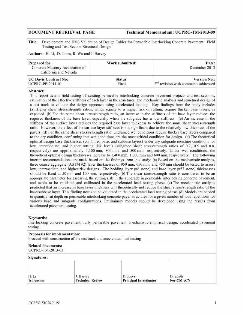
UCPRC-TM-2013-09 i
DOCUMENT RETRIEVAL PAGE Technical Memorandum: UCPRC-TM-2013-09
Title: Development and HVS Validation of Design Tables for Permeable Interlocking Concrete Pavement: Field Testing and Test Section Structural Design
Authors: H. Li, D. Jones, R. Wu and J. Harvey
Prepared for: Concrete Masonry Association of
California and Nevada
Work submitted:
Date:December 2013
UC Davis Contract No: UCPRC-PP-2011-01
Status: Final
Version No.: 2nd revision with comments addressed
Abstract: This report details field testing of existing permeable interlocking concrete pavement projects and test sections, estimation of the effective stiffness of each layer in the structures, and mechanistic analysis and structural design of a test track to validate the design approach using accelerated loading. Key findings from the study include: (a) Higher shear stress/strength ratios, which equate to a higher risk of rutting, require thicker base layers, as expected. (b) For the same shear stress/strength ratio, an increase in the stiffness of the base layer reduces the required thickness of the base layer, especially when the subgrade has a low stiffness. (c) An increase in the stiffness of the surface layer reduces the required base layer thickness to achieve the same shear stress/strength ratio. However, the effect of the surface layer stiffness is not significant due to the relatively low thickness of the pavers. (d) For the same shear stress/strength ratio, undrained wet conditions require thicker base layers compared to the dry condition, confirming that wet conditions are the most critical condition for design. (e) The theoretical optimal design base thicknesses (combined base, and subbase layers) under dry subgrade moisture conditions for low, intermediate, and higher rutting risk levels (subgrade shear stress/strength ratios of 0.2, 0.5 and 0.8, respectively) are approximately 1,300 mm, 800 mm, and 500 mm, respectively. Under wet conditions, the theoretical optimal design thicknesses increase to 1,400 mm, 1,000 mm and 600 mm, respectively. The following interim recommendations are made based on the findings from this study: (a) Based on the mechanistic analysis, three coarse aggregate (ASTM #2) layer thicknesses of 950 mm, 650 mm, and 450 mm should be tested to assess low, intermediate, and higher risk designs. The bedding layer (#8 stone) and base layer (#57 stone) thicknesses should be fixed at 50 mm and 100 mm, respectively. (b) The shear stress/strength ratio is considered to be an appropriate parameter for assessing the rutting risk in the subgrade in permeable interlocking concrete pavement, and needs to be validated and calibrated in the accelerated load testing phase. (c) The mechanistic analysis predicted that an increase in base layer thickness will theoretically not reduce the shear stress/strength ratio of the base/subbase layer. This finding needs to be validated in the accelerated load testing phase. (d) Models are needed to quantify rut depth on permeable interlocking concrete paver structures for a given number of load repetitions for various base and subgrade configurations. Preliminary models should be developed using the results from accelerated pavement testing.
Keywords: Interlocking concrete pavement, fully permeable pavement, mechanistic-empirical design, accelerated pavement testing.
Proposals for implementation: Proceed with construction of the test track and accelerated load testing
Related documents: UCPRC-TM-2013-03
Signatures:
H. Li 1st Author
J. Harvey Technical Review
D. Jones Principal Investigator
D. Smith For CMACN
ii UCPRC-TM-2013-09
DISCLAIMER
The contents of this report reflect the views of the authors who are responsible for the facts and accuracy
of the data presented herein. The contents do not necessarily reflect the official views or policies of the
Concrete Masonry Association of California and Nevada (CMACN) or the Interlocking Concrete
Pavement Institute (ICPI). This report does not constitute a standard, specification, or regulation.
PROJECT OBJECTIVES/GOALS
The objective of this project is to produce thickness design tables for permeable interlocking concrete
pavement (PICP) based on mechanistic analysis and partially validated with accelerated load testing
(ALT). The following tasks will be completed to achieve this objective:
1. Perform a literature and field survey to identify critical responses, failure mechanisms, appropriate performance transfer functions, and modeling assumptions for mechanistic analysis of PICP under truck loading.
2. Measure pavement deflection in the field on several PICP locations to characterize effective stiffness of the different layers in the structure for use in modeling.
3. Perform mechanistic analyses of PICP to develop design tables following the approach documented in California Department of Transportation (Caltrans) Research Report CTSW-RR-09-249.04 for development of structural design tables for permeable/pervious/porous asphalt and concrete pavement.
4. Prepare a plan for validation with accelerated load testing based on the results of the mechanistic analysis.
5. Test responses and, if possible, failure of up to three PICP structures in dry and wet condition with a Heavy Vehicle Simulator (HVS).
6. Analyze the results of the HVS testing to revise/update the structural design tables where necessary.
7. Write a final report documenting the results of all tasks in the study and demonstrating the design tables.
8. Present findings to Caltrans Office of Concrete Pavements and Foundation Program and Office of Stormwater - Design staff in Sacramento, CA.
This report covers Tasks 2 through 4.
UCPRC-TM-2013-09 iii
TABLE OF CONTENTS
LIST OF TABLES ...................................................................................................................................... v LIST OF FIGURES .................................................................................................................................... v 1. INTRODUCTION ............................................................................................................................. 1 1.1 Project Scope ............................................................................................................................ 1 1.2 Background to the Study ........................................................................................................... 1 1.3 Study Objective ........................................................................................................................ 1 1.4 Report Layout ........................................................................................................................... 2 1.5 Measurement Units ................................................................................................................... 2 2. DEFLECTION TESTING PLAN .................................................................................................... 3 2.1 Introduction ............................................................................................................................... 3 2.2 Background to Deflection Testing ............................................................................................ 3 2.3 Deflection Measurement Method ............................................................................................. 3 2.4 Testing Equipment .................................................................................................................... 5 2.4.1 Test Vehicle ................................................................................................................. 5 2.4.2 Road Surface Deflectometer (RSD) ............................................................................. 6 2.5 Deflection Testing Procedure ................................................................................................... 6 2.6 Test Section Locations .............................................................................................................. 7 2.6.1 Existing PICP Projects ................................................................................................. 7 2.6.2 UCPRC Experimental Section ..................................................................................... 8 3. DEFLECTION MEASUREMENT ANALYSIS .......................................................................... 11 3.1 Introduction ............................................................................................................................. 11 3.2 Backcalculation of Stiffness ................................................................................................... 11 3.2.1 Example Deflection Basin Curves ............................................................................. 11 3.2.2 Backcalculated Effective Stiffness of the Surface Layers ......................................... 12 3.2.3 Backcalculated Effective Stiffness of the Base Layers .............................................. 14 3.2.4 Backcalculated Effective Stiffness of the Subgrade Layers ...................................... 15 3.2.5 Effective Stiffness Analysis ....................................................................................... 16 3.3 UCPRC Test Section .............................................................................................................. 18 3.3.1 Backcalculated Effective Stiffness from RSD Measurements ................................... 18 3.3.2 Backcalculated Effective Stiffness from FWD Measurements .................................. 19 3.4 DCP Tests on the UCPRC Sections ........................................................................................ 20 4. MECHANISTIC ANALYSES AND STRUCTURAL DESIGN ................................................. 21 4.1 Introduction ............................................................................................................................. 21 4.2 Design Criteria ........................................................................................................................ 21 4.3 Design Variables ..................................................................................................................... 21 4.3.1 Background ................................................................................................................ 21 4.3.2 Shear Stress Ratio ...................................................................................................... 22 4.4 Critical Responses................................................................................................................... 23 4.5 Input Parameters for Mechanistic Modeling and Structural Analysis .................................... 23 4.5.1 Pavement Structure .................................................................................................... 23 4.5.2 Materials Properties ................................................................................................... 25 4.5.3 Traffic Load ............................................................................................................... 25 4.6 Mechanistic Analysis Results ................................................................................................. 26 4.6.1 Base Layer ................................................................................................................. 26 4.6.2 Subgrade Layer .......................................................................................................... 26 4.6.3 Thickness of Base Layers for Different Shear Stress Ratio Values ........................... 27 4.7 Preliminary Design Tables ...................................................................................................... 28 5. TEST PLAN FOR THICKNESS VALIDATION ........................................................................ 31 5.1 Thickness Design .................................................................................................................... 31 5.2 Test Track Instrumentation ..................................................................................................... 32 5.3 Heavy Vehicle Simulator Test Plan ........................................................................................ 33

iv UCPRC-TM-2013-09
5.3.1 Test Sections .............................................................................................................. 33 5.3.2 Loading Plan .............................................................................................................. 33 5.3.3 Environmental Control ............................................................................................... 33 5.3.4 Measurements ............................................................................................................ 33 6. SUMMARY AND RECOMMENDATIONS ................................................................................ 35 6.1 Summary ................................................................................................................................. 35 6.2 Recommendations ................................................................................................................... 35 REFERENCES .......................................................................................................................................... 37 APPENDIX A: MECHANISTIC ANALYSIS PLOTS ......................................................................... 39

UCPRC-TM-2013-09 v
LIST OF TABLES
Table 2.1: PICP Test Section Details ........................................................................................................... 8 Table 2.2: UCPRC Test Section Details....................................................................................................... 9 Table 3.1: DCP-Determined Strength Characteristics of Base and Subgrade Materials. ........................... 20 Table 4.1: Summary of Input Factorials for Performance Modeling of PICP ........................................... 24
LIST OF FIGURES
Figure 2.1: Road surface deflectometer. ....................................................................................................... 4 Figure 2.2: Test vehicle. ............................................................................................................................... 5 Figure 2.3: Re-distribution of aggregate to change load. ............................................................................. 5 Figure 2.4: Weigh-in-motion pad. ................................................................................................................ 5 Figure 2.5: Measuring the wheel load. ......................................................................................................... 5 Figure 2.6: Encoder for measuring wheel location. ..................................................................................... 6 Figure 2.7: Test section setup. ...................................................................................................................... 6 Figure 2.8: Test sites for field deflection measurement. .............................................................................. 7 Figure 2.9: Paver laying patterns at the different test sites. .......................................................................... 7 Figure 3.1: Raw and filtered deflection basin curves. ................................................................................ 12 Figure 3.2: Effective surface layer stiffness at Target test site (1 MPa = 145 psi). .................................... 13 Figure 3.3: Effective surface layer stiffness at Yolo Credit Union test site. .............................................. 13 Figure 3.4: Effective surface layer stiffness at Matsui Park test site. ......................................................... 13 Figure 3.5: Effective base stiffness at Target test site. ............................................................................... 14 Figure 3.6: Effective base stiffness at Yolo Credit Union test site. ............................................................ 14 Figure 3.7: Effective base stiffness at Matsui Park test site. ...................................................................... 15 Figure 3.8: Effective subgrade stiffness at Target test site. ........................................................................ 15 Figure 3.9: Effective subgrade stiffness at Yolo Credit Union test site. .................................................... 16 Figure 3.10: Effective subgrade stiffness at Matsui Park test site. ............................................................. 16 Figure 3.11: Cumulative distribution of effective surface stiffness at all three test sites. .......................... 17 Figure 3.12: Cumulative distribution of effective base stiffness at all three test sites. .............................. 17 Figure 3.13: Cumulative distribution of effective subgrade stiffness at all three test sites. ....................... 17 Figure 3.14: Cumulative distribution of effective surface stiffness at the two Davis sites. ....................... 18 Figure 3.15: Cumulative distribution of effective base stiffness at the two Davis sites. ............................ 18 Figure 3.16: Cumulative distribution of effective subgrade stiffness at the two Davis sites. .................... 18 Figure 3.17: Effective base stiffness under different loads (dry condition). .............................................. 19 Figure 3.18: Effective base stiffness under dry and wet conditions (37 kN load). ..................................... 19 Figure 3.19: Effective subgrade stiffness in dry and wet conditions (37 kN load). ................................... 19 Figure 3.20: Effective base and subgrade stiffness (FWD) of the porous asphalt section. ........................ 19 Figure 4.1: Suggested base layer thicknesses for different shear stress/strength ratios (ϕ ≠ 0 [dry]). ....... 29 Figure 4.2: Suggested base layer thicknesses for different shear stress/strength ratios (ϕ = 0 [wet]). ....... 30 Figure 5.1: Proposed pavement structure for PICP test track (not to scale). .............................................. 31 Figure 5.2: Proposed test track design. ....................................................................................................... 32
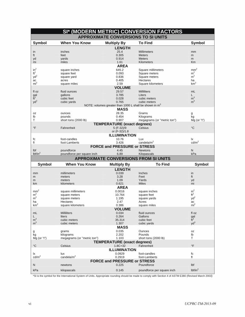
vi UCPRC-TM-2013-09
SI* (MODERN METRIC) CONVERSION FACTORS APPROXIMATE CONVERSIONS TO SI UNITS
Symbol When You Know Multiply By To Find Symbol LENGTH
in inches 25.4 Millimeters mm ft feet 0.305 Meters m yd yards 0.914 Meters m mi miles 1.61 Kilometers Km
AREAin2 square inches 645.2 Square millimeters mm2 ft2 square feet 0.093 Square meters m2 yd2 square yard 0.836 Square meters m2 ac acres 0.405 Hectares ha mi2 square miles 2.59 Square kilometers km2
VOLUMEfl oz fluid ounces 29.57 Milliliters mL gal gallons 3.785 Liters L ft3 cubic feet 0.028 cubic meters m3 yd3 cubic yards 0.765 cubic meters m3
NOTE: volumes greater than 1000 L shall be shown in m3
MASSoz ounces 28.35 Grams g lb pounds 0.454 Kilograms kg T short tons (2000 lb) 0.907 megagrams (or "metric ton") Mg (or "t")
TEMPERATURE (exact degrees)°F Fahrenheit 5 (F-32)/9 Celsius °C
or (F-32)/1.8
ILLUMINATION fc foot-candles 10.76 Lux lx fl foot-Lamberts 3.426 candela/m2 cd/m2
FORCE and PRESSURE or STRESS lbf poundforce 4.45 Newtons N lbf/in2 poundforce per square inch 6.89 Kilopascals kPa
APPROXIMATE CONVERSIONS FROM SI UNITS
Symbol When You Know Multiply By To Find Symbol LENGTH
mm millimeters 0.039 Inches in m meters 3.28 Feet ft m meters 1.09 Yards yd km kilometers 0.621 Miles mi
AREAmm2 square millimeters 0.0016 square inches in2 m2 square meters 10.764 square feet ft2 m2 square meters 1.195 square yards yd2 ha Hectares 2.47 Acres ac km2 square kilometers 0.386 square miles mi2
VOLUMEmL Milliliters 0.034 fluid ounces fl oz L liters 0.264 Gallons gal m3 cubic meters 35.314 cubic feet ft3 m3 cubic meters 1.307 cubic yards yd3
MASSg grams 0.035 Ounces oz kg kilograms 2.202 Pounds lb Mg (or "t") megagrams (or "metric ton") 1.103 short tons (2000 lb) T
TEMPERATURE (exact degrees) °C Celsius 1.8C+32 Fahrenheit °F
ILLUMINATION lx lux 0.0929 foot-candles fc cd/m2 candela/m2 0.2919 foot-Lamberts fl
FORCE and PRESSURE or STRESSN newtons 0.225 Poundforce lbf
kPa kilopascals 0.145 poundforce per square inch lbf/in2
*SI is the symbol for the International System of Units. Appropriate rounding should be made to comply with Section 4 of ASTM E380 (Revised March 2003)

UCPRC-TM-2013-09 1
1. INTRODUCTION
1.1 Project Scope
This project is being coordinated through the Interlocking Concrete Pavement Institute (ICPI) and the
Concrete Masonry Association of California and Nevada with additional support from the California
Nevada Cement Association. The objective of this project is to produce thickness design tables for
permeable interlocking concrete pavement (PICP) based on mechanistic analysis and partially validated
with accelerated load testing (ALT).
1.2 Background to the Study
Although permeable pavements are becoming increasingly common across the United States, they are
mostly used in parking lots, basic access streets, recreation areas, and landscaped areas, all of which carry
very light, slow moving traffic. Only limited research has been undertaken on the mechanistic design and
long-term performance monitoring of permeable pavements carrying higher traffic volumes and heavier
loads, and the work that has been done has focused primarily on pavements with open-graded asphalt or
portland cement concrete surfacings. Very little research has been undertaken on the use of permeable
concrete paver surfaces on these more heavily trafficked pavements.
1.3 Study Objective
The objective of this project is to produce design tables for permeable interlocking concrete pavement
(PICP) based on mechanistic analysis and partially validated with accelerated load testing (ALT).
The tasks to complete this objective include the following:
1. Perform a literature and field survey to identify critical responses, failure mechanisms, appropriate performance transfer functions, and modeling assumptions for mechanistic analysis of PICP under truck loading. This task has been completed and a summary report prepared (1).
2. Measure pavement deflection in the field on several PICP locations to characterize effective stiffness of the different layers in the structure for use in modeling.
3. Perform mechanistic analyses of PICP to develop design tables following the approach documented in California Department of Transportation (Caltrans) Research Report CTSW-RR-09-249.04 for development of structural design tables for permeable/pervious/porous asphalt and concrete pavement (2).
4. Prepare a plan for validation with accelerated load testing based on the results of the mechanistic analysis.
5. Test responses and, if possible, failure of up to three PICP structures in dry and wet condition with a Heavy Vehicle Simulator (HVS).

2 UCPRC-TM-2013-09
6. Analyze the results of the HVS testing to revise/update the structural design tables where necessary.
7. Write a final report documenting the results of all tasks in the study and demonstrating the design tables.
8. Present findings to Caltrans Office of Concrete Pavements and Foundation Program and Office of Stormwater - Design staff in Sacramento, CA.
The report covers Tasks 2 through 4.
1.4 Report Layout
This report covers the pavement deflection measurement and stiffness backcalculation work completed in
Task #2, mechanistic analyses and structural design completed in Task #3, and the accelerated loading test
plan for validation of the structural designs completed in Task #4. Chapters include:
Chapter 2 includes a brief description of pavement deflection testing and details the experiment plan for field deflection testing of existing PICP sections.
Chapter 3 summarizes the results of the deflection testing.
Chapter 4 presents the results and analyses of the mechanistic analysis and preliminary structural designs.
Chapter 5 presents the test plan for thickness validation with a Heavy Vehicle Simulator.
Chapter 6 presents conclusions and recommendations.
Appendix A contains summary plots of the mechanistic analysis results.
1.5 Measurement Units
Metric units are always used by the UCPRC in mechanistic design, the design and layout of HVS test
tracks, for laboratory, accelerated load testing, and field measurements, and for data storage. Where
appropriate in this report, both U.S. customary and metric units are provided. In other cases where data is
collected, analyzed, and discussed, only metric units are used. A conversion table is provided on page vi
at the beginning of this report.

UCPRC-TM-2013-09 3
2. DEFLECTION TESTING PLAN
2.1 Introduction
This chapter describes the experiment plan for deflection testing of existing PICP projects in northern
California. A brief background to deflection testing is provided, followed by a description of the
equipment used in this study to measure deflections, the testing procedure followed, and details on
supplementary testing of subgrade shear strengths in dry and soaked conditions. A description of the test
section locations and pavement structures is also provided.
2.2 Background to Deflection Testing
Pavement surface deflection measurements are a primary method of evaluating the behavior of pavement
structures when subjected to a load. These measurements, which are non-destructive, are used to assess a
pavement’s structural condition, by taking most relevant factors into consideration, including traffic type
and volume, pavement structural section, temperature, and moisture condition. Deflection measurements
can be used in backcalculation procedures to determine:
Pavement structural layer stiffness, used as an indicator to determine what level of traffic loading the pavement can withstand (i.e., design life or remaining life in terms of number of axle loads), and
Subgrade resilient modulus, used to determine the thickness of the pavement that will be required to prevent subgrade failures over the expected design life.
Deflection measurements are used by most departments of transportation as the basis for rehabilitation
designs and often as a trigger for when rehabilitation or reconstruction is required.
All pavements bend under loading to some degree. Although this bending can normally not be
distinguished with the naked eye (measurements are typically recorded in microns or mils) it has a
significant effect on the integrity of the different layers over time. Repeated bending and then relaxation
as the load moves onto and then off a point on a pavement is analogous to repeatedly bending a piece of
wire back and forth – it eventually breaks. In pavements, the “damage” usually materializes as
reorientation of the material particles, cracks and/or shearing, which leads to a reduction in stiffness over
time, which in turn leads to moisture ingress, rutting, and other associated problems.
2.3 Deflection Measurement Method
Pavement deflection is most commonly measured with a falling weight deflectometer (FWD). However,
this equipment is designed for continuous asphalt concrete and portland cement concrete pavements built

4 UCPRC-TM-2013-09
on dense-graded aggregate bases, and was not considered appropriate for testing deflection on pavements
constructed with interlocking concrete pavers (because of the segmented nature of the pavement surface),
overlying open-graded aggregate bases. An FWD also applies an instantaneous dynamic load onto the
pavement surface to simulate a truck wheel load passing over that point at a speed of about 60 km/h
(40 mph). Deflection in the pavement is measured under this load. Open-graded aggregate bases used in
permeable pavements, are usually more stress dependent than dense-graded bases, and can therefore have
a bigger range of stiffness increase and relaxation as the wheel load passes over it. Backcalculating
stiffnesses based on these measurements may therefore provide incorrect results when analyzing PICP. A
review of the literature on PICP (1) revealed that other researchers had experienced problems with
accurately analyzing the stiffness of PICP from FWD deflection measurements.
Based on these concerns, a modified Benkelman beam (road surface deflectometer [RSD]) was instead
used to measure deflection on the test sections. This device, which is standard equipment for measuring
surface deflections on accelerated load tests at the UCPRC, measures the actual deflection between the
dual wheels of a truck as it passes at slow speed over the instrument (Figure 2.1).
Figure 2.1: Road surface deflectometer.
The instrument is not influenced by the segmental nature of the pavers (provided that the four points are in
contact with the surface and not on a joint) and is considered more appropriate for accommodating the

UCPRC-TM-2013-09 5
stress dependent nature of the open-graded aggregate base. These deflection measurements were used to
backcalculate the effective stiffnesses of the individual pavement layers based on multilayer linear elastic
theory. A comparison between the FWD and RSD was undertaken on a fully permeable pavement with a
continuous open-graded asphalt surface to compare the backcalculated stiffnesses of the open-graded base
using the two deflection methods. Testing was done under both dry and wet conditions on this section.
Dynamic cone penetrometer measurements were also taken on this pavement to obtain an indication of the
subgrade shear strength under dry and wet conditions to further verify the results.
2.4 Testing Equipment
2.4.1 Test Vehicle
A single rear axle, dual-wheel dump truck loaded with aggregate was used as the test vehicle (Figure 2.2).
The load area of this truck was dividable, which allowed a load change on the rear axle by distributing the
aggregate (Figure 2.3). Measurements were taken with wheel loads of 35 kN and 45 kN (8,000 lb and
10,000 lb). Axle loads were measured using a weigh-in-motion pad (Figure 2.4 and Figure 2.5).
Figure 2.2: Test vehicle. Figure 2.3: Re-distribution of aggregate to change load.
Figure 2.4: Weigh-in-motion pad. Figure 2.5: Measuring the wheel load.

6 UCPRC-TM-2013-09
2.4.2 Road Surface Deflectometer (RSD)
A road surface deflectometer (RSD) was used to measure the deflection basin caused by the moving load
on the pavement surface (Figure 2.1). An encoder was designed and constructed to precisely measure the
wheel location/distance (Figure 2.6), which is a critical input for backcalculating the pavement stiffness.
Air and pavement surface temperatures were measured using Type-K thermocouple sensors. All data was
collected on a customized data acquisition system (DAS). A setup at a test section is shown in Figure 2.7.
Figure 2.6: Encoder for measuring wheel location.
Figure 2.7: Test section setup.
2.5 Deflection Testing Procedure
Deflection measurements were taken at various locations at each test site on two different lines on the
pavement: the centerline (CL) and approximate outside wheelpath (WP). Five replicate measurements
Road Surface Deflectometer
Encoder
DAS Power Generator
Air Temperature Sensor
Pavement Temperature Sensor
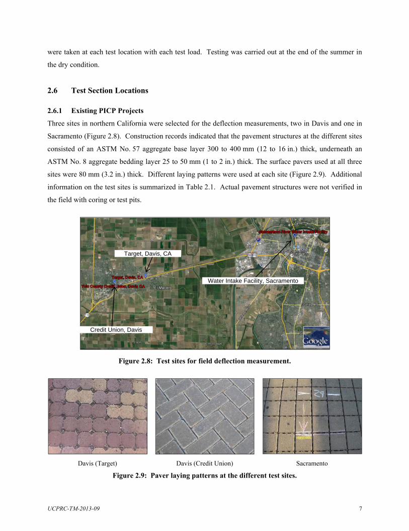
UCPRC-TM-2013-09 7
were taken at each test location with each test load. Testing was carried out at the end of the summer in
the dry condition.
2.6 Test Section Locations
2.6.1 Existing PICP Projects
Three sites in northern California were selected for the deflection measurements, two in Davis and one in
Sacramento (Figure 2.8). Construction records indicated that the pavement structures at the different sites
consisted of an ASTM No. 57 aggregate base layer 300 to 400 mm (12 to 16 in.) thick, underneath an
ASTM No. 8 aggregate bedding layer 25 to 50 mm (1 to 2 in.) thick. The surface pavers used at all three
sites were 80 mm (3.2 in.) thick. Different laying patterns were used at each site (Figure 2.9). Additional
information on the test sites is summarized in Table 2.1. Actual pavement structures were not verified in
the field with coring or test pits.
Figure 2.8: Test sites for field deflection measurement.
Davis (Target) Davis (Credit Union) Sacramento
Figure 2.9: Paver laying patterns at the different test sites.
Water Intake Facility, Sacramento
Target, Davis, CA
Credit Union, Davis
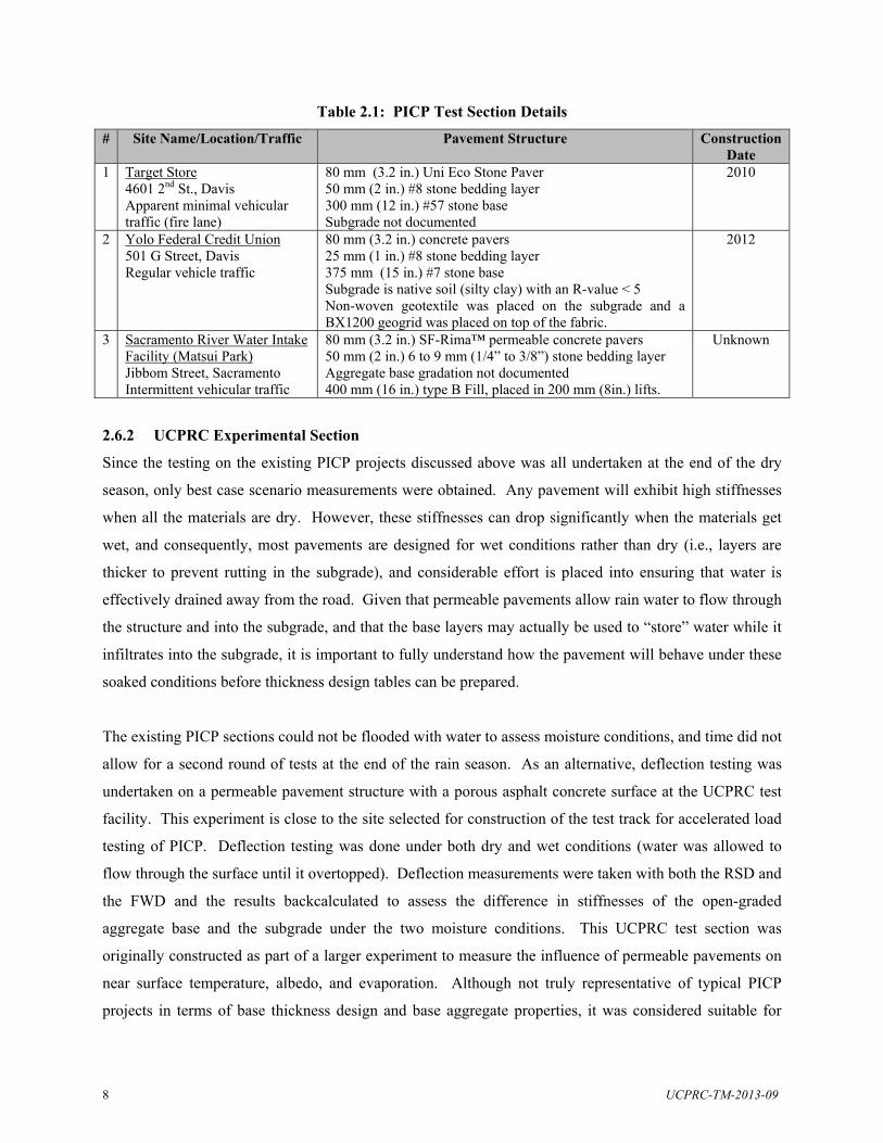
8 UCPRC-TM-2013-09
Table 2.1: PICP Test Section Details
# Site Name/Location/Traffic Pavement Structure Construction Date
1 Target Store 4601 2nd St., Davis Apparent minimal vehicular traffic (fire lane)
80 mm (3.2 in.) Uni Eco Stone Paver 50 mm (2 in.) #8 stone bedding layer 300 mm (12 in.) #57 stone base Subgrade not documented
2010
2 Yolo Federal Credit Union 501 G Street, Davis Regular vehicle traffic
80 mm (3.2 in.) concrete pavers 25 mm (1 in.) #8 stone bedding layer 375 mm (15 in.) #7 stone base Subgrade is native soil (silty clay) with an R-value < 5 Non-woven geotextile was placed on the subgrade and a BX1200 geogrid was placed on top of the fabric.
2012
3 Sacramento River Water Intake Facility (Matsui Park) Jibbom Street, Sacramento Intermittent vehicular traffic
80 mm (3.2 in.) SF-Rima™ permeable concrete pavers 50 mm (2 in.) 6 to 9 mm (1/4” to 3/8”) stone bedding layer Aggregate base gradation not documented 400 mm (16 in.) type B Fill, placed in 200 mm (8in.) lifts.
Unknown
2.6.2 UCPRC Experimental Section
Since the testing on the existing PICP projects discussed above was all undertaken at the end of the dry
season, only best case scenario measurements were obtained. Any pavement will exhibit high stiffnesses
when all the materials are dry. However, these stiffnesses can drop significantly when the materials get
wet, and consequently, most pavements are designed for wet conditions rather than dry (i.e., layers are
thicker to prevent rutting in the subgrade), and considerable effort is placed into ensuring that water is
effectively drained away from the road. Given that permeable pavements allow rain water to flow through
the structure and into the subgrade, and that the base layers may actually be used to “store” water while it
infiltrates into the subgrade, it is important to fully understand how the pavement will behave under these
soaked conditions before thickness design tables can be prepared.
The existing PICP sections could not be flooded with water to assess moisture conditions, and time did not
allow for a second round of tests at the end of the rain season. As an alternative, deflection testing was
undertaken on a permeable pavement structure with a porous asphalt concrete surface at the UCPRC test
facility. This experiment is close to the site selected for construction of the test track for accelerated load
testing of PICP. Deflection testing was done under both dry and wet conditions (water was allowed to
flow through the surface until it overtopped). Deflection measurements were taken with both the RSD and
the FWD and the results backcalculated to assess the difference in stiffnesses of the open-graded
aggregate base and the subgrade under the two moisture conditions. This UCPRC test section was
originally constructed as part of a larger experiment to measure the influence of permeable pavements on
near surface temperature, albedo, and evaporation. Although not truly representative of typical PICP
projects in terms of base thickness design and base aggregate properties, it was considered suitable for

UCPRC-TM-2013-09 9
comparing the change in uncompacted subgrade properties under an open-graded aggregate base when
conditions changed from dry to wet. Test section details are summarized in Table 2.2.
Table 2.2: UCPRC Test Section Details
# Site Name/Location Pavement Structure Construction Date
4 UCPRC Facility porous asphalt 4 in. (100 mm) porous asphalt 1 in. (25 mm) #8 stone bedding layer 12 in. (300 mm) graded aggregate base Silty-clay subgrade (uncompacted)
2011

10 UCPRC-TM-2013-09
Blank page

UCPRC-TM-2013-09 11
3. DEFLECTION MEASUREMENT ANALYSIS
3.1 Introduction
This chapter discusses the analysis of the deflection measurement data collected at the four test locations
discussed in Chapter 2. The primary component of this analysis was the backcalculation of the stiffnesses
of the different pavement layers. Backcalculation is a mechanistic evaluation of pavement surface
deflection basins generated by pavement deflection devices (i.e., the RSD and FWD in this study). In the
backcalculation process, measured surface deflections are matched, within some tolerable error, with a
calculated surface deflection generated from an identical pavement structure using assumed layer
stiffnesses (moduli). The assumed layer moduli in the calculated model are adjusted until they produce a
surface deflection that closely matches the measured one. The combination of assumed layer stiffnesses
that results in this match is then assumed to be near the actual in situ moduli for the various pavement
layers. The backcalculation process is usually iterative and normally done with computer software.
In this study, layer stiffness backcalculation using RSD data was conducted using a Matlab script
(KalmanBack) developed by the UCPRC. KalmanBack uses OpenPave (www.openpave.org) for the
deflection calculation and then uses a Kalman Filter as the search algorithm (3). When matching surface
deflections measured with the RSD, the deflection at the RSD anchoring feet was also accounted for.
3.2 Backcalculation of Stiffness
The pavement structures were simplified into three layers for the backcalculation of stiffness: surface
layer (paver), base layer (aggregate, including bedding layers and base layer), and subgrade layer (soil).
The as-designed layer thicknesses summarized in Table 2.1 and Table 2.2 were used for the
backcalculation analysis. The effective stiffnesses of these three layers were optimized through
minimizing the error between the calculated and the measured deflection basin curves based on multilayer
linear elastic theory, which is commonly used as the basis for pavement design procedures.
3.2.1 Example Deflection Basin Curves
The measured deflection basin curves had some noise, consistent with deflection measurements on
pavements with uneven surfaces. The data were therefore processed using center-moving-average
filtering to reduce this noise. Examples of the raw deflection basin curve and the filtered deflection basin
curve are shown in Figure 3.1.

12 UCPRC-TM-2013-09
(a) Raw deflection basin curve (b) Filtered deflection basin curve
Figure 3.1: Raw and filtered deflection basin curves.
3.2.2 Backcalculated Effective Stiffness of the Surface Layers
Effective stiffnesses were backcalculated from the deflection measurements using layer elastic theory.
The effective stiffness of the surface layers under two different load levels and for two testing lines
(centerline [CL] and wheelpath [WP]) at the three test sites (Target, Yolo Credit Union, and Matsui Park)
are presented in Figure 3.2 through Figure 3.4. The main observations from this analysis include:
There was a significant variation in surface effective stiffness among the three test sections, with very low stiffnesses measured at Matsui Park, intermediate stiffnesses measured at Yolo Credit Union, and higher stiffnesses measured at the Target site. Variation in stiffness was attributed to paver shape, paving laying pattern, degree of interlock between pavers, and confinement. For example, the lower stiffnesses at Matsui Park were attributed in part to the choice of paver (square) and the laying pattern (no interlocking pattern [see Figure 2.9]).
Variations in surface effective stiffness were noted along the length of each test section on both the centerline and the wheelpath. This was attributed in part to construction variability and loosening of the paver interlock under traffic.
The mean effective stiffness of the surface layer under the heavier load was generally slightly higher than that under the lighter load on all three sections.
Lower variation in effective stiffness was measured along the wheelpath compared to the centerline. This was attributed to the stronger and more uniform confining effect from the concrete curb and underlying edge walls close to the wheelpath.
0 1 2 3 4
-3.0
-2.5
-2.0
-1.5
-1.0
-0.5
0.0
Distance (m)
Def
lect
ion
(mm
)
10CL_110CL_210CL_310CL_410CL_5
Test Site: TargetDual-Wheel Load (kN): 34Tire Pressure (kPa): 586.1Surface Temperature (C): 43.3Air Temperature (C): 24.6
0 1 2 3 4
-3.0
-2.5
-2.0
-1.5
-1.0
-0.5
0.0
Distance (m)
Def
lect
ion
(mm
)
10CL_110CL_210CL_310CL_410CL_5
Test Site: TargetDual-Wheel Load (kN): 34Tire Pressure (kPa): 586.1Surface Temperature (C): 43.3Air Temperature (C): 24.6
Smoothing with Center Moving Average n_avg = 100

UCPRC-TM-2013-09 13
Centerline Wheelpath
Figure 3.2: Effective surface layer stiffness at Target test site (1 MPa = 145 psi).
Centerline Wheelpath
Figure 3.3: Effective surface layer stiffness at Yolo Credit Union test site.
Centerline Wheelpath
Figure 3.4: Effective surface layer stiffness at Matsui Park test site.
10 30 50 70 90 110 130 150 170 190
0
500
1000
1500
2000
10 30 50 70 90 110 130 150 170 190
0
500
1000
1500
2000
Distance (m)
Su
rfa
ce S
tiffn
ess
(MP
a)
34 kN47 kN
Site: TargetLocation: CLLayer: SurfaceMoisture: Dry
10 50 90 130 170
0
500
1000
1500
2000
10 40 80 130 170
0
500
1000
1500
2000
Distance (m)
Su
rfac
e S
tiff
ne
ss (
MP
a)
34 kN47 kN
Site: TargetLocation: WPLayer: SurfaceMoisture: Dry
2.5 7.5 12.5 17.5 22.5 27.5
0
500
1000
1500
2000
2.5 7.5 12.5 17.5 22.5 27.5
0
500
1000
1500
2000
Distance (m)
Su
rfa
ce S
tiffn
ess
(MP
a)
36 kN44.5 kN
Site: Yolo Credit UnionLocation: CLLayer: SurfaceMoisture: Dry
7.5 17.5 27.5
0
500
1000
1500
2000
7.5 17.5 27.5
0
500
1000
1500
2000
Distance (m)
Su
rfa
ce S
tiffn
ess
(MP
a)
36 kN44.5 kN
Site: Yolo Credit UnionLocation: WPLayer: SurfaceMoisture: Dry
4 14 24 36
0
500
1000
1500
2000
4 14 24 36
0
500
1000
1500
2000
Distance (m)
Su
rfa
ce S
tiffn
ess
(MP
a)
33 kN43 kN
Site: Matsui ParkLocation: CLLayer: SurfaceMoisture: Dry
14 24
0
500
1000
1500
2000
14 24
0
500
1000
1500
2000
Distance (m)
Su
rfa
ce S
tiffn
ess
(MP
a)
33 kN43 kN
Site: Matsui ParkLocation: WPLayer: SurfaceMoisture: Dry
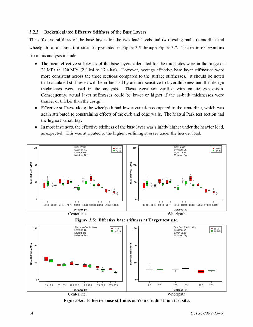
14 UCPRC-TM-2013-09
3.2.3 Backcalculated Effective Stiffness of the Base Layers
The effective stiffness of the base layers for the two load levels and two testing paths (centerline and
wheelpath) at all three test sites are presented in Figure 3.5 through Figure 3.7. The main observations
from this analysis include:
The mean effective stiffnesses of the base layers calculated for the three sites were in the range of 20 MPa to 120 MPa (2.9 ksi to 17.4 ksi). However, average effective base layer stiffnesses were more consistent across the three sections compared to the surface stiffnesses. It should be noted that calculated stiffnesses will be influenced by and are sensitive to layer thickness and that design thicknesses were used in the analysis. These were not verified with on-site excavation. Consequently, actual layer stiffnesses could be lower or higher if the as-built thicknesses were thinner or thicker than the design.
Effective stiffness along the wheelpath had lower variation compared to the centerline, which was again attributed to constraining effects of the curb and edge walls. The Matsui Park test section had the highest variability.
In most instances, the effective stiffness of the base layer was slightly higher under the heavier load, as expected. This was attributed to the higher confining stresses under the heavier load.
Centerline Wheelpath
Figure 3.5: Effective base stiffness at Target test site.
Centerline Wheelpath
Figure 3.6: Effective base stiffness at Yolo Credit Union test site.
10 30 50 70 90 110 130 150 170 190
0
50
100
150
10 30 50 70 90 110 130 150 170 190
0
50
100
150
Distance (m)
Ba
se S
tiffn
ess
(MP
a)
34 kN47 kN
Site: TargetLocation: CLLayer: BaseMoisture: Dry
10 30 50 70 90 110 130 150 170 190
0
50
100
150
10 30 50 70 90 110 130 150 170 190
0
50
100
150
Distance (m)
Ba
se S
tiffn
ess
(MP
a)
34 kN47 kN
Site: TargetLocation: CLLayer: BaseMoisture: Dry
2.5 7.5 12.5 17.5 22.5 27.5
0
50
100
150
2.5 7.5 12.5 17.5 22.5 27.5
0
50
100
150
Distance (m)
Ba
se S
tiffn
ess
(MP
a)
36 kN44.5 kN
Site: Yolo Credit UnionLocation: CLLayer: BaseMoisture: Dry
7.5 17.5 27.5
0
50
100
150
7.5 17.5 27.5
0
50
100
150
Distance (m)
Ba
se S
tiffn
ess
(MP
a)
36 kN44.5 kN
Site: Yolo Credit UnionLocation: WPLayer: BaseMoisture: Dry
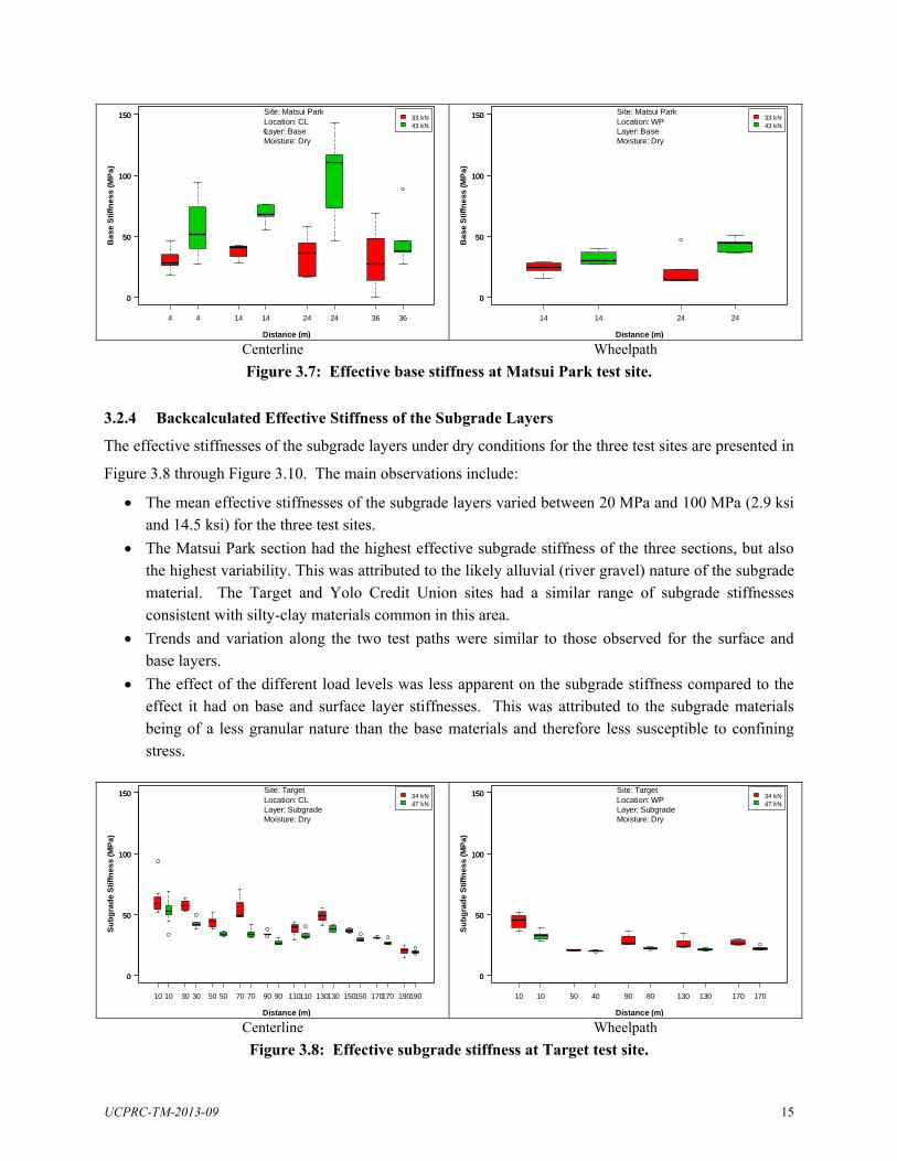
UCPRC-TM-2013-09 15
Centerline Wheelpath
Figure 3.7: Effective base stiffness at Matsui Park test site.
3.2.4 Backcalculated Effective Stiffness of the Subgrade Layers
The effective stiffnesses of the subgrade layers under dry conditions for the three test sites are presented in
Figure 3.8 through Figure 3.10. The main observations include:
The mean effective stiffnesses of the subgrade layers varied between 20 MPa and 100 MPa (2.9 ksi and 14.5 ksi) for the three test sites.
The Matsui Park section had the highest effective subgrade stiffness of the three sections, but also the highest variability. This was attributed to the likely alluvial (river gravel) nature of the subgrade material. The Target and Yolo Credit Union sites had a similar range of subgrade stiffnesses consistent with silty-clay materials common in this area.
Trends and variation along the two test paths were similar to those observed for the surface and base layers.
The effect of the different load levels was less apparent on the subgrade stiffness compared to the effect it had on base and surface layer stiffnesses. This was attributed to the subgrade materials being of a less granular nature than the base materials and therefore less susceptible to confining stress.
Centerline Wheelpath
Figure 3.8: Effective subgrade stiffness at Target test site.
4 14 24 36
0
50
100
150
4 14 24 36
0
50
100
150
Distance (m)
Ba
se
Sti
ffn
ess
(MP
a)
33 kN43 kN
Site: Matsui ParkLocation: CLLayer: BaseMoisture: Dry
14 24
0
50
100
150
14 24
0
50
100
150
Distance (m)
Ba
se
Sti
ffn
ess
(MP
a)
33 kN43 kN
Site: Matsui ParkLocation: WPLayer: BaseMoisture: Dry
10 30 50 70 90 110 130 150 170 190
0
50
100
150
10 30 50 70 90 110 130 150 170 190
0
50
100
150
Distance (m)
Su
bg
rad
e S
tiffn
ess
(MP
a)
34 kN47 kN
Site: TargetLocation: CLLayer: SubgradeMoisture: Dry
10 50 90 130 170
0
50
100
150
10 40 80 130 170
0
50
100
150
Distance (m)
Su
bg
rad
e S
tiffn
ess
(MP
a)
34 kN47 kN
Site: TargetLocation: WPLayer: SubgradeMoisture: Dry
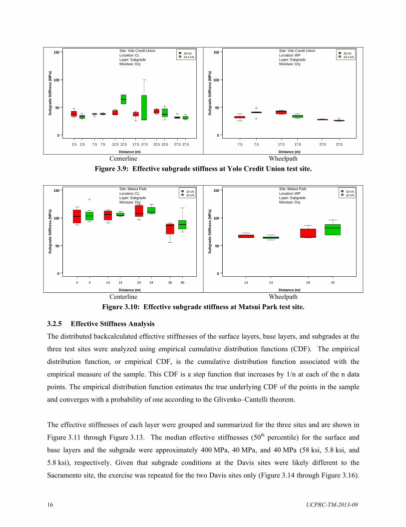
16 UCPRC-TM-2013-09
Centerline Wheelpath
Figure 3.9: Effective subgrade stiffness at Yolo Credit Union test site.
Centerline Wheelpath
Figure 3.10: Effective subgrade stiffness at Matsui Park test site. 3.2.5 Effective Stiffness Analysis
The distributed backcalculated effective stiffnesses of the surface layers, base layers, and subgrades at the
three test sites were analyzed using empirical cumulative distribution functions (CDF). The empirical
distribution function, or empirical CDF, is the cumulative distribution function associated with the
empirical measure of the sample. This CDF is a step function that increases by 1/n at each of the n data
points. The empirical distribution function estimates the true underlying CDF of the points in the sample
and converges with a probability of one according to the Glivenko–Cantelli theorem.
The effective stiffnesses of each layer were grouped and summarized for the three sites and are shown in
Figure 3.11 through Figure 3.13. The median effective stiffnesses (50th percentile) for the surface and
base layers and the subgrade were approximately 400 MPa, 40 MPa, and 40 MPa (58 ksi, 5.8 ksi, and
5.8 ksi), respectively. Given that subgrade conditions at the Davis sites were likely different to the
Sacramento site, the exercise was repeated for the two Davis sites only (Figure 3.14 through Figure 3.16).
2.5 7.5 12.5 17.5 22.5 27.5
0
50
100
150
2.5 7.5 12.5 17.5 22.5 27.5
0
50
100
150
Distance (m)
Su
bg
rad
e S
tiff
ne
ss (
MP
a)
36 kN44.5 kN
Site: Yolo Credit UnionLocation: CLLayer: SubgradeMoisture: Dry
7.5 17.5 27.5
0
50
100
150
7.5 17.5 27.5
0
50
100
150
Distance (m)
Su
bg
rad
e S
tiff
ne
ss (
MP
a)
36 kN44.5 kN
Site: Yolo Credit UnionLocation: WPLayer: SubgradeMoisture: Dry
4 14 24 36
0
50
100
150
4 14 24 36
0
50
100
150
Distance (m)
Su
bg
rad
e S
tiffn
ess
(MP
a)
33 kN43 kN
Site: Matsui ParkLocation: CLLayer: SubgradeMoisture: Dry
14 24
0
50
100
150
14 24
0
50
100
150
Distance (m)
Su
bg
rad
e S
tiffn
ess
(MP
a)
33 kN43 kN
Site: Matsui ParkLocation: WPLayer: SubgradeMoisture: Dry

UCPRC-TM-2013-09 17
Effective stiffness values changed to approximately 500 MPa, 35 MPa and 35 MPa (73 ksi, 5.1 ksi, and
5.1 ksi), respectively.
The results indicate that the effective stiffnesses at the 50th percentile of the surface layers at the Davis
sites were higher than that at the Sacramento site, which was again attributed to paver type, laying pattern,
and degree of paver interlock. The effective stiffnesses at 50 percent CDF of the base and subgrade layers
at the Davis sites were slightly lower than that of the Sacramento site, which was attributed to different
base aggregate sources and the likelihood that the Sacramento site had an alluvial aggregate subgrade,
compared to the silty-clay subgrades common in the Davis area. These effective stiffnesses are
comparable to the results obtained during earlier laboratory testing (1,2) and results cited in the literature
(e.g., 4-6).
Figure 3.11: Cumulative distribution of effective surface stiffness at all three test sites.
Figure 3.12: Cumulative distribution of effective base stiffness at all three test sites.
Figure 3.13: Cumulative distribution of effective subgrade stiffness at all three test sites.
0 500 1000 1500 2000
0.0
0.2
0.4
0.6
0.8
1.0
Surface Stiffness (MPa)
CD
F
Layer: SurfaceSite: All Sites
median=364.3mean=432.5std.dev=430.2N=324
0 50 100 150
0.0
0.2
0.4
0.6
0.8
1.0
Base Stiffness (MPa)
CD
F
Layer: BaseSite: All Sites
median=36.5mean=39.1std.dev=16.9N=324
20 40 60 80 100 120 140
0.0
0.2
0.4
0.6
0.8
1.0
Subgrade Stiffness (MPa)
CD
F
Layer: SubgradeSite: All Sites
median=37.9mean=48.2std.dev=27.2N=324
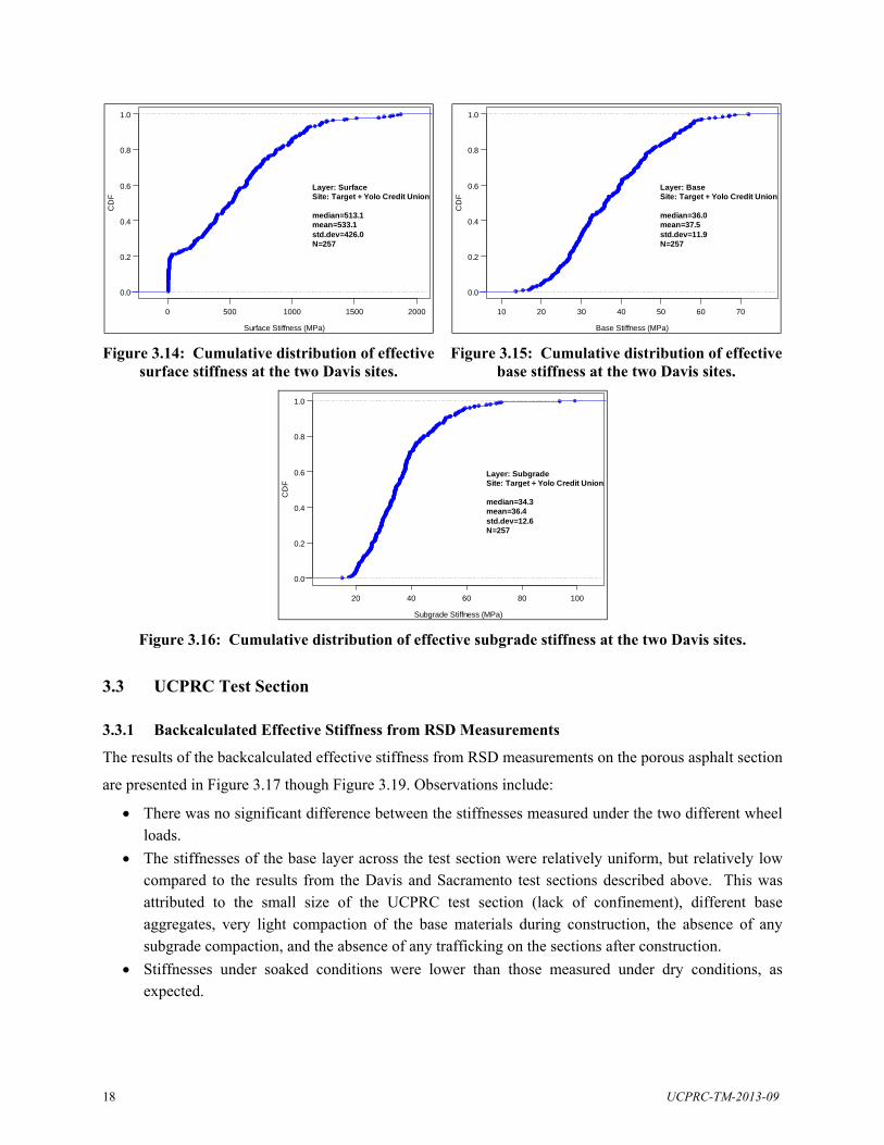
18 UCPRC-TM-2013-09
Figure 3.14: Cumulative distribution of effective surface stiffness at the two Davis sites.
Figure 3.15: Cumulative distribution of effective base stiffness at the two Davis sites.
Figure 3.16: Cumulative distribution of effective subgrade stiffness at the two Davis sites.
3.3 UCPRC Test Section
3.3.1 Backcalculated Effective Stiffness from RSD Measurements
The results of the backcalculated effective stiffness from RSD measurements on the porous asphalt section
are presented in Figure 3.17 though Figure 3.19. Observations include:
There was no significant difference between the stiffnesses measured under the two different wheel loads.
The stiffnesses of the base layer across the test section were relatively uniform, but relatively low compared to the results from the Davis and Sacramento test sections described above. This was attributed to the small size of the UCPRC test section (lack of confinement), different base aggregates, very light compaction of the base materials during construction, the absence of any subgrade compaction, and the absence of any trafficking on the sections after construction.
Stiffnesses under soaked conditions were lower than those measured under dry conditions, as expected.
0 500 1000 1500 2000
0.0
0.2
0.4
0.6
0.8
1.0
Surface Stiffness (MPa)
CD
F
Layer: SurfaceSite: Target + Yolo Credit Union
median=513.1mean=533.1std.dev=426.0N=257
10 20 30 40 50 60 70
0.0
0.2
0.4
0.6
0.8
1.0
Base Stiffness (MPa)
CD
F
Layer: BaseSite: Target + Yolo Credit Union
median=36.0mean=37.5std.dev=11.9N=257
20 40 60 80 100
0.0
0.2
0.4
0.6
0.8
1.0
Subgrade Stiffness (MPa)
CD
F
Layer: SubgradeSite: Target + Yolo Credit Union
median=34.3mean=36.4std.dev=12.6N=257

UCPRC-TM-2013-09 19
3.3.2 Backcalculated Effective Stiffness from FWD Measurements
The effective base and subgrade stiffnesses backcalculated from FWD measurements under dry and wet
conditions at two different temperatures are presented in Figure 3.20. FWD-determined base and
subgrade stiffnesses were comparable, but higher than those determined from RSD measurements,
especially for the subgrade.
Figure 3.17: Effective base stiffness under different loads (dry condition).
Figure 3.18: Effective base stiffness under dry and wet conditions (37 kN load).
Figure 3.19: Effective subgrade stiffness in dry and wet conditions (37 kN load).
Figure 3.20: Effective base and subgrade stiffness (FWD) of the porous asphalt section.
0.5 1 1.5
0
50
100
150
0.5 1 1.5
0
50
100
150
Distance (m)
Ba
se
Sti
ffn
ess
(MP
a)
37.1 kN45.6 kN
Site: B2Location: CLLayer: BaseMoisture: Dry
1 1.5
0
50
100
150
1 1.5
0
50
100
150
Distance (m)
Ba
se
Sti
ffn
ess
(MP
a)
DryWet
Site: B2Location: CLLayer: BaseLoad: Light
1 1.5
0
50
100
150
1 1.5
0
50
100
150
Distance (m)
Su
bg
rad
e S
tiffn
ess
(MP
a)
DryWet
Site: B2Location: CLLayer: SubgradeLoad: Light
0
10
20
30
40
50
60
70
80
90
100
110
120
Base AM Base PM Subgrade AM Subgrade PM
Eff
ecti
ve S
tiff
nes
s (M
Pa)
Dry Wet
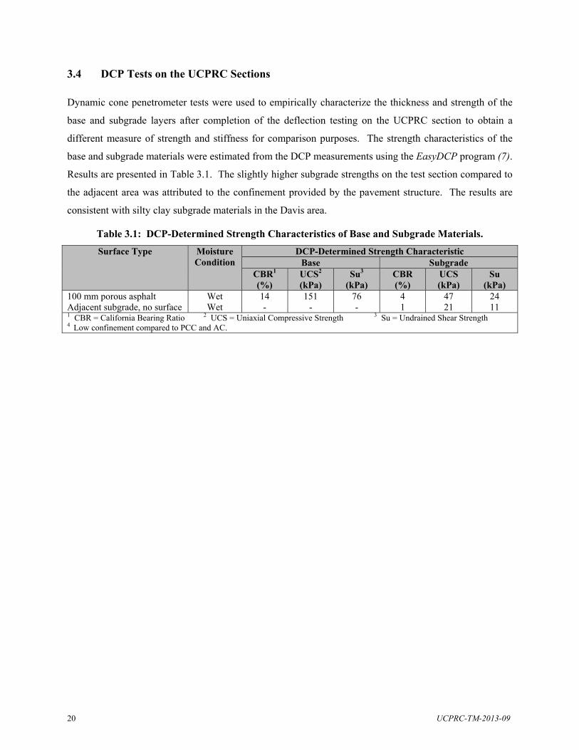
20 UCPRC-TM-2013-09
3.4 DCP Tests on the UCPRC Sections
Dynamic cone penetrometer tests were used to empirically characterize the thickness and strength of the
base and subgrade layers after completion of the deflection testing on the UCPRC section to obtain a
different measure of strength and stiffness for comparison purposes. The strength characteristics of the
base and subgrade materials were estimated from the DCP measurements using the EasyDCP program (7).
Results are presented in Table 3.1. The slightly higher subgrade strengths on the test section compared to
the adjacent area was attributed to the confinement provided by the pavement structure. The results are
consistent with silty clay subgrade materials in the Davis area.
Table 3.1: DCP-Determined Strength Characteristics of Base and Subgrade Materials.
Surface Type Moisture Condition
DCP-Determined Strength Characteristic Base Subgrade
CBR1
(%) UCS2
(kPa) Su3
(kPa) CBR (%)
UCS (kPa)
Su (kPa)
100 mm porous asphalt Adjacent subgrade, no surface
Wet Wet
14 -
151 -
76 -
4 1
47 21
24 11
1 CBR = California Bearing Ratio 2 UCS = Uniaxial Compressive Strength 3 Su = Undrained Shear Strength 4 Low confinement compared to PCC and AC.

UCPRC-TM-2013-09 21
4. MECHANISTIC ANALYSES AND STRUCTURAL DESIGN
4.1 Introduction
This chapter summarizes the results of the mechanistic analyses and theoretical structural designs for
permeable interlocking concrete pavements (PICP). This study was essentially a sensitivity analysis
considering a range of values from worst to best case scenarios. Design criteria, design variables, critical
responses, inputs for the mechanistic modelling and structural analysis, and the range of pavement
structure options are discussed.
4.2 Design Criteria
The most likely failure mode of permeable interlocking concrete pavements is permanent deformation in
the base, subbase, and/or subgrade layers, which will manifest as rutting and/or paver displacement on the
surface. The design criteria for this analysis therefore focused on this type of distress.
4.3 Design Variables
4.3.1 Background
Shear stress/strength ratio (SSR or τf /τmax) was used as the main design variable in this study for
permeable interlocking concrete pavements. The basis for the use of shear strength to shear stress/strength
ratio for design comes from work done at the University of Illinois, primarily under Prof. Marshall
Thompson and carried out by Prof. Erol Tutumleur (8-10). It is based on decades of laboratory testing for
permanent deformation, followed by field validation. The concept was primarily developed for use in
airfields where the shear stresses from aircraft loads and tire pressures are high relative to the strengths of
the subgrade materials. It was selected for use on this permeable pavement project because of the low
shear strengths of saturated, poorly compacted subgrades (which are common conditions in permeable
pavements) where the ratio between shear stresses and strengths can also be high given highway loads and
tire pressures.
The alternative approach considered was the use of a vertical strain criterion, which is typically used
where the shear stresses relative to shear strains are relatively low, which results in relatively low overall
rutting. In this approach, vertical strains are typically calculated from pavement deflection measured over
the full pavement structure. Strains in the localized areas at the top of the base and subgrade layers cannot
be directly measured unless a strain gauge has been specifically installed in that position. Consequently,
the damage and stiffness is calculated from measured deflections and then the strain is calculated from the

22 UCPRC-TM-2013-09
calibrated damage and stiffness model. Vertical strain based approaches are difficult to calibrate when
high shear stress to strength ratios occur in high water content environments, which in turn lead to large
ruts. This has been learned from UCPRC experience on other projects that investigated pavement
performance under soaked conditions and consequently the vertical strain approach was not considered
appropriate for designing permeable pavements.
Shear stress data has not been directly measured for ANY materials in the field because there is currently
no instrument that can effectively measure shear stresses in a pavement structure. In the laboratory, shear
stresses for all materials are calculated based on assumptions about the material and mechanics. Only
limited shear strength data is available from laboratory tests on open-graded bases. Similarly, there is
very little laboratory or field data to support a strain based rutting model for open graded bases. Given
these limitations, the stress/strength ratio concept was considered the most robust approach to
accommodate the high stress to strength ratios, and higher allowable ruts that are part of designing
permeable pavements.
4.3.2 Shear Stress/Strength Ratio
Shear stress/strength ratio is defined as the ratio between the applied shear stress (τf) and the material shear
strength (τmax [τmax = c + σf tanϕ in a triaxial strength test, where c is the cohesion of the material]) on the
failure plane at a specific applied normal and confining stress state (8). The normal and shear stresses (σf
and τmax) acting on a failure plane (oriented at an angle of 45° + ϕ/2, where ϕ is the internal friction angle
of the material) can be calculated according to the Mohr-Coulomb failure theory for specific confining
(σ3) and deviator (σd) stresses applied to a laboratory specimen during triaxial testing.
Materials with lower shear stress/strength ratios are less likely to fail due to shear (i.e., rutting and
permanent deformation) than materials with higher shear stress/strength ratios. Research studies (11,12)
have shown that materials subjected to shear stress/strength ratios higher than 0.7 are likely to accumulate
high permanent deformation and present a higher rutting risk, leading to rapid shear failure in the
pavement. Materials with shear stress/strength ratios between 0.3 and 0.7 represent a medium risk with a
steady but reasonable rate of rutting, while those with shear stress/strength ratios less than about 0.3 are
expected to have little or no rutting after an initial small “bedding-in” rut. Based on these findings, the
following three shear stress/strength ratio design variable categories aligned to the level of rutting risk
were defined for permeable interlocking concrete pavements (1,9):
SSR < 0.3, low risk of rutting;
0.3 ≤ SSR ≤ 0.7, medium risk of rutting;
SSR > 0.7, high risk of rutting.
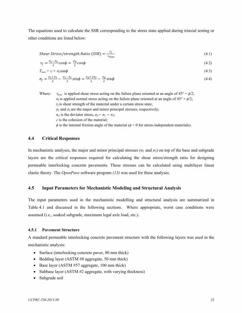
UCPRC-TM-2013-09 23
The equations used to calculate the SSR corresponding to the stress state applied during triaxial testing or
other conditions are listed below:
/
(4.1)
(4.2)
Τmax = c + σf tan (4.3)
(4.4)
Where: τmax is applied shear stress acting on the failure plane oriented at an angle of 45° + ϕ/2; σf is applied normal stress acting on the failure plane oriented at an angle of 45° + ϕ/2; τf is shear strength of the material under a certain stress state; σ1 and σ3 are the major and minor principal stresses, respectively; σd is the deviator stress, σd = σ1 σ3; c is the cohesion of the material; ϕ is the internal friction angle of the material (ϕ = 0 for stress-independent materials).
4.4 Critical Responses
In mechanistic analyses, the major and minor principal stresses (σ1 and σ3) on top of the base and subgrade
layers are the critical responses required for calculating the shear stress/strength ratio for designing
permeable interlocking concrete pavements. These stresses can be calculated using multilayer linear
elastic theory. The OpenPave software program (13) was used for these analyses.
4.5 Input Parameters for Mechanistic Modeling and Structural Analysis
The input parameters used in the mechanistic modelling and structural analysis are summarized in
Table 4.1 and discussed in the following sections. Where appropriate, worst case conditions were
assumed (i.e., soaked subgrade, maximum legal axle load, etc.).
4.5.1 Pavement Structure
A standard permeable interlocking concrete pavement structure with the following layers was used in the
mechanistic analysis:
Surface (interlocking concrete paver, 80 mm thick)
Bedding layer (ASTM #8 aggregate, 50 mm thick)
Base layer (ASTM #57 aggregate, 100 mm thick)
Subbase layer (ASTM #2 aggregate, with varying thickness)
Subgrade soil

24 UCPRC-TM-2013-09
Table 4.1: Summary of Input Factorials for Performance Modeling of PICP
Variable Surface Base Subgrade Axle Type
Axle Load (kN)
Stress Location Thickness
(mm) Stiffness (MPa)
Thickness (mm)
Stiffness (MPa)
c, ϕ (kPa, °)
Stiffness (MPa)
c, ϕ (kPa, °)
Label h1 E1 h2 E2 c, ϕ E3 c, ϕ AT AL SL
Value 80 200 500 1,000 2,000
300 450 600 750 900 1,050 1,200 1,350 1,500
60 90 120 180
45, 0 20 50 100 150
10, 20 and 0 15, 25 and 0 20, 30 and 0 25, 35 and 0
Dual Single
89 UW1
BW2
Factorial Levels
1 4 9 4 1 4 2 1 1 2
Total Calculations
2,304
1 UW = under wheel 2 BW=between wheel
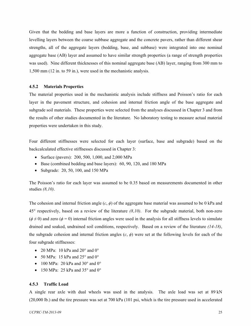
UCPRC-TM-2013-09 25
Given that the bedding and base layers are more a function of construction, providing intermediate
levelling layers between the coarse subbase aggregate and the concrete pavers, rather than different shear
strengths, all of the aggregate layers (bedding, base, and subbase) were integrated into one nominal
aggregate base (AB) layer and assumed to have similar strength properties (a range of strength properties
was used). Nine different thicknesses of this nominal aggregate base (AB) layer, ranging from 300 mm to
1,500 mm (12 in. to 59 in.), were used in the mechanistic analysis.
4.5.2 Materials Properties
The material properties used in the mechanistic analysis include stiffness and Poisson’s ratio for each
layer in the pavement structure, and cohesion and internal friction angle of the base aggregate and
subgrade soil materials. These properties were selected from the analyses discussed in Chapter 3 and from
the results of other studies documented in the literature. No laboratory testing to measure actual material
properties were undertaken in this study.
Four different stiffnesses were selected for each layer (surface, base and subgrade) based on the
backcalculated effective stiffnesses discussed in Chapter 3:
Surface (pavers): 200, 500, 1,000, and 2,000 MPa
Base (combined bedding and base layers): 60, 90, 120, and 180 MPa
Subgrade: 20, 50, 100, and 150 MPa The Poisson’s ratio for each layer was assumed to be 0.35 based on measurements documented in other studies (8,10).
The cohesion and internal friction angle (c, ϕ) of the aggregate base material was assumed to be 0 kPa and
45° respectively, based on a review of the literature (8,10). For the subgrade material, both non-zero
(ϕ ≠ 0) and zero (ϕ = 0) internal friction angles were used in the analysis for all stiffness levels to simulate
drained and soaked, undrained soil conditions, respectively. Based on a review of the literature (14-18),
the subgrade cohesion and internal friction angles (c, ϕ) were set at the following levels for each of the
four subgrade stiffnesses:
20 MPa: 10 kPa and 20° and 0°
50 MPa: 15 kPa and 25° and 0°
100 MPa: 20 kPa and 30° and 0°
150 MPa: 25 kPa and 35° and 0°
4.5.3 Traffic Load
A single rear axle with dual wheels was used in the analysis. The axle load was set at 89 kN
(20,000 lb.) and the tire pressure was set at 700 kPa (101 psi, which is the tire pressure used in accelerated
26 UCPRC-TM-2013-09
load tests). The distance between the two tire centers was set at 340 mm (13.4 in.). The stress under the
wheel and the stress between the wheels were both calculated to identify the most critical stress.
4.6 Mechanistic Analysis Results
4.6.1 Base Layer
The results of the mechanistic analysis for the different base layer (combined bedding and base layers)
stiffness values and thicknesses include the major and minor principal stresses, normal stress at the failure
plane, shear strength at the selected stress state, shear stress at the failure plane, and the shear stress/
strength ratio at the failure plane at the top of the base layer. The results are plotted in Figure A.1 though
Figure A.6 in Appendix A. The results indicate that, according to the multilayer linear elastic design
theory, an increase in the thickness of the base layer does not necessarily reduce the stresses at the top of
that layer.
4.6.2 Subgrade Layer
The results of the mechanistic analysis for the subgrade layer included the same parameters used in the
base layer analysis, except that the shear stress/strength ratio at the top of the subgrade was calculated.
The results are plotted against the different stiffness values for each layer, the different base thicknesses
(combined bedding and base layers), and the internal friction angle of the subgrade in Figure A.7 through
Figure A.18 in Appendix A. The results indicate that increasing the thickness of the base layer
(specifically the coarse ASTM #2 aggregate layer given that this is the “strong” material) reduces the
stresses (absolute values) at the top of the subgrade soil layer, as expected.
During dry conditions, when the subgrade is relatively dry (or at equilibrium moisture content) and has a
nonzero internal friction angle (ϕ ≠ 0), the shear strength of the subgrade soil changes with the thickness
of the base layer (Figure A.11). Interestingly, the effective shear strength of the subgrade soil decreases
slightly as the thickness of the base layer increases. This is attributed to the effective shear strength of
subgrade soils being positively correlated with the normal stress at the failure plane under dry conditions
(ϕ ≠ 0) (as defined in Equation 4.3). An increase in the thickness of the base layer significantly reduces
the normal stress at the failure plane at the top of the subgrade soil layer (Figure A.9), and consequently,
the effective shear strength of the subgrade soil decreases slightly as the thickness of the base layer
increases.
Under wet conditions (i.e., when the subgrade is soaked and has a zero internal friction angle [ϕ = 0]), the
effective shear strength of subgrade soils does not change with the thickness of the base layer (as shown in
Figure A.12). This is because the shear strength of materials with zero internal friction angle is
UCPRC-TM-2013-09 27
independent of the normal stress applied and is determined only by the cohesion of the material (as
defined in Equation 4.3). Therefore, soaked subgrade soils will have constant effective shear strength
regardless of an increase in the thickness of the base layer. The effective shear strength will be equal to
the cohesion of the material which is slightly lower than the effective shear strength of the subgrade soil
under dry conditions.
The normal stress and the shear stress are both higher under wet conditions than those under dry
conditions for an identical structure and identical material properties (Figure A.9, Figure A.10,
Figure A.13, and Figure A.14). The shear stress/strength ratio under wet conditions is also higher than the
shear stress/strength ratio under dry conditions for an identical structure and identical material properties
(Figure A.15 and Figure A.17), as expected. This confirms that wet conditions are the most critical
condition influencing rutting and permanent deformation in subgrade layers in pavements with permeable
interlocking concrete paver surfaces.
Figure A.16 and Figure A.18 show that the shear stress/strength ratio in log scale has a good linear
relationship with the thickness of the base layer (combined bedding and base layers).
4.6.3 Thickness of Base Layers for Different Shear Stress/Strength Ratio Values
Based on the results discussed above, the base layer thicknesses with shear stress/strength ratios of 0.8
(i.e., >0.7), 0.5 (i.e., intermediate between 0.3 and 0.7 [0.3 ≤ SSR ≤ 0.7]), and 0.2 (i.e., <0.3), representing
different rutting risk levels, were estimated using interpolation of the different material properties and
subgrade moisture conditions. The results are presented in Figure 4.1 and Figure 4.2. The main
observations with regard to required base layer thicknesses include:
Higher shear stress/strength ratios, which equate to a higher risk of rutting, require thicker base layers, as expected.
For the same shear stress/strength ratio, an increase in the effective stiffness of the base layer reduces the required thickness of that base layer, especially when the subgrade layer has a low stiffness.
An increase in the stiffness of the surface layer reduces the required base layer thickness to achieve the same shear stress/strength ratio. However, the effect of the surface layer stiffness is not significant due to the relatively low thickness of the pavers (80 mm).
For the same shear stress/strength ratio, wet conditions require thicker base layers compared to the dry condition, confirming that undrained wet conditions are the most critical condition for design.
The theoretical optimal design base thicknesses (combined bedding, base, and subbase layers) for low, intermediate, and higher risk levels (subgrade shear stress/strength ratios of 0.2, 0.5 and 0.8, respectively) under dry subgrade moisture conditions are approximately 1,300 mm, 800 mm, and 500 mm (51 in., 32 in., and 20 in.), respectively. In wet conditions, the theoretical optimal design thicknesses increase to 1,400 mm, 1,000 mm and 600 mm (55 in., 39 in., and 24 in.), respectively.

28 UCPRC-TM-2013-09
4.7 Preliminary Design Tables
Given that no laboratory testing was undertaken in this study, that only limited data was collected from the
field sections, and that all testing on pavers was done under dry conditions, the development of
preliminary design tables (part of Task 3 of this study) was postponed until additional response data under
controlled prolonged trafficking on the test track has been collected.

UCPRC-TM-2013-09 29
Figure 4.1: Suggested base layer thicknesses for different shear stress/strength ratios (ϕ ≠ 0 [dry]).
0.0
0.5
1.0
1.5
2.0T
hick
ness
of
AB
(m
)
60 90 120
180 60 90 120
180 60 90 120
180 60 90 120
180 60 90 120
180 60 90 120
180 60 90 120
180 60 90 120
180 60 90 120
180 60 90 120
180 60 90 120
180 60 90 120
180 60 90 120
180 60 90 120
180 60 90 120
180 60 90 120
180
Stiffness of AB (MPa)
SSR=0.8SSR=0.5SSR=0.2
E1 = 200 MPa
E3 = 20 MPa(c3, Phi3) = (10, 20)
E1 = 200 MPa
E3 = 50 MPa(c3, Phi3) = (15, 25)
E1 = 200 MPa
E3 = 100 MPa(c3, Phi3) = (20, 30)
E1 = 200 MPa
E3 = 150 MPa(c3, Phi3) = (25, 35)
E1 = 500 MPa
E3 = 20 MPa(c3, Phi3) = (10, 20)
E1 = 500 MPa
E3 = 50 MPa(c3, Phi3) = (15, 25)
E1 = 500 MPa
E3 = 100 MPa(c3, Phi3) = (20, 30)
E1 = 500 MPa
E3 = 150 MPa(c3, Phi3) = (25, 35)
E1 = 1000 MPa
E3 = 20 MPa(c3, Phi3) = (10, 20)
E1 = 1000 MPa
E3 = 50 MPa(c3, Phi3) = (15, 25)
E1 = 1000 MPa
E3 = 100 MPa(c3, Phi3) = (20, 30)
E1 = 1000 MPa
E3 = 150 MPa(c3, Phi3) = (25, 35)
E1 = 2000 MPa
E3 = 20 MPa(c3, Phi3) = (10, 20)
E1 = 2000 MPa
E3 = 50 MPa(c3, Phi3) = (15, 25)
E1 = 2000 MPa
E3 = 100 MPa(c3, Phi3) = (20, 30)
E1 = 2000 MPa
E3 = 150 MPa(c3, Phi3) = (25, 35)

30 UCPRC-TM-2013-09
Figure 4.2: Suggested base layer thicknesses for different shear stress/strength ratios (ϕ = 0 [wet]).
0.0
0.5
1.0
1.5
2.0T
hick
ness
of
AB
(m
)
60 90 120
180 60 90 120
180 60 90 120
180 60 90 120
180 60 90 120
180 60 90 120
180 60 90 120
180 60 90 120
180 60 90 120
180 60 90 120
180 60 90 120
180 60 90 120
180 60 90 120
180 60 90 120
180 60 90 120
180 60 90 120
180
Stiffness of AB (MPa)
SSR=0.8SSR=0.5SSR=0.2
E1 = 200 MPa
E3 = 20 MPa(c3, Phi3) = (10, 0)
E1 = 200 MPa
E3 = 50 MPa(c3, Phi3) = (15, 0)
E1 = 200 MPa
E3 = 100 MPa(c3, Phi3) = (20, 0)
E1 = 200 MPa
E3 = 150 MPa(c3, Phi3) = (25, 0)
E1 = 500 MPa
E3 = 20 MPa(c3, Phi3) = (10, 0)
E1 = 500 MPa
E3 = 50 MPa(c3, Phi3) = (15, 0)
E1 = 500 MPa
E3 = 100 MPa(c3, Phi3) = (20, 0)
E1 = 500 MPa
E3 = 150 MPa(c3, Phi3) = (25, 0)
E1 = 1000 MPa
E3 = 20 MPa(c3, Phi3) = (10, 0)
E1 = 1000 MPa
E3 = 50 MPa(c3, Phi3) = (15, 0)
E1 = 1000 MPa
E3 = 100 MPa(c3, Phi3) = (20, 0)
E1 = 1000 MPa
E3 = 150 MPa(c3, Phi3) = (25, 0)
E1 = 2000 MPa
E3 = 20 MPa(c3, Phi3) = (10, 0)
E1 = 2000 MPa
E3 = 50 MPa(c3, Phi3) = (15, 0)
E1 = 2000 MPa
E3 = 100 MPa(c3, Phi3) = (20, 0)
E1 = 2000 MPa
E3 = 150 MPa(c3, Phi3) = (25, 0)

UCPRC-TM-2013-09 31
5. TEST PLAN FOR THICKNESS VALIDATION
5.1 Thickness Design
A test track design was developed using the results from the mechanistic analysis. The theoretical optimal
design base thicknesses (combined bedding, base, and subbase layers) for the three different subgrade
shear stress/strength ratios (0.8, 0.5 and 0.2) under dry conditions are approximately 500 mm, 800 mm and
1,300 mm (20 in., 32 in., and 51 in.), respectively. In wet conditions, the theoretical optimal design
thicknesses increase to 600 mm, 1,000 mm and 1,400 mm (24 in, 40 in., and 56 in.), respectively. Based
on these results, three subbase (i.e., coarse aggregate [ASTM #2]) thicknesses of 450 mm, 650 mm, and
950 mm (18 in., 26 in., and ~38 in.), were selected for the accelerated load test pavement design to
provide high, intermediate, and low risk scenarios (Figure 5.1). The bedding layer (#8 stone) and base
layer (#57 stone) thicknesses were fixed at 50 mm and 100 mm (2 in. and 4 in.), respectively, equating to
total structure thicknesses of 600 mm, 800 mm, and 1,100 mm (24 in., 32 in., and 44 in.) for the three
sections. These subbase layer thicknesses are mostly thinner than the theoretical optimal design
thicknesses and were selected to ensure that the performance and behavior of the test track structure could
be fully understood within the time and budgetary constraints of the project. The proposed test track
design provided to the construction contractor is shown in Figure 5.2. The track design is wide enough for
three side-by-side test sections to allow testing under dry and wet conditions, and if required, a third
moisture condition.
Layer: Pavers with jointing stone Thickness: 80 mm (3.125 in.) Layer: #8 stone bedding Thickness: 50 mm (2.0 in.)
Layer: #57 stone base Thickness: 100 mm (4.0 in)
Layer: #2 stone subbase Thickness: 450, 650, and 950 mm (18, 26, and 38 in)
Layer: Prepared subgrade Thickness: Semi-infinite
Figure 5.1: Proposed pavement structure for PICP test track (not to scale).

32 UCPRC-TM-2013-09
Figure 5.2: Proposed test track design.
5.2 Test Track Instrumentation
Each subsection in each test section will have pressure cells on top of the subgrade and top of the #57
aggregate base layers to measure vertical stress, and a steel reference plate to measure the location of any
permanent deformation. Temperatures will be measured at two different locations on the test track (east
and west side of the test section). At each location, ambient temperatures and temperatures of the
pavement surface and pavement at 25 mm depth will be measured.
Additional manual measurements include profile (laser profilometer) to evaluate surface rutting, surface
deflection (road surface deflectometer), and subbase water content (dipstick).

UCPRC-TM-2013-09 33
5.3 Heavy Vehicle Simulator Test Plan
5.3.1 Test Sections
At least two test sections, with three subsections in each section, will be tested. The first section will be
tested dry, the second after soaking with water. Space for a third test is available between these two
sections if additional testing is required; however, this third section is not instrumented.
5.3.2 Loading Plan
Test loads will start at 25 kN (5,600 lb). This load will be maintained until responses (deflection and
strain) and rut depth rate increase have stabilized. The load will then be increased to 40 kN (9,000 lb) and
maintained at that level until responses and rut depth rate increase have again stabilized. Depending on
test track performance, the load may be increased to higher levels to accelerate the loading. Load
increment levels will be 60 kN (13,500 lb), 80 kN (18,000 lb), and 100 kN (22,500 lb). The same loading
plan will be followed on the dry and wet tests.
All testing will be done with a dual wheel configuration with a tire pressure of 700 kPa (101 psi).
Trafficking will be bi-directional at a speed of 10 km/h (6 mph).
5.3.3 Environmental Control
All testing will be conducted at ambient conditions. Water levels in the subbase will be monitored with
dipsticks. In the wet test, water will be applied to the surface of the test track and allowed to infiltrate
until it overtops the surface. Thereafter, the water level will be maintained at the top of the #2 stone
subbase (i.e., top of the reservoir layer) for the duration of load testing to simulate worst case conditions.
If time and funds permit, a third test will be conducted after water has drained from the #2 stone subbase
(i.e., no water in the reservoir layer, but subgrade will be moist) to simulate intermediate conditions.
5.3.4 Measurements
Measurements will be taken after every 10,000 load repetitions, or more regularly if dictated by
performance. These periodic measurements include a visual evaluation, profile, deflections, and
permanent deformation at the top of the #57 aggregate base and top of the subgrade. Temperatures and
strain measurements from the pressure cells will be measured continuously during trafficking.

34 UCPRC-TM-2013-09
Blank page

UCPRC-TM-2013-09 35
6. SUMMARY AND RECOMMENDATIONS
6.1 Summary
This report details field testing of existing projects and test sections, estimation of the effective stiffness of
each layer in permeable interlocking concrete pavement structures, and mechanistic analysis and structural
design of a test track to validate the design approach using accelerated loading. Key findings from the
study include:
Higher shear stress/strength ratios, which equate to a higher risk of rutting, require thicker base layers, as expected.
For the same shear stress/strength ratio, an increase in the stiffness of the base layer reduces the required thickness of that base layer, especially when the subgrade layer has a low stiffness.
An increase in the stiffness of the surface layer reduces the required base layer thickness to achieve the same shear stress/strength ratio. However, the effect of the surface layer stiffness is not significant due to the relatively low thickness of the pavers (80 mm).
For the same shear stress/strength ratio, wet conditions require thicker base layers compared to the dry condition, confirming that wet conditions are the most critical condition for design.
The theoretical optimal design base thicknesses (combined bedding, base, and subbase layers) for low, intermediate, and higher risk levels (subgrade shear stress/strength ratios of 0.2, 0.5 and 0.8, respectively) under dry subgrade moisture conditions are approximately 1,300 mm, 800 mm, and 500 mm (51 in., 32 in., and 20 in.), respectively. In wet conditions, the theoretical optimal design thicknesses increase to 1,400 mm, 1,000 mm and 600 mm (55 in., 39 in., and 24 in.), respectively.
6.2 Recommendations
The following interim recommendations are made based on the findings from this study:
Based on the mechanistic analysis, three subbase (i.e., coarse aggregate [ASTM #2]) thicknesses of 950 mm, 650 mm, and 450 mm (~38 in., 26 in., and 18 in.) should be tested to assess low, intermediate, and higher risk designs. The bedding layer (#8 stone) and base layer (#57 stone) thicknesses should be fixed at 50 mm and 100 mm (2 in. and 4 in.), respectively.
The shear stress/strength ratio is considered to be an appropriate parameter for assessing the rutting risk in subgrade layers in permeable interlocking concrete pavement. This approach needs to be validated and calibrated in the accelerated load testing phase of this study.
The mechanistic analysis predicted that an increase in base layer thickness will theoretically not reduce the stresses and the shear stress/strength ratio value of the base/subbase layer in permeable interlocking concrete pavements. This finding needs to be validated in the accelerated load testing phase of this study.
Models are needed to quantify the rut depth on permeable interlocking concrete pavements for a given number of load repetitions for various base and subgrade configurations. Preliminary models should be developed using the results from the accelerated load testing phase of this study.

36 UCPRC-TM-2013-09
Blank page

UCPRC-TM-2013-09 37
REFERENCES
1. JONES, D., Li, H. and Harvey, J.T. 2013. Development and HVS Validation of Design Tables
for Permeable Interlocking Concrete Pavement: Literature Review. Davis and Berkeley, CA:
University of California Pavement Research Center. (UCPRC-TM-2013-03).
2. JONES, D., Harvey, J.T., Li, H., Wang, T., Wu, R. and Campbell, B. 2010. Laboratory Testing
and Modeling for Structural Performance of Fully Permeable Pavements under Heavy
Traffic: Final Report. Davis and Berkeley, CA: University of California Pavement Research
Center. (UCPRC-RR-2010-05).
3. CHOI, J.W., Wu, R., Pestana, J.H. and Harvey, J. 2010. New Layer-Moduli Back-Calculation
Method Based on the Constrained Extended Kalman Filter. Journal of Transportation
Engineering, 136(1). (pp 20–30).
4. JONES, D., Harvey, J.T., Li, H. and Campbell, B. 2009. Summary of Laboratory Tests to
Assess Mechanical Properties of Permeable Pavement Materials. Davis and Berkeley, CA:
University of California Pavement Research Center. (UCPRC-TM-2009-01).
5. TUTUMLUER, E. and Seyhan, U. 1999. Laboratory Determination of Anisotropic Aggregate
Resilient Moduli Using an Innovative Test Device. Transportation Research Record: Journal
of the Transportation Research Board, Vol. 1687. (pp. 13-21).
6. AYITHI, A. and Hiltunen, D. 2013. Characterization of Moisture-Dependent Changes in Stiffness
of Unbound Aggregate Base Materials in Florida. Transportation Research Record: Journal of
the Transportation Research Board, Vol. 2349. (pp. 25-31).
7. LEA, J.D. Undated. EasyDCP: An Easy Tool for DCP Data Processing. www.OpenPave.org.
Accessed 2013/09/10.
8. CHOW, L.C. and Tutumluer, E. 2014. Framework for Improved Unbound Aggregate Base Rutting
Model Development for Mechanistic-Empirical Pavement Design. Proceedings Transportation
Research Board 93rd Annual Meeting. Washington, D.C: Transportation Research Board.
9. THOMPSON, M., Gomez-Ramirez, F. and Bejarano, M. 2002. Illi-Pave Based Flexible
Pavement Design Concepts for Multiple Wheel Heavy Gear Load Aircraft. Proceedings 9th
International Conference on Asphalt Pavements. Copenhagen, Denmark. International Society
of Asphalt Pavements.
10. TUTUMLUER, E., Kim, I. and Santoni, R. 2004. Modulus Anisotropy and Shear Stability of
Geofiber-Stabilized Sands. Transportation Research Record: Journal of the Transportation
Research Board, Vol. 1874. (pp. 125-135).

38 UCPRC-TM-2013-09
11. KIM, I. and Tutumluer, E. 2006. Field Validation of Airport Pavement Granular Layer Rutting
Predictions. Transportation Research Record: Journal of the Transportation Research
Board, Vol. 1952. (pp. 48-57).
12. LI, H., Harvey J.T. and Jones, D. 2010. Summary of a Computer Modeling Study to
Understand the Performance Properties of Fully Permeable Pavements. Davis and Berkeley,
CA: University of California Pavement Research Center. (UCPRC-TM-2010-04).
13. LEA, J. undated. OpenPave: An N-Layer, N-Load, N-Point Multi-Layer Elastic Half Space
Calculation. www.OpenPave.org. Accessed 2013/09/10.
14. DAS, B.M. 2007. Advanced Soil Mechanics. New York, NY: Taylor and Francis.
15. NOVA, R. 2012. Soil Mechanics. Hoboken, NJ: John Wiley and Sons.
16. CARTER, M. and Bentley, S.P. 1991. Correlations of Soil Properties. London, UK: Pentech
Press.
17. WNEK, M., Tutumluer, E., Moaveni, M. and Gehringer, E. 2013. Investigation of Aggregate
Properties Influencing Railroad Ballast Performance. Transportation Research Record: Journal
of the Transportation Research Board, Vol. 2374. (pp. 180-189).
18. HUANG, H., Tutumluer, E. and Dombrow, W. 2009. Laboratory Characterization of Fouled
Railroad Ballast Behavior. Transportation Research Record: Journal of the Transportation
Research Board, Vol. 2117. (pp. 93-101).
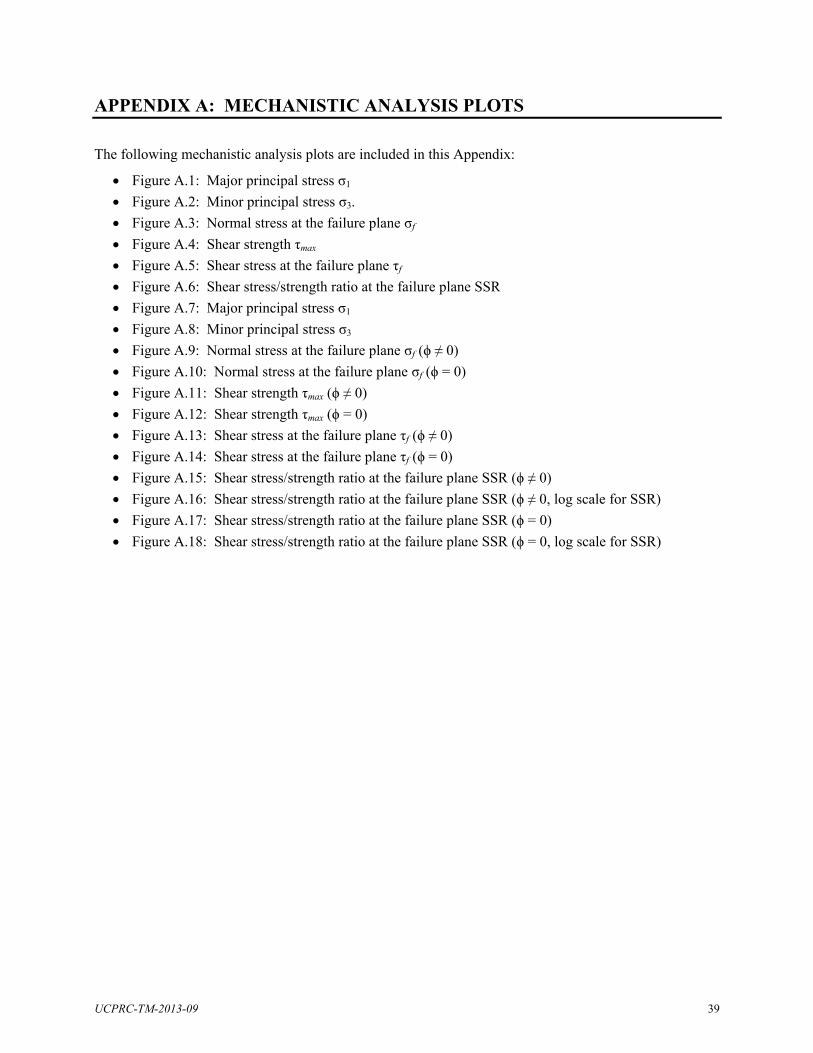
UCPRC-TM-2013-09 39
APPENDIX A: MECHANISTIC ANALYSIS PLOTS
The following mechanistic analysis plots are included in this Appendix:
Figure A.1: Major principal stress σ1
Figure A.2: Minor principal stress σ3.
Figure A.3: Normal stress at the failure plane σf
Figure A.4: Shear strength τmax
Figure A.5: Shear stress at the failure plane τf
Figure A.6: Shear stress/strength ratio at the failure plane SSR
Figure A.7: Major principal stress σ1
Figure A.8: Minor principal stress σ3
Figure A.9: Normal stress at the failure plane σf (ϕ ≠ 0)
Figure A.10: Normal stress at the failure plane σf (ϕ = 0)
Figure A.11: Shear strength τmax (ϕ ≠ 0)
Figure A.12: Shear strength τmax (ϕ = 0)
Figure A.13: Shear stress at the failure plane τf (ϕ ≠ 0)
Figure A.14: Shear stress at the failure plane τf (ϕ = 0)
Figure A.15: Shear stress/strength ratio at the failure plane SSR (ϕ ≠ 0)
Figure A.16: Shear stress/strength ratio at the failure plane SSR (ϕ ≠ 0, log scale for SSR)
Figure A.17: Shear stress/strength ratio at the failure plane SSR (ϕ = 0)
Figure A.18: Shear stress/strength ratio at the failure plane SSR (ϕ = 0, log scale for SSR)

40 UCPRC-TM-2013-09
Figure A.1: Major principal stress σ1.
400 600 800 1000 1200 1400
0
50
100
150
200
Thickness of AB (mm)
Ma
jor
Pri
nci
pa
l Str
ess
(kP
a)
E_AB = 60 MPaE_AB = 90 MPaE_AB = 120 MPaE_AB = 180 MPa
at Top of Subbase
E_Surface = 200 MPaE_SG = 20 MPa
400 600 800 1000 1200 1400
0
50
100
150
200
Thickness of AB (mm)
Ma
jor
Pri
nci
pa
l Str
ess
(kP
a)
E_AB = 60 MPaE_AB = 90 MPaE_AB = 120 MPaE_AB = 180 MPa
at Top of Subbase
E_Surface = 200 MPaE_SG = 50 MPa
400 600 800 1000 1200 1400
0
50
100
150
200
Thickness of AB (mm)
Ma
jor
Pri
nci
pa
l Str
ess
(kP
a)
E_AB = 60 MPaE_AB = 90 MPaE_AB = 120 MPaE_AB = 180 MPa
at Top of Subbase
E_Surface = 200 MPaE_SG = 100 MPa
400 600 800 1000 1200 1400
0
50
100
150
200
Thickness of AB (mm)
Ma
jor
Pri
nci
pa
l Str
ess
(kP
a)
E_AB = 60 MPaE_AB = 90 MPaE_AB = 120 MPaE_AB = 180 MPa
at Top of Subbase
E_Surface = 200 MPaE_SG = 150 MPa
400 600 800 1000 1200 1400
0
50
100
150
200
Thickness of AB (mm)
Ma
jor
Pri
nci
pa
l Str
ess
(kP
a)
E_AB = 60 MPaE_AB = 90 MPaE_AB = 120 MPaE_AB = 180 MPa
at Top of Subbase
E_Surface = 500 MPaE_SG = 20 MPa
400 600 800 1000 1200 1400
0
50
100
150
200
Thickness of AB (mm)
Ma
jor
Pri
nci
pa
l Str
ess
(kP
a)
E_AB = 60 MPaE_AB = 90 MPaE_AB = 120 MPaE_AB = 180 MPa
at Top of Subbase
E_Surface = 500 MPaE_SG = 50 MPa
400 600 800 1000 1200 1400
0
50
100
150
200
Thickness of AB (mm)
Ma
jor
Pri
nci
pa
l Str
ess
(kP
a)
E_AB = 60 MPaE_AB = 90 MPaE_AB = 120 MPaE_AB = 180 MPa
at Top of Subbase
E_Surface = 500 MPaE_SG = 100 MPa
400 600 800 1000 1200 1400
0
50
100
150
200
Thickness of AB (mm)
Ma
jor
Pri
nci
pa
l Str
ess
(kP
a)
E_AB = 60 MPaE_AB = 90 MPaE_AB = 120 MPaE_AB = 180 MPa
at Top of Subbase
E_Surface = 500 MPaE_SG = 150 MPa
400 600 800 1000 1200 1400
0
50
100
150
200
Thickness of AB (mm)
Ma
jor
Pri
nci
pa
l Str
ess
(kP
a)
E_AB = 60 MPaE_AB = 90 MPaE_AB = 120 MPaE_AB = 180 MPa
at Top of Subbase
E_Surface = 1000 MPaE_SG = 20 MPa
400 600 800 1000 1200 1400
0
50
100
150
200
Thickness of AB (mm)
Ma
jor
Pri
nci
pa
l Str
ess
(kP
a)
E_AB = 60 MPaE_AB = 90 MPaE_AB = 120 MPaE_AB = 180 MPa
at Top of Subbase
E_Surface = 1000 MPaE_SG = 50 MPa
400 600 800 1000 1200 1400
0
50
100
150
200
Thickness of AB (mm)
Ma
jor
Pri
nci
pa
l Str
ess
(kP
a)
E_AB = 60 MPaE_AB = 90 MPaE_AB = 120 MPaE_AB = 180 MPa
at Top of Subbase
E_Surface = 1000 MPaE_SG = 100 MPa
400 600 800 1000 1200 1400
0
50
100
150
200
Thickness of AB (mm)
Ma
jor
Pri
nci
pa
l Str
ess
(kP
a)
E_AB = 60 MPaE_AB = 90 MPaE_AB = 120 MPaE_AB = 180 MPa
at Top of Subbase
E_Surface = 1000 MPaE_SG = 150 MPa
400 600 800 1000 1200 1400
0
50
100
150
200
Thickness of AB (mm)
Ma
jor
Pri
nci
pa
l Str
ess
(kP
a)
E_AB = 60 MPaE_AB = 90 MPaE_AB = 120 MPaE_AB = 180 MPa
at Top of Subbase
E_Surface = 2000 MPaE_SG = 20 MPa
400 600 800 1000 1200 1400
0
50
100
150
200
Thickness of AB (mm)
Ma
jor
Pri
nci
pa
l Str
ess
(kP
a)
E_AB = 60 MPaE_AB = 90 MPaE_AB = 120 MPaE_AB = 180 MPa
at Top of Subbase
E_Surface = 2000 MPaE_SG = 50 MPa
400 600 800 1000 1200 1400
0
50
100
150
200
Thickness of AB (mm)
Ma
jor
Pri
nci
pa
l Str
ess
(kP
a)
E_AB = 60 MPaE_AB = 90 MPaE_AB = 120 MPaE_AB = 180 MPa
at Top of Subbase
E_Surface = 2000 MPaE_SG = 100 MPa
400 600 800 1000 1200 1400
0
50
100
150
200
Thickness of AB (mm)
Ma
jor
Pri
nci
pa
l Str
ess
(kP
a)
E_AB = 60 MPaE_AB = 90 MPaE_AB = 120 MPaE_AB = 180 MPa
at Top of Subbase
E_Surface = 2000 MPaE_SG = 150 MPa
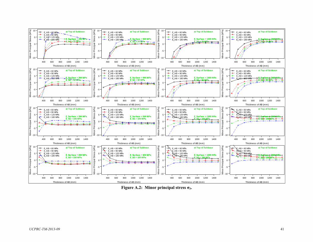
UCPRC-TM-2013-09 41
Figure A.2: Minor principal stress σ3.
400 600 800 1000 1200 1400
-10
-5
0
5
10
Thickness of AB (mm)
Min
or
Pri
nci
pa
l Str
ess
(kP
a)
E_AB = 60 MPaE_AB = 90 MPaE_AB = 120 MPaE_AB = 180 MPa
at Top of Subbase
E_Surface = 200 MPaE_SG = 20 MPa
400 600 800 1000 1200 1400
-10
-5
0
5
10
Thickness of AB (mm)
Min
or
Pri
nci
pa
l Str
ess
(kP
a)
E_AB = 60 MPaE_AB = 90 MPaE_AB = 120 MPaE_AB = 180 MPa
at Top of Subbase
E_Surface = 200 MPaE_SG = 50 MPa
400 600 800 1000 1200 1400
-10
-5
0
5
10
Thickness of AB (mm)
Min
or
Pri
nci
pa
l Str
ess
(kP
a)
E_AB = 60 MPaE_AB = 90 MPaE_AB = 120 MPaE_AB = 180 MPa
at Top of Subbase
E_Surface = 200 MPaE_SG = 100 MPa
400 600 800 1000 1200 1400
-10
-5
0
5
10
Thickness of AB (mm)
Min
or
Pri
nci
pa
l Str
ess
(kP
a)
E_AB = 60 MPaE_AB = 90 MPaE_AB = 120 MPaE_AB = 180 MPa
at Top of Subbase
E_Surface = 200 MPaE_SG = 150 MPa
400 600 800 1000 1200 1400
-10
-5
0
5
10
Thickness of AB (mm)
Min
or
Pri
nci
pa
l Str
ess
(kP
a)
E_AB = 60 MPaE_AB = 90 MPaE_AB = 120 MPaE_AB = 180 MPa
at Top of Subbase
E_Surface = 500 MPaE_SG = 20 MPa
400 600 800 1000 1200 1400
-10
-5
0
5
10
Thickness of AB (mm)
Min
or
Pri
nci
pa
l Str
ess
(kP
a)
E_AB = 60 MPaE_AB = 90 MPaE_AB = 120 MPaE_AB = 180 MPa
at Top of Subbase
E_Surface = 500 MPaE_SG = 50 MPa
400 600 800 1000 1200 1400
-10
-5
0
5
10
Thickness of AB (mm)
Min
or
Pri
nci
pa
l Str
ess
(kP
a)
E_AB = 60 MPaE_AB = 90 MPaE_AB = 120 MPaE_AB = 180 MPa
at Top of Subbase
E_Surface = 500 MPaE_SG = 100 MPa
400 600 800 1000 1200 1400
-10
-5
0
5
10
Thickness of AB (mm)
Min
or
Pri
nci
pa
l Str
ess
(kP
a)
E_AB = 60 MPaE_AB = 90 MPaE_AB = 120 MPaE_AB = 180 MPa
at Top of Subbase
E_Surface = 500 MPaE_SG = 150 MPa
400 600 800 1000 1200 1400
-10
-5
0
5
10
Thickness of AB (mm)
Min
or
Pri
nci
pa
l Str
ess
(kP
a)
E_AB = 60 MPaE_AB = 90 MPaE_AB = 120 MPaE_AB = 180 MPa
at Top of Subbase
E_Surface = 1000 MPaE_SG = 20 MPa
400 600 800 1000 1200 1400
-10
-5
0
5
10
Thickness of AB (mm)
Min
or
Pri
nci
pa
l Str
ess
(kP
a)
E_AB = 60 MPaE_AB = 90 MPaE_AB = 120 MPaE_AB = 180 MPa
at Top of Subbase
E_Surface = 1000 MPaE_SG = 50 MPa
400 600 800 1000 1200 1400
-10
-5
0
5
10
Thickness of AB (mm)
Min
or
Pri
nci
pa
l Str
ess
(kP
a)
E_AB = 60 MPaE_AB = 90 MPaE_AB = 120 MPaE_AB = 180 MPa
at Top of Subbase
E_Surface = 1000 MPaE_SG = 100 MPa
400 600 800 1000 1200 1400
-10
-5
0
5
10
Thickness of AB (mm)
Min
or
Pri
nci
pa
l Str
ess
(kP
a)
E_AB = 60 MPaE_AB = 90 MPaE_AB = 120 MPaE_AB = 180 MPa
at Top of Subbase
E_Surface = 1000 MPaE_SG = 150 MPa
400 600 800 1000 1200 1400
-10
-5
0
5
10
Thickness of AB (mm)
Min
or
Pri
nci
pa
l Str
ess
(kP
a)
E_AB = 60 MPaE_AB = 90 MPaE_AB = 120 MPaE_AB = 180 MPa
at Top of Subbase
E_Surface = 2000 MPaE_SG = 20 MPa
400 600 800 1000 1200 1400
-10
-5
0
5
10
Thickness of AB (mm)
Min
or
Pri
nci
pa
l Str
ess
(kP
a)
E_AB = 60 MPaE_AB = 90 MPaE_AB = 120 MPaE_AB = 180 MPa
at Top of Subbase
E_Surface = 2000 MPaE_SG = 50 MPa
400 600 800 1000 1200 1400
-10
-5
0
5
10
Thickness of AB (mm)
Min
or
Pri
nci
pa
l Str
ess
(kP
a)
E_AB = 60 MPaE_AB = 90 MPaE_AB = 120 MPaE_AB = 180 MPa
at Top of Subbase
E_Surface = 2000 MPaE_SG = 100 MPa
400 600 800 1000 1200 1400
-10
-5
0
5
10
Thickness of AB (mm)
Min
or
Pri
nci
pa
l Str
ess
(kP
a)
E_AB = 60 MPaE_AB = 90 MPaE_AB = 120 MPaE_AB = 180 MPa
at Top of Subbase
E_Surface = 2000 MPaE_SG = 150 MPa
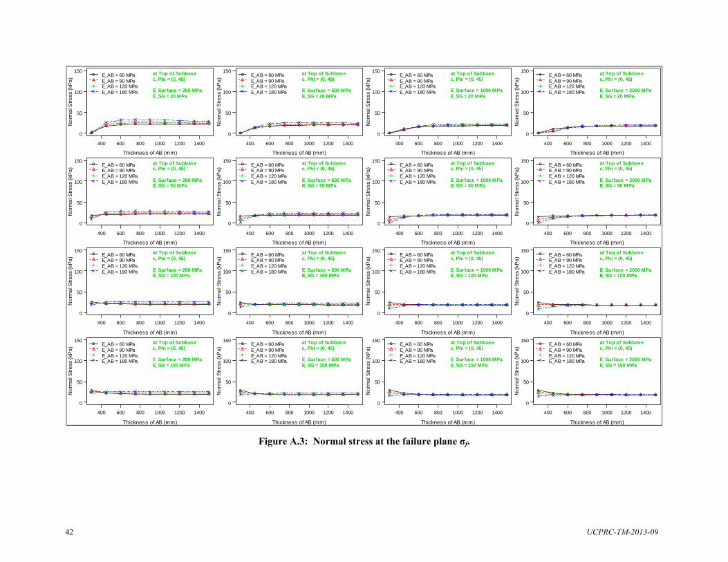
42 UCPRC-TM-2013-09
Figure A.3: Normal stress at the failure plane σf.
400 600 800 1000 1200 1400
0
50
100
150
Thickness of AB (mm)
No
rma
l Str
ess
(kP
a) E_AB = 60 MPa
E_AB = 90 MPaE_AB = 120 MPaE_AB = 180 MPa
at Top of Subbasec, Phi = (0, 45)
E_Surface = 200 MPaE_SG = 20 MPa
400 600 800 1000 1200 1400
0
50
100
150
Thickness of AB (mm)
No
rma
l Str
ess
(kP
a) E_AB = 60 MPa
E_AB = 90 MPaE_AB = 120 MPaE_AB = 180 MPa
at Top of Subbasec, Phi = (0, 45)
E_Surface = 200 MPaE_SG = 50 MPa
400 600 800 1000 1200 1400
0
50
100
150
Thickness of AB (mm)
No
rma
l Str
ess
(kP
a) E_AB = 60 MPa
E_AB = 90 MPaE_AB = 120 MPaE_AB = 180 MPa
at Top of Subbasec, Phi = (0, 45)
E_Surface = 200 MPaE_SG = 100 MPa
400 600 800 1000 1200 1400
0
50
100
150
Thickness of AB (mm)
No
rma
l Str
ess
(kP
a) E_AB = 60 MPa
E_AB = 90 MPaE_AB = 120 MPaE_AB = 180 MPa
at Top of Subbasec, Phi = (0, 45)
E_Surface = 200 MPaE_SG = 150 MPa
400 600 800 1000 1200 1400
0
50
100
150
Thickness of AB (mm)
No
rma
l Str
ess
(kP
a) E_AB = 60 MPa
E_AB = 90 MPaE_AB = 120 MPaE_AB = 180 MPa
at Top of Subbasec, Phi = (0, 45)
E_Surface = 500 MPaE_SG = 20 MPa
400 600 800 1000 1200 1400
0
50
100
150
Thickness of AB (mm)
No
rma
l Str
ess
(kP
a) E_AB = 60 MPa
E_AB = 90 MPaE_AB = 120 MPaE_AB = 180 MPa
at Top of Subbasec, Phi = (0, 45)
E_Surface = 500 MPaE_SG = 50 MPa
400 600 800 1000 1200 1400
0
50
100
150
Thickness of AB (mm)
No
rma
l Str
ess
(kP
a) E_AB = 60 MPa
E_AB = 90 MPaE_AB = 120 MPaE_AB = 180 MPa
at Top of Subbasec, Phi = (0, 45)
E_Surface = 500 MPaE_SG = 100 MPa
400 600 800 1000 1200 1400
0
50
100
150
Thickness of AB (mm)
No
rma
l Str
ess
(kP
a) E_AB = 60 MPa
E_AB = 90 MPaE_AB = 120 MPaE_AB = 180 MPa
at Top of Subbasec, Phi = (0, 45)
E_Surface = 500 MPaE_SG = 150 MPa
400 600 800 1000 1200 1400
0
50
100
150
Thickness of AB (mm)
No
rma
l Str
ess
(kP
a) E_AB = 60 MPa
E_AB = 90 MPaE_AB = 120 MPaE_AB = 180 MPa
at Top of Subbasec, Phi = (0, 45)
E_Surface = 1000 MPaE_SG = 20 MPa
400 600 800 1000 1200 1400
0
50
100
150
Thickness of AB (mm)
No
rma
l Str
ess
(kP
a) E_AB = 60 MPa
E_AB = 90 MPaE_AB = 120 MPaE_AB = 180 MPa
at Top of Subbasec, Phi = (0, 45)
E_Surface = 1000 MPaE_SG = 50 MPa
400 600 800 1000 1200 1400
0
50
100
150
Thickness of AB (mm)
No
rma
l Str
ess
(kP
a) E_AB = 60 MPa
E_AB = 90 MPaE_AB = 120 MPaE_AB = 180 MPa
at Top of Subbasec, Phi = (0, 45)
E_Surface = 1000 MPaE_SG = 100 MPa
400 600 800 1000 1200 1400
0
50
100
150
Thickness of AB (mm)
No
rma
l Str
ess
(kP
a) E_AB = 60 MPa
E_AB = 90 MPaE_AB = 120 MPaE_AB = 180 MPa
at Top of Subbasec, Phi = (0, 45)
E_Surface = 1000 MPaE_SG = 150 MPa
400 600 800 1000 1200 1400
0
50
100
150
Thickness of AB (mm)
No
rma
l Str
ess
(kP
a) E_AB = 60 MPa
E_AB = 90 MPaE_AB = 120 MPaE_AB = 180 MPa
at Top of Subbasec, Phi = (0, 45)
E_Surface = 2000 MPaE_SG = 20 MPa
400 600 800 1000 1200 1400
0
50
100
150
Thickness of AB (mm)
No
rma
l Str
ess
(kP
a) E_AB = 60 MPa
E_AB = 90 MPaE_AB = 120 MPaE_AB = 180 MPa
at Top of Subbasec, Phi = (0, 45)
E_Surface = 2000 MPaE_SG = 50 MPa
400 600 800 1000 1200 1400
0
50
100
150
Thickness of AB (mm)
No
rma
l Str
ess
(kP
a) E_AB = 60 MPa
E_AB = 90 MPaE_AB = 120 MPaE_AB = 180 MPa
at Top of Subbasec, Phi = (0, 45)
E_Surface = 2000 MPaE_SG = 100 MPa
400 600 800 1000 1200 1400
0
50
100
150
Thickness of AB (mm)
No
rma
l Str
ess
(kP
a) E_AB = 60 MPa
E_AB = 90 MPaE_AB = 120 MPaE_AB = 180 MPa
at Top of Subbasec, Phi = (0, 45)
E_Surface = 2000 MPaE_SG = 150 MPa

UCPRC-TM-2013-09 43
Figure A.4: Shear strength τmax.
400 600 800 1000 1200 1400
0
50
100
150
Thickness of AB (mm)
Sh
ea
r S
tre
ng
th (
kPa
) E_AB = 60 MPaE_AB = 90 MPaE_AB = 120 MPaE_AB = 180 MPa
at Top of Subbasec, Phi = (0, 45)
E_Surface = 200 MPaE_SG = 20 MPa
400 600 800 1000 1200 1400
0
50
100
150
Thickness of AB (mm)
Sh
ea
r S
tre
ng
th (
kPa
) E_AB = 60 MPaE_AB = 90 MPaE_AB = 120 MPaE_AB = 180 MPa
at Top of Subbasec, Phi = (0, 45)
E_Surface = 200 MPaE_SG = 50 MPa
400 600 800 1000 1200 1400
0
50
100
150
Thickness of AB (mm)
Sh
ea
r S
tre
ng
th (
kPa
) E_AB = 60 MPaE_AB = 90 MPaE_AB = 120 MPaE_AB = 180 MPa
at Top of Subbasec, Phi = (0, 45)
E_Surface = 200 MPaE_SG = 100 MPa
400 600 800 1000 1200 1400
0
50
100
150
Thickness of AB (mm)
Sh
ea
r S
tre
ng
th (
kPa
) E_AB = 60 MPaE_AB = 90 MPaE_AB = 120 MPaE_AB = 180 MPa
at Top of Subbasec, Phi = (0, 45)
E_Surface = 200 MPaE_SG = 150 MPa
400 600 800 1000 1200 1400
0
50
100
150
Thickness of AB (mm)
Sh
ea
r S
tre
ng
th (
kPa
) E_AB = 60 MPaE_AB = 90 MPaE_AB = 120 MPaE_AB = 180 MPa
at Top of Subbasec, Phi = (0, 45)
E_Surface = 500 MPaE_SG = 20 MPa
400 600 800 1000 1200 1400
0
50
100
150
Thickness of AB (mm)
Sh
ea
r S
tre
ng
th (
kPa
) E_AB = 60 MPaE_AB = 90 MPaE_AB = 120 MPaE_AB = 180 MPa
at Top of Subbasec, Phi = (0, 45)
E_Surface = 500 MPaE_SG = 50 MPa
400 600 800 1000 1200 1400
0
50
100
150
Thickness of AB (mm)
Sh
ea
r S
tre
ng
th (
kPa
) E_AB = 60 MPaE_AB = 90 MPaE_AB = 120 MPaE_AB = 180 MPa
at Top of Subbasec, Phi = (0, 45)
E_Surface = 500 MPaE_SG = 100 MPa
400 600 800 1000 1200 1400
0
50
100
150
Thickness of AB (mm)
Sh
ea
r S
tre
ng
th (
kPa
) E_AB = 60 MPaE_AB = 90 MPaE_AB = 120 MPaE_AB = 180 MPa
at Top of Subbasec, Phi = (0, 45)
E_Surface = 500 MPaE_SG = 150 MPa
400 600 800 1000 1200 1400
0
50
100
150
Thickness of AB (mm)
Sh
ea
r S
tre
ng
th (
kPa
) E_AB = 60 MPaE_AB = 90 MPaE_AB = 120 MPaE_AB = 180 MPa
at Top of Subbasec, Phi = (0, 45)
E_Surface = 1000 MPaE_SG = 20 MPa
400 600 800 1000 1200 1400
0
50
100
150
Thickness of AB (mm)
Sh
ea
r S
tre
ng
th (
kPa
) E_AB = 60 MPaE_AB = 90 MPaE_AB = 120 MPaE_AB = 180 MPa
at Top of Subbasec, Phi = (0, 45)
E_Surface = 1000 MPaE_SG = 50 MPa
400 600 800 1000 1200 1400
0
50
100
150
Thickness of AB (mm)
Sh
ea
r S
tre
ng
th (
kPa
) E_AB = 60 MPaE_AB = 90 MPaE_AB = 120 MPaE_AB = 180 MPa
at Top of Subbasec, Phi = (0, 45)
E_Surface = 1000 MPaE_SG = 100 MPa
400 600 800 1000 1200 1400
0
50
100
150
Thickness of AB (mm)
Sh
ea
r S
tre
ng
th (
kPa
) E_AB = 60 MPaE_AB = 90 MPaE_AB = 120 MPaE_AB = 180 MPa
at Top of Subbasec, Phi = (0, 45)
E_Surface = 1000 MPaE_SG = 150 MPa
400 600 800 1000 1200 1400
0
50
100
150
Thickness of AB (mm)
Sh
ea
r S
tre
ng
th (
kPa
) E_AB = 60 MPaE_AB = 90 MPaE_AB = 120 MPaE_AB = 180 MPa
at Top of Subbasec, Phi = (0, 45)
E_Surface = 2000 MPaE_SG = 20 MPa
400 600 800 1000 1200 1400
0
50
100
150
Thickness of AB (mm)
Sh
ea
r S
tre
ng
th (
kPa
) E_AB = 60 MPaE_AB = 90 MPaE_AB = 120 MPaE_AB = 180 MPa
at Top of Subbasec, Phi = (0, 45)
E_Surface = 2000 MPaE_SG = 50 MPa
400 600 800 1000 1200 1400
0
50
100
150
Thickness of AB (mm)
Sh
ea
r S
tre
ng
th (
kPa
) E_AB = 60 MPaE_AB = 90 MPaE_AB = 120 MPaE_AB = 180 MPa
at Top of Subbasec, Phi = (0, 45)
E_Surface = 2000 MPaE_SG = 100 MPa
400 600 800 1000 1200 1400
0
50
100
150
Thickness of AB (mm)
Sh
ea
r S
tre
ng
th (
kPa
) E_AB = 60 MPaE_AB = 90 MPaE_AB = 120 MPaE_AB = 180 MPa
at Top of Subbasec, Phi = (0, 45)
E_Surface = 2000 MPaE_SG = 150 MPa
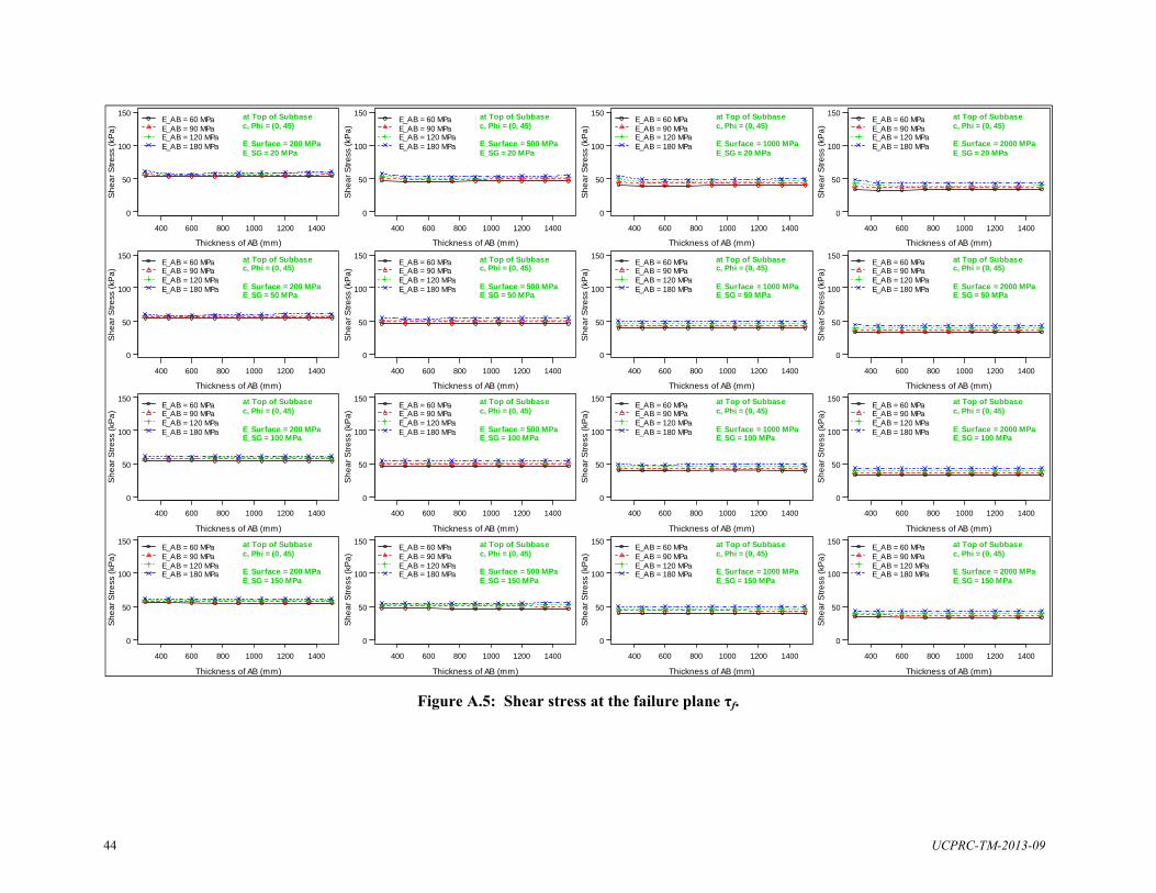
44 UCPRC-TM-2013-09
Figure A.5: Shear stress at the failure plane τf.
400 600 800 1000 1200 1400
0
50
100
150
Thickness of AB (mm)
Sh
ea
r S
tre
ss (
kPa
)E_AB = 60 MPaE_AB = 90 MPaE_AB = 120 MPaE_AB = 180 MPa
at Top of Subbasec, Phi = (0, 45)
E_Surface = 200 MPaE_SG = 20 MPa
400 600 800 1000 1200 1400
0
50
100
150
Thickness of AB (mm)
Sh
ea
r S
tre
ss (
kPa
)
E_AB = 60 MPaE_AB = 90 MPaE_AB = 120 MPaE_AB = 180 MPa
at Top of Subbasec, Phi = (0, 45)
E_Surface = 200 MPaE_SG = 50 MPa
400 600 800 1000 1200 1400
0
50
100
150
Thickness of AB (mm)
Sh
ea
r S
tre
ss (
kPa
)
E_AB = 60 MPaE_AB = 90 MPaE_AB = 120 MPaE_AB = 180 MPa
at Top of Subbasec, Phi = (0, 45)
E_Surface = 200 MPaE_SG = 100 MPa
400 600 800 1000 1200 1400
0
50
100
150
Thickness of AB (mm)
Sh
ea
r S
tre
ss (
kPa
)
E_AB = 60 MPaE_AB = 90 MPaE_AB = 120 MPaE_AB = 180 MPa
at Top of Subbasec, Phi = (0, 45)
E_Surface = 200 MPaE_SG = 150 MPa
400 600 800 1000 1200 1400
0
50
100
150
Thickness of AB (mm)
Sh
ea
r S
tre
ss (
kPa
)
E_AB = 60 MPaE_AB = 90 MPaE_AB = 120 MPaE_AB = 180 MPa
at Top of Subbasec, Phi = (0, 45)
E_Surface = 500 MPaE_SG = 20 MPa
400 600 800 1000 1200 1400
0
50
100
150
Thickness of AB (mm)
Sh
ea
r S
tre
ss (
kPa
)
E_AB = 60 MPaE_AB = 90 MPaE_AB = 120 MPaE_AB = 180 MPa
at Top of Subbasec, Phi = (0, 45)
E_Surface = 500 MPaE_SG = 50 MPa
400 600 800 1000 1200 1400
0
50
100
150
Thickness of AB (mm)
Sh
ea
r S
tre
ss (
kPa
)
E_AB = 60 MPaE_AB = 90 MPaE_AB = 120 MPaE_AB = 180 MPa
at Top of Subbasec, Phi = (0, 45)
E_Surface = 500 MPaE_SG = 100 MPa
400 600 800 1000 1200 1400
0
50
100
150
Thickness of AB (mm)
Sh
ea
r S
tre
ss (
kPa
)
E_AB = 60 MPaE_AB = 90 MPaE_AB = 120 MPaE_AB = 180 MPa
at Top of Subbasec, Phi = (0, 45)
E_Surface = 500 MPaE_SG = 150 MPa
400 600 800 1000 1200 1400
0
50
100
150
Thickness of AB (mm)
Sh
ea
r S
tre
ss (
kPa
)
E_AB = 60 MPaE_AB = 90 MPaE_AB = 120 MPaE_AB = 180 MPa
at Top of Subbasec, Phi = (0, 45)
E_Surface = 1000 MPaE_SG = 20 MPa
400 600 800 1000 1200 1400
0
50
100
150
Thickness of AB (mm)
Sh
ea
r S
tre
ss (
kPa
)
E_AB = 60 MPaE_AB = 90 MPaE_AB = 120 MPaE_AB = 180 MPa
at Top of Subbasec, Phi = (0, 45)
E_Surface = 1000 MPaE_SG = 50 MPa
400 600 800 1000 1200 1400
0
50
100
150
Thickness of AB (mm)
Sh
ea
r S
tre
ss (
kPa
)
E_AB = 60 MPaE_AB = 90 MPaE_AB = 120 MPaE_AB = 180 MPa
at Top of Subbasec, Phi = (0, 45)
E_Surface = 1000 MPaE_SG = 100 MPa
400 600 800 1000 1200 1400
0
50
100
150
Thickness of AB (mm)
Sh
ea
r S
tre
ss (
kPa
)
E_AB = 60 MPaE_AB = 90 MPaE_AB = 120 MPaE_AB = 180 MPa
at Top of Subbasec, Phi = (0, 45)
E_Surface = 1000 MPaE_SG = 150 MPa
400 600 800 1000 1200 1400
0
50
100
150
Thickness of AB (mm)
Sh
ea
r S
tre
ss (
kPa
)
E_AB = 60 MPaE_AB = 90 MPaE_AB = 120 MPaE_AB = 180 MPa
at Top of Subbasec, Phi = (0, 45)
E_Surface = 2000 MPaE_SG = 20 MPa
400 600 800 1000 1200 1400
0
50
100
150
Thickness of AB (mm)
Sh
ea
r S
tre
ss (
kPa
)
E_AB = 60 MPaE_AB = 90 MPaE_AB = 120 MPaE_AB = 180 MPa
at Top of Subbasec, Phi = (0, 45)
E_Surface = 2000 MPaE_SG = 50 MPa
400 600 800 1000 1200 1400
0
50
100
150
Thickness of AB (mm)
Sh
ea
r S
tre
ss (
kPa
)
E_AB = 60 MPaE_AB = 90 MPaE_AB = 120 MPaE_AB = 180 MPa
at Top of Subbasec, Phi = (0, 45)
E_Surface = 2000 MPaE_SG = 100 MPa
400 600 800 1000 1200 1400
0
50
100
150
Thickness of AB (mm)
Sh
ea
r S
tre
ss (
kPa
)
E_AB = 60 MPaE_AB = 90 MPaE_AB = 120 MPaE_AB = 180 MPa
at Top of Subbasec, Phi = (0, 45)
E_Surface = 2000 MPaE_SG = 150 MPa
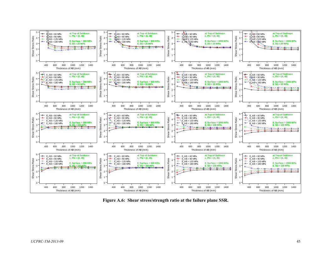
UCPRC-TM-2013-09 45
Figure A.6: Shear stress/strength ratio at the failure plane SSR.
400 600 800 1000 1200 1400
0
1
2
3
4
5
Thickness of AB (mm)
Sh
ea
r S
tre
ss R
atio
E_AB = 60 MPaE_AB = 90 MPaE_AB = 120 MPaE_AB = 180 MPa
at Top of Subbasec, Phi = (0, 45)
E_Surface = 200 MPaE_SG = 20 MPa
400 600 800 1000 1200 1400
0
1
2
3
4
5
Thickness of AB (mm)
Sh
ea
r S
tre
ss R
atio
E_AB = 60 MPaE_AB = 90 MPaE_AB = 120 MPaE_AB = 180 MPa
at Top of Subbasec, Phi = (0, 45)
E_Surface = 200 MPaE_SG = 50 MPa
400 600 800 1000 1200 1400
0
1
2
3
4
5
Thickness of AB (mm)
Sh
ea
r S
tre
ss R
atio
E_AB = 60 MPaE_AB = 90 MPaE_AB = 120 MPaE_AB = 180 MPa
at Top of Subbasec, Phi = (0, 45)
E_Surface = 200 MPaE_SG = 100 MPa
400 600 800 1000 1200 1400
0
1
2
3
4
5
Thickness of AB (mm)
Sh
ea
r S
tre
ss R
atio
E_AB = 60 MPaE_AB = 90 MPaE_AB = 120 MPaE_AB = 180 MPa
at Top of Subbasec, Phi = (0, 45)
E_Surface = 200 MPaE_SG = 150 MPa
400 600 800 1000 1200 1400
0
1
2
3
4
5
Thickness of AB (mm)
Sh
ea
r S
tre
ss R
atio
E_AB = 60 MPaE_AB = 90 MPaE_AB = 120 MPaE_AB = 180 MPa
at Top of Subbasec, Phi = (0, 45)
E_Surface = 500 MPaE_SG = 20 MPa
400 600 800 1000 1200 1400
0
1
2
3
4
5
Thickness of AB (mm)
Sh
ea
r S
tre
ss R
atio
E_AB = 60 MPaE_AB = 90 MPaE_AB = 120 MPaE_AB = 180 MPa
at Top of Subbasec, Phi = (0, 45)
E_Surface = 500 MPaE_SG = 50 MPa
400 600 800 1000 1200 1400
0
1
2
3
4
5
Thickness of AB (mm)
Sh
ea
r S
tre
ss R
atio
E_AB = 60 MPaE_AB = 90 MPaE_AB = 120 MPaE_AB = 180 MPa
at Top of Subbasec, Phi = (0, 45)
E_Surface = 500 MPaE_SG = 100 MPa
400 600 800 1000 1200 1400
0
1
2
3
4
5
Thickness of AB (mm)
Sh
ea
r S
tre
ss R
atio
E_AB = 60 MPaE_AB = 90 MPaE_AB = 120 MPaE_AB = 180 MPa
at Top of Subbasec, Phi = (0, 45)
E_Surface = 500 MPaE_SG = 150 MPa
400 600 800 1000 1200 1400
0
1
2
3
4
5
Thickness of AB (mm)
Sh
ea
r S
tre
ss R
atio
E_AB = 60 MPaE_AB = 90 MPaE_AB = 120 MPaE_AB = 180 MPa
at Top of Subbasec, Phi = (0, 45)
E_Surface = 1000 MPaE_SG = 20 MPa
400 600 800 1000 1200 1400
0
1
2
3
4
5
Thickness of AB (mm)
Sh
ea
r S
tre
ss R
atio
E_AB = 60 MPaE_AB = 90 MPaE_AB = 120 MPaE_AB = 180 MPa
at Top of Subbasec, Phi = (0, 45)
E_Surface = 1000 MPaE_SG = 50 MPa
400 600 800 1000 1200 1400
0
1
2
3
4
5
Thickness of AB (mm)
Sh
ea
r S
tre
ss R
atio
E_AB = 60 MPaE_AB = 90 MPaE_AB = 120 MPaE_AB = 180 MPa
at Top of Subbasec, Phi = (0, 45)
E_Surface = 1000 MPaE_SG = 100 MPa
400 600 800 1000 1200 1400
0
1
2
3
4
5
Thickness of AB (mm)
Sh
ea
r S
tre
ss R
atio
E_AB = 60 MPaE_AB = 90 MPaE_AB = 120 MPaE_AB = 180 MPa
at Top of Subbasec, Phi = (0, 45)
E_Surface = 1000 MPaE_SG = 150 MPa
400 600 800 1000 1200 1400
0
1
2
3
4
5
Thickness of AB (mm)
Sh
ea
r S
tre
ss R
atio
E_AB = 60 MPaE_AB = 90 MPaE_AB = 120 MPaE_AB = 180 MPa
at Top of Subbasec, Phi = (0, 45)
E_Surface = 2000 MPaE_SG = 20 MPa
400 600 800 1000 1200 1400
0
1
2
3
4
5
Thickness of AB (mm)
Sh
ea
r S
tre
ss R
atio
E_AB = 60 MPaE_AB = 90 MPaE_AB = 120 MPaE_AB = 180 MPa
at Top of Subbasec, Phi = (0, 45)
E_Surface = 2000 MPaE_SG = 50 MPa
400 600 800 1000 1200 1400
0
1
2
3
4
5
Thickness of AB (mm)
Sh
ea
r S
tre
ss R
atio
E_AB = 60 MPaE_AB = 90 MPaE_AB = 120 MPaE_AB = 180 MPa
at Top of Subbasec, Phi = (0, 45)
E_Surface = 2000 MPaE_SG = 100 MPa
400 600 800 1000 1200 1400
0
1
2
3
4
5
Thickness of AB (mm)
Sh
ea
r S
tre
ss R
atio
E_AB = 60 MPaE_AB = 90 MPaE_AB = 120 MPaE_AB = 180 MPa
at Top of Subbasec, Phi = (0, 45)
E_Surface = 2000 MPaE_SG = 150 MPa

46 UCPRC-TM-2013-09
Figure A.7: Major principal stress σ1.
400 600 800 1000 1200 1400
0
20
40
60
80
100
Thickness of AB (mm)
Ma
jor
Pri
nci
pa
l Str
ess
(kP
a)
E_AB = 60 MPaE_AB = 90 MPaE_AB = 120 MPaE_AB = 180 MPa
at Top of Subgrade
E_Surface = 200 MPaE_SG = 20 MPa
400 600 800 1000 1200 1400
0
20
40
60
80
100
Thickness of AB (mm)
Ma
jor
Pri
nci
pa
l Str
ess
(kP
a)
E_AB = 60 MPaE_AB = 90 MPaE_AB = 120 MPaE_AB = 180 MPa
at Top of Subgrade
E_Surface = 200 MPaE_SG = 50 MPa
400 600 800 1000 1200 1400
0
20
40
60
80
100
Thickness of AB (mm)
Ma
jor
Pri
nci
pa
l Str
ess
(kP
a)
E_AB = 60 MPaE_AB = 90 MPaE_AB = 120 MPaE_AB = 180 MPa
at Top of Subgrade
E_Surface = 200 MPaE_SG = 100 MPa
400 600 800 1000 1200 1400
0
20
40
60
80
100
Thickness of AB (mm)
Ma
jor
Pri
nci
pa
l Str
ess
(kP
a)
E_AB = 60 MPaE_AB = 90 MPaE_AB = 120 MPaE_AB = 180 MPa
at Top of Subgrade
E_Surface = 200 MPaE_SG = 150 MPa
400 600 800 1000 1200 1400
0
20
40
60
80
100
Thickness of AB (mm)
Ma
jor
Pri
nci
pa
l Str
ess
(kP
a)
E_AB = 60 MPaE_AB = 90 MPaE_AB = 120 MPaE_AB = 180 MPa
at Top of Subgrade
E_Surface = 500 MPaE_SG = 20 MPa
400 600 800 1000 1200 1400
0
20
40
60
80
100
Thickness of AB (mm)
Ma
jor
Pri
nci
pa
l Str
ess
(kP
a)
E_AB = 60 MPaE_AB = 90 MPaE_AB = 120 MPaE_AB = 180 MPa
at Top of Subgrade
E_Surface = 500 MPaE_SG = 50 MPa
400 600 800 1000 1200 1400
0
20
40
60
80
100
Thickness of AB (mm)
Ma
jor
Pri
nci
pa
l Str
ess
(kP
a)
E_AB = 60 MPaE_AB = 90 MPaE_AB = 120 MPaE_AB = 180 MPa
at Top of Subgrade
E_Surface = 500 MPaE_SG = 100 MPa
400 600 800 1000 1200 1400
0
20
40
60
80
100
Thickness of AB (mm)
Ma
jor
Pri
nci
pa
l Str
ess
(kP
a)
E_AB = 60 MPaE_AB = 90 MPaE_AB = 120 MPaE_AB = 180 MPa
at Top of Subgrade
E_Surface = 500 MPaE_SG = 150 MPa
400 600 800 1000 1200 1400
0
20
40
60
80
100
Thickness of AB (mm)
Ma
jor
Pri
nci
pa
l Str
ess
(kP
a)
E_AB = 60 MPaE_AB = 90 MPaE_AB = 120 MPaE_AB = 180 MPa
at Top of Subgrade
E_Surface = 1000 MPaE_SG = 20 MPa
400 600 800 1000 1200 1400
0
20
40
60
80
100
Thickness of AB (mm)
Ma
jor
Pri
nci
pa
l Str
ess
(kP
a)
E_AB = 60 MPaE_AB = 90 MPaE_AB = 120 MPaE_AB = 180 MPa
at Top of Subgrade
E_Surface = 1000 MPaE_SG = 50 MPa
400 600 800 1000 1200 1400
0
20
40
60
80
100
Thickness of AB (mm)
Ma
jor
Pri
nci
pa
l Str
ess
(kP
a)
E_AB = 60 MPaE_AB = 90 MPaE_AB = 120 MPaE_AB = 180 MPa
at Top of Subgrade
E_Surface = 1000 MPaE_SG = 100 MPa
400 600 800 1000 1200 1400
0
20
40
60
80
100
Thickness of AB (mm)
Ma
jor
Pri
nci
pa
l Str
ess
(kP
a)
E_AB = 60 MPaE_AB = 90 MPaE_AB = 120 MPaE_AB = 180 MPa
at Top of Subgrade
E_Surface = 1000 MPaE_SG = 150 MPa
400 600 800 1000 1200 1400
0
20
40
60
80
100
Thickness of AB (mm)
Ma
jor
Pri
nci
pa
l Str
ess
(kP
a)
E_AB = 60 MPaE_AB = 90 MPaE_AB = 120 MPaE_AB = 180 MPa
at Top of Subgrade
E_Surface = 2000 MPaE_SG = 20 MPa
400 600 800 1000 1200 1400
0
20
40
60
80
100
Thickness of AB (mm)
Ma
jor
Pri
nci
pa
l Str
ess
(kP
a)
E_AB = 60 MPaE_AB = 90 MPaE_AB = 120 MPaE_AB = 180 MPa
at Top of Subgrade
E_Surface = 2000 MPaE_SG = 50 MPa
400 600 800 1000 1200 1400
0
20
40
60
80
100
Thickness of AB (mm)
Ma
jor
Pri
nci
pa
l Str
ess
(kP
a)
E_AB = 60 MPaE_AB = 90 MPaE_AB = 120 MPaE_AB = 180 MPa
at Top of Subgrade
E_Surface = 2000 MPaE_SG = 100 MPa
400 600 800 1000 1200 1400
0
20
40
60
80
100
Thickness of AB (mm)
Ma
jor
Pri
nci
pa
l Str
ess
(kP
a)
E_AB = 60 MPaE_AB = 90 MPaE_AB = 120 MPaE_AB = 180 MPa
at Top of Subgrade
E_Surface = 2000 MPaE_SG = 150 MPa

UCPRC-TM-2013-09 47
Figure A.8: Minor principal stress σ3.
400 600 800 1000 1200 1400
-10
-5
0
5
10
Thickness of AB (mm)
Min
or
Pri
nci
pa
l Str
ess
(kP
a)
E_AB = 60 MPaE_AB = 90 MPaE_AB = 120 MPaE_AB = 180 MPa
at Top of Subgrade
E_Surface = 200 MPaE_SG = 20 MPa
400 600 800 1000 1200 1400
-10
-5
0
5
10
Thickness of AB (mm)
Min
or
Pri
nci
pa
l Str
ess
(kP
a)
E_AB = 60 MPaE_AB = 90 MPaE_AB = 120 MPaE_AB = 180 MPa
at Top of Subgrade
E_Surface = 200 MPaE_SG = 50 MPa
400 600 800 1000 1200 1400
-10
-5
0
5
10
Thickness of AB (mm)
Min
or
Pri
nci
pa
l Str
ess
(kP
a)
E_AB = 60 MPaE_AB = 90 MPaE_AB = 120 MPaE_AB = 180 MPa
at Top of Subgrade
E_Surface = 200 MPaE_SG = 100 MPa
400 600 800 1000 1200 1400
-10
-5
0
5
10
Thickness of AB (mm)
Min
or
Pri
nci
pa
l Str
ess
(kP
a)
E_AB = 60 MPaE_AB = 90 MPaE_AB = 120 MPaE_AB = 180 MPa
at Top of Subgrade
E_Surface = 200 MPaE_SG = 150 MPa
400 600 800 1000 1200 1400
-10
-5
0
5
10
Thickness of AB (mm)
Min
or
Pri
nci
pa
l Str
ess
(kP
a)
E_AB = 60 MPaE_AB = 90 MPaE_AB = 120 MPaE_AB = 180 MPa
at Top of Subgrade
E_Surface = 500 MPaE_SG = 20 MPa
400 600 800 1000 1200 1400
-10
-5
0
5
10
Thickness of AB (mm)
Min
or
Pri
nci
pa
l Str
ess
(kP
a)
E_AB = 60 MPaE_AB = 90 MPaE_AB = 120 MPaE_AB = 180 MPa
at Top of Subgrade
E_Surface = 500 MPaE_SG = 50 MPa
400 600 800 1000 1200 1400
-10
-5
0
5
10
Thickness of AB (mm)
Min
or
Pri
nci
pa
l Str
ess
(kP
a)
E_AB = 60 MPaE_AB = 90 MPaE_AB = 120 MPaE_AB = 180 MPa
at Top of Subgrade
E_Surface = 500 MPaE_SG = 100 MPa
400 600 800 1000 1200 1400
-10
-5
0
5
10
Thickness of AB (mm)
Min
or
Pri
nci
pa
l Str
ess
(kP
a)
E_AB = 60 MPaE_AB = 90 MPaE_AB = 120 MPaE_AB = 180 MPa
at Top of Subgrade
E_Surface = 500 MPaE_SG = 150 MPa
400 600 800 1000 1200 1400
-10
-5
0
5
10
Thickness of AB (mm)
Min
or
Pri
nci
pa
l Str
ess
(kP
a)
E_AB = 60 MPaE_AB = 90 MPaE_AB = 120 MPaE_AB = 180 MPa
at Top of Subgrade
E_Surface = 1000 MPaE_SG = 20 MPa
400 600 800 1000 1200 1400
-10
-5
0
5
10
Thickness of AB (mm)
Min
or
Pri
nci
pa
l Str
ess
(kP
a)
E_AB = 60 MPaE_AB = 90 MPaE_AB = 120 MPaE_AB = 180 MPa
at Top of Subgrade
E_Surface = 1000 MPaE_SG = 50 MPa
400 600 800 1000 1200 1400
-10
-5
0
5
10
Thickness of AB (mm)
Min
or
Pri
nci
pa
l Str
ess
(kP
a)
E_AB = 60 MPaE_AB = 90 MPaE_AB = 120 MPaE_AB = 180 MPa
at Top of Subgrade
E_Surface = 1000 MPaE_SG = 100 MPa
400 600 800 1000 1200 1400
-10
-5
0
5
10
Thickness of AB (mm)
Min
or
Pri
nci
pa
l Str
ess
(kP
a)
E_AB = 60 MPaE_AB = 90 MPaE_AB = 120 MPaE_AB = 180 MPa
at Top of Subgrade
E_Surface = 1000 MPaE_SG = 150 MPa
400 600 800 1000 1200 1400
-10
-5
0
5
10
Thickness of AB (mm)
Min
or
Pri
nci
pa
l Str
ess
(kP
a)
E_AB = 60 MPaE_AB = 90 MPaE_AB = 120 MPaE_AB = 180 MPa
at Top of Subgrade
E_Surface = 2000 MPaE_SG = 20 MPa
400 600 800 1000 1200 1400
-10
-5
0
5
10
Thickness of AB (mm)
Min
or
Pri
nci
pa
l Str
ess
(kP
a)
E_AB = 60 MPaE_AB = 90 MPaE_AB = 120 MPaE_AB = 180 MPa
at Top of Subgrade
E_Surface = 2000 MPaE_SG = 50 MPa
400 600 800 1000 1200 1400
-10
-5
0
5
10
Thickness of AB (mm)
Min
or
Pri
nci
pa
l Str
ess
(kP
a)
E_AB = 60 MPaE_AB = 90 MPaE_AB = 120 MPaE_AB = 180 MPa
at Top of Subgrade
E_Surface = 2000 MPaE_SG = 100 MPa
400 600 800 1000 1200 1400
-10
-5
0
5
10
Thickness of AB (mm)
Min
or
Pri
nci
pa
l Str
ess
(kP
a)
E_AB = 60 MPaE_AB = 90 MPaE_AB = 120 MPaE_AB = 180 MPa
at Top of Subgrade
E_Surface = 2000 MPaE_SG = 150 MPa

48 UCPRC-TM-2013-09
Figure A.9: Normal stress at the failure plane σf (ϕ ≠ 0).
400 600 800 1000 1200 1400
0
10
20
30
40
50
Thickness of AB (mm)
No
rma
l Str
ess
(kP
a) E_AB = 60 MPa
E_AB = 90 MPaE_AB = 120 MPaE_AB = 180 MPa
at Top of Subgradec, Phi = (10, 20)
E_Surface = 200 MPaE_SG = 20 MPa
400 600 800 1000 1200 1400
0
10
20
30
40
50
Thickness of AB (mm)
No
rma
l Str
ess
(kP
a) E_AB = 60 MPa
E_AB = 90 MPaE_AB = 120 MPaE_AB = 180 MPa
at Top of Subgradec, Phi = (15, 25)
E_Surface = 200 MPaE_SG = 50 MPa
400 600 800 1000 1200 1400
0
10
20
30
40
50
Thickness of AB (mm)
No
rma
l Str
ess
(kP
a) E_AB = 60 MPa
E_AB = 90 MPaE_AB = 120 MPaE_AB = 180 MPa
at Top of Subgradec, Phi = (20, 30)
E_Surface = 200 MPaE_SG = 100 MPa
400 600 800 1000 1200 1400
0
10
20
30
40
50
Thickness of AB (mm)
No
rma
l Str
ess
(kP
a) E_AB = 60 MPa
E_AB = 90 MPaE_AB = 120 MPaE_AB = 180 MPa
at Top of Subgradec, Phi = (25, 35)
E_Surface = 200 MPaE_SG = 150 MPa
400 600 800 1000 1200 1400
0
10
20
30
40
50
Thickness of AB (mm)
No
rma
l Str
ess
(kP
a) E_AB = 60 MPa
E_AB = 90 MPaE_AB = 120 MPaE_AB = 180 MPa
at Top of Subgradec, Phi = (10, 20)
E_Surface = 500 MPaE_SG = 20 MPa
400 600 800 1000 1200 1400
0
10
20
30
40
50
Thickness of AB (mm)
No
rma
l Str
ess
(kP
a) E_AB = 60 MPa
E_AB = 90 MPaE_AB = 120 MPaE_AB = 180 MPa
at Top of Subgradec, Phi = (15, 25)
E_Surface = 500 MPaE_SG = 50 MPa
400 600 800 1000 1200 1400
0
10
20
30
40
50
Thickness of AB (mm)
No
rma
l Str
ess
(kP
a) E_AB = 60 MPa
E_AB = 90 MPaE_AB = 120 MPaE_AB = 180 MPa
at Top of Subgradec, Phi = (20, 30)
E_Surface = 500 MPaE_SG = 100 MPa
400 600 800 1000 1200 1400
0
10
20
30
40
50
Thickness of AB (mm)
No
rma
l Str
ess
(kP
a) E_AB = 60 MPa
E_AB = 90 MPaE_AB = 120 MPaE_AB = 180 MPa
at Top of Subgradec, Phi = (25, 35)
E_Surface = 500 MPaE_SG = 150 MPa
400 600 800 1000 1200 1400
0
10
20
30
40
50
Thickness of AB (mm)
No
rma
l Str
ess
(kP
a) E_AB = 60 MPa
E_AB = 90 MPaE_AB = 120 MPaE_AB = 180 MPa
at Top of Subgradec, Phi = (10, 20)
E_Surface = 1000 MPaE_SG = 20 MPa
400 600 800 1000 1200 1400
0
10
20
30
40
50
Thickness of AB (mm)
No
rma
l Str
ess
(kP
a) E_AB = 60 MPa
E_AB = 90 MPaE_AB = 120 MPaE_AB = 180 MPa
at Top of Subgradec, Phi = (15, 25)
E_Surface = 1000 MPaE_SG = 50 MPa
400 600 800 1000 1200 1400
0
10
20
30
40
50
Thickness of AB (mm)
No
rma
l Str
ess
(kP
a) E_AB = 60 MPa
E_AB = 90 MPaE_AB = 120 MPaE_AB = 180 MPa
at Top of Subgradec, Phi = (20, 30)
E_Surface = 1000 MPaE_SG = 100 MPa
400 600 800 1000 1200 1400
0
10
20
30
40
50
Thickness of AB (mm)
No
rma
l Str
ess
(kP
a) E_AB = 60 MPa
E_AB = 90 MPaE_AB = 120 MPaE_AB = 180 MPa
at Top of Subgradec, Phi = (25, 35)
E_Surface = 1000 MPaE_SG = 150 MPa
400 600 800 1000 1200 1400
0
10
20
30
40
50
Thickness of AB (mm)
No
rma
l Str
ess
(kP
a) E_AB = 60 MPa
E_AB = 90 MPaE_AB = 120 MPaE_AB = 180 MPa
at Top of Subgradec, Phi = (10, 20)
E_Surface = 2000 MPaE_SG = 20 MPa
400 600 800 1000 1200 1400
0
10
20
30
40
50
Thickness of AB (mm)
No
rma
l Str
ess
(kP
a) E_AB = 60 MPa
E_AB = 90 MPaE_AB = 120 MPaE_AB = 180 MPa
at Top of Subgradec, Phi = (15, 25)
E_Surface = 2000 MPaE_SG = 50 MPa
400 600 800 1000 1200 1400
0
10
20
30
40
50
Thickness of AB (mm)
No
rma
l Str
ess
(kP
a) E_AB = 60 MPa
E_AB = 90 MPaE_AB = 120 MPaE_AB = 180 MPa
at Top of Subgradec, Phi = (20, 30)
E_Surface = 2000 MPaE_SG = 100 MPa
400 600 800 1000 1200 1400
0
10
20
30
40
50
Thickness of AB (mm)
No
rma
l Str
ess
(kP
a) E_AB = 60 MPa
E_AB = 90 MPaE_AB = 120 MPaE_AB = 180 MPa
at Top of Subgradec, Phi = (25, 35)
E_Surface = 2000 MPaE_SG = 150 MPa
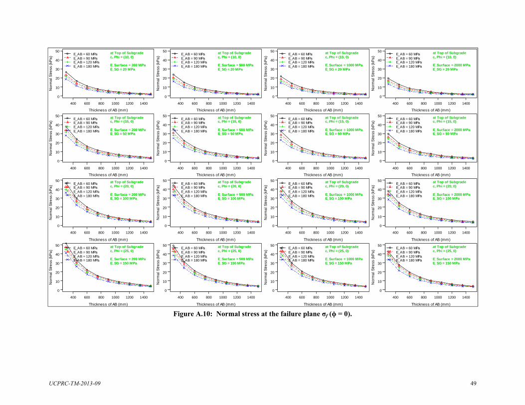
UCPRC-TM-2013-09 49
Figure A.10: Normal stress at the failure plane σf (ϕ = 0).
400 600 800 1000 1200 1400
0
10
20
30
40
50
Thickness of AB (mm)
No
rma
l Str
ess
(kP
a) E_AB = 60 MPa
E_AB = 90 MPaE_AB = 120 MPaE_AB = 180 MPa
at Top of Subgradec, Phi = (10, 0)
E_Surface = 200 MPaE_SG = 20 MPa
400 600 800 1000 1200 1400
0
10
20
30
40
50
Thickness of AB (mm)
No
rma
l Str
ess
(kP
a) E_AB = 60 MPa
E_AB = 90 MPaE_AB = 120 MPaE_AB = 180 MPa
at Top of Subgradec, Phi = (15, 0)
E_Surface = 200 MPaE_SG = 50 MPa
400 600 800 1000 1200 1400
0
10
20
30
40
50
Thickness of AB (mm)
No
rma
l Str
ess
(kP
a) E_AB = 60 MPa
E_AB = 90 MPaE_AB = 120 MPaE_AB = 180 MPa
at Top of Subgradec, Phi = (20, 0)
E_Surface = 200 MPaE_SG = 100 MPa
400 600 800 1000 1200 1400
0
10
20
30
40
50
Thickness of AB (mm)
No
rma
l Str
ess
(kP
a) E_AB = 60 MPa
E_AB = 90 MPaE_AB = 120 MPaE_AB = 180 MPa
at Top of Subgradec, Phi = (25, 0)
E_Surface = 200 MPaE_SG = 150 MPa
400 600 800 1000 1200 1400
0
10
20
30
40
50
Thickness of AB (mm)
No
rma
l Str
ess
(kP
a) E_AB = 60 MPa
E_AB = 90 MPaE_AB = 120 MPaE_AB = 180 MPa
at Top of Subgradec, Phi = (10, 0)
E_Surface = 500 MPaE_SG = 20 MPa
400 600 800 1000 1200 1400
0
10
20
30
40
50
Thickness of AB (mm)
No
rma
l Str
ess
(kP
a) E_AB = 60 MPa
E_AB = 90 MPaE_AB = 120 MPaE_AB = 180 MPa
at Top of Subgradec, Phi = (15, 0)
E_Surface = 500 MPaE_SG = 50 MPa
400 600 800 1000 1200 1400
0
10
20
30
40
50
Thickness of AB (mm)
No
rma
l Str
ess
(kP
a) E_AB = 60 MPa
E_AB = 90 MPaE_AB = 120 MPaE_AB = 180 MPa
at Top of Subgradec, Phi = (20, 0)
E_Surface = 500 MPaE_SG = 100 MPa
400 600 800 1000 1200 1400
0
10
20
30
40
50
Thickness of AB (mm)
No
rma
l Str
ess
(kP
a) E_AB = 60 MPa
E_AB = 90 MPaE_AB = 120 MPaE_AB = 180 MPa
at Top of Subgradec, Phi = (25, 0)
E_Surface = 500 MPaE_SG = 150 MPa
400 600 800 1000 1200 1400
0
10
20
30
40
50
Thickness of AB (mm)
No
rma
l Str
ess
(kP
a) E_AB = 60 MPa
E_AB = 90 MPaE_AB = 120 MPaE_AB = 180 MPa
at Top of Subgradec, Phi = (10, 0)
E_Surface = 1000 MPaE_SG = 20 MPa
400 600 800 1000 1200 1400
0
10
20
30
40
50
Thickness of AB (mm)
No
rma
l Str
ess
(kP
a) E_AB = 60 MPa
E_AB = 90 MPaE_AB = 120 MPaE_AB = 180 MPa
at Top of Subgradec, Phi = (15, 0)
E_Surface = 1000 MPaE_SG = 50 MPa
400 600 800 1000 1200 1400
0
10
20
30
40
50
Thickness of AB (mm)
No
rma
l Str
ess
(kP
a) E_AB = 60 MPa
E_AB = 90 MPaE_AB = 120 MPaE_AB = 180 MPa
at Top of Subgradec, Phi = (20, 0)
E_Surface = 1000 MPaE_SG = 100 MPa
400 600 800 1000 1200 1400
0
10
20
30
40
50
Thickness of AB (mm)
No
rma
l Str
ess
(kP
a) E_AB = 60 MPa
E_AB = 90 MPaE_AB = 120 MPaE_AB = 180 MPa
at Top of Subgradec, Phi = (25, 0)
E_Surface = 1000 MPaE_SG = 150 MPa
400 600 800 1000 1200 1400
0
10
20
30
40
50
Thickness of AB (mm)
No
rma
l Str
ess
(kP
a) E_AB = 60 MPa
E_AB = 90 MPaE_AB = 120 MPaE_AB = 180 MPa
at Top of Subgradec, Phi = (10, 0)
E_Surface = 2000 MPaE_SG = 20 MPa
400 600 800 1000 1200 1400
0
10
20
30
40
50
Thickness of AB (mm)
No
rma
l Str
ess
(kP
a) E_AB = 60 MPa
E_AB = 90 MPaE_AB = 120 MPaE_AB = 180 MPa
at Top of Subgradec, Phi = (15, 0)
E_Surface = 2000 MPaE_SG = 50 MPa
400 600 800 1000 1200 1400
0
10
20
30
40
50
Thickness of AB (mm)
No
rma
l Str
ess
(kP
a) E_AB = 60 MPa
E_AB = 90 MPaE_AB = 120 MPaE_AB = 180 MPa
at Top of Subgradec, Phi = (20, 0)
E_Surface = 2000 MPaE_SG = 100 MPa
400 600 800 1000 1200 1400
0
10
20
30
40
50
Thickness of AB (mm)
No
rma
l Str
ess
(kP
a) E_AB = 60 MPa
E_AB = 90 MPaE_AB = 120 MPaE_AB = 180 MPa
at Top of Subgradec, Phi = (25, 0)
E_Surface = 2000 MPaE_SG = 150 MPa
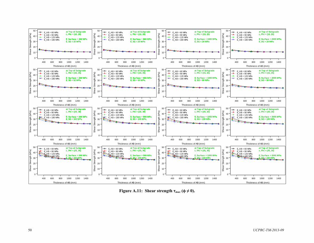
50 UCPRC-TM-2013-09
Figure A.11: Shear strength τmax (ϕ ≠ 0).
400 600 800 1000 1200 1400
0
10
20
30
40
50
Thickness of AB (mm)
Sh
ea
r S
tre
ng
th (
kPa
) E_AB = 60 MPaE_AB = 90 MPaE_AB = 120 MPaE_AB = 180 MPa
at Top of Subgradec, Phi = (10, 20)
E_Surface = 200 MPaE_SG = 20 MPa
400 600 800 1000 1200 1400
0
10
20
30
40
50
Thickness of AB (mm)
Sh
ea
r S
tre
ng
th (
kPa
) E_AB = 60 MPaE_AB = 90 MPaE_AB = 120 MPaE_AB = 180 MPa
at Top of Subgradec, Phi = (15, 25)
E_Surface = 200 MPaE_SG = 50 MPa
400 600 800 1000 1200 1400
0
10
20
30
40
50
Thickness of AB (mm)
Sh
ea
r S
tre
ng
th (
kPa
) E_AB = 60 MPaE_AB = 90 MPaE_AB = 120 MPaE_AB = 180 MPa
at Top of Subgradec, Phi = (20, 30)
E_Surface = 200 MPaE_SG = 100 MPa
400 600 800 1000 1200 1400
0
10
20
30
40
50
Thickness of AB (mm)
Sh
ea
r S
tre
ng
th (
kPa
) E_AB = 60 MPaE_AB = 90 MPaE_AB = 120 MPaE_AB = 180 MPa
at Top of Subgradec, Phi = (25, 35)
E_Surface = 200 MPaE_SG = 150 MPa
400 600 800 1000 1200 1400
0
10
20
30
40
50
Thickness of AB (mm)
Sh
ea
r S
tre
ng
th (
kPa
) E_AB = 60 MPaE_AB = 90 MPaE_AB = 120 MPaE_AB = 180 MPa
at Top of Subgradec, Phi = (10, 20)
E_Surface = 500 MPaE_SG = 20 MPa
400 600 800 1000 1200 1400
0
10
20
30
40
50
Thickness of AB (mm)
Sh
ea
r S
tre
ng
th (
kPa
) E_AB = 60 MPaE_AB = 90 MPaE_AB = 120 MPaE_AB = 180 MPa
at Top of Subgradec, Phi = (15, 25)
E_Surface = 500 MPaE_SG = 50 MPa
400 600 800 1000 1200 1400
0
10
20
30
40
50
Thickness of AB (mm)
Sh
ea
r S
tre
ng
th (
kPa
) E_AB = 60 MPaE_AB = 90 MPaE_AB = 120 MPaE_AB = 180 MPa
at Top of Subgradec, Phi = (20, 30)
E_Surface = 500 MPaE_SG = 100 MPa
400 600 800 1000 1200 1400
0
10
20
30
40
50
Thickness of AB (mm)
Sh
ea
r S
tre
ng
th (
kPa
) E_AB = 60 MPaE_AB = 90 MPaE_AB = 120 MPaE_AB = 180 MPa
at Top of Subgradec, Phi = (25, 35)
E_Surface = 500 MPaE_SG = 150 MPa
400 600 800 1000 1200 1400
0
10
20
30
40
50
Thickness of AB (mm)
Sh
ea
r S
tre
ng
th (
kPa
) E_AB = 60 MPaE_AB = 90 MPaE_AB = 120 MPaE_AB = 180 MPa
at Top of Subgradec, Phi = (10, 20)
E_Surface = 1000 MPaE_SG = 20 MPa
400 600 800 1000 1200 1400
0
10
20
30
40
50
Thickness of AB (mm)
Sh
ea
r S
tre
ng
th (
kPa
) E_AB = 60 MPaE_AB = 90 MPaE_AB = 120 MPaE_AB = 180 MPa
at Top of Subgradec, Phi = (15, 25)
E_Surface = 1000 MPaE_SG = 50 MPa
400 600 800 1000 1200 1400
0
10
20
30
40
50
Thickness of AB (mm)
Sh
ea
r S
tre
ng
th (
kPa
) E_AB = 60 MPaE_AB = 90 MPaE_AB = 120 MPaE_AB = 180 MPa
at Top of Subgradec, Phi = (20, 30)
E_Surface = 1000 MPaE_SG = 100 MPa
400 600 800 1000 1200 1400
0
10
20
30
40
50
Thickness of AB (mm)
Sh
ea
r S
tre
ng
th (
kPa
) E_AB = 60 MPaE_AB = 90 MPaE_AB = 120 MPaE_AB = 180 MPa
at Top of Subgradec, Phi = (25, 35)
E_Surface = 1000 MPaE_SG = 150 MPa
400 600 800 1000 1200 1400
0
10
20
30
40
50
Thickness of AB (mm)
Sh
ea
r S
tre
ng
th (
kPa
) E_AB = 60 MPaE_AB = 90 MPaE_AB = 120 MPaE_AB = 180 MPa
at Top of Subgradec, Phi = (10, 20)
E_Surface = 2000 MPaE_SG = 20 MPa
400 600 800 1000 1200 1400
0
10
20
30
40
50
Thickness of AB (mm)
Sh
ea
r S
tre
ng
th (
kPa
) E_AB = 60 MPaE_AB = 90 MPaE_AB = 120 MPaE_AB = 180 MPa
at Top of Subgradec, Phi = (15, 25)
E_Surface = 2000 MPaE_SG = 50 MPa
400 600 800 1000 1200 1400
0
10
20
30
40
50
Thickness of AB (mm)
Sh
ea
r S
tre
ng
th (
kPa
) E_AB = 60 MPaE_AB = 90 MPaE_AB = 120 MPaE_AB = 180 MPa
at Top of Subgradec, Phi = (20, 30)
E_Surface = 2000 MPaE_SG = 100 MPa
400 600 800 1000 1200 1400
0
10
20
30
40
50
Thickness of AB (mm)
Sh
ea
r S
tre
ng
th (
kPa
) E_AB = 60 MPaE_AB = 90 MPaE_AB = 120 MPaE_AB = 180 MPa
at Top of Subgradec, Phi = (25, 35)
E_Surface = 2000 MPaE_SG = 150 MPa
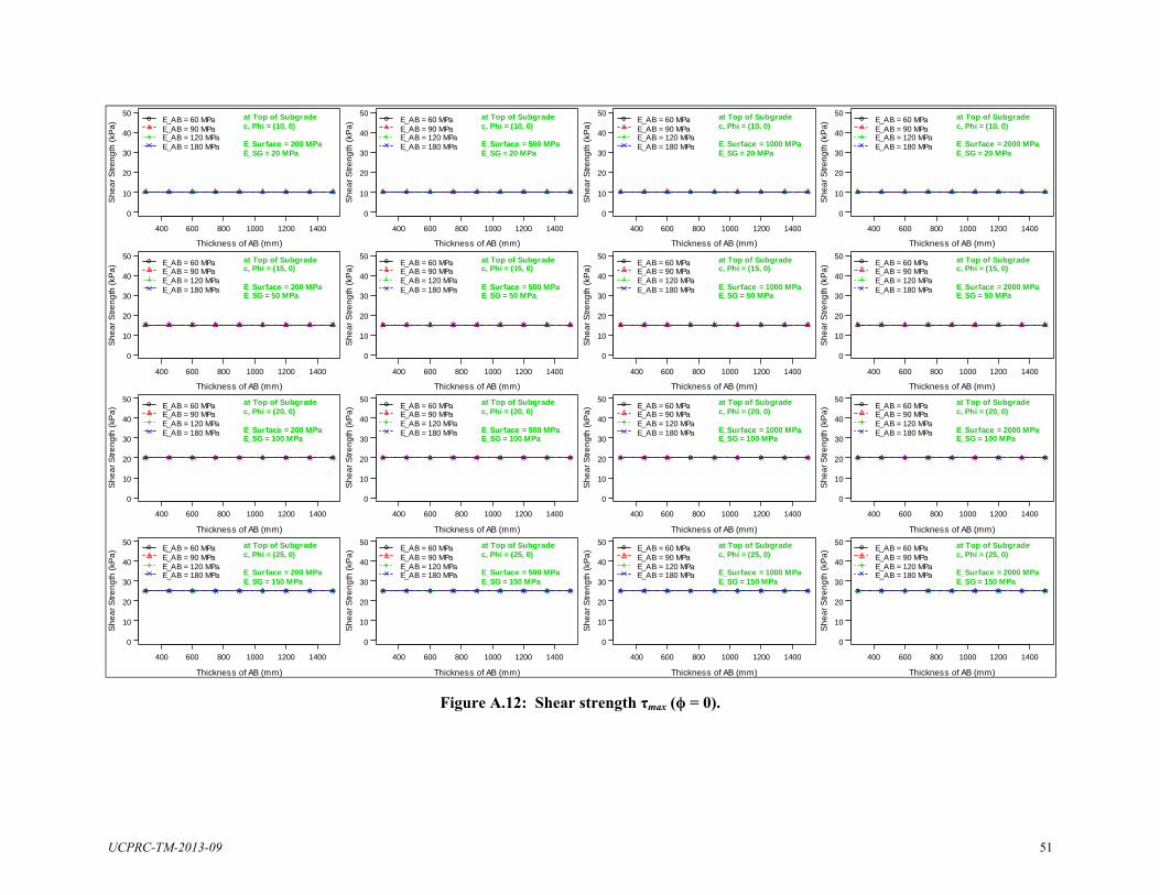
UCPRC-TM-2013-09 51
Figure A.12: Shear strength τmax (ϕ = 0).
400 600 800 1000 1200 1400
0
10
20
30
40
50
Thickness of AB (mm)
Sh
ea
r S
tre
ng
th (
kPa
) E_AB = 60 MPaE_AB = 90 MPaE_AB = 120 MPaE_AB = 180 MPa
at Top of Subgradec, Phi = (10, 0)
E_Surface = 200 MPaE_SG = 20 MPa
400 600 800 1000 1200 1400
0
10
20
30
40
50
Thickness of AB (mm)
Sh
ea
r S
tre
ng
th (
kPa
) E_AB = 60 MPaE_AB = 90 MPaE_AB = 120 MPaE_AB = 180 MPa
at Top of Subgradec, Phi = (15, 0)
E_Surface = 200 MPaE_SG = 50 MPa
400 600 800 1000 1200 1400
0
10
20
30
40
50
Thickness of AB (mm)
Sh
ea
r S
tre
ng
th (
kPa
) E_AB = 60 MPaE_AB = 90 MPaE_AB = 120 MPaE_AB = 180 MPa
at Top of Subgradec, Phi = (20, 0)
E_Surface = 200 MPaE_SG = 100 MPa
400 600 800 1000 1200 1400
0
10
20
30
40
50
Thickness of AB (mm)
Sh
ea
r S
tre
ng
th (
kPa
) E_AB = 60 MPaE_AB = 90 MPaE_AB = 120 MPaE_AB = 180 MPa
at Top of Subgradec, Phi = (25, 0)
E_Surface = 200 MPaE_SG = 150 MPa
400 600 800 1000 1200 1400
0
10
20
30
40
50
Thickness of AB (mm)
Sh
ea
r S
tre
ng
th (
kPa
) E_AB = 60 MPaE_AB = 90 MPaE_AB = 120 MPaE_AB = 180 MPa
at Top of Subgradec, Phi = (10, 0)
E_Surface = 500 MPaE_SG = 20 MPa
400 600 800 1000 1200 1400
0
10
20
30
40
50
Thickness of AB (mm)
Sh
ea
r S
tre
ng
th (
kPa
) E_AB = 60 MPaE_AB = 90 MPaE_AB = 120 MPaE_AB = 180 MPa
at Top of Subgradec, Phi = (15, 0)
E_Surface = 500 MPaE_SG = 50 MPa
400 600 800 1000 1200 1400
0
10
20
30
40
50
Thickness of AB (mm)
Sh
ea
r S
tre
ng
th (
kPa
) E_AB = 60 MPaE_AB = 90 MPaE_AB = 120 MPaE_AB = 180 MPa
at Top of Subgradec, Phi = (20, 0)
E_Surface = 500 MPaE_SG = 100 MPa
400 600 800 1000 1200 1400
0
10
20
30
40
50
Thickness of AB (mm)
Sh
ea
r S
tre
ng
th (
kPa
) E_AB = 60 MPaE_AB = 90 MPaE_AB = 120 MPaE_AB = 180 MPa
at Top of Subgradec, Phi = (25, 0)
E_Surface = 500 MPaE_SG = 150 MPa
400 600 800 1000 1200 1400
0
10
20
30
40
50
Thickness of AB (mm)
Sh
ea
r S
tre
ng
th (
kPa
) E_AB = 60 MPaE_AB = 90 MPaE_AB = 120 MPaE_AB = 180 MPa
at Top of Subgradec, Phi = (10, 0)
E_Surface = 1000 MPaE_SG = 20 MPa
400 600 800 1000 1200 1400
0
10
20
30
40
50
Thickness of AB (mm)
Sh
ea
r S
tre
ng
th (
kPa
) E_AB = 60 MPaE_AB = 90 MPaE_AB = 120 MPaE_AB = 180 MPa
at Top of Subgradec, Phi = (15, 0)
E_Surface = 1000 MPaE_SG = 50 MPa
400 600 800 1000 1200 1400
0
10
20
30
40
50
Thickness of AB (mm)
Sh
ea
r S
tre
ng
th (
kPa
) E_AB = 60 MPaE_AB = 90 MPaE_AB = 120 MPaE_AB = 180 MPa
at Top of Subgradec, Phi = (20, 0)
E_Surface = 1000 MPaE_SG = 100 MPa
400 600 800 1000 1200 1400
0
10
20
30
40
50
Thickness of AB (mm)
Sh
ea
r S
tre
ng
th (
kPa
) E_AB = 60 MPaE_AB = 90 MPaE_AB = 120 MPaE_AB = 180 MPa
at Top of Subgradec, Phi = (25, 0)
E_Surface = 1000 MPaE_SG = 150 MPa
400 600 800 1000 1200 1400
0
10
20
30
40
50
Thickness of AB (mm)
Sh
ea
r S
tre
ng
th (
kPa
) E_AB = 60 MPaE_AB = 90 MPaE_AB = 120 MPaE_AB = 180 MPa
at Top of Subgradec, Phi = (10, 0)
E_Surface = 2000 MPaE_SG = 20 MPa
400 600 800 1000 1200 1400
0
10
20
30
40
50
Thickness of AB (mm)
Sh
ea
r S
tre
ng
th (
kPa
) E_AB = 60 MPaE_AB = 90 MPaE_AB = 120 MPaE_AB = 180 MPa
at Top of Subgradec, Phi = (15, 0)
E_Surface = 2000 MPaE_SG = 50 MPa
400 600 800 1000 1200 1400
0
10
20
30
40
50
Thickness of AB (mm)
Sh
ea
r S
tre
ng
th (
kPa
) E_AB = 60 MPaE_AB = 90 MPaE_AB = 120 MPaE_AB = 180 MPa
at Top of Subgradec, Phi = (20, 0)
E_Surface = 2000 MPaE_SG = 100 MPa
400 600 800 1000 1200 1400
0
10
20
30
40
50
Thickness of AB (mm)
Sh
ea
r S
tre
ng
th (
kPa
) E_AB = 60 MPaE_AB = 90 MPaE_AB = 120 MPaE_AB = 180 MPa
at Top of Subgradec, Phi = (25, 0)
E_Surface = 2000 MPaE_SG = 150 MPa

52 UCPRC-TM-2013-09
Figure A.13: Shear stress at the failure plane τf (ϕ ≠ 0).
400 600 800 1000 1200 1400
0
10
20
30
40
50
Thickness of AB (mm)
Sh
ea
r S
tre
ss (
kPa
)E_AB = 60 MPaE_AB = 90 MPaE_AB = 120 MPaE_AB = 180 MPa
at Top of Subgradec, Phi = (10, 20)
E_Surface = 200 MPaE_SG = 20 MPa
400 600 800 1000 1200 1400
0
10
20
30
40
50
Thickness of AB (mm)
Sh
ea
r S
tre
ss (
kPa
)
E_AB = 60 MPaE_AB = 90 MPaE_AB = 120 MPaE_AB = 180 MPa
at Top of Subgradec, Phi = (15, 25)
E_Surface = 200 MPaE_SG = 50 MPa
400 600 800 1000 1200 1400
0
10
20
30
40
50
Thickness of AB (mm)
Sh
ea
r S
tre
ss (
kPa
)
E_AB = 60 MPaE_AB = 90 MPaE_AB = 120 MPaE_AB = 180 MPa
at Top of Subgradec, Phi = (20, 30)
E_Surface = 200 MPaE_SG = 100 MPa
400 600 800 1000 1200 1400
0
10
20
30
40
50
Thickness of AB (mm)
Sh
ea
r S
tre
ss (
kPa
)
E_AB = 60 MPaE_AB = 90 MPaE_AB = 120 MPaE_AB = 180 MPa
at Top of Subgradec, Phi = (25, 35)
E_Surface = 200 MPaE_SG = 150 MPa
400 600 800 1000 1200 1400
0
10
20
30
40
50
Thickness of AB (mm)
Sh
ea
r S
tre
ss (
kPa
)
E_AB = 60 MPaE_AB = 90 MPaE_AB = 120 MPaE_AB = 180 MPa
at Top of Subgradec, Phi = (10, 20)
E_Surface = 500 MPaE_SG = 20 MPa
400 600 800 1000 1200 1400
0
10
20
30
40
50
Thickness of AB (mm)
Sh
ea
r S
tre
ss (
kPa
)
E_AB = 60 MPaE_AB = 90 MPaE_AB = 120 MPaE_AB = 180 MPa
at Top of Subgradec, Phi = (15, 25)
E_Surface = 500 MPaE_SG = 50 MPa
400 600 800 1000 1200 1400
0
10
20
30
40
50
Thickness of AB (mm)
Sh
ea
r S
tre
ss (
kPa
)
E_AB = 60 MPaE_AB = 90 MPaE_AB = 120 MPaE_AB = 180 MPa
at Top of Subgradec, Phi = (20, 30)
E_Surface = 500 MPaE_SG = 100 MPa
400 600 800 1000 1200 1400
0
10
20
30
40
50
Thickness of AB (mm)
Sh
ea
r S
tre
ss (
kPa
)
E_AB = 60 MPaE_AB = 90 MPaE_AB = 120 MPaE_AB = 180 MPa
at Top of Subgradec, Phi = (25, 35)
E_Surface = 500 MPaE_SG = 150 MPa
400 600 800 1000 1200 1400
0
10
20
30
40
50
Thickness of AB (mm)
Sh
ea
r S
tre
ss (
kPa
)
E_AB = 60 MPaE_AB = 90 MPaE_AB = 120 MPaE_AB = 180 MPa
at Top of Subgradec, Phi = (10, 20)
E_Surface = 1000 MPaE_SG = 20 MPa
400 600 800 1000 1200 1400
0
10
20
30
40
50
Thickness of AB (mm)
Sh
ea
r S
tre
ss (
kPa
)
E_AB = 60 MPaE_AB = 90 MPaE_AB = 120 MPaE_AB = 180 MPa
at Top of Subgradec, Phi = (15, 25)
E_Surface = 1000 MPaE_SG = 50 MPa
400 600 800 1000 1200 1400
0
10
20
30
40
50
Thickness of AB (mm)
Sh
ea
r S
tre
ss (
kPa
)
E_AB = 60 MPaE_AB = 90 MPaE_AB = 120 MPaE_AB = 180 MPa
at Top of Subgradec, Phi = (20, 30)
E_Surface = 1000 MPaE_SG = 100 MPa
400 600 800 1000 1200 1400
0
10
20
30
40
50
Thickness of AB (mm)
Sh
ea
r S
tre
ss (
kPa
)
E_AB = 60 MPaE_AB = 90 MPaE_AB = 120 MPaE_AB = 180 MPa
at Top of Subgradec, Phi = (25, 35)
E_Surface = 1000 MPaE_SG = 150 MPa
400 600 800 1000 1200 1400
0
10
20
30
40
50
Thickness of AB (mm)
Sh
ea
r S
tre
ss (
kPa
)
E_AB = 60 MPaE_AB = 90 MPaE_AB = 120 MPaE_AB = 180 MPa
at Top of Subgradec, Phi = (10, 20)
E_Surface = 2000 MPaE_SG = 20 MPa
400 600 800 1000 1200 1400
0
10
20
30
40
50
Thickness of AB (mm)
Sh
ea
r S
tre
ss (
kPa
)
E_AB = 60 MPaE_AB = 90 MPaE_AB = 120 MPaE_AB = 180 MPa
at Top of Subgradec, Phi = (15, 25)
E_Surface = 2000 MPaE_SG = 50 MPa
400 600 800 1000 1200 1400
0
10
20
30
40
50
Thickness of AB (mm)
Sh
ea
r S
tre
ss (
kPa
)
E_AB = 60 MPaE_AB = 90 MPaE_AB = 120 MPaE_AB = 180 MPa
at Top of Subgradec, Phi = (20, 30)
E_Surface = 2000 MPaE_SG = 100 MPa
400 600 800 1000 1200 1400
0
10
20
30
40
50
Thickness of AB (mm)
Sh
ea
r S
tre
ss (
kPa
)
E_AB = 60 MPaE_AB = 90 MPaE_AB = 120 MPaE_AB = 180 MPa
at Top of Subgradec, Phi = (25, 35)
E_Surface = 2000 MPaE_SG = 150 MPa

UCPRC-TM-2013-09 53
Figure A.14: Shear stress at the failure plane τf (ϕ = 0).
400 600 800 1000 1200 1400
0
10
20
30
40
50
Thickness of AB (mm)
Sh
ea
r S
tre
ss (
kPa
)E_AB = 60 MPaE_AB = 90 MPaE_AB = 120 MPaE_AB = 180 MPa
at Top of Subgradec, Phi = (10, 0)
E_Surface = 200 MPaE_SG = 20 MPa
400 600 800 1000 1200 1400
0
10
20
30
40
50
Thickness of AB (mm)
Sh
ea
r S
tre
ss (
kPa
)
E_AB = 60 MPaE_AB = 90 MPaE_AB = 120 MPaE_AB = 180 MPa
at Top of Subgradec, Phi = (15, 0)
E_Surface = 200 MPaE_SG = 50 MPa
400 600 800 1000 1200 1400
0
10
20
30
40
50
Thickness of AB (mm)
Sh
ea
r S
tre
ss (
kPa
)
E_AB = 60 MPaE_AB = 90 MPaE_AB = 120 MPaE_AB = 180 MPa
at Top of Subgradec, Phi = (20, 0)
E_Surface = 200 MPaE_SG = 100 MPa
400 600 800 1000 1200 1400
0
10
20
30
40
50
Thickness of AB (mm)
Sh
ea
r S
tre
ss (
kPa
)
E_AB = 60 MPaE_AB = 90 MPaE_AB = 120 MPaE_AB = 180 MPa
at Top of Subgradec, Phi = (25, 0)
E_Surface = 200 MPaE_SG = 150 MPa
400 600 800 1000 1200 1400
0
10
20
30
40
50
Thickness of AB (mm)
Sh
ea
r S
tre
ss (
kPa
)
E_AB = 60 MPaE_AB = 90 MPaE_AB = 120 MPaE_AB = 180 MPa
at Top of Subgradec, Phi = (10, 0)
E_Surface = 500 MPaE_SG = 20 MPa
400 600 800 1000 1200 1400
0
10
20
30
40
50
Thickness of AB (mm)
Sh
ea
r S
tre
ss (
kPa
)
E_AB = 60 MPaE_AB = 90 MPaE_AB = 120 MPaE_AB = 180 MPa
at Top of Subgradec, Phi = (15, 0)
E_Surface = 500 MPaE_SG = 50 MPa
400 600 800 1000 1200 1400
0
10
20
30
40
50
Thickness of AB (mm)
Sh
ea
r S
tre
ss (
kPa
)
E_AB = 60 MPaE_AB = 90 MPaE_AB = 120 MPaE_AB = 180 MPa
at Top of Subgradec, Phi = (20, 0)
E_Surface = 500 MPaE_SG = 100 MPa
400 600 800 1000 1200 1400
0
10
20
30
40
50
Thickness of AB (mm)
Sh
ea
r S
tre
ss (
kPa
)
E_AB = 60 MPaE_AB = 90 MPaE_AB = 120 MPaE_AB = 180 MPa
at Top of Subgradec, Phi = (25, 0)
E_Surface = 500 MPaE_SG = 150 MPa
400 600 800 1000 1200 1400
0
10
20
30
40
50
Thickness of AB (mm)
Sh
ea
r S
tre
ss (
kPa
)
E_AB = 60 MPaE_AB = 90 MPaE_AB = 120 MPaE_AB = 180 MPa
at Top of Subgradec, Phi = (10, 0)
E_Surface = 1000 MPaE_SG = 20 MPa
400 600 800 1000 1200 1400
0
10
20
30
40
50
Thickness of AB (mm)
Sh
ea
r S
tre
ss (
kPa
)
E_AB = 60 MPaE_AB = 90 MPaE_AB = 120 MPaE_AB = 180 MPa
at Top of Subgradec, Phi = (15, 0)
E_Surface = 1000 MPaE_SG = 50 MPa
400 600 800 1000 1200 1400
0
10
20
30
40
50
Thickness of AB (mm)
Sh
ea
r S
tre
ss (
kPa
)
E_AB = 60 MPaE_AB = 90 MPaE_AB = 120 MPaE_AB = 180 MPa
at Top of Subgradec, Phi = (20, 0)
E_Surface = 1000 MPaE_SG = 100 MPa
400 600 800 1000 1200 1400
0
10
20
30
40
50
Thickness of AB (mm)
Sh
ea
r S
tre
ss (
kPa
)
E_AB = 60 MPaE_AB = 90 MPaE_AB = 120 MPaE_AB = 180 MPa
at Top of Subgradec, Phi = (25, 0)
E_Surface = 1000 MPaE_SG = 150 MPa
400 600 800 1000 1200 1400
0
10
20
30
40
50
Thickness of AB (mm)
Sh
ea
r S
tre
ss (
kPa
)
E_AB = 60 MPaE_AB = 90 MPaE_AB = 120 MPaE_AB = 180 MPa
at Top of Subgradec, Phi = (10, 0)
E_Surface = 2000 MPaE_SG = 20 MPa
400 600 800 1000 1200 1400
0
10
20
30
40
50
Thickness of AB (mm)
Sh
ea
r S
tre
ss (
kPa
)
E_AB = 60 MPaE_AB = 90 MPaE_AB = 120 MPaE_AB = 180 MPa
at Top of Subgradec, Phi = (15, 0)
E_Surface = 2000 MPaE_SG = 50 MPa
400 600 800 1000 1200 1400
0
10
20
30
40
50
Thickness of AB (mm)
Sh
ea
r S
tre
ss (
kPa
)
E_AB = 60 MPaE_AB = 90 MPaE_AB = 120 MPaE_AB = 180 MPa
at Top of Subgradec, Phi = (20, 0)
E_Surface = 2000 MPaE_SG = 100 MPa
400 600 800 1000 1200 1400
0
10
20
30
40
50
Thickness of AB (mm)
Sh
ea
r S
tre
ss (
kPa
)
E_AB = 60 MPaE_AB = 90 MPaE_AB = 120 MPaE_AB = 180 MPa
at Top of Subgradec, Phi = (25, 0)
E_Surface = 2000 MPaE_SG = 150 MPa
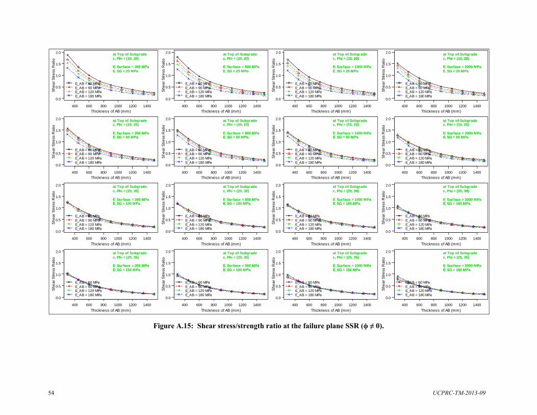
54 UCPRC-TM-2013-09
Figure A.15: Shear stress/strength ratio at the failure plane SSR (ϕ ≠ 0).
400 600 800 1000 1200 1400
0.0
0.5
1.0
1.5
2.0
Thickness of AB (mm)
Sh
ea
r S
tre
ss R
atio
E_AB = 60 MPaE_AB = 90 MPaE_AB = 120 MPaE_AB = 180 MPa
at Top of Subgradec, Phi = (10, 20)
E_Surface = 200 MPaE_SG = 20 MPa
400 600 800 1000 1200 1400
0.0
0.5
1.0
1.5
2.0
Thickness of AB (mm)
Sh
ea
r S
tre
ss R
atio
E_AB = 60 MPaE_AB = 90 MPaE_AB = 120 MPaE_AB = 180 MPa
at Top of Subgradec, Phi = (15, 25)
E_Surface = 200 MPaE_SG = 50 MPa
400 600 800 1000 1200 1400
0.0
0.5
1.0
1.5
2.0
Thickness of AB (mm)
Sh
ea
r S
tre
ss R
atio
E_AB = 60 MPaE_AB = 90 MPaE_AB = 120 MPaE_AB = 180 MPa
at Top of Subgradec, Phi = (20, 30)
E_Surface = 200 MPaE_SG = 100 MPa
400 600 800 1000 1200 1400
0.0
0.5
1.0
1.5
2.0
Thickness of AB (mm)
Sh
ea
r S
tre
ss R
atio
E_AB = 60 MPaE_AB = 90 MPaE_AB = 120 MPaE_AB = 180 MPa
at Top of Subgradec, Phi = (25, 35)
E_Surface = 200 MPaE_SG = 150 MPa
400 600 800 1000 1200 1400
0.0
0.5
1.0
1.5
2.0
Thickness of AB (mm)
Sh
ea
r S
tre
ss R
atio
E_AB = 60 MPaE_AB = 90 MPaE_AB = 120 MPaE_AB = 180 MPa
at Top of Subgradec, Phi = (10, 20)
E_Surface = 500 MPaE_SG = 20 MPa
400 600 800 1000 1200 1400
0.0
0.5
1.0
1.5
2.0
Thickness of AB (mm)
Sh
ea
r S
tre
ss R
atio
E_AB = 60 MPaE_AB = 90 MPaE_AB = 120 MPaE_AB = 180 MPa
at Top of Subgradec, Phi = (15, 25)
E_Surface = 500 MPaE_SG = 50 MPa
400 600 800 1000 1200 1400
0.0
0.5
1.0
1.5
2.0
Thickness of AB (mm)
Sh
ea
r S
tre
ss R
atio
E_AB = 60 MPaE_AB = 90 MPaE_AB = 120 MPaE_AB = 180 MPa
at Top of Subgradec, Phi = (20, 30)
E_Surface = 500 MPaE_SG = 100 MPa
400 600 800 1000 1200 1400
0.0
0.5
1.0
1.5
2.0
Thickness of AB (mm)
Sh
ea
r S
tre
ss R
atio
E_AB = 60 MPaE_AB = 90 MPaE_AB = 120 MPaE_AB = 180 MPa
at Top of Subgradec, Phi = (25, 35)
E_Surface = 500 MPaE_SG = 150 MPa
400 600 800 1000 1200 1400
0.0
0.5
1.0
1.5
2.0
Thickness of AB (mm)
Sh
ea
r S
tre
ss R
atio
E_AB = 60 MPaE_AB = 90 MPaE_AB = 120 MPaE_AB = 180 MPa
at Top of Subgradec, Phi = (10, 20)
E_Surface = 1000 MPaE_SG = 20 MPa
400 600 800 1000 1200 1400
0.0
0.5
1.0
1.5
2.0
Thickness of AB (mm)
Sh
ea
r S
tre
ss R
atio
E_AB = 60 MPaE_AB = 90 MPaE_AB = 120 MPaE_AB = 180 MPa
at Top of Subgradec, Phi = (15, 25)
E_Surface = 1000 MPaE_SG = 50 MPa
400 600 800 1000 1200 1400
0.0
0.5
1.0
1.5
2.0
Thickness of AB (mm)
Sh
ea
r S
tre
ss R
atio
E_AB = 60 MPaE_AB = 90 MPaE_AB = 120 MPaE_AB = 180 MPa
at Top of Subgradec, Phi = (20, 30)
E_Surface = 1000 MPaE_SG = 100 MPa
400 600 800 1000 1200 1400
0.0
0.5
1.0
1.5
2.0
Thickness of AB (mm)
Sh
ea
r S
tre
ss R
atio
E_AB = 60 MPaE_AB = 90 MPaE_AB = 120 MPaE_AB = 180 MPa
at Top of Subgradec, Phi = (25, 35)
E_Surface = 1000 MPaE_SG = 150 MPa
400 600 800 1000 1200 1400
0.0
0.5
1.0
1.5
2.0
Thickness of AB (mm)
Sh
ea
r S
tre
ss R
atio
E_AB = 60 MPaE_AB = 90 MPaE_AB = 120 MPaE_AB = 180 MPa
at Top of Subgradec, Phi = (10, 20)
E_Surface = 2000 MPaE_SG = 20 MPa
400 600 800 1000 1200 1400
0.0
0.5
1.0
1.5
2.0
Thickness of AB (mm)
Sh
ea
r S
tre
ss R
atio
E_AB = 60 MPaE_AB = 90 MPaE_AB = 120 MPaE_AB = 180 MPa
at Top of Subgradec, Phi = (15, 25)
E_Surface = 2000 MPaE_SG = 50 MPa
400 600 800 1000 1200 1400
0.0
0.5
1.0
1.5
2.0
Thickness of AB (mm)
Sh
ea
r S
tre
ss R
atio
E_AB = 60 MPaE_AB = 90 MPaE_AB = 120 MPaE_AB = 180 MPa
at Top of Subgradec, Phi = (20, 30)
E_Surface = 2000 MPaE_SG = 100 MPa
400 600 800 1000 1200 1400
0.0
0.5
1.0
1.5
2.0
Thickness of AB (mm)
Sh
ea
r S
tre
ss R
atio
E_AB = 60 MPaE_AB = 90 MPaE_AB = 120 MPaE_AB = 180 MPa
at Top of Subgradec, Phi = (25, 35)
E_Surface = 2000 MPaE_SG = 150 MPa

UCPRC-TM-2013-09 55
Figure A.16: Shear stress/strength ratio at the failure plane SSR (ϕ ≠ 0, log scale for SSR).
400 600 800 1000 1200 1400
0.1
0.2
0.5
1.0
2.0
Thickness of AB (mm)
Sh
ea
r S
tre
ss R
atio
(lo
g)
E_AB = 60 MPaE_AB = 90 MPaE_AB = 120 MPaE_AB = 180 MPa
at Top of Subgradec, Phi = (10, 20)
E_Surface = 200 MPaE_SG = 20 MPa
400 600 800 1000 1200 1400
0.1
0.2
0.5
1.0
2.0
Thickness of AB (mm)
Sh
ea
r S
tre
ss R
atio
(lo
g)
E_AB = 60 MPaE_AB = 90 MPaE_AB = 120 MPaE_AB = 180 MPa
at Top of Subgradec, Phi = (15, 25)
E_Surface = 200 MPaE_SG = 50 MPa
400 600 800 1000 1200 1400
0.1
0.2
0.5
1.0
2.0
Thickness of AB (mm)
Sh
ea
r S
tre
ss R
atio
(lo
g)
E_AB = 60 MPaE_AB = 90 MPaE_AB = 120 MPaE_AB = 180 MPa
at Top of Subgradec, Phi = (20, 30)
E_Surface = 200 MPaE_SG = 100 MPa
400 600 800 1000 1200 1400
0.1
0.2
0.5
1.0
2.0
Thickness of AB (mm)
Sh
ea
r S
tre
ss R
atio
(lo
g)
E_AB = 60 MPaE_AB = 90 MPaE_AB = 120 MPaE_AB = 180 MPa
at Top of Subgradec, Phi = (25, 35)
E_Surface = 200 MPaE_SG = 150 MPa
400 600 800 1000 1200 1400
0.1
0.2
0.5
1.0
2.0
Thickness of AB (mm)
Sh
ea
r S
tre
ss R
atio
(lo
g)
E_AB = 60 MPaE_AB = 90 MPaE_AB = 120 MPaE_AB = 180 MPa
at Top of Subgradec, Phi = (10, 20)
E_Surface = 500 MPaE_SG = 20 MPa
400 600 800 1000 1200 1400
0.1
0.2
0.5
1.0
2.0
Thickness of AB (mm)
Sh
ea
r S
tre
ss R
atio
(lo
g)
E_AB = 60 MPaE_AB = 90 MPaE_AB = 120 MPaE_AB = 180 MPa
at Top of Subgradec, Phi = (15, 25)
E_Surface = 500 MPaE_SG = 50 MPa
400 600 800 1000 1200 1400
0.1
0.2
0.5
1.0
2.0
Thickness of AB (mm)
Sh
ea
r S
tre
ss R
atio
(lo
g)
E_AB = 60 MPaE_AB = 90 MPaE_AB = 120 MPaE_AB = 180 MPa
at Top of Subgradec, Phi = (20, 30)
E_Surface = 500 MPaE_SG = 100 MPa
400 600 800 1000 1200 1400
0.1
0.2
0.5
1.0
2.0
Thickness of AB (mm)
Sh
ea
r S
tre
ss R
atio
(lo
g)
E_AB = 60 MPaE_AB = 90 MPaE_AB = 120 MPaE_AB = 180 MPa
at Top of Subgradec, Phi = (25, 35)
E_Surface = 500 MPaE_SG = 150 MPa
400 600 800 1000 1200 1400
0.1
0.2
0.5
1.0
2.0
Thickness of AB (mm)
Sh
ea
r S
tre
ss R
atio
(lo
g)
E_AB = 60 MPaE_AB = 90 MPaE_AB = 120 MPaE_AB = 180 MPa
at Top of Subgradec, Phi = (10, 20)
E_Surface = 1000 MPaE_SG = 20 MPa
400 600 800 1000 1200 1400
0.1
0.2
0.5
1.0
2.0
Thickness of AB (mm)
Sh
ea
r S
tre
ss R
atio
(lo
g)
E_AB = 60 MPaE_AB = 90 MPaE_AB = 120 MPaE_AB = 180 MPa
at Top of Subgradec, Phi = (15, 25)
E_Surface = 1000 MPaE_SG = 50 MPa
400 600 800 1000 1200 1400
0.1
0.2
0.5
1.0
2.0
Thickness of AB (mm)
Sh
ea
r S
tre
ss R
atio
(lo
g)
E_AB = 60 MPaE_AB = 90 MPaE_AB = 120 MPaE_AB = 180 MPa
at Top of Subgradec, Phi = (20, 30)
E_Surface = 1000 MPaE_SG = 100 MPa
400 600 800 1000 1200 1400
0.1
0.2
0.5
1.0
2.0
Thickness of AB (mm)
Sh
ea
r S
tre
ss R
atio
(lo
g)
E_AB = 60 MPaE_AB = 90 MPaE_AB = 120 MPaE_AB = 180 MPa
at Top of Subgradec, Phi = (25, 35)
E_Surface = 1000 MPaE_SG = 150 MPa
400 600 800 1000 1200 1400
0.1
0.2
0.5
1.0
2.0
Thickness of AB (mm)
Sh
ea
r S
tre
ss R
atio
(lo
g)
E_AB = 60 MPaE_AB = 90 MPaE_AB = 120 MPaE_AB = 180 MPa
at Top of Subgradec, Phi = (10, 20)
E_Surface = 2000 MPaE_SG = 20 MPa
400 600 800 1000 1200 1400
0.1
0.2
0.5
1.0
2.0
Thickness of AB (mm)
Sh
ea
r S
tre
ss R
atio
(lo
g)
E_AB = 60 MPaE_AB = 90 MPaE_AB = 120 MPaE_AB = 180 MPa
at Top of Subgradec, Phi = (15, 25)
E_Surface = 2000 MPaE_SG = 50 MPa
400 600 800 1000 1200 1400
0.1
0.2
0.5
1.0
2.0
Thickness of AB (mm)
Sh
ea
r S
tre
ss R
atio
(lo
g)
E_AB = 60 MPaE_AB = 90 MPaE_AB = 120 MPaE_AB = 180 MPa
at Top of Subgradec, Phi = (20, 30)
E_Surface = 2000 MPaE_SG = 100 MPa
400 600 800 1000 1200 1400
0.1
0.2
0.5
1.0
2.0
Thickness of AB (mm)
Sh
ea
r S
tre
ss R
atio
(lo
g)
E_AB = 60 MPaE_AB = 90 MPaE_AB = 120 MPaE_AB = 180 MPa
at Top of Subgradec, Phi = (25, 35)
E_Surface = 2000 MPaE_SG = 150 MPa
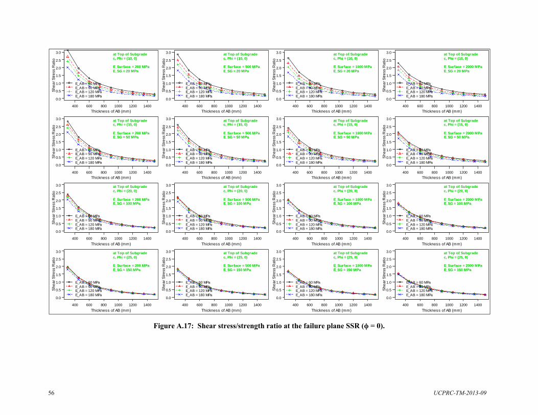
56 UCPRC-TM-2013-09
Figure A.17: Shear stress/strength ratio at the failure plane SSR (ϕ = 0).
400 600 800 1000 1200 1400
0.0
0.5
1.0
1.5
2.0
2.5
3.0
Thickness of AB (mm)
Sh
ea
r S
tre
ss R
atio
E_AB = 60 MPaE_AB = 90 MPaE_AB = 120 MPaE_AB = 180 MPa
at Top of Subgradec, Phi = (10, 0)
E_Surface = 200 MPaE_SG = 20 MPa
400 600 800 1000 1200 1400
0.0
0.5
1.0
1.5
2.0
2.5
3.0
Thickness of AB (mm)
Sh
ea
r S
tre
ss R
atio
E_AB = 60 MPaE_AB = 90 MPaE_AB = 120 MPaE_AB = 180 MPa
at Top of Subgradec, Phi = (15, 0)
E_Surface = 200 MPaE_SG = 50 MPa
400 600 800 1000 1200 1400
0.0
0.5
1.0
1.5
2.0
2.5
3.0
Thickness of AB (mm)
Sh
ea
r S
tre
ss R
atio
E_AB = 60 MPaE_AB = 90 MPaE_AB = 120 MPaE_AB = 180 MPa
at Top of Subgradec, Phi = (20, 0)
E_Surface = 200 MPaE_SG = 100 MPa
400 600 800 1000 1200 1400
0.0
0.5
1.0
1.5
2.0
2.5
3.0
Thickness of AB (mm)
Sh
ea
r S
tre
ss R
atio
E_AB = 60 MPaE_AB = 90 MPaE_AB = 120 MPaE_AB = 180 MPa
at Top of Subgradec, Phi = (25, 0)
E_Surface = 200 MPaE_SG = 150 MPa
400 600 800 1000 1200 1400
0.0
0.5
1.0
1.5
2.0
2.5
3.0
Thickness of AB (mm)
Sh
ea
r S
tre
ss R
atio
E_AB = 60 MPaE_AB = 90 MPaE_AB = 120 MPaE_AB = 180 MPa
at Top of Subgradec, Phi = (10, 0)
E_Surface = 500 MPaE_SG = 20 MPa
400 600 800 1000 1200 1400
0.0
0.5
1.0
1.5
2.0
2.5
3.0
Thickness of AB (mm)
Sh
ea
r S
tre
ss R
atio
E_AB = 60 MPaE_AB = 90 MPaE_AB = 120 MPaE_AB = 180 MPa
at Top of Subgradec, Phi = (15, 0)
E_Surface = 500 MPaE_SG = 50 MPa
400 600 800 1000 1200 1400
0.0
0.5
1.0
1.5
2.0
2.5
3.0
Thickness of AB (mm)
Sh
ea
r S
tre
ss R
atio
E_AB = 60 MPaE_AB = 90 MPaE_AB = 120 MPaE_AB = 180 MPa
at Top of Subgradec, Phi = (20, 0)
E_Surface = 500 MPaE_SG = 100 MPa
400 600 800 1000 1200 1400
0.0
0.5
1.0
1.5
2.0
2.5
3.0
Thickness of AB (mm)
Sh
ea
r S
tre
ss R
atio
E_AB = 60 MPaE_AB = 90 MPaE_AB = 120 MPaE_AB = 180 MPa
at Top of Subgradec, Phi = (25, 0)
E_Surface = 500 MPaE_SG = 150 MPa
400 600 800 1000 1200 1400
0.0
0.5
1.0
1.5
2.0
2.5
3.0
Thickness of AB (mm)
Sh
ea
r S
tre
ss R
atio
E_AB = 60 MPaE_AB = 90 MPaE_AB = 120 MPaE_AB = 180 MPa
at Top of Subgradec, Phi = (10, 0)
E_Surface = 1000 MPaE_SG = 20 MPa
400 600 800 1000 1200 1400
0.0
0.5
1.0
1.5
2.0
2.5
3.0
Thickness of AB (mm)
Sh
ea
r S
tre
ss R
atio
E_AB = 60 MPaE_AB = 90 MPaE_AB = 120 MPaE_AB = 180 MPa
at Top of Subgradec, Phi = (15, 0)
E_Surface = 1000 MPaE_SG = 50 MPa
400 600 800 1000 1200 1400
0.0
0.5
1.0
1.5
2.0
2.5
3.0
Thickness of AB (mm)
Sh
ea
r S
tre
ss R
atio
E_AB = 60 MPaE_AB = 90 MPaE_AB = 120 MPaE_AB = 180 MPa
at Top of Subgradec, Phi = (20, 0)
E_Surface = 1000 MPaE_SG = 100 MPa
400 600 800 1000 1200 1400
0.0
0.5
1.0
1.5
2.0
2.5
3.0
Thickness of AB (mm)
Sh
ea
r S
tre
ss R
atio
E_AB = 60 MPaE_AB = 90 MPaE_AB = 120 MPaE_AB = 180 MPa
at Top of Subgradec, Phi = (25, 0)
E_Surface = 1000 MPaE_SG = 150 MPa
400 600 800 1000 1200 1400
0.0
0.5
1.0
1.5
2.0
2.5
3.0
Thickness of AB (mm)
Sh
ea
r S
tre
ss R
atio
E_AB = 60 MPaE_AB = 90 MPaE_AB = 120 MPaE_AB = 180 MPa
at Top of Subgradec, Phi = (10, 0)
E_Surface = 2000 MPaE_SG = 20 MPa
400 600 800 1000 1200 1400
0.0
0.5
1.0
1.5
2.0
2.5
3.0
Thickness of AB (mm)
Sh
ea
r S
tre
ss R
atio
E_AB = 60 MPaE_AB = 90 MPaE_AB = 120 MPaE_AB = 180 MPa
at Top of Subgradec, Phi = (15, 0)
E_Surface = 2000 MPaE_SG = 50 MPa
400 600 800 1000 1200 1400
0.0
0.5
1.0
1.5
2.0
2.5
3.0
Thickness of AB (mm)
Sh
ea
r S
tre
ss R
atio
E_AB = 60 MPaE_AB = 90 MPaE_AB = 120 MPaE_AB = 180 MPa
at Top of Subgradec, Phi = (20, 0)
E_Surface = 2000 MPaE_SG = 100 MPa
400 600 800 1000 1200 1400
0.0
0.5
1.0
1.5
2.0
2.5
3.0
Thickness of AB (mm)
Sh
ea
r S
tre
ss R
atio
E_AB = 60 MPaE_AB = 90 MPaE_AB = 120 MPaE_AB = 180 MPa
at Top of Subgradec, Phi = (25, 0)
E_Surface = 2000 MPaE_SG = 150 MPa
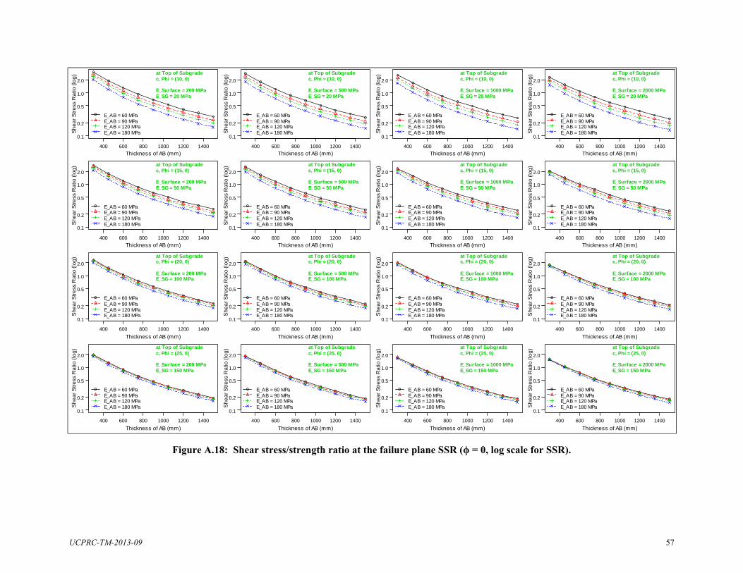
UCPRC-TM-2013-09 57
Figure A.18: Shear stress/strength ratio at the failure plane SSR (ϕ = 0, log scale for SSR).
400 600 800 1000 1200 1400
0.1
0.2
0.5
1.0
2.0
Thickness of AB (mm)
Sh
ea
r S
tre
ss R
atio
(lo
g)
E_AB = 60 MPaE_AB = 90 MPaE_AB = 120 MPaE_AB = 180 MPa
at Top of Subgradec, Phi = (10, 0)
E_Surface = 200 MPaE_SG = 20 MPa
400 600 800 1000 1200 1400
0.1
0.2
0.5
1.0
2.0
Thickness of AB (mm)
Sh
ea
r S
tre
ss R
atio
(lo
g)
E_AB = 60 MPaE_AB = 90 MPaE_AB = 120 MPaE_AB = 180 MPa
at Top of Subgradec, Phi = (15, 0)
E_Surface = 200 MPaE_SG = 50 MPa
400 600 800 1000 1200 1400
0.1
0.2
0.5
1.0
2.0
Thickness of AB (mm)
Sh
ea
r S
tre
ss R
atio
(lo
g)
E_AB = 60 MPaE_AB = 90 MPaE_AB = 120 MPaE_AB = 180 MPa
at Top of Subgradec, Phi = (20, 0)
E_Surface = 200 MPaE_SG = 100 MPa
400 600 800 1000 1200 1400
0.1
0.2
0.5
1.0
2.0
Thickness of AB (mm)
Sh
ea
r S
tre
ss R
atio
(lo
g)
E_AB = 60 MPaE_AB = 90 MPaE_AB = 120 MPaE_AB = 180 MPa
at Top of Subgradec, Phi = (25, 0)
E_Surface = 200 MPaE_SG = 150 MPa
400 600 800 1000 1200 1400
0.1
0.2
0.5
1.0
2.0
Thickness of AB (mm)
Sh
ea
r S
tre
ss R
atio
(lo
g)
E_AB = 60 MPaE_AB = 90 MPaE_AB = 120 MPaE_AB = 180 MPa
at Top of Subgradec, Phi = (10, 0)
E_Surface = 500 MPaE_SG = 20 MPa
400 600 800 1000 1200 1400
0.1
0.2
0.5
1.0
2.0
Thickness of AB (mm)
Sh
ea
r S
tre
ss R
atio
(lo
g)
E_AB = 60 MPaE_AB = 90 MPaE_AB = 120 MPaE_AB = 180 MPa
at Top of Subgradec, Phi = (15, 0)
E_Surface = 500 MPaE_SG = 50 MPa
400 600 800 1000 1200 1400
0.1
0.2
0.5
1.0
2.0
Thickness of AB (mm)
Sh
ea
r S
tre
ss R
atio
(lo
g)
E_AB = 60 MPaE_AB = 90 MPaE_AB = 120 MPaE_AB = 180 MPa
at Top of Subgradec, Phi = (20, 0)
E_Surface = 500 MPaE_SG = 100 MPa
400 600 800 1000 1200 1400
0.1
0.2
0.5
1.0
2.0
Thickness of AB (mm)
Sh
ea
r S
tre
ss R
atio
(lo
g)
E_AB = 60 MPaE_AB = 90 MPaE_AB = 120 MPaE_AB = 180 MPa
at Top of Subgradec, Phi = (25, 0)
E_Surface = 500 MPaE_SG = 150 MPa
400 600 800 1000 1200 1400
0.1
0.2
0.5
1.0
2.0
Thickness of AB (mm)
Sh
ea
r S
tre
ss R
atio
(lo
g)
E_AB = 60 MPaE_AB = 90 MPaE_AB = 120 MPaE_AB = 180 MPa
at Top of Subgradec, Phi = (10, 0)
E_Surface = 1000 MPaE_SG = 20 MPa
400 600 800 1000 1200 1400
0.1
0.2
0.5
1.0
2.0
Thickness of AB (mm)
Sh
ea
r S
tre
ss R
atio
(lo
g)
E_AB = 60 MPaE_AB = 90 MPaE_AB = 120 MPaE_AB = 180 MPa
at Top of Subgradec, Phi = (15, 0)
E_Surface = 1000 MPaE_SG = 50 MPa
400 600 800 1000 1200 1400
0.1
0.2
0.5
1.0
2.0
Thickness of AB (mm)
Sh
ea
r S
tre
ss R
atio
(lo
g)
E_AB = 60 MPaE_AB = 90 MPaE_AB = 120 MPaE_AB = 180 MPa
at Top of Subgradec, Phi = (20, 0)
E_Surface = 1000 MPaE_SG = 100 MPa
400 600 800 1000 1200 1400
0.1
0.2
0.5
1.0
2.0
Thickness of AB (mm)
Sh
ea
r S
tre
ss R
atio
(lo
g)
E_AB = 60 MPaE_AB = 90 MPaE_AB = 120 MPaE_AB = 180 MPa
at Top of Subgradec, Phi = (25, 0)
E_Surface = 1000 MPaE_SG = 150 MPa
400 600 800 1000 1200 1400
0.1
0.2
0.5
1.0
2.0
Thickness of AB (mm)
Sh
ea
r S
tre
ss R
atio
(lo
g)
E_AB = 60 MPaE_AB = 90 MPaE_AB = 120 MPaE_AB = 180 MPa
at Top of Subgradec, Phi = (10, 0)
E_Surface = 2000 MPaE_SG = 20 MPa
400 600 800 1000 1200 1400
0.1
0.2
0.5
1.0
2.0
Thickness of AB (mm)
Sh
ea
r S
tre
ss R
atio
(lo
g)
E_AB = 60 MPaE_AB = 90 MPaE_AB = 120 MPaE_AB = 180 MPa
at Top of Subgradec, Phi = (15, 0)
E_Surface = 2000 MPaE_SG = 50 MPa
400 600 800 1000 1200 1400
0.1
0.2
0.5
1.0
2.0
Thickness of AB (mm)
Sh
ea
r S
tre
ss R
atio
(lo
g)
E_AB = 60 MPaE_AB = 90 MPaE_AB = 120 MPaE_AB = 180 MPa
at Top of Subgradec, Phi = (20, 0)
E_Surface = 2000 MPaE_SG = 100 MPa
400 600 800 1000 1200 1400
0.1
0.2
0.5
1.0
2.0
Thickness of AB (mm)
Sh
ea
r S
tre
ss R
atio
(lo
g)
E_AB = 60 MPaE_AB = 90 MPaE_AB = 120 MPaE_AB = 180 MPa
at Top of Subgradec, Phi = (25, 0)
E_Surface = 2000 MPaE_SG = 150 MPa

58 UCPRC-TM-2013-09