Developing students’ statistical reasoning: connecting research and teaching practice.
579
Published by Springer, 2008 Developing Students’ Statistical Reasoning: Connecting Research and Teaching Practice Joan Garfield, University of Minnesota, USA Dani Ben-Zvi, University of Haifa, Israel With Contributions from Beth Chance and Elsa Medina California Polytechnic State University, San Luis Obispo, California Cary Roseth Michigan State University Andrew Zieffler University of Minnesota
Transcript of Developing students’ statistical reasoning: connecting research and teaching practice.

Published by Springer, 2008
Developing Students’ Statistical Reasoning:
Connecting Research and Teaching Practice
Joan Garfield, University of Minnesota, USA
Dani Ben-Zvi, University of Haifa, Israel
With Contributions from
Beth Chance and Elsa Medina
California Polytechnic State University, San Luis Obispo, California
Cary Roseth
Michigan State University
Andrew Zieffler
University of Minnesota

i
Contents
Foreword Roxy Peck vii
Preface Joan Garfield and Dani Ben-Zvi ix
Part I. The Foundations of Statistics Education 1
Chapter 1 The Discipline of Statistics Education 2
Chapter 2 The Research on Teaching and Learning Statistics 25
Chapter 3 Creating a Statistical Reasoning Learning Environment 56
Chapter 4 Assessment in Statistics Education 82
Chapter 5 Using Technology to Improve Student Learning of Statistics 115
Part II. From Research to Practice:
Developing the Big Ideas of Statistics 148
Introduction
to Part II
Connecting Research to Teaching Practice 149
Chapter 6 Learning to Reason about Data 157
Chapter 7 Learning to Reason about Statistical Models and Modeling 187
Chapter 8 Learning to Reason about Distribution 216
Chapter 9 Learning to Reason about Center 247
Chapter 10 Learning to Reason about Variability 266
Chapter 11 Learning to Reason about Comparing Groups 286
Chapter 12 Learning to Reason about Samples and Sampling Distributions 314
Chapter 13 Learning to Reason about Statistical Inference 351
Chapter 14 Learning to Reason about Covariation 390
Part III. Implementing Change through Collaboration 419
Introduction
to Part III
The Role of Collaboration in Improving Statistics Education:
In Learning, in Teaching, and in Research 420
Chapter 15 Collaboration in the Statistics Classroom 422
Chapter 16 Collaboration in Teaching and Research 438
References 462
Resources 524
Tables of Activities 549
Author Index 556
Subject Index 558

ii
Foreword
Roxy Peck

iii
Preface
Joan Garfield and Dani Ben-Zvi
Statistics education has emerged as an important discipline that supports the teaching and
learning of statistics. The research base for this new field has been increasing in size and
scope but has not always been connected to teaching practice nor accessible to the many
educators teaching statistics at different educational levels. Our goal in writing this book
was to provide a useful resource for members of the statistics education community that
facilitates the connections between research and teaching. Although the book is aimed
primarily at teachers of an introductory statistics course at the high school or college
level, we encourage others interested in statistics education to consider how the research
summaries, ideas, activities and implications may be useful in their line of work as well.
This book builds on our commitment over the past decade to exploring ways to
understand and develop students’ statistical literacy, reasoning and thinking. Despite
living and teaching in two different countries, we have worked together to understand and
promote the scholarship in this area. After co-chairing five international research forums
(SRTL), co-editing a book (The Challenge of Developing Literacy, Reasoning, and
Thinking, Ben-Zvi & Garfield, 2004.), and serving as guest editors for two special issues
of SERJ (Statistics Education Research Journal), it seemed the right time to finally write
a book together that is built on our knowledge, experience, and passion for statistics
education. It has been a great experience working on this book, which required ongoing
reading, writing, discussing, and learning. It took three years to write and revise this
book, which required visits to each other’s homes, phone calls, and innumerable email
exchanges. We now offer our book to the statistics education community and hope that
readers will find it a useful and valuable resource.
The book is divided into three parts. Part I consists of five chapters on important
foundational topics: the emergence of statistics education as a discipline, the research
literature on teaching and learning statistics, practical strategies for teaching students in a
Preface
iv
way that promotes the development of their statistical reasoning, assessment of student
outcomes, and the role of technological tools in developing statistical reasoning.
Part II of the book includes nine chapters, each devoted to one important statistical idea:
data, statistical models, distribution, center, variability, comparing groups, sampling and
sampling distributions, statistical inference, and covariation. These chapters present a
review and synthesis of the research literature related to the statistical topic, and then
suggest implications for developing this idea through carefully structured sequences of
activities.
Part III of the book focuses on what we see as the crucial method of bringing about
instructional change and implementing ideas and methods in this book: through
collaboration. One chapter focuses on collaborative student learning, and the other
chapter discusses collaborative teaching and classroom-based collaborative research.
Although we have presented the chapters in Part II in the order in which we think they
may be introduced to students, we point out that readers may want to read these chapters
in an alternative order. For example, one of our reviewers suggested reading chapters 6,
9, and 10 before the rest of the chapters in Part II. Another suggestion was to read
chapters 1 and 2 and then skip to Part II, then return to chapters 3, 4, 5, 15 and 16.
The suggested activities in Part II have in many cases been adapted from activities
developed by others in the statistics education community, and we present a table of all
activities described in Part II that credits a source, where possible. However, we note that
sometimes it was impossible to track down the person who developed an activity used in
the book, because no one was willing to take credit for it. If we have failed to credit a
creator of an activity used in our book, we apologize for this oversight. We also note that
the activities and lessons are based on particular technological tools we like, such as
TinkerPlots and Fathom, and certain Web applets. However, we acknowledge that
instructors may choose to use alternative technological tools that they have access too or
prefer.

Preface
v
This project would have been impossible without the help pf several dedicated and hard
working individuals. First and most importantly, we would like to thank four individuals
who made important contributions to writing specific chapters. Beth Chance took the lead
in developing the chapters on assessment and technology (assisted by Elsa Medina) and
provided insightful feedback on the research chapter. Cary Roseth wrote the majority of
the chapter on collaborative learning and provided feedback on the chapter on
collaborative teaching and research as well. Andy Zieffler provided valuable assistance in
writing the chapter on covariational reasoning and also gave helpful advice on additional
chapters of the book.
The lessons and activities described in this book were developed and modified over the
past four years as part of a collaborative effort of the undergraduate statistics teaching
team in the Department of Educational Psychology at the University of Minnesota. This
team has included Beng Chang, Jared Dixon, Danielle Dupuis, Sharon Lane-Getaz, and
Andy Zieffler. We greatly appreciate the contributions of these dedicated graduate
students and instructors in developing and revising the lessons, and particularly the
leadership of Andy Zieffler in coordinating this group and providing feedback on needed
changes. We also appreciate Andy’s work in constructing the Website that posts the
lesson plans and activities described in Part II, and the funding for this (as part of the
AIMS project) by the National Science Foundation (Grant number 0535912).
We gratefully acknowledge the tremendously valuable feedback offered by six reviewers
of our earlier manuscript: Gail Burrill, Michelle Everson, Randall Groth, Larry Lesser,
Roxy Peck, and Mike Shaughnessy. We hope they will see how we have utilized and
incorporated their suggestions. We also appreciate feedback and encouragement offered
by the original reviewers of first chapters and prospectus. We also gratefully
acknowledge the important contributions of advisers to the NSF AIMS project who
offered feedback on lessons and activities as well as on the Website. They are Beth
Chance, Bill Finzer, Cliff Konold, Dennis Pearl, Allan Rossman, and Richard Schaeffer.
Bob delMas, co-PI of the AIMS grant has also offered helpful advice. In addition, Rob
Gould, the external evaluator for the AIMS project offered valuable insights and advice.

Preface
vi
We are grateful to Springer Publishers for providing a publishing venue for this book, and
to Harmen van Paradijs the editor, who skillfully managed the publication on their behalf.
We owe deep thanks to Shira Yuval and Idit Halwany, graduate students from the
University of Haifa who assisted in editing and checking details in the manuscript.
Lastly, many thanks go to our spouses Michael Luxenberg and Hava Ben-Zvi and to our
children— Harlan and Rebecca Luxenberg, and Noa, Nir, Dagan, and Michal Ben-Zvi.
They have been our primary sources of energy and support.
Joan Garfield1 and Dani Ben-Zvi
2
University of Minnesota, USA1 and University of Haifa, Israel
2

1
PART I
Foundations of Statistics Education

2
Chapter 1: The Discipline of Statistics Education
The case for substantial change in statistics instruction is built
on strong synergies between content, pedagogy, and technology.
Moore (1997, p. 123).
Overview
This chapter introduces the emerging discipline of statistics education and considers its
role in the development of students who are statistically literate and who can think and
reason about statistical information. We begin with information on the growing
importance of statistics in today’s society, schools and colleges, summarize unique
challenges students face as they learn statistics, and make a case for the importance of
collaboration between mathematicians and statisticians in preparing teachers to teach
students how to understand and reason about data. We examine the differences and
interrelations between statistics and mathematics, recognizing that mathematics is the
discipline that has traditionally included instruction in statistics, describe the history of
the introductory college course, introduce current instructional guidelines, and provide an
overview of the organization and content of this book.
The Growing Importance of Statistics
No one will debate the fact that quantitative information is everywhere and numerical
data are increasingly presented with the intention of adding credibility to advertisements,
arguments, or advice. Most would also agree that being able to provide good evidence-
based arguments and to be able to critically evaluate data-based claims are important
skills that all citizens should have, and therefore, that all students should learn as part of
their education (see Watson, 2006). It is not surprising therefore that statistics instruction
at all educational levels is gaining more students and drawing more attention.
The study of statistics provides students with tools and ideas to use in order to react
intelligently to quantitative information in the world around them. Reflecting this need to
improve students’ ability to think statistically, statistics and statistical reasoning are

Chapter 1: The Discipline of Statistics Education
3
becoming part of the mainstream school curriculum in many countries (e.g., Mathematics
Curriculum Framework for Western Australia, http://www.curriculum.wa.edu.au/;
Mathematics National Curriculum for England, http://www.nc.uk.net/; National Council
of Teachers of Mathematics in the U.S., 2000). At the U.S. college level enrollments in
statistics courses continue to grow (Scheaffer & Stasney, 2004). Statistics is becoming
such a necessary and important area of study, Moore (1998) suggested that it should be
viewed as one of the liberal arts, and that it involves distinctive and powerful ways of
thinking. He wrote: “Statistics is a general intellectual method that applies wherever data,
variation, and chance appear. It is a fundamental method because data, variation, and
chance are omnipresent in modern life” (p. 134).
The Challenge of Learning and Teaching Statistics
Despite the increase in statistics instruction at all educational levels, historically the
discipline and methods of statistics have been viewed by many students as a difficult
topic that is unpleasant to learn. Statisticians often joke about the negative comments they
hear when others learn of their profession. It is not uncommon for people to recount tales
of statistics as the worst course they took in college. Many research studies over the past
several decades indicate that most students and adults do not think statistically about
important issues that affect their lives. Researchers in psychology and education have
documented the many consistent errors that students and adults make when trying to
reason about data and chance in real world problems and contexts. In their attempts to
make the subject meaningful and motivating for students, many teachers have included
more authentic activities and the use of new technological tools in their instruction.
However, despite the attempts of many devoted teachers who love their discipline and
want to make the statistics course an enjoyable learning experience for students, the
image of statistics as a hard and dreaded subject is hard to dislodge. Currently,
researchers and statistics educators are trying to understand the challenges and overcome
the difficulties in learning and teaching this subject so that improved instructional
methods and materials, enhanced technology, and alternative assessment methods may be
used with students learning statistics at the school and college level.
Chapter 1: The Discipline of Statistics Education
4
In our previous book (Ben-Zvi & Garfield, 2004) we list some of the reasons that have
been identified to explain why statistics is a challenging subject to learn and teach.
Firstly, many statistical ideas and rules are complex, difficult, and/or counterintuitive. It
is therefore difficult to motivate students to engage in the hard work of learning statistics.
Secondly, many students have difficulty with the underlying mathematics (such as
fractions, decimals, proportional reasoning, and algebraic formulas) and that interferes
with learning the related statistical concepts. A third reason is that the context in many
statistical problems may mislead the students, causing them to rely on their experiences
and often faulty intuitions to produce an answer, rather than select an appropriate
statistical procedure and rely on data-based evidence. Finally, students equate statistics
with mathematics and expect the focus to be on numbers, computations, formulas, and
only one right answer. They are uncomfortable with the messiness of data, the ideas of
randomness and chance, the different possible interpretations based on different
assumptions, and the extensive use of writing, collaboration and communication skills.
This is also true of many mathematics teachers who find themselves teaching statistics.
The Goals of This Book
Despite the growing body of research related to teaching and learning statistics, there
have been few direct connections made between the research results and practical
suggestions for teachers. Teachers of statistics may be looking for suggestions from the
research literature but find it hard to locate them since studies are published in journals
from other disciplines that are not readily accessible. In addition, many research studies
have been conducted in settings that do not seem to easily transfer to the high school or
college classroom (e.g., studies in a psychology lab, or studies in a teaching experiment at
an elementary school), or have been carried out using methods with which most
statisticians are not familiar (e.g., studies involving collection and analysis of extensive
qualitative data). Statisticians, in contrast, are more familiar with randomized controlled
experiments and often look for studies using these methods, set in high school or college
classrooms, to provide results to inform their teaching.

Chapter 1: The Discipline of Statistics Education
5
We find it fascinating that statistics education has been the focus for researchers in many
disciplines, perhaps because statistical reasoning is used in many disciplines and provides
so many interesting issues and challenges. Today, researchers in mathematics education
study children’s understanding of statistical concepts as well as how they learn to use
data analysis meaningfully. They also study how K–12 teachers understand statistical
ideas and methods and how this affects the way they teach children. Researchers in
psychology explore judgments and decisions made in light of uncertainty, and the use of
intuitions and heuristics in dealing with uncertainty. Researchers in educational
measurement study the assessment of statistical anxiety and attitudes towards statistics, as
well as factors that predict student achievement in statistics courses such as mathematics
background and motivation. Only recently has there been a core set of researchers
looking at understanding of and reasoning about particular statistical concepts, how they
might be developed through carefully planned sequences of activities, and how this might
take place in the classrooms.
Our main goal in writing this book was to build on relevant research that informs the
teaching and learning of statistics to enhance two aspects of teachers’ knowledge: their
knowledge of what it means for students to understand and reason about statistical
concepts, and the pedagogical methods for developing understanding and reasoning about
these concepts. We try to summarize the research and highlight the important statistical
concepts for teachers to emphasize, as well as reveal the interrelationships among
concepts. We also make specific suggestions regarding how to plan and use classroom
activities, integrate technological tools, and assess students’ learning in meaningful ways.
The goals listed above are aimed to help instructors of statistics deal with the challenges
they face, to suggest ways that may help to make statistics instruction more effective, and
to engage students in reasoning and thinking statistically. By compiling and building on
the various research studies that shed light on the difficulties students have learning
statistics, we are able to offer suggestions for how students may be guided to construct
meaning for complex statistical ideas, concepts and procedures. The research literature is
often difficult for statistics teachers to find and access, synthesize, and apply to their
teaching practice. Therefore, we try in this book to provide links between the research

Chapter 1: The Discipline of Statistics Education
6
literature and teaching practice. We include examples, activities, and references to useful
resources. We also incorporate many uses of instructional software and Web tools and
resources. Finally, we offer an accompanying Website with materials to supplement each
chapter (see http://www.tc.umn.edu/~aims).
We begin this first chapter with a brief introduction and historical perspective of the
emerging field of statistics education and the development of the introductory college
course, we present arguments for how statistics differs from mathematics, focus on the
importance of statistical reasoning, and provide an overview of the subsequent chapters in
this book.
The Development of the Field of Statistics Education
Statistics education is an emerging field that grew out of different disciplines and is
currently establishing itself as a unique field of study. The two main disciplines from
which statistics education grew are statistics and mathematics education. As early as 1944
the American Statistical Association (ASA) developed the Section on Training of
Statisticians (Mason, McKenzie, & Ruberg, 1990) that later (1973) became the Section
on Statistical Education. The International Statistical Institute (ISI) similarly formed an
education committee in 1948. The early focus in the statistics world was on training
statisticians, but this later broadened to include training, or education, at all levels. In the
1960s an interest emerged in the mathematics education field about teaching students at
the pre-college level how to use and analyze data. In 1967 a joint committee was formed
between the American Statistical Association (ASA) and the National Council of
Teachers of Mathematics (NCTM) on Curriculum in Statistics and Probability for grades
K–12. In the early 1970s many instructional materials began to be developed in the USA
and in other countries to present statistical ideas in interesting and engaging ways, e.g.,
the series of books Statistics by Example, by Mosteller, Rourke and Thomas (1973) and
Mosteller, Kruskal, Pieters, and Rising (1973a–d), and Statistics: A Guide to the
Unknown by Tanur, Mosteller, Kruskal, Link, Pieters, Rising and Lehmann (1972), which
was recently updated (Peck, Casella, Cobb, Hoerl, Nolan, Starbuck, & Stern, 2006).

Chapter 1: The Discipline of Statistics Education
7
In the late 1970s the ISI created a task force on teaching statistics at school level (Gani,
1979), which published a report, Teaching Statistics in Schools throughout the World
(Barnett, 1982). This report surveyed how and where statistics was being taught, with the
aim of suggesting how to improve and expand the teaching of this important subject.
Although there seemed to be an interest in many countries in including statistics in the K–
12 curriculum, this report illustrated a lack of coordinated efforts, appropriate
instructional materials, and adequate teacher training.
By the 1980s the message was strong and clear: Statistics needed to be incorporated in
pre-college education and needed to be improved at the postsecondary level. Conferences
on teaching statistics began to be offered, and a growing group of educators began to
focus their efforts and scholarship on improving statistics education. The first
International Conference on Teaching Statistics (ICOTS) was convened in 1982 and this
conference has been held in a different part of the world every four years since that date
(e.g., ICOTS-7, 2006, see http://www.maths.otago.ac.nz/icots7/icots7.php; ICOTS-8,
2010, see http://icots8.org/).
In the 1990s there was an increasingly strong call for statistics education to focus more on
statistical literacy, reasoning, and thinking. One of the main arguments presented is that
traditional approaches to teaching statistics focus on skills, procedures, and computations,
which do not lead students to reason or think statistically. In their landmark paper
published in the International Statistical Review, which included numerous commentaries
by leading statisticians and statistics educators, Wild and Pfannkuch (1999) provided an
empirically-based comprehensive description of the processes involved in the
statisticians’ practice of data-based enquiry from problem formulation to conclusions.
Building on the interest in this topic, The International Research Forums on Statistical
Reasoning, Thinking, and Literacy (SRTL) began in 1999 to foster current and innovative
research studies that examine the nature and development of statistical literacy,
reasoning, and thinking, and to explore the challenge posed to educators at all levels—
and to develop these desired learning goals for students. The SRTL Forums offer
scientific gatherings every two years and related publications (for more information see
http://srtl.stat.auckland.ac.nz). Additional explanations and reference to publications

Chapter 1: The Discipline of Statistics Education
8
explicating the nature and development of statistical literacy, reasoning and thinking are
summarized in Chapters 2 and 3 and other relevant chapters in this book.
One of the important indicators of a new discipline is scientific publications devoted to
that topic. At the current time, there are three journals. Teaching Statistics, which was
first published in 1979, and the Journal of Statistics Education, first published in 1993,
were developed to focus on the teaching of statistics as well as statistics education
research. While recently the Statistical Education Research Journal (first published in
2002) was established to exclusively publish research in statistics education. More
information on books, conferences, and publications in statistics education is provided at
the resources section in the end of this book.
Collaborations among Statisticians and Mathematics Educators
Some of the major advances in the field of statistics education have resulted from
collaborations between statisticians and mathematics educators. For example, the
Quantitative Literacy Project (QLP) was a decade-long joint project of the American
Statistical Association (ASA) and the National Council of Teachers of Mathematics
(NCTM) headed by Richard Scheaffer that developed exemplary materials for secondary
students to learn data analysis and probability (Scheaffer, 1990). The QLP first produced
materials in 1986 (Landwehr & Watkins, 1986). Although these materials were designed
for students in middle and high school, the activities were equally appropriate for college
statistics classes, and many instructors began to incorporate these activities into their
classes. Because most college textbooks did not have activities featuring real data sets
with guidelines for helping students explore and write about their understanding, as the
QLP materials provided, additional resources continued to be developed. Indeed, the QLP
affected the nature of activities in many college classes in the late 1980s and 1990s and
led to the Activity Based Statistics project, also headed by Richard Scheaffer, designed to
promote the use of high quality, well structured activities in class to promote student
learning (Scheaffer, Gnanadesikan, Watkins & Witmer, 2004; Scheaffer, Watkins,
Witmer & Gnanadesikan, 2004).

Chapter 1: The Discipline of Statistics Education
9
Members of the statistics and mathematics education disciplines have also worked
together on developing the Advanced Placement (AP) statistics course. This college level
introductory statistics course was first taught to high school students in the U.S. in 1996-
97 and the first exam was given in 1997, as part of the College Board Advanced
Placement Program. Currently hundreds of high school mathematics teachers and college
statistics teachers meet each summer to grade together the open-ended items on the AP
Statistics exam, and have opportunities to discuss teaching and share ideas and resources.
More recent efforts to connect mathematics educators and statisticians to improve the
statistical preparation of mathematics teachers include the ASA TEAMS project (see
Franklin, 2006). A current joint study of the International Association for Statistical
Education (IASE) and the International Congress on Mathematics Instruction (ICMI) is
also focused on this topic (see http://www.ugr.es/~icmi/iase_study/).
Statistics and Mathematics
Although statistics education grew out of statistics and mathematics education,
statisticians have worked hard to convince others that statistics is actually a separate
discipline from mathematics. Rossman, Chance and Medina (2006) describe statistics as a
mathematical science that uses mathematics but is a separate discipline, “the science of
gaining insight from data.” Although data may seem like numbers, Moore (1992) argues
that data are “numbers with a context”. And unlike mathematics, where the context
obscures the underlying structure, in statistics, context provides meaning for the numbers
and data cannot be meaningfully analyzed without paying careful consideration to their
context: how they were collected and what they represent (Cobb & Moore, 1997).
Rossman et al. (2006) point out many other key differences between mathematics and
statistics, concluding that the two disciplines involve different types of reasoning and
intellectual skills. It is reported that students often react differently to learning
mathematics than learning statistics, and that the preparation of teachers of statistics
requires different experiences than those that prepare a person to teach mathematics, such
as analyzing real data, dealing with the messiness and variability of data, understanding

Chapter 1: The Discipline of Statistics Education
10
the role of checking conditions to determine if assumptions are reasonable when solving a
statistical problem, and becoming familiar with statistical software.
How different is statistical thinking from mathematical thinking? The following example
illustrates the difference. A statistical problem in the area of bivariate data might ask
students to determine the equation for a regression line, specifying the slope and intercept
for the line of best fit. This looks similar to an algebra problem: numbers and formulas
are used to generate the equation of a line. In many statistics classes taught by
mathematicians, the problem might end at this stage. However, if statistical reasoning and
thinking are to be developed, students would be asked questions about the context of the
data and they would be asked to describe and interpret the relationship between the
variables, determining whether simple linear regression is an appropriate procedure and
model for these data. This type of reasoning and thinking is quite different from the
mathematical reasoning and thinking required to calculate the slope and intercept using
algebraic formulas. In fact, in many classes, students may not be asked to calculate the
quantities from formulas, but rather rely on technology to produce the numbers. The
focus shifts to asking students to interpret the values in context (e.g., from interpreting the
slope as rise over run to predicting change in response for unit-change in explanatory
variable).
In his comparison of mathematical and statistical reasoning, delMas (2004) explains that
while these two forms of reasoning appear similar, there are some differences that lead to
different types of errors. He posits that statistical reasoning must become an explicit goal
of instruction if it is to be nourished and developed. He also suggests that experiences in
the statistics classroom focus less on the learning of computations and procedures and
more on activities that help students develop a deeper understanding of stochastic
processes and ideas. One way to do this is to ground learning in physical and visual
activities to help students develop an understanding of abstract concepts and reasoning.
In order to promote statistical reasoning, Moore (1998) recommends that students must
experience firsthand the process of data collection and data exploration. These
experiences should include discussions of how data are produced, how and why

Chapter 1: The Discipline of Statistics Education
11
appropriate statistical summaries are selected, and how conclusions can be drawn and
supported (delMas, 2002). Students also need extensive experience with recognizing
implications and drawing conclusions in order to develop statistical thinking. (We believe
future teachers of statistics should have these experiences as well). We have tried to
imbed these principles in specific chapters of this book (Chapters 6–14) suggesting how
different statistical concepts may be taught as well as in the overall chapters on
pedagogical issues in teaching statistics (Chapters 3–5).
Recommendations such as those by Moore (1998) have led to a more modern or
“reformed” college-level statistics course that is less like a mathematics course and more
like an applied science. The next sections provide some background on this course and
the trajectory that led to this change.
Changes in the Introductory College Statistics Course
In his forward to Innovations in Teaching Statistics (Garfield, 2005), George Cobb
described how the modern introductory statistics course has roots that go back to early
books on statistical methods (i.e., Fisher’s 1925 Statistical Methods for Research
Workers and Snedecor’s 1937 Statistical Methods). Cobb wrote:
By 1961, with the publication of Probability with Statistical Applications by Fred
Mosteller, Robert Rourke, and George Thomas, statistics had begun to make its
way into the broader academic curriculum, but here again, there was a catch: in
these early years, statistics had to lean heavily on probability for its legitimacy.
During the late 1960s and early 1970s, John Tukey’s ideas of exploratory data
analysis (EDA) brought a near-revolutionary pair of changes to the curriculum,
first, by freeing certain kinds of data analysis from ties to probability-based
models, so that the analysis of data could begin to acquire status as an
independent intellectual activity, and second, by introducing a collection of
“quick-and-dirty” data tools, so that, for the first time in history, students could
analyze real data without having to spend hours chained to a bulky mechanical
calculator. Computers would later complete the “data revolution” in the beginning
statistics curriculum, but Tukey’s EDA provided both the first technical

Chapter 1: The Discipline of Statistics Education
12
breakthrough and the new ethos that avoided invented examples. 1978 was
another watershed year, with the publication of two other influential books,
Statistics, by David Freedman, Robert Pisani, and Roger Purves, and Statistics:
Concepts and Controversies, by David S. Moore. I see the publication of these
two books 25 years ago as marking the birth of what we regard, for now at least,
as the modern introductory statistics curriculum.
The evolution of content has been paralleled by other trends. One of these is a
striking and sustained growth in enrollments. Two sets of statistics suffice here:
(1) At two-year colleges, according to the Conference Board of the Mathematical
Sciences, statistics enrollments have grown from 27% of the size of calculus
enrollments in 1970, to 74% of the size of calculus enrollments in 2000. (2) The
Advanced Placement exam in statistics was first offered in 1997. There were
7,500 students who took it that first year, more than in the first offering of an AP
exam in any subject. The next year more than 15,000 students took the exam, the
next year more than 25,000, and the next, 35,000.
Both the changes in course content and the dramatic growth in enrollments are
implicated in a third set of changes, a process of democratization that has
broadened and diversified the backgrounds, interests, and motivations of those
who take the courses. Statistics has gone from being a course taught from a book
like Snedecor’s, for a narrow group of future scientists in agriculture and biology,
to being a family of courses, taught to students at many levels, from high school
to post-baccalaureate, with very diverse interests and goals.
Guidelines for Teaching Introductory Statistics
In the early 1990s a working group headed by George Cobb as part of the Curriculum
Action Project of the Mathematics Association of America (MAA) produced guidelines
for teaching statistics at the college level (Cobb, 1992) to be referred to as the new
guidelines for teaching introductory statistics. They included the following
recommendations:

Chapter 1: The Discipline of Statistics Education
13
1. Emphasize Statistical Thinking
Any introductory course should take as its main goal helping students to learn the
basic elements of statistical thinking. Many advanced courses would be improved
by a more explicit emphasis on those same basic elements, namely:
The need for data
Recognizing the need to base personal decisions on evidence (data), and the
dangers inherent in acting on assumptions not supported by evidence.
The importance of data production
Recognizing that it is difficult and time-consuming to formulate problems and to
get data of good quality that really deal with the right questions. Most people
don't seem to realize this until they go through this experience themselves.
The omnipresence of variability
Recognizing that variability is ubiquitous. It is the essence of statistics as a
discipline and it is not best understood by lecture. It must be experienced.
The quantification and explanation of variability
Recognizing that variability can be measured and explained, taking into
consideration the following: (a) randomness and distributions; (b) patterns and
deviations (fit and residual); (c) mathematical models for patterns; (d) model-data
dialogue (diagnostics).
2. More Data and Concepts, Less Theory and Fewer Recipes
Almost any course in statistics can be improved by more emphasis on data and
concepts, at the expense of less theory and fewer recipes. To the maximum extent
feasible, calculations and graphics should be automated.
3. Foster Active Learning
Chapter 1: The Discipline of Statistics Education
14
As a rule, teachers of statistics should rely much less on lecturing, much more on
the alternatives such as projects, lab exercises, and group problem solving and
discussion activities. Even within the traditional lecture setting, it is possible to
get students more actively involved. (Cobb, 1992)
The three recommendations were intended to apply quite broadly, whether or not a course
had a calculus prerequisite, and regardless of the extent to which students are expected to
learn specific statistical methods. Moore (1997) described these recommendations in
terms of changes in content (more data analysis, less probability), pedagogy (fewer
lectures, more active learning), and technology (for data analysis and simulations).
Influence of the Quantitative Literacy Project
In his reflections on the past, present and future of statistics education, Scheaffer (2001)
described the philosophy and style of the “new” statistics content that was embedded in
the revolutionary Quantitative Literacy Project (QLP) materials, described earlier in this
chapter. The QLP attempted to capture the spirit of modern statistics as well as modern
ideas of pedagogy by following a philosophy that emphasized understanding and
communication. Scheaffer, the leader of this project, described the guiding principles of
QLP as:
1. Data analysis is central.
2. Statistics is not probability.
3. Resistant statistics (such as median and interquartile range) should play a large
role.
4. There is more than one way to approach a problem in statistics.
5. Real data of interest and importance to the students should be used.
6. The emphasis should be on good examples and building intuition.
7. Students should write more and calculate less.

Chapter 1: The Discipline of Statistics Education
15
8. The statistics taught in the schools should be important and useful in its own right,
for all students.
Scheaffer (2001) noted that these principles are best put into classroom practice with a
teaching style emphasizing a hands-on approach that engages students to do an activity,
see what happens, think about what they just saw, and then consolidate the new
information with what they have learned in the past. He stressed that this style required a
laboratory in which to experiment and collect data, but the “laboratory” could be the
classroom itself, although the use of appropriate technology was highly encouraged.
Scheaffer recognized that the introductory college course and the Advanced Placement
High School course should also model these principles. Many of the activities developed
from these principles have been adapted into lessons that are described in Part II of this
book.
Changes in the Introductory Statistics Course
Over the decade that followed the publication of the Cobb report (1992), many changes
were implemented in the teaching of statistics. Many statisticians became involved in the
reform movement by developing new and improved versions of the introductory statistics
course and supplementary material. The National Science Foundation funded many of
these projects (Cobb, 1993). But what effect did the report and new projects have on the
overall teaching of statistics?
In 1998 and 1999, Garfield, (reported in Garfield, Hogg, Schau and Whittinghill, 2002)
surveyed a large number of statistics instructors from mathematics and statistics
departments and a smaller number of statistics instructors from departments of
psychology, sociology, business, and economics. Her goal was to determine how the
introductory course was being taught and to explore the impact of the educational reform
movement. The results of this survey suggested that major changes were being made in
the introductory course, that the primary area of change was in the use of technology, and
that the results of course revisions generally were positive, although they required more
time from the course instructor than traditional methods of teaching. Results were
surprisingly similar across departments, with the main differences found in the increased

Chapter 1: The Discipline of Statistics Education
16
use of graphing calculators, active learning and alternative assessment methods in courses
taught in mathematics departments in two year colleges, the increased use of Web
resources by instructors in statistics departments, and the reasons cited for why changes
were made (more mathematics instructors were influenced by recommendations from
statistics education). The results were also consistent in reporting that more changes were
anticipated, particularly as more technological resources became available.
Scheaffer (2001) wrote that there seems to be a large measure of agreement on what
content to emphasize in introductory statistics and how to teach the course. This is
reflected in the course guide for the Advanced Placement statistics course which
organized the content into four broad areas:1
Exploring Data: Describing patterns and departures from patterns.
Sampling and Experimentation: Planning and conducting a study.
Anticipating Patterns: Exploring random phenomena using probability and
simulation.
Statistical Inference: Estimating population parameters and testing hypotheses.
However, Scheaffer noted further important changes needed, and encouraged teachers of
statistics to:
Deepen the discussion of exploratory data analysis, using more of the power of
revelation, residuals, re-expression, and resistance as recommended by the
originators of this approach to data.
Deepen the exposure to study design, separating sample surveys (random
sampling, stratification, and estimation of population parameters) from
experiments (random assignment, blocking, and tests of significant treatment
differences).
1 For more details on the AP statistics course, see
http://www.collegeboard.com/student/testing/ap/sub_stats.html?stats.

Chapter 1: The Discipline of Statistics Education
17
Deepen the understanding of inferential procedures for both quantitative and
categorical variables, making use of randomization and resampling techniques.
The introductory statistics course today is moving closer to these goals, and we hope that
the lessons in this book will help accomplish Scheaffer’s recommendations.
The goals for students at the elementary and secondary level tend to focus more on
conceptual understanding and attainment of statistical literacy and thinking and less on
learning a separate set of tools and procedures. New K–12 curricular programs set
ambitious goals for statistics education, including developing students’ statistical literacy,
reasoning and understanding (e.g., NCTM, 2000; and Project 2061’s Benchmarks for
Science Literacy, American Association for the Advancement of Science, 1993).
As demands for dealing with data in an information age continue to grow, advances in
technology and software make tools and procedures easier to use and more accessible to
more people, thus decreasing the need to teach the mechanics of procedures but
increasing the importance of giving more people a sound grasp of the fundamental
concepts needed to use and interpret those tools intelligently. These new goals, described
in the following section, reinforce the need to reexamine and revise many introductory
statistics courses, in order to help achieve the important learning goals for students.
Current Guidelines for Teaching the Introductory Statistics Course
In 2005 the Board of Directors for the American Statistical Association endorsed a set of
six guidelines for teaching the introductory college statistics course (the Guidelines for
Assessment and Instruction in Statistics Education (GAISE) Project, Franklin & Garfield,
2006). These guidelines begin with a description of student learning goals which are
reprinted here:
Goals for Students in an Introductory Course: What it Means to be Statistically
Educated
The desired result of all introductory statistics courses is to produce statistically educated
students, which means that students should develop statistical literacy and the ability to

Chapter 1: The Discipline of Statistics Education
18
think statistically. The following goals represent what such a student should know and
understand. Achieving this knowledge will require learning some statistical techniques,
but the specific techniques are not as important as the knowledge that comes from going
through the process of learning them. Therefore, we are not recommending specific
topical coverage.
1. Students should believe and understand why
Data beat anecdotes.
Variability is natural and is also predictable and quantifiable.
Random sampling allows results of surveys and experiments to be extended to
the population from which the sample was taken.
Random assignment in comparative experiments allows cause and effect
conclusions to be drawn.
Association is not causation.
Statistical significance does not necessarily imply practical importance,
especially for studies with large sample sizes.
Finding no statistically significant difference or relationship does not
necessarily mean there is no difference or no relationship in the population,
especially for studies with small sample sizes.
2. Students should recognize:
Common sources of bias in surveys and experiments.
How to determine the population to which the results of statistical inference
can be extended, if any, based on how the data were collected.

Chapter 1: The Discipline of Statistics Education
19
How to determine when a cause and effect inference can be drawn from an
association, based on how the data were collected (e.g., the design of the
study)
That words such as “normal”, “random” and “correlation” have specific
meanings in statistics that may differ from common usage.
3. Students should understand the parts of the process through which statistics
works to answer questions, namely:
How to obtain or generate data.
How to graph the data as a first step in analyzing data, and how to know when
that’s enough to answer the question of interest.
How to interpret numerical summaries and graphical displays of data - both to
answer questions and to check conditions (in order to use statistical
procedures correctly).
How to make appropriate use of statistical inference.
How to communicate the results of a statistical analysis.
4. Students should understand the basic ideas of statistical inference:
The concept of a sampling distribution and how it applies to making statistical
inferences based on samples of data (including the idea of standard error)
The concept of statistical significance including significance levels and P-
values.
The concept of confidence interval, including the interpretation of confidence
level and margin of error.
5. Finally, students should know:
Chapter 1: The Discipline of Statistics Education
20
How to interpret statistical results in context.
How to critique news stories and journal articles that include statistical
information, including identifying what's missing in the presentation and the
flaws in the studies or methods used to generate the information.
When to call for help from a statistician.
To achieve these desired learning goals, the following recommendations are offered:
1. Emphasize statistical literacy and develop statistical thinking.
2. Use real data.
3. Stress conceptual understanding rather than mere knowledge of procedures.
4. Foster active learning in the classroom.
5. Use technology for developing conceptual understanding and analyzing data.
6. Use assessments to improve and evaluate student learning.
Although these guidelines are stated fairly simply here, there is more elaboration in the
GAISE report along with suggestions and examples (Franklin & Garfield, 2006). It is also
important to note that today’s introductory statistics course is actually a family of courses
taught across many disciplines and departments. There are many different versions out
there of the introductory course. For example, some courses require a calculus
prerequisite, and others do not require any mathematics beyond high school elementary
algebra. Some courses cover what we might consider more advanced topics (like
ANOVA and multiple regression), and others do not go beyond a simple two sample t-
test. Some course aim at general literacy and developing informed consumers of data,
while other courses are focused on preparing users and producers of statistics. There is
continuing debate among educators as to just what topics belong in the introductory
course and what topics could be eliminated in light of the guidelines, advances in the
practice of statistics, and new technological tools.

Chapter 1: The Discipline of Statistics Education
21
Despite the differences in the various versions of the introductory statistics course, there
are some common learning goals for students in any of these courses that are outlined in
the new guidelines. For example, helping students to become statistically literate and to
think and reason statistically. However, working to achieve these goals requires more
than guidelines. It requires a careful study of research on the development and
understanding of important statistical concepts, as well as literature on pedagogical
methods, student assessment, and technology tools used to help students learn statistics.
We have written this book to provide this research foundation in an accessible way to
teachers of statistics.
Connecting Research to Teaching Practice
Now that statistics education has emerged as a distinct discipline, with its own
professional journals and conferences and with new books being published on teaching
statistics (e.g., Garfield, 2005; Gelman & Nolan, 2002; Gordon and Gordon, 1992;
Moore, 2000), it is time to connect the research, to reform recommendations (such as the
Guidelines for Assessment and Instruction in Statistics Education–GAISE) in a practical
handbook for teachers of statistics. That is what we aim to do in this book.
Our book is structured around the big ideas that are most important for students to learn,
such as data, statistical models, distribution, center, variability, comparing groups,
sampling, statistical inference, and covariation. In doing so, we offer our reflections and
advice based on the relevant research base in statistics education. We summarize and
synthesize studies related to different aspects of teaching and learning statistic and the big
statistical ideas we want students to understand.
A Caveat
A question raised by reviewers of an earlier version of this book was “how do we know
that the materials and approaches described in this book are actually effective?” While
statisticians and statistics educators would like “hard data” on the effectiveness of the
suggestions and materials we provide, we cannot provide data in the form of results from
controlled experiments. It is hard to even imagine what such an experiment might look

Chapter 1: The Discipline of Statistics Education
22
like, since the materials we provide may be implemented in various ways. While we have
seen the activities and methods used effectively over several semesters of teaching
introductory statistics, we have also seen even the most detailed lesson plans
implemented in different ways, where not all activities are used, where there is more
discussion on one topic than another, or when the teacher does more talking and
explaining than was indicated in the lesson plan. These differences in implementation of
the materials is partly due to the fact that our materials are flexible and encourage
discussion and exploration, but also to the power of a teacher’s beliefs about teaching and
learning statistics, the constraints under which they teach, and the nature of different
classroom communities and the students that make up these communities.
Despite the lack of evidence from controlled experiments, we do have a strong
foundation in research as well as current learning theories for our pedagogical method,
which is described in detail in Chapter 3. Again, from our experience observing teachers
using these materials, they appear to encourage the development of students’ statistical
reasoning. We have seen students develop confidence in using and communicating their
statistical reasoning as they are guided in the activities described in our book. The
materials that we describe, and which can be accessed in the accompanying Website,
provide detailed examples of how the pedagogical methods may be used in a statistics
course, and are based on our understanding of the research and its implications for
structuring sequences of activities for developing key statistical ideas.
Our most important and overarching goal is to provide a bridge between educational
research and teaching practice. We encourage readers to reflect on the key aspects of the
sample activities we describe as well as on the overall pedagogical principles they reflect.
Overview of This Book
The following chapter (Chapter 2) provides a brief introduction to the diverse research
literature that addresses the teaching and learning of statistics. We begin with the earliest
studies by psychologist Jean Piaget and then summarize research studies from various
disciplines organized around the major research questions they address. We conclude this
chapter with pedagogical implications from the research literature. Chapter 3 addresses

Chapter 1: The Discipline of Statistics Education
23
instructional issues related to teaching and learning statistics and the role of learning
theories in designing instructions. We propose a Statistical Reasoning Learning
Environment, (SRLE) and contrast this approach to more traditional methods of teaching
and leaning statistics. Chapter 4 discusses current research and practice in the areas of
assessing student learning, and Chapter 5 focuses on the use of technology to improve
student learning of statistics.
Part II of the book consists of nine chapters (Chapters 6 through 14), each focusing on a
specific statistical topic (data, statistical models, distribution, center, variability,
comparing groups, samples and sampling, statistical inference, and covariation). These
chapters all follow a similar structure. They begin with a snapshot of a research-based
activity designed to help students develop their reasoning about that chapter’s topic. Next
is the rationale for this activity, discussion of the importance of understanding the topic,
followed by an analysis of how we view the place of this topic in the curriculum of an
introductory statistics course. Next, a concise summary of the relevant research related to
teaching and learning this topic is provided, followed by our view of implications of this
research to teaching students to reason about this topic.
To connect research to practice, we offer in each chapter a table that provides a bridge
between the research and a possible sequence of practical teaching activities. This list of
ideas and activities can be used to guide the development of students’ reasoning about the
topic. Following this table are descriptions of a set of sample lesson plans and their
associated activities that are posted on the accompanying Website in full detail. The
purpose of this brief description of the lessons is to explain the main ideas and goals of
the activities and emphasize the flow of ideas and their relation to the scholarly literature.
The use of appropriate technological tools is embedded in these sample activities.
The two chapters in Part III (Chapter 15 and 16) focus on one of the most important ways
to make positive changes happen in education, via collaboration. Chapter 15 discusses the
value and use of collaboration in the statistics classroom to facilitate and promote student
learning. Chapter 16 focuses on collaboration among teachers. The first part of this
chapter makes the case for collaboration among teachers of statistics as a way to

Chapter 1: The Discipline of Statistics Education
24
implement and sustain instructional changes and as a way to implement a Statistical
Reasoning Learning Environment described in Chapter 3. The second part of the chapter
describes collaboration among teachers as researchers in order to generate new methods
to improve teaching and learning and to contribute to the knowledge base in statistics
education. The goal of these final chapters is to convince readers that collaboration is an
essential way to bring about instructional change, to create new knowledge, and most
important of all, to improve student learning of statistics.
Supplementary Website for this Book
There is a Website with supplementary materials, produced by the NSF-funded Adapting
and Implementing Innovative Material in Statistics (AIMS) Project (see
http://www.tc.umn.edu/~aims). These materials (which are described in detail in the
Introduction to Part II of this book) include a set of annotated lesson plans, classroom
activities, and assessment items.
Summary
Statistics education has emerged as an important area of today’s curriculum at the high
school and college level, given the growth of introductory courses, desired learning
outcomes for students, and the endorsement of new guidelines for teaching. We hope that
this book will contribute to the growth and visibility of the field of statistics education by
providing valuable resources and suggestions to all the many dedicated teachers of
statistics. By making the research more accessible and by connecting the research to
teaching practice, our aim is to help advance the field, improve the educational
experience of students who study statistics, overturn the much maligned image of this
important subject, and set goals for future research and curricular development.

25
Chapter 2: Research on Teaching and Learning Statistics2
People have strong intuitions about random sampling; …these
intuitions are wrong in fundamental respects;… these intuitions
are shared by naive subjects and by trained scientists; and …they
are applied with unfortunate consequences in the course of
scientific inquiry. (Tversky & Kahneman, 1971, p. 105)
Overview
This chapter provides an overview of current research on teaching and learning statistics,
summarizing studies that have been conducted by researchers from different disciplines
and focused on students at all levels. The review is organized by general research
questions addressed, and suggests what can be learned from the results about each of
these questions. The implications of the research are described in terms of eight
principles for learning statistics from Garfield (1995) which are revisited in light of
results from current studies.
Introduction: The Expanding Area of Statistics Education Research
Today, statistics education can be viewed as a new and emerging discipline, when
compared to other areas of study and inquiry. This new discipline has a research base that
is often difficult to locate and build upon. For many people interested in reading this area
of scholarship, statistics education research can seem to be an invisible, fragmented
discipline, because studies related to this topic of interest have appeared in publications
from diverse disciplines, and are more often thought of as studies in those disciplines
(e.g., psychology, science education, mathematics education, or in educational
technology) than in the area of statistics education. In 2002 the Statistics Education
Research Journal (http://www.stat.auckland.ac.nz/~iase/serj) was established, and the
2 This chapter is partly based on the following paper: Garfield, J., & Ben-Zvi, D. (in press). How students
learn statistics revisited: A current review research on teaching and learning statistics. International
Statistical Review. http://isi.cbs.nl/isr.htm

Chapter 2: Research on Teaching and Learning Statistics
26
discipline now has its first designated scientific journal which focuses exclusively on
high-quality research. This should make it easier for future researchers to become
acquainted with the discipline and locate studies for literature reviews and for teachers of
statistics to look for research relevant to the teaching and learning of statistics.
In addition to SERJ, research studies related to statistics education have been published in
the electronic Journal of Statistics Education (JSE), conference proceedings such as The
International Conference on the Teaching Statistics (ICOTS,
http://www.stat.auckland.ac.nz/~iase/conferences), International Group for the
Psychology of Mathematics Education (PME, http://igpme.org), The Mathematics
Education Research Group of Australasia (MERGA, http://www.merga.net.au), The
International Congress on Mathematics Education meetings (ICME,
http://www.mathunion.org/ICMI), and The International Statistical Institute (ISI,
http://isi.cbs.nl). The numerous presentations and publications from these conferences
reflect the fact that there now exists an active group of educators, psychologists, and
statisticians who are involved in scholarship related to the teaching and learning of
statistics. In addition, more graduate students are completing dissertations in various
departments that relate to teaching and learning statistics. Over 47 doctoral dissertations
have been reported since 2000 (see http://www.stat.auckland.ac.nz/iasedissert).
There is much to learn from the abundant current literature that offers important
contributions to understanding the nature of statistical reasoning and what it means to
understand and learn statistical concepts. In this chapter we provide first an overview of
the foundational research conducted primarily by psychologist on how people make
judgments and decisions when faced with uncertainty. Much of the literature summarized
in previous reviews (e.g., Garfield & Ahlgren, 1988; Garfield, 1995; Shaughnessy, 1992;
Shaughnessy, Garfield, & Greer, 1996) summarized this line of research.
We then provide an overview of the more current research, summarizing a sampling of
studies that have been conducted by researchers from different disciplines (psychology,
mathematics education, educational psychology, and statistics education). We organize
these summaries according to the general research questions addressed, and suggest our

Chapter 2: Research on Teaching and Learning Statistics
27
view of what can be learned from the results. We describe some of the research methods
used in these studies, along with their strengths and limitations. We then provide a
summary of a newer focus of research that examines the development of statistical
literacy, reasoning and thinking. We provide some general implications from the research
in terms of teaching and assessing students and highlight eight principles for learning
statistics. These implications provide a basis for a pedagogical model which we names
the “Statistical Reasoning Learning Environment” (SRLE, described in detail in Chapter
3) as well as provide a foundation for the specific research summaries and implications in
Part II of this book.
Foundational Studies on Statistical Reasoning and Understanding
The initial research in the field was undertaken during the 1950s and 1960s by Piaget and
Inhelder (1975). This early work focused on the developmental growth and structure of
people’s probabilistic thinking and intuitions. Although the researchers of that period
were not motivated by any interest in probability and statistics as part of the school
curriculum, this work inspired much of the later research that did focus on learning and
teaching issues (e.g., Fischbein, 1975).
During the 1970s a new area of research emerged, conducted primarily by psychologists
studying how people make judgments and decisions when faced with uncertainty. A
seminal collection of these studies was published in 1982 (Kahneman, Slovic, and
Tversky, 1982). The researchers in this area focused on identifying many incorrect ways
people reason, labeling “heuristics” (explained below) and biases, and then studying what
factors affected these errors. Although a few psychologists also designed training
activities to overcome some misconceptions, these methods were not necessarily
embedded in a course or curriculum and focused on a particular type of reasoning.
Most of the published research in this area consists of studies of how adults understand or
misunderstand particular statistical ideas. An influential series of studies by Kahneman,
Slovic, and Tversky (1982) revealed some prevalent ways of thinking about statistics,
called “heuristics”, that are inconsistent with a correct understanding. In psychology,
“heuristics” are simple, efficient rules of thumb hard-coded by evolutionary processes

Chapter 2: Research on Teaching and Learning Statistics
28
which have been proposed to explain how people make decisions, come to judgments and
solve problems, typically when facing complex problems or incomplete information.
These rules work well under most circumstances but in certain cases lead to systematic
cognitive biases. Some salient examples of these faulty “heuristics” are summarized
below.
Representativeness
People estimate the likelihood of a sample based on how closely it resembles the
population. Use of this heuristic also leads people to judge small samples to be as
likely as large ones to represent the same population. For example: Seventy percent
Heads is believed to be just as likely an outcome for 1000 tosses as for 10 tosses of a
fair coin.
Gambler’s fallacy
Use of the representativeness heuristic leads to the mistaken view that chance is a
self-correcting process. People mistakenly believe past events will affect future events
when dealing with random activities. For example, after observing a long run of
heads, most people believe that now a tail is “due” because the occurrence of a tail
will result in a more representative sequence than the occurrence of another head.
Base-rate fallacy
People ignore the relative sizes of population subgroups when judging the likelihood
of contingent events involving the subgroups, especially when empirical statistics
about the probability are available (called the “base rate”). For example, when asked
the probability of a hypothetical student taking history (or economics), when the
overall proportion of students taking these courses is 70, people ignore these “base
rate” probabilities, and instead rely on information provided about the hypothetical
student’s personality to determine which course is more likely to be chosen by that
student.
Availability

Chapter 2: Research on Teaching and Learning Statistics
29
Strength of association is used as a basis for judging how likely an event will occur.
For example, estimating the divorce rate in your community by recalling the divorces
of people you know, or estimating the risk of a heart attack among middle-aged
people by counting the number of middle-aged acquaintances who have had heart
attacks. As a result, people’s probability estimates for an event are based on how
easily examples of that event are recalled.
Conjunction fallacy
The conjunction of two correlated events is judged to be more likely than either of the
events themselves. For example, a description is given of a 31-year old woman named
Linda who is single, outspoken, and very bright. She is described as a former
philosophy major who is deeply concerned with issues of discrimination and social
justice. When asked which of two statements are more likely, fewer pick A: Linda is a
bank teller, than B: Linda is a bank teller active in the feminist movement, even
though A is more likely than B.
Additional research has identified misconceptions regarding correlation and causality
(Kahneman, Slovic, & Tversky; 1982), conditional probability (e.g., Falk, 1988;
Pollatsek, Well, Konold, & Hardiman, 1987), independence (e.g., Konold, 1989b),
randomness (e.g., Falk, 1981; Konold, 1991), the Law of Large Numbers (e.g., Well,
Pollatsek, & Boyce, 1990), and weighted averages (e.g., Mevarech, 1983; Pollatsek,
Lima, & Well, 1981).
A related area of work in psychology has identified a way of thinking referred to as the
“outcome orientation”. Konold (1989a) described this way of reasoning as the way
people use a model of probability that leads them to make yes or no decisions about
single events rather than looking at the series of events. For example: A weather
forecaster predicts the chance of rain to be 70% for 10 days. On 7 of those 10 days it
actually rained. How good were his forecasts? Many students will say that the forecaster
didn’t do such a good job, because it should have rained on all days on which he gave a
70% chance of rain. They appear to focus on outcomes of single events rather than being
able to look at series of events – 70% chance of rain means that it should rain. Similarly,

Chapter 2: Research on Teaching and Learning Statistics
30
a forecast of 30% rain would mean it won’t rain. Fifty percent chance of rain is
interpreted as meaning that you can’t tell either way. The power of this notion is evident
in the college student who, on the verge of giving up, made this otherwise perplexing
statement: “I don’t believe in probability; because even if there is a 20% chance of rain, it
could still happen” (Falk & Konold, 1992, p. 155). Later work by Konold and colleagues
documented the inconsistency of student reasoning as they responded to similar
assessment items, suggesting that the context of a problem may affect students’ use (or
lack of use) of intuitions or reasoning strategies (see Konold, Pollatsek, Well, & Gagnon,
1997).
Subsequent research to the foundational studies on faulty heuristics, biases, and
misconceptions focused on methods of training individuals to reason more correctly.
Some critics (e.g., Gigerenzer, 1996, Sedlmeier, 1999) argued that the cause of many
identified misconceptions was actually people’s inability to use proportional reasoning,
required by many of these problems that involved probabilities. They suggested to use a
frequency approach (using counts and ratios rather than percents and decimals), and
observed that subjects performed better on similar tasks when using frequencies rather
than fractions or decimals.
Recognizing these persistent errors, researchers have explored ways to help college
students and adults correctly use statistical reasoning, sometimes using specific training
sessions (e.g., Fong, Krantz & Nisbett, 1986; Nisbett, 1993; Sedlmeier, 1999; Pollatsek et
al., 1987). Some of these studies involve a training component that takes place in a lab
setting and involves paper and pencil assessments of learning the concept of interest.
Lovett (2001) collected participants’ talk-aloud protocols to find out what ideas and
strategies students were using to solve data analysis problems. She found that feedback
could be given to help students improve their ability to select appropriate data analyses.
Researchers continue to examine errors and, misconceptions related to statistical
reasoning. Many of these studies focus on topics related to probability (e.g., Batanero &
Sanchez, 2005; O’Connell, 1999; Fast, 1997; Hirsch & O’Donnell, 2001; Tarr & Laninin,
2005). However, other studies have examined misconceptions and errors related to

Chapter 2: Research on Teaching and Learning Statistics
31
additional topics such as contingency tables (Batanero, Estepa, Godino, & Green, 1996),
sampling distributions (Yu & Behrens, 1995) significance tests (e.g., Falk & Greenbaum,
1995), and a variety of errors in statistical reasoning (e.g., Garfield, 2003; Tempelaar,
Gijselaers, & van der Loeff, 2006).
What Can we Learn from These Studies?
The main message from this body of research seems to be that inappropriate reasoning
about statistical ideas is widespread and persistent, similar at all age levels (even among
some experienced researchers), and quite difficult to change. There are many
misconceptions and faulty intuitions used by students and adults that are stubborn and
difficult to overcome, despite even the best statistics instruction. In addition, students’
statistical reasoning is often inconsistent from item to item or topic to topic, depending on
the context of the problem and students’ experience with the context. Although some
types of training seem to lead to positive results, there is no strong evidence that the
results were sustained beyond the training sessions or could be generalized beyond the
specific types of problems used.
Recent Research on Teaching and Learning Statistics
In this section we provide an overview of the more current research that have been
conducted by researchers from different disciplines, organized according to the general
research questions addressed. We also suggest our view of what can be learned from the
results.
How do School Students Come to Understand Statistics and Probability?
In contrast to studies on misconceptions and faulty heuristics that looked at particular
types of training to overcome or correct these types of problems, another line of inquiry
has focused on how to develop good statistical reasoning and understanding, as part of
instruction in elementary and secondary mathematics classes. Researchers began to take
an interest in studying how children understand basic concepts related to data analysis
when these topics began to be added to the K-12 mathematics curricula (in the 1980s and
1990s, e.g., NCTM, 2000). These studies revealed many difficulties students have with
Chapter 2: Research on Teaching and Learning Statistics
32
concepts that were believed to be fairly elementary such as the mean (Bright & Friel,
1998; Konold, Pollatsek, Well, & Gagnon, 1997; Mokros & Russell, 1995; Rubin, Bruce,
& Tenney, 1991; Russell & Mokros, 1996; Shaughnessy, 1992; 2007). Not surprisingly,
most of the research examining school children’s understanding of data analysis has been
conducted by mathematics education researchers who have focused their studies on
foundational concepts and their interconnections, such as data, distribution, center and
variability (e.g., Bakker & Gravemeijer, 2004; Cobb, McClain, & Gravemeijer, 2003).
The focus of these studies was to investigate how students begin to understand these
ideas and how their reasoning develops when using carefully designed activities assisted
by technological tools.
Studies focused on students in K-12 classes, investigating how they come to understand
statistical ideas such as data (e.g., Ben-Zvi & Arcavi, 2001), distribution (Pfannkuch,
2006; Prodromou & Pratt, 2006; Reading & Reid, 2006; Watson, 2005), variability
(Bakker, 2004; Ben-Zvi, 2004b; delMas & Liu, 2005; Hammerman & Rubin, 2004;
Reading, 2004), and probability (e.g., Abrahamson, Janusz, & Wilensky, 2006; Pratt,
2007). Some involved teaching experiments (Steffe & Thompson, 2000; Cobb, Confrey,
diSessa, Lehrer, & Schauble, 2003) conducted over several weeks, where a team of
researchers and teachers teach and/or closely observe the class to see how particular
activities and tools help develop understanding of a statistical concept or set of concepts
(e.g., Cobb, 1999; Saldanha & Thompson, 2003; Shaughnessy, Ciancetta, Best, &
Canada, 2004).
Interest in probability continues among mathematics educators, primarily documenting
the difficulties students have understanding these concepts at different grade levels, the
common misconceptions about probability, and the role of computer tools to help
students develop reasoning about chance and uncertainty (see Jones, Langrall, &
Mooney, 2007). In a recent compilation of research studies in this area, Jones (2005)
remarks that there is a need to study the evolution and development of students reasoning
and to find ways to link ideas of chance and data, rather than studying probability as a
formal mathematics topic. This type of work is currently underway by Konold who is

Chapter 2: Research on Teaching and Learning Statistics
33
developing the Model Chance software, and conducting studies using the software with
young children (Konold, Kazak, Dahlstrom-Hakki, Lehrer, & Kim, 2007).
What Can we Learn from These Studies?
The studies focused on developing students’ reasoning about data and chance suggest that
these ideas are often more complex and difficult for students to learn than was assumed.
Studies involving elementary and secondary school students that focus on understanding
of particular concepts (e.g., Ben-Zvi, in press; Cobb, McClain, & Gravemeijer, 2003;
Pfannkuch, 2006) show that carefully designed sequences of activities using appropriate
technological tools can help students improve reasoning and understanding over
substantial periods of time (Ben-Zvi, 2000). These studies suggest some possible
sequences of activities that can help students develop ideas of important concepts such as
distribution, variability and covariation, and offer implications for the types of
instructional activities and technological tools that may facilitate students learning and
reasoning. More implications are included later in this chapter.
How do Pre-Service and Practicing Teachers Develop Understanding of Statistics?
A newer line of research that has also been the focus of studies by mathematics educators
is the study of pre-service or practicing teachers’ knowledge of statistics and probability,
and how that understanding develops in different contexts (e.g., Leavy, 2006; Makar &
Confrey, 2005; Pfannkuch, 2006). Some studies of pre-service K-12 teachers focus on
undergraduate college students majoring in elementary or mathematics education and
how they understand and reason about statistics (e.g., Groth & Bergner, 2005).
In one study, Groth and Bergner (2005) examined the use of metaphors as a way to reveal
student understanding, and were disappointed to note that students (pre-service teachers)
who have completed a course in statistics have limited and often incorrect notions of the
idea of sample. Leavy (2006) examined pre-service teachers’ reasoning about the concept
of distribution. In her one group pretest-posttest design that took place during a semester-
long mathematics methods course, participants worked in small groups on two statistical
inquiry projects requiring the collection, representation, analysis and reporting of data

Chapter 2: Research on Teaching and Learning Statistics
34
involving comparing distributions. She found that many teachers appeared to be gaining
in their ability to reason about distributions in comparing groups while others failed to
use the relevant content they had learned when comparing groups of data (see also
Ciancetta, 2007).
Stohl (2005) summarizes studies that examine teachers’ understanding and teaching of
probability. She addresses problems resulting from mathematics teachers’ more
computational approach to thinking about probability and suggests ways to better prepare
teachers to understand and teach this challenging topic.
Some studies on practicing teachers examine how these “students” learn and reason about
statistics as a result of workshops or in-service courses (e.g., Mickelson & Heaton, 2004).
Makar and Confrey (2005) and Hammerman and Rubin (2004) suggest that teachers’
understanding of basic statistical analysis, such as comparing two groups, can be very
confused (e.g., wanting to compare individual data points rather than group trends).
However, they have found that with carefully designed instruction using innovative
visualization software (such as Fathom, Key Curriculum Press, 2006;
http://www.keypress.com/fathom, or TinkerPlots, Konold & Miller, 2005;
http://www.keypress.com/tinkerplots) they can be guided to reason more statistically.
Studies also focus on of how teachers teach and how their knowledge affects their
teaching of statistics (e.g., Canada, 2004; 2006; Makar & Confrey, 2005; Rubin,
Hammerman, Cambell, & Puttick, 2005; Pfannkuch, 2006).
What Can we Learn from These Studies?
The studies focused on pre-service and in-service K-12 teachers suggest that both have
many difficulties understanding and teaching core ideas of probability and statistics. The
studies suggest further explorations are needed in the issues of developing teacher
knowledge of statistics as well as methods of helping teachers to understand the big ideas
of statistics. A current joint IASE-ICMI study is focused on this issue (see
http://www.ugr.es/~icmi/iase_study). Efforts such as the TEAM project (Franklin &
Mewborn, 2006) have attempted to bring mathematics educators and statisticians together
to create new ways to prepare future K-12 teachers of statistics, by making sure that these
Chapter 2: Research on Teaching and Learning Statistics
35
students have a course in statistics as part of their requirements, taught in methods that
emphasize conceptual understanding, data exploration, and use of appropriate
technology. How to help practicing teachers develop a better knowledge of statistics is
still an area that needs to be further explored.
How do College Students Learn Statistics?
Researchers across many disciplines have long been interested in the teaching and
learning of statistics in college classes perhaps because of the tremendous numbers of
students who enroll in introductory statistics course as a requirement for their degree
programs. Some of the studies on college level students examined a particular activity or
intervention; others have looked at use of a technological tool or teaching method (e.g.,
Noll, 2007). Several statisticians who teach statistics have focused their attention on
studying students’ learning in their classes (e.g., Chance, 2002; Lee, Zeleke, & Wachtel,
2002; Wild, Triggs, & Pfannkuch, 1997). Most of these studies involve the researchers'
own classes, sometimes examining one class, or involving multiple classes at the same
institution.
Because of the large number and variety of studies in college settings, this section is
subdivided into several subsections that correspond to important questions regarding the
teaching and learning of statistics after secondary school.
How can Technology be used to Promote Statistical Reasoning?
One of the major areas of current interest is the role technological tools (such as
computers, graphing calculators, software, and Internet) can play in helping students
develop statistical literacy and reasoning. Research on simulation training indicates that
even a well-designed simulation is unlikely to be an effective teaching tool unless
students' interaction with it is carefully structured (Lane & Peres, 2006). Simulations
however can play a significant role in enhancing students’ ability to study random
processes and statistical concepts (Lane & Peres, 2006; Lane & Tang, 2000; Mills, 2004).
Using a collaborative classroom research model that implemented activities and gathered
data in three different institutions, delMas, Garfield, and Chance (1999) studied the

Chapter 2: Research on Teaching and Learning Statistics
36
development of reasoning about sampling distributions, using a simulation program and
research-based activities. They found that student performance on a specially designed
post test to assess students’ reasoning about sampling distributions improved as the
activity was changed to imbed assessments within the activity, and having students make
and test conjectures about different empirical sampling distributions from various
populations. Lunsford, Rowell and Goodson-Espy (2006) replicated this study in a
different type of undergraduate course and found similar results.
Lane and Tang (2000) compared the effectiveness of simulations for teaching statistical
concepts to the effectiveness of a textbook; while Aberson, Berger, Healy, Kyle and
Romero (2000) studied the impact of a Web-based, interactive tutorial used to present the
sampling distribution of the mean on student learning.
In a study of students’ reasoning about the standard deviation, delMas (2005) had
students manipulate a specially designed software tool to create histograms with the
highest or lowest possible standard deviation, given a set of fixed bars. He identified
some common ways students understand and misunderstand the standard deviation, such
as thinking of “spread” as spreading butter, being evenly distributed in a graph. He also
found that students had difficulty reasoning about bars in a histogram having density, in
that they represent several points on a particular interval on a graph.
How Effective is Online Instruction?
Another topic of interest to statistics educators has been the use of online instruction
either in a Web-based course or “hybrid/blended” course, in which a significant amount
of the course learning activity has been moved online, making it possible to reduce the
amount of time spent in the classroom. For example, Utts (2003) and Ward (2004) found
no differences in course performance for students in a hybrid versus a traditional course,
and concluded that hybrid courses were not resulting in decreased student performance,
although Utts noted lower evaluations by students in the hybrid courses. However, no
significant differences in course performance do not imply that there were no real
differences in student outcomes for the compared instructional methods.

Chapter 2: Research on Teaching and Learning Statistics
37
What do Students Remember after Taking Statistics?
Mathews and Clark (2003) and Clark, Karuat, Mathews, and Wimbish (2003)
investigated high achieving students (an A grade in their first statistics course) from four
tertiary institutions on their understanding of the mean, standard deviation and the Central
Limit Theorem. Their interviews of students within the first six weeks of the term after
the completion of the statistics course revealed that students tended to have relatively
unsophisticated understandings of the concepts of mean and standard deviation and
fragmentary recall of the Central Limit Theorem.
How Effective is Active Learning in Teaching Statistics?
Keeler and Steinhorst (1995), Giraud (1997), and Magel (1998) investigated different
methods of cooperative learning in teaching statistics at their institutions, and found
generally positive results. Keeler and Steinhorst (1995) found that when students worked
in pairs, the final grades were higher and more students stayed in the course than in
previous semester. Giraud (1997) found that using cooperative groups in class to work on
assignments led to higher test grades than students in a lecture class. Magel (1998) found
that implementing cooperative groups in a large lecture class also led to improved test
scores compared to grades from a previous semester that did not use group work.
Meletiou and Lee (2002) organized their curricula along a Project-Activities-Cooperative
Learning-Exercises model emphasizing statistical thinking and reasoning and an
orientation towards investigating conjectures and discovery of results using data. Students
were assessed on their understanding at the beginning and end of the course. Increased
understanding was observed on tasks requiring statistical reasoning such as deducing
whether a set of data could have been drawn at random from a particular population.
How Can Formal Statistical Ideas be Developed from Informal Ideas?
Building on collaborative classroom research methods, Garfield, delMas and Chance
(2007) used Japanese Lesson Study to design, test, and revise a lesson to help students
develop reasoning about variability, building formal ideas from informal ideas. Japanese
Lesson Study builds on the idea that teachers can conduct their own classroom research

Chapter 2: Research on Teaching and Learning Statistics
38
by carefully examining a particular problem in their class, trying an activity or set of
activities to develop student learning, and then to evaluate, reflect, and revise the activity.
A group of novice and experienced teachers designed a lesson to help reveal and build on
students’ informal intuitions about variability, which was taught, observed, analyzed, and
revised. Their study suggested a sequence of activities to help students develop a deep
understanding of the concept of variability and measures such as range, interquartile
range, and standard deviation. Schwartz, Sears and Chang (2007) used a similar approach
to develop what they referred to as students’ prior knowledge, using specific activities to
motivate and engage students to develop more formal reasoning about particular
statistical concepts.
Can Training Improve Students’ Statistical Problem Solving?
In one type of study, students are trained in a particular type of procedure to see if this
affects their performance on different outcome measures. For example, Quilici and Mayer
(2002) taught college students to sort statistics word problems on the basis of structural
features (i.e., whether the problem could be solved by t-test, correlation, or chi-square
statistics) rather than surface features (i.e., the problem's cover story). In this study,
college students displayed a higher level of structural awareness (i.e., sorting word
problems on the basis of structural features) at the end rather than the beginning of their
first statistics course. Recognizing that the problem one is working on can be solved
using the same method as a problem one already knows is an important skill in statistical
problem solving. Lovett (2001) collected participants’ talk-aloud protocols to find out
what ideas and strategies students were using to solve data analysis problems. She found
that feedback could be given to help students improve their ability to select appropriate
data analyses. Meyer and Lovett (2002) developed a computer based training program to
provide scaffolding to guide students in analyzing data to solve statistical problems.
What is the Role of Affect in Learning Statistics?
Several researchers have explored factors related to students’ success in statistics classes.
Most of these studies have examined non-cognitive variables, such as students’ attitudes
Chapter 2: Research on Teaching and Learning Statistics
39
and anxiety about statistics, (e.g., Schau & Mattern, 1997). This work has sometimes
included development of instruments to assess student outcomes (e.g., attitudes, anxiety,
and reasoning). Studies have also examined relationships between different student
characteristics (e.g., mathematics background, statistics attitudes, or anxiety) and course
outcomes for students taking statistics in education or psychology courses (e.g., Elmore
& Vasu, 1986; Wisenbaker & Scott, 1997). In addition, some of these studies examined
what graduate students in education, psychology or the social sciences know and
understand while or after learning statistics (e.g., O’Connell & Corter, 1993; Earley,
2001; Finney, 2000; Huberty, Dresden, & Bak, 1993).
How does Students’ Reasoning Develop during a Statistics Course?
In a recent study, Zieffler (2006) studied the growth in the students’ reasoning about
bivariate data over an introductory statistics course. He found that most of the growth in
this reasoning, as measured by four administrations of a bivariate reasoning scale,
happened before students formally studied a unit on bivariate data. His results suggested
that perhaps the course that was designed to help students develop their general statistical
reasoning, was helping them reason well about distributions of bivariate data before they
formally studied that topic. He recommended the use of similar longitudinal studies,
administering a set of items at three or more points of time in order to model the growth
of student during instruction, a suggestion also included in the recent report on Statistics
in Mathematics Education Research (Scheaffer et al., 2007). In a related study, Zieffler,
Garfield, delMas and Gould (2007) explore the growth in students’ statistical reasoning
throughout a 14 week class that embedded a sequence of simulation activities designed to
develop student’s inferential reasoning. They found that students’ reasoning did not
develop in a consistent linear way throughout the course. They also found that in some
cases students’ reasoning about concepts (such as sampling distribution) developed
before the formal study of that topic, supporting the previous results by Zieffler (2006)
about bivariate reasoning.

Chapter 2: Research on Teaching and Learning Statistics
40
What Can we Learn from these Studies?
The many studies that focus on teaching and learning statistics at the college level
continue to point out the many difficulties college students have learning, remembering,
and using statistics, and point to some modest successes. These studies also serve to
illustrate the many practical problems faced by college statistics instructors such as how
to incorporate active or collaborative learning in a large class, whether or not to use
online or “hybrid” course, or how to select one type of software tool as more effective
than another.
Many of these studies set out to answer a question such as “which is better?” However,
these studies reveal that it is difficult to determine the impact of a particular teaching
method or instruction tool on students’ learning in a course due to limitations in study
design or assessments used. While teachers would like research studies to convince them
that a particular teaching method or instructional tool leads to significantly improved
student outcomes, that kind of evidence is not actually available in the research literature.
The results of many of the comparative studies are usually limited to that particular
course setting and cannot be generalized to other courses. For example, if one study
compared a particular type of active learning to a “traditional” course, results can not be
generalized to active learning vs. a “traditional” course, because of the variety of methods
of active learning and the variety of “traditional” courses.
Though not based on comparative experiments, some recent classroom research studies,
while not trying to be comparative, suggest some practical implications for teachers. For
example, developing a deep understanding of statistics concepts is quite challenging and
should not be underestimated. Research suggests that it takes time, a well thought out
learning trajectory, and appropriate technological tools, activities, and discussion
questions to develop deep understanding. Good reasoning about important concepts can
be developed very carefully using activities and tools given enough time and revisiting of
these ideas.
The research studies on attitudes and anxiety suggest that there are few strong (or large)
predictors of how well students do in a statistics course, that there is little change in
Chapter 2: Research on Teaching and Learning Statistics
41
attitudes from beginning to end of a first course in statistics (and sometimes negative
changes) and that difficulties in students’ reasoning and poor attitudes are fairly
widespread. The evidence does not show that if students are good in mathematics or have
good attitudes that they will be likely to succeed in statistics, which is contrary to many
teachers’ beliefs. Instead, students who may not be strong in mathematics may work hard,
enjoy the subject matter, and do very well in an introductory statistics course. Variables
such as motivation, conscientiousness, and desire to learn may be better predictors.
These studies suggest the types of negative value judgments students place on the study
of statistics, how difficult they perceive the subject to be, and how useful, as pertaining to
either one’s course or the field in general. Nevertheless, the studies suggest that teachers
need to cultivate more positive beliefs about the value of statistics and statistical literacy
by being aware that students come to statistics courses with a great variety of
expectations and perspectives on what statistics is about, and their own ability or lack of
ability to succeed in the course.
One consistent problem in many of the quantitative studies focused on college students
has to do with the lack of high quality and consistent measures used to assess student
learning outcomes. It is very common for these studies to use final exam scores or course
grades as outcome measure. These measures are often problematic because they are used
with establishing evidence of validity and reliability and do not necessarily measure
outcome of general value to the wider community (Garfield, 2006). In the past few years
new instruments have been carefully developed and studied (e.g., delMas, Garfield,
Ooms, & Chance, in press) which may lead to less reliance on teacher made measures.
In recent years there has also been more attention paid to distinguishing and defining
learning outcomes in introductory statistics courses, and the frequently used terms for
these outcomes refer to statistical literacy, statistical reasoning, and statistical thinking.
Clarifying desired learning outcomes can also help researchers better develop and use
appropriate measures in their studies, and to align these measures with learning goals
valued by the statistics education community.
Chapter 2: Research on Teaching and Learning Statistics
42
Distinguishing between Statistical Literacy, Reasoning, and Thinking
Although statistics is now viewed as a unique discipline, statistical content is most often
taught in the mathematics curriculum (K–12) and in departments of mathematics (college
level). This has led to exhortations by leading statisticians, such as Moore (1998), about
the differences between statistics and mathematics. These arguments challenge
statisticians and statistics educators to carefully define the unique characteristics of
statistics and in particular, the distinctions between statistical literacy, reasoning, and
thinking (Ben-Zvi & Garfield, 2004). Garfield and Ben-Zvi (in press) present the
following definitions:
Statistical literacy is a key ability expected of citizens in information-laden societies, and
is often touted as an expected outcome of schooling and as a necessary component of
adults’ numeracy and literacy. Statistical literacy involves understanding and using the
basic language and tools of statistics: knowing what basic statistical terms mean,
understanding the use of simple statistical symbols, and recognizing and being able to
interpret different representations of data (Garfield, 1999; Rumsey, 2002; Snell, 1999).
There are other views of statistical literacy such as Gal’s (2000, 2002), whose focus is on
the data consumer: Statistical literacy is portrayed as the ability to interpret, critically
evaluate, and communicate about statistical information and messages. Gal (2002) argues
that statistically literate behavior is predicated on the joint activation of five interrelated
knowledge bases (literacy, statistical, mathematical, context, and critical), together with a
cluster of supporting dispositions and enabling beliefs. Watson and Callingham (2003)
proposed and validated a model of three levels of statistical literacy (knowledge of terms,
understanding of terms in context, and critiquing claims in the media).
Statistical reasoning is the way people reason with statistical ideas and make sense of
statistical information. Statistical reasoning may involve connecting one concept to
another (e.g., center and spread) or may combine ideas about data and chance. Statistical
reasoning also means understanding and being able to explain statistical processes, and
being able to interpret statistical results (Garfield, 2002). We see statistical reasoning as

Chapter 2: Research on Teaching and Learning Statistics
43
the mental representations and connections that students have regarding statistical
concepts.
Statistical thinking involves a higher order of thinking than statistical reasoning.
Statistical thinking is the way professional statisticians think (Wild & Pfannkuch, 1999).
It includes knowing how and why to use a particular method, measure, design or
statistical model; deep understanding of the theories underlying statistical processes and
methods; as well as understanding the constraints and limitations of statistics and
statistical inference. Statistical thinking is also about understanding how statistical
models are used to simulate random phenomena, understanding how data are produced to
estimate probabilities, recognizing how, when, and why existing inferential tools can be
used, and being able to understand and utilize the context of a problem to plan and
evaluate investigations and to draw conclusions (Chance, 2002). Finally, we view
statistical thinking as the normative use of statistical models, methods and applications in
considering or solving statistical problems.
Statistical literacy, reasoning and thinking are unique areas, but there is some overlap
with a type of hierarchy, where statistical literacy provides the foundation for reasoning
and thinking (see Figure 1). A summary of additional models of statistical reasoning and
thinking can be found in Jones, Langrall, Mooney, and Thornton (2004).

Chapter 2: Research on Teaching and Learning Statistics
44
Figure 1: The overlap and hierarchy of statistical literacy, reasoning and thinking
(Artist Website, https://app.gen.umn.edu/artist).
There is a growing network of researchers who are interested in studying the
development of students’ statistical literacy, reasoning, and thinking (e.g., SRTL – The
International Statistical Reasoning, Thinking, and Literacy Research Forums,
http://srtl.stat.auckland.ac.nz/). The topics of these research studies conducted by
members of this community reflect the shift in emphasis in statistics instruction, from
developing procedural understanding, i.e., statistical techniques, formulas, computations
and procedures, to developing conceptual understanding and statistical literacy, reasoning
and thinking.
Current research studies address this shift by concentrating on some core ideas of
statistics, often referred to as the “big ideas.” This research focus is parallel to the
increasing attention that is being paid in the educational research community to the need
to clearly define and focus both research and instruction, and therefore, assessment, on
the “big ideas” of a discipline (Bransford, Brown, & Cocking, 2000; Wiggins, 1998). The
following sections offer a brief summary of some of the research on reasoning about
three of the key “big ideas”: distribution, center, and variability. The amount of research
in these areas illustrates the complexity of studying and developing student’s reasoning
about these ideas.
Limitations of Research Related to Teaching and Learning Statistics
Given that research related to teaching and learning statistics has been conducted across
disciplines, in a fragmented, disconnected way, it is not surprising that several limitations
are apparent in this research. For example:
Too many small studies (e.g., conducted in one class or at one school) with too
broad a focus (e.g., is a Web-based class as effective as a “regular” class) that
cannot generalize answers to larger questions.
Lack of connection to theory or previous research (which makes it difficult to
frame good questions or interpret results).

Chapter 2: Research on Teaching and Learning Statistics
45
Lack of focused questions on the effects of a particular tool or method or activity
on learning to understand a particular concept.
Lack of appropriate research instruments to measure important student outcomes
(e.g., using only instructor designed final exams or course grades as outcome
measures).
Lack of connections among current research and researchers (due to different
disciplines, journals, theoretical backgrounds, problems, etc.).
Failure to look beyond the researcher’s own discipline to other related studies,
perhaps thinking that the work in other disciplines does not apply to their
questions, or because they do not know what is out there or how to find it.
Failure to recognize and note that lack of a statistically significant effect does not
guarantee no effect (treatments may be causing differences that are not detected).
Too many studies conducted by a single researcher rather than a collaborative
team, with different strengths and backgrounds (collaboration in research is
described in Chapter 16).
When teachers of statistics read about the results of a research study and consider how it
might affect their teaching, there are some important questions to keep in mind. First of
all, they should ask what the learning goals of the study were and how they were
measured. If a study uses final exam or course grades, it is useful to know what these
represent and that they measure learning goals of importance. For example, a study that
uses a final exam as a measure of student learning, where the exam consists primarily of
items that can be memorized or computed, most likely is missing important information
on student conceptual learning outcomes.
A second question to consider is whether the explanatory variables are well defined and
consistent with the researcher’s theory and beliefs about learning and teaching. For
example, a study that purports to be investigating the effectiveness of active learning in a
college statistics class, may be defining active learning as having students work in pairs

Chapter 2: Research on Teaching and Learning Statistics
46
on completing a worksheet,. This activity may not be viewed as active learning by other
educators and therefore, the results would not generalize to the broad domain of active
learning methods.
A third question to consider is whether the results of the study suggest something useful
for other teachers, such as a new way to help students understand a concept or develop
understanding. Do the results have specific implications for teaching, rather than broad
implications about a general tool or teaching method? Finally, did the researchers
carefully review the existing literature and was their study based on previous studies and
theories? If so, how do their results support, extend, or contradict previous results and
implications?
Given the growing numbers of students taking statistics at all levels and an increasing
need for these students to develop their statistical understanding and value statistics, more
high quality research is needed to provide guidance to teachers of statistics. Much of this
research will most likely involve some use of qualitative methods, which are described in
the following section.
Research Methodologies: Qualitative Methods
Many of the studies summarized in the chapters of Part II of this book, which provide a
research base for the proposed lessons and instructional activities, have used qualitative
methods. Some studies utilize videotaped classroom observations and teacher or student
interviews as a way to gather data. Other sources of qualitative data include students’
responses to open-ended questions, field notes of teachers and researchers, and samples
of students’ work (e.g., graphs constructed, statistics projects).
Some studies combine qualitative data with quantitative data, using comparison of pre
and post test assessments data along with interviews and/or teaching experiments. A few
other studies include some quantitative data in the context of student assessment, but it is
hard to find a truly quantitative study in the research today that applies an experimental
design or multivariate model.
Chapter 2: Research on Teaching and Learning Statistics
47
It may seem surprising that few statistical summaries are actually included in these
studies, given that the subject being studied is statistics. And it may seem surprising that
the research studies in this book are not traditional designed experiments, involving
control groups compared to groups that have received experimental treatment, the gold
standard of experimental design. However, statistics education currently, tends to follow
the tradition of mathematics and science education, in using mostly qualitative methods
to develop an understanding of the nature of students’ thinking and reasoning, and to
explore how these develop (see Kelly & Lesh, 2000).
Some promising new quantitative methods are beginning to be used in educational
research (Scheaffer, 2007) as well as use of Rasch modeling to transform qualitative into
quantitative data (see Watson & Callingham, 2003; and Watson, Kelly, Callingham and
Shaughnessy, 2003) to model levels of statistical literacy. We believe that research in
statistics education will continue to involve methodologies that provide qualitative data,
and describe some of these methods in the following section.
Teaching Experiments
Although referred to as “experiments,” teaching experiments are a type of classroom-
based research. They do not involve comparisons of a randomly imposed treatment to a
control and do not take place in controlled laboratory settings. Instead, teaching
experiments (which are sometimes called design experiments) take place in regular
classrooms and are part of students’ instruction in a subject. They involve designing,
teaching, observing and evaluating a sequence of activities to help students develop a
particular learning goal (Steffe & Thompson, 2000). The primary goal of conducting a
teaching experiment is not to assess the effectiveness of the pre-formulated instructional
design but rather to improve the design by checking and revising conjectures about the
trajectory of learning for both the classroom community and the individual students who
compose that classroom. Thus the goal is to integrate the teacher’s instructional goals and
directions for learning with the trajectory of students’ thinking and learning. This can
often result in “greater understanding of a learning ecology – a complex, interacting
system involving multiple elements of different types and levels – by designing its

Chapter 2: Research on Teaching and Learning Statistics
48
elements and anticipating how those elements function together to support learning”
(Cobb, Confrey, diSessa, Lehrer, & Schauble, 2003, p. 9).
This type of research is usually high intensity (e.g., 20 weeks) and somewhat invasive, in
that each lesson in a particular design experiment is observed, videotaped and analyzed.
The structure of teaching experiments varies greatly, but they generally have three stages:
preparation for the teaching experiment, the classroom instruction and interaction with
students, and debriefing and analyzing the teaching episodes. These are sometimes
referred to as the preparation phase, the actual experimentation phase, and the
retrospective analysis (Gravemeijer, 2000). In longitudinal studies these phases are
repeated several times (e.g., Hershkowitz, Dreyfus, Schwarz, Ben-Zvi, Friedlander,
Hadas, Resnick, & Tabach, 2002).
The first stage in a teaching experiment is preparation for the actual study. It is during
this stage that the research team, which usually includes researchers and teachers,
envisions how dialogue and activity will occur as a result of planned classroom activity.
The researchers propose a sequence of ideas and knowledge that they hope students will
construct as they participate in the activities and classroom dialogue and plan instruction
to help move students along this path towards the desired learning goal.
During the actual teaching experiment, the researchers test and modify their conjectures
about the statistical learning trajectory as a result of their communication, interaction, and
observation of students. The learning environment also evolves as a result of the
interactions between the teacher and students as they engage in the content. The research
team ideally meets after every classroom session to modify the learning trajectory and
plan new lessons. These meetings are generally audio-taped for future reference. Because
of the constant modification, classroom lessons cannot be planned in detail too far in
advance.
The research team performs the retrospective analysis after an entire teaching experiment
has been completed. It is during this stage that the team develops domain specific
instructional theory to help guide future instruction. They also develop new hypothetical
learning trajectories for future design experiments.

Chapter 2: Research on Teaching and Learning Statistics
49
Action Research
While many of the studies reviewed in this book take place in statistics classes, most do
not follow the rigor of the teaching experiment described above. Many take the form of
classroom or action research (e.g., delMas et al., 1999). Action research in education is an
inquiry process in which teachers typically examine their own educational practice
systematically and carefully using the techniques of research (Glanz, 2003). Action
research has the potential to generate genuine and sustained improvements in schools. It
gives educators new opportunities to reflect on and assess their teaching; to explore and
test new ideas, methods, and materials; to assess how effective the new approaches were;
to share feedback with fellow team members; and to make decisions about which new
approaches to include in the team's curriculum, instruction, and assessment plans. The
action research uses an iterative cycle to study the impact of an activity on students’
reasoning as the researchers develop a model of reasoning about a statistical concept.
General Implications of the Research Literature for Teaching Statistics
Research studies across the disciplines that relate to statistics education provide valuable
information for teachers of statistics. For example, some of the studies reveal the types of
difficulties students have when learning particular topics, so that teachers may be aware
of where errors and misconceptions might occur and how students’ statistical reasoning
might develop, but also what to look for in their informal and formal assessments of their
learning.
We think that the research literature is especially important to consider because it
contradicts many informal or intuitive beliefs held by teachers. For example, that students
earning a grade of A in a statistics class understand the basic ideas of statistics (e.g.,
Clark et al., 2003; Mathews & Clark, 2003), or that students’ reasoning about statistics is
consistent from topic to topic (e.g., Konold, 1995). In addition, even the most clever and
carefully designed technological tool or good instructional activity will not necessarily
lead students to correctly understand and reason about an abstract statistical concept (e.g.,
Chance, DelMas, & Garfield, 2004).

Chapter 2: Research on Teaching and Learning Statistics
50
Principles for Learning Statistics
After reviewing the research related to teaching and learning statistics over a decade ago,
Garfield (1995) proposed 10 principles for learning statistics. Despite the increased
number of studies since that article was published, we believe that these principles are
still valid. They are also consistent with recent cognitive psychology publications on
student learning, such as How People Learn (Bransford et al., 2000), which focus on
promoting learning for understanding and developing student-centered learning
environments and rethinking what is taught, how it is taught, and how it is assessed.
These principles have been regrouped into eight research-supported statements about
student learning of statistics.
1. Students learn by constructing knowledge.
Teaching is not telling, learning is not remembering. Regardless of how clearly a teacher
or book tells them something, students will understand the material only after they have
constructed their own meaning for what they are learning. Moreover, ignoring,
dismissing, or merely “disproving” the students’ current ideas will leave them intact - and
they will outlast the thin veneer of course content (Bakker & Gravemeijer, 2004; Lehrer
& Schauble, 2007).
Students do not come to class as “blank slates” or “empty vessels” waiting to be filled,
but instead approach learning activities with significant prior knowledge. In learning
something new, they interpret the new information in terms of the knowledge they
already have, constructing their own meanings by connecting the new information to
what they already believe (Bransford et al., 2000). Students tend to accept new ideas only
when their old ideas do not work, or are shown to be inefficient for purposes they think
are important.
2. Students learn by active involvement in learning activities.
Research suggests that students learn better if they are engaged in, and motivated to
struggle with, their own learning. For this reason, if no other, students appear to learn
better if they work cooperatively in small groups to solve problems and learn to argue
Chapter 2: Research on Teaching and Learning Statistics
51
convincingly for their approach among conflicting ideas and methods (e.g., Giraud, 1997;
Keeler & Steinhorst, 1995; Magel, 1998). Small-group activities may involve groups of
three or four students working in class to solve a problem, discuss a procedure, or analyze
a set of data. Groups may also be used to work on an in-depth project outside of class.
Group activities provide opportunities for students to express their ideas both orally and
in writing, helping them become more involved in their own learning. However, just
being active and having a good time is not enough to ensure learning. Good learning
activities are carefully designed and the teacher has an important role to listen, probe,
sum up, and assess the main points (e.g., Chick & Watson, 2002; Courtney, Courtney, &
Nicholson, 1994; Perkins & Saris, 2001; Potthast, 1999).
3. Students learn to do well only what they practice doing.
Practice may mean hands-on activities, activities using cooperative small groups, or work
on the computer. Students also learn better if they have experience applying ideas in new
situations. If they practice only calculating answers to familiar, well-defined problems,
then that is all they are likely to learn. Students cannot learn to think critically, analyze
information, communicate ideas, make arguments, tackle novel situations, unless they are
permitted and encouraged to do those things over and over in many contexts. Merely
repeating and reviewing tasks is unlikely to lead to improved skills or deeper
understanding (e.g., Pfannkuch, 2005; Watson, 2004; Watson & Shaughnessy, 2004).
4. It is easy to underestimate the difficulty students have in understanding basic
concepts of probability and statistics.
Many research studies have shown that ideas of probability and statistics are very
difficult for students to learn and often conflict with many of their own beliefs and
intuitions about data and chance (delMas, Garfield, Ooms, & Chance, in press; Jones et
al., 2007; Shaughnessy, 1992, 2007).
5. It is easy to overestimate how well their students understand basic concepts.
A few studies have shown that although students may be able to answer some test items
correctly or perform calculations correctly, they may still misunderstand basic ideas and

Chapter 2: Research on Teaching and Learning Statistics
52
concepts. Also, students who receive top grades in a class may not understand and
remember the basic ideas of statistics (e.g., Clark et al., 2003; Mathews & Clark, 2003)
6. Learning is enhanced by having students become aware of and confront their errors
in reasoning.
Several research studies in statistics as well as in other disciplines show that students’
errors in reasoning (sometime appearing to be misconceptions) are often strong and
resilient – they are slow to change, even when students are confronted with evidence that
their beliefs are incorrect (Bransford et al., 2000).
Students seem to learn better when activities are structured to help students evaluate the
difference between their own beliefs about chance events and actual empirical results. If
students are first asked to make guesses or predictions about data and random events,
they are more likely to care about and process the actual results. When experimental
evidence explicitly contradicts their predictions, students should be helped to evaluate
this difference. In fact, unless students are forced to record and then compare their
predictions with actual results, they tend to see in their data confirming evidence for their
misconceptions of probability (e.g., Jones, Langrall, Thornton, & Mogill, 1999; Konold,
1989; Shaughnessy, 1977). Research in physics instruction also points to this method of
testing beliefs against empirical evidence (e.g., Clement, 1987).
7. Technological tools should be used to help students visualize and explore data, not
just to follow algorithms to predetermined ends.
Technology-based instruction appears to help students learn basic statistics concepts by
providing different ways to represent the same data set (e.g., going from tables of data to
histograms to boxplots) or by allowing students to manipulate different aspects of a
particular representation in exploring a data set (e.g., changing the shape of a histogram
to see what happens to the relative positions of the mean and median). Instructional
software may be used to help students understand abstract ideas. For example, students
may develop an understanding of the Central Limit Theorem by constructing various
populations and observing the distributions of statistics computed from samples drawn

Chapter 2: Research on Teaching and Learning Statistics
53
from these populations (e.g., Ben-Zvi, 2000). The computer can also be used to improve
students’ understanding of probability by allowing them to explore and represent
statistical models, change assumptions and parameters for these models, and analyze data
generated by applying these models (Biehler, 1991; Jones et al., 2007).
Innovative new visualization software, such as Fathom (Key Curriculum Press, 2006;)
and TinkerPlots (Konold & Miller, 2005) are available to students at all levels to explore
data and learn to reason statistically.
8. Students learn better if they receive consistent and helpful feedback on their
performance.
Learning is enhanced if students have ample opportunities to express ideas and get
feedback on their ideas. Feedback should be analytical, and come at a time when students
are interested in it (see Garfield & Chance, 2000). There must be time for students to
reflect on the feedback they receive, make adjustments, and try again before being given
a grade. For example, evaluation of student projects may be used as a way to give
feedback to students while they work on a problem during a course, not just as a final
judgment when they are finished with the course. Since statistical expertise typically
involves more than mastering facts and calculations, assessment should capture students’
ability to reason, communicate, and apply, their statistical knowledge. A variety of
assessment methods should be used to capture the full range of students’ learning, e.g.,
written and oral reports on projects, minute papers (e.g., Angelo & Cross, 1993)
reflecting students’ understanding of material from one class session, or essay questions
included on exams. Teachers should become proficient in developing and choosing
appropriate methods that are aligned with instruction and key course goals, and should be
skilled in communicating assessment results to students (e.g., delMas, Garfield, &
Chance, 1999).
Summary
There has been a tremendous increase in research studies focused on teaching and
learning statistics and probability over the past fifteen years. These studies continue to

Chapter 2: Research on Teaching and Learning Statistics
54
span many different disciplines and differ in focus, theory, methodology, and supporting
literature. However, when reviewed together, they suggest the difficulties students have
learning statistics and the need to revise traditional methods of teaching. The most recent
studies on the development of particular types of learning outcomes and reasoning about
special topics offer many implications for changes in curriculum and teaching methods.
However, there are still many open questions and much work is needed to offer more
specific guidance to teachers of statistics. Since research is now elucidating some
conceptual foundations (e.g., notion of distribution, variability, sampling, and statistical
inference) for statistics education, the consequence is that statistics education is emerging
as a discipline in its own right, not an appendage to mathematics education.
We find the most helpful results to come from collaborative research projects, and
encourage future researchers to find collaborators, ideally from different disciplines, to
combine expertise in the content area (statistics) student learning (education and/or
psychology) and assessment. We provide some examples and suggestions for
collaborative research in Chapter 16. Eventually we hope to see larger studies on
particular questions of interest conducted across several institutions, using high quality
measurement instruments. We are particularly interested in seeing studies that use newer
methods of analysis (e.g., hierarchical linear modeling, analysis of longitudinal data) that
allow the careful study of the growth of reasoning and learning over different
instructional settings and/or over a period of time. The new guidelines for using statistical
methods in mathematics education research (see Scheaffer, 2007) offer many useful
suggestions for improving the growing field of statistics education research as well. We
look forward to the wealth of results from new studies that will inform our knowledge
about how students learn statistics.
The research studies summarized in each chapter in Part II provide more details on the
complexity of teaching and learning different statistical topics, explaining why they are
so difficult for students to learn. These studies suggest that it is important for teachers to
move beyond a focus on skills and computations and the role of teacher as the one who
delivers the content. Instead, the suggested role of teachers is to provide a carefully
designed learning environment, appropriate technological tools, and access to real and

Chapter 2: Research on Teaching and Learning Statistics
55
interesting data sets, as well as scaffolding guidance to students’ emerging statistical
reasoning. Chapter 3 outlines a different instruction model – Statistical Reasoning
Learning Environment (SRLE) – where the teacher orchestrates class work and
discussion and provides timely and nondirective interventions as a representative of the
statistics discipline in the classroom. This type of teaching requires a teacher who is
aware not only of the complexities and difficulty of the concepts but of the desired
learning goals—such as what effective statistical literacy, reasoning, and thinking look
like—so that assessments can be examined and compared to these goals. The research
provided in this chapter and the chapters in Part II can help provide this knowledge base
for teachers of statistics.

56
Chapter 3: Creating a Statistical Reasoning Learning Environment
“Shorn of all subtlety and led naked out of the protective fold of educational
research literature, there comes a sheepish little fact: lectures don’t work
nearly as well as many of us would like to think." (Cobb, 1992, p. 9)
Overview
The research studies from the previous chapter suggested very different ways of teaching
than traditional lectures, which is how most current statistics instructors learned this
subject themselves. Leaving that familiar method to try active learning techniques can be
quite challenging. This chapter offers advice on how to deal with many practical issues
involved in student learning in an interactive statistics class and describes ways to build
what we refer to as a “Statistical Reasoning Learning Environment” (SRLE).
Before addressing these practical instructional issues, we begin by considering theories of
learning that guide our actions as teachers. We summarize some of the important aspects
of current learning theories and provide a model of instruction based on these theories.
We offer suggestions for facilitating successful classroom discussions, building
cooperative learning experiences for students (see also Chapter 15), and using technology
to support students’ construction of statistical knowledge (more in Chapter 5). We also
discuss challenges and constraints that make it difficult to teach in a way that promotes
statistical literacy and reasoning.
Theories of How Students Learn
Whether or not we are aware of it, our own theories of how students learn guide us as we
teach. Many times we tend to teach the way we have experienced instruction; we teach
the way we have been taught. Most of us experienced “traditional” methods of teaching,
where the instructor lectures and provides notes on an overhead or a board (blackboard or
white board), and we have taken notes. Sometimes lectures have been stimulating, and
we often have acquired knowledge. Sometimes we have found it easier to read the notes
or textbook and that has been sufficient to learn the material. Sometimes this

Chapter 3: Creating a Statistical Reasoning Learning Environment
57
lecture/textbook strategy has been possible because what has been assessed on exams is
our ability to remember what the instructor or textbook has told us.
This sequence has been referred to as “teaching is telling and learning is remembering”
and is based on the assumption that knowledge consists of facts and skills (Thompson &
Zeuli, 1999). This theory assumes that the teachers “tell” students the facts and skills they
need to know, that students are empty vessels or blank slates in which they receive the
knowledge, and then they give it back. The degree to which students give back or
remember the correct knowledge is considered the degree to which they have learned.
In fact, despite the literally thousands of efforts to sway instruction and student learning
away from “teaching is telling and learning is remembering” since World War II, few
have had significant or enduring effects (Cohen & Ball, 1999). In recent years, the new
science of learning is beginning to provide knowledge to significantly improve students’
abilities to become active learners who seek to understand complex subject matter and are
better prepared to transfer what they have learned to new problems and settings. In
particular, the theory of learning called “constructivism” describes learning as something
quite different than the telling/remembering sequence.
Constructivism
Although there are different versions of constructivism, the basic idea is that people learn
by constructing knowledge, rather than by receiving knowledge. In the constructivist
theory, the meaning of “knowing” has shifted from being able to remember and repeat
information to being able to find and use it (Simon, 1995).
There are four characteristics of learning in constructivism: (a) an emphasis on
understanding; (b) a focus on the processes of knowing (e.g., Piaget, 1978; Vygotsky,
1978); (c) the principle that people construct new knowledge and understandings based
on what they already know and believe; and (d) the importance of helping people take
control of their own learning, predict their performances on various tasks and to monitor
their current levels of mastery and understanding (metacognition, e.g., Brown, 1975;
Flavell, 1976).

Chapter 3: Creating a Statistical Reasoning Learning Environment
58
In the most general sense, the contemporary view of learning in accordance with the
constructivist theory is that new knowledge and understandings are based on the existing
knowledge and beliefs we already have and are grounded in our experiences (e.g., Cobb,
1994; Piaget, 1978; Vygotsky, 1978). We learn by doing. And when we learn, our
previous knowledge does not go away; it is integrated with the new knowledge. One
implication for teaching is that teachers need to pay attention to the incomplete
understandings, the false beliefs, and the naïve renditions of concepts that learners bring
with them to a given subject. Teachers then need to build on these ideas in ways that help
each student achieve a more mature understanding. If students’ initial ideas and beliefs
are ignored, the understandings that they develop can be very different from what the
teacher intends (Bransford, Brown, & Cocking, 2000).
Sociocultural Theory
A related important perspective is that of sociocultural theory that draws heavily on the
work of Vygotsky (1986), as well as later theoreticians (for example, Wertsch, 1991,
1998). Vygotsky described learning as being embedded within social events and
occurring as a learner interacts with people, objects, and events in the environment. The
sociocultural perspective has a profound implication concerning the important role of
enculturation processes in learning. Briefly stated, the process of enculturation refers to
entering a community or a practice and picking up their points of view. The beginning
student learns to participate in a certain cognitive and cultural practice, where the teacher
has the important role of a mentor and mediator, or the ‘enculturator’ (cf., Schoenfeld,
1992; Resnick, 1988). This is especially the case with regard to statistical thinking, with
its own culture, values and belief systems, and habits of questioning, representing,
concluding and communicating (see Chapter 1). Thus, for statistical enculturation to
occur, specific thinking tools are to be developed alongside cooperative and
communicative processes taking place in the classroom.
Building Instruction on Theories of Learning
The implication of these current theories of learning is that good instructional practice
consists of designing learning environments that stimulate students to construct
Chapter 3: Creating a Statistical Reasoning Learning Environment
59
knowledge. This involves activities that provide students many opportunities to think,
reason, and reflect on their learning, as well as discussing and reflecting with their peers.
It does not mean that teachers should never “tell” students anything directly and instead
should always allow them to construct knowledge for themselves. Rather it means that
learning is enhanced when teachers pay attention to the knowledge and beliefs that
learners bring to a learning task, use this knowledge as a starting point for new
instruction, and monitor students’ changing conceptions as instruction proceeds.
It should be apparent that it is easier to prepare a lecture than it is to design a learning
environment, where students engage in activities and discussions and/or collaborative
projects, supported by technological tools. While the first approach is teacher centered:
“what is it I want to tell my students,” “what material do I want to cover,” etc., the second
approach is more student-centered: “what can I do to promote students learning,” “how
can I engage students in learning, hands-on activities, developing reasoning, discussing
ideas, working in teams,” etc. According to this latter approach, the teacher is cast as an
instructional coach, a co-learner, an enculturator, or a facilitator, rather than as a conduit
of knowledge in a teacher-centered classroom.
Why change from a teacher-centered approach to a student-centered approach? We think
the answer is that the second approach is more effective in helping students build a
deeper understanding of statistics and to be able to leave a class and use what they have
learned in subsequent classes or in the real world. One problem with the “teaching is
telling” approach is that students rarely have a chance to develop a deep understanding of
what they have “learned,” and quickly forget it after they complete a course.
A Statistical Reasoning Learning Environment (SRLE)
An effective and positive statistics classroom can be viewed as a learning environment
for developing in students a deep and meaningful understanding of statistics and helping
students develop their ability to think and reason statistically. We call this type of
classroom the “Statistical Reasoning Learning Environment” (SRLE). By calling it a
learning environment, we emphasize that it is more than a textbook, activities, or

Chapter 3: Creating a Statistical Reasoning Learning Environment
60
assignments that we provide to our students. It is the combination of text materials, class
activities and culture, discussion, technology, teaching approach, and assessment.
Our model is based on six principles of instructional design described by Cobb and
McClain (2004) that on first glance may seem very similar to the six Guidelines for
Assessment and Instruction in Statistics Education (GAISE) recommendations for
teaching statistics. They include the use of real data, activities, technology, and
assessment, however, the Cobb and McClain’s principles go beyond the more general
GAISE guidelines, as shown by the bold formatting in their design principles listed
below:
1. Focuses on developing central statistical ideas rather than on presenting set of
tools and procedures.
2. Use real and motivating data sets to engage students in making and testing
conjectures.
3. Uses classroom activities to support the development of students’ reasoning.
4. Integrates the use of appropriate technological tools that allow students to test
their conjectures, explore and analyze data, and develop their statistical
reasoning.
5. Promotes classroom discourse that includes statistical arguments and
sustained exchanges that focus on significant statistical ideas.
6. Uses assessment to learn what students know and to monitor the development of
their statistical learning as well as to evaluate instructional plans and
progress.
We now elaborate on each of these topics in the SRLE.
1. Focus on Developing Central Statistical Ideas (Content)

Chapter 3: Creating a Statistical Reasoning Learning Environment
61
There are several key statistical ideas that we would like all students to understand at a
deep conceptual level. These ideas serve as overarching goals that direct our teaching
efforts and motivate and guide students’ learning. These include:
Data: Understanding the need for data in making decisions and evaluating
information, the different types of data, how the methods of collecting data (via
surveys) and producing data (in experiments) make a difference in the types of
conclusions that can be drawn, knowing the characteristics of good data and how
to avoid bias and measurement error. Understanding the role, importance of and
distinction between random sampling and random assignment in collecting and
producing data.
Distribution: Understanding that a set of data may be examined and explored as
an entity (a distribution) rather than as a set of separate cases, that a graph of these
(quantitative) data can be summarized in terms of shape, center, and spread; that
different representations of the same data set may reveal different aspects of the
distribution; that visually examining distributions is an important and necessary
part of data analysis, and that distributions may be formed from sets of individual
data values or from summary statistics such as means (e.g., sampling distributions
of means). Distributions also allow us to make inferences by comparing an
obtained sample statistic to a distribution of all possible sample statistics for a
particular theory or hypothesis.
Variability: Understanding that data vary, sometimes in predictable ways. There
may be sources of variability that can be recognized and used to explain the
variability. Sometimes the variability is due to random sampling or measurement
error. Other times, it is due the inherent properties of what is measured (e.g.,
weights of four year olds). An important part of examining data is to determine
how spread out the data are in a distribution. It is usually helpful to know a
measure of center when interpreting measures of variability, and the choice of
these measures depends on the shape and other characteristics of the distribution.
Different variability measures tell you different things about the distribution (e.g.,

Chapter 3: Creating a Statistical Reasoning Learning Environment
62
standard deviation focuses on typical distance from the mean, range tells the
difference between the minimum and maximum value, and IQR reveals the width
of the middle half of the data).
Center: Understanding the idea of a center of a distribution as a “signal in a noisy
process” (Konold & Pollatsek, 2002), which can be summarized by a statistical
measure (such as mean and median). It is most helpful to interpret a measure of
center along with a measure of spread, and these choices often are based on the
shape of the distribution and whether or not there are other features such as
outliers, clusters, gaps, and skewness.
Statistical Models: Understanding that statistical models may be useful in helping
us explain or predict data values. We often compare the data to a model (e.g., the
normal distribution or a regression model) and then see how well the data fit the
model by examining residuals or deviations from the model. We also use models
to simulate data in order to explore properties of procedures or concepts.
Randomness: Understanding that each outcome of a random event is
unpredictable, yet we may predict long term patterns. For example, we cannot
predict if a roll of a fair die will be a 2, or any other number, but we can predict
that over many rolls about 1/6 will be 2’s.
Covariation: Understanding that the relationship between two quantitative
variables may vary in a predictable way (e.g., high values with one variable tend
to occur with high values of another). Sometimes this relationship can be modeled
with a straight line (the regression line). This allows us to predict values of one
variable using values of the other variable. An association does not necessarily
imply causation, although there may be a causal relationship (a randomized
comparative experiment is needed to determine cause and effect).
Sampling: Understanding that much of statistical work involves taking samples
and using them to make estimates or decisions about the populations from which
they are drawn. Samples drawn from a population vary in some predictable ways.

Chapter 3: Creating a Statistical Reasoning Learning Environment
63
We examine the variability within a sample as well as the variability between
samples when making inferences.
Statistical Inference: Understanding that making estimates or decisions is based
on samples of data in observational and experimental studies. The accuracy of
inferences is based on the variability of the data, the sample size and the
appropriateness of underlying assumptions such as random samples of data and
samples being large enough to assume normally distributed sampling
distributions. A P-value is an indicator used to evaluate the strength of evidence
against a particular conjecture but does not suggest the practical importance of a
statistical result. The P-value indicates how likely a sample or experimental result
as extreme as what was observed would be given a particular theory or claim and
helps to answer the question “is this result due to chance or due to an effect of
interest (such as a condition in an experiment).”
While most textbooks present material in a structure based on a logical analyses of the
content, students often see the content as a sequential set of tools and procedures and do
not see how the concepts are interrelated. For example, learning about distribution early
in a course is rarely connected to the ideas of sampling distributions later in a course. We
advocate a focus on these key ideas and the interrelations among them and suggest ways
to present them throughout a course, revisiting them in different contexts, illustrating
their multiple representations and interrelationships, and helping students recognize how
they form the supporting structure of statistical knowledge.
2. Use Real and Motivating Data
Data are at the heart of statistical work, and data should be the focus for statistical
learning as well. Throughout a course, students need to consider methods of data
collection and production and how these methods affect the quality of the data and the
types of analyses that are appropriate. Interesting data sets motivate students to engage in
activities, especially ones that ask them to make conjectures about a data set before
analyzing it.

Chapter 3: Creating a Statistical Reasoning Learning Environment
64
The GAISE report that provides a set of six guidelines for teaching the introductory
college statistics course (see Chapter 1; Franklin & Garfield, 2006) states:
It is important to use real data in teaching statistics, for reasons of authenticity, for
considering issues related to how and why the data were produced or collected,
and to relate the analysis to the problem context. Using real data sets of interest to
students is also a good way to engage them in thinking about the data and relevant
statistical concepts. There are many types of real data including archival data,
classroom-generated data, and simulated data. Sometimes hypothetical data sets
may be used to illustrate a particular point (e.g., the Anscombe data (1973)
illustrates how four data sets can have the same correlation but strikingly different
scatterplots) or to assess a specific concept. It is important to only use created or
realistic data for this specific purpose and not for general data analysis and
exploration. An important aspect of dealing with real data is helping students
learn to formulate good questions and use data to answer them appropriately
based on how and why the data were produced.
There are a variety of easy ways to collect data sets, some of which are described in
Chapter 6 of this book. Many good data sets with a variety of contexts can be readily
accessed on the Web (see resources section of Chapter 6 on Data in the accompanying
Website, http://www.tc.umn.edu/~aims). The GAISE report (Franklin & Garfield, 2006)
cautions teachers to make sure that the questions used with data sets are of interest to
students and that not all data sets interest all students, so data should be used from a
variety of contexts.
3. Use Classroom Activities to Develop Students’ Statistical Reasoning
An important part of the SRLE is the use of carefully designed activities that promote
student learning through collaboration, interaction, discussion, data, and interesting
problems (e.g., McKeachie, Pintrich, Lin, Smith, & Sharma, 1990; Bransford et al.,
2000). The positive effects of active learning have been found for short-term mastery,
long-term retention, or depth of understanding of course material; acquisition of critical

Chapter 3: Creating a Statistical Reasoning Learning Environment
65
thinking or creative problem-solving skills; formation of positive attitudes toward the
subject being taught, and level of confidence in knowledge or skills.
The GAISE report (Franklin & Garfield, 2006) states:
Using active learning methods in class is a valuable way to promote cooperative
learning, allowing students to learn from each other. Active learning allows
students to solve problems, answer questions, formulate questions of their own,
discuss, explain, debate, or brainstorm during class. Thus they are involved in
discovering, constructing, and understanding important statistical ideas and
modeling statistical thinking. Activities have an added benefit in that they often
engage students in learning and make the learning process fun. Other benefits of
active learning methods are the practice students get communicating in the
statistical language and learning to work in teams. Activities offer the teacher an
informal method of assessing student learning and provide feedback to the
instructor on how well students are learning. It is important that teachers not
underestimate the ability of activities to teach the material or overestimate the
value of lectures, which is why suggestions are provided for incorporating
activities even in large lecture classes.
We favor two different models of class activities in the SRLE. The first engages students
in making conjectures about a problem or a data set, as introduced in the preceding
section on using real data. This method involves discussing students’ conjectures,
gathering or accessing the relevant data, using technology to test their conjectures,
discussing the results, and then reflecting on their own actions and thoughts. An activity
like this could be based on “can students in this class correctly identify Coke or Pepsi in a
blind taste test?”, or “which human body measurements have a normal distribution?”
The second type of activity is based on cooperative learning, where two or more students
are given questions to discuss or a problem to solve as a group. For example, students
could be given an activity involving a Web applet for bivariate data where they are asked
to figure out a rule describing how individual points that seem to be outliers may affect
the correlation and fitting of a regression line for set of bivariate data (e.g., the Least

Chapter 3: Creating a Statistical Reasoning Learning Environment
66
Squares Regression and Guess the correlation applets in
http://www.rossmanchance.com/applets/). They try different locations of a point, seeing
the resulting effect on the correlation coefficient and regression line. When using
cooperative learning activities, it is important that students work together as a group (and
often in pairs using technology), not just compare their answers (Johnson, Johnson, &
Smith, 1998). For practical and useful guidelines for using cooperative learning activities
see Chapter 15.
Instructors of large classes often feel that they are unable to introduce active learning in
their classes due to constraints of the physical setup as well as large numbers of students.
The GAISE report (Franklin & Garfield, 2006) suggests ways that active learning can be
implemented in these challenging situations. Suggestions for using cooperative learning
in a large class can be found in Chapter 15 of this book.
4. Integrate the Use of Appropriate Technological Tools
It is impossible to imagine nowadays a statistics class that does not utilize technology
(e.g., computers, Internet, statistical software, graphing calculators, and Web applets) in
several ways. With the accessibility of computers and the prevalence of graphing
calculators, students no longer have to spend time performing tedious calculations. After
understanding how a formula works, they can automate this procedure using technology.
This allows students to focus on the more important tasks of learning how to choose
appropriate analytic methods and how to interpret results.
But technology offers much more than a quick way to generate statistics or graph data.
Technological tools also allow students to develop an understanding of abstract concepts
and the interrelationships between concepts.
We view technology as an integral part of the SRLE. Technology should be used to
analyze data, allowing students to focus on interpretation of results and testing of
conditions rather than on computational mechanics. Technological tools should also be
used to help students visualize concepts and develop an understanding of abstract ideas
through simulations. Some tools offer both types of uses, while in other cases a statistical

Chapter 3: Creating a Statistical Reasoning Learning Environment
67
software package may be supplemented by Web applets. Technology is also used for
course management with systems like Blackboard and WebCT that are playing a larger
role in communication and collaboration capabilities and in assessment.
Regardless of the tools used, it is important to view the use of technology not just as a
way to compute numbers but as a way to explore conceptual ideas and enhance student
learning, collaboration and communication as well. We caution against using technology
merely for the sake of using technology (e.g., entering 100 numbers in a graphing
calculator and calculating statistical summaries) or for pseudo-accuracy (carrying out
results to multiple decimal places). Not all technological tools will have all desired
features. Moreover, new tools appear all the time and need to be carefully evaluated for if
and how they may best be used to enhance student learning. We devote Chapter 5 to the
subject of technology, giving examples of innovative tools and ways to use these tools to
help develop students’ reasoning.
5. Promote Classroom Discourse
Traditional statistics classes usually did not have much discourse, “giving” information
through lectures and asking questions to “get” some answers. This is different from the
kind of dialogue where students respond to each other’s questions and learn to question
each other as well as defend their answers and arguments. In today’s statistics classes, the
use of activities and technology allows for a new form of classroom discourse. Cobb and
McClain (2004) describe the characteristics of effective classroom discourse in which
statistical arguments explain why the way in which the data have been organized gives
rise to insights into the phenomenon under investigation; students engage in sustained
exchanges that focus on significant statistical ideas.
It can be very challenging to create a SRLE with classroom discourse that enables
students to engage in discussions in which significant statistical issues emerge and where
arguments are presented and their meaning is openly negotiated. We offer these
guidelines for teachers:

Chapter 3: Creating a Statistical Reasoning Learning Environment
68
1. Use good questions that encourage students to speculate and think and do not
necessarily have one right answer. For example, asking students what they think a
distribution of Grade Point Averages would look like for students in the class, and
why. Or asking students to reason about what might be compelling evidence that a
student can actually distinguish between two brands of soda in a blind taste test.
2. Require students to explain their reasoning and justify their answers. Then ask
other students if they agree or disagree and why.
3. Create a classroom climate where students feel safe expressing their views, even
if they are tentative. This can be done if teacher encourage students to express
their conjectures, and asking other students to comment on these conjectures, and
allowing students to test some of these conjectures using tools and software,
rather than telling them whether they are right or wrong. Questions that begin with
“what do you think” or “What would happen if” can lead to good class
discussions. Also, if a student responds to a question posed by the teacher, and
gives a wrong answer, it can be better to ask the class “what do you think?” and
let them try to think about how correct or incorrect the answer is and why, rather
than correcting the student.
In the lesson plans that accompany this book (fully presented in the accompanying
Website), we give examples of good questions to motivate students and engage them in
statistical reasoning. We also give questions that encourage students to discuss and share
their reasoning, as well as questions used to help wrap-up a class that has been filled with
activities and cooperative learning.
Managing discussions can be challenging and many instructors are nervous about leaving
their comfortable lecture mode for an open-ended class discussion. For more information
and practical advice about leading and managing discussions, see Davis (1993), and
McKeachie and Svinicki (2006).
6. Use Alternative Assessment

Chapter 3: Creating a Statistical Reasoning Learning Environment
69
In recent years, we have seen many alternative forms of assessment being used in
statistics classes. In addition to quizzes, homework and exams, many teachers use
student's statistical projects as a form of authentic assessment. These projects vary in
structure but typically allow students to pose or select a problem, gather or access
appropriate data to answer the problem, analyze the data, and write up the results in a
technical report and/or presentation. In many cases, projects allow students to collaborate
with peers and professionals. Other forms of alternative assessment are also used to
assess students’ statistical literacy (e.g., critique a graph in a newspaper), their reasoning
(e.g., write a meaningful short essay), or provide feedback to the instructor (e.g., minute
papers).
Students will value what you assess. Therefore assessments need to be aligned with
learning goals. Assessments need to focus on understanding key ideas and not just on
skills, procedures, and computed answers. This should be done with formative
assessments used during a course (e.g., quizzes, small projects, or observing and listening
to students in class) as well as with summative evaluations (course grades). Useful and
timely feedback is essential for assessments to lead to learning. Types of assessment may
be more or less practical in different types of courses. However, it is possible, even in
large classes, to implement good assessments.
Although many statistics instructors have made important changes in their class that
emphasize newer learning goals such as conceptual understanding and developing
students’ statistical literacy, reasoning and thinking, the quizzes and exams given in most
statistics classes still look very traditional. We see many examples in textbooks and on
Websites of assessments that continue to focus on computation, definitions, and skills.
Many instructors write their own assessments, and many of these include single number
answers or forced choice options. While forced choice items can be written in ways to
assess students’ statistical reasoning (see Cobb, 1998), it is a difficult and challenging job
to write such items. The ARTIST Website (https://app.gen.umn.edu/artist) offers an item
bank of more than a thousand items that have been designed to measure students’
statistical literacy, reasoning and thinking, many of which are in forced choice format but
provide examples of more reasoning-based items.
Chapter 3: Creating a Statistical Reasoning Learning Environment
70
We offer a separate chapter in this book that details different types of assessment
methods, examples and advice (see Chapter 4).
A Closer Look at the SRLE
We begin by describing and contrasting what is often referred to as a “traditional” class to
a class that embeds the SRLE perspective. We deliberately exaggerate in the following
description of the “traditional” class to illustrate the contrasting practices and underlying
ideas.
A “Traditional” Class
The students come to class, with no anticipation of what they will learn ready to copy
down what the instructor has to say. The instructor presents a lecture that includes
examples, some data analysis, perhaps some demonstrations. The students listen, take
notes, and perhaps ask questions. They leave class with a homework assignment that uses
information from the class they just attended. They go home, try to solve the problems by
looking back at their notes or looking up worked examples in the textbook, often getting
frustrated if they don’t find an exact match.
Now picture a very different kind of class.
A SRLE Class
The students know that they have to prepare for class by reading a few pages in the
textbook. The text has been chosen so that it is current, high quality, and readable. The
students are given study questions to guide their reading and note taking. Their
introduction to new content takes place outside of class, as they read the material,
practice some examples, and jot down notes. Students are therefore prepared to come to
class with a preliminary exposure to words and techniques, a low level of statistical
literacy.
Imagine we are now going to “see” a class on comparing groups using boxplots. Class
begins with a short summary of what was learned in the previous class, and students are
asked if they have questions on the previous class or on the assigned reading. Students
Chapter 3: Creating a Statistical Reasoning Learning Environment
71
ask some questions that are answered by other students and/or the instructor. The
instructor rarely answers a question directly but often asks students, “What do you
think?” and if another student gives an answer asks, “Do you agree with this answer?
Why?”
Now the class is ready to begin the first activity. A question is given to the students such
as “Do you think that female college students spend more time on cell phones than male
students?” Additional questions are asked such as “What are typical amounts of time
students spend on their cell phones?” or “What type of distribution would you expect to
see for cell phone usage?”
Students get in small groups to discuss these questions and sketch possible distributions,
considering ideas of shape, center, and spread. The instructor asks the groups to share
their conjectures and reasoning, and they listen to each other and compare their
predictions. The students move to computers and access a data set containing this
information that has previously been gathered about the students in the class using an
online student survey. Working in pairs, students generate graphs and statistics to answer
the questions on cell phone use.
Students may be guided to produce side by side boxplots and see what these reveal about
the questions being investigated. They may also compare these boxplots to two
histograms or two dot plots, to see why side by side boxplots can be more effective (as
well as what information is lost) when comparing groups. Students may talk about
appropriate measures of center and spread for the cell phone data, revisiting those ideas
from previous lessons. They may notice outliers in the data and discuss what to do: How
to find out if they are legitimate values or errors, what happens to the graphs and statistics
if those extreme values are removed?
The teacher’s role in this class is to present the problem, guide the discussion, anticipate
misconceptions or difficulties in reasoning, make sure students are engaged and on task
and not experiencing any difficulties. The teacher has to know when to end discussions,
when to correct mistakes, and how to provide a good summary for the activity using the
work students have done, so students can appreciate what they learned from the activity.

Chapter 3: Creating a Statistical Reasoning Learning Environment
72
At the end of class, after the wrap-up discussion and summary, students may be asked to
complete a brief assessment task, providing the teacher with feedback on their learning
for that class.
It should be apparent what a major change there has been in teacher’s role, student’s role
and responsibility, and other aspects of the course. We illustrate these differences in
Table 1.
Table 1: Major changes between a “traditional” statistics class and a SRLE class.
Aspect of the
Course “Traditional” Statistics Class SRLE Class
Focus of course Skills and procedures, covering
content
Big ideas, developing
statistical reasoning and
thinking
Role of textbook Use for examples or homework
problems and to review for test
Read and take notes to prepare
for class
Center Teacher centered Student centered
Role of the teacher Delivers knowledge by telling
and explaining
Facilitates developing of
knowledge through discussion
and activities
Role of technology To compute or check answers,
construct graphs
To explore data, illustrate
concepts, generate simulations,
test conjectures, and
collaborate
Discourse Teacher answers questions Teacher poses questions and
guides a discussion. Students
present arguments. Students

Chapter 3: Creating a Statistical Reasoning Learning Environment
73
answer other students’
questions and are asked if they
agree or disagree with answers.
Peer and instructor feedback.
Data Small data sets to illustrate and
practice procedures
Rich, real data sets to engage
students in thinking and
reasoning and making
conjectures. Many data sets are
generated by the students from
surveys and experiments.
Assessment Focuses on computations,
definitions, formulas. Focus on
short answer and multiple
choice tests. Often only a
midterm and final tests are
given.
Uses a variety of methods,
assesses reasoning and
thinking. Formal and informal
assessment is an integral part
of learning and is aligned with
learning methods and goals.
Students may be asked to
explain their reasoning and
justify their conclusions.
Challenges in Moving to a SRLE
We have presented two extremes: a “traditional” class and a class based on the SRLE.
The contrast between these two approaches is large, and it is apparent that even an eager
and enthusiastic teacher who wants to move from a more traditional approach to a more
SRLE approach is faced with many challenges. These challenges include students,
colleagues, and institution, as well as challenges inherent in instructors.
Student Challenges
Students enroll in statistics classes for a variety of reasons but mostly to fulfill
requirements for different majors. They tend to be a heterogeneous group, whose

Chapter 3: Creating a Statistical Reasoning Learning Environment
74
backgrounds vary from weak to strong mathematically as well as in written skills and
ability to think critically. Students also vary in terms of their motivation, study habits, and
learning styles, and their ability and desire to work with others.
In addition, today’s teachers of statistics need to be aware that students often bring some
background knowledge of statistics from their prior educational experiences and from the
world around them. They are not blank slates who have never heard of an average or seen
a bar graph. They also bring intuitions and misconceptions about chance and randomness.
They bring an understanding of terms such as normal, random, average, sample that are
not easily replaced by the formal statistical use of these terms.
Many students are used to a classroom where the teacher tells and they listen. If they miss
class, they can borrow lecture notes. They are used to working on homework problems
from the textbook that follow examples in the text or in class. They are used to referring
to a textbook only for examples of worked out problems but are not used to reading a
textbook for building understanding or to prepare for class.
A class based on the SRLE can be quite a new experience for them and one that at first
may cause them discomfort. A close look at the lesson plans and activities that
accompany this book will make this evident. In our experience, students are so unfamiliar
with this type of class that even when they are developing and expressing impressive
statistical reasoning, they are not aware that they are learning anything. They also find
that being asked to reason is difficult, and they often want the teacher to just tell them
what to do to solve a problem.
What can we do to help students realize how much more they can learn and enjoy in a
class such as the one we describe in our book? (And do we have experience helping
students come to enjoy, value, and greatly benefit from such a course?). We think it is
important to explain to students the format of the course and the rationale for teaching it
in a way that may be unfamiliar to them and one that is not associated experience taking
mathematics courses. This is an excellent opportunity to point out and demonstrate the
difference between a statistics class and a mathematics class and how statistics is not
mathematics. We have found that using a first day class activity that gets students

Chapter 3: Creating a Statistical Reasoning Learning Environment
75
collecting and informally looking at data and interacting with each other in small groups
is effective to help them see what the course is going to look like while also illustrating
important ideas about data analysis and statistics. An example of such a first day activity
is given in Chapter 6 on Data.
It helps if the instructor repeatedly points out to students what content and dispositions
they are learning and how their statistical reasoning is developing. It is also important that
the assessment be aligned with the class experiences (the activities are not just “for fun”
but have important lessons that they will be responsible for), and that quality feedback on
assessments is provided on what students are learning. If class activities focus on
analyzing data and discussions but exams focus on computations and procedures,
students will be unhappy with this mismatch and will focus only on the latter in their
studies.
One of the biggest challenges is getting students to read their textbook. We find that by
giving short assignments from engaging and readable texts, along with study questions to
guide their reading and note taking, many students do learn how to read their book to
prepare for class. Students quickly learn that they cannot expect the teacher to tell them
what is in the text, and only by reading the textbook can they fully benefit and learn from
the in-class activities. Allowing students to use their answered study questions on in class
exams can also help motivate students to complete the reading and note taking
assignments. We have also found that students tend to ask better questions when they
have already read something about that day’s topic, providing positive reinforcement to
them as well.
By focusing less on computations and more on reasoning, we find that students can do
well in this type of class regardless of their mathematical background. However, we do
not teach a calculus-based class but rather one for liberal arts students. We do not think
that students in our course need anything more than a basic familiarity with elementary
algebra to succeed in introductory statistics. In fact, students are often surprised to learn
that they have to read and write in what they thought would be a “math” class, despite our
efforts to convince them that “statistics is not mathematics.” In fact, this requirement to

Chapter 3: Creating a Statistical Reasoning Learning Environment
76
think and explain can also be unsettling at first. However, as more writing across the
curriculum efforts are being implemented in courses, students should be less surprised to
have writing assignments in their statistics course.
Students may have difficulty accepting that there is often more than one reasonable
answer to many statistics problems and that the goal of solving a statistical problem is not
obtaining “The One Correct Answer”. This may lead students to feel confused and
uncomfortable with the fuzziness of statistical answers and claims but with repeated
experience they should learn to recognize and value the importance of justifying answers
and providing supporting evidence and arguments.
As students differ in their learning styles, background, and experiences, they also differ in
their ability and desire to work collaboratively in groups. Some students feel that they
work better alone or are afraid other students in the group will cause them to receive a
lower grade. There are many good techniques to help students learn to work together
collaboratively, and we offer practical suggestions on this topic in Chapter 15.
Institutional Challenges
Many people find it difficult to change from a more traditional approach because of
institutional constraints. For example, their course is a prerequisite for a second course,
and they are forced to cover so many topics that they can not spend time going into depth
on the big ideas. Another constraint is class size, as larger classes can make activities and
discourse more difficult. Finally, technology resources may be unavailable (e.g., only
have access to Excel or graphing calculators), or students may have limited access to
computers or Internet. A new challenge faced by many statistics instructors is how to
design a course that embraces the principles listed above but that is taught in a Web or
hybrid learning environment that uses both Web and face to face instruction.
It is hard to offer advice in this area. One suggestion is to talk to colleagues in other
departments about their desired learning goals for students and what ideas they consider
really important for students to learn and retain after taking a statistics class. They might
also discuss what might be removed from the course, if these learning goals are achieved,
Chapter 3: Creating a Statistical Reasoning Learning Environment
77
since deep learning takes more time than surface learning. Instructors can also share the
GAISE guidelines that have been endorsed by the American Statistical Association as
support for making recommended changes (Franklin & Garfield, 2006). In addition, they
can share the research showing that students do not learn much from traditional course
(see Chapter 2), that misconceptions are stubborn and hard to overcome, and that research
provides evidence that the SRLE method can be used to support desired changes. Finally
we urge statistics instructors to truly collaborate with their colleagues in working together
to implement desired changes. (See more on instructor collaboration in Chapter 16.)
Instructor Challenges
In order for the recommended changes to take place it is crucial for a teacher to embrace
a students-centered approach to learning. For example, a teacher who is used to
traditional methods of “teaching is telling” will need to develop a different perspective
about his or her role as a facilitator of student learning. The instructor has to believe that
students can learn and develop understanding without the teacher telling them everything
they need to know. The readers of this book may be college teachers of statistics or high
school teachers of statistics. While both types of teachers may have very different
backgrounds, they may feel a common lack of confidence and support to teach using the
methods suggested in this book.
While statisticians may know their subject matter very well and have experience
analyzing different data sets, they may feel more reticent to depart from the lecture
method. This is especially difficult if their experiences as students were only in the
“traditional” type of course format and they have not seen or experienced other models of
teaching. Moore, Cobb, Garfield, & Meeker (1995) wrote that statistics faculty are
conservative and resist giving up the methods of lecturing, despite “waves of technology
and of educational reform” (p. 251). However, repeating the methods that we experienced
as students (lectures of new material followed by practicing problems on isolated topics)
does not work well for most students enrolled in introductory statistics classes today.
Hogg (1992) criticizes the reliance on traditional methods of teaching statistics that lead
to poor students’ outcomes. College teachers of statistics who have not taken coursework

Chapter 3: Creating a Statistical Reasoning Learning Environment
78
on how students learn or have a background in teaching methods may want to refer to a
good reference such How People Learn (Bransford et al., 2000) as well as other
references in this book about teaching and learning for more background on educational
theory and methods.
High school teachers typically have earned their degrees in mathematics or mathematics
education and have taken course work in educational psychology and teaching methods.
They may have limited knowledge of statistics and experience in analyzing data and
using technology. So both sets of teachers have some areas in which they can work to fill
in gaps. The high school teachers can work to deepen their knowledge of statistics (see,
for example, Shaughnessy & Chance, 2005) so that they may develop a deeper
knowledge than they will be using to help their students to learn.
A teacher (whether or not they are in a high school or college setting) will experience
many challenges. These include time constraints in class and outside of class and their
own confidence, comfort, and patience. Time may be the most apparent challenge at first:
time it takes to prepare for a new classroom environment; time to review and think about
using lesson plans rather than lecture notes; time it takes to listen to and assess students;
and time to review and reflect on what students are learning and provide useful and
timely feedback. It is also important to note that tenure-track faculty who are interested
using this approach may be pressured not to spend so much time on their teaching, and
instead put more time into research and publication.
Another challenge is the loss of control, when the class becomes more student-centered
than teacher-centered. The instructor will most likely encounter situations when data
gathered (sometimes improperly) present surprises, experiments backfire, and technology
crashes or fails. It is a challenge to not (quickly) tell students answers but to ask students
what they think and to wait several seconds if no one responds to a question at first.
Instructors who have not used cooperative learning can find it quite difficult to monitor
groups and make sure they are working smoothly. Sometimes interventions are needed if
a group does not work well together or has gone off track.

Chapter 3: Creating a Statistical Reasoning Learning Environment
79
Finally, a teacher who has been confident and comfortable lecturing may be very
uncomfortable giving students an activity to work on in small groups, and walking
around listening, observing, and questioning. We know teachers who have feared or
experienced decreased rating in teaching evaluations when they switched from lecture
classes to active learning formats, and felt that students only wanted them to lecture.
Some students have been frustrated by not having an instructor tell them what then need
to know, and putting more demands on the students to prepare for and participate in class.
We encourage confidence and patience. Confidence that students really can learn well
from each other when working collaboratively if given good activities and guidelines,
confidence that students can learn from their textbook when given study questions and a
good textbook, and confidence that teaching evaluations can be quite high if active
learning if used effectively. We also encourage teachers to find ways to give students
structured tasks outside of class to allow more class time for activities and discourse. We
also encourage collaboration (see Chapter 16) because it is always easier to make changes
when you are not the only one doing this. Chapter 16 offers many suggestions for how to
initiate or participate in a cooperative teaching group.
An Additional Challenge: Implementing the SRLE in an Online Course
It is important to note that more and more introductory statistics classes today are being
taught in an online format or a hybrid format (part online, part face-to-face). Students
appear to value the flexibility of these courses and institutions have found them to be
increasingly cost-effective. There are additional challenges faced by an instructor of an
online or hybrid course who wishes to move to a SRLE, such as how to find ways for
students to make and test conjectures in small groups, how to develop good discussions,
and how to guide students to use different technological tools. While many of the online
courses that are currently taught appear to be more traditional in format, there are
examples of courses that are working to make students more engaged in activities and
discussions (see Everson, 2006; Everson, Zieffler, & Garfield, in press; Tudor, 2006). We
encourage more instructors of these courses to find creative ways to implement important
aspects of the SRLE into their online learning environments.

Chapter 3: Creating a Statistical Reasoning Learning Environment
80
Ways to Move to SRLE
The first step in moving towards the SRLE is to see how one’s current course and
materials align with the components of SRLE described in the previous sections and then
pick a starting point. For example, try an activity and discussion questions included in the
resources for this book.
The Website that accompanies this book provides complete lesson plans, student
handouts, and in some cases data sets, for a SRLE first course in statistics, as well as
other useful resources. Discussion questions, instructions, and sample students results are
on the Website. While some topics are not included in our materials, you will find that
others receive more emphasis in that they are introduced early (in an informal way) then
revisited in more formal ways (e.g., statistical models and sampling variability).
However, many aspects of these topics that can be found in most introductory textbooks
are missing from our lessons, as we have chosen to emphasize the main ideas at a
conceptual level and have left out many procedural aspects and applications of these
ideas. A complete scope and sequence for the topics and their sequences of activities can
be found at the accompanying Website.
In contrast to more traditional introductory courses, there is little focus on computation,
and instead technology is used to analyze data and the students’ role is to use technology
wisely and to interpret their results. There is no formal study of probability and its rules,
no computations involving z scores (but rather, use of a Web applet and focus on the
meaning of z scores), and no use of the z test for quantitative data. Our materials may
look like they are from a radically different course and not one that readers may want to
instantly try. However, we encourage you to review and choose one activity or one lesson
and try it out and see what happens, rather than try to adopt all the lessons as an entire
course.
It is also possible to adopt the principles of SRLE in a course that covers different topics
than the ones we have presented in the chapters in Part 2. We encourage instructors to see
how these principles may be used to design similar activities and discussions for topics
that are not addressed in our book. We also note that developing a SLRE for a course can

Chapter 3: Creating a Statistical Reasoning Learning Environment
81
be achieved by steady change over a period of time and that it does not have to be a
radical, all at once change. In fact, success may be more likely if implemented over a
period of time than if a traditional instructor tries to leap into a SLRE in a single try.
Summary
A Statistical Reasoning Learning Environment is quite different than a traditional lecture-
based classroom, but it may also be quite different from many statistics classes that use
some activities, real data sets, and technology tools. The six principles outlined earlier are
key elements in developing a class where students are engaged in making and testing
conjectures using data, discussing and explaining statistical reasoning, and focusing on
the important big ideas of statistics. The subsequent chapters in this book provide
guidance in moving to such a classroom. The remaining chapters in Part I offer more
detailed suggestions on assessment (Chapter 4) and technology (Chapter 5), and the
concluding chapters in Part III offer additional guidance on collaboration (Chapters 15
and 16). The chapters in Part II suggest lessons based on the SRLE model for each of the
big ideas in an introductory statistics course. These lessons can be adopted or modified as
a way to move towards the SRLE. The resources section at the end of this chapter
provides additional books and articles related to the issues raised in this chapter.

82
Chapter 4: Assessment in Statistics Education3
Teachers need to design assessments backward from the task, asking
at each step of the way “What's the evidence I need of students’
understanding? Will this assessment get at it?” (Wiggins4)
Overview
How do we determine what students know and learn in our statistics classes? In recent
years, much attention has been paid to assessing student learning, examining outcomes of
courses, aligning assessment with learning goals, and alternative methods of assessment.
This is especially true for statistics courses where there is a growing focus on newly
identified learning goals such as statistical literacy, reasoning, and thinking. Over the past
two decades, dramatic changes in the learning goals of statistics has led to a
corresponding rethinking of how we assess our students, and it is becoming more
common to use alternative assessments such as student projects, technical reports, and
oral presentations than in the past. Alternative assessment tasks can also serve as a
powerful learning tool, and in fact we view assessment as an important component of the
learning processes rather than only as a means for testing of students’ outcomes.
In this chapter we will consider the why and how of assessment of student outcomes in
statistics, including changes to traditional assessment practices and consideration of new
assessment tools, and how to utilize assessment feedback to improve course planning and
instruction. This chapter encompasses both research studies about assessment in teaching
and learning statistics and many resources on using assessment in statistics education.
Definitions and Goals of Assessment
3 We gratefully acknowledge the major contributions of Beth Chance and Elsa Medina in the writing of
this chapter.
4 From: http://teacher.scholastic.com/professional/assessment/studentprogress.htm
Chapter 4: Assessment in Statistics Education
83
Assessments are used for many different purposes. Some of these include informing
students of their progress, informing teachers of individual student proficiency, and
providing feedback on how effectively students are learning the desired material in order
to modify instruction. In addition, student assessment data may be used as a way to help
instructors learn about and improve their courses, and to provide information to evaluate
curriculum and programs.
Two main types of assessment are often referred to as formative assessment and
summative assessment. Formative assessment is the in-process monitoring of on-going
efforts in an attempt to make rapid adjustments (e.g., a cook tastes the soup and decides
whether or not to add more spices). Summative assessment tends to record overall
achievement, often to compare outcomes to goals, and typically occurs at the end of a
process (e.g., the customers taste the soup and provide their opinion). Adjustments based
on results from summative assessments can be made for the future, but are less
immediately responsive. Formative and summative assessments can have different
dimensions, each of which may have different goals such as promoting students’ growth,
improving instruction, and demonstrating students’ procedural and conceptual
understanding.
Three broad purposes of assessment are examined in the report Knowing What Students
Know: The Science and Design of Educational Assessment (Pellegrino, Chudowsky, &
Glaser, 2001):
1. To assist learning,
2. To measure individual achievement, and
3. To evaluate programs.
The report goes on to describe the purpose of an assessment as determining priorities, and
how the context of use imposes constraints on the design. Assessment is viewed as a
process of reasoning from evidence. However, assessment results are only estimates of
what a person knows and can do. The report stresses that every assessment, regardless of
its purpose, rests on three pillars:

Chapter 4: Assessment in Statistics Education
84
1. A model of how students represent knowledge and develop competence in the
subject domain,
2. Tasks or situations that allow one to observe students’ performance, and
3. An interpretation method for drawing inferences from the performance evidence
thus obtained.
These three foundational elements—cognition, observation, and interpretation—comprise
an “assessment triangle” that underlie all assessments and must be explicitly connected
and designed as a coordinated whole.
Educational assessment does not exist in isolation but must be aligned with curriculum
and instruction if it is to support learning. Therefore, assessment should be carefully
aligned with the important and valued learning goals. Since the focus of this chapter is on
assessing student learning, the next section attempts to define some important learning
goals for students. An example of using student data to assess an undergraduate statistics
program is Peck and Chance (2005).
Defining Learning Goals: Statistical Literacy, Reasoning, and Thinking
In defining student understanding, it is important to consider different aspects or levels of
understanding. Bloom’s Taxonomy (1956) has long been used to categorize learning
outcomes by their level of abstraction. These levels include:
Knowledge: Can students recall basic information, terms, definitions?
Comprehension: Can students understand, interpret, predict and make
comparisons based on their knowledge?
Application: Can students use the information to solve problems in novel
situations?
Analysis: Do students see patterns, connect and relate ideas, and make inferences?

Chapter 4: Assessment in Statistics Education
85
Synthesis: Can students combine knowledge from several areas and generate new
ideas and make generalizations? Can they make predictions and draw
conclusions?
Evaluation: Can students make judgments and evaluations, recognizing strength
of evidence for a theory? Can they discriminate and make choices?
This taxonomy has been utilized by assessment writers to help write items to assess a
variety of levels of cognitive objectives. Despite its reputation and recognition, writers
using this taxonomy are often faced with the ambiguity of figuring out exactly how to use
it as they contextualize the cognitive objectives they want to assess. In addition, Bloom's
taxonomy is fairly general, and several articles have pointed out problems and limitations
(e.g., Stanley & Bolton, 1957; Cox, 1965; Poole, 1971, 1972; Fairbrother, 1975; Phillips
& Kelly, 1975; Orlandi, 1971; Ormell, 1974; Sax, Eilenberg, & Klockars, 1972; Seddon,
1978). Many instructors have found it difficult to apply this six-level taxonomy, and
some have simplified and collapsed the taxonomy into three general levels (Crooks,
1988). One way to do this is to make the first category – knowledge (recall or recognition
of specific information), the second category – a combination of comprehension and
application, the third category – “problem solving,” while collapsing the remaining three
levels.
Specific guidelines within a discipline appear to be more useful then the general
categories such as those in Bloom’s taxonomy (1956). We have found that using
statistical literacy, reasoning, and thinking, as described in Chapter 2 helps distinguish
between desired learning outcomes both in considering instructional goals as well as in
writing assessment items. We now show how these outcomes might be assessed.
Statistical literacy involves understanding and using the basic language and tools of
statistics: knowing what basic statistical terms mean, understanding the use of simple
statistical symbols, and recognizing and being able to interpret different representations
of data (Rumsey, 2002).

Chapter 4: Assessment in Statistics Education
86
Statistical reasoning is the way people reason with statistical ideas and make sense of
statistical information. Statistical reasoning may involve connecting one concept to
another (e.g., center and spread) or may combine ideas about data and chance. Statistical
reasoning involves understanding concepts at a deeper level than literacy, such as
understanding why a sampling distribution becomes more normal as the sample size
increases. Reasoning also means understanding and being able to explain statistical
processes and being able to interpret particular statistical results (e.g., why a mean is
much larger or smaller than a median, given the presence of an outlier) (Garfield, 2002).
Statistical thinking involves a higher order of thinking than does statistical reasoning.
Statistical thinking has been described as the way professional statisticians think (Wild &
Pfannkuch, 1999). It includes knowing how and why to use a particular method, measure,
design or statistical model; deep understanding of the theories underlying statistical
processes and methods; as well as understanding the constraints and limitations of
statistics and statistical inference. Statistical thinking is also about understanding how
statistical models are used to represent random phenomena, understanding how data are
produced to estimate probabilities, recognizing how, when, and why to use inferential
tools in solving a statistical problem, and being able to understand and utilize the context
of a problem to plan and evaluate investigations and to draw conclusions (Chance, 2002).
Words that Characterize Assessment Items for Statistical Literacy, Reasoning, and
Thinking
One way to distinguish between these related outcomes is by examining the words used
in assessment of each outcome. Table 1 (modified from delMas, 2002) lists words
associated with different assessment items or tasks.
Table 1: Typical words associated with different assessment items or tasks.
Basic Literacy Reasoning Thinking
Identify
Describe
Explain why
Explain how
Apply
Critique
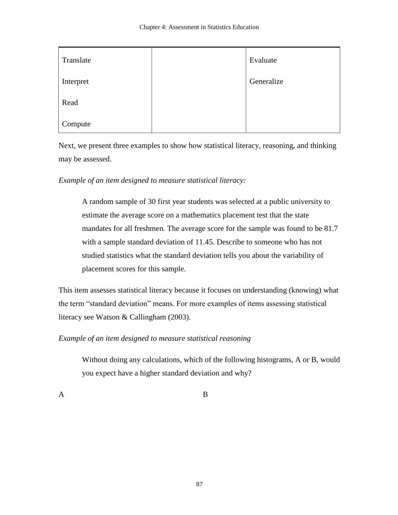
Chapter 4: Assessment in Statistics Education
87
Translate
Interpret
Read
Compute
Evaluate
Generalize
Next, we present three examples to show how statistical literacy, reasoning, and thinking
may be assessed.
Example of an item designed to measure statistical literacy:
A random sample of 30 first year students was selected at a public university to
estimate the average score on a mathematics placement test that the state
mandates for all freshmen. The average score for the sample was found to be 81.7
with a sample standard deviation of 11.45. Describe to someone who has not
studied statistics what the standard deviation tells you about the variability of
placement scores for this sample.
This item assesses statistical literacy because it focuses on understanding (knowing) what
the term “standard deviation” means. For more examples of items assessing statistical
literacy see Watson & Callingham (2003).
Example of an item designed to measure statistical reasoning
Without doing any calculations, which of the following histograms, A or B, would
you expect have a higher standard deviation and why?
A B

Chapter 4: Assessment in Statistics Education
88
This item assesses statistical reasoning because students need to connect and reason about
how the standard deviation of a distribution is affected by spread from the center (mean).
They have to reason about the fact that. Graph B would have a higher average deviation
from the mean than Graph A, because Graph A has a higher proportion of its values
clustered closer to the mean.
Example of an item designed to assess statistical thinking
A random sample of 30 first year students was selected at a public university to
estimate the average score on a mathematics placement test that the state
mandates for all freshmen. The average score for the sample was found to be 81.7
with a sample standard deviation of 11.45.
A psychology professor at a state college has read the results of the university
study. The professor wants to know if students at his college are similar to
students at the university with respect to their mathematics placement exam
scores. This professor collects information for all 53 first year students enrolled
this semester in a large section (321 students) of his "Introduction to Psychology"
course. Based on this sample, he calculates a 95% confidence interval for the
average mathematics placement scores exam to be 69.47 to 75.72. Below are two
possible conclusions that the psychology professor might draw. For each

Chapter 4: Assessment in Statistics Education
89
conclusion, state whether it is valid or invalid. Explain your choice for both
statements. Note that it is possible that neither conclusion is valid.
a. The average mathematics placement exam score for first year students at the
state college is lower than the average mathematics placement exam score of
first year students at the university.
b. The average mathematics placement exam score for the 53 students in this
section is lower than the average mathematics placement exam score of first
year students at the university.
This item assesses statistical thinking because it asks students to think about the entire
process involved in this research study in critiquing and justifying different possible
conclusions.
Comparing Statistical Literacy, Reasoning, and Thinking to Bloom’s Taxonomy
These three statistics learning outcomes also seem to coincide somewhat with Bloom's
more general categories (1956) as they may be collapsed into the three levels described in
the previous section. We see statistical literacy as consistent with the “knowing”
category, statistical reasoning as consistent with the “comprehending” category (with
perhaps some aspects of application and analysis), and statistical thinking as
encompassing many elements of the top four levels of Bloom's taxonomy (application,
analysis, synthesis, and evaluation).
Distinguishing among different types of desired learning outcomes can help statistics
educators design assessment tasks that address the different outcomes and create
classroom environments that allow multiple instructional methods and assessment
opportunities. As learning goals have changed, so have uses of assessment in statistics
instruction, moving away from focusing solely on the purpose of assignment grades as
was common in the past (Garfield, 2000). A wide variety of instruments and methods are
now available to help instructors evaluate how statistical understanding is developing,
and what changes can be made to improve student understanding. As a consequence,
Chapter 4: Assessment in Statistics Education
90
assessment has also been a topic of several research studies in statistics education which
we discuss below.
Research on Assessment in Statistics Education
Recent research on assessment in statistics education has focused on the design, use and
evaluation of:
instruments to assess cognitive outcomes,
instruments to assess attitudes and dispositions, and
alternative forms of assessment (such as, group work, portfolios, and projects)
focusing on application, interpretation, communication, and understanding of the
statistical process.
Assessing Cognitive Outcomes
Most assessments used in statistics courses and in statistics education research focus on
learning, or cognitive outcomes of instruction. Many of the measures of learning and
achievement used in courses provide only a single number summary of student
performance. Due to limitations in this approach, there has been an increasing need to
develop assessment tools that better measure different types of conceptual understanding
to allow assessment of the development of students’ reasoning, that are feasible for large
scale testing. For example, the Statistical Reasoning Assessment (Garfield, 2003) was
developed as a multiple choice test where each correct and incorrect response was
mapped to a previously identified reasoning goal (e.g., common misconceptions such as
the “law of small numbers” and “equiprobability bias,” Garfield, 2002), while focusing
on students’ understanding of statistical concepts and ability to apply statistical
reasoning.
Studies by Konold (1995) suggest that students have deeply held, often contradictory
intuitions about probability and statistics prior to instruction that he maintains he would
not have been able to as easily identify if he had not developed new assessment items
focused on conceptual change that forced him to “articulate my major objectives and to

Chapter 4: Assessment in Statistics Education
91
evaluate the effectiveness of the materials I am designing.” More recently, other
instruments such as the Statistics Concept Inventory (SCI, Allen, Stone, Rhoads, &
Murphy, 2004) and the Comprehensive Assessment of Outcomes in a first Statistics
course (CAOS, Ooms, 2005) have continued this focus on developing reliable and valid
instruments to assess students’ conceptual understanding of statistics. The SCI is modeled
after the Force Concept Inventory used in assessing students’ misconceptions about
Newtonian physics (Halloun & Hestenes, 1985). The CAOS test focuses on statistical
literacy and reasoning and has undergone extensive psychometric analyses and baseline
data have been gathered for comparisons with normative data (delMas, Garfield, Chance
& Ooms, 2006). Goals for both of these instruments include using them to collect data
across student groups and settings for comparative research studies. In addition to these
comprehensive tests, 11 multiple-choice tests on individual topics are available as online
tests (delMas, Ooms, Garfield & Chance, 2006).
Research in science education has highlighted the effectiveness of assessment in
increasing student learning. For example, Posner, Strike, Hewson and Gertzog (1982)
discuss a predict-and-test model as a way to get students to establish sufficient cognitive
dissonance that subsequent instructional intervention has a stronger effect on changing
common misconception. Applying this model in statistics education, delMas, Garfield,
and Chance (1999) asked students to predict (through a quiz) the behavior of sampling
distributions of the mean for different populations before using technology to check their
answers. Students’ interaction with the technology appeared to have much more impact
on their learning when this pre-testing step was used.
Assessing Attitudes and Dispositions
Research has demonstrated that students’ attitudes can be a powerful factor in their
learning of statistics (Gal & Ginsburg, 1994), and it is worthwhile to monitor student
attitudes at the beginning of the course as instruction is being planned, as well as when
the course is evaluated for overall quality and effectiveness. Although this goal has
received less attention in the past, partly due to the difficulty in assessing affective factors
such as attitudes and beliefs involved in the learning process, it is starting to receive more

Chapter 4: Assessment in Statistics Education
92
attention. Many researchers in the field of mathematics education, psychology, and
cognitive sciences (Mandler, 1984; McLeod, 1989 and 1992; Adams, 1989; Fennema,
1989; Schoenfeld, 1983) have stressed the need to assess students’ affective domain
because they influence the cognitive domain. In particular, McLeod (1989) distinguishes
between attitudes and beliefs and discusses why these are important for the learning of
mathematics, and also defines and distinguishes between other constructs such as
emotions and dispositions that are less stable and more likely to change over shorter
periods of time. Pre-conceived notions about the subject and its usefulness appear equally
important in statistics education.
Some instruments have been used to assess students’ attitudes and beliefs about statistics
such as Attitudes Toward Statistics (Wise, 1985) and Survey of Attitudes Toward
Statistics (Dauphinee, Schau, & Stevens, 1997). However, these instruments were not
designed to provide causal information (Gal & Garfield, 1997). One may have to conduct
interviews to find out why students have the beliefs they do about statistics. This is a
limitation in trying to assess students’ affective domain since it is difficult to find the time
for focus groups conducting interviews. Furthermore, since attitudes and beliefs are very
stable, it is difficult for an instructor to make significant changes in attitudes during one
course, but these assessment instruments can at least inform a more long-term change in
the teaching of statistics.
Alternative Assessment Methods
Even good students don’t always display a good understanding
of what’s been taught even though conventional measures …
certify success. (Wiggins & McTighe, 1998, p. 2)
As the instructional goals shift from computational skills to deeper conceptual
understanding of basic statistical ideas, the need for alternative methods of assessment is
even stronger than before. As Wiggins and McTighe point out in the quote above,
conventional methods often fall short of giving the full picture of what students have
learned. Many innovative alternative assessment methods are available to teachers of
statistics such as projects and article critiques, which are described in a later section of

Chapter 4: Assessment in Statistics Education
93
this chapter. While alternative assessment methods provide different types of insight into
students’ understanding and ability, they are also particularly conducive to promoting
student learning.
Informal assessments are also an alternative to traditional quizzes and exams. During a
lesson, questions can be posed orally to probe for common misconceptions and allow
students to discuss their ways of thinking. Students can be asked to provide multiple
solutions to a problem, and then asked to explain their reasoning. Practice in explaining
reasoning and supporting judgments and conclusions will help them better perform these
tasks on later assessments.
The focus on the integration of improved assessment methods and alternative forms of
assessment in introductory statistics allows instructors to assess students’ understanding
at a deeper level, often highlighting very deeply held misconceptions about probability
and statistics. Development of new assessment instruments and tasks is improving our
ability to document these misconceptions and their reasoning processes, as well as track
students’ development of conceptual understanding as they learn new material. In
particular, assessment tools can be utilized themselves as powerful instructional
interventions, especially once students and faculty become more comfortable with the
formative nature of this information rather than relying on them only as summative
evaluations.
Designing Assessments for Statistics Classes
Assessment should support the learning of important concepts or skills and provide
important information to both teachers and students (National Council of Teachers of
Mathematics (NCTM), 1989 & 2000). The NCTM Assessment Standards for School
Mathematics (1995) presents six assessment standards that address mathematics (the
content we teach), learning, equity, openness, inferences, and coherence. Due to the
multiple roles that assessment can play in statistics education, designing an assessment
plan takes careful consideration. Garfield (1994) offers the following assessment
framework from which to build:

Chapter 4: Assessment in Statistics Education
94
What is to be assessed (e.g., a concept, skill, attitude or belief)
The purpose of the assessment (e.g., to assign a grade, to help the teacher modify
instruction, to help the student identify strengths or weaknesses in their
understanding)
Who will do the assessment (e.g., self-assessment by the student, peer-evaluation,
instructor feedback)
The method that will be used (e.g., project, quiz)
The action / feedback that will be implemented as a result of the assessment
Each of these dimensions needs to be considered in designing an assessment to help
ensure that the assessment is aligned with course goals and as effective as possible.
Because assessing students can be time-consuming, in designing assessment tasks we
recommend a focus on two key tenets: 1) assess what is valued, and 2) incorporate
assessment into the learning process.
Assess what is valued
Students pay the most attention to the material on which they are assessed. Students take
their cues as to what is important in the course based on assessments. It is easy to claim
that clear communication, analysis, and synthesize of topics are goals of the course. Yet
even when a teacher models these skills during class, students will not focus on them if
they are not held responsible for demonstrating these types of skills themselves “when it
matters.”
To ensure the teacher is assessing what is valued, it can be helpful to first reflect on what
the teacher cares most that students should be able to do after they have taken a statistics
class. Should they remember a formula? Should they be able to make decisions and
provide arguments based on evidence? Should students be able to conjecture, build
arguments, and pose and frame problems?
Incorporate assessment into the learning process

Chapter 4: Assessment in Statistics Education
95
It is also important to conceive of an assessment program as a process in which students
(and faculty) can receive formative feedback during the course, rather than the traditional
method of using assessments only to determine final course grades. Taking advantage of
the high importance students give to assessments provides an opportunity for substantial
learning and reflection (e.g., the predict-and-test model). For these reasons it is crucial to
consider student assessment simultaneously with the design of instructional activities and
to consider how lessons learned from different assessment components can inform other
parts of the course (for example, using quizzes as sample exam items to help prepare
students for the types of questions they may be asked).
A K–12 teacher may find that incorporating different types of assessment into the
learning process will help students develop the content knowledge and language skills
necessary for success in the next school level. But independently of what level is taught,
teaching students how to learn and reflect on what they know (referred to as a
metacognitive activity) has been shown to improve understanding in different content
areas (White & Frederiksen, 1998; Schoenfeld, 1987) and would better prepare students
to be life-long learners (Bransford, Brown, & Cocking, 2000).
Different Types of Assessment
Many effective types of assessment tools exist, each with different goals and purposes.
Below we highlight a few common practices and their differing roles in the overall
assessment process: Homework, quizzes, exams, projects, critiquing/writing
assignment/lab reports, collaborative tasks, minute papers, and attitudinal measures.
1. Homework
Often students find statistical terminology and statistical way of thinking to be the most
challenging aspects of their first introduction to statistics. Providing them with constant
practice using terms and processes is an important component in developing their
understanding and confidence with the material. Homework assignments can clearly vary
in length and formality (e.g., “practice problems”) but should provide students with
guidance on how to focus their studying of the topics. For example, they should include

Chapter 4: Assessment in Statistics Education
96
application and conceptual questions, especially if those types of questions will be asked
on exams. Questions can also be included that ask students to reflect on the problem
solving process. As with any assessment strategy, it is crucial to supply students with
clear guidelines for the instructors’ expectations (e.g., How much work needs to be
shown in leading to the final answer? Should computer output be included in the write
up?). Students may not be accustomed to being graded on their process (needing to
supply more than just a final boxed answer at the end) or even the correctness of their
approach and they will require time to adjust. Supplying guidelines for performance
expectations can also help students avoid time consuming sidetracks.
In grading homework assignments, it is quite valuable to provide feedback that students
can apply to later assignments. While student assistants can often help grade assignments
at the university level, questions that require more interpretation might be better graded
by the instructor. Being open to alternative approaches and interpretations is especially
important in introductory statistics classes. We also recommend providing students with
access to model solutions, whether instructor written or an anonymous student paper to
help model peer work, and/or the opportunity to review and comment on faulty and
correct solutions provided by other students. (For a comprehensive review of research
related to the effects of homework, see Cooper, Robinson, & Patall, 2006). Other
practical considerations include how much collaboration to allow among students in
doing their homework. See Chapter 15 for a discussion on the benefits of collaboration in
learning statistics.
The instructor also needs to decide on the level of support or scaffolding given in
response to student questions on the assignment. For example, how forthcoming should
the instructor be in supplying help, answers, or hints? Will responses to students be more
Socratic in nature to help students think through the process? Could additional hints be
accompanied by a deduction in points available for a particular problem? Should the
instructor choose to be generous in responding to questions on student homework
problems but only if questions are posed at least 24 hours prior to the due date? This type
of structured support can encourage good habits in students so that they do not delay
working on their homework until the last minute.

Chapter 4: Assessment in Statistics Education
97
2. Quizzes and Exams
Quizzes are useful for providing timely checks of student understanding and feedback on
their progress while exams can assess cumulative knowledge over a longer period of
time. Low-stakes quizzes can be very helpful to students in getting a feel for what types
of questions may appear on exams, especially if exam questions tend to be more
conceptual in nature than textbook problems providing students with some prior
knowledge of what the planned focus will be for a particular exam and the instructor’s
grading style. Alternatively, quizzes can be more focused mini-exams, with an
accompanying higher weight in the overall course grade. This is especially effective for
minimizing grading efforts, allowing homework assignments to be down-weighted or
even optional.
One approach to consider is paired/collaborative quizzes. Significant student learning
occurs in the debates they have with each other in developing a unified response.
Students can also support each other and this approach may alleviate testing anxiety
among many students. In this way, quizzes become a learning tool as well as an
assessment technique. Students can be given time to think individually before the group
discussion and individually graded components can also be incorporated if desired.
Researchers such as Johnson and Johnson (1996) have also discussed issues in forming
these groups (e.g., homogenous or heterogeneous with respect to prior performance?) and
rearranging them during the term (see later comments on collaborative tasks as well).
Another practical consideration is dropping a quiz grade (or more) in the overall grade
calculations. This can help ease tension if students must miss a class day but still provide
incentives to attend class. A decision may depend on whether quizzes are announced in
advance and on how many are administered during the term. Use of quizzes for
attendance incentives can take more prominence for early morning and Friday classes for
college students.

Chapter 4: Assessment in Statistics Education
98
Some instructors worry about using too much in-class time if quizzes are given every
week. Short quizzes can provide meaningful insight into students’ understanding. The
following example shows a one-question quiz that can help the instructor to highlight and
bring to class discussion a common misunderstanding:.
Example (adapted from Ramsey & Schafer, 2002):
True or False? A sample histogram will have a normal distribution if the sample
size is large enough. Explain why. (Sample correct responses: False, because a
large sample size will give a better idea of the shape of the population from which
the data have been sampled, and that population may or may not have a normal
distribution).
Modifying Assessment Questions
It is clear that numerous resources now exist for accessing existing assessment tools. In
selecting an assessment tool, it is important to consider what types of modification are
needed to adapt this instrument to align with the instructor’s learning goals.
Writing Good Items for Quizzes and Exams
Several statistics educators (e.g., Hubbard, 1997; Hayden, 1989) have suggested ways of
improving exam questions such as always providing a meaningful context, using
questions where the goal of the analysis has a purpose, asking more “what if,” “construct
a situation such that…,” and comparative judgment questions, requiring explanations
with calculations, identification and justification of false statements, and objective-format
questions. Cobb (1998) offers ways to write good multiple choice items to assess higher
order thinking and reasoning. As an alterative to writing items, the ARTIST project
provides a selection of over 1000 high quality assessment items in an online, searchable
data base (see Resources section). These items are released only to instructors, and are
not freely accessible on the Web by students.
According to Wild, Triggs, and Pfannkuch (1997), multiple-choice questions can still test
higher level thinking skills. They provide examples of multiple-choice questions that can

Chapter 4: Assessment in Statistics Education
99
help students confront common misconceptions, interpret data, select appropriate
techniques for data analysis, and make appropriate inferences. What multiple-choice
questions cannot do is to assess open-ended thinking because it does “little to help
students develop their own voices” or demonstrate students’ ability to formulate
questions emerging from the data.
The following guidelines can assist instructors in developing their own items for quizzes
and exams:
Include items that allow students to express their reasoning and thinking and
demonstrate their use of statistical language.
In using multiple-choice items, aim for 3-4 answer choices. Try to include
responses that might match different types of student reasoning among the answer
choices and try to avoid options such as “none of the above.” (See Haladyna,
Downing, & Rodriquez, 2002 for additional practical suggestions for writing
multiple-choice items based on measurement research.)
Add a contextual basis to existing questions that may lack a real or realistic
context. For example, rather than asking students to interpret a correlation of 1.2
(an oblivious result of a calculation error), describe the problem being
investigated and the variables being examined (e.g., in a study of attitudes and
achievement in a statistics class, students were given assessments of math anxiety
and algebra proficiency).
Build assessment questions around existing data sources. Finding interesting data
examples is often more difficult. So it may be useful to start with an interesting
research study and build the statistical concepts questions around that study.
Examples of Good Assessment Items
The following items provide some examples of good assessment items, based on the
guidelines in the previous section.
Example:

Chapter 4: Assessment in Statistics Education
100
A study of 78 randomly selected seventh-grade students from a large Midwestern
school measured students’ “self-concept” (SC) through their score on Piers-Harris
Children’s Self-Concept Scale. Within the analysis, researchers found higher SC
scores for 13 years compared to 14 year olds and constructed a 95% confidence
interval for this difference to be (2.38, 29.44).
(a) Which is the best interpretation of this confidence interval?
95% of 13 year old and 14 years had a self concept score between 2.38
and 29.44.
We are 95% confident that 13 year olds score between 2.38 and 29.44
points more than 14 year old scores.
We are 95% confident that the difference in mean concept scores for the
13 year olds and 14 year olds in this study is between 2.38 and 29.44.
95% of intervals constructed this way will capture the difference in the
population means between 2.38 and 29.44.
(b) Explain what is wrong with one of the above interpretations.
(c) Explain whether, and if so how, the above interval would differ if the
confidence level had been 99% instead of 95%.
This item challenges students not only to identify a correct answer but to also identify
answers that are incorrect and explain why they are wrong. It also asks students to reason
about the effect of changing a confidence level to a higher value and why that would
affect the interval width.
Example (adapted from Rossman & Chance, 2001):
Construct a data set of 10 possible student test scores that range between 0 and
100 so the mean is greater than median.

Chapter 4: Assessment in Statistics Education
101
Students need to understand the properties of the measures to “work backwards” in
solving this problem.
Example (adapted from Hubbard, 1997):
Make up a problem that could be solved with the following output.
One-Sample T
Test of mu= 25 vs < 25
N MEAN STDEV SE MEAN T PVALUE
40 23.63 3.95 0.538 -2.55 0.0054
This question requires students to piece together information from generic computer
output but also to generate a suitable context (i.e., one quantitative variable that is
feasible for these summary statistics). This reversal in logic assesses their understanding
of and ability to apply the overall process of going from a research question and data to
an analysis.
Example (adapted from Chance, 2002):
Four different studies obtained data that were used in a test of the hypothesis H0: 1 =
2 3. Based on the information below, order these studies from smallest P-value to
largest P-value. Provide an explanation for your choices. You will be graded primarily on
your explanations.

Chapter 4: Assessment in Statistics Education
102
Given to students who have not studied ANOVA (Analysis of Variance), this question
requires students to integrate and extend different ideas from the course (e.g., the effects
of sample size, within group variation, and between group variation) on the magnitude of
the p-value. A scoring rubric is less concerned with the particular ordering selected (e.g.,
top left vs. bottom right) but more on which of these factors are discussed by the student,
the direction of the effect suggested, and the consistency of the ordering with the written
explanation.
Exam questions can also be designed that require more performance and production by
the students rather than memorization. Questions should also challenge students beyond
traditional textbook problems, especially end of chapter questions where the solution
approach is determined by which chapter is being discussed.
Example:
Your text states that “confidence intervals seek to estimate a population parameter
with an interval of values calculated from an observed sample statistic.” Convince
me that you understand this statement by describing a situation in which one
could use a sample proportion to produce a confidence interval as an estimate of a
population proportion. Clearly identify the population, sample, parameter, and
statistic involved in your example. Do not use any example that appears in your
book.
Example (adapted from Moore & McCabe, 1998):
A university is interested in studying reasons many of their students were failing
to graduate. They found that most attrition was occurring during the first three
semesters so they recorded various data on the students when they entered the
school and their GPA after three semesters. [Students are given data set with
numerous variables.
(a) Describe the distribution of GPA for these students.

Chapter 4: Assessment in Statistics Education
103
(b) Is SAT-Math score a statistically significant predictor of GPA for students
at this school?
(c) Is there a statistically significant difference between the mean GPA values
among the majors at this school?
It is very important to remember that if non-traditional item formats are to be included on
the exams, then students must be prepared in advance, e.g., through examples in review
or earlier assignments and quizzes as discussed above. Students can also be to each
develop and submit their own example questions as part of the review process to help
them anticipate what they will be asked. It is also important to think of the overall time
constraints in combining these questions with more traditional type questions.
Even once exam questions are developed, there are still many practical issues in
administering and grading student responses. Considerations include whether to allow
external aids (e.g., closed book vs. supplying formulas pages vs. open book), the use of
technology during the exam, whether exams should be timed, approaches taken to
constructing exams, how to prepare students for the exam (e.g., use of review sheets,
review problems), and how to provide the best feedback to students post-exam (e.g., is
posting solutions online sufficient or should we always budget class time for
discussion?). There are many possible views on these issues. The ARTIST Website
contains an “Implementation Issues” section where leading statistics educators offer their
personal views and justifications, and a panel session at the 2005 Joint Statistical
Meetings also discussed these issues (Dietz, Gould, Hartlaub, & Rossman, 2005). Two
suggestions we will highlight here are sharing exams with colleagues and collecting
feedback in advance, and jotting down ideas for exam questions as they occur during
class discussions, grading homework assignments, or reading the newspaper.
3. Projects
Projects are an important tool for both assessing many aspects of student learning as well
as helping them experience different stages in posing and solving a statistical problem.
Projects can be viewed as an authentic performance assessment (see Garfield, 1993).

Chapter 4: Assessment in Statistics Education
104
Students quickly realize that the optimal methods are not always practical or feasible and
that compromises, with consequences, have to be made. Students also realize that data
can be messy and they must consider data cleaning issues and unexpected sources of bias.
Oral presentations can also be required to help students to learn to effectively
communicate their analysis.
Projects can focus on a particular aspect of the course (e.g., Smith, 1998) or be term-long,
requiring students to apply tools they learn throughout the course in one overall analysis
(e.g.¸ Chance, 2000). See also the assignments John Holcomb and others have posted on
the ARTIST Website (https://ore.gen.umn.edu/artist/projects.html). Holcomb provides a
series of group assignments followed by individual take home exams to perform similar
analyses.
With term-long projects, periodic reports should be required to maintain consistent
progress on the project. Students can be required to work individually or in groups.
Group management becomes an issue in the latter case, and it may be worth considering
maintaining an individual component in assessing student performance on the project. In
designing a project assessment, it is important to simultaneously consider how to assess
the effectiveness of the project and student work. Students can also be asked to provide
group member evaluation, and presenters can be evaluated on how well they answer
questions during the question/answer period after presenting. For example, in an 8th
grade
class students had to give oral presentations of their projects. It was during the
question/answer period that students’ misunderstandings or confusions were revealed
(Lajoie, 1999). Starkings (1997) warns about the demanding nature of projects, for both
instructors and students, and she provides advice to teachers planning to use projects in
their classes.
4. Critiques/Writing Assignments
Most students will eventually find themselves to be consumers of statistical information
rather than producers. Therefore, if a course goal is developing students’ ability to
process and analyze quantitative information in the media, assignments can be designed
to help develop these skills.

Chapter 4: Assessment in Statistics Education
105
Possible examples are:
1. Providing students with a journal article and asking them to evaluate the use of
statistics and the conclusions drawn.
2. Having students “role play” and asking them to explain some conflicting
information recently cited in the news to a parent, using statistical arguments but
in a way a non-statistician could understand.
3. Writing a “meaningful paragraph” in which students are given a short list of
statistical terms (e.g., sample, population, and sampling distribution) and are
asked to use these terms in a short essay that explains their understanding of these
terms in a particular context.
These tasks focus on requiring students to use their own words to explain their
understanding, an often different experience than directly solving a given problem. Some
examples are below.
Example (from Jordan, 2004):
Write a meaningful paragraph that includes the following terms: sampling
distribution, population mean, sample mean, variability, normal distribution,
sample size, and probability. A “meaningful paragraph” is one continuous piece
of writing, which uses all of the listed words and in which the sentences “make
sense and hang together.” That is, the ideas in the paragraph illustrate that you
understand the new terms in a way that allows you to write “meaningfully” about
them. You may not simply write seven sequential sentences, for example, that
merely define the terms; sentences must demonstrate relationships between the
terms.
Example (from Jordan, 2004):
Suppose you receive the following letter from your dad:
Hey Kiddo,

Chapter 4: Assessment in Statistics Education
106
I am worried about Grandma. Remember that she was diagnosed with high blood
pressure? Well, she’s currently taking the medication Makemewell to lower her
blood pressure. At the time of Grandma’s diagnosis, her doctor said that a
randomized, double-blind experiment had been conducted and that Makemewell
was shown more effective in lowering blood pressure than a placebo. To be
honest, I have no idea what any of that means, but I believed and trusted the
doctor. Now I’ve heard two stories that make me think differently. Larry, our
next-door-neighbor, was taking Makemewell and he got a terrible fever that put
him in the hospital. Also, my coworker, Sally, actually had her blood pressure go
up while she was taking Makemewell! I’m now very suspicious of this
medication.
I know that you’re taking a statistics course at college. Based on the information
I’ve given you, do you think Grandma should stop taking her medication?
Whatever your opinion, will you please explain yourself thoroughly and clearly?
(I will draw on your responses when I talk with the doctor.) And please don’t use
any statistics mumbo jumbo that I won’t understand. I really appreciate your help
with this.
Love, Dad
Your assignment is to type a 1–2 page letter (single-spaced, 12-pt. font)
responding to your dad.
Sometimes models or examples can be used to help students seen the desired features of a
finished writing assignment or project. However, students often fall into the habit of
using model papers as a template instead of using their own thinking. One way around
this is to give students the first model paper after they have submitted their first
assignment and then allowing them to use this model as they revise or prepare the next,
slightly different, assignment. Assignments that ask students to address a particular
audience (e.g., your father, the soda manufacturer) seem to work well in engaging
students (see Jordan, 2004).

Chapter 4: Assessment in Statistics Education
107
Grading Writing Assignments
A key consideration in these types of assignments is how to grade them. Instructors may
benefit from considering articles on grading more generic writing assignments (e.g.,
Elbow, 1997; Bean, 2001). Holistic scoring approaches can be useful in grading writing,
if a rubric or guideline is used. This type of scoring is used in grading open ended
problems in the Advanced Placement Statistics Exam and works well for many
assessment tasks in a statistics course. Instead of relying on an analytic scale where points
are deducted for each error, holistic scoring assigns points based on a categorization of
the overall quality of a student answer and explanation. Careful design and use of scoring
rubrics can produce more consistent scores, especially when only 3 to 5 points are
assigned to each part of the rubric. The following example is adapted from an assignment
developed by Jordan (2004). In this case, up to five points can be assigned to each
criterion in the rubric.
Example: Rubric adapted from Jordan (2004) writing assigning.
Grading Criteria (20 points possible)
____ The explanation to your dad convinces me (your teacher) that you
understand the statistical concepts involved in the assignment. (5 points)
____ The explanation to your dad is thorough, well organized, and clear. (5
points)
____ The explanation to your dad is presented in non-technical terms that he
will understand. (5 points)
____ You successfully paid attention to accepted conventions of language use
(syntax, spelling, grammar, readability, etc.) (5 points)
Example: Rubric for Wetzel (2004) assignment to determine solution to a problem where
they were to determine the weight of average McDonald’s French fry by collecting and
analyzing data.

Chapter 4: Assessment in Statistics Education
108
Basics (5 points): Does the description of the problem solution include all of the
required parts including accurate and appropriate use of terminology?
restatement
measurements - including specifics
questions to ask - including specifics
extra demographic question
how to get randomize - including specifics
other data
Organization (2 points): Is the description organized and neatly presented? Great
answers also include some pluses.
Pluses:
Does the description include any significant extras (e.g., additional detail
on the data collection steps, use of terminology)?
Significant improvements to a basic data collection design.
Extra thought into the specifics of this context - recognizing potential
problems and giving solutions.
Minuses:
Does the description indicate that the student is mimicking a book answer
and not considering the context?
Does the description include a design that would be extremely
impractical?

Chapter 4: Assessment in Statistics Education
109
Does the randomization described introduce a significant confounding
variable that was not identified?
This problem requires thinking and possibly some research. A good answer will
get 7 out of 10 points; in order to get full credit, you need to provide a great
answer.
Such scoring rubrics provide the statistics instructor with more flexibility in allowing
alternative solution approaches, and maintaining scoring consistency in a justifiable
manner, and can be used to emphasize to students the equal weight given to both
communication and calculation. Scoring rubrics should be provided to the students with
the assignment to help clarify expectations and standards.
Teachers may consider raising their expectations as the course progresses and students
build on earlier feedback. Students can also be required to submit self (and group)
evaluations. With longer assignments, intermediate deadlines and/or the opportunity for
revision may be possible.
5. Lab Reports
Most introductory statistics courses have some opportunities for students to also produce
data, using appropriate technology tools. Having students produce technical reports that
integrate computer output with discussion suitable for a nontechnical audience, putting
students in the role of the statistical analyst. Students can be asked to complete several
reports during the term, with clear guidance for the technology skills and discussion
questions to be addressed, as well as guidelines for quality report writing (e.g., Spurrier,
Edwards, and Tombs, 1995). Chance (2000) implemented a series of lab reports,
increasing in their demand of students’ autonomy and integration of ideas. Several of
these reports focused on a full report (introduction, data collection methods, analysis,
discussion, conclusion) for analyses of data students collected themselves (see Guidelines
for Lab Reports in the Appendix). These reports were allocated 20 points for the
computer output, 25 points for discussion and interpretation and 5 points for presentation.
6. Collaborative Assessment Tasks

Chapter 4: Assessment in Statistics Education
110
In a statistics course, asking students to work together to develop a common solution can
be very effective as students have varied backgrounds, experiences, and mathematical
sophistication. This can be done through quizzes and projects as well as in-class
activities. Group work where students are responsible for jointly working together and
having to agree on one answer or write up can lead to good discussions and arguments
that involve explaining their statistical reasoning and enhances student learning.
One particular approach to consider is to combine group assignments with individual
assessments and even having a component of the individual assessment address what they
should have learned from the group assignment (e.g., what was your project about?). For
example, Harkness (2005) describes use of Readiness Assessment Quizzes that may have
three components: an individual component, a group component, and an appeal process,
based on reading assignments given to students before class, prior to instruction on the
material. These multiple-choice questions on general concepts are first taken individually
and then immediately retaken as a group of three to five students. Each student receives
an individual and a group grade, and the belief is that this arrangement for the group work
helps foster comprehension across the group members.
7. Minute Papers
Asking students to provide quick feedback on lessons and which topics are most and least
confusing and/or on what aspects of the course instruction they are finding most and least
helpful can help the instructor address common misconceptions or alter the course.
Minute papers also convey to students that their feedback is important and can be used to
help them reflect on the overall course goals and design. Students use the last five
minutes of class to respond to a few questions on a half sheet of paper or index card (e.g.,
Angelo & Cross, 1993). Minute papers can also be used to give feedback to the
instructor, especially early on or in the middle of the term. This feedback may provide an
instructor with ideas of things that can still be changed in the class (e.g., several students
reporting that it is difficult to read the writing on the board) as well as allow the instructor
to address and justify issues that won’t be changed (e.g., why they won’t change the
software package being used).
Chapter 4: Assessment in Statistics Education
111
Example:
What was the most important point of today’s lecture? What did you consider to
be the muddiest point of today’s lecture? What would you like to learn more
about?
Example:
Please provide feedback on what is working best for you in this class as well as
what you would like me to change in the course structure and style.
It is important for these submissions to be anonymous if the student chooses; this allows
students to feel more comfortable in giving honest responses. Many electronic course
delivery systems (e.g., Blackboard®) enable anonymous surveys while also tracking
completion by individuals if credit is to be assigned. In large classes, subsections of
students can be polled on different days. Discussing with the students feedback from the
minute papers is very important. Sometimes examples can be given of comments and
summaries can be used to give the class an idea of trends in their responses. Students
appreciate knowing that their opinion is important and under consideration and that they
are not alone in their confusion.
8. Student Reflections and Dispositions
Many of the above tools can include self-reflection components as well as formal and
informal opportunities for student feedback. Alternatively, students can be asked to
complete written journals in which they are expected to contribute more reflection on the
process and sharing of their reactions to the materials. They can also be asked to reflect
on an experience with statistics that they have outside of the classroom (e.g., playing
bingo with Grandma or compiling and explaining statistical cartoons).
Guidelines for Developing an Effective Assessment Plan
The previous section highlighted many different tools that can be used to assess students
and now to select a particular tool for a particular assessment task. It is also important to
consider how to combine the tools across the course. In this way, the teacher can make

Chapter 4: Assessment in Statistics Education
112
sure that, as a collection, the assessment tasks are aligned with the important goals for the
course, that the action/feedback from the different components inform each other, and
that no undue burden is placed on the instructor or the students. It may be useful, for
example, for an instructor at the beginning of the course to map out how different
assessments in the course align with learning goals of Statistical Literacy, Reasoning, and
Thinking in order to make sure that items and tasks are balanced and evaluating each type
of outcome, although not necessarily in a single task or exam.
It is crucial to consider the assessment plan as a course is designed and to clearly lay out
the goals and purposes of the assessments as part of the course syllabus. Below we offer
some specific suggestions for developing an overall assessment plan.
Develop an assessment blueprint that matches instructional goals to the
assessment tools. This will involve analyzing the purpose and use of each
assessment. For example, to assess student literacy, consider requiring student
interpretations of articles and graphs. To include assessments of statistical
thinking, consider requiring a student project. In fact, Wiggins & McTighe (1998)
recommend designing a course by beginning with the assessment goals (what
outcomes are desired) and then working backwards to design the instructional
component of the course.
Provide clear guidelines ahead of time to the students (and follow them). Even if
there are problems with an assignment in progress, it is often better to follow the
assignment through to fruition and make notes for next time, rather than to change
an assignment on students midway.
Use a variety ways for students to demonstrate their understanding.
Provide constructive and timely feedback so there is a clear connection between
the assessment and student learning.
Challenge students to extend their knowledge (e.g., ask questions where a solution
or approach is not obvious).

Chapter 4: Assessment in Statistics Education
113
Students need to feel the assessment is fair (to understand the purpose of the task
and to feel that individual grades are an accurate reflection of their knowledge and
effort).
Focus on observable student behavior.
Promote self-reflection and student responsibility.
Consider the overall coordination of the assessment tasks throughout the course.
Don’t try to change all of assessment practices at once or to utilize every
assessment task possible.
Continually reflect on and refine your assessment practices and collaborate with
colleagues.
Practical Considerations
We conclude with some practical advice and things to consider. We begin with the
exhortation that assessment be viewed as an integral part of the learning process and not
as a separate method used only to evaluate performance and assign grades. With all of the
excellent assessment resources available, statistics teacher need not try to write their own
tests, and if fact, are advised to utilize high quality assessment items such as those at the
ARTIST Website. We also advise instructors to think about sampling learning outcomes
rather than trying to assess all topics in a particular test. It is important to remember that
students’ preparation for a test is part of the learning process; and one purpose of a test is
to motivate study and integration of concepts.
While it may seem that every assessment of students must be read by the instructor, this
is not always necessary. Students may be used as peer reviewers of papers and projects,
which also helps their own learning. We also recommend that instructors take advantage
of informal opportunities to assess student learning by carefully listening, asking
questions and observing students. Valuable information can be gained on how students
use the statistical language, express their reasoning, and make a statistical argument as
they work together in groups during class activities.

Chapter 4: Assessment in Statistics Education
114
A comment made by a statistics educator brings home the point about assessing what is
really valued (J. Witmer, personal communication, December 11, 2006). He said, as he
examined a recent test he gave to students that a computer would have earned a passing
grade on it. That led him to reconsider the kinds of questions he asked on exams and to
move from more computational and procedural questions to questions focused more on
statistical literacy and reasoning and conceptual knowledge. This also relates to the issue
of having students memorize material or having them able to access and use appropriate
resources when solving statistical problems, as we do in real statistical work.
A final practical consideration is the use of computer-supported learning systems (such as
Blackboard®) which can help in assessing students’ work by tracking ongoing
assessment, allowing continual revision, providing feedback, supporting collaboration,
posting a paper or artifact in students’ galleries, etc.
Summary
Assessment has been referred to as a way to make visible students’ learning or reasoning.
This is an important purpose of assessment because once reasoning is made visible, it can
be “discussed, challenged, and made more robust” (Hammerman & Rubin, 2004, p. 37).
We encourage instructors to use assessment as a window to view student learning in their
classes, using both formal and informal methods. We hope that teachers will move
beyond using assessment solely as a mechanism for providing grades and measuring
achievement, relying only on students’ responses on exams for a picture of what students
know and what they do not understand. We encourage instructors to use a variety of
methods to better understand and measure student learning, taking notes to identify useful
and not so useful components of their assessment program so that assessment tasks can
be continually modified and improved, while focusing on gathering useful feedback on
their teaching and on students’ learning of important ideas. We end with the motto that
“success builds success”: We encourage instructors to make assessment a positive
experience for students and one that will make them feel successful about learning
statistics.

115
Chapter 5: Using Technology to Improve Student Learning of Statistics5
Interactive software data visualization tools which allow
for the creation of novel representations of data open up
new possibilities for students (and teachers) to make sense
of data, but also place new demands on teachers to assess
the validity of the arguments that students are making with
these representations, and to facilitate conversations in
productive ways. (Hammerman & Rubin, 2004, p. 18)
Overview
It is hard to imagine teaching statistics today without using some form of technology.
However, just 20 years ago that was very common. Today’s statistics classes may be
taught in a classroom with a computer projected on a screen, or may take place in a
laboratory with students working at their own computers. Students commonly own a
calculator more powerful than the computers of 20 years ago. Others may use a portable
computer (laptop) at school, home and on the move. An ever growing format of teaching
today is over the Internet, in the form of a Web-based course with video-taped lectures,
interactive discussions, collaborative projects, and electronic text and assessment
materials. The technology revolution has had a great impact on the teaching of statistics,
perhaps more so than many other disciplines. This is not so surprising given that
technology has changed the way statisticians work and has therefore been changing what
and how we teach (Moore, Cobb, Garfield, & Meeker, 1995).
This chapter presents a broad overview of the role technological tools can play in helping
high school and college introductory statistics students understand and reason about
important statistical ideas. The main goal of this chapter is to provide some background
5 This chapter is based on the following journal article:
Chance, B., Garfield, J., Ben-Zvi, D., & Medina, E. (2007, October). The role of technology in improving
student learning of statistics. Technology Innovations in Statistics Education Journal, 1(1). See
http://repositories.cdlib.org/uclastat/cts/tise/vol1/iss1/art2/

Chapter 5: Using Technology to Improve Student Learning of Statistics
116
of how the technology tools have evolved, a sense of the research findings and open
questions on how technology impacts student learning, and concrete advice, stemming
from the research literature, on using technological tools and how to avoid common
pitfalls or ineffective implementations. We first summarize the impact of technology on
the content, pedagogy, and even format of introductory statistics courses. Then we
highlight some of the common technological tools currently in use in statistics education
and how they can be utilized to support student learning. We summarize some of the
recent research insights gained with respect to using technology to aid instruction and
learning in probability and statistics. While not an exhaustive literature review, the
studies discussed provide additional context for a series of practical recommendations to
the instructor, along with a discussion of possible obstacles and implementation issues,
and questions to consider when selecting different tools.
Changes in Content, Pedagogy, and Course Format
Changes in Content
Technology has led to numerous changes in statistical practice. Many analytically
intractable problems that were previously inaccessible now have approximate solutions
(e.g., Bayesian methods). Many assumptions that were made so that statistical models
could be simplified and usable no longer need to be made. These changes in statistical
practice have a direct impact on the content that should be taught, even in introductory
material. For example, an entire branch of “resampling statistics” (Good, 2006) now
competes with model-based inferential models in practice, while also appearing more
intuitive to students. Another example is the use of statistical tables such as the z and t
tables, which are no longer needed to determine rejection regions or estimate P-values
when statistical software and calculators produce more accurate results much more
quickly. In fact, many statistics educators now argue that previously standard topics in an
introductory course (e.g., short-cut methods for calculating standard deviation) are no
longer necessary to discuss in class. Finally, technology provides ways for us to visualize
and explore data that have led to new methods of data analysis.
Changes in Pedagogy

Chapter 5: Using Technology to Improve Student Learning of Statistics
117
While the impact of technology on the practice of statistics is irrefutable, just as powerful
has been the impact of technology on statistics pedagogy and recommended practices.
For example, the National Council of Teachers of Mathematics (NCTM) Principles and
Standards for School Mathematics states that “the existence, versatility, and power of
technology make it possible and necessary to reexamine what mathematics students
should learn as well as how they can best learn it” (NCTM, 2000). In particular, the
Guidelines for Assessment and Instruction in Statistics Education (GAISE) curriculum
framework for PreK-12 states that “advances in technology and in modern methods of
data analysis of the 1980s, coupled with the data richness of society in the information
age, led to the development of curriculum materials geared toward introducing statistical
concepts into the school curriculum as early as the elementary grades” (Franklin &
Garfield, 2006). Similarly, the GAISE College Report directly recommends the use of
technology for developing understanding of statistical concepts and analyzing data in
teaching an introductory, undergraduate statistics course (Franklin & Garfield, 2006).
Moore (1997) urged a reform of statistics instruction and curriculum based on strong
synergies among content, pedagogy, and technology. However, he cautioned statisticians
to remember that we are “teaching our subject and not the tool” (p. 135), and to choose
appropriate technology for student learning, rather than use the software that statisticians
use, which may not be pedagogical in nature. In fact, many types of technologies are
available nowadays for the statistics teachers. Teachers are encouraged to view the use of
technology not just as a way to compute numbers but as a way to explore concepts and
ideas and enhance student learning (Friel, 2007; Garfield, Chance, & Snell, 2000).
Furthermore, technology should not be used merely for the sake of using technology
(e.g., entering 100 numbers in a graphing calculator and calculating statistical
summaries), or for pseudo-accuracy (carrying out results to a meaningless number of
decimal places) (Franklin & Garfield, 2006). More appropriate uses of technology are
accessing, analyzing and interpreting large real data sets, automating calculations and
processes, generating and modifying appropriate statistical graphics and models,
performing simulations to illustrate abstract concepts and exploring “what happens if…”
type questions.
Chapter 5: Using Technology to Improve Student Learning of Statistics
118
Technology has also expanded the range of graphical and visualization techniques to
provide powerful new ways to assist students in exploring and analyzing data and
thinking about statistical ideas, allowing them to focus on interpretation of results and
understanding concepts rather than on computational mechanics. Graphing calculators
alone, highly valued for their ease of use, low-cost and portability, have been
instrumental in bringing statistical content to lower and lower grade levels.
As the content and focus of the introductory statistics course are changing, statistics
courses are looking even more different than in the past. For example, students are
evaluated less on their ability to manipulate formulas and look up critical values, and
more on their ability to select appropriate analysis tools (e.g., choosing techniques based
on the variables involved), assess the validity of different techniques, utilize graphical
tools for exploration of data, deal with messier data sets, provide appropriate
interpretations of computer output, and evaluate and communicate the legitimacy of their
conclusions.
Changes in Course Format
Technology has also impacted course management in the ways information is provided to
students and shared among students in a class. Course management systems like
Blackboard and WebCT (both can be found at http://www.webct.com) are playing a large
role, both in communication and collaboration capabilities (e.g., on-line discussion
boards, video presentations and tutorials, pooling data across students, sharing instantly
collected data across institutions), as well as in assessment. It is feasible to administer on-
line surveys and quizzes with instant scoring and feedback provided to the students. New
Web 2.0 tools such as Wiki can facilitate collaborative learning and bring about
instructional change to improve student learning of statistics (Ben-Zvi, 2007). These
learning systems give students and teachers more opportunities for communication,
feedback, reflection, and revision.
Technology has a great potential to enhance student achievement and teacher professional
development, and it will most likely continue to impact the practice and the teaching of
statistics in many ways. However, technology has an impact on education only if it used

Chapter 5: Using Technology to Improve Student Learning of Statistics
119
appropriately. Therefore, the focus of this chapter is on how technology can best be used
to improve student learning. The following sections survey the different types of tools
that are currently available and how technology can be used to support student learning.
We summarize recent research results on the role of technology in the statistics classroom
and then, building on this research, we suggest practical guidelines for selecting and
using technology for teaching statistics and also describe obstacles and implementation
issues regarding the use of technological tools in the statistics classroom.
Technological Tools for the Teaching of Statistics and Probability
Using any new tool or representation necessitates change
in the content and pedagogy of statistics instruction and in
many cases teachers are unprepared for these changes.
(Hammerman & Rubin, 2004, p. 18)
The types of technology used in statistics and probability instruction can be broken into
several categories: Statistical software packages, educational software, spreadsheets,
applets/stand-alone applications, graphing calculators, multimedia materials, and data
repositories. There is much overlap in the capabilities of the tools across these categories,
yet no one tool seemingly covers all possible educational uses of technology (Ben-Zvi,
2000; Biehler, 1997). We provide a brief summary of the types of tools available and
some of their benefits and disadvantages. Other resources such as The American
Statistician (http://www.amstat.org/PUBLICATIONS/tas) or The Journal of Statistical
Software (http://www.jstatsoft.org) regularly provide more comprehensive software
reviews. The goal of this section is to provide a flavor for the types of technological tools
available, highlighting some of the more common examples of each type of tool. It is
important to remember that the focus of instruction should remain on the content and not
the tool, and to choose technology that is most appropriate for the student learning goals,
which could involve a combination of technologies. Since new software is continually
being developed for K-16 education, the following discussion does not attempt to be
exhaustive.
1. Statistical Software Packages

Chapter 5: Using Technology to Improve Student Learning of Statistics
120
Statistical packages are software designed for the explicit purpose of performing
statistical analyses. Several packages have been used by statisticians for many years,
including SPSS (http://www.spss.com), S-PLUS (http://www.insightful.com), R
(http://www.r-project.org), SAS (http://www.sas.com), and Minitab
(http://www.minitab.com)., These packages have been evolving into more menu-driven
packages that are more user friendly for students. The term menu-driven is used to
describe a software program that is operated using file menus instead of commands.
Menu-driven is commonly easier for most users as it allows the user to navigate using the
mouse and to hunt and peck a bit more, which has both advantages (students don’t feel as
lost) and disadvantages (often using a trial and error strategy rather than real thought
when choosing a command). As these packages become more user friendly, they are
being increasingly used in introductory courses.
The statistical package Minitab in particular has always had a pedagogical focus and is
becoming increasingly feasible as a tool that allows student exploration and construction
of ideas (e.g., writing “macros” for repeated sampling, graphics that update automatically
as data values are added or manipulated, ease of changing representations). DataDesk
(Velleman, 1998; http://www.datadesk.com) is a similar package but has focused on data
exploration and interactive graphics from its initial development. DataDesk provides
many unique tools that allow students to look for patterns, ask more detailed questions
about the data, and ‘talk’ with the program about a particular set of data. R (Verzani,
2005) is a language and environment for statistical computing and graphics that provides
a wide variety of statistical and graphical techniques, including linear and nonlinear
modeling, statistical tests, time series analysis, classification, and clustering. It is freely
accessible and is being increasingly used in introductory statistics classes. Additional
add-ons can be downloaded to improve the graphical interface of the program
(http://socserv.mcmaster.ca/jfox/Misc/Rcmdr).
More cost effective alternatives to these packages include student versions which are
smaller in scope (does not work for as large of data sets) and several stand alone
statistical packages are also now available for free or at minimal cost, online. For
example, StatCrunch (West, Wu, & Heydt, 2004; http://www.statcrunch.com), is a fully

Chapter 5: Using Technology to Improve Student Learning of Statistics
121
functional, very inexpensive, Web-based statistical package with an easy-to-use interface
and basic statistical routines suited for educational needs.
2. Educational Software
Different kinds of statistical software programs have been developed exclusively for
helping students learn statistics. Fathom (http://www.keypress.com/fathom), a flexible
and dynamic tool was designed with the input of many statistics educators and
educational researchers to help students understand abstract concepts and processes in
statistics, and does not attempt to have the capabilities of more traditional statistical
software tools. Erickson (2002) described Fathom as a dynamic computer learning
environment for teaching data analysis and statistics based on dragging, visualization,
simulation, and networked collaboration. The strongest features of Fathom are the easy
access to multiple, linked representations (see Figure 5) including sliders (see Figures 2
and 3), the ability to build and run simulations, and the many different ways of importing
data from a variety of sources. One small example of the very dynamic, interactive
features of Fathom is pointing on the edge of a histogram bar and dragging the bar, which
immediately updates the graph (see Figure 4).
TinkerPlots was developed to aid younger students’ investigation of data and statistical
concepts (Konold & Miller, 2005; http://www.keypress.com/tinkerplots). This tool has
been widely field tested in math classes in grades 4-8 in both the United States and other
countries (e.g., Ben-Zvi, 2006) with very positive results. Students can begin using
TinkerPlots without knowledge of conventional graphs or different data types, without
thinking in terms of variables or axes. By progressively organizing their data (ordering,
stacking, and separating data icons), students gradually organize data to answer their
questions and actually design their own graphs.
InspireData (http://www.inspiration.com/productinfo/inspiredata) is a commercial
extended version of TableTop that also focuses on visual representations in helping grade
4-8 students “discover meaning as they collect and explore data in a dynamic inquiry
process.” This package also offers linked representations, animations, and easier
annotation of data analyses and presentations.

Chapter 5: Using Technology to Improve Student Learning of Statistics
122
Some of these educational packages are also making it easier for students to access large
data sets (e.g., Census data) and for teachers to access pre-developed classroom exercises.
The limited statistical capabilities may prevent their use beyond an introductory course
(though they are expanding, e.g., Fathom now offers multiple regression), but has
benefits in being less overwhelming to the students and being more geared to the point-
and-click generation.
3. Spreadsheets
Spreadsheets such as Excel (http://office.microsoft.com/) are widely available on many
personal computers. However, care must be exercised in using Excel as a statistical
educational package. Statisticians often criticize Excel’s calculation algorithms and
choice of graphical displays (Cryer, 2001; McCullough & Wilson, 1999; Nash & Quon,
1996). For example, it is still very difficult to make a boxplot in Excel. Even a histogram,
one step in all statistical packages, requires a separate add-in which can take several
minutes to locate and install. Creating the histogram is then still a non-intuitive process,
with unappealing choices for bin limits, output location, and outcome (the default
outcome is a frequency table and not a graph). Moreover, the bars in the Excel graph are
not contiguous – misleading for students in understanding disccrete vs. continuous data,
and labeling is poor (see Figure 1). Excel does have some strengths in helping students
learn to organize data and in “automatic updating” of calculations and graphs as values
are changed, and some advocate Excel due to its widespread use in industry and relatively
easy access (Hunt, 1996). The statistical capabilities of Excel can also be expanded with
additional add-ins (often accompanying statistics textbooks).
05
1015202530354045
Frequency
Bin
Histogram
Frequency
2400180012006000
30
25
20
15
10
5
0
rainfall
Fre
qu
en
cy
Histogram of rainfall

Chapter 5: Using Technology to Improve Student Learning of Statistics
123
Figure 1: Histograms of rainfall data using (a) Excel and (b) Minitab defaults.
4. Applets/Stand-alone Applications
Over the last decade there have been extraordinary growth in the development of on-line
applets that can help students explore concepts in a visual, interactive and dynamic
environment. An applet is a software component that usually performs a narrow function
and runs typically in a Web browser. Many of the applets are easy for students to use and
often capture an interesting “context” for students, e.g., the Monty Hall problem (see for
example http://www.shodor.org/interactivate/activities/AdvancedMontyHall), Sampling
Reese’s Pieces (see for example
http://www.rossmanchance.com/applets/Reeses/ReesesPieces.html). In addition, a large
number of computer programs can be downloaded from the Internet and run without an
Internet connection that allow students to explore a particular concept (e.g., Sampling
SIM allows the student to explore the nature of sampling distributions of sample means
and sample proportions, freely downloadable from:
http://www.tc.umn.edu/~delma001/stat_tools/software.htm).
While these tools are too numerous to list here, the Consortium for the Advancement of
Undergraduate Statistics Education (CAUSE, http://www.causeweb.org) provides a
peer-reviewed annotated list of such tools. Applets can also be found with the online
National Council of Teachers of Mathematics (NCTM) Principles and Standards for
School Mathematics Electronic Examples (http://standards.nctm.org/document/eexamples
and http://illuminations.nctm.org/. See more applets and Web resources in the Resources
section at the end of this book). What these tools often gain in visualization and
interactivity, they may sometimes lose in portability. And while they can be freely and
easily found on the Web, they are not often accompanied by detailed documentation and
activities to guide student use. The time required for the instructor to learn a particular
applet/application, determine how to best focus on the statistical concepts desired, and
develop detailed instructions and feedback for the students may not be as worthwhile as
initially believed.

Chapter 5: Using Technology to Improve Student Learning of Statistics
124
5. Graphing Calculators
Perhaps the most portable technological tool and one that is being increasingly used in 9-
12 grades is the graphing calculator. A graphing calculator is a learning tool designed to
help students visualize and better understand concepts in mathematics, statistics and
science (e.g., Dunham & Dick, 1994; Flores, 2006; Forster, 2007; Marlena, 2007).
Advancements in technology have made the graphing calculator a powerful tool for
analyzing and exploring data. Data can often be downloaded from the Web, saving
students time from keying in data. Some models provide an accessible way for students to
collect and measure light, temperature, voltage, or motion data, and much more. Many
statistical calculations, including inference procedures and probability distributions are
now standard in most brands. Simulations can also be run in a reasonable time frame
allowing students to explore concepts such as sampling distributions (Herweyers, 2002;
Koehler, 2006). Student learning time is short with such technology and schools can
purchase one classroom set for use at school or in a particular course. However, beyond
the introductory statistics course, graphing calculators are not a reasonable substitute for
statistical packages. Students also need to be wary that the output given by the graphing
calculator is not sufficient communication of statistical results (e.g., “calculator-speak,”
graphs with no labels and scales).
Since the calculators by Texas Instruments (and several versions of Casio calculators) are
the most typically used in secondary schools and colleges, what follows is a short
description of some of the capabilities and limitations of these calculators for statistical
analysis. The TI-73 Explorer that was designed specifically for 6-8 grades includes data
collection with CBL (Calculator-Based Laboratory), descriptive statistics, and graphs for
numeric and categorical data. It has a probability simulation application which allows
students to explore probability theory with interactive animations which simulate rolling
dice, tossing coins, and generating random numbers as well as creating bar graphs and
tables. These features are also available for other models, such as, TI-83 Plus, TI-84 Plus,
and TI-89 Titanium, which also provide tests of significance and confidence intervals
(one and two-sample procedures, chi-square tests, linear regression test, and ANOVA). It
is possible to add more advanced applications to later models, such as, residual plots for

Chapter 5: Using Technology to Improve Student Learning of Statistics
125
analysis of variance, pairwise comparison in one-factor experimental design, and
confidence intervals for contrasts used in one-factor experimental design (see Kuhn,
2003).
Graphing calculators however bear several limitations and drawbacks. Some
representations and algorithms (e.g., ax + b vs. a + bx, residuals for transformed data) are
different from those in common software packages. For example, there are circumstances
where students using the TI-83’s random number generator for a simulation study will all
obtain the same set of values (Lee, 2005), and while most statistics books provide tables
based on the area under the standard normal probability curve to the left of the z-value,
the TI-83 and 84 calculators provide the area between two values and the entries’ syntax
may be confusing to students (Lesser, 2007). There are also limitations in the level of
numerical precision and speed (e.g., for simulations) of these calculators.
6. Multimedia Materials
These materials often seek to combine several different types of technology. For
example, ActivStats (http://www.activstats.com) has been used in college classrooms,
combining videos of real world uses of statistics, mini-lectures accompanied by
animation, links to applet-like tools, and the ability to instantly launch a statistical
software package and analyze a data set. An advantage of such an environment is that
students only need to learn one type of technology. In fact, more and more, entire lessons
and even textbooks are written around these types of embedded technology to make them
a “living” textbook, e.g., CyberStats (http://www.cyberk.com; Symanzik & Vukasinovic,
2006). Many other multimedia resources are currently being developed around the world,
several of which were described in the proceedings of the International Conferences on
Teaching Statistics (ICOTS-5, Pereira-Mendoza, Kea, Kea, & Wong, 1998; ICOTS-6,
Phillips, 2002; ICOTS-7, Rossman & Chance, 2006).
7. Data and Materials Repositories
Another popular and important use of the World Wide Web in statistics instruction is in
locating and using pedagogically rich data sets and explorative activities for use with

Chapter 5: Using Technology to Improve Student Learning of Statistics
126
students (e.g., Schafer & Ramsey, 2003). Numerous data repositories exist. The Data and
Story Library (DASL, http://lib.stat.cmu.edu/DASL) and the Journal of Statistics
Education (JSE) Dataset and Stories feature (see
http://www.amstat.org/publications/jse/jse_data_archive.html) are excellent starting
places. These data sets come with “stories” outlining their background and classroom
uses. CAUSE (http://www.causeweb.org) is again a good resource for datasets and peer-
reviewed classroom activities.
The many types of tools and resources listed above offer great choices for instructors, as
well as decisions about how to best use these tools, how often to use them, and for what
purposes and activities. While many of the tools described are bona fide research tools,
others have been developed primarily for learning purposes. We next discuss issues
related to the uses of technological tools in helping students learn and reason about
statistics.
How Technology Can Support Student Learning
As more and more technological tools become available, and as student facility with such
tools greatly increases, it is becoming increasingly important to focus on the best ways to
use such tools in the classroom. Below we provide examples of some of the effective uses
of technology in the statistics classroom. It is important to keep in mind that many of
these learning tools have different goals and it may be necessary to employ different tools
for different learning goals and that a combination may best aid students. If using a
combination of technologies, it is important to address learning curve issues for students.
There’s always overhead in learning to use a tool itself before students can benefit from
the tool for learning statistics. Students do seem adapt at learning to use different types of
software in the same course but teachers may also aim for a more consistent look and
feel, at least in the instructional aids they provide to accompany the tools, and to
consistently provide guidance on when to use the different tools (e.g., in assessments).
Automation of Calculations. With technology students can carry out many calculations
(and graphing tasks) in a short time, with high accuracy and few errors. For example,
allowing the computer or calculator to calculate the standard deviation saves cognitive

Chapter 5: Using Technology to Improve Student Learning of Statistics
127
load and actual classroom time that can instead be spent on the larger concept of variation
and on properties of the calculated value. Reducing the focus on computations frees
students to spend more time focusing on understanding the concepts. There is also less
focus on data entry, manipulating numbers in formulas, and on exercises using only small
and/or artificial data sets. Interactivity, such as sliders, can help students focus on the
effects of changing pieces in the calculation without the burden of recalculating
numerous terms. Assessment tasks can evaluate student ability to explain concepts and
justify conclusions rather than on how they perform rote calculations.
Figure 2. A Fathom slider allows students to gradually change the value of the correlation
coefficient while a scatterplot immediately updates to reflect the new strength of
association between the variables.
Figure 3. A Fathom slider allows students to change the sample size in a one-sample
proportion z-test and instantly see the effects on the sampling distribution, test statistic
and P-value.

Chapter 5: Using Technology to Improve Student Learning of Statistics
128
Emphasis on Data Exploration. The use of technology amplifies students’ ability to
produce many graphs quickly and easily, leaving students more likely to examine
multiple graphs and different representations (Pea, 1987). For example, students can
think more about the effect of bin size in a histogram (e.g., smaller bin sizes in a graph
may reveal bimodal behavior that was initially hidden, see Figure 4). Fathom, for
example, allows students to click on the edge of the bar and drag, immediately updating
the graph in a dynamic and interactive representation. Students may also see how
different graphs of the same data provide different pieces of a story by generating
different graphs on the same screen (Figure 5).
Figure 4. Bin widths are changed in Fathom just by dragging the edges of the histogram
bars.
Figure 5. Students easily make transitions between graph types while specific cases are
highlighted in all graphs simultaneously (Fathom).

Chapter 5: Using Technology to Improve Student Learning of Statistics
129
Technology should be utilized in the classroom to encourage students to explore data sets
more in depth, to allow the data to tell a (possibly unexpected) story to the student, and to
consider related conceptual issues (e.g., Erickson, 2001).
Visualization of Abstract Concepts. Technology enables visualization of statistical
concepts and processes (Biehler, 1993), demonstration of complex abstract ideas and
provision of multiple examples in seconds. Students are better able to explore and “see”
statistical ideas, and teachers are better able to present them to students. Such tools give
students and teachers much more flexibility to ask “what if” questions. For example, we
can select an individual data observation and drag it to immediately see the effects on the
graph and numerical calculations (Figure 6).
Figure 6. The applet “Least Square Regression” from the Rossmanchance Applet
Collection (http://www.rossmanchance.com/applets/index.html) allows student to add
and drag a new observation to see how the regression line changes as the point relocates.
Another example is how TinkerPlots allows students to see the data values “hidden” in
boxplots, as shown in Figure 7.

Chapter 5: Using Technology to Improve Student Learning of Statistics
130
Figure 7. Comparing the number of raisins between two brands using boxplots
with visible case icons in TinkerPlots.
Simulations as a Pedagogical Tool. Technology can also play a significant role in
enhancing students’ ability to study random processes and statistical concepts by giving
them easy access to viewing and designing simulations (e.g., Chance & Rossman, 2006;
Lane & Peres, 2006; Lane & Tang, 2000; Mills, 2004). These tools allow students to
answer ‘what happens if this is repeated a large number of times’ through direct
observation. For middle school students, software tools such as ModelChance
(http://www.umass.edu/srri/serg/projects/ModelChance, now available within
Tinkerplots) allow students to investigate real-world applications of probability (e.g.,
false positives from medical screening), while helping them understand the distinction
between probability and statistics. For older students, abstract concepts such as sampling
distribution (Figure 8) and confidence intervals (Figure 9) become more concrete.
Students’ understanding is developed by carrying out these repetitions, controlling
parameters (such as sample size, number of repetitions), and describing and explaining
the behavior they observe rather than on relying exclusively on theoretical probability
discussions, which can often be counterintuitive to students (delMas, Garfield, & Chance,
1999).

Chapter 5: Using Technology to Improve Student Learning of Statistics
131
Figure 8. Illustration of the Sampling Distributions applet from the “Rice Virtual Lab in
Statistics” (http://onlinestatbook.com/stat_sim/sampling_dist/index.html), which allows
students to specify a population shape (e.g., skewed), different sample statistics (e.g.,
mean), and sample sizes (e.g., n=5 and n=10). The above numerical and graphical
displays results for 10,000 repetitions.

Chapter 5: Using Technology to Improve Student Learning of Statistics
132
Figure 9. Illustration of Simulating Confidence Intervals applet from the Rossmanchance
Applet Collection (http://www.rossmanchance.com/applets/index.html) to generate 300
different random sample proportions and resulting confidence intervals, recording the
percentage of intervals that succeed in capturing the value of the population proportion.
Students can also examine nontraditional distributions (e.g., the sampling distribution of a
median) while easily analyzing the effects of different parameters (e.g., sample size,
population size, and number of samples) on such conceptual ideas (see Figure 10).
Students can modify these parameters and initial conditions to explore and make their
own conclusions.
Investigation of Real Life Problems. One of the most important uses of technology is its
capacity to create opportunities for curriculum and instruction by bringing real-world
problems into the classroom for students to explore and solve (Bransford, Brown, &
Cocking, 2000). Technology facilitates the discussion of more interesting problems and
data sets (which may be large and complicated), often accessed from the Internet. We
now have the power to have students analyze real and often messy data, giving students a
better idea of what statisticians do by having them go through the process of collecting,
analyzing and making conclusions to investigate their own questions. Assessment can
Chapter 5: Using Technology to Improve Student Learning of Statistics
133
focus on giving students data sets and having them complete a full analysis on their own,
which may include “cleaning” the data first (e.g., Holcomb, 2004). Such exercises
empower students as users of statistics and allow them to better understand and
experience the practice of statistics (Ben-Zvi, 2004).
Provision of Tools for Collaboration and Student Involvement. Course management
systems provide communication tools (such as discussion forums, file exchange and
whiteboard), productivity tools (online student guide, searching and progress review),
student involvement tools (group work, self-assessment, student community building, and
student portfolios) as well as administration tools. In these learning environments it
becomes easier for students to collaborate with other students which can help improve the
writing and communication skills needed to convey their findings. They also allow
students do more learning on their own, outside of class, using Web-based or multimedia
materials. This frees the instructor to minimize lecture and to spend more time on data
analysis activities and group discussions.

Chapter 5: Using Technology to Improve Student Learning of Statistics
134
Figure 10. Illustration of change to sampling distribution of a median in
the “Rice Virtual Lab in Statistics” Sampling Distributions applet
(http://onlinestatbook.com/stat_sim/sampling_dist/index.html).
While interest in using technology in teaching and learning statistics is great, there is not
a lot of data available that provide answers to all the questions teachers may have
regarding best uses of technology to support student learning. The following section
provides an overview of some of the current research on using technology to teach
statistics.
Overview of Research on Technology in Statistics Education
Research on the role of technology in teaching and learning statistics has been increasing
over the last decade. In 1996, a special International Association for Statistical Education

Chapter 5: Using Technology to Improve Student Learning of Statistics
135
(IASE) Roundtable was convened in Granada, Spain to discuss the current state of
research on the role of technology in statistics education at that time. While much of the
work reported at the roundtable (Garfield & Burrill, 1997) was on the development of
new tools to help students learn statistics, there was a clear call for more research on
appropriate ways to use these tools to promote student learning. It was suggested that a
new research agenda was needed to identify appropriate methodologies for future studies
on this topic as well as to explore new ways to use technology in studying this topic
(Hawkins, 1997). Given the changes in technology in the past decade, ideas about both of
these aspects of technology are still emerging. In this section, we highlight some of the
more recent research questions being explored and the types of studies involved,
particularly with respect to developing students’ statistical reasoning. The following
section will suggest some implications from the research for teaching practice.
Ben-Zvi describes how technological tools are now being designed to support statistics
learning in the following ways (2000, p. 128):
1. Students’ active construction of knowledge, by “doing” and “seeing” statistics.
2. Opportunities for students to reflect on observed phenomena.
3. The development of students’ metacognitive capabilities, that is, knowledge about
their own learning and thought processes, self-regulation, and control.
In addition, technological tools can bring exciting curricula based on real-world problems
into the classroom; provide scaffolds and tools to enhance learning; and give students and
teachers more opportunities for feedback, reflection, and revision (Bransford, Brown, &
Cocking, 2000). The types of research studies that explore technology in statistics
education can be grouped into three categories:
1. Development, use and study of particular tools (e.g., the creation and use of
Fathom software – Biehler, 2003; Minitools – Cobb, Gravemeijer, Bowers, &
Doorman, 1997).

Chapter 5: Using Technology to Improve Student Learning of Statistics
136
2. How use of particular tools help develop students’ reasoning (e.g., use of
Sampling SIM software to develop reasoning about sampling distributions –
Chance, delMas, & Garfield, 2004).
3. Comparison of tools (e.g., comparing ActivStats, CyberStats, and MM*Stat
multimedia – Alldredge & Som, 2002; Symanzik &Vukasinovic, 2002, 2003,
2006).
Some of the most informative studies were not designed to focus on the use of technology
but on larger teaching experiments that combined innovative instructional activities and
technological tools to promote student reasoning about a particular topic, such as
distribution (e.g., Bakker, 2004, Cobb, 1999; Cobb & McClain, 2004). These studies
focused on the use of a set of Minitools, applications created to help students move along
a learning trajectory. Similarly, the studies of Makar and Confrey (2005) and Rubin,
Hammerman and Konold (2006) explore teachers’ knowledge and reasoning as they use
innovative software (Fathom or TinkerPlots).
Although few studies have been empirical in nature in the field of statistics education,
such studies have provided valuable information on how technological tools can both
improve student learning of particular concepts as well as raise new awareness of student
misconceptions or difficulties (e.g., Batanero, Estepa, Godino, & Green, 1996; Finch &
Cumming, 1998; Shaughnessy, 1992). Cobb and McClain (2004) found that students
were able to more easily make and test conjectures when using such tools to analyze data.
While controlled experiments are usually not possible in educational settings, qualitative
studies are increasingly helpful in focusing on the development of concepts and the use of
skills that technology is intended to facilitate. Investigations by Miller (2000) and Lee
(2000) are examples of qualitative studies of how instructors can integrate technological
tools to support a student-centered learning environment for statistics education. Other
examples are Biehler’s (1998) use of videos and transcripts to explore students’ thinking
as they interacted with statistical software and research by delMas, Garfield, and Chance
(1999) that provides a model of collaborative classroom-based research to investigate the
impact of simulation software on students’ understanding of sampling distributions.

Chapter 5: Using Technology to Improve Student Learning of Statistics
137
One research area where empirical results have been less consistent is in the use of
simulation as a pedagogical tool. Research on simulation training indicates that even a
well-designed simulation is unlikely to be an effective teaching tool unless students’
interaction with it is carefully structured (Lane & Peres, 2006). Chance and Rossman
(2006) illustrate how simulation can be a powerful tool in helping students learn
statistical ideas, particularly the ideas of long-run patterns and randomness, in a concrete,
interactive environment (e.g., using a simulation of sampling Reese’s Pieces or shuffling
playing cards to build on a tactile simulation while allowing the user to easier adjust
parameters such as sample size and immediately explore the impact). Technology is also
used in involving teachers in the design of computational tools that presumably
encourage them as designers to reflect upon the statistical concepts incorporated in the
tools under development. Healy (2006) describes how involvement of Brazilian
mathematics teachers in the collaborative simulation design process helped participants
come to see distributions as statistical entities, with aggregate properties that indicate how
their data are centered and spread.
There have also been studies on the use of graphing calculators in teaching and learning
various subjects (e.g., mathematics – Marlena, 2007; chemistry – Moore-Russo, Cortes-
Figueroa, & Schuman, 2006; statistics – Collins & Mittag, 2005; Forster, 2007). Five
patterns and modes of graphing calculator tool use emerged in a qualitative mathematics
classroom-based study: computational tool, transformational tool, data collection and
analysis tool, visualizing tool, and checking tool (Doerr & Zangor, 2000). These
researchers also found that the use of the calculator as a personal device can inhibit
communication in a small group setting while its use as a shared device supported
mathematical learning in the whole class setting.
Although research supports the use of technology to facilitate and improve the learning of
statistical concepts, Biehler (1997) cautions that statistics educators need a system to
critically evaluate existing software from the perspective of educating students and to
produce future software more adequate both for learning and doing statistics in
introductory courses. Thistead and Velleman (1992), in their summary of technology in
teaching statistics, cite four obstacles that can cause difficulties when trying to

Chapter 5: Using Technology to Improve Student Learning of Statistics
138
incorporate technology into college statistics courses: equipment (e.g., adequate and
updated computer labs), software (availability and costs), projection (of computer screens
in classrooms), and obsolescence (of hardware, software, and projection technologies).
Nowadays, we can see increased availability of computers, access to graphing calculators
and Internet, updated and more widely available software, often via CDs bundled with
textbooks or on the World Wide Web, and new methods of projecting computer screens
such as interactive white boards. But another obstacle is the fact that it takes time and
thought to effectively incorporate new technologies. Success in the use of technology for
teaching means success in placing teachers on the road to new ideas and methods of
teaching, not the sudden transformation of teaching (Huffman, Goldberg, & Michlin,
2003). A first step on this road can be obtaining information on how technology can be
used to support and improve students’ learning in statistics courses and what technology
is available to accomplish this goal.
Recommendations for Using Technology to Teach Statistics and Probability
Articles and presentations on technology in statistics education have pointed to several
effective ways to use technology in the statistics classroom. Below we provide a
summary of our opinions, based on the literature as well as our own experience, as to
what are some important issues to consider.
Too often in statistics courses, students become focused on the numerical
calculations. This tendency can be exacerbated in a computer rich environment,
especially in using statistical packages that easily produce large amounts of (often
unclear) output – students focus on the output instead of the process. Many
teachers also have such expectations and may rely on drill-and-practice uses of
technology rather than the student-centered, rich tasks that offer the greatest value
added for the use of technology (Means, Penuel, & Padilla, 2001). Rather than let
the output be the end result, we believe it is important to discuss the output and
results with students and require them to provide explanations and justifications
for the conclusions they draw from the output and to be able to communicate their
conclusions effectively. Although students can spend time entering data (with an

Chapter 5: Using Technology to Improve Student Learning of Statistics
139
emphasis on ways to organize data, types of variables etc.) it is more useful to
have them do only small amounts of data entry and spend more time exploring,
analyzing and interpreting data.
While technology allows for more student-driven and open-ended explorations,
this may not happen right away, as students first need to become familiar with the
tool and how to use it. Sometimes students become overwhelmed or lost in the
details of the instructions or programming commands and do not see the bigger
statistical ideas being developed. For example, in exploring sampling
distributions, they focus on how many trials to include in the simulation rather
than how the sample size affects the resulting empirical distribution. Teachers
therefore need to carefully structure explorations so that even while learning to
use the software, students are able to focus on the concepts rather only paying
attention to the technology or blindly following a list of commands. In this way,
students may discover and construct meanings for the big ideas of statistics as
they are guided through a series of investigations. For example, instructors can
provide detailed instructions and ask students to interpret the results but then also
include follow-up question asking students to explain the process in their own
words or to update the steps they learned to reflect a change in the scenario or to
apply the technique on their own to a new context.
Care also needs to be taken that students don’t overuse the technology, searching
for menus without thinking about the statistical issues, or producing computer
output without interpretation. Some packages will even provide students with
interpretations (e.g., Fathom’s “verbose” feature provides interpretations of
confidence and P-values for the student), so the instructor needs to consider how
much of this interpretation they want the students to generate for themselves.
Without this careful structuring and guidance, students may only be paying
attention to the software and not to the statistical problem or content (Collins,
Brown, & Newman, 1989). The student activities that include use of technology
should embed questions that guide students in an investigation of statistical

Chapter 5: Using Technology to Improve Student Learning of Statistics
140
problems and encourage the students to discuss and summarize the big concepts
of the lesson before they are summarized by the instructor. In this way, students
should learn to conduct their own explorations with less and less structure and
support from teachers. Both these points underscore that the accompanying
instructions are often more crucial in impacting student learning than the specific
choice of technological tool.
Collaborative learning is often particularly helpful in statistics education and
technology can be used to facilitate and promote collaborative exploration and
inquiry, allowing students to generate their own knowledge of a concept or new
method in a constructivist learning environment (Huffman, Goldberg, & Michlin,
2003; Miller, 2000). Interactions within the groups have an important role with
questioning and critiquing individual perspectives in a mutually supportive
fashion so that a clearer understanding of statistical concepts emerge and
knowledge of statistical ideas develops (Ben-Zvi, 2006). This type of iterative
exploration of data also mirrors statistical practice and helps students develop a
“habit of inquiry” (Wild and Pfannkuch, 1999).
Statistics education is also characterized by the deep rooted misconceptions that
students often hold entering the course. Technology greatly facilitates
employment of a “predict-and-test” strategy that has shown to be effective in
establishing the cognitive dissonance necessary for students to change their ways
of thinking about a concept (e.g., Posner, Strike, Hewson, & Gertzog, 1982).
Students can be required to predict what they will observe (e.g., expected shape of
a distribution, effect of increasing number of observations) and then use the
technology to obtain immediate feedback on their understanding. This is
especially useful when the feedback is directly observable without the need for a
lot of inference by the students, especially from numerical results that may not yet
make sense to students.
We also offer the following more general reminders to consider when planning to use
technology:
Chapter 5: Using Technology to Improve Student Learning of Statistics
141
Technology does not replace the teacher, but teachers need to actively observe the
students, identify their difficulties, probe their thought processes and the
conclusions they are forming, quickly curb any problems they are having with the
technology, keep students on task, and answer questions (Feenberg, 1999).
Teachers don’t have downtime while students are interacting with technology.
Technology should be chosen to facilitate student interaction and accessibility,
maintaining the focus on the statistical concept rather than on the technology
(Moore, 1997). This choice can depend on the learning curve, portability, and
flexibility of the tool (e.g., whether the technological tool can be utilized in other
places in the course such as using the same software to carry out other data
analysis or simulation tasks). It is important to consider the background of the
students and the goals of the course as well as the instructor’s comfort level and
knowledge.
A supportive learning environment is needed that is rich in resources, aids
exploration, creates an atmosphere in which ideas can be expressed freely,
provides encouragement when students make an effort to understand, and allows
students (and teachers) the freedom to make mistakes in order to learn (e.g.,
Brown & Campione, 1994; Cobb, Yackel, & Wood, 1992). Some students may
still feel anxious using technology, so it can be important to integrate the use of
technology gradually and may be useful to provide examples of how the
technology can save them time and minimize errors in completing calculations.
Possible Obstacles to Incorporating Technology in the Statistics Classroom
Integrating technology in the classroom has great potential to enhance teaching and
learning, turning that potential into a reality can be a complex and multifaceted task.
Some of the key factors for successfully integrating technology in the classroom are well-
defined educational visions, curriculum design, and teacher preparation and support
(Kleiman, 2004). This success comes with some “costs” and instructors and
administrators need to think carefully about how to best integrate the tools into the
classroom. This section presents some of the common obstacles teachers must face to

Chapter 5: Using Technology to Improve Student Learning of Statistics
142
create rich learning environments with the use of technology and the necessary support
mechanisms to overcome them.
Need to Re-examine Student Learning Goals. While technology allows changes in
instructional focus, these changes need to be reflected in the course goals and
corresponding student assessments. At the high school level in particular, if standardized
testing will be used as the one measure of students’ success, this will impact how
technology should be incorporated. For technology to gain the most impact on student
learning, other course goals will be necessary. At the college level, changes in learning
outcomes due to use of technology (e.g., doing away with the use of statistical tables and
instead relying on software to compute P-values) may require buy-in from colleagues and
administrators. At any level, changes resulting from incorporating technology may
require endorsement from instructors, parents, and students.
Lack of Awareness of and Comfort with New Technologies. Probability and statistics are
specialized subjects, and many schools may not have a faculty member whose expertise
is in these areas. Since teachers’ schedules are very demanding, little time is available to
learn about new technologies and their capabilities. Teachers who have learned statistics
decades earlier may not be comfortable using the new tools and may not believe in the
value of their use. In some cases, teachers may be able to attend conferences and hear
about new technologies, but this is usually not enough time for them to appreciate the
benefits of the technology and fully learn how to effectively use it in the classroom.
Unless teachers are provided with a long-term support for learning to use and implement
technology, they are unlikely to use it in their classrooms. Internet-based communities of
teachers are becoming an increasingly important tool for overcoming teacher’s isolation
and need for support (e.g., Levin & Waugh, 1998).
Lack of Support for Teachers. According to Ritchie (1996), schools are not yet effectively
implementing instructional technologies in spite of the increase in the capacity of
available educational technology. This study identified lack of administrative support as
one of the most critical impediments for the integration of instructional technology.
Administrative support is needed in order to provide funding for computer labs,

Chapter 5: Using Technology to Improve Student Learning of Statistics
143
consistent technical support for teachers, and on-going professional development for
teachers to have the opportunity to learn new technologies and their uses in classrooms.
Even when the technology is in place and the technical support is available, teachers need
much more support and professional development in learning how to implement a new
pedagogy with technology since technology alone does not make for effective teaching.
To maximize the benefits of technology for students, teachers need to spend time
modifying what they will teach, how they will teach it, and how they will assess it using
technology (U.S. Congress, Office of Technology Assessment, 1995).
Class Time Required for Exploration. One of the largest benefits of using technology is
allowing student exploration of concepts and deeper probing into large messy data sets,
but such investigations can be time consuming. However, time can be saved by
eliminating other components of the course such as hand calculations and replacing them
with better questions or richer discussions for the benefit of more meaningful
understanding by the students. Students’ education will also benefit by more of these
explorations occurring at lower grade levels, increasing student comfort with such
explorations and perhaps leading to a less impacted curriculum at the college level.
The Fact that Technology Can Fail. It is important to realize that computers can crash,
Internet sites may not be available, and so on. Therefore, teaching with technology means
having a plan in case the technology fails during class. Contingency plans include making
handouts of the planned lessons or transparencies revealing the expected outcomes. In
fact, in probability and statistics, even working technology can lead to unexpected results.
It is important for both the teacher and student to be comfortable with randomness and
approximations rather than clean proofs. When technology does fail, the process of
constructing the lesson often prepares teachers to pose questions that can lead students to
have a discussion that can serve as pre-amble to the next class meeting when the
technology will function (Cardenas, 1998).
Time Needed to Implement Changes. Teachers should not expect inclusion of technology
in their classroom to show immediate improvements in student achievement or to be a
solution to all teaching difficulties (U.S. Congress, Office of Technology Assessment,

Chapter 5: Using Technology to Improve Student Learning of Statistics
144
1995, p.159). It is usually the case that effective use of technology takes refinement, trial
and error, and continual improvement. Teachers should not be afraid to try something and
fail; that does not mean the new teaching method is a failure but may indicate
modifications that need to occur for the implementation to be successful in an individual
classroom. Educators cannot forget that part of educating students is preparing them for
life outside the classroom, so even if the use of technology does not provide immediate
success in the teaching and learning of mathematics or statistics concepts, students are
learning how to use technologies that they may encounter in their future jobs.
Unclear Role of Distance Learning. The methods being developed for distance learning,
which incorporate many innovative uses of technology, may allow schools to share
resources and make a high quality probability or statistics class at one school available to
others. However, with increased distance learning courses, it is also unclear as to how
much of a course can be taught exclusively using technology, what the appropriate roles
of an instructor should be, and how much emphasis should still be placed on students
generating calculations and graphs by hand. “Hybrid courses” that combine a distance
component with less frequent face to face meetings are also being used with greater
frequency (e.g., Utts, et al, 2003; Ward, 2004). Smith, Clark, and Blomeyer (2005)
provide a synthesis of new research in K-12 online learning and Mayer (2001) provides
recommendations on effective multimedia presentations.
2. Issues to Consider when Selecting Technology in a Statistics Class
Despite the obstacles listed above, it is still important to try to find ways to access and
utilize appropriate technology to help students learn statistics. The GAISE College
Report (Franklin & Garfield, 2006) lists some issues to consider when selecting
technological tools to use in helping students learn statistics:
Ease of data entry, ability to import data in multiple formats
Interactive capabilities
Dynamic linking between data, graphical, and numerical analyses

Chapter 5: Using Technology to Improve Student Learning of Statistics
145
Ease of use for particular audiences and availability of good instructions and
materials to help learn and use the software.
Availability to students, portability
We believe that no one tool can do it all and that there are many good tools available to
use, many of which are free. Therefore, rather than thinking about one technological tool
for students to use, we encourage teachers to think about what sets of tools will help
student best learn statistics in each unit of the course. What is used to graphically explore
data in one unit may not be the best to illustrate sampling in another.
3. Implementation Issues
The GAISE Report advises educators to remember that technology still needs to be used
carefully. As stated earlier, instructors should first remember to worry less about the
specific choice of technology and instead on why and how it will be used. Careful
planning of the technology implementation is crucial to having a direct impact on student
learning. We list below some of the questions to consider when planning how to use a
particular technology tool with students. We do not try to provide answers to these
questions, because responses will vary from class to class, topic to topic, and depending
on choice of technology.
How much time will students need to explore the technology? How can the
teacher make sure that videos and simulation games do not become “play time”
for students and that they are learning important ideas? How much instructor
demonstration should precede student use of the technology and how much
debriefing afterwards?
How can we avoid students thinking of the computer as a “black box”? How can
we make sure that students understand and trust (to a reasonable extent) what
technology produces? We do not want computer visualizations to just become a
black box generating data. We believe that is important for educators to use a
hands-on activity with devices such as dice or M&Ms to begin an activity, and

Chapter 5: Using Technology to Improve Student Learning of Statistics
146
then move to the computer to simulate larger sets of results. In this way students
may better understand the simulation process and what the data actually represent.
Follow-up assessment also needs to indicate to students that they will be
responsible for understanding and synthesizing what they have learned from the
technology.
How consistently will the software be used? To what extent students will use the
software? Is it only used in class and assignments or can it be used on exams? Are
students assessed on how well they are able to use the software or is it optional to
use it?
How accessible will the technology be for student’s use outside class? The answer
to this question will determine what kind of homework assessments or group
project teachers create. Teachers should keep in mind that students value what is
assessed, so assessments should be aligned with learning goals. If students are
expected to use a lab outside class, what are the lab hours and are these accessible
for most of students?
How many different technologies are students expected to use? For which
technologies should students learn commands (i.e., software packages)? Which
technologies will be demonstrations only (i.e., applets)? Incorporating many
technologies can be overwhelming for students and place conceptual
understanding in second place to technological skills.
Summary
Technology has been and will continue to be a major factor in improving student learning
of statistics. However, effective utilization of technology requires thoughtful and
deliberate planning as well as creativity and enthusiasm. Despite the endless capabilities
that technology offers, instructors should be careful about using sophisticated software
packages that may result in the students spending more time learning to use the software
than applying it. Even in our advanced technological society, some students are not
always ready for the type of technology used in courses. Choice of a particular
technology tool should be made based on ease of use, interactivity, dynamic linkages

Chapter 5: Using Technology to Improve Student Learning of Statistics
147
between data/graphs/analyses, and portability. Good choices if used appropriately can
enhance student collaboration and student-instructor interactions, and often a
combination of several different tools will be necessary.
It is also crucial to consider how best to utilize the technology (e.g., allowing predict-and-
test learning situations and facilitating student interaction, not spending large amounts of
time entering data). There is a need for carefully designed learning activities that guide
and scaffold student interaction with technology. Set-up time should be minimal, and
students often, at least initially, need to be carefully guided through the activity, with the
steps building logically. As they gain more confidence with the tool and fluency with the
statistical language teachers should gradually encourage students to conduct and make
sense of their own explorations, with less and less guidance and structure, while focusing
on the overall larger statistical concept.
What is still lacking is more studies on the most effective ways of integrating technology
into statistics courses in developing students’ reasoning about particular concepts, and
determining appropriate ways to assess the impact on student learning in these contexts.
With an increased emphasis on statistics education at all educational levels, we hope to
see more high quality research projects in years to come that will provide information on
appropriate uses of technology to improve student learning of statistics.

148
PART II
From Research to Practice:
Developing the Big Ideas of Statistics

149
Introduction to Part II
Connecting Research to Teaching Practice
In this section we list the content of the chapters, describe the chapter structure, provide a
guide to the research-based lessons described in each chapter, provide the theory behind
the development of the lessons, and outline the resources in the Website that accompany
each chapter.
A. Chapter Content
Each chapter in Part II of the book (Chapters 6 through 14) addresses one important topic
or big idea in an introductory statistics course. These chapters are presented in the
following order:
Chapter 6. Learning to Reason about Data: the nature and role of data, types of data,
and methods of collecting and producing data.
Chapter 7. Learning to Reason about Statistical Models and Modeling: the idea of a
statistical model, the uses of models in statistics, essential ideas of
probability, the Normal distribution and regression as statistical models.
Chapter 8. Learning to Reason about Distribution: the idea of statistical distribution,
understanding and interpreting graphical representations of data,
introduction to ideas of shape, center and spread.
Chapter 9. Learning to Reason about Center: the idea of center and
representativeness; measuring center of a distribution: uses, properties and
interpretation of means and medians.
Chapter 10. Learning to Reason about Variability: the importance of variability in
statistical thinking, the omnipresence of variation, sources of variability;

Introduction to Part II
150
measuring spread of a distribution: uses, properties and interpretation of
range, standard deviation and interquartile range.
Chapter 11. Learning to Reason about Comparing Groups: reasoning with center and
spread in comparing groups and making informal inferences, using boxplots.
Chapter 12. Learning to Reason about Samples and Sampling Distributions:
sampling variability and sampling distributions, the effect of sample size, the
implications of the Central Limit Theorem.
Chapter 13. Learning to Reason about Statistical Inference: tests of significance, P-
values and confidence intervals.
Chapter 14. Learning to Reason about Covariation: scatterplots, correlation and
simple linear regression.
These chapters present the idea and review research literature on this topic and suggest
ways to build classroom activities based on the research following a progression of ideas
(learning trajectory) to develop the concept.
B. Chapter Structure
Each chapter follows a parallel structure. This structure is outlined below:
1. Snapshot of a research-based activity
A quick glimpse of an innovative research-based classroom activity introducing
the statistical topic.
2. The rationale for this activity
An explanation of how and why this activity helps build reasoning about the
topic.
3. The importance of understanding the topic
Introduction to Part II
151
Description of the topic and its importance.
4. The place of the topic in the curriculum
An analysis of the place of the topic in the curriculum of an introductory statistics
course.
5. Review of the literature related to reasoning about the topic
A synthesis and summary of the most relevant, scholarly research on the topic.
6. Implications of the research: Teaching students to reason about the topic
A presentation of our views of the implications of the research about teaching the
topic.
7. Progression of ideas: Connecting research to teaching
A description that outlines the progression of ideas to provide a bridge between
the research and practical teaching activities. In a table format, we offer the
suggested significant milestones to reach the goal of understanding and reasoning
about the topic. This consists of sub goals and statistical ideas and concepts which
are listed in the left column of the table, with suggested activities for each sub
idea in the right column, for each sub idea. We realize that there may be many
paths to the end goal, but we offer one set that we have tried several times and
feel is effective with students and appears consistent with the research.
The activities listed in the table or described in the chapter do not attempt to cover
all the material that teachers may want to cover in this unit, but give examples of
the types of activities that reflect some of the suggested steps of the research-
based learning trajectory. We also note that wherever we are aware of borrowing
or adapting an activity, we try to credit the author, and this is shown in the Table
of Activities in the Appendix to this book. There are some cases where there are
so many versions of an activity or we have been using and adapting an activity for
so many years, that it is hard to know exactly who created the original version.

Introduction to Part II
152
8. Overview of the lessons
A description of the complete set of two to five lessons (and activities in these
lessons) that have been designed to develop reasoning about the topic (the actual
lessons are on the accompanying Website, http://www.tc.umn.edu/~aims/).
As you read through these materials, please keep in mind that the lessons do not
replace a statistics textbook. This set of sample research-based lessons is also not
exhaustive in the content they include but provide an overall sense of how the
research implications can be integrated into an introductory course. In fact, it
might be that some instructors will want to adapt or use only one lesson from this
collection in a particular class or just one activity from within a lesson or topic.
In addition to the activities included in the lessons that accompany each chapter,
the Website for this book provides suggestions for other types of activities
instructors may want to consider.
9. Website resources for each chapter
Each chapter has a set of resources at the book’s Website
(http://www.tc.umn.edu/~aims/), designed to supplement the print chapters with
digital resources. They include:
The set of annotated lesson plans and activities
Sample data files used in the lesson
Blank student handouts for each activity
A set of items to assess reasoning about the topic, which may be used in
various ways.

Introduction to Part II
153
C. A Guide to the Research-Based Lessons
Each chapter in Part II is accompanied by a set of two to five lesson plans accessed from
the Website that illustrate how class sessions might be taught building on the research
reviewed in the book. A lesson plan gives the idea of what an entire class session might
be. Each lesson contains one or more individual in-class activities and includes overall
lesson goals, opening discussion questions, and a wrap-up discussion of the activities for
the lesson. The theory behind the lessons and the components of the lesson plans are
described in detail below.
The Theory behind the Lessons
The lesson plans and activities within the lessons were developed based on the following
theory:
Learning is constructive. Students learn and build understanding through reading
materials, discussions in class, and collaborative activities where they investigate
statistical problems and discuss their ideas and reasoning with other students (see
Chapter 15). Learning is facilitated by the making and testing of conjectures (see
Chapters 2 and 3).
Learning the big ideas (see chapter 3) of statistics requires an “unpacking” of the
ideas into components that begin with informal notions (based on and influenced
by students’ prior knowledge and intuitions), and build gradually towards formal
notions. Moving through the sequence of informal and formal ideas takes
extended time and places more importance on depth and reasoning as opposed to
breadth of knowledge.
Learning and retaining the big ideas requires the ideas to be explicitly revisited
and reapplied in different contexts (and topics) after they are introduced. This also
involves transferring knowledge from earlier units to applications in later units.
This is based on the view of learning and development of understanding as
complex, iterative and circular (non-linear) processes.

Introduction to Part II
154
Learning the big ideas is facilitated by examining real data sets that engage
students in statistical reasoning, although some formal aspects of the ideas may be
done without a context (e.g., the Central Limit Theorem).
Statistical reasoning requires basic statistical literacy. The role of the textbook is
to help students develop basic literacy: becoming acquainted with language, terms
and symbols and some basic content before coming to class.
Statistical reasoning is best developed by in-class collaborative, inquiry-based
activities that engage students in making and testing conjectures and discussing
results of data analyses.
Statistical thinking builds on statistical literacy and reasoning. It is developed by
explicit modeling of statistical thinking by the instructor throughout a course and
by the student participation in real world data collection, production and analysis
activities, including class activities and out of class student projects.
Collaboration among students in the classroom facilitates and promotes student
learning by providing access to multiple voices and opinions; improving the
quality and completeness of student learning; and creating a positive and
productive learning environment (see Chapter 15).
Becoming knowledgeable in statistics involves both cognitive development and
“enculturation”, socialization processes into the culture and values of “doing
statistics.” Thus, it is important to bring the practice of statistics in class closer to
what it means to use statistics within the discipline.
General Comments about the Lesson Plans
The use of learning goals
The student learning goals may be used to help the instructor keep in mind the goals of
the lesson, to help summarize what was learned at the end of the lesson, and to plan
assessment of student learning and of the effectiveness of the lesson.

Introduction to Part II
155
Students’ prerequisite knowledge for a set of lessons
Each chapter specifies some important prerequisite knowledge for the set of lessons.
However, we do not specify on each lesson plan what students are expected to know
before that particular lesson as we do not believe in the linear progression of ideas and
development of understanding. We view learning as a complex, iterative and circular
process. In our lessons we emphasize making conceptual links among big statistical
ideas, and we highly recommend revisiting ideas and concepts that were mentioned in
previous units.
Teachers’ own knowledge of statistics
We assume that readers of this book are already knowledgeable about the statistical
content covered in a first course. We are not trying to teach the readers (statistics
teachers) content. Instead, we are suggesting ways for them to teach the content to
students.
The role of simulations
One component of the lessons is the use of simulations and informal ideas of inference
early in the course and throughout the course, so that when students reach the material of
formal methods of statistical inference they may build these formal ideas on their
informal notions. To do this we introduce the Simulation of Samples (SOS) model shown
in Chapter 6, early in the first set of lessons, when students are learning about collecting
and producing data. This model, based on the research literature, presents a visual
representation of three levels of data (population, samples, and sampling distributions).
Many lessons on different topics involve repeated sampling of simulated data and
discussions about what is an “usual” value of the sample statistic. In each case, the SOS
Model is used to distinguish between the three levels of data and to focus this final
question of what is an unusual value for a statistic on the third level.
Websites Cited

Introduction to Part II
156
We have tried to only cite stable, well-known and reliable Websites in the lessons and
activities of the following chapters. However, Website locations are likely to change.
Therefore, if you find an error message when trying to locate a reference Website, we
recommend using a search engine to locate the site using key words or phrases (e.g.,
Guessing Correlation applet). We also note that many of the referenced Web applets
require Java to be installed, which can be downloaded freely from http://java.com/.
Finally, these lessons represent our views of what the research suggests, but they are also
colored by our own experiences as teachers and our views of best practices of teaching
particular topics. These lesson plans and activities are not the only ones or necessarily the
best ones, but they are the ones we have developed and used and we find them to work
well in promoting a Statistical Reasoning Learning Environment (Chapter 3). Our goal is
to provide examples of resources that may be reviewed to better illustrate our suggested
sequences of activities, and may be used as is or modified to be used in various courses.

157
Chapter 6: Learning to Reason about Data
High on my list of elements of statistical thinking is the claim
that data beat anecdotes. This is surely a learned principle, and
one much neglected by public opinion. (Moore, 1998, p. 1257)
Snapshot of a Research-based Activity on Distribution
Students arrive in class on the first day of their introductory statistics course. After brief
introductions, the instructor asks them to “Meet and Greet” each other. They are asked to
stand up, to take a pad of paper with them, and to meet at least five other people by
shaking hands and sharing five pieces of data about themselves. This information is to be
recorded on their paper:
1. Your name.
2. The number of credits you are taking this semester.
3. Your intended major or field of study.
4. Your gut reaction when you hear the word statistics.
5. If you are a senior (yes/no).
After students have walked around and gathered enough information, they sit back down
and engage in a class discussion about their data. They are asked to describe how they
recorded their data. Typically some students write down every response while others may
set up a system of categories and tally marks. It is interesting to see what different
organization method were used which leads to a discussion about what seems to be a
good method to organize data, the different types of variables used to collect data (and
different types of data collected, e.g., numbers, words, yes/no data). They are asked about
how responses differ). Students are asked to look at their data and see which, if any
variables, led to a wide variety of responses (variation in the data). There is usually more
variation in credits or majors, and less variation in reactions to the word “statistics”

Chapter 6: Learning to Reason about Data
158
(which sadly, are often quite negative). Students are asked about the questions used and if
they could have been improved, or if they led to ambiguity of responses. For example, the
question: “Are you a senior?” could be answered based on number of credits or year in
school, and those might result in different answers.
Finally, the students are asked about what kinds of summaries can be made about the
class by looking at the data they collected. This leads to a discussion of their sample of
data, and how well their sample represents the entire class. This further leads to the idea
that their samples may be too small and possibly biased and that there are better ways to
take a sample of data.
Rationale for This Activity
The “Meet and Greet” activity is designed to immerse the students in data and
exploratory data analysis from day 1 and to help them think about data collection as well
as what you can learn from data. The lesson helps students begin to see data as a
classifier, where they collect data to yield frequencies of particular values; and to also
being to see data as an aggregate. These views of data are important and more advanced
ways of thinking about data than simpler, intuitive methods of focusing on individual
data values (Konold & Higgins, 2002; Konold et al., 2003, described later in this chapter)
This lesson also helps distinguish statistics from mathematics, by focusing on data and
the context of collecting and interpreting data as “noisy” processes. Data that are not
numerical are also examined, as three different types of data are informally handled. As
we note later in the chapter, there is not a lot of empirical research on how students
develop important ideas about data. This activity and others described in the chapter are
often based on implications from studies about the nature of reasoning about data as well
as more general research about student learning and effective pedagogical methods for
teaching statistics, where specific research studies on learning data are not yet available.
The Importance of Understanding Data Collection and Production
“Statistics is the science of learning from data. Where
the data come from matters.” (Moore, 2005, p. xviii)

Chapter 6: Learning to Reason about Data
159
David Moore eloquently reminds us that the most important information about any
statistical study is how the data were produced. “Before you trust the results of a
statistical study,” he exhorts, “ask about details of how the study was conducted”. Moore
goes on to state: “Data enlighten. They shed light in dark places (ibid, p. xxiii).” He
explains that statistics can help guide us in using data to explore the unknown: how to
produce trustworthy data, how to look at data (starting with plotting graphs), and how to
reach sound conclusions that come with an indication of just how confident we can be.
The three important aspects of statistical science are data production, data analysis, and
statistical inference (inferring conclusions from data). This chapter deals with the first
area, data production.
The Place of Data in the Curriculum
In “traditional” statistics classes, data are introduced on the first day, and distinctions are
made between different types of data (categorical and quantitative). In a subsequent unit
of graphs, the distinction between these two types of data is revisited as categorical data
are tied to pie graphs and bar charts while quantitative data are represented in histograms
and dot plots. From that point on, data are used by students as they learn different
statistical summaries and procedures. Many students could leave their statistics course
never questioning where data come from or realizing that how data are gathered or
produced is directly related to methods of analysis and conclusions drawn.
Several years ago this serious absence began to change as more and more textbooks
included chapters on data collection (why and how to take samples and use surveys) and
methods of producing data (experimental designs) (e.g., De Veaux, Velleman, & Bock,
2005; Moore, 2006; Peck, Olsen, & Devore, 2007; Rossman, Chance, & Lock, 2001;
Watkins, Scheaffer, & Cobb, 2004; Utts, 2004). However, even with this added materials,
many times that information was left behind and not referred to later in the course and
was treated as an isolated unit. Today’s curriculum recommendations (e.g., the GAISE
Project, see Franklin & Garfield, 2006) encourage the study of data production and the
integration of this topic throughout a class. Therefore, explorations of data include
discussions about the purpose for which the data were gathered and how. While there are

Chapter 6: Learning to Reason about Data
160
many suggestions about how to teach about data, so far little empirical research related to
this topic. The next section summarizes existing research as well as important work by
influential statisticians and uses this literature as a basis for suggesting a progression of
ideas and activities to develop reasoning about data.
Review of the Literature Related to Reasoning about Data
In our review of the published literature, we found that he majority of research studies on
reasoning about data were conducted at the primary school level, or identified how
students reason about data rather than how to develop good reasoning about data. In
addition, we found articles by statisticians and statistics educators expressing strong
opinions about the topics related to data. For example, the statistics education literature
stresses the importance of using real (and to a lesser extent, realistic) data, the importance
of students planning surveys and experiments and collecting their own data, and
reflecting on the processes and considerations involved in formulating a statistical
question that can be answered with a survey or experimental study. In particular, the
ideas of where randomization plays a role in statistical study, either through random
sampling or random assignment, is now regarded as an extremely important topic for
students to learn (Cobb, 2007; Franklin & Garfield, 2006).
We begin this literature review with an overview of what statisticians and statistics
educators have written about the nature and importance of exploratory data analysis and
how we would like students to think about data, which have provide a basis for the
learning goals related to this topic. Then we summarize the literature that relates to how
students understand and reason about data and methods used to collect or produce data.
The Nature of Exploratory Data Analysis
Statistics is the science of learning from data (Moore, 2005). One approach to learn from
data is Exploratory Data Analysis (EDA), developed by Tukey (1977). EDA is the
discipline of organizing, describing, representing, and analyzing data, with a heavy
reliance on informal analysis methods, visual displays and, in many cases, technology.
The goal of EDA is to make sense of data, analogous to an explorer of unknown lands

Chapter 6: Learning to Reason about Data
161
(Cobb & Moore, 1997). The original ideas of EDA have since been expanded by
Mosteller and Tukey (1977) and Velleman and Hoaglin (1981), and others. They have
become the accepted way of approaching the analysis of data (Biehler, 1990; Moore,
1990, 1992). EDA has been widely adopted by statistics educators in large part because it
serves the need for more data and what we can learn from them, and does not focus on
the underlying theory and complicated recipes (Biehler & Steinbring, 1991; Cobb &
Moore, 1997; Scheaffer, 2000).
According to Graham (1987), Kader and Perry (1994), Nicholson, Ridgway and
McCusker (2006), and others, data analysis is viewed as a four-stage process: a) specify a
problem, plan, pose a question and formulate a hypothesis; b) collect and produce data
from a variety of sources (survey, experiments); c) process, analyze and represent data;
and d) interpret the results, discuss and communicate conclusions. In reality however,
statisticians do not proceed linearly in this process but rather iteratively, moving forward
and backward, considering and selecting possible paths (Konold & Higgins, 2003). Thus,
“data analysis is like a give-and-take conversation between the hunches researchers have
about some phenomenon and what the data have to say about those hunches. What
researchers find in the data changes their initial understanding, which changes how they
look at the data, which changes their understanding” (Konold & Higgins, 2003, p. 197).
The focus of EDA is not on a set of techniques but on making sense of data, how we
dissect a data set, what we look for, how we look, and how we interpret. EDA postpones
the classical statistical inference assumptions about what kind of model to fit to the data,
with the more direct approach of letting the data speak for themselves (Moore, 2000);
that is, allowing the data to reveal the underlying structure and model through the
translating eyes of a statistically-literate viewer.
Statistical Thinking about Data
Based on in-depth interviews with six professional practicing statisticians and 16
statistics students, Wild and Pfannkuch (1999) provide a comprehensive description of
the processes involved in statistical thinking, from problem formulation to conclusions.
They suggest that a statistician operates (sometimes simultaneously) along four

Chapter 6: Learning to Reason about Data
162
dimensions: investigative cycles, types of thinking, interrogative cycles, and dispositions.
In solving statistical problems, the statisticians interviewed were particularly interested in
giving prominence to grasping the dynamics of the system under investigation, problem
formulation and measurement issues. In the first stages of the investigation statisticians
also attended to data-related issues such as sampling design, data collection, data
management, and data cleaning. Some types of the statisticians’ thinking that emerged
from the interviews are inherently statistical, such as the recognition of need for data,
consideration of variation, reasoning with statistical models and integrating the statistical
and contextual.
Although statistical thinking is a synthesis of statistical knowledge, context knowledge
and the information in data to produce implications, insights and conjectures, these
researchers found that the earliest stages of a statistical investigation are driven almost
entirely by context knowledge. The statistical knowledge contributes more as the thinking
crystallizes. There is a back and forth shuttle between thinking in the context sphere and
the statistical sphere that goes on during all phases of the statistical investigation.
Research on Students Reasoning about Data and Data Analysis
In a “teaching experiment”6 conducted with lower secondary school students in Germany
by Biehler & Steinbring (1991), data analysis was introduced as “detective” work.
Teachers gradually provided students with a data “tool kit” consisting of tasks, concepts,
and graphical representations. The researchers concluded that all students succeeded in
acquiring the beginning tools of EDA, and that both the teaching and the learning became
more difficult as the process became more open. There appears to be a tension between
directive and nondirective teaching methods in this study. A study by de Lange, Burrill,
Romberg and van Reeuwijk (1993) reveals the crucial need for professional development
of teachers in the teaching of EDA in light of the difficulties teachers may find in
changing their teaching strategy from expository authority to guiding and from the
precision of mathematics to the messiness of statistics.
6 See Chapter 2 for a description of a teaching experiment.

Chapter 6: Learning to Reason about Data
163
Based on their observations of school students’ reasoning about data, Konold, Higgins,
Russell and Khalil (2003) suggest a framework for describing increasing levels of
complexity in how people understand data, focusing on how different representations and
uses of these representations highlight or de-emphasize the aggregate characteristics of
data. Konold and colleagues (Konold & Higgins, 2002; Konold et al., 2003) argue that
children see data in several simpler ways before ever noticing aggregate and emergent
features of data sets. Their fourfold schema includes the following different ways of
viewing data, which we consider useful for examining the thinking of adults as well as
children:
1. Data as a pointer to the data collection event but without a focus on actual data
values—in this view, data remind children of their experiences, “We looked at
plants. It was fun.”
2. Data as a focus on the identity of individual cases—these can be personally
identifiable, “That’s my plant! It’s 18 cm tall,” extreme values, “The tallest plant
was 37 cm,” or interesting in some other way.
3. Data as a classifier which focuses on frequencies of particular attribute values, or
“slices,” without an overall view—“There were more plants that were 15 to 20 cm
than 10 to 15 cm.”
4. Data as an aggregate, focusing on overall and emergent characteristics of the data
set as a whole, for example, seeing it as describing variability around a center, or
“noise” around an underlying “signal” (Konold & Pollatsek, 2002)—“These
plants typically grow to between 15 and 20 cm.”
More information on the aggregate view of data and distribution is provided in Chapter 8.
Generating and Formulating Statistical Questions
In the educational research literature, question generation is considered an important
comprehension-fostering (Palincsar & Brown, 1984) and self-regulatory cognitive
strategy. The act of composing questions focuses the student’s attention on content. It

Chapter 6: Learning to Reason about Data
164
involves concentrating on main ideas while checking to see if content is understood
(Palincsar & Brown, 1984). Scardamalia and Breiter (1985) and Garcia and Pearson
(1990) suggest that question generation is one component of teaching students to carry
out higher level cognitive functions for themselves.
Rosenshine, Meister and Chapman (1996) reviewed intervention studies in which
students have been taught to generate questions as a means of improving their
comprehension. Overall, teaching students the cognitive strategy of generating questions
about the material they have read resulted in gains in comprehension, as measured by
tests given at the end of the intervention. All tests were based on new material. The
overall median effect size was 0.36 (64th
percentile) when standardized tests were used
and 0.86 (81st percentile) when experimenter-developed comprehension tests were used.
A data investigation usually begins with a question about the real world. One of the first
challenges is to transform that general question about the real world into a statistical one,
one that we can answer with data. Among other things, the statistical question allows us
to develop measurement instruments and data collection procedures. By analyzing the
data, we answer our statistical question, which ideally (but not always) tells us something
about the real question with which we started (Konold & Higgins, 2003).
In learning how to formulate questions and to collect and analyze data to answer them,
students must learn to walk two fine lines. First, they must figure out how to make a
statistical question specific enough so that they can collect relevant data, yet make sure
that in the process they do not trivialize their question. Second, they must learn to see the
data they have created as separate in many ways from the real-world event they observed,
yet not fall prey to treating data as numbers only. They must maintain a view of data as
“numbers in context” (Moore, 1992) while at the same time abstracting the data from that
context.
Studies on Students’ Reasoning about Data Collection and Study Design
The guidelines for teaching the introductory college statistics course (The GAISE Project,
Franklin & Garfield, 2006) suggest goals for students in an introductory course that

Chapter 6: Learning to Reason about Data
165
include understanding random sampling and random assignment and the distinction
between them. Random sampling allows results of surveys and experiments to be
extended to the population from which the sample was taken. Random assignment in
comparative experiments allows cause and effect conclusions to be drawn.
Although there is consensus among statistics educators that student data collection and
analysis projects are of substantial value, the planning and piloting phases of data
collection are often neglected. Short and Pigeon (1998) asked their college freshman
introductory statistics, graduate statistics, and pre-service teachers to write protocols or
detailed plans for how the data would be collected for a data investigation project, and to
plan and conduct pilot studies before embarking on full scale data collections. They
found that the protocol and pilot study assignments developed important global problem-
solving and communication skills in students. One of the most important advantages of
careful planning of data collections and subsequent analyses that is reported is that
students keep the structure of the data they collect within the boundaries of their
statistical expertise.
Another essential part of effective statistical study design is deciding when and how to
conduct experimental studies rather than non-experimental ones. This can be challenging
even for college students. Heaton and Mickelson (2002) found that undergraduates had
some difficulty matching appropriate data collection methods to the quantifiable
questions they had posed for class projects. Derry, Levin, Osana, Jones and Peterson
(2000) described the development of undergraduates’ statistical thinking ability in regard
to study design and documented students’ tendency to confuse the concepts of random
sampling and random assignment after the course.
Given the difficulties college students have exhibited with deciding when and how to
conduct experiments, one would expect experimental design to be a non-trivial matter for
high school students. Groth (2003) asked high school students how they would go about
designing studies to answer several different quantifiable questions. This study provides a
picture of levels of thinking one might expect from high school students in regard to the
design of statistical studies.

Chapter 6: Learning to Reason about Data
166
The role of “data creation” in learning about data analysis was studied by McClain and
Cobb (2001). The researchers developed an approach in which the teacher talked through
the data creation process with the middle school students. These conversations often
involved extended discussions during which the teacher and students together framed the
particular phenomenon under investigation, clarified its significance, delineated relevant
aspects of the situation that should be measured, and considered how they might be
measured. The teacher then introduced the data the students were to analyze as being
produced by this process. The researchers found that the data creation process grounded
the students’ activity in the context of a problem or question under investigation,
improved their ways of reasoning about data as they made statistical arguments in the
course of their analyses.
Reasoning about Random Samples
Confusion about random samples and sampling applies to school and college students as
well as adults. In their seminal paper, “Belief in the Law of Small Numbers,”
psychologists Tversky and Kahneman (1971) wrote:
“The research suggests that people have strong intuitions about random sampling;
that these intuitions are wrong in fundamental aspects; that these intuitions are
shared by naïve subjects and by trained scientists, and that they are applied with
unfortunate consequences in the course of scientific inquiry … People view a
sample randomly drawn from a population as highly representative, that is, similar
to the population in all essential characteristics. Consequently, they expect any two
samples drawn from a particular population to be more similar to one another and
to the population than sampling theory predicts, at least for small samples.” (p. 24).
Since the publication of this article, many researchers have examined and described the
difficulties students have understanding samples, sampling variability, and inevitably,
sampling distributions and the Central Limit Theorem (CLT). For example, Pollatsek,
Konold, Well and Lima (1984) administered a questionnaire to 205 undergraduate
psychology students in the US. In one experiment, subjects estimated (a) the mean of a
random sample of ten scores consisting of nine unknown scores and a known score that

Chapter 6: Learning to Reason about Data
167
was divergent from the population mean; and (b) the mean of the nine unknown scores.
The modal answer (about 40% of the responses) for both sample means was the
population mean. The results extend the work of Tversky and Kahneman (1971) by
demonstrating that subjects hold a passive, descriptive view of random sampling rather
than an active balancing model. This result was explored further in in-depth interviews
with 31 additional students, where subjects solved the problem while explaining their
reasoning. The interview data replicated the first experiment and further showed (a) that
subjects’ solutions were fairly stable – when presented with alternative solutions
including the correct one, few subjects changed their answer; (b) little evidence of a
balancing mechanism; and (c) that acceptance of both means as the population mean is
largely a result of the perceived unpredictability of “random samples.”
In a summary of articles by psychologists on the topic of reasoning about samples, Well,
Pollatsek, and Boyce (1990) noted that people sometimes reason correctly about sample
size (e.g., that larger samples better represent populations) and sometimes do not (e.g.,
thinking that both large and small samples equally represent a population). To reveal the
reasons for this discrepancy, they conducted a series of experiments that gave college
students questions involving reasoning about samples and sampling. The researchers
found that students used sample size more wisely when asked questions about which
sample size is more accurate than on questions that asked them to pick which sample
would produce a value in the tail of the population distribution, indicating that they do
not understand the variability of sample means.
Reasoning about Methods of Taking Samples of Data
Understanding the relationship between sample and population requires grasping the
representative nature of a random sample. The majority of the elementary students
studied by Metz (1999) were unwilling to generalize from a sample of crickets they had
studied to the larger population of crickets. Among the arguments students gave for not
generalizing from their sample were that a) you can only know about the cases you
observe, b) to characterize a group you must test every member of that group, and c)
sampling does not work because of variability in the population.

Chapter 6: Learning to Reason about Data
168
Jacobs (1999) asked fifth graders to evaluate various sampling methods in a variety of
contexts. Some students rejected the idea of sampling in general, while others struggled
with how information from a sample could give useful information about the whole
population. When faced with conflicting results from samples collected in different ways,
some students did not differentiate between results produced by biased versus unbiased
sampling methods. Rather, they based conclusions on personal experience or said they
would ask a trusted authority to estimate the outcome. Other students evaluated sampling
methods based on whether the results fit with their expectations or were decisive. This
study suggests that students may be entering middle school with surprisingly rich
informal knowledge about sampling that should be useful as a starting point for
instruction.
Biased sampling techniques used by sixth grade students were also observed in a study by
Schwartz, Goldman, Vye, and Barron (1998). Only 40% of the students proposed
sampling methods that avoided obvious bias. A follow up study indicated that fifth and
sixth graders overwhelmingly preferred a stratified or stratified-random sample to a
biased sample. However, the students remained somewhat skeptical about using truly
random sampling methods. For example, to select a sample of school children, roughly
60% of the students indicated a preference for selecting the first 60 children in a line over
drawing 60 student names from a hat. When they can, students purposefully select
individuals to represent the critical population characteristics. Watson and Moritz (2000)
reported similar findings with third and sixth grade students.
It is interesting to note that students appear to accept randomness in games of chance and
see merit in stratification techniques when sampling opinions. What they often struggle
with is how these two ideas connect. As Schwartz et al. (1998) observe: Even though the
children could grasp stratifying in a survey setup and randomness in a chance setup, they
did not seem to have a grasp of the rationale for taking a random sample in a survey
setup. They had not realized that one takes a random sample precisely because one cannot
identify and stratify all the population traits that might covary with different opinions (p.
257).

Chapter 6: Learning to Reason about Data
169
In a rare study at the college level, Dietz (1993) reports on results of a teaching
experiment in several introductory statistics courses of undergraduate mathematics
education and statistics students. One activity was designed to stimulate students, who
had not yet studied sampling, to think creatively about methods of selecting a
representative sample from a population. The students generated possible methods for
selecting a representative sample, computed various summary statistics and made plots
for the variables in each sample, compared their samples statistics to the population
parameters and evaluated the advantages and disadvantages of the proposed sampling
methods. Dietz reported that the students have “invented” simple random sampling,
systematic sampling, stratified sampling, and various combinations thereof. Students
however had difficulties in evaluating and discussing the various “invented” sampling
methods, since they based their evaluation primarily on sample and population measures
of central tendency but ignored the differences in variability. Being actively involved in
their own learning and construction of sampling ideas, students better understood and
longer remembered ideas related to sampling methods. Chapter 12 in this book further
discusses the literature related to reasoning about samples and samplings.
Implications of the Research: Teaching Students to Reason about Data
The literature reviewed suggests that an important component of a statistics course should
be on the nature of data, where data come from, how to produce or collect good data
(random samples and sampling), and what types of analyses and conclusions are
appropriate for data collected in different ways. In order to do this, good, rich data sets
are needed. Some of these may be collected by and about the students in the course to
engage them in the data collection process. Other data sets may be used as well but
always considering the context and the source of data.
In trying to help students develop statistical reasoning about data, it appears helpful to
model for them the kinds of questions we need to ask about data in a study, such as:
1. Was this an observational or experimental study? What types of conclusions are
therefore appropriate?

Chapter 6: Learning to Reason about Data
170
2. What methods or precautions were taken to prevent biased data?
3. How and where was randomization used in the study (random sampling? random
assignment?).
4. What other precautions were taken (e.g., was the study double-blinded, how were
the questions phrased, was there consistency across all measurements? Are the
units and measurements clear, e.g., what “operational definitions” were made
along the way?).
After a unit on data collection and production is finished, these questions should be
revisited throughout the course, so that students are not presented with data sets to
analyze without considering where the data come from and what types of analyses are
appropriate.
Role of Technology in Learning to Reason about Data
The computer has had a major impact on the use of real data in introductory statistics
classes. Many rich data sets are available on the World Wide Web, and most are easily
accessible by statistical software packages. For example, Fathom (Key Curriculum Press,
2006) and TinkerPlots (Konold & Miller, 2005) allow easy access to data files stored on
the Internet. Data can be loaded from a Website in a variety of ways, and the software
will attempt to interpret the incoming data as cases in a collection. While not 100%
foolproof, this feature can greatly reduce the amount of work necessary to get data into a
suitable form. Furthermore, Fathom can directly import samples of U.S. census microdata
(data about individual people) from the Integrated Public Use Microdata Series Web site
(IPUMS, http://www.ipums.umn.edu/) at the University of Minnesota, which is a
coherent US census database spanning 1850 to 2004. This is a rich source of interesting
data, which Fathom makes easy to access and explore.
While some Websites provide data sets that have been cleaned up and formatted to use in
teaching statistics (e.g., DASL, http://lib.stat.cmu.edu/DASL/), others may be messy and
need cleaning before their use. Some instructors are now teaching students to clean and
manage data as part of their introductory course (e.g., Gelman & Nolan, 2002; Holcomb

Chapter 6: Learning to Reason about Data
171
& Spalsbury, 2005). The activities allow students to develop their reasoning about what
the data represent, what constitutes an outlier or an error, where and how the data were
produced, and similar questions. With the abundance of data that are now available in
downloadable form, it seems inappropriate to have student spend time entering data by
hand into the computer or calculator, other than a few examples to learn and experience
the basic process of data entry and storage.
Progression of Ideas: Connecting Research to Teaching
Introduction to the Sequence of Activities to Develop Reasoning about Data
Statistics is the science of data. We therefore begin the study of statistics by introducing
the basic ideas about data: Any set of data contains information about some group of
individuals, the information is organized in variables, and data represent values of a
variable and show the variability of something that is measured. Data are to be viewed as
numbers with a context, where the context provides meaning. There are different ways to
produce data: by taking measurements, sometimes in the context of an experiment, and
by asking questions, such as on a survey. Data vary based on how they are collected. The
data collection method matters, because it can affect the quality of the data. Therefore,
you need to know the source of the data.
Two methods of gathering data are surveys and experiments. These can be studied in any
order, but we present samples and surveys first. Students learn about different types of
sampling methods and the kinds of data they produce. They learn about a random sample,
its characteristics, and how to take a random sample (e.g., simple random sample,
stratified random sample). They learn that a random sample is needed to generalize to a
larger group (population) and why this is important. They learn about characteristics of
good samples and bad samples, the idea of bias, and what can lead to bias or bad data in a
sample survey (e.g., voluntary response samples, poorly worded questions).
When studying about how to produce data in an experiment, students learn the
importance and purpose of randomization to infer cause and effect. They learn about the
basic principles of statistical design of experiments (control, randomization and

Chapter 6: Learning to Reason about Data
172
replication), and what makes it bad, i.e., confounding of the effect of a treatment with
other influences, such as lurking variables, lack of randomization which causes bias, or
systematic favoritism, in experiments.
After understanding basic ideas of surveys and experiments, students can learn what
questions to ask about data collection when looking at data, and how to look at a
statistical problem by considering the entire process. This is the beginning of statistical
reasoning which can be developed through subsequent units on data exploration and
analysis. Therefore, throughout a course, students need to remember the importance of
asking questions about where data come from, why they were gathered, and how that
relates to the questions being investigated and the methods of analysis.
Data Sets Used in Lessons in this Book
Two main data sets were collected from students and repeatedly used in the lessons in
this book. They are a student survey and a set of body measurements. Both are
multivariate data sets and while in most cases, activities have students examine one
variable at a time, the students also look at the variables together, getting a sense of the
multivariate data and how information on one variable may inform understanding data
gathered on other variables.
The survey data can be collected through an online form and contains many questions
that have to do with time (see Figure 2). The body measurements data were collected as
part of an activity in the unit on Center and Spread (see Chapters 9 and 10). The variables
measured for this data set are shown in Figure 2.
First Day Student Survey Questions
1. Which statistics course are you in?
2. Which section are you in?
3. What is your gender? [Male, Female]
4. What is your age in years?

Chapter 6: Learning to Reason about Data
173
5. In which month of the year were you born?
6. Which day of the month were you born on?
7. How many statistics courses are you enrolled in this semester?
8. In which year did you start college?
9. Which semester did you start college? [Fall, Winter/Spring, Summer]
10. In which year do you expect to graduate from college?
11. How many credits are you registered for this semester?
12. How many college credits have you completed?
13. What is your cumulative GPA?
14. How many hours per week do you typically study, on the average?
15. How many miles do you travel (one way) from your current home to campus
each day, to the nearest mile?
16. How many minutes do you estimate it will take you to travel to school each day
this semester, on the average?
17. What type of transportation will you use most often to get to school this
semester? [Walk, Car, Bus, Bike, Other]
18. How many minutes do you exercise each week, on the average?
19. Estimate the number of minutes you typically spend each week communicating
with your parents (email, phone, in person, etc.).
20. Estimate the number of minutes you spend each day eating (meals and snacks).
21. How many minutes each day do you typically spend on the Internet?
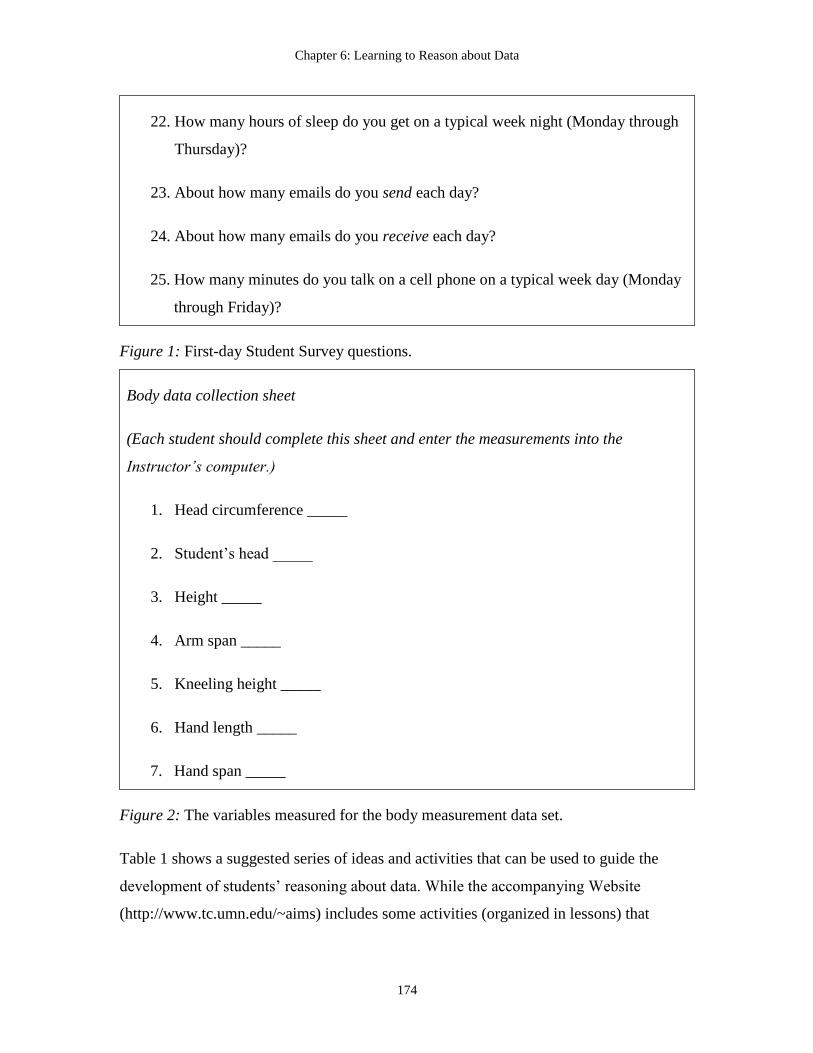
Chapter 6: Learning to Reason about Data
174
22. How many hours of sleep do you get on a typical week night (Monday through
Thursday)?
23. About how many emails do you send each day?
24. About how many emails do you receive each day?
25. How many minutes do you talk on a cell phone on a typical week day (Monday
through Friday)?
Figure 1: First-day Student Survey questions.
Body data collection sheet
(Each student should complete this sheet and enter the measurements into the
Instructor’s computer.)
1. Head circumference _____
2. Student’s head _____
3. Height _____
4. Arm span _____
5. Kneeling height _____
6. Hand length _____
7. Hand span _____
Figure 2: The variables measured for the body measurement data set.
Table 1 shows a suggested series of ideas and activities that can be used to guide the
development of students’ reasoning about data. While the accompanying Website
(http://www.tc.umn.edu/~aims) includes some activities (organized in lessons) that

Chapter 6: Learning to Reason about Data
175
illustrate these steps, many are described more generically. The activities that are not
included in the Website are marked by the symbol .
Table 1: Sequence of activities to develop reasoning about data.
Milestones: Ideas and Concepts Suggested Activities
FORMAL IDEAS OF DATA
Data are values of a variable. Meet and Greet Activity (Lesson 1:
“Data and Variability”)
Measurements produce data. Meet and Greet Activity (Lesson 1)
Data show variability. Meet and Greet Activity (Lesson 1)
Data are numbers with context. Variables on Back Activity (Lesson 1)
There are different kinds of data. Meet and Greet Activity (Lesson 1)
Some variability in data is due to
measurement process.
Meet and Greet, Variables on Back,
and Developing a Class Survey
Activities (Lesson 1)
Importance of taking good
measurements by asking clear
questions.
Developing a Class Survey Activity
(Lesson 1)
It is important to look at multiple
variables (Multivariate data) to better
understand and describe a group.
Developing a Class Survey Activity
(Lesson 1)
Sources of bias in questions. How you Ask a Question Activity
(Lesson 2: “Avoiding Bias”)

Chapter 6: Learning to Reason about Data
176
Importance of asking clear,
unambiguous questions in collection
survey data.
Critiquing the Student Survey Activity
(Lesson 2)
Idea, purpose and importance of
random sampling.
The Gettysburg Address Activity
(Lesson 3: “Random Sampling”)
Different methods and reasons to take
samples.
Student Survey Sampling Activity
(Lesson 3)
Purpose of experiments to produce
data to determine cause and effect.
Taste Test Activity (Lesson 4:
“Randomized Experiments”)
Purpose of randomization in an
experiment.
Taste Test Activity (Lesson 4)
Idea of making an inference based on
a result of an experiment (using
simulation).
Taste Test Activity (Lesson 4)
Importance of randomization in
drawing inferences about results of an
experiment.
Activity involving random
assignment, with introduction to
permutation test to informally test if
results of the experiment are
surprising or due to chance.
(The symbol indicates that this activity
is not included in these lessons.)
Importance of knowing sources of
data: data coming from samples or
from experiments.
Activity where students identify
whether the research is a survey
(observational data) or an experiment.

Chapter 6: Learning to Reason about Data
177
Good data vs. bad data. Activity where students identify
potential sources of bias or
confounding.
What type of conclusions can be
drawn based on the type of data.
Activity identifying the type of
conclusion given a study description.
What kinds of questions to ask about
where data come from.
Activity where students ask
appropriate questions for given sets of
data.
BUILDING ON FORMAL IDEAS OF DATA IN SUBSEQUENT TOPICS
Two sources of variation in
measurement data.
How Big is Your Head Activity
(Lesson 1 in the Variability Unit,
Chapter 10)
Reducing variability in measurement
data.
Gummy Bears Activity (Lesson 2 in
the Comparing Groups Unit, Chapter
11)
Determining cause and effect from an
experiment.
Gummy Bears Revisited Activity
(Lesson 4 in the Statistical Inference
Unit, Chapter 13)
Correlation does not imply causation. Credit Questions Activity (Lesson 1 in
the Covariation Unit, Chapter 14)
Introduction to the Lessons
There are four lessons on collecting and producing data. They begin with types of data
and types of variables and the variability of data. The lessons provide students with
experience using different methods of sampling to develop an appreciation for random

Chapter 6: Learning to Reason about Data
178
sampling and help students understand different sources of variability and bias in data.
Students examine surveys and consider the impact of question wording. They design and
conduct an experiment to illustrate principles of random assignment as well as issues
involved in designing good experiments. The importance of samples and the role of
samples in making inferences are revisited throughout these lessons as a preliminary
introduction to informal ideas of statistical inference.
Lesson 1: Data and Variability
The goal of the first lesson is to help students see that there are different types of data and
different ways to aggregate and display data. This lesson also helps students to see the
importance of context and how statistics differs from mathematics in the emphasis of
context. Student learning goals for this lesson include:
1. To get started with the statistical process of gathering and interpreting data.
2. To see that there are different types of data and that data vary.
3. To see and consider different sources of variability in data.
4. To develop a survey to use to gather data for future activities (student survey).
5. To see that statistics is different from mathematics and that context of the data is
important.
Description of the Lesson
This first class of the course begins with a question about what kinds of students enroll in
this class. That leads into the Meet and Greet Activity, which is described in detail in the
beginning of this chapter. In this activity students informally discuss many important
statistical ideas, such as, methods for data recording, types of variables, types of data,
variation in data, question wording, data summaries and representations, sample of data,
sample represents the population, sample size, bias, and sampling processes.
Chapter 6: Learning to Reason about Data
179
The students then asked to think about other types of information that would be
interesting to gather from members of the class (Developing a Class Survey Activity).
They get into small groups and brainstorm a set of five questions, with the restriction that
these questions collect different kinds of data, so that there is at least one question that
asks for numerical data, one that asks for categorical (nominal) data and one that asks for
yes/no data. Students are encouraged to think of interesting ideas to ask that would
produce data they would care about, so not just “year in school” or “gender”. The
students discuss and create questions that are turned into the instructor, who (before the
next class) compiles and edits them into a class survey that they will complete online.
This final version of the survey includes additional questions added by the instructor,
which will be an important source of data to use in activities on other statistical topics.
A final activity of the first day is to give students an opportunity to reason about data
(Variables on Backs Activity). Students each have a card taped to their back that has a
question on it. Once again, they stand up and walk around the room, this time recording
students’ responses to the question on their back without knowing what the question is.
All the questions are numerical and no units are allowed to be given. Examples of
questions are “how many hours did you sleep last night?”, “How old is our current
president?”, “How many counties are in this state?”, and “what is the last digit of your ID
number?”
After the data are collected, students sit down and look at their data and draw a graph of
their choosing (any graph will do). They use this graph to make a guess about what
question is taped to their back. They take turns standing up, showing their graph to the
class and explaining their reasoning (e.g., “I think my question is how many pets you
have because the data I got have lots of 0s, a few ones, and 2s”). After they have
explained their reasoning, they can take off the card and see what question was actually
taped to their back. The class discussion after this activity involves how students
reasoned about their data, and what they thought about and considered as they
investigated their question.

Chapter 6: Learning to Reason about Data
180
A wrap-up discussion includes comparison of statistics to mathematics, how numbers in
statistics have a context, and the importance of considering the context of data.
Students are also told that this is the kind of activity they will be doing in class: gathering
and analyzing data, and using samples of data to make inferences. It is stressed that data
are the focus of the course, that we strive to collect good data, and that we are interested
in studying the variability in data. They can be asked to summarize why data vary and
sources of variability in data.
Lesson 2: Avoiding Bias
The focus of the second lesson is on helping students understand the idea of biased data
and ways to avoid biased data in question wording and survey administration. Students
suggest and discuss methods of obtaining unbiased data from a survey. Student learning
goals for this lesson include:
1. To recognize common instances of bias resulting from how questions are worded
or by methods or taking surveys.
2. To learn characteristics of good questions that can be answered by data.
3. To see that how you ask a question makes a difference in the quality of data
collected.
Description of the Lesson
Students first see a cartoon that shows a character answering a question on a survey that
illustrates the idea of biased data from a survey and leads to a general discussion about
other factors that can bias survey results, leading to bad data. After an initial discussion of
how and why we take samples, and the use of surveys, students begin the first activity.
Next, in the How you Ask a Question activity, students respond to a set of three questions
to respond to. What they do not know is that there are two different sets of these of
questions, worded in different ways. After the questions are answered, a show of hands is
asked for the answers to each question, and it is clear that students have responded

Chapter 6: Learning to Reason about Data
181
differently. One student is asked to read aloud their question 1, and then a student reads
the other version of question 1. Students are then allowed to see the two sets of questions,
and the data are summarized and compared for the two surveys. A discussion ensues on
wording effects, how the wording of a question makes a difference in how people
respond, the idea of bias in data, and different sources of bias.
This leads into the next activity Critiquing the Student Survey, where students read and
critique the student survey they helped develop on the first day of class and determine if
any of the questions was poorly worded and could lead to biased data. They suggest ways
to improve question wording. (Note: they will take the revised survey online outside of
class). Finally, students work in groups to discuss what kinds of questions might be posed
and answered using the survey data, such as relationship and comparison type questions.
They are encouraged to use the new statistical vocabulary they are learning as they talk
about surveys, samples, populations, and related terms.
A wrap-up discussion summarizes what students have learned about the meaning and
sources of bias in data. They begin to consider ideas of samples in taking surveys, as a
segue to the next day’s topic on types of sampling methods.
Lesson 3: Random Sampling
Lesson 3 focuses on methods of taking samples: why they are important, how to take
good samples, how samples differ from each other, and the importance of random
sampling. Students take what they think is a representative sample using their judgment,
and then compare this to a random sample. They see that non random samples are usually
biased. Student learning goals for this lesson include:
1. To understand reasons for using samples in statistical work.
2. To learn to use the basic vocabulary of sampling and surveys.
3. To understand why good samples are important and how we use samples to make
inferences.
Chapter 6: Learning to Reason about Data
182
4. To understand why we rely on chance rather than our own judgment to pick a
sample.
5. To learn how to take a Simple Random Sample (SRS) and why SRS’s are so
important.
6. To recognize and implement several kinds of probability samples (stratified
random sample, cluster sample, multistage sample, systematic sample).
Description of the Lesson
The lesson begins by asking students to suggest good ways to take a representative
sample of five students from the class, and they discuss methods of obtaining fair and
representative samples for surveys or research purposes. This leads into the Gettysburg
Address activity. Students are shown the famous Gettysburg Address by Abraham
Lincoln and told that statistics are often used in analysis of writing style and to identify
authors of different writings. Their task is to take a good, representative sample of words
from the Gettysburg Address. They do this, and then compute the average word length,
being told that average word length is one statistical characteristics of a writer’s style. A
dot plot of the different sample averages is constructed and examined. The true
population average word length is then compared to this plot, and typically, it is not
anywhere the center of the graph.
Students then take Simple Random Samples of words from the Gettysburg Address,
which is quickly and easily done using Sampling Words Java applet
(http://www.rossmanchance.com/applets/index.html). They can plot distributions of
sample averages and see that these samples are unbiased, and that the true population
mean is in or near the center. They repeat this activity with a larger sample size and see
the effect. A discussion of bias, representative samples, and the effect of sample size is
followed by an activity (Student Survey Sampling) where students discuss how they
would apply different sampling strategies to taking samples of data from students who
have completed the Student Survey.
Lesson 4: Randomized Experiments

Chapter 6: Learning to Reason about Data
183
This final lesson in the Data unit involves carrying out a randomized experiment, and
then considering what is a surprising result. After the randomized experiment is compete
and data are gathered, students run a simulation so that they have a distribution of
possible results under a chance model to compare with their sample, in order to judge if a
particular result is likely to be due to chance, or is too surprising to be attributed to
chance. Student learning goals for this lesson include:
1. To apply the characteristics of a well-defined experiment.
2. To experience the difference between an experiment and an observational study.
3. To learn to recognize instances of confounding in an experiment.
4. To learn the importance of randomization, in randomizing the assignment of
treatments, and how that protects against confounding and makes cause and effect
statements possible.
5. To develop an informal idea of statistical inference, as the extent to which a result
is surprising given a certain claim or theory.
6. To become introduced to and familiar with the Simulation Of Samples Model
(SOS, Figure 3) as a way to represent data in a simulation.
Description of the Lesson
The lesson begins with the students being asked how many of them believe that they can
correctly identify Coke and Pepsi in a blind taste test. They discuss how to determine if
somebody really knows how to distinguish the two or if they are just guessing.
After a discussion about the characteristics of a good experiment and what is needed
(randomization, control, and replication), students are given the details of the experiment
to be performed (Taste Test activity). Those students who think they can identify the
colas become the tasters. A group of students are assigned to pour the tastes in paper
cups, with the order assigned by coin tosses. Another group of students are runners, who
bring the tastes to the tasters, not knowing which is which. The fourth group of students

Chapter 6: Learning to Reason about Data
184
is recorders, who write down what the tasters think each taste is: Coke or Pepsi. The
experiment has 10 trials: each taster has 10 blind tests of the soda. After the data are
collected, the results are analyzed and each student receives a score for their total of
correct identifications.
Next the class discusses how high a score must be to believe that the student really wasn’t
just guessing. The Sampling SIM program is run to simulate what we could expect from
10 trails of this experiment if students really were guessing. They can then compare the
results of the student guesses to this distribution, to see if the result is in the tails
(surprising) and how far in the tails, or in the center (not surprising).
A visual model of the simulation process, adapted from Lane-Getaz (2006), the
Simulation Of Samples (SOS) Model is introduced (see Figure 3). This model is used to
help students understand and distinguish between the statistical model used to generate
the simulation, the sample data generated, and the distribution of sample statistics for
these samples (see Chapter 13 for more detail on this model). The SOS Model is also used
to substrate the process of comparing students’ experimental results to those generated by
a particular model or theory (i.e., what if the student was just guessing).
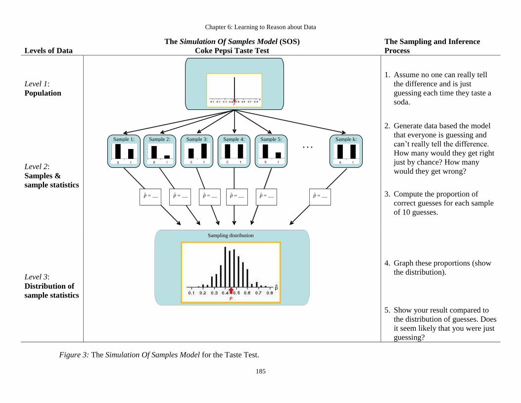
Chapter 6: Learning to Reason about Data
185
Levels of Data
The Simulation Of Samples Model (SOS)
Coke Pepsi Taste Test
The Sampling and Inference
Process
Level 1:
Population
1. Assume no one can really tell
the difference and is just
guessing each time they taste a
soda.
Level 2:
Samples &
sample statistics
2. Generate data based the model
that everyone is guessing and
can’t really tell the difference.
How many would they get right
just by chance? How many
would they get wrong?
3. Compute the proportion of
correct guesses for each sample
of 10 guesses.
Level 3:
Distribution of
sample statistics
4. Graph these proportions (show
the distribution).
5. Show your result compared to
the distribution of guesses. Does
it seem likely that you were just
guessing?
Figure 3: The Simulation Of Samples Model for the Taste Test.
Sampling distribution
… Sample 1: Sample 2: Sample 3: Sample 4: Sample 5: Sample k:
__ˆ p
__ˆ p
__ˆ p
__ˆ p
__ˆ p
__ˆ p

Chapter 6: Learning to Reason about Data
186
Summary
The four sample lessons in the Data unit help students realize the importance of data and
data collection methods in statistics. The class survey that students help to design was
used to collect data that will be analyzed in several subsequent lessons and introduces the
importance of a multivariate data set. The ideas of sources of data, data collection
methods, measurement issues, and variability of data will be revisited and emphasized
again in many of the subsequent lessons. Finally, the importance of randomization and
the use of simulation to make an inference about a surprising result are introduced.

187
Chapter 7: Learning to Reason about Statistical Models and Modeling
One of the most overworked words in statistics education and mathematics
education is “model”. Appearing in a variety of dissimilar contexts, its usage
is at best unclear, and at worst, inappropriate. (Graham, 2006; p. 194)
Snapshot of a Research-based Activity
Class begins with a discussion about the “One-son policy” that was proposed for families
in China to keep the birth rate down but to allow each family to have a son. This policy
allowed a family to keep having children until a son was born, at which point no more
children were allowed. Students are asked to speculate about what would happen to the
ratio of boys to girls if this policy was introduced and about what they would predict the
average family size to be. Most students think that this policy would result in more boys
or a higher ratio of boys to girls. Others think it might result in more girls, because a
family might have several girls before they have a boy. Some students think that the
average number of children might also increase under this policy.
After students make and explain their conjectures, they discuss how to model this process
so that they can simulate data to estimate what would be the ratio of boys to girls and
average family size if the One Son Policy were implemented. First students are
introduced to the idea of making small tokens labeled ‘Boy’ and ‘Girl’ to model the
problem. They are guided to put equal numbers of these tokens in a container, assuming
boy and girl babies are equally likely. The students then draw from tokens, one at a time
from the container with replacement, writing down the outcomes, for example, B, GB, B,
GGGB, etc.
The students are asked to consider other ways that they might model this problem and
generate data, without labeling tokens ‘Girl’ and ‘Boy’, and use a coin. A suggestion is
made to simulate data by tossing coins, with a Head representing a Girl and a Tail
representing a Boy. The students discuss their assumptions for this simulation, such as,
assuming the coin tosses are equally likely to land Tails up or Heads up, and that the

Chapter 7: Learning to Reason about Statistical Models and Modeling
188
result is unpredictable, a random outcome. Preliminary data are gathered and examined,
and students are surprised to see that the ratio of boys to girls is close to 1 and that the
average family size is smaller than predicted. They predict what they think would happen
if more data are gathered.
Students are then guided to use the Fathom software (Key Curriculum Press, 2006) to
simulate larger data sets to answer this question. They discuss the appropriateness of the
coins and Fathom simulations for modeling birth rates, and students bring in their own
knowledge of boys being more likely to be born than girls, so that it is not exactly 50%
boys and 50% girls. However, they note that the coin model was helpful in providing data
that approximates real results and helps estimate an answer to the original questions about
what would happen if the One-Son Policy were adopted. The students also see that it can
be easier to simulate data by finding a useful model than to try to work out a complex
probability problem.
Rationale for This Activity
The One-Son Modeling activity can take place on early in a class, even on the second day
(after the first lesson plan for the topic of Data, from chapter 6). We have introduced it
this early in a course because of the importance of introducing the ideas of random
outcome, model, and simulation. These ideas are interconnected and nicely illustrated in
this first activity. The students can see that the results of a coin toss are random but that
repeated tosses yield predictable patterns (e.g., half Tails, half Heads). They see that coin
tosses can be used as a model for birth rates but that the model is not perfect, just useful.
In other words, students see that statistical models can be useful for simulating data to
answer real world questions, but they are not perfect fits to reality. They are also exposed
to simulation of data as a way to examine chance phenomena, and this sets the stage for
simulations as a helpful process that is used throughout the course. The research basis for
this activity comes from some of the research on understanding models and modeling
described in this chapter that suggests the need for students to create simple models for
chance events, and to use chance devices such as coins or cards to simulate data before
having a computer produce larger amounts of simulated data. We have added on the

Chapter 7: Learning to Reason about Statistical Models and Modeling
189
importance of using language about models and drawing students’ attention to the fact
that what they are doing is creating a model to represent a problem and using the model
to produce data to solve the problem.
The Importance of Understanding Statistical Models and Modeling
It is the job of statisticians to represent the data taken from the
real world with theoretical models. (Graham, 2006; p. 204)
Statisticians use models in different ways, and some of these uses appear in introductory
statistics courses. Two main uses of statistical models are (see schematic illustration in
Figure 1):
1. Select or design and use appropriate models to simulate data to answer a research
question. Sometimes the model is as simple as a random device, sometimes it
takes the form of a statement (such as a null hypothesis) that is used to generate
data to determine if a particular sample result would be surprising if due to
chance. As George Cobb states: Reject any model that puts your data (the
investigated sample) in its tail (2005). Sometime a data set is used to simulate
(bootstrap) more data, creating a simulated population distribution to use in
making statistical inferences.
2. Fit a statistical model to existing data or data that you have collected through
survey or experiment in order to explain and describe the variability. This may be
as simple as fitting the normal distribution to a data set, particularly when
checking assumptions when using a particular procedure. It may involve fitting a
linear model to a bivariate data set to help describe and explain a relationship
between two variables. In advanced courses, data modeling is an essential
technique used to explore relationships between multiple variables. In all of these
cases we examine the fit of a model to data by looking at deviations of the data
from the model.
Figure 1 shows the commonalities and differences between these two uses of statistical
models as well as their role in the ongoing cycle of statistical investigative work.

Chapter 7: Learning to Reason about Statistical Models and Modeling
190
Figure 1: Uses of models in statistical analysis.
Why should students in introductory statistics class need to learn about statistical models?
Because models are foundational part of statistical thinking and working with models is a
big element of the real work of statisticians. It is surprising; therefore, that little explicit
attention is paid to the use of models in most introductory courses. The words “model” or
“modeling” hardly appears in most introductory statistical textbook. When these words

Chapter 7: Learning to Reason about Statistical Models and Modeling
191
are used, it is often in the context of a linear model for bivariate data or the normal
distribution as a mathematical model. Sometimes the term is used in connection with
probability, as in probability models. Although many statisticians talk about the
importance of data modeling and fitting models to data, most students can take an
introductory statistics course and never understand what a statistical model is or how it is
used.
The models statisticians use are actually mathematical models. David Moore (1990)
describes the role of mathematical models in the data analysis process: “Move from
graphic display to numerical measures of specific aspects of the data to compact
mathematical models for the overall pattern” (Page 104). The two most commonly used
mathematical models in an introductory statistics class are the normal distribution and the
linear regression model. Although these two topics involve the use of mathematical
models that are fitted to sample data, students rarely see these topics as related, or as
examples of two different kinds of statistical models that help us analyze data.
The normal curve, which is perfectly symmetric and does not reflect the irregularities of a
data set, is an idealized model that nicely fits many distributions of real data, such as
measurements and test scores. Moore (1990) comments that moving from observations of
data to an idealized description (model) is a substantial abstraction, and the use of models
such as the normal distribution and the uniform distribution is a major step in
understanding the power of statistics. Some software packages, such as Fathom, allow
students to superimpose a model of the normal distribution on a data set. This feature
helps students judge the degree of how well the model fits the data and develops students’
understanding of the model fitting process.
The Place of Statistical Models and Modeling in the Curriculum
We find the lack of explicit attention to statistical models (other than probability models,
in a mathematical statistics class) surprising. While there are examples of ways to model
probability problems using concrete materials and or simulation tools (see Simon, 1994,
Konold, 1993) these do not appear to be part of most introductory statistics classes, and
do not appear to be part of an introduction to the use of models and modeling in statistics.
Chapter 7: Learning to Reason about Statistical Models and Modeling
192
We have thought carefully about how to incorporate lessons on statistical models and
modeling into an introductory course. Rather than treat this topic as a separate unit, we
think that activities that help students develop an understanding of the idea and uses of a
statistical model should be embedded throughout the course, with connections made
between these activities.
The One-son Modeling activity described above is a good way to introduce the related
ideas of model, random outcome, and simulation. In the following unit on data (see
Lesson 4, Chapter 6), we revisit the idea of modeling and simulation after students
conduct a taste test and want to compare their results to what they would expect due to
chance or guessing (the null model). The normal distribution is informally introduced as a
model in the unit on distribution (Chapter 8) and revisited in the units on center (Chapter
9), variability (Chapter 10) and comparing groups (Chapter 11). After completing the
topics in data analysis, the topic of probability distribution can be examined as a type of
distribution based on a model. The normal distribution is then introduced as a formal
statistical model (probability distribution) and as a precursor to the sampling unit (this
activity is described in the end of this chapter). The sampling unit (Chapter 12) revisits
the normal distribution as a model for sampling distributions. In the unit on statistical
inference (Chapter 13), models are used to simulate data to test hypotheses and generate
confidence intervals. Here a model is a theoretical population with specified parameters.
Statistical models are used to find P-values if necessary conditions are met. The final
model introduced after the unit on statistical inference is the regression line as a model of
a linear relationship between two quantitative variables (see Chapter 14). This model is
also tested using methods of statistical inference and examining deviations (residuals).
We find that the idea and use of a statistical model is explicitly linked to ideas of
probability and often to the process of simulation. Therefore, we briefly discuss these
related topics as well in this chapter.
Review of the Literature Related to Reasoning about Statistical Models and
Modeling

Chapter 7: Learning to Reason about Statistical Models and Modeling
193
All models are wrong, but some are useful.
George Box (1979, p. 202)
Models in Mathematics Education
Several researchers in mathematics education have applied mathematical modeling ideas
to data analysis (e.g., Horvath & Lehrer, 1998). Lehrer and Schauble (2004) tracked the
development of student thinking about natural variation as elementary grade students
learned about distribution in the context of modeling plant growth at the population level.
They found that the data-modeling approach assisted children in coordinating their
understanding of particular cases with an evolving notion of data as an aggregate of
cases. In another study by the same researchers, four forms of models and related
“modeling practices” were identified that relate to developing model-based reasoning in
young students (Lehrer & Schauble, 2000). They found that studying students’ data
modeling, in the sense of the inquiry cycle, provided feedback about student thinking that
can guide teaching decisions, an important dividend for improving professional practice.
A related instructional design heuristic called “emergent modeling” is discussed by
Gravemeijer (2002) that provides an instructional sequence on data analysis as an
example. The “emergent modeling” approach was an alternative to instructional
approaches that focus on teaching ready-made representations. Within the “emergent
modeling” perspective, the model and the situation modeled are mutually constituted in
the course of modeling activity. This gives the label “emergent” a dual meaning. It refers
to both the process by which models emerge and the process by which these models
support the emergence of more formal mathematical knowledge.
Models in Statistical Thinking
Statisticians … have a choice of whether to access their data from the
real world or from a model of the real world. (Graham, 2006; p. 204)
How students understand and reason about models and modeling processes have received
surprisingly little attention in statistics education literature. This is surprising since
statistical models play an important part in statistical thinking. The quote by Box, “All

Chapter 7: Learning to Reason about Statistical Models and Modeling
194
models are wrong, but some are useful” (1979, p. 202), is a guiding principle in
formulating and interpreting statistical models, acknowledging that they are ideal and
rarely match precisely real life data. The usefulness of a statistical model is dependant on
the extent that a model is helpful in explaining the variability in the data.
Statistical models have an important role in the foundations of statistical thinking. This is
evident in a study of practicing statisticians’ ways of thinking (Wild & Pfannkuch, 1999).
In their proposed four-dimensional framework for statistical thinking, “reasoning with
statistical models” is considered as a general type of thinking, as well as specific
“statistical” type of thinking, which relates, for example, to measuring and modeling
variability for the purpose of prediction, explanation, or control. The predominant
statistical models are those developed for the analysis of data.
While the term “statistical models” is often interpreted as meaning regression models or
time-series models, Wild and Pfannkuch (1999) consider even much simpler tools such as
statistical graphs as statistical models since they are statistical ways of representing and
thinking about reality. These models enable us to summarize data in multiple ways
depending on the nature of the data. For example, graphs, centers, spreads, clusters,
outliers, residuals, confidence intervals, and P-values are read, interpreted, and reasoned
with in an attempt to find evidence on which to base a judgment.
Moore (1999) describes the role of models to describe a pattern in data analysis as the
final step in a four-stage process.
When you first examine a set of data, (1) begin by graphing the data and
interpreting what you see; (2) look for overall patterns and for striking deviations
from those patterns, and seek explanations in the problem context; (3) based on
examination of the data, choose appropriate numerical descriptions of specific
aspects; (4) if the overall pattern is sufficiently regular, seek a compact
mathematical model for that pattern (p. 251).
Mallows (1998) claims that too often students studying statistics start from a particular
model, assuming the model is correct, rather than learning to choose and fit models to

Chapter 7: Learning to Reason about Statistical Models and Modeling
195
data. Wild and Pfannkuch (1999) add that we do not teach enough of the mapping
between the context and the models. Chance (2002) points out that particularly in courses
for beginning students, these issues are quite relevant and often more of interest to the
student, and the “natural inclination to question studies should be rewarded and further
developed.”
Reasoning about a Statistical Model: Normal Distribution
There is little research investigating students’ understanding of the normal distribution,
and most of these studies examine isolated aspects in the understanding of this concept.
The first pioneering work was carried out by Piaget and Inhelder (1951), who studied
children’s spontaneous development of the idea of stochastic convergence. The authors
analyzed children’s perception of the progressive regularity in the pattern of sand falling
through a small hole (in the Galton apparatus or in a sand clock). They considered that
children need to grasp the symmetry of all the possible sand paths falling through the
hole, the probability equivalence between the symmetrical trajectory, the spread and the
role of replication, before they are able to predict the final regularity that produces a bell-
shaped (normal) distribution. This understanding takes place in the “formal operations”
stage (13- to 14-year-olds).
In a study of college students’ conceptions about normal standard scores, Huck, Cross,
and Clark (1986) identified two misconceptions: On the one hand, some students believe
that all standard scores will always range between –3 and +3, while other students think
there is no restriction on the maximum and minimum values in these scores. Others have
examined people’s behavior when solving problems involving the normal distribution
(Wilensky, 1995, 1997). In interviews with students and professionals with statistical
knowledge, Wilensky asked them to solve a problem by using computer simulation.
Although most subjects in his research could solve problems related to the normal
distribution, they were unable to justify the use of the normal distribution instead of
another concept or distribution, and showed a high “epistemological anxiety”, the feeling
of confusion and indecision that students experience when faced with the different paths
for solving a problem.

Chapter 7: Learning to Reason about Statistical Models and Modeling
196
In recent empirical research on understanding the normal distribution, Batanero, Tauber,
and Sánchez (2004) studied students' reasoning about the normal distribution in a
university-level introductory computer-assisted course. While the analysis suggests that
many students were able to correctly identify several elements in the meaning of normal
distribution and to relate one to another, numerous difficulties understanding normal
distributions were identified and described. The main conclusion in this study is that the
normal distribution is a very complex idea that requires the integration and relation of
many different statistical concepts and ideas. The authors recommend the use of
appropriate activities and computer tools to facilitate the learning of basic notions about
normal distributions (see causeweb.org for some of these resources).
Understanding Ideas Related to Probability Models
The research reviewed in Chapter 2 along with literature reviews by Falk and Konold
(1998), Shaughnessy (2003), Jones (2005) and others illustrate the conceptual difficulties
students have in understanding basic ideas of probability such as randomness. For
example, Falk & Konold, (1994, 1997) found that people attempting to generate random
number sequences usually produce more alternations of heads and tails than expected by
chance. A related research result is that students tend to think that all models of random
events are ones with equally likely outcomes. Lecoutre (1992) refers to this
misconception as the “equiprobability bias”, which she found students to use in solving
different types of probability problems.
Reasoning About the Use of Models to Simulate Data
Studies on the use of simulations cover many different topics, such as how students and
teachers understand statistical models in simulating data (e.g., Sanchez, 2002), the use of
simulation to illustrate abstract concepts such as sampling distributions (e.g., Saldanha &
Thompson, 2002), learning to formulate and evaluate inferences by simulating data (e.g.,
Stohl & Tarr, 2002). While there is a strong belief that physical simulations should
precede computer simulations, this has not yet been a topic of empirical study. Helpful
guidelines for secondary school students on how to select models to simulate problems

Chapter 7: Learning to Reason about Statistical Models and Modeling
197
are included in the Art and Techniques of Simulation – a volume in the Quantitative
Literacy Series (Gnanadesikan, Scheaffer, & Swift, 1987).
Biehler (1991) has presented an extensive analysis of the capabilities and limitations of
simulation techniques in teaching statistics; he points out that “the different roles, goals
and pedagogical perspectives for simulations have not yet been clearly analyzed and
distinguished.” He suggests a basic distinction between “the use of simulating as a
method for solving problems, similar to the professional use outside school and the use of
simulation to provide model environments to explore, which compensate for the ‘lack of
experience’” (p. 183).
To study teachers’ opinions about the instructional use of models in simulating data,
Sanchez (2002) interviewed six high school teachers who participated in a workshop of
simulation activities using Fathom. The analysis of their responses included four general
aspects: the role of simulation in teaching; the different steps to follow in a simulation;
the complexity of starting situations; and the statistical concepts which take part in
simulation activities. The results show that teachers deem as important only certain
aspects of simulation but neglect the fundamental concepts of randomness and
distribution. Sanchez noted that the teachers have centered their attention in certain
modeling aspects like formulation of a model and its simulation but neglected other
aspects like the analysis of results and the validation of the model.
Implications of the Research:
Teaching Students to Reason about Statistical Models and Modeling
Other than some literature on reasoning about the normal distribution or a linear
relationship in bivariate data, there is little research illuminating how students come to
learn and use statistical models. Therefore, we are speculative in putting together a
research-based sequence of activities for this topic.
The literature reviewed implies that it is important to make models an explicit topic in the
introductory statistics course and to help students develop this idea and its multiple
meanings and uses through experiences with real statistical problems and data, rather than
Chapter 7: Learning to Reason about Statistical Models and Modeling
198
through a formal study of probability. The literature also suggests that understanding the
idea of randomness is difficult and that carefully designed activities should be used to
help students understand the ideas of random outcomes, random variables, random
sampling, and randomization.
There are also implications from the literature about the role of probability in an
introductory college statistics course. It is suggested that in order for students to develop
a basic understanding of statistics in a first college course, that they only need the basic
ideas of probability that were introduced above. As Garfield and Ahlgren wrote in 1988
“useful ideas of inference can be taught independently of technically correct probability.”
Therefore, we propose helping students understand the ideas of random outcomes and a
probability distribution. They do not need to learn the language and laws of probability in
such a course. Indeed, research shows that even if students encounter these topics in
probability in an introductory statistics course, few students understand and can reason
about this topic (see reviews by Garfield & Ahlgren, 1988; Hawkins & Kapadia, 1984;
Shaughnessy, 2003).
We agree with David Moore’s (1997) claim that mathematical probability is a “noble and
useful subject” and should be part of the advanced coursework in statistics, and instead of
being part of the introductory course, should be learned in a separate course that is
devoted to this topic. The literature also implies that in order to develop a deep
understanding of the basic ideas outlined in Chapter 3, the traditional course should be
streamlined. Following the lead of Moore (1997), our candidate for the guillotine is
formal probability. Moore recommends that an informal introduction to probability is all
that is needed and that this begin with experience with chance behavior usually starting
with physical devices and moving to computer simulations that help demonstrate the
fundamental ideas such as the Law of Large Numbers.
Technological Tools to Help Students Develop Reasoning about Models
Many Web applets are available to help students see and use the normal distribution (e.g.,
http://www.rossmanchance.com/applets/NormalCalcs/NormalCalculations.html) and fit a
line to data (e.g., http://www.math.csusb.edu/faculty/stanton/m262/regress/regress.html).
Chapter 7: Learning to Reason about Statistical Models and Modeling
199
Applets can also be used to simulate data for a probability problem (see
rossmanchance.com). The simulation tool Probability Explorer (Stohl, 1999-2005;
http://www.probexplorer.com/) enables school students and teachers to design, simulate,
and analyze a variety of probabilistic situations. Model Chance is a new program that is
now being developed as part of the TinkerPlots project, to help student model problems
and simulate data to estimate answers to these problems
(http://cts.stat.ucla.edu/projects/info.php?id=4).
Progression of Ideas: Teaching Students to Reason about Statistical Models and
Modeling
Introduction to a Sequence of Activities to Develop Reasoning about Statistical Models
and Modeling
While most textbook do not introduce the term “model” until the normal distribution and
may not use it again until regression, we believe that the term should be introduced early
in a course and used frequently, to demonstrate and explain how models are used in
statistical work. Since there is no empirical research on an optimal approach for helping
students develop the idea of model in an introductory statistics class, we offer one of
several possible sequences of activities that we have found useful in our courses. These
activities develop the idea of a model to simulate data, and the idea of a model to fit to a
given set of data.
We believe that the idea of a model can be presented informally in the first few days of
class using a fairly simple context. Physical simulations using devices such as coins can
be used to model a random variable as part of solving a problem, and once data have been
simulated using coin tosses, the computer can be used to quickly produce large amounts
of simulated data. It is important that students be made aware of the use of a model, to
represent key features of the event and to produce simulated data.
In the Taste Test activity in the Data topic (see Chapter 6) when the notion of an
experiment is introduced, the idea of a null model (what would happen if results were
only due to chance) can be reintroduced. In this context the model is used to simulate data

Chapter 7: Learning to Reason about Statistical Models and Modeling
200
to informally determine a P-value, indicating whether or not an individual’s identification
of soda brand in a blind taste test may not just be due to chance. The formal idea of
model may be encountered in the context of random variables. Students can model
random outcomes such as coin tosses, dice throwing, and drawing of cards. Each time
students can describe the model (e.g., for a standard deck of Poker cards, where the
outcome is a Heart, this can be modeled as a binomial variable with a probability of ¼).
These models can be used to simulate data, which leads to examining probability
distributions. Different probability problems can also be modeled first using coins or
dice, and then using applets or software to simulate data. In this case, the problem is
modeled by the coins or dice, and then this model is replicated by a technology tool.
After generating empirical probability distributions for binomial random variables, the
probability distribution for the normal distribution can be introduced, as a model that is
often used to describe and interpret real data. This model is seen again as students begin
to examine distributions of sample means and the Central Limit Theorem. Null models
are encountered again in the unit of inference to generate distributions of sample statistics
to run tests of significance. In our proposed sequence of activities, the final model
presented is that of the linear model, used in the unit on covariation, to model the
relationship of two quantitative variables.
What is unique about the lessons in this chapter is that unlike all the other chapters in part
II of this book, we are not offering a unit on models but rather providing several activities
that illustrate and use the idea of statistical models and throughout an introductory course.
While the informal ideas of model are introduced at the beginning of a course, the formal
ideas are encountered midway through the course, and then revisited at additional times
in other topic areas, rather than in set of sequential lessons in a unit of their own.
Table 1: Sequence of activities to develop reasoning about statistical models and
modeling.
Milestones: Ideas and Concepts Suggested Activities
INFOROMAL IDEAS PRIOR TO FORMAL STUDY OF STATISTICAL MODELS

Chapter 7: Learning to Reason about Statistical Models and Modeling
201
Models can be used to portray simple
random outcomes. Random devices
and computers can be used to simulate
data to answer a question about this
context.
One-Son Modeling Activity (Lesson
1: “Using Models to Simulate Data”)
A random outcome, unpredictable, but
giving a predictable pattern over the
long run. The more data, the more
stable the pattern.
Let’s Make a Deal Simulation (Lesson
1)
Designing and using a model can help
to answer a statistical question.
Let’s Make a Deal Simulation (Lesson
1)
The idea and importance of random
samples (revealing the predictable
pattern of random outcomes).
The Gettysburg Address Activity
(Lesson 3, Data Unit, Chapter 6)
Models can be used to generate data to
informally test an experimental result
to provide evidence about whether or
not this result is due to chance.
Taste Test Activity (Lesson 4, Data
Unit, Chapter 6)
Distinguish between the model, the
simulated data, and the sample data.
Taste Test Activity (Lesson 4, Data
Unit, Chapter 6)
The normal distribution as a model for
some distributions of real world data.
Sorting Histograms Activity (Lesson
2, Distribution Unit, Chapter 8)
The mean is a good summary of the
center of a normal distribution.
Choosing an Appropriate Measure of
Center Activity (Lesson 2, Center
Unit, Chapter 9)

Chapter 7: Learning to Reason about Statistical Models and Modeling
202
The mean and standard deviation are
good summaries for a normal
distribution.
How do Students Spend their Time
Activity (Lesson 4, Comparing
Groups Unit, Chapter 11)
FORMAL IDEAS OF STATISTICAL MODELS
Random variables and random
outcomes.
Coins, Cards, and Dice Activity
(Lesson 2: “Modeling Random
Variables”)
Equally likely model does not fit all
random outcomes.
Coins, Cards, and Dice Activity
(Lesson 2)
A probability distribution as a model. Coins, Cards, and Dice Activity
(Lesson 2)
Probability problems can be modeled
using random devices and simulation
tools.
Activity where cards are used to
model a problem, such as Random
Babies activity in Chance and
Rossman (2006b).
(The symbol indicates that this activity
is not included in these lessons.)
Characteristics of normal distribution
as a model.
What is Normal? (Lesson 3: “The
Normal Distribution as a Model”)
What does normal data look like? What is Normal? (Lesson 3)
Using the normal distribution as a
Model.
Normal Distribution Applications
(Lesson 3)
BUILDING ON FORMAL IDEAS OF MODELS IN SUBSEQUENT TOPICS

Chapter 7: Learning to Reason about Statistical Models and Modeling
203
How and why the sampling
distribution of means can be modeled
by the normal distribution.
Central Limit Theorem Activity
(Lesson 3, Samples and Sampling
Unit, Chapter 12)
The null hypothesis as model to which
we compare sample data.
Balancing Coins Activity (Lesson 1,
Statistical Inference Unit, Chapter 13).
When testing a hypothesis, it is often
important to check the condition of
normality of the sampling distribution.
Research Questions Involving
Statistical Methods (Lesson 5,
Statistical Inference Unit, Chapter 13).
The regression line is a useful a model
of bivariate relationship between
quantitative variables.
Diamond Rings Activity (Lesson 2,
Covariation Unit, Chapter 14)
Checking the fit of a model to data, by
examining residuals from a regression
line.
da Vinci and Body Measurements
Activity (Lesson 2, Covariation Unit,
Chapter 14)
Introduction to the Lessons
Three lessons are designed to help students develop an understanding of the importance
and use of statistical models. Other activities involving models are interspersed
throughout other topics in this book. The first lesson has student model birth outcomes in
a situation where there is a “one-son policy”. A probability model is used to simulate data
that is summarized to answer some research questions. The second activity in this lesson
has students uses first a physical and then a computer simulation to model the “Let’s
Make a Deal” game, using the simulated data to find the best strategy for playing the
game. The second lesson has students create binomial models for different random
devices (coins, dice and cards) and use these to generate and then simulate data (on the
computer) to examine and compare probability distributions (each having a different
shape and expected value). The third lesson introduces the normal distribution as a model
of a probability distribution. This model is used to fit to samples of data (e.g., do the data
Chapter 7: Learning to Reason about Statistical Models and Modeling
204
sets appear to have a normal distribution?) and to demonstrate when it is appropriate to
use this model in analyzing data.
Lesson 1: Choosing Models to Simulate Data
The first lesson begins with the One-Son Modeling activity described at the beginning of
this chapter. Next students consider the chances of wining on the game show Let’s Make
a Deal to determine whether one strategy has a higher chance of wining than another,
modeling the game first with cards and then with a Web applet. The Student learning
goals for this lesson include:
1. Be able to use simulation as a tool for answering statistical questions
2. Be able to develop models to simulate data
3. Examine probability as an indication of how likely is an event to happen.
4. Realize that their intuitions about probabilities may be misleading.
Description of the Lessons
The students are told about the “One-Son policy” that was proposed for China as a way to
decrease their birthrate but still allow families to produce a son.
In the early 1990’s China considered adopting a “one son” policy, to help reduce
their birthrate by allowing families to keep having children until they had a son.
Under this plan a family has a child. If it is a son, they stop having children. If it
is a daughter, they can try again. They can keep trying until they have a son and
then they stop having children.
The following questions are posed to students to engage them in reasoning:
1. If a country adopted a policy that let families have children only until they had a
boy, and then they had to stop, what would you expect to happen?

Chapter 7: Learning to Reason about Statistical Models and Modeling
205
2. What would the average number of children per family be? Would you expect
more boys or more girls overall?
Students present their answers and reasoning. Simulation is introduced as a tool
statisticians use to generate data to estimate an answer to this type of question.
Working in pairs, students take a yogurt container that contains two slips of paper. One is
labeled ‘B’ for boys. One is labeled ‘G’ for Girls. They randomly draw one slip of paper
from the container and that will be the first child born in a simulated family. If they draw
a ‘B’, then they are told to stop; the family is done having children. They enter the data
on a chart indicating the result for the first family. If the result is a ‘G’, they draw again.
They keep drawing until they draw a ‘B’, then they stop and enter the data on the chart
for that family. Students repeat this process for five simulated families, getting results
such as: GB, B, GGB, B, GB, etc.
After this first round of simulated data is collected, the number of children in each family
is counted along with the number of girls and the number of boys. Students examine this
small set of data and are asked if the results confirm their original predictions. Next they
consider what they would get if they did not have slips of paper but instead only had a
coin. Students figure out how to do this same simulation using only one coin that is
tossed. They discuss and write out the process so that another group could run the
simulation by following their directions. Students usually determine that one outcome
(heads) will represent a Boy and the other outcome will represent a Girl. They describe
how to repeatedly toss a coin until it lands heads, recording the data each time to simulate
families. Next they simulate this data using the coin, generating data for five more
families.
Now student groups have data for 10 simulated families based on the two sets of
simulations. They tally the total number of girls, the total number of boys, find the ratio
of boys to girls, and find the average number of children per family. Again, they compare
these results to their initial conjectures. These results are also shared with the class and
graphed on the board.

Chapter 7: Learning to Reason about Statistical Models and Modeling
206
Next students are asked what they would expect to find if they repeated this simulation
many more times. They are shown how to use the Fathom to run this simulation and to
gather data for more simulated families, as shown in Figure 2.
Figure 2: Running the One-Son Simulation in Fathom.
A discussion of these data reveals that the results tend to stabilize as more data are
collected. Students are asked what they would expect if more data were generated, and
this leads to an informal discussion of the Law of Large Numbers. Next, a discussion of
choosing models to simulate data leads students to consider real life factors to consider
using a coin or an equally likely binomial model to simulate births. They suggest ways in
which the model of equally likely outcomes may not perfectly fit the data, such as the fact
that the probability of having a boy is actually more than .5. They consider how these
factors could affect simulated results. A wrap-up discussion includes issues involved in
selecting and using models (first the coin, and then the computer simulation of a binomial
model with p=.5) to simulate a real world phenomenon (birth rates of boys and girls).
Students are next introduced to an activity (Let’s Make a Deal Simulation) where they
will check their intuitions about chance events by using simulation to determine

Chapter 7: Learning to Reason about Statistical Models and Modeling
207
probabilities in a game show setting. Let's Make A Deal is introduced as a popular TV
game show from the 1970s.
The task: Suppose you are given three doors to choose from. Behind one door there is a
big prize (a car) and behind the other two, there are goats. Only Monty Hall knows which
door has the prize. You are asked to select a door, and then Monty opens a different door,
showing you a goat behind it. Then you are asked the big question: Do you want to stay
with your original door, or switch to a different door? What would you do?
Students discuss in small groups whether they think there is a higher chance of winning
the prize if they stay with their first door selection or should they switch to the remaining
door and why. A show of hands in the class indicates that most students think that either
the contestant should stay with the first choice or that it does not make a difference;
staying or switching are equally likely to result in winning a prize.
Next, students think about how they could test these conjecture. They design a simulated
game using index cards. Each group is given three index cards, and they write lightly on
each one of the following outcomes: ‘Goat’, ‘Goat’, and ‘Car’. One person is the game
host (Monty Hall) and knows where the car is when the cards placed face down in order.
The other group members take turns being contestants. A recording sheet is used to write
down what strategy was used each time (stay or switch doors) and what the outcome was
(‘Win’ or ‘Lose’). After a few rounds the data are pooled for the class, and it appears that
“switch” is resulting in more wins. But is that just due to chance or a stable result?
Students then use a Web applet that simulates this problem to quickly simulate large
amounts of data, revealing that the chance of winning when they switch doors is about
2/3, and the chance of winning when they stay with their first choice about 1/3. Students
are asked about the correctness of their original intuitions and why they were incorrect. A
quick explanation may be given about why this happens, or students may be given a
written explanation about why it pays to switch doors when playing this game.
The Let’s Make a Deal Simulation activity concludes with a discussion about the use of
models and simulations to easily generate data to estimate answers to statistical questions,
Chapter 7: Learning to Reason about Statistical Models and Modeling
208
and when to trust results of simulations (e.g., when the model is a good fit to the problem
and when there are enough simulations to generate a stable result).
Lesson 2: Modeling Random Variables
This lesson engages students with modeling random variables using coins, cards, and
dice. Students construct probability distributions to represent each of the scenarios and
make predictions on probabilities of other events based on these histograms. They first
generate data with concrete materials and then move to Fathom to simulate larger data
sets and see the stable trend emerge. Student learning goals for this lesson include:
1. Understand use of models to represent random variables and simulate data.
2. Understand how to interpret visual representations for probability.
3. Use a simulation to generate data to estimate probabilities
4. Gain an informal understanding of probability distributions as a distribution with
shape, center and spread.
Description of the Lesson
Students begin by considering different random devises they have encountered, such as
coins, cards, and dice (the Coins, Cards, and Dice activity). Then they make conjectures
about the expected number of:
Heads on five tosses of a fair coin?
Hearts in five draws from a poker deck?
Twos in five rolls of a fair die?
They then reason about what is the same and what is different about these three
experiments. Next, students are led to define three random variables as follows:
X: Number of heads in five tosses
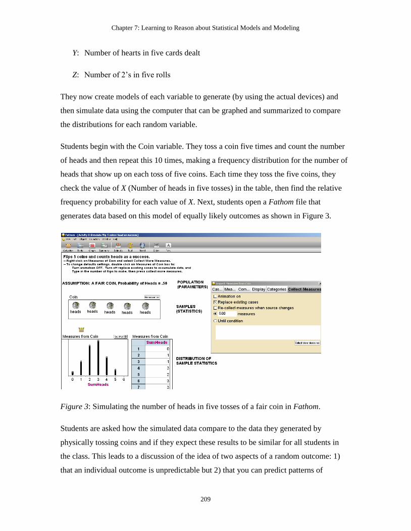
Chapter 7: Learning to Reason about Statistical Models and Modeling
209
Y: Number of hearts in five cards dealt
Z: Number of 2’s in five rolls
They now create models of each variable to generate (by using the actual devices) and
then simulate data using the computer that can be graphed and summarized to compare
the distributions for each random variable.
Students begin with the Coin variable. They toss a coin five times and count the number
of heads and then repeat this 10 times, making a frequency distribution for the number of
heads that show up on each toss of five coins. Each time they toss the five coins, they
check the value of X (Number of heads in five tosses) in the table, then find the relative
frequency probability for each value of X. Next, students open a Fathom file that
generates data based on this model of equally likely outcomes as shown in Figure 3.
Figure 3: Simulating the number of heads in five tosses of a fair coin in Fathom.
Students are asked how the simulated data compare to the data they generated by
physically tossing coins and if they expect these results to be similar for all students in
the class. This leads to a discussion of the idea of two aspects of a random outcome: 1)
that an individual outcome is unpredictable but 2) that you can predict patterns of

Chapter 7: Learning to Reason about Statistical Models and Modeling
210
outcomes for many repetitions, such as the proportion of heads for many tosses of a fair
coin. The simulation is repeated for 500 trials, and relative frequencies are found for the
six possible outcomes (0 to 5 heads). Students again discuss whether they think the
results will vary from student to student and see that the larger sample size has much less
variability. They graph the data and informally describe shape, center and spread. They
see that the expected number of heads for five tosses would be 2 to 3 heads, but that
results can vary from 0 to 5 heads. They can generate the mean and standard deviation
and interpret these values for the distribution (see Figure 4).
Center is about 2.5, and range is 0 to 5
Figure 4: The results of simulating the number of heads in five tosses of a fair coin in
Fathom.
The next part of the Coins, Cards, and Dice activity has students take a deck of cards,
shuffle, draw a card, replace it, draw, and replace, five times. They count the number of
hearts that showed up in their sample of five draws (with replacement) A discussion of
the term “replacement” challenges students to reason about why they would replace the
card drawn each time and how that would affect the results of the experiment so it is not
similar to the coin tosses. This is an informal introduction to the idea of independent
events without going into probability theory. Next, students, use Fathom to simulate this
experiment. They discuss what the model will be, that it is no longer one of equally likely
outcomes, but that the chance of getting one heart when randomly drawn from a deck is
now one-fourth. The students run a new simulation based on a binomial model with
Measures from Coin
SumHeads
2.482
1.0954799
S1 = meanS2 = s

Chapter 7: Learning to Reason about Statistical Models and Modeling
211
p=.25, graph the results, and find measures of center and spread, which are different from
those in the Coin exapmple (Figure 5).
Figure 5: The Fathom simulation of the number of hearts in cards.
This activity is repeated a third time for the Dice example. First students roll a dice five
times counting the number of 2’s that show up. They record the data and compare it with
the class. Then they simulate the data on Fathom, first discussing how the model must be
changed, based on the new probability of getting a two, which is one-sixth.
The results of the three experiments are compared. Students consider what was the same
and what was different across the three experiments and how the differences in the
experiments reveal themselves in the histograms of data. The expected value is also
compared for each experiment, as well as where the same value (e.g., 4) appears in each
Chapter 7: Learning to Reason about Statistical Models and Modeling
212
histogram. This can lead to a discussion on how likely this outcome is (or is not) for each
experiment, based on whether it is in the tail of the distribution, a precursor of the P-
value concept.
Lesson 3: The Normal Distribution as a Model
This lesson introduces students to the formal model of the normal distribution. The
characteristics are examined, as students make and test conjectures about whether data
gathered on different variables have a normal distribution. The unique characteristics of
the mean and standard deviation in a normal distribution are used to examine percentages
of data within one, two and three standard deviations of the mean. The idea of the
standard normal z-score is introduced and used to locate different areas of the
distribution, using a Web applet. Student learning goals for this lesson include:
1. Understand and reason about the normal (and standard normal) distribution as a
model
2. Understand and reason about the important characteristics of this distribution,
e.g., the percentages of data within 1, 2 and 3 standard deviations of the mean.
3. Use standard deviations and z-scores to measure variation from the mean.
Description of the Lesson
Students are asked what they think when they hear the word ‘normal’ and how they could
tell if something is not normal. They contrast a normal data value (e.g., body temp of 98.6
F) in different contexts. They discuss how they think statisticians use this word and how
their use is different from everyday use. Note, they have used the term normal curve
informally in the unit on distribution (Chapter 8) when describing the shape of a data set.
In the What is Normal activity, students consider again the body measurements gathered
earlier in the course (for which some may show a symmetric, bell-shaped pattern and
others do not).
Height

Chapter 7: Learning to Reason about Statistical Models and Modeling
213
Hand span
Hand length
Kneeling height
Arm span
Head circumference
The students make conjectures about which of these variables would have data sets that
when graphed appear to have a normal distribution and why they predict those variables
to have a normal distribution. They consider how to test their conjectures, and use
computer to generate graphs in Fathom. Next they select one distribution that looks
approximately normal, to draw a picture of the graph on their handout and label the axes,
the mean and two standard deviations in each direction. Then they mark their own data
value for this measure (e.g., their height) on the graph. They describe the location of their
value in the overall graph as follows: Are you close to center? In the tails? An outlier?
Next students find the z-score for their body measurement for that variable and explain
what this z-score tells about the location of their body measurement relative to the class
mean.
Students are instructed to open a Web applet that gives areas under the curve for a normal
distribution. They use this applet to find the proportion of the distribution that is more
than their value (e.g., what is the proportion of the curve representing values higher than
their height) and then less than their value. Students discuss whether the obtained results
from the applet makes sense to them and why or why not.
Next students find the value that is one standard deviation above the mean and one
standard deviation below the mean. They use the Applet to find the proportion of the
distribution that is between these two values, and then repeat this for two and three
standard deviations above and below the mean.

Chapter 7: Learning to Reason about Statistical Models and Modeling
214
A class discussion focuses on which of the body measurements seemed to be normal and
how they can tell how well the normal model fits a data set. Statisticians fit models to
data, and this is illustrated by drawing a curve over the plot of a data set. Students
consider and discuss how good a fit there is of the model to the data.
Next, Students then reexamine the use of the Web applet. They see that when they found
the proportions of the distribution that were above and below their own data value, it was
from a normal distribution that has the class mean and standard deviation as the class
data. They used the model of the normal curve to estimate proportions. Students see that
it depends on how well the data fit the model and that when they use z-scores to find
percentages (probabilities) using the normal curve, they are using a statistical model. The
use of models to explain describe, estimate, or predict is revisited, recalling the earlier use
of models to simulate births of boys and girls.
In the Normal Distribution Applications activity students apply the use of intervals used
with the normal distribution (i.e., the middle 68%, 95%, 99.7%, referred to as the
Empirical Rule) to real data sets. They explore and discuss when it is appropriate to use
this rule (a model) to describe or make inferences about a particular set of data. They
explore when and how to use the model to solve the problems in context. A last part of
the activity is to see a Fathom demo on “What are Normal Data?”
In a final wrap-up discussion students are given this popular quote by Box, “all models
are wrong, but some are useful” (1979, p. 202) and discuss how this quotation applies to
the normal distribution as a model.
Summary
Models are one of the most important and yet least understood ideas in an introductory
statistics course. This chapter has tried to make the case that the idea of statistical model
should be made explicit and used repeatedly in an introductory statistics course, so that
students become familiar with the importance of models and modeling in statistical work.
We believe that ideas of probability are best introduced in this context, without having to
go into the formal rules and vocabulary that are better saved for a course in mathematical

Chapter 7: Learning to Reason about Statistical Models and Modeling
215
statistics or probability. We also encourage the explicit discussion of how models are
used to simulate data, from informal uses early in the course to formal uses as part of
tests of significance later in the course. When introducing and using the normal
distribution as a model of certain univariate data sets or the regression line as a model of
certain bivariate data sets, we hope instructors will describe the importance and use of
these modes, and fitting models to data, modeling important aspects of both statistical
practice and statistical thinking for the students to see.

216
Chapter 8: Learning to Reason about Distribution
“Statisticians look at variation through a lens which is
‘distribution’.” (Wild, 2006, p. 11).
Snapshot of a Research-based Activity on Distribution
Groups of three to four students are each given an envelope containing 21 different pieces
of paper, each with a different histogram printed on it. Students sort the graphs into piles,
so that the graphs in each pile have a similar shape. After sorting them into the piles (e.g.,
normal/bell-shaped, left-skewed, right-skewed, bimodal, and uniform) students choose
one histogram from each pile that best represents that category, and these selections are
shared and discussed as a class. Students use their own informal language to “name” each
shape: bell-shaped, bunched to one side, like a ski slope, camel humps, flat, etc. These
informal names are matched to the formal statistical terms such as normal, skewed,
bimodal, and uniform. Finally, students consider which terms are characteristics (e.g.,
skewness) that can apply to graphs in more than one category (e.g., a distribution that is
skewed and bimodal) vs. those that can only be labeled by one name (e.g., uniform or
normal distribution).
Rationale for This Activity
Although this activity may seem like a game for elementary school students, the activity
involves some important challenges and learning outcomes for high school and college
students in a first statistics course. First of all, this activity helps students look at
histograms as an entity, rather than as a set of data values and cases, which research has
shown to be a key problem in reasoning about distributions. Secondly, students often fail
to see the general shape of distributions, because of the effects of randomness (the
“noise”); and expect to see perfect shapes like the models given in their textbooks. This
activity helps them see that there are many types of “normal” distributions or skewed
distributions. They learn to look beyond the individual features of the graph and see the
more general or global characteristics. Finally, this activity focuses on the language used

Chapter 8: Learning to Reason about Distribution
217
to describe distributions, which can often be confusing to students. The word “normal” in
statistics refers to a bell-shaped curve that has certain characteristics while in everyday
life it means typical or not unusual. Students can take an informal name of a shape (e.g.,
ski slope for a right-skewed distribution) and map them to the correct statistical labels,
which can then be used to help remind them of the statistical term (e.g., a teacher talking
about a skewed curve can say, “remember it is like a ski slope”).
The Importance of Understanding Distribution
We begin this section with a poignant illustration, offered by Bill Finzer to participants at
the Fourth International Research Forum on Statistical Reasoning, Thinking and Literacy,
the focus of which was on “Reasoning about Distribution” (Makar, 2005)
The Little Prince, by Antoine de Saint-Exupéry (2000) begins with this drawing.
To adults the drawing looked exactly like a hat.
To the child artist who drew it and to the little prince, it was a drawing of a boa that had
eaten an elephant.
If the little prince showed his picture to a statistician he would say: “This represents a
distribution of data.”

Chapter 8: Learning to Reason about Distribution
218
We like this example because it shows how statisticians look at irregular shapes of data
sets and look beyond the details to see a general shape and structure. This is usually a
first step in any data analysis and leads to important questions about the data to be
analyzed, such as: What mechanism or process might have led to this shape? Are there
any values that need to be investigated (e.g., possible outliers)?
A graph of a distribution reveals variation of a quantitative variable. According to Wild
(2006), statisticians respond to the “omnipresence of variability” in data (Cobb & Moore,
1997) by investigating, disentangling and modeling patterns of variation represented by
distributions of data. He suggests that statisticians look at variation through a lens that is
“distribution”.
Students encounter two main types of “distribution” in an introductory statistics class.
The first type is distributions of sample data that students learn to graph, describe, and
interpret. These are empirical distributions of some particular measured quantity. The
second type of distribution encountered is a theoretical one, e.g., normal or binomial
distributions which are actually probability models (Wild, 2006).
Although the two types share many common features (e.g., they can be described in terms
of shape, center and spread) it is important to help students distinguish between them
because of the way in which we use them. The distinction that underlies empirical versus
theoretical distributions relates to variation. When examining an empirical distribution,
the focus is on description and interpretation of the message in the data, and thinking
about what model may fit or explain the variation of the data. Theoretical distributions
are models to fit to data, to help explain, estimate, or make predictions about the
variability of empirical data. Yet, a third type of distribution students encounter in a
statistics course is a distribution made up of sample statistics, which again has both

Chapter 8: Learning to Reason about Distribution
219
empirical and theoretical versions. These sampling distributions are discussed in detail
Chapter 12.
The Place of Distribution in the Curriculum
Empirical distributions are the foundation of students’ work in an introductory statistics
course, either beginning a course or following a unit on collecting and producing data
(experiments and surveys, Chapter 6). This chapter focuses mainly on teaching and
learning issues related to empirical distributions, while Chapters 7 and 12 respectively
also discuss theoretical distributions. In addition, this chapter focuses on understanding a
single distribution, primarily in the form of dotplots and histograms, while Chapter 11
examines these graphs along with boxplots in the comparison of two or more
distributions.
The methods of Exploratory Data Analysis introduced by Tukey (1977) have had a big
impact on the way distributions are taught in today’s courses. Students use many ideas
and tools to explore data and learn to think of data analysis as detective work. Students
usually learn multiple ways to graph data sets by hand and on the computer. These
methods include dotplots (also called line plots), stem and leaf plots, histograms, and
boxplots. Students learn that different graphs of a data set reveal different characteristics
of the data. For example, a histogram or dotplot give a better idea of the shape of a data
set, while a box plot is often better at revealing an outlier. A stem-and-leaf plot or dotplot
may give a better idea of where there are clumps or gaps in the distribution.
Current statistical software programs (e.g., TinkerPlots, Fathom) allow students to easily
manipulate data representations, for example, to transform one graph of a data set to
another, display several interlinked graphs of the same data set on one screen (a change in
one will show in the others), and some allow students to highlight particular data values
and see where they are located in each graph. These explorations are used to ask
questions about the data: What causes gaps and clusters? Are outliers real data values or
errors in data collection or coding? What factors may help explain the features revealed
in a graph of a distribution? In most introductory courses along with learning how to
graph distributions of data, students are taught to look for specific features of

Chapter 8: Learning to Reason about Distribution
220
distributions and begin to describe them informally (e.g., estimate center and range) and
then more formally (e.g., shape, center, and spread).
Distribution is one of the most important “big ideas” in a statistics class. Rather than
introduce this idea early in a class and then leave it behind, today’s more innovative
curriculum and courses have students constantly revisit and discuss graphical
representations of data, before any data analysis or inferential procedure. In a similar
vein, the ideas of distributions having characteristics of shape, center, and spread can be
revisited when students encounter theoretical distributions and sampling distributions
later in the statistics course.
Review of the Literature Related to Reasoning about Distribution
The research literature provides a strong case that understanding of distributions, even in
the simplest forms, is much more complex and difficult than many statistics teachers
believe. Although little of the research includes college students, the results of studies on
pre-college level students and pre-college level teachers demonstrate the difficulty of
learning this concept, some common misconceptions, and incomplete or shallow
understandings that we believe also apply to college students.
Much of the research on distribution emerged because of the consensus in the statistics
education community that it is a basic building block for a web of key statistical ideas,
such as variability, sampling, and inference (e.g., Garfield & Ben-Zvi, 2004). Other
studies (e.g., Reading & Shaughnessy, 2004; Watson, 2004) focused on broader questions
than how students reason about distribution but yielded relevant results. For example,
Chance, delMas and Garfield (2004) assert that the knowledge of distribution and
understanding of histograms are necessary prerequisites to learning and understanding
sampling distributions.
Developing an Aggregate View of Distribution
A major outcome of several studies on how students solve statistical problems is that they
tend not to see a data set (statistical distribution) as aggregate but rather as individual
values (e.g., Hancock, Kaput, & Goldsmith, 1992). Students need to make a major

Chapter 8: Learning to Reason about Distribution
221
conceptual leap to move from seeing data as a group of individuals – each with its own
characteristics – to seeing the data as an aggregate, a group with emergent properties that
often are not evident in any individual member (Konold & Higgins, 2003). To be able to
think about the data as an aggregate, the aggregate must be constructed by the student
(Hancock et al., 1992, p. 355). Konold and Higgins (2003) explain this difficult transition
in the following way:
With the individuals as the foci, it’s difficult to see the forest for the trees. If the
data values students are considering vary, however, why should they regard or think
about those values as a whole? Furthermore, the answers to many of the questions
that interest students––for instance, Who is tallest? Who has the most? Who else is
like me?––require locating individuals, especially themselves, within the group. We
should not expect students to begin focusing on group characteristics until they have
a reason to do so, until they have a question whose answer requires describing
features of the distribution. (p. 203)
To explore the emergence of second graders’ informal reasoning about distribution, Ben-
Zvi and Amir (2005) studied the ways in which three second grade students (age 7)
started to develop informal views of distributions while investigating real data sets. They
described what it may mean to begin reasoning about distribution by young students,
including two contrasting distributional conceptions: “flat distribution” and
“distributional sense”. The “flat distribution” students focused just on the values of
distribution and did not refer at all to their frequencies, while students who started
acquiring a “distribution sense” showed an appreciation and understanding that a
distribution of a variable tells us what values it takes and how often it takes these values.
The gradual transfer from the incomplete perception of a distribution towards the more
formal sense of distribution presented an immense challenge to these students.
In a teaching experiment with older students (seventh grade students in Israel), Ben-Zvi
and Arcavi (2001) show how students were able to make a transition from local to global
reasoning, from individual-based to aggregate-based reasoning. The researchers found
that carefully designed tasks (e.g., comparing distributions, handling outliers) and
Chapter 8: Learning to Reason about Distribution
222
teachers’ guidance and challenging questions, along with motivating data sets and
appropriate technological tool, helped students to make this transition.
Konold, Pollatsek, Well and Gagnon (1997) interviewed two pairs of high-school
students who had just completed a year-long course in probability and statistics. Using
software and a large data set students had used as part of the course, these students were
asked to explore the data and respond to different questions about the data and to support
their answers with data summaries and graphs. The results suggest that students had
difficulty in thinking about distributions and instead focused on individual cases. They
did not use the methods and statistics learned in the course when comparing two
distributions, but instead relied on more intuitive methods involving comparisons of
individual cases or homogeneous groups of cases in each group. Results were reanalyzed
along with results from two other studies (Konold, Higgins, Russell & Khalil, 2004) and
the following types of responses were suggested as ways students reason about a
distribution of data.
1. Seeing data as Pointers (to the larger event from which the data came).
2. Seeing data as Case-values (values of an attribute for each case in the data set).
3. Seeing data as Classifiers (giving frequency of cases for a particular value).
4. Seeing data as an Aggregate (the distribution as an entity with characteristics such
as shape, center, and spread).
The authors note that although an important goal in statistics is to help students see a
distribution as an aggregate, they feel it is important to pay attention to students’ initial
views of data and to carefully help them gradually develop the aggregate view.
Understanding the Characteristics of a Distribution
Several studies focused on how students come to conceive of shape, center and spread as
characteristics of a distribution and look at data with a notion of distribution as an
organizing structure or a conceptual entity. For example, based on their analysis of
students' responses on the National Assessment of Educational Progress (NAEP) over the

Chapter 8: Learning to Reason about Distribution
223
past fifteen years, Zawojewski and Shaughnessy (2000) suggest that students have some
difficulty finding the mean and the median as well as difficulty selecting appropriate
statistics. They explain that one of the reasons that students do not find the concepts of
mean and median easy may be that they have not had sufficient opportunities to make
connections between centers and spreads; that is, they have not made the link between the
measures of central tendency and the distribution of the data set. Mokros and Russell
(1995) claim that students need a notion of distribution before they can sensibly choose
between measures of center and perceive them as a "representatives" of a distribution.
Reasoning about Graphical Representations of Distributions
One of the difficulties in learning about graphical representations of distributions is
confusion with bar graphs. In elementary school, students may use bars to represent the
value of an individual case (e.g., number of family pets), or a bar can represent the
frequency of a value (e.g., number of families with one pet). Today, some statistics
educators distinguish between these two types of representations, referring to case-value
plots as the graphs where a line or bar represents the value of an individual case, or
student. In contrast, the bars of a histogram represent a set of data points in an interval of
values. While case-value and bar graphs can be arranged in any order (e.g., from smallest
to largest or alphabetical by label), bars in a histogram have a fixed order, based on the
numerical (horizontal) scale. Furthermore, while the vertical scale of a histogram is used
to indicate frequency or proportion of values in a bar (interval), the vertical scale for a bar
graph may represent either a frequency or proportion for a category of categorical data, or
it may represent magnitude (value of a case presented by that bar). These differences can
cause confusion by students, leading them to try to describe shape, center and spread of
bar graphs or to think that bars in a histogram indicate the magnitude of single values
(Bright & Friel, 1998).
Establishing connections or translations among data representations is critical for
developing understanding of graphs, however students cannot make these translations
easily and quickly. To find instructional strategies that help learners understand the
important features of data representations and the connections among them, Bright and

Chapter 8: Learning to Reason about Distribution
224
Friel (1998) studied ways that students in grades 6, 7 and 8 make sense of information in
graphs. They provided students with tasks that examined connections between pairs of
graphs, such as line plot and bar graph or stem-and-leaf plot and histogram. Students
benefited from these activities by recognizing the importance of the changing roles of
plot elements and axes across representations. Bright and Friel suggest that teachers need
to provide learners with opportunities to compare multiple representations of the same
data set. They further suggest that good questions that promote rich classroom discourse
focus on what each of the representations shows. This should encourage recognition of
the similarities and differences in features of the graphs to help learners understand the
important aspects of each representation. They acknowledge that this type of discussion
can be difficult for teachers who are used to asking students to merely construct graphs or
provide correct answers, and encourage more study on ways to promote rich discourse
about distributions of data in the classroom.
Students’ recognition of graphical aspects of a distribution as an entity was studied by
Ainley, Nardi & Pratt (2000). They observed young students (8-12 years) who collected
data during ongoing simple experiments and entered them in spreadsheets. They noted
that despite limited knowledge about graphs, students were able to recognize
abnormalities (such as measurement errors) in graphs and to take remedial action by
adjusting the graphs towards some perceived norm. The researchers have labeled this
behavior, “normalizing”, an activity in which children construct meanings for a trend in
data and in graphs. Ainley and her colleagues claim that children gained this intuitive
sense of regularity from everyday experience, experience gained during the activity, their
sense of pattern, or from an emerging perception of an underlying mathematical model.
The researchers recommend the use of computer-rich pedagogical settings to change the
way in which knowledge about data graphs is constructed.
Helping Students to Reason with Graphs of Distributions
Students often see and use graphs as illustrations rather than as reasoning tools to learn
something about a data set or gain new information about a particular problem or context
(Wild & Pfannkuch, 1999; Konold & Pollatsek, 2002). Current research on student

Chapter 8: Learning to Reason about Distribution
225
statistical understanding of distribution (e.g., Pfannkuch, 2005; Watson, 2005)
recommends a shift of instructional focus from drawing various kinds of graphs and
learning graphing skills to making sense of the data, for detecting and discovering
patterns, for confirming or generating hypotheses, for noticing the unexpected, and for
unlocking the stories in the data. It has been suggested that reasoning with shapes forms
the basis of reasoning about distributions (Bakker, 2004; Bakker and Gravemeijer, 2004).
Others refer to developing skills of visual decoding, judgment, and context as three
critical factors in helping students derive meaning from graphs (Friel, Curcio and Bright,
2001). Reasoning about distributions is more than reasoning about shapes. It is about
decoding the shapes by using deliberate strategies to comprehend the distributions and by
being cognizant of the many referents, which are bound within the distributions.
Furthermore, students have to weigh the evidence to form an opinion on and inference
from the information contained in the distributions (Friel et al., 2001). Such informal
decision-making under uncertainty requires qualitative judgments, which are much harder
than the quantitative judgments made by statistical tests (Pfannkuch, 2005).
In one of the rare studies at the college level, delMas, Garfield and Ooms (2005) analyzed
student performance on a series of multiple-choice items assessing students’ statistical
literacy and reasoning about graphical representations of distribution. They found that
college students, like younger peers in middle school described above, confused bar
graphs and histograms, thinking that a bar graph of individual cases, with categories on
the horizontal scale, could be used to estimate shape, center, and spread. They also
thought that such a bar graph might look like the normal distribution. They tended to
view flat, rectangular shaped histograms as a time series plot, showing no variation when
these graphs typically show much variation in values. The researchers also identified
errors students make in reading and interpreting horizontal and vertical axes. Based on
the difficulties students appeared to have reading and interpreting histograms, the authors
questioned whether students should be taught to use only dotplots and boxplots to
represent data sets. After questioning colleagues they concluded that there were important
reasons to keep histograms in the curriculum as a way of representing distributions of
data, because of the need for students to understand the ideas of area and density required

Chapter 8: Learning to Reason about Distribution
226
understanding theoretical distributions, and because dotplots are not feasible for very
large data sets.
Technological Tools to Develop the Concept of Distribution
Technology can play an important role in developing distributional reasoning by
providing easy access to multiple representations and endless opportunities to
interactively manipulate and compare representations of the same data set. However this
is not a simple task. Biehler (1997) reports that despite using an innovative software tool
to generate and move between different graphs of data, interpreting and verbally
describing these graphs was profoundly difficult for high school and college students,
unless they had a conceptual understanding of the foundational concepts.
To study the impact of technology on distributional understanding, Cobb (1999),
McClain & Cobb (2001), and Bakker & Gravemeijer (2004) examined how a
hypothetical learning trajectory, translated into a particular instructional sequence,
involving the use of Minitools (Cobb, Gravemeijer, Bowers, & Doorman, 1997)
supported the development of students statistical reasoning about distribution. Minitools
are simple but innovative Web applets that were designed and used to assist students to
develop the concept of distribution. Results of these teaching experiments suggest that
students' development of relatively deep understandings of univariate distribution are
feasible goals at the middle school level, when activities, discussion, and tools are used in
particular ways.
For example, one aspect of distribution, shape, can be seen by looking at histograms or
dotplots. To understand what dots in a dotplot represent, students need to realize that a
dot corresponds to a value of a particular variable, and each dot represents one case that
has that particular value. To help students develop this insight, a tool shows them case-
value bars (Minitool 1, see Figure 1). These bars seem to correspond to students’ intuitive
ways of organizing and displaying a set of data. Students then are helped to make a
transition to a second Minitool (Figure 2), which takes the end points of the case-value
bars and stacks them in a dotplot. While each case in Minitool 1 is represented by a bar
whose relative length corresponds to the value of the case, each case in Minitool 2 is

Chapter 8: Learning to Reason about Distribution
227
represented by a dot in a dotplot. Figures 1 and 2 display just one data set at a time,
however all given data sets in Minitools include two groups (e.g., comparing two brands
of batteries), which better help students develop distributional reasoning.
Figure 1. Life span of batteries displayed by a case-value bar graph in Minitool 1 (sorted
by size). Each horizontal bar represents thelife span in hours for a particular battery

Chapter 8: Learning to Reason about Distribution
228
Figure 2. The same data set of life span of batteries displayed by a dotplot in Minitool 2.
Minitool 2 has options to organize data in ways that can help students develop their
understanding of distributions. For example, the dotplot can be divided into equal groups
or into equal intervals, which support the development of an understanding of the median
and quartiles, box plot, density, and histogram respectively (see Figure 3). Many of the
features of the Minitools have been incorporated into the recently published TinkerPlots
software (Konold & Miller, 2005).

Chapter 8: Learning to Reason about Distribution
229
Figure3. (a) Four equal group and box plot overlay option with and without data. (b)
Fixed interval width and histogram overlay options with and without data.
The combination of the two Minitools graphs was found to be useful in helping students
develop the idea of distribution. Bakker and Gravemeijer (2004) identified patterns of
student answers and categorized an evolving learning trajectory that had three stages:
Working with graphs in which data were represented by horizontal bars (Minitool 1,
Figure 1), working with dotplots (Minitool 2, Figure 2), and focusing on characteristics of
the data set, such as bumps, clusters, and outliers using both Minitools.

Chapter 8: Learning to Reason about Distribution
230
Based on their research Bakker and Gravemeijer (2004) suggest several promising
instructional heuristics to support students' aggregate reasoning of distributions: (1)
Letting students invent their own data sets could stimulate them to think of a data set as a
whole instead of individual data points. (2) Growing samples, i.e., letting students reason
with stable features of variable processes, and compare their conjectured graphs with
those generated from real graphs of data. (3) Predictions about the shape and location of
distributions in hypothetical situations. All these methods can help students to look at
global features of distributions and foster a more global view.
Implications of the Research:
Teaching Students to Reason about Distribution
The results of these studies suggest in general that it takes time for students to develop
the idea of distribution as an entity and that they need repeated practicing in examining,
interpreting, discussing and comparing graphs of data. It is important to provide
opportunities for students to build on their own intuitive ideas about ways to graph
distributions of data. Some of the research suggests that students use their own informal
language (e.g., talking about ‘bumps’ and ‘clumps’ of data) before learning more formal
ones (e.g., mode, skewness). The research also suggests that teachers begin having
students use graphical representations of data that show all the data values (e.g., dotplots
or stem-and-leaf plots) and carefully move from these to more abstract and complex
graphs that hide the data (e.g., histograms and boxplots), showing how different graphs
represent the same data. Several studies suggest a sequence of activities that leads
students from individual cases (case-value bars) to dotplots to groups of data points
(clusters in intervals) to histograms. This sequence can later be used to develop the idea
of a boxplot (see Chapter 11). New computer tools (e.g., Minitools, TinkerPlots, and
Fathom), show promise for helping to guide students through this process and to allow
them to connect different graphical representations of distributions.
Teaching Students the Concept of Distribution
The strongest message in the research on understanding graphs and distributions is that
statistics teachers need to be aware of the difficulties students have developing the

Chapter 8: Learning to Reason about Distribution
231
concept of distribution as an entity, with characteristics such as shape, center and spread.
While most textbooks begin a unit on descriptive statistics with graphs of data, when to
use them, how to construct them and how to determine shape, estimate center and spread,
we believe that there are some important steps to precede this. We think it is best to begin
data explorations with a case-value bars that represent individual cases, a type of graph
students are very familiar with and that is more intuitive for them to understand and
interpret. Then, this type of graph can be transformed to a dotplot using diagrams or a
tool such as TinkerPlots. For example, a diagram of case-value bars such as the one
shown below (Figure 4), for a set of students test scores, can be converted by the students
to a dotplot (Figure 5), taking the end point of each case-value and plotting it on a
dotplot.
Figure 4. Exam scores displayed by a case-value bar plot in TinkerPlots.
Figure 5. The same exam scores displayed by a dotplot in TinkerPlots.

Chapter 8: Learning to Reason about Distribution
232
We then suggest having students talk about categories that are useful for grouping the
data, such as students who scored in the 40’s, 50's, 60's, etc. (Figure 6). Those groupings
could lead to bars of a histogram (Figure 7). Students should be encouraged to compare
the three types of graphs of the same data, discussing what each graph does and does not
show them, how they compare and how they are different. We also suggest moving from
small samples of data to large sample, to continuous curves drawn over these graph, to
help students see the plots often have some common shapes. This can also be done by
giving students sets of graphs to sort and classify, as described in the snapshot of an
activity in the beginning of this chapter, so that students can abstract general shapes for a
category of graphs of distributions.
Figure 6. Exam scores grouped by bins of 10 in TinkerPlots.
Figure 7. Exam scores displayed by a histogram in TinkerPlots.
Another way to help students develop ideas of distribution is to help them discover
characteristics of distribution. Giving them sets of graphs to compare can help do this.
For example, an activity originally developed by Rossman, Chance and Lock (2001)

Chapter 8: Learning to Reason about Distribution
233
giving students a set of graphs that are similar in shape and spread but have different
centers, can allow students to discover these characteristics. This can be repeated with
distributions that have similar shapes and centers but differ in spread. We provide
examples of these activities in Lesson 1. We focus on characteristics of distribution first
using dotplots, which are easier for students to read and interpret than histograms.
The research suggests that having students make conjectures about what a set of data
might look like for a particular variable and sample, can help students develop their
reasoning about distribution. Rossman and Chance (2005) have also built on these ideas
in their activities that have students match different dotplots to variables, forcing students
to reason about what shape to expect for a particular variable, (e.g., a rectangular
distribution for a set of random numbers or a skewed distribution for a set of scores on an
easy test). We think it is important to have students do both activities: Draw conjectured
distributions for variables and match distributions to variable descriptions. After students
have studied measures of center and spread, it is suggested that they try to match graphs
of distributions to a set of summary statistics, as in the histogram matching activity by
Scheaffer, Gnanadesikan, Watkins and Witmer (2004). An even more challenging version
of this activity is to have students match two different representations of the same data
set, such as histograms to boxplots (also found in Scheaffer et al., 2004) which we
include in Chapter 11 on Comparing Groups.
Finally, the research suggests that technology can be used to help students see the
connections between different graphical representations of data, helping students to build
the idea of distribution as an entity. We see three important uses of technology:
1. To visualize the transition from case-value graphs to dotplots to histograms, all
based on the same data set.
2. To illustrate the ways that different graphs of the same data reveal different
aspects of the data, by flexibly having multiple representations of the screen at the
same time, allowing students to identify where one or more cases is in a graph.
Chapter 8: Learning to Reason about Distribution
234
3. To flexibly change a graph (e.g., making bins wider or narrower for histograms)
so that a pattern or shape is more distinct, or to add and remove values to see the
affect on the resulting graph.
Fortunately, today’s software tools and Web applets readily provide each of these
different types of functions.
Progression of Ideas: Connecting Research to Teaching
Introduction to the Sequence of Activities to Develop Reasoning about Distribution
Although most statistics textbooks introduce the idea of distribution very quickly, amidst
learning how to construct graphs such as dotplots, stem and leaf plots, and histograms,
the research literature suggests a learning trajectory with many steps that students go
through in order to develop a conceptual understanding of distribution as an entity.
Students need to begin with an understanding of the concept of variable, and that
measurements of variables yield data values that usually vary. A set of data values can be
visually displayed in different ways, the most intuitive way being individual cases, e.g.,
case-value graphs. After students understand how to interpret case-value graphs, they can
be guided to understand dotplots, and then histograms, as one representation is mapped or
transformed to the next, showing their correspondence. In this process, it is important to
emphasize the role of grouping the data into different intervals (bin size), which has an
effect on the graph shape and the possible interpretations that can be drawn from it.
When first looking at dotplots and histograms, students should be encouraged to use their
own language to describe characteristics, and to move from small samples of data to
larger ones, as they move from empirical distributions (dotplots) to theoretical
distributions (density curves). Throughout each of these phases students should make
conjectures about data sets and graphs for particular sets of data where they can reason
about the context, and then should be allowed to test these conjectures by comparing their
graphs to real graphs of data. The ideas of distribution are explicitly revisited in every
subsequent unit in the course: in studying measures of center and spread, in reasoning
about boxplots when comparing groups, when studying the normal distribution as a

Chapter 8: Learning to Reason about Distribution
235
model for a univariate data set, when studying sampling distributions, understanding P-
values, and reasoning about bivariate distributions.
The following table shows the steps of this learning trajectory and what corresponding
activities may be used for each step.
Table 1: Sequence of activities to develop reasoning about distribution.
Milestones: Ideas and Concepts Suggested Activities
INFOROMAL IDEAS PRIOR TO FORMAL STUDY OF DISTRIBUTION
Understand that variables have values
that vary and can be represented with
graphs of data.
Variables on Back Activity (Lesson 1,
Data unit, Chapter 6)
Understand simple graphs of data
where each case is represented with a
bar (e.g., case-value graphs).
An activity where students summarize
and interpret data sets that are of
interest to them, such as class survey
data given in case-value plots. Have
students arrange the points on the
horizontal scale in different orders.
(The symbol indicates that this
activity is not included in these
lessons.)
A distribution is a way to collect and
examine statistics from samples.
Gettysburg Address Activity (Lesson
3, Data unit, Chapter 6)
A distribution can be generated by
simulating data.
Taste Test Activity (Lesson 4, Data
unit, Chapter 6)
Understanding a dotplot. An activity where students see how
the data can be represented in a
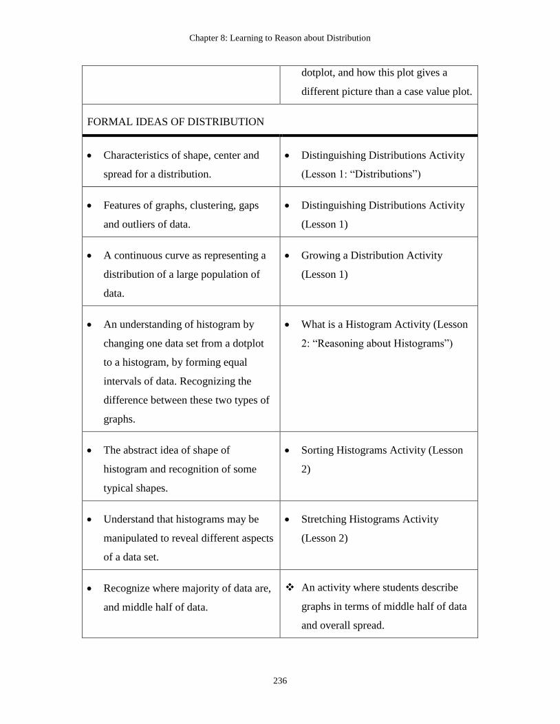
Chapter 8: Learning to Reason about Distribution
236
dotplot, and how this plot gives a
different picture than a case value plot.
FORMAL IDEAS OF DISTRIBUTION
Characteristics of shape, center and
spread for a distribution.
Distinguishing Distributions Activity
(Lesson 1: “Distributions”)
Features of graphs, clustering, gaps
and outliers of data.
Distinguishing Distributions Activity
(Lesson 1)
A continuous curve as representing a
distribution of a large population of
data.
Growing a Distribution Activity
(Lesson 1)
An understanding of histogram by
changing one data set from a dotplot
to a histogram, by forming equal
intervals of data. Recognizing the
difference between these two types of
graphs.
What is a Histogram Activity (Lesson
2: “Reasoning about Histograms”)
The abstract idea of shape of
histogram and recognition of some
typical shapes.
Sorting Histograms Activity (Lesson
2)
Understand that histograms may be
manipulated to reveal different aspects
of a data set.
Stretching Histograms Activity
(Lesson 2)
Recognize where majority of data are,
and middle half of data.
An activity where students describe
graphs in terms of middle half of data
and overall spread.

Chapter 8: Learning to Reason about Distribution
237
Recognize the difference between bar
graphs of categorical data, case value
graphs, and histograms of quantitative
data.
An activity where students examine
and compare these three types of
graphs that all use bars in different
ways.
Only certain types of graphs (e.g.,
dotplots and histograms) reveal the
shape of a distribution.
Exploring Different Representations
of the Same Data Activity (Lesson 2)
Reason about what a
histogram/dotplot would look like for
a variable (integrate ideas of shape,
center and spread) given a verbal
description or sample statistics.
Matching Histograms to Variable
Descriptions Activity (Lesson 2)
BUILDING ON FORMAL IDEAS OF DISTRIBUTION IN SUBSEQUENT TOPICS
Idea of center of a distribution and
how appropriate measures of center
depend on characteristics of the
distribution.
Activities in Lessons 2 (Center Unit,
Chapter 9)
Idea of variability of a distribution and
how appropriate measures of
variability depend on characteristics of
the distribution.
Activities in Lessons 1 and 2
(Variability Unit, Chapter 10)
How a boxplot provides a graphical
representation of a distribution.
Activities in Lessons 1, 2, 3 and 4
(Comparing Groups unit, Chapter 11)
How boxplots and histograms reveal
different aspects of the same
distribution.
Matching Histograms to Boxplots
Activity (lesson 3, Comparing Groups
Unit, Chapter 11)

Chapter 8: Learning to Reason about Distribution
238
Probability distribution as a
distribution of a random variable that
has characteristics of shape, center and
spread.
Coins, Cards, and Dice Activity
(Lesson 2, Modeling Unit, Chapter 7)
The normal distribution as a model of
univariate data that has specific
characteristics of shape, center and
spread.
Activities in Lesson 3, The Normal
Distribution as Model (Models Unit,
Chapter 7)
The idea of sampling distribution as
distributions of sample statistics that
can be described in terms of shape,
center and spread.
Activities in Lessons 1, 2, and 3
(Samples and Sampling Unit, Chapter
12)
How statistical inferences may
involve comparing an observed
sample statistic to a sampling
distribution.
Activities in Lessons 1 and 2,
(Inference Unit, Chapter 13)
Bivariate distribution as represented in
a scatterplot.
Activities in Lesson 1 (Covariation
Unit, Chapter 14)
Characteristics of a bivariate
distribution such as linearity, clusters,
and outliers.
Activities in Lesson 1 (Covariation
Unit, Chapter 14)
Introduction to the Lessons
The two lessons on distribution contain many small activities, which together lead
students from exploring one set of data in a simple, intuitive form, to more sophisticated
activities that involve comparing and matching graphs. While it is not at all “traditional”
to spend two full class sessions on the idea of distribution and basic graphs, we feel

Chapter 8: Learning to Reason about Distribution
239
strongly that unless students understand this idea early on, they will not understand most
of the subsequent course material at a deep level.
Lesson 1: Distinguishing Distributions
In the first activity of this lesson, students are given several different groups of dotplots
and asked to determine the distinguishing feature that distinguishes each of the dotplots in
a group. In this way, the students discover the characteristics of shape, center and spread,
and features such as clusters, gaps and outliers. The activity also helps students see
distributions as a single entity with identifiable characteristics. The second activity has
students make predictions about graphs for a variable measured on their class survey and
then make and test predictions about what would happen if the sample size was increased.
1. To develop the idea of a distribution as a single entity rather than individual
points.
2. To recognize different characteristics of a distribution and understand these
characteristics in an intuitive, informal way.
3. To recognize differences between graphs of small and large samples, and how
graphs of distributions stabilize as more data from the same population is added.
4. To develop an understanding of a density curve as it represents a population.
Description of the Lesson
The lesson begins with a discussion of the term “distribution” and how this differs in
everyday usage and in statistics. Students reason about and discuss pattern, what we need
to know to draw a reasonable graph without knowing the data values.
Next, in the Distinguishing Distributions activity, students are given a series of dotplots
that depict the distributions of hypothetical exam scores in various classes. For example,
they are asked:

Chapter 8: Learning to Reason about Distribution
240
For classes A, B and C, what is the main characteristic that distinguishes these
three graphs form each other? What might explain this difference? (Figure 8)
Figure 8: Distributions of hypothetical exam scores in various classes.
Each set of graphs reveals a different characteristic of distribution: e.g., center, spread,
shape, and outliers. Students are then asked what features are important to examine when
describing distributions, what to look for, features that are always present such as shape,
center and spread, and ones that might be present or absent, depending on the data set.
The following activity (Growing a Distribution) has students making predictions about
number of hours students in their class study each week, both in terms of a typical value
and a range of values. Next, they gather a sample of five data values form students in the
class and graph this using a dotplot. More data are gathered (e.g., the entire class) and

Chapter 8: Learning to Reason about Distribution
241
new dotplots are generated and described. Then students are asked to imagine if four
classes of students were combined, and to draw their imagined plot of study hours per
week. Finally, they consider all students at the university, and draw a smooth curve to
represent this population. The students repeat this by looking at dotplots of three other
variables based on student survey data, and then draw a smooth curve to represent the
distribution of all students at their school for these variables.
A wrap-up discussion focuses on differences between dotplots and smooth curves.
Students discuss what we mean by the term distribution, what are some common
characteristics of a distribution of quantitative data, what information a graph of a
distribution provides and what information a histogram provides that is not revealed by
looking at a bar graph or case value graph (e.g., shape, center, and spread). The students
consider when a histogram might be a better representation of data than a dot plot, what
information can be determined by looking at a dotplot more easily than in a histogram,
and what information is lost or not shown by a histogram.
Lesson 2: Exploring and Sorting Distributions
This lesson begins with a data set of body measurements gathered from a set of students
that includes kneeling heights. After students make some predictions about this variable,
they examine and describe a dotplot of class data on kneeling heights. The students are
led through a transformation of this dot plot into a histogram, using TinkerPlots software.
They compare different representations of the same data to see how different features are
hidden or revealed in different types of graphs.
In the third activity students sort a set of histograms into different piles according to
general shape, which leads students to recognize and label typical shapes, guiding them to
see these distributions as entities, rather than as sets of individual values. They students
further develop the idea of shape by changing bin widths on histograms using Fathom
software to manipulate and reveal how the size of the bins used affects the stability of the
shape. In the fifth and final activity students match histograms to variable descriptions,
reasoning about the connections between visual characteristics of distributions and
variable contexts.
Chapter 8: Learning to Reason about Distribution
242
Student learning goals for this lesson include:
1. To understand how a distribution is represented by a histogram and that a
histogram (or dotplot) allow us to describe shape, center and spread of a
quantitative variable in contrast to a bar graph (bar chart).
2. To understand the differences between case value graphs, bar graphs (case-value
bars) of individual data values and graphs displaying distributions of data such as
histograms.
3. To understand how graphical representations of data reveal the variability and
shape of a data set.
4. To recognize and label typical shapes of distribution, using common statistical
terms (normal, skewed, bimodal and uniform).
5. To understand that the shape of a graph may seem different depending on the
graphing technique used, so it may be important to manipulate a graph to see what
the shape seems to be.
Description of the Lesson
In the What is a Histogram activity, students begin by making conjectures about what
they would expect to see in the distribution of kneeling height data. This data set is then
used to help students develop an understanding of a histogram, by using TinkerPlots to
sort the data into sequential intervals, and then fuse the intervals into bars.
They begin with a graph of the data values, scattered as shown in Figure 9, and after
playing with and examining the data, are guided to arrange the dots into case-value bars,
to sort the smaller values of kneeling heights as shown in Figure 10.

Chapter 8: Learning to Reason about Distribution
243
Figure 9: kneeling heights scattered dots in TinkerPlots.
Figure 10: A case-value graph ordered by kneeling heights.
Students are then guided to use the Separate operation in TinkerPlots to separate the
cases into intervals that are then fused into a histogram, as show in Figures 11 and 12.

Chapter 8: Learning to Reason about Distribution
244
Figure 11: Stacked kneeling height data with frequencies noted in each interval.
Figure 12: A histogram presenting the kneeling height in seven bins.
In the Stretching Histograms activity students use a histogram applet to examine the
effect of bin width on shape, seeing that larger and smaller bin widths may obscure shape
and details (such as gaps, clusters and outliers). Students are then encouraged to think
about the difference between the different types of plots they have seen (Exploring
Different Representations of Data activity). These plots include the dotplot the case-value
graph (value bar graph) and the histogram. They are then asked to consider which graphs
help them better estimate the lowest five values, where “most” of the kneeling heights are
clustered, the middle or typical value of kneeling heights, the spread, and the shape of the

Chapter 8: Learning to Reason about Distribution
245
data. Students discuss how to determine the best representation to answer a particular
question and why one representation may be better than another.
In the next activity (Sorting Histogram), students work in small groups to sort a set of 21
different graphs, representing different data sets. Students sort the stack of into piles,
according to those that look the same or similar, then describe what’s similar about the
graphs in each group, pick one representative graph for each group, and come up with
their own term to describe the general shape of each group. A whole class discussion
follows where group results are compared and then the correct statistical terms for the
graphs (uniform, normal, right- and left-skewed, bimodal) can be introduced or
reinforced. Models (uniform, normal) are been described in terms of symmetry and shape
(bell-shape or rectangular). Other distributions that don’t fit these models can be
described in terms of their characteristics (skewness, bimodality or unimodality, etc.). A
discussion of which descriptors can and cannot go together may follow. For example,
normal and skewed cannot go together.
During this discussion some important points are addressed:
Ideal shapes: density curves vs. histograms (theoretical vs. empirical distributions)
Different versions of ideal shapes
Idea of models, characteristics of distributions
Statistical words vs. informal descriptors
Other ways to describe a distribution
Why is it important to describe a distribution?
Normal, skewed, uniform, bimodal, and symmetric: which can be used together?
How well do they fit the graphs? Which fit best?
Next, students work in groups to discuss and sketch what they expect for the general
shape for some new data sets, and use the statistical terms to describe the shape of each.

Chapter 8: Learning to Reason about Distribution
246
For example, the salaries of all persons employed at the University or grades on an easy
test. There is another whole class discussion to compare answers and explanations.
The final activity (Matching Histograms to Variable Descriptions) has students match
descriptions of variables to graphs of distributions, helping to develop students’ reasoning
about behavior of data in different contexts and how this is related to different types of
shapes of graphs. A wrap-up discussion focuses on the characteristics of distributions and
how they are revealed in different types of graphs.
Summary
Understanding the idea of distribution is an important first step for students who will
encounter distributions of data and later distributions of sample statistics as they proceed
through their statistics course. While most textbooks ask students to look at a histogram
or stem plot and describe the shape, center and spread, many students never understand
the idea of distribution as an entity with characteristics that reveal important aspects of
the variation of the data. The focus of the activities described in this chapter is on
developing a conceptual understanding of distribution, and we have not included
activities where students learn to construct different graphs, a topic well covered in most
textbooks. We encourage instructors to repeatedly have students interpret and describe
distributions as they move through the course, whether plots of sample data or
distributions of sample statistics.

247
Chapter 9: Learning to Reason about Center
A statistician sees group features such as the mean and median as
indicators of stable properties of a variable system—properties that
become evident only in the aggregate. (Konold & Pollatsek, 2002, p.
262)
Snapshot of a Research-based Activity on Center
Pairs of students are given a set of 10 small Post-It® notes and a number line that goes
from 17 to 25. They are asked to think about a group of college students whose mean age
is 21, and construct a dot plot, using the Post-It® notes, of an age distribution with a
mean of 21. Most of the students quickly figure out that they can stack all 10 Post-It®
notes at the 21 point. But then they are told that one of the values is 24, so they have to
figure out where the other values are on the number line (e.g., move one note to 18, to
balance out the 24 being 3 units above the average of 21). Students are instructed to move
one Post-It® note to 17, and arrange the rest of the Post-It® notes so the mean is still 21.
Finally, they move all of the Post-It® notes so that none are at 21 but the mean age is
21.Students use different strategies to do this, such as making sure that every note above
the mean has a value equally placed below the mean. Other students may balance one
note that is four units above the mean with two notes that are two units below the mean,
etc. Different results are compared and discussed.
Students are then instructed to draw dot plots of 10 points that have the same mean of 21,
and then draw deviations from the mean for their graphs. They consider how the
deviations balance each other out, so that if one value is moved producing a deviation of
3 , another value must be moved to have a deviation of 3 . This leads to a discussion
of what a mean “means” in terms of these deviations all cancelling each other out to be
zero.
Rationale for this Activity

Chapter 9: Learning to Reason about Center
248
Although most student have learned how to calculate means before entering their
statistics course, research studies reveal that few understand what a mean really is or what
it tells us about data. Research also shows that students often have difficulty
understanding how the mean and median differ and why they behave differently (e.g., in
the presence of outliers). This activity helps students to build a conceptual understanding
of what the mean and median actually mean and how they are affected by the different
values in a data set. This lesson also introduces the idea of deviation early in the course,
as a way to understand the idea of a mean and what it represents. This deviation idea,
which begins to connect ideas of center and variability, is revisited when learning about
variability and the standard deviation, and again when considering residuals in a
regression analysis. This activity helps students develop a conceptual and a procedural
understanding of the mean. By having the students physically manipulate data values on a
number line they are better able to see and reason about the idea of deviation from the
mean and the balancing of these deviations.
The Importance of Understanding Center
The idea of data as a mixture of signal and noise is perhaps the most
fundamental concept in statistics. (Konold & Pollatsek, 2002, p. 259)
Understanding the idea of center of a distribution of data as a signal amidst noise
(variation) is a key component in understanding the concept of distribution, and is
essential for interpreting data graphs and analyses. While students develop informal ideas
of center in the earlier units as they graph and describe distributions of data, they later
encounter the idea of center more formally as they learn about different measure of
center, how to compute them, what information they provide, and how we use them.
However, it is impossible to consider center without also considering spread, as both
ideas are needed to find meaning in analyzing data.
The Place of Center in the Curriculum

Chapter 9: Learning to Reason about Center
249
Traditional textbook first introduce center, then introduce spread, and then move on to the
next topic. However it may be more helpful to study these topics together because they
are so interrelated (Konold & Pollatsek, 2002; Shaughnessy, 1997).
It is hard to imagine a situation where one would summarize a data set using only a
measure of center without talking about the spread of the data or how much variability
there is around that measure of center. However, there are many instances, particularly in
the media, in which only measures of center are provided for a data set, in some cases,
leading to incorrect conclusions. When comparing groups or making inferences we need
to examine center and spread together: the signal, and the noise around the signal. While
these ideas are introduced in early units on exploring data, these concepts reappear when
looking at theoretical models such as the normal distribution and sampling distributions.
Later on the ideas of center (and spread) are revisited when making statistical inferences
about samples of data.
Review of the Literature Related to Reasoning about Center
(The knowledge of) computational rules not only does not imply
any real understanding of the basic underlying concept, but may
actually inhibit the acquisition of more adequate (relational)
understanding. (Pollatsek, Lima, & Well, 1981, p. 202)
Understanding Means
How students understand ideas of center has been of central interest in the research
literature. Research on the concept of average or mean was at first the most common
topic studied on learning statistics the school level (see Konold & Higgins, 2003;
Shaughnessy, 1992, 2003). The studies suggested that the concept of the average is quiet
difficult to understand by children, college students and even elementary school
preservice and in-service teachers (Russell, 1990; Groth & Bergner, 2006).
Early research typically focused on the single idea of center rather than looking at the
interrelated concepts of center and spread, and on procedural understanding. These
studies focused primarily on the mean, either as a simple average of a single data set or a

Chapter 9: Learning to Reason about Center
250
weighted mean. An early interest was on students understanding the mean as a balance
model (e.g., Hardiman, Well, & Pollatsek, 1984; Strauss, 1987), which is a common
method taught in a statistics course. A balance model illustrates how values are placed on
a balance beam at distances from the mean so that the deviations from the mean are
equal. Hardiman et al. (1984) tested whether improving students’ knowledge of such
balance rules through experience with a balance beam promoted understanding of the
mean. Forty-eight college students enrolled in psychology classes participated in the
study which involved pretest, training, and posttest of paper and pencil items. Students
who were given the balance training performed significantly better on the posttest
problems.
Other studies identified several characteristics of the mean and then examined students’
understanding of these characteristics (Goodchild, 1988; Mevarech, 1983; Strauss &
Bichler, 1988; Leon & Zawojewski, 1993). Mevarech (1983), for example, found that
high school students made mistakes in solving problems about means because they
believed that means have the same properties as simple numbers, and that it is helpful to
provide students corrective-feedback instruction as they solve problems involving
reasoning about the mean. Strauss and Bichler (1988) found that fourth- through eighth-
grade students had a difficult time understanding seven properties of the mean. Leon and
Zawojewski (1993) looked at school and college students’ understanding of four
components of the mean. Using different testing formats, they found that some properties
of the mean are better understood than others. The two properties, “the mean is a data
point located between the extreme values of a distribution”, and “the sum of the
deviations about the mean equals zero” were better understood by students in this study
than the two properties, “when the mean is calculated, any value of zero must be taken
into account”, and “the average value is representative of the values that were averaged.”
Gal, Rothschild and Wagner (1989, 1990) found that sixth-grade students are generally
unable to use the mean to compare two different-sized sets of data. Later work showed
that students had difficulty working backward from a mean to a data set that could
produce such a mean (Cai, 1998). Study by Mokros and Russell (1995) expanded on this

Chapter 9: Learning to Reason about Center
251
task by having students manipulate data values to produce a given mean and studying
how students reasoned during this process.
Earlier research has also concentrated on understanding weighted means. Pollatsek et al.
(1981) reported data from interviews of college students indicating difficulties they had
in understanding the need to weight data in computing a mean. While mathematically
sophisticated college students can easily compute the mean of a group of numbers, this
study indicated that a surprisingly large proportion of these students do not understand
the concept of the weighted mean which is a concept that they often encounter (e.g.,
grade point averages). When asked to calculate a mean in a context that required a
weighted mean, most subjects answered with the simple, or unweighted mean of the two
means given in the problem, even though these two means were from different-sized
groups of scores. Callingham (1997) found that the same problem in a study of pre-
service and in-service teachers. As a result of their study, Pollatsek et al. (1981) wrote
that “for many students dealing with the mean is a computational rather than a conceptual
act” (p. 191). They concluded that knowledge of “computational rules not only does not
imply any real understanding of the basic underlying concept, but may actually inhibit the
acquisition of more adequate (relational) understanding” (p. 202).
What students remember about the mean? In general, it appears that many students who
complete college statistics classes are unable to understand the idea of the mean.
Mathews and Clark (2003) analyzed audio-taped clinical interviews with eight college
freshmen immediately after they completed an elementary statistics course with a grade
of “A”. The point of these interviews was not to see how quickly isolated facts could be
recalled, nor was the point to see how little students remember. Rather, the goal was to
determine as precisely as possible the conceptions of mean, standard deviation and the
Central Limit Theorem which the most successful students had shortly after having
completed a statistics course. The results are alarming since these top students
demonstrated a lack of understanding of the mean, and could only state how to find it,
arithmetically. Interviewing along the same lines a larger (n=17) and more diverse sample
of college students from four distinct campuses, Clark, Karuat, Mathews, and Wimbish
(2003) found overall the same disappointing results. These researchers call therefore for

Chapter 9: Learning to Reason about Center
252
pedagogical reform that will dis-equilibrate the process image of statistical concepts that
students bring with them to college in order to enable them to encapsulate the process of
statistical concepts into objects that are workable entities (Sfard, 1991). For example,
they recommend creating situations in which students have to determine and reflect
which measure of center is more appropriate.
Understanding Medians
Difficulties in determining the medians of data sets have also been documented by
research. Elementary school teachers have difficulty determining the medians of data sets
presented graphically (Bright & Friel, 1998). Only about one-third of twelfth grade
students in the United States who took the NAEP test were able to determine the median
when given a set of unordered data (Zawojewski & Shaughnessy, 2000)
Measures of Center as Typical Values
The typical value interpretation of the arithmetic mean has received a great deal of
attention in curriculum materials and in research literature (Konold & Pollatsek, 2002).
The following is an example of a problem set in a typical value context:
The numbers of comments made by 8 students during a class period were 0, 5, 2,
22, 3, 2, 1, and 2. What was the typical number of comments made that day?
(Konold & Pollatsek, 2002, p. 268).
Several studies have provided insights about students’ thinking in regard to typical value
problems. Mokros and Russell (1995) studied the characteristics of fourth through eighth
graders’ constructions of “average” as a representative number summarizing a data set.
Twenty one students were interviewed, using series of open-ended problems that called
on children to construct their own notion of mathematical representativeness. They
reported that students may respond to typical value problems by: (i) locating the most
frequently occurring value; (ii) executing an algorithm; (iii) examining the data and
giving a reasonable estimate; (iv) locating the midpoint of the data; or (v) looking for a
point of balance within the data set. These approaches illustrate the ways in which school

Chapter 9: Learning to Reason about Center
253
students are (or are not) developing useful, general definitions for the statistical concept
of average, even after they have mastered the algorithm for the mean.
Levels of Reasoning about Measures of Center
In an investigation of the development of school students’ thinking in regard to measures
of center, Watson and Moritz (1999) placed a structure on the categories of thinking
documented by Mokros and Russell (1995). Continuing this line of research, Watson and
Moritz (2000a and b) also used the SOLO taxonomy (Structure of Observed Learning
Outcomes, see Biggs and Collis, 1982) to rank students’ responses to interview questions
about averages. They observed movement from Unistructural, to Multistructural, and
finally to Relational levels of reasoning as students developed from thinking about
centers first from “mosts and middles” and finally to the mean as “representative” of a
data set. Jones, Thornton, Langrall, Mooney, Perry and Putt (2000) and Mooney (2002)
found that the ability to be thoughtful and critical about applying formal measures to
typical value problems marks a relatively sophisticated level of statistical reasoning.
Measures of center as “signals in noisy processes”
A rich spectrum of student reasoning about center is identified by Konold & Pollatsek
(2002): mean as typical value, mean as fair share, mean as data reducer, and finally, mean
as signal amid noise. These researchers suggest that students should be given more
opportunities to work with statistical problems set in contexts that involve searching for
“signals in noisy processes.” The following item is an example of a data analysis problem
that involves detecting a signal in a noisy process:
A small object was weighed on the same scale separately by nine students in a
science class. The weights (in grams) recorded by each student were 6.2, 6.0, 6.0,
15.3, 6.1, 6.3, 6.2, 6.15, 6.2. What would you give as the best estimate of the actual
weight of this object? (Konold & Pollatsek, 2002, p. 268).
In the case of the repeated measures problem above, the arithmetic mean of the weights
that are bunched closely together could be viewed as a signal that estimates the true
weight of the object. The measurement of the object can be viewed as a noisy process that

Chapter 9: Learning to Reason about Center
254
contains variation stemming from various possible sources. Konold and Pollatsek (2002)
acknowledge the possible cognitive complexity in using repeated measurement problems
with students, pointing out that the mean as a reliable indicator of signal was not
universally accepted by scientists during the early development of the discipline of
statistics (Stigler, 1986). Hence, they call for more research on students’ thinking in such
contexts in order to help advise instruction.
Patterns of thinking about average in different contexts were investigated by Groth
(2005) who studied fifteen high school students. He used problems set in two different
contexts: determining the typical value within a set of incomes and determining an
average set in a signal-versus-noise context. Analysis of the problem-solving clinical
interview sessions showed that some students attempted to incorporate formal measures,
while others used informal estimating strategies. Students displayed varying amounts of
attention to both data and context in formulating responses to both problems. Groth
pointed out the need for teachers to be conscious of building students’ statistical
intuitions about data and context and informal estimates of center and connecting them to
formal measures without implying that the formal measures should replace intuition.
Selecting an Appropriate Measure of Center
Another focus of research has been on the challenge of choosing an appropriate measure
of center to represent a data set. The National Assessment of Education Progress (NAEP)
data confirm that school students frequently make poor choices in selecting measures of
center to describe data sets (Zawojewski & Shaughnessy, 2000). Choosing an appropriate
measure of center was also a challenge for students enrolled in an Advanced Placement
high school statistics course (Groth, 2002). Similar results were found by Callingham
(1997) who administered an item containing a data set structured so that the median
would be a better indicator of center than the mean, to a group of pre-service and in-
service teachers. Callingham report that most of them calculated the mean instead of the
more appropriate median.

Chapter 9: Learning to Reason about Center
255
In a study on statistical reasoning about comparing and contrasting mean, median, and
mode of preservice elementary school teachers, Groth and Bergner (2006) described four
levels, basing these on the SOLO Model:
Unistructural-level: responses did not contain any strategy other than definition-
telling when asked to compare and contrast the three measures.
Multistructural-level: responses included definition-telling along with a vague
notion that the mean, median, and the mode are all tools that can be used to
analyze a set of data; responses did not reflect an understanding that each of the
measures is intended to measure what is central or typical to data sets.
Relational-level: responses differ from Multistructural responses in that they
included recognition of the fact that the mean, median, and mode all measure the
center of the data or what is typical about the data in some manner.
Extended abstract–level:” responses include all of the characteristics of those
classified at the relational level but go beyond relational-level responses in that
they included discussions of when one measure of center might be more useful
than another.
Groth and Bergner’s (2006) study illustrated that attaining a deep understanding of these
seemingly easy statistical concepts is a nontrivial matter and that there are complex
conceptual and procedural ideas that need to be carefully developed.
Using the History of Measures of Center to Suggest Instruction
The history of statistics can be a source of inspiration for instructional design. Bakker and
Gravemeijer (2006) systematically examined examples of how measures of center were
described and used, starting in ancient historical periods, and form countries such as India
and Greece, in contexts involving mathematics and science, Based on their analysis of
these examples, Bakker and Gravemeijer (2006) formulate hypotheses about how
students in grades 7 and 8 (12–14-years old) could be supported in learning to reason
with mean and median. The following ideas stemming from the historical

Chapter 9: Learning to Reason about Center
256
phenomenology were found to be most fruitful for helping young children understand
center.
1. Estimation of large numbers can challenge students to develop and use intuitive
notions of mean.
2. Students may use the midrange as a precursor to more advanced notions of
average.
3. Repeated measurement may be a useful instructional activity for developing
understanding of the mean (cf., Petrosino, Lehrer, & Schauble, 2003).
4. To support students’ understanding of the median it is helpful to let them visually
estimate the median in a dot plot and look for a value for which the areas on the
left and right are the same.
5. Skewed distributions can be used to make the usefulness of the median a topic of
discussion.
Such a historical study can help to “unpack” and distinguish different aspects and levels
of understanding of statistical concepts and help instructional designers to look through
the eyes of students. Note that some of these hypotheses are in accordance with the
results of the research studies described above.
Implications of the Research: Teaching Students to Reason about Center
What has been striking over 25 years of research is the difficulty encountered by students
of all ages and teachers in understanding concepts related to center. Although students
may be able to compute simple arithmetic means, they need help in understanding what
means actually mean. Activities can help students develop meaningful models such as
balancing of data values by manipulating deviations from the mean to sum to zero.
The research suggests that careful attention be paid to developing the concepts of
measures of center, focusing on mean and median rather than mode. These ideas should
be first introduced informally as students estimate and reason about typical value for data
Chapter 9: Learning to Reason about Center
257
sets, both large and small, prior to formally studying these topics in a unit on measure of
center. Students may be asked to make and test conjectures about typical values using
real data sets. The research also suggests that students have opportunities to explore the
characteristics of the mean and median and how they are affected by different types of
data sets and distributions. Developing an understanding of deviation may be an
important part of understanding the mean as a balance point, so activities helping students
to see and reason about deviations may help them better understand the mean. The
literature suggests both visual, interactive activates as well as explorations with real data
utilizing technology to produce measures of center, especially for data sets where values
are changed (e.g., outliers are added or removed). Finally, the idea of the center as a
signal in a noisy process should be developed, examining trends in repeated
measurements. This also suggests that ideas of center be introduced along with ideas of
spread or variability, and that these ideas are repeatedly connected as students explore
and interpret data.
Progression of Ideas: Connecting Research to Teaching
Introduction to the Sequence of Activities to Develop Reasoning about Center
The idea of typical value as a summary measure of data set, shown graphically, is first
introduced in early units whenever students make or examine graphs of numerical data.
While students may intuitively look at the mode or peak of a graph or look at the middle
value on the horizontal axis, they can be guided to think about the mean and median as
typical values by looking at different graphs where mode or middle scale value do not
seem to represent good ‘typical’ values. This will help motivate the need for examining
different measures of center and when to use them. These informal examinations and
estimates should include estimates of spread of the data as well, as students respond to
questions such “what is a typical value for these data” and “how spread out are the
data?”, learning to connect ideas of center and variability from the beginning of the
course.
When formal measures of center are introduced, students are guided to explore their
properties using physical and then computer manipulations of data. Properties of the
Chapter 9: Learning to Reason about Center
258
mean and median can be explored and examined in this way. It is helpful for students to
actually work backwards, starting with a given value of mean or median to reason about
how different data sets may be constructed and altered to produce those given values.
This can be done first for mean and then for median. Students then conjecture what
typical values they might find for different types of variable, taking into account the
shapes and characteristics of graphs of these variables. These conjectures can then be
tested using real data and technology, and discussions can examine which measures are
more useful summaries for each variable and why.
When students begin to study formal measures of variability, they see the relationship
between mean and standard deviation, and between medial and Interquartile Range, and
how it makes sense to use these pairings when summarizing different types of
distributions (e.g., means and standard deviations for symmetric distributions, medians
and IQR for very skewed distributions and distributions with outliers). The idea of
examining center at the same time as variability as a way to compare groups is then
encountered as students learn about and compare boxplots. When the Normal distribution
is introduced students will see that the mean has special properties and use in relation
with stand deviations and z-scores.
The mean is again examined when learning about samples and how the mean stabilizes as
sample size gets very large, and the role of the mean in the Central Limit Theorem. As
students move from sampling to statistical inference, they again encounter the mean,
distinguishing between using the mean in an inference based on a large sample from
using the mean as a summary measure of a single data set (when a median might be a
better typical value given the shape of the distribution). The measures of center are also
encountered in the unit on covariation when students look at trends by examining
medians of sequential boxplots, and later as centers of distributions of the two variables.
Table 1: Sequence of activities to develop reasoning about center.
Milestones: Ideas and Concepts Suggested Activities
INFOROMAL IDEAS PRIOR TO FORMAL STUDY OF CENTER

Chapter 9: Learning to Reason about Center
259
Idea of center as a typical or
representative value for a graph of a
variable (e.g., dot).
Distinguishing Distributions (Lesson
1, Distribution Unit, Chapter 8)
The mean as somewhere in between
the highest and lowest value but not
necessarily the middle value or the
midpoint of the horizontal scale.
What does the Mean Mean Activity
(Lesson 1: “Reasoning about
Measures of Center”)
FORMAL IDEAS OF CENTER
Properties of the mean as a balance
point and the value for which all
deviations from that value sum to
zero.
What does the Mean Mean Activity
(Lesson 1)
How the mean is affected by extreme
values.
What does the Mean Mean Activity
(Lesson 1)
The median as the middle value in a
data set.
What does the Median Mean Activity
(Lesson 1)
Properties of the median: under what
conditions it changes or stays the
same.
What does the Median Mean Activity
(Lesson 1)
Comparing properties of the mean and
median.
Means and Medians Activity (Lesson
1)
The idea of a typical value. What is Typical Activity (Lesson 2:
“Choosing Appropriate Measures”)
Understanding why and how to use Choosing an Appropriate Measure of

Chapter 9: Learning to Reason about Center
260
appropriate measures of center for a
sample of data for a particular
variable.
Center Activity (Lesson 2)
BUILDING ON FORMAL IDEAS OF CENTER IN SUBSEQUENT TOPICS
How center and spread are used
together to compare groups.
Activities in Lessons 1, 2, 3 and 4,
Comparing Groups Unit (Chapter 11)
The idea and role of mean in normal
distribution.
What is Normal Activity (Lesson 3,
Statistical Models Unit, Chapter 7)
Recognize stability of measures of
center as sample size increases. When
sample grows, see how measure of
center predict center of larger
population, and how it stabilizes
(varies less).
Sampling activities in Lessons 1, 2,
and 3, Samples and Sampling Unit
(Chapter 12)
Role of mean in making inferences. Activities in Lessons 1, 2, 3, 4 and 5
(Statistical Inference Unit, Chapter 13)
Role of mean in bivariate distribution. An activity involving fitting and
interpreting the regression line to
bivariate data. (The symbol
indicates that this activity is not
included in these lessons.)
Introduction to the Lessons
There are two lessons on reasoning about measures of center. They begin with the
physical activity described earlier where students manipulate Post-It® notes on a number
line to develop an understanding of mean, and then median. Students use a Fathom demo
to contrast how the mean and median behave for different types of data sets. Students

Chapter 9: Learning to Reason about Center
261
make and test conjectures about typical values, testing these using software to generate
graphs and statistics. The last activity has students compare features and uses of different
measures of center when summarizing sample data.
Lesson 1: Reasoning about Measures of Center
While students have heard of means and medians before they enter an introductory high
school or college statistics course, this lesson helps them develop a conceptual
understanding of the mean and median. There are three parts to the lesson: an activity
where students move dots on a plot to explore properties of the mean, a similar activity
with the median, and then Fathom demos to further illustrate the properties of these
concepts. Student learning goals for this lesson include:
1. Develop a conceptual understanding of the mean.
2. Understand the idea of deviations (differences from the mean) and how they
balance out to zero.
3. Understand how these deviations cause the mean to be influenced by extreme
values.
4. Develop an understanding of the median as a middle value that is resistant to
extreme values.
5. Understand the differences between mean and median in their interpretation and
properties.
6. Understand how to select appropriate measures of center to represent a sample of
data.
Description of the Lesson
In the first activity described at the beginning of the chapter (What does the Mean Mean
activity) students are told that the average age (mean) for students in the class is 21 years
and consider what we know about the distribution of students’ ages for this class (e.g.,
Chapter 9: Learning to Reason about Center
262
“Are they all about 21 years old?”), and explain their answer first in a small group and
then to the class. They also explain where this value of 21 came from and how it was
produced. Students make conjectures about the ages of these 10 students and to use 10
Post-It® notes and to form a series of dot plots on a given number line so that the average
is 21 years.Students move one Post-It® note to 24 years, and later one to 17, and figure
out how to move one or more of the other Post-It® notes to keep the mean at 21 years,
discussing their strategies and reasoning with their group and then the class. The term
deviation is introduced to represent the distance of each data value from the mean and
students examine deviations for their plots under different conditions, seeing how they
have to balance to zero.
In the second activity (What does the Median Mean?), students reduce their Post-It®
notes to 9 and arrange them on the same number line used earlier so that the median is 21
years. Again, they are given different constraints (e.g., change one of the values that is
currently higher than 21 years) and determine if and how the median affected. Finally,
students discuss and summarize what would they have to do with a data value in the plot
in order to change the median.
In the final activity of this lesson (Means and Medians), students observe and discuss two
Fathom Demos: The Meaning of Mean and Mean and Median to further understand
properties of these measures. The lesson ends with a wrap-up discussion about use
interpretation, and properties of the mean and median,
Lesson 2: Choosing Appropriate Measures
This lesson introduces the idea of choosing an appropriate measure of center to describe a
distribution. It has students predict typical values for variables that have different
distributions. The lesson then has students find the actual mean and median for those
variables using computer software and examine the distributional features that made their
prediction closer to either the mean or median. It also introduces the idea of outlier
influence on these measures of center. Student learning goals for this lesson include:
1. Deeper conceptual understanding of mean and median.

Chapter 9: Learning to Reason about Center
263
2. Understand when it is better to use each as a summary measure for a distribution
of data.
3. How to generate these statistics using Fathom Software.
Description of the Lesson
Students are first asked how we can describe the typical college students taking an
introductory statistics course, and in what ways do students in this class differ? They
discuss how people use the words: typical, average, and normal in an everyday sense and
how these words are used as statistical terms: mean, median, center, and average.
In the What is Typical activity, students consider a set of variables that were measured on
their first day of class Student Survey. Working in pairs they predict what they might
expect as a typical value for all students enrolled in their statistics class this term. They
are reminded that a typical value is a single number that summarizes the class data for
each variable. They write their prediction in the “First Prediction” column of the table
shown below (Table 2).
Table 2: Predicting and verifying typical values in the What is Typical Activity.
Attribute from Student Survey
First
Prediction
Revised
Prediction
Statistics from
Fathom
Mean Median
Age
Number of statistics courses you
are taking this semester
Credits registered for this
semester
Total college credits completed

Chapter 9: Learning to Reason about Center
264
Cumulative GPA
Hours a week you study
Number of emails you send each
day
Number of emails you receive
each day
Next, they generate dot plots of the data using Fathom software to see if their original
predictions seemed reasonable. Based on the graphs, they are allowed to make revised
predictions for the typical value for each of the variables which are written in the table
above in the “Revised Prediction” column.
Students use Fathom to find the mean and median for each of these variables and
complete the last two columns of the table above. They discuss how close were their
revised predictions to the “typical” values produced by Fathom and for which attributes
were their predictions most accurate. They also consider what results were most
surprising to them and why, and whether in general, were their revised predictions closer
to the means or medians of these variables.
Students are asked to discuss:
Which measures of center were closest to their intuitive ideas of “typical” values?
What information do means and medians provide about a distribution?
How to decide whether to use the mean or median to summarize a data set?
In statistics, what do they think is meant by the word “typical”?
In Choosing an Appropriate Measure of Center activity, students suggest conditions
where the mean and median provide similar information and when they give different
information for the same data set. This leads to a discussion of which measure is more

Chapter 9: Learning to Reason about Center
265
appropriate for each variable and why, and how to choose the best measure of center for a
data set.
Students are asked if it is all right to compute a mean or median without first looking at a
graph of data and then why that is not a good idea. They reason about what information is
missing if all they are given is a measure of center, including what they know and not
know if all they were given were measures of center. This provides a segue to discussion
on spread (the next unit) and reinforces the connection between center and spread. In a
wrap-up discussion students are asked to imagine a variable that could be measured in
two different settings that might yield data sets that have the same mean and different
amounts of spread, one with a little spread and one with a lot of spread, and explain their
reasoning.
Summary
The two lessons in the unit on measures of center are closely connected to ideas of
distribution and variability, so that the ideas of mean and median are always connected to
these concepts and contexts. The intent of the lessons is to help students build a
conceptual understanding of mean and median as well as the idea of center of a
distribution, through physical manipulations of data values, making and testing
conjectures about typical values, and discussing the use and properties of these two
measures. While the concepts may seem simple, and not worth two full lessons, we
believe that that these lessons provide important foundations for and connections to
subsequent units in the course.

266
Chapter 10: Learning to Reason about Variability
Variation is the reason why people have had to develop sophisticated
statistical methods to filter out any messages from the surrounding
noise. (Wild & Pfannkuch, 1999, pp. 235 - 236)
Snapshot of a Research-based Activity on Variability
Students are given pairs of histograms with the assignment to discuss and determine
which graph in each pair would have a higher standard deviation and why. First students
are encouraged to actually draw deviations on the histograms and draw lines from the
mean to represent the number of deviations for each bar of the histogram (e.g., a bar
representing five values would correspond to five lines of the same length, showing
deviations from the center. Some of the histograms are easier to compare than others,
such as those that have a few bars close the center versus a histogram with most bars far
form the center (see examples in Figure 1). The difficult comparisons are for graphs that
have the same range, the same frequencies for each bar, but different numbers of bars
(representing different possible values of the variables).
Thinking about the size and number of deviations from the mean helps the students
reason about which graph would have a larger standard deviation. It also helps them
confront some misleading intuitions such as looking at graph A in the second example
below, and initially describing this graph as having no variability, because it is confused
with a time series graph or a bar graph where the height of the bars indicates that they all
have the same measurement. Drawing deviations from the center helps students to realize
that this histogram is different than a bar graph or time series, and that there are different
deviations from the center that can be “averaged” to produce an estimate of the standard
deviation.

Chapter 10: Learning to Reason about Variability
267
1. A x = .33 B x = 4.33
a. A has a larger standard
deviation than B.
b. B has a larger standard
deviation than A.
c. Both graphs have the
same standard deviation.
2. A x = 2.50 B x = 2.56
a. A has a larger standard
deviation than B.
b. B has a larger standard
deviation than A.
c. Both graphs have the
same standard deviation.
Figure 1: Comparing standard deviations of pairs of histograms from the What Makes the
Standard Deviation Larger or Smaller Activity.
After students compare and discuss their answers, they enter the data for each graph into
Fathom (Key Curriculum Press, 2006) and have the standard deviations computed. They
use Fathom to calculate the actual squared deviations from the mean for each graph.
After the students have checked their answers in this way, the class discusses each pair of
histograms and why the standard deviations were large or smaller in each pair. As they do
this, they construct a set of factors that appear to influence the size of the standard
deviation (e.g., more bars farther from the mean) and those that do not seem to affect the
size (e.g., “bumpiness” of the graph, or different heights of the bars).
Rationale for This Activity
0 1 2 3 4 5
1
2
3
4
5
6
6
FR
EQ
UE
NC
Y
SCORE0 1 2 3 4 5
1
2
3
4
5
6
6
FR
EQ
UE
NC
YSCORE

Chapter 10: Learning to Reason about Variability
268
The standard deviation is an important and much-used measure of variability but one that
is almost impossible for beginning statistics students to understand. While students learn
what the standard deviation is and how it is calculated, they rarely have an understanding
of what this measure is and how to interpret it. The activity described above is a
culminating activity in the unit on variability, because it helps students recognize and
integrate several sub ideas (e.g., a graphical representation of distribution, the mean of a
distribution, spread, and deviation). The idea of standard deviation as an average distance
from the center is developed by first having students estimate the mean of each graph,
taking into account both value (on the number line) and density (frequency of each bar).
Students are guided to reason about deviations from the mean and think about how values
close to and far from the mean affect those deviations and squared deviations.
Entering the data from each histogram themselves (to find the actual standard deviations
for each pair of graphs), helps students remember that each bar in the histogram
represents one or more pieces of data of the same value, distinguishing these graphs from
case value graphs (see more on this issue in Chapter 8). Seeing the squared deviations
illustrates how deviations far from the mean have a greater impact on the size of the
standard deviation.
The Importance of Understanding Variability
Variability is … the essence of statistics as a discipline and it is not
best understood by lecture. It must be experienced (Cobb, 1992).
A major goal of most introductory statistics courses is to help students understand and be
aware of the omnipresence of variability and the quantification and explanation of
variability (Cobb, 1992). These two topics are also highlighted in the GAISE report
(2005):
The omnipresence of variability
Recognizing that variability is ubiquitous. It is the essence of statistics as a
discipline and it is not best understood by lecture. It must be experienced.

Chapter 10: Learning to Reason about Variability
269
The quantification and explanation of variability
Recognizing that variability can be measured and explained, taking into
consideration the following: (a) Randomness and distributions; (b) patterns and
deviations (fit and residual); (c) mathematical models for patterns; (d) model-data
dialogue (diagnostics).
Understanding the ideas of spread or variability of data is a key component of
understanding the concept of distribution, and is essential for making statistical
inferences. While students develop informal ideas of spread in the earlier unit on
graphing and describing distributions, they later encounter these ideas more formally as
they learn about different measure of variability (e.g., range, standard deviation and
interquartile range), what they mean, how to interpret them, how they compare to each
other as statistical summaries of data, and what information they provide and don’t
provide, and how we use them in analyzing data.
There has been increasing attention paid to the importance of students developing an
understanding of and appreciation for variability, as a core component of statistical
thinking (Cobb, 1992; Moore, 1998). However, it is impossible to consider variability
without also considering center, as both ideas are needed to find meaning in analyzing
data.
The Place of Variability in the Curriculum
The idea of spread, or variability should permeate the entire curriculum. We advocate
introducing ideas of spread first informally, and later formally. Ideas of variability can be
introduced the first day of class (see lessons from the data unit) and revisited in the unit
on distribution, where students describe the spread or clustering of values in a graph of a
distribution. When center is introduced, the idea of deviation from the mean is used to
help understand the meaning of the mean, and this idea of deviation form the mean is
then revisited when studying standard deviation. While range is a fairly easy concept for
students to understand, standard deviation is much more difficult. Interquartile range is

Chapter 10: Learning to Reason about Variability
270
also a difficult concept, and best introduced in the context of comparing groups with
boxplots, when it is illustrated visually by the width of the box.
It is hard to imagine a situation where one would summarize a data set using only a
measure of center or using only a measure of spread. When comparing groups or making
inferences we need to look at center and spread together: the signal, and the noise around
the signal. Therefore, ideas of center and spread are most often seen and used together,
whether informally describing distributions, looking at theoretical models such as the
normal distribution and sampling distributions, or in making inferences.
Review of the Literature Related to Reasoning about Variability
Variation vs. Variability
Before we begin to summarize current research on reasoning about variability, we want
to address the question of terminology. An inconsistent use of terminology is noticeable
in research studies about variability. While some use “variability” and “variation”
interchangeably, others distinguish between the meanings of these two words. Reading
and Shaughnessy (2004) suggest the following distinctions: variation is a noun describing
the act of varying, while variability is a noun form of the adjective “variable,” meaning
that something is likely to vary or change. Since this distinction has not yet been agreed
upon in the statistics education research community, we note this argument but have
chosen to use the term variability as the general, omnibus term for these ideas in this
chapter.
The Emergent Research about Variability
Recent discussions in the statistics education community have drawn attention to the fact
that statistics text books, instruction, public discourse, as well as research have been
overemphasizing measures of center at the expense of variability (e.g., Shaughnessy,
1997). Instead, there is a growing consensus to emphasize general distributional features
such as shape, center and spread and the connections among them in students’ early
experiences with data. It is also suggested to focus students’ attention on the nature and
sources of variability of data in different contexts, such as variability in a particular data

Chapter 10: Learning to Reason about Variability
271
set, outcomes of random experiments, and sampling (Shaughnessy, Watson, Moritz, &
Reading, 1999; Gould, 2004). These views are supported by a review of several studies
by Konold and Pollatsek (2002) that has shown that “the notion of an average understood
as a central tendency is inseparable from the notion of spread” (p. 263). Their well-
known metaphor for data as signal and noise implies that students should come to see
statistics as “the study of noisy processes – processes that have a signature, or signal” (p.
260).
Difficulties in Understanding Variability
Despite the widespread belief in the importance of this concept, current research
demonstrates that it is extremely difficult for students to reason about variability and that
we are just beginning to learn how reasoning about variability develops (Garfield & Ben-
Zvi, 2005). Understanding variability has both informal and formal aspects, moving from
understanding that data vary (e.g., differences in data values) to understanding and
interpreting formal measures of variability (e.g., range, interquartile range, and standard
deviation). While students can learn how to compute formal measures of variability, they
rarely understand what these summary statistics represent, either numerically or
graphically, and do not understand their importance and connection to other statistical
concepts. What makes the understanding of the concept even more complex is that
variability may sometimes be desired and of interest, and sometimes be considered error
or noise (Gould, 2004; Konold & Pollatsek, 2002), as well as the interconnectedness of
variability to concepts of distribution, center, sampling, and inference (Cobb, McClain, &
Gravemeijer, 2003).
These difficulties are evident, for example, in a series of interview studies with
undergraduate students who had earned a grade of A in their college statistics course,
Mathew and Clark (2003) found that students could not remember much at all about the
standard deviation. In another interview study of introductory statistics students’
conceptual understanding of the standard deviation, delMas and Liu (2005) designed a
computer environment to promote students’ ability to coordinate characteristics of
variation of values about the mean with the size of the standard deviation as a measure of
Chapter 10: Learning to Reason about Variability
272
that variation. delMas and Liu found that students moved from simple, one-dimensional
understandings of the standard deviation that did not consider variation about the mean to
more mean-centered conceptualizations that coordinated the effects of frequency
(density) and deviation from the mean.
In a study investing students statistical reasoning, using the statistical reasoning
Assessment (SRA), Garfield (2003) found that even students in introductory classes that
were using reform textbooks, good activities, and high quality technology, had significant
difficulty reasoning about different aspects of variability, such as representing variability
in graphs, comparing groups, and comparing the degree of variability across groups.
Developing Students Reasoning about Variability
A variety of contexts have been used in statistics education to study students’ reasoning
about variability at all age levels. For example, in a study of elementary students, Lehrer
and Schauble (in press) contrast students’ reasoning about variability in two contrasting
contexts: (a) measurement and (b) “natural” (biological). When fourth-graders were
engaged in measuring the heights of a variety of objects, distribution emerged as a
coordination of their activity. They were able to invent statistics as indicators of stability
(e.g., center corresponded to “real” length) and variation of measure (e.g., spread
corresponded to sources of error such as tool, person, trial-to-trial). In the context of
natural variation activity (growth of plants), these same students (now fifth-graders) had
difficulties handling sources of natural variation and related statistics. Activities that
promoted investigations of sampling (e.g., “what would be likely to happen to the
distribution of plant heights if we grew them again”), and comparing distributions (e.g.,
“how one might know whether two different distributions of height measurements could
be considered ‘really’ different”) were found useful in developing students understanding
of variability.
In a design research conducted with students in grades 7 and 8 (Bakker, 2004),
instructional activities that could support coherent reasoning about key concepts such as
variability, sampling, data, and distribution were developed. Two instructional activities
were found to enable a conceptual growth: A “growing a sample” activity that had

Chapter 10: Learning to Reason about Variability
273
students think about what happens to the graph when bigger samples are taken, and an
activity requiring reasoning about shape of data.
The advantage in discussing ideas of variability in connection with ideas of center was
described by Garfield, delMas, & Chance (2007). In this study with undergraduate
students, results indicated that students could develop ideas of a lot or a little variability
when asked to make and test conjectures about a series of variables measuring minutes
per day spent on various activities (e.g., time spent studying, talking on the phone, eating,
etc.). They also found that by having students reason abut the distributions of these
variables informally they could move them towards comparisons of formal measures of
variability (e.g., standard deviation, range and interquartile range).
Other contexts examined include variability in data (Ben-Zvi, 2004a; Groth, 2005;
Konold & Pollatsek, 2002; Petrosino, Lehrer, & Schauble, 2003), bivariate relationships
(Cobb, McClain, & Gravemeijer, 2003; Hammerman & Rubin, 2003), comparing groups
(Ben-Zvi, 2004b; Biehler, 2001; Lehrer & Schauble, 2002; Makar & Confrey, 2005),
probability contexts (Reading & Shaughnessy, 2004), measures of spread such as the
standard deviation (delMas & Liu, 2005), and sampling (Chance, delMas & Garfield,
2004; Watson, 2004). These studies are mostly exploratory and qualitative, and their
research goal is often to explore what and how students come to understand ideas of
variability in the different contexts. The kinds of questions and activities used in these
studies suggest ways we can help students develop reasoning about variability across an
entire course as well as assess informal and formal aspects of students understanding of
variability.
Levels of Reasoning about variability
Based on results from a large sample of students on a survey of variability tasks, Watson,
Kelly, Callingham and Shaughnessy (2003) propose a model of students’ reasoning about
variability. Using the SOLO model (Biggs & Collis, 1982) they qualitatively describe
four hierarchical levels of progressively sophisticated understanding of reasoning about
variability: Prestructural, Unistructural, Multistructural and Relational. They suggested
that this scale might be useful in tracking student improvement over time and in relation

Chapter 10: Learning to Reason about Variability
274
to particular sequences of learning activities. The descriptions of these levels, as well as
the work on informal and formal ideas of variability (Garfield, delMas, and Chance;
2007) suggest the need for carefully designed activities designed to lead students to
develop higher or more formal levels of reasoning.
Implications of the Research: Teaching Students to Reason about Variability
Noticeably lacking in the current research literature are studies of how to best impact the
learning of college students who are typically introduced to variability in a unit of
descriptive statistics, following units of graphing univariate data and measures of center.
Measures of variability (or spread) are then introduced, and students learn to calculate
and briefly interpret them. Typically, only the formal notion of variability as measured by
three different statistics (i.e., the range, interquartile range, and standard deviation) is
taught. Students often do not hear the term “variability” stressed again until a unit on
sampling, where they are to recognize that the variability of sample means decreases as
sample size increases. When students are introduced to statistical inference, variability is
then treated as a nuisance parameter because estimating the mean becomes the problem
of importance (Gould, 2004).
Given this typical introduction in textbooks and class discussion, it is not surprising that
few students actually develop an understanding of this important concept. Good activities
and software tools designed to promote an understanding of variability do exist.
However, they are typically added to a lesson or given as an assignment instead of being
integrated into a plan of teaching, and their impact on student understanding has not been
subjected to systematic study. So while there have been positive changes in introductory
statistics classes, they still fall short of giving students the experiences they need to
develop statistical thinking and a deep understanding of key statistical concepts.
We would like our students to follow the way statisticians think about variability. When
statisticians look at one or more data sets, they often appraise and compare the variability
informally and then formally, looking at appropriate graphs and descriptive measures.
They look at both the center of a distribution as well as the spread from the center, often
referring to more than one representation of the data to lead to better interpretations.

Chapter 10: Learning to Reason about Variability
275
Statisticians are also likely to consider sources of variability, including the statistical and
measurement processes by which the data were collected.
Konold and Pollatsek (2002) offer the following suggestions about how we might help
students and future teachers develop ideas of the signal-noise perspective of various
statistical measures:
1. Using processes involving repeated measures;
2. Explorations of stability such as drawing multiple samples from a known
population and evaluating particular features, such as the mean, across these
replications.
3. Comparing the relative accuracy of different measurement methods;
4. Growing samples - students observe a distribution as the sample gets larger;
5. Simulating processes – students investigate why many noisy processes tend to
produce mound-shaped distributions;
6. Comparing groups; or
7. Conducting experiments.
Garfield and Ben-Zvi (2005) outline a list of increasingly sophisticated ideas for
constructing "deep understanding" of variability. This list offers a sequence through
which students may be guided to develop a deep understanding of this concept, as shown
below:
1. Developing intuitive ideas of variability
2. Describing and representing variability with numerical measures
3. Using variability to make comparisons
4. Recognizing variability in special types of distributions

Chapter 10: Learning to Reason about Variability
276
5. Identifying patterns of variability in fitting models
6. Using variability to predict random samples or outcomes
7. Considering variability as part of statistical thinking
Progression of Ideas: Connecting Research to Teaching
Introduction to the Sequence of Activities to Develop Reasoning about Variability
The following table shows a series of steps that can be used to help students first build
informal and then formal ideas of variability. These ideas are first introduced in earlier
units on data, distribution and center. Then the formal idea of standard deviation is
introduced and used to examine and reason about data. The concept of interquartile range
is introduced in the later unit on comparing groups, a unit that helps connect ideas of
center and spread visually and for the purpose of comparing sets of data to answer a
research question. The idea of variability is visited again in the unit on models, when the
normal distribution is introduced and the unique characteristics of the mean and standard
deviation are shown as part of the Empirical Rule. The interconnections of center and
spread are also demonstrated in the sampling, statistical inference and covariation units.
Each time the basic idea of variability is explicitly revisited in that particular context,
emphasized and discussed.
Table 1: Sequence of activities to develop reasoning about variability.
Milestones: Ideas and Concepts Suggested Activities
INFOROMAL IDEAS PRIOR TO FORMAL STUDY OF VARIABILITY
Data vary. Values of a variable
illustrate variability.
Meet and Greet Activity (Lesson 1,
Data Unit, Chapter 6)
Variability in results from a random
experiment.
Activities in Lessons 1 and 2,
Statistical Models Unit (Chapter 7)

Chapter 10: Learning to Reason about Variability
277
Informal idea of spread of data by
examining a graph or comparing
graphs.
Distinguishing Distributions Activity
(Lesson 1, Distributions Unit, Chapter
8).
Range as a simple measure of spread. An activity where students describe
distribution and note range as a
measure of spread. (The symbol
indicates that this activity is not
included in these lessons.)
FORMAL IDEAS OF VARIABILITY
Two ideas of variability: diversity or
measurement error.
How Big is Your Head Activity
(Lesson 1: “Variation”)
Sources of variability, a lot and a little
variability.
How Big is Your Head Activity
(Lesson 1)
Averaging deviations from the mean
as a measure of spread.
Comparing Hand Spans Activity
(Lesson 2: “Reasoning about the
Standard Deviation”)
Standard deviation as a measure of
average distance from the mean.
Comparing Hand Spans Activity
(Lesson 2)
Understanding factors that cause the
standard deviation to be larger or
smaller.
What Makes the Standard Deviation
Larger or Smaller Activity (Lesson 2)
How center and spread are represented
in graphs?
An activity where students match a set
of graphs to the corresponding set of
statistics.
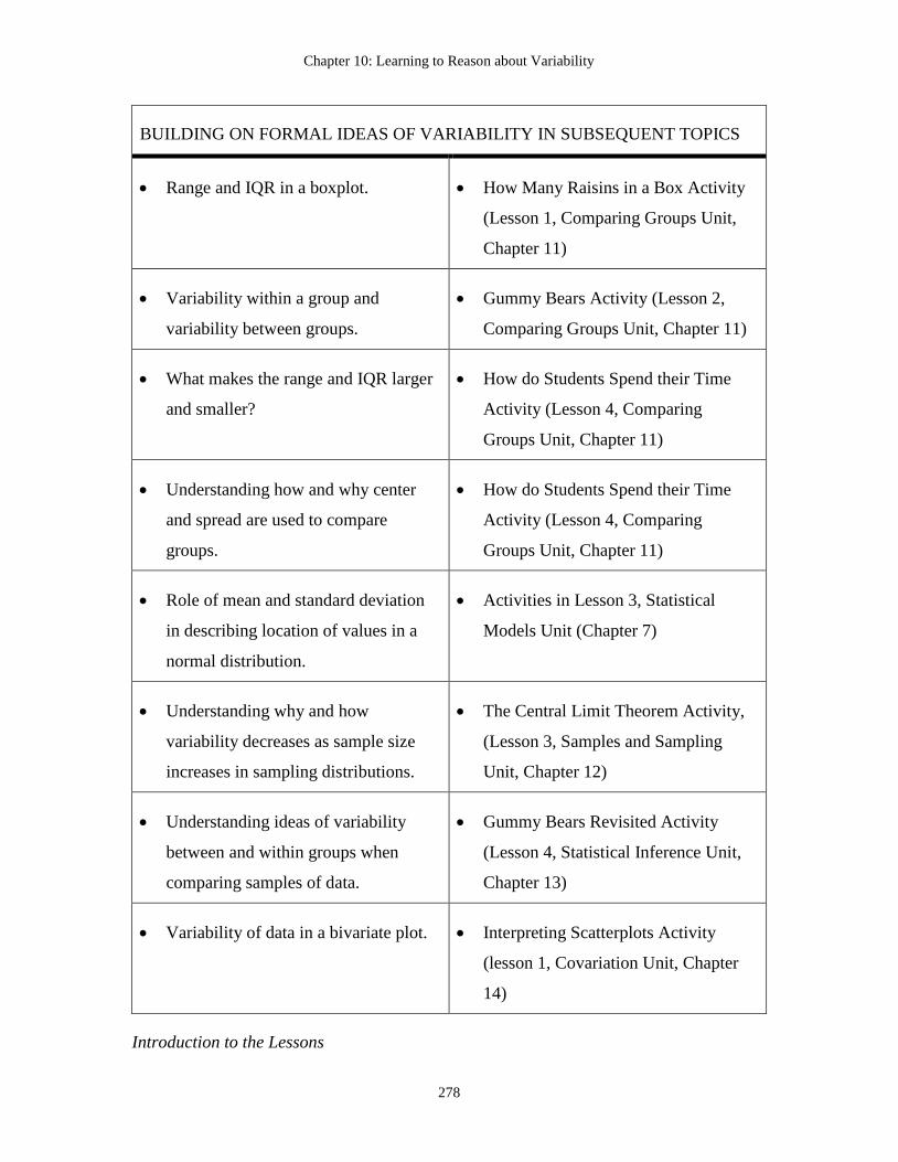
Chapter 10: Learning to Reason about Variability
278
BUILDING ON FORMAL IDEAS OF VARIABILITY IN SUBSEQUENT TOPICS
Range and IQR in a boxplot. How Many Raisins in a Box Activity
(Lesson 1, Comparing Groups Unit,
Chapter 11)
Variability within a group and
variability between groups.
Gummy Bears Activity (Lesson 2,
Comparing Groups Unit, Chapter 11)
What makes the range and IQR larger
and smaller?
How do Students Spend their Time
Activity (Lesson 4, Comparing
Groups Unit, Chapter 11)
Understanding how and why center
and spread are used to compare
groups.
How do Students Spend their Time
Activity (Lesson 4, Comparing
Groups Unit, Chapter 11)
Role of mean and standard deviation
in describing location of values in a
normal distribution.
Activities in Lesson 3, Statistical
Models Unit (Chapter 7)
Understanding why and how
variability decreases as sample size
increases in sampling distributions.
The Central Limit Theorem Activity,
(Lesson 3, Samples and Sampling
Unit, Chapter 12)
Understanding ideas of variability
between and within groups when
comparing samples of data.
Gummy Bears Revisited Activity
(Lesson 4, Statistical Inference Unit,
Chapter 13)
Variability of data in a bivariate plot. Interpreting Scatterplots Activity
(lesson 1, Covariation Unit, Chapter
14)
Introduction to the Lessons

Chapter 10: Learning to Reason about Variability
279
While students have been informally introduced to the idea of spread and range earlier,
this set of lessons looks more closely at variability and the standard deviation. First
students collect measurements to help them recognize two ways of looking at variability,
as noise and as diversity. They informally think about a measure of spread from the
center. The second lesson helps develop the idea of standard deviation and encourages
students to reason about how this statistics is used to measure and represent variability
and factors that affect the standard deviation, making it larger or smaller.
Lesson 1: Variation
This lesson is designed to help students reason informally about variability. Students
compare measurements for two sets of repeated measurements, to discover two kind of
variability: 1) variability as an error of measurement (repeated measures of the same head
circumference); and 2) variability as an indicator of diversity (measurements of different
people’s head circumferences). Students are then introduced to the concept of signal and
noise, and discuss the stability of the mean as more data are collected. Student learning
goals for the lesson include:
1. Understand different types (sources) of variability (when it’s desired and when
it’s noise).
2. Understand the ideas of mean as signal and variability as noise, from repeated
measurements in an experiment.
3. Understand that it is desirable to reduce variability in measurement (by using
experimental protocols).
Description of the Lesson
Students are asked to think about variability in the class, and in particular, of head sizes.
In the How Big is Your Head activity, they plan a method to measure the circumference
of each of their heads, keeping track of the decisions they make about measuring. A class
discussion about this results in a common protocol to use. Students are given a measuring

Chapter 10: Learning to Reason about Variability
280
tape to use, and they measure each of their heads using the protocol established and they
record the data on the board (or on a computer spreadsheet).
Next, as a class, the students choose one person who will have their head measured by
every student in the class. These measurements are also recorded for the class. Students
then work with a partner to obtain a set of additional body measurements (all in
centimeters) listed in Figure 2. These data will be used in other activities in the course.
These data are later entered in Fathom.
Body Data Collection
Height (with shoes on): __________
Arm Span (from fingertip to fingertip with arms out-stretched): __________
Kneeling Height: __________
Hand Length (from the wrist to the tip of the middle finger): __________
Hand Span (from the tip of the thumb to the tip of the pinkie while hand is
stretched): __________
Figure 2: Record sheet for the body measurements survey.
Fathom is used to create a plot of students’ head sizes so that they may be examined and
summarized. Unusual values are examined and discussed to see if they are legitimate or
the result of a faulty measurement process.
Students then select two numbers that seem reasonable for completing the following
sentence. (Note: There is more than one reasonable set of choices.)
The typical head circumference for students in this class is about ________ cm
give or take about ________ cm.
These answers as discussed and lead to a discussion of possible reasons for the variability
in the measurements of students’ head circumferences. Students then consider whether

Chapter 10: Learning to Reason about Variability
281
the observed variability could be reduced and if so, how that might happen. They offer
suggestions for ways to make the measurements more standard.
Next, the class examines data for the repeated measurements of one student’s head
circumference. These data are entered into Fathom and are graphed and summarized in
terms of shape, center and spread. This graph is then compared to the first graph of all
students head circumferences and reasons for the differences are discussed. This time, the
students suggest that the variability is solely due to the measurement process and talk
about ways to reduce that variability.
A class discussion of the difference between these two sets of measurements of head
circumference includes the different types and sources of variability, and when we might
expect (and accept) variability in measurements and when we want to keep it as small as
possible. The concepts of signal and noise are revisited, and the idea of variability as
noise in the case of the repeated measurements of one head is discussed.
A wrap-up discussion includes suggestions for different sources of variability in data, two
kinds of variability: “diversity” (spice of life) and “error or noise”. Students are asked
which type we like to have large and which do we like to have small, and why. They are
finally come up with some other examples of signal and noise, and to consider what we
care about signal and noise when we examine data.
Lesson 2: Reasoning about the Standard Deviation
This lesson encourages students to reason about the standard deviation. Students begin by
visualizing and estimating average distances in an activity involving hand spans. The next
part of the lesson is designed to help students improve their reasoning about and
understanding of variability by thinking about what a standard deviation is and applying
that knowledge to determine which of two graphs has a higher standard deviation.
Student learning goals for the lesson include:
1. Understand and informally estimate deviations from the mean and “typical”
deviation from the mean.

Chapter 10: Learning to Reason about Variability
282
2. Understand standard deviation as a measure of spread
3. Understand what makes standard deviations larger or smaller, what types of
graphs reveal different amounts of variation.
4. Reason about connections between measure of center and spread, and how they
are revealed in graphical representations of data.
Description of the Lesson
In the first activity, Comparing Hand Spans, students examine and compare their hands
and think about variability in hand spans. Students find the hand span for every person in
their group. They use a dot plot to examine how these values vary. They suggest two
sources of variability in these measurements, i.e., two reasons why the measurements are
not all the same.
Next, students record initials above the dots to identify each case. They find the mean and
mark it with a wedge (▲) below the correct place on the number line. They estimate how
far each of their hand span measurements is from the mean of their group. They make a
second dot plot, this time of the differences (deviations) from the mean for each student
in their group, and find the mean of these differences (deviations). Using the idea of
deviations from the mean, students suggest a “typical” distance (deviation) from the
mean.
Fathom is used to re-create the dot plot and to check their calculations and to compute the
standard deviation of the group’s hand span data. Students compare the actual standard
deviation to the “typical” distance (deviation) the group found earlier and to speculate
about the difference in these values.
Students then access the entire set of Hand Spans for the class that were gathered in the
pervious activity and find the standard deviation of these measurements. This statistic is
compared to the standard deviation of hand spans for the small group of four originally
produced, and differences are discussed. Finally, students discuss the idea of a “typical”
deviation and the standard deviation.

Chapter 10: Learning to Reason about Variability
283
The second activity What Makes the Standard Deviation Larger or Smaller continues the
discussion of a typical, or standard, deviation from the mean. First, students examine the
following dot plot (Figure 3), which has the mean marked by a vertical line. Students
consider how large the deviations would be for each data point (dot).
Figure 3: Dot plot from the What Makes the Standard Deviation Larger or Smaller
Activity.
Next students draw in the plot each deviation from the mean as shown below (Figure 4).
Figure 4: Drawing deviations from the mean in a dot plot from the What Makes the
Standard Deviation Larger or Smaller Activity.
Next, students reason about the average size (length) of all of those deviations, and use
this to estimate the standard deviation. They draw the estimated length of the standard
deviation. This process is repeated with a second dot plot as shown below (Figure 5).

Chapter 10: Learning to Reason about Variability
284
Figure 5: Second dot plot from the What Makes the Standard Deviation Larger or
Smaller Activity.
Then students are given a histogram (Figure 6) and they use the same process, thinking
about dots “hidden” by the bars, and to draw and estimate the length of the standard
deviation. The mean of the data set is given (2.57). Students are encouraged to draw in
the appropriate number of dots in each bar of the histogram to make sure they have the
appropriate number of deviations.
Figure 6: A histogram from the What Makes the Standard Deviation Larger or Smaller
Activity.
Students are then given six pairs of histograms, for which they are to try to determine
which graph in the pair would have a larger standard deviation or would they be the
same, and why. The mean for each graph is given just above each histogram. In doing so,
students try to identify the characteristics of the graphs that make the standard deviation
larger or smaller. Two such Pairs of histograms are shown above in Figure 1.

Chapter 10: Learning to Reason about Variability
285
After students complete the set of comparisons, their answers can be discussed and
compared as a class and correct answers provided (e.g., the actual size of the standard
deviation for each graph in the activity). Students elaborate on which graphs were harder
to compare, which were easier and why.
In a wrap-up discussion students comment on why we need measures of variability in
addition to measures of center, and why variability is so important in data analysis. They
speculate on why variability is the basis of statistical analysis and how we represent and
summarize variability.
Summary
The two lessons in this unit focus mainly on the ideas of types of variability and the
meaning of the standard deviation. If students can develop an understanding of this
important measure of spread it will help them learn and reason about the related concept
of sampling error in the unit on sampling (Chapter 12) and margin of error in the unit on
inference (Chapter 13). The next chapter (Chapter 11) introduces the range and
interquartile range as measures of spread in the context of using boxplots to compare
groups.

286
Chapter 11: Learning to Reason about Comparing Groups
As statistics moves to the forefront in education, much interest is
developing around the process of comparing two groups … (which)
previews an important concept later developed in introductory college
statistics courses: statistical inference. (Makar & Confrey, 2002, Page 2)
Snapshot of a Research-based Activity on Comparing Groups
Students are shown a bag of gummy bears (a rubbery-textured confectionery, roughly two
cm long, shaped in the form of little bears) and two stacks of books: one is short (one
book) and one is high (four stacked books). They are shown a launcher made with tongue
depressors and rubber bands (see Figure 1), and make a conjecture about how the height
of a launching pad will result in different distances when gummy bears are launched. The
students discuss different rationales for launches traveling farther from either height
conditions. They are then randomly assigned to small groups to set up and gather data in
one of the two conditions, each small group launching gummy bears 10 times to collect
data for their assigned height (short or high stack of books).
Figure 1: Example of the launching set-up for gummy bears (from Cobb & Miao, 1998).
Once the data are recorded they are analyzed using boxplots to compare the results for the
two conditions. The boxplots are used to determine that the higher launch resulted in
further distances.

Chapter 11: Learning to Reason about Comparing Groups
287
Students’ had previously completed an activity that showed them how dot plots can be
transformed into boxplots, and are reminded again of the dots (individual data values)
hidden within or represented by the box plot. Their attention is drawn to two types of
variability, the variability between the two sets of data (resulting from the two conditions)
and the variability in the data: within each group (in each boxplot). Students recall earlier
discussions in the variability unit on error variability (noise) and signals, in comparing
these groups, and they realize the need for an experimental protocol that will help to keep
the noise small and reveal clearer signals, so that true difference can be revealed. This
experiment is revisited in a later activity when they are able to use a protocol to gather
data with less variability and analyze the difference using a t-test (in the Inference unit,
see Chapter 13).
Rationale for This Activity
While this activity is often used to illustrate the principles of experimental design, we use
it in this unit on comparing groups with boxplots for many reasons. First, it provides an
interesting and motivating context for comparing two groups of data: to answer a
question using an experiment. Second, this activity helps students deepen their
understanding of variability, what causes it, how it affects and experiment, how it is
revealed in graphs, and its role in comparing two groups of data. Finally, we believe that
it is important to revisit principles of experimental design and methods of collecting data
so that students can deepen their understanding of these concepts in different context and
connect these principles to the new topics being studied.
The Importance of Reasoning about Comparing Groups
Comparing two groups of data is an intuitive and interesting task frequently used to
engage students in reasoning about data. Many research studies compare two or more
groups, either on an experimental variable (e.g., use of a new drug) or on an observational
variable (e.g., gender, or age group). While many statistics courses first teach students to
graph, summarize, and interpret data for a single group, often activities involving
comparisons of more than one group are more interesting and provide the context for
meaningful learning. While dotplots can be useful for comparing small data sets, we

Chapter 11: Learning to Reason about Comparing Groups
288
believe that boxplots are a very useful graphical representation for comparing larger data
sets. Although boxplots are often very difficult for students to understand, we think that
this graph is extremely useful because it facilitates the comparison of two or more groups,
allowing for easy comparisons of both center (median), variability, (range and
interquartile range) and other measures of location (upper and lower quartile) as well as
identifying outliers that may not be revealed in a histogram. While our lessons are
designed to help students construct an understanding of boxplots as they may be used to
compare data sets, we believe that it is always helpful for students to use different
graphical representations in exploring and analyzing data.
The reasons for including “Comparing Groups” as a separate topic of instruction include:
1. Comparing two or more groups can be structured as an informal and early version
of statistical inference, and can help prepare students for formal methods of
statistical inference.
2. Problems that involve group comparisons are often more interesting than ones that
involve a single group.
3. Research shows that students at all ages do not have good intuitive strategies for
comparing groups and may have some common misconceptions regarding group
comparisons, that need to be explicitly addressed in instruction (e.g., Konold,
Pollatsek, Well, & Gagnon, 1997).
4. Comparing groups motivates the need for and use of advanced data
representations such as boxplots, a graphical display that is best employed in
group comparison situations, but which is not easily understood or interpreted by
students.
Origin of Boxplots and Their Potential in Education
One of the most effective graphical techniques for comparing groups is to use boxplots.
Boxplots are part of a general tool kit of techniques of Exploratory Data Analysis (EDA,
described in Chapter 6 on data). Tukey (1977) developed various paper-and-pencil

Chapter 11: Learning to Reason about Comparing Groups
289
methods of graph construction to encourage the use of graphic displays for the purpose of
analyzing data. Famous in this regard are the stem-and-leaf plot and the boxplot. Even
though today’s computer software can handle the labor of graph constructions, boxplots
are still used by experts as a powerful way to visually summarize the center and spread of
distributions.
Boxplots are conceptually rich. To understand them, interpreters need at least to know
what minimum, first quartile, median, third quartile, and maximum are. In many
situations, they need to understand that the median is used as a representative measure of
the center of a distribution; that the length of the box (not its height) is a measure of the
spread of the data; and that the range is another measure of spread. In addition, most
computer generated boxplots also show outliers as asterisks or dots beyond the whiskers
end points.
There are probably several reasons why educators around the world decided to introduce
students as young as age 12 to boxplots. First, the boxplot incorporates the median as the
measure of center, and some early research had suggested that the median is easier for
students to understand as a measure of center than is the mean (Mokros & Russell, 1995;
see Chapter 9 on center for further details). Boxplots also provide, in the Interquartile
Range (IQR), a measure of the degree of spread and an alternative to the computationally
more challenging standard deviation (SD). Furthermore, boxplots show both the measure
of spread and center pictorially, which is largely why boxplots are such a powerful way
to quickly compare several groups at once. Therefore the boxplot and the interquartile
range promised to provide better tools for developing an initial feeling for spread than
other graphs and measures of spread.
TinkerPlots (Konold & Miller, 2005; http://www.keypress.com/tinkerplots) includes a
simple graphic display called the “hatplot” that can be used to guide students to the more
sophisticated idea of a boxplot. Each hat is composed of two parts: a central “crown” and
two “brims” on each side of the crown. The “crown” is a rectangle that, in the case of
percentile hatplot, shows the location of the middle 50% of the data – the Interquartile
Range (IQR). The brims are lines that extend out to the minimum and maximum values

Chapter 11: Learning to Reason about Comparing Groups
290
of the data set. There are four different options for how the crown of a hatplot is formed:
based on percentiles (the default, see example in Figure 2), the range, the average
deviation, and the standard deviation. Thus, hatplots can be seen as a generalization of a
boxplot, and may provide means for allowing students to build on intuitive ideas they
have about distributions (Konold, 2002).
Figure 2: Three parallel percentile hatplots of basketball player’s height by their position
in TinkerPlots.
The Place of Comparing Groups in the Curriculum
While this topic can be introduced early in a class, the formal study of comparing groups
and boxplots usually takes place after students have studied measures of center and
spread, as well as the topic of graphical representations of distributions. However, the
ideas of quartile and interquartile range may be introduced at the same time students are
learning about boxplots.
After students study this topic it is helpful to combine all the topics of data analysis and
examine them together before moving on to topics leading to statistical inference. We
therefore offer suggestions in this chapter for activities that integrate ideas of distribution
shape, center and spread, along with comparison of different methods of graphically
representing data. Informal inferences are made when comparing groups in this part of a
course, laying the foundations for more formal study of statistical inference (see Chapter
13). When groups are compared later on, such as in two sample tests of significance,
boxplots are used again to help examine variability between and within groups. Boxplots

Chapter 11: Learning to Reason about Comparing Groups
291
are revisited again in the unit on covariation (Chapter 14) when multiple boxplots are
graphed over time, and the medians help students spot a linear trend.
Review of the Literature Related to Reasoning about Comparing Groups
Studies on comparing groups have focused on how learners approach this topic, what
their typical strategies and difficulties are, and how to help them develop their reasoning
about comparing groups. Early works indicated and demonstrated that the group
comparison problem is one that students do not initially know how to approach and
encounter many difficulties with negotiating comparison strategies. Various strategies to
improve students reasoning about comparing groups were studied, as well as the role of
graphical representations (emphasis on boxplots) in supporting making sense of
comparing data sets situations.
Difficulties in Reasoning about Comparing Groups
Primary school students' use of intuitions and statistical strategies to compare simple data
sets using line plots was explored by Gal, Rothschild and Wagner (1989, 1990). Although
some students in their study used statistical strategies for comparison, many others
focused only on some features of the data, but did not offer a complete synthesis. Others
have used incorrect strategies, such as finding totals when they were inappropriate due to
different sample sizes, or inventing qualitative explanations such as being better because
data are more spread out.
In a follow up study, Watson and Moritz (1999) further identified and detailed categories
of school students' reasoning in comparing two data sets. In their study, 88 students in
grades three to nine initially compared data sets of equal sizes, but were not able to attend
to the issue of unequal sample size. Only in higher reasoning levels the issue of unequal
sample size was resolved with some proportional strategy employed for handling
different sizes. The researchers recommend the use of a combination of visual and
numerical strategies in comparisons of data sets, “hopefully avoiding the tendency to
‘apply a formula’ without first obtaining an intuitive feeling for the data sets involved”
(p. 166).

Chapter 11: Learning to Reason about Comparing Groups
292
This recommendation is supported by additional studies showing that students who
appear to use averages to describe a single group or know how to compute means did not
use them to compare two groups. Gal et al. (1990) found that only half of sixth and ninth
grade students who knew how to compute means went on to use them to compare the two
groups, even when the groups were of unequal size. They generally did not resort to
proportional reasoning or visual comparison of the graphical displays to reach appropriate
conclusions. Similar difficulties were found among high school seniors who had just
completed a yearlong course in probability and statistics (Konold et al., 1997). In this
study, students seldom used medians, means, or percentages when comparing two groups,
though they did use them when summarizing single groups. Konold and colleagues
(1997) argued that students’ reluctance to use averages to compare two groups suggests
that they have not developed a sense of average as a measure of a group characteristic,
which can be used to represent the group (see Chapter 9 on reasoning about center). It
seems therefore that one challenge in instruction of this topic is to make students
comfortable summarizing a difference by comparing two groups using some
representative measure of center, a prerequisite to understand the rationale of statistical
inference in their advanced studies.
Some studies show that students’ difficulties in comparing groups stem from their initial
inability to apply “aggregate-based reasoning” – understanding a distribution as a whole,
an entity that has many features such as center, spread and shape (See Chapter 8 on the
concept of distribution). Bright and Friel (1998), for example, questioned eight grade
students about a stem-and leaf plot that compared the heights of students who did not
play basketball with the heights of basketball players. Although students could identify a
“middle clump” (where the majority of values are) in a single distribution, they could not
generalize their method to determine “How much taller are basketball players than
students?” The students who did make comparisons, compared selected individuals from
each group (e.g., pointed out that the tallest student was shorter than the shortest
basketball player). In the words of Bright and Friel (1998, p. 80), some of these students
could “describe a ‘typical’ student or basketball player, but they did not make the
inference that the ‘typical difference’ in heights could be represented by the ‘difference in
typicals’.” Ben-Zvi (2004) similarly describes how seventh grade students attend to local

Chapter 11: Learning to Reason about Comparing Groups
293
details of the comparisons, such as comparing the difference between two cells in
frequency table, the difference in heights of two adjacent bars in a double bar chart, or
comparing disjoint edge values in the distributions, but find it hard to spot and describe
the difference between the two distributions as a whole.
Instructional Approaches to Develop Reasoning about Comparing Groups
Researchers have offered different methods, instructional materials and sequences, and
technological tools to overcome these difficulties. A teaching experiment in grades seven
and eight by Cobb (1999) suggests that the idea of middle clumps (“hills”) can be
appropriated by students for the purpose of comparing groups. Students using the
Minitools software (Cobb, Gravemeijer, Bowers, & Doorman, 1997) made most of their
decisions about group difference by comparing the numbers of individuals in each group
within narrow slices of the range, which can become a precursor to using histogram or
boxplot for comparing groups. Students gradually developed the language to describe a
data set in global, qualitative terms by referring to its shape, center and spread, which
became a standard way for them to describe and compare groups. As they progressed to
comparing data sets of different sizes, they began talking not just about the location of
two ‘hills’, but the number of cases in a ‘hill’ relative to the number of cases in its group.
The introduction of new technological tools to support students' reasoning about
comparing distributions has created new opportunities in the pedagogy and research of
this topic. Hammerman and Rubin (2004) describe how teachers used a new dynamic
data visualization tool (TinkerPlots) to divide distributions into slices and consequently
compare frequencies and percentages within these slices to make inferences (see grey-
shaded “slices” in Figure 3). The type of thinking observed was “slice-wise comparison
across groups”, which tended to ignore the distribution as a whole. The researchers
suggest that using this new tool engendered and made visible thinking that had previously
lain dormant or invisible. These teachers’ slice-wise comparison reasoning seemed to be
an extension of the “pair-wise comparison” type of reasoning which involves
comparisons of two individual cases or data values, that other researchers have
documented (e.g., Ben-Zvi, 2004; Moritz, 2004).

Chapter 11: Learning to Reason about Comparing Groups
294
Figure 3: Height data by gender, with mean, median and IQR marked (From Rubin,
Hammerman, Puttick and Campbell, 2005).
In a follow up study, Rubin, Hammerman, Puttick and Campbell (2005) found that
teachers characterized data using both traditional aggregate measures such as the mean
and median as well as novel methods for looking at data such as numbers or percentages
around cut points, modal clumps, and overall shape. Teachers using TinkerPlots and
Fathom (Key Curriculum Press, 2006; http://www.keypress.com/fathom) increased their
confidence in what these measures were telling them when the stories each measure or
characterization told pointed in the same direction. Similarly, when multiple samples
from the same population gave some consistency in measures their confidence in the
measure was increased (such as in Figure 3). By contrast, when measures pointed in
different directions teachers were found to spend time further exploring the data so that
they can better understand what story was really being told, and exploring the meaning of
the measures to understand what each was telling them. Such explorations become
necessary in part when the shape of data is not bell-shaped and symmetric (e.g., skewed
distributions), suggesting the importance of learners working with data sets of various
shapes in order to more robustly understand the meaning behind various data analytic
tools.
Two different kinds of measures of data distributions—rule-driven measures and value-
driven measures were identified by Rubin et al. (2005) as they studied the development of
Chapter 11: Learning to Reason about Comparing Groups
295
teachers’ reasoning about comparing groups. While both of these can describe data in an
aggregate way, the researchers believe that value-driven measures are easier to use at
first, perhaps until the meaning and implications of the rule that produces a rule-driven
measure are clear. They also described how some people use rule-driven measures to
create a value around which to make a value-driven comparison, and speculated about the
relative power of using such a value rather than one chosen at random, although context
driven values might be more powerful still.
Research on Learning to Understand Boxplots in Comparing Groups Situations
As described earlier, the boxplot is a valuable tool for data analysis. The use of boxplots,
allows students to compare groups of data by examining both center and spread, and to
contrast within group variability to between groups variability. However, several research
studies have identified problems students having understanding and reasoning about
boxplots. For example, Bakker, Biehler and Konold (2004) claim that several features of
boxplots make them particularly difficult for young students to use in authentic contexts.
In a study of secondary teachers at the end of a professional development sequence,
Makar and Confrey (2004) used interviews to study how teachers reasoned with boxplots
with Fathom to address the research question, “How do you decide whether two groups
are different?” The researchers found that the teachers were generally comfortable
working with and examining traditional descriptive statistical measures as a means of
informal comparison. However, they had major difficulties in regard to variability, in
particular how to 1) interpret variability within a group; 2) interpret variability between
groups; and 3) distinguish between these two types of variability.
Another difficulty in reasoning about boxplots is realizing or remembering that there at
individual cases hidden by the box. This was revealed in a study of high school students
who were observed as they interpreted boxplots and histograms to answer a question that
led them to compare groups (Biehler, 1997; Konold et al., 1997). Despite the fact that
these students had just completed a year-long statistics course, which included instruction
in boxplots and histograms, they struggled to interpret them, probably because these plots
hid individual cases. Some of them even attempted to identify individual cases within
Chapter 11: Learning to Reason about Comparing Groups
296
histograms and boxplots, perhaps in an attempt to recall how the plots encoded data
values.
Quartiles are used in constructing boxplots and in interpreting and comparing boxplots,
which poses additional difficulties to students as they begin to reason about comparing
groups with box plots. There are different ways of finding quartiles, and thus different
definitions of quartiles exist in textbooks and instructional materials, and computer
programs use different definitions and algorithms which are not always well-documented
(Freund & Perles, 1987). Students find these issues confusing and sometimes
counterintuitive (Biehler & Steinbring, 1991).
Quartiles do not match well the way students tend to conceive of distributions. In several
recent studies, researchers noted that students tend to think of a distribution as comprising
three parts, rather than four. They think about a) the majority in the middle (which
usually includes more than 50 percent of the cases); b) low values; and c) high values
(Bakker & Gravemeijer, 2004; Konold, Robinson, Khalil, Pollatsek, Well, Wing, &
Mayr, 2002). Students also referred to the center majorities as ‘clumps,’ which was why
Konold and colleagues (2002) propose calling them ‘modal clumps.’ In light of these
major hurdles, Bakker et al. (2004) recommend that educators consider the various
features as they determine whether, how, and when to introduce boxplots to students.
Implications of the Research: Teaching Students to Reason about Comparing
Groups
The research studies highlight that students have many difficulties understanding
comparing groups, boxplots and the related ideas of quartiles, median, and interquartile
range. It is not intuitive for students to look at data as an aggregate when comparing
groups, so they need to be guided in this process. There are many times in an introductory
statistics course when it is appropriate to compare two or more sets of data, and over time
the guidance can be decreased. It may help to begin with more informal intuitive
comparing methods first and then eventually move to more formal methods.

Chapter 11: Learning to Reason about Comparing Groups
297
Group comparisons require students to revisit and integrate previously learned ideas
about distribution: shape, center and spared. Difficulties students have in roughness of
quartiles and various methods for finding them can be helped if students find quartiles by
dividing data “roughly” into four groups, and not worrying about more precise
computational details.
In order to understand the idea of center and variability represented in the boxplots
students should have many opportunities to look at multiple graphs and multiple statistics
for the same variables, so that they may see how these ideas are reflected using these
different types of summaries. This also helps them to see that we do not just compare
means or medians when comparing groups but we also need to examine variability.
Statistical thinking should be modeled for students as comparison of groups involve
discussions of variability between and variability within groups, and how that affects
inferences, even if they are informal. For example, even though the one group has a high
mean than the other, there is so much scatter and spread in the groups that it is hard to tell
what the ‘trend’ or ‘signal in the noise’ is.
Since students often do not see the data values hidden in a boxplot, they tend to equate
length of whiskers or width of the box with amount of data. Therefore, students need
opportunities to see the data behind the box, using physical and computer examples.
Students may confuse the height of a horizontal boxplot with frequency of data, so it is
important to have students notice and play with this dimension so they realize that it does
not indicate anything about the variable or its frequency. Finally, counterintuitive
examples may help students improve their understanding and reasoning, such as
presenting students with two groups of data where one has a higher interquartile range
but the other has a higher standard deviation, and why these are different.
The role of Technology in Helping Students to Reason about Comparing Groups
Research suggests that students should be scaffolded to reason with boxplots through
keeping the data, in dotplot form, under the boxplots (Bakker et al., 2004). We find
TinkerPlots useful for helping students learn to understand and reason about boxplots.

Chapter 11: Learning to Reason about Comparing Groups
298
This tool allows students to see how a dotplot can be transformed to a boxplot, first
showing where the dots are in boxplot before they are hidden.
While different Web applets exist for boxplots, they typically show the five number
summary for a boxplot of data, allow one group to be expanded into several boxplots
based on a categorical variable (e.g.,
http://www.shodor.org/interactivate/activities/boxplot/?version=1.4.2&browser=MSIE&v
endor=Sun_Microsystems_Inc.0), or rotate back and forth between a boxplot and
histogram of data (e.g.,
http://nlvm.usu.edu/en/nav/frames_asid_200_g_4_t_5.html?open=instructions). These
applets can be useful to help students interpret boxplots and learn how different features
of data sets are presented differently in a histogram or a boxplot.
Progression of Ideas: Connecting Research to Teaching
Introduction to the Sequence of Activities to Develop Reasoning about Comparing
Groups
Students begin comparing groups informally when they examine graphs for different
variables and data sets in the earlier unit on distribution, and as they examine graphs of
data in units on center and variability. Boxplots are introduced as a more formal method
of comparing two groups of data, once students have already studied basic ideas of center
and spread. Discussions can be focused on what we compare when we compare two
dotplots, which is center and spread. Students discuss where the middle half of the data is
in the groups being compared, which can be graphically illustrated, using a hatplot (from
TinkerPlots). This allows students to see the data set as an entity rather than as points or
slices of data (see Chapter 8), and to compare the middles of the two data sets. Medians
can then be added to the hatplots, which transforms them into boxplots. Once boxplots
have been introduced, students should be encouraged to make the connections back to
dotplots, seeing how the dots in a dotplot map to a boxplot, an idea that is often hidden
and confusing to students. Advantages of using boxplots to compare groups can be
examined, as students see that it is easy to compare both center and spread
simultaneously when comparing boxplots for data sets.

Chapter 11: Learning to Reason about Comparing Groups
299
In order to further develop students’ reasoning about boxplots, students can be given sets
of boxplots and histograms and match the two graphs that are for the same set of data,
allowing then to think about how features of a histogram would show up in a boxplot
(e.g., symmetry, skewness, outliers) and vice versa. Students can then be given different
sets of boxplots to compare as they answer research question about how these plots reveal
group differences. This can lead to informal inferences with boxplots as students consider
differences in means relative to variability.
Table 1: Sequence of activities to develop reasoning about comparing groups with
boxplots.
Milestones: Ideas and Concepts Suggested Activities
INFORMAL IDEAS OF COMPARING GROPUS
Informal comparisons of dot plots and
histograms.
Activities in Lessons 1 and 2 of the
Distribution Unit (Chapter 8)
Comparison of graphs to determine
which has a higher and lower standard
deviation.
What Makes the Standard Deviation
Larger or Smaller Activity? (Lesson 2,
Variability Unit, Chapter 10).
FORMAL IDEAS OF COMPARING GROUPS WITH BOXPLOTS
Data as an aggregate rather than points
and slices when comparing groups.
How Many Raisins in a Box Activity
(Lesson 1: “Understanding Boxplots”)
How a boxplot represents a data set,
how points are “hidden” in a boxplot.
How Many Raisins in a Box Activity
(Lesson 1)
Coordination of comparisons of center
and spread in comparing groups.
Gummy Bears Activity (Lesson 2:
“Comparing Groups with Boxplots”)
How variability between and within Gummy Bears Activity (Lesson 2)

Chapter 11: Learning to Reason about Comparing Groups
300
groups are used in comparing groups.
Advantages of using boxplots to
compare groups.
Comparing Boxplots Activity (Lesson
2)
How to make informal inferences
from comparisons of samples of data
using boxplots.
Interpreting Boxplots Activity (Lesson
3: “Reasoning about Boxplots”)
Understanding how features of data
are revealed in different graphs of the
same data.
Matching Histograms to Boxplots
Activity (Lesson 3)
Integrating reasoning about shape,
center and spread in different
graphical representations.
How do Students Spend Their Time
Activity (Lesson 4: “Comparing
Groups with Histograms, Boxplots,
and Statistics”)
REVISITING THE IDEA OF COMPARING GROUPS IN SUBSEQUENT UNITS
Variability between and within groups
when making formal inferences
involving two samples of data.
Gummy Bears Revisited Activity
(Lesson 4, Statistical Inference Unit,
Chapter 13)
Introduction to the Lessons
There are four lessons that lead students to compare groups and develop the idea of
boxplot as a graphical representation of data that reveals both center and spread and
facilitates comparisons of two or more samples of data. The lessons begin with a
comparison of two brands of raisins to show that boxplots help in making comparisons
and informal inferences. Then students are guided to examine more carefully the
characteristics of a boxplot, moving from a dotplot to a hatplot to boxplot, to show how
the dots are hidden by the plot, and what the parts of the box represent. The second lesson
has students make informal inferences using boxplots to compare distances for Gummy

Chapter 11: Learning to Reason about Comparing Groups
301
Bears launched using two different heights for launching pads and focuses on comparing
groups of data using boxplots. The third lesson develops students’ understanding and use
of boxplots by having them interpret boxplots in answering different research questions,
and then match boxplots to histograms. The final lesson, integrates all the main ideas in
data analysis as students use boxplots (and other graphs and statistics) to analyze a
multivariate data set, exploring which variables have larger and smaller amounts of
variability.
Lesson 1: Understanding Boxplots
This lesson introduces the boxplot as a way to graphically compare two or more groups
of data. It has students progress from comparing groups with dotplots, to using hat plots
(a feature of TinkerPlots) and finally moving to boxplots. By using TinkerPlots, students
are able to see the data values ‘hidden’ in a boxplot. Students then examine and compare
two groups of data in a series of questions using boxplots. Student learning goals for this
lesson include:
1. Understand that a boxplot shows where certain percentages of data lie.
2. Understand that a boxplot offers a good way to compare groups of data.
3. Begin to reason about comparing groups using boxplots.
4. Learn how to read and interpret boxplots.
5. Become more fluent in comparing groups of data by comparing shapes, centers
and spreads of two data sets given boxplots.
Description of the Lesson
The lesson begins with a question about how different brands of the same food product
vary, and whether all similar products (of the same size) give the same amount (e.g.,
number of M&M candies in a small bag, or “does the same size bag of potato chips from
two competing companies, give the same amount of chips in each box?”). Students are

Chapter 11: Learning to Reason about Comparing Groups
302
asked how they can make an informed decision about which product to purchase, and this
leads to the need to collect and examine some data.
In the How Many Raisins in a Box activity, students are given small boxes of raisins and
data are collected on the number of raisins in each box for two competing brands. The
data are first collected as two dotplots, but then the class discusses a better way to
graphically compare the two data sets. TinkerPlots is used to help develop an
understanding of a boxplot. First students talk about ways to compare the two data sets,
and one option is to compare where most of the data are, and then where the middle half
of the data are. The hatplots graphs in TinkerPlots are used, where the “hat” is the middle
fifty percent of the data, and the outer brims are the remaining quarters of the data set, as
shown below (Figure 4).
Figure 4: Comparing two data sets (brand of raisins) using the hatplot graph in
TinkerPlots.
Next, the medians are added to the plots by clicking on the Median icon (shown in Figure
5 as red “”). Students can count the data values above and below the median and the
values in each part of the hatplot.

Chapter 11: Learning to Reason about Comparing Groups
303
Figure 5: Converting hatplots to boxplots and the option of hiding the individual data
values in TinkerPlots.
Finally, the hatplots are converted to boxplots and the individual data values can be
hidden (Figure 5). By going back and forth between the hatplot that shows the data values
and the boxplot that hides the data values, students are led to see that the two plots
include the same data points (number of raisins in a box), that the box of the boxplot is
the hat of the hatplot and that the ‘whiskers’ of each boxplot also includes the same data
points as the ‘brims’ of the hat in the hatplot. They can see that the median is now
included inside the box of the boxplot as well, and that this is the only important
difference between the two plots other than hiding the data values. Students see the
individual data points disappear as they go from hatplots to boxplots, illustrating how the
boxplot represents the same number of data points (boxes of raisins), the median is still in
the same place, and there are equal numbers of boxes of raisins on either side of the
median and in each whisker.
A discussion follows of how boxplots help compare the two brands of raisins showing
differences in the center and spread of the numbers of raisins per box. They discuss why
this difference exists as well as why there is variability from box to box, and come up

Chapter 11: Learning to Reason about Comparing Groups
304
with reasons for the two types of variability, within and between brands of raisins. They
also make inferences about what they believe to be true for the larger population of boxes
of raisins for each brand, based on these samples of data, making informal inferences.
Students then try to reason about and draw two boxplots, with 20 data values each, so that
one has a long tail and one has a short tail, but both have five data values in the tail. Next,
they reason about and draw a boxplot that would have the mean equal to a quartile, and
then two different boxplots that both have ten data values lower than the median. How
outliers are determined and represented may also be discussed and how Fathom and other
statistical software packages represent outliers on boxplots.
In a wrap-up discussion, students consider pairs of dotplots, histograms and boxplots, and
to discuss which type of graphical displays make it easier to identify shape, center and
spread, and which type make it easier to compare groups of data.
Lesson 2: Comparing Groups with Boxplots
This lesson continues to use boxplots to compare groups, but this time the focus is on an
experiment. Students make and test conjectures about how the height of a launching pad
will result in distances when gummy bears are launched. Two types of variability are
examined: the variability within each group and the variability between groups. This also
help students distinguish between error variability (noise) and signals (trends), in
comparing groups, and then need for little noise and clearer signals, revising these ideas
from the center and variability units (see Chapters 9 and 10).
Student learning goals for this lesson include:
1. Use boxplots as a way to compare results of an experiment.
2. Deepen understanding of boxplots as a graphical representation of data.
3. Use boxplots to visually represent different types (sources) of variability (when
it’s desired and when it’s noise).

Chapter 11: Learning to Reason about Comparing Groups
305
4. Revisit the ideas of mean as signal and variability as noise, from repeated
measurements in an experiment.
5. Recognize stability of measures of center as sample size increased. When sample
grows, see how measure of center predict center of larger population, and how it
stabilizes (varies less) as sample grows.
6. Distinguish between variability within treatments and variability between
treatments.
7. Understand that it is desirable to reduce variability within treatments (by using
experimental protocols).
8. Revisit idea that the only way to show cause and effect is with a randomized
experiment.
Description of the Lesson
Students are shown a gummy bear and a launching system made from tongue depressor
and rubber bands. They make conjectures about the following question:
Will gummy bears travel a farther distance if they are launched from a steeper
height or a lower height? (A stack of four books, or one book)
They are then given supplies and told how to launch gummy bears and how to measure
the distances that they travel. They are asked how students should be assigned to
conditions, so that the results may be used to infer cause and effect relationships. Then,
randomization is used to assign them to a group that will gather data for one of the two
conditions. Students working in groups gather data for their condition: height of one book
or height of four books. Data are gathered for 10 launches, and recorded in a table. Data
are collected from each group and entered into Fathom. Students are asked how they
think the data should be summarized and graphed so that they can compare the difference
in distances for the two conditions. Various summaries can be generated and various
graphs can be examined. Boxplots of a set of data are shown in Figure 6.

Chapter 11: Learning to Reason about Comparing Groups
306
Figure 6: Boxplots comparing the difference in gummy bear distances for the two
conditions in Fathom.
The following questions are used to guide the discussion of results:
Is there variability in the measurements for each condition? How do we show that
variability?
Is there variability between the two groups (conditions)? How do we look at and
describe that variability?
Why did we get different results for each group within a condition?
What represents the signal and what represents the noise for each condition?
How could we get the signal clearer? What would we have to do? (E.g., add more
teams to each condition? Have each team launch more bears?)
If we made a plot of the sample means from each group, how much variability
would you expect to see in the distribution? Why?

Chapter 11: Learning to Reason about Comparing Groups
307
Based on our experiment, are we willing to say that a higher launch ramp caused
the gummy bears to go farther? What are important parts of an experiment that are
needed in order to show causation?
What are some different sources of variability? There are two kinds of variability:
“diversity” and “error, or noise”. Which do we like to have large? Which do we
like to have small? Why?
The second activity, Comparing Boxplots focuses student’s attention on the different
kinds of information in a boxplot (e.g., quartiles) and how these can be used in comparing
groups. In a wrap-up discussion, students summarize and explain how boxplots help
make the comparison of results more visual and apparent, and how they help us examine
signal and noise in this experiment.
Lesson 3: Reasoning about Boxplots
This lesson consists of activities that can be used to help students develop their reasoning
about boxplots and to deepen their understanding of the concepts of distribution, center
and spread, and how they are interrelated. There are two activities. One has students
practice comparing boxplots and second has students try to compare and match
histograms to boxplots for the same variables. Student learning goals for this lesson
include:
1. Gain experience in using boxplots to compare data sets and draw informal
inferences about the populations represented.
2. Move from scaffolded questions to guide their interpretation and comparison of
boxplots to situations where the scaffolding is removed and they have to analyze
the boxplot comparison without guidance.
3. Deepen their reasoning about different representations of data by having to match
different graphs of the same data.
Description of the Lesson

Chapter 11: Learning to Reason about Comparing Groups
308
In the first activity Interpreting Boxplots, students compare and interpret boxplots. They
are given different research questions along with two side by side boxplots. They are
asked questions that guide them to make comparison based on the boxplots. The early
questions direct their attention to percentages of data in different parts of the boxplot as
shown below (see Figure 7).
The following graph shows the distribution of ages for 72 recent Academy Award
winners split up by gender (36 females and 36 males). Use the graph to help
answer the following questions.
Figure 7: The distribution of ages for 72 recent Academy Award winners split up by
gender.
a) Estimate the percentage of female Oscar winners that were younger than 40.
b) The oldest 50% of male Oscar winners are between which two ages?
c) What would you expect the shape of the distribution to be for male Oscar
winners? Explain.
d) Explain how to find the Interquartile Range (IQR) for the female Oscar winners.
e) Now, find the IQR for the female Oscar winners.

Chapter 11: Learning to Reason about Comparing Groups
309
f) What information does the IQR of the female Oscar winners offer us? Why would
a statistician be more interested in the IQR than in the range?
g) Compare the medians for male and female Oscar winners. What do you conclude
about the ages of male and female Oscar winners? Explain.
h) Compare the IQR for the male and female Oscar winners. What do you conclude
about the ages of male and female Oscar winners now? Explain.
Then other graphs are given with more open ended questions and students work in pairs
to discuss and answer these questions. A class discussion allows comparison of answers
and explanations of student reasoning.
In the second activity (Matching Histograms to Boxplots) students are given a set of five
histograms and a set of five boxplots as shown in Figure 8.

Chapter 11: Learning to Reason about Comparing Groups
310
Figure 8: Matching Histograms to Boxplots Activity.
Students match each histogram to a boxplot of the same data. This activity requires them
to think about how shape of a histogram might be represented in a boxplot, how the
median shown in a boxplot might be located in a histogram, and how spread from the
center is represented in both types of graphs (e.g., a histogram that is more bell shaped
has more clustering to the center and therefore would show a smaller IQR as represented
by the width of a boxplot).
A group discussion follows where students are asked which graphs were the easiest to
match and why, and which were the most difficult to match and why. They identify how
they made the matches, making their reasoning explicit. In a final wrap-up discussion
students are asked what different information is given by histograms and boxplots, and
what similar information each provides. They comment on when it is better to use a
histogram or a boxplot for a data set and they come to realize the importance of looking
at more than one graph when analyzing data.
Lesson 4: Comparing Groups with Histograms, Boxplots, and Statistics
This lesson builds upon and integrates the ideas of distribution: shape, center and spread
as they analyze a multivariate data set. Students make and test conjectures about
variability expected for different variables, and then use graphs and statistics to test their
conjectures. The lesson shows that in analyzing real data we draw on a variety of
methods and the answers we give depend on the methods we use. The analysis of
multivariate data challenges students to see what they can learn from these data about
how students spend their time.
Student learning goals for this lesson include:
1. Review the concepts of distribution, center and spread.
2. Understand how the concepts of distribution, center and spread are related.
3. Know when to use each type of measure of center and variability.

Chapter 11: Learning to Reason about Comparing Groups
311
4. Use boxplots to compare groups.
5. Realize that more than one graph is necessary to understand and analyze data, and
that while boxplots are useful to compare groups, histograms (or dotplots) are also
needed to better see the shape of the data.
6. Informally analyze a multivariate data set to find answers to open-ended questions
that have different possible solutions.
Description of the Lesson
In the activity How do Students Spend their Time, students consider and discuss how
similar or different students are in their class in how they spend their time each day.
Students are then divided into groups of three or four and predict the average number of
minutes per day that students in this class spend on various activities. They record their
predictions in a table (Table 2).
Table 2: Students’ prediction table in the “How do Students Spend their Time?” activity.
Variable Activity
Prediction of Average Time Spent
(minutes per day)
Travel Traveling to school
Exercise Exercise
Parents Communications with parents
by email, phone, or in person
Eating Meals and snacks
Internet Time on the Internet
Study Study time
Cell phone Talk on cell phone

Chapter 11: Learning to Reason about Comparing Groups
312
Students consider the variables and discuss with their group how much variability they
would expect to see for each one as well as the shape of the distribution. Then they
identify one of the variables that they think will have little variability and why they would
expect this variable to have a little variability, discuss the shape of this distribution and
then draw an outline of what they expect this graph to look like, labeling the horizontal
axis with values and the variable name and where they expect the mean or median to be.
After sharing their results in a whole class discussion, they repeat this activity for a
variable that think would have a lot of variability.
Data gathered on the First Day of Class Survey (described in Chapter 6 on data, and
converted from hours per week to minutes per day) are examined, using software, so that
students can compare their predictions to the actual results, discussing any differences
they found. In the last part of the activity students compare side by side boxplots,
histograms, and summary statistics for the entire data set of daily times. Students consider
and discuss what information is shown in each graph, about the variability of the data,
and what each summary statistics tells them as well as which graphs and statistics are
most appropriate for summarizing each variable. Using all of these data, students then
discuss and determine which variable has the smallest and which has the largest amount
of variability and to justify their answers.
In a wrap-up class discussion results are compared and the issue emerges that you can
answer this question in different ways, depending on the choice of graphs or statistics
used. For example, interquartile range may be larger for one variable when you show
boxplots, but the standard deviation may be larger for another variable because of outliers
in the data set. Students then revisit what each measure of variability tells and how these
relate to measures of center and shape of distribution. Students come to explain that there
is no simple answer, and the shape, center and spread are all interconnected. For example,
for a skewed distribution with outliers, it is not helpful to use the standard deviation as a
measure of variability. And that it is not helpful to only consider variability, these
measures need to be examined along with measures of center in order to meaningfully
describe and analyze data. Students also may comment that side by side boxplots were
much easier for comparing all the variables than individual dotplots or histograms.

Chapter 11: Learning to Reason about Comparing Groups
313
Summary
The activities in this unit provide an important bridge from concepts of distribution,
center and variability (the elements of data analysis) to the ideas of statistical inference.
At the same time, the topic of comparing groups helps students integrate and build on
ideas of shape, center and spread, learned in the previous units. Because research has
suggested that students often fail to understand or correctly interpret boxplots, we have
described a full sequence of activities that are designed to help students better understand
and reason about boxplots as a method of graphically representing data as well as an
efficient way to compare groups. Without such a careful progression of ideas along with
software to help students see the points hidden by the graph, we do not believe most
students will understand and correctly use and interpret these graphs.

314
Chapter 12: Learning to Reason about Samples and Sampling
Distributions
Why is the role of sample size in sampling distributions so hard to grasp?
One consideration is that … the rule that the variability of a sampling
distribution decreases with increasing sample size seems to have only few
applications in ordinary life. In general, taking repeated samples and
looking at the distribution of their means is rare in the everyday and only
recent in scientific practice. (Sedlmeier & Gigerenzer, 1997, p. 46)
Snapshot of a Research-based Activity on Sampling
The activity begins with the teacher holding up a bag of Reese’s Pieces candies, which
include a mixture of three different colors (orange, yellow and brown) and asking
students to make conjectures about what they might expect the number of orange candies
to be if they take repeated samples of 25 candies from the bag. Students propose different
numbers such as 10 or 15. They are also asked if they would be surprised (and complain)
if they had only 5 orange candies in their sample of 25 candies. Students consider the
variation they would expect to see from sample to sample in the proportion of orange
candies, acknowledging that they would not expect every sample of 25 to have exactly
the same number of orange candies. Then they count proportions of orange Reese’s
Pieces in samples of 25 candies presented to them in small paper cups, reporting their
counts to be numbers like 11, 12, 13, and 14.
The students plot their individual sample proportions of orange candies in a dot plot on
the board and use the data to discuss the variability between samples, as well as to
estimate the proportion of candies in the large bag from which the candies were sampled.
Then students use a Web applet that simulates sampling Reese’s Pieces from a
hypothetical population (Reese's Pieces Sampling applet from the RossmanChance
Website, http://rossmanchance.com, Figure 3). Students then compare their individual
proportions to distributions of sample proportions produced by a claim about the
population proportion of orange candies. They predict and test the effect of taking larger

Chapter 12: Learning to Reason about Samples and Sampling
315
or smaller samples on the closeness of each sample proportion to the population
parameter, using simulated data from the Web applet. By the end of this activity students
have determined if a result of 5 orange candies in a random sample of 25 Reese’s Pieces
is surprising and would be cause for complaint.
Rationale for This Activity
This Reese’s Pieces Activity helps students focus on how they may expect sample
statistics to vary from sample to sample when taking repeated samples from a population,
an idea that develops slowly with repeated experience with random samples. Students’
intuitions about variability between samples are often misleading: many students either
think samples should be more similar to each other and to the population parameter or
more variable than what we can expect due to chance. In this lesson students also develop
an informal sense of statistical inference when they determine if a particular sample result
is surprising or unusual, by comparing this result to a simulated distribution of sample
statistics.
The approach used in this lesson is to develop conceptual thinking before students are
introduced to the formal ideas of sampling distribution and statistical inference. By
preceding the computer simulation with a parallel concrete activity, students are more
likely to understand and believe the results of the simulation tool, and are able to develop
reasonable ideas of sampling variability. Finally, by having students make conjectures
that they test with data, they become more engaged in reasoning about the statistical
concepts than if the concepts were presented to them.
The Importance of Understanding Samples and Sampling Distributions
Taking samples of data and using samples to make inferences about unknown
populations are at the core of statistical investigations. Although much of data analysis
involves analyzing a single sample and making inferences based on this sample, an
understanding of how samples vary is important in order to make reasoned estimates and
decisions. Most introductory statistics classes include distinctions between samples and
populations, and develop notions of sampling variability by examining similarities and
Chapter 12: Learning to Reason about Samples and Sampling
316
differences between multiple samples drawn from the same population. In high school
and college classes, the study of sampling variability is extended to examining
distributions of sample statistics. Looking at distributions of sample means for many
samples drawn from a single population allows us to see how one sample compares to the
rest of the samples, leading us to determine if a sample is surprising (unlikely) or not
surprising. This is an informal precursor to the more formal notion of P-value that comes
with studying statistical inference. We note that simulations based on randomization
activities, such as those described in Chapter 7 on models, can also be used to examine
the place of an observed value in a distribution of sample statistics to judge whether this
result may be explained by chance or due to a particular treatment or condition.
Comparing means of samples drawn from the same population also helps build the idea
of sampling variability, which leads to the notion of sampling error, a fundamental
component of statistical inference whether constructing confidence intervals or testing
hypotheses. Sampling error indicates how much a sample statistic may be expected to
differ from the population parameter it is estimating. The sampling error is used in
computing margins of error (for confidence intervals) and is used in computing test
statistics (e.g., the t statistic when testing hypotheses).
The idea of a sample is likely to be a familiar one to students. They have all taken
samples before (for example, tasting a food sample at a grocery store) and have an idea of
a sample as something that is drawn from or represents something bigger. Students seem
to have an intuitive sense that each sample may differ from the other samples drawn from
the same larger entity. It may therefore seem surprising that students have such difficulty
understanding the behavior of samples when they study statistics, how they relate to a
population, and what happens when many samples are drawn and their statistics
accumulated in a sampling distribution.
The two central ideas of sampling: sampling representativeness and sampling variability
have to be understood and carefully balanced in order to understand statistical inference.
Rubin, Bruce and Tenney (1990) cautioned that over reliance on sampling
representativeness leads students to think that a sample tells us everything about a

Chapter 12: Learning to Reason about Samples and Sampling
317
population, while over reliance on sampling variability leads students to think that a
sample tells us nothing useful about a population. In fact, the ideas of sample and
sampling distribution build on many core concepts of statistics, and if these concepts are
not well understood, students may never fully understand the important ideas of
sampling. For example, the fundamental ideas of distribution and variability underlie an
understanding of sampling variability (how individual samples vary) and sampling
distribution (the theoretical distribution of a sample statistic computed from all possible
samples of the same size drawn from a population). The idea of center is also involved
(understanding the mean of the sampling distribution) as is the idea of model (the Normal
Distribution as a model that fits sampling distributions under certain conditions). We also
interpret empirical sampling distributions of simulated or collected data in similar ways,
sometimes referring to these as, for example, a distribution of 500 sample means, rather
than referring to it as a (theoretical) sampling distribution. Finally, samples and sampling
variability also build on basic ideas of randomness and chance, or the study of
probability.
The Place of Samples and Sampling Distributions in the Curriculum
The teaching of sampling variability typically comes later in introductory statistics
courses, after the study of the foundational concepts of distribution, center, and
variability. It is often introduced after the formal study of the Normal Distribution and its
characteristics, and after studying probability. However, in recent years some textbooks
introduce ideas of sampling early in a course, along with informal ideas of inference that
are revisited throughout the course until formalizing them later in chapters on
significance tests and confidence intervals.
Sampling and sampling distributions are prerequisite topics that precede the formal
methods of making statistical inferences (constructing confidence intervals and finding P-
values used to compare a sample of data to a distribution based on a null hypothesis).
Often the culminating lesson on sampling distributions is one that introduces and
illustrates the Central Limit Theorem (CLT).

Chapter 12: Learning to Reason about Samples and Sampling
318
The implications of this important theorem are that for large sample sizes, distributions of
sample statistics (typically, means and proportions) will be normal or approximately
normal. This fact allows us to use the normal probability distribution to estimate
probabilities for different intervals of values of sample means (given a particular
population or hypothesis) and allows us to use the z or t distribution when making formal
inferences. Although this theorem is usually included in every introductory statistics
course as a prerequisite for learning statistical inference, most students never appear to
understand this theorem during a course, although some are able to repeat or identify
correct definitions.
Before technology tools were readily available, most text books showed some pictures of
different shaped curves, and then presented what sampling distributions would look like
for a few different sample sizes. The purpose was to show that curves of these sampling
distributions became more normal and narrower as the sample size increased. Then
students were told how to calculate the standard error (sigma over the square root of n,
n
, for the sample mean) and to use this to find probabilities (e.g., that a sample mean is
larger than 3, under a particular null hypothesis). Students often confuse the standard
error with the sample standard deviation (s) and the population value (). Some typical
textbook questions ask students to calculate a probability for a single value (convert x to z
using ) and then repeat the problem for the same value but of a sample mean (convert x
to z using n
). Students often fail to notice or understand the difference between these
two procedures.
Review of the Literature Related to Reasoning about Samples and Sampling
Distributions
Because sampling and sampling distributions are so confusing to students, there has been
a considerable amount of research on this topic, particularly with college students.
However, even at the elementary and secondary level, studies have examined how
students understand and misunderstand ideas of samples and sampling.

Chapter 12: Learning to Reason about Samples and Sampling
319
Studies of Students in Pre-College Level Settings
A study of students’ conceptions of sampling in upper elementary school by Jacobs
(1999) suggested that students understood the idea that a sample is a small part of a
whole and that even a small part can give you an idea of the whole. Watson and Moritz
(2000) also studied children’s intuitive ideas of samples, and identified six categories of
children’s’ thinking about this concept. They point out that while students have a fairly
good “out of school” understanding of the concept of sample, they have difficulty making
the transition to the formal, statistical meaning of this term and the related connotations.
For example, one can make good generalizations from a small sample of food or blood, to
the larger entity from which it was drawn, but these intuitive ideas do not generalize to
the notion of sampling variation and the need for large, representative samples in making
statistical estimates. Watson and Moritz (2000) suggest making explicit these differences
(e.g., between taking a small cube of cheese which represents a homogeneous entity, with
taking a sample from the population of fifth grade students to estimate a characteristic
such as height, which is a population that has much variability). Watson (2004), in a
summary of research on reasoning about sampling, describes how students often
concentrate on fairness, and prefer biased sampling methods such as voluntary samples
because they do not trust random sampling as a process producing fair samples. Saldanha
and Thompson (2002) found both of these types of conceptions on sampling in high
school students in a teaching experiment conducted in a statistics class. Not surprisingly,
they found that only the concept of sampling as part of a repeated process with variability
from sample to sample supported the notion of distribution needed to understand
sampling distributions.
In a teaching experiment with eighth grade students, Bakker (2004) was able to help
students understand that larger samples are more stable (less variable) and better
represent the population, using a sequence of “growing samples” activities. In a growing
a sample activity (see Chapter 8) students predict and explain what happens to a graph
when bigger samples are taken (Konold & Pollatsek, 2002). The goal of the growing
samples activity was to use imagined and computer-simulated sets of data to build
students’ reasoning about sampling in the context of variability and distribution.

Chapter 12: Learning to Reason about Samples and Sampling
320
Activities were designed to begin with students’ own ideas and guide them toward more
conventional notions and representations. Bakker suggests that asking students to make
conjectures about possible samples of data push them to use conceptual tools to predict
the distributions, which helps them develop reasoning about samples.
Studies Involving College Students
Confusion about sampling has been found in college students and professionals. In their
seminal paper, “Belief in the Law of Small Numbers,” psychologists Tversky and
Kahneman (1971) wrote:
The research suggests that people have strong intuitions about random sampling;
that these intuitions are wrong in fundamental aspects; that these intuitions are
shared by naïve subjects and by trained scientists, and that they are applied with
unfortunate consequences in the course of scientific inquiry … People view a
sample randomly drawn from a population as highly representative, that is, similar
to the population in all essential characteristics. Consequently, they expect any
two samples drawn from a particular population to be more similar to one another
and to the population than sampling theory predicts, at least for small samples. (p.
24).
Since the publication of this article, many researchers have examined and described the
difficulties students have understanding samples, sampling variability, and inevitably,
sampling distributions and the Central Limit Theorem. In a summary of articles by
psychologists on this topic, Well, Pollatsek, and Boyce (1990) noted that people
sometimes reason correctly about sample size (e.g., that larger samples better represent
populations) and sometimes do not (e.g., thinking that both large and small samples
equally represent a population). To reveal the reasons for this discrepancy, they
conducted a series of experiments that gave college students questions involving
reasoning about samples and sampling variability.. For example, one problem described a
post office that recorded the heights of local males when they turned 18. The average
height of 18 year old males is known to be 5 feet 9 inches (1.75 meter). Information is
given on two post offices: A which registered 25 males and B which registered 100

Chapter 12: Learning to Reason about Samples and Sampling
321
males. Students are asked which set of heights would have a mean closer to 5 feet 9
inches. Most were able to correctly pick B, which had a larger set of males. Students were
also asked to estimate the percentage of days for each post office that produced an
average height greater than 6 feet (1.83 meter). Fewer students were able to reason
correctly about this problem.
The first part of this problem looked at the accuracy of small samples compared to large
samples and the second part asked students to think about which sample mean would be
more likely to fall in the tail of a distribution of sample means, far away from the
population mean. The researchers found that students used sample size more wisely when
asked the first type of question (which sample size is more accurate) than on the question
that asked them to pick which sample would produce a value in the tail of the population
distribution, indicating that they do not understand the variability of sample means. They
also noted that students confused distributions for large and small samples with
distributions of averages based on large and small samples. The authors concluded that
students’ statistical intuitions are not always incorrect, but may be crude and can be
developed into correct conceptions through carefully designed instruction.
Summarizing the research in this area as well as their own experience as statistics
teachers and classroom researchers, delMas, Garfield and Chance (2004) list the
following common misconceptions about sampling distributions:
The sampling distribution should look like the population (for n > 1).
Sampling distributions for small and large sample sizes have the same variability.
Sampling distributions for large samples have more variability.
A sampling distribution is not a distribution of sample statistics.
One sample (of real data) is confused with all possible samples (in distribution) or
potential samples.

Chapter 12: Learning to Reason about Samples and Sampling
322
The Law of Large Numbers (larger samples better represent a population) is
confused with the Central Limit Theorem (distributions of means from large
samples tend to form a Normal Distribution).
The mean of a positive skewed distribution will be greater than the mean of the
sampling distribution for large samples taken from this population.
In addition, students have been found to believe that a sample is only good (e.g.,
representative) if the sample size represents a large percentage when compared to the
population (e.g., Smith, 2004). To confront the common misconceptions that develop and
to build sound reasoning about samples and sampling distributions, statistics educators
and researchers have turned to technological tools to illustrate the abstract processes
involved in repeated sampling from theoretical populations and help students develop
statistical reasoning.
In a series of studies, Sedlmeier and Gigerenzer (1997) revealed that when subjects seem
to have a good understanding of the effect of sample size, they are thinking of one
frequency distribution (for a sample). When subjects show confusion about sample size,
they are struggling with the more difficult notion of sampling distribution (statistics from
many samples). Sedlmeier (1999) continued this research, and found that if he converted
items that required subjects to consider sampling distributions, to ones that instead
required frequency distributions, higher percentage of correct solutions were obtained.
Building on this work, Saldanha and Thompson (2002) studied high school students
reasoning about samples and sampling distributions in a teaching experiment. They
identified a multiplicative concept of samples that relates the sample to the population as
well as to a sampling distribution in a visual way. This interrelated set of images is
believed to build a good foundation for statistical inference, which suggests that
instructors clearly help students distinguish between three levels of data: the population
distribution, the sample distribution, and the sampling distribution. Lane-Getaz (2006)
provides such a visual model in her Simulation Process Model, which we have adapted
and called the Simulation of Samples model (SOS). This model, shown in Figure 1,
distinguishes between the first level of data (population), many random samples from the
Chapter 12: Learning to Reason about Samples and Sampling
323
population (level 2) along with sample statistics for each sample, and the distribution of
sample statistics (Level 3). In the last level, a sample outcome can be compared to the
distribution of sample statistics to determine if it is a surprising outcome, an informal
approach to statistical inference.
Use of Simulations to Develop Reasoning about Sampling
There are several articles (see Mills, 2002 for a review of these articles) that discuss the
potential advantage of simulations in providing examples of the process of taking
repeated random samples and allowing students to experiment with variables that affect
the outcomes (sample size, population parameters, etc.). In particular, technology allows
students to be directly involved with the “building up” of the sampling distribution,
focusing on the process involved, instead of being presented only the end result.
Recently, numerous instructional computer programs have been developed that focus on
the use of simulations and dynamic visualizations to help students develop their
understanding of sampling distributions and other statistical concepts (e.g., Aberson,
Berger, Healy, Kyle, & Romero, 2000). However, despite the development of flexible
and visual tools, research suggests that just showing students demonstrations of
simulations using these tools will not necessarily lead to improved understanding or
reasoning.

Chapter 12: Learning to Reason about Samples and Sampling
324
The Sampling and Inference
Process Simulation Of Samples Model (SOS): Quantitative Data
Levels of
Data
1. Specify the model: What if …
(Null condition)
Level 1:
Population
Level 2:
Samples &
sample
statistics
2. Generate data based on the
model (simulate random
samples)
3. Compute sample statistics
4. Compile distribution of sample
statistics
Level 3:
Distribution
of sample
statistics
5. Assess rareness of observed
statistic. (Reject model if the
observed statistic is in tail.)
Figure 1: The Simulation of Samples Model (SOS) for quantitative data.
Population:
___:H0
… Sample 1: Sample 2: Sample 3: Sample 4: Sample 5: Sample n:
__x __x __x __x __x __x
Sampling distribution
x
μ

Chapter 12: Learning to Reason about Samples and Sampling Distributions
325
Chance, delMas and Garfield (2004) report the results of a series of studies over a 10-
year period that examined various ways of having students interact with the Sampling
SIM software (delMas, 2001). Sampling SIM software, described in more detail later in
this chapter, is a program that allows students to specify different population parameters
and generate random samples of simulated data along with many options for displaying
and analyzing these samples (see Figure 2). They found that it worked better to have
students first make a prediction about a sampling distribution from a particular population
(e.g., its shape, center and spread), then to generate the distribution using software, and
then to examine the difference between their prediction and the actual data. They then
tried different ways to embed this process, either having students work through a detailed
activity, or be guided by an instructor. Despite students appearing to be engaged in the
activity and realizing the predictable pattern of a normal looking distribution for large
samples from a variety of populations, they nonetheless had difficulty applying this
knowledge to questions asking them to use the Central Limit Theorem to solve problems.
An approach to using the software combines a concrete activity (Sampling Reese’s
Pieces) with the use of some Web applets, before moving to the more abstract Sampling
SIM Software. This sequence of activities will be described in the following section.
Implications of the Research: Teaching Students to Reason about Samples and
Sampling distributions
We believe that it is important to introduce ideas of sample and sampling to students
early in a statistics course, preferably in a unit on data production and collection. By the
time students are ready to study the formal ideas of sampling distributions, they should
have a good understanding of the foundational concept of sample, variability,
distribution, and center. They should also understand the model of the Normal
Distribution and how that model may be used to determine (or estimate) percentages and
probabilities (e.g., use the Empirical Rule).
As students learn methods of exploring and describing data, they should be encouraged to
pay attention to ideas of samples and to consider sampling methods (e.g., where did the
data come from, how was the sample obtained, how do different samples vary). By the

Chapter 12: Learning to Reason about Samples and Sampling Distributions
326
time students begin the formal study of sampling variability, they should understand the
nature of a random sample and the idea of a sample being representative of a population.
They should understand how to choose a good sample and the importance of random
sampling.
While the study of sampling variability typically focuses on taking repeated samples from
a population and comparing a sample statistics, either the sample mean or the sample
proportion; there is a lack of agreement among college statistics teachers and textbooks
about whether to begin with distributions of proportions or distributions of means. Both
have their advantages and disadvantages. Chance and Rossman (2001) present both sides
of the disagreement in the form of a debate. They conclude that it is more important to
pay careful attention to ideas of data collection and sampling throughout the introductory
course, than which statistic is introduced first. They recommend that much time should be
spent on sampling distributions so that students will be able to use these ideas as a basis
for understanding statistical inference.
DelMas et al. (2004) list desired learning outcomes for the situation where distributions
of means are used. These learning outcomes include understanding that:
A sampling distribution for means (based on quantitative data) is a distribution of
sample means (statistics) of a given sample size, calculated from samples that are
randomly selected from a population with mean μ and standard deviation σ. It is a
probability distribution for the sample mean.
The sampling distribution for means has the same mean as the population
(parameter).
As n gets larger, variability of the sample means gets smaller (as a statement, a
visual recognition, and as a prediction of what will happen or how the next picture
will differ).
The standard error of the mean is a measure of variability of sample statistic
values.
Chapter 12: Learning to Reason about Samples and Sampling Distributions
327
The building block of a sampling distribution is a sample statistic. In other words,
the units shown in the distribution are sample statistics, rather than individual data
values (e.g., measurements).
Some values of statistics are more or less likely than others to result from a
sample drawn from a particular population.
It is reasonable to use a normal approximation for a sampling distribution under
certain conditions.
Different sample sizes lead to different probabilities for the same value (know
how sample size affects the probability of different outcomes for a statistic).
Sampling distributions tend to look more normal than the population, even for
small samples unless the population is Normal.
As sample sizes get very large, all sampling distributions for the mean tend to
have the same shape, regardless of the population from which they are drawn.
Averages are more normal and less variable than individual observations. (Again,
unless the population is Normal.)
A distribution of observations in one sample differs from a distribution of
statistics (sample means) from many samples (n greater than 1) that have been
randomly selected.
A sampling distribution would look different for different populations and sample
sizes (in terms of shape, center and spread, and where the majority of values
would be found).
Some values of the sample mean are likely, and some are less likely for different
sampling distributions. For sampling distributions for a small sample size, a
particular sample mean that is farther from the population mean may not be
unlikely, but this same value may be unlikely for a sample mean for a larger
sample.
Chapter 12: Learning to Reason about Samples and Sampling Distributions
328
That the size of the standard error of the mean is determined by the standard
deviation of the population and the sample size, and that this affects the likelihood
of obtaining different values of the sample mean for a given sampling distribution.
Moving from Concrete Samples to Abstract Theory
The research suggests that when students view simulations of data, they may not
understand or believe the results, and instead watch the simulations without reasoning
about what the simulation represents. Therefore, many instructors find it effective to first
provide students with concrete materials (e.g., counting Reese’s Pieces candies or
pennies) before moving to an abstract simulation of that activity. One nice feature of the
Reese’s Pieces Samples applet described below is that it provides an animation to show
the sampling process that can later be turned off, to provide data more quickly when
students understand where the data values are coming from.
One of the challenges in teaching about sampling distributions is that students are already
familiar with analyzing samples of data, a concrete activity. When they are asked to
imagine many, many samples of a given sample size, they are forced to grapple with the
theory that allows them to later make inferences. Many students become confused and
think the point is that they should always take many samples. It is difficult for students to
understand that in order to later make inferences from one single sample from an
unknown population; they must first observe the behavior of samples from a known
population. This is far from a trivial task, and using technology seems to help. It is also
helpful to show a model of the sampling process that distinguishes between three levels:
the population, the samples, and the sample statistics calculated from those samples (see
the SOS Model in Figure 1 above).
Technological Tools to Visualize Sampling and Sampling Distributions
Perhaps the first technology tool designed to illustrate sampling and the Central Limit
Theorem (CLT) was the Sampling Laboratory, which ran only on the Macintosh
platform, described by Rubin and Bruce (1991). This program visually illustrated the
process of taking samples from a population and accumulating distributions of particular

Chapter 12: Learning to Reason about Samples and Sampling Distributions
329
characteristics (e.g., mean or median). Individual samples could also be displayed. Since
then, many Web applets and simulation programs have been developed and are often
used to visually illustrate the CLT. Sampling SIM software (delMas, 2001) as mentioned
earlier, is a free standing program that was developed to develop students’ reasoning
about sampling distributions. Students may select different types of populations (e.g.,
right-skewed, bimodal, normal) as well as different means and standard deviations, and
then explore the impact of changing these parameters on the resulting simulated data.
Figure 2 shows three windows that may be displayed simultaneously in the Sampling SIM
program (delMas, 2001). The Population window shows a population that may be
continuous (as shown) discrete (bars) or binomial. Users may select particular
populations of interest (e.g., normal, skewed, bimodal), choose one of the irregular
shapes shown at the bottom of the Population window, or create their own distributions
by raising and lowering the curve or bars using the mouse. The Samples window shows a
histogram of each random sample that is drawn along with the sample statistics. The
Sampling Distribution window shows the distributions of sample statistics as they
accumulate, during the sampling process. Lines show the placement of the population
mean and median, and a curve representing the Normal Distribution can be superimposed
on the distribution of sample statistics, as well as the outline of the original population.

Chapter 12: Learning to Reason about Samples and Sampling Distributions
330
Figure 2: Screen shots of the Sampling SIM software.

Chapter 12: Learning to Reason about Samples and Sampling Distributions
331
Among the best of the many Web applets that simulate sampling and sampling
distributions are applets from the RossmanChance Website (http://rossmanchance.com/)
that help students make the bridge between sampling objects to sampling abstract data
values. For example, the Reese’s Pieces Samples applet (see Figure 3) samples colored
candies from a population that has a specified percent of orange candies. Different
sample sizes and numbers of samples can be drawn. Animation shows the candies being
sampled but this can be turned out after a while to expedite the sampling. There are other
RossmanChance Web applets that illustrate sampling coins to record their ages, and
sampling word lengths from the Gettysburg Address (see Figure 4, used in the Gettysburg
Address Activity, Lesson 3, Unit on Data, Chapter 6). An advantage to using these applets
is that they may be preceded by actual physical activities in class (taking samples of
candies, coins, and words), which provide a real context for drawing samples.
Figure 3: Reese's Pieces Sampling applet from the RossmanChance Website.

Chapter 12: Learning to Reason about Samples and Sampling Distributions
332
Figure 4: Sampling Words applet from the RossmanChance Website.
Programs such as Fathom (Key Curriculum Press, 2006) can also be used to illustrate the
sampling process, allowing for parameters to be varied such as sample size, number of
samples, and population shape. Although not as visually effective as a computer screen,
samples may also be taken and accumulated using graphing calculators. Despite the
numerous software tools that currently exist to make this difficult concept more concrete,
there is still little research on the most effective ways to use these tools. For example, if a
teacher shows a demonstration of the software to the students, is that effective? Is it better
for students to interact with the software directly, taking their own samples? How much
guidance should be given to students when using the software? Are some tools more
effective than others? All of these research questions are waiting to be investigated.

Chapter 12: Learning to Reason about Samples and Sampling Distributions
333
Progression of Ideas: Connecting Research to Teaching
Introduction to the Sequence of Activities to Develop Reasoning about Samples and
Sampling distributions
Back in 1991, Rubin and Bruce proposed a sequence of ideas to lead high school students
to understand sampling as they participated in activities using Sampling Lab software.
Their list included:
1. A sample statistic is not necessarily the same as the corresponding population
parameter, but it can provide good information about that parameter.
2. Random samples vary, especially for small samples. Therefore, the sample
statistics will vary for each sample as well.
3. The variation from sample to sample is not due to error, but is a consequence of
the sampling process. It occurs even with unbiased sampling methods and
carefully chosen samples.
4. Although sample statistics vary from population parameter, they vary in a
predictable way. Most sample statistics are close to the population parameter, and
fewer are extremely larger or smaller than the population value.
5. Despite sampling variation, a large enough random sample can be used to make a
reasonably good prediction for a population parameter.
6. The goodness of a particular estimate is directly dependent on the size of the
sample. Samples that are larger produce statistics that vary less from the
population value.
The research and related literature reviewed suggest a progression of activities that can be
used to help students develop the ideas of sampling variability and sampling distributions
described above. Table 1 contains a progression of ideas that build on those suggested by
Rubin and Bruce (1991) along with types of activities that may be used to develop these
ideas.

Chapter 12: Learning to Reason about Samples and Sampling Distributions
334
One important implication from the research is that it takes time to help students develop
the ideas related to sampling distribution, longer than just one class session which is the
amount of time typically allotted. In addition, prior to a formal unit on sampling
distribution, students need experience in taking samples and learning how samples do and
do not represent the population. This may be part of an early unit on collecting data
through surveys and experiments, where they learn characteristics of good samples and
reasons for bad samples (e.g., bias). Another implication is that a visual model (e.g., the
SOS model, Figure 1 above) may help students develop a deeper understanding of
sampling distribution and inference, if it is repeatedly used when dealing with repeated
samples and simulations.
Table 1: Sequence of activities to develop reasoning about samples and sampling
distributions.
Milestones: Ideas and Concepts Suggested Activities
INFOROMAL IDEAS PRIOR TO FORMAL STUDY OF SAMPLES AND
SAMPLING DISTRIBUTIONS
Population parameter is fixed but
sample statistics vary from sample to
sample.
The Gettysburg Address Activity
(Lesson 3, Data Unit, Chapter 6)
The idea of a random sample. The Gettysburg Address Activity
(Lesson 3, Data Unit, Chapter 6)
As a sample grows, or as more data
are collected, at some point the sample
provides a stable estimate of the
population parameter.
Growing a Distribution Activity
(Lesson 1, Distribution Unit, Chapter
8).
Larger random samples are more
likely to be representative of the
An Activity where samples are taken
from a specified population and the

Chapter 12: Learning to Reason about Samples and Sampling Distributions
335
population than small ones. size of the sample is increased to
determine at what point the estimates
of the population are stable. (The
symbol indicates that this activity is
not included in these lessons.)
The size of a representative sample is
not related to a particular percentage
of the population. A large well-chosen
sample can be a good one even if it is
a small percent of the population.
An activity where different sample
sizes are examined in light of how
well they represent the population in
terms of shape, center and spread.
FORMAL IDEAS OF SAMPLES AND SAMPLING DISTRIBUTIONS
Sample variability: Samples vary for a
given sample size, for random sample
from the same population.
Reese’s Pieces Activity (Lesson 1:
“Sampling from a Population”)
Variability of sample statistics from
sample to sample.
Reese’s Pieces Activity (Lesson 1)
There are three levels of data involved
in taking random samples: the
population, the individual samples,
and the distribution of sample
statistics.
Reese’s Pieces Activity (Lesson 1)
How and why statistics from small
samples vary more than statistics from
large samples.
Reese’s Pieces Activity (Lesson 1)
Sample statistics can be graphed and
summarized in a distribution, just as
Reese’s Pieces Activity (Lesson 1)

Chapter 12: Learning to Reason about Samples and Sampling Distributions
336
raw data may be graphed and
summarized.
Understanding that a simulation of a
large number (e.g., 500) sample
statistics is a good approximation of a
sampling distribution.
An activity using a simulation
computer tool that draws students’
attention to these ideas.
Understanding that for a large number
of trials (simulations) what is
important to focus on is the change in
sample size, not the change in number
of simulations.
An activity using a simulation
computer tool that draws students’
attention to these ideas.
Although sample statistics vary from
population parameter, they vary in a
predictable way.
Body Temperatures, Sampling Words
and Sampling Pennies Activities
(Lesson 2: “Generating Sampling
Distributions”).
When and why a distribution of
sample statistics (for large enough
samples) looks bell shaped.
Central Limit Theorem Activity
(Lesson 3: “Describing the Predictable
Pattern: The Central Limit Theorem”).
Distributions of sample statistics tend
to have the same predicable pattern for
large random samples.
Central Limit Theorem Activity
(Lesson 3).
Understanding how the Central Limit
Theorem describes the shape, center
and spread of sampling distributions
of sample statistics.
Central Limit Theorem Activity
(Lesson 3).
BUILDING ON FORMAL IDEAS OF SAMPLES AND SAMPLING

Chapter 12: Learning to Reason about Samples and Sampling Distributions
337
DISTRIBUTIONS IN SUBSEQUENT TOPICS
Understand the role of sample
variability in making statistical
inferences.
Activities in Lessons 1, 2, 3 and 4,
Statistical Inference Unit (Chapter 13)
Introduction to the Lessons
Building on the basic idea of a sample, these lessons provide students with experience
across different contexts with how samples vary and factors that affect this variability.
This leads to the idea of accumulating and graphing multiple samples from the same
population (of a given sample size), which leads to the more abstract idea of a sampling
distribution. Different empirical sampling distributions are generated and observed, to see
the predictable pattern that is a consequence of the Central Limit Theorem (CLT).
Finally, students use the CLT to solve problems involving the likelihood of different
values of sample means. Believing that it is more intuitively accessible to students, we
begin the study of sampling with proportions and then move to sample means.
Lesson 1: Sampling from a Population
In this lesson students make and test conjectures about sample proportions of orange
colored candies. They take physical samples from a population of colored candies
(Reese’s Pieces) and construct distributions of sample proportions. Students then use a
Web applet to generate a larger number of samples of candies, allowing them to examine
the distribution of sample proportions for different sample sizes. Students map the
simulation of sample proportions to the Simulation Of Samples model (SOS, Figure 1), a
visual scheme that distinguishes between the population, the samples, and the distribution
of sample statistics (see also Chapter 6 where this model is first introduced). Student
learning goals for this lesson include:
1. Understand variability between samples (how samples vary).
2. Build and describe distributions of sample statistics (in this case, proportions).

Chapter 12: Learning to Reason about Samples and Sampling Distributions
338
3. Understand the effect of sample size on: how well a sample resembles a
population, and the variability of the distribution of sample statistics.
4. Understand what changes (samples and sample statistics) and what stays the same
(population and parameters).
5. Understand and distinguish between the population, the samples, and the
distribution of sample statistics.
Description of the Lesson
The lesson begins with discussion of questions relating to what information a small
sample can provide about a population. Students discuss their opinions about whether a
small sample of Reese’s Pieces can provide a good estimate of the proportion of orange
Reese’s Pieces candies produced by Hershey Company, and whether or not they would
be surprised if they found only 5 Orange Reese’s Pieces in a cup of 25 candies. These
questions lead to a general discussion of sampling that reviews previous material covered
in the introductory course, such as: What is a sample? Why sample? What do we do with
samples? How should we sample? What is a good sample?
Students are then guided through the Reese’s Pieces activity. They are first asked to guess
the proportion of each color candy in a bag of Reese’s Pieces and to predict the number
of orange candies that they would expect in 10 samples of 25 candies. Next, each student
is given a small paper cup of Reese’s Pieces candies, and is instructed to count out 25
without paying attention to the color. Then they count the number of orange candies and
find the proportion of orange candies for their sample (of 25).
These proportions are collected and graphed and the class is asked to describe the graph
in terms of shape, center and spread. Note: this is not an actual sampling distribution
because it does not consist of all possible samples from the population, but it is a
distribution of sample means (and can serve as an approximation to the sampling
distribution). This is an important distinction to make when generating or simulating
sample data.

Chapter 12: Learning to Reason about Samples and Sampling Distributions
339
Students are asked to consider what they know and do not know: they do know the
sample statistics but do not know the population parameter. They are asked to consider
what is fixed and what changes (i.e., the sample statistics change from sample to sample;
the population proportion stays the same regardless of the sample). Attention is drawn to
the variability of the sample statistics, and students refer back to their predicted sample
statistics for 10 samples earlier in the activity. Finally, students are asked to produce an
estimate of the proportion of orange candies in the population of all Reese’s Pieces
candies.
Next, students use a Web applet from RossmanChance Website that has a picture of a
large container of Reese’s Pieces and allows them to draw multiple samples of any size.
They use the proportion of orange candies given at the Website (.45), and then draw
samples size 25 and watch as distributions of samples proportions are visually created
(see Figure 3 above). They are asked to consider what kinds of sample statistics they
might expect if there were 10 candies in each sample instead of 25, or 100 candies in
each sample. It is easy to change the sample size in the applet and simulate data to see
how it affects the variability of the sample proportions for different sample sizes.
Students are asked to complete a blank copy of the SOS Model for the simulation of
Reese’s Pieces they completed.
After completing the activity using the applet, a wrap-up discussion is used to draw
students’ attention to the important aspects of the concept they have just seen
demonstrated. Students are asked to distinguish between how samples vary from each
other, and variability of data within one sample of data. The Law of Large Numbers is
revisited as it relates to the fact that larger samples better represent the population from
which they were sampled. There can be a discussion of how big a sample needs to be to
represent a population. (Students mistakenly think a sample has to be a certain percentage
of the population, so a random sample of 1000 is not big enough to represent a population
of one million.) Finally, students discuss the use of a model to simulate data, and the
value of simulation in allowing us to determine if a sample value is surprising (e.g., 5
orange candies in a cup of 25 candies).

Chapter 12: Learning to Reason about Samples and Sampling Distributions
340
Lesson 2: Generating Sampling Distributions
In this lesson students first speculate about the distribution of normal body temperatures
and then contrast typical and potentially unusual temperatures for an individual person
with a typical and potentially unusual values of means for samples of people. Students
contrast the variability of individual values with the variability of sample means, and
discover the impact on variability for different sample sizes. Web applets are used to
simulate samples and distributions of sample means from two additional populations,
revealing a predictable pattern as they generate sample means for increasingly large
sample sizes, despite the differing population shapes. At he end of the lesson students
discuss how to determine if one value of a sample statistic is surprising or unusual, a
precursor to formal statistical inference. Student learning goals for this lesson include:
1. Be able to generate sampling distributions for the sample mean, for different
populations shapes.
2. Observe a predictable pattern (more normal, narrower, centered on the population
mean) as the sample size increases.
3. Be able to distinguish between the population distribution, sample distribution and
the distribution of sample means.
4. Use the Simulation of Samples model (SOS) to explain the process of creating
sampling distributions.
Description of the Lesson
Class discussion begins with discussion about what is meant by a “normal” body
temperature (e.g., healthy), what might be an unusual “normal” body temperature for
someone who is not sick, and at what point they would consider someone sick as their
temperature is too far beyond the expected range of natural variability. Students are also
asked to consider and discuss at what point they would consider the mean temperature for
a group of students to be unusual or suspicious. They are asked to consider any one
person and how likely a person would be to have a body temperature of 98.6 degrees

Chapter 12: Learning to Reason about Samples and Sampling Distributions
341
Fahrenheit (37 degrees Celsius). This leads to the first activity (Body Temperatures),
where students make conjectures about what they would expect to see in a distribution or
normal body temperatures for the population of healthy adults in terms of shape, center
and spread. They draw graphs of what they would expect this distribution to look like.
Then, students are asked to consider where some particular values would be located on
their graphs: 99.0, 98.0 and 97.2 Fahrenheit (37.2, 36.7 and 36.2 Celsius). They are asked
to think about whether or not any of these values would be considered unusual or
surprising. They are asked to consider a temperature of 96 degrees Fahrenheit (35.6
Celsius). Most students will most likely say that this is a surprising body temperature for
a normal adult. Then they are asked to think about how to determine what a surprising or
unusual value is.
This question leads to a discussion about how much statistical work has to do with
looking at samples from populations and determining if a particular result is surprising or
not, given particular hypotheses. If a result is surprising, students are told, we often call
that a “statistically significant” result. Students are told that they will be looking at what
leads to a sample or research results that are “statistically significant”.
Students are guided to begin by looking at z scores, which are computed using population
values for µ and σ. They are given these values and are asked to find z scores for the body
temperatures considered earlier: 99.0, 98.0 and 97.2 Fahrenheit. Students are next asked
to think about z scores that would be more or less surprising, if they represent an
individual’s body temperature. The next part of the activity is designed to help move
students from considering individual values to considering averages.
As the discussion continues, students are asked to consider a random sample of 10
students who have their temperatures taken using the same method. They are asked
whether they would predict if the average temperature for this sample to be exactly
98.6ºF or close to this value and to give their reasons. They are then asked what about
another sample of 10 different students and if that sample would have the same mean as
the first sample of 10 or whether it would produce a different mean. Students are asked to
think about what would cause differences in sample means.

Chapter 12: Learning to Reason about Samples and Sampling Distributions
342
Working in pairs, students are asked to write down plausible values for five students’
body temperatures and then to write down plausible values of sample mean body temps
for five random samples of ten college students (n=10). Students are asked to think about
and describe how they would expect these two sets of temperatures to compare and which
set would have more variability and why. They are asked to think about what would
happen if they took five random samples of 100 people, what the means of those samples
of 100 people might be. Fathom is used to simulate a population of body temperatures
with the given values of µ and σ, and samples sizes are varied to allow students to
compare their estimates with simulated data (see Figure 5 for a graph of the population).
In the next activity (Sampling Words) students return to the Web applet at
RossmanChance Website that visually illustrates sampling words from the Gettysburg
Address, as shown in Figure 4. (Note, Lesson 3 in Chapter 6 uses this applet to take
random samples). Students use the applet to sample five words and list the word lengths,
then discuss how they vary. They find the mean and standard deviation for their set of
five word lengths and consider what would be an unusual value (word length).
Figure 5: Fathom simulation of human body temperatures.
Students are asked to compare the mean and standard deviation for their sample of five
word lengths to the given values of µ and σ for the population. They next begin taking
samples of five words at a time, using the software, and examine the sample means. They
temp
97.5 98.0 98.5 99.0 99.5 100.0
Collection 2 Dot Plot

Chapter 12: Learning to Reason about Samples and Sampling Distributions
343
are asked to consider what would be unusual values of means for samples of this size and
to consider criteria to use in determining what a surprising value would be. Next, they
generate a distribution of 500 sample means for samples of size 5 and use it to determine
where their hypothetical “unusual” value would be. They are instructed to change the
sample size to 10 and determine what differences will result for a new distribution of 500
sample means. They then repeat this for sample size of 20 and 50.
A whole class discussion follows where students are asked to compare these distributions
in terms of shape, center and spread, to discuss what is different about them, and how
their unusual value fits on each. They are then guided to compute z scores for this value
and compare them.
In the third activity (Sampling Pennies) students take simulated samples from a third
population (ages of pennies) and to see if they notice the same predictable pattern. They
use the Sampling Pennies applet at RossmanChance.com, which shows a skewed
distribution of dates on pennies from which they sample and use to generate distributions
of sample means. Students vary parameters on the applet starting with small sample sizes
and increasing to large sample sizes. Each time, they take 500 samples and look at the
distribution of sample statistics (means or proportions) to describe a predictable pattern.
In a wrap-up discussion, students refer back to the beginning activity that looked at the
variability of individual body temperatures from a normal (distribution) population and
note that:
Some temperatures are more likely than others.
To see if a value is more or less likely (or surprising) we needed to look at their
relative position in the distribution.
Number of standard deviations above and below the mean (z scores) can tell us if
something is unlikely or unusual. This can also be done for sample means after we
learn the appropriate way to find z scores for a sample mean.
Sample means vary too, but they tend to vary less than individual values.

Chapter 12: Learning to Reason about Samples and Sampling Distributions
344
Means from smaller samples vary more than from large ones.
There was a predictable pattern when we took larger sample size and plotted their
means. The predictable pattern was: Symmetric, bell shaped (even when the
populations were skewed), centered on µ, and smaller spread (less variability).
To determine if a sample mean is unusual or surprising, we need to compare it to
many other sample means, of the same size, from the same population. This is a
distribution of sample means.
If a distribution of sample means is normal, we can use z scores to help us see if
values are unlikely or surprising.
Students also discuss how each of the simulations is modeled by the SOS model. The next
lesson helps us determine when it is ok to assume that a distribution of sample means is
normal so that we may use z scores to see if values are unlikely or surprising.
Lesson 3: Describing the Predictable Pattern – The Central Limit Theorem
This lesson moves students from noticing a predictable pattern when they generate
distributions of sample statistics to describing that pattern using mathematical theory (i.e.,
the Central Limit Theorem, CLT). Students investigate the impact of sample size and
population shape on the shape of the sampling distribution, and distinguish between
sample size and number of samples. Students then apply (when appropriate) the
Empirical Rule (68, 95, 99.7 percent within 1, 2 and 3 standard deviations from the mean)
to estimate the probability of sample means occurring in a specific interval. Student
learning goals for this lesson include:
1. Discover the Central Limit Theorem by examining the characteristics of sampling
distributions.
2. See that the Central Limit Theorem describes the predicable pattern that students
have seen when generating empirical distributions of sample means.
Chapter 12: Learning to Reason about Samples and Sampling Distributions
345
3. Describe this pattern in terms of shape, center, and spread; contrasting these
characteristics of the population to the distribution of sample means.
4. See how this pattern allows us to estimate percentages or probabilities for a
particular sample statistic, using the Normal Distribution as a model.
5. Understand how the SOS Model represents the Central Limit Theorem.
6. Understand how we determine if a result is surprising.
Description of the Lesson
The lesson begins with a review discussion of the previous lessons on samples and
distributions of sample statistics. This includes revisiting ideas of variability in data
values and in sample means, how to determine if a particular value or sample statistics is
unlikely (surprising) using z scores, that statistics from small samples have more
variability than those from large samples, and there is a predictable pattern when plotting
the means of many large random samples of a given sample size from a population.
Students are asked to compare z scores for individual words to z-scores for means of
word lengths (from the Gettysburg Address) and use z-scores as a yardstick for distance
from a mean. They are asked to consider which is important: the number of samples or
sample size, and what these terms mean. This is because students often confuse number
of samples (an arbitrary number when performing simulations) with sample size. The
point is made that we often used 500 samples because the resulting distribution of sample
means is very close to what we expect the sampling distribution to look like in terms of
shape, center, and spread.
The focus of the main activity of this lesson (Central Limit Theorem activity) is to
examine and describe in detail the predictable pattern revealed with different populations,
parameters, and sample sizes. The students are asked to make predictions, generate
simulations to test them, and then evaluate their predictions. Their predictions are about
what distributions of sample means will look like as they change the population shape

Chapter 12: Learning to Reason about Samples and Sampling Distributions
346
and sample size. Each time, they take 500 samples, which provides a picture that is very
close to what they would get if they took all possible samples.
This activity can be done using different simulation tools, but we prefer to use Sampling
SIM software (delMas, 2001) and a set of stickers that can be printed using a template
available at the Website. These stickers show three columns of distributions, each headed
by a specified population (see Figure 6). Students are asked to consider three populations,
one at a time, and to predict which of five distributions shown on the stickers will
correspond to a distribution of 500 sample means for a particular sample size. They test
their conjecture by running the simulation, then affix the sticker that matches that
simulation result in a “Scrapbook”. When the activity is finished, students have striking
visual record that allows them to see and describe what happens when different sized
samples are take from a Normal, a skewed, and a trimodal distribution (see Figure 7). If it
is not possible to use stickers, copies of the pages shown in Figures 6 and 7 can be used
instead.

Chapter 12: Learning to Reason about Samples and Sampling Distributions
347
Figure 6: Stickers for the Central Limit Theorem Activity.

Chapter 12: Learning to Reason about Samples and Sampling Distributions
348
Normal
Population
= 5.00
= 1.805
Skewed
Population
= 6.81
= 2.063
Multimodal
Population
= 5.00
= 3.410
Distribution of Sample Means
n = 2
Distribution of Sample Means
n = 2
Distribution of Sample Means
n = 2
Guess 1: A B C D E Guess 4: A B C D E Guess 7: A B C D E
Mean of x = 4.93
SD of x = 1.244
Mean of x = 6.86
SD of x = 1.480
Mean of x = 5.10
SD of x = 2.403
Distribution of Sample Means
n = 9
Distribution of Sample Means
n = 9
Distribution of Sample Means
n = 9
Guess 2: A B C D E Guess 5: A B C D E Guess 8: A B C D E
Mean of x = 5.01
SD of x = 0.578
Mean of x = 6.80
SD of x = 0.694
Mean of x = 5.00
SD of x = 1.125
Distribution of Sample Means
n = 16
Distribution of Sample Means
n = 16
Distribution of Sample Means
n = 16
Guess 3: A B C D E Guess 6: A B C D E Guess 9: A B C D E
Mean of x = 5.00
SD of x = 0.454
Mean of x = 6.83
SD of x = 0.500
Mean of x = 5.00
SD of x = 0.845

Chapter 12: Learning to Reason about Samples and Sampling Distributions
349
Figure 7: Sample of a sampling scrapbook at the end of the Central Limit Theorem
Activity.
As students work through this activity, they see that the predictable pattern is true
regardless of population shape, and that (surprisingly) as the sample size increases, the
distributions look more normal and less like the population (for non Normal populations).
They are encouraged to develop a theory of how to evaluate whether a sample mean is
surprising or not. Students are then guided to use the Central Limit Theorem to apply the
Empirical Rule (68, 95, and 99.7 percentages of data within 1, 2, and 3 standard
deviations in a Normal Distribution) to sampling distributions that appear to be normal.
In a wrap-up discussion, students are asked to contrast the Law of Large Numbers to the
Central Limit Theorem and also to discuss how they are connected. For example, when a
large sample size is generated, individual samples better represent the population (Law of
Large Numbers) and their sample statistics are closer to the population parameters. When
graphing 500 of these sample means, they will cluster closer to μ resulting in less
variability (smaller standard error) and a symmetric bell shape. Students are asked to
distinguish between: populations, samples and sampling distributions. They are asked to
discuss what is similar and what is different and why. Finally, they work in small groups
to respond to questions such as: How can we describe the sampling distribution of sample
means without running simulations? For random samples size 100 from population of
human body temperatures, what would be the shape, center and spread of the distribution
of sample means? And which would be more likely to be closest to 98.6ºF: A mean
temperature based on 9 people or a mean temperature based on 25 people? Finally
students are asked to use the SOS Model to represent the Central Limit Theorem.
Summary
We believe that ideas of samples and sampling distributions should be introduced early in
a statistics course and that by the time students reach the formal study of sampling
distributions, they have already generated and examined different distributions of sample
statistics while making informal inferences. Even given that background, we believe that
the full set of activities described in this chapter are needed in order for students to

Chapter 12: Learning to Reason about Samples and Sampling Distributions
350
understand and appreciate the Central Limit Theorem. Then, when the formal study of
inference is introduced we encourage the revisiting of ideas of sampling distribution and
the reference to the Simulation Of Samples model (Figure 1) so students can see the role
of a sampling distribution in making statistical inferences.

351
Chapter 13: Learning to Reason about Statistical Inference
Despite all the criticisms that we could offer of the traditional
introductory statistics course, it at least has a clear objective: to teach
ideas central to statistical inference. (Konold & Pollatsek, 2002, p. 260)
Snapshot of a Research-based Activity on Statistical Inference
Students revisit an activity conducted earlier in the semester in the unit on comparing
groups with boxplots (Gummy Bears Activity in Lesson 2, Chapter 11). Once again, they
are going to design an experiment to compare the distances of gummy bears launched
from two different heights. The experiment is discussed, the students form groups, and
the conditions are randomly assigned to the groups of students. This time a detailed
protocol is developed and used that specifies exactly how students are to launch the
gummy bears and measures the results. The data gathered this time seem to have less
variability than the earlier activity, which is good. The students enter the data into
Fathom (Key Curriculum Press, 2006) which is used to generate graphs which are
compared to the earlier results, showing less within group variability this time due to the
more detailed protocol.
There is a discussion of the between versus within variability, and what the graphs
suggest about true differences in distances. Fathom is then used to run a two sample t test
and the results show a significant difference, indicated by a small P-value. Next, students
have Fathom calculate a 95 percent confidence interval to estimate the true difference in
mean distances. In discussing this experiment, the students revisit important concepts
relating to designing experiments, how they are able to draw casual conclusions from this
experiment, and the role of variability between and within groups. Connections are drawn
between earlier topics and the topic of inference, as well as between tests of significance
and confidence intervals in the context of a concrete experiment.
The metaphor of making an argument is revisited from earlier uses in the course, this
time in connection with the hypothesis test procedure. Links are shown between the claim

Chapter 13: Learning to Reason about Statistical Inference
352
(that higher stacks of books will launch bears for farther distances), the evidence used to
support he claim (the data gathered in the experiment), the quality and justification of the
evidence (the experimental design, randomization, sample size), limitations in the
evidence (small number of launches) and finally, an indicator of how convincing the
argument is (the P-value). By discussing the idea of the P-value as a measure of how
convincing our data are in refuting a contradictory claim (that the lower height resulted in
farther distances), students see that the farther they are from this contradictory claim, the
more likely we are to win our argument. As they have seen in earlier uses of informal
inference throughout the course, the farther in the tails, the smaller the probability of
observing what was seen in the sample if the contradictory claim is true and the smaller
the P-values. So they link small P-values with convincing evidence and a more
convincing argument.
Rationale for This Activity
Unlike many of the topics in previous chapters of this book, there is little empirical
research on teaching concepts of inference to support the lessons described in this
chapter. However, there are many studies that document the difficulties students have
reasoning and understanding inferential ideas and procedures. Therefore, we are much
more speculative in this chapter, basing our lessons and activities more on writing by
influential statistics educators as well as general research-based pedagogical theories.
Later in this chapter we address the many questions we have about appropriate ways to
help students develop good reasoning about statistical inference and some promising new
direction that are just beginning to be explored.
This particular activity is introduced near the end of a course that is designed to lead
students to understand inferences about one and two means. We use it at a time where the
material often becomes very abstract and challenging for students, a time where it is often
hard to find a motivating activity for students to engage in. Now that students have
already conducted this experiment they are more aware of the need to use good,
consistent protocols for launching gummy bears, to decrease the variability within each
condition, and to provide a convincing argument supporting their claim and refuting the

Chapter 13: Learning to Reason about Statistical Inference
353
alternative claim. Also, now that students are acquainted with formal methods of making
statistical inferences they can do a statistical comparison of the difference in distances
using a two-sample test of significance. The use of the argument metaphor helps students
connect the confusing terminology used regarding hypothesis tests to something they can
understand and relate to, and builds upon earlier uses of this metaphor and associated
terms throughout the course.
The Importance of Understanding Statistical Inference
Drawing inferences from data is now part of everyday life
but it is a mystery as to why and how this type of reasoning
arose less than 350 years ago. (Pfannkuch, 2005, p. 267).
Drawing inferences from data is part of everyday life and critically reviewing results of
statistical inferences from research studies is an important capability for all adults.
Methods of statistical inference are used to draw a conclusion about a particular
population using data-based evidence provided by a sample.
Statistical inference is formally defined as “the theory, methods, and practice of forming
judgments about the parameters of a population, usually on the basis of random
sampling” (Collins English Dictionary, 2003). Statistical inference “moves beyond the
data in hand to draw conclusions about some wider universe, taking into account that
variation is everywhere and the conclusions are uncertain” (Moore, 2004, p. xxiv). There
are two important themes in statistical inference: parameter estimation and hypothesis
testing and two kinds of inference questions: generalizations (from surveys) and
comparison and determination of cause (from randomized comparative experiments). In
general terms, the first is concerned with generalizing from a small sample to a larger
population, while the second has to do with determining if a pattern in the data can be
attributed to a real effect.
Reasoning about data analysis and reasoning about statistical inference are both essential
to effectively work with data and to gaining understanding from data. While the purpose
of exploratory data analysis is exploration of the data and searching for interesting
Chapter 13: Learning to Reason about Statistical Inference
354
patterns, the purpose of statistical inference is to answer specific questions, posed before
the data are produced. Conclusions in EDA are informal, inferred based on what we see
in the data, and apply only to the individuals and circumstances for which we have data in
hand. In contrast, conclusions in statistical inference are formal, backed by a statement of
our confidence in them, and apply to a larger group of individuals or a broader class of
circumstances. In practice, successful statistical inference requires good data production,
data analysis to ensure that the data are regular enough, and the language of probability to
state conclusions (Moore, 2004, p. 172).
The Place of Statistical Inference in the Curriculum
The classical approach to teaching statistical inference was a probability theory-based
explanation couched in formal language. This topic was usually introduced as a separate
topic, after studying data analysis, probability and sampling. However, most students had
difficulty understanding the ideas of statistical inference and instructors realized
something was wrong about its place and portion of the curriculum. For example, an
important part of Moore’s (1997a) plea for substantial change in statistics instruction,
which is built on strong synergies between content, pedagogy, and technology, was the
case to depart from the traditional emphasis of probability and inference. While there has
been discussion on whether to start with means or proportions first in introducing
inference (see Chance & Rossman, 2001), there has been some mention about ways to
bring ideas of inference earlier in a course. The text book Statistics in Action (Watkins,
Scheaffer, & Cobb, 2004) does a nice job of introducing the idea of inference at the
beginning of the course, asking the fundamental question: is a result due to chance or due
to design, and using simulation to try to address this question.
We believe that ideas of inference should be introduced informally at the beginning of the
course, such as having students become familiar with seeing where a sample corresponds
to a distribution of sample statistics, based on a theory or hypothesis. Thus, the informal
idea of P-value can be introduced. These types of informal inferences can be part of a
unit on data and on distribution (does this sample represents a population? would it
generalize to a population?), comparing groups (do the observed differences lead us to

Chapter 13: Learning to Reason about Statistical Inference
355
believe there is a real difference in the groups these samples represent?), sampling (is a
particular sample value surprising?), and then inference (significance tests and confidence
intervals). By integrating and building the ideas and foundations of statistical inference
throughout the course, we believe that students should be less confused by the formal
ideas, procedures, and language when they finally reach the formal study of this topic,
however, there is not yet empirical research to support this conjecture. We also
recommend revisiting the topic of inference in a subsequent unit on covariation, where
students build on applying their inference knowledge to test hypotheses about correlation
coefficients and regression slopes.
Review of the Literature Related to Reasoning about Statistical Inference7
Historically, there were huge conceptual hurdles to overcome
in using probability models to draw inferences from data;
therefore, the difficulty of teaching inferential reasoning should
not be underestimated. (Pfannkuch, 2005, p. 268).
Difficulties in Inferential Reasoning
Research on students’ informal and formal inferential reasoning suggests that students
have many difficulties in understanding and using statistical inference. These results have
been obtained across many populations such as school and college students, teachers,
professionals and even researchers. Many types of misunderstandings, errors and
difficulties in reasoning about inference have been studied and described (e.g., Carver,
1978; Falk & Greenbaum, 1995; Haller & Kraus, 2002; Mittag & Thompson, 2000;
Oakes, 1986; Vallecillos & Holmes, 1994; Wilkerson & Olson, 1997; Williams, 1999;
Liu, 2005; Kaplan, 2006). In addition to studies documenting difficulties in
understanding statistical inference, the literature contains studies designed to help explain
why statistical inference is such a difficult topic for people to understand and use
7 We gratefully acknowledge use of a literature review conducted by Sharon Lane-Getaz for her dissertation
research with Joan Garfield.

Chapter 13: Learning to Reason about Statistical Inference
356
correctly, exhortations for changes in the way inference is used and taught, and studies
exploring ways to develop students reasoning about statistical inference.
Survey Studies on Assessments of Students’ Understanding Statistical Inference
In a study of introductory students’ understandings about “proving” the truth or falsity of
statistical hypotheses, Vallecillos and Holmes (1994) surveyed more than 400 students
from different fields who responded to a 20 item survey. One of the interesting results in
this study was that nearly one-third of the answers reflected a faulty belief that hypothesis
tests logically prove hypotheses. Additional misunderstandings were found among
introductory statistics students at the end of a one-semester introductory statistics course
by Williams (1997, 1999). Williams interviewed eighteen respondents and found that
statistical ideas of P-values and significance were poorly understood. In an earlier study
Williams (1997) identified several sources of students’ misunderstanding of P-values
such as inadequate or vague connections made between concepts and terms used, and
confusion between P-value and significance level. Williams (1999) also found that many
introductory students believed that the P-value is always low.
To assess graduate students’ understanding of the relationships between treatment effect,
sample size, and errors of statistical inference, Wilkerson and Olson (1997) surveyed 52
students. They found many difficulties students had, such as misunderstanding the role of
sample size in determining a significant P-value. Similar results were documented in a
study by Haller and Krauss (2002), who surveyed instructors, scientists and students in
psychology departments at six German universities. The results showed that 80% of the
instructors who taught courses in quantitative methods, almost 90% of instructors who
were not teaching such courses, and 100% of the psychology students identified as
correct at least one false meaning of P-value (Haller & Krauss, 2002).
Additional difficulties in reasoning about inference were identified such as confusion
about the language of significance testing (Batanero, 2000) and confusion between
samples and populations, between and Type I error rate with P-value (Mittag &
Thompson, 2000). In sum, survey studies have identified persistent misuses and

Chapter 13: Learning to Reason about Statistical Inference
357
misinterpretations and common difficulties people have understanding of inference,
statistical estimation, significance tests, and P-values.
Students’ responses to inference items were described as part of an examination of data
from a national class test of the Comprehensive Assessment of Outcomes in a first
Statistics course (CAOS, delMas, Garfield, & Chance, in press). A total of 817
introductory statistics students, taught by 28 instructors from 25 higher education
institutions from 18 states across the United States were included in this study. While the
researchers found a significant increase in percentage of correct scores from pretest to
posttest on items that assessed understanding that low P-values are desirable in research
studies, ability to detect one misinterpretation of a confidence level (95% refers to the
percent of population data values between confidence limits), and ability to correctly
identify the standard interpretation of confidence interval, there were also items that
showed no significant gain from pretest to posttest. For these items, less than half the
students gave correct responses, indicating that students did not appear to learn these
concepts in their courses. These items included ability to detect two misinterpretations of
a confidence level (the 95% is the percent of sample data between confidence limits, and
95% is the percent of all possible sample means between confidence limits), and
understanding of how sampling error is used to make an informal inference about a
sample mean. There was also a significant increase in students selecting an incorrect
response (26% on pretest and 35% on posttest), indicating that they believed that
rejecting the null hypothesis means that the null hypothesis is definitely false. In addition,
although there was statistically significant gain in correct answers to an item that assessed
understanding of the logic of a significance test when the null hypothesis is rejected (37%
correct on the pretest to 47% correct on the posttest), there were still more than half the
students who answered this item incorrectly on the posttest.
Why is Statistical Inference so Difficult to Learn and Use?
Reasoning from a sample of data to make inferences about a population is a hard notion
to most students (Scheaffer, Watkins, & Landwehr, 1998). Thompson, Saldanha and Liu
Chapter 13: Learning to Reason about Statistical Inference
358
(2004) examined this difficulty, noting that literature on statistical inference “smudges”
two aspects of using a sample.
“The first aspect regards attending to a single sample and issues pertaining to ensuring
that an individual sample represents the population from which it is drawn. The second
aspect regards the matter of variability amongst values of a statistic calculated from
individual samples. The two aspects get “smudged” in this way: 1) we (researchers in
general) hope that people develop an image of sampling that supports the understanding
that increased sample size and unbiased selection procedures tend to assure that a sample
will look like the population from which it is drawn, which would therefore assure that
the calculated statistic is near the population parameter; (2) we hope that people develop
an image of variability amongst calculated values of a statistic that supports the
understanding that as sample size increases, the values of a statistic cluster more tightly
around the value of the population parameter” (Thompson et al., 2004, p. 9).
Thompson et al. (2004) state that they see ample evidence from research on
understanding samples and sampling that suggests that students tend to focus on
individual samples and statistical summaries of them instead of on how collections of
samples are distributed. There is also evidence that students tend to base predictions
about a sample’s outcome on causal analyses instead of statistical patterns in a collection
of sample outcomes. They view these orientations as problematic for learning statistical
inference because they appear to “disable students from considering the relative
unusualness of a sampling process’ outcome” (ibid, p. 10). These authors report on a
study that explored students developing reasoning about inference in two teaching
experiments in high school mathematics classes that involve activities and simulations to
build ideas of sampling needed to understand inference. They found that those students
who seemed to understand the idea and use a margin of error for a sample statistics had
developed what Saldanha & Thompson (2002) called a “multiplicative conception of
sample”—a conception of sample that entails recognition of the variability among
samples, a hierarchical image of collections of samples that simultaneously retain their
individual composition, and the idea that each sample has an associated statistic that
varies as samples varied. This study suggested that if students could be guided to develop

Chapter 13: Learning to Reason about Statistical Inference
359
this reasoning, that they would be better able to understand statistical inference. Indeed,
Lane-Getaz (2006) developed a visual diagram to help students develop this type of
reasoning that has been adapted and used in the lessons in this book (Simulation of
Samples Model, see Chapters 6 and 12).
Other studies designed to reveal why students have difficulty learning statistical inference
have examined how this reasoning develops and offer suggested ways to help students
move towards formal inference (e.g., Biehler, 2001; Konold, 1994; Liu, 2005; Pfannkuch,
2005).
Using Simulation to Illustrate Connections between Sampling and Inference
Recent research suggests that improving instruction of sampling will help students better
understand statistical inference (e.g., Watson, 2004). This can be done by using good
simulation tools and activities for teaching sampling distribution and the Central Limit
Theorem (e.g., delMas, Garfield, & Chance, 1999; Chance, delMas, & Garfield, 2004).
However, using these simulation tools is not enough; they need to be linked to ideas of
statistical inference. Lipson (2002) used computer simulations of the sampling process
and concept maps to see how college students connected sampling concepts to statistical
inference. She found that while the simulations appeared to help students understand
some aspects of sampling distributions, students did not appear to be linking these ideas
to hypothesis testing and estimation. In a subsequent study, Lipson, Kokonis and Francis
(2003) devised a computer simulation session to support the development of students’
conceptual understanding of the role of the sampling distribution in hypothesis testing.
The researchers identified four developmental stages through which students progress
while using the visual simulation software: (a) recognition of the software
representations, (b) integration of the three concepts of population, sample, and sampling
distribution; (c) contradiction that the sample may not be typical of the hypothesized
population, and (d) explanation of results from a statistical perspective. A stumbling
block for the students appeared to be that that they looked for a contextual explanation
rather than a statistical explanation, even when they acknowledged the low probability of
the sample coming from hypothesized population. The researchers concluded that current
Chapter 13: Learning to Reason about Statistical Inference
360
software supported the recognition stage only, and suggested that students need to have a
substantial experience in thinking about samples and sampling.
Some statistics educators (e.g., Biehler, 2001; Gnanadesikan, Scheaffer, & Swift, 1987;
Jones, Lipson, & Phillips, 1994; Konold, 1994; Scheaffer, 1992) advocate that inference
should be dealt with entirely from an empirical perspective through simulation methods
to help students understand how statistical decisions are made. One such approach is the
resampling method. Konold (1993) used his Data Scope Software tool to introduce
resampling methods to help students develop a more intuitive idea of a P-value. Mills
(2002) summarizes papers that give examples of how simulation can be used to illustrate
the abstract ideas involved in confidence intervals, it is difficult to locate research studies
that document the impact of these methods on students’ reasoning.
Informal Reasoning about Statistical Inference
A topic of current interest to many researchers as well as teachers of statistics is informal
inferential reasoning rather than formal methods of estimation and tests of significance
(e.g., Pfannkuch, 2005). As new courses and curricula are developed, a greater role for
informal types of statistical inference is anticipated, introduced early, revisited often, and
developed through use of simulation and technological tools.
Informal Inferential Reasoning is the cognitive activities involved in informally drawing
conclusions or making predictions about “some wider universe” from data patterns, data
representations, statistical measures and models, while attending to the strength and
limitations of the drawn conclusions (Ben-Zvi, 2007). Informal inferential reasoning is
interconnected to reasoning about distribution, measures of centre, variability, and
sampling within an empirical enquiry cycle (Pfannkuch, 2006; Wild & Pfannkuch, 1999).
Rubin, Hammerman and Konold (2006) conceptualize informal inferential reasoning as
statistical reasoning that involves consideration of multiple dimensions: properties of data
aggregates, the idea of signal and noise, various forms of variability, ideas about sample
size and the sampling procedure, representativeness, controlling for bias, and tendency.
Bakker, Derry and Konold (2006) suggest a theoretical framework of inference that

Chapter 13: Learning to Reason about Statistical Inference
361
broadens the meaning of statistical inference to allow more informal ways of reasoning
and to include human judgment based on contextual knowledge.
Using the Logic of an Argument to Illustrate Hypotheses Testing
Ben-Zvi (2006) points out that informal inference is closely related also to argumentation.
Deriving logical conclusions from data - whether formally or informally - is accompanied
by the need to provide persuasive explanations and arguments based on data analysis.
Argumentation refers to discourse for persuasion, logical proof, and evidence-based
belief, and more generally, discussion in which disagreements and reasoning are
presented (Kirschner, Buckingham Shum, & Carr, 2003). Integration and cultivation of
informal inference and informal argumentation seem to be essential in constructing
students' statistical knowledge and reasoning in rich learning contexts. This view is
supported by Abelson (1995), who proposes two essential dimensions to informal
argumentation: The act or process of deriving conclusions from data (inference), and
providing persuasive arguments based on the data analysis (rhetoric and narrative).
Part of making a statistical argument is to know how to examine and portray the
evidence. In statistical inference, this means understanding how a sample result relates to
a distribution of all possible samples under a particular null hypothesis. Therefore, one
type of informal inference involves comparing samples to sampling distributions to get a
sense of how surprising the results seem to be. This type of informal reasoning is based
on first having an understanding of sampling and sampling distributions (see Chapter 12).
Students Dispositions Regarding Statistical Inference
Another important research topic is students’ dispositions and their relation to statistical
proficiency. Kaplan (2006) studied the extent to which differences in psychological
dispositions can explain differences in the development of students’ understanding of
hypothesis testing. Kaplan investigated undergraduate students who have taken an
algebra-based statistics course. She used large samples to find relationships between
statistics learning and dispositions and smaller samples to uncover themes and common
conceptions and misconceptions held by undergraduate statistics students. No

Chapter 13: Learning to Reason about Statistical Inference
362
relationships were found between the statistics learning and the dispositions that were
studied: “Need for Cognition”, and “Epistemological Understanding”. The research did
identify three emergent themes in the student discussions of hypothesis testing: how
students consider the experimental design factors of a hypothesis test situation, what
types of evidence students find convincing, and what students understand about P-values.
Teachers’ Understanding of Statistical Inference
Content and pedagogical-content knowledge of statistics teachers have a considerable
influence on what and how they teach in the classroom. Liu (2005) explored and
characterized teachers’ understanding of probability and statistical inference, and
developed a theoretical framework for describing teachers’ understanding. To this end,
she analyzed a seminar with eight high school teachers. Liu revealed that the teachers
experienced difficulties in understanding almost every concept that is entailed in
understanding and employing hypothesis testing. Beyond the complexity of hypothesis
testing as a concept, Liu conjectured that teachers’ difficulties were due to their lack of
understanding of hypothesis testing as a tool, and of the characteristics of the types of
questions for which this tool is designed. Although the teachers were able to root the
interpretation of margin of error in a scheme of distribution of sample statistics, some of
them were concerned with the additive difference between a population parameter and a
sample’s estimate of it. This study revealed a principle source of disequilibrium for these
teachers: They were asked to develop understandings of probability, sample, population,
distribution, and statistical inference that cut across their existing compartments.
Implications of the Research:
Teaching Students to Reason about Statistical Inference
Deepen the understanding of inferential procedures for both
continuous and categorical variables, making use of
randomization and resampling techniques. (Scheaffer, 2001)
The research suggests that understanding ideas of statistical inference are extremely
difficult for students and consist of many different components. Many of these

Chapter 13: Learning to Reason about Statistical Inference
363
components themselves are difficult for students to understand (e.g., sampling
distributions). Simulation and resampling methods are viewed as having the potential to
offer a way to build informal inferences without focusing on the details of mathematics
and formulas. In addition, using data sets and questions in early data analysis units to
have students consider informal inferences (e.g., what does this sample suggest about the
population, what do we believe about the difference in means for these two groups that
these two samples come from) may help develop formal ideas of inference in later units.
In studying the difficulties students have reasoning about statistical inference, many
different types of errors and misunderstanding have been identified, as well as a detailed
descriptions about what it means to reason about different aspects of statistical inference.
Being aware of the complexities of the ideas as well as the common misunderstandings
can help teachers be on the alert for student difficulties through formal and informal
assessments that can be used for diagnostic purposes.
Some of the ideas related to correct (and incorrect) reasoning about two aspects of
statistical inference: P-values and confidence intervals have been detailed by the Tools
for Teaching and Assessing Statistical Inference Project (see
http://www.tc.umn.edu/~delma001/stat_tools/). For example, some common
misconceptions about P-values and confidence intervals are summarized as follows:
Misconceptions about P-values
A P-value is the probability that the null hypothesis is true.
A P-value is the probability that the null hypothesis is false.
A small P-value means the results have significance (statistical and practical
significance are not distinguished).
A P-value indicates the size of an effect (e.g., strong evidence means big effect).
A large P-value means the null hypothesis is true, or provides evidence to support
the null hypothesis.
Chapter 13: Learning to Reason about Statistical Inference
364
If the P-value is small enough, the null hypothesis must be false.
Misconceptions about Confidence Intervals
There is a 95% chance the confidence interval includes the sample mean.
There is a 95% chance the population mean will be between the two values (upper
and lower limits).
95% of the data are included in the confidence interval.
A wider confidence interval means less confidence.
A narrower confidence interval is always better (regardless of confidence level).
Suggestions for Teaching Statistical Inference
As mentioned at the beginning of this chapter, there is little empirical research on the
effectiveness of different instructional strategies, sequences of activities, or technological
tools in helping students develop correct reasoning about statistical inference. However
there are many strong and often conflicting beliefs among statistics educators about
optimal methods of teaching these ideas. Arguments have been made for teaching
inferences on proportions before means, teaching confidence intervals before tests of
significance, not teaching students method of pooling variances in comparisons of two-
sample means, and abandoning t-tests altogether and instead using resampling and
randomization methods. We describe below some of the suggestions that we believe to be
aligned with the approaches described in our book and which we have used to build our
suggested sequences of activities, acknowledging that they are not necessarily based on
empirical research studies, and that their effectiveness is untested at this point.
Connecting Statistical Inference to Data Collection, Description, and Interpretation
Rossman and Chance (1999) offer “Top Ten” list of recommendations for teaching the
reasoning of statistical inference. Their goal is to help students to focus on investigation
and discovery of inferential reasoning, proper interpretation and cautious use of results,

Chapter 13: Learning to Reason about Statistical Inference
365
and effective communication of findings. The list includes the following
recommendations:
1. Have students perform physical simulations to discover basic ideas of inference.
2. Encourage students to use technology to explore properties of inference
procedures.
3. Present tests of significance in terms of P-values rather than rejection regions.
4. Accompany tests of significance with confidence intervals whenever possible.
5. Help students to recognize that insignificant results do not necessarily mean that
no effect exists.
6. Stress the limited role that inference plays in statistical analysis.
7. Always consider issues of data collection.
8. Always examine visual displays of the data.
9. Help students to see the common elements of inference procedures.
10. Insist on complete presentation and interpretation of results in the context of the
data.
Presenting Statistical Inference as Argumentation
A more recent approach to teaching statistical inference is to connect these ideas to the
making of an argument, as described earlier by Ben-Zvi (2006). The logic of arguments
can be used to explain the reasoning of a hypothesis test as follows:
In statistics we argue about claims (hypotheses) we believe to be true or false.
While we cannot prove they are true of false, we can gather evidence to support
our argument.
A hypothesis test can be viewed as a method for supporting an argument.
Chapter 13: Learning to Reason about Statistical Inference
366
An argument (hypothesis test) may originate from two different perspectives:
wanting to argue against a claim (i.e., the null hypothesis) or wanting to argue for
a claim (i.e., the research (alternative) hypothesis).
Just as in real life, even if we convince someone by our argument, we are only
convincing them with evidence, we can’t really establish if our claim is actually
true or not. In a hypothesis test, we only decide if the evidence is convincing
enough to reject the null hypothesis, but not prove it is true or false.
In order to make a good argument, we need four building blocks:
1. A clear claim we are making (and a counterclaim that includes all other
possibilities).
2. Data to support our argument.
3. Evidence that the data are accurate and reliable, not misleading.
4. A good line of reasoning that connects our data to our argument.
In real life when we make an argument, the resolution is that we win or lose the
argument based on how convincing our argument is. This is based on the strength
of our evidence, and how we use the evidence to support our case. In a hypothesis
test the result is to reject or fail to reject the null hypothesis, which is based on the
size of the obtained P-value.
We need to see how far away our data are from the claim we are arguing against.
Therefore, we look for data that are far from what we would expect if the claim
we are arguing against is true. A low P-value results from data that are far from
the claim we are arguing against, and the lower (farther) they are, the stronger the
evidence.
Introducing the idea of an argument would seem to be a useful way to help students
understand the process of making and testing hypotheses and may help students better
understand this complex and often counterintuitive procedure.

Chapter 13: Learning to Reason about Statistical Inference
367
Basing Inference on Simulation and Randomization
While many educators have advocated the use of simulations to help students understand
the connections between sample, population and sampling distribution in inference, to
illustrate the abstract ideas of confidence interval (e.g., Mills, 2002) others have
suggested that traditional approaches to inference be replaced entirely with resampling
methods (e.g., Simon, Atkinson, & Shevokas, 1976; Simon 1994; Konold, 1993). More
recently, in light of flexible and accessible technological tools, educators such as Cobb
(2007) and Kaplan (2007) have suggested radically different approaches to statistical
inference in the introductory course. Their suggestions place inference as the focus of a
course that teaches three R’s: Randomize data production, Repeat by simulation to see
what’s typical, and Reject any model that puts your data in the tail of the distribution (see
Cobb, 2007). We find these ideas very appealing but have not yet explored ways to build
a sequence of lessons around them and try them out in our classes.
Progression of Ideas: Connecting Research to Teaching
Introduction to the Sequence of Activities to Develop Reasoning about Statistical
Inference
The sequence of ideas and activities for inference represent one of many possible ways to
guide students to develop good inferential reasoning, and we do not have a strong
conviction that this sequence is optimal one. Although we have used these lessons and
find them to work well in engaging students, we believe that it might be better to adopt
more of an informal and conceptual approach, rather than leading students to learn the
former aspects of testing hypotheses and constructing confidence intervals. However, few
provide them in this chapter of an example of how to build lessons about inference on the
previous big ideas and activities, and make connections between foundational concepts
and the formal aspects of statistical inference.
We suggest that ideas of informal inference are introduced early in the course and are
revisited in growing complexity throughout the course. Underlying the development of
this inferential reasoning is a fundamental statistical thinking element, consideration of

Chapter 13: Learning to Reason about Statistical Inference
368
variation (Moore, 1990; Wild & Pfannkuch, 1999), and how variability of data and
samples is a key part of making inferences. This means that students have opportunities
to see and describe variability in samples throughout the course as they make informal
inferences about how these samples relate to the population from which they were drawn,
and whether these samples lead us to infer about what that population might be. When
ideas of formal inference are eventually introduced they are devoid of computations and
formulas so that students can focus on what the ideas of null and alterative hypothesis
mean, the idea of P-value, and types of errors. The computer is used to run tests and
generate confidence intervals before students see the formulas. The culmination of this
progression of ideas is giving students a set of research questions and associated data and
having the them use their statistical thinking to choose appropriate procedures, test
conditions, arrive at conclusions and provide evidence to support these conclusions.
In addition to the progression from informal to formal methods of statistical inference, we
suggest the use of two important pedagogical methods. One is the modeling by the
teaching of statistical reasoning and thinking in making statistical inference. This means,
making their thinking visible as they go from claims to conclusions, checking conditions,
considering assumptions, questioning the data, choosing procedures, etc. The second is
the use of the argumentation metaphor for hypothesis testing as described earlier. This
means using the language of arguing about a claim, whether we believe a claim is true,
the role of evidence and using that evidence well, and what it takes to be convinced that
the claim is true or false.
Table 1: Sequence of activities to develop reasoning about statistical inference.
Milestones: Ideas and Concepts Suggested Activities
INFOROMAL IDEAS PRIOR TO FORMAL STUDY OF STATISTICAL
INFERENCE
Making inferences and generalizations
from a sample of simulated data.
One Son Activity, (Lesson 1,
Statistical Models and Modeling Unit,
Chapter 7)

Chapter 13: Learning to Reason about Statistical Inference
369
Statistical inference as an argument. An informal discussion early in a
course about the nature of statistical
inference, and comparing this to
making an argument and providing
evidence to support your claim. (The
symbol indicates that this activity is
not included in these lessons.)
Random sample and how it is
representative of a population.
The Gettysburg Address Activity
(Lesson 3, Data Unit, Chapter 6)
Results being due to chance or due to
design (some other factor).
Taste Test Activity (Lesson 4, Data
Unit, Chapter 6)
As a sample grows the characteristics
become more stable, that with more
data you can better generalize to a
population.
Growing a Distribution Activity
(Lesson 1, Distribution Unit, Chapter
6)
Two samples of data may or may not
represent true differences in the
population.
Activities in Lessons 1, 2, 3 and 4,
Comparing Groups Unit, Chapter 11)
When comparing groups, you must
take into account the variability
between groups relative to the
variability with each group.
Gummy Bears Activity, Lesson 2,
Comparing Groups Unit, Chapter 11)
If the normal distribution provides a
good model for a data set we may
make inferences based on the
Empirical Rule.
Normal Distribution Applications
Activity, (Lesson 3, Statistical Models
and Modeling Unit, chapter 7)

Chapter 13: Learning to Reason about Statistical Inference
370
We can make inferences by comparing
a sample statistic to a distribution of
samples based on a particular
hypothesis.
Activities in Lessons 1 and 2, Samples
and Sampling Unit (Chapter 12)
FORMAL IDEAS OF STATISTICAL INFERENCE
Hypothesis test as making an
argument.
Modeling Coin Tosses Activity
(Lesson 1: “Testing Statistical
Hypotheses”)
Hypothesis test, null and alternative
hypothesis
Balancing Coins Activity (Lesson 1)
The idea of a P-value. P-values Activity (Lesson 2)
Types of errors and correct decisions. Types of Errors Activity (Lesson 2)
What is needed to test a hypothesis? Types of Errors and P-values
Activities, (Lesson 2)
Confidence interval as an estimate of
parameter, with margin of error.
Introduction to Confidence Intervals
(Lesson 2)
Understanding how confidence
intervals may be presented in different
ways.
Introduction to Confidence Intervals
(Lesson 2)
Understanding what the 95 percent
refers to in a confidence interval.
Estimating with Confidence,
Estimating Word Lengths, and What
Does the 95% Mean Activities
(Lesson 3: “Reasoning about
Confidence Intervals”)

Chapter 13: Learning to Reason about Statistical Inference
371
A statistically significant difference
between two groups where
randomization of conditions has taken
place
Gummy Bears Revisited Activity
(lesson 4: “Using Inference in an
Experiment”)
BUILDING ON FORMAL IDEAS OF STATISTICAL INFERENCE IN
SUBSEQUENT TOPICS
Statistically significant correlation
coefficient.
Activities in Lesson 3, Covariation
Unit (Chapter 14)
Statistically significant regression
slope.
Activities in Lesson 3, Covariation
Unit (Chapter 14)
There are many types of statistical
inferences, and software may be used
by correctly choosing the commands.
Research Questions Involving
Statistical Methods Activity (Lesson
5: “Applying Methods of Statistical
Inference”)
Understanding that the interpretation
of P-values and confidence depends
on assumptions being met.
Research Questions Involving
Statistical Methods Activity, (Lesson
5)
Introduction to the Lessons
There are five lessons on statistical inference that begin with informal ideas and lead to
running tests of significance and confidence intervals on the computer. The focus is on
understanding the ideas and methods and interpreting the results, rather than on formulas
and computing test statistics. The lessons proceed very slowly, building on informal ideas
from previous lessons and also integrating ideas of argumentation. The final lesson
provides students with an opportunity to think statistically and to integrate and apply their
knowledge, as they are given only research questions and a data set and need to answer
the questions using the data and software.

Chapter 13: Learning to Reason about Statistical Inference
372
Lesson 1: Testing Statistical Hypotheses
This lesson uses the context of balancing a coin on its edge to introduce formal ideas of
testing hypotheses. The proportion of heads obtained when a balanced coin falls is used
to test a null distribution based on equally likely outcomes. The idea of the P-value is
examined visually and conceptually, and then P-values are found using simulation
software. The argumentation metaphor is used to explain the logic of testing hypothesis.
Student learning goals for this lesson include:
5. Connect informal to formal ideas of statistical inference.
6. Introduce the process and language of significance tests.
7. Use Sampling SIM to conduct an informal test of significance.
8. Understand the use of P-value in a test of significance.
Description of the Lesson
In the Modeling Coin Tosses activity, the instructor holds up a penny and asks what
students expect if the coin is tossed. It is agreed while the outcome of a toss is
unpredictable, that they expect a fair penny to land with Heads up half the time and with
Tails up half the time. Students make a conejcture about what would happen if they
balance a coin on its edge and let it fall, and if this is done many times, would it also land
Heads and Tails in fiarly equal numbers. They are asked how to determine if a balanced
coin is just as likely to land Heads up as it is to land Heads down.
Students discuss in pairs and then write down possible numbers of Heads they might
expect to get for 8 sets of 10 tosses of a fair penny (e.g., list the number of Heads out of
10 for eight repetitions of this experiment). They are asekd whether they expect to get 5
Heads each time, or if they expected some variability between results of each set of 10
tosses, and how variable they expected each set of 10 to be in the numbe of Heads
produced. Students also reaosn about what outcomes they would consider to be less likely
if using a “fair” coin and why.

Chapter 13: Learning to Reason about Statistical Inference
373
Next students use Sampling SIM to model tossing a fair coin ten times. They sketch the
resulting distribution of sample proportions describe it in terms of shape, center and
spread. Students shade in areas of the distribution that include what they would consider
to be surprising results, so that if they obtained one of those results, they might question
the assumption that the coin is equally likely to land Heads up or down (probability of
Heads is 0.5).
In the Balancing Coins activity, students are asked what they think will happen if they
balance sets of 10 pennies on their edge and let them fall, and it they expect the same
number of Heads and Tails when flippoing a coin (p = 0.5). They are introduced to the
idea of testing a statistical hypothesis, as shown below:
Idea 1: Balancing a coin is a “fair” process: Heads and Tails are equally likely to
result.
Idea 2: Balancing a coin is an “unfair” process: There will be a higher percent of
Heads or Tails.
These ideas are then written as statistical hypotheses:
Null hypothesis: The proportion of Heads when we balance a coin repeatedly
is 0.5.
Alternative Hypothesis: The proportion of Heads when we balance a coin repeatedly
is not 0.5. (In other words the proportion is more, or less,
than 0.5.)
The null hypothesis is discussed as an idea of no difference from the norm or prior belief
(e.g., getting the same results as tossing fair coins). The alternative hypothesis is
discussed as a statement that there will not be an equal number of Heads and Tails,
something contrary to the first idea.
Students are told that we gather evidence (data) and determine whether or not it supports
the null hypothesis or whether it provides convincing support for an alternative
hypothesis. To do this, students design an experiment to lead them to make a decision

Chapter 13: Learning to Reason about Statistical Inference
374
about which of the two hypotheses are supported by the data. They discuss what is
needed to test a hypothesis or to make a good argument given this context:
1. A hypothesis to test (e.g., the proportion of Heads is 0.5) (The claim).
2. A sample of data which gives us a sample statistic (e.g., a sample proportion).
3. A sampling distribution for that statistic (based on the null-hypothesis) so we can
see how unusual or surprising it is, by seeing if it is far off in one of the Tails
(surprising) or in the middle (not surprising). This sampling distribution is based
on the null hypothesis and the sample size for our sample data. If our sample
statistic is in one of the Tails, that would lead us to reject 0H (A method to test
the claim).
4. A decision rule: how far is far off in the Tails? How far in one of the Tails does
our sample statistic need to be for us to decide it is so unusual and surprising that
we reject the idea stated in 0H , that the coin is equally likely to land Heads up or
Heads down when we balance it? (How to evaluate the strength of the evidence.)
Students then get in groups and balance coins, counting the result when the coins fall.
The numbers of Heads and Tails are tallied, proportions of Heads for each set of 10
balances are found and gathered for the class. The sample proportions typically range
from .5 to .9.
The next discussion regards an appropriate sampling distribution to use to judge whether
their results are due to chance or whether the chances of getting Heads when balancing a
coin is greater than .5. They decide to refer to the simulation created earlier (in the
Modeling Coin Tosses Activity, Lesson 1), which allows a comparison of their sample
statistics to what they would expect if the coin is equally likely to turn up Heads or Tails
when balanced. Students use their sketches made earlier in the activity to determine
whether or not this result is in a tail. They mark the sample proportion for their group in
the graph and discuss whether they think this result is surprising, and why or why not.

Chapter 13: Learning to Reason about Statistical Inference
375
This leads to an examination of what percent of the distribution has values more extreme
than theirs. They use Sampling SIM to find this area.
This value is discussed as the chance of getting the result students got or a more extreme
one, and is referred to as a P-value. The role of the P-value in making a decision is seen
as helping determine which of the two hypotheses seems more likely. Students discuss
how small a P-value must be to be judged surpassing and leading them to reject the null
hypothesis Again, the argument metaphor is used, and the P-value is described as an
indicator of how convincing the evidence is against the claim (null hypothesis). The
farther it is in the tails, the more we are convinced that the null hypothesis (claim) is
false. So the smaller the P-value, the stronger the evidence. Students evaluate their P-
values and determine whether they reject the claim that the coin is equally likely to land
Heads up or Heads down when balanced on its edge. The class then combines their data
to get a better, more stable estimate of the proportion of Heads, and test this result using
the Sampling SIM software and finding the P-value via simulation.
Students are asked what conclusion can be drawn about the original research question,
and then apply the same procedure in determining whether or not they believe a Euro
coin is equally likely to land Heads up or down when tossed, using data from a series of
100 tosses of a Euro coin.
A wrap-up discussion reviews the process of hypothesis testing (hypotheses, data-sample
statistic, sampling distribution, and decision rule) and how this process maps to making a
convincing argument. The Simulation Of Samples model (SOS) is revisited and used to
map the different levels of data: population, sampling distribution, and sample value.
Lesson 2: P-values and Estimation
This lesson builds on the previous lesson, using the context of balancing coins to test
hypothesis and learn the language of tests of significance. This lesson also introduces the
idea of a confidence interval, helping students see the two parts of the interval (e.g.,
sample statistic and margin of error) and different ways or reporting confidence intervals.

Chapter 13: Learning to Reason about Statistical Inference
376
Students also begin to interpret a confidence interval. Student learning goals for this
lesson include:
1. Review use of simulations for inference.
2. Review the process for hypothesis testing.
3. Learn about the two types of errors when conducting tests of significance.
4. Use Fathom to conduct a test of significance.
5. Understand the idea of a confidence interval as a way to estimate a parameter.
Description of the Lesson
After balancing pennies in the previous lesson, students are asked if they think that
balancing the Euro coin will yield equally likely chances of getting Heads and Tails. In
the P-values activity they are given a sample result from a person who balanced a Euro
100 times and got 31 Heads. First, students repeat the process they used earlier, of finding
this sample proportion and comparing it to the simulated sampling distribution for a null
hypothesis of equally likely outcomes. Next they use Fathom software to find P-values
without simulation. These two P-values are compared and students reason about why the
P-value from the simulation is not exactly the same as the one produced by Fathom
(Sampling SIM ran 500 simulations while Fathom is basing their result on the true
sampling distribution of all possible samples).
In the Types of Errors activity, students review the steps of the previous lesson (Lesson 1
on Testing Statistical Hypotheses) discussing the components needed to test a hypothesis
and how these compare to the argumentation process. They map the types of errors (Type
1 and Type 2) to this context of balancing the Euro coin. For example:
1) We select aH but it is the wrong decision because 0H is true (Type 1 error).
2) We select 0H but it is the wrong decision because 0H is not true (Type 2 error).
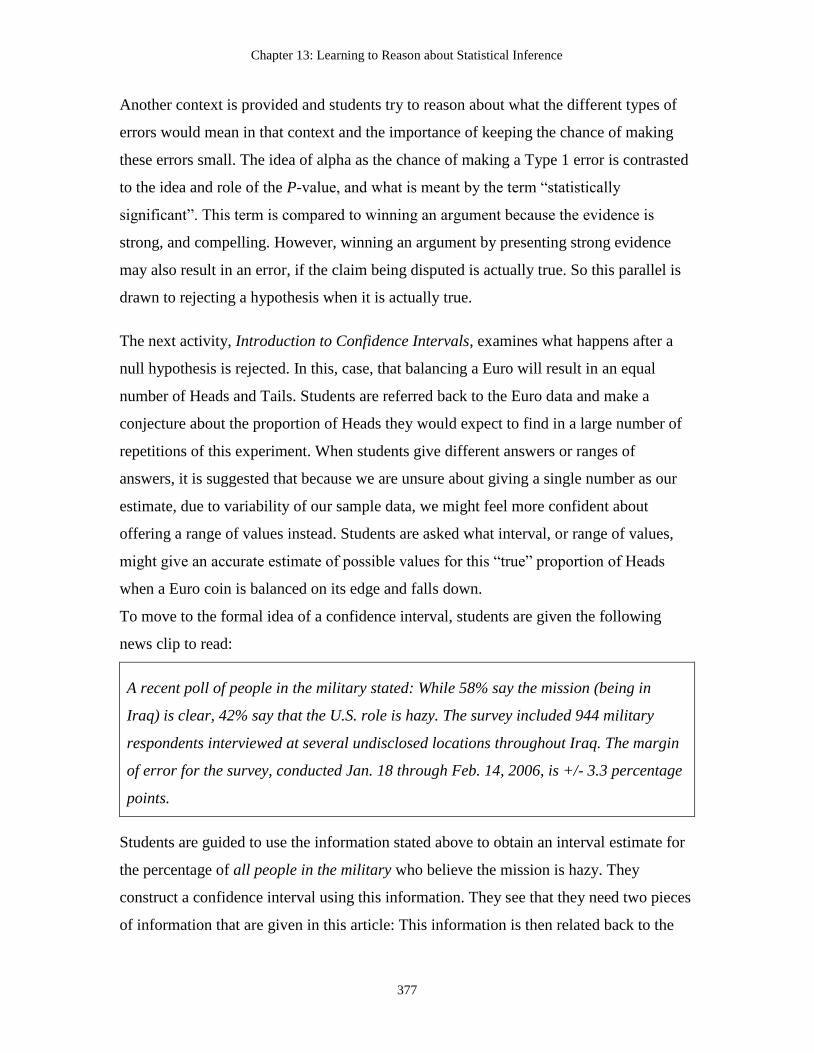
Chapter 13: Learning to Reason about Statistical Inference
377
Another context is provided and students try to reason about what the different types of
errors would mean in that context and the importance of keeping the chance of making
these errors small. The idea of alpha as the chance of making a Type 1 error is contrasted
to the idea and role of the P-value, and what is meant by the term “statistically
significant”. This term is compared to winning an argument because the evidence is
strong, and compelling. However, winning an argument by presenting strong evidence
may also result in an error, if the claim being disputed is actually true. So this parallel is
drawn to rejecting a hypothesis when it is actually true.
The next activity, Introduction to Confidence Intervals, examines what happens after a
null hypothesis is rejected. In this, case, that balancing a Euro will result in an equal
number of Heads and Tails. Students are referred back to the Euro data and make a
conjecture about the proportion of Heads they would expect to find in a large number of
repetitions of this experiment. When students give different answers or ranges of
answers, it is suggested that because we are unsure about giving a single number as our
estimate, due to variability of our sample data, we might feel more confident about
offering a range of values instead. Students are asked what interval, or range of values,
might give an accurate estimate of possible values for this “true” proportion of Heads
when a Euro coin is balanced on its edge and falls down.
To move to the formal idea of a confidence interval, students are given the following
news clip to read:
A recent poll of people in the military stated: While 58% say the mission (being in
Iraq) is clear, 42% say that the U.S. role is hazy. The survey included 944 military
respondents interviewed at several undisclosed locations throughout Iraq. The margin
of error for the survey, conducted Jan. 18 through Feb. 14, 2006, is +/- 3.3 percentage
points.
Students are guided to use the information stated above to obtain an interval estimate for
the percentage of all people in the military who believe the mission is hazy. They
construct a confidence interval using this information. They see that they need two pieces
of information that are given in this article: This information is then related back to the

Chapter 13: Learning to Reason about Statistical Inference
378
problem of finding a confidence interval for the proportion of Heads when balancing a
Euro coin. This includes:
A sample statistic (e.g., the class proportion of Heads when balancing coins), and,
A margin of error (an estimate of how much this statistic varies from sample to
sample for a given sample size, calculated from the sample data and information
from the sampling distribution for the sample statistic).
Students are shown two ways to present confidence intervals:
The sample average, plus or minus a margin of error (e.g., estimating the average
textbook price for statistics, $80 +/- $15).
The two endpoints (low and high values) of the interval. (e.g., $65 to $95).
The relationship of the confidence level to the idea of error is examined, and students
reason about what a confidence interval tells about estimating a parameter and possibly
making an error abut that estimate. Students see that a confidence interval provides two
kinds of information: an interval estimate for the population parameter (rather than a
single number estimate) and a level of confidence (how confident we are that our interval
includes the population value we want to estimate).
A wrap-up discussion includes what the term “margin of error” means, and how this term
is used when interpreting results from a poll. Students describe the sample and the
population for the survey reported above and to critique it, referring back to material from
the unit on Data related to designing good surveys (Lessons 1 and 2 in the unit on Data,
Chapter 6). Students also consider and discuss different interpretations of the poll results,
such as: Can we use our interval to give a guess about the true percentage of all people in
the military that believe the mission is hazy? How? How sure are we? Are there any
problems with generalizing from our sample of 944 military respondents to all people in
the military?
Lesson 3: Reasoning about Confidence Intervals

Chapter 13: Learning to Reason about Statistical Inference
379
This lesson helps students develop their reasoning about confidence intervals by using
simulation to make and test conjectures about factors that affect confidence intervals.
They also have opportunities to discuss common misconceptions as they critique
interpretations of confidence intervals. Student learning goals for this lesson include:
1. Develop reasoning about confidence interval.
2. Understand what 95% confident actually means.
3. Understand how sample size and confidence level affect the length of the
confidence interval.
4. Become familiar finding a confidence interval using Fathom software.
5. Understand connections between confidence intervals and hypothesis tests.
Description of the Lesson
In the Estimating with Confidence activity, students return to the question from the
previous lesson: “What is the true (expected) proportion of Heads when a Euro is
balanced?” Now that they believe that the proportion of Heads when a Euro balanced is
not equal to 0.5, then what is it? Students now know the idea of a confidence interval.
Fathom is used to produce a confidence interval for the sample of data based on
balancing a Euro coin. The class discusses how to interpret this result and are asked what
type of estimate might be more informative about the location of the actual population
parameter, a narrower or wider interval, and why.
Connections are then made between testing a hypothesis and estimating with a
confidence interval, and students see how a confidence interval can be used to test a
hypothesis. Students make a conjecture about how the confidence interval would be
different if they had only 50 pieces of data rather than 100, and then if they had 1000 data
values and why. This conjecture will be examined later in a simulation activity. Students
reflect on the previous unit on sampling and distinguish between the sample statistic and
a population parameter for the Euro coin example, and how much they would expect a
sample statistic to vary from a population parameter.

Chapter 13: Learning to Reason about Statistical Inference
380
In the Estimating Word Lengths activity students return to the Gettysburg Address
activity from the unit on Data (Lesson 3 in Chapter 6) in which they sampled words from
the Gettysburg Address. They use the Gettysburg Address as a population and take
samples and construct confidence intervals to see how they behave and how to interpret
them. They use the Gettysburg Address Web applet to take a random sample of 25 words
and then use Fathom to find a 95% confidence interval to estimate the true mean word
length for all of the words in the Gettysburg Address. Next, the students draw their
confidence intervals on the board, one on top of another. These intervals are compared to
the true population mean word length, and students examine how many of the intervals
generated by the class overlap the true population mean. Students are asked what
percentage of all the intervals in the class they would expect to not overlap the population
mean and find it is close to what they have generated.
The next activity (What Does the 95% Mean?) leads students use Sampling SIM to make
and test conjectures about confidence intervals. They sample data from different
populations such as a normal curve as well as for a skewed distribution, which is shown
in Figure 1.

Chapter 13: Learning to Reason about Statistical Inference
381
Figure 1: A right-skewed population produced by Sampling SIM.
Students generate 200 95% confidence intervals for samples of size 25 and examine how
many do not include the population mean (shown as red lines) and how close the
proportion of intervals that include the mean is to 95% (see Figure 2). They use the
results from Sampling SIM to help answer the following questions that target common
misconceptions about confidence intervals:
Figure 2: Two hundred 95% confidence intervals (sample size 25) form a right-skewed
population in Sampling SIM.
1. Does the level of confidence, 95%, refer to the percent of data values in the
interval?

Chapter 13: Learning to Reason about Statistical Inference
382
2. Does the level of confidence, 95%, refer to the location of the sample mean or
locating the population mean? Explain.
3. Does the level of confidence, 95%, refer to a single interval (e.g., the one you
found in Fathom) or to the process or creating many intervals (e.g., all possible
intervals)? Explain.
Next, students use the Sampling SIM to make and test conjectures about what factors
affect the width of the confidence interval. They then test these conjectures by increasing
and decreasing the level of confidence, and changing the sample size, generating new
simulated intervals each time. See Figure 3 for larger sample size and Figure 4 for larger
confidence level.
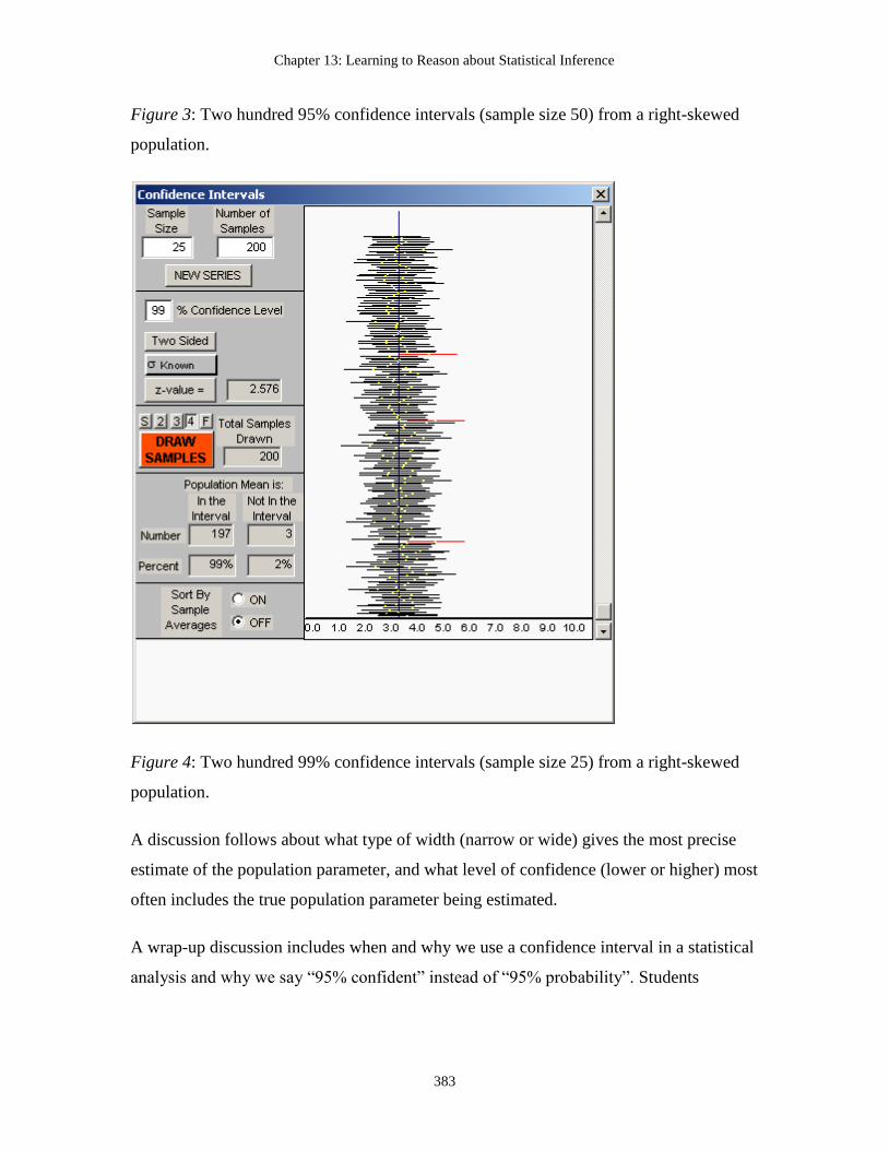
Chapter 13: Learning to Reason about Statistical Inference
383
Figure 3: Two hundred 95% confidence intervals (sample size 50) from a right-skewed
population.
Figure 4: Two hundred 99% confidence intervals (sample size 25) from a right-skewed
population.
A discussion follows about what type of width (narrow or wide) gives the most precise
estimate of the population parameter, and what level of confidence (lower or higher) most
often includes the true population parameter being estimated.
A wrap-up discussion includes when and why we use a confidence interval in a statistical
analysis and why we say “95% confident” instead of “95% probability”. Students

Chapter 13: Learning to Reason about Statistical Inference
384
consider why and how confidence intervals and hypothesis tests are connected, and what
is unique about each approach and the information it provides.
Lesson 4: Using Inference in an Experiment
This lesson described at the beginning of this chapter revisits an earlier experiment,
giving students a chance to try to reduce within group variation and better detect a
difference in the two conditions. Data are gathered and analyzed first graphically and
then using Fathom to run a two sample t-test. The logic of hypothesis tests and
comparison to making an argument are revisited for this context. Student learning goals
for the lesson include:
1. Understand the idea of a two-sample hypothesis test.
2. Differentiate between a one-tailed and a two-tailed test.
3. Use Fathom to conduct a two-sample test.
4. Understand the idea of a two-sample confidence interval (difference in means).
5. Use Fathom to conduct a confidence interval to estimate a difference in means.
6. Revisit the ideas of designing an experiment and making cause and effect
inferences.
7. Revisit ideas of within and between group variation and how they affect a two
sample comparison.
8. Revisit idea of how to reduce variation within a condition, and ideas of signal and
noise in repeated measurements within each condition.
Description of the Lesson
In the Gummy Bears Revisited Activity, students reflect on the earlier Gummy Bear
activity (Lesson 2 in the Comparing Groups Unit, Chapter 11) and to discuss how to
determine if there is a difference between two conditions in an experiment, in this case, if

Chapter 13: Learning to Reason about Statistical Inference
385
there are different average launching distances for the one book or four book launching
pads. Students are asked, in light of recent discussions and activities on statistical
inference, to suggest how, if a difference in sample means is observed, this is not just due
to chance.
The students redo the experiment after first discussing a careful and systematic protocol
to follow in launching the Gummy bears. Treatments are assigned to groups and each
group produces data for 10 launches. Students use Fathom to produce side by side
boxplots, discussing what the boxplots suggest about the differences in flight distances
for the two conditions. Students are asked how to determine if the observed difference in
group means is statistically significant and what this means. The null and alternative
hypotheses are constructed and Fathom is used to run the test. Students contrast one and
two tailed tests for this experiment, and run the test both ways using Fathom, contrasting
the difference in results. Students explain what the results of the hypothesis test suggest
about the difference between the two launching heights. Next, students use a confidence
interval to estimate the mean difference in average launch. They discuss what it means if
a difference of 0 is in the interval or is not in the interval. Since 0 was not in the interval
they concluded that this is a statistically significant difference in flight distances.
In a wrap-up discussion students suggest reasons to use a one-tailed or two-tailed test of
significance, and advantages and disadvantages of each method. They reason about how
the type of test (one or two tailed) affects the P-values obtained and which method is
more conservative. Finally, students give a full statistical conclusion about the
comparison of flight distances for short vs. high launching pads.
Lesson 5: Solving Statistical Problems Involving Statistical Inference
This lesson comes at the end of a course, after the study of covariation (see Chapter 14)
and helps students connect and integrate concepts and processes in statistical inference,
developing their statistical thinking. Student learning goals for the lesson include:
1. Review the process of conducting and interpreting a test of significance.
2. Review the process for finding, reporting, and interpreting confidence intervals.

Chapter 13: Learning to Reason about Statistical Inference
386
3. Review the conditions/assumptions that are necessary for our inferences to be
valid.
4. Be able to research questions to appropriate inferential procedures.
5. Practice using Fathom to conduct tests of significance and to find confidence
intervals.
6. Be able to interpret and justify results of statistical inferences.
Description of the Lesson
Discussion begins by looking back at the first few days of the course when students
simulated data to estimate the probability that a sample statistic was due to either chance
or to some other factor (e.g., ability to correctly identify Coke of Pepsi in a blind taste test
vs. lucky guesses), and then moving ahead to when students learned how to use Fathom
to generate P-values and confidence intervals to help in making inferences and decisions
about population parameters. Now that software can be used to generate statistical results
for inferences, students consider the decisions that have to be made, for example:
a. What type of analysis to run (e.g., test or estimate, one or two samples, etc.).
b. What conditions to check.
c. How to interpret the results (and also know if we made a mistake).
In the Research Questions Involving Statistical Methods activity, students are reminded
that the computer will generate P-values for tests of significance and construct
confidence intervals for population parameters, even if the conditions are not checked and
met. The class discusses how one should interpret the results of a procedure where the
conditions aren’t met. Next, students are given the following table (Table 2) to discuss
and complete it together, which will serve as a guide for running different analyses to
produce inferential statistics in Fathom.

Chapter 13: Learning to Reason about Statistical Inference
387
Table 2: A guide for running different analyses to produce inferential statistics in
Fathom.
Type of Procedure Example of Research Question Fathom Instructions
One sample confidence
interval for proportion
What is the proportion of college
students who graduate in 4 years from
your school?
One sample confidence
interval for a mean
What is the average number of credits
earned by students when they
graduate with a bachelor’s degree?
One sample hypothesis
test for a proportion
Is the proportion of students who
withdraw during their first year equal
to 0.15 (The proportion who withdrew
five years ago)?
Is the proportion of students who
withdraw during their first year less
than 0.15?
One sample hypothesis
test for a mean
Is the average number of years it takes
to finish a degree equal to 5?
Is the average number of years it takes
to finish a degree greater than 4?
Two sample confidence
interval for the
difference between two
means
What is the difference in the average
number of hours spent studying each
week between physics majors and
English majors?
Two sample hypothesis Is there a difference in the mean

Chapter 13: Learning to Reason about Statistical Inference
388
test to compare two
means
GPA’s of first year and fourth year
students?
Students are then given a set of research questions (as shown below in Table 3) and a data
set to use in answering the questions, using Fathom software. The data set contains the
body measurements for a random sample of 50 college students. First, the instructor
models statistical thinking, talking out loud and demonstrating the questions and steps
and interpretations involved in answering one or two of the questions on the list below.
Working together, students then discuss each question, select appropriate procedures, test
conditions, generate graphs and analyses, and interpret their results.
Table 3: Selecting appropriate procedures and hypotheses to given research questions.
Research Question
Type of
Procedure
Null and Alternative
Hypothesis (If Appropriate)
What proportion of students in this class
has a larger arm span than height?
What is the average hand span for
students in this class?
What is the difference in hand spans for
males and females?
Is the average height for female students
greater than 163 cm?
Is the proportion of male students who
are taller than 172.72 cm different from
0.5?

Chapter 13: Learning to Reason about Statistical Inference
389
Is there a difference between males and
females in head circumference?
After students complete this work, group answers to the questions are shared and
justified.
Summary
Most students studying statistics encounter great difficulty when they reach the topics of
statistical inference. Some instructors have compare student response to lecturers on this
topic as “the deer in the headlight” phenomena, as students seem frozen, confused, and
scared when learning these difficult topics. The research literature documents the
difficulty students have understanding inference and typical misconception that persist
regarding P-values and confidence intervals.
Although many statistics courses put statistical inference at the end of a first course in
statistics, we have illustrated a research-based approach that first presents informal ideas
of inference early in the class and revisits these ideas again and again, so that when the
formal ideas are introduced later they are more intuitive and easier to understand. The
idea of statistical hypotheses as making arguments is used to help make this difficult
topic more accessible to students. At the end of the course students are given a set of
research questions and need to integrate and apply all that they have learned to determine
what procedures are needed and appropriate, provide answers, and justify their
conclusions. This process is first modeled by their instructor and then they have the
opportunity to use and develop their own statistical thinking by approaching these
questions as statisticians, rather than just solving a series of textbook problems for each
given procedure. This approach also differs from more standard approaches because the
computational procedures are not emphasized. Instead, the process of using the computer
to test hypotheses and estimating parameters is stressed, along with how to do this wisely
and how to justify and interpret results.

390
Chapter 14: Learning to Reason about Covariation8
Even young children have the tendency to use the covariation of
events as an indicator of causality. (Zimmerman, 2005, p. 22)
Snapshot of a Research-based Activity on Covariation
It is the first day of a unit on bivariate data. Students consider what kind of pattern they
expect to see between the number of semesters a college student has been in school and
the cumulative umber of credits she/he has earned. They make a conjecture about the data
they would see if they took random samples of 100 college students, each group sampled
from all students who are beginning their first, second, third, fourth, fifth and sixth
semesters of college. Then, working in groups, students sketch a sequence of box plots,
showing what they would predict to be the distributions of cumulative college credits for
these six groups of 100 randomly selected college students who have been enrolled for
one to six semesters.
Students discuss their reasoning as they do this, commenting that during the first semester
students take from 10–18 credits, but most take about 13–15 credits. They reason about
center and spread as they draw a predicted boxplot for the first semester. For each
subsequent semester they also think about expected typical values and spread around
those values, drawing a total of six parallel boxplots. They share their reasoning with the
class, explaining that they expect more variability over time even though they expect an
average increase in cumulative credits. Next, they generate and examine graphs and
summary statistics for actual random samples of data for 100 students for each of the first
six semesters of their enrollment, and compare these to their conjectures. See a sample of
such graphs in Figure 1 below.
8 We gratefully acknowledge the major contribution of Dr. Andrew Zieffler to the writing of this chapter.

Chapter 14: Learning to Reason about Covariation
391
Figure 1: A sequence of box plots, showing the distributions of cumulative college
credits for six samples of 100 randomly selected college students, representing first
through sixth semesters.
Students’ attention is drawn to both center and spread of the boxplots for each semester
and how they change over time. Students then discuss and write an explanation about
what these graphs indicate about the relationship between length of time in school and
cumulative credits earned. They are asked questions about how well they think these data
generalize to all students at their institution and what types of inferences they would be
willing to make based on these data. Students then consider a variable that has an inverse
relationship with number of credits, so that values of this variable get smaller as the
number of credits gets bigger. They suggest, for example, the time left before graduation:
that with more credits, there is a shorter time left before graduation. They are asked if this
‘negative’ relationship is a weak one, or if they think it is a strong one, and it is decided
that the relationship is just as strong as the positive relationship with number of semesters
in school.
Finally, a discussion about causation is introduced as the students are asked to discuss
whether the number of semesters of being in school “causes” them to have more credits,
and whether a cause and effect can be determined by examining this bivariate data set.
Rationale for This Activity

Chapter 14: Learning to Reason about Covariation
392
Students may have seen scatterplots before and may have ideas of trends over time, but
most likely do not think about variability in bivariate data. This activity begins by having
them think about variability at six intervals, as well as thinking about the linear trend,
based on the centers (median values) for data in these intervals. Thus, they are guided to
examine and interpret bivariate data by looking for a trend as well as scatter from the
trend, by focusing on both center and spread for one variable (y) relative to values of a
second, ordinal variable (x) (an approach suggested by Cook & Weisberg, 1999). This
activity helps students begin to reason about the idea of a linear relationship between two
variables and helps prepare them to better interpret and reason about scatterplots of data.
When they examine scatterplots they can try to remember the idea of parallel boxplots
and how they represent a series of mini distributions of the y variable, each having center
and spread, for the x variable, as shown in Figure 1.
This lesson also brings up informally two important ideas that are often difficult for
students to understand about covariation. The first is that covariation between two
variables does not mean that one causes the other. The second point is the idea that a
negative association between two variables does not imply a weak association.
The Importance of Understanding Covariation
Reasoning about association (or relationship) between two variables, also referred to as
covariational reasoning, or reasoning about bivariate data, involves knowing how to
judge and interpret a relationship between two variables. Covariational reasoning has also
been defined as the cognitive activities involved in coordinating two varying quantities
while attending to the ways in which they change in relation to each other (Carlson,
Jacobs, Coe, Larsen, & Hsu, 2002). This type of reasoning may take a very mathematical
form (e.g., a linear function), a statistical form (reasoning about a scatterplot), or a more
qualitative form (e.g., causal predictions about events, based on observed associations,
such as spending more time studying seems to lead to better tests grades, as described in
causal model theory in psychology). Covariational reasoning is also viewed as playing an
important role in scientific reasoning (Koslowski, 1996; Schauble, 1996). Although
covariation between events is a necessary but not sufficient basis for inferring a causal

Chapter 14: Learning to Reason about Covariation
393
relationship, it is a basis for making causal inductive inferences in science (Zimmerman,
2005).
The concept of covariation may be unique in that is an important concept in the different
fields of psychology, science, mathematics and statistics, and that covariational reasoning
is described somewhat differently in each discipline. Statisticians may be surprised that
reasoning about covariation, which they think of as a statistical topic focusing on
bivariate distributions of data, is much more complex than the familiar caution that
“correlation does not imply causation,” and beyond reasoning about scatterplots,
correlation, and regression analyses. Indeed, cognitive psychologists McKenzie and
Mikkelsen (in press) wrote that covariational reasoning is one of the most important
cognitive activities that humans perform.
It is our view that to deeply understand covariation in a statistical context one must
understand all the aspects of covariation described in the other disciplines, as well as
understand aspects unique to statistics (such as model fitting and residuals) because of the
inherent variability of real data. Such an understanding involves ideas of structure and
strength of a bivariate relationship as well is its role in causal models and in predicting
events, and the changing values of one variable relative to another, as expressed in a line.
It is no wonder that students have difficulty understanding concepts related to
covariation, including the correlation coefficient, r-squared, and a regression line.
Watkins, Scheaffer, & Cobb (2004) describe six features of a bivariate relationship that
may be used to guide students as they learn to examine and reason about bivariate data.
These are:
1. The individual variables and their variability.
2. The shape of a pattern revealed in a bivariate plot in terms of linearity, clusters,
and outliers.
3. The trend if there is one (positive or negative).
4. The strength of the trend: strong or weak, varying or constant.

Chapter 14: Learning to Reason about Covariation
394
5. Whether the pattern may generalize to other situations (can be tested with
inferential methods, and is also based on how the sample was obtained).
6. If there plausible explanations for the pattern? Is it plausible that one variable may
have a causal relationship or might a third, lurking variable cause the relationship.
These ideas may be developed informally and then revisited in more formal ways.
The Place of Covariation in the Curriculum
Topics involving covariation may be introduced at various times in the curriculum. In
some introductory courses and textbooks scatterplots are introduced as part of a data
analysis unit. The topic of correlation and regression may be introduced before or after
the topic of statistical inference, with arguments made for each placement of the topic
(see Zieffler, 2006). Related ideas of contingency tables and chi-square tests often appear
in a separate unit, many times at the end of a course.
We believe that the topic of covariation may be informally introduced in a unit on
collecting and producing data, and that graphs of bivariate data may be informally
introduced as part of data analysis, but that the formal study of bivariate data takes place
after the study of statistical inference. Our reasons for this are that the study of
covariation builds on and integrates many topics studied earlier in the course, and can
revisit and deepen these ideas as topic taught near or at the end of an introductory course.
These ideas include distribution of data, center and spread, variability, fitting a model to
data, using experiments to infer causation, using correlation to explore relationships
among observational variables, and using statistical inference to run tests on correlations
and regression coefficients to see if observed relationships may be generalized.
We realize that it is somewhat controversial to delay the study of scatterplots, correlation,
and simple linear regression to near the end of the course. We do this based on our review
of the research literature, on our findings that students are able to informally reason about
bivariate data well before formal instruction on this topic (see Zieffler, 2006) and based
on our positive experience teaching the topic at this final point in a course. However,
instructors who want to introduce some of the lessons and activities in this chapter at an
Chapter 14: Learning to Reason about Covariation
395
earlier point in their course are welcome to do so. Finally, we want to revisit the idea
mentioned in Chapter 6 about the importance of students being exposed to multivariate
data sets. Once again, the data sets in this chapter are multivariate, and while students
may examine pairs of variables at a time, they are also encouraged to look at the data sets
in a multivariate way, disusing and integrating information about relationships between
pairs of variables to better understand the variability of individual variables as well as
aspects of the multivariate data set.
Review of the Literature Related to Reasoning about Covariation
Because of its important role in so many disciplines, covariational reasoning has been the
focus of research in psychology, science, and mathematics education, in addition to
statistics education. The research studies related to covariational understanding and
reasoning are quite diverse, and vary according to the disciplinary field of the researchers.
These studies are summarized in four main areas: judgment of covariation, understanding
covariation as functional relationships, covariational reasoning in science education, and
covariational reasoning and judgments in statistics.
Judgment of Covariation
Research by psychologists provides much of the seminal work in covariational reasoning
research. Since the seminal study by Inhelder and Piaget (1958), psychologists have
produced several robust findings, based on large sample sizes and use of randomized
treatment designs and analyses, spanning five decades of research in this area. Regardless
of the importance that covariational reasoning seems to play in the day-to-day lives of
people, much of the research from the field of psychology has generally concluded that
people are surprisingly poor at assessing covariation. A robust finding is that peoples’
prior beliefs about the relationship between two variables have a great deal of influence
on their judgments of the covariation between those variables (e.g., Jennings, Amabile, &
Ross, 1982; Kuhn, Amsel, & O’Loughlin, 1988).
This finding is related to another consistent finding, that of illusory correlation. An
illusory correlation exists when a subject believes there is a correlation between two

Chapter 14: Learning to Reason about Covariation
396
uncorrelated events. This, for example, could encompass relying more on memory rather
than examining the data/cases presented (e.g., subjects would suggest a positive
relationship exists between price and quality even though the data would suggest
otherwise), and viewing data/cases that confirm their expectations as more relevant than
disconfirming cases (e.g., McGahan, McDougal, Williamson, & Pryor, 2000).
Additional studies have examined how people reason about covariation of data in
contingency tables, indicating that people tend to not treat the four cells of a 2-by-2
contingency table as equally important. In fact, peoples’ judgments seem to be most
influenced by the joint presence of variables and least influenced by the joint absence of
variables (e.g., Kao & Wasserman, 1993). Other studies showed that peopled have
difficulty when a bivariate relationship is negative (e.g., Beyth-Marom, 1982), and that
peoples’ covariational judgment of the relationship between two variables tends to be less
than optimum (i.e., smaller than the actual correlation presented in the data or graph)
(e.g., Jennings et al., 1982). Still another consistent finding in these studies is that
subjects have a tendency to form causal relationships based on a covariational analysis
(e.g., Ross & Cousins, 1993).
Research studies have also examined the conditions and accommodations under which
people tend to make better covariational judgments. For instance, researchers have found
that subjects tend to make more accurate judgments when the variables to be examined
are continuous rather than dichotomous (e.g., Jennings et al., 1982), and other studies
have suggested that certain accommodations such as detailed instructions (Alloy &
Abramson, 1979), easy to process formats (Ward & Jenkins, 1965), subjects being told
non-contingency is possible (Peterson, 1980), and low frequency of data/cases (Inhelder
& Piaget, 1958) might help subjects more accurately judge covariation. Subjects have
also been shown to make more accurate judgments when data are presented
simultaneously rather than when it is presented one case at a time (e.g., Seggie &
Endersby, 1972).

Chapter 14: Learning to Reason about Covariation
397
Understanding Covariation as Functional Relationships
Studies on covariational reasoning by mathematics education researchers tend to focus on
lines and understanding functions, or aspects of bivariate reasoning that might be used in
algebra and calculus. For example, Carlson et al. (2002) classified college students'
mental actions affect reasoning about covariation as follows:
1. The coordination of the value of one variable with changes in the other.
2. The coordination of the direction of change of one variable with changes in the
other.
3. The coordination of the amount of change of one variable with the amount of
change in the other.
4. The coordination of the average rate of change of the function with uniform
increments of change in the input variable.
5. The coordination of the instantaneous rate of change of the function with
continuous change in the independent variable for the entire domain of the
function.
Carlson’s studies suggested that most students could determine the direction of change
but that many had difficulties constructing images of continuous rate of change, even
after completion of a second course in calculus. The researchers noted that students have
particular problems representing and interpreting graphical displays. In some cases,
mathematics education researchers have suggested the need for teachers to have students
think about covariation as it occurs in functions in terms of real-life dynamic events (e.g.,
Carlson et al., 2002).
Other researchers have pointed out that covariational reasoning is used extensively in
both algebra (Nemirovsky, 1996) and calculus (Thompson, 1994). In particular, studies
suggest that this type of reasoning plays a major role in students’ understanding of the
derivative, or rate of change (e.g., Carlson et al., 2002), and that this interpretation of
covariation is slow to develop among students (e.g., Monk & Nemirovsky, 1994;

Chapter 14: Learning to Reason about Covariation
398
Nemirovsky, 1996). Studies from mathematics education have also shown that not only is
students’ ability to interpret graphical and functional information slow to develop, but
that students tend not to see the graph of a function as depicting covariation (Thompson,
1994).
Covariational Reasoning in Science Education
Researchers in science education have focused on either the psychological aspect of
covariation in relation to identifying causal factors or on the mathematical aspects of
covariation, such as reasoning about lines and functions. Some researchers have studied
how students use covariational reasoning in solving science problems, finding that
students tend to use sub-optimal solution strategies to determine if a relationship exists or
does not exist in a set of bivariate data, and that students tend to infer a causal
relationship from correlational data (e.g., Adi, Karplus, Lawson, & Pulos, 1978).
In a more recent study by Kanari and Millar (2004) students’ approaches to data
collection and interpretation were studied as they investigated relationships between
variables, as part of students’ ability to reason from data. The authors argue that it is
reasoning from data that distinguishes scientific reasoning from logical reasoning. They
found that students of all ages had a much lower success rate in investigations where the
dependent variable did not covary with the independent variable, than in those where it
did covary. They suggest that school science investigations should include both
covariation and non-covariation cases to develop students’ covariational reasoning.
Covariational Reasoning and Judgments in Statistics
Statistics education research has generally focused on studying students’ covariational
reasoning as part of instruction in statistics. The methodologies used have been primarily
qualitative, following the format of design experiments (e.g., Cobb, McClain, &
Gravemeijer, 2003) while other studies on covariational reasoning in statistics education
have used methods in psychology, using a qualitative coding scheme to help categorize
response data (e.g., Batanero, Estepa, & Godino, 1997; Moritz, 2004; Morris, 1997;
Stockburger, 1982).

Chapter 14: Learning to Reason about Covariation
399
In one of the earlier studies, Stockburger (1982) asked university students enrolled in an
introductory statistics course to complete many times four computer exercises, such as
estimating the correlation coefficient. Stockburger found that students in general did very
poorly on these exercises, and their ability to estimate correlation improved after using
the computer software.
The impact of computers in developing understanding of statistical association was
studied by Batanero, Estepa, Godino, & Green (1996) and Batanero et al. (1997).
Students were asked to assess the existence of correlation between two variables given to
them in a two-by-two contingency table. The researchers then identified incorrect
covariational strategies employed by the students (drawing on strategies first outlined in
1958 by Inhelder & Piaget). Both studies (Batanero et al., 1996; Batanero et al., 1997)
found an overall general improvement in student strategies. They also both revealed the
persistence of what they refer to as a unidirectional misconception. That is, students only
perceive a relationship among the variables in the positive direction.
Both studies also showed that students maintained their causal misconception throughout
the duration of the experiments. Both studies also showed that students had problems
with several features of association such as distinguishing between the role of
independent and dependent variables and reasoning about relationships that were
negative. Finally, students realized that the absolute value of the correlation coefficient
was related to the magnitude of the relationship, but did not relate that idea to the spread
of scatter around the regression line.
Other studies have examined students’ covariational reasoning as they study regression
and reported some of the difficulties associated with this topic including problems with
interpretation (e.g., Sánchez, 1999), and problems with the coefficient of determination,
or 2r (Truran, 1997). Konold (2002) presents a different view of whether or not people
can make accurate covariational judgments. He suggests that people are not poor at
making these judgments, but rather they have trouble decoding the ways in which these
relationships are displayed (e.g., scatterplots or two-by-two contingency tables). His
research has been on middle school students using TinkerPlots (Konold & Miller, 2005).

Chapter 14: Learning to Reason about Covariation
400
Konold found that students were better able to make covariational judgments using a
super-imposed color gradient function in TinkerPlots, possibly because relationships
between variables are explored by use of only one dimension (e.g., horizontal axis) for
one variable and color gradient for the other (see Figure 2). In addition, the task is broken
up into two smaller parts: First, students anticipate what will be seen and second, that
they then examine the new display.
Figure 2: A TinkerPlots graph displays how data of Ozone levels in New York City on
111 successive days in 1973 is associated with the maximum daily temperature9.
In a study of younger children, Moritz (2004) had students translate verbal statements to
graphs and also translate a scatterplot into a verbal statement, and related tasks. The
students were given a written survey that included six or seven open-ended tasks
involving familiar variables. The variables were also chosen so that students would
expect a positive covariation, but the data given in the task represented a negative
covariation. Moritz (2004) found many of the same student difficulties as other studies
9 The TinkerPlots graph in Figure 1 displays data of Ozone levels (Ground-level Ozone in parts per billion)
in New York City on 111 successive days from May to September in 1973. To explore the relationship
between Ozone levels and temperature (Maximum temperature in degrees Fahrenheit) we first presented
the Ozone level on the x-axis, “fully separated” the cases, and then colored the icons with the green
temperature gradient. We notice how as we move up the Ozone scale we tend to go from the lower
temperatures (the lighter green) to the higher temperatures (the darker green).

Chapter 14: Learning to Reason about Covariation
401
have revealed: that students often focused on isolated data points rather than on the global
data set (e.g., Ben-Zvi & Arcavi, 2001). He also found that students would often focus on
a single variable rather than the bivariate data, and that several students had trouble
handling negative covariations when they are contradictory to their prior beliefs.
Two more recent design experiment studies investigated the role of technology in helping
students reason about bivariate data, and how students differentiate between local and
global variation in bivariate data. Gravemeijer (2000) results suggest that students need
an idea of the global trend (prior expectation) and that students have a hard time
distinguishing between arbitrary and structural covariation. He suggests that students
examine and compare several univariate data sets (time series) as an introduction to
examining bivariate data.
This approach was used by Cobb et al. (2003) to help students view bivariate data as
distributed in two-dimensional space, to see scatterplots as situational texts, and to track
the distribution of one variable across the other (scan vertically rather than diagonally).
Using the Minitools software (Cobb, Gravemeijer, Bowers, & Doorman, 1997) students
examine the “vertical variation” across levels of x in graphs of bivariate data. Students
were asked to compare differences in the distribution of the y-variable at different levels
of the x-variable (See Figure 3).

Chapter 14: Learning to Reason about Covariation
402
Figure 3: Minitools software allows students to start looking at the local variation for
different values on the x-axis in addition to the global trend.
The results of their study suggested that the shape of a distribution is a better place to
start than is variability and that there be a continued focus on relative density and on the
shape of the data within vertical slices. They also suggested that an emphasis on shape
could lead to a discussion of strength and direction in a bivariate plot and that the focus
on vertical distribution could lead to a more intuitive idea of the line of best fit.
A recent study by Zieffler (2006) examined students’ development of reasoning about
quantitative bivariate data during a one-semester university-level introductory statistics
course. He found a surprising result that the most growth in covariational reasoning
occurred early in the course, during the unit on data analysis, and before formal study of
bivariate data. One plausible explanation was that students were developing their
statistical reasoning in this earlier part of the course and that facilitated the growth in
covariational reasoning, even before formal instruction on that topic.
Another result of his study is that students seemed to better reason and learn inference
when the bivariate unit came at the end of the course after inference rather than as part of
or immediately following a unit on exploring data, based on a comparison of two
different sequences of course topics in his study. However, no difference was found in
students’ performance on an assessment of covariational reasoning.
The role of technology in helping students to reason about covariation
The research also suggests that particular types and uses of technology may help students
make more accurate judgments of covariation (Batanero et al., 1996, 1997; Cobb et al.,
2003; Gravemeijer, 2000; Konold, 2002; Stockburger, 1982). The appropriate use of
visualizations can change students’ statistical conceptualizations (Rubin, 2001), particular
software that provide flexible, dynamic capabilities and multiple, linked representations,
allowing students to display, manipulate, and analyze data. This type of technology (e.g.,
TinkerPlots and Fathom) appears to help students understand and apply covariational
reasoning (Carlson et al., 2002; Rubin, 2001). Fathom (Key Curriculum Press, 2006)
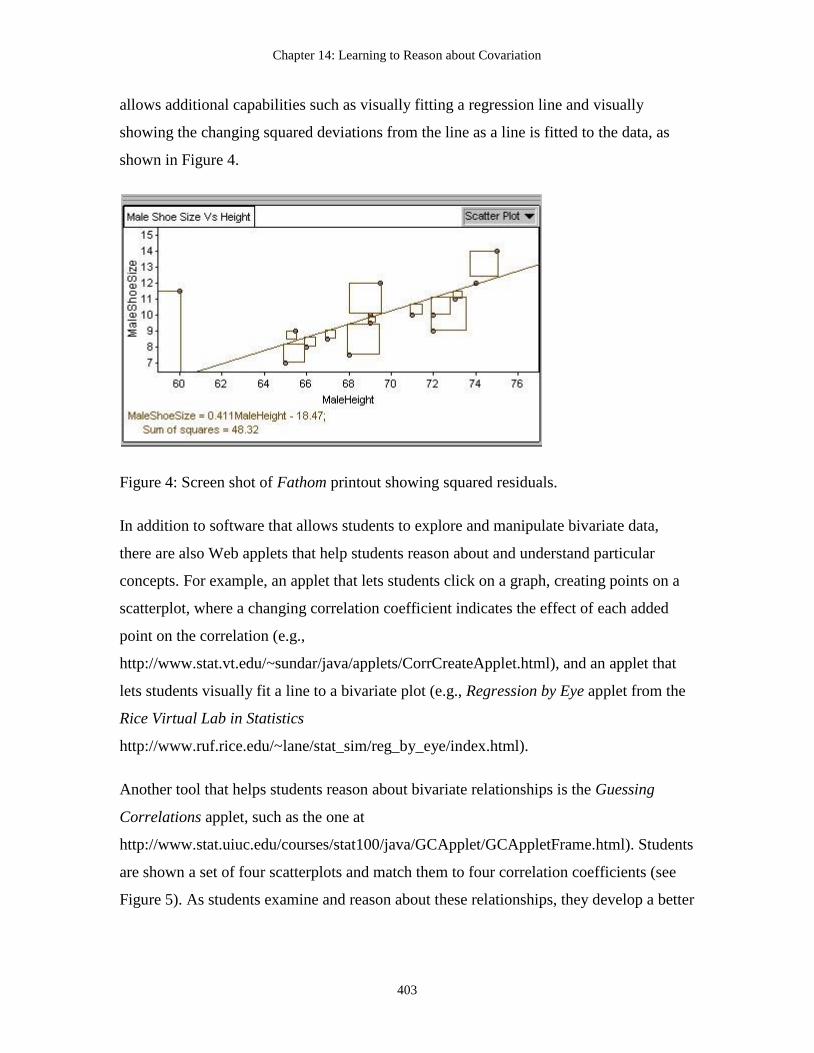
Chapter 14: Learning to Reason about Covariation
403
allows additional capabilities such as visually fitting a regression line and visually
showing the changing squared deviations from the line as a line is fitted to the data, as
shown in Figure 4.
Figure 4: Screen shot of Fathom printout showing squared residuals.
In addition to software that allows students to explore and manipulate bivariate data,
there are also Web applets that help students reason about and understand particular
concepts. For example, an applet that lets students click on a graph, creating points on a
scatterplot, where a changing correlation coefficient indicates the effect of each added
point on the correlation (e.g.,
http://www.stat.vt.edu/~sundar/java/applets/CorrCreateApplet.html), and an applet that
lets students visually fit a line to a bivariate plot (e.g., Regression by Eye applet from the
Rice Virtual Lab in Statistics
http://www.ruf.rice.edu/~lane/stat_sim/reg_by_eye/index.html).
Another tool that helps students reason about bivariate relationships is the Guessing
Correlations applet, such as the one at
http://www.stat.uiuc.edu/courses/stat100/java/GCApplet/GCAppletFrame.html). Students
are shown a set of four scatterplots and match them to four correlation coefficients (see
Figure 5). As students examine and reason about these relationships, they develop a better
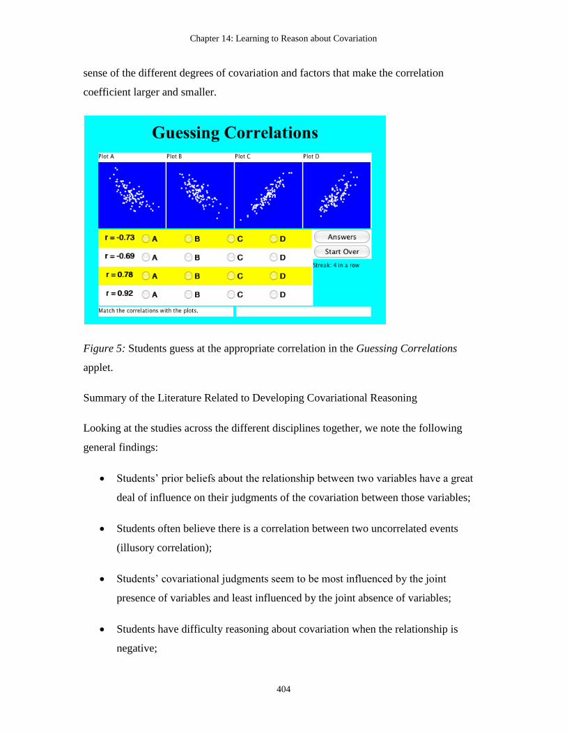
Chapter 14: Learning to Reason about Covariation
404
sense of the different degrees of covariation and factors that make the correlation
coefficient larger and smaller.
Figure 5: Students guess at the appropriate correlation in the Guessing Correlations
applet.
Summary of the Literature Related to Developing Covariational Reasoning
Looking at the studies across the different disciplines together, we note the following
general findings:
Students’ prior beliefs about the relationship between two variables have a great
deal of influence on their judgments of the covariation between those variables;
Students often believe there is a correlation between two uncorrelated events
(illusory correlation);
Students’ covariational judgments seem to be most influenced by the joint
presence of variables and least influenced by the joint absence of variables;
Students have difficulty reasoning about covariation when the relationship is
negative;

Chapter 14: Learning to Reason about Covariation
405
Students’ covariational judgment of the relationship between two variables tends
to be less than optimum (i.e. smaller than the actual correlation presented in the
data or graph); and
Students have a tendency to form causal relationships based on a covariational
analysis.
These findings along with the suggestions based on design experiments lead to some
implications for helping students reason about covariation.
Implications of the Research:
Teaching Students to Reason about Covariation
The research studies reviewed have many implications for the teaching and assessment of
bivariate data. Reasoning about covariation seems to build upon reasoning about
distribution, especially the concepts of shape and variability (Cobb et al., 2003;
Gravemeijer, 2000; Konold, 2002). It is suggested that instruction focus on relative
density and on the shape of the data within vertical slices, leading to ideas of strength and
direction in a bivariate plot, which could lead to a more intuitive idea of the line of best
fit.
The research suggests that using data that has a context seems to be important for better
student understanding of covariation (Adi et al., 1978; Cobb et al., 2003; Gravemeijer,
2000; Moritz, 2004). This especially helps when the data are meaningful to the students
(Moritz, 2004). In addition, the persistence of the positive unidirectional misconception
described above implies that teachers should provide tasks that have students interpret
and reason about data sets that have negative correlations and no covariation, which are
less intuitive and require more thinking on the student part. An awareness of typical
students’ difficulties identified in the research literature can help teachers be on the
lookout for these errors and misconceptions as students work together during activities
and during class discussions, as well as on assessments of learning.
Progression of Ideas: Connecting Research to Teaching

Chapter 14: Learning to Reason about Covariation
406
Introduction to the Sequence of Activities to Develop Reasoning about Covariation
The following sequence of activities presented in lessons are designed to lead students
through a progression of ideas to help them understand the idea of covariation of data and
to develop covariational reasoning. This includes learning to understand and reason about
graphs of bivariate relationships, interpreting and understanding features of bivariate
data, understanding and reasoning about the correlation coefficient, modeling bivariate
data with a line, and making inferences about the nature of bivariate relationships. These
activities build on foundational concepts such as distribution, variability, model,
deviation, and inference.
Table 1: Sequence of activities to develop reasoning about covariation.
Milestones: Ideas and Concepts Suggested Activities
INFOROMAL IDEAS PRIOR TO FORMAL STUDY OF COVARIATION
Understanding when to infer
causation: from an experiment, rather
than from correlated variables.
Taste Test Activity, Lesson 4, Data
Unit (Chapter 6)
FORMAL IDEAS OF COVARIATION
Understanding ideas of trend by
recognizing a positive linear pattern in
the medians of vertical boxplots.
Credit Questions Activity (Lesson 1:
“Reasoning about Scatterplots and
Correlation”)
Understand the nature of bivariate data
and the idea of covariation of two
quantitative variables.
Interpreting Scatterplots Activity
(Lesson 1)
Points in a scatterplot represent pairs
of data for individual cases, measured
on each variable.
Interpreting Scatterplots Activity
(Lesson 1)

Chapter 14: Learning to Reason about Covariation
407
The idea of a linear trend in a bivariate
plot.
Interpreting Scatterplots Activity
(Lesson 1)
Understanding how to distinguish
between a positive trend and a
negative trend, and how this differs
from strength of the trend.
Interpreting Scatterplots Activity
(Lesson 1)
Reasoning about factors that could
cause a linear trend in bivariate data,
and that there could be a lurking
variable (or a causal relationship).
Interpreting Scatterplots Activity
(Lesson 1)
Reasoning about what would be
needed to establish a causal
relationship between two correlated
variables.
Interpreting Scatterplots Activity
(Lesson 1)
Structure and strength in a bivariate
plot: linearity, direction, closeness to
the model of straight line.
Reasoning about the Correlation
Coefficient Activity (Lesson 1)
A correlation coefficient as a measure
of the strength and direction of the
linear relationship.
Reasoning about the Correlation
Coefficient Activity (Lesson 1)
Understating how different aspects of
a bivariate data, as revealed in a
scatterplot, affect the correlation
coefficient.
Guessing Correlations Activity
(Lesson 1)
Understanding how the same
correlation coefficient may be
An activity where students examine
the correlation in data sets that have

Chapter 14: Learning to Reason about Covariation
408
obtained for very different sets of
bivariate data.
the same correlation coefficient but
are very different, including nonlinear
patterns, such as Anscombe Data.
(The symbol indicates that this
activity is not included in these
lessons.)
Fitting a model of a line to data. Diamond Rings Activity (Lesson 2:
“Fitting a Line to Data”)
Strength of the relationship is based on
how well the line (model) fits the data.
Diamond Rings Activity (Lesson 2)
Linear regression as way to model a
linear relationship.
Diamond Rings Activity (Lesson 2)
Regression model in explaining the
relationships between two quantitative
variables.
da Vinci and Body Measurements
Activity (Lesson 2)
What the slope and intercept mean in a
bivariate data model.
da Vinci and Body Measurements
Activity (Lesson 2)
How and why better predictions have
less scatter around the line (and fitted
values).
da Vinci and Body Measurements
Activity (Lesson 2)
Understanding the idea of residuals as
deviations from the line (model) as
providing evidence to assess how well
the line provides a model for a
bivariate data set.
da Vinci and Body Measurements
Activity (Lesson 2)
Understanding how to generalize Testing Relationships: Admissions
Chapter 14: Learning to Reason about Covariation
409
bivariate relationships to a larger
population.
Variables, and Baseball Variables
Activities (Lesson 3: “Inferences
involving Bivariate Data”)
Understanding how to interpret
inferences about correlation
coefficients and regression slopes.
Testing Relationships: Admissions
Variables, and Baseball Variables
Activities (Lesson 3)
Understanding that it is important to
consider the size of the correlation in
addition to the size of the P-value:
practical vs. statistical significance.
Testing Relationships: Admissions
Variables, and Baseball Variables
Activities (Lesson 3)
BUILDING ON FORMAL IDEAS OF COVARIATION IN SUBSEQUENT TOPICS
Knowing how to recognize when a test of
a correlation coefficient or regressions
slope is appropriate to answer a research
question.
Research questions involving statistical
methods activity (Lesson 5, Inference
Unit, Chapter 13)
Introduction to the Lessons
There are three lessons on covariation that focus entirely on the concepts and ideas
without going into the mathematics. The activities in the lesson lead students to first think
about linear trend in the presence of variability, as they move from examinations of
parallel boxplots to a scatterplot to a fitted line. They develop the idea of correlation as a
measure of a linear relationship between two variables, and then use the line as a model
to explain and make predictions based on this relationship. Finally, students learn to
apply ideas of inference to this topic by using tests of significance to test that the
correlation coefficient and regression slope are different than zero.
Lesson 1: Reasoning about Scatterplots and Correlation

Chapter 14: Learning to Reason about Covariation
410
This lesson, as described briefly at the beginning of the chapter, guides students to
develop reasoning about bivariate data by beginning with parallel boxplots and moving to
scatterplots that are viewed as a series of vertical slices of data. In this way, ideas of
center and spread are brought to and integrated into reasoning about bivariate
distributions. Students learn how to examine and interpret scatterplots and begin to
connect values of the correlation coefficient to different types of scatterplots. Causal
factors are also discussed. Student learning goals for this lesson include:
1. Understand the nature of bivariate data and what that points in a scatterplot
represent.
2. Understand and describe shape (form), trend (direction), and variation (strength)
in a scatterplot.
3. Answer contextual questions using information obtained from a scatterplot.
4. Know that a scatterplot is the appropriate graph to create to answer certain
questions about the relationship between two quantitative variables.
5. Estimate correlation coefficients from a scatterplot.
6. Understand that correlation is only about strength of linear trend.
7. Understand that a high correlation does not imply that the data are linear.
8. To be aware of lurking variables and to understand that correlation does not imply
causation.
Description of the Lesson
The lesson begins with a problem involving real student data (Credit Questions activity).
Students are told that university guidance counselors are interested in the number of
credits students accumulate as they progress through their degree programs. They are
interested in studying how long it take a student to reach 60 credits (the requirement to

Chapter 14: Learning to Reason about Covariation
411
reach Junior status) and how the length of time a college student has been in school
relates to the number of credits she/he accumulates.
Students are asked to imagine six cohorts of students whose credit loads are examined,
each group coming from all students in their first, second, third, fourth fifth or sixth
semesters of college. Students are asked to reason about if they expect the average
number of credits that these students have accumulated would differ for students in each
different semester of college. Students also reason about the variation in the total number
of credits accumulated each semester of enrollment.
Next, working in groups, students make conjectures about such a data set. They discuss
and then draw boxplots based on their predictions of what those distributions of
cumulative credits would look like for random samples of 100 students for each of the six
different cohorts. A class discussion follows as students discuss, based on their own
knowledge and experience, what they expect to find in terms of number of credits across
six semesters for students, focusing on center and spread for the number of credits for
each subsequent semester and how the variability increase for each subsequent semester.
Students are then given a data set and use it to generate actual boxplots that are used to
test their conjectures. Students describe the relationship they see between length of time a
college student has been in school and their cumulative number of credits, discussing
trend as well as variation around the trend, in formal language.
Students are asked if they willing to generalize about the relationship found to the
population of all students at the University, based on these data. They also talk about the
fact that there is a strong trend but that one variable does not cause the other, revisiting
ideas of correlation and causation from the earlier unit on data (Chapter 6). Students are
asked to speculate about variables that could have an opposite or inverse relationship with
these variables, distinguishing between a positive and negative trend, acknowledging that
a positive or negative trend be strong or weak.
In the Interpreting Scatterplots activity, students are given a scatterplot representing the
relationship between gestation period (length of pregnancy) and lifespan for a sample of
62 different animals, which has a moderate, positive trend. They first try to separate the

Chapter 14: Learning to Reason about Covariation
412
points into several different vertical slices, or distributions, to determine how the centers
and spread of those distributions are changing, building on the previous boxplot activity.
They are asked if the data indicate a relationship between the two variables, and to
describe the pattern and features of the plot. Students then examine a series of scatterplots
and discuss different features that they see: lots of scatter, little scatter, linear and non
linear patterns, positive and negative directions, different steepness of the linear pattern,
outliers, clusters of points, etc. In the Reasoning about the Correlation Coefficient
activity, students discuss different feature of a scatterplot and how they are used to
interpret and describe bivariate relationships. The correlation coefficient is discussed as a
measure of the linearity of the pattern of points, and how it shows direction as well as
strength.
The next activity (Guessing Correlations) has students using a Web applet to reason
about the correlation coefficient and how different factors make it larger or smaller.
Using the Guessing Correlations applet
(http://www.stat.uiuc.edu/courses/stat100/java/GCApplet/GCAppletFrame.html) students
go through several rounds, talking in pairs about their choices, until they are comfortable
estimating the degree of linearity (correlation) in a dataset. A class discussion follows
about what they learned from this activity as well as the importance of examining a
scatterplot to learn about the relationship between two variables, and not just calculating
a correlation coefficient. Students discuss how the correlation coefficient helps
summarize the relationship between two quantitative variables much like the mean or
standard deviation can be used to describe and summarize a single variable.
A wrap-up discussion has students summarize what the points in the scatterplot represent,
what kind of questions can be answered by examining a scatterplot and correlation for
two variables, what is considered a “low” correlation, and what information a correlation
does and does not provide about two variables. Students are asked whether a high
correlation indicates causation, and how they would determine casual factors.
Lesson 2: Fitting a Line to Data

Chapter 14: Learning to Reason about Covariation
413
This lesson focuses on using the regression line to model bivariate relationships. Students
fit lines to data, discuss the interpretation of the lines in terms of direction and size of the
slope. Students use a regression line to predict values of y based on values of x. They fit
lines to data seeing how the sums of squares are minimized for the regression line. They
also learn about the dangers of extrapolation and see how outliers may affect the fitted
line. Student learning goals for this lesson include:
1. Understand the idea of a line as a model of bivariate relationship.
2. Be able to interpret the slope and y-intercept of a line of best fit in the context of
data.
2. Be able to use a line to predict y from a given x.
3. Understand that a predicted value is not the same as the actual value (in most
cases) and that the difference is the residual.
4. Be able to interpret what the residual means in the context of the data.
5. Understand that extrapolation is not appropriate.
6. Use Fathom to create the line of best fit from a given set of data.
7. Be able to read Fathom output for the line of best fit.
8. Understand the effect of an outlier on the fitted regression line.
Description of the Lesson
The lesson begins with an examination of a data set on diamond rings (Diamond Rings
activity). Students discuss and make conjectures about what they would expect to find in
terms of a relationship between the price of a diamond ring and the number of carats in
the diamond. Next they generate a scatterplot using Fathom that contains the prices of
diamond rings and the carat size of their diamond in each ring. The data look very linear,
and students use Fathom to first estimate where a line would best fit the data. They revisit
the idea of fitting a model to a data set (see Chapter 7), this time using a line as a model

Chapter 14: Learning to Reason about Covariation
414
of the bivariate relationship. They compare the conjectured lines to the regression line (
)(66.222094.154$̂ Carat ), which is shown in Figure 6.
Figure 6: Relationship between the price of a diamond ring (US$) and the number of
carats in the diamond.
Students discuss if the regression line seems to be a good model and how well it fits the
data. They informally discuss the line: its steepness and direction, and what that indicates
about the relationship between the two variables. They also use the line to make informal
predictions for different carat sizes, discussing how the actual prices for each carat size
vary, and that the prediction has error involved. Students also begin to talk about the
scatter of points around the line, as an indication of fit or lack of fit. They talk about
residuals as the vertical deviation of individual points from the line, and see that there can
be an average deviation that indicates fit, and that for this graph that would be smaller
than for the graph of animal data viewed in the previous lesson, which had more scatter
around a fitted line.
The second activity, da Vinci and Body Measurements, has students analyze body
measurements to see if they conform to the “ideal” bivariate relationships described by
Leonardo da Vinci, as listed below:

Chapter 14: Learning to Reason about Covariation
415
Height is equal to the span of the outstretched arms.
Kneeling height is three-fourths of the standing height.
The length of the hand is one-ninth of the height.
Students access the body data collected earlier and begin to examine the three rules listed
above. They first make and examine scatterplots for each pair of variables. Next they use
Fathom to draw on the graphs the line of best fit. They use the graphs and lines to make
predictions of particular values of height, kneeling height and hand length, based on
measurements of arm span and height. These are compared to the ideal values based on
Leonardo’s “rules”. The slopes of the lines are also compared to his rules to see how
closely they correspond. Students are asked questions about x values that are beyond the
domain of x values in the data set, leading to a discussion on extrapolating values and
why that is not a good thing to do.
Students discuss how well a line models the relationships shown in each part of body
data. They are guided to think about residuals as an indicator of fit, and then use the
“Show Squares” feature in Fathom to incorporate the least squares criteria on their
regression lines. They try using movable lines and see that the sum of these squares is
bigger for all lines except the regression line.
In the wrap-up to the lesson, students are asked what they conclude about Leonardo’s
“rules” and to explain their response. Students are given a scatterplot and a regression
line and make a prediction for a value that produces an unusual result, due to
extrapolation, leading them to figure out what was wrong. Next they are given a
scatterplot of a dataset that is not linear, and they are asked whether or not a line of best
fit could be used to predict a value of y in this situation. Finally, they see a demonstration
that shows the effect of outliers on a regression line and reason about why they see two
different effects, depending on when the outlier forces the line or is away from the line.
Lesson 3: Inference Involving Bivariate Data

Chapter 14: Learning to Reason about Covariation
416
Lesson 3 has students make statistical inferences, by testing hypotheses about the
correlation coefficient and regression slope for a sample of bivariate data. Students learn
to do this using Fathom, and to compare these procedures to significance tests involving a
two sample test of means (see Chapter 13). Student learning goals for the lesson include:
1. To learn how to use Fathom to apply a test procedure involving the correlation
coefficient and regression slope.
2. To continue to apply graphical and descriptive methods learned earlier in
conjunction with this test.
3. To revisit and build on the ideas of statistical inference in the context of bivariate
data.
4. To revisit importance of assumptions and testing conditions when making
statistical inferences.
Description of the Lesson
The lesson begins with a discussion of whether or not students believe there is a
relationship between the amount of time a student spends studying per week and his/her
cumulative GPA (Grade Point Average). Students reason about and describe their
conjectures about that relationship. Next, they examine the relationship between hours
studied per week and cumulative GPA for a random sample of undergraduate students
who have taken statistics in this department.
In the Testing Relationships: Admission Variables activity, Students use Fathom to test
their conjectures, examining the relationship between hours studied and cumulative GPA.
They produce and examine scatterplot and correlation coefficients and describe how well
their conjectures matched the data and analyses.
Students are then asked if they think the relationship will hold for all undergraduate
statistics students in the department, the population from which the data were sampled.
They consider what they learned in the previous unit on inference (Chapter 13) and
reason about how to determine if the correlation they found and regression slope are

Chapter 14: Learning to Reason about Covariation
417
actually different than in the population. They write null and alternative hypotheses for
these tests. They discuss what they need a null distribution to compare their sample to,
and a P-value to determine how unlikely their sample results are if the null hypothesis is
true.
Next, students use Fathom to run these tests and generate P-values, which they then
interpret, answering the question about whether the results of the significance tests
suggest that there is a positive relationship between hours studied and cumulative GPA.
A discussion follows on the assumptions that are involved in making this inference.
In the Testing Relationships: Baseball Variables activity, students examine a second data
set that contains player payrolls and won/lost records for a sample of National League
Baseball teams. The research question of interest is: Is there a relationship between a
baseball team’s payroll and winning percentage? Students create, examine, and interpret a
scatterplot to investigate the relationship between payroll and winning percentage for the
sample data. They then generate a correlation coefficient and test the hypothesis that it is
significantly different from 0, and contrast the process used to conduct a hypothesis test
for the correlation to the process used to conduct a hypothesis test for the mean. What is
the same? What is different? A discussion follows where students compare and contrast
the methods used to test hypotheses about the difference in two means and the
relationship between two variables. The sampling distributions for each type of test are
compared. In each case the types of procedures, decisions, and errors are reviewed in
light of a problem with a context that is provided.
This final lesson in the unit revisits the ideas of covariation, relationships, and causation.
The two sample test is revisited as a way to test for cause and effect in an experiment,
while correlation and regression model covariation which may involve a causal factor but
do not provide evidence of causation.
Summary
Covariation is an important and difficult topic for students to learn and reason about. We
have introduced lessons that build ideas informally, remove calculations, and focus on the
Chapter 14: Learning to Reason about Covariation
418
concepts and reasoning. We have left out many traditional topics of bivariate data in the
hopes that students will study them in more detail in further coursework in statistics.
Instead, we have tried to use this unit as a way to revisit and deepen understanding of
previous concepts in the context of bivariate data.

419
PART III
Implementing Change through Collaboration
420
Introduction to Part III
The Role of Collaboration in Improving Statistics Education in
Learning, in Teaching, and in Research
The more voices we allow to speak about one thing, the more eyes,
different eyes we can use to observe one thing, the more complete
will our concept of this thing, our objectivity, be. (Nietzsche)
The two chapters in Part III conclude our book by focusing on one of the most important
ways to make positive changes happen in education, via collaboration. Chapter 15
discusses the value and use of collaboration in the statistics classroom to facilitate and
promote student learning. Chapter 16 focuses on collaboration among teachers and
among classroom researchers. The first part of this chapter makes the case for
collaboration among teachers of statistics as a way to implement and sustain instructional
changes and as a way to implement a Statistical Reasoning Learning Environment
(SRLE, Chapter 3). The second part of the chapter describes collaboration among
teachers as researchers in order to generate new methods to improve teaching and
learning and to contribute to the knowledge base in statistics education. As an
introduction to Part III, we begin by describing the practice of statistics as a collaborative
endeavor.
Collaboration is a fundamental aspect of human activity and society which refers to all
processes wherein people work together with others to achieve a common goal.
Collaboration applies both to the work of individuals as well as to larger collectives and
societies. Research into the general nature and processes of collaboration has intensified
with the growing importance of collaboration in many fields, and the advent of the
Internet (collaborative editing, computer mediated communication, etc.).
Most statistical work is collaborative. Statisticians need to be able to work smoothly on
teams and to communicate effectively with their collaborators, who may have little or no
background in statistics. This is true across academe, business and industry, where
Introduction to Part III
421
statisticians offer statistical consulting for various projects in different disciplines. In this
role, they provide guidance in thinking about and making decisions regarding the
statistical aspects of research projects at various stages including design, data collection
as well as data analysis. The contributions of these statisticians are greatest when
statistical thought is integrated with contextual knowledge in the content areas of the
research project. In a true collaboration, the statistician collaborates on the overall
problem (not just the statistical questions) as an equal researcher, sharing responsibility
for project success or failure, as well as for publication and patenting. Nearly all graduate
and even undergraduate programs in statistics today prepare their students to be statistical
consultants, and some also prepare their students in communication skills, realizing
statistical practice requires high level skills in teamwork, collaboration, and
communication.
If statistics instruction should resemble statistical practice, even for non-statistics majors,
then students should learn about and experience collaboration, teamwork, and develop
their communication skills as part of their learning. However, there are additional
important reasons to use collaboration in the classroom, which are described in Chapter
15. Chapter 16 examines the positive impact of collaboration among teachers of statistics,
in teaching as well as in research.
The goal of these final chapters is to convince readers that collaboration is an essential
way to bring about instructional change, to create new knowledge, and most important of
all, to improve student learning of statistics.

422
Chapter 15: Collaboration in the Statistics Classroom10
A crucial difference exists between simply putting students in
groups to learn and in structuring cooperation among students.
(Johnson, Johnson, & Smith, 1991a, p. iv)
Overview
This chapter attempts to make a convincing case for the use of cooperative learning
experiences for students in the statistics classroom. It builds on the premise that statistics
instruction ought to resemble statistical practice, an inherently cooperative enterprise.
Statisticians typically need to work on teams and communicate effectively with their
collaborators, who may have little or no background in statistics. Today, nearly all
graduate and even undergraduate programs in statistics prepare their students to be
statistical consultants, and some also prepare their students in communication skills,
realizing statistical practice requires high level skills in teamwork, collaboration, and
communication.
We present definitions and examples of cooperative learning, the theory and research that
support the use of cooperative learning, and examples and practical tips for successful
implementation of this instructional method. While this chapter focuses on cooperative
learning in the classroom the following chapter (Chapter 16) focuses on collaboration
among statistics educators and researchers. The argument is made that collaboration
among both parties – i.e., among students and among educators and researchers –
ultimately enhances and sustains the other.
Cooperative Learning in the Statistics Classroom
10 This chapter is based on the following article:
Roseth, C.J., Garfield, J.B., & Ben-Zvi, D. (in press). Collaboration in Learning and Teaching Statistics.
Journal of Statistics Education. Online: http://www.amstat.org/publications/jse/

Chapter 15: Collaboration in the Statistics Classroom
423
Collaboration is not just an end goal of statistics instruction but also a means to help
students learn statistics. Indeed, educators, psychologists, and statisticians alike have all
called for students to have opportunities to work together as they learn statistics (e.g.,
Garfield, 1993; Hogg, 1992; Lovett & Greenhouse, 2002). The recently adopted GAISE
guidelines (see Chapter 3 and Franklin & Garfield, 2006) make similar recommendations
explicit, stating that, “As a rule, teachers of statistics should rely much less on lecturing,
and much more on the alternatives such as projects, lab exercises, and group problem
solving and discussion activities”
(http://www.amstat.org/education/gaise/GAISECollege.htm).
While increasing collaboration and active learning are relatively simple ideas,
implementing such methods is not. Statistics educators may reasonably ask how these
teaching methods should be translated to the statistics classroom. As highlighted by the
7th
International Conference on Teaching Statistics (ICOTS), working cooperatively in
statistics education involves obvious benefits and challenges, with the latter raising
questions about the degree to which cooperative methods actually translate to statistics
education (Osvaldo Fabbroni, Chang Lee, Lievesley, Martin-Guzman, Morettin, &
Rossman, 2007). This chapter addresses this issue by providing specific examples of how
statistics educators may apply a cooperative framework to classroom teaching, student
assessment, and teacher collaboration. Thus, the purpose of this chapter is a practical one,
connecting a theoretical framework to guidelines and materials for statistics teachers.
This first section focuses on practical tips and materials for successfully implementing
cooperative learning methods in the statistics classroom. We begin, however, by
differentiating the terms peer learning, active learning, cooperative learning, and group
work. We also introduce social interdependence theory (Deutsch, 1949, 1962; Johnson &
Johnson, 1989, 2005), the guiding theoretical framework for much of the research on the
effects of cooperation.
Definition of Terms
How is cooperative work different from group work? To use cooperative learning
effectively, statistics teachers must realize that not all groups are cooperative groups.

Chapter 15: Collaboration in the Statistics Classroom
424
Study groups, lab groups, and discussion groups may be groups, but they are not
necessarily cooperative. In fact, while some kinds of groups facilitate student learning
and increase the quality of life in the classroom, other types may hinder student learning
and create disharmony and dissatisfaction in the classroom (Fiechtner & Davis, 1992).
How is cooperative learning different from active learning? Cooperative learning and
active learning are often used interchangeably to describe instructional methods that
allow students to solve problems, participate in activities, and discuss content with
students. While cooperative learning is a form of active learning however, active learning
is not necessarily cooperative. An important distinction is that cooperative learning
methods capitalize on the motivational and epistemic processes that occur between
individuals rather than students’ epistemic curiosity, work ethic, or the provocative nature
of a given activity. From the cooperative learning perspective, engagement and interest
are primarily derived from the way peers’ individual goals are linked to each other.
Simply put, knowing that your peers’ success depends on your own – that you “sink or
swim” together – is a powerful motivator (Kohn, 1986).
An example helps to illustrate this distinction. Consider an activity focusing on
understanding the standard deviation (for the original lesson plan see
http://www.causeweb.org/repository/StarLibrary/activities/delmas2001). In this activity,
student pairs must decide whether one histogram has a larger standard deviation than
another histogram, or if the two histograms have the same standard deviation. This lesson
is clearly active in that students are not passive recipients of the teacher’s knowledge.
Simply asking students to complete the activity however – even asking students to work
together in completing the activity – does not make the activity cooperative. Indeed, it is
possible that some students may choose not to engage in the activity, preferring instead to
let their partner do all of the work.
Now, consider how the histogram activity may be structured cooperatively. Student pairs
are again presented with several pairs of histograms and must decide whether one
histogram has a larger standard deviation than another histogram, or if the two histograms
have the same standard deviation. The key instructional step is then explaining the

Chapter 15: Collaboration in the Statistics Classroom
425
cooperative goal structure. Specifically, students are told that after completing the
histogram activity, individual students will then form new groups of two and compare
their answers. The new pairs must reach consensus about their answers and, most
importantly, both individuals must be able to explain what characteristics of the graphs
support their answer. The instructor will randomly select one individual from the new
pairs to explain their answer for a given problem.
The cooperative structure described above builds on social interdependence theory
(Deutsch, 1949, 1962; Johnson & Johnson, 1989, 2005), the basic premise of which is
that the way in which interdependence is structured moderates how individuals interact
which, in turn, determines outcomes. Cooperative goal structures result in promotive
interaction (such as mutual help and assistance, sharing resources and information, acting
in trustworthy and trusting ways), competitive goal structures result in oppositional
interaction (such as obstructing of each other's goal achievement efforts, hiding resources
and information from each other, acting in distrustful and distrusting ways), and the
absence of goal structures results in the absence of interaction. The basic model proposed
by social interdependence theory may be represented as follows:
Goal structures (Interdependence) Interaction patterns Situational outcomes.
What is different about the cooperatively structured histogram activity?
When individuals perceive that they can reach their goals if and only if the other
individuals with whom they are cooperatively linked also reach their goals, social
interdependence theory predicts that individuals tend to seek outcomes that are beneficial
to all those with whom they are cooperatively linked. Thus, in the histogram activity,
individuals know that, after working together, they must individually present their
answers to another student. Students also know that, after reaching consensus with their
second partner, they are also individually responsible for justifying their answer to the
instructor. In short, whether or not individual students complete the histogram activity
successfully depends on realizing the right answer with his or her partners. It is in this
way that cooperative goal structures tend to result in promotive interaction while
competitive and individualistic goal structures result in oppositional or no interaction
Chapter 15: Collaboration in the Statistics Classroom
426
respectively. Readers interested in the empirical support of social interdependence theory
are referred to several meta-analyses studies (e.g., Johnson & Johnson, 1989; Johnson,
Johnson, Maruyama, Nelson, & Skon, 1981; Roseth, Johnson, & Johnson, in press).
Readers are also referred to related meta-analyses on cooperative effects, albeit from
slightly different theoretical orientations (e.g., Ginsberg-Block, Rohrbeck, & Fantuzzo,
2006; Rohrbeck, Ginsburg-Block, Fantuzzo, & Miller, 2003; Slavin, 1980, 1983, 1995).
From a cooperative learning perspective, any activity may be motivating and interesting
if cooperative structures link students’ goals, behavior, and outcomes. In this book we use
cooperative learning as an terms for all forms of peer learning in which students work
together to maximize their own and each other’s learning (Johnson, Johnson, & Holubec,
1998). Thus, by cooperative learning we also include collaborative learning, peer
tutoring, cross-age tutoring, and other teaching strategies aimed at structuring the way
students interact with each other as they learn. For excellent reviews of these methods see
O’Donnell (2006), Boud, Cohen, and Sampson (2001), and Falchikov (2001). And, for
research focusing on cooperative learning in statistics education, see Chick and Watson
(2002), Courtney, Courtney, and Nicholson (1994), Giraud (1997), Keeler and Steinhorst
(1995), Magel (1998), Perkins and Saris (2001), and Potthast (1999).
Implementing Cooperative Learning
The following sections highlight materials and provide practical tips for effectively using
cooperative learning in the statistics classroom. These recommendations are meant to
address common concerns about using group work, some of which make instructors
reluctant to adopt more student-centered methods or, alternatively, to stop using them
after initial difficulties. Our hope is to provide practitioners with the tools and
understanding needed to capitalize on the benefits of cooperative learning.
We begin by providing a general introduction to the steps typically involved in a
cooperative lesson. We then provide examples of how these methods may be used in the
statistics classroom, focusing especially on the use of cooperative learning assessment
procedures. We emphasize three statistics activities that are also part of a cooperative
learning module available online at the Consortium for the Advancement of

Chapter 15: Collaboration in the Statistics Classroom
427
Undergraduate Statistics Education (CAUSE,
http://serc.carleton.edu/sp/cause/cooperative/example.html).
Conducting a cooperative lesson typically involves four steps: (a) making pre-
instructional decisions about the lesson, (b) explaining the task and cooperative structure
to students, (c) monitoring and, if necessary, intervening with each learning group, and
after the lesson, (d) processing and evaluating student achievement (Johnson et al., 1998;
see also Davis, 1993). While detailed instructions for accomplishing each of these steps is
beyond the scope of this book, we offer a few helpful hints.
Making pre-instructional decisions. Planning a lesson begins with specifying the
academic objectives. In cooperative learning, it is also recommend that educators specify
the social skill objectives that specify what interpersonal and small group skills are to be
emphasized during the lesson. The importance of social skills cannot be overstated as,
increasingly, large numbers of children, adolescents, and young adults do not possess the
social skills necessary to establish and maintain positive relationships with their peers.
Further, research suggests that educators must confront social norms making academic
disinterest increasingly acceptable (Steinberg, Brown, & Dornbusch, 1996). Instructors
must create the conditions in which students feel safe to say things like, “That’s
interesting. Tell me more.” Thus, social skill objectives may enhance student
participation in statistics activities.
Explaining the task and cooperative structure to students. The second and arguably most
important step in a cooperative lesson is telling your students what to do and how to do it.
It is here that instructors must (a) assign students to groups, (b) specify the criteria for
successfully completing the activity, and (c) structure the cooperative goals linking
individual students.
Group size. Cooperative learning groups typically range in size from two to five. In
general, remember that as the size of the learning group increases, so too do the
resources needed to help the group succeed (Johnson & F. Johnson, 2006). Thus,
smaller groups are typically more successful than larger groups of students, especially
when time is short and/or students lack the skills to work with several peers at once.

Chapter 15: Collaboration in the Statistics Classroom
428
Larger groups also decrease individual member’s opportunity to contribute;
correspondingly, smaller groups make it more difficult for students to hide and not
contribute their share of the work. Smaller groups also make it easier to identify any
difficulties students may have in working together.
Individual accountability. Instructors must be clear about the criteria by which student
performance will be evaluated. Following Brophy (2004), effective criterion make
goals immediate (here and now rather than for the distant future), specific (“answer all
questions with no more than one mistake” rather than “do your best”), and
challenging (i.e., difficult but reachable). For example, instead of saying “compare
the two distributions with your neighbor,” it is much more effective to say: “With
your neighbor, identify three similarities and three differences between the two
distributions. After five minutes I will call on one student to share their answers with
the class.”
Make positive interdependence explicit. Above all, cooperative goal structures must
be made explicit. For example, when using a problem set to review for a quiz,
cooperation may be structured by saying: “Each of you has two responsibilities. First,
you are each responsible for learning how to solve the problems and, so doing,
preparing for the quiz. Second, you are responsible for making sure that every
member of your group also knows how to solve the problem. Each member of the
group will receive 5 extra points on their individual quiz if all their group members
score above 85%.”
Monitoring and intervening during the cooperative activity. Once an activity begins,
instructors must monitor and, when necessary, intervene in students’ group work. This is
not the time to get a cup of coffee. To the contrary, cooperative learning requires that
teachers observe interaction among group members, assessing both academic progress
and the appropriate use of interpersonal and small group skills. This is also the time when
the window to student's reasoning and thinking begins to open. Student discourse
provides a uniquely powerful way for educators to understand how students understand a
given concept (Case, 1992).

Chapter 15: Collaboration in the Statistics Classroom
429
Group processing. Finally, time should be given for students to process, reflect and
evaluate what was helpful and unhelpful in completing the assignment. For example,
instructors may ask students to identify at least two behaviors that were helpful to the
group and at least two behaviors that would help the group perform even more effectively
in the future (Davis, 1993). Not only do these discussions help to clarify whether learning
objectives were achieved, they also help to reinforce classroom norms, values and
behavioral expectations. Statements like, “Raise your hand if everyone in your group
participated in your discussion” makes it clear that, in this classroom everyone’s
participation is expected and valued.
Group processing may occur at two levels. Each learning group may discuss what they
accomplished or, in whole-class processing, the teacher may give the class feedback with
students sharing specific examples from their own groups. For more on group processing,
readers are referred to Johnson, Johnson, and Smith (1991a, 1991b), Rau and Heyl
(1990), and Walvoord (1986).
Practical Tips
In this section we suggest some practical tips for statistics instructors willing to try
cooperative learning in their classes.
Assigning students to groups. For brief exercises, students may work effectively with
their friends. For extended cooperative activities however, letting students assemble into
groups of their own choosing is typically not successful (Fiechtner & Davis, 1992).
Random groups, especially for one-time projects, are easy to assemble. They can be set
up before class using a roster or they can be formed spontaneously by having students
count off. For example, in a group of 40 students where you want groups of four, ask
students to count off from 1 to 10, repeating this four times. Then, ask that all the “1’s”
get together in a group, the “2’s” in a second group, etc. This method works well in
creating heterogeneous groups as it rearranges students who started the class sitting
together.

Chapter 15: Collaboration in the Statistics Classroom
430
Using base groups to check in and track preparation for class. In addition to using
different, informal learning groups to complete activities during class, students may also
be assigned to a consistent base group. These students can be given the task of checking
in with each other at the beginning of class, to ask each other questions, compare notes,
and discuss their preparation for class. In our own teaching we have even had students in
a base group give themselves a daily rating on how well prepared they are for class. The
base group then calculates the group mean and charts it over time. By looking at the
group average fluctuate over the semester, students recognize that they are accountability
to their peers and gain awareness of their study habits. Students also gain additional
experience looking and interpreting real data.
Getting groups started on an activity. We suggest that students’ first interaction with each
other be structured. Never let groups suffer through the awkward silence of “getting
started.” Social roles inevitably take over in such instances – e.g., the “talkers” always
talk, and the “quiet” students always remain quiet. Cooperative groups work best when
social roles are trumped by interdependent roles and goal structures. An easy way to
structure the way groups get started is to say something like, “You’re probably
wondering who will start? The person born closest (or farthest) from this room should
begin.” Using questions like this provides a quick way for students to interact personally
without being too distracting or too “touchy-feely.”
Importantly, “structured starts” can also be used post hoc. Anytime instructors hear
silence after beginning an activity is an ideal time to say, “You’re probably wondering
who will go first…” Structuring the start, even after the fact, helps students begin their
work as quickly and as effectively as possible.
Assigning roles to group members. Another practical tip is to assign roles to students that
give them a specific task in the group. Assigning roles can help to avoid traditional social
roles (e.g., female students serving as the note-taker or male students serving as the group
spokesman), and they can also be used to develop thinking and reasoning skills. Roles
can also help “level” perceptions of different status among group members (see Cohen,

Chapter 15: Collaboration in the Statistics Classroom
431
1994; Cohen & Lotan, 1997). Following Garfield (1993) and Johnson et al. (1998),
examples of such critical-thinking roles include the following:
Summarizing out loud: A student summarizes out loud what has just been read or
discussed as completely as possible and without referring to notes or the original
material. Students vocalize their understanding in order to make the implicit
reasoning process overt and thus open to correction and discussion.
Seeking Accuracy: A student seeks accuracy by correcting a member’s summary,
adding important information he or she did not include, and pointing out the ideas or
facts that were summarized incorrectly (e.g., “I’m not sure if that is right. I thought it
was…”).
Seeking Elaboration: A student relates material being learned to earlier learned
material and to other things they know (e.g., “This is like what we studied last
week…” or, “How does this relate to…?”).
Extending Answers: A student extends other members’ answers or conclusions by
adding further information or implications (e.g., “Here is something else to
consider…” or, “I also think that…”).
Probing Questions: A student asks questions of the group that lead to deeper
understanding of synthesis (e.g., “Would it work in this situation…?”, “What else
makes you believe…?” or, “Would this also work…?”).
Helping students build their teamwork skills. The greater the students’ teamwork skills,
the higher will be the quality and quantity of their learning. Operationally, teamwork
skills are defined by specifying which behaviors are and are not appropriate within
learning groups. It is not enough to tell students what skills you wish to see them use
during the lesson. Teachers must also explain exactly what is expected by modeling the
skill in front of the class. Students must have a clear idea of what the skill sounds and
looks like. For example, consider what it looks and sounds like when students do not pay
attention. Not paying attention often looks like slouching, reading the newspaper,

Chapter 15: Collaboration in the Statistics Classroom
432
completing the Sudoku, checking e-mail, sleeping, etc. Not paying attention can also
sounds like finger tapping, turning pages, gossiping with a peer, typing, snoring, etc. In
our experience, demonstrating such behaviors can offer a moment of levity in the
classroom, with humor making it “safe” for students to engage in more productive
behaviors that, in other contexts, may not be socially acceptable among their peers.
Practical examples of social skills that enhance critical thinking were provided above (see
“assigning roles to group members”).
Helping a group that is not working well together. Not every group will work well
together. Students vary in their preparation, motivation, and preferences for learning. If a
group does not seem to be working well together it is important to try to figure out the
cause. Is one student unprepared and perhaps not willing to help? Are students sitting
silently because they don’t understand where to begin? The teacher can help by going to
the group and asking a question or offering a prompt to get them going. If one student
seems to be a problem, the teacher can invite that student into the hallway and find out
what seems to be going wrong. If a student says that the rest of the group members are
not contributing or that they themselves have not prepared well, the instructor can offer
advice to the student or the group, as appropriate.
Here again we emphasize that forming different, random groups for each activity can
prevent the problem of some groups working consistently better than others. Simply put,
random assignment ensures that individual differences in achievement, interpersonal
skills and the like are evenly distributed across learning groups. Over time, these
differences are also distributed across all learning groups, ensuring that – again, over time
– any effects of between-group differences are minimized. Importantly, randomization of
student groups also helps students to get to know as many of their classmates as possible,
a key step in turning a classroom into a caring, supportive learning community. Consider
the following student’s comment on the introductory statistics course evaluation:
“I have never had a professor or instructor that was this effective … I always felt
valued, always … we would work in groups frequently which always helped …
Big picture: he provided a unique learning environment that will help a variety of

Chapter 15: Collaboration in the Statistics Classroom
433
learning styles … Working in groups has made a big impact. Having built rapport
with the other students quickly in the semester helped. Having a base group and
assigned seating really helped me not feel so lost. Having to report to what level
we did our homework to our base groups, made each of us accountable and
probably made each of us come to class more and do homework more. Overall, I
can’t compare his style to any other professor or instructor I have ever had
here…”
Assessment and Cooperative Learning
Assessment provides yet another opportunity to capitalize on the effects of cooperative
activities. For example, in the GIG procedure (Group preparation, Individual assessment,
Group assessment; Johnson & Johnson, 2002), students first meet in their cooperative
learning groups to discuss study questions and to come to consensus about the answers.
The cooperative goal is to ensure that all group members understand how to answer the
study questions correctly. Next, students take the assessment (e.g., quiz, test, etc.)
individually, the task (obviously) being to answer each question correctly. Last, after all
group members have finished the individual portion of the assessment, the group as a
whole then meets again to complete the group portion of the test.
There are a myriad of ways of using the GIG procedure. As suggested earlier, extra credit
may be awarded if every member of the learning group scores above a certain threshold
on the individual assessment. Other times, students may meet in their cooperative
learning groups and retake the entire test, the cooperative goal being to reach consensus
on the answers and to ensure that all members can explain the answer. Calling on
individual members of a group is, again, one way to ensure that individuals are
accountable for contributing to the group goal.
In our own undergraduate statistics courses, we use a procedure whereby students
complete the individual portion of a quiz at home. Individual questions emphasize
statistical literacy, thus providing each student with a structured review of the material.
The next day, students turn in their individual quiz and meet in cooperative learning
groups to complete the group portion of the quiz. For the group portion, students are

Chapter 15: Collaboration in the Statistics Classroom
434
randomly assigned to groups of three, thus ensuring that different students work together
during every assessment. Group quiz questions emphasize statistical reasoning and
thinking, thus going beyond the individual portion of the quiz and capitalizing on the
power of group discourse to realize deeper understanding of the concepts.
In our version of group assessment, every individual member of the group writes their
own answers to each question. Students are told that one, randomly chosen member of
each group will have their quiz graded, and that their score will be given to the group as a
whole. Thus, we structure the sink-or-swim requirement, with the cooperative goal of
getting the best possible grade encouraging discourse, helping, and individual
accountability. Group members also review each other’s quiz answers until every
member is satisfied with each other’s answers. If students cannot agree on an answer,
instructors intervene and/or encourage them to compare their answer with an adjacent
group. As in other cooperative activities, these assessments serve as windows to students’
reasoning and thinking. The group quizzes also reinforce and deepen students’
understanding of the course’s more complex topics. It is our experience that an incredible
amount of learning occurs during these group assessments, with students often leaving
class smiling and saying, “I really understand this now!” Samples of groups assessments
can be viewed at our Website of resources.
Using Cooperative Learning in Large Classes
A frequently asked question about implementing cooperative groups in statistics classes
is how to do this in a large class. This is a reasonable concern, as the logistics of
managing large groups does require some additional planning. We emphasize however
that cooperative learning can be used in classes of almost any size. In fact, many faculty
have commented that cooperative learning is especially important in large classes, where
getting students involved can be especially challenging (e.g., MacGregor, Cooper, Smith,
& Robinson, 2000). Few if any students are willing to ask questions and volunteer
answers in front of hundreds of classmates, but there is nothing threatening about
speaking with two or three people in a small group. Thus, Felder (2001) has argued that
the only difference between a large and small class is the number of small groups that

Chapter 15: Collaboration in the Statistics Classroom
435
you have working at one time.
In statistics classes, Magel (1998) and Harkness (2005) write about their experiences
using small groups for learning and assessment in large statistics classes, both finding
very positive results. Also interesting are the reports of eight engineering faculty who use
cooperative learning in classes ranging from 20 to 400 students (see
http://clte.asu.edu/active/implework.htm). While noting that adjustments for class size
have to be made, these faculty also describe very positive experiences. Some tips for
implementing cooperative groups in large classes include:
1. Find good ways to quickly assign students to groups, such as giving them a group
number as they walk in the classroom, and then showing on an overhead the
location of where each group number will meet that day.
2. Assign regular seats to students and then assign long term base groups based on
seating location, so groups of 2 to 4 students sitting near each other form a group.
Allow students time to discuss content, make conjectures, and question each
other’s conclusions or assertions during specific times in the class. The Think-
Pair-Share method works particularly well for such discussions (Ledlow, 2001).
3. After a group activity call on randomly selected students from a few groups to
report on the results of their group activity. Let students know in advance that this
will occur, so they know they each have to be accountable for the results of the
group activity.
4. Establish a signal for quickly getting groups to stop talking and listen to the
instructor – e.g., use a whistle or turn the lights off and on.
5. Use undergraduate teaching assistants and undergraduate peer teachers to
facilitate small group work. Have these facilitators walk around during class
activities, listen to student discussion and answer questions.
For more suggestions for managing cooperative learning activities in large classes, see
Johnson et al. (1991b), MacGregor et al. (2000), and the Website, “Implementing

Chapter 15: Collaboration in the Statistics Classroom
436
Cooperative Learning – Working with Large Classes”
(http://clte.asu.edu/active/implework.htm).
Online Materials for Statistics Educators
While many activities can be easily structured to facilitate cooperative learning, we
highlight three statistics activities that are already structured for cooperative learning.
They are available online at the Consortium for the Advancement of Undergraduate
Statistics Education (CAUSE; see
http://serc.carleton.edu/sp/cause/cooperative/example.html).
Body Measures: Exploring Distributions and Graphs - Using cooperative learning
methods, this lesson introduces distributions for univariate data, emphasizing how
distributions help us visualize central tendencies and variability. Students collect real
data on head circumference and hand span, then describe the distributions in terms of
shape, center, and spread. The lesson moves from informal to more technically
appropriate descriptions of distributions.
Histogram Sorting - Using cooperative learning methods, this activity provides
students with 24 histograms representing distributions with differing shapes and
characteristics. By sorting the histograms into piles that seem to go together, and by
describing those piles, students develop awareness of the different versions of
particular shapes (e.g., different types of skewed distributions, or different types of
normal distributions), and that not all histograms are easy to classify. Students also
learn that there is a difference between models (normal, uniform) and characteristics
(skewness, symmetry, etc.).
Understanding the standard deviation: What makes it larger or smaller? - Using
cooperative learning methods, this activity helps students develop a better intuitive
understanding of what is meant by variability in statistics. Emphasis is placed on the
standard deviation as a measure of variability. This lesson also helps students to
discover that the standard deviation is a measure of the density of values about the
Chapter 15: Collaboration in the Statistics Classroom
437
mean of a distribution. As such, students become more aware of how clusters, gaps,
and extreme values affect the standard deviation.
Summary
The purpose of cooperative learning is ultimately to improve the learning of every
individual student. Using these methods, students learn statistics in ways that not only
enhance their statistical reasoning and communication skills, but also give them practice
in working collaboratively, which models the collaborative nature of real statistical work.
Cooperative learning groups also enhance critical thinking, conceptual understanding,
and other higher order skills.
Group work does not necessarily constitute cooperative group work. Thus, statistics
educators must understand the theoretical underpinnings of these methods and become
experienced through practicing this method. An important way to support instructors in
this process is through collaborative teaching groups. Indeed, it is our belief that
successfully using cooperative learning depends, at least in part, on successful
collaboration among statistics educators and researchers, the subject of the next chapter.
438
Chapter 16: Collaboration in Teaching and Research
What is good for students is even better for faculty.
(Johnson, Johnson, & Smith, 1991a, p. 115)
Overview
While cooperative learning has been widely promoted for use in the classroom, it has
been much less visible as a method of faculty development and instructional change. The
same authors who have widely disseminated research on the positive effects of
collaboration in student learning, state that “the research that validates the use of
cooperative learning in the classroom also validates the use of cooperative faculty teams
at the department or college level” (Johnson, Johnson, & Smith, 1991a, p. 115). These
authors note that most faculty are not used to, nor skilled in working in groups with their
peers. However, the use of cooperative faculty groups can be a powerful way to bring
about needed changes in teaching and curriculum, such as those outlined in Chapter 3 of
this book. This chapter describes and advocates the use of two different but related forms
of faculty collaborations: in a teaching group and in a research group. There is also a
description of Japanese Lesson study and its use to help faculty collaborate in the
improvement of teaching and the production of research based lessons.
Collaboration in Teaching Statistics
Most people who teach statistics (and this is also true in other disciplines) do so in
relative isolation, even if they have colleagues who also teach statistics. What we do in
our classrooms is often known only by us and by our students. Academic freedom allows
many college faculty to develop and teach courses without any collaboration with other
colleagues, and rarely do we have our colleagues sit in our classes to even see how we are
teaching. In this chapter we propose a major alternative to the teaching of statistics as a
solo activity. We build an argument for forming a collaborative teaching group with other
faculty either at the same school or at comparable schools, to discuss and share teaching
experiences and ideas and to provide support with teaching challenges.

Chapter 16: Collaboration in Teaching and Research
439
In an article devoted to this topic, Rumsey (1998) described cooperative teaching of
statistics as “an environment where teachers share ideas and experiences, support each
other, and work together toward a common goal of quality teaching. Individual
accountability is reflected by the performance and effectiveness of each instructor.”
What Collaboration in Teaching Provides
We see six main reasons why forming a collaborative teaching group can help us become
better teachers of statistics.
1. When we collaborate with other teachers, we can accomplish more and at a higher
level than working alone (Rumsey, 1998). For example, we can produce better
materials, assessments, and teaching techniques by building on the diverse
backgrounds and experiences of the teachers in the group.
2. Collaboration promotes reflection on our teaching by verbalizing and justifying
what we believe and practice, which also leads us to question our beliefs and
practices.
3. Collaboration can motivate and support us in making changes that may be
daunting to try on our own. It can provide an environment to reflect on these
changes and move forward, rather than abandoning efforts when they are not
immediately successful.
4. Collaboration provides a mechanism to develop and maintain a level of
consistency from section to section within the same course. For example,
collaboratively developing and using a common syllabus, teaching materials and
assessment materials facilitates consistency, and developing these as a group with
discussion about what is important for students to learn can ensure that they are
high quality and represent a shared vision.
5. Collaboration provides a sense of community: Working together towards a mutual
goal also results in emotional bonding where group members develop positive
feelings towards the group and commitment towards working together. Rumsey

Chapter 16: Collaboration in Teaching and Research
440
(1998) notes that discussions and group decision making about teaching, testing
and grading, as well as soliciting and providing feedback to peers, creates an
atmosphere of teamwork and community that can improve and enhance our work
environment and our job satisfaction.
6. Collaboration provides support and guidance for new teachers: New instructors
can benefit from the support and experience a more positive beginning to their
career teaching statistics.
Cooperative teaching groups can expand our knowledge and awareness of other
perspectives on teaching and learning. Verbally sharing and discussing ideas with
colleagues can help us better articulate our goals for students, help us reflect on activities
in ways that allow us to improve them, and provide insights into ways to improve
teaching. For example, in a discussion with colleagues about the sequence of activities
used in the distribution unit (Chapter 8), it became clear that the order should be reversed,
an approach we probably would not have considered without this discussion.
While most teachers may keep their teaching experiences to themselves, especially when
things do not go well in a particular class, a cooperative teaching group provides support
in challenging situations. Such a group can also provide advice and support in dealing
with difficult situations (e.g., technology problems or a student having problems using the
software).
The Role of Collaborative Teaching in Supporting Innovation and Change
A very important type of support offered by a cooperative teaching group is support for a
teacher trying to move from a lecture style of teaching to a more active learning
approach, especially a teacher who has felt comfortable lecturing and is not initially
comfortable in a student-centered classroom. Colleagues can offer tips, advice and
empathy while supporting their peer in making this difficult change. This may prevent the
instructor from saying (as we have heard others say) “I have tried cooperative groups, but
it didn’t work for me so I am going back to the lecture method I’m used to.”

Chapter 16: Collaboration in Teaching and Research
441
As readers may have recognized in reading Chapter 3 in this book, developing a
Statistical Reasoning Learning Environment (SRLE) is a radically different approach to
teaching than what is being done in most introductory statistics classes today. We suspect
that some instructors who may be interested in trying this approach may find it daunting
to undertake on their own and may worry that their colleagues or department will not be
supportive of their efforts. Therefore, we encourage the use of a cooperative teaching
group to discuss the desired changes, what it would take to implement them, and how to
provide the necessary support. It might be that one member of the group begins one
change in the desired direction and reports on this to the group for feedback, or that
several members of the group together try to implement a change and discuss their efforts
and results. We strongly believe that this type of collaborative teaching group can play a
major role in supporting and sustaining instructional innovation and curricular change.
It is important to note that beginning a collaborative teaching group takes commitment.
Rumsey (1998) also points out that the main disadvantage of cooperative teaching is that
it demands time, and in fact may require a large initial time commitment. However she
also points out that once the group is established and new materials and methods are in
place, the individual time commitment diminishes and takes on more of a maintenance
role. She also notes that any attempt to make changes in teaching requires a large amount
of effort on the part of the instructor, but that a collaborative teaching group can
minimize the amount of effort needed.
How Does a Collaborative Teaching Group Work?
We provide six examples of different types of collaborative teaching groups. The first
four are more structured around specific courses at single institution. The last two or
more informal and include faculty from multiple institutions.
1. Introductory Statistics at Kansas State
Rumsey (1998) described weekly teaching meetings of a faculty member and graduate
teaching assistants. The primary goals were to offer a forum to confirm statistical
concepts, to discuss and present ways to teach the concepts in the spirit of general

Chapter 16: Collaboration in Teaching and Research
442
education, and to provide a testing ground for new ideas. Each meeting included an
overview of the material for the upcoming week (based on a common syllabus). They
discussed the teaching philosophy, which was to move from the traditional approach
(hand computations and formulas, the flow-chart approach to working problems, daily
lectures, and small, contrived datasets and examples) toward an environment of
discovery, hands-on activities, critical thinking, and making connections to the students'
everyday lives and professional careers through relevant, real-world examples.
Discussion topics included textbook selection, writing good assessment items,
implementing teaching techniques such as group work or leading good discussions, and
ways to bring more relevance into the classes. After the first semester of cooperative
teaching, the format and goals of the group were altered as needs changed and more
resources had been collected or developed.
Rumsey (1998) felt positive about the use of cooperative teaching in helping the
department move to a more “general education” approach to teaching statistics than a
traditional, more mathematical approach. She wrote:
The cooperative teaching approach allows us to implement the pedagogical
themes of general education in a way that minimizes the overall amount of
additional time and effort. This is accomplished through teamwork and
cooperation among instructors as they develop and share ideas, receive and offer
feedback, and work together toward the common goal of teaching introductory
statistics in the best way possible. We are very happy with the progress we have
made in establishing a teaching resource notebook and a weekly teaching meeting
structure; ideas are collectively developed, presented, tested, and written down in
an organized form for easy retrieval and use. Our instructors have the
responsibility and the freedom to develop their own teaching styles and leadership
qualities; this is an important investment in the future of statistics education.
2. A Cooperative Model at Auckland, New Zealand
Wild (2006) describes using quality management ideas and teamwork to implement
systems to deliver continual improvement in the Auckland University large first-year

Chapter 16: Collaboration in Teaching and Research
443
service courses despite a continual turnover of personnel. This collaborative team serves
over 3500 students per year. It has a small stable core of people who do much of the
teaching and almost all of the development. Their aim in collaborating with each other is
to find “ways to seal enhancements permanently into the system as a whole so that the
courses improved each time they were taught, regardless of who taught them.”
The group of teachers works collectively on a common product used by all. They share
their best ideas and favorite tricks with the rest of the team so everyone can take
advantage of them in order to try to capture as much as possible of what makes the best
teachers good and transfer that to everyone in the group so everyone in the group can
learn from and take advantage of these best practices. The teamwork produced a very
flexible, well-integrated learning environment with high-quality activities and supporting
materials such as animated Lecture Slides with narrated soundtrack, extensive Computer
Manuals and Tutorials with narrated movies, Applets, video clips, a large online test bank
with extensive feedback, online Forums that get tens of thousands of hits each month,
extensive use of online surveys, and instant-messaging discussion groups.
Wild (2006) notes that it became clear that when the system retains the most important
contributions from those who move on, teacher turnover is an advantage rather than a
burden. It continually revitalizes the team with fresh ideas, enthusiasm and creativity.
There has been recognition of the team’s success in the form of several university
teaching awards and a national teaching excellence award. The team members also find
time for other cooperative activities such as being involved in the development of the
national curriculum for statistics in schools and running nation-wide outreach activities
like the New Zealand CensusAtSchool project (http://www.censusatschool.org.nz/) and
teacher workshops.
Wild (2006) describes some of the advantages of the collaborative teamwork:
The team is very productive because they are no longer doing their preparation
work in parallel reinventing their own slightly different versions of the wheel.
They are working closely together, are regularly in discussion and sparking ideas
off one another … This way of working is particularly valuable where there is

Chapter 16: Collaboration in Teaching and Research
444
turnover or where you have, from time to time, to use inexperienced people and
want to avoid significant drops in the quality of teaching and assessment
experienced by students. But there also are a myriad of unexpected subtle ways in
which teamwork can increase quality and creativity. Much of it stems from the
way in which smart, committed people who are teaching the same material,
regularly discussing their experiences and polishing a common set of resources,
continually learn from one another and their environment. It is superb for teacher
development.
3. Introductory Graduate and Undergraduate Statistics Courses at the University of
Minnesota
The Department of Educational Psychology has always provided statistics courses for
students in the department as well as students across the University of Minnesota. In 1998
the department chair asked one of the authors (Joan Garfield), to take charge of the
introductory graduate and undergraduate statistics courses, which at that time were
challenging. Various faculty and graduate students taught the course, and the courses
were taught in inconsistent ways. Many students did not complete the courses and had to
retake them, and complaints about instructors were frequently made to the department
chair. Garfield was given carte blanche to redesign the courses and work with graduate
students to prepare them to teach a newer, more effective introductory course. Thus, the
original objectives were to improve the introductory course, to ensure that the multiple
sections were taught in an effective and consistent way, and to prepare graduate students
to teach these courses.
The course revisions built on current theories of learning -- actively engaging students in
constructing knowledge, using cooperative groups to enhance student learning, and
utilizing state of the art technology to analyze data and to illustrate abstract concepts. In
addition, a variety of high quality assessment methods were introduced to evaluate
student learning and for course evaluation and improvement.
As the new courses were being designed and implemented, the department constructed a
state of art computer lab to support the teaching of these courses. This lab allowed the

Chapter 16: Collaboration in Teaching and Research
445
integration of multimedia software as well as statistical software into these classes. A
collaborative teaching group was established that consisted of Garfield and the graduate
students who were either serving as Teaching Assistants (TAs) or course instructors. All
of these students were required to attend weekly meetings, and all future course
instructors were required to first serve as a TAs and attend every class session to see how
activities and technology were used and how discussions and collaborative learning were
facilitated.
The weekly meetings were used to discuss the course content, to share activities used to
develop concepts, to have TAs share problems they noticed in their grading, to discuss
ways to help students better understand these areas, and to make sure that the courses
were being taught in fairly consistent manners. Each instructor used the same textbook
and covered the same content but wrote their own syllabus and exams. However, copies
of materials were widely shared so that new instructors did not have to start from scratch.
Garfield was also able to help alert the instructors to difficult concepts and
misconceptions students have in each topic area, often justifying choices of activities,
technology, and content. For example, she needed to explain why software used for
teaching (e.g., Data Desk) was different than software used for research (e.g., SPSS). She
provided supervision for the instructors by observing them teach and providing feedback
on their teaching. By observing them at different points in time, she could monitor
changes and improvements in their teaching. She also had the instructors give out
midterm feedback forms, which were discussed as a group noting similarities and
sometimes differences from section to section. This model seemed to help graduate
students prepare to teach the introductory course, and some positive outcomes were soon
noted:
1. Fewer complaints about instructors
2. Fewer incompletes and dropouts
3. Increased demand for the courses
4. Higher mean ratings on course evaluations

Chapter 16: Collaboration in Teaching and Research
446
5. Increased interest from graduate students to serve as TAs in preparation to teach
the introductory courses.
One of the first graduate students to become a TA and teach this course was Michelle
Everson, who became such a popular and effective teacher, she was hired as a full time
Instructor to oversee the introductory graduate course and coordinate the collaborative
group of teachers and TAs for this course. She now meets regularly with the instructional
staff for this class, prepares and revises course materials, observes the teachers, collects
and monitors midterm feedback from students in the course as well as end of course
evaluations, and provides feedback to the graduate students teaching these courses. Dr.
Everson has developed an innovative online version of the introductory courses (see
Everson, 2006) and is preparing graduate students to teach this online course as well as
the in class version of the course. She meets with the online instructors and TAs in a
separate collaborative teaching group.
Graduate students who wish to teach the undergraduate course continue to serve as TAs
first, sitting on the entire course for at least one semester. The course instructors vary
from graduate students to PhDs who teach the course on an adjunct basis. Over the past
few years this group has decided to change textbooks, software and sequences of course
content, all as a result of group discussions.
4. Collaboration in a Complete and Radical Revision of the Undergraduate Course
The current version of the undergraduate introductory course that served as the model for
lessons described in this book was the results of an intense, two-year teaching
collaboration. This collaboration began in the summer, as a faculty member met with two
graduate students weekly, to completely redesign the course. The impetus for this change
was the desire to use a new textbook that seemed more aligned with their curricular goals
(Statistics in Action by Watkins, Scheaffer and Cobb, 2004), the desire to use Fathom
software (Key Curriculum Press, 2006), the desire to better utilize the classroom
computer lab, and the goal of focusing on the big ideas of statistics rather than
procedures. They also wanted to develop a course aligned with the GAISE guidelines
(see Chapter 1; Franklin & Garfield, 2006). The way to do this transformation was

Chapter 16: Collaboration in Teaching and Research
447
through intense, ongoing, collaboration. Both graduate students were experienced high
school teachers who had also taught the previous version of this course at the college
level.
The group developed a lesson plan format (as a result of the Japanese Lesson study
project, described later in this chapter) and decided to use it in developing lessons for
each day of the course. The plan was to divide the course into topic areas, and each took
some of these areas. They developed lesson plans and produced accompanying student
handouts. They tried to focus on the big ideas, create good discussion questions to engage
students and have them make and test conjectures using data, and gather and use data
from the students.
Each week that summer the group met for several hours to review lesson plans and
student activities, discuss, argue, and revise them. During the fall semester the group
continued to meet weekly to debrief how the lessons went and to look ahead at the
lessons to come. The group also discussed assessments used in the course in terms of
their development, use, and the feedback provided. Although it was a challenging
experience for the two graduate students, they were also excited by the positive results
they were seeing. The collaborative group provided support, encouragement and positive
feedback.
The collaborative teaching group resulted in a unique and innovative course that none of
the participants could have designed alone, provided a mechanism to teach this course in
a reflective way that allowed them to evaluate and improve it, and developed materials
that could be shared with the wider statistics education community (as part of an NSF
grant and this book). The lessons have continued to change as the new members are
added each year and as some students graduate and leave. However, each year a group of
faculty and students continues to meet weekly to discuss the activities, design new
assessments, and make revisions to the course materials.
The two types of collaborative groups used in this department as described above had
similarities and differences. However, they both led to many positive outcomes, which
include:

Chapter 16: Collaboration in Teaching and Research
448
1. Development of a course that focuses on the big ideas, incorporates innovative
technology, and has students actively engaged in learning statistics.
2. Courses that are taught in a fairly consistent way across sections. In the
undergraduate course, the same syllabus and assessment are used across sections.
3. Student satisfaction with the undergraduate and graduate introductory statistics
courses has been consistently higher. The doctoral students teaching the courses
typically receive positive or excellent student teaching evaluations. Several have
won graduate student teaching awards for excellence in teaching.
4. Increased numbers of sections of each course due to high student demand, from 6
a year to almost 20 sections a year (with up to 35 students per section).
5. More diversity in the areas of specialization of the graduate students in this
program (e.g., Learning and Cognition, Quantitative Methods, and School
Psychology) as students from different areas express their desire to participate in
teaching and assisting in teaching statistics. Therefore, this is also creating a
diverse group of excellent teachers of statistics.
6. Two fulltime instructors (former graduate students in the department) now
supervise each of the statistics courses and meet with each instructional team, as
described above. They also observe and supervise the new group of doctoral
students teaching the courses.
5. A Collaborative Group across Institutions
A more informal group of teachers of statistics was formed in fall 2005 in the Twin
Cites area of Minnesota. This group, called Stat Chat is described as an informal but
informative monthly get-together of local statistics educators (see
http://www.macalester.edu/~kaplan/statchat/index.html). The group is convened by
three faculty and draws about a 12 to 20 participants at each meeting. After a year of
loosely organized meetings (e.g., various presentations of current projects and teaching
methods), the meetings now have a different theme each month (e.g., online

Chapter 16: Collaboration in Teaching and Research
449
assessment, simulation software, connecting to other disciplines). Meetings follow a
structure that includes dinner and “Data for Dessert”, (a presentation of a dataset or
method for collecting data that might be useful for a class).
The main part of the meeting consists of a presentation (e.g., implementing the GAISE
guidelines in a course) or a series of small presentations (e.g., different uses of online
assessments) interspersed with discussion. Another format is to have a general topic
(e.g., using Bayesian statistics in an introductory statistics class) and no presentations,
just discussion. The benefits are that participants share ideas and materials, raise issues
that lead to reflections on teaching practice, and suggest solutions to practical problems
that arise in teaching (e.g., how to deal with cheating in an online testing format).
Meeting in the evening on one designated day per month (e.g., the last Tuesday of each
month) seems to help people commit to coming to the meetings. Materials are posted to
the Website from each presentation, and additional materials may be added that are
discussed or seem relevant. Anyone in the group is invited to suggest a topic, give a
presentation, or lead a discussion.
6. A Virtual Collaborative Teaching Group
Another option for faculty who do not have colleagues or graduate students available to
form a collaborative group is to form a group with colleagues at other institutions. One
informal collaboration among teachers of statistics at different institutions is the Isolated
Statisticians Group (see http://www.lawrence.edu/fast/jordanj/isostat.html). This is a
collection of academic statisticians, each of whom is usually the only statistician (or one
of two) in a mathematics department. Their Website states: “In such circumstances it is
difficult to have meaningful discussions with departmental colleagues about the fine
points of teaching or practicing statistics.” While this group has many members, a few
active participations on the email listserv raise questions or provide suggestions in
responses to questions, mostly about teaching statistics (e.g., how to choose a good text
for a mathematics statistics course, a good Web applet to use for a particular topic, how
to help students overcome a particular misconception about randomization).

Chapter 16: Collaboration in Teaching and Research
450
Many group members meet at the annual mathematics and statistics conferences. This
loose collaboration provides some support but many of the members are silent, so there is
less of a sense of developing shared materials and approaches than in a formal group.
With today’s technological advances, it seems possible that a collaborative group could
be formed by statistics teachers at different schools, which could be maintained using
Web conference calls, collaborative editing Websites (such as Wikis), and emails.
How to Get Started: Forming a Collaborative Teaching Group
Cooperative activity among faculty should be as carefully structured as is cooperative
interactions among students in classrooms (Johnson, Johnson, & Smith, 1991b). These
authors provide many practical suggestions for what they term “Collegial Support
Groups”, groups to support colleagues in implementing cooperative learning in the
classroom. However, their suggestions generalize to cooperative teaching groups such as
those described earlier. Johnson, Johnson and Smith suggest three key activities of such a
group:
1. Frequent professional discussions about student learning
2. Discussing, planning and developing curriculum materials
3. Teaching together and/or observing each other teach.
These authors also discuss how such a group can provide support and leadership in
implementing cooperative learning strategies in one’s classes, an experience that can be
challenging and difficult for many instructors used to teaching in more traditional,
teacher-centered formats.
Based on her experience at Kansas State, Rumsey (1998) offered some practical tips for
forming and using a cooperative teaching group to promote instructional change: These
include creating an agreed upon structure, being clear and realistic about expectations of
group members, being flexible and creative while at the same time, being organized, and
offering support and guidance in a structured environment. Weekly teaching meetings
help greatly in this regard.

Chapter 16: Collaboration in Teaching and Research
451
We think that there are many ways to start such a group. In the examples described above
or by Rumsey, there was often a faculty member who started the group and required
graduate teaching assistants to participate. It is also possible to start such a group with
faculty colleagues and invite interested students to join. It helps to have one person who
is wiling to schedule and run the meetings and coordinate the group, although tasks can
often be divided among, and selected by, group members. We encourage members of the
group to observe each other’s classes to see how the same lesson can be taught. It is very
illuminating to then compare the difference outcomes of the same lesson in two different
settings by two different teachers.
Summary: Collaborative Groups to Implement Change in Teaching
The social psychologist Kurt Lewin is credited with the saying that “the way to change
individuals is by changing groups” (D. Johnson, personal communication, December 14,
2006). Johnson, an international expert on collaboration, sees collaborative teaching
groups as a method to engender real and sustained changes in teaching. He also suggested
that such a group can serve as a way for novice teachers to become aware of and
comfortable using approaches to teaching that are different than their own training.
Consider a new PhD in statistics who has only experienced traditional methods of
teaching and is now at an institution where active learning is encouraged. Never having
experienced active learning, this person may be reluctant to try something other than
lectures. A collaborative teaching group can help the new teacher by sharing experiences,
inviting the person to see their classes, and providing guidance and support.
While many academics may initially feel most comfortable thinking about and making
decisions about teaching on their own, we strongly urge them to consider forming a
collaborative group with other statistics teachers. We realize that there is an investment in
time involved but even devoting one hour per week to such a group can have major,
positive benefits. The positive benefits of participating in a collaborative group include
promoting and sustaining innovation and changes in teaching and can lead to improved
statistical teaching, and, we believe, to improved student learning.

Chapter 16: Collaboration in Teaching and Research
452
Collaboration in Producing New Knowledge: Collaborative Classroom-based
Research
Another important area of collaboration is in classroom-based research. Members of
collaborative classroom research group may be statistics faculty but may also include
colleagues in other disciplines such as psychology, measurement, and/or mathematics
education.
What is a Collaborative Classroom Research?
“Classroom research,” also referred to as “action research,” is an increasingly popular
approach to educational research, where research is conducted in the classroom, focusing
on problems and questions that arise from teaching. In contrast to more traditional forms
of scientific or lab-based research, classroom research does not attempt to answer
questions definitively nor to find and generalize solutions to problems. While classroom
research is often described in the context of elementary and secondary education, it is
recommended for use by post secondary instructors as a tool for studying and improving
their classes (Cross & Steadman, 1996).
Classroom research can also be done collaboratively, which brings in more viewpoints,
perspectives, and instructional settings. delMas, Garfield and Chance (1999) developed a
model of collaborative classroom research for statistics education. They outline four
stages, structured around the following questions:
1. What is the problem? What difficulties are students having (across the different
classes taught by the group of teachers) learning a particular topic or learning
from a particular type of instructional activity? The identification of the problem
emerges from the teachers’ experience in the classroom, through observing
students, reviewing student work, and reflecting on this information. Once a
problem begins to be identified, published research is studied to better understand
the problem, to see what has already been learned, and to understand what might
be causing the difficulty.

Chapter 16: Collaboration in Teaching and Research
453
2. What technique might be developed and used in each of the teacher’s classrooms
to address the learning problem? A new instructional technique may be designed
and implemented in class, a modification may be made to an existing technique,
or alternative materials may be used, to help address the learning problem.
3. What types of evidence might be gathered in each classroom to help evaluate
whether the new technique or materials is effective? Types of assessments and
data need to be gathered and evaluated, that will provide feedback on
effectiveness of the technique or materials.
4. What should be done next in each class setting, based on what was learned? Once
a change has been made, and data have been gathered and used to evaluate the
impact of the change, the researchers consider how the technique or materials
might be further modified to improve student learning. They also address the
question of how should new data be gathered and evaluated.
For each stage the statistics instructors would discuss and come to consensus on
responses to these questions, leading them to carry out a focused research project within
their own classrooms, allowing them to jointly create materials, design methods, and
compare results.. These stages are carried out in an iterative cycle, as new information
gathered in each round often leads back to modifying and trying out new materials and
methods.
The authors point out that while the results of many classroom research studies may not
be viewed as suitable for dissemination because they focus on a particular class setting
and are not generalizable, nevertheless the results of a carefully designed collaborative
classroom research project can yield valuable insights into the teaching and learning of
statistics. They concluded that collaborative classroom research is an exciting and
productive model for research in statistics education and encouraged other statistics
faculty to try out this model in their own classrooms as a way to better understand and
improve student learning of statistics. (Note: the third lesson in the Sampling Unit,
Chapter 12, resulted from their research findings.)

Chapter 16: Collaboration in Teaching and Research
454
For more information on the results of this collaborative research group as they studied
students reasoning about sampling distributions and how that was impacted by an
instructional materials and Sampling SIM software, see Chance, delMas and Garfield
(2004). Lunsford, Rowell and Goodson-Espy (2006) extended this research and method
as they investigated student understanding of sampling distributions, finding similar
results but with a different population of students.
Japanese Lesson Study as One Form of Collaborative Classroom Research
Japanese Lesson Study (JLS) is a method used by teachers to collaboratively develop
“research lessons” that are used by teachers to carefully and systematically study how to
achieve a particular learning goal (Hiebert, Morris, & Glass, 2003; Fernandez, Cannon, &
Chokshi, 2003). JLS has been studied and written about extensively and is the focus of
many new research projects in mathematics and science education (e.g., Fernandez, 2002;
Lewis, 2000; Lewis & Tsuchida, 1998). Rather than offer a new technique for teaching
students, it offers a set of concrete steps that teachers can take, over time, to improve their
teaching (Stigler & Hiebert, 1999).
These lessons embody theories about how to help students reach particular learning goals
(Hiebert, Gallimore, & Stigler, 2002). They are classroom lessons taught to a regular
class of students but that have special features linked to the research process. According
to Lewis and Tsuchida (1998), JLS lessons are focused on important learning goals,
carefully planned in collaboration with other teachers, observed by teachers, recorded,
discussed, and then revised. They consist of research lessons developed over time by a
study group and contain descriptions of the learning goals, the rationale for the lesson
design, descriptions of activities, anticipated responses of students, and suggested
responses by the teachers. These lessons may be disseminated widely to other teachers,
provide a professional knowledge base for teachers, and thereby contribute to the
improvement of teaching and learning.
Roback, Chance, Legler, & Moore (2006) summarize Curcio (2002), in outlining several
important aspects of a lesson study group:
Chapter 16: Collaboration in Teaching and Research
455
1. Collaborative planning. It is recommended (Fernandez, 2002) that groups of 4-6
teachers come together for 10-15 hours over 3-4 weeks to carefully plan a single
specific lesson (as opposed to a longer unit of material) that will address one or
more overarching goals.
2. Teaching and observing. One member of the group teaches the lesson as
designed, while the other group members and outsiders observe the class, taking
detailed notes regarding the reactions and engagement of the students.
3. Analytic reflection. The teacher, other group members, and observers gather soon
after the lesson has been taught to share thoughts and insights, and to evaluate the
success of the lesson in meeting its objectives.
4. Ongoing revision. Based on experience and evidence, the lesson is often revised
and taught again, and the process is repeated.
Japanese Lesson Study in Statistics
There have been a few uses of JLS method in the context of a college statistics course.
One group took place in the Department of Educational Psychology at the University of
Minnesota, with two faculty members, one full time instructor, and several graduate
students (Garfield, delMas, & Chance, 2007). The second group was based at St. Olaf
College in Minnesota, with faculty from several different colleges (Roback et al., 2006).
The University of Minnesota JLS Group
This group decided to try to adapt JLS to college statistics classes as a way to examine
and develop students’ statistical thinking and reasoning about variability. They saw JLS
as a form of design experiment (Cobb, Confrey, diSessa, Lehrer, & Schauble, 2003; The
Design-Based Research Collective, 2003) in that JLS could be used to enrich their
understanding of students’ reasoning and learning (e.g., lesson designs are based on
hypothetical learning trajectories and developed through iterative design cycles that
compare teacher/researcher conjectures to dense descriptive observations of the learning
environment). Their main research question became: Can we construct activities through

Chapter 16: Collaboration in Teaching and Research
456
a JLS process that will engage students, elicit and build on their informal intuitions about
variability, and help develop their formal reasoning about variability? A secondary
research goal was to see how the JLS experience impacted novice and experienced
teachers of statistics (Garfield, delMas, & Chance, 2005).
The JLS group at the University of Minnesota began in September, 2003, and originally
consisted of two faculty, one full-time instructor and four doctoral students who teach
their own sections of introductory statistics. It took five sessions to discuss the learning
goal and design a lesson that was ready to be taught. The group developed a plan that
involved immersing students in a real data set (data on graduating seniors) and required
them to use technology to test their conjectures about the data. After developing the
lesson as a group, one person taught the lesson in a class, and the others observed, taking
notes on their observations of how students were engaged, their conjectures, reasoning,
and misconceptions. The group also collected student worksheets and minute papers
written by the students provide data on the impact of the lesson.
At the next group meeting the lesson was debriefed and critiqued. During spring semester
the group continued to meet every other week and developed a new version of this lesson,
based on a new set of data, collected from students in all sections of the introductory
statistics classes on the first day of spring semester. One of the TAs taught the revised
lesson, which was broken into two parts. The group observed the lesson, and later
discussed and critiqued it, and then developed the second part, which was taught during
the next to last week of the semester. Again, the lesson was later discussed and critiqued
it and further revisions were made.
As a result of the JLS group, two research-based lessons were developed, that include a
student activity sheet, a data set, teacher notes, and observation notes. These two lessons
appeared to lead students to a deeper understanding of statistical measures of variability
and their complexities as well as limitations. This evidence was based on written student
assessments as well as observations of students working in groups during the lessons.
In addition to the production of innovative lesson plans that seemed to be effective in
moving students towards statistical thinking by developing their reasoning about

Chapter 16: Collaboration in Teaching and Research
457
variability, the JLS experience had important effects on both the novice and experienced
teachers. See Garfield, delMas and Chance (2007) for more details on this lesson and the
research results.
Impact on Experienced Teachers
Collaborative discussions and planning of lessons appeared to be very productive for
teachers of statistics. It forced questions about the relationship of an activity to important
learning goals, and it challenged the group to predict how students might respond and
how to respond to their responses. It also helped all participants to clarify and deepen
their own understanding of the concept of variability and develop a better knowledge of
how students come to learn and reason about variability.
The group also felt that their experience in the JLS group over the year deepened their
own understanding of the complexities of the concept of variability and helped them to
better understand students’ difficulties with this concept and the related statistical
measures. They also benefited from the experience of observing the teaching of their
research lessons, activities that allowed students to construct knowledge and engage in
statistical thinking, rather than just follow procedures to a predictable outcome.
Impact on Novice Teachers
The JLS group was ostensibly used to develop a lesson in statistics, but this experience
was also designed to impact novice teachers by modeling the development of lessons that
engage students in active learning, stimulate good discussions, and lead to important
learning goals. The lessons developed provided an alternative to lecturing, working out
problems, and offering explanations, which is the dominant method that all of the
graduate students (novice teachers) had experienced as students of statistics.
By the end of the year, these TAs appeared to believe that a well designed activity to help
students construct important ideas is an important and valuable instructional method and
that developing such an activity with colleagues, discussing, trying it, watching it,
evaluating, and revising it, is a useful method of ongoing professional development.

Chapter 16: Collaboration in Teaching and Research
458
Because of the conversations and group discussions, the TAs appear to have carried over
some of the techniques used in the research lesson in their courses. They recognized the
power of an activity that engages students in reasoning about statistics and were
impressed with the end results of the lesson and students’ understanding. This was quite a
contrast to their own experience as students of statistics.
The St. Olaf College JLS Group
A second JLS group consisted of faculty from different colleges met at St. Olaf College
in 2004. They wrote about their experience getting started (Roback et al, 2006):
We began our undertaking intrigued by what we knew of Japanese Lesson Study,
but extremely “green” with respect to its implementation. Not only were we
newcomers to the ideas shaping lesson study, but we could find nothing in the
literature to guide the implementation of lesson study specifically at the college
level, especially in an upper-level statistics course. Thus, we embarked on a pilot
implementation—a preliminary attempt to assess the feasibility of Japanese
Lesson Study principles in upper-level undergraduate statistics courses. We hoped
to gain insight into concrete benefits and potential pitfalls.
In the end, this group focused on developing a lesson for a Mathematical Statistics course
at St. Olaf that was taught in the spring semester. The course has a prerequisite of
Probability Theory, so it was targeted toward juniors and seniors who were mathematics
majors or statistics concentrators with no previous course in applied statistics. They spent
their first meeting watching a videotape overview of Japanese Lesson Study (Curcio,
2002) and discussing the lesson study philosophy and process. The goal of their second
meeting was to brainstorm about big goals and content for a research lesson. The
discussion was wide-ranging, and it consumed much of the next few meetings as they
discussed the important ideas they wanted students to remember from this statistics class.
Eventually, a lesson was collaboratively developed on goodness-of-fit tests and sampling
distributions.
Specific objectives used to develop and later evaluate the lesson were:

Chapter 16: Collaboration in Teaching and Research
459
1. engaging students in an active way with lesson material;
2. having students apply statistical thinking to develop a test statistic;
3. having students suggest the need to examine an empirical sampling distribution
(assuming the null is true) to decide if an observed test statistic value is
surprising;
4. introducing the theory of the chi-square statistic, distribution, and goodness-of-fit
test; and
5. extending goodness-of-fit tests from the categorical to the discrete to the
continuous case.
The lesson was taught in the next-to-last week of the semester, immediately after a unit
on regression analysis and inference. Only one of the group members was able to observe
the class and take notes on his observations. Roback et al. (2006) provide complete
details of this lesson. In reflecting on their use of the lesson study experience, they wrote:
Is lesson study a worthwhile endeavor at the undergraduate level, and, in
particular, for an upper-level course such as Mathematical Statistics? Our pilot
experience with lesson study principles suggests that the answer is yes, with
proper preparation, faculty commitment, and realistic expectations.
They also described specific benefits as:
1. Focused and energized collaboration.
2. Insight into student learning.
3. Development of a strong lesson plan.
4. Facilitation of pedagogical research.
The authors also offer suggestions for other colleagues interested in forming a lesson
study group for a college statistics course, noting that focusing intensely on a single

Chapter 16: Collaboration in Teaching and Research
460
lesson can provide an “achievable and generalizable” means for examining an entire
course as a whole. They note that this process required commitment and time, but that
this results in a valuable and worthwhile experience “which has had a lasting impact on
our teaching beyond the single lesson on which we collaborated.”
Summary of Japanese Lesson Study in Statistics
Japanese Lesson Study may be viewed as a special type of collaborative teaching group,
as well as a unique form of collaborative classroom research. By bringing together a set
of teachers who teach the same course and having them together develop a research-
based lesson to achieve an important learning goal, these groups are contributing to the
knowledge base for teaching statistics (Stigler & Hiebert, 1999). Indeed, it was the JLS
experience at the University of Minnesota that led to the creation of the series of lessons
that are now part of this book and will contribute to the knowledge base for statistics
education. We encourage teachers of statistics to consider forming collaborative groups,
and to try developing a “research” lesson that involves students in constructing
knowledge of an important statistical idea. We believe that going through the process of
designing, teaching, critiquing, revising, and re-teaching this lesson will not only
contribute important new knowledge to teaching statistics but will ground this knowledge
in practical classroom context. Thus, we see collaborative classroom research as a vital
way to connect research and teaching practice.
Summary of Collaboration among Teachers and Researchers
Ultimately, our success in teaching for understanding depends on our
design skills: our abilities to deign activities and assessments that
naturally raise questions and new ideas instead of telling students what
we know, and assuming they understand. (Wiggins, 1998, p. 175)
We see collaboration as the mechanism achieve what Wiggins describes in the above
quote. Collaborative learning moves to a more student-centered approach where students
are learning from experience and from each other, rather than ‘receiving’ knowledge
from the teacher. Teachers working together collaboratively can help lead and support

Chapter 16: Collaboration in Teaching and Research
461
each other in moving to a more student centered classroom that uses collaboration in
effective ways. And collaborative classroom research can help develop and identify
effective activities and assessment to contribute to the knowledge base on teaching and
learning statistics. It is our belief that all of these forms of collaboration are forms of
“communities of practice”11
(Lave & Wenger, 1991), in that all involve learning as part
of a group (whether students learning from each other, teachers learning from each other,
or researchers learning from their collaborative project as well as form each other). These
different types of collaboration are all needed to improve student learning of statistics, so
we end our book with a plea for statistics teachers to build on the collaborative
foundations of statistical work and try one of more of these methods in the coming year.
11 The concept of a community of practice (often abbreviated as CoP) refers to the process of social learning
that occurs when people who have a common interest in some subject or problem collaborate over an
extended period to share ideas, find solutions, and build innovations.

462
References
Abelson, R.P. (1995). Statistics as principled argument. Hillsdale, NJ: Erlbaum.
Aberson, C.L., Berger, D.E., Healy, M.R., Kyle, D., & Romero, V.L. (2000). Evaluation
of an interactive tutorial for teaching the Central Limit Theorem. Teaching of
Psychology, 27, 289-291.
Abrahamson, D., Janusz, R.M., & Wilensky, U. (2006, March). There once was a 9-block
… - A middle-school design for probability and statistics. Journal of Statistics
Education, 14(1). Retrieved July 15, 2007, from
http://www.amstat.org/publications/jse/v14n1/abrahamson.html
Adams, V.M. (1989). Affective issues in teaching problem solving: a teacher’s
perspective. In D.B. McLeod, & B.M. Adams (Eds.). Affect and mathematical
problem solving. New York: Springer-Verlag.
Adi, H., Karplus, R., Lawson, A., & Pulos, S. (1978). Intellectual development beyond
elementary school VI: Correlational reasoning. School Science & Mathematics,
78(8), 675-683.
Ainley, J., Nardi, E., & Pratt, D. (2000). The construction of meanings for trend in active
graphing. International Journal of Computers for Mathematical Learning, 5, 85-
114.
Alldredge, J.R., & Som, N.A. (2002). Comparison of multimedia educational materials
used in an introductory statistical methods course. In B. Phillips (Ed.), Proceedings
of the Sixth International Conference on Teaching of Statistics. [CD-ROM].
Voorburg, The Netherlands: International Statistical Institute. Retrieved September
28, 2007 from http://www.stat.auckland.ac.nz/~iase/publications/1/6c4_alld.pdf
Allen, K., Stone, A., Rhoads, T.R., & Murphy, T.J. (2004). The statistics concepts
inventory: Developing a valid and reliable instrument. Proceedings, American
Society for Engineering Education Annual Conference and Exposition. Retrieved

References
463
September 20, 2007, from:
https://engineering.purdue.edu/SCI/pubs/ASEE%202004%20SCI.pdf
Alloy, L.B., & Abramson, L.Y. (1979). Judgment of contingency in depressed and
nondepressed students: Sadder but wiser? Journal of Experimental Psychology:
General, 108, 441-485.
American Association for the Advancement of Science (1993). Benchmarks for science
literacy (Project 2061). New York: Oxford University Press.
Angelo, T., & Cross, K. (1993). A handbook of classroom assessment techniques for
college teachers (2nd edition). San Francisco: Jossey-Bass.
Anscombe, F.J. (1973). Graphs in statistical analysis. American Statistician, 27, 17-21.
Aronson, E., Blaney, N., Stephan, C., Sikes, J., & Snapp, M. (1978). The jigsaw
classroom. Beverly Hills, CA: Sage.
Bakker, A. (2004). Design research in statistics education: On symbolizing and computer
tools. Utrecht, the Netherlands: CD Beta Press.
Bakker, A. (2004, November). Reasoning about shape as a pattern in variability. Statistics
Education Research Journal, 3(2), 64-83. Retrieved July 15, 2007, from
http://www.stat.auckland.ac.nz/~iase/serj/SERJ3(2)_Bakker.pdf
Bakker, A., & Gravemeijer, K.P.E. (2004). Learning to reason about distributions. In D.
Ben-Zvi & J. Garfield (Eds.), The challenge of developing statistical literacy,
reasoning, and thinking (pp. 147-168). Dordrecht, the Netherlands: Kluwer
Academic Publishers.
Bakker, A., & Gravemeijer, K.P.E. (2006). An historical phenomenology of mean and
median. Educational Studies in Mathematics, 62(2), 149-168.

References
464
Bakker, A., & Hoffmann, M. (2005). Diagrammatic reasoning as the basis for developing
concepts: A semiotic analysis of students’ learning about statistical distribution.
Educational Studies in Mathematics, 60, 333–358.
Bakker, A., Biehler, R., & Konold, C. (2004). Should young students learn about
Boxplots? In G. Burrill & M. Camden (Eds.), Curricular development in statistics
education, IASE 2004 Roundtable on Curricular Issues in Statistics Education,
Lund Sweden. Voorburg, the Netherlands: International Statistics Institute.
Bakker, A., Derry, J., & Konold, C. (2006). Technology to support diagrammatic
reasoning about center and variation. In A. Rossman & B. Chance (Eds.),
Proceedings of the Seventh International Conference on Teaching Statistics,
Salvador, Brazil. Voorburg, the Netherlands: International Statistical Institute.
Retrieved July 15, 2007, from
http://www.stat.auckland.ac.nz/~iase/publications/17/2D4_BAKK.pdf
Bandura, A. (1977). Social learning theory. Englewood Cliffs, N.J.: Prentice-Hall.
Barnett, V. (Ed.) (1982). Teaching statistics in schools throughout the world. Voorburg,
The Netherlands: The International Statistical Institute.
Barron, B. (1991). Collaborative problem solving: Is team performance greater than
what is expected from the most competent member? Unpublished doctoral
dissertation, Vanderbilt University, Nashville, TN.
Bass, H., Usiskin, Z., & Burrill, G. (2002). Studying classroom teaching as a medium for
professional development: Proceedings of a U.S. - Japan Workshop. Washington,
DC: National Academies Press.
Batanero, C. & Sánchez, E. (2005). What is the nature of high school student’s
conceptions and misconceptions about probability? In G. Jones (Ed.), Exploring
probability in school: challenges for teaching and learning (pp. 260-289).
Dordrecht, the Netherlands: Kluwer Academic Publisher.

References
465
Batanero, C. (2000). Controversies around the role of statistical tests in experimental
research. Mathematical Thinking and Learning, 2(1&2), 75-97.
Batanero, C., Estepa, A., & Godino, J.D. (1997). Evolution of students’ understanding of
statistical association in a computer based teaching environment. In J.B. Garfield &
G. Burrill (Eds.), Research on the role of technology in teaching and learning
statistics: Proceedings of the 1996 IASE Round Table Conference (pp.191-205).
Voorburg, The Netherlands: International Statistical Institute.
Batanero, C., Estepa, A., Godino, J.D., & Green, D.R. (1996). Intuitive structures and
preconceptions about association in contingency tables. Journal for Research in
Mathematics Education, 27(2), 151-169.
Batanero, C., Tauber, L. & Sánchez, V. (2004). Student’s reasoning about the normal
distribution. In D. Ben-Zvi & J.B. Garfield (Eds.), The Challenge of Developing
Statistical Literacy, Reasoning, and Thinking (pp. 257-276). Dordrecht, The
Netherlands: Kluwer Academic Publishers.
Bean, J. (2001). Engaging ideas: The professor’s guide to integrating writing, critical
thinking, and active learning in the classroom. San Francisco: Jossey-Bass.
Ben-Zvi, D. (2000). Toward understanding the role of technological tools in statistical
learning. Mathematical Thinking and Learning, 2(1&2), 127–155.
Ben-Zvi, D. (2004a). Reasoning about data analysis. In D. Ben-Zvi & J. Garfield (Eds.),
The challenge of developing statistical literacy, reasoning, and thinking (pp. 121-
145). Dordrecht, the Netherlands: Kluwer Academic Publishers.
Ben-Zvi, D. (2004b, November). Reasoning about variability in comparing distributions.
Statistics Education Research Journal, 3(2), 42-63. Retrieved July 15, 2007, from
http://www.stat.auckland.ac.nz/~iase/serj/SERJ3(2)_BenZvi.pdf
Ben-Zvi, D. (2006). Scaffolding students' informal inference and argumentation. In A.
Rossman & B. Chance (Eds.), Proceedings of the Seventh International Conference
on Teaching Statistics. [CD-ROM]. Voorburg, The Netherlands: International

References
466
Statistical Institute. Retrieved July 15, 2007, from
http://www.stat.auckland.ac.nz/~iase/publications/17/2D1_BENZ.pdf
Ben-Zvi, D. (2007a). What is hidden beyond the data? Helping young students to reason
and argue about some wider universe. In SRTL-5 Proceeding (2007)
Ben-Zvi, D. (2007b, October). Using wiki to promote collaborative learning in statistics
education. Technology Innovations in Statistics Education Journal 1(1). Retrieved
October 15, 2007, from http://repositories.cdlib.org/uclastat/cts/tise/vol1/iss1/art4/
Ben-Zvi, D., & Amir, Y. (2005). How do Primary School Students Begin to Reason
about Distributions? In K. Makar (Ed.), Reasoning about distribution: A collection
of current research studies. Proceedings of the Fourth International Research
Forum on Statistical Reasoning, Thinking, and Literacy (SRTL-4), University of
Auckland, New Zealand, 2-7 July, 2005. Brisbane: University of Queensland.
Ben-Zvi, D., & Arcavi, A. (2001). Junior high school students’ construction of global
views of data and data representations. Educational Studies in Mathematics, 45(1-
3), 35-65.
Ben-Zvi, D., & Garfield, J. (2004a). Statistical literacy, reasoning, and thinking: goals,
definitions, and challenges. In D. Ben-Zvi & J. Garfield (Eds.), The challenge of
developing statistical literacy, reasoning, and thinking (pp. 3-16). Dordrecht, the
Netherlands: Kluwer Academic Publishers.
Ben-Zvi, D., & Garfield, J. (Eds.) (2004b). The challenge of developing statistical
literacy, reasoning, and thinking. Dordrecht, The Netherlands: Kluwer Academic
Publishers.
Ben-Zvi, D., Garfield, J., & Zieffler, A. (2006). Research in the statistics classroom:
Learning from teaching experiments. In G.F. Burrill (Ed.), Thinking and reasoning
about data and chance: Sixty-eighth NCTM Yearbook (pp. 467-481). Reston, VA:
National Council of Teachers of Mathematics.

References
467
Beyth-Marom, R. (1982). Perception of correlation reexamined. Memory & Cognition,
10, 511-519.
Biehler, R. & Kombrink, K. (1999). Der datendetektiv auf spurensuche. Mathematik
lehren, 97, 23-46.
Biehler, R. & Steinbring, H. (1991). Entdeckende statistik, stengel-und-blätter, boxplots:
konzepte, begründungen und erfahrungen eines unterrichtsversuches [statistics by
discovery, stem-and-leaf, boxplots: basic conceptions, pedagogical rationale, and
experiences from a teaching experiment]. Der Mathematikunterricht, 37(6), 5-32.
Biehler, R. (1990). Changing conceptions of statistics: A problem area for teacher
education. In A. Hawkins (Ed.), Training teachers to teach statistics (pp. 20-29).
Voorburg, The Netherlands: International Statistical Institute.
Biehler, R. (1991). Computers in probability education. In R. Kapadia & M. Borovcnik
(Eds.), Chance encounters: Probability in education (pp. 169–211). Amsterdam:
Kluwer.
Biehler, R. (1993). Software tools and mathematics education: The case of statistics. In
C. Keitel & K. Ruthven (Eds.), Learning from computers: Mathematics education
and technology (pp. 68-100). Berlin: Springer.
Biehler, R. (1994). Probabilistic thinking, statistical reasoning and the search for causes:
Do we need a probabilistic revolution after we have thought data analysis? In
Proceedings of the Fourth International Conference on Teaching Statistics.
Marrakech, Morocco: ISI.
Biehler, R. (1997a). Software for learning and doing statistics. International Statistical
Review, 65, 167-189.
Biehler, R. (1997b). Students’ difficulties in practicing computer-supported data analysis:
Some hypothetical generalizations from results of two exploratory studies. In J.
Garfield & G. Burrill (Eds.), Research on the role of technology in teaching and

References
468
learning statistics, (pp. 169-190). Voorburg, The Netherlands: International
Statistical Institute.
Biehler, R. (1998). Students – statistical software – statistical tasks: A study of problems
at the interfaces. In L. Pereira-Mendoza (Ed.), Proceedings of the Fifth
International Conference on Teaching Statistics (pp. 1025-1031). Voorburg, The
Netherlands: International Statistical Institute. Retrieved September 28, 2007 from
http://www.stat.auckland.ac.nz/~iase/publications/2/Topic7zg.pdf
Biehler, R. (2001). “Girls (tend to) watch less television than boys” – Students’
hypotheses and data exploration strategies in group comparison tasks. Talk
presented at LOGOS #10, Mathematics Education Unit, Department of
Mathematics, The University of Auckland, New Zealand.
Biehler, R. (2003). Interrelated learning and working environments for supporting the use
of computer tools in introductory classes. Proceedings of IASE Satellite Conference
on Statistics Education and the Internet [CD-ROM]. Voorburg, Netherlands:
International Statistical Institute.
Biggs, J. B., & Collis, K. F. (1982). Evaluating the quality of learning: The SOLO
taxonomy. New York: Academic Press.
Bloom, B.S. (Ed.) (1956). Taxonomy of educational objectives: the classification of
educational goals: handbook I, cognitive domain. New York: Longmans, Green.
Blum, W., Galbraith, P.L., Henn, H.W., & Niss, M. (Eds.) (2006). Modelling and
applications in mathematics education: The 14th ICMI Study (New ICMI Study
Series). New York: Springer.
Boud, D., Cohen, R., & Sampson, J. (2001). Peer learning in higher education: Learning
from and with each other, (pp. 1-17). London: Kogan Page.
Box, G.E.P. (1979). Robustness in scientific model building. In R.L. Launer, & G.N.
Wilkinson (Eds.), Robustness in statistics (pp. 201-236). New York: Academic
Press.

References
469
Bransford, J., Brown, A.L., & Cocking, R.R. (Eds.) (2000). How people learn: Brain,
mind, experience, and school. Washington, DC: National Academy Press.
Bright, G.W., & Friel, S.N. (1998). Graphical representations: Helping students interpret
data. In S.P. Lajoie (Eds.), Reflections on statistics: Agendas for learning, teaching,
and assessment in K-12 (pp. 63–88). Mahwah, NJ: Lawrence Erlbaum Associates.
Brophy, J. (2004). Motivating students to learn, (2nd
ed.). Mahwah, NJ: Lawrence
Erlbaum.
Brown, A. (1975). The development of memory: Knowing, knowing about knowing, and
knowing how to know. In H.W. Reese (Ed.), Advances in child development and
behavior (Vol. 10). New York: Academic Press.
Brown, A.L., & Campione, J.C. (1994). Guided discovery in a community of learners. In
K. McGilly (Ed.), Classroom lessons: Integrating cognitive theory and classroom
practice (pp. 229–270). Cambridge, MA: MIT Press.
Cai, J. (1998). Exploring students' conceptual understanding of the averaging algorithm.
School Science and Mathematics, 2, 93–98.
Callingham, R.A. (1997). Teachers' multimodal functioning in relation to the concept of
average. Mathematics Education Research Journal, 9(2), 205-224.
Canada, D. (2004). Pre-service elementary teachers conceptions of variability.
Unpublished doctoral dissertation, Portland State University, Portland, OR.
Canada, D. (2006, May). Elementary pre-service teachers’ conceptions of variation in a
probability context. Statistics Education Research Journal, 5(1), 36–64. Retrieved
July 15, 2007, from
http://www.stat.auckland.ac.nz/~iase/serj/SERJ5(1)_Canada.pdf
Cardenas, K. (1998, May/June). Technology in today’s classroom: It slices and it dices,
but does it serve us well? Academe, 84(3), 27-29.

References
470
Carlson, M., Jacobs, S., Coe, E., Larsen, S., & Hsu, E. (2002). Applying covariational
reasoning while modeling dynamic events. Journal for Research in Mathematics
Education, 33(5), 352-378.
Carver, R.P. (1978). The case against statistical significance testing. Harvard
Educational Review, 48(3), 378-399.
Case, R. (1992). The mind’s staircase: Exploring the conceptual underpinnings of
children’s thought and knowledge. Mahwah, NJ: Lawrence Erlbaum.
Chance, B., Garfield, J., Ben-Zvi, D., & Medina, E. (2007, October). The role of
technology in improving student learning of statistics. Technology Innovations in
Statistics Education Journal 1(1). Retrieved October 15, 2007, from
(http://repositories.cdlib.org/uclastat/cts/tise/vol1/iss1/art2/)
Chance, B.L., delMas, R., & Garfield, J. (2004). Reasoning about sampling distributions.
In D. Ben-Zvi & J. Garfield (Eds.), The challenge of developing statistical literacy,
reasoning, and thinking (pp. 295-323). Dordrecht, The Netherlands: Kluwer
Academic Publishers.
Chance, B.L. & Rossman, A.J. (2001). Sequencing topics in introductory statistics: A
debate on what to teach when. The American Statistician, 55, 140-144.
Chance, B.L. (2000). Experiences with authentic assessment techniques in an
introductory statistics course. In T.L. Moore (Ed.) Teaching Statistics: Resources
for Undergraduate Instructors (pp. 209-218). Washington DC: Mathematical
Association of America.
Chance, B.L. (2002, November). Components of statistical thinking and implications for
instruction and assessment. Journal of Statistics Education, 10(3). Retrieved July
15, 2007, from http://www.amstat.org/publications/jse/v10n3/chance.html
Chance, B.L., & Rossman, A.J. (2006). Using simulation to teach and learn statistics. In
A. Rossman & B. Chance (Eds.), Proceedings of the Seventh International
Conference on Teaching Statistics. [CD-ROM]. Voorburg, The Netherlands:

References
471
International Statistical Institute. Retrieved July 15, 2007, from
http://www.stat.auckland.ac.nz/~iase/publications/17/7E1_CHAN.pdf
Chick, H.L., & Watson, J.M. (2002). Collaborative influences on emergent statistical
thinking – a case study. Journal of Mathematical Behavior, 21, 371-400.
Chu, S. (2001, July). Pricing the C's of diamond stones. Journal of Statistics Education,
9(2). Retrieved December 6, 2006, from
http://www.amstat.org/publications/jse/v9n2/datasets.chu.html
Ciancetta, M. (2007). Undergraduate and graduate statistics students’ reasoning when
comparing distributions. Unpublished doctoral dissertation, Portland State
University, Portland, OR.
Clark, J., Karuat, G., Mathews, D., & Wimbish, J. (2003). The fundamental theorem of
statistics: Classifying Student understanding of basic statistical concepts.
Unpublished paper.
Clement, J. (1987). Overcoming students' misconceptions in physics: The role of
anchoring intuitions and analogical validity. Proceedings of the Second
International Seminar, Misconceptions and Educational Strategies in Science and
Mathematics. Ithaca, NY: Cornell University.
Cobb, G.W. (1992). Report of the joint ASA/MAA committee on undergraduate
statistics. In the American Statistical Association 1992 Proceedings of the Section
on Statistical Education, (pp. 281–283). Alexandria, VA: American Statistical
Association.
Cobb, G.W. (1993, July). Reconsidering statistics education: A national science
foundation conference. Journal of Statistics Education, 1(1), 1-28. Retrieved
November 6, 2006, from http://www.amstat.org/publications/jse/v1n1/cobb.html
Cobb, G.W. (1998). The objective-format question in statistics: Dead horse, old bath
water, or overlooked baby? Paper presented at the annual AERA meeting.

References
472
Cobb, G.W. (2005). The introductory statistics course: A saber tooth curriculum?
Presentation at United States Conference on Teaching Statistics. Columbus, Ohio.
Available from
http://www.causeweb.org/uscots/uscots05/plenary/USCOTS_Dinner_Cobb.ppt
Cobb, G.W. (2007, October). The Introductory Statistics Course: A Ptolemaic
Curriculum? Technology Innovations in Statistics Education, 1(1). Online:
http://repositories.cdlib.org/uclastat/cts/tise/
Cobb, G.W., & Moore, D. (1997). Mathematics, statistics, and teaching. American
Mathematical Monthly, 104, 801-823.
Cobb, G.W.,& Miao, W. (1998). Bears in space: Activities to introduce basic ideas of
design. In L. Pereira-Mendoza (Ed.), Proceedings of the Fifth International
Conference on Teaching Statistics. Voorburg, The Netherlands: International
Statistical Institute. Retrieved September 28, 2006, from
www.stat.auckland.ac.nz/~iase/publications/2/Topic2n.pdf
Cobb, P. (1994). Where is the mind? Constructivist and sociocultural perspectives on
mathematical development. Educational Researcher, 23(7), 13-20.
Cobb, P. (1999). Individual and collective mathematical development: The case of
statistical data analysis. Mathematical Thinking and Learning, 1(1), 5–43.
Cobb, P., & McClain, K. (2004). Principles of instructional design for supporting the
development of students’ statistical reasoning. In D. Ben-Zvi & J. Garfield (Eds.),
The challenge of developing statistical literacy, reasoning, and thinking (pp. 375–
396). Dordrecht, The Netherlands: Kluwer Academic Publishers.
Cobb, P., Confrey, J., diSessa, A., Lehrer, R., & Schauble, L. (2003). Design experiments
in educational research. Educational Researcher, 32(1), 9-13.
Cobb, P., Gravemeijer, K.P.E., Bowers, J. & Doorman, M. (1997). Statistical Minitools
[applets and applications]. Nashville & Utrecht: Vanderbilt University, TN &
References
473
Freudenthal Institute, Utrecht University. Available from:
http://peabody.vanderbilt.edu/depts/tandl/mted/Minitools/Minitools.html
Cobb, P., McClain, K. & Gravemeijer, K.P.E (2003). Learning about statistical
covariation. Cognition and Instruction, 21, 1-78.
Cobb, P., Yackel, E., & Wood, T.L. (1992). A constructivist alternative to the
representational view of mind in mathematics education. Journal for Research in
Mathematics Education, 23(1), 2-33.
Cohen, D.K., & Ball, D.L. (1999). Instruction, capacity, and improvement. Philadelphia,
PA: Consortium for Policy Research in Education, University of Pennsylvania
(CPRE RR-43).
Cohen, E.G. (1994) Designing groupwork: strategies for heterogeneous classrooms. NY:
Teachers College Press.
Cohen, E.G., & Lotan, R.A. (Eds.) (1997). Working for equity in heterogeneous
classrooms: Sociological theory in practice. NY: Teachers College Press.
Cohen, E.G., Lotan, R.A., Scarloss, B.A., & Arellano, A.R. (1999). Complex instruction:
Equity in cooperative learning classrooms. Theory into Practice, 38, 80-86.
Collins (2003). Collins English Dictionary (6Rev Ed edition). Collins.
Collins, A., Brown, J.S., & Newman, S.E. (1989). Cognitive apprenticeship: Teaching the
crafts of reading, writing, and mathematics. In L.B. Resnick (Ed.), Knowing,
learning, and instruction: Essays in honour of Robert Glaser, (pp. 453-494).
Hillsdale, NJ: Erlbaum.
Collins, L., & Mittag, K. (2005, May). Effect of calculator technology on student
achievement in an introductory statistics. Statistics Education Research Journal,
4(1), 7-15. Retrieved October 15, 2007, from
http://www.stat.auckland.ac.nz/~iase/serj/SERJ4(1)_Collins_Mittag.pdf

References
474
Connolly, P., & Vilardi, T. (1989). Writing to learn mathematics and science. NY:
Teachers College Press.
Cook, R.D., Weisberg, S. (1999). Applied regression including computing and graphics.
(Wiley Series in Probability and Statistics). New York: Wiley-Interscience.
Cooper, H., Robinson, J.C., & Patall, E.A. (2006). Does homework improve academic
achievement? A synthesis of research, 1987-2003. Review of Educational Research,
76(1), 1-62.
Courtney, D.P. Courtney, M., & Nicholson, C. (1994). The effect of cooperative learning
as an instructional practice at the college level. College Student Journal, 28, 471-
477.
Cox, R.C. (1965). Item selection techniques and evaluation of instructional objectives.
Journal of Educational Measurement, 2(2), 181-185.
Crooks, T. J. (1988, Winter). The impact of classroom evaluation practices on students.
Review of Educational Research, 58(4), 438-481.
Cross, P.K., & Steadman, M.H. (1996). Classroom research: Implementing the
scholarship of teaching. San Francisco, CA: Jossey–Bass.
Cryer, J. (2001). Problems with using Microsoft Excel for statistics. Presented at the
American Statistical Association (ASA) Joint Statistical Meeting, Atlanta, Georgia.
Curcio, F.R. & Artzt, A.F. (1997). Assessing students’ statistical problem-solving
behaviors in a small-group setting. In I. Gal, & J.B. Garfield (Eds.), The assessment
challenge in statistics education. Netherlands: IOS Press.
Curcio, F.R. (2002). A user’s guide to Japanese lesson study: Ideas for improving
mathematics teaching. Reston, VA: National Council of Teachers of Mathematics.

References
475
Dansereau, D. (1985). Learning strategy research. In J. Segal, S. Chipman, & R. Glaser
(Eds.), Thinking and learning skills: Relating instruction to research (Vol. 1, pp.
259-297). Hillsdale, NJ: Lawrence Erlbaum Associates, Inc.
Dauphinee, T.L., Schau, C., & Stevens, J.J. (1997). Survey of attitudes toward statistics:
factor structure and factorial invariance for women and men. Structural Equation
Modeling, 42, 129-141.
Davis, B.G. (1993). Tools for teaching. Jossey-Bass Publishers: San Francisco.
de Lange, J., Burrill, G., Romberg, T.A., & van Reeuwijk, M. (1993). Learning and
testing mathematics in context: The case of data visualization. Scotts Valley, CA:
Wings for Learning.
de Saint-Exupéry, A. (2000). The little prince. Harcourt Children's Books.
De Veaux, R.D., Velleman, P.F., & Bock, D.E. (2005). Stats: Data and models. Boston:
Pearson Education, Inc.
delMas, R.C. (2001). Sampling SIM (version 5) [Computer software]. Retrieved
November 12, 2006 from: http://www.tc.umn.edu/~delma001/stat_tools
delMas, R.C. (2002, November). Statistical literacy, reasoning, and learning: A
commentary. Journal of Statistics Education, 10(3). Retrieved November 6, 2006,
from http://www.amstat.org/publications/jse/v10n3/delmas_intro.html
delMas, R.C. (2004). A comparison of mathematical and statistical reasoning. In D. Ben-
Zvi, & J. Garfield (Eds.), The challenge of developing statistical literacy,
reasoning, and thinking (pp. 79–96). Dordrecht, The Netherlands: Kluwer
Academic Publishers.
delMas, R.C. (2005). Activities to promote an understanding of variability. Paper
presented at the Annual Meeting of the American Mathematics Association of
Two-Year Colleges (AMATYC). San Diego, CA, November 11.

References
476
delMas, R.C., & Liu, Y. (2005, May). Exploring students’ conceptions of the standard
deviation. Statistics Education Research Journal, 4(1), 55–82. Retrieved November
14, 2006, from
http://www.stat.auckland.ac.nz/~iase/serj/SERJ4(1)_delMas_Liu.pdf
delMas, R.C., Garfield, J., & Chance, B. (1999, November). A model of classroom
research in action: Developing simulation activities to improve students’ statistical
reasoning. Journal of Statistics Education, 7(3). Retrieved December 18, 2006,
from http://www.amstat.org/publications/jse/secure/v7n3/delmas.cfm
delMas, R.C., Garfield, J., & Chance, B. (2004). Using assessment to study the
development of students’ reasoning about sampling distributions. Paper presented
at the Annual meeting of the American Educational Research Association, San
Diego.
delMas, R.C., Garfield, J., & Ooms, A. (2005). Using assessment items to study students’
difficulty with reading and interpreting graphical representations of distributions.
Presented at the Fourth Forum on Statistical Reasoning, Thinking, and Literacy
(SRTL-4), July 6, 2005. Auckland, New Zealand.
delMas, R.C., Garfield, J., Ooms, A., & Chance, B. (in press). Assessing Students’
Conceptual understanding after a first course in statistics. Statistics Education
Research Journal.
delMas, R.C., Ooms, A., Garfield, J., & Chance, B. (2006). Assessing students’ statistical
reasoning. In A. Rossman & B. Chance (Eds.), Proceedings of the Seventh
International Conference on Teaching Statistics [CD-ROM]. International
Statistical Institute. Retrieved July 15, 2007, from
http://www.stat.auckland.ac.nz/~iase/publications/17/6D3_DELM.pdf
Delquadri, J.C., Greenwood, C.R., Whorton, D., Carta, J.J., & Hall, R.V. (1986).
Classwide peer tutoring. Exceptional Children, 52, 535-542.

References
477
Derry, S.J., Levin, J.R., Osana, H.P., Jones, M.S., & Peterson, M. (2000). Fostering
students’ statistical and scientific thinking: Lessons learned from an innovative
college course. American Educational Research Journal, 37, 747-773.
Deutsch, M. (1949). A theory of cooperation and competition. Human Relations, 2, 129-
151.
Deutsch, M. (1962). Cooperation and trust: Some theoretical notes. In M. Jones (Ed.),
Nebraska symposium on motivation. Lincoln: University of Nebraska Press.
DeVries, D.L., & Edwards, K.J. (1973). Learning games and student teams: Their effects
of classroom process. American Educational Research Journal, 10, 307-318.
Dietz, E.J. (1993). A cooperative learning activity on methods of selecting a sample. The
American Statistician, 47(2), 104-108.
Dietz, E.J., Gould, R., Hartlaub, B., & Rossman, J. (2005). Nuts and bolts of classroom
assessment. Invited panel presentation, Joint Statistical Meetings, Minneapolis.
Doerr, H.M., & Zangor, R. (Feb., 2000). Creating meaning for and with the graphing
calculator. Educational Studies in Mathematics, 41(2), 143-163.
Dunham, P.H., & Dick, T.P. (1994). Connecting research to teaching: research on
graphing calculators. The Mathematics teacher, 87(6), 440–445.
Dunn, D.S. (1996). Collaborative writing in a statistics and research methods course.
Teaching of Psychology, 23(1), 38-40.
Earley, M.A. (2001). Improving statistics education through simulations: the case of the
sampling distribution. Paper presented at the Annual Meeting of the Mid-Western
Educational Research Association. Chicago, Illinois, October 24-27.
Elbow, P. (1997). High stakes and low stakes in assigning and responding to writing. In
M.D. Sorcinelli, & P. Elbow (Eds.), Writing to learn: strategies for assigning and
responding to writing across the disciplines (pp. 5-13). San Francisco: Jossey-Bass.

References
478
Elmore, P.B., & Vasu, E.S. (1986). Model of statistics achievement using spatial ability,
feminist attitudes and mathematics-related variables as predictors. Educational and
Psychological Measurement, 46, 215-222.
Erickson, T. (2001). Data in depth: Exploring mathematics with Fathom. Emeryville,
CA: Key Curriculum Press.
Erickson, T. (2002). Fifty Fathoms: Statistics demonstrations for deeper understanding.
Oakland, CA: EEPS Media.
Ernie, K. (1996). Technology reviews: DataScope and Prob Sim. Mathematics Teacher,
89, 359-360.
Everson, M. (2006). Group discussion in online statistics courses. E-learn Magazine,
(4/14/06). Available from:
http://www.elearnmag.org/subpage.cfm?section=case_studies&article=35-1
Everson, M., Zieffler, A. & Garfield, J. (accepted for publication). Implementing new
reform guidelines in teaching introductory college statistics courses. Teaching
Statistics.
Fairbrother, R.W. (1975). The reliability of teachers' judgment of the abilities being
tested by multiple choice items. Educational Research, 17(3), 202-210.
Falchikov, N. (2001). Learning together: Peer tutoring in higher education. London:
Routledge Falmer.
Falk, R. (1981).The perception of randomness. In C. Comiti & G. Verguaud (Eds.),
proceedings of the fifth International Conference for the Psychology of
Mathematics Education (pp. 222-229). Grenoble, France.
Falk, R. (1988). Conditional probabilities: insight and difficulties. In R. Davidson & J.
Swift (Eds.), Proceedings of the second International Conference on Teaching
Statistics. Victoria B.C.: University of Victoria.

References
479
Falk, R., & Greenbaum, C.W. (1995). Significance tests die hard: The amazing
persistence of a probabilistic misconception. Theory & Psychology, 5, 75–98.
Falk, R., & Konold, C. (1992). The psychology of learning probability. In F.S. Gordon &
S.P. Gordon (Eds.), Statistics for the twenty-first century (pp. 151-164).
Mathematical Association of America.
Falk, R., & Konold, C. (1994). Random means hard to digest. Focus on Learning
Problems in Mathematics, 16, 2-12.
Falk, R., & Konold, C. (1997). Making sense of randomness: Implicit encoding as a basis
for judgment. Psychological Review, 104, 301-318.
Falk, R., & Konold, C. (1998). Subjective randomness. In S. Kotz, C.B. Read, & D.L.
Banks (Eds.), Encyclopedia of statistical sciences (pp. 653-659). NY, NY: J. Wiley
& Sons.
Fantuzzo, J.W., King, J.A., & Heller, L. R. (1992). Effects of reciprocal peer tutoring on
mathematics and school adjustment: A component analysis. Journal of Educational
Psychology, 84, 331-339.
Fast, G.R. (1997). Using analogies to produce long term conceptual change: Overcoming
high school mathematics students' probability misconceptions. Paper presented at
the Annual Meeting of the American Educational Research Association, Chicago,
IL.
Feenberg, A. (1999, Summer). Whither educational technology? Peer Review, 1(4).Lee,
C. (2000). Developing student-centred learning environments in the technology era
- the case of introductory statistics. Presented at the American Statistical
Association (ASA) Joint Statistical Meeting, Indianapolis, Indiana.
Felder, R. (2001). Interview transcript retrieved October 2, 2007 from Foundation
Coalition, Active/Cooperative Learning Website:
http://clte.asu.edu/active/implework.htm

References
480
Fennema, E. (1989). The study of affect and mathematics: A proposed generic model for
research. In McLeod, D.B. & Adams, B.M. (Eds.), Affect and Mathematical
Problem Solving (pp. 205-219). New York: Springer-Verlag.
Fernandez, C. (2002). Learning from Japanese approaches to professional development:
The case of lesson study. Journal of Teacher Education, 53(5), 390-405.
Fernandez, C., Cannon, J., & Chokshi, S. (2003). A U.S.-Japan lesson study collaboration
reveals critical lenses for examining practice. Teaching and Teacher Education,
19(2), 171-185.
Fiechtner, S. B., & Davis, E. A. (1992). Why some groups fail: A survey of students'
experiences with learning groups. In A. Goodsell, M. Maher, V. Tinto, and
Associates (Eds.), Collaborative learning: A sourcebook for higher education.
University Park: National Center on Postsecondary Teaching, Learning, and
Assessment, Pennsylvania State University.
Fillebrown, S. (1994, November). Using Projects in an Elementary Statistics Course for
Non-Science Majors. Journal of Statistics Education, 2(2). Retrieved November 6,
2006, from: http://www.amstat.org/publications/jse/v2n2/fillebrown.html
Finch, S., & Cumming, G. (1998). Assessing conceptual change in learning statistics. In
L. Pereira-Mendoza (Ed.), Proceedings of the Fifth International Conference on
Teaching Statistics (pp. 897-904). Voorburg, The Netherlands: International
Statistical Institute. Retrieved on September 28, 2007 from
http://www.stat.auckland.ac.nz/~iase/publications/2/Topic7n.pdf
Finney, S.J. (2000). The meaning of success for students in statistical methods courses: A
phenomenological study. Paper presented at the annual meeting of the American
Educational Research Association, New Orleans.
Fischbein, E. (1975). The intuitive sources of probabilistic thinking in children.
Dordrecht, The Netherlands: D. Reidel.

References
481
Fisher, R. A. (1925). Statistical methods for research workers. Oliver and Boyd,
Edinburgh.
Flavell, J.H. (1976). Metacognitive aspects of problem-solving. In L.B. Resnick (Ed.),
The nature of intelligence. Hillsdale, NJ: Erlbaum
Flores, A. (2006). Using graphing calculators to redress beliefs in the "law of small
numbers". In G.F. Burrill (Eds.), Thinking and reasoning about data and chance:
Sixty-eighth NCTM Yearbook (pp. 291-304). Reston, VA: National Council of
Teachers of Mathematics.
Fong, G.T., Krantz, D.H., & Nisbett, R.E. (1986). The effects of statistical training on
thinking about everyday problems. Cognitive Psychology, 18, 253–292.
Forster, P.A. (2007, Mar). Technologies for teaching and learning trend in bivariate data.
International Journal of Mathematical Education in Science and Technology,
38(2), 143-161.
Franklin, C. (2006). The statistical education of grades Pre-K-2 Teachers: A shared
responsibility. In G.F. Burrill (Ed.), Thinking and reasoning about data and
chance: Sixty-eighth NCTM Yearbook (pp. 335-344). Reston, VA: National Council
of Teachers of Mathematics.
Franklin, C., & Garfield, J. (2006). The Guidelines for Assessment and Instruction in
Statistics Education (GAISE) project: Developing statistics education guidelines for
pre K-12 and college courses. In G.F. Burrill, (Ed.), Thinking and reasoning about
data and chance: Sixty-eighth NCTM Yearbook (pp. 345-375). Reston, VA:
National Council of Teachers of Mathematics. Available from:
http://www.amstat.org/Education/gaise/GAISECollege.htm, and
http://www.amstat.org/education/gaise/GAISEPreK-12.htm
Franklin, C.A., & Mewborn, D.S. (2006). The statistical education of grades Pre-K-2
teachers: A shared responsibility. In G. F. Burrill (Ed), Thinking and reasoning with

References
482
data and chance: Sixty-eighth Yearbook. Reston, VA: National Council of Teachers
of Mathematics (NCTM).
Freund, J.E., & Perles, B.M. (1987). A new look at quartiles of ungrouped data. The
American Statistician, 41(3), 200-203.
Friel, S. (2007). The research frontier: Where technology interacts with the teaching and
learning of data analysis and statistics. In G.W. Blume & M.K. Heid (Eds.),
Research on technology and the teaching and learning of mathematics: Cases and
Perspectives (Vol. 2, pp. 279-331). Greenwich, CT: Information Age Publishing,
Inc.
Friel, S.N., Curcio, F.R., & Bright, G.W. (2001). Making sense of graphs: Critical factors
influencing comprehension and instructional implications. Journal for Research in
Mathematics Education, 32(2), 124-158.
Fuchs, D., Fuchs, L.S., Mathes, P.G., & Simmons, D.C. (2002). Preliminary evidence on
the social standing of students with learning disabilities in PALS and no-PALS
classrooms. Learning Disabilities Research, 17, 205-215.
GAISE (2005a). Guidelines for assessment and instruction in statistics education
(GAISE) report: A curriculum framework for PreK-12 statistics education. The
American Statistical Association (ASA). Retrieved December 4, 2006 from
http://www.amstat.org/education/gaise/GAISEPreK-12.htm
GAISE (2005b). Guidelines for Assessment and Instruction in Statistics Education
(GAISE) college report. The American Statistical Association (ASA). Retrieved
December 4, 2006 from http://www.amstat.org/education/gaise/GAISECollege.htm
Gal, I. & Ginsburg, L. (1994, November). The role of beliefs and attitudes in learning
statistics: towards an assessment framework. Journal of Statistics Education, 2(2).
Retrieved November 6, 2006, from
http://www.amstat.org/publications/jse/v2n2/gal.html

References
483
Gal, I. (ed.) (2000). Adult numeracy development: Theory, research, practice. Cresskill,
NJ: Hampton Press.
Gal, I. (2002). Adults’ statistical literacy: Meaning, components, responsibilities. The
International Statistical Review, 70(1), 1–25.
Gal, I., & Garfield, J. (Eds.) (1997). The Assessment Challenge in Statistics Education.
Amsterdam: IOS Press.
Gal, I., Rothschild, K., & Wagner, D.A. (1989). Which group is better? The development
of statistical reasoning in elementary school children. Paper presented at the
meeting of the Society for Research in Child Development, Kansas City.
Gal, I., Rothschild, K., & Wagner, D.A. (1990). Statistical concepts and statistical
heuristics in school children: convergence or divergence? Paper Presented at the
Annual Meeting of the American Educational Research Association. Boston,
Massachusetts, U.S.A.
Gani, J. (1979). The role of ISI in the field of statistical education: 1949-1979.
International Statistical Review, 47(3), 237-244.
Garcia, G.E., & Pearson, P.D. (1990). Modifying reading instruction to maximize its
effectiveness for all students (Report No. 489). Urbana-Champaign, IL: Center for
the Study of Reading.
Garfield, J. (1993, July). Teaching statistics using small-group cooperative learning.
Journal of Statistics Education, 1(1). Retrieved December 30, 2006, from
http://www.amstat.org/publications/jse/v1n1/Garfield.html
Garfield, J. (1994, July). Beyond testing and grading: using assessment to improve
student learning. Journal of Statistics Education, 2(1). Retrieved November 6,
2006, from: http://www.amstat.org/publications/jse/v2n1/garfield.html
Garfield, J. (1995). How students learn statistics. International Statistical Review, 63, 25-
34.

References
484
Garfield, J. (1999). Thinking about statistical reasoning, thinking, and literacy. Paper
presented at First International Research Forum on Statistical Reasoning, Thinking
and Literacy (STRL-1), Kibbutz Be’eri, Israel.
Garfield, J. (2000). Beyond testing and grading: New ways to use assessment to improve
student learning. In T.L. Moore (Ed.) Teaching statistics: resources for
undergraduate instructors (pp. 201-208). Washington DC: Mathematical
Association of America.
Garfield, J. (2002a). Histogram Sorting. Statistics Teaching and Resource Library
(STAR). Retrieved December 24, 2006, from
http://www.causeweb.org/repository/StarLibrary/activities/
Garfield, J. (2002b, November). The challenge of developing statistical reasoning.
Journal of Statistics Education, 10(3). Retrieved July 15, 2007, from
http://www.amstat.org/publications/jse/v10n3/garfield.html
Garfield, J. (2003, May). Assessing statistical reasoning. Statistics Education Research
Journal, 2(1), 22-38. Retrieved December 26, 2006, from
http://www.stat.auckland.ac.nz/~iase/serj/SERJ2(1)
Garfield, J. (2006). Collaboration in statistics education research: Stories, reflections, and
lessons learned. In A. Rossman and B. Chance (Eds.), Proceedings of the Seventh
International Conference on Teaching Statistics. [CD-ROM]. Voorburg, The
Netherlands: International Statistical Institute. Retrieved December 26, 2006, from
http://www.stat.auckland.ac.nz/~iase/publications/17/PL2_GARF.pdf
Garfield, J. (Ed.). (2005). Innovations in teaching statistics (MAA Notes number 65).
Washington, D.C.: Mathematical Association of America.
Garfield, J., & Ahlgren, A. (1988). Difficulties in learning basic concepts in probability
and statistics: implications for research. Journal for Research in Mathematics
Education, 19(1), 44-63.

References
485
Garfield, J., & Ben-Zvi, D. (2004). Research on statistical literacy, reasoning, and
thinking: issues, challenges, and implications. In D. Ben-Zvi & J. Garfield (Eds.),
The challenge of developing statistical literacy, reasoning, and thinking (pp. 397-
409). Dordrecht, The Netherlands: Kluwer Academic Publishers.
Garfield, J., & Ben-Zvi, D. (2005, May). A framework for teaching and assessing
reasoning about variability. Statistics Education Research Journal, 4(1), 92-99.
Retrieved December 26, 2006, from
http://www.stat.auckland.ac.nz/~iase/serj/SERJ4(1)_Garfield_BenZvi.pdf
Garfield, J. & Chance, B. (2000). Assessment in statistics education: issues and
challenges. Mathematics Thinking and Learning, 2, 99-125.
Garfield, J. & delMas, R. (1991). Students’ conceptions of probability. In D. Vere-Jones,
S. Carlyle & B.P. Dawkins (Eds.), Proceedings of the Third International
Conference on Teaching Statistics, Dunedin, New Zealand (Vol. 2, pp. 338-339).
Voorburg, The Netherlands: International Statistical Institute. Retrieved September
28, 2007 from http://www.stat.auckland.ac.nz/~iase/publications/18/BOOK1/A9-
8.pdf
Garfield, J., & Burrill, G. (Eds.). (1997). Research on the role of technology - teaching
and learning statistics. Voorburg, The Netherland: International Statistical Institute.
Garfield, J., Chance, B., & Snell, J.L. (2000). Technology in college statistics courses. In
D. Holton et al. (Eds.), The teaching and learning of mathematics at university
level: An ICMI study (pp. 357-370). Dordrecht, The Netherlands: Kluwer Academic
Publishers. Retrieved December 4, 2006 from
http://www.dartmouth.edu/~chance/teaching_aids/books_articles/technology.html
Garfield, J., delMas, R., & Chance, B. (2005). The impact of Japanese lesson study on
teachers of statistics. paper presented at the Joint Statistical Meetings, Minneapolis,
MN.

References
486
Garfield, J., delMas, R., & Chance, B. (2007). Using students’ informal notions of
variability to develop an understanding of formal measures of variability. In M.
Lovett & P. Shah (Eds.), Thinking with Data (pp. 117-148). Mahwah, NJ:
Lawrence Erlbaum Associates.
Garfield, J., Hogg, B., Schau, C., & Whittinghill, D. (2002, July). First courses in
statistical science: The status of educational reform efforts. Journal of Statistics
Education, 10(2). Retrieved November 6, 2006, from
http://www.amstat.org/publications/jse/v10n2/garfield.html
Gelman, A., & Nolan, D. (2002). Teaching Statistics: A Bag of tricks. New York: Oxford
University Press.
Gigerenzer, G. (1996). On narrow norms and vague heuristics: a reply to Kahneman and
Tversky (1996). Psychological Review, 103(3), 592-596.
Ginsburg-Block, M. D., Rohrbeck, C. A., & Fantuzzo, J. W. (2006). A meta-analytic
review of social, self-concept, and behavioral outcomes of peer-assisted learning.
Journal of Educational Psychology, 98, 732-749.
Giraud, G. (1997, November). Cooperative learning and statistics instruction. Journal of
Statistics Education 5(3). Retrieved December 30, 2006, from:
http://www.amstat.org/publications/jse/v5n3/giraud.html
Glanz, J. (2003). Action research: an educational leader’s guide to school improvement.
Norwood, MA: Christopher-Gordon Publishers.
Gnanadesikan, M., Scheaffer, R.L., & Swift, J. (1987). The art and techniques of
simulation. Palo Alto, CA: Dale Seymour Publications.
Good, P. (2006). Resampling methods (3rd Ed). Birkhauser.

References
487
Goodchild, S. (1988). School pupils' understanding of average. Teaching Statistics, 10(3),
77-81.
Gordon, F., & Gordon, S. (Eds.) (1992). Statistics for the twenty-first century (MAA
Notes Volume 26). Washington DC: Mathematical Association of America.
Gould, R. (2004, November). Variability: One statistician's view. Statistical Education
Research Journal, 3(2), 7-16. Retrieved November 14, 2006, from
http://www.stat.auckland.ac.nz/~iase/serj/SERJ3(2)_Gould.pdf
Graham, A. (1987). Statistical investigations in the secondary school. Cambridge, UK:
Cambridge University Press.
Graham, A. (2006). Developing thinking in Statistics. London: Paul Chapman Publishing.
Gravemeijer, K.P.E. (2000). A rationale for an instructional sequence for analyzing one-
and two-dimensional data sets. Paper presented at the annual meeting of the
American Educational Research Association, Montreal, Canada.
Gravemeijer, K.P.E. (2002). Developing research, a course in elementary data analysis as
an example. In F. Lin (Eds.), Common Sense in Mathematics Education (pp. 43-
68). Taipei, Taiwan: National Taiwan Normal University.
Groth, R.E. & Bergner, J.A. (2006). Preservice elementary teachers' conceptual and
procedural knowledge of mean, median, and mode. Mathematical Thinking and
Learning, 8, 37-63.
Groth, R.E. (2002). Characterizing secondary students’ understanding of measures of
central tendency and variation. In D.S. Mewborn, P. Sztajn, D.Y. White, H.G.
Wiegel, R.L. Bryant & K. Nooney (Eds.), Proceedings of the twenty-fourth annual
meeting of the North American Chapter of the International Group for the
Psychology of Mathematics Education (Volume 1, pp. 247-257). Columbus, OH:
ERIC Clearinghouse for Science, Mathematics, and Environmental Education.

References
488
Groth, R.E. (2003). High school students’ levels of thinking in regard to statistical study
design. Mathematics Education Research Journal, 15, 252-269.
Groth, R.E. (2005). An investigation of statistical thinking in two different contexts:
Detecting a signal in a noisy process and determining a typical value. Journal of
Mathematical Behavior, 24, 109-124.
Groth, R.E., & Bergner, J.A. (2005, November). Preservice elementary school teachers'
metaphors for the concept of statistical sample. Statistics Education Research
Journal, 4(2), 27-42. Retrieved July 15, 2007, from
http://www.stat.auckland.ac.nz/~iase/serj/SERJ4(2)_groth_bergner.pdf
Haladyna, T.M., Downing, S.M., & Rodriguez, M.C. (2002). A review of multiple-choice
item-writing guidelines for classroom assessment. Applied Measurement in
Education, 15(3), 309-334.
Haller, H., & Krauss, S. (2002). Misinterpretations of significance: A problem students
share with their teachers? Methods of Psychological Research, 7(1), 1-20.
Halloun, I., & Hestenes, D. (1985). The initial knowledge state of college physics
students. American Journal of Physics, 53(11), 1043-1055.
Hammerman, J., & Rubin, A. (2003). Reasoning in the presence of variability. In C. Lee
(Eds.), Reasoning about variability: A collection of current research studies.
Dordrecht, the Netherlands: Kluwer Academic Publisher.
Hammerman, J.K., & Rubin, A. (2004, November). Strategies for managing statistical
complexity with new software tools. Statistics Education Research Journal, 3(2),
17-41. Retrieved December 4, 2006 from
http://www.stat.auckland.ac.nz/~iase/serj/SERJ3(2)_Hammerman_Rubin.pdf
Hancock, C., Kaput, J.J., & Goldsmith, L.T. (1992). Authentic inquiry with data: Critical
barriers to classroom implementation. Educational Psychologist, 27(3), 337–364.

References
489
Hardiman, P., Well, A., & Pollatsek, A. (1984). Usefulness of a balance model in
understanding the mean. Journal of Educational Psychology, 76, 792-801.
Harkness, W. (2005). Becoming an active learning facilitator in the statistics classroom.
In J.B. Garfield (Ed.), Innovations in teaching statistics, MAA Notes # 65 (pp. 93-
100). Washington, D.C.: Mathematical Association of America.
Hawkins, A. (1997). Myth-conceptions. In J. Garfield & G. Burrill (Eds.), Research on
the role of technology - teaching and learning statistics (pp. 1-14). Voorburg, The
Netherland: International Statistical Institute.
Hawkins, A.S., & Kapadia, R. (1984). Children's conception of probability-A
psychological and pedagogical review. Educational Studies in Mathematics, 15,
349-377.
Hayden, R. (1989). Using writing to improve student learning of statistics. The WAC
Journal (Writing Across the Curriculum), 8, 198-205.
Healy, L. (2006). Constructing simulations to express developing statistical knowledge.
In A. Rossman & B. Chance (Eds.), Proceedings of the Seventh International
Conference on Teaching Statistics [CD-ROM]. Voorburg, The Netherlands:
International Statistical Institute. Retrieved July 15, 2007, from
http://www.stat.auckland.ac.nz/~iase/publications/17/7G1_HEAL.pdf
Heaton, R.M., & Mickelson, W.T. (2002). The learning and teaching of statistical
investigation in teaching and teacher education. Journal of Mathematics Teacher
Education, 5, 35-59.
Hershkowitz, R., Dreyfus, T., Schwarz, B., Ben-Zvi, D., Friedlander, A., Hadas, N.,
Resnick, T., & Tabach, M. (2002). Mathematics curriculum development for
computerized environments: A designer – researcher – teacher – learner activity. In
L.D. English (Ed.), Handbook of International Research in Mathematics
Education: Directions for the 21st century (pp. 657-694). London: Laurence
Erlbaum Associates Publishers.

References
490
Herweyers, G. (2002) Simulating experiments with the graphic calculator Ti83plus. In B.
Phillips (Ed.), Proceedings of the sixth International Conference on Teaching
Statistics [CD-ROM], Cape Town. Voorburg, the Netherlands: International
Statistics Institute. Retrieved October 14, 2007, from
http://www.stat.auckland.ac.nz/~iase/publications/1/7d2_herw.pdf
Hiebert, J., Gallimore, R., & Stigler, J.W. (2002). A knowledge base for the teaching
profession: What would it look like and how can we get one? Educational
Researcher, 31(5), 3-15.
Hiebert, J., Morris, A.K., & Glass, B. (2003). Learning to learn to teach: An "experiment"
model for teaching and teacher preparation in mathematics. Journal of Mathematics
Teacher Education, 66, 201-222.
Hirsch, L.S., & O'Donnell, A.M. (2001, July). Representativeness in Statistical
Reasoning: Identifying and Assessing Misconceptions. Journal of Statistics
Education, 9(2). Retrieved July 15, 2007, from
http://www.amstat.org/publications/jse/v9n2/hirsch.html
Hogg, R. V. (1992). Towards lean and lively courses in statistics. In F. Gordon, & S.
Gordon (Eds.), Statistics for the twenty-first century (pp. 3-13). Washington, DC:
Mathematical Association of America.
Holcomb, J. & Spalsbury, A. (2005, November). Teaching students to use summary
statistics and graphics to clean and analyze data. Journal of Statistics Education,
13(3). Retrieved December 6, 2006, from
http://www.amstat.org/publications/jse/v13n3/datasets.holcomb.html
Holcomb, J. (2004). Assessing student learning in introductory statistics: an authentic
assessment approach. Presented at ARTIST Roundtable Conference on Assessment
in Statistics, Lawrence University.
Horvath, J.K., & Lehrer, R. (1998). A model-based perspective on the development of
children's understanding of chance and uncertainty. In S.P. Lajoie (Ed.), Reflections

References
491
on statistics: agendas for learning, teaching and assessment in K-12 (pp. 121-148).
Mahwah, NJ: Lawrence Erlbaum Associates.
Hubbard, R. (1997, March). Assessment and the process of learning statistics. Journal of
Statistics Education, 5(1). Retrieved November 6, 2006, from
http://www.amstat.org/publications/jse/v5n1/hubbard.html
Huberty, C.J., Dresden, J., & Bak, B. (1993). Relations among dimensions of statistical
knowledge. Educational and Psychological Measurement, 53, 523-532.
Huck, S., Cross, T.L., & Clark, S.B. (1986). Overcoming misconceptions about z-scores.
Teaching Statistics, 8(2), 38–40.
Huffman, D. Goldberg, F., & Michlin, M. (2003). Using computers to create
constructivist learning environments: Impact on pedagogy and achievement.
Journal of Computers in Mathematics and Science Teaching, 22(2), 151-168.
Hunt, D. N. (1996). Teaching statistics with Excel 5.0. Maths & Stats, 7(2), 11-14.
Inhelder, B. & Piaget, J. (1958). The growth of logical thinking from childhood to
adolescence. London: Routledge & Kegan Paul.
Jacobs, V.R. (1999). How do students think about statistical sampling before instruction?
Mathematics Teaching in the Middle School, 5(4), 240–246.
Jennings, D., Amabile, T., & Ross, L. (1982). Informal covariation assessment:
Databased versus theory-based judgments. In D. Kahneman, P. Slovic, & A.
Tversky (Eds.), Judgment under uncertainty: Heuristics and biases (pp. 211-230).
Cambridge, England: Cambridge University Press.
Johnson, D.W., & Johnson, F.P. (2006). Joining together: Group theory and group skills,
(9th
ed.). Boston: Allyn & Bacon.
Johnson, D.W., & Johnson, R.T. & Holubec, E. (1998). Cooperation in the classroom (6th
ed.). Edina, MN: Interaction Book Company.

References
492
Johnson, D.W., & Johnson, R.T. (1989). Cooperation and competition: Theory and
research. Edina, MN: Interaction Book Company.
Johnson, D.W., & Johnson, R.T. (1991). Learning together and alone: Cooperative,
competitive, and individualistic learning. Englewood Cliffs, NJ: Prentice Hall.
Johnson, D.W., & Johnson, R.T. (2002). Meaningful assessment: A manageable and
cooperative process. Boston, MA: Allyn & Bacon.
Johnson, D.W., & Johnson, R.T. (2005). New developments in social interdependence
theory. Genetic, Social, and General Psychology Monographs, 131, 285 – 358.
Johnson, D.W., Johnson, R.T., & Smith, K. (1991a). Cooperative learning: Increasing
college faculty instructional productivity. ASHE-ERIC Higher Education Report,
No. 4, Washington DC, The George Washington University School of Education
and Human Development.
Johnson, D.W., Johnson, R.T., & Smith, K. (1991b). Active learning: cooperation in the
College Classroom. Edina, MN: Interaction Book Company. Change to the newer
version.
Johnson, D.W., Johnson, R.T., & Smith, K.A. (1998). Active learning: Cooperation in
the college classroom (2nd
Ed.). Edina, MN: Interaction Book Co.
Johnson, D.W., Johnson, R.T., (1996). Meaningful and manageable assessment through
cooperative learning. Edina, Minnesota: Interaction Book Company.
Johnson, D.W., Maruyama, G., Johnson, R. T., Nelson, D., & Skon, L. (1981). The
effects of cooperative, competitive, and individualistic goal structures on
achievement: A meta-analysis. Psychological Bulletin, 89, 47-62.
Jones, G.A. (2005). Reflections. In G.A. Jones (Ed.), Exploring probability in school:
challenges for teaching and learning (pp. 367-372). New York: Springer.

References
493
Jones, G.A., Langrall C.W., & Mooney E.S. (2007). Research in probability: Responding
to classroom realities. In F.K. Lester (Ed.), The Second Handbook of Research on
Mathematics (pp. 909–956). Reston, VA: National Council of Teachers of
Mathematics (NCTM).
Jones, G.A., Langrall, C.W., Mooney, E.S., & Thornton, C.A. (2004). Models of
development in statistical reasoning. In D. Ben-Zvi & J. Garfield (Eds.), The
Challenge of Developing Statistical Literacy, Reasoning, and Thinking (pp. 97-
117). Dordrecht, the Netherlands: Kluwer Academic Publishers.
Jones, G.A., Langrall, C.W., Thornton, C.A., & Mogill, A.T. (1999). Students'
probabilistic thinking in instruction. Journal for Research in Mathematics
Education, 30, 487-519.
Jones, G.A., Thornton, C.A., Langrall, C.W., Mooney, E.S., Perry, B., & Putt, I.J. (2000).
A framework for characterizing children's statistical thinking. Mathematical
Thinking and Learning, 2(4), 269-307.
Jones, P., Lipson, K., & Phillips, B. (1994). A role for computer intensive methods in
introducing statistical inference. In L. Brunelli & G. Cicchitelli (Eds.), Proceedings
of the first scientific meeting of the International Association for Statistical
Education (pp. 1255-1263). Perugia, Italy: University of Perugia
Jordan, J. (2004, August). The use of writing as both a learning and an assessment tool.
Paper presented at the ARTIST Roundtable Conference on Assessment in Statistics.
Retrieved November 6, 2006, from
http://www.rossmanchance.com/artist/proceedings/jordan.pdf
Kader, G. & Perry, M. (1994). Learning statistics with technology. Mathematics
Teaching in the Middle School, 1(2), 130-136.
Kagan, S. (1988). Cooperative learning. San Juan Capistrano, CA: Resources for
Teachers.

References
494
Kahneman, D., Slovic, P., & Tversky, A. (Eds.). (1982). Judgment under uncertainty:
Heuristics and biases. New York: Cambridge University Press.
Kanari, Z. & Millar, R. (2004). Reasoning from data: How students collect and interpret
data in science investigations. Journal of Research in Science Teaching, 41(7), 748-
769.
Kao, S.F., & Wasserman, E.A. (1993). Assessment of an information integration account
of contingency judgment with examination of subjective cell importance and
method of information presentation. Journal of experimental psychology: Learning,
memory, and cognition, 19, 1363-1386.
Kaplan, D. (2007, October). Computing and Introductory Statistics. Technology
Innovations in Statistics Education, 1(1). Online:
http://repositories.cdlib.org/uclastat/cts/tise/
Kaplan, J. J. (2006). Factors in statistics learning: developing a dispositional attribution
model to describe differences in the development of statistical proficiency.
Unpublished Ph.D. Dissertation, University of Texas, Austin. Available from:
http://www.stat.auckland.ac.nz/~iase/publications/dissertations/06.Kaplan.Dissertat
ion.pdf
Keeler, C. M., & Steinhorst, R. K. (1995, July). Using small groups to promote active
learning in the introductory statistics course: A report from the field. Journal of
Statistics Education, 3(2). Retrieved December 30, 2006, from
http://www.amstat.org/publications/jse/v3n2/keeler.html
Kelly, A.E., & Lesh, R.A. (Eds.). (2000). Handbook of research design in mathematics
and science education. Mahwah, NJ: Erlbaum.
Key Curriculum Press (2006). Fathom Dynamic Data™ Software (Version 2.03)
[Computer software]. Emeryville, CA: Key Curriculum Press. Available:
http://www.keypress.com/fathom

References
495
King, A., Saffieri, A., & Adlegais, A. (1998). Mutual peer tutoring: Effects of structured
tutorial interaction to scaffold peer learning. Journal of Educational Psychology,
90, 134-152.
Kirschner, P.A., Buckingham-Shum, S.J., & Carr, C.S. (2003). Visualizing
argumentation: Software tools for collaborative and educational sense-making.
London, England: Springer Verlag.
Kleiman, G.M. (2004). Myths and realities about technology in k-12 schools: Five years
later. Contemporary Issues in Technology and Teacher Education, 4(2), 248-253.
Koehler, M.H. (2006). Using graphing calculator simulations in teaching statistics. In
G.F. Burrill (Eds.), Thinking and reasoning about data and chance: Sixty-eighth
NCTM Yearbook (pp. 257-272). Reston, VA: National Council of Teachers of
Mathematics.
Kohn, A. (1986). No contest: The case against competition. Boston: Houghton Mifflin.
Konold C. (1995a). Confessions of a coin flipper and would-be instructor. The American
Statistician, 49, 203-209.
Konold, C. & Miller, C. (1994). DataScope [Computer software]. Santa Barbara:
Intellimation Library for the Macintosh.
Konold, C. & Miller, C.D. (2005). TinkerPlots: Dynamic Data Exploration (Version 1.0)
[Computer software]. Emeryville, CA: Key Curriculum Press. Available:
http://www.keypress.com/tinkerplots
Konold, C. & Pollatsek, A. (2002). Data analysis as the search for signals in noisy
processes. Journal for Research in Mathematics Education, 33(4), 259-289.
Konold, C. (1989a). Informal conceptions of probability. Cognition and Instruction, 6,
59-98.

References
496
Konold, C. (1989b). An outbreak of belief in independence? In the Eleventh Annual
Meeting of the North American Chapter of the International Group for the
Psychology of Mathematics Education (Vol. 2, pp. 203 – 209). New Brunswick,
NJ: Center for Mathematics, Science and Computer Education.
Konold, C. (1993). Understanding probability and statistical inference through
resampling. In L. Brunelli & G. Cicchitelli (Eds.), Proceedings of the First
Scientific Meeting of the International Association for Statistical Education, (pp.
199-211). Perugia, Italy: Universita di Perugia.
Konold, C. (1994a). Teaching Probability through modeling Real Problems. Mathematics
Teacher, 87, 232-235.
Konold, C. (1994b). Understanding probability and statistical inference through
resampling. In L. Brunelli & G. Cicchitelli (Eds.), Proceedings of the first scientific
meeting of the International Association for Statistical Education (pp. 199-211).
Perugia, Italy: Universita di Perugia.
Konold, C. (1995b, March). Issues in assessing conceptual understanding in probability
and statistics. Journal of Statistics Education, 3(1). Retrieved July 15, 2007, from
http://www.amstat.org/publications/jse/v3n1/konold.html
Konold, C. (2002a). Hat Plots?. Unpublished manuscript, University of Massachusetts,
Amherst.
Konold, C. (2002b). Teaching concepts rather than conventions. New England Journal of
Mathematics, 34(2), 69-81.
Konold, C., & Higgins, T. (2002). Highlights of related research. In S.J. Russell, D.
Schifter & V. Bastable (Eds.), Developing mathematical ideas: Working with data
(pp. 165–201). Parsippany, NJ: Seymour. (Staff-development materials for
elementary teachers.). Available from:
http://www.umass.edu/srri/serg/papers/KonoldHiggins.pdf

References
497
Konold, C., & Higgins, T. (2003). Reasoning about data. In J. Kilpatrick, W.G. Martin, &
D.E. Schifter (Eds.), A research companion to principles and standards for school
mathematics (pp.193-215). Reston, VA: National Council of Teachers of
Mathematics (NCTM).
Konold, C., & Miller, C. (1996). Prob Sim [Computer software]. Computer Program.
Amherst, MA.
Konold, C., Higgins, T., Russell, S.J., & Khalil, K. (2003). Data seen through different
lenses. Unpublished Manuscript, Amherst, MA.
Konold, C., Kazak, S., Dahlstrom-Hakki, I., Lehrer, R., & Kim, M.J. (2007, August).
Students building data models. Paper presented at the Fifth International Research
Forum on Statistical Reasoning, Thinking and Literacy (SRTL-5). The University
of Warwick, UK.
Konold, C., Pollatsek, A., Well, A., & Gagnon, A. (1997). Students analyzing data:
research of critical barriers. In J. Garfield & G. Burrill (Eds.), Research on the role
of technology in teaching and learning statistics (pp. 151-168). Voorburg, the
Netherlands: International Statistical Institute.
Konold, C., Robinson, A., Khalil, K., Pollatsek, A., Well, A.D., Wing, R., & Mayr, S.
(2002). Students' use of modal clumps to summarize data. In B. Phillips (Ed.),
Proceedings of the sixth International Conference on Teaching Statistics [CD-
ROM], Cape Town. Voorburg, the Netherlands: International Statistics Institute.
Retrieved September 28, 2007 from
http://www.stat.auckland.ac.nz/~iase/publications/1/8b2_kono.pdf
Koslowski, B. (1996). Theory and evidence: The development of scientific reasoning
(Learning, development, & conceptual change). Cambridge, MA: MIT Press.
Kuhn, D., Amsel, E., & O’Loughlin, M. (1988). The development of scientific thinking
skills. Orlando, FL: Academic Press.
References
498
Kuhn, J.R.D. (2003, November). Graphing Calculator Programs for Instructional Data
Diagnostics and Statistical Inference. Journal of Statistics Education, 11(2).
Retrieved October 8, 2007, from www.amstat.org/publications/jse/v11n2/kuhn.html
Lajoie, S.P. (1999). Understanding of statistics. In E. Fennema & T.A. Romberg (Eds.),
Mathematics classrooms that promote understanding (pp. 109-132). Mahwah, NJ:
Lawrence Erlbaum Associates.
Landwehr, J.M., & Watkins, A.E. (1986). Exploring data (The Quantitative Literacy
Series). Palo Alto, CA: Dale Seymour.
Lane, D.M., & Peres, S. C. (2006). Interactive Simulations in the Teaching of Statistics:
Promise and Pitfalls. In A. Rossman and B. Chance (Eds.), Proceedings of the
Seventh International Conference on Teaching Statistics. [CD-ROM]. Voorburg,
The Netherlands: International Statistical Institute. Retrieved July 15, 2007, from
http://www.stat.auckland.ac.nz/~iase/publications/17/7D1_LANE.pdf
Lane, D.M., & Tang, Z. (2000). Effectiveness of simulation training on transfer of
statistical concepts. Journal of Educational Computing Research, 22(4), 383-396.
Lane-Getaz, S.J. (2006). What is statistical thinking, and how is it developed? In G.F.
Burrill (Ed.), Thinking and reasoning about data and chance: Sixty-eighth NCTM
Yearbook (pp 273-289). Reston, VA: National Council of Teachers of Mathematics.
Lave, J., & Wenger, E. (1991). Situated learning: Legitimate peripheral participation.
Cambridge, England: University of Cambridge Press.
Leavy, A. (2006, November). Using Data Comparisons to Support a Focus on
Distribution: Examining Pre-Service Teachers' Understandings of Distribution
When Engaged in Statistical Inquiry. Statistics Education Research Journal, 5(2),
89-114. Retrieved July 15, 2007, from
http://www.stat.auckland.ac.nz/~iase/serj/SERJ5(2)_Leavy.pdf
Lecoutre, M.P. (1992). Cognitive models and problem spaces in "purely random"
situations. Educational Studies in Mathematics, 23(6), 557-568.
References
499
Ledlow, S., (2001). Using Think-Pair-Share in the college classroom. Retrieved October
2, 2007 from Arizona State University, Center for Learning and Teaching
Excellence Website: http://clte.asu.edu/active/usingtps.pdf
Lee, C., Zeleke, A., & Wachtel, H. (2002). Where do students get lost? The concept of
variation. In B. Phillips (Ed.), Developing a statistically literate society:
proceedings of the sixth international conference on teaching statistics (CD-ROM).
Voorburg: The Netherlands. Retrieved September 28, 2007 from
http://www.stat.auckland.ac.nz/~iase/publications/1/10_08_le.pdf
Lehrer, R., & Schauble, L. (2000). Inventing data structures for representational
purposes: Elementary grade students' classification models. Mathematical Thinking
and Learning, 2, 49-72.
Lehrer, R., & Schauble, L. (2002). Distribution: A resource for understanding error and
natural variation. In B. Phillips (Ed.), Proceedings of the sixth international
conference on teaching statistics: Developing a statistically literate society.
Voorburg, The Netherlands. Retrieved September 28, 2007 from
http://www.stat.auckland.ac.nz/~iase/publications/1/8b3_lehr.pdf
Lehrer, R., & Schauble, L. (2004). Modeling natural variation through distribution.
American Educational Research Journal, 41(3), 635-679.
Lehrer, R., & Schauble, L. (2007). Contrasting emerging conceptions of distribution in
contexts of error and natural variation. In M. Lovett & P. Shah (Eds.), Thinking
with data (pp. 149-176). Mahwah, NJ: Lawrence Erlbaum Associates.
Leon, M.R., & Zawojewski, J.S. (1993). Conceptual understanding of the arithmetic
mean. Paper presented at the Annual Meeting of the American Educational
Research Association, Atlanta GA.
Lesh, R., & Doerr, H.M. (2003). Beyond constructivism: Models and modeling
perspectives on mathematics teaching, learning, and problem solving. Mahwah,
NJ: Lawrence Erlbaum Associates.

References
500
Lesser, L. (2007, January). Technology Tips: Using graphing calculators to do statistics:
A pair of problematic pitfalls. Mathematics Teacher, 100(5), 375.
Levin, J., & Waugh, M. (1998). Teaching Teleapprenticeships: Frameworks for
integrating technology into teacher education. Interactive Learning Environments,
6(1-2), 39-58.
Lewis, C. & Tsuchida, I. (1998). A lesson is like a swiftly flowing river: How research
lessons improve Japanese education. American Educator, 22(4), 12-17, 50-52.
Lewis, C. (2000). Lesson study: The core of Japanese professional development. Invited
address to the Special Interest Group on Research in Mathematics Education,
Annual meeting of the American Educational Research Association (AERA), New
Orleans.
Lipson, K. (2002). The role of computer based technology in developing understanding
of the concept of sampling distribution. In B. Phillips (Ed.), Developing a
statistically literate society: proceedings of the sixth international conference on
teaching statistics. Voorburg, The Netherlands: International Statistical Institute.
Retrieved September 28, 2007 from
http://www.stat.auckland.ac.nz/~iase/publications/1/6c1_lips.pdf
Lipson, K., Kokonis, S., & Francis, G. (2003). Investigation of students’ experiences with
a Web-based computer simulation. Proceedings of the 2003 IASE Satellite
Conference on Statistics Education and the Internet, Berlin [CD-ROM]. Voorburg,
The Netherlands: International Statistical Institute. Retrieved November 29, 2006,
from: http://www.stat.auckland.ac.nz/~iase/publications/6/Lipson.pdf
Liu, Y. (2005). Teachers’ understandings of probability and statistical inference and
their implications for professional development. Unpublished Ph.D. Dissertation.
Available from:
http://www.stat.auckland.ac.nz/~iase/publications/dissertations/05.liu.Dissertation.p
df

References
501
Lovett, M.C. (2001). A Collaborative convergence on studying reasoning processes: A
case study in statistics. In S. Carver & D. Klahr (Eds.), Cognition and instruction:
Twenty-five years of progress (pp. 347-384). Mahwah, NJ: Erlbaum.
Lovett, M.C., & Greenhouse, J. B. (2002) Applying cognitive theory to statistics
instruction. The American Statistician, 54(3), 196-206.
Lunsford, M.L., Rowell, G.H., & Goodson-Espy, T. (2006, November). Classroom
research: Assessment of student understanding of sampling distributions of means
and the central limit theorem in post-calculus probability and statistics classes.
Journal of Statistics Education, 14(3). Retrieved December 28, 2006, from
http://www.amstat.org/publications/jse/v14n3/lunsford.html
MacGregor, J., Cooper, J. L., Smith, K. A., & Robinson, P. (2000). Strategies for
energizing large classes: From small groups to learning communities. San
Francisco: Jossey-Bass.
Magel, R. C. (1998, November). Using cooperative learning in a large introductory
statistics class. Journal of Statistics Education, 6(3). Retrieved December 30, 2006,
from: http://www.amstat.org/publications/jse/v6n3/magel.html
Makar, K. (Ed.) (2005). Reasoning about distribution: A collection of current research
studies. Proceedings of the Fourth International Research Forum on Statistical
Reasoning, Thinking, and Literacy (SRTL-4), University of Auckland, New
Zealand, 2 - 7 July. Brisbane: University of Queensland.
Makar, K., & Confrey, J. (2002). Comparing two distributions: Investigating secondary
teachers' statistical thinking. Proceedings of the 6th
International Conference on
Teaching Statistics. Cape Town, S.A.: ISI.
Makar, K., & Confrey, J. (2004). Secondary teachers’ statistical reasoning in comparing
two groups. In D. Ben-Zvi & J. Garfield (Eds.), The challenge of developing
statistical literacy, reasoning, and thinking (pp. 353–374). Dordrecht, The
Netherlands: Kluwer Academic Publishers.

References
502
Makar, K., & Confrey, J. (2005). using distributions as statistical evidence in well-
structured and ill-structured problems. In K. Makar (Ed.), Reasoning about
distribution: A collection of current research studies. Proceedings of the Fourth
International Research Forum on Statistical Reasoning, Thinking, and Literacy
(SRTL-4), University of Auckland, New Zealand, 2-7 July. Brisbane: University of
Queensland.
Mallows, C. (1998). The zeroth problem. The American Statistician, 52, 1-9.
Mandler, G. (1984). Mind and body. New York: Norton.
Marlena, H. (2007). What students choose to do and have to say about use of multiple
representations in college algebra. Journal of Computers in Mathematics and
Science Teaching, 26(1), 27-54.
Mason, J. (2001). Modelling Modelling: Where is the centre of gravity of-for-when
modelling?. In J. Matos, W. Blum, S. Houston & S. Carreira (Eds.), Modelling and
mathematics education: ICTMA 9 applications in science and technology (pp. 39-
61). Chichester, Horwood Publishing.
Mason, R.L., McKenzie, J.D., Jr., & Ruberg, S.J. (1990). A brief history of the American
Statistical Association, 1839-1989. American Statistician, 44(2), 68-73.
Mathews, D., & Clark, J. (2003). Successful students’ conceptions of mean, standard
deviation and the Central Limit Theorem. Unpublished paper.
Mayer, R.E. (2001) Multimedia Learning. New York: Cambridge University Press.
McClain, K., & Cobb, P. (2001). Supporting students' ability to reason about data.
Educational Studies in Mathematics, 45(1-3), 103-129.
McCullough, B.D., & Wilson, B. (1999). On the accuracy of statistical procedures in
Microsoft Excel 97. Computational Statistics and Data Analysis, 31, 27-37.

References
503
McGahan, J.R., McDougal, B., Williamson, J.D., & Pryor, P.L. (2000). The equivalence
of contingency structure for intuitive covariation judgments about height, weight,
and body fat. Journal of Psychology, 134, 325-335.
McKeachie, W.J., & Svinicki, M. (2006). Teaching tips: Strategies, research, and theory
for college and university teachers (12th Edition). Boston: Houghton Mifflin.
McKeachie, W.J., Pintrich, P.R., Lin, Y.G., Smith, D.A., & Sharma, R. (1990). Teaching
and learning in the college classroom: A review of the research literature (2nd
Ed.). Ann Arbor, MI: University of Michigan, National Center for Research to
Improve Postsecondary Teaching and Learning.
McKenzie, C.R.M., & Mikkelsen, L.A. (in press). A Bayesian view of covariation
assessment. Cognitive Psychology. Available from:
http://psy.ucsd.edu/~mckenzie/McKenzie&MikkelsenInPressCogPsych.pdf
McLeod, D.B. (1989). The role of affect in mathematical problem solving. In D.B.
McLeod, & B.M. Adams, (Eds.), Affect and mathematical problem solving. New
York: Springer-Verlag.
McLeod, D.B. (1992). Research on affect in mathematics education: A
reconceptualization. In D. A. Grows (Ed.), Handbook of Research on Mathematics
Teaching and Learning (pp. 575-596). New York: Macmillan.
Means, B., Penuel, W., & Padilla, C. (2001). The connected school: Technology and
learning in high school. San Francisco, CA: Jossey-Bass.
Meletiou, M., & Lee, C. (2002, December). Teaching students the stochastic nature of
statistical concepts in an introductory statistics course. Statistics Education
Research Journal, 1(2), 22-37. Retrieved July 15, 2007, from
http://www.stat.auckland.ac.nz/~iase/serj/SERJ1(2).pdf
Metz, K.E. (1999). Why sampling works or why it can't: Ideas of young children engaged
in research of their own design. In R. Hitt & M. Santos (Eds.), Proceedings of the
Twenty-First Annual Meeting of the North American Chapter of the International

References
504
Group for the Psychology of Education (pp. 492-498). Columbus, OH: ERIC
Clearinghouse of Science, Mathematics, and Environmental Education.
Mevarech, Z.R. (1983). A deep structure model of students' statistical misconceptions.
Educational Studies in Mathematics, 14, 415-429.
Mevarech, Z.R. (1983). A deep structure model of students' statistical misconceptions.
Educational Studies in Mathematics, 14, 415-429.
Meyer, O. & Lovett, M. (2002). Implementing a computerized tutor in a statistical
reasoning course: getting the big picture. In B. Phillips (Ed.), Proceedings of the
sixth international conference on teaching statistics: Developing a statistically
literate society. Voorburg, The Netherlands. Retrieved September 28, 2007 from
http://www.stat.auckland.ac.nz/~iase/publications/1/10_16_me.pdf
Mickelson, W.T. & Heaton, R.M. (2004). Primary teachers' statistical reasoning about
data. In D. Ben-Zvi & J. Garfield (Eds.), The challenge of developing statistical
literacy, reasoning, and thinking (pp. 295–324). Dordrecht, The Netherlands:
Kluwer Academic Publishers.
Miller, J. (2000). The quest for the constructivist statistics classroom: viewing practice
through constructivist theory. Unpublished Ph.D. Dissertation, Ohio State
University. Retrieved December 4, 2006 from
http://www.stat.auckland.ac.nz/~iase/publications/dissertations/00.Miller.Dissertati
on.pdf
Mills, J.D. (2002, March). Using computer simulation methods to teach statistics: A
review of the literature. Journal of Statistics Education, 10(1). Retrieved December
28, 2006, from http://www.amstat.org/publications/jse/v10n1/mills.html
Mills, J.D. (2004). Learning abstract statistics concepts using simulation. Educational
Research Quarterly, 28(4), 18-33.

References
505
Mittag, K.C., & Thompson, B. (2000). A national survey of AERA members’ perceptions
of statistical significance tests and other statistical issues. Educational Researcher,
29(4), 14-20.
Mokros, J., & Russell, S.J. (1995). Children’s concepts of average and representativeness.
Journal for Research in Mathematics Education, 26(1), 20-39.
Monk, S., & Nemirovsky, R. (1994). The case of Dan: Student construction of a
functional situation through visual attributes. In E. Dubinsky, J. Kaput, & A.
Schoenfeld (Eds.), Research in collegiate mathematics education (Vol. 1, pp. 139-
168). Providence, RI: American Mathematics Society.
Mooney, E.S. (2002). A framework for characterizing middle school students' statistical
thinking. Mathematical Thinking and Learning, 4(1), 23-63.
Moore, D.S. (1990). Uncertainty. In L.A. Steen (Ed.), On the shoulders of giants: A new
approach to numeracy (pp. 95–137). Washington, D.C.: National Academy of
Sciences.
Moore, D.S. (1992). Teaching statistics as a respectable subject. In F. and S. Gordon
(Eds.), Statistics for the twenty-first century [MAA Notes #26], (pp. 14-25).
Washington, DC: Mathematical Association of America.
Moore, D.S. (1997). New pedagogy and new content: The case of statistics. International
Statistical Review, 65(2), 123-137.
Moore, D.S. (1998). Statistics among the liberal arts. Journal of the American Statistical
Association, 93, 1253–1259.
Moore, D.S. (1999). Discussion: What Shall We Teach Beginners? International
Statistical Review, 67, 250-252.
Moore, D.S. (2004). The basic practice of statistics (3rd
edition). New York: W.H.
Freeman.

References
506
Moore, D.S. (2005). Learning from data. In R. Peck, G. Casella, G. Cobb, R. Hoerl, D.
Nolan, R. Starbuck, & H. Stern (Eds.), Statistics: A guide to the unknown (4th
Edition). Belmont, CA: Thomson Publishers.
Moore, D.S. (2006).The basic Practice of Statistics (4th
Edition). New York: W.H.
Freeman.
Moore, D.S., & McCabe, G. (2005). Introduction to the practice of statistics (5th
edition).
New York: W.H. Freeman & Co.
Moore, D.S., Cobb, G.W., Garfield, J. & Meeker, W.Q. (1995, August). Statistics
education fin de siecle. The American Statistician, 49(3), 250-260.
Moore, T.L. (Ed.) (2000). Teaching Statistics: Resources for Undergraduate Instructors.
(MAA Notes Number 52). Washington DC: Mathematics Association of America.
Moore-Russo, D.A., Cortes-Figueroa, J.E., & Schuman, M.J. (2006, Jan). Using a CBL
unit, a temperature sensor, and a graphing calculator to model the kinetics of
consecutive first-order reactions as safe in-class demonstrations. Journal of
Chemical Education, 83(1), 64-68.
Moritz, J.B. (2004). Reasoning about covariation. In D. Ben-Zvi, & J. Garfield (Eds.),
The challenge of developing statistical literacy, reasoning and thinking (pp.227-
256). Dordrecht, The Netherlands: Kluwer Academic Publishers.
Morris, E. (1997). An investigation of students’ conceptions and procedural skills in the
statistical topic correlation. CITE Report No. 230. Centre for Information
Technology in Education, Institute of Educational Technology, Walton Hall: The
Open University.
Mosteller, F., & Tukey, J.W. (1977). Data analysis and regression: A second course in
statistics (Addison-Wesley Series in Behavioral Science). Reading, MA: Addison-
Wesley.

References
507
Mosteller, F., Kruskal, W.H., Pieters, R.S., & Rising, G.R. (Eds.) (1973a). Statistics by
example: Exploring data. Reading, MA: Addison-Wesley.
Mosteller, F., Kruskal, W.H., Pieters, R.S., & Rising, G.R. (Eds.) (1973b). Statistics by
example: Weighing chances. Reading, MA: Addison-Wesley.
Mosteller, F., Kruskal, W.H., Pieters, R.S., & Rising, G.R. (Eds.) (1973c). Statistics by
example: Detecting patterns. Reading, MA: Addison-Wesley.
Mosteller, F., Kruskal, W.H., Pieters, R.S., & Rising, G.R. (Eds.) (1973d). Statistics by
example: Finding models. Reading, MA: Addison-Wesley.
Mosteller, F., Rourke, R.E.K., & Thomas, G.B. (1973). Probability with statistical
applications. Reading, MA: Addison-Wesley.
Nash, J. C., & Quon, T. K. (1996).Issues in teaching statistical thinking with
spreadsheets. Journal of Statistics Education, 4(1). Retrieved December 4, 2006
from http://www.amstat.org/publications/jse/v4n1/nash.html
National Council of Teachers of Mathematics (1989). Curriculum and Evaluation
Standards for School Mathematics. Reston, VA: National Council of Teachers of
Mathematics (NCTM).
National Council of Teachers of Mathematics (1995). Assessment standards for school
mathematics. Reston, VA: National Council of Teachers of Mathematics (NCTM).
National Council of Teachers of Mathematics (2000). Principles and Standards for
School Mathematics. Reston, VA: National Council of Teachers of Mathematics
(NCTM).
Nemirovsky, R. (1996). A functional approach to algebra: Two issues that emerge. In N.
Dedrarg, C. Kieran, & L. Lee (Eds.), Approaches to algebra: Perspectives for
research and teaching (pp. 295-313). Boston: Kluwer Academic Publishers.

References
508
Nicholson, J., Ridgway, J., & McCusker, S. (2006). Reasoning with data – Time for a
rethink? Teaching Statistics, 28(1), 2-9.
Nisbett, R. (1993). Rules for reasoning. Hillsdale, NJ: Erlbaum.
Noll, J. (2007). Statistics teaching assistants’ statistical content knowledge and
pedagogical content knowledge. Unpublished doctoral dissertation, Portland State
University, Portland, OR.
Noss, R., Pozzi, S., & Hoyles, C. (1999). Touching epistemologies: Meanings of average
and variation in nursing practice. Educational Studies in Mathematics, 40, 25–51.
O’Connell, A.A. (1999). Errors in probability problem-solving. Educational Research
and Evaluation, 5(1), 1-21.
O’Donnell, A.M. (2006). The role of peers and group learning. In P.A. Alexander & P.H.
Winne (Eds.), Handbook of educational psychology (2nd
Ed.) (pp. 781-802).
Mahwah, NJ: Lawrence Erlbaum Associates.
Oakes, M. (1986). Statistical inference: A commentary for the social and behavioral
sciences. New York: Wiley.
O'Connell, A.A., & Corter, J.E. (1993). Student misconceptions in probability problem-
solving. Proceedings of the AERA Conference (pp. 1-15). Atlanta.
Ooms, A. (2005). Assessment in first courses of statistics: today and tomorrow. Paper
presented at the Joint Statistical Meetings, Minneapolis, MN.
Orlandi, L.R. (1971). Evaluation of learning in secondary school social studies. In B.S.
Bloom, J.T. Hastings & G. Madaus (Eds.), Handbook on formative and summative
evaluation of student learning. New York: McGraw Hill.
Ormell, C.P. (1974). Bloom's taxonomy and the objectives of education. Educational
Research, 17, 3-18.

References
509
Osvaldo Fabbroni, E., Chang Lee, J., Lievesley, D., Martin-Guzman, P., Morettin, P. A.,
& Rossman, A. (2007, July). The challenges for cooperation in statistics education.
Panel discussion at the 7th
International Conference on Teaching Statistics,
Salvador, Bahia, Brazil.
Palincsar, A.S., & Brown, A.L. (1984). Reciprocal teaching of comprehension-fostering
and comprehension-monitoring activities. Cognition and Instruction, 2(2), 117-175.
Pea, R.D. (1987). Cognitive technologies for mathematics education. In A. H. Schoenfeld
(Ed.), Cognitive science and mathematics education (pp. 89-122). Hillsdale, NJ:
Lawrence Erlbaum Associates.
Peck, R., & Chance, B. (2005). Assessing effectiveness at the program level:
Undergraduate statistics program evaluation. Proceedings of the 2005 Joint
Statistical Meetings, Minneapolis, MN.
Peck, R., Casella, G., Cobb, G., Hoerl, R., Nolan, D., Starbuck, R., & Stern, H. (Eds.).
(2006). Statistics: A guide to the unknown (4th
Edition). Belmont, CA: Duxbury
Press.
Peck, R., Olsen, C., & Devore, J.L. (2007). Introduction to Statistics and Data Analysis
(3rd edition). Belmont, CA: Duxbury Press.
Pellegrino, J. (2002). Understanding how students learn and inferring what they know:
Implications for the design of curriculum, instruction and assessment. In M.J. Smith
(Ed.), NSF K-12 mathematics and science curriculum and implementation centers
conference proceedings (pp. 76-92). Washington, D.C.: National Science
Foundation and American Geological Institute.
Pellegrino, J.W., Chudowsky, N., Glaser, R. (Eds.) (2001). Knowing what students know:
The science and design of educational assessment. Washington, DC: National
Academy Press.
Pereira-Mendoza, L., Kea, L.S., Kee, T.W., & Wong, W.K. (Eds.). (1998). Proceedings
of the Fifth International Conference on Teaching Statistics. Voorburg, The
References
510
Netherlands: International Statistical Institute. Retrieved December 4, 2006 from
http://www.stat.auckland.ac.nz/~iase/publications.php?show=2
Perkins, D.V., & Saris, R. N. (2001). A “jigsaw classroom” technique for undergraduate
statistics courses. Teaching of Psychology, 28, 111-113.
Peterson, C. (1980). Recognition of noncontingency. Journal of Personality and Social
Psychology, 38, 727-734.
Petrosino, A.J., Lehrer, R., & Schauble, L. (2003). Structuring error and experimental
variation as distribution in the fourth grade. Mathematical Thinking and Learning,
5, 131–156.
Pfannkuch, M. (2005a). Informal inferential reasoning: A case study. In K. Makar (Ed.),
Reasoning about distribution: a collection of research studies. Proceedings of the
Fourth International Forum on Statistical Reasoning, Thinking, and Literacy
(SRTL-4), University of Auckland, New Zealand, 2-7 July. Brisbane: University of
Queensland [CD-ROM].
Pfannkuch, M. (2005b). Probability and statistical inference: How can teachers enable
learners to make the connection? In G.A. Jones (Ed.), Exploring Probability in
School: Challenges for Teaching and Learning (pp. 267-294). New York: Springer.
Pfannkuch, M. (2006a). Informal inferential reasoning. Proceedings of the Seventh
International Conference on Teaching Statistics. Voorburg, The Netherlands:
International Statistical Institute. Available from:
http://www.stat.auckland.ac.nz/~iase/publications/17/6A2_PFAN.pdf
Pfannkuch, M. (2006b, November). Comparing Box plot distributions: a teacher's
reasoning. Statistical Education Research Journal, 5(2), 27-45. Retrieved July 15,
2007, from http://www.stat.auckland.ac.nz/~iase/serj/SERJ5(2)_Pfannkuch.pdf
Pfannkuch, M., & Reading, C. (2006, November). Reasoning about distribution: A
complex process. Statistical Education Research Journal, 5(2), 4-9. Retrieved July
15, 2007, from http://www.stat.auckland.ac.nz/~iase/serj/SERJ5(2).pdf

References
511
Phillips, B. (Ed.). (2002). Developing a statistically literate society. Proceedings of the
Sixth International Conference on Teaching Statistics. Voorburg, The Netherlands:
International Statistical Institute. Retrieved December 4, 2006 from
http://www.stat.auckland.ac.nz/~iase/publications.php?show=1
Phillips, D.C., & Kelly, M.E. (1975). Hierarchical theories of development in education
and psychology. Harvard Educational Review, 45, 351-375.
Piaget, J. (1978). Success and understanding. Cambridge MA: Harvard University Press.
Piaget, J., & Inhelder, B. (1951). La génese de l'idée de hasard chez l'enfant. Paris:
Presses Universitaires de France.
Piaget, J., & Inhelder, B. (1975). The origin of the idea of chance in children. London:
Routledge & Kegan Paul.
Pollatsek, A., Konold, C., Well, A., & Lima, S. (1984). Beliefs underlying random
sampling. Memory and Cognition, 12, 395-401.
Pollatsek, A., Lima, S., & Well, A.D. (1981). Concept or computation: students'
misconceptions of the mean. Educational Studies in Mathematics, 12, 191-204.
Pollatsek, A., Well, A.D., Konold, C., & Hardiman, P. (1987). Understanding conditional
probabilities. Organizational Behavior and Human Decision Processes, 40, 255-
269.
Poole, R.L. (1971). Characteristics of the taxonomy of educational objectives: Cognitive
domain. Psychology in the Schools, 8, 379-385.
Poole, R.L. (1972). Characteristics of the taxonomy of educational objectives: Cognitive
domain--A replication. Psychology in the Schools, 9, 83-88.
Posner, G.J., Strike, K.A., Hewson, P.W., & Gertzog, W.A. (1982). Accommodation of a
scientific conception: toward a theory of conceptual change. Science Education,
66(2), 211-227.
References
512
Potthast, M.J. (1999). Outcomes of using small-group cooperative learning experiences in
introductory statistics courses. College Student Journal, 33, 34-42.
Pratt, D. (2007). How do teachers foster students' understanding of probability? In G.A.
Jones (ed.), Exploring probability in school: Challenges for teaching and learning
(pp. 182-201). The Netherlands: Kluwer Academic Publishers.
Prodromou, T., & Pratt, D. (2006, November). The role of causality in the co-ordination
of two perspectives on distribution within a virtual simulation. Statistical Education
Research Journal, 5(2), 69-88. Retrieved July 15, 2007, from
http://www.stat.auckland.ac.nz/~iase/serj/SERJ5(2).pdf
Quilici, J.L., & Mayer, R.E. (2002). Teaching students to recognize structural similarities
between statistics word problems. Applied Cognitive Psychology, 16(3), 325-342.
Radke-Sharpe, N. (1997). assessment issues in introductory and advanced statistics
courses. Paper presented at the Joint Statistical Meetings.
Ramsey, F.L., & Schafer, D.W. (2002). The statistical sleuth, a course in methods of data
analysis, second edition. Belmont, CA: Duxbury Press.
Rau, W., & Heyl, B. (1990). Humanizing the college classroom: Collaborative learning
and social organization among students. Teaching Sociology, 18, 141-155.
Reading, C. (2004, November). Student description of variation while working with
weather data. Statistics Education Research Journal, 3(2), 84-105. Retrieved July
15, 2007, from http://www.stat.auckland.ac.nz/~iase/serj/SERJ3(2)_Reading.pdf
Reading, C., & Reid, J. (2006, November). An emerging hierarchy of reasoning about
distribution: From a variation perspective. Statistical Education Research Journal,
5(2), 46-68. Retrieved July 15, 2007, from
http://www.stat.auckland.ac.nz/~iase/serj/SERJ5(2)_reading_reid.pdf

References
513
Reading, C., & Shaughnessy, M. (2004). Reasoning about variation. In D. Ben-Zvi & J.
Garfield (Eds.), The challenge of developing statistical literacy, reasoning, and
thinking (pp. 201–226). Dordrecht, The Netherlands: Kluwer Academic Publishers.
Resnick, L. (1988). Treating mathematics as an ill-structured discipline. In R. Charles &
E. Silver (Eds.), The teaching and assessing of mathematical problem solving (pp.
32-60). Reston, VA: National Council of Teachers of Mathematics.
Ritchie, D. (1996). The administrative role in integration of technology. Bulletin of the
National Association of Secondary School Principals, 80(582), 42-52.
Roback, P., Chance, B., Legler, J., & Moore, T. (2006, July). Applying Japanese lesson
study principles to an upper-level undergraduate statistics course. Journal of
Statistics Education, 14(2). Retrieved December 28, 2006, from
http://www.amstat.org/publications/jse/v14n2/roback.html
Rohrbeck, C.A., Ginsburg-Block, M. D., Fantuzzo, J. W., & Miller, T. R. (2003). Peer-
assisted learning interventions with elementary school students: A meta-analytic
review. Journal of Educational Psychology, 95, 240-257.
Rosenshine, B., Meister, C., & Chapman, S. (1996). Teaching students to generate
questions: A review of the intervention studies. Review of Educational Research
66(2), 181-221.
Roseth, C.J, Johnson, D. W., & Johnson, R. T. (under review). Promoting achievement
and social goals: A meta-analysis of cooperative, competitive, and individualistic
goal structures.
Roseth, C.J., Fang, F. Johnson, D.W., Johnson, R.T. (2006, April). Meeting early
adolescents’ developmental needs: A meta analysis of the effects of cooperative,
competitive, and individualistic goal structures. Paper presented at AERA Annual
Meeting, San Francisco.
Ross, J.A., & Cousins, J.B. (1993). Patterns of student growth in reasoning about
correlational problems. Journal of Educational Psychology, 85, 49-65.

References
514
Rossman, A. & Chance, B. (2001). Workshop statistics: discovery with data, second
edition. Emeryville, CA: Key College Publishing.
Rossman, A. & Chance, B. (2002). A data-oriented, active-learning, post-calculus
introduction to statistical concepts, applications, and theory. In B. Phillips (Ed.),
Proceedings of the Sixth International Conference on Teaching of Statistics, Cape
Town. Voorburg, The Netherlands: International Statistical Institute. Retrieved
September 28, 2007 from
http://www.stat.auckland.ac.nz/~iase/publications/1/3i2_ross.pdf
Rossman, A., & Chance, B. (1999). Teaching the reasoning of statistical inference: A
“top ten” list. College Mathematics Journal, 30(4), 297-305. Retrieved November
29, 2006, from http://rossmanchance.com/papers/topten.html
Rossman, A., & Chance, B. (2004). INsight into Statistical Practice, Instruction and
REasoning (INSPIRE) 2004 workshop online materials. Retrieved December 6,
2006, from http://statweb.calpoly.edu/chance/inspire/
Rossman, A., & Chance, B. (2005). Workshop statistics student toolkit. Emeryville, CA:
Key College Publishing
Rossman, A., & Chance, B. (Eds.) (2006a). Working cooperatively in statistics education.
Proceedings of the Seventh International Conference on Teaching Statistics.
Voorburg, The Netherlands: International Statistical Institute. Retrieved December
4, 2006 from http://www.stat.auckland.ac.nz/~iase/publications.php?show=17
Rossman, A., Chance, B., & Lock, R. (2001). Workshop statistics: Discovery with data
and Fathom. Emeryville, CA: Key College Publishing.
Rossman, A., Chance, B., & Medina, E. (2006). Some important comparisons between
statistics and mathematics, and why teachers should care. In G.F. Burrill (Ed.),
Thinking and reasoning about data and chance: Sixty-eighth NCTM Yearbook (pp.
323-334). Reston, VA: National Council of Teachers of Mathematics.

References
515
Rossman, A., Chance, B.L. (2006b). Investigating statistical concepts, applications, and
methods. Brooks/Cole.
Rubin, A. (2001). Visualizing statistical relationships. Project funded by Research on
Learning and Education, National Science Foundation.
Rubin, A., & Bruce, B. (1991). Using computers to support students’ understanding of
statistical inference. New England Mathematics Journal, 23, 9-20.
Rubin, A., Bruce, B., & Tenney, Y. (1991). Learning about sampling: Trouble at the core
of statistics. In D. Vere-Jones (Ed.), Proceedings of the Third International
Conference on Teaching Statistics (Vol. 1, pp. 314–319). Voorburg, The
Netherlands: International Statistical Institute. Retrieved September 28, 2007 from
http://www.stat.auckland.ac.nz/~iase/publications/18/BOOK1/A9-4.pdf
Rubin, A., Hammerman, J., & Konold, C. (2006). Exploring informal inference with
interactive visualization software. Proceedings of the Seventh International
Conference on Teaching Statistics. Voorburg, The Netherlands: International
Statistical Institute. Retrieved July 15, 2007, from
http://www.stat.auckland.ac.nz/~iase/publications/17/2D3_RUBI.pdf
Rubin, A., Hammerman, J., Cambell, C., & Puttick, G. (2005). The effect of
distributional shape on group comparison strategies (SRTL-4). In K. Makar (Ed.),
Reasoning about distribution: A collection of current research studies. Proceedings
of the Fourth International Research Forum on Statistical Reasoning, Thinking,
and Literacy (SRTL-4), University of Auckland, New Zealand, 2-7 July. Brisbane:
University of Queensland.
Rubin, A., Hammerman, J.K., Puttick, G., & Campbell, C. (2005). Developing models of
distributions using TinkerPlots. In K. Makar (Ed.), Reasoning about distribution: A
collection of current research studies. Proceedings of the Fourth International
Research Forum on Statistical Reasoning, Thinking, and Literacy, Auckland, 2-7
July 2005, [CD-ROM, with video segment]. Brisbane, Australia: University of
Queensland.

References
516
Rumsey, D.J. (1998). A cooperative teaching approach to introductory statistics. Journal
of Statistics Education, 6(1). Retrieved December 28, 2006, from
http://www.amstat.org/publications/jse/v6n1/rumsey.html
Rumsey, D.J. (2002, November). Statistical literacy as a goal for introductory statistics
courses. Journal of Statistics Education, 10(3). Retrieved July 15, 2007, from
http://www.amstat.org/publications/jse/v10n3/rumsey2.html
Russell, S.J. (1990). Issues in training teachers to teach statistics in the elementary
school: A world of uncertainty. In A. Hawkins (Ed.), Training teachers to teach
statistics: Proceedings of the International Statistical Institute Round Table
Conference (pp. 59-71). Voorburg, Netherlands: International Statistical Institute.
Russell, S.J., & Mokros, J. (1996). What do children understand about average? Teaching
Children Mathematics, 2, 360–364.
Saldanha, L.A., & Thompson, P.W. (2001). Students’ reasoning about sampling
distributions and statistical inference. In R. Speiser & C. Maher (Eds.), Proceedings
of The Twenty- Third Annual Meeting of the North American Chapter of the
International Group for the Psychology of Mathematics Education (pp. 449-454).
Snowbird, Utah. Columbus, Ohio: ERIC Clearinghouse.
Saldanha, L.A., & Thompson, P.W. (2002). Conceptions of sample and their relationship
to statistical inference. Educational Studies in Mathematics, 51(3), 257-270.
Saldanha, L.A., & Thompson, P.W. (2003). Conceptions of sample and their relationship
to statistical inference. Educational Studies in Mathematics, 51, 257-270.
Sánchez, E.S. (2002). Teachers’ beliefs about usefulness of simulations with the
educational software Fathom for developing probability concepts in statistics
classroom. In B. Phillips (Ed.), Proceedings of The Sixth International Conference
on Teaching Statistics (CD-ROM). Voorburg The Netherlands: International
Statistical Institute. Retrieved September 28, 2007 from
http://www.stat.auckland.ac.nz/~iase/publications/1/6e2_sanc.pdf

References
517
Sánchez, F.T. (1999). Significado de la correlación y regression para los estudiantes
universitarios [Meanings of correlation and regression for undergraduates].
Unpublished doctoral dissertation, University of Granada.
Sax, G., Eilenberg, E.G., & Klockars, A.J. (1972). Achievement as a function of test item
complexity and difficulty. Journal of Educational Psychology, J 6, 89-103.
Scardamalia. M., & Bereiter, C. (1985). Fostering the development of self-regulation in
children's knowledge processing. In S.F. Chipman, J.W. Segal, & R. Glaser (Eds.),
Thinking and learning skills: Research and open questions. Hillsdale, NJ:
Lawrence Erlbaum Associates.
Schafer, D.W. & Ramsey, F. L. (2003, March). Teaching the craft of data analysis.
Journal of Statistics Education Volume, 11(1). Retrieved December 4, 2006 from
http://www.amstat.org/publications/jse/v11n1/schafer.html
Schau, C., & Mattern, N. (1997a). Assessing students’ connected understanding of
statistical relationships. In I. Gal & J.B. Garfield (Eds.), The assessment challenge
in statistics education (pp. 91–104). Amsterdam, Netherlands: IOS Press.
Schau, C., & Mattern, N. (1997b). Use of map techniques in teaching applied statistics
courses. The American Statistician, 51, 171-175.
Schau, C., Stevens, J., Dauphinee, T.L. & Del Vecchio, A. (1995). The development and
validation of the survey of attitudes toward statistics. Educational and
Psychological Measurement, 55, 868-875.
Schauble, L. (1996). The development of scientific reasoning in knowledge-rich contexts.
Developmental Psychology, 32(1), 102 - 119.
Scheaffer, R.L. (1990). The ASA-NCTM Quantitative Literacy Project: An overview. In
the Proceedings of the Third International Conference on the Teaching of Statistics
(ICOTS-3) (pp. 45-49). Dunedin, New Zealand. Retrieved December 12, 2006,
from http://www.stat.auckland.ac.nz/~iase/publications/18/BOOK1/A1-2.pdf.

References
518
Scheaffer, R.L. (1992). Data, discernment and decisions: An empirical approach to
introductory statistics. In F. Gordon & S. Gordon (Eds.), Statistics for the twenty-
first century (pp. 69-82). Washington, DC: The Mathematical Association of
America.
Scheaffer, R.L. (2000). NSF-funded workshop points the way to undergraduate
symposium. Amstat News, 276, 18-19.
Scheaffer, R.L. (2001, Winter). Statistics education: Perusing the past, embracing the
present, and charting the future. Newsletter for the Section on Statistical Education,
7(1). Retrieved November 6, 2006, from
http://www.amstat.org/sections/educ/newsletter/v7n1/Perusing.html
Scheaffer, R.L. (2007). Using Statistics effectively in mathematics education research: A
report from a series of workshops organized by the American Statistical
Association. Available:
http://www.amstat.org/research_grants/pdfs/SMERReport.pdf
Scheaffer, R.L., & Stasney, E.A. (2004). The state of undergraduate education in
statistics: A report from the CBMS 2000. The American Statistician, 56(4), 165-
271.
Scheaffer, R.L., Gnanadesikan, M., Watkins, A., & Witmer, J. (2004). Activity-based
statistics: Student guide (2nd
edition, Revised by Tim Erickson). Key College
Publishing.
Scheaffer, R.L., Watkins, A.E. & Landwehr, J.M. (1998). What every high-school
graduate should know about statistics. In S.P. Lajoie (Ed.), Reflections on statistics:
Learning, teaching, and assessment in grades K-12 (pp. 3-31). Mahwah, NJ:
Lawrence Erlbaum Associates.
Schoenfeld, A.H. (1983). Episodes and executive decisions in mathematical problem
solving skills. In R. Lesh & M. Landau (Eds.), Acquisition of mathematical
concepts and processes (pp. 345-395). New York: Academic Press.

References
519
Schoenfeld, A.H. (1987). What’s all the fuss about metacognition? In A.H. Schoenfeld
(Ed.), Cognitive science and mathematics education (pp. 189-215). Hillsdale, NJ:
Lawrence Erlbaum Associates.
Schoenfeld, A.H. (1992). Learning to think mathematically: Problem solving,
metacognition, and sensemaking in mathematics. In D. Grouws. (Ed). Handbook of
research on mathematics teaching and learning. New York: MacMillan.
Schwartz, D.L., Goldman, S.R., Vye, N.J., & Barron, B.J. (1998). Aligning everyday and
mathematical reasoning: The case of sampling assumptions. In S.P. Lajoie (Ed.),
Reflections on statistics: Learning, teaching, and assessment in grades K-12 (pp.
233-273). Mahwah, NJ: Lawrence Erlbaum.
Schwartz, D.L., Sears, D., & Chang, J. (2007). Reconsidering prior knowledge. In M. C.
Lovett, & P. Shah (Eds.), Thinking with data (pp. 319-344). Mahwah, NJ:
Lawrence Erlbaum Associates. Available:
http://aaalab.stanford.edu/papers/Schwartz_Reconsidering_Prior_K.pdf
Seddon, G.M. (1978). The properties of Bloom's taxonomy of educational objectives for
the cognitive domain. Review of Educational Research, 48(2), 303-323.
Sedlmeier, P. (1999). Improving statistical reasoning: Theoretical models and practical
implications. Hillsdale, NJ: Erlbaum.
Sedlmeier, P., & Gigerenzer, G. (1997). Intuitions about sample size: The empirical law
of large numbers. Journal of Behavioral Decision Making, 10, 33-51.
Seggie, J., & Endersby, H. (1972). The empirical implications of Piaget’s concept of
correlation. Australian Journal of Psychology, 24, 3-8.
Sfard, A. (1991). On the dual nature of mathematical conceptions: Reflections on
processes and objects as different sides of the same coin. Education Studies in
Mathematics, 22(1), 1-36.
References
520
Sharan, S., & Hertz-Lazarowitz, R. (1980). A group investigation method of cooperative
learning in the classroom. In S. Sharan, P. Hare, C. Webb, & R. Hertz-Lazarowitz
(Eds.), Cooperation in education (pp. 14-46). Provo, UT: Brigham Young
University Press.
Shaughnessy J.M., & Chance, B. (2005). Statistical questions from the classroom.
Reston, VA: National Council of Teachers of Mathematics.
Shaughnessy, J.M. (1977). Misconceptions of probability: An experiment with a small-
group, activity-based, model building approach to introductory probability at the
college level. Educational Studies in Mathematics, 8, 285-316.
Shaughnessy, J.M. (1992). Research in probability and statistics: Reflections and
directions. In D. Grouws (Ed.), Handbook of research on mathematics teaching and
learning (pp. 465–494). New York: Macmillan.
Shaughnessy, J.M. (1997). Missed opportunities in research on the teaching and learning
of data and chance. In F. Biddulph & K. Carr (Eds.), People in mathematics
education (Proceedings of the 20th annual meetings of the Mathematics Education
Research Group of Australasia) (pp. 6-22). Rotorua, New Zealand: MERGA.
Shaughnessy, J.M. (2003). Research on students' understanding of probability. In J.
Kilpatrick, W.G. Martin, & D. Schifter (Eds.), A research companion to principles
and standards for school mathematics (pp. 216 - 226). Reston, VA: National
Council of Teachers of Mathematics.
Shaughnessy, J.M. (2007). Research on statistics learning and reasoning. In F.K. Lester
(Ed.), The Second Handbook of Research on Mathematics (pp. 957–1010).
Information Age Pub Inc.
Shaughnessy, J.M., & Dick, T.P. (1991). Monty’s dilemma: Should you stick or switch?
The Mathematics Teacher, 84, 252-256.
Shaughnessy, J.M., & Pfannkuch, M. (2002). How faithful is Old Faithful? Statistical
thinking: A story of variation and prediction. Mathematics Teacher, 95(4), 252-259.

References
521
Shaughnessy, J.M., Ciancetta, M., Best, K, & Canada, D. (2004, April). Students’
attention to variability when comparing distributions. Paper presented at the
Research Pre-session of the 82nd
annual meeting of the National Council of
Teachers of Mathematics, Philadelphia, PA.
Shaughnessy, J.M., Garfield, J., & Greer, B. (1996). Data handling. In A.J. Bishop, K.
Clements, C. Keitel, J. Kilpatrick, & C. Laborde (Eds.), International handbook of
mathematics education (Vol. 1, pp. 205-237). Dordrecht, Netherlands: Kluwer.
Shaughnessy, J.M., Watson, J., Moritz, J., & Reading C. (1999). School mathematics
students' acknowledgment of statistical variation: There's more to life than centers.
Paper presented at the Research Pre-session of the 77th Annual meeting of the
National Council of Teachers of Mathematics, San Francisco, CA.
Short, T.H., & Pigeon, J.G. (1998, March). Protocols and pilot studies: Taking data
collection projects seriously. Journal of Statistics Education, 6(1). Retrieved
December 6, 2006, from: http://www.amstat.org/publications/jse/v6n1/short.html
Shulman, L. (1987). Knowledge and teaching: Foundations of the new reform. Harvard
Educational Review, 57, 1-22.
Simon J.L. (1994, November). What some puzzling problems teach about the theory of
simulation and the use of resampling. The American Statistician, 48(4), 290-293.
Simon, J., Atkinson, D., & Shevokas, C. (1976). Probability and statistics: Experimental
results of a radically different teaching method. American Mathematical Monthly,
83(9), 733-739.
Simon, M.A. (1995). Reconstructing mathematics pedagogy from a constructivist
perspective. Journal for Research in Mathematics Education, 26(2), 114-145.
Skinner, B.F. (1976). About Behaviorism. New York: Vintage Books.
Slavin, R.E. (1980). Cooperative learning. Review of Educational Research, 50, 315-342.

References
522
Slavin, R.E. (1983). When does cooperative learning increase student achievement?
Psychological Bulletin, 94, 429-445.
Slavin, R.E. (1995). Cooperative learning (2nd
Ed.). Boston: Allyn & Bacon.
Smith, G. (1998, November). Learning statistics by doing statistics. Journal of Statistics
Education, 6(3). Retrieved November 6, 2006, from
http://www.amstat.org/publications/jse/v6n3/smith.html
Smith, K.A. (2000). Going deeper: Formal small-group learning in large classes. New
directions for teaching and learning, 81, 25-46.
Smith, M.H. (2004, July). A sample/population size activity: Is it the sample size of the
sample as a fraction of the population that matters?. Journal of Statistics Education,
12(2). Retrieved November 12, 2006 from
http://www.amstat.org/publications/jse/v12n2/smith.html
Smith, R., Clark, T., & Blomeyer, R.L. (2005). A synthesis of new research on K–12
online learning. Retrieved March 20, 2007 from
http://www.ncrel.org/tech/synthesis/
Snedecor, G.W. (1937). Statistical methods. Ames, Iowa: Collegiate Press.
Snell, L. (1999). Using chance media to promote statistical literacy. Paper presented at
the 1999 Joint Statistical Meetings, Dallas, TX.
Stanley, J.C., & Bolton, D.T. (1957). A review of Bloom's “Taxonomy of educational
objectives” and J. R. Gerberick's “Specimen objective test items, a guide to
achievement test construction.” Educational and Psychological Measurement, J 7,
631-634.
Starkings, S. (1997). Assessing student projects. In I. Gal & J.B. Garfield (Eds.), The
assessment challenge in statistics education (p. 139). Netherlands: IOS Press.

References
523
Steffe, L.P., & Thompson, P.W. (2000). Teaching experiment methodology: Underlying
principles and essential elements. In A.E. Kelly & R.A. Lesh (Eds.), Handbook of
research design in mathematics and science education (pp. 267-307). Hillsdale, NJ:
Lawrence Erlbaum Associates, Publishers.
Steinberg, L., Brown, B., & Dornbusch, S. (1996). Beyond the classroom: Why school
reform has failed and what parents need to do. New York: Simon and Schuster.
Sterrett, A. (Ed.) (1992). Using writing to teach mathematics. MAA Notes, No. 16.
Washington, D.C.: Mathematical Association of America.
Stigler, J., & Hiebert, J. (1999). The teaching gap: Best ideas from the world's teachers
for improving education in the classroom. New York, NY: Summit Books.
Stigler, S.M. (1986). The history of statistics: the measurement of uncertainty before
1900. Cambridge, MA: Harvard University Press.
Stockburger, D.W. (1982). Evaluation of three simulation exercises in an introductory
statistics course. Contemporary Educational Psychology, 7(4), 365-370.
Stohl, H., & Tarr, J.E. (2002). Developing notions of inference with probability
simulation tools. Journal of Mathematical Behavior, 21(3), 319-337.
Stohl, H., & Harper, S.R. (2005, April). Technology Tips: Fool Me Twice, Shame on Me.
Mathematics Teacher, 98(8), 560-563.
Stohl, J. (2005). Probability in teacher education and development. In G. A. Jones (Ed.),
Exploring probability in school: Challenges for teaching and learning (pp. 345-
366). NY: Springer.
Strauss, S. (1987). Educational-developmental psychology: Some case studies. In L.
Liben (Ed.), Development and learning: Conflict or convergence? (pp. 133-157).
Hillsdale, NJ: Erlbaum.

References
524
Strauss, S., & Bichler, E. (1988). The development of children's concepts of the
arithmetic average. Journal for Research in Mathematics Education, 19(1), 64–80.
Stromberg, A., & Ramanathan, S. (1996). Easy implementation of writing in introductory
statistics courses. The American Statistician, 50(2), 159-164.
Symanzik, J., & Vukasinovic, N. (2002). Teaching statistics with electronic textbooks. In
W. Härdle and B. Rönz (eds.), COMPSTAT 2002: Proceedings in computational
statistics (pp. 79-90). Heidelberg: Physica-Verlag.
Symanzik, J., & Vukasinovic, N. (2003). Comparative review of ActivStats, CyberStats,
and MM*Stat. MSOR (Maths, Stats & Operational Research) Connections, 3(1),
37-42. Retrieved December 18, 2006, from
http://ltsn.mathstore.ac.uk/newsletter/feb2003/pdf/activstatscyberstatsmmstat.pdf
Symanzik, J., & Vukasinovic, N. (2006, March). Teaching an introductory statistics
course with CyberStats, an electronic textbook. Journal of Statistics Education,
14(1). Retrieved December 18, 2006, from
http://www.amstat.org/publications/jse/v14n1/symanzik.html
Tanur, J.M., Mosteller, F., Kruskal, W.H., Link, R.F., Pieters, R.S., Rising, G.R., &
Lehmann, E.L., (Eds.). (1972). Statistics: A guide to the unknown (3rd edition).
Duxbury Press.
Tarr, J.E., & Lannin, J.K. (2005). How can teachers build notions of conditional
probability and independence?. In G. A. Jones (Ed.), Exploring probability in
school: Challenges for teaching and learning (pp. 215-238). NY: Springer.
Tempelaar, D.T., Gijselaers, W.H. & van der Loeff, S.S. (2006, March). Puzzles in
statistical reasoning. Journal of Statistics Education, 14(1). Retrieved July 15,
2007, from http://www.amstat.org/publications/jse/v14n1/tempelaar.html
The Design-Based Research Collective (2003). Design-based research: An emerging
paradigm for educational inquiry. Educational Researcher, 32(1), 5-8.

References
525
Thistead, R.A., & Velleman, P.F. (1992). Computers and modern statistics. In D. Hoaglin
& D. Moore (Eds.), Perspectives on contemporary statistics (pp. 41-53).
Washington, DC: Mathematics Association of America.
Thompson, C.L., & Zeuli, J.S. (1999). The frame and the tapestry: Standards-based
reform and professional development. In L. Darling-Hammond & G. Sykes (Eds.),
Teaching as the learning profession: handbook of policy and practice (pp. 341-
375). San Francisco: Jossey-Bass.
Thompson, P.W. (1994). Images of rate and operational understanding of the
fundamental theorem of calculus. Educational Studies in Mathematics, 26, 229-
274.
Thompson, P.W., Saldanha, L.A., Liu, Y. (2004). Why statistical inference is hard to
understand. Paper presented at the Annual Meeting of the American Educational
Research Association, San Diego.
Truran, J.M. (1997). Understanding of association and regression by first year economics
students from two different countries as revealed in responses to the same
examination questions. In J. Garfield, & J.M. Truran (Eds.), Research papers on
stochastics educations from 1997 (pp. 205-212). Minneapolis, MN: University of
Minnesota.
Tudor G.E. (2006). Teaching introductory statistics online – satisfying the students.
Journal of Statistics Education, 14(3). Retrieved December 18, 2006, from
www.amstat.org/publications/jse/v14n3/tudor.html
Tukey, J.W. (1977). Exploratory data analysis. Reading, Mass: Addison-Wesley.
Tversky, A., & Kahneman, D. (1971). Belief in the law of small numbers. Psychological
Bulletin, 76, 105-110. (Reprinted in D. Kahneman, P. Slovic, & A. Tversky (1982)
Judgment under uncertainty: heuristics and biases. Cambridge University Press.)

References
526
U.S. Congress, Office of Technology Assessment (1995, April). Teachers and
technology: Making the connection. OTA-EHR-616. Washington DC: U.S.
Government Printing Office.
Utts, J. (2003). What educated citizens should know about statistics and probability. The
American Statistician, 57(2), 74–79.
Utts, J., Sommer, B., Acredolo, C., Maher, M. W. & Matthews, H. R. (2003). A study
comparing traditional and hybrid internet-based instruction in introductory statistics
classes. Journal of Statistics Education, 11(3). Retrieved December 18, 2006, from
http://www.amstat.org/publications/jse/v11n3/utts.html
Utts, M. (2004). Seeing through statistics (3rd
Edition). Duxbury Press.
Vallecillos, J.A., & Holmes, P. (1994). Students' understanding of the logic of hypothesis
testing. In Proceedings of the Fourth International Conference on Teaching
Statistics. Marrakech, Morocco: International Statistical Institute.
Velleman, P. (1998). Learning data analysis with Data Desk. Reading, MA: Addison-
Wesley.
Velleman, P.F., & Hoaglin, D.C. (1981). Applications, Basics, and Computing of
Exploratory Data Analysis. Boston, MA: Duxbury Press.
Verzani, J. (2005). Using R for introductory statistics. Chapman & Hall/CRC.
von Hippel, P. T. (2005). Mean, median, and skew: Correcting a textbook rule. Journal of
Statistics Education, 13 (2). Retrieved November 6, 2006, from
www.amstat.org/publications/jse/v13n2/vonhippel.html
Vygotsky, L. (1978). Mind in society. Cambridge, MA: Harvard University Press.
Vygotsky, L. (1986). Thought and language. Cambridge, MA: The MIT Press.
Walvoord, B. F. (1986). Helping students write well: A guide for teachers in all
disciplines. (2nd ed.) New York: Modern Language Association.

References
527
Ward, B. (2004, November). The best of both worlds: a hybrid statistics course. Journal
of Statistics Education, 12(3), 74–79. Retrieved July 15, 2007, from
http://www.amstat.org/publications/jse/v12n3/ward.html
Ward, W., & Jenkins, H. (1965). The display of information and the judgment of
contingency. Canadian Journal of Experimental Psychology, 19, 231-241.
Watkins, A.E., Scheaffer, R.L., & Cobb, G.W. (2004). Statistics in action: Understanding
a world of data. Emeryville, CA: Key Curriculum Press.
Watson, J.M. (1997). Assessing statistical thinking using the media. In I. Gal, & J.B.
Garfield (Eds.), The assessment challenge in statistics education. Netherlands: IOS
Press.
Watson, J.M. (2004). Developing reasoning about samples. In D. Ben-Zvi & J. Garfield
(Eds.), The challenge of developing statistical literacy, reasoning and thinking (pp.
277-294). Dordrecht, The Netherlands: Kluwer Academic Publishers.
Watson, J.M. (2005). Developing an awareness of distribution. In K. Makar (Ed.),
Reasoning about distribution: A collection of research studies. Proceedings of the
Fourth International Forum on Statistical Reasoning, Thinking, and Literacy
(SRTL-4), University of Auckland, New Zealand, 2-7 July. Brisbane: University of
Queensland [CD-ROM].
Watson, J.M. (2006). Statistical literacy at school: Growth and goals (Studies in
mathematical thinking and learning series). Lawrence Erlbaum Associates.
Watson, J.M., & Callingham, R. (2003). Statistical literacy: A complex hierarchical
construct. Statistics Education Research Journal, 2, 3-46.
Watson, J.M., & Moritz, J.B. (1999). The beginning of statistical inference: Comparing
two data sets. Educational Studies in Mathematics, 37(2), 145-168.
Watson, J.M., & Moritz, J.B. (2000a). Developing concepts of sampling. Journal for
Research in Mathematics Education, 31, 44-70.

References
528
Watson, J.M., & Moritz, J.B. (2000b). Development of understanding of sampling for
statistical literacy. Journal of Mathematical Behavior, 19(1), 109-136.
Watson, J.M., & Moritz, J.B. (2000c). The longitudinal development of understanding of
average. Mathematical Thinking and Learning, 2, 11-50.
Watson, J.M., & Moritz, J.B. (2000d). The development of concepts of average. Focus on
Learning Problems in Mathematics, 21, 15-39
Watson, J.M., & Shaughnessy, J.M. (2004). Proportional reasoning: Lessons from
research in data and chance. Mathematics Teaching in the Middle School, 10, 104-
109.
Watson, J.M., Kelly, B.A., Callingham, R.A., & Shaughnessy, J. M. (2003). The
measurement of school students’ understanding of statistical variation.
International Journal of Mathematical Education in Science and Technology, 34, 1-
29.
Well, A.D., Pollatsek, A., & Boyce, S.J. (1990). Understanding the effects of sample size
on the variability of the mean. Journal of Organizational Behavior and Human
Decision Processes, 47, 289-312.
Wertsch, J.V. (1991). Voices of the mind: A sociocultural approach to mediated action.
Cambridge, MA: Harvard University Press.
Wertsch, J.V. (1998). Mind as action. New York: Oxford University Press.
West, W.R., Wu, Y., & Heydt, D. (2004). An introduction to StatCrunch 3.0. Journal of
Statistical Software, 9(5).
Wetzel, N. (2004, August). Class data collection and analysis – assessment. Paper
presented at the ARTIST Roundtable Conference on Assessment in Statistics.
Available from http://www.rossmanchance.com/artist/proceedings/wetzel.pdf

References
529
White, B.C., & Frederiksen, J. (1998). Inquiry, modeling, and metacognition: Making
science accessible to all students. Cognition and Instruction, 16(1), 3-118.
Whitehead, A.N. (1929). The aims of education. New York: Macmillan.
Wiggins, G. (1998). Understanding by design. Alexandria, VA: ASCD Press.
Wiggins, G., & McTighe, J. (1998). Understanding by design. Alexandria, VA:
Association for Supervision and Curriculum Development.
Wild, C.J. (2006, November). The concept of distribution. Statistics Education Research
Journal, 5(2), 10-26. Retrieved July 15, 2007, from
http://www.stat.auckland.ac.nz/~iase/serj/SERJ5(2)_Wild.pdf
Wild, C.J., & Pfannkuch, M. (1999). Statistical thinking in empirical enquiry.
International Statistical Review, 67(3), 223–265.
Wild, C.J., Triggs, C., & Pfannkuch, M. (1997). Assessment on a budget: Using
traditional methods imaginatively. In I. Gal & J.B. Garfield (Eds.), the assessment
challenge in statistics education. Netherlands: IOS Press. Available from
http://www.gen.umn.edu/artist/Wild.pdf
Wilensky, U. (1995). Learning probability through building computational models. In D.
Carraher & L. Meira (Eds.), Proceedings of the 19th PME Conference (Vol. 3, pp.
152–159). Recife, Brazil: Organizing Committee.
Wilensky, U. (1997). What is normal anyway? Therapy for epistemological anxiety.
Educational Studies in Mathematics, 33, 171–202.
Wilkerson, M., & Olson, J.R. (1997). Misconceptions about sample size, statistical
significance, and treatment effect. The Journal of Psychology, 131(6), 627-631.
Williams, A.M. (1997). Students' understanding of hypothesis testing: the case of the
significance concept. In F. Biddulph & K. Carr (Eds.), People in Mathematics
Education: Proceedings of the Twentieth Annual Conference of the Mathematics
References
530
Education Research Group of Australasia (pp. 585-591). Rotorua, New Zealand:
MERGA.
Williams, A.M. (1999). Novice students' conceptual knowledge of statistical hypothesis
testing. In J.M. Truran, & K.M. Truran (Eds.), Making the difference: Proceedings
of the Twenty-second Annual Conference of the Mathematics Education Research
Group of Australasia (pp. 554-560). Adelaide, South Australia: MERGA.
Wise, S. (1985). The development and validation of a scale measuring attitudes toward
statistics. Educational and Psychological Measurement, 45(2), 401-405.
Wisenbaker, J., & Scott, J. (1997). Modeling aspects of students’ attitudes and
achievement in introductory statistics courses. Paper presented at annual meeting of
the American Educational Research Association (AERA), Chicago, IL.
Yackel, E., Cobb, P., & Wood, T. (1991). Small group interactions as a source of learning
opportunities in second-grade mathematics. Journal for Research in Mathematics
Education, 22, 390-408.
Yu, C.H., & Behrens, J.T. (1995). Applications of multivariate visualization to behavioral
sciences. Behavior Research Methods, Instruments, and Computers, 27(2), 264-
271.
Zawojewski, J.S., & Shaughnessy, J.M. (2000). Mean and median: Are they really so
easy? Mathematics Teaching in the Middle School, 5(7), 436–440.
Zieffler, A. (2006). A longitudinal investigation of the development of college students’
reasoning about bivariate data during an introductory statistics course.
Unpublished Ph.D. thesis, University of Minnesota. Available from:
http://www.stat.auckland.ac.nz/~iase/publications/dissertations/06.Zieffler.Dissertat
ion.pdf
Zieffler, S.A. (2006). A longitudinal investigation of the development of college students’
reasoning about bivariate data during an introductory statistics course.
Unpublished Ph.D. Thesis. University of Minnesota. Retrieved July 15, 2007, from

References
531
http://www.stat.auckland.ac.nz/~iase/publications/dissertations/06.Zieffler.Dissertat
ion.
Zieffler, S.A., Garfield, J., delMas, R., & Gould, R. (2007). Studying the development of
college students’ reasoning about statistical inference. Paper presented at the Fifth
International Research Forum on Statistical Reasoning, Thinking and Literacy
(SRTL-5). University of Warwick, UK.
Zimmerman, C. (2005). The development of scientific reasoning: What psychologists
contribute to an understanding of elementary science learning. Paper
commissioned by the National Academies of Science (National Research Council’s
Board of Science Education, Consensus Study on Learning Science, Kindergarten
through Eighth Grade). Available from:
http://www7.nationalacademies.org/bose/Corinne_Zimmerman_Final_Paper.pdf

532
Resources
This section provides useful information on major books, conferences, and publications
in statistics education.
Chapter 1: The Discipline of Statistics Education
A. Professional Organizations that Support Statistics Education
The Consortium for the Advancement of Undergraduate Statistics Education
(CAUSE)
http://www.causeweb.org/
Arising from a strategic initiative of the American Statistical Association, CAUSE is
a national organization whose mission is to support and advance undergraduate
statistics education in four target areas: resources, professional development,
outreach, and research.
The American Statistical Association, Section on Statistical Education
http://www.amstat.org/sections/educ/
This is an active group of statisticians and statistics educators who are involved in and
dedicated to the teaching of statistics. They organize sessions on statistics education
at the annual Joint Statistics Meetings (see below) and produce a newsletter on
current activities and news related to teaching and learning statistics. They oversee
nominations and awards for excellence in teaching statistics.
The International Association for Statistical Education (IASE)
http://www.stat.auckland.ac.nz/~iase/
IASE (a section of The International Statistical Institute) is the international umbrella
organization for statistics education. IASE seeks to promote, support and improve

Resources
533
statistical education at all levels everywhere around the world. It fosters international
cooperation and stimulates discussion and research. It disseminates ideas, strategies,
research findings, materials and information using publications, international
conferences (such as ICOTS, the International Conference On Teaching Statistics,
every four years), and has a rich Website.
The Mathematics Association of America, Special Interest Group in Statistics
Education (SIGMAA)
http://www.pasles.com/sigmaastat/
This is a special interest group for mathematicians who teach statistics. The purpose
of this group is to facilitate the exchange of ideas, through meetings, sessions,
publications, and electronic media about teaching statistics and the undergraduate
curricula and to foster increased understanding of statistics among members of the
Mathematics Association of America (MAA) and among broader constituencies; to
promote the discipline of statistics among students; and to work cooperatively with
other organizations to encourage effective teaching and learning of statistics.
The National Council of Teachers of Mathematics (NCTM)
http://www.nctm.org/
Data and Chance are among the five main content areas in the Principles and
Standards for School Mathematics document (National Council of Teachers of
Mathematics, 2000). The NCTM has published many books about teaching statistics
at the school level (some of them are mentioned below).
B. Publications
I. Books on Teaching Statistics
Ben-Zvi, D., & Garfield, J. (Eds.) (2004). The challenge of developing statistical
literacy, reasoning, and thinking. Dordrecht, The Netherlands: Kluwer Academic
Publishers (Springer).

Resources
534
This book collects, presents, and synthesizes cutting edge research on different
aspects of statistical reasoning and applies this research to the teaching of statistics to
students at all educational levels. It presents the research foundation on which
teaching should be based. The chapters in this volume are written by leading
researchers in statistics education.
Burrill, G. (Ed.) (2006). Thinking and reasoning with data and chance: 2006 NCTM
yearbook. Reston, VA: National Council of Teachers of Mathematics.
The 2006 NCTM Sixty-eighth Yearbook focuses on students' and teachers' learning
and reasoning about data and chance. Topics include the relation between
mathematics and statistics, the development and enrichment of mathematical concepts
through the use of statistics, and a discussion of the research related to teaching and
learning statistics. The accompanying CD offers support material for many of the
articles, including lessons, software demonstrations, and video clips of classrooms.
Garfield, J. (Ed.) (2005). Innovations in teaching statistics (MAA Notes Volume 65).
Washington, DC: Mathematics Association of America.
A book of stories about teaching statistics. These stories are told by fourteen different
instructors of innovative statistics courses, who demonstrate that learning statistics
can be a positive, meaningful, and even exciting experience. In the classes of the
instructors whose stories fill this book, students are engaged in learning, are
empowered to do statistics, and appreciate the instructional methods of their teachers.
Each chapter begins by describing how the author became a teacher of statistics, then
provides details about the courses they currently teach, describing their teaching
methods, textbook, types of student assessments, and uses of technology. One typical
class is described in detail, to provide a snapshot of what each person's teaching looks
like. The writers then tell the story of the process they went through in developing an
innovative course, and conclude their chapters with a discussion of their future plans
for course revision or development.

Resources
535
Gelman, A., & Nolan, D. (2002). Teaching statistics: A bag of tricks. New York:
Oxford University Press.
This book provides a wealth of demonstrations, examples and projects that involve
active student participation. Part I of the book presents a large selection of activities
for introductory statistics and Part II gives tips on what does and what doesn't work in
class. Part III presents material for more advanced courses on topics such as decision
theory, Bayesian statistics and sampling.
Gordon, F., & Gordon, S. (Eds.) (1992). Statistics for the Twenty-first Century (MAA
Notes Volume 26). Washington DC: Mathematical Association of America.
This book suggests innovative ways of bringing an introductory statistics course to
life. The articles focus on current developments in the field, and how to make the
subject attractive and relevant to students. All articles provide suggestions, ideas, and
a list of resources to faculty teaching a wide variety of introductory statistics courses.
Some of the ideas presented include exploratory data analysis, computer simulations
of probabilistic and statistical principles, "real world" experiments with probability
models, and individual statistical research projects to reinforce statistical methods and
concepts.
Moore, T.L. (Ed.) (2000). Teaching statistics: Resources for undergraduate
instructors (MAA Notes Volume 52). Washington DC: Mathematics Association of
America.
This book is a collection of articles on various aspects of statistics education along
with a collection of descriptions of several effective and innovative projects. The
book opens with a classic article produced by the MAA Focus Group on Statistics
Education during the infancy of the statistics education reform movement. Following
sections include motivation for and advice on how to use real data in teaching, how to
choose a textbook at the introductory or mathematical statistics level, how to make
effective use of technology, and how to more effectively assess students by going
beyond the reliance on in-class examinations.

Resources
536
Shaughnessy J.M., & Chance, B. (2005). Statistical questions from the classroom.
Reston, VA: National Council of Teachers of Mathematics.
This book deals with the teaching of some of the more difficult conceptual
conundrums in teaching introductory statistics.
The Best of Teaching Statistics: Three collections of articles from Teaching Statistics.
Some of the best articles from Teaching Statistics have been put together in the
following three publications.
1. The Best of Teaching Statistics - published in 1986 and available online:
http://www.rsscse.org.uk/ts/bts/contents.html.
2. Teaching Statistics at its Best - 50 of the best articles from Volumes 6-14
(Edited by D. Green, 1994). Some of the articles are available online:
http://www.rsscse.org.uk/ts/best.html.
3. Getting the Best from Teaching Statistics - The latest anthology with articles
from Volumes 15-21. Available online:
http://www.rsscse.org.uk/ts/gtb/contents.html.
The Navigations Series on Data Analysis and Probability, published by the National
Council of Teachers of Mathematics, Reston, VA.
Grade-band books with activities and materials to implement ideas from the NCTM
Principles and Standards for School Mathematics (2000). There are four books -
Navigating through Data Analysis and Probability (prekindergarten–grade 2, grades
3–5, 6–8, and 9–12), and two books - Navigating through Probability (grades 6–8,
and 9–12).
II. Journals and Newsletters
Statistics Education Research Journal (SERJ)
http://www.stat.auckland.ac.nz/~iase/serj

Resources
537
SERJ is a peer-reviewed electronic journal of the International Association for
Statistical Education (IASE) and the International Statistical Institute (ISI). SERJ is
published electronically twice a year and is free. SERJ aims to advance research-
based knowledge that can help to improve the teaching, learning, and understanding
of statistics or probability at all educational levels and in both formal (classroom-
based) and informal (out-of-classroom) contexts. Such research may examine, for
example, cognitive, motivational, attitudinal, curricular, teaching-related, technology-
related, organizational, or societal factors and processes that are related to the
development and understanding of statistical knowledge. In addition, research may
focus on how people use or apply statistical and probabilistic information and ideas,
broadly viewed.
Journal of Statistical Education (JSE)
http://www.amstat.org/publications/jse/
The JSE disseminates knowledge for the improvement of statistics education at all
levels, including elementary, secondary, post-secondary, post-graduate, continuing
and workplace education. It is distributed electronically and, in accord with its broad
focus, publishes articles that enhance the exchange of a diversity of interesting and
useful information among educators, practitioners, and researchers around the world.
The intended audience includes anyone who teaches statistics, as well as those
interested in research on statistical and probabilistic reasoning. All submissions are
rigorously refereed using a double-blind peer review process.
Teaching Statistics
http://www.rsscse.org.uk/ts/
Teaching Statistics seeks to help those teaching any type of statistics to pupils aged 9
to 19 by showing how statistical ideas can illuminate their work and how to make
proper use of statistics in their teaching. It is also directed towards those who teach
statistics as a separate subject and to those who teach statistics in conjunction with
mathematics courses. In the USA, teachers will find it useful in teaching the data-

Resources
538
handling aspects of the Principles and Standards for School Mathematics (NCTM,
2000).
STATS Magazine
http://www.amstat.org/advertising/index.cfm?fuseaction=stats
Stats is a lively magazine, directed towards student members of the American
Statistical Association (ASA) and the ASA school membership. Stats features career
information, student experiences, current problems, case-studies, first person stories
from leaders in the field, and humor.
Statistics Teacher Network
http://www.amstat.org/education/stn/
The Statistics Teacher Network (STN) is a newsletter published three times a year by
the American Statistical Association and the National Council of Teachers of
Mathematics Joint Committee on Curriculum in Statistics and Probability for Grades
K-12. STN is a free publication whose purpose is to keep grades K-12 teachers
informed of statistical workshops, programs, and reviews of books, software, and
calculators. In addition, articles are included describing statistical activities that have
been successful in the classroom.
Newsletter of the Section on Statistical Education of the American Statistical
Association
http://www.amstat.org/sections/educ/newsletter/index.html
The newsletter provides section members with: (1) short descriptions and references
to resources where they can learn about new ideas in how to teach or how people
learn statistics; (2) news items about current happenings in the teaching of statistics
that are of interest to teachers of statistics but are not directly applicable to classroom
practice; and (3) actual descriptions of teaching ideas.

Resources
539
International Statistical Review
http://isi.cbs.nl/isr.htm
The International Statistical Review provides a comprehensive review of work in
statistics, over the whole spectrum of the statistical profession, including the most
relevant aspects of probability. It publishes original research papers of wide interest;
integrated critical surveys of particular fields of statistics and probability; and reports
on recent developments in statistics, computer facilities, survey programs, teaching
methods and experience.
III. Articles on the Introductory Statistics Course
These are important articles on undergraduate statistics education that often provide
historical insights into developments and issues regarding the introductory statistics
course.
Cobb, G. (1993, July). Reconsidering statistics education: a National Science Foundation
conference. Journal of Statistics Education, 1(1). Retrieved November 6, 2006,
from http://www.amstat.org/publications/jse/v1n1/cobb.html
Cobb, G.W., & Moore, D. (1997). Mathematics, statistics, and teaching. American
Mathematical Monthly, 104, 801-823.
Garfield, J., Hogg, B., Schau, C., & Whittinghill, D. (2002, July). First courses in
statistical science: the status of educational reform efforts. Journal of Statistics
Education, 10(2).Retrieved November 6, 2006, from
http://www.amstat.org/publications/jse/v10n2/garfield.html
Moore, D. S. (1992). Teaching statistics as a respectable subject. In F. & S. Gordon
(Eds.), Statistics for the Twenty-First century (pp. 14-25). Washington DC: The
Mathematical Association of America.

Resources
540
Moore, D.S. (1995, January). The craft of teaching. MAA FOCUS, 15(2), 5-8. Retrieved
November 6, 2006, from http://www.stat.purdue.edu/~dsmoore/articles/Craft.pdf
Moore, D.S. (1997). New pedagogy and new content: The case of statistics. International
Statistical Review, 65, 123-137. Retrieved November 6, 2006, from
http://www.stat.purdue.edu/~dsmoore/articles/PedagogyContent.pdf
Moore, D.S. (1998, December). Statistics among the liberal arts. Journal of the American
Statistical Association, 93(144), 1253-1259. Retrieved November 6, 2006, from
http://www.stat.purdue.edu/~dsmoore/articles/LibArts.pdf
Scheaffer, R.L. (2001, Winter). Statistics education: perusing the past, embracing the
present, and charting the future. Newsletter for the Section on Statistical Education,
7(1). Retrieved November 6, 2006, from
http://www.amstat.org/sections/educ/newsletter/v7n1/Perusing.html
C. Conferences
ICOTS – International Conference on the Teaching of Statistics (2010, every four
years)
http://www.stat.auckland.ac.nz/~iase/conferences
The ICOTS conferences, held by IASE, are the most important events on the
international statistics education calendar. ICOTS-7, Brazil, 2006, see
http://www.maths.otago.ac.nz/icots7/icots7.php; ICOTS-8, Slovenia, 2010, see
http://icots8.org/.
SRTL – Statistical Reasoning Thinking and Literacy International Research Forums
(2007, every two years)
http://srtl.stat.auckland.ac.nz/
The SRTL series of biennial research forums bring together researchers working in
the fields of statistical reasoning, thinking and literacy.

Resources
541
IASE Roundtable (2008, every 4 years)
http://www.stat.auckland.ac.nz/~iase/conferences
These are small workshop conferences that bring together a select international group
of experts to address a particular theme and to make recommendations from which
institutions and individuals engaged in statistical education and training (in developed
and developing countries) may benefit. The 2004 Roundtable addressed Curricular
Development in Statistics Education. The 2008 will address Statistics Education in
School Mathematics: Challenges for Teaching and Teacher Education. IASE
Roundtables are held near the site of ICME conferences (listed below).
IASE Satellite Conferences (2007, every two years)
http://www.stat.auckland.ac.nz/~iase/conferences
These are themed conferences held in close proximity to the ISI congresses. The 2005
conference focused on Statistics Education and the Communication of Statistics, and
the 2007 conference on Assessing Student Learning in Statistics.
American Statistical Association with Mathematical Association of America Joint
Statistical Meetings (JSM) – (every year)
http://www.amstat.org/meetings/jsm/2007/index.cfm
JSM is the largest gathering of statisticians held in North America. The Section on
Statistical Education of the American Statistical Association organizes a wide variety
of invited and contributed paper sessions as well as roundtable discussions and
posters.
USCOTS – United States Conference on Teaching Statistics (2007, every two years)
http://www.causeweb.org/uscots/uscots05/
USCOTS is a U.S. conference that focuses on undergraduate level statistics education
(including Advanced Placement Statistics), targeting statistics teachers. It aims at

Resources
542
sharing ideas, methods, and research results regarding what teachers want to know
about teaching statistics; facilitating incorporating new ideas, methods, and resources
into existing courses and programs; and promoting connections between all teachers
of undergraduate level statistics throughout the U.S.
The International Statistical Institute (ISI) Session (2007, every two years)
http://isi.cbs.nl/
The biannual scientific conference of the International Statistical Institute (ISI) has
been held since 1853, recent sessions attracting in excess of 2,000 delegates.
Participants include academics, government and private sector statisticians and
related experts from various institutes. ISI Sessions provide an opportunity for
statisticians to attend scientific meetings focusing on their own specialty and at the
same time absorb new research in other statistical fields that may have unanticipated
applications to one’s own specialty.
Joint Mathematics Meetings (every year)
http://www.ams.org/amsmtgs/national.html
The Joint Mathematics Meetings are held for the purpose of advancing mathematical
achievement, encouraging research, and providing the communication necessary to
progress in the field. The SIGMAA for Statistics Education (listed above) organizes
several sessions on teaching statistics and has their annual business meeting at this
conference.
ICME – International Congress on Mathematical Education (2008, held every four
years)
http://www.mathunion.org/ICMI/ICME_congress.html
A major event in the life of the international mathematics education community is
formed by the quadrennial International Congress on Mathematical Education, ICME,
held under the auspices of the International Commission on Mathematical Instruction

Resources
543
(ICMI, http://www.mathunion.org/ICMI/). This major scientific gathering includes
several sessions on statistics education.
D. Websites
CAUSE (Consortium for the Advancement of Undergraduate Statistical Education)
http://www.causeweb.org/
Arising from a strategic initiative of the American Statistical Association, CAUSE is
a national organization whose mission is to support and advance undergraduate
statistics education, in four target areas: resources, professional development,
outreach, and research.
International Statistical Literacy Project
http://www.stat.auckland.ac.nz/~iase/islp
The mission of the International Statistical Literacy Project (ISLP) is to provide those
interested in statistical literacy with information and resources, and to aid them in the
development of statistical literacy around the world. It replaces the World Numeracy
Project of the International Statistical Institute (ISI).
The International Association for Statistical Education (IASE) Website
http://www.stat.auckland.ac.nz/~iase/
The IASE Website disseminates ideas, strategies, research findings, materials and
information related to statistics education.
Adapting and Implementing Innovative Material in Statistics Project (AIMS)
http://www.tc.umn.edu/~aims/
This project is adapting and implementing innovative materials for introductory
statistics courses. These materials include textbooks, software, Web resources, and

Resources
544
special simulation tools, lesson plans and student activity guides. The suggested
lessons are designed to involve students in small and large group discussion,
computer explorations, and hands-on activities.
The Guidelines for Assessment and Instruction in Statistics Education (GAISE)
GAISE College Report: http://www.amstat.org/Education/gaise/GAISECollege.htm
GAISE PreK-12 Report: http://www.amstat.org/education/gaise/GAISEPreK-12.htm
Chapter 2: Research on Teaching and Learning Statistics
A. Books
Ben-Zvi, D., & Garfield, J. (2004). The challenge of developing statistical literacy,
reasoning, and thinking. Dordrecht, the Netherlands: Kluwer Academic Publishers.
This book collects, presents, and synthesizes cutting edge research on different
aspects of statistical reasoning and applies this research to the teaching of statistics to
students at all educational levels. It presents the research foundation on which
teaching should be based. The chapters in this volume are written by leading
researchers in statistics education.
Lajoie, S.P. (1998). Reflections on statistics: Learning, teaching, and assessment in
grades K-12 (studies in mathematical thinking and learning series). Mahwah, NJ:
Lawrence Erlbaum Associates.
This volume represents the emerging findings of an interdisciplinary collaboration
among a group of mathematics educators, cognitive scientists, teachers, and
statisticians to construct an understanding of how to introduce statistics education and
assessment for students in elementary and secondary schools. A premise of this
volume is that when students are introduced to statistics at the K-12 level and
provided with opportunities to do statistics that are related to actual life situations,

Resources
545
they will be better prepared for decision making in the real world. The book is
organized around four interdependent themes: content, teaching, learning, and
assessment.
Lovett, M. C., & Shah, P. (Eds.) (2007). Thinking with data (Carnegie Mellon
Symposia on Cognition Series). Mahwah, NJ: Lawrence Erlbaum Associates.
A collection of papers presented at the 33rd Carnegie Symposium on Cognition:
Thinking with Data. This volume is organized around three themes: a) reasoning
about uncertainty and variation b) statistical reasoning and data analysis, and c)
learning from and making decisions with data.
B. Articles
These are important articles on the nature, scope and main themes of research in statistics
education.
Batanero, C., Garfield, J., Ottaviani, M.G., & Truran, J. (2000, May). Research in
statistical education: Some priority questions. Statistical Education Research
Newsletter, 1(2), 2–6. Retrieved December 3, 2006, from
http://www.stat.auckland.ac.nz/~iase/serj/newsmay00.pdf
Joliffe, F. (1998). What is research in statistical education? In L. Pereira-Mendoza, L. Seu
Kea, T. Wee Kee, & W.K. Wong (Eds.), Proceedings of the Fifth International
Conference on Teaching Statistics, (pp. 801–806). Singapore: International
Statistical Institute.
Jones, G.A., & Thornton, C.A. (2005). An overview of research into the teaching and
learning of probability. In G.A. Jones (Ed.), Exploring probability in school:
challenges for teaching and learning, (pp. 65-92). New York: Springer.
Shaughnessy, J.M. (2007). Research on statistics learning and reasoning. In F.K. Lester
(Ed.), Second handbook of research on mathematics teaching and learning (pp.
957-1010). Information Age Pub Inc.
Resources
546
C. Websites
CAUSEweb.org: Research Section
http://www.causeweb.org/research/
These Web pages include lists of important reading in or related to research in
statistics education, a searchable data base of abstracts of over 2000 articles related to
the research in statistics education, and practical advice about conducting statistics
education research. Links are provided to journals that publish research in this area, to
conferences where statistics education research is presented, and to Websites of active
statistics education research groups and their projects.
Chapter 3: Creating a Statistical Reasoning Learning Environment
A. Websites
Webinars of the Consortium for the Advancement of Undergraduate Statistics
Education (CAUSE)
http://www.causeweb.org
Free monthly Web-based seminars for up to 25 statistics educators. Sessions are
recorded for others to view later.
B. Books and Articles
Burrill, G. (Ed.) (2006). Thinking and reasoning with data and chance. Reston, VA:
National Council of Teachers of Mathematics.
The 2006 NCTM Sixty-eighth Yearbook focuses on students' and teachers' learning
and reasoning about data and chance. Topics include the relationship between
mathematics and statistics, the development and enrichment of mathematical concepts
through the use of statistics, and a discussion of the research related to teaching and

Resources
547
learning statistics. The accompanying CD offers support material for many of the
articles, including lessons, software demonstrations, and video clips of classrooms.
Davis, B.G. (1993). Tools for teaching (Jossey Bass Higher and Adult Education
Series). San Francisco: Jossey-Bass.
A compendium of classroom-tested strategies and suggestions designed to improve
the teaching practices of all college instructors, including beginning, mid-career, and
senior faculty members. The book describes 49 teaching tools that cover both
traditional practical tasks – writing a course syllabus, delivering an effective lecture –
as well as newer, broader concerns, such as responding to diversity on campus and
coping with budget constraints.
Moore, D.S. (1995). The craft of teaching. Mathematical Association of America
FOCUS, 15(2), 5-8.
This paper presents David Moore’s philosophy of teaching statistics, composed on the
occasion of winning a major teaching award. David Moore is a well-known
statistician (and former President of the American Statistical Association) who has
had a major impact on the reform of the introductory statistics course.
Moore, T.L. (2000). Teaching statistics: Resources for undergraduate instructors.
Washington DC: MAA.
This book is a collection of articles on various aspects of statistics education along
with a collection of descriptions of several effective and innovative projects. The
book opens with a classic article produced by the MAA Focus Group on Statistics
Education during the infancy of the statistics education reform movement.
Subsequent sections include motivation for and advice on how to use real data in
teaching, how to choose a textbook at the introductory or mathematical statistics
level, how to make effective use of technology, and how to more effectively assess
students by going beyond the reliance on in-class examinations.

Resources
548
Shaughnessy J.M., & Chance, B. (2005). Statistical questions from the classroom.
Reston, VA: National Council of Teachers of Mathematics.
This small book presents eleven short discussions of some of the most frequently
asked questions about statistics. Some of the questions, such as “What is the
difference between a sample and a sampling distribution?” involve major concepts in
statistics. Other questions such as “Why are deviations squared?” deal briefly with
some of the more technical aspects of the mathematics in statistical theory. The
authors offer teachers of statistics some quick insight and support in understanding
these issues and explaining these ideas to their own students.
Chapter 4: Assessment in Statistics Education
A. Books
Angelo, T., & Cross, K. (1993). A handbook of classroom assessment techniques
for college teachers (2nd
edition). San Francisco: Jossey-Bass.
A collection of practical ways to assess student learning and for giving the instructor
student feedback on various course components; includes ideas like the minute paper
and the punctuated lecture.
Gal, I., & Garfield, J. (Eds.) (1997). The assessment challenge in statistics
education. Amsterdam: IOS Press. Available from
http://www.stat.auckland.ac.nz/~iase/publications/assessbk/
A collection of articles, both conceptual and practical, on issues of assessment in
statistics education.
Gold, B., Keith, S., & Marion, W. (Eds.). (1999). Assessment practices in
undergraduate mathematics, MAA Notes #49. Washington, D.C.: Mathematical
Association of America.

Resources
549
A collection of articles discussing assessment practices and techniques ranging from
program assessment to classroom assessment to assessment of teaching.
Pellegrino, J.W., Chudowsky, N., & Glaser, R. (Eds.) (2001). Knowing what
students know: the science and design of educational assessment. National
Research Council. Available from
http://www.nap.edu/catalog.php?record_id=10019
This report reviews and synthesizes advances in the cognitive sciences and
measurement and to explore their implications for improving educational assessment.
It addresses assessments used in both classroom and large scale contexts for three
broad purposes: to assist learning, to measure individual achievement, and to evaluate
programs.
Wiggins, G. & McTighe, J. (2005). Understanding by design (Expanded 2nd
Edition). Prentice Hall.
This book brings to bear the author’s understanding of teaching for understanding and
its implications for performance-based assessment including pragmatic advice,
background, and extensive references. An accompanying workbook is the
Understanding by design: professional development workbook (Workbook edition)
by the same authors, published by the Association for Supervision & Curriculum
Deve (March 2004).
B. Articles
Below are two important articles on alternative methods of assessment in the introductory
statistics course. In addition, there are many readings at the ARTIST Website
(https://app.gen.umn.edu/artist/).
Chance, B. (2000). Experiences with authentic assessment techniques in an introductory
statistics course. In T.L. Moore (Ed.) Teaching statistics: resources for
undergraduate instructors (pp. 209-218). Washington D.C: Mathematical
Association of America.

Resources
550
Garfield, J. (2000). Beyond testing and grading: New ways to use assessment to improve
student learning. In T.L. Moore (Ed.) Teaching statistics: resources for
undergraduate instructors (pp. 201-208). Washington DC: Mathematical
Association of America.
C. Assessment Items
ARTIST
https://app.gen.umn.edu/artist/
One of the broadest endeavors is the ARTIST project, which provides a variety of
assessment resources including sample assignments, research instruments, discussion
of implementation issues, and the Assessment Builder, which provides free
downloadable access to over 1,000 high quality assessment items that focus on
statistical literacy, reasoning, and thinking.
Survey of Attitudes Toward Statistics (SATS)
http://www.unm.edu/~cschau/satshomepage.htm
This is a tool for assessing student’s attitudes towards statistics.
D. Research Instruments
A collection of research instruments can be found at the ARTIST Website
(https://app.gen.umn.edu/artist/).
Chapter 5: Using Technology to Improve Student Learning of Statistics
A. Websites
Consortium for the Advancement of Undergraduate Statistics Education
(CAUSE)

Resources
551
http://www.causeweb.org
A collection of resources and services aimed at supporting and advancing
undergraduate statistics education in the areas of resources: peer-reviewed collections
of examples, datasets, activities, tools, professional development, outreach and
research.
CHANCE Database
http://www.dartmouth.edu/~chance
A collection of materials related to a quantitative literacy course developed around
current news stories involving probability and statistics. Resources include an
ongoing archive of articles, videos, data, activities, and other teaching aids.
The Data and Story Library (DASL)
http://lib.stat.cmu.edu/DASL
A library of datafiles and stories illustrating basic statistical methods. Searches can be
conducted by topic, statistical method, or data subjects.
Journal of Statistics Education(JSE) Data Archive
http://www.amstat.org/publications/jse/jse_data_archive.html
A collection of datasets submitted by instructors with background details and
instructions for classroom use.
Rice Virtual Lab in Statistics
http://www.ruf.rice.edu/~lane/rvls.html
Includes java applets that can be downloaded for off line demonstrations, an online
statistics text, case studies, and an analysis lab of basic statistical analysis tools.
Rossmanchance Applet Collection

Resources
552
http://www.rossmanchance.com/applets/index.html
An informal collection of applets useful for data analysis, sampling distribution
simulations, probability and inference.
Tools for Teaching and Assessing Statistical Inference
http://www.tc.umn.edu/~delma001/stat_tools
A collection of materials and software geared to helping students understand core
concepts underlying statistical inference, including sampling distributions, confidence
intervals, and P-values.
The National Council of Teachers of Mathematics (NCTM) Illuminations
http://illuminations.nctm.org/
A selected Web Links that are useful school mathematics education resources on the
Internet. A section on data analysis & probability is provided. Each resource has been
approved by an NCTM editorial board.
The National Library of Virtual Manipulatives (NLVM)
http://nlvm.usu.edu/en/nav/vlibrary.html
A library of interactive, web-based virtual manipulatives or concept tutorials, mostly
in the form of Java applets, for mathematics instruction (K-12 emphasis). The project
in Utah State University includes data analysis & probability learning tools related to
the Principles and Standards for School Mathematics (NCTM, 2000).
Statistics Online Computational Resource (SOCR)
http://www.socr.ucla.edu/
This resource provides portable online aids for probability and statistics education,
technology based instruction and statistical computing. SOCR tools and resources

Resources
553
include a repository of interactive applets, computational and graphing tools,
instructional and course materials.
Shodor Education Foundation Interactive
http://www.shodor.org/interactivate/activities/tools.html
A collection of interactive Java-based courseware for exploration in science and
mathematics that includes sections on statistics and probability.
B. Books and Journals
Technology Innovations in Statistics Education (TISE)
http://repositories.cdlib.org/uclastat/cts/tise
A journal that reports on studies of the use of technology to improve statistics
learning at all levels, from kindergarten to graduate school and professional
development.
The 1996 IASE Roundtable on the Role of Technology
http://www.stat.auckland.ac.nz/~iase/publications.php?show=8
The proceedings of the 1996 International Association for Statistical Education
(IASE) Roundtable that discussed the current state of research on the role of
technology in statistics education (Garfield & Burrill, 1997).
The 2003 IASE conference on Statistics Education and the Internet
http://www.stat.auckland.ac.nz/~iase/publications.php?show=6
The proceedings of a conference that was dedicated to the recent increase in the use
of the Internet as a resource for helping teach statistics.
C. Articles

Resources
554
Garfield, J., Chance, B., & Snell, J.L. (2000). Technology in college statistics courses. In
D. Holton et al. (Eds.), The teaching and learning of mathematics at university
level: An ICMI study (pp. 357-370). Dordrecht, The Netherlands: Kluwer
Academic Publishers. Available from:
http://www.dartmouth.edu/~chance/teaching_aids/books_articles/technology.ht
Malone, C.J., & Bilder, C.R. (2001, July). Statistics course web sites: beyond
syllabus.html. Journal of Statistics Education, 9(2). Retrieved December 18,
2006, from http://www.amstat.org/publications/jse/v9n2/malone.html
Mulekar, M. (2000, July). Internet resources for AP statistics teachers. Journal of
Statistics Education 8(2). Retrieved December 18, 2006, from
http://www.amstat.org/publications/jse/secure/v8n2/mulekar.cfm
Velleman, P.F. & Moore, D.S. (1996). Multimedia for teaching statistics: Promises and
pitfalls. The American Statistician, 50, 217-225.
D. Statistical Software for Teaching Statistics
The following are well known statistical software packages but by no means is an
exhaustive list.
DataDesk (http://www.datadesk.com)
Fathom (http://www.keypress.com/fathom)
JMP (http://www.jmp.com)
Minitab (http://www.minitab.com)
Model Chance (http://www.umass.edu/srri/serg/projects/ModelChance)
R (http://www.r-project.org)
StatCrunch (http://www.statcrunch.com)
Resources
555
TinkerPlots (http://www.keypress.com/tinkerplots)
E. Other Statistical Software
ActivStats (http://www.activstats.com)
CyberStats (http://www.cyberk.com)
Excel (http://office.microsoft.com)
SAS (http://www.sas.com)
S-plus (http://www.insightful.com)
SPSS (http://www.spss.com)
STATA (http://www.stata.com)
F. Class Management Software
Blackboard (http://www.webct.com)
Moodle (http://moodle.org)
Chapter 15: Collaboration in the Statistics Classroom
A. Websites
Collaborative Learning: Group Work and Study Teams
http://teaching.berkeley.edu/bgd/collaborative.html
Barbara Gross Davis (University of California Berkeley) presents a helpful set of
guidelines and advice on using collaborative learning in the college classroom.
B. Articles

Resources
556
Dunn, D.S. (1996). Collaborative writing in a statistics and research methods course.
Teaching of Psychology, 23(1), 38-40.
Verkoeijen, P.P.J.L., Imbos, Tj., van de Wiel, M.W.J., Berger, M.P.F., & Schmidt, H.G.
(2002, July). Assessing knowledge structures in a constructive statistical learning
environment. Journal of Statistics Education 10(2). Retrieved December 30, 2006,
from http://www.amstat.org/publications/jse/v10n2/verkoeijen.html
Chapter 16: Collaboration in Teaching and Research
Books
Lewis, C. (2002). Lesson study: A handbook of teacher-led instructional
improvement. Philadelphia: Research for Better Schools.
This handbook illuminates both the key ideas underlying lesson study and the
practical support needed to make it succeed in any subject area. It addresses topics
including the basic steps of lesson study, supports, misconceptions, system impact,
how to pioneer lesson study in your setting, schedules, data collection examples,
protocols for lesson discussion and observation, and instructional plans.

557
Appendix: Tables of Activities
Table 1. Table of activities by chapter.
Topic and
Chapter
Lesson Name and
Number
Activity Title Credits and References
Chapter 6
Data
1. Data and
Variability
Meet and Greet
Developing a Class Survey
Variables on Backs The INSPIRE project, Rossman and Chance, 2004;
http://statweb.calpoly.edu/chance/inspire
2. Avoiding Bias How you Ask a Question Rossman and Chance (reference requested)
Critiquing the Student Survey
3. Random
Sampling
Gettysburg Address Workshop Statistics, Rossman and Chance, 2002
Student Survey Sampling
4. Randomized
Experiments
Taste Test The Chance Project, http://www.dartmouth.edu/~chance/
Chapter 7
Statistical
Models and
Modeling
1. Using Models to
Simulate Data
One Son Modeling Activity Konold activity using the Prob Sim software (Ernie, 1996).
Let’s Make a Deal Simulation 1. The Chance Project, http://www.dartmouth.edu/~chance/.
2. Shaughnessy and Dick, 1991.
2. Modeling
Random
Variables
Coins, Cards, and Dice
3. The Normal
Distribution as a
Model
What is Normal?
Normal Distribution
Applications
Chapter 8
Distribution
1. Distinguishing
Distributions
Distinguishing Distributions Workshop Statistics, Rossman and Chance, 2002
Growing a Distribution
2. Exploring and
Sorting
Distributions
What is a Histogram? 1. The Statistics Teaching and Resource (STAR) Library (Garfield, 2002). This
is for Sorting Distributions only Stretching Histograms
Exploring Different

Table of Activities
558
Topic and
Chapter
Lesson Name and
Number
Activity Title Credits and References
Representations of Data 2. Workshop Statistics (Rossman, Chance, 2001).
All refs should be Rossman and Chance
This is for Matching Histograms to Variable Descriptions
Sorting Histograms
Matching Histograms to
Variable Descriptions
Chapter 9
Center
1. Reasoning about
Measures of
Center
What does the Mean Mean?
What does the Median Mean?
Means and Medians Fifty Fathoms (Erickson, 2002).
2. Choosing
Appropriate
Measures
What is Typical?
Choosing an Appropriate
Measure of Center
Chapter 10
Variability
1. Variation How Big is Your Head?
2. Reasoning about
the Standard
Deviation
Comparing Hand Spans Statistics in Action, (Watkins, Schaeffer, and Cobb
What Makes the Standard
Deviation Larger or Smaller?
delMas (2001), the STAR library,
http://www.causeweb.org/repository/StarLibrary/activities/delmas2001/
Chapter 11
Comparing
Groups
1. Understanding
Boxplots
How Many Raisins in a Box?
2. Comparing
Groups with
Boxplots
Gummy Bears Cobb and Maio (1998)
Comparing Boxplots
3. Reasoning about
Boxplots
Interpreting Boxplots
Matching Histograms to
Boxplots
Activity-Based Statistics (Scheaffer et al., 2004).
4. Comparing
Groups with
Histograms,
Boxplots, and
Statistics
How do Students Spend Their
Time?
Garfield, delMas, and Chance (2007)
Chapter 12 1. Sampling from a Reese’s Pieces Workshop Statistics (Rossman & Chance, 2002).

Table of Activities
559
Topic and
Chapter
Lesson Name and
Number
Activity Title Credits and References
Samples and
Sampling
Distributions
Population
2. Generating
Sampling
Distributions
Body Temperatures
Sampling Words
Sampling Pennies
3. Describing the
Predictable
Pattern: The
Central Limit
Theorem
Central Limit Theorem delMas and Garfield, Tools for Teaching and Assessing Statistical Inference
http://www.tc.umn.edu/~delma001/stat_tools/
Chapter 13
Statistical
Inference
1. Testing
Statistical
Hypotheses
Modeling Coin Tosses
Balancing Coins Activity-Based Statistics (Scheaffer et al., 2004).
2. P-values and
Estimation
P-values
Types of Errors
Introduction to Confidence
Intervals
3. Reasoning about
Confidence
Intervals
Estimating with Confidence
Estimating Word Lengths
What Does the 95% Mean?
4. Using Inference
in an
Experiment
Gummy Bears Revisited Cobb and Maio (1998)
5. Solving
Statistical
Problems
Involving
Statistical
Inference
Research Questions Involving
Statistical Methods
Chapter 14
Covariation
1. Reasoning about
Scatterplots and
Credit Questions Zieffler (2006)
Interpreting Scatterplots Zieffler (2006)

Table of Activities
560
Topic and
Chapter
Lesson Name and
Number
Activity Title Credits and References
Correlation Reasoning about the Correlation
Coefficient
Zieffler (2006)
Guessing Correlations Guessing Correlations applet,
http://www.stat.uiuc.edu/courses/stat100/java/GCApplet/GCAppletFrame.html
2. Fitting a Line to
Data
Diamond Rings Chu, 2001.
da Vinci and Body
Measurements
Statistics in Action (Watkins et al., 2004, p. 136).Why give page numbers?
3. Inferences
Involving
Bivariate Data
Testing Relationships:
Admissions Variables
Zieffler (2006)
Testing Relationships: Baseball
Variables
Zieffler (2006)

Tables of Activities
561
Table 2. The sequence of activities table.
This table provides a list of all activities in Table 1 in the actual order in which they can
be taught.
Topic Lesson Name and Number Activity Title
Data 1. Data and Variability Meet and Greet
Developing a Class Survey
Variables on Backs
Statistical Models
and Modeling
1. Using Models to Simulate
Data
One Son Modeling Activity
Lets Make a Deal Simulation
Data 2. Avoiding Bias How you Ask a Question
Critiquing the Student Survey
3. Random Sampling Gettysburg Address
Student Survey Sampling
4. Randomized Experiments Taste Test
Distribution 1. Distributions Distinguishing Distributions
Growing a Distribution
2. Exploring and Sorting
Distributions
What is a Histogram?
Sorting Histograms
Matching Histograms to
Variable Descriptions
Creating graphs for variables
without data
Exploring Different
Representations of the Same
Data
Center 1. Reasoning about Measures of
Center
What does a Mean Mean?
What does a Median Mean?
Means and Medians
2. Choosing Appropriate
Measures
What is Typical?
Choosing an Appropriate
Measure of Center
Variability 1. Variation How Big is Your Head?

Tables of Activities
562
Topic Lesson Name and Number Activity Title
2. Reasoning about the Standard
Deviation
Comparing Hand Spans
What Makes the Standard
Deviation Larger or Smaller?
Comparing
Groups
1. Understanding Boxplots How Many Raisins in a Box?
2. Comparing Groups with
Boxplots
Gummy Bears
Comparing Boxplots
3. Reasoning about Boxplots Interpreting Boxplots
Matching Histograms to
Boxplots
4. Comparing Groups with
Histograms, Boxplots, and
Statistics
How do Students Spend Their
Time?
Statistical Models
and Modeling
2. Modeling Random Variables Coins, Cards, and Dice
3. The Normal Distribution as a
Model
What is Normal?
Normal Distribution
Applications
Sampling
1. Sampling from a Population Reece's Pieces
2. Generating Sampling
Distributions
Body Temperature
Sampling words
Sampling Pennies
3. Describing the Predictable
Pattern: The Central Limit
Theorem
Central Limit Theorem
Statistical
Inference
1. Testing Statistical Hypotheses Modeling Coin Tosses
Balancing Coins
2. P-values and Estimation P-values
Types of Errors
Introduction to Confidence
Intervals
3. Reasoning about Confidence
Intervals
Estimating with Confidence
Estimating Word Lengths
What Does the 95% Mean?
4. Using Inference in an
Experiment
Gummy Bears Revisited

Tables of Activities
563
Topic Lesson Name and Number Activity Title
5. Solving Statistical Problems
Involving Statistical Inference
Research Questions Involving
Statistical Methods
Covariation
1. Reasoning about Scatterplots
and Correlation
Credit Questions
Interpreting Scatterplots
Reasoning about the
Correlation Coefficient
Guessing Correlations
2. Fitting a Line to Data Diamond Rings
da Vinci and Body
Measurements
3. Inferences involving
Bivariate Data
Testing Relationships:
Admissions Variables
Testing Relationships: Baseball
Variables

564
Author Index

565
Subject Index
action research
activities
assessment
samples
implications
instruments
issues
methods
averages, see center
causation, cause and effect
center
center of a distribution
mean
median
midpoint
midrange
signal in a nosy process
mode
central limit theorem
chance
chance model
classroom research
cognitive development

Subject Index
566
comparing groups
confidence interval
cooperative learning
collaboration
students
teachers
researchers
correlation
covariation
curriculum
guidelines
standards
data
data sets
data representation
data production
multivariate data
real data
simulating data
data analysis
Exploratory Data Analysis (EDA)
data handling
data exploration
density

Subject Index
567
frequency
design experiments
dispersion, see variability
dispositions, beliefs
statistical-
students'
distribution
center
empirical
sampling
shape
spread
theoretical
enculturation
graphing calculator
graphs
bar graph
boxplot
case value graph
dot plot
histogram
pie chart
scatterplot
stemplot

Subject Index
568
history of statistics
inference, see statistical inference
instructional design
introductory college course
intuitions
Japanese Lesson Study
learning
computer-assisted learning
conceptual
difficulties
procedural
principles
lesson plans
mathematical reasoning
mathematics
misconceptions
model
modeling
probability
statistical
modeling
multivariate data
normal distribution
empirical rule

Subject Index
569
areas under the normal curve
Normal model
online learning
outliers
pattern
percentile
population
prediction
preparation of teachers, see teacher preparation
probability
models
simulations
qualitative data, research
quartiles
randomness
random outcome
random assignment
random sampling
randomization
randomization test
random variable
regression
least squares
linear model for bivariate data

Subject Index
570
reform movement
resources
assessment
books
articles
professional organizations
technology
Websites
sampling
bias
repeated sampling
sample
variability
sampling distributions
sequences of ideas and activities
statistical inference
informal inference
formal inference
tests of significance
confidence intervals
students
challenges
statistical literacy
statistical reasoning

Subject Index
571
Statistical Reasoning Learning Environment (SRLE)
statistical thinking
test of significance
teachers' knowledge
elementary
secondary
college
teaching
implications
issues
technology
Data Desk
Fathom
graphing calculator
Internet
Issues
Java applets
Minitab
Minitools
Model Chance
simulation software
statistical software
spreadsheets
TinkerPlots

Subject Index
572
Wiki
thinking:
mathematical
statistical
trend
variable
lurking variable
variability
interquartile range
range
standard deviation
variance
sampling variability
variation