Developing methodology of pulsed thermal NDT of materials: Step-by-step analysis of reference samples

Mohd Zaki UMAR 12, Ibrahim AHMAD 1, Vladimir VAVILOV 3, Waldemar SWIDERSKI 4, Ab. Razak

HAMZAH 2, W.S WAN ABDULLAH 2

1National University of Malaysia, 43600, Bangi, Selangor, Malaysia; Tel: +6(03)89250511, Fax: +6(03)89250907; email: zaki@nuclearmalaysia.gov.my, ibrahim@eng.ukm.my

2Malaysian Nuclear Agency, 43000, Kajang, Selangor, Malaysia; email: razak_hamzah@nuclearmalaysia.gov.my; wansaffiey@nuclearmalaysia.gov.my 3Tomsk Polytechnic University, 7 Savinykh St., Tomsk, 634028 Russia; email:

innovation@mail.tomsknet.ru 4Military Institute of Armament Technology, 05-220 Zieloka, Prymasa Wyszynskiego 7 St., Poland;

email: waldemar.swiderski@wp.pl

Abstract The concept of pulsed thermal nondestructive testing including the simulation of finite-size defects in solid materials, optimization of test procedures and advanced data treatment has been proposed. The experimental results have been obtained on a bakelite reference sample which contains bottom-hole defect surrogates of different depth and thickness. Keywords: thermal nondestructive testing, modeling, image processing, defect characterization 1. Introduction Pulsed thermal nondestructive testing (TNDT) has been considered as a reliable tool for inspecting both metals and non-metals. Various aspects of this technique have been thoroughly studied by many authors, merely to mention simulation of subsurface defects, optimization of heating protocols and advanced data analysis [1-3]. However, a few papers describe step-by-step practical test procedures which can be regarded as implementations of a close-up inspection methodology. In this study, we present an attempt to summarize such methodology in application to solid materials. 2. Inspection methodology We believe that TNDT research funds can be significantly saved by first modeling potential test procedures which can be practically applied to a test object. A proper theoretical analysis should enable optimization of heating protocols and development of defect characterization algorithms. Then, choosing an optimal data processing algorithm should provide a maximum signal-to-noise ratio and thus lead to realization of defect detection limits. Finally, ‘best’ images can be converted into binary maps of defects which are preferred by end-users. All above-mentioned inspection steps will be discussed below. 2.1 Reference sample Reference samples with bottom-hole defects are typical in TNDT due to good repetition of defect parameters, even if such artificial defects badly simulate real test cases. To model TNDT of materials, we have analyzed a reference sample made of bakelite (see the defect description in Fig. 1a). Following our previous experience, we suggest

NDT.net - The e-Journal of Nondestructive Testing (May 2008)For more papers of this publication click: www.ndt.net/search/docs.php3?MainSource=25

applying the time-based Fourier transformation to any image sequence obtained as a result of a TNDT experiment. It is often believed that the so-called ‘phasegrams’ of which example is shown in Fig. 1b may reveal hidden defects best of all due to reduced influence of surface noise. 2.2 Comparing experimental and theoretical informative parameters Two pairs of informative parameters are typical in TNDT: the maximum absolute differential temperature signal { }m d nd mT T T∆ = − and the time of its appearance( )m Tτ ∆ ,

and the maximum running contrast { / }m m nd mC T T= ∆ and the corresponding time

( )m Cτ . The first parameter is attractive from the physical point of view; being

compared to the temperature resolution resT∆ of a used IR system, it allows evaluating

TNDT detection limits. However, T∆ is linearly proportional to the absorbed energy (power) ( )W P and thus is related to a heat source rather than to a tested sample. The C parameter is independent on ( )W P and can be compared to the noise running contrast

nC which characterizes a particular material. For example, it was found that naturally-

black or black-painted materials are characterized by nC ~1-4%. In both cases, the ratio

/m resT T∆ ∆ and/or /m nC C represent the signal-to-noise ratio.

a) b)

Fig. 1. Bakelite sample scheme (a) and phasegram (b)

a) b)

Fig. 2. Matching experimental (a) and theoretical (b) temperature evolutions in non-defect area (retrieved value Q ~ 20 kW/m2)

D =10 mm l =1 mm

D =10 mm l =2.5 mm

D =10 mm l =3 mm

D =10 mm l =4 mm

D =5 mm l =3 mm

D =10 mm l =3 mm

D =15 mm l =3 mm

D =20 mm l =3 mm

1 2 3 4

5 6 7 8

Tnd (experiment)

Tnd (theory)

Td ∆T

Experimental data is often normalized, e.g. by a maximum temperature mT at the end of

heating. In this case, the normalized contrast { / }normm m mC T T= ∆ appears but it is

identical to mT∆ . The values of and , ( ),m m mT T Cτ∆ ∆ and ( )m Cτ which appeared in

our experiment have been found by considering two points for each defect: a central (defect) point and a point placed close to a defect but still regarded as non-defect. The temporal evolutions of T∆ and C are shown in Fig. 3 along with the corresponding maximum values. In accordance to the TNDT theory, it is seen that maximums of C occur later than the maximums of T∆ . Oppositely, if both maximums would occur within heating, their order will be reversed.

Defect #1 Defect #2 Defect #3 Defect #4

∆Tm=7.68oC, τm=45 s Cm=0.42, τm=58 s

∆Tm=6.89oC, τm=48 s Cm=0.39, τm=53 s

∆Tm=4.79oC, τm=40 s Cm=0.21, τm=45 s

∆Tm=1.46oC, τm=39 s Cm=0.05, τm=44 s

Defect #5 Defect #6 Defect #7 Defect #8 ∆Tm=3.98oC, τm=34 s

Cm=0.20, τm=50 s ∆Tm=5.91oC, τm=38 s

Cm=0.25, τm=43 s ∆Tm=12.61oC, τm=28 s

Cm=0.38, τm=37 s ∆Tm=37.08oC, τm=14 s

Cm=0.97, τm=20

Fig. 3. Experimental evolutions of T∆ and C in the inspection of the bakelite reference sample

Three-dimensional theoretical temperature distributions were calculated with the ThermoCalc-6L program from Innovation, Ltd., Russia. Round-shape defects were

C C C C

ττττ ττττ ττττ ττττ

ττττ ττττ ττττ ττττ

∆∆∆∆T ∆∆∆∆T ∆∆∆∆T ∆∆∆∆T

∆∆∆∆T ∆∆∆∆T ∆∆∆∆T ∆∆∆∆T

ττττ ττττ ττττ ττττ

ττττ ττττ ττττ ττττ

C C C C

substituted with parallelepipeds having the same lateral area (Fig. 3a) and T∆ and C values were determined for each defect by analyzing the corresponding temporal evolutions (Fig. 3b). The comparison between the theoretical and experimental values of , ( ),m m mT T Cτ∆ ∆ and ( )m Cτ is presented in Table 1. The average divergence

between the theory and the experiment (neglecting extreme values) is 32% by T∆ and 19% by ( )m Tτ ∆ , respectively 41% by mC and 21% by ( )m Cτ that is explained by: 1)

uneven heating, i.e. varying value of Q, and 2) noisy character of T∆ and C evolutions.

Table 1. Comparing experimental and theoretical informative parameters in the inspection of the bakelite reference sample

Experiment Theory

Defect

mT∆ , oC

( )m Tτ ∆ ,

s mC ( )m Cτ ,

s mT∆ ,

oC

( )m Tτ ∆ ,

s mC ( )m Cτ ,

s

1 7.7 ºC 47 s 0.42 60 s 10.8 11.4

63 65

0.66 0.71

76 78

2 6.9 ºC 50 s 0.39 55 s 9.5 9.6

56 55

0.56 0.56

67 66

3 4.8 ºC 42 s 0.21 47 s 7.2 7.1

48 47

0.39 0.39

58 57

4 1.5 ºC 41 s 0.05 46 s 3.0 3.1

39 39

0.15 0.15

48 48

5 4.0 ºC 36 s 0.20 52 s 3.1 3.1

61 60

0.19 0.18

69 68

6 5.9 ºC 40 s 0.25 45 s 7.2 6.8

48 47

0.39 0.37

58 57

7 12.6 ºC 30 s 0.38 39 s 10.8 10.3

40 40

0.55 0.52

52 51

8 37.1 ºC 17 s 0.97 22 s 49.9 47.6

19 19

1.7 1.6

31 30

a) b)

Fig. 3. Modeling 3D temperature distributions in the bakelite reference sample

(ThermoCalc-6L): a – scheme of defects and example of temperature distribution, b - temporal profiles of temperature in defect and sound areas

2.3 Signal-to-noise ratio concept In practice, optimal detection parameters are determined by analyzing temporal evolution of a signal-to-noise ratio SNR which adheres to a particular defect and can be calculated if two areas are chosen: defect and non-defect:

d nd

nd

T TSNR

σ−= , …………………………………………………………………….(1)

where ,d ndT T are the mean temperatures in chosen areas, and ndσ is the standard

deviation of temperature in a non-defect area. The example of the ( )SNR τ evolutions for Defect #5 and #8 is shown in Fig. 4. It is clear that optimal observation times correspond to times when SNR values are maximal. These values are subjective because they depend on how the areas are defined. Typically, a defect area should cover a ‘visible’ part of the corresponding defect and a non-defect area may cover a whole sample or an area comparable to the defect area by size and shape. It is important that the SNR concept reflects distribution of pixel amplitudes but does not explain the heuristic nature of how a trained operator identifies defects on a noisy background. In fact, in some cases, a defect which is characterized by a lower SNR value can be easier detected by an experienced operator due to other informative features, such as shape, pixel coupling, signal temporal behavior etc.

a) b)

Fig. 4. Temporal evolution of SNR values for Defect # 5 (a) and # 8 (b) through a source sequence while viewing reference sample under 90o

2.4 Comparing test procedures and processing algorithms SNR is a good tool for optimizing test procedures and data processing algorithms. Some examples are shown in Table 2. First of all, it is well seen that a higher heating power ensures higher SNR values probably because, in the particular experiments, the additive noise dominated over multiplicative (surprisingly, the phasegrams proved to be inefficient under low-power heating). Shuttering thermal radiation after heating has been useful due to cutting reflected radiation. Finally, it has been found that different defects may require different processing algorithms, e.g. Defect #8 is better seen in the image of Fourier magnitude (as well as in the ‘best’ source image) rather than in the phasegram, while the phase treatment has proven to be optimal in identifying Defect #5.

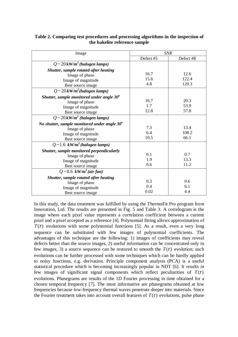
Table 2. Comparing test procedures and processing algorithms in the inspection of the bakelite reference sample

SNR Image

Defect #5 Defect #8 ~ 20Q kW/m2 (halogen lamps)

Shutter, sample rotated after heating Image of phase

Image of magnitude Best source image

16.7 15.6 4.8

12.6 122.4 120.3

~ 20Q kW/m2(halogen lamps) Shutter, sample monitored under angle 30o

Image of phase Image of magnitude Best source image

16.7 1.7 12.8

20.3 53.9 57.8

~ 20Q kW/m2 (halogen lamps) No shutter, sample monitored under angle 30o

Image of phase Image of magnitude Best source image

7.3 6.4 10.5

13.4 108.2 66.1

~1.6Q kW/m2 (halogen lamps) Shutter, sample monitored perpendicularly

Image of phase Image of magnitude Best source image

0.1 1.9 0.6

0.7 13.3 11.2

~ 0.6Q kW/m2 (air fan) Shutter, sample rotated after heating

Image of phase Image of magnitude Best source image

0.3 0.4 0.02

0.6 6.1 4.4

In this study, the data treatment was fulfilled by using the ThermoFit Pro program from Innovation, Ltd. The results are presented in Fig. 5 and Table 3. A correlogram is the image where each pixel value represents a correlation coefficient between a current pixel and a pixel accepted as a reference [4]. Polynomial fitting allows approximation of

( )T τ evolutions with some polynomial functions [5]. As a result, even a very long sequence can be substituted with few images of polynomial coefficients. The advantages of this technique are the following: 1) images of coefficients may reveal defects better than the source images, 2) useful information can be concentrated only in few images, 3) a source sequence can be restored to smooth the ( )T τ evolution; such evolutions can be further processed with some techniques which can be hardly applied to noisy functions, e.g. derivation. Principle component analysis (PCA) is a useful statistical procedure which is becoming increasingly popular in NDT [6]. It results in few images of significant signal components which reflect peculiarities of ( )T τ evolutions. Phasegrams are results of the 1D Fourier processing in time obtained for a chosen temporal frequency [7]. The most informative are phasegrams obtained at low frequencies because low-frequency thermal waves penetrate deeper into materials. Since the Fourier treatment takes into account overall features of ( )T τ evolutions, pulse phase

thermography (PPT) is often regarded as a processing technique No. 1. This technique requires no specific knowledge on analyzed functions and can be applied to arbitrary signal evolutions. Finally, dynamic thermal tomography (DTT) is a special data treatment technique which is based on the fact that, in one-sided TNDT, deeper defects produce lower signals at longer times, therefore, selecting particular intervals of mτ is

equivalent to ‘slicing’ a material by separate layers [8]. It is seen that, in the case of Defect #4, the highest SNR=6.1 occurs in the

correlogram which is a result of applying the correlation algorithm to a set of images.

a) b)

c) d)

e) f)

Fig. 5. Advanced data treatment in the inspection of the bakelite reference sample (ThermoFit Pro): a – best source image (SNR=1.6), b – phasegram, SNR=3.9, c - PCA image (component #3), SNR=4.3, d - correlogram by PCA, SNR=6.1, e - same as Fig. 5d, 3D presentation, f -

thermal tomogram of the 2.7-2.8 mm layer

Table 3. Efficiency of processing algorithms (Defect #4) in the inspection of the bakelite reference sample

Image SNR

Correlogram by PCA 6.1 Correlogram by the source sequence 5.4 Image of the polynomial coefficient A3(3) * 4.4 Image of the polynomial coefficient A2(3) 4.3 PCA image (component #3) 4.3 Image of the polynomial coefficient A1(3) 3.9 Phasegram 3.9 Source image normalized by the end of heating 3.9 PCA image (component #4) 2.8 Image of the polynomial coefficient A5(6) 2.3 Image of Fourier magnitude 1.8 Best source image (at 37 s) 1.6 Image of the polynomial coefficient A1(6) 1.4 PCA image (component #2) 1.2

* A3(3) specifies the third polynomial member (polynomial function order is 3) 2.5 Maps of defects A map of defects is a binary image which appears as a result of ‘thresholding’ any source image. This concept can be easily illustrated by considering an image histogram. First, the user has to define defect and non-defect areas (see squares in the image of Fig. 6) which produce two corresponding populations characterized by a particular SNR value according to Eq. (1). Choosing such areas is a subjective process but effective while comparing different images at a fixed configuration of defect and non-defect areas. In a histogram, these populations can be well-separated or cross each other. In the first case, ‘thresholding’ is trivial but, in the second case, the location of a threshold defines the probability of false alarm . .f aP and the probability of correct detection . .c dP

(see the histogram in Fig. 6). In such way, a particular configuration of defect and non-defects areas results in a single SNR value but plentiful pairs of . .f aP and . .c dP .

Some binary images are presented in Fig. 7. The first two images are obtained by ‘thresholding’ the best source image (all 8 defects are covered by defect areas and the rest of the sample is regarded as non-defect to produce SNR=2.5). Another pair of binary images was obtained by a phasegram (SNR=13.6). Let us consider Defect #4. It is not seen in the source binary image (Fig. 7a) because of the low . .f aP =5% value

accepted. However, this defect turns to be visible if to accept . .f aP =30% (Fig. 7b). In the

phasegram binary image, Defect #4 is clearly seen at both . .f aP =5% and 30% values. It

is worth noting that enhancing correct detection can be achieved by relaxing requirements to . .f aP

Fig. 6. Identifying defect and non-defect areas in the bakelite reference sample (ThermoFit Pro,

Statistics option, best source image, SNR=2.5, . .f aP =30%, . .c dP =78%)

Pf.a.

Pc.d.

Threshold

а) b)

c) d)

Fig. 7. Maps of defects in the bakelite reference sample: a – by source image, SNR=2.5,

. .f aP =5%, . .c dP =67%, b – by source image, SNR=2.5, . .f aP =30%, . .c dP =78%, c – by

phasegram, SNR=13.6, . .f aP =5%, . .c dP =95%, d - by phasegram, SNR=13.6, . .f aP =30%,

. .c dP =98%

2.6 1D and 3D defect characterization Several defect identification procedures have been proposed in pulsed TNDT [9-12]. Two defect characterization algorithms conventionally called 1D and 3D are implemented in the ThermoFit Pro. The 1D algorithm assumes defects to be laterally infinite, thus only two defect parameters (defect depth l and defect thickness d) can be evaluated. The input parameters are material thermal properties and a heating time. The program calculates a maximum running contrast and a time of its appearance over a defect chosen by a user and then produces images of defect depth and thickness. The results of applying this algorithm to all 8 defects in the reference sample are presented in Table 4. The accuracy in evaluating defect depth is from 20 to 30% on average. Note that defect thickness estimates are fairly inaccurate due to the fact that the above-described algorithm is valid for thin hidden defects, such as delaminations, rather than for bottom-holes. Table 5 contains characterization results obtained with the 3D algorithm. The principal feature of this algorithm is that the user has to evaluate maximum and minimum lateral size D of an identified defect by using a kind of a threshold algorithm (the example is shown in Fig. 6). Except small-size defects, the accuracy of determining D has been from 5 to 30% in our case, while errors in the determining defect depth l have been typically less than 10%, i.e. better than in the case of the 1D algorithm (defect thickness estimates are also invalid in this case).

Defect #4

Table 4. Defect characterization by a 1D algorithm

Defect parameter estimate, mm Defect # l d

1 2.4 (20%) 0.95 2 2.4 (20%) 0.88 3 2.6 (13%) 0.70 4 2.8 (7%) 0.46 5 2.2 (45%) 0.62 6 2.3 (23%) 0.70 7 1.8 (28%) 0.70 8 1.3 (30%) 0.42

Fig. 6. Defect characterization by a 3D algorithm (image binarization)

Table 5. Defect characterization by a 3D algorithm

Defect parameter estimate, mm Defect # D l d

1 21.0 (5%) 2.8 (6.7%) 0.89 2 16.4 (9.3%) 2.8 (6.7%) 0.82 3 12.9 (29%) 2.7 (10%) 0.48 4 6.0 (20%) 3.5 (16.7%) 0.10 5 11.7 (17%) 2.9 (27.5%) 0.50 6 11.7 (17%) 2.7 (10%) 0.66 7 14.2 (42%) 2.0 (20%) 0.64 8 15.1 (51%) 1.2 (20%) 0.62

3. Conclusion

In this study, we have summarized the concept of TNDT including the simulation of finite-size defects in solid materials, optimization of test procedures and advanced data treatment based on maximizing a signal-to-noise ratio and applying 1D and 3D defect characterization algorithms. The experimental results have been obtained on a bakelite reference sample which contains bottom-hole defect surrogates of different depth and thickness. The proposed approach is quite general thus allowing optimizing pulsed TNDT findings. Acknowledgements Acknowledgements are attributed to Dr. Vavilov and his colleagues for their kind assistances in making this research happened. Special thanks to IAEA for giving me a chance to perform my intensive training at Tomsk Institute of Introscopy, Tomsk, Russia Federation.

D

References

1. Vavilov V.P., D.D. Burleigh and Demin V.G. Advanced modeling of thermal NDT problems: from buried landmines to defects in composites.-Proc. SPIE “Thermosense XXIV”, Vol. 4710, pp. 507-521.

2. Vavilov V.P. and Maldague X. Optimization of heating protocol in thermal NDT: back to the basics.-Intern. E. & Instr., pp.132-138.

3. Vavilov V.P. Evaluating the efficiency of data processing algorithms in transient thermal NDT.- Proc. SPIE “Thermosense XXVI”, Vol. 5405, 2004, pp. 336-347.

4. ThermoFit Pro operation manual, Innovation Ltd., Russia, 2007, 72 p. 5. Grinzato E., Bison P.G., Marinetti S. and Vavilov V. Thermal NDE enhanced

by 3D numerical modeling applied to works of art.-In: Proc. 15th World Conf. on NDT, Rome (Italy), 15-21 Oct. 2000 (available only on CD), 9 p.

6. Hermosilla-Lara S., Joubert P.-I., Placko D. et al. Enhancement of open-cracks detection using a principal component analysis/wavelet technique in photothermal nondestructive testing.-Abstr. Intern. Conf. Quant. Infrared Thermography QIRT’02, Dubrovnik, Croatia, Sept. 24-27, 2002, p. 12-13.

7. Maldague X., Marinetti S. Pulse phase infrared thermography.-J. Appl. Phys., 1996, Vol. 79, p. 2694-2698.

8. Vavilov V., Maldague X. Dynamic thermal tomography: new promise in the IR thermography of solids.-Proc. SPIE, "Thermosense-XIV", 1992, Vol. 1682, p. 194-206.

9. Vavilov V., Grinzato E., Bison P.G., Marinetti S. Thermal characterization and tomography of carbon fibre reinforced plastics using individual identification technique.-Mater. Evaluation, May 1996, Vol. 54, No.6, p. 604-611.

10. Krapez J.-C., Maldague X., Cielo P. Thermographic NDE: Data inversion procedure (Part II: 2D analysis and experimental results).-Res. in NDE, 1991. No. 2, p. 101-124.

11. Winfree W.P., Zalameda J.N. Thermographic determination of delaminations depth in composites. // Proc. SPIE “Thermosense-XXV”, 2003, Vol. 5073, p. 363-373.

12. Almond D.P., Saintey S., Lau S.K. Edge effects and defect sizing by transient thermography.-"Proc. Quant. Infr. Thermography QIRT'94", Eurotherm Seminar #42, Sorrento, Italy, August 23-26, 1994, p. 247-252.