Speech Communication 44 (2004) 113–125

www.elsevier.com/locate/specom

Developing an audio-visual speech source separation algorithm

David Sodoyer a,b,*, Laurent Girin a, Christian Jutten b, Jean-Luc Schwartz a

a Institut de la Communication Parlee, (ICP: Speech Communication Institute), INPG/Universite Stendhal/CNRS UMR 5009,

ICP, INPG, 46 Av. Felix Viallet, 38031 Grenoble Cedex 1, Franceb Laboratoire des Images et des Signaux, (LIS: Laboratory of Images and Signals), INPG/Universite Joseph Fourier/CNRS UMR 5083

Received 2 March 2004; received in revised form 12 October 2004; accepted 13 October 2004

Abstract

Looking at the speaker�s face is useful to hear better a speech signal and extract it from competing sources before

identification. This might result in elaborating new speech enhancement or extraction techniques exploiting the audio-

visual coherence of speech stimuli. In this paper, a novel algorithm plugging audio-visual coherence estimated by sta-

tistical tools on classical blind source separation algorithms is presented, and its assessment is described. We show, in

the case of additive mixtures, that this algorithm performs better than classical blind tools both when there are as many

sensors as sources, and when there are less sensors than sources. Audio-visual coherence enables a focus on the speech

source to extract. It may also be used at the output of a classical source separation algorithm, to select the ‘‘best’’ sensor

with reference to a target source.

� 2004 Elsevier B.V. All rights reserved.

Keywords: Blind source separation; Audio-visual coherence; Speech enhancement; Audio-visual joint probability; Spectral information

1. Introduction

For understanding speech, two senses are better

than one: to paraphrase the formula used by Bern-stein and Besnoıt (1996) to introduce the AVSP

special session in ICSLP�96, we know, since Sumby

0167-6393/$ - see front matter � 2004 Elsevier B.V. All rights reserv

doi:10.1016/j.specom.2004.10.002

* Corresponding author. Tel.: +33 0476574850; fax: +33

0476574710.

E-mail address: sodoyer@icp.inpg.fr (D. Sodoyer).

and Pollack (1954) at least, that lipreading im-

proves speech identification in noise, and since

Petajan (1984), that Audio-Visual Speech Recog-

nition outperforms Audio Speech Recognition inthe same conditions. Recently, Grant and Seitz

(2000) discovered that vision of the speaker�s facealso intervenes in the audio detection of speech in

noise. This result (confirmed by Kim and Davis,

2001, 2004; Bernstein et al., 2004) lead us show

(Schwartz et al., 2002, 2004) that vision may en-

hance audio speech in noise and therefore provide

what we called a ‘‘very early’’ contribution to

ed.

114 D. Sodoyer et al. / Speech Communication 44 (2004) 113–125

speech intelligibility, different and complementary

to the classical lipreading effect. In parallel, we

exploited, since the middle of the 90s, a technolog-

ical counterpart of this idea. Girin et al. (1997,

2001) developed a first system for enhancing audiospeech embedded in white noise, thanks to a filter-

ing approach, with filter parameters estimated

from the video input (see recent developments by

Deligne et al., 2002 and Goecke et al., 2002; and

also Berthommier, 2003, 2004). The present paper

describes a set of new experiments and develop-

ments on another approach, exploring the link be-

tween two signal processing streams that werealmost completely separated: sensor fusion in

audio-visual (AV) speech processing, and blind

source separation (BSS) techniques (see e.g. Jutten

and Herault, 1991; Taleb and Jutten, 1999). This

extends preliminary work providing the basis of

the method (Sodoyer et al., 2002, 2003) (see also

an original link of a different kind between source

separation and audio-visual localization in Okunoet al., 2001; Nakadai et al., 2004).

In this paper, the theoretical foundations are

presented (Section 2). The evaluation corpora are

described in Section 3, together with an analysis

of audio-visual coherence in the corresponding

material. Comparison methodology and results

are provided in Section 4 for the case with as many

sensors as sources. The more difficult case involv-ing less sensors than sources is addressed in Sec-

tion 5, before a general discussion in Section 6

and a final conclusion.

2. Theory

Let us consider the case of a stationary additivemixture of sources, to be separated:

x ¼ As

where s contains N unknown signals, A is the un-

known P · N mixing matrix, x are the P observa-

tions. Separation consists in estimating output

signals y as close as possible to the sources s. Out-put signals are computed from the observations xby applying an N · P matrix B which is called the

separation matrix:

y ¼ Bx

If the number of sources N equals the number of

sensors P, A is a square matrix. If it is regular, per-

fect separation is possible by taking B = A�1. If P

is lower than N, then A is no more invertible and

there is no exact solution, which makes the prob-lem much more complex.

In the Audio-Visual Speech source Separation

(AVSS) approach, we suppose that one source,

say s1, is a speech signal, and we exploit additional

observations which consist of a video signal V1 ex-

tracted from speaker 1�s face and synchronous

with the acoustic signal s1 that we want to extract.

Typically, V1 contains the trajectory of basic geo-metric lip shape parameters, supposing that they

can be automatically estimated by any kind of

lip-tracking system. The goal is hence the extrac-

tion of one audio-visual source merged in a mix-

ture of two or more acoustic signals.

Classical BSS algorithms consider statistically

independent sources, and basically involve higher

(than 2) order statistics. The AVSS algorithm con-siders decorrelated sources, and in addition lip mo-

tion associated to the source s1 that has to be

extracted. The lip pattern provides no information

on the glottal source, and incomplete information

about the vocal tract. Hence it is classical to con-

sider that the visual input is partially linked to

the transfer function in a source-filter model of

the speech signal.

2.1. Exploiting spectral information

First, let us assume that we know a number of

spectral components of s1, defined by a filter bank

on a given time frame (typically, 20-ms windows

separated by 20-ms intervals in our application).

Let Hi( f ) be the frequency response of the ithbandpass FIR filter, and hi(t) be its temporal im-

pulse response. The energy of the source s1 at theoutput of the filtering process is provided by the

autocorrelation with zero delay of the filtered sig-

nal hi{ s1}(t) = hi(t)*s1(t). The normalized energy

of s1 in the ith band is:

chi ¼ffiffiffiffiffiffiffiffiffiffiffiffiffiffiffiffiffirhifs1gð0Þrs1ð0Þ

sð1Þ

D. Sodoyer et al. / Speech Communication 44 (2004) 113–125 115

where ru(t) denotes the autocorrelation function of

signal u. If one output, say y1, provides an estimate

of s1, we should obtain:ffiffiffiffiffiffiffiffiffiffiffiffiffiffiffiffiffirhify1gð0Þry1ð0Þ

s¼ chi ð2Þ

In an N · N mixture, the direction of s1 is de-

fined by N � 1 parameters, hence it is easy to show

that N � 1 spectral coefficients are necessary and

sufficient to extract s1 (keeping a gain indetermi-nacy). Therefore, we introduce the following

‘‘spectral coefficient’’ criterion Jsc, based on a bank

of (N � 1) band-pass filters:

J scðy1Þ ¼XN�1

i¼1

ffiffiffiffiffiffiffiffiffiffiffiffiffiffiffiffiffirhify1gð0Þry1ð0Þ

s� chi

!2

ð3Þ

The minimization of this criterion allows the sepa-ration of the source s1, provided that the N · N

matrix of the sn spectral coefficients is regular

(Sodoyer et al., 2002).

2.2. The AVSS algorithm

In the real case, we do not know the exact spec-

tral components of the source s1, but we can esti-mate the spectrum through lip characteristics

associated with the sound s1. It is classical to con-

sider that the visual parameters of the speaking

face and the spectral characteristics of the acoustic

transfer function of the vocal tract are related by a

complex relationship which can be described in

statistical terms (see e.g. Yehia et al., 1998). Hence,

we assume that we can build a statistical modelproviding the joint probability of a video vector

V containing parameters describing the speaker�sface (e.g., lip characteristics) and an audio vector

S containing spectral characteristics of the sound

(i.e. chi terms at the output of a filter bank). Let

us denote this joint probability pav(S,V).This statistical model can be designed from a

learning corpus, by modeling the probabilitypav(S,V) as a mixture of Gaussian kernels. The

learning corpus is used for estimating the mean,

the covariance matrix and the weight of each

Gaussian kernel, through an Expectation Maximi-

zation (EM) algorithm (Dempster et al., 1977).

Then the separation algorithm consists in esti-

mating a separation matrix B for which the first

output y1 produces a spectral vector Y1 as coher-

ent as possible with the video input V1. This results

in minimizing the following Audio-Visual (AV)criterion:

J avðyÞ ¼ � logðpavðY 1,V1ÞÞ ð4ÞIt is easy to show that, if there is only one

Gaussian kernel, this AV criterion provides a lin-

ear regression estimate of the chi terms from V1:

hence Jav(y) becomes equivalent to Jsc(y), replac-ing chi by their visual estimate. However, it may

happen that the video input V1, at some instants,

is associated to a large series of possible spectra,

and hence produces very poor separation (the

‘‘viseme’’ problem, see Benoıt et al., 1992). For

solving this problem, we introduce the possibility

to cumulate the probabilities over time. For this

purpose, we assume that the values of audioand visual characteristics at several consecutive

time frames are independent from each other,

and we define an integrated audio-visual criterion

by:

J avT ðyÞ ¼XT�1

k¼0

J avðyðkÞÞ ð5Þ

where y(k) is the content of the signal y in the kth

time frame before the current one.

2.3. Definition of a reference BSS algorithm:

from JADE to JADEtrack

It is necessary to compare the efficiency of ourAVSS algorithm with a classical BSS algorithm,

in order to be able to assess the interest of the

audio-visual approach. A number of reference

BSS algorithms exploiting statistical independence

between the sources are available in the literature

(e.g. Jutten and Herault, 1991; Cardoso and Sou-

loumiac, 1993; Hyvarinen, 1999). They are able

to perfectly solve the source separation problemin simple cases (such as linear additive models with

as many sensors as sources). The reference BSS

algorithm we will use is JADE (Cardoso and Sou-

loumiac, 1993) well known for its simplicity and

speed.

116 D. Sodoyer et al. / Speech Communication 44 (2004) 113–125

BSS algorithms suffer however from two inde-

terminacy problems. Firstly, the lack of knowledge

about the energy of the sources leads to a ‘‘gain

indeterminacy’’ (that is, the separating matrix

can be multiplied by a diagonal matrix withoutmodifying the value of the criterion to minimize).

Secondly, and more seriously, an important draw-

back of this family of algorithms is their indetermi-

nacy with respect to the permutation of sources.

The consequence is the impossibility to know

where (i.e. on which sensor) a given source is ex-

tracted. For a non-stationary signal, like speech,

the energy varies in each frame. Experimentally,it leads to permutation which can vary from one

frame to the next one. Of course, this leads to se-

vere difficulties in the application of the algorithm.

A simple way to deal with the permutation

problem is to search for the permutation that

should be applied at each time frame, in order to

maximize the continuity of the output of each sen-

sor, in reference to the previous frame. For thisaim, considering that the BSS algorithm has found

a given separating matrix B(n � 1) for frame

(n � 1) and another separating matrix B(n) for

frame (n), we chose to apply to B(n) all possiblepermutations, and we defined a corrected separat-

ing matrix B*(n) by the algorithm:

B�ðnÞ ¼ argminpermjBpermðnÞ � Bðn� 1Þj ð6Þwhere jMj = trace(MTM) defines the square of theFrobenius norm of a given matrix M.

This results in minimizing the distance between

the coefficients characterizing each sensor after

separation, between time n � 1 and time n. In this

equation, as throughout this work, the gain inde-

terminacy is solved by normalizing each line of Bmatrices so that the B diagonal values are all

‘‘1’’. The algorithm resulting from the applicationof this procedure on JADE is called JADEtrack.

Both JADE and JADEtrack will be used as refer-

ence algorithms in the following.

It is important to mention at this point that the

AVSS algorithm does not suffer from the permuta-

tion indeterminacy problem, since maximizing the

coherence of the video component of the target

source s1 and the spectral characteristics of thesensor output y1 naturally imposes that s1 is esti-

mated by y1. The gain indeterminacy is solved, as

for JADE, by normalizing each line of B matrices

so that the B diagonal values are all ‘‘1’’.

2.4. A combined BSS–AVSS algorithm

For relaxing the permutation indeterminacy of

BSS algorithms, we purpose to combine the prop-

erties of BSS and AVSS criteria, by first estimating

a separating matrix by a BSS technique, and then

applying an AVSS criterion for selecting the sensor

providing the best s1 estimation at the output of

BSS. By applying this principle to JADE, we take

profit of all its qualities of performance and speedfor estimating quickly and efficiently the separa-

tion matrix. Then, the selected sensor is the one

which maximizes the AVSS criterion in Eq. (5).

The resulting algorithm is called hereafter the JA-

DEAVSS algorithm.

3. Audio-visual material

3.1. Corpora

We used two types of audio-visual corpora for

assessing the separation algorithms.

The first corpus is a corpus of French logatoms,

that is non-sense V1–C–V2–C–V1 utterances,

where V1 and V2 are same or different vowelswithin [a, i, y, u] and C is a consonant within the

plosives set [p, t, k, b, d, g, #] (# means no plosive).

The 112 sequences (4 · V1, 7 · C, 4 · V2) were

pronounced twice by a single male speaker, which

resulted in a training set (first repetition) and a test

set (second repetition). This logatom corpus pre-

sents the interest that it groups in a restricted set

all the basic problems to be addressed by audio-vi-sual studies. Indeed, it contains stimuli with simi-

lar lips and different sounds (such as [y] vs. [u] or

[p] vs. [b]). It also contains pairs of sounds difficult

to distinguish, particularly in noise, while their lips

are quite distinctive (e.g. [i] vs. [y], or [b] vs. [d]). It

is the corpus on which all preliminary studies have

been realized.

The second corpus consists in 107 meaningfulcontinuous sentences uttered by the same French

speaker, of which we used the first 54 sentences

for the training set and the remainder 53 for the

D. Sodoyer et al. / Speech Communication 44 (2004) 113–125 117

test set. This corpus represents a large jump in dif-

ficulty compared with the previous one, for two

reasons. Firstly, the complexity of the audio-visual

material is much larger, and secondly the test set is

quite different from the training set, which is notthe case in the logatom corpus.

3.2. Audio and visual parameter extraction

Both corpora were completely analyzed in order

to extract sequences of audio and visual parame-

ters aligned in time. These parameters then pro-

vided the input to the AVSS separationalgorithm. The video data consist of two basic geo-

metric parameters describing the speaker�s lip

shape, namely width (LW) and height (LH) of

the labial internal contour. These parameters were

automatically extracted every 20ms by using a face

processing system (Lallouache, 1990). This system

exploits a chroma-key process on lips with blue

make-up, and with carefully controlled head posi-tion and light.

Sounds were sampled at 16kHz. On 20-ms win-

dows synchronous with the video frames, we com-

puted 32 spectral parameters providing power

spectral densities (PSD) at the output of a bank

of 32 filters equally spaced between 0 and 5kHz.

PSDs were converted into dBs, and a principal

component analysis (PCA) was applied to reducethe number of spectral components to Na = 1, 5

or 8 dimensions. Hence the total dimension of

the audio-visual space is (Na + 2).

3.3. Modeling and assessing audio-visual coherence

For each corpus, the Gaussian mixture model

of the pav(S1,V1) probability was tuned by anEM algorithm applied to the training data set,

containing 2495 audio-visual vectors (112 stimuli,

about 24 vectors per stimulus) in the logatom case

and 5297 vectors in the sentences case. The sim-

plicity of the logatom corpus allows a careful study

of the repartition of Gaussian kernels, in relation

with the visual and auditory properties of the cor-

responding vowels and plosives in the corpus (seeSodoyer et al., 2002). For the sentence corpus,

the study is more complex. Therefore, for assessing

the validity of the audio-visual modeling in this

case, we compared the value of the integrated

AV criterion JavT(y) applied to two different audio

stimuli: (i) the true audio source s1 coherent with

the video input at each time frame and (ii) an

audio input s2 coming from another similar sen-tence corpus, uttered by another male speaker.

Comparison of JavT(s1) and JavT(s2) was systemat-

ically done for the 2606 frames of the sentence test

corpus, and for each frame, we selected the signal

associated to the smaller JavT(si). This was done

for various values of Na (i.e. 1, 5 and 8), various

numbers of Gaussian kernels in the audio-visual

probability modeling (NG = 12, 18 and 24) andvarious temporal window integration widths

T = 10, 20, 40.

On Fig. 1, we display the recognition rate, that

is the percentage of cases where s1 is selected rather

than s2 (JavT(s1) < JavT(s2)). It appears that the

performance increases largely with T and Na, and

marginally with NG. It reaches a very high level

(about 99%) for T = 40, for 8 (or possibly 5) audiodimensions, and for 18 or 24 Gaussian kernels (see

Fig. 1). This shows that the audio-visual probabil-

ity modeling captures the audio-visual natural

coherence quite well. Incidentally, the fact that

the performance is already very high for T = 20

frames (more than 95%) is quite interesting. A

duration of 20 frames corresponds to 400ms, that

is roughly two syllables. This seems enough toclearly distinguish audio-visual coherence from

incoherence, and the data on the detection of

audio-visual asynchronies (see Grant et al.,

2004), suggest that human subjects would not per-

form much better (200ms instead of 400ms). No-

tice that even very poor spectral information

may be quite efficient: one spectral parameter suf-

fices to produce 85% correct recognition with 40frames in Fig. 1. This is also coherent with psycho-

physical data (Grant et al., 2004).

4. Experiments in the N · N case

4.1. Methodology

In this first series of experiments, there are as

many sensors as sources. In this case, the mixing

matrix A is an N · N matrix supposed to be

recognition rate

65.00%

70.00%

75.00%

80.00%

85.00%

90.00%

95.00%

100.00%

T=10

T=20

T=40

NG=12 Na : 1 5 8

NG =18 Na : 1 5 8

NG =24 Na : 1 5 8

Fig. 1. Correct recognition scores (see text) for various numbers of spectral components, Na = 1, 5, and 8; various numbers of

Gaussian kernels in the audio-visual probability modeling, NG = 12, 18 and 24; and various temporal window integration widths

T = 10, 20, 40.

118 D. Sodoyer et al. / Speech Communication 44 (2004) 113–125

non-singular. Hence if B is a good estimation of

A�1, it is trivial that y is a good estimation of the

original sources s. We tested three values of N, thatis N = 2, 3 and 5.

Tests were performed on both corpora. s1 is thespeech source to extract (2606 test frames for the

logatom and the sentence corpus) and the N � 1

other sources are corrupting speech sources bor-

rowed from another sentence corpus uttered by

other speakers. A property sought for a BSS algo-

rithm is equivariance, which is characterized bythe fact that performance (independently of per-

mutation and gain indeterminacy problems) does

not depend on the mixing matrix, but just on

properties of input sources. Equivariance can be

achieved by implementing a ‘‘relative gradient

technique’’ (Cardoso and Laheld, 1996) or the

closely related ‘‘natural gradient technique’’

(Amari, 1998). Therefore, throughout this work,the optimisation of the AVSS criterion JavT(y)(Eq. 5) was realized by a relative gradient in order

to make the AVSS algorithm equivariant. To

check that this property was ensured, for each va-

lue of N we tested two different mixture matrices

A1 and A2. We compared several temporal inte-

gration widths T with T = 1, 10, 20 and 40

frames. For each mixture, the N observationsare defined by:

xn ¼XNp¼1

anpsp ð7Þ

which are characterized by input SNRs, in refer-

ence to s1, provided by:

SNRinðnÞ ¼ 10 log a2n1Es1

XNp¼2

a2npEsp

, ! ð8Þ

with Esi the energy of source i in the current frame.

Input SNR values displayed in Table 1 are mean

values averaged over the test frames.

For each test frame, and for a given separating

matrix B, the AVSS procedure consists in comput-ing y = Bx, in estimating the spectrum Y1 accord-

ing to the process described in Section 3.2

(spectral analysis followed by projection on the se-

lected principal components), and in computing

the probability pav(Y1,V1) thanks to the model de-

scribed in Section 3.3. The number of Gaussian

kernels is NG = 18, and the audio dimension is

Na = 8. The optimal B matrix, which minimizesthe integrated criterion JavT(y), produces an out-

put y1 which is the estimation of the source s1.The output SNR is given by:

SNRout ¼ 10 log g211Es1

XNp¼2

g21pEsp

, ! ð9Þ

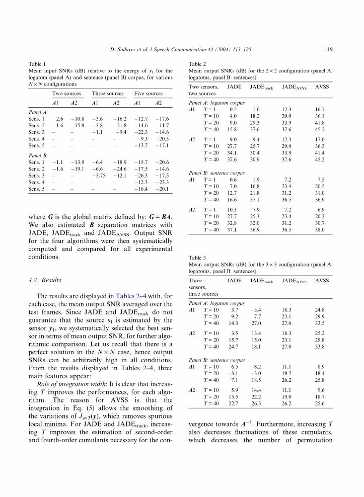
Table 1

Mean input SNRs (dB) relative to the energy of s1 for the

logatom (panel A) and sentence (panel B) corpus, for various

N · N configurations

Two sources Three sources Five sources

A1 A2 A1 A2 A1 A2

Panel A

Sens. 1 2.6 �10.8 �3.6 �16.2 �12.7 �17.6

Sens. 2 1.6 �15.9 �3.8 �21.8 �14.6 �11.7

Sens. 3 – – �1.1 �9.4 �22.3 �14.6

Sens. 4 – – – – �9.3 �20.3

Sens. 5 – – – – �13.7 �17.1

Panel B

Sens. 1 �1.1 �13.9 �6.4 �18.9 �15.7 �20.6

Sens. 2 �1.6 �19.1 �6.6 �24.6 �17.5 �14.6

Sens. 3 – – �3.75 �12.1 �26.3 �17.5

Sens. 4 – – – – �12.3 �23.3

Sens. 5 – – – – �16.4 �20.1

Table 2

Mean output SNRs (dB) for the 2 · 2 configuration (panel A:

logatoms, panel B: sentences)

Two sensors,

two sources

JADE JADEtrack JADEAVSS AVSS

Panel A: logatom corpus

A1 T = 1 0.5 1.0 12.3 16.7

T = 10 4.0 18.2 29.9 36.1

T = 20 9.0 29.3 33.9 41.8

T = 40 15.8 37.6 37.6 45.2

A2 T = 1 9.0 9.4 12.3 17.0

T = 10 27.7 25.7 29.9 36.3

T = 20 34.1 30.4 33.9 41.4

T = 40 37.6 30.9 37.6 45.2

Panel B: sentence corpus

A1 T = 1 0.6 1.9 7.2 7.5

T = 10 7.0 16.8 23.4 20.5

T = 20 12.7 21.8 31.2 31.0

T = 40 16.6 37.1 36.5 36.9

A2 T = 1 10.3 7.9 7.2 6.9

T = 10 27.7 25.3 23.4 20.2

T = 20 32.8 32.0 31.2 30.7

T = 40 37.1 36.9 36.5 38.0

Table 3

D. Sodoyer et al. / Speech Communication 44 (2004) 113–125 119

where G is the global matrix defined by: G = BA.We also estimated B separation matrices with

JADE, JADEtrack and JADEAVSS. Output SNR

for the four algorithms were then systematically

computed and compared for all experimentalconditions.

Mean output SNRs (dB) for the 3 · 3 configuration (panel A:

logatoms, panel B: sentences)

Three

sensors,

three sources

JADE JADEtrack JADEAVSS AVSS

Panel A: logatom corpus

A1 T = 10 3.7 �5.4 18.3 24.8

T = 20 9.2 7.7 23.1 29.9

T = 40 14.3 27.0 27.0 33.5

A2 T = 10 3.5 13.4 18.3 25.2

T = 20 15.7 15.0 23.1 29.8

T = 40 24.7 18.1 27.0 33.8

Panel B: sentence corpus

A1 T = 10 �6.5 �8.2 11.1 8.9

T = 20 �3.1 �3.0 19.2 18.4

T = 40 7.1 18.5 26.2 25.8

A2 T = 10 5.9 14.4 11.1 9.6

T = 20 15.5 22.2 19.0 18.7

T = 40 22.7 26.3 26.2 25.6

4.2. Results

The results are displayed in Tables 2–4 with, for

each case, the mean output SNR averaged over the

test frames. Since JADE and JADEtrack do not

guarantee that the source s1 is estimated by thesensor y1, we systematically selected the best sen-

sor in terms of mean output SNR, for further algo-

rithmic comparison. Let us recall that there is a

perfect solution in the N · N case, hence output

SNRs can be arbitrarily high in all conditions.

From the results displayed in Tables 2–4, three

main features appear:

Role of integration width: It is clear that increas-ing T improves the performances, for each algo-

rithm. The reason for AVSS is that the

integration in Eq. (5) allows the smoothing of

the variations of JavT(y), which removes spurious

local minima. For JADE and JADEtrack, increas-

ing T improves the estimation of second-order

and fourth-order cumulants necessary for the con-

vergence towards A�1. Furthermore, increasing T

also decreases fluctuations of these cumulants,

which decreases the number of permutation

Table 4

Mean output SNRs (dB) for the 5 · 5 configuration (panel A:

logatoms, panel B: sentences)

Five sensors,

five sources

JADE JADEtrack JADEAVSS AVSS

Panel A: logatom corpus

A1 T = 20 �22.5 �20.2 15.1 22.5

T = 40 �22.1 0.7 19.1 26.5

A2 T = 20 �17.7 �8.7 15.1 22.3

T = 40 �15.6 11.4 19.1 26.7

Panel B: sentence corpus

A1 T = 20 �18.0 �9.2 9.7 10.7

T = 40 �15.3 16.7 16.7 16.9

A2 T = 20 �12.3 �18.1 9.7 11.9

T = 40 �10.0 �7.9 16.7 16.7

120 D. Sodoyer et al. / Speech Communication 44 (2004) 113–125

switches from one frame to the next. Of course,

JADEAVSS enjoys the same property as both

JADE and AVSS. In the remainder of the study,

we shall concentrate on the values T = 20 and

T = 40.

Separation performance: In all cases, the JADE

algorithm provides poor results because of permu-

tation problems. JADEtrack corrects this problemrather well, and provides a good baseline for fur-

ther assessment of AVSS and JADEAVSS. On

the logatom corpus, both techniques largely

outperform JADEtrack. Furthermore, AVSS itself

largely outperforms JADEAVSS for both

integration widths. The result is much less

contrasted for sentences. AVSS and JADEAVSS

outperform JADEtrack only slightly, anddepending on configurations, while performances

of AVSS and JADEAVSS are quite similar in all

conditions.

Equivariance: The JADE algorithm is shown to

be equivariant (see Cardoso and Souloumiac,

1993) but the permutation problems do not allow

to verify this property. However, solving this prob-

lems thanks to the audio-visual selector ensuresthat JADEAVSS displays a remarkable stability of

output SNRs from one mixing matrix to the other

(compare A1 and A2 in all cases). Though we

implemented a relative gradient descent in AVSS,

equivariance is slightly less well achieved, probably

because of the sensitivity of the gradient descent to

initial conditions.

5. Experiments in the P < N case

In this section, we consider mixtures with less

observations than sources, that is P < N. In this

case, it is known that there is no perfect solution,since s1 does not in general belong to the

hyperplane defined by the x sensors. In other

words, the inverse matrix of A does not exist, and

the identification of A is not sufficient for

perfectly recovering the sources. The experimental

question now concerns the compared ability of

our different algorithms to find good estimates of s1.

5.1. Maximizing SNR through audio-visual

coherence

The P < N case is likely to provide a very good

test bed for our algorithm. Indeed, in this case,

BSS algorithms suffer from an intrinsic limitation.

They must find a solution minimizing various

kinds of independence criteria (e.g. higher-orderstatistical moments) but they cannot focus on

one or the other source. On the contrary, the

AVSS criterion is directed towards the source to

extract.

In the hyperplane defined by the set of sensor

observations (x), the best estimate of s1 maximiz-

ing the signal-to-noise ratio SNR should minimize

a criterion of least mean square error, Jlms:

J lms ¼ Ey1ðtÞ

ky1ðtÞk� s1ðtÞks1ðtÞk

� �2" #

ð10Þ

With the Bessel–Parseval formula, we can trans-form the cumulated distance in time into a cumu-

lated distance in frequency:

Ey1ðtÞ

ky1ðtÞk� s1ðtÞks1ðtÞk

� �2" #

¼Z þ1

�1

y1ðf Þky1ðf Þk

� s1ðf Þks1ðf Þk

��������2

df ð11Þ

where y1(f) and s1(f) are the Fourier transforms of

y1(t) and s1(t).

Table 5

Mean Input SNRs (dB) in reference to s1 for the logatom (panel

A) and sentence (panel B) corpus, for various P · N

configurations

Two sensors, three sources

A1 A2 A3 A4

Panel A

Sens. 1 0.9 �4.4 �15.2 �17.9

Sens. 2 �0.3 �11.3 �5.3 �1.8

Panel B

Sens. 1 �1.9 �7.1 �17.7 �20.7

Sens. 2 �2.8 �14.2 �8.1 �4.7

Table 6

Mean output SNRs (dB for the 2 · 3 configuration (panel A:

logatoms, panel B: sentences)

Two sensors,

three sources

JADE JADEtrack JADEAVSS AVSS

Panel A: logatom corpus

A1 T = 20 1.1 2.4 4.2 4.4

T = 40 1.9 4.3 4.5 5.1

A2 T = 20 �7.8 �6.0 �1.0 �0.5

T = 40 �7.9 �6.7 �0.6 0.1

A3 T = 20 �2.7 �1.2 �1.5 �1.3

D. Sodoyer et al. / Speech Communication 44 (2004) 113–125 121

If we assume that the phases of y1(f) and s1(f)are equal, we can express Jlms as a spectral distance

between y1 and s1:

Ey1ðtÞ

ky1ðtÞk� s1ðtÞks1ðtÞk

� �2" #

¼Z þ1

�1

j yðf Þ jky1ðf Þk

� j s1ðf Þ jks1ðf Þk

� �2

df

If we perform a discrete approximation of the

Fourier transform by a filter bank, we have:

Ey1ðtÞ

ky1ðtÞk� s1ðtÞks1ðtÞk

� �2" #

�XFf¼1

j y1ðf Þ jffiffiffiffiffiffiffiffiffiffiffiffiffiffiffiffiffiffiffiffiffiffiffiffiPff¼1

j y1ðf Þj2

s � j s1ðf Þ jffiffiffiffiffiffiffiffiffiffiffiffiffiffiffiffiffiffiffiffiffiffiffiPFf¼1

j s1ðf Þj2s

0BBBB@

1CCCCA

2

ð12Þ

which is quite close to the criterion defined by Eq.(3). Hence, it appears that the AV criterion defined

in Eq. (4), which provides an audio-visual approx-

imation of the criterion in Eq. (3), should lead to

an estimation of s1 with a close to maximal

SNR. The temporal integration in Eq. (5) is the

AV approximation of an integrated spectral crite-

rion cumulating spectral distances between s1 andy1 on T consecutive temporal windows. Therefore,minimizing JavT should be close to maximizing the

SNR on this integrated window. In fact, the loga-

rithmic transform of PSDs in dBs, induces a dis-

crepancy between the theoretical Jlms criterion

and the practical JavT one.

T = 40 �0.8 �0.4 �0.6 �0.4

A4 T = 20 2.6 7.8 11.7 12.7

T = 40 5.6 7.2 11.9 12.2

Panel B: sentence corpus

A1 T = 20 �2.6 0.5 0.1 �0.4

T = 40 �1.2 1.7 1.4 0.7

A2 T = 20 �9.0 �10.2 �4.4 �5.3

T = 40 �10.9 �11.0 �4.4 �4.8

A3 T = 20 �5.0 �3.5 �5.4 �6.3

T = 40 �3.6 �3.2 �4.7 �4.6

A4 T = 20 0.8 9.5 7.3 6.7

T = 40 2.4 9.2 8.2 7.2

5.2. Methodology

We tested a simple P < N configuration, with

two sensors and three sources. In this case, the

equivariance property cannot be satisfied since

there is no exact solution. The solution found

by AVSS depends on both the mixing matrix Aand the energy of the sources. We tested four dif-

ferent mixing matrices (Table 5). Notice that the

non-stationarity of the speech sources results invariations of the geometry of the problem from

frame to frame. Hence, each mixing matrix corre-

sponds in fact to testing many different configura-

tions. The study was done on both corpora, with

the same methodology as in Section 4.

5.3. Results

The results are shown in Table 6 for the log-atom and sentence corpora. Mean output SNRs

are not very large for all algorithms, which is

122 D. Sodoyer et al. / Speech Communication 44 (2004) 113–125

logical since perfect recovery of the sources is

impossible in undetermined mixtures (P < N, see

here above). They are generally larger for AVSS

and JADEAVSS than for JADEtrack (and of course

JADE), both for logatoms and sentences, thoughthe difference is not very large, and depends on

the mixing matrix. Once more, the performances

are similar for AVSS and JADEAVSS. Notice that

temporal integration here does not produce much

increase in separation. The reason is probably that

non-stationarity in the P < N case leads to fluctu-

ations of the separation matrix, which blurs the

efficiency of integration for all methods.

Gain/JADE - LogatomT=20 frames

-5

0

5

10

15

20

25

30

35

40

45

JADEtrack JADEAVSS

Gain/JADE - LogatomT=40 frames

0

5

10

15

20

25

30

35

40

45

50

JADEtrack JADEAVSS

(a)

(b)

Fig. 2. Mean output SNR gain in reference to the JADE algorithm fo

T = 20 (a) and T = 40 (b), for various P · N settings (averaging Result

JADEAVSS and AVSS.

6. Discussion

The series of experiments presented in this pa-

per confirm interest in the AVSS technique.

Firstly, the theoretical foundations introduced inSodoyer et al. (2002) for the N · N case, and devel-

oped here for the P < N case, seem sound. Sec-

ondly, the extension to a sentence corpus

demonstrates that the method can indeed be ap-

plied to realistic data, without suffering too much

of the increasing complexity of the phonetic mate-

rial. The fact that 400ms are enough to distinguish

a coherent audio-visual stimulus from an incoher-

corpus -

2 x 2

3 x 3

5 x 5

2 x 3

AVSS

corpus -

2 x 2

3 x 3

5 x 5

2 x 3

AVSS

r the logatom corpus, with a temporal window integration width

s for all tested matrices) and for the three algorithms JADEtrack,

D. Sodoyer et al. / Speech Communication 44 (2004) 113–125 123

ent one in the probability distribution model (Fig.

1) is quite encouraging in this respect.

However, we must admit that the robustness in

increasing phonetic complexity is limited. In the

summary picture displayed in Figs. 2 and 3 it isclear that for logatoms (Fig. 2) there is a strong

hierarchy AVSS JADEAVSS JADEtrack JADE, while for sentences (Fig. 3), the pattern is

severely reduced, with something like: AVSS = JA-

DEAVSS > JADEtrack JADE (denoting by and > the assertions ‘‘has a largely/slightly better

performance than’’). It is nevertheless interesting

that algorithms incorporating the AVSS criterion

Gain/JADE - SentencT=20 frame

0

5

10

15

20

25

30

JADEtrack JADEAVSS

Gain/JADE - SenteT=40 fram

0

5

10

15

20

25

30

35

JADEtrack JADEAVSS

(a)

(b)

Fig. 3. Mean output SNR gain in reference to the JADE algorithm for

T = 20 (a) and T = 40 (b), for various P · N settings (averaging Result

JADEAVSS and AVSS.

remain better than JADEtrack for sentences, partic-

ularly in the ‘‘less sensors than sources’’ condition.

The comparison between JADEAVSS and AVSS

is a bit disappointing, considering that the large

advantage displayed by AVSS for logatoms disap-pears for sentences. This clearly illustrates the need

for more powerful models for estimating the

pav(S,V) probability, able to deal with large con-

tinuous speech corpora, particularly when we shall

deal with multi-speaker applications. However the

good performance of the JADEAVSS algorithm is

interesting. It shows that AVSS does introduce a

significant gain at the output of JADE, by its

e corpus -s

2 x 2

3 x 3

5 x 5

2 x 3

AVSS

nce corpus -es

2 x 2

3 x 3

5 x 5

2 x 3

AVSS

the sentence corpus, with a temporal window integration width

s for all tested matrices) and for the three algorithms JADEtrack,

124 D. Sodoyer et al. / Speech Communication 44 (2004) 113–125

systematic selection of a coherent output, as close

as possible to the source to extract. The crucial

point is that the JADEAVSS algorithm keeps the

nice properties of JADE (speed and equivariance),

which could be important for future applications.We are presently considering other ways to com-

bine BSS and AVSS techniques, e.g. for more com-

plex mixtures of sources.

7. Conclusion

Altogether, the technological counterpart of the‘‘very early’’ visual enhancement of audio speech

looks quite promising. The method is very efficient

in the case of additive mixtures of sources with as

many sensors as sources. In this paper, we show

that the method seems able to deal with less sen-

sors than sources, thanks to its ability to focus

on the target source. This might also lead to effi-

cient BSS/AVSS combined algorithms exploitingboth independence criteria, and AV coherence cri-

teria to select a given source in a mixture. Of

course, further developments are still necessary

for a complete demonstration of the efficiency of

the technique. They will involve larger multi-

speaker corpora, more powerful learning tools

for AV association, and they should address more

complex mixtures (including convolutive ones). Itis already possible however to assert that the con-

nection of BSS techniques with the field of AV

speech processing is an exciting new challenge for

future research in both communities.

References

Amari, S.-L., 1998. Natural gradient works efficiently in

learning. Neural Comput. 10, 251–276.

Benoıt, C., Lallouache, M.T., Mohamadi, T., Abry, C., 1992. A

set of visual French visemes for visual speech synthesis. In:

Bailly, G. et al. (Eds.), Talking Machines. Elsevier, Amster-

dam, pp. 485–504.

Bernstein, L.E., Benoıt, C., 1996. For speech perception by

humans or machines, three senses are better than one. In:

Proc. ICSLP�96, pp. 1477–1480.Bernstein, L.E., Takayanagi, S., Auer E.T., Jr., 2004. Enhanced

auditory detection with AV speech: Perceptual evidence for

speech and non-speech mechanisms. This volume.

Berthommier, F., 2003. Audiovisual speech enhancement based

on the association between speech envelope and video

feature. In: Proc. Eurospeech�03, Geneva, pp. 1045–

1048.

Berthommier, F., 2004. A phonetically neutral model of the

low-level audiovisual interaction. This volume.

Cardoso, J.F., Souloumiac, A., 1993. Blind beamforming for

non-Gaussian signals. IEE Proc.—F 140, 362–370.

Cardoso, J.F., Laheld, B., 1996. Equivariant adaptative source

separation. IEEE Trans. SP 44, 3017–3030.

Deligne, S., Potamianos, G., Neti, C., 2002. Audio-visual

speech enhancement with AVCDCN (AudioVisual Code-

book Dependent Cepstral Normalization). In: Proc.

ICSLP�2002, pp. 1449–1452.Dempster, A.P., Laird, N.M., Rubin, D.B., 1977. Maximum

likelihood from incomplete data via the EM algorithm. J.

Roy. Statist. Soc. 39, 1–38.

Girin, L., Feng, G., Schwartz, J.-L., 1997. Can the visual input

make the audio signal pop out in noise? A first study of the

enhancement of noisy VCV acoustic sequences by audiovi-

sual fusion. In: Proc. AVSP�97, pp. 37–40.Girin, L., Schwartz, J.L., Feng, G., 2001. Audio-visual

enhancement of speech in noise. J. Acoust. Soc. Am. 109,

3007–3020.

Goecke, R., Potamianos, G., Neti, C., 2002. Noisy audio

feature enhancement using audio-visual speech data. In:

Proc. Internat. Conf. Acoust., Speech, Signal Process., pp.

2025–2028.

Grant, K.W., Seitz, P., 2000. The use of visible speech cues for

improving auditory detection of spoken sentences. J.

Acoust. Soc. Am. 108, 1197–1208.

Grant, K.W., van Wassenhove, V., Poeppel, D., 2004. Detec-

tion of auditory and auditory–visual synchrony. This

volume.

Hyvarinen, A., 1999. Fast and robust fixed-point algorithms for

Independent Component Analysis. IEEE Trans. Neural

Networks 10, 626–634.

Jutten, C., Herault, J., 1991. Blind separation of sources. Part I:

An adaptive algorithm based on a neuromimetic architec-

ture. Signal Process. 24, 1–10.

Kim, J., Davis, C., 2001. Visible speech cues and auditory

detection of spoken sentences: an effect of degree of

correlation between acoustic and visual properties. In: Proc.

AVSP�2001, pp. 127–131.Kim, J., Davis, C., 2004. Testing the cuing hypothesis for the

AV speech detection advantage. This volume.

Lallouache, M.T., 1990. Un poste �visage-parole�. Acquisition et

traitement de contours labiaux. In: Proc. XVIII JEPs,

Montreal, pp. 282–286.

Nakadai, K., Matsuura, D., Okuno, H.G., Tsujino, H., 2004.

Improvement of three simultaneous speech recognition by

using AV integration and scattering theory for humanoid.

This volume.

Okuno, H.G., Nakadai, K., Lourens, T., Kitano, H., 2001.

Separating three simultaneous speeches with two micro-

phones by integrating auditory and visual processing. In:

Proc. Eurospeech 2001, pp. 2643–2646.

D. Sodoyer et al. / Speech Communication 44 (2004) 113–125 125

Petajan, E.D., 1984. Automatic Lipreading to Enhance Speech

Recognition. Doct. Thesis, University of Illinois.

Schwartz, J.L., Berthommier, F., Savariaux, C., 2002. Audio-

visual scene analysis: Evidence for a ‘‘very-early’’ integra-

tion process in audio-visual speech perception. In: Proc.

ICSLP�2002, pp. 1937–1940.Schwartz, J.L., Berthommier, F., Savariaux, C., 2004. Seeing to

hear better: Evidence for early audio-visual interactions in

speech identification. Cognition 93, B69–B78.

Sodoyer, D., Schwartz, J.L., Girin, L., Klinkisch, J., Jutten, C.,

2002. Separation of audio-visual speech sources. Eurasip

JASP 2002, 1164–1173.

Sodoyer, D., Girin, L., Jutten, C., Schwartz, J.L., 2003.

Extracting an AV speech source from a mixture of signals.

In: Proc. Eurospeech 2003, pp. 1393–1396.

Sumby, W.H., Pollack, I., 1954. Visual contribution to speech

intelligibility in noise. J. Acoust. Soc. Am. 26, 212–

215.

Taleb, A., Jutten, C., 1999. Source separation in postnonlinear

mixtures. IEEE Trans. SP 10, 2807–2820.

Yehia, H., Rubin, P., Vatikiotis-Bateson, E., 1998. Quantitative

association of vocal-tract and facial behavior. Speech

Communication 26, 23–43.