The Cone of Silence: Speech Separation byLocalization

Teerapat Jenrungrot∗ Vivek Jayaram∗ Steve Seitz Ira Kemelmacher-ShlizermanUniversity of Washington

{tjenrung, vjayaram, seitz, kemelmi}@cs.washington.edu

Abstract

Given a multi-microphone recording of an unknown number of speakers talkingconcurrently, we simultaneously localize the sources and separate the individualspeakers. At the core of our method is a deep network, in the waveform domain,which isolates sources within an angular region θ±w/2, given an angle of interestθ and angular window size w. By exponentially decreasing w, we can perform abinary search to localize and separate all sources in logarithmic time. Our algorithmallows for an arbitrary number of potentially moving speakers at test time, includingmore speakers than seen during training. Experiments demonstrate state-of-the-artperformance for both source separation and source localization, particularly in highlevels of background noise.

1 Introduction

The ability of humans to separate and localize sounds in noisy environments is a remarkable phe-nomenon known as the “cocktail party effect.” However, our natural ability only goes so far – wemay still have trouble hearing a conversation partner in a noisy restaurant or during a call with otherspeakers in the background. One can imagine future earbuds or hearing aids that selectively cancelaudio sources that you don’t want to listen to. As a step towards this goal, we introduce a deep neuralnetwork technique that can be steered to any direction at run time, cancelling all audio sources outsidea specified angular window, aka cone of silence (CoS) [1].

But how do you know what direction to listen to? We further show that this directionally sensitiveCoS network can be used as a building block to yield simple yet powerful solutions to 1) soundlocalization, and 2) audio source separation. Our experimental evaluation demonstrates state ofthe art performance in both domains. Furthermore, our ability to handle an unknown number ofpotentially moving sound sources combined with fast performance represents additional steps forwardin generality. Audio demos can be found at our project website.2

We are particularly motivated by the recent increase of multi-microphone devices in everyday settings.This includes headphones, hearing aids, smart home devices, and many laptops. Indeed, most ofthese devices already employ directional sensitivity both in the design of the individual microphonesand in the way they are combined together. In practice however, this directional sensitivity is limitedto either being hard tuned to a fixed range of directions (e.g., cardioid), or providing only limitedattenuation of audio outside that range (e.g., beam-forming). In contrast, our CoS approach enablestrue cancellation of audio sources outside a specified angular window that can be specified (andinstantly changed) in software.

Our approach uses a novel deep network that can separate sources in the waveform domain withinany angular region θ ± w

2 , parameterized by a direction of interest θ and angular window size w. Forsimplicity, we focus only on azimuth angles, but the method could equally be applied to elevation

∗Equal Contribution2https://grail.cs.washington.edu/projects/cone-of-silence/

34th Conference on Neural Information Processing Systems (NeurIPS 2020), Vancouver, Canada.

arX

iv:2

010.

0600

7v1

[cs

.SD

] 1

2 O

ct 2

020

Person 1Person 2Person 3

Input Mixture

Ground Truth Signals by Person

Ground Truth Positions Step 1: Search Regions(w = 90°)

Output Signals by Regionfrom Separation Network

Final Output Signalsfrom Separation Network

Step 2: Search Regions(w = 45°)

Step 5: Search Regions(w = 2°)

…

Denotes a person at that location

Refine Refine Refine

No Signal

No Signal

No Signal

Output Signals by Regionfrom Separation Network

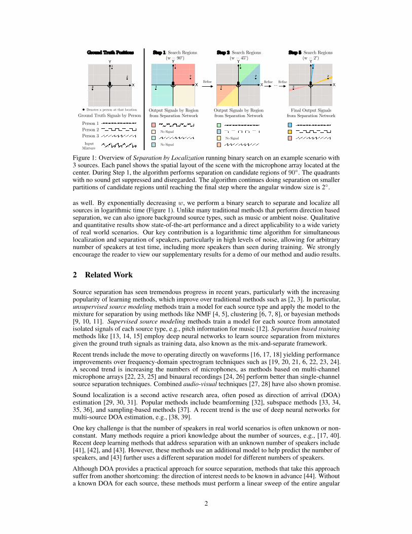
Figure 1: Overview of Separation by Localization running binary search on an example scenario with3 sources. Each panel shows the spatial layout of the scene with the microphone array located at thecenter. During Step 1, the algorithm performs separation on candidate regions of 90◦. The quadrantswith no sound get suppressed and disregarded. The algorithm continues doing separation on smallerpartitions of candidate regions until reaching the final step where the angular window size is 2◦.

as well. By exponentially decreasing w, we perform a binary search to separate and localize allsources in logarithmic time (Figure 1). Unlike many traditional methods that perform direction basedseparation, we can also ignore background source types, such as music or ambient noise. Qualitativeand quantitative results show state-of-the-art performance and a direct applicability to a wide varietyof real world scenarios. Our key contribution is a logarithmic time algorithm for simultaneouslocalization and separation of speakers, particularly in high levels of noise, allowing for arbitrarynumber of speakers at test time, including more speakers than seen during training. We stronglyencourage the reader to view our supplementary results for a demo of our method and audio results.

2 Related Work

Source separation has seen tremendous progress in recent years, particularly with the increasingpopularity of learning methods, which improve over traditional methods such as [2, 3]. In particular,unsupervised source modeling methods train a model for each source type and apply the model to themixture for separation by using methods like NMF [4, 5], clustering [6, 7, 8], or bayesian methods[9, 10, 11]. Supervised source modeling methods train a model for each source from annotatedisolated signals of each source type, e.g., pitch information for music [12]. Separation based trainingmethods like [13, 14, 15] employ deep neural networks to learn source separation from mixturesgiven the ground truth signals as training data, also known as the mix-and-separate framework.

Recent trends include the move to operating directly on waveforms [16, 17, 18] yielding performanceimprovements over frequency-domain spectrogram techniques such as [19, 20, 21, 6, 22, 23, 24].A second trend is increasing the numbers of microphones, as methods based on multi-channelmicrophone arrays [22, 23, 25] and binaural recordings [24, 26] perform better than single-channelsource separation techniques. Combined audio-visual techniques [27, 28] have also shown promise.

Sound localization is a second active research area, often posed as direction of arrival (DOA)estimation [29, 30, 31]. Popular methods include beamforming [32], subspace methods [33, 34,35, 36], and sampling-based methods [37]. A recent trend is the use of deep neural networks formulti-source DOA estimation, e.g., [38, 39].

One key challenge is that the number of speakers in real world scenarios is often unknown or non-constant. Many methods require a priori knowledge about the number of sources, e.g., [17, 40].Recent deep learning methods that address separation with an unknown number of speakers include[41], [42], and [43]. However, these methods use an additional model to help predict the number ofspeakers, and [43] further uses a different separation model for different numbers of speakers.

Although DOA provides a practical approach for source separation, methods that take this approachsuffer from another shortcoming: the direction of interest needs to be known in advance [44]. Withouta known DOA for each source, these methods must perform a linear sweep of the entire angular

2

space, which is computationally infeasible for state-of-the-art deep networks at fine-grained angularresolutions.

Some prior work has addressed joint localization and separation. For example, [45, 46, 47, 48, 49, 50]use expectation maximization to iteratively localize and separate sources. [51] uses the idea ofDirectional NMF, while [52] poses separation and localization as a Bayesian inference problem basedon inter-microphone phase differences. Our method improves on these approaches by combiningdeep learning in the waveform domain with efficient search.

3 Method

In this section we describe our Cone of Silence network for angle based separation. The target angleθ and window size w are learned independently; Separation at θ is handled entirely by a pre-shiftstep, while an additional network input is used to produce the window of size w. We also describehow to use the network for separation by localization via binary search.

Problem Formulation: Given a known-configuration microphone array with M microphones andM > 1, the problem of M -channel source separation and localization can be formulated in termsof estimating N sources s1, . . . , sN ∈ RM×T and their corresponding angular position θ1, . . . , θNfrom an M -channel discrete waveform of the mixture x ∈ RM×T of length T , where

x =

N∑i=1

si + bg. (1)

Here bg represents the background signal, which could be a point source like music or diffuse-fieldbackground noise without any specific location.

In this paper we explore circular microphone arrays, but we also describe possible modifications tosupport linear arrays. The center of our coordinate system is always the center of the microphonearray, and the angular position of each source, θi, is defined based on this coordinate system. In theproblem formulation we assume the sources are stationary, but we describe how to handle potentiallymoving sources in Section 4.5. In addition, we only focus on separation and localization by azimuthangle, meaning that we assume the sources have roughly the same elevation angle. As we show in theexperimental section, this assumption is valid for most real world scenarios.

3.1 Cone of Silence Network (CoS)

We propose a network that performs source separation given an angle of interest θ and an angularwindow size w. The network is tasked with separating speech only coming from azimuthal directionsbetween θ − w

2 and θ + w2 and disregarding speech coming from other directions. In the following

sections we describe how to create a network with this property. Figure 2 shows our proposed networkarchitecture. θ and w are encoded in a shifted input x′ and a one-hot vector h as described in Section3.1.2 and Section 3.1.3 respectively.

3.1.1 Base Architecture

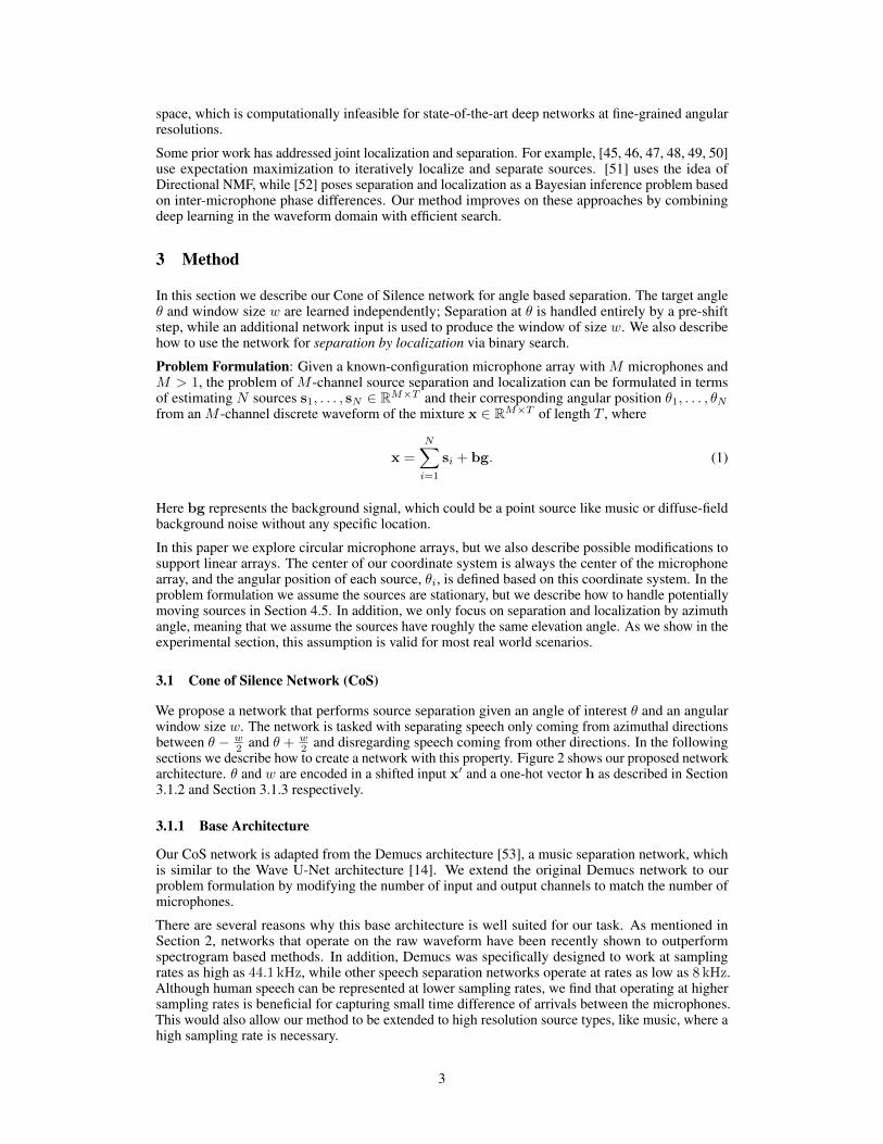
Our CoS network is adapted from the Demucs architecture [53], a music separation network, whichis similar to the Wave U-Net architecture [14]. We extend the original Demucs network to ourproblem formulation by modifying the number of input and output channels to match the number ofmicrophones.

There are several reasons why this base architecture is well suited for our task. As mentioned inSection 2, networks that operate on the raw waveform have been recently shown to outperformspectrogram based methods. In addition, Demucs was specifically designed to work at samplingrates as high as 44.1 kHz, while other speech separation networks operate at rates as low as 8 kHz.Although human speech can be represented at lower sampling rates, we find that operating at highersampling rates is beneficial for capturing small time difference of arrivals between the microphones.This would also allow our method to be extended to high resolution source types, like music, where ahigh sampling rate is necessary.

3

Input

Bi-LSTM

Encoder Block

Encoder Block

Linear

...

Output

Decoder Block

Decoder Block

Encoder0

Encoder1

Encoder1

Decoder0

...

Decoder1

Encoderk-1

Encoderk

Encoderk

Decoderk

Decoderk-1

Encoder Block

Decoder Block

Decoder2Encoder2

h

h

h h

h

h

Encoder2

Encoderk Conv1D

Venc,k,1

h

Conv1D

Venc,k,2

Encoderk+1

GLU

ReLU

Encoder Block

Encoderk Conv1D

Vdec,k,1

h

ConvTr1D

Vdec,k,2

Decoderk-1R

eLU

GLU

Decoder Block

Decoderk

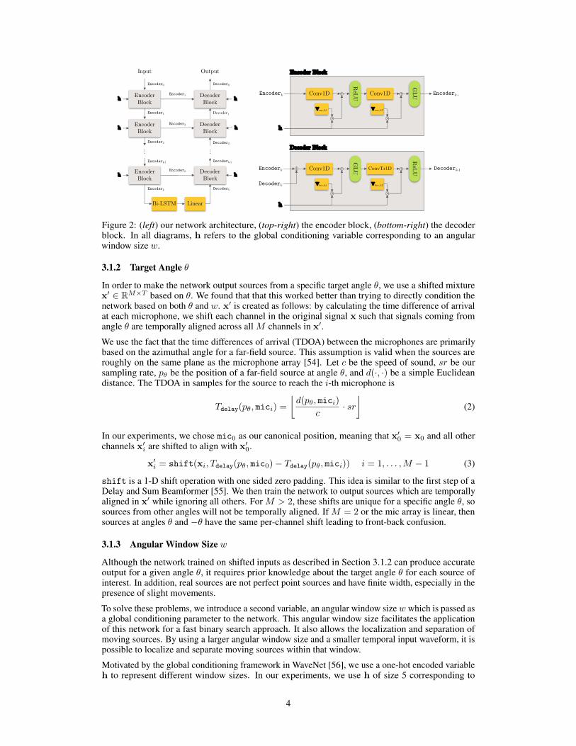
Figure 2: (left) our network architecture, (top-right) the encoder block, (bottom-right) the decoderblock. In all diagrams, h refers to the global conditioning variable corresponding to an angularwindow size w.

3.1.2 Target Angle θ

In order to make the network output sources from a specific target angle θ, we use a shifted mixturex′ ∈ RM×T based on θ. We found that that this worked better than trying to directly condition thenetwork based on both θ and w. x′ is created as follows: by calculating the time difference of arrivalat each microphone, we shift each channel in the original signal x such that signals coming fromangle θ are temporally aligned across all M channels in x′.

We use the fact that the time differences of arrival (TDOA) between the microphones are primarilybased on the azimuthal angle for a far-field source. This assumption is valid when the sources areroughly on the same plane as the microphone array [54]. Let c be the speed of sound, sr be oursampling rate, pθ be the position of a far-field source at angle θ, and d(·, ·) be a simple Euclideandistance. The TDOA in samples for the source to reach the i-th microphone is

Tdelay(pθ, mici) =⌊d(pθ, mici)

c· sr⌋

(2)

In our experiments, we chose mic0 as our canonical position, meaning that x′0 = x0 and all otherchannels x′i are shifted to align with x′0.

x′i = shift(xi, Tdelay(pθ, mic0)− Tdelay(pθ, mici)) i = 1, . . . ,M − 1 (3)

shift is a 1-D shift operation with one sided zero padding. This idea is similar to the first step of aDelay and Sum Beamformer [55]. We then train the network to output sources which are temporallyaligned in x′ while ignoring all others. For M > 2, these shifts are unique for a specific angle θ, sosources from other angles will not be temporally aligned. If M = 2 or the mic array is linear, thensources at angles θ and −θ have the same per-channel shift leading to front-back confusion.

3.1.3 Angular Window Size w

Although the network trained on shifted inputs as described in Section 3.1.2 can produce accurateoutput for a given angle θ, it requires prior knowledge about the target angle θ for each source ofinterest. In addition, real sources are not perfect point sources and have finite width, especially in thepresence of slight movements.

To solve these problems, we introduce a second variable, an angular window size w which is passed asa global conditioning parameter to the network. This angular window size facilitates the applicationof this network for a fast binary search approach. It also allows the localization and separation ofmoving sources. By using a larger angular window size and a smaller temporal input waveform, it ispossible to localize and separate moving sources within that window.

Motivated by the global conditioning framework in WaveNet [56], we use a one-hot encoded variableh to represent different window sizes. In our experiments, we use h of size 5 corresponding to

4

window sizes from the set {90◦, 45◦, 23◦, 12◦, 2◦}. By passing h to the network with our shiftedinput x′, we can explicitly make the network separate sources from the region θ± w

2 . We embed h toall encoder and decoder blocks in the network, using a learning linear projection V·,k,· as shown inFigure 2. Formally, the equations for the encoder block and decoder block can be written as follows:

Encoderk+1 = GLU(Wencoder,k,2 ∗ ReLU(Wencoder,k,1 ∗ Encoderk+Vencoder,k,1h) +Vencoder,k,2h),

(4)

Decoderk−1 = ReLU(Wdecoder,k,2 ∗> GLU(Wdecoder,k,1 ∗ (Encoderk + Decoderk)+Vdecoder,k,1h) +Vdecoder,k,2h).

(5)

The notation W·,k,· ∗ x denotes a 1-D convolution between the weights for the layer of an encod-ing/decoding block at level k and an input x. The notation ∗> denotes a transposed convolutionoperation. Empirically we found that passing h to every encoder and decoder block worked signif-icantly better than passing it to the network only once. Evidence that the CoS network learns thedesired window size is presented in Figure 4.

3.1.4 Network Training

Consider an input mixture x of N sources s1, . . . , sN with the corresponding locations θ1, . . . , θNalong with a target angle θt and window size w. The network is trained with the following objectivefunction:

L(x; s1, . . . , sN , θt, w) =

∥∥∥∥∥x′ −N∑i=1

s′i · I(θt −

w

2≤ θi < θt +

w

2

)∥∥∥∥∥1

(6)

where x′ and s′i are the shifted signals of the input mixture and ground truth signal as described inSection 3.1.2 based on the target angle θt. x′ is the output of the network using the shifted signal x′and the angular window w. I(·) is an indicator function, indicating whether si is present in the regionθt ± w

2 . If no source is present in the region θt ± w2 , the training target is a zero tensor 0.

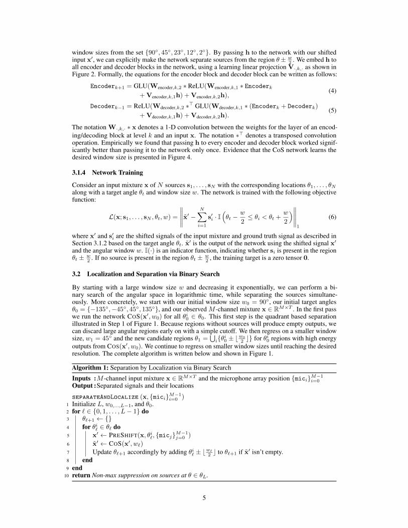
3.2 Localization and Separation via Binary Search

By starting with a large window size w and decreasing it exponentially, we can perform a bi-nary search of the angular space in logarithmic time, while separating the sources simultane-ously. More concretely, we start with our initial window size w0 = 90◦, our initial target anglesθ0 = {−135◦,−45◦, 45◦, 135◦}, and our observed M -channel mixture x ∈ RM×T . In the first passwe run the network COS(x′, w0) for all θi0 ∈ θ0. This first step is the quadrant based separationillustrated in Step 1 of Figure 1. Because regions without sources will produce empty outputs, wecan discard large angular regions early on with a simple cutoff. We then regress on a smaller windowsize, w1 = 45◦ and the new candidate regions θ1 =

⋃i{θi0 ± b

w0

2 c} for θi0 regions with high energyoutputs from COS(x′, w0). We continue to regress on smaller window sizes until reaching the desiredresolution. The complete algorithm is written below and shown in Figure 1.

Algorithm 1: Separation by Localization via Binary Search

Inputs :M -channel input mixture x ∈ RM×T and the microphone array position {mici}M−1i=0Output :Separated signals and their locations

separateAndLocalize (x, {mici}M−1i=0 )1 Initialize L, w0,...,L−1, and θ0.2 for ` ∈ {0, 1, . . . , L− 1} do3 θ`+1 ← {}4 for θi` ∈ θ` do5 x′ ← PRESHIFT(x, θi`, {micj}

M−1j=0 )

6 x′ ← COS(x′, w`)7 Update θ`+1 accordingly by adding θi` ± b

w`

2 c to θ`+1 if x′ isn’t empty.8 end9 end

10 return Non-max suppression on sources at θ ∈ θL.

5

To avoid duplicate outputs from adjacent regions, we employ a non-maximum suppression step beforeoutputting the final sources and locations. For this step, we consider both the angular proximity andsimilarity between the sources. If two outputted sources are physically close and have similar sourcecontent, we remove the one with the lower source energy. For example, for outputs (x′i, θi) and(x′j , θj) with ‖x′i‖ > ‖x′j‖, we remove (x′j , θj) if |θi − θj | < εθ and ‖x′i − x′j‖ < εx.

3.3 Runtime Analysis

Suppose we have N speakers and the angular space is discretized into r = 360◦

w angular bins. Thebinary search algorithm runs for at most O(log r) steps and requires at most O(N) forward passeson every step. Thus, the total number of forward passes is O(N log r) while a linear sweep alwaysruns in O(r) forward passes.

In most cases, N � r, so the binary search is clearly superior. For instance, when operating at a2◦ resolution, the average number of forward passes our algorithm takes to separate 2 voices in thepresence of background is 32.64, compared to 180 for a linear sweep. A forward pass of the networkon a single GPU takes 0.03 s for a 3 s input waveform at 44.1 kHz, meaning that the binary searchalgorithm in this scenario could keep up with real-time while the linear search could not.

4 Experiments

In this section, we explain our synthetic dataset and manually collected real dataset. We shownumerical results for separation and localization on the synthetic dataset and describe qualitativeresults on the real dataset.

4.1 Synthetic Dataset

Numerical results are demonstrated on synthetically rendered data. To generate the synthetic dataset,we create multi-speaker recordings in simulated environments with reverb and background noises.All voices come from the VCTK dataset [57], and the background samples consist of recordingsfrom either noisy restaurant environments or loud music. The train and test splits are completelyindependent and there are no overlapping identities or samples. We chose VCTK over other widelyused datasets like LibriSpeech [58] and WSJ0 [59] because VCTK is available at a high samplingrate of 48 kHz compared to 16 kHz as offered by others. In the supplementary materials, we showresults and comparisons with lower sampling rates.

To synthesize a single example, we create a 3-second mixture at 44.1 kHz by randomly selecting Nspeech samples and a background segment and placing them at arbitrary locations in a virtual roomof a randomly chosen size. We then simulate room impulse responses (RIRs) using the image sourcemethod [60] implemented in the pyroomacoustics library [61]. To approximate a diffuse-fieldbackground noise, the background source is placed further away, and the RIR for the backgroundis generated with high-order images, causing indirect reflections off room walls [62]. All signalsare convolved with the corresponding RIRs and rendered to a 6-channel circular microphone array(M = 6) of radius 2.85 in (7.25 cm). The volumes of the sources are chosen randomly in order tocreate challenging scenarios; the input SDR is between −16 dB and 0 dB for most of the dataset. Fortraining our network, we use 10,000 examples with N chosen uniformly between 1 and 4, inclusively,at random, and for evaluating we use 1,000 examples with N dependent on the evaluation task.

4.2 Source Separation

To evaluate the source separation performance of our method, we create mixtures consisting of 2voices (N = 2) and 1 background, allowing comparisons with deep learning methods that require afixed number of foreground sources. We use the popular metric scale-invariant signal-to-distortionratio (SI-SDR) [63]. When reporting the increase from the input to output SI-SDR, we use the labelSI-SDR improvement (SI-SDRi). For deep learning baselines in the waveform domain we chose TAC[40], a recently proposed neural beamformer, and a multi-channel extension of Conv-TasNet [18], apopular speech separation network. For this multi-channel Conv-TasNet, we changed the number ofinput channels to match the number of microphones in order to process the full mixture. To comparewith spectrogram based methods, we use oracle baselines based on the time-frequency representation

6

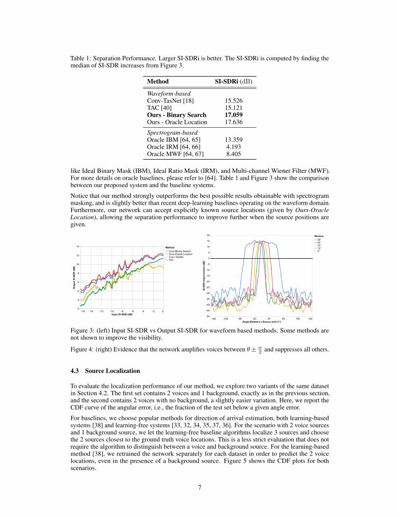
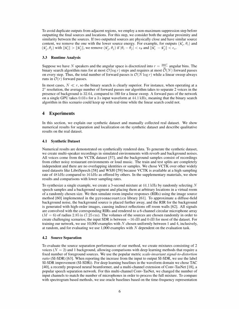
Table 1: Separation Performance. Larger SI-SDRi is better. The SI-SDRi is computed by finding themedian of SI-SDR increases from Figure 3.

Method SI-SDRi (dB)

Waveform-basedConv-TasNet [18] 15.526TAC [40] 15.121Ours - Binary Search 17.059Ours - Oracle Location 17.636

Spectrogram-basedOracle IBM [64, 65] 13.359Oracle IRM [64, 66] 4.193Oracle MWF [64, 67] 8.405

like Ideal Binary Mask (IBM), Ideal Ratio Mask (IRM), and Multi-channel Wiener Filter (MWF).For more details on oracle baselines, please refer to [64]. Table 1 and Figure 3 show the comparisonbetween our proposed system and the baseline systems.

Notice that our method strongly outperforms the best possible results obtainable with spectrogrammasking, and is slightly better than recent deep-learning baselines operating on the waveform domain.Furthermore, our network can accept explicitly known source locations (given by Ours-OracleLocation), allowing the separation performance to improve further when the source positions aregiven.

−16 −14 −12 −10 −8 −6 −4 −2 0Input SI-SDR (dB)

0

2

4

6

8

10

12

14

Out

put S

I-SD

R (d

B)

Ours-Binary SearchOurs-Oracle LocationConv-TasNetTAC

Method

-140 -100 -60 -20 20 60 100 140Angle Between a Source and 𝜃 (°)

-50

-45

-40

-35

-30

-25

-20

-15

-10

-5

0

5

10

15

20

SI-S

DR

Impr

ovem

ent (

dB)

90°45°23°12°2°

Window

Figure 3: (left) Input SI-SDR vs Output SI-SDR for waveform based methods. Some methods arenot shown to improve the visibility.

Figure 4: (right) Evidence that the network amplifies voices between θ± w2 and suppresses all others.

4.3 Source Localization

To evaluate the localization performance of our method, we explore two variants of the same datasetin Section 4.2. The first set contains 2 voices and 1 background, exactly as in the previous section,and the second contains 2 voices with no background, a slightly easier variation. Here, we report theCDF curve of the angular error, i.e., the fraction of the test set below a given angle error.

For baselines, we choose popular methods for direction of arrival estimation, both learning-basedsystems [38] and learning-free systems [33, 32, 34, 35, 37, 36]. For the scenario with 2 voice sourcesand 1 background source, we let the learning-free baseline algorithms localize 3 sources and choosethe 2 sources closest to the ground truth voice locations. This is a less strict evaluation that does notrequire the algorithm to distinguish between a voice and background source. For the learning-basedmethod [38], we retrained the network separately for each dataset in order to predict the 2 voicelocations, even in the presence of a background source. Figure 5 shows the CDF plots for bothscenarios.

7

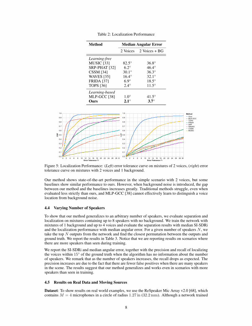
Table 2: Localization Performance

Method Median Angular Error2 Voices 2 Voices + BG

Learning-freeMUSIC [33] 82.5◦ 36.8◦SRP-PHAT [32] 6.2◦ 46.4◦CSSM [34] 30.1◦ 36.3◦WAVES [35] 16.4◦ 32.1◦FRIDA [37] 6.9◦ 18.5◦TOPS [36] 2.4◦ 11.5◦

Learning-basedMLP-GCC [38] 1.0◦ 41.5◦Ours 2.1◦ 3.7◦

0 2 4 6 8 10 12 14 16 18 20 22 24 26 28 30Error Tolerance (°)

0.0

0.1

0.2

0.3

0.4

0.5

0.6

0.7

0.8

0.9

1.0

CD

F

OursMLP-GCCTOPSFRIDASRPWAVESCSSMMUSIC

Method

0 2 4 6 8 10 12 14 16 18 20 22 24 26 28 30Error Tolerance (°)

0.0

0.1

0.2

0.3

0.4

0.5

0.6

0.7

0.8

0.9

1.0

CD

F

OursMLP-GCCTOPSFRIDASRPWAVESCSSMMUSIC

Method

Figure 5: Localization Performance: (Left) error tolerance curve on mixtures of 2 voices, (right) errortolerance curve on mixtures with 2 voices and 1 background.

Our method shows state-of-the-art performance in the simple scenario with 2 voices, but somebaselines show similar performance to ours. However, when background noise is introduced, the gapbetween our method and the baselines increases greatly. Traditional methods struggle, even whenevaluated less strictly than ours, and MLP-GCC [38] cannot effectively learn to distinguish a voicelocation from background noise.

4.4 Varying Number of Speakers

To show that our method generalizes to an arbitrary number of speakers, we evaluate separation andlocalization on mixtures containing up to 8 speakers with no background. We train the network withmixtures of 1 background and up to 4 voices and evaluate the separation results with median SI-SDRiand the localization performance with median angular error. For a given number of speakers N , wetake the top N outputs from the network and find the closest permutation between the outputs andground truth. We report the results in Table 3. Notice that we are reporting results on scenarios wherethere are more speakers than seen during training.

We report the SI-SDRi and median angular error, together with the precision and recall of localizingthe voices within 15◦ of the ground truth when the algorithm has no information about the numberof speakers. We remark that as the number of speakers increases, the recall drops as expected. Theprecision increases are due to the fact that there are fewer false positives when there are many speakersin the scene. The results suggest that our method generalizes and works even in scenarios with morespeakers than seen in training.

4.5 Results on Real Data and Moving Sources

Dataset: To show results on real world examples, we use the ReSpeaker Mic Array v2.0 [68], whichcontains M = 4 microphones in a circle of radius 1.27 in (32.2mm). Although a network trained

8

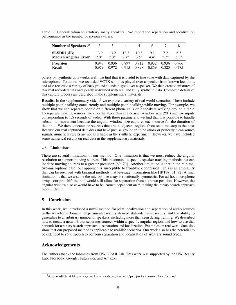
Table 3: Generalization to arbitrary many speakers. We report the separation and localizationperformance as the number of speakers varies.

Number of Speakers N 2 3 4 5 6 7 8

SI-SDRi (dB) 13.9 13.2 12.2 10.8 9.1 7.2 6.3Median Angular Error 2.0◦ 2.3◦ 2.7◦ 3.5◦ 4.4◦ 5.2◦ 6.3◦

Precision 0.947 0.936 0.897 0.912 0.932 0.936 0.966Recall 0.979 0.972 0.915 0.898 0.859 0.825 0.785

purely on synthetic data works well, we find that it is useful to fine-tune with data captured by themicrophone. To do this we recorded VCTK samples played over a speaker from known locations,and also recorded a variety of background sounds played over a speaker. We then created mixtures ofthis real recorded data and jointly re-trained with real and fully synthetic data. Complete details ofthis capture process are described in the supplementary materials.

Results: In the supplementary videos3 we explore a variety of real world scenarios. These includemultiple people talking concurrently and multiple people talking while moving. For example, weshow that we can separate people on different phone calls or 2 speakers walking around a table.To separate moving sources, we stop the algorithm at a coarser window size (23◦) and use inputscorresponding to 1.5 seconds of audio. With these parameters, we find that it is possible to handlesubstantial movement because the angular window size captures each source for the duration ofthe input. We then concatenate sources that are in adjacent regions from one time step to the next.Because our real captured data does not have precise ground truth positions or perfectly clean sourcesignals, numerical results are not as reliable as the synthetic experiment. However, we have includedsome numerical results on real data in the supplementary materials.

4.6 Limitations

There are several limitations of our method. One limitation is that we must reduce the angularresolution to support moving sources. This in contrast to specific speaker tracking methods that canlocalize moving sources to a greater precision [69, 70]. Another limitation is that in the minimaltwo-microphone case, our approach is susceptible to front-back confusion. This is an ambiguitythat can be resolved with binaural methods that leverage information like HRTFs [71, 72] A finallimitation is that we assume the microphone array is rotationally symmetric. For ad-hoc microphonearrays, our pre-shift method would still allow for separation from a known position. However, theangular window size w would have to be learned dependent on θ, making the binary search approachmore difficult.

5 Conclusion

In this work, we introduced a novel method for joint localization and separation of audio sourcesin the waveform domain. Experimental results showed state-of-the-art results, and the ability togeneralize to an arbitrary number of speakers, including more than seen during training. We describedhow to create a network that separates sources within a specific angular region, and how to use thatnetwork for a binary search approach to separation and localization. Examples on real world data alsoshow that our proposed method is applicable to real-life scenarios. Our work also has the potential tobe extended beyond speech to perform separation and localization of arbitrary sound types.

Acknowledgements

The authors thank the labmates from UW GRAIL lab. This work was supported by the UW RealityLab, Facebook, Google, Futurewei, and Amazon.

3Also available at https://grail.cs.washington.edu/projects/cone-of-silence/

9

Broader Impact Statement

We believe that our method has the potential to help people hear better in a variety of everydayscenarios. This work could be integrated with headphones, hearing aids, smart home devices, orlaptops, to facilitate source separation and localization. Our localization output also provides a moreprivacy-friendly alternative to camera based detection for applications like robotics or optical tracking.We note that improved ability to separate speakers in noisy environments comes with potential privacyconcerns. For example, this method could be used to better hear a conversation at a nearby tablein a restaurant. Tracking speakers with microphone input also presents a similar range of privacyconcerns as camera based tracking and recognition in everyday environments.

10

References

[1] https://en.wikipedia.org/wiki/Cone_of_Silence_(Get_Smart).[2] J-F Cardoso. Blind signal separation: statistical principles. Proceedings of the IEEE,

86(10):2009–2025, 1998.[3] Francesco Nesta, Piergiorgio Svaizer, and Maurizio Omologo. Convolutive bss of short mixtures

by ica recursively regularized across frequencies. IEEE transactions on audio, speech, andlanguage processing, 19(3):624–639, 2010.

[4] Bhiksha Raj, Tuomas Virtanen, Sourish Chaudhuri, and Rita Singh. Non-negative matrixfactorization based compensation of music for automatic speech recognition. In EleventhAnnual Conference of the International Speech Communication Association, 2010.

[5] Nasser Mohammadiha, Paris Smaragdis, and Arne Leijon. Supervised and unsupervised speechenhancement using nonnegative matrix factorization. IEEE Transactions on Audio, Speech, andLanguage Processing, 21(10):2140–2151, 2013.

[6] Efthymios Tzinis, Shrikant Venkataramani, and Paris Smaragdis. Unsupervised deep clusteringfor source separation: Direct learning from mixtures using spatial information. In ICASSP 2019-2019 IEEE International Conference on Acoustics, Speech and Signal Processing (ICASSP),pages 81–85. IEEE, 2019.

[7] Hiroshi Sawada, Shoko Araki, and Shoji Makino. Underdetermined convolutive blind sourceseparation via frequency bin-wise clustering and permutation alignment. IEEE Transactions onAudio, Speech, and Language Processing, 19(3):516–527, 2010.

[8] Y. Luo, Z. Chen, J. R. Hershey, J. Le Roux, and N. Mesgarani. Deep clustering and conventionalnetworks for music separation: Stronger together. In 2017 IEEE International Conference onAcoustics, Speech and Signal Processing (ICASSP), pages 61–65, 2017.

[9] Kousuke Itakura, Yoshiaki Bando, Eita Nakamura, Katsutoshi Itoyama, Kazuyoshi Yoshii, andTatsuya Kawahara. Bayesian multichannel audio source separation based on integrated sourceand spatial models. IEEE/ACM Transactions on Audio, Speech, and Language Processing,26(4):831–846, 2018.

[10] Vivek Jayaram and John Thickstun. Source separation with deep generative priors. arXivpreprint arXiv:2002.07942, 2020.

[11] Laurent Benaroya, Frédéric Bimbot, and Rémi Gribonval. Audio source separation with a singlesensor. IEEE Transactions on Audio, Speech, and Language Processing, 14(1):191–199, 2005.

[12] Nancy Bertin, Roland Badeau, and Emmanuel Vincent. Enforcing harmonicity and smoothnessin bayesian non-negative matrix factorization applied to polyphonic music transcription. IEEETransactions on Audio, Speech, and Language Processing, 18(3):538–549, 2010.

[13] Tavi Halperin, Ariel Ephrat, and Yedid Hoshen. Neural separation of observed and unobserveddistributions. arXiv preprint arXiv:1811.12739, 2018.

[14] Andreas Jansson, Eric Humphrey, Nicola Montecchio, Rachel Bittner, Aparna Kumar, andTillman Weyde. Singing voice separation with deep u-net convolutional networks. 2017.

[15] Aditya Arie Nugraha, Antoine Liutkus, and Emmanuel Vincent. Multichannel audio sourceseparation with deep neural networks. IEEE/ACM Transactions on Audio, Speech, and LanguageProcessing, 24(9):1652–1664, 2016.

[16] Daniel Stoller, Sebastian Ewert, and Simon Dixon. Wave-u-net: A multi-scale neural networkfor end-to-end audio source separation. arXiv preprint arXiv:1806.03185, 2018.

[17] Yi Luo and Nima Mesgarani. Tasnet: time-domain audio separation network for real-time,single-channel speech separation. In 2018 IEEE International Conference on Acoustics, Speechand Signal Processing (ICASSP), pages 696–700. IEEE, 2018.

[18] Yi Luo and Nima Mesgarani. Conv-tasnet: Surpassing ideal time–frequency magnitude maskingfor speech separation. IEEE/ACM transactions on audio, speech, and language processing,27(8):1256–1266, 2019.

[19] John R Hershey, Zhuo Chen, Jonathan Le Roux, and Shinji Watanabe. Deep clustering:Discriminative embeddings for segmentation and separation. In 2016 IEEE InternationalConference on Acoustics, Speech and Signal Processing (ICASSP), pages 31–35. IEEE, 2016.

11

[20] Chenglin Xu, Wei Rao, Xiong Xiao, Eng Siong Chng, and Haizhou Li. Single channel speechseparation with constrained utterance level permutation invariant training using grid lstm. In2018 IEEE International Conference on Acoustics, Speech and Signal Processing (ICASSP),pages 6–10. IEEE, 2018.

[21] Chao Weng, Dong Yu, Michael L Seltzer, and Jasha Droppo. Deep neural networks for single-channel multi-talker speech recognition. IEEE/ACM Transactions on Audio, Speech, andLanguage Processing, 23(10):1670–1679, 2015.

[22] Takuya Yoshioka, Hakan Erdogan, Zhuo Chen, and Fil Alleva. Multi-microphone neural speechseparation for far-field multi-talker speech recognition. In 2018 IEEE International Conferenceon Acoustics, Speech and Signal Processing (ICASSP), pages 5739–5743. IEEE, 2018.

[23] Zhuo Chen, Xiong Xiao, Takuya Yoshioka, Hakan Erdogan, Jinyu Li, and Yifan Gong. Multi-channel overlapped speech recognition with location guided speech extraction network. In 2018IEEE Spoken Language Technology Workshop (SLT), pages 558–565. IEEE, 2018.

[24] Xueliang Zhang and DeLiang Wang. Deep learning based binaural speech separation inreverberant environments. IEEE/ACM transactions on audio, speech, and language processing,25(5):1075–1084, 2017.

[25] Rongzhi Gu, Shi-Xiong Zhang, Lianwu Chen, Yong Xu, Meng Yu, Dan Su, Yuexian Zou, andDong Yu. Enhancing end-to-end multi-channel speech separation via spatial feature learning.arXiv preprint arXiv:2003.03927, 2020.

[26] Cong Han, Yi Luo, and Nima Mesgarani. Real-time binaural speech separation with preservedspatial cues. arXiv preprint arXiv:2002.06637, 2020.

[27] Hang Zhao, Chuang Gan, Andrew Rouditchenko, Carl Vondrick, Josh McDermott, and AntonioTorralba. The sound of pixels. In Proceedings of the European Conference on Computer Vision(ECCV), pages 570–586, 2018.

[28] Andrew Rouditchenko, Hang Zhao, Chuang Gan, Josh McDermott, and Antonio Torralba. Self-supervised audio-visual co-segmentation. In ICASSP 2019-2019 IEEE International Conferenceon Acoustics, Speech and Signal Processing (ICASSP), pages 2357–2361. IEEE, 2019.

[29] François Grondin and James Glass. Multiple sound source localization with svd-phat. arXivpreprint arXiv:1906.11913, 2019.

[30] Or Nadiri and Boaz Rafaely. Localization of multiple speakers under high reverberation using aspherical microphone array and the direct-path dominance test. IEEE/ACM Transactions onAudio, Speech, and Language Processing, 22(10):1494–1505, 2014.

[31] Despoina Pavlidi, Anthony Griffin, Matthieu Puigt, and Athanasios Mouchtaris. Real-timemultiple sound source localization and counting using a circular microphone array. IEEETransactions on Audio, Speech, and Language Processing, 21(10):2193–2206, 2013.

[32] Joseph Hector DiBiase. A high-accuracy, low-latency technique for talker localization inreverberant environments using microphone arrays. Brown University Providence, RI, 2000.

[33] Ralph Schmidt. Multiple emitter location and signal parameter estimation. IEEE transactionson antennas and propagation, 34(3):276–280, 1986.

[34] Hong Wang and Mostafa Kaveh. Coherent signal-subspace processing for the detection andestimation of angles of arrival of multiple wide-band sources. IEEE Transactions on Acoustics,Speech, and Signal Processing, 33(4):823–831, 1985.

[35] Elio D Di Claudio and Raffaele Parisi. Waves: Weighted average of signal subspaces for robustwideband direction finding. IEEE Transactions on Signal Processing, 49(10):2179–2191, 2001.

[36] Yeo-Sun Yoon, Lance M Kaplan, and James H McClellan. Tops: New doa estimator forwideband signals. IEEE Transactions on Signal processing, 54(6):1977–1989, 2006.

[37] Hanjie Pan, Robin Scheibler, Eric Bezzam, Ivan Dokmanic, and Martin Vetterli. Frida: Fri-based doa estimation for arbitrary array layouts. In 2017 IEEE International Conference onAcoustics, Speech and Signal Processing (ICASSP), pages 3186–3190. IEEE, 2017.

[38] Weipeng He, Petr Motlicek, and Jean-Marc Odobez. Deep neural networks for multiple speakerdetection and localization. In 2018 IEEE International Conference on Robotics and Automation(ICRA), pages 74–79. IEEE, 2018.

12

[39] Sharath Adavanne, Archontis Politis, Joonas Nikunen, and Tuomas Virtanen. Sound eventlocalization and detection of overlapping sources using convolutional recurrent neural networks.IEEE Journal of Selected Topics in Signal Processing, 13(1):34–48, 2018.

[40] Yi Luo, Zhuo Chen, Nima Mesgarani, and Takuya Yoshioka. End-to-end microphone permu-tation and number invariant multi-channel speech separation. In ICASSP 2020-2020 IEEEInternational Conference on Acoustics, Speech and Signal Processing (ICASSP), pages 6394–6398. IEEE, 2020.

[41] Takuya Higuchi, Keisuke Kinoshita, Marc Delcroix, Katerina Zmolíková, and TomohiroNakatani. Deep clustering-based beamforming for separation with unknown number of sources.In Interspeech, pages 1183–1187, 2017.

[42] Naoya Takahashi, Sudarsanam Parthasaarathy, Nabarun Goswami, and Yuki Mitsufuji. Recur-sive speech separation for unknown number of speakers. arXiv preprint arXiv:1904.03065,2019.

[43] Eliya Nachmani, Yossi Adi, and Lior Wolf. Voice separation with an unknown number ofmultiple speakers. arXiv preprint arXiv:2003.01531, 2020.

[44] Hidri Adel, Meddeb Souad, Abdulqadir Alaqeeli, and Amiri Hamid. Beamforming techniquesfor multichannel audio signal separation. arXiv preprint arXiv:1212.6080, 2012.

[45] J. Traa and P. Smaragdis. Multichannel source separation and tracking with ransac and di-rectional statistics. IEEE/ACM Transactions on Audio, Speech, and Language Processing,22(12):2233–2243, 2014.

[46] Michael I Mandel, Ron J Weiss, and Daniel PW Ellis. Model-based expectation-maximizationsource separation and localization. IEEE Transactions on Audio, Speech, and LanguageProcessing, 18(2):382–394, 2009.

[47] Futoshi Asano and Hideki Asoh. Sound source localization and separation based on the emalgorithm. In ISCA Tutorial and Research Workshop (ITRW) on Statistical and PerceptualAudio Processing, 2004.

[48] Yuval Dorfan, Dani Cherkassky, and Sharon Gannot. Speaker localization and separation usingincremental distributed expectation-maximization. In 2015 23rd European Signal ProcessingConference (EUSIPCO), pages 1256–1260. IEEE, 2015.

[49] Antoine Deleforge, Florence Forbes, and Radu Horaud. Acoustic space learning for sound-source separation and localization on binaural manifolds. International journal of neuralsystems, 25(01):1440003, 2015.

[50] Michael I Mandel, Daniel P Ellis, and Tony Jebara. An em algorithm for localizing multiplesound sources in reverberant environments. In Advances in neural information processingsystems, pages 953–960, 2007.

[51] Johannes Traa, Paris Smaragdis, Noah D Stein, and David Wingate. Directional nmf forjoint source localization and separation. In 2015 IEEE Workshop on Applications of SignalProcessing to Audio and Acoustics (WASPAA), pages 1–5. IEEE, 2015.

[52] Daniel Johnson, Daniel Gorelik, Ross E Mawhorter, Kyle Suver, Weiqing Gu, Steven Xing,Cody Gabriel, and Peter Sankhagowit. Latent gaussian activity propagation: using smoothnessand structure to separate and localize sounds in large noisy environments. In Advances in NeuralInformation Processing Systems, pages 3465–3474, 2018.

[53] Alexandre Défossez, Nicolas Usunier, Léon Bottou, and Francis Bach. Demucs: Deep extractorfor music sources with extra unlabeled data remixed. arXiv preprint arXiv:1909.01174, 2019.

[54] J-M Valin, François Michaud, Jean Rouat, and Dominic Létourneau. Robust sound sourcelocalization using a microphone array on a mobile robot. In Proceedings 2003 IEEE/RSJInternational Conference on Intelligent Robots and Systems (IROS 2003)(Cat. No. 03CH37453),volume 2, pages 1228–1233. IEEE, 2003.

[55] Don H. Johnson and Dan E. Dudgeon. Array Signal Processing: Concepts and Techniques.Simon & Schuster, Inc., USA, 1992.

[56] Aaron van den Oord, Sander Dieleman, Heiga Zen, Karen Simonyan, Oriol Vinyals, AlexGraves, Nal Kalchbrenner, Andrew Senior, and Koray Kavukcuoglu. Wavenet: A generativemodel for raw audio. arXiv preprint arXiv:1609.03499, 2016.

13

[57] Christophe Veaux, Junichi Yamagishi, Kirsten MacDonald, et al. Superseded-cstr vctk corpus:English multi-speaker corpus for cstr voice cloning toolkit. 2016.

[58] Vassil Panayotov, Guoguo Chen, Daniel Povey, and Sanjeev Khudanpur. Librispeech: anasr corpus based on public domain audio books. In 2015 IEEE International Conference onAcoustics, Speech and Signal Processing (ICASSP), pages 5206–5210. IEEE, 2015.

[59] John Garofalo, David Graff, Doug Paul, and David Pallett. Csr-i (wsj0) complete. LinguisticData Consortium, Philadelphia, 2007.

[60] Jont B Allen and David A Berkley. Image method for efficiently simulating small-roomacoustics. The Journal of the Acoustical Society of America, 65(4):943–950, 1979.

[61] Robin Scheibler, Eric Bezzam, and Ivan Dokmanic. Pyroomacoustics: A python package foraudio room simulation and array processing algorithms. In 2018 IEEE International Conferenceon Acoustics, Speech and Signal Processing (ICASSP), pages 351–355. IEEE, 2018.

[62] Michael Vorländer. Auralization: fundamentals of acoustics, modelling, simulation, algorithmsand acoustic virtual reality. Springer Science & Business Media, 2007.

[63] Jonathan Le Roux, Scott Wisdom, Hakan Erdogan, and John R Hershey. Sdr–half-baked orwell done? In ICASSP 2019-2019 IEEE International Conference on Acoustics, Speech andSignal Processing (ICASSP), pages 626–630. IEEE, 2019.

[64] Fabian-Robert Stöter, Antoine Liutkus, and Nobutaka Ito. The 2018 signal separation evaluationcampaign. In International Conference on Latent Variable Analysis and Signal Separation,pages 293–305. Springer, 2018.

[65] DeLiang Wang. On ideal binary mask as the computational goal of auditory scene analysis. InSpeech separation by humans and machines, pages 181–197. Springer, 2005.

[66] Antoine Liutkus and Roland Badeau. Generalized wiener filtering with fractional power spec-trograms. In 2015 IEEE International Conference on Acoustics, Speech and Signal Processing(ICASSP), pages 266–270. IEEE, 2015.

[67] Ngoc QK Duong, Emmanuel Vincent, and Rémi Gribonval. Under-determined reverberantaudio source separation using a full-rank spatial covariance model. IEEE Transactions on Audio,Speech, and Language Processing, 18(7):1830–1840, 2010.

[68] https://wiki.seeedstudio.com/ReSpeaker_Mic_Array_v2.0/.[69] J. Traa and P. Smaragdis. A wrapped kalman filter for azimuthal speaker tracking. IEEE Signal

Processing Letters, 20(12):1257–1260, 2013.[70] Xinyuan Qian, Alessio Brutti, Maurizio Omologo, and Andrea Cavallaro. 3d audio-visual

speaker tracking with an adaptive particle filter. In 2017 IEEE International Conference onAcoustics, Speech and Signal Processing (ICASSP), pages 2896–2900. IEEE, 2017.

[71] F. Keyrouz. Robotic binaural localization and separation of multiple simultaneous sound sources.In 2017 IEEE 11th International Conference on Semantic Computing (ICSC), pages 188–195,2017.

[72] Ning Ma, Tobias May, and Guy J Brown. Exploiting deep neural networks and head movementsfor robust binaural localization of multiple sources in reverberant environments. IEEE/ACMTransactions on Audio, Speech, and Language Processing, 25(12):2444–2453, 2017.

[73] Diederik P Kingma and Jimmy Ba. Adam: A method for stochastic optimization. arXiv preprintarXiv:1412.6980, 2014.

14

Supplementary Materials

Person 1Person 2Person 3

Input Mixture

Ground Truth Signals by Person

Ground Truth Positions Step 1: Search Regions(w = 90°)

Output Signals by Regionfrom Separation Network

Final Output Signalsfrom Separation Network

Step 2: Search Regions(w = 45°)

Step 5: Search Regions(w = 2°)

…

Denotes a person at that location

Refine Refine Refine

No Signal

No Signal

No Signal

Output Signals by Regionfrom Separation Network

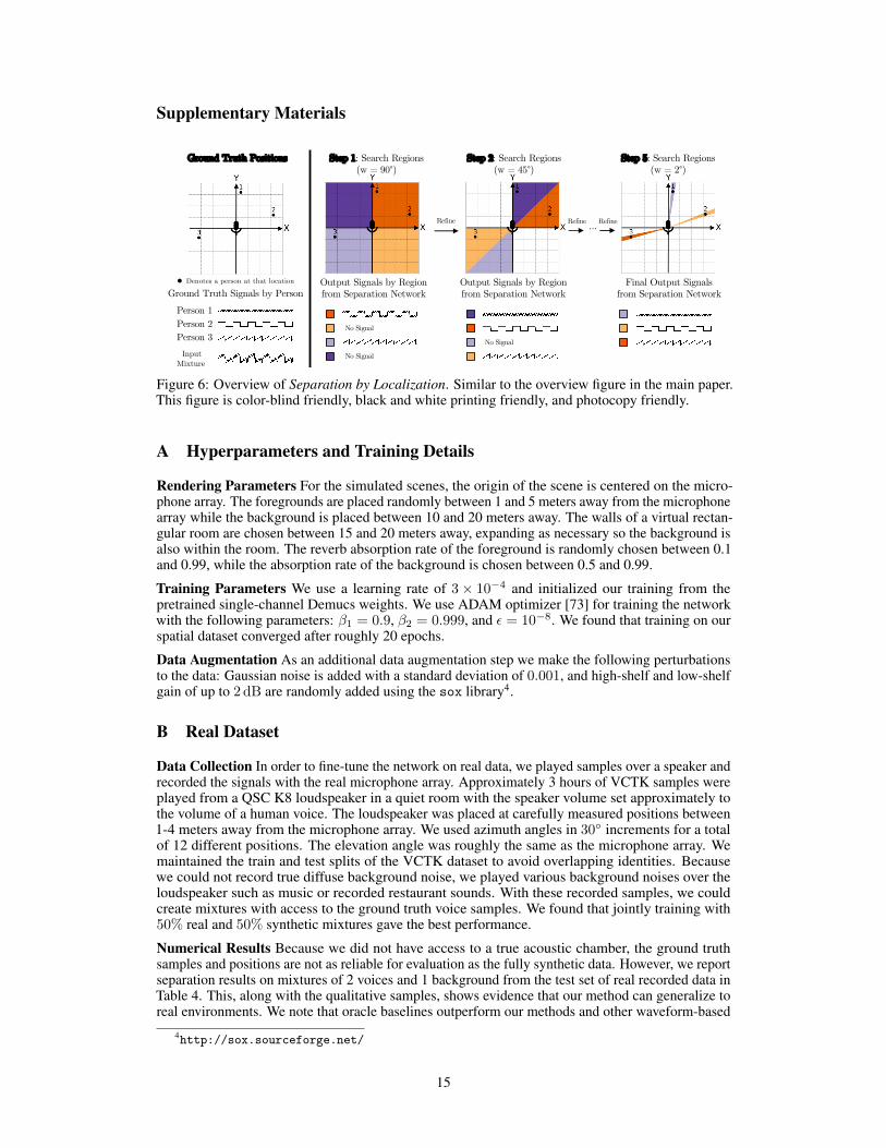
Figure 6: Overview of Separation by Localization. Similar to the overview figure in the main paper.This figure is color-blind friendly, black and white printing friendly, and photocopy friendly.

A Hyperparameters and Training Details

Rendering Parameters For the simulated scenes, the origin of the scene is centered on the micro-phone array. The foregrounds are placed randomly between 1 and 5 meters away from the microphonearray while the background is placed between 10 and 20 meters away. The walls of a virtual rectan-gular room are chosen between 15 and 20 meters away, expanding as necessary so the background isalso within the room. The reverb absorption rate of the foreground is randomly chosen between 0.1and 0.99, while the absorption rate of the background is chosen between 0.5 and 0.99.

Training Parameters We use a learning rate of 3× 10−4 and initialized our training from thepretrained single-channel Demucs weights. We use ADAM optimizer [73] for training the networkwith the following parameters: β1 = 0.9, β2 = 0.999, and ε = 10−8. We found that training on ourspatial dataset converged after roughly 20 epochs.

Data Augmentation As an additional data augmentation step we make the following perturbationsto the data: Gaussian noise is added with a standard deviation of 0.001, and high-shelf and low-shelfgain of up to 2 dB are randomly added using the sox library4.

B Real Dataset

Data Collection In order to fine-tune the network on real data, we played samples over a speaker andrecorded the signals with the real microphone array. Approximately 3 hours of VCTK samples wereplayed from a QSC K8 loudspeaker in a quiet room with the speaker volume set approximately tothe volume of a human voice. The loudspeaker was placed at carefully measured positions between1-4 meters away from the microphone array. We used azimuth angles in 30◦ increments for a totalof 12 different positions. The elevation angle was roughly the same as the microphone array. Wemaintained the train and test splits of the VCTK dataset to avoid overlapping identities. Becausewe could not record true diffuse background noise, we played various background noises over theloudspeaker such as music or recorded restaurant sounds. With these recorded samples, we couldcreate mixtures with access to the ground truth voice samples. We found that jointly training with50% real and 50% synthetic mixtures gave the best performance.

Numerical Results Because we did not have access to a true acoustic chamber, the ground truthsamples and positions are not as reliable for evaluation as the fully synthetic data. However, we reportseparation results on mixtures of 2 voices and 1 background from the test set of real recorded data inTable 4. This, along with the qualitative samples, shows evidence that our method can generalize toreal environments. We note that oracle baselines outperform our methods and other waveform-based

4http://sox.sourceforge.net/

15

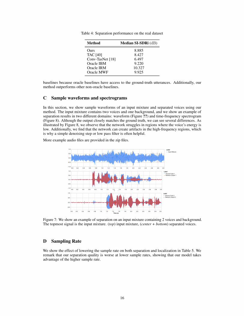
Table 4: Separation performance on the real dataset

Method Median SI-SDRi (dB)

Ours 8.885TAC [40] 8.427Conv-TasNet [18] 6.497Oracle IBM 9.220Oracle IRM 10.327Oracle MWF 9.925

baselines because oracle baselines have access to the ground-truth utterances. Additionally, ourmethod outperforms other non-oracle baselines.

C Sample waveforms and spectrograms

In this section, we show sample waveforms of an input mixture and separated voices using ourmethod. The input mixture contains two voices and one background, and we show an example ofseparation results in two different domains: waveform (Figure ??) and time-frequency spectrogram(Figure 8). Although the output closely matches the ground truth, we can see several differences. Asillustrated by Figure 8, we observe that the network struggles in regions where the voice’s energy islow. Additionally, we find that the network can create artifacts in the high-frequency regions, whichis why a simple denoising step or low pass filter is often helpful.

More example audio files are provided in the zip files.

0.0 0.2 0.4 0.6 0.8 1.0 1.2 1.4 1.6 1.8 2.0 2.2 2.4 2.6 2.8 3.0Time (s)

-1.0

-0.5

0.0

0.5

1.0

Input MixtureLabel

0.0 0.2 0.4 0.6 0.8 1.0 1.2 1.4 1.6 1.8 2.0 2.2 2.4 2.6 2.8 3.0Time (s)

-1.0

-0.5

0.0

0.5

1.0

Ground Truth 1Network Output 1

Label

0.0 0.2 0.4 0.6 0.8 1.0 1.2 1.4 1.6 1.8 2.0 2.2 2.4 2.6 2.8 3.0Time (s)

-0.5

0.0

0.5

1.0

Ground Truth 2Network Output 2

Label

Figure 7: We show an example of separation on an input mixture containing 2 voices and background.The topmost signal is the input mixture. (top) input mixture, (center + bottom) separated voices.

D Sampling Rate

We show the effect of lowering the sample rate on both separation and localization in Table 5. Weremark that our separation quality is worse at lower sample rates, showing that our model takesadvantage of the higher sample rate.

16

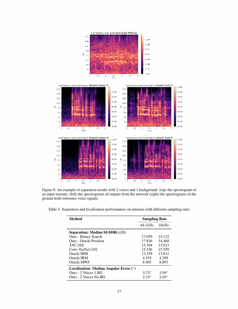
Figure 8: An example of separation results with 2 voices and 1 background. (top) the spectrogram ofan input mixture, (left) the spectrograms of outputs from the network (right) the spectrograms of theground truth reference voice signals.

Table 5: Separation and localization performances on datasets with different sampling rates

Method Sampling Rate44.1kHz 16kHz

Separation: Median SI-SDRi (dB)Ours - Binary Search 17.059 14.132Ours - Oracle Position 17.636 14.468TAC [40] 15.104 13.613Conv-TasNet [18] 15.526 15.559Oracle IBM 13.359 13.611Oracle IRM 4.193 4.289Oracle MWF 8.405 8.893

Localization: Median Angular Error (◦)Ours - 2 Voices 1 BG 3.73◦ 3.98◦

Ours - 2 Voices No BG 2.13◦ 2.68◦

17