DOKUZ EYLÜL UNIVERSITY

GRADUATE SCHOOL OF SOCIAL SCIENCES

DEPARTMENT OF MARITIME BUSINESS ADMINISTRATION

MARITIME BUSINESS ADMINISTRATION

DOCTORAL THESIS

Doctor of Philosophy (PhD)

DEVELOPING A MODEL FOR MEASURING THE

CAPACITY OF DRY BULK PORTS IN TURKEY

Seçil GÜLMEZ

Supervisor

Prof. Dr. Soner ESMER

İZMİR-2019

ii

THESIS APPROVAL PAGE

iii

DECLERATION

I hereby declare that this doctoral thesis titled as “Developing a Model for

Measuring the Capacity of Dry Bulk Ports in Turkey” has been written myself in

accordance with the academic rules and ethical conduct. I also declare that all materials

benefited in this thesis consist of mentioned resources in the reference list. I verify all

these with my honour.

20/05/2019

Seçil GÜLMEZ

iv

ABSTRACT

Doctoral Thesis

Doctor of Philosophy

Developing a Model for Measuring the Capacity of Dry Bulk Ports in Turkey

Seçil GÜLMEZ

Dokuz Eylül University

Graduate School of Social Sciences

Department of Maritime Business Administration

Maritime Business Administration Ph.D. Program

Ports are defined as critical nodes in international trade and one of the

critical part of international transport. For this reason, these essential

infrastructures are a strategic point for both stakeholders and port operators.

Continuous development of maritime transport, macro, and micro

environmental factors triggered and accelerated the development of ports. To

keep up with these ongoing developments, the ports are continuously improving

themselves technologically and expand and upgrading their infrastructure or

tend to invest in building new ports to satisfy the demand created by increasing

trade volume. Under these circumstances, port operators should plan the

capacity regarding the supply and demand conditions.

In this study, it was attempted to develop a capacity measurement model

for dry bulk terminals within an integrated viewpoint. A literature review was

conducted at first to develop a capacity measurement model, and factors affecting

the port capacity were determined in line with information achieved from the

literature. Measurable factors were attempted to reflect empirical equations for

measuring berth handling capacity, storage yard capacity, and transfer

equipment capacity of the dry bulk terminals. These factors constitute the basis

of the empirical equations. Empirical equations were also tested by a simulation

model using real-world data obtained from the port, which serve multiple bulk

v

cargoes. To test these equations by using simulation, the conceptual model was

generated. Simulation model and conceptual model were verified by comparing

and testing the equations manually.

Apart from developing a capacity measurement model for the dry bulk

terminal, this study introduced two concepts. These concepts are realizable

capacity level and theoretical gang number. These concepts were discussed

thoroughly, and the effects of these concepts were measured within the context of

the study. In addition to that, the effects of the berth occupancy ratio, which was

frequently used by researchers in measuring berth handling capacity, was deeply

discussed to determine its function in berth handling capacity measurements and

functional comparison between the berth occupancy rate and berth utilization

factor was discussed.

The result of the study has shown that the model could be used for

measuring the capacity dry bulk terminal capacity. Apart from the actual

capacity of the port, results showed that realizable capacity might be considered

when measuring the port capacity. The results implied that theoretical number

of gang and berth utilization factor could be used for determining the realizable

capacity of the port in addition to actual or proper capacity of the port.

Keywords: Dry Bulk Terminal, Capacity Measurement, Berth Handling

Capacity, Storage Yard Capacity, Transfer Equipment Capacity, Simulation

Model, Empirical Equation.

vi

ÖZET

Doktora Tezi

Kuru Yük Limanlarında Kapasite Ölçümü Üzerine Bir Model Önerisi

Seçil GÜLMEZ

T.C.

Dokuz Eylül Üniversitesi

Sosyal Bilimler Enstitüsü

Denizcilik İşletmeleri Yönetimi Anabilim Dalı

Denizcilik İşletmeleri Yönetimi Doktora Programı

Limanlar uluslararası ticarette önemli düğüm noktaları ve uluslararası

taşımacılığın önemli bir parçası olarak tanımlanmaktadır. Bu sebeple bu önemli

altyapılar hem liman operatörleri hem de paydaşları için stratejik noktalardır.

Deniz taşımacılığının sürekli olarak gelişme kaydetmesi, makro ve mikro çevresel

faktörler de liman gelişimini tetikleyerek bu gelişimi hızlandırmıştır. Devam eden

gelişmelere ayak uydurabilmek ve artan ticaret hacminin yarattığı talebe karşılık

verebilmek adına limanlar kendilerini altyapısal ve teknolojik olarak

geliştirmekte ve hatta yeni liman inşası yatırımlarına yönelmektedirler. Bu

koşullar altında liman operatörlerinin arz ve talep koşullarını dikkate alarak

kapasite planlaması yapmaları gerekmektedir.

Bu çalışmada, bütünleşik bir bakış açısıyla dökme yük terminalleri için

bir kapasite ölçüm modeli geliştirilmeye çalışılmıştır. Kapasite ölçüm modelini

oluşturmak için öncelikle bir literatür taraması gerçekleştirilmiştir ve

literatürden elde edilen bilgiler doğrultusunda liman kapasitesine etki eden

faktörler belirlenmiştir. Ölçülebilir faktörler, dökme yük terminallerinin rıhtım

elleçleme kapasitesi, depolama sahası kapasitesi ve transfer ekipmanı kapasitesi

ölçümü için geliştirilen ampirik denklemlere yansıtılmaya çalışılmıştır. Bu

faktörler ampirik denklemlerin temelini oluşturmaktadır. Ayrıca ampirik

formüller çok çeşitli yük türüne hizmet veren bir dökme yük terminalinden elde

edilen uygulamaya dayanan veriler aracığıyla test edilmiştir. Bu formülleri

vii

simülasyon aracılığıyla test edebilmek için kavramsal model oluşturulmuştur.

Oluşturulan simülasyon modeli ve kavramsal model birbirleri ile

karşılaştırılarak ve formüllerin manuel olarak çözümlenmesi ile doğrulanmıştır.

Dökme yük terminalleri için kapasite ölçüm modeli geliştirilmesinin

dışında bu çalışma iki farklı kavram ortaya koymuştur. Bu iki kavram

gerçekleştirilebilir kapasite ve ekipmanın saatlik teorik hareket sayısıdır. Bu

kavramlar tez kapsamında etraflıca tartışılmış ve bu kavramların etkisi

ölçülmüştür. Buna ek olarak, literatürde konunun uzmanları tarafından sıklıkla

kullanılan rıhtım işgal oranının liman kapasitesi üzerindeki etkisi ve liman

kapasitesi hesaplamasındaki rolü derinlemesine tartışılmış ve rıhtım işgal oranı

ve rıhtım kullanım faktörünün fonksiyonel olarak karşılaştırılması tartışılmıştır.

Çalışmanın sonuçları, oluşturulan modelin dökme yük terminalleri

kapasite ölçümü için kullanılabileceğini göstermiştir. Çalışmaya ait sonuçlar,

güncel kapasiteden farklı olarak, gerçekleştirilebilir kapasitenin de dökme yük

terminalleri kapasite ölçümünde kullanılabileceğini göstermiştir. Limanın güncel

kapasite ölçümüne ek olarak, ekipmanın saatlik teorik hareket sayısı ve rıhtım

kullanım faktörü gerçekleştirilebilir kapasite hesaplamalarında

kullanılabileceğini göstermiştir.

Anahtar Kelimeler: Dökme Yük Terminali, Kapasite Ölçümü, Rıhtım Elleçleme

Kapasitesi, Depolama Sahası Kapasitesi, Transfer Ekipmanı Kapasitesi,

Simülasyon Modeli, Ampirik Formül.

viii

DEVELOPING A MODEL FOR MEASURING THE CAPACITY OF DRY

BULK PORTS IN TURKEY

CONTENTS

THESIS APPROVAL PAGE ii

DECLERATION iii

ABSTRACT iv

ÖZET vi

CONTENTS viii

LIST OF ABBREVIATIONS xii

LIST OF TABLES xiv

LIST OF FIGURES xvi

LIST OF APPENDICES xviii

INTRODUCTION 1

CHAPTER ONE

DRY BULK TERMINALS: AN INTRODUCTION TO TERMINAL

SYSTEM

1.1. A SHORT VIEW OF PLANNING AND DESIGN CONCEPTS OF THE

DRY BULK TERMINALS 13

1.2. PHYSICAL CHARACTERISTICS OF THE DRY BULK TERMINALS 18

1.2.1. Dry Bulk Terminal Layout 20

1.2.1.1. Berth Planning as a Component of Dry Bulk Terminal Layout 21

1.2.1.2. Storage Yard Planning as a Component of Dry Bulk Terminal

Layout 24

1.2.1.3. Gate Planning as a Component of Dry Bulk Terminal Layout 31

1.2.1.4. Equipment Planning as a Component of Dry Bulk Terminal Layout 31

1.3. DRY BULK TERMINAL OPERATIONS 40

1.3.1. Import Cargo Operation Process 42

1.3.1.1. Seaside Operation Process 42

1.3.1.2. Landside Operation Process 43

1.3.2. Export Cargo Operation Process 44

ix

1.3.2.1. Landside Operation Process 44

1.3.2.2. Seaside Operation Process 45

CHAPTER TWO

SCOPE AND CONCEPT OF PORT CAPACITY

2.1. AN OVERVIEW OF PORT CAPACITY 47

2.1.1. Equipment Capacity 52

2.1.2. Berth Handling Capacity 55

2.1.3. Storage Yard Capacity 58

2.1.4. Gate Capacity 62

2.2. FACTORS AFFECTING PORT CAPACITY 63

2.3. TYPES OF PORT CAPACITY 69

2.3.1. Theoretical Capacity 70

2.3.2. Actual Capacity 70

2.3.3. Forced Capacity 71

2.3.4. Developable Capacity 71

2.3.5. Optimum Capacity 71

2.4. RELATIONSHIP BETWEEN THE PORT CAPACITY AND COST 73

CHAPTER THREE

REVIEW OF THE PORT CAPACITY MEASUREMENT EQUATIONS

3.1. THE CAPACITY CALCULATION IN DRY BULK TERMINALS 76

3.1.1. Berth Handling Capacity Measurement Approaches in Dry Bulk

Terminals 76

3.1.2. Storage Yard Capacity Measurement Approaches 79

3.1.2.1. Measuring Required Storage Yard Capacity of Dry Bulk Terminals 80

3.1.2.2. Measuring Storage Yard Capacity of Dry Bulk Terminal 83

3.1.2.3. Measuring Stacking Capacity of the Stockpiles 85

3.1.3. Equipment Capacity Measurement Approaches 89

3.1.3.1. Belt Conveyor Capacity 89

3.1.3.2. Screw Conveyor/Unloader Capacity 93

3.1.3.3. Pneumatic Conveyor System Capacity 100

x

3.1.3.4. Reclaimer Capacity 101

3.1.4. Other Related Factors Used in Measurement of Dry Bulk Terminal

Capacity 104

3.1.4.1. Berth Occupancy Ratio 104

3.1.4.2. Ship Turnround Time 110

3.1.4.3. Service Time 111

3.1.4.4. Storage Yard Utilization 113

3.1.4.5. Turnover Rate 114

3.1.4.6. Peak Factor 114

3.2. EVALUATION OF THE CAPACITY MEASUREMENT EQUATIONS 115

3.2.1. Evaluation of the Berth Handling Capacity Measurement Equations 115

3.2.2. Evaluation of the Storage Yard Capacity Measurement Equations 117

3.2.3. Evaluation of the Equipment Capacity Measurement Equations 120

3.2.4. Evaluation of the Other Related Factors in Measurement of Dry Bulk

Terminal Capacity 121

3.2.4.1. Evaluation of Measurement Approaches of Berth Ocupancy Ratio 121

CHAPTER FOUR

A RESEARCH ON CAPACITY MEASUREMENT IN DRY BULK

TERMINALS IN TURKEY

4.1. QUALITATIVE RESEARCH 124

4.1.1. The Logic of Content Analysis 124

4.1.2. The Research Process of Content Analysis 129

4.1.2.1. Determiation of the Research Questions 131

4.1.2.2. Material Selection: Determination of Target Population, Sampling,

Keywords and Research Strings 132

4.1.2.3. Descriptive Analysis 135

4.1.2.4. Selection of the Categories 136

4.1.2.5. Evaluation of the Materials 136

4.1.2.6. Findings of the Content Analysis 143

4.1.3. Concluding the Content Analysis 146

4.2. QUANTITATIVE RESEARCH 147

4.2.1. Development of Empirical Capacity Measurement Equations for Dry Bulk

xi

Terminals 147

4.2.1.1. Formulation of the Berth Handling Capacity of Dry Bulk Terminals 147

4.2.1.2. Formulation of the Storage Yard Capacity of Dry Bulk Terminals 150

4.2.1.3. Formulation of Dry Bulk Terminal Equipment Capacity 167

4.2.1.4. Formulation of Berth Utilization Factor 172

4.2.2. Simulating Port Capacity Calculation Model 175

4.2.2.1. Sampling and Data Collection Process for Model TestingFormulation 176

4.2.2.2. Designing of the Conceptual Model 180

4.2.2.3. Formulation of Input Variables 186

4.2.2.4. Preperation of Data for Building Simulation Model 190

4.2.2.5. Analysis of the Data 201

4.2.2.6. Validation and Verification 209

CONCLUSIONS AND RECOMMENDATIONS 210

REFERENCES 217

APPENDICES

xii

LIST OF ABBREVIATIONS

AST Average Service Time

AWT Average Waiting Time

BOR Berth Occupancy Ratio

d Day

dm Decimetre

DWT Deadweight ton

fpm Feet per Meter

ft3 Cubic Feet

G Gang

g Grams

GPH Gang per Hour

GRT Gross Tonnage

ha Hectare

h, hr, hrs Hour

in Inches

Kg Kilogram

kt Kiloton

lb Libre

LOA Length Overall

m2 Square Meter

m3 Cubic Meter

MHC Mobile Harbour Crane

mm Millimetre

NRT Net Registered Tonnage

s, sec Second

SOF Statement of Fact

t Ton

TAT Turn Around Time

Tb Service Time

TGN Theoretical Gang Number

xiii

tpg Ton per Gang

tph Ton per Hour

Tw Waiting Time

t/y Ton per Year

xiv

LIST OF TABLES

Table 1: Planning Periods of the Ports pp. 16

Table 2: Proposed Quay-Length Factors for the Dry Bulk Terminals pp. 24

Table 3: Proposed Storage Factor Values for the Terminals pp. 26

Table 4: Total Terminal Factor Values pp. 27

Table 5: Ranges of the Storage Yard Length-Width Ratio and Lane

Length-Width pp. 27

Table 6: Equipment Capacities, Vessel Sizes, and Suitable Materials pp. 54

Table 7: Required Gross Storage Area According to Cargo Ton pp. 61

Table 8: Port Capacity Related Factors pp. 64

Table 9: Through Filling Configurations with regard to Material

Characteristics pp. 95

Table 10: Rate Changes of the Screw Conveyors with regard to

Inclination Angle pp. 96

Table 11: Variables Accounted in Measuring Berth Capacity pp. 115

Table 12: Parameters Accounted in Measuring the Storage Yard

Capacity pp. 118

Table 13: The Parameters used in Measuring Berth Occupancy Ratio pp. 122

Table 14: Material Collection Approach pp. 133

Table 15: Number of Studies pp. 135

Table 16: Categories and Sub-Categories pp. 136

Table 17: Modelling Approaches Employed in Port Capacity

Measurement Literature pp. 141

Table 18: Nomenclatures of the Berth Capacity Measurement

Parameters pp. 147

Table 19: Nomenclature of the Storage Yard Capacity Measurement

Parameters of Dry Bulk Terminals pp. 151

Table 20: Nomenclatures of the Pneumatic Conveyor Capacity pp. 170

Table 21: Cargo Groups and Materials subjected to Import and Export

in Iskenderun Region pp. 177

xv

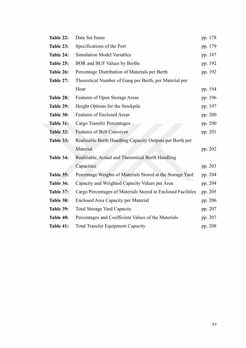
Table 22: Data Set Items pp. 178

Table 23: Specifications of the Port pp. 179

Table 24: Simulation Model Variables pp. 187

Table 25: BOR and BUF Values by Berths pp. 192

Table 26: Percentage Distribution of Materials per Berth pp. 192

Table 27: Theoretical Number of Gang per Berth, per Material per

Hour pp. 194

Table 28: Features of Open Storage Areas pp. 196

Table 29: Height Options for the Stockpile pp. 197

Table 30: Features of Enclosed Areas pp. 200

Table 31: Cargo Transfer Percentages pp. 200

Table 32: Features of Belt Conveyor pp. 201

Table 33: Realizable Berth Handling Capacity Outputs per Berth per

Material pp. 202

Table 34: Realizable, Actual and Theoretical Berth Handling

Capacities pp. 203

Table 35: Percentage Weights of Materials Stored at the Storage Yard pp. 204

Table 36: Capacity and Weighted Capacity Values per Area pp. 204

Table 37: Cargo Percentages of Materials Stored in Enclosed Facilities pp. 205

Table 38: Enclosed Area Capacity per Material pp. 206

Table 39: Total Storage Yard Capacity pp. 207

Table 40: Percentages and Coefficient Values of the Materials pp. 207

Table 41: Total Transfer Equipment Capacity pp. 208

xvi

LIST OF FIGURES

Figure 1: Research Process pp. 8

Figure 2: Iterative Phases of the Terminal Planning pp. 14

Figure 3: General View of Dry Bulk Terminal Layout pp. 21

Figure 4: Examples of Dry Bulk Terminal Pier and Wharf pp. 22

Figure 5: Different Types of Berth Layout pp. 23

Figure 6: Dome Closed Storage Examples pp. 29

Figure 7: Examples of Different Closed Areas pp. 29

Figure 8: Silo Structures at the Dry Bulk Terminals pp. 30

Figure 9: Dry Bulk Vessel Loaders pp. 33

Figure 10: Dry Bulk Grab Unloading Equipment pp. 34

Figure 11: Pneumatic Unloader pp. 36

Figure 12: Dry Bulk Cargo Vertical Handling Equipment pp. 36

Figure 13: Conveyor Systems pp. 38

Figure 14: Storage Yard Equipment pp. 39

Figure 15: Dry Bulk Terminal Process pp. 41

Figure 16: Relationship of Layout Planning and Capacity pp. 52

Figure 17: Different Stockpile Configurations pp. 59

Figure 18: Examples of Circular Storage System pp. 60

Figure 19: Stacking Methods pp. 60

Figure 20: Diversities of the Capacity Types pp. 69

Figure 21: View of an End Coned Trapezoid Stockpile from Top-Front-

Side pp. 87

Figure 22: Different Angle of Surcharge Values according to Material

Characteristics pp. 90

Figure 23: Schematic Representation of Cross-Sectional Area of the

Material loaded onto the 3 Idler Belt Conveyor Configuration pp. 91

Figure 24: Types of the Screw Conveyor and Pitches pp. 94

Figure 25: Schematic Illustration of the Difference between the Bench,

Block and Pilgrim Step Reclaiming Methods pp. 102

xvii

Figure 26: Schematic Representation of the Cross-Sectional Area

Variables pp. 103

Figure 27: Schematic Representation of Ship Turnaround Time pp. 111

Figure 28: Content Analysis Steps of Forman and Damschroder (2008) pp. 127

Figure 29: Analytic Steps of the Content Analysis pp. 128

Figure 30: Research Steps followed in Content Analysis pp. 130

Figure 31: Distribution of the Studies over Databases pp. 137

Figure 32: Distribution of the Categories of the Document over

Document Type pp. 138

Figure 33: The Distribution of the Focused Topics of the Study over

Databases pp. 139

Figure 34: The Distribution of the Focused Topic of the Studies over

Years pp. 140

Figure 35: The Distribution of the Focused Topic of the Study over

Types of Ports pp. 142

Figure 36: The Distribution of the Focused Themes over Focused Port

Section pp. 143

Figure 37: Hierarchy Chart of the Categories and Sub-Categories pp. 144

Figure 38: Similarity Analysis of the Nodes pp. 145

Figure 39: Conceptual Model of Berth Handling Capacity Calculation pp. 181

Figure 40: Conceptual Model of Storage Yard Capacity Calculation pp. 183

Figure 41: Conceptual Model of Transfer Equipment Capacity

Calculation pp. 185

Figure 42: Cargo Amounts per Months pp. 191

Figure 43: Frequency Distributions of Cargo Amount per Month within

the given Rages pp. 191

Figure 44: Open Storage Area Cargo Amounts per Mont pp. 195

Figure 45: Enclosed Storage Area Cargo Amounts per Mont pp. 199

Figure 46: Relation of Validation and Verification pp. 209

xviii

LIST OF APPENDICES

APPENDIX 1 Properties of Bulk Solid Materials app. 1

APPENDIX 2. Required Coefficients for Calculating 3 Equal Roll Idlers

Conveyor Belt Capacity app. 6

APPENDIX 3. Bulk Solid Materials Table app. 8

APPENDIX 4. RProject Codes for Simulation Model app. 24

1

INTRODUCTION

Ports are one of the critical infrastructure and strategical nodes in international

transportation by reason of linking other modes of transport. These infrastructures are

nodal interfaces where logistics, distribution, and trade activities performed (Bichou,

2013: 1). The increasing impact of the technological development on transport, cargo

handling, storage activities and the transhipping have transformed the ports into highly

specialized facilities for specific cargo types (Dundovic and Kovacic, 2007:247).

Although the ports serve with multipurpose facilities, the latest form of ports and

operation systems are highly designed to serve specific ship type or trade (Bichou,

2013: 135).

Ports have several functions. The primary functions of the ports can be listed

as follows (Frankel, 1985:3-4; Ligteringen, 2012: 45: Stopford, 2009: 29; Frankel,

1987: 7-9)

Loading and unloading of the cargoes

Giving service to vessels and cargoes (packaging, safeguarding,

consolidation, deconsolidation, classification of the cargoes, storage of

the cargoes, maintenance, etc.)

Packaging and safeguarding of the cargoes

Documentation and managing the information about cargo and vessels

Providing commercial and financial services

Supporting industrial activities

Interfeeder transferring

Direct transferring of the cargoes

The variety of these services can differ according to the port/terminal type.

Generally main terminal types can be listed as follows: (i) general cargo terminals: (ii)

multipurpose terminals, (iii) RO-RO terminals, (iv) container terminals, (v) liquid bulk

terminals; (vi) inland water transport terminals, (vii) cruise terminals, and (viii) dry

bulk terminals. The types of terminals are generally specialized according to the types

of cargoes handled (Ligteringen, 1999: 6-5). Within the context of the study and the

research objectives, it is focused on the dry bulk terminals.

2

A broad definition of dry bulk terminal is "A bulk port terminal is a zone of the

port where sea-freight docks on a berth and is stored in a buffer area called yard for

loading, unloading or transshipment of cargo.” (Robenek et al. 2012: 2). In addition

to the definition, dry bulk terminals can be evaluated as a single or multi-channel

system that comprises several sub-systems divided into functions according to the

availability of the resources (Hess et al. 2007: 61; Schott and Lodewijks, 2007:375).

Dry bulk terminals are different from the other types of terminals regarding the factors

such as location, draft, infrastructure type, terminal layout, storage facilities, terminal

equipment and additional services (UNCTAD, 1985b: 168). The characteristics of the

terminal also show difference because dry bulk cargoes can vary by the density of the

material (Bugaric et al. 2012:1508). Dry bulk terminals specialized in dry bulk cargoes

(Burns, 2015: 124). These types of cargoes generally assessed under the two main

categories as “major dry bulk cargoes” and “minor dry bulk cargoes” (UNCTAD,

1985b: 168). There is a more specific distinction for major dry bulk commodities. Five

major bulk commodities are iron ore, coal, grain, bauxite and alumina, phosphate rock.

The remaining dry bulk commodities such as steel, cement, fertilizer, forest products,

sulfur, scrap, etc. are classified as minor dry bulk commodities (RMT, 2014: 1; Frankel

et al. 1985: 3).

Dry bulk terminals need to be planned and be designed in line with the

requirements as well as other terminals types which are specialized on specific cargo

group. Macro and microenvironmental factors compel seaports to develop (UNCTAD,

1985b; Kleinheerenbrink, 2012:21). By the port planning, the balance between idle

and inadequate capacity can be achieved, and throughput capability of the terminal can

be controlled and be directed in line with the business interests (Frankel, 1987:11).

Planning and designing the terminals are multifaceted issues that planners

should be addressed. For this reason, the issue consists of various disciplines such as

coastal engineering, policy, statistics, traffic engineering, economics, etc. (Velsink,

1990:7). The terminal design includes seaside and landside interfaces as essential

components of the terminal. The seaside interface comprises berth infrastructures and

superstructures, channels, berth handling equipment, whereas the landside interface of

the terminal encompasses the storage yard area, storage yard equipment, gate and

hinterland connection links of the terminal (Ramirez-Naffarrate et al. 2016: 1; Roy et

3

al. 2016: 472). Even though the synchronization of these areas is quite difficult, it can

be achieved with an integrated approach (Wu, 2014:61; Ramirez-Naffarrate et al.

2016: 3). The essential factor in planning is capacity considerations (Malavasi, 2005:

471). The Capacity subject is an important indicator that the port can provide specific

services with a particular infrastructure (Dekker, 2005:3; Bichou, 2013: 51). The

layout design is highly associated with the capacity issue. Terminal planning and

design regarding sea and landside affect the capacity and the other related issues due

to equipment planning and other critical issues related to capacity. Planning and

designing of the terminals or ports to be performed in this context will enable the port

to achieve its ultimate aims in the capacity subject.

This study attempts to develop a new measurement model regardless of the

export or import dry bulk cargo terminal by integrating measurable factors that affect

the capacity stated in the literature and based on the capacity measurement equations.

Generic equations were simulated with real-world data of the dry bulk terminal. The

results obtained through the simulation were illustrated, and the simulation model was

verified.

Several processes were followed to reach this aim. The existing equations were

analysed through the literature review and content analysis, and the disregarded

parameters were identified. Empirical equations were attempted to develop by

considering measurable neglected parameters in the literature. While doing this, the

simulation model was generated by regarding different alternatives that the port might

implement, and the model was tested. The details of the study are evaluated under the

below titles.

a. Specifying the Research Questions and Aim of the Study

Capacity is one of the critical characteristics of transport infrastructures

(Bichou, 2013). Deciding on the port capacity, the balance between shortages and

over-capacity should be appropriately balanced (Dekker and Verhaeghe, 2006). Port

must provide adequate capacity to vessels with cargo handling infrastructure and

intermodal transport options (Gaur et al. 2011). In the event of a failure in proper

planning of port capacity, vessel congestion frequently occurs in the port area

4

(UNCTAD, 1985). In another case, the excess capacity may lead to inefficient port

investments.

According to Çağlar (2012:122), the importance of capacity planning can be

evaluated under four title;

Unnecessary investments will create idle capacity and it will not only create

disadvantages but also harms port tariff structure

Determining the right capacity requirements is the most critical parameter that

will show when the port infrastructure investments should start

Port capacity is a parameter used to determine efficiency and effectiveness

levels at ports to find capacity utilization rates, to improve the operational and

administrative process and to increase port profitability

Seaport capacity is an important issue in terms of port privatization. One of the

main aims of port privatization is to increase efficiency and effectiveness based

on the port capacity.

The research article of Esmer and Duru (2017), “Port Governance in Turkey:

The Age of Global Terminal Operators” emphasized on the changing structure of the

port industry and governance implementations in Turkey. In the study, researchers

discussed devolution processes and throughput increase of Turkish ports. The study

also pointed on the rise in throughput capacity of the national port. In addition to this

study, TÜRKLİM (2017) report on “Turkish Ports” drawn attention on the Turkish

port sector and the capacity developments of Turkish port. In line with these

researches, the research field specified as “port capacity”. Accordingly, research

questions can be stated as follows:

R.Q. 1. How is port capacity measured?

R.Q.2.Which methods/approaches have been conducted to measure the capacity of

ports in the extant literature?

R.Q.3.What are the critical issues addressed in capacity measurement in ports?

R.Q.4.What are the main factors affecting port capacity?

R.Q.5.What is the relationship between the measurable factors affecting the port

capacity? How do these factors affect the port capacity, and what is the direction of

this impact?

5

R.Q.6. What do different capacity output values mean and for which purpose do

different capacity outputs use?

When specifying the research aim, an initial literature review was conducted

on several databases. After examination of the studies on port capacity measurement

and factors affecting the port capacity, it was found that the researches on the capacity

measurement of ports are relatively limited. Moreover, as far as the author’s

knowledge, dry bulk terminals were addressed as an issue with a lesser extent of

scientific papers than that of the other terminal types.

After conducting an initial literature review, a meeting was held with two sector

representatives for 90 minutes. One of the participants works as a manager at the port,

and the other participator works at the port as a port operation chief. During the

meeting, factors affecting port capacity and equations utilized for measuring terminal

capacity, especially in dry bulk terminals, were argued. All the equations and related

parameters were explained to the participators placed in the equations. Sector

representatives drew attention on that specific bulk density, diversity of the equipment,

human factor, the capacity of equipment according to bulk material’s characteristics,

the efficiency of the operation processes of the port, and speed of the customs clearance

had not been regarded in capacity measuring equations. Depending on this situation,

they stated that the equipment, berth handling, and the storage yard capacity would

change.

As a result of specifying the research aim efforts and in accordance with the

research questions, the objective of the study is to explore the current methodology on

port capacity measurement and critical issues addressed in capacity measurement in

dry bulk terminals in accordance with the factors affecting terminal capacity. Besides,

this study attempts to explore and to explain the relationship between the primary

issues in port capacity measurement, the effects of these factors on port capacity and

direction of these effects. In addition to above-mentioned objectives, this study also

aims to find the means and intended use of different capacity output values. This study

aims to develop empirical capacity measurement equations for dry bulk terminals by

analysing the existing formulations systematically and to develop a capacity

6

measurement model for dry bulk terminals regarding berth handling, equipment, and

storage yard.

b. Research Design and Process of the Study

In this part of the “Introduction” section, it has been attempted to explain the

research design characteristics and research approaches and methods conducted in this

study.

The research design refers to the general idea behind the research and includes

a strategy of inquiry and method employed in the study (Creswell, 2014: 5). The

strategy for both designing and performing research depend on the nature of the study,

whether it is qualitative or quantitative (Neuman, 2014:165). According to Thomas

(2010:301), research mode is commonly classified as qualitative and quantitative,

although research methods are being classified in different perspectives. In addition to

that, Thomas (2010:301) stated that qualitative and quantitative concept could be

explained on two different levels. At the first level, qualitative and quantitative imply

the nature of the knowledge of how the world and the ultimate aim of the research are

interpreted. At the second level, qualitative and quantitative imply nature of the

research method as a way of data collection, analysis approach, interpreting the results

obtained through analysis approach. Also qualitative and quantitative research

methods, mixed research method was commonly referred in several studies (Sounders

et al., 2009: 137; Rolfe, 2013; Creswell, 2014: 4; Thomas, 2010:302). Mixed research

methods can be evaluated as an inquiry approach to the study. This concept brings

both qualitative and quantitative approaches together in the study (Creswell, 2014: 14).

In line with these approaches, this study adopts both qualitative and quantitative

methods together.

Strategies of inquiry refer to the type of three methods of design (qualitative,

quantitative and mixed methods) or pattern which provides a particular path for

procedures conducted in designing the researches (Creswell, 2014: 11). In this study,

research methodology was built on the literature review (by conducting content

analysis), and simulation.

7

The research design also performed according to exploratory, explanatory, and

descriptive research purposes (Altunışık et al. 2012:71). The objectives of this study

include three research purposes as well. This study aims to explore the current

methodology on port capacity measurement and critical issues addressed in capacity

measurement in dry bulk terminals in accordance with the factors affecting terminal

capacity and the explanation of the relationship between the primary issues in port

capacity measurement. Explanatory aim of this study constitutes the explanation of the

effects of these factors on port capacity and direction of these effects. Besides, it was

descriptively attempted to provide the means and intended use of different capacity

output values.

The qualitative part of this study was performed to investigate the critical

variables addressed in capacity measurement in ports, factors affecting the port

capacity, how port capacity is measured, which methods/approaches was conducted to

measure port capacity. A literature review was conducted on several databases to find

these answers. In addition to that, a content analysis was conducted to examine these

aims, as mentioned above.

The quantitative part of the study was performed to develop capacity

measurement equations for dry bulk terminals and simulate this equation through

RProject software. The simulation and its conceptual model explain the relationships

between the primary issues in port capacity measurement and how port capacity is

affected by the factors and the direction of these impacts on port capacity based on the

literature. It should be highlighted that the relationships between the parameters that

affect the port capacity, can be identified as causal and any change of in value of

parameters will change the whole functional operation of the equation (Bertrand and

Fransoo, 2002:249).

Means of different capacity output values and the intended purposes of its

outputs were attempted to describe through both simulation model and literature

review Iterative cycle of evaluation of was performed to explain the meanings of

capacity types and how these capacity types can be used in evaluating the port

capacity.

8

Considering the time interval, this study is classified as cross-sectional in terms

of collecting the information about port capacity and collecting the cross-sectional data

only for testing the empirical equations.

To answer the research questions and to reach the research aims, several

processes were followed. Main steps followed during the research is illustrated in

Figure 1.

Figure 1: Research Processes

Source: Compiled by Author

9

Research process started with the determination of the research field.

Determination of the research idea pursued this process. To determine the research

aim, this process was supported by the literature review. An initial literature review

process and specifying research aim processes were carried out simultaneously to

enlarge the research aims and to analyse the gap. Within this process, capacity

measurement equations were determined through the literature review, and these

equations were analysed thoroughly. Apart from finding the existing equations in the

literature, factors affecting the port capacity were analysed. By using these equations

and related parameters related to port capacity, empirical equations were developed

for berth handling capacity, storage yard capacity, and transfer equipment capacity.

When developing the equations, the iterative research effort was conducted to

determine certain functions of these parameters on the capacity and to eliminate the

faults. After completion of the equation development process, the research sample was

determined. While determining the research sample, it was paid attention to be a dry

bulk terminal with a certain throughput volume. Data were obtained as a result of a

series of meetings. The conceptual model design was formed according to the

simulation model requirements. After that, the input variables were listed to make sure

about all the parameters reflected in the simulation and conceptual model. Data

obtained from the terminal was not suitable for direct use in the simulation model. For

this reason, real-world data was made suitable for entering the simulation model by

organizing and managing. After obtaining the simulation outcomes, these results were

tested by operating the equations manually. In addition to that conceptual model and

simulation model were compared in terms of checking the compatibility and

verification was provided. After all these processes results were evaluated in terms of

examining the applicability of the model.

c. Originality of the Study

When the literature review was conducted, the relatively limited study was

obtained. Generally, studies on port capacity progressed based on performance,

capacity planning, and forecasting and market analysis. Studies mostly employed the

optimization techniques to model the capacity of the port and mostly focused on the

10

container terminals. It was found out that performance, capacity planning, cost, and

economic analysis researches fed themselves.

With this literature review, it was focused on the reports, books, and

dissertation to investigate the capacity measurement approaches. Generally, UNCTAD

reports and other reports published by UNCTAD (Thomas, 1985; de Monie, 1987;

Haeidi, 2014) focused on capacity measurement and capacity planning of the several

terminal types by considering performance issues of the terminal. The studies focused

only on the capacity calculation, and equation development for ports were commonly

performed for container terminal in the literature. UDHB (2015b:231), Park et al.

(2014: 185), National Research Council (1998: 81) and KMI (1998) provided berth

handling capacity measurement equations based on the several assumptions. These

assumptions were not explicitly explained by the researches and meaning of

parameters reflected capacity measurement equations were not explained in detail.

Also, these equations did not provide a piece of significant information about the

calculation of equipment capacity. Nearly all these equations reflected the number of

gang and gang per ton, but this implicit approach did not provide detailed information.

Scholars generally used design approaches for storage yard, and the required

terminal area was considered commonly. When existing equations were examined, it

was seen that the National Research Council, (1998: 81) Salminen (2013:32-33) and

UDHB (2015b: 231) did not consider the stockpile implementations. Besides, the peak

factor of storage yard and sousplan shipments were not reflected in the current

equations. Even though the annual throughput is included in the measurement formula,

each shipment may not be transferred to the storage yard area. This circumstance

impedes estimation of the storage yard capacity when demand fluctuates. Moreover,

joint evaluation of the peak factor for both berth and storage yard capacity may result

in overinvestments. Studies also did not make a clear distinction about sousplan

shipments. Only National Research Council (1998:81) considered the cargoes handled

at the storage yard.

Apart from developing capacity measurement equations, this study introduces

theoretical gang number and realizable capacity. Finding the number of the gang is

difficult when certain service time is unknown. If ports record the number of gang

performed in an hour, that value can be used. Otherwise, the catalog values can be

11

used. That is why researches did not point on this issue. Oral (2014) mentioned the

gang number, grab filling rate, weight of grab, lifting capacity of the grab equipment.

However, grab filling rate was based on several assumptions (Oral, 2014). A concept

used for determining the number of gang under the normal operational conditions

considering material characteristics was introduced called as theoretical number of

gang. Theoretical gang number is different from the actual gang number. Hold

structure, picking and dropping height of the cargo, material nature, crane operator

skill affect the hourly gang capacity of the grab cranes directly. In typical operation

conditions, grab crane performs more gang in an hour. However, grab filling rate is

not constant during the operation. Grab filling differs in different height of the hold

and differs according to material density. Grab crane can perform more gang than the

gang theoretically can perform. For this reason, theoretical number of gang is always

lower than the actual number of gang.

When evaluating the definitions of capacity types in the literature, it can be

made a clear distinction between the capacity types. Theoretical capacity takes into

account the amount of cargo that the port can perform 365 days and 24 hours. Besides,

actual capacity considers the usual traffic conditions of the port. Accordingly, actual

capacity calculations take into account the berth occupancy levels while theoretical

capacity accepts the berth(s) as fully utilized. However, there is no capacity type

explains the circumstance that the port can reach under the real conditions and the port

does not suffer from the low demand as far as it is known. This situation leads to an

uncertainty about evaluating the capacity of the port and creates a gap in the literature

to measure the port capacity.

Realizable capacity explains the possible output levels where the terminal is

independent of actual demand conditions and the capacity output that can be realized

by its resources as if the ships always called to the port. This gap also brings other

questions such as the function of berth occupancy ratio. Accordingly, the function of

berth occupancy ratio needs to be discussed thoroughly in the light of the literature on

berth occupancy to find its intended function.

Apart from the reasons mentioned above, the majority of the researches divided

the ports according to their import and export activities or focused on the port handled

single material. In this study, it was attempted to develop a capacity measurement

12

model for dry bulk terminals served to multiple cargoes and without discrimination,

whether export or import activities.

d. Structure of the Study

This study structured in four chapters. Chapter I provides a snapshot of dry

bulk terminals. This chapter summarizes the dry bulk terminal designing and planning

concepts, physical characteristics of the dry bulk terminals, terminal layout and its

components (equipment, berth, storage yard, and gate), terminal operations performed

in the terminal and cargo flow processes.

Chapter II explains the scope and concept of the port capacity. In this chapter,

port capacity is defined from the different viewpoints. Subsections explain the capacity

concept of each terminal component. Factors affecting the port capacity are illustrated,

and several capacity types are explained in this chapter.

Chapter III reviews the existing capacity measurement equations of port for

only dry bulk terminals. These equations sectioned as berth handling, storage yard

handling, and transfer equipment capacity measurement equations. Relatively limited

equations are analysed in detail.

Chapter IV comprises the research methodology. This chapter provides the

literature review, content analysis, equation development approaches, and developing

simulation model efforts.

Conclusions, recommendations, and appendices are provided in the related

section.

13

CHAPTER ONE

DRY BULK TERMINALS: AN INTRODUCTION TO TERMINAL SYSTEM

1.1.A SHORT VIEW OF PLANNING AND DESIGN CONCEPTS OF THE DRY

BULK TERMINALS

Development in maritime trade, equipment and information technologies have

been resulted in continuous development of the ports. Moreover, increasing in

maritime demand pushes ports to develop their infrastructure and superstructure

(UNCTAD, 1985b: 27). With the development of commercial activities, cargo

technology and the port users’ requirements push the ports to modernize (Frankel,

1987: 11). The need of changing forces the ports to develop its terminal and the

connection links (Kleinheerenbrink, 2012:21).

Port development means that constructing new ports or expansion of the

current port facilities or sites (Tsinker, 2004:7.). Kleinheerenbrink, 2012:21)

summarized the characteristics of the terminal development:

New terminal requirement

Expanding the present terminal infrastructure

Enhancing the existing terminal activities

o Equipping the terminal with highly specialized, automated, flexible,

and sufficient equipment

o Increasing the performance outputs of the facilities

More awareness of the environmental impacts

Accelerating the service level by developing infrastructures of connection

links (infrastructure)

In conjunction with the development trends in port, port planning has gained

importance. The primary goal of the port planning is to provide balance between

inadequacy and excess capacity at reasonable cost, price and service levels. It is about

the finding the balance between the economic, business factor and the constraints

caused by the land availability, spatial planning factors, sustainability issues, and

political factors (Bichou, 2013: 51). With the port planning, the capabilities of the port

can be further controlled and capitalized on business interests (Frankel, 1987: 11).

14

Once planning the layout of the terminal, the subject should be assessed as

multi-faceted (Wiese et al. 2013: 222). Port planning task requires the combination of

different disciplines and evaluation from a broad perspective. For this reason, port

planning is assessed an interdisciplinary activity that includes several topics associated

with the investment, operation, design, capacity, and policy (Bichou, 2013: 51).

Associated disciplines are oceanography, coastal engineering, hydraulics, traffic

engineering, transport engineering, civil engineering, maritime engineering, geology,

seismology, geo-technology, hydro-nautics, economics, econometrics, management

and organization, sociology, biology, ecology (Velsink, 1994: 7).

Port planning includes several steps processes. The iterative process spiral of

the port development are illustrated in Figure 2.

Figure 2: Iterative Phases of the Terminal Planning

Source: Frankel et al., 1985:191

Scroll wheel represents the iterative planning processes of the ports based on

the major tasks. The conceptual level aims to improve a feasible solution spectrum by

developing alternatives as much as possible. Rather than qualitative analysis, options

are evaluated quantitatively. In this stage, a comprehensive evaluation must be

15

performed for dry bulk terminals. The density of the cargoes, equipment

characteristics, and special requirements for the storage according to material

characteristics must be criticized. Because, each cargo type necessitates different

equipment and handling procedures (Keceli, 2016:3). A rough estimation of the sites,

equipment, cost, and revenue are performed during the preliminary design level. The

quantitative evaluations superseded qualitative assessments. These evaluations

generally include eliminating the alternatives by calculating the costs and benefits per

options. The contract design level of planning aims to determine the boundaries of

exact planning specifications and information on the evaluation of bidding contract,

which will include cost, and construction planning (Frankel, et al., 1985: 191-195).

Different substantial assignments guide the terminal planning. These

assignments are (Frankel, 1987: 21)

Economic foundations for port development

o Analysis of economic and commercial activities

o Analysis of commodity flow

Transport System (Seaway, rail and road transport)

Changes in freight pattern

o Evaluation of the physical form of commodities and it flows

Technological changes in land transport and change in shipping

phenomena

o Analysis of the trends in both vessel, shipping, equipment, and cost

issues.

Logistical aspects (cargo handling transfer and storage of the cargoes,

documentation, etc.)

Technologies of logistic activities

o Assessment of existing methods

o Evaluation of finance, marketing, and brokerage activities

Facility inventories at the terminal and operation analysis

o Assessment of port inventories (infrastructure, superstructures)

o Operating and maintenance methods

o Capacity and productivity evaluation

Review of the existing facilities and forthcoming requirements

16

o Evaluation of current inventories and short-term development plan

Engineering Studies

o Hydrographical, geophysical, topographical navigational assessment of

the port sites

Specifying the alternatives for port development

o Deciding on new establishment or developing the existing port sites,

and facilities

o Evaluation of alternative development paths based on the cost and

benefit analysis

Financial Studies

o Analysis of expenditures and revenues of port operations

o Deciding on port tariffs

o Evaluation of the cash-flows, and competitive analysis

Analysis of the environment

o Assessment of the impact of these structures on the environment and

community.

o Evaluation of the physical, environmental and human resources

Planning of the ports are structured in three main periods (Velsink, 1994: 4-2)

stated in Table 1:

Table 1: Planning Periods of the Ports

Type Period (Years) Examples of the Implementation

Short Term Planning 1-2 Minor changes in layout

Medium Term Planning 5-10 The first stage of the master plan

Long-Term Planning 20-30 Master plan

Source: Velsink, 1990: 4-2

Tsinker (2004:10) and Velsink (1994:5) stated the factors that should be

considered both in long-term and medium-term planning as follows:

17

Long-term planning factors:

Determination of the functions of ports (foreign trade oriented; supporting

the industrial and mercantile development; appealing the transshipment

activities)

Determination of the responsibilities of the port in the construction of

facilities and operations.

Forecasting the land usage and future expansion plan to satisfy the master

plan’s needs.

Estimating the cargo flows, alternative sites

Optimizing all sublevels of the planning performed by several disciplines

that included in the port planning

Medium-term planning factors:

Analysis of the performance and capacity

Operational and physical design of the port in the limits of budget

Financial analysis

Deciding on the investments

Comprehensive design

Due to its capital-intensive nature, the planner should pay attention to the

financial and economic practicability of the investments considering long process of

return on investment, and payback periods. In the previous years, the master plans had

a function of land use plan that was centrally controlled and primarily linked to the

growth strategies and financing of the state. However, nowadays the role of the master

plan have changed as business cases (Taneja, et al. 2011: 6-7). Masterplans can be

assessed as the blueprint for the future development of the port. The primary objective

of a master plan is to make space reservation for the feature requirements by

considering the environmental and legal issues, to establish sustainable port

operations. In comparison with the past, national and regional port masterplans aimed

to generate optimum allotments of the outputs throughout the country or the region,

new function of the port master plan considers the port capacity, interface of port-

hinterland link, industrial progress and the cost of the port infrastructure (Ligteringen,

1999: 4-2).

18

Dry bulk terminals have three essential components in terms of designing the

terminal. These are berth and quay, storage yard, equipment and gate

(Kleinheerenbrink et al. 2012: 107). Within this context, the following sections are

designed considering berth, storage yard, equipment, and gate.

1.2.PHYSICAL CHARACTERISTICS OF THE DRY BULK TERMINALS

Choosing the most suitable port layout and form is a strategic and long-run

decision that should be decided at the initial stages of the planning (Bichou, 2013:

315). The terminal layout should be planned considering the transfer points to facilitate

all transportation needs (van Vianen et al.,2015:1). All system should be designed and

planned to achieve the connection between the whole sea and land transport chain and,

be planned to adopt the changing demand and supply patterns (Schott and Lodewijks,

2007:376-378).

Several layout combinations can be implemented in the dry bulk terminal.

Terminal requirements generally determine the layout of the terminal. In general, the

needs of the dry bulk terminal are the adequate size of the area, handling equipment,

infrastructure, and storage area (Dundovic and Kovacic, 2007:252). Regarding the

requirements, terminal design is highly depend on the equipment type, stockyard

management, routing, maintenance options, ambient, commodity type, size of the

vessel, regional cargo characteristics, and options of expansions, (UNCTAD, 1985a:

15-16; UNCTAD, 1985b: 168; Schott and Lodewijks, 2007:378; Agerschou, et al.

2004: 315). The factors affecting the terminal layout and the form of the facilities can

be summarized as follows (Bichou, 2013: 135).

General specifications of the vessels, i.e. draft, length, gears, superstructure,

beam, ship size, derrick

Type of cargo traffic, i.e. general cargo, container, breakbulk, bulk, passenger,

transshipment, export, import, direct call

Environmental characteristics of the region considering the topographic,

oceanographic, climatic factors and engineering factors such as dredging,

construction

19

Type of cargo, i.e. hazardous, refrigerated, standard; type of packaging, i.e.

full-load, less load, palletized, containerized

Area, cost and capacity restrictions

Operational considerations, i.e. labor and equipment

Locational settlement and form of the freight site planned to establish within

or outside of the port or terminal.

All of these factors also interact with each other. For example, the size of the

vessels called to port determines the characteristics of the terminal in terms of

infrastructure and superstructure. The port should provide adequate services to vessels

with suitable berths, draft, equipment, infrastructure, and superstructure. In case of

failing to provide proper services to vessels, the ports may need to install new offshore

equipment, storage facilities, and suitable berths (UNCTAD, 1985a: 15-16; UNCTAD,

1985b: 168).

The effect of the cargo type on the terminal layout shows similar characteristics

as the effect of the ship sizes on the terminal design. Rather than a single cargo type,

the port may prefer to provide services to multiple cargoes. In such cases, the terminal

must be planned flexibly to serve various cargoes types (Dundovic and Kovacic,

2007:255). Different cargo types may require specialized equipment and storage type

(UNCTAD, 1985a: 15-16; UNCTAD, 1985b: 168)

Apart from the physical infrastructure characteristics, the terminals diversify

according to export, and import specialization and design of these terminals may differ

according to these tendencies (Wu, 2014; 61). Dry bulk terminals are divided into two

categories according to their export and import activities. Export and import terminals

have specific layout due to provide export and import cargo flow. For the coal, ore and

the other minerals, export terminals are generally located at the appropriate site that is

close to the resources in general (Agerschou, et al., 2004: 315) Wu, 2014:61). These

terminals targets accelerating the outflow of the cargoes (Wu, 2014:61). Even a

terminal is not located near to the resources; it should be well linked to the resources

via rail and road.

The export dry bulk terminal needs to direct connection with the loading

equipment and ship to support the continuous loading with tolerating the movement of

the vessel. In case of using single spout systems, the length of berth should be longer.

20

Because the vessel requires moving along the berth (Agerschou, et al., 2004: 315). In

some cases, export terminal may stocks the commodities by considering the prices. In

some other, due to the ownership and locational factors, export terminals focus on the

limited cargo type (Wu, 2014:61).

The situation at the import terminals is not different from the export terminals.

All equipment should be linked with the vessels. Thus, for the import terminals, it is

entailed the smooth conditions comparing with the export terminals. It is difficult to

keep a suitable position between the unloading equipment and the pile in the vessel

hold due to the pitch and heave motions. Handling equipment used in export dry bulk

terminals is pneumatic equipment, crane-mounted grabs, bucket wheels, screw

conveyor and chain buckets (Agerschou, et al., 2004: 317).

1.2.1. Dry Bulk Terminal Layout

Ports are comprised of two main interfaces that are seaside and landside. The

phase of loading/unloading and the temporary storage of cargoes at the storage yard

encompasses seaside interface in which quayside resources (equipment etc.) of the

terminal are used whereas landside interface includes the activities of the receiving

and the sending the cargoes by rail and trucks (Ramirez-Naffarrate et al. 2016: 1; Roy

et al. 2016: 472). Despite the difficulty at synchronization of the these activities,

seaside and the landside activities should be interconnected in an integrative approach

(Wu, 2014:61; Ramirez-Naffarrate et al. 2016: 3).

According to Hemert (1984: 45) terminal settlement is crucial for the planning

considerations and its shape and size are restricted by the physical natural domain. The

import and export activities of the terminal affect the terminal layout significantly.

Because the storage needs of the cargoes have an impact on the terminal settlement.

General dry bulk terminal layout is shown in Figure 3.

21

Figure 3: General View of Dry Bulk Terminal Layout

Source: Port Technology (22.08.2012)

Layout planning process includes the seaside and landside layout planning

(Wiese et al. 2013: 226). The main layout components of a dry bulk terminal are berth,

storage yard, and gate. Following sections provide detailed information.

1.2.1.1.Berth Planning as a Component of Dry Bulk Terminal Layout

A berth is a designated area at the quayside of the terminal where the vessels

can moor for handling activities. Berths can be categorized according to the cargo and

ship type (tanker berth, general cargo berth, dry bulk berth, etc.), size and layout (deep-

water berth, etc.) (Burns, 2015:120). A berth is one of the primary facility where the

vessels berthed (Lun et al. 2010: 183). These facilities should be adequate to establish

the related equipment to serve for loading and discharging the cargoes (Lu et al.

2010:183-184). Characteristics of the berth facilities at the ports depends on the several

factors such as size and number of the vessels, cargo types and volume, basin for

maneuvering, acceptable service time, need of the bow thruster or bow rudder for the

berthing, and prevailing weather conditions (winds, wave etc.) (Stopford, 2009: 30;

Thoresen, 2003:84; Vivek and Prasad, 2016:46; Burns, 2015:20).

Berth structures are called with different terms according to its construction as

pier, and wharf or quay (UDHB, 2010: 4; Vivek and Durga Prasad, 2016:46). Pier is

22

the berthing places projecting to sea from shore (whether perpendicular or specified

angle) that is built on concrete, steel, wood and stone props or as a floating platform.

Wharf or quay is the berthing places structured parallel to the shoreline. These

structures may be positioned adjacent to or near to the shore (UDHB, 2010: 4; Vivek

and Prasad, 2016:46). Figure 4 illustrates the schematic representation of the typical

pier and quay.

Figure 4: Examples of Dry Bulk Terminal Pier and Wharf

Source: Port Gdansk, 28.08.2019 (left); Sea-Invest, 28.08.2019 (right)

Apron as a part of the seaside layout encompasses the area between the quay

wall and the transit sheds or open storage area. Besides, the apron may be seen as a

combination of rail, road and the spaces interrupted by the equipment based on its

functions in the previous years (Agerschou et. Al., 2004: 265). The layout of the

seaside positioned between the storage yard area, and the quay wall should be designed

with the aim of achieving high performance. Design outputs should be planned to

perform operation more efficiently. Besides equipment constraints and features should

be considered (Wiese et al. 2013; 222).

Several berth layout can be seen in real world. According to Bierwirth and

Meisel (2015: 676) classified the berth layout according to spatial characteristics: The

discrete layout, the continuous layout, and the hybrid layout. The discrete berth layout

refers to the division of the quay into a smaller berth. Each berth can provide services

to only a vessel at a given time. Besides, in continuous berth layout, vessels can berth

to quay in the free position. Hybrid berth layout has the characteristics of both

continuous and discrete layouts. Quay is divided into the smaller berths. However, the

23

vessel may berth the divided piece of a berth, or more than one ship may berth at the

same piece owing to vessel size. Draft restricts the possible berthing position and

dividing the berths (Bierwirth and Meisel, 2015:676; Umang et al. 2011: 12; Al-

hammadi and Diabat, 2015:269; Umang et al. 2013: 14-15).

Figure 5: Different Types of Berth Layout

Source: Umang et al. 2013:15

As stated in Figure 5, positions of the vessels in the three berth layout shows the

difference. While only one vessel can berth at allocated areas in discrete berth layout,

there is not any classification in continuous berth layout. In hybrid berth areas, more

than one vessel can berth or one vessel interrupt two discrete berth areas.

All berth planning activities aim to achieve operational efficiency, to increase

the volume capacity by decreasing the service time, and to satisfy the requirements of

the industry (Burns, 2015:125). For this reason, optimum handling choices should be

made during the berth planning (Noritake and Kimura 1983:323). The planning system

should provide flexible operations to overcome the tentative schedule of the vessel

arrival and departure (Lun et al. 2010: 187).

There are several challenges in planning the berths. In case of the vessel arrive

in port regularly, and loading and discharging times are constant, planning the berth

24

capacity would be simple. Thus, the full utilization of the berth would be provided by

the port without the queue of the vessels. However, the actual conditions of the vessels

are depended on the randomness, so planning the berth capacity is a complicated

matter. The randomness of the ship arrival and ship service time affect the waiting

time of the vessels and the vessel arrival rate. These two factors are critical for the

determination of berth occupancy rate, which used in berth capacity planning

(UNCTAD, 1985: 28).

One another important factor when planning the capacity of the berths is quay

length factor. This factor is used when new construction and expanding the existing

port. Quay length factor is the ratio of the annual throughput to the quay length (van

Vianen et al. 2011:4). The factor shows the amount of cargo (ton) per meter by

eliminating the effects of the difference in bulk densities. This factor provides an

opinion about the berth capacity. The parameter is mainly used for determining the

spatial requirements at the berth. Table 2 illustrates the quay length factors values.

Table 2: Proposed Quay-Length Factors for the Dry Bulk Terminals

Reference Coal (kt/m) Iron Ore (kt/m)

Ligteringen, 2000 25-75 50-150

Import Terminal Export Terminal

Coal Iron Ore Coal Iron-Ore

van Vianen, 2011: 4 10-30 25-75 50-150

Source: Compiled in accordance with the information provided by Vianen et al. 2011:4

1.2.1.2.Storage Yard Planning as a Component of Dry Bulk Terminal Layout

Storage yard planning encompasses the management of area configuration,

determination of export/import and transshipment requirements activities.

Additionally, cargo transfer planning, stowing, allocation of the spaces and equipment

and labor to the area where the operations are performed (Bichou, 2013: 73).

The dimensioning and design of the storage yards are essential in the planning

of the terminal. What makes it so important is the cost and efficiency subjects.

Undersized storage yard leads to an increase in the waiting time of the vessel, and it

means the cost for the terminal operators. Besides, the return of investment takes time,

25

and the terminal operators have to bear the high investments cost (van Vianen et al.

2012:1).

The requirements of a flexible storage area and the stock control are presented

below (van Vianen et al. 2012:1).

Simultaneous unloading and loading operations possibility from ship to train

or truck

Discharged cargoes from the ship are transported by wagons.

The terminal should be able to separate different cargo types and stack the

cargoes separately.

The terminal must have road access for the inspection

All related equipment must be convenient for handling the several types of dry

bulk cargoes.

Before introducing the main structures in the storage yard area, it is necessary

to determine the storage yard requirements to construct appropriate structures and to

effective design of the terminal storage yard area.

Port planners consider the required storage yard area in the stage of port

construction or expansion to determine the terminal capacity. Required storage space

in the terminal area differs due to the type and, stacking characteristics of the cargo.

Regarding the capacity factor of the storage area, it is crucial to plan the allowable

spaces for the predominant cargoes demanded by the terminal to provide flexibility in

case of trade changes. This circumstance raises the challenges for the ports in terms of

land surplus (UNCTAD, 1983: 4).

Once the evaluating of the required space in the terminal area, stacking factor

should be established in the first step. Stacking factor of the cargo is contingent on the

below-mentioned factors (UNCTAD, 1983:5):

Bulk/weight rate or stowage factor of cargo

The bearing strength of the area subjected to storage

The height of the stack not excepting the angles of repose or resistance of the

packing case or storage case or height and diameter of the tanks

Characteristics of the equipment used at the storage area for the cargo transfer

between the berth and the area and the width of the lanes and the turning circle.

26

Required space for the classification of cargoes before performing the stacking

and handling breakages.

Required space for land transport loading/unloading operations

Safety distance between the stocking piles, and pollution prevention measures.

Analysing the above-mentioned factors and practicing it with the real conditions

provides stacking factor with regard to weight/volume per area utilized for the

calculation of required spaces for any specific cargo (UNCTAD, 1983: 5).

There are number of capacity indicators used in determining the required storage

yard area and these factors used in the planning of the below mentioned structures.

These indicators are storage factor, total terminal factor, storage yard length-width

ratio, lane length-width ratio.

Storage factor is assessed as the ratio of the annual throughput of the terminal

and the specified area used for the storage (van Vianen et al. 2011: 4). This rule of

thumbs method provides insights about capacity requirements in terminal area. In the

literature, generalization has been performed for the coal and iron ore terminals. Table

3 indicates the storage factor values of import and export cargo terminals.

Table 3: Proposed Storage Factor Values for the Terminals

Reference Import Cargo Terminal

(t/m2)

Export Cargo Terminal

(t/m2)

Coal Iron Ore Coal Iron Ore

Ligteringen, 2000 15-75 45-80 60-180 70-210

van Vianen et al. 2011:6 15-25 30-40 15-20 30-40

Source: van Vianen, 2011: 6

Total terminal factor is the ratio of gross storage area to total terminal area.

Gross storage area encompasses the stockpiles and the internal infrastructure

constructed in the terminal area. Total terminal area involve the both landside and

water side areas (apron, buildings, quay, etc.) (Kox, 2017:92). This factor is used in

the determination of the required terminal area. The ranges of the total terminal factor

are indicated in Table 4:

27

Table 4: Total Terminal Factor Values

Indicator Import Export

Total Terminal Factor 1-3 1-5

Source: Kleinheerenbrink, 2016:46

The range of the total terminal factor differs according to terminal type. Total

terminal factor is between 1 and 3 in import terminals while this value is between 1

and 5 in export terminals.

Storage yard length-width ratio and lane length-width ratio provides useful

insights into design process of dry bulk terminal. The values of the storage yard length-

width ratio and the lane length and width are illustrated in Table 5.

Table 5: Ranges of the Storage Yard Length-Width Ratio and Lane Length-Width

Indicator Import Export

Storage Yard Length-Width Ratio 1.2 - 4.6 1.3 - 4.5

Length of Lanes (m) 300-1200 300-1300

Width of Lanes (m) 30-75 30-85

Source: Kleinheerenbrink, 2012:45

It can be deduced form the ratios that the design issues is differentiated from

export to import terminals. The minimum and the maximum values covers a wider

range, comparing to import terminals.

Storage yards can be classified according to both storage conditions and storage

shapes. Storage conditions are associated with the storage of cargoes in open, closed-

enclosed areas and silo shed or dome. In the classification of the storage yard according

to storage shapes is assessed into two categories: Longitudinal and circular storage

yards.

Installing the open storage areas are relatively inexpensive comparing to closed

facilities. Open storage areas do not need to establish the buildings to storing the

cargoes. However, taking additional measurements to prevent environmental pollution

and preventing cargo contamination may necessitate the additional investment (Schott

and Lodewijks, 2007: 377).

28

Open storage areas are used in the dry bulk terminals frequently. Generally,

cargoes that are least affected by the weather conditions are stored in these areas. In

the open areas, cargoes can be stacked in the long lanes. Lanes are separated by the

equipment used by the stacking the cargoes (Ligteringen, 1999: 6-9). Bulk storage is

fulfilled by the stockpiles in the open storage area. The stockpile must be planned to

store maximum amount of material in the minimum area to obtain maximum

utilization of the storage area. The presence of adequate land for the storage is

restricted by the natural conditions and cost of acquisition. For this reason, the storage

method should be well planned in terms of the maximum gaining utilization of the area

(UNCTAD, 1985b: 180).

Long lanes and longitudinal stockpiles are implemented at the longitudinal

storage yards. Besides, circular storage yards practices the circular stockpiles. Two

storage yard types have pros and cons. According to Wolpers (24.02.2019) advantages

and the disadvantages of the longitudinal and circular storage system are:

The circular storage system has lower investment costs

Storage volume in circular systems is higher than the longitudinal system

The circular system requires shorter belt conveyor

In case of there are enough spaces the layout design can be performed more

flexible

Longitudinal storage yards are agile to demand fluctuations comparing the

circular systems.

Closed storage implementation is less flexible, and it limits the capacity

comparing to the open area implementations in terms of storage and handling (Schott

and Lodewijks, 2007:377). However, materials can be affected by weather conditions,

and it needs unique storage. Protection-required commodities may be stored in the silo,

shed, and bin. Moreover, low-density commodities need to be stored in closed areas

for not to blow away (Frankel et al., 1985: 151).

Portal-framed (shed or horizontal storage) structures and domes are the primary

types of closed storage. Materials are filled in these structures by a belt conveyor

system positioned at the top of the structures while reclaimer equipment, bulldozers,

and conveyors positioned on the ground performs the reclaiming of the materials (Kox,

2017:53; UNCTAD, 1985b: 181). Circular stackers, reclaimers, and bulldozers are

29

utilized in dome structures. Domes can be filled by using conveyor belts positioned at

the top. Figure 6 illustrates the covered storage yard structures.

Figure 6: Dome Closed Storage Examples

Source: Green Port (24.02.2019) (left); CST (24.02.2019) (right)

In addition to the storage by type of cargo, increasing interest in preventing

environmental pollution has also led to the storage of materials in closed storage areas.

Another form of the closed storage area is illustrated in Figure 7.

Figure 7: Examples of Different Closed Areas

Source: EBS, 25.02.2019 (left); Dome Corp, 25.02.2019 (right and bottom)

30

Silos are cylindrical structures established in the dry bulk terminals. The

conveyors or bucket elevators feed silo from the top of the structure. Reclaiming is

performed by gravity feed tunnel from the base. By the gravity feed system, live

storage is increased. Silo height determines the cargo amount that can be accessed in

the gravity feed system namely the size of the silo. Cost of the silo installation depends

on the size and the commodity characteristics (specific bulk density) to be stored in

the silo (Frankel et al., 1985: 165-168). Figure 8 illustrates the silo structures.

Figure 8: Silo Structures at the Dry Bulk Terminals

Source: Port Consultants Rotterdam, 25.02.2019 (left); Jurong Port, (25.02.2015) (right);

Copenhagen Merchants Group, (25.02.2019) (bottom)

Single or multiple silos can be established at the terminal. These structures are

commonly utilized for storing the cereals and fodders. In these structures, protection

measurements must be taken to prevent moisten of the commodities. Materials used

for construction must be carefully selected so that the commodities are not corroded

and not to be affected the cereals quality negatively (UNCTAD, 1985b, 181).

31

1.2.1.3.Gate Planning as a Component of Dry Bulk Terminal Layout

Gate planning encompasses the planning of lanes for the vehicles/trucks, sizing

of waiting areas and parking areas, synchronizing the traffic between berth-yard-gate

and the arranging the required gate components. In gate planning, locations where

trucks loaded or unloaded, must be determined by the requirements of the terminal and

equipment (Böse: 2015: 17). Port gate planning requires the forecasting of the gate

throughout such as a number of road vehicles pass through the gate in a specific period

(Keceli, 2016: 2). Port planners make an effort to decrease horizontal transport by

utilizing the yard equipment to loading or unloading the trucks to minimize the

operating costs in practice. This process also encompasses the railway station design

in case the railway network (Böse: 2015: 17).

Working principle of gate planning is similar to berth planning. However, it

focuses on the bookings of the inland vehicle, delivery, and receipt of the landside

vehicles. In addition to planning rail and truck entry/exit, planning comprises the

activities of storage yard-warehouse consignments, the configuration of the cargoes.

The challenges faced in the gate planning are cut-off policies, delaying of arrivals,

problems created by the documentation or clearance, and direct or indirect transfer

options. Lack of proper gate planning leads to disruptions in inspections, queues, and

congestion on the ports on both the roads and the port interface between the berth,

storage yard, and gate, and between the port and hinterland connection link. For this

reason, it is critical to plan the entrance and exit channels to provide better and efficient

operations (Bichou, 2013:78).

1.2.1.4.Equipment Planning as a Component of Dry Bulk Terminal Layout

Handling equipment used at the dry bulk terminals is examined under the three

categories as loading/unloading, horizontal transport equipment and storage yard

equipment. Below sections provides the detailed information about the equipment used

at the dry bulk terminals.

32

Vessel Loading Equipment

Comparing the discharging systems, vessel-loading systems are simpler. These

systems require feed elevators or conveyor systems, loading chute. Many vessel

loading system can easily perform the loading activity by using the gravity. Rest of the

vessels loaders may equipped with the flight conveyors or helical chutes to avoid the

material deterioration or may designed in accordance with the chutes or centrifugal

slingers belts (UNCTAD, 1985b: 170).

Loading the vessel at the dry bulk terminal generally performed by using

continuous loaders which fed by a belt system (Kleinheerenbrink, 2012:33).

Continuous ship unloaders is designed to discharge the dry bulk materials by providing

continuous flow. Generally, these equipment are evaluated under the four category.

The details of the equipment are provided as follows:

Travelling Loaders: These type of loaders can move along a line, which is

parallel to quay. Movable conveyors usually feed the travelling loader boom

(UNCTAD, 1985b: 170; Kox, 2017: 49). The boom is designed either dynamically to

fit the vessel or statically (UNCTAD, 1985b: 170).

Radial Loaders (Quadrant): Radial loaders include boom, which can perform

slewing motion approximately 90 degrees of angle. Commodities are loaded through

arm conveyor located at the end of the rotated boom (UNCTAD, 1985b: 171). This

equipment equipped with a telescopic boom and bridge assisted by the pivot point.

Radial or quadrant loaders can move circularly along the radial track through the tool

fitted at the front (Kox, 2017: 49; Thyssenkrupp, 10.03.2019; 8).

Slewing Bridge Loaders: Comparing to travelling loaders, installation costs

of slewing bridge-loaders are cheaper. In addition, installing dust control system and

enclosing the conveyor belts are simple (UNCTAD, 1985b: 172).

Linear Loaders: This equipment travels linearly parallel to the vessel.

(UNCTAD, 1985b: 172). A pivot point provides rotating motion. Boom of the linear

loader has a shuttle motion, which provides forward and retraction moving. It can also

move longitudinally to reach the entire warehouse of the ship on pivot point

(Campbell, 2007:35; Ligteringen and Velsink, 2012: 213).

Figure 9 illustrates the different types of vessel loaders

33

Figure 9: Dry Bulk Vessel Loaders

Source: Genmacrane, 10.03.2019 (Travelling Loader (top-left)); Thyssenkrupp, 10.03.2019

(Radial Loader, (top-right); Direct Industry, 10.03.2019 (Linear Loader (bottom-left))

Vessel Unloading Equipment

There are several functional types of equipment used for unloading the vessel.

Four basic systems (grabs, pneumatic system, vertical conveyor and bucket elevator)

(UNCTAD, 1985b: 172; Ligteringen and Velsink, 2012: 203) are evaluated in this

section.

Grab Unloading: Grab is an equipment that attached to the rope of the gantry

type unloader or the mobile harbor crane. After picking the cargoes from the holds, it

is dropped into a hopper, which feeds the belt conveyor (Ligteringen and Velsink,

2012: 205), or trucks. Many factor affects the obtainable rate of the grab such as speed

of hoisting and travelling, distance of the vertical and horizontal, cargo characteristics,

experience of the operator, and volumetric capacity of the ship holds. The mechanical

and operator issues restrict number of crane gang (UNCTAD, 1985b: 172; Ligteringen

and Velsink, 2012: 204). There are several grabbing cranes in operation. Types of

grabbing cranes are evaluated under three category as travelling overhead trolley

unloader, the revolving grabbing crane and mobile harbor crane.

34

Travelling Overhead Trolley Unloader: This equipment has a supported

boom projection that extends over the ship holds (UNCTAD, 1985b: 173). Grab can

move along the boom. Cargo transferring is performed through trolley from the ship

hold to hopper positioned at the quay (UNCTAD, 1985b: 173). Hopper feeds conveyor

or directly trucks. This equipment travels perpendicular to the quay (Kox, 2017: 50).

Revolving Grabbing Crane: The crane is similar to the level luffing type

cranes and commonly used at the dry bulk terminals. The equipment lifts the cargo

then drops a hopper positioned at the front of the equipment and on the same track.

Hopper feeds the conveyors or drops the cargoes directly to the wagons or trucks

(Ligteringen and Velsink, 2012: 205; UNCTAD, 1985b: 173).

Mobile Harbor Crane (MHC): This flexible equipment is widely used in the

smaller dry bulk terminals. Several materials can be unloaded from the vessel. The

crane type is equipped with the additional tower structure which enables the crane

operator to control handling operation by viewing ship hold. Productivity rate of the

MHC is similar to the revolving grabbing crane. Figure 10 illustrates the grab vessel

unloaders.

Figure 10: Dry Bulk Grab Unloading Equipment

Source: Dry Cargo International, 10.03.2019 (Revolving Grabbing Crane, (left)); YNF

Publishers, 10.03.2019 (Mobile Harbor Crane, (right)); Port Gantry Crane, 10.03.2019

(Travelling Overhead Trolley Unloader (bottom))

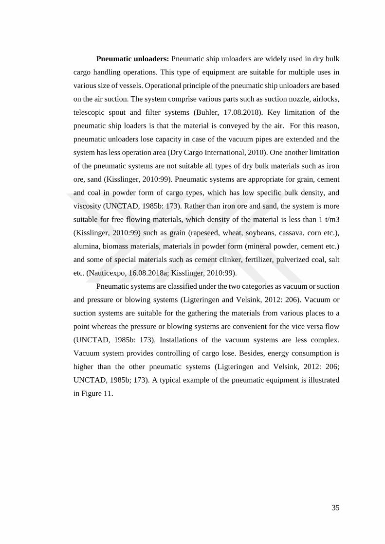
35

Pneumatic unloaders: Pneumatic ship unloaders are widely used in dry bulk

cargo handling operations. This type of equipment are suitable for multiple uses in

various size of vessels. Operational principle of the pneumatic ship unloaders are based

on the air suction. The system comprise various parts such as suction nozzle, airlocks,

telescopic spout and filter systems (Buhler, 17.08.2018). Key limitation of the

pneumatic ship loaders is that the material is conveyed by the air. For this reason,

pneumatic unloaders lose capacity in case of the vacuum pipes are extended and the

system has less operation area (Dry Cargo International, 2010). One another limitation

of the pneumatic systems are not suitable all types of dry bulk materials such as iron

ore, sand (Kisslinger, 2010:99). Pneumatic systems are appropriate for grain, cement

and coal in powder form of cargo types, which has low specific bulk density, and

viscosity (UNCTAD, 1985b: 173). Rather than iron ore and sand, the system is more

suitable for free flowing materials, which density of the material is less than 1 t/m3

(Kisslinger, 2010:99) such as grain (rapeseed, wheat, soybeans, cassava, corn etc.),

alumina, biomass materials, materials in powder form (mineral powder, cement etc.)

and some of special materials such as cement clinker, fertilizer, pulverized coal, salt

etc. (Nauticexpo, 16.08.2018a; Kisslinger, 2010:99).

Pneumatic systems are classified under the two categories as vacuum or suction

and pressure or blowing systems (Ligteringen and Velsink, 2012: 206). Vacuum or

suction systems are suitable for the gathering the materials from various places to a

point whereas the pressure or blowing systems are convenient for the vice versa flow

(UNCTAD, 1985b: 173). Installations of the vacuum systems are less complex.

Vacuum system provides controlling of cargo lose. Besides, energy consumption is

higher than the other pneumatic systems (Ligteringen and Velsink, 2012: 206;

UNCTAD, 1985b; 173). A typical example of the pneumatic equipment is illustrated

in Figure 11.

36

Figure 11: Pneumatic Unloader

Source: Nauticexpo, 16.08.2018a

Vertical Screw Conveyors: These systems are equipped with a vertical screw

placed in the tabular covering. The system can be used both horizontal and vertical

angle. Vertical screw conveyors can handle granular powdered, fibrous and semi-

liquid commodities. The throughput efficiency depends on the material free flowing.

In order to overcome this problem, these conveyors equipped with a free driven spiral

(UNCTAD, 1985b: 175). Figure 12 illustrates the vertical conveyor equipment.

Figure 12: Dry Bulk Cargo Vertical Handling Equipment

Source: Siwertell, 2017

37

Bucket Elevators: this system is equipped with the turning bucket wheels

continuously, which is hang from the luffing boom. At the same time, bucket wheels

dig the hardened materials. These systems are expensive in terms of requiring stronger

quay structure (UNCTAD, 1985b: 175; Ligteringen and Velsink, 2012: 208).

Horizontal Transport Equipment

Conveyor systems are frequently used for transferring the cargo from the

storage yard area to the berth side or vice-versa (Frankel et al., 1985: 173; Ligteringen

and Velsink, 2012: 214). In addition to the conveyors, the trucks may perform this

transfer. Conveyor system has a major effect on the terminal layout. In the long-run,

the conveyor systems should be designed to suitable for efficient maintenance and

repair activities (UNTAD, 1985b: 176).

Conveyor belt usage is limited by the distance within the port area due to the

economic and transport considerations. Road or rail transport equipment can be

utilized to perform transferring activities when the distance between the berth and yard

area is longer (Ligteringen and Velsink, 2012: 215).

The advantages of the conveyor systems are (Ligteringen and Velsin,

2012:215; UNCTAD, 1985b:176; Frankel et al.,1985: 173):

Construction of these systems are easy

Energy efficiency consumption

These systems can be adopted to another systems

It provides complete discharging

Enables minimum friction and noise

There are several belt conveyor types in practice. These are wider rubber belts,

chain conveyors, en-masse conveyor, screw conveyor, screw mounted,

aeromechanical, fluidizing gravity conveyor, bi-cable systems, and vibratory

(McGlinchey, 2008: 199; Bulk Inside, 11.03.2019; UNTAD, 1985b: 176). The shape

of these systems may be in the form of U-shape, V-shape (Ligteringen and Velsink,

2012: 215), and flat. These systems can be designed as an enclosed system to prevent

dust and cargo losses. Figure 13 illustrates the different types of conveyor belt systems.

38

Figure 13: Conveyor Systems

Source: Macgregor, 11.03.2019 (Screw Conveyor (left)); McGlinchey, 2008: 242 (En Masse

Conveyor (right)); Sawhney Industries, 11.03.2019 (Belt Conveyor (bottom))

Storage Yard Equipment

Many equipment is used in the storage yard. Commonly used equipment are

the stacker, reclaimer or stacker-reclaimer, bulldozers, and circular or longitudinal

blending bed equipment.

The working principle of stacker equipment is to ensure that the cargoes are

continuously stacked in the storage yard area. The equipment stacks the several

material through a tripper, which enables the equipment to be allocate anywhere. When

commodities are stacking out from the pile, stacking out conveyors equipped with a

slewing maneuverable or fixed boom, are used (UNCTAD, 1985b: 177; Ligteringen

and Velsink, 2012: 217).

Reclaimer equipment provides continuous retrieving of the materials from the

storage area. Reclaimer is equipped with a bucket wheel, which mounted at the end of

the boom and equipped with an intermediate belt conveyor fed by the bucket wheels

(Ligteringen and Velsink, 2012: 217; UNCTAD, 1985b: 177-178).

39

Stacking and reclaiming functions of these storage yard equipment can be built

in one equipment: Stacker-reclaimer (Ligteringen and Velsink, 2012: 217). Stacker-

reclaimer equipment is highly efficient equipment. The advantages of the stacker-

reclaimer require limited number of conveyors. However, the system may decrease the

total terminal performance due to perform simultaneous operation in vessels and trains

(van Vianen, 2012: 101). Another disadvantage of the stacker reclaimer is that two

functions (reclaiming and stacking) cannot be used at the same time. Because of

having large capacity, stacker-reclaimer needs significant track establishment

(UNCTAD, 1985b: 178).

Bulldozers can also be used at the dry bulk terminal to stack or transfer the

materials to storage yard area. Moreover, the equipment can also be used for pushing

the furthest stacks to more accessible points where reclaimer can reach (UNCTAD,

1985b: 178).

Circular blending bed is mostly used for homogenizing and storage of the

materials. Circular blending bed has the ability of storing and reclaiming

simultaneously (Thysenkrupp, 11.03.2019b). In addition, longitudinal blending beds

are widely used in the dry bulk terminals.

Figure 14 illustrates the storage yard equipment.

Figure 14: Storage Yard Equipment

Source: Thyssenkrupp, 11.03.2019a (Stacker (right)); Metso, 11.03.2019 (Stacker-reclaimer

(left)); Thyssenkrupp, 11.03.2019b (Circular Blending Bed (bottom))

40

1.3.DRY BULK TERMINAL OPERATIONS

Planning the operations is the primary assignment for all activities in a

terminal. Changeable activities require a systematic approach to plan port operations

comprehensively. Comprehensive planning is significant to allocate the resources and

provide the effective coordination of the operations, especially the involving parties

outside the port. In case the operation is planned ineffectively, it is impossible to

acquire the throughput although the berth is capable (Thomas, 1985c:1). Before

making productivity and cost estimation, it is crucial that equipping, layout and method

of cargo handling operations must be recognized (UNCTAD, 1985: 56).

Robenek et al. (2012:2) evaluated dry bulk terminal operation planning under

the two title: Tactical level and operational level. Tactical level refers to the allocation

of the resources such as berth, storage policies, labor, equipment, and yard

management. Besides, the operational level is associated with a series of decision

making which encompasses the yard equipment and crane scheduling activities and

flexible planning of these activities that are suitable according to last minute changes.

Dry bulk cargo handling encompasses the different organizations related to

control and handling of cargo flow from ship to transport or storage and needs

installations which ensure the maximum service to the ships with minimum costs

(Bugaric et al. 2012:1508). Main consideration underlying the bulk terminal

operations is to advance operational efficiency and to increase the ship turnaround time

at ports providing the continual flow of cargo (UNCTAD, 1985:30; Burns, 2015:124).

The system in the port should be planned to allow working with the full potential of

loaders or unloaders and working in a synchronized manner (UNCTAD, 1985:30).

Equipment and storage should also be taken into consideration to achieve the continual

cargo flow.

In a general term, seaport terminals consist of three primary systems as the

entrance, storage yard and exit systems (Schott and Lodewijks, 2007:376). The starting

point of the systems is vary depending on the export or import activities of the dry bulk

terminal. Based on the flow direction of the bulk cargoes, the terminal is denominated

as “export terminal” or “import terminal” (Kleinheerenbrink et al., 2012: 108).

Moreover, a queue of the dry bulk terminal operations can divergent regarding

41

equipment used in the terminal, services, layout of the terminal or types of cargo. It is

difficult to illustrate the standard terminal operations queue and the flow of the cargoes

due to the reasons mentioned above. For this reason, the operation queue of the dry

bulk terminal is indicated in general terms considering the import and export cargo

process in Figure 15.

Figure 15: Dry Bulk Terminal Process

Source: Kleinheerenbrink, 2012: 25

In import shipments, the process starts with the arriving of the vessels to the

terminal. After berthing of the vessel, unloading operation of the cargoes begins.

Unloaded cargoes are transferred to the storage yard. After the stacking process, the

cargoes transferred to the exit by railway according to the availability of the railway

links or trucks.

In the export cargo process, there is a reverse flow of cargo comparing to the

import cargo operations. The process starts with the arriving of the trucks or wagons

to the terminal. The cargoes arrive at the terminal gate to be transferred to the storage

yard. After this process, cargoes are transferred to the berths vessel to be loaded, and

the ship unberth.

Due to the reasons mentioned above (different processes in import/export cargo

flow in the terminal), the process is evaluated under two main categories as seaside

and landside operations. The general process in the dry bulk terminal cannot be

schematization in a single process. For this reason, dry bulk terminal operations are

described in general terms. More detailed operation process is explained as follows:

42

1.3.1. Import Cargo Operation Process1

This section provides import cargo operation according to seaside and landside

operations.

1.3.1.1.Seaside Operation Process

The queue of the seaside operations of the import materials are described as

follows:

Pre-berthing operations: A typical pre-berthing operation includes the

processes of the permission to the berth, pilot guide requests (Wadhwa, 1990: 237).

Before the vessel berths, it applies to a commercial service unit for various services

such as proforma invoice, SAP, identification, reporting, etc. with the receipt of the

commercial approval and the documentation unit forms the documentation control and

the work orders. At this stage, the documentation such as preparation of the cargo

manifest, mate’s receipt packing list and discharging permissions are performed. After

obtaining the operation approval, the operation unit monitors the operation, feedbacks,

traces the vessel’s documents and related operational documents.

Berthing: In import dry bulk cargo operations, the entrance system includes

the seaside where the vessels arrive and deliver the cargoes. Vessels may wait at the

berth to get service after the arriving to the berth (Hess et al. 2007: 61). In this process,

the vessel is allocated to the berth, and the port gives pilot guide instructions. After

this process, the equipment is allocated to start handling operations. To be given this

instruction, truck tracking should be performed, and the safety must be ensured.

Unloading of the cargoes: After the berthing of dry bulk vessels, cargoes are

unloaded by using ship unloaders such as mobile cranes, floating cranes, grabs, screw

conveyor, cranes, continuous unloaders, chain bucket, hopper, crane-mounted grabs,

bucket wheel etc. (Agerschou et al., 2004:318; Schott and Lodewijks, 2007:376;

Bugaric et al. 2012:1512; Bugaric et al. 2012:406; Park and Noh, 1987:236; Burns,

2015:124;). Cranes discharge the materials to storage area directly or drop the

1 In this section, the details of the operational processes are formed in the light of the information

provided by Limak Uluslararası Liman İşletmeciliği A.Ş. and Atakaş Liman İşletmeciliği ve Ticaret

A.Ş.

43

materials into a hopper which feed the conveyor (Agerschou et al., 2004:318).

Pneumatic systems discharge materials in powder and granular form.

Transferring the cargoes to storage yard: In this stage, conveyors are

generally used as transfer equipment. Cargoes are dropped into a hopper (bunker)

which feeds the conveyor belt system (Schott and Lodewijks, 2007:376). Belt system

transfers the cargoes to the stackers which stacks the cargoes on the storage yard

(Schott and Lodewijks, 2007:376). The cargo transfer is performed by the conveyor

systems (Bugaric et al. 2012:1512; Agerschou et al., 2004: 318; Bugaric et al.

2012:406; Park and Noh, 1987:236). In this stage, different planning issues should be

followed. If cargoes exit without being stored, the trucks that are allowed to pass are

weighted. If the cargoes are to be stored, the trucks planned to perform this operation

are directed to the storage yard area. Trucks are weighted in this area. After the

equipment planning and the location determination activities, the cargoes are picked

up to the storage area.

1.3.1.2.Landside Operation Process

Storage Yard: The function of the storage yard in dry bulk terminals is the

admittance of the cargoes from the berth if the land or railway transport is not fulfilled

(Bugaric et al. 2012:1512; Bugaric et al. 2012:406; Park and Noh, 1987:236). While

some of the dry bulk cargoes need to be stored in closed storage area, some of the

cargoes are stored in open storage areas (Schott and Lodewijks, 2007: 377). The

materials required the closed storage areas are transferred to silos or enclosed facilities

alongside the berth in the terminal by conveyor systems. The materials which do not

need closed storage area, are transferred in open storage areas for stacking (Burns,

2015:124). In the process of storage operation, the documentation unit records the

cargo information to be stored in the area to the system.

Transferring the cargoes to gate: Exit systems in the dry bulk terminal is fed

by reclaimer which retrieving the cargoes from the storage yard. The exit systems are

also feeding the conveyor belts (Schott and Lodewijks, 2007:376; Park and Noh,

1987:236). The cargoes leave from the storage area undergo a process of

documentation. The planning unit sends the trucks to the storage area. The equipment

44

is assigned to the operation site as well as equipment allocations. After the cargoes are

checked by the system, cargoes are moved from the storage area. The trucks are

weighted before leaving from the port or entering to the port.

Gate Operations: The operations in this stage is based on the efficient control

of the entrance and exits to port areas. Planning includes the several services such as

bookings, departure and arrival schedules, delivering the cargoes and picking up

services, controlling, validation and inspection of the cargoes and monitoring the

vehicle passages (Bichou, 2013:144). Pre-gate is exit channel where vehicles checked,

weighted and examined before entry or exit (Keçeli, 2016:8; Mazouz et al. 2017: 610).

This process includes many inspections of the cargo condition and the documents (Lai

and Leung, 2000:89). For example, the license plate of the trucks and the customer are

registered in the port system to leave the cargoes from the port area. Following these

activities, the trucks are checked via the port system. If necessary, trucks are weighted.

After these processes, access to the exit gate is provided. Besides dry bulk cargo is

discharged in wagons, barge or train lead outstation (Schott and Lodewijks, 2007:376).

1.3.2. Export Cargo Operation Process2

This section provides import cargo operation according to seaside and landside

operations.

1.3.2.1.Landside Operation Process

The queue of the landside operations of the export materials are described as

follows:

Pre-gate and Gate Operations: In export, dry bulk cargo operations start at the

land side of the terminal. According to the situations that the railway connection is

available, export dry bulk cargoes can be delivered by train, in the case of railway

connection is not available, trucks perform this operation. In the terminal, which has

2 In this section, the informations about the details of the operational prossess are formed in the light

of the operational processess information provided by Limak Uluslararası Liman İşletmeciliği A.Ş.

and Atakaş Liman İşletmeciliği ve Ticaret A.Ş.

45

railway connection, the tipplers unload the cargoes, or self-unloading wagons are used

to discharge the cargoes from the wagons (Schott and Lodewijks, 2007:376).

Entrance gate can be assessed as the important channel in which vehicles enter

the port area, and checked weighted and examined (Mazouz et al. 2017: 610).

Checking the trucks before entering the gate is performed in this stage (Keceli, 2016:

8). In this process, the planning department provides information about the vessel to

the operation department. In case the trucks arrive at the port from the outside, truck

list to be entered to port area is notified to the gate. Gate control unit checks the trucks

and the trucks that are allowed to pass are registered, and the entry permissions are

granted. If weighting is necessary, the vehicles are weighted. After these operations,

the trucks are directed to the operation sites.

Transferring the cargoes to storage yard: In truck-based delivering the export

cargoes, truck unloaders are used for unloading operations. After dropping the cargoes

which is discharged by the vibratory feeders or apron feeders to the hopper, the feeder

equipment feeds the belt systems that transfer the cargoes to the storage yard (Schott

and Lodewijks, 2007:376).

Storage yard: The same activities fulfilled in the export storage yard are the

same as the import storage yard (Schott and Lodewijks, 2007:376). For the materials

stored in the open yards, a combination of usage of the reclaiming and stacking devices

is commonly practiced. With reversing the boom conveyors, commodities drop onto

the pile. Earth-moving equipment, i.e. bulldozers scraping the commodities into a

fixed position, hoppers below ground level that bring it to belt conveyors are used in

the closed storage area operations (Agerschou et al., 2004:316). Cargoes are stacked

in the vehicles at the storage yard area. If the port supplies the vehicles (trucks etc.)

and regards weighing as necessary, the trucks are weighed while vehicle is loaded.

1.3.2.2.Seaside Operation Process

Transferring the cargoes to the berth: The trucks moved to the operation site

leave the cargo to be loaded onto the vessel. At this stage, if necessary, trucks are

weighted. The equipment is allocated to the berth.

46

Loading the cargoes: Several techniques can be implemented for loading the

vessels. According to the terminal layout and equipment, single spout systems may be

used for the loading the materials. One another technique is that conveying the

commodities to an elevated position alongside the vessel is up to load the ship hold by

spouts. Gantry devices traveling below the tripping mechanism that spreads the

materials over the hatch by slewing conveyor with controllable spout at the end

(Agerschou et al., 2004:315). Vessels are loaded by the grab, bucket wheel, conveyor

belts, loading spout, mobile cranes (Schott and Lodewijks, 2007:376; Burn, 2015:215).

Unberthing: In export dry bulk terminals, exit systems are concluded at the

berth (Schott and Lodewijks, 2007:376). At this stage the vessel departures from the

berth by signing the operation documents.

Terminal operations must be organized to indicate the tonnage rate per hour for

each of the equipment (UNCTAD, 1985b:184).

47

CHAPTER II

SCOPE AND CONCEPT OF PORT CAPACITY

2.1.AN OVERVIEW OF PORT CAPACITY

Capacity as a general terms is defined by the Swamidass (2000:74) as

“Capacity is the maximum possible output over a specified period of time. In cases

where the output is nonhomogeneous, capacity may be measured in terms of the

available machine hours”. While Oxford Dictionary (01.05.2019) and Turkish

Language Society (01.05.2019) define the capacity as “The amount that something can

produce”, Olhager and Johansson (2012:23) defines the capacity as “Capacity is

concerned with the available (work) time per (calendar) time unit; e.g. hours per day.”

Port capacity is well-defined by the Frankel (1987: 170): ‟A port’s capacity is

normally defined as the cargo volume that the port is capable of handling within 1

year and is often expressed as a throughput in tons per unit length of a wharf per year

(MT/m/yr or LT/ft/yr), multiplied by the available berth length, for each type of berth

separately”. In the literature, various researchers define the port capacity. Gaur et al.

(2011: 295) defined port capacity as a function of final output of production at each

stage of the operations in the port. Zenzerovic et al. (2011:2), and Bassan (2007: 3)

evaluated port capacity as loading or discharging amount of the specific berths at the

terminal within the particular period (Ding, 2010: 126). Besides scholars assessed the

port capacity from many different viewpoints. From the engineering perspective,

Bichou (2013: 51) defined the port capacity as the maximum utilization rate obtained

in short term with existing infrastructure and resources technically. From the supply

perspective, port capacity is the ability of the port to accept a certain number of ships

at the same time, and it is represented as the quantity of cargo, the number of handled

the vessel, the total cargo quantity in a significant period (Dundovic, and Zenzerovic,

2000: 217). The level of service that the terminal can offer to its customer is another

crucial factor for the supply side perspective. Therefore, the port capacity can also be

defined from the supply viewpoint as the maximum throughput once the vessels arrive

at the port and services are provided continuously (Ding, 2010:126). Besides, from the

demand viewpoint, port capacity purports the port traffic capacity or the maximum

48

quantity of the throughput of specified berth (Zenzerovic: 2005: 168; Zenzerovic et al.

2011: 46). From the value-driven viewpoint, the capacity is the value corresponding

to the highest vessel cycle that the port can handle while ensuring the minimum service

quality. According to the value-driven perspective, port capacity cannot be separated

from its service level, perceived quality, and the final value and these considerations

are depended on the terminal characteristics, the performance of the terminal

equipment, demand circumstances, and the outside factors (Morales-Fusco et al.

2010:696). It can be inferred from these definitions that port capacity shows not only

the degree of the port capability but also the infrastructure capacity such as transport

system. From the bottleneck perspective, port capacity can be evaluated as a

measurement of determining the significant network constraints, and it enables the

assessment of the port performance based on the safety and economic sense (Bellsola

Olba et al., 2014:1).

The amount representing the handling unit is expressed in different terms in

different port or terminal types. The units processed in the container ports are

represented in TEU, in ton or pallets for bulk or general cargo ports, and in a number

of the wheeled vehicles for Ro-Ro ports in a certain period (Bassan, 2007: 3).

Moreover, the term capacity can be defined to indicate the different operational

capabilities of the ports.

Many of the researches on port capacity and capacity planning problems

focused on identifying the bottlenecks and constraints at the port and concentrated on

solving these problems. Capacity constraint results in inadequate capacity at ports by

preventing the port efficiency (Gaur et al. 2011: 298). Ports are divided into the main

components to identify the bottlenecks. These components are vessel arrival capacity,

berth capacity, ship-apron transfer capacity, apron-warehouse capacity, storage yard

capacity, storage yard-land transport capacity, gate capacity, services, and hinterland

connection capacity (Gaur et al. 2011: 5-6; Park et al. 2014:179; Meersman et al. 1997:

6) and these components are significant to determine the output level of a port (Gaur

et al. 2011: 5-6). The bottleneck at the ports affects the operational aspects, i.e., waiting

time, turnaround time, service time, etc. (Bassan, 2007:5). The cause of the bottleneck

in ports originated in the inadequate capacity of subsystems of the port (Bugaric et al.

2012: 1509). From this perspective, capacity can be seen as an indicator and limiting

49

factor that assists in determining the constraints of any link (National Research

Council, 1998: 10; Bellsola Olba et al. 2014: 1). It enables the assessment of the port

performance systems (Bellsola et al. 2014: 1). Improvement efforts are shaped within

the context of the constraints (Bassan, 2007:5). Within these subsystems, the weakest

part determines the capacity of the entire port (Meersman et al. 1997: 6).

The growth in the world economy, acceleration in technology and investment,

rising of new economic leaders in the world, increased international specialization,

substantial world population growth have been possible with the growth of world

trade. Industrialization has triggered the further development of overseas trade and

unification of the economies (WTO, 2013:46). This massive progress has shaped the

transport requirements, especially in ports, by pushing the port to integrate into the

global supply chains and by increasing the need of specialized services (Ng and Pallis,

2010:2147). Moreover, factors such as growth in trade and cargo volume, economic

activities and changing frame of the supply chain have increased the pressure on the

ports in terms of both competition and capacity issues. Although many ports share the

same hinterland, they have various competitive conditions. One of the factors that

determine the competitive conditions between the ports is the capacity bottlenecks in

the face of increasing demand (Asteris and Collins, 2007:2274).

Port capacity is the strategic point for the expansion of the ports and the

development of the existing ports (Luo et al. 2012: 120). In response to the increase in

demand, competition, and the ship sizes increase the ambitions of the port' expansion

and development simultaneously (Fan et al., 2012: 1121). As mentioned earlier

sections, the capacity should be balanced with the trade volume to sustain port

performance as well as providing international and domestic competitiveness (Jeevan

et al. 2015:85; Dekker and Verhaeghe, 2006:174). Therefore, the lack of

understanding of the mechanism of market dynamics can lead to excess capacity in

practice (Notteboom and Rodrigue, 2006:16). At this point, the port needs to examine

its capacity to provide sufficient services to its customers and maintain its competitive

advantages (Cullinane et al. 2006: 361). The accurate estimation of the supply and

demand is an essential indicator for establishing or expanding the ports in terms of

determining the capacity requirements, the continuity of capacity demand, income,

investment timing, efficiency and effectiveness level of the ports. Because idle

50

capacity, which is the result of unnecessary investments, will damage not only the

investors, but also other ports in the region and especially it harms the port tariff

structure. Additionally, capacity utilization rates provide insights into the efficiency

and effectiveness of the port. Improving these rates contributes to the operational and

managerial process improvements (TÜRKLİM, 2017:101).

Port industry has capital-intensive nature and needs substantial investments in

infrastructure and equipment by facing challenges of the environment of uncertainty

(Haralambides, 2017: 27; Li et al. 2017:849; Lagoudis et al. 2014: 300). For this

reason, these investments should be performed considering comprehensive capacity

planning. Capacity planning differs from capacity management concept. Capacity

management stands for the managerial approach of the owner under the service

difficulties such as sufficient capacity or excess capacity. The capacity management

decision depends on the results of the capacity planning (Dekker, 2005: 5).

Capacity planning is the primary decision process to meet the demand while

building, enlarging or modernizing the port. In a broad sense, capacity planning refers

to the examination of economic and technical aspects of balancing supply and demand

(Dekker, 2005: 5). Being able to provide adequate services for port customers is the

critical point in capacity planning (Tang et al. 2016:174). Port capacity design includes

the examination of the expected demand and supplying sufficient capacity and

improving the strategies to plan supply and demand (Bichou, 2013:53). Moreover,

performance is another significant point in capacity planning. While this phenomenon

includes the balancing supply and demand, it also aims to achieve both service level

maximization and resource optimization (Li et al. 2017:849)

One of the main approaches to port capacity planning is the building new

infrastructures and installing faster equipment (Kim and Morrison, 2012:2014).

Although the physical expansion of port can be seen as the simplest method to expand

beyond the port boundaries, this expensive choice may be constrained by the shortage

in land areas where may impede future expansion, particularly the ports located in or

near the city centre (Cullinane, et al. 2006: 361; Li et al. 2017:849). Physical expansion

may lead to other issues in the competitive structure of the ports. After the investments

are made, the ports may offer low-level prices to increase return on investment (Bae

et al. 2013:480). Also, supplying more capacity by physical expansion lead to excess

51

capacity problems. If there is an imbalance between the supply and demand, the level

of competition will be affected. In that situation, ports need to compete rigorously to

enhance its market share. This circumstance may cause to disruptive pricing.

Inadequacy in creating demand will increase the tendency of the port to compete in

existing services (De Langen and Pallis, 2007:439).

The competitive conditions are not only limited to capacity expansion. The use

of maximum capacity, as well as the desire to reach minimum waiting times, also

increased the pressures on ports for further improvements in productivity and

efficiency (Haralambides, 2017:26-27). Besides, ocean carriers and shippers bear the

time-related costs. Therefore, this situation determines the shippers and ocean carriers’

port choices. Qualifications of the services of the port such as speed and quality of the

services determine the time-related costs compensated by shippers, inland and water

carrier such as inventory and depreciation costs (Talley, 2006:500).

The port capacity plays a vital part in planning the transport systems and its

quality (Malavasi and Ricci, 2005: 471). It can be evaluated as an essential indicator

of the transport infrastructure and capability of the port’s ability to provide a specific

service (Dekker, 2005:3; Bichou, 2013: 51). Ports should serve with adequate capacity

to sea traffic regarding handling and transport options in its hinterland (Gaur et al.

2011:53).

As mentioned in Chapter I, the port layout design is closely related to port

capacity. Layout planning to be carried out according to the planning of the seaside

and landside directly affects the equipment and capacity to be used at the ports. Also,

capacity planning affects the layout planning of the port. Schematic representation of

the relationships of layout planning and the capacity is illustrated in Figure 16.

52

Figure 16: Relationship of Layout Planning and Capacity

Source: Wiese et al., 2013:227

According to Figure 16, seaside capacity is essential in determining the storage

yard capacity and the landside capacity. The capacity, which is planned on this basis,

affects the layout planning and design of the entire port through equipment choice.

2.1.1. Equipment Capacity

Selection of the type and capacity of the handling equipment is a complicated

process due to the reasons such as operation economy, the convenience of the

conveying systems for specific material and susceptibility of the cargoes to

deterioration (Agerschou et al., 2004: 319) because the equipment capacity and its type

is determinative for the overall terminal capacity.

There is a highly positive relationship between equipment performance

parameters and the port capacity. Because the loading and discharging capacity of all

the storage facilities restricted by the equipment capacity. There are three fundamental

capacity types in the literature for the equipment as peak capacity, rated capacity and

effective capacity (Ligteringen and Velsink, 2012:203; UNCTAD, 1985b: 170).

53

Peak capacity (cream digging rate) refers to the maximum hourly handling rate,

which can be attained under certain optimum conditions. Unloading rate should be

synchronized with all downstream facilities and equipment. Apart from the peak

capacity, rated capacity (free digging rate) is the handling rate based on the cycle time

of a fully loaded grab or bucket between the digging point and positioned point of the

hopper and back. The value of the capacity can be found dividing the carrying capacity

of the grab by the effective time required for the one cycle. Rated capacity is a useful

indicator when comparing the equipment. Effective capacity refers to the average

hourly rate achieved during the handling of the materials. The time includes the

transition of the equipment between ship holds, cleaning of the holds, but non-working

time is not counted. Effective capacity is used in planning stage of the port as an

indicator. Port planner considers the effective capacity, whereas equipment designer

pays attention to the peak capacity (Ligteringen and Velsink, 2012:203; UNCTAD,

1985:170).

In addition to indicators as mentioned above, which is related to equipment

capacity, another factor, which provides insight into the equipment capacity when

planning the terminals, is called as “Equipment Installation Factor”. Equipment

installation factor is found by dividing the installed capacity (ton/h) by the required

equipment capacity to handle the annual amount of cargo which attained by the

terminal. In order to calculate this factor, required equipment capacity should be

considered as the equipment is performing continuous operation (365 days, 24 hours)

(van Vianen, 2015: 14).

Material types and the average capacity values of the equipment mentioned in

Chapter I, Section 1.2.1.4. are specified in Table 6.

54

Table 6: Equipment Capacities, Vessel Sizes, and Suitable Materials 1

Equipment Type Capacity

(tph*) Suitable Material for Handling Vessel Size (DWT)

Travelling Loader 500 - 9,200 Fertilizer, Urea, Ammonium

Sulphate, Iron Ore, Coal,

Petroleum Coke

40,000-270,000

Radial Loader 8,000-11,000 Iron Ore, Iron Ore Pellet Up to 180,000

Slewing Bridge

Loader

1,700-15,000 Fertilizer 52,000-270,000

Linear Loader 2,000-11,000 Coke, Sulphur, Coal 60,000-180,000

Travelling

Overhead Trolley

Unloader

1,000 - 15,000 Iron Ore, Coal, İlmenite, Animal

Feed, Clinker, Cement, Other

Bulk Material

80,000-160,000

Mobile Harbour

Crane

550 -2,300 Scrap, Agri-bulk, Up to 30,000

Pneumatic Unloader 160 - 800 Cement, Malt Rice, Cocoa Beans,

Urea, Cement 5,000-60,000

Vertical Screw

Conveyors

100 - 800 Urea, Fly Ash, Gypsum, Cement,

Lime, Raw Meal, Apatite,

Limestone, Powder

15,000-6,000

Bucket Elevators 1,300 - 5,000 Free Flowing Granular Products,

Coal Iron Ore Up to 180,000

Belt Conveyors 2,000 Grain, Oilseed and derivatives,

Coal, Ore, Mineral, Fertilizer,

Woodchips, Lumpy or Granular

Materials

Up to 130,000

Screw Conveyors 1,500 Cement, Grain, Coal, Lime, Raw

Meal, Apatite, Urea, Fly Ash,

Gypsum, Alumina, Biomass

-

En-masse

Conveyors

286-1501,6 Agricultural Products -

Stacker 1,600-3,000 Coal, Iron Ore Fines, Iron Ore

Pellets, Coke, Olivine -

Bucket Wheel

Reclaimer

2,000 Coal, Iron Ore Fines, Iron Ore

Pellets, Coke, Olivine -

1 Table 6 has been compiled from various equipment supplier’s websites by taking into consideration

the maximum and minimum values of the rated capacities. The values of equipment capacities vary

according to the cargo type, equipment brand and model.

55

Table 6: Equipment Capacities, Vessel Sizes, and Suitable Materials (Continue)

Bucket Wheel

Stacker Reclaimer

Coal, Iron Ore Fines, Iron Ore

Pellets, Coke, Olivine -

Stacking 500-6,000

Reclaiming 4,500-20,000

Circular Blending

Bed

Coal, Limestone, Marl, Clay,

Coal, Mine, Cement, Fertilizer,

Grain -

Stacking 2,500

Reclaiming 1,200

*tph: ton per hour

Source: Adapted by the Author using the sources of Dahm, 11.03.2015; Liebherr, 13.03.2019;

Vigan, 13.03.2019; IBAU Hamburg, 13.03.2019; DSD, 13.03.2019; Macgregor, 13.03.2019;

Siwertell, 12.03.2019; Port Technology, 12.03.2019; Yuntian Machinery, 13.03.2019; Fam,

13.03.2019; Bühler, 12.03.2019; Siwertell, 12.03.2019; Konecrane, 13.03.2019; GSI,

13.03.2019; Thyssenkrupp, 13.03.2019 (a); Thyssenkrupp Robins, 13.03.2019; Thyssenkrupp,

13.03.2019 (b); Dry Cargo International, 01.10.2011.

2.1.2. Berth Handling Capacity

The berth where the cargoes are handled from/to terminal yards and vessels

associates the landside and seaside activities (Salminen, 2013:23). Berth capacity of a

port refers to the amount of cargo a port can handle from all the existing berths during

the specified period (Oral, 2014:228; De Monie, 1987:12).

The berth is an essential factor in determining overall port capacity. Berths

affect the operating principles of the other terminal subsystems in terms of meeting the

ship traffic and handling the materials in these areas (Bugaric et al. 2012: 1508).

Therefore, all performance factors and the service level of the berth will also affect the

entire terminal system and its capacity. Level of service is the measure of the capability

of the facilities to render service to the terminal (port) user. It refers to the operational

conditions of the terminal regarding the determinants such as travel time, traffic,

safety, suitability, maneuver freedom, speed, and elimination of damages (National

Research Council, 1998: 18). Efficiency in cargo handling activities effects the service

capacity of the port (Tan et al. 2015: 15). Assessing berth capacity within the viewpoint

of the service level changes the berth capacity definition as the maximum amount of

56

cargo that can be handled at the berth within a specific period without decreasing the

service level below a widely accepted level (Tang et al. 2016:175).

The common purpose of the ports is to offer higher service quality to all

customers as well as achieving higher efficiency and minimizing costs (Mwasenga,

2012: 4). Meeting the targets of determined capacity is possible by keeping the

performance indicators at the optimum levels because the performance indicators

characterize the port service level and capacity (Lee et al. 2014:427).

There are several performance indicators in the literature. Although these

indicators are used in the measurement of the port performance, these parameters are

also used in planning and measuring berth capacity. One of these indicators is waiting

time to service time ratio. It is expressed as Tw/Tb, where Tw is waiting time of vessels;

Tb is the service time of vessels at the berth (Laing and Hecker, 1989: 83; Layaa and

Duallert, 2014: 151; Bellasola Olba et al. 2017: 2). Although Tang et al. (2016:117)

called this performance indicator as berth occupancy; it does not fully meet the concept

of berth occupancy rate. The ratio indicates the level of service delivered by the

terminal (UNCTAD, 1985a: 30). Waiting time-to-service time ratio describes the

efficiency level of the port regarding the overall port with sailing time (Bellasola Olba

et al. 2017:2). This ratio indicates the service level since the waiting time of a vessel

depends on the amount of cargo carried by vessel (Layaa and Duallert, 2014:150). It

is accepted that the waiting time should not exceed 10-50 % of the working time.

However, this ratio is deceptive due to the service time deterioration. Therefore, this

ratio can be seen as a useful tool only when the conditions are constant. The rate is

advantageous when the economic optimum investment plan is prepared (less than 30

% is preferable) (UNCTAD, 1985a: 30). This ratio creates a discrepancy between the

shipping lines, ship owners or charterers and the port authority. Shipping lines, ship

owners or charterers choose the low waiting time-to-service time ratio. However, the

port authorities want to achieve higher berth utilization. Hence, the balance between

these claims should be considered (Layaa and Duallert, 2014: 151). Mostly ship

owners and shippers consider this indicator as port selection criteria to save the time

and money.

One of the main factors that should be considered in the measurement of berth

capacity is statistical distributions. The correct evaluation of the berth capacity

57

depends on the statistical distribution parameters. Commonly used statistical

distributions used in measuring the berth capacity are service time distribution, ship

arrival distribution and ship inter-arrival time distribution. Service time distribution

shows the distributions of the service time per ship. Service time primarily depends on

the amount of cargo carried by vessel and loading/unloading rate of the equipment

(Shabayek and Yeung, 2000: 329).

Moreover weather conditions, and cargo type affects the service time

distribution. Inter-arrival time distribution shows the time at which ships arrive at the

port. Arrival rate of the vessel illustrates the frequencies of the vessel’s arrivals. These

distributions affect the berth occupancy, storage yard utilization, and equipment

utilization. In dry bulk terminals, vessel arrivals show a random tendency. According

to the UNCTAD (1985: 187), Erlang 2 distribution is preferred to determine the inter-

arrival time distribution and the service time distribution in queueing approach rather

than Erlang 1 distribution due to the tendency of slightly simplifying the arrivals.

Besides, Bugaric et al., (2012:1514) stated that the service time of the vessels is

obtained in accordance with the normal distribution, whereas inter-arrival of the ships

obtained according to Erlang 1 in bulk cargo import terminal. Dragovic et al. (2006:

290-291) stated the arrival of the vessels and the inter-arrival of the vessels were best

fitted with the exponential distribution and the service time is measured by Erlang

distribution although container terminal did not show the stochastic arrival. According

to Altıok (2000: 6), the service time of the vessel fits the Erlang distribution in bulk

loading ports. Kozan (1997: 242-243) specified the service time shows consistency

with the Erlang distribution, whereas the inter-arrival distribution of the vessels

consistent with the exponential distribution. According to van Vianen et al. (2012:3)

distributions are highly correlated with the terminal type. In the ports, which give

service to third parties, the distribution can be modeled by the negative exponential

distribution because the owner of the cargo is different from the operator. Besides in

single user terminals (e.g., power plants or steel producers), the best-fitted distribution

is the Erlang 2.

58

2.1.3. Storage Yard Capacity

When all components of the port are considered as a link of a chain that

determines the port capacity, storage yard is one of the most critical chains when

measuring the port capacity. The port capacity is highly associated with the size of the

total yard area (Park et al. 2012:3; Park and Dragovic, 2009: 204) because the size of

the storage is the limiting factor in managing the logistics activities for many terminals

(Chen et al. 2004:1).

Since the port can be qualified as a system and all the subsystems, affect each

other. All subsystems of the port must work harmoniously to achieve the goals.

Because berths and storage yard area are the components of the port system, the

parameters affecting the berth also affects the storage yard area. Therefore, statistical

distribution determines the storage yard capacity as well as the berth capacity. Arrival

rates, and the amount of the cargo brought by vessels to be stored in the storage yard

area directly influence the port capacity. In addition to the above-mentioned statistical

distributions, storage time distributions also affect the storage yard capacity. As stated

in Chapter I Section 1.1., decisions of constructing the new port or expanding the

existing structures affected by the port capacity. Moreover, equipment types and

characteristics, types of cargo, stockpile and stacking, and storage policy implemented

in the terminal area directly affect the storage capacity of the port.

Stockpiles may be in the form of trapezoidal shape, a trapezoidal shape with

end cones, conical, circular, triangular and triangular with end cones. The stockpile

configuration is illustrated in Figure 17:

59

Figure 17: Different Stockpile Configurations

Source: Basics in Stacker Reclaimer, 28.11.2017

Several parameters restrict the stockpile capacity. These parameters are the

bearing capacity of the ground, length, and width of the stockpile, the stockpile

geometry, types, height and outreach of the stacking equipment. Determining the

optimum pile size is crucial for the equipment because the volume of the storage yard

capacity can be enlarged by the size of the pile (Frankel et al., 1985: 158).

In case the use of luffing non-slewing stackers, triangular and conical shapes

can be formed, whereas luffing cum slewing stacker allows to the triangular,

trapezoidal and triangular shape of the stockpile (Basics in Stacker Reclaimer,

28.11.2017).

Circular storage yard system is a circular system that the stockpiles established

on the circular ground. Circular systems include the luffing-slewing stackers and

bridge-type reclaimer, which can turn around the central column. The equipment can

reach the total area where stockpile is formed (Wolpers, 24.02.2019; UNCTAD,

1985b: 181). In the case of limited storage spaces, circular storage yard

implementations may be reasonable (UNCTAD, 1985b:181). Additionally, circular

storage yards is generally applied when materials need to blending or when there is a

need for immediate storage (Kleinheerenbrink, 2012: 43). Figure 18 shows the circular

storage system.

60

Figure 18: Examples of Circular Storage System

Source: Thyssenkrupp, (24.02.2019) (left); Noen, (24.02.2019) (right)

Commodities can be stacked to stockpiles with different stacking methods. The

difference in stacking method stems from the blending requirements of the

commodities, prevailing weather conditions, design and size of storage yard and

equipment (Ökten et al. 2013:2; Beumer Group, 24.02.2019). Complex stacking

methods allows for better blending percentages. The absence of blending requirement

enables the use of simpler stacking methods (Beumer Group, 24.02.2019). There are

several stacking methods in practice. Commonly used methods are chevron, chevcon,

cone shell (Strata), and windrow stacking methods. Figure 19 illustrates the schematic

representation of the stacking methods.

Figure 19: Stacking Methods

Source: Beumer Group, (24.02.2019)

Coneshell stacking method is used when there is no need for blending the

commodities (Beumer Group, 24.02.2019). This method is developed for the portal

scraper reclaimer. Blending has a limited effect because commodities are reclaimed

laterally (Wolpers, 24.02.2019). In the cone shell type method, commodities are

61

stacked in conical shape until it is reaching the maximum height. After finishing the

first cone, the equipment moves one step forward to form the second cone. Coneshell

stacking is completed gradually (Ökten et al. 2013:2). Chevron stacking method is

another choice when blending is required. This method does not need to slew gear

equipped stackers. Chevcon form is the same application of the chevron stacking

method in circular storage (Beumer Group, 24.02.2019). Equipment moves with the

constant speed on the line and turns back. The boom of the equipment can be raised or

lowered according to the height of the stockpile (Wolpers, 24.02.2019). However, the

stockpile height is limited by the height of the equipment. Stockpile shape in chevron

stacking is triangular. Rain-water flows down the edges of the triangle stockpile

(Ökten et al. 2013:2). Chevron is preferred due to less complicated and cheaper

characteristics (Kolonja et al. 2016:4). Strata stacking method requires complex and

expensive equipment (Beumer Group, 24.02.2019). Besides, in the windrow stacking

method, commodities are stacked with the slewing movement. The equipment travels

forth and back along the lane by changing the boom height (Ökten et al. 2013:2).

Windrow method is the sophisticated methods that require high technology equipment

(Kolonja et al., 2016:4).

There are several rules of thumbs estimation about the requirements of storage

yard capacity. According to Hemert (1984:45-46), a terminal should be able to store

the two months of the total annual throughput or the should have a potential of storing

5-6 times largest vessels called to the ports. Thereby the required storage yard capacity

should be designed to be least affected by demand fluctuations (Hemert, 1984: 45).

Storage yard requirements per cargo ton proposed by the Hemert (1984:46) are

illustrated in Table 7:

Table 7: Required Gross Storage Area According to Cargo Ton

Category Ton Gross Storage Area (ha)

1 250,000 to 350,000 6-8

2 500,000 to 750,000 12-15

3 750,000 to 1,250,000 20-30

Source: Hemert, 1984:46

62

Besides Lodewijks, et al. (2007: 6) suggested that the conceivable amount of

the stock accepted as 10% of the annual throughput of the terminal. However,

according to van Vianen et al. (2011: 9), this percentage should be 5-22% in import

coal and iron ore terminals, and 3-10% in export coal and iron ore terminals. Herewith

percentage of the annual cargo volume provides insight into the needed storage area

(Dundovic and Kovacic, 2007: 254).

2.1.4. Gate Capacity

Gate capacity encompasses the swift inspection of the cargo and data exchange,

increasing the gate hours, installing the assignment system by improving the land-port

interface and providing the connection between the port and its hinterland (Dekker,

2005: 41).

As with the berth and storage yard capacities, there are some challenges faced

in the planning of gate capacity. Extra space is required to increase the gate capacity.

In absence of sufficient space for the expansion, this situation creates a constraint for

the ports. Excessive investment costs cause challenges in increasing gate capacity.

Besides, expanding the gate capacity to relieve the congestion at the gate may results

in underutilization of the gate structures (Guan, 2009: 143).

Terminal gate system is highly associated with traffic congestion at the

terminal (Guan, 2009:12). Level of congestion at the terminal gate determines the

terminals’ accessibility with its hinterland. Congestion creates long queues at the

terminal gate, meaning higher waiting times and inefficient gate operations (Ramirez-

Naffarate et al. 2016: 2).

When planning the gate capacity, gate lane layout, forecasting cargo amount

and truck arrivals should be designed in the gate capacity planning stage (Ramirez-

Nafaratte et al. 2016: 4). Because gate capacity depends on the truck arrivals,

processing time per trucks, and process quality (Sharda and Voß, 2015:309) thus,

efficient planning of the terminal gates and gate-processing increases the gate capacity

(Guan, 2009: 188). Additionally, gate-processing procedures affect the capacity of the

terminal apart from the infrastructural problems faced at the terminal gate. Decreasing

the gate processing time enables increasing in the truck passages, accordingly increase

63

gate capacity (Guan, 2009:183). Technological systems used at the terminal can solve

the processing inefficiencies by accelerating the gate operations (Islam and Olsen,

2011:415).

2.2.FACTORS AFFECTING THE PORT CAPACITY

Even though measuring the port capacity is seen as simple, the capacity is a

complex phenomenon because it is a function of various factors. Researchers carried

out many researches on the terminal capacity focusing on the different component of

the terminal. Ports as a complex system can be affected by the many factors. Table 8

indicates these factors:

64

Table 8: Port Capacity Related Factors

BERTH

Length of the Quay Wall Hartmann and Halecker, 2015:136-137; Sheikholeslami et al. 2013: 434; Ding, 2010: 125;

Layaa and Dullaert, 2014: 150; Frankel, 1987: 171

Number of the Berth Frankel, 1987: 171; Bugaric and Petrovic, 2012:1508; Park et al. 2014:186

Size of the Quay Li et al. 2017: 849; Laya and Duallert, 2014: 150; Frankel, 1987: 171; Acar and Gürol, 2015:

5; Park et al. 2014 176; van Vianen, 2011: 4; van Vianen et al. 2012: 3

Number and Characteristics of Equipment Hartmann and Halecker et al., 2015:136-137; Park el. al. 2014:176: Acar and Gürol, 2015:5;

Li et al. 2017: 849; Ding, 2010: 125; Layaa and Dullaert, 2014: 150; Oral, 2014:228; Wiese

et al. 2013: 226; Sheikholeslami et al. 2013: 434; Ding, 2010: 125; Frankel, 1987: 171;

UNCTAD, 1985b: 180

Draft Hartmann et al. 2015:136-137; National Research Council, 1998: 9; Acar and Gürol, 2015:5;

Tang et al. 2016: 176; Souf-Aljen, et al., 2016: 39; Wadhwa, 1990: 240; Frankel, 1987: 171

Mooring Times Hartmann and Halecker, 2015:136-137

Safety Distance Hartmann and Halecker, 2015:136-137; Park et al. 2014:176;

Throughput Density (Handling Volume) National Research Council, 1998:79: Bichou, 2013:58; Frankel, 1987: 171; Hartmann and

Halecker, 2015:136-137

Stowage Plan Hartmann and Halecker, 2015:136-137; Ashar, 2013:7; Casey and Kozan, 2012: 1126

Weather Conditions (Tides, Wind, Wave,

Storms, Fog, Swells, etc.)

Hartmann and Halecker, 2015:136-137; Hess and Hess, 2010: 148; Bugaric et al. 2012: 1510;

Sheikholeslami et al. 2013: 434; Wadhwa, 1990: 239

Bunkering Services Özkan et al. 2016: 139

65

Table 8: Port Capacity Related Factors (Continued)

Type of the Cargo UNCTAD, 1985b: 180; Bichou, 2013:75; van Vianen et al. 2012:3

Vessel Capacity Hartmann and Halecker, 2015:136-137; Özkan et al. 2016: 139: Ding, 2010: 127; Frankel,

1987: 171-172; Bicho, 2013:75

Statistical Distributions (Arrival Rate of the

Vessels, Inter-Arrival Rate, etc.)

Kia et al. 2002: 534; Hartmann and Halecker, 2015:136-137; National Research Council,

1998:79; Özkan et al. 2016: 139; van Vianen, 2012:3; Kleinherenbrink, 2012:43; Kox,

2017:35; Wanhill, 1976:121; Assadipour et al. 2015: 48; Radmilovic and Jovanovic, 2006:

99; Chang et al. 2012: 245; Noritake and Kimura, 1983: 339; UNCTAD, 1985: 28; Shabayek

and Yeung, 2000: 327; Bot, 2012: 75

Conditions of the Entrance Channel (Physical

Characteristics) and Vessel Queuing Capacity

Tang et al. 2016: 176; Sheikholeslami et al. 2013: 434; Maloni and Jackson, 2005: 2; Fan et

al. 2012: 1122; Wadhwa, 1990: 239-240; Tang et al. 2016: 186; Frankel, 1987: 171; Frankel,

1987: 171 Hartmann and Halecker, 2015:136-137

STORAGE YARD

Stacking Capacity Hartmann and Halecker, 2015:136-137

Size of the Storage Yard Area Dundovic and Zenzerovic, 2000: 219; Layaa and Dullaert, 2014: 150; Frankel, 1987: 171;

National Research Council, 1998:79; Bichou,2013:58; Acar and Gürol, 2015:5; Li et al. 2017:

849; Sheikholeslami et al. 2013: 434

Bearing Capacity of the Ground UNCTAD, 1985b: 180; Kleinheerenbrink, 2012:44; Kox, 2017:53

Conditions of the Internal Roads of the Port

(Physical and Traffic Condition)

Roy et al. 2016: 475; Özkan et al. 2016: 139; Fan et al. 2012: 1122; Maloni and Jackson,

2005: 2; Fan et al. 2012: 1122; Wadhwa, 1990: 240; Hartmann and Halecker, 2015:136-137

66

Table 8: Port Capacity Related Factors (Continued)

Terminal Layout Planning Wiese et al. 2015:226; Özkan et al. 2016: 139; Loyen, 2001: 91; Lee et al. 2014: 449; Bugaric

et al. 2012: 1510; Mosca et al. 2000: 153; Zamanirad et al.2017:21

Stacking Height UDHB, 2015: 235

Stacking Policy UDHB, 2015: 235

Downtime (Due to maintenance, repair, shift

change, weather conditions, the time taken by

crane movement, waiting time, opening and

closing the hatch covers, waiting times)

Oral, 2014: 228; Tang et al. 2016: 176; Hess and Hess, 2010: 148; Zamanirad et al. 2017: 22;

Frankel, 1987: 171

GATE

Number of Terminal Gate and Lane Özkan et al. 2016: 139; Sharda and Voß, 2015: 209; Ramirez-Nafarrate et al. 2016:4

Security Control Özkan et al. 2016: 139; Sharda and Voß, 2015: 209

Processing Time Sharda and Voß, 2015: 209; Guan, 2009: 188

IT Sharda and Voß, 2015: 209; Islam and Olsen, 2011:414; Guan, 2009: 188

Truck Arrival Rate Guan, 2009: 226; Sharda and Voß, 2015: 309

EQUIPMENT

Conditions of Infrastructure and Superstructure Sheikholeslami et al. 2013: 434; Maloni and Jackson, 2005: 2; Li et al. 2017: 849; Frankel,

1987: 171

67

Table 8: Port Capacity Related Factors (Continued)

PERFORMANCE

Dwell Time (Average Number of Days in

Storage)

National Research Council, 1998:79; Kia et al. 2002: 536; UDHB, 2015:235; Chen et al.

2004:1

Gang Productivity National Research Council, 1998:79

Level and Quality of the Service and Handling

Operations

Bierwirth and Meisel, 2015:157

Berth Occupancy Tang et al. 2016: 176; Zamanirad et al. 2017: 21; Frankel, 1987: 171

Overall Productivity Bichou, 2013:58; Chang et al. 2012:243

Operational Productivity Sheikholeslami et al. 2013: 434; Mosca et al. 2000: 153; Ding, 2010: 125

Labour Productivity Frankel, 1987: 171; Park et al. 2014:176; Maloni and Jackson, 2005: 2; Wadhwa, 1990: 240;

Islam and Olsen, 2011:414; Sharda and Voß, 2015: 310

Availability of the Ship Crane Frankel, 1987: 172

Resource Utilization Ding, 2010: 125; Fan et al. 2012: 1122

Technical Availability Hartmann and Halecker, 2015:136-137

Service Time (actual handling time) Kia et al. 2002: 534; De Wielle and Ray, 1968; Shabayek and Yeung, 2001:135; Lusby et al.

2009:2; Matella et al. 2012:62; Chang et al. 2012: 246; Ligteringen and Velsink, 2012:18;

Jovovic et al., 2009:157

Total Waiting Time De Wielle and Ray, 1968

Ship Idle Time Kia et al. 2002: 534; Chang et al. 2012: 243

Working Days and Working Hours Frankel, 1987: 171; Ding, 2010: 125

68

Table 8: Port Capacity Related Factors (Continued)

OPERATION

Pilot and Tug Availability Hartmann and Halecker, 2015:136-137

Operational Strategies Lee et al. 2014: 449

Port price Policy Santos et al. 2016:823

The speed of the Operation National Research Council, 1998: 103-104

Scheduling and Bookings Frankel, 1987: 171

Cargo Information Hartmann and Halecker, 2015:136-137

Strikes Hess and Hess, 2010:148

Full and Empty Container Repositioning in the

Terminal

TRMTI, 2015: 235

Supply and Demand Chang et al. 2012: 243; Wadhwa, 1990: 239; Frankel, 1987: 171

Stakeholders (Users, Stevedores,

Governments, Shippers)

Maloni and Jackson, 2005: 2

Technological Developments Maloni and Jackson, 2005: 2; Santos et al. 2016:823

Customs and Safety Hartmann and Halecker, 2015:136-137; Özkan et al. 2016: 139

HINTERLAND

Hinterland Connection Loyen, 2001: 91; Wan et al. 2013:417; Özkan et al. 2016: 139; Maloni and Jackson, 2005: 2;

Fan et al. 2012: 1122; Wadhwa, 1990: 240

Source: Compiled from Several Sources by the Author

69

Within the context of the existing literature, the factors affecting port capacity

are examined under five categories. Five categories are berth, storage yard, gate,

productivity, operation, and hinterland. Not all variables affecting port capacity have

the same effect, and the effects of these variables are not constant. When these

variables are examined mathematically, the measurable parameters have different

effects on capacity. When the port is considered as a system, all factors interact with

each other, although it is categorized under five main headings.

Within the context of the study, the port capacity measuring model is focused

on the variables that can be measured technically.

2.3.TYPES OF THE PORT CAPACITY

According to UNCTAD report on “Berth Throughput: Systematic Methods for

Improving General Cargo Operations” (1973), cargo handling capacity of ports was

divided into two categories as intrinsic capacity and proper capacity. Intrinsic capacity

refers to throughput level which can be achieved only under the ideal circumstances

without any constraints at all the levels of the ports (storage, transfer, berth utilization)

whereas proper capacity implies achievable throughput level under the actual working

conditions regarding reasonable interruptions and operational conditions.However,

some other studies on port capacity stated additional capacity types, for instance,

optimum capacity, forced capacity, developable capacity, maximum capacity and idle

capacity (Oral, 2014; 227; Esmer, 2003). Types of the port capacity are indicated in

Figure 20.

Figure 20: Diversities of the Capacity Types

Source: TÜRKLİM, 2017: 102

70

2.3.1. Theoretical Capacity

The capacity is the amount of goods and services that a port can obtain by using

its production abilities within a specified period of time (per hour per ship for 24 hours

per day and 365 days per year) without any bottleneck or constraint at different

operation processes (National Research Council, 1998; Esmer, 2003; UNCTAD,

1985b; Park et al. 2014; Layaa and Dullaert, 2011; Ligteringen and Velsink, 2012:

122). It is mainly linked to physical conditions and the size of the infrastructure

(Meersman et al. 2012). The mathematical calculation determines the capacity under

certain assumptions, and the capacity illustrates how much cargo can be handled per

year (Oral, 2014:227).

Theoretical capacity is considered as the desired maximum usage of the

terminal’s physical facilities, equipment or persons, and maximum achievable cargo

flow within a specific period (Lasalle and Hendry, 2009: 40; National Research

Council, 1998: 10). Correct timing of the maintenance of the equipment, the accurate

stock control will prevent the delay and increase the theoretical capacity (Oral,

2014:227). Theoretical capacity must be evaluated from an integrated development

approach, and it includes all operation processes at the terminal (Gaur et al. 2011:298).

2.3.2. Actual Capacity

Actual capacity refers to a practical and obtainable throughput level calculated

by regarding actual operating circumstances at the port (National Research Council,

1998) and needs utilization of berth, handling equipment ratio, actual handling time,

actual quay working days (Park et al. 2014). The capacity is generally calculated by

considering available resources of ports with the cargo volume data and the ship traffic

based on the previous years (Oral, 2014:227). The capacity is affected by the amount

of cargoes and sharing of the cargoes between the ports in the region based on

considering the amount of cargoes and number of ships called to the port (TÜRKLİM,

2017: 103).

71

2.3.3. Forced Capacity

In contrast to optimum capacity, forced capacity is defined as excessing the

actual capacity under certain circumstances (TÜRKLİM, 2017: 104; Oral, 2014:227).

Forced capacity might be possible by extending working hours, postponing the

equipment maintenance, supplying additional equipment from the outside of the port

temporarily (Oral, 2014:227; TÜRKLİM, 2017: 104). Although there are numbers of

disadvantages of excess capacity over workers’ health, equipment usage (Oral,

2014:227), it can be seen as an operational necessity in terms of providing shorter

turnaround time to ships and increasing customer satisfaction (Haralambides, 2002).

2.3.4. Developable Capacity

It can be attainable when the port invests in infrastructure and superstructure in

the future and in the case providing optimum equipment for ships in terms of both

technically and numerically (Oral, 2014:227).

Developable capacity is vital in terms of indicating the maximum cargo volume

and vessel traffic that the port can reach in the future. Developable capacity shows the

potential capacity of the port, and it is possible by developing the existing port facilities

and equipment. Ports may develop its capacity by constructing new berths, gates,

storage buildings or areas, increasing the berth draft by dredging activities, and

investing in new equipment (TÜRKLİM, 2017: 105).

2.3.5. Optimum Capacity

Optimum capacity can be defined as the capacity that the port can operate the

most efficiently and effectively (Oral, 2014:227). When the capacity is evaluated from

the other viewpoint, it refers to the capacity level at which the services and activities

carried out at the port begins to increase the average operating costs (Bichou, 2013:

51-52). Economic analysis specifies the critical point of the capacity where extra

resources and spending are not worth to cost of the capacity increase. The economic

72

analysis aims to achieve maximization of the total benefits that provides the maximum

commercial and economic gains (National Research Council, 1998: 10; Meersman et

al. 1997: 6). According to Ligteringen and Velsink (2012:123) optimum capacity

stands for both economically optimum capacity and optimized capacity. Economically

optimum capacity refers to attain minimum cost level per cargo ton. Accordingly,

reaching maximum throughput level with the minimum costs. Besides optimized

capacity means that the optimizing the port resources to attain maximum throughput

by eliminating the deficiencies.

Optimum capacity of a port should fulfill the optimization requirements and

specified limits to serve to its customers by reducing the delays and increasing the

profits (Dundovic and Zenzerovic, 2000: 217). Generally, the optimum capacity rate

should be 75% of the theoretical capacity. If the rate below 75%, it is accepted as

inefficiency in port service delivery (TÜRKLİM, 2017:103).

When evaluating the definitions mentioned above on capacity types, it can be

made a clear distinction between the capacity types. Theoretical capacity takes into

account the amount of cargo that the port can perform 365 days and 24 hours. Besides,

actual capacity considers the usual traffic conditions of the port. Accordingly, actual

capacity calculations take into account the berth occupancy levels while theoretical

capacity accepts the berth(s) as fully utilized. However, which capacity type explains

the circumstance that the port can reach under the real conditions (interruptions due to

weather conditions, equipment downtime, periodical maintenance of the equipment,

equipment movement, lunchtime etc.) and the port does not suffer from the low

demand as far as it is known. As described in the earlier section in this chapter, the

capacity level is determined by considering maximum possible output within a

specified period (Swamidess, 2000:74) and this capacity level is significant for

deciding on investment, marketing, planning strategies.

Apart from the inadequacy of port infrastructure and superstructure, a port may

suffer from the low demand with existing infrastructure. In that situation, the capacity

level of port and realizable capacity level should be explained according to capacity

types. Which capacity type does explain the situation mentioned above? Can the actual

capacity concept explain this circumstance? The impact of the demand (vessel traffic)

is essential in actual capacity because it takes into account the actual traffic conditions,

73

but it has been considered that this capacity type does not fully explain this situation.

The possible output level should be discussed by considering the above-mentioned

questions.

For this reason, a definition is required that explains the possible output levels

where the terminal is independent of actual demand conditions and the capacity output

that can be realized by its resources as if the ships always called to the port. Within the

context of the study, the type of capacity that explains this concept called as realizable

capacity. This subject has been discussed in Chapter IV, Section 4.2.1.4.

This study focuses on the theoretical, actual, and realizable capacity

measurement of dry bulk terminals.

2.4.THE RELATIONSHIP BETWEEN THE PORT CAPACITY AND COSTS

There are various uncertainties regarding measurement, planning, and

management of the capacity. These uncertainties delimit several decision-making and

activities in the port. The long-term estimation of the direction and the volume of the

development is a challenge faced by the port planners as a severely limiting factor in

predicting future network demand (Dekker, 2005: 68; Dekker and Verhaeghe, 2006,

174). Determination of the cost model for the port is another unpredictable factor that

determines the demand level. In addition to that, methods used in prediction of the

demand level have been performed under several assumptions. As the premises have

an uncertain structure, it creates constraints in term of a valid demand estimation. Data

reliability is the factor which increases the uncertainty, and which leads to certain

complexity in planning and measuring the capacity (Dekker, 2005: 68).

With the investigation of the existing situation of the ports considering both

uncertainties, excess capacity, capacity shortages, and related performance subjects,

the port planner should develop the possible competition strategies to survive within

the highly competitive environment (Dekker and Verhaeghe, 2006: 174).

The competition conditions, which were continued at the different stages in the

past, have now been replaced by competition through logistics chains. In general, ports

still have an essential place in the transport chain (Meersman et al. 1997: 12). The

competitiveness of the ports continues in many different functional areas. Some of

74

these areas are capacity, design, cost and performance dimensions. The port planner

should make a customized design within the context of the supply-demand and cost-

benefit analysis (Dekker and Verhaeghe, 2006: 174).

When the port competition is evaluated from the long-term perspective, ports

desire to ensure about that the existing capacity will not create a potential capacity

shortage in the future (Meersman et al. 1997: 13). It is necessary to make the difficult

decision to balance the capacity shortage and excess capacity, (Dekker and Verhaeghe,

2006:174). The decision process starts with accurate demand estimation (Meersman et

al. 1997: 13). Port planners can review several alternatives at the decision-making

phase. These alternatives usually consist of two assessments as structural and non-

structural. Structural and non-structural alternatives motivate the port planning in

different directions. Non-structural methods imply the increasing productivity and

managing supply and demand whereas expansion planning and hereafter additional

investments

Decisions are further prominent in the non-structural methods implementations

(Dekker and Verhaeghe, 2006:174). The additional capacity may be acquired by

improving the performance parameters in non-structural planning methods (Fung,

2002: 77). These alternatives can also be evaluated as a level of activities. The first

level is the increasing performance of the current structure and advancing the system

at a second level (Gaur, et al. 2011: 310). The situations that require the evaluation of

these alternatives are the problems caused by inadequate capacity and excess capacity

subjects.

Capacity shortages cause congestion and impede the flow of the cargo. As the

distinction between the supply and demand closes, this results in possible congestion

and unsafe conditions (Cambridge Systematic, 1998:103). Inadequate capacity causes

the port to increase its prices and decrease the demand. (Dekker and Verhaeghe, 2006:

174; Dekker, 2005: 11; Islam and Olsen, 2013:86). Moreover, it creates a series of

problems such as inefficiency in supply chain activities, delays, storage yard

congestion, excessive lead-time, and transit time, extreme costs and imbalance in

inventory levels of the shippers, trading activities, and accident risks (Islam and Olsen,

2013:86; Maloni and Jackson, 2005:2; National Research Council, 1998: 103). In

competition conditions, this situation decreases the service demand of the ports in

75

question, and the ports are highly sensitive against the seasonal demand changes in the

short term (Dekker, 2005: 11).

The capacity shortage may stimulate the capacity expansion decision.

Expanding the ports can be seen as a strategic argument to broaden competitiveness

(Dekker and Verhaeghe, 2006: 174). However, over-investment in capacity to expand

the port capacity brings about many severe problems by leading excessive capacity.

Excess capacity is the sign of the unnecessary capacity supply, which results in

extreme competition, offering services to customers with lower prices (Dekker, 2005:

11). Excess capacity affects the price and tariff structure of the port services. When the

port overcomes the congestion problem, it may serve more vessels with higher sizes.

At the same time, other competing ports may lower their prices to attract more

customers. Therefore, the demand level limits the congestion level of the port at this

stage. The congestion at the port also affects the demand for other competing ports

(Bae, et al. 2013:480-489; Turner et al. 2004: 344).

Both excess capacity and capacity shortage is a prospective reason to profit

losses in terms of giving cause for ineffective use of the port’s resources (Chang et al.

2012: 242). Thereby capacity, performance, and cost are closely related. Bae et al.

(2013:482) explained the relations as:

The ports capable of servicing an adequate amount of ships can attract more

customers if they can overcome the congestion.

Ports with excess capacity may set lower prices to attract more customers

whereas ports with an inadequate capacity may set higher prices to reduce the

effect of the congestion. Nevertheless, the port with an insufficient capacity

will have to set lower prices to maintain its market share in this case.

76

CHAPTER THREE

REVIEW OF THE PORT CAPACITY MEASUREMENT EQUATIONS

3.1. THE CAPACITY CALCULATION IN DRY BULK TERMINALS

In this section, all empirical equations used in the terminal capacity

measurement in the research streams have been examined. As mentioned in earlier

chapters, the port or terminal capacity is measured by determining each component of

the terminal (the berth, storage yard, gate, and equipment capacities). The minimum

value of these components are regarded as the terminal capacity as a restricted factor.

In the current section, the equations employed in measuring dry bulk terminal capacity

are reviewed with the aim of determining each factor used for measuring terminal

capacity comprehensively and developing the capacity-measuring method for dry bulk

terminals in Chapter IV.

This section is structured as follows: Measuring equations used in the dry bulk

terminal collected under the title of berth handling capacity, storage yard capacity, and

equipment capacity. Each measuring equation is explained. Variables used in the

measuring dry bulk terminal capacity is assessed in detail in Section 5.2. Measuring

approaches related to berth handling capacity, storage yard capacity and equipment

capacity have been examined within the context of the study. Gate capacity is out of

the scope of this study.

3.1.1. Berth Handling Capacity Measurement Approaches in Dry Bulk Terminals

Dry bulk terminal differs from the other terminal types due to material and

equipment characteristics. Approaches to the capacity measurement of berth handling

capacity of the dry bulk terminals are the same with the general cargo terminals. No

certain discrimination has been found in the literature.

In this section, berth handling capacity-measuring methodology is given.

Scholars developed several approaches to measure berth handling capacity. Several

calculation methods can be found in the literature. This diversities stem from both the

77

material characteristics, the equipment types and evaluation of the capacity issue with

the different viewpoints.

The equation mentioned in the UDHB (2015b: 231) assessed that the maximum

handling capacity of a berth as a function of quay and quay cranes:

Ky=nv*t*pv*ϕ

y ; Equation (1)

Where Ky is the maximum handling capacity of berth [ton], nv is the number of

quay crane [-]; t is the number of hours worked in a year [hour]; pv is the quay crane

productivity [ton/hours]; ϕy is the berth occupancy rate [-]. In the second equation of

UDHB (2015:231), maximum handling capacity of the berth is a function of vessel

and quay cranes:

Ky=p*GT* (t*ϕy

GT

nv*pv+tm+e

); Equation (2)

Where GT is the average amount of cargo per ship [ton]; tm+e is the time taken

by the ship maneuvering and sum of additional time [hour]; p is the peak factor [-].

UDHB (2015:231) assessed the port capacity as a function of the average amount of

cargo handled at the berth in the second formula.

UDHB (2015b:231) assessed the terminal capacity in two different ways:

Quay-quay crane and vessel-quay crane. Peak factor and the additional time for

berthing were regarded in Equation 2.

National Research Council (1998:81) assessed berth handling capacity of the

terminal as vessel/apron-apron/vessel transfer capacity. The equation that is evaluated

as a function of the number of vessel calls and, the average amount of cargo per vessel

is mentioned in the below Equation (3).

Q1=

(A*T)

365; T=TU+TL=DWT*L; A=

365

I; DWT=(D-5)2 ;

D=MLLW-1 for MLLW≤CD; D=CD-1 for CD≤MLLW; Equation (3)

78

Where Q1 is the total amount of throughput in the berth per day [ton]; A is the

ship calls in a year [-]; T is the average amount of cargo per vessel [ton]. TU is the

amount of cargoes unloaded per vessel [ton]; TL is the amount of cargoes loaded per

vessel [ton]. I is the average interarrival time [day]; DWT is the maximum size of the

vessels arrived; D is the maximum draft of the berths [meter]; MLLW is the average

value of the lower water depth [meter]; CD is the depth of the channel [meter]; L is the

load factor per vessel (0.00 ≤ L ≤1.00) [-].

Another approach of National Research Council (1998:81) that evaluates the

vessel/apron-apron/vessel capacity is mentioned in the following equation:

Q2=

(G2*H2)

365; G2=N2*W2*Y2*B; B=

O2

Y2; Equation (4)

Where Q2 refers to the vessel to apron or apron to vessel transfer capacity

[ton/day]; G2 is the transfer unit hours in a year between vessel and apron or apron and

vessel [hour]. H2 refers transfer rate [tons per hour or per gang]; N2 indicates how much

gang is performed per ship [-]; W2 shows operational time (working hours) per day

[hour]; Y2 is the operational time in a year (working days per year) [day]; B is the

occupancy ratio of berth [-]; O2 is the total number of days the berth is utilized [day].

KMI (1998) calculated specialized berth handling capacity with the following

equation (Park et al. 2014:181):

Berth handling capacity=B*N*C* ∑ Pi *E*H*D*O*U; Equation (5)

Where B is the number of berth [-]; N is the number of the quay crane [-]; C is

the capability of the crane that performs hourly (nominal recovery*10 turns)

[ton/hour]; ∑ Pi is the occupancy ratio of the cargo i (in case two or more types of

cargo handled in the same berth) [-]; E is the working efficiency of the crane (70%)

[%]; H is the working hours in a day (standard value is 16 hours) [hour]; D is the

working days in a year (standard value is 300 days) [day]; O is the berth occupancy

ratio (from 10%, 50% to 60% as a standard rate depending on number of berth) [-]; U

is the utilization factor of machine (standard value is 90%) [%]. In the equation

mentioned above, KMI (1998) paid regard to the occupancy ratio of the different

79

cargoes in addition to berth occupancy ratio. This approach stems from distinguishing

specialized berth, and the berth handles more than one cargo.

Park et al. (2014:185) performed a comprehensive evaluation. The study

proposed a capacity calculation equation for general cargo berth as:

Y=B*( ∑ ∑ Ci*Vj*Tij)mj=1 *Dk*Hk*Ol

ni=1 ; Equation (6)

Where Y is the handling capacity of the specified berth [ton]; B is the number

of the berth [-]; Ci is the ratio of cargo type handled at each berth [%]; Vj is the ratio

of the vessel size arrived in a berth (i.e., ratio of the vessels which less than 5,000 tons

are 3.2%) [%]; Tij is the hourly handling capacity concerning the type of cargo and

size of vessel (multiplying the number of the gang with the hourly gang capacity)

[ton/hour]; Dk is the working days in a year [day]; Hk is the working hours in a day

[hour]; Ol is the berth occupancy ratio (40% for one berth, 50% for 2 berths, 55% for

3 berths, 60% for 4 berths, 65% for 5 berths, 70% for 6 or more berths) [-]; i refers to

a particular type of cargo [-]; j refers to a particular vessel size [-]; k refers to the

handling method (mechanic/non-mechanic) [-]; l refers to the number of berths in

which the handling activity is performed [-].

Ligteringen and Velsink (2012:155) submitted another approach to measure

general cargo terminal capacity. The equation is as follows:

Cb=P*Ngs*nhy*mb Equation (7)

Where Cb is the total amount of cargo per berth [ton/year]; P is the average

productivity of gang; Ngs is a number of gang per vessel [-]; total operational working

hours per year [-]; mb is the berth occupancy ratio [-]. Equation (7) is used when the

early level of the terminal planning to perform a rough estimation.

3.1.2. Storage Yard Capacity Measurement Approaches

Existing literature addressed the storage yard capacity of terminals into two

perspectives. The first one is the static capacity of the terminal. The static capacity of

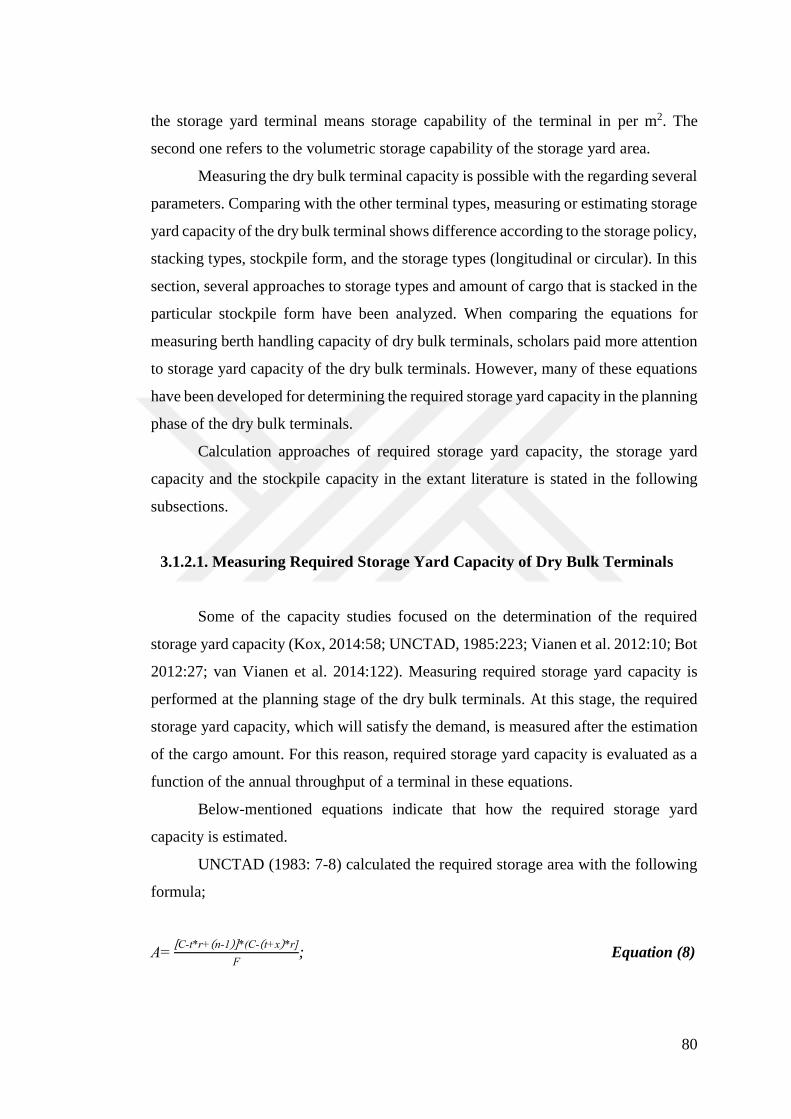
80

the storage yard terminal means storage capability of the terminal in per m2. The

second one refers to the volumetric storage capability of the storage yard area.

Measuring the dry bulk terminal capacity is possible with the regarding several

parameters. Comparing with the other terminal types, measuring or estimating storage

yard capacity of the dry bulk terminal shows difference according to the storage policy,

stacking types, stockpile form, and the storage types (longitudinal or circular). In this

section, several approaches to storage types and amount of cargo that is stacked in the

particular stockpile form have been analyzed. When comparing the equations for

measuring berth handling capacity of dry bulk terminals, scholars paid more attention

to storage yard capacity of the dry bulk terminals. However, many of these equations

have been developed for determining the required storage yard capacity in the planning

phase of the dry bulk terminals.

Calculation approaches of required storage yard capacity, the storage yard

capacity and the stockpile capacity in the extant literature is stated in the following

subsections.

3.1.2.1. Measuring Required Storage Yard Capacity of Dry Bulk Terminals

Some of the capacity studies focused on the determination of the required

storage yard capacity (Kox, 2014:58; UNCTAD, 1985:223; Vianen et al. 2012:10; Bot

2012:27; van Vianen et al. 2014:122). Measuring required storage yard capacity is

performed at the planning stage of the dry bulk terminals. At this stage, the required

storage yard capacity, which will satisfy the demand, is measured after the estimation

of the cargo amount. For this reason, required storage yard capacity is evaluated as a

function of the annual throughput of a terminal in these equations.

Below-mentioned equations indicate that how the required storage yard

capacity is estimated.

UNCTAD (1983: 7-8) calculated the required storage area with the following

formula;

A=[C-t*r+(n-1)]*(C-(t+x)*r]

F; Equation (8)

81

Where C is the ship capacity for cargo [ton]; t number of days that handling

operations are performed in the berth [day]; F is the stacking characteristics of the port

according to cargo type [ton/ha]; r is the arrival and departure rate of vehicles for the

land transport [ton/day]; n is the total vessel calls during a year [-]; x is the interarrival

time of the vessels [days].

Ligteringen and Velsink (2012:157) calculated the required area for general

cargo terminals with the following equations:

Agr=farea*fbulk*Nc*td

mc*hs*ρcargo*365; Equation (9)

Where Nc is the total cargo amount which is stored at the terminal [ton]; ρcargo

is the average density of the cargoes [ton/m3]; fbulk is the bulking factor caused by

stripping and stacking the cargoes separately [-]; farea is the ratio of the net and gross

area including traffic lanes; td is the average dwell time of the cargoes; hs is the average

stockpile height [meter]; mc is the estimated storage occupancy ratio [-].

Kleinheerenbrink (2012: 66) determined the required storage yard area based

on the size of pile lines:

required storage yard area=width of the stockyard*length of the stockyard; Equation (10)

wstockyard=npiles*(w+s)+s; Equation (11)

Where wstockyard is the width of the storageyard; w is the pile lane width; s is the

distance between the two pile lanes.

In addition to the approaches developed for estimating the storage yard

capacity of the dry bulk terminals, required storage yard area [m2] should be

determined to measure the required storage yard capacity. PIANC (2014) and Kox

(2017: 58-60) approached the required storage area capacity hereinbelow.

PIANC (2014) calculated the needed gross storage area with the following

equation (Kox, 2014:58):

Agr,i=Ci*td*farea

ρc*hs*365*ms; Equation (12)

82

Where Agr,i is the needed gross storage area for each cargo type [m2] (including

roads, the area occupied by the equipment, infrastructure, and superstructure); Ci is the

total amount of cargo handled in a year considering cargo type [ton/year], td is the

average dwell time of the cargo [days]; farea is the ratio of gross and net storage area;

ρc is the mean number of specific bulk density of the cargoes [ton/m3]; hs is the mean

number of stacking height [m]; ms is estimated storage occupancy ratio (the ratio is

calculated by the dividing average stack of the cargo in the stockpile to design capacity

of the stockpile) [-].

Kox (2017: 58) also transformed the Equation (12) into the below-stated

formula to measure the required storage volume in the cubic base:

Vstorage, i=Ci*td

ρc*365*ms; Equation (13)

Where Vstorage, i is the required storage volume per specific cargo type [m3], Ci

is the amount of the cargo handled in a year by cargo type [ton/year]; td is the average

dwell time of the specific cargo in the stockpile [days]; ρc is the mean number of

specific bulk density of the cargoes [ton/m3]; ms is estimated storage occupancy ratio

(the ratio is calculated by the dividing average stack of the cargo in the stockpile to

design capacity of the stockpile) [-].

Kox (2017: 59) utilized the following equation for calculating the needed gross

storage area according to cargo types:

Agr,i=nlanes*llane*wlane*farea

; Equation (14)

Where Agr,i is the needed gross storage area per cargo type [m2]; nlanes is the

total number of lanes; llane is the needed lane length [m]; wlane is the needed lane width

[m]; farea is the gross and net storage area ratio. Moreover, Kox (2017:60) proposed an

equation to calculate the gross required total terminal area regarding further areas such

as administrative buildings, terminal infrastructure, and superstructure:

At=∑ Agr,i

a; Equation (15)

83

Where At is the total storage area in m2 required for the terminal (along with

the area occupied by the stockpiles, infrastructure and superstructure of the terminal;

Agr,i is the gross needed area [m2]; a is the total terminal factor that refers to

percentage of gross storage area (including the roads within the stockpile) according

to the total area of terminal [-].

3.1.2.2. Measuring Storage Yard Capacity of Dry Bulk Terminal

In this section, the equations in the existing literature have been examined.

Limited study has been found in the literature to be used for estimating the storage

yard capacity of the dry bulk terminals.

National Research Council (1998:81) explained the functional relationship of

storage yard capacity of the terminals by using the below-mentioned equation:

Q4= QY

365 Equation (16)

QY=HC*365

TA;

HC=GH*SF

2000;

GH=NH*(1+SB);

NH=AA*AH;

AA=AS*SP;

AS=TS*(1-DS);

Where Q4 is the average cargo amount handled in storage yard [ton]; QY is the

annual cargo throughput handled in the storage yard [ton]. HC is the handling capacity

of cargo [ton]; TA is the average dwell time in the storage yard [day]; GH is gross

holding volume; SF is the stowage factor of the specific cargo; NH is the net holding

volume of the cargo; SB broken stowage factor (unused spaces); AA is the mean of

stacking area; AH is the mean number of stacking height; AS is the standard storage

area (regular); SP is the percentage of the total storage area which is utilized for

stacking; TS is the entire storage area; DS is the safety factor for demand fluctuations.

84

National Research Council (1998:81) approached the storage yard capacity of the dry

bulk terminal as the function of annual throughput achieved by the terminal.

Salminen (2013:32-33). developed another approach. The study assessed the

dry bulk and the general cargo terminal capacity in the same equation considering both

static and dynamic capacity of the terminal. Moreover, the study of the Salminen

(2013:32-33) measured both storage yard and warehouse capacity of dry bulk-general

cargo terminals based on theoric and actual capacities. For dry bulk yard capacity, the

study presented a series of equations as:

STDBY(mass)=sDBY

dDBY; sDBY=

rDBYtDBY

oDBY-mDBY

; Equation (17)

STDBY(volume)=dDBY*hDBY; Equation (18)

SADBY=STDBY*uDBY; Equation (19)

DTDBY(mass)=sDBY*

oDBY-mDBYtDBY

dDBY; Equation (20)

DTDBY(volume)=STDBY*tDBY

oDBY-mDBY; Equation (21)

DADBY=DTDBY*uDBY; Equation (22)

Where STDBY is the theoric capacity (static); SADBY is the actual capacity of the

dry bulk terminal (static); DTDBY is the theoric capacity of the dry bulk terminal

(dynamic); dDBY is the determined area for the terminal yard; hDBY is the stacking

implementations in the terminal; oDBY is the working days; mDBY is the nonworking

days; rDBY is the annual throughput; sDBY is the size of bulk commodities; tDBY is the

average idle time of dry bulk commodities; uDBY is the utilization lower limits.

In addition to storage yard capacity regarding the mass and volume, dry bulk

warehouse capacity as called by the Salminen (2013:33-34) estimated with the

following equations (Salminen, 2013: 33-34):

STDBWH(mass)=cDBWH

sDBWH; (The equation can be equals to cDBWH) Equation (23)

STDBWH (volume)=dDBWH*sDBWH; Equation (24)

SADBWH=STDBWH*uDBWH; Equation (25)

DTDBWH(mass)=STDBWH*oDBWH

tDBWH; Equation (26)

85

DTDBWH(volume)=STDBWH

tDBWHoDBWH

; Equation (27)

DADBWH(mass)=SADBWH*oDBWH

tDBWH; Equation (28)

DADBWH (volume)=DTDBWH*uDBWH Equation (29)

Where STDBWH is the theoric capacity of dry bulk terminal warehouse (static);

SADBWH is the actual capacity of the terminal warehouse (static); DTDBWH is the theoric

capacity of terminal warehouse (dynamic); DADBWH is the actual capacity of the

terminal warehouse; cDBWH is the size of the bulk commodities stored in the terminal

warehouse (i.e., maximum acceptable mass of bulk commodities); dDBWH determined

area for terminal warehouse; oDBWH is the working days in a year; sDBWH is the stacking

implementations; tDBWH is the average aligning time of the commodities at the terminal;

uDBWH is the utilization of lower limits for the dry bulk terminal warehouse.

UDHB (2015:235) used the below-mentioned equation when calculating the

storage yard capacity of the dry bulk and general cargo terminals:

KD=365

tk*Ad*hd*p*a*h*γ ; Equation (30)

Where KD is the annual storage capacity of the dry bulk or general cargo terminals

[ton]; tk is the average dwell time of the cargo at the terminal [day]; Ad is the storage

yard area [m2 or ha] hd is the average storage occupancy factor (0.50-0.80)[-]; p is the

occupancy reduction coefficient (0.80-0.85) [-]; a is the net storage coefficient (0.55-

0.85) [-]; h is the stacking height [-]; γ is the specific bulk density of the cargo [ton/m3].

3.1.2.3. Measuring Stacking Capacity of the Stockpiles

Apart from measuring the storage capacity of the dry bulk terminal area,

stockpile design and layout are important factors to achieve maximum storage

efficiency from the total terminal area. When estimating the storage yard capacity of a

dry bulk terminal, these factors should be taken into consideration. Several studies

(Kox, 2017:59), van Vianen et al. 2014:21; UNCTAD, 1985:189; Bot, 2012:27-28)

86

accounted the stockpile design to measure the mass of cargo stored at the dry bulk

terminals.

UNCTAD (1985:223) considered that the dry bulk terminals mostly utilized

the trapezoidal shape stockpiles. When calculating the stockpile capacity, UNCTAD

(1985: 223) assessed trapezoidal stockpile dimension with the following formula:

hmax=0.5*b*tan (α )

Amax=0.5*b*hmax= 0.25*b2 *tan (α)

A= r/hmax *(0.2)= r/hmax* Amax

Below-mentioned formula is obtained:

A=(b-h cot(α))h; or A=(b-rhmaxcot(α))rhmax;

A= (b-r(0.5 b tan (α)) cot(α))rhmax;

Amax=0.5bhmax Thus;

A=r (2-r)

Volume=A*length Equation (31)

Capacity in tons= volume

Stowage Factor Equation (32)

Where α is the angle of repose; h is the stockpile height; b is the base of

stockpile; hmax is the maximum stockpile height; r is the stockpile height and maximum

height ratio; A is the stockpile cross-sectional area; Amax is maximum cross sectional

area of stockpile.

Moreover van Vianen et al. (2012:10) transformed the UNCTAD (1985:181)

equation into the following equation:

m= [h

hmax(2-

h

hmax) (

1

4w2tanα) lρ] ; hmax=

𝑤tan(α)

2 Equation (33)

Where m is the stockpile mass; h is the stockpile height; hmax is the maximum

stockpile height; w is the stockpile width; α angle of repose; l is the stockpile length;

ρ is the specific bulk density.

87

Kox (2017: 60) developed an approach to specifying the required stockpile

volume for the particular material:

Vsp,i=Ci*rc

ρc

; Equation (34)

Where the Vsp,i is the needed storage volume of the stockpile according to

commodity type [m3];Ci is the annual throughput [ton]; rc is the capacity ratio which

shows the percentage of the total amount of cargo handled in a year that should be

stored at the terminal at a given time [-]; ρc is the average specific bulk density

[ton/m3].

Then, Bot (2012:27) modified UNCTAD (1985:223) equation to calculate the

stockpile length. Schematic representation of the components of the equation used for

determining the stockpile length is indicated in Figure 21.

Figure 21: View of an End Coned Trapezoid Stockpile from Top-Front-Side

Source: Bot, 2012:27

Lengthstockpile=Mass.Stowage Factor-

Π*l12

*h

3-l1*l2.h

(l1+l2)h*2l1; Equation (35)

l1=h

tan(α) And l2=b-

2h

tan(α);

Where b is the base of the stockpile (2l1+l2) [meter]; α is the angle of repose

of the stockpile of specific bulk commodity [o]; h is the height [meter]; l1 is the base

of right triangle part of the trapezoid [meter]; l2 is the distance between the two right

triangle part [meter].

88

Kox, (2017:59) determined the number of the lane that stockpiles are

positioned with the following equation:

llane=Vstorage

[hpile

hpile,max*(2-

hpile

hpile,max)*(

1

4wlane

2*tanθ)]*nlanes

; Equation (36)

Where llane required length of stockpile [meter]; Vstorage is the total required

storage volume [m3]; hpile is the stockpile height [meter]; wlane is the stockpile width

[meter]; θ angle of repose [o]; nlanes is number of stockpile lane [meter]; hpile,max is the

maximum height of stockpile can reach (= 1

2wlane*tanθ) [meter].

In addition to the trapezoidal shape of the stockpile, van Vianen et al.

(2012:10), van Vianen et al. (2014:122) regarded the end cones to their equation to

measure stockpile mass considering the shear effect of bulk commodities. The study

stated that trapezoidal shape with end cones is commonly used in practice rather than

the trapezoidal stockpiles. The equation is stated as follows:

m=hlρ (w-h

tan(α)) +

1

3ρΠ (

h3

tan2(α)) +ρh (w-

2h

tan(α))

h

tan(α); Equation (37)

Where m is the stockpile mass [ton]; h is the stockpile height [meter]; l is the

stockpile length (trapezoidal part) [meter]; ρ is the specific bulk density [ton/m3]; w is

the stockpile width [meter]; α is the angle of repose of bulk commodity [o].

Ligteringen and Velsink (2012: 218) calculated the stockpile capacity in cross-

section triangular pile form by using the below-mentioned equation:

V=b*1

2*h*l*mb; Equation (38)

Where V is the maximum volume of the cargo in the storage yard [m3]; b is the

stockpile width [meter]; h is the stockpile height [meter]; l is the sum of stockpile

length [meter]; mb is the utilization rate of the stockpile [-].

89

3.1.3. Equipment Capacity Measurement Approaches

In this section, the capacity measuring formulas of the equipment used in the

dry bulk terminals are examined. Although many equipment is used for the unloading

and loading operations at the dry bulk terminal, many of this equipment have similar

parts and similar working principles. For this reason, only fundamental calculation

principles of belt conveyor, screw conveyor, and reclaimer considered to the

evaluation of the equipment capacity. There is no study on the mobile harbour cranes

or modelling of mobile harbour crane motion in the existing body of the literature. For

this reason, the equation on an average number of gang per vessel (if the port does not

provide the total number of gang performed within a specific period) and the amount

of cargo (ton basis) per gang have been attempted to develop a formula in Chapter IV,

Section 4.2.1.3.

3.1.3.1.Belt Conveyor Capacity

As mentioned in the earlier sections, several types of belt conveyors can be

found in practice (T shape, U shape, Flatted, etc.). The shape of the belt conveyors

based on the idler drums laid under the belt.

Belt capacity is the function of the belt width, the speed of the belts, specific

bulk density of the materials, the troughing angle, surcharge angle and the angle of

repose, capacity factor, idler configuration and inclination angle (Tsakalakis and

Michalakopoulas, 2015:2; Scholtz, 2017: 966; Fenner Dunlop, 2009).

Apart from the factors which determine the belt conveyor carrying capacity

such as belt width, belt speed, specific bulk density and angle of repose, some other

important factors (surcharge angle, inclination angle, troughing angle and idler

configuration should be specified clearly. The angle of surcharge is crucial in

calculating the cross-sectional area. The angle of surcharge is defined as the dynamic

angle of repose. When materials loaded onto the belt surface, the material is agitated

with the movement of the belts. With the crossing over the carrying idler, the surface

of the materials is inclined to flatten the slope of the surface. This angle is less than

90

the angle of repose, and in practice, the range of the troughed conveyor belt conveyor

angles are 0o, 20o, 35o, and 45o (Schultz, 1985: 969).

Figure 22: Different Angle of Surcharge Values according to Material Characteristics

Source: CEMA; Tsakalakis and Michalakopoulas, 2015:2

The inclination angle is another important factor which determines the belt

conveyor capacity. Belt conveyor does not always establish the 0o angle. According

to the configuration, belt conveyor moves the inclination. The cross-sectional area of

the inclined load is less than the horizontal cross-sectional area of the load. A rough

estimation of the inclined load capacity of the belt conveyor can be calculated as

multiplying the horizontal load capacity by the cosine of the angle of inclination

(Cosθ). Troughing angle is the angle of idler rollers’ position according to a

horizontal plane. Idler configuration refers to several idlers used in the belt

configuration. Generally, belt configurations are flatted, three idler rollers or five

idler rollers in practice. However, three equal rolls are mostly used (Fenner Dunlop,

2009: 19).

The most important parameter for calculating the conveyor belt carrying

capacity is the cross-sectional area. Despite its complexity, several approaches have

been developed to measure the cross-sectional area of the material loaded onto the belt.

The cross-sectional area of the material loaded onto the belt that is perpendicular to

the belt surface is the crucial factor determining the belt conveyor capacity. The value

depends on the characteristics of the material, belt width, and the idler configuration

(Woodcock and Mason, 1987: 277). The most critical parameters, which are used to

calculate, cross-sectional area troughing angle, the angle of repose, and the angle of

the surcharge. The angle specifications of the materials are shown in Appendix I.

91

Figure 23: Schematic Representation of Cross-Sectional Area of the Material loaded onto the

3 Idler Belt Conveyor Configuration

Source: Schultz, 1985:970

Several studies developed calculation approaches to belt conveyor capacity

(Schultz, 1985: 969; Woodcock and Mason, 1987: 277; Fruchtbaum (1988: 23);

Fenner Dunlop, 2009:20). Calculation approaches of the belt conveyor capacity in the

literature are reviewed and stated as follows.

Schultz, 1985: 969 expressed the belt conveyor capacity as follows:

TPH=A*BD*S

4800; Equation (39)

Where A is the cross-sectional area of the material (perpendicular), [in2]; BD is

the specific bulk density of the materials [lb/ft3]; S is the speed of the belt [ft/min].

Woodcock and Mason, 1987: 277 expressed the flat belt conveyor capacity as

follows:

��s=ρbksAv

A=1

6b

2tanδ; Then,

��s=1

6ρ

bvb

2tan δ; Equation (40)

92

Where ��s is the belt conveyor carrying capacity [ton/s]; ρb is the specific bulk

density [ton/m3]; A is the average cross-sectional area of the material shape (the shape

is perpendicular to the belt surface) [m2]; v is the speed of the belt [m/s]; ks is the slope

factor [-]; b is the width of the flow of the load placed onto the belt (contact perimeter)

[m]; δ is the surcharge angle [o].

However, not all the belt conveyors only designed as a flat, but also two or

three troughing idler belts are widely used in practice. Calculation of the cross-

sectional area of the material loaded onto the belt can be measured as follows

(Woodcock and Mason, 1987: 279).

A=Ub2

��s=ρbksUb2v Equation (41)

Where b is the contact perimeter of the materials and U is the shape factor.

Although U can be clearly expressed as (tan δ

6), for two, three or five troughing belts,

it can be taken advantage from the conversion table to determine the shape factor.

Fruchtbaum (1988: 23) evaluated the belt conveyor carrying capacity for the

three rolling idler as follows:

e=0.055E+0.9(*)

Area of surcharge= F*E2

Total Area Ar=As+ FE2

Total capacity in ton=Arwv

2000; Equation (42)

(*)Empirical value differs according to the model of the belt conveyor.

Where e is the edge distance [in], E is the bottom length of the belt [in]; F is

the surcharge factor required for calculating the cross-sectional area of the

surcharge; w is the specific bulk density [lb/ft3]; v is the speed of the belt [fpm]; Ar

is the cross-sectional area; As is the cross-sectional area of the surcharged part of

the shape.

Fenner Dunlop (2009:20) used the below-mentioned formula to calculate

belt conveyor carrying capacity:

93

Capacity=3.6*Load Cross Section Area [m2]*Belt Speed [m/s]* Material Density

[kg/m3]

The load cross-section area differs according to the roll idler configuration.

For the three or five roll idler configuration below mentioned formula could be used

to calculate the carrying capacity of the belt conveyor in ton per hour (tph) (Fenner

Dunlop, 2009:20):

Capacity (tph)= Capacity (According to the belt width and belt speed)* Material Density

(kg/m3)* Capacity Factor*Belt Speed(m/s)/1000 (three idlers) Equation (43)

Capacity (tph)= Capacity (According to the belt width and surcharge angle)* Material

Density* Belt Speed/1000 (five idler) Equation (44)

In general sense, the equipment producers provide the capacity factor and

capacity according to the cross-sectional area in the equipment manual. The capacity

factors and the capacity according to the cross-sectional area are presented in

Appendix II.

3.1.3.2.Screw Conveyor/Unloader Capacity

As mentioned in the Chapter I section 1.2.1.4., screw conveyors are commonly

used equipment in the dry bulk terminals. The crucial parameters for calculating the

screw conveyor capacity are the diameter of the screw, the diameter of the outer

frame, specific bulk density, material factor, nature of the material (flowability, size,

abrasiveness miscellaneous or hazards) (See Appendix III), percentage of the filling

(trough loading), screw pitch, speed of the revs, types of the conveyor (sectional,

helicoid, cut flight, ribbon, and paddle) and the type of the pitch ( standard pitch,

variable pitch, short pitch, tapered flight, stepped flight, stepped pitch) (Fruchtbaum,

1988:141; Woodcock and Mason, 1987:344; Hinterlong and Sinden, 1985:1033;

94

KWS, 04.01.2016). Several types of conveyors and the pitches are illustrated in

Figure 24.

Figure 24: Types of the Screw Conveyor and Pitches

Source: Fruchtbaum, 1988:141

Screw conveyors contain several parts and consist of pipe, helix (flight), flight

mounting, etc. (Bucklin et al. 2013: 154; Hinterlong and Sinden, 1985:1035). Helix

means flight of the screw. Besides the distance between two helixes is denominated

as the pitch (Bucklin et al. 2013: 154). Flights of the screw conveyors can be

produced either helicoid or sectional. Helicoid flights are produced by rolling the

straight frame or lane thro rod into the running helix. Besides sectional flights are

produced from a straight disc (Hinterlong and Sinden, 1985: 1035). U shape or tube

shape implementations of the screw conveyor can be found in practice. The coverage

95

of the screws may be composed of the cylinder for tube coverage or trough for U

shape of screw conveyors (Bucklin et al. 2013: 154-155).

The usage of U shape conveyors or enclosed conveyors can differ according to

intended purposes and its flexibility. For example, U shape conveyors are the most

flexible choice for horizontal transport within the perspective of the easy of the

maintenance and economical reasons. However, it cannot be applicable for the

inclination angle greater than the 20o (Powder Bulk Solids, 21.02.2017).

Trough-loading refers to the percentage of the loading of the pitch. Trough

loading factor is crucial for the screw conveyor size. It is highly recommended that

the trough loading of the abrasive materials should be kept a minimum filling

percentage, whereas nonabrasive materials may be kept higher levels of trough filling

(KWS, 04.01.2016). Several trough-filling configurations and particular materials in

accordance with the filling rates are shown in Table 9:

Table 9: Through Filling Configurations with regard to Material Characteristics

Material Characteristics Trough

Filling

Rate [%]

Schematic

Illustration Density

[lbs/ft3]

Material Type Abrasiveness* Flowability**

50-120 Alumina, glass cullet,

potash

Extremely Hard 15

15-60 Carbon black, spent

brewer grain, fish meal,

Mildly Free-flowing 30A

30-80 Flue dust, crushed

bauxite, cement clinker

Very Average 30B

5-40 Baking soda, alfalfa,

hulled rice

Non Very 45

Source: KWS, 04.01.2016

*Abrasiveness: Mildly: 1-17; Moderately: 18-67; Extremely: 66-416

** Flowability: Very Free Flowing-Flow Function>10; Free Flowing-Flow Function>4

but<10; Average Flowability-Flow Function>2 but<4; Sluggish-Flow Function<2 (FMC

Technologies (2009:25-34)

The inclination of the screw conveyor is also essential in terms of the

horsepower and the capacity. The angle of inclination is essential for equipment to

be called vertically. In some resources, the inclination angle should be greater than

96

200 (Woodcock and Mason, 1987; 354) while other sources accept screw conveyor

as vertical with upper than 350 inclination angle (Fruchtbaum, 1988: 154) or 70o-90o

(Fayed and Skocir, 1997) or 45o (Powder Bulk Solid, 04.04.2019). The capacity of

the screw conveyors decreases with increasing inclination angle. According to Fayed

and Skocir (1997), the screw conveyor losses efficiency between the 20% and 50%.

According to Bucklin et al. (2013: 154-155), the gradient changes in capacity

efficiency of the screw conveyors are illustrated in Table 10:

Table 10: Rate Changes of the Screw Conveyors with regard to Inclination Angle

Inclination

Angle [o]

The rate of

Change of

Capacity [%]

Reference

10-20 10-40 Powder Bulk Solids, 21.02.2017; KWS, 04.01.2016

15 30 Bucklin et al., 2013: 155-154

15 25 Kase Conveyor, 03.04.2019

25 55 Bucklin et al., 2013: 155-154

25 50 Tomaskova and Sinay, 2014: 228; Kase Conveyor,

03.04.2019

30 10-70 Powder Bulk Solids, 21.02.2017; KWS, 04.01.2016

45 30-90 Powder Bulk Solids, 21.02.2017; KWS, 04.01.2016

Source: Compiled from several sources

Apart from the inclination angle, the other capacity factors such as mixing

peddle, type of flight, the shape of the coverage (U or cylinder) also affect the mass

throughput of the equipment. For this reason, when calculating the screw conveyor

capacity, the equipment capacity tables should be used similar to capacity

calculations of belt conveyors.

Various calculation approaches can be found in the existing literature. The

calculation approaches are examined as noted below.

Hinterlong and Sinden (1985), CEMA, 2003: 19-45 and Wable and Kurkute

(2015: 293) and determined the capacity of the screw conveyors with the following

equation:

97

C

rpm=

0.7458 (Ds2-Dp

2)P K 60

1728 Equation (45)

Where C denotes the capacity [ft3/hr]; rpm is the revs of the screw per minute

[revs/min]; Ds is the screw diameter [in]; Dp is the diameter of the tube [in]; P is the

distance between the pitches [in]; K is the percentage of the referenced trough loading

[%, e.g., 0.45, etc.]

Woodcock and Mason (1987:340) attempted to calculate encloased screw

conveyor speed with the following formula:

��s=Π

4(Dc

2-Dsh2 )(λ-ts)N; Equation (46)

Where Dc is the diameter of the screw; Dsh is the diameter of the outside of the

conveyor which the screw is embedded; λ is the screw pitch, ts is the thickness of a

screw, N is the speed of revolution [revs/s]. Moreover, the research of Woodcock and

Mason (1987: 346) stated the velocity of the screw conveyor; then the calculated the

volumetric throughput of the U shape screw conveyor equipment as:

𝑈 = λN;

��s=AbλN;

Moreover, mass flow rate of the screw conveyor can be calculated finally by

using Equation (47):

��𝑠 = 𝜌𝑏𝐴𝑏λN; Equation (47)

Where U is the average speed of the screw, λ is the screw pitch (the distance

between the two flights); N is the speed of the revolution; Vs is the volumetric

throughput of the equipment; ms is the mass flow rate of the equipment; Ab is the cross-

sectional area of the material which is moving between the two flights; 𝜌𝑏 is the

specific bulk density of the material. When including the cross sectional area into the

formula of the mass flow rate, below-stated equation can be obtained:

98

��s=𝜌𝑏1

4𝛱(Dc

2-Dsh2 )kλN Equation (48)

Where k is the filling factor [%]. The further specific type of screw conveyor

can be used in practice. It also has an effect on the screw conveyor capacity. If the

special type of the flight and the mixing paddles positioned into the flights are

considered for the capacity of the screw conveyors, Equation (48) then becomes as

follows:

��s=ρb

1

4Π(Dc

2-Dsh2 )

kλN

CFfCFm; Equation (49)

Where CFf is the factor of particular types of flight; CFm is the factor of the

mixing paddles positioned into the flights. For the standard screw conveyor type, the

value of CFf should be taken as 1.

Bates (2008: 206) measured the effective screw conveyor capacity with the

following equation:

Effective conveyed volume per revs=0.45*3.142/4 (D2-K2)P Equation (50)

Where K is the outer screw diameter (d or D*tan*ɸw), P is the flight; d is the

shaft diameter, ɸw denotes the side friction of the bulk commodities on the flight

surface.

Bucklin et al. (2013: 155) calculated the theoretical capacity of screw conveyor

considering filling factor 100% with the following equation.

Ccap=(D2-d

2)PN

36.6; Equation (51)

Where Ccap refers to the volumetric capacity of the screw conveyor (filling

factor 1.0) [ft3/h]; D is the screw diameter [in]; d is the shaft diameter [in]; P refers to

pitch (the value is the generally equals to D); N is the revs per minute.

Vav (24.02.2019) calculated the screw conveyor capacity as follows:

99

Q=3.14*D2

4*s*n*sg*i*60 Equation (52)

V= Screw Diameter*3.14*Rotations Per Minute

60; Equation (53)

Where Q is the capacity of the equipment [kg/h]; D is the diameter of the screw

[dm]; s is the pitch [dm]; n is the number of revs [revs/min]; sg is the specific bulk

density [g]; i is the trough filling factor [-], and V is the speed of the screw conveyor

[m/s].

According to German DIN 15262 (Minkin et al. 2017:88), screw conveyor

equipment capacity is calculated as follows:

lm=ds2 Π

4vFρ

b; Equation (54)

vs=ns*lst;

Where lm is the mass of throughput [t/h]; ds is the outer diameter of the screw

[m]; vF is the velocity of conveying [m/s]; ρb is the specific bulk density of the material

[kg/m3]; vs is the ideal speed of the conveying [m/s]; ns refers to revs speed of the

screw [rps, rpm]; lst is the pitch [m].

Bolat and Boğoçoğlu (2012:2) and Tomaskova and Sinay (2014: 228)

mathematically expressed the approximate efficiency of the related equipment as:

Q=π

4.(D2-d

2).S.n.ρ.ѱ.k; Equation (55)

Where Q is the mass of throughput [m3/s]; D is the diameter of the screw [m];

d is the shaft diameter [m]; S is the pitch of screw [m]; n is the speed of revs [rpm]; ρ

is the specific bulk density; ѱ is the filling factor of the screw conveyor [%]; k is the

incline factor [-]. k or C (capacity factor termed in the Tomaskova and Sinay

(2014:228) as “C”) used only the inclination occurred. In the horizontal screw

conveyor, the factor may not be used.

100

3.1.3.3.Pneumatic Conveyor System Capacity

Several flow modes can be found in practice. These are dilute phase (positive

pressure, negative pressure or vacuum and negative-positive combination), and dense

phase (Bhaita, 05.04.2019; Woodcock and Mason, 1987: 386; Mills, 2004:5; Pan,

1999:157)

Dilute phase flow mode is commonly used for transferring the materials. In the

dilute phase conveying method, high mass of flow is achieved based on the material

characteristics and the air velocity of the conveying with a high flow speed and low

pressure while the materials are suspended in the air (Bhaita, 1986: 18; Woodcock and

Mason, 1987: 386; Fruchtbaum, 1988:429; Mills, 2004:5). However, this system

conveys a high amount of air and a small amount of particles. Due to achieving the

high velocities, dilute phase implementations needs a higher power to perform the flow

(Bhaita, 1986: 18), and running costs are much higher than the mechanical conveyors

(Woodcock and Mason, 1987:392).

In the dense-phase, the system needs to fewer velocities and enables cleaning

performance more efficiently. Fluidized dense-phase flow mode is an option that is

more suitable when there are long distance implementations to minimise airflow,

power, and speed of the transport. However, for materials, which are not suitable for

the fluidized dense-phase, flow, dilute-phase or by-pass can be seen as another choice

(Wypych, 1999: 284:285). Manufacturers and designers heavily tend to use of dense-

phase pneumatic conveying systems in terms of lower air consumption. Thus, the

running costs can be decreased (Woodcock and Mason, 1987: 393; Fruchtbaum, 1988:

434).

The capacity measuring of the pneumatic systems is more complicated

comparing to other equipment types. The factors determining the conveying capacity

of a pneumatic system are material characteristics, air flow rate, material flow rate,

mass flow rate ratio, diameter of the pipe, and velocity (Wypych, 1999:283; Pan,

1999:158-159; Raj P et al. 2017: 248-250; Mills, 2004: 5-13)

However, the most important efforts to calculate the pneumatic conveyor is to

the determination of the velocity of the particles and the air flow within the pipe.

Scholars mostly attempted to calculate the velocity of the airflow and solid flow. The

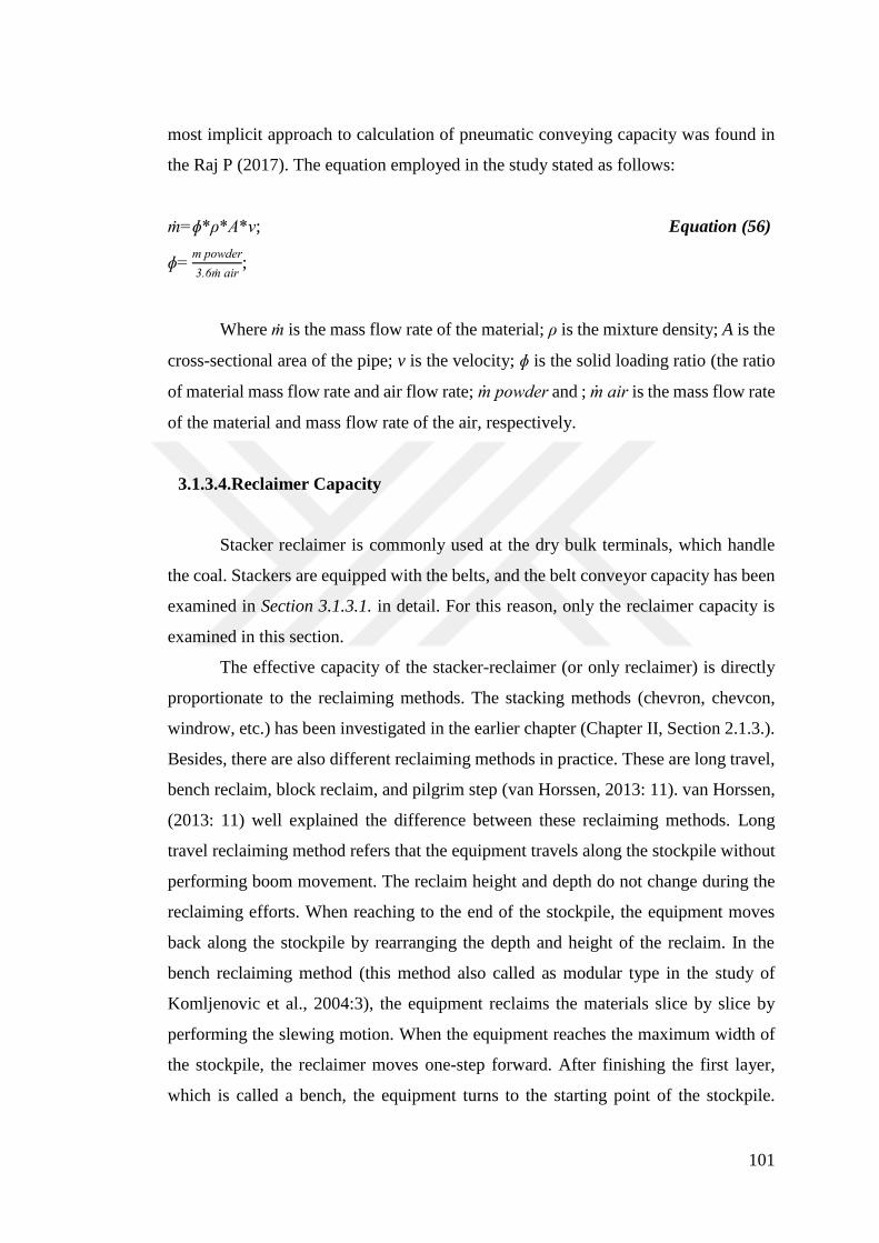
101

most implicit approach to calculation of pneumatic conveying capacity was found in

the Raj P (2017). The equation employed in the study stated as follows:

ṁ=ɸ*ρ*A*v; Equation (56)

ɸ=m powder

3.6ṁ air;

Where ṁ is the mass flow rate of the material; ρ is the mixture density; A is the

cross-sectional area of the pipe; v is the velocity; ɸ is the solid loading ratio (the ratio

of material mass flow rate and air flow rate; m powder and ; m air is the mass flow rate

of the material and mass flow rate of the air, respectively.

3.1.3.4.Reclaimer Capacity

Stacker reclaimer is commonly used at the dry bulk terminals, which handle

the coal. Stackers are equipped with the belts, and the belt conveyor capacity has been

examined in Section 3.1.3.1. in detail. For this reason, only the reclaimer capacity is

examined in this section.

The effective capacity of the stacker-reclaimer (or only reclaimer) is directly

proportionate to the reclaiming methods. The stacking methods (chevron, chevcon,

windrow, etc.) has been investigated in the earlier chapter (Chapter II, Section 2.1.3.).

Besides, there are also different reclaiming methods in practice. These are long travel,

bench reclaim, block reclaim, and pilgrim step (van Horssen, 2013: 11). van Horssen,

(2013: 11) well explained the difference between these reclaiming methods. Long

travel reclaiming method refers that the equipment travels along the stockpile without

performing boom movement. The reclaim height and depth do not change during the

reclaiming efforts. When reaching to the end of the stockpile, the equipment moves

back along the stockpile by rearranging the depth and height of the reclaim. In the

bench reclaiming method (this method also called as modular type in the study of

Komljenovic et al., 2004:3), the equipment reclaims the materials slice by slice by

performing the slewing motion. When the equipment reaches the maximum width of

the stockpile, the reclaimer moves one-step forward. After finishing the first layer,

which is called a bench, the equipment turns to the starting point of the stockpile.

102

Despite its resemblance to the bench reclaiming, the equipment does not travel until

the end of the stockpile in block reclaiming method. When reaching a certain distance,

reclaimer equipment moves backward to reclaim the next layer. Pilgrim step method

of the reclaim is another method of the block reclaim. However, reclaimer travels back

after performing the particular slewing motions in the pilgrim method. Generally,

slewing motions comprise of even numbers (6, 8 or 10). While the reclaimer moves

back, the boom of the equipment is positioned above the rails with the same angle of

rail (van Horssen, 2013:11-13; Komljenovic et al., 2004:3). The difference of these

methods are schematically illustrated in Figure 25:

Figure 25: Schematic Illustration of the Difference between the Bench, Block and Pilgrim

Step Reclaiming Methods

Source: van Horssen, 2013:13

A limited research streams have been found in measuring reclaimer capacity.

Although the calculation of the theoretical capacity seems simple, the effective

capacity of the reclaimer is a little bit complex. The approaches to calculating the

reclaimer capacity are investigated as follows:

van Horssen (2013: 3) evaluated the reclaiming capacity of the reclaimer as:

Q=A*v; Equation (57)

Q=V

∆t; Equation (58)

103

Where Q is the current reclaiming capacity [m3/s]; A is the cross-sectional area

of the piece at the specified point [m2]; v is the current velocity of the bucket [m/s].

Equation (58) calculates the reclaiming capacity of each segment where V is the

volume of each segment [m3]; ∆t is the time when the segment is reclaimed [s]. The

important parameter when calculating the reclaiming capacity is the determination of

the cross-sectional area. van Horssen (2013:18) stated the formula of the cross-

sectional area of a slice as follows:

A=rb2(π-(2.cos-1 (

∆r

2rb) - sin (2.cos-1 (

∆r

2rb) ); Equation (59)

Where rb is the radius of the bucket wheel [m]; h is the reclaim height [m]; ∆r is the

thickness of the slice [m]. As illustrated in Figure 25, ∆r can be equals to the length

of the bucket edge. Each of the variables used in the calculation of the cross-sectional

area of a slice illustrated in Figure 24:

Figure 26: Schematic Representation of the Cross-Sectional Area Variables

Source: van Horssen, 2013:18

Komljenovic et al. (2004) studied the effective reclaiming capacity. The study

stated the theoretical capacity of the reclaiming as follows:

104

Qt=60. Er . ni Equation (60)

Where Qt is the theoretical reclaiming rate [m3/h]; Er is the volume of the

bucket; discharge density of buckets [1/min]. Komljenovic et al. (2004: 3) stated that

the effective capacity of the reclaimer is more important than the theoretical capacity

of the equipment in terms of reflecting the real world situations. According to

Komljenovic et al. (2004: 9), the general formula of the effective capacity of the

reclaimer is stated as below:

Qeff

=V

tk+tm; Equation (61)

Where Qeff is the effective reclaiming capacity [m3/ton]; V is the mass volume

of reclaimed material [m3]; tk is the digging time taken by a cut [h]; tm is the

maneuvering time the equipment during the reclaiming operation [h]. Equation (52)

can be employed in the bench type, and block method is reclaiming.

3.1.4. Other Related Factors Used in Measurement of Dry Bulk Terminal

Capacity

As mentioned in Chapter II and Section 2.2. several factors have an impact on

the terminal capacity. However many factors cannot be measured or modeled.

Generally modeled parameters are berth occupancy ratio, peak factor ship turnaround

time, storage yard utilization and turnover rate. For this reason, only the parameters

which can be expressed or be reflected in the equations are examined in this study.

3.1.4.1. Berth Occupancy Ratio

The term berth occupancy ratio (BOR) describes the percentage of time that

a group of berth facilities is occupied by the ships to be serviced (Tsinker, 2004: 33).

In another word, the berth occupancy rate shows the utilization degree of the berth (de

Weille and Ray, 1968: 5). While 25% of the berth occupancy rate signs the

underutilization of the resources, 70% of the berth occupancy value can be regarded

105

as a sign of congestion (de Langen and Helminen, 2015: 20). The optimum value range

of the BOR is 60-70% (India Ministry of Shipping, 2011: 73). Throughput

requirements and locational constraints determine the optimum rates (Zamanirad et al.

2017: 21). This indicator also shows the level of average service rate that higher levels

of average service rate signs low berth occupancy rates, but lower service rates suggest

higher berth utilization levels (Layaa and Duallert, 2014: 151). The higher utilization

levels may be the consequence of either traffic intensity of the port or slower

operations. It creates excessive service time and the higher demurrage costs for the

port authority (Jagerman and Altiok, 2003:224).

Although berth occupancy ratio is a performance indicator of a terminal, it is

commonly used in measuring berth handling capacity. Researchers developed several

approaches to measure BOR. These approaches are based on the queuing theory or

empirical expressions of the current situations. In this section, several approaches to

berth occupancy ratio, and the variables used to calculate berth occupancy rate is

examined.

Tsinker (2004: 33) assumed that the M/E2/n queue model is suitable to measure

berth occupancy level of the berths and expressed the berth occupancy formula as:

ko=λµ

n ; Equation (62)

Where ko is the occupancy factor of a berth; λ is the average arrival rate per

day; µ is average service time per ship; n is the number of berths. Similarly, de Weille

and Ray (1968: 5) emitted Equation (62) as a berth occupancy ratio. However, they

regarded the time as a yearly basis as well as de Langen and Helminen (2015: 20). The

equation of de Langen and Helminen stated as follows:

BOR(%)= μ(in days)

n*

100

360 days Equation (63)

Where µ is servicing time at berths (total time of ships at berths); n refers the

total number of the berth.

106

India Ministry of Shipping (2011: 73) refers to the BOR formula in the report

on “Performance Audit of Functioning of Major Port Trust in India of Union

Government”. The equation is:

the time that berth is utilized

total available time ; Equation (64)

It can be deduced from this implicit formula that the “time that berth is

utilized” regards only the times when the berth is used. “Total available time” is

considered as the working days in a year or observed period.

Gurning and Fikri (2016: 10) considered the below-mentioned formula when

assessing the BOR to obtain optimum throughput:

BOR= Vs*St

Effective time*n*100% Equation (65)

Where Vs is a total number of ships served in a year [unit/year], St is service

time [hours/days]; “Effective Time” is total berthing time in a year [h]. The equation

of Gurning and Fikri (2016:10) is similar to Tsinker (2004:33) and de Langen and

Helminen (2015:20). However, apart from Tsinker (2004: 33) and de Langen and

Helminen, Gurning and Fikri (2016:20) evaluated all the variables in a yearly basis

rather than distributional rates and regarded the effective time at the berth, not the 360

days fully (2015:20).

Chung (1993: 5) assessed berth occupancy ratio as:

BOR %= Total time that ships work

Total time of ships alongside*100; Equation (66)

According to Equation 66, Chung (1993:5) developed a formula based on the

time spent by the ships at the berth rather than the probabilistic evaluation of the ship

arrival rate and service rate.

National Research Council (1998:81) assessed the berth occupancy ratio with

the following equation:

107

BOR=O2

Y2; Equation (67)

Where O2 indicates the number of days, the berth is occupied within a year; Y2

is the operational time in a year (total working hours in a year). National Research

Council (1998:81) considered BOR as a function of the total amount of cargo handled

at the terminal. However, other factors such as vessel and quay lengths, idle times at

the berth, waiting time, service time, etc. did not consider. This equation is similar to

the equation used by Chung (1993:5) (Equation 66).

Tang et al. (2016:175) calculated the BOR based on the average waiting time

and average service time as:

BOR=AWT

AST ; Equation (68)

Where AWT refers to the average waiting time of the vessels at the berth; AST

is the average service time offered to vessels at the berth.

Timur (2017:2) used the below-mentioned formula:

BOR= (Vs*St

H*n) 100% Equation (69)

Where Vs is the number of vessels called in a year [-]; St is service time [h/d];

H refers to working days in a year [d]; n is the number of the berth [-]. This approach

is the same as de Langen and Helminen (2015:20) and Gurning and Fikri (2016:10).

Radmilovic and Jovanovic (2006:101) formulated the BOR in their study as:

ρ=λᾱ

µc ; Equation (70)

Where ρ is the berth occupancy ratio; λ is the average arrival rate of ships; µ is

the average service rate of containers; ᾱ is the mean number of containers at each set

in the queue system; c is the number of service channel. The study considered the ship

arrival or container groups and the average quantity of the containers in each group

(group sizes regarded as random variables).

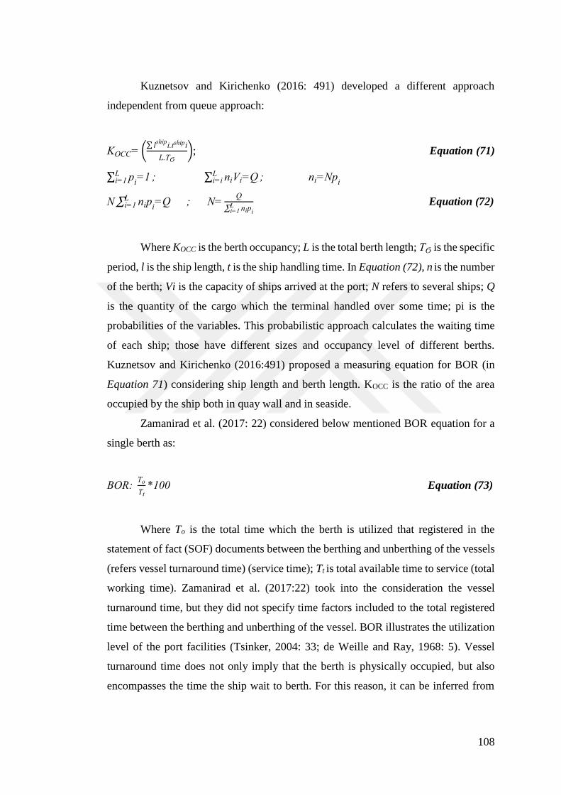
108

Kuznetsov and Kirichenko (2016: 491) developed a different approach

independent from queue approach:

KOCC= (∑ l

shipi.tshipi

L.TϬ); Equation (71)

∑ pi=1L

i=1 ; ∑ niVi=QLi=i ; ni=Np

i

N ∑ nipi=QL

i=1 ; N=Q

∑ nipiLi=1

Equation (72)

Where KOCC is the berth occupancy; L is the total berth length; TϬ is the specific

period, l is the ship length, t is the ship handling time. In Equation (72), n is the number

of the berth; Vi is the capacity of ships arrived at the port; N refers to several ships; Q

is the quantity of the cargo which the terminal handled over some time; pi is the

probabilities of the variables. This probabilistic approach calculates the waiting time

of each ship; those have different sizes and occupancy level of different berths.

Kuznetsov and Kirichenko (2016:491) proposed a measuring equation for BOR (in

Equation 71) considering ship length and berth length. KOCC is the ratio of the area

occupied by the ship both in quay wall and in seaside.

Zamanirad et al. (2017: 22) considered below mentioned BOR equation for a

single berth as:

BOR: To

Tt*100 Equation (73)

Where To is the total time which the berth is utilized that registered in the

statement of fact (SOF) documents between the berthing and unberthing of the vessels

(refers vessel turnaround time) (service time); Tt is total available time to service (total

working time). Zamanirad et al. (2017:22) took into the consideration the vessel

turnaround time, but they did not specify time factors included to the total registered

time between the berthing and unberthing of the vessel. BOR illustrates the utilization

level of the port facilities (Tsinker, 2004: 33; de Weille and Ray, 1968: 5). Vessel

turnaround time does not only imply that the berth is physically occupied, but also

encompasses the time the ship wait to berth. For this reason, it can be inferred from

109

the formula that the study assumed that vessel berthed just after it arrived at the port.

Considering this statement, To can be interpreted as service time at berth.

Layaa and Duallert (2014:151) explained the correlation between berth

occupancy and service rates as:

ϴ=λ

µK Equation (74)

Where ϴ is the BOR; λ refers to the average arrival rate of the vessels, µ is the

average service rate; and K is the number of a service channel in the port (berth). Layaa

and Duallert (2014:151) analyzed the BOR from the viewpoint of the queuing

approach as de Langen and Helminen (2015: 20).

Metalla et al. (2012: 62) considered BOR as hourly-occupied meters:

BOR= [∑ Service time in port (hrs*meters used)

∑ Available hours*meters] *100 ; Equation (75)

Apart from the queuing approach, Metalla et al. (2012:62) considered the

meters used by the vessels during the total service time and divided the total available

meters of the quay wall during the total available time to serve.

Thoresen (2003: 332) evaluated the BOR as:

BOR=TWTC*100

BN*WD*WH

SCS

; Equation (76)

BOR=GSTS*100

BN*WD*WH Equation (77)

Where TWTC is total working hours between arrival and departure time of the

vessel from/to berth; BN is the number of the berth; WD is the working days in a week;

WH working hours in a day; SCS is the total number of container ships berthing in a

week; GSTS is total quay cranes working hours in a week regarding peak factor. In

Equation (76), Thoresen (2003: 332) considered nearly the same approach with the

Layaa and Duallert (2014:151), Timur (2016:2), Gurning and Fikri (2016:10), Tsinker

(2004: 33) and de Langen and Helminen (2015: 20) except for weekly calculation of

110

berth occupancy. In Equation (77), crane working hours are distributed between berths

by total time worked per week.

In the formulation of Saanen (2004:102), berth occupancy ratio assessed as:

BOR=∑ Vessel Lengthi*Vessel Service Timei

ni=1

Quay Lenght*Measurement Period ; Equation (78)

Where n is the total number of the vessels berthed in a specific period (i.e., a

year); “vessel service time” refers to the total berthing time of the vessels (service

time). In this formula, the length of the quay occupied by vessels within a specified

period was calculated by time. According to Saanen (2004:102), alternative

measurement approaches poorly calculate berth occupancy due to disregarding vessel

length. Since, either one or two vessels may berth on the same berth at a different time.

3.1.4.2.Ship Turnaround Time

Ship turnaround time is the main indicator of vessel performance (Chung,

1993: 1), and identified as a total time spent by ships from entering time to departure

time at the port. It is also affected by all services offered to the vessel as well as waiting

time at the port and additional delays (de Langen and Helminen, 2015: 18; India

Ministry of Shipping, 2011: 65; Mwasenga, 2012: 4). As an efficiency indicator, ship

turnaround time creates financial value for both ship owner/charterer and port (de

Langen and Helminen, 2015: 18). Ship turnaround time does not mean only the idle

time spent at the port but also affected by cargo volume, port facility conditions, and

cargo nature (Chung, 1993: 1). In this section, measurement approaches to ship

turnaround time are reviewed to perform more accurate estimation of berth occupancy

rate by specifying the functions of the waiting time and service time.

Figure 27 illustrates the schematic portrayal of ship turnaround time:

111

Figure 27: Schematic Representation of Ship Turnaround Time

Source: India Ministry of Shipping, 2011:69

Ship turnaround time covers all times which spent by a vessel at the port. Ship

turnaround time (TAT) is calculated as follows (de Langen and Helminen 2015:18;

Radmilovic and Jovanovic, 2006):

TAT= Tw+ Tb+ Tber+ Tunber Equation (79)

Where Tw is waiting time for the berth, Tb is the servicing time at the terminal,

Tber is berthing time of a vessel, and Tunber means the unberthing time of a vessel.

3.1.4.3.Service Time

Service time refers to the period that the ship serviced at the berth. Thus, service

time as a function of the time depends on the amount of cargo to be loaded to ship or

112

unloaded from the ship, specifications of the ship, cargo characteristics, design

efficiency of equipment and other related resourced utilized at the berth (Mwasenga,

2012: 6). As a function of the total amount of cargo, service time, thus the total amount

of cargo, affects the waiting time of other vessels that are currently waiting in the

queue. Average service time may show the utilization level of the terminal

superstructure. While long service time is the sign of low utilization level, short service

time is assumed as high utilization level of the terminal superstructure (Layaa and

Duallert, 2014:150). This parameter determines the berth occupancy level of the

berths.

Zamanirad et al. (2017:22) used the below-mentioned formula to calculate

service time:

To= ∑ (Tunberthed-Tallmadefast)ini=1 ; Equation (80)

alternatively, in dry bulk terminals;

To=A.T.

PB+Ns*Tother ; Equation (81)

Where Tunberthed is the official recording time that the ship departed from the

berth; Tallmadefast is the time the ship berthed and ready for cargo operations and

inspections; i is a total number of the ship berthed within the specific period. In

Equation (47), A.T. refers to the total amount of cargo which berth(s) handled in a

year; PB is the productivity of quay equipment [ton or TEU per hour]; N is the total

number of vessels berthed within a year; Tother is the time spent to perform inspections,

surveys, clearance, and documentation.

Wanhill (1976: 121) stated the total time required for service to V vessels

during the given T (days) (S) is:

S=( (Q

r) +γV); Equation (82)

113

Where r is the average handling rate per day; y is the fraction of a day needed

for berthing and unberthing a vessel; Q is the total amount of cargo to be handled over

T days; V is the number of vessels called to the port.

Then the service time (s) required per day expressed as follows:

s= 1

T(

Q

r+γV) =

q

r+γλ Equation (83)

Where the q refers to the total amount of cargo to be discharged daily; 𝜆 shows

the mean of ship arrival per day. Service time per ship (1

𝜇) can be expressed as:

1

µ=

s

λ=

q

λr+γ ; Equation (84)

Where q

λ=G. G refers to the average amount of cargo per vessel.

3.1.4.4.Storage Yard Utilization

Apart from the storage yard utilization which indicates the utilization level of

storage, storage occupancy term found in the dry bulk terminal (Mwasenga, 2012: 15).

Apart from the berth utilization, Beaumont (2017:49) assessed storage yard utilization

as the utilization degree of the remaining available areas. An excessive level of storage

yard utilization affects the service time of the cargoes and leads to congestion at the

storage yard area (Raballand et al. 2012:70).

This term is expressed as proportionally in the literature (Ligteringen and

PIANC Velsink, 2012:157; PIANC, 2014; Kox, 2017: 58):

Net Storage Area

Gross Storage Area; Equation (85)

Net storage area refers to the areas only used for the storage, whereas gross

storage area includes both internal roads, buildings, and all facilities.

Besides PIANC (2014) assessed the storage yard utilization in terms of the

stockpile. The approach addressed the occupancy factor in the dry bulk terminals in B

114

Storage occupancy=Average mass of cargo in the stockpile

Design capacity of the stockpile; Equation (86)

3.1.4.5.Turnover Rate

The turnover rate represents the replenishment rate or replenishment rate of a

storage yard within a certain period. This also means that the port can stack the

materials directly proportionate to the turnover rate. Turnover rate added to the

equations as a multiplier. Turnover rate is closely linked to the dwell time of the

cargoes, and it expressed in the literature as follows (UDHB, 2015b: 235; Salminen,

2013:32-34; National Research Council (1998:81; PIANC, 2014; Kox, 2017:58;

Ligteringen and Velsink, 2012:157):

dwell time

365 or

365

dwell time; Equation (87)

Total days in a year (365) was represented in some studies as effective days.

3.1.4.6.Peak Factor

Peak factor refers to the peaks of the throughput volume during a certain time

in a year (Scholtz, 2017:51). Due to demand fluctuations of cargo, throughput level

shows difference over the observed time. This situation leads complexity in capacity

usage during the peak periods of cargo throughput.

Peak factor has two effects on the capacity. The first one is the boosting effect

on the capacity. When measuring the required storage yard area, berth handling

capacity peak factor can be used as boosting factor. Because when making the required

capacity calculation for a certain amount of load, planning should be performed

considering the increase caused by demand fluctuations. The results shows how much

capacity can be supplied for the certain volume of cargo. Accordingly Tsinker

(2004:34) and Scholtz (2017:51,83,90,96), used the peak factor as a multiplier to

determine required storage yard and required container ground slot, respectively.

115

However, when determining the maximum or realizable capacity of a terminal, peak

factor has a limiting effect on the capacity. For this reason, it indicates how much

capacity the port will supply against the demand fluctuations when demand is peak.

According to Scholtz (2017: 127), peak factor is calculated by dividing the

monthly peak throughput volume by mean number of throughput volume for each

month during the observed period.

3.2. EVALUATION OF THE CAPACITY MEASUREMENT EQUATIONS

In this section, the equations obtained from the literature, and the variables used

in measuring the dry bulk terminal capacity are determined. Parameters used in

measuring both berth and storage yard capacity are analyzed. Besides existing

equations related to the berth occupancy ratio are mathematically expressed.

3.2.1. Evaluation of the Berth Handling Capacity Measurement Equations

With the reviewing of the different calculation equations, variables used for the

measure the berth handling capacity is summarized in Table 11.

Table 11: Variables Accounted in Measuring Berth Handling Capacity

Variable Reference

Number of the Equipment UDHB, 2015b: 231; KMI (1998); Park et al. 2014:181

Number of Berth Park et al. (2014:185)

Equipment Productivity UDHB, 2015b: 231; KMI (1998); Park et al. 2014:181;

Ligteringen and Velsink (2012:155)

Crane Efficiency KMI (1998); Park et al. 2014:181

Equipment Utilization KMI (1998); Park et al. 2014:181

Occupancy Ratio of Particular

Cargo

KMI (1998); Park et al. 2014:181

Working Hours

UDHB, 2015b: 231; National Research Council,

1998:91; KMI (1998); Park et al. 2014:181; Ligteringen

and Velsink (2012:155)

116

Table 11: Variables Accounted in Measuring Berth Handling Capacity (Continued)

Working Days National Research Council, 1998:91; KMI (1998); Park

et al. 2014:181

Berth Occupancy Rate

UDHB, 2015b: 231; National Research Council,

1998:91; KMI (1998); Park et al. 2014:181; Ligteringen

and Velsink (2012:155)

Total Days the Berth is

Utilized

National Research Council, 1998:91

Average Amount of Cargo per

Ship

UDHB, 2015b: 231; National Research Council, 1998:91

Peak Factor UDHB, 2015b: 231

Additional Time

(maneuvering, etc)

UDHB, 2015b: 231

Number of Ship National Research Council, 1998:91

Average Arrival Time of the

Vessels

National Research Council, 1998:91

Size of the Vessels National Research Council, 1998:91; Park et al.

(2014:185)

Draft National Research Council, 1998:91

Load Factor National Research Council, 1998:91

Number of Gang National Research Council, 1998:91; Ligteringen and

Velsink (2012:155)

Source: Compiled by Author from Several Studies

Considering the equations of berth handling capacity calculation for dry bulk

terminals, most of the equations expresses that the berth handling capacity is the

function of the amount of cargo handled at the berth. Therefore, the total number

arrivals of the vessel, average cargo amount per ship or ship size variables are included

in the berth handling capacity calculation equations. Additionally, equipment capacity

has an essential position in these equations. Equipment capacity determines the total

amount of cargo (ton basis) that can be handled within a certain period with the existing

equipment. Generally, the daily/weekly/annual working hours are considered to be

actual operation time or the distinction between these time indicators are considered

indiscriminately (Daily working hour is considered as 24 hours and the annual working

117

days are considered as 365 days). Berth occupancy ratio is generally placed in the

equations.

Once reviewing the existing literature, a little attention has been paid on the

capacity calculation methodology dry bulk terminal. It was noticed that the general

cargo terminal capacity equations were also regarded for the dry bulk cargo terminals

(UDHB, 2015b:231; National Research Council, 1998: 81; KMI, 1998; Park et al.

2014:185).

With the examination of the existing literature on the berth handling capacity

of the dry bulk terminals, it was noticed that the equations did not provide the detailed

information of the equipment capacity. However, vessel size and cargo types affects

the equipment capacity. Particular equipment does not reveal the same performance in

different cargo types. For this reason, the handling rate of the equipment according to

the different cargo types should be determined. In order to state this detail in the

equations, it should be specified according to particular cargo type (i.e., 2,000 ton/hour

for grain) or be added as a coefficient, which determines the equipment capacity

according to the cargo type (i.e., 75%). KMI (1998) stated the “working efficiency of

the crane” also the equipment capacity, yet Equation (5) did not consider the vessel

sizes. Because the same cargo type may be carried by the different size of the vessel.

Only Park et al. (2014:185) paid attention to this situation. However, the study did not

consider the peak factor.

National Research Council (1998:91) did not consider the working days and

hours. Equation (3) provides only the daily handling amount of the cargoes and actual

berth handling capacity of the terminal. Due to the demand fluctuations, a terminal

may perform throughput below its capacity level. Therefore terminal capacity is

neither limited to a number of vessels called to the terminal nor carrying capacities of

these vessels.

3.2.2. Evaluation of the Storage Yard Capacity Measurement Equations

Examination of the capacity calculation equations of storage yard has been

provided the parameters specified in Table 12 are obtained.

118

Table 12: Parameters Accounted in Measuring the Storage Yard Capacity

Variable Reference

Size of the Storage Yard Area National Research Council (1998:81); Salminen

(2013:32-33); UDHB (2015:235)

Vessel Capacity (ton basis) UNCTAD (1983: 7-8)

Working Days UNCTAD (1983: 7-8); Salminen (2013:32-33)

Stacking Characteristics UNCTAD (1983: 7-8); Salminen (2013:32-33)

Arrival and departure Rate of the

Truck

UNCTAD (1983: 7-8)

Number of Vessels UNCTAD (1983: 7-8)

Interarrival Time of the Vessel UNCTAD (1983: 7-8)

The total amount of Cargo stored

at the terminal

Ligteringen and Velsink (2012:157)

Specific Bulk Density Ligteringen and Velsink (2012:157); PIANC, 2014;

Kox, 2014:59; National Research Council (1998:81);

UDHB (2015:235); UNCTAD (1985:223); Vianen et al.

(2012:10); Kox, 2017:60; Bot, 2012:27

Bulking Factor Ligteringen and Velsink (2012:157)

Ratio of Net and Gross Storage

Area

Ligteringen and Velsink (2012:157); PIANC, 2014;

Kox, 2014:58; National Research Council (1998:81);

UDHB (2015:235)

Stockpile Height Ligteringen and Velsink (2012:157); PIANC, 2014;

Kox, 2014:58; National Research Council (1998:81);

UDHB (2015:235); UNCTAD (1985:223); van Vianen

et al. (2012:10); Bot, 2012:27; Kox, (2014:59);

Ligteringen and Velsink (2012: 218)

Stockpile Length UNCTAD (1985:223); van Vianen et al. (2012:10); Bot,

2012:27; Ligteringen and Velsink (2012: 218)

Stockpile Width Vianen et al. (2012:10); Bot, 2012:27; Kox, (2014:59);

Ligteringen and Velsink (2012: 218);

Storage Occupancy Ratio Ligteringen and Velsink (2012:157); PIANC, 2014;

Kox, 2014:58; Salminen (2013:32-33); UDHB

(2015:235); Ligteringen and Velsink (2012: 218)

119

Table 12: Parameters Accounted in Measuring the Storage Yard Capacity

The width of the Storage Yard Kleinheerenbrink (2012: 66)

Number of a Lane Kox (2014: 59)

Length of the Storage Yard Kleinheerenbrink (2012: 66)

Length of the Lane Kleinheerenbrink (2012: 66); Kox (2014: 59)

Width of a Lane Kox (2014: 59)

Distance between the Lanes Kleinheerenbrink (2012: 66)

Annual Throughput PIANC, 2014; Kox, 2014:58; National Research

Council (1998:81); Salminen (2013:32-33); Kox

(2017:60);

Average Dwell Time Ligteringen and Velsink (2012:157); PIANC, 2014;

Kox, 2014:58; National Research Council (1998:81);

Salminen (2013:32-33); UDHB (2015:235)

Gross Holding Volume National Research Council (1998:81)

Peak Factor National Research Council (1998:81)

Unused Spaces National Research Council (1998:81)

Angle of Repose UNCTAD (1985:223); Bot, 2012:27; van Vianen et. al.

(2012:10); Kox, (2014:59)

Source: Compiled by the Authors from Several Studies

Generally, studies measured the required terminal area. Thereby the amount of

cargo handled at the terminals was considered as a function of the required terminal

area. It can be deduced from the equations in the literature that dwell time (storage

time of the cargoes), specific bulk density, stockpile geometry, the angle of repose are

important factors affecting the storage yard capacity of the terminals. Because dwell

time provides that how many times the terminal is replenished. Stacking efficiency is

one of the other important parameters in the utilization of the terminal area statically.

While stacking efficiency measured by considering stacking height and container slot

utilization in the container terminals, in dry bulk and general cargo terminals stacking

efficiency was measured by stockpile efficiency.

As in the berth handling capacity, dry bulk terminals and general cargo

terminals were evaluated in the same formulas. In dry bulk terminals, extant studies

focused on designing storage yard capacity of the dry bulk terminals. In the stage of

designing of dry bulk terminals, studies centred on stockpile design.

120

Scholars mostly performed various studies on the storage yard capacity of the

dry bulk terminals comparing the berth handling capacity. However, this progression

has continued in the planning and the designing of the storage yard terminals. The

underlying reason of propensity to the planning and designing may stem from adoption

of the different implementations of the terminals.

When existing equations was examined, it was seen that National Research

Council (1998:81) did not reflect the working hours and days in a specific period.

Moreover, the National Research Council equation disregarded the stockpile form as

well as Salminen (2013:32-33) and UDHB (2015: 231). Besides the peak factor of

storage yard, and sousplan shipments was not reflected in the current equations. Even

though the annual throughput is included in the formula, each shipment may not be

transferred to the storage yard area. This circumstance impedes estimation of the

storage yard capacity when demand fluctuates. Moreover, joint evaluation of the peak

factor for both berth and storage yard capacity may result in overinvestments.

In the measuring equations of storage yard capacity, studies did not

differentiate sousplan shipments. National Research Council (1998:81) considered the

cargoes handled at the storage yard.

3.2.3. Evaluation of the Equipment Capacity Measurement Equations

Sufficient approaches have been found in the literature. Scholars, generally,

addressed the belt conveyors, 3 idlers and five idlers belt conveyors. Flat and 3 idler

rollers are commonly used in practice. Calculation approaches of the belt conveyors

mainly based on the cross-sectional area of the mass of materials (perpendicular to the

belt), idler angle, the angle of surcharge, etc. when calculating the belt conveyor

capacity, capacity factors can be taken as reference.

Screw conveyor capacity is based on the material, screw pitch, cross-sectional

area of the material filled into the pipe, material characteristics, filling rate and the

slope angle. As well as in the determination of the belt conveyor capacity, design

guidelines for the screw conveyors should be referenced to specify the related factors

such as shape, flight, inclination, mixing paddles.

121

Pneumatic conveyor capacity has more complicated approaches than the other

equipment. Due to conveying the material and air together, the mass flow rate of the

mixture should be considered. In addition to that one important issue in calculating the

conveying capacity of the pneumatic equipment is solid loading ratio. Several

calculation parameter and coefficients change the hourly capacity of the equipment.

As well as other equipment, these parameters also stand for the pneumatic conveyors.

Solid loading ratio show difference according to the air density, material density, and

conveying characteristics. Scholars heavily addressed the velocity, losses power, etc.

To make the capacity measuring formula more explicit, an empirical equation is tried

to be developed in Chapter IV Section 4.2.1.3.

3.2.4. Evaluation of the Other Related Factors used in Measurement of Dry Bulk

Terminal Capacity

Turnover rate, and storage yard utilization is clearly explained in the literature.

However, several approaches to berth occupancy ratio have been found in the existing

body of the literature. Scholars attempted to measure berth occupancy ratio with the

queueing approach and the empirical models. For this reason, berth occupancy ratio

addressed thoroughly in this section.

3.2.4.1. Evaluation of Measurement Approaches of Berth Occupancy Ratio

When BOR equations are evaluated, the fundamental required parameters to

calculate BOR are average service time, average arrival times of the vessels and

number of servers (berths). Average service time is included in the BOR equation by

taking reciprocal of the service time (1/the time between berthing and deberthing time)

(Layaa and Duallert, 2014: 153; Radmilovic and Javanovic, 2006:101). Other studies

(Tsinker, 2004: 43; de Langen and Helminen, 2015:20; Gurning and Fikri, 2016:10

Timur, 2016:2) considered the total service time in an observed period. Dividing the

total number of vessels calls within a year by 365 days provides the average arrival

rate of the vessels (Layaa and Duallert, 2014: 153).

122

Although Tang et al. (2016: 174) stated that the AWT/ AST ratio could be used

to determine BOR in the master planning phase, BOR level is affected by the several

variables such as size of the ship, efficiency of the quay cranes, number of hatch,

amount of cargo, characteristics of the cargo, safety procedures etc. Because of the

changing of these variables from case to case, rough estimations may not reflect the

real-world situations. Besides, waiting time of the vessels with less cargo may not be

tolerated by comparing the vessels, which have more cargo. This ratio may be

deceptive. Waiting time to-service time will increase if the service time worsens. Thus,

AWT/AST is used for measuring the service level of the port (UNCTAD, 1985: 30).

As a different approach, Chung (1993:5) evaluated BOR as an independent indicator

from the number of berth or meters used.

Considering the equations to be used for determining BOR level, these

approaches do not enable to calculate locational occupation of berth facilities in meters

as mentioned in the Bellsola Olba et al. (2017: 3). Although BOR equations seem

different, each of mathematical operations implies the same logic and considers the

meters used by the vessels. The variables used to calculate BOR in the literature is

illustrated in Table 13.

Table 13: The Parameters used in Measuring Berth Occupancy Ratio

Variables References

Average Arrival Rate of the

Vessels

Tsinker (2004: 33); de Langen and Helminen (2015:

20); Radmilovic and Jovanovic (2006:101); Layaa and

Duallert (2014:151)

Average Service Time per

Vessel (or service time

hours/days or total time the

berth is utilized)

Tsinker (2004: 33); Gurning and Fikri (2016: 10);

Timur (2016:2); Radmilovic and Jovanovic (2006:101);

Zamanirad et al. (2017:22); Layaa and Duallert

(2014:151); Metalla et al. (2012: 62); Thoresen (2003:

332); Saanen (2004:102)

Total available time (Effective

time or working days or total

time of ship alongside or

working days in a year or

measurement period)

de Langen and Helminen (2015: 20); India Ministry of

Shipping (2011: 73); Gurning and Fikri (2016: 10);

Timur (2016:2); Kuznetsov and Kirichenko (2016:491);

Zamanirad et al. (2017:22); Metalla et al. (2012: 62);

Thoresen (2003: 332); Saanen (2004:102)

123

Table 13: The Parameters used in Measuring Berth Occupancy Ratio (Continued)

Handling Time or Crane

Working Hour

Kuznetsov and Kirichenko (2016: 491); Thoresen

(2003: 332)

Length of the Vessel Kuznetsov and Kirichenko (2016: 491); Metalla et al.

(2012: 62); Saanen (2004:102)

Number of Vessels (in a year or

a week or average calls per day)

Gurning and Fikri (2016: 10); Timur (2016:2);

Kuznetsov and Kirichenko (2016: 491); Thoresen

(2003: 332)

Length of the Quay Wall Kuznetsov and Kirichenko (2016: 491); Metalla et al.

(2012: 62); Saanen (2004:102)

Number of Service Channel

(Berths)

Tsinker (2004: 33); de Langen and Helminen (2015:

20); Gurning and Fikri (2016: 10); Timur (2016:2);

Radmilovic and Jovanovic (2006:101); Layaa and

Duallert (2014:151); Thoresen (2003: 332)

Average Amount of Cargo per

Vessel

Radmilovic and Jovanovic (2006:101); Kuznetsov and

Kirichenko (2016: 491)

Source: Compiled by the author from several resources

As it can be seen from the equations, berth occupancy ratio is the parameter

that indicates the utilization of the berth. This parameter is commonly used in

calculation of berth handling capacity (Equation 1, 4, 5, 6, and 7). Generally, berth

occupancy ratio calculations consider average arrival rate, number of ship call,

equipment working hours, and average service time per ship parameters. As can be

seen from the equations mentioned above, berth occupancy ratio refers to the time

consumed at the berth by vessels and this concept depends on the vessel traffic.

BOR determines utilization level of the berths from the viewpoint of port, and

determines service level of the port from the viewpoint of the port customers by

considering the vessel traffic and equipment-working hour.

124

CHAPTER FOUR

A RESEARCH ON CAPACITY MEASUREMENT IN DRY BULK

TERMINALS IN TURKEY

This study is designed and the research questions supported qualitatively and

quantitatively. In the first step, the literature review has been performed in accordance

with the research questions and content analysis has been conducted to the existing

literature on port capacity. The content analysis of port capacity has been presented at

the 8th National Logistics and Supply Chain Congress (Gülmez and Esmer, 2019). In

the second step, empirical equations have been attempted to develop in the light of

Chapter 3. At the final stage, these equations have been simulated via RProject. In

additionally, the results have been tested.

4.1.QUALITATIVE RESEARCH

In this section, the literature on capacity measurement in ports was analysed by

systematic content analysis to evaluate the critical issues addressed in the capacity

measurement in ports, focused themes, modelling approaches, the interrelation

between the themes. Google Scholar and peer-reviewed databases (Scopus and Web

of Science) were chosen for the analysis of the considerations mentioned above. The

result of the content analysis and the specified research gaps were used to develop the

capacity measurement model for dry bulk terminals.

4.1.1. The Logic of Content Analysis

There are many methods to analyse qualitative data (Elo and Kyngas,

2008:107). The content analysis method is one of the analysis methods to analyse data.

Content analysis is a series of the technique used for the systematic analysis of text

(Mayring, 2000: 1). The method can be used for any document with the aim of

determining the inference from the data (Kondracki et al. 2002: 224). Content analysis

as a powerful tool enables researchers to analyse phenomena and drawings in the

125

specified document (Stemler, 2001:2). Documents can be text, video, voice record,

picture form (Forman and Damschroder, 2008:59).

Pros and cons of the content analysis can be listed as follows (Mayring, 2000:2-

3; Kondracki et al. 2002:227):

It allows materials to be placed in a logical model to deduce related messages

It allows performing a systematic analysis of the data in accordance with the

objectives by pursuing the analysis rules

It provides flexibility in building categories in terms of revising them to

interpret data.

It enables the reliability and validity tests of the analysis by coder agreement

standards.

Generalization of theory, implications are limited with the research sample

included in the sample.

It is not a suitable method for requiring labor-intensive researches.

It fails to explain correlations and causal relationships between the materials.

Content analysis can be performed both qualitatively and quantitatively

(Seuring and Gold, 2012: 546; Kondracki et al. 2002:227; White and Marsh, 2006: 27;

Forman and Damschroder, 2008: 39-40). The distinction of two approaches to content

analysis stems from objectives of understanding the phenomena and making

inferences from the events. The objective of the qualitative content analysis is to

comprehend the facts such as views, motivations, and processes rather than

generalization of the theories and approaches from the sample by statistical

implications (Forman and Damschroder, 2008:41). This approach interested in

picturizing the events and not identifying the issues objectively (White and Marsh,

2006:38). Besides quantitative content analysis is defined by the Berelson (1952:18)

as a quantitative illustration of the content systematically and objectively (Rourke and

Anderson, 2004:5). The debate on the difference between quantitative and qualitative

content analysis was placed in several studies. According to Forman and Damschroder

(2008: 41), qualitative analysis can be conducted to interpret quantitative results or to

create objects for closed-end surveys. Besides Rourke and Anderson, 2004:5 specified

that the quantitative content analysis implies splitting the content into smaller units,

building the categories by the units and scoring each category. The difference between

126

the quantitative and qualitative content analysis was also evaluated based on the

inductive and deductive analysis approaches. Kondracki et al. (2002:225) generalized

the studies according to apply deductive and inductive approaches. According to this

point of view, the qualitative content analysis employs inductive analysis, whereas

quantitative content analysis employs deductive analysis as implied by the White and

Marsh, (2006: 34-35). White and Marsh (2006: 35) performed specific classification

of qualitative and quantitative content analysis according to research approaches,

research orientations, purpose, data, categorization diagram, coding, proof argument,

usage of the computer-based analysis program. The highlighted issues in the

quantitative content analysis can be listed as follows:

Being deductive

Formulation of the hypotheses hyperlinks between the variables

Enabling to generalizable population

Developing a coding diagram

Objectivity

Validity and reliability testing

Providing statistical tests

Proofing results supported by the evidence from the text

Whereas, from the perspective of qualitative content analysis, the highlighted

issues can be listed as follows:

Being inductive

Based on the research question

Analyzing data may reproduce new themes

Sampling selection serves to research questions

Developing coding scheme iteratively

Subjectivity in some circumstances

Presenting the data as a percentage

Different type of steps or methods for conducting content analysis can be found

in the extant literature. Here, it is focused on the Seuring and Gold (2012), Forman and

Damschroder (2008) and White and Marsh (2006: 30), since these processes

complement each other.

127

Figure 28: Content Analysis Steps of Forman and Damschroder (2008)

Source: Generated from Forman and Damschroder (2008: 42-59)

According to Forman and Damschroder (2008), the design of the study begins

with the determining research questions as a first step of conducting the content

analysis. Due to data may be collected in different forms (video record, interview or

complex text, etc.) transcription technique of different types of data is essential for

data labeling. The management process encompasses transforming the different forms

of data into apparent labeling for coding. As a third step, the researcher reaches the

consensus on data coherence before organizing the data for the analysis. The

underlying reason is that the relevant links will be established by ensuring the data

coherence. The reduction is divided into three sub-processes. (1) Reducing the data: It

provides a logical approach to data. This process comprises simplifying the raw data

required to response to the research question. (2) Dividing data into controllable

themes. (3) Building the categories to meet the requirements of research questions by

rearranging the data. Coding activity is placed in the “Immersion, Reduction, and

Interpretation of Data” category. The codes, themes, and memos obtained in three

stages are interpreted in the final stage (Forman and Damschroder, 2008:48).

Apart from the Forman and Damschroder (2008: 42-59), White and Marsh,

2006: 30 developed a process for quantitative content analysis: (i) Hypothesizing the

phenomenon: (ii) defining the suitable data; (iii) selecting the sampling and application

method; (iv) illustration the sample; (v) building data collection unit; (vi) building

coding plan to test hypothesis; (vii) data coding; (viii) controlling the reliability of

coding (if required); (ix) examining coded data and performing statistical tests; (x)

provide the results.

The other analytic process of content analysis is proposed by Seuring and Gold

(2012). Figure 29 illustrates these processes:

Design of the Study Data Management

Immersion, Reduction , and Interpretation of

Data

128

Figure 29: Analytic Steps of the Content Analysis

Source: Created from Seuring and Gold, 2012:547-548

Seuring and Gold (2012) methodology refers the materials subjected to content

analysis are specified with the predetermined keywords, journals, topics in the first

step, In the descriptive statistics process, the statistical distributions of the data on the

years or subjects are determined in accordance with the research objectives. At the

stage of category selection, categories are prepared for content analysis. Categories are

built by inductive and deductive approaches. The evaluation of the data consists of

processes of subcategorization of the categories by performing iterative coding for

content analysis. According to Mayring (2000:4) categories can be built with the

systematically implementing of inductive and deductive approaches. The main idea

behind the inductive categorization is to develop a descriptive category, which is based

on the theory or research questions. In the inductive categorization, initial process

sustains tentatively, and categories are gradually simplified. Feedback cycles follow

the initial process. In the feedback cycle process, categories iteratively analyzed and

final categories are reduced concerning reliability considerations. Besides, deductive

categorization renders the theoretical facets of analysis in conjunction with the text.

Once the content analysis is performed, computer software programmes can

also be used. Software programs provide a broad spectrum of flexibility for researchers

to analyze texts. The researcher can find the determined words and extract the

paragraphs or sentences which contains the determined word. This strategy supports

enhancing the validity of the arguments (Stemler, 2001:3). Despite providing greater

flexibility to manage data, it does not provide the data analysis (Forman and

Damschroder, 2008:59).

Material Collection

Descriptive Analysis

Catogry Selection

Material Evaluation

129

Researchers benefit from this software such as linking the materials, building

theoretical models, performing queries, reporting, making a comparison (Forman and

Damschroder, 2008:60). Moreover, counting words, frequency analysis can also be

employed by the programmes The functions of the software tools can be listed as

Processing the data, segmenting the text into smaller unit, writing the notes, grouping

the classifications, coding; linking the text with the determined words to serve coding

objectives; monitoring the each step of analysis and duplicating the analysis( if it is

necessary); performing quantitative analysis of the data (i.e. frequency analysis)

(White and Marsh, 2006: 40).

There are many tools for performing content analysis by software. Nvivo is one

of the computer software. Nvivo is a useful tool for transforming the mass qualitative

data into meaningful themes and categories (QSR International (a), 30.01.2019).

Nvivo can transform the static data to the dynamic base and makes the relationship

network between the categories more visible by text formatting command. Moreover,

the software hyperlinks documents and categories (Çetin and Baştuğ, 2018:310).

Nvivo allows researchers to create code reports, codes or to link the code

documents with other data set involved in the software (Forman and Damschroder,

2008:60). With this program, cases, attributes, codes, and nodes can be stored in the

body of software to explore, change and arrange. The process of document

arrangement can be maintained throughout the project. The researcher can import the

data to Nvivo with the broad spectrum of text format (Bazeley and Richards, 2000:5;

Richards, 1999:4). Moreover, records, matches, and links can be associated with each

other by maintaining access to data or context to satisfy the research questions

(Bazeley and Jackson, 2013:2).

4.1.2. The Research Process of Content Analysis

In the light of the Seuring and Gold (2012:547-548) and Forman and

Damschroder (2008: 42-59; White and Marsh, 2006: 27), the process of the research

is formulated in Figure 30:

130

Figure 30: Research Steps followed in Content Analysis

Source: Created by author

The detailed explanations of the steps are provided in the below-related headings.

Research approach of this study was built based on the qualitative content analysis

method. Research questions were developed, and themes were developed after the data

collection process. However, analysis and the implications were performed based on

the statistical data (frequencies, tests, etc.). In terms of selecting the sample of the

research from the generalizable population and receiving the correct answers to the

research question, this study employed both qualitative and quantitative content

analysis method.

Step 1 •Determination of the Research Question

Step 2

•Material Collection

• Identification of the proper data

• First Stage• Determination of the Databases

• Determination of the Keywords

• Determination of the Search Strings, Field, Type of Document, Time Range

• Second Stage• Rearranging the components in the first stage

Step 3

•Managing the Data (This process feeds the Step 4)

• Data decontexttualisation for labelling

• Reaching the Consensus on Data Convenience

Step 4

•Descriptive Statistics

• Providing the Statistical Distributions of the Determined Materials

Step 5

•Selection of the Categories

• Building the Categories Inductively and Deductively in accordance with the Research Question

• Coding the Texts for Evaluation

Step 6

• Evaluation of the Materials

• Analysis of the Materials

• Evaluating the Categories and Determination of the Subcategories by Iterative Coding Cycles

• Coding the data

• Refining and Specifiying the Categories and Subcategories

Step 7 •Analysis of Findings

131

4.1.2.1.Determination of the Research Questions

As the ports are essential nodes in terms of international transportation, they

are considered as strategic places for the port users and the port operators. Due to the

rapid technological developments in maritime transport and the increased integration

of air, sea, land and railway modes of transport, the need for design and planning of

cargo handling technologies in the terminal facilities has increased (Frankel, 1987).

Port planning is a field that investment, capacity, design, operation, strategy and policy

issues are examined simultaneously. The primary purpose of port planning is to

establish a balance between capacity shortage and overcapacity at a reasonable cost,

reasonable price and service levels (Bichou, 2013:51). Because of ports show capital-

intensive nature, it is necessary to determine the demand, the infrastructure of a port

that can meet the demand, the service structure, the utilization levels of the

infrastructure, the investment cost, service tariffs, economic benefits and the

applicability of the port investment project for port capacity planning (Dekker,

2005:16). Therefore, port planning and capacity planning cannot be evaluated

independently from each other. While capacity in ports is considered to be an essential

feature of the infrastructure that demonstrates the ability to provide a specific service,

such as cargo handling (Dekker, 2005:7), it also demonstrates the ability to provide

relevant services at specific costs and service life levels (Bichou, 2013:51). Capacity

measurement as an indicator of the critical elements of ports, determining the necessity

of new port investments, competition status, determining the tariff structure to be

applied, the appropriateness of the investment time, determining the demand,

increasing the port performance and profitability, change depending on the capacity

(Oral, 2014:226). Thus, capacity affects port planning and design directly (Ding,

2010:124).

From this point of view and the objective of the dissertation, the following research

questions were determined to perform a systematic content analysis of port capacity

literature:

132

R.Q. 1: What are the critical issues addressed in capacity measurement in ports?

R.Q.2: Which methods/approaches have been conducted to measure the capacity of

ports in the extant literature?

R.Q.3: What is the relationship between the primary issues in port capacity

measurement?

4.1.2.2. Material Selection: Determination of the Target Population, Sampling,

Keywords and Research Strings

The literature review was performed four times in previous periods. The studies

on capacity measurement in ports were lastly obtained from Google Scholar and the

peer-reviewed databases (Web of Science and Scopus) by using Harzing’s Publish or

Perish software on 15.01.2019.

The material selection process was performed in three stages. In the initial

stage, the keywords used for the search were determined as “port capacity”, “capacity

calculation” in English and 365 studies were obtained in total. Once these studies were

examined, it was determined that the obtained materials include the studies in different

research fields. For this reason, keywords were refined and narrowed to achieve

research streams on capacity measurement in ports directly. In the first stage, it was

observed that only the research streams on measurement in port capacity were

provided with the determined research string.

It was realized that scholars performed the port capacity measurement studies

in more specific titles such as “berth capacity”, “storage yard or yard capacity”, “gate

capacity”. Therefore, the keywords were altered, and the search outputs were included

in the sampling of the study. Table 14 illustrates the processes followed for material

collection.

133

Table 14: Material Collection Approach

Database Search Strings Query Limitations Output

Field of Search Type of the Document Time Range

INITIAL STAGE

1 Scopus "port capacity" AND "capacity calculation."

Title, Abstract, Keyword,

Content

Article, Review,

Conference Proceedings - 200

2 Web of

Science “port capacity” OR “capacity calculation” Title or Topic

Article, Review,

Conference Proceedings - 128

3 Google

Scholar "port capacity" AND "capacity calculation"

Title, Abstract, Keyword,

Content, Thesis

Article, Review,

Conference Proceedings - 37

FIRST STAGE

4 Scopus

"port capacity" AND "capacity calculation" ("seaport" OR

"terminal")

Title, Abstract, Keyword,

Content

Article, Review,

Conference Proceedings - 45

5 Web of

Science "port capacity" OR "seaport capacity" OR "port terminal capacity" Title or Topic

Article, Review,

Conference Proceedings - 13

6 Google

Scholar

“port capacity” OR “capacity calculation”-“seaport” OR “terminal”

OR “port”-NOT “airport”

Title, Abstract, Keyword,

Content, Thesis

Article, Review,

Conference

Proceedings, Thesis

- 10

SECOND STAGE

7

Scopus

("capacity calculation" AND "berth capacity") OR ("capacity

calculation" AND "storage yard capacity") OR ("capacity

calculation" AND "yard capacity") OR ("capacity calculation" AND

"stockyard capacity") OR ("capacity calculation" AND "gate

capacity")-("seaport" OR "terminal")- NOT “airport”

Title, Abstract, Keyword,

Content

Article, Review,

Conference Proceedings -

2

(Duplication)

134

Table 14: Material Collection Approach (Continued)

8

Web of

Science

"port capacity" OR "berth capacity" OR "storage yard capacity" OR

"yard capacity" OR "stockyard capacity" OR "gate capacity" Title or Topic

Article, Review,

Conference Proceedings -

15

(13

Duplications,

2 New)

9 Google

Scholar

"port capacity" OR "berth capacity" OR "storage yard capacity" OR

"yard capacity" OR "stockyard capacity" OR "gate capacity"

Title, Abstract, Keyword,

Content

Article, Review,

Conference

Proceedings, Thesis

- 4

(Duplication)

Source: Compiled by the Author

135

As a result of the query, achieved studies were evaluated, the studies that

included the related keywords, but not directly related to the capacity measurement of

ports were eliminated. Additionally, two studies (1 study in Scopus, and one study in

Web of Science) were written in English, but the full texts of these studies were written

in different languages. Therefore, these studies were eliminated. Table 15 shows the

final achieved studies from the databases.

Table 15: Number of Studies

Database Number of the Studies

(at the end of the first stage)

Number of the Studies

(after the final elimination)

Scopus 45 26

Web of Science 15 14

Google Scholar 10 9

Total 70 49

Source: Compiled by the Author

Ultimately, 49 studies indexed in the Scopus, Web of Science and Google

Scholar were examined.

4.1.2.3.Descriptive Analysis

The classification of the data was carried out by using Nvivo 12 software. All

studies obtained from databases were imported to the software as individual cases, and

values assigned to each case as attributes: these attributes are name of the journal, type

of the document (review, article, book, book section, thesis, conference proceedings),

category of the document (empirical and theoretical), the method, which is employed,

focused type of port (bulk cargo terminal, general cargo terminal, container terminal,

Ro-Ro terminal, liquid bulk terminal and all ports for the studies that did not specified

the terminal type), focused topic of the study, focused section of the port (berth,

storage yard, gate and all sections for the studies did not specify the section of the

terminal) and database. The studies were tabulated and descriptively analyzed.

136

4.1.2.4.Selection of the Categories

The categories subject to content analysis were prepared in accordance with

the research questions. Each of the studies were examined, and the focused topics of

the studies were found out. Detailed evaluation of the categories was provided in the

“Evaluating the Materials” section and the categories used in the coding were

redeveloped.

4.1.2.5.Evaluation of the Materials

“Developing Capacity Measurement Method”, “Capacity Planning”, “Cost and

Economic Analysis”, “Analysis of Existing Methods”, “Performance”, and

“Forecasting and Market Analysis” that were assessed under the “Focused Topic of

the Study” category were re-examined to employ content analysis with the Nvivo

software. As a result of the re-examining, “Developing Capacity Measurement

Method” and “Analysis of Existing Methods” were eliminated. Sub-categories were

developed under the “Capacity Planning”, “Cost and Economic Analysis”,

“Performance”, and “Forecasting and Market Analysis” categories. When building

sub-categories, keywords, which evokes these themes, were determined. These

categories were built as deductive and inductive iterative coding cycles (Seuring and

Gold, 2012: 546) and each sub-category was iteratively eliminated or added. Since the

languages of the studies are English, the subcategories determined in English.

Table 16: Categories and Sub-Categories

CATEGORIES

Capacity

Planning

Cost and Economic

Analysis Performance

Forecasting and Market

Analysis

SUB-CATEGORIES

Construction Cost Utilization Forecast

Expansion Capital Efficiency Market

Design Investment Effectiveness Supply

Bottleneck Economic Service Level Demand

137

Table 16: Categories and Sub-Categories (Continued)

Inadequate Depreciation Congestion Consumer

Overcapacity Performance

Planning

Development

Source: Compiled by the Author

Statistical Distributions of the Researches

Within the scope of the research, the studies obtained regardless of the date

range. Distribution of the studies over databases, distribution of the category of

document over type of the document, distribution of focused topic of the study over

databases and time, the method employed in the study and focused topic of the study,

distribution of the focused topic of the study over focused type of the port and

distribution of the focused topic of the study over focused section of the port were

analysed under seven different topics.

Distribution of the Researches and Databases

The distribution of the studies obtained from three different databases over

databases is illustrated in Figure 31.

Figure 31: Distribution of the Studies over Databases

Source: Compiled by the Author

138

Predominant research streams on capacity measurement in ports were obtained

from the Scopus. Web of Science constitutes 29% of the total studies whereas Google

Scholar has 18% of this share.

Distribution of the Categories of the Document and Document Type

As a consequence of the classification efforts of the studies as empirical and

theoretical, findings are shown in Figure 32:

Figure 32: Distribution of the Categories of the Document over Document Type

Source: Compiled by the Author

In the initial phase, the studies were classified as a review, conference

proceedings, article, book, book section, and thesis. However, after the analysis of the

studies, the studies were obtained in “conference proceedings, article, book section

and thesis” categories. As a result of the classification, 46 studies were performed in

empirically, whereas only three studies were carried out in theoretically. While article

type of studies have the highest number of empirical studies, only one study which is

the book section was obtained. Theoretical studies were performed as an article. The

studies evaluated in the theoretical category are considerably less than the empirical

category.

139

Distribution of the Focused Topics and Databases

Focused points of the study were developed by analysing the existing studies

in the literature. Figure 33 shows the distribution of the focused point of the studies

over databases.

Figure 33: The Distribution of the Focused Topics of the Study over Databases

Source: Compiled by the Author

The highest number of studies in which capacity measurement methods were

developed were obtained from the Google Scholar database. While the studies on

capacity planning were mostly obtained from the Scopus, no study was obtained from

the Google Scholar. Cost and economic analysis were found in all of the databases.

There were no studies on the testing or analyzing of the existing measurement methods

in the Web of Science. Comparing to other databases, Scopus has more study on

performance. Web of Science predominantly focused on forecasting and market

analysis studies. Extant researches mostly focused on the capacity planning and

performance categories in the literature of capacity measurement in ports.

140

Distribution of Focused Topics and Year

Figure 34 illustrates the distribution of the focused topic of the study over the

years.

Figure 34: The Distribution of the Focused Topic of the Studies over Years

Source: Compiled by the Author

According to Figure 34 performance and capacity planning subjects were

continuously studied. It was determined that studies focused on the performance were

increased by the year 2000. In addition, a higher increase was recorded in the years

between 2010-2015 compared to other categories. The studies on developing the

capacity measurement methods were progressed in discretely. According to the

findings, only one study has been conducted in recent years. Although the studies

focused on forecasting and market analysis was addressed in the previous years (2000

and 2005) discretely, it showed the continuity between the years of 2014 and 2016.

Analysis of the Methods Employed in the Researches and Focused Topics

49 studies obtained as a result of the database query was examined. It was

determined that 21 methods were employed in these studies. Table 17 demonstrates

modeling approaches to analyze the focused topic of the study.

141

Table 17: Modelling Approaches Employed in Port Capacity Measurement Literature

Methods Developing Capacity

Measurement Method

Capacity

Planning

Cost and

Economic Analysis

Analysis of

Existing Methods

Performance Forecasting and

Market Analysis

Total

Survey

1 1

Discrete Event Simulation

1

2 1 4

Computer-based Simulation Methods 1 2 1

4

8

Fuzzy Comprehensive Evaluation

1

1

Non-linear Programming

1

1

General Equilibrium Model

1

1

Genetic Algorithm 1 1

1

3

Goal Programming

1

1

Statistical Methods-Data Analysis

1 2 1

1 5

Queuing Approach

4 1

4

9

Literature Review

1

1

Mathematical Programming

1 1

Interview

1

1

Game Theory

1

1

Case Study 2

1

3

Regression Analysis

1 1

Heuristic Algorithm

1

1

Simulation-Markov Chain 1

1

Simulation-System Dynamics

1

1

Neural Artificial Network

1

1

Time Series Analysis

1 2 3

Total 5 13 7 2 15 7 49

142

The most commonly employed methods/approaches in the extant studies are

computer-based simulation methods and queuing approach. It was determined that the

literature on capacity measurement in port employed the quantitative methods rather

than qualitative. Besides, optimization techniques were frequently employed in the

analysis of capacity measurement in ports.

Distribution of Focused Topics and Focused Port Type

In accordance with the research questions, the main topics concentrated on the

types of ports were determined. Figure 35 demonstrates the main topics concentrated

on the port types.

Figure 35: The Distribution of the Focused Topic of the Study over Types of Ports

Source: Compiled by the Author

Concentration was observed on the container terminals in all the key themes.

The minimum interest was paid on the general cargo terminals. Extant literature mostly

focused on the capacity planning and performance themes in container terminals

comparing the other related topics.

143

Distribution of the Focused Themes and Focused Port Section

It has been determined that the focused port sections, where the main topics

concentrated were investigated. Figure 36 illustrates the findings.

Figure 36: The Distribution of the Focused Themes over Focused Port Section

Source: Compiled by the Author

In the light of the findings, all themes were discussed the all port sections as a

whole. The other noteworthy aspect was that the studies focused on the berth section

after all sections in the performance category whereas the studies secondarily focused

on the storage yard section in the capacity-planning theme.

4.1.2.6.Findings of the Content Analysis

The content analysis applied by using Nvivo 12 software package. As stated in

the “Descriptive Analysis”, 49 documents were imported to Nvivo as cases. Then the

attribute values (name of the journal, type of the document, category of the document,

focused type of the document, focused topic of the study, the focused section of the

port, database) were introduced to the programme. Categories and sub-categories were

assigned as nodes to perform the content analysis.

144

Once the content analysis was performed categories added as free nodes in the

“Node” tab, sub-categories were assigned under the free nodes as tree nodes. Heading

of the sub-categories were searched in the 49 studies by text query. “Text Query” tab

opened, and the keywords of sub-categories determined for text search were written in

the search box. Searching the exact meanings of the keywords leads to incomplete

evaluation of the texts. Because a word has synonyms and it may be in simple past,

simple present, infinitive form, etc.

For this reason, “Exact Matching” level fails to satisfy conducting content

analysis. Instead of fixing the “Exact Matching”, the query was executed with “With

Stemmed Words” in “Broad Context”. The paragraphs involving the determined words

were coded to the corresponding nodes.

The word frequencies of sub-categories and the number of references in the

paragraphs were determined. Service level (1603 words), performance (807 words)

sub-categories were the most repetitive words in the “Performance” category.

Frequencies of development (1331 words) and planning (1000 words) repeated more

than the other sub-categories in the “Capacity Planning” category. Cost (1492 words)

and economics (855 words) keywords were the most repetitive words in “Cost and

Economic Analysis” category, whereas frequencies of the demand (668 words) and

forecast (612 words) keywords repeated more in “Forecasting and Market Analysis”

category. Hierarchy chart of the sub-categories is demonstrated in Figure 37.

Figure 37: Hierarchy Chart of the Categories and Sub-Categories

Source: Compiled by the Author

145

Cluster analysis was conducted to determine the relationship between the key

themes which research streams paid attention. Clustering analysis distinguishes

meaningless components by combining the components with an ordinary meaning to

ensure perceptual integrity (Krippendorff, 2004:208). The clustering analysis can

determine the similarity between the nodes where the coding is performed. The

similarity metric is the statistical methods that calculated the correlation between the

determined items such as nodes, attributes, etc. Nvivo enables the usage of the Pearson

Correlation Coefficient, Jaccard’s Coefficient and Sorensen’s Coefficient (QSR

International (b), 31.10.2019). Figure 38 indicates the relationship between the

identified sub-categories.

Figure 38: Similarity Analysis of the Nodes

Source: Compiled by the Author

The relationship networks were found in the sub-categories of “Investment”,

“Efficiency”, “Demand”, “Congestion”, “Planning”, “Cost”, “Service Level”,

“Development” and “Expansion”. Relationship level of determined categories was

obtained Pearson Correlation Coefficient. “Service Level”, “Performance”,

“Congestion”, “Construction” and “Design” is highly correlated with each other.

146

While the relationship between “Demand”, “Effectiveness”, “Investment,

“Expansion” and “Project” sub-categories is highly correlated, a high correlation was

found between “Efficiency”, “Economics” and “Forecasting” sub-categories.

4.1.3. Concluding the Content Analysis

The literature on capacity measurement in ports made progress on capacity

planning, cost and economic analysis, evaluation of existing measurement methods,

performance, forecasting, and market analysis. Capacity measurement methods in the

studies were generally based on optimization techniques. It was observed that the

studies mostly focused on the container terminals rather than the other terminal types.

These studies encompass all parts of the terminals (storage yard, equipment, berth, and

gate) predominantly. In the “Performance” category, the most discussed topics were

service level and performance, while in “Capacity Planning” category, the most

discussed topics were development and planning. In “Cost and Economic Analysis”

category, the mostly focused topics were cost and investment whereas in “Forecasting

and Market Analysis” category, demand and forecast were the highly focused theme.

As a result of the clustering analysis, it was observed that the strongest relation

networks were found in the “investment, efficiency, demand, congestion, planning,

cost, performance and capacity planning issues. Moreover, service level, performance,

congestion, construction, and design are highly correlated subcategories. While

demand, effectiveness, investment, expansion, project subcategories were highly

correlated, a high correlation was found between efficiency, economics, forecast, and

analysis. This results were supported by the extant literature (Bichou, 2013:5; Dekker,

2005:16; Oral, 2014:226; Ding, 2010:124; UNCTAD, 1985:27-38; Wu, 2014:62;

Kleinheerenbrink, 2012; 22: Bot, 2012:117; Kox, 2017:82).

Most of the research streams generally focused on the container terminals. The

consequences showed that the capacity measurement issue was addressed scantly for

different terminal types. It was also investigated that capacity measurement was

progressed based on the optimization. These measurements are based on several

assumptions and constraints. However, a limited number of studies calculated installed

capacity of the port were identified.

147

4.2. QUANTITATIVE RESEARCH

In this section, empirical equations for measuring dry bulk terminal capacity

have been attempted to develop in the light of the empirical equations mentioned in

Chapter III in the first step. As a second step, the equations have been coded at the

RProject to simulate and test the developed equations.

4.2.1. Development of Empirical Capacity Measurement Equations for Dry Bulk

Terminals

In this section, it is aimed to develop capacity measurement equations for

measuring the berth handling capacity, storage yard capacity, equipment capacity, and

berth occupancy ratio. The related equations have been examined and the variables

used in these equations in Chapter III have been reviewed. Accordingly, several

variables, which are underestimated by the scholars, have been added to the related

equations. The details of the equations have been explained below mentioned sections.

4.2.1.1. Formulation of the Berth Handling Capacity of Dry Bulk Terminals

As stated in Chapter III, various formulas were developed in the existing

literature to measure berth handling capacity of the port. Based on these equations, the

main parameters to be used to measure the berth handling capacity of dry bulk

terminals are given in Table 18.

Table 18: Nomenclatures of the Berth Handling Capacity Measurement Parameters of Dry

Bulk Terminals

Measuring Parameters of Berth Handling Capacity Symbol Unit

Number of Berth Bn [-]

Number of Handling Equipment (j) Ej,n [-]

Number of Grab Unloader EG,n [-]

Number of Pneumatic Unloader Epne,n [-]

Number of Stacker Equipment Estc,n [-]

148

Table 18: Nomenclatures of the Berth Handling Capacity Measurement Parameters of Dry

Bulk Terminals (Continued)

Number of Screw Type Unloader Escr,n [-]

Hour capability of handling equipment (j) according to cargo (i) (ton per

hour or a ton per gang per hour) (For general representation)

Cj,i t/h

Grab Unloader/Loaders (ton per gang per hour) Cmhc,i t/h

The Volume of Grab * Vg m3

Number of Gang* Gngn g/h

Ton per Gang* Gngt t/g

Maximum Lifting Capacity of the Grab Unloader/Loader* Cmax,lift t

Net Weight of the Grab* WTg,net t

Pneumatic Loaders/Unloaders Cpneu,i t/h

Screw Loader/Unloader Capacity Cscr,i t/h

Bulk Density of the Cargo (i) ρi t/m3

Berth Occupancy Ratio BOR -

Working Hours in a Day tpd h

Working Days in a Year t d

Peak Factor PF %

Source: Compiled by Author

*Values explained under “Formulation of number of Gang according to Different

Commodity Types” subheading

With the evaluation of the berth handling capacity equations in the extant

literature and considering the parameters placed in Table 18, the below-mentioned

equation is determined to be measured realizable berth handling capacity of dry bulk

terminals:

Cberth= ∑ (Cj,i*Ej,n*BUF)* tpd* t / PFnB=1 ; Equation (89)

Where B is the berth number [-]; Cj,i is the capacity of equipment (j) according

to cargo (i); Ej,n is the number of equipment (j); tpd working hours per day; t is the

working days in a year; BUF is berth utilization factor (explained in Section 4.2.1.4.)

[-]; PF is the peak factor [-].

149

Equation 89 is the formula in which the berth handling capacity is generally

represented. When developing the equation mentioned above Equation 5 (KMI, 1998),

and Equation 6 (Park et al., 2014:185) were referenced to place the ton per gang and

hourly number of gang. However, BUF was developed with a different approach from

BOR.

In practice, berth-handling capacity should be calculated by considering the

particular berth and berth occupancy ratio belonging to the particular berth. For this

reason, existing equipment is allocated to the particular berth and calculation is

performed by each individual berth. After this process, the general berth handling

capacity can be found by summing up the each values belonging to each berth.

Despite its simplicity, Equation (89) constitutes originality in terms of taking

into consideration of the different dry bulk materials and real operational conditions.

Generally, producers provide standard rates for the handling capacity of the

equipment. However, crane hourly capacity is directly associated with the maximum

weight which crane can lift, weight of the grab and volumetric capacity of the grab,

crane operators. Only Oral (2014:231) addressed these issues by considering several

assumptions. Other studies that developed a calculation formula for berth handling

capacity did not pointed on this issue. Although all equations mentioned hourly

capacity of the equipment (Park et al., 2014:185; KMI, 1998; Ligteringen and Velsink,

2012:155; National Research Council, 1998:81; UDHB, 2015b: 231), these researches

did not point on how hourly capacity of the equipment was calculated. This formula is

original in terms of determining the equipment capacities in accordance with the real

operation conditions and considering different materials. Moreover, the feature that

distinguishes Equation 89 from the other equations is not only the parameters, but also

the way this equation is applied. Since net service time regarded as the time that the

equipment worked, the working efficiency of the equipment stated in the KMI (1998)

was not taken into account. With this approach, vessel size, hatch structure of the

vessel, the effect of crane operator and the effect of the bulk material type on the

capacity can be measured.

Equipment capacities differs by the material types in practice. Specific bulk

density changes hourly rate of the berth handling equipment. For this reason, Equation

(89) has been mainly built on the equipment capability, which differs according to dry

150

bulk solid material. Although grab is not fully loaded, crane may have reached its

maximum achievable weight. Therefore, ton per gang indicator should be determined

by regarding the maximum lifting weight of the crane rather than grab volume for these

type of solid bulk materials. In the opposite case, hourly capacity of the crane should

be determined based on volumetric capacity of grab.

Existing equations evaluated the berth handling capacity by considering only

gang capacity or one type of equipment. However, a port may use several equipment

together. Every equipment has different working principles; therefore, the result

achieved by regarding single equipment can provide misleading values about the

capacity.

As it mentioned in the study of Park et al. (2014), the discrimination of the

ratios of cargo type, vessel size, handling type parameters are reasonable in terms of

identification of the effects of ships size on equipment capacity. However, measuring

the equipment capacity regarding the several parameters requires the motion

modelling of grab loaders/unloaders. Because, when the ship size increase, the

equipment outreach increases at the same time. In this situation, the lifting capacity

can be changed in the different angles, or these motions take much more time.

Increasing the time extends the elapsed time to perform a gang. Because of that, the

hourly capacity of the equipment differs. The fact that the actual number of gang per

hour has not clearly determined. It is the most important limitation of this study. The

assumptions about number of gang and the ton per hour capacity of the mobile harbour

crane is explained under “Formulation of Theoretical Gang Number by Commodity

Types” subheading in this chapter. Finding number of gang according to the Equation

(108) is possible only when the actual service time is known.

4.2.1.2. Formulation of the Storage Yard Capacity of Dry Bulk Terminals

Measuring the dry bulk terminals’ storage yard capacity is more complicated

comparing the berth handling capacity. As mentioned in Chapter I, Section 1.2.1.2.,

open storage area, enclosed or covered storage area, silos, domes, and sheds should be

assessed separately. Because, while covered storage area and silos have determined

shape and volume, open storage area has not a specified shape. However, in an open

151

storage area of the terminal, there is not a specified volume. This situation creates a

challenge for measuring the storage capacity of the area.

Extant literature generally focused on the design of the storage area

(Ligteringen and Velsink, 2012: 157; Kox, 2017: 58). Measuring equations determine

the required storage capacity, required lane length (Kox, 2017: 59), lane width,

required stockpile length (Kleinheerenbrink, 2012, 28). In this study, the capacity of

the terminals, which have been designed and perform its handling activities, has been

tried to be measured. For this reason, design parameters were not considered to

measure dry bulk storage yard capacity.

Once evaluating the equations of storage yard capacity, the significant

parameters founded in the research streams have been listed in Chapter II, Section 2.2.

Table 8. The main parameters to be taken into account in the calculation of the storage

yard capacity of dry bulk terminals are given in Table 19.

Table 19: Nomenclature of the Storage Yard Capacity Measurement Parameters of Dry Bulk

Terminals

Measuring Parameters of Storage Yard Capacity Symbol Unit

Storage Yard Capacity of a Dry Bulk Terminal Cstorage t

Open Storage Area Capacity COA t

Open Longitudinal Storage Yard Capacity (ID-Preserved Policy) COA,lID t

Number of Lane nlane [-]

Number of Stockpile ns [-]

Mass of Stockpile (about stockpile geometry) ms t

o The Distance between Two Stockpiles ds m

o Maximum Height of the Equipment heq,max m

o Height allowed by the bearing capacity qmax

ρ

m

o Length of the Lane llane m

o The width of a Lane wlane m

o The height of the Stockpile hs m

o Length of the Stockpile ls m

o The width of the Stockpile ws m

o Maximum Height allowed by Lane Width hw,max m

o The tangent of the Mean Angle of Repose tanθ o

152

Table 19: Nomenclature of the Storage Yard Capacity Measurement Parameters of Dry

Bulk Terminals (Continued)

Average Amount of Cargo per Vessel ��s,t on t

Average Dwell Time of the Cargoes td,OA d

Peak Factor of Cargoes Stored in Open Storage Area PFOA [-]

Open Longitudinal Storage Yard Capacity (CAM-Policy) COA,lCAM t

Number of Lane nlane [-]

Length of a Lane llane [-]

Mass of Stockpile (General representation of stockpile

geometry)

ms t

Mass of a Stockpile (by trapezoidal shape) ms,ts t

Mass of a Stockpile (by trapezoidal shape with end cones) ms,tec t

Mass of a Stockpile (by triangular shape with end cones) ms,trec t

Length of the Stockpile ls m

Average Dwell Time of the Cargoes in Open Storage Area td,OA d

Peak Factor of Cargoes Stored in Open Storage Area PFOA [-]

Open Circular Storage Yard Capacity (Circular Stockpile) COA,c,cir t

Number of Circular Bed nbed [-]

Mass of Cargo in the Circular Stockpile ms,cir t

o The radius of the Area covered by the Equipment r1 m

o The radius of the Top of Circular Mass r2 m

o Net Angle seen from the Centre of the Circle K o

Peak Factor of Cargoes Stored in Open Storage Area PFOA [-]

Open Circular Storage Yard Capacity (Conical Stockpile) COA,c,con t

Number of Spaces Allocated for the Conical Stockpile noA,c [-]

Mass of Cargo in Conical Stockpile ms,con t

Radius of the Circular Ground r m

Average Dwell Time of the Cargoes td,OA d

Peak Factor of Cargoes Stored in Open Storage Area PFOA [-]

Closed Storage Area Capacity CCA t

Silo Storage Capacity Csilo t

Installed Volume of the Silo Vsilo m3

Number of Silo nsilo [-]

Peak Factor of the Cargoes Stored in the Silo PFsilo [-]

Averages of the Specific Bulk Density of Cargo (i) ρi t/m3

Average Dwell Time of the Cargoes Stored in the Silo td,silo d

153

Dome Storage Capacity Cdome t

Installed Volume of the Dome Vdome m3

Number of Dome ndome [-]

Peak Factor of the Cargoes Stored in the Dome PFdome [-]

Averages of the Specific Bulk Density of the Cargoes ρi t/m3

Average Dwell Time of the Cargoes Stored in the Dome td,dome d

Shed Storage Capacity Cshed t

Installed Volume of the Shed Vshed m3

Number of Shed nshed [-]

Peak Factor of the Cargoes Stored in the Shed PFshed [-]

Averages of the Specific Bulk Density of the Cargoes ρi t/m3

Average Dwell Time of the Cargoes Stored in the Dome td,shed d

Enclosed-Covered Storage Area capacity (In Stockpile Form) CEA, s t

Mass of Cargo in Stockpile ms t

Mass of a Stockpile (by trapezoidal shape) ms,ts t

Mass of a Stockpile (by trapezoidal shape with end cones) ms,tec t

Mass of a Stockpile (by triangular shape with end cones) ms,trec t

Number of Enclosed-Covered Area nEA [-]

Peak Factor of Cargoes Stored in Enclosed Areas in Stockpile

Form

PFEA [-]

Averages of the Specific Bulk Density of the Cargoes ρi t/m3

Average Dwell Time of The Cargoes Stored in the Closed Areas

in Stockpile Forms

td,EA, s d

Source: Compiled by Author

Cstorage= ∑ COAl,CAM COAl,ID COA,c,cir COA,c,con Csilo Cdome Cshed CEA,s; Equation (90)

Where Cstorage is the total storage yard capacity of a dry bulk terminal; COAl,CAM

is the open longitudinal storage yard area capacity which CAM policy

implemented, COAl,ID is the open longitudinal storage yard area capacity which ID-

Preserved policy implemented; COA,c,cir refers to the capacity of the open circular

storage yard area that the cargoes are stored in circular stockpiles; COA,c,con is the open

circular storage yard area capacity that the cargoes stacked in conical stockpiles; Csilo

is the silo storage capacity; Csilo is the storage capacity of the silo; Cdome is the storage

154

capacity of the dome; Cshed is the storage capacity of the shed; CEA,s is the storage

capacity of the enclosed area that cargoes are stacked in a stockpile form.

A dry bulk terminal may not apply all storage implementations simultaneously.

For this reason, in Equation 90, related variables can be eliminated in line with the

measurement objectives.

The following equation was used when calculating the open storage area

capacity of ports, which was implemented ID-preserved storage policy.

COAl,ID=nlane*ns*Vs,t on*365

td,OA∗PFOA; Equation (91)

Where COAl,ID is the storage capacity of the longitudinal open storage area of

the terminal where ID-Preserved policy is implemented [ton]; nlane is the number of

lanes [-]; ��s,ton is the average amount of cargo per vessel subjected to storage [ton]; td

is the average dwell time. PFOA is the peak factor of cargoes stored in the open storage

areas [-].

In addition to the equation as mentioned above, Equation (92) was built to

measure the open storage area of the dry bulk terminal that CAM-Policy is

implemented

COAl,CAM=nlane*ms*365

td,OA∗PFOA; Equation (92)

Where COA,lCAM is the storage capacity of the longitudinal open storage area of

the terminal where CAM storage policy is implemented [ton]; ms refers to the mass of

cargo in the stockpile concerning stockpile geometry (the value of the mass of

stockpile changes by stockpile geometry) [ton]; td,OA is the average dwell time of the

cargoes [day]; PFOA is the peak factor of the cargoes stored in open area [-].

The dry bulk terminals also use circular storage systems in accordance with

their functions. In case the circular storage yard is used, storage yard capacity of the

circular storage yard can be measured with the following equation:

COA,c,cir=nbed*ms,c*365

td,OA∗PFOA; Equation (93)

155

Where COA,cir is the circular storage yard capacity [ton]; nbed is the number of

circular bed [-], ms,c is the mass of circular stockpile [ton]; td,OA is the average dwell

time of the cargoes [day]; PFOA is the peak factor of cargoes stored in the open areas

[-].

In the case of the conical stockpile is used in the dry bulk terminal, storage yard

capacity of the terminal can be measured with the following formula:

COA,c,con=noA,c*ms,con*365

td,OA∗PFOA; Equation (94)

Where CoA,con is the dry bulk storage yard capacity in case of conical stockpile

[ton]; noA,c is the number of spaces allocated for the conical stockpile [-]; ms,con is the

stockpile mass in each allocated area [ton]; td,OA is the average dwell time of the

cargoes (day); PFOA is the peak factor of cargoes stored in the open areas [-].

The storage capacity of the enclosed areas is designed in two different methods.

The first method depends on the installed volume of these structures. The reason

behind this is usage of these structures as silos. Depending on the equipment used to

load dome or shed, dome and sheds can be used in the same functions as a silo. The

storage capacity of the enclosed areas equals to total storage capacity of these areas

(CCA)

If silos are used in the dry bulk terminals, the following equation is employed

to measure the capacity of the silos:

Csilo=Vsilo*nsilo*ρi*365

td,silo∗PFsilo; Equation (95)

Where Csilo is the storage capacity of the silo [ton]; Vsilo is the volume of the

silo [m3]; PFsilo is the peak factor of the cargoes subject to storage in silos[-]; ρi is the

average of the specific bulk density of the commodities [ton/m3], td,silo is the average

dwell time of the cargoes stored in the silos [day].

Similar to silo capacity, dome capacity is measured by using the following

equation:

156

Cdome=Vdome*ndome*ρi*365

td,dome∗PFdome; Equation (96)

Where Cdome is the storage capacity of the dome [ton]; Vdome is the installed

volume of the dome [m3]; ndome is the number of domes; PFdome is the peak factor of

the cargoes stored in the dome [-]; ρi is the averages of the specific bulk density

[ton/m3]; td,dome is the average dwell time of the cargoes stored in the dome [day].

The shed is another enclosed structure used in dry bulk terminals. As in silo

and dome, shed capacity is measured regarding its installed capacity;

Cshed=Vshed*nshed*ρi*365

td,shed∗PFshed; Equation (97)

Where Cshed is the storage capacity of the shed [ton]; Vshed is the installed

volume of the shed [m3]; nshed is the number of sheds installed at the terminal (-);

PFshed is the peak factor of the cargoes subject to storage [-];ρi is the average of the

specific bulk density of the commodities [ton/m3]; td,shed is the average dwell time of

the cargoes stored in the sheds [day].

In the second method of measuring enclosed or covered areas, the number of

stockpile and stockpile geometry variables are used to measure storage capacity. Only

shed and dome structure is considered.

If the cargoes are stacked as stockpiles in these enclosed structures, the

following equation can be used to measure the specified closed areas;

CEA, s=ms*nEA*365

td,EA, s*PFEA, s; Equation (100)

Where CEA, s is the storage capacity of the enclosed areas where the cargoes

stacked in stocks [ton]; ms is the mass of cargo in the determined stockpile geometry

(when calculating this variable, the equation of that geometry should be considered)

[ton]; PFEA, s is the peak factor of the cargoes that stored in closed areas where

stockpile is used [-]; td,EA, s is the average dwell time of the cargoes stored in the closed

areas in the stockpile forms [day].

157

Generally, storage yard capacity has been addressed twofold in the literature.

The first one is required storage yard capacity which is mostly used port and terminal

design. The second one is stacking capacity of the stockpile. Required storage yard

capacity measurement is the calculation based on how much capacity will be needed

in the future or in terminal design phase depending on the estimation of the potential

of port throughput. With such an assessment, the capacity of port to be realized with

the existing facilities may not yield accurate results. Because although the port

throughput is related to capacity issue, it is directly proportional to the port marketing

efforts, relationships between its stakeholders, the potential and requirement of the

region where port is located. Although the existing capacity of the port has the

potential to handle certain level of cargo, port’s actual cargo potential may fall behind

these levels. For this reason, these levels may not provide the actual results.

Stacking capacity is another important factor that determines the storage yard

capacity of the terminal, and capacity levels can change according to stacking

characteristics and stacking policy. Stacking characteristics and stacking policy

determine actual capacity levels of the port capacity. These issues were addressed

separately in the literature. Stacking characteristics and stacking policy have been

poorly integrated in evaluation formula of storage yard capacity. This study integrates

stacking characteristics with regard to stockpile geometry and stacking policy, much

as it has been reflected as binary. All the areas such as open area, enclosed area, silo,

dome, shed have been modelled regarding stockpile geometry and ID-Preserved and

CAM storage policy by expressing capacity of these areas algebraically. Additionally,

peak factor of the storage yard areas has been evaluated differently from berth. Given

the fluctuations in demand, peak factor of storage yard needs to be evaluated apart

from berth. Because sousplan implementation reduce the amount of cargo stored in the

area. In this case, storage yard capacity is not affected as high as berth capacity.

Details of the development processes of the equations are explained in the

following sections.

158

Equation Development Steps of Storage Yard Capacity for Dry Bulk Terminals

The storage yard capacity of the open area is highly associated with the design

parameters, types of storage yard (i.e. longitudinal, circular (Kox, 2017, 43), length of

the lanes, width of the lanes, equipment used at the terminal area, technical features of

the equipment (max outreach of the boom, height of the boom etc.), stockpile geometry

(trapezoidal shape with end cones, trapezoidal shape, triangular shape with end cones,

coned), average cargo amount in a stockpile, number of stockpile in the lane.

Therefore, it was decided that some steps should be followed to measure the

storage capacity of the open areas. The actions to be considered in measuring storage

yard capacity of the dry bulk terminals are as follow:

Open Storage Area (Storage Capacity)

o Determining the open storage yard type (longitudinal or circular)

Determining the designed lane width (If longitudinal is used) (Also

stockpile width)

Determining the number of lanes installed (If longitudinal is used)

Determining the designed lane length (If longitudinal is used)

Determining the stockpile height

Determining the size of the planned circular area (If circular storage is

used)

Determining the number of circular areas established (If circular storage is

used)

o Designing stockpile geometry used at the terminal

Trapezoidal shape with end cones

Triangular shaped with end cones

Coned shape

o Determining the average amount of cargo in a stockpile

The average angle of repose of the cargoes

The average bulk density of the cargoes

Determining stockpile length (concerning CAM or ID preserved storage

policy)

Determining stockpile width

159

Determining stockpile height (concerning the maximum height of the

equipment can reach, bearing capacity of the ground, height allowed by

the specified width)

The diameter of the ground (if circular storage is used )

Covered Storage Area (Storage Capacity)

o Determining the enclosed or covered storage yard type (longitudinal or

circular)

Determining the designed lane length (If longitudinal is used)

Determining the designed lane width (If longitudinal is used)

Determining the number of lanes

Determining the size of the planned circular area (If circular storage is

used)

Determining the number of circular areas installed (If circular storage is

used)

o Designed stockpile geometry used at the terminal

Trapezoidal shape with end cones

Triangular shaped with end cones

Coned shape

o Determining the average amount of cargo in a stockpile

The average angle of repose of the cargoes

The average bulk density of the cargoes

Determining stockpile length (concerning CAM or ID preserved storage

policy)

Determining stockpile width

Determining stockpile height (concerning the maximum height of the

equipment can reach, bearing capacity of the ground, height allowed by

the specified width)

The diameter of the ground (if circular storage is used )

Silo (Storage Capacity)

o The diameter of the silo

o The height of the silo

o Determining the average amount of cargo in a silo

160

The average angle of repose of the cargoes

The average bulk density of the cargoes

o Number of Silo

Measuring the Storage Capacity of Longitudinal Open Storage Area

The capacity measurement of open areas was performed in accordance with the

steps mentioned above. The details are provided below.

Determination of Lane Length

In case the longitudinal storage is used, lane width, lane length, the number of

the lane, stockpile geometry, the maximum height of the equipment used at the

terminal, maximum outreach of the equipment and bearing capacity are determined at

the designing phase of the terminal.

For this reason, the lane width and the lane length is considered as the designed

size. ID-Preserved policy logic is based on the fact that cargoes of customers do not

mix. Stockpile is created into the separate stacks. Therefore, the determination of the

required length for the stockpile within the designated lane width can be achieved by

determining the tonnage of the cargoes in each stockpile. It would be reasonable to

consider the averages of the cargo tonnages subjected to storage for determining the

amount of cargo in each stock (Ligteringen and Velsink, 2012). Once this length has

been identified, it is possible to determine how many stockpiles can be placed in the

specified lane length. Besides, stocks are not separated if CAM-based storage policy

is implemented. Hence, by considering the stockpile geometry, it is possible to

calculate the storage capacity by the lane width and length.

Storage capacity can be calculated through the width and length of the lane

considered the stockpile geometry.

161

Determination of Stockpile Width

The stockpile width is limited to the width of the lane. Therefore, this study

attempts to determine the cargo amount that can be stored in the installed and allocated

areas. The factors that restrict the height of the stockpile are the maximum height of

the equipment and the bearing capacity of the ground. Height restriction will also affect

the width of the stockpile. After reaching a certain height, the cargo shifts towards the

edges. Therefore, the cargo can be stacked at a certain height, to the extent that the

certain width permits. As the stack height increases, the area to be covered by the

stockpile on the ground increases. Because of these factors, designed capacity and the

amount of cargo that can be stacked show difference in the implementation.

Determination of Stockpile Height

The height of the stockpile is restricted by the bearing capacity of the ground

and the maximum height of the equipment used for stacking the cargoes at the

terminal. This situation added to the model as binary variables to determine the

stockpile height. Thus,

If heq,max ˃ qmax

ρ;

The allowable height of the stockpile is qmax

ρi

If heq,max˂qmax

ρ; maximum allowable height is heq,max

Where qmax

ρ is the maximum allowable height concerning bearing capacity of

the ground [m], ρi is the average density of the cargoes [t/m3]; heq,max is the maximum

height of the equipment [m].

Besides, lane width has a particular effect on the stockpile height. The height

can be determined to the extent the lane width permits. However, if the stockpile height

allowed by the lane width is higher than the bearing capacity of the ground and

maximum height allowed by the equipment, the stockpile width is narrowed

accordingly. Conversely, in case the bearing capacity of the ground and the equipment

162

height exceeds the maximum height allowed by the lane width, the height-determining

factor is the width of a lane. Under these circumstances;

llane=ls

wlane=ws

hs=min {qmax

ρ; heq,max; hw,max}

Where hs is the height of stockpile [m].

Stockpile Geometry

Generally, several geometric shapes are used in the designing of a stockpile.

These shapes are a trapezoid, trapezoidal with end cones, triangular, triangular with

end cones, coned, etc.

The below-mentioned section explains the calculations of the mass of cargo in

the stockpile with regard to pile geometry.

Trapezoidal Shape of Stockpile

Equation (33) that was adopted from the UNCTAD (1985) by van Vianen et

al. (2012:10) can be employed for the trapezoidal shape of a stockpile. The following

formula, which is obtained from van Vianen (2012:10) by making little modification,

can be used to calculate the mass of cargo at the stockpile.

Vs,ton= ms,ts=2*h*(2*w*tanθ-2h)*w2*tanθ*l*ρi

w2*tan2θ*4; Equation (101)

Where ��s,ton is the average amount of cargo per ship (The ratio of the total

amount of cargo to be stored in the terminal to the number of the vessel which carries

the cargoes subjected to storage); �� is the averages of the angle of repose of the

commodities; ρi is the averages of the specific bulk density of the commodities. As

this thesis focuses on the calculation of the dry bulk terminals where multiple

commodities are handled simultaneously, averages of the angle of repose and specific

163

bulk density of the commodities are taken into account to calculate the total mass of

cargo in stockpiles in the same equation.

Trapezoidal Shape with end Cones Stockpiles

In the calculation of the mass of cargo in a trapezoidal shape with end cones,

the following equation that is obtained from van Vianen, (2015:78) by little modifying:

Vs,ton=ms,tec= (l-2h

tanθ) h (w-

h

tanθ) +

h2

tanθ(w-

2h

tanθ) +

πh3

3tan2θ Equation (102)

The logic of the averages of specific bulk density in the trapezoid shape of the

stockpile is applied in the type of trapezoidal shape with end cones stockpile.

Triangular Shape with End Cones of Stockpile

One another stockpile geometry frequently used stacking the cargoes is

triangular with end cones.

ms,trec= (ρi(3hwl+hπw2

6); Equation (103)

Where ms, trec is the mass of triangular stockpile with end cones; h is the height

of the stockpile; w is the width of the stockpile (also it equals to 2h

tanθ); l is the length of

the triangular stockpile; ρi is the averages of the specific bulk densities of the

commodities.

Determination of Stockpile Size in ID-Preserved Implementations

With the determination of the height, the width of the stockpile, and stockpile

geometry, the amount of cargo that can be placed in a lane can be found out.

164

Stockpile height and width determination criteria were described in Section

1.1.1. and Section 1.1.2. Now, it is explained how many stockpiles can be placed by

considering stockpile geometry, width and height into a lane.

Determination of the Number of Stockpiles placed into a Lane

With the determination of stockpile height, width and geometry, as stated in

the ID-preserved policy, there must be a certain distance between the two stockpiles

so that the loads do not interfere. The gap between the two stocks is limited to the

implementations of the port.

In the case of a given length of the stockpile, the number of stockpiles that can

be placed in a lane is calculated by the following equation:

ns=llane

(ls+ds)); Equation (104)

Where ns is the number of stockpiles placed in a lane; llane is the length of a

lane; ls is the length of a stockpile; ds is the distance between two stockpiles. The

equation mentioned above is built by the fact that there is a space left in the front and

back of each stockpile.

Determination of Stockpile Size in CAM-Policy Implementations

In the CAM-Policy implementations, commodities are not considered

separately. All commodities are stored in a single stockpile. As is the case with the ID-

Preserved policy, the average amount of cargo subjected to storage is not taken into

account to measure the stockpile capacity that can be stored in a lane. Therefore, the

lane length limits the length of the stockpile, and the width of the stockpile is limited

by the lane width. The cargo amount that can be stored depends on the stockpile

geometry, the bearing capacity of the ground and the maximum height of the

equipment.

165

Measuring the Storage Capacity of Circular Open Storage Area

In this type of storage and stacking system, the number of circular ground

allocated, the diameter of the circular bed, are the important variables in the measuring

number of tons in a stockpile. As is the case with the other stacking implementations,

the maximum height of the equipment, the bearing capacity, and the height that the

diameter can allow are important to determine the height of the stockpile.

Circular open storage area has circular beds created for the blending of the

cargoes. However, the stockpile formed by stacker type equipment is conical, and it

is not evaluated under the longitudinal storage yards. For this reason, conical-shaped

stockpile was assessed under the circular open storage areas.

Circular Stockpile: Chevcon type stacking is commonly used in circular open storage.

Blending type equipment is frequently used equipment for chevron-type circular

storage. The stockpile geometry of this type of storage is formed on a circular bed.

In this type of circular storage, the configuration of both ends may show a

difference. While the starting point of the stockpile is a rectangular shape due to

equipment specifications, the form at the end point is conical. The detail was

considered when developing the equation.

To measure the determined shape of stockpile following formula is developed:

ms,c=ρi[(

h(r1-r2)

2*

K

360*π(r1-r2)) +

(r1-r2)2πh

12+

(r1-r2)h2

2tanθ]; Equation (105)

Where mc,s is the mass of circle stockpile; r1-r2 is the stockpile width, h is the

height of the stockpile; K is the net angle to be considered for the calculation. K is

calculated by eliminating the areas over the circle, where occupied by the width of

equipment and stockpile ends. In the above-mentioned formula, the ends of the

stockpile are different. One side ends with the conical shape whereas the other side

ends with a triangular shape (with the smooth surface).

Conical Stockpile: The height of the conical stockpiles depends on the bearing

capacity of the ground, the maximum height of the ground, and the diameter of the

conic as in other examples of the stockpile. Under these circumstances, provided that

166

the lowest value of the qmax

ρ, heq,max, and h,w,max is taken, the capacity of conical stockpile

can be measured as follows:

ms,con=Π*r2*h

3*ρ

i; Equation (106)

To measure the conical stockpile capacity at the dry port ports where multiple

bulk solids are handled, Equation 106 can be transformed into the following equation:

ms, con=Π*r3*tanθ

3*ρ

i;

Where ms, con is the conical stockpile capacity; r is the radius of the base circle

[m]; tanθ is the tangent of the mean of the angle of repose [o]; ρi is the mean of the

specific bulk density of the commodities [ton/m3].

Hence, the circular storage yard capacity which conical stockpiles is used can

be calculated as follows:

COA, c,c=nOA,c*ms,con*365

td,OA*PFOA

; Equation (107)

Where COA,c,c is the circular storage yard capacity which conical stockpile is

used [ton]; nOA,c is the number of the allocated area for the conical stockpile (similar

to bed) [-]; ms,con is the mass of the cargo in conical stockpile; td,OA is the average dwell

time of the cargoes [day]; PFOA is the peak factor of cargoes stored in the open areas

[-].

Measuring Storage Capacity of the Enclosed Storage Area

Different forms of the enclosed area can be seen at the dry bulk terminals.

These forms can be either shed, silo or domes. Storage in closed or covered areas varies

depending on the equipment to be used. In addition, commodities can be stored in these

areas longitudinally and circularly or stacked in a silo, dome and shed geometry. In

167

case of continuous filling of these areas (i.e., band) the installed volume of these

structures should be taken into consideration. Besides, if the commodities are to be

stored as stockpiles in enclosed or covered areas, capacity measurement of the method

of these areas will be the same as the method followed in measuring the longitudinal

open storage areas.

Measuring the Silo, Dome and Shed Storage Capacity

Generally, as these structures are filled throughout their volumes, the installed

size is used to calculate the storage capacity of these structures. Commodities to be

stored in the dome, shed and silo may vary and the variables such as peak factor and

dwell time of the cargoes to be stored in these areas may also differ. These variables

are indicated in Equation (95), (96), and (97).

Apart from the equations mentioned above, if the cargoes are stacked as

stockpiles in sheds and domes structures (only one stock is considered per structure),

Equation (100) can be used.

4.2.1.3. Formulation of the Dry Bulk Equipment Capacity

In this section, the approaches have been addressed to develop measuring

equations for the pneumatic conveyors, the number of gang (for the grab loading or

unloading) and amount of cargo per gang (regarding the specific bulk densities of the

materials), truck carrying and bulldozer carrying capacity. To measure the equipment

capacity, the equations in Chapter III, Section 3.1.3 have been used for the modelling

within the context of the dissertation. For the measuring screw conveyor and belt

conveyor capacity (for three idlers), and flat belt conveyor carrying capacity, Equation

55 and Equation 43 and Equation 40 has been employed, respectively. For calculating

storage yard stacking equipment capacity, van Horssen (2013: 3) approach (Equation

57 and Equation 59) has been used in the study.

168

Formulation of Theoretical Gang Number by Commodity Types

The mobile harbour cranes and travelling overhead trolley, revolving grabbing

crane and mobile harbour crane perform loading/unloading operations via grab.

Equipment has different motions and specifications. Revolving grabbing crane and

mobile harbour crane have three main motions as hoisting, luffing and slewing.

Hoisting motion refers to lifting motion whereas luffing is the linear motion of boom

through up and down. Besides, the slewing motion refers to the rotation movement of

the boom. It is quite difficult to model the motion of the equipment due to complexity

of the operator experience. Modelling requires observation of crane motions in practice

and differs according to the operator’s experience. For this reason, an assumption has

been made considering the grab volume and the total number of gang performed for a

particular material. This approach can be considered for each berth if the berths are

divided for a particular material. To do this, it is necessary to determine the amount of

cargo that can be handled per gang by considering the specific bulk density.

If it is necessary, for the calculation of grab actual capacity, the below-

mentioned equation can be used:

gph=

mi,ttl

(ρi*Vg) or (Cmax,lift-WTg,net)

STi,act; Equation (108)

Where gph is the number of gang per hour [g/h]; mi,ttl is the total amount of

cargo for the material (i) [t]; ρi is the specific bulk density [t/m3]; Vg is the volume of

the grab [m3]; STi,act is the actual berth service time for the cargo (i) [h]. Then the

hourly handling capacity of the grab equipment can be found by multiplying the

Equation (108) with the gang per ton. Gang per ton differs according to the specific

bulk density of the material and maximum lifting capacity of the crane, weight of the

grab and grab volume. For this reason, grab capacity has been represented as a binary

object in the model as mentioned below:

{If ρ

i*Vg<Cmax,lift-WTg,net; Gng

t=ρ

i*Vg

If ρi*Vg>Cmax,lift-WTg,net; Gng

t=Cmax,lift-WTg,net

};

169

Where Cmax,lift is the maximum lifting capacity of the crane [t]; WTg,net is the

net weight of the grab [t].

Equation (108), it can be useful when the number of gang is not available.

Indeed, mobile crane manufacturers do not provide the gang number in their manuals.

Equipment manuals only provided the lifting capacity, jib length, total weight the crane

can lift, hoisting lowering speeds, and maximum radius (Liebherr, 15.05.2019;

Konecranes, 15.05.2019; Mina, 15.05.2019; Crane Market, 15.05.2019; Bromma,

15.05.2019).

Additionally, the determination of the number of gang is difficult when certain

values of net service time is not available. If ports record the number of gang

performed in an hour, that value can be used. Otherwise, the catalogue values can be

employed.

In this study, a concept used for determining the number of gang under the

normal operational conditions considering material characteristics was introduced

called as theoretical number of gang. Theoretical gang number is different from the

actual gang number. Hold structure, picking and dropping height of the cargo, material

nature, crane operator skill directly affect the hourly gang capacity of the grab cranes.

In normal operational conditions, grab crane performs more gang in an hour. However,

grab filling rate is not constant. Grab filling differs in different height of the hold. For

example, grab filling rate decrease as it reaches to the bottom of the holds (assuming

the weight allowed by the volume fills the internal clearance).

It is not possible to establish a certain equation to determine the number of gang

if the port or stevedores do not record gang number. For this reason, assuming that

the grab handling equipment performs loading and discharging operation with a full

filling rate in each gang during the net operation time, it can provide a theoretical

number of gang within an operation time per vessel.

Grab crane can perform more gang than the gang theoretically can perform.

For this reason, theoretical number of gang is always lower than the actual number of

gang. Theoretical gang number that can be performed for a given material within

specific operation times can be determined by Equation (108).

170

Formulation of Pneumatic Conveyor Carrying Capacity

As mentioned in Chapter III Section 3.1.3.3., several approaches developed for

the pneumatic conveying capacity in the literature. These studies generally attempted

the estimate the velocity of the air, material, material losses and design of the

pneumatic conveying. For this reason, a rough estimation has been performed to

estimate pneumatic conveying capacity.

Table 20: Nomenclature of the Pneumatic Conveyor Capacity

Measuring Parameters of Pneumatic Conveyor Capacity Symbol Unit

Volumetric Flow Rate V m3/s

Conveying Velocity v m/s

Cross-Sectional Area of the Pipe A m2

The density of the Air plus Material ρmix kg/m3

The volume of Material (i) Vi m3

Total of Mass Flow Rate of Air and Material (i) per Second mmix kg/s

Mass Flow Rate of the Material (i) mi kg/s

Solid Loading Ratio ɸ [-]

Source: Compiled by Author

To find the pneumatic conveying capacity, the volumetric mass of flow rate

should be determined in the first step. Volumetric flow rate can be calculated by using

the below-mentioned equation:

�� = 𝑣𝐴

Where �� denotes volumetric mass of flow rate [m3/s]; v is the conveying

velocity [m/s]; A is the cross-sectional area of the pipe. However, finding volumetric

mass flow rate is not enough for calculation of the ton per hour capacity of the

pneumatic conveyor capacity. For this reason, mass of material and air mixture should

be determined considering the material-air ratio (solid loading ratio). The equation

used to find the mass of material and air mixture is mentioned in the following

equation:

171

mmix =Vρmix

;

Where mmix is the total flow rate of the mixture [kg/s]; ρmix

is the density of the

mixture [kg/m3]. Solid loading ratio [ɸ ] which has been referenced to in the literature

as material/gas flow (Mills, 2004:243) can change according to conveying

characteristics (dilute or dense phase). By using this ratio, cubic meter value of 1kg of

material and air can be found. To find the mass of mixture flow rate, the mass of air

and material divided by the volumetric mass of flow of the material and air. By

determination of the result of the equations as mentioned above, Equation (109) can

be used for the measuring conveying capacity of the pneumatic system can be

calculated with the following formula:

mi=vAρmixɸ

ɸ+1; Equation (109)

Formulation of Truck and Bulldozer Carrying Capacity

Trucks and bulldozers can be used as transfer equipment at the dry bulk

terminals as well as belt and screw conveyor. As well as in the determination of the

number of gang, the binary object has been generated for the truck and bulldozer

carrying capacity as follows:

{If ρ

i*Vtrk>Maxtrk; CCtrk=Maxtrk

If ρi*Vtrk>Maxtrk; CCtrk=ρ

i*Vtrk

};

{If ρ

i*Vbld>Maxbld; CCbld=Maxbld

If ρi*Vbld<Maxbld; CCbld=ρ

i*Vbld

};

Where Vtrk is the volume of the truck bed [m3]; Maxtrck is the maximum capacity

of the truck [ton]; Ctrk is the truck carrying capacity [ton]; Vbld is the volume of the

bulldozer grab; Maxbld is the maximum capacity of the bulldozer [ton]; Cbld is the

bulldozer carrying capacity [ton]. Thus, hourly carrying capacity of the trucks and

bulldozers can be calculated with the following equation.

172

Ctrk=Etrk,n*CCtrk*T/On,trk,i*tpd*t;

Cbld=Ebld,n*CCbld*T/On,bld,i*tpd*t; Equation (110)

Where Ctrk is the hourly transfer capacity of the truck for cargo (i) [ton/h]; Etrk,n

is the number of truck [-]; CCtrk is the carrying capacity of the truck with regard to

volume of the truck, specific bulk density and maximum weight the truck can carry

[ton]; T/On,trk,i is the number of turnover of the truck in an hour [truck/h]; Cbld is the

hourly transfer capacity of the bulldozer for cargo (i); CCbld,i the carrying capacity of

the bulldozer with regard to volume of the truck, specific bulk density and maximum

weight the bulldozer can carry [ton]; [ton/h]; Ebld,n is the number of bulldozer [-];

T/On,bld,i is the number of turnover of the bulldozer in an hour [bulldozer/h].

4.2.1.4. Formulation of the Berth Utilization Factor

Berth occupancy ratio, as mentioned in the literature, has an indicator function

that shows congestion level of the berth, and traffic and operational berth utilization

level. As mentioned in Chapter III, Section 3.2.4.1., berth occupancy rate is commonly

used for the berth handling capacity calculations. However, this concept should be

discussed within the context of the capacity types and following questions: “Which

factor or coefficient differs when calculating the different capacity types and why?”,

“What is the real function of the berth occupancy rate?”, “What do different capacity

outputs mean?”, “Is there any relationship between the installed and existing port

capacity and ship traffic?”, “Is ship traffic a decisive factor in the determination of port

capacity?”, “How does the attainable capacity of the port be measured?”, “How does

the right combination of parameters be performed to measure the capacity that the port

can achieve?”. These questions have not been discussed thoroughly in the literature as

far as is known. Besides, the existing capacity calculation efforts did not state which

capacity results were obtained. An assumption can be made to deepen these differences

further and to make a clear distinction.

Berths are the major facilities at the port to handle the cargo and utilization of

these structures is essential for measuring the cargo throughput. Asset utilization of

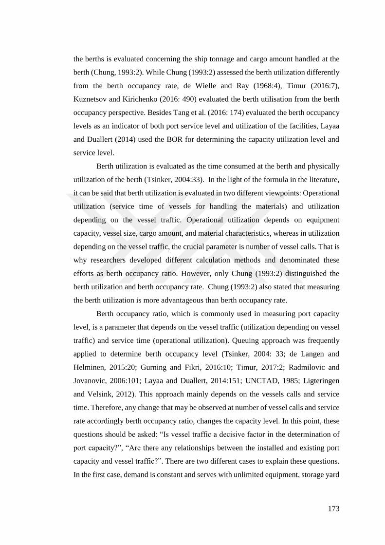
173

the berths is evaluated concerning the ship tonnage and cargo amount handled at the

berth (Chung, 1993:2). While Chung (1993:2) assessed the berth utilization differently

from the berth occupancy rate, de Wielle and Ray (1968:4), Timur (2016:7),

Kuznetsov and Kirichenko (2016: 490) evaluated the berth utilisation from the berth

occupancy perspective. Besides Tang et al. (2016: 174) evaluated the berth occupancy

levels as an indicator of both port service level and utilization of the facilities, Layaa

and Duallert (2014) used the BOR for determining the capacity utilization level and

service level.

Berth utilization is evaluated as the time consumed at the berth and physically

utilization of the berth (Tsinker, 2004:33). In the light of the formula in the literature,

it can be said that berth utilization is evaluated in two different viewpoints: Operational

utilization (service time of vessels for handling the materials) and utilization

depending on the vessel traffic. Operational utilization depends on equipment

capacity, vessel size, cargo amount, and material characteristics, whereas in utilization

depending on the vessel traffic, the crucial parameter is number of vessel calls. That is

why researchers developed different calculation methods and denominated these

efforts as berth occupancy ratio. However, only Chung (1993:2) distinguished the

berth utilization and berth occupancy rate. Chung (1993:2) also stated that measuring

the berth utilization is more advantageous than berth occupancy rate.

Berth occupancy ratio, which is commonly used in measuring port capacity

level, is a parameter that depends on the vessel traffic (utilization depending on vessel

traffic) and service time (operational utilization). Queuing approach was frequently

applied to determine berth occupancy level (Tsinker, 2004: 33; de Langen and

Helminen, 2015:20; Gurning and Fikri, 2016:10; Timur, 2017:2; Radmilovic and

Jovanovic, 2006:101; Layaa and Duallert, 2014:151; UNCTAD, 1985; Ligteringen

and Velsink, 2012). This approach mainly depends on the vessels calls and service

time. Therefore, any change that may be observed at number of vessel calls and service

rate accordingly berth occupancy ratio, changes the capacity level. In this point, these

questions should be asked: “Is vessel traffic a decisive factor in the determination of

port capacity?”, “Are there any relationships between the installed and existing port

capacity and vessel traffic?”. There are two different cases to explain these questions.

In the first case, demand is constant and serves with unlimited equipment, storage yard

174

area, and berth handling facilities. This port has actual capacity depending on the

vessel traffic, has a theoretical capacity depending on working hours and a realizable

capacity level. In the second case, assume that the same port cannot provide service

due to the demand insufficiency (low vessel calls). The following questions should be

asked, “Can this situation change the actual, realizable, and theoretical capacity of the

port?”. The second case does not change the attainable realizable capacity and

theoretical capacity of the port. However, the actual capacity will change due to vessel

traffic conditions. This case also differentiates the capacity types, and realizable

capacity concept asserted in Chapter II, Section 2.3. Although National Research

Council (1998:78) and UNCTAD (1973) defined the intrinsic and practical capacity,

different studies in the literature utilized the berth occupancy ratio for measuring

throughput capacity of the port. However, these studies did not explain the situations

mentioned above. This creates the need for a new concept for realizable capacity

measurement. This concept is called as berth utilization factor in this study.

Berth occupancy ratio (employs queueing approach) which considers the ship

traffic and service time can be used in actual capacity measurement attempts.

However, it may fall behind to determine berth utilization level that the port can attain

independently of vessel traffic. For this reason, operational utilization of the berth

needs to be considered to measure realizable capacity, which explains the possible

output levels where the terminal is independent of actual demand conditions (vessel

traffic). Determination of berth utilization level according to operational utilization of

the berth may show realizable capacity level when the port is not affected by the vessel

traffic.

Berth utilization factor, which considers only operational utilization of the

berth, can be expressed mathematically as follows:

∑ (∑ STi,act

nv=1

(∑ Btnv=1 )+(Vn*tbe)

)ni=1 ; Equation (111)

Where STi,act is total actual service time in the berth [hour]; Bt is the total time

the berth is occupied by a vessel [hour]; Vn is the number of vessel [-]; tbe is the time

taken by berthing operation of a vessel; i refers to number of berth [-], v refers to vessel

175

number [-]. i is the berth number [-]. STi,act refers to the net service time whereas Bt

includes both net service time and idle time at the berth. Equation (111) is similar to

Zamanirad et al. (2017:22), Chung, (1993:5) and India Ministry of Shipping (2011:73),

but it differs from the other formula in terms of reflecting the berthing operation.

4.2.2. Simulating Port Capacity Calculation Model

Simulation modelling employed by computer specialists, mathematicians

provides many advantages for the several industrial areas and organizations

(governmental, military, educational, traffic control, computer system design,

electronics, physics, environmental, economics and social sciences, chemical

industries, designing of transport, communication, manufacturing, computer system

design) about enhancing the effectiveness and efficiency (Ülgen and Williams, 2002:

3; Praehofer, 1991: 287). Simulation modelling and analysis can solve large spectrum

of problems. The reasons behind the being popular in the business environment are the

increase in boundless competition, cost-reduction efforts, explanation and estimation

capabilities of the simulation, and requirements of effective decision-making, effective

problem identification considerations (Ülgen and Williams, 2002: 3).

According to Gilbert and Troitzsch (2005:17) the logic of the simulation is

starts with the model development. Modelling is the illustration of the real world

phenomena in the form of mathematical equations, flow charts, software programme

or algorithm. Therefore, simulation is the technique that is drawn in connection with

the model to acquire the answer about complicated matters (Lewis and Orav, 2018:9).

Several steps have been identified for the simulation-based studies in the

literature. This process mainly starts with the determination of research question(s) as

well as in the scientific research process (Mihram, 1976:72; Gilbert and Troitzsch

2005:19; Ülgen and Williams, 2002: 13; Ulgen, et al. 1998: 2). This process directs

the basis of the model. Models can be built based on the several assumptions. These

assumptions, inputs and process definitions drive the model (Gilbert and Troitzsch

2005:19; Ülgen and Williams, 2002: 13). After determination of the assumptions, the

model can be designed. When designing the model, simplification creates a set of

challenges for the model developer deciding about the exclusion of pointless or

176

inclusion of parameters. It will be necessary to measure more parameters with the

addition of these parameters. This will be challenging in terms of the validity of these

results (Gilbert and Troitzsch 2005:19-26). Model building process follows the model

designing. The model designer can utilize the several software programs after

completion of the model building; simulation results can be obtained by executing the

program (Gilbert and Troitzsch (2005:19). However, the model should be checked in

terms of validation and verification. In this stage, model builder should examine the

model in terms of building the model correctly (verification) and building the correct

model (Ülgen and Williams, 2002:18; Ülgen and Williams, 2001:107; Andersson,

1974:6-7). This stage will be possible running the model and measuring the model

behaviours. Moreover, the sensitivity test can also be applied to investigate the model

in terms of measuring the behaviour of the model against the stated assumptions. The

last stage is publishing the simulation results (Gilbert and Troitzsch, 2005:17).

There are several analytical tools to perform simulation analysis. Java, C,

FORTRAN, GPSS, ARENA, Simple++, Prolog, C++, Smalltalk, SIMSCRIPT, Lisp

etc. (Gilbert and Troitzsch, 2005:19; Ülgen and Williams, 2002:18; Ülgen and

Williams, 2001:115).

4.2.2.1. Sampling and Data Collection Process for Model Testing1

For the testing the generated model, the population of the research was chosen

as dry bulk terminals in Iskenderun Region. Iskenderun region has wide hinterland

and the hinterland can reach three countries and fifteen cities located near this region

(Ateş, 2014:448, İsdemir, 2017). The ports located in Iskenderun Bay are Limak Port,

Milangaz LPG Terminal, Sasa Terminal, Petrol Ofisi Pier Port, Yazıcı Port, Orhan

Ekinci Port, Assan Port, Isdemir Port, MMK Metalurji Port, Delta Terminal, Aygaz

Terminal, Port of Toros, Ceyhan Marine Export Terminal, Botaş Terminal, İsken Port,

and Denbirport Terminal. While the ports in the north of the region perform mostly in

liquid cargo handling activities, the ports mostly in bulk, general cargo and container

are located in the south of the region (UDHB, 2015).

1 The some of the information mentioned under this title was published as a research article in “Gülmez,

S., Esmer, S. And Ateş, A. (2018). An Analysis of Seaborne Trade through Iskenderun Bay. Maritime

Faculty Journal. 10(1), 83-107”

177

Research sample has been chosen among the ports located in Iskenderun Bay,

which its core business is dry bulk commodities. For choosing the right sample,

preliminary study was performed. In the study, amount of cargo tonnages and

commodity groups of bulk cargoes were explored on the basis of ports (Gülmez et. al.

2018). The tendencies of the region is illustrated in Table 21.

Table 21: Cargo Groups and Materials subjected to Import and Export in Iskenderun Region

Cargo Groups Materials

Iron Iron and steel products, pig iron, slab, processed iron, steel roll, iron

pipes, iron wire rod, sheet metal, slag, iron wire rod, iron ore, iron ore

concentrate

Mineral Aluminium, florspat, barium, calcite, aluminium ore, bauxite,

manganese ore, calcite, chromium, chromium ore

Coal Coking coal, pit coal, goudron

Fertilizer Urea fertilizer, phosphatic fertilizer, compound fertilizer, compost

fertilizer

Cement White cement, cement

Petroleum Benzole, natural bitumen, gas oil, diesel oil, petroleum coke

Chemical Coustic soda, paraxylene

Other Pumice stone, tufa, gypsum, ingot, gypsoplast, wheat, plant equipment,

wind turbine tower, tank truck, tanker truck bed, miscellaneous

materials, cossette, corn, pallet, plastic tank, prefabricated materials,

trailer, fodder and pasture, soy beans, flour, floating platform

Source: Gülmez, et al. 2018: 92

An interview was held with the sectoral consultants to choose the right sample

among the ports. In accordance with the advices of sectoral consultants, the sample

subjected to capacity calculation was chosen as a port having a certain volume of cargo

and maintaining continuity of its cargo volume. However, name of the port and the

data set obtained from the port were not shared in this study. In order to test the model,

a data set template was generated in 64 items. 64 items was prepared to be used directly

in the model. During the creation of this template, model inputs were determined in

detail. The requested items are shown in the Table 22:

178

Table 22: Data Set Items

ITEMS

The Name of the Vessel Specific Bulk Density of the Material

GRT Amount of Cargo much greater than the Normal Condition

DWT Duration of the Closing and Opening Hatch Covers

NRT Duration of Berthing

LOA Duration of Unberthing

Beam Technical Specifications of the Equipment Used in the Berth

Number of Hold which Handling

Operation is Performed

Periodical Maintenance

Date and Time of Application for

Berthing

Average Number of Movements between Ship Holds

Date and Time of Berthing Technical Specifications of the Equipment Used in the

Storage Yard Area

Date and Time of Application for

Unberthing

Technical Specifications of the Transfer Equipment

Date and Time of Unberthing Maximum Speed Limit Within the Port Area

Duration of Berthing and

Unberthing

Total m2 of the Port Area

Net Working Time Net Storage Area (m2)

Material Type Area of Service Buildings (m2)

Amount of Stored Cargo Total Area of the Roads (m2)

Amount of Sousplan Stacking Policy

Open Storage or Closed Storage Number of Lane

Cargo Type (Dry form or big bag) Average Stacking Height

Amount of Transit The Distance between the Stockpile

Handling Equipment Number of Closed Area (Shed, Silo, Dome, etc)

Loading Tonnage Stacking Characteristics of Closed Areas

Unloading Tonnage The Average Distance between Storage Yard and Berth

Number of Gang Bearing Capacity of the Ground

Berth No Working Days

Specific Bulk Density of the

Material

Working Hours in a Day

Dwell Time Average Downtime due to Weather Conditions

Cargo Type (Dry form or big bag) Average Downtime due to Equipment Failure

Amount of Transit Number of Berth and Size of the Berths

179

Table 22: Data Set Items (Continued)

Handling Equipment Draft of the Berths

Loading Tonnage Working Hours of the Berths

Unloading Tonnage Additional Downtime

Berth No

Source: Compiled by the Author

The port determined as a sample, serves multiple cargo groups. Moreover, it

performs both export and import activities at the same time. In the first step, we

contacted port managers via e-mail and got an appointment. Interview was held at the

port. During the 90 minutes, research motivations and model were discussed and

shared with the port managers. In addition to this, cargo groups, equipment,

infrastructure and port process are discussed. The template include 64 items was

shared with the port managers. After 6 days, the data set covering 3 years was sent

from the port via e-mail. However, the data obtained from the port was not suitable for

direct implementation. For this reason, some of parts of the data were processed and

transformed into suitable data to be used for the model. Features of the port determined

as the research sample is illustrated in Table 23.

Table 23: Specifications of the Port

SPECIFICATIONS OF BERTHS AND BERTH HANDLING EQUIPMENTS

Number of Berths # 4

Berth Handling

Equipment

Berth Length Draft Grab Weight SWL Capacity

Grab Crane at #1 185 10.5

2 ton 6 ton 125 tph

Grab Crane at #1 3 ton 8 ton 175 tph

Grab Crane at #2 270 13

6.5ton 17 ton 400 tph

Grab Crane at #2 6.5ton 17 ton 400 tph

Grab Crane at #3 270 13

13.2 ton 30 ton 600 tph

Grab Crane at #3 13.2 ton 30 ton 600 tph

Grab Crane at #4 220 10

8 ton 20 ton 580 tph

Grab Crane at #4 8 ton 20 ton 580 tph

SPECIFICATIONS OF TRANSFER EQUIPMENTS

Belt Conveyor #2,#4 600 tph

180

Table 23: Specifications of the Port (Continued)

Belt Conveyor #1 400 tph

Belt Conveyor #5, #7 800 tph

STORAGE AREA SPECIFICATIONS

Closed Area Facilities Installed

Volume

Capacity

Flat Grain 211*54*10 60,000 ton

Fertilizer 1 204*51*11 35,000 ton

Fertilizer 2 204*48*10 32,000 ton

Dwell Time 45 days

OPEN STORAGE AREA SPECIFICATIONS

Dedicated Area Area

Concentrated Open Storage Area 11,500 m2

Non Paved Storage Space for Coal 500,000 m2

Additional Storage Space for General Purpose with Capacity 275,000 m2

Office Building 10,000 m2

Roads 32,407.5 m2

Bearing Capacity of the Ground 7 t

Average Stacking Height 10 m

Dwell Time 45 days

GENERAL SPECIFICATIONS

Working Days 347

Working Hours in a Day

Three Shifts in a Day 22,5 h

Source: Compiled by the Author

4.2.2.2.Designing of the Conceptual Model

Designing of the conceptual model includes decision-making process about

how the system should be demonstrated concerning the capabilities and components

ensured by the tool. Creation of conceptual modelling efforts reduces the risk of

running the simulation. Building conceptual model provides greater advantages to

ensure that all variables are included in the model and that certain subjects are

examined (Ulgen et al. 1994). Within the context of the study, conceptual model was

generated based on the calculation process of port capacity regarding three basic

component of the port and illustrated in Figure 39.

181

Figure 39: Conceptual Model of Berth Handling Capacity Calculation

182

In conceptual model of berth handling capacity, the calculation process has

been abstracted. Ports use several combinations of equipment. In this study, the issue

has been addressed in broader perspective considering the possibility of using different

handling equipment combination. For this reason, all the berth handling equipment

previously examined in Chapter I has been included in the simulation model.

Generated empirical equations mentioned in Chapter IV, Section 4.2.1.1. for

measuring berth handling capacity is included in the simulation model.

First step starts with the identifying the variables. Four main equipment (grab

handling equipment, pneumatic unloader, stacker, and screw type unloader) are

included to the model. The system works by performing a set of query about the usage

of these equipment. For instance, in case of using grab handling equipment, system

obtains the results by performing the specified operations. Once again if grab handling

equipment and stacker used together at the berth, the mathematical operations are

performed by the system and the results are summed.

The special conditions are identified for the grab handling equipment and

stacker. As stated previously, grab handling equipment capacity depends on the lifting

capacity of the crane, volume of the grab, density of the subjected material, weight of

the grab. Accordingly, this situation has been reflected to conceptual model and

simulation as a decision. If specific bulk density is low and the volume is high,

calculation module regards the volume of the grab to determine capacity. In an

opposite case, module regards the grab crane lifting capacity.

Another decision has been defined for the stacker type equipment. According

the conceptual model, if stacker type loader/unloader is equipped with the flat belt, the

equation which performs the calculation with the flat belt variables will be operated.

Whereas in case stacker is equipped with three throughing idler, the equations which

is identified for the three throughing idler will be regarded.

As well as in calculation module of berth handlingcapacity, a conceptual model

has been prepared for measuring storage yard capacity of a dry bulk terminal. Figure

40 illustrates the conceptual model of storage yard capacity.

183

Figure 40: Conceptual Model of Storage Yard Capacity Calculation

184

Conceptual model of storage handling capacity shows how the model is

abstracted. As a first step, all input variables has been identified in accordance with

the simulation model. In the next step, one of the most important point is the

determination of stockpile height. This situation depends on three different

circumstances and identification have been performed regarding these situation

(bearing capacity of the ground, equipment maximum height, height depend on the

width). Similar with the berth handling capacity measurement, different scenarios has

been identified for different implementations. For instance, a port can employ both

longitudinal and circular storage yard implementations. Accordingly, the result will be

evaluated together. However, when only one of the storage types is implemented, the

different process will be followed. If only longitudinal storage type is implemented,

simulation model queries that which storage policy is implemented (ID-Preserved and

CAM). Because ID-Preserved storage policy based on cargo segregation of the piles,

stockpile length will be found according to stockpile geometry. A port may also

implement the different stockpile geometry. A final step, the conceptual model queries

whether different storage policies are applied together or not. If the result is positive,

then the simulation model runs both CAM and ID-Preserved equations.

For the closed area capacity measurement, simulation model performs the

similar inquiries. The simulation runs the defined equation for measuring the specified

storage capacity of the area after performing a query about the storage facility type. In

case of using dome, silo or shed, model performs the equation by using the determined

inputs.

The process defined for the enclosed areas is similar to process of open areas.

If stockpile method is used at enclosed areas as well as at the open storage areas,

simulation performs a query. ın accordance with the stockpile geometry employed at

the enclosed area, stacking capacity of the stockpile is determined and added to the

total storage capacity of the terminal.

Finally the conceptual model of the transfer equipment, which is one of the

important component of the terminal, is shown in Figure 41.

185

Figure 41: Conceptual Model of Transfer Equipment Capacity Calculation

186

Different equipment have been considered for measuring transfer equipment

capacity of a dry bulk terminal. Different equations have been identified for each

equipment. For the conceptual model of capacity calculation of transfer equipment,

the variables to be used in the model have been identified as well as in other conceptual

models. System queries the whether stated equipment are used or not. Decision have

not been defined only for the reclaimer. Reclaimer and stacker have been evaluated

differently due to impracticability for the simultaneous operation. Similar to the

capacity calculation of berth handling equipment, the same conditions and decisions

identified for the stacker equipment. For the screw conveyors, only the shape factor

considered. As mentioned in the earlier chapters of the study, screw conveyor parts

show difference in accordance with the horizontal or vertical usage of the equipment.

Screw conveyor as a transfer equipment can perform cargo transfer horizontally. In

that situation, “U” shape screw conveyors can be used. That is why two decisions have

been identified for the screw conveyors. Following the decisions, each equation

identified for each circumstance operates. Likewise, measuring berth handling

capacity, two decisions have been identified for the belt conveyor whether flat belt or

three throughing idler belt. For the truck and bulldozer transfer capacity, situations

have been identified similar to grab handling equipment capacity. Logic of these

situations are based on the density of the material, carrying part volume of truck and

bulldozer and lifting capacity of these vehicles. System continues operation by

applying the empirical equations and provides the results. Considering the usage of

these equipment together, the process is stopped by summing up the results obtained

from the other equipment.

4.2.2.3. Formulation of Input Variables

Inputs and related components should be determined to simulation model to

achieve related output values. It is a complicated process to decide on which system

variables should be included in the simulation model. In order to overcome this

complex process, variables which illustrates the real system can be listed and the

required parameters can be evaluated for the simulation model (Gilbert and Troitzcch,

187

2005:22; Ülgen et al. 1994:3). The variables of the port capacity measurement is

illustrated in Table 24.

Table 24: Simulation Model Variables

Input Variables Symbol

Number of Berth Bn

Number of Handling Equipment (j) Ej,n

Number of Grab Unloader EG,n

Number of Pneumatic Unloader Epne,n

Number of Stacker Equipment Estc,n

Number of Screw Type Unloader Escr,n

Hour capability of Handling Equipment Cj,i

Grab Unloader/Loaders (ton per gang per hour) Cmhc,i

The Volume of Grab Vg

Actual Service Time STi,act

Number of Gang Gngn

Ton per Gang Gngt

Maximum Lifting Capacity of the Grab Unloader/Loader Cmax,lift

Net Weight of the Grab WTg,net

Pneumatic Loaders/Unloaders Cpneu,i

Screw Loader/Unloader Capacity Cscr,i

Bulk Density of the Cargo (i) ρi

Working Hours in a Day tpd

Working Days in a Year t

Peak Factor PF

Open Longitudinal Storage Yard Capacity (ID-Preserved Policy) COA,lID

Number of Lane nlane

Number of Stockpile ns

Mass of Stockpile (about stockpile geometry) ms

The distance between Two Stockpiles ds

Maximum Height of the Equipment heq,max

Height allowed by the bearing capacity qmax

ρ

188

Table 24: Simulation Model Variables (Continued)

Length of the Lane llane

The width of a Lane wlane

The height of the Stockpile hs

Length of the Stockpile ls

The width of the Stockpile ws

Maximum Height allowed by Lane Width hw,max

The tangent of the Mean Angle of Repose tanθ

Average Amount of Cargo per Vessel ��s,t on

Average Dwell Time of the Cargoes td,OA

Peak Factor of Cargoes Stored in Open Storage Area PFOA

Open Longitudinal Storage Yard Capacity (CAM-Policy) COA,lCAM

Number of Lane nlane

Length of a Lane llane

Mass of Stockpile (General representation of stockpile geometry) ms

Mass of a Stockpile (by trapezoidal shape) ms,ts

Mass of a Stockpile (by trapezoidal shape with end cones) ms,tec

Mass of a Stockpile (by triangular shape with end cones) ms,trec

Length of the Stockpile ls

Average Dwell Time of the Cargoes in Open Storage Area td,OA

Peak Factor of Cargoes Stored in Open Storage Area PFOA

Open Circular Storage Yard Capacity (Circular Stockpile) COA,c,cir

Number of Circular Bed nbed

Mass of Cargo in the Circular Stockpile ms,cir

The radius of the Area covered by the Equipment r1

The radius of the Top of Circular Mass r2

Net Angle seen from the Centre of the Circle K

Peak Factor of Cargoes Stored in Open Storage Area PFOA

Open Circular Storage Yard Capacity (Conical Stockpile) COA,c,con

Number of Spaces Allocated for the Conical Stockpile noA,c

Mass of Cargo in Conical Stockpile ms,con

Radius of the Circular Ground r

Average Dwell Time of the Cargoes td,OA

189

Table 24: Simulation Model Variables (Continued)

Peak Factor of Cargoes Stored in Open Storage Area PFOA

Closed Storage Area Capacity CCA

Silo Storage Capacity Csilo

Installed Volume of the Silo Vsilo

Number of Silo nsilo

Peak Factor of the Cargoes Stored in the Silo PFsilo

Averages of the Specific Bulk Density of Cargo (i) ρi

Average Dwell Time of the Cargoes Stored in the Silo td,silo

Dome Storage Capacity Cdome

Installed Volume of the Dome Vdome

Number of Dome ndome

Peak Factor of the Cargoes Stored in the Dome PFdome

Volumetric Flow Rate V

Conveying Velocity v

Cross-Sectional Area of the Pipe A

The density of the Air plus Material ρmix

The volume of Material (i) Vi

Total of Mass Flow Rate of Air and Material (i) per Second mmix

Mass Flow Rate of the Material (i) mi

Solid Loading Ratio ɸ

Hourly Truck Capacity Ctrk

Truck Carrying Capacity CCtrk

The Volume of Truck Bed Vtrk

Maximum Capacity of the Truck Maxtrck

Number of Truck Etrk,n

Truck Turnover T/On,trk,i

Hourly Capacity of Bulldozers Cbld

Volume of the Bulldozer’s Grab Vbld

Hourly Capacity of the Truck Cbld

Carrying Capacity of the Bulldozer CCbld

Maximum Capacity of the Bulldozer’s Grab Maxbld

Number of Bulldozers Ebld,n

190

Table 24: Simulation Model Variables (Continued)

Screw Diameter D

Diameter of the Outside of the Screw Conveyor d

Filling Factor ѱ

Screw Pitch λ

Speed of the Revolution N

Flight Factor CFf

Mixing Padles Factor CFm

Incline Factor k

Number of Screw Conveyor Escr,n

Velocity of the Belt Conveyor vb

Width of the Belt b

Slope Factor ks

Number of Belt Conveyor Eb,n

Capacity according to Belt Width and Belt Speed Cw,v

Cross Sectional Area of the Piece of Stockpile Aps

Volume of the Each Segment Vrec

Number of Reclaimer E,rec,n

Source: Generated by Author

All above-mentioned variables was evaluated as input variables and reflected

to the simulation model.

4.2.2.4.Preparation of Data for Building Simulation Model

This section describes data that has been prepared fır the simulation model by

manipulating these real world data.

Preparation of Berth Handling Capacity Measurement Data

Preparation process of berth handling capacity data started with the

determination of peak factor and berth utilization factors. Firstly, cargo amounts per

191

month is determined and tabulated. The cargo amount per month in 36 months

observed period is illustrated in Figure 42.

Figure 42: Cargo Amounts per Months

Source: Generated by Author

According to the Figure 42, cargo amount in 2018 is higher than the 2016

values. It can be seen from the figure, cargo amount decreased in April, June and

September. However, a significant fluctuations have not been recorded according the

data set. In line with this statement, frequencies of the cargoes within the determined

range is illustrated in Figure 43.

Figure 43: Frequency Distributions of Cargo Amount per Month within the given Rages

Source: Generated by Author

192

In line with the Figure 43, peak factor value has been calculated regarding the

Scholtz (2017:127) approach. Peak factor of the port has been determined as 1.21.

BUF value has been obtained through the equation in Chapter IV, Section

4.2.1.4. Besides, BOR value has been achieved through Equation (62) and (74).net

working time (gang time), berth occupancy time, number of vessel and the time taken

by berthing manoeuvrings. In dataset berth occupancy time included the ship

unberthing time, but berthing time is not included. For this reason, only the average

time taken by the berthing manoeuvring of the vessel. In accordance with the data set,

BOR and BUF values per berth are indicated in Table 25.

Table 25: BOR and BUF Values by Berths

Berth No # BUF BOR

#1 0.735675261 0.137040372

#2 0.897318528 0.703609644

#3 0.876403013 0.613559345

#4 0.752884182 0.613703437

Source: Compiled by Author

With the determination of frequency distributions of the cargo amount per

month, percentage distribution of the materials have been determined. Materials and

their percentages have been cross-tabulated to determine the gang number regarding

the material characteristics, service time, lifting capacity of the crane, grab volume,

grab weight and service time. In line with the three-year data the percentages of the

materials per berth is illustrated in Table 26.

Table 26: Percentage Distribution of Materials per Berth

Material Percentage per Berth

#1 #2 #3 #4

Ammonium Sulphate 0.38 0.011 0.002 0.0005

M.A.P. 0.19 - - -

Urea 0.40 - - -

193

Table 26: Percentage Distribution of Materials per Berth (Continued)

Sunflower Seed - 0.001 - 0.0002

Sunflower Seed Cake - - - 0.000041

Basalt - 0.002 - 0.0007

Cement - 0.014 0.007 0.0171

D.A.P. - 0.004 0.002 0.0004

Urea - 0.060 0.008 0.0064

Flaxseed - 0.002 - 0.0002

Clinker - 0.302 - -

Lignite - 0.442 0.673 0.0096

Corn - 0.009 0.012 0.0067

Corn Meal - 0.016 0.005 0.0012

NPK - 0.001 - 0.0003

Petroleum Coke - 0.11 0.267 -

Pumice - 0.001 0.001 0.0009

Soy Bean - 0.026 0.016 0.0015

Soy Bean Meal - 0.00031 0.005 0.0011

Sunflower Seed Hull - - 0.001 -

Coke Breeze - - 0.002 -

Wheat Bran - - - 0.0001

Corn Gluten - - - 0.000045

Source: Compiled by Author

According to the data, the port handled 3 types of materials in berth #1, 16

different material in berth #2, 13 material in berth #3, and 17 types of materials in berth

no #4 during three years.

Total amount of cargo per berth and total net service time per material have

been determined and the calculation has been performed through Equation (108). The

port records the net service time per vessel berth occupancy time per vessel separately.

When determining the theoretical number of gang, only the net service time and total

amount of cargo per material has been used. Theoretical number of gang (TGN) per

berth per material per hour is provided in Table 27.

194

Table 27: Theoretical Number of Gang per Berth, per Material per Hour

Material #1 TGN (gph) #2 TGN (gph) #3TGN (gph) #4 TGN (gph)

Ammonium Sulphate 22 24 7 16

M.A.P. 24 - - -

Urea 28 - - -

Sunflower Seed - 13 - 7

Sunflower Seed Cake - - - 7

Basalt - 12 - 23

Cement - 8 4 7

D.A.P. - 36 9 11

Urea - 30 9 26

Flaxseed - 31 - 10

Clinker - 20 - -

Lignite - 41 25 25

Corn - 40 19 18

Corn Meal - 25 8 8

NPK - 10 - 8

Petroleum Coke - 49 32 -

Pumice - 30 14 7

Soy Bean - 38 13 17

Soy Bean Meal - 16 16 14

Sunflower Seed Hull - - 20 -

Coke Breeze - - 22 -

Wheat Bran - - - 33

Corn Gluten - - - 6

Source: Compiled by Author

Preparation of Storage Yard Capacity Measurement Data

Open Storage Area Capacity

To measure open storage yard capacity, the similar path with the berth handling

capacity has been followed. As a first step, peak factor of the storage yard has been

195

determined. After this process, number of lane, lane widths and height of the stockpile

according to allowed height by lane width determined.

One of the contribution of this study is peak factor of storage yard. Peak factor

of open is an important parameter to determine the required storage yard area.

However, this study has not been attempted to determine required storage yard area.

Thus, it affects the storage yard capacity as a divisor not the multiplier. Peak factor

value of storage yard has been determined separately for open storage area and closed

storage area.

Firstly, cargo amounts per month is determined and tabulated. The per month

values of cargo amount for open storage area within 36 months observed period is

illustrated in Figure 44.

Figure 44: Open Storage Area Cargo Amounts per Mont

Source: Compiled by Author

Comparing to the berth handling, cargo amount for open storage area is more

volatile. 2016 and 2018 values of the storage yard cargo amount has nearly the same

rises and falls whereas 2017 value shows different attitude.

Under this circumstances, peak factor value of open storage area has been

found as 1.35.

To measure open storage area capacity, number of lane is determined. The port

has 9 divided areas. Table 28 illustrates the properties of these areas.

196

Table 28: Features of Open Storage Areas

Area Lane

Length (m)

Lane Width

(m)

Road

With (m)

Area Width

(m)

Area

Length (m)

Number of

Lane (m)

Area #1 276 50 7.5 290 276 5

Area #1 276 25 0 25 276 1

Area #2 212 50 7.5 110 212 2

Area #3 241 50 7.5 50 241 1

Area #4 243 50 7.5 50 243 1

Area #4 114 50 7.5 50 114 1

Area #5 122 50 7.5 50 122 1

Area #5 72 15.8 0 15.8 72 1

Area #6 386 50 7.5 116 382 2

Area #7 174 50 7.5 132 174 2

Area #8 143 50 7.5 178 143 3

Area #9 185 50 7.5 100 185 2

Area #9 178 40 0 60 178 1

Source: Compiled by Author

Area sizes has been determined via Google Maps. Road with implemented at

the area is 7.5 m. 50 m width has been considered for the lane width (van Vianen,

2012; Kleinheerenbrink, 2012:45).

After determination of the area sizes, height allowed by lane width is

determined. In addition, it is necessary to determine how much height will be allowed

by specified width. To find the final stockpile height, it should be compared to other

height values allowed by equipment height, bearing capacity of the ground.

Triangular shape with end cones geometry has been regarded as reference

stockpile geometry. Because if stockpile height is over the height allowed by lane

width, materials will be flow down during the stacking materials. Accordingly, lane

width will be widen. Height allowed by lane width differs since there are different lane

widths, material density. For this reason, amount of cargo that can be stored in each

dedicated area have been calculated separately and percentage weight of these

materials has been summed. In the light of this operation, Table 29 shows values of

three different height values considering the area size and material properties.

197

Table 29: Height Options for the Stockpile

Area # Material Height allowed by Bearing Capacity of the

Ground (qmax/ρi) (m)

Height allowed by Equipment Height

(heq,max) (m)

Height Allowed by Lane Width

(hw,max) (m)

Area #1 Petroleum Coke 10.00714796 10 43.3025

Area #1 Petroleum Coke 10.00714796 10 21.65125

Area #2 Petroleum Coke 10.00714796 10 43.3025

Area #3 Petroleum Coke 10.00714796 10 43.3025

Area #4 Petroleum Coke 10.00714796 10 43.3025

Area #4 Petroleum Coke 10.00714796 10 43.3025

Area #5 Petroleum Coke 10.00714796 10 43.3025

Area #5 Petroleum Coke 10.00714796 10 13.68359

Area #6 Petroleum Coke 10.00714796 10 43.3025

Area #7 Petroleum Coke 10.00714796 10 43.3025

Area #8 Petroleum Coke 10.00714796 10 43.3025

Area #9 Petroleum Coke 10.00714796 10 43.3025

Area #9 Petroleum Coke 10.00714796 10 34.642

Area #1 Lignite 9.333333333 10 19.5325

Area #1 Lignite 9.333333333 10 9.76625

Area #2 Lignite 9.333333333 10 19.5325

Area #3 Lignite 9.333333333 10 19.5325

Area #4 Lignite 9.333333333 10 19.5325

Area #4 Lignite 9.333333333 10 19.5325

198

Table 29: Height Options for the Stockpile (Continued)

Area #5 Lignite 9.333333333 10 19.5325

Area #5 Lignite 9.333333333 10 6.17227

Area #6 Lignite 9.333333333 10 19.5325

Area #7 Lignite 9.333333333 10 19.5325

Area #8 Lignite 9.333333333 10 19.5325

Area #9 Lignite 9.333333333 10 19.5325

Area #9 Lignite 9.333333333 10 15.626

Source: Generated by Author

199

Height allowed by bearing capacity of the ground has been calculated

considering the petroleum coke and lignite materials. Only two of these materials have

been stored at the open storage area. Reference height value has been considered 10 m

(equipment height) for petroleum coke for all stated areas, while height allowed by

bearing capacity of the ground (9.33 m) has been regarded for all stated areas except

in Area #5 (6.17 m).

The height allowed by the lane width has not suitable for the triangular shape

with end cones within the limits of bearing capacity and equipment height. Thus,

stockpile geometry becomes trapezoidal shape with end cones. The port already uses

this stockpile geometry.

Enclosed Storage Area Capacity

Firstly, cargo amounts per month has been determined and tabulated. Per

month values of cargo amount for enclosed areas within 36 months is illustrated in

Figure 45.

Figure 45: Enclosed Storage Area Cargo Amounts per Month

Source: Generated by Author

The same attitude of the cargo amounts can be seen in enclosed areas. A similar

trend has been seen in all months except for July, October and November when 36

months-data of closed area has been examined.

200

Under this circumstances, peak factor value of enclosed storage area have been

found as 1.30. Average dwell time of the materials stored in enclosed areas is 45 days.

The port has three enclosed area. The properties of enclosed areas are shown

in Table 30.

Table 30: Features of Enclosed Areas

Facility Total Installed

Volume (m3)

Stored Material

A 1 102,000 Ammonium Sulphate, D.A.P., M.A.P. and Urea

A 2 102,000 Ammonium Sulphate, D.A.P., M.A.P. and Urea

B 113,940 Corn, Corn Gluten, Corn Meal, Flaxseed, Soybean,

and Soybean Meal

Source: Created by Author

Total installed volume of “B” is 113,940 m3; “A 1” is 102,000 m3; “A 2” is

102,000 m3. Corn, corn gluten, corn meal, flaxseed, soybean, and soybean meal

materials are stored in “B”. Ammonium sulphate, D.A.P., urea, and M.A.P. materials

are stored in “A 1” and “A 2” facilities.

Preparation of Equipment Capacity Measurement Data

Cargo transfer in the port has been performed both as sousplan and as from/to

storage yard area. Percentages of the cargo transfer is shown in Table 31.

Table 31: Cargo Transfer Percentages

Transfer Percentage

Sousplan 0.37792581

Internal Transport 0.51098268

Conveyor 0.111091511

Source: Compiled by Author

201

While the majority of the cargoes were transferred directly to the storage yard

area, 37% of these cargoes were transferred as sousplan without being stored in the

area.

Port only has belt conveyor as a transfer equipment. Apart from belt conveyor,

cargo transfer is also performed through truck. However, port has not any truck.

Outsourced trucks perform some part of cargo transfer. These trucks have not any

significant property. The number and property of truck shows difference from

operation to operation. For this reason, truck transfer capacity has been disregarded in

this study.

The characteristics of the belt conveyors are shown in Table 32.

Table 32: Features of Belt Conveyor

Number of

Equipment

Belt Width Belt

Speed

Idler Throughing

Angle

Inclination

Angle

3 1000 mm 1.25 m/s 45o 15o

Source: Compiled by Author

The port has three conveyors with the same characteristics. These belt

conveyors are equipped with 3 roll throughing idler.

The simulation results of the capacities have been provided in Section 4.2.2.6.

4.2.2.5. Analysis of the Data

Berth Handling Capacity of the Port

Berth handling capacity calculation has been performed according to Equation

(89) by using simulation model. With this implementation, realizable berth handling

capacity that can be carried out separately according to the material type and material

percentage handled at the each berth has been calculated. Each capacity output has

been multiplied by the percentages of material handled at each berth to find a single

value for realizable berth handling capacity. Table 33 illustrates the results.

202

Table 33: Realizable Berth Handling Capacity Outputs per Berth per Material

Material #1 Capacity #2 Capacity #3 Capacity #4 Capacity

Ammonium Sulphate 1,670,294.475 4,161,279.65 2,529,310.908 3,191,008.457

M.A.P. 1,765,126.304

Urea 1,731,773.626

Sunflower Seed 1,457,096.919 1,358,701.898

Sunflower Seed Cake 803,240.6008

Basalt 2,920,684.246 536,7903.289

Cement 1,733,866.521 1,501,467.056 1,633,709.697

D.A.P. 5,732,885.935 2,987,086.298 1,959,673.679

Urea 3,915,107.692 2,445,091.104 3,792,540.367

Flaxseed 3,772,550.485 1,458,669.372

Clinker 4,867,807.077

Lignite 5,350,647.18 6,791,919.733 3,675,846.817

Corn 3,375,012.907 3,338,002.151 1,697,891.149

Corn Meal 2,787,399.053 1,858,269.239 931,992.4841

NPK 1,587,832.309 1,420,549.479

Petroleum Coke 5,963,063.67 8,106,835.393

Pumice 2,176,605.165 2,114,098.215 1,633,709.697

Soy Bean 3,954,977.35 1,408,304.557 1,977,177.711

Soy Bean Meal 1,780,226.588 3,709,293.763 1,742,623.676

Sunflower Seed Hull 1,521,390.02

Coke Breeze 4,432,859.612

Wheat Bran 1,347,810.5

Corn Gluten 678,024.5322

Capacity per Berth (ton) 1,714,509.288 5,012,422.912 6,875,669.724 113,644.715

Total Realizable Berth Handling Capacity (ton/year) 13,716,246.639

Source: Compiled by Author

After implementation of the Equation (89) realizable berth handling capacity

has been found as 13,716,246.639 ton/year through simulation. The same operation

has been performed for the theoretical and actual capacity. When the theoretical

capacity has been calculated, peak factor, BUF and BOR disregarded. Additionally,

working hours in a day and working days in a year replaced the 24 and 365

respectively. The results are provide in Table 34.

203

Table 34: Realizable, Actual and Theoretical Berth Handling Capacities

Total Realizable Berth

Handling Capacity

(ton/year)

Total Actual Berth

Handling Capacity

(ton/year)

Total Theoretical Berth

Handling Capacity

(ton/year)

13,716,246.639 10,063,267.44 21,530,674.61

Source: Compiled by Author

When comparing the berth handling output values, theoretical berth handling

capacity has the maximum output value as expected. However, there is a significant

difference between actual berth handling capacity and realizable capacity output

values. This difference stem from the BOR and BUF values. When considering the

vessel traffic in measuring berth capacity, berths are not utilized in its efficient rate

(UNCTAD, 1985b; KMI, 1998; Park et al. 2014:181,186).

Storage Yard Capacity of the Port

Open Storage Yard Capacity

The calculation of open storage yard capacity has been performed according to

Equation (92). Although port is owner of the storage yard area, it has rented each of

these areas to different customers. For this reason, CAM-Storage policy approach has

been implemented at the open storage area. This type of storage policy has been

applied in the calculations.

Open storage yard capacity has been calculated regarding stockpile geometry,

dwell time, angle of repose, specific bulk density, CAM-Storage policy

implementation, height of the stockpile, peak factor of open storage areas and number

of lane for the each material. As a first step, percentage weights of lignite and

petroleum coke have been calculated.

Table 35 shows the percentages of the materials stored at the storage yard.

204

Table 35: Percentage Weights of Materials Stored at the Storage Yard

Materials Percentage

Petroleum Coke 0.673

Lignite 0.327

Source: Generated by Author

According to dataset, only petroleum coke and lignite are stored in the open

storage area. Petroleum coke has the highest proportion with 0.673 value comparing

the lignite. In line with this information, petroleum coke and lignite materials have

been calculated separately and different capacity values has been obtained (#

Capacity). Amount of cargo that can be stored in open storage areas is illustrated in

Table 36.

Table 36: Capacity and Weighted Capacity Values per Area

Area # Material #Capacity (ton) Weighted Capacity (t/y)

Area #1 Petroleum Coke 2,500,525.84

4,747,647.697

Area #1 Petroleum Coke 217,447.56

Area #2 Petroleum Coke 763,353.13

Area #3 Petroleum Coke 435,339.53

Area #4 Petroleum Coke 439,040.42

Area #4 Petroleum Coke 200,332.77

Area #5 Petroleum Coke 215,136.35

Area #5 Petroleum Coke 27,848.24

Area #6 Petroleum Coke 1,407,308.65

Area #7 Petroleum Coke 622,719.17

Area #8 Petroleum Coke 761,987.19

Area #9 Petroleum Coke 663,429.00

Area #9 Petroleum Coke 246,701.60

Area #1 Lignite 2,105,013.44

2,772,475.467

Area #1 Lignite 144,604.17

Area #2 Lignite 638,059.84

Area #3 Lignite 365,236.33

Area #4 Lignite 368,422.98

205

Table 36: Capacity and Weighted Capacity Values per Area (Continued)

Area #4 Lignite 162,884.13

2,772,475.467

Area #5 Lignite 175,630.72

Area #5 Lignite 14,102.19

Area #6 Lignite 1,179,790.16

Area #7 Lignite 516,967.19

Area #8 Lignite 627,271.60

Area #9 Lignite 552,020.32

Area #9 Lignite 195,330.07

Total (ton/year) 7,520,123.164

Source: Generated by Author

According to Table 36, weighted capacity value of petroleum coke is

4,747,647.697 ton per year, and weighted capacity value of lignite is 2,772,475.467

ton per year. Total open storage area capacity for petroleum coke and lignite is

7,520,123.164 ton per year.

Enclosed Storage Area Capacity

To calculate the enclosed storage area capacity, weighted percentages of each

material for three different enclosed area have been calculated by simulation model.

The cargo percentages of the materials stored in “A 1-2” and “B” facilities are shown

in Table 37

Table 37: Cargo Percentages of Materials Stored in Enclosed Facilities

Facility Material Percentage

A 1-2 Ammonium Sulphate 0.250050502

A 1-2 D.A.P. 0.07690191

A 1-2 Urea 0.607607398

A 1-2 M.A.P. 0.065440189

B Corn 0.251173485

B Corn Gluten 0.045196118

206

Table 37: Cargo Percentages of Materials Stored in Enclosed Facilities (Continued)

B Corn Meal 0.212440515

B Flaxseed 0.02408569

B Soybean 0.347644049

B Soybean Meal 0.119460143

Source: Created by Author

In “A 1-2” facilities, the highest proportion of these materials belong to urea.

Besides, soybean has the highest proportion in “B” facility. These percentages have

been used for obtaining only one capacity output value. To obtain capacity output

values of above mentioned materials, Equation (100) has been employed. The results

are provided in Table 38.

Table 38: Enclosed Area Capacity per Material

Facility Material Percentage #Capacity Output

A 1-2 Ammonium Sulphate 0.250050502 1,267,292.32

A 1-2 D.A.P. 0.07690191 1,163,749.138

A 1-2 Urea 0.607607398 952,851.3682

A 1-2 M.A.P. 0.065440189 1,159,937.732

B Corn 0.251173485 3,441,153.0992

B Corn Gluten 0.045196118 424,692.0203

B Corn Meal 0.212440515 454,849.7661

B Flaxseed 0.02408569 496,715.8132

B Soybean 0.347644049 424,337.2233

B Soybean Meal 0.119460143 454,140.1721

Total Enclosed Area Capacity 1,477,246.484

Source: Created by Author

Enclosed areas stated above has been calculated for each material. Each of

capacity output value have been multiplied by the real weighted percentages of the

materials. As a result of this operation, the real capacity value of each enclosed area

has been achieved. With the calculation of the enclosed area capacity, total storage

area capacity (open storage area and enclosed storage area) has been achieved. Total

area capacity of the port is shown in Table 39.

207

Table 39: Total Storage Yard Capacity

Area Capacity (t/y)

Open Storage Area 7,520,123.164

Enclosed Area 1,477,246.484

Total Area 8,997,369.648

Source: Created by Author

According to simulation results, storage yard capacity of the port is achieved as

8,997,369.648 t/y. open storage area capacity has the higher value than closed storage

area capacity at the specified material densities and angle of reposes. This calculation

has been performed according to petroleum coke and lignite materials.

Transfer Equipment Capacity of the Port

The mathematical operation has been performed according to Equation (43). Each

value belonging the material required for the calculation has been obtained from

Appendix I. Firstly, percentage weights of the cargoes transferred by conveyor belt

has been determined. The values have been identified in simulation model after

obtaining the coefficients for capacity of belt conveyor for three idler belt conveyor,

capacity factor from Fenner Dunlop (2009:21-22). Table 40 illustrates percentages of

the materials and the coefficient values for each material.

Table 40: Percentages and Coefficient Values of the Materials

Material Percentage Capacity of 3 Idler Belt Capacity Factor

Ammonium Sulphate 0.172806431 497 1.08

D.A.P. 0.053145843 497 1.15

Urea 0.419909039 497 1.15

M.A.P. 0.045224806 497 1.15

Corn 0.077590976 497 1.15

Corn Gluten 0.013961708 497 1.15

Corn Meal 0.065625824 497 1.15

208

Table 40: Percentages and Coefficient Values of the Materials (Continued)

Flaxseed 0.007440404 497 1.08

Soybean 0.107392072 497 0.94

Soybean Meal 0.036902896 497 1.08

Source: Compiled by Author

Urea has the highest value among the other materials whereas flaxseed has the

lowest percentage. “Capacity of 3 idler belt conveyor” can be determined according to

belt width and belt speed. “Capacity Factor” is also determined by angle of surcharge

and angle of throughing idler. The values mentioned above and in Table 34 has been

identified in simulation model. The results are given in Table 41.

Table 41: Total Transfer Equipment Capacity

Material #Capacity (t/y) Percentage Weighted Capacity (t/y)

Ammonium Sulphate 1,5230,332.61 2,631,899.427

D.A.P. 14,892,446.27 791,471.6097

Urea 12,193,596.84 5,120,201.532

M.A.P. 14,843,671.89 671,302.1882

Corn 7,885,192.622 611,819.7909

Corn Gluten 9,730,490.277 135,854.2655

Corn Meal 10,421,460.76 683,916.9482

Flax Seed 10,687,952.71 79,522.68587

Soybean 7,946,973.513 853,441.9519

Soybean Meal 9,771,842.475 360,609.2892

Total Equipment Capacity (t/y) 11,940,039.69

Source: Generated by Author

Belt conveyor capacity has been determined per each material. Capacity values

of each material has been considered to determine total equipment capacity by

calculating the real capacity percentages. According to simulation results, belt

conveyor capacity has been found as 11,940,039.69 ton per year.

209

4.2.2.6.Validation and Verification

Verification can be provide easily by using software programs in terms of

identifying the errors and mistakes into the simulation model. Verification of the

model includes the process of whether it works correctly or not. Besides validation

refers to testing the compatibility of the model behaviour with the target system

behaviour (Gilbert and Troitzsch, 2005: 22). Validation and verification can be

schematically illustrated as in Figure 46:

Figure 46: Relation of Validation and Verification

Source: Ulgen and Williams, 2001: 114

According to Figure 46, validation is performed between the simulation model

and real system. However, in this study, a simulation model was not created in which

the behaviour of the real system could be observed. Furthermore, the absence of an

output value that could be referred was restricted the validation efforts. Validation is

mostly performed in the studies that describe the process, which needed to be validated

to make sure about the reliable results (Kox, 2017:122).

Verification is performed between the model behaviour and the modeller’s

objectives. Two verifications were conducted in the study. Firstly, the simulation

model was compared with the conceptual model and it was found to be compatible

with each other. Another validation was performed of the testing the compatibility of

the simulation results and manual operation of the equations. Both of operations were

checked to eliminate the faults. According to this verification, both operations

provided the same capacity outputs.

210

CONCLUSIONS AND RECOMMENDATIONS

A limited study addressing the capacity calculation based on empirical equation

development were found in the literature with the determined research strings. Some of these

studies mostly focus on optimization and performance, especially in container terminals. In

this study berth handling, storage yard and equipment were attempted to measure by

developing empirical formula and simulation model within an integrated perspective. In this

context, several empirical equations for berth handling, storage yard area and equipment and

they were tested by the simulation model. In line with the research streams on port and

terminal capacity, factors affecting port capacity were analysed thoroughly. The measurable

parameters, which were not reflected before to the capacity calculation equations (lifting

capacity of the crane, grab volume, material density, grab weight, storage yard peak factor)

were attempted to reflect the capacity measurement equations.

This study has originalities in terms of analysing berth handling capacity, storage

yard capacity, and equipment capacity of dry bulk terminal capacity from a complementary

perspective. This study is also crucial in terms of bringing the equipment, berth handling,

and storage yard capacity equations and terminal design issues together and introducing

theoretical gang capacity, berth utilization factor, peak factor of storage yard, realizable

capacity concepts by explaining functions of different types of capacity and related

coefficients.

Equipment capacity, working days in a year, working hours in a day, utilization level

of the berths and number of equipment are essential parameters in the determination of berth

handling capacity. When examining the existing literature, it was noticed that the capacity

of berth handling equipment was not explained in detail. Some scholars obtained the hourly

capacity of berth handling equipment by multiplying the number of the gang and the amount

of cargo per gang in an hour. However, as far as is known, there is a gap in the determination

of hourly gang number of grab cranes in the literature. In this study, real-world data was

used to determine the theoretical number of gang per material and per equipment. Hourly

gang capacity of the berth handling equipment is affected by the draft of the ship and berth,

hold type of the ship, boom angle of the crane. These factors change hourly gang capacity

211

of the equipment. Besides, the grab-filling rate differs during the handling operation, and it

is not possible to obtain 100% of filling in every gang. The reason behind calling the gang

number as theoretical gang number is that the amount of cargo handled by each gang is not

the same. In actual service conditions, a berth-handling equipment can perform more gangs

than theoretical number of the gang. However, net service time will not change, as the

handling rate is certain (considering the same climatic conditions, the same ship size, the

same crane, and the same ship characteristics). For this reason, theoretical gang number will

increase or decrease in line with the operation time of grab (depended on volume of grab,

crane lifting capacity, grab weight and material density factors). Accordingly, theoretical

number of gang is always lower than the actual number of gang.

To achieve only one capacity value for each component of the terminal served to

multiple commodity types, weighted averages of the cargoes were determined based on the

throughput volume in previous years. When calculating the capacity of each of the

component, the capacity of each component was calculated according to the material. Then

the capacity outputs were calculated by including the percentages of the materials in the

calculation.

Although capacity is classified as intrinsic and proper capacity (National Research

Council, 1998: 72), a different spectrum of capacity types can be found in the literature.

These capacity types can be calculated in accordance with the objectives and provide

different results. However, as far as is known, no study was found regarding coefficients to

be determined in accordance with each type of capacity in the literature. Within this context,

berth utilization concept was introduced in this study, and a clear distinction between berth

occupancy ratio and berth utilization factor concepts was made. Berth utilization factor can

be defined as the amount of cargo that the port can handle in case it is not affected by the

demand conditions. Demand condition is one of the essential factor affecting the amount of

cargo handled in the port. Considering the actual traffic conditions at the port, the actual

capacity that the port can perform can be determined by considering the coefficient of berth

occupancy ratio. However, there is no capacity concept identified to determine the port

capacity in case port serves with relatively adequate equipment and infrastructure, yet there

is not enough demand. In addition, there is not any related parameter (coefficient) to

212

calculate this capacity concept in the literature. Therefore, reliable capacity is introduced as

a concept that can exactly explain this situation. Realizable capacity shows the realizable

capacity value of the port that the berth can reach when ships called to the port. Realizable

capacity can be calculated through the berth utilization factor showing how many tons can

be achieved without being affected by the demand. Besides, berth occupancy rate is used

when actual capacity is attempted to calculate.

Calculation of storage yard capacity were also poorly attempted to measure in the

literature. A relatively limited study was found in the literature on measuring dry bulk

storage yard capacity. This study addressed the storage yard capacity within an integrated

perspective. A process was created to measure the storage yard capacity. This process can

be followed in storage yard capacity calculation of dry bulk terminals to avoid confusion.

The terminal was assessed according to whether it is longitudinal or circular in the first step.

Then two different storage policy (CAM storage policy and ID-Preserved storage policy)

was determined. Specific empirical equations were generated for each case. In case of

implementing ID-Preserved storage policy, stockpile length was determined considering the

average cargo per vessel. Besides, three different reference value was considered for

determining the stockpile height. These reference values are height allowed by lane width,

height allowed by equipment, height allowed by bearing capacity of the ground. Also, each

of stockpile geometry (trapezoidal shape with end cones, trapezoidal shape, circular

stockpile, triangular stockpile, conical stockpile) commonly applied in the dry bulk terminals

was analysed and determined stockpile height was considered according to stockpile

geometry. For the closed areas, silo, dome, shed and enclosed area empirical equations were

developed.

Peak factor is an influential parameter in the determination of required capacity. An

approach was attempted to develop that can be applied in practice and to give better ideas

about capacity. Apart from the peak factor value determined for measuring berth handling

capacity, another peak factor value was also considered for storage area. The underlying

reason for determining different peak value for storage area is that sousplan transfer of the

cargoes does not occupy the terminal area. Peak factor was not used for determining the

213

required area in this study; it was used for finding the capacity value that the port could serve

with sufficient capacity to its customers.

In light with above-mentioned information, a simulation model was generated for

calculating the dry bulk terminal capacity by using RProject. Empirical formulas were

testing through real-world data. Cases mentioned above and related equations were

identified in the simulation model. Capacity measurement of the port offered services to

multipole cargoes was performed using the simulation model, which was suitable for each

case.

Real-world data was prepared for the simulation model. Firstly, it was attempted to

determine the theoretical gang number regarding the net service time. Theoretical gang

numbers were achieved per berth per material type. Amount of material per gang was

determined considering the material density, crane lifting capacity grab weight, and grab

volume. Required parameters were entered to the simulation model. For the storage yard

capacity, installed volume of the enclosed areas and number of lane, angle of repose of the

materials, material percentages, specific bulk density of the materials and the heights were

entered manually into the simulation model.

Realizable capacity, actual capacity, and theoretical capacity of the dry bulk terminal

were calculated by applying real-world data. In actual capacity calculation, berth occupancy

ratio was applied to the formula, whereas berth utilization factor used for calculating the

realizable capacity. The berth occupancy rate values of the terminal were recorded as 0.13,

0.70, 0.61, 0.61 for berth no #1, berth no #2, berth no#3, and berth no #4, respectively.

Besides, berth utilization factors were recorded as 0.70, 0.89, 0.87, and 0.75. Averages of

berth occupancy ratio of the specified berth were 0.51. This value was close to the value

stated in the literature for the terminals with four berths (UNCTAD, 1985b; Park et al. 2014:

186). Berth #1 had the lowest value among the other berths in two different values. The

underlying reason for a lower coefficient of berth utilization and berth occupancy rate value

may be the berth size and draft restrictions. Berth #1 is the smallest berth of the terminal,

and the equipment capacity is limited comparing the other equipment allocated to other

berths. In general terms, the realizable capacity value was higher than the actual capacity.

214

Theoretical capacity was calculated by considering 365 days and 24 hours. Theoretical berth

capacity had the highest value among the other capacity types as it was expected.

a. Implications for Researchers

The result of this study provides various implications for both researchers and

practitioners. Implications for researchers can be assessed as follows.

In the light of the results obtained by the simulation model, theoretical gang number,

peak factor of storage yard, and realizable capacity were introduced. Although researchers

commonly pointed on the hourly gang number and ton per gang, determination attempt of

these parameters was limited as far as is known. It can be deduced from the literature that

hourly gang capacity of the grab equipment depends on the size of the ship, material to be

handled, boom angle of the equipment, grab weight, rotation speed of the equipment, lifting

capacity, volume of the gang, etc. A concept used for determining the number of gang under

the normal operational conditions considering material characteristics was introduced and

called as theoretical number of gang. With this concept, it was tried to explain some

assumptions with real-world data on a more realistic basis and with fewer assumptions.

Theoretical gang number approach can be used in the determination of ton per gang and ton

per hour of the grab equipment unless it is kept a record.

Realizable capacity explains the possible output levels where the terminal is

independent of actual demand conditions and the capacity output that can be realized by its

resources as if the ships always called to the port. Besides the function of the berth occupancy

ratio was tried to discussed and explained within the context of the measuring berth handling

capacity. The discussion about berth occupancy ratio and realizable capacity are regarded as

a contribution to the literature. Also using the berth utilization factor in the realizable

capacity estimation of the dry bulk terminals and discussing berth occupancy ratio open a

new perspective for the literature and for the further researches.

In this study, peak factor was also used to measure storage yard capacity of the dry

bulk terminal apart from the peak factor value used in the measurement of the berth handling

capacity of the dry bulk terminals by considering the sousplan transfers. Peak factor was not

215

used for determining the required area in this study; it was used for finding the capacity value

that the port could serve with sufficient capacity to its customers. It is also regarded as a new

perspective for measuring storage yard capacity of dry bulk terminals.

b. Practical Implications

Considering all these critical issues, the results of the study provides implications for

practitioners. With the capacity calculation model of the dry bulk port, the capacity of the

port can be calculated with a realistic approach to preventing critical problems.

As mentioned in the earlier part of the study, capacity planning and capacity

measurement as a requirement of this planning are essential for the port operators in terms

of planning the investments, balancing the supply and demand, determining the performance

level of the port, and for privatization. Primarily, port industry is a capital-intensive industry

that entrance barrier high and investment costs are considerably high. For this reason,

unnecessary investments in this sector can lead to several problems in terms of returns on

investment. In addition to that, idle capacity caused by unnecessary investments constitutes

several disadvantages on port tariff structure. Ports may set competitive prices to ensure the

return on investment, and it affects the regional competitive structure. Besides, the

determination of precise capacity requirements is crucial in terms of investment timing. The

port capacity issue is also crucial for privatization, infrastructure development, and new port

building efforts. Particularly, the government may set contractual clauses about increasing

the capacity of the port in privatization. Realistic capacity measurement method provides

greater advantages about issues as mentioned above.

In this study, it was attempted to determine berth handling, storage yard, and

equipment capacities of dry bulk terminals, which handles multiple cargoes. The ports

served to different material type do not have a single output. Each material has a different

specific bulk density, and this stand for several capacity output values for the ports.

However, a single output value is more preferred than the several capacity output values.

For this reason, this study took into consideration the percentage weights of the cargo

amounts handled by the port in the previous years; hence, a single capacity output was

216

obtained. With such a measurement, the port operators can determine how much capacity

they have for a specific material depending on the cargo estimation. Moreover, this approach

allows port operators to plan the capacity by materials.

c. Limitations of the Study

The output value of the capacity differs according to acceptance. Berth handling,

storage yard capacity, and equipment capacity have no reference or absolute value.

Therefore, it creates a limitation about the comparison of the capacity output with the

reference or absolute values.

The port has only grab cranes and conveyor belt equipment. Due to this reason, other

equipment capacities was not tested. Another limitation of the study was that, ton per gang

and number of gang was not explained in the existing studies. These studies did not explained

how they calculated these factors. For this reason, the output values of the theoretical gang

number number could not be compared with other studies.

In order to obtain more realistic results, grab crane can be modelled in further studies.

Port shared only the three years of real-world data. A broader dataset may provide

more realistic gang numbers and ton per gang amounts.

Some of the parameters used in the calculations (number of gang, ton per gang, peak

factor, berth occupancy ratio, berth utilization factor) were entered to simulation model

manually. A new simulation model can be developed to obtain these parameters according

to the dataset.

217

REFERENCES

Acar, A. Z., and Gürol, P. (2015). Limanların İşlem Hacmi ile Ekipman ve Altyapı

İlişkisinin Belirlenmesi. II. Ulusal Liman Kongresi. İzmir.

Agerschou, H., I., Dand, I., Ernst, T., Ghoos, H., Jensen, O. J., Korsgaard, J., Land,

J.M. Mckay, T., Oumeraci, H., Petersen, J.B., Runge-Schmidt, L., and Svendsen, H.L.

(2004). Planning and Design of Ports and Marine Terminals (Second). London:

Thomas Telford.

Al-Hammadi, J., and Diabat, A. (2015). An Integrated Berth Allocation and Yard

Assignment Problem for Bulk Ports: Formulation and Case Study. RAIRO -

Operations Research, 51(1), 267–284.

Altiok, T. (2000). Tandem Queues in Bulk Port Operations. Annals of Operations

Research, 93, 1–14.

Altunışık, R., Coşkun, R., Bayraktaroğlu, S. and Yıldırım, E. (2012). Sosyal Bilimlerde

Araştırma Yöntemleri: SPSS Uygulamalı. Sakarya Yayıncılık: Adapazarı.

Anderson, J. R. (1974). Simulation: Methodology and Application in Agricultural

Economics. Review of Marketing and Agricultural Economics, 42(01), 3–55.

Ashar, A. (2013). Berth Productivity. The Journal of Commerce.

Assadipour, G., Ke, G. Y., and Verma, M. (2015). Planning and Managing Intermodal

Transportation of Hazardous Materials with Capacity Selection and Congestion.

Transportation Research Part E: Logistics and Transportation Review, 76, 45–57.

Asteris, M., and Collins, A. (2007). Developing Britain’s Port Infrastructure: Markets,

Policy, and Location. Environment and Planning A, 39(9), 2271–2286.

218

Bae, M. J., Chew, E. P., Lee, L. H., and Zhang, A. (2013). Container Transhipment

and Port Competition. Maritime Policy and Management, 40(5), 479–494.

Basics in Stacker Reclaimer, 28.11.2017. Stockpile Configuration. Basics in Stacker

Reclaimer. Access Date: 24.02.2019. Available at:

http://basicsinstackerreclaimer.blogspot.com/2017/11/stockpile-configuration.html

Bassan, S. (2007). Evaluating Seaport Operation and Capacity Analysis - Preliminary

Methodology. Maritime Policy and Management, 34(1), 3–19.

Bates, L. (2008). Screw Conveyors. Bulk Solids Handling: Equipment Selection and

Operation. (McGlinchey, D.). Blackwell Publishing: UK.

Bazeley, P., and Jackson, K. (2013). Qualitative Data Analysis with NVivo. SAGE

Publications.

Bazeley, P., and Richards, L. (2000). The Nvivo Qualitative Project Book. SAGE

Publications.

Beaumont, P., and Beaumont, P. (2017). Cyber-Risks in Maritime Container Ports: An

Analysis of Threats and Simulation of Impacts. ISG MSc Information Security Thesis

Series,

Bellsolà Olba, X., Daamen, W., Vellinga, T., and Hoogendoorn, S. (2014). An

Approach to Port Network Capacity. International Workshop on Next Generation

Nautical Traffic Models, November 2015.

Bellsolà Olba, X., Daamen, W., Vellinga, T., and Hoogendoorn, S. P. (2017). Network

Capacity Estimation of Vessel Traffic: An Approach for Port Planning. Journal of

Waterway, Port, Coastal, and Ocean Engineering, 143(5), 1–9.

219

Berelson, B. (1952). Content Analysis in Communications Research, Glencoe: The

Free Press.

Bertrand, J.W.M. and Fransoo, J.C. (2002). Modelling and Simulation: Operations

Management Research Methodologies Using Quantitative Modelling. International

Journal of Operations & Production Management, 22(2), 241-264.

Beumer Group. Storage& Blending Bed Technology. Access Date: 24.02.2019.

Available at: https://www.beumergroup.com/en/products/conveying-

technology/storage-blending-bed

BCTOC. (1988). Revising Busan Container Port Phase III and its Hinterland

Development Plan (Contract Research Report Written in Korean) (Busan: The Busan

Container Terminal Operating Corporation).

Bhaita, A. Pneumatic Conveying Systems.

Bichou, K. (2013). Port Operations, Planning and Logistics. Informa Law from

Routledge. 49.

Bierwirth, C., and Meisel, F. (2015). A follow-p Survey of Berth Allocation and Quay

Crane Scheduling Problems in Container Terminals. European Journal of Operational

Research, 244(3), 675–689.

Bolat, B., and Bogoclu, M. E. (2012). Increasing of Screw Conveyor Capacity. Journal

of Trends in the Development of Machinery and Associated Technology, 16(1), 207–

210.

Bot, P. (2012). Determining the Required Storage Capacity of an Import Dry Bulk

Terminal. TU Delft University.

220

Böse, J.W. (2015). General Considerations on Container Terminal Planning.

Handbook of Container Planning. New York: Springen.pp.3-22

Bromma. Mobile Harbour Crane Spreaders. Available at:

http://www.yalco.com.tr/Eklenti/18,brommamobileharbourcranexpdf.pdf?0. Access

Date. 15.05.2019.

Bucklin, R., Thompson, S., Montross, M., and Abdel-Hadi, A. (2013). Grain Storage

Systems Design. Handbook of Farm, Dairy and Food Machinery Engineering: Second

Edition.

Bugaric, U. S., Petrovic, D. B., Jeli, Z. V, and Petrovic, D. V. (2012). Optimal

Utilization of the Terminal for Bulk Cargo Unloading. Simulation, 88(12), 1508–1521.

Bugaric, U. S., Petrovic, D. B., Jeli, Z. V, and Petrovic, D. V. (2012). Optimal

Utilization of the Terminal for Bulk Cargo Unloading. Simulation, 88(12), 1508–1521.

Bulk Inside. Mechanical Conveying. Access Date: 11.03.2019. Available at:

https://bulkinside.com/equipment-guide/mechanical-conveying

Burns, M. G. (2015). Port Management and Operations. CRC Press Taylor & Francis

Group.

Bühler. Belt Conveyors. Access Date: 12.03.2019. Available at:

https://www.buhlergroup.com/global/en/products/belt-conveyors.htm

Bühler. Unloaders. Access Date: 17.08.2018. Available at:

https://www.porttechnology.org/images/uploads/equipment_brochures/Booklet_Sele

cting_the_right_unloader.pdf.

Campbell, E. (2007). Engineering Screening Study of Project Alternatives: Summary

Report.

221

Casey, B., and Kozan, E. (2012). Optimising Container Storage Processes at

Multimodal Terminals. Journal of the Operational Research Society, 63(8), 1126–

1142.

Chang, Y. T., Tongzon, J., Luo, M., and Lee, P. T. W. (2012). Estimation of Optimal

Handling Capacity of a Container Port: An Economic Approach. Transport Reviews,

32(2), 241–258.

CEMA. (2003). Screw Conveyors for Bulk Materials‖, Book Number-350, Third

Edition.

Chen, P., Fu, Z., Lim, A., and Rodrigues, B. (2004). Port Yard Storage Optimization.

IEEE Transactions on Automation Science and Engineering, 1(1), 26–37.

Chu, C., and Huang, W. (2005). Determining Container Terminal Capacity on the basis

of an Adopted Yard Handling System. Transport Reviews, 25(2), 181–199.

Chung, K. C. (1993). Port Performance Indicators. World Bank.

Chung, K. C. (1993). Port Performance Indicators. Transportation, Water and Urban

Development Department the World Bank.

Copenhagen Merchants Group. Aarhus Bulk Terminal. Access Date: 25.02.2019.

Available at: https://www.copmer.com/terminals/aarhus-bulk-terminal/

Crane Market. Mobile Harbour Crane Specifications.

https://cranemarket.com/specs/mobile-harbour-cranes. Access Date: 15.05.2019.

Creswell, J. (2009). Research Design: Qualitative, Quantitative, and Mixed Methods

Approaches. Sage: USA.

222

CST. Aluminium Domes. Access Date: 24.02.2019. Available at:

https://www.cstindustries.com/geodesic-aluminum-dome-covers-manufacturer/

Cullinane, K., Wang, T.-F., Song, D.-W., and Ji, P. (2006). The Technical Efficiency

of Container Ports: Comparing Data Envelopment Analysis and Stochastic Frontier

Analysis. Transportation Research Part A: Policy and Practice, 40(4), 354–374.

Çağlar, V. (2012). Türk Özel Lımanlarinin Etkınlık ve Verımlılık Analızı. Dokuz Eylül

University.

Çetin, İ. B., and Baştuğ, S. (2018). A Qualitative Analysis of Maritime Literature. Int.

J. Logistics Economics and Globalisation, 7(4), 307–319.

Dally, H. K. (1983). Container Handling and Transport: A Manual of Current

Practice. CS Publications.

Dahm, A. (11.03.2015). Largest Mobile Harbour Crane New from Liebherr, KHL.

Access Date: 13.03.2019, Available at: https://www.khl.com/news/largest-mobile-

harbour-crane-new-from-liebherr/105815.article

de Langen, P., and Pallis, A. (2007). Entry barriers in seaports. Maritime Policy and

Management, 34(5), 427–440.

de Langen, P., and Helminen, R. (2015). EU Terminal Productivity Indicator.

PORTOPIA - 7th Framework Programme - Towards a Competitive and Resource

Efficient Port Transport System, 1.

de Monie, G. (1987). Measuring and Evaluating Port Performance and Productivity.

UNCTAD Monographs on Port Management, No. 6.

223

de Weille, J., and Ray, A. (1968). The Optimum Number of Berths of a Port

(International Bank for Reconstruction and Development International Development

Association No. Economics Department Working Paper. No.29).

Dekker, S. (2005). Port Investment: Towards an Integrated Planning of Port Capacity.

Delft University.

Dekker, S., and Verhaeghe, R. (2006). Concepts for Integrated Planning of Port

Capacity - Application to Rotterdam Expansion Plans. Promet - Traffic - Traffico,

18(3), 173–178.

Ding, Y. Z. (2010). Throughput Capacity of a Container Terminal Considering the

Combination Patterns of the Types of Arriving Vessels. Journal of Shanghai Jiaotong

University (Science), 15(1), 124–128.

Direct Industry. Ship Loader. Access Date: 10.03.2019: Available at:

http://www.directindustry.com/prod/fam/product-7253-55849.html

DIN 15262: Schneckenförderer für Schüttgut - Berech- nungsgrundsätze (Screw

Conveyor for Bulk Solid - Basic Principles of Calculation. January 1083

Dragovic, B., Park, N. K., and Radmilovic, Z. (2006). Ship-Berth Link Performance

Evaluation: Simulation and Analytical Approaches. Maritime Policy & Management,

33(3), 281–299.

Dry Cargo International. Bulk Handling with Pneumatic and Mechanical Equipment.

Access Date: 17.08.2018. Available at https://www.drycargomag.com/bulk-handling-

with-pneumatic-and-mechanical-equipment

Dry Cargo International. (01.10.2011). PLM Cranes Sells Crane to Gulf Power.

Access Date: 13.03.2019. Available at: https://www.drycargomag.com/plm-cranes-

sells-crane-to-gulf-power

224

DSD. Horizontal and Vertical Screw Conveyors for a Large-Capacity Ship Unloader.

Access Date: 13.03.2019. Available at: http://www.dsd-

dostal.cz/images/reference/en/z5617_en_horizontal_and_vertical_screw_conveyors_

ship_unloader.pdf

Dome Corporation. Bulk Solid Storage: Storage Facilities for Industrial Bulk Solids.

Access Date: 25.02.2019, Available at: http://dome-corp-

na.com/applications/industrial-materials-storage/

Dundović, Č., and Kovačić, M. (2007). Planning of Terminal Construction at the Port

of Ploče. Promet - Traffic - Traffico, 19(4), 247–257.

Dundovic, C., and Zenzerovic, Z. (2000). An Optimal Capacity Planning Model for

General Cargo Seaport. Promet-Traffic & Transportation, 12(5–6), 217–221.

EBS (European Bulk Services). HES International Further Expands Covered Storage

at Subsidiary European Bulk Services (EBS). Access Date: 25.02.2019, Available at:

https://www.ebsbulk.nl/en/2017/05/02/hes-international-further-expands-covered-

storage-capacity-at-subsidiary-european-bulk-services-ebs/

Elo, S., and Kyngäs, H. (2008). The Qualitative Content Analysis Process. Journal of

Advanced Nursing, 62(1), 107–115.

Esmer, S. (2008). Performance Measurements of Container Terminal Operations.

Dokuz Eylul University Journal of Graduate School of Social Sciences, 10(1), 238–

255.

Esmer, S. (2003). Ege ve Marmara Bölgesi Limanlari Arz-Talep Projeksiyonu. Yüksek

Lisans Tezi. Dokuz Eylül Üniversitesi.

225

Fam. Continuous Ship Unloaders. Access Date: 13.03.2019. Available at:

http://www.fam.de/english/Products/Port%2520technology/Conti%2520ship%2520u

nloaders/detail.0.100000000024654.0.html

Fan, L., Wilson, W. W., and Dahl, B. (2012). Congestion, Port Expansion and Spatial

Competition for US Container Imports. Transportation Research Part E: Logistics and

Transportation Review, 48(6), 1121–1136.

Fayed, M. E., and Skocir, T. (1997). Mechanical Conveyors: Selection and Operation.

Pennsyvania: Technomic Publishing Co. Inc.

Fenner Dunlop. (2009). Conveyor Handbook. Conveyor Belting Worldwide.

FMC Technologies. (2009). Link-Belt: Screw Conveyors, 197–220.

Forman, J., and Damschroder, L. (2008). Qualitative Content Analysis. Empirical

Methods for Biometrics: A Premier, 11, 39–62.

Frankel, E. G. (1987). Port Planning and Development. Canada: A Wiley-Interscience

Publication.

Frankel, E. G., Cooper, J., Chang, Y. W., and Tharakan, G. (1985). Bulk Shipping and

Terminal Logistics. Washington: The World Bank.

Fruchtbaum, J. (1988). Bulk Materials Handling Handbook. Springer

Science+Business Media New York.

Fung, M. K. (2002). Forecasting Hong Kong’s Container Throughput: An Error-

Correction Model. Journal of Forecasting, 21(1), 69–80.

Gaur, P. (2005). Port Planning as a Strategic Tool : A Typology, April.

226

Gaur, P., Pundir, S., and Sharma, T. (2011). Ports Face Inadequate Capacity,

Efficiency and Competitiveness in a Developing Country: Case of India. Maritime

Policy & Management, 38(3), 293–314.

Genmacrane. Ship Loader. Access Date: 10.03.2019. Available at:

http://www.genmacrane.com/product_detail/ship-loader-15198052277475706.html

Gilbert, N., and Troitzsch, K. G. (2005). Simulation as a Method. Simulation for the

Social Scientist.

Green Port. Dry Bulk Covered Storage Options. Access Date: 24.04.2018. Available

at: https://www.greenport.com/news101/Projects-and-Initiatives/dry-bulk-covered-

storage-options

GSI. Intersystems En-Masse Chaın Conveyors. Access Date: 13.03.2019. Available

at: http://www.grainsystems.com/products/material-handling/chain-conveyors/

intersystems-enmasse-conveyors.html

Guan, C. Q. (2009). Analysis of Marine Container Terminal Gate Congestion, Truck

Waiting Cost, and SYstem Optimization. New Jersey’s Science and Technology

University.

Gurning, R. O. S., and Fikri, F. (2016). The Assessment of Berth Occupancy Ratio

(BOR) to Achieve Required Standardised Level and Optimum Throughput: A Case of

Oil and Gas Terminal in Kalimantan. The 2nd Conference on Innovation and Industrial

Applications (CINIA 2016) pp. 9–12.

Gülmez, S. and Esmer, S. (2019). Limanlarda Kapasite Ölçümü. 8. Ulusal Lojistik ve

Tedarik Zinciri Kongresi. Niğde Ömer Halisdemir Üniversitesi. Niğde. 25-27 Nisan.

Gülmez, S., Esmer, S., and Ateş, A. (2018). An Analysis of Seaborne Trade through

Iskenderun Bay. Maritime Faculty Journal. 10(1). pp. 83-107.

227

Haedi, H. N. (2014). Analysis of the Optimization and Expansion for Pontianak Port.

UNCTAD Port Management Series, 1(1), 18–20.

Haralambides, H. E. (2002). Competition, Excess Capacity, and the Pricing of Port

Infrastructure. International Journal of Maritime Economics, 4(4), 323–347.

Haralambides, H. (2017). Globalization, Public Sector Reform, and the Role of Ports

in International Supply Chains. Maritime Economics and Logistics (Vol. 19). Palgrave

Macmillan UK.

Hartmann, M. H., and Halecker, B. (2015). Management of Innovation in the Industrial

Internet of Things Things. ISPIM Conference Proceedings, June 1.

Hess, M., Kos, S., and Hess, S. (2007). Queuing System in Optimization Function of

the Port’s Bulk Unloading Terminal. Science in Traffic and Transport, 19(2), 61–70.

Hess, S., and Hess, M. (2010). Predictable Uncertainty about Terminal Operations in

the Sea. Transport, 25(2), 148–154.

Hinterlong, B.J. and Sinden, A.D. (1985). Screw, Vibratory, and En Masse Conveyor.

Materials Handling Handbook, Second Eds. (Kulwiec, A.):Wiley and Sons

Hoffmann, J., Juan, W., and Miroux, A. (2015). Developments in International

Seaborne Trade. United Nations Publ, 1–28.

IBAU Hamburg. Ship Loaders and Unloaders for All Kinds of Pulverised Bulk Goods.

Access Date: 13.03.2019, Available at:

https://www.ibauhamburg.com/en/activities/cement/ship-unloaders/

IMSBC. International Maritime Solid Bulk Cargoes Code.

228

India Ministry of Shipping, (2011). Performance Audit of Functioning of Major Port

Trust in India of Union Government. New Delhi.

Islam, S., and Olsen, T. (2013). Factors Affecting Seaport Capacity: Managerial

Implications for a Simulation Framework. 22nd National Conference of the Australian

Society for Operations Research, December, 84–90.

Islam, S., and Olsen, T. L. (2011). Factors Affecting Seaport Capacity. 19th

International Congress on Modelling and Simulation, (December), 412–418.

Itsuro, W. (1991) .Container Terminal Storage Capacity Analysis, Container Age,

April, pp. 51–61.

Itsuro, W. (2001). Container Terminal Planning- A Theoretical Approach

Leatherhead, UK: World Cargo Publishing.

Jagerman, D., and Altiok, T. (2003). Vessel Arrival Process and Queueing in Marine

Ports Handling Bulk Materials. Queueing Systems, 45(3), 223–243.

Jeevan, J., Ghaderi, H., Bandara, Y. M., Saharuddin, A. H., and Othman, M. R. (2015).

The Implications of the Growth of Port Throughput on the Port Capacity: The Case of

Malaysian Major Container Seaports. International Journal of E-Navigation and

Maritime Economy, 3, 84–98.

Jurong Port. On the Move with Dry Bulk. Access Date: 25.02.2019. Available at:

http://www.jp.com.sg/our-expertise/cargoes/dry-and-liquid-bulk/

Jovovic, D., Dragovi, B., Dragovi, V., and Škuri, M. (2009). A Port Capacity Study :

Planning Models and Evaluation. In International Forum on Shipping, Ports and

Airports (IFSPA) 2009 - Post-Financial Tsunami: The Way Forward for Shipping,

Transport and International Trade (pp. 157–168). Hong Kong Polytechnic University.

229

Kase Conveyor. Screw Conveyor Engineering Guide. Access Date: 04.04.2019.

Available at: https://www.kaseconveyors.com/resources/screw-conveyor-

engineering-guide/conveyor-capacity-table/

Keceli, Y. (2016). A Simulation Model for Gate Operations in Multi-Purpose Cargo

Terminals. Maritime Policy and Management, 43(8), 945–958.

Kia, M., Shayan, E., and Ghotb, F. (2002). Investigation of Port Capacity under a New

Approach by Computer Simulation. Computers & Industrial Engineering, 42, 533–

540.

Kim, J., and Morrison, J. R. (2012). Offshore Port Service Concepts: Classification

and Economic Feasibility. Flexible Services and Manufacturing Journal, 24(3), 214–

245.

Kisslinger, T. (2010). Facts about Pneumatic Ship Unloaders. Port Technology

International, 99–100.

Kleinheerenbrink, A.J.A. (2012). Design Tool for Dry Bulk Terminals. TU Delft

University.

Kleinheerenbrink, A. J. A., Vianen, T. A. Van, Dekkers, J. A., and Lodewijks, G.

(2012). Appendix A : Scientific Research Paper: A Design Tool for Dry Bulk

Terminals, 107–113.

KMI. (1988). Operational Efficiency Study on Korean Port (II) (Contract Research

Report Written in Korean) (Seoul: The Korea Maritime Institute).

KMI (Korea Maritime Institute). (1998). National Reports of Measurement of Port

Proper Handling Capacity, The Ministry of Oceans and Fisheries.

230

KMPA. (1986). Estimation of Port Handling Capacity (Internal Report Written in

Korean) (Seoul: The Korea Maritime and Port Administration).

KMPA. (1989). Feasibility Study on Master Development Plan for the Port of Busan

(Policy Report Written in Korean) (Seoul: The Korea Maritime and Port

Administration).

Kolonja, B., Knežević, D., Stanković, R., Stevanović, D., and Trummer, D. (2016).

Coal Homogenization Stockyard Sizing, Openpit Mine Tamnava-West Field Case

Study, September, 235–246.

Komljenovic, D., Paraszczak, J., Fytas, K., and Drebenstedt, C. (2004). Methodology

to Calculate the Effective Reclaiming Capacity of Rail-Mounted Boom-Type Bucket

Wheel Reclaimer and Stacker/Reclaimer. Bulk Solids Handling, 24(3), 158–170.

Kondracki, N. L., Wellman, N. S., and Amundson, D. R. (2002). Content Analysis:

Review of Methods and Their Applications in Nutrition Education. Journal of

Nutrition Education and Behavior, 34(4), 224–230.

Konecrane. AGD Grab Unloader: Reliable and Productive Bulk Unloading. Access

Date: 13.03.2019. Available at:

https://www.konecranes.com/sites/default/files/download/konecranes_brochure_agd

_grab_unloader_2014_en_vfinal_0.pdf

Konecranes. Model 2 Mobile Harbor Cranes. Available at:

https://www.konecranes.com/equipment/mobile-harbor-cranes/model-2-mobile-

harbor-cranes. Access Date: 15.05.2019.

Kox, S. A. J. (2017). A Tool for Estimating Marine Terminal Dimensions and Costs in

a Project’s Feasibility Phase: Taking into Account Uncertainties. Delft University of

Technology.

231

Kozan, E. (1996). Comparison of Analytical and Simulation Planning Models of

Seaport Container Terminals. Transportation Planning and Technology, 20 March)

235–248.

Krippendorff, K. (2004). Content Analysis: An Introduction to Its Methodology. Sage

Publications (Second Edi, Vol. 31). California: Sage Publications.

Kuznetsov, A., and Kirichenko, A. (2016). Simulation for Service Quality and Berths

Occupancy Assessment. TransNav, the International Journal on Marine Navigation

and Safety of Sea Transportation, 10(3), 489–492.

Kyu Park, N., Dragović, B., Zrnić, N., and S-H Moon, D. (2012). Simulation Approach

of Container Terminal Modelling. The 7th Vienna International Conference on

Mathematical Modelling (MATHMOD 2012). Vienna.

KWS. (04.01.2016). Screw Conveyors Engineering Guide. Acess Date: 03.04.2019.

Available at: https://www.kwsmfg.com/wp-content/themes/va/pdf/Screw-Conveyor-

Engineering-Guide.pdf

Lagoudis, I. N., Rice, J. B., and Salminen, J. B. (2014). Port Investment Strategies

Under Uncertainty: The Case of A Southeast Asian Multipurpose Port. Asian Journal

of Shipping and Logistics, 30(3), 299–319.

Lai, K. K., and Leung, J. (2000). Analysis of Gate House Operations in a Container

Terminal. International Journal of Modelling and Simulation, 20(1), 89–94.

Laing, E. T., and Hecker, G. (1989). A Note on Optimal Waiting-to-Service-time

Ratios in Large Ports. Maritime Policy and Management, 16(1), 83–86.

Lasalle, J. L., and Hendry, A. (2009). Dublin Port National Development Plan Study

Report. Development, (July).

232

Layaa, J., and Dullaert, W. (2014). Measuring and Analysing Terminal Capacity in

East Africa: The Case of the Seaport of Dar Es Salaam. Maritime Economics &

Logistics, 16(2), 141–164.

Lee, B. K., Lee, L. H., and Chew, E. P. (2014). Analysis on Container Port Capacity:

A Markovian Modeling Approach. OR Spectrum, 36(2), 425–454.

Leech, J. (2010). Design of an Efficient Coal Export Terminal. Proceeding of the

Queensland Mining and Engineering. Mackay. Australia

Lewis, P.A.W., Orav, E.J. (2018) Simulation Methodology for Statisticians,

Operations Analysts, and Engineers. Second Eds. Florida: CRC Press.

Li, H., Zhou, C., Lee, B. K., Lee, L. H., Chew, E. P., and Goh, R. S. M. (2017).

Capacity Planning for Mega Container Terminals With Multi-Objective And Multi-

Fidelity Simulation Optimization. IISE Transactions, 49(9), 849–862.

Liebherr. LHM 120 Mobile Harbour Crane. Available at:

https://www.liebherr.com/en/aus/products/maritime-cranes/port-equipment/mobile-

harbour-crane/details/lhm120.html. Access Date: 15.05.2019.

Liebherr. Mobile Harbour Crane. Access Date: 13.03.2019, Available at:

https://www.liebherr.com/external/products/products-assets/240176-2/liebherr-lhm-

280-mobile-harbour-crane-datasheet-english-.pdf

Ligteringen, H. (1999). Ports and Terminals. TU Delft Technische Universiteit Delft.

Ligteringen, 2000. Ports and Terminals. Lecturers Notes. Delft University of

Technology

Ligteringen, H., and Velsink, H. (2012). Ports and Terminals (First). Delft: VSSD.

233

Ližbetin, J., and Caha, Z. (2015). Methodology for the Calculation of Functional

Elements in Warehouses of Public Intermodal Logistics Centers. Naše More, 62(SI),

143–146.

Lodewijks, G., Schott, D. L., and Ottjes, J. A. (2007). Modern Dry Bulk Terminal

Design. International Materials Handling Conference, 1–18.

Loyen, R. (2001). Functional Shifts in the Port of Antwerp : A Throughput Model.

International Journal of Maritime History, 13(2), 73–93.

Lun, Y. H. V., Lai, K. H., and Cheng, T. C. E. (2010). Shipping and Logistics

Management. Shipping and Logistics Management.

Luo, M., Liu, L., and Gao, F. (2012). Post-entry container port capacity expansion.

Transportation Research Part B: Methodological, 46(1), 120–138.

Lusby, R., Larsen, J., Buhrkal, K., Ropke, S., and Zuglian, S. (2011). Models for the

discrete berth allocation problem: A computational comparison. Transportation

Research Part E: Logistics and Transportation Review, 47(4), 461–473.

Malavasi, G., and Ricci, S. (2005). The Sea-Side Port Capacity: A Synthetic

Evaluation Model. WIT Transactions on the Built Environment, 79, 471–480.

Maloni, M., and Jackson, E. (2005). North American Container Port Capacity: An

Exploratory Analysis. Transportation Journal, 44(2), 16.

Mayring, P. (2000). Qualitative Content Analysis. Forum Qualitative Research, 1(2),

10.

Mazouz, A., Naji, L., and Lyu, Y. (2017). Container – Terminal – Gate – System

Optimization. The Journal of Applied Business Research, 33(3), 605–614.

234

Macgregor. Horizontal and Vertical Screw Conveyors for Cement Carriers. Access

Date: 11.03.2019. Available at:

https://www.macgregor.com/globalassets/picturepark/imported-assets/71759.pdf

McGlinchey, D. (2008). Bulk Solids Handling: Equipment Selection and Operation.

Blackwell Publishing Ltd.

Meersman, H., Steenssens, C., and van de Voorde, E. (1997). Container Throughput,

Port Capacity and Investment. Antwerp.

Meersman, H., Van de Voorde, E., and Vanelslander, T. (2012). Port Congestion and

Implications to Maritime Logistics. Maritime Logistics : Contemporary Issues, 49–68.

Metalla, O., Koxhaj, A., and Stana, A. (2012). Optimization of Operations in Durres

Port Container’s Terminal. Romanian Economic and Business Review, 7(3), 55–65.

Metso. Efficient Stockyard Management. Access Date: 11.03.2019. Available at:

https://www.metso.com/products/stackers/bucketwheel/

Mihram, G. A. (1976). Simulation Methodology. Theory and Decision, 7, 67–94.

Mills, D. (2003). Pneumatic Conveying Design Guide. Elsevier (Second Edi). Great

Britain: Elsevier.

Mina. MHC-Mobile Harbour Crane. Access Date: 15.05.2019. Available at:

http://www.minamakina.com/eng/mhc.html.

Minkin, A., Katterfeld, A., and Gröger, T. (2017). Screw and Shaftless Screw

Conveyors. Application of the Discrete Element Method in Materials Handling, 27(2),

84–93.

235

MOMAF. (1998). Optimal Port Capacity Study on National Ports (Contract Research

Report Written in Korean) (Seoul: The Korea Maritime Institute).

Morales-Fusco, P., Saurí, S., and Spuch, B. (2010). Quality Indicators and Capacity

Calculation for RoRo Terminals. Transportation Planning and Technology, 33(8),

695–717.

Mosca, R., Giribone, P., and Bruzzone, A. G. (2000). Simulation of Dock Management

and Planning in a Port Terminal. International Journal of Modelling and Simulation,

20(2), 153–157.

Ministry of Transport of the People's Republic of China (MTPRC) (2014). Design

Code of General Layout Of Seaport. JTS 165-2013. China Communications, Press

Beijing.

Mwasenga, H. (2012). Port Performance Indicators A Case of Dar es Salaam Port. Ad

Hoc Expert Meeting on Assessing Port Performance.

National Research Council. (1998). NCHRP Report 399: Multimodal Corridor and

Capacity Analysis Manual.

Neuman, W.L. (2014). Social Research Methods: Qualitative and Quantitative

Approaches. (7th Eds.). Pearson: UK

Ng, A. K. Y., and Pallis, A. A. (2010). Port Governance Reform s in Diversified

Institutional Frameworks: Generic Solutions, Implementation Asymmetries.

Environment and Planning A, 42(9), 2147–2167.

Noen. For Circular Stockyard. Access Date: 24.02.2019. Available at:

http://www.noen.cz/en/reference/ss800tr-for-circular-stockyard-scr-0-80-8-25/

236

Noritake, M., and Kimura, S. (1983). Optimum Number and Capacity of Seaport

Berths. Journal of Waterway, Port, Coastal, and Ocean Engineering, 109(3), 323–

339.

Notteboom, T., and Rodrigue, J.-P. (2006). Challenges in the Maritime-Land

Interface : Maritime Freight and Logistics, October, 1–28.

Olhager, J. and Johansson, P. (2012). Linking Long-Term Capacity Management for

Manufacturing and Service Operations. Journal of Engineering and Technology

Management, 29, 22-33.

Oral, E. Z. (2014). Genel Kargo Lımanlarinin Kapasıte Analızı. 8. Kıyı Mühendisliği

Sempozyumu (pp. 225–234). İstanbul.

Oxford Dictionary. Capacity. Access Date: 01.05.2019. Available at:

https://en.oxforddictionaries.com/definition/capacity

Ökten, G., Kural, O., and Algurkaplan, E. (2013). Storage of Coal: Problems and

Precautions. In Energy Storage Systems (Vol. 2). EOLSS Publication.

Özkan, E. D., Nas, S., and Güler, N. (2016). Capacity Analysis of Ro-Ro Terminals

by Using Simulation Modeling Method. The Asian Journal of Shipping and Logistics,

32(3), 139–147.

Pan, R. (1999). Material Properties and Flow Modes in Pneumatic Conveying. Powder

Technology, 104(2), 157–163.

Park, C. S., and Yong Deok Noh. (1987). A Port Simulation Model for Bulk Cargo

Operations. Simulation, 48, 236–246.

Park, N. K., Yoon, D. G., and Park, S. K. (2014). Port Capacity Evaluation Formula

for General Cargo. The Asian Journal of Shipping and Logistics, 30(2), 175–192.

237

Park, N., and Dragović, B. (2009). A Study of Container Terminal Planning. FME

Transactions, 37, 203–209.

PIANC. (2014). Report no. 158: Masterplans for the Development of Existing Ports,

Technical Report. The World Association for Waterborne Transport Infrastructure

(PIANC).

Port Consultants Rotterdam. Preliminary Design of 25 Grain Silos-Egypt. Access

Date: 25.02.2019. Available at: http://portconsultantsrotterdam.nl/preliminary-design-

grain-silos-egypt/

Port Gdansk. Dry Bulk Terminal. Access Date: 28.02.2019. Available at:

https://www.portgdansk.pl/events/1259/10.jpg

Port Technology. Dragon Steel Chooses Bucket Elevator Continuous Ship Unloader.

Access Date: 12.03.2019. Available at:

https://www.porttechnology.org/technical_papers/dragon_steel_chooses_bucket_elev

ator_continuous_ship_unloaders

Port Technology. Rotterdam in Era of Big Growth. Access Date: 22.08.2012.

Available at: https://www.porttechnology.org/industry_sectors/rotterdam_in_era

_of_big_growth

Powder Bulk Solids. (21.02.2017). Designing Inclined Screw Conveyors for Industrial

Applications. Access Date: 03.04.2019, Available at:

https://www.powderbulksolids.com/article/Designing-Inclined-Screw-Conveyors-

for-Industrial-Applications-02-21-2017

Praehofer, H. (1991). Systems Theory Instrumented Modeling and Simulation

Methodology. Cybernetics and Systems, 22(3), 283–312.

238

QSR International (a). “What is NVIVO”. Access Date: 30.01.2019 Available at:

https://www.qsrinternational.com/nvivo/what-is-nvivo

QSR International (b). About Cluster Analysis. Access Date: 31.01.2019. Available

at: http://help-

nv11.qsrinternational.com/desktop/concepts/about_cluster_analysis.htm

Raballand, G., Refas, S., Beuran, M., and Işık, G. (2012). Estimated Impacts and

Political Economy of Long Dwell Times. In Why Does Cargo Spend Weeks in Sub-

Saharan African Ports?: Lessons from Six Countries (pp. 69–78). Washington: The

World Bank.

Radmilović, Z., and Jovanović, S. (2006). Berth occupancy at container terminals:

Comparison of analytical and empirical results. Promet - Traffic - Traffico, 18(2), 99–

103.

Raj P, A., Joseph, A., S, H., and Thomas, E. T. (2017). Design of Pneumatic

Conveying System. International Journal for Innovative Research in Science &

Technology, 3(11), 246–251.

Ramirez-Nafarrate, A., Gonzalez-Ramirez, R. G., Smith, N. R., Guerra-Olivares, R.,

and Voß, S. (2016). Impact on Yard Efficiency of a Truck Appointment System for a

Port Terminal. Annals of Operations Research, 1–22.

Richards, L. (1999). Using NVIVO in Qualitative Research. SAGE Publications.

Robenek, T., Umang, N., and Bierlaire, M. (2012). Integrated Berth Allocation and

Yard Assignment in Bulk Ports using Column Generation. Proceedings of Swiss

Transport Research Conference, April.

Rolhe, G. (2013). Philosophical Basis for Research. Quantitative Health Research:

Issues and Methods, 11-25.

239

Rourke, L., and Anderson, T. (2004). Validity in Quantitative Content Analysis.

Educational Technology Research & Development, 52(1), 5–18.

Roy, D., Gupta, A., and De Koster, R. B. M. (2016). A Non-Linear Traffic Flow-Based

Queuing Model to Estiate Container Terminal Throughput with AGVs. International

Journal of Production Research, 54(2), 472–493.

Saanen, Y. A. (2004). An Approach for Designing Robotized Marine Container

Terminals. Delft University of Technology.

Salminen, J. B. (2013). Measuring the Capacity of a Port System: A Case Study on a

Southeast Asian Port. Doctoral Dissertation, Massachusetts Institute of Technology.

Sanders, F., Verhaeghe, R., and Dekker, S. (2007). Investment dynamics for a

congested transport network with competition: application to port planning. The

Proceedings of the 23th International Conference of The System Dynamics Society,

17–21.

Santos, A. M. P., Mendes, J. P., and Guedes Soares, C. (2016). A Dynamic Model for

Marginal Cost Pricing of Port Infrastructures. Maritime Policy and Management,

43(7), 812–829.

Saunders, Mark N. K., Lewis, Philip, Thornhill, Adrian and Bristow, Alexandra

(2015). Understanding Research Philosophy and Approaches to Theory Development.

(Saunders, Mark N. K., Lewis, Philip and Thornhill, Adrian eds.). Research Methods

for Business Students. Harlow: Pearson Education, 122–161.

Scholtz, C. (2017). Durban Container Terminal : Capacity Analysis and Feasibility of

a Dry Port Concept. Stellenbosch University.

240

Schott, D. L., and Lodewijks, G. (2007). Analysis of Dry Bulk Terminals: Chances for

Exploration. Particle and Particle Systems Characterization, 24(4–5), 375–380.

Schultz, G.A. (1985). Belt Conveyors. Materials Handling Handbook, Second Eds.

(Kulwiec, A.): Wiley and Sons

Sea-Invest. Antwerp Bulk Terminal. Companies. Access Date: 28.02.2019, Available

at: http://www.sea-invest.com/company-detail/antwerp-bulk-terminal/

Seuring, S., and Gold, S. (2011). Conducting Content-Analysis Based Literature

Reviews in Supply Chain Management. Supply Chain Management: An International

Journal.

Shabayek, A. A., and Yeung, W. W. (2000). A Queuing Model Analysis of the

Performance of the Hong Kong Container Terminals. Transportation Planning and

Technology, 23(4), 323–351.

Shabayek, A. A., and Yeung, W. W. (2001). Effect of Seasonal Factors on

Performance of Container Terminals. Journal of Waterway, Port, Coastal, and Ocean

Engineering, 127(3), 135–140.

Shan, T. (2012). Genetic Algorithm for Dynamic Berth Allocation Problem with

Discrete Layout (pp. 261–264).

Sheikholeslami, A., Ilati, G., and Yeganeh, Y. E. (2013). Practical Solutions for

Reducing Container Ships’ Waiting Times at Ports Using Simulation Model. Journal

of Marine Science and Application, 12(4), 434–444.

Siwertell. 11. 07.2017. Dry Bulk Handling Brochure. Access Date: 10.03.2019,

Available at: https://issuu.com/siwertell/docs/drybulkhandling_brochure_siwertell2

241

Siwertell. Conveying Systems to Cope with Every Challenge. Access Date: 12.03.2019.

Available at: https://www.siwertell.com/products/conveying-systems

Siwertell, Horizontal and Vertical Screw Conveyors. Access Date: 12.03.2019.

Available at: https://cargotec.picturepark.com/Website/?Action=downloadAsset&

AssetId=32999

Souf-Aljen, A. S., Maimun, A., Rahimuddin, and Zairie, N. (2016). Port Capacity

Forecasting and the Impact of the Dredging Works on Port Sea Operations Using

Discrete Event Simulation. Jurnal Teknologi, 78(9–4), 31–40.

Stemler, S. (2001). An Overview of Content Analysis. Practical Assessment &

Evaluation, 7(17), 1–10.

Stojanovic, L., Komljenovic, D., Malbasic, V., and Knezevic, M. (2017).

Mathematical Model of Stacking Operation of Stacker/Reclaimers. 7th Balkanmine

Congress (pp. 287–296).

Stopford, M. (2009). Maritime Economics. Routledge Tylor & Francis Group (Third

Edit). Oxon: Routledge Tylor & Francis Group.

Sun, M., and Wang, J. (2008). Methodology of Simulation Science and Technology.

2008 Asia Simulation Conference - 7th International Conference on System Simulation

and Scientific Computing, ICSC 2008, 989–994.

Swamidass, P.M. (2000). Encyclopedia of Production and Manufacturing

Management. Kluwer Academic Publishers: Boston, MA.

Talley, W. K. (2006). Port Performance: An Economics Perspective. Research in

Transportation Economics (Vol. 17, pp. 499–516).

242

Tan, Z., Li, W., Zhang, X., and Yang, H. (2015). Service Charge and Capacity

Selection of an Inland River Port with Location-Dependent Shipping Cost and Service

Congestion. Transportation Research Part E: Logistics and Transportation Review,

76, 13–33.

Taneja, P., Ligteringen, H., and Walker, W. E. (2011). Flexibility in port planning and

design. European Journal of Transport and Infrastructure Research, 12(1), 66–87.

Tang, G., Wang, W., Song, X., Guo, Z., Yu, X., and Qiao, F. (2016). Effect of Entrance

Channel Dimensions on Berth Occupancy of ContainerTerminals. Ocean Engineering,

117, 174–187.

Tang, G., Wang, W., Song, X., Guo, Z., Yu, X., and Qiao, F. (2016). Effect of Entrance

Channel Dimensions on Berth Occupancy of Container Terminals. Ocean

Engineering, 117, 174–187.

Thomas, B. J. (1985). Operations Planning in Ports Monograph No.4. UNCTAD

Monographs on Port Management. United Nations Publications.

Thomas, P.Y. (2010). Towards Developing a Web-Based Blended Learning

Environment. Ph.D. Thesis, University of Bostwana.

Thoresen, C. A. (2003). Port Designer’s Handbook: Recommendations and

Quidelines. London: Thomas Telford.

Thyssenkrupp (a). Bucket Wheel Stacker/Reclaimer. Access Date: 13.03.2019.

Available at: https://www.thyssenkrupp-industrial-solutions.com/de/download?p=

2F0338C5054E96414459FD038D54FD5EBAC0B507672114D09A4669BA15CA39

9A046C7248BDD2361A5F41D784FDE82C5AC8CB6AC0BAC14F92ECAE27C45

3450E68B58C5057C0A5B990A3A5B64437CE6A68

243

Thyssenkrupp (b). Open Pit Mining, Mineral Processing, Material Handling Program.

Access Date: 13.03.2019. Available at:

http://www.krupprobins.com/Publications/literature/pdf/0734_open_pit_mining.pdf

Tyhsennkurp. Scraper-Type Reclaimers and Blending Beds. Access Date: 24.02.2019.

Available at: https://www.thyssenkrupp-industrial-solutions.com/en/products-and-

services/materials-handling/stockyard systems/scraper-type-reclaimers-and-blending-

beds/

Thyssenkrupp. Ship Loaders. Access Date: 10.03.2019. Available at:

https://www.thyssenkrupp-industrial-solutions.com/media/products_services/mining

_systems/materials_handling/shiploaders/shiploaders.pdf

Thyssenkrupp (a). Stackers. Access Date: 11.03.2019. Available at:

https://www.thyssenkrupp-industrial-solutions.com/en/products-and-

services/materials-handling/stockyard-systems/stackers/

Thyssenkrupp (b). Circular Blending Bed. Access Date: 11.03.2019. Available at:

https://www.thyssenkrupp-industrial-solutions.com/en/products-and-services/cement

-plants/raw-material-preparation/bulk-material-storage-and-blending/circular-

blending-bed/

Thyssenkrupp Robins. Mining and Materials Handling. Access Date: 13.03.2019.

Available at: http://www.krupprobins.com/Publications/literature/pdf/0510_general

_catalog.pdf

Timur, H. Z. (2016). Evaluation on Container Products in East Nilam Terminal,

Tanjung Perak Port. Journal of the Civil Engineering Forum, 2(1), 113.

Tomašková, M., and Sinay, J. (2014). The Use of Screw Conveyors in Practical

Applications. Tomašková, M., and Sinay, J. (2014). The Use of Screw Conveyors in

Practical Applications. Applied Mechanics and Materials , 683, 225–231.

244

Tsakalakis, K. G., and Michalakopoulas, T. (2015). Mathematical Modeling of the

Conveyor Belt Capacity. The 8th International Conference for Conveying and

Handling of Particular Solids (pp. 1–13).

Tsinker, G. P. (2004). Port Engineering, Planning, Construction, Maintenance, and

Security. John Wiley and Sons.

Turner, H., Windle, R., and Dresner, M. (2004). North American Containerport

Productivity: 1984-1997. Transportation Research Part E: Logistics and

Transportation Review, 40(4), 339–356.

Turkish Language Society. Kapasite. Access Date: 01.05.2019. Available at:

http://www.tdk.gov.tr/index.php?option=com_gts&kelime=KAPAS%C4%B0TE

TÜRKLİM, (2017). Türk Limancılık Sektörü 2017 Raporu.

UDHB. (2010). Ulaştırma Kıyı Yapıları Master Plan Çalışması: Sonuç Raporu.

UDHB (2015a). Deniz Ticareti 2015 Yılı İstatistikleri. Available at:

http://www.ubak.gov.tr/BLSM_WIYS/DTGM/tr/Kitaplar/20161116_165220_64032

_1_64480.pdf, Access Date: 22.01.2018.

UDHB. (2015b). Limanlar Gerı Saha Karayolu ve Demıryolu Bağlantıları Master

Plan Çalışmasi Sonuç Raporu-Ekler.

Ulgen, O. M., Black, J. J., Johnsonbaugh, B., and Klungle, R. (1994). Simulation

Methodology: A Practitioner’s Perspective. International Journal of Industrial

Engineering, Applications and Practice.

245

Ulgen, O. M., and Williams, E. J. (2001). Simulation Methodology, Tools and

Application. In K. B. Zandin (Ed.), Statistics and Operations Research and

Optimization (pp. 101–118). McGraw-Hill.

Umang, N., Bierlaire, M., and Vacca, I. (2011). The Berth Allocation Problem in Bulk

Ports. Swiss Transport Research Conference 2011, April.

Umang, N., Bierlaire, M., and Vacca, I. (2013). Exact and Heuristic Methods to Solve

the Berth Allocation Problem in Bulk Ports. Transportation Research Part E:

Logistics and Transportation Review, 54, 14–31.

UNCTAD. (1973). Berth Throughput: Systematic Methods for Improving General

Cargo Operations: Geneva: United Nations Publications

UNCTAD. (1976). Port Performance Indicators. Geneva: United Nations

Publications.

UNCTAD. (1983). Planning Land Use in Port Areas: Getting the Most out of Port

Infrastructure Monograph No.02: UNCTAD Monograph on Port Management. United

Nations Publications.

UNCTAD. (1985). Port Development: A Handbook for Planners in Developing

Countries (Second Eds.). New York: United Nations Publications.

Ülgen, O. M., and Williams, E. J. (2002). Simulation Methodology, Tools, and

Applications. Simul (pp. 1–39).

van HEMERT, J. K. (1984). Coal Receiving Terminals in Relation to Electricity

Generation in Developing Countries. Natural Resources Forum, 8(1), 37–49.

246

van Horssen, K. C. (2013). Bucketwheel Stacker/Reclaimers: An Analysis of

Stacking/Reclaiming Methods. Faculty Mechanical, Maritime and Materials

Engineering, 51.

van Vianen, T. A., Ottjes, J. A., Negenborn, R. R., Lodewijks, G., and Mooijman, D.

L. (2012). Simulation-Based Operational Control of A Dry Bulk Terminal.

Proceedings of 2012 9th IEEE International Conference on Networking, Sensing and

Control, ICNSC 2012, April.

van Vianen, T., Ottjes, J., and Lodewijks, G. (2015). Belt Conveyor Network Design

Using Simulation. Journal of Simulation, 1–9.

van Vianen, T., Ottjes, J., and Lodewijks, G. (2011). Dry Bulk Terminal

Characteristics. In Bulk Solids (pp. 1–10). India.

van Vianen, T. (2015). Simulation-Integrated Design of Dry Bulk Terminals. TU Delft

University

van Vianen, T., Ottjes, J., and Lodewijks, G. (2012). Stockyard Dimensioning for Dry

Bulk Terminals. TRAIL Research School, October.

van Vianen, T., Ottjes, J., and Lodewijks, G. (2014). Simulation-Based Determination

of the Required Stockyard Size for Dry Bulk Terminals. Simulation Modelling

Practice and Theory, 42, 119–128.

van Vianen, T., Ottjes, J., and Lodewijks, G. (2015). Simulation-Based Rescheduling

of the Stacker-Reclaimer Operation. Journal of Computational Science.

Vav. Calculation Screw Conveyors. Access Date: 24.02.2019. Available at:

https://www.vav-nl.com/en/calculations/calculations-screw-conveyors/.

247

Velsink, H. (1994). Ports and Terminals: Planning and Functional Design. Delft: TU

Delft University of Technology.

Vigan. Pneumatic Barge Unloaders. Access Date: 13.03.2019, Available at:

http://www.vigan.com/en/pneumatique-tower.pdf

Vivek, T., and Durga Prasad, R. (2016). Analysis and Design of Marine Berthing

Structure. International Journal of Engineering Research and Application, 6(12), 46–

56.

Wable, M. M., and Kurkute, V. K. (2015). Design and Analysis of Screw Conveyor at

Inlet of Ash / Dust Conditioner. International Journal of Emerging Technology and

Advanced Engineering, 5(5), 291–296.

Wadhwa, L. C. (1990). Capacity and Performance of Bulk Handling Ports.

Proceedings of Australasian Transport Research Forum. 15, 235–249.

Wan, Y., Zhang, A., and Yuen, A. C. L. (2013). Urban Road Congestion, Capacity

Expansion and Port Competition: Empirical Analysis of US Container Ports. Maritime

Policy and Management, 40(5), 417–438.

Wanhill, S. (1976). Optimal Handling Capacity at a Berth. Maritime Policy &

Management: The Flagship Journal of International Shipping and Port Research,

4(2), 121–123.

White, M. D., and Marsh, E. E. (2006). Content Analysis: A Flexible Methodology.

Library Trends, 55(1), 22–45.

Wiese, J., Suhl, L., and Kliewer, N. (2013). An Analytical Model for Designing Yard

Layouts of a Straddle Carrier Based Container Terminal. Flexible Services and

Manufacturing Journal, 25(4), 466–502.

248

Wolpers, F.M. Homogenization of Bulk Material in Longitudinal and Circular

Stockpile Arrangements. Access Date: 24.02.2019. Available at:

http://www.saimh.co.za/beltcon/beltcon8/paper818.html

Woodcock, C. R., and Mason, J. S. (1987). Bulk Solids Handling: An Introduction to

the Practice and Technology. Bulk Solids Handling.

WTO, W. T. O. (2013). Trends in International Trade. World Trade Report, 64.

Wu, M. (2014). Dry Bulk Terminal Capacity Planning. Port Technology International,

61(February), 61–65.

Wypych, P. W. (1999). Pneumatic Conveying of Powders over Long Distances and at

Large Capacities. Powder Technology, 104(3), 278–286.

YNF Publishers. Liebherr Mobile Harbor Cranes Head for Record Year. Access Date:

10.03.2019. Available at: https://www.ynfpublishers.com/2014/11/liebherr-mobile-

harbour-cranes-head-record-year

Yun, W. Y., and Choi, Y. S. (1999). A Simulation Model for Container-Terminal

Operation Analysis Using an Object-Oriented Approach. International Journal of

Production Economics, 59(1–3), 221–230.

Yuntian Machinery. Mechanical System. Access Date: 13.03.2019. Available at:

http://www.chinayt.com/english/productdetail?id=13

Zamanirad, S., Mazaheri, S., and Ghafourian, M. (2017). Introducing a Method for

More Precise Prediction of Berth Occupancy Ratio in Bulk Liquid Terminals.

International Journal of Coastal & Offshore Engineering, 1(2), 21–26.

249

Zeng, J., Zhang, Z., Guan, X., and Gao, R. (2013). An Optimization of Storage Yard

Planning in Whampoa Terminal. Advances in Information Sciences and Services

(AISS), 5(4), 580–586.

Zenzerović, Z. (2005). Kvantitativne Metode u Funkciji Optimalnog Funkcioniranja

Sustava Kontejnerskog Prijevoza Morem, Pomorski Zbornik, 43. pp. 165-191.

Zenzerović, Z., Vilke, S., and Jurjević, M. (2011). Queuing Theory in Function of

Planning the Capacity of the Container Terminal in Port of Rijeka. Pomorstvo-

Scienctific Journal of Maritime Research, 25(1), 45–69.

APPENDICES

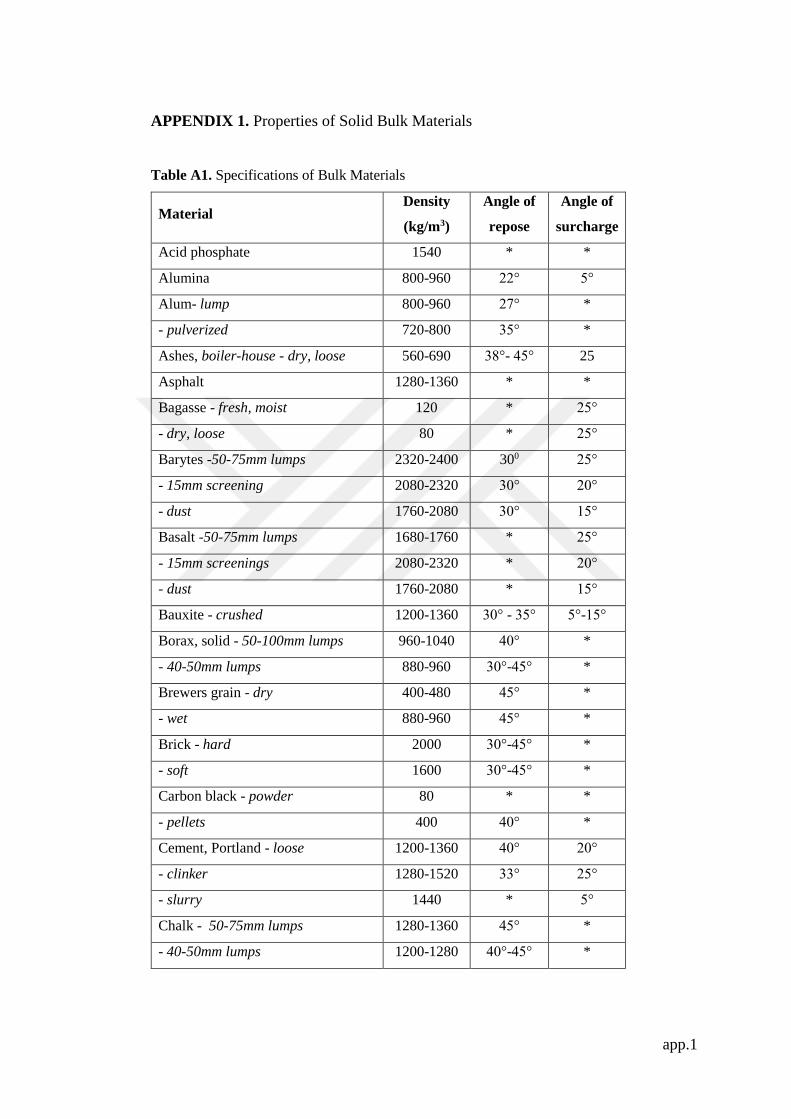
app.1

APPENDIX 1. Properties of Solid Bulk Materials

Table A1. Specifications of Bulk Materials

Material Density

(kg/m3)

Angle of

repose

Angle of

surcharge

Acid phosphate 1540 * *

Alumina 800-960 22° 5°

Alum- lump 800-960 27° *

- pulverized 720-800 35° *

Ashes, boiler-house - dry, loose 560-690 38°- 45° 25

Asphalt 1280-1360 * *

Bagasse - fresh, moist 120 * 25°

- dry, loose 80 * 25°

Barytes -50-75mm lumps 2320-2400 300 25°

- 15mm screening 2080-2320 30° 20°

- dust 1760-2080 30° 15°

Basalt -50-75mm lumps 1680-1760 * 25°

- 15mm screenings 2080-2320 * 20°

- dust 1760-2080 * 15°

Bauxite - crushed 1200-1360 30° - 35° 5°-15°

Borax, solid - 50-100mm lumps 960-1040 40° *

- 40-50mm lumps 880-960 30°-45° *

Brewers grain - dry 400-480 45° *

- wet 880-960 45° *

Brick - hard 2000 30°-45° *

- soft 1600 30°-45° *

Carbon black - powder 80 * *

- pellets 400 40° *

Cement, Portland - loose 1200-1360 40° 20°

- clinker 1280-1520 33° 25°

- slurry 1440 * 5°

Chalk - 50-75mm lumps 1280-1360 45° *

- 40-50mm lumps 1200-1280 40°-45° *

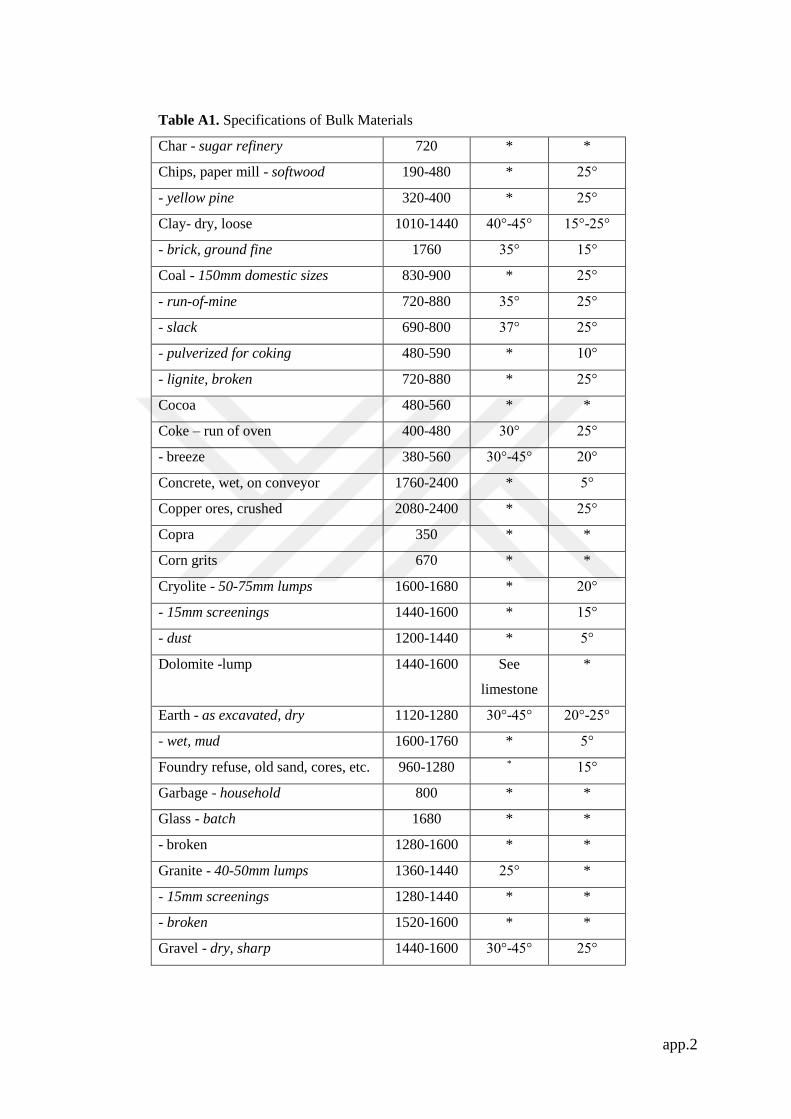
app.2

Table A1. Specifications of Bulk Materials

Char - sugar refinery 720 * *

Chips, paper mill - softwood 190-480 * 25°

- yellow pine 320-400 * 25°

Clay- dry, loose 1010-1440 40°-45° 15°-25°

- brick, ground fine 1760 35° 15°

Coal - 150mm domestic sizes 830-900 * 25°

- run-of-mine 720-880 35° 25°

- slack 690-800 37° 25°

- pulverized for coking 480-590 * 10°

- lignite, broken 720-880 * 25°

Cocoa 480-560 * *

Coke – run of oven 400-480 30° 25°

- breeze 380-560 30°-45° 20°

Concrete, wet, on conveyor 1760-2400 * 5°

Copper ores, crushed 2080-2400 * 25°

Copra 350 * *

Corn grits 670 * *

Cryolite - 50-75mm lumps 1600-1680 * 20°

- 15mm screenings 1440-1600 * 15°

- dust 1200-1440 * 5°

Dolomite -lump 1440-1600 See

limestone

*

Earth - as excavated, dry 1120-1280 30°-45° 20°-25°

- wet, mud 1600-1760 * 5°

Foundry refuse, old sand, cores, etc. 960-1280 * 15°

Garbage - household 800 * *

Glass - batch 1680 * *

- broken 1280-1600 * *

Granite - 40-50mm lumps 1360-1440 25° *

- 15mm screenings 1280-1440 * *

- broken 1520-1600 * *

Gravel - dry, sharp 1440-1600 30°-45° 25°

app.3

Table A1. Specifications of Bulk Materials

- wet 1600-1920 32° 25°

Gutta percha 960 * *

Gypsum - 50-75mm lumps 1200-1280 30° 20°

- 15mm screenings 1120-1280 40° 15°

- dust 960-1120 42° *

Hops - brewery and moist 560 30°-45° *

Ice - crushed 640 * *

Iron borings - machine shop 2000 * *

Iron ores, depends on iron

percentage

1600-3200 35° 25°

Iron pyrites - 50-75mm lumps 2160-2320 * 20°

- 15mm screenings 1920-2160 * 15°

- dust 1680-1920 * 5°

Lead ores, depends on lead

percentage

3200-4320 30° 15°

Limestone - 50-75mm lumps 1440-1520 30°-40° 25°

- 15 mm screenings 1280-1440 * 15°

- dust 1200-1280 * 5°

Linseed cake - crushed 760-780 * *

Manganese ore 2000-2240 39° *

Malt meal 570-640 * *

Meal 700 * *

Paper pulp 640-960 * 5°

Petroleum coke 560-640 * *

Phosphate rock 1360 * *

Pitch 1150 * *

Quartz, solid – 50-75mm lumps 1440-1520 35° *

- 40-50mm lumps 1360-1440 35° *

- dust 1120-1280 40° *

Rock, soft, excavated with shovel 1600-1760 * 20°

Rubber 930 * *

Rubber - reclaim 560 * *

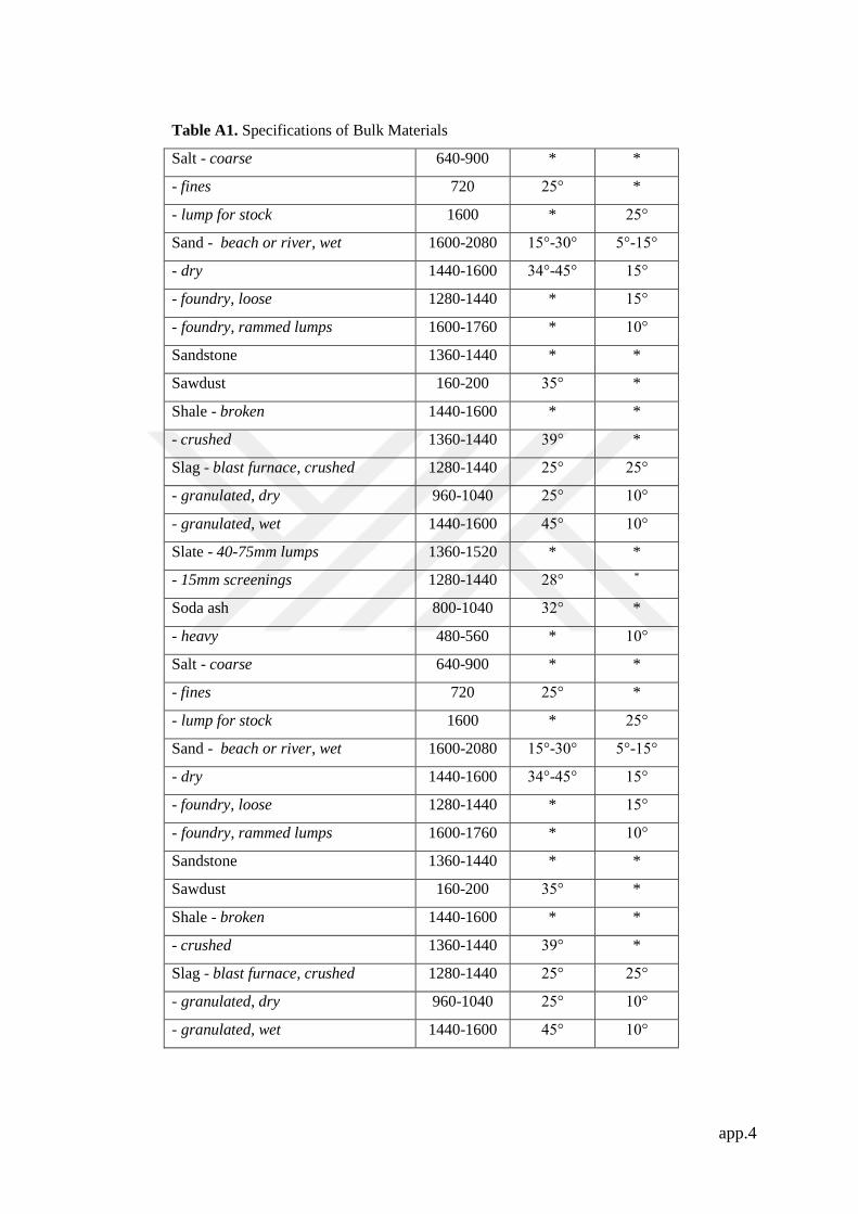
app.4

Table A1. Specifications of Bulk Materials

Salt - coarse 640-900 * *

- fines 720 25° *

- lump for stock 1600 * 25°

Sand - beach or river, wet 1600-2080 15°-30° 5°-15°

- dry 1440-1600 34°-45° 15°

- foundry, loose 1280-1440 * 15°

- foundry, rammed lumps 1600-1760 * 10°

Sandstone 1360-1440 * *

Sawdust 160-200 35° *

Shale - broken 1440-1600 * *

- crushed 1360-1440 39° *

Slag - blast furnace, crushed 1280-1440 25° 25°

- granulated, dry 960-1040 25° 10°

- granulated, wet 1440-1600 45° 10°

Slate - 40-75mm lumps 1360-1520 * *

- 15mm screenings 1280-1440 28° *

Soda ash 800-1040 32° *

- heavy 480-560 * 10°

Salt - coarse 640-900 * *

- fines 720 25° *

- lump for stock 1600 * 25°

Sand - beach or river, wet 1600-2080 15°-30° 5°-15°

- dry 1440-1600 34°-45° 15°

- foundry, loose 1280-1440 * 15°

- foundry, rammed lumps 1600-1760 * 10°

Sandstone 1360-1440 * *

Sawdust 160-200 35° *

Shale - broken 1440-1600 * *

- crushed 1360-1440 39° *

Slag - blast furnace, crushed 1280-1440 25° 25°

- granulated, dry 960-1040 25° 10°

- granulated, wet 1440-1600 45° 10°

app.5

Table A1. Specifications of Bulk Materials

Slate - 40-75mm lumps 1360-1520 * *

- 15mm screenings 1280-1440 28° *

Soda ash 800-1040 32° *

Sugar cane stalks 400 * *

Sugar - raw 880-1040 37° *

- refined 880 * *

Sulphur - 50-75mm lumps 1360-1440 35° 25°

- 15mm screenings 1200-1360 * 15°

Talc - solid 2640 * *

- 50-75mm screenings 1440-1520 * *

- dust 1220-1280 * *

Turf - dry 480 * *

Wheat 720-770 28° 10°

Zinc ores, crushed 2400-2560 38° 20°

Zinc oxide - light 160-480 * 10°

- heavy 480-560 * 10°

Source: Fenner Dunlop, 2009:24-26

app. 6

APPENDIX 2. Required Coefficients for Calculating 3 Equal Roll Idlers Conveyor

Belt Capacity

Fenner Dunlop, (2009:20-21) “Conveyor Handbook” was presented the

general values of the capacity factor and the capacity with regard to cross sectional

area. Table A2, A3 illustrate the capacity factors and the capacity of the troughed belts

regarding the cross sectional area for three equal troughing roll idlers.

Table A2.1. Capacity Factors for Three Equal Idler

Surcharge

Angle

Idler Troughing Angle

20o 25o 30o 35o 45o

0o 0.43 0.53 0.61 0.69 0.81

5 o 0.52 0.61 0.69 0.77 0.88

1 o 0.61 0.70 0.77 0.84 0.94

15o 0.70 0.78 0.86 0.92 1.04

20o 0.79 0.87 0.94 1.00 1.08

25o 0.88 0.96 1.03 1.08 1.15

Source: Fenner Dunlop, 2009:20

Table A2.2. Capacity of Belt Conveyors for Three Equal Idler*

Belt

Width

(mm)

Belt Speed (mps)

0.5 0.75 1 1.25 1.5 2 2.5 3 3.5 4 4.5 5

400 26 39 52 65 78 104 130 156 182 209 235 261

450 34 51 69 86 103 137 172 206 240 274 309 343

500 44 65 87 109 131 175 218 262 306 349 393 437

600 66 99 131 164 197 263 329 394 460 526 592 657

650 78 118 157 196 235 314 392 471 549 628 706 785

750 107 161 215 268 322 429 536 644 751 858 965 1073

800 123 185 247 308 370 493 617 740 863 987 1110 1233

900 159 238 318 397 477 635 794 953 1112 1271 1430 1589

1000 199 298 398 497 597 795 994 1193 1392 1591 1790 1989

1050 221 331 441 551 662 882 1103 1323 1544 1764 1985 2206

1200 292 438 585 731 877 1169 1462 1754 2046 2339 2631 2923

1350 374 561 748 936 1123 1497 1871 2245 2619 2994 3368 3742

1400 404 606 807 1009 1211 1615 2019 2422 2826 3230 3634 4037

app. 7

Table A2.2. Capacity of Belt Conveyors for Three Equal Idler*

1500 466 699 932 1165 1398 1865 2331 2797 3263 3729 4195 4662

1600 533 800 1066 1333 1599 2132 2665 3198 3731 4265 4798 5331

1800 680 1020 1361 1701 2041 2721 3402 4082 4762 5443 6123 6803

2000 846 1268 1691 2114 2537 3382 4228 5073 5919 6764 7610 8455

2200 1029 1543 2057 2572 3086 4115 5143 6172 7201 8229 9258 10287

Source: Fenner Dunlop, 2009:21

(*) Values are taken according to the specific bulk density (1000 kg/m3), surcharge

angle (20o) and idler angle (35o).

For the different values of the surcharge angle and the idler angle, capacity

values shown in the Table A2.1 should be multiplied with the values shown in Table

A2.2.

app.8

APPENDIX 3. Bulk Solid Materials Table

Table A3.1. Bulk Materials Classification Table

Major Class Material Characteristics Included Code Designation

Density Bulk Density, Loose Actual lbs/ft3

Size

Very

Fine

No.200 Sieve (.0029”) And

Under

A200

No.100 Sieve (.0059”) And

Under

A100

No. 40 Sieve (.16”) And Under A60

Fine No. 6 Sieve (.132”) And Under B6

Granular 1\2” And Under C1/2

Granular 3” And Under D3

(1)Lumpy

Over 3” To Be Special

Dx X = Actual Maximum Size

Irregular Stringy, Fibrous, Cylindrical,

Slabs, etc.

E

Flowability

Very Free Flowing – Flow Function > 10 1

Free Flowing – Flow Function > 4 But < 10 2

Average Flowability – Flow Function > 2 But

< 4

3

Sluggish – Flow Function < 2 4

Abrasiveness

Mildly Abrasive – Index 1-17 5

Moderately Abrasive – Index 18-67 6

Extremely Abrasive – Index 68-416 7

Miscellaneous

Properties or

Hazards

Builds Up and Hardens F

Generates Static Electricity G

Decomposes – Deteriorates in Storage H

Flammability J

Becomes Plastic or Tends to Soften K

Very Dusty L

Aerates and Becomes Fluid M

Explosiveness N

Stickiness-Adhesion O

app.9

Source: FMC Technologies, 2009: 20

A.3.2. Bulk Material Properties

Material Weight

lbs/ft3 Material Code

Component

Series

Mat’L Factor

Fm

Adipic Acid 45 45A10035 2B .5

Alfalfa Meal 14-22 18B645WY 2D .6

Alfalfa Pellets 41-43 42C1/2 25 2D .5

Alfalfa Seed 10-15 13B6 15N 1A-1B-1C .4

Almonds, Broken 27-30 29C1/2 35Q 2D .9

Almonds, Whole Shelled 28-30 29C1/2 35Q 2D .9

Alum, Fine 45-50 48B6 35U 1A-1B-1C .6

Alum, Lumpy 50-60 55B6 25 2A-2B 1.4

Alumina 55-65 58B6 27MY 3D 1.8

Alumina Fines 35 35A10027MY 3D 1.6

Alumina Sized or Briquette 65 65D337 3D 2.0

Aluminate Gel (Aluminate

Hydroxide)

45 45B635 2D 1.7

Aluminum Chips, Dry 7-15 11E45V 2D 1.2

Aluminum Chips, Oily 7-15 11E45V 2D .8

Aluminum Hydrate 13-20 17C1/2 35 1A-1B-1C 1.4

Aluminum Ore (See Bauxite) - - - -

Aluminum Oxide 60-120 90A10017M 3D 1.8

Aluminum Silicate (Andalusite) 49 49C1/2 35S 3A-3B .8

Miscellaneous

Properties or

Hazards

Contaminable, Affecting Use P

Degradable, Affecting Use Q

Gives off Harmful or Toxic Gas or Fumes R

Highly Corrosive S

Mildly Corrosive T

Hygroscopic U

Interlocks, Mats or Agglomerates V

Oils Present W

Packs Under Pressure X

Very Light and Fluffy – May Be Windswept Y

Elevated Temperature Z

app.10

A.3.2. Bulk Material Properties

Aluminum Sulfate 45-58 52C1/2 25 1A-1B-1C 1.0

Ammonium Chloride, Crystalline 45-52 49A10045FRS 3A-3B .7

Ammonium Nitrate 45-62 54A4035NTU 3D 1.3

Ammonium Sulfate 45-58 52C1/2 35FOTU 1A-1B-1C42C 1.0

Antimony Powder - A10035 2D 1.6

Apple Pomace, Dry 15 15C1/2 45Y 2D 1.0

Arsenate of Lead (See Lead

Arsenate)

- - - -

Arsentic Oxide (ArsenoliteX1) 100-120 110A?35R - -

Arsentic Pulverized 30 30A10025R 2D .8

Asbestos-Rock (Ore) 81 81D337R 3D 1.2

Asbestos-Shredded 20-40 30E46XY 2D 1.0

Ash, Black Ground 105 105B635 1A-1B-1C 2.0

Ashes, Coal, Dry - 1 2⁄ ” 35-45 40C1/2 46TY 3D 3.0

Ashes, Coal, Dry - 3” 35-40 38D346T 3D 2.5

Ashes, Coal, Wet - 1 2⁄ ” 45-50 48C1/2 46T 3D 3.0

Ashes, Coal, Wet - 3” 45-50 48D346T 3D 4.0

Ashes, Fly (See Fly Ash) - - - -

Asphalt, Crushed - 1 2⁄ 45 45C1/2 45 1A-1B-1C 2.0

Bagasse 7-10 9E45RVXY 2A-2B-2C 1.5

Bakelite, Fine 30-45 38B625 1A-1B-1C 1.4

Baking Powder 40-55 48A10035 1B .6

Baking Soda (Sodium

Bicarbonate)

40-55 48A10025 1B .6

Barite (Barium Sulfate) - 1 2⁄ 120-180 150D336 3D 2.6

Barite, Powder 120-180 150A10035X 2D 2.0

Barium Carbonate 72 72A10045R 2D 1.6

Bark, Wood, Refuse 10-20 15E45TVY 3D 2.0

Barley, Fine, Ground 24-38 31B635 1A-1B-1C .4

Barley, Malted 31 31C1/2 35 1A-1B-1C .4

Barley, Meal 28 28C1/2 35 1A-1B-1C .4

Barley, Whole 36-48 42B625N 1A-1B-1C .5

Basalt 80-105 93B627 3D 1.8

Bauxite, Dry, Ground 68 68B625 2D 1.8

app.11

A.3.2. Bulk Material Properties

Bauxite, Crushed + 1 2⁄ ” – 3” 75-85 80D336 3D 2.5

Beans, Castor, Meal 35-40 38B635W 1A-1B-1C .8

Beans, Castor, Whole Shelled 36 36C1/2 15W 1A-1B-1C .5

Beans, Navy, Dry 48 48C1/2 15 1A-1B-1C .5

Beans, Navy, Steeped 60 60C1/2 25 1A-1B-1C .8

Bentonite, Crude 34-40 37D345X 2D 1.2

Bentonite, -100 Mesh 50-60 55A10025MXY 2D .7

Benzene Hexachloride 56 56A10045R 1A-1B-1C .6

Bicarbonate of Soda (Baking

Soda)

- - 1B .6

Blood, Dried 35-45 40D345U 2D 2.0

Blood, Ground, Dried 30 30A10035U 1A-1B 1.0

Bone Ash (Tricalcium Phosphate) 40-50 45A10045 1A-1B 1.6

Boneblack 20-25 23A10025Y 1A-1B 1.5

Bonechar 27-40 34B635 1A-1B 1.6

Bonemeal 50-60 55B635 2D 1.7

Bones, Whole(1) 35-50 43E45V 2D 3.0

Bones, Crushed 35-50 43D345 2D 2.0

Bones, Ground 50 50B635 2D 1.7

Borate of Lime 60 60A10035 1A-1B-1C .6

Borax, Fine 45-55 50B625T 3D .7

Borax Screening - 1 2⁄ 55-60 58C1/2 35 2D 1.5

Borax, 11 2⁄ ” – 2” Lump 55-60 58D335 2D 1.8

Borax, 2” - 3” Lump 60-70 65D335 2D 2.0

Boric Acid, Fine 55 55B625T 3D .8

Boron 75 75A10037 2D 1.0

Bran, Rice-Rye Wheat 16-20 18B635NY 1A-1B-1C .5

Braunite (Manganese Oxide) 120 120A10036 2D 2.0

Bread Crumbs 20-25 23B635PQ 1A-1B-1C .6

Brewer’s Grain, spent, dry 14-30 22C1/2 45 1A-1B-1C .5

Brewer’s Grain, spent, wet 55-60 58C1/2 45T 2A-2B .8

Brick, Ground - 1 6⁄ ” 100-120 110B637 3D 2.2

Bronze Chips 30-50 40B645 2D 2.0

Buckwheat 37-42 40B625N 1A-1B-1C .4

app.12

A.3.2. Bulk Material Properties

Calcine, Flour 75-85 80A10035 1A-1B-1C .7

Calcium Carbide 70-90 80D325N 2D 2.0

Calcium Carbonate (See

Limestone)

- - - -

Calcium Fluoride (See

Fluorspar)

- - - -

Calcium Hydrate (See Lime,

Hydrated)

- - - -

Calcium Hydroxide (See Lime,

Hydrated)

- - - -

Calcium Lactate 26-29 28D345QTR 2A-2B .6

Calcium Oxide (See Lime,

unslaked)

- - - -

Calcium Phosphate 40-50 45A10045 1A-1B-1C 1.6

Calcium Sulfate (See Gypsum) - - - -

Carbon, Activated, Dry, Fine (1) - - - -

Carbon Black, Pelleted(1) - - - -

Carbon Black, Powder(1) - - - -

Carborundum 100 100D327 3D 3.0

Casein 36 36B635 2D 1.6

Cashew Nuts 32-37 35C1/2 45 2D .7

Cast Iron, Chips 130-200 165C1/2 45 2D 4.0

Caustic Soda 88 88B635RSU 3D 1.8

Caustic Soda, Flakes 47 47C1/2

45RSUX

3A-3B 1.5

Celite (See Diatomaceous Earth) - - - -

Cement, Clinker 75-95 85D336 3D 1.8

Cement, Mortar 133 133B635Q 3D 3.0

Cement, Portland 94 94A10035Q 2D 1.4

Cement, Aerated (Portland) 60-75 68A10016M 2D 1.4

Cerrusite (See Lead Carbonate) - - - -

Chalk, Crushed 75-95 85D325 2D 1.9

Chalk, Pulverized 67-75 71A10025MXY 2D 1.4

Charcoal, Ground 18-28 23A10045 2D 1.2

Charcoal, Lumps 18-28 23D345 2D 1.4

app.13

A.3.2. Bulk Material Properties

Chocolate, Cake Pressed 40-45 43D325 2B 1.5

Chrome Ore 125-140 133D336 3D 2.5

Cinders, Blast Furnace 57 57D336T 3D 1.9

Cinders, Coal 40 40D336T 3D 1.8

Clay (See Bentonite,

Diatomaceous Earth, Fuller’s

Earth, Kaolin & Marl)

- - - -

Clay, Ceramic, Dry, Fines 60-80 70A10035P 1A-1B-1C 1.5

Clay, Calcined 80-100 90B636 3D 2.4

Clay, Brick, Dry, Fines 100-120 110C1/2 36 3D 2.0

Clay, Dry, Lumpy 60-75 68D335 2D 1.8

Clinker, Cement (See Cement

Clinker)

- - - -

Clover Seed 45-48 47B625N 1A-1B-1C .4

Coal, Anthracite (River & Culm) 55-61 60B635TY 2A-2B 1.0

Coal, Anthracite, Sized - 1 2⁄ 49-61 55C1/2 25 2A-2B 1.0

Coal, Bituminous, Mined 40-60 50D335LNXY 1A-1B .9

Coal, Bituminous, Mined, Sized 45-50 48D335QV 1A-1B 1.0

Coal, Bituminous, Mined, Slack 43-50 47C1/2 45T 2A-2B .9

Coal, Lignite 37-45 41D335T 2D 1.0

Cocoa Beans 30-45 38C1/2 25Q 1A-1B .5

Cocoa, Nibs 35 35C1/2 25 2D .5

Cocoa, Powdered 30-35 33A10045XY 1B .9

Cocoanut, Shredded 20-22 21E45 2B 1.5

Coffee, Chaff 20 20B625MY 1A-1B 1.0

Coffee, Green Bean 25-32 29C1/2 25PQ 1A-1B .5

Coffee, Ground, Dry 25 25A4035P 1A-1B .6

Coffee, Ground, Wet 35-45 40A4045X 1A-1B .6

Coffee, Roasted Bean 20-30 25C1/2 25PQ 1B .4

Coffee, Soluble 19 19A4035PUY 1B .4

Coke, Breeze 25-35 30C1/2 37 3D 1.2

Coke, Loose 23-35 30D737 3D 1.2

Coke, Petrol, Calcined 35-45 40D737 3D 1.3

Compost 30-50 40D745TV 3A-3B 1.0

Concrete, Pre-Mix Dry 85-120 103C1/2 36U 3D 3.0

app.14

A.3.2. Bulk Material Properties

Copper Ore 120-150 135DX35 3D 4.0

Copper Ore, Crushed 100-150 125D336 3D 4.0

Copper Sulphate, (Bluestone) 75-95 85C1/2 35S 2A-2B-2C 1.0

Copperas (See Ferrous Sulphate) - - - -

Copra, Cake Ground 40-45 43B645HW 1A-1B-1C .7

Copra, Cake, Lumpy 25-30 28D335HW 2A-2B-2C .8

Copra, Lumpy 22 22E35HW 2A-2B-2C 1.0

Copra, Meal 40-45 42B635HW 2D .7

Cork, Fine Ground 5-15 10B635JNY 1A-1B-1C .5

Cork, Granulated 12-15 14C1/2 35JY 1A-1B-1C .5

Corn, Cracked 40-50 45B625P 1A-1B-1C .7

Corn Cobs, Ground 17 17C1/2 25Y 1A-1B-1C .6

Corn Cobs, Whole(1) 12-15 14E35 2A-2B -

Corn Ear(1) 56 56E35 2A-2B -

Corn Germ 21 21B635PY 1A-1B-1C .4

Corn Grits 40-45 43B635P 1A-1B-1C .5

Cornmeal 32-40 36B635P 1A-1B .5

Corn Oil, Cake 25 25D745HW 1A-1B .6

Corn Seed 45 45C1/2 25PQ 1A-1B-1C .4

Corn Shelled 45 45C1/2 25 1A-1B-1C .4

Corn Sugar 30-35 33B635PU 1B 1.0

Cottonseed, Cake, Crushed 40-45 43C1/2 45HW 1A-1B 1.0

Cottonseed, Cake, Lumpy 40-45 43D745HW 2A-2B 1.0

Cottonseed, Dry, Delinted 22-40 31C1/2 25X 1A-1B .6

Cottonseed, Dry, Not Delinted 18-25 22C1/2 45XY 1A-1B .9

Cottonseed, Flakes 20-25 23C1/2 35HWY 1A-1B .8

Cottonseed, Hulls 12 12B635Y 1A-1B .9

Cottonseed, Meal, Expeller 25-30 28B645HW 3A-3B .5

Cottonseed, Meal, Extracted 35-40 37B645HW 1A-1B .5

Cottonseed, Meats, Dry 40 40B635HW 1A-1B .6

Cottonseed, Meats, Rolled 35-40 38C1/2 45HW 1A-1B .6

Cracklings, Crushed 40-50 45D345HW 2A-2B-2C 1.3

Cryolite, Dust 75-90 83A10036L 2D 2.0

Cryolite, Lumpy 90-110 100D1636 2D 2.1

Cullet, Fine 80-120 100C1/2 37 3D 2.0

app.15

A.3.2. Bulk Material Properties

Cullet, Lump 80-120 100D1637 3D 2.5

Culm (See Coal, Anthracite) - - - -

Cupric Sulphate (Copper Sulfate) - - - -

Detergent (See Soap Detergent) - - - -

Diatomaceous Earth 11-17 14A4036Y 3D 1.6

Dicalcium Phosphate 40-50 45A4035 1A-1B-1C 1.6

Disodium Phosphate 25-31 28A4035 3D .5

Distiller’s Grain, Spent Dry 30 30B635 2D .5

Distiller’s Grain, Spent Wet 40-60 50C1/2 45V 3A-3B .8

Dolomite, Crushed 80-100 90C1/2 36 2D 2.0

Dolomite, Lumpy 90-100 95DX36 2D 2.0

Earth, Loam, Dry, Loose 76 76C1/2 36 2D 1.2

Ebonite, Crushed 63-70 67C1/2 35 1A-1B-1C .8

Egg Powder 16 16A4035MPY 1B 1.0

Epsom Salts (Magnesium

Sulfate)

40-50 45A4035U 1A-1B-1C .8

Feldspar, Ground 65-80 73A10037 2D 2.0

Feldspar, Lumps 90-100 95D?37 2D 2.0

Feldspar, Powder 100 100A20036 2D 2.0

Feldspar, Screenings 75-80 78C1/2 37 2D 2.0

Ferrous Sulfide - 1 2⁄ 120-135 128C1/2 26 1A-1B-1C 2.0

Ferrous Sulfide -100M 105-120 113A10036 1A-1B-1C 2.0

Ferrous Sulphate 50-75 63C1/2 35U 2D 1.0

Fish Meal 35-40 38C1/2 45HP 1A-1B-1C 1.0

Fish Scrap 40-50 45D?45H 2A-2B-2C 1.5

Flaxseed 43-45 44B635X 1A-1B-1C .4

Flaxseed Cake (Linseed Cake) 48-50 49D?45W 2A-2B .7

Flaxseed Meal (Linseed Meal) 25-45 35B645W 1A-1B .4

Four Wheat 33-40 37A4045LP 1B .6

Flue Dust, Basic Oxygen Furnace 45-60 53A4036LM 3D 3.5

Flue Dust, Blast Furnace 110-125 118A4036 3D 3.5

Flue Dust, Boiler H. Dry 30-45 38A4036LM 3D 2.0

Fluorspar, Fine (Calcium

Fluoride)

80-100 90B636 2D 2.0

Fluorspar, Lumps 90-110 100D736 2D 2.0

app.16

A.3.2. Bulk Material Properties

Flyash 30-45 38A4036M 3D 2.0

Foundry Sand, Dry (See Sand) - - - -

Fuller’s Earth, Dry, Raw 30-40 35A4025 2D 2.0

Fuller’s Earth, Oily, Spent 60-65 63C1/2 45OW 3D 2.0

Fuller’s Earth, Calcined 40 40A10025 3D 2.0

Galena (See Lead Sulfide) - - - -

Gelanite, Granulated 32 32B635PU 1B .8

Gilsonite 37 37C1/2 35 3D 1.5

Glass, Batch 80-100 90C1/2 37 3D 2.5

Glue, Ground 40 40B645U 2D 1.7

Glue, Pearl 40 40C1/2 35U 1A-1B-1C .5

Glue, Veg, Powdered 40 40A4045U 1A-1B-1C .6

Gluten, Meal 40 40B635P 1B .6

Granite, Fine 80-90 85C1/2 27 3D 2.5

Grape Pomace 15-20 18D345U 2D 1.4

Graphite Flake 40 40B625LP 1A-1B-1C .5

Graphite Flour 28 28A10035LMP 1A-1B-1C .5

Graphite Ore 65-75 70DX35L 2D 1.0

Guano Dry(1) 70 70C1/2 35 3A-3B 2.0

Gypsum, Calcined 55-60 58B635U 2D 1.6

Gypsum, Calcined, Powdered 60-80 70A10035U 2D 2.0

Gypsum Raw -1” 70-80 75D325 2D 2.0

Hay, Chopped(1) 8-12 10C1/2 35JY 2A-2B 1.6

Hexanedioic Acid (See Adipic

Acid)

- - - -

Hominy, Dry 35-50 43C1/2 35D 1A-1B-1C .4

Hops, Spent, Dry 35 35D335 2A-2B-2C 1.0

Hops, Spent, Wet 50-55 53D345V 2A-2B 1.5

Ice, Crushed 35-45 40D3350 2A-2B .4

Ice, Flaked(1) 40-45 43C1/2 350 1B .6

Ice, Cubes 33-35 34D3350 1B .4

Ice, Shell 33-35 34D3450 1B .4

Ilmenite Ore 140-160 150D337 3D 2.0

Iron Ore Concentrate 120-180 150A4037 3D 2.2

Iron Oxide Pigment 25 25A10036LMP 1A-1B-1C .10

app.17

A.3.2. Bulk Material Properties

Iron Oxide, Millscale 75 75C1/2 36 2D 1.6

Iron Pyrites (See Ferrous Sulfide) - - - -

Iron Sulphate (See Ferrous

Sulfate)

- - - -

Iron Vitriol (See Ferrous Sulfate) - - - -

Kafir (Corn) 40-45 43C1/2 25 3D .5

Kaolin Clay 63 63D325 2D 2.0

Kaolin Clay-Tale 42-56 49A4035LMP 2D 2.0

Kryalith (See Cryolite) - - - -

Lactose 32 32A4035PU 1B .6

Lamp Black (See Carbon Black) - - - -

Lead Arsenate 72 72A4035R 1A-1B-1C 1.4

Lead Arsenite 72 72A4035R 1A-1B-1C 1.4

Lead Carbonate 240-260 250A4035R 2D 1.0

Lead Ore - 1 6⁄ 200-270 235B635 3D 1.4

Lead Ore - 1 2⁄ 180-230 205C1/2 36 3D 1.4

Lead Oxide (Red Lead)

– 100 Mesh

30-150 90A10035L 2D 1.2

Lead Oxide (Red Lead)

– 200 Mesh

30-180 105A20035LP 2D 1.2

Lead Sulphide – 100 Mesh 240-260 250A10035R 2D -

Lignite (See Coal Lignite) - - - -

Limanite, Ore, Brown 120 120C1/2 47 3D 1.7

Lime, Ground, Unslaked 60-65 63B635U 1A-1B-1C .6

Lime Hydrated 40 40B635LM 2D .8

Lime, Hydrated, Pulverized 32-40 36A4035LM 1A-1B .6

Lime, Pebble 53-56 55C1/2 25HU 2A-2B 2.0

Limestone, Agricultural 68 68B635 2D 2.0

Limestone, Crushed 85-90 88DX36 2D 2.0

Limestone, Dust 55-95 75A4046MY 2D 1.6-2.0

Lindane (Benzene Hexachloride) - - - -

Linseed (See Flaxseed) - - - -

Litharge (Lead Oxide) - - - -

Lithopone 45-50 48A32535MR 1A-1B 1.0

Malze (See Milo) - - - -

app.18

A.3.2. Bulk Material Properties

Malt, Dry, Ground 20-30 25B635NP 1A-1B-1C .5

Malt, Meal 26-40 38B625P 1A-1B-1C .4

Malt, Dry Whole 20-30 25C1/2 35P 1A-1B-1C .5

Malt, Sprouts 13-15 14C1/2 35P 1A-1B-1C .4

Magnesium Chloride (Magnesite) 33 33C1/2 45 1A-1B 1.0

Manganese Dioxide(1) 70-85 78A10035NRT 2A-2B 1.5

Manganese Ore 125-140 133Dx37 3D 2.0

Manganese Oxide 120 120A10036 2D 2.0

Manganese Sulfate 70 70C1/2 37 3D 2.4

Marble, Crushed 80-95 88B637 3D 2.0

Marl, (Clay) 80 80Dx36 2D 1.6

Meat, Ground 50-55 53E45HQTX 2A-2B 1.5

Meat, Scrap (W/bone) 40 40E46H 2D 1.5

Mica, Flakes 17-22 20B616MY 2D 1.0

Mica, Ground 13-15 14B636 2D .9

Mica, Pulverized 13-15 14A10036M 2D 1.0

Milk, Dried, Flake 5-6 6B635PUY 1B .4

Milk, Malted 27-30 29A4045PX 1B .9

Milk, Powdered 20-45 33B625PM 1B .5

Milk Sugar 32 32A10035PX 1B .6

Milk, Whole, Powdered 20-36 28B635PUX 1B .5

Mill Scale (Steel) 120-135 123E46T 3D 3.0

Milo, Ground 23-36 34B625 1A-1B-1C .5

Milo Maize (Kafir) 40-45 43B615N 1A-1B-1C .4

Molybdenite Powder 107 107B626 2D 1.5

Monosodium Phosphate 50 50B636 2D .6

Mortar, Wet(1) 150 150E46T 3D 2.0

Mustard Seed 45 45B615N 1A-1B-1C .4

Naphthalene Flakes 45 45B635 1A-1B-1C .7

Niacin (Nicotinic Acid) 35 35A4035P 2D .8

Oats 26 26C1/2 25MN 1A-1B-1C .4

Oats, Crimped 19-26 23C1/2 35 1A-1B-1C .5

Oats, Crushed 22 22B645NY 1A-1B-1C .6

Oats, Flour 35 35A10035 1A-1B-1C .5

Oat Hulls 8-12 10B635NY 1A-1B-1C .5

app.19

A.3.2. Bulk Material Properties

Oats, Rolled 19-24 22C1/2 35NY 1A-1B-1C .6

Oleo Margarine (Margarine) 59 59E45HKPWX 2A-2B .4

Orange Peel, Dry 15 15E45 2A-2B 1.5

Oxalic Acid Crystals – Ethane

Diacid Crystals

60 60B635QS 1A-1B 1.0

Oyster Shells, Ground 50-60 55C1/2 36T 3D 1.6-2.0

Oyster Shells, Whole 80 80D336TV 3D 2.1-2.5

Paper Pulp (4% or less) 62 62E45 2A-2B 1.5

Paper Pulp (6% to 15%) 60-62 61E45 2A-2B 1.5

Paraffin Cake - 1 2⁄ " 45 45C1/2 45K 1A-1B .6

Peanuts, Clean, in shell 15-20 18D335Q 2A-2B .6

Peanut Meal 30 30B635P 1B .6

Peanuts, Raw, Uncleaned

(unshelled)

15-20 18D336Q 3D .7

Peanuts, Shelled 35-45 40C1/2 35Q 1B .4

Peas, Dried 45-50 48C1/2 15NQ 1A-1B-1C .5

Perlite-Expanded 8-12 10C1/2 36 2D .6

Phosphate Acid Fertilizer 60 60B625T 2A-2B 1.4

Phosphate Disodium (See

Sodium Phosphate)

- - - -

Phosphate Rock, Pulverized 60 60B636 2D 1.7

Phosphate Sand 90-100 95B637 3D 2.0

Plaster of Paris (See Gypsum) - - - -

Plumbago (See Graphite) - - - -

Polystyrene Beads 40 40B635PQ 1B .4

Polyvinyl, Chloride Powder 20-30 25A10045KT 2B 0.1

Polyvinyl, Chloride Pellets 20-30 25E45KPQT 1B .6

Polyethelene, Resin Pellets 30-35 33C1/2 45Q 1A-1B .4

Potash (Muriate) Dry 70 70B637 3D 2.0

Potash (Muriate) Mine Run 75 75Dx37 3D 2.2

Potassium Carbonate 51 51B636 2D 1.0

Potassium Chloride Pellets 120-130 125C1/2 25TU 3D 1.6

Potassium Nitrate - 1 2⁄ 76 76C1/2 16NT 3D 1.2

Potassium Nitrate - 1 6⁄ 80 80B626NT 3D 1.2

Potassium Sulfate 42-48 45B646X 2D 1.0

app.20

A.3.2. Bulk Material Properties

Potato Flour 48 48A20035MNP 1A-1B .5

Pumice - 1 6⁄ 42-48 45B646 3D 1.6

Pyrite, Pellets 120-130 125C1/2 26 3D 2.0

Quartz, - 100 Mesh 70-80 75A10027 3D 1.7

Quartz, - 1 2⁄ 80-90 85C1/2 27 3D 2.0

Rice, Bran 20 20B635NY 1A-1B-1C .4

Rice, Grits 42-45 44B635P 1A-1B-1C .4

Rice, Polished 30 30C1/2 15P 1A-1B-1C .4

Rice, Hulled 45-49 47C1/2 25P 1A-1B-1C .4

Rice, Hulls 20-21 21B635NY 1A-1B-1C .4

Rice, Rough 32-36 34C1/2 35N 1A-1B-1C .6

Rosin - 1 2⁄ 65-68 67C1/2 45Q 1A-1B-1C 1.5

Rubber, Reclaimed Ground 23-50 37C1/2 45 1A-1B-1C .8

Rubber, Pelleted 50-55 53D345 2A-2B-2C 1.5

Rye 42-48 45B615N 1A-1B-1C .4

Rye Bran 15-20 18B635Y 1A-1B-1C .4

Rye Feed 33 33B635N 1A-1B-1C .5

Rye Meal 35-40 38B635 1A-1B-1C .5

Rye Middlings 42 42B635 1A-1B .5

Rye, Shorts 32-33 33C1/2 35 2A-2B .5

Safflower, Cake 50 50D326 2D .6

Safflower, Meal 50 50B635 1A-1B-1C .6

Safflower Seed 45 45B615N 1A-1B-1C .4

Saffron (See Safflower) - - - -

Sal Animoniac (Ammonium

Chloride)

- - - -

Salt Cake, Dry Coarse 85 85B636TU 3D 2.1

Salt Cake, Dry Pulverized 65-85 75B636TU 3D 1.7

Salicylic Acid 29 29B637U 3D .6

Salt, Dry Coarse 45-60 53C1/2 36TU 3D 1.0

Salt, Dry Fine 70-80 75B636TU 3D 1.7

Saltpeter – (See Potassium

Nitrate)

- - - -

Sand Dry Bank (Damp) 110-130 120B647 3D 2.8

Sand Dry Bank (Dry) 90-110 100B637 3D 1.7

app.21

A.3.2. Bulk Material Properties

Sand Dry Silica 90-100 95B627 3D 2.0

Sand Foundry (Shake Out) 90-100 95D337Z 3D 2.6

Sand (Resin Coated) Silica 104 104B627 3D 2.0

Sand (Resin Coated) Zircon 115 115A10027 3D 2.3

Sawdust, Dry 10-13 12B645UX 1A-1B-1C .7

Sea-Coal 65 65B636 2D 1.0

Sesame Seed 27-41 34B626 2D .6

Shale, Crushed 85-90 88C1/2 36 2D 2.0

Shellac, Powdered or Granulated 31 31B635P 1B .6

Silicon Dioxide (See Quartz) - - - -

Silica, Flour 80 80A4046 2D 1.5

Silica Gel + 1 2⁄ ”-3” 45 45D337HKQU 3D 2.0

Slag, Blast Furnace Crushed 130-180 155D337Y 3D 2.4

Slag, Furnace Granular, Dry 60-65 63C1/2 37 3D 2.2

Slate, Crushed - 1 2⁄ 80-90 85C1/2 36 2D 2.0

Slate, Ground - 1 6⁄ 82-85 84B636 2D 1.6

Sludge, Sewage, Dried 40-50 45E47TW 3D .8

Sludge, Sewage, Dry Ground 45-55 50B46S 2D .8

Soap, Beads or Granules 15-35 25B635Q 1A-1B-1C .6

Soap, Chips 15-25 20C1/2 35Q 1A-1B-1C .6

Soap Detergent 15-50 33B635FQ 1A-1B-1C .8

Soap , Flakes 5-15 10B635QXY 1A-1B-1C .6

Soap, Powder 20-25 23B625X 1A-1B-1C .9

Soapstone, Talc, Fine 40-50 45A20045XY 1A-1B-1C 2.0

Soda Ash, Heavy 55-65 60B636 2D 1.0

Soda Ash, Light 20-35 28A4036Y 2D .8

Sodium Aluminate, Ground 72 72B636 2D 1.0

Sodium Aluminum Fluoride

(See Kryolite)

- - - -

Sodium Aluminum Sulphate(1) 75 75A10036 2D 1.0

Sodium Bentonite

(See Bentonite)

- - - -

Sodium Bicarbonate

(See Baking Soda)

- - - -

Sodium Chloride (See Salt) - - - -

app.22

A.3.2. Bulk Material Properties

Sodium Carbonate (See Soda

Ash)

- - - -

Sodium Hydrate (See Caustic

Soda)

- - - -

Sodium Hydroxide (See Caustic

Soda)

- - - -

Sodium Borate (See Borax) - - - -

Sodium Nitrate 70-80 75D325NS 2A-2B 1.2

Sodium Phosphate 50-60 55A35 1A-1B .9

Sodium Sulfate (See Salt Cake) - - - -

Sodium Sulfite 96 96B646X 2D 1.5

Sorghum, Seed

(See Kafir or Milo)

- - - -

Soybean, Cake 40-43 42D335W 2A-1B-1C 1.0

Soybean, Cracked 30-40 35C1/2 36NW 2D .5

Soybean, Flake, Raw 18-25 22C1/2 35Y 1A-1B-1C .8

Soybean, Flour 27-30 29A4035MN 1A-1B-1C .8

Soybean Meal, Cold 40 40B635 1A-1B-1C .5

Soybean Meal, Hot 40 40B635T 2A-2B .5

Soybeans, Whole 45-50 48C1/2 26NW - 1.0

Starch 25-50 38A4015M 1A-1B-1C 1.0

Steel Turnings, Crushed 100-150 125D346WV 3D 3.0

Sugar Beet, Pulp, Dry 12-15 14C1/2 26 2D .9

Sugar Beet, Pulp, Wet 25-45 35C1/2 35X 1A-1B-1C 1.2

Sugar, Refined, Granulated Dry 50-55 53B635PU 1B 1.0-1.2

Sugar, Refined, Granulated Wet 55-65 60C1/2 35X 1B 1.4-2.0

Sugar, Powdered 50-60 55A10035PX 1B .8

Sugar, Raw 55-65 60B635PX 1B 1.5

Sulphur, Crushed - 1 2⁄ 50-60 55C1/2 35N 1A-1B .8

Sulphur, Lumpy – 3” 80-85 83D335N 2A-2B .8

Sulphur, Powdered 50-60 55A4035MN 1A-1B .6

Sunflower Seed 19-38 29C1/2 15 1A-1B-1C .5

Talcum, - 1 2⁄ 80-90 85C1/2 36 2D .9

Talcum Powder 50-60 55A20036M 2D .8

Tanbark, Ground(1) 55 55B645 1A-1B-1C .7

app.23

A.3.2. Bulk Material Properties

Timothy Seed 36 36B635NY 1A-1B-1C .6

Titanium Dioxide (See Ilmenite

Ore)

- - - -

Tobacco, Scraps 15-25 20D345Y 2A-2B .8

Tobacco, Snuff 30 30B645MQ 1A-1B-1C .9

Tricalcium Phosphate 40-50 45A4045 1A-1B 1.6

Triple Super Phosphate 50-55 53B636RS 3D 2.0

Trisodium Phosphate 60 60C1/2 36 2D 1.7

Trisodium Phosphate, Granular 60 60B636 2D 1.7

Trisodium Phosphate, Pulverized 50 50A4036 2D 1.6

Tung Nut Meats, Crushed 28 28D325W 2A-2B .8

Tung Nuts 25-30 28D315 2A-2B .7

Urea Polls, Coated 43-46 45B625 1A-1B-1C 1.2

Vermiculite, Expanded 16 16C1/2 35Y 1A-1B .5

Vermiculite, Ore 80 80D336 2D 1.0

Vetch 48 48B616N 1A-1B-1C .4

Walnut Shells, Crushed 35-45 40B636 2D 1.0

Wheat 45-48 47C1/2 25N 1A-1B-1C .4

Wheat, Cracked 40-45 43B625N 1A-1B-1C .4

Wheat, Germ 18-28 23B625 1A-1B-1C .4

White Lead, Dry 75-100 88A4036MR 2D 1.0

Wood Chips, Screened 10-30 20D345VY 2A-2B .6

Wood Flour 16-36 26B635N 1A-1B .4

Wood Shavings 8-16 12E45VY 2A-2B 1.5

Zinc, Concentrate Residue 75-8 78B637 3D 1.0

Zinc Oxide, Heavy 30-35 33A10045X 1A-1B 1.0

Zinc Oxide, Light 10-15 13A10045XY 1A-1B 1.0

Source: FMC Technologies, 2009: 26-34

app. 24

APPENDIX 4. RProject Codes for Simulation Model

getwd()

setwd("C:/Users/Google Drive/Program Deneme/R")

library(tidyverse)

###Input variables will be added here

### BERTH HANDLING

##Berth handling operation choices' functions

#Grab Function

use_grab <- function(eta_G_i) {

C_j_i <- Gng_t*Gng_n

E_j_n <- E_G_n

eta_j_i <- eta_G_i

if (ro_i*V_g > (C_max_lift-WT_g_net))

{

Gng_t <- C_max_lift-WT_g_net

}

else {

Gng_t <- ro_i*V_g

}

w <- Gng_m*Gng_t* E_g_n*BOR*eta_G_i*t_pd*t*PF

return(w)

}

#Pneumatic Unloader Function

use_pne <- function(eta_pne_i){

app. 25

C_j_n <- n_pne*A*p_mix*phi/(phi+1)

E_j_n <- E_pne_n

eta_j_i <- eta_pne_i

x <-

n_pne*A*ro_mix*phi/((phi+1)*E_pne_n*BOR*eta_pne_i*t_pd*t*

PF)

return(x)

}

#Stacker Function

# Flat Belt is used 1, not used 0

use_stc <- function(flat_belt,eta_fb_i,eta_3b_i){

if (flat_belt == 1){

C_j_n <- C_w_s*ro_i*CF*cos(alpha)*(v_b/100)

E_j_n <- E_stc_n

eta_j_i <- eta_fb_i

y <-

(tan(delta)/6*ro_i)*v_b*b^(2*cos(alpha))*E_stc_n*BOR*eta_

fb_i*t_pd*t*PF

}

else if (flat_belt == 0){

C_j_n <- C_w_s*ro_i*CF*cos(alpha)*(v_b/100)

E_j_n <- E_stc_n

eta_j_i <- eta_3b_i

y <-

C_w_s*ro_i*CF*cos(a)*(v_b/100)*E_stc_n*BOR*eta_3b_i*t_pd*

t*PF

}

return(y)

}

#Screw Type Unloader Function

app. 26

use_scr <- function(eta_scr_i){

C_j_n <- pi/4*(D*D-d*d)*lambda*N*ro_i*psi*k

E_j_n <- E_scr_n

eta_j_i <- eta_scr_i

z <- (pi/4)*(D*D -

d*d)*lambda*N*ro_i*psi*k*E_scr_n*eta_scr_i*t_pd*t*PF

return(z)

}

##Berth Handling Operation Main Function

# If one or more of the following eqiupment were used for

the operation, enter 1.

#Eqiupment used 1 not used 0. Arrange the data frame

according to this nomenclature

Grab = 0

PneumaticUnloader = 0

Stacker = 0

ScrewTypeUnloader = 0

berth_handling <-

function(Grab,PneumaticUnloader,Stacker,ScrewTypeUnloader

) {

if (Grab != 0){

a <- use_grab(eta_G_i)

}

if (PneumaticUnloader != 0){

b <- use_pne(eta_pne_i)

}

if (Stacker != 0){

c <- use_stc(flat_belt,eta_fb_i,eta_3b_i)

}

app. 27

if (ScrewTypeUnloader != 0){

d <- use_scr(eta_scr_i)

}

total_berth <- a+b+c+d

return(total_berth)

print("Total Berth Handling Capacity: ",total_berth)

}

### TRANSFER EQUIPMENT

## Transfer Equipment operation choices' functions

#Reclaimer Function

use_reclaimer <- function(eta_rec_i,E_rc_n,v_rec){

C_j_n <- A*v_rec

E_j_n <- E_rec_n

eta_j_i <- eta_rec_i

tt <- A* v_rec*3600*E_rec_n*eta_rec_i*t_pd*t

return(tt)

}

# Stacker Function

#If flat belt is used 1, not used 0.

use_stacker <-

function(flat_belt_2,eta_fb_i,eta_3b_i,E_stc_n){

if (flat_belt_2 == 1){

C_j_n <- tan(delta)/sigma*ro_i*v_b*b^2*cos(alpha)

E_j_n <- E_stc_n

eta_j_i <- eta_fb_i

app. 28

ss <-

tan(delta)*ro_i*v_b*b^2*cos(alpha)*E_stc_n*eta_fb_i*t_pd*

t

}

else {

C_j_n <- C_w_s*ro_i*CF*cos(alpha*v_b/100)

E_j_n <- E_stc_n

eta_j_i <- eta_3b_i

ss <- C_w_s

*ro_i0CF*cos(alpha)*(v_b/100)*E_stc_n*eta_3b_i*t_pd*t

}

}

#Screw Conveyor Function

#If is U shaped 1, not 0.

use_scr_con <- function(U_type,eta_uscr_i,E_uscr_n){

if (U == 1){

C_j_n <- ro_i*(pi/4)*(D*D-

d*d)*psi*lambda*(N/60)*(CF_f*CF_m)

E_j_n <- E_uscr_n

eta_j_i <- eta_uscr_i

xx <- ro_i*(pi/4)*(D*d-

d*d)*psi*lambda*(N/60)*CF_f*CF_m*E_uscr_n*eta_uscr_i*t_pd

*t

}

else {

C_j_n <- ro_i*(pi/4)*(D*D-d*d)*N*lambda*ro_i*psi*k

E_j_n <- E_uscr_n

eta_j_i <- eta_uscr_i

xx <- ro*(pi/4)*(D*d-

d*d)*lambda*N*ro_i*psi*k*E_uscr_n*eta_uscr_con*t_pd*t

}

app. 29

return(xx)

}

#Belt Conveyor Function

use_belt_conveyor <-

function(flat_belt_3,eta_fb_i,E_fb_n){

if (flat_belt_3 == 1){

C_j_n <- tan(delta)/(sigma*ro_i*v_b*b^2*cos(alpha))

E_j_n <- E_fb_n

eta_j_i <- eta_fb_i

yy <-

tan(delta)*sigma*ro_i*v_b*(b^(2*cos(alpha)))*E_fb_n*eta_f

b_i*t_pd*t

}

else{

C_j_n <- C_w_s*p_i*CF*cos(alpha)*v_b/100

E_j_n <- E_3_n

eta_j_i <- eta_3b_i

yy <-

C_w_s*ro_i*CF*(cos(alpha)*v_b/100)*E_3_n*eta_3b_i*t_pd*t

}

return(yy)

}

#Truck Function

use_truck <- function(eta_trk_i,Max_trk){

if (ro_i*V_trk > Max_trk){

CC_trk <- Max_trk

C_j_n <- Max_trk*Te/O_trk_i

E_j_n <- E_trk_n

app. 30

eta_j_i <- eta_trk_i

zz <- Max_trk*Te/O_trk_i*E_trk_n*eta_trk_i*t_pd*t

}

else{

C_trk <- ro_i*V_trk

C_j_n <- ro_i*V_trk*Te/O_trk_i

E_j_n <- E_trk_n

eta_j_i <- eta_trk_i

zz <- ro_i*V_trk*Te/O_trk_i*E_trk_n*eta_trk_i-t_pd*t

}

}

#Bulldozer Function

use_bulldozer <- function(eta_bld_i,Max_bld){

if (ro_i*V_bld > Max_bld){

C_bld <- Max_bld

C_j_n <- Max_bld*Te/O_bld_i

E_j_n <- E_bld_n

eta_j_i <- eta_bld_i

ww <- Max_bld*Te/O_bld_i*E_bld_n*eta_bld_i*t_pd*t

}

else{

C_bld <- ro_i*V_bld

ww <- ro_i*V_bld*Te/O_bld_i*E_bld_n*eta_bld_i*t_pd*t

}

}

#Transfer Equipment Main Function

app. 31

# If one or more of the following eqiupment were used for

the operation, enter 1.

#Eqiupment used 1 not used 0. Arrange the data frame

according to this nomenclature

ReClaimer = 0

Stacker = 0

ScrewConveyor = 0

BeltConveyor = 0

Truck = 0

Bulldozer = 0

transfer_equipment <-

function(ScrewConveyor,BeltConveyor,Truck,Bulldozer) {

if (ScrewConveyor != 0){

aa <- use_scr_con(U_type,eta_uscr_i,E_uscr_n)

}

if (BeltConveyor != 0){

bb <- use_belt_conveyor(flat_belt_3,eta_b)

}

if (Truck != 0){

cc <- use_truck(eta_trk_i,Max_trk)

}

if (Bulldozer != 0){

dd <- use_bulldozer(eta_bld_i,Max_bld)

}

if (Stacker != 0){

ee <-

use_stacker(flat_belt_2,eta_fb_i,eta_3b_i,E_stc_n)

}

if (ReClaimer != 0){

ff <- use_reclaimer(eta_rec_i,E_rc_n,v_rec)

}

app. 32

total_transfer_equipment <- aa+bb+cc+dd+ee+ff

return(total_transfer_equipment)

print("Total Transfer Equipment Capacity:

",total_transfer_equipment)

}

### STORAGE YARD

#Selecting h

if (q_max_i/ro_i > h_eq_max){

if (h_w_max > h_eq_max){

h<-h_eq_max

}else {h<-h_w_max}

} else {

if (h_w_max >q_max(ro_i)) {

h<-q_max/ro_i

}else{h<-h_w_max}

}

#Are open and closed storage area applied together? Yes

1, No 0.

OCTogether <- 0

if (OCTogether == 1){

C_storage <- C_OA + C_CA

}

#C_OA or C_CA, Operation=1 yields C_CA, Operation=0

yields C_OA

Operation <- 0

if(OCTogether == 0){

app. 33

if (Operation == 1){

if (Dome != 0){

C_dome <- V_dome*n_dome*PF_dome*ro_i*365/t_d_dome

}

else if (Shed != 0){

C_Shed <- V_shed*n_shed*PF_shed*ro_i*365*t_d_shed

}

else if (Silo != 0){

C_silo <- V_silo*n_silo*PF_silo*ro_i*365/t_d_silo

}

else if(EnclosedStructure != 0){

C_EA <- m_s*n_EA*PF_EA*365/t_d_EA

}

C_CA <- C_dome+C_shed+C_silo+C_EA

}

else if (Operation == 0){

#Are Longitudinal and Circular storage yard type

applied together ? Yes 1, No 0.

if(LongitudinalCircular == 1){

C_OA <- C_OA_IID+C_OA_ICAM+C_OA_c_cir+C_OA_c_con

}

else if(LongitudinalCircular == 0){

#Only put into operation C_OAI_ID and/or C_OAI_CAM

or C_OA_C

# xxx creates a choice between C_OAI_ID and/or

C_OAI_CAM or C_OA_C

xxx <- 0

if (xxx == 0){

#Put into operation C_OAI_ID and/or C_OAI_CAM

app. 34

#Finding m_s_ts and l_S will be operated from

outside. It depends on Geometry(TS,TEC,TREC)

n_s <- l_lane/(l_s+d_S)

C_OAI_ID <- n_lane*n_s*V_s_ton*PF_OA*360/t_d_OA

C_OAI_CAM <- n_lane*m_s*PF_OA*360/t_d_OA

#Are ID-Presented CAM storage policy applied

together in longitudinal area

#IDUsed parameter is defined for the craete

condition. IDUsed=1 yields the addition of this parameter

#IDUsed == 2 means C_OA_I = C_OAI_ID,

(else)IDUsed == 0 means C_OA_I = C_OAI_CAM

IDUsed <- 0

if(IDUsed == 1){

C_OA_I <- C_OAI_ID + C_OAI_CAM

}

else if(IDUsed == 2) {

C_OA_I <- C_OAI_ID

}

else {

C_OA_I <- C_OAI_CAM

}

}

else {

#Use C_OA_C

C_OA_C_con <- n_OA_c*m_s_con*PF_OA*360/t_d_OA

C_OA_C_cir <- n_bed*m_sc*PF_OA*360/t_d_OA

#Are conical and circular stockpile applied

together in circular area?

#CirCon parameter is defined. If applied together

1, not 0.

CirCon <- 0

if(CirCon == 1){

app. 35

C_OA_C <- C_OA_C_cir*C_OA_C_con

}

else {

if(C_OA_C_con > 0){

C_OA_C <-C_OA_C_con

}

else{

C_OA_C <- C_OA_C_cir

}

}

}

}

}

}