Determination of TDC in internal combustion engines by a newly developed thermodynamic approach

lable at ScienceDirect

Applied Thermal Engineering 30 (2010) 1914e1926

Contents lists avai

Applied Thermal Engineering

journal homepage: www.elsevier .com/locate/apthermeng

Determination of TDC in internal combustion enginesby a newly developed thermodynamic approach

Emiliano Pipitone*, Alberto BeccariDipartimento di Meccanica, University of Palermo, viale delle scienze, 90128 Palermo, Italy

a r t i c l e i n f o

Article history:Received 9 September 2008Accepted 9 April 2010Available online 23 June 2010

Keywords:Top dead centre determinationSpark ignition engineCompression ignition engineTDC

* Corresponding author. Tel.: þ39 (0) 916657162; fE-mail address: [email protected] (E. Pipiton

1359-4311/$ e see front matter � 2010 Elsevier Ltd.doi:10.1016/j.applthermaleng.2010.04.012

a b s t r a c t

In-cylinder pressure analysis is nowadays an indispensable tool in internal combustion engine research &development. It allows the measure of some important performance related parameters, such as indicatedmean effective pressure (IMEP), mean friction pressure, indicated fuel consumption, heat release rate, massfraction burned, etc.. Moreover, future automotive engine will probably be equipped with in-cylinderpressure sensors for continuous combustion monitoring and control, in order to fulfil the more and morestrict emission limits. For these reasons, in-cylinder pressure analysis must be carried out with maximumaccuracy, in order to minimize the effects of its characteristic measurement errors. The exact determinationof crank positionwhen the piston is at top dead centre (TDC) is of vital importance, since a 1� degrees errorcan cause up to a 10% evaluation error on IMEP and 25% error on the heat released by the combustion: theposition of the crank shaft (and hence the volume inside the cylinder) should be knownwith the precisionof at least 0.1 crank angle degrees, which is not an easy task, even if the engine dimensions are well known:it corresponds to a piston movement in the order of one tenth of micron, which is very difficult to estimate.A good determination of the TDC position can be pursued by means of a dedicated capacitive TDC sensor,which allows a dynamic measurement (i.e. while engine is running) within the required 0.1� precision[1,2]. Such a sensor has a substantial cost and its use is not really fast, since it must be fitted in the sparkplug or injector hole of the cylinder. A different approach can be followed using a thermodynamic method,whose input is in-cylinder pressure sampled during the compression and expansion strokes: some of thesemethods, more or less valid, can be found in literature [3e8]. This paper will discuss a new thermodynamicapproach to the problem of the right determination of the TDC position. The base theory of the methodproposed is presented in the first part, while the second part deals with the assessment of the method andits robustness to the most common in-cylinder pressure measurement errors.

� 2010 Elsevier Ltd. All rights reserved.

1. Base theory of the method

The compression and expansion processes in a motored (i.e.without combustion) engine can be described observing the energytransformations regarding the unity mass which remains in thecylinder. The first law of thermodynamics states that:

dq� pdv ¼ du (1)

where dq represents the elementary specific heat received by thegas from the cylinder walls, p and v represent the gas pressure andspecific volume, and u the specific internal energy.

The gas involved in the process is air and can be assumed to bea perfect gas, thus the following equations are also valid:

ax: þ39 (0) 916657163.e).

All rights reserved.

p v ¼ R0T0dpp

þ dvv

¼ dTT

du ¼ cVdT R0 ¼ cP � cV

9>>>=>>>;

(2)

being T the gas temperature, cP and cV the constant pressure andconstant volume specific heat, and R’ the gas constant.

The compression-expansion process in a motored engine can beassumed to be frictionless, hence the second law of thermody-namics states that the specific entropy variation dS of the in-cylinder gas is:

dS ¼ dqT

(3)

thus, from equations (1) and (2) the specific entropy variationresults:

mailto:[email protected]

www.sciencedirect.com/science/journal/13594311

http://www.elsevier.com/locate/apthermeng

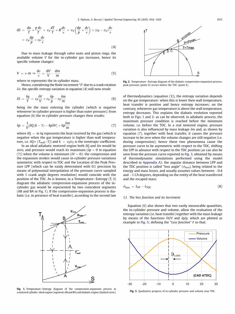
Fig. 2. TemperatureeEntropy diagram of the diabatic compression-expansion process:peak pressure (point D) occurs before the TDC (point E).

E. Pipitone, A. Beccari / Applied Thermal Engineering 30 (2010) 1914e1926 1915

dS ¼ duT

þ p dvT

¼ cVdTT

þ R0dvv

¼ cV

�dpp

þ dvv

�þ ðcP � cVÞ

dvv

¼ cVdpp

þ cPdvv

(4)

Due to mass leakage through valve seats and piston rings, theavailable volume V for the in-cylinder gas increases, hence itsspecific volume changes:

V ¼ v$m0dvv

¼ dVV

� dmm

(5)

where m represents the in-cylinder mass.Hence, considering thefinite increment “d“due to a crank rotation

dw, the specific entropy variation in equation (4) will now result:

dS ¼ dqT

¼ cPdVV

þ cVdpp

� cPdmm

(6)

being dm the mass entering the cylinder (which is negativewhenever in-cylinder pressure is higher than outer pressure); fromequation (6) the in-cylinder pressure changes then results:

dp ¼ 1V½dQðk� 1Þ � kpdV � þ kp

dmm

(7)

where dQ ¼ m dq represents the heat received by the gas (which isnegative when the gas temperature is higher than wall tempera-ture, i.e. dQf (TwalleT)) and k ¼ cP/cV is the isentropic coefficient.

In an ideal adiabatic motored engine both dQ and dm would bezero, and pressure would reach its maximum (dp ¼ 0 in equation(7)) when the volume is minimum (dV ¼ 0): the compression andthe expansion strokes would cause in-cylinder pressure variationssymmetric with respect to TDC and the Location of the Peak Pres-sure LPP (which can be easily determined with 0.1 precision bymeans of polynomial interpolation of the pressure curve sampledwith 1 crank angle degrees resolution) would coincide with theposition of the TDC. As is known, in a TemperatureeEntropy (T, S)diagram the adiabatic compression-expansion process of the in-cylinder gas would be represented by two coincident segments(AB and BA in Fig. 1). If the compression-expansion process is dia-batic (i.e. in presence of heat transfer), according to the second law

Fig. 1. TemperatureeEntropy diagram of the compression-expansion process inamotoredcylinder: ideal engine (segmentsABandBA)anddiabatic engine (dashedcurve).

of thermodynamics (equation (3)), the entropy variation dependson the gas temperature: when this is lower then wall temperature,heat transfer is positive and hence entropy increases; on thecontrary, whenever gas temperature is above the wall temperature,entropy decreases. This explains the diabatic evolution reportedboth in Figs. 1 and 2: as can be observed, in adiabatic process, themaximum pressure condition is reached before the minimumvolume, i.e. before the TDC. In a real motored engine, pressurevariation is also influenced by mass leakage dm and, as shown byequation (7), together with heat transfer, it causes the pressureincrease to be zero when the volume changes are still negative (i.e.during compression); hence these two phenomena cause thepressure curve to be asymmetric with respect to the TDC, shiftingthe LPP in advance with respect to the TDC position (as can also beseen from the pressure curve reported in Fig. 3, obtained by meansof thermodynamic simulations performed using the modeldescribed in Appendix A): the angular distance between LPP andthe TDC position is called “loss angle” (wloss), being related to theenergy and mass losses, and usually assumes values between �0.4and �1 CA degrees, depending on the entity of the heat transferredand the escaped mass:

wloss ¼ LPP � LTDC (8)

1.1. The loss function and its increment

Equation (6) also shows that two easily measurable quantities,the in-cylinder pressure and volume, allow the evaluation of theentropy variation (i.e. heat transfer) together with themass leakageby means of the functions dV/V and dp/p, which are plotted asexample in Fig. 5; defining the “Loss function” F so that:

-30 -20 -10 0 10 20 30

[CAD ATDC]

PressureVolume

LOSS

Fig. 3. Qualitative progress of in-cylinder pressure and volume near TDC.

-180 -120 -60 0 60 120 180

[CAD ATDC]

dp/p

dv/v

p/pv/v

Fig. 5. Qualitative progress of dV/V and dp/p (obtained using the model described inAppendix A with dw ¼ 1 CAD).

E. Pipitone, A. Beccari / Applied Thermal Engineering 30 (2010) 1914e19261916

dF ¼ cPdVV

þ cVdpp

(9)

it will result:

dF ¼ dSþ cPdmm

(10)

The entity of the variation of the Loss function, dF, which gathers thesum of the two losses, is then determined by the capability of thecylinder walls to exchange heat with the gas and by the amount ofgas escaping from the cylinder. The qualitative progress of the Lossfunction variation in a real cylinder during a compression-expansionprocess, together with its two constitutive terms dS and cP dm/m, isshown for example in Fig. 4: the entropy variation starts witha positive value (being T< Twall) anddecreases, crossing the zero linewhenT¼ Twall, and reaching aminimumnear the TDCposition (herethe heat flux from the gas to the wall is maximum), then starts toincrease becoming positive before the Bottom Dead Centre (BDC);the relative mass leakage dm/m, being related to the differencebetween in-cylinder pressure and outer pressure, follows a similartrend, reaching a minimum near the TDC: it follows that, in thisposition, the loss function variation equals the sum of the two lossangle causes. Following this concept the authors tried to obtaininformation on the loss angle entity directly from the loss functionvariation.When the gas pressure reaches the peak value (i.e.at LPP),the ratio dp/p is zero, and equation (9) becomes:

dFLPP ¼�cpdVV

�LPP

(11)

The latter equation shows that at the peak pressure position theknowledge of the loss function increment dF allows to determinethe value of dV/V which, depending only on engine geometry (seeFig. 5 and equation (12)), is a known function of the crank shaftposition, and hence of the loss angle. The function dV/V can beexpressed as:

dVV

¼sinðwÞ

1þ cosðwÞffiffiffiffiffiffiffiffiffiffiffiffiffiffiffiffiffiffiffi

m2�sin2ðwÞp

!dw

2r�1 þ mþ 1� cos ðwÞ �

ffiffiffiffiffiffiffiffiffiffiffiffiffiffiffiffiffiffiffiffiffiffiffiffiffiffiffim2 � sin2ðwÞ

q (12)

where r is the volumetric compression ratio and m expresses therod to crank ratio (i.e. the ratio between connecting rod length andcrank radius). Since the loss angle is normally around �1�

(¼ �0.017 radians), further approximations can be made:

sinðwlossÞzwloss cosðwlossÞz1

-1.4

-1.2

-1.0

-0.8

-0.6

-0.4

-0.2

0.0

0.2

-180 -120 -60 0 60 120 180

[CAD ATDC]

[J/kg

K

]

d

dS = dQ / mT

cp dm/m

ideal adiabatic

FS= q/T

cp m/m

Fig. 4. Loss function variation dF and its two constitutive terms (obtained using themodel described in Appendix A with dw ¼ 1 CAD).

It follows that, at the peak pressure position, equation (12)becomes:

�1V

dVdw

�LPP

¼wloss

�1þ 1ffiffiffiffiffiffiffiffiffiffiffiffiffiffiffi

m2�wloss

p�

2r�1 þ m�

ffiffiffiffiffiffiffiffiffiffiffiffiffiffiffiffiffiffiffiffiffiffim2 � wloss

p (13)

Hence, being wloss2 << m2, equations (11) and (13) yield:

wloss ¼ 2r� 1

$m

mþ 1$

�1cp

dFdw

�LPP

(14)

This demonstrates that the loss angle can be easily correlated tothe loss function increment dF evaluated at the peak pressure posi-tion. Unfortunately dF undergoes great distortions even with smallphase errors between dp/p and dV/V: Fig. 6, as example, shows someloss function variation curves calculated by means of the thermo-dynamic model exposed in Appendix A assuming different phaseerrors (expressed as fraction of the loss angle). As can be seen,a pressure phasing error equal to the loss angle (which meansLPP ¼ 0) introduces a considerable error in the evaluation of thefunction dF. This fact, without a reliable way to evaluate the dF atthe peak pressure position, would make equation (14) useless. Thesame Fig. 6 however shows the existence of two zones common toeachof the curves: in these twocrankpositions the two fundamentalfunctions for the calculus of the entropy variation, dp/p and dV/V,reach their extreme values (at about �30 CAD ATDC in Fig. 5), andhence are poorly influenced by small phase errors (i.e. in the order ofthe loss angle); for this reason, according to equation (9), in thesetwo crank positions the loss function variation remains almostunchanged. This fact implies that assuming a TDC position errorequal to the loss angle (easily achievable setting LPP¼ 0), the valuesof the loss function variation dF1 and dF2 in the two points relative to

-4.5

-3.5

-2.5

-1.5

-0.5

0.5

-180 -90 0 90 180[CAD ATDC]

dS [J/kg K]

loss angle 1/2 loss angle0

-1/2 loss angle - loss angle (LPP=0)

F [J/kg K]

Fig. 6. Loss function variation dF for different phase errors (obtained using the modeldescribed in Appendix A with dw ¼ 1 CAD).


the minimum and maximum of the function dV/V will be nearlycorrect. Hence, in order to determine the loss angle from equation(14), a correlation between dF1 and dFLPP has been searched, and, asshown in Appendix B, it has been found that, for a given engine, theratio between dFLPP and dF1 is almost constant, i.e.:

dFLPPzF$dF1 ¼ F$dFmindV=V (15)

where F is a proportionality constant.As shown in Appendix B this constant mainly depends on the

engine compression ratio and on the heat transfer law, and its meanvalue has been estimated to be 1.95. Thus equation (15) becomes:

dFLPPz1:95$dFmindV=V (16)

As a result, the top dead centre position can be determinedphasing the pressure cycle with an initial error equal to the lossangle (i.e. setting LPP ¼ 0) and calculating the loss function incre-ment dF1 at the minimum dV/V position w1, which requires,according to equation (9), the estimation of the functions dV/V anddp/p. Unfortunately both of these functions can be affected bymeasurement errors: the in-cylinder pressure acquisition can be infact subjected to bias error (above all if an un-cooled piezoelectrictransducer is used) and to electric and mechanical noise, while thein-cylinder volume estimation may present inaccuracy related tothe compression ratio, which is normally known with someapproximation (�3%). Moreover, as shown in equation (9), thespecific heat at constant pressure and volume are required, whichare functions of the gas temperature; this in turn can be deducedapplying the perfect gas law by means of the gas temperature atinlet valve closure, which is normally known with an approxima-tion as high as 30 �C.

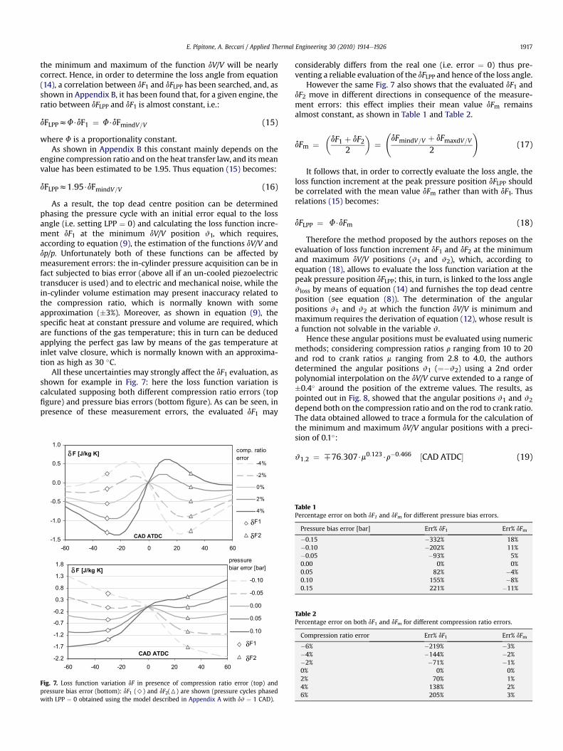
All these uncertainties may strongly affect the dF1 evaluation, asshown for example in Fig. 7: here the loss function variation iscalculated supposing both different compression ratio errors (topfigure) and pressure bias errors (bottom figure). As can be seen, inpresence of these measurement errors, the evaluated dF1 may

-1.5

-1.0

-0.5

0.0

0.5

1.0

-60 -40 -20 0 20 40 60

CAD ATDC

F [J/kg K]

-4%

-2%

0%

2%

4%

dF1

dF2

comp. ratio error

δF1

δF2

-2.2

-1.7

-1.2

-0.7

-0.2

0.3

0.8

1.3

1.8

-60 -40 -20 0 20 40 60

CAD ATDC

F [J/kg K]

-0.10

-0.05

0.00

0.05

0.10

dF1

dF2

pressure biar error [bar]

δF1

δF2

Fig. 7. Loss function variation dF in presence of compression ratio error (top) andpressure bias error (bottom): dF1 (>) and dF2(6) are shown (pressure cycles phasedwith LPP ¼ 0 obtained using the model described in Appendix A with dw ¼ 1 CAD).

considerably differs from the real one (i.e. error ¼ 0) thus pre-venting a reliable evaluation of the dFLPP and hence of the loss angle.

However the same Fig. 7 also shows that the evaluated dF1 anddF2 move in different directions in consequence of the measure-ment errors: this effect implies their mean value dFm remainsalmost constant, as shown in Table 1 and Table 2.

dFm ¼�dF1 þ dF2

2

�¼ dFmindV=V þ dFmaxdV=V

2

!(17)

It follows that, in order to correctly evaluate the loss angle, theloss function increment at the peak pressure position dFLPP shouldbe correlated with the mean value dFm rather than with dF1. Thusrelations (15) becomes:

dFLPP ¼ F$dFm (18)

Therefore the method proposed by the authors reposes on theevaluation of loss function increment dF1 and dF2 at the minimumand maximum dV/V positions (w1 and w2), which, according toequation (18), allows to evaluate the loss function variation at thepeak pressure position dFLPP; this, in turn, is linked to the loss anglewloss by means of equation (14) and furnishes the top dead centreposition (see equation (8)). The determination of the angularpositions w1 and w2 at which the function dV/V is minimum andmaximum requires the derivation of equation (12), whose result isa function not solvable in the variable w.

Hence these angular positions must be evaluated using numericmethods; considering compression ratios r ranging from 10 to 20and rod to crank ratios m ranging from 2.8 to 4.0, the authorsdetermined the angular positions w1 (¼�w2) using a 2nd orderpolynomial interpolation on the dV/V curve extended to a range of�0.4� around the position of the extreme values. The results, aspointed out in Fig. 8, showed that the angular positions w1 and w2depend both on the compression ratio and on the rod to crank ratio.The data obtained allowed to trace a formula for the calculation ofthe minimum and maximum dV/V angular positions with a preci-sion of 0.1�:

w1;2 ¼ H76:307$m0:123$r�0:466 ½CAD ATDC� (19)

Table 1Percentage error on both dF1 and dFm for different pressure bias errors.

Pressure bias error [bar] Err% dF1 Err% dFm

�0.15 �332% 18%�0.10 �202% 11%�0.05 �93% 5%0.00 0% 0%0.05 82% �4%0.10 155% �8%0.15 221% �11%

Table 2Percentage error on both dF1 and dFm for different compression ratio errors.

Compression ratio error Err% dF1 Err% dFm

�6% �219% �3%�4% �144% �2%�2% �71% �1%0% 0% 0%2% 70% 1%4% 138% 2%6% 205% 3%

2122232425262728293031

9 11 13 15 17 19 21

Compression ratio

mu

mix

am

fo

noi

tis

oP

V/V

]C

DT

AD

AC

[

4.03.42.8

Rod to crank ratio

Fig. 8. Position of maximum dV/V with varying compression ratio and for different rodto crank ratio.


1.2. Procedure for TDC position estimation

Summarizing, once the motored pressure cycle has beensampled, the procedure for the TDC estimation consist of 5 steps,here resumed:

1) the pressure cycle must be phased setting LPP ¼ 0 (in this waythe position error is exactly equal to the unknown loss anglewloss): for this purpose a 2nd order polynomial fitting per-formed on the pressure curve around the maximum pressurevalue position allows a sufficient precision

2) the angular position w1 and w2 of the minimum and maximumdV/V must be evaluated (for example using equation (19))

3) the loss function increments dF1 and dF2 at the angular positionw1 and w2 must be calculated by means of equation (9)

dF ¼ cPdVV

þ cVdpp

and hence their mean value dFm ¼ 1/2 (dF1 þ dF2)

4) the loss function increment dFLPP at the peak pressure positioncan be determined from equation (18)

dFLPP ¼ F$dFm

Table 3Simulation conditions for the evaluation of the loss angle entity (more details can befound in Appendix A).

Manifold absolute pressure 0.4 to 1.0 bar (steps of 0.1)Engine speed 1000 to 3000 rpm (steps of 500)Compression ratio 10 and 22Rod to crank ratio 3.27Bore 70.80 mmStroke 78.86Leakage flow area AN 0.507 mm2

Walls temperature 70 �C

where the constant F can be estimated by means of equation (46)(reported Appendix B) or set to the mean value 1.95, as determinedin Appendix B

5) the loss angle wloss, and hence the TDC location, can be thenevaluated by means of equation (14)

wloss ¼ 2r� 1

$m

mþ 1$

�1cp

dFdw

�LPP

-1.0

-0.9

-0.8

-0.7

-0.6

-0.5

-0.4

0.1 0.3 0.5 0.7 0.9 1.1

MAP [bar]

]C

DT

AD

AC

[el

gn

as

sol

.

1000 rpm1500 rpm2000 rpm2500 rpm3000 rpm

Fig. 9. Loss angle value determined with compression r

It is worthwhile to mention that the first step is not necessary if thepressure cycle has already been phased with an error lower thanthe loss angle. Moreover the specific heat cP and cV in equations (6),(9), (11) and (14) should be temperature dependent and evaluatedaccording to the classical known functions valid for air, as reportedin Appendix A. However a satisfactory approximation is equallyreached if the cP and cV are supposed to be constant. In this case theevaluation of the gas temperature is completely avoidable for theTDC determination.

2. Assessment of the method

In order to ascertain the reliability of the method proposed,a series of simulations has been performed to generate plausible in-cylinder pressure curves compatible with the real compression-expansion process which takes place in a motored engine cylinder,taking into account both mass leakages and heat transfers. Thepressure curves obtained have been then used to test both thereliability of the proposed method in the determination of TDC andits robustness to the most common encountered measurementproblems. Details on the thermodynamic model used for thegeneration of the pressure curves are given in Appendix A.

A first series of simulations has been performed in order toestimate the entity of the loss angle and its dependence from theengine operative condition of speed and Manifold Absolute Pres-sure (MAP). The simulations were carried out, as resumed inTable 3, taking into consideration the dimensions of a commercialavailable automotive engine, two compression ratios (10 and 22),different conditions of MAP and speed and employing threedifferent heat transfer models (reported in Appendix A). For eachsimulated pressure curve, the seven points around the maximumvalue have been interpolated by means of a 2nd order polynomial,thus obtaining the location of the pressure peak (LPP) as the vertexabscissa: this procedure ensured a precision of 0.001 CAD, which isamply higher than the required one of 0.1 CAD. Once known theLPP, the loss angle is known by its definition:

wloss ¼ LPP � LTDC

As a result, the diagrams in Fig. 9 shows the loss angle valuesobtained with compression ratio ¼ 10 employing theWoschni heat

-1.0

-0.9

-0.8

-0.7

-0.6

-0.5

-0.4

0 500 1000 1500 2000 2500 3000 3500

engine speed [rpm]

]C

DT

AD

AC

[el

gn

as

sol

0.4 bar0.5 bar0.6 bar0.7 bar0.8 bar0.9 bar1.0 bar

atio r ¼ 10 using the Woschni heat transfer model.

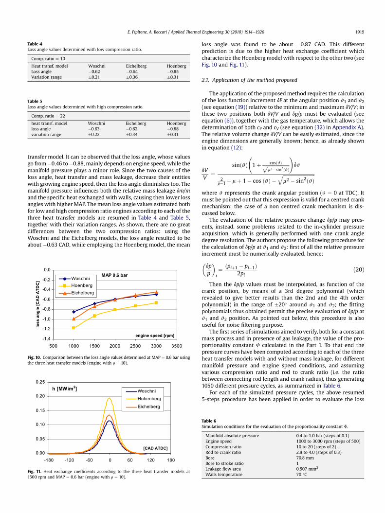
Table 4Loss angle values determined with low compression ratio.

Comp. ratio ¼ 10

Heat transf. model Woschni Eichelberg HoenbergLoss angle �0.62 �0.64 �0.85Variation range �0.21 �0.36 �0.31

Table 5Loss angle values determined with high compression ratio.

Comp. ratio ¼ 22

heat transf. model Woschni Eichelberg Hoenbergloss angle �0.63 �0.62 �0.88variation range �0.22 �0.34 �0.31


transfer model. It can be observed that the loss angle, whose valuesgo from�0.46 to�0.88, mainly depends on engine speed, while themanifold pressure plays a minor role. Since the two causes of theloss angle, heat transfer and mass leakage, decrease their entitieswith growing engine speed, then the loss angle diminishes too. Themanifold pressure influences both the relative mass leakage dm/mand the specific heat exchanged with walls, causing then lower lossangles with higherMAP. Themean loss angle values estimated bothfor low and high compression ratio engines according to each of thethree heat transfer models are resumed in Table 4 and Table 5,together with their variation ranges. As shown, there are no greatdifferences between the two compression ratios: using theWoschni and the Eichelberg models, the loss angle resulted to beabout �0.63 CAD, while employing the Hoenberg model, the mean

MAP 0.6 bar

-1.4

-1.2

-1.0

-0.8

-0.6

-0.4

-0.2

0.0

500 1000 1500 2000 2500 3000 3500

engine speed [rpm]

lo

ss an

gle [C

AD

A

TD

C] Woschni

HoenbergEichelberg

Fig. 10. Comparison between the loss angle values determined at MAP ¼ 0.6 bar usingthe three heat transfer models (engine with r ¼ 10).

0.00

0.05

0.10

0.15

0.20

0.25

-180 -120 -60 0 60 120 180

[CAD ATDC]

h [MW /m2] Woschni

Hohenberg

Eichelberg

Fig. 11. Heat exchange coefficients according to the three heat transfer models at1500 rpm and MAP ¼ 0.6 bar (engine with r ¼ 10).

loss angle was found to be about �0.87 CAD. This differentprediction is due to the higher heat exchange coefficient whichcharacterize the Hoenbergmodel with respect to the other two (seeFig. 10 and Fig. 11).

2.1. Application of the method proposed

The application of the proposed method requires the calculationof the loss function increment dF at the angular position w1 and w2(see equation (19)) relative to the minimum and maximum dV/V; inthese two positions both dV/V and dp/p must be evaluated (seeequation (6)), together with the gas temperature, which allows thedetermination of both cP and cV (see equation (32) in Appendix A).The relative volume change dV/V can be easily estimated, since theengine dimensions are generally known; hence, as already shownin equation (12):

dVV

¼sinðwÞ

1þ cosðwÞffiffiffiffiffiffiffiffiffiffiffiffiffiffiffiffiffiffiffi

m2�sin2ðwÞp

!dw

2r�1 þ mþ 1� cos ðwÞ �

ffiffiffiffiffiffiffiffiffiffiffiffiffiffiffiffiffiffiffiffiffiffiffiffiffiffiffim2 � sin2ðwÞ

qwhere w represents the crank angular position (w ¼ 0 at TDC). Itmust be pointed out that this expression is valid for a centred crankmechanism: the case of a non centred crank mechanism is dis-cussed below.

The evaluation of the relative pressure change dp/p may pres-ents, instead, some problems related to the in-cylinder pressureacquisition, which is generally performed with one crank angledegree resolution. The authors propose the following procedure forthe calculation of dp/p at w1 and w2: first of all the relative pressureincrement must be numerically evaluated, hence:

�dpp

�i¼ ðpiþ1 � pi�1Þ

2pi(20)

Then the dp/p values must be interpolated, as function of thecrank position, by means of a 3rd degree polynomial (whichrevealed to give better results than the 2nd and the 4th orderpolynomial) in the range of �20� around w1 and w2; the fittingpolynomials thus obtained permit the precise evaluation of dp/p atw1 and w2 position. As pointed out below, this procedure is alsouseful for noise filtering purpose.

The first series of simulations aimed to verify, both for a constantmass process and in presence of gas leakage, the value of the pro-portionality constant F calculated in the Part 1. To that end thepressure curves have been computed according to each of the threeheat transfer models with and without mass leakage, for differentmanifold pressure and engine speed conditions, and assumingvarious compression ratio and rod to crank ratio (i.e. the ratiobetween connecting rod length and crank radius), thus generating1050 different pressure cycles, as summarized in Table 6.

For each of the simulated pressure cycles, the above resumed5-steps procedure has been applied in order to evaluate the loss

Table 6Simulation conditions for the evaluation of the proportionality constant F.

Manifold absolute pressure 0.4 to 1.0 bar (steps of 0.1)Engine speed 1000 to 3000 rpm (steps of 500)Compression ratio 10 to 20 (steps of 2)Rod to crank ratio 2.8 to 4.0 (steps of 0.3)Bore 70.8 mmBore to stroke ratio 1Leakage flow area 0.507 mm2

Walls temperature 70 �C


angle value, which in turn allows to estimate the TDC location: this,compared to the knownTDC location of the thermodynamic model,allowed to determine the TDC estimation error of the methodproposed for each of the pressure cycles.

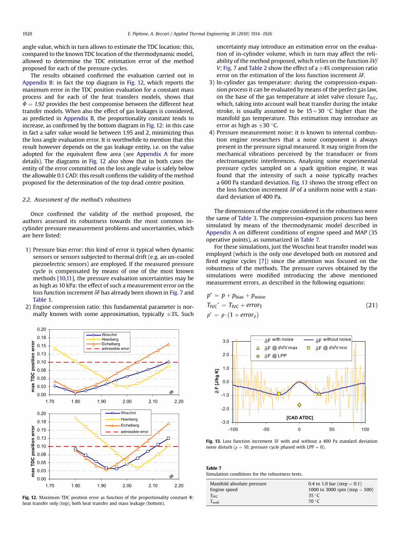
The results obtained confirmed the evaluation carried out inAppendix B: in fact the top diagram in Fig. 12, which reports themaximum error in the TDC position evaluation for a constant massprocess and for each of the heat transfers models, shows thatF ¼ 1.92 provides the best compromise between the different heattransfer models. When also the effect of gas leakages is considered,as predicted in Appendix B, the proportionality constant tends toincrease, as confirmed by the bottom diagram in Fig. 12: in this casein fact a safer value would lie between 1.95 and 2, minimizing thusthe loss angle evaluation error. It is worthwhile to mention that thisresult however depends on the gas leakage entity, i.e. on the valueadopted for the equivalent flow area (see Appendix A for moredetails). The diagrams in Fig. 12 also show that in both cases theentity of the error committed on the loss angle value is safely belowthe allowable 0.1 CAD: this result confirms the validity of themethodproposed for the determination of the top dead centre position.

2.2. Assessment of the method’s robustness

Once confirmed the validity of the method proposed, theauthors assessed its robustness towards the most common in-cylinder pressure measurement problems and uncertainties, whichare here listed:

1) Pressure bias error: this kind of error is typical when dynamicsensors or sensors subjected to thermal drift (e.g. an un-cooledpiezoelectric sensors) are employed. If the measured pressurecycle is compensated by means of one of the most knownmethods [10,11], the pressure evaluation uncertainties may beas high as 10 kPa: the effect of such ameasurement error on theloss function increment dF has already been shown in Fig. 7 andTable 1.

2) Engine compression ratio: this fundamental parameter is nor-mally known with some approximation, typically �3%. Such

0.00

0.03

0.05

0.08

0.10

0.13

0.15

0.18

0.20

1.70 1.80 1.90 2.00 2.10 2.20

Φ

ro

rr

en

oi

ti

so

pC

DT

xa

m

WoschniHoenbergEichelbergadmissible error

0.00

0.03

0.05

0.08

0.10

0.13

0.15

0.18

0.20

1.70 1.80 1.90 2.00 2.10 2.20

Φ

ro

rr

en

oi

ti

so

pC

DT

xa

m

WoschniHoenbergEichelbergadmissible error

Fig. 12. Maximum TDC position error as function of the proportionality constant F:heat transfer only (top), both heat transfer and mass leakage (bottom).

uncertainty may introduce an estimation error on the evalua-tion of in-cylinder volume, which in turn may affect the reli-ability of themethod proposed, which relies on the function dV/V; Fig. 7 and Table 2 show the effect of a�4% compression ratioerror on the estimation of the loss function increment dF.

3) In-cylinder gas temperature: during the compression-expan-sion process it can be evaluated bymeans of the perfect gas law,on the base of the gas temperature at inlet valve closure TIVC,which, taking into account wall heat transfer during the intakestroke, is usually assumed to be 15O30 �C higher than themanifold gas temperature. This estimation may introduce anerror as high as �30 �C.

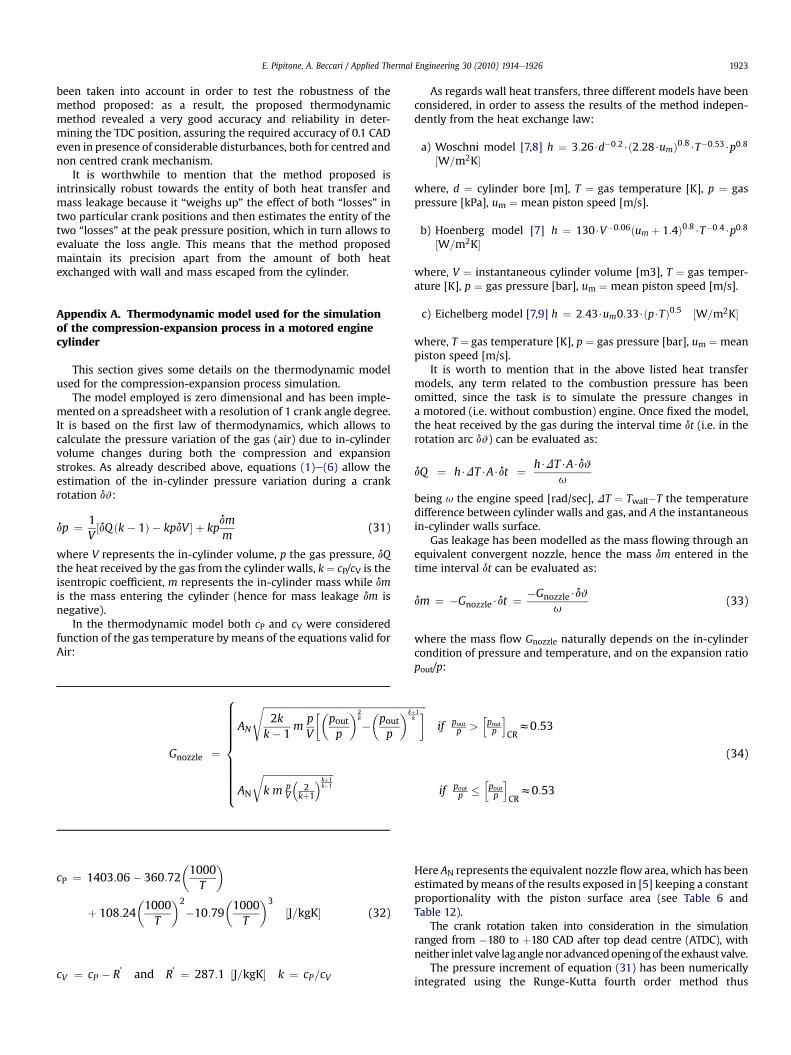
4) Pressure measurement noise: it is known to internal combus-tion engine researchers that a noise component is alwayspresent in the pressure signal measured. It may origin from themechanical vibrations perceived by the transducer or fromelectromagnetic interferences. Analysing some experimentalpressure cycles sampled on a spark ignition engine, it wasfound that the intensity of such a noise typically reachesa 600 Pa standard deviation. Fig. 13 shows the strong effect onthe loss function increment dF of a uniform noise with a stan-dard deviation of 400 Pa.

The dimensions of the engine considered in the robustness werethe same of Table 3. The compression-expansion process has beensimulated by means of the thermodynamic model described inAppendix A on different conditions of engine speed and MAP (35operative points), as summarized in Table 7.

For these simulations, just theWoschni heat transfer model wasemployed (which is the only one developed both on motored andfired engine cycles [7]) since the attention was focused on therobustness of the methods. The pressure curves obtained by thesimulations were modified introducing the above mentionedmeasurement errors, as described in the following equations:

p’ ¼ pþ pbias þ pnoiseTIVC’ ¼ TIVC þ errorTr’ ¼ r$

�1þ errorr

(21)

Table 7Simulation conditions for the robustness tests.

Manifold absolute pressure 0.4 to 1.0 bar (step ¼ 0.1)Engine speed 1000 to 3000 rpm (step ¼ 500)TIVC 35 �CTwall 70 �C

-3.0

-2.0

-1.0

0.0

1.0

2.0

3.0

-100 -50 0 50 100

[CAD ATDC]

F [J/kg

K

]

dF with noise dF without noise

dF @ dV/V max dF @ dV/V min

dF @ LPP

FFF

FF

Fig. 13. Loss function increment dF with and without a 400 Pa standard deviationnoise disturb (r ¼ 10, pressure cycle phased with LPP ¼ 0).

Table 8Maximum TDC position errors for different measurement disturbances e (r ¼ 10,F ¼ 1.95).

Disturbance entity Max TDC position error [CAD]

No disturbance 0.042TIVC þ30 �C 0.041TIVC �30 �C 0.044Compression ratio þ5% 0.045Compression ratio �5% 0.038Pressure bias error þ10 kPa 0.034Pressure bias error �10 kPa 0.063Pressure signal noise st. dev. 600 Pa 0.043

Table 11Maximum TDC position error obtained in the robustness test of Table 10.

Maximum TDC position errors [CAD]

compression ratio ¼ 10 0.058 0.035 0.065 0.039 0.061 0.032 0.066 0.036compression ratio ¼ 22 0.041 0.037 0.045 0.041 0.045 0.037 0.048 0.040


On a first step the measurement errors were introduced one ata time, then the resulting pressure, volume and temperature datawere employed to compute the loss angle by means of theproposed method. Table 8 reports the maximum TDC position errorfound for each of the disturbances introduced: as can be seen, itremained always below the 0.1�. The worst effect is played by thenegative pressure bias error, while noise effect was adequatelyattenuated by means of the filtering properties of the 3rd orderpolynomial used to fit the dp/p values.

In order to test the robustness of the method also for a highcompression ratio engine, the simulations of Table 7 have beenrepeated setting the compression ratio to 22. Each disturbance hasbeen applied again identically, except for the noise, which has beensupposed to increase proportionally to the pressure levels, and hasbeen amplified to reach a standard deviation of 1800 Pa. As shownin Table 9 the results obtained confirmed the reliability of themethod even with high compression ratio engine, safely reachingthe required precision of 0.1 CAD.

Even if the method proposed revealed to be robust against eachof the measurement errors assumed, it must be considered that ina real experimental test these disturbances may occur simulta-neously. Hence, in order to assess the robustness of the methodwhen the disturbances are simultaneously present, the pressurecycles simulated in the 35 operative conditions of Table 7 weremodified using the combination of disturbances reported in Table10 and then employed to determine the loss angle by means ofthe proposed method. The maximum TDC position errors obtainedfor each disturbances combination are presented in Table 11 bothfor low and high compression ratio: as shown, in the case of lowcompression ratio (r ¼ 10), the simultaneous presence of

Table 9Maximum TDC position errors for different measurement disturbances e (r ¼ 22,F ¼ 1.95).



Table 10Disturbances combinations used in the robustness test.

Pressure signal noise st. dev. 600 Pa (r ¼ 10) or 1800 Pa (r ¼ 22)

TIVC error �30 �C þ30 �CCompression ratio error �5% þ5% �5% þ5%Pressure bias error [kPa] �10 þ10 �10 þ10 �10 þ10 �10 þ10

disturbances induced a maximum errors of 0.066 CAD, while in thecase of high compression ratio engine (r ¼ 22), the maximum TDCposition evaluation error was 0.048 CAD.

The method proposed hence revealed to be robust enough toallow a safe evaluation of the TDC position (themaximum error waslower than the required 0.1 crank angle degrees) even in presenceof the typical in-cylinder pressure measurement errors anddisturbances.

2.3. Non centred crank mechanism

If the engine is endowed of a non centred crank mechanism, thecrank angle position with respect to the cylinder axis when theconnecting rod and the crank are aligned (i.e. when the piston is attop dead centre) is not zero but assumes the value w T, as depicted inFig. 14.

If the angular position are still evaluated with respect to thecylinder axis, then the angle w T must be accounted for in orderto correctly evaluate the TDC position by means of the ther-modynamic method. As shown in Fig. 14, the angular positionsof Top (w T) and Bottom (w B) Dead Centre can be calculatedsince:

sinwT ¼ zlþ r

sinwB ¼ zl� r

(22)

where z is the crank pin offset (i.e. the distance between the crankpin and the cylinder axis), while l and r are the connecting rodlength and the crank radius respectively. For a non centred crankmechanism, the piston stroke results to be:

c ¼ffiffiffiffiffiffiffiffiffiffiffiffiffiffiffiffiffiffiffiffiffiffiffiffiðlþ rÞ2�z2

q�

ffiffiffiffiffiffiffiffiffiffiffiffiffiffiffiffiffiffiffiffiffiffiffiffiðl� rÞ2�z2

q(23)

hence, from Fig. 14, the in-cylinder volume is:

V ¼ AC$

24 cr� 1

þ ðlþ rÞ$coswT � l

ffiffiffiffiffiffiffiffiffiffiffiffiffiffiffiffiffiffiffiffiffiffiffiffiffiffiffiffiffiffiffiffiffiffiffiffi1�

�s� sinw

m

�2s

� r$cosw

35

(24)

being AC the cylinder section area and s the ratio z/l.

Fig. 14. Representation of a non centred crank mechanism.


Equation (12) then becomes:

dVV

¼sinw$

1þ cosw�sm$cotwffiffiffiffiffiffiffiffiffiffiffiffiffiffiffiffiffiffiffiffiffiffiffiffiffi

m2�ðsinw�smÞ2p

!

cr$ðr�1Þþðmþ1Þ$coswT�m$

ffiffiffiffiffiffiffiffiffiffiffiffiffiffiffiffiffiffiffiffiffiffiffiffiffiffiffiffiffiffi1��s�sinw

m

2r�cosw

$dw (25)

which, besides allowing the correct estimation of the loss functionincrement dF by means of equation (6), can also be used for thenumerical evaluation of the angular position w1 and w2 of minimumand maximum dV/V through polynomial interpolation: the authorshowever observed that, for this purpose, equation (19), which hasbeen derived for centred crank mechanism, still gives good results.Being the loss angle in the order of �1 CAD z �0.017 radians, thefollowing approximation can be made:

wloss << 10sinwlosszwloss cos wlossz1�s� sinwloss

m

2<< 10

ffiffiffiffiffiffiffiffiffiffiffiffiffiffiffiffiffiffiffiffiffiffiffiffiffiffiffiffiffiffiffiffiffiffiffiffiffi1�

�s� sinwloss

m

2rz1

(26)

hence equation (25) becomes:

�dVV

�LPP

¼wloss þ wloss

m � sc

r$ðr�1Þ þ ðmþ 1Þ$coswT � m� 1$dw (27)

The crank pin offset z is usually small with respect to the rodlength l, then also w T << 1 and hence.

coswTz1 wTzsinwT ¼ zlþ r

¼ s1þ 1=m

¼ m$smþ 1

(28)

Equation (27) thus gives:

Table 12Dimensions of the engine with crank pin offset.

Compression ratio 10Rod to crank ratio 3.27Bore 70.80 mmCrank radius 35.40 mmCrank pin offset 2 mm (s ¼ 0.017)Leakage flow area 0.507 mm2

Table 13Maximum TDC position errors for different measurement disturbances (non centredcrank mechanism, F ¼ 1.95).



Table 14Maximum TDC position errors obtained in the robustness test (non centred crank mech

Pressure signal noise st. dev. 600 Pa

TIVC error �30 �CCompression ratio error �5% þ5%Pressure bias error [kPa] �10 þ10 �10Max TDC position error 0.044 0.058 0.044

�dVV

�LPP

¼wloss$

�1þmm

� s

cr$ðr�1Þ

$dw (29)

which, together with the latter of equations (28) and equation (11),allows to evaluate the loss angle:

wloss ¼ s$mmþ 1

þ c=rr� 1

$m

mþ 1$

�1cp

dFdw

�LPP

¼ wT þ c=rr� 1

$m

mþ 1$

�1cp

dFdw

�LPP

(30)

As can be noted equation (30) differs from equation (14) for thepresence of the angular offset w T and for the ratio c/r which is lessthan 2 for a non centred crank mechanism.

In order to verify the reliability of the method with a non cen-tred crank mechanism, the simulations in the operative conditionsof Table 7 have been repeated with and without measurementdisturbances using the engine data of Table 12: the results, resumedin Table 13, clearly show that the method proposed still estimatesthe TDC position with a maximum error of 0.049 CAD.

Table 14 instead reports the maximum TDC position estimationerrors obtained with the simultaneous presence of the measure-ment disturbances for each of the 35 operative conditions: also inthis case the maximum TDC position errors found remained underthe required accuracy of 0.1 CAD. The method proposed thusrevealed a good reliability even when the engine used is charac-terized by a non centred crank mechanism.

3. Conclusions

As is known to internal combustion engines researcher, theexact determination of the crank position when the piston is at TopDead Centre (TDC) is of crucial importance for indicating analysis:the maximum allowable error results to be about 0.1 Crank AngleDegrees (CAD). Due to wall heat transfer and mass leakage, undermotored condition (i.e. without combustion) the TDC position doesnot coincide with the Location of Pressure Peak (LPP) but follows itby an angular arc called “loss angle”, which, depending on theengine, is normally in the range of 1 Crank Angle Degrees (CAD).

This paper presents a new thermodynamic method for theestimation of the TDC position in internal combustion engines. Themethod relies on the definition of a proper function, called “lossfunction”whose increment is directly connected to the two “losses”,i.e. wall heat transfer and gas leakage.

As described in the first part of the paper, the estimation of theloos function increment in two particular crank positions allows todetermine the loss angle.

In the second part of the paper, the method is put to the test bymeans of thermodynamic simulations, thus verifying its capabilityto determine the loss angle under many different operativeconditions of engine speed andmanifold pressure, both for low andhigh compression ratio engines, and using three different heatrelease models. Moreover, typical in-cylinder pressure measure-ment errors and disturbances (pressure bias errors, pressure signalnoise, compression ratio and gas temperature uncertainty) have

anism, F ¼ 1.95).

þ30 �C�5% þ5%

þ10 �10 þ10 �10 þ100.058 0.045 0.073 0.045 0.073


been taken into account in order to test the robustness of themethod proposed: as a result, the proposed thermodynamicmethod revealed a very good accuracy and reliability in deter-mining the TDC position, assuring the required accuracy of 0.1 CADeven in presence of considerable disturbances, both for centred andnon centred crank mechanism.

It is worthwhile to mention that the method proposed isintrinsically robust towards the entity of both heat transfer andmass leakage because it “weighs up” the effect of both “losses” intwo particular crank positions and then estimates the entity of thetwo “losses” at the peak pressure position, which in turn allows toevaluate the loss angle. This means that the method proposedmaintain its precision apart from the amount of both heatexchanged with wall and mass escaped from the cylinder.

Appendix A. Thermodynamic model used for the simulationof the compression-expansion process in a motored enginecylinder

This section gives some details on the thermodynamic modelused for the compression-expansion process simulation.

The model employed is zero dimensional and has been imple-mented on a spreadsheet with a resolution of 1 crank angle degree.It is based on the first law of thermodynamics, which allows tocalculate the pressure variation of the gas (air) due to in-cylindervolume changes during both the compression and expansionstrokes. As already described above, equations (1)e(6) allow theestimation of the in-cylinder pressure variation during a crankrotation dw:

dp ¼ 1V½dQðk� 1Þ � kpdV � þ kp

dmm

(31)

where V represents the in-cylinder volume, p the gas pressure, dQthe heat received by the gas from the cylinder walls, k ¼ cP/cV is theisentropic coefficient, m represents the in-cylinder mass while dmis the mass entering the cylinder (hence for mass leakage dm isnegative).

In the thermodynamic model both cP and cV were consideredfunction of the gas temperature bymeans of the equations valid forAir:

Gnozzle ¼

8>>>>>>>>>><>>>>>>>>>>:

AN

ffiffiffiffiffiffiffiffiffiffiffiffiffiffiffiffiffiffiffiffiffiffiffiffiffiffiffiffiffiffiffiffiffiffiffiffiffiffiffiffiffiffiffiffiffiffiffiffiffiffiffiffiffiffiffiffiffiffiffiffiffiffiffiffiffiffiffi2k

k� 1m

pV

��poutp

�2k

��poutp

�kþ1k�s

if poutp >

hpoutp

iCRz0:53

AN

ffiffiffiffiffiffiffiffiffiffiffiffiffiffiffiffiffiffiffiffiffiffiffiffiffiffiffiffiffik m p

V

�2

kþ1

kþ1k�1

rif pout

p �hpoutp

iCRz0:53

(34)

cP ¼ 1403:06� 360:72�1000T

�

þ 108:24�1000T

�2�10:79

�1000T

�3½J=kgK� (32)

cV ¼ cP � R’ and R’ ¼ 287:1 ½J=kgK� k ¼ cP=cV

As regards wall heat transfers, three different models have beenconsidered, in order to assess the results of the method indepen-dently from the heat exchange law:

a) Woschni model [7,8] h ¼ 3:26$d�0:2$ð2:28$umÞ0:8$T�0:53$p0:8

½W=m2K�

where, d ¼ cylinder bore [m], T ¼ gas temperature [K], p ¼ gaspressure [kPa], um ¼ mean piston speed [m/s].

b) Hoenberg model [7] h ¼ 130$V�0:06ðum þ 1:4Þ0:8$T�0:4$p0:8

½W=m2K�

where, V ¼ instantaneous cylinder volume [m3], T ¼ gas temper-ature [K], p ¼ gas pressure [bar], um ¼ mean piston speed [m/s].

c) Eichelberg model [7,9] h ¼ 2:43$um0:33$ðp$TÞ0:5 ½W=m2K�

where, T ¼ gas temperature [K], p ¼ gas pressure [bar], um ¼ meanpiston speed [m/s].

It is worth to mention that in the above listed heat transfermodels, any term related to the combustion pressure has beenomitted, since the task is to simulate the pressure changes ina motored (i.e. without combustion) engine. Once fixed the model,the heat received by the gas during the interval time dt (i.e. in therotation arc dw) can be evaluated as:

dQ ¼ h$DT$A$dt ¼ h$DT$A$dwu

being u the engine speed [rad/sec], DT ¼ Twall�T the temperaturedifference between cylinder walls and gas, and A the instantaneousin-cylinder walls surface.

Gas leakage has been modelled as the mass flowing through anequivalent convergent nozzle, hence the mass dm entered in thetime interval dt can be evaluated as:

dm ¼ �Gnozzle$dt ¼ �Gnozzle$dw

u(33)

where the mass flow Gnozzle naturally depends on the in-cylindercondition of pressure and temperature, and on the expansion ratiopout/p:

Here AN represents the equivalent nozzle flow area, which has beenestimated bymeans of the results exposed in [5] keeping a constantproportionality with the piston surface area (see Table 6 andTable 12).

The crank rotation taken into consideration in the simulationranged from �180 to þ180 CAD after top dead centre (ATDC), withneither inlet valve laganglenoradvancedopeningof theexhaust valve.

The pressure increment of equation (31) has been numericallyintegrated using the Runge-Kutta fourth order method thus

Table 15

Compression ratios r 10 to 20Rod to crank ratios m 2.8 to 4.0Twall 70�CTIVC 40�Cg 1.32wLPP �1

1.80

1.85

1.90

1.95

2.00

2.05

2.10

8 10 12 14 16 18 20 22

compression ratio

oi

ta

rn

oi

ta

ir

av

yp

or

tn

E

WoschniEichelbergHoehnberg

Fig. 15. Entropy variation ratio as function of compression ratio for three different heattransfer models


obtaining the in-cylinder pressure; the gas temperature has beencalculated by means of the perfect gas law:

T ¼ ppIVC

VVIVC

TIVC (35)

where pIVC, VIVC and TIVC denote the thermodynamic state of the gasat the inlet valve closure.

Appendix B

In this section an analytical relation between the loss functionvariation at the peak pressure position dFLPP and at the minimumdV/V position dF1 is derived.

As first step, the in-cylinder evolutionwill be considered withoutmass leakage; hence the ratio between the two loss function incre-ments can be expressed in terms of entropy variations:

dFLPPdFw1

hdSLPPdSw1

¼ ½dQ=T� LPP½dQ=T �w1

(36)

where the amount of heat received by the gas from thewalls duringthe time interval dt is:

dQ ¼ hAðTwall � TÞdt (37)

being h the heat transfer coefficient, A the area of the heat exchangesurface, T and Twall the gas and wall temperatures. Hence theentropy variations ratio becomes:

dSLPPdSw1

¼ ½hAðTwall � TÞ=T � LPP½hAðTwall � TÞ=T �w1

(38)

The total in-cylinder wall surface area A is:

A ¼ p$d$�xþ d

2

�¼ p$d2

2

�x

d=2þ 1�

(39)

where x represents the piston distance from the cylinder top(function of the crank angle w):

x ¼ d2

"2

r� 1þ 1� cosðwÞ þ senðwÞ2

2m

#(40)

Here r is the volumetric compression ratio, while m is the rod tocrank ratio (i.e. the ratio between the connecting rod length and thecrank radius). Introducing the dimensionless variable c ¼ 2x/d, theratio between the heat transfer surfaces become:

ALPP

Aw1

¼ ½cþ 1� LPP½cþ 1�w1

(41)

According to the most used model for heat transfer betweengas and internal combustion engine cylinder, the heat transfer hcoefficient is related to gas pressure p, temperature T and volumeV by means of three power with exponents a, b and crespectively:

h a paTbVc

Hence the ratio of the heat transfer coefficient becomes:

hLPPhw1

¼

hpaTbVc

iLPPh

paTbVciw1

(42)

Both gas pressure and temperature are linked to in-cylindervolume by the polytropic law:

pVg ¼ costTVg�1 ¼ cost

where g is the mean polytropic index.It follows that the ratio between the heat transfer coefficient is:

hLPPhw1

¼�Vw1

VLPP

�gðaþbÞ�b�c

¼�cw1

cLPP

�gðaþbÞ�b�c

(43)

The last fundamental ratio in equation (38) regards thetemperature difference between gas and wall:

½ðTwall � TÞ=T � LPP½ðTwall � TÞ=T �w1

¼ ½Twall � T � LPP½Twall � T� w1

�cLPPcw1

�g�1

(44)

If TIVC represents the gas temperature at inlet valve closure, thenthe ratio between the temperature differences becomes:

½Twall � T � LPP½Twall � T� w1

¼Twall � TIVC

�cIVCcLPP

g�1

Twall � TIVC

�cIVCcw1

�g�1 (45)

Hence, from equations (38), (41), and (43)e(45), the entropyvariations ratio can be evaluated by means of:

dSLPPdSw1

¼�cw1

cLPP

�b½cþ 1� LPP½cþ 1�w1

hTwall � TIVC

�cIVCcLPP

g�1i�Twall � TIVC

�cIVCcw1

�g�1� (46)

being the exponent b ¼ g (a þ b) e (b þ c) e (g e 1).As can be noted, this ratio mainly depends on the engine

geometry and on the heat transfer law, then for a given engine, itcan be considered a constant:

dSLPPdSw1

¼ F (47)

Assuming the values in Table 15 and taking into consideration threedifferent heat transfer models (Woschni [7,8], Eichelberg [7,9] andHohenberg [7]) it has been found that the values assumed by theratio of equation (46) ranges from 1.81 to 2.05 according to thecompression ratio and the engine heat transfer law, as shown inFig. 15. A negligible dependence has been found with respect to the

Table 16Mean entropy variation ratio using three different heat transfer models.

Heat transfer model a b c F (mean value)

Woschni 0.8 �0.53 0 1.91Eichelberg 0.5 0.50 0 1.83Hohenberg 0.8 �0.40 �0.06 2.03


rod to crank ratio m. The mean results obtained by each heattransfermodel are resumed in Table 16, and, as can be noted, for theconstant F a mean value equal to 1.92 could be adopted.

Thus the following relation can be assumed to calculate the lossfunction increment dFLPP at the peak pressure position, once the dF1at the minimum dV/V position has been evaluated:

dFLPPz1:92dF1 (48)

This relation however has been derived for a constant massprocess; it will be now shown that a similar relation can be derivedin presence of mass leakage.

As shown in equation (10), for a real adiabatic evolution the lossfunction increment is:

dF ¼ cPdmm

(49)

It follows that for an adiabatic process in presence of mass leakage(neglecting the specific heat change) the ratio of the loss functionincrement is:

dFLPPdFw1

¼

hcPdmm

iLPPh

cPdmmiw1

zdmLPP

dmw1

mw1

mLPP(50)

The mass escaping from cylinder through valve seats and pistonrings during the crank rotation dw (i.e. during the time interval dt)can be evaluated by means of the equation for the mass flowthrough a convergent nozzle. Once the gas pressure is above thecritical pressure (which is about 2 times the outer pressure), theleakage mass is:

dm ¼ �Gnozzledt ¼ �AN

ffiffiffiffiffiffiffiffiffiffiffiffiffiffiffiffiffiffiffiffiffiffiffiffiffiffiffiffiffiffiffiffiffiffiffiffiffiffik$m$

pV

�2

gþ 1

�gþ1g�1

sdt (51)

where AN is the constant equivalent flow area. It follows that theratio in equation (50) becomes:

dFLPPdFw1

¼

" ffiffiffiffiffiffiffiffiffiffiffiffiffiffiffiffiffiffiffiffiffiffiffiffiffiffiffiffiffiffiffiffik$m$

pV

�2

gþ1

kþ1k�1

r #LPP" ffiffiffiffiffiffiffiffiffiffiffiffiffiffiffiffiffiffiffiffiffiffiffiffiffiffiffiffiffiffiffiffi

k$m$pV

�2

gþ1

kþ1k�1

r #w1

mw1

mLPP(52)

Assuming that during the rotation arc from w1 to TDC the isen-tropic coefficientk remains constant, the loss function ratiobecomes:

dFLPPdFw1

¼ffiffiffiffiffiffiffiffiffiffiffiffiffiffiffiffiffiffiffiffiffiffiffiffiffiffiffiffiffiffiffiffiffiffiffiffiffiffiffiffiffiffiffih pm$V

iLPP

.h pm$V

iw1

r(53)

The mass escaped in the considered crank rotation arc canamount to few percentage points of the total mass, hence:

ffiffiffiffiffiffiffiffiffiffiffimw1

mLPP

rz1 (54)

Thus by means of the polytropic law pVg ¼ constant and of thealready introduced dimensionless variable c ¼ 2x/d, the ratio inequation (53) becomes:

dFLPPdFw1

¼�cw1

cLPP

�gþ12

(55)

Using the same values of Table 15 it was found that this ratio movesfrom1.94 to2.07,with ameanvalueof 2,which is not too far fromtheresult obtained in the case of heat transfers andnomass leakage (seeequation (48)), i.e. 1.92. Hence, considering a real diabatic process,the constant F should assume a value between 1.9 and 2, i.e. 1.95

References

[1] 428 TDC Sensor at www.avl.com.[2] TDC sensor Type 2629B at www.kistler.com.[3] Ylva Nilsson, Lars Eriksson, “Determining TDC Position Using Symmetry and

Other Methods”, SAE Paper 2004-01-1458.[4] Mitsue Morishita, Kushiyama Tadashi, “An Improved Method for Determining

the TDC Position in a PV Diagram”, SAE Paper 980625.[5] A. Hribernik, “Statistical Determination of Correlation Between Pressure and

Crankshaft Angle During Indication of Combustion Engines”, SAE Paper 982541.[6] Marek J. Stas, “Thermodynamic Determination of T.D.C. in Piston Combustion

Engines”, SAE Paper 960610.[7] C.A. Finol, K. Robinson, Thermal modelling of modern engines: a review of

empirical correlations to estimate the in-cylinder heat transfer coefficient.Proceedings of the Institution of Mechanical Engineers, Part D: Journal ofAutomobile Engineering 220 (2006).

[8] J.I. Ramos, Internal Combustion Engine Modeling. Hemisphere PublishingCorporation, 1989.

[9] J.H. Horlock, D.E. Winterbone, The Thermodynamics and Gas Dynamics ofInternal Combustion Engines, vol. II, Clarendon Press, Oxford, 1986.

[10] Randolph Andrew L., “Methods of processing cylinder-pressure transducersignals to maximize data accuracy”, SAE Paper 900170.

[11] Brunt Michael F.J., Pond Christopher R., “Evaluation of techniques for absolutecylinder pressure correction”, SAE Paper 970036.

Symbols and abbreviations

A: in-cylinder heat exchange surface areaAc: cylinder section area ¼ (p d2)/4AN: equivalent nozzle flow area for mass leakage calculationc: engine strokecP: constant pressure specific heat of the gascV: constant volume specific heat of the gasd: piston boredY: differential of the generic function YerrorT: gas temperature uncertainty at inlet valve closureerrorr: engine compression ratio uncertaintyF: loss functionh: heat exchange coefficientk: gas isentropic coefficient ¼ cP/cVl: rod lengthm: in-cylinder gas massp: in-cylinder gas pressurep’: in-cylinder gas pressure affected by measurement errorsQ: heat received by the gas from the cylinder wallsq: specific heat received by the gas from the cylinder wallsr: crank radiusR’: in-cylinder gas constantS: in-cylinder gas specific entropyT: in-cylinder gas temperaturet: timeTwall: cylinder walls temperatureu: in-cylinder gas specific internal energyum: mean piston speedv: in-cylinder gas specific volumeV: in-cylinder volumex: piston distance from the cylinder topz: crank pin offsetc: adimensional piston position ¼ 2x/ddF1 ¼ dFmin dV/V: loss function increment at the minimum dV/V angledF2 ¼ dFmax dV/V: loss function increment at the maximum dV/V angledFLPP: loss function increment at the peak pressure positiondFm: mean loss function increment ¼ 1/2 (dF1þdF2)dt: time interval during the elementary crank rotation dwdY: finite increment of the generic function Y during the elementary crank rotation

dwF: proportionality constantg: exponent of the polytropic evolutionm: engine rod to crank ratiow: crank positionw1: crank position for the minimum dV/V

http://www.avl.com

http://www.kistler.com


w2: crank position for the maximum dV/VwB: BDC crank position measured with respect to cylinder axis (non centred crank

mechanism)wloss: loss anglewT: TDC crank position measured with respect to cylinder axis (non centred crank

mechanism)r: engine compression ratios: adimensional crank pin offset ¼ z/lATDC: after top dead centreBDC: bottom dead centre

BTDC: before top dead centreCA: crank angleCAD: crank angle degree(s)IMEP: indicated mean effective pressureIVC: inlet valve closureLPP: location of pressure peakLTDC: location of top dead centreMAP: manifold absolute pressureTDC: top dead centre

Determination of TDC in internal combustion engines by a newly developed thermodynamic approach

Documents

Transcript of Determination of TDC in internal combustion engines by a newly developed thermodynamic approach