Determinants of Portuguese local governments’ indebtedness
36
“Determinants of Portuguese local governments’ indebtedness” Linda Gonçalves Veiga Francisco José Veiga NIPE WP 16/ 2014
Transcript of Determinants of Portuguese local governments’ indebtedness

““DDeetteerrmmiinnaannttss ooff PPoorrttuugguueessee llooccaall ggoovveerrnnmmeennttss’’
iinnddeebbtteeddnneessss””
LLiinnddaa GGoonnççaallvveess VVeeiiggaa
FFrraanncciissccoo JJoosséé VVeeiiggaa
NIPE WP 16/ 2014

““DDeetteerrmmiinnaannttss ooff PPoorrttuugguueessee llooccaall ggoovveerrnnmmeennttss’’ iinnddeebbtteeddnneessss””
LLiinnddaa GGoonnççaallvveess VVeeiiggaa
FFrraanncciissccoo JJoosséé VVeeiiggaa
NNIIPPEE** WWPP 1166// 22001144
URL: http://www.eeg.uminho.pt/economia/nipe

Determinants of Portuguese local governments’ indebtedness
Linda Gonçalves Veiga Universidade do Minho and NIPE
E-mail: [email protected]
and
Francisco José Veiga Universidade do Minho, NIPE
E-mail: [email protected]
Abstract: Using an extensive dataset covering all Portuguese local governments (308), this paper
analyzes the determinants of municipal deficits and debt. The results clearly indicate the existence
of a political budget cycle, but there is no evidence that fiscal policy is used strategically to
condition the decisions of subsequent governments. Furthermore, local governments that enjoy
larger support in the town-hall and for which there is party similarity between the mayor and the
prime-minister have larger budget balances. Finally, larger shares of investment and of interest
payments in expenditures, and higher unemployment rates increase indebtedness, while higher
private sector wages, more construction licenses, and greater percentages of the municipal area
assigned to urban use are associated with lower indebtedness.
JEL: D7, H7, P16
Keywords: public debt, budget deficits, local governments, Portugal
October 2014

1
1. Introduction
Due to the accumulation of private and public debt,1 Portugal was severely affected by the
international economic and financial crisis and was, from May 2011 to May 2014, under an
economic and financial assistance program negotiated between the Portuguese authorities and
officials from the European Commission (EC), the European Central Bank (ECB) and the
International Monetary Fund (IMF). Among the structural reforms agreed with the external
authorities, is a reorganisation of local government administration to significantly reduce the
number of such entities, to enhance service delivery, improve efficiency, and reduce costs.
To the best of our knowledge, there is a gap in the literature regarding Portuguese local
governments’ indebtedness.2 This paper tries to fill this gap by analysing the drivers of
municipalities’ deficits and debt. Portugal is also an interesting case study because local
governments are all subject to the same political and administrative rules and laws, mayors have
substantial autonomy to make decisions, and we have gathered a comprehensive dataset on local
public finances, electoral results, economic, demographic and social conditions of municipalities,
covering the entire country, since 1979.
The average and standard deviation of municipalities’ primary budget balances as a
percentage of a three-year moving average of revenues without loans, from 1979 to 2011, are
presented in Figure 1. Over 33 years, only in seven (1979, 1986, 1987, 1995, 2007, 2011 and 2012)
did municipalities have, on average, a budget surplus. There is a clear pattern of electoral budget
cycles (Rogoff and Sibert, 1988),3 with a reduction of the average budget balance during electoral
1 In 2011, private sector debt represented 326% of GPD and public debt 108%.
2 Two PhD theses were recently defended on this topic (Ribeiro, 2012; and Lobo, 2013).
3 Since the re-establishment of democracy in 1974, local elections occurred in 1976, 1979, 1982, 1985, 1989,
1993, 1997, 2001, 2005, 2009, and in 2013. They were always held in December, except the last three, which
took place in October.

2
periods, and improvements afterwards. The standard deviation of the budget balance is higher in
mid-1980s and in the last years of the sample period.
Figure 1. Municipalities’ real budget balance (% of a three-year moving average of real total
revenues without loans)
The following graph (Figure 2) shows the percentage of municipalities with deficit in each
year.4 For most of the years (24), more than half of the municipalities had a deficit. The highest
percentage of municipalities with a deficit (more than 80%) was reached in 1981 and 1982. There
is a clear pattern of opportunistic management of local public finances, with an increase in the
percentage of undisciplined municipalities before elections, reaching a peak during election years, 4 There are 308 municipalities in Portugal. For 1984 and 1985 data is only available for 172 and 178
municipalities, respectively. Data for municipalities belonging to the autonomous regions of Madeira (11)
and Azores (19) are available from 1989 onwards. Three municipalities were created in 1998 (Odivelas, Trofa
and Vizela).
-10
01
02
03
0
1980 1985 1990 1995 2000 2005 2010
Mean St.Dev.
Note: The vertical lines correspond to the election years.Source: DGAL.

3
and decreasing afterwards. The years with the lowest percentage of municipalities presenting
deficits (1979 - 33%, 2011 – 28%, and 2012 – 13%) are associated with the first IMF intervention in
the country (1977/79), the start of the recent economic adjustment program in May 2011, and the
shortage of external credit since then.
Figure 2. Percentage of municipalities with deficit (1979-2012)
Note: Red bars signal local election years.
The accumulation of deficits over time led to a significant increase in debt. As can be seen
from Figure 3, in six years (20035 to 2009), local public debt as a percentage of a three-year
moving average of total revenues without loans rose by 33 percentage points, from 76% to 109%.
Only in 2011 and 2012 there were substantial reductions of the weight of debt, which
corresponded to 93% of total revenues without loans in 2012 (approximately the average in 2008).
5 Official data on debt is only available since 2003.
0
10
20
30
40
50
60
70
80
90
100
1979 1981 1983 1985 1987 1989 1991 1993 1995 1997 1999 2001 2003 2005 2007 2009 2011

4
There is also a significant increase in the dispersion (standard deviation) of local governments’
behaviour until 2009, and a clear pattern of debt accumulation in election years.
Figure 3. Gross total debt per capita ( % of a three-year moving average of real total revenues
without loans)
Although at the aggregate level municipal public debt only represents around 5% of GDP,6
there is considerable variation in the behavior of local governments, and some are extremely
indebted. The lowest value of the weight of debt on total revenue was achieved in Penedono in
2007, a small municipality of 3 322 inhabitants, and the highest (673%) in Povoação in 2009 (7
thousand inhabitants). Recently, several measures were taken and a new local finance law was
6 The debt series used in the paper does not include debt accumulated by local public firms because it is not
available. If local pubic firms’ debt was taken into account unsustainability problems in some municipalities
would be more severe.
40
60
80
100
120
2002 2004 2006 2008 2010 2012
Mean St.Dev.
Note: The vertical lines correspond to the 2005 and 2009 elections.Source: DGAL.

5
approved in September 2013 to correct and prevent unsustainable paths. According to the new
local finance law, a municipality has an excessive debt when its gross debt exceeds 150% of the
average current revenues over the previous three years. In 2012, 95 municipalities out of 308
exceeded this limit, and 51 (26) had debts over 225% (300%) of current revenues. The sovereign
debt crisis created unprecedented challenges to Portuguese local governments which were
already facing difficulties to obtain funding. Better knowledge on public finance decision-making
by local governments is therefore necessary to prevent future crises.
The rest of the article is organized as follows. Section 2 addresses the reasons for fiscal
indiscipline, revising the literature on the subject. Section 3 describes the institutional framework
in which Portuguese municipalities operate. Section 4 describes the empirical analysis and section
5 concludes.
2. Reasons for fiscal indiscipline
Several reasons have been presented in the literature to explain fiscal indiscipline. The common
pool problem (Tullock, 1959; Weingast, Shepsle and Johnsen, 1981) is one of the most studied.
When there is no cooperation among decision makers, and political actors can take the full credit
of additional spending, benefiting significant constituencies, but fail to fully internalize the costs
that all tax payers must bear, they tend to overspend and to accumulate large and persistent
budget deficits. In the case of local governments, if they expect to receive funds from the central
government in case of financial distress, local tax collection will be too low and local spending too
high. This moral hazard problem in the case of bailout by the central government is known as the
soft-budget constraint problem (Kornai, 1979; Kornai, Maskin and Roland, 2003). It has been
studied, among others, by Velasco (2000), Djankov and Murell (2002), Rodden et al. (2003),
Krogstrup and Wyplosz (2010), Petterson-Lindbom (2010) and Hopland (2013).

6
Pioneering contributions on whether the establishment of fiscal rules is a useful device or
not to secure fiscal discipline in US states are Holtz-Eakin (1988), Alt and Lowry (1994), Poterba
(1994), and Bohn and Inman (1996). More recently, Milesi-Ferretti (2003), von Hagen, J. and G.
Wolff (2006), and Beetsma, Giuliodori, and Wierts (2009) investigated whether the establishment
of fiscal rules encourages or not creative accounting. Hopland (2013) studied fiscal adjustment in
Norwegian local governments and the effects of balanced budget regulations.
Lizzeri (1999) proposes a model of redistributive politics, where politicians care about
being in office and use deficits to better target promises to voters. For other analyses of the rents
appropriated while being in office see Milesi-Ferretti and Spolaore (1994), Battaglini and Coate
(2008), and Yared (2010). According to Alt and Lassen (2006), fiscal transparency decreases debt
accumulation by reducing the electoral cycle in deficits.
On the effect of political issues on fiscal outcomes, Roubini and Sachs (1989) were the first
to suggest that political instability leads to larger deficits.7 Persson and Sevenson (1989) and
Alesina and Tabellini (1990) developed models of the strategic use of debt. According to Persson
and Sevenson (1989) a conservative (liberal) government accumulates more (less) debt when it
knows it will be succeeded by a liberal (conservative) government, in order to force its successor
to spend less (more). In the model of Alesina and Tabellini (1990), polarization gives rise to a
deficit bias irrespective of the ideology of the party in office. The more likely it is that the current
government will be replaced by a government of different ideology, the larger the equilibrium
level of debt. Pettersson-Lidbom (2001), using data for Swedish local governments, found
evidence in favour of the Persson and Svensson (1989) model. More recently, Hodler (2011)
suggested that a conservative government may strategically run a budget deficit not only to
7 Others have followed, such as Alesina and Tabellini (1990), Persson and Sevenson (1989), Lizzeri (1999),
Volkering and Haan (2001), and Perotti and Kentopoulos (2002).

7
influence the public spending of the left-wing opposition candidate, but also to influence the
election outcome. Using data for Spanish local governments, Sollé-Ollé (2006) analyzed the effects
of party competition on budget outcomes. He found that when the electoral margin of the
incumbent at the preceding election increased, left-wing governments increased the level of
spending, own revenues and deficit, while right-wing governments decreased these items.
Recently, Song, Storeslettten and Zilibotti (2012) developed a dynamic politico-economic
model of government debt where debt is used by governments to shift the fiscal burden to future
generations. The larger the political power of the old, the larger the accumulation of debt.
3. Legal and institutional framework
Portugal is a unitary8 and centralized country, where local governments’ expenditures currently
represent around 8% of total public expenditures. There are 308 municipalities in the country (278
of which are in the mainland), all subject to the same legal and institutional framework.
During the first years of democracy, municipalities were highly dependent on transfers
from the central government. Over time, there has been a progressive decentralization process
with more functions being attributed to local governments, but also more own revenues.9
Currently, municipalities have responsibilities in the following areas (Law 159/99): rural and urban
equipment; energy; transports and communications; education; heritage, culture and science;
leisure and sport; health; social action; housing; civil protection; environment and sanitation;
8 Administrative regions were established only in the archipelagos of Azores and Madeira. Local
governments include municipalities and parishes (freguesias), but the latter have very limited functions and
resources.
9 Own revenues are obtained by subtracting transfers and loans from total revenues. In 1979, the first year
for which local fiscal data is available, own revenues represented 8.5% of total revenues while in 2011 they
represented 34.5%.

8
consumer protection; promotion of development; spatial planning and urban design; municipal
police; foreign cooperation.
Three local finance laws (Law 1/79, Law 42/98 and Law 2/2007) regulated the financial
system of municipalities during the period under analysis (1979-2011). Taking into account the
whole sample, the main item of municipalities’ expenditures is the acquisition of capital goods
(representing, on average, 41.9% of total expenditures), followed by costs with personnel (25.3%),
acquisition of goods and services (15.9%), current and capital transfers (9.5%), loans (3.2%),
interest and other financial expenditures (2.3%), and others (1.6%). Municipal revenues consist of:
direct taxes that include property taxes, property transfer taxes, vehicle taxes, and business taxes
(14.0%); indirect taxes (1.4%); fees, fines and other penalties (2.1%); property revenues (1.7%);
capital and current transfers (66.0%); revenues from sales of goods and services (7.4%); revenues
from sales of capital goods (1.6%); revenues on financial assets (0.2%); and loans (6.2%).
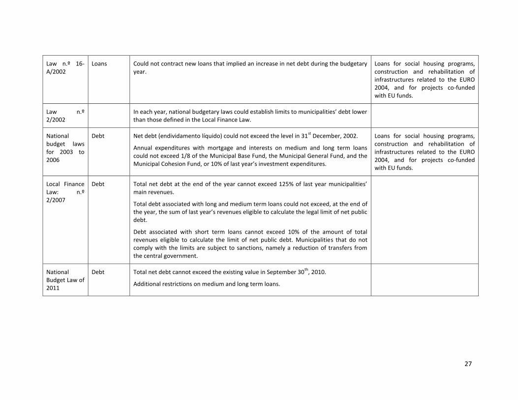
The first rules regarding municipalities’ ability to contract debt were established by decree
law 258/79. Since then, several changes occurred, as summarized in Table 1.10 Previous rules have
been criticized by several authors, namely Cabo (2009) and Lobo (2013). They disagree that the
limits only applied to the amount and purpose of short term loans, and to expenditures on
mortgage and interest of medium and long term loans. Therefore, the rules did not take into
account additional indebtedness or the stock of debt. Furthermore, the limits were set according
to investment and transfers from the central government, not taking into account the net capacity
or necessity of funding of the municipality. This has several disadvantages: (1) a decrease in the
market interest rate or an expansion in the time for paying the loans increases the legal
indebtedness limits even without an improvement of the economic situation of the municipality;
10
A new local finance law was published in September 2013 (Law 73/2013), which came into force in
January 2014. Since it does not apply to our sample period, it is not described in Table 1.
9
(2) a reduction in transfers from the central government to municipalities may lead to excessive
indebtedness, even if the municipality does not contract additional loans; (3) debts to suppliers or
leasing contracts are not considered; (4) the higher the investment the larger the debt limit.
[Insert Table 1 about here]
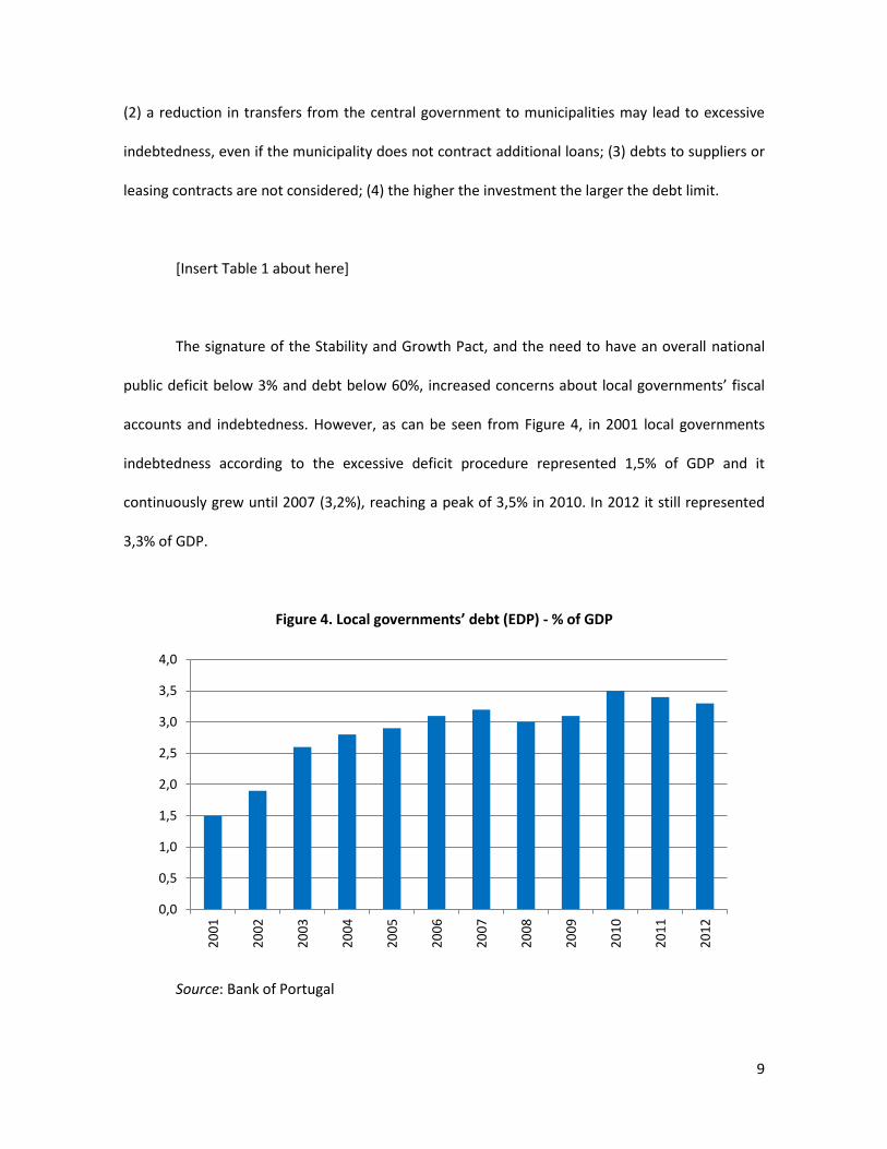
The signature of the Stability and Growth Pact, and the need to have an overall national
public deficit below 3% and debt below 60%, increased concerns about local governments’ fiscal
accounts and indebtedness. However, as can be seen from Figure 4, in 2001 local governments
indebtedness according to the excessive deficit procedure represented 1,5% of GDP and it
continuously grew until 2007 (3,2%), reaching a peak of 3,5% in 2010. In 2012 it still represented
3,3% of GDP.
Figure 4. Local governments’ debt (EDP) - % of GDP
Source: Bank of Portugal
0,0
0,5
1,0
1,5
2,0
2,5
3,0
3,5
4,0
20
01
20
02
20
03
20
04
20
05
20
06
20
07
20
08
20
09
20
10
20
11
20
12

10
4. Empirical analysis
The main objective of the present paper is to analyze the determinants of Portuguese local
governments’ indebtedness. The panel dataset is composed of annual data on fiscal, economic,
political and social variables for all 308 Portuguese municipalities, from 1979 to 2012. Data on
municipal debt were kindly provided by DGAL (Direção Geral das Autarquias Locais) and the
remaining local fiscal data were collect from DGAL’s annual publication Municipal Finances
(Finanças Municipais). Political data was obtained from the National Elections Commission (CNE),
employment data from the Institute of Employment and Professional Training (IEFP) and from the
Ministry of Labor and Social Solidarity (MTSS), economic and demographic data from the National
Statistics Institute (INE), and socio-economic indicators from the Marktest’s Sales Index database.
Descriptive statistics are presented in Table 2.
[Insert Table 2 about here]
The following two sections present our preliminary results regarding the main
determinants of Portuguese local government’s indebtedness. The estimations for budget
balances will use the entire sample, as there is data available for the period 1979-2012. Official
(DGAL) data on municipal debt is available only from 2003 onwards.
4.1 Budget Balances

11
The dependent variable in our empirical model for budget balances is the primary budget
balance11 as a percentage of a 3-year moving average of real total revenues excluding loans of
municipality i at year t (PBBit). Sets of financial, political, and socio-economic variables are included
as regressors. Financial variables consist of the first lag of the share of investment expenditures on
total expenditures (Share_Invit-1), the share of interest payments on debt on total expenditures
(Share_Interestit-1), and the share of own revenues on total revenues without loans
(Share_Own_Revit-1). Given that investments generate medium and long term benefits, it is likely
that municipalities that have a larger share of investment on total expenditures choose to delay
some of the outlays to the future by having deficits. Own revenues include, among others, local
taxes and fees charged by local governments, which are more easily perceived by voters than
those associated with transfers from the central government. Therefore, a positive coefficient is
expected for the estimated coefficient associated with this variable. Assuming that more indebted
municipalities want to avoid insolvency, the share of real interest payments on real total
expenditures is likely to improve the budget balance.
To capture political issues, the following variables were included:
- Election Yearit, Before_EYit and After_EYit: represent, respectively, the election year, and
the years before and after the election year.
- Leftit: is a dummy for left-wing mayors. According to Persson and Svensson (1989), left-
wing governments are less willing to incur debt than right-wing ones. Alt and Lassen
(2006) also find support for this hypothesis. We also include a dummy variable for mayors
not affiliated with any party (Independentit), so that the only partisan dummy left out is
that for right-wing mayors.
11
Local finance data is reported in a cash basis. Thus, the overall balance is obtained by excluding the
transactions in financial assets and liabilities from the totals of revenues and expenditures. The primary
balance is then obtained also excluding interest payments from current expenditure.

12
- Tenureit: number of years the mayor has been in office.
- %Seatsit: Percentage of seats held by the mayor’s party in the town hall.
- Coalitionit: dummy variable for coalition governments.
- Recandit: is a dummy variable equal to one during the entire term when the mayor runs
for re-election, and zero otherwise.
- Same_partyit: dummy variable that assumes the value of one when the mayor and the
prime-minister belong to the same party.
Two demographic variables are also included in the baseline model:
- %65it percentage of the population over 65 years old.
- Densityit: population density measures the number of inhabitants by squared kilometer.
Socio-economic variables that may also influence the budget balance are taken into account. They
are included in the regressions, one at a time. These variables are:
- Lic_new_constructionit: Number of licenses for new constructions per inhabitant.
- Tourismit: Number of touristic facilities per inhabitant.
- Unempit: Unemployment rate in the municipality. Higher unemployment rates are
expected to lead to higher expenditures by the local government, namely on social
aspects, and to lower revenues.
- %Area_urbanit: Percentage of the municipal area assigned to urban use. Since municipal
revenues during the sample period were strongly influenced by the amount of
construction, the increases in the area assigned to urban use are expected to have a
positive effect on municipal revenues.12
- Earningit: Real monthly earnings per capita of individuals working in private firms.
12
Data for %Area_urbanit is not available for the 30 municipalities of the islands of Azores and Madeira.

13
In order to control for the passage of time, we included dummies for each mandate since 1979
(m1 to m9). The empirical model can be summarized as follows:
itmitijti
p
j
jit yy
βX'
,,
1
iTtNi ,...,1 ,...,1 (1)
where yit is the dependent variable and p is its number of lags included in the model, 'itX is a
vector of explanatory variables, is a vector of parameters to be estimated, i is the individual
effect of municipality i, φm is the effect of mandate (term) m, and it is the error term.
Since in this dynamic panel data model the lagged value of the dependent variable is
correlated with the error term, it, even if the latter is not serially correlated, OLS, fixed or random
effects estimates will be inconsistent. As the time dimension of the panel increases, the bias
reduces but Judson and Owen (1999) found that the bias of the least squares dummy variable
(LSDV) approach can be significant, even when the number of periods is as large as 30. Although
the dataset used in the paper covers a 33-year period, the panel is unbalanced, and the average
number of observations per municipality in most regressions is around 25. Therefore, in the
sample, there is a clear dominance of cross sections (N=308) over time periods and the fixed
effects model may still suffer from dynamic panel bias.
Arellano and Bond (1991) developed a Generalized Method of Moments (GMM) estimator
that solves the problems noted above. First differencing (1) removes the individual effects (i) and
produces an equation that is estimable by instrumental variables:
itmtijti
p
j
jit yy
βX'
,,
1
iTtNi ,...,1 ,...,1 (2)

14
The valid instruments are: levels of the dependent variable, lagged two or more periods
(yi1,…,yit-2); levels of the endogenous variables, lagged two or more periods (xi1,…,xit-2); levels of the
pre-determined variables, lagged one or more periods (xi1,…,xit-1); and the levels of the exogenous
variables, current or lagged (xi1,…,xit) or, simply, the first differences of the exogenous variables
(xit). More moment conditions are available if we assume that the explanatory variables (xit) are
uncorrelated with the individual effects (i). In this case, the first lags of these variables (xit-1) can
be used as instruments in the levels equation. The estimation then combines the set of moment
conditions available for the first-differenced equations with the additional moment conditions
implied for the levels equations. Arellano and Bover, 1995 and Blundell and Bond (1998) show that
this extended GMM estimator is preferable to that of Arellano and Bond (1991) when the
dependent variable and/or the independent variables are persistent.13
The results of fixed effects estimations are reported in Table 3. As expected, greater
shares of investment expenditure in total expenditures are associated with lower budget balances,
and greater shares of interest payments have the opposite effect. That is, municipalities which
invest relatively more run lower balances, or larger deficits, and those that face higher interest
payments tend to solve the problem by running primary surpluses. Somewhat surprisingly, the
share of own revenues is not statistically significant. Thus, the share of own revenues does not
seem to affect the local governments’ primary budget balances.
[Insert Table 3 about here]
13
Difference-in-Hansen tests indicate that, for our data, the system-GMM is preferable to the difference-
GMM, which only includes the first-differenced equations.

15
The empirical results clearly indicate the presence of a political budget cycle. Not only do
budget balances tend to be lower in the election year than in any other year of the electoral cycle,
but also they are lower in year before the elections than in the remaining two years. These results
are consistent with those of Veiga and Veiga (2007) who found that municipal investment
expenditures considerably increased in the electoral year and in the year before elections.
Regarding the remaining political variables, there is some support for the hypotheses that left-
wing mayors (columns 3 to 5), as well as those belonging to the prime-minister’s party (columns 1,
2 and 6), run more positive budget balances, while the remaining variables do not seem to
influence budget balances. Regarding, demographic variables, a greater percentage of elderly
people seems to lead to better budget balances (columns 3 to 5), while population density may
not matter (it is statistically significant only in column 3). Finally, issuing more licenses for new
constructions (column 2) is associated with higher budget balances. Surprisingly, the assignment of
a larger percentage of the municipal territory to urban use worsen budget balances (column 5).
The other socio-economic variables do not seem to affect budget balances.
The results for the estimation of the previous models using System-GMM are reported in
Table 4. Two-step results using robust standard errors corrected for finite samples are reported. T-
statistics are in parenthesis, and the p-values of the autocorrelation and Hansen tests are shown at
the bottom of the table. Since the absence of second order autocorrelation and the validity of the
instrument matrix are never rejected, our estimations are valid.14 Most of the variables that were
statistically significant in the fixed-effects estimations continue to be relevant determinants of the
budget-balance with the System-GMM estimations. The main difference is that the dummy
14
Taking into account that the level of indebtedness of the municipality may influence the structure of expenditures and revenues, the three fiscal variables included as explanatory variables (the share of investment expenditures on total expenditures, the share of interest payments on debt on total expenditures, and the share of own revenues on total revenues without loans) were treated as endogenous. In order to avoid an excessive number of instruments, only lags 2 and 3 were used as instruments for the endogenous variables.

16
signaling left-wing mayors is no longer statistically significant. Additionally, there is robust
evidence that municipalities where the mayor’s party has a larger representation in the town-hall
and dominates the national government have higher budget balances. The demographic variables
suggest, again, a positive effect of percentages of the population above 65 on the budget balance
and practically no robust effects of population density. Finally, a larger number of licenses for new
constructions (column 2) and a lower unemployment rate (column 4) improve the fiscal situation
of the municipality.
[Insert Table 4 about here]
The political determinants of primary budget balances were further investigated in the
estimations whose results are reported in Table 5. As in the previous table, there is robust
evidence of a political budget cycle, as the election year dummy is always statistically significant
and negatively signed. Results also show that municipalities where mayors enjoy a larger support
in the Town Hall and belong to the party in the central government have larger budget balances. In
column 1, we analyzed whether mayors who run again for office would be more or less
opportunistic than those who do not, by including an interaction between the election year
dummy and the dummy Recand. Although the estimated coefficient for this interaction is positive,
suggesting that mayors running for office again internalize the future costs of running deficits in
electoral years, it is not statistically significant. Column 2 reveals that obtaining a larger margin of
victory at municipal elections improves the budget balances, but the reverse is true for left-wing
governments. Sollé-Olé (2006) reported a similar result for Spanish local governments. In the
following columns, we tested for differences in electoral year budget balances based on strategic
deficit management: when the local government party changes (column 4), when the mayor

17
changes (column 5), when the new local government has a different ideology than its predecessor
(column 6). The dummy variable New_party(mayor)it equals one in municipal election years, when
a new party (politician) wins the election. According to Allesina and Tabellini (1990) incumbents
anticipating that they will lose the next election may increase the budget deficit in order to
constrain the options of their successors. To check the validity of Persson and Svensson’s (1989)
hypothesis that fiscal policy is used strategically only when a change in ideology is expected by the
incumbent mayor, a dummy variable equal to one in municipal election years when the Town Hall
changes from left to right was introduced in the model (Left*New_partyit). None of these variables
was statistically significant, suggesting that the budget balance is not used strategically by
incumbent politicians. Finally, we tested if the fragmentation of the Town-Hall, measured by the
number of effective parties, influences the budget balance. As can be seen in column 6, there is no
evidence of such an effect.
[Insert Table 5 about here]
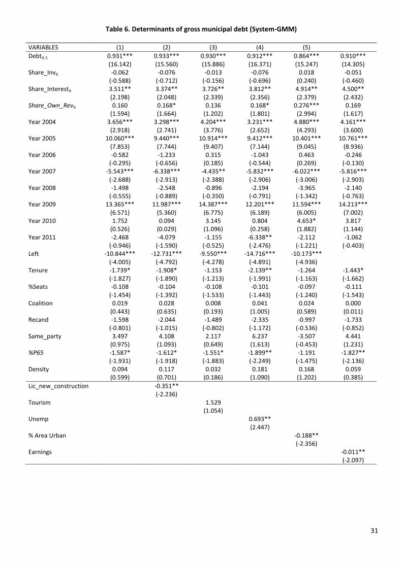
4.2. Debt
The dependent variable in the empirical model for municipal debt is the real gross debt as a
percentage of the three-year moving average of total effective revenues (without loans) of
municipality i at year t (Debtit). As explained above, official debt data is available from 2003 to
2012. The baseline model includes the same set of financial, political, and socio-economic
variables used in the estimations for the primary budget balance. Given the short time dimension
of the sample (10 years), year dummies are included instead of the electoral dummies and the
dummies for the mandates. Since debt is a persistent variable, the empirical model includes lags of
the dependent variable in the right hand-side. Because in this sample there is a clear dominance of
18
cross sections over time periods (N=308 and T=10), only results for the System-GMM15 estimator
are reported, as fixed-effects results would clearly be biased.
As can be seen from Table 6,16 larger shares of interest payments on debt on total
expenditures increase gross debt. Surprisingly, there is some indication (columns 2, 4 and 5) that a
larger share of own revenues has a similar effect. Regarding political variables, municipalities ran
by the party that dominates the national government tend to accumulate less debt. This may be
due to the fact that governments often try to distribute more grants to municipalities run by their
party (Veiga and Veiga, 2013). As happened in the previous tables, there is clear evidence of
political budget cycles. The dummies signaling municipal electoral years (2005 and 2009) are
highly statistically significant and positively signed, indicating an increase of more than 10
percentage points in debt over the three-year moving average of revenues in these years. It should
be noted that 2005 and 2009 were also legislative election years, probably intensifying the
electoral effects captured by the dummy variables. Additionally, left-wing local governments seem
to accumulate less debt, while the remaining political variables did not show up as statistically
significant. Regarding demographic variables, the percentage of elderly does not seem to affect
municipal debt, while greater population density seems to be associated with lower indebtedness.
Finally, a higher number of construction licenses issued, a greater percentage of the municipal
area assigned to urban use, and higher average wages in the private sector firms in the
municipality are associated with lower indebtedness, while higher unemployment rates have the
opposite effect. 15
Difference-in-Hansen tests indicate that, for our data, the System-GMM is preferable to the Difference-
GMM, which only includes the first-differenced equations.
16 Two-step results using robust standard errors corrected for finite samples are reported. T-statistics are in
parenthesis, and the p-values of the autocorrelation and Hansen tests are shown at the bottom of the table.
Since the absence of second order autocorrelation and the validity of the instrument matrix are never
rejected, our estimations are valid.

19
The political determinants of municipal debt were further investigated using models
similar to those of Table 5 for primary budget balances. As happened for primary budget balances,
there is no evidence of strategic debt management or that mayors running for re-election increase
debt more in electoral years than those not running for r-election.17
[Insert Table 6 about here]
5. Conclusions
Results of estimations for municipal primary budget balances and gross debt clearly indicate the
presence of political budget cycles. In accordance with the rational opportunistic cycles of Rogoff
and Sibert (1988), mayors manipulate economic local public finances before elections in a manner
that could signal greater competence. Our results reveal that budget deficits and debt increase in
the electoral year and, by a smaller amount, in the previous.
Local government that enjoy greater support in the town hall tend to have higher budget
balances, and there is also weak evidence that left-wing mayors generate lower levels of debt than
right-wing ones and independents. No evidence was found for strategic deficit or debt
management, tenure of mayors, or running again for office. Municipalities where there is party
similarity between the mayor and the national government tend to have higher budget balances
and lower debt, which suggests some favoring of these municipalities in the allocation of
intergovernmental transfers.
The structure of expenditures and revenues also affects municipal budget balances and
debt. Higher shares of investment expenditure are associated with lower budget balances, while
higher shares of interest payments have the opposite effect and increase debt. Regarding the
17
Although not reported in the paper, the results are available from the authors upon request.

20
effects of socio-economic variables, higher unemployment rates generate higher deficits and debt,
while issuing more construction licenses seems to generate higher budget balances and lower
debt. The assignment of a larger percentage of the municipal territory to land use and higher
average wages in the private firms located in the municipality are also associated with lower
indebtedness.
When comparing the electoral effect in the budget deficit and debt it is notable that the
former is much smaller than the latter, which suggests that extra-budgetary items not included in
the deficit are reflect in the debt. Preliminary research reveals a substantial difference between
changes in debt and the deficit that cannot be explained by net expenditures associated with
financial assets. This is a topic that we intend to explore in the near future. Additionally, we would
also like to investigate the determinants of different types of debt, namely of financial debt (short-
term and medium and long-term) and non-financial debt.
Acknowledgements
The authors would like to thank participants at the 2014 PEARL Seminar in Rennes for very helpful
comments. They are also thankful for the financial support provided by ERDF funds through
the Operational Program Factors of Competitiveness -COMPETE and by national funds
through the Portuguese Foundation for Science and Technology (FCT) under research
grants FCOMP-01-0124-FEDER-037268 (PEst-C/EGE/UI3182/2013) and FCOMP-01-0124-
FEDER-020420 (PTDC/EGE-ECO/118501/2010).
21
Bibliography
Alesina, Alberto and Tabellini, Guido (1990). A positive theory of fiscal deficits and government
debt. The Review of Economic Studies 57(3): 403-414.
Alt, James E and Lassen, David Dreyer (2006). Fiscal transparency, political parties, and debt in
OECD countries. European Economic Review 50: 1403-39.
Alt, J and Lowry, R (1994). Divided government, fiscal institutions and budget deficits: Evidence
from the States. American Political Science 88(4): 811-828.
Arellano, Manuel and Bond, Stephan (1991). Some tests of specification for panel data: Monte
Carlo evidence and an application to employment equations. The Review of Economic Studies
58: 277-297.
Arellano, Manuel Bover, Olympia (1995). Another look at the instrumental variable estimation of
error-component models. Journal of Econometrics 68: 29-51.
Bastida, Francisco; Beyaert, Arielle and Benito, Bernardino (2013). Electoral cycles and local
government debt management. Local Government Studies 39(1): 107-132.
Battaglini, Marco and Coate, Stephen (2008). A dynamic theory of public spending, taxation and
debt. American Economic Review 98(1): 201-236.
Beetsma, Roel; Giuliodori, Massimo and Wierts, Peter (2009). Planning to cheat: EU fiscal policy in
real time. Economic Policy 24(60): 755-804.
Bohn, H and R.P. Inman (1996). Balanced-Budget Rules and Public Deficits: Evidence from The U.S.
States. Carnegie-Rochester Conference Series on Public Policy 45: 13-76.
Cabo, Sérgio (2009). Saneamento e reequilíbrio financeiro municipal. Revista de Finanças Públicas
e Direito Fiscal, Anno II(2).
Djankov, S. and Murell, P. (2002). Enterprise Restructuring in Transition: A Quantitative Survey.
Journal of Economic Literature XI: 739-792.

22
Hodler, Roland (2011). Elections and the strategic use of budget deficits. Public Choice 148: 149-
161.
Holtz-Eakin, D. (1988). The line item veto and public sector budgets: evidence from the states.
Journal of Public Economics 36:269–292.
Holtz-Eakin, D., Newey, W. and Rosen, H.S. (1988). Estimating vector autoregressions with panel
data. Econometrica 56, 1371-1395.
Hopland, Arnt (2013). Central government control and fiscal adjustment: Norwegian evidence.
Economics of Governance 14(2): 185-203.
Kornai, J (1979). Resource-constrained versus demand-constrained systems. Econometrica
47:801–819.
Kornai, J.; Maskin, E. and Roland, G. (2003). Understanding soft budget constraint. Journal of
Economic Literature 41: 1095-1136.
Krogstrup, Signe and Wyplosz, Charles (2010). A common pool theory of supranational deficit
ceilings. European Economic Review 54(2): 273-281.
Judson, Ruth and Owen, Anne (1999). Estimating dynamic panel data models: A practical guide for
macroeconomists. Economics Letters. 65: 9-15.
Lizzeri, Alessandro (1999). Budget deficits and redistributive politics. Review of Economic Studies
66: 909-928.
Lobo, Flora (2013). A descentralização orçamental e o endividamento publico subnacional – Uma
aplicação aos municípios portugueses. PhD Thesis. Universidade de Coimbra.
Milesin-Ferretti, G. and Spolaore, E. (1994). How cynical can an incumbent be? Strategic policy in a
model of government spending. Journal of Public Economics 55(1): 121-140.
Milesin-Ferretti, Gian (2003). Good, bad or ugly? On the effects of fiscal rules with creative
accounting. Journal of Public Economics 88: 377-394.

23
Perotti, R. and Kentopoulos, Y. (2002). Fragmented fiscal policy. Journal of Public Economics 86:
191-222.
Persson, Torsten and Sevenson, Lars (1989). Why a stubborn conservative would run a deficit:
Policy with time-inconsistent preferences. Quarterly Journal of Economics 104(2): 325-345.
Petterson-Lindbom, Per (2010). Dynamic commitment and the soft budget constraint: An
empirical test. American Economic Journal: Economic Policy 2(3): 154-179.
Pettersson-Lidbom, Per (2001). An empirical investigation of the strategic use of debt. Journal of
Political Economy 109(3): 570-583.
Poterba, James (1994). State responses to fiscal crises: The effects of budgetary institutions and
politics. Journal of Political Economy 102(4): 799-821,
Ribeiro, Nuno A. B. (2012). Factores determinantes do endividamento na Administração Local: o
caso dos municípios Portugueses. PhD Thesis. Facultat de Ciências Económicas y
Empresariales, Universidade Autónoma de Madrid.
Rodden, E.; Eskeland, G.S.; Litvack J (eds) (2003). Fiscal decentralization and the challenge of hard
budget constraint. The MIT Press, Cambridge.
Rogoff, K. and Sibert, A. (1988), “Elections and Macroeconomic Policy Cycles,” Review of
Economics Studies, 55: 1-16.
Roubini, Nouriel and Sachs, Jeffrey (1989). Political and economic determinants of budget deficits
in the industrial democracies. European Economic Review 33: 903-938.
Solé-Ollé, Albert (2006). The effects of party competition on budget outcomes: Empirical evidence
from local governments in Spain. Public Choice 126: 145-176.,
Song, Zheng; Stosletten, Kjetil and Zilibotti, Fabrizio (2012). Rotten parents and disciplined
children: A politico-economic theory of public expenditure and debt. Econometrica 80(6):
2785-2803.

24
Tullock, G. (1959). Some Problems of Majority Voting. Journal of Political Economy 67: 571-579.
Veiga, Linda and Veiga, Francisco (2007). Political business cycles at the municipal level. Public
Choice 131, 45-64.
Veiga, Linda and Veiga, Francisco (2013). Intergovernmental fiscal transfers as pork barrel. Public
Choice 155 (3/4): 335-353.
Velasco, A. (2000). Debt and deficits with fragmented fiscal policy-making. Journal of Public
Economics 76: 105-25.
Volkering, B. and de Haan, J. (2001). Fragmented government effects on fiscal policy: New
evidence. Public Choice 109: 221-42.
Von Hagen, J. and Wolff, G. (2006). What do deficits tell us about debt? Empirical evidence on
creative accounting with fiscal rules in the EU. Journal of Banking and Finance 30: 3259–79.
Weingast, B. R.; Shepsle, K. A. and Johnsen, C. (1981). The political economy of benefits and costs:
A neo-classical approach to distributive politics. Journal of Political Economy 89(4): 642-664.
Yared, Pierre (2010). Politicians, taxes and debt. Review of Economic Studies 77: 806-840.

25
Table 1. Descriptive statistics
Variable Observations Mean Std. Dev Minimum Maximum
Real Primary Budget Balance % 3-y revenues
9797 -0,683 14,388 -261,512 354,133
Real Debt % 3-y revenues 8549 176,393 283,007 0,000 673,377
Share_Inv 9730 40,839 17,525 0,000 121,570
Share_Interest 9797 2,425 2,938 0,000 51,481
Share_Own_Rev 9797 26,302 19,110 0,249 124,746
Election Year 9797 0,260 0,439 0,000 1,000
Before_EY 9797 0,259 0,438 0,000 1,000
After_EY 9797 0,267 0,442 0,000 1,000
Left 9797 0,549 0,498 0,000 1,000
Independent 9797 0,006 0,079 0,000 1,000
Tenure 9790 7,357 5,757 0,000 36,000
%Seats 9787 60,220 12,124 28,571 100,000
Coalition 9797 0,056 0,231 0,000 1,000
Recand 9349 0,537 0,499 0,000 1,000
Same_party 9797 0,386 0,487 0,000 1,000
%P65 9796 18,736 6,342 5,300 44,183
Density 9797 0,029 0,087 0,000 1,128
Lic_new_construction 6933 5,240 3,349 0,000 51,106
Tourism 6416 0,232 0,402 0,000 5,213
Unemployment rate 4680 6,202 2,633 0,590 17,399
% Area Urban 4379 9,990 11,851 0,334 68,772
Earnings (average) 7529 775,838 167,771 407,994 1904,367
Margin of victory 9787 19,986 14,750 0,018 87,926
New mayor 9790 0,058 0,233 0,000 1,000
New party 9790 0,094 0,292 0,000 1,000
Effective number parties 9787 2,069 0,454 1,000 4,455
Sources: DGAL, CNE, IEFP, MTSS, INE and Marktest.
Note: Sample restricted to the 9797 observations for which there is data on the real primary budget.

26
Table 2. Limits to indebtedness over time
Law Target Limit Exception
Decree-law 258/79
Medium and long term loans
Only for reproductive investments on social or cultural activities, and for rescuing municipalities in financial distress.
Could not exceed 1/12 of the investment expenditures approved in the municipal budget for that year.
Annual expenditures on mortgage and interests could not exceed 20% of the approved annual expenditure on investment.
Decree-law 98/84
Short term loans
Could not exceed 5% of the Financial Equilibrium Fund.18
Annual expenditures with mortgage and interest associated with long and medium term loans could not exceed the highest value of 20% of the FEF or of 20% of last year investment expenditure.
Loans for the construction of houses and for the rehabilitation of buildings
Law n.º 1/87 Short term loans
Could not exceed 10% of the Financial Equilibrium Fund.
Annual expenditures with mortgage and interest associated with long and medium term loans could not exceed the highest limit of 3/12 of the FEF or of 20% of last year investment expenditure.
Law n.º 42/98 Medium and long term loans
Annual expenditures with mortgage and interest associated with long and medium term loans could not exceed the highest value of 3/12 of the sum of the Municipal Base Fund and the Municipal General Fund or of 20% of last year investment expenditure.
Decree-law n.º 94/01
Short term loans
Could not exceed 10% of the sum of the Municipal Base Fund, the Municipal General Fund and the Municipal Cohesion Fund.
18
The financial equilibrium fund was the main transfer received by municipalities from the central government, until the local finance law n. 42/98.
27
Law n.º 16-A/2002
Loans Could not contract new loans that implied an increase in net debt during the budgetary year.
Loans for social housing programs, construction and rehabilitation of infrastructures related to the EURO 2004, and for projects co-funded with EU funds.
Law n.º 2/2002
In each year, national budgetary laws could establish limits to municipalities’ debt lower than those defined in the Local Finance Law.
National budget laws for 2003 to 2006
Debt
Net debt (endividamento líquido) could not exceed the level in 31st
December, 2002.
Annual expenditures with mortgage and interests on medium and long term loans could not exceed 1/8 of the Municipal Base Fund, the Municipal General Fund, and the Municipal Cohesion Fund, or 10% of last year’s investment expenditures.
Loans for social housing programs, construction and rehabilitation of infrastructures related to the EURO 2004, and for projects co-funded with EU funds.
Local Finance Law: n.º 2/2007
Debt Total net debt at the end of the year cannot exceed 125% of last year municipalities’ main revenues.
Total debt associated with long and medium term loans could not exceed, at the end of the year, the sum of last year’s revenues eligible to calculate the legal limit of net public debt.
Debt associated with short term loans cannot exceed 10% of the amount of total revenues eligible to calculate the limit of net public debt. Municipalities that do not comply with the limits are subject to sanctions, namely a reduction of transfers from the central government.
National Budget Law of 2011
Debt Total net debt cannot exceed the existing value in September 30th
, 2010.
Additional restrictions on medium and long term loans.

28
Table 3. Determinants of the primary budget balance (Fixed Effects)
VARIABLES (1) (2) (3) (4) (5) (6)
PBBit-1 0.055*** 0.039* 0.030 0.001 0.016 0.030 (3.714) (1.805) (1.247) (0.047) (0.456) (1.547) Share_Invt-1 -0.072*** -0.060*** -0.067*** -0.099*** -0.089*** -0.071*** (-4.771) (-3.620) (-3.705) (-3.951) (-3.397) (-4.282) Share_Interest t-1 0.920*** 0.951*** 0.955*** 0.809** 0.833** 0.788*** (10.293) (8.426) (7.134) (2.512) (2.478) (6.169) Share_Own_Rev t-1 0.022 0.038 0.027 -0.025 -0.014 0.019 (1.078) (1.499) (0.868) (-0.637) (-0.342) (0.743) Election Year -6.139*** -5.553*** -5.845*** -5.462*** -5.685*** -6.548*** (-13.476) (-11.026) (-11.103) (-8.952) (-9.266) (-12.434) Before_EY -2.622*** -1.465*** -1.712*** -1.418*** -1.520*** -2.365*** (-7.087) (-3.893) (-4.314) (-2.923) (-3.078) (-5.631) After_EY -1.633*** -2.162*** -2.276*** -2.504*** -2.352*** -1.986*** (-4.275) (-5.382) (-5.128) (-4.928) (-4.464) (-5.241) Left 0.536 0.901* 1.500*** 1.768** 1.391* 0.650 (1.173) (1.717) (2.741) (2.272) (1.797) (1.305) Independent 0.873 1.150 1.687 0.770 -0.524 1.358 (0.527) (0.591) (0.895) (0.355) (-0.252) (0.692) Tenure 0.034 -0.001 -0.009 -0.029 -0.026 0.015 (1.092) (-0.016) (-0.223) (-0.494) (-0.441) (0.424) %Seats -0.004 0.004 0.013 0.024 0.026 0.008 (-0.300) (0.235) (0.732) (0.908) (0.967) (0.543) Coalition 0.289 -0.668 0.031 0.316 0.371 -0.908 (0.358) (-0.516) (0.023) (0.197) (0.211) (-0.788) Recand -0.568 -0.598 -0.505 -0.214 -0.443 -0.578 (-1.361) (-1.072) (-0.803) (-0.245) (-0.454) (-1.266) Same_party 0.741** 0.744** 0.564 0.286 0.535 0.656* (2.291) (2.164) (1.569) (0.671) (1.238) (1.909) %P65 0.153 0.256 0.340* 0.630** 0.692** 0.289 (1.306) (1.637) (1.893) (2.345) (2.545) (1.572) Density 11.780 -28.112 -49.185** -34.538 6.660 (1.127) (-1.494) (-2.456) (-0.934) (0.769)
Lic_new_construction 0.133* (1.807) Tourism -0.561 (-0.585) Unemp 0.156 (0.920) % Area Urban -0.674** (-2.119) Earnings 0.000 (0.141)
Observations 8,797 6,434 5,925 4,279 3,992 6,986 Municipalities 308 308 308 308 278 308 Adjusted R2 0.138 0.100 0.097 0.068 0.076 0.091
Sources: DGAL, CNE, IEFP, MTSS, INE and Marktest. Notes: Fixed effects estimations including dummy variables for mandates. The dependent variable is the primary budget balance as a percentage of the 3-year moving average of effective revenues (without loans). T-statistics are between parentheses. Significance level for which the null hypothesis is rejected: ***, 1%, **, 5%, and *, 10%..

29
Table 4. Determinants of the primary budget balance (System-GMM)
VARIABLES (1) (2) (3) (4) (5) (6)
PBBit-1 0.128*** 0.110*** 0.107*** 0.082*** 0.097*** 0.083*** (6.198) (5.267) (4.781) (2.826) (2.860) (4.241) Share_Invit -0.274*** -0.218*** -0.196*** -0.236*** -0.210*** -0.302*** (-6.726) (-5.447) (-4.964) (-5.451) (-5.246) (-8.036) Share_Interestit 0.960*** 1.005*** 0.997*** 0.383** 0.486*** 0.864*** (11.790) (11.962) (10.423) (2.106) (2.763) (7.977) Share_Own_Revit 0.013 0.083** 0.087* 0.072 0.061 0.040 (0.375) (2.313) (1.910) (1.443) (1.416) (1.200) Election Year -5.680*** -4.399*** -4.747*** -4.713*** -5.132*** -5.902*** (-13.223) (-9.807) (-10.064) (-8.604) (-9.222) (-13.356) Before_EY -2.624*** -1.259*** -1.494*** -1.416*** -1.609*** -2.235*** (-7.264) (-3.609) (-4.149) (-2.950) (-3.362) (-5.977) After_EY -1.227*** -1.362*** -1.379*** -1.388*** -1.464*** -1.427*** (-3.425) (-3.792) (-3.232) (-2.803) (-2.681) (-3.780) Left -0.703 -0.571 -0.461 -0.171 -0.328 -0.341 (-1.566) (-1.378) (-1.026) (-0.341) (-0.740) (-0.831) Independent 1.684 0.451 0.548 0.812 -0.389 1.072 (0.682) (0.213) (0.262) (0.347) (-0.170) (0.439) Tenure 0.028 0.003 0.001 0.011 -0.001 0.045 (0.913) (0.106) (0.025) (0.316) (-0.017) (1.412) %Seats 0.041*** 0.041** 0.038** 0.024 0.029 0.030* (2.687) (2.494) (2.186) (1.197) (1.454) (1.910) Coalition -0.459 -1.389 -1.249 -0.879 -1.537 -1.700 (-0.534) (-1.137) (-0.991) (-0.639) (-1.241) (-1.544) Recand -0.094 0.105 0.247 1.348 1.039 0.605 (-0.215) (0.201) (0.431) (1.581) (1.125) (1.345) Same_party 0.805** 0.925*** 0.862** 0.843** 0.711* 0.596* (2.426) (2.825) (2.537) (2.030) (1.720) (1.779) %P65 0.154*** 0.203*** 0.213*** 0.203** 0.162** 0.207*** (2.795) (3.804) (3.448) (2.422) (2.491) (3.593) Density -1.840 -7.075 -9.368* -6.662 -2.863 (-0.680) (-1.529) (-1.735) (-1.393) (-1.129)
Lic_new_construction 0.193*** (3.380) Tourism 0.359 (0.661) Unemp -0.155* (-1.683) % Area Urban -0.034 (-1.098) Earnings -0.003 (-1.542)
Observations 8,796 6,434 5,925 4,279 3,992 7,017 N. municipalities 308 308 308 308 278 308 N. instruments 277 287 263 262 261 311 Arellano-Bond AR(1), p-value 0.000 3.69e-10 2.39e-09 4.79e-06 2.23e-05 0.000 Arellano-Bond AR(2), p-value 0.627 0.282 0.326 0.222 0.173 0.638 Hansen, p-value 0.166 0.341 0.244 0.190 0.317 0.360 Diff Hansen_1, p-value 1.000 0.992 0.995 0.999 0.996 0.996 Diff Hansen_2, p-value 0.993 0.793 0.774 0.665 0.965 0.558
Sources: DGAL, CNE, IEFP, MTSS, INE and Marktest. Notes: System-GMM estimations for dynamic panel-data models, including dummies for mandates. Sample period: 1979-2011.
The dependent variable is the primary budget balance as a percentage of the 3-year moving average of effective revenues
(without loans). Two-step results using robust standard errors corrected for finite samples. T-statistics are in parenthesis.
Significance level at which the null hypothesis is rejected: ***, 1%; **, 5%, and *, 10%.

30
Table 5. Additional political determinants of the primary budget balance (System-GMM)
VARIABLES (1) (2) (3) (4) (5) (6)
PBBit-1 0.123*** 0.123*** 0.123*** 0.123*** 0.123*** 0.123*** (6.206) (6.208) (6.199) (6.197) (6.231) (6.174) Share_Invit -0.283*** -0.281*** -0.277*** -0.277*** -0.278*** -0.276*** (-6.761) (-6.707) (-6.733) (-6.696) (-6.722) (-6.639) Share_Interestit 0.952*** 0.954*** 0.958*** 0.958*** 0.957*** 0.962*** (11.403) (11.501) (11.624) (11.612) (11.616) (11.528) Share_Own_Revt -0.011 -0.011 -0.010 -0.009 -0.010 -0.009 (-0.327) (-0.321) (-0.281) (-0.264) (-0.303) (-0.276) Election Year -4.760*** -4.285*** -4.243*** -4.274*** -4.232*** -4.275*** (-8.507) (-11.360) (-10.542) (-9.658) (-10.541) (-11.310) Left -0.585 0.216 -0.602 -0.598 -0.500 -0.580 (-1.325) (0.404) (-1.366) (-1.359) (-1.100) (-1.312) Independent 1.867 1.737 1.830 1.819 1.821 1.577 (0.750) (0.689) (0.732) (0.729) (0.728) (0.620) Tenure 0.014 0.011 0.012 0.010 0.012 0.009 (0.465) (0.347) (0.394) (0.332) (0.422) (0.307) %Seats 0.038** 0.020 0.037** 0.037** 0.037** 0.076** (2.480) (0.848) (2.364) (2.414) (2.361) (2.525) Coalition -0.464 -0.532 -0.490 -0.491 -0.486 -0.405 (-0.531) (-0.608) (-0.561) (-0.561) (-0.554) (-0.463) Recand -0.397 -0.225 -0.185 -0.168 -0.179 -0.179 (-0.837) (-0.506) (-0.421) (-0.365) (-0.408) (-0.405) Same_party 0.820** 0.802** 0.839** 0.833** 0.842** 0.828** (2.435) (2.386) (2.481) (2.467) (2.485) (2.465) %P65 0.117** 0.123** 0.120** 0.121** 0.119** 0.124** (2.128) (2.236) (2.177) (2.192) (2.161) (2.280) Density -0.694 -0.778 -0.612 -0.621 -0.594 -1.023 (-0.258) (-0.299) (-0.229) (-0.234) (-0.223) (-0.392)
Election Year * Recand 0.841 (1.234) Margin of Victory 0.037* (1.839) Left * Margin of Victory -0.043* (-1.903) New party -0.122 0.171 (-0.158) (0.167) New Mayor 0.015 (0.020) Left * New Party -0.624 (-0.429) Number of effective parties 1.171 (1.453)
Observations 8,796 8,796 8,796 8,796 8,796 8,796 Municipalities 308 308 308 308 308 308 No. of instruments 276 277 276 276 277 276 AR(1), p-value 0.000 0.000 0.000 0.000 0.000 0.000 AR(2), p-value 0.485 0.465 0.469 0.467 0.467 0.468 Hansen, p-value 0.155 0.147 0.153 0.151 0.153 0.148 Diff Hansen_1, p-value 1.000 1.000 1.000 1.000 1.000 1.000 Diff Hansen_2, p-value 1.000 1.000 1.000 1.000 1.000 1.000
Sources: DGAL, CNE, IEFP, MTSS, INE and Marktest. Notes: System-GMM estimations for dynamic panel-data models, including dummies for mandates. Sample period: 1979-2011. The dependent variable is the primary budget balance as a percentage of the 3-year moving average of effective revenues (without loans). Two-step results using robust standard errors corrected for finite samples. T-statistics are in parenthesis. Significance level at which the null hypothesis is rejected: ***, 1%; **, 5%, and *, 10%.
31
Table 6. Determinants of gross municipal debt (System-GMM)
VARIABLES (1) (2) (3) (4) (5)
Debtit-1 0.931*** 0.933*** 0.930*** 0.912*** 0.864*** 0.910*** (16.142) (15.560) (15.886) (16.371) (15.247) (14.305) Share_Invit -0.062 -0.076 -0.013 -0.076 0.018 -0.051 (-0.588) (-0.712) (-0.156) (-0.696) (0.240) (-0.460) Share_Interestit 3.511** 3.374** 3.726** 3.812** 4.914** 4.500** (2.198) (2.048) (2.339) (2.356) (2.379) (2.432) Share_Own_Revit 0.160 0.168* 0.136 0.168* 0.276*** 0.169 (1.594) (1.664) (1.202) (1.801) (2.994) (1.617) Year 2004 3.656*** 3.298*** 4.204*** 3.231*** 4.880*** 4.161*** (2.918) (2.741) (3.776) (2.652) (4.293) (3.600) Year 2005 10.060*** 9.440*** 10.914*** 9.412*** 10.401*** 10.761*** (7.853) (7.744) (9.407) (7.144) (9.045) (8.936) Year 2006 -0.582 -1.233 0.315 -1.043 0.463 -0.246 (-0.295) (-0.656) (0.185) (-0.544) (0.269) (-0.130) Year 2007 -5.543*** -6.338*** -4.435** -5.832*** -6.022*** -5.816*** (-2.688) (-2.913) (-2.388) (-2.906) (-3.006) (-2.903) Year 2008 -1.498 -2.548 -0.896 -2.194 -3.965 -2.140 (-0.555) (-0.889) (-0.350) (-0.791) (-1.342) (-0.763) Year 2009 13.365*** 11.987*** 14.387*** 12.201*** 11.594*** 14.213*** (6.571) (5.360) (6.775) (6.189) (6.005) (7.002) Year 2010 1.752 0.094 3.145 0.804 4.653* 3.817 (0.526) (0.029) (1.096) (0.258) (1.882) (1.144) Year 2011 -2.468 -4.079 -1.155 -6.338** -2.112 -1.062 (-0.946) (-1.590) (-0.525) (-2.476) (-1.221) (-0.403) Left -10.844*** -12.731*** -9.550*** -14.716*** -10.173*** (-4.005) (-4.792) (-4.278) (-4.891) (-4.936) Tenure -1.739* -1.908* -1.153 -2.139** -1.264 -1.443* (-1.827) (-1.890) (-1.213) (-1.991) (-1.163) (-1.662) %Seats -0.108 -0.104 -0.108 -0.101 -0.097 -0.111 (-1.454) (-1.392) (-1.533) (-1.443) (-1.240) (-1.543) Coalition 0.019 0.028 0.008 0.041 0.024 0.000 (0.443) (0.635) (0.193) (1.005) (0.589) (0.011) Recand -1.598 -2.044 -1.489 -2.335 -0.997 -1.733 (-0.801) (-1.015) (-0.802) (-1.172) (-0.536) (-0.852) Same_party 3.497 4.108 2.117 6.237 -3.507 4.441 (0.975) (1.093) (0.649) (1.613) (-0.453) (1.231) %P65 -1.587* -1.612* -1.551* -1.899** -1.191 -1.827** (-1.931) (-1.918) (-1.883) (-2.249) (-1.475) (-2.136) Density 0.094 0.117 0.032 0.181 0.168 0.059 (0.599) (0.701) (0.186) (1.090) (1.202) (0.385)
Lic_new_construction -0.351** (-2.236) Tourism 1.529 (1.054) Unemp 0.693** (2.447) % Area Urban -0.188** (-2.356) Earnings -0.011** (-2.097)

32
Observations 2,631 2,623 2,631 2,598 2,367 2,470 Municipalities 308 308 308 308 278 308 No. of instruments 298 299 269 299 258 306 AR(1), p-value 0.000118 0.000126 0.000119 0.000110 0.000700 0.000204 AR(2), p-value 0.780 0.796 0.772 0.152 0.100 0.743 Hansen, p-value 0.312 0.288 0.150 0.294 0.243 0.365 Diff Hansen_1, p-value 0.979 0.971 0.992 0.841 0.748 0.997 Diff Hansen_2, p-value 0.945 0.944 0.770 0.961 0.493 0.764
Sources: DGAL, CNE, IEFP, MTSS, INE and Marktest. Notes: System-GMM estimations for dynamic panel-data models, including dummies for mandates. Sample period: 1979-2011.
The dependent variable is the primary budget balance as a percentage of the 3-year moving average of effective revenues
(without loans). Two-step results using robust standard errors corrected for finite samples. T-statistics are in parenthesis.
Significance level at which the null hypothesis is rejected: ***, 1%; **, 5%, and *, 10%.
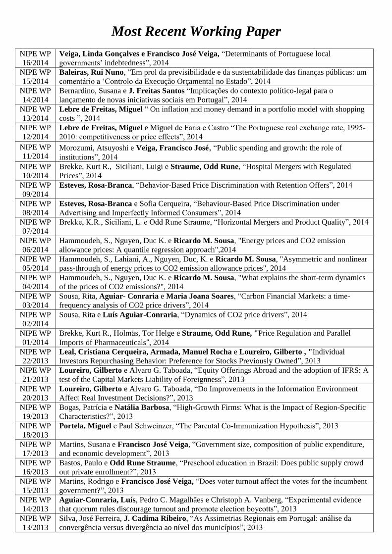
Most Recent Working Paper
NIPE WP
16/2014
Veiga, Linda Gonçalves e Francisco José Veiga, “Determinants of Portuguese local
governments’ indebtedness”, 2014
NIPE WP
15/2014
Baleiras, Rui Nuno, “Em prol da previsibilidade e da sustentabilidade das finanças públicas: um
comentário a ‘Controlo da Execução Orçamental no Estado”, 2014
NIPE WP
14/2014
Bernardino, Susana e J. Freitas Santos “Implicações do contexto político-legal para o
lançamento de novas iniciativas sociais em Portugal”, 2014
NIPE WP
13/2014
Lebre de Freitas, Miguel “ On inflation and money demand in a portfolio model with shopping
costs ”, 2014
NIPE WP
12/2014
Lebre de Freitas, Miguel e Miguel de Faria e Castro “The Portuguese real exchange rate, 1995-
2010: competitiveness or price effects”, 2014
NIPE WP
11/2014 Morozumi, Atsuyoshi e Veiga, Francisco José, “Public spending and growth: the role of
institutions”, 2014
NIPE WP
10/2014
Brekke, Kurt R., Siciliani, Luigi e Straume, Odd Rune, “Hospital Mergers with Regulated
Prices”, 2014
NIPE WP
09/2014
Esteves, Rosa-Branca, “Behavior-Based Price Discrimination with Retention Offers”, 2014
NIPE WP
08/2014
Esteves, Rosa-Branca e Sofia Cerqueira, “Behaviour-Based Price Discrimination under
Advertising and Imperfectly Informed Consumers”, 2014
NIPE WP
07/2014
Brekke, K.R., Siciliani, L. e Odd Rune Straume, “Horizontal Mergers and Product Quality”, 2014
NIPE WP
06/2014
Hammoudeh, S., Nguyen, Duc K. e Ricardo M. Sousa, "Energy prices and CO2 emission
allowance prices: A quantile regression approach",2014
NIPE WP
05/2014
Hammoudeh, S., Lahiani, A., Nguyen, Duc, K. e Ricardo M. Sousa, "Asymmetric and nonlinear
pass-through of energy prices to CO2 emission allowance prices", 2014
NIPE WP
04/2014
Hammoudeh, S., Nguyen, Duc K. e Ricardo M. Sousa, "What explains the short-term dynamics
of the prices of CO2 emissions?", 2014
NIPE WP
03/2014
Sousa, Rita, Aguiar- Conraria e Maria Joana Soares, “Carbon Financial Markets: a time-
frequency analysis of CO2 price drivers”, 2014
NIPE WP
02/2014
Sousa, Rita e Luís Aguiar-Conraria, “Dynamics of CO2 price drivers”, 2014
NIPE WP
01/2014
Brekke, Kurt R., Holmäs, Tor Helge e Straume, Odd Rune, "Price Regulation and Parallel
Imports of Pharmaceuticals”, 2014
NIPE WP
22/2013
Leal, Cristiana Cerqueira, Armada, Manuel Rocha e Loureiro, Gilberto , "Individual
Investors Repurchasing Behavior: Preference for Stocks Previously Owned”, 2013
NIPE WP
21/2013
Loureiro, Gilberto e Alvaro G. Taboada, “Equity Offerings Abroad and the adoption of IFRS: A
test of the Capital Markets Liability of Foreignness”, 2013
NIPE WP
20/2013
Loureiro, Gilberto e Alvaro G. Taboada, “Do Improvements in the Information Environment
Affect Real Investment Decisions?”, 2013
NIPE WP
19/2013
Bogas, Patrícia e Natália Barbosa, “High-Growth Firms: What is the Impact of Region-Specific
Characteristics?”, 2013
NIPE WP
18/2013
Portela, Miguel e Paul Schweinzer, “The Parental Co-Immunization Hypothesis”, 2013
NIPE WP
17/2013
Martins, Susana e Francisco José Veiga, “Government size, composition of public expenditure,
and economic development”, 2013 NIPE WP
16/2013
Bastos, Paulo e Odd Rune Straume, “Preschool education in Brazil: Does public supply crowd
out private enrollment?”, 2013
NIPE WP
15/2013
Martins, Rodrigo e Francisco José Veiga, “Does voter turnout affect the votes for the incumbent
government?”, 2013
NIPE WP
14/2013
Aguiar-Conraria, Luís, Pedro C. Magalhães e Christoph A. Vanberg, “Experimental evidence
that quorum rules discourage turnout and promote election boycotts”, 2013
NIPE WP
13/2013
Silva, José Ferreira, J. Cadima Ribeiro, “As Assimetrias Regionais em Portugal: análise da
convergência versus divergência ao nível dos municípios”, 2013