Detection improvement for anti‑collision radar - DR-NTU

This document is downloaded from DR‑NTU (https://dr.ntu.edu.sg)Nanyang Technological University, Singapore.

Detection improvement for anti‑collision radar

Qu, Yao Wen

2005

Qu, Y. W. (2005). Detection improvement for anti‑collision radar. Master’s thesis, NanyangTechnological University, Singapore.

https://hdl.handle.net/10356/3162

https://doi.org/10.32657/10356/3162

Nanyang Technological University

Downloaded on 15 Jan 2022 05:28:23 SGT

Detection Improvement for Anti-collision Radar

Qu Yao Wen

School of Electrical & Electronic Engineering

A thesis submitted to the Nanyang Technological University

in fulfillment of the requirement for the degree of

Master of Engineering

2005

ATTENTION: The Singapore Copyright Act applies to the use of this document. Nanyang Technological University Library

Statement of Originality

I hereby certify that the work embodied in this thesis is the result of original

research done by me and has no been submitted for a higher degree to any

other University or Institute.

3JJ.LL&#£ .(£.«r.J&$u)e^

in


Summary

This thesis illustrates the necessity and design process of performance improvement for

radar detection by using novel CFAR detectors. A qualitative discussion of the need for

and applications of conventional CFAR detectors is presented first. Typical applications

are given as examples of where the radar system may be utilized. A closer look under the

Swerling 2 assumption is presented as well.

The second portion of the thesis generally introduce the underlying electromagnetic

theories that radar detection is built upon. The radar range equation, radar cross section,

noise in systems, and vehicular applications are explained. The portion focuses on the

radar detection. The general detection theory of Bayes and the Neyman-Pearson theorem

are applied in our analysis for detection of targets with group fluctuations. The

traditional approach of Swerling model I to IV and binary detection are all discussed with

relation to the detect process. Among radar environment models, Swerling II is used

because of its close space and low fluctuation properties. In a scenario of closely spaced

targets special attention has to be paid to anti-collision radar signal processing. I present

several advanced CFAR processing techniques. This processing results in a significant

improvement. Algorithms are developed for Swerling II models of radar cross section

(RCS) fluctuations and binary detection. Based on the firm ground, I have made further

researches in to the conventional Cell-Average ( CA-CFAR) and Order-Statistic ( OS-

CFAR ) in a homogeneous background .

In this thesis, I proposed four new radar CFAR synthesizing the advantages of CA-

CFAR and OS-CFAR. In a homogeneous background, the mathematical models of the

four new CFAR detectors are derived and their performance have been evaluated and

compared with that of CA-CFAR and OS-CFAR. It is proved that this CFAR approach is

computationally efficient and increases the detection performance. Numerous research

IV


and simulation test results are given to show that adopting the proposed approach one can

achieve much better performance than the reported methods and results to date.

Furthermore, some new methods, such as neural network and fuzzy integration are

present for signal detection and CFAR data fusion as the future work. Neural network

and fuzzy integration have been considered for signal detection primarily because they

may be trained to operate with acceptable performance, in an environment under which

the optimum signal detector is not available. Since interference attract more and more

attention, recently neural networks have been considered for overcoming the obstacles of

interference which limit detection accuracy in most signal detection applications.

A new method about 'car on curve' also proposed to solve the non-detection of

necessary objects and reduce the false alert rate. Numerous research and simulation test

results are given to illustrate the success of the design procedure and to support choices

of specific types.

V


TABLE OF CONTENTS

1.Introduction 1

1.1 Introduction to Radar 1

1.2 Anti-collision Radar Background 3

1.3 The Radar Equation 8

1.4 Maximum Range and Noise 11

1.5 Radar Applications 12

1.6 Pulsed Radar 17

1.7 Doppler Radar 19

1.8 Frequency-Modulated-Continuous-Wave Radar 23

1.9 Noise in Microwave Systems 28

1.10 Radar Cross Section 30

1.11 Vehicular Applications 32

1.12 Objectives 37

1.13 Organization of This Thesis 38

2.Traditional CFAR Processors 40

2.1 Introduction 40

2.2 Statistical Decision Theory for Anti-collision Radar 42

2.3 Detection Criteria 44

2.4 Bayes's Concepts for Radar 48

2.5 Binary Detection 52

VI


2.6 Cell Averaging CFAR 54

2.7 Order Statistics CFAR 56

2.8 Other CFAR Techniques 57

2.9 Mathematical Model of CA-CFAR and OS-CFAR 58

2.10 Results 61

2.11 Conclusion 63

3. Novel CFAR Detectors 64

3.1 Introduction 64

3.2 Detection Principle and Model Formulation 65

3.3 Mathematical Model of Novel CFAR 69

3.4 Mathematical Model of And-Ca-Os CFAR 71

3.5 Mathematical Model of And-Os-Os CFAR 72

3.6 Mathematical Model of And-Os-Os-Os CFAR 73

3.7 Mathematical Model of And-Ca-Os-Os CFAR 75

3.8 Results 77

3.9 Performance Comparison 87

3.10 Conclusion 88

4. Improved Radar Detection on Curved Section of a Road 89

4.1 Introduction 89

4.2 Radar Antennas 90

4.3 Anti-Collision Radar Antenna Arrays 92


4.4 Classical Azimuth Measurement 97

4.5 Trace Target on The Curve 100

4.6 Improve The Azimuth Measurement 101

4.7 Results 105

4.8 Conclusion 107

5.CFAR Radar Sensors for Collision Avoidance 108

5.1 Vehicular Application 108

5.2 Application of Novel CFAR Detectors 109

5.3 Conclusion 113

6.Conclusion and Recommendation 114

6.1 Conclusion 114

6.2 Recommendation for Future Work 116

References 119

Appendix A 134

Appendix B 136

Appendix C 138

VIII


LIST OF FIGURES

1.1 Automotive radar system 5

1.2 Typical application for the anti-collision radar systems 6

1.3 Radar ranging concept with a pulsed radar 9

1.4 A bistatic radar with two sparely located antennas are connected to the transmitter and the receiver 16

1.5 A monostatic radar with single antenna and a duplexer switch connecting and disconnecting the transmitter and the receiver 17

1.6 Typical pulse radar systems 19

1.7 Principle of Doppler shift 20

1.8 Geometric relationships in the Doppler shift 22

1.9 Block diagram of a typical Doppler radar system 23

1.10 Block diagram of a typical FMCW radar system 24

1.11 Frequency-time relationships in FMCW radar, (a) Triangular frequency modulation; (b) Beat note of (a) 26

1.12 Frequency-time relationships in FMCW radar when the received signal is shifted in frequency by the Doppler effect, (a) Transmitted and echo frequencies; (b) Beat frequency 28

1.13 Noise in a cascaded microwave systems 29

1.14 Cross section fluctuation 32

2.1 Block diagram of CFAR 42

2.2 Possible hypothesis testing errors and their probabilities 45

2.3 Decision regions and probabilities 47

2.4 Block diagram of Cell-averaging CFAR 55

IX


2.5 Block diagram of Order-statistics CFAR 57

2.6 The effect of n on Pd of Ca-CFAR when Pfa=10e-8 and n is reference cells number and designed Pfa=10e-8 62

2.7 The effect of k on Pd of Os-CFAR when n=16 is the reference cells number and designed Pfa=10e-4 62

3.1 Block diagram of And-Ca-Os CFAR 71

3.2 Block diagram of And-Os-Os CFAR 73

3.3 Block diagram of And-Os-Os-Os CFAR 75

3.4 Block diagram of And-Ca-Os-Os CFAR 77

3.5 The effect of n on Pd of And-Ca-Os CFAR where n is the reference cells number and designed Pfa=10e-8 83

3.6 The effect ofPfa on Pd of And-Ca-Os CFAR when n= 16, k= 12 83

3.7 The effect of n on Pd of And-Ca-Os CFAR where n=16 is the reference cells number and designed Pfa=10e-8 84

3.8 The effect of Pfa on Pd of And Os-Os CFAR when n=16,k= 12 84

3.9 The effect of k and c on Pd of And-Ca-Os-Os CFAR when the reference cells number E=16, M=N=8 and designed Pfa=10e-8 85

3.10 The effect of Pfa on Pd of And-Ca-Os-Os CFAR when the reference cells number E=16, M=N=8, k=c=4 85

3.11 The effect of 1 on Pd of And-Os-Os-Os CFAR when the reference cells number E=16, M=N=8, k=c=4, and designed Pfa=10e-8 86

3.12 The effect of Pfa on Pd of And-Os-Os-Os CFAR when the reference cells number E=16,1=10, M=N=8,k=c=4 86

3.13 Comparison of Pd among the Six CFAR detectors with the number of reference cells n=l6 and Pfa=l0e-8 87

4.1 Geometry configuration of a linear array antenna 96

X


4.2 Line representation of radiators of a linear array antenna 97

4.3 Monopulse phase comparison 99

4.4 Car on the road 101

4.5 Beam steering logic 103

4.6 Measuring azimuth using three antennas 104

4.7 Azimuth measuring error d6 versus target azimuth 6 at different d IX 106

5.1 Anti-collision FMCW radar block diagram 112

5.2 The structure of the applied CFAR detector 112

6.1 The basic diagram of a proposal fuzzy-neural network detector for anti-collision radar systems 118

XI


LIST OF TABLES

1.1. Typical RCS values at microwave frequencies 33

1.2 Technology and performance features 34

1.3 Types and characteristics of obstacle detection sensor 36

2.1 Summary of a statistical terminology and our radar engineering equivalents 49

3.1 Scaling constant T of And Os-Os CFAR for different E and k, 1 values 79

3.2 Scaling constant T of And Os-Os-Os CFAR for different E and M,N, k, 1 values 80

3.3 Scaling constant T of And Ca-Os-Os CFAR for different E and M,N, k, 1 values 81

3.4 Scaling constant T of And Ca-Os CFAR for different E and k, 1 values 82


Abbreviations

Radar:

FLAR:

AICC:

CFAR:

CA-CFAR:

OS-CFAR:

FMCW:

CW:

NP:

PD:

PDF:

PFA:

SNR:

RCS:

And Os-Os CFAR:

And OS-Os-Os CFAR:

And Ca-Os-Os CFAR:

And Ca-Os CFAR:

IID:

Radio Detection and Ranging

Forward Looking Automotive Collision Warning Radar

Autonomous Intelligent Cruise Control Systems

Constant False Alarm Rate

Cell -Average Constant False Alarm Rate

Order-Statistic Constant False Rate

Frequency Modulated Continuous Wave

Continuous Wave

Neyman-Pearson

Probability of Detection

Probability density function

Probability of False Alarm Rate

Signal to Noise Ratio

Radar Cross Section

And Order Statistic - Order Statistic Constant False Rate

And Order Statistic - Order Statistic - Order Statistic Constant

False Rate

And Cell average - Order Statistic - Order Statistic Constant

False Rate

And Cell average - Order Statistic Constant False Rate

Independent and Identically Distributed


Acknowledgements

With my deepest appreciation, I acknowledge my supervisors, Professor Nemai

Karmakar and Co-supervisor Professor Jeffrey S. Fu, for their support, guidance,

understanding, inspiration, enthusiastic help and invaluable advice, for allowing me

considerable freedom in conducting this research.

I wish to thank the staff of the Radar lab, especially Lim Joseph, Lim Hannah, who

provided an efficient tool and opened their resource to users. And without these, it would

not have been possible for me to complete this work.


Chapter 1

Introduction

1.1 Introduction to Radar

Because of the strong economic growth in the world, the size of the vehicle fleet has

increased considerably during the last 10 years. Statistics of accidents show that more

than half of all collisions are rear end collisions. More than half a million people die

annually by road accident [1], so it is believed by people that a radar system capable of

alerting a driver in a timely fashion to the existing of impending collision would have a

potential for drastically reducing accident seriousness as well as frequency [2]. With

these systems the car driver's stress will be reduced and car driving will be more relaxing

and comfortable.

In history safety systems in car applications have been developed, which are

commonly referred to as "Forward Looking Automotive Collision Warning Radar"

(FLAR). Modern developments are focused on so called "Autonomous Intelligent Cruise

Control Systems" (AICC), which means in addition to the Collision Warning Systems a

car's brake and accelerations are controlled automatically by the radar system including a


1.1. Introduction to Radar -2-

traffic analyzing computer [3]. The collisions can be avoided totally by the use of AICC-

computer.

In fact, other technologies are under investigation for vehicular applications including

ultrasonic, infrared, laser and video imaging. However, radar is considered the preferred

technology when all factors are considered. The weather and darkness penetration

capabilities of radar are especially well suited to vehicle applications [4].

Though many radar prototypes have been produced, and results or papers have been

published, to date, however, no truly effective system has been widely developed and

marketed. Except the consideration to cost, the principal reason is the unacceptably low

detection probability and high false alarm rates. The high detection probability and low

false alarm rate requirements puts tough demands on radar sensor. For whether FLAR or

AICC systems, the predominant task is to design an anti-collision radar system with small

false-to-real hazard detection ratios [5]. Radar system must measure the three

discriminations of a target simultaneously, those are range, velocity and azimuth angle.

Due to the strong requirements for extremely high detection probability and low false

alarm rates, the target detection procedure in a radar sensor for car application is a very

important point. With the use of an FMCW concept, under the restriction of limited

computation power and in conjunction with typical traffic scenarios, the target detection

procedure for a practical automotive cruise control system merits particular attention. In

dense traffic situation, a certain number of vehicles must be reliably detected [6].

Besides this, fixed objects like traffic signs, crash barriers or trees appear in the received


1.2. Anti-collision Radar Background - 3 -

echo signal. And in addition to that, ground clutter, depending on the road conditions as

well as weather effects, like rain or snow clutter may become apparent, too [7].

Hence, the novel CFAR procedure as a part of the detection algorithm to be developed

must cope with the high dynamics. It must work robustly in everyday traffic and in any

weather conditions. Regarding this and the fact that the detector has to meet the above

mentioned requirements concerning detection probability, false alarm rate and low

computation complexity.

Furthermore, the statistics show that high false detections of unnecessary objects and

non-detections of necessary objects in the traffic often take places when the radar

vehicle is running on the curve (Fig. 1.1) [8]. A new antenna technique is proposed in

this thesis to strive for accuracy of radar measurement, simulation results illustrate that

the method make a good improvement over the classical antenna tracking technologies.

1.2 Anti-collision Radar Background

Radar is a radio detection and ranging system which is based upon the knowledge of the

electromagnetic scattering and propagation properties of various targets and media [9].

Radar can determine the existence of a target by sensing the presence of a reflected wave.

The radar is the name of an electronic system used for detection and location of objects.

The fundamental objectives of a radar system are to detect the presence of a target and

estimate the position and/or motion of the target [10]. The beauty of radar is that it allows



an extension of senses. Vision only works when the environment is lit and clear of

smoke, clouds, snow etc. Radar allows one to see or detect objects in the dark or behind

clouds or objects that are tens and even hundreds of miles away.

A radar's function is intimately related to properties and characteristics of

electromagnetic waves as they interface with physical objects (the targets). Thus the

earliest roots of radar can be associated with the theoretical work of Maxwell (in 1865)

that predicted electromagnetic wave propagation and the experimental work of Hertz (in

1886) that confirmed Marxwell's theory. The experimental work demonstrated that the

radio waves could be reflected by physical objects. This fundamental fact forms the basis

by which radar performs on its main functions; by sensing the presence of a reflected

wave, the radar can determine the existence of a target (the process of detection).Various

early forms of radar devices were developed between about 1903 and 1925 that were also

able to measure distance to a target (called the target's range) besides detecting the

target's presence. Radar development was accelerated during World War II. Since that

time development has continued such that present-day systems are very sophisticated and

advanced. In essence, radar is a maturing field, but many exciting advances are yet to be

discovered due to the advent of new technologies.

Due to the versatility of radar, and its many attractive features, it has become an

attractive solution to detection schemes for applications other than aircraft. Recently

academic and industrial research engineers have paid a lot of attention to the use of radar

for automotive applications. Such applications including collision avoidance and

warning systems, automatic cruise control systems, and futuristic automated highways


1.2. Anti-collision Radar Background

are illustrated in Fig. 1.1 and Fig 1.2. Fig 1.1 shows the close up view of an automotive

radar systems. As can be seen in Fig 1.2, a car is equipped with so many warning and

detection radars. These radars are capable of looking to the side, front and rare of a

vehicle and warn if any detection occurs in the lines of sight of the radars.

Figure 1.1 Automotive radar systems


1.2. Anti-collision Radar Background -6-

Collision Warning Automatic

Distance Control

Parking Aid %

Cut-in Collision Warning

Blind Spot

Detection

Cut-in Collision Warning

Blind Spot

Detection

Parking Aid

Rear-end collision warning

Figure 1.2 Typical application for the anti-collision radar systems



Several types of radar which are commonly used are Doppler, frequency-modulated,

and pulsed Doppler radars. Each type of radar has its set of benefits which suit it to an

application. In the study of radar for automotive applications one finds that the dominant

radar technology is that of frequency-modulated radar.

As the name suggests, frequency modulated continuous wave (FMCW) radar is a

technique for obtaining range information from a radar by frequency modulating a

continuous signal. The technique has a very long history [12], but in the past its use has

limited to certain specialized applications, such as traffic anti-collisions. However, there

is now renewed interested in the technique for three main reasons. First, the most general

advantage possessed by FMCW is that the modulation is readily compatible with a wide

variety of solid-state transmitters. Secondly, the frequency measurement which must be

performed to obtain range measurement from such a system can now be performed

digitally, using a processor based on the fast Fourier transform (FFT) [13]. A third

reason for the interest in FMCW radars is that their signals are very difficult to detect

with conventional intercept receivers [14].

The frequency modulation used by the radar can take many forms. Linear and

sinusoidal modulations have both been used in the past. Linear frequency modulation is

the most versatile, however, and is most suitable, when used with an FFT processor, for

obtaining range information from targets over a wide range. For this reason the renewed

interest is in FMCW, in particular on linear FMCW radar.

The radar system presented in this thesis fills a niche in the vehicular radar sector. The

FMCW radar transceiver presented herein provides an elegant solution to the traffic


1.3. The Radar Equation - 8 -

safety. Several radar systems have already been developed to aid in head-on collision

avoidance systems [15]. The goals of the research presented in this thesis is to improve

detection performance for Anti-collision radar by (i) using novel CFAR detectors and (ii)

antenna's precision on measurement technique. Novel CFAR detectors are presented in

chapter 3 and antenna's precision measurement technique is presented in chapter 4. The

anti-collision radar is made compact by using millimeter-wave frequencies.

1.3 The Radar Equation

The ability of radar to detect the presence of a target is expressed in terms of the radar

equation, which is worth deriving, rather than just quoting, because of the insight it gives

into the way radars work [16]. Fig 1.3 shows a pulsed radar. A transmitted carrier pulse

is echoed by a target and a delayed pulse is received by a receiver of the radar.

We begin with the transmitter, which has a peak power output Pi [W]. If this power is

radiated isotropically by the antenna, then the power flux (the power density per unit area)

at a range R is given by

5 = - ^ - [Wm-1] (1.1)


/. 3. The Radar Equation -9-

Transmit pulse

Round-trip propagation" time (Range)

Target echo

Time

Figure 1.3 Radar ranging concept with a pulsed radar

Where AxR2 is the area of a sphere of radius R through which all the power passes.

If the transmitting antenna is not isotropic and concentrates the power towards the target,

then we modify Eq. (1.1) by introducing the gain factor Gi (transmitting of the antenna).

The power flux in the direction of the beam is now

Power flux at the target = P,G,

4TTR2 [Wm'1] (1.2)


1.3. The Radar Equation - 10 -

The target intercepts a portion of this incident power and re-radiates it. The measure of

the incident power intercepted by the target and power radiated back towards the radar is

called the radar cross-section, which is often abbreviated to RCS and is given the symbol

G . The RCS of a target has unit of area (m2) and indicates how large the target appears

to be as viewed by the radar. RCS is defined as the power re-radiated towards the radar

per unit solid angle divided by the incident power flux per An steradians. In reality, the

target may be physically much larger in area than the RCS but trying to keep a low radar

profile (such as a Stealth aircraft), there is no fixed RCS for a target, no number that can

be painted on the side to say how big it appears to a radar set [17]. The RCS of a target

depends on the angle of incidence at which it is viewed, the radar frequency and the

polarization used. The RCS also fluctuates with time, as we shall see later.

The amount of this returning power that is intercepted by the antenna of the radar is

determined by its effective area At. The mean power received by the radar Pi is thus

Pr = PGaAt

(4TTR2)2

The next move is to substitute for At [18]:

Gr = AnAtlX2 (1.4)

where Gr = gain of the receiving antenna. Finally, the inevitable inefficiencies in a

radar system must somehow be introduced and, for now, this is best done by lumping

them all together as a system loss factor Ls. Loss factors may be arranged to appear on


1.4. Maximum Ranse and Noise - 11

either the top or bottom of an equation, but we will adopt the convention that Ls is

always less than 1, and therefore appears on the top. Using this definition, the power

received by the radar, from the target, is given by

Pr = P>G'afL* [w] (1.5)

1.4 Maximum Range and Noise

Although Eq.(1.5) is a complete description of the power received, it is still not useful

because it does not indicate whether this power is larger or smaller than the background

noise level [19]. Unfortunately, noise is always present, either as internal noise from the

electronics, or as external noise from such sources as the galaxy, the atmosphere, man-

made interference or even deliberate jamming signals. All these noise sources are

wideband compared to the radar signal, and one of the functions of a radar receiver is to

tailor the bandwidth to accept the signal, without permitting any unnecessary further

noise to enter.

Here we can compare the power received from the target with the noise power, in what

is variously known as the signal-to-noise ratio, SNR or S/N:


1.5. Radar Applications -12 -

Pr _ P,G,GraA2Ls N ' (4n)}R4N

SNR = ^ = r ' ^ u / l ^ s (1.6)

where N is the noise power in watts.

This is the all important radar equation, which is much used in one form or another.

Often, the radar equation is used to solve for one unknown. For example, supposing a

particular SNR is required for reliable target detection. The maximum detection range

R max 01 a given radar can be calculated from (1.6).

*„, = ( rfSraPL )l/4 (4;r)3 TV(SNR) min

1.5 Radar Applications

Since its inception in the 1930's of the 20th century, radar has undergone many

developmental changes. As a result of these changes it has found application in many

areas which concern detecting targets on the ground, on the sea, in the air, in space, and

even below ground. Interestingly many of the techniques developed in radar research are

being successfully used in areas of wireless communications and signal processings. The

major areas of radar application are described briefly as follows.

• Miltary

Radar is an important part of air-defense system as well as the operation of offensive

missiles and other weapons. In air defense it performs the functions of surveillance (for

example using high resolution synthetic aperture radar) and weapon control.



• Synthetic Aperture Radar

Theis radar achieves increased resolution in angle, or cross-range, by storing the

squentialy received signals in memory over a period of time and then adding them as if

they were from a large array antenna. Its output is a high-rewolution image of scene.

• Remote Sensing Application

This term is used to imply sensing of the environment, including:

(1) Weather

(2) Planetary observation, such as mapping of Venus

(3) Short-range below-ground probing

(4) Mapping of sea ice to route shipping in an effcient manner

• Doppler radar as weather radar

The image comes from a Doppler weather radar, which is capable of retrieving velocity

as well as reflectivity information of particles the EM waves interact with.

• Air Traffic Control

Radars are employed to safely control air traffic in the vicinity of airports (Air

Surveillance Radar, or ASR), and en route from one airport to another (Air Route

Surveillance Radar, or ARSR), as well as ground vehicular traffic and taxiing of aircraft

on the ground (Airport Surface Detection Equipment, or ASDE). The radar sends out a



short, high-power pulse of radio waves which are reflected from a plane and received by

the same antenna.

• Law Enforcement and Highway Safety

The radar speed meter, familiar to many, is used by police for enforcing speed limits.

Police are now using a laser technique to measure the speed of cars. This technique is

called lidar, as it uses light instead of radio waves. In recent years, radar is considered for

making vehicles safer by warning of pending collision, actuating the air bag, or warning

of obstructions or people a vehicle in the side of blind zone. Also it is employed for the

detection of intruders.

• Aircraft Safety and Navigation

The airborne weather-avoidance radar outlines regions of precipitation and dangerous

wind shear to allow pilot to avoid hazardous conditions. Low-flying military aircraft rely

on terrain avoidance to avoid colliding with obstructions or high terrain. Military aircraft

employ ground-mapping radars to image a scene. The radio altimeter is also a radar to

indicate the height of an aircraft above the terrain.

• Ship Safety

Radars are found on ships and boats for collision avoidance and to observe navigation

buoys, especially when the visibility is poor. Similar shore-based radars are used for

surveillance of harbors and river traffic.



• Space

Space vehicles use radar for rendezvous and docking. Large ground-based radars are used

for detection and tracking of satellites. The field of radar astronomy using Earth-based

systems helps in understanding the nature of meteors. Radars have been used to meaure

distances in the solar system.

• Industrial Applications

Radar has found applications in industry for the non-contact meaurement of speed and

distance. It has been used for oil and gas exploration. Entomologists and ornihologists

have applied radar to study the movements of insects and birds.

Radar can be typed according to their waveform. A continuous-wave (CW) type is one

that transmits continuously (usually with a constant amplitude); it can have contain

frequency modulation (FM), the usual case, or can be constant-frequency. When the

transmitted waveform is pulsed (with or without FM), we have a pulsed radar type.

Examples of a continuous wave radar system are Doppler radar and frequency-

modulated-continuous-wave (FMCW) radar. On the contrary, a pulsed radar scheme is

one which has very short pulses of microwave radiation transmitted towards a potential

target with a known interval between pulses.

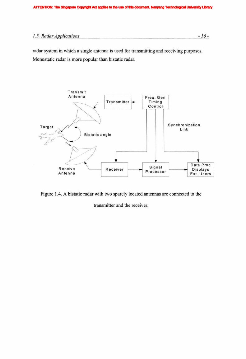
Bistatic radar (shown as Fig 1.4) is a radar system in which the transmitter and receiver

use different antennas at different locations. Monostatic radar (shown as Fig 1.5) is a


1.5. Radar Applications 16

radar system in which a single antenna is used for transmitting and receiving purposes.

Monostatic radar is more popular than bistatic radar.

Target

Transmit Antenna

Receive Antenna

Freq. Gen Timing Control

Synchronizat ion Link

Data Proc Displays

Ext. Users

Figure 1.4. A bistatic radar with two sparely located antennas are connected to the

transmitter and the receiver.


1.6. Pulsed Radar -17-

Antenna / Antenna Controller

Duplexer

Transmitter/ Modulator

£ Receiver

~Z_ T .

Freq. Gen Timing Control

Signal Processor

..//

Target

Data Proc Displays

Ext. Users

Figure 1.5. A monostatic radar with single antenna and a duplexer switch connecting and

disconnecting the transmitter and the receiver.

1.6 Pulsed Radar

The operation of a typical pulse radar may be described with the aid of the block diagram

shown in Fig. 1.6.

Pulsed radar is the most common form of radar used today. Pulsed radar transmits a

train of narrow rectangular-shaped pulses modulating a microwave carrier signal. The

distance of the target is determined by measuring the round trip time required for the

pulse to reach the target and return. Due to the fact that electromagnetic waves travel at

the speed of light c, the range may be determined by



R = C-f (1.8)

Where the factor of two is due to the fact that the wave must take a round trip, covering

twice the distance between the radar and target [20]. Once a pulse is transmitted the

system must wait for the return of that pulse before transmitting the next pulse otherwise

ambiguities may occur [21]. A difficulty encountered with pulsed radar systems is the

generation of high power short duration pulses. High power microwave generation puts

large demands on equipment. Further it complicates the situation. The high power signal

must be completely isolated from the low noise receiver front end. If the system isolation

is not high enough, two system-level negatives are encountered. First, the reflected signal

from a target is usually 60 dB to 100 dB lower in power than the transmitted signal. If the

front end isolation is not enough the low noise amplifier in the receiver will become

saturated with the transmitted signal which will drown out the returned signal. Secondly,

and a more costly downside, is the possibility that the high power of the transmitter will

destroy the receiver's sensitive circuitry. These problems are overcome with a high

isolation duplexer switch as shown in Fig 1.6.



Fig 1.6 Typical pulsed radar systems

1.7 Doppler Radar

Doppler radar is the simplest form of a continuous wave radar system. Doppler radar has

many applications such as weather forecasting and uses in vehicular sensors. However,

Doppler radar has a very distinct disadvantage in that it cannot determine the range of

target. Doppler radar is only useful when the relative velocity between the radar system

and target is the desired information. In addition, Doppler radar cannot distinguish

between zero relative velocity and the lack of a target. The mechanism by which Doppler

works is that of the Doppler effect. The apparent compression of waves when the

source and observation are approaching each other and the rarefaction of waves when the

relative velocity is in the negative direction, or the two objects are diverging, is the

Doppler effect. Target radial velocity is extracted from the Doppler frequency shift


1.7. Doppler Radar - 2 0 -

between the transmitted signal and the received echo. Doppler shift is the frequency shift

of the echo signal caused by the target's motion with respect to the radar. This is

electromagnetic equivalent of the acoustic effect heard when a vehicle sounding its horns

in driven past an observer. The Doppler shift is used both to measure the velocity of

targets and to resolve targets occurring at the same time but moving at different velocities.

The latter use is the primary method of discriminating moving targets from clutters.

d>

Figure 1.7 Principle of Doppler shift.

By definition the Doppler shift is the difference between the frequencies of the received

and transmitted waves. A positive Doppler shift is from an inbound target and a negative

shift from a target outbound from the radar.

fd=fR-fr (1-9)

where,/r = transmit frequency


1.7. Doppler Radar -21

fit = receive frequency

A target velocity vector (both magnitude and direction) can be measured from the

Doppler shift. The exact expression of Doppler shift is: [22]

d T

1 + v Ic * 1

1-v Ic R

(1.10)

or, fd -fit -fr (1.11)

where,

For,

yields the Doppler shift:

fR = l + vR/c J-vR/c h

V

vR « c, / =f K T

1 + 2-5-c

(1.12)

(1.13)

d T C

(1.14)

Only the radial component of velocity contributes to the Doppler shift. Figure 1.7 depicts

the role of radial velocity in the direction of targets in clutter [23], a fixed radar. No

target Doppler shift occurs when the velocity is tangential to the radar's antenna axis.

The radial velocity is:

v R = v.cos {y H) cosOv) (115)


1.7. Doppler Radar - 22 -

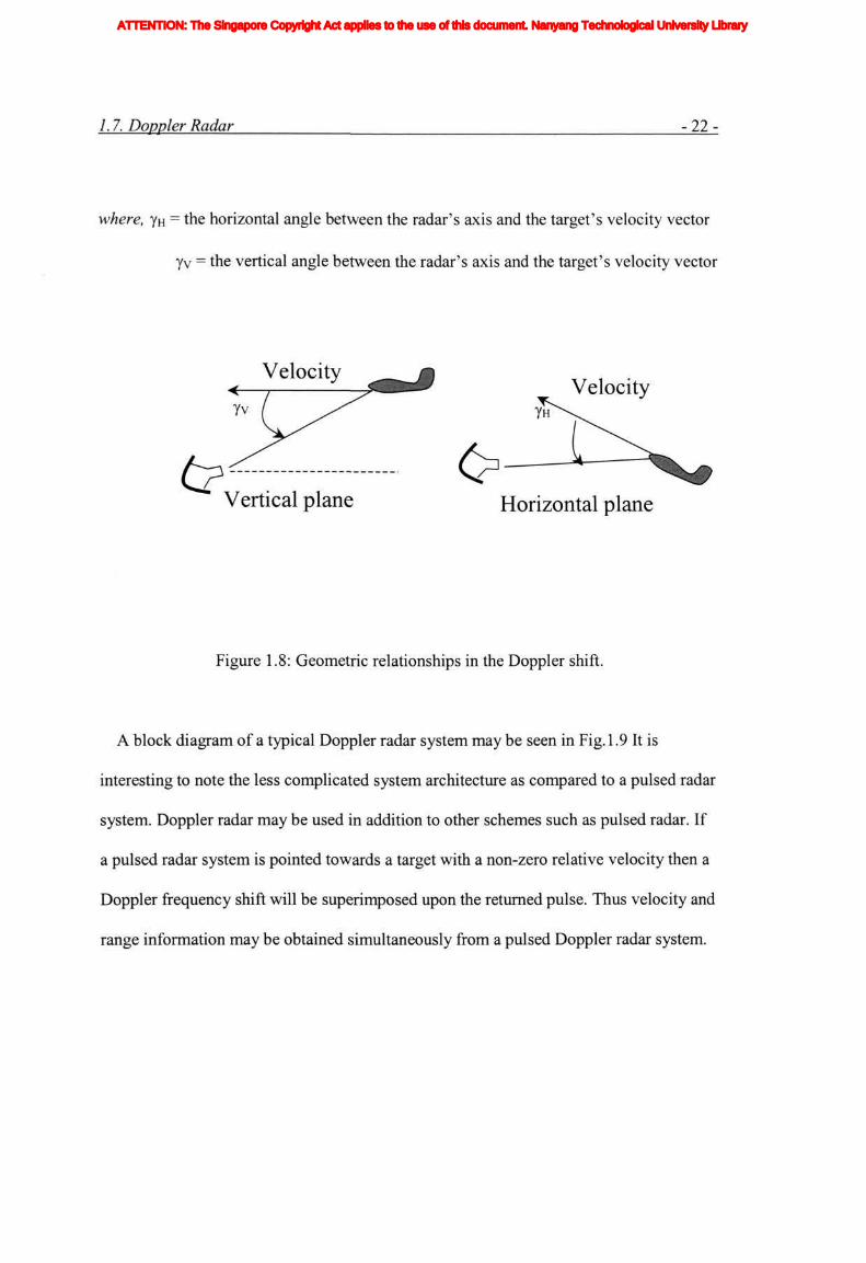
where, YH = the horizontal angle between the radar's axis and the target's velocity vector

yv = the vertical angle between the radar's axis and the target's velocity vector

Velocity n <—T :__^fc^ Yv / /"^

&^~ o Vertical plane Horizontal plane

Figure 1.8: Geometric relationships in the Doppler shift.

A block diagram of a typical Doppler radar system may be seen in Fig. 1.9 It is

interesting to note the less complicated system architecture as compared to a pulsed radar

system. Doppler radar may be used in addition to other schemes such as pulsed radar. If

a pulsed radar system is pointed towards a target with a non-zero relative velocity then a

Doppler frequency shift will be superimposed upon the returned pulse. Thus velocity and

range information may be obtained simultaneously from a pulsed Doppler radar system.

Velocity


1.8. Frequency-modulated-continuous-wave Radar 23

Antenna

Duplexer

1 r Detector

Mixer

transmitter /o

Beat-frequency amplifier OUTPUT

Figure 1.9: Block diagram of a typical Doppler radar system

1.8 Frequency-Modulated-Continuous-Wave Radar

Frequency-modulated-continuous-wave (FMCW) radar is one form of continuous wave

radar. The significant advantage of FMCW radar system is that it can detect target range

and velocity simultaneously by computing the time delay and the Doppler shift in the

received signal. FMCW use a form of frequency modulation. The frequency modulation

provides a signature relationship between the frequency of the transmitted signal and the

duration of the round trip of the signal from the radar to the target. Another significant

advantage of FMCW radar system may be seen in Fig. 1.10. Although the dramatic

increase in information available from a FMCW radar system, we easily observe the

substantially less complicated design compared to a pulsed system.


1.8. Frequency-modulated-continuous-wave Radar -24-

FM transmitter

Transmitting antenna

Modulator

Receiving antenna

Figure 1.10 Block diagram of a typical FMCW radar system

Figure 1.11 shows a sketch of a triangular LFM (linear frequency modulated) waveform.

The dashed line in Fig 1.11 represents the return waveform from a stationary target at

range R. The beat frequency fo is also sketched in Fig 1.11 (b). It is defined as the

difference between the transmitted and received signals. The time delay At is a measure

of target range, as defined in Eq.(1.16):

A/ = 2R (1.16)

Fig 1.11 (a) shows a triangular frequency-modulation waveform. The resulting beat

frequency as a function of time is shown in Fig 1.11 (b) for triangular modulation. The

beat note is of constant frequency except at the turn-around region. If the frequency is

modulated at a rate fm over a range Af, the beat frequency is



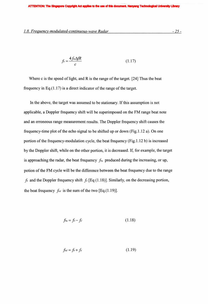
fi-&&- (1.17)

Where c is the speed of light, and R is the range of the target. [24] Thus the beat

frequency in Eq.(l .17) is a direct indicator of the range of the target.

In the above, the target was assumed to be stationary. If this assumption is not

applicable, a Doppler frequency shift will be superimposed on the FM range beat note

and an erroneous range measurement results. The Doppler frequency shift causes the

frequency-time plot of the echo signal to be shifted up or down (Fig. 1.12 a). On one

portion of the frequency-modulation cycle, the beat frequency (Fig. 1.12 b) is increased

by the Doppler shift, while on the other portion, it is decreased. If, for example, the target

is approaching the radar, the beat frequency fiu produced during the increasing, or up,

potion of the FM cycle will be the difference between the beat frequency due to the range

fb and the Doppler frequency shift fid [Eq (1.18)]. Similarly, on the decreasing portion,

the beat frequency fi>d is the sum of the two [Eq.(1.19)].

fiu = fb-fd (1.18)

fid = fi, + fd (1.19)



sdidTransmitted signal

dashed received signal

o i

( (1) -J rr 0)

B fi m u

hn

(a) Triangular Frequency Modulation

\ i / " Time

(b) Beat Note of (a)

Fig 1.11 Frequency-time relationships in FMCW radar.

The range frequency fo may be extracted by measuring the average beat frequency; That

is fb = i [fiu + fid] and fd = i [_/w - y*u]. So the range to the target R, and its relative

velocity: V, are found with (1.20) and (1.21), respectively. [25]



RJ-h±M± (1.20) 8/-4T

4/o

where c is the velocity of light, /o is the center frequency of the transmitted signal.

fm is the modulation frequency and A/ is the maximum frequency deviation.

When two or more targets and objects exist, the beat signals obtained from them have

multiple frequency components. Consequently, in order to detect the distance to a target

and its relative velocity accurately, it is essential to select the pair of the beat signals from

the same object without error. In order to use a millimeter-wave radar as the sensor for an

adaptive cruise control (ACC) system or an automated driving system, it is necessary to

reduce the target misrecognition rate as much as possible.


1.9 Noise in Microwave systems -28-

i I -" solid:Transmitted signal I

___-—— dashed:received signal ^

§ /o cr LL

§ /o cr LL

At "^~^^ Time

i

\ i

i

(a) Transmitted and Echo Frequencies

1 /"

\

/ \

z

1 /"

\

/ \

z a) m / o

\

/ \

z a) m / o

Time

(b) Beat Frequency

Figure 1.12 Frequency-time relationships in FMCW radar when the received signal is

shifted in frequency by the Doppler effect

1.9 Noise in Microwave Systems

Noise power is a result of random processes such as the flow of charges or holes in a

solid state device and the thermal vibrations in any component at a temperature above

absolute zero. In either case the noise level of a system sets the lower limit on the

strength of a signal that can be detected in the presence of the noise. Thus in a radar



system the noise characteristics of the receiver are one of the most important system

parameters.

All sources of noise may be equated to a noisy resistor at a certain temperature. [26]

The noise produced by a resistor in a specified bandwidth, B, will produce the noise

power

Pn = kTB (1.22)

Where k is Boltzmann's constant, T is the temperature of the resistor in degrees Kelvin,

and B is the system bandwidth in Hz. It is clear that the only way to get a completely

noiseless system is to keep the system temperature at absolute zero since a system with

zero bandwidth is useless.

N,

F1/G1

N1

-*• F2/G2

N2 No

F3/G3

Ni

To

FN/G 12 No

Figure 1.13 Noise in a cascaded microwave systems



It is also interesting to note that the noise figure of a microwave system is dominated by

the noise figure of the first stage. The noise figure of a cascaded microwave system

^ r- F 2 - I F 3 - I FN-\ ,, _„-FN = FI + + + ...+ (1.23)

G\ G\Gi G\GI...GN -1

Where F.v and GN are the noise figure and gain of each stage. [26] A cascaded

microwave system and its noise-related parameters is illustrated in Fig 1.13. It is very

clear that the noise figure of the first stage is the dominant term in the summation in Eqn

(1.23).

To support the hypothesis, we can take Fig 5.1 (page 111) as an example. We can see

that the first stage of the system is a low noise amplifier (LNA), assume its noise figure is

ldB with a gain of lOdB then the noise figure of the second stage (mixer) will only

contribute 1/10 th of its noise to the overall system noise figure. This implies that the

most crucial part in a radar system is the low noise front end of the receiver because the

second stage is generally a mixer, whose noise performance tends to be poor or even

terrible. For different radars there will be different percentage of noise contribution. It

can be varied from 10% to more than 50%.

1.10 Radar Cross Section

The radar cross section (RCS) of a target (shown as Fig 1.14) is an (fictional) area

intercepting that amount of power, which, when scattered equally in all directions,


1.10. Radar Cross Section -31-

produces an echo at the radar equal to that from the target. Mathematically the RCS is

expressed as [27]

(1.24) power reflected toward source I unit solid angle , Er

a = = lim 4nR — incident power density I AK *->0° Et

where, R = distance between radar and target

Er = reflected field strength at radar

Ei = strength of incident field at large

Although many forms of the RCS formula exist, the version presented in Eq (1.24) is

the most commonly used. The lower case character sigma (a) is the most commonly

used symbol to represent RCS in radar literature. In theory, the RCS can be determined

by solving Maxwell's equations with the proper boundary conditions applied.

Usually, an object which is not symmetric will have a RCS with angular variations

which require a study at each angle of interest. A widely available table with typical RCS

values of several targets may be seen in Table 1.1. [28] It is informative to notice that

objects with large flat surfaces such as cars and pickup trucks have RCS values much

larger than those of objects considerably larger, such as jumbo jets.


1.10. Radar Cross Section -32-

Figure 1.14 : Cross section fluctuation

1.11 Vehicular Applications

The use of radar technology in commercial vehicular applications can provide great

benefits in safety and driver's convenience. Radar can be used for forward and side

obstacle detection and collision warning as well as extended applications including

adaptive cruise control and automatic braking for collision avoidance. Other technologies

are under investigation for these applications including ultrasonic, infrared, laser and

video imaging. However, as can be seen in Table 1.2 and 1.3, radar is considered the

preferred technology when all factors are considered. The weather and darkness

penetration capabilities of radar are especially well suited to vehicular applications.


1.11. Vehicular Applications - 33 -

Table 1.1. Typical RCS values at microwave frequencies

Radar Target RCS, m2

Conventional unmanned winged missile 0.5

Small, single engine aircraft 1.0

Small fighter or jet airliner 2.0

Large fighter 6.0

Medium bomber or jet airliner 20

Jumbo jet 40

Small open boat 100

Small pleasure boat 2.0

Cabin cruiser 10

Pickup truck 200

Automobile 100

Bicycle 2

Human being 1

Bird 0.01

Insect io-5



Table 1.2 Technology and performance features

\ . Technologies

Performance Feature \ .

Ultra

sonic

Infrared Laser Video Radar

Darkness Penetration Good Good Good Poor Good

Adverse Weather

Penetration

Poor Poor Poor Poor Good

Low Cost Hardware

Possibility

Good Good Fair Poor Good

Low Cost Signal

Processing

Good Good Good Poor Good

Sensor Dirt/moisture

Performance

Fair Poor Poor Poor Good

Long Range Capability Poor Fair Good Good Good

Target Discrimination

Capability

Poor Poor Fair Good Good

Minimizing False Alarms Poor Poor Fair Fair Good

Temperature Stability Poor Fair Good Good Good



A demand for assisted driving in poor conditions has spurred manufacturers to search

for a solution. Infrared solutions have a serious drawback which has kept research into

these systems to a minimum. An infrared sensor cannot "see" through air with a lot of

moisture in it. Thus a system based upon infrared would not function in dense fog and

heavy rain or snow. One of the research goals for automobile sensors is the ability to

improve safety and comfort in adverse weather conditions. Due to the serious

shortcomings of infrared sensors most research has now become focused upon the use of

electromagnetic radiation in the form of radar to solve vehicular sensing requirements.

In collision avoidance systems, a radar system warns the operator of the vehicle

when it is too close to an adjacent vehicle or when the closing speed to the next vehicle

exceeds a prescribed rate. Such systems are currently available in up-scale cars such as

Cadillac, Lexus, and Mercedes. These installations consist of simple radar systems that

look out of the front of the car. An automated cruise control system may be an extension

of a collision avoidance system. The current state of cruise control in vehicles is limited

to speed control. The operator sets a computer to a desired speed once the speed is

achieved. The computer then adjusts the accelerator to keep the vehicle at a constant

speed regardless of the car, which is on a hill or on a flat road. Future automated cruise

control systems will integrate radar systems with current cruise control technology to

make driving safer and more comfortable. A radar system may be implemented in an

automated cruise control system in order to feed closing rate vehicle proximity



Table 1.3 Types and characteristics of obstacle detection sensor

Sensor Advantages Disadvantages

Ultrasonic

Sensor

•Simple structure and low

cost

•Relative velocity

detectable (directly)

•Difficulty of medium to

long distance detection

•Highly affected by wind

Laser radar •Comparatively inex

pensive

•Minor technical

difficulties

•Weak to rain and dirt

Microwave

Radar

•Strong against rain and dirt

•Relative velocity

detectable(directly)

•Presently expensive

•compliance with Radio

Law prerequisite

Image sensor •Compact size

•Number of objects

detectable

•Weak to rain, dirt and

night time application

•Complex recognition logic

information to a decision making computer. The computer would then make speed

adjustments accordingly. A step beyond automated cruise control is the concept of an



automated highway. In an automated highway application all the vehicles on a roadway

would have radar coverage on all sides of the vehicle. In addition, all vehicles would be

equipped with computers that are networked to a "highway" computer that controls the

speed of traffic, what lane a vehicle is in, and how may vehicles may get on the highway.

While such systems are still some way in the future, research is currently being

performed on related topics.

1.12 Objectives

The anti-collision radar detection properties depend basically on the performance of

CFAR detector design (work in FMCW radar systems). The research activities presented

here is focused into a new type of CFAR detector to meet the requirements of reliability

(extremely low false alarm rate) and short response time (extreme short delay) for traffic

applications. The main aspects are summarized as follows:

1.) Improved anti-collision system detection performance;

2.) Improved anti-collision system detection probability on the curve;

3.) Improved anti-collision system reliability;

4.) Extremely low system false alarm rate;

5.) Shorter reaction time;

6.) Low cost.


1,13 Organization of the Thesis - 38 -

1.13 Organization of This Thesis

The following chapters of this report will describe in detail the theory and design of Anti-

collision radar detection systems.

Chapter 1 discusses fundamentals and theories of radar detection in general. The

FMCW concepts for anti-collision radar, RCS, Detection criteria, and Vehicular

applications are described in detail in this chapter .

Chapter 2 gives a brief introduction to the traditional CFAR processors, including CA-

CFAR, OS-CFAR and other CFAR techniques. All conventional CFAR detectors'

advantages and limitations are discusses in detail.

In Chapter 3, four novel CFAR detectors synthesizing the advantages of CA-CFAR and

OS-CFAR are proposed. Each CFAR detector's features are presented in details. The

simulation results and performance analysis show that the new approaches can improve

the radar systems performance and are very useful in practices.

Chapter 4 proposes a novel detection antenna design technique to improve the

detection performance of anti-collision radar systems, especially when the car is on a

road curve.

Chapter 5 introduces an application of the novel CFAR algorithm on the vehicular

technology of collision avoidance.


1.13 Organization of the Thesis - 39 -

Finally, in chapter 6, some concluding remarks of the work of this dissertation are

given. This chapter also gives recommendations for our future work of the CFAR data

fusion including fuzzy-neural network fusion implementation and proposal of some other

novel ideas.


Chapter 2

Traditional CFAR Processors

2.1 Introduction

Anti-collision radar performance is often degraded by the presence of false targets, or

clutter. To combat this problem, radar detection processing can use an algorithm to

estimate the clutter energy in the target test cell, and then adjust the detection threshold to

reflect changes in this energy at different test cell positions. The threshold algorithms use

detection cells near target test cell to estimate the background clutter level, and then set

the threshold to guarantee the desired false alarm probability. This technique approaches

a constant false alarm rate (CFAR) in most clutter backgrounds.

A basic method of approaching CFAR operation uses cell averaging (Finn and Johnson,

1968). Here several resolution cells on each side of the cell being tested for a target are

sampled to develop an estimate of the noise level. N represents the number of reference

cells. The square-law detected range samples (here we set N=2n, n is the numbers of the

sliding windows) are sent serially into a shift register N+l=2n+l.


2.1. Introduction -41 -

A relatively simple algorithm uses the average received energy in 2N nearby range cells

to obtain a threshold. This algorithm yields a CFAR when the clutter in the estimation

cell is identically, independently, and Rayleigh envelope distributed [29]. As N increases,

the signal-to-noise ratio (SNR) required by this algorithm to guarantee a particular

probability of detection, decreases. When N approaches infinity the variance of

the clutter power estimate vanishes, and the threshold is set optimally in terms of

minimizing required SNR.

Constant false alarm rate (CFAR) processors are the commonly used detectors in radar

systems to maintain control of the false alarm rate in the face of local variations in the

background noise level. In the CFAR detection scheme, the square-law detected range

samples are sent serially into a shift register N+l=2n+l. The target decision is commonly

performed using the sliding window technique.

In Fig 2.1, Y is the cell under test, Xi to X2n are the reference cells. If the value of Y is

larger than the product of Z and T, i.e. Y > ZT, then the target is detected. Otherwise, if

Y is less than the product of Z and T, i.e. Y < ZT, we will get the report from radar of no

target.

In this chapter, we will discuss some traditional CFAR processors and their

distinguishing characteristic.


2.2. Statistical Decision Theory for Anti-collision Radar -42-

Input Samples Square Law

Detector Test Cell

X1 Xn Y Xn+1 X2n

s~>

CFAR Processor

s~> z fi s~>

Target

No Target

Comparator

Threshold T

Fig.2.1: Block diagram of CFAR

2.2 Statistical Decision Theory for Anti-collision Radar

Reverend Thomas Bayes's (1702-1761) introduced the fundamental concepts of classical

statistical decision theory [30]. The theory assumes probabilistic descriptions of the

measurement values and prior knowledge to compute a probability value for each

hypothesis. Bayes's methods provided a means to update one's degree of belief expressed

as a probability about a hypothesis on the basis of prior knowledge and recent


2.2. Statistical Decision Theory for Anti-collision Radar - 43 -

observations (Appendix A). For the first time, this provided a tool for quantitative

inferences or learning. Bayesian and related statistical decision approaches are directly

applied to the processing of multisensor data to perform binary decisions (the detection

problem: signal present or absent). Although originally applied to single sensors,

extensions to multiple sensors have developed optimal decision criteria for distributed

decision making when the decisions are distributed between sensors and the central node

where decisions are fused [31,32]. In our application, bases detection and classification

on decision theory, in which measurements are compared with alternative hypotheses to

decide which hypothesis "best" describes the measurement.

A generalization of minimum Pe criterion assigns costs to each type of error. Suppose

that we wish to design a system to automatically inspect a machine part. The result of the

inspection is either to use the part in a product if it is deemed satisfactory or else to

discard it. We could set up the hypothesis test

Ho: part is defective

Hi: part is satisfactory

and assign costs to the errors. Let Cybe the cost if we decide Hi, but Hj is true. For

example, we would probably want Cio> Coi. If we decide the part is satisfactory but it

proves to be defective, the entire product may be defective and we incur a large cost (Cio).

If, however, we decide that the part is defective when it is not, we incur the smaller cost

of the part only (Coi). Once costs have been assigned, the decision rule is based on

minimizing the expected cost or Bayes risk R defined as [33]:


2.4. Bayes s Concepts for Radar - 44

i i

R = E(C) = X X C"P(<Hi! Hi)P{Hi) (2.1) 1=0 ;=0

Usually, if no error is made, we do not assign a cost so that Coo = Ci I = 0. However, for

convenience we will retain the more general form. Also, note that if Coo = Cn = 0, Cio =

Coi=l, thenR = Pe.

Under the reasonable assumption that Cio>Coo, Coi>Cn, the detector that minimizes the

Bayes risk is to decide Hi if [34]

PixlHi) > (C,o-Coo)P(//o)

P(x/Ho) (COI-CII )P(JZI)

See Appendix A for the proof. Once again, the conditional likelihood ratio is compared

to a threshold.

2.3 Detection Criteria

The detector that maximizes the probability of detection for a given probability of false

alarm is the likelihood ratio test as specified by the Neyman-Pearson (NP) Theorem

(Appendix B). The threshold is found from the false alarm constraint.

As shown in Fig 2.2, we can make two types of errors. If we decide Hi but Ho is true,

we make a Type I error. On the other hand, if we decide Ho but Hi is true, we make a

Type II error. Note that with this scheme these two errors are unavoidable to some extent


2.4. Bayes's Concepts for Radar - 45 -

but may be traded off against each other [35]. Clearly, the Type I error probability

(P(Hi;Ho)) is decreased at the expense of increasing the Type I error probability

(P(Ho;Hi)). It is not possible to reduce both error probabilities simultaneously. A typical

approach then in designing an optimal detector is to hold one error probability fixed

while minimizing the other.

Fig 2.2 Possible hypothesis testing errors and their probabilities

As shown in Fig 2.3, let Ri be the set of values in that R that map into the decision

Hi or

Ri=(x: decide Hi or reject Ho) (2.3)


2.4. Bayes 's Concepts for Radar - 46 -

This region is termed as the critical region in statistics. The set of points in RN that

map into the decision Ho is the complement set of Ri or Ro=(x: decide Ho or reject Hi).

Clearly, Ro U Ri = ^'v since Ro and Ri partition the data space. The Pfa constraint then

becomes

Pfa= \P(x;Ho)dx = a (2.4)

In statistics, a is termed as the significance level or size of the test. Now there are

many sets Ri that satisfy (2.3). Our goal is to choose the one that maximizes

PD= \P{x;Hx)dx (2.5) R\

In statistics, PD is called the power of the test and the critical region that attains the

maximum power is the best critical region. Table 2.1 is a summary of a statistical

terminology and our radar engineering equivalents.

The NP theorem tells us how to choose Ri if we are given P(x;Ho), P(x;Hi),

To maximize PD for a given PFA = a decide Hi if


2.4. Bayes 's Concepts for Radar -47-

L(x) = — - > y P(x;Ho)

(2.6)

where the threshold y is found from

PFA= J P(x;Ho)dx = a (jKi(*)>r)

(2.7)

The function L(x) is termed the likelihood ratio since it indicates for each value of x

the likelihood of Hi versus the likelihood of Ho.

Figure 2.3 Decision regions and probabilities


2.4. Bayes 's Concepts for Radar - 48 -

2.4 Hayes's Concepts for Radar

Bayes's decision theory is a systematic method of assigning cost factors to the correct

and incorrect decisions that can be made process (Appendix A). We make use of a

particular form of the general theory as usually applied to radar [36]. Two important

A A

specializations are used. First, we will average P(XIS r{9)) over all random parameters

and use the result to ultimately solve the optimum detection problem. Second, we will

choose special cost factors for radar (below). Let us define

P{XISr{G))g = \P(X ISr{9))P(G)dG (2.8)

A

Hence, here we define X(t) as the received waveform, X is a vector random variable

having all the observation random variable Xik as its components [37]. When no target is

present the joint probability density functions of the observation random variables will be

different than when target is present. In the former case X(t) consists of noise only, while

in the latter case X(t) is the sum of the received signal plus noise. The joint probability

density functions of the observation random variables, conditional on no signal and signal

A A A

present cases, respectively, are denoted by P(XIQi) and P{XI Sr{6)). The notation

A

Sr{6) is used to imply that the received signal, Sr(t), may depend on some random

parameters 0\, 9i,....,0M , defined by the vector


2.4 Bayes 's Concepts for Radar - 49 -

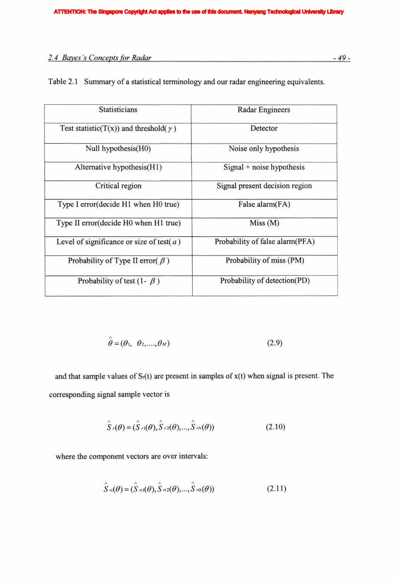
Table 2.1 Summary of a statistical terminology and our radar engineering equivalents.

Statisticians Radar Engineers

Test statistic(T(x)) and threshold( y) Detector

Null hypothesis(HO) Noise only hypothesis

Alternative hypothesis(Hl) Signal + noise hypothesis

Critical region Signal present decision region

Type I error(decide HI when HO true) False alarm(FA)

Type II error(decide HO when HI true) Miss (M)

Level of significance or size of test( a) Probability of false alarm(PFA)

Probability of Type II error( ft) Probability of miss (PM)

Probability of test (1- /?) Probability of detection(PD)

0 = (0\, 02,....,0M) (2.9)

and that sample values of Sr(t) are present in samples of x(t) when signal is present. The

corresponding signal sample vector is

Sr(0)=(Sri(0),Sr2(0),...,SrN(0)) (2.10)

where the component vectors are over intervals:

S ri(0) = (S M(0), S ri2(0),..., S rik{0)) (2.11)


2.4.. Bayes 's Concepts for Radar - 50 -

for i = 1, 2, ..., N. The elements of (2.11) are just the sample values of Sr(t) at times

t,k:

Srik(0)=Sr(tik) (2.12)

The left side of (2.8) is a notational definition; the over bar represents the statistical

A

average of the quantity with respect to all the random parameters of the vector 9. The

A

right side of (2.8) defines the actual averaging operation; here P{6) is the joint

A A

probability density function of random variables (0\, 6I,....,0M) = 0 . P{0) uses the

actual density for those random variables that are known and uses the least favorable

(uniform) density for those variables with unknown statistics.

Ultimately the signal processor must process the various observations to produce a

single variable from which a decision is made of target plus noise present (referred to as

decision S+N ) or noise only present (referred to decision N). If we think of any one set

A

of observations, which is one value of X as a point in NK-dimensional hyperspace, then

some points will correspond to the decision S+N call the space of such points Ti. All

other hyperspace points, denoted by To, must correspond to the decision N. All of

hyperspace denoted by V, is the sum of the two spaces, or T = Ti + To. Based on these

spaces we define average detection probability Pd; average miss probability Pmtss; false

alarm probability Pfa; and noise probability Pnoise by [37-39]

Pd = f \P{XI S r(6))ed X = average detection probability (2.13)


2.4.. Bayes 's Concepts for Radar - 51 -

~Pnuss = JrQ j>(AVSr{0))gdX = \-~Pd = average miss probability (2.14)

Pfa = J JP(X/ 0)dX = false alarm probability (2.15)

Pno.se = Jro j>(A7 0)dX=\-Pfa = noise probability (2.16)

Clearly the final decision process can lead to only four outcomes, two are correct and

two are wrong. Bayes's theory assigns costs to these decisions as follows:

1. Decide N when N is true: Cost = Cn (2.17 a)

2. Decide N when S+N is true: Cost = C12 (2.17 b)

3. Decide S+N when N is true: Cost = C21 (2.17 c)

4. Decide S+N when S+N is true: Cost = C22 (2.17 d)

Now let D be a random variable representing the radar's "decision"; it can only have

outcomes N and S+N. Similarly let T be a random variable representing the "true case;" it

has outcomes N and S+N with probabilities of occurrence defined as P (T=N) = q and

P(T= S+N) = p= 1-q, respectively. The joint probabilities of the four outcomes of (2.17),

with T independent of D, are

P(N, N) = P(D = N, T = N) = Pno,seq (2.18 a)


http://Pno.se

2.5. Binary Detection -52-

~P(N, S + N) = ~P(D = N, T = S + N) = Pmissp (2.18 b)

P(S + N, N) = P(D = S + N, T = N) = Pfaq (2.18 c)

P(S + N, S + N) = P(D = S + N, T = S + N) = Pdp (2.18 d)

The Bayes procedure defines an average cost, denoted byZ,, for the four decisions of

(2.17) [38, 39]

I = CnP(N,N) + CnP(N,S + N) + CuP(S + N,N) + C22~P(S + N,S + N) . . A — — A (2.19)

= Cuq + Cnp + j . . . j{(C2. - C. i)qp( XI0) - (Cn - Cn)pP{XI S r(0))$ }d X

The last form of (2.19) has used (2.18) and (2.13) through (2.16).

2.5 Binary Detection

In binary detection the radar observes a particular range cell in each of N pulse intervals

and counts the number of threshold crossings (single-pulse detections) that takes place.

This number can be as small as zero, or as large as N if the range cell gives a detection in

every one of the N pulse intervals. At the end of N pulse intervals the radar declares a

target is present if M or more threshold crossings occur, and no target is present if less

than M crossings occur. M is called as a second threshold. Clearly the important

parameters in making a final detection are Pfai, Pdi, M, and N. In this section we relate

these parameters to the overall desired false alarm and detection probabilities, which we


2.5. Binary Detection -53-

denote by Pfa and Pd , respectively. The discussions to follow center mainly on the

nonfluctuating target. Binary detection is known by various names, such as M of N

detection, and coincidence detection. It appears to have been originated by Swerling

(1952) and Schwartz (1956). Some early theoretical work was due to Harrington (1955)

and Capon (1960). More recently Miller (1985), Brunner (1990), Weiner (1991), and Han

et al (1993) have extended the theory to include fluctuating targets and distributed

detection systems.

False alarm probability Pfa corresponds to when noise only is being received. Assume

that the N pulse intervals result in sequence of exactly k threshold crossing followed by

exactly N-k noncrossings (for the range cell under examination). The probability of this

sequence is PkfaX(1 - Pfal)

N~k • The order in which threshold crossings occurs is not

important, and any sequence of exactly k crossings in N intervals has the same

probability. Form combinatorial analysis the number of such sequences equals the

binominal coefficient [39, 40, 41]

(N} TV' = — (2.20)

[KJ K\(N-k)\

Thus the probability if sequence of exactly k threshold crossings (of an order) in N

intervals is

p(k 0/AO= k . o - ^ . r * (2.2i)


2.6. Cell Averaging CFAR -54

A false alarm will occur if, at the end of N intervals, M or more crossings occur. Its

probability becomes

Pfa = X P(k of N) = X [N)p^(\-P^r-k (2.22) k=M k=M\"-J

when a target with constant cross section is present, the preceding steps can be

repeated to obtain the probability of detection. The steps again lead to (2.22) except with

Pfai replaced by Pdi:

k=M KKJ P^\-P^-K (2.23)

This expression and (2.23) are the two fundamental quantities that define binary

detection.

2.6 Cell Averaging CFAR

An popular CFAR processor is the cell averaging (CA) CFAR processor which

adaptively sets the threshold by estimating the mean level in a window of N range cells.

The CA-CFAR processor is the optimum CFAR processor (maximizes detection

probability) in a homogeneous background when the reference cells contain independent

and identically distributed (IID) observations governed by an exponential distribution. As


2.6. Cell Averaging CFAR 55-

the size of the reference window increases, the detection probability approaches that of

the optimum detector which is based on a fixed threshold.

Target

No Target

Threshold setting

Fig.2.4: Block diagram of Cell-averaging CFAR

Two major problems that require careful investigation in such a CFAR detection

scheme are those presented by 1) regions of clutter power transition and by 2) multiple

target environments. The first situation occurs when the total noise power received within

a single reference window changes abruptly. The presence of such a clutter edge may

result in severe performance degradation in an adaptive threshold scheme leading to

excessive false alarms or serious target masking depending upon whether the cell under

test is a sample from clutter background or from relatively clear background with target

return, respectively. The second situation is encountered when there are two or more

closely spaced targets in range. The interfering targets that appear in the reference

window along with the target under investigation (known as primary target) may raise the


2.6. Cell Averaging CFAR - 56 -

threshold unnecessarily. Often a CFAR detector only reports the stronger of the two

targets.

2.7 Order Statistics CFAR

The order statistics (OS) CFAR processor estimates the noise power simply by selecting

the k-th largest cell in the reference window of 2n, the threshold is obtained from one of

the ordered samples of the reference window. The range samples are first ordered

according to their magnitudes, and the statistic Z is taken to be the k-th largest sample.

Rohing has noted that the false alarm probability of the OS processor is dependent of the

total noise power in the exponential noise model. The order statistics (OS) CFAR scheme

is suitable to alleviate these problems above [discussed in 2.6] to some degree. Its

performance in a multiple target environment is clearly superior.


2.7. Order Statistics CFAR -57-

Input Samples Square Law

Detector Test Cell

X1

Target

Xn Xn+1 X2n

Comparator

Sort and select the K-th cell No Target

Threshold

Fig.2.5 Block diagram of Order-statistics CFAR

The OS -CFAR processor exhibits some loss of detection power in homogeneous

noise background compared to the CA processors.

2.8 Other CFAR Techniques

There are other CFAR detectors which are now shown as follows to deal with different

clutter or target situations.

a) Trimmed-mean CFAR: The trimmed-mean™ [42] scheme is a more

generalized OS-CFAR processor in which the ordered range cells of a particular


2.8. Mathematical Model ofCA-CFAR and OS-CFAR z58z

reference window are trimmed or censored from both the upper and the lower

ends.

b) Exicisor-CFAR: In excisor CFAR, a hard (upper) limit is applied to the

cells' amplitude for threshold calculation [43]. This prevents large outliers from

biasing the threshold. Values above the limit are removed from the threshold

calculation.

c) CM/L-CFAR: A new CFAR procedure is presented, which relies on a

hybrid clutter-map/L-CFAR [44, 45] strategy, aimed at improving the system

robustness against possible nonhomogeneities, while reserving target detect

ability in a homogeneous environment. In CM/L-CFAR procedure, the returns

from the range cells in each map cell are preliminarily processed through an L-

filter, prior to being used for estimation purposes: this preserves the proper system

immunity of CM-CFAR, to spatial discontinuities in the radar cross-section of

clutter, while introducing robustness against range spread or spurious targets.

2.9 Mathematical Model of CA-CFAR and OS-CFAR

The formulas were derived under the assumptions that the receiver noise is Gaussion

distributed, the detection envelope is Rayleigh distributed, and with Swerling case II

target, Y represents the cell under test. T is the scaling factor and the cells are

independent, identically distributed (IID).


2.8. Mathematical Model ofCA-CFAR and OS-CFAR -59-

The detection probability and false probability [46, 47, 48] are defined and calculated

as follows:

Under Ho, we have

/o(v) = - e x p \-2- (2.24)

Under Hi, we have

My) = I

(l+X)M exp

y

(l + A)M. (2.25)

where X is the signal-to-noise-ratio (SNR)

For the CA-CFAR processor,

1 2!

p=-J\yi (2.26)

The PDF ofP is [49]:

N f „VA '-1)

fiiP)-^ exTp(-Np I fj)

T(N) (2.27)

The CDF of Pis:


2.9. Mathematical Model ofCA-CFAR and OS-CFAR 60

FP(p) = \-exP(-Np/M)ZiJ^^ i=0

(2.28)

For the OS-CFAR processor, Q=q(k), The PDF of Q is [50]

1 (N} fQ(q) = -k , [\-cxV(-q/M)f-Uxp[-(N-k + \)q/M] (2.29)

The CDF of Q is:

m FQ(q) = Y\ . tl-expHr///)]*exp[-(;V-*)«?///] (2.30)

For CA-CFAR,

Pfa = (1 + 77 AT)"

(2.31)

PD =

{\ + T/[(\ + A)N]}N (2.32)

For OS-CFAR,

Pfa = k (N}r(N-k+T+\)r(k) yk j r(7v+r+i)

(2.33)

PD = k* r[N-k + T/(l + A) + l]T(k)

T[N + T/(l + A) + l] (2.34)


2.9. Mathematical Model ofCA-CFAR and OS-CFAR - 61 -

2.10 Results

The actual probability of detection achieved by the CA-CFAR and OS-CFAR detectors

has been evaluated by means of computer simulation. The results are shown as Fig 2.6

and Fig 2.7, respectively.

As false alarm probability is fixed, the scaling constant T can be calculated, so that the

performance can be evaluated.

For CA-CFAR detector's simulation, the reference cells number n are 8, 16, 32, 64,

respectively, and the false alarm probability is 10"8. It can be seen that as the n increases,

the detection probability will increase.

For OS-CFAR detector's simulation, we can draw the conclusion: if the reference cells

number n is fixed, as k increases, the detection probability will increase.


2.10 Results and Conclusions -62-

0.7 0.7 0.7

- Ca n=8

0.6 Ca n=16 — - Ca n=32 - - Ca n=64 ** " _—'

n ^ ^ ' ""

dete

ctio

n

Pfa=10-8 / '

*s y S-

% 0.3 ' y

1 / /

Pro

y y 0.2

0.1 //

°l .4s'. ^ ^ - ^ ^

°l ) 5 10 15 20 25 30 35 40 S/N

S i p n a l - t o nose r a t i o . d R

Fig 2.6 The effect of n on Pd of CA-CFAR when Pfa=10e-8 and n is reference cells

number and designed Pfa=10e-8

0.8

0.7

0.6

Q % 0.5 • "53 *B 0.4

H 0.3 O Bk

0.2

0.1

0 t

0.8

0.7

0.6

Q % 0.5 • "53 *B 0.4

H 0.3 O Bk

0.2

0.1

0 t

i i

i i

i i

i

1 0.8

0.7

0.6

Q % 0.5 • "53 *B 0.4

H 0.3 O Bk

0.2

0.1

0 t

i i

i i

i i

i

- Os n=16,k=8 Os n=16,k=10 Os n=16,k=12 Os n=16,k=14

0.8

0.7

0.6

Q % 0.5 • "53 *B 0.4

H 0.3 O Bk

0.2

0.1

0 t

i i

i i

i i

i

pf a=10"4 ^

0.8

0.7

0.6

Q % 0.5 • "53 *B 0.4

H 0.3 O Bk

0.2

0.1

0 t j 5 10 15 20

S/N 25 30 35 4l 0 5 10 15 20

S/N S i p n a l t o n o i s e r a t i o d R

F2.7 The effect of k on Pd of OS-CFAR when n=T6 is the reference cells number and

designed Pfa=10e-4


2.11 Conclusion -63-

2.11 Conclusion

In this Chapter, the effective and flexible traditional CFAR processors, including CA-

CFAR, OS-CFAR and other CFAR techniques, are introduced and applied to solve the

anti-collision radar detection problems. We have analyzed the performance of CA-CFAR

and OS-CFAR processors. Those conventional CFAR detectors' advantages and

limitations are discusses in detail. Meanwhile, we derive the formulations for these

CFAR detectors and show the simulation results in that situation.


Chapter 3

Novel CFAR Detectors

3.1 Introduction

In all radars' detection is the process of deciding whether or not a target is present. It is

accomplished by comparing the signal-plus-interference which radar received, after all

processing has occurred, to a threshold. If the signal-plus-interference, or interference

alone, crosses the threshold, a detection is declared. If not, no detection occurs.

Because noise and clutter are always random phenomena, a decision concerning the

presence or absence of a target echo is to be made by setting up a decision threshold. In

these systems, thresholds are set automatically by sensing the average interference level

and setting the threshold based on it, so that a small constant rate of false alarms occurs.

The CA-CFAR method was first introduced by Finn and Johnson [51]. This adaptive

method can play an effective part in much noise and clutter environments, and provide

nearly the best ability of signal detection while preserving the enough constant false


3.1 Introduction - 6 5 -

alarm rate. Rohling [52] proposed the OS-CFAR processor. This processor possesses the

good ability to counter the multiple targets.

Although the CA-CFAR method can provide a good ability of signal detection while

preserving the enough constant false alarm rate, such a CFAR detection performance is

usually degraded for two major problems: 1) regions of clutter power transition and by 2)

multiple target environments.

Compared to the CA processors, The OS -CFAR processor exhibits some loss of

detection power in homogeneous noise background.

To make full use of the collected data, four new radar CFAR detectors synthesizing the

advantages of CA-CFAR and OS-CFAR are proposed. It is defined as And-Ca-Os CFAR,

And-Os-Os CFAR, And-Os-Os-Os , and And-Ca-Os-Os CFAR algorithm as shown in

Fig 3.1, Fig 3.2, Fig 3.3, Fig 3.4 respectively, where N represents the number of reference

cells, T is the scaling constant.

These CFAR structure are computationally efficient. In the following sections, the

exact mathematical formulas for the four CFAR algorithms are derived and their

performance are shown.

3.2 Detection Principle and Model Formulation


3.2 Detection Principle and Model Formulation - 66 -

A block diagram of the modified CFAR detectors is shown in Fig 3.1. The system

collects a number E=M+N of reference samples and implements the adaptive threshold

test [53, 54]

V > TZ (3.0) wo

where Z is the final background noise estimation, T is a threshold parameter to control

the desired probability of false alarm, Pfa and V is the cell-under-test variate. The

different themes of all CFAR detectors is to estimate Z according to different methods. If

the decision about the presence (hypothesis Hi) of a target in the test cell has been made

according to Eqn (3.0), the right reference window stops shifting. The test cell variate V

will be censored. Thus, generally speaking interfering target numbers in the right sub-

window are always less than those in the left sub-window. This is a new kind of

automatic censoring technique in CFAR detection schemes. By using the techniques we

can achieve better detection performance both in the presence and absence of interference.

A binary hypothesis testing paradigm under the Swerling case 2 assumption is

under Ho, we have

/o(v) = —exp ( v^

I fj (3-1)


3.2 Detection Principle and Model Formulation - 6 7 -

under Hi, we have

/>(v) = 1

(l + »M exp

(\ + A)M

(3-2)

where X is the per pulse average SNR. Without loss of generality, and because we

analyse only the cases of homogeneous reference and multiple target environment, the

noise level is set to unit, i.e, /j. =1. Thus, the reference cell variates xi, / e M and yj,

j&N are taken to be statistically independent and identically distributed (IID) with

common PDF:

Mx) = fy(j) = e-* x>0 (3.3)

The local estimators operate on reference samples taken in a range surrounding the cell-

under-test variate V. We refer to X as the leading and Y as lagging window estimator.

Functions of (xi,...,xm) and (yi,...,yn) are the local pools of reference samples. The

modified CFAR use the local estimators below

X = X(k) Y = ya) (3-4)

It has been shown that the jth ranked sample (out of a total Nl samples ) has a

probability density function

Mx) = j rN.\ U J

[F.(x)r[l-F.(x)r-'f.(x) (3.5) N\-j


3.2 Detection Principle and Model Formulation - 6 8 -

where j is equal to k or 1, Ni is M or N and Ft(x) ,f,(x) correspond with Fx(x), Fy(x)

and fx(x), fy{x) respectively.

Using Eqns (3.2) and (3.3) in Eqn (3.5) we get the PDF of the k- th ranked sample of

the leading window and the 1- th ranked sample of the lagging window, respectively

fk(x) = fi(x) = k fM

k k-\ [exp(-*)r-*+ '[l-exp(-;c)r (3.6)

and

f,(X) = fy(x) = l [exp(-x)]A'-'+,[l-exp(-x)] / - i (3.7)

And we can write their CDF , respectively, as

M

F*(*) = F,(x) = £ M\

[l-exp(-x)][cxp(-x)r- (3.8) (=* v J

and

N f ]y\ F,{y) = Fy{y) = Jj '

j=i \J J [l-exp(-v)y[exp(-v)r- ' (3.9)

For any CFAR employing Eqn (3.0), where V and Z are independent random variables

we can show, following Ritcey and Hines [54] that


3.2. Mathematical Model of Novel CFAR - 69

Pa = ?r(V >TZ) = -{ ^LM^h(M)d(-TM) (3.10)

where h{/j) = E{e MV) andd(ju) = E{e " ) are moment generating functions(MGF). For

a Swerling case 2 primary target, h(/u) = (\ + bju)~x ,b = \ + A. Here d(-Tu) is analytic in

the LHP and Eqn (3.11) can immediately be evaluated in terms of the residue at the

simple pole, /u = -b'x. Thus, the detection probability is simply related to the MGF of the

zby

(T Pd = d -u (3.11)

and the false-alarm probability is given by

Pfa = d(T) (3.12)

Obviously, the MGF d(u) of the reference cell estimator Z is a key quantity in our

analysis.

3.3 Mathematical Model of Novel CFAR


3.3. Mathematical Model of Novel CFAR 70

In the And-OS-OS-OS CFAR detector, the estimation of the noise level in the cell under

test in the sum of the outputs of leading window the k th order statistics and the lagging

window the 1 th order statistics, i.e.

Z=X+Y (3.13)

The PDF of Z defined by eqn.3.14 is given by (Eqn.3.13)

fi(z)=[fx{x)fy{z-x)dx z>0 (3.14)

Using Eqn.(3.13), the MGF of the noise -level estimation in Eqn.(3.14) is given for a

homogeneous environment by

dx(M)=[e~f':fi*fy(Z)dz = d,(M)dy(M) (3-15)

where

dx({i) = k

fM

\k j f e - [ e x p ( - z ) — [l-exp(-z)r<fe= k

yk j

r(M-k+v+\)r(k) r ( M + / / + i )

(3.16)

^)=/fHf^[exp(-Z)-[i-eXp(-z)r&= i["Y{N;/^+Zil) ^ {i J* [i ) r(iv+//+i)


3.3. Mathematical Model of Novel CFAR -71-

By substituting Eqn.(3.15) into Eqn.(3.11) and Eqn (3.12), respectively, we obtain the

detection probability of the CFAR.

So based on derivation above, we got mathematical models of the new CFAR detectors

as follows ( section 3.4 - 3.7):

3.4 Mathematical Model of And-Ca-Os CFAR

This CFAR structure is computationally efficient. As shown in Fig 3.1, where N,M

represents the number of reference cells, T is the scaling constant and Zi, Z2 represent the

numbers calculated from CA processing and OS processing respectively.

Input Samples

I .latched Square law filter detector

Sum and get the average Z l , Sum and get the average

*(

tt t ' t t ' X M X1 V A fl ... Y N

Ul'i-H Sort and select K-th cell

Fusion Center Target

No target

Fig.3.1 Block diagram of And-Ca-Os CFAR


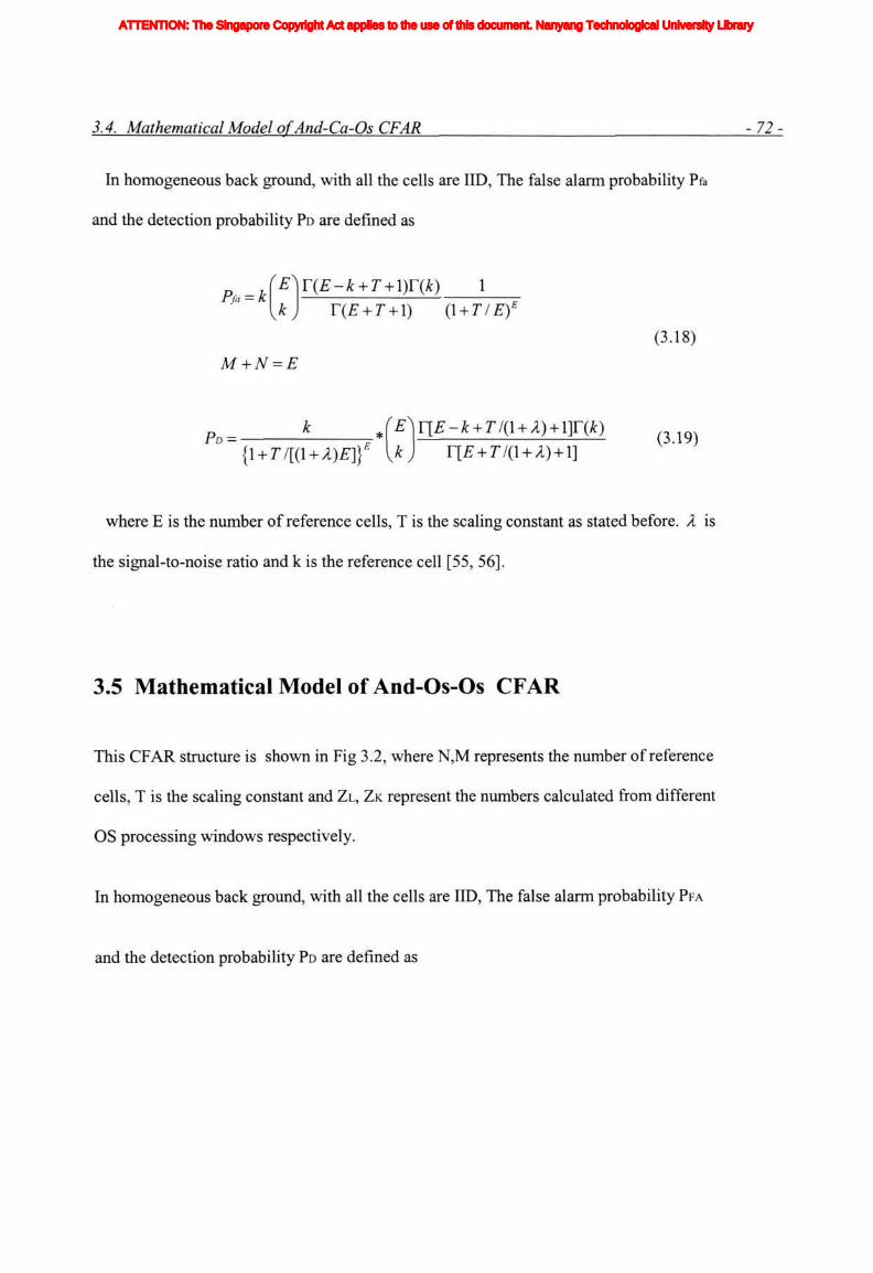
3.4. Mathematical Model of And-Ca-Os CFAR - 72 -

In homogeneous back ground, with all the cells are IID, The false alarm probability Pfa

and the detection probability PD are defined as

Pfa = k fE\T(E-k + T + \)Y{k) 1_

T(E + T + \) (X + TIEf

(3.18)

M + N = E

PD = k

{\ + T/[(\ + A)E]Y .*

yk j

Y[E-k + T/(\ + A) + \]r(k)

T[E + T/(\ + A) + \] (3.19)

where E is the number of reference cells, T is the scaling constant as stated before. X is

the signal-to-noise ratio and k is the reference cell [55, 56].

3.5 Mathematical Model of And-Os-Os CFAR

This CFAR structure is shown in Fig 3.2, where N,M represents the number of reference

cells, T is the scaling constant and ZL, ZK represent the numbers calculated from different

OS processing windows respectively.

In homogeneous back ground, with all the cells are IID, The false alarm probability PFA



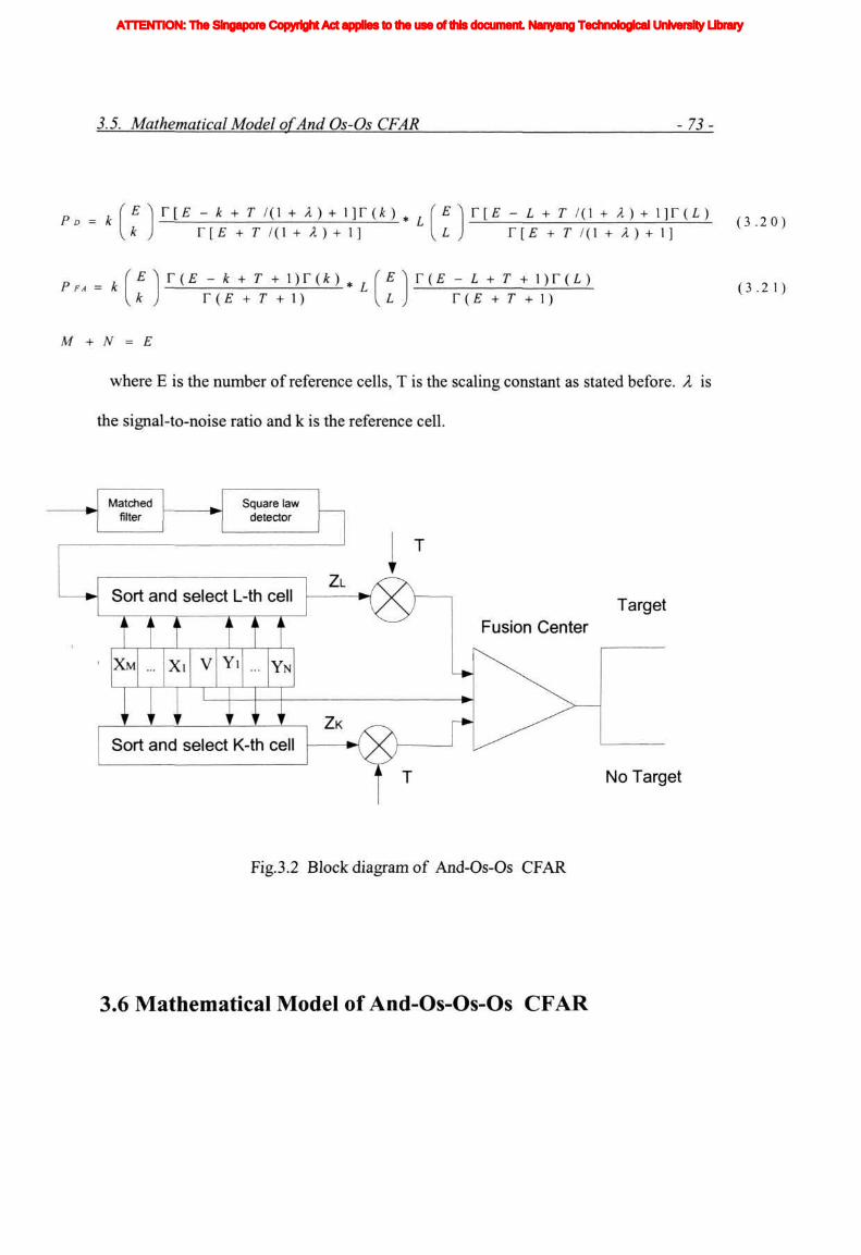
3.5. Mathematical Model of And Os-Os CFAR -73-

PD = k ' E \ r[E - k + T l(\ + A) + \]r(k)

r[E + T /(l + X) + 1] v ^ y

r [ £ - L + r /(i + A ) + i ] r ( L ) r [ £ + r /(i + A) + i]

( 3 . 2 0 )

P ^ = i / IT \

v * y

r(E - k + T + \)r(k) r (E + T + i) v * y

r ( £ - L + T + \)r(L) r(E + T + \)

( 3 . 2 1 )

M + N = E

where E is the number of reference cells, T is the scaling constant as stated before. A, is

the signal-to-noise ratio and k is the reference cell.

Matched filter

Square law detector

Sort and select L-th cell

ffl t t t Target

X M Xi V Y i Y N

f } f i r 1

\ f } f i r } r i r 1 r

Sort and select K-th cell

No Target

Fig.3.2 Block diagram of And-Os-Os CFAR

3.6 Mathematical Model of And-Os-Os-Os CFAR


3.5. Mathematical Model of And Os-Os CFAR 74

This CFAR structure is shown in Fig 3.3, where N, M represents the number of reference


In homogeneous back ground, with all the cells are IID, the false alarm probability Pfa


Cr\ Pfa=k

'M\Y{M-k + T + \)T{k)M (1-r(M + r+i) yk j \ ' j

T(E-l + T + \)r(l) N

V(E + T + \)

T(N-c + T + \)r(c)

Y(N + T +1)

(3.22)

Po = k (M\Y[M-k + TI{\ + X) + \]T{k),

\ k . T[M + T/(\ + A) + l] (E)

r[E-l + T/(l + A) + \]T(l)

T[E + T/(\ + A) + \]

N\r[N-c + T/(l + A) + \]T

\ c J r[N + T/(l + A) + \]

(3.23)

M+N=E

where E is the number of reference cells, T is the scaling constant as stated before. A is



3.7. Mathematical Model of And-Ca-Os-Os CFAR -75

Matched filter

Square law Matched filter detector

, M H

t i l T t t X M

Sort and select k-th cell

Target

No target

Fig.3.3 Block diagram of And-Os-Os-Os CFAR

3.7 Mathematical Model of And-Ca-Os-Os CFAR

This CFAR structure is shown in Fig 3.4, where N, M represents the number of reference



3.7. Mathematical Model of And-Ca-Os-Os CFAR - 76-

In homogeneous back ground, with all the cells are IID, the false alarm probability Pfa


Po = k M\Y\M -k+T /(1+A)+1]T(*).

v * y I W +77(1+ *) + !] {\ + T/[(\ + A)E]y

(N\

V c J

Y[N - c + T/(\ + A) + \]T(c)

T[N + T/(\ + A) + \] (3

Pfa=k (M}r(M-k + T + \)F(k)

k 1 'an

T(M + T + \) (\ + T/Ey

T(N-c + T + \)Y(c)

V(N + T + \) (3.25)

M+N=E

where E is the number of reference cells, T is the scaling constant as stated before. X is



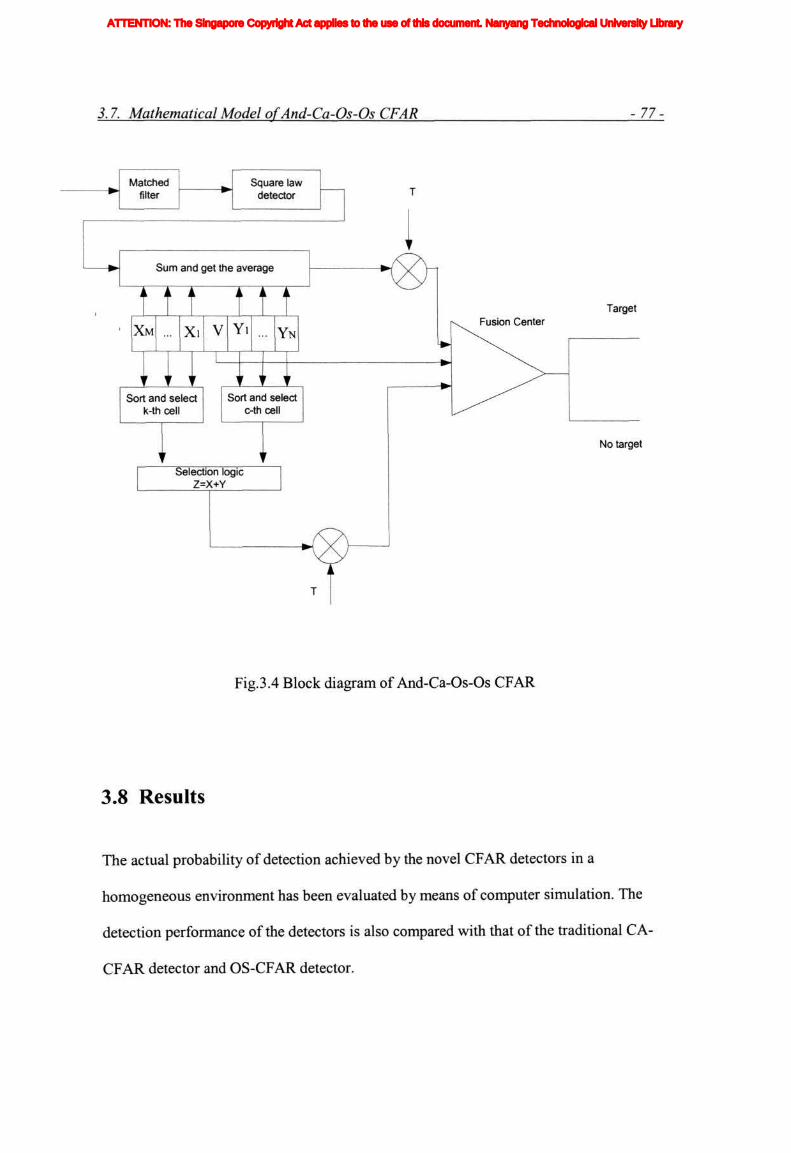
3.7. Mathematical Model of And-Ca-Os-Os CFAR -77-

Matched filter

Sum and get the average

t t t t t t X M XI

v v v

V

Sort and select k-th cell

Sort and select c-th cell

Selection logic Z=X+Y

No target

Fig.3.4 Block diagram of And-Ca-Os-Os CFAR

3.8 Results

The actual probability of detection achieved by the novel CFAR detectors in a

homogeneous environment has been evaluated by means of computer simulation. The

detection performance of the detectors is also compared with that of the traditional CA-

CFAR detector and OS-CFAR detector.


3.8. Results -78-

As false alarm probability is fixed, the scaling constant T can be calculated to evaluate

performances. The program (see Appendix C) which based on Secant Line iteration is

used to calculate the threshold. It combats the heavy work caused by Divide line method

and complicated work (need to calculate complex differential coefficient) result from the

Newton iteration method.

For different reference numbers E, and k, 1, c, M, N value settings and false alarm

probabilities, the scaling constant Ts of new CFAR detectors are listed below

respectively.

It can be seen from the calculated T values that as number of reference cells E increases,

T decreases. This is rationale since the more information can be obtained, the more

decisive the threshold and so the lower T value. It also could be seen when the false

alarm probability decreases, the threshold scaling factor T increases.. As T increases, the

detection probability will decrease, this is due to the higher the scaling constant, the

higher the threshold, it is more difficult for the cell under test to go beyond the threshold,

so the PD will decrease. This is the same trend as the CA-CFAR and OS- CFAR. To

illustrate this further, the detection probabilities versus Pfa and different reference cells E

have been plotted (Fig 3.5 to Fig 3.13).


3.8. Results -79-

Table 3.1 Scaling constant T of And-Os-Os CFAR for different E and k, 1 values

\

E=16

k=8

L=8

E=16

k=10

L=10

E=16

k=12

L=12

E=16

k=14

L=14

E=32

k=16

L=16

E=32

k=20

L=20

E=32

k=24

L=24

E=32

k=28

L=28

Pfa=\0~4 9.4671 6.3679 4.4251 3.0249 7.9113 5.4640 3.8383 2.6026

Pfa = \0-5 12.8324 8.4938 5.8479 3.9816 10.2815 7.0501 4.9329 3.3420

Pfa = \0-* 16.7233 10.8850 7.4214 5.0300 12.8318 8.7342 6.0863 4.1189

Pfa = \0-7 21.2205 13.5733 9.1602 6.1771 15.5756 10.5219 7.3012 4.9347

pfa = \o-* 26.4173 16.5944 11.0802 7.4307 18.5269 12.4192 8.5801 5.7906

P/a = icr9 32.4214 19.9883 13.1991 8.7990 21.7012 14.4322 9.9262 6.6880


3.8. Results -80

Table 3.2 Scaling constant T of And-Os-Os-Os CFAR for different E and M,N, k, 1 values

\ \ \ \ \ \ \ \ \ \

M=8 E=16

N=8 1=14

k=4

c=4

M=8 E=16

N=8 1=12

k=4

c=4

M=8 E=16

N=8 1=10

k=4

c=4

M=8 E=16

N=8 1=8

k=4

c=4

M=8 E=16

N=8 1=14

k=2

c=2

M=8 E=16

N=8 1=14

k=6

c=6

M=16 E=32

N=16 1=16

k=8

c=8

M=16 E=32

N=16 1=28

k=8

c=8

Pfa =10^ 3.7530 4.6611 5.5990 6.6384 5.2094 2.6529 5.4246 3.1690

Pfa = W5 4.9938 6.2289 7.5396 9.0323 7.0367 3.5008 7.0694 4.0883

Pfa=\0-6 6.3807 7.9964 9.7549 11.8099 9.1276 4.4352 8.8460 5.0632

Pfa = \0-7 7.9291 9.9872 12.2813 15.0290 11.5163 5.4634 10.7636 6.0961

Pfa=\0-* 9.6559 12.2279 15.1604 18.7565 14.2419 6.5938 12.8322 7.1901

Pfa=\0-9 11.5802 14.7483 18.4395 23.0698 17.3491 7.8351 15.0626 8.3481


3.8. Results -81 -

Table 3.3 Scaling constant T of And-Ca-Os-Os CFAR for different E and M,N, k, 1 values

\

M=8 E=16

N=8

k=2

c=2

M=8 E=16

N=8

k=4

c=4

M=8 E=16

N=8

k=6

c=6

M=8 E=16

N=8

k=6

c=2

M=16 E=32

N=16

k=8

c=8

M=16 E=32

N=16

k=12

c=12

M=16 E=32

N=16

k=14

c=14

Pfa = \0-* 7.7981 5.1454 3.3758 4.8153 4.4732 2.8945 2.2128

Pfa = \0-5 10.4164 6.8196 4.4599 6.4054 5.7619 3.7265 2.8511

Pfa = \0^ 13.3645 8.6767 5.6534 8.1746 7.1242 4.6044 3.5344

p/fl = io-7 16.6812 10.7335 6.9640 10.1386 8.5631 5.5295 4.2516

Pfa = \0'8 20.4100 13.0087 8.4005 12.3149 10.0817 6.5034 5.0075

P/a = 10"9 24.6003 15.5229 9.9726 14.7232 11.6835 7.5276 5.8033


3.8. Results -82-

Table 3.4 Scaling constant T of And-Ca-Os CFAR for different E and k, 1 values

\

E=16

k=8

E=16

k=10

E=16

k=12

E=16

k=14

E=32

k=16

E=32

k=20

1=32

k=24

E=32

k=28

Pfa = \0-4 6.7885 5.7910 4.8580 3.9295 6.0727 5.1910 4.3401 3.4558

Pfa = \0'5 8.9421 7.6046 6.3696 5.1583 7.7876 6.6490 5.5582 4.4346

Pfa = 10^ 11.3150 9.5906 8.0182 6.4971 9.5887 8.1765 6.8330 5.4610

Pfa = \0-7 13.9291 11.7645 9.8147 7.9532 11.4800 9.7763 8.1666 6.5361

Pfa = \0~* 16.8084 14.1432 11.7710 9.5346 13.4659 11.4514 9.5610 7.6613

Pfa = 10"9 19.9793 16.7454 13.9001 11.2504 15.5510 13.2052 11.0185 8.8378


3.8. Results - 83 -

Signat-to-noise ratio.dB

Fig 3.5 The effect of n on Pd of And-Ca-Os CFAR where n is the reference cells number and designed Pfa=10e-8

Fig 3.6 The effect of Pfa on Pd of And-Ca-Os CFAR when n=16,k=12


3.8. Results -84-

0 8

W=16 And 0«-0» CFAR

30 40 Signal-to-noise ratio.dB

Pft=10-*

80

Fig 3.7 The effect of n on Pd of And-Ca-Os CFAR where n=16 is the reference cells number and designed Pfa=10e-8

0 8

-

1 1 1

N=16.k=N12. And Os-Os CFAR

i i

^ - ^

.

Ph=10^ / " " "

/ / ^ Ph=icr*

-

/ / .

-

/ " V Pf*=io7

-

• i i i i i

i 1

40 Signat-to-noise ratio,dB

Fig 3.8 The effect of Pfa on Pd of And-Os-Os CFAR when n=16,k=12


3.8. Results -85-

0 7

0 6

0 7

0 6 Pf»=10^ And Ca-Os-Os CFAR

l l l

0.5 - z.

1-•B

1-•B

— k=c=2

Prob

abili

ty

o

k-c=6 „ . -

Prob

abili

ty

o -

0.2 -/£^ k-e"4

-

0.1

i -0.1

i ) 5 10 15 20 Signal-to-noise ralio.dB

25 30 36 40

Fig 3.9 The effect of k and c on Pd of And-Ca-Os-Os CFAR when the reference cells number E=16,M=N=8and designedPfa=10e-8

0.6 • E=16.M=N=8,k=c=4 And Ca-Os-Os CFAR

i •

j . -

•s

I Pfa=10"7 — ^ - -^s^

r -r r 0 2 -

_/ yS

0 1 -

i i

°0 S 10 15 20 25 30 35 40 Signal-to-noisa ratio ,d8

Fig 3.10 The effect of Pfa on Pd of And-Ca-Os-Os CFAR when the reference cells number E=16,M=N=8.k=c=4


3.8. Results -86-

a 03

I * 025 -

Pfa=10-° E=16.M=M=8,k=c=4. And Os-Os-Os CFAR

15 20 25 SignaMo-noise ratio.dB

Fig 3.11 The effect of 1 on Pd of And-Os-Os-Os CFAR when the reference cells number E=16 ,M=N=8,k=c=4, and designed Pfa=10e-8

0.7

0.6

0.7

0.6 E=16.N10.r*4=N=8.k=c=4. And Os-Os-Os CFAR

0.5

ion

8 0.4 ^^ ^> -1 S^ ^ ^ •s s^ ^ S ^

Illy

X / ^ ^ J 03 J 03

Pro

/ / S ^ ^ 0 2 / / s ^ 0 2

0.1

°

0.1

° 3 5 10 15 20 25 30 36 40 Signal-to-noise ratio.dB

Fig 3.12 The effect of Pfa on Pd of And-Os-Os-Os CFAR when the reference cells number E=l 6,1=10,M=N=8.k=c=4


3.9 Performance Comparison - 87 -

3.9 Performance Comparison

0 7 , , , , 1 1 r

OR - r*»w* Number of reference cells is 16

Signal-to-noise ratio.dB

Fig 3.13 Comparison of Pd among the six CFAR detectors with the number of reference cells n=16 and Pfa=10e-8

To compare the performance among the And-Os-Os CFAR, And-Ca-Os CFAR, And-Os-

Os-Os CFAR, And-Ca-Os-Os CFAR, Ca-CFAR and Os-CFAR detectors, the

formulations of Os-CFAR and Ca-CFAR are derived from the same approach as And-Os-

Os CFAR, And-Ca-Os CFAR, And-Os-Os-Os CFAR, and And-Ca-Os-Os CFAR. The

detection probability and false alarm probability of each CFAR detector is shown above.

The detection probability under different signal-to-noise is actually compared among the

six detectors. In Fig 3.13, the number of reference cells is n=16, a designed probability of

false alarm Pfa=10e-8. It can be seen that the And-Ca-Os CFAR is achieving the best

detection probability in the six detectors. And-Ca-Os CFAR is better than And-Os-Os-Os

CFAR and And-Os-Os CFAR. The And-Os-OS CFAR has a very close performance with


3.10. Conclusion -88-

the CA-CFAR. The Os-CFAR probability detection performance is the worst among the

six CFAR detectors. From the simulation results, for the new CFAR detectors there will

be different improved percentage of probability of detection contribution. It can be varied

from 0.60% to more than 49% at different signal-to-noise ratios.

3.10 Conclusion

In this chapter, we propose four novel CFAR detectors synthesizing the advantages of

CA-CFAR and OS-CFAR. They are the improvement from the traditional CA-CFAR and

OS-CFAR. Analytical expressions for the detection probability and false alarm

probability of the four detectors are obtained. The performance of the proposed CFAR

detectors has been examined first and then compared with that of CA-CFAR and OS-

CFAR. It is proved that the And-Ca-Os CFAR approach is computationally efficient and

increases the detection performance extremely among these CFAR detectors. So we

recommend And-Ca-Os CFAR to the anti-collision radar applications.


Chapter 4

Improved Radar Detection on Curved

Section of a Road

4.1 Introduction

In anti-collision radar systems, the high detection probability and low false alarm rate

puts tough demands on radar sensor, especially on radar antenna [57]. People have

realized to get high detection probability and low false alarm rates, radar antenna must

measure the three discriminations of a target simultaneously, those are range, velocity

and azimuth angle.

Due to the strong requirements for extremely high accurately detection, the anti-

collision radar antenna design for car application is a very important point. The statistics

show that high false detections of unnecessary objects and non-detections of necessary

objects in the traffic often take places when the radar vehicle is running on the curve. To


4.2 Radar Antenna - 9 0 -

cope with the difficult situation, I proposed a new antenna techniques to improve the

radar detection performance. The novel antenna could robustly work in everyday any

traffic situations and in any weather conditions. The method make a good improvement

over the classical antenna tracking technologies.

4.2 Radar Antennas

The purpose of the radar antenna is to act as a transducer between free-space propagation

and guided-wave (transmission-line) propagation. The function of the antenna during

transmission is to concentrate the radiated energy into a shaped beam which points in the

desired direction in space. On reception the antenna collects the energy contained in the

echo signal and delivers it to the receiver. Thus the radar antenna is called upon to fulfill

reciprocal but related roles. In the radar equation derived in Chapter 1 [Eqn.1.7] these

two roles were expressed by the transmitting gain and the effective receiving aperture.

The two parameters are proportional to one another. An antenna with a large effective

receiving aperture implies a large transmitting gain.

The large apertures required for a long-range detection result in narrow beamwidths,

one of the prime characteristics of radar [60]. Narrow beamwidths are important if

accurate angular measurements are to be made or if targets close to one another are to be

resolved. The advantage of microwave frequencies for radar application is that with

apertures of relatively small physical size, but large in terms of wavelengths, narrow

beamwidths can be obtained conveniently.


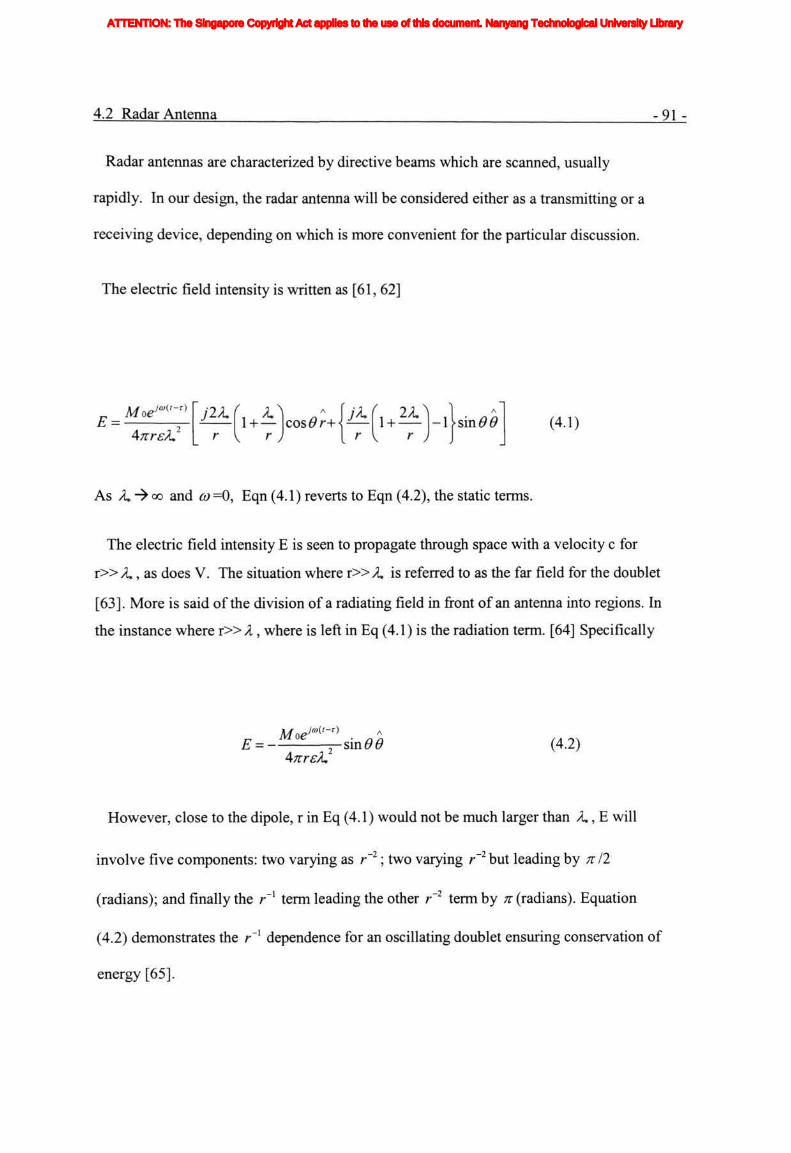
4.2 Radar Antenna - 9 1 -

Radar antennas are characterized by directive beams which are scanned, usually

rapidly. In our design, the radar antenna will be considered either as a transmitting or a

receiving device, depending on which is more convenient for the particular discussion.

The electric field intensity is written as [61, 62]

E = Moe ja(t-r)

AtnreX.

'j2A.(. A.\ * \jK{ 1 + — cos#r+^-— 1 + K r J I r

- U s i n 0 0 r )

(4.1)

As A, -> co and co =0, Eqn (4.1) reverts to Eqn (4.2), the static terms.

The electric field intensity E is seen to propagate through space with a velocity c for

r » A,, as does V. The situation where r » A, is referred to as the far field for the doublet

[63]. More is said of the division of a radiating field in front of an antenna into regions. In

the instance where x»A , where is left in Eq (4.1) is the radiation term. [64] Specifically

_ MoeM-T) . « E = — sin6><9

47rreA. (4.2)

However, close to the dipole, r in Eq (4.1) would not be much larger than A,, E will

involve five components: two varying as r~2; two varying r"2but leading by nil

(radians); and finally the r"1 term leading the other r'1 term by ;r (radians). Equation

(4.2) demonstrates the r~l dependence for an oscillating doublet ensuring conservation of

energy [65].


4.3 Anti-collision Radar Antenna Arrays - 92

4.3 Anti-collision Radar Antenna Arrays

The antenna array radiation pattern can be derived from basic relations by considering the

propagation of electric field from a set of radiating elements. The works of Schekunoff

(1943) and Stratton (1941) provide the background material applicable to the linear array

discussed in this section [66, 67, 68]. Consider N radiating elements, equally spaced a

distance d apart, each element radiating equal amplitude ao, but with a phase progression

difference between adjacent elements, as shown in Figure 4.1. The phase difference in

adjacent elements may be expressed by

&</> = 27r-sm0 (4.3)

where 9 is the look angle; that is, angle taken of the incoming wave. To accommodate

for the progressive beam scanning effect, a phase progression 58 between adjacent

elements is introduced [69, 70] The total phase difference of the radiating fields from the

adjacent elements may be expressed as

y = L$ + 88 = 2K — <su\.0 + 88 (4.4) A


4.3 Anti-collision Radar Antenna Arrays 93

The outputs Ei of all the elements are summed via lines of equal length to give the sum

output E, as in Figure 4.2. If source 1 is taken as the phase centre so that the field from

source 2 is advanced by y/, source 2 is advanced by 2 y/, and progressively onwards until

the source N is advanced by (N-l) y/, then the sum output E can be written as a

geometric series [71]:

E = cto(\ + eJV' +ej2¥ +... + en"-l)¥) >(AM)r> (4.5)

For brevity, ao=\. multiply Eq (4.5) by elv and by simple geometry,

Ee1¥ =ao(eJ¥ +ejl* +eJiw +... + eJ"¥) JNiy t (4.6)

Subtracting Eq (4.6) from Eq (4.5) and dividing by (1 - e'v ),

jNy

E = 1-e imj/

-JNY jNy/

1-e IV )U>

e 2 eJ¥ -e1

(4.7)

Rearranging Eq (4.7),

E = j(N-\)¥ sin

sin

Ny/

(¥\

\± J

(4.8)


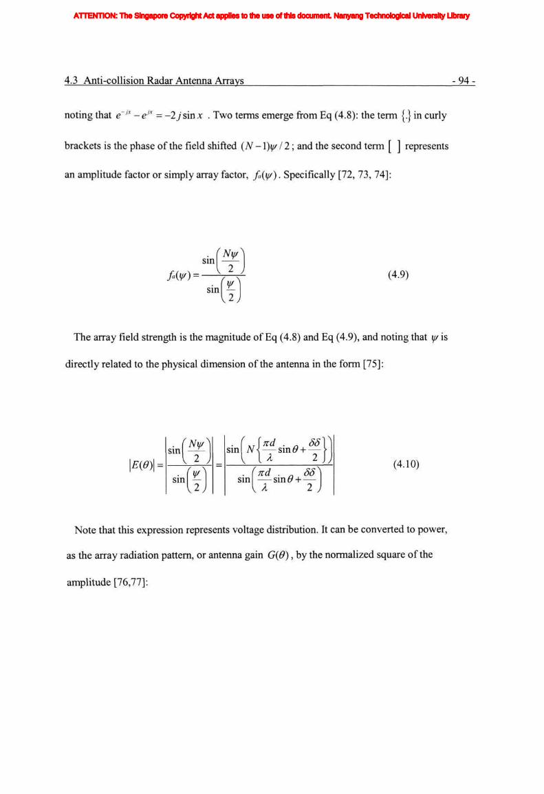
4.3 Anti-collision Radar Antenna Arrays - 9 4 -

noting that e >x -e'x = -2 j sin x . Two terms emerge from Eq (4.8): the term {.] in curly

brackets is the phase of the field shifted (N - \)y/12; and the second term [ ] represents

an amplitude factor or simply array factor, fa{y/). Specifically [72, 73, 74]:

Mr)

• (Nys sin —r-l 2

sin

(4.9)

v^y

The array field strength is the magnitude of Eq (4.8) and Eq (4.9), and noting that y/ is

directly related to the physical dimension of the antenna in the form [75]:

\E{0)\ -

• (Nyf sin —— I 2

sin ^

v^y

sin XT\nd _ 85 N<—sm6' + —

V U 2 sin

nd . 88 -sin# +

I 2 j

(4.10)

Note that this expression represents voltage distribution. It can be converted to power,

as the array radiation pattern, or antenna gain G{0), by the normalized square of the

amplitude [76,77]:



G{6) = \E{0)\2

N2

sin 55 tf{—sin**

1 A 2 iVsin nd 55

— sin# + — v A 2

(4.11)

In essence, the array pattern could be defined as the full elevation pattern of a broadside

array that substitutes (imaginary) isotropic radiators in place of the elements actually used

[78]. The broadside of the array is the direction in which maximum radiation is almost

perpendicular to the plane (line) of the array [79]

When directive elements are used, the resultant radiation pattern is expressed as

G{6) = Gt(0) =

. (.And . a 55]} sin N<— sin# + —

l U 2

- i 2

TV sin nd 55 — sin# +

v A 2

(4.12)

where Gi{0) is the individual element factor, or radiation pattern of an individual

element.

In a two dimensional rectangular planar array, the radiation pattern may sometimes be

written as the product of the two planes that contain the principal axes of the antennas

[80]. Following equation (4.12) and neglecting phase progression effect for simplicity

(i.e. 55 = 0) , the product radiation pattern



G{9) n,m

nd . _ sin | n — sin#„

_k ' • (*d • a «sin —sine ' u

sin nd .

m — sin 0 A

• ( n d • a

wsin —sin^ . I A

(4.13)

where n,m= number of radiators in 0n, 6m dimensions with spacing d, a respectively.

Note that 6n, 9m are not necessarily the elevation, azimuth angles normally associated

with antenna beam [81,82].

An advantage of two-dimensional array is that one can scan and shape the beam in two

directions. However this type of array tends to have a rather complex and costly feed

network.

e e e e 9 o

E, E2 Ea t N-1 E N E2 Ea t N-1 E N

r ^

d d

d r ^

d

1 t

d

Fig 4.1 Geometry configuration of a linear array antenna


4.4. Classical Azimuth Measurement -97-

Boresight A

+ P

N-1 N Elements

Fig 4.2 Line representation of radiators of a linear array antenna

4.4 Classical Azimuth Measurement

Monopulse tracking is a process through which the radar receiver processes two (or

sometimes four) signals for phase and amplitude information [83, 84, 85]. Amplitude

comparison monopulse is used in situations where more than one antenna is used and

each antenna illuminates a slightly different space [86]. This is commonly the case with

reflector antennas where multiple feed antennas may be used to produce multiple beams.

However, in the case of automotive radar, when design space is at a premium and costs

must be minimized, multiple small antennas are often used together in an array



environment. In this situation it is far more practical to use phase comparison monopulse.

Phase comparison monopulse functions on the fact that if a target is not directly at the

broadside of an antenna array then the reflected signal will cause a phase difference in

each element of the array [87, 88]. Fig 4.3 is an illustration of a phase comparison radar's

antenna array. The distance from antenna 1 to the target is

Ri = R + -sin(0) (4.14)

where d is the distance between antenna 1 from antenna 2, R is the distance from the

middle point (of antenna 1 and antenna 2) to the target, and the distance from antenna 2

to the target is

Ri = R--sm(0) (4.15)

The phase difference between the reflected signals in the two antenna elements is

approximately

In A<p = —dsin(0) (4.16)

A



When 6, as seen in Fig. 4.5, is a small angle. The phase difference between antenna

channels is approximately a linear function of the angle 0.

Target

Fig 4.3 Monopulse phase comparison

A phase comparison monopulse system requires a circuit that will form the sum and

difference of the reflected signal. Recently much attention has been paid to various

methods of processing received signals at lower frequencies [89]. The advantage of

performing such a task at lower frequencies is that the hardware required to form the sum


4.5. Trace Target On The Curve -100 -

and difference channels is readily available and is often made of lumped elements instead

of a printed type hybrid. It is also an interesting topic for my future research work.

4.5 Trace Target On The Curve

Unfortunately, there is not a straight road from the start to the end. One of the high false

detections of unnecessary objects and non-detections of necessary objects in the traffic

often take places when the radar vehicle is running on the curve ( Fig.4.4) [90,91]. To

prevent it, the radar beam is steered at the location of the target so as to trace it properly.

We could set up a mathematics model as follows.

First, the curve radius R of the presently running lane is estimated by the yaw rate and

the vehicle speed as Equation 4.17, then the beam steering angle # is determined

accordingly as expressed below:

R = — (4.17) (Oy

where v is the vehicle speed; and<y> is the yaw rate.

That means if there is a target exists in the running direction on the lane, and the

distance of the target detected by the radar is L, 6 is determined as expressed below:

9 = sm~\LI2R) (4.18)


4.5. Trace Target On The Curve 101

If there is no target exists in the running direction on the lane, the distance L in

equation 4.18 is set the same as the warning distance to a stationary vehicle [92].

From the above, the target can be traced even if the distance to the target changes at a

curve.

!•£

)

A

Fig 4.4 Car on the road

4.6 Improve The Azimuth Measurement

From Eq. 4.16 (differential the equation's two sides), we can get


4.6. Improve The Azimuth Measurement -102

In d<f> = — d cos 9d9 (4.19)

A

d6 = d<j> (4.20) In d cos 9

From Eq 4.20, we can see that the improvement of azimuth could be realized if we

adopt high accuracy phase measurement instrument (to get small dtp), or reduce the

value of AI d .

It also could be concluded that when 9 - 0, or the target is located the normal line of

the antenna, the error of measuring azimuth d6 is smallest. The dd augment with 9. So

as to guarantee high accuracy measuring azimuth, we should limit the value of 0.

Although raise the d IA could increase the measuring azimuth, from Eq.4.19 we could

know that within a certain range of 9 (within the azimuth measurement) when the d IA

grow up enough, the value of <f> may exceed In :

<f) = 2nN + y/ (4.21)

where N is integer, y < In. The phase measurement instrument actually take the

reading of the y/. Then we could not definite the real <j> because of the uncertain N.


4.6. Improve The Azimuth Measurement - 103 -

Target vehicle

Fig 4.5 Beam steering logic

In order to solve the ambiguity question and uniquely identify the azimuth <j> of the

target, we propose a precise azimuth measuring method using three antennas shown as

Fig 4.6.

From Fig 4.6, we assume the target exists in the running direction at an angle of 9. The

distance between antennas 1 and 2 is dn , and antennas 1 and 3 is dn . We need to

properly set-up dn to satisfy the Eq.4.19 at the range of the measuring azimuth:


4.6. Improve The Azimuth Measurement -104-

. In , . .. _ 012 = — dnsmO <2TT (4.22)

wherein is the difference phase of the received signals for antennas 1 and 2. 1̂2 is

taken directly on the instrument 1.

To meet the measurement demand, design du bigger enough, then we could get Eq

4.23

1̂3 = —Ji3sin# = 2TTN + y/ (4.23)

receiver

Instrument 1 ( <t>n

receiver

Instrument 2

receiver

antenna 3

Fig.4.6 Measuring azimuth using three antennas


4.6. Improve The Azimuth Measurement -105 -

<j)u is measured from the instrument 2. The actual reading is y/, which is less than 2K . So

as to make certain N , we could make use of relations as follows:

</>n _ dn

(f>n dn

(f)n=—-0i2 (4.24) dn

We could obtain <f>\i from <f)n (the reading of instrument 1), but the $n contains the

reading error of the instrument, the error of $u ( Eq.4.24) is dnl dn times the amount of

the instrument reading error. So <f>\i obtained from Eq 4.24 is just the approximate value

of Eq.4.23. {dnl dn)(/>n divided by 2K , the integer of quotient is N. So we could

make a certain N. Then Eq.4.23 can be used to calculate <f>n and confirm 6. The value

of (du I A) is bigger enough to satisfy the demand of the precision measurement of

azimuth angle error dd.

4.7 Results

The simulation results (Fig 4.7) shows the calculations relationship between the

azimuth measuring error and the target azimuth angel 9 at different d IX. Where d is

the distance between the detective antennas (shown in Fig 4.3), and X is the radar


4.7. Results -106-

transmitted wavelength. It can be seen that when 0 = 0, i.e. the target is located at the

normal line of the antenna, the error of the measuring azimuth dO is the smallest.

180° The error dO augments with 0 (from 0 to ± ). When d IX increase, the QuoxdO

n

reduced rapidly.

-\ r

0

d/3L=1

611=2

d/X=3

dfl.=4

J L -1 -0.8 -0.6 -0.4 -0.2 0

e 0.2 0.4 0.6 0.8 1

Fig 4.7 Azimuth measuring error dO versus target azimuth 6? at different d I' k



4.8 Conclusion

In this chapter, we developed a new beam steering logic method and a novel antenna

configure technology. From the simulation results, we could observe that the false

detections of unnecessary objects and failures to detect necessary objects, which used to

be major problems in anti-collision radar detection performance especially when a car is

on the curve, had been substantively reduced.


Chapter 5

CFAR Radar Sensors for Collision

Avoidance

5.1 Vehicular Application

In collision avoidance systems a radar system warns the operator of the vehicle when it is

too close to an adjacent vehicle or when the closing speed to the next vehicle exceeds a

prescribed rate. Such systems are currently available in up-scale cars such as Cadillac,

Lexus, and Mercedes [93]. These installations consist of simple radar systems that look

out of front of the car. An automated cruise control system maybe an extension of a

collision avoidance system. The current state of cruise control in vehicles is limited to

speed control. The operator sets a computer to a desires speed once the speed is achieved

[94]. The computer then adjusts the accelerator to keep the vehicle at a constant speed

irregardless of whether the car is on a hill or on a flat road. Future automated cruise

control systems will integrate radar systems with current cruise control technology to

make driving safer and more comfortable. A radar system may be implemented in an


5.1 Vehicular Application - 109 -

automated cruise control system in order to feed closing rate vehicle proximity

information to a decision making computer. The computer would then make speed

adjustments accordingly. While such systems are still some way in the future, research is

currently being performed on related topics [95-97].

The radar detection properties depend basically on the waveform design. In our

research activities we focused on continuous wave frequency modulated (FM) transmit

signals [98]. The main requirement is to measure target range and velocity

simultaneously in multi-target situations [99]. To meet the requirements for reliability

(extreme low false alarm rate) and reaction time (extreme short delay) we discussed the

specifics of the radar system's requirements, side looking surrounding and forward

looking the car. An illustration of this type of application is given in Fig. 1.2. The signal

from the systems are considered simultaneously for target detection and tracking in a data

fusion process.

5.2 Application of Novel CFAR Detectors

The novel CFAR strategy was selected for the calculation of the adaptive thresholds in

the Anti-collision radar systems. In FMCW radars (shown in Fig 5.1) that use frequency-

coded waveforms to measure simultaneously range and speed of a number of objects,

these advantages become significant. The structure of the applied CFAR detector is

shown in Fig 5.2.


5.2 Applied Novel CFAR Detector -110

The calculation of a decision threshold in this case is carried out in the frequency

domain. Hence, the random variables Xi.. .XN do not represent time simples, but bins in

the power spectrum. For each cell in the considered window the measured value at the

FFT output will be described as random variables Xi. In the pure noise case Ho, these

random variables and the value Y of the cell under test are assumed to be independent

and identically exponentially distributed with the probability density function (PDF)

f -e-3"" x>Q

Py0(x) = Pxi(x) = J \

i

0 Otherwise (5.1)

where // stands for the average clutter power.

Yo = Y/Ho = {Noise} (5.2)

If a target situation Hi occurs in the test cell the random variable Yi is assumed to be

distributed according to the following Rice PDF:


5.2. Applied Novel CFAR Detector -111

-e1" J*/o 2G -

Pn{x) =

v_

x>0

Otherwise (5.3)

Yx = YI H\ = {Noise} + Signal (5.4)

where G2 describes the S/N ratio and G is assumed to be Rayleigh-distributed for

targets with fluctuating amplitude (Swerling case II).

PG(X) =

r"

2x e~u

Go2 x>0

0 Otherwise (5.5)

where Go2=E{G2}

The parameter // stands for the average clutter power and is unknown, fj. has to be

estimated based on the cells in the reference window. A value for the decision threshold

S = T*Z is composed of the estimation Z, depending on // and a scaling factor Z, which

is selected so as to ensure the desired false alarm rate.


5.2. Applied Novel CFAR Detector -112

Frequency multiplexed waveform

Power coupler


LNA

3 dB splitter

Low pass filter

IF(beat frequency)

output

Receiving antenna Mixer

Power coupler <


LNA

Low pass filter

IF(beat frequenc y) output

Mixer Receiving antenna

Fig. 5.1 Anti-collision FMCW radar block diagram

F1

Waveform A

Waveform B

F2

FFT l2 + Q2 Spectrum Novel CFAR

Number of Test cells

Fig 5.2 The structure of the applied CFAR detector

(where I stands for in-phase and Q stands for quadrature)



5.3 Conclusion

To make use of the significant advantages of the novel CFAR algorithm, we introduce an

application on the vehicular technology of collision avoidance. The Anti-collision

FMCW Radar Block Diagram and the structure of the applied CFAR detector are also

presented in this chapter. The novel CFAR strategy will play a more and more important

part for improving the performance of the anti-collision radars.


Chapter 6

Conclusion and Recommendation

6.1 Conclusion

Heavy responsibility lies upon vehicle researchers to develop an obstacle detection sensor,

especially an anti-collision radar which has high expectations for active safety, since it is

not easy to decrease the traffic accidents in number by using a conventional technology.

The millimeter-wave radar has excellent characteristics to correspond with the social

demands for promoting safety-driving and reduce traffic collision accidents. It would be

Certainly that the radar systems should play a more and more important role in industrial

field and commercial applications [100].

It is emphasized in this thesis that the novel And-Ca-Os, And-Ca-Os-Os, And-Os-Os,

And-Os-Os-Os CFAR detectors have been proposed and show high performance in Anti-

collision radar detection measurement accuracy about the target range and velocity


6.1 Conclusion -115

information. We also have obtained the analytical expressions for the detection

probability and false alarm probability.

The performance of the novel CFAR detectors have been examined in details and then

compared with that of the traditional Ca-CFAR and Os-CFAR detectors . From the

simulation results we could see that the novel CFAR detectors have a better detection

probability than the classical CFAR detectors under different designed false alarm

probabilities.

Based on the novel CFAR detectors, a anti-collision frequency-modulated-continuous-

wave (FMCW) radar model has been presented.

We also developed a new beam steering logic method and a novel antenna configure

technology. By using this, the false detections of unnecessary objects and failures to

detect necessary objects, which used to be major problems in anti-collision radar

detection performance especially when a car is on the curve, can be substantively reduced.

Hence, the summary of major contributions of this thesis is as follows:

1.) Four new types of CFAR detector models are proposed to obtain better results on anti-

collision radar CFAR data fusion. Simulation results show that approach is effective and

flexible, and provides a universal way to solve the high false alarm problem for anti-

collision radar systems.


6.2. Recommendation and Future Work -116-

2.) The derivation of equations for the novel CFAR detection system is presented. Cases

are considered where weak random signals are observed in additive Gaussian noise-plus-

clutter of unknown power.

3.) For these four new CFAR detectors we obtain analytic expressions of the false alarm

rate, the detection probabilities and the measure ADT under the Swerling case 2

assumption. Comparing to the conventional CFAR detectors in homogeneous background

and in the presence of strong interfering targets, the new CFAR detectors have better

detection performance.

4.) A novel method on Secant Line iteration (Appendix C) is proposed for obtaining

better results on calculating the threshold of CFAR detector for a given constant false

alarm rate. It combats the problem of heavy and complicated work resulting from divide

line method and Newton iteration method.

5.) A new proposal of antenna design to improve the anti-collision radar detection

performance when car is on the curve.

6.2 Recommendation and Future Work

We have made good performance progress by using the novel CFAR detectors with

Swerling II model.



Furthermore, we would be interested in examining the Novel CFAR detectors

performance in a more generic environment, such as Weibull model and Swerling case I,

III and IV models.

We will check that under these environments, the performance of the novel CFAR

detectors will be superior to the traditional Os-CFAR and Ca-CFAR detectors.

Considering the practice applications in traffic avoid collision affairs, the performance

of the novel CFAR detectors will be examined under multi-target situation and at the

clutter edge.

We will also study the novel CFAR detector's detection loss features in detail.

Especially in the simulation traffic environment. Such as 1) regions of clutter power

transition; 2) multiple target environments; 3) closely spaced target environment.

In the majority of Anti-collision radar applications, the primary factor limiting detection

accuracy is interference [101]. Interference cannot be represented analytically, rather, it is

modeled as a random process. In recent years, neural networks have been considered for

signal detection primarily because a neural network may be trained to operate with

acceptable performance, in an environment under which the optimum signal detector is

not available. So implement the CFAR scheme as a part of a fuzzy data fusion scheme by

choosing an appropriate membership function to represent the CFAR threshold. Once the

threshold membership function of the Fuzzy Integrator has been set up, the false alarm

rate of the scheme is independent of fluctuation in interference mean power and depends



only on the number of signals integrated by the data fusion unit and the required false

alarm rate.

Input Signals Fuzzy network

and Neural network

Detection Decision

Fig 6.1 The basic diagram of a proposal fuzzy-neural network detector for anti-collision

radar systems

So it is interesting to design a novel Fuzzy-neural network detector for improving the

performance of the neural network detector. The proposal diagram is shown as Fig 6.1.


-119-

References

[1] Stove, A.G. "Linear FMCW radar techniques," Radar and Signal Processing, IEE

Proceedings F , Volume: 139 Issue: 5 , Oct. 1992 pp. 343 -350.

[2] Peyton Z.Peebiles, JR., "Radar principles" ISBN 0-471-25205-0 John Wiley & Sons,

1998, pp. 289.

[3] M.I.Skolnik, "Introduction to radar systems," McGraw Hill, New York, NY, 1980.

[4] M.Wallman, "Disturbance detection and suppression in FMCW radar signals,"

Royal Inst. Of Technology, Signal Processing, Stockholm Swedden, 1996. pp. 378.

[5] Hidayet.M, and P.A. Mclannes, "On the Specification of an Antenna Pattern for a

Synthetic Aperture Radar," International Conference RADAR-77, Oct. 25- 28, 1977,

IEE (London) Conf. Publ., no.155. pp.391-395.

[6] Nicholls, M.R. "Millimetre wave collision avoidance radars" Millimetre-Wave

Radar, IEE Colloquium on , 1990 pp. 3/1 -3/7.


-120-

[7] GANDHI, and KASSAM, S.A., "Analysis of CFAR processors in nonhomogeneous

background nonhomogeneous background," IEEE Trans., 1988, AES-24,(4), pp.427-

445.

[8] Stove, A.G. "Obstacle detection radar for cars," Electronics & Communication

Engineering Journal, Volume: 3 Issue: 5 , Oct. 1991 pp. 232 -240.

[9] Griffiths, H.D. "New ideas in FM radar," Electronics & Communication

Engineering Journal, Volume: 2 Issue: 5, Oct. 1990 pp. 185 -194.

[10] ROHLING, H. "Radar CFAR threshold in clutter and multiple target situations,"

IEEE Trans., 1983, AES-19, (4), pp. 608-621.

[11] RICKARDj.T., and DILLARD,G.H. "Adaptive detection algorithms for multiple

target situations," IEEE Trans.,1977, AES-13, (14), pp.338-343.

[12] HIMONAS,S.D. and BARKAT.M, "A robust radar CFAR detector for multiple

target situations," Proceeding of IEEE National Radar Conference, 1989, pp.85-90.

[13] HIMONAS, S. D. and BARKAT, M, "Automatic censored CFAR detection for

nonhomogeneous environments," IEEE Trans., 1992, AES-28, (1), pp.286-304.

[14] HANSEN, V.G. "Detectability loss due to greatest of selection in a cell-averaging


-121 -

CFAR," IEEE Trans., 1980, AES-16,(1), pp.116-118.

[15] ELIAS-FUSTE, A. R., DE MERCADO, M. G. and DAVO, E.R. "Analysis of some

modified order statistic CFAR: OSGO and OSSO CFAR," IEEE Trans., 1990,

AES-26,(1), pp. 197-202.

[16] RITCEY, J. A. and HINES, J. L. "Performance of max family of order-statistic

CFAR detectors," IEEE Trans., 1991, AES-27, (1), pp. 48-57.

[17] DAVID, H. A. "Order statistics," (Wiley,1991), pp. 478.

[18] PAPOULIS, A. "Probability, random variables, and stochastic processes,"

(McGraw-Hill, New York, 1984), pp. 34.

[19] M.GRECO, F. GINI, A.FARINA and J. B. BILLINGLEY, "Validation of

windblown radar ground clutter spectral shape," IEEE Trans., 2001,

AES/37/2/06328, pp. 38-41.

[20] Skolnik, M. I. "Introduce to radar systems," McGraw-Hill, Inc, 1962. pp 2-3.

[21] Gini. f, Montanari, M., and Verazzani, L. (2000). "Estimation of chirp radar signals

in compound-Guassian clutter: A cyclostationary approach," IEEE Transactions on

Signal Processing, 48,4 (Apr.2000), pp.1029-1039.


-122-

[22] Barlow, E. J., "Doppler Radar," Proc. IRE, April, 1949. vol. 37, pp. 340-355.

[23] Raffaelli, L. "Millimeter-wave automotive radars and related technology"

Microwave Symposium Digest, 1996., IEEE MTT-S International, Volume: 1 , 1996

vol.1, pp. 35-38.

[24] Saunders, W. K., "Radar Handbook," McGraw-Hill Book Co., New York, 1970. pp

173-179.

[25] Hyltin, T. M. "Radar Handbook," McGraw-Hill Book Company, New York, 1970.

Chap. 30. pp 146-148.

[26] Mumford, W. W., and E. Scheibe " Noise: performance factors in communication

systems," Horizon House Microwave, Inc., Dedham, Mass. 1968. pp 14-19.

[27] Crispin, J. W., Jr., and K. M. Siegel, "Methods of radar cross section analysis,"

Academic Press, New York, 1968. pp. 21-24.

[28] Skolnik, M. I. "Introduce to radar systems," McGraw-Hill, Inc. International Edition

1981. pp. 44.

[29] Kendall, Sir., A. Stuart, "The advanced theory of statics," Vol. 2, Macmillan, New

York, 1979, pp 34-42.


- 123 -

[30] Lehmann, E. L., " Testing statistical hypotheses," J. Wiley, New York, 1959, pp.

68-74.

[31] You He, "Performance of some generalised modified order statistics CFAR detectors

with automatic censoring technique in multiple target situations," Radar, Sonar and

Navigation, IEE Proceedings - , Volume: 141 , Issue: 4 , Aug. 1994, pp.205 - 212.

[32] Iskander, D.R., Zoubir,A.M, and Boashash, B (1999) "A method for estimating the

parameters of the K-distribution" IEEE Transactions on Signal Processing,

47,3 (1999), pp. 880-884.

[33] Mashade M.B.EI, "M-sweeps detection analysis of cell-averaging cfar processors in

multiple-target situations," IEE Proc. -Radar, Sonar Navig., vol. 141, Apr. 1994,

pp. 259-266.

[34] Peterson, W. W., T.G. Birdsall, and W.C. Fox, "The theory of signal detect ability,"

IRE Trans., Sep. 1987, pp 48-54.

[35] Mashade M. B. EI, " Detection performance of trimmed-mean cfar processor with

noncoherent integration," IEE Proc- Radar, Sonar Navig., vol;. 142, Feb. 1995, pp.

18-24.


- 124-

[36] Mashade M. B. EI, "Monopluse detection analysis of the trimmesd mean cfar

processor in nonhomogeneous situations," IEE Proc- Radar, Sonar Navig., vol/143,

Apr. 1996, pp. 87-94.

[37] Shnidman, D. A., "Radar detection probabilities and their calculation" Aerospace

and Electronic Systems, IEEE transactions. Pp. 928-950.

[38] Fuller,W., "An introduction to probability theory and its applications," 2d ed., John

Wiley & Sons, Inc., New York, 1957. vol.1, pp. 23-38.

[39] Woodward, P. M. "Probability and information theory with applications to radar,"

McGraw-Hill Book Company, New York, 1953. pp 12-21.

[40] Dillard, G. M., "A moving -window detector for binary integration," IEEE Trans.,

vol. IT-13, January, 1967. pp. 2-6.

[41] Hansen, V. G., "Optimization and performance of multilevel quantization in

automatic detectors," IEEE Trans., vol. AES-10, March, 1974. pp. 274-280.

[42] Fulvio Gini and Fabrizio Lombardini, "On distributed signal detection with multiple

local free parameters," IEEE Trans. On Aerospace and Electronic System, vol. 35,

Oct. 1999, pp. 1457-1466.


-125-

[43] Han Y.I. and Kim T., "Performance of excision go-cfar detectors in non-

homogeneous environments," IEE Proc,-Radar, Sonar Navig., Apr. 1996, vol 143,

pp.105-112.

[44] Abenz K. and Wohlhauser A., "Advanced Mathematics for Practicing Engineers,".

Deham, MA: Artech House, 1986. pp. 35-47.

[45] David, H. A. "Order statistics" (Wiley, 1981), pp. 38-43.

[46] RITCEY, J. A., and HINES, J. L., "Performance of max family of order-statistic

CFAR detectors," IEEE Trans., 1991, AES-27, (1), pp.48-57.

[47] Smith, M.E., Varshney, P.K., "Intelligent CFAR processor based on data

variability," Aerospace and Electronic Systems, IEEE Transactions on , Volume:

36 , Issue: 3 , July 2000, pp.837 - 847.

[48] Liu. Zhoufeng, Ping. Qingwei and He Peikun, "An improved algorithm for the

detection of vehicle group targets in high-resolution S AR images," Microwave and

Millimeter Wave Technology, 2002. Proceedings. ICMMT 2002. 2002 3rd

International Conference on , 17-19 Aug. 2002 pp:572 - 575.

[49] Himonas, S.D. and Barkat, M., "An adaptive CFAR signal detector for spatially

correlated noise samples," Decision and Control, 1990., Proceedings of the 29th

IEEE Conference on , 5-7 Dec. 1990, pp.3540 - 3545.


- 126 -

[50] Kaplan, L.M.and Murenzi, R., "Evaluation of CFAR and texture based target

detection statistics on SAR imagery," Acoustics, Speech, and Signal Processing,

1998. ICASSP '98. Proceedings of the 1998 IEEE International Conference

on , Volume: 4 , 12-15 May 1998, pp.2141 - 2144.

[51] Hong. Yi, Li. Ji-Yun and Ruan. Xin-Chang, "OSEXCA-CFAR processor on

nonhomogeneous background," Radar 97 (Conf. Publ. No. 449) ,14-16 Oct. 1997

pp.734 - 737.

[52] Lampropoulos, G.A.; Gigli, G.; Sevigny, L.; Beaudoin, A.; Seeker, J.; "Detection

of targets from electro-optical and SAR data using chaotic predictors and optimal

CFAR detectors," Geoscience and Remote Sensing Symposium, 2002. IGARSS '02.

2002 IEEE International, Volume: 1 , 24-28 June 2002 pp.107 - 109.

[53] Goldman, H., "Performance of the excision CFAR detection in the presence of

interferers." Radar and Signal Processing, IEE Proceedings F, Volume: 137, Issue:3,

June 1990. pp. 163-171.

[54] Hensen, V. G., "Constant false alarm rate processing in search radars," Proc of IEE

International Radar Conference, (London, U.K.), 1973. pp. 325-332.

[55] Di. Vito, A.; Morreti, G., "Probability of false alarm in CA-CFAR device

downstream from linear-law detector," Electronics Letters , Volume: 25 , Issue:

25 , 7 Dec. 1989, pp.1692 - 1693.

[56] M.B. Mashade, "Analysis of censored-mean level cfar processor in multiple target

and nonuniform clutter," IEE Proc.-Radar, Sonar Navig., Oct. 1995. vol. 142, pp.

103-108.

[57] J.D. Kraus, " Antennas since Herze and Marconi," IEEE Trans. Antennas Propagate.,


-127-

Vol. AP-33, No.2, February 1985, pp. 131-137.

[58] C.A.Balanis, " Antenna Theory: A Review," Proc. IEEE, Vol. 80, no. 1, January

1992, pp. 7-23.

[59] C.A.Deschamps, " Part 11-Geometrical Representation of the Polarization of a Plane

Electromagnetic Wave," Proc. IRE, Vol. 39, May 1951, pp.540-544.

[60] D.M. Pozar, " Directivity of Omnidirectional Antennas," IEEE Antennas and

Propagation Magazine, Vol.35, No.5, October 1993, pp. 50-51.

[61] S.A. Schelk, "Mathematical Theory of Linear Arrays," Bell System Tech. J.,

January, 1943, vol.22, pp.80-107.

[62] J.D. Kraus, "Antennas," McGraw-Hill, New York, 1988. pp. 65-68.

[63] J. Romeu and R. Pujol, "Array," Software Book in Electromagnetics, Vol. II,

Chapter 12, CAEME Center for Multimedia Education, University of Utah, 1995,pp.

467-481.

[64] A.Z.Elsherbeni and P.H. Ginn. " Interactive analysis of Antenna Arrays," Software

Book in Electromagnetics, Vol. II, chapter 6, CAEME Center for Multimedia

Education, University of Utah, 1995, pp. 337-366.


- 128 -

[65] A.Z. Elsherbeni and CD. Taylor Jr., "Interactive Antenna Pattern Visualization,"

Software Book in Electromagnetics, Vol. II, Chapter 8, CAEME Center for

Multimedia Education, University of Utah, 1995, pp.367-410.

[66] W.R. Scott Jr., " A General Program for Plotting Three-dimensional Antenna

Patterns," IEEE Antennas and Propagation Society Newsletter, December

1989, pp. 6-11.

[67] J.S. Hollos, T. J. Lyon, and L. Clayton Jr.(eds.), "Microwave Antenna

Measurements," Scientific-Atlanta, Inc., July 1970, pp. 345-348.

[68] A.Z. Elsherbeni and CD. Taylor Jr., " Antenna Pattern Plotter," Copyright® 1995,

Electrical Engineering Department, The University of Mississippi, University, MS,

pp.36-38.

[69] W.A. wheeler, " Small Antennas," IEEE Trans. Antennas Propagate., Vol. AP-23,

No.4, July 1975, pp.462-469.

[70] W.R. Scott, Jr., " A General Program for Plotting Three-Dimensional Antenna

Patterns," IEEE Antennas and Propagation Society Newsletter, December

1989, pp. 6-11.


-129 -

[71] C.A. Balanis, "Advanced Engineering Electromagnetics," John Wiley & Sons, Inc.,

New York, 1989. pp.87-89.

[72] R.Mittra(Ed.), "Computer Techniques for Electronmagnetics, Pergamon," New

York, 1973,pp.57-59.

[73] J. Moore and P. Pizer (Eds.), "Moment Methods in Electromagnetics: Techniques

and Applications," Letchworth, UK: Research Studies Press,1984, pp. 465-468.

[74] J. J. Wang, "Generalized Moment Methods in Electromagnetics," John Wiley &

Sons, Inc., New York, 1991, pp. 98-101.

[75] K. Fujimoto and J.R. James, "Mobile Antenna Systems Handbook," Artech House,

Norwood, MA, 1994, pp. 45-48.

[76] M. A Jensen and Y. Rahmat-Samii, "Performance Analysis of Antennas for Hand-

Held Transceivers Using FDTD," IEEE Trans. Antennas Propagate., Vol.42, No. 8,

august 1994, pp. 1106-1113.

[77] M.A Jensen and Y. Rahmat-Samii, "EM Interaction of Handset Antennas and a

Human in Personal Communications," Proc. IEEE, Vol. 83, No.l January 1995, pp.

7-17.


-130-

[78] C. A. Balanis, K. D. Katsibas and P.A. tirkas, " Antenna Considerations for

wireless Communication systems and Networks," 5l International Conference on

Advances in Communication and Control, June 26-30,1995, Rethymnon, Crete,

Greece, pp.38-43.

[79] D. Decarlo, " automation of In-Flight Antenna Measurements," MSEE Problem

report, dept. of Electrical engineering, west Virginia University, July 1980, pp. 34-

35.

[80] S. A. Schelkunoff, " A Mathematical theory of Linear Arrays," Bell System

Technical Journal, Vol.22, 1943, pp. 80-107.

[81] H. G. Booker and P. C. Clemmow, " The concept of an Angular spectrum of Plane

waves, and Its relation to That of Polar Diagram and Aperature distribution,: Proc.

IEE (London), Paper No. 922, Radio section, Vol. 97, pt. Ill, January 1950, pp. 11-

17.

[82] P. M. Woodward, " A Method for Calculating the Field over a Plane Aperture

Requored to Produce a Given Polar Diagram," J.IEE, Vol. 93, pt. IIIA, 1946, pp.

1554-1558.


- 131 -

[83] T. T. Taylor, " Design of Line-Source antennas for Narrow Beamwidth and Low

Side-Lobes," IRE Trans. Antennas Propagat., Vol. AP-3, No. !, January 1955, pp.

16-28.

[84] R. Tang and R.W. Burns, " Array Technology," Proc. IEEE, Vol. 80, No. 1, January

1992, pp 173-182.

[85] R. S. Elliott, " On Discretizing Continuous Aperture Distributions," IEEE Trans.

Antennas Propagat., Vol. AP-25, No. 5 , September 1977, pp. 617-621.

[86] R. C. Hansen (ed.) Microwave Scanning antennas. Vol. I, Academic Press, New

York, 1964, pp.56.

[87] J. Ruze, " Physical Limitations on antennas," MIT Research Lab., Electronics Tech.

October 30,1952, pp. 248.

[88] H. J. Orchard, R.S. Elliott, and G. J. Stern. " Optimizing the Synthesis of Shaped

Beam Antenna Patterns," IEE Proceedings, Part H, 1985, pp. 63-68.

[89] R. S. Elliott, " Design of line Source Antennas for Narrow Beamwidth and

Asymmetric Antenna Patterns." IEE Proceedings, Part H, 1985, pp. 63-68.

[90] S. Silver (ed.), "Microwave antenna Theory and Design," MIT Radiation


- 132 -

Laboratory Series, Vol.12, McGraw-Hill, New York, 1965, Chapter 6, pp. 169-199.

[91] D. M. Pozar, "Microwave Engineering," Addison-wesley, Reading, MA, 1993.

pp.68.

[92] R. C. Johnson and H. Jasik (eds.), "Antenna Engineering Handbook," 2nd. Ed.,

McGraw-Hill, New York, 1984, pp. 2-14 to 2-41.

[93] Woll, J. D. "Monopulse Doppler radar for vehicle applications" Intelligent

Vehicles '95 Symposium., Proceedings of the , 1995, pp. 42 -47.

[94] Watterson , J. W., "An optimum multilayer perception neural receiver for signal

detection," IEEE Trans. Neural Networks, vol. 1, 1990, pp. 298-300.

[95] Lippmann, R. P. and Beckman, P., "Adaptive neural net preprocessing for signal

detection in non-gaussian noise," Advance Neural Inform. Process. Syst,

vol. 1,1989. pp. 1431-1435.

[96] Michalopoulou, Z., Nolte, L. and Alexandrou, D., " Performance evaluation of

multilayer perceptions in signal detection and classification," IEEE Trans. Neural

pp. 56-58.

[97] Gandhi P.P. and Ramamurti V., "Nerval networks for signal detection in non-


-133-

gaussion noise," IEEE Trans. On signal Processing, vol. 45,1997, pp. 2846-

2851.

[98] Eriksson, L.H.; As, B.-O. "Automotive radar for adaptive cruise control and

collision warning/avoidance," Radar 97 (Conf. Publ. No. 449), 1997 pp. 1 6 -

20.

[99] Nishi, T., Takagi, T., "A proposal of collision avoidance algorithm for driving

support system" Industrial Electronics Society, 2001. IECON '01. The 27th Annual

Conference of the IEEE , Volume: 1 , 2001 pp. 80 -83 vol.1.

[100] Nicholls, M.R. "Millimetre wave collision avoidance radars" Millimetre-Wave

Radar, IEE Colloquium on , 1990 pp. 3/1 -3/7.

[101] Fikkema, P.G., Johnson, S.G., "Vehicle collision warning and avoidance system

using real-time FFT" Vehicular Technology Conference, 1996. Mobile Technology

for the Human Race., IEEE 46th , Volume: 3 , 1996 vol.3, pp. 1820 - 1824.


-134-

Appendix A

Minimum Bayes Risk detection Binary

Hypothesis

We minimize R as given by (3.17). note that if Coo=Cn=0, Coi=Cio=l, then R-Pe and so

our derivation also applies to the minimum Pe problem. Now

1=0 y=o

Let Ri={x: decide HI} be the critical region and R0 denote its complement (decide Ho).

Then,

R = CooP(Ho) \p{X I Ho)dx + Co\P(H\) \P{X \ H\)dx + CwP(Ho) \P(X \ Ho)dx + C\J>(Hi) JP(X | Hi)dx R0 R0 R] R\


- 135 -

But

\P{X I Hi)dx =1 - JP(X | H,)dx + C.. RO R\

Since Ri and Ro partition the entire space. Using this we have

R = CnP(//.) + CooP(Ho) + J[|(Cio/'(//o) - CooP(Ho))P(X I Ho) + (CuP(H,) - Co>P(H>))P(X I //i)| dxP(X I Ho)dx + Cm

We include x in Ri only if the integrand is negative or we decide Hi if

(Cio - Coo)P(Ho)P(x I Ho) < (Coi - C. \)P(Hx)P(x /Hi).

Assuming Cio>Coo, Coi>Cn, we have finally

PjxIHx) (Cw-Coo)P(Ho) P(x/Ho)> (Coi-Cn)P(Hi)


136

Appendix B

Neyman-Pearson theorem

We use Lagrangian multipliers to maximize PD for a given PFA. Forming the Lagrangian

F = PD+X(PFA-CC)

= JP(X; Hx)dx + X( j>(x; Ho)dx - a) R\

j(P(x; HI) + AP(x; Ho))dx - Xa R\

To maximize F we include x in Ri if the integrand is positive for that value of x or if

P(x;Hi) + XP(x;Ho)>0

When P(X; Hi) + X P(x; Ho)=0, x may be included in either Ro or Ri. since the

probability of this occurrence is zero (assuming that the PDFs are continuous), Hence, the


- 137 -

> sign in 3 A. 1 and the subsequent results can be replaced with >= if desired. We choose

to retain the > sign in our development. We thus decide Hi if

P(x;Ho)

The Lagrangian multiplier is found from the constraint and must satisfy A <0.

Otherwise, we decide HI if the likelihood ratio P(x; Hi)/P(x; Ho) exceeds a negative

number. Since the likelihood ratio is always nonnegative, we would always decide Hi,

irrespective of the hypothesis, resulting in PFA=1. we let y=- X so that finally we decide

Hi if

P(x;Hi) ———->v P(x;Ho)

Where the threshold y >0 is found from PFA= a .


- 138 -

Appendix C

% Divide line method code

function y=erfen(fun,a,b,esp)

if nargin<4 esp=le-4;end

if feval(fun,a)*feval(fun,b)<0

n=l;

c=(a+b)/2;

while c>esp

if feval(fun,a)*feval(fun,c)<0

b=c; c=(a+b)/2;

elseif feval(fun,c)*feval(fun,b)<0

a=c; c=(a+b)/2;


-139

else y=e; esp =10000;

end

n=n+l;

end

y=c;

elseif feval(fun,a)= =0

y=a;

elseif feval(fun,b)= =0

y=b;

else disp('these, may not be a root in the intercaT)

end

n

f\X*)


-140-

% Newton iteration method code

function y= newton(xo)

xi=xo-fc(xo)/df(xo);

n=l;

while(abs(xi-xo)>=l .0e-4)&(n<=l 00000000)

xo=xi;

xi=xo-fc(xo)/df(xo);

n=n+l;

end

xl

n

f(Xk)(Xk-Xk-x)

f(Xt)-f(X-i)


-141-

% Secant Line iteration code

function y=ger(xo,xi)

x2=xi-fc(xi)*(xi-xo)/(fc(xi)-fc(xo));

n=l;

while(abs(xi-xo)>=1.0e-4)&(n<=100000000)

xo=xi;xi=X2;

X2=xi-fc(xi)*(xi-xo)/(fc(xi)-fc(xo));

n=n+l;

end

X2

n


Detection improvement for anti‑collision radar - DR-NTU

Documents

Transcript of Detection improvement for anti‑collision radar - DR-NTU