Detecting Unusual Program BehaviorUsing the Statistical Component of theNext-generation Intrusion DetectionExpert System (NIDES) 1

Debra AndersonTeresa F. LuntHarold JavitzAnn TamaruAlfonso Valdes

Computer Science LaboratorySRI-CSL-95-06, May 1995

1This report was prepared for Trusted Information Systems, Mountain View, California, Contract No.910097C under RomeLab Contract F30602-91-C-0067.

Contents

1 Introduction1.1 Project Description . . . . . . . . . . . . . . . . . . . . . . . . . . . . . . . . . . . . .1.2 NIDES Statistical Algorithm Description . . . . . . . . . . . . . . . . . . . . . . . . .

1.2.1 Measures . . . . . . . . . . . . . . . . . . . . . . . . . . . . . . . . . . . . . .1.2.2 Half-life . . . . . . . . . . . . . . . . . . . . . . . . . . . . . . . . . . . . . . . .1.2.3 Differences between Long- and Short-term Profiles � The Q Statistic . . . .1.2.4 Scoring Anomalous Behavior - The S and T2 Statistic . . . . . . . . . . . . .

2 Customizations for Safeguard2.1 New Measures. . . . . . . . . . . . . . . . . . . . . . . . . . . . . . . . . . . . . . . .2.2 Configuration Items . . . . . . . . . . . . . . . . . . . . . . . . . . . . . . . . . . . .2.3 Half-life of Short-term Profile . . . . . . . . . . . . . . . . . . . . . . . . . . . . . . .

2.3.1 Number of Category Bins Reduced to 16 . . . . . . . . . . . . . . . . . . . . .2.4 Statistical Component Wrapper . . . . . . . . . . . . . . . . . . . . . . . . . . . . . .2.5 Utilities . . . . . . . . . . . . . . . . . . . . . . . . . . . . . . . . . . . . . . . . . . .

3 Experiment Descriptions3.1 Audit Data Analysis and Organization . . . . . . . . . . . . . . . . . . . . . . . . . .3.2 Overview of Experiments . . . . . . . . . . . . . . . . . . . . . . . . . . . . . . . . .3.3 Procedures of Concept, Verification, and Refinement Experiments . . . . . . . . . . .

3.3.1 Profile Building. . . . . . . . . . . . . . . . . . . . . . . . . . . . . . . . . . .3.3.2 False-positive Analysis . . . . . . . . . . . . . . . . . . . . . . . . . . . . . . .3.3.3 True-positive Analysis . . . . . . . . . . . . . . . . . . . . . . . . . . . . . . .

3.4 Concept Experiment . . . . . . . . . . . . . . . . . . . . . . . . . . . . . . . . . . . .3.4.1 Configuration . . . . . . . . . . . . . . . . . . . . . . . . . . . . . . . . . . . .3.4.2 False-positive Test Results . . . . . . . . . . . . . . . . . . . . . . . . . . . . .3.4.3 True-positive Test Results . . . . . . . . . . . . . . . . . . . . . . . . . . . . .3.4.4 Conclusions . . . . . . . . . . . . . . . . . . . . . . . . . . . . . . . . . . . . .

1133455

779

11111214

151516181821212222222323

i

3.4.5 Concept Experiment Figures and Tables . . . . . . . . . . . . . . . . . . . . . 243.5 Verification Experiment . . . . . . . . . . . . . . . . . . . . . . . . . . . . . . . . . . 30

3.5.1 Configuration . . . . . . . . . . . . . . . . . . . . . . . . . . . . . . . . . . . . 303.5.2 False-positive Test Results . . . . . . . . . . . . . . . . . . . . . . . . . . . . 303.5.3 True-positive Test Results . . . . . . . . . . . . . . . . . . . . . . . . . . . . . 303.5.4 Conclusions . . . . . . . . . . . . . . . . . . . . . . . . . . . . . . . . . . . . . 313.5.5 Verification Experiment Figures and Tables . . . . . . . . . . . . . . . . . . . 32

3.6 Refinement Experiment . . . . . . . . . . . . . . . . . . . . . . . . . . . . . . . . . . 383.6.1 Configuration . . . . . . . . . . . . . . . . . . . . . . . . . . . . . . . . . . . . 383.6.2 False-positive Test Results . . . . . . . . . . . . . . . . . . . . . . . . . . . . . 383.6.3 True-positive Tests Results . . . . . . . . . . . . . . . . . . . . . . . . . . . . 383.6.4 Conclusions . . . . . . . . . . . . . . . . . . . . . . . . . . . . . . . . . . . . . 403.6.5 Refinement Experiment Figures and Tables . . . . . . . . . . . . . . . . . . . 40

3.7 Cross-profiling Experiment . . . . . . . . . . . . . . . . . . . . . . . . . . . . . . . . 543.7.1 Configuration . . . . . . . . . . . . . . . . . . . . . . . . . . . . . . . . . . . . 543.7.2 Results of Cross-Profiling . . . . . . . . . . . . . . . . . . . . . . . . . . . . . 543.7.3 Cross-profiling Experiment Figures and Tables . . . . . . . . . . . . . . . . . 55

3.8 Grouping Experiment . . . . . . . . . . . . . . . . . . . . . . . . . . . . . . . . . . . 593.8.1 Grouping by NIDES Scoring Mechanism . . . . . . . . . . . . . . . . . . . . . 593.8.2 Grouping by Long-Term Profile Overlap . . . . . . . . . . . . . . . . . . . . . 603.8.3 Group Selection . . . . . . . . . . . . . . . . . . . . . . . . . . . . . . . . . . 603.8.4 Configuration . . . . . . . . . . . . . . . . . . . . . . . . . . . . . . . . . . . . 613.8.5 Results . . . . . . . . . . . . . . . . . . . . . . . . . . . . . . . . . . . . . . . 613.8.6 Grouping Experiment Figures and Tables . . . . . . . . . . . . . . . . . . . . 62

4 Conclusions 694.1 Experiment Deficiencies . . . . . . . . . . . . . . . . . . . . . . . . . . . . . . . . . . 71

Glossary 73

Bibliography 77

List of Figures

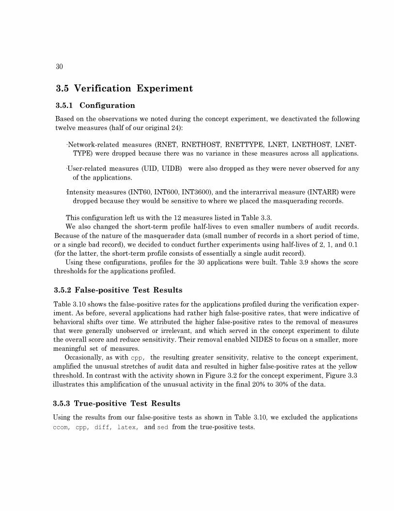
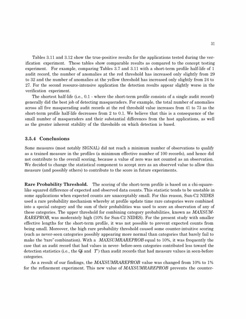
3.1 Plot of Application ccom Scores during Concept Experiment False-positive Testing . 273.2 Plot of Application cpp Scores during Concept Experiment False-positive Testing . . 353.3 Plot of Application cpp Scores during Verification Experiment False-positive Testing 353.4 Measure S-values for Grep and Latex . . . . . . . . . . . . . . . . . . . . . . . . . . 453.5 Long-term Profile Category Bins for Application Grep (Measures I/O and MEMUSE) 463.6 Long-term Profile Category Bins for Application Grep (Measures MEMCMB and

O P E N F ) . . . . . . . . . . . . . . . . . . . . . . . . . . . . . . . . . . . . . . . . . . . 4 73.7 Long-term Profiles Category Bins for Application Grep (Measures PGFLT and PGIN) 483.8 Long-term Profiles Category Bins for Application Grep (Measures PRCTIME and

SIGNAL) . . . . . . . . . . . . . . . . . . . . . . . . . . . . . . . . . . . . . . . . . . 493.9 Long-term Profiles Category Bins for Application Grep (Measures SCPU and

T E X T S Z ) . . . . . . . . . . . . . . . . . . . . . . . . . . . . . . . . . . . . . . . . . . 5 03.10 Long-term Profiles Category Bins for Application Grep (Measure UCPU) . . . . . . 513.11 Average Measure S-values over all Three experiments . . . . . . . . . . . . . . . . . . 53

iii

List of Tables

2.1 Safeguard Audit Data Mappings to Measures . . . . . . . . . . . . . . . . . . . . . . 10

3.1 Audit Data Set Summary . . . . . . . . . . . . . . . . . . . . . . . . . . . . . . . . . 163.2 Experiment Subjects and Numbers of Audit Records . . . . . . . . . . . . . . . . . 173.3 Measures Used for Experiments . . . . . . . . . . . . . . . . . . . . . . . . . . . . . . 193.4 Safeguard Experiment Configuration Summary . . . . . . . . . . . . . . . . . . . . . 203.5 Score Thresholds for the Concept Experiment . . . . . . . . . . . . . . . . . . . . . . 253.6 False-positive Rates (percent) for the Concept Experiment . . . . . . . . . . . . . . . 263.7 True-positive Results for the Concept Experiment (Masquerading Application#1) . 283.8 True-positive Results for the Concept Experiment (Masquerading Application #2) . 293.9 Score Thresholds for the Verification Experiment . . . . . . . . . . . . . . . . . . . . 333.10 False-positive Rates (percent) for the Verification Experiment . . . . . . . . . . . . . 343.11 True-positive Results from Verification Experiment (Masquerading Application #1) 363.12 True-positive Results for the Verification Experiment (Masquerading Application #2) 373.13 Score Thresholds for the Refinement Experiment . . . . . . . . . . . . . . . . . . . . 413.14 False-positive Rates (percent) for the Refinement Experiment . . . . . . . . . . . . . 423.15 True-positive Results from Refinement Experiment (Masquerading Application #1) . 433.16 True-positive Results from Refinement Experiment (Masquerading Application #2) . 443.17 True-positive Comparison for Three Experiments . . . . . . . . . . . . . . . . . . . . 523.18 Cross Profile Chart (26 subjects, 1% threshold level) . . . . . . . . . . . . . . . . . . 563.19 Cross Profile Chart-Continued (26 subjects, 1% threshold level) . . . . . . . . . . . . 573.20 True-positive Percentages for Cross-Profiling Experiment . . . . . . . . . . . . . . . . 583.21 Application Pairs for which Both True-positive Rates are ≤ 20 % . . . . . . . . . . . 633.22 Distance Based on Scoring Mechanism - NIDES-Based Grouping . . . . . . . . . . . 643.23 Distance Based on Scoring Mechanism - Functional Grouping . . . . . . . . . . . . . 643.24 Profile Overlap - NIDES-Based Grouping . . . . . . . . . . . . . . . . . . . . . . . . 653.25 Profile Overlap - Functional-Based Grouping . . . . . . . . . . . . . . . . . . . . . . 653.26 Score Thresholds for Group Experiment . . . . . . . . . . . . . . . . . . . . . . . . . 663.27 False-positive Rates for the Group Experiment . . . . . . . . . . . . . . . . . . . . . 67

v

vi

3.28 True-positive Chart for Grouping Experiments . . . . . . . . . . . . . . . . . . . . . 673.29 Anomaly Rates for Group Cross profiling - Half-life = 0.1 . . . . . . . . . . . . . . . 68

Chapter 1

Introduction

As part of the Audit Data Analysis task of the Safeguard project, SRI has been under contractto Trusted Information Systems (TIS) to evaluate the ability of the Next-generation IntrusionDetection Expert System (NIDES) to detect the use of computer systems for other than authorizedapplications.

The principal goal of the Safeguard Audit Data Analysis task was to explore methods of de-tecting and reporting attempts by those whose use of exported computer systems is restricted toapproved applications or classes of applications, to bypass or defeat those software execution re-strictions. As part of this task, audit trail analysis techniques were considered as potentially usefulin detecting misuse of restricted technology.

To date, NIDES has been used to monitor computer users by examining audit trail informationusing a custom non-parametric statistical component as well as a rule-based component. In theparadigm explored by SRI [1, 2, 4, 5], the subjects considered up to now have been computerusers. For the present study, the methodology is adapted to consider applications as subjects. Thisdirectly addresses the stated goal of monitoring usage to detect unauthorized use of applicationsor application classes on restricted systems. With recent changes in export restrictions, this goalis perhaps less urgent now than when the study was undertaken. Nonetheless, the methodology asadapted here is useful in the detection of Trojan horses and other masquerading applications.

This report presents the findings of SRI�s analysis of the NIDES statistical analysis component�sability to detect unauthorized application execution based on system-level audit trails.

1.1 Project Description

SRI developed a set of audit analysis techniques to support detection of the use of computersystems for other than authorized applications in environments in which users are permitted todevelop and install their own application software. The analysis software developed for this project

1

2

was a straightforward adaptation of the current NIDES software, specifically the NIDES statisticalanalysis component.

Our efforts were divided into the following general tasks:

In conjunction with TIS, we determined the available and appropriate audit data sets thatcould be collected for analysis purposes. As part of this process TIS converted the datainto the NIDES audit record format. TIS provided all the audit data we used in developingprofiles of acceptable application behavior and performing experiments in detecting abnormalactivity.

We modified the NIDES statistical analysis software to support our experiments. Most of ourmodifications were to support the use of a set of statistical measures suitable for analyzingthe audit data provided by TIS. These modifications included code changes as well as changesto the NIDES configuration files associated with the statistical analysis component.

We performed five complete experiments:

Three experiments - concept, verification, and refinement - were run to determine themost suitable configurations for the Safeguard application of NIDES. Each of these firstthree experiments included the following steps:

1. We set up a predetermined set of configurations for the experiment. Each experimentwe ran had a different configuration.

2. We ran TIS-supplied audit data through the statistical analysis component of NIDESto develop baseline profiles of applications.

3. We performed false-positive tests on the profiles developed to determine if the profilewas stable enough to be used in subsequent tests.

4. We ran tests using data that included masquerading applications to perform true-positive testing.

5. We reviewed the results of the experiment to determine the appropriate configurationfor subsequent experiments. Our goal was to improve NIDES performance as our

�experiments progressed.

- For our fourth experiment we ran a cross-profiling experiment to perform additionaltrue-positive testing, using the configuration setting of our refinement experiment.

- Lastly, we performed experiments with application groups using information gatheredduring the cross-profiling experiment.

Overall our results from the first (concept) experiment to our third (refinement) experimentimproved. We had higher detection rates and generally lower false-positive rates. The cross-profiling experiment gave us additional insight into similarities of the applications in our test set

3

and how easily one application in the test set could masquerade as another application in the testset. We also gained some understanding of the results one obtains when profiling application groupsinstead of individual applications - in general, the ability to detect anomalous activity (detectionsensitivity) seemed to decrease when we worked with application groupings.

1.2 NIDES Statistical Algorithm Description

In this section, we provide an overview of the NIDES statistical algorithm, for a more detaileddescription, see [3].

The statistical approach used in NIDES is to compare a subject�s short-term behavior withthe subject�s historical or long-term behavior. In the traditional NIDES framework, a subject is auser of a computer system. In the Safeguard context, a subject is an application. In comparingshort-term behavior with long-term behavior, the statistical component is concerned both with long-term behaviors that do not appear in short-term behavior, and with short-term behaviors that arenot typical of long-term behavior. Whenever short-term behavior is sufficiently unlike long-termbehavior, a warning flag is raised. In general, short-term behavior is somewhat different fromlong-term behavior, because short-term behavior is more concentrated on specific activities andlong-term behavior is distributed across many activities. To accommodate this expected deviationbetween short-term and long-term behavior, the NIDES statistical component keeps track of theamount of deviation that it has seen in the past between a subject�s short-term behaviors and long-term behaviors. The NIDES statistical component issues a warning only if the current short-termbehavior is very unlike long-term behavior relative to the amount of deviation between these typesof behaviors that it has seen in the past.

The NIDES statistical approach requires no a priori knowledge about what type of behaviorwould result in compromised security. It simply compares short-term and long-term behaviors todetermine whether they are statistically similar. This feature of the NIDES statistical componentmakes it ideally suited for the Safeguard task. A masquerading application does not compromisesecurity in any of the typical ways, but nevertheless is an event that is anomalous and warrantsdetection. If the masquerading application has different characteristics from the application whoseidentity is being expropriated (and the short-term behavior for the application whose identity isbeing expropriated is not too erratic), the NIDES statistical component should be able to recognizethese differences and identify the masquerade.

1.2.1 Measures

Aspects of subject behavior are represented as measures (e.g., file access, CPU usage, hour of use).For each measure, we construct a probability distribution of short-term and long-term behaviors.For example, for the measure of file access, the long-term probability distribution would consistof the historical probabilities with which different files have been accessed, and the short-term

4

probability distribution would consist of the recent probabilities with which different files havebeen accessed. In this case, the categories to which probabilities are attached are the file names.In the case of continuous measures, such as CPU time, the categories to which probabilities areattached are ranges of values, which we sometimes refer to as �bins� (these ranges of values aremutually exclusive and span all values from 0 to infinity). We refer to the collection of measuresand their long-term probability distributions as the subject�s profile.

We have classified the NIDES measures into four groups: activity intensity, audit record dis-tribution, categorical, and continuous. These different types of measures serve slightly differentpurposes. The activity intensity measures determine whether the volume of activity generated isnormal. The audit record distribution measure determines whether, for recently observed activity(say, the last few hundred audit records generated), the types of actions being generated are nor-mal. The categorical and continuous measures determine whether, within a type of activity (say,accessing a file), the types of actions being generated are normal.

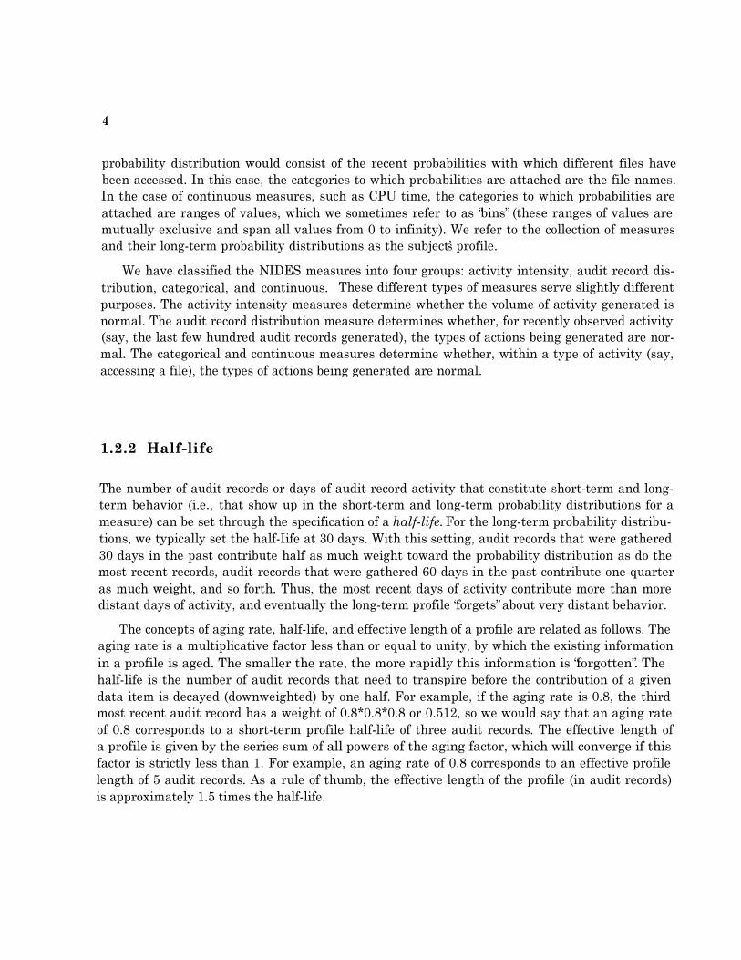
1.2.2 Half-life

The number of audit records or days of audit record activity that constitute short-term and long-term behavior (i.e., that show up in the short-term and long-term probability distributions for ameasure) can be set through the specification of a half-life. For the long-term probability distribu-tions, we typically set the half-Iife at 30 days. With this setting, audit records that were gathered30 days in the past contribute half as much weight toward the probability distribution as do themost recent records, audit records that were gathered 60 days in the past contribute one-quarteras much weight, and so forth. Thus, the most recent days of activity contribute more than moredistant days of activity, and eventually the long-term profile �forgets� about very distant behavior.

The concepts of aging rate, half-life, and effective length of a profile are related as follows. Theaging rate is a multiplicative factor less than or equal to unity, by which the existing informationin a profile is aged. The smaller the rate, the more rapidly this information is �forgotten�. Thehalf-life is the number of audit records that need to transpire before the contribution of a givendata item is decayed (downweighted) by one half. For example, if the aging rate is 0.8, the thirdmost recent audit record has a weight of 0.8*0.8*0.8 or 0.512, so we would say that an aging rateof 0.8 corresponds to a short-term profile half-life of three audit records. The effective length ofa profile is given by the series sum of all powers of the aging factor, which will converge if thisfactor is strictly less than 1. For example, an aging rate of 0.8 corresponds to an effective profilelength of 5 audit records. As a rule of thumb, the effective length of the profile (in audit records)is approximately 1.5 times the half-life.

5

1.2.3 Differences between Long- and Short-term Profiles � The Q Statistic

The degree of difference between a long-term profile for a measure and the short-term profile for ameasure is quantified using a chi-square-like statistic, with the long-term profile playing the �role� ofthe actual probability distribution and the short-term profile playing the �role� of the observations.We call the resultant numerical value Q. (There is a different Q value for each measure.) Largevalues of Q mean that the long-term and short- term profiles for the measure are very differentfrom one another and therefore warrant some suspicion; a Q value of zero means that they agreecompletely.

In calculating the Q statistic,, we need to refer to the categories that have been defined foreach measure. As with the chi-square statistic, it is desirable that categories that are rarely ornever observed in the long-term distribution be collapsed together. In NIDES we have defined aparameter that controls how many categories are collapsed together. This parameter sets an upperlimit on the combined probability of all category bins that are considered rare for scoring purposes.We continue to combine categories into the �rare� category, starting with the category with thesmallest long-term probability, as long as the total long-term probability of all of the collapsedcategories is less than the value for this parameter.

For each audit record, the NIDES statistical component generates a vector of Q values, withlarge values indicating suspicious activity. But, how large a Q value is too large? Unfortunately, itis not possible to refer Q directly to a chi-square table of cutoff values to determine if the differencebetween the two probability distributions is statistically significant. The traditional chi-squaremethod cannot be applied in environments where the audit records that contribute to the short-term profiles are not independent, nor in systems where the short-term profiles are based upon veryfew audit records. Since the distribution of Q is not chi-squared, we need to track its values todetermine what its distribution looks like. Every time another audit record arrives, a new value of Qis generated. We observe these values over a substantial portion of the profile-building period. Webegin to observe Q values during the second stage of the profile-building period, which commencesas soon as we have constructed reasonably stable historical profiles for the observed categories. Weuse these values for Q to build a long-term probability distribution for Q. (Each measure has itsown Q and a long-term distribution for that Q statistic.) The Q distributions look somewhat likelong-tailed and stretched-out chi-square distributions.

1.2.4 Scoring Anomalous Behavior - The S and T2 Statistic

As with all other long-term distributions in NIDES, the long-term distribution of Q is categorizedinto ranges of values (called bins). From this distribution, we can obtain the tail probability ofobtaining a value for Q at least as great as the observed value. We transform this tail probabilityand denote the transformed variable as S, and define the transformation so that S has a half-normaldistribution. (A half-normal distribution looks like the right-hand side of a normal distribution,

6

except that the height of the probability distribution is doubled so that there is still unit area underthe curve. This is also the distribution of the absolute value of a normally distributed variable.)The mapping from tail probabilities of the Q distribution to half-normal values requires only a tableof normal probabilities. For example, if the current Q statistic is at its 80th percentile (i.e., the tailprobability is 20%), then the corresponding value for S is 1.28 (i.e., the same as the 90th percentileof a normal distribution). If the current Q statistic is at its 90th percentile, the corresponding valuefor S is 1.65 (i.e., the same as the 95th percentile of a normal distribution).

As each audit record is received, it is possible to generate the corresponding vector of S values.High S values correspond to measures that are unusual relative to the usual amount of discrepancythat occurs between long-term and short-term profiles. Small S values correspond to measures thatare not unusual relative to the amount of discrepancy that typically occurs between long-term andshort-term profiles. We combine the S scores into an overall statistic that we call T2. The T2

statistic is a summary judgment of the abnormality of many measures, and is in fact the sum ofthe squares of the S statistics (i.e., where there are m measures).

Because each S statistic follows the same half-normal distribution (when the audit recordsbeing observed come from the subject who owns the account), the T2 statistic is approximatelydistributed like a chi-squared variable with m degrees of freedom. However, the are not necessar-ily independent, so rather than rely on the chi-square distribution to provide threshold values forT2, we build a long-term distribution for T2

. We then observe the upper threshold values for T2.(The long-term distribution for T2 is built during the last stage of the profile building period, afterreasonably stable long-term distributions for the Q statistics have been constructed.) We declarerecent audit records to be anomalous at the �yellow� level whenever the T2 value is over the 1%value of the long-term profile for T2, and at the �red� level whenever the T2 is over the 0.1% ofthe long-term profile.

Chapter 2

Customizations for Safeguard

In preparation for our experiments, we made some modifications to the NIDES statistical analysiscomponent software and examined the various configurable items to determine the best configu-rations to use under the Safeguard context. These changes were needed because of three primarydifferences between the Safeguard and Sun-C2 applications of NIDES.

First, the volume of audit data under the Safeguard application was substantially less than thevolume of data we see under the Sun-C2 environment. The number of audit records generated inthe Safeguard application for a single activity is far fewer than the number in traditional NIDESapplications for that same activity. Under BSM or C2 auditing, a single user will generate as manyaudit records in a single day as were obtained for the application with the most audit records overa single month in the Safeguard data.

Second, the nature of the Safeguard audit data is different in that it captures, in a single auditrecord, all the information for a single instance of an application use, while within the Sun-C2context we would build the analogous information from a large number of audit records, each ofwhich might affect one or a few of the possible measures. With the C2 audit data it would taketens or hundreds of audit records to represent� a single user activity, whereas in the Safeguard auditdata each use of an application is reflected in a single audit record. Lastly, the safeguard data hadapplications, rather than users as subjects.

Furthermore, the objective of the Safeguard study was to flag small numbers or even singleinstances of anomalous activity, whereas Sun-C2 was tuned to detect a time interval (correspondingto hundreds of audit records or more) of such activity.

2.1 New Measures

The set of measures was modified to include behavior aspects that pertain specifically to applica-tions, such as process time, detailed CPU and memory usage, and page faults. All of these new

7

8

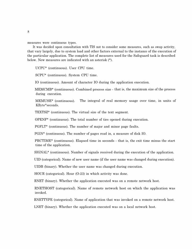
measures were continuous types.It was decided upon consultation with TIS not to consider some measures, such as swap activity,

that vary largely, due to system load and other factors external to the instance of the execution ofthe particular application. The complete list of measures used for the Safeguard task is describedbelow. New measures are indicated with an asterisk (*).

UCPU* (continuous). User CPU time.

SCPU* (continuous). System CPU time.

IO (continuous). Amount of character IO during the application execution.

MEMCMB* (continuous). Combined process size - that is, the maximum size of the processduring execution.

MEMUSE* (continuous). The integral of real memory usage over time, in units ofKByte*seconds.

TEXTSZ* (continuous). The virtual size of the text segment.

OPENF* (continuous). The total number of ties opened during execution.

PGFLT* (continuous). The number of major and minor page faults.

PGIN* (continuous). The number of pages read in, a measure of disk IO.

PRCTIME* (continuous). Elapsed time in seconds - that is, the exit time minus the starttime of the application.

SIGNAL* (continuous). Number of signals received during the execution of the application.

UID (categorical). Name of new user name (if the user name was changed during execution).

UIDB (binary). Whether the user name was changed during execution.

HOUR (categorical). Hour (O-23) in which activity was done.

RNET (binary). Whether the application executed was on a remote network host.

RNETHOST (categorical). Name of remote network host on which the application wasinvoked.

RNETTYPE (categorical). Name of application that was invoked on a remote network host.

LNET (binary). Whether the application executed was on a local network host.

9

LNETHOST (categorical). Name of local network host on which this application was invoked.

LNETTYPE (categorical). Name of application that was invoked on a local network host.

INTARR (continuous). Number of seconds elapsed since the last audit record for this appli-cation.

I60 (continuous/intensity). Rate of audit record activity every 60 seconds (1 minute).

I600 (continuous/intensity). Rate of audit record activity every 600 seconds (10 minutes).

I3600 (continuous/intensity). Rate of audit record activity every 3600 seconds (1 hour).

Only one module in the statistical component was changed to support these new measures,namely the function that converts the audit data into activity records. Table 2.1 lists the relevantdata fields TIS provided in the audit data (NIDES format) and the corresponding measures towhich the fields were mapped.

2.2 Configuration Items

A number of parameters within the statistical component can be configured to support any partic-ular system. On the following list, those items marked with an asterisk were modified according tothe particular experiment(s) we ran. These modifications are discussed in detail in Section 3.

l Short-term profile half-life *. This is the half-life of the short-term profile, measured in auditrecord counts.

l Long-term profile half-life. This is the half-life of the long-term profile measured in days.

l Threshold percentages (yellow, red). These percentages respectively represent the warningand critical thresholds at which anomalous activity is reported.

l Minimum effective-N. This is the effective minimum number of audit records necessary for aparticular measure to be considered �trained� so that it may contribute to the overall scoring.

l Training days. This is the number of days required for the long-term profile to be trained.Scores produced by the statistical component during this training period are considered un-stable and are thus ignored.

l Scalar Values. These numbers are used to scale observed values for continuous measures inorder to assign the values to bins. The scalar values estimate a value beyond the maximumvalue that we ever expect to see for a continuous measure (i.e., the mean value plus fourstandard deviations). A scalar value was calculated for each continuous measure.

10

NIDES Audit Field TIS Data Description

atime Exit Time

hostname �SOL�

actionaunameounamepidttynameargcount

syscallerrnorvalres_utimeres_stimeres_rtimeres_memres_iores_rw

�IA_EXIT�command name

(empty)Integral of Memory Usage

Terminal NameText Size

Open FilesPage Faults

Page InsUser Time

System TimeElapsed Process TimeCombined Process Size

Character IOS i g n a l s

Corresponding Measure

HOUR, INTARRI60, I600, I3600

RNET,RNETHOST,RNETTYPELNET,LNETHOST,LNETTYPE

(None)(NIDES subject name)

UID, UIDBMEMUSE

(None)TEXTSZOPENFPGFLTPGINUCPUSCPU

PRCTIMEMEMCMB

IOSIGNAL

Table 2.1: Safeguard Audit Data Mappings to Measures

11

Q Max values. These numbers are used to scale Q values for all measures. These valuesplay the same role for Q scores that the scalar values play for raw observations of continuousmeasures.

Modes of operation *. The statistical component can be run in various modes, such as trainingor testing mode. One common testing mode is to disable the long-term profile updater, sothat audit records are scored against trained profiles, but the profiles do not adapt to thenew data.

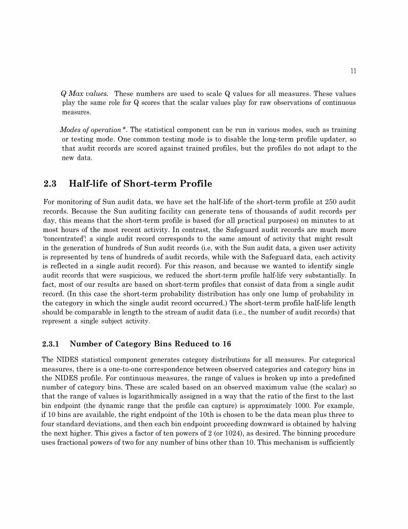
2.3 Half-life of Short-term Profile

For monitoring of Sun audit data, we have set the half-life of the short-term profile at 250 auditrecords. Because the Sun auditing facility can generate tens of thousands of audit records perday, this means that the short-term profile is based (for all practical purposes) on minutes to atmost hours of the most recent activity. In contrast, the Safeguard audit records are much more�concentrated�; a single audit record corresponds to the same amount of activity that might resultin the generation of hundreds of Sun audit records (i.e, with the Sun audit data, a given user activityis represented by tens of hundreds of audit records, while with the Safeguard data, each activityis reflected in a single audit record). For this reason, and because we wanted to identify singleaudit records that were suspicious, we reduced the short-term profile half-life very substantially. Infact, most of our results are based on short-term profiles that consist of data from a single auditrecord. (In this case the short-term probability distribution has only one lump of probability inthe category in which the single audit record occurred.) The short-term profile half-life lengthshould be comparable in length to the stream of audit data (i.e., the number of audit records) thatrepresent a single subject activity.

2.3.1 Number of Category Bins Reduced to 16

The NIDES statistical component generates category distributions for all measures. For categoricalmeasures, there is a one-to-one correspondence between observed categories and category bins inthe NIDES profile. For continuous measures, the range of values is broken up into a predefinednumber of category bins. These are scaled based on an observed maximum value (the scalar) sothat the range of values is logarithmically assigned in a way that the ratio of the first to the lastbin endpoint (the dynamic range that the profile can capture) is approximately 1000. For example,if 10 bins are available, the right endpoint of the 10th is chosen to be the data mean plus three tofour standard deviations, and then each bin endpoint proceeding downward is obtained by halvingthe next higher. This gives a factor of ten powers of 2 (or 1024), as desired. The binning procedureuses fractional powers of two for any number of bins other than 10. This mechanism is sufficiently

12

robust that the scaling maxima need not be accurately estimated; errors of a factor of 2 or even 4are easily tolerated.

The Sun-C2 application of NIDES classifies continuous data into 32 bins with �third root oftwo� bin spacing, so that 30 bins give the desired dynamic range with some overflow bins left.This is appropriate with an effective profile length of hundreds of audit records, as on the average areasonable number of the category bins will be populated. However, in the Safeguard application, wehave very short effective profile lengths and the short-term profile has a very �lumpy� distribution(indeed, only one bin is touched per measure if the short-term profile consists of a single auditrecord). For this reason, we reduced the number of bins into which continuous measures areclassified to 16 with the appropriate fractional logarithmic spacing to give a dynamic range of 1000with some overflow bins. Examination of the long-term profiles generated using 16 bins indicateda reasonable population of a broad middle range of the bins and sparse or no population of theextremes, so that we believe the range, scaling, and number of bins were appropriate for theSafeguard data. The number of Q bins was also reduced from 32 to 16.

Scalars and QMaxes As part of the binning process, scalar and QMAX values are used todetermine bin locations. To get the desired range of binning for continuous measures, we scannedall audit data files and noted the mean and variances of the observed values for each continuousmeasure. From these values, we computed the standard deviation and set the scalar value to besomewhere between 3 to 4 times the standard deviation (we ended up rounding off scalar values).Observed values were then placed in bins based upon this scalar value according to the approachdiscussed above.

Obtaining QMAX values required a small amount of statistical processing. The first stage ofthe training period was allowed to complete (typically in ten days worth of data) and then a day�sworth of Q values were collected across all subjects. The QMAX value was then set at the Q scoremean plus 3 to 4 standard deviations.

2.4 Statistical Component Wrapper

A special �wrapper� was developed to isolate the statistical component for experimentation (thecurrent NIDES system includes a rulebased component, a resolver, and a user interface). This wrap-per simplified the customization process of statistical configuration, and also enabled a relativelyquick turn-around time for setting up and running experiments.

This wrapper is similar to the batch analysis version of NIDES, but does not contain therulebased component. It can be invoked directly from the Unix shell, and reads NIDES auditrecords directly from a file or a list of files.

More than one option can be specified in one invocation of the wrapper, which has the followingfeatures:

13

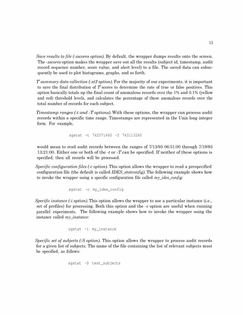
Save results to file (-xscores option). By default, the wrapper dumps results onto the screen.The -xscores option makes the wrapper save out all the results (subject id, timestamp, auditrecord sequence number, score value, and alert level) to a file. The saved data can subse-quently be used to plot histograms, graphs, and so forth.

T2 summary data collection (-xt2 option). For the majority of our experiments, it is importantto save the final distribution of T2 scores to determine the rate of true or false positives. Thisoption basically totals up the final count of anomalous records over the 1% and 0.1% (yellowand red) threshold levels, and calculates the percentage of these anomalous records over thetotal number of records for each subject.

Timestamp ranges (-t and -T options). With these options, the wrapper can process auditrecords within a specific time range. Timestamps are represented in the Unix long integerform. For example,

sgstat -t 742571460 -T 743113260

would mean to read audit records between the ranges of 7/13/93 06:51:00 through 7/19/9313:21:00. Either one or both of the -t or -T can be specified. If neither of these options isspecified, then all records will be processed.

Specific configuration files (-c option). This option allows the wrapper to read a prespecifiedconfiguration file (the default is called IDES_statconfig). The following example shows howto invoke the wrapper using a specific configuration file called my_ides_config:

sgstat -c my_ides_config

Specific instance (-i option). This option allows the wrapper to use a particular instance (i.e.,set of profiles) for processing. Both this option and the -c option are useful when runningparallel experiments. The following example shows how to invoke the wrapper using theinstance called my_instance:

sgstat -i my_instance

Specific set of subjects (-S option). This option allows the wrapper to process audit recordsfor a given list of subjects. The name of the file containing the list of relevant subjects mustbe specified, as follows:

sgstat -S test_subjects

14

2.5 Utilities

A number of software utilities were used or developed to aid in the execution and analysis of ourSafeguard experiments. Many of these utilities already existed in some form, and were modified toaccommodate the particular needs of this project.

arcount. This utility was used during the audit record analysis task. It reads a list of auditdata files (in NIDES format) and summarizes the audit record distribution by printing outhow many audit records were available for each subject on a daily basis. This utility allowedus to determine which subjects (applications) were eligible for our experiments (see Section3.1).

tchange. This utility was used throughout our experiments. It shifts the timestamps in agiven NIDES audit data file in any direction (later or earlier). This tool allowed us to selectportions of the various data files and concatenate them together in a desired chronologicalorder to represent continuous activity.

data_make. This utility was used to create masquerader data. Given an input file, output file,subject name that will be masquerading, and the subject it will pretend to be, this utilitychanges the identity of selected audit data. Audit record order is preserved and the resultingdata set is written to a specified file.

change_prof. This utility changes the timestamp of any given profile, and also changes itssubject name. The utility was particularly useful for the cross-profiling experiments (seeSection 3.7), as well as for synchronizing profile dates to correspond with a particular auditdata set.

dump_prof. This utility dumps out entire profile contents (both short-term snapshots andlong-term) of any given subject. The contents can either be displayed on the screen or savedinto a file.

bins and whichbins. These utilities were used to analyze continuous measures. Bins prints outthe ranges of the bins given a maximum value for scaling, and whichbins indicates which bina given value would fall into. These utilities were used as an aid to create profile histograms.

We also used a few COTS applications, such as xgraph and wingz, to create graphs and charts.

Chapter 3

Experiment Descriptions

TIS supplied approximately three months of audit data to SRI. We performed five major experi-ments using this data.

3.1 Audit Data Analysis and Organization

As part of our experiment preparation, we analyzed the audit data to ascertain the overall charac-teristics of the data (volume, daily activity, distribution of activity). From this preliminary analysis,we determined which applications were good subject candidates and which audit data fields (hencemeasures) were sufficiently available to conduct our experiments.

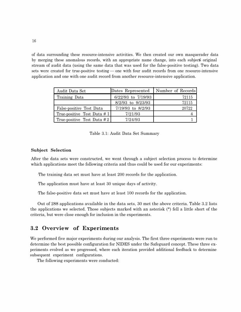
We organized the TIS audit data into three parts. Table 3.1 summarizes the audit data setswe used for our experiments. The first data set was used to train NIDES historical profiles, thatis, historical bin probabilities, the empirical distribution of audit record Q and T2 scores, and theyellow and red thresholds of the T2 statistic. As it was essential to collect enough volume andvariety of data to incorporate each subject�s full spectrum of behavior into its profile, we used(approximately) two months of activity.

The second data set supplied previously unseen application data that was scored against thatapplication�s historical profile, and the rate of exceedances above the threshold tabulated. Suchexceedances are termed �false-positives� because they represent records identified by NIDES asbeing above a detection threshold when it is known that they are not masqueraders. This is asopposed to �true-positives,� that is, application records that when scored against another applica-tion�s profile exceed the detection threshold. The false-positive rate for NIDES or any detectionsystem that learns patterns should always be estimated using data not used in the learning phase,as we do here.

The third data set was used to conduct true-positive tests. TIS had indicated to us where tworesource-intensive applications were being monitored, and we selected approximately 2 to 3 weeks

15

16

of data surrounding these resource-intensive activities. We then created our own masquerader databy merging these anomalous records, with an appropriate name change, into each subject�s originalstream of audit data (using the same data that was used for the false-positive testing). Two datasets were created for true-positive testing � one with four audit records from one resource-intensiveapplication and one with one audit record from another resource-intensive application.

Audit Data Set Dates Represented Number of Records

Training Data 6/22/93 to 7/19/93 721158/2/93 to 9/23/93 72115

False-positive Test Data 7/19/93 to 8/2/93 20722True-positive Test Data # l 7/21/93 4True-positive Test Data # 2 7/24/93 1

Table 3.1: Audit Data Set Summary

Subject Selection

After the data sets were constructed, we went through a subject selection process to determinewhich applications meet the following criteria and thus could be used for our experiments:

· The training data set must have at least 200 records for the application.

· The application must have at least 30 unique days of activity.

· The false-positive data set must have at least 100 records for the application.

Out of 288 applications available in the data sets, 30 met the above criteria. Table 3.2 liststhe applications we selected. Those subjects marked with an asterisk (*) fell a little short of thecriteria, but were close enough for inclusion in the experiments.

3.2 Overview of Experiments

We performed five major experiments during our analysis. The first three experiments were run todetermine the best possible configuration for NIDES under the Safeguard concept. These three ex-periments evolved as we progressed, where each iteration provided additional feedback to determinesubsequent experiment configurations.

The following experiments were conducted:

17

This table lists the number of audit records used for our experiments for each application profiled. The trainingrecord counts represent the number of records that were used to train profiles; the test record counts represent thenumber of records that were used during the false-positive testing phase of the experiments. The column showingunique days lists the number of days for each subject for which any audit record data were available.Note: * indicates a borderline subject.

Table 3.2: Experiment Subjects and Numbers of Audit Records

18

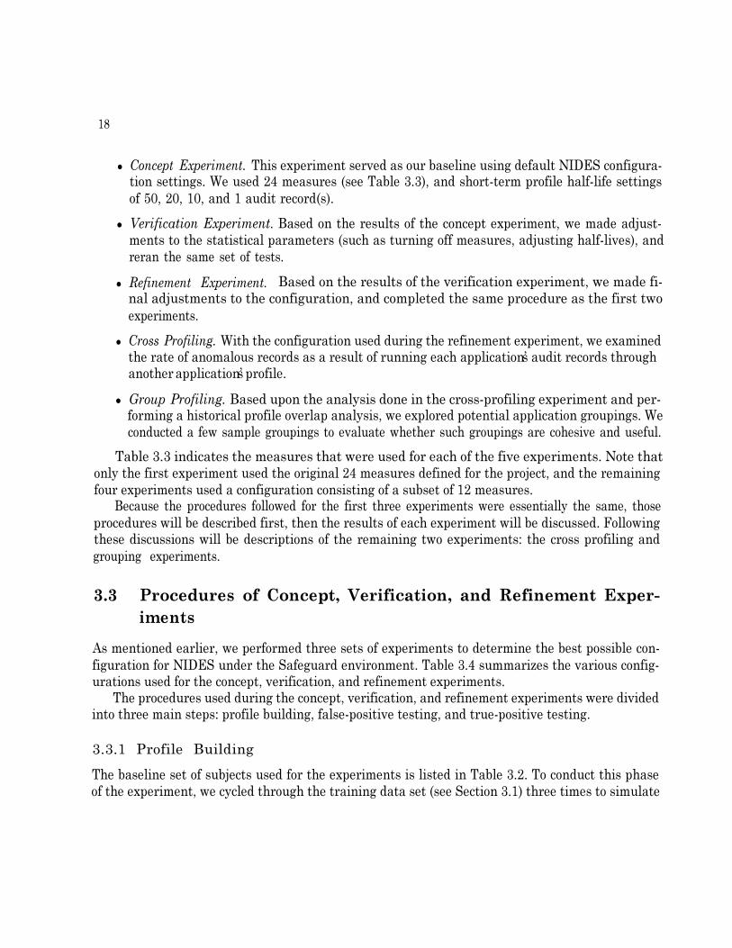
l Concept Experiment. This experiment served as our baseline using default NIDES configura-tion settings. We used 24 measures (see Table 3.3), and short-term profile half-life settingsof 50, 20, 10, and 1 audit record(s).

l Verification Experiment. Based on the results of the concept experiment, we made adjust-ments to the statistical parameters (such as turning off measures, adjusting half-lives), andreran the same set of tests.

l Refinement Experiment. Based on the results of the verification experiment, we made fi-nal adjustments to the configuration, and completed the same procedure as the first twoexperiments.

l Cross Profiling. With the configuration used during the refinement experiment, we examinedthe rate of anomalous records as a result of running each application�s audit records throughanother application�s profile.

l Group Profiling. Based upon the analysis done in the cross-profiling experiment and per-forming a historical profile overlap analysis, we explored potential application groupings. Weconducted a few sample groupings to evaluate whether such groupings are cohesive and useful.

Table 3.3 indicates the measures that were used for each of the five experiments. Note thatonly the first experiment used the original 24 measures defined for the project, and the remainingfour experiments used a configuration consisting of a subset of 12 measures.

Because the procedures followed for the first three experiments were essentially the same, thoseprocedures will be described first, then the results of each experiment will be discussed. Followingthese discussions will be descriptions of the remaining two experiments: the cross profiling andgrouping experiments.

3.3 Procedures of Concept, Verification, and Refinement Exper-iments

As mentioned earlier, we performed three sets of experiments to determine the best possible con-figuration for NIDES under the Safeguard environment. Table 3.4 summarizes the various config-urations used for the concept, verification, and refinement experiments.

The procedures used during the concept, verification, and refinement experiments were dividedinto three main steps: profile building, false-positive testing, and true-positive testing.

3.3.1 Profile Building

The baseline set of subjects used for the experiments is listed in Table 3.2. To conduct this phaseof the experiment, we cycled through the training data set (see Section 3.1) three times to simulate

19

Table 3.3: Measures Used for Experiments

20

Experiment No. of Measures Half-lives Significant Differences in Experiments

Concept 24 50,20,10,1 Standard NIDES configurationVerification 12 2,1,0.1 Reduced number of measures;

smaller short-term profile half-livesRefinement 12 2,1,0.1 Rare probability sum reduced from 10% to 1%;

nonobservations counted

This table summarizes the configurations used during our first three experiments: concept, verification and refinement.The half-life column lists the short-term profile half-life configurations used. The significant changes column highlightsthe major differences between the experiments.

Table 3.4: Safeguard Experiment Configuration Summary

approximately 180 days (6 months) worth of data. We felt that this was sufficient to producereasonably stable historical profiles for each applications. These profiles were then saved to serveas baseline profiles for the false-positive and true-positive tests.

The following configurations were used during all the profile-building processes for all experi-ments where profiles were developed:

· False-positive thresholds were set to 1% (warning/yellow) and 0.1% (critical/red).

· The long-term half-life was set to 20 days.

· The profile-training period was set to 20 days.

· The minimum effective- N was set to 100 records. This value is essentially the minimumnumber of observations required for training before a measure can contribute to the statisticalscoring.

· From the historical profiles that were created, we obtained the yellow and red score thresholds andrecorded them into tables. These are the score thresholds used in determining the false-positiveand true-positive rates.

Because the threshold values are empirically determined, it is not possible to infer somethingabout the subject�s behavior by comparison to, say, a suitably normalized chi-square. Furthermore,with longer profile half-lives, the training data set contains a number of audit records that is onlya few times as long as the effective short-term profile length (see the glossary for a description ofprofile length). For example, with a short-term profile half-life of 50 records (which corresponds toan effective short-term profile length of about 75), a training data set of 300 records contains onlyfour independent realizations of the short-term profile. This renders estimates of the thresholds,particularly the red threshold (99.9 percentile) somewhat unstable.

21

For these reasons, comparing the score threshold values for an application from one half-lifeconfiguration to another does not give useful information. Within a given configuration (i.e. a setof measures and a single half-life), it is qualitatively true that the subjects with higher thresholdsare more forgiving of unusual activity, so that applications masquerading as these subjects wouldbe harder to detect.

3.3.2 False-positive Analysis

Our false-positive tests were performed using a set of never-seen-before data (approximately twoweeks worth), that is, data not used as part of the training process. Using the trained profiles builtearlier, we processed this new data and recorded the total number of records that exceeded theyellow and red thresholds. This number was then converted into a percentage that we refer to asthe false-positive rate for that subject.

The false-positive rate should be low, since we expect a subject�s behavior to be consistent withits past behavior. The false positive rate obtained from data unseen by the training mechanismwill generally be higher than the nominal rate NIDES uses when setting its threshold values. Assuch, we expect to see rates somewhat above the nominal 1% and 0.1% false positives (as expectedfor our nominal yellow and red threshold values). However, rates significantly higher than theseindicate some change in the nature of activity for the subject in question between the training andtest set (which we sometimes refer to as an �unstable� profile). A change in behavior is indicatedby a qualitative change in the graph of T2 versus time (Figure 3.1 in Section 3.4.5 is an example).Subjects with unacceptable false-positive rates were identified at this step.

For verification purposes, we also ran an additional false-positive test using the training dataset that was used to build the profiles. We expected to find, and did find, that the false-positiverates for the training set were very close to nominal levels (i.e., 1% and 0.1%), except when therewere insufficient numbers of audit records in the training set.

During the false-positive test, long-term profile updating was disabled so that potentially anoma-lous data would not be incorporated into the historical profile.

3.3.3 True-positive Analysis

We used the results of the false-positive tests to determine which subjects had reasonably stableprofiles with which to perform true-positive tests. The purpose of true-positive testing was to seeif or how soon anomalous records could be detected using the trained profiles created in the earlierprofile-building phase.

We had two data sets available for the true-positive testing (see Section 3.1). The first data setcontained four known anomalous records (produced by the same resource-intensive application),and the second data set contained one known anomalous record produced by another resource-intensive application.

22

For each subject we obtained a �score� value for each masquerading audit record and determinedif that score was above the red (0.1%) threshold, above the yellow (1%) threshold, or below boththresholds. If the score was above either boundary we considered it a successful detection. For eachapplication used in the true-positive test, we indicated for each anomalous audit record whetherthe record was detected as being abnormal (Table 3.7 in Section 3.4.5 is an example).

3.4 Concept Experiment

3.4.1 Configuration

Our baseline experiment was conducted using the following configurations:

· Twenty-four measures were used (see Table 3.3).

· Four different half-lives for the short-term profile were used: 50, 20, 10, and 1. In contrastto the tens of thousands of audit records that are generated in a Sun-C2 UNIX environment,Safeguard audit data records are much more concentrated; a single audit record correspondsto a complete instance of an activity. For this reason, and because we wanted to identifya handful of (or single) audit records that were suspicious, we started our baseline withsignificantly shorter half-lives when compared to the half-lives of hundreds of audit recordsused for the Sun-C2 data.

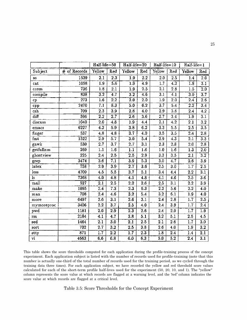
Using these configurations, profiles for 30 applications were built. Table 3.5 shows the scorethresholds for the applications profiled.

3.4.2 False-positive Test Results

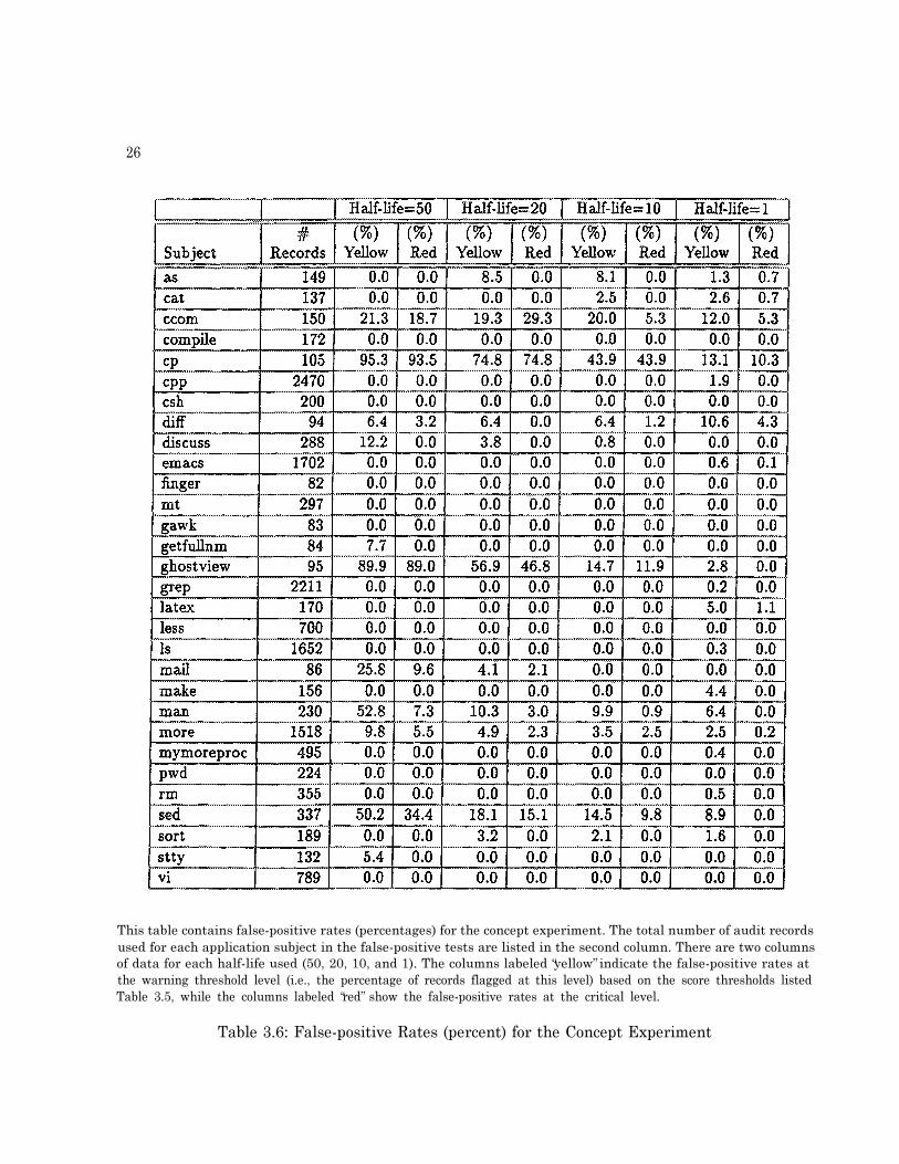
Table 3.6 shows the resultant false-positive rates for the applications profiled. The false-positiverates were unacceptably large for a number of applications (e.g., ccom, cp, ghostview, mail,man, and sed), particularly when the short-term profile half-lives were large (i.e., 50 or 20). Thelonger half-lives (50, 20, and even 10) displayed much higher false-positive rates because the longerhalf-lives split the data into too few independent observations for statistical stability meaning thatthe short-term profile (i.e, there were only a small number of independent realizations of the short-term profile - see Section 3.3.1 and the glossary for discussion of profile realizations).

This aspect of the data (i.e., decreasing false-positive rates with decreasing half-life rates) alsocaused us to conclude that there were small shifts in the behavior of the subjects during the testingperiod. It is these kind of shifts that are most easily detected when larger half-life configurationsare used.

To establish the existence of pattern shifts, we looked at plots of T2 (the detection score) versustime. Figure 3.1 shows such a plot for ccom, in which there is an apparent shift in behavior toward

23

the last part of the graph. This plot indicates a period in the testing data when there were markedchanges in the subject�s behavior.

We discussed this finding with TIS staff, and they could offer no explanation of why suchchanges would occur. We decided that these changes were sufficiently small with the shorter half-lives and that we could continue on to true-positive testing if we used shorter half-life (on theorder of one audit record) configurations. In addition, given the objective of this project, such areduction in half-life would be desirable for reasons other than ensuring a reasonable false-positiverate. However, five applications (ccom, cp, ghostview, man, and sed) had sufficiently large false-positive rates at the red threshold with a half-life of 1 that we believed that these applications hadtemporarily unstable profiles and hence would not be used during our true-positive tests.

3.4.3 True-positive Test Results

Using the results from our false-positive test, as shown in Table 3.6, we excluded the applicationsccom, cp, ghostviev, man, and sed from the true-positive tests. These applications exhibitedan unusually high false-positive rate, and were deemed unusable for the true-positive tests (unpre-dictable results).

Tables 3.7 and 3.8 summarize the results of the two true-positive tests. Each subject containsinformation regarding the number of records in its anomalous data-set, and the position of the four(or one) anomalous record(s) within the set. For each half-life, we have recorded an asterisk (*)for detection above the critical (red) threshold, a plus (+) for detection above the warning (yellow)threshold, and a dash (-) for no detection. Shorter half-lives were generally more successful thanlonger half-lives in detecting masqueraders, primarily because there were so few masquerader auditrecords. (If there had been more masquerader audit records, the longer half-lives would haveimproved success in detecting the masquerading episodes.) Because the results with smaller short-term profile half-lives were favorable, we decided to concentrate on shorter half-lives in the nextexperiment.

A half-life of 1 seemed to show some residual effects after the masquerader data disappeared.This effect occurred because with a half-life of 1 it takes about four audit records for a given auditrecord to be erased from the short-term profile. To allow the short-term profile to contain a singleaudit record, we decided to set the short-term half-life to some number smaller than 1 (say 0.1).This causes the previous audit record to contribute to the short-term profile, making theshort-term profile essentially equivalent to the current audit record.

3.4.4 Conclusions

Our decision to use smaller short-term profile half-lives in our next experiment also convinced usto drop the intensity and interarrival measures. These measures are less meaningful with smallershort-term profile half-lives and they can be affected by how the masquerader data was injected,

24

and thus give spurious detections. For the Sun version of NIDES, we were concerned about bursts ofthousands of audit records that could indicate an intrusion attempt. By contrast, for the Safeguardtask, we are actually trying to identify individual audit records that are masqueraders. If there werethousands (or even hundreds or tens) of masquerading audit records, we do not want to identifythem through increased volume; we would want to identify a large percentage of them individuallyas masqueraders.

3.4.5 Concept Experiment Figures and Tables

The following pages contain figures and tables showing the results of the concept experiments.

25

This table shows the score thresholds computed for each application during the profile-training process of the conceptexperiment. Each application subject is listed with the number of records used for profile-training (note that thisnumber is actually one-third of the total number of records used for the training period, as we cycled through thetraining data three times). For each application subject, we have recorded the yellow and red threshold score valuescalculated for each of the short-term profile half-lives used for the experiment (50, 20, 10, and 1). The "yellow"column represents the score value at which records are flagged at a warning level, and the �red� column indicates thescore value at which records are flagged at a critical level.

Table 3.5: Score Thresholds for the Concept Experiment

26

This table contains false-positive rates (percentages) for the concept experiment. The total number of audit recordsused for each application subject in the false-positive tests are listed in the second column. There are two columnsof data for each half-life used (50, 20, 10, and 1). The columns labeled �yellow� indicate the false-positive rates atthe warning threshold level (i.e., the percentage of records flagged at this level) based on the score thresholds listedTable 3.5, while the columns labeled �red� show the false-positive rates at the critical level.

Table 3.6: False-positive Rates (percent) for the Concept Experiment

27

The graph shown here represents a plot of the scores from the false-positive test for the application ccom. The x-axisrepresents the audit record number (starting from 0), and the y-axis indicates the anomaly score value of each recordfor that subject. (Note the behavior shift from about record 110 onward.)

Figure 3.1: Plot of Application ccom Scores during Concept Experiment False-positive Testing

28

This table shows the results of the first of two true-positive tests performed during the concept experiment. Thesecond column indicates the number of records used during the true-positive testing; the next column shows thepositions of the masquerader data in the application�s audit record stream. The remaining columns summarize theresults of the test for each short-term profile half-life used (50, 20, 10, and 1). Each half-life column contains fourcharacters indicating the results of each of the four masquerading records data going through the application�s profile.For each half-life, we have recorded an asterisk (*) for detection above the critical (red) threshold, a plus (+) fordetection above the warning (yellow) threshold, and a dash (-) for no detection.

Table 3.7: True-positive Results for the Concept Experiment (Masquerading Application #l)

29

This table shows the results of the second of two true-positive tests performed during the concept experiment. Thesecond column indicates the number of records used during the true-positive testing; the next column shows theposition of the masquerader data in the application�s audit record stream. The remaining columns summarize theresults of the test for each short-term profile half-life used (50, 20, 10, and 1). Each half-life column contains onecharacter indicating the results of the masquerading record going through the application�s profile. For each half-life,we have recorded an asterisk (*) for detection above the critical (red) threshold, a plus (+) for detection above thewarning (yellow) threshold, and a dash (-) for no detection.

Table 3.8: True-positive Results for the Concept Experiment (Masquerading Application #2)

30

3.5 Verification Experiment

3.5.1 Configuration

Based on the observations we noted during the concept experiment, we deactivated the followingtwelve measures (half of our original 24):

· Network-related measures (RNET, RNETHOST, RNETTYPE, LNET, LNETHOST, LNET-TYPE) were dropped because there was no variance in these measures across all applications.

· User-related measures (UID, UIDB) were also dropped as they were never observed for anyof the applications.

· Intensity measures (INT60, INT600, INT3600), and the interarrival measure (INTARR) weredropped because they would be sensitive to where we placed the masquerading records.

This configuration left us with the 12 measures listed in Table 3.3.We also changed the short-term profile half-lives to even smaller numbers of audit records.

Because of the nature of the masquerader data (small number of records in a short period of time,or a single bad record), we decided to conduct further experiments using half-lives of 2, 1, and 0.1(for the latter, the short-term profile consists of essentially a single audit record).

Using these configurations, profiles for the 30 applications were built. Table 3.9 shows the scorethresholds for the applications profiled.

3.5.2 False-positive Test Results

Table 3.10 shows the false-positive rates for the applications profiled during the verification exper-iment. As before, several applications had rather high false-positive rates, that were indicative ofbehavioral shifts over time. We attributed the higher false-positive rates to the removal of measuresthat were generally unobserved or irrelevant, and which served in the concept experiment to dilutethe overall score and reduce sensitivity. Their removal enabled NIDES to focus on a smaller, moremeaningful set of measures.

Occasionally, as with cpp, the resulting greater sensitivity, relative to the concept experiment,amplified the unusual stretches of audit data and resulted in higher false-positive rates at the yellowthreshold. In contrast with the activity shown in Figure 3.2 for the concept experiment, Figure 3.3illustrates this amplification of the unusual activity in the final 20% to 30% of the data.

3.5.3 True-positive Test Results

Using the results from our false-positive tests as shown in Table 3.10, we excluded the applicationsccom, cpp, diff, latex, and sed from the true-positive tests.

31

Tables 3.11 and 3.12 show the true-positive results for the applications tested during the ver-ification experiment. These tables show comparable results as compared to the concept testingexperiment. For example, comparing Tables 3.7 and 3.11 with a short-term profile half-life of 1audit record, the number of anomalies at the red threshold has increased only slightly from 29to 32 and the number of anomalies at the yellow threshold has increased only slightly from 24 to27. For the second resource-intensive application the detection results appear slightly worse in theverification experiment.

The shortest half-life (i.e., 0.1 - where the short-term profile consists of a single audit record)generally did the best job of detecting masqueraders. For example, the total number of anomaliesacross all five masquerading audit records at the red threshold value increases from 41 to 73 as theshort-term profile half-life decreases from 2 to 0.1. We believe that this is a consequence of thesmall number of masqueraders and their substantial differences from the host applications, as wellas the greater inherent stability of the thresholds on which detection is based.

3.5.4 Conclusions

Some measures (most notably SIGNAL) did not reach a minimum number of observations to qualifyas a trained measure in the profiles (a minimum effective number of 100 records), and hence didnot contribute to the overall scoring, because a value of zero was not counted as an observation.We decided to change the statistical component to accept zero as an observed value to allow thismeasure (and possibly others) to contribute to the score in future experiments.

Rare Probability Threshold. The scoring of the short-term profile is based on a chi-square-like squared difference of expected and observed data counts. This statistic tends to be unstable insome applications when expected counts are unacceptably small. For this reason, Sun-C2 NIDESused a rare probability mechanism whereby at profile update time rare categories were combinedinto a special category and the sum of their probabilities was used to score an observation of any ofthese categories. The upper threshold for combining category probabilities, known as MAXSUM-RAREPROB, was moderately high (10% for Sun-C2 NIDES). For the present study with smallereffective lengths for the short-term profile, it was not possible to prevent expected counts frombeing small. Moreover, the high rare probability threshold caused some counter-intuitive scoring(such as never-seen categories possibly appearing more normal than categories that barely fail tomake the �rare� combination). With a MAXSUMRAREPROB equal to 10%, it was frequently thecase that an audit record that had values in never- before-seen categories contributed less toward thedetection statistics (i.e., the Q�s and T2 ) than audit records that had measure values in seen-beforecategories.

As a result of our findings, the MAXSUMRAREPROB value was changed from 10% to 1%for the refinement experiment. This new value of MAXSUMRAREPROB prevents the counter-

32

intuitive possibility of bins with small but real probabilities being scored as more unusual thannever-seen-before bins.

3.5.5 Verification Experiment Figures and Tables

The following pages contain figures and tables showing the results of the verification experiments.

33

This table shows the score thresholds computed for each application during the profile-training process of the veri-fication experiment. Each application subject is listed with the number of records used for training (note that thisnumber is actually one-third of the total number of records used for the training period, as we cycled through thetraining data three times). For each application subject, we have recorded the yellow and red threshold score valuescalculated for each of the short-term profile half-lives used for the experiment (2, 1, and 0.1). The "yellow" columnrepresents the score value at which records are flagged at a warning level, and the "red" column indicates the scorevalue at which records are flagged at a critical level.

Table 3.9: Score Thresholds for the Verification Experiment

35

The graph shown here represents a plot of the scores from the false-positive test for the application cpp during theconcept experiment. The x-axis represents the audit record number (starting from 0), and the y-axis indicates theanomaly score value of each record for that subject.

Figure 3.2: Plot of Application cpp Scores during Concept Experiment False-positive Testing

The graph shown here represents a plot of the scores from the false-positive test for the application cpp during theverification experiment. The x-axis represents the audit record number (starting from 0), and the y-axis indicatesthe anomaly score value of each record for that subject. Note the amplification of the abnormal data stretches withthe reduced measure set used during the verification experiment vs. the concept experiment.

Figure 3.3: Plot of Application cpp Scores during Verification Experiment False-positive Testing

36

This table shows the results of the first of two true-positive tests performed during the verification experiment.The second column indicates the number of records used during the true-positive testing; the next column showsthe positions of the masquerader data in the application�s audit record stream. The remaining columns summarizethe results of the test for each short-term profile half-life used (2, 1, and 0.1). Each half-life column contains fourcharacters indicating the results of each of the four masquerading records data going through the application�s profile.For each half-life, we have recorded an asterisk (*) for detection above the critical (red) threshold, a plus (+) fordetection above the warning (yellow) threshold, and a dash (-) for no detection.

Table 3.11: True-positive Results from Verification Experiment (Masquerading Application #l)

3'7

This table shows the results of the second of two true-positive tests performed during the verification experiment. Foreach subject we list the number of records used during the true-positive testing; the next column shows the position ofthe masquerader data in the application�s audit record stream. The remaining columns summarize the results of thetest for each short-term profile half-life used (2, 1, and 0.1). Each half-life column contains one character indicatingthe result of the masquerading record going through the application�s profile. For each half-life, we have recordedan asterisk (*) for detection above the critical (red) threshold, a plus (+) for detection above the warning (yellow)threshold, and a dash (-) for no detection.

Table 3.12: True-positive Results for the Verification Experiment (Masquerading Application #2)

38

3.6 Refinement Experiment

3.6.1 Configuration

Results from the verification experiment indicated that we needed to make two additional adjust-ments before we were convinced that the statistical component was satisfactorily adapted to theSafeguard audit data. First, because we noticed that the probability for the rare categories seemedrather high, and thus masked the contribution of categories with small-but-not-rare probabilitiesduring the verification experiment, we reduced the MAXSUMRAREPROB value from 10% to 1%.

Because some measures did not reach a minimum number of observations to qualify as a trainedmeasure, and hence did not contribute to the overall scoring during our verification experiment,we modified the code such that an observed value of zero (i.e., a non-event) was counted into theprofile.

We used the same 12 measures as in the verification experiment, and the same half-life set: 2,1, and 0.1 (single). Using these configurations, we built profiles for the 30 applications. Table 3.13shows the score thresholds for the applications profiled.

3.6.2 False-positive Test Results

Table 3.14 shows the false-positive rates for the applications profiled. We noted considerable im-provements in the false-positive rates. The progressive refinements achieved our objective withrespect to false-positive rates, especially for shorter profile half-lives. Most subjects with falsedetection rates significantly above nominal levels have a relatively small amount of data, such asdiff. The one exception is cpp, which, as we discussed in Subsection 3.5.2, appears to have anunacceptably unstable profile. Otherwise, false-positive rates were well within acceptable limits,especially as we proceeded to the smallest short-term profile half-life values.

3.6.3 True-positive Tests Results

Applications ccom, diff, cpp, and sed were eliminated from the true-positive testing because ofhigh false-positive rates as indicated in Table 3.14.

Tables 3.15 and 3.16 show the true-positive results for the applications tested. The results forthe different half-lives are quite comparable. For between 18 and 19 of the 26 applications, NIDESwas able to identify one or more of the masquerading audit records using the red threshold. In threeto five of the remaining applications there were two or more audit records that exceeded the yellowthreshold. Only two applications (vi and grep) appeared to be quite tolerant of the masqueradingapplications. These results suggest that masquerades by these resource-intensive applications forany appreciable number of audit records would almost certainly be identified, except possibly whenmasquerading as vi or grep.

39

For the short-term profile half-life of 0.1 (i.e., the single audit record profile length) and thefour masquerader records from the first application, NIDES in this final configuration declared ared alert on 37 of 104 opportunities and a yellow alert on an additional 38, detecting as unusual72% of the masquerader data. In addition, this application generated at least one red alert whenattempting to masquerade 19 of the 26 other applications, indicating a high probability of eventualdetection with continued use. For only one host application, vi, was it the case that all four auditrecords from the unauthorized application escaped detection altogether. The results for the secondresource-intensive application were even more impressive, with 25 red- and 1 yellow-level detectionsin 26 opportunities (again, with the short-term profile half-life of 0.1). For both masqueradingapplications, we observed 101 detections in 130 opportunities (approximately 77%). Failure todetect is due either to the fact that the masquerader data hit some of the same category bins thatthe host application hits or to the large variation of the short-term profile about historical behaviorfor the host application (this latter effect inflates the T2 threshold and may consider records normalthat overlap the historical profile minimally in so far as category bins).

As seen in Table 3.15, whether the masquerading application can go undetected depends onthe particular application that is being �impersonated.� For example, with a half-life of 0.1, allaudit records of the resource-intensive application are flagged if that application masquerades aslatex. In contrast, only the last audit record engenders a raised suspicion level if that applicationmasquerades as grep. This situation is explored in more depth in Figure 3.4. Referring to the latexgraph, we see that the four masquerading audit records receive very high S-values (in excess of 3.5)on 7, 8, 7, and 4 measures, respectively. Referring to the grep graph, we see substantially fewerlarge S-values. The first masquerading audit record possesses no large S-values, and therefore looksvery much like a typical grep record. The next two masquerading audit records have only singlelarge S-values and are not very different from typical grep records. The fourth masquerading auditrecord demonstrates four S-values in excess of 3.5 and therefore raises some suspicion. However,as seen from the relatively high values for the yellow and red thresholds for grep in Table 3.13,individual grep records show sufficient variability that although suspicious, the presence of fourlarge S-values is not enough to declare an audit record anomalous using the red threshold criteria.The fourth masquerading audit record violates only the yellow, or warning, threshold.

Even greater insight can be gained by examining Figures 3.5 through 3.10, which show thelong-term distribution (in gray) for each measure of the subject grep. In addition, the black barsrepresent the histogram of the four masquerading audit records. Examining the graph for theMEMUSE (memory use) measure, we see that only one of the four masquerading audit records"resides" in a bin that is sparsely populated with grep records, and as seen in Figure 3.4, that auditrecord receives an S-value of about 3.6. The other three masquerading audit records reside in binsthat do not infrequently see grep records, and therefore these masquerading audit records receivemuch lower S-values for MEMUSE. We also see a number of measures with many bins with smallamounts of probability in the grep profile. For example, the I/O measure possesses ten bins (bins 1through 7 and 14 through 16) for which there are small amounts of probability. This indicates that

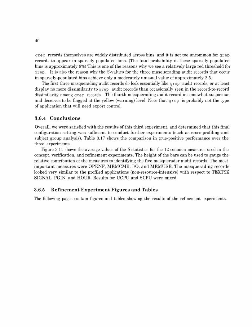
40

grep records themselves are widely distributed across bins, and it is not too uncommon for greprecords to appear in sparsely populated bins. (The total probability in these sparsely populatedbins is approximately 8%) This is one of the reasons why we see a relatively large red threshold forgrep. It is also the reason why the S-values for the three masquerading audit records that occurin sparsely-populated bins achieve only a moderately unusual value of approximately 2.5.

The first three masquerading audit records do look essentially like grep audit records, or at leastdisplay no more dissimilarity to grep audit records than occasionally seen in the record-to-recorddissimilarity among grep records. The fourth masquerading audit record is somewhat suspiciousand deserves to be flagged at the yellow (warning) level. Note that grep is probably not the typeof application that will need export control.

3.6.4 Conclusions

Overall, we were satisfied with the results of this third experiment, and determined that this finalconfiguration setting was sufficient to conduct further experiments (such as cross-profiling andsubject group analysis). Table 3.17 shows the comparison in true-positive performance over thethree experiments.

Figure 3.11 shows the average values of the S statistics for the 12 common measures used in theconcept, verification, and refinement experiments. The height of the bars can be used to gauge therelative contribution of the measures to identifying the five masquerader audit records. The mostimportant measures were OPENF, MEMCMB, I/O, and MEMUSE. The masquerading recordslooked very similar to the profiled applications (non-resource-intensive) with respect to TEXTSZSIGNAL, PGIN, and HOUR. Results for UCPU and SCPU were mixed.

3.6.5 Refinement Experiment Figures and Tables

The following pages contain figures and tables showing the results of the refinement experiments.

41

This table shows the score thresholds computed for each application during the profile-training process for therefinement experiment. Each application subject is listed with the number of records used for training (note that thisnumber is actually one-third of the total number of records used for the training period, as we cycled through thetraining data three times). For each application subject, we have recorded the yellow and red threshold score valuescalculated for each of the short-term profile half-lives used for the experiment (2, 1, and 0.1). The �yellow� columnrepresents the score value at which records are flagged at a warning level, and the �red�) column indicates the scorevalue at which records are flagged at a critical level.

Table 3.13: Score Thresholds for the Refinement Experiment

42

This table contains false-positive rates (percentages) for the refinement experiment. The total number of audit recordsused for each application subject in the false-positive tests are listed in the second column. Next are two columnsof data for each half-life used (2, 1, and 0.1). The columns labeled "yellow" indicate the false-positive rates at thewarning threshold level (i.e., the percentage of records flagged at this level) based on the score thresholds listed inTable 3.13, while the columns labeled �red� show the false-positive rates at the critical level.

Table 3.14: False-positive Rates (percent) for the Refinement Experiment

43

This table shows the results of the first of two true-positive tests performed during the refinement experiment. Thesecond column indicates the number of records used during the true-positive testing. The next column shows thepositions of the masquerader data in the application�s audit record stream. The remaining columns summarizethe results of the test for each short-term profile half-life used (2, 1, and 0.1). Each half-life column contains fourcharacters indicating the results of each of the four masquerading records data going through the application�s profile.For each half-life, we have recorded an asterisk (*) for detection above the critical (red) threshold, a plus (+) fordetection above the warning (yellow) threshold, and a dash (-) for no detection.

Table 3.15: True-positive Results from Refinement Experiment (Masquerading Application #1)

44

This table shows the results of the second of two true-positive tests performed during the refinement experiment.The second column indicates list the number of records used during the true-positive testing. The next column showsthe positions of the masquerader data in the application�s audit record stream. The remaining columns summarizethe results of the test for each short-term profile half-life used (2, 1, and 0.1). Each half-life column contains onecharacter indicating the results of the masquerading record going through the application�s profile. For each half-life,we have recorded an asterisk (*) for detection above the critical (red) threshold, a plus (+) for detection above thewarning (yellow) threshold, and a dash (-) for no detection.

Table 3.16: True-positive Results from Refinement Experiment (Masquerading Application #2)

This figure shows the S scores by measure for the four records from the first resource-intensive application as processedthrough the profiles for grep and latex, respectively. Recall that the S score is obtained for each measure by ahalf-normal transformation of the Q distribution. High S values indicate that the audit record in question differssignificantly from the underlying historical profile. Our half-normal inversion returns a maximum value of 4. Thetop figure shows moderately elevated S scores for some of the four records against the grep profile for the measuresMEMCB, MEMUSE, PRCTIME, and SCPU. The lower figure shows that many of the measures have elevated Sscores (including several at the theoretical maximum) for the four records scored against latex. This indicates thatthese records appear more unusual against the latex profile than against that for grep. The final step in the scoringmechanism compares this �unusualness� versus the �unusualness� of records against their own profiles (i.e., scoresfor grep against the grep profile).

Figure 3.4: Measure S-values for Grep and Latex

46

Historical grep profile data are shown in gray for the bin probabilities of the I/O and MEMUSE measures. Theobserved bin values for the four masquerader records are shown in black. The gray bars represent the historicallyobserved probabilities for the application grep that the audit data�s observed value for the I/O and MEMUSEmeasures will fall into a particular bin. The black bars show the bin locations by percentage of the four masqueraderdata records. For the I/O measure, we observe that grep’s activity usually falls between bins 7 and 14, although thereare a number of bins with small but non-zero probability. This indicates that it is not unusual for grep observationsto fall into some bin with fairly small probability. Three of the four masquerader records fall into such bins. Thefourth lands in bin 8, which has moderate historical probability. We thus expect three of the masquerader recordsto have somewhat high S scores for I/O, but scores by no means off the chart due to grep s frequency of landing inlow-probability bins. The fourth masquerader audit record will appear relatively normal in S. This is what is observedin Figure 3.4, with three masquerader S scores at 2.5 and one at 1.3 for this measure against the grep profile. Thusit is seen that the S scores do not go to their maximum when unusual bins are observed if the underlying subjectregularly hits unusual bins. The lower figure shows that for MEMUSE, three of the four masquerader records fallinto bins with quite reasonable probability, so that the corresponding S scores would be on the low side. The recordin bin 15 should receive a moderately high S. Again, this is confirmed in Figure 3.4.

Figure 3.5: Long-term Profile Category Bins for Application Grep (Measures I/O and MEMUSE)

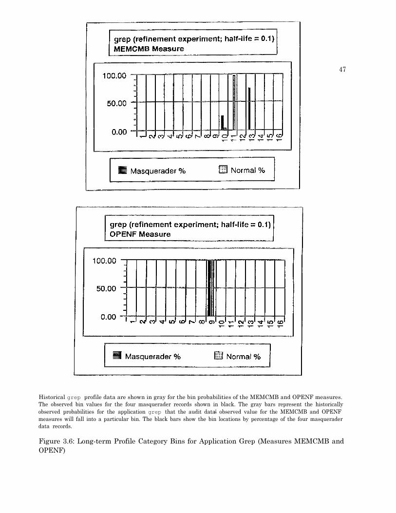
47

Historical grep profile data are shown in gray for the bin probabilities of the MEMCMB and OPENF measures.The observed bin values for the four masquerader records shown in black. The gray bars represent the historicallyobserved probabilities for the application grep that the audit data�s observed value for the MEMCMB and OPENFmeasures will fall into a particular bin. The black bars show the bin locations by percentage of the four masqueraderdata records.

Figure 3.6: Long-term Profile Category Bins for Application Grep (Measures MEMCMB andOPENF)

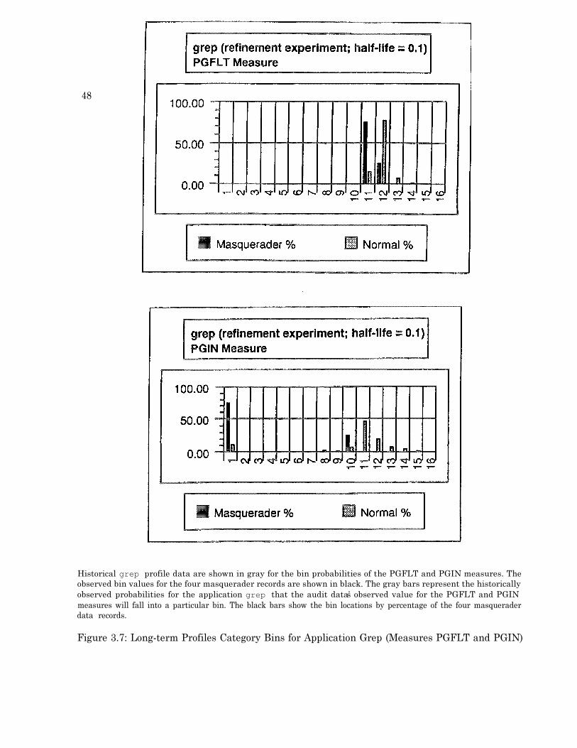
48

Historical grep profile data are shown in gray for the bin probabilities of the PGFLT and PGIN measures. Theobserved bin values for the four masquerader records are shown in black. The gray bars represent the historicallyobserved probabilities for the application grep that the audit data�s observed value for the PGFLT and PGINmeasures will fall into a particular bin. The black bars show the bin locations by percentage of the four masqueraderdata records.

Figure 3.7: Long-term Profiles Category Bins for Application Grep (Measures PGFLT and PGIN)

49

Historical grep profile data are shown in gray for the bin probabilities of the PRCTIME and SIGNAL measures. Theobserved bin values for the four masquerader records are shown in black. The gray bars represent the historicallyobserved probabilities for the application grep that the audit data�s observed value for the PRCTIME and SIGNALmeasures will falI into a particular bin. The black bars show the bin locations by percentage of the four masqueraderdata records.

Figure 3.8: Long-term Profiles Category Bins for Application Grep (Measures PRCTIME andSIGNAL)

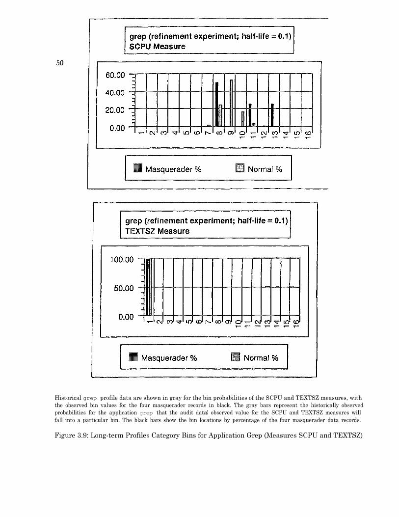
Historical grep profile data are shown in gray for the bin probabilities of the SCPU and TEXTSZ measures, withthe observed bin values for the four masquerader records in black. The gray bars represent the historically observedprobabilities for the application grep that the audit data�s observed value for the SCPU and TEXTSZ measures willfall into a particular bin. The black bars show the bin locations by percentage of the four masquerader data records.

Figure 3.9: Long-term Profiles Category Bins for Application Grep (Measures SCPU and TEXTSZ)

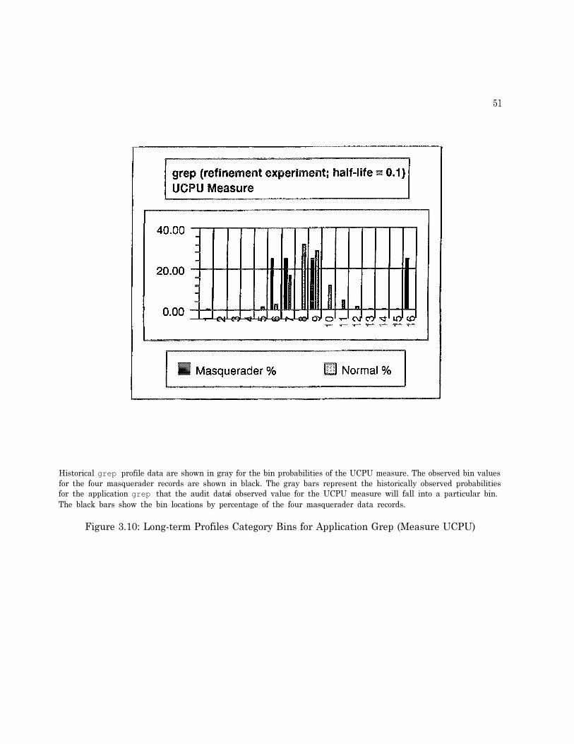
51

Historical grep profile data are shown in gray for the bin probabilities of the UCPU measure. The observed bin valuesfor the four masquerader records are shown in black. The gray bars represent the historically observed probabilitiesfor the application grep that the audit data�s observed value for the UCPU measure will fall into a particular bin.The black bars show the bin locations by percentage of the four masquerader data records.

Figure 3.10: Long-term Profiles Category Bins for Application Grep (Measure UCPU)

52

This table summarizes the results of the true-positive tests performed during the concept, verification, and refinementexperiments for a short-term profile half-life of 1 for the concept experiment and 0.1 for the verification and refinementexperiments. Each half-life column contains one character indicating the results of the masquerading record goingthrough the application�s profile. We have recorded an asterisk (*) for detection above the critical (red) threshold,a plus (+) for detection above the warning (yellow) threshold, and a dash (-) for no detection. At the bottomof the table we include counts of the number of �red� threshold detections (*), �yellow� threshold detections (+),non-detections (-) and the total detections (red plus yellow) for each experiment.

Table 3.17: True-positive Comparison for Three Experiments

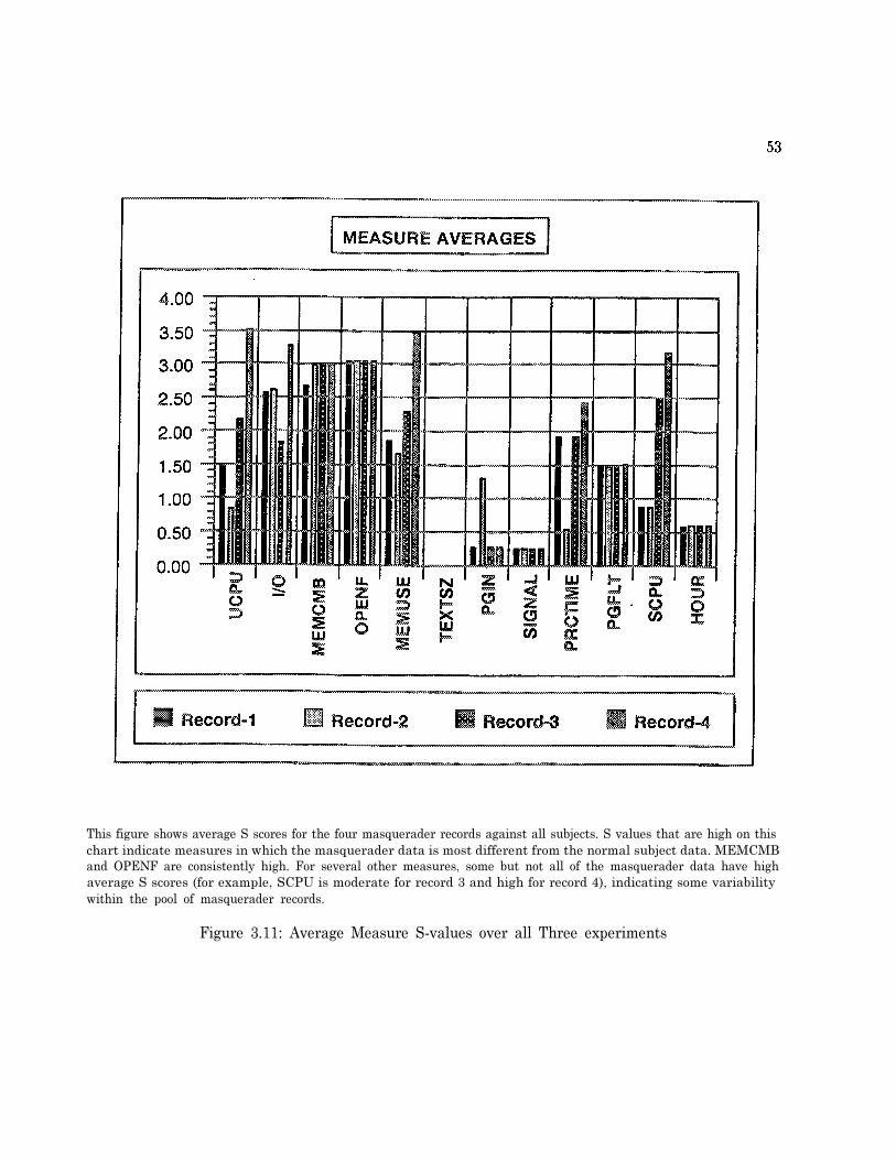
This figure shows average S scores for the four masquerader records against all subjects. S values that are high on thischart indicate measures in which the masquerader data is most different from the normal subject data. MEMCMBand OPENF are consistently high. For several other measures, some but not all of the masquerader data have highaverage S scores (for example, SCPU is moderate for record 3 and high for record 4), indicating some variabilitywithin the pool of masquerader records.

Figure 3.11: Average Measure S-values over all Three experiments

54

3.7 Cross-profiling Experiment

Cross profiling is the term we use when running one subject�s audit data through another subject�slong-term profile. The purpose of cross profiling is two-fold:

· Cross profiling allows us to determine how unique an application�s profile is and how successfulother applications might be in trying to masquerade as the �host� application.

· By examining the true-positive rate from cross profiling we can also obtain extensive informa-tion on the similarities or differences of profiles. This can be used as an aid for determiningpossible groupings of subjects.

3.7.1 Configuration

For the cross-profile experiment, we used the same configuration as in the refinement experiment(12 measures) and the same subjects as those in the true-positive test phase (26 subjects). Becauseof time constraints, we selected only a short-term profile half-life of 0.1 because this choice seemedmost consistent with our desire to identify individual audit records that were masqueraders. Weused the same trained profiles and data set that were used for the false-positive tests during therefinement experiment.

We recorded the true-positive percentages (anomalous record rates) for the yellow threshold;these are shown in Tables 3.18 and 3.19.

3.7.2 Results of Cross-Profiling

Table 3.18 and 3.19 show the true-positive percentages for all applications combined during thecross-profiling experiment. Within each cell in these tables are two numbers. The first entryrepresents the detection rate for the application listed on the column heading against the profile ofthe subject in the row heading. For example, on the row headed compile under the column for as,the first number, 48.5% is the rate of detection of as data when run through the profile of compile.The second entry in the cell reverses the relationship of the two applications. For example, thenumber of 67.3% in the compile row under the as column is the detection rate of compile datawhen run through the profile of as. Comparing the detection rates between applications on thesecharts shows several possible relationships. In some cases, an application could pass through theprofile of another application (a low detection rate), but the other application could not easily passthrough the original application. Examples of such asymmetric detection rates include gawk andcp with rates of 10.7% and 100%, pwd and compile with rates of 98.1% and 0.l%, and sort andless with rates of 95.7% and 17.1%. Still others formed pairs or small groups in which applicationscould mutually pass through each other�s profiles. Examples include csh and compile (4.6% and2.0%), ls and compile (3.4% and 2.7%), and ls and finger (2.2% and 4.4%). A third case has

55

applications with consistently high rates, indicating that neither application can pass through theother�s profile without raising suspicion.

Table 3.20 summarizes the true-positive percentages shown in Tables 3.18 and 3.19. Table 3.20shows the minimum, maximum, and average true-positive rates with the yellow threshold (1%)for each application. The chart also shows the percentage of applications that were in each of thefollowing ranges of rates: 0 to 25%, 26 to 50%, 51 to 75% and 76 to 100%. For example, for theapplication as, 28% of the applications had a detection rate between 0 and 25% when run againstas�s profile, 16% had a detection rate between 26 and 50%, 24% had a detection rate between 51and 75% and 32% had a detection rate between 76 and 100%.

Subjects with high average detection rates, such as getfullnm and latex, are very sensitive topotential masquerader data. Others, with low average rates, such as vi and grep, are more tolerantand would be candidates for a masquerading attempt. Observe that the thresholds in Table 3.13for getfullnm and latex are somewhat low, while those for vi and grep are on the high side. Thismay explain the low detection rate for masquerader data using vi as a host profile and confirmsour low detection rates for vi under our true-positive tests in the first three experiments.

3.7.3 Cross-profiling Experiment Figures and Tables

The following pages contain figures and tables showing the results of the cross-profiling experiments.

56

This table shows the true-positive percentages for all applications that were used for the cross-profiling experiment.To read this chart, let subject A be the host represented by the row, and subject B be the subject represented in thecolumn. Each cell contains two values: the top value is the detection rate of B�s data being run through A�s profile,and the bottom number is the detection rate of A�s data being run through B�s profile.

Table 3.18: Cross Profile Chart (26 subjects, 1% threshold level)

57

This table shows the true-positive percentages for all applications that were used for the cross-profiling experimenTo read this chart, let subject A be the host represented by the row, and subject B be the subject represented in thecolumn. Each cell contains two values: the top value is the detection rate of B�s data being run through A�s profile,and the bottom number is the detection rate of A�s data being run through B�s profile.

Table 3.19: Cross Profile Chart-Continued (26 subjects, 1% threshold level)

58

This table shows the true positive detection percentages obtained by running each subject�s data through the profilesfor all other subjects (�cross-profiling�). The first three columns are the minimum, maximum, and average detectionpercents. For example, for the application as, at least one "guest� subject had only 0.1% of its records declaredanomalous against as, and at least one subject had all its records so declared. Across all guest subjects, the averagedetection rate of the as profile was 53.62%. The last four columns give a breakdown of what percent of guest subjectswere detected at various levels. For example, referring to as, we see that 28% (7 subjects) had a detected rate between0 and 25%, that is 0 to 25% of the subject�s data when run through as�s profile was flagged as anomalous, 16% (4subjects) were detected between 26 and 50% of the time, 24% (6 subjects) were at a 51 and 75% rate, and 32% (8subjects) were over a 75% rate.

Table 3.20: True-positive Percentages for Cross-Profiling Experiment

59

3 . 8 G r o u p i n g E x p e r i m e n t

Using the results from the cross-profiling experiment, we performed a grouping experiment todetermine whether the development of profiles of application groups would enhance our detectionabilities.

We used two approaches to examine to what degree applications can be classified into groups:grouping using the NIDES scoring mechanism, and grouping by long-term profile overlap.

The first approach (grouping by NIDES scoring mechanism) gives a sense of how similar ap-plication groups look to NIDES. We used profiles constructed by using the 0.1 short-term profilehalf-life and examined all pairwise false-positive rates at the 1% (�yellow� threshold) cutoff (seeSection 3.7). For the 26 applications, there are 650 pairs (26 times 25) of �A vs. B� and �B vs. A�(note that these are not symmetric).

The second approach (grouping by long-term profile overlap) helped us assess the usefulness ofa default profile for a new application based on some hypothesized functional or other grouping.

3.8.1 Grouping by NIDES Scoring Mechanism

With respect to identifying potential subject groupings from the cross-profiling experiment, therewere some interesting observations. For some application pairs, both true-positive rates were veryhigh (over 90%). For many other pairs, the true-positive rates were very different. For example, rshactivity masquerading as getfullum had a 99.970 true-positive rate, while getfullnm masqueradingas rsh had a true-positive rate of 0. This indicates that the profile for rsh (either in categories or inits variance about those categories) in some sense encompasses that for getfullnm (i.e., the valuestypically seen for getfullnm are a subset of the values typically seen for rsh, but not vice-versa.)Getfullnm is one of the applications with the highest overall detection sensitivity.

Similar applications are those for which both true-positive rates are low. We selected all ap-plication pairs for which both true-positive rates were under 20% and came up with the list ofapplication pairings shown in Table 3.21. Only 33 of the possible 650 application pairs passedeven this fairly generous criterion, indicating that even these groupings might be statistical quirks.It is apparent that applications that warrant grouping are rather rare. To-further explore whichapplications we might group we defined a distance measure

where p(A vs. B) and p(B vs. A) are the true-positive rates of two mutually masquerading appli-cations, A masquerading as B, and B masquerading as A (see Table 3.19).

We observed that the most similar application pairs are not functionally related (only lessand more have a distance measure of less than 5 and are functionally related). Only one editor(emacs) made the list, exhibiting a weak similarity to ghostview. We conclude from this thatthe NIDES scoring mechanism (with this measure set) concludes subjects are similar probably

60

based on aggregate resource usage or large variance about this usage (for example, use of a largenumber of files or a highly variant number of files from instance to instance) rather than on sharedfunctionality. Of course, NIDES knows nothing of the application�s functionality.

3.8.2 Grouping by Long-Term Profile Overlap

An alternative approach to grouping considers the similarity of the long-term profiles for twoapplications. On a per-measure basis, we examined the combined category set for each applicationpair, and took the sum across bins of the smaller of the two category probabilities. If, for example,category X has probabilities 0.3 for A and 0.1 for B, then category X contributes 0.1 to the sum.For a category that has nonzero probability in one profile and zero in the other, the contributionis zero. It is thus apparent that a measure for which perfect overlap exists has a similarity of1, whereas totally different profiles have a similarity of 0. The per-measure similarities are thenaveraged across measures, resulting in an overall similarity between 0 and 1 for the profiles ofany two applications. Note that, unlike the NIDES scoring mechanism, this grouping measure issymmetric, so that only half the earlier number of application pairs need be considered.

3.8.3 Group Selection

Based on the combination of these two approaches, we selected two subject groups. In addition, wedecided to form another grouping of applications recommended to us by TIS, based on functionalityof application. Note that for the third group, we were only able to include subjects for which we hadtrained profiles. TIS�s list had more subjects, but insufficient audit data was available to includethese. The three groups were:

� GroupA - compile, less, and more. This grouping is derived from a combination of theNIDES scoring mechanism and a profile overlap analysis.

� GroupB - cat, cp, and rrn. This grouping is derived from a combination of the NIDES scoringmechanism and a profile overlap analysis.

� GroupC - cat, fmt, less, man, more, and sort. This is the suggested functional groupingfrom TIS.

We refer to GroupA and GroupB as the NIDES-based groupings because they were obtained asthe best results of mutually low within-group detection rates using the NIDES scoring mechanismand a high degree of profile overlap. GroupC is obtained from a hypothesized functional relation(here, file manipulation) irrespective of how similar the members look to NIDES.

Table 3.22 shows the distance measures for the NIDES-based groupings. Values near zeroindicate a high degree of similarity; note that the within-group similarities are much higher than the

61

between-group similarities. The diagonals are the distance of an application from itself, essentiallytwice the false-positive rate. Table 3.23 presents the same distances for the functional grouping.Note that these distances are generally much greater than for the NIDES-based groupings. Tables3.24 and 3.25 present the profile overlap statistics for the same groupings; in these tables, a valuenear 100 indicates a high degree of overlap. Again we observe significantly greater overlap for theNIDES-based groups.

3.8.4 Configuration

For the grouping experiment configuration, we used the same 12 measures as in the refinementexperiment, and used the short-term profile half-life of 0.1.

We did a short version of the cross-profiling tests by running individual subject data (thesame 26 subjects from the cross-profiling experiment) through the three group profiles. We alsoconducted true-positive testing using the resource-intensive application data.

3.8.5 Results

Table 3.26 summarizes the score thresholds for both the yellow and red thresholds for the threegroups that were profiled for this experiment.

Table 3.27 shows the false-positive rate of individual group member�s data running through itsgroup profile. The charts are similar to the false-positive tables in the previous experiments.

For purposes of the grouping experiment, we define a �false-positive� as a detection for a subjectrun against a group profile of which it is a member, and a �true-positive� as a detection for a subjectrun against a group profile of which it is not a member.

The group profiles are additionally dominated by members who contribute the bulk of thetraining data (for example, more contributes about five times as much data to the GroupC profileas does man - see Table 3.27). This can lead to high false-positive rates for individual groupmembers while still maintaining an approximately correct rate for the group as a whole (see theGroupC false-positive rates for man shown in Table 3.27).

Table 3.28 summarizes the true-positive rates for the group profiles. Generally, we expect agroup profile to be somewhat less sensitive in detection of anomalous data. This was weakly truefor the NIDES-based groupings, although it is important to point out that profiles for members ofthe NIDES-based groupings were more generic and forgiving as compared to other profiles. Thefunctional grouping was seen to be less sensitive (as compared to the sensitivity of its componentmembers) against the resource-intensive data and significantly less sensitive when examining atrue-positive rate based on cross-profiling.

Table 3.29 shows the anomaly rates for all experiment subjects running through each of thegroup profiles. Due to time constraints, we used only the 0.1 short-term profile half-life for thisexperiment. Both the yellow and red anomaly rates were recorded. Note that this table has the

62

rows as guest data, and the columns are the host profiles. In particular, note that applicationswith similar functionality (as indicated by the TIS grouping) do not necessarily appear similar asindicated by the NIDES-based grouping.

3.8.6 Grouping Experiment Figures and Tables

The following pages contain figures and tables showing the results of the grouping experiments.

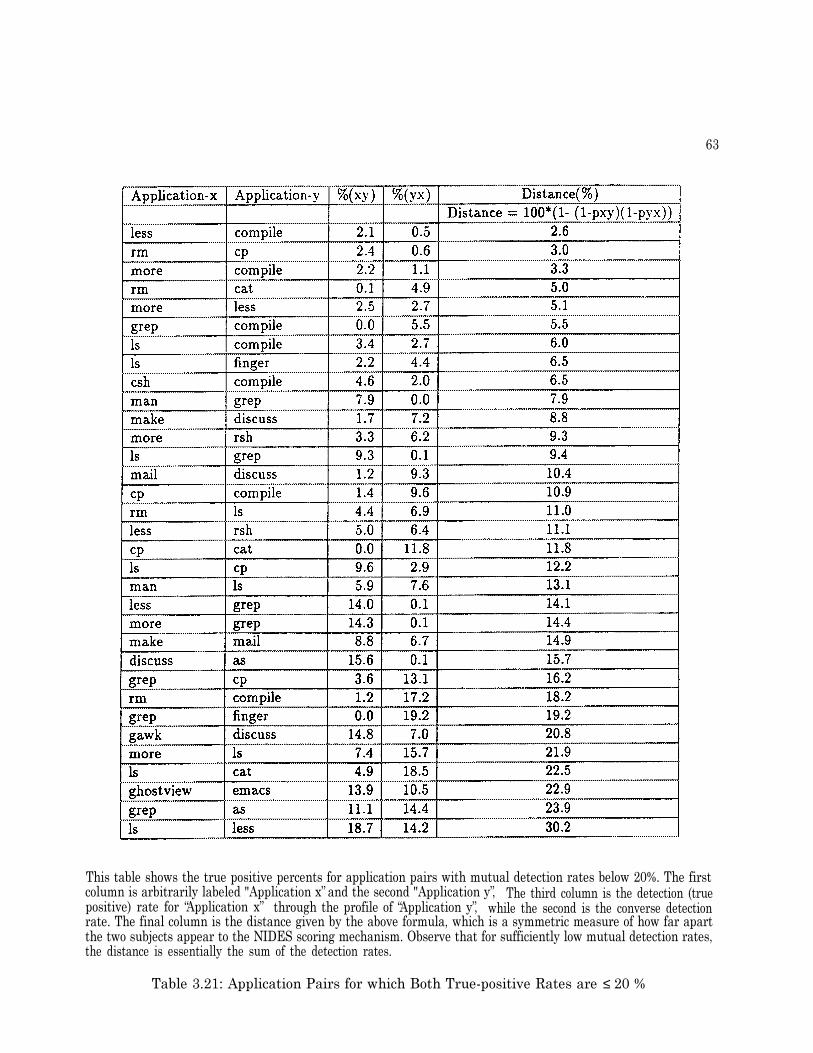
63

This table shows the true positive percents for application pairs with mutual detection rates below 20%. The firstcolumn is arbitrarily labeled "Application x� and the second "Application y�, The third column is the detection (truepositive) rate for �Application x� through the profile of �Application y�, while the second is the converse detectionrate. The final column is the distance given by the above formula, which is a symmetric measure of how far apartthe two subjects appear to the NIDES scoring mechanism. Observe that for sufficiently low mutual detection rates,the distance is essentially the sum of the detection rates.

Table 3.21: Application Pairs for which Both True-positive Rates are ≤ 20 %

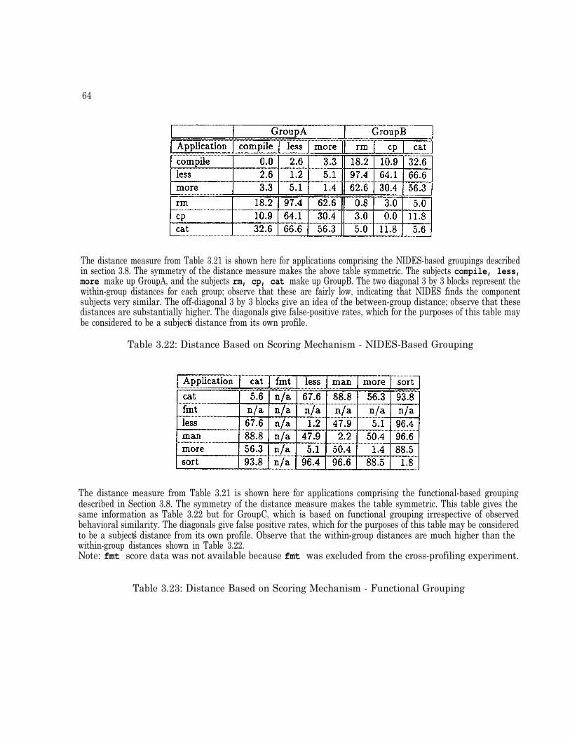
64

The distance measure from Table 3.21 is shown here for applications comprising the NIDES-based groupings describedin section 3.8. The symmetry of the distance measure makes the above table symmetric. The subjects compile, less,more make up GroupA, and the subjects rm, cp, cat make up GroupB. The two diagonal 3 by 3 blocks represent thewithin-group distances for each group; observe that these are fairly low, indicating that NIDES finds the componentsubjects very similar. The off-diagonal 3 by 3 blocks give an idea of the between-group distance; observe that thesedistances are substantially higher. The diagonals give false-positive rates, which for the purposes of this table maybe considered to be a subject�s distance from its own profile.

Table 3.22: Distance Based on Scoring Mechanism - NIDES-Based Grouping

The distance measure from Table 3.21 is shown here for applications comprising the functional-based groupingdescribed in Section 3.8. The symmetry of the distance measure makes the table symmetric. This table gives thesame information as Table 3.22 but for GroupC, which is based on functional grouping irrespective of observedbehavioral similarity. The diagonals give false positive rates, which for the purposes of this table may be consideredto be a subject�s distance from its own profile. Observe that the within-group distances are much higher than thewithin-group distances shown in Table 3.22.Note: fmt score data was not available because fmt was excluded from the cross-profiling experiment.

Table 3.23: Distance Based on Scoring Mechanism - Functional Grouping

65

This table shows the profile overlap statistics for members in GroupA and GroupB, the NIDES-based groupings.Each cell contains the percentage of profile overlap of each group member with another group member (note that thetables are symmetric, and that a member compared to itself is always 100%).

Table 3.24: Profile Overlap - NIDES-Based Grouping

This table shows the profile overlap statistics for members in GroupC, the functional-based grouping. Each cellcontains the percentage of profile overlap of each group member with another group member (note that the tablesare symmetric, and that a member compared to itself is always 100%).

Table 3.25: Profile Overlap - Functional-Based Grouping

66

This table shows the score thresholds for each application computed during the group profile-training process. Eachapplication group is listed with the number of records used for training. For each group, we have recorded the yellowand red threshold score values calculated for each of the short-term profile half-lives used for the grouping experiment(2, 1 and 0.1). The �yellow� column represents the score value at which records will be flagged at a warning level,and the �red� column indicates the score value at which records will be flagged at a critical level.

Table 3.26: Score Thresholds for Group Experiment

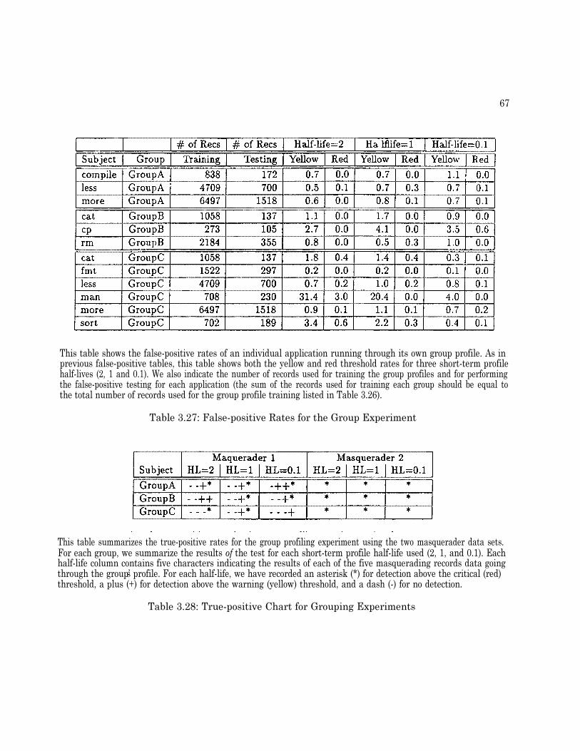
67

This table shows the false-positive rates of an individual application running through its own group profile. As inprevious false-positive tables, this table shows both the yellow and red threshold rates for three short-term profilehalf-lives (2, 1 and 0.1). We also indicate the number of records used for training the group profiles and for performingthe false-positive testing for each application (the sum of the records used for training each group should be equal tothe total number of records used for the group profile training listed in Table 3.26).

Table 3.27: False-positive Rates for the Group Experiment

This table summarizes the true-positive rates for the group profiling experiment using the two masquerader data sets.For each group, we summarize the results of the test for each short-term profile half-life used (2, 1, and 0.1). Eachhalf-life column contains five characters indicating the results of each of the five masquerading records data goingthrough the group�s profile. For each half-life, we have recorded an asterisk (*) for detection above the critical (red)threshold, a plus (+) for detection above the warning (yellow) threshold, and a dash (-) for no detection.

Table 3.28: True-positive Chart for Grouping Experiments

68

This table shows the anomaly rates resulting from running cross-profile tests with groups. To read this table, werefer to the host as the group whose profile was used and guest as the application whose data was used to run againstthe host�s profile. For example, the detection rate for running cp�s audit data through GroupB�s profile is 3.5% and0.6% respectively for the yellow and red threshold levels. Next to the guest application names we also note whetherthe guest was a member of a group or groups, and the group(s) it was a member of.

Table 3.29: Anomaly Rates for Group Cross profiling - Half-life = 0.1

Chapter 4

Conclusions

Overall, the NIDES statistical component was successful in its efforts to detect masqueradingapplications, whether these were special resource-intensive applications or standard applicationsrun through historical profiles other than their own. The primary conclusions drawn from theexperiments undertaken as part of the NIDES Safeguard project are as follows:

· The set of measures available for differentiating applications appears generally sufficient forthis task. Identifying the relevant set of 12 measures permitted a high degree of differentiationof applications with acceptable false-positive rates.

· NIDES can be and has been modified for the task of detecting when an audit stream hasbeen infected with data from a masquerading application. In addition NIDES can be and hasbeen modified so that it can detect individual audit records from masquerading applications.The modifications required for Safeguard were minor, having to do mainly with profile agingrates. The motivation for the more rapid profile aging used here versus that used for usermonitoring is that the Safeguard data captures in a single audit record the total informationset for the execution of an application;information that is typically spread over hundreds ofaudit records of user-level Unix audit data. In addition, the shorter profile length is moreappropriate for identifying single abnormal audit records.

· Masquerading applications (from which we had five audit records) can usually be detectedby NIDES, with 101 detections in 130 opportunities. With respect to the four audit recordsgenerated by one of these resource-intensive applications, we were able to detect one or moreof these individual records at the red threshold for 19 of 26 host applications. For threeadditional hosts there were three or more detections at the yellow threshold. For only twohosts were there no detections or only a single detection at the yellow threshold. Resultswith respect to the single audit record from the second resource-intensive application wereeven better. We were able to detect this individual record at the red threshold for 25 out

69

70

of 26 host applications, and at the yellow threshold for the remaining host application. Ifthese audit records from the sample masquerading applications are representative of typicalmasqueraders, we believe that NIDES will be generally successful in detecting them.

l Not all pairs of applications can be differentiated. Some applications are very �generic� withrespect to the available measures and can easily masquerade as other applications. A fewother applications with highly variable behaviors are particularly �forgiving� hosts. Theselatter applications are generally more vulnerable to masquerader data successfully slippingthrough.

l NIDES generally has a reasonably high probability of detecting individual audit records thatare masquerading as other applications. There are exceptions that appear to be partially theresult of highly variable behavior by the �host� application and partially the result of similarbehavior by the masquerading and �host� applications.

l For some applications, it would be desirable to have training data that stretches over addi-tional months of calendar time, because these applications demonstrate �shifts� in behaviorover different months.

l Using the long-term profiles, it was possible to assess whether different applications couldbe grouped. Very few applications appeared to cluster together, and the derived clusterswere quite small. In the few cases where we identified reasonable clusters, all or most of themembers of the cluster were �forgiving� hosts.

l Clustering on the basis of functionality (i.e., groupings suggested by TIS on the basis of thefunction of the software) did not yield cohesive groups. The historical profile developed byNIDES was more forgiving than would be expected based on the detection sensitivity of theindividual members. Because of this, we believe that clustering or grouping of applications isgenerally not desirable. Most applications are sufficiently different from all other applicationsthat clustering only reduces the ability of NIDES to detect masqueraders.

In spite of the overall high detection rates of resource-intensive application data, we caution thata base of five masquerading audit records is too small to lead to definitive conclusions, and therehas never been an assertion that these five audit records are representative of all masqueraders.Therefore, we also performed cross-profiling experiments, wherein each of the 26 applications forwhich we could build profiles acted as a masquerader for each of the other 25 applications. Theproportion of audit records detected during cross-profiling is a lower bound on our ability to detect�true� masqueraders, under the assumption that masqueraders are very different from the applica-tions that were our �normal� subjects. These results were very encouraging. For 16 of the 26 hostapplications, we were able to detect at the red threshold 50% or more of the masquerading auditrecords. For only two applications were the average percentage of masqueraders identified at the

71

red threshold below 15%. However, detection capability was not uniform across masqueraders, andmost applications could not be differentiated from at least one masquerading �normal� application.(In these cases, the masquerading application generated audit records that were within the rangeof behavior observed for audit records generated by the host application.) Whether the inabilityto find all potential masquerading applications is a deficiency depends on whether the applicationsthat cannot be adequately differentiated might be representative of the type of masqueraders thatpose a security threat.

4.1 Experiment Deficiencies

Our ability to tune NIDES to the Safeguard environment, and our ability to test the detectioncapability of NIDES, would have been greatly enhanced if the following were available:

l Additional data from normal applications. Very few of the applications that we received hadsufficient numbers of audit records to build accurate long-term profiles. We were able toprofile only 30 out of 288 applications represented in the data. Additional data would allowus to test a wider variety of applications.

l Additional chronological time for applications. Some applications demonstrated changes inbehavior over time. A longer training period would have allowed that behavior to be reflectedin the normal profiles, thus reducing the false-positive anomaly rate.

l Additional masquerading applications. We were provided with only two examples of mas-querading applications. These probably do not span the range of applications that might bemasqueraders.

l Additional audit records from masquerading applications. If the �normal� applications areany indication, there can be substantial variation from audit record to audit record withinan application. There is no reason to believe that variability is any less substantial withinmasquerading applications. We would encourage the development of 50 audit records for eachmasquerading application.

l Improved scenario development. In testing NIDES we have taken the extreme position that itis necessary to identify each and every instance of a masquerading application and that, if astream of audit records contained a single masquerading audit record, it would be importantto identify that record. More reasonable scenarios might postulate the presence of multiplemasquerading audit records and require that the stream be identified as �infected�. Webelieve NIDES could be configured to find infected audit record streams even more reliablythan attempts to identify individual and isolated audit records.

Glossary

Aging factor The factor by which past data are multiplied so as to fade their value at a desiredrate. For a half-life of k audit records, for example, the factor is set at the kth root of 1/2, sothat after k steps the data are faded to one-half of their original contribution. Storing profilesas aged cumulative totals permits relatively compact profile structures and allows the systemto adapt to changes in subject behavior. NIDES has a short-term aging factor applied toeach audit record and a long-term factor applied to daily totals at update time.

Bin Table entry to which an observed value is assigned. For categorical measures, such as HOUR,there is a one-to-one correspondence between bins and observed category values. For contin-uous measures, the bins correspond to value ranges.

Categorical measure A measure that assumes values in discrete categories. For some such mea-sures, such as HOUR, the values are known beforehand (the hours 0, 1,2, . . . . 23). For others,new categories are allocated by NIDES as they are encountered.

Category An observed value (such as error type or hour of use on a 24-hour clock) for categoricalmeasures, or a value range for a continuous measure such as SCPU.

Continuous measure A measure that takes continuous values, such as SCPU in time units.

Cross profiling An experiment in which data for each subject are tested against the trainedprofile for each other subject. Long-term profile update is disabled for such experiments.

Detection A declaration by NIDES that a stream of audit data contains anomalous activity. Theycan be at a �yellow� (caution) or �red� (critical) threshold.

Detection rate The percent of audit records in a given audit data stream that trigger detections.

False positive A detection for a subject against its own profile.

Effective n The effective length of the short term profile, which equals the series sum-of all powersof the aging factor (or approximately 1.5 times the short-term half-life, but never less thanone).

73

74

Half-life The number of audit records (in the case of the short-term profile) or the number of days(in the case of the long-term profile) by which time the contribution of a data item to thepresent cumulative totals is reduced by one half. The short-term profile half-life for Safeguardis set at a small number of audit records (a half-life of 1 or 0.1, the latter corresponding to ashort-term profile of a single record).

Historical effective n The effective count of audit records contributing to the long-term profile.It consists of the sum of all daily totals, each weighted by the appropriate power of thelong- term aging factor.

Historical profile See long-term profile.

Long-term profile For each subject and measure, the observed categories and the observed long-term probabilities for each category, the historical effective n, and the empirical Q distribu-tions. For the subject there is also an empirical score (T2) distribution, which is aggregatedacross all measures. At the end of each day, this profile is aged by the long-term aging factorand combined with the new daily totals.

Minimum effective n The minimum count of records in the long-term profile that must be ac-cumulated before the scoring mechanism is considered reliable. It is measure specific.

Profile aging rate, half-life and length The concepts of aging rate, half-life, and effectivelength of a profile are closely related. The aging rate is a multiplicative factor less thanor equal to unity, by which the existing information in a profile is aged. The smaller the rate,the more rapidly this information is �forgotten�. The half-life is the number of audit recordsthat need to transpire before the contribution of a given data item is decayed (downweighted)by one half. For example, if the aging rate is 0.8, the third most recent audit record has aweight of 0.8*0.8*0.8 or 0.512, so we would say that an aging rate of 0.8 corresponds to ashort-term profile half-life of three audit records. The effective length of a profile is given bythe series sum of all powers of the aging factor, which will converge if this factor is strictlyless than 1. For example, an aging rate of 0.8 corresponds to an effective profile length of5 audit records. As a rule of thumb, the effective length of the profile (in audit records) isapproximately 1.5 times the half-life.

Profile realization The short-term profile realization is a value that indicates the amount ofactivity that has contributed to the information in the short-term profile. The larger thenumber of profile realizations the more observations of subject activity. The number of profilerealizations is based on the number of audit records that have contributed to the short-termprofile related to the short-term profile length. For example, with a short-term profile half-life of 50 records (which corresponds to an effective short-term profile length of about 75), a

75

training data set of 300 records contains only four independent realizations of the short-termprofile.

Profile training The general procedure of updating profiles, adding and dropping categories,and adjusting the empirical distributions for Q and T2. It proceeds in three stages. Inthe first, category probabilities are obtained from a number of days of raw data. In thesecond, the Q distribution is estimated over an additional number of days. Finally, theT2 distribution is estimated, after which time NIDES is ready to score audit records. Ina production environment, profile training continues indefinitely. For experimentation withknown masquerader data, profile updating and training are disabled.

Profile update The merging of the historical profile with new information at the end of each day.Long-term probabilities are converted to effective counts (by multiplying by the historicaleffective n). The new daily counts are summed in, and the results converted back to proba-bilities. Categories that have too low a probability are folded into a �rare� category, whichcan change daily.

Q-score A chi-square-like square difference statistic based on the difference between the short-and long-term profiles for each measure.

QMax A scale value used to assign the Q-score into bins to obtain its empirical distribution.

S-value A unitless quantity obtained by inverting the observed Q-score using the Q empiricaldistribution and a half-normal transform. This results in all measure scores being comparablydistributed.

Scalar A value used to scale observed (raw) values to assign them to category (range) bins.

Short-term profile For each subject and measure, the number of counts recently observed foreach category in the long-term profile with special handling for new categories. Due to theaging procedure, these counts are generally fractional.

True positive A detection for a subject (possibly a masquerader) against another subject�s profile.

Threshold The NIDES-estimated value for T2 at which a detection is declared. It is set toachieve no greater than some user-specified percent (usually 1% for yellow, 0.1% for red) offalse positives.

T2 The overall NIDES score on which anomalies are declared, aggregated across all measures.

[l] R. Jagannathan, T. F. Lunt, F. Gilham, A. Tamaru, C. Jalali, P. Neumann, D. Anderson, T. D.Garvey, and J. Lowrance. Requirements specification: Next generation intrusion-detectionexpert system(NIDES). Technical report, Computer Science Laboratory, SRI International,Menlo Park, California, September 1992.

[2] R. Jagannathan, A. Tamaru, F. Gilham, D. Anderson, C. Jalali and C. Dodd, H. S. Javitz,A. Valdes, T. F. Lunt, and P. G. Neumann. Next generation intrusion-detection expert system(NIDES) software design specifications. Technical report, Computer Science Laboratory, SRIInternational, Menlo Park, California, March 1993.

[3] H. S. Javitz and A. Valdes. The SRI statistical anomaly detector. In Proceedings of the 1991IEEE Symposium on Research in Security and Privacy, May 1991.

[4] H. S. Javitz, A. Valdes, T. F. Lunt, A. Tamaru, M. Tyson, and J. Lowrance. Next generationintrusion-detection expert system (NIDES): Statistical algorithms rationale and rationale forproposed resolver. Technical report, Computer Science Laboratory, SRI International, MenloPark, California, March 1993.

[5] T. F. Lunt, Ann Tamaru, Fred Gilham, R. Jagannathan, Caveh Jalali, H. S. Javitz, A. Valdes,P. G. Neumann, and T. D. Garvey. A real-time intrusion-detection expert system (IDES), finaltechnical report. Technical report, Computer Science Laboratory, SRI International, MenloPark, California, February 1992.

77

Computer Science LaboratorySRI INTERNATIONAL

Technical Reports - 1995

SRI-CSL-95-01, March 1995Formal Methods and their Role in the Certification of Critical Systems, John Rushby

SRI-CSL-95-02, January 1995Adaptive Fault-Resistant Systems, Jack Goldberg, Li Gong, Ira Greenberg, Raymond Clark, E.Douglas Jensen, Kane Kim, and Douglas M. Wells

SRI-CSL-95-03, January 1995Mechanized Formal Verification - Seven Papers, David Cyrluk, Patrick Lincoln, Steven P. Miller,Paliath Narendran, Sam Owre, Sreeranga Rajan, John Rushby, Natarajan Shankar, Jens UlrikSkakkebaek, Mandayam Srivas, and Friedrich von Henke

SRI-CSL-95-04, July 1995Formal Verification of a Commercial Microprocessor, Steven P. Miller and Mandayam Srivas.

SRI-CSL-95-05, July 1995Execution Driven Distributed Simulation of Parallel Architectures, Livio Ricciulli, Patrick Lin-coln, and José Meseguer.

SRI-CSL-95-06, May 1995Detecting Unusual Program Behavior Using the Statistical Component of the Next-generationIntrusion Detection Expert System (NIDES), Debra Anderson, Teresa F. Lunt, Harold Javitz,Ann Tamaru, and Alfonso Valdes.

SRI-CSL-95-07, May 1995Next Generation Intrusion Detection Expert System (NIDES): A Summary. Debra Anderson,Thane Frivold, and Alfonso Valdes.

SRI-CSL-95-08, June 1995Correct Schema Transformations, Xiaolei Qian.

SRI-CSL-95-09, June 1995Query Folding, Xiaolei Qian.

SRI-CSL-95-11, June 1995Architecture and Techniques for Fast Computer Tomography, Iskender Agi.

SRI-CSL-95-18, November 1995View-based Access Control with High Assurance, Xiaolei Qian.

Technical Reports - 1987 - 1994

SRI-CSL-94-01, January 1994General Logics and Logical Frameworks, Narciso Martí-Oliet and Jose Meseguer.

SRI-CSL-94-02, April 1994Semantic Interoperation: A Query Mediation Approach, Xiaolei Qian and Teresa Lunt.

SRI-CSL-94-03, March 1994Elements of Trusted Multicasting, Li Gong and Nachum Shacham.

SRI-CSL-94-04R, March 1994, Revised October 1994Adaptive Fault Tolerance: Two Papers Jack Goldberg, Li Gong, Ira Greenberg, and ThomasLawrence.

SRI-CSL-94-05, April1994A Formal Approach to Correct Refinement of Software Architectures, Mark Moriconi, XiaoleiQian, and R.A. Riemenschneider.

SRI-CSL-94-06, July 1994GLU Programmer�s Guide Version 0.9, R. Jagannathan and Chris Dodd

SRI-CSL-94-07, April 1994Action and Change in Rewriting Logic, Narciso Martí-Oliet and Jo& Meseguer.

SRI-CSL-94-08, May 1994Authentication, Key Distribution, and Secure Broadcast in Computer Networks Using No En-cryption or Decryption, Li GongAlso included: Using One-Way Functions for Authentication, Li GongSecure, Keyed, and Collisionful Hash Functions, Thomas A. Berson, Li Gong, and T. Mark A.Lomas.

SRI-CSL-94-10, October 1994Transformations in High Level Synthesis: Formal Specification and Efficient Mechanical Verifi-cation, P. Sreeranga Rajan.

SRI-CSL-94-11, May 1994Specification, Transformation, and Programming of Concurrent Systems in Rewriting Logic,Patrick Lincoln, Narciso Martí-Oliet and José Meseguer.

SRI-CSL-94-12,Aug. 1994A Policy Framework for Multilevel Relational Databases, Xiaolei Qian and Teresa F. Lunt.

SRI-CSL-94.14,Oct. 1994Fail-Stop Protocols: An Approach to Designing Secure Protocols, Li Gong.

SRI-CSL-94-15, Oct. 1994Efficient Network Authentication Protocols: Lower Bounds and Optimal Implementations, LiGong.

SRI-CSL-93-01, March 1993Critical System Properties: Survey and Taxonomy, John Rushby.

SRI-CSL-93-02, March 1993A Formally Verified Algorithm for Interactive Consistency under a Hybrid Fault Model, PatrickLincoln and John Rushby.

SRI-CSL-93-03, December 1993Multidimensional Problem Solving in Lucid, A.A. Faustini and R. Jagannathan

SRI-CSL-93-04, May 1993Eight Papers on Formal Verification, Patrick Lincoln, Sam Owre, Natarajan Shankar, JohnRushby, and Friedrich von Henke.

SRI-CSL-93-05, August 1993Rewriting Logic as a Logical and Semantic Framework, Narciso Martí-Oliet and José Meseguer.

SRI-CSL-93-06, November 1993A Model-Theoretic Semantics of the Multilevel Secure Relational Model, Xiaolei Qian.

SRI-CSL-93-07, November 1993Formal Methods and the Certification of Critical Systems, John Rushby.

SRI-CSL-93-08, December 1993A Lazy Approach to Compositional Verification, by N. Shankar

SRI-CSL-93-09, December 1993Abstract Datatypes in PVS, by N. Shankar

SRI-CSL-93-10, December 1993A Duration Calculus Proof Checker: Using PVS as a Semantic Framework, by J.U. Skakkebaekand N. Shankar

SRI-CSL-93-11, December 1993Linear Logic and Proof Theory: Three Papers, by Patrick Lincoln, Andre Scedrov, NatarajanShankar, and Timothy Winkler

SRI-CSL-93-12, December 1993Microprocessor Verification in PVS: A Methodology and Simple Example, by David Cyrluk

SRI-CSL-93-13, December 1993The Complexity and Composability of Secure Interoperation, by Li Gong and Xiaolei Qian.

SRI-CSL-92-01, July 1992 �Formal Verification of an Oral Messages Algorithm for Interactive Consistency, by John Rushby.

SRI-CSL-92-02, July 1992Noninterference, Transitivity, and Channel-Control Security Policies, by John Rushby.

SRI-CSL-92-03, March 1992Introducing OBJ, by Joseph A. Goguen, Timothy Winkler, José Meseguer, Kokichi Futatsugi,and Jean-Pierre Jouannaud.

SRI-CSL-92-04, March 1992Survey of Object-Oriented Analysis/Design Methodologies and Future CASE Frameworks, byDonovan Hsieh.

SRI-CSL-92-05, April1992A Real-Time Intrusion-Detection Expert System (IDES), by Teresa F. Lunt, Ann Tamaru, FredGilham, R. Jagannathan, Caveh Jalali, and Peter G. Neumann.

SRI-CSL-92-06, May 1992Multiparadigm Logic Programming, by José Meseguer.

SRI-CSL-92-07, July 1992Simulation and Performance Estimation for the Rewrite Rule Machine, by Hitoshi Aida, JosephA. Goguen, Sany Leinwand, Patrick Lincoln, José Meseguer, Babak Taheri, and Timothy Win-kler.

SRI-CSL-92-08, July 1992A Logical Theory of Concurrent Objects and its Realization in the Maude Language, by JoséMeseguer .

SRI-CSL-92-09, Sept. 1992On the Semantics of Place/Transition Petri Nets, by José Meseguer, Ugo Montanari, andVladimiro Sassone.

SRI-CSL-92-11, Sept. 1992Using Rewriting Logic to Specify, Program, Integrate, and Reuse Open Concurrent Systems ofCooperating Agents, by José Meseguer, Kokichi Futatsugi, and Timothy Winkler.

SRI-CSL-92-12, November,1992Mechanized Verification of Real-Time Systems Using PVS, by N. Shankar.

SRI-CSL-92-13, December, 1992GLu: A Hybrid Language for Parallel Applications Programming, by R. Jagannathan and A.A.Faustini.

SRI-CSL-92-14, December, 1992Solving the Inheritance Anomaly in Concurrent Object-Oriented Programming, by JoséMeseguer .

SRI-CSL-92-15, December, 1992A Logical Semantics for Object-Oriented Databases, by José Meseguer and Xiaolei Qian.

SRI-CSL-91-01, February 1991Multilevel Security for Knowledge Based Systems, by Thomas D. Garvey and Teresa F. Lunt.

SRI-CSL-91-02, February 1991An Introduction to Formal Specification and Verification Using EHDM, by John Rushby, Friedrichvon Henke, and Sam Owre.

SRI-CSL-91-03, June 1991Formal Specification and Verification of a Fault-Masking and Transient-Recovery Model forDigital Flight-Control Systems, by John Rushby.

SRI-CSL-91-04, June 1991Mechanical Verification of a Schematic Protocol for Byzantine Fault-Tolerant Clock Synchro-nization, by N. Shankar.

SRI-CSL-91-05, February 1991Conditional Rewriting Logic as a Unified Model of Concurrency, by José Meseguer.

SRI-CSL-91-06, March 1991Final Algebras, Cosemicomputable Algebras, and Degrees of Unsolvability, by Lawrence S. Moss,José Meseguer, and Joseph A. Goguen.

SRI-CSL-91-07, April1991From Petri Nets to Linear Logic Through Categories: A Survey, by Narciso Martí-Oliet and JoséMeseguer .

SRI-CSL-91-08, November 1991Parallel Programming in Maude, by José Meseguer and Timothy Winkler.

SRI-CSL-90-01, February 1990Duality in Closed and Linear Categories, by Narciso Martí-Oliet and José Meseguer.

SRI-CSL-90002R, February 1990, Revised June 1990Rewriting as a Unified Model of Concurrency, by José Meseguer.

SRI-CSL-90-03R, February 1990, Rev. Dec. 1990Compiling Concurrent Rewriting onto the Rewrite Rule Machine, by Hitoshi Aida, JosephGoguen, and José Meseguer.

SRI-CSL-90-04, August, 1989Secure Knowledge-Based Systems, by Teresa F. Lunt and Jonathan K. Millen

SRI-CSL-90-06, June, 1990Order-Sorted Algebra Solves the Constructor-Selector, Multiple Representation and CoercionProblems, by José Meseguer and Joseph Goguen.

SRI-CSL-90-07, July,1990A Logical Theory of Concurrent Objects, by José Meseguer.

SRI-CSL-90-08, August,1990Decision Problems for Propositional Linear Logic, by Patrick Lincoln, John Mitchell, AndreScedrov, and Natarajan Shankar.

SRI-CSL-90-09, October, 1990On Location: Points about Regions, by Judith S. Crow and Peter B. Ladkin.

SRI-CSL-90-10, October 1990 On the Design of Dependable Computer Systems for Critical Applications, by Peter G. Neumann.

SRI-CSL-90-11, November 1990The GLU Programming Language, by R. Jagannathan and A.A. Faustini

SRI-CSL-90-12, November 1990Axiomatizing the Algebra of Net Computations and Processes, by Pierpaolo Degano, JoséMeseguer, and Ugo Montanari.

SRI-CSL-90-13, December 1990Semantic Specifications for the Rewrite Rule Machine, by Joseph A. Goguen.

SRI-CSL-90-15, December 1990A Logic to Unify Semantic Network Knowledge Systems with Object-Oriented Database Models,by Donovan Hsieh.

SRI-CSL-90-16, December 1990Inclusions and Subtypes, by Narciso Martí-Oliet and José Meseguer.

SRI-CSL-90-17, December 1990Architectural Design of the Rewrite Rule Machine Ensemble, by Hitoshi Aida, Sany Leinwand,and José Meseguer.

SRI-CSL-89-1, January 1989An Intensional Parallel Processing Language for Applications Programming, by E.A. Ashcroft,A.A. Faustini, and R. Jagannathan.

SRI-CSL-89-2, January 1989Dataflow-based Methodology for Coarse-Grain Multiprocessing on a Network of Workstations,by R. Jagannathan, Alan Downing, William Zaumen, and Rosanna Lee.

SRI-CSL-89-3R, February 1989, Revised August 1991Formal Verification of the Interactive Convergence Clock Synchronization Algorithm usingEHDM, by John Rushby and Friedrich von Henke.

SRI-CSL-8904R, March 1989, Rev. June 1989From Petri Nets to Linear Logic, by Narciso Martí-Oliet and José Meseguer.

SRI-CSL-89-5, March 1989General Logics, by José Meseguer.

SRI-CSL-89-6, March 1989The Rewrite Rule Machine Project, by Joseph Goguen, José Meseguer, Sany Leinwand, TimothyWinkler, and Hitoshi Aida.

SRI-CSL-89-8, July 1989A Categorical Manifesto, by Joseph A. Goguen.

SRI-CSL-89-9, Sept. 1989A Practical Approach to Semantic Configuration Management, by Mark Moriconi.

SRI-CSL-89-10, July 1989Order-sorted Algebra I: Equational Deduction for Multiple Inheritance, Overloading, Exceptionsand Partial Operations, by Joseph A. Goguen and José Meseguer.

SRI-CSL-89-11, December 1989An Algebraic Axiomatization of Linear Logic Models, by Narciso Martí-Oliet and José Meseguer.

SRI-CSL-88-1, January 1988Higher Order Functions Considered Unnecessary for Higher Order Programming, by JosephGoguen.

SRI-CSL-88-2R2, January 1988, Rev. 2, August 1988What is Unification? A Categorical View of Substitution, Equation and Solution, by JosephGoguen.

SRI-CSL-88-3R, January 1988, Rev. June 1989Petri Nets Are Monoids, by José Meseguer and Ugo Montanari.

SRI-CSL-88-4R2, August 1988OBJ as a Theorem Prover with Applications to Hardware Verification, by Joseph Goguen.

SRI-CSL-88-5, May 1988A Descriptive and Prescriptive Model for Dataflow Semantics, by R. Jagannathan.

SRI-CSL-88-7R, Sept. 1988Quality Measures and Assurance for AI Software, by John Rushby.

SRI-CSL-88-10R, Sept. 1988, Rev. Jan. 1989Cell, Tile, and Ensemble Architecture of the Rewrite Rule Machine, by Joseph A. Goguen, SanyLeinwand, and Timothy Winkler.

SRI-CSL-88-11, Sept. 1988Software for the Rewrite Rule Machine, by Joseph A. Goguen and José Meseguer.

SRI-CSL-88-13, Oct. 1988Relating Models of Polymorphism, by José Meseguer.

SRI-CSL-88-14, Nov. 1988Reasoning about Design Changes, by Mark Moriconi and Gail A. Harrison.

SRI-CSL-87-1, May1987The Rewrite Rule Machine Project, by Joseph Goguen, Claude Kirchner, Sany Leinwand, JoséMeseguer, and Timothy C. Winkler.

SRI-CSL-87-2, May 1987Concurrent Term Rewriting as a Model of Computation, by Joseph Goguen, Claude Kirchner,and José Meseguer.

SRI-CSL-87-3, May 1987An Abstract Machine for Fast Parallel Matching of Linear Patterns, by Ugo Montanari andJoseph Goguen.

SRI-CSL-87-7, July 1987Unifying Functional, Object-Oriented and Relational Programming with Logical Semantics! byJoseph Goguen and José Meseguer.