design of an outdoor wireless local area network and
80
DESIGN OF AN OUTDOOR WIRELESS LOCAL AREA NETWORK AND ANTENNA ANALYSIS Except where reference is made to the work of others, the work described in this thesis is my own or was done in collaboration with my advisory committee. This thesis does not include proprietary or classified information. _______________________________________ Suzanne Oudit Certificate of Approval: ______________________________ ______________________________ Stuart M. Wentworth Lloyd S. Riggs, Chair Associate Professor Professor Electrical and Computer Engineering Electrical and Computer Engineering ______________________________ ______________________________ Zebediah Whitehead Stephen L. McFarland Information Technology Specialist III Dean Engineering Network Services Graduate School
-
Upload
khangminh22 -
Category
Documents
-
view
2 -
download
0
Transcript of design of an outdoor wireless local area network and

DESIGN OF AN OUTDOOR WIRELESS LOCAL AREA NETWORK AND
ANTENNA ANALYSIS
Except where reference is made to the work of others, the work described in this thesis is
my own or was done in collaboration with my advisory committee. This thesis does not
include proprietary or classified information.
_______________________________________
Suzanne Oudit
Certificate of Approval:
______________________________ ______________________________
Stuart M. Wentworth Lloyd S. Riggs, Chair
Associate Professor Professor
Electrical and Computer Engineering Electrical and Computer Engineering
______________________________ ______________________________
Zebediah Whitehead Stephen L. McFarland
Information Technology Specialist III Dean
Engineering Network Services Graduate School

DESIGN OF AN OUTDOOR WIRELESS LOCAL AREA NETWORK AND
ANTENNA ANALYSIS
Suzanne Oudit
A Thesis
Submitted to
the Graduate Faculty of
Auburn University
in Partial Fulfillment of the
Requirements for the
Degree of
Master of Science
Auburn, Alabama
August 7, 2006
iii
DESIGN OF AN OUTDOOR WIRELESS LOCAL AREA NETWORK AND
ANTENNA ANALYSIS
Suzanne Oudit
Permission is granted to the Auburn University to make copies of this thesis at its
discretion, upon the request of individuals or institutions and at their expense. The author
reserves all publication rights.
_______________________
Signature of Author
_______________________
Date of Graduation

iv
VITA
Suzanne A. N. Oudit, daughter of Ian Oudit and Viola (Ramsaran) Oudit, was born on
October 11, 1980 in San Fernando, Trinidad, West Indies. She graduated in May 2002
from the University of the West Indies (U.W.I), St. Augustine with a Bachelor’s of
Science in Electrical and Computer Engineering. She then joined the Electrical
Engineering department of Auburn University as a graduate student in January 2004.
v
THESIS ABSTRACT
DESIGN OF AN OUTDOOR WIRELESS LOCAL AREA NETWORK AND
ANTENNA ANALYSIS
Suzanne Oudit
Master of Science, August 7, 2006
(BSc. University of the West Indies, 2002)
80 Typed Pages
Directed by Lloyd S. Riggs
One of the ongoing projects of the Engineering Network Services (ENS) at Auburn
University (AU) is to design and implement an outdoor Wireless Local Area Network
(WLAN). This project involved using Access Points (AP) that are provided by Meru
Networks. The AU College of Engineering is acting as the test bed for the proposed AU
WLAN. This thesis provides detailed documentation of the considerations involved in the
implementation of the WLAN.
Another aspect of the project dealt with the analysis of WLAN antennas. Theoretical
antenna radiation models were created and compared with the same from manufacturer’s
data sheets. A commercial cellular antenna manufactured by CSA Wireless was
investigated. As part of the study of the CSA Wireless antenna, a patch antenna was
fabricated and its performance characterized.

vi
Outdoor field measurements were conducted in the vicinity of the AP and the results
obtained were compared to the general antenna coverage patterns.

vii
ACKNOWLEDGEMENTS
I would like to thank God for guiding me and giving me the encouragement, strength
and will to pursue my goal in accomplishing this project and have the pleasure to see it
terminate fruitfully when at times the struggle seemed as though it would never end.
To Dr. Lloyd Riggs, my project supervisor, a special thanks to him for his concern,
support and guidance throughout this exercise and for having the faith in me to execute a
successful project. To Dr. Michael Baginski who suggested and made arrangements for
me to do work with the Engineering Network Services, Auburn University. To Dr. Stuart
Wentworth for assisting me conduct some measurements.
In my efforts to achieve overall success, there were some special individuals who
contributed significantly and who I would like to thank sincerely. These are: Dr. Daniel
Faircloth, Mr. Zebediah Whitehead, Mr. Jitendra Palasagaram and Mr. Joe Haggerty.
To my parents, Ian and Viola Oudit, an extraordinary acknowledgement to them for
being supportive and keeping the faith at all times.

viii
Style manual of journal used Graduate School: Guide to preparation and submission of
theses and dissertations
Computer software used: Microsoft Office XP
ix
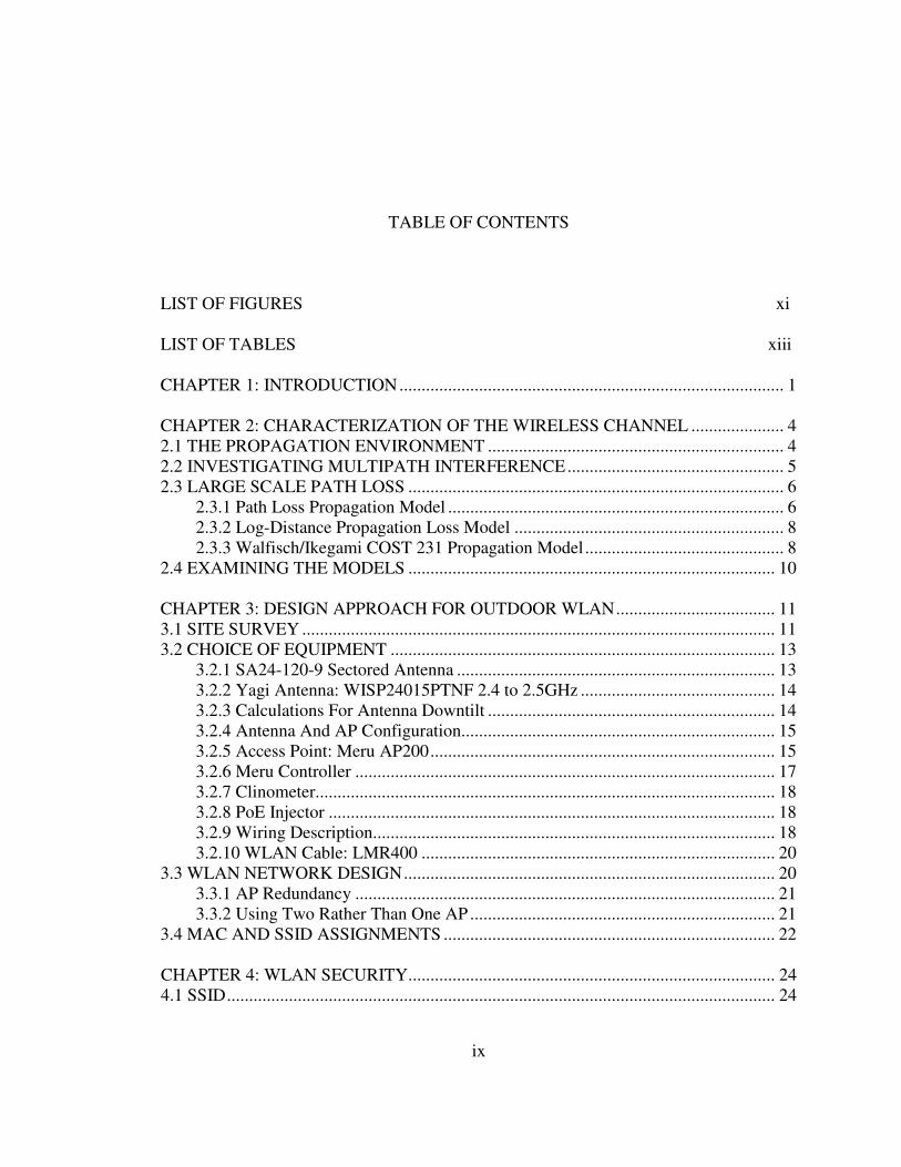
TABLE OF CONTENTS
LIST OF FIGURES xi
LIST OF TABLES xiii
CHAPTER 1: INTRODUCTION....................................................................................... 1
CHAPTER 2: CHARACTERIZATION OF THE WIRELESS CHANNEL ..................... 4
2.1 THE PROPAGATION ENVIRONMENT ................................................................... 4
2.2 INVESTIGATING MULTIPATH INTERFERENCE................................................. 5
2.3 LARGE SCALE PATH LOSS ..................................................................................... 6
2.3.1 Path Loss Propagation Model ............................................................................ 6
2.3.2 Log-Distance Propagation Loss Model ............................................................. 8
2.3.3 Walfisch/Ikegami COST 231 Propagation Model............................................. 8
2.4 EXAMINING THE MODELS ................................................................................... 10
CHAPTER 3: DESIGN APPROACH FOR OUTDOOR WLAN.................................... 11
3.1 SITE SURVEY ........................................................................................................... 11
3.2 CHOICE OF EQUIPMENT ....................................................................................... 13
3.2.1 SA24-120-9 Sectored Antenna ........................................................................ 13
3.2.2 Yagi Antenna: WISP24015PTNF 2.4 to 2.5GHz ............................................ 14
3.2.3 Calculations For Antenna Downtilt ................................................................. 14
3.2.4 Antenna And AP Configuration....................................................................... 15
3.2.5 Access Point: Meru AP200.............................................................................. 15
3.2.6 Meru Controller ............................................................................................... 17
3.2.7 Clinometer........................................................................................................ 18
3.2.8 PoE Injector ..................................................................................................... 18
3.2.9 Wiring Description........................................................................................... 18
3.2.10 WLAN Cable: LMR400 ................................................................................ 20
3.3 WLAN NETWORK DESIGN.................................................................................... 20
3.3.1 AP Redundancy ............................................................................................... 21
3.3.2 Using Two Rather Than One AP ..................................................................... 21
3.4 MAC AND SSID ASSIGNMENTS ........................................................................... 22
CHAPTER 4: WLAN SECURITY................................................................................... 24
4.1 SSID............................................................................................................................ 24

x
4.2 UNDERSTANDING THE IMPLEMENTATION OF SECURITY IN THE AU
NETWORK BASED UPON CISCO’S CONFIGURATION .......................................... 24
4.2.1 What is Cisco Clean Access?........................................................................... 24
4.2.2 Cisco Clean Access Components..................................................................... 25
4.3 THE AUTHENTICATION PROCESS ...................................................................... 26
4.4 VPN............................................................................................................................. 27
CHAPTER 5: OUTDOOR MEASUREMENTS.............................................................. 28
5.1 SIGNAL STRENGTH READINGS TO PREDICT AP COVERAGE...................... 28
5.2 MEASUREMENTS PROCEDURE ........................................................................... 28
5.3 BUILDING HEIGHTS TO PREDICT COVERAGE RANGE.................................. 30
CHAPTER 6: A THEORETICAL ANALYSIS OF AP AND ANTENNA COVERAGE
……………………………………………………………………………………33
6.1 USING MALTAB TO PLOT THE MANUFACTURER’S DATA........................... 33
6.2 DEVELOPING A THEORETICAL MODEL............................................................ 34
6.3 VERIFICATION TEST.............................................................................................. 36
6.3.1 Contour Plots Of Far-Field Radiation Pattern For SA24-120-9 Antenna........ 39
6.4 COORDINATE ROTATION AND TRANSLATION .............................................. 40
6.5 COMPARING THE ANALYTICAL AND MEASURED PLOTS ........................... 42
CHAPTER 7: ANTENNA ANALYSIS: CREATING THE RADIATION PATTERN
FOR THE CELLULAR ANTENNA.................................................................... 44
7.1 BACKGROUND ........................................................................................................ 45
7.2 DETERMINING THE SINGLE ELEMENT FUNCTIONS...................................... 46
7.3 DETERMINING THE ARRAY FACTOR FUNCTION........................................... 47
7.4 CORRECTION FACTOR .......................................................................................... 48
7.5 RESULTS OF PATTERN MULTIPLICATION ....................................................... 48
CHAPTER 8: GENERAL ANALYSIS OF THE INPUT IMPEDANCE
CHARACTERISTIC ............................................................................................ 51
8.1 BACKGROUND ........................................................................................................ 51
8.2 ANALYZING THE PCSS090-10-0 ANTENNA....................................................... 52
8.2.1 Using The VNA ............................................................................................... 52
8.3 BUILDING THE MICROSTRIP PATCH AND CONDUCTING
MEASUREMENTS.............................................................................................. 55
8.4 SMITH CHART ANALYSIS..................................................................................... 56
8.4.1 Smith Chart Of PCSS090-10-0 Antenna ......................................................... 57
8.4.2 Commercial Board Antenna Smith Chart ........................................................ 59
8.5 COMPARING A THEORETICAL VALUE OF IMPEDANCE TO THE
MEASURED VALUE.......................................................................................... 60
8.6 SUMMARY................................................................................................................ 60
CONCLUSION................................................................................................................. 62
RECOMMENDATIONS.................................................................................................. 64
REFERENCES ................................................................................................................. 66

xi
LIST OF FIGURES
Figure 2.1 Graph of multipath interference for Broun AP.................................................. 5
Figure 2.2 Graph of multipath interference for APa1......................................................... 6
Figure 2.3 Comparing the theoretical models with measured data................................... 10
Figure 3.1 Proposed coverage area ................................................................................... 12
Figure 3.2 Flow diagram of site selection......................................................................... 13
Figure 3.3 Figure showing how the downtilt coverage was calculated ............................ 14
Figure 3.4 Frequency and Channel assignment in the United States................................ 16
Figure 3.5 Example of 802.11b channel allocation .......................................................... 16
Figure 3.6 All of meru’s APs on channel 6 ...................................................................... 17
Figure 3.7 Diagram depicting Meru’s Virtual AP ............................................................ 17
Figure 3.8 PoE to backbone wiring configuration ............................................................ 19
Figure 3.9 Network Diagram of the WLAN to the wired LAN........................................ 21
Figure 4.1 Cisco’s method for getting onto the network .................................................. 25
Figure 4.2 Flow diagram showing what is taking place at Perfigo................................... 26
Figure 4.3 VPN associated with WLAN........................................................................... 27
Figure 5.1 Variation of signal strength from Broun Hall’s AP......................................... 29
Figure 5.2 Variation of signal strength from the APs for Aerospace- APa1 (upper plot),
APa2 (lower plot).................................................................................................. 30
Figure 6.1 Polar plot generated in matlab based on raw data for (a) H-plane (b) E-plane
............................................................................................................................... 34
Figure 6.2 3D Coordinate orientation for the analysis below........................................... 34
Figure 6.3 Manufacturer’s data (red) overlaid with the model (blue) for radiation patterns
a) Elevation, m b) Horizontal, n............................................................................ 36
Figure 6.4 Coordinate system relative to exact geographic measurements ...................... 37
Figure 6.5 Process for creating Figures 6.6 and 6.7.......................................................... 38
Figure 6.6 Contour plot of a radiation pattern with equal E and H-plane half power
beamwidth............................................................................................................. 38
Figure 6.7 Contour of the antenna for field pattern .......................................................... 39
Figure 6.8 Comparing the original axes with the new ones after a 20o downtilt or rotation
……………………………………………………………………………………40
Figure 6.9 Ground plot after translation and rotation ....................................................... 42
Figure 6.10 Empirical results for Broun Hall antenna’s ground coverage ....................... 43
Figure 7.1 PCSS090-10-0 6-element microstrip patch antenna........................................ 44
Figure 7.2 3D coordinate system for PCSS090-10 antenna ............................................. 46
Figure 7.3 H-plane pattern multiplication......................................................................... 49
Figure 7.4 E-plane pattern multiplication ......................................................................... 50
xii
Figure 8.1 PCSS090-10-0 antenna connected to VNA..................................................... 52
Figure 8.2 VSWR vs. Frequency for a matched load ....................................................... 53
Figure 8.3 VSWR vs. Frequency for the PCSS090-10-0 antenna inside radome............. 54
Figure 8.4 VSWR vs. Frequency for the PCSS090-10-0 antenna outside radome........... 55
Figure 8.5 (a)Fabricated patch based upon commercial cellular patch (b)SMA connector
used to provide an edge-feed to the patch............................................................. 56
Figure 8.6 Smith Chart of PCSS090-10-0 outside radome............................................... 57
Figure 8.7 Smith Chart of PCSS090-10-0 inside radome................................................. 58
Figure 8.8 Smith Chart of commercial board antenna...................................................... 59
Figure 8.9 Examples of matching alterations ................................................................... 61

xiii
LIST OF TABLES
Table 3.1 ESSID and MAC addresses of the APs ............................................................ 23
Table 5.1 Buildings’ height where the APs were located................................................. 31
Table 5.2 Inner and outer radius calculations for the three APs based on [1] .................. 31
1
CHAPTER 1: INTRODUCTION
ENS is attempting to improve their wireless service to engineering students. Once
satisfactory results are obtained, outdoor service will be provided campus-wide. The
ultimate goal is to have Auburn University act as a host site providing wireless
networking service, both audio and data, to the city of Auburn and possibly to its city
limits. Similar work is already being conducted at other universities. Currently, the
University of Georgia is coordinating an outdoor WLAN project “throughout 24 blocks
of downtown Athens that will be used to research and explore applications for wireless
technology in a real-world environment” [11].
Broadband connectivity is available in all buildings via Ethernet cabling but the
coverage provided by these systems is far from ubiquitous. The importance of such an
outdoor wireless system is to allow users untethered network access that would not
confine them within the walls of their department. It is desirable for the campus network
to grow geographically larger while still retaining efficiency and speed.
When deploying a WLAN, the cost, coverage and capacity must be evaluated and
depends among other things on the frequency of operation. The network designer strives
to minimize costs but at the same time provide quality service to the user and achieving
their goals usually is not readily attainable without a compromise. In short, network
designers usually try to create a system that accommodates as many users as possible
2
without jeopardizing service. In the planning phase of the WLAN, the designers should
choose equipment that can be easily scaled to support anticipated applications like
streaming video.
Once the WLAN is successfully deployed, it can be used by faculty and students to
perform innovative wireless research and tests for mobile media design that could be
integrated into the degree curriculum and push AU to the forefront of a fascinating
research area.
Antenna analysis requires one to not only have a good understanding of antenna
theory but also to be able to manipulate 3D geometry in both the Cartesian and spherical
coordinate systems and furthermore carry out simulations, interpret, and compare results
to the manufacturer’s data sheet.
This document is divided into chapters that follow in roughly chronological order the
steps taken to analyze the proposed WLAN. The two main concentrations in this thesis
are the WLAN design and the antenna analysis.
Chapter 2 presents plots of multipath interference in order to demonstrate that the
multipath channel has small scale fading and is random. Existing empirical large-scale
models developed for various environments are compared with the outdoor
measurements conducted.
Chapter 3 is the beginning phase of the WLAN design. Once a site survey is
completed, it is very necessary to choose the equipment to be used in the design. The
individual components are chosen based on their functionality and the service they
provide to the overall system. Here, one is presented with the WLAN’s hardware
architecture. The Media Access Control (MAC) and Service Set Identifier (SSIDs) are
3
used to identify the specific AP that is under test and differentiates if from other AP
signals present.
A wireless system is generally not as secure as its wired counterpart. The focus of
Chapter 4 is to investigate different possible security measures. Several levels of
hardware and software security were necessary in order to maintain privacy and security
for the users, and to protect network resources and equipment.
As discussed in Chapter 5, once the AP and antenna was mounted, the signal strength
had to be measured to determine the range of coverage offered by the chosen location.
Matlab plots are used to provide a visual representation of the coverage area. Given the
mounting height of the antenna, the antenna’s downtilt angle was chosen to achieve the
best ground coverage.
In Chapter 6 the ground coverage pattern of a candidate AP design is investigated. In
particular, the radiation patterns specified by Pacific Wireless for the SA24-120-9
sectored antenna are examined in some detail.
In Chapter 7 the radiation pattern of a cellular phone transmitting antenna is derived
by applying a technique referred to as Pattern Multiplication [13]. Again, theoretical
results are compared to that of published data from the manufacturer.
In Chapter 8, further analysis of the base-station antenna, PCSS090-10-0 from Chapter
7 is conducted. An attempt is made to achieve a deeper understanding of how the input
impedance of a single isolated patch was related to the same for the six-patch antenna.
The analysis is based on measured Voltage Standing Wave Ratio (VSWR) values and
Smith Chart plots.
4
CHAPTER 2: CHARACTERIZATION OF THE WIRELESS CHANNEL
Chapter 2 mentions factors that cause impairments in the wireless channel. Existing
empirical models are introduced and compared with the actual measured data to see
which model most closely represents the environment in which the AU WLAN would
operate. In order to plan AP layout, theoretical models were used to predict signal
attenuations or coverage of the proposed WLAN.
2.1 THE PROPAGATION ENVIRONMENT
Corruptive elements distort the information-carrying signal as it penetrates the
propagation medium between the transmitter and receiver in an outdoor environment.
The corruptive elements along the electromagnetic path are in the form of multipath
delay spread, reflections, scattering, diffraction and penetration.
Small-scale fading is used to describe the rapid fluctuations of the amplitudes, phases
or multipath delays of a radio signal over a short period of time or travel distance, so that
the large-scale path loss effects may be ignored. Large-scale fading models try to predict
the signal strength for an arbitrary Transmitter-Receiver, T-R separation typically
hundreds or thousands of meters [10].
5
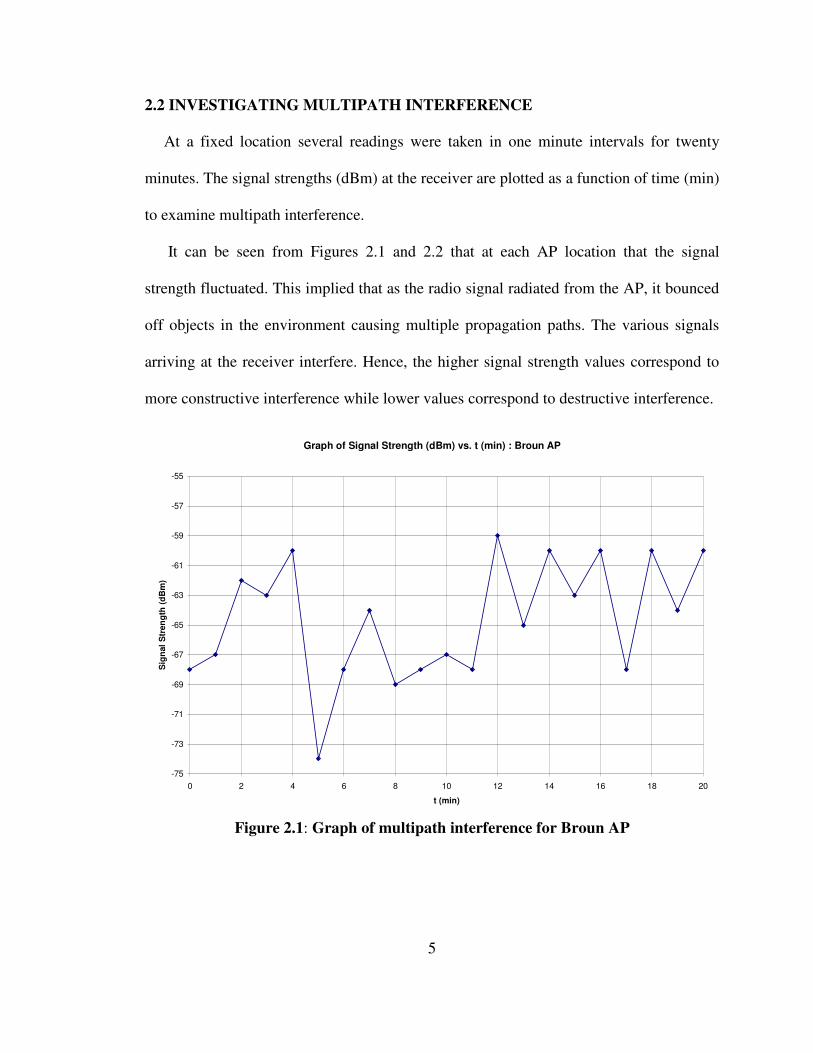
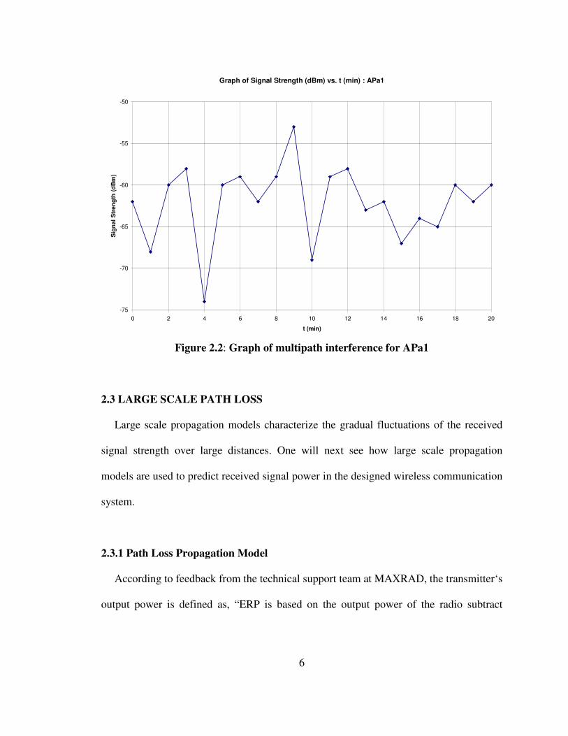
2.2 INVESTIGATING MULTIPATH INTERFERENCE
At a fixed location several readings were taken in one minute intervals for twenty
minutes. The signal strengths (dBm) at the receiver are plotted as a function of time (min)
to examine multipath interference.
It can be seen from Figures 2.1 and 2.2 that at each AP location that the signal
strength fluctuated. This implied that as the radio signal radiated from the AP, it bounced
off objects in the environment causing multiple propagation paths. The various signals
arriving at the receiver interfere. Hence, the higher signal strength values correspond to
more constructive interference while lower values correspond to destructive interference.
Graph of Signal Strength (dBm) vs. t (min) : Broun AP
-75
-73
-71
-69
-67
-65
-63
-61
-59
-57
-55
0 2 4 6 8 10 12 14 16 18 20
t (min)
Sig
nal
Str
en
gth
(d
Bm
)
Figure 2.1: Graph of multipath interference for Broun AP
6
Graph of Signal Strength (dBm) vs. t (min) : APa1
-75
-70
-65
-60
-55
-50
0 2 4 6 8 10 12 14 16 18 20
t (min)
Sig
nal
Str
en
gth
(d
Bm
)
Figure 2.2: Graph of multipath interference for APa1
2.3 LARGE SCALE PATH LOSS
Large scale propagation models characterize the gradual fluctuations of the received
signal strength over large distances. One will next see how large scale propagation
models are used to predict received signal power in the designed wireless communication
system.
2.3.1 Path Loss Propagation Model
According to feedback from the technical support team at MAXRAD, the transmitter‘s
output power is defined as, “ERP is based on the output power of the radio subtract
7
jumper loss to the antenna plus antenna gain.” Based on this, the Effective Radiated
Power is given by,
ERP = Ptx- Lc + GA (2.1)
where the transmitter output power, Ptx is -10dB, the SA24-120-9 antenna gain, GA is
9dB and the LMR400 cable loss, Lc, is the loss per meter (0.2dB/m [17]) plus the
connection loss (0.2dB). Since the length of LMR400 cable was approximately four feet
(1.2192m), the cable loss was estimated per meter. Considering these values in equation
2.1 yields ERP = -1.4dB or 28.6dBm.
The Free Space Path Loss (FSPL) propagation model is used to predict the received
signal strength when the transmitter and receiver have a clear, unobstructed LOS path
between them. It is impossible to specify performance for all environments but the free
space performance characteristics provide the most suitable reference for comparing
relative antenna performance.
Using the FSPL equation [15],
PL(d) = 20log10fc + 20log10d – 147.56 (dB) (2.2)
where the center frequency, fc = 2.4GHz,
PL(d) = 40 + 20log10(d) (dB) (2.3)
In the plot of Figure 2.3, the received power for the FSPL model (transmitted power
less the path loss) is compared to the measured data.
8
2.3.2 Log-Distance Propagation Loss Model
The average large scale path loss for an arbitrary T-R separation can be expressed as a
function of the distance using a path loss exponent, n. Propagation models indicate that
the average received signal power decreases logarithmically with distance, therefore
PL(d) α (d/do)n (2.4)
or
PL(dB) = PL(do) + 10nlog10(d/do) (2.5)
where PL is the path loss, d is the distance indicative of the T-R separation and do is the
close-in reference distance determined from measurements from the transmitter.
From the FSPL equation, where PL = 40 + 20 log10(do) (dB), do was set to 42m based
on the empirical data. For free-space, the path loss exponent is 2 but for this application
the propagation path was not entirely free space so n was set to 2.3. The Log-distance
model plot is shown in Figure 2.3.
2.3.3 Walfisch/Ikegami COST 231 Propagation Model
The Walfisch/Ikegami COST 231 propagation model considers the impact of rooftops
and building height by using diffraction to predict average signal strength at street level.
The model considers the path loss to be a sum of three factors, free space loss (Lf), roof
top to street diffraction and scatter loss (Lrts) and multiscreen loss (Lms).
Lc(dB) = Lf(dB) + Lrts(dB) + Lms(dB) (2.6)
where
R = T-R separation 0.03048km to 0.213km
9
fc = operating frequency, 2400MHz
W = street width, 5m
h_r = building height, 19.2m
h_m = mobile devices’s height, 1.65m
f = incident angle relative to the street, 20o
b = distance between buildings, 7m
are all parameters needed to compute Lc(dB) assuming that the building height exceeds
the mobile height in a suburban area [9].
After inserting the values for all the parameters in equation 2.6, the result of the
Walfisch/Ikegami COST 231 propagation model’s path loss is,
Lc(dB) = 112.74 + 38log10(R) (2.7)
The COST 231 propagation model’s plot is shown in Figure 2.3.
10
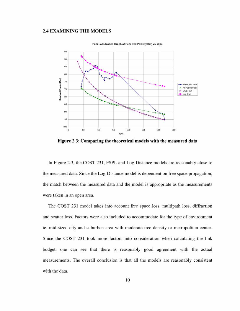
2.4 EXAMINING THE MODELS
Path Loss Model: Graph of Received Power(dBm) vs. d(m)
-100
-95
-90
-85
-80
-75
-70
-65
-60
-55
-50
0 50 100 150 200 250 300 350
d(m)
Receiv
ed
Po
wer(
dB
m)
Measured data
FSPL(Maxrad)
COST231
Log Dist.
Figure 2.3: Comparing the theoretical models with the measured data
In Figure 2.3, the COST 231, FSPL and Log-Distance models are reasonably close to
the measured data. Since the Log-Distance model is dependent on free space propagation,
the match between the measured data and the model is appropriate as the measurements
were taken in an open area.
The COST 231 model takes into account free space loss, multipath loss, diffraction
and scatter loss. Factors were also included to accommodate for the type of environment
ie. mid-sized city and suburban area with moderate tree density or metropolitan center.
Since the COST 231 took more factors into consideration when calculating the link
budget, one can see that there is reasonably good agreement with the actual
measurements. The overall conclusion is that all the models are reasonably consistent
with the data.
11
CHAPTER 3: DESIGN APPROACH FOR OUTDOOR WLAN
Chapter 3 explains considerations made when designing a wireless network. It
examines the equipment choice and performance and how the hardware is connected
from the wireless side to the existing wired network backbone. One is also presented with
the role of Media Access Control (MAC) addresses and Service Set Identifiers (SSID)
that are assigned early in the design for later testing of the WLAN.
3.1 SITE SURVEY
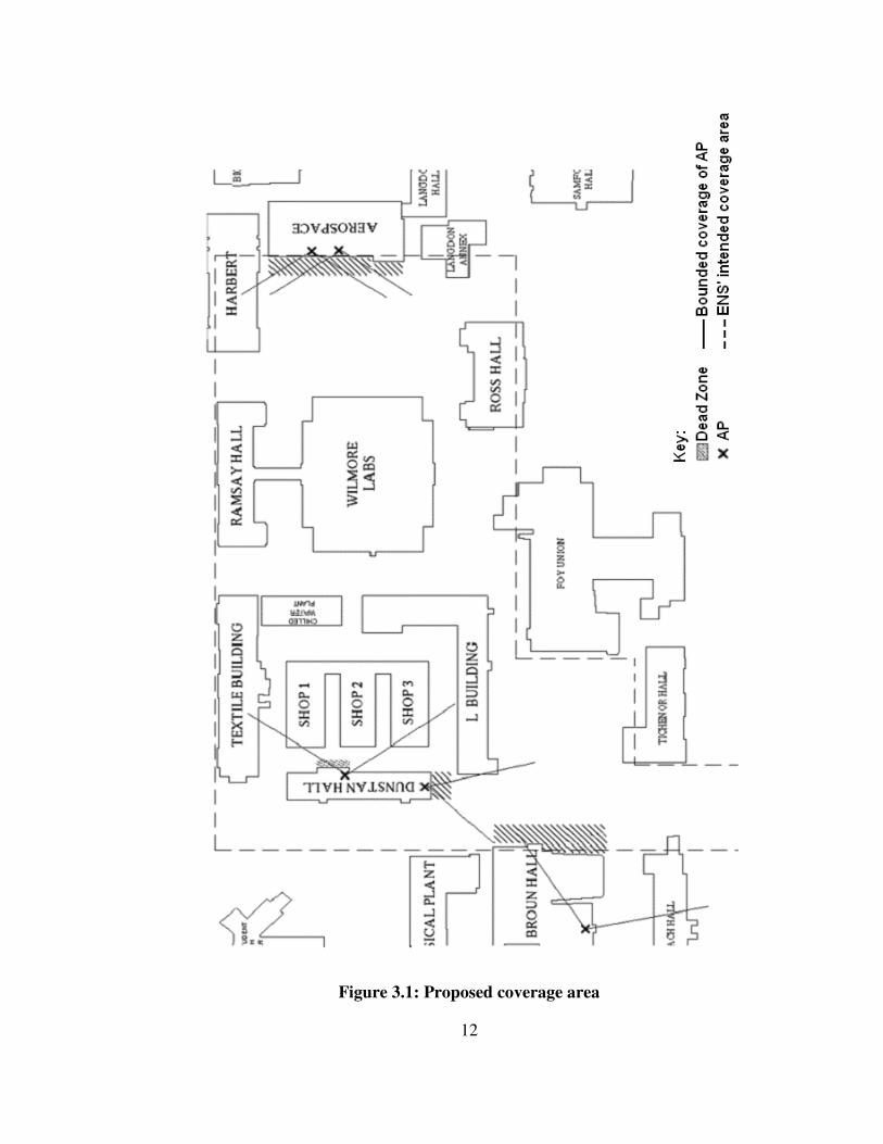
On a map (Figure 3.1) of the engineering portion of campus, the areas that were to
have wireless service were established. A site analysis was conducted to identify the best
antenna positions for an optimum and seamless blanket of coverage. This task was done
to minimize dead spots and identify those areas that would be receiving low powered
signals and hence low bandwidth connections. Planning was essential in the early stages
of the project so that troubleshooting in the later stages would require less effort. If there
was any disruption in service, the user would not be wondering if his device or the AP or
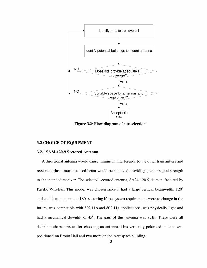
even the application server may be faulty. Figure 3.2 shows a flow diagram describing
the method for determining the site selection.
12
Figure 3.1: Proposed coverage area
13
Identify area to be covered
Identify potential buildings to mount antenna
Does site provide adequate RF coverage?
Suitable space for antennas and equipment?
Acceptable
Site
YES
YES
NO
NO
Figure 3.2: Flow diagram of site selection
3.2 CHOICE OF EQUIPMENT
3.2.1 SA24-120-9 Sectored Antenna
A directional antenna would cause minimum interference to the other transmitters and
receivers plus a more focused beam would be achieved providing greater signal strength
to the intended receiver. The selected sectored antenna, SA24-120-9, is manufactured by
Pacific Wireless. This model was chosen since it had a large vertical beamwidth, 120o
and could even operate at 180o sectoring if the system requirements were to change in the
future, was compatible with 802.11b and 802.11g applications, was physically light and
had a mechanical downtilt of 45o. The gain of this antenna was 9dBi. These were all
desirable characteristics for choosing an antenna. This vertically polarized antenna was
positioned on Broun Hall and two more on the Aerospace building.
14
3.2.2 Yagi Antenna: WISP24015PTNF 2.4 to 2.5GHz
The WISP24015PTNF is a product of PCTEL MAXRAD. The Yagi antenna was
positioned on the roof of Dunstan Building since in the preliminary design phase, the
intent was for this antenna to compensate for the dead spot directly in front of Broun Hall
while providing additional coverage as far as possible along the Haley concourse. The
befitting characteristics of this antenna in the WLAN would be its 30o horizontal
beamwidth and its 15dBi gain.
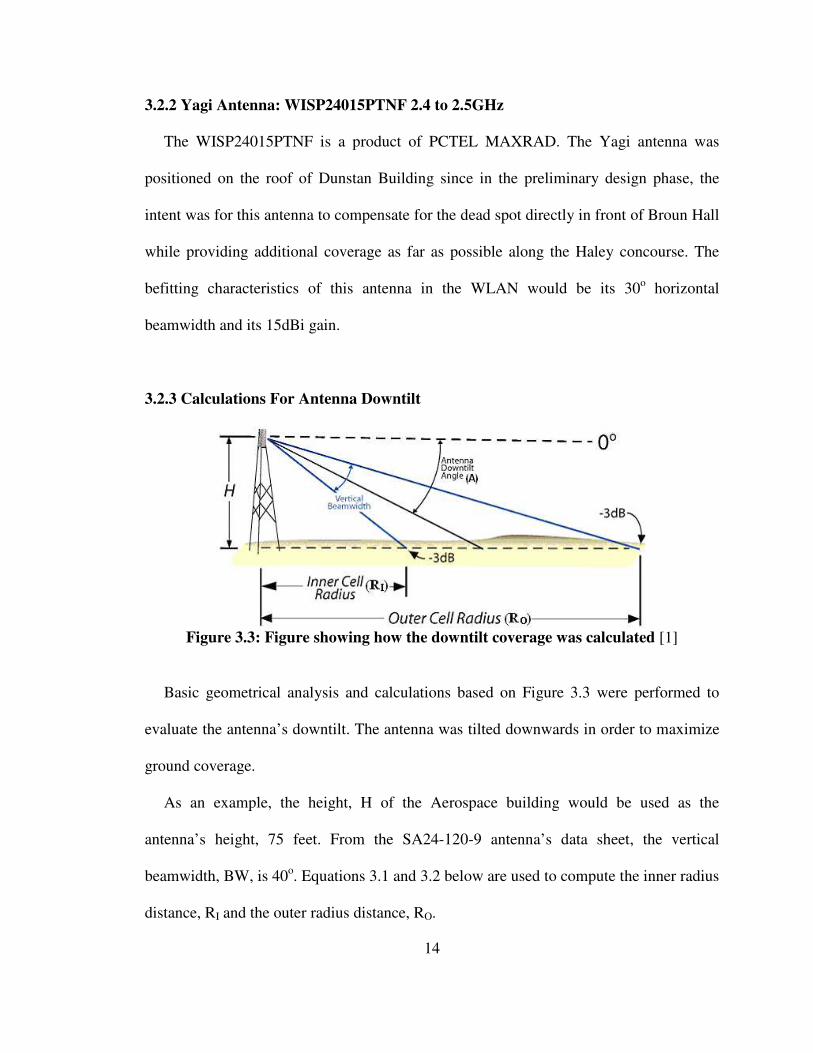
3.2.3 Calculations For Antenna Downtilt
Figure 3.3: Figure showing how the downtilt coverage was calculated [1]
Basic geometrical analysis and calculations based on Figure 3.3 were performed to
evaluate the antenna’s downtilt. The antenna was tilted downwards in order to maximize
ground coverage.
As an example, the height, H of the Aerospace building would be used as the
antenna’s height, 75 feet. From the SA24-120-9 antenna’s data sheet, the vertical
beamwidth, BW, is 40o. Equations 3.1 and 3.2 below are used to compute the inner radius
distance, RI and the outer radius distance, RO.

15
RI (feet) = H / tan(A + (BW/2)) (3.1)
RO (feet) = H / tan(A - (BW/2)) (3.2)
In the calculations, the downtilt angle, A was varied such that RI was made a minimum
value and RO was made a maximum value to achieve a maximum antenna coverage area.
RO would be at a maximum (infinity) if the downtilt angle is a value equal to BW/2.
Basically, the outer radius would be at 0o implying that the -3dB edge of the main lobe
would also be at 0o. In the calculations, a value slightly higher than BW/2 was chosen.
3.2.4 Antenna And AP Configuration
The AP and antenna acted as one unit. If antenna positioning was not properly
addressed, then the AP may not have been able to attain maximum effective range. The
antenna operated like an “ear”, hearing the weaker signals and then transmitting an
amplified response to the wireless device. See Figure 3.9 for the antenna and AP
configuration.
3.2.5 Access Point: Meru AP200
2.4GHz and 5GHz band systems are not directly compatible. Not long ago one did not
have to worry about operating in various frequency bands as only 802.11b (2.4GHz)
products were available. Vendors however have been offering dual-band radio Network
Interface Cards (NICs). Meru’s AP can accommodate 802.11a (5.8GHz), 802.11b and
802.11g clients thus diminishing the interoperability problem.
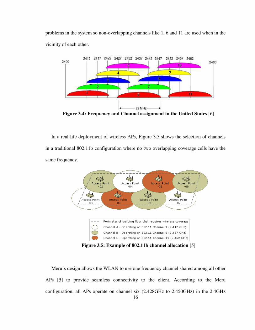
Figure 3.4 illustrates the frequency channel assignment in the United States for
traditional 802.11b. If adjacent signal frequencies overlap, they could cause interference
16
problems in the system so non-overlapping channels like 1, 6 and 11 are used when in the
vicinity of each other.
Figure 3.4: Frequency and Channel assignment in the United States [6]
In a real-life deployment of wireless APs, Figure 3.5 shows the selection of channels
in a traditional 802.11b configuration where no two overlapping coverage cells have the
same frequency.
Figure 3.5: Example of 802.11b channel allocation [5]
Meru’s design allows the WLAN to use one frequency channel shared among all other
APs [5] to provide seamless connectivity to the client. According to the Meru
configuration, all APs operate on channel six (2.428GHz to 2.450GHz) in the 2.4GHz
17
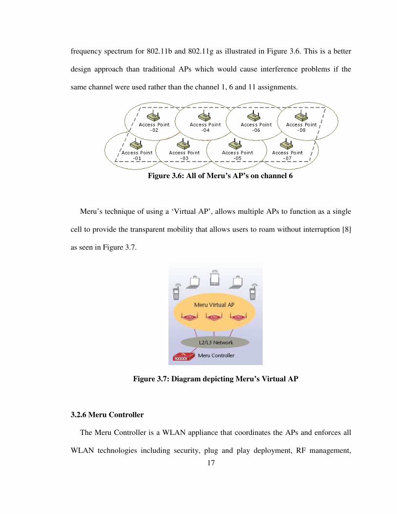
frequency spectrum for 802.11b and 802.11g as illustrated in Figure 3.6. This is a better
design approach than traditional APs which would cause interference problems if the
same channel were used rather than the channel 1, 6 and 11 assignments.
Figure 3.6: All of Meru’s AP’s on channel 6
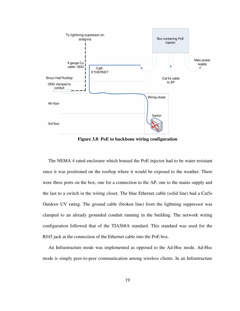
Meru’s technique of using a ‘Virtual AP’, allows multiple APs to function as a single
cell to provide the transparent mobility that allows users to roam without interruption [8]
as seen in Figure 3.7.
Figure 3.7: Diagram depicting Meru’s Virtual AP
3.2.6 Meru Controller
The Meru Controller is a WLAN appliance that coordinates the APs and enforces all
WLAN technologies including security, plug and play deployment, RF management,

18
mobility, contention management and Quality of Service, QoS. The controller is located
on a Layer 3 switched network in Haley Center.
3.2.7 Clinometer
The meter used to measure the downtilt angle was a commercial clinometer. This
measuring device was used to measure the angle of line-of-sight above or below the
horizontal. It was also used to set the horizontal bearing (angle, cardinal direction) of the
main lobe of the antenna.
3.2.8 PoE Injector
“802.3af is an IEEE standard for powering network devices via Ethernet cable. Also
known as Power-over-Ethernet, it provides 48 volts over 4-wires” [4] of an eight wire
data cable rather than have separate power cables for the operation of the AP. The PoE
injector minimizes the number of wires that must be strung in order to install the network
resulting in lower system costs, shorter downtime, easier maintenance and greater
installation flexibility. See Figure 3.8 for PoE configuration.
3.2.9 Wiring Description
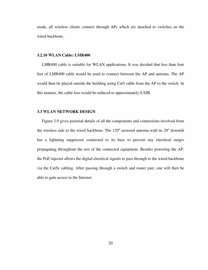
The diagram in Figure 3.8 indicates the wiring configuration from the PoE to the
network’s backbone.
19
Box containing PoE
injector
Cat 5e cable
to AP
Main power
supply
Broun Hall Rooftop
4th floor
3rd floor
6 gauge Cu
cable: GND Cat5:
ETHERNET
GND clamped to conduit
Wiring closet
Switch
To lightning supressor on
antenna
Figure 3.8: PoE to backbone wiring configuration
The NEMA 4 rated enclosure which housed the PoE injector had to be water resistant
since it was positioned on the rooftop where it would be exposed to the weather. There
were three ports on the box, one for a connection to the AP, one to the mains supply and
the last to a switch in the wiring closet. The blue Ethernet cable (solid line) had a Cat5e
Outdoor UV rating. The ground cable (broken line) from the lightning suppressor was
clamped to an already grounded conduit running in the building. The network wiring
configuration followed that of the TIA568A standard. This standard was used for the
RJ45 jack at the connection of the Ethernet cable into the PoE box.
An Infrastructure mode was implemented as opposed to the Ad-Hoc mode. Ad-Hoc
mode is simply peer-to-peer communication among wireless clients. In an Infrastructure
20
mode, all wireless clients connect through APs which are attached to switches on the
wired backbone.
3.2.10 WLAN Cable: LMR400
LMR400 cable is suitable for WLAN applications. It was decided that less than four
feet of LMR400 cable would be used to connect between the AP and antenna. The AP
would then be placed outside the building using Cat5 cable from the AP to the switch. In
this manner, the cable loss would be reduced to approximately 0.5dB.
3.3 WLAN NETWORK DESIGN
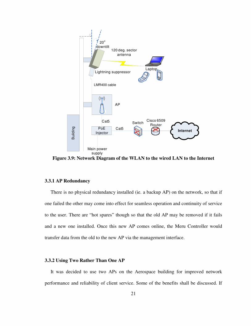
Figure 3.9 gives pictorial details of all the components and connections involved from
the wireless side to the wired backbone. The 120o sectored antenna with its 20
o downtilt
has a lightning suppressor connected to its base to prevent any electrical surges
propagating throughout the rest of the connected equipment. Besides powering the AP,
the PoE injector allows the digital electrical signals to pass through to the wired backbone
via the Cat5e cabling. After passing through a switch and router pair, one will then be
able to gain access to the Internet.
21
InternetPoE
Injector
120 deg. sector
antenna
Lightning suppressor
AP
Bu
ildin
g
20o
downtilt
Cat5
Main power supply
Cat5
Cisco 6509
Router
Laptop
Switch
LMR400 cable
Figure 3.9: Network Diagram of the WLAN to the wired LAN to the Internet
3.3.1 AP Redundancy
There is no physical redundancy installed (ie. a backup AP) on the network, so that if
one failed the other may come into effect for seamless operation and continuity of service
to the user. There are “hot spares” though so that the old AP may be removed if it fails
and a new one installed. Once this new AP comes online, the Meru Controller would
transfer data from the old to the new AP via the management interface.
3.3.2 Using Two Rather Than One AP
It was decided to use two APs on the Aerospace building for improved network
performance and reliability of client service. Some of the benefits shall be discussed. If
22
the network becomes saturated, one AP would not have to compromise service if the
other is free. Load balancing could swap clients between APs. A single AP would receive
all the noise from the environment or other wireless users but with two APs, the noise
would be halved per AP. Two APs would double the capacity and be able to
accommodate more traffic for that particular geographic location or support a client using
a high bandwidth application.
3.4 MAC AND SSID ASSIGNMENTS
The public name of the WLAN is the SSID. All wireless devices on a WLAN must
employ the same alpha-numeric SSID in order to communicate with each other. Table 3.1
shows the MAC addresses with their corresponding SSIDs.
It was quite helpful to have the SSIDs when taking signal strength measurements for
the different APs to create the coverage plots in Matlab. Initially, a laptop equipped with
Netstumbler, a network analyzer application, was used to acquire each AP’s signal
strength. The received signal displayed on Netstumbler was a combination of signals
from different APs at that particular location. The problem arose when one could not
differentiate the desired signal from the unwanted signals. To combat this problem, the
handheld device (PDA) equipped with the AirMagnet software was used whereby one
saw the signal strength for the particular AP based upon its SSID which was provided by
the network administrator.

23
Table 3.1: ESSID and MAC addresses of the APs
ENS made the hidden SSIDs available to the author for testing purposes. Generally, if
one connected to the WLAN, one would be connecting to the valid SSID’s of Meru_Test
and Tsunami.
MAC ADDRESS LOCATION (ESSID)
000CE605531E Aerospaceroof_1
000CE60A76DD Aerospaceroof_2
000CE001ED5 Broun Roof
24
CHAPTER 4: WLAN SECURITY
Security is an essential component of a WLAN design. Since a wireless system is not
as secure as a wired one, levels of security had to be included to prevent intruders from
viewing, modifying or stealing a user’s private information.
4.1 SSID
In the configuration used in the AU network, each AP advertises its presence to all
wireless devices in range several times per second by broadcasting beacon frames that
carry its SSID. One might ask, does the SSID provide network security? Since the SSID
is being broadcasted, its plaintext can be sniffed by rogue clients but they may not enter
the network unless they are authenticated via a username and password.
4.2 UNDERSTANDING THE IMPLEMENTATION OF SECURITY IN THE AU
NETWORK BASED UPON CISCO’S CONFIGURATION [14]
4.2.1 What is Cisco Clean Access?
Cisco Clean Access is a powerful, easy to use network management and security
solution. With comprehensive security features, user-authentication tools, and bandwidth
and traffic-filtering controls, Cisco Clean Access is a complete solution for controlling
25
and securing the network all in one place rather than having to propagate the policies
throughout the network on many devices.
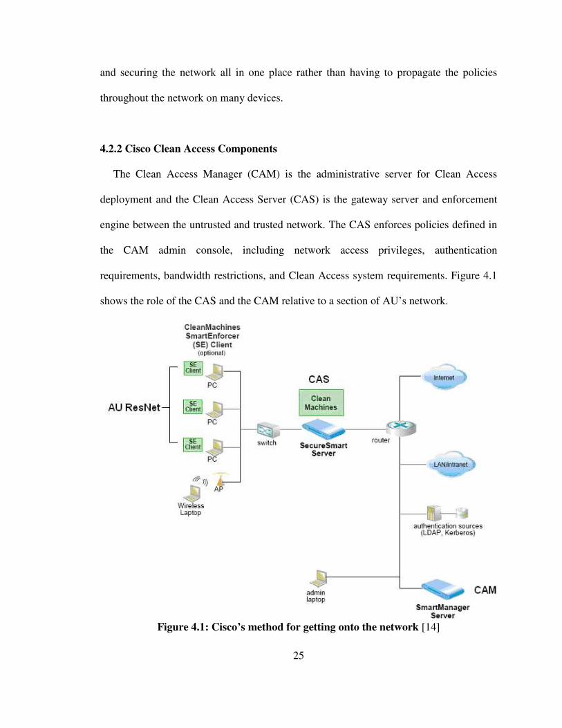
4.2.2 Cisco Clean Access Components
The Clean Access Manager (CAM) is the administrative server for Clean Access
deployment and the Clean Access Server (CAS) is the gateway server and enforcement
engine between the untrusted and trusted network. The CAS enforces policies defined in
the CAM admin console, including network access privileges, authentication
requirements, bandwidth restrictions, and Clean Access system requirements. Figure 4.1
shows the role of the CAS and the CAM relative to a section of AU’s network.
Figure 4.1: Cisco’s method for getting onto the network [14]
26
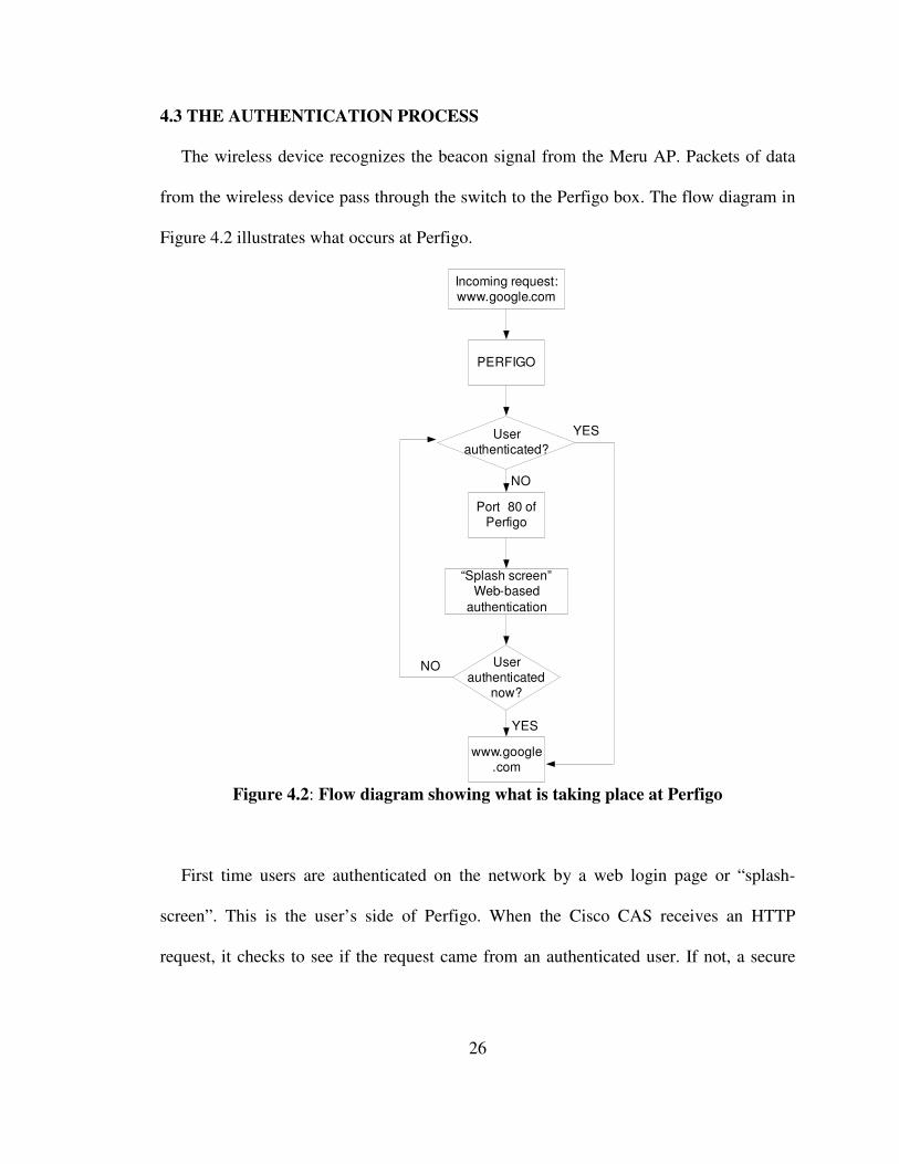
4.3 THE AUTHENTICATION PROCESS
The wireless device recognizes the beacon signal from the Meru AP. Packets of data
from the wireless device pass through the switch to the Perfigo box. The flow diagram in
Figure 4.2 illustrates what occurs at Perfigo.
Incoming request: www.google.com
PERFIGO
User authenticated?
Port 80 of Perfigo
“Splash screen”Web-based
authentication
User authenticated
now?
www.google.com
YES
YES
NO
NO
Figure 4.2: Flow diagram showing what is taking place at Perfigo
First time users are authenticated on the network by a web login page or “splash-
screen”. This is the user’s side of Perfigo. When the Cisco CAS receives an HTTP
request, it checks to see if the request came from an authenticated user. If not, a secure
27
login page is presented to the user. The login credentials can be authenticated by the
CAM [14].
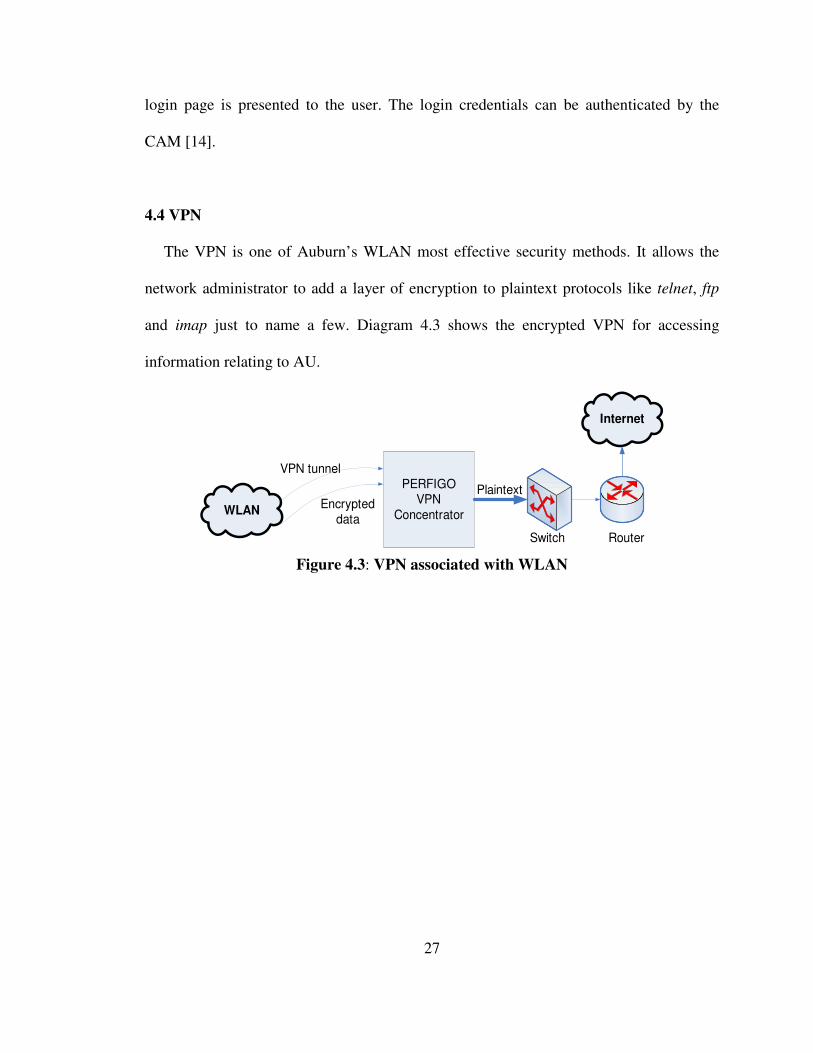
4.4 VPN
The VPN is one of Auburn’s WLAN most effective security methods. It allows the
network administrator to add a layer of encryption to plaintext protocols like telnet, ftp
and imap just to name a few. Diagram 4.3 shows the encrypted VPN for accessing
information relating to AU.
WLAN
Internet
PERFIGOVPN
Concentrator
VPN tunnel
Encrypted data
Plaintext
Switch Router
Figure 4.3: VPN associated with WLAN

28
CHAPTER 5: OUTDOOR MEASUREMENTS
Chapter 5 describes how antenna or field strength measurements were conducted and
the equipment and material that were needed. Matlab plots of the field intensity
measurements are included to indicate coverage areas.
5.1 SIGNAL STRENGTH READINGS TO PREDICT AP COVERAGE
Measurements were conducted on the AU campus where all the engineering schools
were located. The materials used were a 25 feet Craftsman measuring tape and chalk. A
Compaq iPAQ pocket PC equipped with the AirMagnet software and having a Cisco
Aironet 350 wireless adapter was used to measure the received signal strength from the
antenna.
5.2 MEASUREMENTS PROCEDURE
On a scaled map of the engineering campus, points were located at 50 feet intervals
from each other. A cluster of points were identified that were located in the vicinity of the
AP that was under test. At a particular test point, the pocket PC that contained the
wireless card was held facing the AP. From the AirMagnet software, the known MAC
addresses of the APs were found and the corresponding signal strength received (dBm)
29
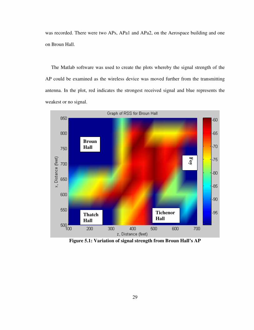
was recorded. There were two APs, APa1 and APa2, on the Aerospace building and one
on Broun Hall.
The Matlab software was used to create the plots whereby the signal strength of the
AP could be examined as the wireless device was moved further from the transmitting
antenna. In the plot, red indicates the strongest received signal and blue represents the
weakest or no signal.
Figure 5.1: Variation of signal strength from Broun Hall’s AP
Broun
Hall
Foy
Thatch
Hall
Tichenor
Hall
30
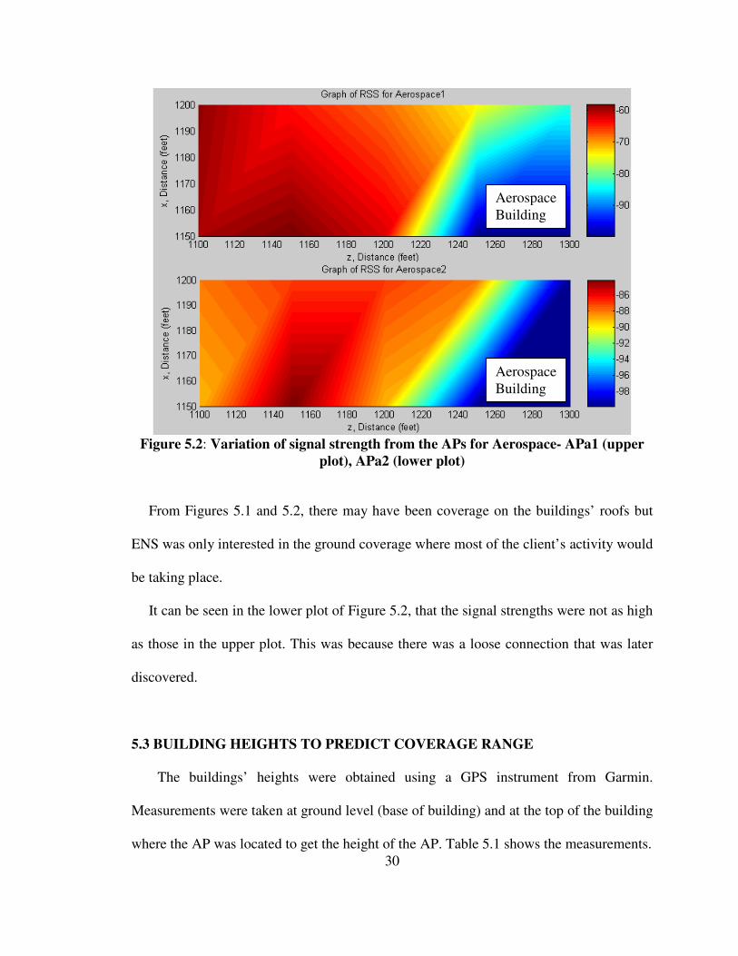
Figure 5.2: Variation of signal strength from the APs for Aerospace- APa1 (upper
plot), APa2 (lower plot)
From Figures 5.1 and 5.2, there may have been coverage on the buildings’ roofs but
ENS was only interested in the ground coverage where most of the client’s activity would
be taking place.
It can be seen in the lower plot of Figure 5.2, that the signal strengths were not as high
as those in the upper plot. This was because there was a loose connection that was later
discovered.
5.3 BUILDING HEIGHTS TO PREDICT COVERAGE RANGE
The buildings’ heights were obtained using a GPS instrument from Garmin.
Measurements were taken at ground level (base of building) and at the top of the building
where the AP was located to get the height of the AP. Table 5.1 shows the measurements.
Aerospace
Building
Aerospace
Building
31
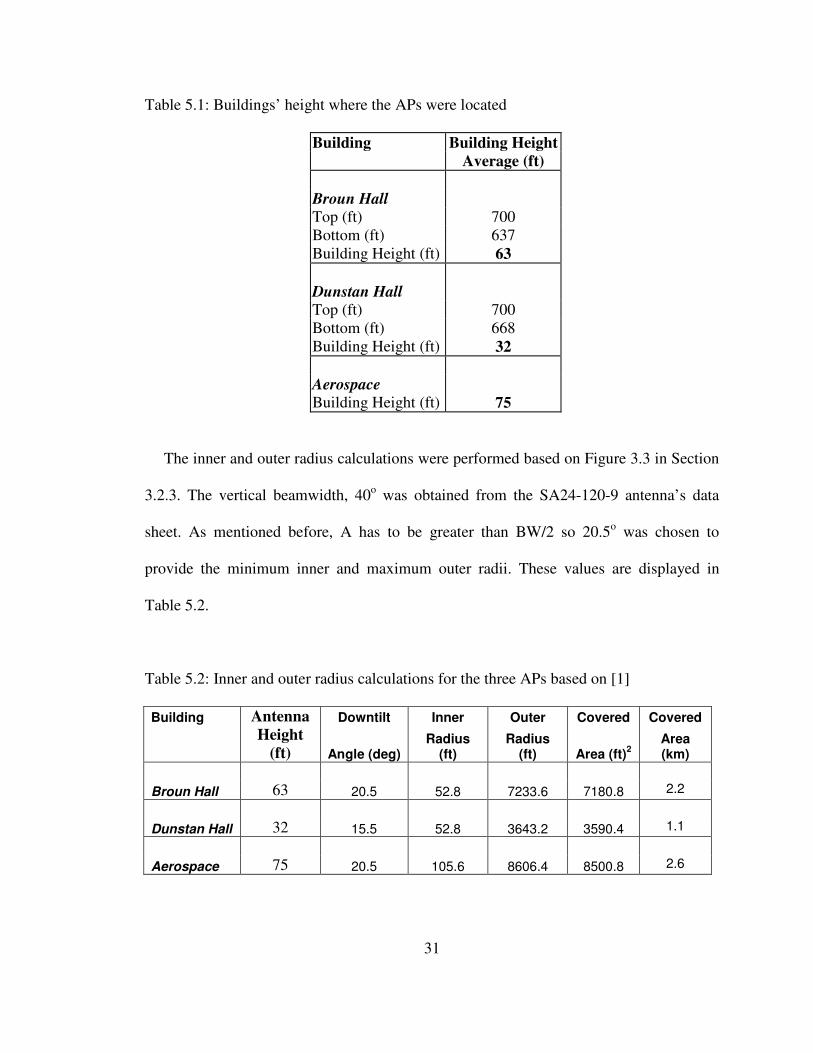
Table 5.1: Buildings’ height where the APs were located
Building Building Height
Average (ft)
Broun Hall
Top (ft) 700
Bottom (ft) 637
Building Height (ft) 63
Dunstan Hall
Top (ft) 700
Bottom (ft) 668
Building Height (ft) 32
Aerospace
Building Height (ft) 75
The inner and outer radius calculations were performed based on Figure 3.3 in Section
3.2.3. The vertical beamwidth, 40o was obtained from the SA24-120-9 antenna’s data
sheet. As mentioned before, A has to be greater than BW/2 so 20.5o was chosen to
provide the minimum inner and maximum outer radii. These values are displayed in
Table 5.2.
Table 5.2: Inner and outer radius calculations for the three APs based on [1]
Building Antenna Downtilt Inner Outer Covered Covered
Height
(ft) Angle (deg) Radius
(ft) Radius
(ft) Area (ft)2
Area (km)
Broun Hall 63 20.5 52.8 7233.6 7180.8 2.2
Dunstan Hall 32 15.5 52.8 3643.2 3590.4 1.1
Aerospace 75 20.5 105.6 8606.4 8500.8 2.6

32
The empirical data in Figure 5.1 showed that the coverage range for the AP situated on
Broun Hall was approximately 700 feet. This was not comparable to the theoretical value
of 7180.8 feet. The calculation was done for an ideal environment devoid of scatters,
interference, reflections, diffraction, that is perfectly flat (no terrain), no buildings, trees
or other interferers in the propagation path. If the antenna mounted on the building had no
downtilt and its main beam was radiating horizontally, then the coverage distance in the
horizontal plane would have been greater than 700 feet and possibly closer to the
theoretical value.

33
CHAPTER 6: A THEORETICAL ANALYSIS OF AP AND ANTENNA
COVERAGE
In this section, a theoretical model is developed in order to compare predicted and
measured E and H-plane radiation patterns based upon the manufacturer’s measured data
for the SA24-120-9 sectored antenna and the theoretical model developed. A further
analysis is presented to estimate the ground coverage of the SA24-120-9 antenna. The
analysis is based in part on measurements of the antenna’s horizontal and vertical
beamwidths, (120o and 40
o respectively). Once the ground coverage is estimated, it will
be compared to actual field measurements of the same.
6.1 USING MALTAB TO PLOT THE MANUFACTURER’S DATA
Figure 6.1 presents a Matlab plot of the radiation pattern in the horizontal, H-plane
and vertical, E-plane based upon measured data provided by the antenna manufacturer.

34
Figure 6.1: Polar plot generated in Matlab based on measured data for (a) H and (b)
E-plane
6.2 DEVELOPING A THEORETICAL MODEL
A reasonable model of a far-field antenna pattern with a single major lobe [12] is
E = cosn(θ )cos(φ )âθ + cos
m(θ )sin(φ )â φ (6.1)
where 0 ≤ φ ≤ 2π and 0 ≤ θ ≤ π. n and m are the powers of the cosine function that
determine the beamwidth of the antenna pattern in the E and H-planes.
Assume the orientation in Figure 6.2.
y
x
z
θφ
Figure 6.2: 3D Coordinate orientation for the analysis below

35
where y points vertically upwards, x is along the edge of the building (N-S) and z is
horizontal and away from the building (E-W). In the z-y plane or E-plane cut where φ is
90o,
E θ = cosm
(θ ) (6.2)
In the z-x plane or H-plane cut where φ is 0o,
E φ = cosn(θ ) (6.3)
Since the antenna pattern plots are normalized (maximum of unity) and the -3dB
beamwidth is known to be 120o, n can be chosen to approximately match the measured
data using
cosn(60
o) = 0.707 (6.4)
resulting in n = 0.5. Similarly, to determine m for the vertical beamwidth, one may solve
cosm
(15o) = 0.707 (6.5)
where m = 10.
Even though the data sheet quoted the antenna having a 40o vertical beamwidth, where
one would expect to use cosm
(20o) = 0.707 to determine m, the measured data showed the
antenna actually had a vertical beamwidth of approximately 30o. Hence, cos
m(15
o) =
0.707 was used to determine m.
According to [13], the gain of an antenna with a single main lobe is given
approximately byHE HPHP
G41253= . If one assumes that the gain and the half-power
beamwidth in the H-plane are known (9dBi and 120o
respectively for the antenna under
study) then the HPE must be 38o which is reasonably close to the 30
o value quoted above.
36
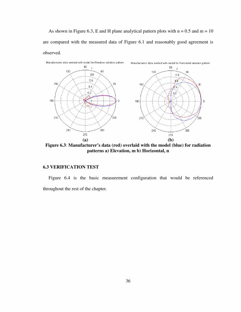
As shown in Figure 6.3, E and H plane analytical pattern plots with n = 0.5 and m = 10
are compared with the measured data of Figure 6.1 and reasonably good agreement is
observed.
(a) (b)
Figure 6.3: Manufacturer’s data (red) overlaid with the model (blue) for radiation
patterns a) Elevation, m b) Horizontal, n
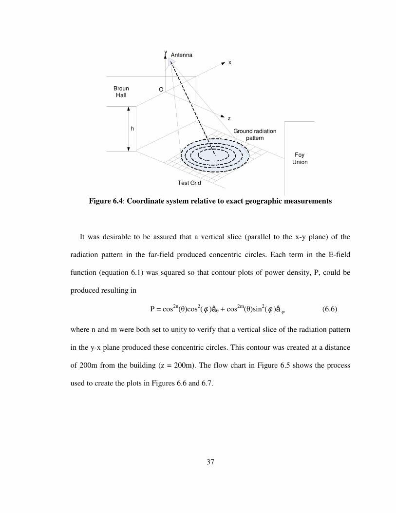
6.3 VERIFICATION TEST
Figure 6.4 is the basic measurement configuration that would be referenced
throughout the rest of the chapter.
37
O
y
x
z
Broun Hall
h
Foy
Union
Test Grid
Antenna
Ground radiation pattern
Figure 6.4: Coordinate system relative to exact geographic measurements
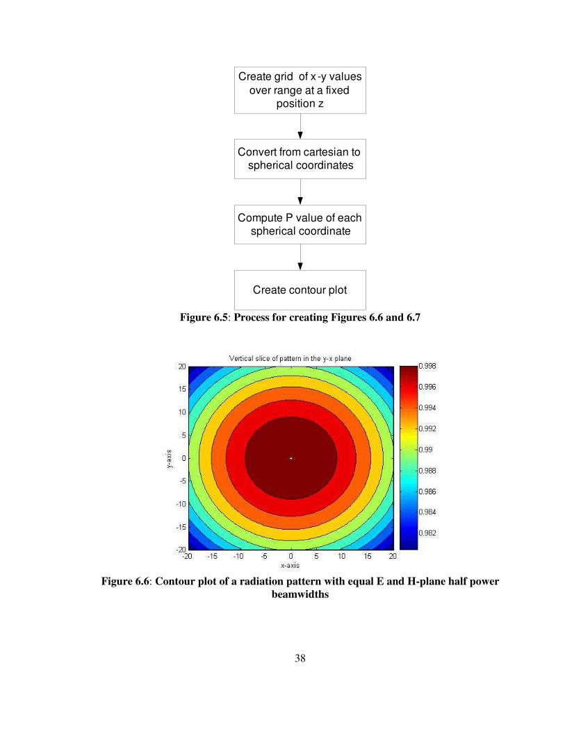
It was desirable to be assured that a vertical slice (parallel to the x-y plane) of the
radiation pattern in the far-field produced concentric circles. Each term in the E-field
function (equation 6.1) was squared so that contour plots of power density, P, could be
produced resulting in
P = cos2n
(θ)cos2(φ )âθ + cos
2m(θ)sin
2(φ )â φ (6.6)
where n and m were both set to unity to verify that a vertical slice of the radiation pattern
in the y-x plane produced these concentric circles. This contour was created at a distance
of 200m from the building (z = 200m). The flow chart in Figure 6.5 shows the process
used to create the plots in Figures 6.6 and 6.7.
38
Create grid of x -y values
over range at a fixed position z
Convert from cartesian to spherical coordinates
Compute P value of each spherical coordinate
Create contour plot
Figure 6.5: Process for creating Figures 6.6 and 6.7
Figure 6.6: Contour plot of a radiation pattern with equal E and H-plane half power
beamwidths
39
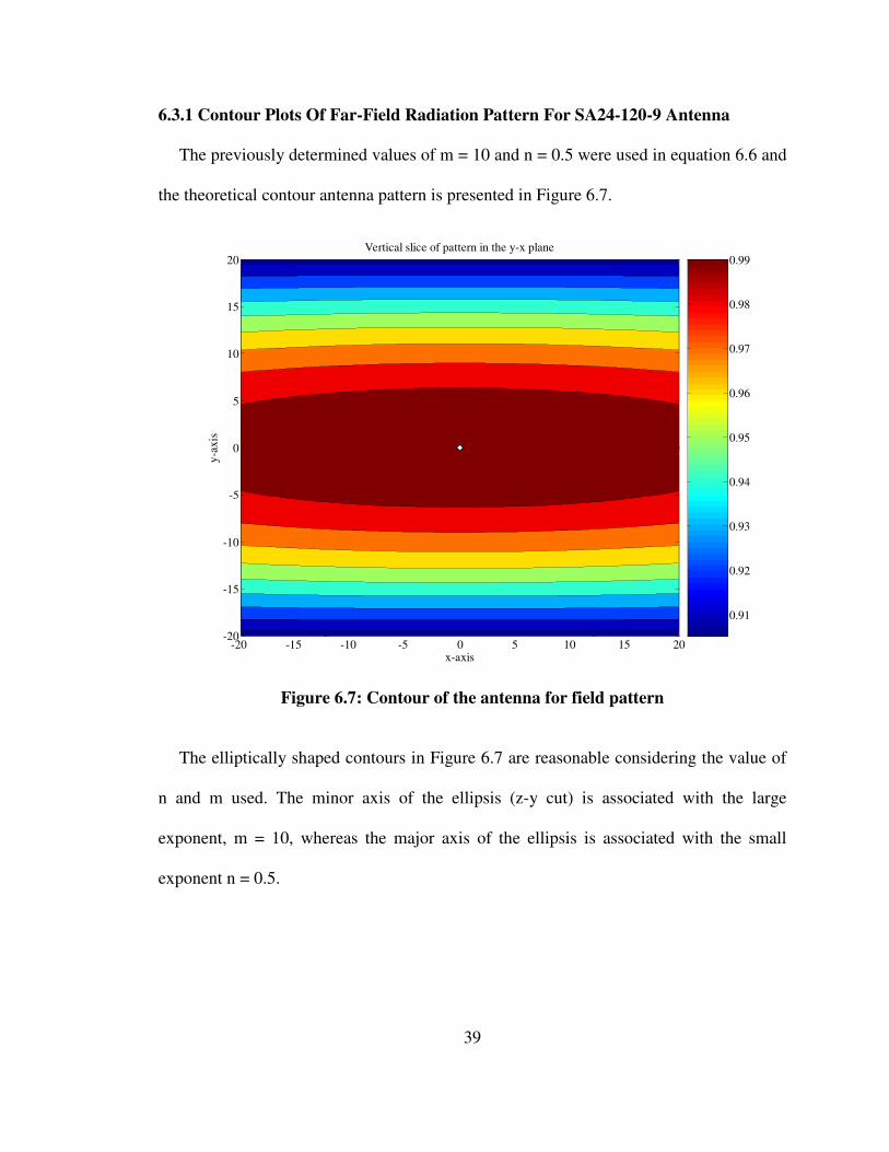
6.3.1 Contour Plots Of Far-Field Radiation Pattern For SA24-120-9 Antenna
The previously determined values of m = 10 and n = 0.5 were used in equation 6.6 and
the theoretical contour antenna pattern is presented in Figure 6.7.
x-axis
y-a
xis
Vertical slice of pattern in the y-x plane
-20 -15 -10 -5 0 5 10 15 20-20
-15
-10
-5
0
5
10
15
20
0.91
0.92
0.93
0.94
0.95
0.96
0.97
0.98
0.99
Figure 6.7: Contour of the antenna for field pattern
The elliptically shaped contours in Figure 6.7 are reasonable considering the value of
n and m used. The minor axis of the ellipsis (z-y cut) is associated with the large
exponent, m = 10, whereas the major axis of the ellipsis is associated with the small
exponent n = 0.5.
40
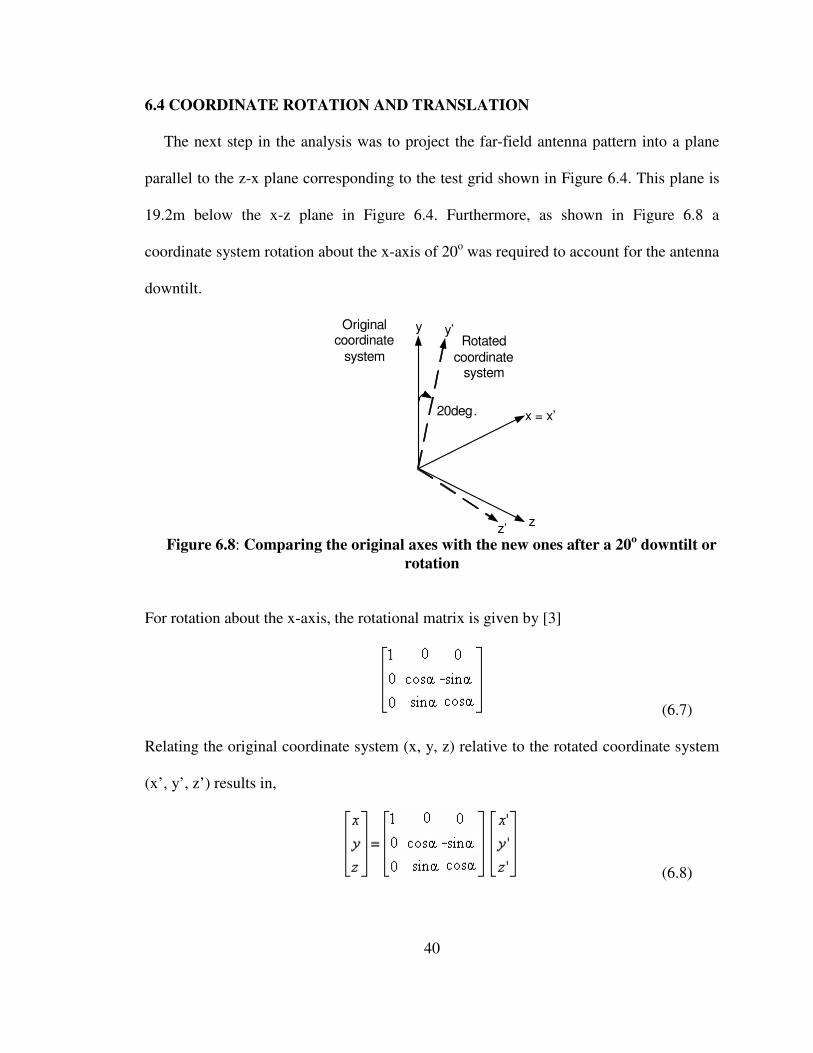
6.4 COORDINATE ROTATION AND TRANSLATION
The next step in the analysis was to project the far-field antenna pattern into a plane
parallel to the z-x plane corresponding to the test grid shown in Figure 6.4. This plane is
19.2m below the x-z plane in Figure 6.4. Furthermore, as shown in Figure 6.8 a
coordinate system rotation about the x-axis of 20o was required to account for the antenna
downtilt.
x = x’
y y’
zz’
Original coordinate
systemRotated
coordinate system
20deg.
Figure 6.8: Comparing the original axes with the new ones after a 20
o downtilt or
rotation
For rotation about the x-axis, the rotational matrix is given by [3]
(6.7)
Relating the original coordinate system (x, y, z) relative to the rotated coordinate system
(x’, y’, z’) results in,
(6.8)

41
To get the new coordinates, the inverse of the rotational matrix would have to be
multiplied by the old coordinate values resulting in
(6.9)
Translation was a simple procedure whereby 19.2 was subtracted from each y-value in
a particular range in Matlab. Essentially, the z-x plane was moved from parallel to the
building’s roof to ground level. The remaining procedure follows the method described
in Figure 6.5.
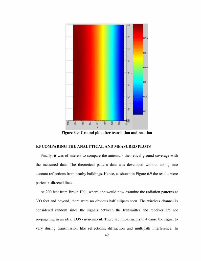
It was hypothesized that the antenna’s contour pattern when projected onto the ground
would consist of a small segment of concentric ellipses. It can be seen from Figure 6.9
that the hypothesized result is in reasonable agreement with the simulated results.
42
Figure 6.9: Ground plot after translation and rotation
6.5 COMPARING THE ANALYTICAL AND MEASURED PLOTS
Finally, it was of interest to compare the antenna’s theoretical ground coverage with
the measured data. The theoretical pattern data was developed without taking into
account reflections from nearby buildings. Hence, as shown in Figure 6.9 the results were
perfect x-directed lines.
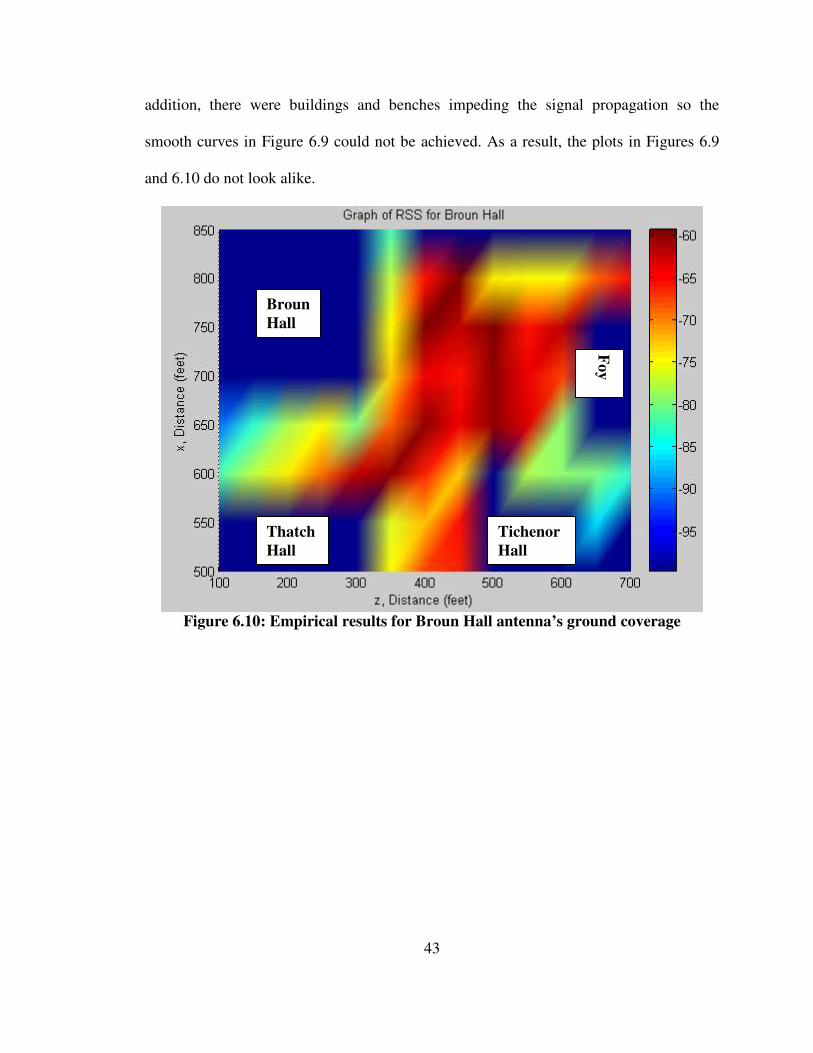
At 200 feet from Broun Hall, where one would now examine the radiation patterns at
300 feet and beyond, there were no obvious half ellipses seen. The wireless channel is
considered random since the signals between the transmitter and receiver are not
propagating in an ideal LOS environment. There are impairments that cause the signal to
vary during transmission like reflections, diffraction and multipath interference. In
43
addition, there were buildings and benches impeding the signal propagation so the
smooth curves in Figure 6.9 could not be achieved. As a result, the plots in Figures 6.9
and 6.10 do not look alike.
Figure 6.10: Empirical results for Broun Hall antenna’s ground coverage
Broun
Hall
Foy
Thatch
Hall
Tichenor
Hall
44
CHAPTER 7: ANTENNA ANALYSIS: CREATING THE RADIATION
PATTERNS FOR THE CELLULAR ANTENNA
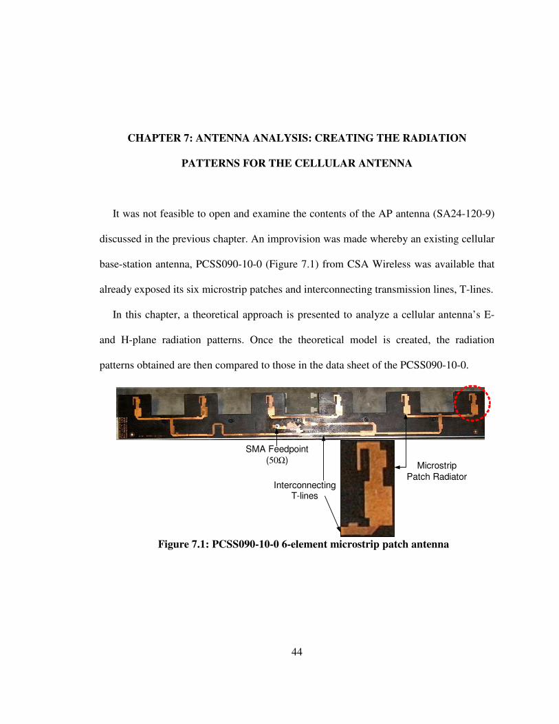
It was not feasible to open and examine the contents of the AP antenna (SA24-120-9)
discussed in the previous chapter. An improvision was made whereby an existing cellular
base-station antenna, PCSS090-10-0 (Figure 7.1) from CSA Wireless was available that
already exposed its six microstrip patches and interconnecting transmission lines, T-lines.
In this chapter, a theoretical approach is presented to analyze a cellular antenna’s E-
and H-plane radiation patterns. Once the theoretical model is created, the radiation
patterns obtained are then compared to those in the data sheet of the PCSS090-10-0.
Interconnecting T-lines
SMA Feedpoint
(50Ω)Microstrip
Patch Radiator
Figure 7.1: PCSS090-10-0 6-element microstrip patch antenna

45
7.1 BACKGROUND
The technique of determining the far-field pattern of an array of identical microstrip
patches or antenna elements is referred to as Pattern Multiplication [13]. To obtain the
antenna’s overall far-field E-plane radiation pattern, the single microstrip patch function
in the E-plane has to be multiplied by the corresponding array factor function in the E-
plane. The array factor is simply the pattern due to an array of isotropic point sources
located at the center of each microstrip patch element. Furthermore, each isotropic point
source must have the same amplitude and relative phase as its corresponding microstrip
patch element. The principle of pattern multiplication can also be used to determine the
final H-plane radiation pattern.
In conducting the analysis, some assumptions have to be made. The array is linear, ie.
the antenna patches are evenly spaced along a line. Furthermore, it is assumed that each
antenna element has equal magnitude excitation. Figure 7.2 provides the coordinate
system relative to the antenna’s orientation that is used to determine the principal plane
pattern functions.

46
x
y
z
3D coordinate system
6-element antenna
Feedline
E-plane
H-plane
E-fields
Figure 7.2: 3D coordinate system for PCSS090-10 antenna
7.2 DETERMINING THE SINGLE ELEMENT FUNCTIONS
As derived in reference [13] the microstrip element E-plane (x-z cut) and H-plane (y-z
cut) is given by
Fe(θ) = cos
θβsin
2
L E-plane, φ = 0
o (7.1)
and
Fh(θ) = cosθ
θβ
θβ
sin2
sin2
sin
W
W
H-plane, φ = 90o (7.2)
47
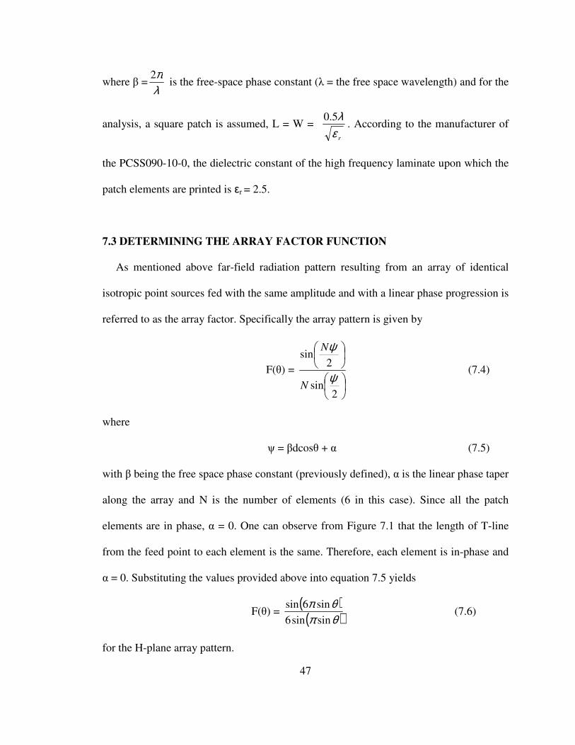
where β =λπ2
is the free-space phase constant (λ = the free space wavelength) and for the
analysis, a square patch is assumed, L = W = rελ5.0
. According to the manufacturer of
the PCSS090-10-0, the dielectric constant of the high frequency laminate upon which the
patch elements are printed is εr = 2.5.
7.3 DETERMINING THE ARRAY FACTOR FUNCTION
As mentioned above far-field radiation pattern resulting from an array of identical
isotropic point sources fed with the same amplitude and with a linear phase progression is
referred to as the array factor. Specifically the array pattern is given by
F(θ) =
2sin
2sin
ψ
ψ
N
N
(7.4)
where
ψ = βdcosθ + α (7.5)
with β being the free space phase constant (previously defined), α is the linear phase taper
along the array and N is the number of elements (6 in this case). Since all the patch
elements are in phase, α = 0. One can observe from Figure 7.1 that the length of T-line
from the feed point to each element is the same. Therefore, each element is in-phase and
α = 0. Substituting the values provided above into equation 7.5 yields
F(θ) = ( )
( )θπθπ
sinsin6
sin6sin (7.6)
for the H-plane array pattern.
48
In the E-plane cut where φ = 0o, the array factor is unity due to the isotropic nature of
the microstrip patch.
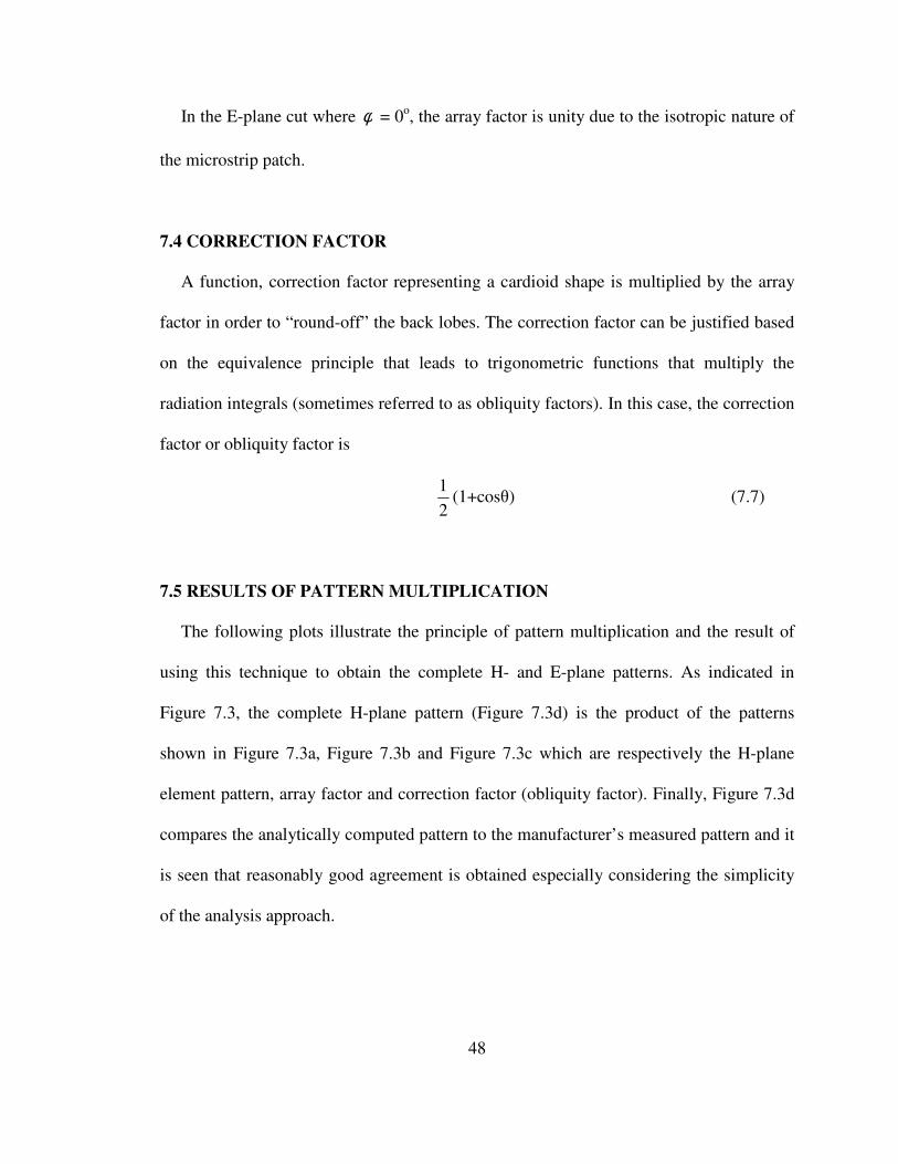
7.4 CORRECTION FACTOR
A function, correction factor representing a cardioid shape is multiplied by the array
factor in order to “round-off” the back lobes. The correction factor can be justified based
on the equivalence principle that leads to trigonometric functions that multiply the
radiation integrals (sometimes referred to as obliquity factors). In this case, the correction
factor or obliquity factor is
2
1(1+cosθ) (7.7)
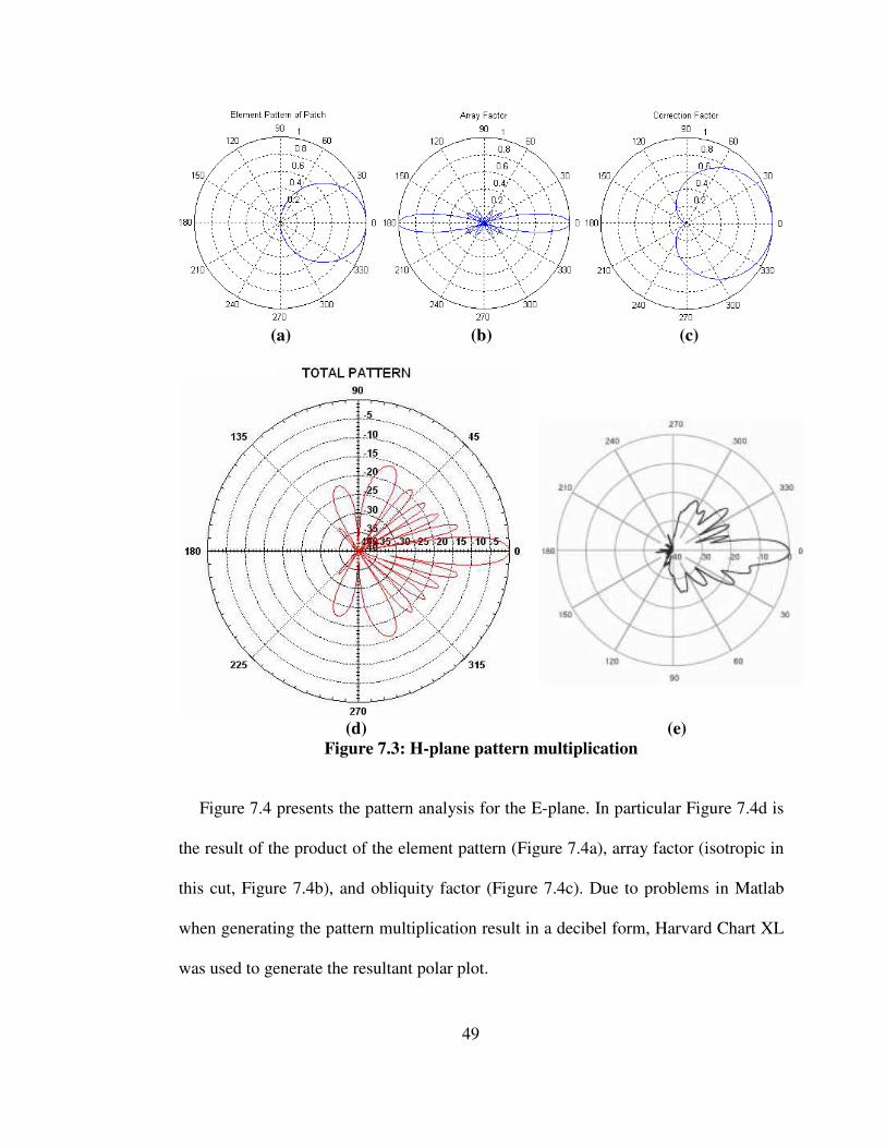
7.5 RESULTS OF PATTERN MULTIPLICATION
The following plots illustrate the principle of pattern multiplication and the result of
using this technique to obtain the complete H- and E-plane patterns. As indicated in
Figure 7.3, the complete H-plane pattern (Figure 7.3d) is the product of the patterns
shown in Figure 7.3a, Figure 7.3b and Figure 7.3c which are respectively the H-plane
element pattern, array factor and correction factor (obliquity factor). Finally, Figure 7.3d
compares the analytically computed pattern to the manufacturer’s measured pattern and it
is seen that reasonably good agreement is obtained especially considering the simplicity
of the analysis approach.
49
(a) (b) (c)
(d) (e)
Figure 7.3: H-plane pattern multiplication
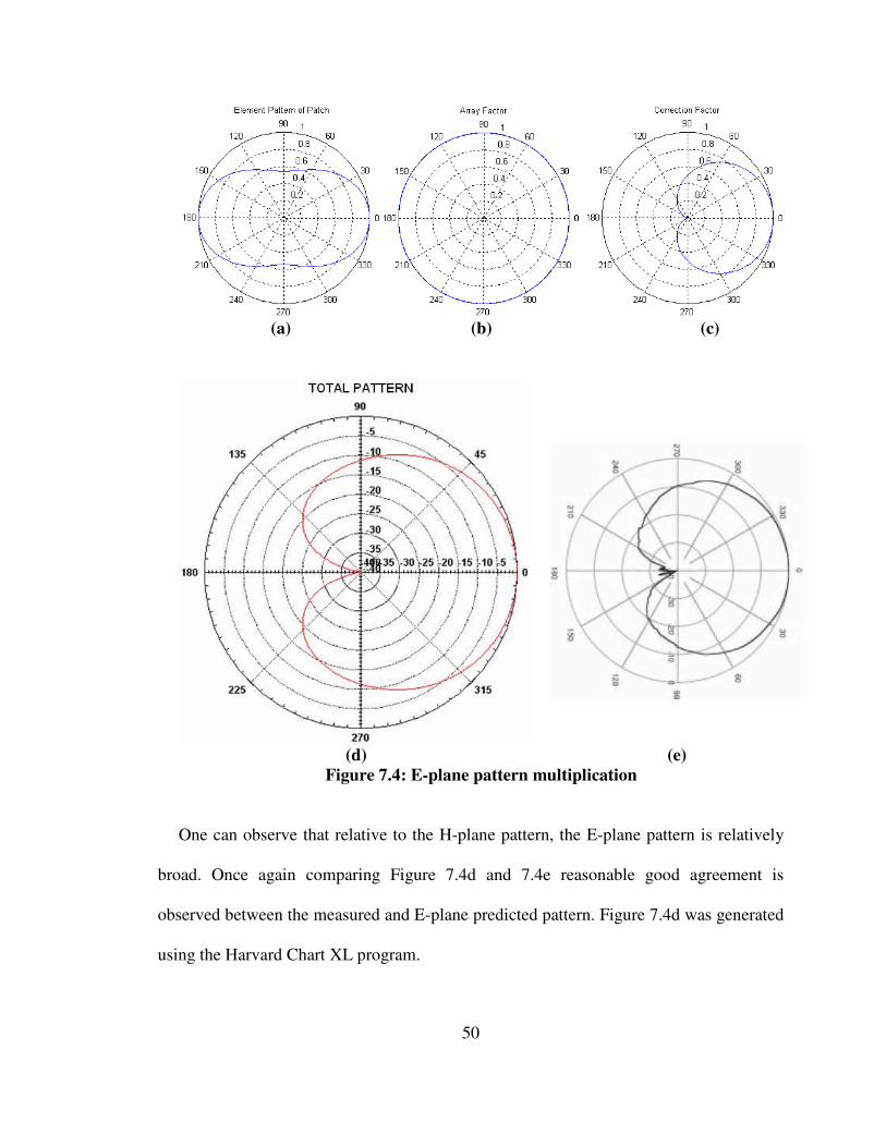
Figure 7.4 presents the pattern analysis for the E-plane. In particular Figure 7.4d is
the result of the product of the element pattern (Figure 7.4a), array factor (isotropic in
this cut, Figure 7.4b), and obliquity factor (Figure 7.4c). Due to problems in Matlab
when generating the pattern multiplication result in a decibel form, Harvard Chart XL
was used to generate the resultant polar plot.
50
(a) (b) (c)
(d) (e)
Figure 7.4: E-plane pattern multiplication
One can observe that relative to the H-plane pattern, the E-plane pattern is relatively
broad. Once again comparing Figure 7.4d and 7.4e reasonable good agreement is
observed between the measured and E-plane predicted pattern. Figure 7.4d was generated
using the Harvard Chart XL program.
51
CHAPTER 8: GENERAL ANALYSIS OF THE INPUT IMPEDANCE
CHARACTERISTIC
8.1 BACKGROUND
Chapter 8 continues with the analysis of the PCSS090-10-0 cellular antenna. The
objective of this section is to conduct a general analysis of the input impedance
characteristic of the base station antenna. A single microstrip patch identical to the one
used on the PCSS090-10-0 was built and analyzed in an attempt to gain a more complete
understanding of how the input impedance of a single isolated patch was related to the
same for the six-patch antenna. As indicated in Figure 8.1, a Hewlett Packard Vector
Network Analyzer (8753-C) was used to measure the input impedance to the antenna.
The measurement was repeated with the antenna inserted half-way into its radome.
Measurements with and without the radome are presented in Figures 8.3 and 8.6 and
Figures 8.4 and 8.7 respectively. Furthermore, the analyzer was programmed to display
the Voltage Standing Wave Ratio (VSWR) and Smith Chart plots over the range of
frequencies from 1500 to 2200MHz. According to the manufacturer’s data sheet, the
antenna is designed to operate with acceptably low VSWR over the range of frequencies
from 1850 to 1990MHz.

52
VNASMA
adaptors
PCSS090-10-0 antenna
Figure 8.1: PCSS090-10-0 antenna connected to VNA
8.2 ANALYZING THE PCSS090-10-0 ANTENNA
8.2.1 Using The VNA
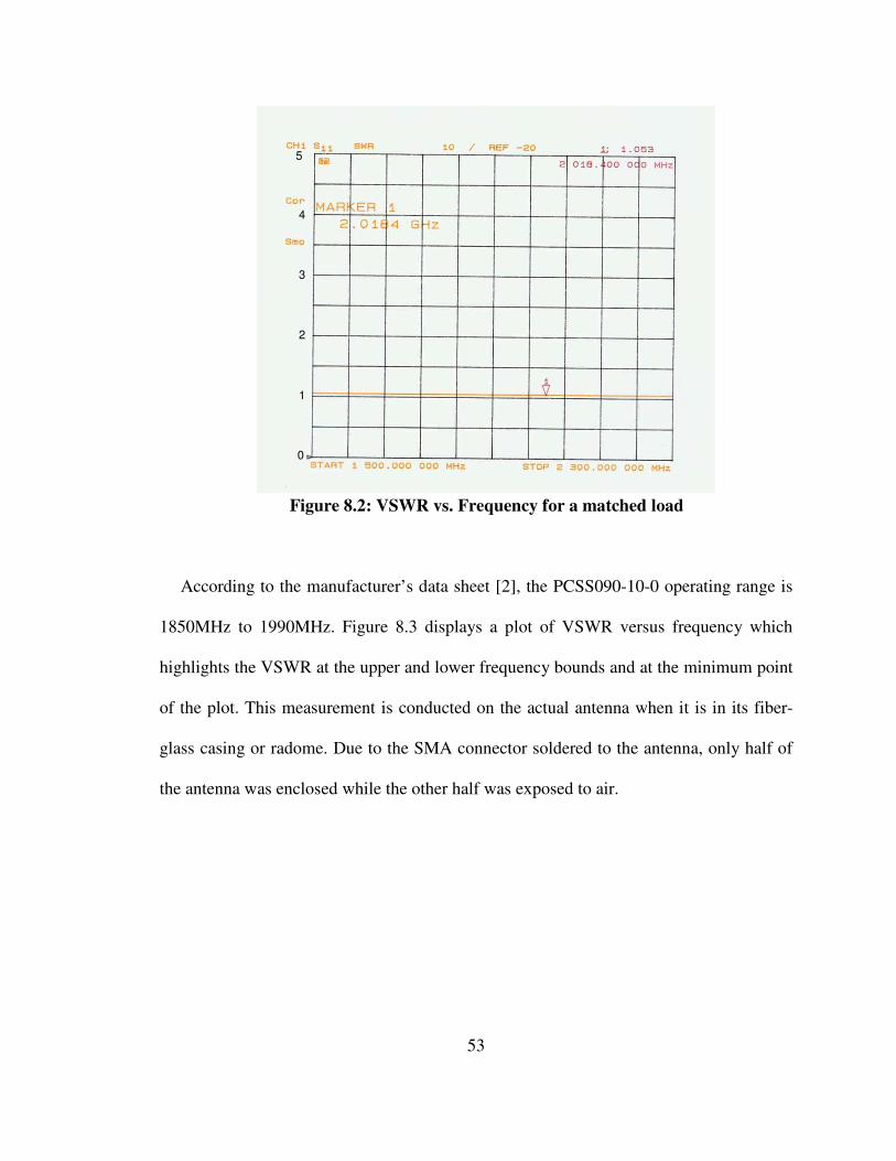
The VNA is used to measure the VSWR of the base station antenna when it is
connected to the analyzer. Before any antenna measurements are made, the VNA was
calibrated with the following standard terminations, short circuit, open circuit and a 50Ω
matched load by manually connecting them to the test ports of the VNA. Figure 8.2
shows a VSWR plot for a matched load being connected to the VNA terminal. The
VSWR of 1.053:1 proved that the calibration is sound as there are negligible reflections
at the load.
53
0
1
2
3
4
5
Figure 8.2: VSWR vs. Frequency for a matched load
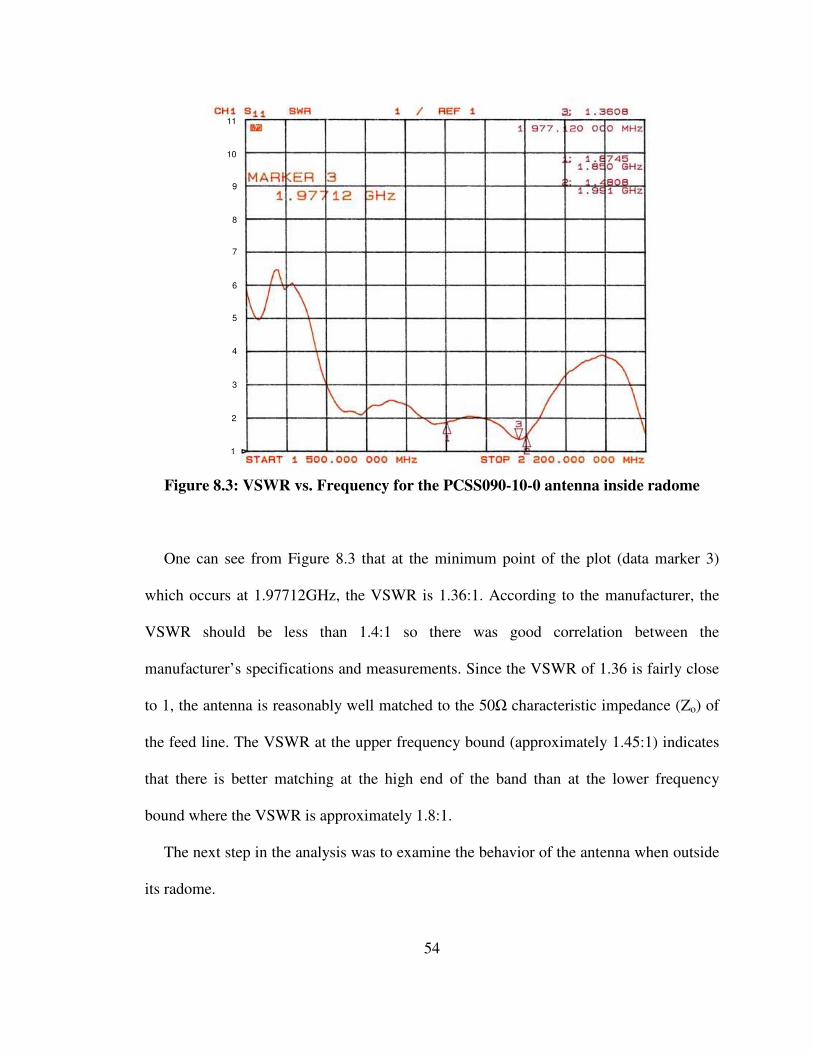
According to the manufacturer’s data sheet [2], the PCSS090-10-0 operating range is
1850MHz to 1990MHz. Figure 8.3 displays a plot of VSWR versus frequency which
highlights the VSWR at the upper and lower frequency bounds and at the minimum point
of the plot. This measurement is conducted on the actual antenna when it is in its fiber-
glass casing or radome. Due to the SMA connector soldered to the antenna, only half of
the antenna was enclosed while the other half was exposed to air.
54
1
2
3
4
5
6
7
8
9
10
11
Figure 8.3: VSWR vs. Frequency for the PCSS090-10-0 antenna inside radome
One can see from Figure 8.3 that at the minimum point of the plot (data marker 3)
which occurs at 1.97712GHz, the VSWR is 1.36:1. According to the manufacturer, the
VSWR should be less than 1.4:1 so there was good correlation between the
manufacturer’s specifications and measurements. Since the VSWR of 1.36 is fairly close
to 1, the antenna is reasonably well matched to the 50Ω characteristic impedance (Zo) of
the feed line. The VSWR at the upper frequency bound (approximately 1.45:1) indicates
that there is better matching at the high end of the band than at the lower frequency
bound where the VSWR is approximately 1.8:1.
The next step in the analysis was to examine the behavior of the antenna when outside
its radome.
55
1
2
3
4
5
6
7
8
9
10
11
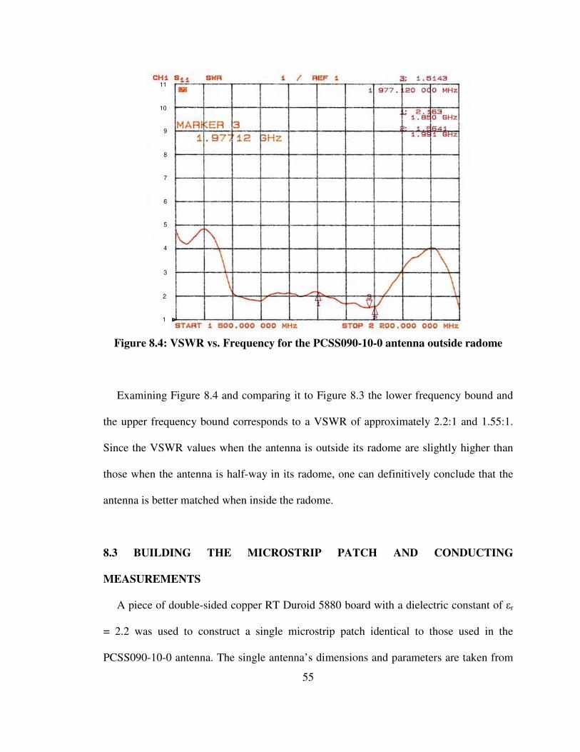
Figure 8.4: VSWR vs. Frequency for the PCSS090-10-0 antenna outside radome
Examining Figure 8.4 and comparing it to Figure 8.3 the lower frequency bound and
the upper frequency bound corresponds to a VSWR of approximately 2.2:1 and 1.55:1.
Since the VSWR values when the antenna is outside its radome are slightly higher than
those when the antenna is half-way in its radome, one can definitively conclude that the
antenna is better matched when inside the radome.
8.3 BUILDING THE MICROSTRIP PATCH AND CONDUCTING
MEASUREMENTS
A piece of double-sided copper RT Duroid 5880 board with a dielectric constant of εr
= 2.2 was used to construct a single microstrip patch identical to those used in the
PCSS090-10-0 antenna. The single antenna’s dimensions and parameters are taken from
56
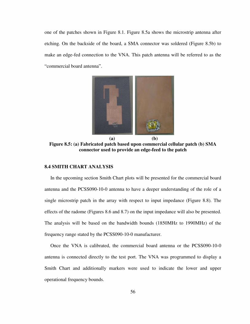
one of the patches shown in Figure 8.1. Figure 8.5a shows the microstrip antenna after
etching. On the backside of the board, a SMA connector was soldered (Figure 8.5b) to
make an edge-fed connection to the VNA. This patch antenna will be referred to as the
“commercial board antenna”.
(a) (b)
Figure 8.5: (a) Fabricated patch based upon commercial cellular patch (b) SMA
connector used to provide an edge-feed to the patch
8.4 SMITH CHART ANALYSIS
In the upcoming section Smith Chart plots will be presented for the commercial board
antenna and the PCSS090-10-0 antenna to have a deeper understanding of the role of a
single microstrip patch in the array with respect to input impedance (Figure 8.8). The
effects of the radome (Figures 8.6 and 8.7) on the input impedance will also be presented.
The analysis will be based on the bandwidth bounds (1850MHz to 1990MHz) of the
frequency range stated by the PCSS090-10-0 manufacturer.
Once the VNA is calibrated, the commercial board antenna or the PCSS090-10-0
antenna is connected directly to the test port. The VNA was programmed to display a
Smith Chart and additionally markers were used to indicate the lower and upper
operational frequency bounds.
57
8.4.1 Smith Chart Of PCSS090-10-0 Antenna
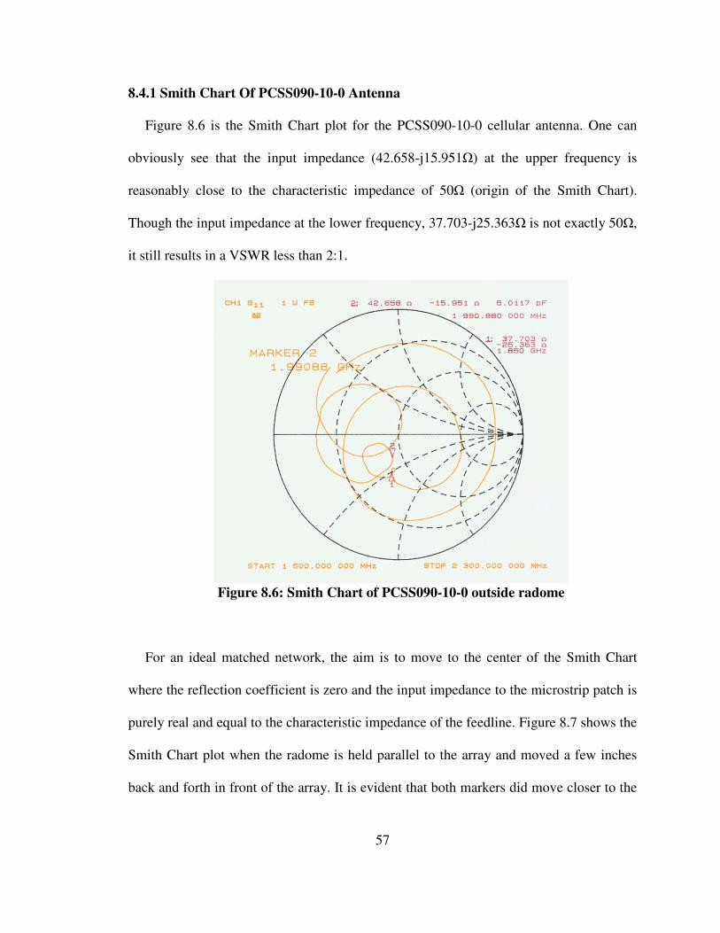
Figure 8.6 is the Smith Chart plot for the PCSS090-10-0 cellular antenna. One can
obviously see that the input impedance (42.658-j15.951Ω) at the upper frequency is
reasonably close to the characteristic impedance of 50Ω (origin of the Smith Chart).
Though the input impedance at the lower frequency, 37.703-j25.363Ω is not exactly 50Ω,
it still results in a VSWR less than 2:1.
Figure 8.6: Smith Chart of PCSS090-10-0 outside radome
For an ideal matched network, the aim is to move to the center of the Smith Chart
where the reflection coefficient is zero and the input impedance to the microstrip patch is
purely real and equal to the characteristic impedance of the feedline. Figure 8.7 shows the
Smith Chart plot when the radome is held parallel to the array and moved a few inches
back and forth in front of the array. It is evident that both markers did move closer to the
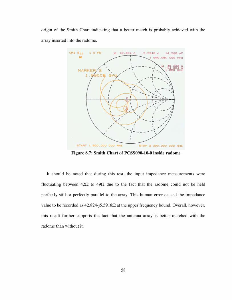
58
origin of the Smith Chart indicating that a better match is probably achieved with the
array inserted into the radome.
Figure 8.7: Smith Chart of PCSS090-10-0 inside radome
It should be noted that during this test, the input impedance measurements were
fluctuating between 42Ω to 49Ω due to the fact that the radome could not be held
perfectly still or perfectly parallel to the array. This human error caused the impedance
value to be recorded as 42.824-j5.5918Ω at the upper frequency bound. Overall, however,
this result further supports the fact that the antenna array is better matched with the
radome than without it.
59
8.4.2 Commercial Board Antenna Smith Chart
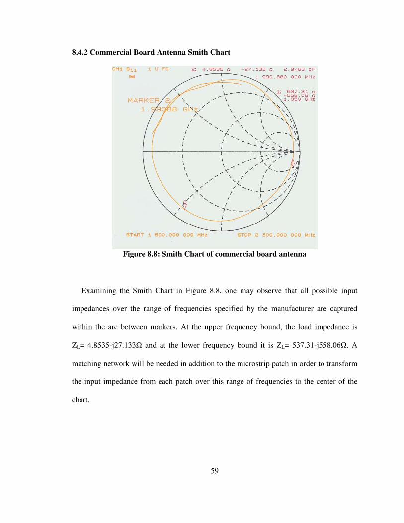
Figure 8.8: Smith Chart of commercial board antenna
Examining the Smith Chart in Figure 8.8, one may observe that all possible input
impedances over the range of frequencies specified by the manufacturer are captured
within the arc between markers. At the upper frequency bound, the load impedance is
ZL= 4.8535-j27.133Ω and at the lower frequency bound it is ZL= 537.31-j558.06Ω. A
matching network will be needed in addition to the microstrip patch in order to transform
the input impedance from each patch over this range of frequencies to the center of the
chart.
60
8.5 COMPARING A THEORETICAL VALUE OF IMPEDANCE TO THE
MEASURED VALUE
According to [13], an approximate expression for the input impedance of an edge-fed
patch is given by
ZA =
− W
L
r
r
190
2
εε
Ω (8.1)
where the dimensions of the patch are, length, L = 4.5cm, width, W = 1.9cm and the
dielectric constant of the commercial board antenna’s substrate is 2.2 leading to ZA =
2.04kΩ. For L > W, a high value of input impedance looking into the single patch is
expected. On the plot of Figure 8.8, at the upper frequency bound, the input impedance is
775Ω. This is a high value but not comparable to the theoretical value of 2.04kΩ. The
difference in results is attributed to the fact that the theoretical analysis is based on a
rectangle with length, L and width, W. Considerations were not made for the irregular-
shaped PCSS090-10-0 patch.
8.6 SUMMARY
The commercial board antenna represents a single microstrip patch of the PCSS090-
10-0 antenna. When placed in the array with the other five elements with matching
networks while in the presence of the radome, the overall input impedance is near 50Ω.
The matching of the actual patches to the input transmission line on the PCSS090-10-0
antenna is made by adjusting the widths of the T-line connecting the patches to the
common feed point and by inserting stubs of various positions along the interconnecting
61
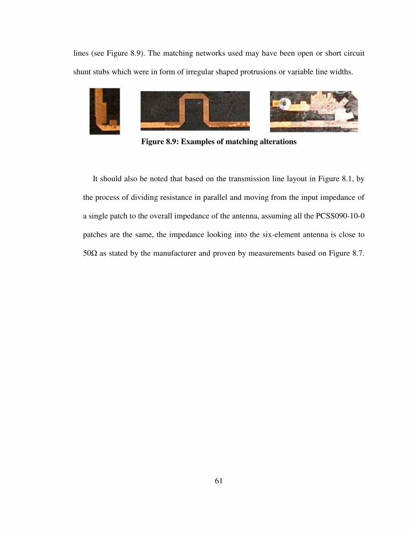
lines (see Figure 8.9). The matching networks used may have been open or short circuit
shunt stubs which were in form of irregular shaped protrusions or variable line widths.
Figure 8.9: Examples of matching alterations
It should also be noted that based on the transmission line layout in Figure 8.1, by
the process of dividing resistance in parallel and moving from the input impedance of
a single patch to the overall impedance of the antenna, assuming all the PCSS090-10-0
patches are the same, the impedance looking into the six-element antenna is close to
50Ω as stated by the manufacturer and proven by measurements based on Figure 8.7.

62
CONCLUSION
There are many factors that affect the propagation of radio signals and no one model
can accurately account for all factors. Existing theoretical models were used to compute
signal attenuation and predicted values were compared to measured data to determine
which model best represents the operating environment of the WLAN. All the models
tested were in fairly good agreement with the measured data. The best performing model
was the one that incorporated the most environmental factors.
In designing the WLAN, once the network designer decides where the hardware is to
be positioned to obtain maximum coverage, appropriate equipment and cabling can then
be chosen based on performance and how conveniently the hardware can be intergrated
into the existing network. The “text-book” design that was done, worked perfectly when
physically implemented. Ultimately, when the entire system is completely installed and
configured, the true performance test will be if the wireless and wired system can co-exist
with no problems.
A wireless network does not have the level of security as its wired counterpart.
Besides using SSID’s and VPN’s, Cisco’s Clean Access suite is implemented in the AU
wireless network.
Once the APs and antennas were configured and mounted on the buildings, signal
strength readings were recorded and Matlab plots created to provide a graphical
63
representation of the coverage provided by the APs on Broun Hall and the Aerospace
building. A theoretical analysis was conducted based on manufacturer’s data to estimate
the ground coverage of the SA24-120-9 antenna. This theoretical model was then
compared with actual field measurements. During the analysis, it was discovered that the
manufacturer’s data sheet plots did not match the measured data they supplied. Due to the
on-campus construction, the number of data points collected was limited because of
restricted access areas. More data would definitely have given a better representation of
the coverage area.
A theoretical approach of pattern multiplication was used to recreate the E- and H-
plane radiation cuts of the PCSS090-10-0 cellular antenna. The models developed were
compared with the corresponding E and H planes stated by the manufacturer and there
was reasonable similarity between them.
The antenna when examined inside and outside its radome and measurements
indicated that it was more closely matched to a 50Ω characteristic when inside the
radome. A single microstrip element identical to those used in the array was built and its
input impedance measured. Because the patch’s length to width ratio is small, its input
impedance is large and the T-lines and stubs on the actual antenna were designed to
reduce the combined high input impedance of each element to approximately 50Ω.
64
RECOMMENDATIONS
The network designer could consider a device that is multi-functional. For example,
while performing its primary function, acting as a wireless AP, the device could also have
built in switch and router functionality. Once this proposed device is configured
correctly, it could introduce hardware redundancy where the wireless network connects to
the wired backbone which can be advantageous to the overall system.
The PoE and AP were two separate units in the establishing of the antenna and AP
connection to the wired backbone (Figure 3.9). One device could be used for both
purposes and this might reduce cost by minimizing cabling requirements and also a single
unit would occupy less space. For example, with integrated IEEE 802.3af PoE, the
ProCurve Wireless Access Point 420 offers a cost-effective means to deploy either an
802.11b or 802.11g wireless network.
Using devices that implement Multiple Input-Multiple Output (MIMO) technology
can help improve the network’s overall performance regarding capacity and coverage.
The use of two or more antennas, along with the transmission of multiple signals (one for
each antenna) at the source and the destination might help eliminate problems caused by
multipath wave propagation [16]. The compromise with such a system is the additional
costs incurred with installing more antennas at both the transmitter and the receiver. The
long term effects would be beneficial since “a properly-designed MIMO system can

65
increase effective coverage by up to eight times and simultaneously deliver up to six
times greater effective throughput” [15].

66
REFERENCES
[1] Downtilt Coverage Radius, www.terabeam.com
[2] PCSS090-10 data sheet, www.csa-wireless.com
[3] Rotational Matrices, www.euclideanspace.com
[4] IEEE 802.3af, www.answers.com/topic/802-3af
[5] “Selecting Channel Frequencies for Wireless APs”, www.technet2.microsoft.com
[6] “Channel Deployment Issues for 2.4GHz 802.11 WLANs”, www.cisco.com
[7] Stuart M. Wentworth, Fundamentals Of Electromagnetics With Engineering
Applications, Wiley, 2005
[8] “Fulfilling the requirements of wireless networks for the enterprise”,
www.csgcorp.com
[9] Clint Smith, Practical Cellular & PCS Design, McGraw-Hill, 1998
[10] Theodore S. Rappaport, Wireless Communications Principles and Practices, 2e,
Prentice Hall, 2002
[11] “University of Georgia Upgrades Celebrated Wireless Research Network with
BelAir Networks Wide-Area Wi-Fi Infrastructure”, www.bbwexchange.com
[12] Dr. Riggs, Professor, Auburn University
[13] Warren L. Stutzman, Gary A. Thiele, Antenna Theory and Design, 2e, Wiley,
1998
[14] “Cisco Clean Access Manager Installation and Administration Guide”,
www.cisco.com
[15] “MIMO's multi-dimensional approach multiplies capacity”,
www.commsdesign.com

67
[16] MIMO, www.whatis.com