Politecnico di Torino

Porto Institutional Repository

[Doctoral thesis] Design, Implementation and Testing of Advanced ControlLaws for Fixed-wing UAVs

Original Citation:Sartori D. (2014). Design, Implementation and Testing of Advanced Control Laws for Fixed-wingUAVs. PhD thesis

Availability:This version is available at : http://porto.polito.it/2571146/ since: October 2014

Published version:DOI:10.6092/polito/porto/2571146

Terms of use:This article is made available under terms and conditions applicable to Open Access Policy Article("Creative Commons: Attribution-Noncommercial-Share Alike 3.0") , as described at http://porto.polito.it/terms_and_conditions.html

Porto, the institutional repository of the Politecnico di Torino, is provided by the University Libraryand the IT-Services. The aim is to enable open access to all the world. Please share with us howthis access benefits you. Your story matters.

(Article begins on next page)

POLITECNICO DI TORINO

SCUOLA DI DOTTORATO

Dottorato di Ricerca in Ingegneria Aerospaziale - XXVI ciclo

Tesi di Dottorato

Design, Implementation and Testing of Advanced

Control Laws for Fixed-wing UAVs

Daniele Sartori

Tutori Coordinatore del corso di dottorato

Prof. Giorgio Guglieri Prof.ssa Fulvia Quagliotti

Prof.ssa Fulvia Quagliotti

Prof. Matthew Rutherford

Prof. Kimon Valavanis

2014

ABSTRACT

The present PhD thesis addresses the problem of the control of small fixed-wing Unmanned

Aerial Vehicles (UAVs). In the scientific community much research is dedicated to the study

of suitable control laws for this category of aircraft. This interest is motivated by the several

applications that these platforms can perform and by their peculiarities as dynamical systems.

In fact, small UAVs are characterized by highly nonlinear behavior, strong coupling between

longitudinal and latero-directional planes, and high sensitivity to external disturbances and

to parametric uncertainties. Furthermore, the challenge is increased by the limited space

and weight available for the onboard electronics. The aim of this PhD thesis is to provide a

valid confrontation among three different control techniques and to introduce an innovative

autopilot configuration suitable for the unmanned aircraft field.

Three advanced controllers for fixed-wing unmanned aircraft vehicles are designed and

implemented: PID with H∞ robust approach, L1 adaptive controller and nonlinear back-

stepping controller. All of them are analyzed from the theoretical point of view and validated

through numerical simulations with a mathematical UAV model. One is implemented on a

microcontroller board, validated through hardware simulations and tested in flight.

The PID with H∞ robust approach is used for the definition of the gains of a commer-

cial autopilot. The proposed technique combines traditional PID control with an H∞ loop

shaping method to assess the robustness characteristics achievable with simple PID gains.

It is demonstrated that this hybrid approach provides a promising solution to the problem

of tuning commercial autopilots for UAVs. Nevertheless, it is clear that a tradeoff between

robustness and performance is necessary when dealing with this standard control technique.

The robustness problem is effectively solved by the adoption of an L1 adaptive controller

for complete aircraft control. In particular, the L1 logic here adopted is based on piecewise

constant adaptive laws with an adaptation rate compatible with the sampling rate of an au-

topilot board CPU. The control scheme includes an L1 adaptive controller for the inner loop,

while PID gains take care of the outer loop. The global controller is tuned on a linear decou-

pled aircraft model. It is demonstrated that the achieved configuration guarantees satisfying

performance also when applied to a complete nonlinear model affected by uncertainties and

Abstract

parametric perturbations.

The third controller implemented is based on an existing nonlinear backstepping tech-

nique. A scheme for longitudinal and latero-directional control based on the combination of

PID for the outer loop and backstepping for the inner loop is proposed. Satisfying results are

achieved also when the nonlinear aircraft model is perturbed by parametric uncertainties. A

confrontation among the three controllers shows that L1 and backstepping are comparable

in terms of nominal and robust performance, with an advantage for L1, while the PID is

always inferior.

The backstepping controller is chosen for being implemented and tested on a real fixed-

wing RC aircraft. Hardware-in-the-loop simulations validate its real-time control capability

on the complete nonlinear model of the aircraft adopted for the tests, inclusive of sensors

noise. An innovative microcontroller technology is employed as core of the autopilot sys-

tem, it interfaces with sensors and servos in order to handle input/output operations and it

performs the control law computation. Preliminary ground tests validate the suitability of

the autopilot configuration. A limited number of flight tests is performed. Promising results

are obtained for the control of longitudinal states, while latero-directional control still needs

major improvements.

iii

CONTENTS

Abstract . . . . . . . . . . . . . . . . . . . . . . . . . . . . . . . . . . . . . . . . . . . . ii

Contents . . . . . . . . . . . . . . . . . . . . . . . . . . . . . . . . . . . . . . . . . . . iv

List of Figures . . . . . . . . . . . . . . . . . . . . . . . . . . . . . . . . . . . . . . . . vii

List of Tables . . . . . . . . . . . . . . . . . . . . . . . . . . . . . . . . . . . . . . . . . xi

Nomenclature . . . . . . . . . . . . . . . . . . . . . . . . . . . . . . . . . . . . . . . . . xiii

Acknowledgments . . . . . . . . . . . . . . . . . . . . . . . . . . . . . . . . . . . . . . xvi

1. Preface . . . . . . . . . . . . . . . . . . . . . . . . . . . . . . . . . . . . . . . . . . 1

2. Introduction . . . . . . . . . . . . . . . . . . . . . . . . . . . . . . . . . . . . . . . . 4

2.1 Overview of UAV technology . . . . . . . . . . . . . . . . . . . . . . . . . . . 4

2.2 Control problem and proposed solutions . . . . . . . . . . . . . . . . . . . . . 11

2.3 PID with H∞ related work and contribution . . . . . . . . . . . . . . . . . . . 13

2.4 L1 related work and contribution . . . . . . . . . . . . . . . . . . . . . . . . . 15

2.5 Backstepping related work and contribution . . . . . . . . . . . . . . . . . . . 16

3. Fixed-wing Aircraft Mathematical Model . . . . . . . . . . . . . . . . . . . . . . . 18

3.1 Reference frames . . . . . . . . . . . . . . . . . . . . . . . . . . . . . . . . . . 18

3.1.1 Generic body axes . . . . . . . . . . . . . . . . . . . . . . . . . . . . . 18

3.1.2 Wind axes . . . . . . . . . . . . . . . . . . . . . . . . . . . . . . . . . . 18

3.1.3 NED axes . . . . . . . . . . . . . . . . . . . . . . . . . . . . . . . . . . 19

3.1.4 ECEF axes . . . . . . . . . . . . . . . . . . . . . . . . . . . . . . . . . 20

3.2 Euler angles . . . . . . . . . . . . . . . . . . . . . . . . . . . . . . . . . . . . . 20

3.3 Notable Euler angles . . . . . . . . . . . . . . . . . . . . . . . . . . . . . . . . 22

3.3.1 Body axes - Wind axes . . . . . . . . . . . . . . . . . . . . . . . . . . 22

Contents

3.3.2 Body axes - NED axes . . . . . . . . . . . . . . . . . . . . . . . . . . . 23

3.4 Nonlinear mathematical model . . . . . . . . . . . . . . . . . . . . . . . . . . 24

3.4.1 Forces equation . . . . . . . . . . . . . . . . . . . . . . . . . . . . . . . 24

3.4.2 Moments equation . . . . . . . . . . . . . . . . . . . . . . . . . . . . . 25

3.4.3 Attitude equation . . . . . . . . . . . . . . . . . . . . . . . . . . . . . 25

3.5 Linear mathematical model . . . . . . . . . . . . . . . . . . . . . . . . . . . . 26

3.6 Aircraft models . . . . . . . . . . . . . . . . . . . . . . . . . . . . . . . . . . . 29

3.6.1 MH850 UAV model . . . . . . . . . . . . . . . . . . . . . . . . . . . . 30

3.6.2 MH850 UAV actuators model . . . . . . . . . . . . . . . . . . . . . . . 33

3.6.3 C172P aircraft model . . . . . . . . . . . . . . . . . . . . . . . . . . . 36

3.6.4 Ultrastick 25e aircraft model . . . . . . . . . . . . . . . . . . . . . . . 37

4. H∞ Robust Approach to PID Design . . . . . . . . . . . . . . . . . . . . . . . . . . 40

4.1 Introduction to PID technique . . . . . . . . . . . . . . . . . . . . . . . . . . 40

4.2 Introduction to H∞ approach . . . . . . . . . . . . . . . . . . . . . . . . . . . 41

4.3 Problem formulation and proposed control design . . . . . . . . . . . . . . . . 43

4.4 Practical application and simulation results . . . . . . . . . . . . . . . . . . . 49

4.5 Conclusions . . . . . . . . . . . . . . . . . . . . . . . . . . . . . . . . . . . . . 60

5. L1 Adaptive Controller . . . . . . . . . . . . . . . . . . . . . . . . . . . . . . . . . 61

5.1 Introduction to L1 adaptive controller . . . . . . . . . . . . . . . . . . . . . . 61

5.2 Problem formulation and proposed control approach . . . . . . . . . . . . . . 62

5.3 Implementation and simulation results . . . . . . . . . . . . . . . . . . . . . . 65

5.3.1 Linear case design and simulation results . . . . . . . . . . . . . . . . 66

5.3.2 Nonlinear case simulation results . . . . . . . . . . . . . . . . . . . . . 69

5.3.3 Parametric robustness validation . . . . . . . . . . . . . . . . . . . . . 73

5.4 Conclusions . . . . . . . . . . . . . . . . . . . . . . . . . . . . . . . . . . . . . 73

6. Backstepping Nonlinear Controller . . . . . . . . . . . . . . . . . . . . . . . . . . . 76

6.1 Introduction to backstepping nonlinear controller . . . . . . . . . . . . . . . . 76

6.2 Problem formulation and proposed control approach . . . . . . . . . . . . . . 77

6.2.1 Shaping of the equations of motion . . . . . . . . . . . . . . . . . . . . 78

6.2.2 Backstepping controller design . . . . . . . . . . . . . . . . . . . . . . 80

6.2.3 Control strategy . . . . . . . . . . . . . . . . . . . . . . . . . . . . . . 84

6.3 Simulation results . . . . . . . . . . . . . . . . . . . . . . . . . . . . . . . . . 87

6.3.1 Parametric robustness validation . . . . . . . . . . . . . . . . . . . . . 89

v

Contents

6.3.2 Confrontation among backstepping, L1 and PID controllers . . . . . . 92

6.4 C172P SIL simulation results . . . . . . . . . . . . . . . . . . . . . . . . . . . 95

6.5 C172P HIL simulation results . . . . . . . . . . . . . . . . . . . . . . . . . . . 98

6.6 Conclusions . . . . . . . . . . . . . . . . . . . . . . . . . . . . . . . . . . . . . 101

7. Experiments and Flight Tests . . . . . . . . . . . . . . . . . . . . . . . . . . . . . . 103

7.1 Sensors noise model . . . . . . . . . . . . . . . . . . . . . . . . . . . . . . . . 103

7.1.1 Velocity measurement . . . . . . . . . . . . . . . . . . . . . . . . . . . 103

7.1.2 Altitude measurement . . . . . . . . . . . . . . . . . . . . . . . . . . . 105

7.1.3 Attitude measurement . . . . . . . . . . . . . . . . . . . . . . . . . . . 106

7.2 Kalman filter . . . . . . . . . . . . . . . . . . . . . . . . . . . . . . . . . . . . 107

7.3 Ultrastick 25e simulation results . . . . . . . . . . . . . . . . . . . . . . . . . 108

7.4 Ultrastick 25e HIL simulation results . . . . . . . . . . . . . . . . . . . . . . . 112

7.5 Aircraft - Controller integration . . . . . . . . . . . . . . . . . . . . . . . . . . 112

7.6 Command - Deflection correlation . . . . . . . . . . . . . . . . . . . . . . . . 119

7.7 Preliminary ground tests . . . . . . . . . . . . . . . . . . . . . . . . . . . . . . 120

7.8 Preliminary flight tests . . . . . . . . . . . . . . . . . . . . . . . . . . . . . . . 121

7.9 Conclusions . . . . . . . . . . . . . . . . . . . . . . . . . . . . . . . . . . . . . 125

8. Conclusions . . . . . . . . . . . . . . . . . . . . . . . . . . . . . . . . . . . . . . . . 128

Appendices . . . . . . . . . . . . . . . . . . . . . . . . . . . . . . . . . . . . . . . . . . 131

A. Evaluation of an L1 Controller for Wing Rock Suppression . . . . . . . . . . . . . 132

A.1 Introduction . . . . . . . . . . . . . . . . . . . . . . . . . . . . . . . . . . . . . 132

A.2 Wing rock model . . . . . . . . . . . . . . . . . . . . . . . . . . . . . . . . . . 134

A.3 Controller design . . . . . . . . . . . . . . . . . . . . . . . . . . . . . . . . . . 139

A.4 Implementation and simulation results . . . . . . . . . . . . . . . . . . . . . . 142

A.5 Conclusions . . . . . . . . . . . . . . . . . . . . . . . . . . . . . . . . . . . . . 145

B. Ultrastick 25e onboard connections schemes . . . . . . . . . . . . . . . . . . . . . . 148

Bibliography . . . . . . . . . . . . . . . . . . . . . . . . . . . . . . . . . . . . . . . . . 151

vi

LIST OF FIGURES

2.1 Tupolev Tu-143 reconnaissance drone [9]. . . . . . . . . . . . . . . . . . . . . 5

2.2 Aerosonde Mark 4.7 UAV for Antartic climate studies [14]. . . . . . . . . . . 6

2.3 Example of GCS from Aeronautics Defense Systems [21]. . . . . . . . . . . . 8

2.4 Example of EO/IR payload from Controp [22]. . . . . . . . . . . . . . . . . . 9

3.1 Generic body axes . . . . . . . . . . . . . . . . . . . . . . . . . . . . . . . . . 19

3.2 Wind axes . . . . . . . . . . . . . . . . . . . . . . . . . . . . . . . . . . . . . . 19

3.3 NED and ECEF axes orientation . . . . . . . . . . . . . . . . . . . . . . . . . 20

3.4 Two generic reference frames . . . . . . . . . . . . . . . . . . . . . . . . . . . 21

3.5 Euler angles for body axes - wind axes rotation . . . . . . . . . . . . . . . . . 23

3.6 Sequence of rotations to align FN to FB . . . . . . . . . . . . . . . . . . . . . 23

3.7 MH850 UAV . . . . . . . . . . . . . . . . . . . . . . . . . . . . . . . . . . . . 31

3.8 MH850 UAV model in ACI software tool . . . . . . . . . . . . . . . . . . . . . 32

3.9 GWS IQ-100 analog servo. . . . . . . . . . . . . . . . . . . . . . . . . . . . . . 34

3.10 Time domain normalized input and output series for V = 7.5 m/s. . . . . . . 34

3.11 Bode plot for the servo transfer function . . . . . . . . . . . . . . . . . . . . . 35

3.12 Cessna 172P aircraft . . . . . . . . . . . . . . . . . . . . . . . . . . . . . . . . 36

3.13 Ultrastick 25e aircraft . . . . . . . . . . . . . . . . . . . . . . . . . . . . . . . 37

4.1 Longitudinal control scheme . . . . . . . . . . . . . . . . . . . . . . . . . . . . 43

4.2 Latero-directional control scheme . . . . . . . . . . . . . . . . . . . . . . . . . 44

4.3 Root locus plot . . . . . . . . . . . . . . . . . . . . . . . . . . . . . . . . . . . 45

4.4 Robust control scheme . . . . . . . . . . . . . . . . . . . . . . . . . . . . . . . 46

4.5 P −K −∆ framework (a) and M −∆ framework (b) . . . . . . . . . . . . . 48

4.6 MicroPilot MP2028 autopilot [109] . . . . . . . . . . . . . . . . . . . . . . . . 50

4.7 MP2028 scheme as implemented in the simulator [108] . . . . . . . . . . . . . 50

4.8 Longitudinal plane characteristics, gains optimized for requirements . . . . . 52

4.9 Latero-directional plane characteristics, gains optimized for requirements . . . 53

4.10 3D trajectory view, gains optimized for requirements . . . . . . . . . . . . . . 55

List of Figures

4.11 Aircraft commands, gains optimized for requirements . . . . . . . . . . . . . . 55

4.12 Longitudinal plane characteristics, gains optimized for performance . . . . . . 56

4.13 Latero-directional plane characteristics, gains optimized for performance . . . 57

4.14 3D trajectory view, gains optimized for performance . . . . . . . . . . . . . . 58

4.15 Aircraft commands, gains optimized for performance . . . . . . . . . . . . . . 59

4.16 Flight parameters responses, gains optimized for performance . . . . . . . . . 59

5.1 L1 controller scheme . . . . . . . . . . . . . . . . . . . . . . . . . . . . . . . . 66

5.2 L1 with PID global controller scheme . . . . . . . . . . . . . . . . . . . . . . . 66

5.3 Linear model inner loop variables . . . . . . . . . . . . . . . . . . . . . . . . . 69

5.4 Linear model outer loop variables . . . . . . . . . . . . . . . . . . . . . . . . . 70

5.5 Linear model commands . . . . . . . . . . . . . . . . . . . . . . . . . . . . . . 70

5.6 Nonlinear model inner loop variables . . . . . . . . . . . . . . . . . . . . . . . 71

5.7 Nonlinear model outer loop variables . . . . . . . . . . . . . . . . . . . . . . . 72

5.8 Nonlinear model commands . . . . . . . . . . . . . . . . . . . . . . . . . . . . 72

5.9 Nonlinear model inner loop variables with parametric uncertainties . . . . . . 74

5.10 Nonlinear model outer loop variables with parametric uncertainties . . . . . . 74

5.11 Nonlinear model commands with parametric uncertainties . . . . . . . . . . . 75

6.1 Controlled variables and reference axes . . . . . . . . . . . . . . . . . . . . . . 78

6.2 Backstepping control strategy for fixed-wing aircraft . . . . . . . . . . . . . . 87

6.3 Nonlinear model outer loop variables . . . . . . . . . . . . . . . . . . . . . . . 89

6.4 Nonlinear model inner loop variables . . . . . . . . . . . . . . . . . . . . . . . 90

6.5 Nonlinear model commands . . . . . . . . . . . . . . . . . . . . . . . . . . . . 90

6.6 Nonlinear model outer loop variables with parametric uncertainties . . . . . . 91

6.7 Nonlinear model inner loop variables with parametric uncertainties . . . . . . 91

6.8 Nonlinear model commands with parametric uncertainties . . . . . . . . . . . 92

6.9 Outer loop variables confrontation among the proposed controllers . . . . . . 93

6.10 L1 controlled navigation variables with parametric uncertainties . . . . . . . . 93

6.11 PID controlled navigation variables with parametric uncertainties . . . . . . . 94

6.12 FlightGear SIL layout . . . . . . . . . . . . . . . . . . . . . . . . . . . . . . . 95

6.13 FlightGear SIL simulated maneuver for C172P . . . . . . . . . . . . . . . . . 96

6.14 FlightGear SIL simulated maneuver commands for C172P . . . . . . . . . . . 97

6.15 FlightGear HIL layout . . . . . . . . . . . . . . . . . . . . . . . . . . . . . . . 98

6.16 FlightGear HIL setup . . . . . . . . . . . . . . . . . . . . . . . . . . . . . . . 99

6.17 XMOS XK-1A board . . . . . . . . . . . . . . . . . . . . . . . . . . . . . . . . 100

viii

List of Figures

6.18 HIL hardware connections . . . . . . . . . . . . . . . . . . . . . . . . . . . . . 100

6.19 FlightGear HIL simulated maneuver for C172P . . . . . . . . . . . . . . . . . 101

6.20 FlightGear HIL simulated maneuver commands for C172P . . . . . . . . . . . 102

7.1 Pitot airspeed measurement scheme . . . . . . . . . . . . . . . . . . . . . . . 104

7.2 Pitot calibration curve, comparison of data from pitot and wind tunnel . . . . 105

7.3 Bosch BMP085 barometric sensor on Sparkfun breakout board . . . . . . . . 106

7.4 Vectornav VN-100 development board . . . . . . . . . . . . . . . . . . . . . . 107

7.5 Example of Vectornav VN-100 string for attitude in Euler angles . . . . . . . 107

7.6 Kalman filtering action on a noisy altitude measurement . . . . . . . . . . . . 109

7.7 Simulink outer loop response for Ultrastick 25e, trim conditions hold . . . . . 109

7.8 Simulink outer loop response for Ultrastick 25e, maneuver . . . . . . . . . . . 110

7.9 Simulink commands for Ultrastick 25e, maneuver . . . . . . . . . . . . . . . . 111

7.10 Simulink HIL layout . . . . . . . . . . . . . . . . . . . . . . . . . . . . . . . . 113

7.11 Simulink HIL outer loop response for Ultrastick 25e, trim conditions hold . . 113

7.12 Simulink HIL outer loop response for Ultrastick 25e, maneuver . . . . . . . . 114

7.13 Simulink HIL commands for Ultrastick 25e, maneuver . . . . . . . . . . . . . 114

7.14 Ultrastick 25e controller integration scheme . . . . . . . . . . . . . . . . . . . 116

7.15 PWM signal representation . . . . . . . . . . . . . . . . . . . . . . . . . . . . 116

7.16 Sparkfun OpenLog micro-SD data logger . . . . . . . . . . . . . . . . . . . . . 117

7.17 Pitot installation on the Ultrastick 25e right wing . . . . . . . . . . . . . . . . 119

7.18 Ultrastick 25e aircraft with sensors and microcontroller board . . . . . . . . . 120

7.19 Ultrastick 25e aileron servo calibration curves . . . . . . . . . . . . . . . . . . 121

7.20 Ultrastick 25e ground test, V control . . . . . . . . . . . . . . . . . . . . . . . 122

7.21 Ultrastick 25e ground test, h control . . . . . . . . . . . . . . . . . . . . . . . 122

7.22 Ultrastick 25e ground test, ψ control . . . . . . . . . . . . . . . . . . . . . . . 123

7.23 Airfield used for the flight tests . . . . . . . . . . . . . . . . . . . . . . . . . . 124

7.24 Ultrastick 25e during ground preparation and in flight . . . . . . . . . . . . . 125

7.25 Ultrastick 25e longitudinal flight test, V control . . . . . . . . . . . . . . . . . 126

7.26 Ultrastick 25e longitudinal flight test, h control . . . . . . . . . . . . . . . . . 126

7.27 Ultrastick 25e longitudinal flight test, latero-directional variables . . . . . . . 127

A.1 Configuration models A (left) and C (right) tested in the wind tunnel . . . . 134

A.2 Experimental setup . . . . . . . . . . . . . . . . . . . . . . . . . . . . . . . . . 135

A.3 Free motion simulation for model A; α = 32.5, φ0 = 1, φ0 = 0/s . . . . . . 137

A.4 Free motion simulation for model C; α = 32.5, φ0 = 1, φ0 = 0/s. . . . . . . 139

ix

List of Figures

A.5 Block scheme of L1 controller adopted for wing rock suppression . . . . . . . 141

A.6 Controlled roll angle and roll rate; α = 32.5, φ0 = 10, φ0 = 0/s. . . . . . . 143

A.7 Total nondimensional control input; α = 32.5, φ0 = 10, φ0 = 0/s. . . . . . 144

A.8 Controller action; α = 25, 30, 35, 40, φ0 = 10, φ0 = 0/s. . . . . . . . . . 145

A.9 Controller action; α = 32.5, φ0 = −30,−15, 15, 30, φ0 = 0/s. . . . . . . 145

A.10 Model C free and controlled motion; α = 42.5, φ0 = 10, φ0 = 0/s. . . . . . 146

A.11 Model C perturbed controlled motion; α = 32.5, φ0 = 10, φ0 = 0/s. . . . . 146

B.1 Ultrastick 25e power setup and servos integration scheme . . . . . . . . . . . 148

B.2 Ultrastick 25e pitot sensor integration scheme . . . . . . . . . . . . . . . . . . 149

B.3 Ultrastick 25e barometric pressure sensor integration scheme . . . . . . . . . 149

B.4 Ultrastick 25e IMU sensor and data logger integration scheme . . . . . . . . . 150

x

LIST OF TABLES

2.1 Levels of autonomy . . . . . . . . . . . . . . . . . . . . . . . . . . . . . . . . . 9

3.1 Employed controllers and aircraft models . . . . . . . . . . . . . . . . . . . . 30

3.2 MH850 UAV characteristics . . . . . . . . . . . . . . . . . . . . . . . . . . . . 31

3.3 MH850 UAV modes . . . . . . . . . . . . . . . . . . . . . . . . . . . . . . . . 32

3.4 C172P aircraft characteristics . . . . . . . . . . . . . . . . . . . . . . . . . . . 36

3.5 Ultrastick 25e aircraft characteristics . . . . . . . . . . . . . . . . . . . . . . . 38

3.6 MH850, C172P and Ultrastick 25e aircraft specific properties . . . . . . . . . 39

4.1 Longitudinal plane gains optimized for requirements . . . . . . . . . . . . . . 54

4.2 Latero-directional plane gains optimized for requirements . . . . . . . . . . . 54

4.3 Cumulative error, gains optimized for requirements . . . . . . . . . . . . . . . 54

4.4 Longitudinal plane gains optimized for performance . . . . . . . . . . . . . . 56

4.5 Latero-directional plane gains optimized for performance . . . . . . . . . . . . 57

4.6 Cumulative error, gains optimized for performance . . . . . . . . . . . . . . . 58

5.1 Outer loop PID gains . . . . . . . . . . . . . . . . . . . . . . . . . . . . . . . 68

5.2 Parameters for the parametric robustness validation cases . . . . . . . . . . . 73

6.1 Control sequence for the system of Equation (6.1) . . . . . . . . . . . . . . . 77

6.2 Change of variable relationships . . . . . . . . . . . . . . . . . . . . . . . . . . 83

6.3 Relationship between variables and commands . . . . . . . . . . . . . . . . . 86

6.4 MH850 backstepping controller gains . . . . . . . . . . . . . . . . . . . . . . . 88

6.5 MH850 outer loop PID gains . . . . . . . . . . . . . . . . . . . . . . . . . . . 88

6.6 C172P backstepping controller gains . . . . . . . . . . . . . . . . . . . . . . . 98

6.7 C172P outer loop PID gains . . . . . . . . . . . . . . . . . . . . . . . . . . . . 98

7.1 Kalman filter parameters . . . . . . . . . . . . . . . . . . . . . . . . . . . . . 108

7.2 Ultrastick Simulink backstepping controller gains . . . . . . . . . . . . . . . . 111

7.3 Ultrastick Simulink outer loop PID gains . . . . . . . . . . . . . . . . . . . . 112

List of Tables

7.4 Ultrastick Simulink HIL outer loop PID gains . . . . . . . . . . . . . . . . . . 115

7.5 Power budget for the onboard electronics . . . . . . . . . . . . . . . . . . . . 118

A.1 Aerodynamic coefficients for model A . . . . . . . . . . . . . . . . . . . . . . 136

A.2 Aerodynamic coefficients for model C . . . . . . . . . . . . . . . . . . . . . . 138

xii

NOMENCLATURE

Alon, Alat State matrices

Blon, Blat Input matrices

C(s) Plant controller transfer function

CL, CY Aerodynamic coefficients

CLα Lift aerodynamic derivative

Clδa , Clδe , Clδr Roll moment control derivatives

Clβ , Clβ , Clp, Clr Roll moment aerodynamic derivatives

Cmδa , Cmδe , Cmδr Pitch moment control derivatives

Cm0, Cmα, Cmα, Cmq Pitch moment aerodynamic derivatives

Cnδa , Cnδe , Cnδr Yaw moment control derivatives

Cnβ , Cnβ , Cnp, Cnr Yaw moment aerodynamic derivatives

F Total force vector [N]

FB(XB , YB , ZB) Generic Body axes coordinate system

FE(XE , YE , ZE) ECEF axes coordinate system

FN (XN , YN , ZN ) NED axes coordinate system

FW (XW , YW , ZW ) Wind axes coordinate system

Fx, Fy, Fz Components of the force vector F along body axes [N]

G(s) Plant transfer function

I Aircraft inertia tensor [kg· m2]

Nomenclature

KP , KI , KD PID gains

Kmult Multiplicative gain for the root locus plot

Lift Lift force [N]

MP Overshoot

Mx, My, Mz Components of the moment vector M about body axes [N· m]

M Total moment vector [N·m]

M(s) LFT matrix transfer function

T Engine thrust [N]

V Aircraft linear velocity vector [m/s]

X, Y , Z Aerodynamic and propulsion forces along body axes [N]

Xaero, Yaero, Zaero Aerodynamic forces along body axes [N]

b Wingspan [m]

c Wing mean aerodynamic chord [m]

g = 9.81 m/s2 Gravity acceleration

g2, g3 Gravity acceleration components [m/s2]

kα,1, kα,2, kβ,1, kβ,2 Backstepping controller gains

m Aircraft mass [kg]

p, q, r Components of the angular acceleration vector ω [rad/s2]

p, q, r Nondimensional angular velocities about body axes

p, q, r Components of the angular velocity vector ω [rad/s]

tS Settling time [s]

tr Rise time [s]

ulat Latero-directional plane control vector

ulon Longitudinal plane control vector

xiv

Nomenclature

u, v, w Components of the linear velocity vector V along body axes [m/s]

uc(t) Generic control signal

uad(t) Adaptive control signal

xlat Latero-directional plane state vector

xlon Longitudinal plane state vector

x(t) Estimation of the state signal

x(t) State signal

∆(s) Unstructured uncertainties transfer function

[Ψ], [Θ], [Φ] Elementary rotation matrices associated with general Euler angles

Ψ, Θ, Φ General Euler angles [rad]

α Angle of attack [rad]

β Sideslip angle [rad]

γ Ramp angle [rad]

δa Aileron command [rad]

δe Elevator command [rad]

δth Throttle command

θ Pitch angle [rad]

µ Structured singular value

φ Roll angle [rad]

ψ Yaw or heading angle [rad]

ω Aircraft angular acceleration vector about body axes [rad/s2]

ω Aircraft angular velocity vector about body axes [rad/s]

xv

ACKNOWLEDGMENTS

I wish to thank all the people that directly and indirectly helped me during the realization

of this work: my tutors in Torino, Prof. Giorgio Guglieri and Prof.ssa Fulvia Quagliotti,

and in Denver, Prof. Matthew Rutherford and Prof. Kimon Valavanis, for the opportunity

to develop this project and for constantly guiding and advising me; my colleagues in Torino

for dragging me to coffee breaks even if they always had to wait for me finishing to write an

email; the guys at the DU2SRI lab for the dim sum binges and for teaching me the mysteries

of electronics; my family who still has not clue what a PhD is; my little ninja for always

supporting me in hard times, no matter what.

1. PREFACE

The present PhD thesis is realized within the Department of Mechanical and Aerospace

Engineering (DIMEAS) of the Politecnico di Torino for the fulfillment of the PhD degree in

Aerospace Engineering. The research project was mainly carried out within the Unmanned

Aerial Vehicles (UAVs) research group of this department and for a total of nine months at

the University of Denver Unmanned Systems Research Institute (DU2SRI).

Both of these universities are active in a wide range of research projects related to the

unmanned aircraft technology. The first one, thanks to its aerospace background, focuses

on unmanned aircraft design and development with an emphasis on their Guidance, Nav-

igation and Control (GNC) systems. Examples of the activities include the realization of

a small fixed-wing aircraft for civil surveillance missions, the design of path planning and

guidance algorithms and the implementation of control logic to a self-developed autopilot.

The DU2SRI is managed by the Department of Electrical and Computer Engineering and

by the Department of Computer Science. Its focal points are robotics, automation, compu-

tational intelligence and distributed intelligence multi agent systems. Some of the on-going

projects include the realization of a sense-and-avoid RADAR-based sensor system, the design

of autonomous take-off and landing logic for rotorcrafts and the implementation of a control

and communication protocol for decentralized multi-robot team formation.

The combination of the expertise from these research groups allowed the realization this

PhD thesis. The aim of the project is the design and the implementation of three advanced

control laws for fixed-wing unmanned aircraft vehicles: PID with H∞ robust approach, L1

adaptive controller and nonlinear backstepping controller. The idea is to provide a valid con-

frontation among three different techniques that might help to guide the selection of a suitable

control law for small fixed-wing UAV. Among the controllers, the backstepping method is

selected for being implemented on a microcontroller and tested in flight on a real UAV. This

is relevant because, as it will be explained in Chapter 2, the large majority of the flying

autopilots for fixed-wing UAVs still relies on PIDs. Furthermore, it is innovative because the

number of backstepping controllers guaranteeing longitudinal and latero-directional control

for fixed-wing aircraft which have actually flown is even more restricted.

1. PREFACE

The approach in the realization of the PhD project was the following. The three con-

trollers were designed separately and sequentially. For each of them a bibliographic study was

initially performed in order to understand the state of the art and to identify the innovative

contributions. The adopted controllers were chosen taking into account three parameters:

suitability and benefit in the application to UAV autopilots, interest of the scientific com-

munity, possibility to introduce an innovation. For two of them, PID and L1, applicative

exercises were initially performed to acquire confidence with the control techniques and to

assess their performance, see for instance Appendix A. In the preliminary phase a Sliding

Mode Controller (SMC) was also evaluated based on the wing rock motion case [1]. It was

then disregarded because of its high-frequency switching nature that might generate the

chattering phenomenon, an oscillation in the control action incompatible with the control

surfaces adopted.

Once each controller was identified, the following phase consisted in the study and in

the definition of its mathematical basis. The theoretical foundation of the control law was

generally taken from existing work, but it was elaborated and combined in such a way to

guarantee an innovative contribution. The software implementation and the realization of

numerical simulations were used to validate the proposed approach. All controllers were

tested for the MH850 UAV, see Section 3.6.1. The same aircraft configuration was employed

to guarantee easy confrontation: complex maneuvers and robustness to uncertainty in the

model parameters were assessed.

As it will be explained in Section 6.3.2, the backstepping controller was selected for the

implementation on a real fixed-wing model aircraft. The definition of the backstepping ap-

proach together with the first steps towards implementation were carried out at the DU2SRI.

The adoption of an innovative microcontroller technology allowed its real time validation

through hardware-in-the-loop simulations (HIL), see Section 6.5. A considerable part of the

PhD project was dedicated to the integration of the controller on the aircraft and to the in-

terface among all subsystems for the realization of a complete autopilot system, see Chapter

7. Ground tests were initially carried out to verify the functioning of the autopilot system

and to verify the correct action of the backstepping controller. Different practical problems

were solved in this phase and the control law was adjusted to deal with real implementation.

Finally, preliminary flight tests were carried out at the DU2SRI. Unfortunately, some logistic

and technical difficulties limited the number of tests to a handful.

The thesis is structured in the following way. Chapter 2 introduces the UAV technol-

ogy and defines the control problem addressed in this work. The solutions here proposed

are illustrated with an emphasis on their contribution to the state of the art. Chapter 3

2

1. PREFACE

describes the mathematical linear and nonlinear aircraft models employed for the definition

and the testing of the controllers. The vehicles adopted for the simulations and their physi-

cal characteristics are also introduced. Chapter 4 and Chapter 5 deal, respectively, with the

design and the numerical simulations of the H∞-based PID controller and of the L1 adaptive

controller. In Chapter 6 the backstepping design is presented together with the results of

the main software simulations. Here a comparison among the three controllers is proposed

and, following the decision to implement the backstepping controller, hardware simulations

are introduced to validate its real time implementability on a microcontroller. Chapter 7

describes the preparation for the flight tests. This include the validation through software

and hardware simulations of the control law for the selected RC aircraft model. The physical

integration of the controller on the vehicle is presented, the problems encountered and the

adopted solutions are illustrated. The results of preliminary ground and flight tests are pro-

posed. Finally, Chapter 8 draws the conclusions and suggests possible improvements to be

carried out during future work. Two appendices can be found at the end of the thesis. The

first one describes the applicative exercise of L1 to the wing rock phenomenon, the second

one illustrates the connection schemes of the autopilot system.

3

2. INTRODUCTION

This chapter introduces the main features of the unmanned aircraft technology and describes

the state of the art relative to the control of these vehicles. The proposed solutions which

will be analyzed in this thesis are illustrated underlining their advantages and drawbacks,

emphasizing their contribution to the existing work.

2.1 Overview of UAV technology

UAV stands for Unmanned Aerial Vehicle. This acronym comprehends a broad range of

powered, aerial vehicles that do not carry any human operator, use aerodynamic forces to

provide vehicle lift, can fly autonomously or be piloted remotely, can be expendable or recov-

erable, and can carry a lethal or nonlethal payload. Ballistic or semi-ballistic vehicles, cruise

missiles, and artillery projectiles are not considered UAVs [2].

The interest for this category of vehicles has its origins in the military environment during

the Cold War. Within the United States Air Force, the necessity of avoiding risky surveillance

missions over the enemy territory became evident during the Korean War and after the 1960

shooting down of Gary Power’s U2 above the Soviet Union [3]. This requirement gave birth

to the first generation of reconnaissance drones, among them the most significant was the

Ryan Model 147 Lightning Bug which was widely employed in the Vietnam conflict [4]. On

the other side of the Iron Curtain the Soviet Union carried out unmanned reconnaissance

missions with a family of drones from the Tupolev design bureau, the first being the Tu-123

Yastreb introduced into active service in 1964 [5], see Fig. 2.1.

Meanwhile in Europe, British and West German forces started operating the Canadian

designed and jointly produced Canadair CL-89, later adopted also by Italian and French

armies. In the following years a variety of projects with increasing levels of autonomy and

capability were conceived, but the application of unmanned vehicles experienced alternating

periods according to the current status of rival technologies, strategic vision, political doctrine

and geopolitical framework. The major event which imposed UAVs as important tools for

the military field was the 1990 Gulf War where their operational ability in combat situations

2. INTRODUCTION

Fig. 2.1: Tupolev Tu-143 reconnaissance drone [9].

was proved [6]. The primary UAV employed was the Pioneer, a vehicle developed by the U.S.

together with the Israel Aircraft Industries [7]. The end of the Cold War strongly reduced

military expenditures for strategic reconnaissance and forced to find inexpensive alternatives

[8]. Nowadays major air forces worldwide rely on the UAV technology for a wide range

of missions, many of them being for reconnaissance, target acquisition and communication

support. It is estimated that more than 50 countries are currently developing more than 1000

Unmanned Aerial Vehicles [5]. Among them much emphasis is now given to small portable

systems, easy to deploy and maintain, relatively inexpensive and so expendable.

The development of UAVs for civil applications started only 20 years ago, supported by

the know-how achieved in the military field at the cost of large investments. One of the key

programs that promoted the use of UAVs for commercial science applications began in 1994

and was managed by NASA with the collaboration of several industries and universities [10].

The ERAST (Environmental Research Aircraft and Sensor Technology) program laid the

foundations for the commercial applications of sensor and communication technologies found

in modern civil UAVs. Reduced size and weight of sensors, increased computational power

of microcontroller boards, reduced cost of electronic components and high-density energy

sources are now allowing the civil UAV market to thrive. The players in this field are not

only large industries or government organizations: small companies, research centers and

universities have the possibility to propose creative and effective solutions for determined

applications. A serious limitation to the full growth of the civil UAV market is the national

airspace authority regulation [11]. Many restrictions are still imposed to the flight in public

airspace, in particular where densely populated [12]. A gradual relaxation of the requirements

is in progress thanks to an increase of reliability of the technologies adopted and to a more

accurate assessment of the risks involved. Some of the most popular uses include [8][13]:

5

2. INTRODUCTION

• wildfire detection

• pollution monitoring

• event security

• traffic monitoring

• law enforcement

• disaster relief

• search and rescue

• pipeline and transmission line inspection

• meteorology, see Fig. 2.2

• remote aerial mapping

Fig. 2.2: Aerosonde Mark 4.7 UAV for Antartic climate studies [14].

Both military and civilian missions where UAVs are widely employed can be classified as

D3: Dull, Dirty and Dangerous. Dull missions require long flying time and require minimum

crew intervention, with physical fatigue and loss of concentration being the major problems.

The emphasis on the task accomplishment is more on the payload features and less on the

pilot skills. Surveillance and reconnaissance are typical cases. Dirty are the missions where

the aircraft has to fly into an environment hazardous for the health of the crew, because

6

2. INTRODUCTION

of possible exposure to nuclear, biological or chemical agents. Unmanned aircraft are easier

to decontaminate compared to a traditional ones. Some scientific or military missions fall

within this category. Finally, Dangerous are the missions where the life of the crew is in put

in danger because of hostile environment, adverse weather or risky maneuvers.

The most obvious advantage of employing UAVs relies in the absence of the human body

and its weaknesses from the aircraft. The problems related to human factor are eliminated

or transferred to the ground, where they can be handled in a more comfortable way. For

instance, tired operators can be simply replaced after a normal shift. Another advantage of

UAVs is in benefits for the aircraft design. The maximum g-load is imposed by the aircraft

structure and not by the crew resistance, allowing the aircraft to perform more aggressive

maneuvers. All the systems dedicated to the crew can be removed: the weight and the volume

available for the payload increase or, as an alternative, the overall aircraft size decreases. The

aircraft shape can be optimized for the mission and this results in better aerodynamics and

a more stealthy profile. As the size is reduced, noise and sight impact decrease, as well

as emissions. These features are vital in environmental missions where the disturbance to

inhabitants or animals must be minimized. Finally, for the same mission profile, buying

and operating a UAV is economically more favorable than operating an equivalent manned

aircraft. It is estimated that the cost of a UAV and its control station is 40% to 80% the

cost of the corresponding manned aircraft [15]. Similarly the operating costs are calculated

to be around 40%.

Any typical UAV mission requires the aircraft to be part of a more complex system,

generally referred as Unmanned Aircraft System (UAS). This definition includes a variety

of subsystems, the most important being the aircraft itself, the Ground Control Station

(GCS) and the operators. The operators fulfill the tasks that once belonged to the onboard

crew: piloting the aircraft, following air traffic regulation restrictions, tactical navigation,

communication and payload operation. An open issue is whether the person responsible for

the conduct of the UAV should be a former aircraft pilot or a specifically trained operator

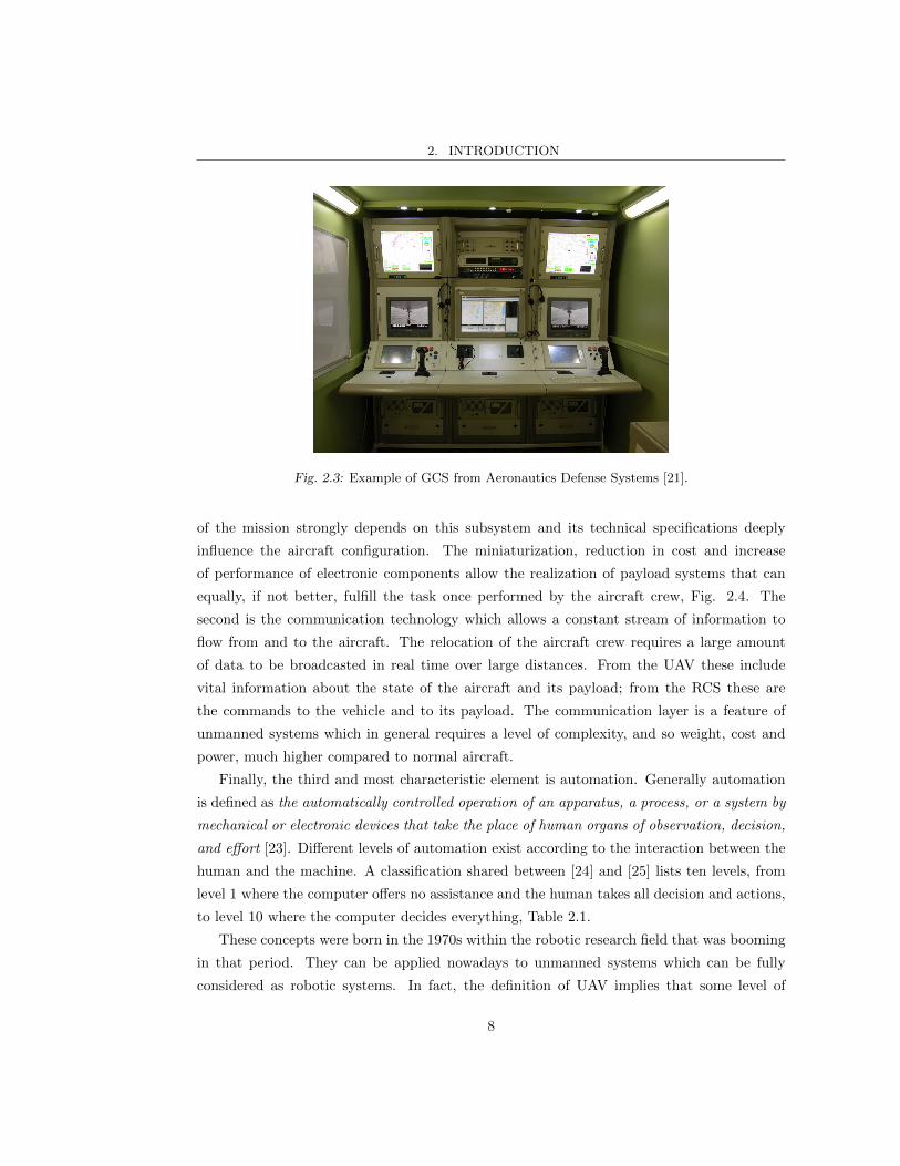
[16][17]. The interface between the operators and the aircraft is the Ground Control Station,

see Fig. 2.3. Here the large amount of data about the UAV mission are presented in a optimal

way to guarantee maximum situation awareness [18][19][20]. These information include the

status of the onboard systems, the aircraft position, neighbor air traffic and payload data.

At the same time the GCS allows the ground crew to remotely operate the aircraft and its

payload in order to accomplish the designated mission.

The advancements in three technological fields played a key role in the UAV success. The

first one is the payload technology which is the core of the UAV system. The accomplishment

7

2. INTRODUCTION

Fig. 2.3: Example of GCS from Aeronautics Defense Systems [21].

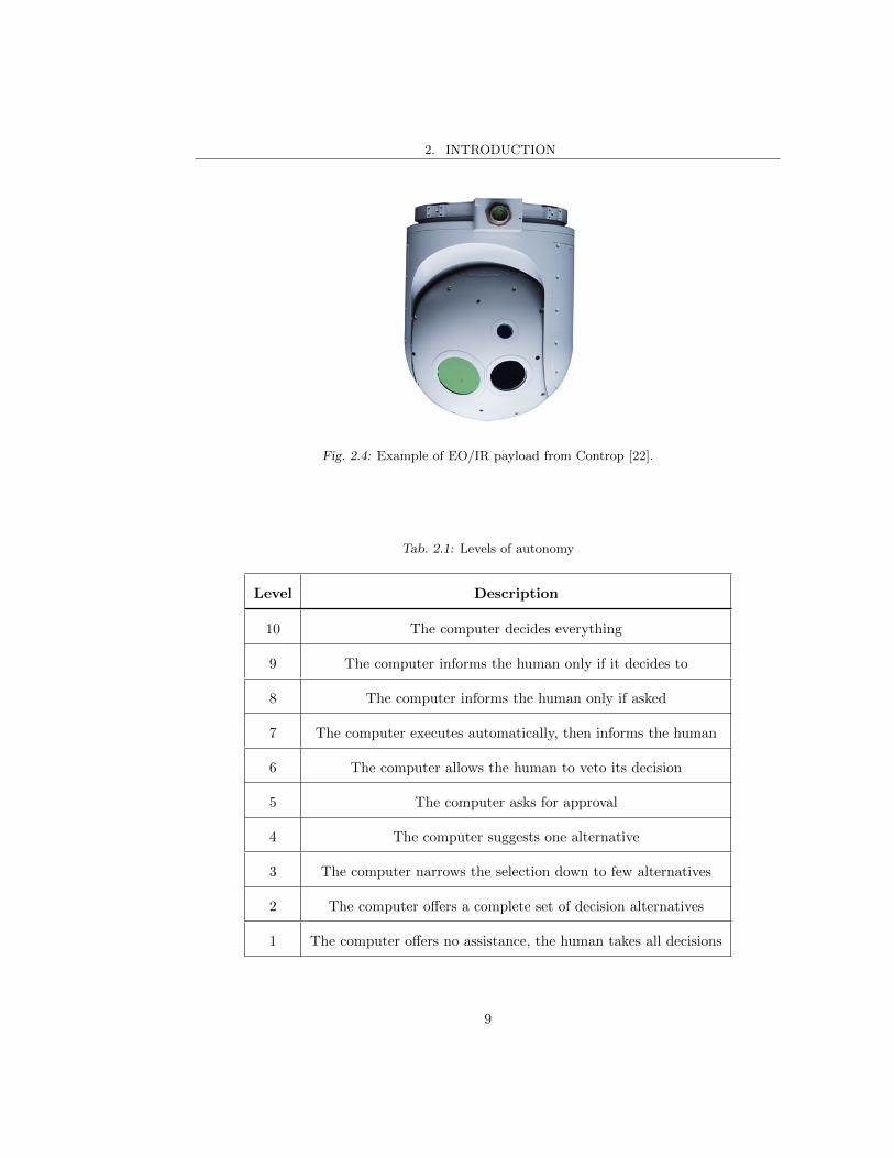
of the mission strongly depends on this subsystem and its technical specifications deeply

influence the aircraft configuration. The miniaturization, reduction in cost and increase

of performance of electronic components allow the realization of payload systems that can

equally, if not better, fulfill the task once performed by the aircraft crew, Fig. 2.4. The

second is the communication technology which allows a constant stream of information to

flow from and to the aircraft. The relocation of the aircraft crew requires a large amount

of data to be broadcasted in real time over large distances. From the UAV these include

vital information about the state of the aircraft and its payload; from the RCS these are

the commands to the vehicle and to its payload. The communication layer is a feature of

unmanned systems which in general requires a level of complexity, and so weight, cost and

power, much higher compared to normal aircraft.

Finally, the third and most characteristic element is automation. Generally automation

is defined as the automatically controlled operation of an apparatus, a process, or a system by

mechanical or electronic devices that take the place of human organs of observation, decision,

and effort [23]. Different levels of automation exist according to the interaction between the

human and the machine. A classification shared between [24] and [25] lists ten levels, from

level 1 where the computer offers no assistance and the human takes all decision and actions,

to level 10 where the computer decides everything, Table 2.1.

These concepts were born in the 1970s within the robotic research field that was booming

in that period. They can be applied nowadays to unmanned systems which can be fully

considered as robotic systems. In fact, the definition of UAV implies that some level of

8

2. INTRODUCTION

Fig. 2.4: Example of EO/IR payload from Controp [22].

Tab. 2.1: Levels of autonomy

Level Description

10 The computer decides everything

9 The computer informs the human only if it decides to

8 The computer informs the human only if asked

7 The computer executes automatically, then informs the human

6 The computer allows the human to veto its decision

5 The computer asks for approval

4 The computer suggests one alternative

3 The computer narrows the selection down to few alternatives

2 The computer offers a complete set of decision alternatives

1 The computer offers no assistance, the human takes all decisions

9

2. INTRODUCTION

autonomy is achieved. Remotely Piloted Vehicles (RPV) or model aircraft do not belong to

this category. The term drone, currently much abused, indicates a category of vehicles which

can perform pre-programmed tasks with the autonomy limited to the flight phase. There is

no interaction with the human agent and no decisional ability. The first unmanned aircraft

systems developed in the 1960s for reconnaissance mission were actually drones. They were

launched on a pre-programmed path with a sequence of data to be acquired, these information

were recovered only at the end of the flight [15]. On the contrary, current UAVs are more

and more conceived with onboard systems that replicate and substitute, on different levels,

human capabilities and intelligence. Interaction with the human operator is constant and

guaranteed through the communication system. The level of autonomy for each phase of the

UAV mission is defined in the design process and it depends on the complexity of the system

considered.

The benefits provided by the automation of some processes are several. First of all the

workload for the ground crew can be drastically reduced. This increases the focus on the tasks

and improves the global performance and the mission probability of success. Furthermore,

a reduction in costs can be achieved as a smaller number of man-hours is required. Another

benefit appears in case of fault, the system can detect it and act in order to minimize its

impact on the mission. In particular in case of weak or disturbed/jammed radio link between

aircraft and GCS, an appropriate level of autonomy could be fundamental [26].

The core technology at the basis of automation in the UAV field is the autopilot system.

An autopilot is a device able to define and impose the commands that an aircraft has to

maintain in order to follow a desired flight condition, determined according to the mission

requirements. Autopilots are present on commercial airliners as relief to the crew workload,

but on an unmanned aircraft they become an essential part of the aircraft Flight Control

System. Guided by an autopilot system, an unmanned aircraft is required to fly between

a series of waypoints, pre-determined or updated in real time. This assignment process is

called Navigation. The definition of the aircraft flight parameters requested to approach

these waypoints is the Guidance. It varies according to the mission considered, the aircraft

properties and the payload features. The Control process is responsible for maintaining an

aircraft attitude that guarantees the respect of the defined flight conditions.

As it will be discussed in detail in the next section, much effort is put in the definition of

an appropriate logic for the aircraft control.

10

2. INTRODUCTION

2.2 Control problem and proposed solutions

The interest in the problem of finding suitable control laws for UAVs is growing in response

to the recognition that these platforms will soon be performing missions in many civilian

applications. The wide range of possible missions is strongly stimulating the development of

unmanned aerial vehicles very different in size and configuration. A significant part of the

research is dedicated to the design of adequate onboard controllers. A particular interest,

especially in civilian applications, is for mini fixed-wing aircraft which are cheap to build

and to maintain, easily deployable, crashable and have low kinetic energy in case of impact.

According to a classification proposed in [11] the mini-UAV category includes aircraft with a

weight between 0.2 kg and 2.4 kg. The drawback of this configuration is in its flight dynamics

behavior: highly nonlinear, strongly coupled between the longitudinal and latero-directional

planes, very sensible to external disturbances and parametric uncertainties. Furthermore,

the reduced dimensions of the fuselage limit the available space and weight for onboard

electronics and the dedicated power supply. These issues motivate why small fixed-wing

UAVs represent an interesting platform for testing advanced control techniques. The aim

is to meet the always more demanding requirements for flight maneuvering and mission

accomplishment.

Recent surveys illustrate the current technologies available for autopilot systems and

describe the control laws commonly employed, see [27] and [28]. The use of PID gains is

still a popular approach in practice, in particular when dealing with commercial off-the-

shelf autopilots such as the MicroPilot MP Series [29]. This method guarantees simple

implementation and low computational effort. The designer has adequate control over the

system response and a clear understanding of the control action. In detail, starting with

proportional gain and adding integral and derivative terms, the designers can obtain a zero

steady state error and a fast time response for a step input reference. The tuning of the

PID gains can be performed with many non-heuristic methods, as explained in [30] and [31].

In the last twenty years, some researchers have focused their attention on the development

of automatic tuning and adaptation techniques for the definition of the PID gains. They

eliminate graphical, heuristic and trial and error procedures to verify the robustness of the

selected parameters.

One drawback of the simple PID approach is the inability to deal with the flight envelope

that might be required in most non-trivial mission profiles. As the performance of a PID

controller decreases far from the design point, gain scheduling is a common approach to

extend the validity of this technique to the whole flight envelope. Another disadvantage of

11

2. INTRODUCTION

traditional PIDs is that they do not guarantee enough robustness to the extent of model

parametric uncertainties which can occur in small fixed-wing UAVs.

Therefore, researchers are currently developing nonlinear, adaptive and robust control

laws able to theoretically guarantee satisfying performance over a large flight envelope also

in presence of uncertainties. For instance the authors of [32] propose a nonlinear model pre-

dictive control for fixed-wing UAV path tracking, [33] investigates the feasibility of H2 and

H∞ autopilots for longitudinal UAV control and [34] presents a combined adaptive control

law based on shunting method and passification for an UAV autopilot homing guidance sys-

tem. Nevertheless, the constraints imposed by real-time implementation often make these

algorithms unsuitable for the limited computational platforms available for small scale UAVs.

As an example, the controller proposed in [32] is successfully implemented in a dedicated

onboard computer installed on an experimental fixed-wing UAV and tested with real-time

hardware-in-the-loop simulations. The authors, however, underline the need for a compro-

mise between smooth convergence and computational performance in the determination of

the receding horizon size.

High computational requirements, complex algorithms and the necessity to smoothly com-

bine high-level intelligent tasks with low-level input/output routines are the main obstacles.

The miniaturization and reduction in cost of micro-controllers, together with their increase

in performance, see [35] and [36], is now enabling researchers to implement unmanned air-

craft driven by self-developed control laws. Whereas several examples have been published

for rotorcraft, an excellent survey is [37], there are relatively few for fixed-wing aircraft. The

diffusion of frameworks for control law development (e.g., [38]-[41]) has helped to reduce

the barriers to successful implementation. Two examples are [42], where a neural network

adaptive controller is used for the transition from horizontal flight to hover, and [43], where

a nonlinear dynamic inversion approach is used for formation flight.

Within this context three autopilot configurations are here proposed and compared. The

first one combines traditional PID control with an H∞ loop shaping approach to assess the

robustness characteristics achievable with the PID technique. As commonly done, the PIDs

are applied to the control loops of a linearized and decoupled aircraft model. In contrast

to the PID method, two configurations based on advanced control laws are also presented

here: the first one relies on the L1 adaptive controller and the second one on the nonlinear

backstepping controller. In these cases, emphasis is given to the design of the control laws

and to their real-time implementation capability. Differently from many related studies, the

possibility to implement the proposed solutions on microcontroller boards allows to actually

exploit their benefits on a fixed-wing UAV. Both of these approaches share the same structure,

12

2. INTRODUCTION

the advanced control law takes care of the inner loop variables, while outer loop variables

are controlled via PIDs. This choice allows the designer to maintain a clear understanding of

the control action, it limits the required computational power and eases the implementation

procedure.

The full PID controller is proposed because it still represents a potentially relevant tech-

nique in modern autopilots for UAVs, especially when combined with the H∞ approach. One

aim of the present thesis is to emphasizes the implementability of the proposed controllers,

and the PID is unbeatable from this point of view. Furthermore, it is interesting to ob-

serve its performance when compared to more advanced control laws which involve higher

computational cost.

The choice of L1 is motivated by the need of an adaptive controller able to handle the

presence of model uncertainties due to the platform variations which occur during the flight

tests, such as the variation in the payload mass and its position. The simple structure, the

reduced presence of oscillations in the implementation and a reasonable computation effort

make the L1 adaptive controller an ideal candidate as autopilot control law. Moreover, this

adaptive algorithm guarantees bounded inputs and outputs, uniform transient response and

steady-state tracking [44].

The backstepping controller is chosen for its ability to deal with nonlinearities. Unlike

traditional linear control techniques, such as LQ or feedback linearization, a nonlinear control

law applied to nonlinear aircraft dynamics guarantees satisfying performance over the whole

flight envelope [45]. With backstepping control design, useful nonlinearities are maintained

and additional nonlinear damping terms can be introduced to increase robustness to model

errors or to improve transient performance [46]. Furthermore, as backstepping belongs to

the Lyapunov family of techniques it has guaranteed convergence of the tracking error and

asymptotic stability [47].

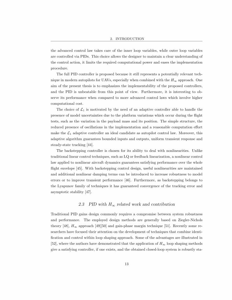
2.3 PID with H∞ related work and contribution

Traditional PID gains design commonly requires a compromise between system robustness

and performance. The employed design methods are generally based on Ziegler-Nichols

theory [48], H∞ approach [49][50] and gain-phase margin technique [51]. Recently some re-

searchers have focused their attention on the development of techniques that combine identi-

fication and control within loop shaping approach. Some of the advantages are illustrated in

[52], where the authors have demonstrated that the application of H∞ loop shaping methods

give a satisfying controller, if one exists, and the obtained closed-loop system is robustly sta-

13

2. INTRODUCTION

ble. The idea behind H∞ loop shaping is to improve robustness with the design of a controller

that minimizes the signal transmission from disturbances and measurement noise. Alterna-

tively, convex optimization techniques can be used to tune the controller. These methods are

based on frequency loop shaping theory (sensitivity function and its complementary func-

tion) and specifications are usually given in the form of a desired loop shaping function. In

[53] a method that integrates identification and PID parameters tuning is presented. The

system uncertainty is modeled considering a multiplicative uncertainty structure.

Many robust stability and performance problems can be considered in the H∞ framework

and a complete theory for control systems synthesis exists. However, the order of the opti-

mal control is high, comparable to the order of the plant. Some authors have considered the

problem of synthesizing PID controllers and they propose a parametric approach based on

the generalization of the Hermite-Biehler theorem. When applying this method for a given

fixed proportional gain, the set of stabilizing gains is obtained by the intersection of linear

inequalities. In [54] a computational characterization of all stabilizing PID controllers for an

arbitrary plant is provided. This H∞ optimal design, usually carried out by force optimiza-

tion search, is computationally very time-consuming. For this reason the work described in

[55] proposes a computationally efficient procedure for H∞ PID optimal design instead of

brute force search. This method reveals some important structural properties of H∞ PID

controllers, however it is validated only for Single Input Single Output (SISO) systems. The

authors of [56] have proposed a set of simple closed formulas for the explicit computation

of the parameters in finite terms. They eliminate graphical, heuristic and trial and error

procedures to verify the robustness of the selected parameters.

The method here illustrated follows an hybrid approach based on H∞ loop shaping theory

where nominal stability is guaranteed using root locus method [57], as proposed in [56]. In

this case, root locus is applied to identify the desired value of the PID derivative gain and

zeros. These are later employed to define the proportional and integrative gains. Gains are

chosen on one hand to obtain adequate robust stability and performance, on the other hand to

optimize closed-loop performance in terms of step response and waypoints tracking. Besides,

specifications for PIDs design are chosen to guarantee that the weighted H∞ norm of the

interconnection system matrix is less than a specified constant value. The relevance of the

proposed method is theoretical, since a robust solution is provided for the PID design with

standard optimization method and practical, since the computational effort is limited. As

the final purpose of this mixed approach is the tuning of an autopilot for fixed-wing aircraft

control, some simulations illustrate the compliance to the defined performance requirements.

It is verified that an adequate mission oriented design is a key feature to obtain satisfactory

14

2. INTRODUCTION

flying and handling qualities and good closed-loop response with an acceptable stability

margin. In order to achieve them full robustness can not be guaranteed.

2.4 L1 related work and contribution

A variety of adaptive control techniques have been proposed for the derivation of autopilot

inner loop control. Researchers in [58] implement a two-loop controller where the inner loop

is a dynamic inversion controller with an adaptive neural network and the outer loop is a

LQR controller. Similarly, [59] presents the implementation of an adaptive neural network

controller for autonomous flight. However, traditional model-based adaptive controllers may

not be applicable since they are generally useful on the condition that the system dynamics

are linear-in-the-parameters. In [60] the authors illustrate a complex adaptive controller

based on neural networks using backstepping technique. The main feature of the work of [60]

is that the adaptive controller is designed assuming that all of the nonlinear functions of the

system have uncertainties, the neural network weights are adjusted adaptively via Lyapunov

theory. Similarly, [61] derives an adaptive backstepping approach for the longitudinal aircraft

control and a Lyapunov analysis of the stability properties of the closed loop system was

considered.

The L1 adaptive control methodology addresses some of the problems exhibited by these

traditional adaptive control approaches. It provides fast and robust adaptation simultane-

ously leading the system input and output signals to the desired transient performance, in

addition it guarantees steady-state tracking. The decoupling between fast adaptation and

robustness is achieved with the introduction of a low-pass filter on the adaptive control sig-

nal. This key element can be designed based on robustness and performance specifications.

The complete theory behind the L1 technique is presented in [65] and [44].

This very recent control logic has been the object of the attention of many research

projects that are trying to build L1-based autopilot systems for UAVs. Many of them are

carried out by the collaboration of different research groups with the creators of the con-

troller, Naira Hovakimyan and Changyu Cao. In one of the first works, the authors of [62]

propose an L1 adaptive pitch controller for mini UAV and validate the proposed algorithm

in experimental flight tests. A drawback of [62] is the implementation and validation of a

single loop, a pitch attitude hold. In [63] the L1 controller is employed for the control of an

aircraft dedicated to collect biological samples. The L1 adaptivity is used to compensate for

the altered aircraft dynamics caused by the installation of the sampling instruments. One

of the most complete works about L1 is presented in [64]. Here the inner loop of a commer-

15

2. INTRODUCTION

cial autopilot is equipped with L1 controller for path following taking into account model

uncertainties and environmental disturbances. Extensive flight tests validate the proposed

approach.

In relation with the existing work previously discussed, the present project validates an

L1 controller applied to a complete nonlinear UAV aircraft model inclusive of model uncer-

tainties and unmodeled dynamics. The control law is designed and tuned starting from a

linear decoupled state space model which was derived about a specific flight condition. The

contribution resides in the demonstration that, using a low fidelity linear model significantly

different from the nonlinear model, the L1 controller is robust to model changes and a gain

retuning is not required. Moreover, the effectiveness of the tuned controller is demonstrated

for different aircraft configurations. In fact, uncertainties related to mass properties together

with variations in longitudinal stability derivatives are considered. Another important ad-

vantage is that both the outer loop PID gains tuned on the linear case do not require an

additional tuning.

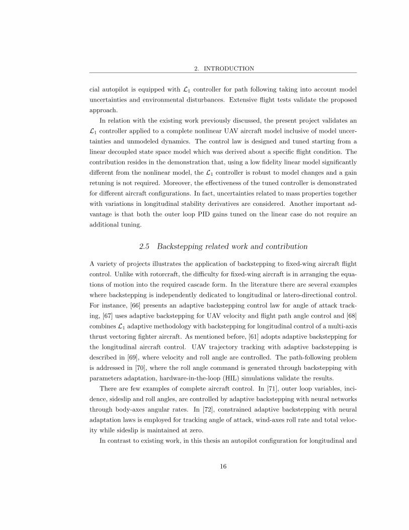
2.5 Backstepping related work and contribution

A variety of projects illustrates the application of backstepping to fixed-wing aircraft flight

control. Unlike with rotorcraft, the difficulty for fixed-wing aircraft is in arranging the equa-

tions of motion into the required cascade form. In the literature there are several examples

where backstepping is independently dedicated to longitudinal or latero-directional control.

For instance, [66] presents an adaptive backstepping control law for angle of attack track-

ing, [67] uses adaptive backstepping for UAV velocity and flight path angle control and [68]

combines L1 adaptive methodology with backstepping for longitudinal control of a multi-axis

thrust vectoring fighter aircraft. As mentioned before, [61] adopts adaptive backstepping for

the longitudinal aircraft control. UAV trajectory tracking with adaptive backstepping is

described in [69], where velocity and roll angle are controlled. The path-following problem

is addressed in [70], where the roll angle command is generated through backstepping with

parameters adaptation, hardware-in-the-loop (HIL) simulations validate the results.

There are few examples of complete aircraft control. In [71], outer loop variables, inci-

dence, sideslip and roll angles, are controlled by adaptive backstepping with neural networks

through body-axes angular rates. In [72], constrained adaptive backstepping with neural

adaptation laws is employed for tracking angle of attack, wind-axes roll rate and total veloc-

ity while sideslip is maintained at zero.

In contrast to existing work, in this thesis an autopilot configuration for longitudinal and

16

2. INTRODUCTION

latero-directional fixed-wing UAV control based on the backstepping technique is presented.

The objective is double: the adaptation of an existing backstepping controller with the aim

of generating an autopilot configuration suitable for mini-UAVs; its real-time implementation

on a microcontroller board. The inner loop variables angle of attack, sideslip angle and wind-

axes roll rate are controlled via the backstepping approach described in [74]. This method is

designed for general aircraft maneuvering within the whole flight envelope. Nonlinear natural-

stabilizing aerodynamic loads are included and employed by the controller. This approach is

different from feedback linearization, where these forces are first modeled and then canceled.

Less dynamic outer loop variables, velocity, altitude and heading, are controlled by PID

gains. The main purpose of this work, in fact, is to provide a starting framework for the

actual employment of backstepping control on flying UAVs. Adaptation and a more advanced

outer loop design is beyond the scope of this thesis.

A constant in all the approaches summarized above is the combination of backstep-

ping controller with complex adaptive laws. The benefits of combining nonlinear control

with adaptation are clear, but the problems of real-time implementation are considerable.

Aside from [70], none of the implementations described above has been performed on micro-

controllers suitable for small UAVs. The algorithm described in [75], based on adaptive

backstepping for directional control in presence of crosswind, is currently being implemented.

This effort is aided by the limited number of controlled variables and by the simplicity of

the adaptation approach. The only application of the backstepping controller on a flying

fixed-wing unmanned aircraft is presented in [76]. There, basic roll and pitch angles hold

and trimming tasks are achieved through adaptive backstepping implemented on a Pro-

cerus Kestrel autopilot. In the present thesis an innovative use of microprocessor technology

based on cutting-edge transistor computers is employed to support the controller implemen-

tation [77]. The combination of this tool with the proposed control layout strongly facilitates

the passage from theoretical simulation to practical application. In fact, the proposed con-

trol scheme is validated through HIL simulations, real-time operation is demonstrated with

satisfying flight performances

17

3. FIXED-WING AIRCRAFT MATHEMATICAL MODEL

The model of the aircraft is defined by three sets of differential equations governing the

aircraft dynamics. They describe the forces and moments acting on the aircraft, and its

orientation state with respect to a reference frame [78]. In this chapter the full nonlinear

model is presented together with the simplified linear model valid about a steady flight

condition. Both of them will be employed in this project. Some tools necessary to fully

understand the equations of motions are introduced first, these include the main reference

frames and the Euler angles. Finally, the aircraft adopted for the simulations and for the

flight tests are introduced, in particular the MH850 UAV which represents the testbed for

all the controllers proposed in this thesis.

3.1 Reference frames

A reference frame is a set of axes employed as coordinate system in order to represent the

position and the orientation of a dynamical system, in this case the aircraft. A large variety

of reference frames exist in the aeronautic field, an introduction to the ones used in this work

is necessary for sake of clarity.

3.1.1 Generic body axes

Generic body axes have the origin in the aircraft center of gravity. They are defined as

follows: XB and ZB lie in the aircraft plane of symmetry, with XB generally parallel to the

fuselage reference line and directed towards the aircraft nose, ZB is directed from the upper

to the lower surface of the wing airfoil; the YB axis is selected so that the coordinate frame

is right-handed, see Fig. 3.1. Generic body axes are fixed with respect to the aircraft, the

moments of inertia calculated in this reference frame do not change during the motion.

3.1.2 Wind axes

The wind axes reference system has the origin in the aircraft center of gravity and it is defined

as follows: the longitudinal axis XW is aligned with the direction of the airspeed vector V

3. FIXED-WING AIRCRAFT MATHEMATICAL MODEL

Fig. 3.1: Generic body axes

in absence of wind, the lateral axis YW is orthogonal to XW and oriented from left to right

with respect to the center of mass trajectory, ZW completes the right handed frame by lying

in the plane of symmetry of the aircraft, directed from the upper to the lower wing airfoil

surface, see Fig. 3.2. The direction of wind axes changes with respect to the aircraft as,

while maneuvering, the angle of attack and the sideslip angle change.

Fig. 3.2: Wind axes

3.1.3 NED axes

North-East-Down (NED) axes are centered in the aircraft center of gravity. The vertical

axis ZN is directed along the local gravity acceleration vector, XN points towards north,

YN points towards east. The XN and YN axes belong to a plane parallel to another plane

tangent to the Earth surface at zero altitude. Fig. 3.3 shows NED axes orientation with

respect to an Earth Centered Earth Fixed (ECEF) reference frame (XE , YE , ZE).

19

3. FIXED-WING AIRCRAFT MATHEMATICAL MODEL

Fig. 3.3: NED and ECEF axes orientation

3.1.4 ECEF axes

The origin of the Earth Centered Earth Fixed (ECEF) system is the earth center of mass.

The ZE axis points towards the North Pole. The direction of XE is determined by the

intersection of the plane defined by the Greenwich meridian and the equatorial plane. The

axis YE completes the right handed reference frame, it lies in the equatorial plane and points

90 degrees east of the XE direction, see Fig. 3.3. The ECEF reference system rotates together

with the earth about the ZE axis with an angular speed ΩE = 7.272 · 10−5 rad/s .

3.2 Euler angles

The Euler angles are a tool used to define the orientation of a reference frame with respect

to another one. The Euler angles Ψ,Θ,Φ are the parameters representing three independent

angular rotations necessary to align two reference frames. For instance, taking into consid-

eration the coordinate systems F1(X1, Y1, Z1) and F2(X2, Y2, Z2) represented in Fig. 3.4,

the sequence Ψ,Θ,Φ aligns F2 to F1. The rotations are performed in sequence and the order

of the rotations is fixed.

Euler angles are also employed to define the transformation of the components of a generic

vector between two reference frames. The components of a vector which undergoes a sin-

gle rotation are calculated using the elementary rotation matrix. In fact, assuming [RX1 ,

RY1, RZ1

]T to be a generic vector of the F1 coordinate system, the relationship with the

20

3. FIXED-WING AIRCRAFT MATHEMATICAL MODEL

Fig. 3.4: Two generic reference frames

corresponding vector [RX2, RY2

, RZ2]T in the final coordinate system F2 is

RX2

RY2

RZ2

= [Ψ] [Θ] [Φ]

RX1

RY1

RZ1

= [T21]

RX1

RY1

RZ1

where [T21] is the complete transformation matrix and [Ψ], [Θ], [Φ] are the elementary

rotation matrices:

[Ψ] =

cos Ψ − sin Ψ 0

sin Ψ cos Ψ 0

0 0 1

, [Θ] =

cos Θ 0 sin Θ

0 1 0

− sin Θ 0 cos Θ

, [Φ] =

1 0 0

0 cos Φ − sin Φ

0 sin Φ cos Φ

As the elementary matrices [Ψ], [Θ], [Φ] are orthogonal, also [T21] is orthogonal. Thus

[T21]−1 = [T12] = [T21]T , which yields to define the inverse transformation as

RX1

RY1

RZ1

= [T21]T

RX2

RY2

RZ2

21

3. FIXED-WING AIRCRAFT MATHEMATICAL MODEL

3.3 Notable Euler angles

Two of the most important Euler angles that will be used in the present work are here

illustrated. They represent the rotations necessary to align some of the frames illustrated in

Section 3.1.

3.3.1 Body axes - Wind axes

In order to align the wind axes reference frame FW to generic body axes reference frame FB

two rotations are necessary. The first rotation is of magnitude -β about ZW and the second

one about YB equal to α. The corresponding Euler angles are

Ψ = −β Θ = α

where α is called angle of attack and β is the sideslip angle, see Fig. 3.5. The analytical

definition of the aerodynamic angles α and β is

α = arctanw

u

β = arcsinv

V

(3.1)

with

V = |V | =√u2 + v2 + w2

where u, v, w are the components of the velocity vector V along the XB , YB and ZB axes

respectively.

The two rotations allow the definition of the angular velocities in wind axes ωw =

(pw, qw, rw)T as

ωw = Rwbω (3.2)

where Rwb is the rotation matrix

Rwb =

cosα cosβ sinβ sinα cosβ

− cosα sinβ cosβ − sinα sinβ

− sinα 0 cosα

22

3. FIXED-WING AIRCRAFT MATHEMATICAL MODEL

Fig. 3.5: Euler angles for body axes - wind axes rotation

and ω = (p, q, r)T is the vector containing the angular velocity components about the body

axes.

3.3.2 Body axes - NED axes

The rotations necessary to align NED axes FN reference frame to a generic body axes refer-

ence frame FB are three

Ψ = ψ Θ = θ Φ = φ

An illustration of the rotation procedure is represented in Fig. 3.6. These angles have a

Fig. 3.6: Sequence of rotations to align FN to FB

physical meaning which is very relevant in the study of the aircraft navigation:

23

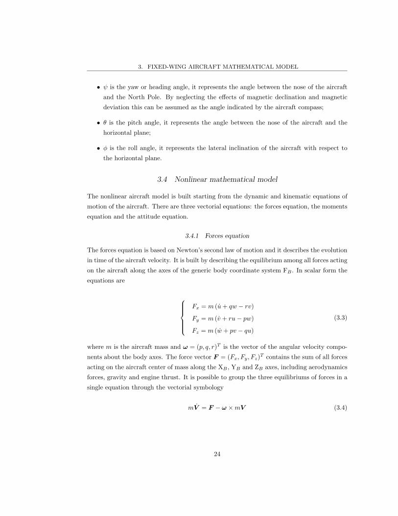
3. FIXED-WING AIRCRAFT MATHEMATICAL MODEL

• ψ is the yaw or heading angle, it represents the angle between the nose of the aircraft

and the North Pole. By neglecting the effects of magnetic declination and magnetic

deviation this can be assumed as the angle indicated by the aircraft compass;

• θ is the pitch angle, it represents the angle between the nose of the aircraft and the

horizontal plane;

• φ is the roll angle, it represents the lateral inclination of the aircraft with respect to

the horizontal plane.

3.4 Nonlinear mathematical model

The nonlinear aircraft model is built starting from the dynamic and kinematic equations of

motion of the aircraft. There are three vectorial equations: the forces equation, the moments

equation and the attitude equation.

3.4.1 Forces equation

The forces equation is based on Newton’s second law of motion and it describes the evolution

in time of the aircraft velocity. It is built by describing the equilibrium among all forces acting

on the aircraft along the axes of the generic body coordinate system FB . In scalar form the

equations are

Fx = m (u+ qw − rv)

Fy = m (v + ru− pw)

Fz = m (w + pv − qu)

(3.3)

where m is the aircraft mass and ω = (p, q, r)T is the vector of the angular velocity compo-

nents about the body axes. The force vector F = (Fx, Fy, Fz)T contains the sum of all forces

acting on the aircraft center of mass along the XB , YB and ZB axes, including aerodynamics

forces, gravity and engine thrust. It is possible to group the three equilibriums of forces in a

single equation through the vectorial symbology

mV = F − ω ×mV (3.4)

24

3. FIXED-WING AIRCRAFT MATHEMATICAL MODEL

3.4.2 Moments equation

The equilibrium of the moments acting about the three generic body axes allows writing in

scalar form the three moments equations

L = pIxx − rIxz − pqIxz + qr(Izz − Iyy)

M = qIyy + pr(Ixx − Izz) + (p2 − r2)Ixz

N = rIzz − pIxz + pq(Iyy − Ixx) + qrIxz

(3.5)

The three total moments L, M and N act respectively about the XB , YB and ZB axes,

and can be grouped in the vector M = (L,M,N)T . The generic Iij , with i, j=x, y, z,represents an element of the aircraft inertia tensor

I =

Ixx 0 −Ixz

0 Iyy 0

−Ixz 0 Izz

The tensor is symmetric and has some null elements thanks to the aircraft symmetry in the

longitudinal plane. In vectorial form the final equation can be written as

Iω = M − ω × Iω (3.6)

where ω = (p, q, r)T is the vector containing the derivatives of the angular velocity compo-

nents about body axes.

3.4.3 Attitude equation

The attitude equation describes the behavior of the aircraft attitude with time and it is based

on the kinematic equations of motion. The equation is obtained by expressing the derivatives

in time of the Euler angles. In this case we are considering the Euler angles between body

and NED axes, their dynamics are expressed by

φ = p+ q sinφ tan θ + r cosφ tan θ

θ = q cosφ− r sinφ

ψ = q sinφ/ cos θ + r cosφ/ cos θ

(3.7)

25

3. FIXED-WING AIRCRAFT MATHEMATICAL MODEL

By defining the vector Φ = (φ, θ, ψ)T and calling [E(Φ)] the rotation matrix

[E(Φ)] =

1 sinφ tan θ cosφ tan θ

0 cosφ − sinφ

0 sinφ/ cos θ cosφ/ cos θ

it is possible to write the attitude equation as

Φ = [E(Φ)]ω (3.8)

Note that the matrix [E(Φ)] does not depend on the angle ψ and it is singular when θ=±90 degrees.

It is also useful to write down the equations that define the angular velocities about body

axes according to the Euler angles and their derivatives

p = φ− ψ sin θ

q = θ cosφ+ ψ cos θ sinφ

r = ψ cos θ cosφ− θ sinφ

(3.9)

3.5 Linear mathematical model

The nonlinear equations of motion have a general validity within the flight envelope, with

the mentioned singularity for θ=± 90 degrees. They provide a powerful tool for studying

the performance and the dynamic behavior of the aircraft. In some occasions the accuracy

provided by the nonlinear model might not be necessary, and a lighter mathematical model

would be preferable. Linearizing the equations of motion about a steady flight condition

results in two low order linear systems more comfortable to handle and with good accuracy

in the surroundings of the defined point.

The approach employed to obtain the linear model is based on the small-disturbance

theory [79]. It is assumed that the motion of the aircraft is composed of two contributions,

the steady condition plus a small perturbation. All variables appearing in the nonlinear model

of Equations (3.3), (3.5), (3.7) and (3.9) are written in such form. With some mathematical

manipulation, based on the assumptions that flight conditions are symmetric, propulsive

forces are constant, and that perturbations are small, it is possible to obtain the reduced

equations which describe the linear disturbance dynamics.

26

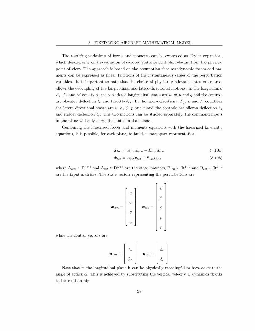
3. FIXED-WING AIRCRAFT MATHEMATICAL MODEL

The resulting variations of forces and moments can be expressed as Taylor expansions

which depend only on the variation of selected states or controls, relevant from the physical

point of view. The approach is based on the assumption that aerodynamic forces and mo-

ments can be expressed as linear functions of the instantaneous values of the perturbation

variables. It is important to note that the choice of physically relevant states or controls

allows the decoupling of the longitudinal and latero-directional motions. In the longitudinal

Fx, Fz and M equations the considered longitudinal states are u, w, θ and q and the controls

are elevator deflection δe and throttle δth. In the latero-directional Fy, L and N equations

the latero-directional states are v, φ, ψ, p and r and the controls are aileron deflection δa

and rudder deflection δr. The two motions can be studied separately, the command inputs

in one plane will only affect the states in that plane.

Combining the linearized forces and moments equations with the linearized kinematic

equations, it is possible, for each plane, to build a state space representation

xlon = Alonxlon +Blonulon (3.10a)

xlat = Alatxlat +Blatulat (3.10b)

where Alon ∈ R4×4 and Alat ∈ R5×5 are the state matrices, Blon ∈ R4×2 and Blat ∈ R5×2

are the input matrices. The state vectors representing the perturbations are

xlon =

u

w

θ

q

xlat =

v

φ

ψ

p

r

while the control vectors are

ulon =

δe

δth

ulat =

δa

δr

Note that in the longitudinal plane it can be physically meaningful to have as state the

angle of attack α. This is achieved by substituting the vertical velocity w dynamics thanks

to the relationship

27

3. FIXED-WING AIRCRAFT MATHEMATICAL MODEL

α =w

V0

where V0 is the total linear velocity at steady state. Furthermore, in control applications it

might be necessary to regulate the value of the altitude h. The altitude dynamics can simply

be modeled as

h = V0 sin γ = V0 sin (θ − α)

where γ = θ − α is the ramp angle, the angle between the total velocity vector and the

horizon. By applying the small-disturbance theory the sine of an angle can be identified with

the angle itself, so that

h = V0θ − V0α

In this cases the longitudinal state vector becomes

xlon =

u

α

θ

q

h

(3.11)

and the new matrices of the state space representation will have a larger size, Alon ∈ R5×5

and Blon ∈ R5×2. It is interesting to observe that the addition of the altitude equation adds

a null eigenvalue to the state matrix Alon. In fact, altitude motion does not contribute to

the aircraft dynamic behavior.

Similarly, in the latero-directional plane it can be useful to express the sideslip angle β.

This is done by replacing the v dynamics with the β dynamics thanks to

β =v

V0

As result the latero-directional state vector becomes

28

3. FIXED-WING AIRCRAFT MATHEMATICAL MODEL

xlat =

β

φ

ψ

p

r

(3.12)

and the size of the new state space matrices remains unchanged.

3.6 Aircraft models

The possibility to carry out the present project within two different research groups and the

necessity to employ several simulation tools forced the adoption of three different aircraft

models: the MH850 UAV, the Cessna 172P aircraft and the Ultrastick 25e RC aircraft.

The Politecnico di Torino UAV research group employs the MH850 UAV. Its mathematical

model is used as testbed for the simulated implementation of all the proposed control laws.

The performance confrontation among the three controllers is carried out with this aircraft

model.

The necessity to perform an initial assessment of the backstepping controller ability to

work in real time when implemented on a microcontroller board requires the adoption of the

Cessna 172P aircraft nonlinear model. This model is present in FlightGear flight simulator

and it is employed for the hardware-in-the-loop simulations tests.

Finally, the University of Denver Unmanned Systems Research Institute uses the Ultra-

stick 25e RC aircraft. The final aim of the activity in Denver is the flight testing of the

backstepping controller with the Ultrastick 25e. An accurate nonlinear model of this air-

craft is initially employed to validate the controller in real-life conditions and to tune the

controller gains accordingly. The controller is implemented on a microcontroller board and

integrated with the required sensors on the aircraft. Preliminary ground and flight tests with

the Ultrastick 25e are carried out.

The adoption of many controllers, aircraft models and simulation tools may generate some

confusion. Therefore Table 3.1 is added for sake of clarity. In any case, the possibility to

successfully test the backstepping controller for many different platforms and flight conditions

is a demonstration of its universal ability to control fixed-wing UAVs.

29

3. FIXED-WING AIRCRAFT MATHEMATICAL MODEL

Tab. 3.1: Employed controllers and aircraft models

Aircraft H∞ L1 Backstepping

MH850 linear model X X -

MH850 nonlinear model X X X

C172P nonlinear model - - X

Ultrastick 25e nonlinear model - - X

Ultrastick 25e aircraft - - X

3.6.1 MH850 UAV model

The MH850 aircraft is a mini-UAV developed by MAVTech s.r.l. spin-off company and by the

Department of Mechanical and Aerospace Engineering (DIMEAS) of Politecnico di Torino.

The MH850 is a man-portable high performance UAV designed with a focus on light weight

and long endurance characteristics and with a special attention to stability and handling

qualities. The primary mission of the UAV is surveillance of protected areas, monitoring of

geological events and support to rescue missions.

The MH850, see Fig. 3.7, is characterized by tailless configuration, electric propulsion

and non-movable vertical fins at wingtips [80] - [82]. The wingspan is 85 cm, the approximate

mass 1 kg and the cruise speed 14 m/s. Aircraft aerodynamic control is achieved with elevons:

they control longitudinal motion when symmetrically deflected and latero-directional motion

when asymmetrically deflected. The aircraft structure is designed to be rugged and crashable,

the fuselage is realized in sintered nylon, the wings are made of Expanded PolyPropylene

(EPP) foam and the fins at wingtips in carbon fiber. Take-off is performed by hand launch

or through a catapult, when the mission is over the aircraft lands on its belly. The main data

for the MH850 UAV are reported in Table 3.2. An analysis of the decoupled linear models of

Equations (3.10a) and (3.10b) allows calculating the M850 dynamical modes, see Table 3.3.

At the considered airspeed (14 m/s) just the spiral mode is slightly unstable having a real

positive pole equal to 0.0061.

In order to build the aircraft mathematical models previously described it is necessary to

estimate the aerodynamic and control derivatives of the vehicle. This is performed thanks to

a software tool available at the DIMEAS and called Aircraft Configuration Interface (ACI),

see Fig. 3.8. ACI is a Java-based interface that handles input/output operations for the main

30

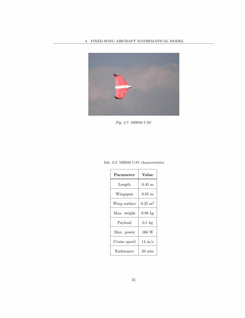
3. FIXED-WING AIRCRAFT MATHEMATICAL MODEL

Fig. 3.7: MH850 UAV

Tab. 3.2: MH850 UAV characteristics

Parameter Value

Length 0.45 m

Wingspan 0.85 m

Wing surface 0.25 m2

Max. weight 0.98 kg

Payload 0.1 kg

Max. power 160 W

Cruise speed 14 m/s

Endurance 50 min

31

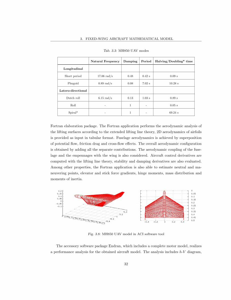
3. FIXED-WING AIRCRAFT MATHEMATICAL MODEL

Tab. 3.3: MH850 UAV modes

Natural Frequency Damping Period Halving/Doubling* time

Longitudinal

Short period 17.06 rad/s 0.48 0.42 s 0.09 s

Phugoid 0.89 rad/s 0.08 7.02 s 10.28 s

Latero-directional

Dutch roll 6.15 rad/s 0.13 1.03 s 0.89 s

Roll - 1 - 0.05 s

Spiral* - 1 - 69.24 s

Fortran elaboration package. The Fortran application performs the aerodynamic analysis of

the lifting surfaces according to the extended lifting line theory, 2D aerodynamics of airfoils

is provided as input in tabular format. Fuselage aerodynamics is achieved by superposition

of potential flow, friction drag and cross-flow effects. The overall aerodynamic configuration

is obtained by adding all the separate contributions. The aerodynamic coupling of the fuse-

lage and the empennages with the wing is also considered. Aircraft control derivatives are

computed with the lifting line theory, stability and damping derivatives are also evaluated.

Among other properties, the Fortran application is also able to estimate neutral and ma-

neuvering points, elevator and stick force gradients, hinge moments, mass distribution and

moments of inertia.

Fig. 3.8: MH850 UAV model in ACI software tool

The accessory software package Endran, which includes a complete motor model, realizes

a performance analysis for the obtained aircraft model. The analysis includes h-V diagram,

32

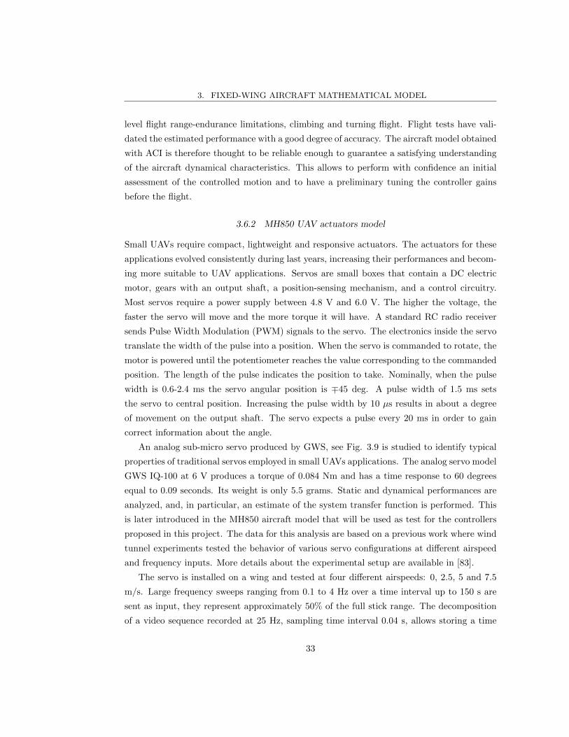
3. FIXED-WING AIRCRAFT MATHEMATICAL MODEL

level flight range-endurance limitations, climbing and turning flight. Flight tests have vali-

dated the estimated performance with a good degree of accuracy. The aircraft model obtained

with ACI is therefore thought to be reliable enough to guarantee a satisfying understanding

of the aircraft dynamical characteristics. This allows to perform with confidence an initial

assessment of the controlled motion and to have a preliminary tuning the controller gains

before the flight.

3.6.2 MH850 UAV actuators model

Small UAVs require compact, lightweight and responsive actuators. The actuators for these

applications evolved consistently during last years, increasing their performances and becom-

ing more suitable to UAV applications. Servos are small boxes that contain a DC electric

motor, gears with an output shaft, a position-sensing mechanism, and a control circuitry.

Most servos require a power supply between 4.8 V and 6.0 V. The higher the voltage, the

faster the servo will move and the more torque it will have. A standard RC radio receiver

sends Pulse Width Modulation (PWM) signals to the servo. The electronics inside the servo

translate the width of the pulse into a position. When the servo is commanded to rotate, the

motor is powered until the potentiometer reaches the value corresponding to the commanded

position. The length of the pulse indicates the position to take. Nominally, when the pulse

width is 0.6-2.4 ms the servo angular position is ∓45 deg. A pulse width of 1.5 ms sets

the servo to central position. Increasing the pulse width by 10 µs results in about a degree

of movement on the output shaft. The servo expects a pulse every 20 ms in order to gain

correct information about the angle.

An analog sub-micro servo produced by GWS, see Fig. 3.9 is studied to identify typical

properties of traditional servos employed in small UAVs applications. The analog servo model

GWS IQ-100 at 6 V produces a torque of 0.084 Nm and has a time response to 60 degrees

equal to 0.09 seconds. Its weight is only 5.5 grams. Static and dynamical performances are

analyzed, and, in particular, an estimate of the system transfer function is performed. This

is later introduced in the MH850 aircraft model that will be used as test for the controllers

proposed in this project. The data for this analysis are based on a previous work where wind

tunnel experiments tested the behavior of various servo configurations at different airspeed

and frequency inputs. More details about the experimental setup are available in [83].

The servo is installed on a wing and tested at four different airspeeds: 0, 2.5, 5 and 7.5

m/s. Large frequency sweeps ranging from 0.1 to 4 Hz over a time interval up to 150 s are

sent as input, they represent approximately 50% of the full stick range. The decomposition

of a video sequence recorded at 25 Hz, sampling time interval 0.04 s, allows storing a time

33

3. FIXED-WING AIRCRAFT MATHEMATICAL MODEL

Fig. 3.9: GWS IQ-100 analog servo.

domain input and output series of points. Fig. 3.10 illustrates a time series for 7.5 m/s where

input and output data are normalized and the average value is subtracted. In order to reduce

the noise influence on the model, a first order Butterworth lowpass filter is applied to the

data with a cut off frequency equal to half the Nyquist frequency. The study is performed at

V = 7.5 m/s as this speed is closer to the flight conditions encountered by the MH850 UAV.

Fig. 3.10: Time domain normalized input and output series for V = 7.5 m/s.

The experimental time series is elaborated with Matlab to estimate the system transfer

function. The selected approach relies on the Prediction-Error Minimization Method (PEM).

This algorithm estimates a discrete-time state space model using the subspace method, then

it refines it by minimizing the prediction error generated from an optimally determined

predictor [84]. In this case the error is numerically minimized through the scalar cost function

34

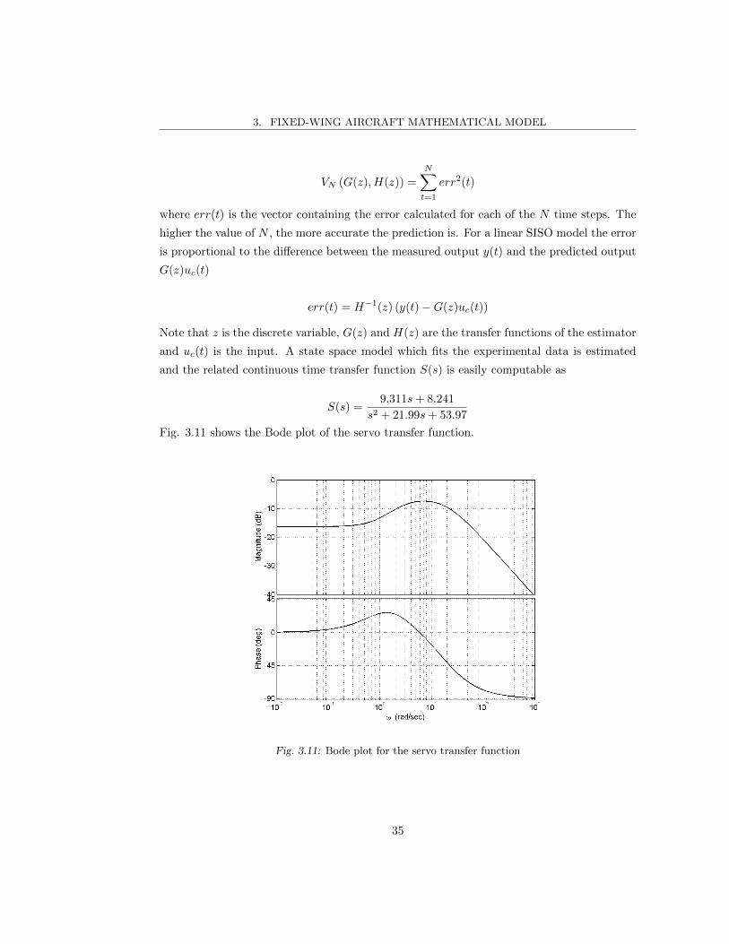
3. FIXED-WING AIRCRAFT MATHEMATICAL MODEL

VN (G(z), H(z)) =

N∑t=1

err2(t)

where err(t) is the vector containing the error calculated for each of the N time steps. The

higher the value of N , the more accurate the prediction is. For a linear SISO model the error

is proportional to the difference between the measured output y(t) and the predicted output

G(z)uc(t)

err(t) = H−1(z) (y(t)−G(z)uc(t))

Note that z is the discrete variable, G(z) and H(z) are the transfer functions of the estimator

and uc(t) is the input. A state space model which fits the experimental data is estimated

and the related continuous time transfer function S(s) is easily computable as

S(s) =9.311s+ 8.241

s2 + 21.99s+ 53.97

Fig. 3.11 shows the Bode plot of the servo transfer function.

Fig. 3.11: Bode plot for the servo transfer function

35

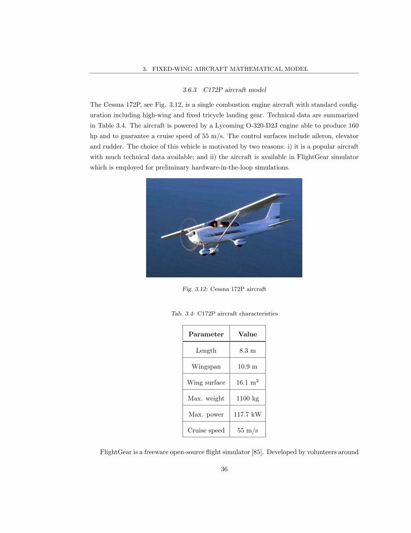
3. FIXED-WING AIRCRAFT MATHEMATICAL MODEL

3.6.3 C172P aircraft model

The Cessna 172P, see Fig. 3.12, is a single combustion engine aircraft with standard config-

uration including high-wing and fixed tricycle landing gear. Technical data are summarized

in Table 3.4. The aircraft is powered by a Lycoming O-320-D2J engine able to produce 160

hp and to guarantee a cruise speed of 55 m/s. The control surfaces include aileron, elevator

and rudder. The choice of this vehicle is motivated by two reasons: i) it is a popular aircraft

with much technical data available; and ii) the aircraft is available in FlightGear simulator

which is employed for preliminary hardware-in-the-loop simulations.

Fig. 3.12: Cessna 172P aircraft

Tab. 3.4: C172P aircraft characteristics

Parameter Value

Length 8.3 m

Wingspan 10.9 m

Wing surface 16.1 m2

Max. weight 1100 kg

Max. power 117.7 kW

Cruise speed 55 m/s

FlightGear is a freeware open-source flight simulator [85]. Developed by volunteers around

36

3. FIXED-WING AIRCRAFT MATHEMATICAL MODEL

the world, it offers to academic developers an experienced tool to test their aircraft models

and control laws, see for instance [86] - [88]. FlightGear version 2.6.0 is used and the JSBSim

flight dynamics library is employed for the C172P. JSBSim is an open source flight dynamics

model defining the six-degree of freedom equations which characterize the aircraft motion

[89].

3.6.4 Ultrastick 25e aircraft model

The Ultrastick 25e is the aircraft chosen for testing the backstepping controller into flight,

see Fig. 3.13. The main obstacle in testing a controller is the difference between the the-

oretical aircraft model and the real-life model. Unmodeled dynamics, high order nonlinear

terms, parametric uncertainties and external disturbances can introduce unexpected behav-

iors which can affect the controller performance. The backstepping controller ability to deal

with nonlinearities proves to be an advantage in these situations, but having a reliable and

accurate mathematical model of the aircraft is still a necessary requirement. In fact, the pos-

sibility to perform an accurate tuning of the controller gains in simulation allows to foresee

the controlled behavior of the aircraft. This considerably reduces the risk and time of the

flight tests.

Fig. 3.13: Ultrastick 25e aircraft

A mathematical model based just on theoretical assumptions, even if very detailed, can

hardly reach the level of accuracy required. A model based on experimental tests is preferred.

The work described in [90] and [91] deals with this issue, the authors describe the procedure to

experimentally identify the model of the Ultrastick 25e aircraft. The aircraft has traditional

configuration, electrical propulsion and control is achieved through elevator, ailerons and

37

3. FIXED-WING AIRCRAFT MATHEMATICAL MODEL

rudder. Its characteristics are summarized in Table 3.5.

Tab. 3.5: Ultrastick 25e aircraft characteristics

Parameter Value

Length 1.05 m

Wingspan 1.27 m

Wing surface 1.27 m2

Max. weight 1.8 kg

Payload 0.3 kg

Max. power 500 W

Cruise speed 17 m/s

The procedure consists in a preliminary modeling based on wind tunnel tests, the obtained

baseline model is used to define flight tests where frequency domain system identification is

used to build a definitive model. The result of this work is accessible at [92]. Among other

tools offered by this website, one of the most relevant is a Simulink model of the aircraft.

This is available in linear and nonlinear form, it embodies an accurate model of the aircraft

dynamics, including trim conditions, actuators transfer functions and electric motor behavior.

Furthermore, sensors noise from experimental data is added to the aircraft state variables,

an optional wind/gust simulation tool is available.

Considering the completeness and accuracy of the work illustrated and taking into ac-

count other elements such as aircraft size, performance and availability on the market, the

Ultrastick 25e is chosen as the aircraft model for testing the backstepping controller.

Finally, it is interesting to observe that the characteristics of the employed aircraft models

differ considerably not only in terms of configuration, absolute dimension, weight and power.

Relative values of the C172P, such as power-to-weight ratio and wing loading, are poorer

than those of the large majority of small UAVs, see Table 3.6. Testing the controller on a

less performing platform helps to prove its universality and to identify its limits.

38

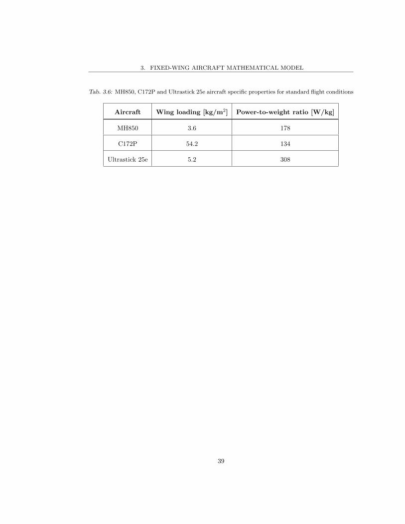
3. FIXED-WING AIRCRAFT MATHEMATICAL MODEL

Tab. 3.6: MH850, C172P and Ultrastick 25e aircraft specific properties for standard flight conditions

Aircraft Wing loading [kg/m2] Power-to-weight ratio [W/kg]

MH850 3.6 178

C172P 54.2 134

Ultrastick 25e 5.2 308

39

4. H∞ ROBUST APPROACH TO PID DESIGN

As illustrated in Section 2 this chapter deals with the design of a PID controller based on a

robust H∞ approach. The aim is to apply a novel robust technique to a traditional method

still popular in the design of autopilots for UAVs. After a brief introduction to PID and H∞

principles, the mathematical formulation of the problem is presented. A series of simulations

and a practical application case validate the proposed approach, finally some conclusions are

drawn based on the obtained results.

4.1 Introduction to PID technique

The PID technique was developed in the first decades of the 20th century for automatic ship

steering. The first theoretical formulation from Minorsky [93] was published in 1922 and

applied with successful results to U.S. Navy ships. The early mechanical implementation

soon led to electronic analog controllers that determined the success of PIDs in industrial

applications. Their benefits, as illustrated in Section 2, made this approach very popular in

a large variety of applications, including aviation where it still thrives nowadays.

The basic principle of PIDs is the regulation of a feedback signal, in particular of the

error between the measured and the desired state. The PID gains adjust the control ac-

tion according to the properties of the error signal err(t). The starting point is a simple

proportional gain KP which determines the control action uc(t) as

uc(t) = KP · err(t)

The limits of adopting only a proportional gain are the possible steady-state offset in response

to a constant reference and the inability to reject a constant disturbance. Furthermore, an

excessively large value of KP might lead to instability, in particular when dealing with high-

order systems.

In to order to eliminate the steady state error the integral gain KI is commonly adopted

to support the proportional action. Its contribution is proportional through the gain KI to

the integral of the error from the initial time to the considered moment t

4. H∞ ROBUST APPROACH TO PID DESIGN

uc(t) = KI ·∫ t

0

err(τ) dτ

The integral contribution has the advantage of taking into account the past values of the

error. For this reason, it is possible to have a control action different from zero also when the

error is zero. The addition of the integral term to a simple proportional controller improves

the tracking of the steady state response. The drawback of increasing KI is a slower response

for equal overshoot, or a rise in overshoot for an unchanged response velocity.

Finally, a derivative term is added to improve stability by increasing the damping of the

response thanks to an anticipatory behavior. The rate of change of the signal is used so that

its contribution to the total control action is proportional to the gain KD

uc(t) = KD ·derr(t)

dt

The sum of all the three contributions yields to the proportional-integral-derivative con-

troller, a linear combination of the error, its integral and its derivative in time

uc(t) = KP · err(t) +KI ·∫ t

0

err(τ) dτ +KD ·derr(t)

dt

The PID control formulation in the frequency domain is

UC(s) = KP +KI

s+KD · s (4.1)

4.2 Introduction to H∞ approach

The H∞ control problem was initially formulated in 1981 by Zames [94] as an alternative to

the 1960s Linear Quadratic Gaussian (LQG) theory used for targeting robust control. Within

LQG theory uncertainties are modeled as a white noise Gaussian process which is added to

the system as an extra input vector. This approach is valid when modeling measurement

noise but can not be adopted when dealing with parameter uncertainties. The early H∞

frequency domain formulations, which originated high-dimensional optimal or near-optimal

controllers, were quickly replaced in the late 1980s by simpler time-domain approaches that

accelerated the research on this topic [95]. Among others, major contributions to H∞ theory

are the works from Doyle, for instance [96], where the structured singular value tool is in-

troduced for testing robust stability, or [97], where the first solution to a general MIMO H∞

optimal control problem is proposed. Very relevant is also the research from Francis, in [98]

he gives a detailed treatment of the theory for H∞ control. More related to the work here

41

4. H∞ ROBUST APPROACH TO PID DESIGN

proposed is the contribution of Glover and McFarlane who in [99] and [100] introduced the

H∞ loop-shaping design method which provides systematic procedures for obtaining sensible

controllers that meet performance objectives and guarantee robustness against model uncer-

tainty and unmeasured disturbances. An accurate treatment of H∞ design, also considering

the case of dynamic output feedback, is [101].

Nowadays, after the publication of many papers and books on the subject, H∞ is one of

the most effective approaches to target multivariable robust control. Its combination with

loop shaping provides a tool that can be effectively applied to flight control laws design

with satisfying results. An advantage over classical control is its simplicity of application

to robust problems involving multivariable systems with cross-coupling between channels,

which is typical of fixed-wing aircraft behavior.

The origin of the name comes from the H∞ norm, as H∞ is the space where the norm

is defined. This space has a rational transform and is bounded in the right half plane

comprehensive of the imaginary axis. The norm represents the maximum absolute value of

the signal transform in the jω axis. Its definition for a scalar signal uc is

‖uc‖∞ = supω|UC(jω)|

In this case, it can be also demonstrated that the H∞ norm is the maximum of the absolute

value of the function over the whole right plane. In the multivariable case, for instance for a

vector or a matrix G(s), the H∞ norm is defined as

‖G(jω)‖∞ = supωσ [G(jω)]

where σ(ω) is the maximum singular value of the argument of the matrix for every value of

ω. As a matter of fact, the H∞ norm of a input-output dynamic operator can be simply

computed as follows: for SISO systems it is the maximum absolute value in frequency of

its transfer function, for MIMO systems it is the maximum absolute singular value of the

transfer matrix.

The idea behind H∞ approach is to address the issue of worst-case controller design for

linear plants subject to unknown additive disturbances and plant uncertainties. The H∞

norm is a tool used to measure the effect of an exogenous input, which is the disturbance

acting on the system, over an output of the system. It is required that in all conditions

the influence of the disturbance on the designated output is minimum. This requirement is

generally expressed imposing that the H∞ norm of a transfer matrix connecting the input

to the output is bounded under a defined threshold. Finding an appropriate controller

respecting this condition is the aim of the H∞ design problem.

42

4. H∞ ROBUST APPROACH TO PID DESIGN

4.3 Problem formulation and proposed control design

Typically, the objective of a control design problem expresses requirements in terms of distur-

bances attenuation, effects of the measurement noise and robustness to model uncertainties.

The described robust approach targets these issues with a method that can be considered in

the class of H∞ loop shaping. A graphical procedure, based on root locus method, is applied

to evaluate preliminary PID controller gains in order to satisfy nominal stability. Finally,

these parameters are tuned to comply with nominal performance, robust stability and robust

performance requirements by following H∞ theory.

This approach is applied to a fixed-wing UAV linear model, where decoupling between

longitudinal and latero-directional planes exists. Note that the linear model with the states

defined in Equation (3.11) and Equation (3.12) is employed. In the longitudinal plane the

linear speed u is controlled by elevator δe, while altitude h is controlled by throttle δth, see

Fig. 4.1. Three PID controllers have to be designed. There are two feedbacks on the speed

loop, pitch angle θ and speed u, and one on the altitude loop, altitude h. The state vector

of the system in this plane, in addition to θ, u and h, includes the angle of attack α and the

pitch angular velocity q. In the latero-directional plane, Fig. 4.2, the ailerons δa control the

heading angle through two feedbacks on roll and heading angles, respectively φ and ψ. Two

PID loops need to be configured. In this plane the state vector of the system is defined by

φ, ψ, the sideslip angle β, roll angular velocity p and yaw angular velocity r.

Fig. 4.1: Longitudinal control scheme

43

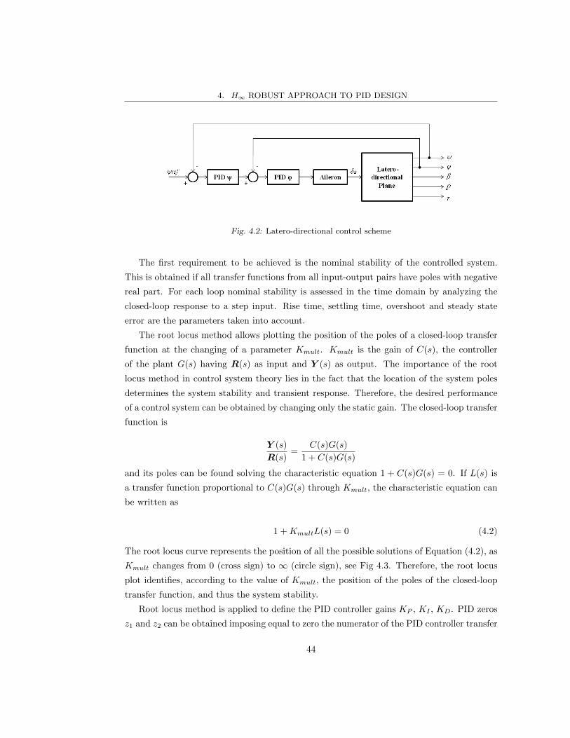
4. H∞ ROBUST APPROACH TO PID DESIGN

Fig. 4.2: Latero-directional control scheme

The first requirement to be achieved is the nominal stability of the controlled system.

This is obtained if all transfer functions from all input-output pairs have poles with negative

real part. For each loop nominal stability is assessed in the time domain by analyzing the

closed-loop response to a step input. Rise time, settling time, overshoot and steady state

error are the parameters taken into account.

The root locus method allows plotting the position of the poles of a closed-loop transfer

function at the changing of a parameter Kmult. Kmult is the gain of C(s), the controller

of the plant G(s) having R(s) as input and Y (s) as output. The importance of the root

locus method in control system theory lies in the fact that the location of the system poles

determines the system stability and transient response. Therefore, the desired performance

of a control system can be obtained by changing only the static gain. The closed-loop transfer

function is

Y (s)

R(s)=

C(s)G(s)

1 + C(s)G(s)

and its poles can be found solving the characteristic equation 1 + C(s)G(s) = 0. If L(s) is

a transfer function proportional to C(s)G(s) through Kmult, the characteristic equation can

be written as

1 +KmultL(s) = 0 (4.2)

The root locus curve represents the position of all the possible solutions of Equation (4.2), as

Kmult changes from 0 (cross sign) to ∞ (circle sign), see Fig 4.3. Therefore, the root locus

plot identifies, according to the value of Kmult, the position of the poles of the closed-loop

transfer function, and thus the system stability.

Root locus method is applied to define the PID controller gains KP , KI , KD. PID zeros

z1 and z2 can be obtained imposing equal to zero the numerator of the PID controller transfer

44

4. H∞ ROBUST APPROACH TO PID DESIGN

Fig. 4.3: Root locus plot

function of Equation (4.1), KDs2 +KP s+KI = 0. The application of Vieta’s formula to this

quadratic expression yields to the following relationship between the zeros and the coefficients

of the equation

z1 + z2 = −KPKD

z1 · z2 = KIKD

from which

KP = −KD · (z1 + z2)

KI = KD · (z1 · z2)

The derivative gain KD coincides with Kmult. Therefore the design of a PID controller

requires the definition of three parameters: the two PID zeros z1 and z2 and the gain Kmult.

The zeros are chosen arbitrarily with negative real part in order to increase the stability of

the system. The root locus method is applied to define a value of Kmult that satisfies the

closed-loop step response requirements in terms of rise time tr, settling time tS and overshoot

45

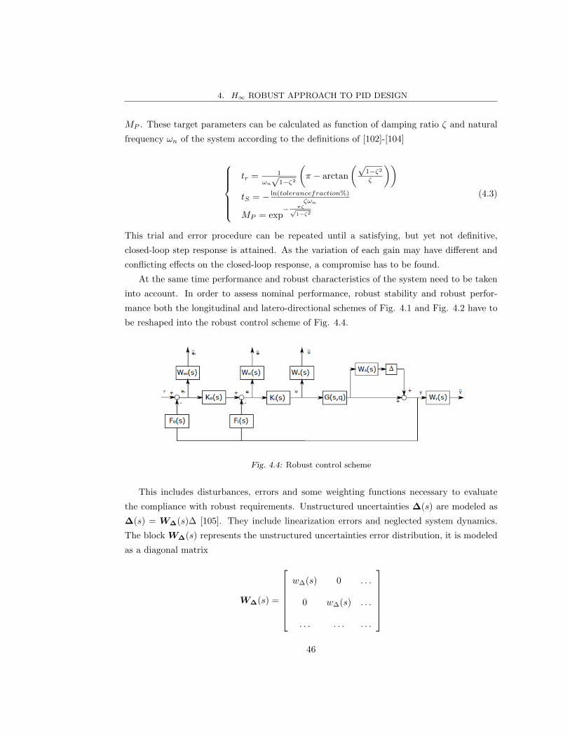
4. H∞ ROBUST APPROACH TO PID DESIGN

MP . These target parameters can be calculated as function of damping ratio ζ and natural

frequency ωn of the system according to the definitions of [102]-[104]

tr = 1

ωn√

1−ζ2

(π − arctan

(√1−ζ2ζ

))tS = − ln(tolerancefraction%)

ζωn

MP = exp− πζ√

1−ζ2

(4.3)

This trial and error procedure can be repeated until a satisfying, but yet not definitive,

closed-loop step response is attained. As the variation of each gain may have different and

conflicting effects on the closed-loop response, a compromise has to be found.

At the same time performance and robust characteristics of the system need to be taken

into account. In order to assess nominal performance, robust stability and robust perfor-

mance both the longitudinal and latero-directional schemes of Fig. 4.1 and Fig. 4.2 have to

be reshaped into the robust control scheme of Fig. 4.4.

Fig. 4.4: Robust control scheme

This includes disturbances, errors and some weighting functions necessary to evaluate

the compliance with robust requirements. Unstructured uncertainties ∆(s) are modeled as

∆(s) = W∆(s)∆ [105]. They include linearization errors and neglected system dynamics.

The block W∆(s) represents the unstructured uncertainties error distribution, it is modeled

as a diagonal matrix

W∆(s) =

w∆(s) 0 . . .

0 w∆(s) . . .

. . . . . . . . .

46

4. H∞ ROBUST APPROACH TO PID DESIGN

where the diagonal elements contain the error distribution along the frequency range. This

is assumed to be low at low frequencies, where the linearization approximations appear, and

high at high frequencies where the aircraft fast dynamics are neglected. The selected transfer

function is

w∆(s) =s+ ωLFs+ ωHF

with ωLF = 1 rad/s and ωHF = 200 rad/s. The block ∆ is unknown but it must respect the

condition ‖∆‖∞ < 1 [106].

Weo(s) and Wei(s) represent, respectively, the errors of the outer and inner loops. The

aim of having no steady state error for step input command means that, in the frequency

domain, the gain must be null for s = 0. This is achieved by defining the error transfer

functions as high-pass filters with a cutoff frequency equal to the considered loop bandwidth.

Wu(s) and Wy(s) are the weighting functions on the input and output signals. The first

poses a limit on the available control action, for example the maximum elevons deflection,

the second on the value of the outputs, for example the angle of attack has to be smaller

than the stall angle. In the scheme of Fig. 4.4 Ko(s) and Ki(s) are, respectively, the outer

and inner loop PID controllers, Fo(s) and Fi(s) are, respectively, the outer and inner loop

closing matrices.

The next step requires the introduction of Linear Fractional Transformations (LFT) [107].

According to [106] the system of Fig. 4.4 can be redrawn into a general LFT interconnection,

Fig. 4.5.(a). Here ∆ represents all the possible uncertainties, P (s) is the interconnection

matrix, K(s) is the controller, uc is the control signal, y is the measurement, w is a vector

signal including noise, z is a vector signal including all the controlled states, uc∆ and y∆

are the input and output signals given by the uncertainties.

Thanks to the formulation of Fig. 4.5.(a) the plant, the controller, the performance

weights and the uncertainties are grouped into a unified framework. The plant and the

controller can still be enclosed into a unique matrix M(s) computing a lower LFT. The

result is the M −∆ framework, Fig. 4.5.(b), a popular configuration for robust design and

analysis of uncertain feedback systems. The matrix M(s) can be partitioned into four blocks

according to the input and output dimensions, so that y∆

z

=

M11(s) M12(s)

M21(s) M22(s)

uc∆

w

= M(s)

uc∆

w

The matrix M(s) is the starting point for the analysis of nominal performance, robust

47

4. H∞ ROBUST APPROACH TO PID DESIGN

Fig. 4.5: P −K −∆ framework (a) and M −∆ framework (b)

stability and robust performance through the use of small gain theorem [106]. For a constant

γ > 0 the system of Fig. 4.5.(b) is well-posed and internally stable for all ∆(s) if and only if

‖M(s)‖∞ ≤ γ with ‖∆‖∞ ≤1

γ

The small gain condition is sufficient to guarantee internal stability even if uncertainties are

nonlinear and time-varying.

Nominal performance is achieved if, for the nominal model M(s) (∆ = 0), the energy

of the output z, due to energy-bounded disturbances, is also bounded. A condition easier

to verify is obtained assuming stable the interconnection of Fig. 4.5.(b). As the submatrix

M22(s) links z with w, it can be stated that nominal performance is attained if

‖M22(s)‖∞ ≤ 1

Robust stability is achieved when all the members of the family of systems including

uncertainties are nominally stable. Assuming M(s) internally stable, the resulting robust

stability condition is

‖M11(s)‖∞ ≤ 1

Robust performance is guaranteed when all the members of the family of systems with un-

certainties achieve nominal performance. In other words, the output z should have bounded

energy for all energy-bounded disturbances and for all models in the set, this is expressed as

‖z(s)‖2 ≤ 1 ∀ w ∈ L2, ‖w(s)‖2 ≤ 1 , ∀∆(s) | ‖∆(s)‖∞ ≤ 1

48

4. H∞ ROBUST APPROACH TO PID DESIGN

The verification of this requirement passes through the µ analysis of the frequency response

of the full matrix M(s). In [106] it is shown that an uncertain system is robustly stable and

satisfies (even if only partially) H∞ performance for all ∆(s) if, and only if, the structured

singular value µ∆ of the corresponding interconnection model is no greater than one. The

frequency dependent structured singular value with respect to the uncertainty is defined as

µ∆ (M(s)) =1

min σ (∆(s)) : ∆(s) ∈ ∆,det (1−M(s)∆(s)) = 0

where σ represents the largest singular value and ∆ ⊂ Cn×n is defined as

∆ =diag [δ1Ir1, . . . , δSIrs,∆1, . . . ,∆F ] : δi ∈ C,∆j ∈ Cmj×mj

with ‖δi‖∞ < 1; r1, . . . , rS and m1, . . . ,mF are positive integers. As a matter of fact the

robust performance condition is

µ∆ (M11(s)) ≤ 1

The computation of µ∆ is a difficult nonconvex problem and research was mainly concen-

trated in establishing its upper and lower boundaries. The upper boundary, which is of

interest in this case, can be efficiently computed by solving a complex optimization problem.

However, the gap between µ∆ and its upper boundary can be arbitrarily large, therefore only

a sufficient condition for robust stability can be achieved and checked with structured singu-

lar value. A robust controller design based on µ analysis is less conservative than classical

robust H∞ design.

4.4 Practical application and simulation results

The PID gains defined with the presented robust control strategy are applied to a multi-loop

commercial autopilot integrated on the MH850 UAV. The selected system is the MicroPilot

MP2028, a multi-loop PID autopilot designed for fully autonomous operations. Its capabil-

ities include airspeed hold, altitude hold, turn coordination, GPS waypoint navigation and

autonomous launch and recovery. Its compact dimensions (100 x 40 x 20 mm) and low weight

(28 g) makes it suitable for mini-UAV applications. The MicroPilot MP2028, represented in

Fig. 4.6, offers several control loops [108] as shown in Fig. 4.7.

A linear decoupled model of the MH850 aircraft, see Equation (3.10a) and Equation

(3.10b), is created. The state vectors, as already mentioned, follow the representations of

Equation (3.11) and Equation (3.12) where α, h and β are included. The mathematical

49

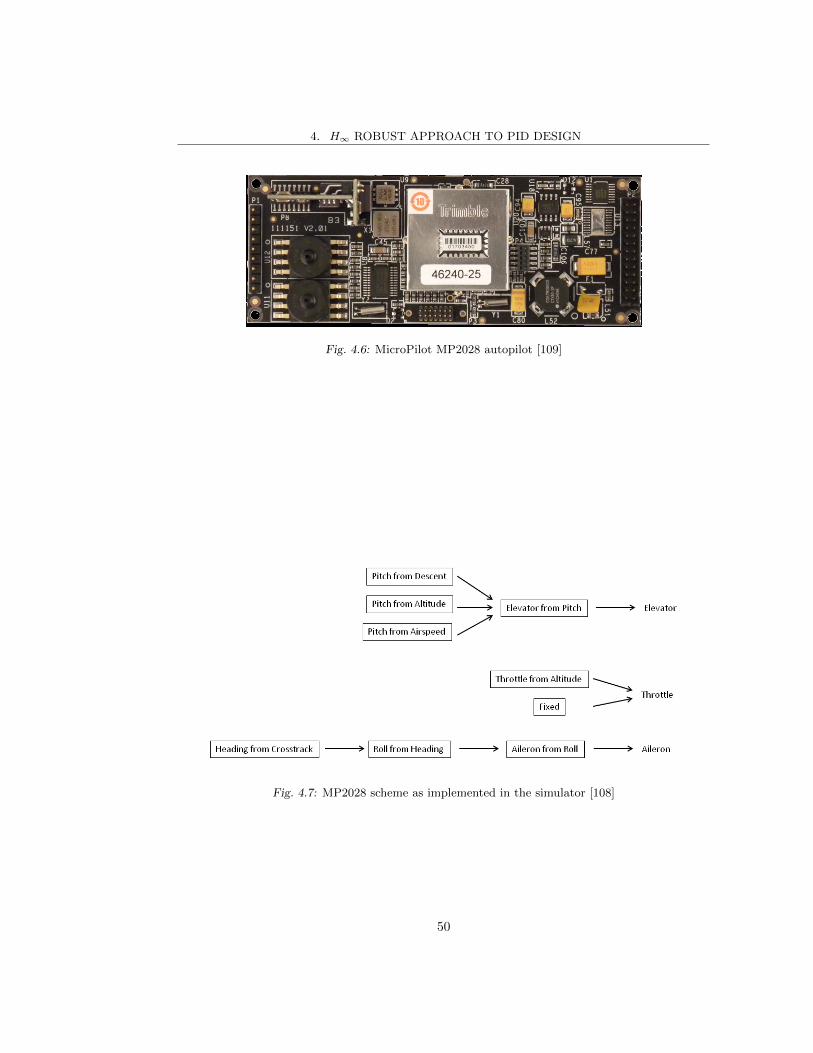
4. H∞ ROBUST APPROACH TO PID DESIGN

Fig. 4.6: MicroPilot MP2028 autopilot [109]

Fig. 4.7: MP2028 scheme as implemented in the simulator [108]

50

4. H∞ ROBUST APPROACH TO PID DESIGN

model of the plant include actuators: the throttle is described with a first order transfer

function while elevons with the second order transfer function defined in Section 3.6.2. As

stated in the previous section, five PID gains need to be designed, three for the longitudinal

plane and two for the latero-directional plane. The controller definition process is handled

with MathWorks Matlab software environment and its Robust Control Toolbox.

The application of the root locus procedure and the resulting PID tuning allows closing

longitudinal and latero-directional control loops with step response characteristics that satisfy

the MH850 specifications of Equation (4.3)

tr ∼= 2s

tS ∼= 60s

MP∼= 55%

(4.4)

Unfortunately the resulting PID gains need to be adjusted. In fact, a contrast between

closed-loop response characteristics and robust specifications emerges. Initially priority is

given to robust specifications requirements, a decay on the closed-loop response is considered

acceptable as long as nominal stability is maintained. As a consequence, the PID gains are

modified with a trial and error procedure with the intention of satisfying nominal perfor-

mance, robust stability and robust performance. From the images of Fig. 4.8, that refer

to the longitudinal plane, it is clear that not all requirements can be achieved even accept-

ing, for instance, a slow step response in the pitch from airspeed loop. The defined unitary

boundaries are crossed in two cases out of three.

Similar considerations can be drawn for the latero-directional plane, see Fig. 4.9, even

if here results are more satisfactory. In fact, by comparing robust stability, nominal perfor-

mance and robust performance plots, it can be seen that the latero-directional plane is more

compliant with requirements in terms of maximum value achieved and width of frequency

interval crossing. The obtained PID gains are summarized in Table 4.1 and Table 4.2.

The aircraft behavior with the assigned gains is simulated using a Fortran based software

which implements a commercial multi-loop PID autopilot, Micropilot MP2028 (Fig. 4.6) or

equivalent. Its capabilities include attitude, airspeed and altitude hold, turn coordination

and sequential GPS waypoint navigation. The simulator has been tested and experimentally

validated using flight test data [110][111]. The aircraft rigid body model is detailed in terms

of propulsive, aerodynamic and inertial actions. The propulsion system is modeled with

propeller, DC motor and batteries and its aerodynamics is implemented using the blade

element theory corrected for inflow effects. Blade airfoil aerodynamics is generated with a

51

4. H∞ ROBUST APPROACH TO PID DESIGN

Fig. 4.8: Longitudinal plane characteristics, gains optimized for requirements

Reynolds number dependent database. The DC motor is parametrized with no-load and stall

current, nominal voltage and stall torque. The simulator allows a post-flight analysis as it

stores in memory the assigned commands and the aircraft states along the flight path. The

use of such simulation environment plays a key role in the reduction of expensive and risky

flight tests.

The path chosen for testing the aircraft behavior is a 500 m side square with a constant

100 m altitude, cruise speed is 15 m/s. The simulator of the MP2028 autopilot is set with

the flyto navigation mode with a 1 Hz GPS update rate. In this mode the aircraft is flown to

the waypoint maintaining altitude and airspeed, the desired heading is set with no attempt

to travel in straight line between two points [108].

The results obtained with these PID gains are not adequate, as visible from Table 4.3

and Fig. 4.10. Table 4.3 indicates the cumulative error of some navigation parameters. For

a general parameter k in a simulation with N steps the cumulative error ec is defined as

ec =

N∑i=1

|Ki − ki|

52

4. H∞ ROBUST APPROACH TO PID DESIGN

Fig. 4.9: Latero-directional plane characteristics, gains optimized for requirements

where ki is the parameter at the ith step and Ki is the reference value of the same parameter

at that step.

Fig. 4.10 represents the 3D view of the path with respect to the defined waypoints.

The aircraft passes through the first waypoint which is in line with the starting point, the

following waypoints are missed with an error which has an order of magnitude comparable to

the path dimension. Remarkable oscillations on the longitudinal plane are also observable.

This undesired performance is due to a slow response in the latero-directional plane and

to an underdamped behavior in the longitudinal plane. Oscillations in the commands are

significant, in particular for throttle and elevator which control altitude and speed, see Fig.

4.11.

As the flight trajectory proves to be unsatisfactory, nominal performance, robust stability

and robust performance conditions are relaxed. Gains are now tuned with the purpose of

improving the aircraft behavior along the path without forgetting the other requirements.

These results are plotted in Fig. 4.12 and Fig. 4.13.

The shortening in the step response settling time coincides with a worsening in the compli-

ance with robust requirements. In the longitudinal plane two peaks are observable at 10−1.8

rad/s and 101.3 rad/s which correspond to the natural frequencies of the underdamped poles

53

4. H∞ ROBUST APPROACH TO PID DESIGN

Tab. 4.1: Longitudinal plane gains optimized for requirements

KP KI KD

Elevator from Pitch -0.04 -0.25 -0.002

Pitch from Airspeed -0.0002 -0.0001 -0.0001

Throttle from Altitude 0.055 0.0005 0

Tab. 4.2: Latero-directional plane gains optimized for requirements

KP KI KD

Aileron from Roll 0.08 0 0

Roll from Heading 0.05 0 0

Tab. 4.3: Cumulative error, gains optimized for requirements

Parameter Cumulative Error

Cross track 7 289 412 m

Heading angle 390 846 deg

Altitude 66 860 m

True airspeed 88 135 m/s

Pitch angle 3 275 deg

Roll angle 59 deg

54

4. H∞ ROBUST APPROACH TO PID DESIGN

Fig. 4.10: 3D trajectory view, gains optimized for requirements

Fig. 4.11: Aircraft commands, gains optimized for requirements

55

4. H∞ ROBUST APPROACH TO PID DESIGN

Fig. 4.12: Longitudinal plane characteristics, gains optimized for performance

of the closed-loop system. The latero-directional plane still proposes better results, both in

terms of step response settling time and respect of the unitary threshold. A peak is observ-

able at 100.8 rad/s where a pole with 0.085 damping is present. The new PID gains are

indicated in Table 4.4 and Table 4.5. A general increase in the absolute value of the gains is

remarked, except in the case of the throttle from altitude loop.

Tab. 4.4: Longitudinal plane gains optimized for performance

KP KI KD

Elevator from Pitch -0.3 -3.25 -0.01

Pitch from Airspeed -0.0021 -0.00087 -0.0015

Throttle from Altitude 0.019 0.0002 0.01

If the simulations are performed over the same path of the previous case, the cumulative

errors of Table 4.6 are now obtained. The percentage of the new value with respect to the

previous value is indicated between brackets. Except from the roll angle, a considerable

56

4. H∞ ROBUST APPROACH TO PID DESIGN

Fig. 4.13: Latero-directional plane characteristics, gains optimized for performance

Tab. 4.5: Latero-directional plane gains optimized for performance

KP KI KD

Aileron from Roll 0.12 0.0005 0.001

Roll from Heading 1.5 0.005 0.01

improvement of the cumulative errors is achieved. The roll angle unsatisfying result is moti-

vated by the four turns performed by the aircraft where error is accumulated; in the previous

case, in fact, a single long turn was executed. Improvements are visible from Fig. 4.14,

the new path is smooth and regular, no altitude oscillations are recorded and waypoints are

reached with precision. Fig. 4.15 illustrates the commands, during the turns also an elevator

action is observable.

A good match between reference and actual flight parameters is guaranteed, see Fig.

4.16. During the initial transition to trimmed flight the aircraft loses altitude and gains

speed, finally the error cancels out as steady flight condition is reached.

57

4. H∞ ROBUST APPROACH TO PID DESIGN

Tab. 4.6: Cumulative error, gains optimized for performance

Parameter Cumulative Error

Cross track 216 651 m (3%)

Heading angle 167 540 deg (42%)

Altitude 9 315 m (14%)

True airspeed 2 955 m/s (3%)

Pitch angle 7 deg (0.2%)

Roll angle 439 deg (744%)

Fig. 4.14: 3D trajectory view, gains optimized for performance

58

4. H∞ ROBUST APPROACH TO PID DESIGN

Fig. 4.15: Aircraft commands, gains optimized for performance

Fig. 4.16: Flight parameters responses, gains optimized for performance

59

4. H∞ ROBUST APPROACH TO PID DESIGN

4.5 Conclusions

In this chapter the problem of designing a multi-loop PID controller for a commercial UAV

autopilot was tackled. The criterion for the definition of the PID gains was not merely based

on the aircraft performance, but it also considered the robustness of the resulting system.

In fact, sensor noise, parametric uncertainties and external disturbances are major issues

affecting flight control systems of small UAVs.

A graphical method and a robust a posteriori control validation were proposed. PID gains

were determined by a tradeoff between step response characteristics and robust performance.

The design process was divided into two steps: initially the preliminary parameters of the

controller were estimated with the root locus method, later the definitive PID gains were

defined according to robust specifications.

The effectiveness of this approach was crosschecked with a comprehensive simulation tool

which includes the aircraft mathematical model and the principal control functions of the

autopilot. Results show that this hybrid technique provides a promising solution to the

problem of tuning commercial autopilots for UAVs with the aim of enforcing robustness to

plant variations and external disturbances. Nevertheless, it is clear that a tradeoff between

robustness and performance is necessary when dealing with such a simple and traditional

control technique. In the next chapter a controller specifically designed to target robustness

issues is presented.

60

5. L1 ADAPTIVE CONTROLLER

The need for robustness to unmodeled dynamics and parametric model uncertainties is

paramount when controlling the flight of Unmanned Aerial Vehicles. In Chapter 4 it is

demonstrated that traditional PID control technique struggles to guarantee at the same time

robustness and appropriate flight qualities. It is possible to find a good compromise, but more

advanced control laws that satisfy both requirements are currently available. One of them

is the L1 adaptive controller. In this chapter the application of an L1 adaptive controller to

the MH850 test case is presented. In particular, it is demonstrated that the proposed con-

trol design can stabilize the nonlinear system, even if the controller parameters are selected

starting from a decoupled linear model. A brief introduction to the L1 control is followed by

the problem formulation and by the application example where its robustness to parameters

variation is also tested. In Appendix A a further example of the application of L1 to aircraft

control is presented.

5.1 Introduction to L1 adaptive controller

The L1 adaptive controller is a recent technique. It was first presented by its creators C.

Cao and N. Hovakimyan at a conference in 2006 [112] and further formalized and expanded

in the following years. The L1 controller is a modification of the Model Reference Adaptive

Controller (MRAC), a technique which was first developed by the MIT in the late 1950s

[113] for solving the problem of adaptive flight control. In those years, as explained in [114],

there was no deep theoretical knowledge of the approaches that were implemented, and

much was based on empirical results. The introduction of Lyapunov stability theory into

adaptive control, see for instance [115], and in particular the definition of the condition for

global stability introduced in [116], led to a better understanding of the adaptive approach.

In the 1980s the theory behind adaptive control was completed, but the applications were

limited to some specific commercial products. The need for a controller able to handle

reconfiguration and damage control for air vehicles, and so to limit the costly validation and

verification procedures, gave in the years 2000s a second life to adaptive control thanks to

5. L1 ADAPTIVE CONTROLLER

a joint program among NASA, U.S. Air Force, academia and industry. L1 has its origins in

this new interest for adaptive control techniques.

The main feature of L1 is the ability to guarantee robustness and transient performance

with fast adaptation. The ability to quickly adapt to model changes, sudden failures and plant

uncertainties is crucial for an adaptive controller, but usually this requirement is conflicting

with the need to avoid poor robustness or destabilization. The L1 controller architecture

allows decoupling the design for robustness and adaptation. In this case, fast adaptation

is beneficial not only for performance but also for robustness. The design for robustness is

achieved with classical and robust control methods. Fast adaptation is an advantage because

error norms are inversely proportional to the square root of the adaptation rates, their limit

is imposed only by high-frequency noise and by the computational power of the operating

device. In the L1 controller the presence of a filter in the control action is crucial and it

represents the main feature to distinguish it from the MRAC approach. This filter, in fact,

is responsible for the tradeoff between performance and robustness. It is also employed to

avoid high frequency in the control signal and to shape nominal response, its design can be

handled by linear theory. The filter and the largest value of the unknown parameters are

included in certain transfer functions that need to satisfy a condition on their L1 norm. The

name L1 adaptive controller comes from this condition.

5.2 Problem formulation and proposed control approach

The problem of finding a control architecture able to deal with the high level of uncertainty

characterizing small UAVs is the challenge here proposed for the L1 adaptive controller.

In particular, in this section uncertain system input gain and time- and state-dependent

unknown nonlinearities are introduced as major source of uncertainties. Furthermore, it is

assumed that only a linear decoupled model is available for the controller design. The scope

is to verify the ability of the so tuned L1 controller to handle a complete nonlinear aircraft

model.

The dynamics of the considered system are the described by

x(t) = Amx(t) +Bmωuuad(t) + f(x(t), z(t), t), x(0) = x0

xz(t) = g(xz(t), x(t), t), xz(0) = xz0

z(t) = g0(xz(t), t)

y(t) = Cx(t)

(5.1)

which represents a general linear system affected by uncertainties. The known matrix Am ∈

62

5. L1 ADAPTIVE CONTROLLER

Rn×n is Hurwitz and specifies the desired dynamics of the closed-loop system, Bm ∈ Rn×m

and C ∈ Rm×n are known constant matrices that guarantee the controllability and observ-

ability of the system. This system includes ωu ∈ Rm×m, the uncertain system input gain

matrix, z(t) ∈ Rp and xz(t) ∈ Rl, respectively the output and state vector of internal unmod-

eled dynamics, and the unknown nonlinear functions f : R×Rn×Rp 7→ Rn, g0 : R×Rl 7→ Rp

and g : R×Rl×Rn 7→ Rn. Another form of writing the first line of Equation (5.1) generates

the system

x(t) = Amx(t) +Bm(ωuuad(t) + f1(x(t), z(t), t)) +Bumf2(x(t), z(t), t), x(0) = x0

xz(t) = g(xz(t), x(t), t), xz(0) = xz0

z(t) = g0(xz(t), t)

y(t) = Cx(t)

(5.2)

where Bum ∈ Rn×(n−m) is a constant matrix so that BTmBum = 0 and the rank of B =

[Bm, Bum] is n. The unknown nonlinear functions f1 : R × Rn × Rp 7→ Rm and f2 :

R×Rn ×Rp 7→ R(n−m) satisfy the condition f1(x(t), z(t), t)

f2(x(t), z(t), t)

= B−1f(x(t), z(t), t)

The matched component of the uncertainties is represented by f1(·), while the unmatched

components by Bumf2(·).The L1 adaptive controller here applied is extensively described in the book of the cre-

ators of the controller [44]. The adaptive law, as explained in [117] and [118], is piecewise

constant and guarantees fast estimation. The main feature is that the adaptation rate can

be associated with the sampling rate of an autopilot board CPU. Moreover, this adaptive

algorithm guarantees bounded inputs and outputs, uniform transient response and steady-

state tracking. This extension of the L1 controller was applied to the NASA AirSTAR [119]

and to the Boeing X-48B [120] aircraft. A key feature of this controller, as explained in the

previous works, is that the hardware interface is executed at a lower rate (about 10−100 Hz)

than the control algorithm (about 100 − 1000 Hz), therefore demanding insignificant CPU

power. Thus, the computational power can be dedicated to fast adaptation.

Before defining the control law some assumptions on the system of Equation (5.2) are

necessary:

63

5. L1 ADAPTIVE CONTROLLER

• Assumption 1: The H∞ norm of the unknown nonlinear functions f1 and f2 is bounded;

• Assumption 2: The functions f1 and f2 satisfy semiglobal Lipschitz condition;

• Assumption 3: The xz dynamics are BIBO stable with respect to both initial conditions

xz0 and input x(t);

• Assumption 4: The system input gain matrix ωu is assumed to be an unknown non-

singular strictly row-diagonally dominant matrix with know signum of its elements. It

belongs to a known compact convex set Ω so that ωu ∈ Ω ⊂ Rm×m, and the nominal

value ωu0 ∈ Ω is known;

• Assumption 5: The transmission zeros of the transfer matrixHm(s) = C (sI−Am)−1Bm

lie in the open left half plane.

Further details for these assumptions and their complete formulations are illustrated in [44].

The proposed control law adopts as state predictor ˙x(t) = Amx(t) +Bm(ωu0uad(t) + σ1(t)) +Bumσ2(t), x(0) = x0

y(t) = Cx(t)

where σ1(t) ∈ Rm and σ2(t) ∈ Rn−m are the adaptive estimates. The piecewise-constant

adaptation laws are σ1(t)

σ2(t)

= −

Im 0

0 In−m

B−1Φ−1(Ts)µ(iTs) (5.3)

for i = 0, 1, 2, ..., and t ∈ [iTs, (i + 1)Ts], where Ts > 0 is the adaptation sampling time

associated with the sampling rate of the CPU installed on the autopilot board. In Equation

(5.3) also

Φ(Ts) = A−1m (eAmTs − In), ∈ Rn×n

µ(iTs) = eAmTs x(iTs),

appear, where x(t) = x(t) − x(t) is the error between the predicted state and the system

state.

Finally, the last element of the controller is the control law defined as

uad(t) = −Kχ(t)

64

5. L1 ADAPTIVE CONTROLLER

where K ∈ Rm×m is a feedback matrix. Calling s the complex argument resulting from the

Laplace transform of the corresponding time domain signal, it is possible to define

χ(s) = D(s)η(s)

η(t) = ωu0uad(t) + η1(t) + η2m(t)− rg(t)

η1(t) = σ1(t)

η2m(s) = H−1m (s)Hum(s)σ2(s)

rg(s) = Kg(s)r(s)

D(s) is a proper stable transfer matrix of dimension m×m, r(t) is the reference signal that

the state x(t) needs to follow. The choice of K and D(s) requires that the low-pass filter

C(s)

C(s) = ωuKD(s) (Im + ωuKD(s))−1

for all ωu ∈ Ω, is strictly proper stable with DC gain C(0) = Im. Furthermore, it is required

that C(s)H−1m is a proper stable transfer matrix. The transfer functions Hm(s) and Hum(s)

are calculated starting from the matrices of the systems (5.1) and (5.2)

Hm(s) = C(sIn −Am)−1Bm

Hum(s) = C(sIn −Am)−1Bum

while the feedforward prefilter Kg(s) is chosen as the constant matrix Kg = −(CA−1m Bm)−1

to achieve decoupling among the signals. In fact, this allows the diagonal elements of the

desired transfer matrix M(s) = C(sIn − Am)−1BmKg to have DC gain equal to one and

the off-diagonal elements to have zero DC gain. The scheme of the adopted L1 controller is

represented in Fig. 5.1.

5.3 Implementation and simulation results

The L1 adaptive controller is now designed on the linear model of the aircraft which separates

the longitudinal and latero-directional dynamics. Final tests will be carried out on the

nonlinear model which better represents the behavior of the real aircraft.

The L1 controller is assigned to the control of the inner loop variables that need a faster

response and are more prone to be affected by unmodeled uncertainties. These include the

pitch angle θ, the longitudinal component of the airspeed u and the roll angle φ. Altitude

h and heading ψ outer navigation loops are instead controlled by simple PIDs. Fig. 5.2

65

5. L1 ADAPTIVE CONTROLLER

Fig. 5.1: L1 controller scheme

represents the global control scheme and highlights the control actions and the controlled

variables. In the scheme the symbol y represents all the longitudinal and latero-directional

states as they will be defined in Equations (5.4) and (5.5).

Fig. 5.2: L1 with PID global controller scheme

5.3.1 Linear case design and simulation results

The L1 adaptive controller parameters are designed on the linear decoupled model of the

MH850 aircraft. Reference flight conditions for building the model are speed u0 = 15 m/s,

altitude h0 = 100 m, angle of attack α0 = 4.1 deg, pitch angle θ0 = 4.1 deg (the ramp angle γ0

is considered zero), β0 = 0 deg, φ0 = 0 deg, ψ0 = 0 deg and no body axes angular velocities.

The linearization of the equations of motion results in the decoupling of the longitudinal

and latero-directional planes, each of them modeled with standard continuous time-invariant

66

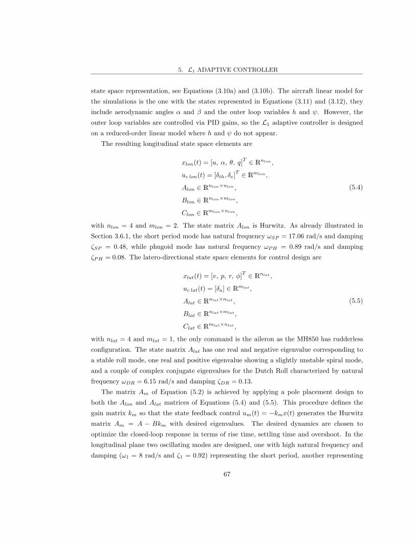
5. L1 ADAPTIVE CONTROLLER

state space representation, see Equations (3.10a) and (3.10b). The aircraft linear model for

the simulations is the one with the states represented in Equations (3.11) and (3.12), they

include aerodynamic angles α and β and the outer loop variables h and ψ. However, the

outer loop variables are controlled via PID gains, so the L1 adaptive controller is designed

on a reduced-order linear model where h and ψ do not appear.

The resulting longitudinal state space elements are

xlon(t) = [u, α, θ, q]T ∈ Rnlon ,

uc lon(t) = [δth, δe]T ∈ Rmlon ,

Alon ∈ Rnlon×nlon ,

Blon ∈ Rnlon×mlon ,

Clon ∈ Rmlon×nlon ,

(5.4)

with nlon = 4 and mlon = 2. The state matrix Alon is Hurwitz. As already illustrated in

Section 3.6.1, the short period mode has natural frequency ωSP = 17.06 rad/s and damping

ζSP = 0.48, while phugoid mode has natural frequency ωPH = 0.89 rad/s and damping

ζPH = 0.08. The latero-directional state space elements for control design are

xlat(t) = [v, p, r, φ]T ∈ Rnlat ,

uc lat(t) = [δa] ∈ Rmlat ,

Alat ∈ Rnlat×nlat ,

Blat ∈ Rnlat×mlat ,

Clat ∈ Rmlat×nlat ,

(5.5)

with nlat = 4 and mlat = 1, the only command is the aileron as the MH850 has rudderless

configuration. The state matrix Alat has one real and negative eigenvalue corresponding to

a stable roll mode, one real and positive eigenvalue showing a slightly unstable spiral mode,

and a couple of complex conjugate eigenvalues for the Dutch Roll characterized by natural

frequency ωDR = 6.15 rad/s and damping ζDR = 0.13.

The matrix Am of Equation (5.2) is achieved by applying a pole placement design to

both the Alon and Alat matrices of Equations (5.4) and (5.5). This procedure defines the

gain matrix km so that the state feedback control um(t) = −kmx(t) generates the Hurwitz

matrix Am = A − Bkm with desired eigenvalues. The desired dynamics are chosen to

optimize the closed-loop response in terms of rise time, settling time and overshoot. In the

longitudinal plane two oscillating modes are designed, one with high natural frequency and

damping (ω1 = 8 rad/s and ζ1 = 0.92) representing the short period, another representing

67

5. L1 ADAPTIVE CONTROLLER

the phugoid with lower natural frequency and damping (ω2 = 3 rad/s and ζ2 = 0.8). In the

latero-directional plane two real negative eigenvalues are chosen (λ1 = −6 and λ2 = −10), the

desired oscillating mode representing the dutch roll is defined by ω3 = 5 rad/s and ζ3 = 0.5.

The total control action uc is the combination of the state feedback control um and the

adaptive control uad

uc(t) = −kmx(t) + uad(t)

The adaptive control uad is defined following the L1 approach described in Section 5.2.

This procedure is performed on both the longitudinal and latero-directional models when

considered affected by uncertain system input gain and time- and state-dependent unknown

nonlinearities, see Equation (5.2). The adaptation time step Ts is chosen equal to 0.001

seconds. Filter bandwidths are chosen as 60 rad/s in the longitudinal plane for both the

matched and unmatched signals, while in the latero-directional plane the values selected are

12 rad/s for the matched signal and 8 rad/s for the unmatched. The complete control scheme

includes two PID controllers dedicated to altitude and heading angle control. As the hybrid

approach described in Chapter 4 results of difficult application to the considered structure,

the PIDs are tuned manually taking in consideration the specifications expressed in Equation

(4.4). The value of the PID gains are summarized in Table 5.1. The controller synthesis and

all simulations are performed using MathWorks Matlab/Simulink software environment.

Tab. 5.1: Outer loop PID gains

KP KI KD

Pitch from Altitude 0.0345 0.0061 0.016

Roll from Heading 0.55 0 0

The first set of simulations imposes a step reference signal to the three navigation-related

variables u, h and ψ. Results for the inner loop variables directly controlled with L1 are il-

lustrated in Fig. 5.3. The corresponding outer loop controlled by the combination of L1 and

PID gains is represented in Fig. 5.4. These results show the ability of the controller configu-

ration to handle with satisfying performance a maneuver where a contemporary variation of

all variables is performed. Inner loop variables, in particular the speed, demonstrate a good

tracking despite the abrupt transition imposed by the step inputs. Coupling between speed

u and pitch angle θ is caused by the fact that both elevator δe and throttle δth contribute

68

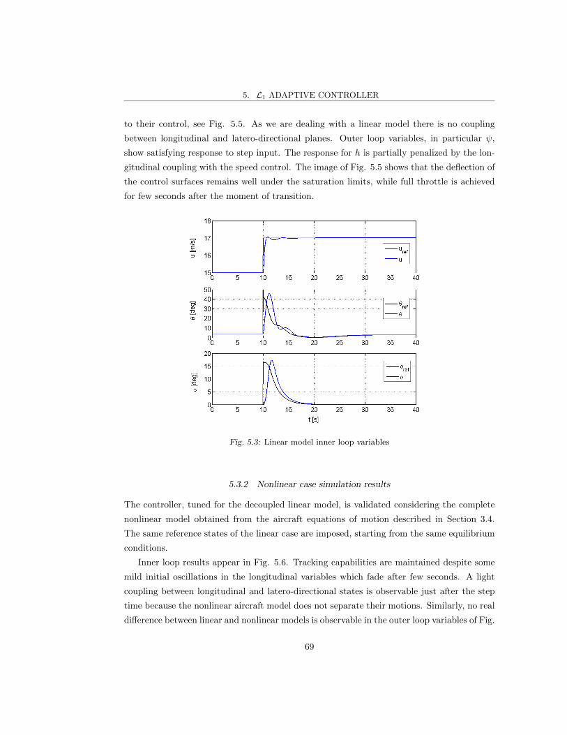
5. L1 ADAPTIVE CONTROLLER

to their control, see Fig. 5.5. As we are dealing with a linear model there is no coupling

between longitudinal and latero-directional planes. Outer loop variables, in particular ψ,

show satisfying response to step input. The response for h is partially penalized by the lon-

gitudinal coupling with the speed control. The image of Fig. 5.5 shows that the deflection of

the control surfaces remains well under the saturation limits, while full throttle is achieved

for few seconds after the moment of transition.

Fig. 5.3: Linear model inner loop variables

5.3.2 Nonlinear case simulation results

The controller, tuned for the decoupled linear model, is validated considering the complete

nonlinear model obtained from the aircraft equations of motion described in Section 3.4.

The same reference states of the linear case are imposed, starting from the same equilibrium

conditions.

Inner loop results appear in Fig. 5.6. Tracking capabilities are maintained despite some

mild initial oscillations in the longitudinal variables which fade after few seconds. A light

coupling between longitudinal and latero-directional states is observable just after the step

time because the nonlinear aircraft model does not separate their motions. Similarly, no real

difference between linear and nonlinear models is observable in the outer loop variables of Fig.

69

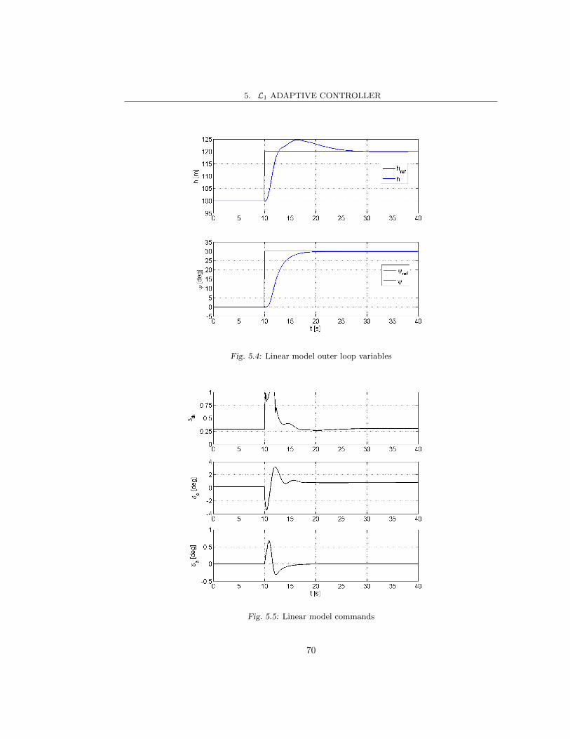
5. L1 ADAPTIVE CONTROLLER

Fig. 5.4: Linear model outer loop variables

Fig. 5.5: Linear model commands

70

5. L1 ADAPTIVE CONTROLLER

5.7. On the contrary, the controller seems to better perform on the nonlinear model. Note

that here the longitudinal variable h shows minimal initial oscillations thanks to a proper

PID initialization at starting time. The oscillations problem in the nonlinear case, in fact, is

caused by an incorrect estimation of the initial longitudinal commands from the L1 controller.

This is motivated by the different physical meaning of linear and nonlinear aircraft models.

In the linear case the controller acts on the already trimmed aircraft which is flying in an

equilibrium state. Therefore, the commands computed by L1 are the variation about the trim

commands, Fig. 5.5 shows the total commands originated by these two contributions. In the

nonlinear case, instead, the L1 controller needs to compute the total commands. Because

of this, starting from initial estimates, it requires a couple of seconds to achieve trimmed

flight, see Fig. 5.8. In this time interval the aircraft responds to the incorrect commands

in an undesired way, until the controller, damping these motions, forces the aircraft into

the desired steady state. Note that the latero-directional plane is already trimmed. In fact,

as the initial conditions are described by symmetric flight with no angular velocities, the

initial estimated command δa = 0 deg already guarantees trimmed flight. Except from the

oscillatory interval, the nonlinear commands are comparable to linear commands in terms of

behavior.

Fig. 5.6: Nonlinear model inner loop variables

71

5. L1 ADAPTIVE CONTROLLER

Fig. 5.7: Nonlinear model outer loop variables

Fig. 5.8: Nonlinear model commands

72

5. L1 ADAPTIVE CONTROLLER

5.3.3 Parametric robustness validation

A validation of the control scheme robustness to aircraft parameters uncertainties is per-

formed with two test cases. In both of them significant variations in aircraft mass, inertia

and static margin are considered. The altered parameters are introduced in the nonlinear

aircraft model while the controller settings remain unchanged from the nominal case. Case

1 contemplates a heavier aircraft, with higher inertia and with a reduced static margin so

that the derivatives Cmα and Cmδe are weaker. In Case 2 the aircraft is lighter, has lower

inertia and its center of gravity is moved forward so that the magnitude of the derivatives is

higher. In both cases the variation in m, I, Cmα and Cmδe is 30% from the nominal value.

The adopted parameters are summarized in Table 5.2.

Tab. 5.2: Parameters for the parametric robustness validation cases

Parameter Nominal Case 1 Case 2

m [kg] 0.9 1.17 0.819

I [kg · m2]

0.0109 0 −4.6e−5

0 0.0119 0

−4.6e−5 0 0.0223

0.0142 0 −5.98e−5

0 0.0155 0

−5.98e−5 0 0.0291

0.0076 0 −3.22e−5

0 0.0083 0

−3.22e−5 0 0.0156

Cmα -0.3434 -0.2404 -0.4464

Cmδe -0.7317 -0.5122 -0.9512

The results of the simulations performed with the altered parameters are represented in

Fig. 5.9, Fig. 5.10 and Fig. 5.11. For all variables no substantial difference is noticeable.

However, it is interesting to observe the steady state value for the longitudinal variable θ.

The alteration of the mass and of the derivatives Cmα and Cmδe results in a different pitch

angle at equilibrium. As a consequence, trim elevator deflection δe changes too.

5.4 Conclusions

In this chapter it is demonstrated that a combination of PID and L1 adaptive controller

is a suitable control logic for UAV autopilots. The PIDs take care of outer loop variables

altitude and heading while L1 controls inner loop states. In particular, an L1 approach

based on piecewise constant adaptation laws is selected in order to guarantee adaptation

rates compatible with an autopilot board CPU and low computational effort.

It is illustrated how the tuning of the controller on a linear aircraft model is sufficient

73

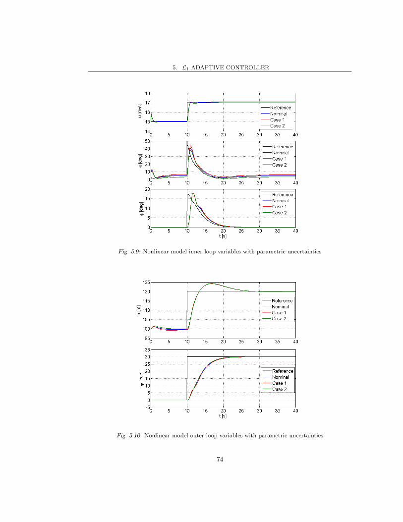
5. L1 ADAPTIVE CONTROLLER

Fig. 5.9: Nonlinear model inner loop variables with parametric uncertainties

Fig. 5.10: Nonlinear model outer loop variables with parametric uncertainties

74

5. L1 ADAPTIVE CONTROLLER

Fig. 5.11: Nonlinear model commands with parametric uncertainties

to guarantee satisfying flight performance also for the high-fidelity nonlinear model. This is

relevant because a simplified linear model of the aircraft is in general easily available and

easier to build and run. Furthermore, the adaptive nature of L1 guarantees a minimum

variation of the controlled states also when the aircraft model is subject to large parametric

uncertainties, which is typical of unmanned aircraft.

75

6. BACKSTEPPING NONLINEAR CONTROLLER

This chapter deals with the application of a backstepping nonlinear technique to the longi-

tudinal and latero-directional control of the inner loop of a fixed-wing UAV. As explained in

Section 2, this kind of approach has seen limited examples in the literature, and even less are

the projects where real implementation was performed. Here the proposed method is briefly

explained from the theoretical point of view and extensively validated with various software

simulation cases. Furthermore, the designed controller is implemented on a microcontroller

board and tested through hardware simulations.

6.1 Introduction to backstepping nonlinear controller

The concept of backstepping controller was developed in the early 1990s starting from the

ideas of Tsinias [121], Byrnes and Isidori [122], Sontag and Sussmann [123], Kokotovic and

Sussmann [124], and Saberi, Kokotovic and Sussmann [125]. The major contributions from

these researchers who were investigating nonlinear feedback control theory were summarized

and formalized by Kokotovic in 1992 [126]. Three years later a book dealing with the complete

theory for uncertain nonlinear systems was published by the same author together with

Kstic and Kanellakopoulos [46]. Here a thorough treatment of the backstepping approach,

including adaptivity, is presented.

The name backstepping derives from the recursive nature of the controller, the design

process starts from the inner scalar function and “steps back” towards the external con-

trol input moving through a sequence of integrations. Each of these nonlinear differential

equations governing the system is considered as a subsystem to be controlled [47]. The back-

stepping controller is designed so that the external control input controls in cascade all the

subsystems, step by step, from the outer subsystem to the inner subsystem. Each subsystem

is stabilized about the origin by a virtual control input which is the state of the differential

equation higher in order. This technique requires that the equations describing the system

dynamics may assume a certain structure, called strict-feedback form or, the more general,

pure-feedback form [46]. An example of pure-feedback form is

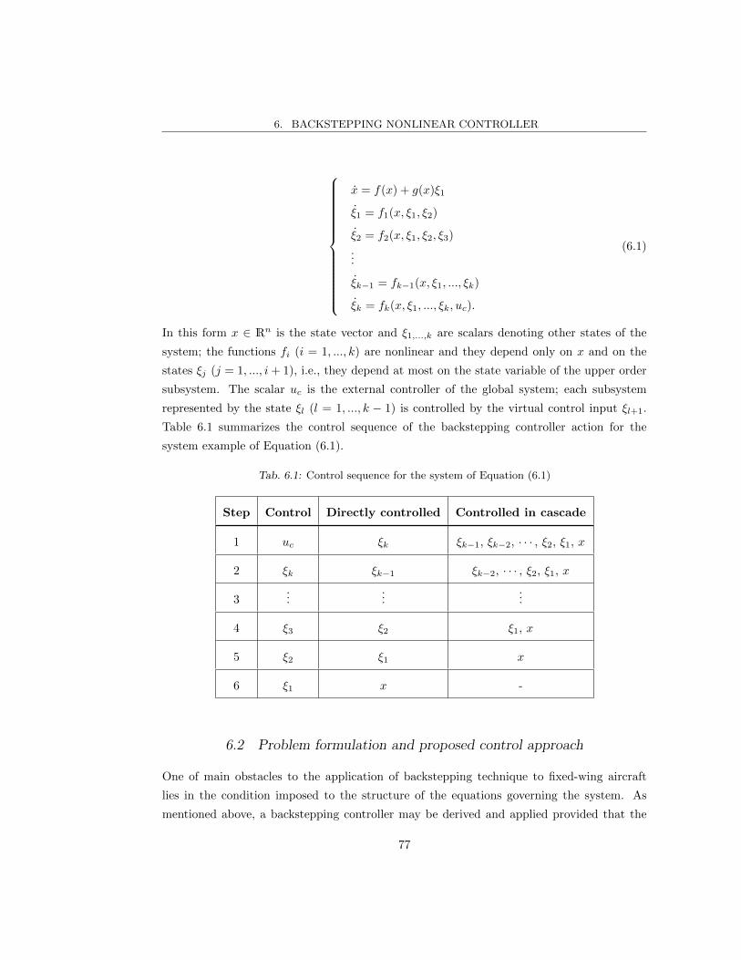
6. BACKSTEPPING NONLINEAR CONTROLLER

x = f(x) + g(x)ξ1

ξ1 = f1(x, ξ1, ξ2)

ξ2 = f2(x, ξ1, ξ2, ξ3)

...

ξk−1 = fk−1(x, ξ1, ..., ξk)

ξk = fk(x, ξ1, ..., ξk, uc).

(6.1)

In this form x ∈ Rn is the state vector and ξ1,...,k are scalars denoting other states of the

system; the functions fi (i = 1, ..., k) are nonlinear and they depend only on x and on the

states ξj (j = 1, ..., i+ 1), i.e., they depend at most on the state variable of the upper order

subsystem. The scalar uc is the external controller of the global system; each subsystem

represented by the state ξl (l = 1, ..., k − 1) is controlled by the virtual control input ξl+1.

Table 6.1 summarizes the control sequence of the backstepping controller action for the

system example of Equation (6.1).

Tab. 6.1: Control sequence for the system of Equation (6.1)

Step Control Directly controlled Controlled in cascade

1 uc ξk ξk−1, ξk−2, · · · , ξ2, ξ1, x

2 ξk ξk−1 ξk−2, · · · , ξ2, ξ1, x

3...

......

4 ξ3 ξ2 ξ1, x

5 ξ2 ξ1 x

6 ξ1 x -

6.2 Problem formulation and proposed control approach

One of main obstacles to the application of backstepping technique to fixed-wing aircraft

lies in the condition imposed to the structure of the equations governing the system. As

mentioned above, a backstepping controller may be derived and applied provided that the

77

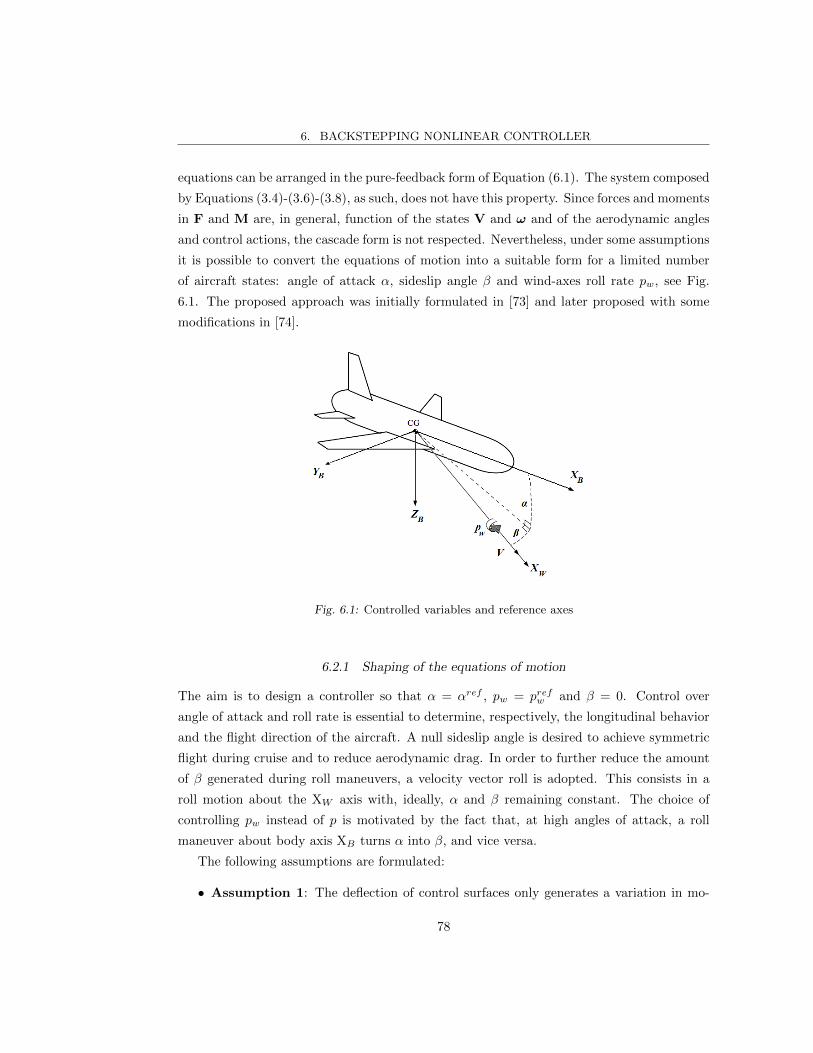
6. BACKSTEPPING NONLINEAR CONTROLLER

equations can be arranged in the pure-feedback form of Equation (6.1). The system composed

by Equations (3.4)-(3.6)-(3.8), as such, does not have this property. Since forces and moments

in F and M are, in general, function of the states V and ω and of the aerodynamic angles

and control actions, the cascade form is not respected. Nevertheless, under some assumptions

it is possible to convert the equations of motion into a suitable form for a limited number

of aircraft states: angle of attack α, sideslip angle β and wind-axes roll rate pw, see Fig.

6.1. The proposed approach was initially formulated in [73] and later proposed with some

modifications in [74].

Fig. 6.1: Controlled variables and reference axes

6.2.1 Shaping of the equations of motion

The aim is to design a controller so that α = αref , pw = prefw and β = 0. Control over

angle of attack and roll rate is essential to determine, respectively, the longitudinal behavior

and the flight direction of the aircraft. A null sideslip angle is desired to achieve symmetric

flight during cruise and to reduce aerodynamic drag. In order to further reduce the amount

of β generated during roll maneuvers, a velocity vector roll is adopted. This consists in a

roll motion about the XW axis with, ideally, α and β remaining constant. The choice of

controlling pw instead of p is motivated by the fact that, at high angles of attack, a roll

maneuver about body axis XB turns α into β, and vice versa.

The following assumptions are formulated:

• Assumption 1: The deflection of control surfaces only generates a variation in mo-

78

6. BACKSTEPPING NONLINEAR CONTROLLER

ments, the variation in forces is small enough to be neglected.

• Assumption 2: Lift and side force coefficients, CL and CY , only depend on aerody-

namic angles and not on aerodynamic angle rates of change: CL = CL(α), CY = CY (β).

Derivatives CLα and CY β can be neglected.

The first assumption is reasonable for aircraft with traditional configuration, so that control

surfaces are far from the aircraft center of gravity [78]. The deflection of a control surface

generates forces and, as a consequence, moments. The comparison between the control

derivative for a force and the one for the resulting moment shows that, in general, the moment

derivative has same order of magnitude or is larger. In fact, its definition includes, among

other terms, the product between the force derivative and the distance of the control surface

from the center of gravity. Furthermore, the addition of a reference lever-arm distance in the

moment mathematical formulation, see for instance Equation (6.16), increases the moment

contribution with respect to the force contribution. Once the trim condition is achieved, the

control deflections for maneuver are minimal, reducing to a negligible value the variation of

forces so produced.

Assumption 2 is considered valid in steady flight or during smooth maneuvers. In fact, the

disregarded aerodynamic derivatives CLα and CY β are originated by the delay in the pressure

distribution of the unsteady flow to adjust to sudden attitude variation. Assumption 2 is

on the conservative side as it targets progressive maneuvers, the ability of backstepping to

control aggressive flight will be demonstrated.

The differential equations governing the variation in time of the controlled variables α,

β and pw are now obtained. The definition of the aerodynamic angles α and β is expressed

in Equation (3.1). The equations relating their derivatives with the angular velocities and α

and β themselves are

α = q − (p cosα+ r sinα) tanβ +Zaero cosα− (Xaero + T ) sinα+mg2

mV cosβ

β = p sinα− r cosα+Yaero − T cosα sinβ +mg3

mV

(6.2)

where T is the engine thrust and Xaero, Yaero, Zaero are the aerodynamic forces in body

axes. The gravity acceleration components g2 and g3 are

g2 = g(cosα cos θ cosφ+ sinα sin θ)

g3 = g(cosβ cos θ sinφ+ sinβ cosα sin θ − sinα sinβ cos θ cosφ)(6.3)

79

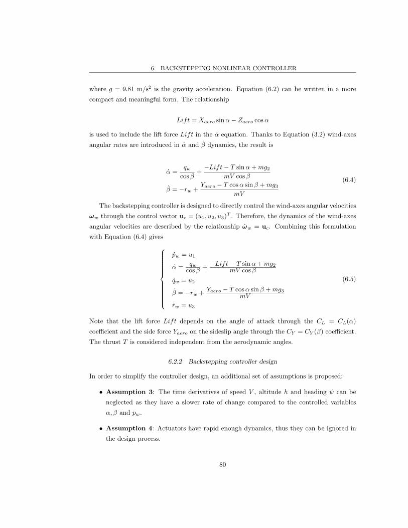
6. BACKSTEPPING NONLINEAR CONTROLLER

where g = 9.81 m/s2 is the gravity acceleration. Equation (6.2) can be written in a more

compact and meaningful form. The relationship

Lift = Xaero sinα− Zaero cosα

is used to include the lift force Lift in the α equation. Thanks to Equation (3.2) wind-axes

angular rates are introduced in α and β dynamics, the result is

α =qw

cosβ+−Lift− T sinα+mg2

mV cosβ

β = −rw +Yaero − T cosα sinβ +mg3

mV

(6.4)

The backstepping controller is designed to directly control the wind-axes angular velocities

ωw through the control vector uc = (u1, u2, u3)T . Therefore, the dynamics of the wind-axes

angular velocities are described by the relationship ωw = uc. Combining this formulation

with Equation (6.4) gives

pw = u1

α =qw

cosβ+−Lift− T sinα+mg2

mV cosβ

qw = u2

β = −rw +Yaero − T cosα sinβ +mg3

mV

rw = u3

(6.5)

Note that the lift force Lift depends on the angle of attack through the CL = CL(α)

coefficient and the side force Yaero on the sideslip angle through the CY = CY (β) coefficient.

The thrust T is considered independent from the aerodynamic angles.

6.2.2 Backstepping controller design

In order to simplify the controller design, an additional set of assumptions is proposed:

• Assumption 3: The time derivatives of speed V , altitude h and heading ψ can be

neglected as they have a slower rate of change compared to the controlled variables

α, β and pw.

• Assumption 4: Actuators have rapid enough dynamics, thus they can be ignored in

the design process.

80

6. BACKSTEPPING NONLINEAR CONTROLLER

Assumptions 3 is mainly valid for cruise flight and progressive maneuvers. Here a controlled

variation in the aircraft equilibrium state has a primary effect on the faster dynamics char-

acterizing the attitude, and a secondary effect on the slow-changing variables defining the

navigation. Finally, Assumption 4 is very common and generally reasonable, provided that

Assumptions 2 and 3 are respected.

Equation (6.5) is not suitable for the application of a total backstepping controller because

the cascade form is not respected, in particular due to the presence of β in the α dynamics,

and vice versa. However by separating its dynamics as

pw = u1 (6.6) α =qw

cosβ+−Lift− T sinα+mg2

mV cosβ

qw = u2

(6.7)

β = −rw +Yaero − T cosα sinβ +mg3

mV

rw = u3

(6.8)

three sub-controllers stabilizing the desired states α, β and pw can be defined. A cross-

coupling exists. In fact, it is possible to observe the presence of β in the α dynamics and,

at the same time, the presence of α in the β dynamics. During the individual sub-control

design mathematics imposes β constant in the α controller, and α constant in the β con-

troller. Instead, when dealing with the simultaneous control action on the three variables,

this assumption is disregarded because not physically realistic and not necessary, as it will

be shown later. Because of this coupling, the computation of a control action considers,

at each moment, the value of the state controlled by another control action. For instance,

the control law defining u2 is evaluated with the instantaneous value of β controlled by u3.

This occurrence is beneficial when dealing with maneuvers where strong coupling between

longitudinal and latero-directional planes exists.

A simple proportional controller is chosen for pw, Equation (6.6), while the cascade form

of Equation (6.7) and Equation (6.8) allows the application of backstepping controller for α

and β. Note that Equations (6.7) and (6.8) have the similar structure

ω1 = f(ω1, y) + ω2

ω2 = uw(6.9)

A single backstepping controller designed for Equation (6.9) is suitable for Equations (6.7)

and (6.8). As it is preferable to have the origin as the desired equilibrium point, a change of

81

6. BACKSTEPPING NONLINEAR CONTROLLER

variables is defined

x1 = ω1 −H

x2 = ω2 + f(H, y)

Ω(x1) = f(x1 +H, y)− f(H, y)

where H is the reference value for the controlled variable. The resulting dynamics are

x1 = Ω(x1) + x2

x2 = uw(6.10)

The external control input uw controls x2 that, in cascade, acts as virtual control to stabilize

x1. Table 6.2 summarizes the relationships between the variables used in the new and in the

original systems. The functions fα(α, yα) and fβ(β, yβ) are

fα(α, yα) =−Lift− T sinα+mg2

mV

fβ(β, yβ) =Yaero − T cosα sinβ +mg3

mV

As fully demonstrated in [74] through Lyapunov stability theory, a simple globally stabi-

lizing control law for the system of Equation (6.10) is

uw = −ku(x2 + Ψ(x1)) (6.11)

if, for all x1 6= 0, a constant ku exists so that

ku ≥Ω(x1)

x1

The function Ψ(x1) is built so that Ψ(x1) = −xref2 , where xref2 is the desired value for

the state x2 acting as virtual control input for the subsystem x1. This choice guarantees

asymptotic stability for the subsystem x1

W (x1)|x2=xref2= (Ω(x1)−Ψ(x1))x1 < 0, x1 6= 0

having chosen as temporary control Lyapunov function

W (x1) =1

2x2

1

82

6. BACKSTEPPING NONLINEAR CONTROLLER

Tab. 6.2: Change of variable relationships

General system Longitudinal Latero-directional

ω1 α β

ω2qw

cosβ−rw

uwu2

cosβ−u3

y β α

f(ω1, y)fα(α, yα)

cosβfβ(β, yβ)

H αref 0

x1 α− αref β

x2qw

cosβ+fα(αref , yα)

cosβ−rw + fβ(0, yβ)

Ω(x1)fα(α, yα)

cosβ− fα(αref , yα)

cosβfβ(β, yβ)− fβ(0, yβ)

Furthermore it can be demonstrated that Ψ′(x1), the time derivative of Ψ(x1), is bounded

0 < Ψ′(x1) < ku

The global control Lyapunov function used to define the control law of Equation (6.11) is

VL =

∫ x1

0

−Ψ′(y) (Ω(y)−Ψ(y)) dy +1

2(x2 + Ψ(x1))

2

which satisfies

VL = −Ψ′(x1) (Ω(x1)−Ψ(x1))2 − (ku −Ψ′(x1)) x2

2

where x2 = x2 − xref2 .

A linear control is chosen assigning Ψ(x1) = k1x1 so that

uw = −k2(x2 + k1x1)

with k2 > k1 > max0, ku. For k2 > 2k1 the controller is optimal as it minimizes the cost

function

83

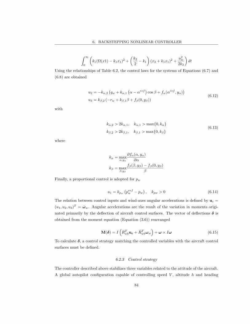
6. BACKSTEPPING NONLINEAR CONTROLLER

∫ ∞0

(k1(Ω(x1)− k1x1)2 +

(k2

2− k1

)(x2 + k1x1)2 +

u2w

2k2

)dt

Using the relationships of Table 6.2, the control laws for the systems of Equations (6.7) and

(6.8) are obtained

u2 = −kα,2(qw + kα,1

(α− αref

)cosβ + fα(αref , yα)

)u3 = kβ,2 (−rw + kβ,1β + fβ(0, yβ))

(6.12)

with

kα,2 > 2kα,1, kα,1 > max0, kα

kβ,2 > 2kβ,1, kβ,1 > max0, kβ(6.13)

where

kα = maxα,yα

∂fα(α, yα)

∂α

kβ = maxβ,yβ

fβ(β, yβ)− fβ(0, yβ)

β

Finally, a proportional control is adopted for pw

u1 = kpw(prefw − pw

), kpw > 0 (6.14)

The relation between control inputs and wind-axes angular accelerations is defined by uc =

(u1, u2, u3)T = ωw. Angular accelerations are the result of the variation in moments origi-

nated primarily by the deflection of aircraft control surfaces. The vector of deflections δ is

obtained from the moment equation (Equation (3.6)) rearranged

M(δ) = I(RTwbuc + RTwbωw

)+ ω × Iω (6.15)

To calculate δ, a control strategy matching the controlled variables with the aircraft control

surfaces must be defined.

6.2.3 Control strategy

The controller described above stabilizes three variables related to the attitude of the aircraft.

A global autopilot configuration capable of controlling speed V , altitude h and heading

84

6. BACKSTEPPING NONLINEAR CONTROLLER

ψ is required. In real-life implementation, these variables could be easily measured with,

respectively, a pitot tube, a barometric pressure sensor and magnetometer. The control

strategy is defined as follows: the backstepping controller acts on α, β and pw in the inner

loop, three PID controllers act on V , h and ψ in the outer loop. This approach separates

the fast dynamics, characterizing aircraft attitude, from the slower dynamics, characterizing

aircraft navigation. The prompt response of the backstepping controller is necessary when

dealing with fast-changing inner loop variables. These, in fact, are of prime importance for

the aircraft safety. For instance, an immediate control of α for a UAV affected by vertical

gust could prevent the stall and dangerous flight regimes. Consistent with Assumption 3,

slower variation of the navigation variables can be successfully handled using traditional PID

technique. PID gains are tuned manually following a trial and error approach. The goal is

optimizing the response in terms of values of overshoot, rise time, settling time and ringing

compatible with aircraft behavior, see Equation (4.3).

The PID controlling the speed feeds the backstepping controller with the desired angle

of attack, while the PID controlling the heading defines the desired roll rate. These values

are limited in magnitude in order to avoid the request of a motion incompatible with the

aircraft dynamics during sudden maneuvers. In particular, standard values for the imposed

saturation are the stall angle of attack for αref and typical roll rate for pref . Note that in the

outer loop the desired roll rate is expressed in body axes (pref ), the conversion to wind axes

(prefw ) is performed with Equation (3.2). The control surfaces employed are the elevator δe,

the aileron δa and the rudder δr. According to Assumption 1 these only generate a variation

in moments and not in forces. The deflection vector δ = (δe, δa, δr)T is obtained substituting

in Equation (6.15) the most general expressions of the moments

L(δa, δe, δr) =1

2ρV 2Sb

(Clββ + Clβ β + Clpp+ Clr r + Clδaδa + Clδeδe + Clδrδr

)M(δa, δe, δr) =

1

2ρV 2Sc (Cm0 + Cmαα+ Cmαα+ Cmq q + Cmδaδa + Cmδeδe + Cmδrδr)

N(δa, δe, δr) =1

2ρV 2Sb

(Cnββ + Cnβ β + Cnpp+ Cnr r + Cnδaδa + Cnδeδe + Cnδrδr

)(6.16)

and solving the resulting linear system with three equations and three unknowns. The

nondimensional angular rates p, q and r calculated as

p =pb

2V, q =

qc

2V, r =

rb

2V

and ρ is the air density, b is the aircraft wingspan, c the mean aerodynamic chord and S the

85

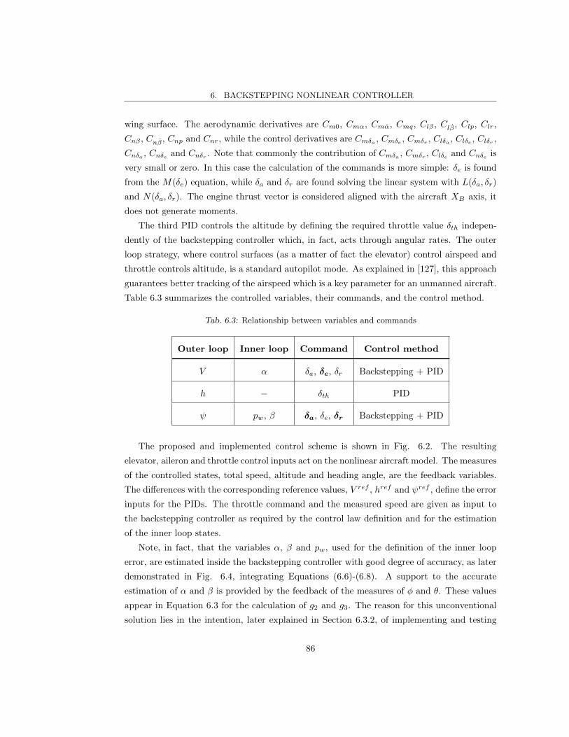
6. BACKSTEPPING NONLINEAR CONTROLLER

wing surface. The aerodynamic derivatives are Cm0, Cmα, Cmα, Cmq, Clβ , Clβ , Clp, Clr,

Cnβ , Cnβ , Cnp and Cnr, while the control derivatives are Cmδa , Cmδe , Cmδr , Clδa , Clδe , Clδr ,

Cnδa , Cnδe and Cnδr . Note that commonly the contribution of Cmδa , Cmδr , Clδe and Cnδe is

very small or zero. In this case the calculation of the commands is more simple: δe is found

from the M(δe) equation, while δa and δr are found solving the linear system with L(δa, δr)

and N(δa, δr). The engine thrust vector is considered aligned with the aircraft XB axis, it

does not generate moments.

The third PID controls the altitude by defining the required throttle value δth indepen-

dently of the backstepping controller which, in fact, acts through angular rates. The outer

loop strategy, where control surfaces (as a matter of fact the elevator) control airspeed and

throttle controls altitude, is a standard autopilot mode. As explained in [127], this approach

guarantees better tracking of the airspeed which is a key parameter for an unmanned aircraft.

Table 6.3 summarizes the controlled variables, their commands, and the control method.

Tab. 6.3: Relationship between variables and commands

Outer loop Inner loop Command Control method

V α δa, δe, δr Backstepping + PID

h − δth PID

ψ pw, β δa, δe, δr Backstepping + PID

The proposed and implemented control scheme is shown in Fig. 6.2. The resulting

elevator, aileron and throttle control inputs act on the nonlinear aircraft model. The measures

of the controlled states, total speed, altitude and heading angle, are the feedback variables.

The differences with the corresponding reference values, V ref , href and ψref , define the error

inputs for the PIDs. The throttle command and the measured speed are given as input to

the backstepping controller as required by the control law definition and for the estimation

of the inner loop states.

Note, in fact, that the variables α, β and pw, used for the definition of the inner loop

error, are estimated inside the backstepping controller with good degree of accuracy, as later

demonstrated in Fig. 6.4, integrating Equations (6.6)-(6.8). A support to the accurate

estimation of α and β is provided by the feedback of the measures of φ and θ. These values

appear in Equation 6.3 for the calculation of g2 and g3. The reason for this unconventional

solution lies in the intention, later explained in Section 6.3.2, of implementing and testing

86

6. BACKSTEPPING NONLINEAR CONTROLLER

Fig. 6.2: Backstepping control strategy for fixed-wing aircraft

in flight the backstepping controller on a real aircraft. The possibility to effectively estimate

these variables much simplifies the structure of the autopilot system and significantly reduces

the development time and cost. The need for a measure of α and β would be undermined

by the lack of affordable, reliable and compact aerodynamic angles sensors suitable for small

UAVs.

6.3 Simulation results

In order to test the proposed control approach, the controller is implemented in MathWorks

Matlab/Simulink and applied to the MH850 nonlinear aircraft model already employed in the

previous chapters. The integration of the equations is performed through a 2nd order Heun

method with 0.01 seconds time step. This low-order method is chosen as tradeoff between

accuracy and computational power required. It is interesting to explain how the calculation

of the commands for the MH850 rudderless configuration is performed. As already pointed

out, the δe command is found from the M(δe) equation as Cmδa = 0. Both L and N moments

are function of the remaining command δa, this generates a system of two equations with one

unknown which cannot be solved. It is chosen to disregard the N(δa) equation and to obtain

δa from L(δa). This is motivated by the strong predominance of the rolling moment over the

yawing moment in case of aileron deflection. In fact, for the MH850 UAV Clδa ≈ 10 · Cnδa .

87

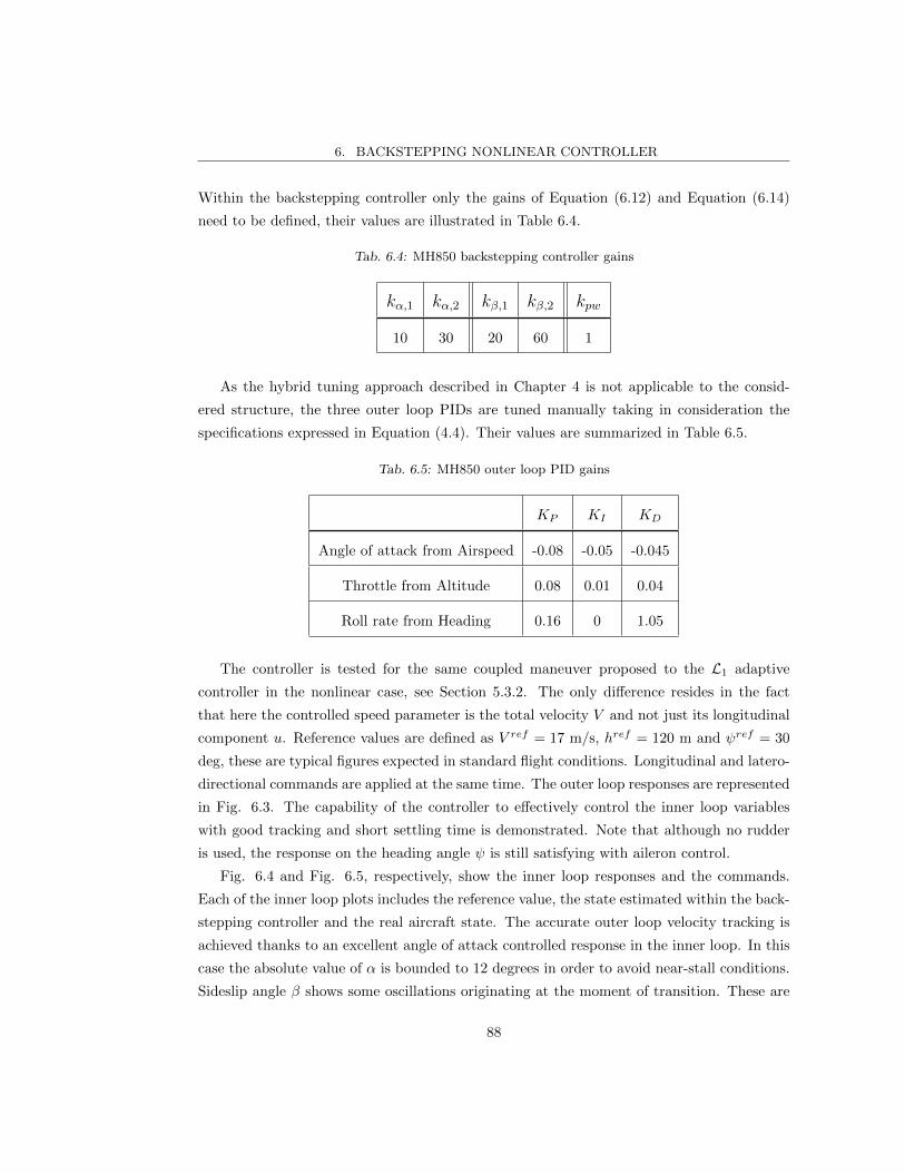
6. BACKSTEPPING NONLINEAR CONTROLLER

Within the backstepping controller only the gains of Equation (6.12) and Equation (6.14)

need to be defined, their values are illustrated in Table 6.4.

Tab. 6.4: MH850 backstepping controller gains

kα,1 kα,2 kβ,1 kβ,2 kpw

10 30 20 60 1

As the hybrid tuning approach described in Chapter 4 is not applicable to the consid-

ered structure, the three outer loop PIDs are tuned manually taking in consideration the

specifications expressed in Equation (4.4). Their values are summarized in Table 6.5.

Tab. 6.5: MH850 outer loop PID gains

KP KI KD

Angle of attack from Airspeed -0.08 -0.05 -0.045

Throttle from Altitude 0.08 0.01 0.04

Roll rate from Heading 0.16 0 1.05

The controller is tested for the same coupled maneuver proposed to the L1 adaptive

controller in the nonlinear case, see Section 5.3.2. The only difference resides in the fact

that here the controlled speed parameter is the total velocity V and not just its longitudinal

component u. Reference values are defined as V ref = 17 m/s, href = 120 m and ψref = 30

deg, these are typical figures expected in standard flight conditions. Longitudinal and latero-

directional commands are applied at the same time. The outer loop responses are represented

in Fig. 6.3. The capability of the controller to effectively control the inner loop variables

with good tracking and short settling time is demonstrated. Note that although no rudder

is used, the response on the heading angle ψ is still satisfying with aileron control.

Fig. 6.4 and Fig. 6.5, respectively, show the inner loop responses and the commands.

Each of the inner loop plots includes the reference value, the state estimated within the back-

stepping controller and the real aircraft state. The accurate outer loop velocity tracking is

achieved thanks to an excellent angle of attack controlled response in the inner loop. In this

case the absolute value of α is bounded to 12 degrees in order to avoid near-stall conditions.

Sideslip angle β shows some oscillations originating at the moment of transition. These are

88

6. BACKSTEPPING NONLINEAR CONTROLLER

Fig. 6.3: Nonlinear model outer loop variables

generated by the magnitude of the gain necessary to achieve a satisfying tracking of pw and

therefore of ψ. The limited directional damping provided by the vertical fins at the wingtips

of the MH850 is insufficient to prevent their onset. In any case the magnitude of the oscilla-

tions is minimal, less than 0.4 degrees, barely noticeable in a real aircraft application. The

elevons deflections always remain within the 20 degrees maximum value, throttle saturation

is measured only for few seconds after the step time.

6.3.1 Parametric robustness validation

The backstepping controller is validated by testing its performances when parametric uncer-

tainties are introduced in the nonlinear aircraft model. The same two cases already proposed

for the L1 controller are considered. Significant variations in aircraft mass, inertia and static

margin are adopted, the altered parameters were summarized in Table 5.2.

The comparison with the nominal case is analyzed. In the outer loop response of Fig.

6.6 V and ψ tracking, which are controlled through backstepping, remain almost unchanged

despite the considerable variation of the parameters. A slightly higher oscillatory behavior

in V is observable for Case 1 motivated by a lower pitch damping. The altitude response,

controlled with throttle through PID, suffers stronger variations from the nominal case. As

89

6. BACKSTEPPING NONLINEAR CONTROLLER

Fig. 6.4: Nonlinear model inner loop variables

Fig. 6.5: Nonlinear model commands

90

6. BACKSTEPPING NONLINEAR CONTROLLER

Fig. 6.6: Nonlinear model outer loop variables with parametric uncertainties

Fig. 6.7: Nonlinear model inner loop variables with parametric uncertainties

91

6. BACKSTEPPING NONLINEAR CONTROLLER

Fig. 6.8: Nonlinear model commands with parametric uncertainties

expected the aircraft with higher mass and inertia has a slower response to step input, higher

overshoot and settling time. In the inner loop, Fig. 6.7, lateral oscillations are emphasized

in Case 1. It is interesting to observe how the α trim condition changes in the two cases.

The commands plot of Fig. 6.8 confirms that full throttle command is required longer for

the heavier aircraft of Case 1. The backstepping controller proves to be robust to substantial

parametric uncertainties as it guarantees satisfying performances in all the examined cases.

6.3.2 Confrontation among backstepping, L1 and PID controllers

The three controllers proposed in this project are compared in their outer loop performances

for the nominal case, see Fig. 6.9. The comparison of the responses indicates that L1 is the

best performer on the longitudinal plane, while backstepping guarantees better ψ control.

The PID has worst performance in the V and ψ control, while the h response is equivalent to

the one from backstepping because the same gains for altitude control are employed. Note, in

fact, that in this case the nonlinear model is tested and the PID gains designed in Chapter 4

need to be adjusted in order to accommodate for this. As PID and backstepping controllers

share the throttle to altitude loop, the gains tuned for the backstepping already represent a

satisfying choice.

92

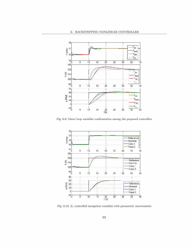
6. BACKSTEPPING NONLINEAR CONTROLLER

Fig. 6.9: Outer loop variables confrontation among the proposed controllers

Fig. 6.10: L1 controlled navigation variables with parametric uncertainties

93

6. BACKSTEPPING NONLINEAR CONTROLLER

It is also interesting to see how the three controllers behave when then nonlinear aircraft

model is affected by parametric uncertainties related to its dynamical properties, see Table

5.2. The test was already proposed for L1 and backstepping, the main results for the navi-

gation variables are here summarized and the PID case is included. Fig. 6.10 illustrates the

results for L1, in the previous section the backstepping case was analyzed, see Fig. 6.6. The

adaptive nature of L1 guarantees minimal differences among the considered cases. Backstep-

ping is comparable but penalized by the control of the altitude performed with the throttle

only via PID. The PID technique, in fact, proves not to be robust enough to handle large

variations in aircraft model parameters. According to Fig. 6.11 the aircraft loses directional

control, it accelerates while quickly losing altitude. It crashes to the ground in less than 10

seconds. Despite backstepping and PID controllers were almost equivalent in the nominal

case, it is clear that a traditional PID configuration is not able to deal with substantial

changes in the aircraft parameters.

Fig. 6.11: PID controlled navigation variables with parametric uncertainties

The idea behind the proposed thesis is to actually implement and test a controller on a

fixed-wing UAV. Among the three proposed controllers one needs to be chosen. The PID

is discarded for two reasons. First of all it is widely employed and thus its implementa-

tion would not represent any innovative contribution. Furthermore, one of its well known

94

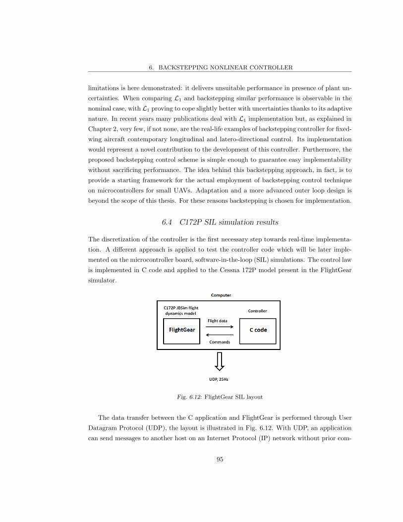
6. BACKSTEPPING NONLINEAR CONTROLLER

limitations is here demonstrated: it delivers unsuitable performance in presence of plant un-

certainties. When comparing L1 and backstepping similar performance is observable in the

nominal case, with L1 proving to cope slightly better with uncertainties thanks to its adaptive

nature. In recent years many publications deal with L1 implementation but, as explained in

Chapter 2, very few, if not none, are the real-life examples of backstepping controller for fixed-

wing aircraft contemporary longitudinal and latero-directional control. Its implementation

would represent a novel contribution to the development of this controller. Furthermore, the

proposed backstepping control scheme is simple enough to guarantee easy implementability

without sacrificing performance. The idea behind this backstepping approach, in fact, is to

provide a starting framework for the actual employment of backstepping control technique

on microcontrollers for small UAVs. Adaptation and a more advanced outer loop design is

beyond the scope of this thesis. For these reasons backstepping is chosen for implementation.

6.4 C172P SIL simulation results

The discretization of the controller is the first necessary step towards real-time implementa-

tion. A different approach is applied to test the controller code which will be later imple-

mented on the microcontroller board, software-in-the-loop (SIL) simulations. The control law

is implemented in C code and applied to the Cessna 172P model present in the FlightGear

simulator.

Fig. 6.12: FlightGear SIL layout

The data transfer between the C application and FlightGear is performed through User

Datagram Protocol (UDP), the layout is illustrated in Fig. 6.12. With UDP, an application

can send messages to another host on an Internet Protocol (IP) network without prior com-

95

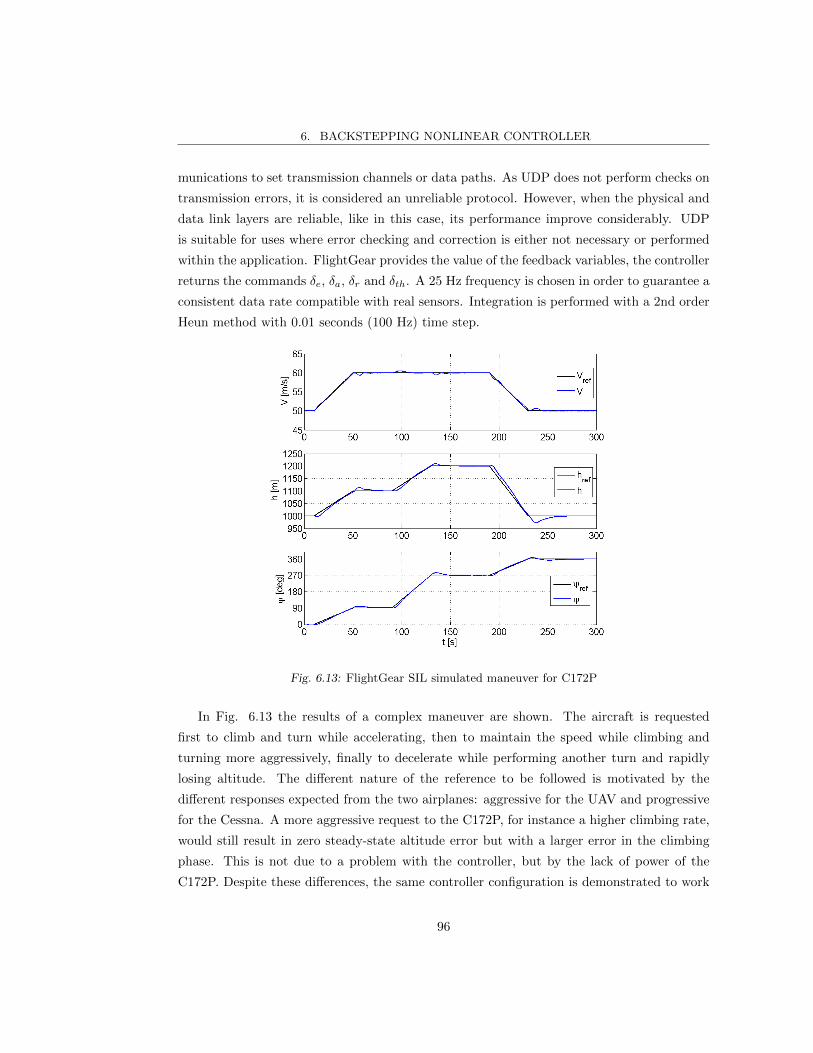
6. BACKSTEPPING NONLINEAR CONTROLLER

munications to set transmission channels or data paths. As UDP does not perform checks on

transmission errors, it is considered an unreliable protocol. However, when the physical and

data link layers are reliable, like in this case, its performance improve considerably. UDP

is suitable for uses where error checking and correction is either not necessary or performed

within the application. FlightGear provides the value of the feedback variables, the controller

returns the commands δe, δa, δr and δth. A 25 Hz frequency is chosen in order to guarantee a

consistent data rate compatible with real sensors. Integration is performed with a 2nd order

Heun method with 0.01 seconds (100 Hz) time step.

Fig. 6.13: FlightGear SIL simulated maneuver for C172P

In Fig. 6.13 the results of a complex maneuver are shown. The aircraft is requested

first to climb and turn while accelerating, then to maintain the speed while climbing and

turning more aggressively, finally to decelerate while performing another turn and rapidly

losing altitude. The different nature of the reference to be followed is motivated by the

different responses expected from the two airplanes: aggressive for the UAV and progressive

for the Cessna. A more aggressive request to the C172P, for instance a higher climbing rate,

would still result in zero steady-state altitude error but with a larger error in the climbing

phase. This is not due to a problem with the controller, but by the lack of power of the

C172P. Despite these differences, the same controller configuration is demonstrated to work

96

6. BACKSTEPPING NONLINEAR CONTROLLER

for aircraft different in size and configuration with adequate results.

Fig. 6.14: FlightGear SIL simulated maneuver commands for C172P

All variables are tracked with good accuracy in every phase of the maneuver. Speed

tracking performs the best, the quick response is guaranteed by the choice of using the elevator

instead of the throttle for its control. Similarly, the heading angle shows good results despite

some mild overshoot. The altitude response is penalized by some overshoot/undershoot

and some mild oscillations in the settling phase, note also the difference in slope between

reference and actual values. The slower engine response and the low power-to-weight ratio

are responsible for this. In this project, envisaging the UAV application, priority is given to

the speed which is a sensible parameter to avoid stall. Finally, it is interesting to observe

how the changes in altitude affect the speed. The corresponding commands are illustrated in

Fig. 6.14. The surfaces deflections always remain well within the saturation limits, around

20 degrees for elevator and aileron, 16 degrees for the rudder. The motor instead goes full

throttle during the climbing phases. The gains used in this simulation are summarized in

Table 6.6 and Table 6.7.

97

6. BACKSTEPPING NONLINEAR CONTROLLER

Tab. 6.6: C172P backstepping controller gains

kα,1 kα,2 kβ,1 kβ,2 kpw

6 18 5 15 1

Tab. 6.7: C172P outer loop PID gains

KP KI KD

Angle of attack from Airspeed -0.0105 -0.0021 0

Throttle from Altitude 0.012 0.001 0.0355

Roll rate from Heading 0.29 0.011 2.1

6.5 C172P HIL simulation results

After testing the controller in discrete time using software-in-the-loop approach, the next

natural step is the hardware-in-the-loop simulation (HIL). The controller is implemented on

a control board and tested in real time with the simulated aircraft model.

Fig. 6.15: FlightGear HIL layout

The HIL scheme is represented in Fig. 6.15 and its real implementation in Fig. 6.16.

The simulator for the HIL is always FlightGear, its settings remain unchanged. This time

the simulator does not communicate directly with the controller. A Python application,

98

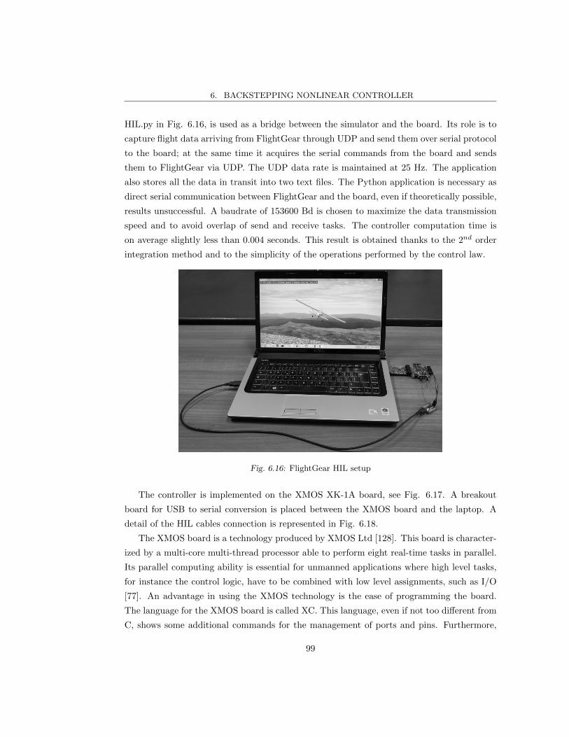
6. BACKSTEPPING NONLINEAR CONTROLLER

HIL.py in Fig. 6.16, is used as a bridge between the simulator and the board. Its role is to

capture flight data arriving from FlightGear through UDP and send them over serial protocol

to the board; at the same time it acquires the serial commands from the board and sends

them to FlightGear via UDP. The UDP data rate is maintained at 25 Hz. The application

also stores all the data in transit into two text files. The Python application is necessary as

direct serial communication between FlightGear and the board, even if theoretically possible,

results unsuccessful. A baudrate of 153600 Bd is chosen to maximize the data transmission

speed and to avoid overlap of send and receive tasks. The controller computation time is

on average slightly less than 0.004 seconds. This result is obtained thanks to the 2nd order

integration method and to the simplicity of the operations performed by the control law.

Fig. 6.16: FlightGear HIL setup

The controller is implemented on the XMOS XK-1A board, see Fig. 6.17. A breakout

board for USB to serial conversion is placed between the XMOS board and the laptop. A

detail of the HIL cables connection is represented in Fig. 6.18.

The XMOS board is a technology produced by XMOS Ltd [128]. This board is character-

ized by a multi-core multi-thread processor able to perform eight real-time tasks in parallel.

Its parallel computing ability is essential for unmanned applications where high level tasks,

for instance the control logic, have to be combined with low level assignments, such as I/O

[77]. An advantage in using the XMOS technology is the ease of programming the board.

The language for the XMOS board is called XC. This language, even if not too different from

C, shows some additional commands for the management of ports and pins. Furthermore,

99

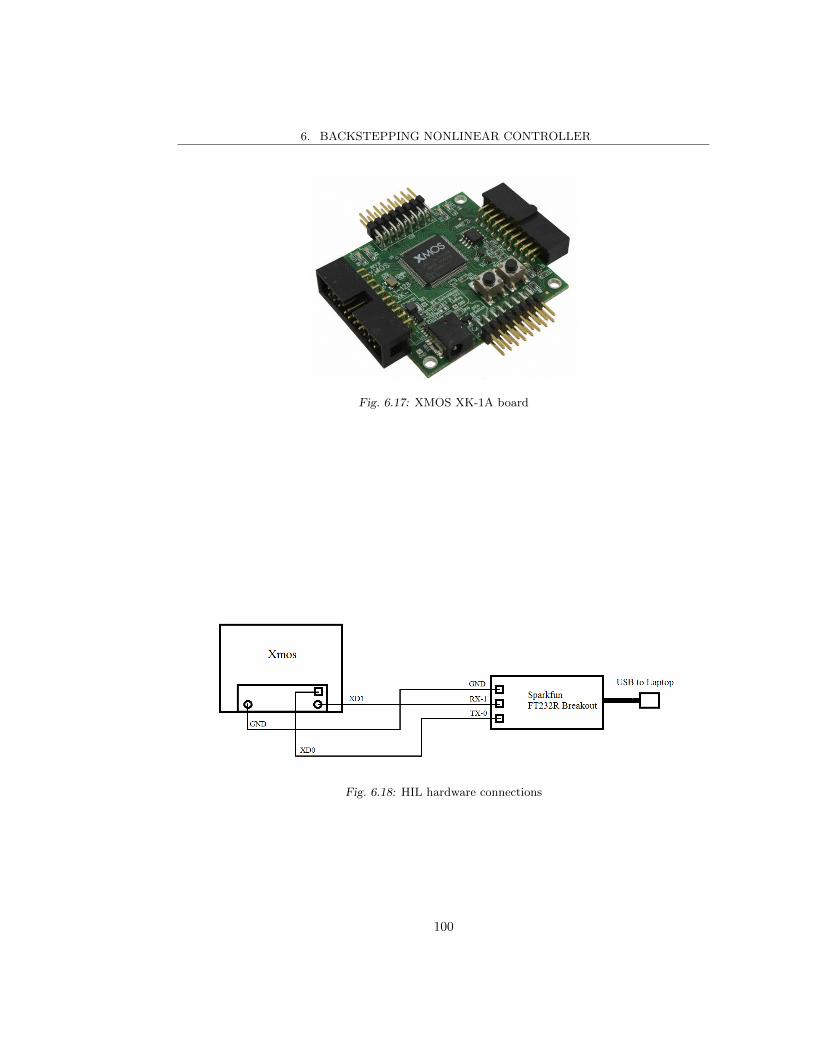
6. BACKSTEPPING NONLINEAR CONTROLLER

Fig. 6.17: XMOS XK-1A board

Fig. 6.18: HIL hardware connections

100

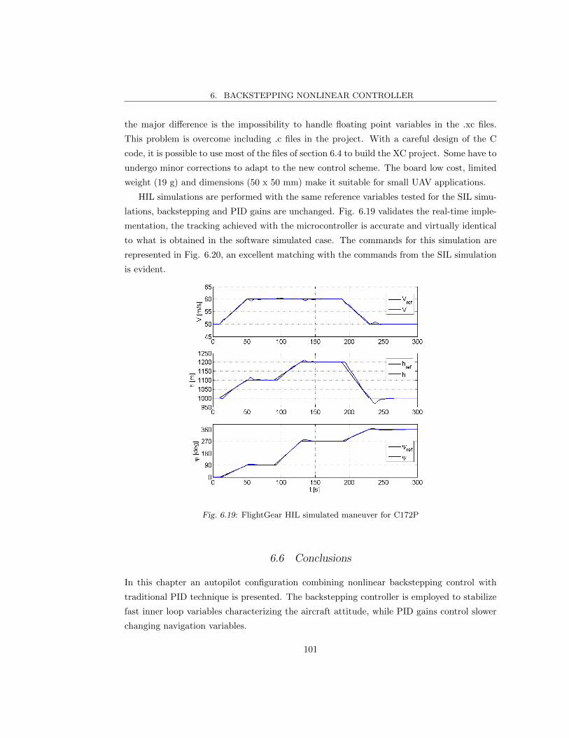
6. BACKSTEPPING NONLINEAR CONTROLLER

the major difference is the impossibility to handle floating point variables in the .xc files.

This problem is overcome including .c files in the project. With a careful design of the C

code, it is possible to use most of the files of section 6.4 to build the XC project. Some have to

undergo minor corrections to adapt to the new control scheme. The board low cost, limited

weight (19 g) and dimensions (50 x 50 mm) make it suitable for small UAV applications.

HIL simulations are performed with the same reference variables tested for the SIL simu-

lations, backstepping and PID gains are unchanged. Fig. 6.19 validates the real-time imple-

mentation, the tracking achieved with the microcontroller is accurate and virtually identical

to what is obtained in the software simulated case. The commands for this simulation are

represented in Fig. 6.20, an excellent matching with the commands from the SIL simulation

is evident.

Fig. 6.19: FlightGear HIL simulated maneuver for C172P

6.6 Conclusions

In this chapter an autopilot configuration combining nonlinear backstepping control with

traditional PID technique is presented. The backstepping controller is employed to stabilize

fast inner loop variables characterizing the aircraft attitude, while PID gains control slower

changing navigation variables.

101

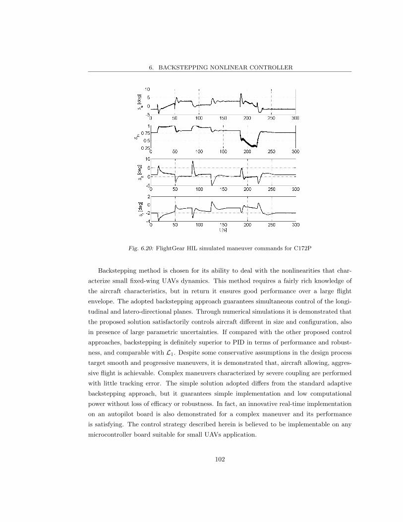
6. BACKSTEPPING NONLINEAR CONTROLLER

Fig. 6.20: FlightGear HIL simulated maneuver commands for C172P

Backstepping method is chosen for its ability to deal with the nonlinearities that char-

acterize small fixed-wing UAVs dynamics. This method requires a fairly rich knowledge of

the aircraft characteristics, but in return it ensures good performance over a large flight

envelope. The adopted backstepping approach guarantees simultaneous control of the longi-

tudinal and latero-directional planes. Through numerical simulations it is demonstrated that

the proposed solution satisfactorily controls aircraft different in size and configuration, also

in presence of large parametric uncertainties. If compared with the other proposed control

approaches, backstepping is definitely superior to PID in terms of performance and robust-

ness, and comparable with L1. Despite some conservative assumptions in the design process

target smooth and progressive maneuvers, it is demonstrated that, aircraft allowing, aggres-

sive flight is achievable. Complex maneuvers characterized by severe coupling are performed

with little tracking error. The simple solution adopted differs from the standard adaptive

backstepping approach, but it guarantees simple implementation and low computational

power without loss of efficacy or robustness. In fact, an innovative real-time implementation

on an autopilot board is also demonstrated for a complex maneuver and its performance

is satisfying. The control strategy described herein is believed to be implementable on any

microcontroller board suitable for small UAVs application.

102

7. EXPERIMENTS AND FLIGHT TESTS

The previous chapter illustrates the design of the adopted backstepping approach, its imple-

mentation and the results of the simulations that prove its ability to control different aircraft

configurations, also when working in real time on a microcontroller board. This chapter

deals in detail with the preparation of the flight tests. The controller is integrated on a real

aircraft, the following sections explain the setup defined, the problems encountered and the

solutions proposed.

7.1 Sensors noise model

The backstepping strategy acts on three feedback variables, velocity V , altitude h and head-

ing ψ, three sensors able to measure these parameters are thus necessary. Note, in fact,

that the inner loop variables α, β and pw are accurately estimated inside the backstepping

controller, as it was demonstrated in Fig. 6.4. This unconventional but effective approach

is adopted to maintain simple the physical integration of the controller on the aircraft and

because of the lack of affordable, reliable and small aerodynamic angles sensors. The feed-

back of φ and θ must be provided as well to improve the inner loop states estimation. In

this section the methods used to measure the outer loop variables are introduced. The data

obtained by the sensors are used to characterize the noise spectrum which is included in

the Simulink aircraft model in order the make the simulation as real as possible. In fact,

the noise is expected to have great influence on the controller performance. The statistical

properties of the sensors noise are analyzed, Gaussian white noise is added in Simulink to

disturb the measurement.

7.1.1 Velocity measurement

The total velocity V is a key parameter as it strongly influences the aircraft states through

is quadratic presence in the forces and moments acting on the airplane. In the controller

structure here proposed the velocity is considered as a navigation outer loop variable, but

as visible from Equation (6.5) it also directly affects the attitude of the aircraft. Achieving

7. EXPERIMENTS AND FLIGHT TESTS

a good measurement of the velocity is essential to achieve a good performance of the con-

troller. The pitot tube method is chosen for its good precision and for its high sampling rate

compatible with the controller frequency action. GPS is dismissed as not able to provide

accurate data with high frequency.

The pitot principle of functioning is represented in Fig. 7.1. A pitot probe collects the

total and static pressures encountered by the flying aircraft, these are carried to the Freescale

Semiconductors MPXV7002 transducer [129] through two silicon tubes. The transducer out-

puts an analog voltage proportional to the difference between total and static pressure, this

voltage is digitalized with a Linear Technology LTC 1865 16-bit Analog to Digital Converter

(ADC) [130]. The digital voltage is read by the XMOS board which first converts the voltage

value into pressure difference, as the pressure difference is equal to the dynamic pressure the

airspeed is easily retrieved.

Fig. 7.1: Pitot airspeed measurement scheme

The law relating the voltage V olt with the pressure difference dP is assumed linear with

very limited error and the coefficients c1 and c2 are obtained through wind tunnel calibration,

see Fig. 7.2. As a consequence the relationship between pressure difference and freestream

velocity is quadratic. In this case the linear law is defined by

104

7. EXPERIMENTS AND FLIGHT TESTS

Fig. 7.2: Pitot calibration curve, comparison of data from pitot and wind tunnel

dP = 995.9 · V olt− 2489.75

The wind tunnel tests were performed at the Politecnico di Torino fluid dynamics test

facility. Five measurements at different velocity were performed, each one lasting for 20

seconds. The numbers plotted on Fig. 7.2 represent the mean values for each measurement.

As each time series is characterized by noise, the adoption of a filter is necessary. Further

details about the filtering operation will be introduced in Section 7.2. The ADC is able to

sample data with a frequency up to 125 kHz when one channel is used. In this case the

sampling frequency is limited to 20 Hz to match the slowest sensor, the barometric pressure

sensor.

7.1.2 Altitude measurement

The measurement of the altitude is performed through a barometric pressure sensor, in

particular by a Bosch BMP085 transducer [131] mounted on a Sparkfun breakout board

[132], see Fig. 7.3. Considering the data frequency, range and precision required and the

limited weight and space budget, other options such as GPS or laser and ultrasonic sensors

were excluded.

105

7. EXPERIMENTS AND FLIGHT TESTS

Fig. 7.3: Bosch BMP085 barometric sensor on Sparkfun breakout board

The estimation of the altitude h relies on the measure of the local air pressure p through

the formula

h = 44330 ·

(1−

(p

p0

)0.1903)

(7.1)

where p0 is the equivalent pressure at sea level for the moment and the location considered.

This parameter is generally available through weather station websites or can be calculated

inverting the formula of Equation (7.1) in a location with known altitude after a single pres-

sure measurement. In order to be independent from this value that can be unavailable or

change during the day, the parameter given to the controller will be the height above the air-

field (AGL, above ground level altitude) and not the absolute altitude. A first measurement

is performed and stored when the control board is powered on the ground at the beginning

of each flight, the AGL is obtained subtracting this value to future measurements.

The barometric pressure sensor has 4 operating modes, each characterized by a combi-

nation of sampling frequency and precision: the higher the precision, the lower the sampling

frequency. The operating mode characterized by a 0.4 m root mean square noise error and 20

Hz sampling frequency is chosen as it offers the best compromise. The only faster frequency

available, 22 Hz, comes with a typical 0.5 m error; the improvement of sampling speed is not

enough to justify its choice. Like the pitot, this sensor is affected by noise and its output

need to be filtered, more details will be added in Section 7.2.

7.1.3 Attitude measurement

The measurement of the attitude angles φ, θ and ψ is performed with a Vectornav VN-100

IMU chip [133] mounted on a development board, see Fig. 7.4. This sensor incorporates

a 3-axis magnetometer, a 3-axis accelerometer and 3-axis gyroscope with extended Kalman

106

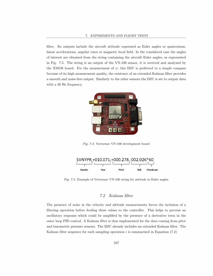
7. EXPERIMENTS AND FLIGHT TESTS

filter. Its outputs include the aircraft attitude expressed as Euler angles or quaternions,

linear accelerations, angular rates or magnetic local field. In the considered case the angles

of interest are obtained from the string containing the aircraft Euler angles, as represented

in Fig. 7.5. The string is an output of the VN-100 sensor, it is received and analyzed by

the XMOS board. For the measurement of ψ, this IMU is preferred to a simple compass

because of its high measurement quality, the existence of an extended Kalman filter provides

a smooth and noise-free output. Similarly to the other sensors the IMU is set to output data

with a 20 Hz frequency.

Fig. 7.4: Vectornav VN-100 development board

Fig. 7.5: Example of Vectornav VN-100 string for attitude in Euler angles

7.2 Kalman filter

The presence of noise in the velocity and altitude measurements forces the inclusion of a

filtering operation before feeding these values to the controller. This helps to prevent an

oscillatory response which could be amplified by the presence of a derivative term in the

outer loop PID control. A Kalman filter is thus implemented for the data coming from pitot

and barometric pressure sensors. The IMU already includes an extended Kalman filter. The

Kalman filter sequence for each sampling operation i is summarized in Equation (7.2)

107

7. EXPERIMENTS AND FLIGHT TESTS

pi = pi−1 +Q

K =pi

pi +R

xi = xi−1 +K · (xi − xi−1)

pi = (1−K) · pi

(7.2)

Here xi is the filtered variable, xi is the measured variable and pi is the estimated error. K

is the Kalman gain, Q is the process noise variance and R is the sensor noise variance. The

value of R can be found by experimental tests, the value of Q is more difficult to estimate

and it can be used as a parameter for tuning the intensity of the filter action.

Table 7.1 illustrates the values of R and Q chosen for both sensors. Moreover it indicates

the standard deviation σ, with and without Kalman filter, from a mean value representing

the trim condition. The improvement achieved with the filter is remarkable. Fig. 7.6 shows

an example of filtering action on a randomly varying altitude measurement. It is possible

to see how the filter was tuned in order to reduce the oscillations without introducing a

considerable delay in the filtered time series.

Tab. 7.1: Kalman filter parameters

Measurement R Q σ σKalman

V 0.029 0.0005 0.17 m/s 0.05 m/s

h 0.19 0.0008 0.44 m 0.16 m

7.3 Ultrastick 25e simulation results

Simulations are performed merging the Simulink model of the backstepping controller with

the aircraft Simulink model available from the University of Minnesota UAV research group,

see Section 3.6.4. The resultant system is integrated in discrete time with a time step of

0.01 seconds, equal to the controller action frequency, Heun method is still used. Sensors

noise and a Kalman filter are modeled as described in the previous sections. The Simulink

model is built so that the trim commands are already an input for the aircraft. Because of

that, the backstepping controller, instead of calculating the absolute commands, calculates

the commands variation to be added to the trim commands.

108

7. EXPERIMENTS AND FLIGHT TESTS

Fig. 7.6: Kalman filtering action on a noisy altitude measurement

Fig. 7.7: Simulink outer loop response for Ultrastick 25e, trim conditions hold

109

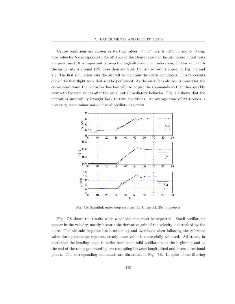
7. EXPERIMENTS AND FLIGHT TESTS

Cruise conditions are chosen as starting values: V=17 m/s, h=1571 m and ψ=0 deg.

The value for h corresponds to the altitude of the Denver research facility where initial tests

are performed. It is important to keep the high altitude in consideration, for this value of h

the air density is around 15% lower than sea level. Controlled results appear in Fig. 7.7 and

7.8. The first simulation asks the aircraft to maintain the cruise conditions. This represents

one of the first flight tests that will be performed. As the aircraft is already trimmed for the

cruise conditions, the controller has basically to adjust the commands so that they quickly

return to the trim values after the usual initial oscillatory behavior. Fig. 7.7 shows that the

aircraft is successfully brought back to trim conditions. An average time of 20 seconds is

necessary, some minor noise-induced oscillations persist.

Fig. 7.8: Simulink outer loop response for Ultrastick 25e, maneuver

Fig. 7.8 shows the results when a coupled maneuver is requested. Small oscillations

appear in the velocity, mostly because the derivative gain of the velocity is disturbed by the

noise. The altitude response has a minor lag and overshoot when following the reference

value during the slope segment, steady state value is successfully achieved. All states, in

particular the heading angle ψ, suffer from some mild oscillations at the beginning and at

the end of the ramp generated by cross-coupling between longitudinal and latero-directional

planes. The corresponding commands are illustrated in Fig. 7.9. In spite of the filtering

110

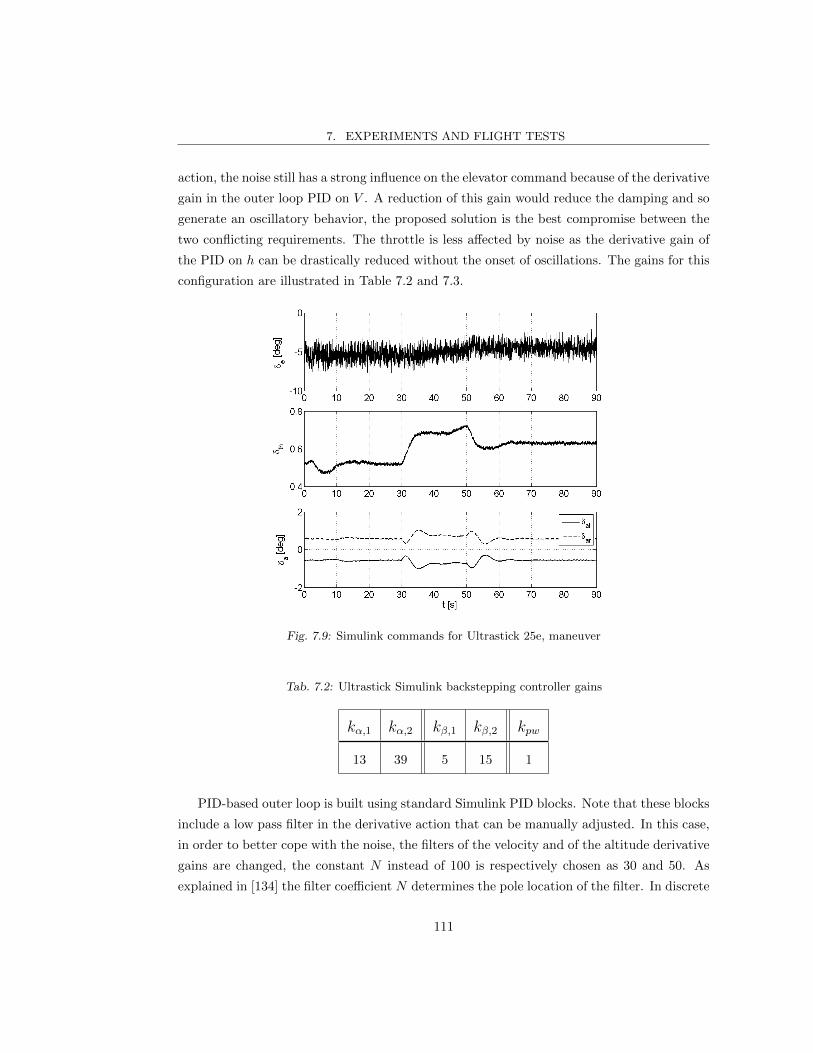
7. EXPERIMENTS AND FLIGHT TESTS

action, the noise still has a strong influence on the elevator command because of the derivative

gain in the outer loop PID on V . A reduction of this gain would reduce the damping and so

generate an oscillatory behavior, the proposed solution is the best compromise between the

two conflicting requirements. The throttle is less affected by noise as the derivative gain of

the PID on h can be drastically reduced without the onset of oscillations. The gains for this

configuration are illustrated in Table 7.2 and 7.3.

Fig. 7.9: Simulink commands for Ultrastick 25e, maneuver

Tab. 7.2: Ultrastick Simulink backstepping controller gains

kα,1 kα,2 kβ,1 kβ,2 kpw

13 39 5 15 1

PID-based outer loop is built using standard Simulink PID blocks. Note that these blocks

include a low pass filter in the derivative action that can be manually adjusted. In this case,

in order to better cope with the noise, the filters of the velocity and of the altitude derivative

gains are changed, the constant N instead of 100 is respectively chosen as 30 and 50. As

explained in [134] the filter coefficient N determines the pole location of the filter. In discrete

111

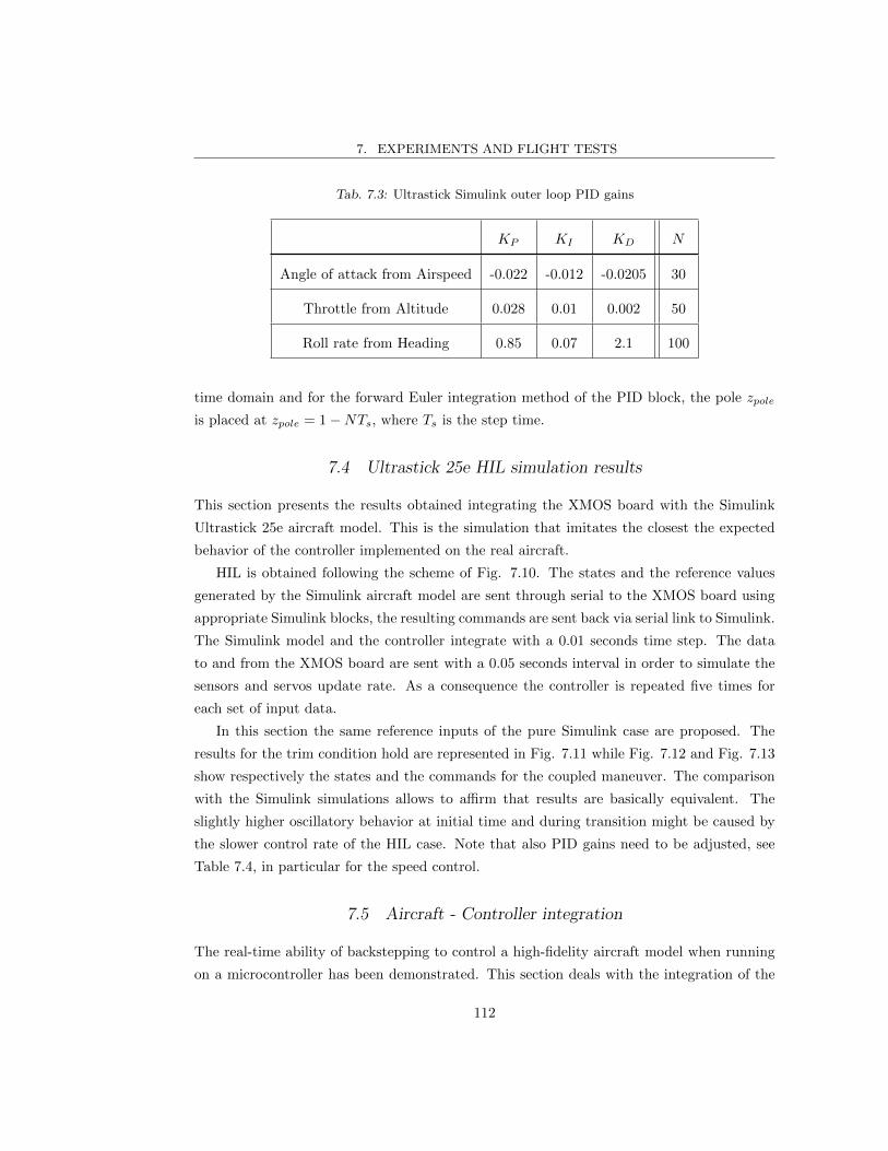
7. EXPERIMENTS AND FLIGHT TESTS

Tab. 7.3: Ultrastick Simulink outer loop PID gains

KP KI KD N

Angle of attack from Airspeed -0.022 -0.012 -0.0205 30

Throttle from Altitude 0.028 0.01 0.002 50

Roll rate from Heading 0.85 0.07 2.1 100

time domain and for the forward Euler integration method of the PID block, the pole zpole

is placed at zpole = 1−NTs, where Ts is the step time.

7.4 Ultrastick 25e HIL simulation results

This section presents the results obtained integrating the XMOS board with the Simulink

Ultrastick 25e aircraft model. This is the simulation that imitates the closest the expected

behavior of the controller implemented on the real aircraft.

HIL is obtained following the scheme of Fig. 7.10. The states and the reference values

generated by the Simulink aircraft model are sent through serial to the XMOS board using

appropriate Simulink blocks, the resulting commands are sent back via serial link to Simulink.

The Simulink model and the controller integrate with a 0.01 seconds time step. The data

to and from the XMOS board are sent with a 0.05 seconds interval in order to simulate the

sensors and servos update rate. As a consequence the controller is repeated five times for

each set of input data.

In this section the same reference inputs of the pure Simulink case are proposed. The

results for the trim condition hold are represented in Fig. 7.11 while Fig. 7.12 and Fig. 7.13

show respectively the states and the commands for the coupled maneuver. The comparison

with the Simulink simulations allows to affirm that results are basically equivalent. The

slightly higher oscillatory behavior at initial time and during transition might be caused by

the slower control rate of the HIL case. Note that also PID gains need to be adjusted, see

Table 7.4, in particular for the speed control.

7.5 Aircraft - Controller integration

The real-time ability of backstepping to control a high-fidelity aircraft model when running

on a microcontroller has been demonstrated. This section deals with the integration of the

112

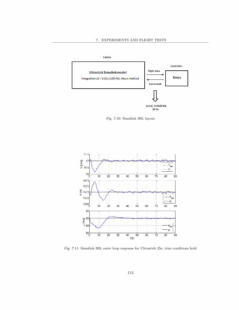
7. EXPERIMENTS AND FLIGHT TESTS

Fig. 7.10: Simulink HIL layout

Fig. 7.11: Simulink HIL outer loop response for Ultrastick 25e, trim conditions hold

113

7. EXPERIMENTS AND FLIGHT TESTS

Fig. 7.12: Simulink HIL outer loop response for Ultrastick 25e, maneuver

Fig. 7.13: Simulink HIL commands for Ultrastick 25e, maneuver

114

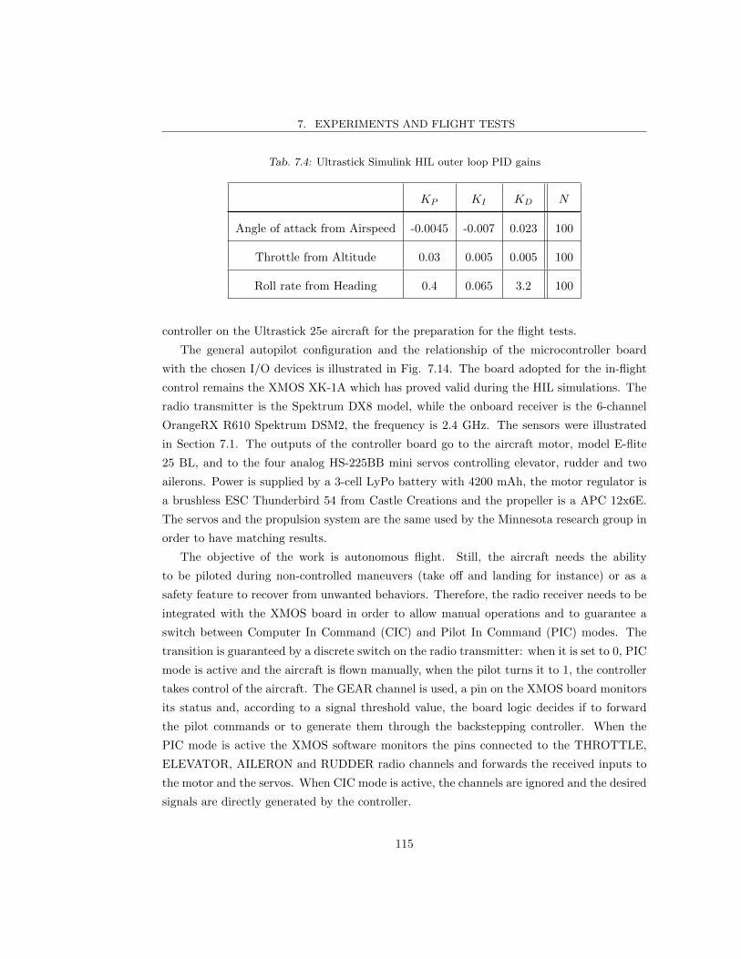
7. EXPERIMENTS AND FLIGHT TESTS

Tab. 7.4: Ultrastick Simulink HIL outer loop PID gains

KP KI KD N

Angle of attack from Airspeed -0.0045 -0.007 0.023 100

Throttle from Altitude 0.03 0.005 0.005 100

Roll rate from Heading 0.4 0.065 3.2 100

controller on the Ultrastick 25e aircraft for the preparation for the flight tests.

The general autopilot configuration and the relationship of the microcontroller board

with the chosen I/O devices is illustrated in Fig. 7.14. The board adopted for the in-flight

control remains the XMOS XK-1A which has proved valid during the HIL simulations. The

radio transmitter is the Spektrum DX8 model, while the onboard receiver is the 6-channel

OrangeRX R610 Spektrum DSM2, the frequency is 2.4 GHz. The sensors were illustrated

in Section 7.1. The outputs of the controller board go to the aircraft motor, model E-flite

25 BL, and to the four analog HS-225BB mini servos controlling elevator, rudder and two

ailerons. Power is supplied by a 3-cell LyPo battery with 4200 mAh, the motor regulator is

a brushless ESC Thunderbird 54 from Castle Creations and the propeller is a APC 12x6E.

The servos and the propulsion system are the same used by the Minnesota research group in

order to have matching results.

The objective of the work is autonomous flight. Still, the aircraft needs the ability

to be piloted during non-controlled maneuvers (take off and landing for instance) or as a

safety feature to recover from unwanted behaviors. Therefore, the radio receiver needs to be

integrated with the XMOS board in order to allow manual operations and to guarantee a

switch between Computer In Command (CIC) and Pilot In Command (PIC) modes. The

transition is guaranteed by a discrete switch on the radio transmitter: when it is set to 0, PIC

mode is active and the aircraft is flown manually, when the pilot turns it to 1, the controller

takes control of the aircraft. The GEAR channel is used, a pin on the XMOS board monitors

its status and, according to a signal threshold value, the board logic decides if to forward

the pilot commands or to generate them through the backstepping controller. When the

PIC mode is active the XMOS software monitors the pins connected to the THROTTLE,

ELEVATOR, AILERON and RUDDER radio channels and forwards the received inputs to

the motor and the servos. When CIC mode is active, the channels are ignored and the desired

signals are directly generated by the controller.

115

7. EXPERIMENTS AND FLIGHT TESTS

Fig. 7.14: Ultrastick 25e controller integration scheme

The signals used to control servos and motor are represented with Pulse Width Modu-

lation (PWM), a technique to control analog components using a digital microcontroller. A

square wave signal is generated. It alternates a period up (on) and period down (off), the

time up is defined as the pulse width. A fast alternation of this up-down pattern simulates

analog signals ranging from 0 V (off) to maximum voltage (on). Servos nominal voltage is

5 V and their update rate is 50 Hz, the basic frame period is therefore of 20 ms. A neutral

position signal is represented by 1.5 ms up and 18.5 ms down. A maximum signal is achieved

with 2 ms up and a minimum signal with 1 ms up. Fig. 7.15 illustrates an example of PWM

signal.

Fig. 7.15: PWM signal representation

116

7. EXPERIMENTS AND FLIGHT TESTS

When in autonomous mode all sensors data and command PWM are recorded for post-

flight analysis on a micro-SD card. The used device is a Sparkfun OpenLog [135] as rep-

resented in Fig. 7.16. It is configured to work with a baudrate of 115200 Bd, the data of

interest are saved as columns on a simple text file.

Fig. 7.16: Sparkfun OpenLog micro-SD data logger

A limit of the selected XMOS XK-1A board model became clear while integrating the

subcodes that handle all the subsystems. A problem of available stack memory was often

encountered and it forced to reorganize the code many times. This was beneficial as it

forced to optimize the already implemented functions, but it strongly limits the development

possibilities as little margin for modifications is left. The XMOS technology has proved to

be reliable and suitable for the role, but the adoption of a more performing board model is

suggested.

The only source of power on the aircraft is the battery with nominal 11.1 V. The battery

supplies power to the electric motor and to all the onboard systems. As the servos, the RX

radio and the microcontroller require a 5 V supply, a form of voltage regulation is required.

An initial setup where the regulated output is provided to all utilities by a single motor

controller via BEC was tested. Unfortunately, when all the servos where overloaded this

resulted in a drop of voltage which caused the microcontroller to crash and the loss of radio

connection. In fact, the considered ESC has maximum continuous voltage equal to 2.5 A. By

observing the power budget illustrated in Table 7.5 it is clear that during challenging flight

conditions when servos are employed at their maximum this value is not sufficient.

This problem was overcome by the use of two motor controllers, both connected to the

main battery. One is responsible for powering the servos via BEC, the other simply acts as a

DC regulator for the radio and, in cascade, the XMOS board and all sensors. All devices are

117

7. EXPERIMENTS AND FLIGHT TESTS

Tab. 7.5: Power budget for the onboard electronics

Component Maximum current

Servo 4 × 1 A

XMOS 0.5 A (just CPU)

Data logger 6 mA

Barometric sensor 0.012 mA

Airspeed sensor 10 mA

Heading sensor 65 mA

ADC 0.85 mA

Radio receiver 50 mA

Total > 4.6 A

grounded together. Appendix B illustrates the physical connections among all components.

The pitot tube is installed on the right wing so that the pressure ports are in the undis-

turbed flow ahead of the wing leading edge. The right wing is chosen in order to partially

balance the reaction torque induced by the motor. In fact, as the motor spins in positive

direction about the XB axis, a negative rotation in induced to the aircraft fuselage, causing

the right wing to rise and the left one to drop. The aerodynamic disturbance created by the

pitot installation reduces the lift on the right wing reducing the overall rolling moment. As

the motor induced rolling moment is in general counterbalanced by aileron trim, the adopted

solution reduces the needed aileron deflection in steady flight. The installation of the pitot

sensor is represented in Fig. 7.17, the analog transducer is placed directly inside the wing as

it is preferable to run into the wing an electric cable instead of a silicon tube. This solution

might introduce some noise but it considerably reduces pressure losses. The pitot tube is

aligned with the aircraft fuselage. As stated by [136], generally pitot tubes can handle flows

with an angle up to ± 12 degrees with respect to their axis, well beyond the values of α and

β here expected.

Finally Fig. 7.18 illustrates the disposition of all electronic devices within the Ultrastick

25e bay. The IMU is tighten to a wooden support firmly blocked on the fuselage. All other

118

7. EXPERIMENTS AND FLIGHT TESTS

Fig. 7.17: Pitot installation on the Ultrastick 25e right wing

devices are just positioned in the free space, when flying they are wrapped in foam to reduce

vibrations and mutual friction. The electric schemes for connecting all devices together are

illustrated in Appendix B.

7.6 Command - Deflection correlation

In order to match the surface deflection defined by the backstepping controller with the

real aircraft surface deflection, a calibration has to be performed. The idea is to identify

the mathematical correlation between the PWM given to each servo and the corresponding

surface deflection. In such a way, when the backstepping controller calculates a desired

deflection, the conversion to the PWM for the servo is straightforward.

Using a specifically designed calibration code, discrete PWM steps from minimum (1000

microseconds) to maximum (2000 microseconds) are sent to all servos. The resulting trailing

edge points are recorded on a paper sheet, the servo center of rotation is indicated too. A set

of around 20 points is recorded for each control surface, a 50 microseconds interval is used.

Vectors of PWMs and corresponding rotations are processed with Matlab to generate the

PWM-angular displacement curve. A linear relationship is not assumable and an asymmetry

119

7. EXPERIMENTS AND FLIGHT TESTS

Fig. 7.18: Ultrastick 25e aircraft with sensors and microcontroller board

between positive and negative deflections is sometimes observable. Furthermore, the quality

of data is affected by a degree of error due to the small rotations involved. For all these

reasons, two second order polynomials are used to interpolate the rotation of the surfaces,

one for each direction of deflection. Least squares method is applied. Aileron is the case

displayed in Fig. 7.19, the upper part illustrates the results for negative deflections while

the lower for positive deflections. The equations describing the curves for the aileron are

represented in Equation (7.3). Similar curves are obtained for elevator and rudder, they are

implemented in the backstepping controller XC code. −991.8 · δa2 + 888.3 · δa + 1504.6 = 0 δa > 0

165.5 · δa2 + 980.5 · δa + 1506.6 = 0 δa < 0(7.3)

For the motor a similar test is performed, for each PWM value a rotational regime is

measured through an optical tachometer. Tests confirm that a linear relationship can be

assumed with good confidence. No throttle corresponds to the minimum PWM and full

throttle to maximum PWM.

7.7 Preliminary ground tests

The configuration for the ground tests is slightly different from the one adopted for the

flight. First, the propeller is not mounted for safety reasons. Second, as the aircraft is still

and so the pitot would indicate zero velocity, the code is corrected to assign a fictitious input

120

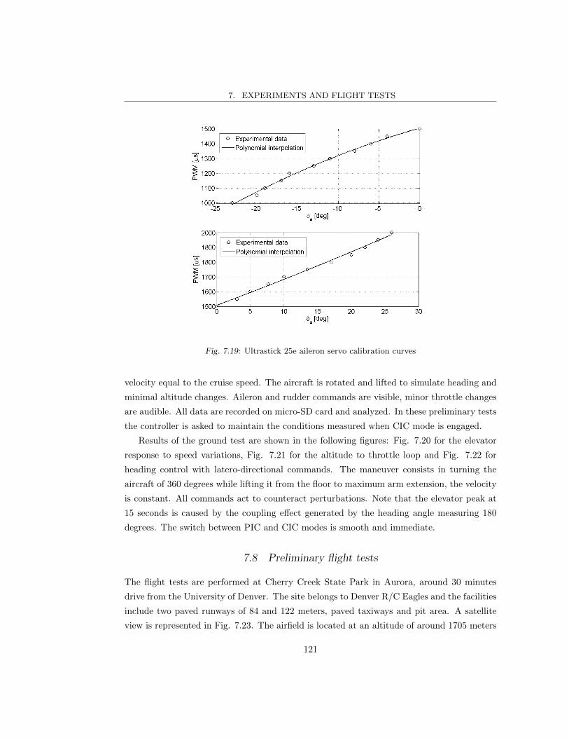
7. EXPERIMENTS AND FLIGHT TESTS

Fig. 7.19: Ultrastick 25e aileron servo calibration curves

velocity equal to the cruise speed. The aircraft is rotated and lifted to simulate heading and

minimal altitude changes. Aileron and rudder commands are visible, minor throttle changes

are audible. All data are recorded on micro-SD card and analyzed. In these preliminary tests

the controller is asked to maintain the conditions measured when CIC mode is engaged.

Results of the ground test are shown in the following figures: Fig. 7.20 for the elevator

response to speed variations, Fig. 7.21 for the altitude to throttle loop and Fig. 7.22 for

heading control with latero-directional commands. The maneuver consists in turning the

aircraft of 360 degrees while lifting it from the floor to maximum arm extension, the velocity

is constant. All commands act to counteract perturbations. Note that the elevator peak at

15 seconds is caused by the coupling effect generated by the heading angle measuring 180

degrees. The switch between PIC and CIC modes is smooth and immediate.

7.8 Preliminary flight tests

The flight tests are performed at Cherry Creek State Park in Aurora, around 30 minutes

drive from the University of Denver. The site belongs to Denver R/C Eagles and the facilities

include two paved runways of 84 and 122 meters, paved taxiways and pit area. A satellite

view is represented in Fig. 7.23. The airfield is located at an altitude of around 1705 meters

121

7. EXPERIMENTS AND FLIGHT TESTS

Fig. 7.20: Ultrastick 25e ground test, V control

Fig. 7.21: Ultrastick 25e ground test, h control

122

7. EXPERIMENTS AND FLIGHT TESTS

Fig. 7.22: Ultrastick 25e ground test, ψ control

above ground level. Flying altitude above the ground is limited to 400 feet (122 meters) due

to the proximity with Centennial Airport. The surrounding is mainly composed of grassland,

two streets run on the north and on the south side of the runway, the closest houses are 620

meters south-west of the airfield. Flight tests are performed early in the morning starting

from 8 am in order to avoid wind disturbance. In optimal days the wind was acceptable for

flight until around 11 am, no preferred wind direction was noticeable.

Due to a crash during the maiden flight in piloted mode, some logistics problems with

spare parts orders and a software problem that took long to be found, the flight tests schedule

was seriously delayed. Autonomous flight tests were performed only during the last week of

the project.

Globally five flights were carried out, of these four were dedicated to latero-directional

control and one to longitudinal control. The code was modified so that when backstepping

is controlling the latero-directional plane with aileron and rudder, the pilot still has throttle

and elevator control. The contrary happens when backstepping controls the longitudinal

plane. This approach allows testing the controller behavior without controller-induced cross-

coupling effects and so facilitates the initial PID tuning procedure. During the autonomous

flight the pilot is asked to avoid touching the stick unless minimal corrections are required

123

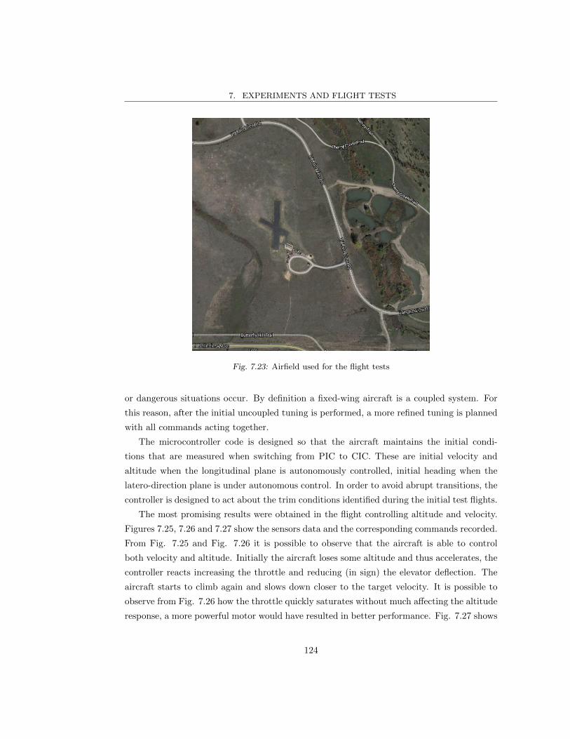
7. EXPERIMENTS AND FLIGHT TESTS

Fig. 7.23: Airfield used for the flight tests

or dangerous situations occur. By definition a fixed-wing aircraft is a coupled system. For

this reason, after the initial uncoupled tuning is performed, a more refined tuning is planned

with all commands acting together.

The microcontroller code is designed so that the aircraft maintains the initial condi-

tions that are measured when switching from PIC to CIC. These are initial velocity and

altitude when the longitudinal plane is autonomously controlled, initial heading when the

latero-direction plane is under autonomous control. In order to avoid abrupt transitions, the

controller is designed to act about the trim conditions identified during the initial test flights.

The most promising results were obtained in the flight controlling altitude and velocity.

Figures 7.25, 7.26 and 7.27 show the sensors data and the corresponding commands recorded.

From Fig. 7.25 and Fig. 7.26 it is possible to observe that the aircraft is able to control

both velocity and altitude. Initially the aircraft loses some altitude and thus accelerates, the

controller reacts increasing the throttle and reducing (in sign) the elevator deflection. The

aircraft starts to climb again and slows down closer to the target velocity. It is possible to

observe from Fig. 7.26 how the throttle quickly saturates without much affecting the altitude

response, a more powerful motor would have resulted in better performance. Fig. 7.27 shows

124

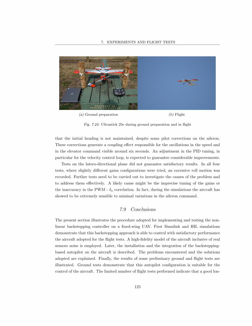
7. EXPERIMENTS AND FLIGHT TESTS

(a) Ground preparation (b) Flight

Fig. 7.24: Ultrastick 25e during ground preparation and in flight

that the initial heading is not maintained, despite some pilot corrections on the aileron.

These corrections generate a coupling effect responsible for the oscillations in the speed and

in the elevator command visible around six seconds. An adjustment in the PID tuning, in

particular for the velocity control loop, is expected to guarantee considerable improvements.

Tests on the latero-directional plane did not guarantee satisfactory results. In all four

tests, where slightly different gains configurations were tried, an excessive roll motion was

recorded. Further tests need to be carried out to investigate the causes of the problem and

to address them effectively. A likely cause might be the imprecise tuning of the gains or

the inaccuracy in the PWM - δa correlation. In fact, during the simulations the aircraft has

showed to be extremely sensible to minimal variations in the aileron command.

7.9 Conclusions

The present section illustrates the procedure adopted for implementing and testing the non-

linear backstepping controller on a fixed-wing UAV. First Simulink and HIL simulations

demonstrate that this backstepping approach is able to control with satisfactory performance

the aircraft adopted for the flight tests. A high-fidelity model of the aircraft inclusive of real

sensors noise is employed. Later, the installation and the integration of the backstepping-

based autopilot on the aircraft is described. The problems encountered and the solutions

adopted are explained. Finally, the results of some preliminary ground and flight tests are

illustrated. Ground tests demonstrate that this autopilot configuration is suitable for the

control of the aircraft. The limited number of flight tests performed indicate that a good lon-

125

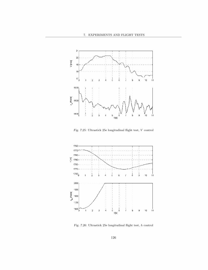
7. EXPERIMENTS AND FLIGHT TESTS

Fig. 7.25: Ultrastick 25e longitudinal flight test, V control

Fig. 7.26: Ultrastick 25e longitudinal flight test, h control

126

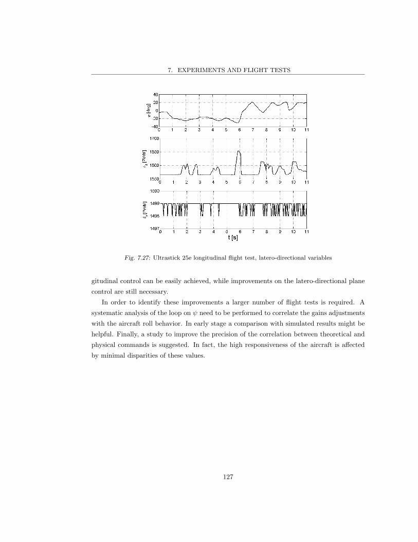
7. EXPERIMENTS AND FLIGHT TESTS

Fig. 7.27: Ultrastick 25e longitudinal flight test, latero-directional variables

gitudinal control can be easily achieved, while improvements on the latero-directional plane

control are still necessary.

In order to identify these improvements a larger number of flight tests is required. A

systematic analysis of the loop on ψ need to be performed to correlate the gains adjustments

with the aircraft roll behavior. In early stage a comparison with simulated results might be

helpful. Finally, a study to improve the precision of the correlation between theoretical and

physical commands is suggested. In fact, the high responsiveness of the aircraft is affected

by minimal disparities of these values.

127

8. CONCLUSIONS

The present PhD thesis illustrates the design and the development of three advanced control

laws for unmanned aircraft vehicles: PID with H∞ robust approach, L1 adaptive controller

and nonlinear backstepping controller. All controllers are first illustrated in their theoretical

form and then successfully applied through numerical simulations to the MH850 aircraft

model. The backstepping controller is chosen for being integrated and tested on a real

aircraft. Further simulations are performed in real time through a microcontroller board to

asses its performance. Ground tests validate the structure of the proposed autopilot, while

the limited number of flight tests indicates that a longer development is necessary to achieve

a mature configuration.

The obtained results demonstrate that these control laws are suitable for the application

to autopilots of unmanned aircraft. The hybrid PID tuning approach described in Chapter

4 guarantees satisfying flight performance even if this is limited about the design point. The

proposed H∞ method for the assessment of the robust characteristics is an effective tool

that allows to underline the limits of the PID approach: a tradeoff between performance and

robustness needs to be accepted. It was demonstrated, in fact, that the above-mentioned

reference tracking results were achieved sacrificing the system robustness to sensors noise,

parametric uncertainties and external disturbances. At the same time, trying to respect the

H∞-imposed boundaries strongly limited the aircraft performance.

In order to address the robustness problem in a more systematic way, the L1 adaptive

controller was chosen, see Chapter 5. In particular, an L1 approach based on piecewise

constant adaptation laws was selected, it guarantees adaptation rates compatible with an

autopilot board CPU and low computational effort. The adaptive nature of this controller has

proven to offer satisfying performance and excellent robustness to parameter uncertainties.

Furthermore, it was demonstrated that this control method can be easily designed and tuned

on a simplified linear aircraft model and successfully applied to a complete nonlinear model.

The backstepping controller proved too its ability to stabilize the selected aircraft model

with satisfying results, see Chapter 6. Despite the presence of a pure PID control in its

Throttle to Altitude loop, very good robustness to parametric uncertainty was achieved. A

8. CONCLUSIONS

comparison among all controllers demonstrated that backstepping and L1 are comparable

in terms of nominal performance, with a slight advantage for L1 in the robustness test.

PIDs are somehow inferior in the nominal case and completely fail in case some parametric

disturbances are introduced. Considering these results, the simple structure of the proposed

approach and the innovative contribution, the backstepping controller was chosen for being

integrated and tested on a flying aircraft.

The backstepping controller demonstrated to be easily implementable on a microcontroller

board and to guarantee satisfying performance also when running in real time. In particular,

complex maneuvers with the high-fidelity model of the UAV selected for the flight were tested.

The XMOS innovative microcontroller technology was introduced for the HIL simulations and

it was selected as the core component of the autopilot system. The autopilot was completed

integrating the XMOS board with servos, sensors and the radio system. In this phase a limit

of the adopted XK-1A board became evident due to the low stack memory available. The

XMOS technology has proved to be reliable and suitable for the role, but the adoption of a

more performing board model is suggested. Some practical problems were overcome in the

physical realization of the system. One of them was the supply of regular power to all the

systems, the adoption of two DC stabilizers was the solution. Another issue, which is still

open, was the correlation between theoretical and practical commands. A correlation curve

based on experimental data was built.

A series of preliminary ground tests validated the autopilot configuration. The transition

between piloted and controlled flight was smooth and immediate, and it guaranteed a safe

flight. The backstepping controller moved the aircraft commands in such a way to counteract

fictitious perturbations. Unfortunately the number of flight tests was very limited, they

were not able to provide useful results. A crash in piloted mode during the maiden flight,

some logistics problems with the order of the spare parts and a problem with the IMU

magnetometer strongly delayed the tests schedule. The handful of performed flights indicated

that good longitudinal control can be easily reached with limited development while some

more work must be invested on the latero-directional plane. In particular, the adjustment of

the gains and the correlation between the theoretical and physical deflection of the ailerons

need to be addressed.

Future developments to the present work should target the backstepping controller and

its application to flight tests. PID is a widely employed technique and L1, being very recent,

is the object of the attention of many researchers who are still exploring its possibilities.

Backstepping, instead, is a well developed technique that, unfortunately, has seen a limited

number of practical applications to the fixed-wing UAV field. The approach presented in

129

8. CONCLUSIONS

this thesis is deliberately kept simple in order to create an initial framework for the actual

implementation of backstepping to unmanned fixed-wing flight. The method adopted and the

technical solutions proposed are strong basis for future improvements. As already mentioned,

some adjustments to the autopilot physical configuration are suggested. Once these are

completed, the backstepping controller structure can be developed including adaptivity and

substituting PIDs with more advanced control techniques.

130

Appendices

131

Appendix A

EVALUATION OF AN L1 CONTROLLER FOR WING ROCK

SUPPRESSION

This appendix illustrates the initial work done within this PhD project to become familiar

with the L1 technique. The test case is the wing rock phenomenon on a highly-swept delta

wing. The text here proposed is largely taken from an article published on the AIAA Journal

of Guidance, Control, and Dynamics [137].

A.1 Introduction

The wing rock phenomenon appears on aircraft characterized by highly swept wing, leading

edge extensions and slender forebody when flying at high angles of attack. It consists in an

oscillatory motion about the roll axis which increases in amplitude up to a limit cycle. The

appearance of wing rock is due to a nonlinear variation of the roll damping with angles of

attack and sideslip. Aircraft configurations with slender forebodies are affected by wing rock

because of the unsteady interaction between primary forebody vortices and lifting surfaces

(leading edge extensions, wing and stabilizers). It can be encountered by high-speed civil

transport and combat aircraft in their flight envelope and when this occurs their handling

qualities and maneuvering capabilities are seriously degraded. For this reason the suppression

of wing rock is a relevant issue, it can be achieved by changing forebody cross-section and

slenderness or by the adoption of forebody vortex control techniques (boundary layer suction-

blowing and/or movable forebody strakes). The action of these devices must be regulated by

an appropriate control law able to handle the complexity of this phenomenon characterized

by nonlinearity and parameter uncertainty.

Different techniques have been proposed, such as synergetic optimal controllers [138],

fuzzy PD controllers [139] or variable phase controller [140]. Singh [141] presented a direct

adaptive and neural control of the wing rock. With the adaptive control the structure of

nonlinearity of the plant is considered, while in the neural control radial basis function neural

APPENDIX A. EVALUATION OF AN L1 CONTROLLER FOR WING ROCK SUPPRESSION

network is used. Joshi [142] presented a simple rule-based controller to suppress the limit

cycle behavior of the wing rock. The rule base is constructed to be linearly separable. A

simple neural controller with a single neuron is trained. This method permitted to reduce

the computational effort due to parameter tuning. More recently, Liu [143] proposed a

new reinforcement adaptive fuzzy control scheme, in which the adaptive channel combined

with reinforcement-learning strategy is applied to tune the parameters. Similarly, Cao [144]

applied an innovative adaptive and robust L1 controller.

The purpose of the present work is to get familiar with the L1 adaptive controller tech-

nique thanks to its application to the suppression of the wing rock phenomenon on a high

swept wing aircraft. Adaptive control is chosen because the adaptation channel improves the

performance robustness of the feedback path and reduces the tuning effort required to achieve

desired closed-loop performance, particularly while operating in the presence of uncertainties

and failures. The model considered in this study includes the fuselage and nonlinear uncer-

tainties. The approach presented is similar to [144], where the nonlinearities are function

of the sensor measurement errors, modeled as white noise, and a reduction of the actuator

effectiveness is also considered.

A posteriori robust assessment is performed. First, to verify the scalability of the con-

troller, some simulations are carried out considering a wide range of angles of attack and

initial conditions. Second, the controller designed on the nominal model is tested on a model

with perturbed parameters, so that the steady state value of the limit cycle reaches a ± 10

degrees offset from the nominal case. The proposed approach is simple, robust and stable. As

demonstrated in [145]-[148] L1 adaptive control is capable of compensating for unexpected,

unknown, severe failure events, while delivering predictable performance across the flight

envelope without enforcing persistence of excitation, or resorting to gain–scheduling of the

control parameters or control reconfiguration. It is shown that L1 adaptive control archi-

tecture has an appropriate structure for the integration of conventional frequency–domain

filtering techniques, while providing at the same time a suitable framework for the analy-

sis of the effect of these techniques in the stability and performance characteristics of the

closed–loop system.

The wing rock model will be discussed in the next section, together with the definition

of the experimental parameters. The most relevant design features of L1 adaptive control

will then be recalled in Section A.3, where the most peculiar aspects related to the present

application will be discussed with some more details. Some results are then proposed in

Section A.4, finally a section of Conclusions summarizes the main findings.

133

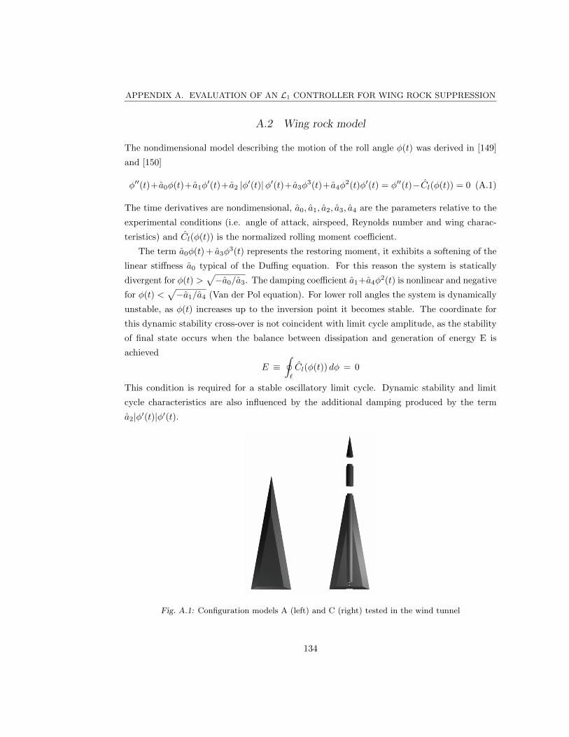
APPENDIX A. EVALUATION OF AN L1 CONTROLLER FOR WING ROCK SUPPRESSION

A.2 Wing rock model

The nondimensional model describing the motion of the roll angle φ(t) was derived in [149]

and [150]

φ′′(t)+ a0φ(t)+ a1φ′(t)+ a2 |φ′(t)|φ′(t)+ a3φ

3(t)+ a4φ2(t)φ′(t) = φ′′(t)−Cl(φ(t)) = 0 (A.1)

The time derivatives are nondimensional, a0, a1, a2, a3, a4 are the parameters relative to the

experimental conditions (i.e. angle of attack, airspeed, Reynolds number and wing charac-

teristics) and Cl(φ(t)) is the normalized rolling moment coefficient.

The term a0φ(t) + a3φ3(t) represents the restoring moment, it exhibits a softening of the

linear stiffness a0 typical of the Duffing equation. For this reason the system is statically

divergent for φ(t) >√−a0/a3. The damping coefficient a1+a4φ

2(t) is nonlinear and negative

for φ(t) <√−a1/a4 (Van der Pol equation). For lower roll angles the system is dynamically

unstable, as φ(t) increases up to the inversion point it becomes stable. The coordinate for

this dynamic stability cross-over is not coincident with limit cycle amplitude, as the stability

of final state occurs when the balance between dissipation and generation of energy E is

achieved

E ≡∮`

Cl(φ(t)) dφ = 0

This condition is required for a stable oscillatory limit cycle. Dynamic stability and limit

cycle characteristics are also influenced by the additional damping produced by the term

a2|φ′(t)|φ′(t).

Fig. A.1: Configuration models A (left) and C (right) tested in the wind tunnel

134

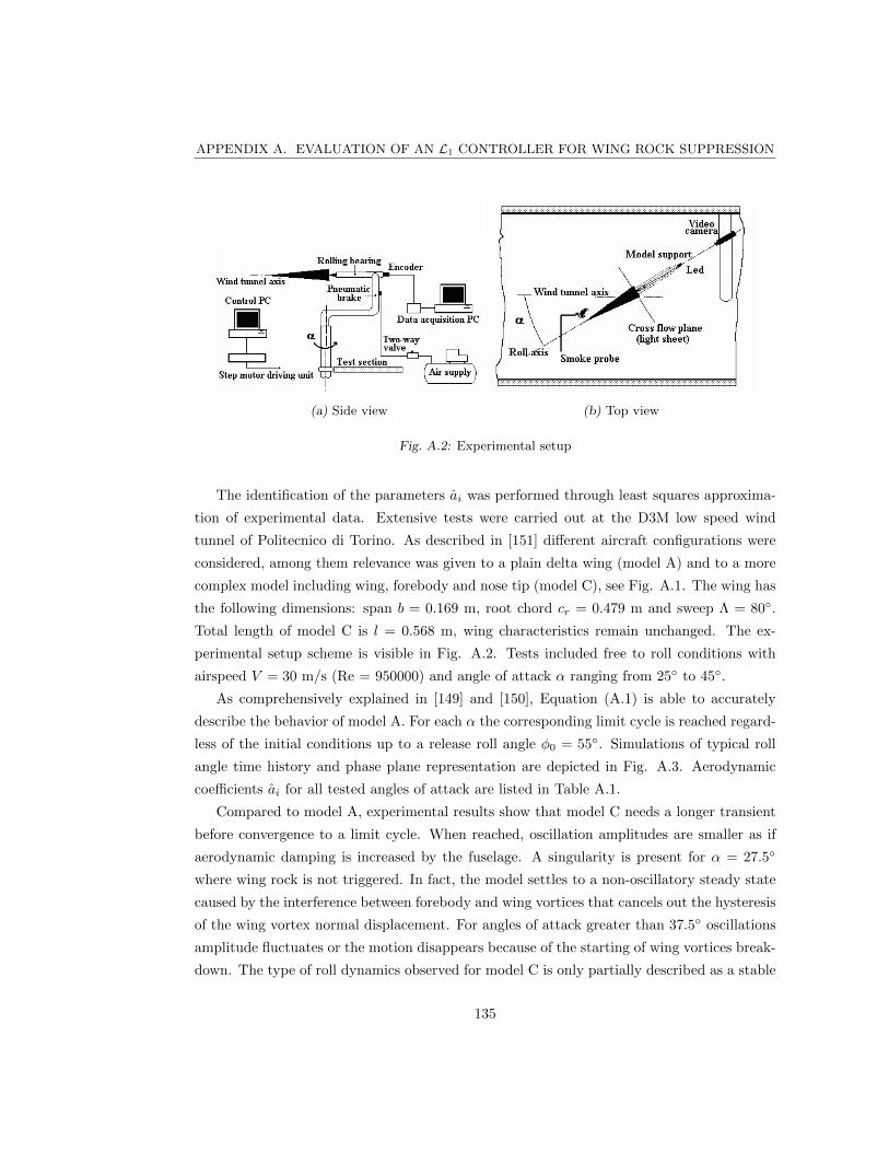
APPENDIX A. EVALUATION OF AN L1 CONTROLLER FOR WING ROCK SUPPRESSION

(a) Side view (b) Top view

Fig. A.2: Experimental setup

The identification of the parameters ai was performed through least squares approxima-

tion of experimental data. Extensive tests were carried out at the D3M low speed wind

tunnel of Politecnico di Torino. As described in [151] different aircraft configurations were

considered, among them relevance was given to a plain delta wing (model A) and to a more

complex model including wing, forebody and nose tip (model C), see Fig. A.1. The wing has

the following dimensions: span b = 0.169 m, root chord cr = 0.479 m and sweep Λ = 80.

Total length of model C is l = 0.568 m, wing characteristics remain unchanged. The ex-

perimental setup scheme is visible in Fig. A.2. Tests included free to roll conditions with

airspeed V = 30 m/s (Re = 950000) and angle of attack α ranging from 25 to 45.

As comprehensively explained in [149] and [150], Equation (A.1) is able to accurately

describe the behavior of model A. For each α the corresponding limit cycle is reached regard-

less of the initial conditions up to a release roll angle φ0 = 55. Simulations of typical roll

angle time history and phase plane representation are depicted in Fig. A.3. Aerodynamic

coefficients ai for all tested angles of attack are listed in Table A.1.

Compared to model A, experimental results show that model C needs a longer transient

before convergence to a limit cycle. When reached, oscillation amplitudes are smaller as if

aerodynamic damping is increased by the fuselage. A singularity is present for α = 27.5

where wing rock is not triggered. In fact, the model settles to a non-oscillatory steady state

caused by the interference between forebody and wing vortices that cancels out the hysteresis

of the wing vortex normal displacement. For angles of attack greater than 37.5 oscillations

amplitude fluctuates or the motion disappears because of the starting of wing vortices break-

down. The type of roll dynamics observed for model C is only partially described as a stable

135

APPENDIX A. EVALUATION OF AN L1 CONTROLLER FOR WING ROCK SUPPRESSION

Tab. A.1: Aerodynamic coefficients for model A

α a0A a1A a2A a3A a4A

25.0 0.00543 -0.01426 0.41336 -0.00465 0.00263

27.5 0.00594 -0.01765 0.38793 -0.00487 0.01689

30.0 0.00657 -0.02040 0.38008 -0.00537 0.02596

32.5 0.00732 -0.03104 0.53884 -0.00623 0.04189

35.0 0.00794 -0.03137 0.53455 -0.00751 0.05144

37.5 0.00914 -0.00246 0.00105 -0.01059 0.03736

40.0 0.00902 -0.01881 0.62351 -0.01187 0.06119

42.5 0.00999 -0.03219 1.5118 -0.02862 0.06867

45.0 0.01135 -0.03712 2.4252 -0.08113 0.02935

136

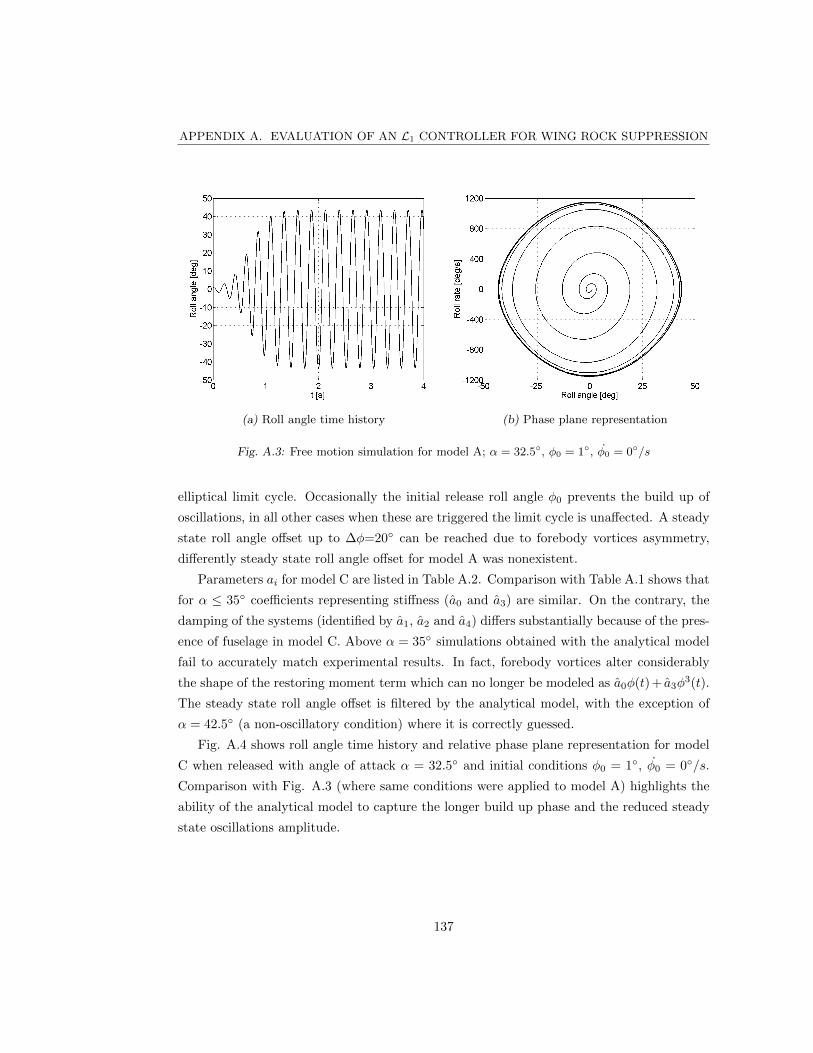
APPENDIX A. EVALUATION OF AN L1 CONTROLLER FOR WING ROCK SUPPRESSION

(a) Roll angle time history (b) Phase plane representation

Fig. A.3: Free motion simulation for model A; α = 32.5, φ0 = 1, φ0 = 0/s

elliptical limit cycle. Occasionally the initial release roll angle φ0 prevents the build up of

oscillations, in all other cases when these are triggered the limit cycle is unaffected. A steady

state roll angle offset up to ∆φ=20 can be reached due to forebody vortices asymmetry,

differently steady state roll angle offset for model A was nonexistent.

Parameters ai for model C are listed in Table A.2. Comparison with Table A.1 shows that

for α ≤ 35 coefficients representing stiffness (a0 and a3) are similar. On the contrary, the

damping of the systems (identified by a1, a2 and a4) differs substantially because of the pres-

ence of fuselage in model C. Above α = 35 simulations obtained with the analytical model

fail to accurately match experimental results. In fact, forebody vortices alter considerably

the shape of the restoring moment term which can no longer be modeled as a0φ(t) + a3φ3(t).

The steady state roll angle offset is filtered by the analytical model, with the exception of

α = 42.5 (a non-oscillatory condition) where it is correctly guessed.

Fig. A.4 shows roll angle time history and relative phase plane representation for model

C when released with angle of attack α = 32.5 and initial conditions φ0 = 1, φ0 = 0/s.

Comparison with Fig. A.3 (where same conditions were applied to model A) highlights the

ability of the analytical model to capture the longer build up phase and the reduced steady

state oscillations amplitude.

137

APPENDIX A. EVALUATION OF AN L1 CONTROLLER FOR WING ROCK SUPPRESSION

Tab. A.2: Aerodynamic coefficients for model C

α a0C a1C a2C a3C a4C

25.0 0.00615 -0.02644 0.82603 -0.00940 0.04934

27.5 0.00310 -0.00057 1.0025 -0.01157 -1.1908

30.0 0.00523 -0.00406 0.09998 -0.00167 -0.00183

32.5 0.00729 -0.01260 0.33063 -0.00506 -0.00378

35.0 0.00591 -0.03024 1.0703 -0.00285 -0.03726

37.5 -0.00406 -0.00588 1.084 0.03646 -0.15374

40.0 0.00574 -0.00771 -0.03172 -0.01095 0.16302

42.5 -0.0040 -0.03261 2.3447 0.13848 0.90542

45.0 -0.00089 -0.02071 0.8361 0.13752 2.8685

138

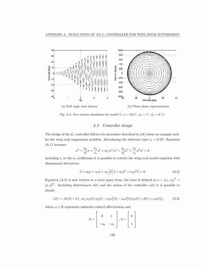
APPENDIX A. EVALUATION OF AN L1 CONTROLLER FOR WING ROCK SUPPRESSION

(a) Roll angle time history (b) Phase plane representation

Fig. A.4: Free motion simulation for model C; α = 32.5, φ0 = 1, φ0 = 0/s.

A.3 Controller design

The design of the L1 controller follows the procedure described in [44] where an example tack-

les the wing rock suppression problem. Introducing the reference time ts = b/2V , Equation

(A.1) becomes

φ′′ +a0

t2sφ+

a1

tsφ′ + a2 |φ′|φ′ +

a3

t2sφ3 +

a4

tsφ2φ′ = 0

including ts in the ai coefficients it is possible to rewrite the wing rock model equation with

dimensional derivatives

φ+ a0φ+ a1φ+ a2

∣∣∣φ∣∣∣ φ+ a3φ3 + a4φ

2φ = 0 (A.2)

Equation (A.2) is now written in a state space form, the state is defined as x = [x1, x2]T =

[φ, φ]T . Including disturbances d(t) and the action of the controller u(t) it is possible to

obtain

x(t) = Ax(t) + b(−a2 |x2(t)|x2(t)− a3x

31(t)− a4x

21(t)x2(t) + d(t) + ωu(t)

), (A.3)

where ω ∈ R represents unknown control effectiveness and

A =

0 1

−a0 −a1

, b =

0

1

139

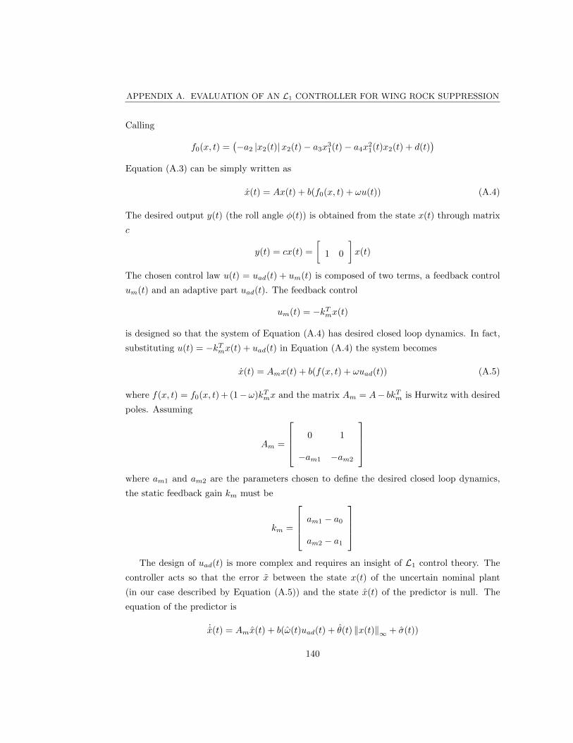
APPENDIX A. EVALUATION OF AN L1 CONTROLLER FOR WING ROCK SUPPRESSION

Calling

f0(x, t) =(−a2 |x2(t)|x2(t)− a3x

31(t)− a4x

21(t)x2(t) + d(t)

)Equation (A.3) can be simply written as

x(t) = Ax(t) + b(f0(x, t) + ωu(t)) (A.4)

The desired output y(t) (the roll angle φ(t)) is obtained from the state x(t) through matrix

c

y(t) = cx(t) =

[1 0

]x(t)

The chosen control law u(t) = uad(t) + um(t) is composed of two terms, a feedback control

um(t) and an adaptive part uad(t). The feedback control

um(t) = −kTmx(t)

is designed so that the system of Equation (A.4) has desired closed loop dynamics. In fact,

substituting u(t) = −kTmx(t) + uad(t) in Equation (A.4) the system becomes

x(t) = Amx(t) + b(f(x, t) + ωuad(t)) (A.5)

where f(x, t) = f0(x, t) + (1−ω)kTmx and the matrix Am = A− bkTm is Hurwitz with desired

poles. Assuming

Am =

0 1

−am1 −am2

where am1 and am2 are the parameters chosen to define the desired closed loop dynamics,

the static feedback gain km must be

km =

am1 − a0

am2 − a1

The design of uad(t) is more complex and requires an insight of L1 control theory. The

controller acts so that the error x between the state x(t) of the uncertain nominal plant

(in our case described by Equation (A.5)) and the state x(t) of the predictor is null. The

equation of the predictor is

˙x(t) = Amx(t) + b(ω(t)uad(t) + θ(t) ‖x(t)‖∞ + σ(t))

140

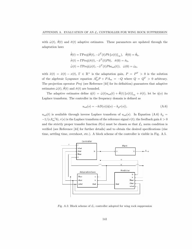
APPENDIX A. EVALUATION OF AN L1 CONTROLLER FOR WING ROCK SUPPRESSION

with ω(t), θ(t) and σ(t) adaptive estimates. These parameters are updated through the

adaptation laws

˙θ(t) = ΓProj(θ(t),−xT (t)Pb ‖x(t)‖∞), θ(0) = θ0,

˙σ(t) = ΓProj(σ(t),−xT (t)Pb), σ(0) = σ0,

˙ω(t) = ΓProj(ω(t),−xT (t)Pbuad(t)), ω(0) = ω0,

with x(t) = x(t) − x(t), Γ ∈ R+ is the adaptation gain, P = PT > 0 is the solution

of the algebraic Lyapunov equation ATmP + PAm = −Q where Q = QT > 0 arbitrary.

The projection operator Proj (see Reference [44] for its definition) guarantees that adaptive

estimates ω(t), θ(t) and σ(t) are bounded.

The adaptive estimates define η(t) = ω(t)uad(t) + θ(t) ‖x(t)‖∞ + σ(t), let be η(s) its

Laplace transform. The controller in the frequency domain is defined as

uad(s) = −kD(s)(η(s)− kgr(s)), (A.6)

uad(t) is available through inverse Laplace transform of uad(s). In Equation (A.6) kg =

−1/(cA−1m b), r(s) is the Laplace transform of the reference signal r(t); the feedback gain k > 0

and the strictly proper transfer function D(s) must be chosen so that L1 norm condition is

verified (see Reference [44] for further details) and to obtain the desired specifications (rise

time, settling time, overshoot, etc.). A block scheme of the controller is visible in Fig. A.5.

Fig. A.5: Block scheme of L1 controller adopted for wing rock suppression

141

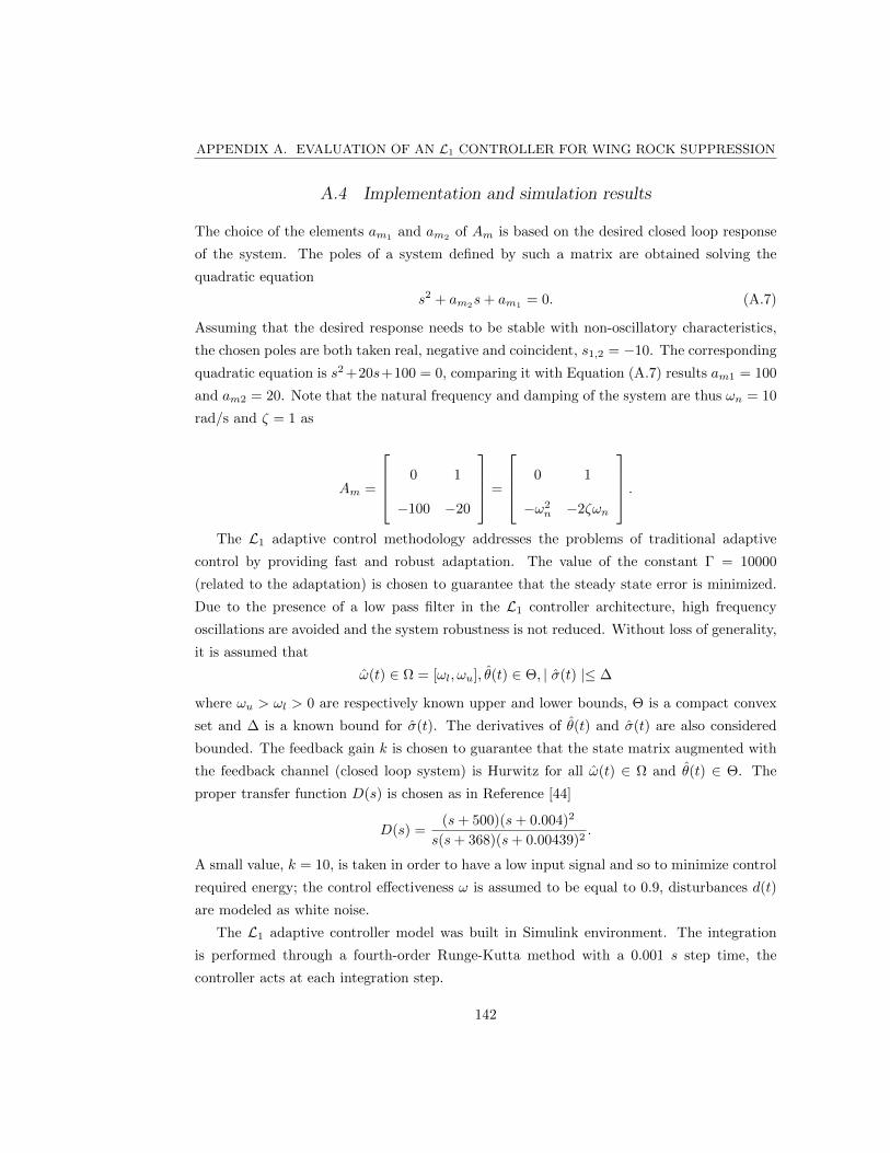
APPENDIX A. EVALUATION OF AN L1 CONTROLLER FOR WING ROCK SUPPRESSION

A.4 Implementation and simulation results

The choice of the elements am1and am2

of Am is based on the desired closed loop response

of the system. The poles of a system defined by such a matrix are obtained solving the

quadratic equation

s2 + am2s+ am1

= 0. (A.7)

Assuming that the desired response needs to be stable with non-oscillatory characteristics,

the chosen poles are both taken real, negative and coincident, s1,2 = −10. The corresponding

quadratic equation is s2 +20s+100 = 0, comparing it with Equation (A.7) results am1 = 100

and am2 = 20. Note that the natural frequency and damping of the system are thus ωn = 10

rad/s and ζ = 1 as

Am =

0 1

−100 −20

=

0 1

−ω2n −2ζωn

.The L1 adaptive control methodology addresses the problems of traditional adaptive

control by providing fast and robust adaptation. The value of the constant Γ = 10000

(related to the adaptation) is chosen to guarantee that the steady state error is minimized.

Due to the presence of a low pass filter in the L1 controller architecture, high frequency

oscillations are avoided and the system robustness is not reduced. Without loss of generality,

it is assumed that

ω(t) ∈ Ω = [ωl, ωu], θ(t) ∈ Θ, | σ(t) |≤ ∆

where ωu > ωl > 0 are respectively known upper and lower bounds, Θ is a compact convex

set and ∆ is a known bound for σ(t). The derivatives of θ(t) and σ(t) are also considered

bounded. The feedback gain k is chosen to guarantee that the state matrix augmented with

the feedback channel (closed loop system) is Hurwitz for all ω(t) ∈ Ω and θ(t) ∈ Θ. The

proper transfer function D(s) is chosen as in Reference [44]

D(s) =(s+ 500)(s+ 0.004)2

s(s+ 368)(s+ 0.00439)2.

A small value, k = 10, is taken in order to have a low input signal and so to minimize control

required energy; the control effectiveness ω is assumed to be equal to 0.9, disturbances d(t)

are modeled as white noise.

The L1 adaptive controller model was built in Simulink environment. The integration

is performed through a fourth-order Runge-Kutta method with a 0.001 s step time, the

controller acts at each integration step.

142

APPENDIX A. EVALUATION OF AN L1 CONTROLLER FOR WING ROCK SUPPRESSION

Simulations include different initial conditions and angles of attack for both models. First

a detailed analysis is performed for the case when model A and C have release angle α = 32.5

and initial conditions φ0 = 10 and φ0 = 0/s. Fig. A.6 shows the controlled response for

model A and C, in both cases the controller effectively sets to zero the roll angle and the roll

rate in few seconds. No remarkable difference is observable between the two models, both

systems dynamics are dominated by the control law. The nondimensional total control input

u(t) is very similar too, as illustrated in Fig. A.7. White noise modeled disturbances do not

affect the action of the L1 controller.

(a) Model A (b) Model C

Fig. A.6: Controlled roll angle and roll rate; α = 32.5, φ0 = 10, φ0 = 0/s.

Scalability of the controller is tested varying angle of attack and initial conditions for

models A and C. Results for α = 25, 30, 35, 40 and φ0 = 10, φ0 = 0/s appear in Fig.

A.8. No remarkable difference is visible between the models, the controller suppresses wing

rock independently of α. This simulation includes the condition α = 40 where the analytical

model for configuration C fails to accurately describe the experimental behavior.

The variation of initial conditions is depicted in Fig. A.9. The reference angle of attack

is maintained at α = 32.5 while the initial roll angle changes between φ0 = −30 and

φ0 = 30, initial roll rate is maintained at φ0 = 0/s. In this interval the motion is perfectly

controlled, apparently better for model C. Note that the L1 controller here developed is not

able to suppress wing rock for model A for starting roll angles larger than φ0 = ±32 when

φ0 = 0/s. Larger initial roll angles can be achieved only when an opposite initial roll rate

is applied to facilitate the controller action; for instance the starting condition φ0 = 33 can

143

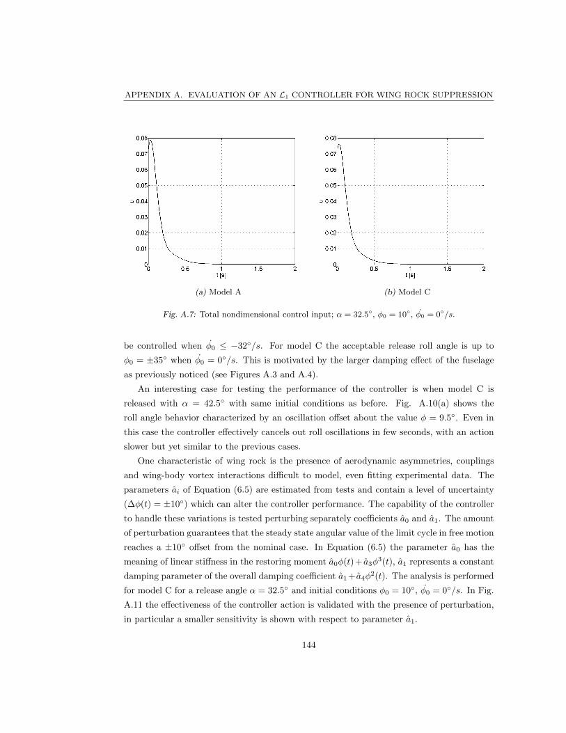
APPENDIX A. EVALUATION OF AN L1 CONTROLLER FOR WING ROCK SUPPRESSION

(a) Model A (b) Model C

Fig. A.7: Total nondimensional control input; α = 32.5, φ0 = 10, φ0 = 0/s.

be controlled when φ0 ≤ −32/s. For model C the acceptable release roll angle is up to

φ0 = ±35 when φ0 = 0/s. This is motivated by the larger damping effect of the fuselage

as previously noticed (see Figures A.3 and A.4).

An interesting case for testing the performance of the controller is when model C is

released with α = 42.5 with same initial conditions as before. Fig. A.10(a) shows the

roll angle behavior characterized by an oscillation offset about the value φ = 9.5. Even in

this case the controller effectively cancels out roll oscillations in few seconds, with an action

slower but yet similar to the previous cases.

One characteristic of wing rock is the presence of aerodynamic asymmetries, couplings

and wing-body vortex interactions difficult to model, even fitting experimental data. The

parameters ai of Equation (6.5) are estimated from tests and contain a level of uncertainty

(∆φ(t) = ±10) which can alter the controller performance. The capability of the controller

to handle these variations is tested perturbing separately coefficients a0 and a1. The amount

of perturbation guarantees that the steady state angular value of the limit cycle in free motion

reaches a ±10 offset from the nominal case. In Equation (6.5) the parameter a0 has the

meaning of linear stiffness in the restoring moment a0φ(t)+ a3φ3(t), a1 represents a constant

damping parameter of the overall damping coefficient a1 + a4φ2(t). The analysis is performed

for model C for a release angle α = 32.5 and initial conditions φ0 = 10, φ0 = 0/s. In Fig.

A.11 the effectiveness of the controller action is validated with the presence of perturbation,

in particular a smaller sensitivity is shown with respect to parameter a1.

144

APPENDIX A. EVALUATION OF AN L1 CONTROLLER FOR WING ROCK SUPPRESSION

(a) Model A (b) Model C

Fig. A.8: Controller action; α = 25, 30, 35, 40, φ0 = 10, φ0 = 0/s.

(a) Model A (b) Model C

Fig. A.9: Controller action; α = 32.5, φ0 = −30,−15, 15, 30, φ0 = 0/s.

A.5 Conclusions

This work describes the application of an L1 adaptive controller for the suppression of the

wing rock phenomenon. Both an isolated highly swept wing and a complete configuration

with fuselage and forebody are analyzed for different angles of attack and initial conditions.

Disturbances and changes in the state parameters are included to validate the robustness of

145

APPENDIX A. EVALUATION OF AN L1 CONTROLLER FOR WING ROCK SUPPRESSION

(a) Free motion (b) Controlled motion

Fig. A.10: Model C free and controlled motion; α = 42.5, φ0 = 10, φ0 = 0/s.

(a) Perturbation of a0 (b) Perturbation of a1

Fig. A.11: Model C perturbed controlled motion; α = 32.5, φ0 = 10, φ0 = 0/s.

the controller to adapt to the level of uncertainty that characterizes wing-body rock modeling.

In each of the simulated cases the controller effectively cancels oscillations in short time with

a limited amount of energy input. No remarkable difference in performance is observable

among the different scenarios suggesting that the design is able to handle the effect of aircraft

configuration with adequate robustness.

146

APPENDIX A. EVALUATION OF AN L1 CONTROLLER FOR WING ROCK SUPPRESSION

This test has helped to acquire confidence with the L1 technique and has demonstrated

the excellent performance of this controller in dealing with robustness issues. Therefore, it is

expected to guarantee satisfying results in the application to the control of fixed-wing UAVs,

in particular when the model is affected by parametric uncertainties.

147

Appendix B

ULTRASTICK 25E ONBOARD CONNECTIONS SCHEMES

A schematic of the power setup and of the servos connections appears in Fig. B.1. Colors

of lines represent different kind of connection: blue for signal, red for power and black for

ground. On the lower bottom of Fig. B.1 the RX radio appears. The radio receives the

PIC/CIC signal on the GEAR channel and the surfaces and throttle commands on the

remaining channels. These, identified with the letters from C to G, are sent to the XMOS

board where the logic described in Chapter 7 is implemented. The output of the board

consists of the four commands, originated by the pilot or by the backstepping controller,

letters J to M. A prototype board built with appropriate pins forwards the commands to the

motor and to the servos.

Fig. B.1: Ultrastick 25e power setup and servos integration scheme

Fig. B.2 illustrates the physical connections of the pitot sensor with the XMOS board,

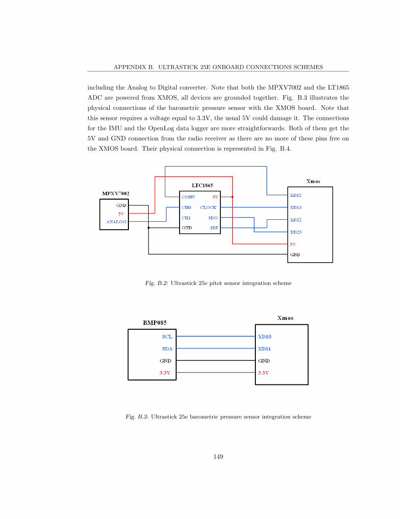
APPENDIX B. ULTRASTICK 25E ONBOARD CONNECTIONS SCHEMES

including the Analog to Digital converter. Note that both the MPXV7002 and the LT1865

ADC are powered from XMOS, all devices are grounded together. Fig. B.3 illustrates the

physical connections of the barometric pressure sensor with the XMOS board. Note that

this sensor requires a voltage equal to 3.3V, the usual 5V could damage it. The connections

for the IMU and the OpenLog data logger are more straightforwards. Both of them get the

5V and GND connection from the radio receiver as there are no more of these pins free on

the XMOS board. Their physical connection is represented in Fig. B.4.

Fig. B.2: Ultrastick 25e pitot sensor integration scheme

Fig. B.3: Ultrastick 25e barometric pressure sensor integration scheme

149

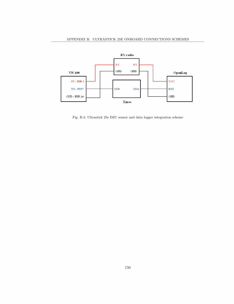
APPENDIX B. ULTRASTICK 25E ONBOARD CONNECTIONS SCHEMES

Fig. B.4: Ultrastick 25e IMU sensor and data logger integration scheme

150

BIBLIOGRAPHY

[1] G. Guglieri, D. Sartori, Design of a Sliding Mode Control for Wing Rock Suppression in

Highly-Swept Wing Aircraft, International Journal of Aerospace Sciences, Vol. 2, No. 1,

pp. 1-10, 2013.

[2] U.S. Department of Defense, DoD Dictionary of Military Associated Terms, Joint Publi-

cation 1-02, Washington DC, USA, 5 January 2007.

[3] Hector L. Cruz, Role of DoD Unmanned Aerial Vehicles for Homeland Security, U.S.

Army War College, Carlisle, PA, USA, 30 March 2010.

[4] C. Peebles, Dark Eagles: A History of Top Secret U.S. Aircraft Programs, Presidio Press,

1999.

[5] K. Dalamagkidis, K. P. Valavanis, L. A. Piegl, On Integrating Unmanned Aircraft Systems

into the National Airspace System, Springer Netherlands, 2012.

[6] U.S. Department of Defense, Conduct of the Persian Gulf Conflict: An Interim Report

to Congress, Washington, DC, USA, April 1992.

[7] S. J. Zaloga, Unmanned Aerial Vehicles: Robotic Air Warfare 19172007, Osprey Pub-

lishing Ltd., 2008.

[8] Z. Sarris, Survey of UAV Applications in Civil Markets (June 2001), 9th IEEE Mediter-

ranean Conference on Control Automation (MED ’01), Dubrovnik, Croatia, 27-29 June

2001.

[9] http://www.fyjs.cn/

[10] T. H. Cox, C. J. Nagy, M. A. Skoog, I. A. Somers, Civil UAV Capability Assessment,

NASA, December 2004.

[11] K. Dalamagkidis, K. P. Valavanis, On unmanned aircraft systems issues, challenges

and operational restrictions preventing integration into the National Airspace System,

Progress in Aerospace Sciences, Vol. 44, No. 78, pp. 503519, OctoberNovember 2008.

Bibliography

[12] E. W. Liu, Business case assessment of unmanned systems level of autonomy, MIT

Master Thesis, June 2012.

[13] www.aiaa.org/cauav/

[14] http://cires.colorado.edu/index.html

[15] R. Austin, Unmanned Aircraft Systems: UAVS Design, Development and Deployment,

2nd edition, Wiley, 2011.

[16] B. T. Schreiber, D. R. Lyon, E. L. Martin, H. A. Confer, Impact of Prior Flight Ex-

perience on Learning Predator UAV Operator Skills, United States Air Force Research

Laboratory, Mesa, AZ, USA, February 2002.

[17] J. L. Weeks, Unmanned Aerial Vehicle Operator Qualifications, United States Air Force

Research Laboratory, Mesa, AZ, USA, March 2000.

[18] J.L. Drury, L. Riek, N. Rackliffe, A decomposition of UAV-related situation awareness,

HRI ’06 Proceedings of the 1st ACM SIGCHI/SIGART conference on Human-robot in-

teraction, pp. 88-94, Salt lake City, UT, USA, 2-4 March 2006.

[19] A. A. H. E. Goossens, G. J. M. Koeners, E. Theunissen, Development and Evaluation

of Level 3 Situation Awareness Support Functions for UAV Operator Station, The 23rd

Digital Avionics Systems Conference, Vol. 2, pp 12.D.4-1 - 12.D.4-8, 24-28 October 2004

.

[20] T. Fong, C. Thorpe, Vehicle Teleoperation Interfaces, Autonomous Robotics, Vol. 11,

No. 1, pp. 9-18, July 2001.

[21] http://www.aeronautics-sys.com/

[22] http://www.controp.com/

[23] T. B. Sheridan, Telerobotics, Automation, and Human Supervisory Control, MIT Press,

Cambridge, 1992.

[24] T. B. Sheridan, W. L. Verplank, Human and Computer Control of Undersea Teleopera-

tors, Cambridge, MA, USA, 1978.

[25] R. Parasuraman, T. B. Sheridaan, C. D. Wickens, A Model for Types and Levels of Hu-

man Interaction with Automation, IEEE Transactions on Systems, Man and Cybernetics,

Part A: Systems and Humans, Vol. 30, No. 3, pp. 286-297, August 2002.

152

Bibliography

[26] R. Frampton, UAV Autonomy, Defence Codex - The Journal for Defence Engineering

and Science, UK Ministry of Defence, No.1, 2008.

[27] H. Y. Chao, Y. C. Cao, Y. Q. Chen, Autopilots for Small Unmanned Aerial Vehicles:

A Survey, International Journal of Control Automation and Systems, Vol. 8, No. 1, pp.

36-44, February 2010,.

[28] A. Ollero, L. Merino, Control and Perception Techniques for Aerial Robotics, Annual

Reviews in Control, Vol. 28, No. 2, pp. 167-178, 2004.

[29] http://www.micropilot.com

[30] P. Cominos, N. Munro, PID Controllers: Recent Tuning Methods and Design to Specifi-

cation, IEE Proceedings on Control Theory and Applications, Vol. 149, No. 1, pp. 46-53,

Jan. 2002.

[31] K. J. Astrom, T. Hagglund, PID Controllers: Theory, Design, and Tuning, 2nd ed.,

ISA, Durham, NC, USA, 1995.

[32] Y. Kang, J. K. Hedrick, Linear Tracking for a Fixed-Wing UAV Using Nonlinear Model

Predictive Control, IEEE Transactions on Control Systems Technology, Vol. 17, No. 5,

pp. 1202-1210, Sept. 2009.

[33] F. Santoso, M. Liu, G. Egan, H2 and H∞ robust autopilot synthesis for longitudinal

flight of a special unmanned aerial vehicle: a comparative study, IET Control Theory &

Applications, Vol. 2, No. 7, pp. 583-594, July 2008.

[34] A. Fradkov, B. Andrievsky, Combined Adaptive Controller for UAV Guidance, European

Journal of Control, Vol. 11, No. 1, pp. 71-79, 2005.

[35] H. Tu, X. Du, The Design of Small UAV Autopilot Hardware System Based on DSP,

Proceedings of the 2010 International Conference on Intelligent Computation Technology

and Automation (ICICTA), Vol. 3, pp. 780-783, Changsha, China, May 2010.

[36] H. Guanglin, G. Rujun, Y. Shi, Application of FPGA in Small UAV Autopilot Based

on Embedded Linux System, Proceedings of the 33rd Annual Conference on the IEEE

Industrial Electronics Society, pp. 731-734, Taipei, Taiwan, Nov. 2007.

[37] F. Kendoul, Survey of Advances in Guidance, Navigation, and Control of Unmanned

Rotorcraft Systems, Journal of Field Robotics, Vol. 29, No. 2, pp. 315-378, March/April

2012.

153

Bibliography

[38] Y. C. Paw, G. J. Balas, Development and Application of an Integrated Framework for

Small UAV Flight Control Development, Mechatronics, Vol. 21, No. 5, pp. 789-802, Aug.

2011

[39] M. I. Lizarraga, G. H. Elkaim, G. M. Horn, R. Curry, V. Dobrokhodov, I. Kaminer,

Low Cost Rapidly Reconfigurable UAV Autopilot For Research and Development of Guid-

ance, Navigation and Control Algorithms, Proceedings of the ASME 2009 International

Design Engineering Technical Conferences & Computers and Information in Engineering

Conference, Vol. 3, pp. 585-594, San Diego, CA, USA, August/September 2009.

[40] D. Jung, E. J. Levy, D. Zhou, R. Fink, J. Moshe, A. Earl, P. Tsiotras, Design and

Development of a Low-Cost Test-Bed for Undergraduate Education in UAVs, Proceedings

of the 44th IEEE Conference on Decision and Control 2005 and 2005 European Control

Conference, pp. 2739-2744, Seville, Spain, December 2005.

[41] J. A. Miller, P. D. Minear, A. F. Niessner, A. M. DeLullo, B. R. Geiger, L. N. Long, J. F.

Horn, Intelligent Unmanned Air Vehicle Flight Systems, Journal of Aerospace Computing,

Information, and Communication, Vol. 4, No. 5, pp. 816-835, May 2007.

[42] E. N. Johnson, M. A. Turbe, A. D. Wu, S. K. Kannan, J. C. Neidhoefer, Flight Test

Results of Autonomous Fixed-Wing UAV Transitions to and from Stationary Hover, Pro-

ceedings of AIAA Guidance, Navigation, and Control Conference and Exhibit, Keystone,

CO, USA, August 2006.

[43] Y. Gu, B. Seanor, G. Campa, M. R. Napolitano, L. Rowe, S. Gururajan, S. Wan, Design

and Flight Testing Evaluation of Formation Control Laws, IEEE Transactions on Control

Systems Technology, Vol. 14, No. 6, pp. 1105-1112, November 2006.

[44] N. Hovakimyan, C. Cao, L1 Adaptive Control Theory - Guaranteed Robustness with Fast

Adaptation, Society for Industrial and Applied Mathematics, Philadelphia, 2010.

[45] O. Harkegard, Backstepping Designs for Aircraft Control - What is there to gain?, Divi-

sion of Automatic Control, Department of Electrical Engineering Linkopings Universitet,

Sweden, Tech. Rep. LiTH-ISY-R-2339, March 2001.

[46] M. Krstic, I. Kanellakopoulos, P. Kokotovic, Nonlinear and Adaptive Control Design,

1st ed., Wiley, New York, 1995.

[47] K-S. Kim, Y. Kim, Robust Backstepping Control for Slew Maneuver Using Nonlinear

Tracking Function, IEEE Transactions on Control Systems Technology, Vol. 11, No. 6,

pp. 822-829, November 2003.

154

Bibliography

[48] J. G. Ziegler, N. B. Nichols, Optimum Settings for Automatic Controllers, Transactions

of the ASME, Vol. 64, pp. 759-769, 1942.

[49] H. Panagopoulos, K. J. Astrom, PID Control Design and H∞ Loop Shaping, Proceed-

ings of the International Conference on Control Applications, pp. 103-108, Koala Coast,

HI, USA, 1999.

[50] M. Zhuang, D. P. Atherton, Automatic Tuning of Optimum PID Controllers, IEE Pro-

ceedings of Control Theory and Applications, Vol. 140, No. 3, pp. 216-224, 1993.

[51] W. K. Ho, C. C. Hang, L. S. Cao, Tuning of PID Controllers Based on Gain and Phase

Margin Specifications, Automatica, Vol. 31, No. 3, pp. 497-502, 1995.

[52] D. C. Mc Farlane, K. Glover, A Loop Shaping Design Procedure Using H∞ Synthesis,

IEEE Transactions on Automatic Control, Vol. 37, No. 6, pp. 759-769, 1992.

[53] E. Grassi, K. S. Tsakalis, S. Dash, S. V. Gaikwad, W. MacArthur, G. Stein, Inte-

grated System Identification and PID Controller Tuning by Frequency Loop-shaping, IEEE

Transactions on Control Systems Technology, Vol. 9, No. 2, pp. 285-294, 2001.

[54] A. Datta, M. T. Ho, S. P. Bhattacharyya, Structure and Synthesis of PID Controllers,

Springer, London, 2000.

[55] M-T. Ho, Synthesis of H∞ PID controllers: A parametric approach, Automatica, Vol.

39, No. 1, pp. 1069-1075, 2003.

[56] L. Ntogramatzidis, A. Ferrante. Exact tuning of PID controllers in control feedback

design, IET Control Theory and Application, Vol. 5, No. 4, pp. 565-578, 2011.

[57] G. F. Franklin, J. D. Powell, A. Emami-Naeini, Feedback Control of Dynamic Systems,

4th ed., Prentice Hall, 2002.

[58] C. Schumacher, R. Kumar, Adaptive control of UAVs in close-coupled formation flight,

Proceedings of the American Control Conference, Vol. 2, pp. 849-853, Chicago, IL, USA,

2000.

[59] J. Moon, R. Sattigeri, J. V. R. Prasad, A. J. Calise, Adaptive Guidance and Control for

Autonomous Formation Flight, American Helicopter Society 63rd Annual Forum, Virginia

Beach, VA, USA, 2007.

155

Bibliography

[60] D. H. Shin, Y. Kim, Reconfigurable Flight Control System Design Using Adaptive Neural

Networks, IEEE Transactions on Control Systems Technology, Vol. 12, No. 1, pp. 87-100,

2004.

[61] J. Farrell, M. Polycarpou, M. Sharma, Adaptive backstepping with magnitude, rate, and

bandwidth constraints: Aircraft longitude control, Proceedings of the American Control

Conference, Vol. 5, pp. 3898-3904, Denver CO, USA, 2003.

[62] R. W. Beard, N. B. Knoebel, C. Cao, N. Hovakimyan, J. S. Matthews, An L1 Adaptive

Pitch Controller for Miniature Air Vehicles, AIAA Guidance, Navigation, and Control

Conference and Exhibit, Keystone, CO, USA, 21-24 August 2006.

[63] J. Wang, V. Patel, C. A. Woolsey, N. Hovakimyan, D. Schmale, L1 Adaptive Control of

a UAV for Aerobiological Sampling, American Control Conference 2007, pp. 4660-4665,

New York, NY, USA, July 2007.

[64] I. Kaminer, A. Pascoal, E. Xargay, N. Hovakimyan, C. Cao, V. Dobrokhodov, Path Fol-

lowing for Small Unmanned Aerial Vehicles Using L1 Adaptive Augmentation of Com-

mercial Autopilots, Journal of Guidance, Control, and Dynamics, Vol. 33, No. 2, pp.

550-564, 2010.

[65] C. Cao, N. Hovakimyan, Design and Analysis of a Novel L1 Adaptive Control Architec-

ture with Guaranteed Transient Performance, IEEE Transactions on Automatic Control,

Vol. 53, No.2, pp. 586-591, 2008.

[66] H-S. Ju, C-C. Tsai, Longitudinal Axis Flight Control Law Design by Adaptive Back-

stepping, IEEE Transactions on Aerospace and Electronic Systems, Vol. 43, No. 1, pp.

311-329, Jan. 2007.

[67] F. Gavilan, J. A. Acosta, R. Vazquez, Control of the longitudinal flight dynamics of an

UAV using adaptive backstepping, Proceedings of the 18th IFAC World Congress, Vol.

18, No. 1, pp. 1892-1897, Milan, Italy, August/September 2011.

[68] K. Liu, J. Zhu, B. Yu, Longitudinal Controller Design for a Fighter Aircraft Using

L1 Adaptive Backstepping, Proceedings of the 2011 9th World Congress on Intelligent

Control and Automation, pp. 341-346, Taipei, Taiwan, June 2011.

[69] W. Ren, E. Atkins, Nonlinear Trajectory Tracking for Fixed Wing UAVs via Backstep-

ping and Parameter Adaptation, Proceedings of the AIAA Guidance, Navigation, and

Control Conference and Exhibit, San Francisco, CA, USA, August 2005.

156

Bibliography

[70] D. Jung, P. Tsiotras, Bank-to-Turn Control for a Small UAV Using Backstepping and

Parameter Adaptation, Proceeding of the 17th IFAC World Congress, Vol. 17, No. 1, pp.

4406-4411, Seoul, South Korea, July 2008.

[71] T. Lee, Y. Kim, Nonlinear Adaptive Flight Control Using Backstepping and Neural

Networks Controller, Journal of Guidance, Control, and Dynamics, Vol. 24, No. 4, pp.

675-682, July 2001.

[72] L. Sonneveldt, Q. P. Chu, J. A. Mulder, Nonlinear Flight Control Design Using Con-

strained Adaptive Backstepping, Journal of Guidance, Control, and Dynamics, Vol. 30,

No. 2, pp. 322-336, March 2007.

[73] O. Harkegard, S. Torkel Glad, Flight Control Design Using Backstepping, Proceedings

of the 5th IFAC Symposium, St. Petersburg, Russia, July 2001.

[74] O. Harkegard, Backstepping and Control Allocation with Applications to Flight Con-

trol, Ph.D. dissertation No. 820, Department of Electrical Engineering, Linkoping Univ.,

Linkoping, Sweden, 2003.

[75] A. Brezoescu, T. Espinoza, P. Castillo, R. Lozano, Adaptive Trajectory Following for a

Fixed-Wing UAV in Presence of Crosswind, Journal of Intelligent & Robotic Systems,

Vol. 69, No. 1-4, pp. 257-271, January 2013.

[76] J. S. Matthews, N. B. Knoebel, S. R. Osborne, R. W. Beard, A. Eldredge, Adaptive Back-

stepping Control for Miniature Air Vehicles, Proceedings of the 2006 American Control

Conference, Minneapolis, MN, USA, June 2006.

[77] G. Martins, A. Moses, M. J. Rutherford, K. P. Valavanis, Enabling intelligent unmanned

vehicles through XMOS Technology, Journal of Defense Modeling and Simulation Appli-

cations, Methodology, Technology, Vol. 9, No. 1, pp. 71-82, January 2012.

[78] B. Etkin, L. D. Reid, Dynamics of Flight: Stability and Control, John Wiley & Sons,

3rd edition, New York, NY, USA, 1996.

[79] R. C. Nelson, Flight Stability and Automatic Control, McGraw-Hill, 3nd edition, Boston,

MA, USA, 1998.

[80] P. Marguerettaz, D. Sartori, G. Guglieri, F. B. Quagliotti, Design and Development of

a Man Portable Unmanned Aerial System for Alpine Surveillance Missions, UAS Inter-

national 2010, Paris, France, June 2010.

157

Bibliography

[81] E. Capello, G. Guglieri, P. Marguerettaz, F. B. Quagliotti, Preliminary Assessment of

Flying and Handling Qualities for Mini-UAVs, Journal of Intelligent & Robotic Systems,

Vol. 65, No. 1-4, pp. 43-61, Jan. 2012.

[82] E. Capello, G. Guglieri, F. B. Quagliotti, D. Sartori, Design and Validation of an L1

Adaptive Controller for Mini-UAV Autopilot, Journal of Intelligent & Robotic Systems,

Vol. 69, No. 1-4, pp 109-118, January 2013.

[83] G. Guglieri, D. Sartori, Experimental Characterization of Actuators for Micro Air Ve-

hicles, International Journal of Micro Aerial Vehicles, Vol. 3, No. 2, pp. 49-59, June

2011.

[84] L. Ljung, System Identification - Theory for the User, Prentice-Hall, 2nd ed., 1999.

[85] http://www.flightgear.org/

[86] H. Park, D-H. Kim, J-G. Kim, C-H. Chang, Experimental Evaluation of Unmanned

Aerial Vehicle System Software Based on the TMO Model, Journal of Computing Science

and Engineering, Vol. 2, No. 4, pp. 357-374, December 2008.

[87] E. F. Sorton, S. Hammaker, Simulated Flight Testing of an Autonomous Unmanned

Aerial Vehicle Using FlightGear, Proceedings of AIAA Infotech@Aerospace, Arlington,

VA, USA, September 2005.

[88] D. Jung, P. Tsiotras, Modeling and Hardware-in-the-Loop Simulation for a Small Un-

manned Aerial Vehicle, Proceedings of AIAA Infotech@Aerospace, Rohnert Park, CA,

USA, May 2007.

[89] http://jsbsim.sourceforge.net/

[90] A. Dorobantu, A. M. Murch, B. Mettler, G. J. Balas, Frequency Domain System Iden-

tification for a Small, Low-Cost, Fixed-Wing UAV, AIAA Guidance, Navigation, and

Control Conference, Portland, OR, USA, August 2011.

[91] Y. C. Paw, Synthesis and Validation of Flight Control for UAV, PhD Thesis, University

of Minnesota, MN, USA, 2009.

[92] http://www.uav.aem.umn.edu/

[93] N. Minorsky, Directional stability of automatically steered bodies, Journal of the Ameri-

can Society for Naval Engineers, Vol. 34, No. 2, pp. 280309, 1922.

158

Bibliography

[94] G. Zames, Feedback and optimal sensitivity: model reference transformations, multiplica-

tive seminorms, and approximate inverses, IEEE Transactions on Automatic Control,

Vol. AC-26, pp. 301-320, 1981.

[95] T. Basar, P. Bernhard, H∞ Optimal Control and Related Minimax Design Problems -

A Dynamic Game Approach, 2nd ed., Birkhauser, Boston, USA, 2008.

[96] J. C. Doyle, Analysis of feedback systems with structured uncertainties, IEE Proceedings

D of Control Theory and Applications, Vol. 129, No. 6, pp. 242-250, 1982.

[97] J. C. Doyle, Lecture Notes in Advances in Multivariable Control, ONR/Honeywell Work-

shop, Minneapolis, MN, USA, 1984.

[98] B. A. Francis, A course in H-infinity control theory, Lecture Notes in Control and

Information Science, Springer, 1987.

[99] K. Glover, D. C. Mc Farlane, Robust stabilization of normalized coprime factor plant de-

scriptions with H-infinity bounded uncertainty, IEEE Transactions on Automatic Control,

Vol. 34, No. 8, pp. 821-830, 1989.

[100] D. C. McFarlane, K. Glover, Robust Controller Design Using Normalized Coprime

Factor Plant Descriptions, Lecture Notes in Control and Information Science, No. 138,

Springer-Verlag, Berlin, 1989.

[101] H. W. Knobloch, A. Isidori, D. Flockerzi, Topics in Control Theory, Birkhauser, Berlin,

Germany, 1993.

[102] T. Hagglund, K. J. Astrom, Automatic Tuning of PID controllers, in W. S. Levine

(Ed) The Control Handbook, pp. 817-826, IEEE/CRC Press, 1995.

[103] B. C. Kuo, F. M. Golnaraghi, Automatic Control Systems, Wiley & Sons, 2003.

[104] K. Ogata, Modern Control Engineering, Prentice Hall, 1970.

[105] T. Wen, C. Tongwen, H. J. Marquez, Robust Controller Design and PID Tuning for

Multivariable Processes, Asian Journal of Control, Vol. 4, No. 4, pp. 439-451, 2002.

[106] K. Zhou, J. C. Doyle, Essentials of robust control, Prentice Hall, 1999.

[107] S. Skogestad, I. Postlethwaite, Multivariable Feedback Control, John Wiley & Sons,

1996.

159

Bibliography

[108] Micropilot, Micropilot Autopilot Installation and Operation, Stony Mountain, Canada,

2010.

[109] http://www.micropilot.com/pdf/brochures/uav-autopilots.pdf

[110] E. Capello, G. Guglieri, F. B. Quagliotti, A Software Tool Mission Design and Autopilot

Integration: an Application to Micro Aerial Vehicles, European Simulation Interoperabil-

ity Workshop, Edinburgh, Scotland, 2008.

[111] E. Capello, G. Guglieri, F. B. Quagliotti, UAVs and Simulation: an experience on

MAVs’, Aircraft Engineering and Aerospace Technology, Vol. 81, No. 1, pp. 38-50, 2009

[112] C. Cao, N. Hovakimyan, Design and analysis of a novel L1 adaptive control architecture,

Part I: Control signal and asymptotic stability, American Control Conference, pp. 3397-

3402, Minneapolis, MN, USA, June 2006.

[113] H. P. Whitaker, Massachusetts Institute of Technology presentation, in Proceedings of

the Self-Adaptive Flight Control Symposium, pp. 50-78, Philip C. Gregory ed., Wright-

Patterson Air Force Base, Fairborn, OH, USA, 1959.

[114] K. J. Astrom, Adaptive control around 1960, IEEE Conference on Decision and Con-

trol, pp. 2784-2789, New Orleans, LA, USA, January 1995.

[115] P. C. Parks, Liapunov redesign of model reference adaptive control systems, IEEE

Transactions on Automatic Control, Vol. 11, No. 3, pp. 362-367, 1966.

[116] G. C. Goodwin, P. J. Ramadge, P. E. Caines, Discrete-time multivariable adaptive

control, IEEE Transactions on Automatic Control, AC-25, pp. 449-456, 1980.

[117] C. Cao, N. Hovakimyan, L1 Adaptive Output-feedback Controller for non-strictly-

positive-real Reference Systems: Missile Longitudinal Autopilot Design, AIAA Journal

of Guidance, Control and Dynamics, Vol. 32, No. 3, pp. 717-726, 2009.

[118] E. Xargay, N. Hovakimyan, C. Cao, L1 Adaptive Controller for Multi-Input Multi-

Output Systems in the presence of nonlinear unmatched uncertainties, Proceedings of

American Control Conference, pp. 875-879, 2010.

[119] I. M. Gregory, E. Xargay, C. Cao, N. Hovakimyan, Flight Test of L1 Adaptive Control

on the NASA AirSTAR Flight Test Vehicle, AIAA Guidance, Navigation and Control

Conference, Toronto, Canada, August 2010.

160

Bibliography

[120] T. Leman, E. Xargay, G. Dullerud, N. Hovakimyan, L1 Adaptive Control Augmentation

System for the X-48B Aircraft, AIAA Guidance, Navigation and Control Conference,

Chicago, IL, USA, August 2009.

[121] J. Tsinias, Sufficient Lyapunov-like conditions for stabilization, Mathematics of Con-

trol, Signals and Systems, Vol. 2, No. 4, pp. 343-357, 1989.

[122] C. I. Byrnes, A. Isidori, New results and examples in nonlinear feedback stabilization,

Systems & Control Letters, Vol. 12, No. 5, pp. 437-442, June 1989.

[123] E. D. Sontag, H. J. Sussmann, Further comments on the stabilizability of the angular

velocity of a rigid body, Systems & Control Letters, Vol. 12, No. 3, pp. 213-217, April

1989.

[124] P. V. Kokotovic, H. J. Sussmann, A positive real condition for global stabilization of

nonlinear systems, Systems & Control Letters, Vol. 13, No. 2, pp. 125-133, August 1989.

[125] A. Saberi, P. V. Kokotovic, H. J. Sussmann, Global stabilization of partially linear

composite systems, SIAM Journal of Control and Optimization, Vol. 28, No. 6, pp. 1491-

1503, 1990.

[126] P. V. Kokotovic, The joy of feedback: nonlinear and adaptive, IEEE Control Systems,

Vol. 12, No. 3, pp. 7-17, June 1992.

[127] G. Guglieri, Effect of Autopilot Modes on Flight Performances of Electric Mini-UAVs,

The Aeronautical Journal, Vol. 117, No. 1187, pp. 57-69, January 2013.

[128] http://www.xmos.com/

[129] http://www.freescale.com/webapp/sps/site/prod summary.jsp?code=MPXV7002

[130] http://www.linear.com/product/LTC1865

[131] http://www.bosch-sensortec.com/homepage/products 3/environmental sensors 1/bmp085 1/bmp085

[132] https://www.sparkfun.com/products/11282

[133] http://www.vectornav.com/

[134] http://www.mathworks.it/it/help/simulink/slref/pidcontroller.html?searchHighlight=pid

[135] https://www.sparkfun.com/products/9530

161

Bibliography

[136] M. S. Selig, R. W. Deters, G. A. Williamson, Wind Tunnel Testing Airfoils at Low

Reynolds Numbers, 49th AIAA Aerospace Sciences Meeting, Orlando, FL, USA, January

2011.

[137] E. Capello, G. Guglieri, D. Sartori, Performance Evaluation of an L1 Adaptive Con-

troller for Wing-body Rock Suppression, Journal of Guidance, Control, and Dynamics,

Vol. 35, No. 6, pp. 1702-1708, November-December 2012.

[138] A. Nusawardhana, S. H. Zak, W. A. Crossley, Nonlinear Synergetic Optimal Con-

trollers, Journal of Guidance, Control, and Dynamics, Vol. 4, No. 30, pp. 1134-1148,

July-August 2007.

[139] Z. L. Liu, C-Y. Su J. Svoboda, Control of Wing Rock Using Fuzzy PD Controller, The

12th IEEE International Conference on Fuzzy Systems, Vol. 1, pp. 414-419, May 2003.

[140] Z. L. Liu, C-Y. Su, J. Svoboda, Variable Phase Control of Wing Rock, Aerospace

Science and Technology, Vol. 10, No. 1, pp. 27-35, January 2006.

[141] S. N. Singh, W. Yim, W. R. Wells, Direct Adaptive and Neural Control of Wing-Rock

Motion of Slender Delta Wings, Journal of Guidance, Control, and Dynamics, Vol. 18,

No. 1, pp. 25-30, January-February 1995.

[142] S. V. Joshi, A. G. Sreenatha, J. Chandrasekhar, Suppression of wing rock of slender

delta wings using a single neuron controller, IEEE Transactions on Control Systems

Technology, Vol. 6, No. 5, pp. 671-677, September 1998.

[143] Z. L. Liu, Reinforcement adaptive fuzzy control of wing rock phenomena, IEE Proceed-

ings - Control Theory Applications, Vol. 152, No. 6, pp. 615-620, November 2005.

[144] C. Cao, N. Hovakimyan, E. Lavretsky, Application of L1 Adaptive Controller to Wing-

Rock, Proceedings of AIAA Guidance, Navigation, and Control Conference and Exhibit,

AIAA-2006-6426, Keystone, CO, USA, August 2006.

[145] V. V. Patel, C. Cao, N. Hovakimyan, K. A. Wise, E. Lavretsky, L1 adaptive controller

for tailless unstable aircraft in the presence of unknown actuator failures, International

Journal of Control, Vol. 82, No. 4, pp. 705-720, April 2009.

[146] V. Dobrokhodov, I. Kitsios, I. Kaminer, K. D. Jones, E. Xargay, N. Hovakimyan, C.

Cao, M. I. Lizrraga, I. M. Gregory, Flight Validation of Metrics Driven L1 Adaptive

Control, Proceedings of AIAA Guidance, Navigation, and Control Conference, AIAA-

2008-6987, Honolulu, HI, USA, August 2008.

162

Bibliography

[147] I. M. Gregory, C. Cao, E. Xargay, N. Hovakimyan, X. Zou, L1 Adaptive Control Design

for NASA AirSTAR Flight Test Vehicle, Proceedings of AIAA Guidance, Navigation, and

Control Conference, AIAA-2009-5738, Chicago, IL, USA, August 2009.

[148] I. M. Gregory, E. Xargay, C. Cao, N. Hovakimyan, Flight Test of L1 Adaptive Controller

on the NASA AirSTAR Flight Test Vehicle, Proceedings of AIAA Guidance, Navigation,

and Control Conference, AIAA 2010-8015, Toronto, Canada, August 2010.

[149] G. Guglieri, F. B. Quagliotti, Experimental observation and discussion of the wing rock

phenomenon, Aerospace Science and Technology, Vol. 1, No. 2, pp. 111-123, February

1997.

[150] G. Guglieri, F. B. Quagliotti, Analytical and Experimental Analysis of Wing Rock,

Nonlinear Dynamics, Vol. 24, No. 2, pp. 129-146, 2001.

[151] G. Guglieri, A comprehensive analysis of wing rock dynamics for slender delta wing

configurations, Nonlinear Dynamics, Vol. 67, No. 4, pp 1559-1575, September 2012.

163