Design andcontrol for recycle plants with heat-integratedseparators

Chemical Engineering Science 59 (2004) 53–70www.elsevier.com/locate/ces

Design and control for recycle plants with heat-integrated separators

Shih-Wen Lina, Cheng-Ching Yub;∗

aDepartment of Chemical Engineering, National Taiwan University of Science and Technology, Taipei 106 07, TaiwanbDepartment of Chemical Engineering, National Taiwan University, Taipei 106 17, Taiwan

Received 8 November 2002; received in revised form 29 August 2003; accepted 5 September 2003

Abstract

This work analyzes the tradeo3 between steady-state economics and dynamic controllability for heat-integrated recycle plants. Theprocess consists of one reactor, two distillation columns, and two recycle streams 4rst studied by Tyreus and Luyben (Ind. Eng. Chem.Res. 32 (1993) 1154) and further explored by Cheng and Yu (A.I.Ch.E. J. 49 (2003) 682) and, in this work, the two distillation columnsare heat integrated. The design problem di3ers from typical column sequencing and heat-integration design, because we can design thereactor composition. Optimal trajectories for heat-integrated recycle plants with direct and indirect sequences are analyzed as the reactorcomposition of C (zC) varies. Provided with correct direction for heat integration, at any given zC , the >owsheet is established for bothsequences. It turns out the heat-integrated recycle plant with direct sequence is economically optimal throughout the entire range of zC .For dynamic controllability, the reachable production range is identi4ed as the recycle ratios (recycle >ow rate/production rate) vary.Results show that the steady-state controllability deteriorates gradually as the degree of heat integration increases and, to the extreme, atthe 50% energy saving line, we have lost one control degree of freedom. However, if the recycle plant is optimally designed (zC ≈ 0:6),acceptable turndown ratio is observed and little tradeo3 between steady-state economics and dynamic operability may result. Finally,rigorous nonlinear simulations are used to test control performance of di3erent process con4gurations (with and without heat integration).The results reveal that improved control can be achieved for well-designed heat-integrated recycle plants (compared to the plants withoutenergy integration). More importantly, better performance is achieved with up to 40% energy saving and close to 20% saving in totalannual cost.? 2003 Elsevier Ltd. All rights reserved.

Keywords: Heat integration; Recycle process; Plantwide control; Design and control

1. Introduction

Last decade has seen signi4cant progress in the design ofplantwide control systems and most of the work addressesthe issue of control structure design or the e3ects of mate-rial recycle on overall process dynamics. The timely bookof Luyben et al. (1999) and the review of Larsson andSkogestad (2000) provide an updated summary.On the other hand, we have seen extensive literature

on the design and control of heat-integrated distillationsystems. Tyreus and Luyben (1976) examine the controlissue of double-e3ect distillation and an auxiliary reboileris suggested for improved control performance. Chiangand Luyben (1988) study the control for three di3er-ent heat-integration con4gurations: feed-split, light-split

∗ Corresponding author. Tel.: +886-2-3365-1759; fax: +886-2-2362-3040.

E-mail address: [email protected] (C.C. Yu).

forward (integration), and light-split reverse. They con-clude that the light-split reverse is the most controllablescheme. Weitz and Lewin (1996) study the same sys-tem using the disturbance cost as a controllability mea-sure and same conclusion is drawn. Han and Park (1996)use nonlinear model-based control to eliminate interac-tion for double-e3ect columns and good performance canbe achieved for high-purity speci4cation. Wang and Lee(2002) explore nonlinear PI control for binary high-purityheat-integrated columns with light split/reverse con4gura-tion. Yang et al. (2000) use simpli4ed model derived fromstate space equation to evaluate disturbance propagationfor double-e3ect column under feed-split con4guration.Interaction between design and control for heat-integratedand/or thermally coupled distillation systems are studied byRix and Gelbe (2000) and Bildea and Dimian (1999) usingdynamic RGA as a controllability measure. An optimiza-tion approach is taken by Bansal et al. (2000) to investi-gate the interaction of design and control for double-e3ect

0009-2509/$ - see front matter ? 2003 Elsevier Ltd. All rights reserved.doi:10.1016/j.ces.2003.09.019

mailto:[email protected]

54 S.-W. Lin, C.C. Yu /Chemical Engineering Science 59 (2004) 53–70

distillation. Rev et al. (2001) provide a comprehensivestudy on the energy saving for ternary systems. Separa-tion con4gurations, internal thermal coupling and externalheat-integration are explored.However, much less work has been done on the prac-

tically important process: heat-integrated recycle plantswhere both material and energy recycles exist simultane-ously. This work analyzes the tradeo3 between steady-stateeconomics and dynamic controllability for heat-integratedrecycle plants. The process consists of one reactor, twodistillation columns, and two recycle streams 4rst studiedby Tyreus and Luyben (1993) and further explored byCheng and Yu (2003) and, in this work, the two distillationcolumns are heat integrated.

2. Steady-state economics

2.1. Process con2gurations

The process studied is a ternary system with the followingreaction: A+B → C (Tyreus and Luyben, 1993; Cheng andYu, 2003). Two reactants A and B are fed to a CSTR whichis operated isothermally. The reaction is second order andthe rate can be expressed as

R= kVRzAzB; (1)

where R is the reaction rate, k is the rate constant, zA and zBare the mole fractions for reactants A and B, and VR is thereactor holdup. The reactor eJuent is assumed to be a satu-rated liquid and contains a ternary mixture of A, B, and C,because some A and B remain unreacted. Here, A is the lightcomponent (LK), B is the heavy component (HK), and theproduct C is an intermediate boiler (IK) and relative volatil-ities are: A=4, B=1, and C =2 at atmospheric pressure.Table 1 gives physical properties of the reaction/separationsystem. To separate the intermediate boiler (C) from the

Table 1Basic physical properties for the reaction and separation system

Molecular weight (MW) MWA = 50, MWB = 50, MWC = 100Averaged density (�avg) 75 (lbm=ft3)Heat of vaporization (LH) 50000/3 (Btu/lbmol)Reaction A + B → CRate expression R = kVRzAzB (lbmol/h)Rate constant k = 1 (h−1) for nominal caseRelative volatility A=C=B = 4=2=1 for low-pressure

columnA=C=B = 3:24=1:8=1 for high-pressurecolumn

Temperatures Computed from Clausius–Clapeyronequation

1T

− 1T0

=R

LHln

∑ixi∑ix0; i

Assuming normal boiling point of A of200◦F and temperature driving force forheat integration is 30◦F

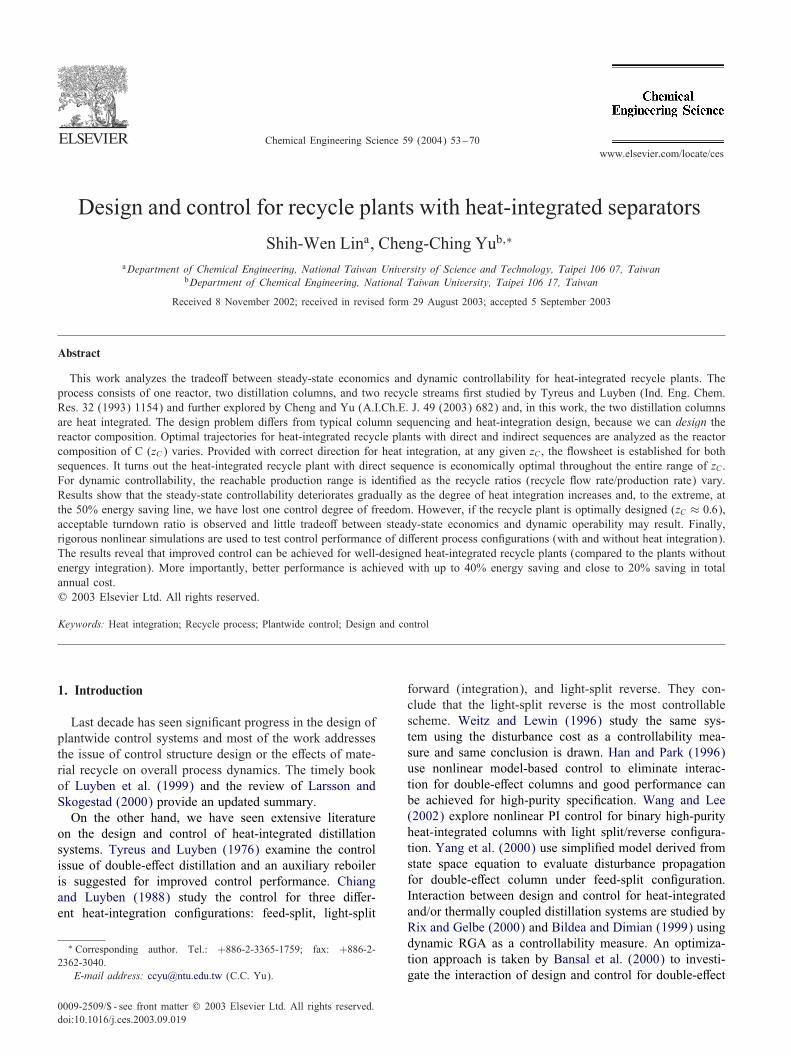
XD1,A=0.99

XD1,C=0.01

XD2,A=0.01

XD2,B=0.01

XD2,C=0.98

D2=100 lb-mol/h

XB2,B=0.99

XB2,C=0.01

Fig. 1. Process >owsheet and speci4cations for the recycle plant withdirect separation sequence.

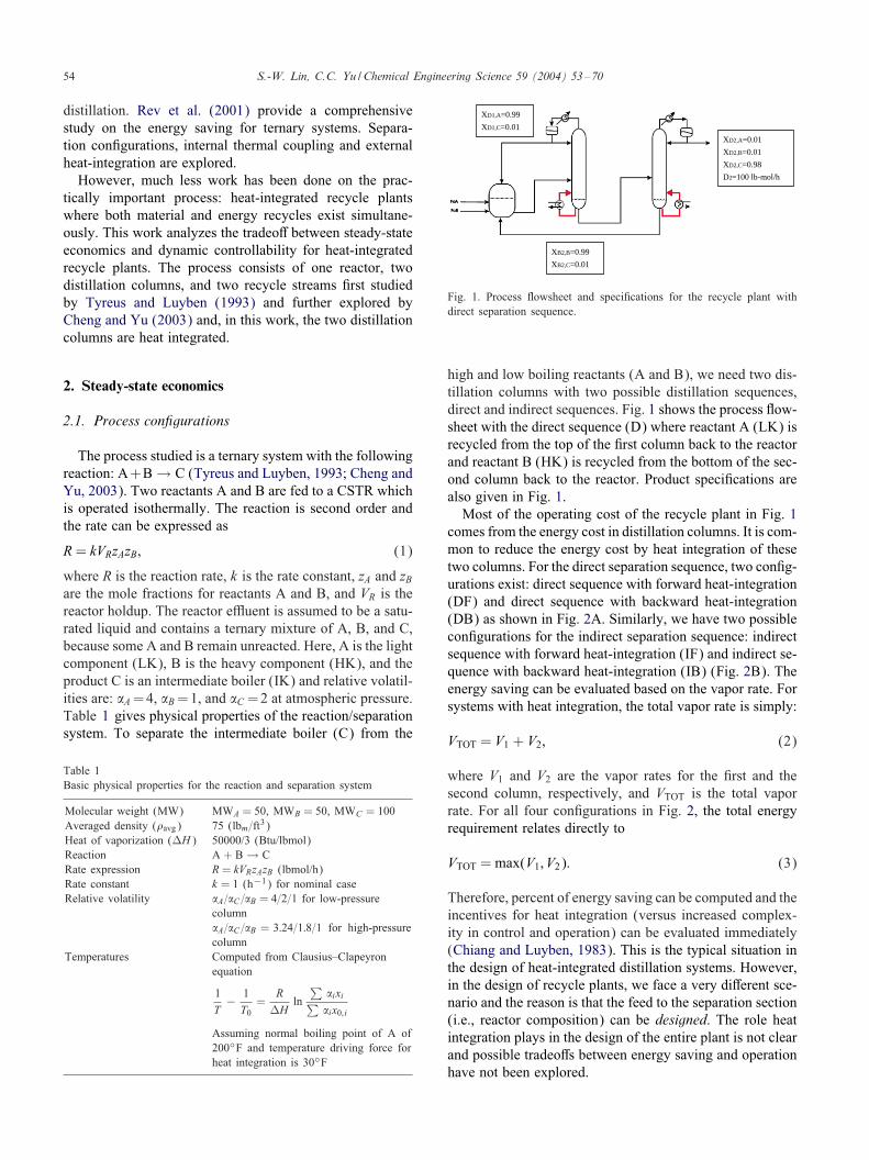
high and low boiling reactants (A and B), we need two dis-tillation columns with two possible distillation sequences,direct and indirect sequences. Fig. 1 shows the process >ow-sheet with the direct sequence (D) where reactant A (LK) isrecycled from the top of the 4rst column back to the reactorand reactant B (HK) is recycled from the bottom of the sec-ond column back to the reactor. Product speci4cations arealso given in Fig. 1.Most of the operating cost of the recycle plant in Fig. 1

comes from the energy cost in distillation columns. It is com-mon to reduce the energy cost by heat integration of thesetwo columns. For the direct separation sequence, two con4g-urations exist: direct sequence with forward heat-integration(DF) and direct sequence with backward heat-integration(DB) as shown in Fig. 2A. Similarly, we have two possiblecon4gurations for the indirect separation sequence: indirectsequence with forward heat-integration (IF) and indirect se-quence with backward heat-integration (IB) (Fig. 2B). Theenergy saving can be evaluated based on the vapor rate. Forsystems with heat integration, the total vapor rate is simply:

VTOT = V1 + V2; (2)

where V1 and V2 are the vapor rates for the 4rst and thesecond column, respectively, and VTOT is the total vaporrate. For all four con4gurations in Fig. 2, the total energyrequirement relates directly to

VTOT = max(V1; V2): (3)

Therefore, percent of energy saving can be computed and theincentives for heat integration (versus increased complex-ity in control and operation) can be evaluated immediately(Chiang and Luyben, 1983). This is the typical situation inthe design of heat-integrated distillation systems. However,in the design of recycle plants, we face a very di3erent sce-nario and the reason is that the feed to the separation section(i.e., reactor composition) can be designed. The role heatintegration plays in the design of the entire plant is not clearand possible tradeo3s between energy saving and operationhave not been explored.

S.-W. Lin, C.C. Yu /Chemical Engineering Science 59 (2004) 53–70 55

Fig. 2. Heat-integrated recycle plant with: (A) direct separation sequence (forward and backward integration); and (B) indirect separation sequence(forward/backward integration).

2.2. Generation of process 4owsheet and total annual cost

Before getting to the steady-state design, the followingassumptions are made. Using the direct sequence as an ex-ample (Fig. 2A), the assumptions are

(1) The process components have constant density.(2) The >ow rate of the product stream D2 is 4xed at

100 lbmol=h.(3) The product speci4cation is xD2;C = 0:98.(4) There is no component A leaving the bottom of the

second column (xB2;A =0). Therefore, the compositionof the heavy recycle stream B2 is speci4ed to be xB2;B=0:99, and xB2;C = 0:01.

(5) There is no component B leaving the top of the 4rstcolumn (xD1;B = 0). Therefore, the composition of thelight recycle stream D1 is speci4ed to be xD1;A = 0:99,and xD1;C = 0:01.

(6) The relative volatility of the high-pressure column isassumed to be 90% of the lower pressure one (i.e.,i;HP = 0:9i;LP; Chiang and Luyben, 1983).

With given speci4cations, we can complete the steady-statedesign for any given reactor product composition (zC)and reactant distribution with di3erent direction of heatintegration. The steady-state conditions of all streams inthe ternary recycle system are calculated from balanceequations (Cheng and Yu, 2003). The low-pressure col-umn is assumed to be at atmospheric and the pressurefor the high-pressure column can be computed from the

Clausius–Clapeyron equation

Psati = Psat

i;0 exp[−LHi

R

(1T

− 1T0

)]; (4)

where Psat is the vapor pressure, LH is the heat of vaporiza-tion, and R is the gas constant. The temperatures are inferredfrom the following expression (Glinos, 1984):1T

− 1T0

=R

LHln

∑ixi∑ix0; i

; (5)

where the subscript 0 stands for a reference temperature. Inthis work, we assume the normal boiling point for the lightcomponent (A) is 200◦F and temperature driving force forheat transfer is 30◦F. With this assumption, we can computethe temperature on each tray.Next, standard column shortcut approach is taken for the

heat-integrated columns. First, the Fenske equation is ap-plied to 4nd the minimum number of trays (NT;min) and totalnumber of trays is set to twice of NT;min and the feed tray islocated with the Kirkbride equation. Next, provided with as-sumed physical properties, the column is sized, tray holdupis computed, and liquid hydraulic time constant is computedas shown in the appendix. The heat transfer areas for the re-boiler and condenser are also computed from the vapor >owrates (see the appendix). The reactor is also sized assumingan aspect ratio of 2. From steady-state design, we can de-termine all the process >ow rates and the equipment sizes.Before leaving the design section it should be emphasizedthat a standard column design procedure (NT = 2NT;min)is adapted here for the design of heat-integrated columns.As pointed out by one of the reviewer that an additional


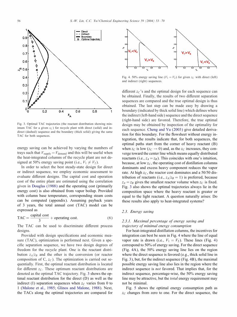
Fig. 3. Optimal TAC trajectories (the reactant distribution showing min-imum TAC for a given zC) for recycle plant with direct (solid) and in-direct (dashed) sequence and the boundary (thick solid) giving the sameTAC for both sequences.

energy saving can be achieved by varying the numbers oftrays such that Vsupply =Vdemand and this will be useful whenthe heat-integrated columns of the recycle plant are not de-signed at 50% energy saving point (i.e., V1 �= V2).

In order to select the best steady-state design for director indirect sequence, we employ economic assessment toevaluate di3erent designs. The capital cost and operationcost of the entire plant are estimated using the correlationgiven in Douglas (1988) and the operating cost (primarilyenergy cost) is also obtained from vapor boilup. Providedwith column base temperature, corresponding steam costscan be computed (appendix). Assuming payback yearsof 3 years, the total annual cost (TAC) model can beexpressed as

TAC =capital cost

3+ operating cost: (6)

The TAC can be used to discriminate di3erent processdesigns.Provided with design speci4cations and economic mea-

sure (TAC), optimization is performed next. Given a spe-ci4c separation sequence, we have two design degrees offreedom for the recycle plant. One is the reactant distri-bution zA=zB and the other is the conversion (or reactorcomposition of C, zC). The optimization is carried out se-quentially. First, the optimal reactant distribution is locatedfor di3erent zC . These optimum reactant distributions aredenoted as the optimal TAC trajectory. Fig. 3 shows the op-timal reactant distribution for the direct (D) as well as theindirect (I) separation sequences when zC varies from 0 to1 (Malone et al., 1985; Glinos and Malone, 1988). Next,the TACs along the optimal trajectories are compared for

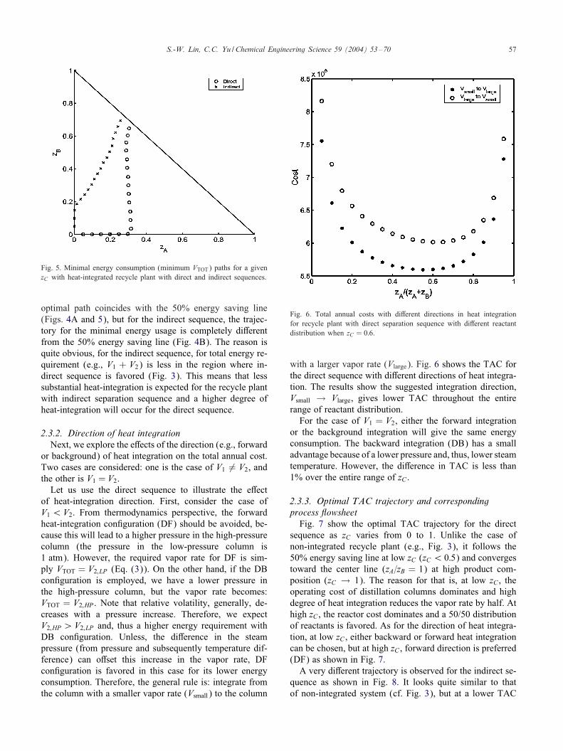
Fig. 4. 50% energy saving line (V1 = V2) for given zC with direct (left)and indirect (right) sequences.

di3erent zC’s and the optimal design for each sequence canbe obtained. Finally, the results of two di3erent separationsequences are compared and the true optimal design is thusobtained. The last step can be made easy by drawing aboundary (indicated by thick solid line) which de4nes wherethe indirect (left-hand side) sequence and the direct sequence(right-hand side) are favored. Therefore, the true optimaldesign may be obtained by inspection of the optimality foreach sequence. Cheng and Yu (2003) give detailed deriva-tion for this boundary. For the >owsheet without energy in-tegration, the results indicate that, for both sequences, theoptimal paths start from the corner of heavy reactant (B)when zC is low (zC → 0) and, as the zC increases, they con-verge toward the center line which means equally distributedreactants (i.e., zA = zB). This coincides with one’s intuition,because, at low zC , the operating cost of distillation columnsdominants and excess heavy component reduces the vaporrate. At high zC , the reactor cost dominates and a 50/50 dis-tribution of reactants (i.e., zA=zB = 1) is preferred, becausezA = zB gives the smallest reactor volume when zC is 4xed.Fig. 3 also shows the optimal trajectories always lie in thecomposition space where the heavy reactant is greater orequal to the light reactant. A question naturally arises: Dothese results also apply to heat-integrated systems?

2.3. Energy saving

2.3.1. Maximal percentage of energy saving andtrajectory of minimal energy consumptionFor heat-integrated distillation columns, the incentives for

integration can best be seen in Fig. 4 where the line of equalvapor rate is drawn (i.e., V1 = V2). These lines (Fig. 4)correspond to 50% of energy saving. For the direct sequence(Fig. 4A), the 50% energy saving line lies on the regionwhere the direct sequence is favored (e.g., thick solid line inFig. 3), but, for the indirect sequence (Fig. 4B), the maximalpossible energy saving line also lies in the region where theindirect sequence is not favored. That implies that, for theindirect sequence, percentage-wise, the 50% energy savingline may be attractive, but the total energy requirement maynot be minimal.Fig. 5 shows the optimal energy consumption path as

zC changes from zero to one. For the direct sequence, the


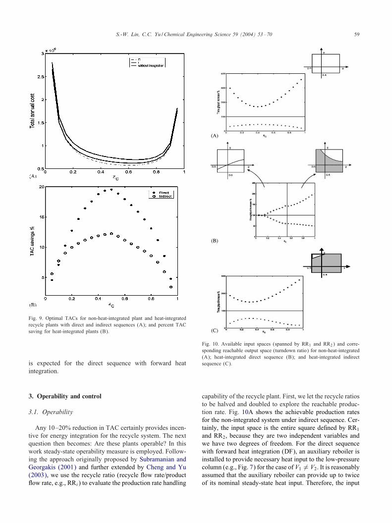
Fig. 5. Minimal energy consumption (minimum VTOT) paths for a givenzC with heat-integrated recycle plant with direct and indirect sequences.

optimal path coincides with the 50% energy saving line(Figs. 4A and 5), but for the indirect sequence, the trajec-tory for the minimal energy usage is completely di3erentfrom the 50% energy saving line (Fig. 4B). The reason isquite obvious, for the indirect sequence, for total energy re-quirement (e.g., V1 + V2) is less in the region where in-direct sequence is favored (Fig. 3). This means that lesssubstantial heat-integration is expected for the recycle plantwith indirect separation sequence and a higher degree ofheat-integration will occur for the direct sequence.

2.3.2. Direction of heat integrationNext, we explore the e3ects of the direction (e.g., forward

or background) of heat integration on the total annual cost.Two cases are considered: one is the case of V1 �= V2, andthe other is V1 = V2.Let us use the direct sequence to illustrate the e3ect

of heat-integration direction. First, consider the case ofV1 ¡V2. From thermodynamics perspective, the forwardheat-integration con4guration (DF) should be avoided, be-cause this will lead to a higher pressure in the high-pressurecolumn (the pressure in the low-pressure column is1 atm). However, the required vapor rate for DF is sim-ply VTOT = V2;LP (Eq. (3)). On the other hand, if the DBcon4guration is employed, we have a lower pressure inthe high-pressure column, but the vapor rate becomes:VTOT = V2;HP . Note that relative volatility, generally, de-creases with a pressure increase. Therefore, we expectV2;HP ¿V2;LP and, thus a higher energy requirement withDB con4guration. Unless, the di3erence in the steampressure (from pressure and subsequently temperature dif-ference) can o3set this increase in the vapor rate, DFcon4guration is favored in this case for its lower energyconsumption. Therefore, the general rule is: integrate fromthe column with a smaller vapor rate (Vsmall) to the column

Fig. 6. Total annual costs with di3erent directions in heat integrationfor recycle plant with direct separation sequence with di3erent reactantdistribution when zC = 0:6.

with a larger vapor rate (Vlarge). Fig. 6 shows the TAC forthe direct sequence with di3erent directions of heat integra-tion. The results show the suggested integration direction,Vsmall → Vlarge, gives lower TAC throughout the entirerange of reactant distribution.For the case of V1 = V2, either the forward integration

or the background integration will give the same energyconsumption. The backward integration (DB) has a smalladvantage because of a lower pressure and, thus, lower steamtemperature. However, the di3erence in TAC is less than1% over the entire range of zC .

2.3.3. Optimal TAC trajectory and correspondingprocess 4owsheetFig. 7 show the optimal TAC trajectory for the direct

sequence as zC varies from 0 to 1. Unlike the case ofnon-integrated recycle plant (e.g., Fig. 3), it follows the50% energy saving line at low zC (zC ¡ 0:5) and convergestoward the center line (zA=zB = 1) at high product com-position (zC → 1). The reason for that is, at low zC , theoperating cost of distillation columns dominates and highdegree of heat integration reduces the vapor rate by half. Athigh zC , the reactor cost dominates and a 50/50 distributionof reactants is favored. As for the direction of heat integra-tion, at low zC , either backward or forward heat integrationcan be chosen, but at high zC , forward direction is preferred(DF) as shown in Fig. 7.A very di3erent trajectory is observed for the indirect se-

quence as shown in Fig. 8. It looks quite similar to thatof non-integrated system (cf. Fig. 3), but at a lower TAC


Fig. 7. Optimal TAC trajectory (x) and corresponding direction(s) for heat integration for recycle plant with direct separation sequence (minimal energyconsumption trajectory (circle) also shown).

Fig. 8. Optimal TAC trajectory and corresponding direction for heat integration for recycle plant with indirect separation sequence.

as the result of heat integration. But the optimal trajectoryis far away from the 50% energy saving line, and, there-fore, a lesser degree of heat integration is encountered. Theoptimal path starts from the corner of heavy reactant (B)and converges toward the center line for the same reasonas explained earlier. Since this is the region where V1 ¿V2

(Fig. 4B), backward integration (IB) is the optimal onethroughout the entire range of zC .

Fig. 9A compares the TACs for three di3erent cases:without heat integration, direct sequence with heat inte-gration, and indirect sequence with heat integration. Asexpected, the heat-integrated plant with direct sequencegives the lowest TAC. Fig. 9B shows the percent savingon TAC. For the direct sequence, it ranges from 5% to20% and for the indirect sequence it is within 12%. Attrue optima (zC ≈ 0:6), a further 18% saving in TAC


Fig. 9. Optimal TACs for non-heat-integrated plant and heat-integratedrecycle plants with direct and indirect sequences (A); and percent TACsaving for heat-integrated plants (B).

is expected for the direct sequence with forward heatintegration.

3. Operability and control

3.1. Operability

Any 10–20% reduction in TAC certainly provides incen-tive for energy integration for the recycle system. The nextquestion then becomes: Are these plants operable? In thiswork steady-state operability measure is employed. Follow-ing the approach originally proposed by Subramanian andGeorgakis (2001) and further extended by Cheng and Yu(2003), we use the recycle ratio (recycle >ow rate/product>ow rate, e.g., RRi) to evaluate the production rate handling

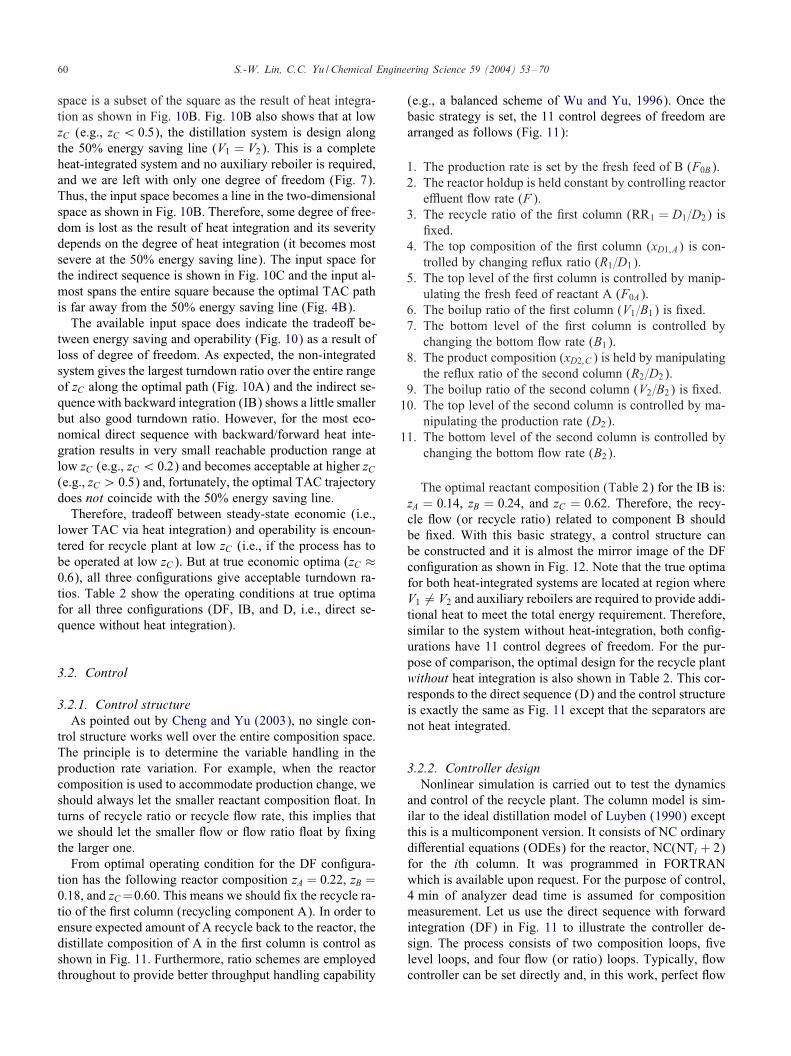
Fig. 10. Available input spaces (spanned by RR1 and RR2) and corre-sponding reachable output space (turndown ratio) for non-heat-integrated(A); heat-integrated direct sequence (B); and heat-integrated indirectsequence (C).

capability of the recycle plant. First, we let the recycle ratiosto be halved and doubled to explore the reachable produc-tion rate. Fig. 10A shows the achievable production ratesfor the non-integrated system under indirect sequence. Cer-tainly, the input space is the entire square de4ned by RR1

and RR2, because they are two independent variables andwe have two degrees of freedom. For the direct sequencewith forward heat integration (DF), an auxiliary reboiler isinstalled to provide necessary heat input to the low-pressurecolumn (e.g., Fig. 7) for the case of V1 �= V2. It is reasonablyassumed that the auxiliary reboiler can provide up to twiceof its nominal steady-state heat input. Therefore, the input


space is a subset of the square as the result of heat integra-tion as shown in Fig. 10B. Fig. 10B also shows that at lowzC (e.g., zC ¡ 0:5), the distillation system is design alongthe 50% energy saving line (V1 = V2). This is a completeheat-integrated system and no auxiliary reboiler is required,and we are left with only one degree of freedom (Fig. 7).Thus, the input space becomes a line in the two-dimensionalspace as shown in Fig. 10B. Therefore, some degree of free-dom is lost as the result of heat integration and its severitydepends on the degree of heat integration (it becomes mostsevere at the 50% energy saving line). The input space forthe indirect sequence is shown in Fig. 10C and the input al-most spans the entire square because the optimal TAC pathis far away from the 50% energy saving line (Fig. 4B).The available input space does indicate the tradeo3 be-

tween energy saving and operability (Fig. 10) as a result ofloss of degree of freedom. As expected, the non-integratedsystem gives the largest turndown ratio over the entire rangeof zC along the optimal path (Fig. 10A) and the indirect se-quence with backward integration (IB) shows a little smallerbut also good turndown ratio. However, for the most eco-nomical direct sequence with backward/forward heat inte-gration results in very small reachable production range atlow zC (e.g., zC ¡ 0:2) and becomes acceptable at higher zC(e.g., zC ¿ 0:5) and, fortunately, the optimal TAC trajectorydoes not coincide with the 50% energy saving line.Therefore, tradeo3 between steady-state economic (i.e.,

lower TAC via heat integration) and operability is encoun-tered for recycle plant at low zC (i.e., if the process has tobe operated at low zC). But at true economic optima (zC ≈0:6), all three con4gurations give acceptable turndown ra-tios. Table 2 show the operating conditions at true optimafor all three con4gurations (DF, IB, and D, i.e., direct se-quence without heat integration).

3.2. Control

3.2.1. Control structureAs pointed out by Cheng and Yu (2003), no single con-

trol structure works well over the entire composition space.The principle is to determine the variable handling in theproduction rate variation. For example, when the reactorcomposition is used to accommodate production change, weshould always let the smaller reactant composition >oat. Inturns of recycle ratio or recycle >ow rate, this implies thatwe should let the smaller >ow or >ow ratio >oat by 4xingthe larger one.From optimal operating condition for the DF con4gura-

tion has the following reactor composition zA = 0:22, zB =0:18, and zC=0:60. This means we should 4x the recycle ra-tio of the 4rst column (recycling component A). In order toensure expected amount of A recycle back to the reactor, thedistillate composition of A in the 4rst column is control asshown in Fig. 11. Furthermore, ratio schemes are employedthroughout to provide better throughput handling capability

(e.g., a balanced scheme of Wu and Yu, 1996). Once thebasic strategy is set, the 11 control degrees of freedom arearranged as follows (Fig. 11):

1. The production rate is set by the fresh feed of B (F0B).2. The reactor holdup is held constant by controlling reactor

eJuent >ow rate (F).3. The recycle ratio of the 4rst column (RR1 = D1=D2) is

4xed.4. The top composition of the 4rst column (xD1;A) is con-

trolled by changing re>ux ratio (R1=D1).5. The top level of the 4rst column is controlled by manip-

ulating the fresh feed of reactant A (F0A).6. The boilup ratio of the 4rst column (V1=B1) is 4xed.7. The bottom level of the 4rst column is controlled by

changing the bottom >ow rate (B1).8. The product composition (xD2;C) is held by manipulating

the re>ux ratio of the second column (R2=D2).9. The boilup ratio of the second column (V2=B2) is 4xed.10. The top level of the second column is controlled by ma-

nipulating the production rate (D2).11. The bottom level of the second column is controlled by

changing the bottom >ow rate (B2).

The optimal reactant composition (Table 2) for the IB is:zA = 0:14, zB = 0:24, and zC = 0:62. Therefore, the recy-cle >ow (or recycle ratio) related to component B shouldbe 4xed. With this basic strategy, a control structure canbe constructed and it is almost the mirror image of the DFcon4guration as shown in Fig. 12. Note that the true optimafor both heat-integrated systems are located at region whereV1 �= V2 and auxiliary reboilers are required to provide addi-tional heat to meet the total energy requirement. Therefore,similar to the system without heat-integration, both con4g-urations have 11 control degrees of freedom. For the pur-pose of comparison, the optimal design for the recycle plantwithout heat integration is also shown in Table 2. This cor-responds to the direct sequence (D) and the control structureis exactly the same as Fig. 11 except that the separators arenot heat integrated.

3.2.2. Controller designNonlinear simulation is carried out to test the dynamics

and control of the recycle plant. The column model is sim-ilar to the ideal distillation model of Luyben (1990) exceptthis is a multicomponent version. It consists of NC ordinarydi3erential equations (ODEs) for the reactor, NC(NTi + 2)for the ith column. It was programmed in FORTRANwhich is available upon request. For the purpose of control,4 min of analyzer dead time is assumed for compositionmeasurement. Let us use the direct sequence with forwardintegration (DF) in Fig. 11 to illustrate the controller de-sign. The process consists of two composition loops, 4velevel loops, and four >ow (or ratio) loops. Typically, >owcontroller can be set directly and, in this work, perfect >ow


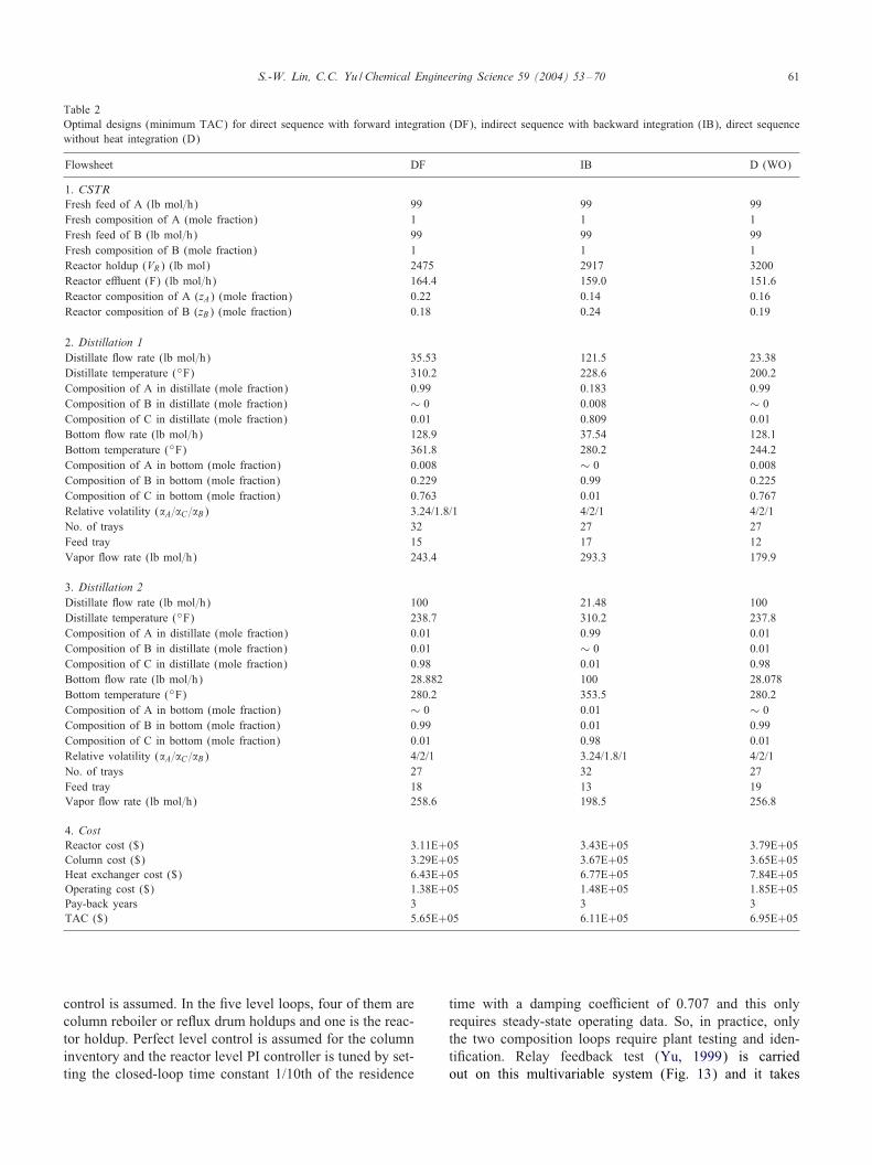
Table 2Optimal designs (minimum TAC) for direct sequence with forward integration (DF), indirect sequence with backward integration (IB), direct sequencewithout heat integration (D)

Flowsheet DF IB D (WO)

1. CSTRFresh feed of A (lb mol=h) 99 99 99Fresh composition of A (mole fraction) 1 1 1Fresh feed of B (lb mol=h) 99 99 99Fresh composition of B (mole fraction) 1 1 1Reactor holdup (VR) (lb mol) 2475 2917 3200Reactor eJuent (F) (lb mol=h) 164.4 159.0 151.6Reactor composition of A (zA) (mole fraction) 0.22 0.14 0.16Reactor composition of B (zB) (mole fraction) 0.18 0.24 0.19

2. Distillation 1Distillate >ow rate (lb mol=h) 35.53 121.5 23.38Distillate temperature (◦F) 310.2 228.6 200.2Composition of A in distillate (mole fraction) 0.99 0.183 0.99Composition of B in distillate (mole fraction) ∼ 0 0.008 ∼ 0Composition of C in distillate (mole fraction) 0.01 0.809 0.01Bottom >ow rate (lb mol=h) 128.9 37.54 128.1Bottom temperature (◦F) 361.8 280.2 244.2Composition of A in bottom (mole fraction) 0.008 ∼ 0 0.008Composition of B in bottom (mole fraction) 0.229 0.99 0.225Composition of C in bottom (mole fraction) 0.763 0.01 0.767Relative volatility (A=C=B) 3.24/1.8/1 4/2/1 4/2/1No. of trays 32 27 27Feed tray 15 17 12Vapor >ow rate (lb mol=h) 243.4 293.3 179.9

3. Distillation 2Distillate >ow rate (lb mol=h) 100 21.48 100Distillate temperature (◦F) 238.7 310.2 237.8Composition of A in distillate (mole fraction) 0.01 0.99 0.01Composition of B in distillate (mole fraction) 0.01 ∼ 0 0.01Composition of C in distillate (mole fraction) 0.98 0.01 0.98Bottom >ow rate (lb mol=h) 28.882 100 28.078Bottom temperature (◦F) 280.2 353.5 280.2Composition of A in bottom (mole fraction) ∼ 0 0.01 ∼ 0Composition of B in bottom (mole fraction) 0.99 0.01 0.99Composition of C in bottom (mole fraction) 0.01 0.98 0.01Relative volatility (A=C=B) 4/2/1 3.24/1.8/1 4/2/1No. of trays 27 32 27Feed tray 18 13 19Vapor >ow rate (lb mol=h) 258.6 198.5 256.8

4. CostReactor cost ($) 3.11E+05 3.43E+05 3.79E+05Column cost ($) 3.29E+05 3.67E+05 3.65E+05Heat exchanger cost ($) 6.43E+05 6.77E+05 7.84E+05Operating cost ($) 1.38E+05 1.48E+05 1.85E+05Pay-back years 3 3 3TAC ($) 5.65E+05 6.11E+05 6.95E+05

control is assumed. In the 4ve level loops, four of them arecolumn reboiler or re>ux drum holdups and one is the reac-tor holdup. Perfect level control is assumed for the columninventory and the reactor level PI controller is tuned by set-ting the closed-loop time constant 1/10th of the residence

time with a damping coeQcient of 0.707 and this onlyrequires steady-state operating data. So, in practice, onlythe two composition loops require plant testing and iden-ti4cation. Relay feedback test (Yu, 1999) is carriedout on this multivariable system (Fig. 13) and it takes


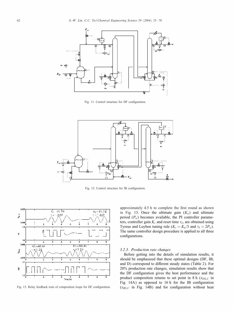
Fig. 11. Control structure for DF con4guration.

Fig. 12. Control structure for IB con4guration.

Fig. 13. Relay feedback tests of composition loops for DF con4guration.

approximately 4:5 h to complete the 4rst round as shownin Fig. 13. Once the ultimate gain (Ku) and ultimateperiod (Pu) becomes available, the PI controller parame-ters, controller gain Kc and reset time �I , are obtained usingTyreus and Luyben tuning rule (Kc = Ku=3 and �I = 2Pu).The same controller design procedure is applied to all threecon4gurations.

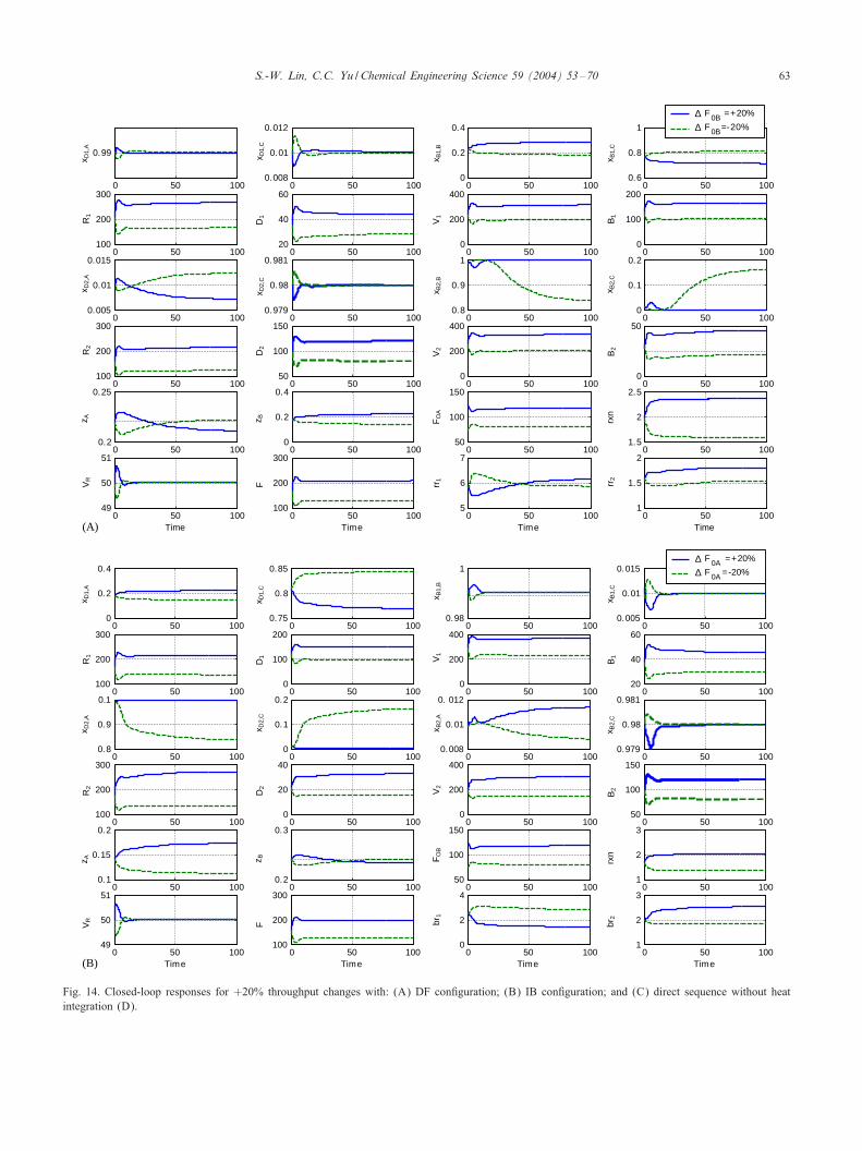
3.2.3. Production rate changesBefore getting into the details of simulation results, it

should be emphasized that these optimal designs (DF, IB,and D) correspond to di3erent steady states (Table 2). For20% production rate changes, simulation results show thatthe DF con4guration gives the best performance and theproduct composition returns to set point in 8 h (xD2;C inFig. 14A) as opposed to 16 h for the IB con4guration(xB2;C in Fig. 14B) and for con4guration without heat


0 50 100

0.99

x D1,

Ax D

2,A

R1

R2

z A z BD

2D

1x D

1,C

x D2,

C

x B1,

B

x B1,

Cx B

2,C

B1

B2

rr2

rxn

x B1,

Cx B

2,C

B1

B2

br2

rxn

x B2,

BV

1V

2F

OA

rr1

x B1,

Bx B

2,A

V1

V2

FO

Bbr

1

VR

Fz B

D2

D1

F

0 50 1000.008

0.01

0.012

0 50 1000

0.2

0.4

0 50 1000.6

0.8

1

0 50 100100

200

300

0 50 10020

40

60

0 50 1000

200

400

0 50 1000

100

200

0 50 1000.005

0.01

0.

x D1,

Ax D

2,A

R1

R2

z AV

R

015

0 50 1000.979

0.98

0.981

0 50 1000.8

0.9

1

0 50 1000

0.1

0.2

0 50 100100

200

300

0 50 10050

100

150

0 50 1000

200

400

0 50 1000

50

0 50 1000.2

0.25

0 50 1000

0.2

0.4

0 50 10050

100

150

0 50 1001.5

2

2.5

0 50 10049

50

51

Time0 50 100

100

200

300

Time0 50 100

5

6

7

Time0 50 100

1

1.5

2

Time

∆ F 0B =+20%

∆ F 0B=-20%

0 50 1000

0.2

0.4

0 50 1000.75

0.8

0.85

0 50 1000.98

1

0 50 1000.005

0.01

0.015

0 50 100100

200

300

0 50 1000

100

200

0 50 1000

200

400

0 50 10020

40

60

0 50 1000.8

0.9

0.1

0 50 1000

0.1

0.2

0 50 1000.008

0.01

0. 012

0 50 1000.979

0.98

0.981

0 50 100100

200

300

0 50 1000

20

40

0 50 1000

200

400

0 50 10050

100

150

0 50 1000.1

0.15

0.2

0 50 1000.2

0.3

0 50 10050

100

150

0 50 1001

2

3

0 50 10049

50

51

Time0 50 100

100

200

300

Time0 50 100

0

2

4

Time0 50 100

1

2

3

Time

∆ F 0A =+20%

∆ F 0A =-20%

(A)

(B)

x D1,

Cx D

2,C

Fig. 14. Closed-loop responses for +20% throughput changes with: (A) DF con4guration; (B) IB con4guration; and (C) direct sequence without heatintegration (D).


x B1,

Cx B

2,C

B1

B2

rr2

rxn

x B1,

Bx B

2,B

V1

V2

FO

Arr

1

z BD

2D

1x D

1,C

x D2,

CF

x D1,

Ax D

2,A

R1

R2

z AV

R

0 50 100

0.99

0 50 1000.008

0.01

0.012

0 50 1000

0.2

0.4

0 50 1000.6

0.8

1

0 50 100100

200

300

0 50 1000

20

40

0 50 100100

200

300

0 50 1000

100

200

0 50 1000.008

0.01

0.012

0 50 1000.979

0.98

0.981

0 50 1000.8

0.9

1

0 50 1000

0.1

0.2

0 50 100100

200

300

0 50 10050

100

150

0 50 1000

200

400

0 50 1000

50

0 50 1000.1

0.15

0.2

0 50 1000.15

0.2

0.25

0 50 10050

100

150

0 50 1001

1.5

2

0 50 10049

50

51

Time0 50 100

100

200

300

Time0 50 100

6

7

8

Time0 50 100

1

2

3

Time

∆ F 0B =+20%

∆ F 0B=-20%

(C)

Fig. 14. continued.

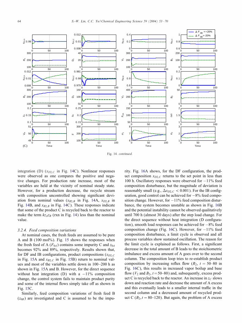
integration (D) (xD2;C in Fig. 14C). Nonlinear responseswere observed as one compares the positive and nega-tive changes. For production rate increase, most of thevariables are held at the vicinity of nominal steady state.However, for a production decrease, the recycle streamwith composition uncontrolled showing signi4cant devi-ation from nominal values (xB2;B in Fig. 14A, xD2;B inFig. 14B, and xB2;B in Fig. 14C). These responses indicatethat some of the product C is recycled back to the reactor tomake the term kzAzB (rxn in Fig. 14) less than the nominalvalue.

3.2.4. Feed composition variationsAt nominal cases, the fresh feeds are assumed to be pure

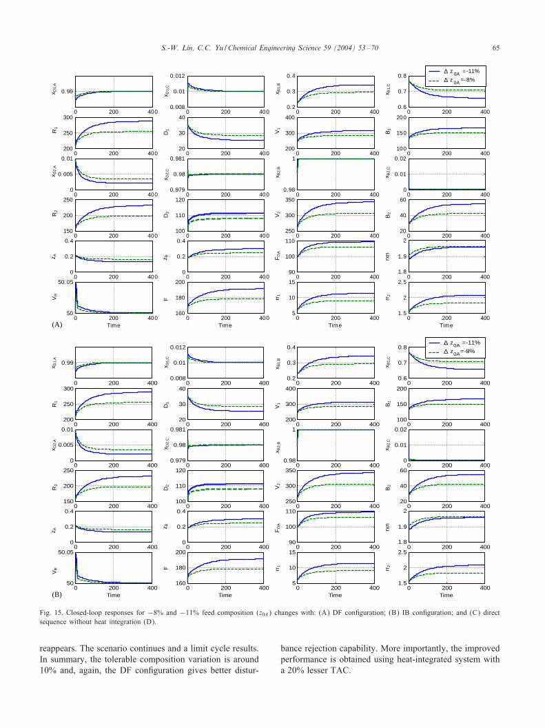
A and B (100 mol%). Fig. 15 shows the responses whenthe fresh feed of A (F0A) contains some impurity C and z0Abecomes 92% and 89%, respectively. Results shown that,for DF and IB con4gurations, product compositions (xD2;Cin Fig. 15A and xB2;C in Fig. 15B) return to nominal val-ues and most of the variables settle down in 100–200 h asshown in Fig. 15A and B. However, for the direct sequencewithout heat integration (D) with a −11% compositionchange, the control system fails to maintain product purityand some of the internal >ows simply take o3 as shown inFig. 15C.Similarly, feed composition variations of fresh feed B

(z0B) are investigated and C is assumed to be the impu-

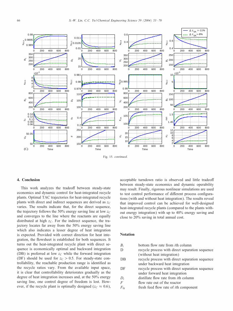
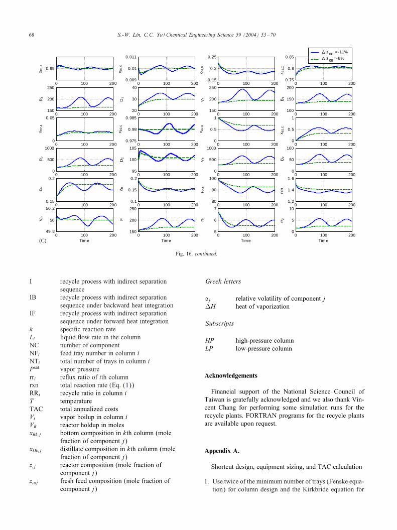
rity. Fig. 16A shows, for the DF con4guration, the prod-uct composition xD2;C returns to the set point in less than100 h. Oscillatory responses were observed for −11% feedcomposition disturbance, but the magnitude of deviation isreasonably small (e.g., LxD2;C ¡ 0:001). For the IB con4g-uration, good control can be achieved for −8% feed compo-sition change. However, for −11% feed composition distur-bance, the system becomes unstable as shown in Fig. 16Band the potential instability cannot be observed qualitativelyuntil 700 h (almost 30 days) after the step load change. Forthe direct sequence without heat integration (D con4gura-tion), smooth load responses can be achieved for −8% feedcomposition change (Fig. 16C). However, for −11% feedcomposition disturbance, a limit cycle is observed and allprocess variables show sustained oscillation. The reason forthe limit cycle is explained as follows. First, a signi4cantdecrease in the total amount of B leads to the stoichiometricimbalance and excess amount of A goes over to the secondcolumn. The composition loop tries to re-establish productcomposition by increasing re>ux >ow (R2, t = 50–80 inFig. 16C), this results in increased vapor boilup and base>ow (V2 and B2, t=50–80) and, subsequently, excess prod-uct C is recycled back to the reactor. An increase in zC slowsdown and reaction rate and decrease the amount of A excessand this eventually leads to a smaller internal traQc in thesecond column and a decreased amount of recycled prod-uct C (B2; t = 80–120). But again, the problem of A excess


x B1,

Cx B

2,C

B1

B2

rr2

rxn

x B1,

Cx B

2,C

B1

B2

rr2

rxn

x B1,

Bx B

2,B

V1

V2

FO

Arr

1x B

1,B

x B2,

BV

1V

2F

OA

rr1

z BD

2D

1x D

1,C

x D2,

Cx D

1,C

x D2,

CF

z BD

2D

1F

x D1,

Ax D

2,A

R1

R2

z AV

Rx D

1,A

x D2,

AR

1R

2z A

VR

0 200 400

0.99

0 200 4000.008

0.01

0.012

0 200 4000.2

0.3

0.4

0 200 4000.6

0.7

0.8

0 200 400200

250

300

0 200 40020

30

40

0 200 400200

300

400

0 200 400100

150

200

0 200 4000

0.005

0.01

0 200 4000.979

0.98

0.981

0 200 4000.98

1

0 200 4000

0.01

0.02

0 200 400150

200

250

0 200 400100

110

120

0 200 400250

300

350

0 200 40020

40

60

0 200 4000

0.2

0.4

0 200 4000

0.2

0.4

0 200 40090

100

110

0 200 4001.8

1.9

2

0 200 40050

50. 05

Time0 200 400

160

180

200

Time0 200 400

5

10

15

Time0 200 400

1.5

2

2.5

Time

∆ z 0A = -11%

∆ z 0A =-8%

0 200 400

0.99

0 200 4000.008

0.01

0.012

0 200 4000.2

0.3

0.4

0 200 4000.6

0.7

0.8

0 200 400200

250

300

0 200 40020

30

40

0 200 400200

300

400

0 200 400100

150

200

0 200 4000

0.005

0.01

0 200 4000.979

0.98

0.981

0 200 4000.98

1

0 200 4000

0.01

0.02

0 200 400150

200

250

0 200 400100

110

120

0 200 400250

300

350

0 200 40020

40

60

0 200 4000

0.2

0.4

0 200 4000

0.2

0.4

0 200 40090

100

110

0 200 4001.8

1.9

2

0 200 40050

50.05

Time0 200 400

160

180

200

Time0 200 400

5

10

15

Time0 200 400

1.5

2

2.5

Time

∆ z0A =-11%

∆ z0A=-8%

(A)

(B)

Fig. 15. Closed-loop responses for −8% and −11% feed composition (z0A) changes with: (A) DF con4guration; (B) IB con4guration; and (C) directsequence without heat integration (D).

reappears. The scenario continues and a limit cycle results.In summary, the tolerable composition variation is around10% and, again, the DF con4guration gives better distur-

bance rejection capability. More importantly, the improvedperformance is obtained using heat-integrated system witha 20% lesser TAC.


x B1,

Cx B

2,C

B1

B2

rr2

rxn

x B1,

Bx B

2,B

V1

V2

FO

Arr

1

z BD

2D

1x D

1,C

x D2,

CF

x D1,

Ax D

2,A

R1

R2

z AV

R

(C)

0 200 400 600 800

0.989

0.9895

0.99

0 200 400 600 8000.01

0.0105

0.011

0 200 400 600 800

0.4

0.6

0 200 400 600 8000.4

0.6

0

×10-3 ×10-3

200 400 600 800

200250300350

0 200 400 600 80015

20

0 200 400 600 800

200250300350

0 200 400 600 800

150

200

250

0 200 400 600 800

2468

0 200 400 600 8000.979

0.98

0.981

0 200 400 600 8000.99

0.995

0 200 400 600 800

5

10

0 200 400 600 800200

400

600

800

0 200 400 600 800100

105

110

0 200 400 600 800200

400

600

800

0 200 400 600 800

50

100

150

0 200 400 600 8000.060.08

0.10.120.14

0 200 400 600 8000.2

0.4

0 200 400 600 800

100

105

0 200 400 600 800

1.45

1.5

0 200 400 600 80050

50.05

Time0 200 400 600 800

150

200

250

Time0 200 400 600 800

10

15

20

Time0 200 400 600 800

2468

1012

Time

∆ z 0A =-11%

∆ z 0A=-8%

Fig. 15. continued.

4. Conclusion

This work analyzes the tradeo3 between steady-stateeconomics and dynamic control for heat-integrated recycleplants. Optimal TAC trajectories for heat-integrated recycleplants with direct and indirect sequences are derived as zCvaries. The results indicate that, for the direct sequence,the trajectory follows the 50% energy saving line at low zCand converges to the line where the reactants are equallydistributed at high zC . For the indirect sequence, the tra-jectory locates far away from the 50% energy saving linewhich also indicates a lesser degree of heat integrationis expected. Provided with correct direction for heat inte-gration, the >owsheet is established for both sequences. Itturns out the heat-integrated recycle plant with direct se-quence is economically optimal and backward integration(DB) is preferred at low zC while the forward integration(DF) should be used for zC ¿ 0:5. For steady-state con-trollability, the reachable production range is identi4ed asthe recycle ratios vary. From the available input space,it is clear that controllability deteriorates gradually as thedegree of heat integration increases and, at the 50% energysaving line, one control degree of freedom is lost. How-ever, if the recycle plant is optimally designed (zC ≈ 0:6),

acceptable turndown ratio is observed and little tradeo3between steady-state economics and dynamic operabilitymay result. Finally, rigorous nonlinear simulations are usedto test control performance of di3erent process con4gura-tions (with and without heat integration). The results revealthat improved control can be achieved for well-designedheat-integrated recycle plants (compared to the plants with-out energy integration) with up to 40% energy saving andclose to 20% saving in total annual cost.

Notation

Bi bottom >ow rate from ith columnD recycle process with direct separation sequence

(without heat integration)DB recycle process with direct separation sequence

under backward heat integrationDF recycle process with direct separation sequence

under forward heat integrationDi distillate >ow rate from ith columnF >ow rate out of the reactorF0i fresh feed >ow rate of ith component


x B1,

Cx B

2,C

B1

B2

rr2

rxn

x B1,

Cx B

2,C

B1

B2

rr2

rxn

z BD

2D

1x D

1,C

x D2,

Cx D

1,C

x D2,

CF

z BD

2D

1F

x D1,

Ax D

2,A

R1

R2

z AV

R

(A)

x D1,

Ax D

2,A

R1

R2

z AV

R

(B)

x B1,

Bx B

2,B

V1

V2

FO

Arr

1x B

1,B

x B2,

AV

1V

2F

OB

rr1

0 50 100

0.99

0 50 1000.0095

0.01

0.0105

x

0 50 1000.15

0.2

0.25

0 50 1000.75

0.8

0 50 100200

250

300

0 50 10030

40

50

0 50 100200

250

300

0 50 100120

140

160

0 50 1000

0.01

0.02

0 50 1000.979

0.98

0.981

0 50 1000.5

1

0 50 1000

0.5

0 50 100150

200

250

0 50 10095

100

105

0 50 100250

300

350

0 50 10020

40

60

0 50 1000.22

0.23

0.24

0 50 1000.1

0.15

0.2

0 50 10080

90

100

0 50 1001.6

1.8

2

0 50 10049.8

50

50.2

Time0 50 100

150

200

250

Time0 50 100

5

5.5

6

Time0 50 100

1.5

2

2.5

Time

∆ z 0B =- 11%

∆ z 0B=-8%

0 200 400 600 800

0.2

0.25

0 200 400 600 800

0.75

0.8

0 200 400 600 800

0.988

0.99

0.992

0 200 400 600 800

0.008

0.01

0.012

0 200 400 600 800

180

200

0 200 400 600 800

130

140

150

0 200 400 600 800300

350

0 200 400 600 800

25

30

35

0 200 400 600 8000.99

0.995

0 200 400 600 800

5

10

0 200 400 600 800

0.012

0.014

0.016

0 200 400 600 8000.979

0.98

0.981

0 200 400 600 800

200

250

300

0 200 400 600 800

25

30

35

0 200 400 600 800200

250

300

0 200 400 600 800100

105

110

0 200 400 600 800

0.15

0.2

0 200 400 600 8000.160.18

0.20.22

0 200 400 600 800100

105

110

0 200 400 600 800

1.62

1.64

1.66

1.68

0 200 400 600 80050

50.02

50.04

Time0 200 400 600 800

160

165

170

Time0 200 400 600 800

11.5

22.5

Time0 200 400 600 800

2

2.5

3

Time

∆ z 0B =- 11%

∆ z 0B=-8%

Fig. 16. Closed-loop responses for −8% and −11% feed composition (z0B) changes with: (A) DF con4guration; (B) IB con4guration; and (C) directsequence without heat integration (D).


x B1,

Cx B

2,C

B1

B2

rr2

rxnz B

D2

D1

x D1,

Cx D

2,C

F

x D1,

Ax D

2,A

R1

R2

z AV

R

(C)

x B1,

Bx B

2,B

V1

V2

FO

Arr

1

0 100 200

0.99

0 100 2000.009

0.01

0.011

0 100 2000.15

0.2

0.25

0 100 2000.75

0.8

0.85

0 100 200150

200

250

0 100 20020

30

40

0 100 200150

200

250

0 100 200100

150

200

0 100 2000

0.05

0 100 2000.975

0.98

0.985

0 100 2000

0.5

1

0 100 2000

0.5

1

0 100 2000

500

1000

0 100 20095

100

105

0 100 2000

500

1000

0 100 2000

50

100

0 100 2000.15

0.2

0 100 2000.1

0.15

0.2

0 100 20080

90

100

0 100 2001.2

1.4

1.6

0 100 20049. 8

50

50. 2

Time0 100 200

150

200

250

Time0 100 200

5

6

7

Time0 100 200

0

5

10

Time

∆ z 0B =-11%

∆ z 0B=-8%

Fig. 16. continued.

I recycle process with indirect separationsequence

IB recycle process with indirect separationsequence under backward heat integration

IF recycle process with indirect separationsequence under forward heat integration

k speci4c reaction rateLi liquid >ow rate in the columnNC number of componentNFi feed tray number in column iNTi total number of trays in column iPsat vapor pressurerri re>ux ratio of ith columnrxn total reaction rate (Eq. (1))RRi recycle ratio in column iT temperatureTAC total annualized costsVi vapor boilup in column iVR reactor holdup in molesxBk; j bottom composition in kth column (mole

fraction of component j)xDk;j distillate composition in kth column (mole

fraction of component j)z;j reactor composition (mole fraction of

component j)z;oj fresh feed composition (mole fraction of

component j)

Greek letters

j relative volatility of component jLH heat of vaporization

Subscripts

HP high-pressure columnLP low-pressure column

Acknowledgements

Financial support of the National Science Council ofTaiwan is gratefully acknowledged and we also thank Vin-cent Chang for performing some simulation runs for therecycle plants. FORTRAN programs for the recycle plantsare available upon request.

Appendix A.

Shortcut design, equipment sizing, and TAC calculation

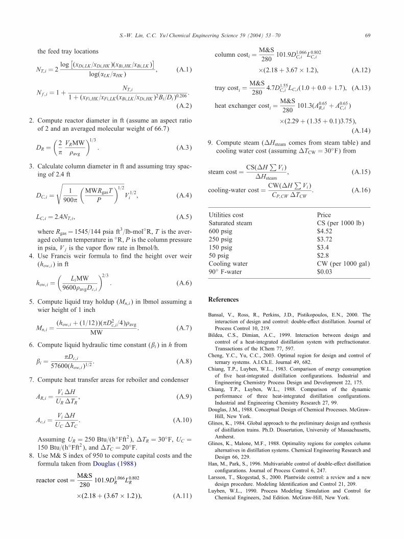
1. Use twice of the minimum number of trays (Fenske equa-tion) for column design and the Kirkbride equation for


the feed tray locations

NT;i = 2log

[(xDi;LK =xDi;HK)(xBi;HK =xBi;LK)

]log(LK=HK)

; (A.1)

Nf;i = 1 +NT;i

1 + (xFi;HK =xFi;LK (xBi;LK =xDi;HK)2Bi=Di)0:206:

(A.2)

2. Compute reactor diameter in ft (assume an aspect ratioof 2 and an averaged molecular weight of 66.7)

DR =(2"VRMW�avg

)1=3

: (A.3)

3. Calculate column diameter in ft and assuming tray spac-ing of 2:4 ft

DC;i =

√1

900"

(MWRgasT

P

)1=2

V 1=2i ; (A.4)

LC; i = 2:4NT;i; (A.5)

where Rgas = 1545=144 psia ft3=lb-mol◦R, T is the aver-aged column temperature in ◦R, P is the column pressurein psia, V j is the vapor >ow rate in lbmol/h.

4. Use Francis weir formula to 4nd the height over weir(how; i) in ft

how; i =(

LiMW9600�avgDc; i

)2=3

: (A.6)

5. Compute liquid tray holdup (Mn;i) in lbmol assuming awier height of 1 inch

Mn;i =(how; i + (1=12))("D2

c; i=4)�avgMW

: (A.7)

6. Compute liquid hydraulic time constant ('i) in h from

'i ="Dc; i

57600(how; i)1=2: (A.8)

7. Compute heat transfer areas for reboiler and condenser

AR; i =Vi LHUR LTR

; (A.9)

Ac; i =Vi LHUC LTC

: (A.10)

Assuming UR = 250 Btu=(h◦Fft2), LTR = 30◦F, UC =150 Btu=(h◦Fft2), and LTC = 20◦F.

8. Use M& S index of 950 to compute capital costs and theformula taken from Douglas (1988)

reactor cost =M&S280

101:9D1:066R L0:802R

×(2:18 + (3:67× 1:2)); (A.11)

column costi =M&S280

101:9D1:066C; i L0:802C; i

×(2:18 + 3:67× 1:2); (A.12)

tray costi =M&S280

4:7D1:55C; i LC; i(1:0 + 0:0 + 1:7); (A.13)

heat exchanger costi =M&S280

101:3(A0:65R; i + A0:65

C; i )

×(2:29 + (1:35 + 0:1)3:75);(A.14)

9. Compute steam (LHsteam comes from steam table) andcooling water cost (assuming LTCW = 30◦F) from

steam cost =CS(LH

∑Vi)

LHsteam; (A.15)

cooling-water cost =CW(LH

∑Vi)

CP;CW LTCW: (A.16)

Utilities cost PriceSaturated steam CS (per 1000 lb)600 psig $4.52250 psig $3.72150 psig $3.450 psig $2.8Cooling water CW (per 1000 gal)90◦ F-water $0.03

References

Bansal, V., Ross, R., Perkins, J.D., Pistikopoulos, E.N., 2000. Theinteraction of design and control: double-e3ect distillation. Journal ofProcess Control 10, 219.

Bildea, C.S., Dimian, A.C., 1999. Interaction between design andcontrol of a heat-integrated distillation system with prefractionator.Transactions of the IChem 77, 597.

Cheng, Y.C., Yu, C.C., 2003. Optimal region for design and control ofternary systems. A.I.Ch.E. Journal 49, 682.

Chiang, T.P., Luyben, W.L., 1983. Comparison of energy consumptionof 4ve heat-integrated distillation con4gurations. Industrial andEngineering Chemistry Process Design and Development 22, 175.

Chiang, T.P., Luyben, W.L., 1988. Comparison of the dynamicperformance of three heat-integrated distillation con4gurations.Industrial and Engineering Chemistry Research 27, 99.

Douglas, J.M., 1988. Conceptual Design of Chemical Processes. McGraw-Hill, New York.

Glinos, K., 1984. Global approach to the preliminary design and synthesisof distillation trains. Ph.D. Dissertation, University of Massachusetts,Amherst.

Glinos, K., Malone, M.F., 1988. Optimality regions for complex columnalternatives in distillation systems. Chemical Engineering Research andDesign 66, 229.

Han, M., Park, S., 1996. Multivariable control of double-e3ect distillationcon4gurations. Journal of Process Control 6, 247.

Larsson, T., Skogestad, S., 2000. Plantwide control: a review and a newdesign procedure. Modeling Identi4cation and Control 21, 209.

Luyben, W.L., 1990. Process Modeling Simulation and Control forChemical Engineers, 2nd Edition. McGraw-Hill, New York.


Luyben, W.L., Tyreus, B.D., Luyben, M.L., 1999. Plantwide ProcessControl. McGraw-Hill, New York.

Malone, M.F., Glinos, K., Marquez, F.E., Douglas, J.M., 1985. Simple,analytical criteria for the sequencing of distillation columns. A.I.Ch.E.Journal 31, 683.

Rev, E., Emtir, M., Szitkai, Z., Mizsey, P., Fonyo, Z., 2001. Energysaving of integrated and coupled distillation systems. Computers andChemical Engineering 25, 119.

Rix, A., Gelbe, H., 2000. On the impact of mass and heat integration ondesign and control of distillation column systems. Transactions of theIChem 78, 542.

Subramanian, S., Georgakis, C., 2001. Steady-state operabilitycharacteristics of idealize reactors. Chemical Engineering Science 56,5111.

Tyreus, B.D., Luyben, W.L., 1976. Dynamics and control ofheat-integrated distillation columns. Chemical Engineering Progress72 (9), 59.

Tyreus, B.D., Luyben, W.L., 1993. Dynamics and control of recyclesystems. 4. Ternary systems with one or two recycle streams. Industrialand Engineering Chemistry Research 32, 1154.

Wang, S.J., Lee, E.K., 2002. Nonlinear control of high-purityheat-integrated distillation system. Journal of Chemical Engineering ofJapan 35 (9), 848.

Weitz, O., Lewin, D.R., 1996. Dynamic controllability and resiliencydiagnosis using steady state process >owsheet data. Computers andChemical Engineering 20, 325.

Wu, K.L., Yu, C.C., 1996. Reactor/separator processes with recycle-1.Candidate control structure for operability. Computers and ChemicalEngineering 20, 1291.

Yang, Y.H., Lou, H.H., Huang, Y.L., 2000. Steady state disturbancepropagation modelling of heat integrated distillation processes.Chemical Engineering Research and Design 78 (A2), 245.

Yu, C.C., 1999. Autotuning of PID Controllers. Springer, London.

Design andcontrol for recycle plants with heat-integratedseparators

Documents

Transcript of Design andcontrol for recycle plants with heat-integratedseparators